Automatic Glycemia Regulation of Type I Diabetes
209
HAL Id: tel-02513088 https://tel.archives-ouvertes.fr/tel-02513088 Submitted on 20 Mar 2020 HAL is a multi-disciplinary open access archive for the deposit and dissemination of sci- entific research documents, whether they are pub- lished or not. The documents may come from teaching and research institutions in France or abroad, or from public or private research centers. L’archive ouverte pluridisciplinaire HAL, est destinée au dépôt et à la diffusion de documents scientifiques de niveau recherche, publiés ou non, émanant des établissements d’enseignement et de recherche français ou étrangers, des laboratoires publics ou privés. Automatic Glycemia Regulation of Type I Diabetes Taghreed Mohammadridha To cite this version: Taghreed Mohammadridha. Automatic Glycemia Regulation of Type I Diabetes. Automatic. École centrale de Nantes, 2017. English. NNT : 2017ECDN0008. tel-02513088
-
Upload
khangminh22 -
Category
Documents
-
view
0 -
download
0
Transcript of Automatic Glycemia Regulation of Type I Diabetes

HAL Id: tel-02513088https://tel.archives-ouvertes.fr/tel-02513088
Submitted on 20 Mar 2020
HAL is a multi-disciplinary open accessarchive for the deposit and dissemination of sci-entific research documents, whether they are pub-lished or not. The documents may come fromteaching and research institutions in France orabroad, or from public or private research centers.
L’archive ouverte pluridisciplinaire HAL, estdestinée au dépôt et à la diffusion de documentsscientifiques de niveau recherche, publiés ou non,émanant des établissements d’enseignement et derecherche français ou étrangers, des laboratoirespublics ou privés.
Automatic Glycemia Regulation of Type I DiabetesTaghreed Mohammadridha
To cite this version:Taghreed Mohammadridha. Automatic Glycemia Regulation of Type I Diabetes. Automatic. Écolecentrale de Nantes, 2017. English. NNT : 2017ECDN0008. tel-02513088
Taghreed MOHAMMADRIDHA
du grade de Docteur de lʼÉcole Centrale de Nantes
sous le sceau de l’Université Bretagne Loire.
École doctorale : Sciences et Technologies de l’Information et Mathématiques.
Discipline : Automatique, Productique et Robotique.
Unité de recherche : Laboratoire des Sciences du Numérique de Nantes.
Soutenue le 10 Mai 2017
Automatic Glycemia Regulation of Type I Diabetes
JURY
Président : DAROUACH Mohamed, Professeur des universités, IUT Henry Poincaré de Longwy. Rapporteurs : MOUNIER Hugues, Professeur des universités, Université Paris-Sud, Paris.
TARBOURIECH Sophie, Directrice de Recherche CNRS, LAAS, Toulouse. Examinateurs: CHAILOUS Lucy, Docteur, CHU Hôpital Nord Laennec - Nantes.
LEFEBVRE Marie-Anne, Maître de Conférences, Centrale Supélec, Rennes.
Directeur de thèse : MOOG Claude, Directeur de Recherche CNRS, Ecole Centrale de Nantes.
Automatic Glycemia Regulation of Type
I Diabetes
Taghreed MohammadRidha
Supervised by: Claude MOOG
Ecole Centrale de Nantes
Laboratoire des Sciences du Numérique de Nantes
This dissertation is submitted for the degree of
Doctor of Philosophy
Doctoral School: STIM July 2017


I would like to dedicate this humble work to the gracioussouls of our beloved Prophet of mercy Mohammad, his
cousin Ali and his daughter Fatima.Peace be upon Mohammad and his holy Family.
I also dedicate this work to the brave Iraqi army whotook the noble mission of fighting and defeating terrorism
for Iraq and for the world peace.


Acknowledgements
All praises to Allah for His blessing in completing this thesis. Iwould like to ask him to make this work as another useful tool fortype 1 diabetes treatment.
I would like to express my sincere gratitude to my advisor Prof.C. H. Moog for the continuous support of my Ph.D study, forhis patience, motivation, and immense knowledge.
I also thank my fellow labmates and the visiting researchers forthe stimulating and valuable discussions.
Last but not the least, I would like to thank my family: myparents and to my sister and brothers for supporting me spirituallythroughout writing this thesis and my life in general.

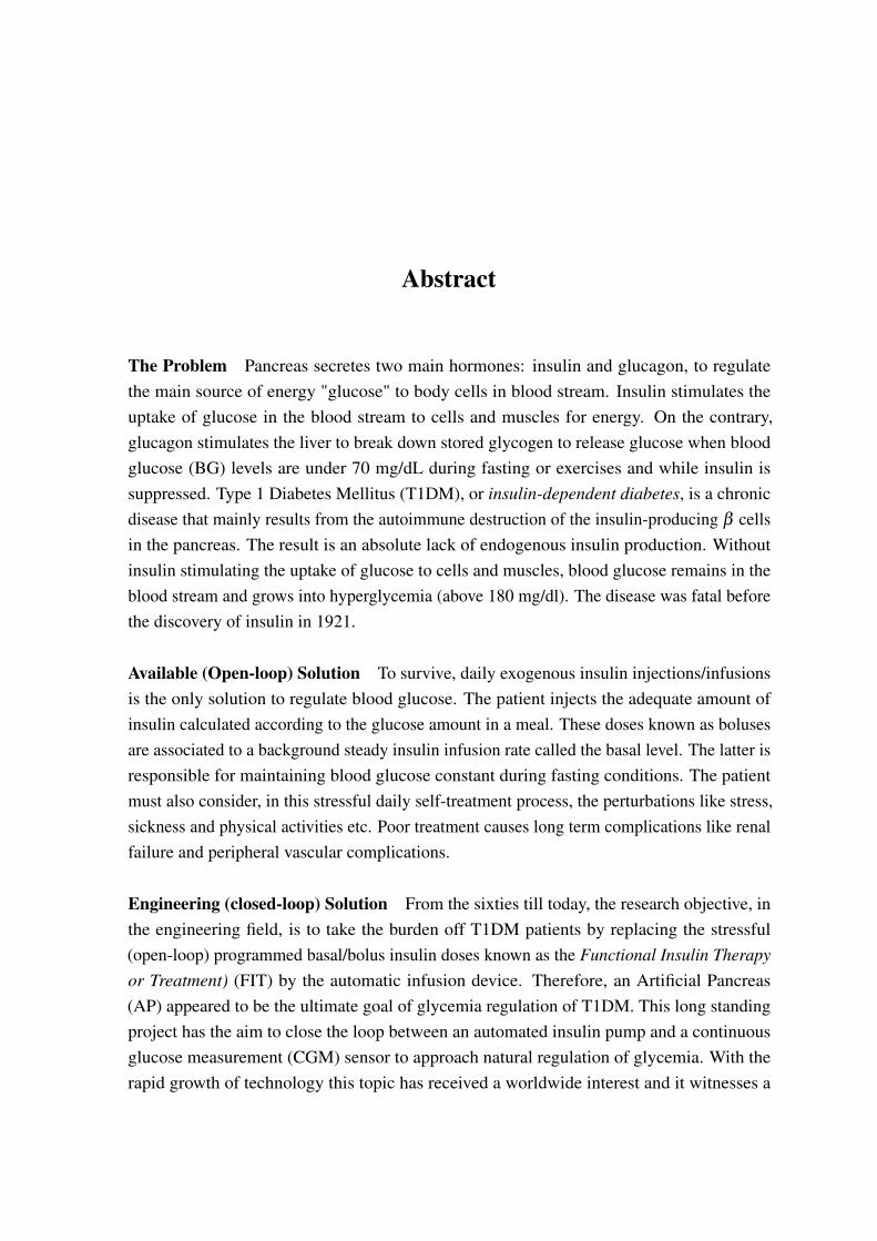
Abstract
The Problem Pancreas secretes two main hormones: insulin and glucagon, to regulate
the main source of energy "glucose" to body cells in blood stream. Insulin stimulates the
uptake of glucose in the blood stream to cells and muscles for energy. On the contrary,
glucagon stimulates the liver to break down stored glycogen to release glucose when blood
glucose (BG) levels are under 70 mg/dL during fasting or exercises and while insulin is
suppressed. Type 1 Diabetes Mellitus (T1DM), or insulin-dependent diabetes, is a chronic
disease that mainly results from the autoimmune destruction of the insulin-producing β cells
in the pancreas. The result is an absolute lack of endogenous insulin production. Without
insulin stimulating the uptake of glucose to cells and muscles, blood glucose remains in the
blood stream and grows into hyperglycemia (above 180 mg/dl). The disease was fatal before
the discovery of insulin in 1921.
Available (Open-loop) Solution To survive, daily exogenous insulin injections/infusions
is the only solution to regulate blood glucose. The patient injects the adequate amount of
insulin calculated according to the glucose amount in a meal. These doses known as boluses
are associated to a background steady insulin infusion rate called the basal level. The latter is
responsible for maintaining blood glucose constant during fasting conditions. The patient
must also consider, in this stressful daily self-treatment process, the perturbations like stress,
sickness and physical activities etc. Poor treatment causes long term complications like renal
failure and peripheral vascular complications.
Engineering (closed-loop) Solution From the sixties till today, the research objective, in
the engineering field, is to take the burden off T1DM patients by replacing the stressful
(open-loop) programmed basal/bolus insulin doses known as the Functional Insulin Therapy
or Treatment) (FIT) by the automatic infusion device. Therefore, an Artificial Pancreas
(AP) appeared to be the ultimate goal of glycemia regulation of T1DM. This long standing
project has the aim to close the loop between an automated insulin pump and a continuous
glucose measurement (CGM) sensor to approach natural regulation of glycemia. With the
rapid growth of technology this topic has received a worldwide interest and it witnesses a
viii
great ongoing development. Though it is a long standing problem, so far, there is no fully
automated viable device available for diabetic patients. As will be detailed in the literature
survey of Chapter 2, different control strategies have been tested in silico and in vivo for this
purpose.
Contributions To close the loop between an insulin pump and a blood glucose sensor,
two main types of control algorithms have been used: non-model-based and model based
controllers. These are Model-free Control (MFC), positive Sliding Mode Control (SMC)and
positive state feedback control. The controllers have been tested on T1DM simulators to
evaluate their performances. In addition, an important open-loop result is obtained that is,
hypoglycemia prediction under basal injection during fasting phase. The following points
summarize the work done in this thesis in a chronological order:
1. First application of MFC (intelligent Proportional (iP) and intelligent Proportional-
Integral-Derivative (iPID) controllers) for glycemia regulation of T1DM.
2. A Positive SMC is designed for the first time for glycemia regulation respecting the
positivity constraint of the insulin pump. The controller is positive everywhere inside
the largest invariant set of plasma insulin.
3. The theory of positively invariant sets of linear systems is employed for the first time on
a T1DM model. The major outcome is glycemia regulation, hypoglycemia prevention
and prediction.
4. The largest positively invariant set under constant basal insulin injection (open-loop)
in fasting phase is found. It is used to predict and prevent from future hypoglycemia.
5. The input/state positivity analyses are considered for the first time to design a pos-
itive state feedback controller to regulate glycemia. Inside the closed-loop largest
positively invariant set glycemia is regulated and hypoglycemia is prevented. Future
hypoglycemia is predicted when the system initial condition is outside the largest
Positively Invariant Set (PIS).
ix
Publication List
1. International Journals
• T. MohammadRidha, C.H. Moog, M. Aït-Ahmed, L. Chaillous, M. Krempf, I.
Guilhem and J.Y. Poirier, "Model Free iPID Control for Glycemia Regulation of
Type-1 Diabetes", IEEE Transactions on Biomedical Engineering, accepted.
• K. Menani, T. MohammadRidha, N. Magdelaine, M. Abdelaziz and C. H. Moog,
” Positive Sliding Mode Control for Glycemia Regulation”, submitted to Interna-
tional Journal of Systems Science (under second revision).
• T. MohammadRidha, P.S. Rivadeneira, M. Cardelli, N. Magedelaine and C.H.
Moog, "Positively Invariant Sets of a T1DM Model: Hypoglycemia Prediction
and Avoidance", submitted to Automatica.
• N. Magdelaine, P. S. Rivadeneira, L. Chaillous, Anne-Laure Fournier-Guilloux,
M. Krempf, T. Mohammadridha, M. Ait-Ahmed, C. H. Moog "Hypo-Free Hyper-
Minimizer for the Artificial Pancreas", submitted to Control Engineering Practice.
2. International Conferences (with proceedings)
• T. MohammadRidha, and C.H. Moog, "Model Free Control for Type-1 Diabetes:
A Fasting-Phase Study", 9th IFAC Symposium on Biological and Medical Sys-
tems, Berlin, Germany, Volume 48, Issue 20, 2015, Pages 76–81.
dx.doi.org/10.1016/j.ifacol.2015.10.118
• T. MohammadRidha, C.H. Moog, E. Delaleau, M. Fliess and C. Join, “A Variable
Reference Trajectory for Model-Free Glycemia Regulation”, SIAM Conf. on
Control and its Applications, July 2015, Paris, France, pp. 60-67.
• T. MohammadRidha, P.S. Rivadeneira, M. Cardelli, N. Magedelaine and C.H.
Moog,"Toward Hypoglycemia Prediction and Avoidance for Type 1 Diabetic
Patients", accepted in the 56th IEEE Conference on Decision and Control, De-
cember, 2017, Melbourne, Australia.
3. International Conferences (without proceedings)
T. MohammadRidha, P.S. Rivadeneira, J.E. Sereno, M. Cardelli and C.H. Moog,
“Description of the Positively Invariant Sets of a Type 1 Diabetic Patient Model”, IFAC
XVII CLCA 2016, Medellin, Colombia, October 2016.

Contents
List of Figures xvii
1 General Introduction 1
1.1 Chapter Introduction in French . . . . . . . . . . . . . . . . . . . . . . . . 1
1.1.1 Le problème . . . . . . . . . . . . . . . . . . . . . . . . . . . . . 1
1.1.2 Solution disponible (boucle ouverte) . . . . . . . . . . . . . . . . . 1
1.1.3 Solution d’ingénierie (boucle fermée) . . . . . . . . . . . . . . . . 2
1.1.4 Notre contribution . . . . . . . . . . . . . . . . . . . . . . . . . . 2
1.2 General Introduction . . . . . . . . . . . . . . . . . . . . . . . . . . . . . 3
1.3 Thesis Overview . . . . . . . . . . . . . . . . . . . . . . . . . . . . . . . 6
2 Glycemia Regulation: from natural to artificial 9
2.1 Chapter Introduction in French . . . . . . . . . . . . . . . . . . . . . . . . 9
2.2 Introduction . . . . . . . . . . . . . . . . . . . . . . . . . . . . . . . . . . 10
2.3 Blood glucose: The ubiquitous fuel in biology . . . . . . . . . . . . . . . 10
2.3.1 Glucose Production . . . . . . . . . . . . . . . . . . . . . . . . . 10
2.3.2 Glucose Consumption . . . . . . . . . . . . . . . . . . . . . . . . 10
2.4 Glycemia Regulation: Glucose homeostasis . . . . . . . . . . . . . . . . . 11
2.5 Pancreatic secretion . . . . . . . . . . . . . . . . . . . . . . . . . . . . . . 12
2.6 Defect of Glucose homeostasis: Diabetes . . . . . . . . . . . . . . . . . . 13
2.7 T1DM . . . . . . . . . . . . . . . . . . . . . . . . . . . . . . . . . . . . . 14
2.7.1 Complications . . . . . . . . . . . . . . . . . . . . . . . . . . . . 15
2.8 The survival: insulin therapy . . . . . . . . . . . . . . . . . . . . . . . . . 16
2.8.1 Insulin delivery . . . . . . . . . . . . . . . . . . . . . . . . . . . . 16
2.8.2 FIT: how to . . . . . . . . . . . . . . . . . . . . . . . . . . . . . . 18
2.8.3 Insulin on Board (IOB) . . . . . . . . . . . . . . . . . . . . . . . . 18
2.9 Artificial Pancreas . . . . . . . . . . . . . . . . . . . . . . . . . . . . . . . 19
2.10 Literature Survey: Closing the loop . . . . . . . . . . . . . . . . . . . . . . 21

xii Contents
2.10.1 PID . . . . . . . . . . . . . . . . . . . . . . . . . . . . . . . . . . 22
2.10.2 MPC . . . . . . . . . . . . . . . . . . . . . . . . . . . . . . . . . 24
2.10.3 Sliding Mode Control (SMC) . . . . . . . . . . . . . . . . . . . . 25
2.10.4 Positivity and state feedback Control . . . . . . . . . . . . . . . . 27
2.11 Conclusions . . . . . . . . . . . . . . . . . . . . . . . . . . . . . . . . . . 27
3 Glucose-insulin Dynamics: Mathematical modeling 31
3.1 Chapter Introduction in French . . . . . . . . . . . . . . . . . . . . . . . . 31
3.2 Introduction . . . . . . . . . . . . . . . . . . . . . . . . . . . . . . . . . . 32
3.3 Compartmental Modeling of Biological Systems . . . . . . . . . . . . . . 32
3.4 Historical Models . . . . . . . . . . . . . . . . . . . . . . . . . . . . . . . 33
3.4.1 Bergman minimal model . . . . . . . . . . . . . . . . . . . . . . . 33
3.5 Hovorka’s model . . . . . . . . . . . . . . . . . . . . . . . . . . . . . . . 34
3.5.1 Glucose subsystem . . . . . . . . . . . . . . . . . . . . . . . . . . 34
3.5.2 Insulin subsystem . . . . . . . . . . . . . . . . . . . . . . . . . . . 36
3.5.3 Insulin action subsystem . . . . . . . . . . . . . . . . . . . . . . . 36
3.6 Dalla Man model: Uva/Padova Simulator . . . . . . . . . . . . . . . . . . 36
3.6.1 Glucose subsystem . . . . . . . . . . . . . . . . . . . . . . . . . . 37
3.6.2 Insulin subsystem . . . . . . . . . . . . . . . . . . . . . . . . . . 37
3.7 A long-term model of glucose-insulin dynamics of T1DM . . . . . . . . . 38
3.7.1 Glucose subsystem . . . . . . . . . . . . . . . . . . . . . . . . . . 39
3.7.2 Insulin subsystem . . . . . . . . . . . . . . . . . . . . . . . . . . . 40
3.7.3 Digestion subsystem . . . . . . . . . . . . . . . . . . . . . . . . . 40
3.7.4 Overall model . . . . . . . . . . . . . . . . . . . . . . . . . . . . . 41
3.7.5 A more physiological representation of Magdelaine’s model . . . . 41
3.8 Stability and equilibrium of T1DM models . . . . . . . . . . . . . . . . . 42
3.8.1 Hovorka’s model: equilibrium . . . . . . . . . . . . . . . . . . . . 43
3.8.2 Autonomous system . . . . . . . . . . . . . . . . . . . . . . . . . 43
3.8.3 Fasting phase . . . . . . . . . . . . . . . . . . . . . . . . . . . . . 44
3.8.4 Magdelaine’s Model: equilibrium . . . . . . . . . . . . . . . . . . 45
3.8.5 Autonomous system: D(t),u(t) = 0 . . . . . . . . . . . . . . . . . 45
3.8.6 Fasting phase . . . . . . . . . . . . . . . . . . . . . . . . . . . . . 45
3.8.7 Uva/Padova Equilibria: A fasting test . . . . . . . . . . . . . . . . 45
3.9 Conclusion . . . . . . . . . . . . . . . . . . . . . . . . . . . . . . . . . . 46
Contents xiii
4 Fully automatic Model-free Control for Glycemia Regulation 49
4.1 Chapter Introduction in French . . . . . . . . . . . . . . . . . . . . . . . . 49
4.2 Introduction . . . . . . . . . . . . . . . . . . . . . . . . . . . . . . . . . . 50
4.3 Model-free control: Recalls . . . . . . . . . . . . . . . . . . . . . . . . . . 51
4.3.1 Ultra-local Model . . . . . . . . . . . . . . . . . . . . . . . . . . . 51
4.4 Intelligent Proportional iP . . . . . . . . . . . . . . . . . . . . . . . . . . 52
4.5 Effect of u(t −h) . . . . . . . . . . . . . . . . . . . . . . . . . . . . . . . 52
4.5.1 Neutral Delay Systems . . . . . . . . . . . . . . . . . . . . . . . . 53
4.5.2 Academic example: iP control . . . . . . . . . . . . . . . . . . . . 54
4.6 Estimation of F . . . . . . . . . . . . . . . . . . . . . . . . . . . . . . . . 56
4.7 iPID . . . . . . . . . . . . . . . . . . . . . . . . . . . . . . . . . . . . . . 58
4.8 Variable reference iP for Glycemia regulation . . . . . . . . . . . . . . . . 59
4.9 Constraints and limitations . . . . . . . . . . . . . . . . . . . . . . . . . . 59
4.10 iP Control implementation . . . . . . . . . . . . . . . . . . . . . . . . . . 60
4.10.1 Constant Reference . . . . . . . . . . . . . . . . . . . . . . . . . . 60
4.10.2 Variable Reference iP . . . . . . . . . . . . . . . . . . . . . . . . . 61
4.11 Simulation results . . . . . . . . . . . . . . . . . . . . . . . . . . . . . . . 62
4.11.1 Simulator 1: clinical data . . . . . . . . . . . . . . . . . . . . . . . 62
4.11.2 In silico Test . . . . . . . . . . . . . . . . . . . . . . . . . . . . . 62
4.12 iPID Control . . . . . . . . . . . . . . . . . . . . . . . . . . . . . . . . . . 68
4.13 Standard PID . . . . . . . . . . . . . . . . . . . . . . . . . . . . . . . . . 69
4.14 Methods . . . . . . . . . . . . . . . . . . . . . . . . . . . . . . . . . . . . 70
4.14.1 Simulator 1 . . . . . . . . . . . . . . . . . . . . . . . . . . . . . . 70
4.14.2 Simulator 2: UVa/Padova T1DM simulator . . . . . . . . . . . . . 70
4.15 In silico results and statistics . . . . . . . . . . . . . . . . . . . . . . . . . 72
4.15.1 Simulator 1, without measurement noise . . . . . . . . . . . . . . . 72
4.15.2 Simulator 2, with measurement noise: Uva/Padova . . . . . . . . . 73
4.15.3 IV sensor . . . . . . . . . . . . . . . . . . . . . . . . . . . . . . . 73
4.15.4 CGM sensor . . . . . . . . . . . . . . . . . . . . . . . . . . . . . 74
4.16 Discussion . . . . . . . . . . . . . . . . . . . . . . . . . . . . . . . . . . . 75
4.17 Conclusions . . . . . . . . . . . . . . . . . . . . . . . . . . . . . . . . . . 76
5 Positive Sliding Mode Control for Glycemia Regulation 83
5.1 Chapter Introduction in French . . . . . . . . . . . . . . . . . . . . . . . . 83
5.2 Introduction . . . . . . . . . . . . . . . . . . . . . . . . . . . . . . . . . . 84
5.3 Positivity and Positive Invariance for Linear Systems . . . . . . . . . . . . 84
5.3.1 Motivation . . . . . . . . . . . . . . . . . . . . . . . . . . . . . . 85
xiv Contents
5.3.2 Preliminaries . . . . . . . . . . . . . . . . . . . . . . . . . . . . . 85
5.3.3 Externally Positive Systems . . . . . . . . . . . . . . . . . . . . . 85
5.3.4 Internally Positive Systems . . . . . . . . . . . . . . . . . . . . . . 86
5.4 PIS of Insulin Subsystem: Open-loop . . . . . . . . . . . . . . . . . . . . 88
5.5 Introduction to Sliding Mode Control . . . . . . . . . . . . . . . . . . . . 90
5.6 SMC Design of insulinemia subsystem . . . . . . . . . . . . . . . . . . . . 90
5.6.1 Reachability Condition . . . . . . . . . . . . . . . . . . . . . . . . 90
5.6.2 Reaching Time . . . . . . . . . . . . . . . . . . . . . . . . . . . . 91
5.7 Invariance of the Surface S . . . . . . . . . . . . . . . . . . . . . . . . . . 92
5.8 Positive invariance in S− . . . . . . . . . . . . . . . . . . . . . . . . . . . 93
5.9 Positive Invariance in S+ . . . . . . . . . . . . . . . . . . . . . . . . . . . 95
5.10 Positive Invariance Under Positive SMC . . . . . . . . . . . . . . . . . . . 97
5.10.1 On the surface S . . . . . . . . . . . . . . . . . . . . . . . . . . . 97
5.10.2 In the subset S+ . . . . . . . . . . . . . . . . . . . . . . . . . . . 98
5.10.3 In the subset S− . . . . . . . . . . . . . . . . . . . . . . . . . . . . 99
5.11 Glycemia System . . . . . . . . . . . . . . . . . . . . . . . . . . . . . . . 104
5.11.1 Positivity of xd and Choice of k1 . . . . . . . . . . . . . . . . . . . 106
5.12 Variable Discontinuity Gain k1 . . . . . . . . . . . . . . . . . . . . . . . . 106
5.12.1 Reachability of s for xd = Ieq + kos1 . . . . . . . . . . . . . . . . . 107
5.12.2 The set M+ . . . . . . . . . . . . . . . . . . . . . . . . . . . . . . 108
5.12.3 Is u > 0 in The set M+ . . . . . . . . . . . . . . . . . . . . . . . . 108
5.13 Numerical Simulation Results . . . . . . . . . . . . . . . . . . . . . . . . 108
5.14 Conclusion . . . . . . . . . . . . . . . . . . . . . . . . . . . . . . . . . . 109
5.15 Perspectives . . . . . . . . . . . . . . . . . . . . . . . . . . . . . . . . . . 111
6 Description of Positively Invariant Sets in R3 117
6.1 Chapter Introduction in French . . . . . . . . . . . . . . . . . . . . . . . . 117
6.2 Introduction . . . . . . . . . . . . . . . . . . . . . . . . . . . . . . . . . . 118
6.3 Positivity Analyses of T1DM Models . . . . . . . . . . . . . . . . . . . . 119
6.3.1 Hovorka and Dalla Man Models . . . . . . . . . . . . . . . . . . . 119
6.3.2 Magdelaine’s Model . . . . . . . . . . . . . . . . . . . . . . . . . 120
6.4 PIS in Ω(C) . . . . . . . . . . . . . . . . . . . . . . . . . . . . . . . . . . 122
6.4.1 Open-loop . . . . . . . . . . . . . . . . . . . . . . . . . . . . . . 122
6.5 Polyhedral PIS . . . . . . . . . . . . . . . . . . . . . . . . . . . . . . . . 123
6.6 Non-Polyhedral PIS [99, 100] . . . . . . . . . . . . . . . . . . . . . . . . 125
6.7 The Largest PIS in Ω(C) . . . . . . . . . . . . . . . . . . . . . . . . . . . 127
6.8 Fasting-Hypoglycemia Prediction: Open-loop [100] . . . . . . . . . . . . . 130
Contents xv
6.9 Closed-loop PIS under a Nonnegative State Feedback . . . . . . . . . . . . 131
6.9.1 Stability . . . . . . . . . . . . . . . . . . . . . . . . . . . . . . . . 132
6.10 Positivity and Invariance [101] . . . . . . . . . . . . . . . . . . . . . . . . 132
6.10.1 Polyhedral PIS . . . . . . . . . . . . . . . . . . . . . . . . . . . . 132
6.10.2 Stability of F . . . . . . . . . . . . . . . . . . . . . . . . . . . . . 133
6.11 Non-Polyhedral PIS . . . . . . . . . . . . . . . . . . . . . . . . . . . . . . 135
6.11.1 Critical time t . . . . . . . . . . . . . . . . . . . . . . . . . . . . 136
6.11.2 Minimum Condition ¨x1 > 0 . . . . . . . . . . . . . . . . . . . . . 138
6.11.3 The Closed-loop Surface S . . . . . . . . . . . . . . . . . . . . . . 139
6.12 Largest Closed-loop PIS [101] . . . . . . . . . . . . . . . . . . . . . . . . 140
6.12.1 Finding S+ using Lambert Function . . . . . . . . . . . . . . . . . 140
6.13 Pump-off hypoglycemia Prediction u =−ub . . . . . . . . . . . . . . . . . 142
6.13.1 Critical time . . . . . . . . . . . . . . . . . . . . . . . . . . . . . 142
6.14 Fasting-Hypoglycemia Prediction: a General algorithm . . . . . . . . . . . 143
6.15 The Polyhedral PIS in R3+: C = I33 . . . . . . . . . . . . . . . . . . . . . 144
6.15.1 Open-loop u = 0 . . . . . . . . . . . . . . . . . . . . . . . . . . . 144
6.15.2 Closed-loop u(t) = Fx(t)> 0 . . . . . . . . . . . . . . . . . . . 144
6.16 Numerical Results . . . . . . . . . . . . . . . . . . . . . . . . . . . . . . . 145
6.16.1 Fasting phase . . . . . . . . . . . . . . . . . . . . . . . . . . . . . 145
6.16.2 Including meals . . . . . . . . . . . . . . . . . . . . . . . . . . . . 146
6.17 Conclusion . . . . . . . . . . . . . . . . . . . . . . . . . . . . . . . . . . 149
6.18 Perspectives . . . . . . . . . . . . . . . . . . . . . . . . . . . . . . . . . . 150
7 Conclusions and Perspectives 155
7.1 General Conclusion and Perspectives in French . . . . . . . . . . . . . . . 155
7.2 General Conclusion and Perspectives . . . . . . . . . . . . . . . . . . . . . 158
Résumé de la thèse 163
Appendix A 175
A.1 On the estimated derivative ye(t) . . . . . . . . . . . . . . . . . . . . . . . 175
A.1.1 Algebraic Derivative Estimator . . . . . . . . . . . . . . . . . . . . 175
A.2 The delay on u(t) . . . . . . . . . . . . . . . . . . . . . . . . . . . . . . . 177
A.2.1 example 1 . . . . . . . . . . . . . . . . . . . . . . . . . . . . . . . 178
A.2.2 example 2 . . . . . . . . . . . . . . . . . . . . . . . . . . . . . . . 178
A.2.3 Influence of the integration horizon T . . . . . . . . . . . . . . . . 178
A.3 iP Results with noise . . . . . . . . . . . . . . . . . . . . . . . . . . . . . 180

xvi Contents
A.4 Luenberger Observer Design . . . . . . . . . . . . . . . . . . . . . . . . . 182
A.5 MAGE and Diabetic Stability . . . . . . . . . . . . . . . . . . . . . . . . 183
List of Figures
2.1 Glucose Homeostasis . . . . . . . . . . . . . . . . . . . . . . . . . . . . . 12
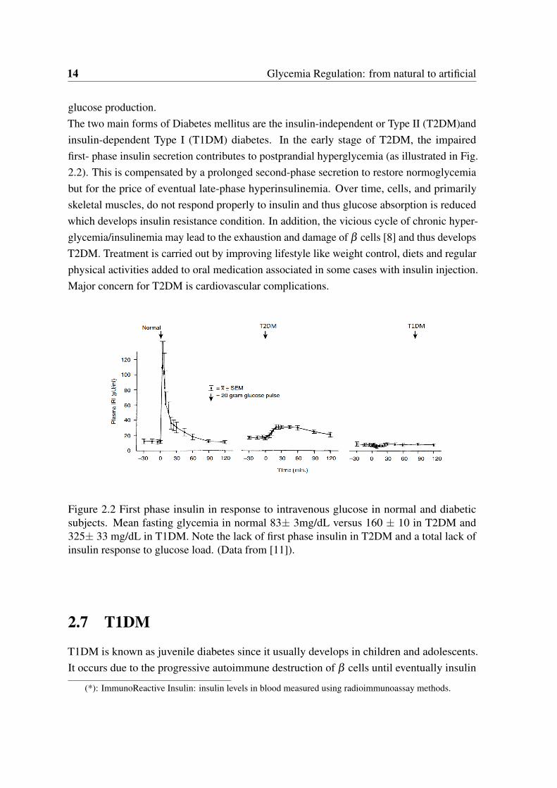
2.2 First phase insulin in response to intravenous glucose in normal and diabetic
subjects. Mean fasting glycemia in normal 83± 3mg/dL versus 160 ± 10 in
T2DM and 325± 33 mg/dL in T1DM. Note the lack of first phase insulin in
T2DM and a total lack of insulin response to glucose load. (Data from [11]). 14
2.3 Illustration of IP implantable pump. Right image modified from [19] and
left image IP pump and its insulin delivery communicator: MIP 2007C,
Medtronic/Minimed, Northridge, CA, USA. . . . . . . . . . . . . . . . . . 17
2.4 Insulin delivery system MiniMedr640G systemˆ, insulin pump in black and
a CGM in white. . . . . . . . . . . . . . . . . . . . . . . . . . . . . . . . 19
2.5 A smart-phone based portable artificial pancreas: Diabetes Assistant system
(Dias) as presented in [28] where it was used in clinical trials. . . . . . . . . 21
2.6 Photograph of overall equipment including BG autoanalyzer, control cabinet
and servo-syringes which connected to injection sites. Photo taken from [30] 22
3.1 Relationship between pharmacokinetics PK and pharmacodynamics PD [49]. 33
3.2 Hovorka’s compartmental model with meal subsystem. d(t) [g/min] is the
CHO input rate [70]. . . . . . . . . . . . . . . . . . . . . . . . . . . . . . 35
3.3 Dalla Man compartmental model of insulin-glucose system [71]. . . . . . . 39
3.4 Principal component of Uva/Padova T1DM simulator [73]. . . . . . . . . . 40
3.5 Magdelaine’s T1DM simulator. . . . . . . . . . . . . . . . . . . . . . . . . 41
3.6 Glycemia behavior during fasting scenario for adult5 of Uva/Padova simula-
tor. upper panel for u(t)=2U/h and middle panel for u=0 U/h and lower panel
for u(t)= the basal rate provided by the simulator. . . . . . . . . . . . . . . 46
4.1 IF2 response for open-loop, iP with α =−139 and iPvref α−1 =−198. (a): Meal intake.
(b): BG behavior. (c): iP and iPvref insulin infusion rates. . . . . . . . . . . . . . . . 63

xviii List of Figures
4.2 IF3 response for open-loop, iP with α =−129 and iPvref α−1 =−174. (a): Meal intake.
(b): BG behavior. (c): iP and iPvref insulin infusion rates. . . . . . . . . . . . . . . . 64
4.3 BE response for open-loop, iP and iPvref (a): Meal intake. (b): BG behavior. (c): iP and
iPvref insulin infusion rates. . . . . . . . . . . . . . . . . . . . . . . . . . . . . 65
4.4 LR response for open-loop, iP and iPvref (a): Meal intake. (b): BG behavior. (c): iP and
iPvref insulin infusion rates. . . . . . . . . . . . . . . . . . . . . . . . . . . . . 66
4.5 IF9 response for open-loop, iP and iPvref (a): Meal intake. (b): BG behavior. (c): iP and
iPvref insulin infusion rates. . . . . . . . . . . . . . . . . . . . . . . . . . . . . 67
4.6 IF2 response for open-loop, PID and iPID (p =−0.14,α =−0.16) (a): Meal intake. (b):
BG behavior. (c): Insulinemia. (d): PID and iPID insulin infusion rates. . . . . . . . . . 72
4.7 IF9 response for open-loop, PID and iPID. (a): CHO amount in meals. (b) BG behavior. (c):
PID versus iPID insulin infusion rates. . . . . . . . . . . . . . . . . . . . . . . . 79
4.8 LR response for open-loop, PID and iPID. (a):CHO amount in meals. (b): BG behavior. (c):
PID versus iPID insulin infusion rates. . . . . . . . . . . . . . . . . . . . . . . . 79
4.9 BG behavior of Uva/Padova simulator under iPID and PID control employing
IV sensor. The bars represents CHO amounts in each meal in grams. Upper
Panel is BG behavior and the lower panel is the insulin infusions by each
controller. . . . . . . . . . . . . . . . . . . . . . . . . . . . . . . . . . . . 80
4.10 Average BG of the (10 adults 25 runs) of Uva/Padova simulator under iPID control: solid
line represents the mean and the dashed is the standard deviation (SD). 70% confidence
interval is yielded with mean BG ± SD, and 95% confidence interval is with mean BG ±
1.96SD. . . . . . . . . . . . . . . . . . . . . . . . . . . . . . . . . . . . . . 80
4.11 Average BG behavior under iPID for heavy meal scenario of adults 5, 7 an 9
(5 runs each) of Uva/Padova simulator. The bars represent CHO amounts in
each meal in grams. . . . . . . . . . . . . . . . . . . . . . . . . . . . . . 81
5.1 The blue region represents Ω(G) the largest PIS for the insulinemia au-
tonomous subsystem. The arrows represent the vector fields. . . . . . . . . 89
5.2 Largest PIS in S− for bk = 1,λ = 0.5,x(0) = (x10,−1), x10 = 0.378. S− is
in light violet area, M is in blue and Ms is bounded by the solid violet line. 95
5.3 Invariance of S+. . . . . . . . . . . . . . . . . . . . . . . . . . . . . . . . 96
5.4 The largest PIS: M+. . . . . . . . . . . . . . . . . . . . . . . . . . . . . . 97
5.5 The lines ueq − k = 0 (u=0 in S+) with respect to the line s = 0 for a nonneg-
ative control in S+, with λm = 1,λ = 1.2785 and k = 0.91. . . . . . . . . . 100
5.6∣∣∣ λ
λm−1
∣∣∣eλ
λm > 1 only when λλm
> 1.2785. . . . . . . . . . . . . . . . . . . 103
List of Figures xix
5.7 Phase plane plot: with λ = 0.8 satisfying (5.51) i.e. 0.7 < λ < 1.3 but
not satisfying (5.58), with k = 0.91, x(0) = (x10,−6), x10 = 4.8887 for the
(bounding) trajectory in S−. x(0) = (4.8887,2) for the trajectory in S+. . . 103
5.8 Phase plane plot: with λ = 1.2785 satisfying (5.58), with k = 0.91, x(0) =
(x10,−6), x10 = 3.4438 for the (bounding) trajectory in S− , and x(0) =
(3.4438,2) for the trajectory in S+. . . . . . . . . . . . . . . . . . . . . . . 104
5.9 A block diagram of the overall SMC controlled system. . . . . . . . . . . . 105
5.10 Glycemia response of IF2 under SMC, ko = 0.014Ieq. (a): BG behavior. (b):
insulinemia versus its desired trajectory x1(t) and xd(t). (c): SMC control.
(d):phase plane of insulin x1,x2 of patient labeled IF2 showing the sliding
surface s = 0 and the control lines u = 0 in s > 0 and s < 0. . . . . . . . . . 112
5.11 Glycemia response of IF2 under SMC, ko = 0.02Ieq. (a): BG behavior. (b):
insulinemia versus its desired trajectory x1 and xd . (c): SMC control. . . . . 113
5.12 Glycemia response of BE under SMC. (a): BG behavior. (b): insulinemia
versus its desired trajectory x1 and xd . (c): SMC control. (d): Phase plane of
insulin x1,x2 of patient labeled BE showing the sliding surface s = 0 and the
trajectory that characterizes Ms− . . . . . . . . . . . . . . . . . . . . . . . . 114
5.13 Glycemia response of IF3 under SMC. (a): BG behavior. (b): insulinemia
versus its desired trajectory x1 and xd . (c): SMC control. (d): phase portrait
in x1 − x2 plane. . . . . . . . . . . . . . . . . . . . . . . . . . . . . . . . . 115
6.1 The largest polyheral PIS in open-loop using IF2 patient parameters. The
largest Polyhedral PIS Ω(G) is with w = w. The plane w2x = 0 is with
c = 1000 to characterize Ω(G2). . . . . . . . . . . . . . . . . . . . . . . . 125
6.2 Ω(G) the largest open-loop polyhedral PIS, θ2 = 11.6,θ3 = 122 of IF2
patient. . . . . . . . . . . . . . . . . . . . . . . . . . . . . . . . . . . . . 126
6.3 Ωm the open-loop PIS for the glycemia state x1(t), θ2 = 11.6,θ3 = 122 of
IF2 patient. . . . . . . . . . . . . . . . . . . . . . . . . . . . . . . . . . . 127
6.4 Lambert W -function and its two branches. . . . . . . . . . . . . . . . . . . 141
6.5 Closed-loop response of glycemia for five virtual patients with xo = (140,0,0).146
6.6 The control u(t) for IF2 patient. . . . . . . . . . . . . . . . . . . . . . . . 146
6.7 A trajectory plot in phase portrait for IF2 with x(0) = (140,0,0), the blue
plane represents Fx = 0 with K = 0.05. . . . . . . . . . . . . . . . . . . . 147
6.8 Observer behavior: insulin states and their estimation in closed-loop K = 0.03.148
6.9 BG behavior of BE patient under state feedback control with K = 0.03. . . 151
6.10 BG behavior of LR patient under state feedback control with K = 0.03. . . 151
6.11 BG behavior of 10 adults under 5 runs with K = 0.005. . . . . . . . . . . . 152

xx List of Figures
6.12 Control Variability Grid Analysis (CVGA) plot of Uva/Padova (10 adults
5 runs) simulations. . . . . . . . . . . . . . . . . . . . . . . . . . . . . . . 152
6.13 The state feedback insulin infusion rates of adult7 of Uva/Padova simulator:
a one sample of the (10 adults 5 runs) simulations. . . . . . . . . . . . . 153
6.14 BG behavior of BE patient (Simulator 1): nominal system versus uncertain
parameters. K = 0.03, θ2,3 = 70%θ2,3 u lower bound is −ub =−0.0167. . . 153
A.1 Unit step function f (t) in dotted red curve and its delay using the integral
buffer in red solid curve versus the transport delay f (t −h) in dotted blue
curve. . . . . . . . . . . . . . . . . . . . . . . . . . . . . . . . . . . . . . 178
A.2 Sinusoid function in dotted red and its delay using the integral buffer in solid
red versus the transport delay in dotted blue. . . . . . . . . . . . . . . . . . 179
A.3 f (t) and f (t −h) using the integral buffer versus the transport delay T = 2sec.179
A.4 f (t) and f (t −h) using the integral buffer versus the transport delay setting
T = 0.3sec. . . . . . . . . . . . . . . . . . . . . . . . . . . . . . . . . . . 180
A.5 A block diagram of a T1D glucose-insulin dynamics. with modeling error
on the output . . . . . . . . . . . . . . . . . . . . . . . . . . . . . . . . . 180
A.6 IF2 BG response. (a) Open-loop CGM data and BG model output as in (3.17) 181
A.7 IF2 BG response with noise under iP with −α = 180 and iPvref −α = 198.
(a) Meal intake (b) BG response (c) iP and iPvref control rates . . . . . . . 181
A.8 IF3 BG response with noise under iP with −α = 176 and iPvref −α = 223.
(a) Meal intake (b) BG response (c) iP and iPvref control rates . . . . . . . 182
A.9 IF3 BG response with noise under iP with −α = 175 and iPvref −α = 175.
(a) Meal intake (b) BG response (c) iP and iPvref control rates . . . . . . . 183

List of Figures xxi
Glossary
AP Artificial Pancreas
BG Blood Glucose
CGM Continuous Glucose Monitor
CSII Continuous Subcutaneous Insulin Infusion
CIPII Continuous Intraperitoneal Insulin Infusion
CHO Carbohydrate
DIA Duration of Insulin Action
FDA Food and Drugs Administration
FIT Functional Insulin Therapy
HSMC Higher order Sliding Mode Control
iP intelligent Proportional controller
iPvref intelligent Proportional with variable reference
iPID intelligent Proportional Integral Derivative controller
IP Intraperitoneal
IV Intravenous glucose sensor
IVGTT Intravenous Glucose Tolerance Test
IFB Insulin FeedBack
IOB Insulin On Board
MAGE Mean Amplitude of Glycemic Excursion
MFC Model-free Control
MPC Model Predictive Control
MSII Multiple Subcutaneous Insulin Injections

xxii List of Figures
OGTT Oral Glucose Tolerance Test
PD Proportional Derivative controller
PDs Pharmacodynamics: is the relationship between the drug concentration in the body
and its intended and antagonistic effects achieved with time.
PK Pharmacokinetics: is defined as the relation between the drug input (e.g. insulin) and
its produced concentration in the body with time.
PID Proportional Integral Derivative controller
PIS Positively Invariant Set
T1DM Type 1 Diabetes Mellitus
T2DM Type 2 Diabetes Mellitus
TDD Total Daily Dose
SC Subcutaneous injection route
SMC Sliding Mode Control
Chapter 1
General Introduction
1.1 Chapter Introduction in French
1.1.1 Le problème
Le pancréas sécrète deux hormones principales : l’insuline et le glucagon. Elles régulent la
source principale de l’énergie «le glucose» des cellules du corps dans la circulation sanguine.
L’insuline stimule l’absorption de glucose par les cellules et les muscles. Au contraire, le
glucagon stimule le foie pour décomposer le glycogène stocké et libérer du glucose lorsque
le taux de glucose sanguin (BG) est inférieur à 70 mg/dl pendant le jeûne ou lors des
efforts physiques et que l’insuline est supprimée. Le diabète de type 1 (DT1), ou diabète
insulinodépendant, est une maladie chronique qui résulte principalement de la destruction
auto-immune des cellules beta produisant de l’insuline dans le pancréas. Il en résulte un
manque absolu de production endogène d’insuline. Sans insuline stimulant l’absorption de
glucose aux cellules et aux muscles, la glycémie n’est pas visible et donc elle s’accumule
(au-dessus de 180 mg/dl) dans la circulation sanguine conduisant à des complications à long
terme. La maladie était fatale avant la découverte de l’insuline en 1921.
1.1.2 Solution disponible (boucle ouverte)
Pour survivre, les injections/infusions quotidiennes d’insuline exogène sont la seule solution
pour réguler la glycémie. Le patient injecte la quantité adéquate d’insuline calculée en
fonction de la quantité de glucose absorbée dans un repas. Ces doses, connues sous le nom
de bolus, sont associées à un taux de perfusion régulière d’insuline de fond appelé niveau
basal. Ce dernier est responsable de maintenir la glycémie constante pendant les conditions
de jeûne. Le patient doit également considérer, dans ce processus d’auto-traitement quotidien
2 General Introduction
qui peut être une source de stress, les perturbations comme le stress, la maladie et les activités
physiques, etc.
1.1.3 Solution d’ingénierie (boucle fermée)
Depuis les années soixante jusqu’à nos jours, l’objectif de la recherche, dans le domaine de
l’ingénierie, est de prendre le fardeau des patients T1DM en remplaçant les doses stressantes
d’insuline basale / bolus (boucle ouverte) connues sous le nom d’insulinothérapie fonction-
nelle (ITF) par un dispositif automatique. Par conséquent, un pancréas artificiel (PA) est le but
ultime de la régulation de la glycémie DT1. Ce projet de longue date a pour but de fermer la
boucle entre une pompe à insuline automatisée et un capteur de mesure continue du glucose
(MCG) pour reproduire la régulation naturelle de la glycémie. Avec la croissance rapide de la
technologie ce sujet a reçu un intérêt mondial et il est l’objet d’un grand développement en
cours. Bien qu’il s’agisse d’un problème ancien, jusqu’à présent, il n’existe pas de dispositif
viable entièrement automatisé disponible pour les patients diabétiques. Comme on le verra
plus en détail dans la littérature du chapitre 2, différentes stratégies de contrôle ont été testées
in silico et in vivo dans ce but.
1.1.4 Notre contribution
Pour fermer la boucle entre une pompe à insuline et un capteur de glucose sanguin, deux
principaux types d’algorithmes de contrôle ont été utilisés : des commandes basées sur des
modèles et des commandes non basées sur des modèles. Il s’agit de la commande sans modèle
(CSM), de la commande positive par modes glissants (CMG) et d’une commande positive
par retour d’état. Les contrôleurs ont été testés sur des simulateurs T1DM pour évaluer leurs
performances. En outre, on obtient des résultats importants en boucle ouverte, c’est-à-dire
une prédiction d’hypoglycémie sous injection basale pendant la phase de jeûne. De manière
exhaustive, nous listons l’ensemble de nos contributions :
1. Première application de CSM (contrôleurs proportionnels et Proportionel-Intégral-
Dérivé intelligents) pour la régulation de glycémie de T1DM.
2. Une CMG positive est conçue pour la première fois pour la régulation de la glycémie en
respectant la contrainte de positivité de la pompe à insuline. La commande est positive
partout à l’intérieur du plus grand ensemble invariant d’insuline dans le plasma.
3. La théorie des ensembles invariants positifs de systèmes linéaires est employée pour
la première fois sur un modèle T1DM. Le principal résultat est la régulation de la
glycémie, la prévention et la prédiction de l’hypoglycémie.

1.2 General Introduction 3
4. Le plus grand ensemble positivement invariant sous injection basale constante d’insu-
line (boucle ouverte) en phase de jeûne est trouvé. Il est utilisé pour prédire et prévenir
une future hypoglycémie.
5. Les analyses de positivité d’entrée / d’état sont considérées pour la première fois pour
concevoir un retour d’état positif pour réguler la glycémie. En boucle fermée, la glycé-
mie est réglée tout en restant positive et l’hypoglycémie est évitée. L’hypoglycémie
future est prédite lorsque la condition initiale du système est en dehors du plus grand
ensemble positivement invariant.
1.2 General Introduction
The problem of regulating glycemia of Type-1 Diabetes Mellitus (T1DM) is investigated
in this work. T1DM is a chronic autoimmune disease affecting approximately 25 million
individuals in the world. A T1DM patient suffers from an absolute lack of insulin due to
autoimmune destruction of pancreatic β -cells. Insulin stimulates the uptake of glucose in
the blood stream to cells and muscles for energy. Without insulin stimulating the uptake
of glucose to cells and muscles, blood glucose remains in the blood stream and grows into
hyperglycemia. To survive, exogenous insulin injections is the only solution to regulate
glycemia. The disease was fatal before the discovery of insulin in 1921.
Current treatment requires programmed injections. These are either multiple daily insulin
injections or continuous subcutaneous insulin infusion (CSII) delivered via a pump. While
calculating insulin doses, the patient must consider many factors like carbohydrates in every
meal and physical activities. Poor treatment causes long term complications like renal failure
and peripheral vascular complications. As a result, automatic control of these injections
has received a wide interest especially with the rapid development of sensing technologies
and insulin pumps. For more than 50 years, the idea of an Artificial Pancreas (AP) device
was envisioned. The core of the device is the control algorithm that closes the loop between
blood glucose measurements and insulin injections of T1DM patients. The objective is to
replace the manual injections and to enhance the stressful everyday life of T1DM patients.
The main challenge is hypoglycemia that is an acute complication in the life of a T1DM
subject especially in nocturnal time. It is a major open problem which stood against the
realization of AP device.
In general the focus of any research on AP is to design a control algorithm adaptable to
different patient insulin sensitivity and robust enough to deal with non modeled dynamics,
uncertainties and measurement noise. An important factor that affects controllers performance
4 General Introduction
is to achieve the trade-off between reducing hyperglycemia and avoiding hypoglycemia.
Moreover, the positivity of the control input (insulin infusion) must be taken into account in
the design.
The mainstream of control algorithms, that was used previously in different clinical tests,
is the Proportional-Integral-Derivative (PID) controller and the Model Predictive Control
(MPC). MPC is popular in this field as it handles the system constraints in the design. Its
main drawback is the cumbersome optimization process. PID was also frequently tested as
it was observed that it mimics pancreatic β -cells behavior. Moreover, its design does not
require a precise model of the system.
In this work two main controller types are employed: model-based and non-model based
controllers. To asses their efficiency, both types are tested in silico on two T1DM simulators.
The first simulator is a long-term model that is derived from clinical data of T1DM subjects
and developed in LS2N laboratory in France. The second simulator is the Uva/Padova T1DM
simulator that is approved by the Food and Drugs Administration (FDA) for closed-loop
control validations. All controllers designed and tested hereafter are fully automatic without
meal announcements nor supplementary insulin doses.
In this work, Model-free control (MFC) is designed for glycemia regulation for the first
time. In its control, poorly known dynamics and perturbations are estimated on line via
the unique knowledge of the input/output measurements. The estimation is employed in
the control law to compensate for perturbations and the loop is closed via a simple PID
controller. MFC with PID in the feedback is called intelligent PID (iPID). It offers the
simple features of a PID control in the frame of a model free design. In opposition to
previous PID studies, the control algorithm developed hereafter is fully automated without
any feed-forward or supplementary insulin doses. Intelligent proportional (iP) is firstly tested
employing a variable reference trajectory to circumvent the poor postprandial behavior of
constant reference iP. Variable reference iP produced an impulsive control of fast reaction to
meals that yielded a reduced postprandial hyperglycemia. To further enhance postprandial
response, additional closed loop terms are added and an iPID is designed using a constant
glycemia reference. In silico results comparison showed a better postprandial glycemia
regulation with constant reference iPID over iP employing a variable reference. iPID is also
compared to a classic PID on the well known Uva/Padova T1DM simulator. The results
showed that the postprandial response was improved with iPID reducing hyperglycemic
excursions with minimal hypoglycemic events. Moreover, the results showed that iPID,
who has the classic PID structure with new adaptive feature, emulated insulin delivery of
pancreatic β -cell. MFC showed a good robustness level. The system is considered as a black
box and MFC parameters are tuned empirically based on the input/output measurements.
1.2 General Introduction 5
Another robust controller is designed and tested in this thesis, that is Sliding Mode
Control (SMC). A positive SMC is designed for the first time for glycemia regulation. The
controller is positive everywhere in the largest closed-loop Positively Invariant Set (PIS) of
plasma insulin subsystem. Two-stage SMC is designed, the second stage SMC2 block uses
the glycemia error (with respect to the desired level) to design the desired insulin trajectory.
Then the plasma insulin state is forced to track the reference via first stage control SMC1.
The switching variable of SMC1 is the first order polynomial of the insulin error. Sliding
mode of SMC1 guarantees insulin reference tracking. The resulting desired insulin trajectory
is the required virtual control input of the glycemia system to eliminate glycemia error.
Glycemia error is the switching variable of SMC2. Glycemia is steered to the normal set
point during sliding mode of SMC2. In silico trial is performed to validate the theoretical
results on the nominal system during fasting phase. Robustness of SMC against parameter
change, meal perturbations and sensor noise is considered as a perspective.
Due to the discontinuity of the control law, designing a positive SMC everywhere in
the largest PIS such that glycemia remains invariant within the desired level is much more
complex. The positive SMC is a proof of concept and the design can be extended to include
hypoglycemia constraint. In other words, the future problem maybe to design a positive
SMC in the largest PIS where glycemia is above hypoglycemic threshold (70 mg/dL).
The problem of finding the largest PIS where glycemia remains invariant within or above
the desired threshold is addressed via a simple continuous control law. In other words, to
design a positive controller that takes hypoglycemia constraint into account and establishes
a tight control. The loop is closed via a positive state feedback controller. First of all, the
control law is simple and continuous. Thus, the design of a positive state feedback in the
largest PIS such all system states are positive, is less complex than that with SMC. Moreover,
the theory of invariant polyhedra for continuous linear systems is directly applied to find a
positive state feedback controller. The largest PIS of the open-loop system (where only a
basal insulin rate is infused) is firstly obtained. Secondly, the largest PIS of the closed-loop
system under a stabilizing positive state feedback control is found. Inside the PIS, glycemia
is regulated to its desired level without hypoglycemia risk. The main outcome of the largest
open and closed-loop PIS for glycemia system is the hypoglycemia prediction. A solution
to avoid the life-threatening barrier to the optimal diabetic treatment. Hypoglycemia is
predicted here based on the system initial conditions. The prediction is established when
the initial conditions are outside the largest closed-loop PIS (BG<70 mg/dL). In this case,
the loop is opened to either administrate basal insulin only, or to switch the pump off. If the
initial condition belongs to the open-loop (basal) PIS then the loop is opened to inject basal
insulin only. Otherwise, if future hypoglycemia is also predicted under basal injection, then
6 General Introduction
the pump is switched off signaling severe hypoglycemia. In this manner, positivity analysis is
shown to be very useful for tight glycemia regulation and also for hypoglycemia prediction.
1.3 Thesis Overview
The next chapter is an introductory chapter that presents the problem of glycemia regulation
in humans from healthy to diabetic subjects. The disease is introduced in its two types
reviewing the available programmed insulin therapy. The state of the of AP studies and the
related clinical trials is reviewed in the end of Chapter 2.
In Chapter 3, a review of the main mathematical models and T1DM simulators that
describe glucose-insulin dynamics of T1DM is given. A new long-term glycemia-insulinemia
model that was derived from real T1DM clinical data is presented. The existence of an
equilibrium point of a T1DM model in fasting conditions is discussed from the physiological
point of view. On these bases, the presented mathematical models are assessed to find out
whether they give a good description of glycemia-insulinemia dynamics T1DM.
In Chapter 4, MFC design theory is recalled and a brief stability study of iP controller
is presented. A counter academic example of an unstable linear system is given showing that
it can not be stabilized by an iP. Thereafter, iP controller is tested for glycemia regulation
employing a constant reference and a variable reference trajectory. The iP behavior is
compared to a constant reference iPID. Model-free iPID performance is also compared to a
classic PID and the in silico results showed a better postprandial response with the iPID. The
overall MFC results are discussed and a general conclusion is given.
In Chapter 5, SMC is designed for glycemia regulation. The largest PIS of insulin
system is firstly found in open and closed-loop. Then, the parameters of SMC are designed
to yield a positive control everywhere in the closed-loop PIS. The desired insulin trajectory
is designed to steer glycemia error to its desired level via a second SMC. The design steps of
the second SMC control are detailed.
In Chapter 6, positivity and invariance of overall system in R3 is presented in open-loop
(under constant basal insulin injection) and under positive state feedback control. In the
first part of the chapter, the largest open-loop PIS is firstly found such that glycemia error is
nonnegative. At first the polyhedral PIS is characterized. This is followed by characterizing
the surface that bounds the largest PIS. The result is used to predict hypoglycemia under basal
injection. In the second part of Chapter 6, a positive state feedback controller is designed
such that glycemia state remains invariant above hypoglycemia threshold. The resulting
largest polyhedral PIS is presented. The limiting surfaces of the largest PIS are then found.
Open and closed-loop PIS results are used to implement a general hypoglycemia prediction

1.3 Thesis Overview 7
algorithm. The resulting positive state feedback controller is tested in silico to validate the
theoretical results.
Finally, a general conclusion is given in Chapter 7 followed by the planned future work
of this thesis. Each chapter begins with a French introduction and the overall thesis resume
in French is presented directly after Chapter 7.

Chapter 2
Glycemia Regulation: from natural to
artificial
2.1 Chapter Introduction in French
Il s’agit d’un chapitre introductif sur la régulation de la glycémie pancréatique chez l’homme
sain et diabétique. Tout d’abord, la production de glucose sanguin endogène est brièvement
revue suivie de l’introduction des principaux organes qui consomment le glucose comme
une source d’énergie majeure. Les hormones pancréatiques principales sont l’insuline et le
glucagon. Leurs rôles principaux sont définis. Le diabète dans ses deux types est présenté ainsi
que le traitement quotidien de chacun mettant le focus sur DT1. La description commence par
le traitement manuel jusqu’à la solution artificielle, c’est-à-dire la régulation de la glycémie
en boucle fermée dans la cadre d’un PA. L’état de l’art des études de PA est revu et l’accent
est mis sur les courants principaux des algorithmes de commande utilisés. L’état de l’art des
études AP commence avec le régulateur PID dans les essais in silico et in vivo. Ceci est
suivi par la commande industrielle plus avancée, le CP et les réalisations principales de cette
commande à ce jour. Une étude de CMG conçue pour la régulation de la glycémie, en tant
que commande robuste, est ensuite présentée. Finalement, certaines études de la commande
par retour d’état sont revues. Une conclusion générale de ces algorithmes de commande et
leur contribution au projet AP global est présentée. Leurs principaux problèmes ouverts sont
également soulignés donnant les solutions de cette thèse pour chacun.
10 Glycemia Regulation: from natural to artificial
2.2 Introduction
This is an introductory chapter for pancreatic glycemia regulation in humans from healthy
to diabetic. Firstly, endogenous blood glucose production is briefly reviewed followed by
introducing the main organs that consume blood glucose as a major energy source. the key
pancreatic hormones: insulin and glucagon and their principal roles are defined. Diabetes
mellitus in its two types is introduced presenting the daily treatment of each putting the focus
on T1DM. The passage turn from manual self treatment to artificial solution i.e. glycemia
regulation via closed-loop control under AP project. The state of the art of AP studies are
reviewed and the focus is on the mainstream of the employed control algorithms.
2.3 Blood glucose: The ubiquitous fuel in biology
Glucose: a name given to the grape sugar by the committee of the French Académie des
Sciences in its report on July 1838. The name is contrived from the Greek glukus, "sweet
to the taste" and the suffix -ose, derived from the Latin -osus, became biochemical suffix
indicating a carbohydrate [1]. Carbohydrates (CHO) are the body’s primary energy source
and glucose is their basic unit which is absorbed quickly as a single component.
2.3.1 Glucose Production
• The liver: it plays a central role to balance glucose uptake and storage. In absorptive
state it stocks the elevated postprandial glucose (around two-thirds of blood glucose
(BG)[2]) as glycogen. Conversely, in post-absorptive or fasting phase glucose release
is activated to maintain glucose homeostasis.
• The kidneys: during fasting state, kidneys participate to glucose production of about
20 25% of glucose release in this condition [3].
• Intestine: recently a novel function of intestinal endogenous glucose production was
described [4]. It contributes to 20 25% of total fasting endogenous glucose produc-
tion.
2.3.2 Glucose Consumption
A steady glucose supply, transported by the blood stream, is needed by most of tissues and
organs:
2.4 Glycemia Regulation: Glucose homeostasis 11
• The brain is the major consumer of about 120g of glucose daily, which corresponds to
60% of the utilization of glucose by the whole body in the resting state [2]. Glucose is
the only fuel for the brain except for starvation where liver breaks down fatty acids
into ketone bodies to partly replace glucose.
• Muscles: In addition to glucose, they consume fatty acids and ketone bodies. In resting
state, fatty acids covers 85% of their energy needs [2].
• Kidneys: their glucose consumption, filtration, and re-absorption play an important
role in glucose homeostasis. They contribute to about 20% of the total glucose removed
from the circulation [3].
Blood glucose concentration or glycemia1 is measured in terms of either molar concentra-
tion (mmol/L) or mass concentration (mg/dL) and the over night or fasting normoglycemia,
is within 70-100 mg/dL for a non-diabetic. This tight control is mainly achieved through the
balance between glucose consumption and production. The process of preserving glucose in
its narrow normal limits is called Glucose homeostasis [5].
2.4 Glycemia Regulation: Glucose homeostasis
The property of a system to maintain its variables relatively constant (in their normal levels)
to keep a stable internal environment is called homeostasis. The term originally referred
to the processes within living organisms like the internal body temperature and glycemia
regulation. The principle is also found in automatic control such as the classic examples of
thermostat and autopilot. Glucose homeostasis is a natural control mechanism that regulates
glycemia based on the interaction and balance between two main pancreatic hormones:
insulin and glucagon. They have antagonistic effects to maintain normoglycemia, insulin
promotes glucose transport to cells to reduce elevated glycemia, while glucagon stimulates
endogenous glucose production to rise low glycemia (see Fig. 2.1 )2. From automatic control
point of view glucose homeostasis represents a negative feedback control.
It is maintained by a variety of cellular mechanisms. Important mechanisms are carried
out by hormones and the pancreas plays the fundamental role.
1first recognized by the French physiologist François Magendie in the early 19th century [1]2 image taken from https://zhiyaobme.wordpress.com/2014/10/17/balance-mattars

12 Glycemia Regulation: from natural to artificial
Figure 2.1 Glucose Homeostasis
2.5 Pancreatic secretion
The pancreas represents the control center of glucose homeostasis via its endocrine function of
secreting the glycemia regulating hormones into the blood stream. Its major glucoregulators
are:
1. Insulin: secreted by β Langerhans cells in response to glucose and nervous stimuli. It
is the key hormone in glucose metabolism. It promotes
• glucose transport to most cells: like in resting skeletal muscles and adipose tissue.
Some tissues do not rely on insulin for efficient glucose uptake like in the brain
who uses non insulin-sensitive transporters [6], [7].
• glucose storage by the liver and the muscles in the form of glycogen.
• inhibits endogenous glucose production.
2.6 Defect of Glucose homeostasis: Diabetes 13
2. Glucagon: secreted by α Langerhans cells in response to low blood glucose concentra-
tions as in fasting state. It promotes the breakdown of glycogen in the liver to release
glucose and stimulates the conversion of fatty and amino acids into glucose.
Insulin is secreted in the following phases:
• Basal rate: a steady background rate secreted during post-absorptive state i.e. overnight
or during fasting, that balances the endogenous glucose production to maintain normo-
glycemia.
• Cephalic phase: is stimulated by the sight, smell and taste of food before any nutrient
intestinal absorption.
• First phase: the initial rapid acute pulse of insulin 5-10 min after β cells are signaled
that glycemia is abruptly elevated. It promotes peripheral utilization of the nutrient
and suppresses endogenous glucose production [8], [9].
• Second phase: prolonged insulin secretion following the first phase which is related to
the degree and stimulus duration and sustained until normoglycemia is attained.
In addition to the endocrine system, the pancreas function is also controlled by the
autonomic nervous system. For example, during stressful situations and physical exercise
alpha cells are stimulated to release glucagon into the blood stream to fulfill the energy needs
[10].
2.6 Defect of Glucose homeostasis: Diabetes
Any metabolic abnormality involving organs or hormones breaks the continuous balance
between glucose transport, storage and metabolism which causes impaired glucose home-
ostasis. Deficiency of insulin secretion and/or action leads to elevated glucose concentrations
or Hyperglycemia. Prolonged hyperglycemia cause serious long-term complications like
renal failure, blindness, cardiac diseases and peripheral vascular complications that represent
the main cause of mortality in diabetics [5]. Recurrent hyperglycemia condition indicates
diabetes if it is greater than 126 mg/dL 3 after 8-hours fasting or greater than 200 mg/dL
for a 2-hours postprandial measurement after 75g oral glucose load. Dawn hyperglycemia
or dawn phenomenon is observed in diabetics which is defined as the early morning abrupt
rise in glycemia above fasting levels without antecedent hypoglycemia. It occurs due to
increased nocturnal secretion of cortisol and the growth hormones that stimulates hepatic
3According to American Diabetes Association (ADA).
14 Glycemia Regulation: from natural to artificial
glucose production.
The two main forms of Diabetes mellitus are the insulin-independent or Type II (T2DM)and
insulin-dependent Type I (T1DM) diabetes. In the early stage of T2DM, the impaired
first- phase insulin secretion contributes to postprandial hyperglycemia (as illustrated in Fig.
2.2). This is compensated by a prolonged second-phase secretion to restore normoglycemia
but for the price of eventual late-phase hyperinsulinemia. Over time, cells, and primarily
skeletal muscles, do not respond properly to insulin and thus glucose absorption is reduced
which develops insulin resistance condition. In addition, the vicious cycle of chronic hyper-
glycemia/insulinemia may lead to the exhaustion and damage of β cells [8] and thus develops
T2DM. Treatment is carried out by improving lifestyle like weight control, diets and regular
physical activities added to oral medication associated in some cases with insulin injection.
Major concern for T2DM is cardiovascular complications.
Figure 2.2 First phase insulin in response to intravenous glucose in normal and diabeticsubjects. Mean fasting glycemia in normal 83± 3mg/dL versus 160 ± 10 in T2DM and325± 33 mg/dL in T1DM. Note the lack of first phase insulin in T2DM and a total lack ofinsulin response to glucose load. (Data from [11]).
2.7 T1DM
T1DM is known as juvenile diabetes since it usually develops in children and adolescents.
It occurs due to the progressive autoimmune destruction of β cells until eventually insulin
(*): ImmunoReactive Insulin: insulin levels in blood measured using radioimmunoassay methods.
2.7 T1DM 15
is no more produced. By the time of diagnosis, more than 80-90% of the β cells have been
destroyed due to the large gap between the autoimmunity onset and diabetes onset. However,
recent studies showed that they never reach zero in some established T1D patients [12]. Main
symptoms of T1DM are increased thirst, fatigue and frequent urination. The only treatment
is the exogenous insulin therapy.
2.7.1 Complications
• Acute complications
1. Hypoglycemia: a fall of blood glucose below normal levels. Mainly frequent
hypoglycemia in T1DM is related to three reasons [13] : i) unregulated insulin
injection and sustained hyperinsulinemia. ii) impaired glucagon response to
hypoglycemia which begins within 5 years of disease diagnosis. iii) defect in the
autonomic counterregulatory response of nervous system and reduced awareness
of hypoglycemia. The latter impairment results from hypoglycemia per se (i.e.
the patient has a history of hypoglycemia) during intensive insulin therapy. The
average T1DM patient suffers from two episodes of common hypoglycemia per
weak and one severe (often with seizure and coma) per year. Severe hypoglycemia
leads to cerebral damage (at plasma glucose levels of 30-35 mg/dL) or even death
to 2-4% of patients. (see[5] and the references therein).
Overnight hypoglycemia is more frequent and attributes to nocturnal sudden death
"dead-in -bed" syndrome which is a more serious concern for young patients.
2. Ketoacidosis: It occurs during hyperglycemia due to a lack or reduce effec-
tive insulin against increased hepatic and renal glucose production. It is a life-
threatening complication that indicates increased level of ketone bodies and
acidity in the blood. It develops when the body starts to break down fats to
release energy to compensate for faulty glucose metabolism. This metabolic
state is sometimes the first sign of diabetes. Its treatment necessitates immediate
hospitalization, re-hydration and insulin replacement.
• Chronic complications
Management of diabetes during childhood have implications of the future development
of the long-term complications. These include micro-vascular and macro-vascular
complications. The latter cover circulatory and cardiovascular such as stroke and
myocardial infraction (heart attack). Whereas the micro-vascular complications include
nephropathy (kidney damage), neuropathy (usually starts with feet) and retinopathy
[14].
16 Glycemia Regulation: from natural to artificial
2.8 The survival: insulin therapy
Before the discovery of insulin by Banting, Best Macloed and Collip in 1921, T1DM was
a fatal disease. To survive, the patients were under severe diets to limit glycemia growth
which did not much to their life span. According to International Diabetes Federation (IDF)
diabetes atlas - 7th edition, there are 415 million diabetics world wide and it estimates 642
million incidences in 2040 among people aged 20-79 4. It estimates 0.5 million of T1DM
among children only in 2015. For the no-cure disease, exogenous insulin therapy is the only
treatment for survival. According to the ADA, insulin can be found in the following types:
1. Rapid-acting: 15 min onset 5, peaks time of about one hour and a total duration of 2-4
hours.
2. Short-acting (regular): 30 min onset, peak time within 2-3 hours and total effective
duration 3-6 hours.
3. intermediate-acting: 2-4 hours, peaks within 4-12 hours and is effective in 12-18 hours.
4. long-acting: several hours onset, and regulates glycemia evenly (peakless) and effective
over 24-hour period.
5. inhaled insulin 6: 12-15 min onset peaks by 30 min and cleared out after 180 min.
2.8.1 Insulin delivery
Insulin is delivered mostly by subcutaneous (SC) injection using an insulin syringe. At
increased cost, an insulin pen is more accurate and more convenient. Continuous Subcu-
taneous Insulin Infusion (CSII) using a electromechanical pump administers insulin even
more accurately. However, it has a higher risk of ketoacidosis resulting from some pump
infusion-related issues as pipe clogs or insulin leak[16].
Two main forms of treatments: conventional and functional or intensive. Those regimens
are to control blood glucose in the normal bounds by mimicking the normal insulin secretion.
Dose size and frequency is based on the insulin type, meal (size, composition and timing)
and exercise throughout the day.
• Conventional: A standard fixed insulin administration that requires fixed daily meals
to be taken at set times corresponding to 1 to 3 injections per day. Short and regular
4includes diagnosed and non-diagnosed subjects5the time taken by insulin to reach blood stream and starts acting.6 recently approved by Food and Drugs Administration (FDA) [15].

2.8 The survival: insulin therapy 17
insulin accompanied with intermediate-acting are usually used. The dietary and activity
regimens are set to match the fixed insulin doses. The physician modifies and updates
the regimen based on major changes in life-style like illness. This regimen is more
affordable to diabetics than the intensive therapy.
• Functional (or Flexible) Insulin Therapy/Treatment (FIT): in this regimen insulin is
infused in two separate rates: continuous basal rate (long-acting insulin) and insulin
boluses7 to account for meals (short-acting). The dosing is adjusted according to
glycemia reading, meal size (carbohydrate intake) and physical activities. It is a self-
management therapy where BG is monitored 3-5 times a day and insulin doses are
calculated following a predefined program. FIT provides a good glycemic control in
a more flexible life-style but requires a higher financial budget and an experienced
assisting team. This basal-bolus regime can be given by either Multiple Subcutaneous
Insulin Injections (MSII) or by CSII [15].
• Intraperitoneal (IP) administration: Insulin delivery using Continuous Intraperitoneal
Insulin Infusion (CIPII) through implantable IP pumps (see Fig. 2.3). Insulin delivered
through the IP route is absorbed rapidly into the portal vein and thus is a more
physiologic mode of insulin as compared to SC delivery [17]. IP implanted pumps
last years and they are refilled with transcutaneous insulin which has 1 min onset,
20-25 min peak time, and 1-2 h as total duration [18]. CIPII is emerging as a valuable
treatment option for closed-loop BG control.
Figure 2.3 Illustration of IP implantable pump. Right image modified from [19] and leftimage IP pump and its insulin delivery communicator: MIP 2007C, Medtronic/Minimed,Northridge, CA, USA.
7from Latin which means the administration of discrete dose of a substance like drug to rapidly achieve aneffective therapeutic concentration in the blood stream. Insulin bolus is injected (or infused) intravenously orsubcutaneously in an amount to account for the upcoming meal load

18 Glycemia Regulation: from natural to artificial
2.8.2 FIT: how to
A general common algorithm to calculate FIT for T1DM subject is described as follows [20]:
1. Total Daily Dose (TDD) is calculated roughly as: TDI=0.55* body weight [kg].
2. Daily basal injection is usually 40-50% of TDD.
3. Insulin to CHO ratio I:CHO is defined as how many grams of CHO are covered by one
unit of insulin. If the 500 rule8 is used then I:CHO=500 ÷ TDD.
4. Insulin Sensitivity (correction) Factor (ISF) estimates the point drop of glycemia in
mg/dL for every unit of insulin. If rapid or short-acting insulin is used then ISF is
obtained by 18009 rule ISF=1800÷TDD.
N.B. The subject sensitivity to insulin is not a fixed value and it potentially varies during the
day, due to sickness, physical activities or stress. Therefore, this calculation serves as basic
start-up value that may be adjusted by the individual during the day.
Before meal intake, the patient weighs its CHO and according to his I/CHO ratio he
deduces the necessary meal bolus to be injected. Then, he measures his BG and if the reading
is above the desired target the subject should inject a pre-meal correction dose:
Correction dose =BG target - BG reading
ISF(2.1)
Then the subject injects the prandial bolus of rapid-acting insulin 20 min prior to the
meal 10.
2.8.3 Insulin on Board (IOB)
Bolus calculation (BC) in CSII regimen can be found as a feature of modern insulin pumps.
Beside taking into account the right hand side of (2.1), bolus calculators take another
important aspect into consideration: the approximation of the insulin decay curve [23]. This
curve estimates the remaining amount of insulin in the body from previous insulin bolus
which is defined as the insulin on board (IOB). IOB must be taken into account correctly to
8The 500 CHO rule assumes that the subject consumption+endogenous production of glucose is about 500gper day. This rule is applied when rapid or short-acting insulin is used otherwise, with regular type a 450g ruleis applied.
9 Dr. Paul Davidson proposed the first the insulin management system of 1500 formula for the ISF and 450for I:CHO in the mid 1980s and it was later modified to 1800 for ISF and 500 for I: CHO [21]
10a 20 min bolus prior to a meal is shown to significantly lower BG better than 20 min post-meal bolus orimmediate pre-meal injection [22]

2.9 Artificial Pancreas 19
reduce the size of future bolus to avoid insulin stacking that leads to later hypoglycemia [24].
The BC pump setting that critically affects IOB correct calculation is the Duration of Insulin
Action (DIA). As detailed in [24], the widespread confusion in accurate DIA setting has
lead to more common insulin stacking which has a direct impact on hypoglycemia. Among
the authors recommendations, insulin manufacturers verify actual DIA for their short-acting
insulins. Based on a generic insulin sensitivity variation curve, [23] developed a dynamic
IOB estimator to be used in CSII or closed-loop treatments that showed better simulation
results than the current static pump IOB approximations.
2.9 Artificial Pancreas
In diabetic patients the physiological closed-loop system of the glucose homeostasis is broken
due to the deficiency or lack of beta cells response to glycemia elevation. Therefore the patient
needs to self-monitor his blood glucose using a glucometer and inject insulin accordingly
taking into account the external perturbations like meals and exercise. Blood glucose sensing
technology has evolved rapidly providing a feedback tool for diabetic patients. The two main
sensors used by diabetic individuals are finger-stick glucose meters and Continuous Glucose
Monitor (CGM). The former reads blood glucose levels by taking blood samples obtained by
pricking the finger. CGM measures glucose levels in the interstitial fluid providing real time
readings. CGMs are mainly accompanied with insulin pumps in CSII of FIT as illustrated in
Fig. 2.4.
Figure 2.4 Insulin delivery system MiniMedr640G systemˆ, insulin pump in black and aCGM in white.
In this manner, insulin administration is not automated as the subject himself closes the
loop between the CGM and the insulin pump and controls his BG following the algorithm of
FIT. FIT + CSII provide a more flexible life style since it adapts to external loads like variable

20 Glycemia Regulation: from natural to artificial
meal amounts and timings. However, the self BG regulation is cumbersome and T1DM
subjects still have a stressful everyday life maintaining tight BG control while reducing
the frequency and severity of hypoglycemia. Mimicking normal pancreas through different
therapeutic strategies is surely not an easy task and thus the alternative solution is the
development of artificial pancreas. Different approaches have been evaluated:
1. Bio-artificial pancreas: β cells or islet encapsulation in an immunoisolating semi-
permeable membrane. The concept is to surgically implant the islet tissue to artificially
function as a pancreas. The membrane should allow nutrient, insulin, glucose and
waste exchange with surrounding environment. Islet encapsulating can avoid foreign
body response and thus avoiding immunosuppressive medications. The approach is
quite promising but the research field is still on development to address the current
challenges such as materials used to create the tissue with the required properties and
its lifetime and the sufficiency of donor islets[25].
2. Insulin gene therapy: the transfer of a foreign gene into body cells to produce insulin.
Insulin gene could be injected to no-β cells [26]. This approach is applied to the
treatment of T1DM either by preventing the autoimmune destruction of β cells for the
new diabetics, or by engineering a β cell replacement [27]. The research is ongoing
and advancing to develop a therapy with a more precisely regulated insulin production
and secretion.
3. Artificial pancreas (the device): a closed-loop system composed of a control algorithm
device that administers insulin delivery of the pump depending on the real time reading
of the CGM.
Artificial Pancreas (AP) studies and tests have been evolving rapidly in parallel with the
technological advances. Automation of BG regulation has received a world-wide attention
and clinical trials of different control algorithms have been conducted and showed satisfac-
tory results that meet their own objectives. Yet, challenges are facing the realization of a
commercialized AP. Those range from technical like CGM performance (calibration and
delay), insulin delays, safety and reliability and robust communication between components
[29]. Others are physiological like insulin sensitivity and the positive irreversible insulin
injection as it can not be removed from the body once it is injected. Those challenges give
rise to increased hypoglycemic events and thus less efficient BG control.
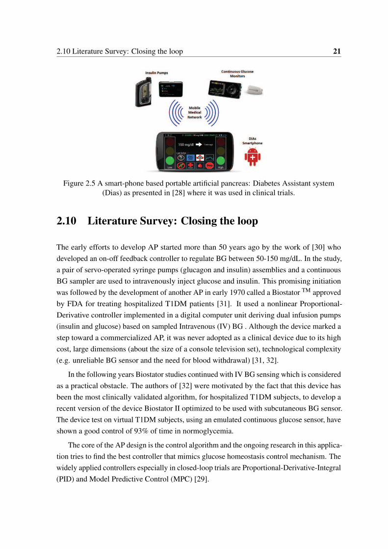
2.10 Literature Survey: Closing the loop 21
Figure 2.5 A smart-phone based portable artificial pancreas: Diabetes Assistant system(Dias) as presented in [28] where it was used in clinical trials.
2.10 Literature Survey: Closing the loop
The early efforts to develop AP started more than 50 years ago by the work of [30] who
developed an on-off feedback controller to regulate BG between 50-150 mg/dL. In the study,
a pair of servo-operated syringe pumps (glucagon and insulin) assemblies and a continuous
BG sampler are used to intravenously inject glucose and insulin. This promising initiation
was followed by the development of another AP in early 1970 called a Biostator TM approved
by FDA for treating hospitalized T1DM patients [31]. It used a nonlinear Proportional-
Derivative controller implemented in a digital computer unit deriving dual infusion pumps
(insulin and glucose) based on sampled Intravenous (IV) BG . Although the device marked a
step toward a commercialized AP, it was never adopted as a clinical device due to its high
cost, large dimensions (about the size of a console television set), technological complexity
(e.g. unreliable BG sensor and the need for blood withdrawal) [31, 32].
In the following years Biostator studies continued with IV BG sensing which is considered
as a practical obstacle. The authors of [32] were motivated by the fact that this device has
been the most clinically validated algorithm, for hospitalized T1DM subjects, to develop a
recent version of the device Biostator II optimized to be used with subcutaneous BG sensor.
The device test on virtual T1DM subjects, using an emulated continuous glucose sensor, have
shown a good control of 93% of time in normoglycemia.
The core of the AP design is the control algorithm and the ongoing research in this applica-
tion tries to find the best controller that mimics glucose homeostasis control mechanism. The
widely applied controllers especially in closed-loop trials are Proportional-Derivative-Integral
(PID) and Model Predictive Control (MPC) [29].
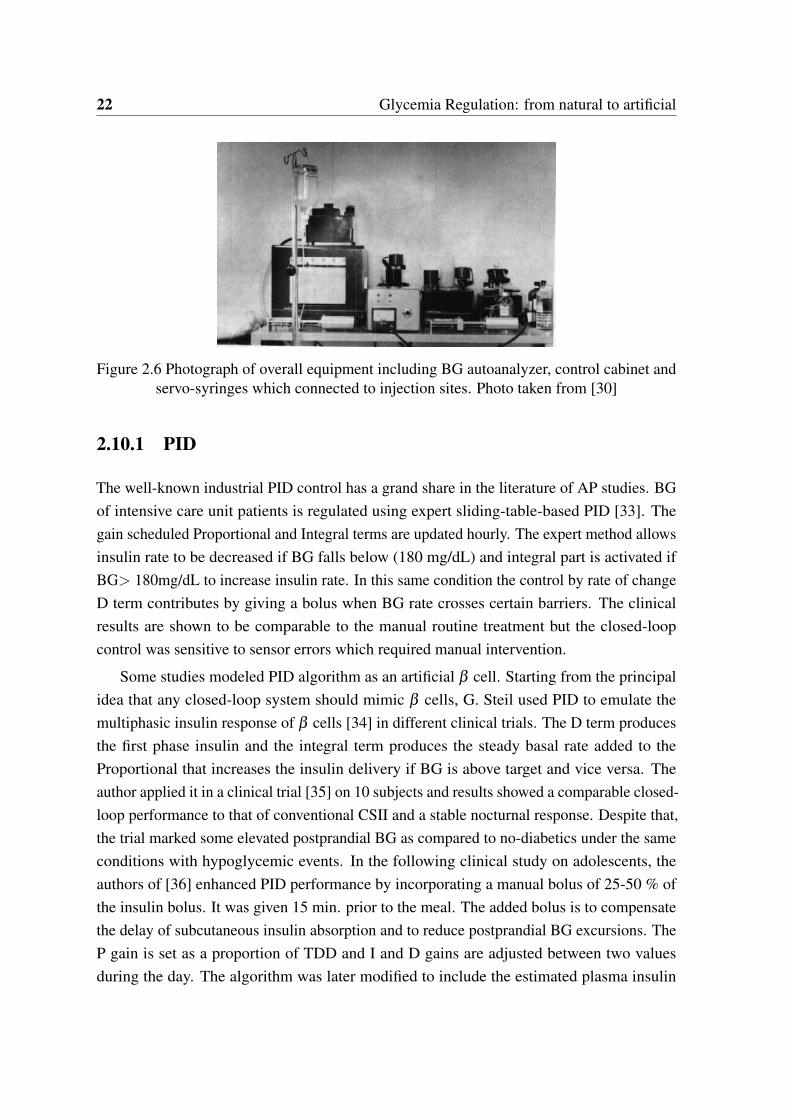
22 Glycemia Regulation: from natural to artificial
Figure 2.6 Photograph of overall equipment including BG autoanalyzer, control cabinet andservo-syringes which connected to injection sites. Photo taken from [30]
2.10.1 PID
The well-known industrial PID control has a grand share in the literature of AP studies. BG
of intensive care unit patients is regulated using expert sliding-table-based PID [33]. The
gain scheduled Proportional and Integral terms are updated hourly. The expert method allows
insulin rate to be decreased if BG falls below (180 mg/dL) and integral part is activated if
BG> 180mg/dL to increase insulin rate. In this same condition the control by rate of change
D term contributes by giving a bolus when BG rate crosses certain barriers. The clinical
results are shown to be comparable to the manual routine treatment but the closed-loop
control was sensitive to sensor errors which required manual intervention.
Some studies modeled PID algorithm as an artificial β cell. Starting from the principal
idea that any closed-loop system should mimic β cells, G. Steil used PID to emulate the
multiphasic insulin response of β cells [34] in different clinical trials. The D term produces
the first phase insulin and the integral term produces the steady basal rate added to the
Proportional that increases the insulin delivery if BG is above target and vice versa. The
author applied it in a clinical trial [35] on 10 subjects and results showed a comparable closed-
loop performance to that of conventional CSII and a stable nocturnal response. Despite that,
the trial marked some elevated postprandial BG as compared to no-diabetics under the same
conditions with hypoglycemic events. In the following clinical study on adolescents, the
authors of [36] enhanced PID performance by incorporating a manual bolus of 25-50 % of
the insulin bolus. It was given 15 min. prior to the meal. The added bolus is to compensate
the delay of subcutaneous insulin absorption and to reduce postprandial BG excursions. The
P gain is set as a proportion of TDD and I and D gains are adjusted between two values
during the day. The algorithm was later modified to include the estimated plasma insulin
2.10 Literature Survey: Closing the loop 23
concentration as a feedback term. The authors of [37] added estimated plasma Insulin in the
Feedback loop (IFB) of the PID control law. IFB works to attenuate insulin delivery from the
feedback loop over the increase in estimated plasma insulin levels to prevent overdosing.
The aim is to reduce postprandial hypoglycemia. The modified PID control was tested
on 8 adults and results revealed a good estimation of plasma insulin but with postprandial
hypoglycemia episodes. A similar approach was tested on human subjects [38] which
compared the two iterations of PID with and without IFB. The authors considered the
perspective of [37] and constructed IFB as a linear combination of subcutaneous, plasma
and the interstitial/effective insulin concentrations. The authors considered IFB as a "brake"
on the insulin infusion in the feedback loop to prevent postprandial hypoglycemia. Results
came up without postprandial hypoglycemia. A subsequent study conducted on diabetic
dogs [39] marked an improvement of postprandial BG without undershoot hypoglycemia. It
was shown that the addition of IFB is equivalent to the placement of the poles of the insulin
compartmental model to the desired locations by choosing the IFB gain. PID+ IFB has also
shown a reduced risk of nocturnal hypoglycemia regardless of the preceding afternoon level
of physical activity as compared to conventional CSII regimen [40] in an inpatient study. A
recent PID study [18] utilized IFB in a fully implantable AP system with intraperitoneal (IP)
insulin delivery and glucose sensors. Their AP incorporated an anti-reset windup 11 method
to limit the integral rate of change and prevent postprandial hypoglycemia. It was shown in
the in silico test that the IP route for AP is promising as it provided a faster behavior. Since
the insulin injection is a positive input, thus PID is followed by a saturation function to block
any negative input. Thus, PID designers usually incorporate some anti-windup protection for
the integrator, or even remove the integral and replace it by the patient specific basal rate in a
PD+Basal control [41]. The authors compared PID and PD+Basal on Uva/Padova simulator
and concluded that the latter reduced postprandial hyperglycemia, but and conversely to PID,
it failed to respond appropriately to changes in insulin sensitivity.
As an overall view, frequent PID employment for glycemia regulation shows its merits
as a simple and efficient control algorithm. In this thesis, model-free control is chosen as it
offers the simple features of a PID control in the frame of a model free design. In opposition
to previous PID studies, the control algorithm designed hereafter (in Chapter 4) is fully
automated without any feed-forward or IFB terms.
11Integral wind-up occurs when the integral term builds up (in response to the error signal) and accumulatesbeyond the actuator saturation limit. It takes significantly long time to recover to get back to be within theactuator operating range. It causes excessive overshoot, sustained oscillations and long settling time.
24 Glycemia Regulation: from natural to artificial
2.10.2 MPC
Model Predictive Control (MPC) is the advanced industrial counterpart of PID. The main
idea of MPC is that a mathematical model of the plant is used to predict the future behavior
of the process output during a sliding time window or the prediction horizon. The prediction
is used to optimize the control signal during a control horizon. The prediction and then the
optimization are updated using feedback measurements of the controlled variable. MPC is
widely known in the industry as an advanced algorithm that can handle process constraints.
Its predictive nature and constraint handling pushed MPC to the top of the list of controllers
used in AP application. Numerous publications have shown its potentials in both in silico
and in vivo test studies.
Of the early in silico studies of MPC is that of a nonlinear auto regressive model identified
off-line using artificial neural network [42]. They showed the feasibility of SC route in closed-
loop AP when compared to Biostator II with IV route. The authors of [43] designed MPC
tested on a nineteen-order compartmental model. Two MPC of two internal models are
compared: a linear identified step response model of the original nonlinear system, and
a linearised model of the patient with Kalman state estimation with improved results. A
clinical proof of the concept is realized in a 15 clinical trials study of nonlinear MPC in
[44]. The experiments were performed during fasting conditions on 10 subjects using IV
BG sampling and SC insulin delivery . Hovorka’s nonlinear model [45] is employed as an
internal model with time-varying parameters that are estimated at each control step. Linear
MPC acknowledged by the meal announcement (meal information is given to the controller)
is tested in silico in[46] and compared to PID under same conditions. A linearised internal
model of a nonlinear system and its parameters are obtained from the average values of
the population. For both PID and MPC, one parameter is tuned per individual, Kp for the
former and the output prediction weighting parameter for MPC. Although both showed
deteriorated performance with imperfect meal knowledge amount, the effect on MPC was
marginal. To avoid postprandial hyperglycemia, [47] presented a meal detection algorithm to
notify MPC by an upcoming meal. It was shown that a meal is flagged 30 min before meal
onset to notify MPC to switch the desired BG level from constant to a variable trajectory
that mimics a generic BG absorption profile for different meal loads using a meal library.
Another comprehensive in silico study [48] used MPC associated with meal size estimation,
IOB and a pump shut-off procedure to avoid hypoglycemia. The meal estimation provided a
feed-forward tool to automatically give priming meal boluses. IOB is computed based on
2.10 Literature Survey: Closing the loop 25
fitting Pharmacodynamics PDs 12 curves to two compartmental models. IOB is used as an
additional constraint to avoid hypoglycemia. The test is accomplished on the Uva/Padova
T1DM simulator [50]. MPC was also tested under dynamic IOB (dIOB) constraint in [23].
In this study dIOB took into account diurnal insulin sensitivity variation and used it to adjust
the static available IOB (sIOB) estimations. The authors used a technique to superimpose
diurnal insulin sensitivity (depending on the time of the day) on the sIOB to personalize it.
The purpose was similar to that of IFB, to avoid insulin stacking to prevent hypoglycemia.
Improved hypoglycemia prevention was noticed employing dIOB as a constraint in the study
that was conducted on 100 patients of Uva/Padova simulator.
An outpatient study was performed in [51] of a wearable AP(DiAs) device of a smart
phone core on 20 patients under 42 hours of 28h of AP. This proof of concept encouraged
future trials. A bihormonal (Glucagon and insulin) AP outpatient study was performed in
[52] using MPC control for insulin delivery and Proportional-Derivative control for glucagon
( the gains were chosen to be functions of BG level for better control). Meal size information
is forwarded to the controller to trigger a small automatic priming bolus. The bionic wearable
device consisted of a smart phone and SC pumps and a 5 min CGM. They performed two
studies: 5 days under open-loop control and another 5 days under AP for 20 adults and 38
adolescents. Under AP, the only given information to initialize the controller is the patient’s
weight. As compared with open-loop, the device showed improved mean BG with less
hypoglycemia.
2.10.3 Sliding Mode Control (SMC)
Sliding mode Control has been employed for glycemia regulation due to its known robustness
properties against model parameters uncertainties and external disturbances [53]. This can
be established by directing the state trajectory of the system toward a pre-designed surface
(during reaching phase) along which the trajectory slides to reach the desired reference
value. Classic SMC is a discontinuous controller that yields high frequency chattering in
the control action. In modern SMC theory, Higher Order SMC (HOSMC) is presented as
a solution to this problem, it provided a continuous controller when designed in [53] for
glycemia regulation of T1DM. The in silico test was performed on Bergman T1DM model
and robustness was checked testing the controller on three virtual subjects under meal intake
as an external disturbance. Finite time convergence was achieved for the switching variable
but asymptotic convergence for the glucose error was yielded. To reduce persistent error
12 Pharmacodynamics (PDs): is the relationship between the drug concentration in the body and its intendedand antagonistic effects achieved with time. Pharmacokinetics (PK): is defined as the relation between the druginput (e.g. insulin) and its produced concentration in the body with time [49] (see Fig. 3.1 in Chapter 3).
26 Glycemia Regulation: from natural to artificial
and improve SMC performance against meals, meal announcement scheme was used in
[54]. Moreover, to alleviate the system’s time delay problem, the authors designed SMC in a
Smith predictor 13 structure. SMC design was based on an internal model that was identified
on Hovorka’s T1DM model (see §3.5 for Hovorka model details). Sigmoid-like function
was used to avoid chattering. The design was tested in silico on six patients in nominal
conditions and also under modeling errors and parametric uncertainties like variation in
insulin sensitivity of the patient.
For glycemia regulation, SMC was usually used as a model-based control mainly em-
ploying Bergman minimal T1DM model (see §3.4.1 for details on the model) e.g. in [53],
[55] and [56]. The authors of [55] designed HOSMC to regulate glycemia based on Bergman
minimal model and on Sorensen complex model [57]. The controller was validated in silico
on six virtual patients of Hovorka T1DM simulator and in vivo on laboratory rats. During
the validation, the same controller with exactly the same parameters was tested that showed
a good robustness level. However, as far as the author knows, SMC studies, concerning
glycemia regulation, have never considered the positive input constraint. In other words,
insulin injection/infusion is a nonnegative input and thus the only admissible SMC is the
nonnegative SMC. For that reason, a positive SMC for BG regulation of T1DM will be
presented in Chapter 5. Moreover, for a model-based control design, like MPC or SMC,
the system model plays a capital role in the overall controller performance. Therefore, an
appropriate model that provides a good description of glycemia-insulinemia dynamics for a
T1DM must be chosen. Unfortunately, the historical models like Bergman have non-natural
equilibria that are not consistent with T1DM glycemic behavior in real life. As explained
in [58], those equilibria imply a set of basal insulin that keeps BG level constant. Whereas
a T1DM patient has a unique basal insulin level (independent from BG) that stabilizes BG
at any value, namely a critically stable system and not asymptotic as the historical models
present. For theses reasons, the employed model in this thesis is the recently developed long-
term T1DM model [58]. This model has shown a good description of glycemia-insulinema
dynamics of T1DM as compared to other models (see Chapter 3 for more details). It is used
to design a nonnegative SMC in Chapter 5 for glycemia regulation. The model parameters
were identified on T1DM clinical data supported by university hospital center of Nantes and
Rennes.
13The basic idea of Smith Predictor is to use the system model to predict the pure time delay for the controller[54].
2.11 Conclusions 27
2.10.4 Positivity and state feedback Control
As stated earlier and according to the literature of AP studies, input/output constraints of
T1DM closed-loop system is mainly taken into account by MPC. Recently, positivity of the
closed-loop controller is considered in the design by [59]. The authors treated glycemia-
insulinemia system as a class of internally positive systems where the input response is
slower than that of the disturbance. To achieve a trade-off between hyper and hypoglycemia
peaks under positive control, they used a model-based control design where the controller
is the result of a minimization of the output response of two time instants. State feedback
is also employed for glycemia regulation. However, positivity of the controller has not
been considered. Take for instance two recent state feedback design based on Bergman
model [60] and [61]. The feedback gains of the controller designed in [60] are the solution
of an optimization program that uses some uncertainty bounds on the model parameters.
Robustness and simplicity of the linear controller were the main achievements of this work.
Other researchers [61] used observer-based state feedback controller. The feedback gains are
designed using pole placement method based on Bergman linearized model. The controller
results are compared to an adaptive PID and the simulations showed comparable performance.
The authors considered the fixed design state feedback controller as simpler and less complex
to implement compared to the adaptation technique of th PID. Two important remarks are
highlighted from these two publications:
1. Bergman model for non-diabetic subject was used: both publications keep the internal
insulin regulatory function in the model. This function does not exist for T1DM
subjects (See § 3.4.1 and Remark 1). The result is that when the controller is off,
endogenous basal plasma insulin is yielded! see Fig. 2 in [60].
2. Positivity of the state feedback controller is not considered in the design.
2.11 Conclusions
Researchers are working for decades to find the optimal continuous insulin delivery to
regulate glycemia for a T1DM either via biological solutions or using engineering techniques
and closed-loop control. The ultimate goal for the latter solution is the realization of a reliable
AP device. A brief history of the main AP control algorithms is presented. As an overall
overview, the following points are worth noting:
PID benefits
28 Glycemia Regulation: from natural to artificial
• It was shown that PID mimics the pancreatic β -cell insulin secretion. This behavior
was observed in response to a step change in BG [37]. The derivative term produces the
first phase insulin and compensates for the delay in Pharmacokinetic/Pharmacodynamic
(PK/PDs) curve. The integral term produces the steady basal rate added to the Propor-
tional term that increases the insulin delivery if BG is above target and vice versa.
• Tuning a PID controller does not require precise mathematical model in its design.
However, optimal tuning may not be a straightforward matter especially under external
disturbances like meals.
PID drawbacks
• It was shown that fully automatic PID is not sufficient to achieve the trade-off between
hyperglycemia reduction and hypoglycemia prevention. It was either supported by IFB
or by supplementary meal boluses.
• Another PID drawback is its degraded performance due to the actuator saturation
(nonnegative insulin infusion). The saturation to zero, whenever PID goes negative (to
compensate for negative error), means that the loop is broken. In this case, the system
is no more under control. Another consequence is the integral windup which forced
many researchers to replace the integral term by the insulin basal rate.
MPC features and drawbacks
• MPC is an advanced industrial counterpart of the PID. MPC main advantage is its
capability in handling system constraints: hypoglycemia for the output and positivity
constraint for the input.
• The main drawback of MPC is its cumbersome optimization procedures.
• This model-based controller requires sometimes model linearization (if nonlinear mod-
els are used) and parameter identification to cope with changes in system parameters.
This complicates the parameter tuning process per individual.
• According to the meta-analysis provided by [62], MPC performance is not superior to
that of a PID, bearing in mind that the latter’s parameters are derived empirically or
are based on a model which may not be the optimal choice.

2.11 Conclusions 29
This thesis solution In this thesis, Model-free PID or intelligent PID (iPID) is used for
the first time for glycemia regulation of T1DM. It has the nice properties of a simple PID
with some adaptive features. Model-free control has already been successfully applied in
many concrete and diverse situations (see [63] and the references therein). Fully automatic
iPID is tested and compared to the model-free intelligent Proportional or iP controller and
also to classic PID control. The test was conducted in silico on two simulators as detailed in
Chapter4.
SMC main features
• SMC is a variable structure controller which has its share in the literature of AP being
a robust controller.
• Robustness of SMC is exhibited from being a variable structure control. It uses a
discontinuous function to steer the state trajectory to a pre-specified path toward the
equilibrium.
• The sliding surface is reached in finite time.
• SMC robustness properties has been shown in several closed-loop studies via in silico
tests and an in vivo one on laboratory rats.
SMC drawback and open problem
• The major side effect of the discontinuity in the control law is the high frequency
chattering. Several solutions are available in the literature to alleviate this problem,
one of which is via HOSMC.
• None of SMC studies considered the nonnegative constraint on the control action.
Our solution Therefore, in Chapter 5, nonnegative SMC is designed for glycemia reg-
ulation for the first time. SMC is designed to be nonnegative everywhere in the largest
closed-loop positively invariant set of the insulin subsystem of the T1DM model in [58].
Two stage SMC is designed, the last stage SMC2 block uses the glycemia error to design
the desired insulin trajectory. Then the plasma insulin state is forced to track the reference
via SMC1. The switching variable of SMC1 is the first order polynomial of the insulin error.
Sliding mode of SMC1 guarantees insulin reference tracking. The resulting desired insulin
trajectory is the required virtual control input of the glycemia system to eliminate BG error.
BG error is the switching variable of SMC2. BG is steered to the normal set point during
30 Glycemia Regulation: from natural to artificial
sliding mode of SMC2. In silico trial is performed to validate the theoretical results on the
nominal system.
Concerning the available T1DM models
• Model-based controllers, like SMC and MPC, require an internal model that provides
a good description of glycemia-insulinemia dynamics for a T1DM. Otherwise, a poor
closed-loop response is yielded.
• Historical T1DM models that are widely used in closed-loop studies, like Bergman,
have strange equilibria that are not consistent with T1DM glycemic behavior in real
life (more details are found in §3.8).
More details about mathematical modeling of this biological system, especially concerning
the widely employed models, are presented in Chapter 3. Equilibrium of these models and a
recently developed long-term model [58] are discussed in this chapter as well.
Positivity and positive state feedback in this thesis To the best of our knowledge, posi-
tivity analyses and invariance of glycemia-insulinemia system were not considered previously
for the control design purposes. This motivated open and closed-loop input/output positivity
analyses of the linear affine model in [58] in Chapter 6. It is shown that glycemia output does
not remain positive for any positive input. Therefore, the largest positively invariant set in
open-loop and under positive state feedback control are found.
The main issues of the previous state feedback designs in the literature (in subsection
2.10.4) are taken into account in the design of a positive state feedback controller in Chapter
6. The result is a stable closed-loop system under positive controller that regulates BG and
prevents hypoglycemia. Another important achievement is that hypoglycemia is predicted
in case the initial condition is outside the invariant set. Future hypoglycemia episodes are
predicted in both open-loop and closed-loop cases. It is the main result of the computation of
the largest positively invariant sets.
Chapter 3
Glucose-insulin Dynamics:
Mathematical modeling
3.1 Chapter Introduction in French
Dans ce chapitre, nous présentons une revue des modèles mathématiques qui décrivent la
dynamique glucose-insuline du DT1. La modélisation mathématique en biologie est utilisée
comme un outil utile pour décrire et simuler des systèmes physiologiques et leurs variables à
des fins différentes. Le système glucose-insuline a gagné beaucoup d’intérêt dans la littérature
de ce domaine. Il permet de simuler et de tester l’administration d’insuline pour le DT1 en
particulier des algorithmes de commande en boucle fermée pour préparer la voie à un AP
fiable.
Le focus, dans ce chapitre, est mis sur les modèles bien connus et largement utilisés dans
la littérature et plus spécifiquement dans les études de PA. Ils sont principalement utilisés
pour construire des simulateurs DT1 et des commandes basées sur des modèles pour des tests
en boucle fermée. Ils vont des modèles non linéaires minimaux aux modèles à ordre élevé et
certains modèles linéaires récemment présentés. Deux des modèles historiques largement
connus sont considérés et validés en tant que modèles à court terme et un nouveau modèle
linéaire à long terme est présenté dans ce chapitre qui sera utilisé dans le reste de la thèse.
L’existence du point d’équilibre d’un modèle DT1 dans des conditions de jeûne est discutée
du point de vue physiologique.
32 Glucose-insulin Dynamics: Mathematical modeling
3.2 Introduction
In this chapter a review of the mathematical models that describe glucose-insulin dynamics of
T1DM is presented. The focus will be on the well known widely used models in the literature
and more specifically in AP studies. They are mainly used to build up T1DM simulators
and model-based controllers for closed-loop tests. They range from minimal to high order
nonlinear models and some recently presented linear models. Two of the widely known
historical models are reviewed as short-term models and a new long-term linear model is
presented in this chapter which will be used in the rest of the thesis. The existence of an
equilibrium point of a T1DM model in fasting conditions is discussed from the physiological
point of view.
3.3 Compartmental Modeling of Biological Systems
Compartmental models are used to describe the transport process of materials between
interconnected volumes (e.g. drugs) in a biological system. They can be seen as systems
composed of interconnected chambers or stirred tanks of well mixed materials. The compart-
ments exchange materials which are concentrations or molar amounts of chemical species
which represent the system states variables [64]. For instance, for T1DM subject, injected
insulin enters first the subcutaneous tissue (first compartment) before its transfer to the
plasma compartment. The flow rate between compartments is described usually by ordi-
nary differential equations following mass conservation law. It states that the difference
between the flow in and flow out determines the amount of the material in the compartment
[65]. Compartmental models are widely used in pharmacokinetics (PK), for illustrating the
concentration-time curves of a drug after administration. PK describes thus the availability
duration of the drug in the body and defines the dosage and route of administration; whereas,
pharmacodynamics (PDs) is the physiological response of the drug and its effect on the
biological system with time [64]. The mathematical description between the drug delivery to
the response mechanisms comprise the combination PK/PDs. For instance, [66] presented a
three-differential equation insulin system: a two compartmental model for PK response for
subcutaneous to plasma insulin and a third for PDs response called the effective (or active)
insulin in compartments remote from plasma that interacts directly on glycemia level.

3.4 Historical Models 33
Figure 3.1 Relationship between pharmacokinetics PK and pharmacodynamics PD [49].
3.4 Historical Models
Several Mathematical models are available in the literature to describe the glucose-insulin
dynamics. The modeling process usually starts with the interpretation of plasma glucose
and insulin concentrations during glucose tolerance tests. These are either intravenous
glucose tolerance test (IVGTT) or an Oral route (OGTT). Those models range from minimal
models starting by the 1961’s Bolie model [67], Bergman’s [68] to other more complex like
Sorensen’s model 19 equations model [57]. Here the three models that are widely used in
AP in silico tests will be reviewed.
3.4.1 Bergman minimal model
It is a well known classical model that is first developed in 1979 and then insulin sensitivity
is evaluated using a clinical study on 18 hospitalized healthy subjects [68]. The standard
formulation of the model is a system of three differential equations [69]:
G(t) =−p1.(G(t)−Gb)−X(t).G(t) (3.1)
X(t) =−p2.X(t)+ p3.(I(t)− Ib) (3.2)
I(t) = p4.(G(t)− p5)+.t − p6(I(t)− Ib) (3.3)
Where G(t) [mg/dL]:plasma glucose concentration, I(t) [µU/mL] plasma insulin con-
centration, X(t) [min−1] interstitial/active insulin in remote compartment. The suffix b
refers to basal state. Parameters p5 [mg/dL] is a pancreatic "glycemia threshold" above
which the pancreas starts secreting insulin. p1, p2, p6 [min−1], p3 [min−2 /µU/mL] and p4
[µU/mL/(mg.min/dL)] are rate coefficients, for more details see [69] and [68]. The plus sign
in (3.3) means:
(G(t)− p5)+ =
8<:
0 i f G p5
(G− p5) i f G > p5
(3.4)
34 Glucose-insulin Dynamics: Mathematical modeling
This model was developed on healthy subjects and this fact can be seen from the term
p4.(G(t)− p5)+ which represents pancreatic insulin secretion when BG exceeds certain
threshold.
Remark 1. It is good to mention that several T1DM closed-loop glycemia regulation studies
considered p4(G(t)− p5)+ as an internal insulin regulatory function that does not exist for
T1DM cases. The parameter p1 has been also argued to be reduced to zero for a diabetic
patient (see [55] and the references therein). Thus p1 and p4 are set to zero in (3.1) and (3.3)
when Bergman model was employed for closed-loop glycemia regulation as in [53] and [55].
3.5 Hovorka’s model
This model, which was developed on healthy subjects [45], describes the input/output relation-
ship between subcutaneous insulin infusion as input and intravenous glucose concentration
as output. It has also meal ingestion and intravenous (IV) glucose infusion as exogenous
glucose inputs 1 [44].
The glucose kinetics parameters values are determined using glucose tracers on normal
subjects during overnight fasting phase and during IVGTT. This model consists of:
1. Glucose subsystem: absorption, distribution and disposal.
2. Insulin subsystem: absorption, distribution and disposal.
3. Insulin-action subsystem: its action on glucose transport, disposal and endogenous
production.
3.5.1 Glucose subsystem
8>>><>>>:
Q1(t) =−h
Fc01
VGG(t) + x1(t)iQ1(t)+ k12Q2(t)−FR +UG(t)+EGP0[1− x3(t)]
Q2(t) = x1(t).Q1(t)− [k12 + x2(t)]Q2(t)
G(t) = Q1(t)VG
(3.5)
where Q1,Q2 [mmol] glucose masses in the accessible 2 (plasma) and non-accessible com-
partments (e.g. interstitial and intracellular distribution space [45]). k12 transfer-rate constant
from non-accessible to accessible compartment. VG [L] distribution volume of the accessible
1Glucose is infused intravenously during clinical studies when hypoglycemia is detected.2represents plasma and tissues that equilibrate quickly with plasma [45]
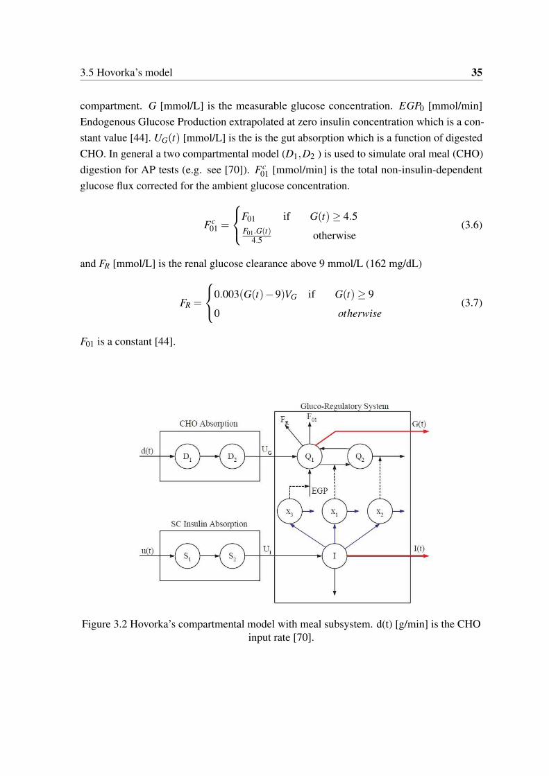
3.5 Hovorka’s model 35
compartment. G [mmol/L] is the measurable glucose concentration. EGP0 [mmol/min]
Endogenous Glucose Production extrapolated at zero insulin concentration which is a con-
stant value [44]. UG(t) [mmol/L] is the is the gut absorption which is a function of digested
CHO. In general a two compartmental model (D1,D2 ) is used to simulate oral meal (CHO)
digestion for AP tests (e.g. see [70]). Fc01 [mmol/min] is the total non-insulin-dependent
glucose flux corrected for the ambient glucose concentration.
Fc01 =
8<:
F01 if G(t)≥ 4.5F01.G(t)
4.5 otherwise(3.6)
and FR [mmol/L] is the renal glucose clearance above 9 mmol/L (162 mg/dL)
FR =
8<:
0.003(G(t)−9)VG if G(t)≥ 9
0 otherwise(3.7)
F01 is a constant [44].
Figure 3.2 Hovorka’s compartmental model with meal subsystem. d(t) [g/min] is the CHOinput rate [70].
36 Glucose-insulin Dynamics: Mathematical modeling
3.5.2 Insulin subsystem
• Absorption model [44]:
8<:
S1(t) = u(t)− S1(t)tmax,I
S2(t) =S1(t)−S2(t)
tmax,I
(3.8)
where S1(t),S2(t)[mmol] two-compartment chain representing absorption of subcuta-
neously administered short-acting insulin. u(t) [mmol/min] insulin infusion rate and tmax,I
[min] time-to-maximum insulin absorption.
• The plasma insulin concentration I(t)
I(t) =UI
VI− keI(t) (3.9)
where ke[min−1] is the fractional elimination rate, UI [mU]= S2(t)tmax,I
is the appearance of
insulin in plasma and VI [L] is the distribution volume.
3.5.3 Insulin action subsystem
It is of three actions on glucose kinetics
xi(t) =−kaixi(t)+ kbiI(t), i = 1,2,3. (3.10)
where xi(t) [min−1] the remote effects of insulin on glucose for i = 1 distribution/transport,
i = 2 disposal and i = 3 on endogenous glucose production. kai [min−1] are the deactivation
rate constants, and kbi [min−1] are the activation rate constants. SIT = kb1ka1
represents insulin
sensitivity of distribution/transport, SID = kb2ka2
insulin sensitivity of disposal and SIE = kb3ka3
is insulin sensitivity of EGP. Model parameters and constants values can be found in [44].
A T1DM simulator is realized from this model known as APCam for (Artificial Pancreas
project at Cambridge) of 18 virtual patients. It is developed by the University of Cambridge
for closed-loop control test studies.
3.6 Dalla Man model: Uva/Padova Simulator
This model is developed based on OGTT rather than the intravenous perturbations to develop
a meal simulator [71]. Meal data set of 204 normal individuals is used to validate a model

3.6 Dalla Man model: Uva/Padova Simulator 37
of glucose ingestion and absorption. The identification process is also realized on smaller
database of 14 T2DM subjects. This compartmental model is composed of two main
subsystems: glucose and insulin. It describes also the relationship between the plasma
measurements of glucose and glucose rate of appearance in plasma due to:
• the glucose rate of appearance in plasma (meal intake) Ra [mg/kg/min],
• the liver’s EGP(t) [mg/kg/min],
• dependent and independent utilization of glucose Uid(t) and Uii(t) [mg/kg/min]respectively,
• renal excretion E(t),
• insulin secretion and degradation.
3.6.1 Glucose subsystem
A two compartmental subsystem that is shown in the first panel of Fig. 3.3 consisting of
plasma glucose mass Gp(t) and tissues Gt(t) [mg/kg]
8>>><>>>:
Gp(t) = EGP(t)+Ra(t)−Uii(t)−E(t)− k1.Gp(t)+ k2.Gt(t), Gp(0) = Gpb
Gt(t) =−Uid(t)+ k1.Gp(t)− k2.Gt(t), Gt(0) = Gtb
G(t) =Gp
VG, G(0) = Gb
(3.11)
where VG [dL/kg] is the glucose distribution volume, G(t) [mg/dL] is the plasma glucose
concentration and k1,k2 [min−1] are the rate parameters, the suffix b refers to basal state.
Note that intestinal glucose absorption subsystem whose output is Ra(t) and insulin
dependent glucose utilization Uid(t) unit model are nonlinear models (see [71]for more
details). Description of these unit models and the rest like EGP(t) and E(t) are detailed in
[71].
3.6.2 Insulin subsystem
As illustrated in the second panel of Fig. 3.3, it is also a two compartmental model of insulin
mass in plasma Ip(t) [pmol/kg] and insulin mass in the liver Il(t) [pmol/kg]
8>>><>>>:
Il(t) =−(m1 +m3(t)).Il(t)+m2.Ip(t)+S(t), Il(0) = Ilb
Ip(t) =−(m2 +m4).Ip(t)+m1.Il(t), Ip(0) = Ipb
I(t) =Ip
VI, I(0) = Ib
(3.12)
38 Glucose-insulin Dynamics: Mathematical modeling
where S(t) [pmol/kg/min] is insulin secretion, m1,m2 [min−1] are transport rates, m4,
[min−1] m5 [min.kg/pmol] are the degradation rate parameters and m6 [dimensionless] is
a constant. In summary this T1DM model consists of 13 differential equations and 35
parameters per subject. Despite the fact that the model is validated on non-diabetic and
T2DM subjects, it is realized to be a T1DM simulator that is known as Uva/Padova T1DM
Metabolic Simulator. To simulate a T1DM, the above insulin secretion model was replaced
by the exogenous insulin infusion model in [72]:
8<:
Isc1(t) =−(kd + ka1).Isc1(t)+u(t), Isc1(0) = Isc1b
Isc2(t) = kd.Isc1(t)− ka2.Isc2(t), Isc2(0) = Isc2b
(3.13)
Where Isc1, Isc2 [pmol/kg] are the insulin masses in the subcutaneous space, ka1,ka2 [min−1]
are their rate constants. kd [min−1] is the insulin rate constant of dissociation and u(t)
[pmol/kg/min] is the exogenous insulin infusion rate. In addition to this change, a higher
EGP (vs normal) is introduced in [72] to account for higher basal rates for T1DM subjects.
The remaining parameters are kept as they were for non-diabetic. Uva/Padova T1DM
simulator is approved by the FDA to test and validate any closed-loop control algorithms
for the artificial pancreas studies. It is considered now as a mandatory validation step that
precedes any clinical trials as detailed earlier in the bibliography of Chapter 2.
3.7 A long-term model of glucose-insulin dynamics of T1DM
This model is developed based on the clinical data of the University Hospital Centers of
Nantes and Rennes [58]. It has the following advantages over other existing models in the
literature:
1. The parameters are identified on standard clinical diary 3 (in- or outpatient data) for a
time span up to two days.
2. Unlike the existing models, its glycemic stability property is consistent with T1DM
glycemic behavior (see [58] for more details).
3. It permits calculating FIT tools such as ISF and basal rate of insulin.
3Mainly consists of CGM record, insulin injection history and estimated CHO intake.
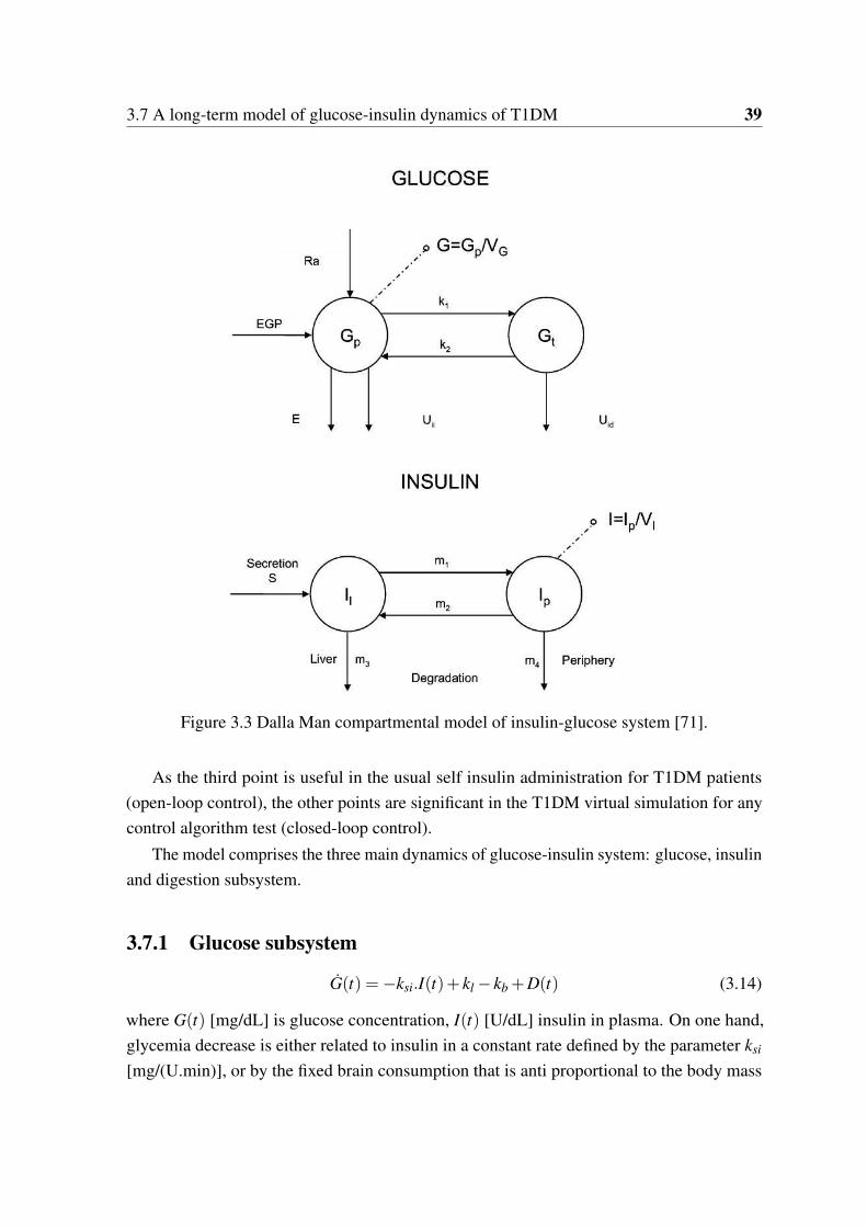
3.7 A long-term model of glucose-insulin dynamics of T1DM 39
Figure 3.3 Dalla Man compartmental model of insulin-glucose system [71].
As the third point is useful in the usual self insulin administration for T1DM patients
(open-loop control), the other points are significant in the T1DM virtual simulation for any
control algorithm test (closed-loop control).
The model comprises the three main dynamics of glucose-insulin system: glucose, insulin
and digestion subsystem.
3.7.1 Glucose subsystem
G(t) =−ksi.I(t)+ kl − kb +D(t) (3.14)
where G(t) [mg/dL] is glucose concentration, I(t) [U/dL] insulin in plasma. On one hand,
glycemia decrease is either related to insulin in a constant rate defined by the parameter ksi
[mg/(U.min)], or by the fixed brain consumption that is anti proportional to the body mass
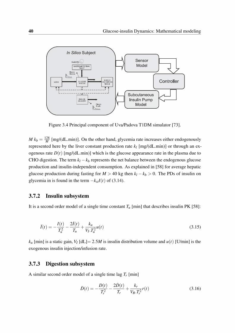
40 Glucose-insulin Dynamics: Mathematical modeling
Figure 3.4 Principal component of Uva/Padova T1DM simulator [73].
M kb =128M
[mg/(dL.min)]. On the other hand, glycemia rate increases either endogenously
represented here by the liver constant production rate kl [mg/(dL.min)] or through an ex-
ogenous rate D(t) [mg/(dL.min)] which is the glucose appearance rate in the plasma due to
CHO digestion. The term kl − kb represents the net balance between the endogenous glucose
production and insulin-independent consumption. As explained in [58] for average hepatic
glucose production during fasting for M > 40 kg then kl − kb > 0. The PDs of insulin on
glycemia in is found in the term −ksiI(t) of (3.14).
3.7.2 Insulin subsystem
It is a second order model of a single time constant Tu [min] that describes insulin PK [58]:
I(t) =−I(t)
T 2u
−2I(t)
Tu+
ku
VI.T 2u
u(t) (3.15)
ku [min] is a static gain, VI [dL]= 2.5M is insulin distribution volume and u(t) [U/min] is the
exogenous insulin injection/infusion rate.
3.7.3 Digestion subsystem
A similar second order model of a single time lag Tr [min]
D(t) =−D(t)
T 2r
−2D(t)
Tr+
kr
VB.T 2r
r(t) (3.16)

3.7 A long-term model of glucose-insulin dynamics of T1DM 41
kr [unitless] is a static gain, VB [dL]= 0.65M is the blood volume and r(t) [mg/min] is the
CHO amount rate. As detailed in [58], five clinical diaries of T1DM subjects are used to
identify the model parameters. The same injection/meal scenario is applied i.e. u(t),r(t) are
taken from the diary of the patient to create a glycemia output to be fitted on the CGM curve
from the diary using data fitting and least square method.
3.7.4 Overall model
The state space representation of the overall T1DM system is written as follows considering
the glucose rise due meals D(t) as a perturbation:
0B@
G(t)
I(t)
I(t)
1CA=
0B@
0 −ksi 0
0 0 1
0 − 1T 2
u− 2
Tu
1CA
0B@
G(t)
I(t)
I(t)
1CA+
0B@
0
0ku
VI .T 2u
1CAu(t)+
0B@
kl − kb
0
0
1CA+
0B@
1
0
0
1CAD(t) (3.17)
The perturbation D(t) will be considered as external unknown input which is zero during
Insulinemia Model
Digestion Model
I
D
u
r
Insulin PK Insulin PD
Glycemia Dynamics
Figure 3.5 Magdelaine’s T1DM simulator.
fasting times. In addition, it is not affected by the change of variables in the following section.
3.7.5 A more physiological representation of Magdelaine’s model
The model (3.17) has one state as the derivative of plasma insulin. Since this variable does
not have a physiological meaning, and based on [66], a new state variable is introduced the
subcutaneous insulin Isc = TuI + I [U/min]. In this manner, PK/PDs insulin model includes
subcutaneous and plasma insulin compartments. To simplify the change of variables let
x1 = I,x2 = I and:
xsc = θ3x2 − x1 (3.18)
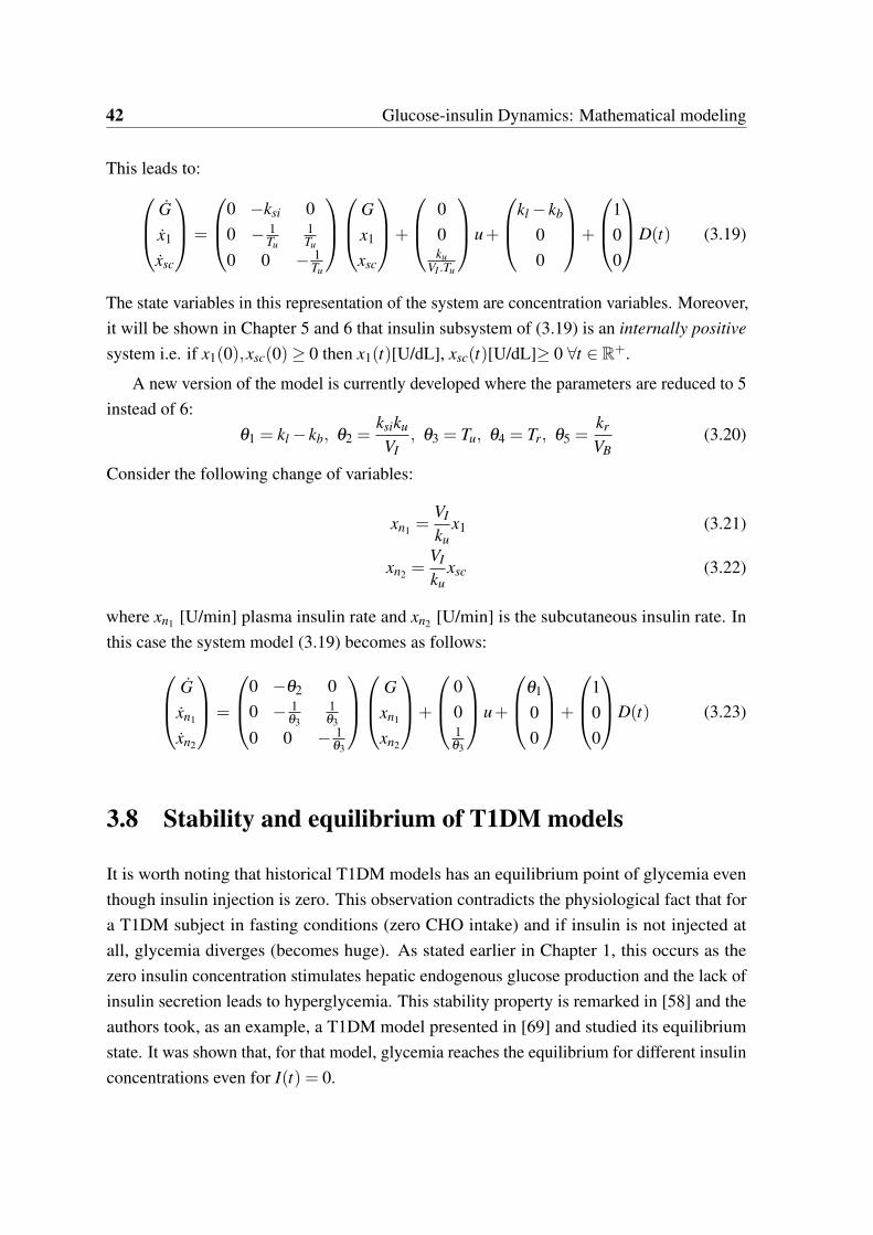
42 Glucose-insulin Dynamics: Mathematical modeling
This leads to:
0B@
G
x1
xsc
1CA=
0B@
0 −ksi 0
0 − 1Tu
1Tu
0 0 − 1Tu
1CA
0B@
G
x1
xsc
1CA+
0B@
0
0ku
VI .Tu
1CAu+
0B@
kl − kb
0
0
1CA+
0B@
1
0
0
1CAD(t) (3.19)
The state variables in this representation of the system are concentration variables. Moreover,
it will be shown in Chapter 5 and 6 that insulin subsystem of (3.19) is an internally positive
system i.e. if x1(0),xsc(0)≥ 0 then x1(t)[U/dL], xsc(t)[U/dL]≥ 0 8t 2 R+.
A new version of the model is currently developed where the parameters are reduced to 5
instead of 6:
θ1 = kl − kb, θ2 =ksiku
VI, θ3 = Tu, θ4 = Tr, θ5 =
kr
VB(3.20)
Consider the following change of variables:
xn1 =VI
kux1 (3.21)
xn2 =VI
kuxsc (3.22)
where xn1 [U/min] plasma insulin rate and xn2 [U/min] is the subcutaneous insulin rate. In
this case the system model (3.19) becomes as follows:
0B@
G
xn1
xn2
1CA=
0B@
0 −θ2 0
0 − 1θ3
1θ3
0 0 − 1θ3
1CA
0B@
G
xn1
xn2
1CA+
0B@
0
01θ3
1CAu+
0B@
θ1
0
0
1CA+
0B@
1
0
0
1CAD(t) (3.23)
3.8 Stability and equilibrium of T1DM models
It is worth noting that historical T1DM models has an equilibrium point of glycemia even
though insulin injection is zero. This observation contradicts the physiological fact that for
a T1DM subject in fasting conditions (zero CHO intake) and if insulin is not injected at
all, glycemia diverges (becomes huge). As stated earlier in Chapter 1, this occurs as the
zero insulin concentration stimulates hepatic endogenous glucose production and the lack of
insulin secretion leads to hyperglycemia. This stability property is remarked in [58] and the
authors took, as an example, a T1DM model presented in [69] and studied its equilibrium
state. It was shown that, for that model, glycemia reaches the equilibrium for different insulin
concentrations even for I(t) = 0.

3.8 Stability and equilibrium of T1DM models 43
Here, the equilibrium state of Hovorka’s and Magdelaine’s models are further investigated.
These analyses are followed by a simulation example of Uva/Padova simulator that shows
the non-natural set of equilibria during fasting phase.
3.8.1 Hovorka’s model: equilibrium
3.8.2 Autonomous system
The equilibrium point is analyzed first for the autonomous system i.e. in fasting conditions:
UG(t) = 0, and zero insulin injection: u(t) = 0. Starting with the insulin absorption subsystem
(3.8) S1,2 = 0 yields :
S1 = 0,S2 = 0 (3.24)
and from (3.9) plasma insulin concentration in its equilibrium (I = 0) yields Ieq = 0 and thus
from (3.10) xi = 0 implies xieq= 0. Applying this result in the glucose model (3.5) leads to:
−Fc01 + k12Q2(t)−FR +EGP0 = 0 (3.25)
Q2(t) = 0 (3.26)
In the region where G < 4.5mmol/L where Fc01 = F01
G4.5 ,FR = 0:
Geq = 4.5EGP0
F01(3.27)
Geq = 7.4 mmol/L higher than the given operating threshold 4.5 mmol/L, i.e. there is no
equilibrium in this region. Similarly, in the region 4.5 G < 9 mmol/L one has Fc01 = F01
and FR = 0 substituting in (3.5) leads to:
Q1(t) = EGP0 −F01 6= 0 (3.28)
As EGP0 −F01 > 0 [44], and as G = Q1VG
, this results in a diverging glycemia and thus there
is no equilibrium in the region 4.5 G < 9 for the autonomous system. Conversely, when
G(t) ≥ 9 mmol/L, according to (3.6) and (3.7) this leads to Fc01 = F01 mmol which is a
constant, and FR = 0.003(G(t)−9)VG and from (3.26) yields:
Geq = 9+EGP0 −F01
0.003(VG)(3.29)
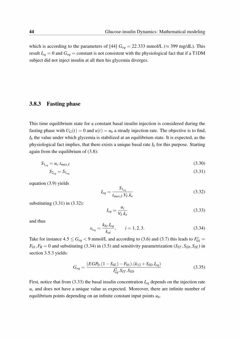
44 Glucose-insulin Dynamics: Mathematical modeling
which is according to the parameters of [44] Geq = 22.333 mmol/L ( 399 mg/dL). This
result Ieq = 0 and Geq = constant is not consistent with the physiological fact that if a T1DM
subject did not inject insulin at all then his glycemia diverges.
3.8.3 Fasting phase
This time equilibrium state for a constant basal insulin injection is considered during the
fasting phase with UG(t) = 0 and u(t) = ub a steady injection rate. The objective is to find,
Ib the value under which glycemia is stabilized at an equilibrium state. It is expected, as the
physiological fact implies, that there exists a unique basal rate Ib for this purpose. Starting
again from the equilibrium of (3.8):
S1eq= uc.tmax,I (3.30)
S2eq= S1eq
(3.31)
equation (3.9) yields
Ieq =S1eq
tmax,I.VI.ke(3.32)
substituting (3.31) in (3.32):
Ieq =uc
VI.ke(3.33)
and thus
xieq=
kbi.Ieq
kai, i = 1,2,3. (3.34)
Take for instance 4.5 Geq < 9 mmol/L and according to (3.6) and (3.7) this leads to Fc01 =
F01,FR = 0 and substituting (3.34) in (3.5) and sensitivity parametrization (SIT ,SID,SIE) in
section 3.5.3 yields:
Geq =(EGP0.(1−SIE)−F01).(k12 +SID.Ieq)
I2eq.SIT .SID
(3.35)
First, notice that from (3.33) the basal insulin concentration Ieq depends on the injection rate
uc and does not have a unique value as expected. Moreover, there are infinite number of
equilibrium points depending on an infinite constant input points ub.
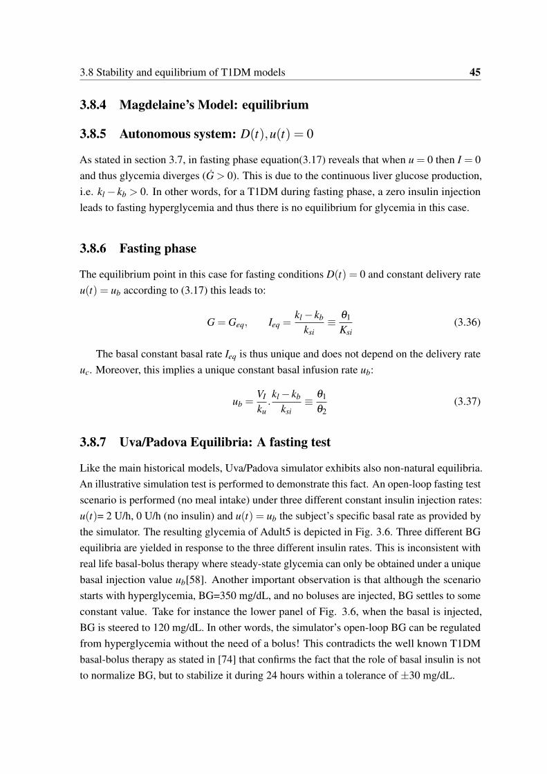
3.8 Stability and equilibrium of T1DM models 45
3.8.4 Magdelaine’s Model: equilibrium
3.8.5 Autonomous system: D(t),u(t) = 0
As stated in section 3.7, in fasting phase equation(3.17) reveals that when u = 0 then I = 0
and thus glycemia diverges (G > 0). This is due to the continuous liver glucose production,
i.e. kl − kb > 0. In other words, for a T1DM during fasting phase, a zero insulin injection
leads to fasting hyperglycemia and thus there is no equilibrium for glycemia in this case.
3.8.6 Fasting phase
The equilibrium point in this case for fasting conditions D(t) = 0 and constant delivery rate
u(t) = ub according to (3.17) this leads to:
G = Geq, Ieq =kl − kb
ksi
θ1
Ksi(3.36)
The basal constant basal rate Ieq is thus unique and does not depend on the delivery rate
uc. Moreover, this implies a unique constant basal infusion rate ub:
ub =VI
ku.kl − kb
ksi
θ1
θ2(3.37)
3.8.7 Uva/Padova Equilibria: A fasting test
Like the main historical models, Uva/Padova simulator exhibits also non-natural equilibria.
An illustrative simulation test is performed to demonstrate this fact. An open-loop fasting test
scenario is performed (no meal intake) under three different constant insulin injection rates:
u(t)= 2 U/h, 0 U/h (no insulin) and u(t) = ub the subject’s specific basal rate as provided by
the simulator. The resulting glycemia of Adult5 is depicted in Fig. 3.6. Three different BG
equilibria are yielded in response to the three different insulin rates. This is inconsistent with
real life basal-bolus therapy where steady-state glycemia can only be obtained under a unique
basal injection value ub[58]. Another important observation is that although the scenario
starts with hyperglycemia, BG=350 mg/dL, and no boluses are injected, BG settles to some
constant value. Take for instance the lower panel of Fig. 3.6, when the basal is injected,
BG is steered to 120 mg/dL. In other words, the simulator’s open-loop BG can be regulated
from hyperglycemia without the need of a bolus! This contradicts the well known T1DM
basal-bolus therapy as stated in [74] that confirms the fact that the role of basal insulin is not
to normalize BG, but to stabilize it during 24 hours within a tolerance of ±30 mg/dL.
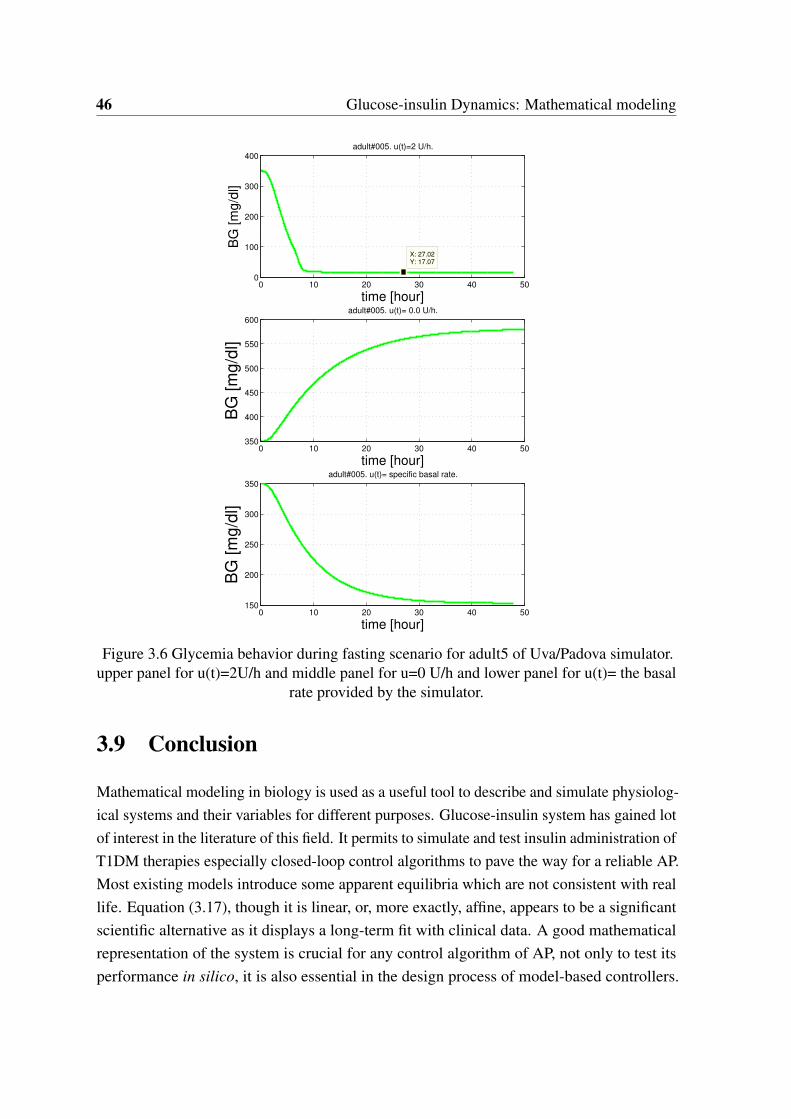
46 Glucose-insulin Dynamics: Mathematical modeling
0 10 20 30 40 500
100
200
300
400
X: 27.02Y: 17.07
adult#005. u(t)=2 U/h.
time [hour]
BG
[m
g/d
l]
0 10 20 30 40 50350
400
450
500
550
600adult#005. u(t)= 0.0 U/h.
time [hour]
BG
[m
g/d
l]
0 10 20 30 40 50150
200
250
300
350adult#005. u(t)= specific basal rate.
time [hour]
BG
[m
g/d
l]
Figure 3.6 Glycemia behavior during fasting scenario for adult5 of Uva/Padova simulator.upper panel for u(t)=2U/h and middle panel for u=0 U/h and lower panel for u(t)= the basal
rate provided by the simulator.
3.9 Conclusion
Mathematical modeling in biology is used as a useful tool to describe and simulate physiolog-
ical systems and their variables for different purposes. Glucose-insulin system has gained lot
of interest in the literature of this field. It permits to simulate and test insulin administration of
T1DM therapies especially closed-loop control algorithms to pave the way for a reliable AP.
Most existing models introduce some apparent equilibria which are not consistent with real
life. Equation (3.17), though it is linear, or, more exactly, affine, appears to be a significant
scientific alternative as it displays a long-term fit with clinical data. A good mathematical
representation of the system is crucial for any control algorithm of AP, not only to test its
performance in silico, it is also essential in the design process of model-based controllers.

3.9 Conclusion 47
Thus, the simulation results based on poor models are misleading and may lead to a poor
closed-loop behavior during a real clinical trial. In this thesis, model-based controllers, SMC
and state feedback, are designed employing the long-term model (3.17). Our early work of
positivity analyses, presented in Chapter 5, for sliding mode control was established on the
standard model (3.17). After observing the new model representation of insulin dynamics
in Section 3.7.5, it is employed in the positive invariance analyses in Chapter 6. Insulin
subsystem in this case represents an internally positive system as will be shown later.

Chapter 4
Fully automatic Model-free Control for
Glycemia Regulation
4.1 Chapter Introduction in French
Dans ce chapitre, la théorie et la conception de la commande sans modèle (CSM) sont
présentées. Il est présenté ici comme un algorithme de commande du PA pour la première
fois. La commande CSM est choisie car elle offre les fonctions simples d’une commande PID
en s’affranchissant de tout modèle mathématique. Contrairement aux études PID précédentes,
l’algorithme de commande développé ci-après est entièrement automatique sans aucune dose
d’insuline complémentaire. La commande proportionnelle sans modèle où les résultats de
la commande proportionnelle intelligente iP sont d’abord présentés et analysés avec des
systèmes linéaires stables et instables. Le focus est mis sur la stabilisation du régulateur iP via
ses paramètres de réglage, en particulier pour le cas instable. Ensuite, on présente les résultats
préliminaires du régulateur iP avec une trajectoire de référence constante, puis une trajectoire
de référence variable pour la régulation de la glycémie. Le correcteur iP est testé en utilisant
une trajectoire de référence variable pour contrecarrer le mauvais comportement postprandial
avec la référence constante. Le iP avec référence variable produit une commande impulsive
et une réaction rapide aux repas engendrant une hyperglycémie postprandiale réduite. Pour
améliorer encore la réponse postprandiale, des termes de boucle fermée supplémentaires sont
ajoutés et un PID intelligent (iPID) est conçu en utilisant une référence de glycémie constante.
De plus, la boucle de CSM est fermée via un PID car on a observé que le PID classique
émulait le comportement des cellules beta déficientes du pancréas chez un patient DT1 (voir
l’étude de la littérature sur le PID au Chapitre 2). La comparaison des résultats in silico
montre une meilleure régulation de la glycémie postprandiale avec le iPID et une référence
50 Fully automatic Model-free Control for Glycemia Regulation
constante par rapport au iP en utilisant une référence variable. iPID est également comparé
à un PID classique sur le simulateur Uva / Padova. Les résultats ont montré que la réponse
postprandiale était améliorée avec l’iPID réduisant les excursions hyperglycémiques avec
des événements hypoglycémiques minimes. En outre, iPID imite mieux le comportement
postprandial des cellules beta du pancréas qu’un PID avec une réponse plus rapide.
4.2 Introduction
In this chapter, the theory and design of Model-free Control (MFC) are presented. It is
presented here as an AP control algorithm for the first time. MFC is chosen as it offers the
simple features of a PID control in the frame of a model free design. In opposition to previous
PID studies, the control algorithm developed hereafter is fully automated without any feed-
forward or supplementary insulin doses. Model-free proportional control or intelligent
Proportional iP control results are first presented and analyzed with stable and unstable linear
systems. The focus is on the stabilizability of iP controller via its design parameters especially
for the unstable case. Thereafter, the preliminary results of constant and variable reference
trajectory iP controller for glycemia regulation are presented. iP is tested employing a variable
reference trajectory to circumvent the poor postprandial behavior of constant reference iP.
Variable reference iP produced an impulsive control of fast reaction to meals that yielded a
reduced postprandial hyperglycemia. To further enhance postprandial response, additional
closed loop terms are added and an intelligent PID (iPID) is designed using a constant
glycemia reference. Moreover, MFC loop is closed via PID as classic PID was observed to
emulate the behavior of the missing pancreatic β -cell in T1DM (see the literature survey
of PID in Chapter2). In silico results comparison showed a better postprandial glycemia
regulation with constant reference iPID over iP employing a variable reference. iPID is
also compared to a classic PID on the well known Uva/Padova T1DM simulator. iPID is
compared to a standard PID controller in two cases: i) each controller parameters were tuned
independently on a case study and then the design is applied on other subjects adapting
one weighting parameter to avoid hypoglycemia and results are compared. ii) A reference
PD+basal control previously designed to reduce BG risk index is compared to iPD+basal
blocking the integral term to the basal rate of the patient. The superiority of the intelligent part
of iPD over the classic is shown in this case by setting the same feedback gains. The results
showed that the postprandial response was improved with iPID reducing hyperglycemic
excursions with minimal hypoglycemic events. Moreover, the results showed that iPID,
who has the classic PID structure with new adaptive feature, emulated insulin delivery of
pancreatic β -cell.
4.3 Model-free control: Recalls 51
4.3 Model-free control: Recalls
Model-free control consists in controlling a given unknown plant as a first order, second
or eventually higher order 1 linear system, the so-called ultra-local model. The latter is
estimated online.
4.3.1 Ultra-local Model
Model-free control is designed based on an ultra-local model of order ν [63], for a Single
Input Single Output (SISO) system:
y(ν) = F +αu (4.1)
where:
• u,y are the input and output signals respectively. These are the only signals required to
be known for the design.
• α 2 R is a non-physical design parameter, which is chosen so that αu and y(ν) have
the same magnitude.
• The order of differentiation ν may in general be chosen 1 or 2 and has no connection
with the order of the system which is unknown [63].
• F stands for unknown system dynamics and perturbations. It is estimated and approxi-
mated by a piece-wise constant function during a quite short time lapse. It is estimated
based on the knowledge of the input u and the estimate of the derivative of output
measurement y(ν)e [76]:
Fe = y(ν)e −αu(t −h) (4.2)
where u(t −h) is a delayed version of the control, taken as a crude a crude approximation of
u(t) and h is a non-zero small delay (might be one sampling instant) to avoid any algebraic
loop [77, 75]. The role of h will be further discussed in the sequel. The computation of Fe
necessitates a good estimation of the ν th-order derivative of the output signal y(ν)e that may
be noisy.
Remark 2. In (4.2), a numerical differentiator is required to estimate y(ν). This is a major
feature for the performance of Model Free Control. At this stage, a trade off exists between the
value of ν and the accuracy of Fe: the higher the integer ν is, the richer is the controller in the
1In the literature of MFC it was never taken higher than two [75, 63].

52 Fully automatic Model-free Control for Glycemia Regulation
sense that is involves a large number of tuning parameters, and control actions. Unfortunately,
in practice this is challenged by the increasing difficulty to achieve an accurate estimate of
the higher order derivative y(ν).
4.4 Intelligent Proportional iP
Let y(t) denote a reference trajectory to be tracked, considering a first order ultra-local
model ν = 1, closing the loop with a proportional control yields the following intelligent
proportional iP controller [63]:
u =−Fe + y+Kpe
α(4.3)
where y is the reference input, e = y− y and Kp is the proportional gain. Combining
Equations (4.2) with ν = 1 and (4.3) yields:
e+KPe = 0 (4.4)
F does not appear anymore with the assumption that Fe F . However, as a simple counter
example, and as will be shown in section 4.5.2, the following linear second order system can
not be stabilized using iP controller
y(t)− y(t) = u(t) (4.5)
Ideally the closed-loop system always leads to the error polynomial equation (4.4) and it
is stable for any KP > 0. However, in practice, even if the derivative in (4.2) was perfectly
estimated it remains a small delay h in u(t −h)
Fe(t) = y(t)−αu(t −h) (4.6)
thus the latter influences on the stability of closed-loop iP as will be discussed in the following
section.
4.5 Effect of u(t −h)
The goal in this section is to show that some non obvious necessary conditions have to
be completed for the doability of an iP controller. Those conditions are shown to be just
independent form the quality of the estimation of ye(t). So, assume at this stage that ideally
4.5 Effect of u(t −h) 53
the derivative of the output is perfectly estimated, that is ye(t) = y(t). Substituting (4.2) in
(4.3) with ν = 1 yields
u(t) = u(t −h)+e(t)+Kpe(t)
α(4.7)
The effect of the delay h on the stability of the closed-loop system will be investigated next.
Stability is studied in the light of neutral delay system in a brief review.
4.5.1 Neutral Delay Systems
Whenever the delay h introduced in eq. (4.2) is not small enough, then the above approxima-
tion of the time derivative of the control input is no more valid. Still it is possible to analyze
the closed-loop system, under the assumption that y(t) is perfectly estimated/known, to arrive
at the same conclusion. So, in this section, it is shown that the iP control (4.7) yields a neutral
closed-loop system. The byproduct is again that a necessary condition for the stability of the
MFC closed-loop system is the stability of this neutral system. Consider the special case of a
linear SISO system:
x(t) = Annx(t)+Bn1u(t) (4.8)
y(t) =Cx(t) (4.9)
A copy of the delayed dynamics (4.9) reads:
x(t −h) = Ax(t −h)+Bu(t −h) (4.10)
For simplicity assume C1n = [1 0 ...0] and Bn1 = [0 0 ...1]T and let y = 0 . Subtracting
(4.10) from (4.9) and substituting (4.7) yields:
x(t)− x(t −h) = A[x(t)− x(t −h)]−B[Cx(t)+KpCx(t)
α] (4.11)
the latter leads to:
[Inn +1α
BC]x(t)− x(t −h) = [A−Kp
αBC]x(t)−Ax(t −h) (4.12)
Denote A0 = [Inn +1α BC], A1 = [A−
Kp
α BC] and the characteristic equation of (4.12) in
Laplace domain:
qo(s,e−hs) = det
s[A0 − Inne−hs]−A1 +Ae−hs
, s 2 C (4.13)
54 Fully automatic Model-free Control for Glycemia Regulation
where det(.) denotes the determinant of a matrix. The stability of (4.13) is necessary for a
stable closed-loop system under iP controller. Thus, iP controller is not a universal controller
and its stability is not simply defined by (4.4) as presented in the literature of MFC.
A sufficient stability condition for (4.12) is that the system is asymptotically stable if its
characteristic equation satisfies[78]:
supRe(s) : det
s[A0 − Inne−hs]−A1 +Ae−hs= 0< 0 (4.14)
The stability of system (4.11) for any delay h can be studied using the literature of
neutral-delay systems. If the latter polynomial is of the form qo(s,ehs) = p(s)+ q(s)e−hs
then the sufficient stability conditions of Theorem 2.1 of [79] can be applied as will be shown
in the following example in 4.5.2.
The purpose, so far, was just to show the possibility of examining stability of iP controller
via neutral delay systems. To go further, it is suggested to seek the necessary stability
conditions of neutral systems (if any) for the iP controlled system (4.12) to give a hint on the
choice h,Kp and α .
4.5.2 Academic example: iP control
In this section a counter example is presented to show that stability can not be always
guaranteed with iP controller. Consider the following linear system:
8>>><>>>:
x1(t) = x2(t)
x2(t) =−ax2(t)+u(t)
y(t) = x1(t)
(4.15)
In the unstable case a < 0. The stability of the closed-loop system under iP control with a
zero reference y = 0 is investigated. The following computations are obtained from [80].
Suppose ye = y. For this system F =− ya
and α = 1a. Combining (4.6) and (4.7) yields the
following controller:
u(t) =−y(t)+Kpy(t)
α(1−δh)(4.16)
where δh is the delay operator of amplitude h: f (t)− f (t−h) = (1−δh) f (t). The closed-loop
system is thus:
y(t) =−ay(t)−y(t)+Kpy(t)
α(1−δh)(4.17)
4.5 Effect of u(t −h) 55
Rearranging the above equation yields
h ddt(
ddt
+a)(1−δh)+a(ddt
+Kp)iy(t) = 0 (4.18)
Taking Laplace transform to the above equation yields2
s(s+a)(1− e−hs)+a(s+Kp) (4.19)
rearranging yields the following characteristic polynomial of the form:
s2 +2as+aKp − e−hs(s2 +as) = 0 (4.20)
the stability of the above polynomial is studied via its roots. Use Theorem 2.1 of [79] on
the system whose transfer function G(s) = r(s)p(s)+q(s)e−hs . Note that deg p(s) = deg q(s) as
required in [81]. The characteristic polynomial (4.20) is of the form p(s)+q(s)e−hs with
p(s)
q(s)=−
1+a
s+Kp
(s2 +as)
(4.21)
orp(s)
q(s)=−1−
1αs
−aKp −a
s2 +O(1s3 ) (4.22)
According to [79], the roots sn of p(s)+q(s)e−hs satisfy
sn =λn
h−
1αλn
+h
α2n
a2
2−a(Kp −a)
+o(
1n2 ) (4.23)
for sufficiently large integer n. Equation (4.22) leads to λn = 2πni. For stability, we have the
following situations:
if a(Kp −3a
2)> 0, then (4.15) has infinite number of unstable poles (4.24)
if a(Kp −3a
2)< 0, then (4.15) has infinite number of stable poles (4.25)
Obviously, the following two conditions must be satisfied for the stability of (4.15) and
(4.16):
1. Satisfying (4.25).
2. There is no further unstable root of (4.20).
2note that L f (t −h)= F(s)e−hs.
56 Fully automatic Model-free Control for Glycemia Regulation
The second condition is verified numerically using Quasi-Polynomial Mapping Based
Rootfinder [82] as suggested in [81]. For the special case a = −1 with Kp satisfying
condition 1 above, the quasi characteristic polynomial (4.20) has always an unstable root for
different values of h (e.g. h = 0.001,0.01 and 1) according to the numerical application of
qpmr function of [82]. Thus, even though condition 1 is satisfied, no stabilizing h is found
to yield zero number of unstable roots of (4.20). It is good to notice that these analyses are
valid under the assumption that ye = y which is never the case in practice. If the estimate
includes approximations for ye and u(t) (other than u(t −h)), and if these have regulatory
effect, then a stabilizing controller may well be obtained.
In the following section the estimator of F in (4.1) with ν = 1 for iP controller will be
derived according to [63].
4.6 Estimation of F
Equation (4.1) for an iP controller becomes:
y = F +αu (4.26)
F may be assumed to be approximated by a piecewise constant function Fe. Rewrite then
Equation (4.26) in the operational domain [63]:
sY (s) =Fe
s+αU(s)+ y(0) (4.27)
where Fe is a constant. Differentiate both sides w.r.t. s to eliminate the initial condition
y(0):
Y (s)+dY (s)
dss =−
Fe
s2 +αdU(s)
ds(4.28)
To filter the output multiply both sides by s−2
Y (s)
s2 +dY (s)
ds.1s=−
Fe
s4 +α
s2 .dU(s)
ds(4.29)
Take the inverse of Laplace transform of (4.29) and using the following properties:
L−1G1(s)G2(s)=
Z t
0g1(t − τ)g2(τ)dτ (4.30)
L−1
diG(s)
dsi= (−t)ig(t) (4.31)
4.6 Estimation of F 57
then we have the estimation Fe in the time interval t 2 [0, T ]
Fe(0) =−6
T 3
Z T
0
(T −2τ)y(τ)+ατ(T − τ)u(τ)
dτ (4.32)
where T is a small estimation time window which depends on sampling period and the noise
intensity [63].
To obtain Fe(t) at any time instant t, shift the functions y(τ) and u(τ) into y(t + τ) and
u(t + τ) (if y(T ) by y(t +T )) respectively keeping the interval width τ 2 [0,T ], i.e. sliding
the time window for the functions y, u and Fe without changing the variables.
Fe(t) =−6
T 3
Z T
0
(T −2τ)y(t + τ)+ατ(T − τ)u(t + τ)
dτ (4.33)
The above equation allows to estimate the Fe(t) in the interval [t, t +T ] as τ 2 [0, T ].
To make the estimation causal in time, invert the time intervals i.e. T to −T and τ to −τ .
First change T to −T in (4.33):
Fe(t) =6
T 3
Z −T
0
(−T −2τ)y(t + τ)+ατ(−T − τ)u(t + τ)
dτ (4.34)
or
Fe(t) =6
T 3
Z 0
−T
(T +2τ)y(t + τ)+ατ(T + τ)u(t + τ)
dτ (4.35)
Then change the variable τ to τ 0,τ 0 =−τ , dτ =−dτ 0, τ 2 [−T,0] implies τ 0 2 [T,0]:
Fe(t) =−6
T 3
Z 0
T
(T −2τ 0)y(t − τ 0)−ατ 0(T − τ 0)u(t − τ 0)
dτ 0 (4.36)
Now to simplify the writing of the above equation change the integral limits into (t −T, t)
using the following change of variables σ = t − τ 0, dτ 0 = −dσ and τ 0 2 [T, 0] leads to
σ 2 [t −T, t]:
Fe(t) =6
T 3
Z t
t−T
(T −2t +2σ)y(σ)−α(t −σ)(T − t +σ)u(σ)
dσ (4.37)
For numerical implementation, the following Fe is preferred:
Fe(t) =−6
T 3
Z T
0
(T −2σ 0)y(σ 0+ t −T )+ασ 0(T −σ 0)u(σ 0+ t −T )
dσ 0 (4.38)
where σ 0 = T − τ 0
58 Fully automatic Model-free Control for Glycemia Regulation
Remark 3. The estimator equation as appeared in section 3.4.1 of [63] (first estimator
formula) seems to be valid only when the integral limits are [0, T ] and thus it estimates only
in the first time window Fe(0). To support this claim, suppose that u(t) = 0 in (4.26) thus
Fe(t) = y(t) (see Appendix A.1 for demonstration) i.e. the first term of Fe in (4.37) represents
an estimation of the first derivative of y(t) (as stated in the first MFC publications as in
[83]). An illustrative example to compute Fe = y(t) for some function y(t) in Appendix A.1
is presented to compare (4.37) (u(t) = 0) to the estimator equation in section 3.4.1 of [63]
with u(t) = 0.
Remark 4. The second term of Fe in (4.37) buffers the input signal u(t) and adds a delay of
h = T2 to the buffered signal u(t −h) as demonstrated by some illustrative examples in A.2.
Remark 5. There are two forms of the estimators of Fe: the standard (4.6) and the one in
(4.37). The latter assumes Fe is constant whereas this is not the case in the standard form.
The methods are numerically quite different which led to quite different results. Thus, the
following question arises: what is the best form of estimation of Fe? Another question is
that does the choice of the estimation window T has an infleunce on the stability of the
closed-loop system?
For some applications more control actions may be needed in the control law for stability,
like the case in Section 4.5.2 when a =−1, or for faster convergence of the error signal. This
motivates to close the loop via a PID to yield an intelligent PID, or iPID.
4.7 iPID
iPID is designed by setting ν = 2 in (4.1). The local model becomes:
y = F +αu (4.39)
The iPID control law is:
u =−Fe + y+Kp(e+Ki
Redt +Kd e)
α(4.40)
where y is the reference input, e = y− y and the usual feedback gains are Kp,Ki,Kd .
The estimation equation (4.2) of F becomes:
Fe = ye −αu(t −h) (4.41)
4.8 Variable reference iP for Glycemia regulation 59
As stated earlier u(t−h) is a delayed version of u(t). Assuming a perfect estimation in (4.41),
applying the control law in (4.40) into (4.39), F will be canceled out and the following error
dynamics is obtained:
e++Kp(Kd e+ e+Ki
Zedt) = 0 (4.42)
The system in Section 4.5.2 can now be stabilized for both a =±1 using iPID as more
control parameters: Kd,Ki are available.
Concerning glycemia regulation, two MFC designs will be presented next:
• iP control: even though the system (3.17) is stable (critically), employing a constant
reference, iP performance is poor. Thus, a variable reference iP is presented as a
solution to enhance the closed-loop performance.
• iPID: constant reference is employed with iPID which is compared to iP and standard
PID controllers.
The statistical parameters showed that iPID outperforms its classic PID counterpart and its
performance also dominates iP controller.
4.8 Variable reference iP for Glycemia regulation
The control design of an artificial pancreas, is tackled via the newly introduced model-free
control and its corresponding iP. The purpose is to show the efficiency of this non-model
based controller, which has already been successfully applied in many concrete and diverse
situations (see [63] and the references therein), as an artificial pancreas control algorithm. It
results in an insulin injection for T1DM which displays via constant references an acceptable
nocturnal/fasting response, but unfortunately a poor postprandial behavior due to long
hyperglycemia. When a variable reference is introduced, that switches between a constant
one, when glycemia is more or less normal or moderate, and an exponential decay reference
path, when a high glycemia rate indicates a meal intake, the in silico postprandial response is
enhanced.
In the following section the main constraints and limitations of the system to be controlled
are presented which hold for any control algorithm.
4.9 Constraints and limitations
As detailed in Section 3.8.5, during fasting/nocturnal conditions if a very low constant insulin
rate (u < ueq) is injected to a T1DM then glycemia diverges. Whereas, the case u > ueq leads

60 Fully automatic Model-free Control for Glycemia Regulation
to hypoglycemia. The objective is to inject the adequate amount of insulin to compensate
for meal disturbance without late hypoglycemia. Therefore, the challenge is to maintain the
trade-off between hyper and hypoglycemia in both postprandial and fasting phases.
Thus, for an insulin-dependent diabetic, the control objective is to steer G from hyper-
glycemia into the normal interval [70,120] mg/dL relatively fast. Two main constraints are
emphasized:
• hypoglycemic limit of 70 mg/dL,
• the input is nonnegative (u ≥ 0).
The latter point means that insulin infusion rate cannot be reversed once it is spread out in
the blood stream. If BG drops into hypoglycemia, the only possible control is to shut off the
insulin pump temporarily and to have some carbohydrates to raise BG back to normal level.
4.10 iP Control implementation
4.10.1 Constant Reference
The iP control law as presented in (4.3) is applied where Fe is estimated according to (4.38).
The parameters are specified as follows:
• T = nTs, where Ts is the sampling time, and n ≥ 1 is an integer,
• Ts = 1 min, n = 3, T = 3 min,
• since BG responds inversely to the control variable, α is negative and adjusted per
patient.
• KP = 0.01.
• The constant set point is Gr = 120 mg/dL.
iP design in [84] is modified and corrected here where T is reduced to be as small as T = 3
min. (as recommended in the MFC literature) and α is the only parameter adjusted per
patient (instead of Kp) for an optimal performance. This constant reference iP is tested
in silico on five virtual patients of the T1DM simulator presented in (3.17). It has a poor
postprandial performance with persisting hyperglycemia as shown in Fig. 4.1. To enhance its
performance during postprandial phase and to circumvent the lack of a standard insulin bolus
a more aggressive action is required. For this purpose, a meal detection scheme is introduced
to obtain faster controlled infusion rate via a variable reference iP control designed in the
next subsection.
4.10 iP Control implementation 61
4.10.2 Variable Reference iP
The iP designed in the previous section is applied here with the same design parameters.
The remaining step in this design is to define the variable reference input to the controller.
The time-varying reference trajectory which was introduced in [85] for the purpose of PID
switching control, is modified in order to be utilized here:
Gref(t) =
8>><>>:
(G(ts)−Gr)exp− t−ts
τref + Gr if G(t)≥ Gs
Gr if G(t)< Gs
(4.43)
• ts is the switching time,
• τref = 3min. is a design parameter,
• Gr = 120 is the previous constant set point, Gs is the switching threshold.
The following properties hold:
1. The time-varying trajectory starts decaying directly at G(ts).
2. The switching threshold Gs is set to 140 mg/dL while Gr = 120 mg/dL to avoid
hypoglycemia.
3. ts is the switching/reset time: to re-start the trajectory if (t − ts)> 45 min and G > 0
(if BG is still increasing). In other words, a meal is detected if the rate of BG change is
non negative and BG is growing above 140 mg/dL.
When G is above the postprandial hyperglycemia level (G ≥ 140mg/dL)3, the controller
switches from a constant reference Gr = 120 mg/dL to an exponential-decay trajectory
initiated at Gref(t) = G(ts). It settles eventually at Gr. The resulting discontinuity produces
an impulsive control due to e that appears in the iP control law. This bolus-shaped insulin
rate permits to have a fast response in order to regulate G towards the normal level and to
avoid extended postprandial hyperglycemia.
iP test results on patients IF9 and LR which were not included in [84] are included here as
well. Once they are designed, the parameters T , τref, Kp are kept constant. The closed-loop
design, with constant or variable reference, will be compared to the open-loop therapy with
the same meal protocol. The control will first be designed and tested on IF2 subject, variable
reference iP will be denoted as iPvref in the sequel.
3140 mg/dL is defined as the 2 hours postprandial hyperglycemia, [86].
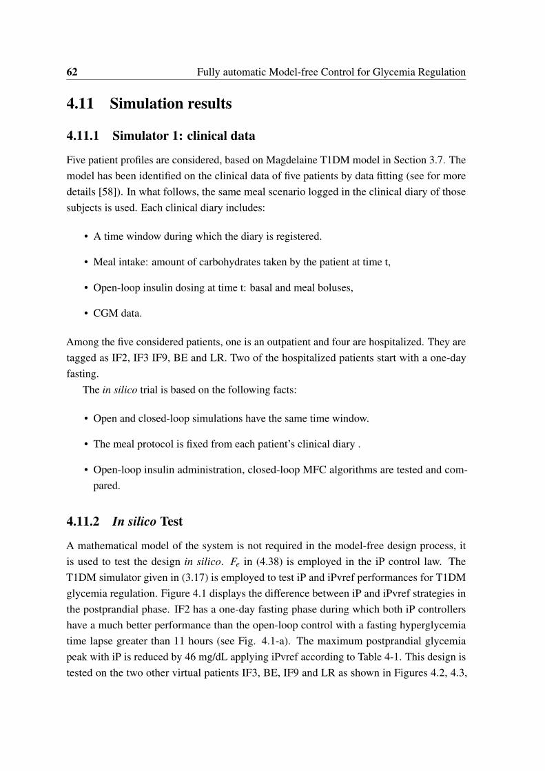
62 Fully automatic Model-free Control for Glycemia Regulation
4.11 Simulation results
4.11.1 Simulator 1: clinical data
Five patient profiles are considered, based on Magdelaine T1DM model in Section 3.7. The
model has been identified on the clinical data of five patients by data fitting (see for more
details [58]). In what follows, the same meal scenario logged in the clinical diary of those
subjects is used. Each clinical diary includes:
• A time window during which the diary is registered.
• Meal intake: amount of carbohydrates taken by the patient at time t,
• Open-loop insulin dosing at time t: basal and meal boluses,
• CGM data.
Among the five considered patients, one is an outpatient and four are hospitalized. They are
tagged as IF2, IF3 IF9, BE and LR. Two of the hospitalized patients start with a one-day
fasting.
The in silico trial is based on the following facts:
• Open and closed-loop simulations have the same time window.
• The meal protocol is fixed from each patient’s clinical diary .
• Open-loop insulin administration, closed-loop MFC algorithms are tested and com-
pared.
4.11.2 In silico Test
A mathematical model of the system is not required in the model-free design process, it
is used to test the design in silico. Fe in (4.38) is employed in the iP control law. The
T1DM simulator given in (3.17) is employed to test iP and iPvref performances for T1DM
glycemia regulation. Figure 4.1 displays the difference between iP and iPvref strategies in
the postprandial phase. IF2 has a one-day fasting phase during which both iP controllers
have a much better performance than the open-loop control with a fasting hyperglycemia
time lapse greater than 11 hours (see Fig. 4.1-a). The maximum postprandial glycemia
peak with iP is reduced by 46 mg/dL applying iPvref according to Table 4-1. This design is
tested on the two other virtual patients IF3, BE, IF9 and LR as shown in Figures 4.2, 4.3,
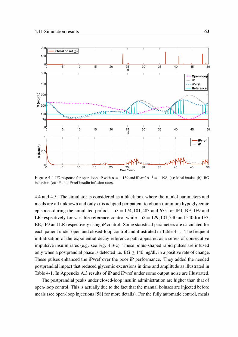
4.11 Simulation results 63
0 5 10 15 20 25 30 35 40 45 500
100
200
(a)
r:Meal onset (g)
0 5 10 15 20 25 30 35 40 45 500
70
120
200
300
400
500
(b)
G (
mg
/dL
)
Open−loop
iP
iPvref
Reference
Open−loop
iP
iPvref
Reference
0 5 10 15 20 25 30 35 40 45 500
0.5
1
Time (hour)
u (
U/m
in)
iPvref
iP
Figure 4.1 IF2 response for open-loop, iP with α =−139 and iPvref α−1 =−198. (a): Meal intake. (b): BGbehavior. (c): iP and iPvref insulin infusion rates.
4.4 and 4.5. The simulator is considered as a black box where the model parameters and
meals are all unknown and only α is adapted per patient to obtain minimum hypoglycemic
episodes during the simulated period. −α = 174,101,483 and 675 for IF3, BE, IF9 and
LR respectively for variable-reference control while −α = 129,101,340 and 540 for IF3,
BE, IF9 and LR respectively using iP control. Some statistical parameters are calculated for
each patient under open and closed-loop control and illustrated in Table 4-1. The frequent
initialization of the exponential decay reference path appeared as a series of consecutive
impulsive insulin rates (e.g. see Fig. 4.3-c). These bolus-shaped rapid pulses are infused
only when a postprandial phase is detected i.e. BG ≥ 140 mg/dL in a positive rate of change.
These pulses enhanced the iPvref over the poor iP performance. They added the needed
postprandial impact that reduced glycemic excursions in time and amplitude as illustrated in
Table 4-1. In Appendix A.3 results of iP and iPvref under some output noise are illustrated.
The postprandial peaks under closed-loop insulin administration are higher than that of
open-loop control. This is actually due to the fact that the manual boluses are injected before
meals (see open-loop injections [58] for more details). For the fully automatic control, meals

64 Fully automatic Model-free Control for Glycemia Regulation
Table 4-1: Time performance indicators for open and closed-loop iP controllers.
Patient
%Time in target
[70-180] - [70-140]
%Time in hypo.
[<70]
%Time in hyper.
[180-250]|[>250]
Mean ± std
Min:Max(BG)
Open-
loop iP iPvref
Open
-loop iP iPvref
Open-
loop iP iPvref
Open-
loop iP iPvref
Open-
loop iP iPvref
IF2 55|30 56|29 59|30 0 0 0 45|0 31|13 40|2 169±47 176±63 168±49 74|230 80|297 88|251
IF3 78|77 68|17 80|36 22 5 0 0|0 17|10 13|8 91±23 168±55 155±50 46|142 56|317 72 | 298
BE 82|48 73|44 70|83 0 0 0 14|4 21|6 17|0 155±39 153±52 128±44 84|260 73|269 73 | 230
IF9 70|65 69|26 72|27 37 0 0 8|6 4|19 4|18 108±62 180±108 174±104 49|320 85|499 80 | 495
LR 57|32 35|17 50|22 2 3 6 33|8 33|30 21|23 171±54 209±82 185± 80 63|300 60|408 59 | 409
0 5 10 15 20 25 30 35 40 450
50
100
150
(a)
r:Meal onset (g)
0 5 10 15 20 25 30 35 40 450
70
120
200
300
400
500
(b)
G (
mg
/dL
)
0 5 10 15 20 25 30 35 40 450
0.1
0.2
0.3
0.4
Time (hour)
u (
U/m
in)
iPvref
iP
Open−loop
iP
iPvref
Reference
Figure 4.2 IF3 response for open-loop, iP with α =−129 and iPvref α−1 =−174. (a): Meal intake. (b): BGbehavior. (c): iP and iPvref insulin infusion rates.
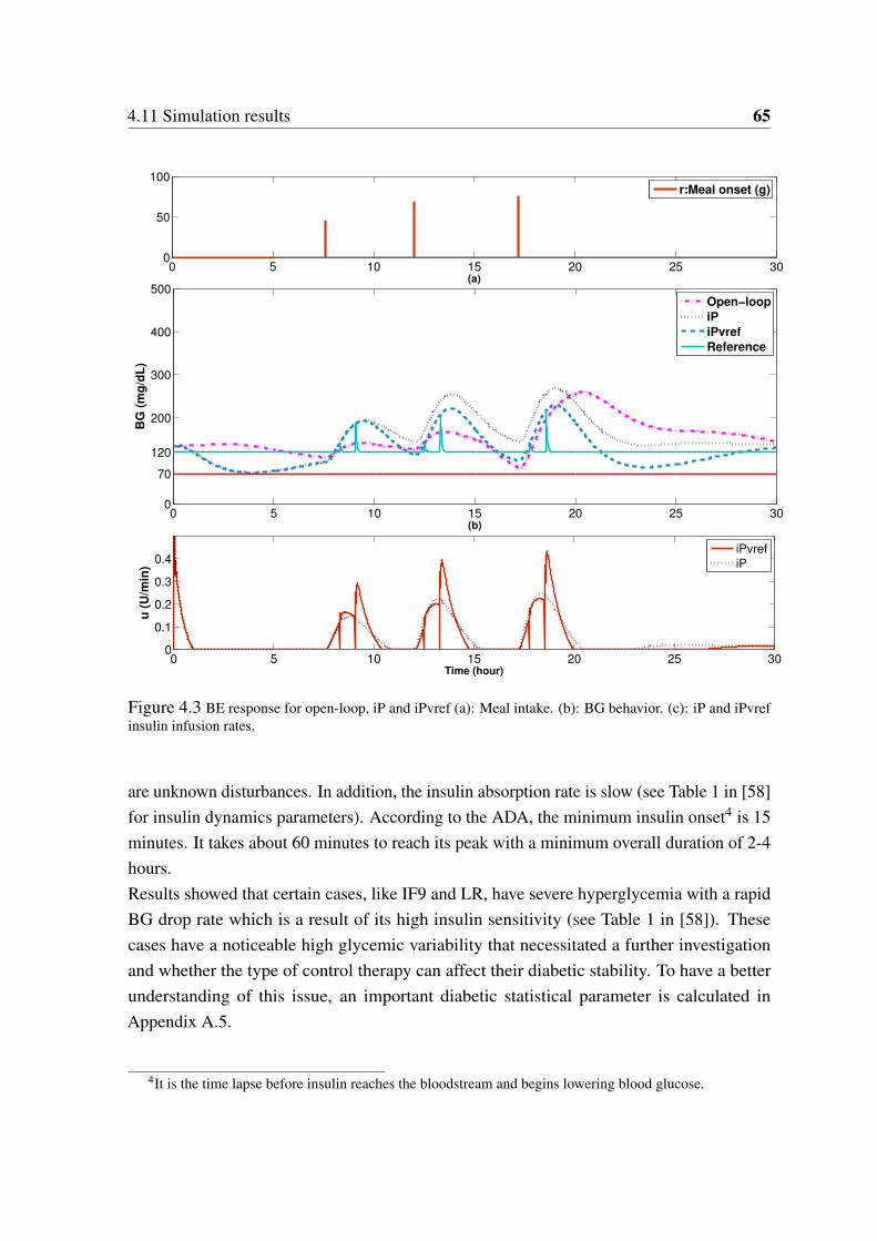
4.11 Simulation results 65
0 5 10 15 20 25 300
50
100
(a)
r:Meal onset (g)
0 5 10 15 20 25 300
70
120
200
300
400
500
(b)
BG
(m
g/d
L)
0 5 10 15 20 25 300
0.1
0.2
0.3
0.4
Time (hour)
u (
U/m
in)
Open−loop
iP
iPvref
Reference
iPvref
iP
Figure 4.3 BE response for open-loop, iP and iPvref (a): Meal intake. (b): BG behavior. (c): iP and iPvrefinsulin infusion rates.
are unknown disturbances. In addition, the insulin absorption rate is slow (see Table 1 in [58]
for insulin dynamics parameters). According to the ADA, the minimum insulin onset4 is 15
minutes. It takes about 60 minutes to reach its peak with a minimum overall duration of 2-4
hours.
Results showed that certain cases, like IF9 and LR, have severe hyperglycemia with a rapid
BG drop rate which is a result of its high insulin sensitivity (see Table 1 in [58]). These
cases have a noticeable high glycemic variability that necessitated a further investigation
and whether the type of control therapy can affect their diabetic stability. To have a better
understanding of this issue, an important diabetic statistical parameter is calculated in
Appendix A.5.
4It is the time lapse before insulin reaches the bloodstream and begins lowering blood glucose.
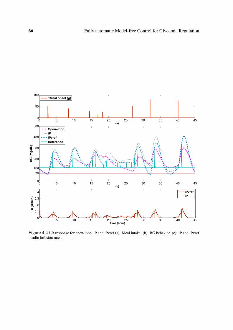
66 Fully automatic Model-free Control for Glycemia Regulation
0 5 10 15 20 25 30 35 40 450
50
100
(a)
r:Meal onset (g)
0 5 10 15 20 25 30 35 40 450
70
120
200
300
400
500
(b)
BG
(m
g/d
L)
0 5 10 15 20 25 30 35 40 450
0.1
0.2
0.3
0.4
Time (hour)
u (
U/m
in)
iPvref
iP
Open−loop
iP
iPvref
Reference
Figure 4.4 LR response for open-loop, iP and iPvref (a): Meal intake. (b): BG behavior. (c): iP and iPvrefinsulin infusion rates.
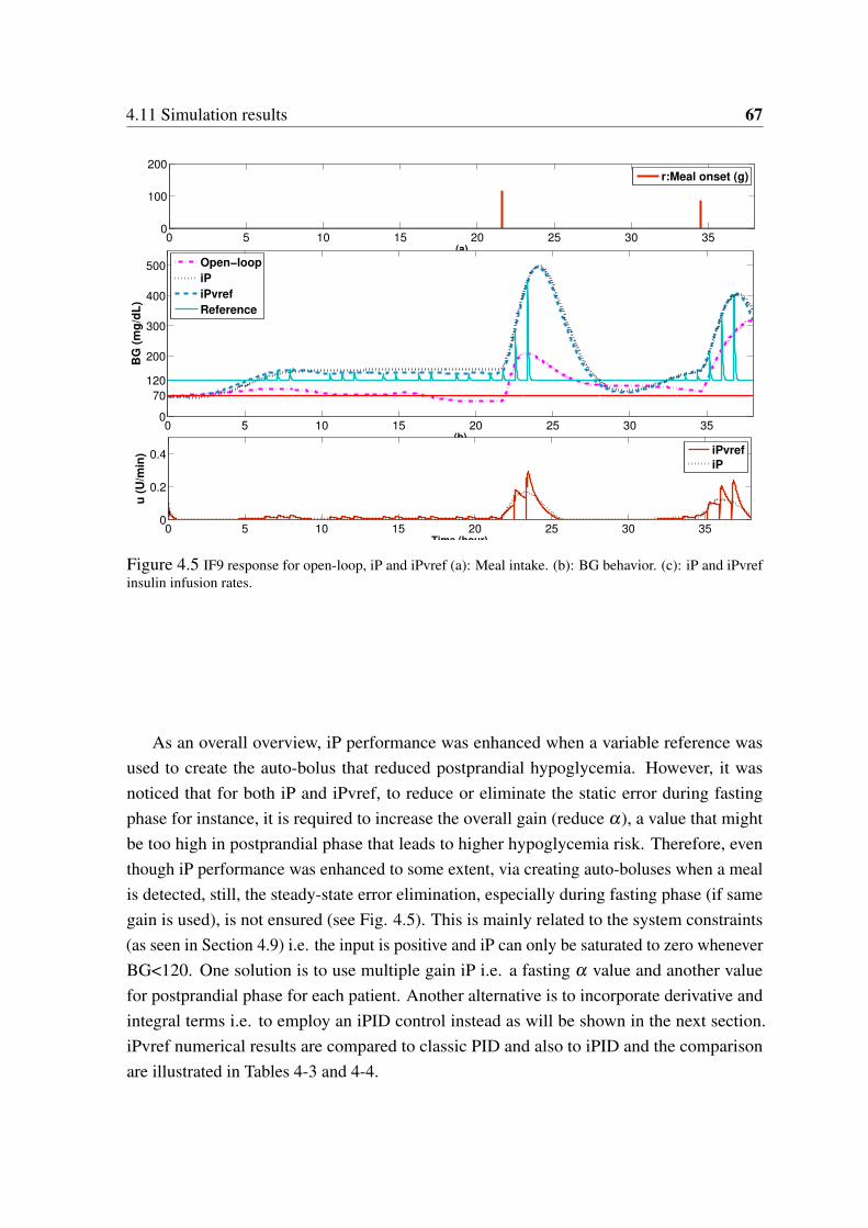
4.11 Simulation results 67
0 5 10 15 20 25 30 350
100
200
(a)
r:Meal onset (g)
0 5 10 15 20 25 30 350
70
120
200
300
400
500
(b)
BG
(m
g/d
L)
0 5 10 15 20 25 30 350
0.2
0.4
Time (hour)
u (
U/m
in)
Open−loop
iP
iPvref
Reference
iPvref
iP
Figure 4.5 IF9 response for open-loop, iP and iPvref (a): Meal intake. (b): BG behavior. (c): iP and iPvrefinsulin infusion rates.
As an overall overview, iP performance was enhanced when a variable reference was
used to create the auto-bolus that reduced postprandial hypoglycemia. However, it was
noticed that for both iP and iPvref, to reduce or eliminate the static error during fasting
phase for instance, it is required to increase the overall gain (reduce α), a value that might
be too high in postprandial phase that leads to higher hypoglycemia risk. Therefore, even
though iP performance was enhanced to some extent, via creating auto-boluses when a meal
is detected, still, the steady-state error elimination, especially during fasting phase (if same
gain is used), is not ensured (see Fig. 4.5). This is mainly related to the system constraints
(as seen in Section 4.9) i.e. the input is positive and iP can only be saturated to zero whenever
BG<120. One solution is to use multiple gain iP i.e. a fasting α value and another value
for postprandial phase for each patient. Another alternative is to incorporate derivative and
integral terms i.e. to employ an iPID control instead as will be shown in the next section.
iPvref numerical results are compared to classic PID and also to iPID and the comparison
are illustrated in Tables 4-3 and 4-4.
68 Fully automatic Model-free Control for Glycemia Regulation
4.12 iPID Control
In this section the feasibility of iPID for glycemia regulation is tested in silico. This section
and the following sections results are extracted from and based on the publication [87].
Firstly, iPID is compared to iPvref performance. Secondly, iPID is compared to a standard
PID on two T1DM simulators with and without measurement noise. The first simulator
is the long-term linear time-invariant model (3.17). The controller is also validated on the
UVa/Padova metabolic simulator on 10 adults under 25 runs/subject for noise robustness test.
iPID previously designed and tested for fasting conditions [88] is corrected and tested in
[87] including postprandial phase on a larger cohort of T1DM patients from the Uva/Padova
simulator. The parameter α is tuned here such that y and αu f have the same order of
magnitude as suggested in [63], for a better estimation of F . This is an advantageous
robustness property of the intelligent controller as α can be used to individualize the controller
for each subject. Moreover, the tuning of α is based on the output and previously applied
input that are already available for the controller. As BG responds inversely to the control
variable, α is negative. The PID parameters of (4.40) are Kp = 3 10−5,Ki = 0.001 and
Kd = 250 tuned and tested on patient tagged as IF2.
Remark 6. In silico tests of iPID are obtained with and without CGM measurement noise. To
test the feasibility of the iPID control, it is tested on Simulator 1 in a noise-free environment
in order to have a perfect estimation of Fe and thus to test the performance of an ideal iPID.
Using Simulator 2 or the Uva/Padova simulator, the robustness of iPID against CGM noise
was tested.
A Luenberger observer is used to estimate y(t) (see Appendix A.4 for the design). The
input to the observer is the pure blood glucose output of the model in Simulator 1. For
simulator 2, the noisy sensor signal of the simulator is differentiated to obtain y(t) using the
algebraic derivative estimator in Appendix A.1 that has a filtering properties (see [83] and
the references therein).
To estimate y(t) for both simulators, a two-stage differentiation is done: a Dormand-
Prince ode45 numerical differentiator method is utilized followed by Luenberger first order
derivative estimator for Simulator 1 and the algebraic differentiator for Simulator 2 respec-
tively.
Fe is estimated according to (4.41), with ye(t) is estimated as explained previously. The
delay buffer in (A.22) of Appendix A.2 is useful to obtain a delayed signal like u(t −h), thus
eq. (4.41) becomes:
Fe(t) = ye(t)−6
T 3
Z t
t−Tα(t −σ)(T − t +σ)u(σ)dσ (4.44)

4.13 Standard PID 69
For simulator 1, the controller is sent every 5 minutes and the integration time window is
T = 20 min. (recall that h = T/2). For the Uva/Padova simulator, the built-in sampling time
is one minute and T = 5 min.
4.13 Standard PID
A standard PID controller is designed and compared to the iPID performance [87]. The classic
PID parameters are tuned on IF2 subject to yield a tight BG control, with a performance
comparable to that of iPID, with maximum time percentage in euoglycemia and minimum
hypoglycemic episodes. For this purpose, the two-day meal scenario is used as logged in the
clinical diary. The controller parameters are Kpc = 0.0005,Kdc = 250 and Kic = 0.001.
For comparison, this standard PID will be also scaled by a constant parameter p when
applied on different patients. It will be tuned per individual to minimize hypoglycemic
events during the simulation period. Individualizing only one control parameter per subject
is employed previously by [46] in an in silico trial for both PID and MPC, Kpc for the former
and the output prediction weighting parameter for MPC.
Remark 7. The integral term is limited to limit the integral windup due to control saturation
resulting from the inherent large and slow error dynamics especially during postprandial
phase. As time grows, the integral action excessively builds up to cope with postprandial
hyperglycemia yielding severe BG oscillations. For this system there is no negative action to
compensate for negative error excursions. Insulin injection is a positive input, i.e. insulin can
not be removed in case of over dosing, thus the input is saturated to zero. The result is input
saturation, on one hand, and oscillatory behavior and hypoglycemia in the output channel on
the other hand. For this reason, PID users usually incorporate some anti-windup protection
for the integrator, or even replace the integral by the patient optimal basal rate in PD+Basal
control [41]. The authors compared PID and PD+Basal on Uva/Padova simulator. They
concluded that the latter outperformed in reducing postprandial hyperglycemia, but and
conversely to PID, it failed to respond appropriately to changes in insulin sensitivity.
In this work and as will be shown in the next section, iPID is tested in two cases:
i) an anti wind-up scheme is employed for the integral action, for both PID and iPID, to
avoid the long-term accumulation. It discharges when hyperglycemia is attained (BG ≥ 180
mg/dL).
ii) The integral action is turned off and replaced by the subject’s specific basal rate, i.e.
iPD+basal.
70 Fully automatic Model-free Control for Glycemia Regulation
4.14 Methods
iPID controller is tested in silico on two different simulators. The first is the long-term model
identified on clinical data of five T1DM subjects (see § 3.7). The same meal scenario logged
in the clinical diary of those subjects is used. The second trial is performed on the well
known Uva/Padova metabolic simulator that is approved by FDA (see §3.6). The second trial
is performed on ten adults using a meal scenario of other published results of PID and MPC
controllers. For both tests, all simulator parameters are unknown to the controller and meals
are unannounced disturbances.
4.14.1 Simulator 1
The in silico tests will be performed on simulator 1 on five T1DM subjects using the clinical
diary as explained in Section 4.11.1. The open-loop basal-bolus injections of each diary will
be compared here to the closed-loop algorithms PID and iPID. The details of the simulation
results are presented in Section 4.15.
4.14.2 Simulator 2: UVa/Padova T1DM simulator
The PID designed in [89] that was compared to MPC performance, will be re-simulated here
under the same meal scenario and compared to iPID performance. The PID was actually a
(PD+basal rate) where the integral term is replaced by the subject’s specific basal rate. The
authors optimized PD weights to minimize average BG risk. This design is employed here
for the iPID i.e. turning the integral term off and replace it by the subject’s specific basal.
The purpose is to study the effect of the intelligent part of the iPID over a classic PID. The
PID as appeared in [89], sampled every 5 minutes is described as follows changing only the
set point to 120 mg/dL :
un = 6.37510−5Pn +basal +0.0046Dn, (4.45)
Pn = yn −120 (4.46)
Dn = yn − yn−1 (4.47)
Where Pn,Dn are the proportional and derivative gains respectively. yn is BG at instant n.
The Uva/Padova built in basal rate will be used for each subject in the current study. The
desired set point for both controllers is set to 120 instead of the previously chosen 140 mg/dL
in [89]. The meal scenario is a 36 hours of six unannounced 20 min. duration meals. The
meal amount and timing are given in Table 4-2.
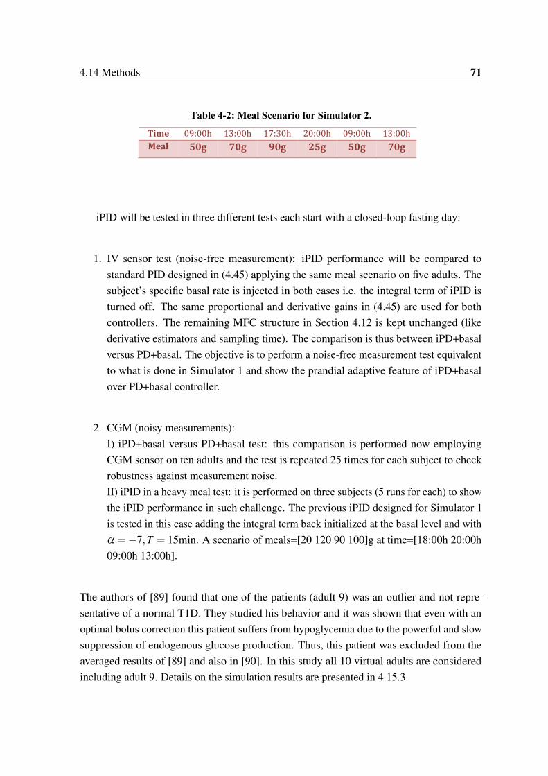
4.14 Methods 71
Table 4-2: Meal Scenario for Simulator 2.
Time 09:00h 13:00h 17:30h 20:00h 09:00h 13:00h
Meal 50g 70g 90g 25g 50g 70g
iPID will be tested in three different tests each start with a closed-loop fasting day:
1. IV sensor test (noise-free measurement): iPID performance will be compared to
standard PID designed in (4.45) applying the same meal scenario on five adults. The
subject’s specific basal rate is injected in both cases i.e. the integral term of iPID is
turned off. The same proportional and derivative gains in (4.45) are used for both
controllers. The remaining MFC structure in Section 4.12 is kept unchanged (like
derivative estimators and sampling time). The comparison is thus between iPD+basal
versus PD+basal. The objective is to perform a noise-free measurement test equivalent
to what is done in Simulator 1 and show the prandial adaptive feature of iPD+basal
over PD+basal controller.
2. CGM (noisy measurements):
I) iPD+basal versus PD+basal test: this comparison is performed now employing
CGM sensor on ten adults and the test is repeated 25 times for each subject to check
robustness against measurement noise.
II) iPID in a heavy meal test: it is performed on three subjects (5 runs for each) to show
the iPID performance in such challenge. The previous iPID designed for Simulator 1
is tested in this case adding the integral term back initialized at the basal level and with
α =−7,T = 15min. A scenario of meals=[20 120 90 100]g at time=[18:00h 20:00h
09:00h 13:00h].
The authors of [89] found that one of the patients (adult 9) was an outlier and not repre-
sentative of a normal T1D. They studied his behavior and it was shown that even with an
optimal bolus correction this patient suffers from hypoglycemia due to the powerful and slow
suppression of endogenous glucose production. Thus, this patient was excluded from the
averaged results of [89] and also in [90]. In this study all 10 virtual adults are considered
including adult 9. Details on the simulation results are presented in 4.15.3.
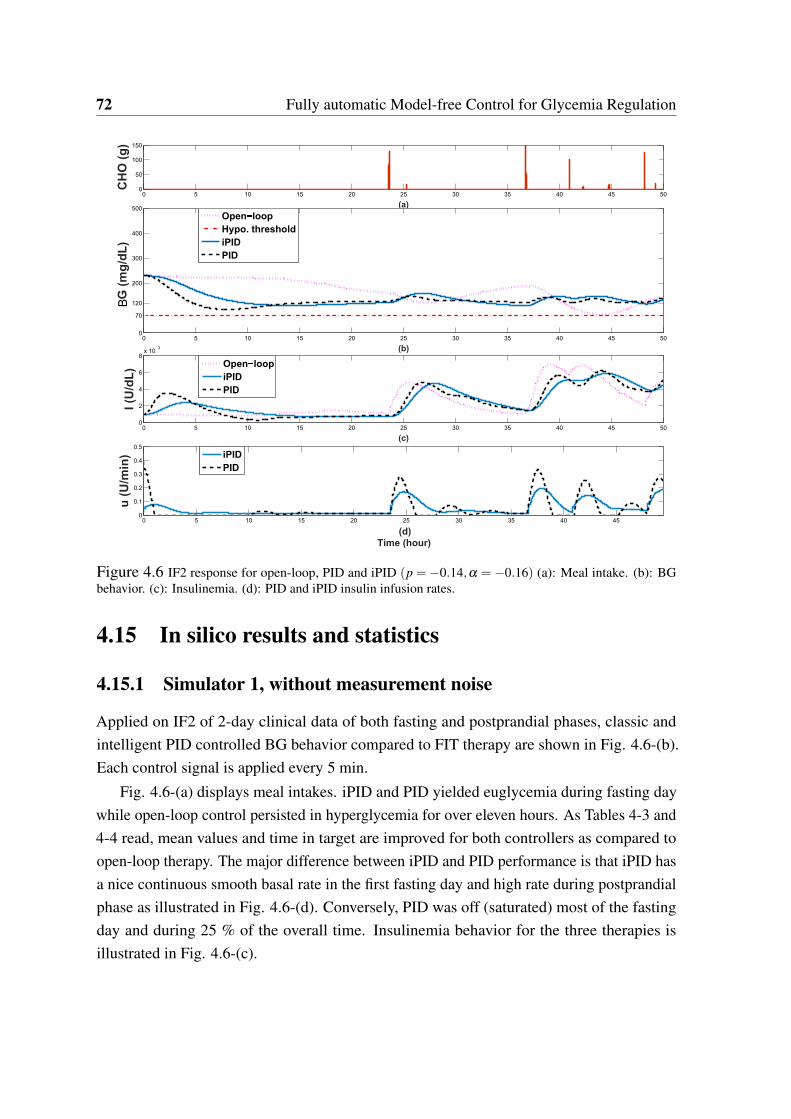
72 Fully automatic Model-free Control for Glycemia Regulation
0 5 10 15 20 25 30 35 40 45 500
50
100
150
(a)
CH
O(g
)
0 5 10 15 20 25 30 35 40 45 500
70
120
200
300
400
500
(b)
G(m
g/d
L)
Open loop
Hypo. threshold
iPID
PID
0 5 10 15 20 25 30 35 40 45 500
2
4
6
8x 10
3
(c)
I (U
/dL
) Open loop
iPID
PID
0 5 10 15 20 25 30 35 40 450
0.1
0.2
0.3
0.4
0.5
(d)
Time (hour)
u (
U/m
in) iPID
PID
B
Figure 4.6 IF2 response for open-loop, PID and iPID (p = −0.14,α = −0.16) (a): Meal intake. (b): BGbehavior. (c): Insulinemia. (d): PID and iPID insulin infusion rates.
4.15 In silico results and statistics
4.15.1 Simulator 1, without measurement noise
Applied on IF2 of 2-day clinical data of both fasting and postprandial phases, classic and
intelligent PID controlled BG behavior compared to FIT therapy are shown in Fig. 4.6-(b).
Each control signal is applied every 5 min.
Fig. 4.6-(a) displays meal intakes. iPID and PID yielded euglycemia during fasting day
while open-loop control persisted in hyperglycemia for over eleven hours. As Tables 4-3 and
4-4 read, mean values and time in target are improved for both controllers as compared to
open-loop therapy. The major difference between iPID and PID performance is that iPID has
a nice continuous smooth basal rate in the first fasting day and high rate during postprandial
phase as illustrated in Fig. 4.6-(d). Conversely, PID was off (saturated) most of the fasting
day and during 25 % of the overall time. Insulinemia behavior for the three therapies is
illustrated in Fig. 4.6-(c).
4.15 In silico results and statistics 73
iPID: a three-phase control
Both controllers are tested on the four other subjects tagged as IF3, IF9, BE and LR changing
−α = 0.32,0.43,0.18,1.6 and −p = 0.65,1.3,0.45,3.5 for iPID and PID respectively as
designed in Section 4.13. α may have a range of acceptable values per individual that verify
the order of magnitude of the estimators terms. This is an interesting feature of iPID as it
permits to detect and respond to the varying insulin sensitivity. The in silico test is conducted
applying meal scenarios as logged in the clinical diary (see [58] for more details).
As illustrated in Table 4-3 and 4-4, satisfactory BG behavior is achieved under both
controls with high percentage of time in target and mean values without severe hypoglycemic
events. The first three subjects are assessed in [87] as stable diabetics according to the Mean
Amplitude of Glycemic Excursion (MAGE) index while IF9 and LR are brittle diabetics (see
Appendix A.3).
Although meals are unannouned for both controls, iPID produced a faster bolus-shaped
infusion and thus a reduced postprandial BG excursion without the risk of late hypoglycemia
(see Fig. 4.8-(b)and 4.7 (b)). This improvement of iPID over its classic counterpart can be
observed also by the time percentage in hyperglycemia and the maximum peak as shown in
Table 4-4. The overall average percentage of BG in [180, 250] is 12.6% versus 14.6% and
BG >250 is 1.6% versus 4.8% for iPID and PID respectively. iPID control has a better mean
and time-in-target values with less hyperglycemia in amplitude and duration as compared
to PID control. The average over all percentage of BG in [70, 180] is 85.6% versus 80.4%
with overall mean 141± 37 versus 147 ± 42 for iPID and PID respectively. As illustrated in
Tables 4-3 and 4-4, PID and iPID control performances dominated those of iPvref control.
4.15.2 Simulator 2, with measurement noise: Uva/Padova
4.15.3 IV sensor
In this test a scenario of 33 hours of fasting followed by the meal scenario mentioned earlier
in Section 4.14.2 tested on five patients ( adults 1, 3, 7, 8, 10). The objective is to test the
superiority of the intelligent part of iPD+basal over standard PD+basal performance in (4.45)
employing the same feedback gains with α =−7. As detailed in Section 4.14.2, the integral
term is turned off and the subjects specific basal rate is injected in both algorithms. As
illustrated in Fig. 4.9, although both controllers reacted fast to meal perturbations, iPD+basal
was more aggressive which had a higher impact on postprandial hyperglycemia without a
risk of late hypoglycemia. As a result, iPD+basal achieved a better trade-off between hyper
and hypoglycemia with average overall mean of 138 versus 155 mg/dL for PD+basal.
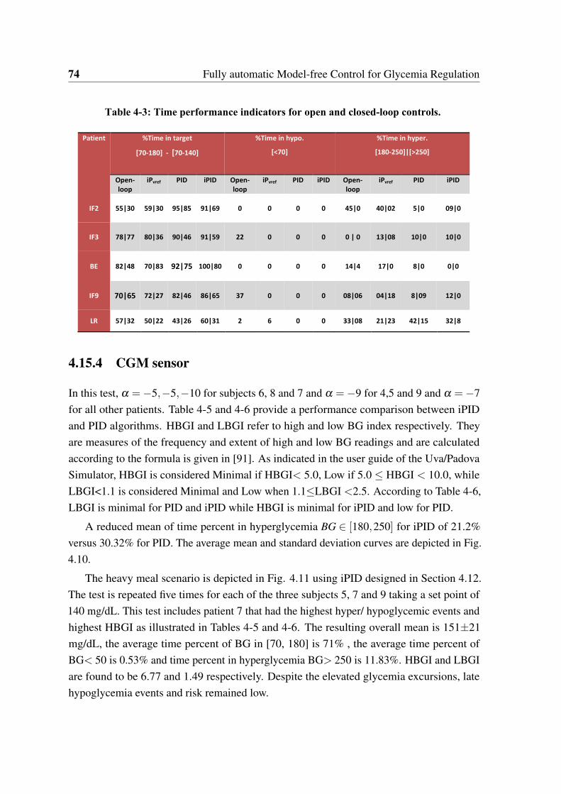
74 Fully automatic Model-free Control for Glycemia Regulation
Table 4-3: Time performance indicators for open and closed-loop controls.
Patient %Time in target
[70-180] - [70-140]
%Time in hypo.
[<70]
%Time in hyper.
[180-250]|[>250]
Open-
loop
iPvref PID iPID Open-
loop
iPvref PID iPID Open-
loop
iPvref PID iPID
IF2 55|30 59|30 95|85 91|69 0 0 0 0 45|0 40|02 5|0 09|0
IF3 78|77 80|36 90|46 91|59 22 0 0 0 0 | 0 13|08 10|0 10|0
BE 82|48 70|83 92|75 100|80 0 0 0 0 14|4 17|0 8|0 0|0
IF9 70|65 72|27 82|46 86|65 37 0 0 0 08|06 04|18 8|09 12|0
LR 57|32 50|22 43|26 60|31 2 6 0 0 33|08 21|23 42|15 32|8
4.15.4 CGM sensor
In this test, α =−5,−5,−10 for subjects 6, 8 and 7 and α =−9 for 4,5 and 9 and α =−7
for all other patients. Table 4-5 and 4-6 provide a performance comparison between iPID
and PID algorithms. HBGI and LBGI refer to high and low BG index respectively. They
are measures of the frequency and extent of high and low BG readings and are calculated
according to the formula is given in [91]. As indicated in the user guide of the Uva/Padova
Simulator, HBGI is considered Minimal if HBGI< 5.0, Low if 5.0 HBGI < 10.0, while
LBGI<1.1 is considered Minimal and Low when 1.1LBGI <2.5. According to Table 4-6,
LBGI is minimal for PID and iPID while HBGI is minimal for iPID and low for PID.
A reduced mean of time percent in hyperglycemia BG 2 [180,250] for iPID of 21.2%
versus 30.32% for PID. The average mean and standard deviation curves are depicted in Fig.
4.10.
The heavy meal scenario is depicted in Fig. 4.11 using iPID designed in Section 4.12.
The test is repeated five times for each of the three subjects 5, 7 and 9 taking a set point of
140 mg/dL. This test includes patient 7 that had the highest hyper/ hypoglycemic events and
highest HBGI as illustrated in Tables 4-5 and 4-6. The resulting overall mean is 151±21
mg/dL, the average time percent of BG in [70, 180] is 71% , the average time percent of
BG< 50 is 0.53% and time percent in hyperglycemia BG> 250 is 11.83%. HBGI and LBGI
are found to be 6.77 and 1.49 respectively. Despite the elevated glycemia excursions, late
hypoglycemia events and risk remained low.
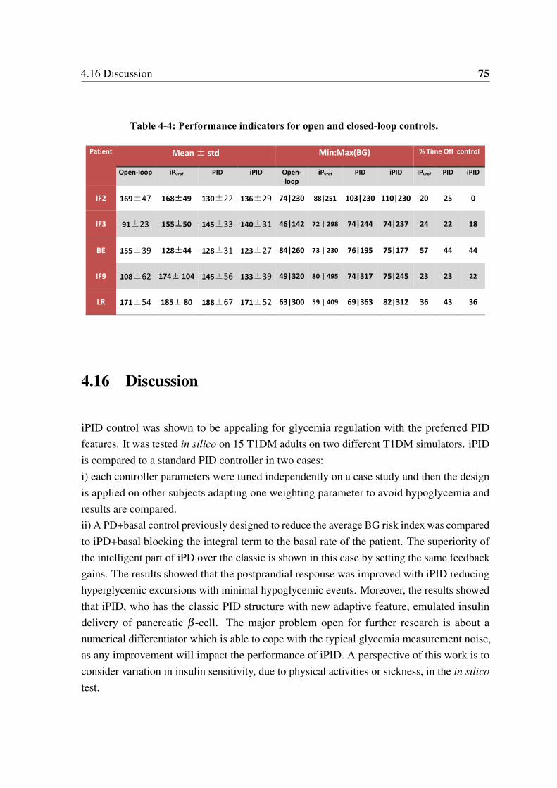
4.16 Discussion 75
Table 4-4: Performance indicators for open and closed-loop controls.
Patient Mean ± std Min:Max(BG) % Time Off control
Open-loop iPvref PID iPID Open-
loop
iPvref PID iPID iPvref PID iPID
IF2 169±47 168±49 130±22 136±29 74|230 88|251 103|230 110|230 20 25 0
IF3 91±23 155±50 145±33 140±31 46|142 72 | 298 74|244 74|237 24 22 18
BE 155±39 128±44 128±31 123±27 84|260 73 | 230 76|195 75|177 57 44 44
IF9 108±62 174± 104 145±56 133±39 49|320 80 | 495 74|317 75|245 23 23 22
LR 171±54 185± 80 188±67 171±52 63|300 59 | 409 69|363 82|312 36 43 36
4.16 Discussion
iPID control was shown to be appealing for glycemia regulation with the preferred PID
features. It was tested in silico on 15 T1DM adults on two different T1DM simulators. iPID
is compared to a standard PID controller in two cases:
i) each controller parameters were tuned independently on a case study and then the design
is applied on other subjects adapting one weighting parameter to avoid hypoglycemia and
results are compared.
ii) A PD+basal control previously designed to reduce the average BG risk index was compared
to iPD+basal blocking the integral term to the basal rate of the patient. The superiority of
the intelligent part of iPD over the classic is shown in this case by setting the same feedback
gains. The results showed that the postprandial response was improved with iPID reducing
hyperglycemic excursions with minimal hypoglycemic events. Moreover, the results showed
that iPID, who has the classic PID structure with new adaptive feature, emulated insulin
delivery of pancreatic β -cell. The major problem open for further research is about a
numerical differentiator which is able to cope with the typical glycemia measurement noise,
as any improvement will impact the performance of iPID. A perspective of this work is to
consider variation in insulin sensitivity, due to physical activities or sickness, in the in silico
test.
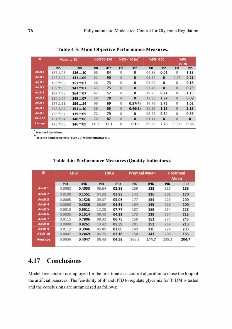
76 Fully automatic Model-free Control for Glycemia Regulation
Table 4-5: Main Objective Performance Measures.
* Standard deviation.
** n is the number of tests (over 25) where min(BG)<50.
ID Mean ± SD* %BG 70-180 %BG < 50 (n)
** %BG >250 %BG
50-70
PID iPID PID iPID PID iPID PID iPID PID iPID
Adult 1 167±06 136±10 68 84 0 0 04.38 0.02 0 1.13 Adult 2 153±07 131±09 81 90 0 0 01.64 0 0.08 0.21 Adult 3 183±05 153±07 46 73 0 0 07.00 0 0 0.16 Adult 4 169±05 147±07 63 75 0 0 03.48 0 0 0.29 Adult 5 197±06 164±07 42 57 0 0 19.25 8.21 0 1.15 Adult 6 180±04 145±07 58 78 0 0 13.36 2.97 0 0.09 Adult 7 177±11 156±14 66 69 0 0.57(4) 14.79 9.75 0 1.02 Adult 8 208±04 151±10 36 65 0 0.46(3) 24.19 1.15 0 2.16 Adult 9 159±07 139±09 72 79 0 0 05.97 0.54 0 0.36
Adult 10 161±04 140±06 70 87 0 0 01.14 0 0 0 Average 175±06 146±09 60.2 75.7 0 0.10 09.50 2.26 0.008 0.66
Table 4-6: Performance Measures (Quality Indicators).
ID LBGI HBGI
Premeal Mean Postmeal
Mean
PID iPID PID iPID PID iPID PID iPID
Adult 1 0.0002 0.4053 06.64 02.88 159 133 225 188
Adult 2 0.0100 0.1551 04.33 01.95 142 126 202 170
Adult 3 0.0005 0.1528 09.37 05.06 177 154 226 200
Adult 4 0.0005 0.3836 06.89 04.51 164 149 216 200
Adult 5 0.0010 0.5511 12.28 07.77 187 165 254 228
Adult 6 0.0003 0.1514 09.43 04.31 173 139 254 215
Adult 7 0.0115 0.7806 09.32 06.75 159 152 275 245
Adult 8 0.0000 0.8261 14.42 05.59 201 152 268 213
Adult 9 0.0112 0.3946 05.85 03.80 149 136 224 203
Adult 10 0.0007 0.2469 05.75 03.18 158 141 208 185
Average 0.0036 0.4047 08.43 04.58 166.9 144.7 235.2 204.7
4.17 Conclusions
Model-free control is employed for the first time as a control algorithm to close the loop of
the artificial pancreas. The feasibility of iP and iPID to regulate glycemia for T1DM is tested
and the conclusions are summarized as follows:
4.17 Conclusions 77
1. iP
• Constant reference iP has shown a poor postprandial response. Under a small
estimation time window, the proportional gains α and Kp were not sufficient to
reduce hyperglycemia peaks without late hypoglycemia.
• iP postprandial performance was enhanced by introducing a variable reference
trajectory for the controller. Whenever meals were detected, the controller
switched between a constant set point, to an exponential decay reference path.
This variable reference yielded a postprandial bolus-shaped injection rate which
was more effective in handling hyperglycemia peaks.
• In silico tests: the fully automatic model-free iPvref has shown a better postpran-
dial performance with respect to conventional iP.
• A good fasting-postprandial compromise can not be yielded using fixed design.
• To further improve the fully automatic controller, a two-phases gain scheduling
is proposed: α for fasting phase, and another for postprandial phase. Another
possibility, that was realized here, is to increase the degree of control complexity
to close the loop with iPID.
2. iPID
• Constant reference iPID performance indicators dominated those of iPvref in
silico control.
• iPID was compared to classic PID behavior that were optimally designed for a
T1DM subject of Simulator 1. iPID showed a better glycemia response according
to some statistical parameters. It was shown that iPID better emulated β cells
behavior than PID control by infusing a faster postprandial (first phase) insulin
pulse.
• iPID was tested on Uva/Padova T1DM simulator on three adults under CGM sen-
sor noise. The fully automatic iPID response to a relatively heavy meal scenario
was satisfactory avoiding late hypoglycemia. The same design parameters were
used for the three subjects.
• iPD+basal was compared to an existing PD+basal control from a previous study.
For a clear comparison, both controllers are compared employing the same gain
parameters.
• in silico Uva/Padova test results, under CGM noise, on 10 adults 25 runs have
shown the superiority of the intelligent controller over its classic counterpart. The
78 Fully automatic Model-free Control for Glycemia Regulation
intelligent controller detected meals and reacted faster to meal perturbations as
compared to a classic PD without neglecting safety.
Diabetic stability is studied through the MAGE index (in Appendix A.5) to explain the
excessive glycemic variability in some subjects. They are found to be brittle patients, rare
cases that usually need extensive care and of BG fluctuations that are difficult to predict
and regulate. For the MAGE-stable patients, the new design yielded a satisfactory glycemic
response under the fully automatic MFC.
As a general overview, a better postprandial BG response was obtained with iPID as
compared to classic PID and to iPvref. A good robustness level was shown tuning only one
parameter from one patient to another. It was tuned empirically to reduce hyperglycemia with
least hypoglycemic episodes during the simulation time. The controller was fully automatic
without any meal announcement nor supplementary boluses. iPID combines the classic PID
nice properties with new adaptive features. However, the following remarks are worth noting:
1. System constraints are not taken into account in the design, namely, hypoglycemia
threshold and the positivity of the controller. The controller was saturated to zero
which is the lower admissible bound.
2. When the controller saturates to zero, the loop is broken and glycemia is not under
iPID control.
3. Integral windup is another known defect for PID-like controllers.
4. Hypoglycemia avoidance is not ensured.
Thus, maintaining a tight BG control, especially during postprandial phase is also not an easy
task for this fully automatic iPID.
Regarding MFC in general, some questions were raised concerning the stability of the
controller and iP was taken as a case study. It was shown that closed-loop stability, for iP
controller, is not simply related to the first order error dynamics resulting form the ultra-local
model. Via a second-order academic example, it was shown that closing the loop with iP does
not guarantee stability. Stability analyses related to the delay on the control law probably
worth further investigation. Other questions regarding the choice of the estimation function
of the ultra-local model are underlined. During the design of iPID, for instance, it was found
that a problem open for further research is about a numerical second order differentiator
which is able to cope with the typical glycemia measurement noise, as any improvement will
impact the performance of iPID.
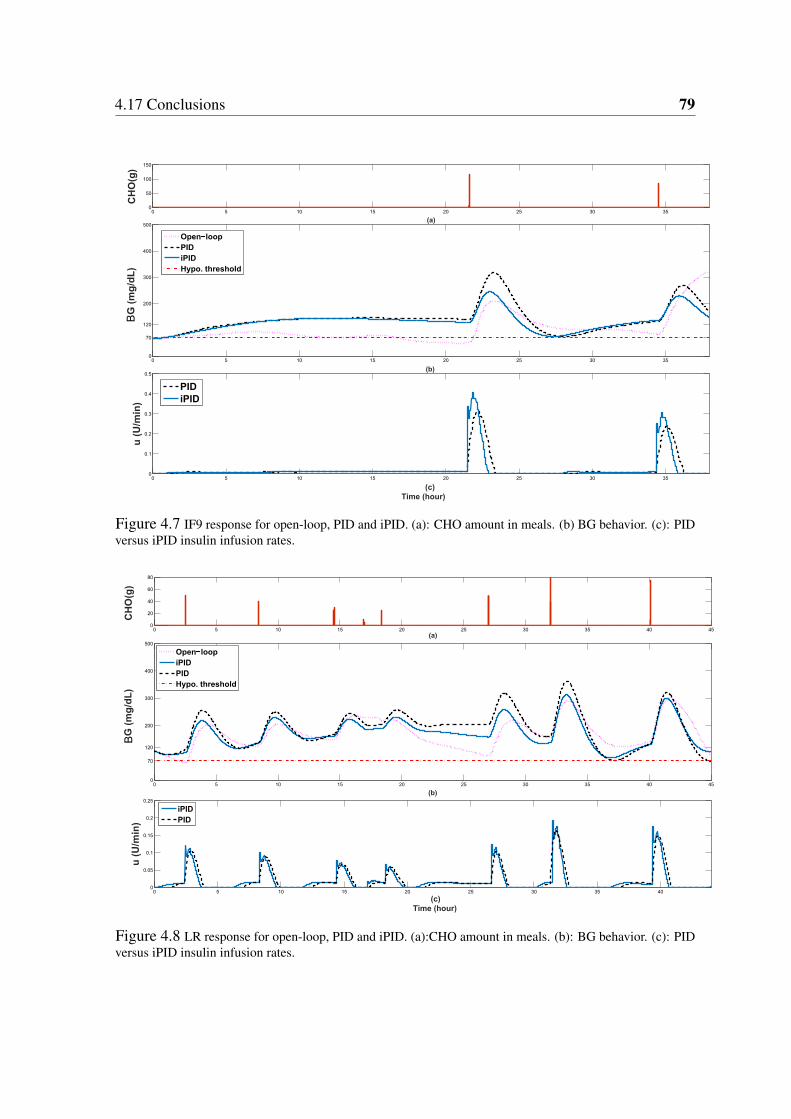
4.17 Conclusions 79
0 5 10 15 20 25 30 350
50
100
150
(a)
CH
O(g
)
0 5 10 15 20 25 30 350
70
120
200
300
400
500
(b)
G (
mg
/dL
)
Open loop
PID
iPID
Hypo. threshold
0 5 10 15 20 25 30 350
0.1
0.2
0.3
0.4
0.5
(c)
Time (hour)
u (
U/m
in)
PID
iPID
B
Figure 4.7 IF9 response for open-loop, PID and iPID. (a): CHO amount in meals. (b) BG behavior. (c): PIDversus iPID insulin infusion rates.
0 5 10 15 20 25 30 35 40 450
20
40
60
80
(a)
CH
O(g
)
0 5 10 15 20 25 30 35 40 450
70
120
200
300
400
500
(b)
G(m
g/d
L)
Open loop
iPID
PID
Hypo. threshold
0 5 10 15 20 25 30 35 400
0.05
0.1
0.15
0.2
0.25
(c)
Time (hour)
u (
U/m
in)
iPID
PID
B
Figure 4.8 LR response for open-loop, PID and iPID. (a):CHO amount in meals. (b): BG behavior. (c): PIDversus iPID insulin infusion rates.
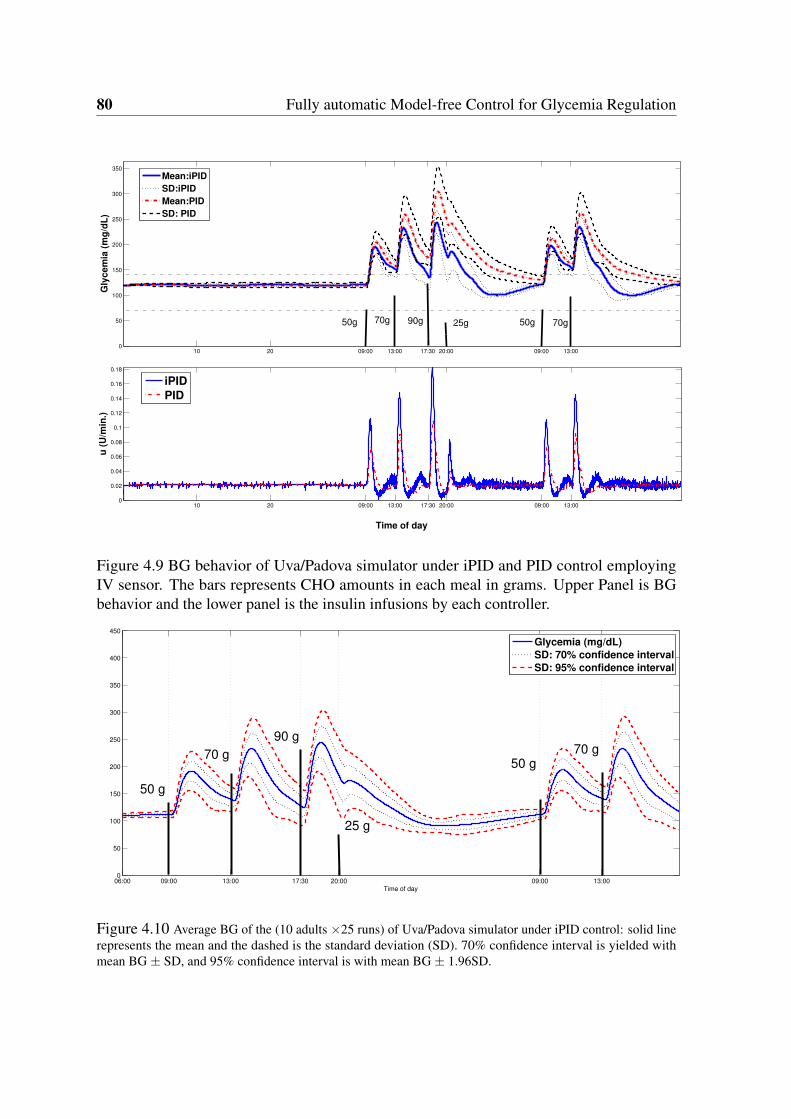
80 Fully automatic Model-free Control for Glycemia Regulation
10 20 09:00 13:00 17:30 20:00 09:00 13:000
0.02
0.04
0.06
0.08
0.1
0.12
0.14
0.16
0.18
Time of day
u (
U/m
in.)
iPID
PID
10 20 09:00 13:00 17:30 20:00 09:00 13:000
50
100
150
200
250
300
350
Gly
cem
ia (
mg
/dL
)
Mean:iPID
SD:iPID
Mean:PID
SD: PID
50g50g 70g 70g25g90g
Figure 4.9 BG behavior of Uva/Padova simulator under iPID and PID control employingIV sensor. The bars represents CHO amounts in each meal in grams. Upper Panel is BGbehavior and the lower panel is the insulin infusions by each controller.
06:00 09:00 13:00 17:30 20:00 09:00 13:000
50
100
150
200
250
300
350
400
450
Time of day
Glycemia (mg/dL)
SD: 70% confidence interval
SD: 95% confidence interval
90 g
70 g50 g
70 g
50 g
25 g
Figure 4.10 Average BG of the (10 adults 25 runs) of Uva/Padova simulator under iPID control: solid linerepresents the mean and the dashed is the standard deviation (SD). 70% confidence interval is yielded withmean BG ± SD, and 95% confidence interval is with mean BG ± 1.96SD.
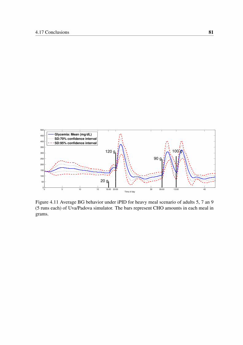
4.17 Conclusions 81
0 5 10 15 18:00 20:00 30 09:00 13:00 450
50
100
150
200
250
300
350
400
450
500
Time of day
Glycemia: Mean (mg/dL)
SD:70% confidence interval
SD:95% confidence interval
20 g
120 g
90 g
100 g
Figure 4.11 Average BG behavior under iPID for heavy meal scenario of adults 5, 7 an 9(5 runs each) of Uva/Padova simulator. The bars represent CHO amounts in each meal ingrams.

Chapter 5
Positive Sliding Mode Control for
Glycemia Regulation
5.1 Chapter Introduction in French
Dans les études de PA, deux catégories principales d’algorithmes de commande ont été
employées : les commandes basées sur des modèles et les commandes non basées sur des
modèles (sans modèle). Chaque catégorie a ses propres avantages et inconvénients. Au
chapitre 4, le réglateur iPID (sans modèle) fut conçu et testé. La conception était basée sur
l’historique de l’entrée de commande et les mesures de sortie. Le régulateur révèle un bon
niveau de robustesse lorsqu’il est appliqué sur différents patients virtuels. Dans ce chapitre,
on utilise la commande par modes glissants (CMG), connue pour sa robustesse vis à vis des
perturbations et la dynamique non modélisée. Dans le chapitre 4, une saturation a été ajoutée
pour contraindre le contrôleur à être non négatif. La commande CMG est conçue ici pour
être positive sans la nécessité d’une saturation. Selon la littérature du PA au chapitre 2, la
positivité de la commande n’a pas été prise en compte. Alors, l’existence d’une commande
CMG positive est obtenue ici pour la régulation de la glycémie pour la première fois. Les
propriétés des ensembles positivement invariants sont utilisées à cette fin. On trouve le plus
grand ensemble positivement invariant en boucle fermée pour le sous système d’insuline sous
CMG. L’insuline contrôlée est l’entrée (variable de commande) du compartiment glycémique
pour réguler sa concentration. La trajectoire de référence d’insuline est conçue pour être
l’insuline plasmatique nécessaire pour réguler la glycémie. L’erreur de glycémie (par rapport
à la normoglycémie) est utilisée pour concevoir la trajectoire de référence de l’insuline pour
éliminer cette erreur. La trajectoire de référence de l’insuline est conçue via une seconde
commande par modes glissants et est renvoyée, en tant qu’entrée de référence, à la commande
84 Positive Sliding Mode Control for Glycemia Regulation
par modes glissants de la première étape. Ainsi, une fois que l’état d’insuline est piloté vers
sa référence souhaitée, la glycémie est elle-même pilotée vers son niveau normal.
5.2 Introduction
In AP studies, two main categories of control algorithms were employed: model-based
and non-model based (model-free) controllers. Each category had its own advantages and
drawbacks. In Chapter 4, model-free PID controller was designed and tested. The design
was based on the history of the control input and the output measurements. The controller
showed a good level of robustness when applied on different virtual patients. In this chapter
sliding model control, that is known for its robustness against perturbations and non-modeled
dynamics, is employed. In Chapter 4, a saturation was added to constrain the controller to be
nonnegative. The model-based SMC is designed herein to be positive without the need of a
saturation. According to the AP literature in Chapter 2, positive SMC has not been considered.
Thus, the existence of a positive SMC for glycemia regulation is shown here for the first
time. The properties of positively invariant sets are utilized for this purpose. The largest
closed-loop positively invariant set of insulin system under sliding mode control is found.
SMC is designed to be positive everywhere in the largest closed-loop positively invariant
set. The controlled insulin is the input (control variable) to the glycemia compartment to
regulate its concentration. The desired insulin trajectory is designed to be the required plasma
insulin to regulate glycemia. The error of glycemia (from its desired level) is used to design
the insulin reference trajectory to eliminate this error (see Fig. 5.9). The insulin reference
trajectory is designed via a second sliding mode control and it is fed back, as a reference
input, to the first stage sliding mode control. Thus, once the insulin state is steered toward
its desired reference, glycemia is directed toward its normal level. Lyapunov stability and
reachability conditions are verified for both controllers.
The work in this chapter is submitted to be published and under revision [92].
5.3 Positivity and Positive Invariance for Linear Systems
In the next subsection, the main motivations behind studying positivity and positive invariance
properties of system (3.17), in this chapter and the following chapter, are presented.

5.3 Positivity and Positive Invariance for Linear Systems 85
5.3.1 Motivation
The glucose-insulin interaction as a physiological process relates positive variables like
concentrations or molar amounts. Thus, the input/output positive constraints of the long-term
T1DM model in § 3.7 is taken into account in the controller design in the current and the
following chapter. In addition, the realization of the mentioned T1DM model is not positive.
In other words, not all the positive initial conditions lead to a positive state trajectories for
any t ≥ 0 for insulin and glycemia state variables. Therefore, the largest open-loop Positive
Invariant Set (PIS) for the insulin dynamics is identified. It is the set where the plasma insulin
variable remains positive. Thereafter, the largest closed-loop PIS under SMC is found. The
result is a positive control everywhere in the largest closed-loop PIS of insulin system. The
theory of linear positive systems and positively invariant sets is employed for this purpose.
The PIS theory is involved in different control problems like: constrained control, robustness
analysis and optimization [93]. Moreover, to the best of our knowledge, the existence and
characterization of PIS to design a positive control of glycemia-insulinemia models have
not been considered previously. A part from MPC which takes constraints inherently in the
optimization process, saturation (to zero) is the basic solution to stop the negative control.
For these reasons, closed-loop PIS is found and employed to design a positive SMC (in this
chapter) and positive state feedback controller later in Chapter 6.
The following subsection gives a brief introduction of positive systems and positively
invariant sets. It will be used and applied on the T1DM model (3.17) to study the positivity
of its state variables: insulin, in this chapter and glycemia in the next chapter.
5.3.2 Preliminaries
Some useful definitions and theorems of positive systems and positively invariant sets are
now recalled from [94, 95]. They will be used throughout this chapter and the following
chapters.
In the following, any matrix E 2 Rnm is said to be nonnegative, denoted by E ≥ 0 or
E 2 Rnm+ , if its entries ei j > 0 8(i, j).
5.3.3 Externally Positive Systems
Definition 1. [94] The following linear system:
8<:
x(t) = Ax(t)+Bu(t)
y(t) =Cx(t)(5.1)
86 Positive Sliding Mode Control for Glycemia Regulation
where x 2 Rn,A 2 Rnn,B 2 Rnm,C 2 Rpn, is said to be an externally positive system if
for any nonnegative input u(t) ≥ 0 and zero initial conditions, the output is nonnegative
y(t)≥ 0 for any t ≥ 0.
External positivity is characterized as follows.
Theorem 1. [94] System (5.1) is externally positive if and only if its impulse response h(t)
is nonnegative:
h(t) =CeAtB 2 Rpm+ , t ≥ 0 (5.2)
Obviously, the property of external positivity is inherent to the system and does not
depend on the special state coordinates used to describe the dynamics (5.1).
The stronger notion of internal positivity is recalled next, and shown to be useful to
analyze the insulinemia subsystem in Section 6.3.2.
5.3.4 Internally Positive Systems
Definition 2. [94] System (5.1) is positive or internally positive if for any x(0) 2 Rn+ and
u(t) 2 Rm+ the state trajectory x(t) 2 Rn
+ and the output y(t) 2 Rp+.
Internal positivity is easily characterized thanks to the so-called Metzler matrices whose
off-diagonal elements have to be nonnegative.
Definition 3. A matrix H = [hi j] 2 Rnm is Metzler if hi j > 0 for i 6= j.
Theorem 2. [94] The system (5.1) is internally positive if and only if
i) A is a Metzler matrix,
ii) B 2 Rnm+ ,C 2 R
pn+
Surprisingly, in opposition to external positivity, the property of internal positivity is state
coordinates dependent. It is not invariant under a change of state coordinates as it is easily
shown by the following example.
Example 1. The system
8>>>>>><>>>>>>:
z(t) =
0BBB@
0 0 −1
0 0 1
0 −1 −2
1CCCAz+
0BBB@
0
0
1
1CCCAu
y(t) = z2
(5.3)

5.3 Positivity and Positive Invariance for Linear Systems 87
is not internally positive in the z coordinates since the A matrix is not Metzler.
However, the following change of state variables:
8>>><>>>:
z1 =−z1
z2 = z2
z3 = z2 + z3
(5.4)
yields
8>>>>>><>>>>>>:
˙z =
0BBB@
0 0 1
0 −1 1
0 0 −1
1CCCA z+
0BBB@
0
0
1
1CCCAu
y(t) = z2
(5.5)
which fulfills the conditions of Theorem 2 and is thus internally positive.
Remark 8. Internal positivity implies external positivity and this can be shown using the
output time response of system (5.1) in the light of the impulse response:
y(t) =CeAtx(0)+Z t
0h(t − τ)u(τ)dτ (5.6)
To yield y(t)≥ 0, Theorem 1 requires only h(t)≥ 0 for x(0) = 0, while Theorem 2 requires
also x(0) ≥ 0,C ≥ 0 and B > 0 for internal positivity. The converse is not true, i.e. an
externally positive system is not necessarily internally positive e.g. system (5.3). Despite
the fact that this system is not positive according to Theorem 2, it is externally positive with
h(t) = te−t > 0.
The following definitions and theorems are useful to study positivity and set invariance
especially for the systems that are neither internally nor externally positive.
Definition 4. A nonempty set M Rn is a Positively Invariant Set (PIS) of (5.1) if 8xo 2
M =) x(t,xo) 2 M 8t ≥ 0.
Definition 5. For any G 2 Rrn , ρ 2 Rr, Ω(G) denotes the polyhedron
Ω(G) = x 2 Rn|Gx ≥ ρ . (5.7)
In what follows, the vector ρ = [0]r1if not specified otherwise.
88 Positive Sliding Mode Control for Glycemia Regulation
Proposition 1. [95] The polyhedral set Ω(G) is a positively invariant set for system (5.1) if
and only if there exists a Metzler matrix H such that:
GA−HG = 0. (5.8)
Hρ > 0 (5.9)
Corollary 1. The positive orthant Ω(I) = Rn+ is PIS, if and only if A is Metzler.
Proof. It follows from Proposition 1 where H = A.
Corollary 2. The positive orthant Rn+ of an internally positive system is a PIS.
Proof. It follows from Theorem 2 and Corollary 1.
As will be discussed in more details in Chapter 6, the T1DM model (3.17) is not positive
neither internally nor externally according to Theorems 2 and 1. This is true for both the
original realization in (3.17) and transformed one (3.23). This fact triggered the search to
find the largest set where the state variables remain positive at all times i.e. the largest PIS.
Invariance analyses were initially discussed for the original state representation (3.17) and
specifically on the second order insulin subsystem as a start. Those analyses, as will be
presented in this chapter, were undertaken in open and closed-loop control.
The next section investigates invariance properties of the open-loop insulin subsystem.
5.4 PIS of Insulin Subsystem: Open-loop
Consider the insulin subsystem (3.15) which is equivalent to:
(x(t) = Ax(t)+Bu(t)
y(t) =Cx(t)(5.10)
x(t) = [x1(t) x2(t)]T
where y(t) is the output and x1 = I,x2 = I are the system states with: A =
0B@
0 1
−λ 2m −2λm
1CA,
B =
0
b
!, C =
h1 0
i
λm = 1Tu, b =
Kuλ 2m
Vi, b > 0. The plasma insulin is nonnegative in the following set Ω(C),
however, this set is not a PIS according to Proposition 1. In the following theorem the largest
PIS in Ω(C) for the open-loop insulin subsystem is presented.
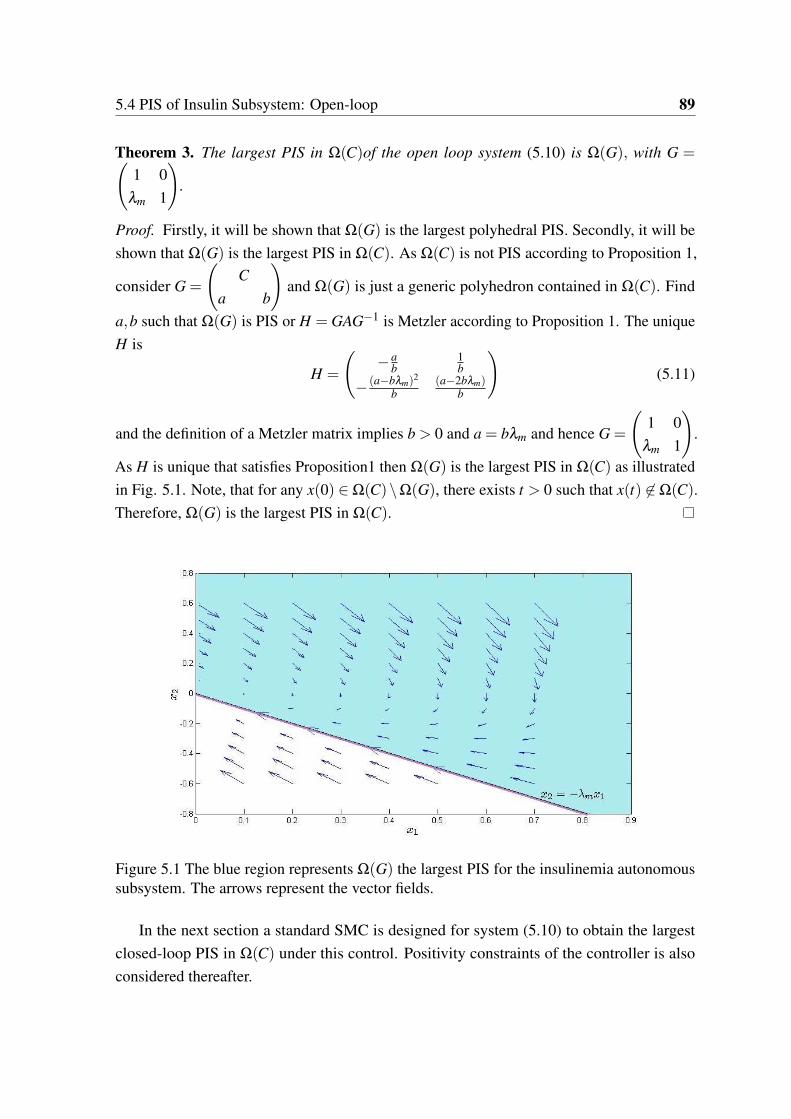
5.4 PIS of Insulin Subsystem: Open-loop 89
Theorem 3. The largest PIS in Ω(C)of the open loop system (5.10) is Ω(G), with G = 1 0
λm 1
!.
Proof. Firstly, it will be shown that Ω(G) is the largest polyhedral PIS. Secondly, it will be
shown that Ω(G) is the largest PIS in Ω(C). As Ω(C) is not PIS according to Proposition 1,
consider G =
C
a b
!and Ω(G) is just a generic polyhedron contained in Ω(C). Find
a,b such that Ω(G) is PIS or H = GAG−1 is Metzler according to Proposition 1. The unique
H is
H =
−a
b1b
− (a−bλm)2
b
(a−2bλm)b
!(5.11)
and the definition of a Metzler matrix implies b > 0 and a = bλm and hence G =
1 0
λm 1
!.
As H is unique that satisfies Proposition1 then Ω(G) is the largest PIS in Ω(C) as illustrated
in Fig. 5.1. Note, that for any x(0) 2 Ω(C)\Ω(G), there exists t > 0 such that x(t) 62 Ω(C).
Therefore, Ω(G) is the largest PIS in Ω(C).
Figure 5.1 The blue region represents Ω(G) the largest PIS for the insulinemia autonomoussubsystem. The arrows represent the vector fields.
In the next section a standard SMC is designed for system (5.10) to obtain the largest
closed-loop PIS in Ω(C) under this control. Positivity constraints of the controller is also
considered thereafter.
90 Positive Sliding Mode Control for Glycemia Regulation
5.5 Introduction to Sliding Mode Control
Sliding mode control is a particular type of Variable Structure Control (VSC) systems which
evolved in Russia. It appeared outside of Russia in the mid of 1970’s when a survey paper
by Utkin (1977) was published in English. SMC has now a solid position in the field of
linear and non-linear control theory [96]. VSC system utilizes a set of continuous subsystems
(structures) and a switching function. The switching among different functions is determined
by the plant states. The discontinuous manner goes on so that the desired performance is
achieved. SMC uses the high-frequency discontinuous control action to derive the state
trajectories into a specified and user-defined surface in state space (called sliding or switching
surface) and to maintain them on this surface or within its neighborhood while moving
toward the equilibrium. During sliding mode the desired performance is maintained even in
the presence of disturbances/uncertainties.
5.6 SMC Design of insulinemia subsystem
Since the overall glucose-insulin system is a cascade of the second order insulinemia subsys-
tem and the first order glycemia subsystem, the glycemia regulation problem may be split
into the stabilization of the two subsystems. The objective of the first control problem is to
stabilize the error e(t) between the insulinemia and its desired value xd:
e(t) = x1 − xd
xd ≥ 0 is assumed to be a constant reference value for the insulinemia at this stage.
The sliding surface is defined by :
s(x) = e+λe (5.12)
where λ is a positive real parameter so that e(t)! 0 when s = 0.
5.6.1 Reachability Condition
The aim is to achieve asymptotic convergence of the error e to zero using the control u that
drives the sliding variable s to zero in finite time. This task is achieved by using the following
Lyapunov function:
V =12
s2 (5.13)
5.6 SMC Design of insulinemia subsystem 91
The adequate control is computed as a solution to V 0, or equivalently ss < 0 with
s 6= 0 which is termed as the the reachability condition.
ss = s(−λ 2mx1 +(λ −2λm)x2 +bu) (5.14)
The standard sliding mode control law consists of the sum of a continuous equivalent control
ueq(t) and a discontinuous control udis(t):
u = ueq +udis (5.15)
where the continuous part ueq is the solution of s = 0 :
ueq(t) =1b[λ 2
mx1 +(2λm −λ )x2] (5.16)
while
udis(t) =−k sign(s) (5.17)
and V is then:
ss =−kb|s|< 0 (5.18)
thus, ss < 0 is guaranteed whenever k > 0.
5.6.2 Reaching Time
Definition 6. Denote tr the time instant when the sliding manifold is reached s(tr) = 0.
tr can be calculated using
s(t) =−bk sign(s(t)) (5.19)
with u = ueq − k sign(s), integrating both sides of (5.19) in the interval [0, t] yields
Z t
0
ds(t)
sign(s(t))=−bk
Z t
0dt (5.20)
yields
|s(t)|− |s(0)|=−bkt (5.21)
and at t = tr sliding occurs and s(tr) = 0 thus:
tr =|s(0)|
bk(5.22)

92 Positive Sliding Mode Control for Glycemia Regulation
where s(0) = s(x(0)).
In the next sections, output/control positivity and invariance conditions will be investi-
gated. In order to find the largest closed-loop PIS in Ω(C), and later under nonnegative SMC,
the set Ω(C) will be divided into three regions:
i) on the surface s = 0: S = x 2 Ω(C)|s(x) = 0 (5.23)
ii) in the region s 0: S− = x 2 Ω(C)|x2 −λ (x1 − xd) (5.24)
iii) in the region s ≥ 0: S+ = x 2 Ω(C)|x2 ≥−λ (x1 − xd). (5.25)
5.7 Invariance of the Surface S
In ideal sliding mode, the sliding surface represents an invariant manifold of the system [97].
Once this manifold is reached, the state trajectories remain on it for all future times. The
invariance condition of s = 0 is thus
8<:
s = 0
s = 0(5.26)
Since the sliding manifold is shown to be PIS, the invariance of the following subsets
will be investigated during the reaching phase when t < tr.
Using Lyapunov attractivity condition (5.18) the following sets are PIS:
S+R = x 2 R2|s ≥ 0 (5.27)
S−R = x 2 R2|s 0 (5.28)
Thus S+ S+R , S− S−R . In words, if x(0) 2 S+R (2 S−R respectively) then x(t) 2 S+R (S−Rrespectively) 8t 2 R+ thanks to Lyapunov condition (5.18). This can be shown using s(t) in
(5.19) and its solution in (5.21) as follows:
(∣∣s(t)
∣∣−∣∣s(0)
∣∣) 0, 8t > 0 (5.29)
5.8 Positive invariance in S− 93
or equivalently
8<:
0 ≥ s(t)> s(0) if s < 0
0 s(t)< s(0) if s > 0(5.30)
and this implies that if s(0) 2 S+R (S−R respectively) then s(t) 2 S+R (S−R respectively) for any
t > 0. As a result, any state trajectory initiated in S+R (S−R respectively) will remain there for all
future times. However, our interest in the following sections is to find the largest closed-loop
PIS in S+ and S− and then the largest overall PIS in Ω(C).
Remark 9. As stated earlier S+R ,S−R are PIS, however since S+Ω(C)\S+R ,S−Ω(C)\S−R
and Ω(C) is not PIS then S−,S+ are not necessarily PIS. Therefore the largest PIS in
S+(S−respectively) is found such that x1(t)≥ 0 for any t > 0 and positive invariance of each
set is ensured via the Lyapunov reachability condition. As S S+(S−respectivlely) is a PIS
as shown earlier, therefore, the invariance of S+(S− respectively) is analyzed during the
reaching phase s(x) 6= 0 in S+ and S− respectively.
5.8 Positive invariance in S−
In the reaching phase of S− i.e. s(x)< 0, the closed-loop system is
8<:
x1 = x2
x2 =−λx2 +bk(5.31)
with state variables time solution8<:
x1(t) = x10 +x20−x2(t)+bkt
λ
x2(t) =bkλ+(x20 −
bkλ)e−λ t
(5.32)
Theorem 4. Assuming ideal sliding mode, the largest PIS in S− is
Ms− := M[x0 2 S−|x20 > 0 (5.33)
as illustrated in Fig. 5.2, where
M :=n
x0 2 S−|x10 ≥ x10, x20 0o
(5.34)
94 Positive Sliding Mode Control for Glycemia Regulation
x10 =− bk
λ 2 lnbk−λx20
bk
+
x20
λ
(5.35)
Proof. • Case 1: x20 > 0. According to the second equation of (5.32) and (5.24):
x1(t) = x10 +x20
λ(1− e−λ t)+
bk
λ 2
λ t − (1− e−λ t)
(5.36)
x10 ≥ 0,x20 > 0, the first and second terms are nonnegative, hence, it suffices to verify
that:bk
λ 2
λ t − (1− e−λ t)
> 0 (5.37)
or
λ t ≥ (1− e−λ t) (5.38)
which is true for any λ > 0 and t ≥ 0. Thus, the set x(0) 2 S−|x20 > 0 is a PIS.
• Case 2: x20 0
In this case, x1(t)2 S− is not guaranteed for any t as it decreases until x1(t) = x2(t
) =
0. Thus, define the critical time t < tr which is the solution of x1(t) = 0:
t =1λ
lnbk−λx20
bk
(5.39)
Note that (5.39) is well defined in Case 2. The test of the critical point x(t) reveals a
minimum since x1(t)> 0. For a given x(0) substituting t = t in (5.32) yields a point
of the trajectory in the phase plane (x1(t),0) where x1(t
) = min(x1(t)). To find the
largest PIS in S− such that x1(t) > 0, it is required that min(x1) = 0 i.e. the global
minimum at x1(t) = 0 such that x1(t) 2 S− for any t. The largest PIS in S− must have
the global minimum of its state trajectories at the origin. Thus, the substitution of
(5.39) into (5.32), to have x1(t) = 0 yields
x10 =− bk
λ 2 lnbk−λx20
bk
+
x20
λ
(5.40)
and hence (5.35) and the set M characterizes the set of points whose trajectories have
a nonnegative minimum. To verify that x10 > 0 in (5.40), taking into account that the
current case x20 =−|x20|, the right-hand side of (5.35) is nonnegative or:
λ
bk|x20|> ln
1+
λ |x20|
bk
(5.41)
which is true as it as (5.41) is equivalent to t ≥ ln(1+ t).
If x(0) 2 M and s(x) = 0 M ( tr ≥ t ) then x 2 M8t > 0. However, M is not
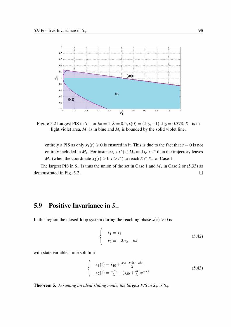
5.9 Positive Invariance in S+ 95
Figure 5.2 Largest PIS in S− for bk = 1,λ = 0.5,x(0) = (x10,−1), x10 = 0.378. S− is inlight violet area, M is in blue and Ms is bounded by the solid violet line.
entirely a PIS as only x1(t)> 0 is ensured in it. This is due to the fact that s = 0 is not
entirely included in M. For instance, x(t) 2 M and tr < t then the trajectory leaves
M (when the coordinate x2(t)> 0, t > t) to reach S S− of Case 1.
The largest PIS in S− is thus the union of the set in Case 1 and M in Case 2 or (5.33) as
demonstrated in Fig. 5.2.
5.9 Positive Invariance in S+
In this region the closed-loop system during the reaching phase s(x)> 0 is
8<:
x1 = x2
x2 =−λx2 −bk(5.42)
with state variables time solution8<:
x1(t) = x10 +x20−x2(t)−bkt
λ
x2(t) =−bk
λ+(x20 +
bkλ)e−λ t
(5.43)
Theorem 5. Assuming an ideal sliding mode, the largest PIS in S+ is S+
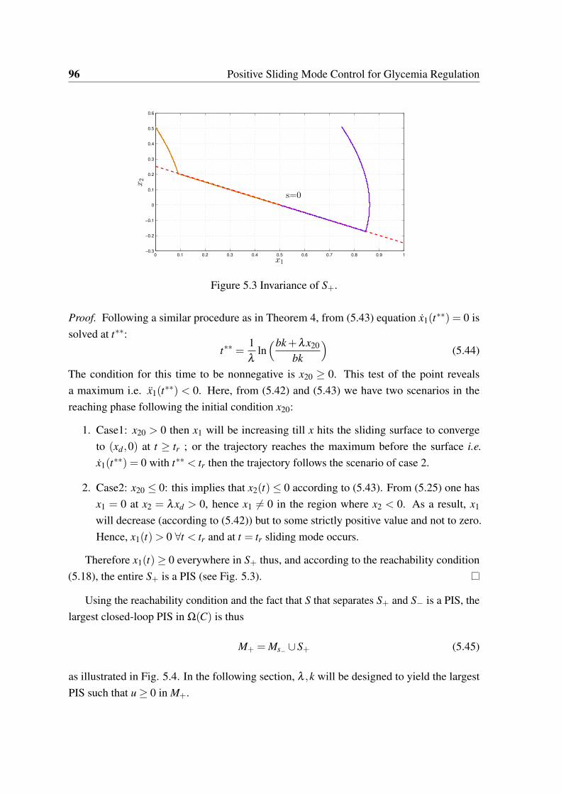
96 Positive Sliding Mode Control for Glycemia Regulation
0 0.1 0.2 0.3 0.4 0.5 0.6 0.7 0.8 0.9 1−0.3
−0.2
−0.1
0
0.1
0.2
0.3
0.4
0.5
0.6
x1
x2
s=0
Figure 5.3 Invariance of S+.
Proof. Following a similar procedure as in Theorem 4, from (5.43) equation x1(t) = 0 is
solved at t:
t =1λ
lnbk+λx20
bk
(5.44)
The condition for this time to be nonnegative is x20 ≥ 0. This test of the point reveals
a maximum i.e. x1(t) < 0. Here, from (5.42) and (5.43) we have two scenarios in the
reaching phase following the initial condition x20:
1. Case1: x20 > 0 then x1 will be increasing till x hits the sliding surface to converge
to (xd,0) at t ≥ tr ; or the trajectory reaches the maximum before the surface i.e.
x1(t) = 0 with t < tr then the trajectory follows the scenario of case 2.
2. Case2: x20 0: this implies that x2(t) 0 according to (5.43). From (5.25) one has
x1 = 0 at x2 = λxd > 0, hence x1 6= 0 in the region where x2 < 0. As a result, x1
will decrease (according to (5.42)) but to some strictly positive value and not to zero.
Hence, x1(t)> 0 8t < tr and at t = tr sliding mode occurs.
Therefore x1(t)≥ 0 everywhere in S+ thus, and according to the reachability condition
(5.18), the entire S+ is a PIS (see Fig. 5.3).
Using the reachability condition and the fact that S that separates S+ and S− is a PIS, the
largest closed-loop PIS in Ω(C) is thus
M+ = Ms− [S+ (5.45)
as illustrated in Fig. 5.4. In the following section, λ ,k will be designed to yield the largest
PIS such that u ≥ 0 in M+.
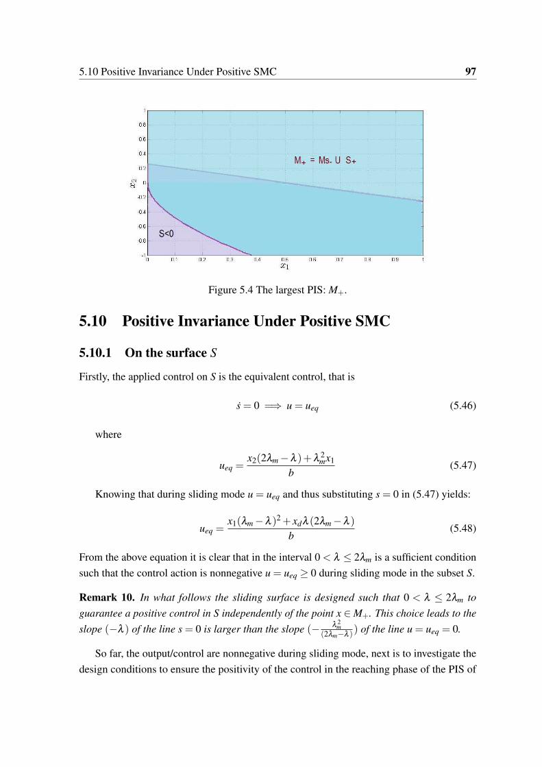
5.10 Positive Invariance Under Positive SMC 97
Figure 5.4 The largest PIS: M+.
5.10 Positive Invariance Under Positive SMC
5.10.1 On the surface S
Firstly, the applied control on S is the equivalent control, that is
s = 0 =) u = ueq (5.46)
where
ueq =x2(2λm −λ )+λ 2
mx1
b(5.47)
Knowing that during sliding mode u = ueq and thus substituting s = 0 in (5.47) yields:
ueq =x1(λm −λ )2 + xdλ (2λm −λ )
b(5.48)
From the above equation it is clear that in the interval 0 < λ 2λm is a sufficient condition
such that the control action is nonnegative u = ueq ≥ 0 during sliding mode in the subset S.
Remark 10. In what follows the sliding surface is designed such that 0 < λ 2λm to
guarantee a positive control in S independently of the point x 2 M+. This choice leads to the
slope (−λ ) of the line s = 0 is larger than the slope (−λ 2
m
(2λm−λ )) of the line u = ueq = 0.
So far, the output/control are nonnegative during sliding mode, next is to investigate the
design conditions to ensure the positivity of the control in the reaching phase of the PIS of

98 Positive Sliding Mode Control for Glycemia Regulation
S+ and S−. Define the following sets where u ≥ 0 in S− and S+ respectively:
• In S− \S u = ueq + k:
M+k =
x 2 S− \S|x2 ≥−bk−λ 2
mx1
2λm −λ
(5.49)
• In S+ \S u = ueq − k:
M−k =
x 2 S+ \S|x2 ≥bk−λ 2
mx1
2λm −λ
(5.50)
With the choice of λ according to Remark 10, SMC is nonnegative on the sliding surface,
in M+k and in M−k.
However, whether M+k S+, M−k Ms− or in other words u ≥ 0 everywhere in the PIS
of S+,S− respectively is not ensured. Therefore, in the following subsections, the design
conditions of the pair (λ ,k) are found to yield the largest PIS in S+,Ms− respectively such
that u ≥ 0.
5.10.2 In the subset S+
As stated earlier in Theorem 5, the subset S+ is a PIS. The control is non-negative in the set
M−k , but not everywhere in S+. The following theorem will give necessary conditions such
that u ≥ 0 everywhere in S+ \S or to have S+ \S M−k.
Theorem 6. Assuming (0 λ 2λm), the following statements are equivalent:
1. S+ \S M−k.
2. u ≥ 0 everywhere in S+.
3.
λm −
sλ 2
m −bk
xd
λ λm +
sλ 2
m −bk
xd
, 0 < k λ 2
mxd
b. (5.51)
Proof. According to Remark 10, during sliding mode u = ueq > 0 in S and hence it remains
to show that u = (ueq − k)≥ 0 in S+ \S. From Remark 10 the slope (-λ ) of the line s = 0
is larger than the slope −λ 2
m
(2λm−λ ) of the line u = 0 i.e. λ <λ 2
m
(2λm−λ ) . Thus, if the following
holds
(ueq − k)∣∣∣x1=0
s
∣∣∣x1=0
(5.52)
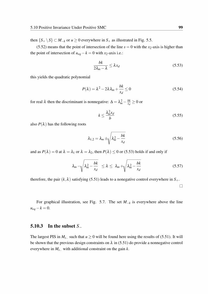
5.10 Positive Invariance Under Positive SMC 99
then S+ \S M−k or u ≥ 0 everywhere in S+ as illustrated in Fig. 5.5.
(5.52) means that the point of intersection of the line s = 0 with the x2-axis is higher than
the point of intersection of ueq − k = 0 with x2-axis i.e.:
bk
2λm −λ λxd (5.53)
this yields the quadratic polynomial
P(λ ) = λ 2 −2λλm +bk
xd
0 (5.54)
for real λ then the discriminant is nonnegative: ∆ = λ 2m − bk
xd≥ 0 or
k λ 2
mxd
b(5.55)
also P(λ ) has the following roots
λ1,2 = λm ±
sλ 2
m −bk
xd
(5.56)
and as P(λ ) = 0 at λ = λ1 or λ = λ2, then P(λ ) 0 or (5.53) holds if and only if
λm −
sλ 2
m −bk
xd
λ λm +
sλ 2
m −bk
xd
(5.57)
therefore, the pair (k,λ ) satisfying (5.51) leads to a nonegative control everywhere in S+.
For graphical illustration, see Fig. 5.7. The set M−k is everywhere above the line
ueq − k = 0.
5.10.3 In the subset S−
The largest PIS in Ms− such that u ≥ 0 will be found here using the results of (5.51). It will
be shown that the previous design constraints on λ in (5.51) do provide a nonnegative control
everywhere in Ms− with additional constraint on the gain k.

100 Positive Sliding Mode Control for Glycemia Regulation
0 0.02 0.04 0.06 0.08 0.1 0.12 0.14 0.16 0.18 0.21
1.1
1.2
x1
x2
S+bk(2λm−λ)
λxd
s = 0
S−
ueq − k = 0
Figure 5.5 The lines ueq − k = 0 (u=0 in S+) with respect to the line s = 0 for a nonnegativecontrol in S+, with λm = 1,λ = 1.2785 and k = 0.91.
Theorem 7. Assuming (5.51) then u ≥ 0 everywhere in Ms− if and only if
1.2785λm < λ λm +
sλ 2
m −bk
xd
, 0 < k 0.9224xdλ 2
m
b(5.58)
Proof. As stated earlier u = ueq > 0 in S. Thus, in what follows the positivity of the control
during the reaching phase is considered i.e.when u = ueq + k.
• Case 1: x 2 Ms− ,x2 > 0
In this case ueq ≥ 0 hence, u = (ueq + k)≥ 0.
• Case 2: x 2 Ms− ,x2 0
Here, to yield u ≥ 0 everywhere in Ms− i.e. M+k Ms− , design k and λ , satisfying
(5.51), such that the line u = ueq+k = 0 and the trajectory limiting the set M in (5.34)
do not intersect. For this purpose, from (5.34) define f1(x2) =−
bkλ 2 ln(bk−λx2
bk)+ x2
λ
and using (5.49) define f2(x2) =λ−2λm
λ 2m
x2 −bkλ 2
mand then F(x2), f1(x2)− f2(x2) = 0.
F(x2) =−bk
λ 2 ln(bk−λx2
bk)− x2
1λ+
λ −2λm
λ 2m
+
bk
λ 2m
(5.59)
If an intersection exists then F(x2) = 0 has a solution, thus find x2 0 solving
F(x2) = 0. To simplify the search of the solution (if any), note that F(0) = bkλ 2
m> 0,

5.10 Positive Invariance Under Positive SMC 101
limx2!−∞
F(x2) = +∞ and also note that
dF(x2)
dx2=
bk
λ (bk−λx2)−
1λ+
2λm −λ
λ 2m
(5.60)
dF(x2)dx2
|x2=0 =2λm−λ
λ 2m
> 0, limx2!−∞
dF(x2)dx2
= − (λ−λm)2
λλ 2m
< 0. This reads that F(x2) has a
minimum point and as the initial and final values of F(x2) are both positive, then if
minx20
(F(x2)) > 0 the intersection between f1, f2 does not exist. This means that as
u ≥ 0 everywhere in Ms− , thus the aim now is not to find a solution x2 0 such that
F(x2) = 0, but rather to ensure minx20
(F(x2)) > 0. At the minimum point dF(x2)dx2
= 0,
one has:
x2 = bkλ −2λm
(λ −λm)2 (5.61)
which is a unique solution i.e. the minimum point is global. In order to verify whether
min(F(x2))> 0 substitute (5.61) in (5.59) which yields:
min(F(x2)) =−bk
λ 2 ln
1−λ 2 −2λλm
(λ −λm)2
−bk
(λ −2λm)
λλ 2m
+bk
λ 2m
(5.62)
min(F(x2))> 0 () −(λ −2λm)
λλ 2m
+1
λ 2m
>1
λ 2 ln λ 2
m
(λ −λm)2
(5.63)
using the property ln(ab)n = n ln(a
b):
λ
λm> ln
∣∣∣ λm
λ −λm
∣∣∣ (5.64)
which can be rewritten asλ
λm> ln
∣∣∣ 1λλm
−1
∣∣∣ (5.65)
or ∣∣∣ λ
λm−1
∣∣∣eλ
λm > 1 (5.66)
As illustrated in Fig. 5.6, equation (5.66) is satisfied only when λλm
> 1.2785 and
comparing this new constraint with (5.51):
λ
λm> 1.2785 and 1−
qλ 2
m − bkxd
λm
λ
λm 1+
qλ 2
m − bkxd
λm(5.67)

102 Positive Sliding Mode Control for Glycemia Regulation
and as 1−
qλ 2
m−bkxd
λm< 1.2785 then
1.2785 <λ
λm 1+
qλ 2
m − bkxd
λm(5.68)
which implies 1.2785 1+
qλ 2
m−bkxd
λmand hence k 0.9224 xdλ 2
m
byielding (5.58).
Using the results of Theorems 6 and 7, SMC designed in (5.58) is nonnegative everywhere
in M+.
See Fig. 5.8 for a graphical illustrative example. The region above the lines ueq + k = 0
and ueq − k = 0 represents M+k and M−k respectively. The trajectory in orange passing
through the subset S− is the one that characterizes the PIS Ms−. As shown, λ satisfies (5.58)
ensures a positive control everywhere in M+. Whereas, as shown in Fig. 5.7, the value of λ
satisfies only (5.51) thus ensures a nonnegtaive control everywhere in S+ but not in Ms− as
the red region represents x 2 Ms−and u < 0. The parameters λm,b,xd in the figures are taken
to simplify the example and its illustrations.
Remark 11. The admissible λ that satisfies the positivity constraints in (5.58) is within the
interval 1.2785λm < λ λm +q
λ 2m − bk
xd< 2λm. As a result, the closed-loop eigenvalue is
larger than that of the open-loop yielding a relatively faster time response.
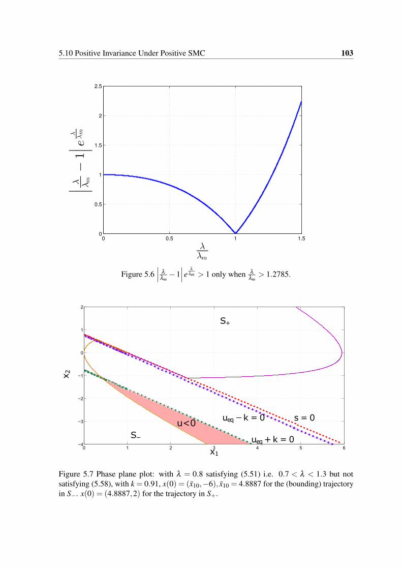
5.10 Positive Invariance Under Positive SMC 103
0 0.5 1 1.50
0.5
1
1.5
2
2.5
λ
λm
∣ ∣ ∣
λ λm
−1
∣ ∣ ∣e
λ
λm
Figure 5.6∣∣∣ λ
λm−1
∣∣∣eλ
λm > 1 only when λλm
> 1.2785.
0 1 2 3 4 5 6−4
−3
−2
−1
0
1
2
x1
x2
S+
Sueq+k = 0
ueq k = 0 s = 0u<0
Figure 5.7 Phase plane plot: with λ = 0.8 satisfying (5.51) i.e. 0.7 < λ < 1.3 but notsatisfying (5.58), with k = 0.91, x(0) = (x10,−6), x10 = 4.8887 for the (bounding) trajectoryin S−. x(0) = (4.8887,2) for the trajectory in S+.
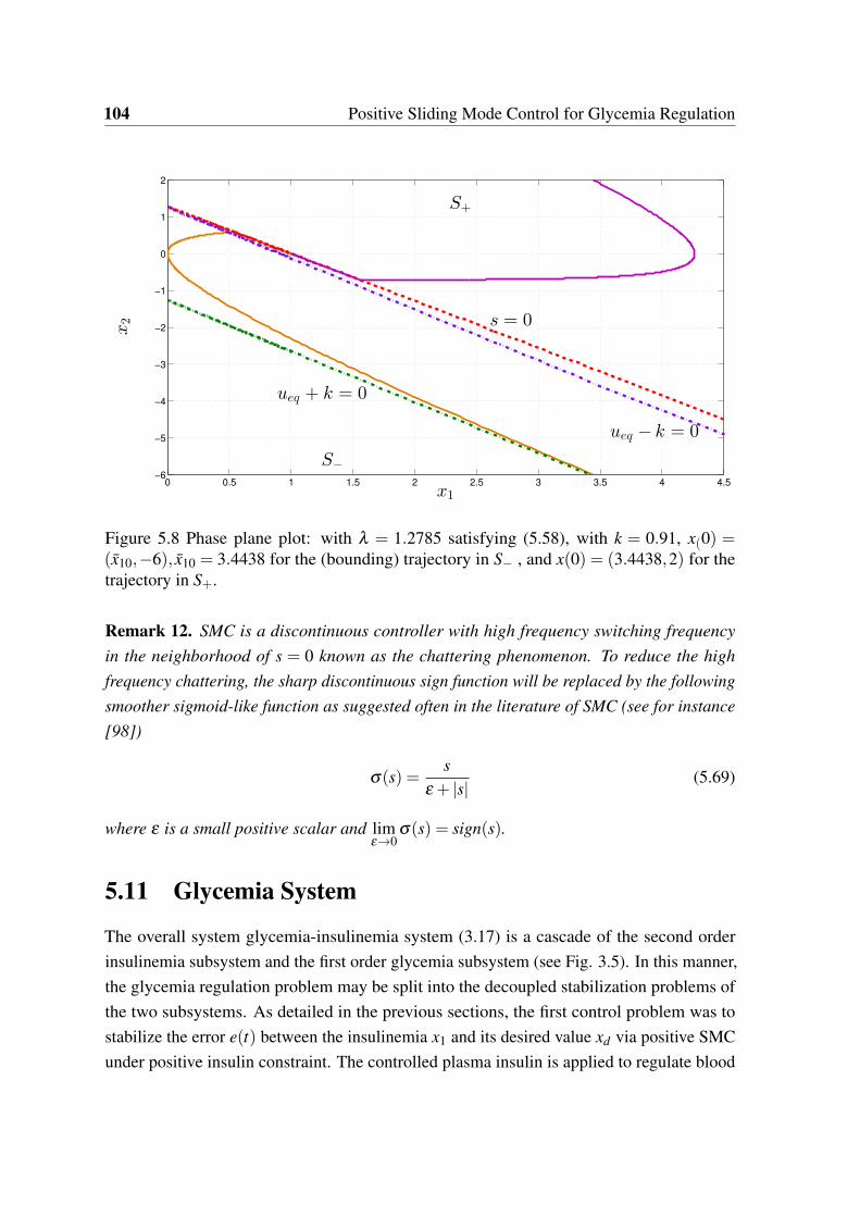
104 Positive Sliding Mode Control for Glycemia Regulation
0 0.5 1 1.5 2 2.5 3 3.5 4 4.5−6
−5
−4
−3
−2
−1
0
1
2
x1
x2
S+
S−
ueq − k = 0
s = 0
ueq + k = 0
Figure 5.8 Phase plane plot: with λ = 1.2785 satisfying (5.58), with k = 0.91, x(0) =(x10,−6), x10 = 3.4438 for the (bounding) trajectory in S− , and x(0) = (3.4438,2) for thetrajectory in S+.
Remark 12. SMC is a discontinuous controller with high frequency switching frequency
in the neighborhood of s = 0 known as the chattering phenomenon. To reduce the high
frequency chattering, the sharp discontinuous sign function will be replaced by the following
smoother sigmoid-like function as suggested often in the literature of SMC (see for instance
[98])
σ(s) =s
ε + |s|(5.69)
where ε is a small positive scalar and limε!0
σ(s) = sign(s).
5.11 Glycemia System
The overall system glycemia-insulinemia system (3.17) is a cascade of the second order
insulinemia subsystem and the first order glycemia subsystem (see Fig. 3.5). In this manner,
the glycemia regulation problem may be split into the decoupled stabilization problems of
the two subsystems. As detailed in the previous sections, the first control problem was to
stabilize the error e(t) between the insulinemia x1 and its desired value xd via positive SMC
under positive insulin constraint. The controlled plasma insulin is applied to regulate blood
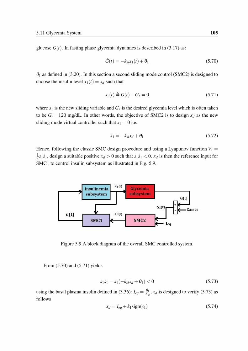
5.11 Glycemia System 105
glucose G(t). In fasting phase glycemia dynamics is described in (3.17) as:
G(t) =−ksix1(t)+θ1 (5.70)
θ1 as defined in (3.20). In this section a second sliding mode control (SMC2) is designed to
choose the insulin level x1(t) = xd such that
s1(t), G(t)−Gr = 0 (5.71)
where s1 is the new sliding variable and Gr is the desired glycemia level which is often taken
to be Gr =120 mg/dL. In other words, the objective of SMC2 is to design xd as the new
sliding mode virtual controller such that s1 = 0 i.e.
s1 =−ksixd +θ1 (5.72)
Hence, following the classic SMC design procedure and using a Lyapunov function V1 =12s1s1, design a suitable positive xd > 0 such that s1s1 < 0. xd is then the reference input for
SMC1 to control insulin subsystem as illustrated in Fig. 5.9.
Figure 5.9 A block diagram of the overall SMC controlled system.
From (5.70) and (5.71) yields
s1s1 = s1(−ksixd +θ1)< 0 (5.73)
using the basal plasma insulin defined in (3.36): Ieq =θ1Ksi
, xd is designed to verify (5.73) as
follows
xd = Ieq + k1sign(s1) (5.74)
106 Positive Sliding Mode Control for Glycemia Regulation
where k1 > 0. Therefore, the objective of the SMC1 control u(t), as explained earlier, is to
reach s = 0 and then asymptotically direct x1(t) to xd given in (5.74). As xd is designed via
SMC2 above to ensure that (5.73) holds and then to achieve s1 = 0
5.11.1 Positivity of xd and Choice of k1
• s1 = 0 i.e. at the equilibrium then xd = Ieq > 0
• s1 > 0 or hyperglycemia region then xd = (Ieq + k1)> 0 for any k1 > 0.
• s1 < 0 or hypoglycemia region, to have xd > 0 then k1 < Ieq.
As a result, k1 < Ieq is the lower bound to ensure that the desired plasma insulin value is
positive. Moreover, the constraint on the gain k given in (5.58) will take this lower bound
into account setting xd = Ieq − k1 i.e.
0 < k 0.9224(Ieq − k1)λ
2m
b(5.75)
Remark 13. Taking k1 < Ieq is sufficient to have xd > 0 for any s1. However, this gain value
in times of hyperglycemia (s1 >> 0) yields xd = (Ieq + k1) < 2Ieq which yield a relatively
slow convergence of BG to its normal level (see the insulin injections of T1D patients in
[58]). Therefore, the switching gain k1 needs to be adapted according to the switching region
to yield a sufficiently high insulin reference value when G > Gr and thus a faster response.
5.12 Variable Discontinuity Gain k1
To obtain a sufficiently fast glycemic response, the gain k1 is chosen to be proportional to the
offset G−Gr when s1 > 0 i.e. the switching function is adapted as follows
8<:
If s1 > 0 then xd = Ieq + kos1
If s1 0 then xd = Ieq + k1sign(s1), k1 < Ieq
(5.76)
where ko[U/mg]> 0 is a proportional gain. The gain k1 is constant and xd > 0 when s1 0
as explained in section 5.11.1. In this manner s1 > 0 leads to a variable reference value:
xd(s1) = Ieq+ko(G−Gr) and the insulin sliding surface in this case s= x2+λ (x1−xd(s1)) is
not a line but rather a trajectory as will be shown in the simulation results section. Therefore,
if glycemia level is below the desired level s1 < 0 then the desired insulin is less than the basal
xd = (Ieq − k1)< Ieq which permits the glycemia to grow due to the endogenous production

5.12 Variable Discontinuity Gain k1 107
(for details see [58]). Moreover, in case G = Gr then the insulin is steered to the basal
xd = Ieq to maintain glycemia at that value.
In the following section, the gain ko is designed such that the reachability condition of
the surface s is verified when the new variable reference xd(s1) is applied i.e. when s1 > 0.
5.12.1 Reachability of s for xd = Ieq + kos1
In the region s1 0 the desired insulin value xd is a constant and the previous design analyses
of s and k,λ of the first SMC hold. In the case where s1 > 0 then the sliding surface s
becomes
s = x2 +λ (x1 − (Ieq + kos1)) (5.77)
and the reachability condition ss < 0 with u as described in (5.15) and (5.16) is thus
s(−ksign(s)−λkos1) =−(k|s|+λko s s1)< 0 (5.78)
with ko > 0 the surface s is reachable if (k|s|+λko s s1) > 0, and the case where ss1 ≥ 0
directly verifies the reachability condition as k,ko and λ are positive scalars. Otherwise, the
case when ss1 < 0 is studied for given λ and k as follows:
• Case1: s1 > 0, s < 0: hence from (5.78) ss < 0 implies
k|s|−λk0|s|s1 > 0 (5.79)
and hence
ko <k
λ max |s1|(5.80)
and from (5.70) and Ieq = θ1Ksi
then s1 > 0 or G > 0 means that x1 < Ieq and thus
max(s1) = limx1!0
G = θ1.
• Case2: s1 < 0, s > 0: setting |s1| = −s1 in (5.78) leads also to (5.80). However,
s1 < 0 and (5.70) imply x1 > Ieq and thus max |s1| depends on the maximum registered
plasma insulin level. For instance as presented in [58], the highest plasma insulin
among the five clinical data, as interpreted by the model, is max(x1) = 0.01 U/dL. For
this example, (5.70) leads to max |s1|= |−0.01ksi +θ1|.
Therefore, max(max |s1|) is obtained from case 2 when s1 < 0 due to
(max |s1|)∣∣∣(x1>Ieq)
> θ1 ≥ (max |s1|)∣∣∣(x1<Ieq)
(5.81)
108 Positive Sliding Mode Control for Glycemia Regulation
In this manner, denoting x1 = max(x1 > Ieq) then max |s1(x1)| is used in (5.80) to obtain the
lower bound of ko .
5.12.2 The set M+
Bearing in mind that the state solution (5.43) and (5.32) are not affected by the choice of
xd and consequently Theorems 5 and 4 hold and the largest PIS M+ is not affected by the
choice of xd > 0.
5.12.3 Is u > 0 in The set M+
In the case s1 > 0 where the desired insulin is variable xd(s1), it can be shown that the
previous design of k,λ such that u(t) ≥ 0 for a constant xd holds also for xd = Ieq + kos1.
First of all, the control law in (5.15) has not changed and it is still positive during sliding
mode i.e. s = 0 implies that u = ueq in (5.48) which is positive in M+ by simply taking
λ < 2λm. Secondly, the design conditions in the region s > 0 when xd was a constant (e.g.
xd = (Ieq + kos1)∣∣∣s1=0
) are re-verified. As shown in section 5.10.2 the parameters k,λ are
designed such that u ≥ 0 everywhere in S+ \S or
s > u > 0 −λ (x1 − xd)>bk−λ 2
mx1
2λm −λ(5.82)
When xd = (Ieq + kos1)∣∣∣s1>0
then s > 0 is equivalent to x2 >−λ (x1 − Ieq)+λkos1 , thus,
s
∣∣∣s1>0
> s
∣∣∣s1=0
> u > 0 (5.83)
As a result, the design conditions on k and λ in (5.51) yielding a nonnegative control when
xd = Ieq hold also for xd = Ieq + kos1. These design conditions ensure λ < 2λm and hence a
positive control during sliding in the subset S. The final design conditions given by (5.58),
which yielded starting from (5.51) to ensure a positive control in Ms− , hold also since they
do not depend on xd but rather on k and λ . Consequently, u ≥ 0 everywhere in M+ with
xd = Ieq + kos1.
5.13 Numerical Simulation Results
In this section, SMC is designed and applied on five virtual patients whose parameters are
given in [58]. The control parameters are designed to fulfill the conditions (5.58) and (5.75)

5.14 Conclusion 109
and (5.80):
k = 0.88kmax, k1 = 0.3Ieq (5.84)
λ = 0.9λmax > 1.2785λm, ko = 0.014Ieq < komax(5.85)
kmax = (0.9224 xdλ 2m
b), λmax = λm +
qλ 2
m − bkxd
with xd = Ieq − k1 according to (5.75), komax=
kλ max |s1(x1)|
, x1 = 0.025 U/dL. As stated in Remark 12, to avoid the chattering phenomenon
in the control signal, the signum function for the insulin subsystem is replaced by the
sigmoid-like function in (5.69) with ε = (110−4)Ieq.
The first simulation starts with hyperglycemia initial condition G(0) = 250 mg/dL and
x1(0) = 9.710−4U/dL x2(0) = 0.110−4 U/(dL.min). The benefit of taking xd = Ieq+kos1
is that it is supposed to be larger than if one would take a fixed gain xd = Ieq + k1,k1 < Ieq as
explained in Remark 13. This advantage appears when s1 >> 0, for instance, as illustrated
in Fig. 5.10 (a)-(b), at t = 0 glycemia offset is s1 = 130 mg/dL and xd = 2310−4 > 2Ieq
U/dL knowing that Ieq = 8.0410−4 U/dL. The control u(t) is positive the entire time as
illustrated in panel (c) of Fig. 5.10. Fig. 5.10 (d) illustrates the phase portrait in the x1 − x2
plane and how the trajectory slides on the new surface s(x,xd(s1)). It is good to notice that
increasing the gain ko leads to a faster glycemia response but the resulting trajectory xd will
be faster for the state x1 to follow as depicted in Fig. 5.11 (a)-(b). As a matter of fact, it is a
compromise between glycemia behavior/response time and insulinemia reference tracking.
The second test is performed on patient BE with G(0) = 70 mg/dL and x2(0) =−0.1
10−4U/(dL.min) and x1(0) = 1.7510−4U/dL satisfying (5.40) i.e. on the edge of the the
set Ms− . In this case where s1 < 0 a constant desired insulinemia xd = Ieq + k1sign(s1) is
applied according to (5.76) and as shown in Fig. 5.12 (a)-(c). As a result the sliding surface
is composed of two straight lines depending on xd as illustrated in Fig. 5.12-(d).
For IF3 patient, the test starts with hypoglycemia G(0)= 50 mg/dL and x1(0)= 2010−4
U/dL, x2(0) = 0 U/(dL.min). In this case the controller administers two different insulin
rates based on xd(s1), the first is less than the basal injection rate u = 0.014 < ub U/min.
(recall (3.37)) which permits glycemia to augment as a consequence of the endogenous liver
production (see (5.70)). Finally, when G = 120 mg/dL the injected insulin is the rate that
maintains the equilibrium u = ub = 0.012 U/min.
5.14 Conclusion
Positivity analyses of the insulin model presented in [58] was studied in this chapter for
the open and closed-loop system. Plasma insulin state is nonnegative in nature, but math-

110 Positive Sliding Mode Control for Glycemia Regulation
ematically the second-order model is not positive. For that purpose, the set of points of
the second-order model where the plasma insulin is nonnegative was firstly found. It is
the largest open-loop PIS that can be defined as the feasible set of initial conditions where
the model correctly describes the input-free response of the biological system. Secondly,
sliding mode control with constraints of positivity is designed for insulinemia system to
regulate the plasma insulin to some desired value. The largest PIS where the plasma insulin
variable is nonnegative under SMC was found. Thereafter, the positivity of SMC was ensured
everywhere in this set via the design of k and λ . The additional positive input constraint does
not reduce the largest closed-loop PIS.
As the plasma insulin is the input state variable to the glycemia subsystem, it was
considered as a virtual control variable to regulate glycemia. Thus, the error between blood
glucose measurement and its desired constant value was regulated by a second sliding mode
controller (SMC2) which is a virtual insulin variable. The virtual controller was designed to
be the adequate reference insulin xd > 0 to eliminate glycemia error s1 = 0. The designed
virtual controller xd was used as a desired reference input for SMC1 block. The control effort
of SMC1 or u(t) is directed to reach s = 0 and then to force x1(t) = xd . It was shown also that
a variable reference trajectory xd(s1, t)> 0 during hyperglycemia is also a viable solution to
yield a relatively faster glycemia response compared to a constant set point. The simulation
is made on virtual patients derived from real life clinical data. The simulation results
demonstrated the validity and the efficiency of the proposed theoretical results. Positive
SMC to regulate glycemia has shown a satisfactory results in terms of following the insulin
designed target and regulating glycemia to normal levels without hypoglycemic episodes.
The gain of SMC2 is chosen to achieve the trade off between a relatively fast glycemic
behavior and avoiding hypoglycemic events. It was noticed that the overall system response
was rather slow even though the design parameters of SMC1 were set to their maximum
admissible limit to maintain a positive control. This is an expected consequence of designing
a positive control instead of applying an unconstrained controller and arbitrarily saturating
it to zero or to turning it off whenever it goes negative. Moreover, for this class of systems
where a nonnegative control is the only admissible input, even if the output response was
rather slow to attain the target, the situation remains under control. In other words, it is
always possible to inject a supplementary dose (e.g. a small bolus) to solve the problem. This
is actually an important factor as it means that the system is under the admissible control and
the risk of hypoglycemia due to overdosing is reduced.
5.15 Perspectives 111
5.15 Perspectives
The following points are worth considering as future work to the presented positive SMC for
glycemia regulation of T1D patients:
1. Meal perturbations or the postprandial phase and its influence on the largest closed-loop
PIS is to be studied.
2. Positivity analyses for glycemia state variable is to be investigated to find the largest
PIS under nonnegative SMC control. In other words, to find by which means the region
where s1 < 0 can be reduced for the purpose of lowering the risk of hypoglycemia.
3. Model uncertainties and measurement noise and how they affect the largest PIS and
the positivity of the controller.
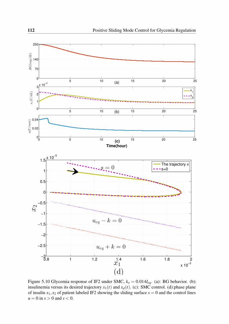
112 Positive Sliding Mode Control for Glycemia Regulation
5 10 15 20 250
70
140
250
BG(m
g/dL)
(a)
5 10 15 20 250
1
2
3x 10
−3
x1(U
/dL)
(b)
0 5 10 15 20 250
0.02
0.04
u(U
/min)
(c)
Time(hour)
x1
xd
0.8 1 1.2 1.4 1.6 1.8 2
x 10−3
−3
−2.5
−2
−1.5
−1
−0.5
0
0.5
1
1.5x 10
−5
x1
(d)
x2
The trajectory x
s=0s = 0
ueq + k = 0
ueq − k = 0
Figure 5.10 Glycemia response of IF2 under SMC, ko = 0.014Ieq. (a): BG behavior. (b):insulinemia versus its desired trajectory x1(t) and xd(t). (c): SMC control. (d):phase planeof insulin x1,x2 of patient labeled IF2 showing the sliding surface s = 0 and the control linesu = 0 in s > 0 and s < 0.
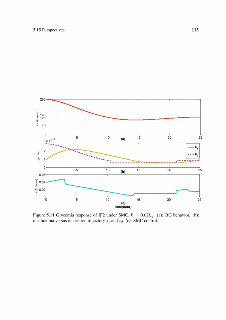
5.15 Perspectives 113
5 10 15 20 250
70
120140
250
BG(m
g/dL)
(a)
5 10 15 20 250
1
2
3x 10
−3
x1(U
/dL)
(b)
0 5 10 15 20 250
0.02
0.04
0.06
u(U
/min)
(c)
Time(hour)
x1
xd
Figure 5.11 Glycemia response of IF2 under SMC, ko = 0.02Ieq. (a): BG behavior. (b):insulinemia versus its desired trajectory x1 and xd . (c): SMC control.

114 Positive Sliding Mode Control for Glycemia Regulation
0 5 10 15 20 25
70
120140
250
BG(m
g/dL)
(a)
0 5 10 15 20 250
1
2
x 10−3
x1(U
/dL)
(b)
0 5 10 15 20 250
0.02
0.04
u(U
/min)
(c)
Time(hour)
x1
xd
0 0.1 0.2 0.3 0.4 0.5 0.6 0.7 0.8 0.9 1
x 103
3.5
3
2.5
2
1.5
1
0.5
0
0.5
1
1.5x 10
5
x1
x2
The trajectory x
s=0
ueq k = 0
ueq + k = 0
s = 0
x1
(d)
Figure 5.12 Glycemia response of BE under SMC. (a): BG behavior. (b): insulinemia versusits desired trajectory x1 and xd . (c): SMC control. (d): Phase plane of insulin x1,x2 of patientlabeled BE showing the sliding surface s = 0 and the trajectory that characterizes Ms− .
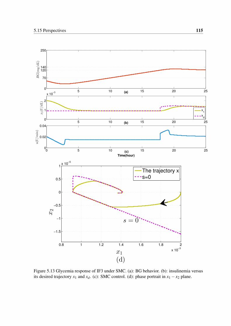
5.15 Perspectives 115
5 10 15 20 250
70
120140
250
BG(m
g/dL)
(a)
5 10 15 20 250
1
2
x 10−3
x1(U
/dL)
(b)
0 5 10 15 20 250
0.02
0.04
u(U
/min)
(c)
Time(hour)
x1
xd
0.8 1 1.2 1.4 1.6 1.8 2
x 10−3
−1.5
−1
−0.5
0
0.5
1x 10
−5
x1
(d)
x2
The trajectory x
s=0
s = 0
Figure 5.13 Glycemia response of IF3 under SMC. (a): BG behavior. (b): insulinemia versusits desired trajectory x1 and xd . (c): SMC control. (d): phase portrait in x1 − x2 plane.

Chapter 6
Description of Positively Invariant Sets
in R3
6.1 Chapter Introduction in French
Dans ce chapitre, les propriétés d’invariance du modèle glycémique global, telles que la
positivité de l’erreur entre la glycémie est son niveau normal est non négative (pour éviter
l’hypoglycémie). Dans le chapitre 5, l’analyse de la positivité du sous-système insuline
dans les cas boucles ouverte et fermée a été étudiée. Une commande CMG positive dans le
plus grand ensemble positivement invariant (EPI) du sous-système d’insuline a été conçue
pour réguler la glycémie. Cependant, la positivité de l’erreur de la glycémie (par rapport à
l’hypoglycémie) n’a pas été prise en compte dans cette synthèse. En raison de la discontinuité
de la loi de commande, concevoir une CMG positive partout dans le plus grand EPI de R3
tel que l’erreur de la glycémie est non négative est beaucoup plus complexe. Néanmoins,
la robustesse de la CMG est encourageante pour mettre le problème en perspective. Dans
ce chapitre, la boucle est fermée par une loi de commande continue : un régulateur par
retour d’état. La théorie des polyèdres invariants pour les systèmes linéaires continus peut
être directement appliquée pour trouver une commande positive par retour d’état. De plus,
le régulateur est continu et la structure en boucle fermée qui en résulte est unique. Par
conséquent, trouver le plus grand EPI en boucle fermée dans R3 (pour le système global),
sous commande positive, est moins complexe.
Tout d’abord, le plus grand EPI du système en boucle ouverte (où seul un débit basal
d’insuline est infusé) est obtenu. Deuxièmement, le plus grand EPI du système en boucle
fermée sous la commande positive stabilisante par retour d’état est trouvé. À l’intérieur
de cet EPI, la glycémie est régulée sans risque d’hypoglycémie. Le résultat principal du
118 Description of Positively Invariant Sets in R3
plus grand EPI en boucles ouverte et fermée est la prédiction d’hypoglycémie. Comme
montré dans le Chapitre 2, l’hypoglycémie est une complication commune grave pour un
DT1. Il s’agit donc d’un problème majeur à résoudre pour la conception du pancréas artificiel.
L’hypoglycémie est prédite ici en fonction des conditions initiales du système. La prédiction
est établie lorsque les conditions initiales sont en dehors du plus grand EPI en boucle fermée
(glycémie <70 mg / dL). Dans ce cas, on vérifie si la condition initiale appartient au EPI
de boucle ouverte (sous l’injection basale). Si oui, la boucle est ouverte et le débit basal est
injecté. Sinon, une hypoglycémie future est également prévue avec l’injection basale, alors la
pompe est arrêtée signalant un épisode hypoglycémique sévère. De cette manière, l’analyse
de positivité s’avère très utile pour la régulation de la glycémie et aussi pour la prédiction de
l’hypoglycémie et éventuellement la nécessité d’un resucrage.
6.2 Introduction
The problem of finding the largest PIS where glycemia remains invariant within or above the
desired threshold, is addressed in this chapter. In Chapter 5, positivity analysis of the insulin
subsystem in open and closed-loop cases was studied. A positive SMC everywhere in the
largest PIS of the insulin subsystem was designed to regulate glycemia. However, positivity
of BG error (with respect to hypoglycemia) was not taken into account in the design. Due to
the discontinuity of the control law, designing a positive SMC everywhere in the largest PIS
in R3 such that BG error is nonnegative is much more complex. This problem is addressed
in this chapter via a simple continuous control law. The loop is closed via a state feedback
controller. First of all, the control law is simple and continuous and the resulting closed-loop
structure is unique. Therefore, finding the largest closed-loop PIS in R3 (for the overall
system), under positive control, is less complex than that with SMC1. Moreover, the theory
of invariant polyhedra for continuous linear systems is directly applied to find a positive state
feedback controller.
Firstly, the largest PIS of the open-loop system (where only a basal insulin rate is infused)
is obtained. Secondly, the largest PIS of the closed-loop system is found under a stabilizing
positive state feedback control. Inside the PIS, glycemia is regulated without hypoglycemia
risk. The main outcome of the largest open and closed-loop PIS for glycemia system is
the hypoglycemia prediction. As shown in Chapter 2, hypoglycemia is a serious common
complication in T1DM. It is, thus, a major open problem to be solved for the artificial
pancreas design. Hypoglycemia is predicted here based on the system initial conditions. The
prediction is established when the initial conditions are outside the largest closed-loop PIS
1 Nevertheless, the robustness of SMC is encouraging to put the problem as a future work.
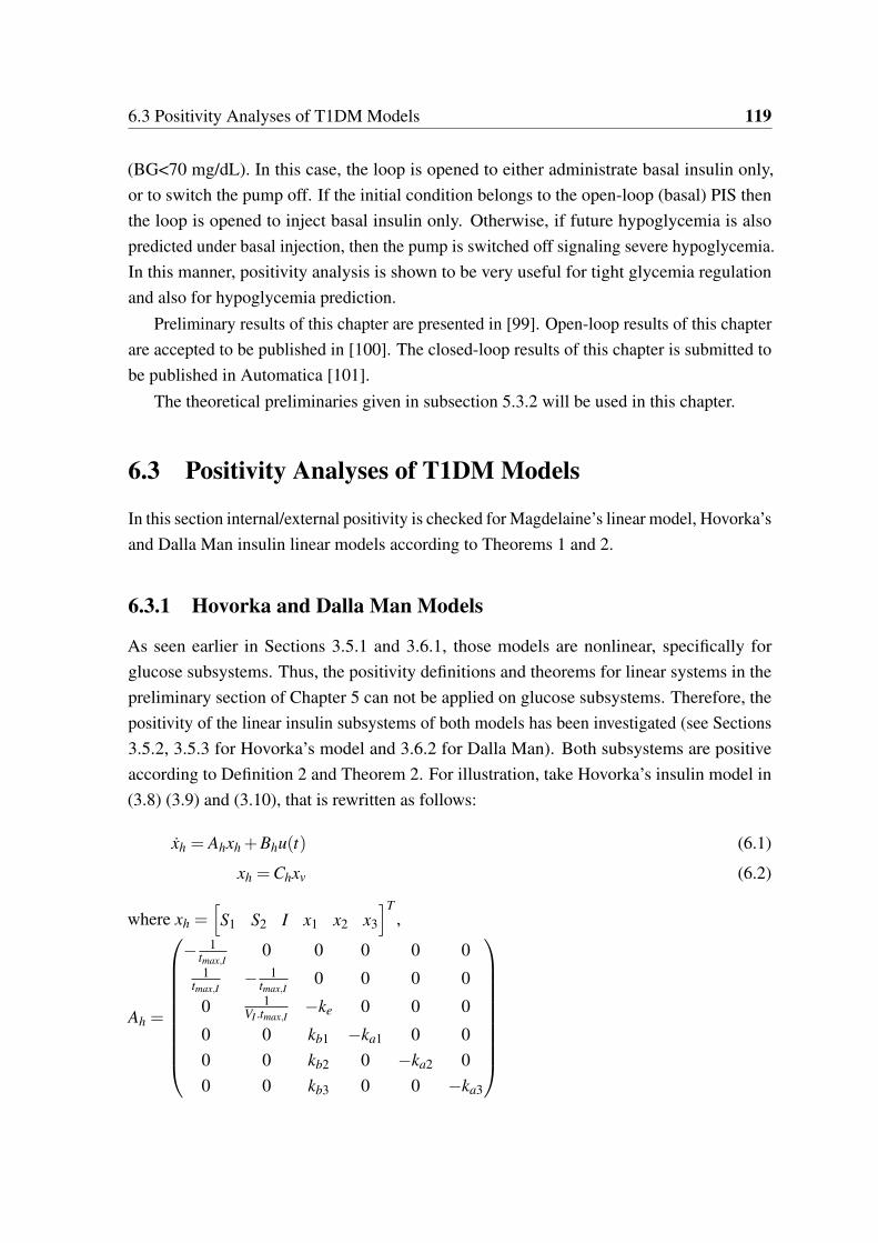
6.3 Positivity Analyses of T1DM Models 119
(BG<70 mg/dL). In this case, the loop is opened to either administrate basal insulin only,
or to switch the pump off. If the initial condition belongs to the open-loop (basal) PIS then
the loop is opened to inject basal insulin only. Otherwise, if future hypoglycemia is also
predicted under basal injection, then the pump is switched off signaling severe hypoglycemia.
In this manner, positivity analysis is shown to be very useful for tight glycemia regulation
and also for hypoglycemia prediction.
Preliminary results of this chapter are presented in [99]. Open-loop results of this chapter
are accepted to be published in [100]. The closed-loop results of this chapter is submitted to
be published in Automatica [101].
The theoretical preliminaries given in subsection 5.3.2 will be used in this chapter.
6.3 Positivity Analyses of T1DM Models
In this section internal/external positivity is checked for Magdelaine’s linear model, Hovorka’s
and Dalla Man insulin linear models according to Theorems 1 and 2.
6.3.1 Hovorka and Dalla Man Models
As seen earlier in Sections 3.5.1 and 3.6.1, those models are nonlinear, specifically for
glucose subsystems. Thus, the positivity definitions and theorems for linear systems in the
preliminary section of Chapter 5 can not be applied on glucose subsystems. Therefore, the
positivity of the linear insulin subsystems of both models has been investigated (see Sections
3.5.2, 3.5.3 for Hovorka’s model and 3.6.2 for Dalla Man). Both subsystems are positive
according to Definition 2 and Theorem 2. For illustration, take Hovorka’s insulin model in
(3.8) (3.9) and (3.10), that is rewritten as follows:
xh = Ahxh +Bhu(t) (6.1)
xh =Chxv (6.2)
where xh =hS1 S2 I x1 x2 x3
iT
,
Ah =
0BBBBBBBBB@
− 1tmax,I
0 0 0 0 01
tmax,I− 1
tmax,I0 0 0 0
0 1VI .tmax,I
−ke 0 0 0
0 0 kb1 −ka1 0 0
0 0 kb2 0 −ka2 0
0 0 kb3 0 0 −ka3
1CCCCCCCCCA
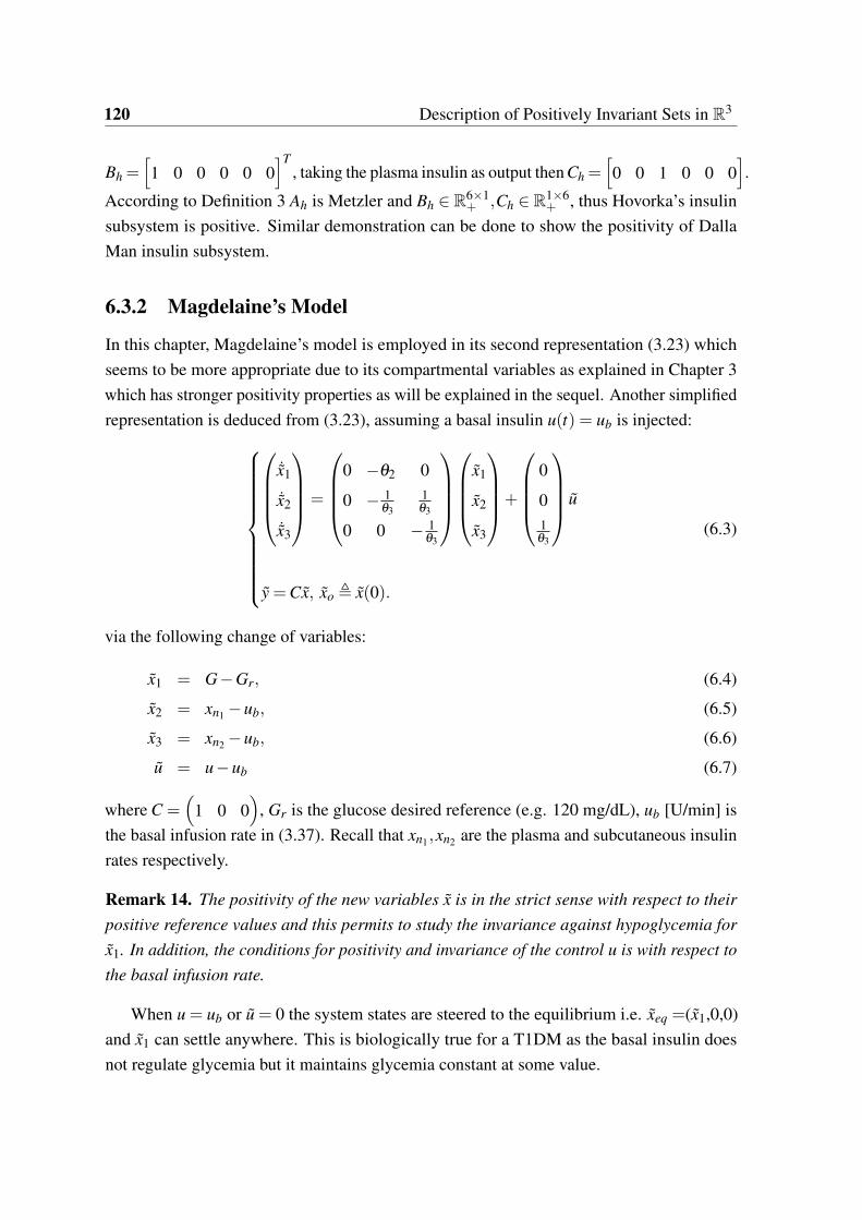
120 Description of Positively Invariant Sets in R3
Bh =h1 0 0 0 0 0
iT
, taking the plasma insulin as output then Ch =h0 0 1 0 0 0
i.
According to Definition 3 Ah is Metzler and Bh 2 R61+ ,Ch 2 R16
+ , thus Hovorka’s insulin
subsystem is positive. Similar demonstration can be done to show the positivity of Dalla
Man insulin subsystem.
6.3.2 Magdelaine’s Model
In this chapter, Magdelaine’s model is employed in its second representation (3.23) which
seems to be more appropriate due to its compartmental variables as explained in Chapter 3
which has stronger positivity properties as will be explained in the sequel. Another simplified
representation is deduced from (3.23), assuming a basal insulin u(t) = ub is injected:
8>>>>>>>>><>>>>>>>>>:
0BBB@
˙x1
˙x2
˙x3
1CCCA=
0BBB@
0 −θ2 0
0 − 1θ3
1θ3
0 0 − 1θ3
1CCCA
0BBB@
x1
x2
x3
1CCCA+
0BBB@
0
01θ3
1CCCA u
y =Cx, xo , x(0).
(6.3)
via the following change of variables:
x1 = G−Gr, (6.4)
x2 = xn1 −ub, (6.5)
x3 = xn2 −ub, (6.6)
u = u−ub (6.7)
where C =
1 0 0
, Gr is the glucose desired reference (e.g. 120 mg/dL), ub [U/min] is
the basal infusion rate in (3.37). Recall that xn1 ,xn2 are the plasma and subcutaneous insulin
rates respectively.
Remark 14. The positivity of the new variables x is in the strict sense with respect to their
positive reference values and this permits to study the invariance against hypoglycemia for
x1. In addition, the conditions for positivity and invariance of the control u is with respect to
the basal infusion rate.
When u = ub or u = 0 the system states are steered to the equilibrium i.e. xeq =(x1,0,0)
and x1 can settle anywhere. This is biologically true for a T1DM as the basal insulin does
not regulate glycemia but it maintains glycemia constant at some value.

6.3 Positivity Analyses of T1DM Models 121
Remark 15. According to Theorem 2, neither the system in its original coordinates nor
system (6.3) are internally positive as their system matrices are not Metzler. Moreover,
according to Theorem 1 they are not externally positive. To show that via Theorem 1,
compute the impulse response h(t) of (6.3):
h(t) =(θ2 +
θ2t
θ3
)e− t
θ3 −θ2 (6.8)
Thus, the impulse response of the output limt!∞
h(t) = −θ2 and the system is not externally
positive either.
Remark 16. Although the overall system (6.3) is not positive, its insulin subsystem (x2, x3)
is internally positive according to Theorem 2 as the insulin subsystem presented by 22
lower right block of matrix A is Metzler, B > 0 and C > 0. According to Corollary 2, R2+ for
this subsystem is a PIS. Note that although the insulin subsystem is internally positive in the
new coordinates (6.3), it is not in the coordinates (3.17). This is just very similar to what is
described in Example 1 in subsection 5.3.2.
Remark 17. It is good to mention that the insulin subsystem in (3.23), with u(t)> 0, is also
positive according to Definition 2 and Theorem 2. This means that insulin subsystem in
x−coordinates in (6.3) is not only positive but also for any x2(0)>−ub and x3(0)>−ub then
x2(t)>−ub, x3(t)>−ub for any u(t)>−ub and t > 0. In other words, for any u(t)>−ub,
the set x 2 R3|x2,3 >−ub is a PIS.
Remark 18. Internal positivity property is not invariant under the change of state coordinates
and this is evident in the change from (3.17) to (6.3) where the insulin subsystem in (3.17) is
not positive whereas in (6.3) it is positive.
Remark 16 is interpreted as follows: the set Ω(C) is not PIS and this motivates the search
for the largest PIS of (6.3)in open and closed-loop cases. This is useful to
1. Find the PIS where the system behaves as an externally positive system 2.
2. Ensure that the positivity constraint on glycemia is respected i.e. x1(t) > 0. In the
PIS in Ω(C) glycemia is restricted to be above or at the desired level Gr in (6.4), thus
hypoglycemia is avoided as Gr > 70 mg/dL.
Concerning insulin positivity constraints, as stated in Remark 17, they remain invariant
x2,3 >−ub for any u >−ub.
2or even internally if C = I33
122 Description of Positively Invariant Sets in R3
6.4 PIS in Ω(C)
In this section, the largest PIS Ωm := xo 2 Ω(C)|Cx(t)> 08t > 0 is found, i.e. the largest
set of initial conditions such that state trajectories never cross the plane Cx = 0. Since each
trajectory is unique (does not cross others), the subset of those which are tangent to the plane
Cx = 0 defines a boundary of Ωm. These trajectories tangent to the plane Cx = 0 are such
that there exists t > 0 solution of Cx(t) = 0 and C ˙x(t) = 0 for some initial conditions.
These trajectories pass by the line
L ,
8<:
Cx = 0
C ˙x = 0(6.9)
L is actually a set of extrema. L is a set of minima for the passing trajectories whose initial
condition xo 2Ω(C) (or Cxo > 0). The concavity of the trajectory Cx is decided by C ¨x(t) and
from (6.3) C ¨x1(t) =−θ2
θ3x3(t
), hence a minimum occurs if x3(t)< 0. Thus, a boundary is
given by the set of trajectories whose minimum is zero i.e. the set
S , xo 2 Ω(C)|mint>0
(Cx(t)) = 0 (6.10)
Theorem 8. The largest PIS Ωm Ω(C) consists of all points xo 2 Ω(C) such that:
1. limt!∞
Cx(xo, t) 2 Ω(C).
2. mint>0
Cx(xo, t) 2 Ω(C) whenever such a minimum exists.
Proof. Point 1 follows directly from the definition of a PIS. Point 2 follows also from the
definition of a PIS that is, the trajectory x(t) 2 Ω(C) for any t > 0.
6.4.1 Open-loop
The state solution of system (6.3) during the fasting phase with u = 0 is:
x1(t) = x10 +θ2θ3 (x20 + x30)(e− t
θ3 −1)+θ2x30te− t
θ3 , (6.11)
x2(t) =
x20 +
x30t
θ3
e− t
θ3 , (6.12)
x3(t) = x30e− t
θ3 . (6.13)
6.5 Polyhedral PIS 123
The final value of the output BG is limt!∞
Cx(xo, t) = lxo where l =
1 −θ2θ3 −θ2θ3
and
the set of points that satisfies the final value condition of Theorem 8 is simply the polyhedron3
Ω(G) with
G :=
C
l
!(6.14)
Note that since only the first condition of Theorem 8 is satisfied then Ωm Ω(G). In the
next section, it is demonstrated that Ω(G) is not a PIS and the largest polyhedral PIS in Ω(G)
is found. Thereafter, the largest PIS Ωm is found [100, 101].
6.5 Polyhedral PIS
According to Proposition 1 neither the set Ω(C) nor the set Ω(G) are PIS, therefore the
largest polyhedral PIS in Ω(G) is found. It will be useful later in finding Ωm. The largest
polyhedral PIS is sought in a smaller polyhedron Ω(Go) Ω(G) where
Go :=
G
w
!(6.15)
and w = (a b c) where a,b and c are unknown constants. The next Theorem states that the
largest polyhedral PIS is Ω(G) := Ω(Go|w=w) with w := (1 −θ2θ3 0).
Theorem 9. The largest polyhedral PIS in Ω(G) for system (6.3) with u = 0 is Ω(G).
Proof. The set Ω(Go) is a PIS according to Proposition1 if the constants a,b,c, are chosen
such that H = GoAG−1o is Metzler. Thus, choose a,b,c such that H verifies Definition 3:
h13 =−θ2
(b− c)> 0 () b− c < 0 (6.16)
h12 =−c
θ3(b− c)> 0 and(6.16) () c > 0 (6.17)
h31 =(b+aθ2θ3)
2
θ2θ 23 (b− c)
> 0 and(6.16) () b =−aθ2θ3 (6.18)
h32 =−b2 +acθ2θ3
θ2θ 23 (b− c)
, (6.18) () b 6 0 (6.19)
and the remaining off diagonal terms are h21 = h12 = 0. From (6.19) and (6.16) the term h32
is nonnegative in either of the following cases:
3Recall Definition 5 of a polyhedron
124 Description of Positively Invariant Sets in R3
Case 1: a = 0,b = 0,c > 0 (6.20)
Case 2: a > 0,b =−aθ2θ3,c > 0 (6.21)
w satisfying (6.20) or (6.21) renders Ω(Go) a PIS and next is to find the largest polyhedral
PIS. Denote Go satisfying case 1 in (6.20) as G1 =
0B@
C
l
w1
1CA where w1 = (0 0 c),c > 0. For
Case 2 denote G2 =
0B@
C
l
w2
1CA where w2 = (a −aθ2θ3 c) satisfying (6.21).
Firstly, it will be shown that x 2 Ω(G1) implies x 2 Ω(G2) or equivalently Ω(G1)
Ω(G2) for c> 0. Secondly, it will be shown that Ω(G2|c=0)Ω(G) is the largest polyhedral
PIS.
1. Ω(G1) Ω(G2) is shown as follows:
x 2 Ω(G1) is equivalent to satisfying all of the following inequalities
x1 > 0 (6.22)
x1 −θ2θ3x2 −θ2θ3x3 > 0 (6.23)
cx3 > 0 (6.24)
(6.23) yields x1 −θ2θ3x2 > θ2θ3x3 and (6.24) implies x1 −θ2θ3x2 > 0 which in turn
implies that a(x1 − θ2θ3x2)+ cx3 > 0 for any a > 0,c > 0 or equivalently w2x > 0.
Therefore Ω(G1) Ω(G2). See Fig. 6.1 for graphical illustration.
2. Ω(G2) Ω(G) follows from
If x3 > 0 then (6.23) implies x1 −θ2θ3x2 > 0. (6.25)
If x3 < 0 then w2x > 0,c > 0 implies x1 −θ2θ3x2 > 0. (6.26)
or equivalently a(x1 −θ2θ3x2)> 0 for a > 0, therefore x 2 Ω(G2) implies x 2 Ω(G).
Thus, Ω(G) is the largest polyhedral PIS as depicted in Fig. 6.2.
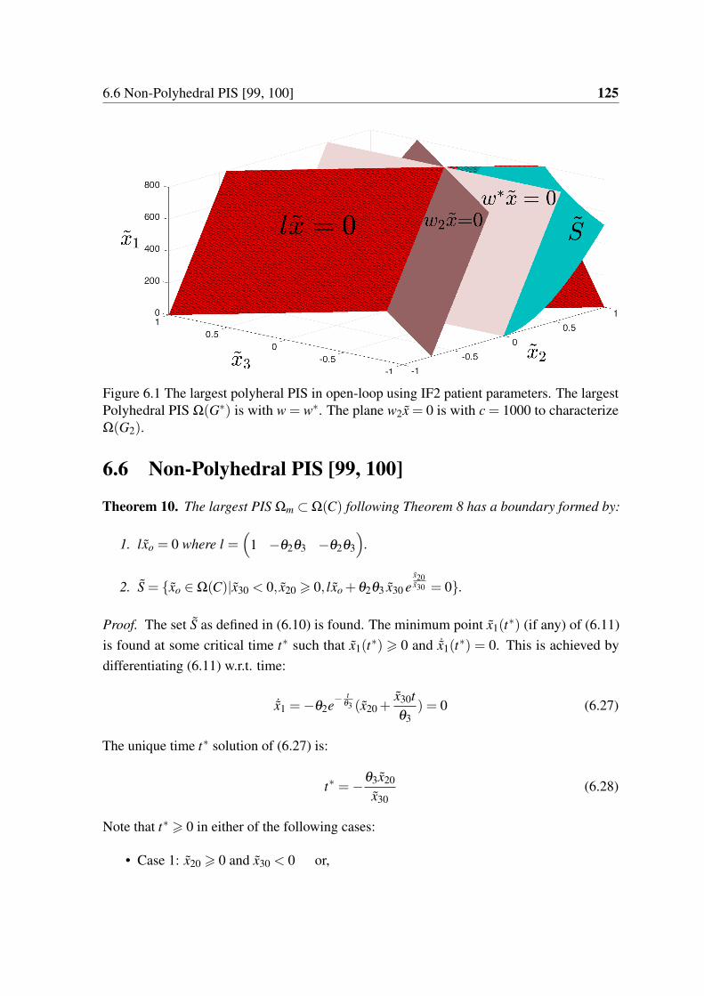
6.6 Non-Polyhedral PIS [99, 100] 125
Figure 6.1 The largest polyheral PIS in open-loop using IF2 patient parameters. The largestPolyhedral PIS Ω(G) is with w = w. The plane w2x = 0 is with c = 1000 to characterizeΩ(G2).
6.6 Non-Polyhedral PIS [99, 100]
Theorem 10. The largest PIS Ωm Ω(C) following Theorem 8 has a boundary formed by:
1. lxo = 0 where l =
1 −θ2θ3 −θ2θ3
.
2. S = xo 2 Ω(C)|x30 < 0, x20 > 0, lxo +θ2θ3 x30 ex20x30 = 0.
Proof. The set S as defined in (6.10) is found. The minimum point x1(t) (if any) of (6.11)
is found at some critical time t such that x1(t) > 0 and ˙x1(t
) = 0. This is achieved by
differentiating (6.11) w.r.t. time:
˙x1 =−θ2e− t
θ3 (x20 +x30t
θ3) = 0 (6.27)
The unique time t solution of (6.27) is:
t =−θ3x20
x30(6.28)
Note that t > 0 in either of the following cases:
• Case 1: x20 > 0 and x30 < 0 or,
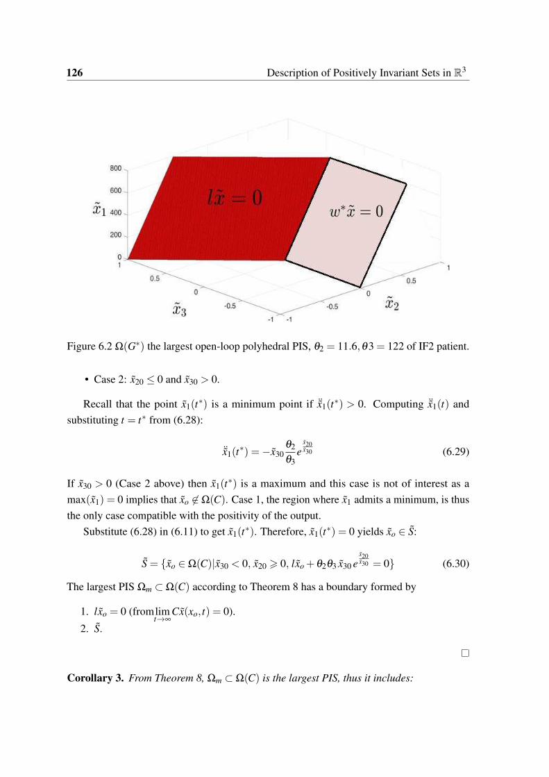
126 Description of Positively Invariant Sets in R3
Figure 6.2 Ω(G) the largest open-loop polyhedral PIS, θ2 = 11.6,θ3 = 122 of IF2 patient.
• Case 2: x20 0 and x30 > 0.
Recall that the point x1(t) is a minimum point if ¨x1(t
) > 0. Computing ¨x1(t) and
substituting t = t from (6.28):
¨x1(t) =−x30
θ2
θ3e
x20x30 (6.29)
If x30 > 0 (Case 2 above) then x1(t) is a maximum and this case is not of interest as a
max(x1) = 0 implies that xo 62 Ω(C). Case 1, the region where x1 admits a minimum, is thus
the only case compatible with the positivity of the output.
Substitute (6.28) in (6.11) to get x1(t). Therefore, x1(t
) = 0 yields xo 2 S:
S = xo 2 Ω(C)|x30 < 0, x20 > 0, lxo +θ2θ3 x30 ex20x30 = 0 (6.30)
The largest PIS Ωm Ω(C) according to Theorem 8 has a boundary formed by
1. lxo = 0 (fromlimt!∞
Cx(xo, t) = 0).
2. S.
Corollary 3. From Theorem 8, Ωm Ω(C) is the largest PIS, thus it includes:
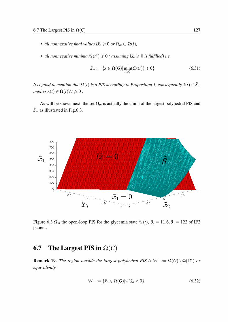
6.7 The Largest PIS in Ω(C) 127
• all nonnegative final values lxo > 0 or Ωm Ω(l),
• all nonnegative minima x1(t)> 0 ( assuming lxo > 0 is fulfilled) i.e.
S+ := x 2 Ω(G)|mint>0
(Cx(t))> 0 (6.31)
It is good to mention that Ω(l) is a PIS according to Proposition 1, consequently x(t) 2 S+
implies x(t) 2 Ω(l)8 t > 0 .
As will be shown next, the set Ωm is actually the union of the largest polyhedral PIS and
S+ as illustrated in Fig.6.3.
~
Figure 6.3 Ωm the open-loop PIS for the glycemia state x1(t), θ2 = 11.6,θ3 = 122 of IF2patient.
6.7 The Largest PIS in Ω(C)
Remark 19. The region outside the largest polyhedral PIS is W− := Ω(G) \Ω(G) or
equivalently
W− := xo 2 Ω(G)|wxo < 0. (6.32)

128 Description of Positively Invariant Sets in R3
Aiming to find the largest PIS in Ω(G), it is required to find a subset (if any) in W− such
that x(t) 2 Ω(G) for any t > 0.
Theorem 11. The largest PIS in Ω(G) is Ωm = Ω(G)[ S+.
Proof. According to Theorem 9, the largest polyhedral PIS in Ω(G) is Ω(G), otherwise if
x(t) 2 Ω(G)\Ω(G) then necessarily x(t) 2W− according to Remark 19.
x(t) 2W− is equivalent to satisfying simultaneously the following inequalities
x1(t)> 0, (6.33)
x1(t)−θ2θ3(x2(t)+ x3(t))> 0, (6.34)
x1(t)−θ2θ3x2(t)< 0. (6.35)
(6.33) and (6.35) imply that x2(t)> 0, while (6.34) and (6.35) implies that x3(t)< 0. The
subset W− is thus located in the region x2(t)> 0, x3(t)< 0 of Ω(G). W− is not a PIS because
there exists t > 0 such that x2(t) = 0 hence x(t) 62W− for t > t. Therefore, x(t) 2W−
only during 0 t < t, t is the instant where x2(t) = 0 and at which the trajectory leaves
W−. 4
Thus find the set of trajectories initiated in W− that remain in Ω(G) for all time.
As explained before, x(t) 2 W− implies x3(t) < 0 at any t 2 [0, t). At t = t there
are two possibilities either x3(t) < 0 or x3(t
) = 0. The case x3(t) = x2(t
) = 0 or
x(t) = (x1(t),0,0) 2 Ω(G) is in fact an equilibrium point. As for the case x3(t
) < 0,
recall from (6.3) that ˙x1(t) =−θ2x2(t) and ¨x1(t) =−θ2θ3(x2(t)+ x3(t)), then
x2(t) = 0, x3(t
)< 0 () Cx(t) = mint>0
(Cx(t)) (6.36)
Thus, to maintain x(t) 2 Ω(G) it is required that mint>0
Cx(t)> 0 and hence the set S+. Hence,
the only admissible set in W− is W−\ S+5.
xo 2 S+ implies x(t) 2W− for any 0 t < t, thereafter x(t) 2 Ω(G)\W− for any t > t
or equivalently
x(t) 2 S+ 0 t t, x(t) 2 Ω(G) t > t (6.37)
4As inequality (6.34) represent the PIS Ω(l), thus, the trajectory leaving W− means that one or both of theinequalities (6.33) and (6.35) no more hold. Satisfying (6.33) for any t > 0 is the objective, thus, the focus isput on the time t at which (6.35) no more holds.
5note that S+ 6W− due to x(t) 2 S+ but x(t) 62W−.

6.7 The Largest PIS in Ω(C) 129
In words, the trajectory initiated in S+ enters the PIS Ω(G) at t = t to remain there6.
Thus, xo 2 S+[Ω(G) implies x(t) 2 S+[Ω(G) for any t > 0, hence S+[Ω(G) is a PIS.
As shown, S+ is the largest admissible set outside the largest polyhedral PIS. Thus, from
(6.37) the union S+[Ω(G) = Ωm is the largest PIS in Ω(G).
S+ as defined in (6.31) for system (6.11)-(6.13) is
S+ = xo 2 Ω(G)|x30 < 0, x20 > 0, lxo +θ2θ3 x30 ex20x30 > 0 (6.38)
Recall from Remark 17 that the feasible set of initial conditions in Ωm is xo 2 Ωm such
that x20 >−ub, x30 >−ub.
The set of points where hypoglycemia occurs is
S− :=W− \ (W−\ S+) (6.39)
Remark 20. The fact that xo 2 Ω(G) implies that limt!∞
Cx(xo, t)> 0 according to Corollary
3. Therefore, due to the nonnegative initial and final values of Cx(t), hypoglycemia events
Cx(t) < 0 are temporary (if any) i.e. the trajectory Cx(t) pass by a negative minimum.
According to (6.28), the minimum time instant is unique, thus it is a global minimum. Thus,
the set of points (initial conditions) which has hypoglycemia nadirs is S−. It is a negative
minimum set that will be useful in the following section to predict hypoglycemia.
The largest PIS of the open-loop case is where glycemia is maintained above or on a pre-
specified level (see (6.4)) e.g. a point in the normal range Gr 2 [70,120] mg/dL. In addition,
Gr = 70 is the least admissible reference value beyond which hypoglycemia (G < 70) zone
starts. Checking the offset with hypoglycemia threshold is very useful as it ensures that once
glycemia initiated in Ωm then hypoglycemic risk is avoided. Moreover, the largest PIS of the
T1DM model is useful for determining the region where hypoglycemia occurs. As will be
shown in the next section, given the initial condition and checking its inclusion in the PIS:
xo 2 Ω(C)\Ωm helps predicting that there exists t > 0 such that G(t)< 70 mg/dL.
6As stated earlier, inequality (6.34) is equivalent to Ω(l) which is a PIS, thus, according to (6.31), xo 2S+ Ω(l) implies that (6.34) holds 8t > 0.
130 Description of Positively Invariant Sets in R3
6.8 Fasting-Hypoglycemia Prediction: Open-loop [100]
Proposition 2. In the fasting phase and with u = 0 and setting Gr = 70 mg/dL, hypoglycemia
is predicted whenever
1. xo 2 S−, or
2. xo 2 Ω(C) but xo 62 Ω(G) i.e. lx < 0.
Proof. Follows immediately from:
1. xo 2 S− is the negative minimum region i.e. using (6.28) in (6.11), yields x1(t, xo)< 0.
2. xo 2 Ω(C)|lxo < 0: negative final value i.e. limt!∞
x1(t, xo) = lxo < 0.
x1(t)< 0 is equivalent to the fact that xo 62 Ωm and the future hypoglycemic events (in
time and value) can be predicted:
• The temporary episodes (point 1 above): the time t of event is computed in (6.28) and
hypoglycemia value x1(t) is obtained from (6.11).
• Persisting hypoglycemia solving (6.11): hypoglycemia level is predicted from limt!∞
x1(t, xo)=
lxo < 0. The time at which hypoglycemia starts can be found numerically solving
(6.11).
In either of the above cases, the solution is to stop the insulin injection and turn the
pump off i.e. u(t) = −ub. The off case is maintained until some finite time t = t1 > 0
after which the trajectory enters the PIS again x(t1) 2 Ωm due to the endogenous glucose
production. This is explained as follows: when u(t) = −ub (or u = 0) then according
to (6.3): limt!t1
(x2(t), x3(t)) = −ub, as a result x1(t) > 0 8t > t1. In the case of a severe
predicted hypoglycemic event x1(t)<< 0 where turning the pump off is not sufficient then a
hypoglycemic alert is signaled and the patient is strongly advised to take some exogenous
glucose (CHO).
Assuming that xo 2 Ωm, the set of equilibrium points of (6.3) is
limt!∞
x(t) = (lxo,0,0) (6.40)
and the glycemia state can settle anywhere: limt!∞
x1 = lxo > 0. Therefore, in the next sec-
tion glycemia regulation to normal level such that x1 = 0 is established via a stabilizing
nonnegative state feedback.
6.9 Closed-loop PIS under a Nonnegative State Feedback 131
6.9 Closed-loop PIS under a Nonnegative State Feedback
In what follows, the largest closed-loop PIS is found under the following full state feedback
control [101]:
u = Fx , F =
K1 K2 K3
(6.41)
The closed-loop system is:
˙x = (A+BF)x, with A+BF =
0B@
0 −θ2 0
0 − 1θ3
1θ3
K1θ3
K2θ3
K3−1θ3
1CA (6.42)
First of all, Ω(C) for the closed-loop system is not a PIS for any F according to Proposi-
tion 1.Secondly, the next theorem states that a PIS can not be constructed by adding a second
constraint i.e. Ω(C)\Ω(w) is not a PIS where w = (a b c) for any real constants a,b,c .
Theorem 12. Ω(C)\Ω(w) is not a PIS for any a,b,c and any F.
Proof. Let H =
h1 h2
h3 h4
!, Ω(C)\Ω(w) is PIS according to Proposition1 if H, solution of
C
w
!(A+BF) = H
C
w
!, is Metzler or equivalently h2 > 0,h3 > 0 s.t.
0 −θ2 0
K1cθ3
− (b−K2c+aθ2θ3)θ3
(b−c+K3c)θ3
!=
h1 +ah2 bh2 ch2
h3 +ah4 bh4 ch4
!(6.43)
From the first row it results b < 0 and c = 0 and first entry reads h2 =−h1a
yielding a < 0.
Taking the last entry of the second row and using the result c = 0 it leads immediately to
b = 0 which contradicts the previous result of b < 0 thus a Metzler H does not exist for any
a,b,c and any F .
In practice it is required that Fx > 0, therefore the closed-loop PIS for system (6.42) will
be found in the following section with stabilizing K1,K2,K3 such that x 2 Ω(C)\Ω(F) for
any t 2 R+. The conditions for stability are derived with standard tools in the following
subsection.
132 Description of Positively Invariant Sets in R3
6.9.1 Stability
Stability conditions of the closed-loop system are investigated via the characteristic equation
of A+BF :
θ 23 λ 3 +θ3(2−K3)λ
2 +(1−K2 −K3)λ +K1θ2 = 0 (6.44)
According to Routh-Hurwitz stability criterion the coefficients for a cubic polynomial must
satisfy:
1. an > 0
K1 > 0, K3 < 2, K3 +K2 < 1 (6.45)
2. a2a1 > a3a0 or:
θ2θ3K1 < (2−K3)(1−K2 −K3) (6.46)
In what follows, these conditions are used to design F for a stable closed-loop system.
6.10 Positivity and Invariance [101]
In this section, the largest closed-loop PIS ΩmF Ω(C)\Ω(F) is found for a stabilizing
F . The largest closed-loop polyhedral PIS is found which is used to find the largest non-
polyhedral PIS.
6.10.1 Polyhedral PIS
The set Ω(Gk) with Gk =
1 0 0
K1 K2 K3
!is not a PIS according to Proposition 1 for any
given F . Therefore, a polyhedral PIS is sought in a smaller polyhedron adding a third face to
Ω(Gk) to yield Ω(Ge) where Ge =
Gk
w
!,w is as defined earlier after (6.15). According
to Proposition 1 He = Ge(A+BF)G−1e has the following off-diagonal terms:

6.10 Positivity and Invariance [101] 133
H12 =cθ2
∆(6.47)
H13 =−K3θ2
∆(6.48)
H21 =K2
2 a−K1K2(b+ c)+K1K3(b+aθ2θ3)−K21 cθ2θ3
θ3∆(6.49)
H23 =−K2
2 +K1K3θ2θ3
θ3∆(6.50)
H31 =−K1b2 −ab(K2 +K3)−K3a2θ2θ3 +ac(K2 +K1θ2θ3)
θ3∆(6.51)
H32 =b2 + c∆+aθ2θ3c
θ3∆(6.52)
where ∆ = K3b−K2c. The off-diagonal entries of the matrix He are made nonnegative
via a family of stabilizing feedback gain ranges depending on the different choices of the
constants a,b and c of w. One of those choices is w = w =
1 −θ2θ3 0
leading to
Ge =
Gk wT
, then the following range of stabilizing gain matrix F is obtained such that
He is Metzler and thus Ω(Ge) is a PIS:
0 < K1 −K2
θ2θ3, K2 < 0, K3 −
K22
K1θ2θ3(6.53)
6.10.2 Stability of F
Stability conditions of K2,K3 in (6.45) and are compatible with invariance conditions of
(6.53). For K1 in (6.53), this range falls in the stable range of (6.46) if
−K2 < (2−K3)(1−K2 −K3) (6.54)
0 < 2(1−K3)−K2 −K3(1−K2 −K3) (6.55)
from (6.53) K2 < 0,K3 < 0 thus the above inequality holds and thus (6.53) is compatible
with stability conditions in (6.45) and (6.46).
It is good to notice that the limit case where K2 = −K,K1 = − K2θ2θ3
, K3 = −K2
2K1θ2θ3
or
F = F with
F , K(1 −θ2θ3 −θ2θ3),K > 0 (6.56)
134 Description of Positively Invariant Sets in R3
leads to Ge G. The following theorem presents the largest polyhedral PIS for any F
satisfying (6.53).
Theorem 13. For any F satisfying (6.53), the largest PIS Ω(Ge) setting w = w is obtained
with F = F.
Proof. The hypothesis is that for any x 2R3 such that the following inequalities are satisfied:
x1 > 0, (6.57)
K1x1 +K2x2 +K3x3 > 0, (6.58)
x1 −θ2θ3x2 > 0. (6.59)
implies
Fx > 0 x1 −θ2θ3(x2 + x3)> 0 (6.60)
this statement is demonstrated region by region as follows:
• If (x3 + x2) 0 then (6.60) is yielded immediately satisfying (6.57) only.
• If (x2 + x3)> 0 and x3 0.
In this region the inequality (6.60) holds directly from (6.57) and (6.59).
• If (x2 + x3)> 0 and x3 > 0.
From (6.53) one has K3x3 −K2
2K1θ2θ3
x3, K1 > 0, thus form (6.58) the following in-
equality holds
0 x1 +K2
K1x2 +
K3
K1x3 x1 +
K2
K1(x2 −
K2
K1θ2θ3x3) (6.61)
also from (6.53) one has K2 < 0, K1 − K2θ2θ3
, multiplying the latter inequality by K2x3K2
1
yields K2K1(− K2
K1θ2θ3)x3
K2K1
x3, hence (6.61) becomes:
x1 +K2
K1(x2 −
K2
K1θ2θ3x3) x1 +
K2
K1(x2 + x3) (6.62)
also from (6.53) one has K2K1
−θ2θ3, thus (x2 + x3)K2K1
−θ2θ3(x2 + x3), hence:
0 x1 +K2
K1x2 +
K2
K1x3 x1 −θ2θ3(x2 + x3). (6.63)

6.11 Non-Polyhedral PIS 135
Therefore, for any F satisfying (6.53) then x 2 Ω(Ge) implies x 2 Ω(G) or the largest PIS is
obtained with F = F. Moreover, as F Kl, then this result holds also for any K > 0.
In the next section, the procedure followed to find the non-polyhedral PIS of the open-loop
is applied to find the surface that characterizes the closed-loop non-polyhedral PIS.
Remark 21. The first condition of Theorem 8 is guaranteed for the closed-loop system as
glycemia error is driven asymptotically to zero and the origin is the new stable equilibrium.
Remark 22. Note that Ω(F) Ω(l) with l as defined earlier, moreover, this set is a PIS
according to Proposition 1. The set denoted as Ω(G) defined in (6.14) will be used to label
the closed-loop positive input/output set as:
Ω(C)\Ω(F) Ω(G) (6.64)
The remaining non- investigated region is x 2 Ω(G) \Ω(G) which implies x 2 W−,
where W− is as defined in (6.32).
Similarly to what has been done for the open-loop system, the largest closed-loop PIS
in Ω(G) is the union between the largest polyhedral PIS and the largest set in W− whose
trajectories remain in Ω(G). Firstly, the non-polyhedral set S Ω(G) will be computed.
Later, it will be shown that, the largest closed-loop PIS is again Ω(G)[ S+, where S+ is as
defined in (6.31) but for the closed-loop system.
Remark 23. Recall that the feasible set of insulin states is such that x2,3(t)>−ub. Thus the
admissible set of initial conditions xo 2 Ω(G) (respectively in any set in Ω(G)) is such that
x20 > −ub, x30 > −ub. According to Remark 17, x2,3(t) > −ub for any u(t) > −ub, t > 0.
according to Remark 22 the set Ω(F) is a PIS and thus u(t) > 0 for any t > 0. Thus, if
x20 >−ub ,x30 >−ub then x2,3(t)>−ub for any t > 0.
In what follows consider xo 2 Ω(G) such that x20 >−ub and x30 >−ub.
6.11 Non-Polyhedral PIS
In this Section, it is shown that the largest PIS in Ω(G) is bounded by S. The set S ischaracterized for the closed-loop system such that S Ω(G). Consider the stable positive
state feedback control found in Theorem 13, F = K
1θ2
−θ3 −θ3
with K > 0 for the
system (6.3) yielding closed-loop eigenvalues λ1,2 =− 1θ3
and λ3 =−K. The resulting statesolution with xo = (x10 x20 x30)
T is:
x1(t) =1
K2
x10
h(K2θ3t+K2θ 2
3 −2Kθ3−Kt)e− t
θ3 +e−Kti+θ2θ3x20
h(1+Kt−K2θ3t)e
− tθ3 −e−Kt
i
136 Description of Positively Invariant Sets in R3
+ x30
h(tθ2 +θ2θ3 −Kθ2θ3t)e
− tθ3 −θ2θ3e−Kt
i(6.65)
x2(t)=1
K2
Kx10
θ2θ3
h(Kθ3t−t−θ3)e
− tθ3 +θ3e−Kt
i+ x20
h(1+Kt−K2θ3t−Kθ3+K2θ 2
3 )e− t
θ3 −Kθ3e−Kti
+x30
θ3
h(t −Kθ3t +Kθ 2
3 )e− t
θ3 −Kθ 23 e−Kt
i(6.66)
x3(t) =1
K
K[e−Kt − e
− tθ3 ][−
x10
θ2+θ3x20]+ x30[Kθ3e−Kt − e
− tθ3 ]
(6.67)
where
K = Kθ3 −1 (6.68)
6.11.1 Critical time t
The critical time t such that x1(t) = 0 is found by solving ˙x1(t
) =−θ2x2(t) = 0. Multi-
plying x2(t) = 0 by (e
tθ3 K2θ2θ3) and using (6.68) yields:
Kx10
htK −θ3
+θ3e
− Kt
θ3
i+θ2θ3x20
h1+Kt(−K)−Kθ3 +K2θ 2
3
−Kθ3e
− Kt
θ3
i
+θ2x30
ht(−K)+Kθ 2
3
−Kθ 2
3 e− Kt
θ3
i= 0 (6.69)
rearranging
− tKh−Kx10 +θ2θ3Kx20 +θ2x30
i= Kθ3e
− Kt
θ3
h− x10 +θ2θ3(x20 + x30)
i
+Kθ3x10 −θ2θ3x20
1+K2θ 2
3 −Kθ3
−θ2θ 2
3 Kx30 (6.70)
and thus
t=Kθ3e
(−K)t
θ3
h− x10 +θ2θ3(x20 + x30)
i+Kθ3
hx10 +θ2θ3(x20 − x30)
i−θ2θ3(1+K2θ 2
3 )x20
(−K)h−Kx10 +θ2θ3Kx20 +θ2x30
i
(6.71)
using Kθ3(θ2θ3x20) =−Kθ3(θ2θ3x20)+2Kθ3(θ2θ3x20) and rearranging
t =Kθ3e
(−K)t
θ3
h− x10 +θ2θ3(x20 + x30)
i+Kθ3
hx10 −θ2θ3(x20 + x30)
i−θ2θ3(1+K2θ 2
3 )x20 +2Kθ3(θ2θ3x20)
(−K)h−Kx10 +θ2θ3Kx20 +θ2x30
i
(6.72)
simplifying
6.11 Non-Polyhedral PIS 137
t =Kθ3e
(−K)t
θ3
h− x10 +θ2θ3(x20 + x30)
i+Kθ3
hx10 −θ2θ3(x20 + x30)
i−θ2θ3K2x20
(−K)h−Kx10 +θ2θ3Kx20 +θ2x30
i (6.73)
Let
q1(xo) :=−Kx10 +θ2θ3Kx20 +θ2x30 (6.74)
and recall that
lxo = x10 −θ2θ3(x20 + x30). (6.75)
Substituting q1(xo) and lxo in (6.73) and rearranging terms yields
t =Kθ3lxo(1− e
− Kt
θ3 )− K2x20θ2θ3
(−K)q1(xo)(6.76)
To solve for t > 0, use also mint>0
(Cx(t)) = x1(t) = 0. Thus, equating (6.65) to zero,
rearranging, multiplying by et
θ3 and using (6.68) results in:
−tK[−Kx10 +θ2θ3Kx20 +θ2x30]+ x10(K2θ 2
3 −2Kθ3)+θ2θ3(x20 + x30) = e− K
θ3t[−x10 +θ2θ3(x20 + x30)].
(6.77)
Adding and subtracting x10 to the left hand side of the above equation and using (6.74) and
(6.75) yields:
− tKq1(xo)+ x10K2 = lxo(1− e− K
θ3t
). (6.78)
The above equation yields:
t =lxo(1− e
− Kθ3
t
)− x10K2
(−K)q1(xo)(6.79)
Now to solve for t > 0, first equate (6.76) and (6.79):
lxo(1− e− K
θ3t
)− x10K2 = Kθ3lxo(1− e(−K)t
θ3 )− K2x20θ2θ3 (6.80)
which is simplified to
− Klxo(1− e− K
θ3t
) = K2[x10 − x20θ2θ3]. (6.81)

138 Description of Positively Invariant Sets in R3
Recall that wxo = x10 − x20θ2θ3, thus
e− K
θ3t
= 1+Kwxo
lxo. (6.82)
Take the natural logarithm for both sides:
−K
θ3t = ln(1+
Kwxo
lxo) (6.83)
which is solved in t as
t =−θ3
Kln(1+
Kwxo
lxo) (6.84)
For a defined natural logarithm solution the argument must satisfy (1+ Kwxo
lxo)> 0, and
according to Remark22 lxo > 0 , thus
Kwxo >−lxo (6.85)
For t to be positive in (6.84), two cases are considered:
• K > 0K > 1θ3
implies ln(1+ Kwxo
lxo) 0 or the argument of natural logarithm satisfies
(0 < (1+ Kwxo
lxo) 1) yielding
− lxo < Kwxo 0, (6.86)
and
Kwxo 0 () wxo 0 (6.87)
• K < 0 K < 1θ3
implies ln(1+ Kwxo
lxo)> 0 or (1+ Kwxo
lxo)> 1 that is
Kwxo > 0 () wxo 0 (6.88)
The minimum condition C ¨x(t)> 0 is presented in the next section to find the surface
S Ω(G) and to identify the closed-loop set of nonnegative minimum S+ defined earlier.
6.11.2 Minimum Condition ¨x1 > 0
Assuming that the time t > 0 exists, then, as stated earlier the point x1(t) = 0, ˙x1(t
) = 0 is
a minimum if ¨x1(t)> 0 or equivalently:
x3(t)< 0 (6.89)
6.11 Non-Polyhedral PIS 139
from (6.67)
K(e−Kt − e
− t
θ3 )[−x10
θ2+θ3x20]+ x30(Kθ3e−Kt − e
− t
θ3 )< 0 (6.90)
multiplying by θ2et
θ3 and rearranging
Ke− Kt
θ3
h− x10 +θ2θ3(x20 + x30)
i−h−Kx10 +θ2θ3Kx20 +θ2x30
i< 0 (6.91)
and substituting (6.74) and (6.75) in the above inequality yields
−Klxoe− Kt
θ3 −q1(xo)< 0 (6.92)
substituting (6.82) in the above equation yields the condition for a minimum point as follows
q1(xo)>−Klxo(1+Kwxo
lxo) (6.93)
The region of minimum is thus defined as the set that verifies (6.86) (or (6.88) depending
on the choice of K) and (6.93):
• From (6.86) where K > 0 K > 1θ3
yields the following minimum region
Q1 :=n
xo 2 Ω(G)
∣∣∣ 0 > Kwxo >−lxo, q1(xo)>−Klxo(1+Kwxo
lxo
)o, K > 0 (6.94)
• From (6.88) the following minimum region is obtained
Q2 :=n
xo 2 Ω(G)
∣∣∣ Kwxo > 0, q1(xo)>−Klxo(1+Kwxo
lxo
)o, K < 0 (6.95)
6.11.3 The Closed-loop Surface S
The set S as defined (6.10) for the closed-loop system is found in this subsection. Substitute
(6.84) in (6.65) to get x1(t) = 0 which yields xo 2 S in the regions Q1 (or in Q2 respectively
depending on the choice of K):
S =n
xo 2Q1
∣∣∣ K
Kx10 −θ2x20
=−q1(xo) ln
1+
Kwxo
lxo
o, if K > 0 (6.96)
140 Description of Positively Invariant Sets in R3
6.12 Largest Closed-loop PIS [101]
The largest closed-loop PIS is characterized in the following theorem.
Theorem 14. The largest closed-loop PIS in Ω(G) is ΩmF= Ω(G)[ S+.
Proof. The final value of x(t) is in Ω(G), bearing in mind that the closed-loop system
equilibrium is the origin. The additional constraint or Ω(F) already represents a PIS as
stated earlier in Remark 22 i.e. xo 2Ω(G) implies x(t)2Ω(l). What remains is thus to ensure
Cx(t)> 0 for any t > 0 in the set Ω(G). According to Theorem13 the largest polyhedral PIS
is Ω(G) and if x 2 Ω(G)\Ω(G) then necessarily x(t) 2W−. From this point, the reader is
referred to the proof of Theorem 11 to show that S+[Ω(G) is the largest closed-loop PIS7.
The Surface S in (6.96), together with the planes Cx = 0 and lx = 0, they form the boundary
of the largest closed-loop PIS.
As S is found for the limit case x1(t) = 0, to find the set S+, given the initial condition
(xo 2W−) solve (6.84) to find x1(t)> 0 and not only x1(t
) = 0. In this case, a solution of
(6.84) can be found numerically as presented in the following section.
6.12.1 Finding S+ using Lambert Function
A way to solve (6.84) is using Lambert W -function which characterizes the solutions y=W (z)
for yey = z , for any complex number z. Real solutions W (z) are only obtained in the real
range z > −e−1 [102]. Equation (6.84) is rewritten to look like yey = z. Rearrange and
multiply both sides of (6.76) by ekt
θ3
θ3:
eKt
θ3
Kt
θ3+
Klxo − K2θ2x20
q1(xo)
=
Klxo
q1(xo)(6.97)
denote q2(xo) =Klxo−K2θ2x20
q1(xo)multiply both sides by eq2(xo) yields
eKt
θ3+q2(xo)
Kt
θ3+q2(xo)
= eq2(xo)
Klxo
q1(xo)(6.98)
the above equation matches the form yey = z , thus the solution y =W (z)
Kt
θ3+q2(xo) =W
eq2(xo)
Klxo
q1(xo)
(6.99)
7S+ is as defined in (6.31)

142 Description of Positively Invariant Sets in R3
6.13 Pump-off hypoglycemia Prediction u =−ub
In this section, pump off state u =−ub ( u = 0) for system (6.3) is studied to predict off-state
hypoglycemia episodes. High hypoglycemia risk is signaled in this case and the patient must
take exogenous glucose to avoid the future hypoglycemic episode. This important step will
complete the general hypoglycemia prediction algorithm in § 6.14.
Setting u =−ub (u = 0 pump-off condition) in (6.3) yields the following solution with
the set of initial conditions (x10, x20, x30):
x1(t) = x10 +θ2θ3(x20 + x30 +2ub)(e− t
θ3 −1)+θ2(x30 +ub)te− t
θ3 +θ2ubt (6.101)
x2(t) =
x20 +ub +
(x30 +ub)t
θ3
e− t
θ3 −ub, (6.102)
x3(t) = (x30 +ub)e− t
θ3 −ub. (6.103)
To predict pump-off hypoglycemia, the decreasing rate of change condition ( ˙x1(t)< 0) is
studied to find the time instant t at which ˙x1(t) = 0.
Note that glycemia will diverge if zero insulin injection is maintained (see (6.101)) due to
endogenous glucose production. Thus any pump-off hypoglycemia event will be temporary
having hypoglycemic nadir x1(t)< 0. Therefore, the focus will be again on the minimum
conditions of glycemia mint>0
(Cx(t)).
6.13.1 Critical time
As explained earlier, the time instant t such that Cx(t) = mint>0
(Cx(t)) is the solution of
˙x1(t) = 0:
t =θ3
x30 +ub
[ubet
θ3 − (x20 +ub)] (6.104)
The point ˙x1(t) = 0 is a minimum if ¨x1(t
)> 0 and thus x3(t)< 0 equivalently:
x30 <−ub(1− et
θ3 ) =) x30 < 0 (6.105)
The time instant t can be calculated using Lambert W -function, thus rearranging (6.104) to
become
t =−θ3
x20 +ub
x30 +ub
+W(−
ube−
x20+ubx30+ub
x30 +ub
)(6.106)
6.14 Fasting-Hypoglycemia Prediction: a General algorithm 143
In this manner, hypoglycemia episodes can be predicted given the initial conditions and
using (6.104) in (6.101). It is good to mention that the system, in this case, does not have any
equilibrium due to the divergence of glycemia (continuous endogenous glucose production
versus zero insulin injection see (6.101)).
In the following section, a general algorithm of hypoglycemia prediction for open and
closed-loop system is presented.
6.14 Fasting-Hypoglycemia Prediction: a General algorithm
The PIS of open and closed-loop systems can be used to detect and predict future hypo-
glycemic episodes given the initial condition xo apply the following procedure:
1. If xo 62 Ωm f(xo 2 S−), then check whether xo 2 Ωm if yes then set K = 0 and apply
the basal control to stabilize glycemia to some equilibrium according to (6.11)-(6.13).
Once the system is at rest at some t = t1, then x(t1) 2 Ωm fthen turn on the state
feedback control u = Fx to steer glycemia to its reference.
2. Otherwise
Proposition 3. If xo 62 Ωm then the following Hypoglycemia alert algorithm is applied:
(a) Solve (6.104) in t (if any).
(b) Check for a minimum by evaluating t in (6.103).
(c) If x3(t)< 0 then check whether x1(t
)< 0.
During hypoglycemia alert (u = −ub) the patient is strongly advised to take some
carbohydrates.
u = −ub (pump is off) is maintained until the state trajectory enters one of the PIS
Ωm,Ωm f.
In the next section, the largest polyhedral PIS of the overall system including the plasma
and the subcutaneous insulin rates x2 and x3 respectively is found. In this case the output
matrix becomes C = I33. The PIS is firstly characterized in open-loop case u(t) = 0 and
then for the closed-loop system such that u(t) = Fx(t)> 0.
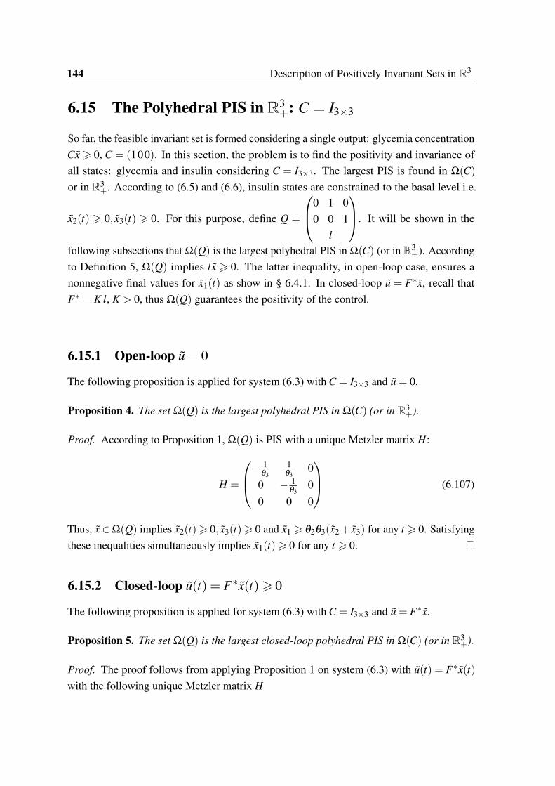
144 Description of Positively Invariant Sets in R3
6.15 The Polyhedral PIS in R3+: C = I33
So far, the feasible invariant set is formed considering a single output: glycemia concentration
Cx > 0, C = (100). In this section, the problem is to find the positivity and invariance of
all states: glycemia and insulin considering C = I33. The largest PIS is found in Ω(C)
or in R3+. According to (6.5) and (6.6), insulin states are constrained to the basal level i.e.
x2(t) > 0, x3(t) > 0. For this purpose, define Q =
0B@
0 1 0
0 0 1
l
1CA. It will be shown in the
following subsections that Ω(Q) is the largest polyhedral PIS in Ω(C) (or in R3+). According
to Definition 5, Ω(Q) implies lx > 0. The latter inequality, in open-loop case, ensures a
nonnegative final values for x1(t) as show in § 6.4.1. In closed-loop u = Fx, recall that
F = K l, K > 0, thus Ω(Q) guarantees the positivity of the control.
6.15.1 Open-loop u = 0
The following proposition is applied for system (6.3) with C = I33 and u = 0.
Proposition 4. The set Ω(Q) is the largest polyhedral PIS in Ω(C) (or in R3+).
Proof. According to Proposition 1, Ω(Q) is PIS with a unique Metzler matrix H:
H =
0B@− 1
θ3
1θ3
0
0 − 1θ3
0
0 0 0
1CA (6.107)
Thus, x 2 Ω(Q) implies x2(t)> 0, x3(t)> 0 and x1 > θ2θ3(x2+ x3) for any t > 0. Satisfying
these inequalities simultaneously implies x1(t)> 0 for any t > 0.
6.15.2 Closed-loop u(t) = Fx(t)> 0
The following proposition is applied for system (6.3) with C = I33 and u = Fx.
Proposition 5. The set Ω(Q) is the largest closed-loop polyhedral PIS in Ω(C) (or in R3+).
Proof. The proof follows from applying Proposition 1 on system (6.3) with u(t) = Fx(t)
with the following unique Metzler matrix H
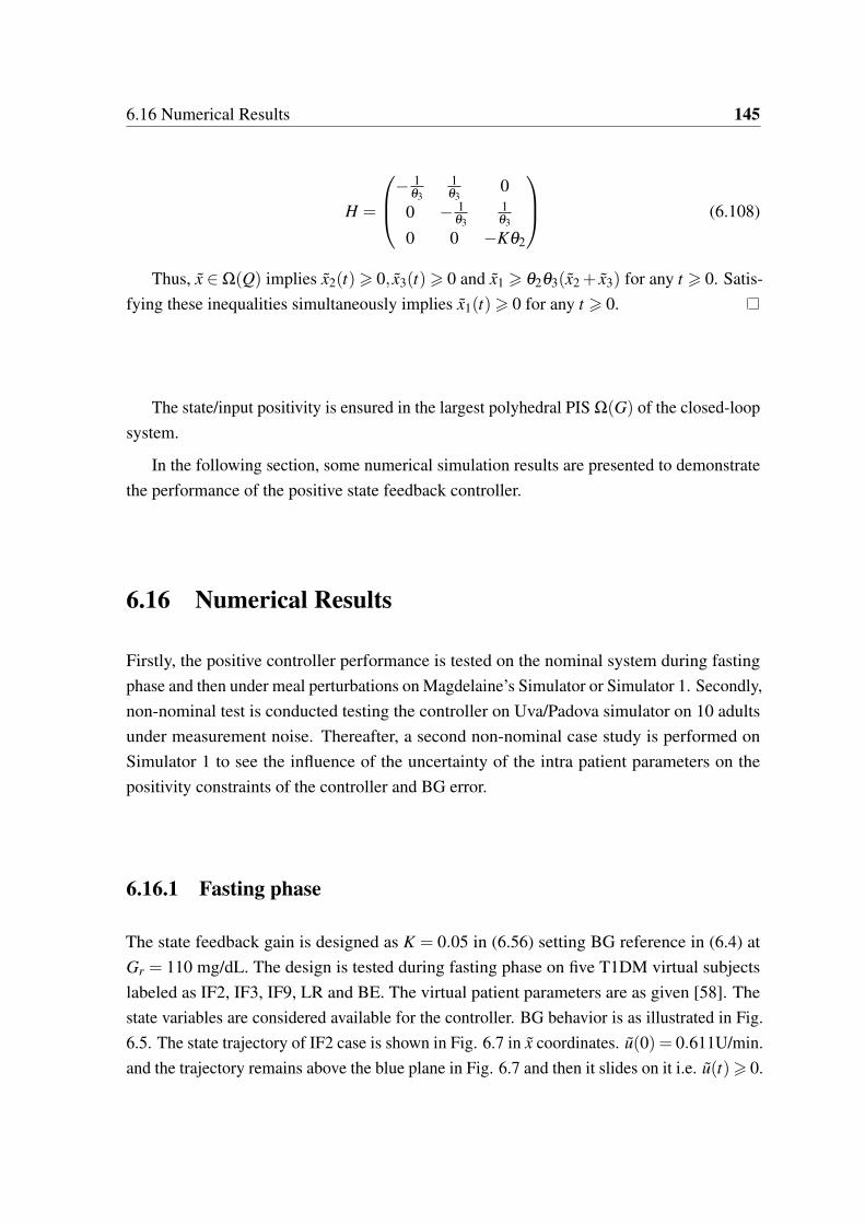
6.16 Numerical Results 145
H =
0B@− 1
θ3
1θ3
0
0 − 1θ3
1θ3
0 0 −Kθ2
1CA (6.108)
Thus, x 2 Ω(Q) implies x2(t)> 0, x3(t)> 0 and x1 > θ2θ3(x2 + x3) for any t > 0. Satis-
fying these inequalities simultaneously implies x1(t)> 0 for any t > 0.
The state/input positivity is ensured in the largest polyhedral PIS Ω(G) of the closed-loop
system.
In the following section, some numerical simulation results are presented to demonstrate
the performance of the positive state feedback controller.
6.16 Numerical Results
Firstly, the positive controller performance is tested on the nominal system during fasting
phase and then under meal perturbations on Magdelaine’s Simulator or Simulator 1. Secondly,
non-nominal test is conducted testing the controller on Uva/Padova simulator on 10 adults
under measurement noise. Thereafter, a second non-nominal case study is performed on
Simulator 1 to see the influence of the uncertainty of the intra patient parameters on the
positivity constraints of the controller and BG error.
6.16.1 Fasting phase
The state feedback gain is designed as K = 0.05 in (6.56) setting BG reference in (6.4) at
Gr = 110 mg/dL. The design is tested during fasting phase on five T1DM virtual subjects
labeled as IF2, IF3, IF9, LR and BE. The virtual patient parameters are as given [58]. The
state variables are considered available for the controller. BG behavior is as illustrated in Fig.
6.5. The state trajectory of IF2 case is shown in Fig. 6.7 in x coordinates. u(0) = 0.611U/min.
and the trajectory remains above the blue plane in Fig. 6.7 and then it slides on it i.e. u(t)> 0.
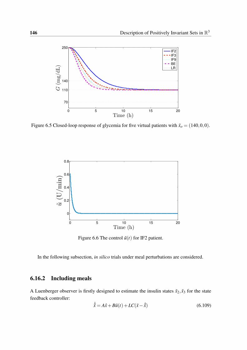
146 Description of Positively Invariant Sets in R3
0 5 10 15 20
70
110
140
250
G(m
g/dL)
Time (h)
IF2
IF3
IF9
BE
LR
Figure 6.5 Closed-loop response of glycemia for five virtual patients with xo = (140,0,0).
0 5 10 15 20
0
0.2
0.4
0.6
0.8
u(U
/min)
Time (h)
Figure 6.6 The control u(t) for IF2 patient.
In the following subsection, in silico trials under meal perturbations are considered.
6.16.2 Including meals
A Luenberger observer is firstly designed to estimate the insulin states x2, x3 for the state
feedback controller:˙x = Ax+Bu(t)+LC(x− ˆx) (6.109)
6.16 Numerical Results 147
Figure 6.7 A trajectory plot in phase portrait for IF2 with x(0) = (140,0,0), the blue planerepresents Fx = 0 with K = 0.05.
based on the BG output measurement i.e. C = (100). L is the observer gain matrix designed
using pole placement method with the following poles λL = −(10K 1θ3
1θ3) that yielded a
relatively fast convergence as shown in Fig. 6.8.
Nominal test The test is conducted on two patients tagged as BE and LR applying the
meal scenario of the clinical diary in [58]. The reference value is set to Gr = 120 mg/dL and
the results are compared to the patient manual open-loop injections. The BG behavior and
the closed-loop injections are illustrated in Fig. 6.9 and 6.10. As shown, hypoglycemia is
completely prevented throughout the simulation. In BE case, the estimation error illustrated
in Fig. 6.8 at the beginning of the simulation led the controller to slightly cross the basal rate
for a while i.e. −ub < u < 0, i.e. min(u) =−0.0083 >−ub. Other than that, the controller
remains positive for the remaining simulation time. In LR case (Fig. 6.10), no estimation
error is considered here where ˆx2,3(0) = x2,3(0).
Although parameters uncertainties are not taken into account in the design of the positive
control and its largest PIS, a robustness test is also conducted in the following trials.
Non-nominal test
1. Uva/Padova trial This in silico trial comprises a fasting period of around 30 hours
followed by normal 36 hours meal scenario of subsection 4.14.2. The controller is
tested on ten virtual T1DM adults in noisy environment using Dexcom 70 CGM sensor
and a generic insulin pump. For robustness against measurement noise, the trial is
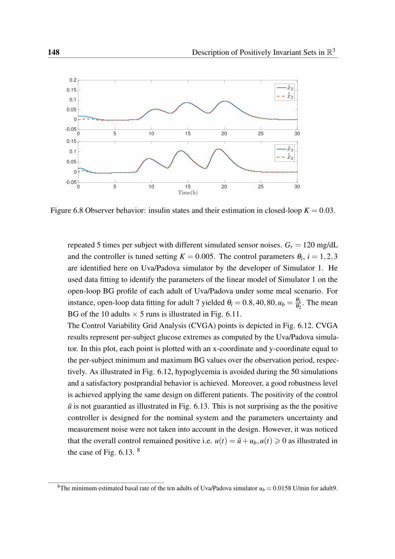
148 Description of Positively Invariant Sets in R3
0 5 10 15 20 25 30-0.05
0
0.05
0.1
0.15
0.2
x2
ˆx2
0 5 10 15 20 25 30
Time(h)
-0.05
0
0.05
0.1
0.15
x3
ˆx3
Figure 6.8 Observer behavior: insulin states and their estimation in closed-loop K = 0.03.
repeated 5 times per subject with different simulated sensor noises. Gr = 120 mg/dL
and the controller is tuned setting K = 0.005. The control parameters θi, i = 1,2,3
are identified here on Uva/Padova simulator by the developer of Simulator 1. He
used data fitting to identify the parameters of the linear model of Simulator 1 on the
open-loop BG profile of each adult of Uva/Padova under some meal scenario. For
instance, open-loop data fitting for adult 7 yielded θi = 0.8,40,80,ub =θ1θ2
. The mean
BG of the 10 adults 5 runs is illustrated in Fig. 6.11.
The Control Variability Grid Analysis (CVGA) points is depicted in Fig. 6.12. CVGA
results represent per-subject glucose extremes as computed by the Uva/Padova simula-
tor. In this plot, each point is plotted with an x-coordinate and y-coordinate equal to
the per-subject minimum and maximum BG values over the observation period, respec-
tively. As illustrated in Fig. 6.12, hypoglycemia is avoided during the 50 simulations
and a satisfactory postprandial behavior is achieved. Moreover, a good robustness level
is achieved applying the same design on different patients. The positivity of the control
u is not guarantied as illustrated in Fig. 6.13. This is not surprising as the the positive
controller is designed for the nominal system and the parameters uncertainty and
measurement noise were not taken into account in the design. However, it was noticed
that the overall control remained positive i.e. u(t) = u+ub,u(t)> 0 as illustrated in
the case of Fig. 6.13. 8
8The minimum estimated basal rate of the ten adults of Uva/Padova simulator ub = 0.0158 U/min for adult9.
6.17 Conclusion 149
2. Simulator 1 Another robustness test is performed on Simulator 1 to explore the
controller performance under an intra-patient parameters uncertainty9. Assume that
the insulin sensitivity factor θ2 and insulin time constant θ3 are underestimated by
30% i.e. θ2,3 = 0.7θ2,3. The controller (and the observer respectively) are based on
the uncertain parameters: F = ( 1θ2
− θ3 − θ3). The resulting BG behavior of patient
BE is illustrated in Fig. 6.14. As shown, the positivity of controller in the uncertain
case is no more guaranteed and it hits the negative lower limit10 u(t) =−ub several
times. Moreover, hypoglycemia threshold is slightly crossed.
From these results, it is shown that a good robustness level is achieved. Yet, positivity and
invariance properties of the input/output of the closed-loop system are affected by parameters
uncertainties and also by measurement noise. For these reasons, positivity and invariance of
the closed-loop system considering parameters uncertainty is envisioned as a perspective of
this work.
6.17 Conclusion
The main results of this chapter are summarized in the following points:
• The first characterization of the largest PIS of glycemia dynamical system under fixed
basal insulin input.
• The major outcome of this PIS is that any initial condition outside this set signals
future hypoglycemia episode.
• This basal PIS outcome is general: basal injection is essential for glycemia regulation
in both open and closed-loop. Glycemia dynamics under basal control is found in
nocturnal time, pre-prandial and follows the postprandial bolus.
• This hypoglycemia prediction holds from any initial condition independently from the
previous control that was applied to the system.
The system in open-loop is critically stable of one pole at the origin and two repeated negative
poles. In other words, under basal injection (u = 0) glycemia state can settle anywhere. To
regulate glycemia to normal level, state feedback control is designed.
9without any observer estimation error ˆx2,3(0) = x2,3(0).10Recall that the lower negative bound for u(t) is −ub which corresponds to the zero limit of the overall
insulin injection: u(t) = (u(t)+ub)> 0.
150 Description of Positively Invariant Sets in R3
• First positive state feedback control is designed to regulate glycemia. This is due to
the fact that glycemia regulation is a positive control problem, namely, once insulin is
injected it can not be taken back.
• The controller is designed such that glycemia remains invariant above or within the
desired set point.
• In the resulting largest PIS, tight glycemia regulation is achieved and thus hypo-
glycemia is prevented.
• A general hypoglycemia prediction algorithm is implemented benefiting from the
largest open and closed-loop PIS.
• Hypoglycemia prediction permits to decide in advance whether to keep the current
control strategy, to turn to basal or to switch the pump off completely.
• The numerical simulations demonstrated the invariance properties of the state/input
solutions.
• Hypoglycemia, the major challenge and open problem for AP studies, is avoided.
• Uncertainty of system parameters affects the observer and the overall control especially
in respecting positivity constraints.
6.18 Perspectives
Input/output positivity constraints have been treated in this chapter for the nominal system.
Parameters uncertainties and measurement noise were not taken into account in the design of
positive controller and the resulting largest PIS. Positivity analysis under these circumstances
is considered as a perspective. The future work of this chapter results are summarized as
follows:
• To consider the bounds of the parameter uncertainties in the design of the positive
controller and the characterization of the largest PIS.
• To take the worst case scenario of the parameters uncertainties in the hypoglycemia
prediction algorithm.
• To implement and realize the positive closed-loop control algorithm incorporating the
hypoglycemia prediction algorithm and test the resulting artificial pancreas in silico.
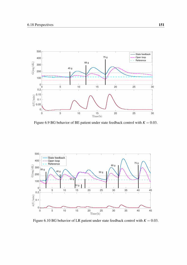
6.18 Perspectives 151
0 5 10 15 20 25 300
100
200
300
400
500
G(m
g/dL)
State feedback
Open loop
Reference
0 5 10 15 20 25 30
Time(h)
0
0.05
0.1
0.15
0.2
u(U
/min)
45 g
68 g
75 g
Figure 6.9 BG behavior of BE patient under state feedback control with K = 0.03.
0 5 10 15 20 25 30 35 40 450
100
200
300
400
500
G(m
g/dL)
State feedback
Open loop
Reference
0 5 10 15 20 25 30 35 40 45
Time(h)
0
0.1
0.2
u(U
/min)
50 g40 g
30 g
50 g
80 g75 g
10 g
Figure 6.10 BG behavior of LR patient under state feedback control with K = 0.03.
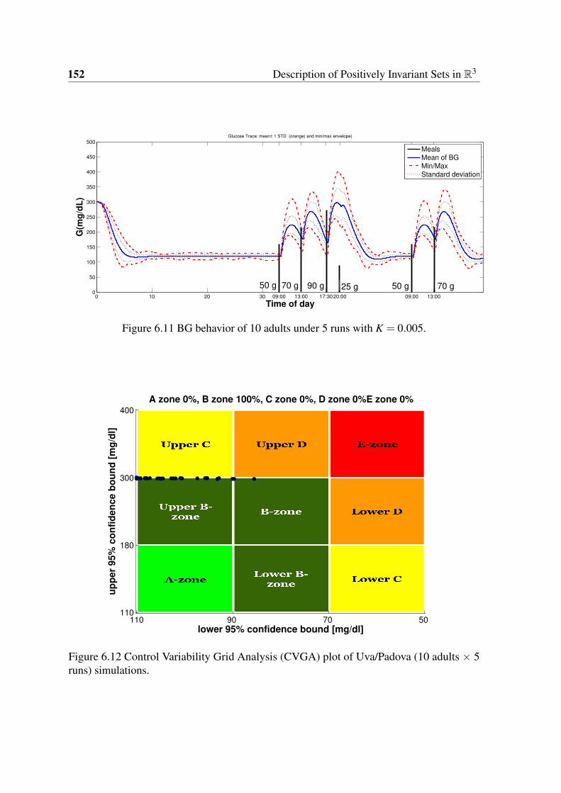
152 Description of Positively Invariant Sets in R3
0 10 20 30 09:00 13:00 17:3020:00 09:00 13:000
50
100
150
200
250
300
350
400
450
500Glucose Trace: mean ± 1 STD (orange) and min/max envelope)
Time of day
G(m
g/d
L)
MealsMean of BG
Min/MaxStandard deviation
25 g90 g70 g50 g 50 g 70 g
Figure 6.11 BG behavior of 10 adults under 5 runs with K = 0.005.
lower 95% confidence bound [mg/dl]
up
per
95%
co
nfi
den
ce b
ou
nd
[m
g/d
l]
A zone 0%, B zone 100%, C zone 0%, D zone 0%E zone 0%
110 90 70 50
400
300
180
110
Figure 6.12 Control Variability Grid Analysis (CVGA) plot of Uva/Padova (10 adults 5runs) simulations.
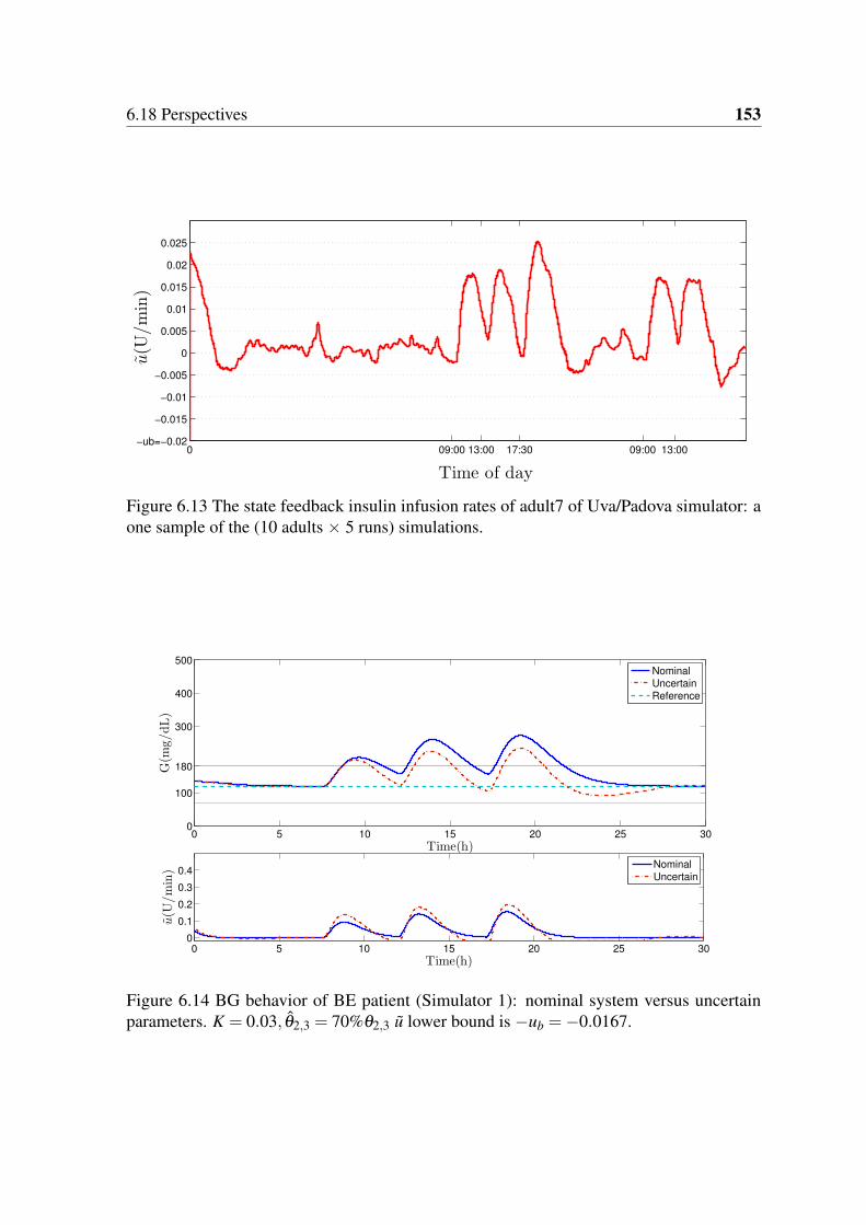
6.18 Perspectives 153
0 09:00 13:00 17:30 09:00 13:00−ub=−0.02
−0.015
−0.01
−0.005
0
0.005
0.01
0.015
0.02
0.025
Time of day
u(U
/min)
Figure 6.13 The state feedback insulin infusion rates of adult7 of Uva/Padova simulator: aone sample of the (10 adults 5 runs) simulations.
0 5 10 15 20 25 300
100
180
300
400
500
G(m
g/dL)
Time(h)
0 5 10 15 20 25 30
0
0.1
0.2
0.3
0.4
Time(h)
u(U
/min)
Nominal
Uncertain
Reference
Nominal
Uncertain
Figure 6.14 BG behavior of BE patient (Simulator 1): nominal system versus uncertainparameters. K = 0.03, θ2,3 = 70%θ2,3 u lower bound is −ub =−0.0167.


Chapter 7
Conclusions and Perspectives
7.1 General Conclusion and Perspectives in French
Avant de passer à l’évaluation des algorithmes de commande, un facteur important est
discuté, qui est la modélisation mathématique du système de DT1. D’après le bref aperçu des
principaux modèles de la littérature PA, les points suivants sont conclus :
• Les modèles historiques largement utilisés comme Bergman ont des points d’équilibre
non naturels qui ne sont pas compatibles avec le comportement glycémique de DT1
dans la vie réelle.
• Ces équilibres non naturels impliquent un ensemble d’insuline basale qui mantient la
glycémie constante. Alors qu’un patient DT1 a un niveau d’insuline basale unique qui
stabilise glycemié à n’importe quelle valeur.
• Une bonne description mathématique de la dynamique glycémie-insulinémie d’un DT1
est requise pour tout algorithme de commande pour la validation in silico et parfois
dans sa conception comme modèle interne.
• Une mauvaise réponse en boucle fermée est donc attendue lorsque toute conception
d’algorithme de commande (ou simulation) est basée sur un mauvais modèle mathé-
matique.
Pour ces raisons, le modèle employé dans cette thèse est le modèle de DT1 à long
terme récemment développé. Ce modèle a montré une bonne description de la dynamique
glycémie-insulinémie de DT1.
La commande sans modèle (CSM) est conçu pour la régulation de la glycémie pour la
première fois.
156 Conclusions and Perspectives
Résumé des résultats de CSM et conclusions principales
• iP est d’abord testée en utilisant une trajectoire de référence variable.
• L’hyperglycémie est réduite par la commande impulsive en forme de bolus résultant
d’une réaction rapide aux repas. Cependant, un bon compromis de performance basal-
postprandial par sujet ne peut être cédé en utilisant une conception fixe.
• Les résultats in silico ont montré une meilleure régulation de la glycémie postprandiale
avec une iPID de référence constante par rapport au iP avec référence variable et par
rapport au PID classique.
• Une solution, utilisée dans la littérature de PA, pour éviter le "windup" du term intégra,l
consiste à remplacer le terme intégral par le débit basal spécifique du sujet, c’est-à-dire
PD + débit basal.
• iPD + débit basal a été comparé à PD + débit basal. Le régulateur intelligent a détecté
les repas et a réagi plus rapidement à ces perturbations par rapport à un PD classique.
CSM a montré un bon niveau de robustesse. Le système est considéré comme une boîte noire
et les paramètres du CSM sont réglés empiriquement sur la base des mesures d’entrée/sortie.
En ce qui concerne la performance, les questions suivantes ont été soulevées :
1. Les contraintes du système ne sont pas prises en compte dans la conception, à savoir le
seuil d’hypoglycémie et la positivité du contrôleur. Le régulateur a été saturé à zéro
qui est la limite inférieure admissible.
2. Lorsque le régulateur est saturé à zéro, la boucle est cassée et la glycémie n’est plus
sous contrôle iPID.
3. Pour les systèmes sous contraintes d’actionneur, le problème de saturation du term
intégral est un défaut connu pour les régulateurs de type PID.
4. L’évitement de l’hypoglycémie n’est pas assurée.
Ainsi, le maintien d’une contrôle glycémique "serrée", en particulier pendant la phase
post-prandiale, n’est pas une tâche facile pour cet iPID entièrement automatique.
En dehors de l’application spécifique de la glycémie, la stabilité en boucle fermée, en
particulier pour le régulateur iP, est non seulement liée à la première dynamique d’erreur
résultant de la commande constituent le modèle ultra-locale. Il a été montré, par un exemple,
qu’un système ne peut pas être stabilisé inconditionnellement par une commande iP.

7.1 General Conclusion and Perspectives in French 157
Les résultats principaux de la conception du CMG dans ce travail sont :
• L’existence d’un CMG positif pour la régulation de la glycémie a été montrée ici pour
la première fois.
• Au meilleur de la connaissance de l’auteur, CMG positif n’a pas été considéré précé-
demment dans l’histoire des études du PA.
• Le plus grand EPI où la variable d’insuline plasmatique est non négative sous CMG a
été trouvé.
• La positivité du GMC a été assurée partout dans cet ensemble via les paramètres de
conception. Ainsi, les contraintes d’entrée / d’état, du système d’insuline du second
ordre, sont respectées.
• La contrainte CMG positive supplémentaire ne réduisait pas le plus grand EPI en
boucle fermée.
Le futur CMG positif
• Le CMG positif conçu est une preuve de concept et la conception peut être étendue
pour inclure la contrainte d’hypoglycémie.
• Les incertitudes des paramètres et les perturbations des repas seront prises en compte
dans la conception du CMG positif.
Le problème de trouver le plus grand EPI où la glycémie reste invariant, dans ou au-
dessus du seuil souhaité, a également été considéré dans ce travail. La boucle est fermée par
l’intermédiaire d’un régulateur par retour d’état positif.
Prestations de la conception de la commande par retour d’état positive contre le CMG
positif
• La loi de commande est simple et continue et la structure en boucle fermée qui en
résulte est unique.
• Donc, trouver le plus grand PIS en boucle fermée (pour le système global), sous
commande positive, est moins complexe que celui avec CMG.
158 Conclusions and Perspectives
Les mérites de cette commande par retour d’état positive sont :
• La contrainte des injections d’insuline (comme entrée positive) dans la conception de
la commande par retour d’etat n’a pas été considérée précédemment dans les études du
PA.
• En comparaison avec le courant dominant des algorithmes de commande de PA,
le retour d’état positif conçu rassemble la simplicité de conception en prenant des
contraintes du système en compte.
• Dans le plus grand EPI en boucle fermée, un contrôle "serré" de la glycémie est atteint
et l’hypoglycémie est totalement évitée.
• Un autre résultat important du plus grand EPI de la glycémie du système en boucle
ouverte et fermée est la prédiction de l’hypoglycémie. Une solution pour éviter la
barrière potentiellement mortelle au traitement diabétique optimal.
L’analyse de positivité s’avère très utile pour la régulation étroite de la glycémie et aussi
pour la prédiction de l’hypoglycémie.
Perspectives de la commande positive par retour de l’état
• Considérer les incertitudes des paramètres intra-patient dans la conception de la com-
mande.
• Prendre le pire scénario des incertitudes des paramètres dans l’algorithme de prédiction
de l’hypoglycémie.
• Implémenter et réaliser l’algorithme de commande en boucle fermée incorporant
l’algorithme de prédiction d’hypoglycémie et tester le pancréas artificiel résultant in
silico.
7.2 General Conclusion and Perspectives
Before going through closed-loop control assessment, an important factor is highlighted, that
is mathematical modeling of T1DM system. From the the brief overview of the main models
in the AP literature, the following points are concluded:
• The widely used historical models like Bergman have non-natural equilibria that are
not consistent with T1DM glycemic behavior in real life.

7.2 General Conclusion and Perspectives 159
• Those non-natural equilibria imply a set of basal insulin that maintains BG constant.
Whereas a T1DM patient has a unique basal insulin level that stabilizes BG at any
value.
• A good mathematical description of glycemia-insulinemia dynamics for a T1DM is
required for any controller for the in silico validation and sometimes in its design as
internal model.
• A poor closed-loop response is thus expected when any control algorithm design (or
simulation) is based on a poor mathematical model.
For theses reasons, the employed model in this thesis is the recently developed long-term
T1DM model. This model has shown a good description of glycemia-insulinema dynamics
of T1DM.
MFC is designed for glycemia regulation for the first time. In opposition to previous PID
studies, the control algorithm developed here is fully automated without any feed-forward or
supplementary insulin doses.
MFC results summary and main conclusions
• iP is firstly tested employing a variable reference trajectory.
• Hyperglycemia is reduced via the resulting bolus-shaped impulsive control of fast
reaction to meals. However, a good, per-subject, fasting-postprandial performance
compromise can not be yielded using fixed design.
• In silico results showed a better postprandial glycemia regulation with constant refer-
ence iPID and over iP with variable reference and over classic PID.
• One solution, used in the literature of AP, to avoid the integral windup is to replace the
integral term by the subject’s specific basal rate, i.e. PD+basal.
• iPD+basal was compared to PD+basal. The intelligent controller detected meals and
reacted faster to theses perturbations as compared to a classic PD without neglecting
safety.
iPID combines the classic PID nice properties with new adaptive features. MFC showed a
good robustness level. The system is considered as a black box and MFC parameters are
tuned empirically based on the input/output measurements. Regarding the performance, the
following issues were raised:

160 Conclusions and Perspectives
1. System constraints are not taken into account in the design, namely, hypoglycemia
threshold and the positivity of the controller. The controller was saturated to zero
which is the lower admissible bound.
2. When the controller saturates to zero, the loop is broken and glycemia is not under
iPID control.
3. For systems under actuator constraints, the integral windup is known defect for PID-like
controllers.
4. Hypoglycemia avoidance is not ensured.
Thus, maintaining a tight BG control, especially during postprandial phase, is not an easy
task for this fully automatic iPID. Aside from the specific glycemia application, closed-loop
stability, specifically for iP controller, is not simply related to the first order error dynamics
resulting form the ultra-local model. It was shown, via an example, that a system can not be
unconditionally stabilized by an iP control.
The main outcomes of SMC design in this work
• The existence of a positive SMC for glycemia regulation was shown without the need
of a saturation.
• To the best of the author knowledge, positive SMC has not been considered previously
in the history of AP studies.
• The largest PIS where the plasma insulin variable is nonnegative under SMC was
found.
• The positivity of SMC was ensured everywhere in this set via the design parameters.
Thus, input/state constraints, of the second order insulin system, are respected.
• The additional positive SMC constraint does not reduce the largest closed-loop PIS.
The future positive SMC
• The designed positive SMC is a proof of concept and the design can be extended to
include hypoglycemia constraint.
• Parameter uncertainties and meal perturbations are to be considered in the design of
positive SMC.

7.2 General Conclusion and Perspectives 161
The problem of finding the largest PIS where glycemia remains invariant within or above
the desired threshold was also considered in this work. The loop is closed via a positive state
feedback controller.
Positive state feedback design benefits over positive SMC design
• The control law is simple and continuous and the resulting closed-loop structure is
unique.
• Therefore, finding the largest closed-loop PIS in R3 (for the overall system), under
positive control, is less complex than that with SMC.
The merits of this state feedback are:
• The constraint of insulin injections (as positive input) in the design of state feedback
controller has not been considered previously in AP studies.
• In comparison to the mainstream of AP controllers, the designed positive state feedback
gathers the simplicity of the design taking system constraints into account.
• In the largest closed-loop PIS, tight glycemia control is achieved where hypoglycemia
is prevented.
• Another important outcome of the largest open and closed-loop PIS for glycemia
system is the hypoglycemia prediction. A solution to avoid the life-threatening barrier
to the optimal diabetic treatment.
Positivity analysis is shown to be very useful for tight glycemia regulation and also for
hypoglycemia prediction.
Perspectives of the positive state feedback
• To consider the the intra-patient parameter uncertainties in the design of the positive
controller.
• To take the worst case scenario of the parameters uncertainties in the hypoglycemia
prediction algorithm.
• To implement and realize the positive closed-loop control algorithm incorporating the
hypoglycemia prediction algorithm and test the resulting artificial pancreas in silico.

Résumé de la thèse
Le problème de la régulation de la glycémie du diabète de type 1 (DT1) est étudié dans ce
travail. Le DT1 est une maladie auto-immune et chronique qui touche environ 25 millions
d’individus dans le monde. Un patient diabétique souffre d’un manque absolu d’insuline due
à la destruction auto-immune des cellules beta du pancréas. L’insuline stimule l’absorption
de glucose dans le sang par les cellules et les muscles. Sans insuline stimulant l’absorption
du glucose, la glycémie reste dans la circulation sanguine et conduit à l’hyperglycémie, état
défini par une glycémie supérieure à 180 mg/dL. Pour survivre, l’injection exogène d’insuline
est la seule solution pour réguler la glycémie. La maladie était fatale avant la découverte de
l’insuline en 1921.
Le traitement actuel nécessite des injections programmées. Il s’agit, soit de multiples
injections quotidiennes d’insuline, soit d’une perfusion d’insuline sous-cutanée continue
(PCSI) délivrée par une pompe. Tout en calculant les doses d’insuline, le patient doit consi-
dérer beaucoup de facteurs comme la quantité de glucide dans chaque repas et les activités
physiques. Un mauvais traitement cause des complications à long terme comme l’insuf-
fisance rénale et les complications vasculaires périphériques. En conséquence, l’injection
automatique d’insuline a reçu un grand intérêt notamment avec le développement rapide de
la technologie des capteurs de glycémie et des pompes à insuline. Depuis plus de 50 ans,
l’idée de développer un dispositif de Pancréatique Artificiel (PA) a été envisagée. Le cœur du
dispositif est l’algorithme de commande qui ferme la boucle entre les mesures de glucose
sanguin et les injections d’insuline d’un patient diabétique.
En général, le but de toute recherche sur le PA est de concevoir un algorithme de
commande adaptable à la sensibilité à l’insuline du patient et suffisamment robuste pour
traiter les dynamiques non modélisées, les incertitudes et le bruit de mesure. Un facteur
important qui affecte la performance des algorithmes de commande est de parvenir à un
compromis entre la réduction de l’hyperglycémie et l’évitement de l’hypoglycémie. De
plus, la positivité de l’infusion d’insuline doit être prise en compte dans la conception du
réglateur. De même, toutes les concentrations d’insuline ou de glucose sont des variables
d’état positives.
164 Conclusions and Perspectives
Le courant dominant des algorithmes de commande utilisés précédemment dans différents
tests cliniques est le régulateur Proportionel-Intégral-Dérivativé (PID) et la commande
prédictive (CP). CP est populaire dans ce domaine car il gère les contraintes du système dans
sa conception. L’inconvénient principal de la CP est son lourd processus d’optimisation. Le
PID a également été fréquemment testé car il a été observé qu’il imitait le comportement
des cellules beta déficientes dans le pancréas. En outre, sa conception ne nécessite pas un
modèle précis du système.
Dans ce travail, deux types de commandes sont utilisés : les commandes basées sur des
modèles et les commandes non-basées sur des modèles. Pour évaluer leur efficacité, les
deux types sont testés in silico sur deux simulateurs de DT1. Le premier simulateur est un
modèle à long terme développé au LS2N et qui est déduit à partir des données cliniques de
sujets DT1. Le deuxième est le simulateur Uva / Padova qui est approuvé par le Food and
Drugs Administration (FDA). Tous les régulateurs conçus et testés ci-après sont entièrement
automatiques sans annonces de repas ni des doses supplémentaires d’insuline.
Dans ce travail, la commande sans modèle (CSM) est utilisée pour la première fois pour
la régulation de la glycémie. Les dynamiques et les perturbations inconnues sont estimées en
ligne grâce à la connaissance unique des mesures d’entrée / sortie. L’estimation est utilisée
dans la loi de commande pour compenser les perturbations et la boucle est fermée via un
régulateur PID simple. La CSM avec un PID dans la boucle est appelé PID intelligent (iPID).
Elle offre les fonctions simples d’un contrôle PID dans le cadre d’une conception sans
modèle. Contrairement aux études PID précédentes, le iPID est entièrement automatique sans
aucune dose d’insuline supplémentaire. On montre tout d’abord qu’un système du second
ordre ne peut pas être stabilisé de manière inconditionnelle par un régulateur iP. On teste
d’abord le régulateur proportionnel intelligent (iP) en utilisant une trajectoire de référence
variable pour contourner le mauvais comportement postprandial de la référence constante
iP. La référence variable produit un débit impulsif en réaction rapide aux repas qui réduit
l’hyperglycémie postprandiale dans le cas du régulateur iP. Pour améliorer encore la réponse
postprandiale, des termes supplémentaires de boucle fermée sont ajoutés et un PID intelligent
(iPID) est conçu en utilisant une référence de glycémie constante. Les résultats in silico de la
comparaison ont montré une meilleure régulation de la glycémie postprandiale pour le iPID
avec une référence constante contre le iP avec une référence variable. Le régulateur iPID est
également comparé à un PID classique. Les résultats ont montré que la réponse postprandiale
a été améliorée avec le régulateur iPID réduisant les excursions hyperglycémiques avec des
événements hypoglycémiques minimes. De plus, le iPID imitait mieux le comportement
postprandial naturel des cellules beta du pancréas qu’un PID avec une réponse plus rapide.
La CSM a montré un bon niveau de robustesse. Le système est considéré comme une boîte
7.2 General Conclusion and Perspectives 165
noire, et les paramètres de la commande CSM sont réglés de manière empirique en se fondant
sur les mesures d’entrée / sortie.
Un autre algorithme de commande robuste est conçu et testé dans cette thèse : la com-
mande par modes glissants (CMG). Notre contribution essentielle est la démonstration de
l’existence d’un régulateur rigoureusement positif apte à assurer la positivité des variables
d’état, en particulier l’insuline de plasma. Un régulateur CMG positif est conçu pour la
première fois pour la régulation de la glycémie. La commande est positive partout dans
le plus grand ensemble positivement invariant (EPI) du sous-système d’insuline dans le
plasma. Deux CMG sont calculées ; le deuxième bloc CGM2 utilise l’erreur de glycémie
(par rapport au niveau souhaité) pour concevoir la trajectoire d’insuline souhaitée. Ensuite,
l’état d’insuline dans le plasma est forcé de suivre la référence via la commande CMG1. La
variable de commutation de CMG1 est un polynôme de premier ordre de l’erreur d’insuline.
La commande par modes glissants CMG1 garantit le suivi des références d’insuline. La
trajectoire d’insuline souhaitée résultante est l’entrée de commande virtuelle requise du
système glycémique pour éliminer l’erreur de glycémie. L’erreur de glycémie est la variable
de commutation de CMG2. La glycémie est pilotée vers le point de consigne normal pendant
le mode de glissement de CMG2. L’essai in silico est effectué pour valider les résultats
théoriques sur le système nominal pendant la phase de jeûne. La robustesse de la commande
CMG par rapport aux changements de paramètres, aux perturbations des repas et au bruit
des capteurs est considérée comme une perspective. En raison de la discontinuité de la loi de
commande, la conception d’une commande CMG positive partout dans le plus grand EPI
dans R3 telle que la glycémie reste dans le niveau souhaité est beaucoup plus complexe. La
commande CMG positive est une preuve de concept et la conception peut être étendue pour
inclure la contrainte d’hypoglycémie. En d’autres termes, le futur problème peut être de
concevoir une commande CMG positive dans le plus grand EPI où la glycémie est supérieure
au seuil hypoglycémique (Glycémie >70 mg/dL).
Le problème de trouver le plus grand EPI où la glycémie reste invariant dans ou au-
dessus du seuil souhaité, est adressé via une loi de commande simple et continue. Il s’agit
de concevoir une commande positive qui prend la contrainte d’hypoglycémie en compte et
établit un contrôle "serré" de la glycémie. La boucle est fermée via un régulateur positif par
retour d’état. Tout d’abord, la loi de commande est simple et continue. Le retour d’état qui en
résulte est unique. Par conséquent, trouver le plus grand EPI en boucle fermée en R3 (pour
le système global), sous commande positive, est moins complexe que celui avec CMG. De
plus, la théorie des polyèdres invariants pour les systèmes linéaires continus est appliquée
directement pour trouver un régulateur positif par retour d’état. Le plus grand EPI du système
en boucle ouverte (où seul un débit basal d’insuline est infusé) est d’abord calculé. En second
166 Conclusions and Perspectives
lieu, on détermine le plus grand EPI du système en boucle fermée sous une commande par
retour d’état positif et stabilisant. À l’intérieur de cet EPI, la glycémie est régulée au niveau
désiré sans risque d’hypoglycémie puisque les variables d’état sont garanties positives.
Le résultat principal des plus grands EPI en boucle ouverte et fermée est la prédiction
de l’hypoglycemie. Une solution alternative de resucrage permettra d’éviter la barrière de
l’hypoglycémie dans le traitement diabétique optimal. L’hypoglycémie est prédite ici en
fonction des conditions initiales du système. La prédiction est établie lorsque les conditions
initiales sont en dehors du plus grand EPI en boucle fermée (Glycémie <70 mg / dL). Dans
ce cas, la boucle est ouverte soit pour administrer l’insuline basale seulement, soit pour
arrêter totalement la pompe. Si la condition initiale appartient au EPI en boucle ouverte
(seulement sous injection du débit basal), la boucle est ouverte pour injecter l’insuline basale
uniquement. Sinon, si une hypoglycémie future est également prédite sous injection basale,
alors la pompe est arrêtée signalant une hypoglycémie sévère. De cette manière, l’analyse
de positivité s’avère très utile pour une régulation stricte de la glycémie et aussi pour la
prédiction de l’hypoglycémie.
References
[1] W. S. Haubrich. Medical Meanings: A Glossary of Word Origins. American Collegeof Physicians, 2003.
[2] J. M. Berg, J. L. Tymoczko, and L. Stryer. Biochemistry. 5th edition, Section 30.2,W.H. Freeman, New York, 2002.
[3] M. Stumvoll. Glucose Production by the Human Kidney–its Importance Has BeenUnderestimated. Nephrology Dialysis Transplantation, 13(12):2996–2999, 1998.
[4] G. Mithieux and A. Gautier-Stein. Intestinal Glucose Metabolism Revisited . DiabetesResearch and Clinical Practice, 105(3):295 – 301, 2014.
[5] L. Szablewski. Glucose Homeostasis-mechanism and Defects. INTECH Open AccessPublisher, 2011.
[6] S. M. Gray, R. I. Meijer, and E. J. Barrett. Insulin Regulates Brain Function, But HowDoes It Get There? Diabetes, 63(12):3992–3997, 2014.
[7] Y. Minokoshi, C. R. Kahn, and B. B. Kahn. Tissue-specific Ablation of the GLUT4Glucose Transporter or the Insulin Receptor Challenges Assumptions About InsulinAction and Glucose Homeostasis. Journal of Biological Chemistry, 278(36):33609–33612, 2003.
[8] A. Caumo and L. Luzi. First-phase Insulin Secretion: Does it Exist in Real Life? Con-siderations on Shape and function. American Journal of Physiology-EndocrinologyAnd Metabolism, 287(3):E371–E385, 2004.
[9] M. K. Cavaghan. The Beta Cell and First-phase Insulin Secretion. Medscape DiabetesEndocrinol, 6(2), 2004.
[10] T. Taylor. Pancreas Anatomy, October 2012. [online article, visited 19-04-2016]http://www.innerbody.com/image/endo03.html.
[11] M. A. Pfeifer, J. B. Halter, and D. Porte. Insulin Secretion in Diabetes Mellitus. TheAmerican Journal of Medicine, 70(3):579 – 588, 1981.
[12] M. A. Atkinson. The Pathogenesis and Natural History of Type 1 Diabetes. ColdSpring Harbor Perspectives in Medicine, 2(11):a007641, 2012.
[13] R. J. McCrimmon and R. S. Sherwin. Hypoglycemia in Type 1 Diabetes. Diabetes,59(10):2333–2339, 2010.
168 REFERENCES
[14] R. Couch et al. Diabetes Education for Children with Type 1 Diabetes Mellitus andTheir Families. 2008.
[15] E. Bhatia and A. Aggarwal. Insulin Therapy for Patients with Type 1 Diabetes.Journal-Association of Physicians of India, 55(L):29, 2007.
[16] B. D. Saboo and P. A. Talaviya. Continuous Subcutaneous Insulin Infusion: PracticalIssues. Indian Journal of Endocrinology and Metabolism, 16(Suppl 2):S259, 2012.
[17] P. R. Dijk et al. Intraperitoneal Insulin Infusion: Treatment Option for Type 1 DiabetesResulting in Beneficial Endocrine Effects Beyond Glycaemia. Clinical endocrinology,81(4):488–497, 2014.
[18] L. M. Huyett et al. Design and Evaluation of a Robust PID Controller for a FullyImplantable Artificial Pancreas. Industrial & Engineering Chemistry Research,54(42):10311–10321, 2015.
[19] S. J. Logtenberg et al. Improved Glycemic Control With Intraperitoneal VersusSubcutaneous Insulin in Type 1 Diabetes. Diabetes Care, 32(8):1372–1377, 2009.
[20] San Francisco Diabetes Teaching Center at the University of California. CalculatingInsulin Dose. [online article, visited on 2016-04-27] Diabetes Education Online,http://www.dtc.ucf.edu.
[21] J. Walsh, R. Roberts, and T. Bailey. Guidelines for Insulin Dosing in ContinuousSubcutaneous Insulin Infusion Using New Formulas from a Retrospective study ofIndividuals with Optimal Glucose Levels. Journal of Diabetes Science and Technology,4(5):1174–1181, 2010.
[22] E. Cobry et al. Timing of Meal Insulin Boluses to Achieve Optimal PostprandialGlycemic Control in Patients with Type 1 Diabetes. Diabetes Technology & Thera-peutics, 12(3):173–177, 2010.
[23] C. Toffanin et al. Dynamic Insulin on Board: Incorporation of Circadian InsulinSensitivity Variation. Journal of Diabetes Science and Technology, 7(4):928–940,2013.
[24] J. Walsh, R. Roberts, and L. Heinemann. Confusion Regarding Duration of InsulinAction A Potential Source for Major Insulin Dose Errors by Bolus Calculators. Journalof diabetes science and technology, 8(1):170–178, 2014.
[25] V. Iacovacci et al. The Bioartificial Pancreas (BAP): Biological, Chemical andEngineering Challenges . Biochemical Pharmacology, 100:12 – 27, 2016.
[26] P. A. Halban et al. Gene and Cell-Replacement Therapy in the Treatment of Type 1Diabetes: How High Must the Standards Be Set? Diabetes, 50(10):2181–2191, 2001.
[27] P. C. Nett, H. W. Sollinger, and T. Alam. Hepatic Insulin Gene Therapy in Insulin-Dependent Diabetes Mellitus. American Journal of transplantation, 3(10):1197–1203,2003.

REFERENCES 169
[28] P. Keith-Hynes et al. The Diabetes Assistant: A Smartphone-Based System forReal-time Control of Blood Glucose. Electronics, 3(4):609–623, 2014.
[29] F. J. Doyle et al. Closed-Loop Artificial Pancreas Systems: Engineering the Algorithms.Diabetes Care, 37(5):1191–1197, 2014.
[30] A. H. Kadish. Automation Control of Blood Sugar a Servomechanism for GlucoseMonitoring and Control. ASAIO Journal, 9(1):363–367, 1963.
[31] W. L. Clarke et al. Closed-loop Artificial Pancreas Using Subcutaneous GlucoseSensing and Insulin Delivery and a Model Predictive Control Algorithm: the VirginiaExperience. Journal of Diabetes Science and Technology, 3(5):1031–1038, 2009.
[32] I. Pagkalos et al. A Vhdl Implementation of the Biostator II Glucose Control Algorithmfor Critical Care. In Biomedical Circuits and Systems Conference (BioCAS), 2011IEEE, pages 94–97. IEEE, 2011.
[33] F. Chee et al. Expert PID Control System for Blood Glucose Control in Critically IllPatients. Information Technology in Biomedicine, IEEE Transactions on, 7(4):419–425, 2003.
[34] G. M. Steil, A. E. Panteleon, and K. Rebrin. Closed-loop Insulin Delivery—the Pathto Physiological Glucose Control. Advanced drug delivery reviews, 56(2):125–144,2004.
[35] G. M. Steil et al. Feasibility of Automating Insulin Delivery for the Treatment of Type1 Diabetes. Diabetes, 55(12):3344–3350, 2006.
[36] S. A. Weinzimer et al. Fully Automated Closed-loop Insulin Delivery versus Semiau-tomated Hybrid control in Pediatric Patients with Type 1 Diabetes Using an ArtificialPancreas. Diabetes Care, 31(5):934–939, 2008.
[37] G. M. Steil et al. The Effect of Insulin Feedback on Closed Loop Glucose Control.The Journal of Clinical Endocrinology & Metabolism, 96(5):1402–1408, 2011.
[38] J. L. Ruiz et al. Effect of Insulin Feedback on Closed-Loop Glucose Control: ACrossover Study. Journal of diabetes science and technology, 6(5):1123–1130, 2012.
[39] M. Loutseiko et al. Closed-loop Insulin delivery Utilizing Pole Placement to Com-pensate for Delays in subcutaneous insulin delivery. Journal of Diabetes Science andTechnology, 5(6):1342–1351, 2011.
[40] J. L. Sherr et al. Reduced Hypoglycemia and Increased Time in Target Using Closed-loop Insulin Delivery During Nights with or without antecedent Afternoon Exercise inType 1 Diabetes. Diabetes Care, 36(10):2909–2914, 2013.
[41] S. Laxminarayan et al. Use of a Food and Drug Administration-Approved Type1 Diabetes Mellitus Simulator to Evaluate and Optimize a Proportional-Integral-Derivative Controller. Journal of Diabetes Science and Technology, 6(6):1401–1412,2012.
170 REFERENCES
[42] Z. Trajanoski, W. Regittnig, and P. Wach. Simulation Studies on Neural predictiveControl of Glucose Using the Subcutaneous Route. Computer Methods and Programsin Biomedicine, 56(2):133–139, 1998.
[43] R. S. Parker, F. J. Doyle III, and N. A. Peppas. A Model-based Algorithm forBlood Glucose Control in type I Diabetic Patients. Biomedical Engineering, IEEETransactions on, 46(2):148–157, 1999.
[44] R. Hovorka et al. Nonlinear Model Predictive Control of Glucose Concentration inSubjects with Type 1 Diabetes. Physiological measurement, 25(4):905, 2004.
[45] R. Hovorka et al. Partitioning Glucose Distribution/transport, Disposal, and Endoge-nous Production During IVGTT. American Journal of Physiology-Endocrinology andMetabolism, 282(5):E992–E1007, 2002.
[46] L. Magni et al. Model Predictive Control of Type 1 Diabetes: An In silico Trial.Journal of Diabetes Science and Technology, 1(6):804–812, 2007.
[47] E. Dassau et al. Implications of Meal Library & Meal Detection to Glycemic Controlof Type 1 Diabetes Mellitus Through MPC control. Energy (KJ), 1516:35, 2008.
[48] H. Lee et al. A Closed-loop Artificial Pancreas Using Model Predictive Controland a Sliding Meal Size Estimator. Journal of diabetes science and technology,3(5):1082–1090, 2009.
[49] S. Arnolds et al. How Pharmacokinetic and Pharmacodynamic Principles Pave TheWay for Optimal Basal Insulin Therapy in Type 2 Diabetes. International Journal ofClinical Practice, 64(10):1415–1424, 2010.
[50] B. P. Kovatchev et al. In silico Model and Computer Simulation Environment Ap-proximating the Human Glucose/Insulin Utilization. Food and Drug AdministrationMaster File MAF, 1521, 2008.
[51] B. P. Kovatchev et al. Feasibility of Outpatient Fully Integrated Closed-loop ControlFirst Studies of Wearable Artificial Pancreas. Diabetes Care, 36(7):1851–1858, 2013.
[52] S. J. Russell et al. Outpatient Glycemic Control with a Bionic Pancreas in Type 1Diabetes. New England Journal of Medicine, 371(4):313–325, 2014.
[53] P. Kaveh and Y. B. Shtessel. Blood glucose regulation using higher-order sliding modecontrol. International Journal of Robust and Nonlinear Control, 18(4-5):557–569,2008.
[54] A. Abu-Rmileh and W. Garcia-Gabin. Wiener sliding-mode control for artificialpancreas: A new nonlinear approach to glucose regulation. Computer Methods andPrograms in Biomedicine, 107(2):327–340, 2012.
[55] Ana Gabriela Gallardo Hernández et al. High-order sliding-mode control for bloodglucose: Practical relative degree approach. Control Engineering Practice, 21(5):747–758, 2013.
REFERENCES 171
[56] N. T. Parsa, A. R. Vali, and R. Ghasemi. Back Stepping Sliding Mode Control ofBlood Glucose for Type I Diabetes. World Academy of Science, Engineering andTechnology, International Journal of Medical, Health, Biomedical, Bioengineeringand Pharmaceutical Engineering, 8(11):779–783, 2014.
[57] J. T. Sorensen. A Physiologic Model of Glucose Metabolism in Man and its Use to De-sign and Assess Improved Insulin Therapies for Diabetes. PhD thesis, MassachusettsInstitute of Technology, 1985.
[58] N. Magdelaine et al. A Long-term Model of the Glucose-Insulin Dynamics of Type1 Diabetes. IEEE Transactions on Biomedical Engineering, 62(6):1546–1552, May2015.
[59] G. C. Goodwin et al. A Fundamental Control Limitation for Linear Positive Systemswith Application to Type 1 Diabetes Treatment. Automatica, 55:73–77, 2015.
[60] H. Zakeri and S. Ozgoli. A Polynomial Modeling and State Feedback Control of BloodGlucose Regulatory in Diabetic Patients. In Intelligent and Advanced Systems (ICIAS),2012 4th International Conference on, volume 1, pages 388–392. IEEE, 2012.
[61] A. Hariri and L. Y. Wang. Observer-based state feedback for enhanced insulin controlof type ‘i’diabetic patients. The Open Biomedical Engineering Journal, 5:98, 2011.
[62] G. M. Steil. Algorithms for a Closed-loop Artificial Pancreas: the Case forProportional-Integral-Derivative Control. Journal of Diabetes Science and Technology,7(6):1621–1631, 2013.
[63] M. Fliess and C. Join. Model-free Control. International Journal of Control,86(12):2228–2252, 2013.
[64] J. B. Bassingthwaighte et al. Compartmental Modeling in the Analysis of BiologicalSystems. Computational Toxicology: Volume I, pages 391–438, 2012.
[65] M. Blomhøj, T. H. Kjeldsen, and J. Ottesen. Compartment Models (Notes). Latestversion available at: http://www4.ncsu.edu/ msolufse/Compartmentmodels.pdf, 2014.
[66] M. Loutseiko et al. Closed-loop Insulin Delivery Utilizing Pole Placement to Com-pensate for Delays in Subcutaneous Insulin Delivery. Journal of Diabetes Science andTechnology, 5(6):1342–1351, 2011.
[67] V. W. Bolie. Coefficients of Normal Blood Glucose Regulation. Journal of AppliedPhysiology, 16(5):783–788, 1961.
[68] R. N. Bergman, L. S. Phillips, and C. Cobelli. Physiologic Evaluation of FactorsControlling Glucose Tolerance in Man: Measurement of Insulin Sensitivity and Beta-cell Glucose Sensitivity from the Response to Intravenous Glucose. Journal of ClinicalInvestigation, 68(6):1456, 1981.
[69] A. De Gaetano and O. Arino. Mathematical Modeling of the Intravenous GlucoseTolerance Test. Journal of Mathematical Biology, 40(2):136–168, 2000.
172 REFERENCES
[70] D. Boiroux et al. Optimal Insulin Administration for People with Type 1 Diabetes.IFAC Proceedings Volumes, 43(5):248–253, 2010.
[71] C. Dalla Man, R. A. Rizza, and C. Cobelli. Meal Simulation Model of the Glucose-Insulin System. IEEE Transactions on Biomedical Engineering, 54(10):1740–1749,Oct 2007.
[72] C. Dalla Man et al. GIM, Simulation Software of Meal Glucose—insulin Model.Journal of Diabetes Science and Technology, 1(3):323–330, 2007.
[73] C. Cobelli, E. Renard, and B. Kovatchev. Artificial Pancreas: Past, Present, Future.Diabetes, 60(11):2672–2682, 2011.
[74] A. Mohn et al. Insulinothérapie fonctionnelle: un modèle d’approche éducativepour les patients ayant un diabète de type 1. Médecine des Maladies Métaboliques,6(6):469–476, 2012.
[75] M. Fliess and C. Join. Model-free Control and Intelligent PID controllers: To-wards a Possible Trivialization of Nonlinear Control? IFAC Proceedings Volumes,42(10):1531–1550, 2009.
[76] M. Fliess and C. Join. Intelligent pid controllers. In 16th Mediterrean Conference onControl and Automation, 2008.
[77] M. Fliess, C. Join, and H. Sira-Ramirez. Complex continuous Nonlinear Systems:Their Black Box Identification and Their Control. IFAC Proceedings Volumes,39(1):416–421, 2006.
[78] M. Voicu. Advances in Automatic Control, volume 754. Springer Science & BusinessMedia, 2012.
[79] J. R. Partington and C. Bonnet. H∞ and BIBO Stabilization of Delay Systems ofNeutral Type . Systems & Control Letters, 52(3–4):283 – 288, 2004.
[80] H. Mounier. Personal Communication, University of Paris-Sud, France, 2017.
[81] C. Bonnet. Personal Communication, INRIA, Paris, France, 2017.
[82] T. Vyhlidal. Quasi-Polynomial Mapping Based Rootfinder.http://www.cak.fs.cvut.cz/algorithms/qpmr, 2008. [Online; accessed 24-May-2017].
[83] S. Choi et al. Model-free Control of Automotive Engine and Brake for Stop-and-GoScenarios. In European Control Conference (ECC), pages 3622–3627, 2009.
[84] T. MohammadRidha et al. A Variable Reference Trajectory for Model-free GlycemiaRegulation. In SIAM CT15, Paris, France, 2015.
[85] G. Marchetti et al. An Improved PID Switching Control Strategy for Type 1 Diabetes.IEEE TBME, 55(3):857–865, 2008.
REFERENCES 173
[86] H. W. Rodbard et al. American Association of Clinical Endocrinologists MedicalGuidelines for Clinical Practice for the Management of Diabetes Mellitus. Endocrinepractice, 13:1–68, 2007.
[87] T. MohammadRidha et al. Model Free iPID Control for Glycemia Regulation ofType-1 Diabetes. Accepted in IEEE Transactions on Biomedical Engineering, April,2017.
[88] T. MohammadRidha and C. H. Moog. Model Free Control for Type-1 Diabetes: AFasting-Phase Study. In 9th IFAC Symposium on Biological and Medical Systems,Berlin, Germany, August 2015.
[89] F. Cameron et al. A Closed-loop Artificial Pancreas Based on Risk Management.Journal of Diabetes Science and Technology, 5(2):368–379, 2011.
[90] I. Ben Abbes et al. A Closed-Loop Artificial Pancreas Using a Proportional IntegralDerivative with Double Phase Lead Controller Based on a New Nonlinear Model ofGlucose Metabolism. Journal of Diabetes Science and Technology, 7(3):699–707,2013.
[91] F. J. Service. Glucose Variability. Diabetes, 62(5):1398, 2013.
[92] K. Menani et al. Positive Sliding Mode Control for Glycemia Regulation. InternationalJournal of Systems Science, July, 2017.
[93] F. Blanchini. Survey Paper: Set Invariance in Control. Automatica (Journal of IFAC),35(11):1747–1767, 1999.
[94] L. Farina and S. Rinaldi. Positive Linear Systems: Theory and Applications, volume 50.John Wiley & Sons, 2011.
[95] E. B. Castelan and J. C. Hennet. On Invariant Polyhedra of Continuous-time LinearSystems. IEEE Transactions on Automatic Control, 38(11):1680–85, 1993.
[96] G. Monsees. Discrete-time Sliding Mode Control. TU Delft, Delft University ofTechnology, 2002.
[97] A. Vignoni. Invariance and Sliding Modes. Application to Coordination of Multi-agent Systems, Bioprocesses Estimation, and Control in Living Cells. Master’s thesis,Universitat Politècnica de València, València, 2014.
[98] C. Edwards and S. Spurgeon. Sliding Mode Control: Theory and Applications. CRCPress, 1998.
[99] Taghreed MohammadRidha et al. Description of the Positively Invariant Sets of a Type1 Diabetic Patient Model. The 17th CLCA Latin American Conference of AutomaticControl, 2016.
[100] T. MohammadRidha et al. Toward Hypoglycemia Prediction and Avoidance for Type1 Diabetic Patients. 56th IEEE Conference on Decision and Control, accepted, July,2017.
174 REFERENCES
[101] T. MohammadRidha et al. Positively Invariant Sets of a T1DM Model: HypoglycemiaPrediction and Avoidance. Automatica, submitted, July, 2017.
[102] D. A. Barry et al. Analytical Approximations for Real Values of the Lambert W-function. Mathematics and Computers in Simulation, 53(1):95–103, 2000.
[103] F. Zaccardi et al. Group of Signs: A New Method to Evaluate Glycemic Variability.Journal of Diabetes Science and Technology, 2(6):1061–1065, 2008.
[104] C. R. Marling et al. Characterizing Blood Glucose Variability Using New Metrics withContinuous glucose monitoring data. Journal of Diabetes Science and Technology,5(4):871–878, 2011.
[105] G.D. Molnar et al. Mean Amplitude of Glycemic Excursions, a Measure of DiabeticInstability. Diabetes, 19(9):644–655, 1970.
[106] J. C. Segen. The Dictionary of Modern Medicine. CRC Press, 1992.
[107] F. Bertuzzi et al. Brittle Type 1 Diabetes Mellitus. Current Medicinal Chemistry,14(16):1739–1744, 2007.

Appendix A
A.1 On the estimated derivative ye(t)
A.1.1 Algebraic Derivative Estimator
To estimate the derivative of a signal y(t) using the algebraic derivative estimator (see[83]
and the references therein), start from Taylor series:
y(t) = ΣNi=0
y(0)(i)t i
i!(A.1)
To estimate the first derivative set N = 1:
y(t) = y(0)+ y(0)t (A.2)
Take Laplace for above knowing that y(0), y(0) are constants yields:
sY (s) = y(0)+y(0)
s(A.3)
Remark 24. Note that at this stage, (A.3) is also obtained if Fe = y(t) in(4.26) (setting
u(t) = 0) and taking Laplace to the result. In this case, Fe in (4.27) is equivalent to y(0) in
(A.3) Fe = y(0), thus Fe will estimate y(t).
Differentiate both sides of (A.3) w.r.t. s:
Y (s)+sdY (s)
ds=−
y(0)s2 (A.4)
To filter out, multiply both sides by s−2:
Y (s)
s2 +dY (s)
sds=−
y(0)s4 (A.5)
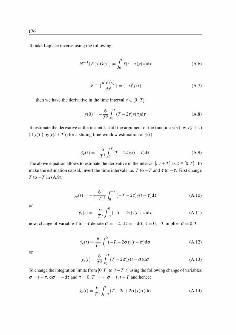
176
To take Laplace inverse using the following:
L−1F(s)G(s)=
Z t
0f (t − τ)g(τ)dτ (A.6)
L−1
diF(s)
dsi= (−t)i f (t) (A.7)
then we have the derivative in the time interval τ 2 [0, T ]:
y(0) =−6
T 3
Z T
0(T −2τ)y(τ)dτ (A.8)
To estimate the derivative at the instant t, shift the argument of the function y(τ) by y(t + τ)
(if y(T ) by y(t +T )) for a sliding time window estimation of y(t)
ye(t) =−6
T 3
Z T
0(T −2τ)y(t + τ)dτ (A.9)
The above equation allows to estimate the derivative in the interval [t t +T ] as τ 2 [0 T ]. To
make the estimation causal, invert the time intervals i.e. T to −T and τ to −τ . First change
T to −T in (A.9):
ye(t) =−6
(−T )3
Z −T
0(−T −2τ)y(t + τ)dτ (A.10)
or
ye(t) =−6
T 3
Z 0
−T(−T −2τ)y(t + τ)dτ (A.11)
now, change of variable τ to −τ denote σ =−τ , dτ =−dσ , τ = 0,−T implies σ = 0,T :
ye(t) =6
T 3
Z 0
T(−T +2σ)y(t −σ)dσ (A.12)
or
ye(t) =6
T 3
Z T
0(T −2σ)y(t −σ)dσ (A.13)
To change the integration limits from [0 T ] to [t−T t] using the following change of variables
σ = t − τ , dσ =−dτ and τ = 0, T =) σ = t, t −T and hence:
ye(t) =6
T 3
Z t
t−T(T −2t +2σ)y(σ)dσ (A.14)
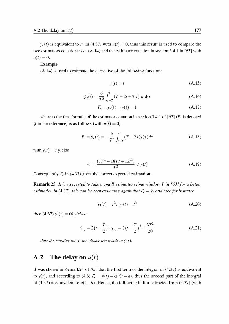
A.2 The delay on u(t) 177
ye(t) is equivalent to Fe in (4.37) with u(t) = 0, thus this result is used to compare the
two estimators equations: eq. (A.14) and the estimator equation in section 3.4.1 in [63] with
u(t) = 0.
Example
(A.14) is used to estimate the derivative of the following function:
y(t) = t (A.15)
ye(t) =6
T 3
Z t
t−T(T −2t +2σ) σ dσ (A.16)
Fe = ye(t) = y(t) = 1 (A.17)
whereas the first formula of the estimator equation in section 3.4.1 of [63] (Fe is denoted
φ in the reference) is as follows (with u(t) = 0) :
Fe = ye(t) =−6
T 3
Z t
t−T(T −2τ)y(τ)dτ (A.18)
with y(t) = t yields
ye =(7T 2 −18Tt +12t2)
T 2 6= y(t) (A.19)
Consequently Fe in (4.37) gives the correct expected estimation.
Remark 25. It is suggested to take a small estimation time window T in [63] for a better
estimation in (4.37), this can be seen assuming again that Fe = ye and take for instance
y1(t) = t2, y2(t) = t3 (A.20)
then (4.37) (u(t) = 0) yields:
y1e= 2
(t −
T
2
), y2e
= 3(t −
T
2
)2+
3T 2
20(A.21)
thus the smaller the T the closer the result to y(t).
A.2 The delay on u(t)
It was shown in Remark24 of A.1 that the first term of the integral of (4.37) is equivalent
to y(t), and according to (4.6) Fe = y(t)−αu(t − h), thus the second part of the integral
of (4.37) is equivalent to u(t −h). Hence, the following buffer extracted from (4.37) (with
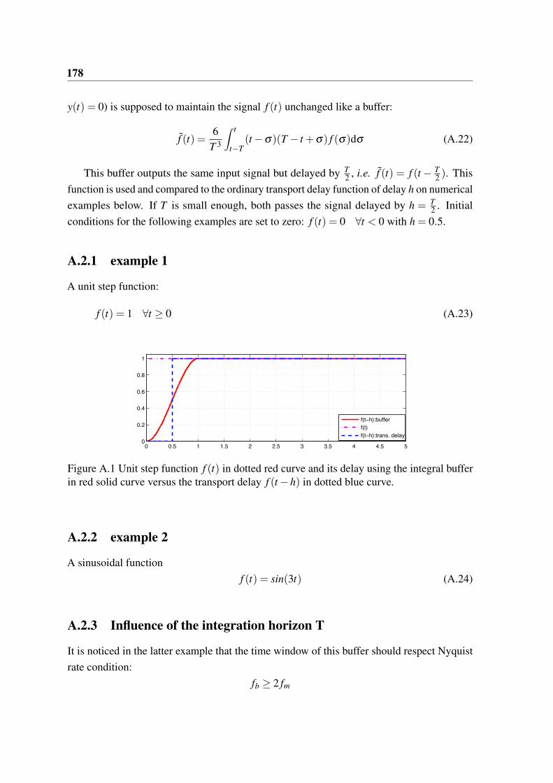
178
y(t) = 0) is supposed to maintain the signal f (t) unchanged like a buffer:
f (t) =6
T 3
Z t
t−T(t −σ)(T − t +σ) f (σ)dσ (A.22)
This buffer outputs the same input signal but delayed by T2 , i.e. f (t) = f (t − T
2 ). This
function is used and compared to the ordinary transport delay function of delay h on numerical
examples below. If T is small enough, both passes the signal delayed by h = T2 . Initial
conditions for the following examples are set to zero: f (t) = 0 8t < 0 with h = 0.5.
A.2.1 example 1
A unit step function:
f (t) = 1 8t ≥ 0 (A.23)
0 0.5 1 1.5 2 2.5 3 3.5 4 4.5 50
0.2
0.4
0.6
0.8
1
f(t−h):buffer
f(t)
f(t−h):trans. delay
Figure A.1 Unit step function f (t) in dotted red curve and its delay using the integral bufferin red solid curve versus the transport delay f (t −h) in dotted blue curve.
A.2.2 example 2
A sinusoidal function
f (t) = sin(3t) (A.24)
A.2.3 Influence of the integration horizon T
It is noticed in the latter example that the time window of this buffer should respect Nyquist
rate condition:
fb ≥ 2 fm
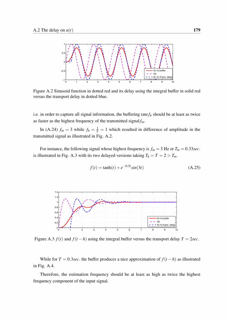
A.2 The delay on u(t) 179
0 1 2 3 4 5 6 7 8 9 10−1
−0.5
0
0.5
1
f(t−h):buffer
f(t)
f(t−h):Trans. delay
Figure A.2 Sinusoid function in dotted red and its delay using the integral buffer in solid redversus the transport delay in dotted blue.
i.e. in order to capture all signal information, the buffering rate fb should be at least as twice
as faster as the highest frequency of the transmitted signal fm.
In (A.24) fm = 3 while fb = 1T= 1 which resulted in difference of amplitude in the
transmitted signal as illustrated in Fig. A.2.
For instance, the following signal whose highest frequency is fm = 3 Hz or Tm = 0.33sec.
is illustrated in Fig. A.3 with its two delayed versions taking Tb = T = 2 > Tm.
f (t) = tanh(t)+ e−0.5tsin(3t) (A.25)
0 1 2 3 4 5 6 7 8 9 100
0.2
0.4
0.6
0.8
1
1.2
1.4
f(t−h):buffer
f(t)
f(t−h):trans. delay
Figure A.3 f (t) and f (t −h) using the integral buffer versus the transport delay T = 2sec.
While for T = 0.3sec. the buffer produces a nice approximation of f (t −h) as illustrated
in Fig. A.4.
Therefore, the estimation frequency should be at least as high as twice the highest
frequency component of the input signal.
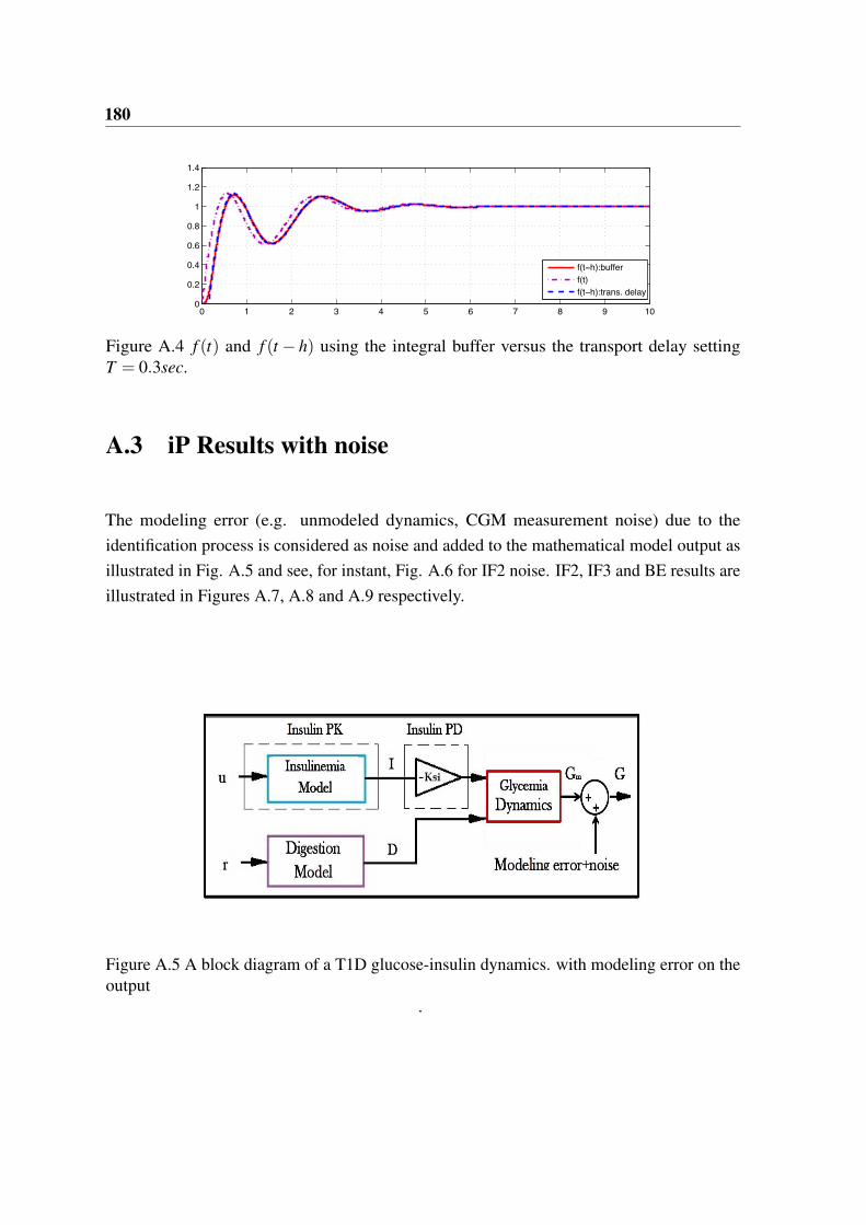
180
0 1 2 3 4 5 6 7 8 9 100
0.2
0.4
0.6
0.8
1
1.2
1.4
f(t−h):buffer
f(t)
f(t−h):trans. delay
Figure A.4 f (t) and f (t − h) using the integral buffer versus the transport delay settingT = 0.3sec.
A.3 iP Results with noise
The modeling error (e.g. unmodeled dynamics, CGM measurement noise) due to the
identification process is considered as noise and added to the mathematical model output as
illustrated in Fig. A.5 and see, for instant, Fig. A.6 for IF2 noise. IF2, IF3 and BE results are
illustrated in Figures A.7, A.8 and A.9 respectively.
Figure A.5 A block diagram of a T1D glucose-insulin dynamics. with modeling error on theoutput
.
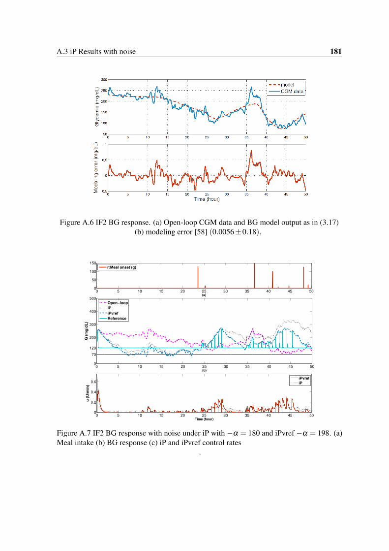
A.3 iP Results with noise 181
Figure A.6 IF2 BG response. (a) Open-loop CGM data and BG model output as in (3.17)(b) modeling error [58] (0.0056±0.18).
0 5 10 15 20 25 30 35 40 45 500
50
100
150
(a)
r:Meal onset (g)
0 5 10 15 20 25 30 35 40 45 500
70
120
200
300
400
500
(b)
G (
mg
/dL
)
Open−loop
iP
iPvref
Reference
0 5 10 15 20 25 30 35 40 45 500
0.2
0.4
0.6
Time (hour)
u (
U/m
in)
iPvref
iP
Figure A.7 IF2 BG response with noise under iP with −α = 180 and iPvref −α = 198. (a)Meal intake (b) BG response (c) iP and iPvref control rates
.
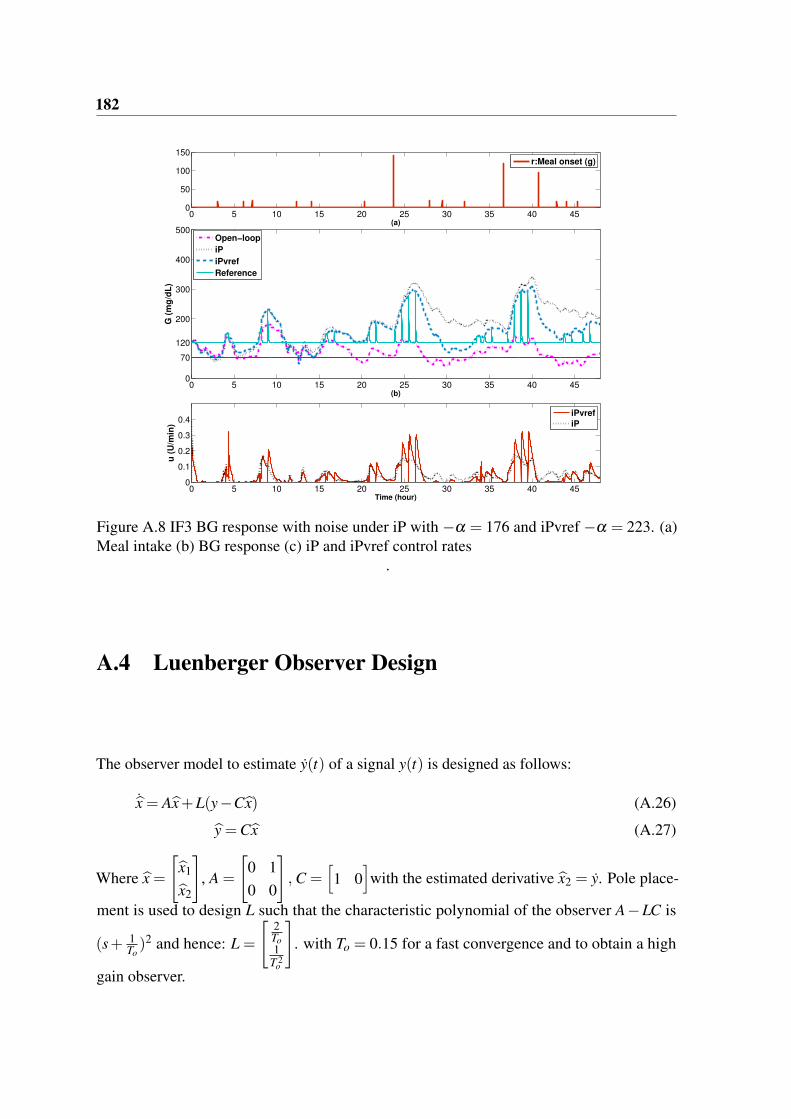
182
0 5 10 15 20 25 30 35 40 450
50
100
150
(a)
r:Meal onset (g)
0 5 10 15 20 25 30 35 40 450
70
120
200
300
400
500
(b)
G (
mg
/dL
)
0 5 10 15 20 25 30 35 40 450
0.1
0.2
0.3
0.4
Time (hour)
u (
U/m
in)
iPvref
iP
Open−loop
iP
iPvref
Reference
Figure A.8 IF3 BG response with noise under iP with −α = 176 and iPvref −α = 223. (a)Meal intake (b) BG response (c) iP and iPvref control rates
.
A.4 Luenberger Observer Design
The observer model to estimate y(t) of a signal y(t) is designed as follows:
bx = Abx+L(y−Cbx) (A.26)
by =Cbx (A.27)
Where bx ="bx1
bx2
#, A =
"0 1
0 0
#, C =
h1 0
iwith the estimated derivative bx2 = y. Pole place-
ment is used to design L such that the characteristic polynomial of the observer A−LC is
(s+ 1To)2 and hence: L =
"2To1
T 2o
#. with To = 0.15 for a fast convergence and to obtain a high
gain observer.
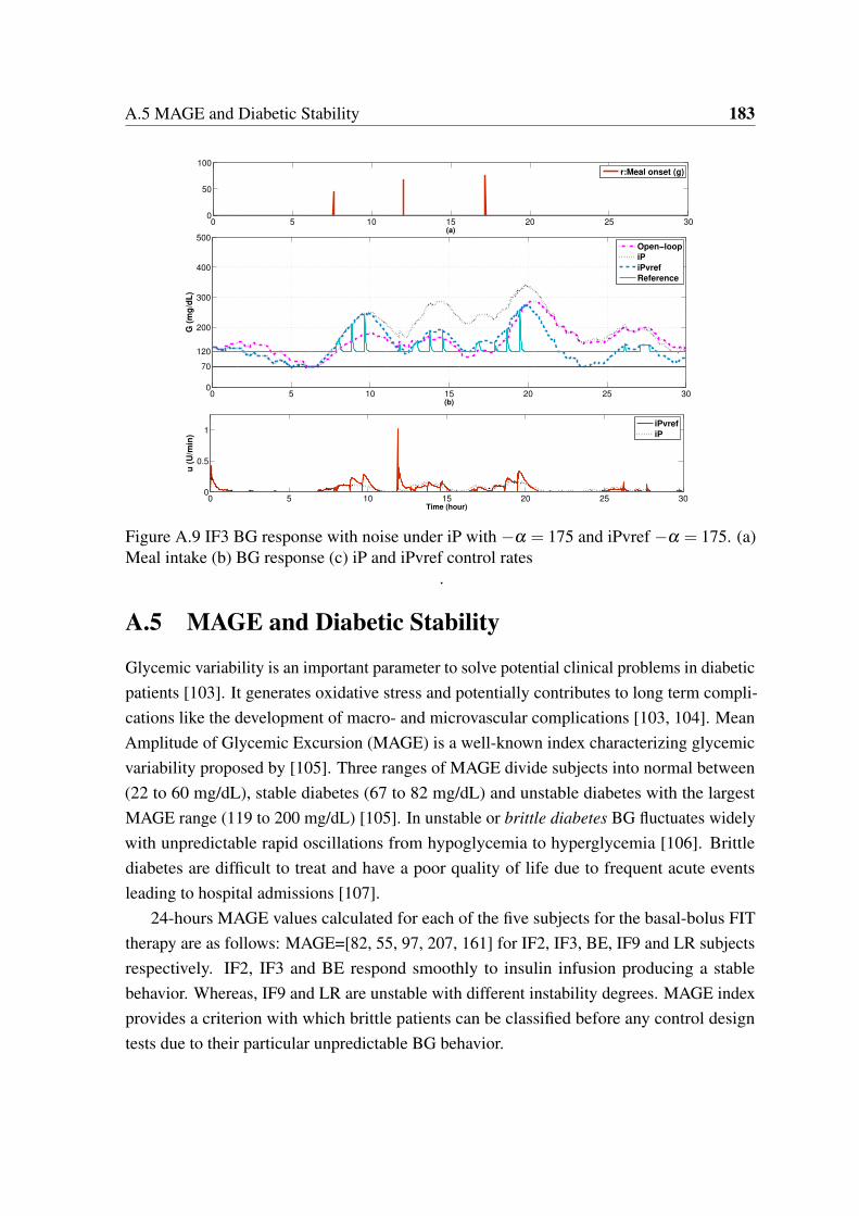
A.5 MAGE and Diabetic Stability 183
0 5 10 15 20 25 300
50
100
(a)
r:Meal onset (g)
0 5 10 15 20 25 300
0.5
1
Time (hour)
u (
U/m
in)
iPvref
iP
0 5 10 15 20 25 300
70
120
200
300
400
500
(b)
G (
mg
/dL
)
Open−loop
iP
iPvref
Reference
Figure A.9 IF3 BG response with noise under iP with −α = 175 and iPvref −α = 175. (a)Meal intake (b) BG response (c) iP and iPvref control rates
.
A.5 MAGE and Diabetic Stability
Glycemic variability is an important parameter to solve potential clinical problems in diabetic
patients [103]. It generates oxidative stress and potentially contributes to long term compli-
cations like the development of macro- and microvascular complications [103, 104]. Mean
Amplitude of Glycemic Excursion (MAGE) is a well-known index characterizing glycemic
variability proposed by [105]. Three ranges of MAGE divide subjects into normal between
(22 to 60 mg/dL), stable diabetes (67 to 82 mg/dL) and unstable diabetes with the largest
MAGE range (119 to 200 mg/dL) [105]. In unstable or brittle diabetes BG fluctuates widely
with unpredictable rapid oscillations from hypoglycemia to hyperglycemia [106]. Brittle
diabetes are difficult to treat and have a poor quality of life due to frequent acute events
leading to hospital admissions [107].
24-hours MAGE values calculated for each of the five subjects for the basal-bolus FIT
therapy are as follows: MAGE=[82, 55, 97, 207, 161] for IF2, IF3, BE, IF9 and LR subjects
respectively. IF2, IF3 and BE respond smoothly to insulin infusion producing a stable
behavior. Whereas, IF9 and LR are unstable with different instability degrees. MAGE index
provides a criterion with which brittle patients can be classified before any control design
tests due to their particular unpredictable BG behavior.

Taghreed MOHAMMADRIDHA
La Régulation Automatique de la Glycémie du Diabète de Type I
Automatic Glycemia Regulation of Type I Diabetes
Résumé
Cette thèse étudie le contrôle en boucle fermée pour la régulation de la glycémie du diabète de type 1 (DT1). Deux catégories principales de commande sont conçues: l'une est basée sur un modèle et l'autre non. Pour tester leur efficacité, les deux types sont testés in silico sur deux simulateurs de DT1. Le premier est un modèle à long terme qui est dérivé des données cliniques des sujets de DT1 et le second est le simulateur Uva/Padova. Tout d'abord, la commande sans modèle (CSM) est conçue. Après avoir montré qu'un régulateur proportionnel intelligent (iP) à référence constante peut être mis en défaut sur un simple second ordre, nous avons conçu un régulateur iP à référence variable. Une solution alternative est un régulateur proportionnel-intégral-dérivé intelligent (iPID) à référence constante. Une meilleure performance globale est obtenue avec iPID par rapport à iP et par rapport à un PID classique. Deuxièmement, une commande par modes glissants (CMG) garantie positive est conçue pour la première fois pour la régulation de la glycémie. La conception de cette commande est basée sur un modèle. La commande CMG est choisie pour la régulation de la glycémie en raison de ses propriétés de robustesse bien connues. Cependant, notre contribution majeure est l'assurance d'une commande rigoureusement positive. La commande CMG est conçue pour être positive partout dans un ensemble invariant du sous-système d'insulinémie du plasma. Enfin, un régulateur positif par retour d'état est calculé pour la première fois pour la régulation de la glycémie. Le plus grand ensemble positif invariant (EPI) est trouvé. Non seulement la positivité de la commande est révisée, mais plutôt un contrôle glycémique serré est atteint. Lorsque l'état initial du système appartient à l’EPI, l'hypoglycémie est évitée. Dans le cas contraire, l'hypoglycémie future est prédite pour tout état initial en dehors de l'EPI. Mots clés Diabète de type I, régulation de la glycémie, Commande
positive, prédiction de l'hypoglycémie, Ensemble
invariant, Insulin on board, Commande par modes
glissants, Commande sans modèle.
Abstract
This thesis investigates closed-loop control for glycemia
regulation of Type1 Diabetes Mellitus (T1DM). Two main
controller categories are designed: non-model-based and
model-based. To test their efficiency, both types are
tested in silico on two T1DM simulators.
The first is a long-term model that is derived from clinical
data of T1DM subjects and the second is the
Uva/Padova simulator. Firstly, Model-free Control (MFC)
is designed: a variable reference intelligent Proportional
(iP) control and a constant reference intelligent
Proportional-Integral-Derivative (iPID). Better overall
performance is yielded with iPID over iP and over a
classic PID. Secondly, a positive Sliding Mode Control
SMC is designed for the first time for glycemia regulation.
The model-based controller is chosen for glycemia
regulation due to its well-known robustness properties.
More importantly, our main contribution is that SMC is
designed to be positive everywhere in the positively
invariant set for the plasma insulin subsystem.
Finally, a positive state feedback controller is designed
for the first time to regulate glycemia. The largest
Positively Invariant Set (PIS) is found. Not only control
positivity is respected but rather a tight glycemic control
is achieved. When the system initial condition belongs to
the PIS, hypoglycemia is prevented, otherwise future
hypoglycemia is predicted for any initial condition outside
the PIS.
Key Words Type I Diabetes, Glycemia Regulation, Positive
Control, Hypoglycemia prediction, Positively
invariant set, Insulin on board, Sliding mode control,
Model-free control.