Automatic aviation safety reports classification - University of ...

1

Faculty of Electrical Engineering,Mathematics & Computer Science

Automatic aviationsafety reports classification

Andres Felipe Torres CanoM.Sc. ThesisAugust 2019

Supervisors:dr. C. Seifert

dr.ir. M. van Keulen

Faculty of Electrical Engineering,Mathematics and Computer Science

University of TwenteP.O. Box 217

7500 AE EnschedeThe Netherlands

This work is licensed under a Creative Commons “Attribution-ShareAlike 4.0 International” license.

https://creativecommons.org/licenses/by-sa/4.0/deed.en



Preface

This thesis is dedicated to my family, especially to my parents and future wife.I want to thank to my supervisors Christin and Maurice for their valuable guidance and

feedback. I also extend my gratitude to all the great lecturers that I had at UTwente.In the same way, thanks to all my colleagues at KLM, to my manager Bertjan and my

great friend Arthur.

iii

IV PREFACE

Abstract

In this master thesis we present an approach to automatically classify aviation safety reportsby applying supervised machine learning. Our proposed model is able to classify 7 differenttypes of safety reports according to a taxonomy hierarchy of more than 800 labels using adataset with 19 815 reports which is highly imbalanced. The reports comprise numerical,categorical and text fields that are written in english and dutch languages. Such reports aremanually categorized by safety analysts in a multi-label setting. The reports are later aggre-gated according to such taxonomies and reported in dashboards that are used to monitorthe safety of the organization and to identify emerging safety issues. Our model trains oneclassifier per each type of report using a LightGBM base classifier in a binary relevancesetting, achieving a final macroaveraged F0.5 score of 50.22%. Additionally, we study theimpact of using different text representation techniques in the problem of classifying aviationsafety reports, concluding that term frequency (TF) and term frequency inverse documentfrequency (TF-IDF) are the best methods for our setting. We also address the imbalancedlearning problem by using SMOTE oversampling, improving our classifier performance by41%. Furthermore, we evaluate the impact of using hierarchical classification in our classi-fier with results suggesting that it does not improve the performance for our task.

Finally, we run an experiment to measure the reliability of the manual classification pro-cess that is carried out by the analysts using Krippendoff’s mvα. We also present somesuggestions to improve such process.

v

VI ABSTRACT

Contents

Preface iii

Abstract v

1 Introduction 11.1 Problem Statement . . . . . . . . . . . . . . . . . . . . . . . . . . . . . . . . . 21.2 Research Questions . . . . . . . . . . . . . . . . . . . . . . . . . . . . . . . . 31.3 Outline . . . . . . . . . . . . . . . . . . . . . . . . . . . . . . . . . . . . . . . . 3

2 Background 52.1 Operational Risk Management . . . . . . . . . . . . . . . . . . . . . . . . . . 52.2 Machine Learning . . . . . . . . . . . . . . . . . . . . . . . . . . . . . . . . . 62.3 Text Classification . . . . . . . . . . . . . . . . . . . . . . . . . . . . . . . . . 62.4 Multi-label Classification . . . . . . . . . . . . . . . . . . . . . . . . . . . . . . 72.5 Text Representation . . . . . . . . . . . . . . . . . . . . . . . . . . . . . . . . 82.6 Inter-annotator Agreement . . . . . . . . . . . . . . . . . . . . . . . . . . . . . 82.7 Imbalanced Learning . . . . . . . . . . . . . . . . . . . . . . . . . . . . . . . . 102.8 Metrics . . . . . . . . . . . . . . . . . . . . . . . . . . . . . . . . . . . . . . . 10

3 Related Work 133.1 Extreme Multi-label Classification . . . . . . . . . . . . . . . . . . . . . . . . . 143.2 Hierarchical Text Classification . . . . . . . . . . . . . . . . . . . . . . . . . . 15

4 Dataset 17

5 Methodology 23

6 Experimental Setup 256.1 Baseline . . . . . . . . . . . . . . . . . . . . . . . . . . . . . . . . . . . . . . . 256.2 Pre-processing . . . . . . . . . . . . . . . . . . . . . . . . . . . . . . . . . . . 266.3 Multi-label Classification . . . . . . . . . . . . . . . . . . . . . . . . . . . . . . 266.4 Text Representation . . . . . . . . . . . . . . . . . . . . . . . . . . . . . . . . 276.5 Imbalanced Learning . . . . . . . . . . . . . . . . . . . . . . . . . . . . . . . . 276.6 Hierarchical Classification . . . . . . . . . . . . . . . . . . . . . . . . . . . . . 286.7 Classifier Per Report Type . . . . . . . . . . . . . . . . . . . . . . . . . . . . . 28

vii

VIII CONTENTS

6.8 Technical Evaluation . . . . . . . . . . . . . . . . . . . . . . . . . . . . . . . . 296.9 Human Evaluation . . . . . . . . . . . . . . . . . . . . . . . . . . . . . . . . . 29

7 Results & Discussion 317.1 Baseline Evaluation . . . . . . . . . . . . . . . . . . . . . . . . . . . . . . . . 317.2 Machine Learning Models Evaluation . . . . . . . . . . . . . . . . . . . . . . . 327.3 Text Representation Evaluation . . . . . . . . . . . . . . . . . . . . . . . . . . 327.4 Imbalanced Learning Evaluation . . . . . . . . . . . . . . . . . . . . . . . . . 327.5 Hierarchical Classification Evaluation . . . . . . . . . . . . . . . . . . . . . . . 357.6 Classifier Per Type of Report Results . . . . . . . . . . . . . . . . . . . . . . . 357.7 Inter-annotator Agreement . . . . . . . . . . . . . . . . . . . . . . . . . . . . . 357.8 Comparison to Related Work . . . . . . . . . . . . . . . . . . . . . . . . . . . 38

8 Conclusion 398.1 Conclusion . . . . . . . . . . . . . . . . . . . . . . . . . . . . . . . . . . . . . 398.2 Limitations . . . . . . . . . . . . . . . . . . . . . . . . . . . . . . . . . . . . . 408.3 Recommendations for the Company . . . . . . . . . . . . . . . . . . . . . . . 418.4 Future Work . . . . . . . . . . . . . . . . . . . . . . . . . . . . . . . . . . . . . 41

References 43

Appendices

A Appendix 49A.1 Summary of Notation . . . . . . . . . . . . . . . . . . . . . . . . . . . . . . . . 49A.2 Parameters . . . . . . . . . . . . . . . . . . . . . . . . . . . . . . . . . . . . . 49A.3 Human Evaluation Interface . . . . . . . . . . . . . . . . . . . . . . . . . . . . 51

Chapter 1

Introduction

With approximately 35 000 employees and moving more than 32 million passengers, KLMis one of the leading airlines in Europe. Safety is of vital importance in the aviation industryand it is managed at KLM by the Integrated Safety Management System (ISMS). One of theprocesses in the ISMS is to collect and analyze safety reports. The reports are reviewed byanalysts and categorized with one or more labels that are called taxonomies. Such reportsare aggregated according to such taxonomies and reported in dashboards that are usedto monitor the safety of the organization and to identify emerging safety issues. Today,the taxonomy classification is done manually and it is the desire of the management thatsuch categorization is performed automatically because it is expected that the number ofreceived reports is going to increase in the following year. Additionally, the management hasalso expressed concerns about the consistency of the report categorization. There is animpression that the categorization process varies significantly. This means that one reportthat is categorized today with certain labels would get a slightly different categorization if it iscategorized again in one month. Such situation can negatively affect the trust that is given tothe aggregated information that is used to monitor the safety of the organization. Therefore,there is a need to check the categorization process and to measure the trust in the data.

This master thesis presents our approach to automatically classify the safety reports byapplying supervised machine learning. In the same way, the development of this researchdelivers important insights about the categorization process and how can it be improved.Firstly, exploratory data analysis (EDA) is used to understand the dataset and to devise themachine learning techniques that can be applied. Secondly, a quick baseline with a logisticregression classifier and a multi-label decision tree is established to serve as a starting pointfor the automatic classification. Such baseline is used to identify the pre-processing stepsthat need to be applied to the dataset and to identify the machine learning techniques thatwill be evaluated. Then, a set of experiments is designed to collect results that support theanswers to our research questions. Next, the results of our experiments are analyzed andconclusions are derived.

1

2 CHAPTER 1. INTRODUCTION

1.1 Problem Statement

The main goal of this research is to automatically classify the different safety reports ac-cording to the defined taxonomy. Each taxonomy is a set of labels organized as a hierarchy.There are 7 different types of reports. Each report can be categorized with one or morelabels from different taxonomies. The taxonomies that can be applied to each type of reporthave been established by the company. Due to the business requirements, it is not nec-essary to focus on the zero-shot learning problem, meaning that it is not important to havegood performance on labels with a few examples.

The secondary goal is to examine the current data generation process, to measure itsreliability and to issue recommendations to improve it.

The main problem can be posed as a multi-label classification task, where N is thenumber of instances in the dataset S. Having xi to be one example and X the set of allexamples, yi is the ordered tuple of labels associated to one example and Y the set of alltuples containing labels. yi represents one single label and L is the number of unique labelsin Y. More formally:

S = {(xi,yi)|1 ≤ i ≤ N,xi ⊆ X,yi ⊆ Y}

L = |Y|

yi = (y1, y2, ..., yL), yi ∈ {0, 1}

A single taxonomy ti = (vi, ei) is a tree that is considered a rooted directed acyclic graph(DAG) with root ρ by definition [1] [2]. All the taxonomies comprise the set T of such graphs:

T = {(v1, e1) , (v2, e2) , ..., (vK, eK) |vi \ {ρi} ∩ vj \ {ρj} , i 6= j}

vi = {y1,y2, ...,yi|yi ⊆ Y}

ei = {(yi,yj)|yi ⊆ Y,yj ⊆ Y, i 6= j}

After inspecting the taxonomies used to classify the aviation safety reports, we observedthat the mentioned taxonomies exhibit the following properties:

• A single label yi only belongs to one taxonomy, meaning that each taxonomy is acomplete independent tree.

• The root of each taxonomy ρ is not considered a label and it is excluded from ouranalysis because it can be derived from the report type.

A summary of notation is displayed in Appendix A.1.

1.2. RESEARCH QUESTIONS 3

1.2 Research Questions

The proposed approach is to apply supervised machine learning to automatically classifythe reports. In order to solve it, we will address the following research questions:

• RQ1: What are the influencing factors on the accuracy of applying supervised machinelearning to classify aviation safety reports automatically? As influencing factors weinvestigate feature representation and classification model types. More concretely, wewant to evaluate what is the impact of using word embeddings over TF-IDF?, whatis the impact of using different multi-label learning models? and does hierarchicalclassification perform better than flat classification?

• RQ2: How can we measure the reliability of the report classification process that isperformed by human analysts? With this question we aim to discover the metric thatis more suitable for measuring such reliability.

1.3 Outline

This thesis is structured as follows: Chapter 2 introduces the background and Chapter 3 il-lustrates the related work. Chapter 4 presents the dataset and the exploratory data analysis.Chapter 5 describes the research methods used. In Chapter 6 we detail the different exper-iments that were performed. The results of such experiments are displayed and discussedin Chapter 7. Finally, this thesis concludes in Chapter 8.

4 CHAPTER 1. INTRODUCTION

Chapter 2

Background

In the following sections we introduce some background concepts. Section 2.1 describesOperational Risk Management. Section 2.2 provides a brief introduction to machine learn-ing, while Section 2.3 introduces text classification. Section 2.4 presents multi-label clas-sification. Section 2.5 focuses on text representation and inter-annotator agreement is ex-plained in Section 2.6. Section 2.7 introduces imbalanced learning. The metrics that will beused in this thesis are presented in Section 2.8.

2.1 Operational Risk Management

Operational Risk Management (ORM) is a key component of every Safety Management Sys-tem implemented in any aviation organization. The main objective for ORM is “to make surethat all risks remain at an acceptable level” [3]. Many methodologies for ORM contemplatesome kind of hazard identification where collecting and analyzing safety data is at the core ofthe process. Such data typically includes flight data events, safety reports, safety surveys,audit results and other type of data that are stored in a safety database. “The databaseshould be routinely analysed in order to detect any adverse trends and to monitor the ef-fectiveness of earlier risk reduction actions. This analysis may lead to the identification ofa potential Safety Issue which needs to be formally risk assessed to determine the level ofrisk and to design appropriate risk reduction measures” [3].

The data stored in the safety database are further enriched using descriptors or keywordsin order to expedite reporting and trend analysis. According to the International Civil Avia-tion Organization Safety Management Manual, “Safety data should ideally be categorizedusing taxonomies and supporting definitions so that the data can be captured and storedusing meaningful terms ... Taxonomies enable analysis and facilitate information sharingand exchange” [4]. The descriptors or taxonomies are applied with the primary objective ofidentifying any safety issues that affect the current operation.

A practical requirement that has been established is that the method for applying tax-onomies should be easy to use and not create an unreasonable workload [3]. Given thefact that large airlines may have to process several hundred safety reports per month, goodtools and automation are critical success elements in Safety Management Systems. This

5

6 CHAPTER 2. BACKGROUND

last requirement can be accomplished by employing different machine learning techniquesto apply the taxonomies in an automated manner.

2.2 Machine Learning

Machine learning can be defined “as a set of methods that can automatically detect pat-terns in data, and then use the uncovered patterns to predict future data, or to perform otherkinds of decision making under uncertainty” [5]. Machine learning pretends to create modelsthat learn such patterns without manually hard-coding the patterns. Many daily tasks thathumans perform can be automated using it. Machine learning powered systems can trans-late text and speech, perform spam detection, detect faces in pictures, detect fraudulenttransactions and predict passenger flow in an airline, just to name a few examples.

The methods used in machine learning are generally categorized in two broad groups:supervised learning and unsupervised learning. In supervised machine learning, “the avail-able data includes information about the correct way to classify at least some of the data” [6],in other words, the data contains examples and “each example is also associated with a la-bel or target” [7]. In unsupervised learning, the examples in the dataset contain no targetsor labels and the algorithms are used to “learn useful properties of the structure of thisdataset” [7].

2.3 Text Classification

Text classification or categorization is “the activity of labeling natural language texts withthematic categories from a predefined set” [8]. Such texts include documents, forms, books,social media messages and more. Labeling refers to the process of annotating each doc-ument with the categories [9]. Text classification can be performed manually by a humanor automatically using machine learning. The latter approach has been effective, reaching“an accuracy comparable to that achieved by human experts, and a considerable savings interms of expert labor power, since no intervention from either knowledge engineers or do-main experts is needed for the construction of the classifier or for its porting to a different setof categories” [8]. Automated text classification is covered by the field of supervised learn-ing, although unsupervised techniques could be used to improve the classification accuracy.Please refer to [8] for an introduction to text classification using machine learning. [10] pro-vide an extensive survey on different approaches to perform automatic text classification.Given that the safety reports mainly comprise text, the methods and techniques in the areaof text classification are crucial to fulfill our objective of classifying automatically such re-ports. As one report can be labeled with one or more taxonomies, it is necessary to exploremulti-label classification models.

2.4. MULTI-LABEL CLASSIFICATION 7

2.4 Multi-label Classification

Most of the machine learning classification techniques that can be applied to the text cat-egorization problem are developed to assign a single label from a set of categories to thedocument. This means that the categories are mutually exclusive and this is called multi-class classification. In contrast, assigning multiple classes that are not mutually exclusive iscalled multi-label, any-of or multi-value classification [9].

According to [11], the assumptions for this multi-label problem settings are:

1. The set of labels is predefined, meaningful and human-interpretable (albeit by an ex-pert), and all relevant to the problem domain.

2. The number of possible labels is limited in scope, such that they are human-browsable,and typically not greater than the number of attributes.

3. Each training example is associated with a number of labels from the label set.

4. The number of attributes representing training examples may vary, but there is no needto consider extreme cases of many thousands of attributes since attribute-reductionstrategies can be employed in these cases.

5. The number of training examples may be large - a multi-label classifier may have todeal with potentially hundreds of thousands of examples.

Additionally, [12] expands the multi-label settings with the following:

6. Labels may be correlated.

7. Data may be unbalanced.

Multi-label learning methods are categorized in three groups: problem transformation, al-gorithm adaptation and ensemble methods. The problem transformation approach convertsor decomposes the multi-label problem in one or several single-label (multi-class) problemsthat can be solved using classical machine learning algorithms. The algorithm adaptationmethod consists of modifying or creating new machine learning algorithms to learn frommulti-label data. Ensemble methods combine these two approaches or use traditional en-semble methods like bagging. Refer to [12] and [13] for an introduction and comparison ofmethods for multi-label learning.

One problem transformation method that is worth mentioning is called Binary Relevance(BR) which consists in training one base classifier per each label. The base classifier canuse logistic regression, support vector machines or any other binary classifier. BR is astraightforward method to implement that gives a good baseline for multi-label learning. Themain disadvantage is that training one classifier per label is not efficient and it can becomeprohibitive in problems with a lot of labels.

[13] evaluated several multi-label methods and concluded that the best performing meth-ods across all tasks are RF-PCT and HOMER [14], followed by BR (Binary Relevance) and


CC (Classifier chains) [11], using SVM and decision trees as base classifiers. [15] proposethe multi-label informed feature selection framework (MIFS), that performs feature selec-tion in multi-label data, exploiting label correlations to select discriminative features acrossmultiple labels. [16] introduce extreme learning machine for multi-label classification (ELM-ML). ELM-ML outpeformed other evaluated methods in most of the experiments in terms ofprediction and test time. [17] propose the canonical-correlated autoencoder (C2AE) whichis a deep learning approach that outpeforms other models. Unfortunately, C2AE is onlyevaluated in one text dataset and the authors do not provide a performance reference forthis single dataset. [18] propose GroPLE, a method that uses a group preserving label em-bedding strategy to transform the labels to a low-dimensional label space while retainingsome properties of the original group. This approach performs better than other evaluatedmethods in most of the experiments.

The methods mentioned in the previous paragraph could serve as a starting point forthis thesis. However, the main disadvantage detected in the analyzed literature is that mostmulti-label methods proposed are tested on datasets with small label cardinality, while ourproblem deals with 800 labels approximately. One popular dataset with a label cardinalitysimilar to our problem is the Delicious dataset [14], hence methods that perform well in suchdataset will be prioritized.

2.5 Text Representation

Most of the machine learning models receive matrices with numbers as input. An activearea of research is how to transform the given text into a suitable input for the machinelearning models. “A traditional method for representing documents is called Bag of Words(BOW). This representation technique only includes information about the terms and theircorresponding frequencies in a document independent of their locations in the sentence ordocument” [10]. Other traditional approaches are n-grams, TF and TF-IDF. Please referto [19] for an introduction to such techniques. Modern approaches are word2vec [20], GloVe[21], fastText [22], ELMo [23] and BERT [24]. BERT is the current state of the art model fortext representation. For the scope of this project, it is really important to find a good textrepresentation that maximizes the predictive capacity of the developed classification model.

2.6 Inter-annotator Agreement

The safety data mentioned in Section 2.1 are classified according to the defined taxonomiesby event analysts that are also called coders or annotators. Such analysts are humans and itis expected to find some variability in their judgments due to different causes like experience,training and personal circumstances. Therefore, inter-annotator agreement is measured withthe objective of assessing the reliability of the annotations given by the annotators.

According to Krippendorff “reliability is the degree to which members of a designatedcommunity agree on the readings, interpretations, responses to, or uses of given texts or

2.6. INTER-ANNOTATOR AGREEMENT 9

data” [25]. Such definition is given in the field of content analysis, where researchers analyzedifferent media (books, newspapers, TV, radio, articles, photographs, etc) with the objectiveof drawing some conclusions. In this context, the researchers demonstrate the trustwor-thiness of their data and the reproducibility of their experiments by providing a measure ofreliability. In other words, “it represents the extent to which the data collected in the studyare correct representations of the variables measured” [26]. Such definitions are applicableto our task because the taxonomies are applied with the primary objective of identifying anysafety issues that affect the current airline operation.

There are several coefficients to measure the inter-annotator agreement. The mostused coefficients are percentage agreement; Cohen’s κ; Bennett, Alpert, and Goldstein’sS; Scott’s π and Krippendorff’s α [27]. Most of such proposed scores are defined for binaryor multi-class settings but not for multi-label experiments. Some extensions to such methodshave been proposed to support multi-label tasks. We will use Krippendorff’s α because ithas been proved that Cohen’s κ tends to overestimate the agreement. Scott’s π is similarto Krippendorff’s α, and the most notable difference is that the latter corrects for small sam-ple sizes [25]. Additionally, Krippendorff’s α can be used in multi-label settings. It is alsoapplicable to any number of annotators in contrast to the majority of agreement scores thatare only applicable to two annotators. Furthermore, it is chance-corrected, meaning that itwill discount the agreement that is achieved just by chance. Moreover, it can be applied toseveral type of variables (nominal, ordinal, interval, etc) and to any sample size. Finally, itcan be applied to data with missing values. This choice is aligned with the suggestions givenin [27].

Krippendorff’s α assume that different annotators produce similar distributions in theirannotator scheme, while Cohen’s κ calculate the distributions among the coders that pro-duced the reliability data. As we will see in future chapters, the dataset was produced bydifferent analysts that were changing across time, confirming that for our case Krippendorff’sα is a more suitable metric.

Krippendorff’s α is defined as “the degree to which independent observers, using the cat-egories of a population of phenomena, respond identically to each individual phenomenon”.In order to calculate the mentioned agreement, we will use the multi-valued mvα for nominaldata as proposed in [28]:

mvα = 1− mvDo

mvDe

Where mvDo is the observed disagreement for multi-value(multi-label) and mvDe is theexpected disagreement for multi-value data.

It is worth noting that it has been demonstrated “that agreement coefficients are poorpredictors of machine-learning success” [27]. However, an acceptable level of agreementamong the analysts is needed as a starting point to assure that the dataset is reliable andthat there is some consistency in the labels that are used to train the machine learningalgorithm.


2.7 Imbalanced Learning

The performance of most machine learning algorithms can be seriously affected by datasetsthat contain labels or classes with examples that are not evenly distributed. It is common tofind datasets including a class with hundreds of examples and another class with less thanten of them. In some cases, the classes with the most examples will get good predictingperformance while the minority classes will get poor performance. Depending on the usecase, this poor performance in the minority classes could be ignored, but other cases requirethe underrepresented classes to perform well.

Researchers have proposed different techniques to address this issue. One way to dealwith such problem consists of assigning weights or costs to the examples. Some machinelearning classification techniques can be extended to re-weight their predictions in order tocounter the data imbalance. Popular machine learning implementations of logistic regres-sion, decision trees, support vector machines, random forest, between others, support thementioned weighting technique. Another popular method is under-sampling the majorityclass. This includes randomly selecting examples until a desired ratio between the majorityand minority class is achieved. Other techniques include using clustering or nearest neigh-bors to select the subsample [29]. The last method to improve the imbalanced learningproblem is to perform over-sampling of the minority class. This could be done either by re-sampling the data with replacement or to generate synthetic data from the minority class bythe use of some technique [30].

2.8 Metrics

In the following section, several metrics are presented. Firstly, classical machine learningevaluation measures are defined to allow easy comparison with other models. Then, metricsthat are used to characterize the dataset are described.

True positives (TP) are the number of examples correctly predicted as having a givenlabel.

False positives (FP) are the number of examples incorrectly predicted as having a givenlabel.

False negatives (FN) are the number of examples incorrectly predicted as not having agiven label.

Precision (P) is the fraction of correctly predicted labels over all the predicted labels.

Precision =TP

TP + FP

Recall (R) is the fraction of correctly predicted labels over the labels that were supposedto be predicted.

Recall =TP

TP + FN

2.8. METRICS 11

F Measure (Fβ) is a “single measure that trades off precision versus recall” [9]:

Fβ =(β2 + 1)PR

β2P +R

In this thesis, we will use Fβ=1 also known as F1 that balances both precision and recall.Due to business needs, it is the desire of the management to emphasize precision, therefore,Fβ=0.5 (F0.5) will be used as our primary metric.

Macroaveraging computes a simple average over the labels by evaluating the metriclocally for each category and then globally by averaging over the results of the differentcategories [8] [9].

Microaveraging aggregates the TP, FP and FN results together across all classes andthen computes the global metric.

Microaveraging is driven by the performance of the classes with more examples, mean-while macroaveraging gives equal importance to each class, making it suitable to evaluatethe overall model performance in presence of imbalanced datasets.

Label average (LAvg) is the average number of labels per example:

LAvg(S) =1

N

N∑i=1

|yi|

Label density (LDen) is the label average divided by the number of labels:

LDen(S) =1

N

N∑i=1

|yi|L

=LAvg(S)

L

Chapter 3

Related Work

This section describes the related work. We analyze the work that has been done to classifyaviation safety reports automatically. Furthermore, we describe state of the art research thatcan be applied to answer our research questions.

Different Natural Language Processing (NLP) techniques are applied in [31] to create anaviation safety report threshold-based classifier using correlations between the labels andthe extracted linguistic features. The authors identify some linguistic characteristics that arespecific to the aviation domain:

• There are many acronyms are used and they need to be grouped or expanded. Forexample, “A/C” could be expanded into “aircraft” and “TO” means “take-off”.

• Some terms that appear in the reports are considered conceptually equivalent, forexample “bad weather” and “poor weather”.

This research is different from [31] in the way that more sophisticated NLP and machinelearning techniques are used to classify the safety reports. Some of the authors’ ideas aboutthe linguistic processing of the reports are worth considering for this work.

[32] apply NLP and machine learning techniques to classify aviation safety reports andto suggest emerging patterns that can be incorporated to improve the taxonomy used. Theydevelop a tool for report retrieval as well. Furthermore, the authors offer an introduction tothe overall process of safety reporting in the aviation industry.

The main difference from [32] is that this research aims to classify 7 different types ofreports with different types of fields, while the authors focus in one type of report using onlya text field. Additionally, the taxonomy trees used are limited to a maximum height of 2 with37 labels, while our height is up to 4 and more than 800 labels. To solve the multi-labelclassification problem they used BR with SVM as base classifier, therefore, 37 different clas-sifiers were trained. The authors have specifically refrained from applying machine learningtechniques to a problem with such a big number of categories like ours.

13

14 CHAPTER 3. RELATED WORK

3.1 Extreme Multi-label Classification

Extreme multi-label classification or learning is a challenging problem that tries to classifydocuments in multi-label settings with thousands or millions of labels. This problem differsfrom [11] assumptions as follows:

1. The number of possible labels are not limited in scope anymore, they are not human-browsable and they could be greater than the number of attributes.

2. There are many labels that have no examples or just a few examples associated.

Having such a big label space, BR methods that train one classifier per each label can becomputationally expensive and prediction time could be high as each classifier needs to beevaluated. Therefore, most approaches used to solve the extreme multi-label classificationare either based on trees or on embeddings [33] and BR is not even considered. Embed-ding methods transform the labels by creating a mapping to a low-dimensional space. Aclassifier is trained on such low-dimensional space, which should perform better due to thecompressed space. After the prediction task, the results need to be mapped back to theoriginal label space. Embedding methods primarily focus on improving the compression ormapping by preserving different properties from the original label space. Tree methods tryto learn a hierarchy from the data. Such hierarchy is exploited to gradually reduce the labelspace as the tree is traversed, improving prediction time and having comparable accuracy.

A tree based method called FastXML is proposed in [33]. FastXML learns an ensembleof trees, creating a hierarchy over the feature space. It performs significantly better thanmulti-label random forests (MLRF) and LPSR. Additionally, it scales efficiently in problemswith millions of labels. The authors evaluated FastXML in medium and large datasets. Anembedding based method is used in SLEEC which learns “a small ensemble of local dis-tance preserving embeddings which can accurately predict infrequently occurring (tail) la-bels” [34]. SLEEC outperforms FastXML in most of the experiments run by the authors. [35]propose DiSMEC that outperforms FastXML and SLEEC in most of the experiments. [36]build on top of FastXML two new methods called PfastXML and PfastreXML. Both outper-form FastXML and SLEEC by a large margin. It is important to note that DiSMEC, PfastXMLand PfastreXML were not evaluated in a dataset with a label cardinality similar to our problemsuch as Delicious [14]. DXML is proposed in [37], establishing a deep learning architecturewith graph embeddings. The embeddings consist of modeling the label dependencies witha graph. DXML outperforms SLEEC and FastXML in most of the experiments. However,FastXML performs better in the Delicious dataset. XML-CNN is presented in [38] proposinga simple deep learning architecture that outperforms FastXML and SLEEC in most of theexperiments. The experiments do not include a dataset with a label cardinality similar toour problem. Even though extreme multi-label classification methods are optimized for prob-lems with thousands or millions of labels, some of them seem to perform reasonably wellon datasets with hundreds of labels, like the one used in this research. Consequently, it isworth considering some of these methods for our evaluations.

3.2. HIERARCHICAL TEXT CLASSIFICATION 15

3.2 Hierarchical Text Classification

Hierarchical text classification is a specific case of text classification where the labels areorganized in a hierarchical structure, in the same way that the taxonomies for safety reportsare organized. A simple approach for this problem is to ignore the hierarchical structureof the labels, flattening them and using a multi-label classifier. Other approaches try toexploit the hierarchy, decomposing the classification problem into a small sets of problems[39]. Basic approaches to solve this problem are presented in [39] and [40]. [41] proposea byte level n-grams and a hierarchical classification approach using kNN and SVM. Theauthors define the approach local classifier per parent node (LCPN). This method is similarto the one in [40]. A deep learning model called hierarchically regularized deep graph-CNN(HR-DGCNN) is proposed in [42]. Such approach outperforms XML-CNN. As hierarchicaldatasets are scarce, HR-DGCNN is only evaluated in two datasets, none of them with alabel cardinality similar to our problem.

16 CHAPTER 3. RELATED WORK

Chapter 4

Dataset

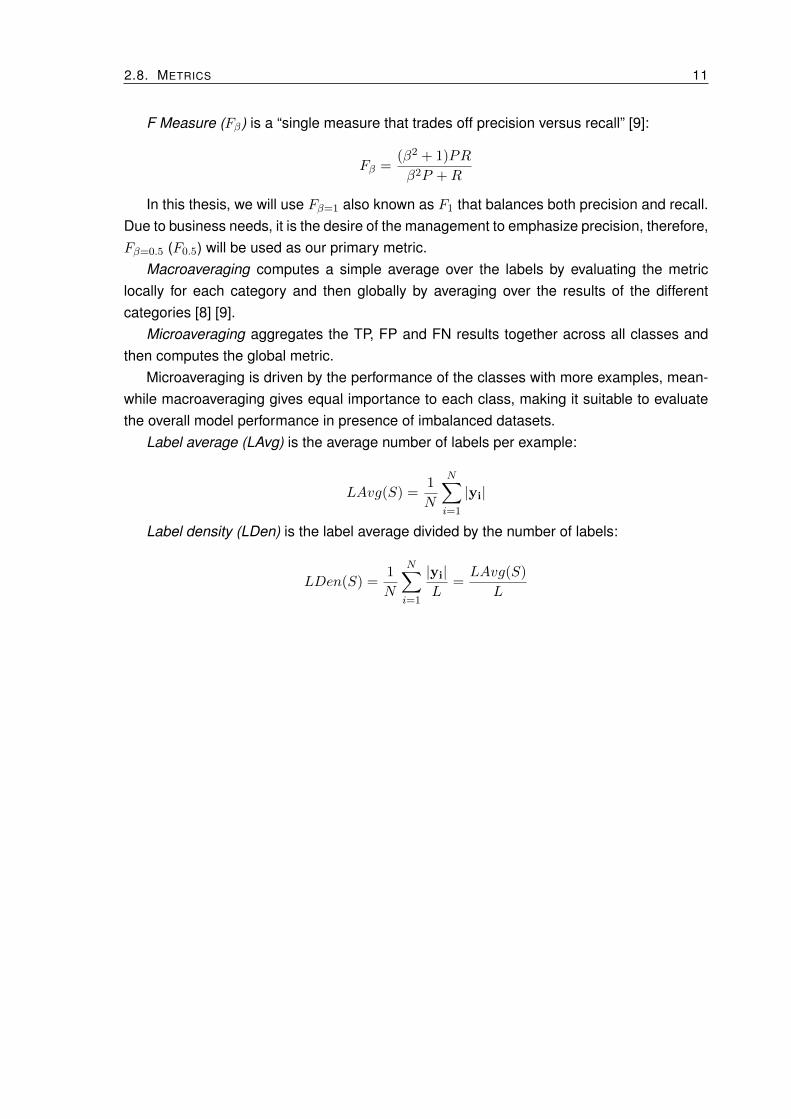
The dataset used for this research contains 19 815 samples. Each sample represents afilled report that has been categorized with one or more labels. There are 7 different types ofreports that share some fields, but most of the fields are unique for each type of report. Thefields contain text written using natural language in english and dutch. There are also date,numerical and categorical fields. The dataset contains 196 fields in total and it comprisesreports from July 2016 to February 2019. The layout of one of such report types is shown inFigure 4.1.

There are 859 unique labels. Such labels are clustered in 13 different taxonomies asshown in Table 4.1.

Such taxonomies represent an entire hierarchy of labels, meaning that each taxonomyis a tree-like structure. The max height of a tree is 4, but most of them are 3. Here are someexamples of such hierarchies:

G. External

G.3 External factors

G.3.1 Drone

G.3.2 Kite

G.3.3 Laser

G.3.4 Volcanic ash

H. Flight

H.13 Wildlife strike

H.13.1 Birdstrike - Miscellaneous

H.13.2 Multiple Birdstrike

H.13.3 Single Birdstrike

H.13.4 Wildlife strike

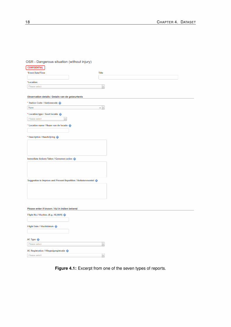
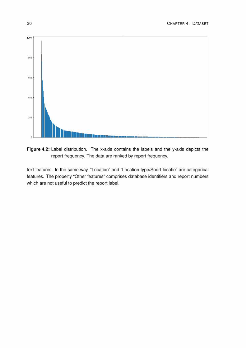
Each label has 44.99 examples on average (LAvg) with a standard deviation of 93.53.The label density (LDen) is 0.0524. There are 72 labels with only one example. Figure 4.2

17

18 CHAPTER 4. DATASET

Figure 4.1: Excerpt from one of the seven types of reports.

19

Table 4.1: The different taxonomies in the dataset with the number of reports that have beencategorized with labels belonging to that taxonomy.

Taxonomy Frequency

A. Cargo 403B. Consequences 3126C. Environmental Safety - (Possible) Consequences 642D. Environmental Safety - Causes 215E. Environmental Safety - Event types 218F. Environmental Safety - Processes 235G. External 1262H. Flight 4477I. Ground 3671J. Inflight 3970K. Occupational Safety Causes 7161L. Occupational Safety Impacts 2101M. Technical 1244

Table 4.2: The different report types in the dataset with the number of reports per each type.

Report Type Frequency

ASR - Air Safety Report 8461CIR - Cargo Incident Report 386ENV - Environmental Safety Report 635GHR - Ground Handling Safety Report 3004OSR - Accident with Injury 2598OSR - Dangerous situations (without injury) 3462VSR - Voluntary Safety Report 1269

displays the histogram for the labels. It can be observed that such histogram is similar to apower-law distribution, a typical characteristic for multi-label problems.

Table 4.2 displays the different report types along with its report frequency. The airsafety reports (ASR) account for almost half of the examples, followed by occupational safetyreports for dangerous situation (OSR without injury).

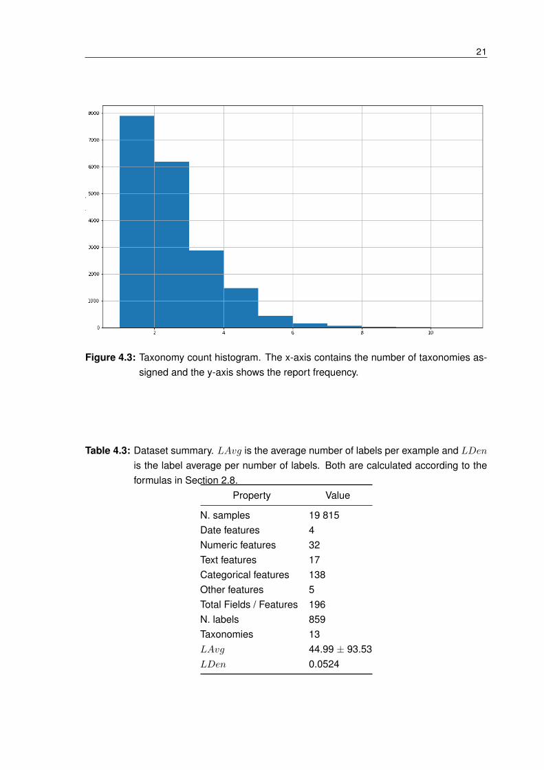
Figure 4.3 depicts the histogram of the number of taxonomies assigned to a report. Itcan be seen that almost eight thousand reports have been labeled with one taxonomy andaround six thousand have been labeled with two taxonomies. This means that near 73% ofthe reports have been classified with one to two taxonomies. On average, each report has2.02 taxonomies assigned with a standard deviation of 1.17.

Finally, Table 4.3 contains a summary of the dataset properties. The mentioned fea-tures correspond to the different fields that a report contains. For example, the field “EventDate/Time” in Figure 4.1 is one date feature, while “Title” and “Description/Beschrijving” are


Figure 4.2: Label distribution. The x-axis contains the labels and the y-axis depicts thereport frequency. The data are ranked by report frequency.

text features. In the same way, “Location” and “Location type/Soort locatie” are categoricalfeatures. The property “Other features” comprises database identifiers and report numberswhich are not useful to predict the report label.

21

Figure 4.3: Taxonomy count histogram. The x-axis contains the number of taxonomies as-signed and the y-axis shows the report frequency.

Table 4.3: Dataset summary. LAvg is the average number of labels per example and LDenis the label average per number of labels. Both are calculated according to theformulas in Section 2.8.

Property Value

N. samples 19 815Date features 4Numeric features 32Text features 17Categorical features 138Other features 5Total Fields / Features 196N. labels 859Taxonomies 13LAvg 44.99 ± 93.53LDen 0.0524

Chapter 5

Methodology

The main approach used in this research is to set up a quick baseline using a classicalmachine learning model. Setting up this quick baseline will help us to build a basic pipelineto transform the given dataset into the features that will be used to train our model. Thisbaseline will help us to learn more about the dataset and to uncover some possible problemsand mistakes in the code that trains and evaluates the different experiments.

After setting the baseline, the data were inspected to identify the features that could becleaned and pre-processed. After identifying a possible feature, code was written to clean orpre-process such data and then its impact was assessed by running the same pipeline andcomparing the metrics (macro F1 and macro F0.5). This was executed in an iterative manner,evaluating just one step at a time and incorporating the learnings gradually into our process.Beyond the well-known pre-processing steps that are commonly used by machine learningpracticioners like lowercasing, stemming and removing accents, some domain specific stepswere applied with the help of domain experts.

As there are several machine learning techniques that could be used to solve our prob-lem, the procedure described above was used to probe more advanced machine learningapproaches and some parameters in order to identify the most promising candidates for theexperiments of this research, thus reducing our search space. Figure 5.1 depicts a diagramof the described approach.

This step deemed important because the following insights were identified:

• The long-tail in our taxonomy distribution is problematic. The taxonomies with very

Figure 5.1: Diagram displaying the main approach used in this research. The “Change”feedback loop means that we change a pre-preprocessing step or classifier at atime according to the results of the previous iteration.

23

24 CHAPTER 5. METHODOLOGY

few examples represent a zero-shot learning problem that it is not important for thebusiness objective as the company is interested in predicting frequent taxonomiescorrectly instead of predicting rare ones that are used for infrequent events. Therefore,labels with less than 20 examples were discarded.

• The data imbalance is problematic as well. The fact that the taxonomy distributionresembles a power-law is giving us a taxonomy with almost 800 examples while hav-ing tens of taxonomies only with 20 examples (after the cutoff value). A quick test onour baseline helped to identify that using the synthetic minority over-sampling tech-nique(SMOTE) [30] worked way better than any other imbalanced learning techniquesfor multi-labeled data.

• In the text preprocessing aspect, using word unigrams delivered equal or better resultsthan using bigrams, or char n-grams(n = 3, 4, 5).

• The high dimensionality of the post-processed features affected the performance of theclassifiers. Different dimensionality reduction techniques were tested. Principal com-ponent analysis, latent semantic analysis, χ2 based feature selection and recursivefeature elimination resulted in little improvement to our task.

• A very promising gradient boosting decision tree was identified: LightGBM [43]. Thepreliminary results demonstrated that it was performing better than other candidateslike RandomForest and classifiers based in neural networks.

After analyzing these insights, a feature pipeline was established and a group of experi-ments was designed to answer the proposed research questions.

Chapter 6

Experimental Setup

In this section we present the different experiments that we carry out in order to generatedata that will support the answers to our request sections.

6.1 Baseline

In order to quantify the improvements achieved in this thesis, a baseline was establishedusing two fast and popular models. Our first step is to pre-process the dataset as follows:

• The fields containing “yes/no/NA” were normalized, because some of them contained“yes” and “no” while others had “on” and “off”. Invalid values were imputed as “NA”because some examples contained random text1 in such fields.

• The categorical fields were lowercased.

• English stop words were removed from text fields using the stop words list in [44].

• The text fields were tokenized using the regular expression “\b\w\w+\b”.

• The text fields were encoded using TF-IDF.

• The categorical fields were one-hot encoded.

• The numerical and date fields were excluded as they didn’t improve the baseline per-formance.

After the pre-processing, a first model was trained using the BR method with logisticregression (LR) as base classifier. The second model is a decision tree classifier in a multi-label setting (MLDT). The implementation provided by [44] version 0.20.2 was used with thedefault parameters: l2 regularization, tolerance 1−4 and liblinear solver for LR; gini criterion,the minimum samples required to split an internal node is 2 and the minimum number ofsamples required to be a leaf node is 1 for MLDT.

1Some report fields containing unrelated text information were reused by the system administrator to storethe values for some categorical fields, resulting in some samples containing invalid values for the categoricalfields.

25

26 CHAPTER 6. EXPERIMENTAL SETUP

6.2 Pre-processing

For all the experiments described in the following sections we built a feature pipeline that iscomposed as follows:

• Remove the labels that have less than 20 examples.

• The fields containing “yes/no/NA” were normalized, because some of them contained“yes” and “no” while others had “on” and “off”. Invalid values were imputed as “NA”because some examples contained random text2 in such fields.

• Some domain specific field pre-processing was applied. This included using specialtokens in the form “<token-type>” to replace unique identifiers for baggage, runways,aircraft, written forms, unit load devices (ULD) and flights. The dates were also re-placed for a special token “<date>”.

• The categorical fields were lowercased.

• All the text fields were concatenated together.

• All the accented characters were converted to their unaccented counterparts.

• Tokenize text fields using the regular expression “(?u)<?\b\w\w+\b>?”. Such regularexpression preserved the special tokens that replaced the identifiers and dates.

• Stemming with the Lancaster algorithm [45] was applied to the text fields.

• The categorical fields were one-hot encoded.

• The numerical and date fields were excluded as they didn’t improve the baseline per-formance.

• We only use the ten thousand most frequent text tokens.

6.3 Multi-label Classification

The machine learning techniques for our experiment were selected as follows: logistic re-gression (LR), LightGBM (LGBM) [43], multi-label decision tree (MLDT), support vector ma-chines (SVM), Classifier Chain (CC) [46], FastXML [33], PfastXML, PfastReXML [36] andDiSMEC [35]. They were selected because they presented good results in research paperswhen applied to problems similar to ours. They were also selected because they providedan implementation for scikit-learn [44] or their provided implementations were relatively easyto adapt to scikit-learn’s pipeline. The objective of this experiment is to identify the multi-label techniques that can be applied in the upcoming experiments. The outcome of this

2Some report fields containing unrelated text information were reused by the system administrator to storethe values for some categorical fields, resulting in some samples containing invalid values for the categoricalfields.

6.4. TEXT REPRESENTATION 27

experiment is to use BR and CC with LGBM, SVM, DT and LR. The other techniques werediscarded.

6.4 Text Representation

For evaluating the text representation techniques, term frequency (TF), term frequency in-verse document frequency (TF-IDF), W2Vec and FastText were selected. For W2Vec weused a pre-trained model that was trained using the Google News dataset as describedin [47]. For FastText a pre-trained model that was trained on the Common Crawl with sub-word information [48] was used. Both pre-trained models have a dimension of 300 and areavailable publicly 3. Having such dimensions to represent a single word or token implies thateven a short text will have a highly dimensional representation. This high dimensionality pro-duces a problem to our current compute capability. Additionally, applying this technique totexts will yield a different dimension per example and most of the machine learning modelsrequire a fixed dimension input. A possible solution is to have a fixed document length thatrequires longer documents to be truncated and shorter documents to be padded with zerosor any other value. This solution has the disadvantage that it still has a high dimensionalitywhen documents tend to be long. A more plausible solution is to sum or average the resultingvectors by document. Such approach has the downside that some information is lost in theprocess but the dimensionality is reduced dramatically. For this same reason and becausewe do not have enough computational resources, state of the art techniques like ELMo andBERT were not considered. The mentioned representation techniques were evaluated usingthe following experiment: we train the four selected classifiers (LGBM, SVM, DT and LR) ina binary relevance setting with each of the text representation techniques, so we simulatean end-to-end evaluation and the performance of the models is compared. The classifierchain was not used because their predictions cannot be made in parallel, meaning that theevaluations would have taken too much time to complete. The outcome of this experimentis to select TF and TF-IDF as text representation techniques. They not only perform betterthan embeddings in this case, but have a much smaller memory footprint, because it is notneeded to load the pre-trained weights.

6.5 Imbalanced Learning

After deciding the text representation, it was necessary to determine if oversampling ourdataset with SMOTE can improve the performance of the classifiers. Therefore, we trainedthe four selected classifiers (LGBM, SVM, DT and LR) in a binary relevance setting withSMOTE and compared them against their imbalanced counterparts. This was done for bothTF and TF-IDF text representation techniques. It was a big surprise to discover that theperformance of LGBM improves dramatically by using SMOTE, while it affects negativelythe performance of the decision trees.

3https://code.google.com/archive/p/word2vec/ and https://fasttext.cc/docs/en/english-vectors.html


6.6 Hierarchical Classification

To assess the performance of hierarchical classification over flat classification, we comparea classifier without any information about the label hierarchy against a hierarchy of classifiersbased on the ideas from [40]. In this case, we leverage the fact that our labels are dividedin different trees. We train a multi-label classifier to choose which trees should be appliedto the report and we train a multi-label classifier per each tree that will give us the leaflabels. At prediction time, we run a taxonomy classifier on the example to get which of thethirteen taxonomies the example belongs to. Then, for each of such predicted taxonomies,we retrieve its respective trained leaf node classifier and run the example through it. Thefinal prediction is the concatenation of the individual predictions emitted by the leaf nodeclassifiers. The name for this classifier is local classifier per taxonomy and leaves (LCTL).Consequently, we select the best performing techniques in our previous experiments anduse them as base classifiers for the LCTL approach. Then we proceed compare themagainst the results of such classifiers in a flat setting. The results of this experiment showthat using LCTL results in a slight performance improvement against their flat counterparts.

6.7 Classifier Per Report Type

The high feature dimensionality represents a big problem for all the evaluated machine learn-ing models, even after keeping only the top ten thousand text tokens. With the objective offurther reducing such dimensionality, we assume that the data for each type of report areindependent. This is further supported by the fact that each report type has a lot of uniquefields. Furthermore, some fields may be shared by several reports but they contain informa-tion with totally different distributions because each report aims to gather different types ofinformation. This could lead to the case where certain classifier learns some pattern for onetype of report that is immediately “unlearned” due to the patterns found in another type ofreport. Following these assumptions, we can train one model per each report type. Whilesuch assumptions might not be completely true, training one model per report reduces theamount of features each model has to focus on and effectively increases the model perfor-mance.

To evaluate the impact of training a model per report type, we compare this approachwith the results of the experiments described before. This means that we train the per reportmodel in both flat and LCTL settings with different base classifiers.

Finally, the results of these experiments lead to our proposed model: Train one classifierper report type using SMOTE, TF-IDF, binary relevance (BR) and LGBM. Such classifieroutperforms any other technique at least by 3%.

6.8. TECHNICAL EVALUATION 29

6.8 Technical Evaluation

All the experiments are performed using 5-fold cross validation with iterative stratificationfor multi-label data [49]. For each experiment we calculate the precision, recall, F1 andF0.5 metrics, aggregating them using microaveraging and macroaveraging as explained inSection 2.8. The parameters used to train all the models are detailed in Appendix A.2.

6.9 Human Evaluation

The expressed concerns about the process of categorizing the reports by the human an-alysts derived in the secondary goal of this research. The development of the first goalto apply machine learning to automatically classify the safety reports confirmed such con-cerns: the trained models for taxonomies with a considerable amount of examples were notperforming as expected.

In order to diagnose such problem, the misclassified examples were examined. It wasdiscovered that labels are partially missing from some examples. To a lesser extent, it wasalso discovered that some labels were incorrectly assigned. Such discoveries led us toexamine the current categorization process which is described in the next paragraph.

The analysts specialize in one, two or three types of reports. This means that some do-main knowledge is required to analyze each type of report. The analysts come from differentbackgrounds. Some of them are full-time analysts while others work part-time. In certaincases, temporary analysts will categorize some reports. A single report will be categorizedby just one analyst and saved into the database. Once a report has been labeled, the label-ing outcome won’t be checked again by another analyst. This situation has a few exceptionssuch as an analyst reviewing a report for historical reasons and then “fixing” the labels afterconsidering that something is not right. It is important to consider that the categorization isdone among other tasks that need to be performed in the analysis of the same report, whichmeans that the analyst’s attention and expertise is not only focused on categorizing reports.Additionally, we have identified that it is not completely clear when certain labels should beapplied. During the training process that the analysts go through, they are handed somedocumentation about the taxonomies and how to apply certain labels, however, such docu-mentation is not extensive. Even though some label names are self-descriptive, this couldbe not enough and a clear description should be provided. Furthermore, the big taxonomyposes a problem because it is not feasible for the analyst to go through the entire list ofpossible labels to annotate the report with the exact labels as pointed out by [36]. Giventhis fact, we cannot consider our current dataset as the golden ground truth for our machinelearning effort, meaning that there exists the possibility that a prediction is marked as a falsepositive while it is a true positive.

We strongly believe that some of the theories of content analysis [25] can be used tomeasure and improve the report categorization process. Consequently, we arrange an ex-periment to measure the reliability of the process using Krippendorff’s multi-valued α fornominal data (mvα) as exposed in Section 2.6. Such experiment will help us to set a starting


point to solve the problems exposed above.The experiment was carried out with 5 analysts that participated voluntarily. Each analyst

was asked to review up to 50 real reports according to the report types that they categorizein their day to day work. If an analyst normally categorizes more than one report type, the50 reports will contain a proportional amount of each report type. This proportion is calcu-lated over the report type distribution in our dataset, which means, that stratified samplingwas employed instead of sampling them uniformly. To make things clear, if two analystsspecialize on the ASR type, each analyst will label the same 50 ASR reports. For the caseof those categorizing GHR, CIR and ENV types; each analyst will need to classify the same37 GHR, 5 CIR, and 8 ENV reports. The number of 50 reports was agreed with the analystsaccording to their workload.

A web application was created in order to gather the data for this experiment. Theuser interface was designed to be the most similar to the application they normally use tocategorize the reports. An screenshot of such user interface is displayed in Appendix A.3.It was decided to create such application because we wanted the analysts to use a singleinterface to read and categorize the reports. Additionally, as the reports for this experimentwere real, the web application allowed us to hide the labels for the reports that were alreadyclassified, therefore preventing bias. The results were collected anonymously, so we cannottrace back the answers to a particular analyst.

The outcome of the experiment is the data to calculate the current inter-annotator agree-ment and to suggest some improvements in the categorization process. After implementingthe mentioned suggestions, the experiment can be carried out again to determine if the sug-gestions resulted in any improvement to the process. It is out of the scope of this researchto implement and measure the impact of such suggestions.

Chapter 7

Results & Discussion

The results of all the experiments that were executed during this project are presented in thefollowing subsections.

The following abbreviations are used in the tables: binary relevance (BR), logistic regres-sion (LR), LightGBM (LGBM), decision tree (DT), multi-label decision tree (MLDT), supportvector machines (SVM) and Classifier Chain (CC). Binary relevance and classifier chain aremethods that require a base classifier, therefore, we announce the respective method fol-lowed by the base classifier used. For example, BR LR means that the method used isbinary relevance with a logistic regression base classifier.

Even though we report diverse metrics for our experiments, we are looking to optimizethe macro F0.5 measure. We chose the macro average because we have an unbalanceddataset with almost a power-law distribution. Macroaveraging gives equal importance toeach class, making it suitable to evaluate the overall model in our case. The F0.5 metric waschosen by business needs (see Section 2.8).

7.1 Baseline Evaluation

Table 7.1 displays the results obtained using a 5-fold cross validation.

Table 7.1: Baseline resultsBRLR MLDT

Macro precision 0.4194 0.3215Macro recall 0.1634 0.2746Macro F1 0.2120 0.2862Macro F0.5 0.2773 0.3020Micro precision 0.8115 0.4742Micro recall 0.3421 0.4214Micro F1 0.4813 0.4462Micro F0.5 0.6367 0.4626

31

32 CHAPTER 7. RESULTS & DISCUSSION

7.2 Machine Learning Models Evaluation

In this section we present the results of using different machine learning models to solvethis specific problem. Such results are displayed in table 7.2. The evaluated models arecompared using both term frequency (TF) and term frequency inverse document frequency(TF-IDF). The multi-label model classifier chain using logistic regression or SVM as baseclassifier performed best, followed by binary relevance with logistic regression or SVM asbase classifiers as well. These four best models have in common that they all use termfrequency as text representation features. The extreme multi-label techniques with TF havethe best recall and an acceptable performance in the rest of the metrics. These resultssuggest that our problem of report classification still lies in the area of classic multi-labelclassification. Even though the number of labels L is greater than eight hundred, it is feasibleto train BR in less than an hour using multiple cores in a regular laptop computer, and thusextreme multi-label classification is not needed.

Unfortunately, CC is a method that is slower than BR. Although its complexity is almostthe same as BR if L is small [46], this is not the case. Additionally, the predictions for classifierchain models cannot be parallelized, imposing a big performance penalty. Therefore, it isnot possible to always evaluate it in further experiments.

7.3 Text Representation Evaluation

In this section we present the impact of using recent word embeddings over TF-IDF forthis particular problem that involves multi-label learning and hierarchical classes. Word2Vec(W2Vec) and FastText embeddings are aggregated using sum and average (mean) methods.The experiment results are listed in Table 7.3.

It is clear that TF and TF-IDF outperform the other methods. For the embeddings case,summing always performs better than averaging. FastText sum ranks 4th place, meaningthat is the best performer for the embeddings. It is important to note that the fact that we areaveraging or summing such embeddings can seriously affect their performance because weinevitably lose some information in the aggregation process. However, not aggregating themderives in a even higher feature dimensionality, becoming prohibitive for our research.

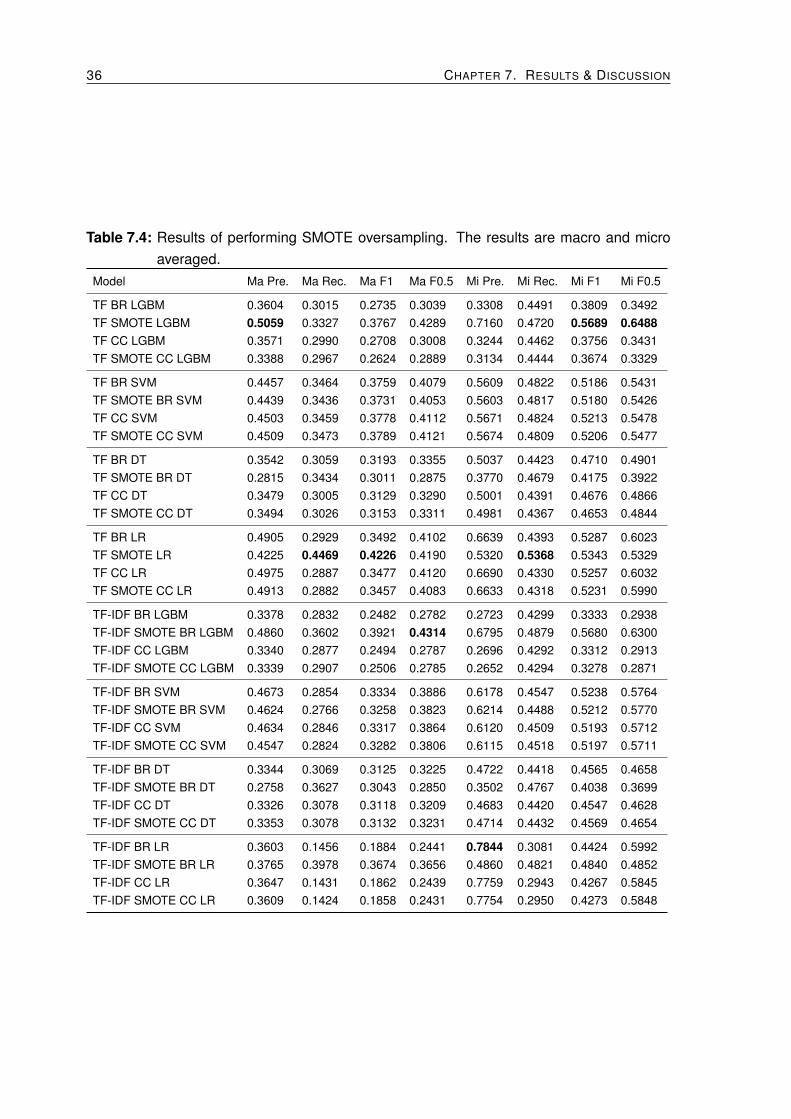
7.4 Imbalanced Learning Evaluation

In this section we present the impact of using the SMOTE [30] over sampling technique.We evaluate the four base classifiers in a binary relevance setting with both TF and TF-IDF.We only oversample the classes with less than 200 examples. In these results, we can seethat LGBM’s performance is improved dramatically by the use of SMOTE and BR. Logisticregression perceives a good performance improvement combining SMOTE with TF-IDF. Forthe case of SVM, there is a slightly decrease in performance. The perfomance of DT isdecreased by the use of SMOTE. From this experiment we conclude that SMOTE should be

7.4. IMBALANCED LEARNING EVALUATION 33

Table 7.2: Machine Learning models experiment results. The results are macro and microaveraged.

Model Ma Pre. Ma Rec. Ma F1 Ma F0.5 Mi Pre. Mi Rec. Mi F1 Mi F0.5

Binary Relevance

TF BR LGBM 0.3604 0.3015 0.2735 0.3039 0.3308 0.4491 0.3809 0.3492TF BR SVM 0.4457 0.3464 0.3759 0.4079 0.5609 0.4822 0.5186 0.5431TF BR DT 0.3542 0.3059 0.3193 0.3355 0.5037 0.4423 0.4710 0.4901TF BR LR 0.4905 0.2929 0.3492 0.4102 0.6639 0.4393 0.5287 0.6023TF-IDF BR LGBM 0.3378 0.2832 0.2482 0.2782 0.2723 0.4299 0.3333 0.2938TF-IDF BR SVM 0.4673 0.2854 0.3334 0.3886 0.6178 0.4547 0.5238 0.5764TF-IDF BR DT 0.3344 0.3069 0.3125 0.3225 0.4722 0.4418 0.4565 0.4658TF-IDF BR LR 0.3603 0.1456 0.1884 0.2441 0.7844 0.3081 0.4424 0.5992

Extreme multi-label

TF FastXML 0.3617 0.4056 0.3480 0.3433 0.4011 0.6140 0.4852 0.4310TF PfastXML 0.3532 0.4035 0.3445 0.3383 0.4010 0.6140 0.4852 0.4309TF PfastReXML 0.3603 0.4075 0.3495 0.3441 0.4024 0.6160 0.4868 0.4323TF DiSMEC 0.3634 0.4057 0.3478 0.3438 0.4013 0.6144 0.4855 0.4312TF-IDF FastXML 0.2909 0.3459 0.2843 0.2768 0.3770 0.5772 0.4561 0.4051TF-IDF PfastXML 0.2869 0.3449 0.2836 0.2754 0.3760 0.5756 0.4549 0.4040TF-IDF PfastReXML 0.2949 0.3456 0.2858 0.2792 0.3766 0.5765 0.4555 0.4046TF-IDF DiSMEC 0.2946 0.3470 0.2855 0.2788 0.3760 0.5756 0.4548 0.4040

Multi-label decision tree

TF MLDT 0.3041 0.2674 0.2769 0.2895 0.4595 0.4176 0.4375 0.4504TF-IDF MLDT 0.3006 0.2702 0.2768 0.2875 0.4538 0.4151 0.4335 0.4454

Classifier Chain

TF-IDF CC LGBM 0.3340 0.2877 0.2494 0.2787 0.2696 0.4292 0.3312 0.2913TF-IDF CC SVM 0.4634 0.2846 0.3317 0.3864 0.6120 0.4509 0.5193 0.5712TF-IDF CC DT 0.3326 0.3078 0.3118 0.3209 0.4683 0.4420 0.4547 0.4628TF-IDF CC LR 0.3647 0.1431 0.1862 0.2439 0.7759 0.2943 0.4267 0.5845TF CC LGBM 0.3571 0.2990 0.2708 0.3008 0.3244 0.4462 0.3756 0.3431TF CC SVM 0.4503 0.3459 0.3778 0.4112 0.5671 0.4824 0.5213 0.5478TF CC DT 0.3479 0.3005 0.3129 0.3290 0.5001 0.4391 0.4676 0.4866TF CC LR 0.4975 0.2887 0.3477 0.4120 0.6690 0.4330 0.5257 0.6032


Table 7.3: Text representation experiment results. The results are macro and micro aver-aged.


Term Frequency

TF BR LGBM 0.3604 0.3015 0.2735 0.3039 0.3308 0.4491 0.3809 0.3492TF BR SVM 0.4457 0.3464 0.3759 0.4079 0.5609 0.4822 0.5186 0.5431TF BR DT 0.3542 0.3059 0.3193 0.3355 0.5037 0.4423 0.4710 0.4901TF BR LR 0.4905 0.2929 0.3492 0.4102 0.6639 0.4393 0.5287 0.6023

Term Frequency Inverse Document Frequency

TF-IDF BR LGBM 0.3378 0.2832 0.2482 0.2782 0.2723 0.4299 0.3333 0.2938TF-IDF BR SVM 0.4673 0.2854 0.3334 0.3886 0.6178 0.4547 0.5238 0.5764TF-IDF BR DT 0.3344 0.3069 0.3125 0.3225 0.4722 0.4418 0.4565 0.4658TF-IDF BR LR 0.3603 0.1456 0.1884 0.2441 0.7844 0.3081 0.4424 0.5992

Word2Vec

W2Vec mean BR LGBM 0.3061 0.1821 0.1847 0.2237 0.3032 0.3189 0.3108 0.3062W2Vec mean BR SVM 0.3020 0.2398 0.2547 0.2748 0.4480 0.4101 0.4282 0.4398W2Vec mean BR DT 0.1949 0.1773 0.1810 0.1873 0.3349 0.3066 0.3201 0.3288W2Vec mean BR LR 0.2944 0.1179 0.1531 0.1990 0.7400 0.2591 0.3838 0.5396W2Vec sum BR LGBM 0.2960 0.1738 0.1773 0.2156 0.3109 0.3100 0.3102 0.3105W2Vec sum BR SVM 0.2979 0.3320 0.3035 0.2972 0.3745 0.4534 0.4101 0.3879W2Vec sum BR DT 0.1957 0.1749 0.1796 0.1868 0.3323 0.3014 0.3160 0.3256W2Vec sum BR LR 0.3692 0.3045 0.3235 0.3448 0.4874 0.4294 0.4565 0.4745

FastText

FastText mean BR LGBM 0.3023 0.1721 0.1759 0.2157 0.2971 0.3009 0.2989 0.2978FastText mean BR SVM 0.2352 0.2109 0.2134 0.2222 0.3505 0.3637 0.3570 0.3531FastText mean BR DT 0.1902 0.1713 0.1758 0.1825 0.3231 0.2957 0.3087 0.3172FastText mean BR LR 0.2747 0.1088 0.1416 0.1845 0.7084 0.2266 0.3433 0.4969FastText sum BR LGBM 0.2966 0.1695 0.1721 0.2105 0.2967 0.2983 0.2974 0.2969FastText sum BR SVM 0.3576 0.3255 0.3302 0.3421 0.4562 0.4591 0.4576 0.4567FastText sum BR DT 0.1928 0.1709 0.1762 0.1838 0.3284 0.2973 0.3121 0.3217FastText sum BR LR 0.4282 0.2630 0.3108 0.3618 0.5947 0.4034 0.4807 0.5431

7.5. HIERARCHICAL CLASSIFICATION EVALUATION 35

used in conjunction with LGBM and LR, both in a BR setting. On the other hand, DT hashad a consistent poor performance so far, therefore we decide to discard it.

7.5 Hierarchical Classification Evaluation

The results of the experiment to assess the impact of hierarchical classification over flat clas-sification are displayed in Table 7.5. We evaluate LGBM, SVM and LR with TF and TF-IDFin a local classifier per taxonomy and leaves (LCTL) mode. Then, we proceed to comparethem to their flat counterparts. We run each possible combination in binary relevance andclassifier chain multi-label settings. LGBM and LR in a binary relevance setting are evalu-ated using SMOTE oversampling because those are the only models that benefit from thattechnique. It can be seen that LCTL brings a slight improvement in the performance of mostof the classifiers.

7.6 Classifier Per Type of Report Results

To test our hypothesis that training one independent classifier per report type performs betterthan training one classifier for the entire dataset, we used this proposed technique with thebest combinations that resulted from previous experiments. The results are presented onTable 7.6.From the table is clear that the combination of TF-IDF, SMOTE, BR and LGBM perreport type outperforms any other model that has been evaluated in this research. It canalso be concluded that training one classifier per each report type brings moderate to bigperformance improvements for the evaluated models. On the other hand, using LCTL doesnot perform that well. We hypothesize that training per report type divides the search spacewell enough, meaning that the additional partitioning brought by LCTL is of little help.

7.7 Inter-annotator Agreement

The inter-annotator agreement measure mvα is 57.45%. The 5 analysts labeled in total160 out of 250 reports. Unfortunately, the holiday season coincided with our experiment,preventing the analysts to label the entire selected sample for this experiment. Betweenthe 160 labeled reports, 34 were comparable, meaning that at least two analysts labeledthe same 34 reports, which is a requirement for the metric. The agreement results werecalculated using the open source software1 provided by the mvα authors [28].

The result of mvα = 57.45% is difficult to interpret. [25] recommends that conclusionsshould not be made about data with less than 66.7%. However, the authors “recommendsuch levels with considerable hesitation. The choice of reliability standards should alwaysbe related to the validity requirements imposed on the research results, specifically to thecosts of drawing wrong conclusions”. The authors also mention guidelines that have been

1https://github.com/rcraggs/mvna


Table 7.4: Results of performing SMOTE oversampling. The results are macro and microaveraged.


TF BR LGBM 0.3604 0.3015 0.2735 0.3039 0.3308 0.4491 0.3809 0.3492TF SMOTE LGBM 0.5059 0.3327 0.3767 0.4289 0.7160 0.4720 0.5689 0.6488TF CC LGBM 0.3571 0.2990 0.2708 0.3008 0.3244 0.4462 0.3756 0.3431TF SMOTE CC LGBM 0.3388 0.2967 0.2624 0.2889 0.3134 0.4444 0.3674 0.3329

TF BR SVM 0.4457 0.3464 0.3759 0.4079 0.5609 0.4822 0.5186 0.5431TF SMOTE BR SVM 0.4439 0.3436 0.3731 0.4053 0.5603 0.4817 0.5180 0.5426TF CC SVM 0.4503 0.3459 0.3778 0.4112 0.5671 0.4824 0.5213 0.5478TF SMOTE CC SVM 0.4509 0.3473 0.3789 0.4121 0.5674 0.4809 0.5206 0.5477

TF BR DT 0.3542 0.3059 0.3193 0.3355 0.5037 0.4423 0.4710 0.4901TF SMOTE BR DT 0.2815 0.3434 0.3011 0.2875 0.3770 0.4679 0.4175 0.3922TF CC DT 0.3479 0.3005 0.3129 0.3290 0.5001 0.4391 0.4676 0.4866TF SMOTE CC DT 0.3494 0.3026 0.3153 0.3311 0.4981 0.4367 0.4653 0.4844

TF BR LR 0.4905 0.2929 0.3492 0.4102 0.6639 0.4393 0.5287 0.6023TF SMOTE LR 0.4225 0.4469 0.4226 0.4190 0.5320 0.5368 0.5343 0.5329TF CC LR 0.4975 0.2887 0.3477 0.4120 0.6690 0.4330 0.5257 0.6032TF SMOTE CC LR 0.4913 0.2882 0.3457 0.4083 0.6633 0.4318 0.5231 0.5990

TF-IDF BR LGBM 0.3378 0.2832 0.2482 0.2782 0.2723 0.4299 0.3333 0.2938TF-IDF SMOTE BR LGBM 0.4860 0.3602 0.3921 0.4314 0.6795 0.4879 0.5680 0.6300TF-IDF CC LGBM 0.3340 0.2877 0.2494 0.2787 0.2696 0.4292 0.3312 0.2913TF-IDF SMOTE CC LGBM 0.3339 0.2907 0.2506 0.2785 0.2652 0.4294 0.3278 0.2871

TF-IDF BR SVM 0.4673 0.2854 0.3334 0.3886 0.6178 0.4547 0.5238 0.5764TF-IDF SMOTE BR SVM 0.4624 0.2766 0.3258 0.3823 0.6214 0.4488 0.5212 0.5770TF-IDF CC SVM 0.4634 0.2846 0.3317 0.3864 0.6120 0.4509 0.5193 0.5712TF-IDF SMOTE CC SVM 0.4547 0.2824 0.3282 0.3806 0.6115 0.4518 0.5197 0.5711

TF-IDF BR DT 0.3344 0.3069 0.3125 0.3225 0.4722 0.4418 0.4565 0.4658TF-IDF SMOTE BR DT 0.2758 0.3627 0.3043 0.2850 0.3502 0.4767 0.4038 0.3699TF-IDF CC DT 0.3326 0.3078 0.3118 0.3209 0.4683 0.4420 0.4547 0.4628TF-IDF SMOTE CC DT 0.3353 0.3078 0.3132 0.3231 0.4714 0.4432 0.4569 0.4654

TF-IDF BR LR 0.3603 0.1456 0.1884 0.2441 0.7844 0.3081 0.4424 0.5992TF-IDF SMOTE BR LR 0.3765 0.3978 0.3674 0.3656 0.4860 0.4821 0.4840 0.4852TF-IDF CC LR 0.3647 0.1431 0.1862 0.2439 0.7759 0.2943 0.4267 0.5845TF-IDF SMOTE CC LR 0.3609 0.1424 0.1858 0.2431 0.7754 0.2950 0.4273 0.5848

7.7. INTER-ANNOTATOR AGREEMENT 37

Table 7.5: Hierarchical classification experiment results. Hierarchical models are under-lined. The results are macro and micro averaged.


TF SMOTE BR LGBM 0.5059 0.3327 0.3767 0.4289 0.7160 0.4720 0.5689 0.6488TF LCTL SMOTE BR LGBM 0.5116 0.3331 0.3784 0.4319 0.7111 0.4877 0.5785 0.6514TF LCTL CC LGBM 0.4898 0.2746 0.3220 0.3845 0.7155 0.4557 0.5568 0.6422

TF BR SVM 0.4457 0.3464 0.3759 0.4079 0.5609 0.4822 0.5186 0.5431TF LCTL BR SVM 0.5094 0.2982 0.3498 0.4119 0.6913 0.4786 0.5656 0.6349TF LCTL CC SVM 0.4997 0.3032 0.3530 0.4122 0.6751 0.4845 0.5642 0.6259

TF SMOTE BR LR 0.4225 0.4469 0.4226 0.4190 0.5320 0.5368 0.5343 0.5329TF LCTL SMOTE BR LR 0.4608 0.3643 0.3870 0.4183 0.6259 0.5067 0.5600 0.5977TF LCTL CC LR 0.4416 0.2091 0.2571 0.3205 0.7575 0.4078 0.5302 0.6466

TF-IDF SMOTE BR LGBM 0.4860 0.3602 0.3921 0.4314 0.6795 0.4879 0.5680 0.6300TF-IDF LCTL SMOTE BR LGBM 0.5195 0.3362 0.3823 0.4373 0.7124 0.4916 0.5817 0.6536TF-IDF LCTL CC LGBM 0.4923 0.2748 0.3229 0.3855 0.7185 0.4567 0.5584 0.6446

TF-IDF BR SVM 0.4673 0.2854 0.3334 0.3886 0.6178 0.4547 0.5238 0.5764TF-IDF LCTL BR SVM 0.5045 0.2970 0.3481 0.4094 0.6897 0.4775 0.5643 0.6334TF-IDF LCTL CC SVM 0.5031 0.3039 0.3546 0.4143 0.6762 0.4831 0.5635 0.6261

TF-IDF SMOTE BR LR 0.3765 0.3978 0.3674 0.3656 0.4860 0.4821 0.4840 0.4852TF-IDF LCTL SMOTE BR LR 0.4590 0.3637 0.3850 0.4156 0.6223 0.5042 0.5571 0.5944TF-IDF LCTL CC LR 0.4492 0.2072 0.2565 0.3223 0.7566 0.4051 0.5277 0.6447

Table 7.6: Results of training one classifier per report type. The results are macro and microaveraged.


TF-IDF SMOTE BR LGBM 0.5717 0.4136 0.4541 0.5022 0.7400 0.5450 0.6277 0.6906TF-IDF LCTL SMOTE BR LGBM 0.5674 0.4189 0.4558 0.5015 0.7139 0.5420 0.6162 0.6713TF SMOTE BR LR 0.4987 0.4782 0.4770 0.4860 0.6131 0.5870 0.5997 0.6076TF LCTL SMOTE BR LR 0.5011 0.4718 0.4740 0.4854 0.6095 0.5699 0.5891 0.6012TF-IDF CC SVM 0.4973 0.3336 0.3797 0.4304 0.6464 0.5023 0.5653 0.6113TF-IDF LCTL CC SVM 0.4672 0.3524 0.3827 0.4190 0.5835 0.5009 0.5390 0.5649


proposed for Cohen’s κ, which can be applicable to Krippendorff’s α. For this reason, webelieve that we can use the interpretations for Cohen’s κ proposed by [26] to interpret the

mvα calculated in this research. The paper proposes that a value between 40% and 59% isconsidered a weak agreement.

7.8 Comparison to Related Work

Researchers in [31] apply Natural Language Processing (NLP) techniques to create an avi-ation safety report threshold-based classifier using correlations between the labels and theextracted linguistic features. These correlations are weighted by document length and thefinal classification is decided by a set of thresholds and manual rules. In contrast, our re-search performs the classification based on learning the rules automatically from data, with-out any manual rules. Unfortunately, the authors do not provide any metrics to compare ourapproaches.

[32] apply NLP and binary relevance with support vector machines (BR SVM) to classifyaviation safety reports automatically. They report a microaverage F1 of 79.15% in their bestmodel. Our best model reports a F1 of 62.77%. Our problem is considered harder becausethis research aims to classify 7 different types of reports with different types of fields, whilethe authors focus in one type of report using only a text field. Additionally, their taxonomyconsists of 37 labels, while ours is comprised by more than 800 labels. This high amount oflabels represents the main challenge of our research. Finally, [32] have 7 times more dataand they do have a better pre-processing strategy with 637 hand-written rules to pre-processthe data, which we think can improve the accuracy performance of the classifier.

Chapter 8

Conclusion

8.1 Conclusion

Based on the experimental results, it can be concluded that classical multi-label machinelearning techniques can be applied successfully to the problem of automatic safety reportsclassification.

The answer to RQ1 is stated as follows: the accuracy of applying machine learning toclassify aviation safety reports automatically is influenced mainly by training one classifierper each type of report and the use of classical multi-label categorization techniques.

The baseline that was established with logistic regression is improved by 81% employingour proposed configuration that trains a LGBM classifier in a binary relevance setting pereach type of report while using a TF-IDF text representation with SMOTE oversampling.This configuration achieves a macroaveraged F0.5 score of 50.22%. Our results suggestthat using aggregated embeddings does not bring any benefits to our classification task.

TF and TF-IDF clearly outperform the embeddings when tested in downstream tasks forthe report classification. Additionally, TF and TF-IDF are less computationally expensive totrain and to evaluate the models.

Using a simple multi-label learning model like binary relevance has the best impact in theperformance of the classification task. In our specific case, the performance gain surpassesthe fact that it is computationally more expensive when compared to extreme multi-labelmodels. Additionally, it is still feasible to train binary relevance models in commodity hard-ware given our current dataset.

The use of SMOTE oversampling improves the performance of LGBM when used incombination with binary relevance by 41%. The performance of logistic regression is alsoimproved to a lesser extent. SVM and classifier chain (CC) do not perceive any benefit bythe use of SMOTE.

Using hierarchical classification with LCTL slightly improves the performance of mostclassifiers. However, our results suggest that the performance is decreased when a LCTLclassifier is trained per each report type.

Training one classifier per report type offers a substantial improvement in classificationperformance. We believe that this method decreases the feature dimensionality and sparsity

39

40 CHAPTER 8. CONCLUSION

dramatically. Additionally we assume that the data for each type of report are independent.Such assumptions proved to be valid as the classification performance was improved by theapplication of this strategy.

With respect to the RQ2, the report classification process reliability should be measuredusing Krippendorff’s mvα. Our reliability study showed a mvα of 57.45%, which can beinterpreted as a weak agreement. Therefore, the labeling process needs to be improved. Werecommend to the organization to aim to improve the metric to a 66.7% which is considereda moderate agreement.

8.2 Limitations

There are important limitations to this research. In the text representation evaluation, weaggregate Word2Vec and FastText embeddings using sum or average (see Section 6.4),possibly affecting their representational capacity. This decision was made in order to keepthe computation feasible with our current infrastructure. We do not claim that this is the bestapproach. There are other ways to limit the high dimensionality that such techniques bring,like truncating the text up to a certain length. Furthermore, we were not able to evaluate stateof the art techniques like ELMo and BERT due to their high demand of GPU resources.

In the same way, the fact that we merge all the report text fields is seen as a limitation.This decision was made again to keep the experiment within the boundaries of our currentinfrastructure.

In the hierarchical classification experiment we exclusively evaluate LCTL, which usesonly two levels of the hierarchy. Although the results are promising, it is needed to furtherevaluate the impact of exploiting the full hierarchy and the use of more advanced approachesfor hierarchical classification.

We assume the report types to be independent, which represents a limitation becausesome reports share fields. Therefore, discovering the correlations between the report typesand their fields could bring better insights about how to further improve the classificationperformance.

An additional limitation of this research is that we do not use propensity scored metrics.We argue in Section 6.9 that we do not consider our dataset as the “gold” ground truthbecause every example may have missing labels. Therefore, we can erroneously treat acorrect prediction as a false positive. Using propensity scored metrics addresses this limita-tion, as they provide unbiased estimates of the metric computed on the “gold” ground truth.See [36] for a further explanation about this rationale.

We are not considering the languages that appear in our dataset. English stop wordsand stemming are used even though dutch language is present in some fields. The problemis not easy to address because both languages are occasionally combined in a single report.This means that the content of one text field might be written in english while another fieldin the same report could be in dutch. In like manner, for the same field, it is possible to findthe english content in one report and dutch in the next report. A possible solution will be to

8.3. RECOMMENDATIONS FOR THE COMPANY 41

use automatic translation in such cases.Our final limitation is that the sample for the inter-annotator agreement experiment is

small. Our sample size is not the ideal for such studies, especially in the face of such a bigtaxonomy. However, our analysts’ time was limited during the period when the experimentwas carried out.

8.3 Recommendations for the Company

The main recommendation for the company is to use our proposed model to classify thesafety reports automatically. The model should be implemented as a software componentintegrated in the enterprise information systems. Such integration is realized as a pipelinethat extracts the reports from the safety database, applies the suggested pre-processingand classifies the reports in an online manner. It is also suggested to implement a similarpipeline for re-training the model periodically, as hundreds of new reports arrive each monthand every machine learning model benefits of more data.

In order to improve data quality and reliability, the following recommendations are issued,based on [25]. Each descriptor of any of the taxonomies must be clearly detailed by themeans of including a description and clear instructions about when should it be applied.Additionally, it is suggested to list the minimum knowledge that an analyst requires to beable to analyze each type of safety report. Furthermore, a standard training program foreach new analyst could be deployed in order to improve the consistency of the classification.

Reliability tests can be run periodically between the analysts and discrepancies shouldbe analyzed and reconciled so the organization discovers what kind of cases need to beincluded in the coding procedure or manual and what parts can be improved. It is suggestedto use Krippendorff’s mvα to measure such reliability. After updating the coding procedure, areliability test can be performed again to verify that an improvement has been made. Basedon [25] and [26], we recommend that the organization should aim to have at least 66.7%in agreement. It is worth noting that this reliability measures the reliability of the annotationprocedure, which is independent of the actual annotators used. This will guarantee thateven when the annotators are changed, the quality of the annotation won’t be reduced if theannotation procedure is followed.

If the annotators or analysts find themselves discussing how to a apply a particular tax-onomy or consulting each other an unanticipated problem, those are signs that the codinginstructions need to be updated and improved. It could also mean that a re-training of theanalysts is needed.

8.4 Future Work

The presented research can be extended in many ways. The first is to use a classifier basedon deep learning. We have proposed a good starting point to classify aviation safety reportsusing classical machine learning techniques. The results of this research can be used as a

42 CHAPTER 8. CONCLUSION

baseline to benchmark the improvements achieved by the use of deep learning. However,the use of deep learning requires a considerable amount of data, so these efforts might haveto wait until more data are available. Transfer learning could be a viable option to try whilemore data arrives. One remaining question is what deep learning architecture improves ourcurrent results? because most of the current deep learning approaches focus only on smalltexts, while our problem comprises larger texts and other types of features.

Another direction for future work is to measure the impact of state of the art text repre-sentation techniques like ELMo, BERT and Transformer XL. Such representations are morelikely to be used in conjunction with deep learning approaches. BERT also offers a classifierthat could be tested, but it would require some modifications as it is intended for multi-classproblems and not for multi-label.

A second question that remains open is how to address the different languages that arepresent in the text? As presented in Chapter 4, the text fields can contain either englishor dutch languages. Such question represents a challenge because the same report couldhave one field in english and another field in dutch. Furthermore, the same field could bewritten in english in one report and written in dutch in the next report.

Our work can also extended to classify the aviation safety reports using a different setof categories. As an example, our proposed model can be trained to classify the reportsaccording to risk categories. It can also be trained to determine if the report needs to beforwarded to any aviation authority.

Bibliography

[1] S. Saha Ray, Graph Theory with Algorithms and its Applications. India: SpringerIndia, 2013. [Online]. Available: http://link.springer.com/10.1007/978-81-322-0750-4

[2] R. Diestel, Graph Theory, ser. Graduate Texts in Mathematics. Berlin, Heidelberg:Springer Berlin Heidelberg, 2017, vol. 173. [Online]. Available: http://link.springer.com/10.1007/978-3-662-53622-3

[3] A. W. Group and others, The ARMS methodology for operational risk assessment inaviation organisations, 2010.

[4] ICAO, Safety Management Manual, 4th ed., 2018.

[5] K. P. Murphy, Machine learning : a probabilistic perspective. MIT Press, 2012.[Online]. Available: http://mitpress-ebooks.mit.edu/product/machine-learning

[6] J. Leskovec, A. Rajaraman, and J. D. Ullman, Mining of massive datasets,2nd ed., 2014. [Online]. Available: https://www.cambridge.org/ch/academic/subjects/computer-science/knowledge-management-databases-and-data-mining/mining-massive-datasets-2nd-edition?format=HB

[7] I. Goodfellow, Y. Bengio, and A. Courville, Deep Learning. MIT Press, 2016.

[8] F. Sebastiani, “Machine learning in automated text categorization,” ACM ComputingSurveys (CSUR), vol. 34, no. 1, pp. 1–47, 2002. [Online]. Available: https://dl.acm.org/citation.cfm?id=505283

[9] C. D. Manning, An Introduction to Information Retrieval, online ed., 2009.

[10] B. Altnel and M. C. Ganiz, “Semantic text classification: A survey of past and recentadvances,” Information Processing and Management, vol. 54, no. 6, pp. 1129–1153,2018.

[11] J. Read, “Scalable Multi-label Classification,” Ph.D. dissertation, University of Waikato,Hamilton, New Zealand, 2010. [Online]. Available: https://hdl.handle.net/10289/4645

[12] E. Gibaja and S. Ventura, “A Tutorial on Multilabel Learning,” ACM Computing Surveys,vol. 47, no. 3, pp. 1–38, 4 2015. [Online]. Available: http://dl.acm.org/citation.cfm?doid=2737799.2716262

43

http://link.springer.com/10.1007/978-81-322-0750-4



http://mitpress-ebooks.mit.edu/product/machine-learning

https://www.cambridge.org/ch/academic/subjects/computer-science/knowledge-management-databases-and-data-mining/mining-massive-datasets-2nd-edition?format=HB



https://dl.acm.org/citation.cfm?id=505283

https://dl.acm.org/citation.cfm?id=505283

https://hdl.handle.net/10289/4645

http://dl.acm.org/citation.cfm?doid=2737799.2716262


44 BIBLIOGRAPHY

[13] G. Madjarov, D. Kocev, D. Gjorgjevikj, and S. Dzeroski, “An extensive experimentalcomparison of methods for multi-label learning,” Pattern Recognition, vol. 45, no. 9, pp.3084–3104, 9 2012.

[14] G. Tsoumakas, I. Katakis, and I. P. Vlahavas, “Effective andEfficient Multilabel Classification in Domains with Large Numberof Labels,” 2008. [Online]. Available: https://www.semanticscholar.org/paper/Effective-and-Efficient-Multilabel-Classification-Tsoumakas-Katakis/aa6ee637e9f86148dadbc849983159ea24d2d204

[15] L. Jian, J. Li, K. Shu, and H. Liu, “Multi-label informed feature selection,” in IJCAI Inter-national Joint Conference on Artificial Intelligence, 2016.

[16] X. Sun, J. Xu, C. Jiang, J. Feng, S. S. Chen, and F. He, “Extreme learning machine formulti-label classification,” Entropy, 2016.

[17] C.-K. Yeh, W.-C. Wu, W.-J. Ko, and Y.-C. F. Wang, “Learning Deep Latent Spaces forMulti-Label Classification,” Proceedings of the Thirty-First AAAI Conference on ArtificialIntelligence (AAAI-17), 2017.

[18] V. Kumar, A. K. Pujari, V. Padmanabhan, and V. R. Kagita, “Group preserving labelembedding for multi-label classification,” Pattern Recognition, pp. 23–34, 2019.

[19] D. Jurafsky and J. H. Martin, Speech and Language Processing 3rd edition draft, 2018.

[20] T. Mikolov, K. Chen, G. Corrado, and J. Dean, “Efficient Estimation ofWord Representations in Vector Space,” 1 2013. [Online]. Available: http://arxiv.org/abs/1301.3781

[21] J. Pennington, R. Socher, and C. D. Manning, “GloVe: Global Vectors for WordRepresentation,” in Empirical Methods in Natural Language Processing (EMNLP),2014, pp. 1532–1543. [Online]. Available: http://www.aclweb.org/anthology/D14-1162

[22] P. Bojanowski, E. Grave, A. Joulin, and T. Mikolov, “Enriching Word Vectors withSubword Information,” 7 2016. [Online]. Available: http://arxiv.org/abs/1607.04606

[23] M. E. Peters, M. Neumann, M. Iyyer, M. Gardner, C. Clark, K. Lee, andL. Zettlemoyer, “Deep contextualized word representations,” 2 2018. [Online].Available: http://arxiv.org/abs/1802.05365

[24] J. Devlin, M.-W. Chang, K. Lee, and K. Toutanova, “BERT: Pre-training of DeepBidirectional Transformers for Language Understanding,” 10 2018. [Online]. Available:http://arxiv.org/abs/1810.04805

[25] K. Krippendorff, Content Analysis: An Introduction to Its Methodology, 2nd ed. SagePublications, 2004.

https://www.semanticscholar.org/paper/Effective-and-Efficient-Multilabel-Classification-Tsoumakas-Katakis/aa6ee637e9f86148dadbc849983159ea24d2d204



http://arxiv.org/abs/1301.3781


http://www.aclweb.org/anthology/D14-1162




BIBLIOGRAPHY 45

[26] M. L. McHugh, “Interrater reliability: the kappa statistic.” Biochemia medica, vol. 22,no. 3, pp. 276–82, 2012. [Online]. Available: http://www.ncbi.nlm.nih.gov/pubmed/23092060http://www.pubmedcentral.nih.gov/articlerender.fcgi?artid=PMC3900052

[27] R. Artstein and M. Poesio, “Inter-coder agreement for computational linguistics,” 2008.

[28] K. Krippendorff and R. Craggs, “The Reliability of Multi-Valued Coding of Data,”Communication Methods and Measures, vol. 10, no. 4, pp. 181–198, 10 2016. [Online].Available: https://www.tandfonline.com/doi/full/10.1080/19312458.2016.1228863

[29] G. Lemaitre, F. Nogueira, and C. K. Aridas, “Imbalanced-learn: A Python Toolboxto Tackle the Curse of Imbalanced Datasets in Machine Learning,” 9 2016. [Online].Available: http://arxiv.org/abs/1609.06570

[30] N. V. Chawla, K. W. Bowyer, L. O. Hall, and W. P. Kegelmeyer, “SMOTE: SyntheticMinority Over-sampling Technique,” Journal Of Artificial Intelligence Research, 6 2011.[Online]. Available: http://arxiv.org/abs/1106.1813http://dx.doi.org/10.1613/jair.953

[31] C. Pimm, C. Raynal, N. Tulechki, E. Hermann, G. Caudy, and L. Tanguy, “NaturalLanguage Processing (NLP) tools for the analysis of incident and accident reports,”pp. –, 2012. [Online]. Available: https://hal.archives-ouvertes.fr/halshs-00953658

[32] L. Tanguy, N. Tulechki, A. Urieli, E. Hermann, and C. Raynal, “Natural languageprocessing for aviation safety reports: From classification to interactive analysis,”Computers in Industry, vol. 78, no. C, pp. 80–95, 5 2016. [Online]. Available:https://linkinghub.elsevier.com/retrieve/pii/S0166361515300464

[33] Y. Prabhu and M. Varma, “FastXML: A Fast, Accurate and Stable Tree-classifier foreXtreme Multi-label Learning,” in Proceedings of the 20th ACM SIGKDD internationalconference on Knowledge discovery and data mining - KDD ’14, 2014.

[34] K. Bhatia, H. Jain, P. Kar, M. Varma, and P. Jain, “SLEEC - Sparse local embeddingsfor extreme multi-label classification,” NIPS, vol. 87, no. 1, pp. 76–87, 2015.

[35] R. Babbar and B. Shoelkopf, “DiSMEC - Distributed Sparse Machines for Extreme Multi-label Classification,” in Proceedings of the Tenth ACM International Conference on WebSearch and Data Mining, 2016.

[36] H. Jain, Y. Prabhu, and M. Varma, “Extreme Multi-label Loss Functions for Recom-mendation, Tagging, Ranking & Other Missing Label Applications,” in Proceedings ofthe 22nd ACM SIGKDD International Conference on Knowledge Discovery and DataMining - KDD ’16, 2016.

[37] W. Zhang, J. Yan, X. Wang, and H. Zha, “Deep Extreme Multi-label Learning,” in ICMR’18: Proceedings of the 2018 ACM on International Conference on Multimedia Re-trieval, 2017.

http://www.ncbi.nlm.nih.gov/pubmed/23092060 http://www.pubmedcentral.nih.gov/articlerender.fcgi?artid=PMC3900052

http://www.ncbi.nlm.nih.gov/pubmed/23092060 http://www.pubmedcentral.nih.gov/articlerender.fcgi?artid=PMC3900052

https://www.tandfonline.com/doi/full/10.1080/19312458.2016.1228863


http://arxiv.org/abs/1106.1813 http://dx.doi.org/10.1613/jair.953

https://hal.archives-ouvertes.fr/halshs-00953658

https://linkinghub.elsevier.com/retrieve/pii/S0166361515300464

46 BIBLIOGRAPHY

[38] J. Liu, W.-C. Chang, Y. Wu, and Y. Yang, “Deep Learning for Extreme Multi-label TextClassification,” in Proceedings of the 40th International ACM SIGIR Conference on Re-search and Development in Information Retrieval - SIGIR ’17, 2017.

[39] S. Dumais and H. Chen, “Hierarchical classification of Web content,” in Proceedings ofthe 23rd annual international ACM SIGIR conference on Research and development ininformation retrieval - SIGIR ’00. New York, New York, USA: ACM Press, 2000, pp.256–263. [Online]. Available: http://portal.acm.org/citation.cfm?doid=345508.345593

[40] J. W. Xu, V. Singh, V. Govindaraju, and D. Neogi, “A hierarchical classification model fordocument categorization,” in Proceedings of the International Conference on DocumentAnalysis and Recognition, ICDAR, 2009.

[41] J. Graovac, J. Kovacevic, and G. Pavlovic-Lazetic, “Hierarchical vs. flat n-gram-basedtext categorization: Can we do better?” Computer Science and Information Systems,vol. 14, no. 1, pp. 103–121, 2017.

[42] Y. Liu, L. Wang, Q. Yang, Y. He, H. Peng, J. Li, Y. Song, and M. Bao, “Large-ScaleHierarchical Text Classification with Recursively Regularized Deep Graph-CNN,”in Proceedings of the 2018 World Wide Web Conference on World Wide Web - WWW’18. New York, New York, USA: ACM Press, 2018, pp. 1063–1072. [Online]. Available:http://dl.acm.org/citation.cfm?doid=3178876.3186005

[43] G. Ke, Q. Meng, T. Finley, T. Wang, W. Chen, W. Ma, Q. Ye, and T.-Y. Liu, “LightGBM:A Highly Efficient Gradient Boosting Decision Tree,” in NIPS ’17, 2017, p. 9. [Online].Available: https://github.com/Microsoft/LightGBM.

[44] F. Pedregosa, G. Varoquaux, A. Gramfort, V. Michel, B. Thirion, O. Grisel, M. Blon-del, P. Prettenhofer, R. Weiss, V. Dubourg, J. Vanderplas, A. Passos, D. Cournapeau,M. Brucher, M. Perrot, and E. Duchesnay, “Scikit-learn: Machine Learning in Python,”Journal of Machine Learning Research, vol. 12, pp. 2825–2830, 2011.

[45] C. D. Paice and C. D., “Another stemmer,” ACM SIGIR Forum, vol. 24, no. 3, pp. 56–61,11 1990. [Online]. Available: http://portal.acm.org/citation.cfm?doid=101306.101310

[46] J. Read, B. Pfahringer, G. Holmes, and E. Frank, “Classifier chains for multi-labelclassification,” Machine Learning, vol. 85, no. 3, pp. 333–359, 12 2011. [Online].Available: http://link.springer.com/10.1007/s10994-011-5256-5

[47] T. Mikolov, I. Sutskever, K. Chen, G. Corrado, and J. Dean, “DistributedRepresentations of Words and Phrases and their Compositionality,” 10 2013. [Online].Available: http://arxiv.org/abs/1310.4546

[48] T. Mikolov, E. Grave, P. Bojanowski, C. Puhrsch, and A. Joulin, “Advancesin Pre-Training Distributed Word Representations,” 12 2017. [Online]. Available:http://arxiv.org/abs/1712.09405

http://portal.acm.org/citation.cfm?doid=345508.345593


https://github.com/Microsoft/LightGBM.

http://portal.acm.org/citation.cfm?doid=101306.101310

http://link.springer.com/10.1007/s10994-011-5256-5



BIBLIOGRAPHY 47

[49] K. Sechidis, G. Tsoumakas, and I. Vlahavas, “On the Stratification of Multi-label Data,”in Machine Learning and Knowledge Discovery in Databases. Springer, Berlin, Hei-delberg, 2011, pp. 145–158.

48 BIBLIOGRAPHY

Appendix A

Appendix

A.1 Summary of Notation

The following table contains a summary of the notation used in this master thesis:

Table A.1.

Table A.1: Table of NotationS The entire datasetX The set of all examplesxi Single exampleY The set of all labelsyi The set of labels associated to one exampleyi A single labelL Number of labelsN Number of instances in S

K Number of taxonomiesT The set of taxonomiesti A single taxonomy treevi The set of vertices for a single taxonomyei The set of directed edges for a single taxonomyρi The root node of the taxonomy ti

A.2 Parameters

In this section, we provide the parameters that were used to train all the machine learningmodels used in the experiments.

49

50 APPENDIX A. APPENDIX

Table A.2: Parameters used to train the logistic regression classifier.

Parameter Value

Regularization l2Tolerance 1−4

Optimizer liblinear

Table A.3: Parameters used to train the multi-label decision tree classifier.Parameter Value

Criterion giniMinimum samples required to split an internal node 2Minimum number of samples required to be a leaf node 1

Table A.4: Parameters used to train the support vector machine classifier.

Parameter Value

Regularization l2Tolerance 1−4

Loss Squared hingeMax iterations 1000Penalty C 1.0

Table A.5: Parameters used to train the LGBM classifier.Parameter Value

Boosting type GBDTMaximum tree leaves for base learners 31Boosting learning rate 0.1Number of estimators 100Minimum split gain 0Minimum child weight 1−3

Minimum child samples 20Maximum number of bins 255Number of iterations 100

A.3. HUMAN EVALUATION INTERFACE 51

Table A.6: Parameters used to train the FastXML, PfastXML, PfastReXML and DiSMECclassifiers.

Parameter Value

Number of trees 1Maximum tree leaves 10Maximum labels per leaf 20Alpha 1−4

Epochs 2Loss logSparse multiple 25Gamma 30Blend 0.8Leaf eps 1−5

Auto weight 25

A.3 Human Evaluation Interface

Figure A.1 displays the user interface for the web application that was developed for theagreement experiment. In the left side the taxonomies are presented as a browsable tree.The right side displays the report contents. The interface is designed to be similar to theinterface that is used by the analysts in their daily work.

52 APPENDIX A. APPENDIX

Figure A.1: This is the user interface that the analyst used to label the reports for the agree-ment experiment. The contents of the report have been deleted to prevent in-formation leakage and ensure the privacy of the reporter.

Automatic aviation safety reports classification - University of ...

Documents

Transcript of Automatic aviation safety reports classification - University of ...