Automated Segmentation of Mouse Brain Images Using ExtendedMRF

Min Hyeok Bae1, Rong Pan1,*, Teresa Wu1, and Alexandra Badea21 Department of Industrial, Systems and Operations Engineering, Arizona State University, Tempe,Arizona 85287-5906, USA2 Center for In Vivo Microscopy, Box 3302, Duke University Medical Center, Durham, NC 27710,USA

AbstractWe introduce an automated segmentation method, extended Markov Random Field (eMRF) toclassify 21 neuroanatomical structures of mouse brain based on three dimensional (3D) magneticresonance imaging (MRI). The image data are multispectral: T2-weighted, proton density-weighted,diffusion x, y and z weighted. Earlier research (Ali et al., 2005) successfully explored the use of MRFfor mouse brain segmentation. In this research, we study the use of information generated fromSupport Vector Machine (SVM) to represent the probabilistic information. Since SVM in generalhas a stronger discriminative power than the Gaussian likelihood method and is able to handlenonlinear classification problems, integrating SVM into MRF improved the classification accuracy.The eMRF employs the posterior probability distribution obtained from SVM to generate aclassification based on the MR intensity. Secondly eMRF introduces a new potential function basedon location information. Third, to maximize the classification performance eMRF uses thecontribution weights optimally determined for each of the three potential functions: observation,location and contextual functions, which are traditionally equally weighted. We use the voxel overlappercentage and volume difference percentage to evaluate the accuracy of eMRF segmentation andcompare the algorithm with three other segmentation methods – mixed ratio sampling SVM (MRS-SVM), atlas-based segmentation and MRF. Validation using classification accuracy indices betweenautomatically segmented and manually traced data shows that eMRF outperforms other methods.

KeywordsAutomated segmentation; Data mining; Magnetic resonance microscopy; Markov Random Field;Mouse brain; Support Vector Machine

IntroductionMRI is often the imaging modality of choice for noninvasive characterization of brain anatomybecause of its excellent soft tissue contrast. Its detailed resolution allows the investigation ofnormal anatomical variability bounds, as well as the quantization of volumetric changesaccompanying neurological conditions. A prerequisite for such studies is an accuratesegmentation of the brain; therefore many studies have focused on tissue classification intowhite matter, gray matter and cerebrospinal fluid (CSF), as well as anatomical structuresegmentation. Several successful methods for tissue segmentation include statisticalclassification and geometry-driven segmentation (Ballester et al., 2000), statistical pattern

*To whom all correspondences should be made: Tel: +1 480 965 4259 Fax: +1 480 965 8692 rong.pan@asu.edu.

NIH Public AccessAuthor ManuscriptNeuroimage. Author manuscript; available in PMC 2010 July 1.

Published in final edited form as:Neuroimage. 2009 July 1; 46(3): 717–725. doi:10.1016/j.neuroimage.2009.02.012.

NIH

-PA Author Manuscript

NIH

-PA Author Manuscript

NIH

-PA Author Manuscript

recognition methods based on a finite mixture model (Andersen et al., 2002), expectationmaximization algorithm (Kovacevic et al., 2002), artificial neural network (Reddick et al.,1997), hidden Markov Random Field (Zhang et al., 2001), and region-based level-set and fuzzyclassification (Suri, 2001). Compared to anatomical structure segmentation, tissuesegmentation is a relatively easier task (Heckmann et al., 2006). This is because the MR signalsare in general distinctive enough to have the brain tissues classified into white matter, graymatter and CSF while the anatomical structures can be composed of more than one tissue type,and have ambiguous contours. Nevertheless, segmenting neuroanatomical structures hasrecently attracted considerable attention since it can provide stronger foundation to help in theearly diagnosis of a variety of neurodegenerative disorders (Fischl et al., 2002).

Automated methods for segmenting the brain in anatomically distinct regions can rely on eithera single imaging protocol, or multispectral data. For example, Duta et al. (1998) havesegmented T1-weighted MR images of the human brain into 10 neuroanatomical structuresusing active shape models. Fischl et al., (2002) accomplished an automated labeling of eachvoxel in the MR human brain images into 37 neuroanatomical structures using MRF.Heckemann et al. (2006) segmented T1-weighted human MR images into 67 neuroanatomicalstructures using nonrigid registration with free-form deformations, and combined labelpropagation and decision fusion for classification. Multispectral imaging was used as the basisof segmentation for example by Zavaljevski et al. (2000) and Amato et al. (2003). Zavaljevskiet al. (2000) used Gaussian MRF and maximum likelihood method on multi-parameter MRimages (including T1, T2, proton density, Gd+ T1 and perfusion imaging) to segment thehuman brain into 15 neuroanatomical structures. Amato et al. (2003) used independentcomponent analysis (ICA) and nonparametric discriminant analysis to segment the humanbrain into nine classes.

Developments in small animal imaging capabilities have led to increased attention being givento the problem of mouse brain segmentation, since mice provide excellent models for theanatomy, physiology, and neurological conditions in humans, with whom they share more than90 percent of the gene structure. Unfortunately, the methods for human brain anatomicalstructure segmentation cannot directly be applied with the same success to the mouse brain.This is probably due to the facts that (1) a normal adult mouse brain is approximately 3000times smaller than an adult human brains – thus the spatial resolution needs to be scaledaccordingly from the 1-mm3 voxels commonly used in the study for human brains to voxelvolumes < 0.001 mm3; (2) the inherent MR contrast of the mouse brain is relatively lowcompared to the human brain.

Research on mouse brain image segmentation is still limited thus far and the major directionsof research include the atlas based approach and the probabilistic information based approach.The atlas based approach is to create a neuroanatomical atlas, also called reference atlas, usingtraining brains and nonlinearly register the atlas to test brains with the scope of labeling eachvoxel of the test brains (Mazoyer et al., 2002; Kovacevic et al., 2005; Ma et al., 2005; Bock etal., 2006). For example, Ma et al. (2005) segmented T2*-weighted magnetic resonancemicroscopy (MRM) images of 10 adult male formalin-fixed, excised C57BL/6J mouse brainsinto 20 anatomical structures. They chose one mouse brain image out of the 10 mouse brainsas a reference atlas. The rest nine testing images were aligned to the reference atlas using asix-parameter rigid-body transformation and then the reference atlas were mapped to the ninetesting brain images using a nonlinear registration algorithm. The registration step yields avector field, called a deformation field, which contains information on the magnitude anddirection required to deform a point in the reference atlas to the appropriate point in the testingbrain images. Using the deformation fields, the labeling of the reference atlas is transformedto the testing images to predict the labeling of the testing images. Kovacevic et al. (2005) builta variational atlas using the MR images of nine 129S1/SvImJ mouse brains. The MR images

Bae et al. Page 2

Neuroimage. Author manuscript; available in PMC 2010 July 1.

NIH

-PA Author Manuscript

NIH

-PA Author Manuscript

NIH

-PA Author Manuscript

of the genetically identical mouse brains are aligned and nonlinearly registered to create thevariational atlas comprised of an unbiased average brain. The probabilistic information basedapproach uses probabilistic information extracted from training datasets of MR images for thesegmentation. Ali et al. (2005) incorporates multi-spectral MR intensity information, locationinformation and contextual information of neuroanatomical structures for segmentation ofMRM images of the C57BL/6J mouse brain into 21 neuroanatomical structures using the MRFmethod. They modeled the location information as a prior probability of occurrence of aneuroanatomical structure at a location in the 3D MRM images and the contextual informationas a prior probability of pairing of two neuroanatomical structures.

MRF has been widely used in many image segmentation problems and image reconstructionproblems such as denoising and deconvolution (Geman and Geman, 1984). It provides amathematical formulation for modeling local spatial relationships between classes. In the brainimage segmentation problem, the probability of a label for a voxel is expressed as a combinationof two potential functions: one is based on the MR intensity information and the other is basedon contextual information, such as the labels of voxels in a predefined neighborhood aroundthe voxel under study. Bae et al. (2008) developed an enhanced SVM model, called Mix-Ratiosampling-based SVM (MRS-SVM), using the multispectral MR intensity information andvoxel location information as input features. The MRS-SVM provided a comparableclassification performance with the probabilistic information based approach developed in Aliet al. (2005). Furthermore, Bae’s study also suggested that compared to MRF, the MRS-SVMoutperforms for larger structures, but underperforms for smaller structures.

Based on these studies which suggest that integrating a powerful SVM classifier into theprobabilistic information based approach may improve the overall accuracy of mouse brainsegmentation, we introduce a novel automated method for brain segmentation, called extendedMRF (eMRF). In this method (eMRF), we use the voxel location information by adding alocation potential function. Other than using Gaussian probability distribution to construct apotential function based on MR intensity, the SVM classifier is used to model the potentialfunction of MR intensity. We assess the accuracy of the automated brain segmentation methodin a population of five adult C57BL6 mice, imaged using multiple (five) MR protocols. All 21neuroanatomical structures are segmented, and the accuracy is evaluated using two metricsincluding the volume overlap percentage (VOP) and volume difference percentage (VDP). Theuse of these two metrics allows us to compare the accuracy of our method with the atlas-basedsegmentation, MRF and MRS-SVM methods.

Materials and MethodsSubjects and Magnetic Resonance Microscopy data

The MRM images used in this work were provided by the Center for In Vivo Microscopy inDuke University Medical Center and they were previously used in Ali et al. (2005) as well.Five formalin-fixed C57BL/6J male mice of approximately 9 weeks in age were used. TheMRM image acquisition consisted of isotropic 3D T2-weighted, proton density-weighted,diffusion x, y and z weighted scans. Image acquisition parameters for all acquisition protocolsinclude the field of view of 12×12×24 mm and matrix size of 128×128×256. All protocols usedthe same flip angle of 135 degrees and 2 excitations (NEX). Specific to the PD image, TE/TRwas 5/400 ms and bandwidth was 62.5 KHz; for the T2 weighted image, TE/TR was 30/400ms and bandwidth was 62.5 kHz bandwidth; and for the three diffusion scans, TE/TR was15.52/400 ms, and bandwidth was 16.25 MHz. The Stejskal Tanner sequence was used for theacquisition of the diffusion-weighted scans. Bipolar diffusion gradients of 70 G/cm with pulseduration of 5 ms and inter-pulse interval of 8.56 ms were applied along the three axes and theeffective b value of 2600 s/mm2 was used. A 9-parameter affine registration which accountsfor scaling, rotation and translation was applied to each mouse brain, to bring it into a common

Bae et al. Page 3

Neuroimage. Author manuscript; available in PMC 2010 July 1.

NIH

-PA Author Manuscript

NIH

-PA Author Manuscript

NIH

-PA Author Manuscript

space. Manual labeling of 21 neuroanatomical structures was done by two experts using T2-weighted datasets of the five mouse brains. These manual labelings were regarded as truelabeling for each voxel. Table 1 presents the list of the 21 neuroanatomical structures andabbreviations to be segmented in this work.

Markov Random Field TheoryMRF theory is a class of probability theory for modeling the spatial or contextual dependenciesof physical phenomena. It has been used for brain image segmentation by modelingprobabilistic distribution of the labeling of a voxel jointly with the consideration of the labelsof a neighborhood of the voxel (Fischl et al., 2002; Ali et al., 2005). For simplicity, let usconsider a 2D image represented by an m×n matrix, let X be a vector of signal strength and Ybe the associated labeling vector, that is, X=(x11, x12, …, x1n, …, xm1, … xmn), and Y=(y11,y12, …, y1n, …, ym1, … ymn). We will rewrite yab as yi where i=1, 2, …, S, S=mn, Y is said tobe a MRF on S with respect to a neighborhood N if and only if the following two conditionsare satisfied:

(Eq. 1)

(Eq. 2)

where S-{i} denotes the set difference, and Ni denotes the set of sites neighboring site i. Eq. 1is called the positivity property and Eq. 2 is the Markovianity property, which states onlyneighboring labels (or clique) have direct interaction with each other. If these conditions aresatisfied, the joint probability P(Y) of any random field is uniquely determined by its localconditional probabilities.

The equivalence between the MRF and Gibbs distribution (Hammersley-Clifford theorem)provides a mathematically efficient way of specifying the joint probability P(Y) of an MRF.The theorem states the joint probability P(Y) can be specified by the clique potential functionVc(Y) which can be defined by any appropriate potential function based on a specific system’sbehavior. For more information about potential function, please refer to Li (2001). That is, theprobability P(Y) can be equivalently specified by a Gibbs distribution as follows:

(Eq. 3)

where is a normalizing constant, ΩY is the set of the all possible Y on S,and U(Y) is an energy function which is defined as a sum of clique potential Vc(Y) over allcliques c ∈ C:

(Eq. 4)

where a clique, c, is a set of points that are all neighbors of each other and C is a set of cliques,or the neighborhood of the clique under study. The value of Vc(Y) depends on a certainconfiguration of labels on the clique c.

Bae et al. Page 4

Neuroimage. Author manuscript; available in PMC 2010 July 1.

NIH

-PA Author Manuscript

NIH

-PA Author Manuscript

NIH

-PA Author Manuscript

For the image segmentation problem, we try to maximize a label’s posterior probability forgiven specific features, that is P(Y|X). With the assumption of feature independency theposterior probability can be formulated using Bayesian theorem as:

(Eq. 5)

Eq. 5 can be rewritten as:

(Eq. 6)

Typically in MRF, a multivariate Gaussian distribution is used for P(X|Y) and the maximumlikelihood estimation is performed to find the labeling based on MR signals. This modelassumes that the relationship between the features and labels follows the Gaussian distribution.In some of image segmentation problems, this assumption is too restrictive to model thecomplex dependencies between the features and the labels (Lee et al., 2005). If some datamining techniques, such as SVM, are integrated with MRF, the overall segmentationperformance will be improved due to their powerful class discrimination abilities even for thecases with complex relationship between the features and labels.

Support Vector Machines TheorySVM (Vapnik, 1995) was initially designed for binary classification by constructing an optimalhyperplane which gives the maximum separation margin between two classes. Considering atraining set of m samples (xi, yi), i=1, 2, …, m where xi ∈ Rn and yi ∈ {+1, −1}. Samples withyi=+1 belong to positive class while those with yi=−1 belong to negative class. SVM traininginvolves finding the optimal hyperplane by solving the following optimization problem:

(Eq. 7)

where w is the n dimensional vector, b is a bias term, ξ= {ξ1, …, ξm} and QP is the objectivefunction of the prime problem. The non-negative slack variable (ξi) allows Eq. 7 to alwaysyield feasible solutions even in a non-separable case. The penalty parameter (C) controls thetrade-off between maximizing the class separation margin and minimizing the classificationerror. A larger C usually leads to higher training accuracy, but may over-fit the training dataand cause the classifier un-robust. To enhance the linear separability, the mapping function(Φ(xi)) projects the samples into a higher-dimensional dot-product space called the featurespace. Figure 1 shows the optimal hyperplane in solid line, which can be obtained by solvingEq. 7. The squares represent the samples from the positive class and the circles represent thesamples from the negative class. The samples which satisfy the equality are called supportvectors. In Figure 1, the samples represented as the filled squares and the filled circles are thesupport vectors.

Eq. 7 presents a constrained optimization problem. By introducing the non-negativeLagrangian multiplier αi and βi, it can be converted to an unconstrained problem as shownbelow:

Bae et al. Page 5

Neuroimage. Author manuscript; available in PMC 2010 July 1.

NIH

-PA Author Manuscript

NIH

-PA Author Manuscript

NIH

-PA Author Manuscript

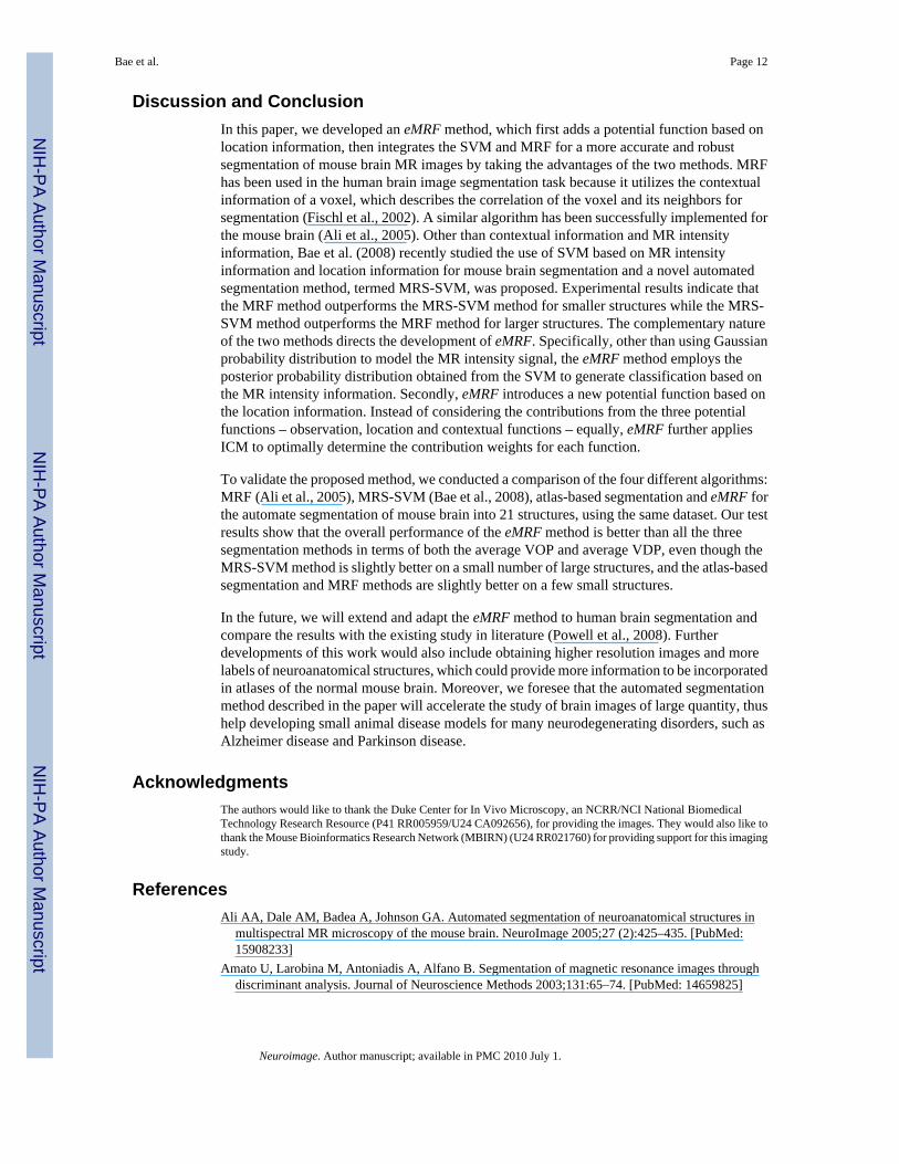
(Eq. 8)

where α = {α1, …,αm} and β = {β1, …, βm}. Furthermore, by differentiating with respect tow, b and ξi and introducing the Karush-Kuhn-Tucker (KKT) condition, Eq. 8 is converted tothe following Lagrangian dual problem:

(Eq. 9)

The optimal solution αi* for the dual problem determines the parameters w* and b* of the

following optimal hyperplane, also known as SVM decision function:

(Eq. 10)

where K(xi, xj) is a kernel function defined as K(xi,xj)=Φ(xi)TΦ(xj). The kernel functionperforms the nonlinear mapping implicitly. We chose a Radial Basis Function (RBF) kernel,defined as:

(Eq. 11)

where γ in Eq. 11 is a parameter related to the span of an RBF kernel. The smaller the valueis, the wider the kernel spans.

To extend the application of SVM for multiclass classification, a number of methods have beendeveloped, which mainly fall in three categories: One-Against-All (OAA), One-Against-One(OAO) and All-At-Once (AAO). In OAA method, one SVM is trained with the positive classrepresenting one class and the negative class representing the others. Therefore, it builds ndifferent SVM models where n is the number of the classes. The idea of AAO is similar to thatof OAA, but it determines n decision functions at once in one model, where the kth decisionfunction separates the kth class from the other classes. In OAO method, a SVM is trained toclassify the kth class and the lth class. Therefore, it constructs n(n−1)/2 SVM models. Hsu andLin (2002) reported that the training time of OAO method is less than that of OAA or AAOmethod. OAO is more efficient on large datasets than OAA and AAO method. Thus, OAOmethod is used in this study. In OAO method, the following problem is to be solved:

(Eq. 12)

Bae et al. Page 6

Neuroimage. Author manuscript; available in PMC 2010 July 1.

NIH

-PA Author Manuscript

NIH

-PA Author Manuscript

NIH

-PA Author Manuscript

eMRFAs discussed earlier in Eq. 6, traditional MRF mainly focuses on MR intensity as well as thecontextual relationship. Research on brain segmentation has concluded that beside of MRintensity and contextual relationship with neighboring structures, location within the brain alsoplays an important role (Fischl et al., 2002;Ali et al., 2005,Bae et al., 2008). To incorporate thethree different types of information into an image segmentation model, Bayesian theorem isused. Consider a 3D MR image represented by an m×n×o matrix, with its associatedmultivariate intensity vector X=(x111, x112, …, x11o, …, x1n1, … xm11, …, xmno), a locationvector L=(l111, l112, …, l11o, …, l1n1, … lm11, …, lmno), and class label configuration Y=(y111, y112, …, y11o, …, yl1n1, … ym11, …, ymno). We rewrite yabc as yi where i=1, 2, …, S, andS=mno. The posterior probability of having a label configuration Y given a multivariateintensity vector X and a location vector L is formulated as follows:

(Eq. 13)

Assuming X and L independent from each other yields following expression:

(Eq. 14)

If we make logarithmic transformation to Eq. 14, we obtain

(Eq. 15)

Each term of the right hand side of Eq. 15 can be regarded as the contribution to labeling fromMR signal intensities, voxel coordinates, and prior belief of label, which incorporates thecontextual information into the labeling decision. The function can be modified as following:

(Eq. 16)

where w1, w2 and w3 are model parameters which indicate the degree of contribution of eachterm to the posterior probability P(Y|X,L), and Ni denotes the neighboring sites of site i.

The first term, Ai(yi, xi), in Eq. 16 is the observation potential function that models the MRintensity information. EMRF model employs SVM in order to take advantage of the excellentdiscriminative ability of SVM. Since SVM decision function gives as output the distance froman instance to the optimal separation hyperplane, Platt (2000) proposed a method for mappingthe SVM outputs into posterior probability by applying a sigmoid function whose parametersare estimated from the training process. The observation potential function is defined asfollows, for voxel i:

(Eq. 17)

Bae et al. Page 7

Neuroimage. Author manuscript; available in PMC 2010 July 1.

NIH

-PA Author Manuscript

NIH

-PA Author Manuscript

NIH

-PA Author Manuscript

where fk(xi) is the SVM decision function for class k, α and β are the parameters determinedfrom the training data. P(yi=k|xi) is the likelihood that the label yi is labeled as class k giventhe MR intensity xi. When applying SVM to MR image segmentation, the overlapping of MRsignals is a critical issue. Adding the three coordinates (x, y and z coordinates of each datapoint in a 3D MR image) as features into SVM classifier helps in classification by relievingthe class overlapping problem of MR intensities between different structures (Bae et al.,2008). In one of our preliminary experiments, it is interesting to find that using two MRprotocols (T2-weighted and proton density-weighted) along with coordinate features yieldbetter segmentation performance than using all the five MR protocols 1. Our preliminary resultalso indicates that adding more MR contrasts does not aid the classifier because it increasesthe overlapping among MR signals and makes the dataset noisier. Thus, the intensity featurevector X forms a five dimensional vector, consisting of the two MR intensities (T2-weightedand proton-density (PD) weighted acquisition) and the three coordinate features.

The second term Bi(yi, li) in Eq. 16, is the location potential function. Fischl et al. (2002) pointout that the number of possible neuroanatomical structures at a given location in a brain atlasbecomes small as registration become accurate. Therefore, the location of a voxel in a 3D imageafter registration is critical for classification of the voxel into the neuroanatomical classes. Thelocation potential function is computed as follows:

(Eq. 18)

where P(yi=k|li=r) is the probability that a voxel’s label yi is predicted as class k given that thelocation li of the voxel is r. The denominator in Eq. 18 is equal to the number of mice used inthe training set. This location information is similar to the apriori probability used in humanbrain segmentation study (Ashburner and Friston, 1997) as implemented in SPM.

The third term Vi(yi,yNi) in Eq. 16 is the contextual potential function which models thecontextual information using MRF. Based on the MRF theory, the prior probability of havinga label at a given site i is determined by the label configuration of the neighborhood of the sitei. The contextual potential function for site i will have a higher value as the number of neighborsthat have the same label increases. It is defined as

(Eq. 19)

where n(Ni) is the number of voxels in a neighborhood of site i. We use a first orderneighborhood system as a clique, which consists of the adjacent six voxels in the four cardinaldirections in a plane and the front and back directions through the plane.

In fact, other than observation and contextual potential function, eMRF introduces locationpotential function to the problem. Secondly, noticing that each potential function canindependently classify a voxel, eMRF model integrates them together and assigns weightoptimally to each of them based on their classification performance from the training set. The

1Using the two indices VOP (the larger the better), VDP (the smaller the better) introduced in the next section, the experiment on twoMR protocols with coordinates yields 72.42% VOP and 19.21% VDP in average. The experiment on all five MR protocols withcoordinates generates 59.38% VOP and 24.16% VDP.

Bae et al. Page 8

Neuroimage. Author manuscript; available in PMC 2010 July 1.

NIH

-PA Author Manuscript

NIH

-PA Author Manuscript

NIH

-PA Author Manuscript

weight parameter indicates the contributions from the three different potential functions topredict the labeling. The optimal weight parameter is determined by grid search on severalpossible sets of w1, w2 and w3 using cross-validation. The Y that maximizes the posteriorprobability P(Y|X,L) corresponds to the most likely label given the information of X and L.This is known as the maximum a posterior (MAP) solution which is well known in the machinevision literatures (Li, 2001). Finding the optimal solution of the joint probability of a MRF

is very difficult because of the complexity caused by the interaction amongmultiple labels. A local search method called iterated conditional modes (ICM) proposed byBesag (1986) is used in this study to locate the optimal solutions. The ICM algorithm is tomaximize local conditional probabilities sequentially by using the greedy search in the iterativelocal maximization. It is expressed as

(Eq. 20)

Given the data xi and li, the algorithm sequentially updates into by switching thedifferent labels to maximizing P(yi|xi, li) for every site i in turn. The algorithm terminates whenno more labels are changed. In the ICM algorithm, how to set the initial estimator y(0) is veryimportant. We use the MAP solution based on only the location information as the initialestimator of the ICM algorithm, i.e.,

(Eq. 21)

Performance MeasurementsThe VOP and VDP are used to measure the performance of the proposed automatedsegmentation procedure (Fischl et al., 2002; Ali et al., 2005, Hsu and Lin, 2002). The VOPand VDP are calculated by comparing the automated segmentation with the true voxel labeling(from the manual segmentation). Denote LA and LM as labeling of the structure i by automatedsegmentation and manual segmentation respectively, and V(L) as the volume of the labeling.The volume overlap percentage for class i is defined as

This performance index is the larger the better. When all the labels from the automated andmanual segmentation coincide, VOPi(LA, LM) is 100%. VOP is very sensitive to the spatialdifference of the two labelings, because a slight difference in spatial location of the twolabelings can cause significant decreases in the numerator of VOPi(LA, LM).

The VDP for class i is used for quantifying the volume difference of the structures delineatedby the two segmentations, and it is defined as

Bae et al. Page 9

Neuroimage. Author manuscript; available in PMC 2010 July 1.

NIH

-PA Author Manuscript

NIH

-PA Author Manuscript

NIH

-PA Author Manuscript

This performance index is smaller the better. When all the labelings from the two segmentationsare identical, VDPi(LA, LM) is 0.

ResultsSegmentation and Model Validation

The eMRF algorithm was implemented and tested on a group of 90 μm isotropic resolutionMR images of five C57/BL6 mice. To assure the validity of all results from this experiment,a five-fold cross validation was used in the every step of the experiment. Each mouse was usedas a test brain, while the remaining four mice were used as the training set. Hence we testedthe algorithm on five distinct training and testing sets. To calculate the observation potentialfunction in Eq. 17, we built five SVM models for the five different training sets using the MRS-SVM procedure (Bae et al., 2008). Building a SVM model for mouse brain segmentation ischallenging because the number of the classes is large (>20) and the classes are highlyimbalanced. The MRS-SVM procedure enabled us to build SVM model for the brainsegmentation efficiently and effectively. Testing each SVM model yielded the posteriorprobability P(Y|X) in Eq. 17 for each tested mouse. The location potential function wascalculated for the five mouse based on Eq. 18. After the observation and location potentialfunctions were calculated for each mouse, the ICM algorithm was used to provide thecontextual potential function in Eq. 19 and the posterior probability P(Y|X,L) in Eq. 16. To findthe best weight for each potential function we conducted a grid search over the range of eachwi= {0.1, 0.2, …, 0.9} (i=1, 2, 3), where w1 + w2 + w3= 1. The best model parameters determinedwere w1=.1, w2=.6 and w3=0.3 for observation, location and contextual functions, respectively.

We also implemented the atlas-based segmentation for the same mouse brain images tocompare its performance with the eMRF method. One mouse brain image was chosen out ofthe five mouse brains as a reference brain. First, the rest four testing images were realigned tothe reference brain using a 12-parameter affine registration which adjusts the global positionand size differences between the individual brain images. Next, the reference brain was mappedto the testing brain images using a nonlinear registration which deforms each neuroanatomicalstructure into a common space. The registrations were done using Image Registration Toolkit(ITK) software and the registration parameters were optimized by the software. Each imageof the five mouse brain was used as the reference brain, while the remaining four images wereused as the testing brains. Therefore, each brain image was segmented four times with differentreference brain each time.

Table 2 presents estimates of the segmentation performance based on two metrics: VOP andVDP between the automated and manual label images. These estimates are based on five mousebrains, and with the use of five-fold cross validation. The results for the eMRF method arecompared with three other segmentation methods – the aforementioned atlas-basedsegmentation method, the MRS-SVM method (Bae et al., 2008) and the MRF method (Ali etal., 2005). Overall eMRF outperforms all the three segmentation methods. Compared to MRS-SVM the average VOP of eMRF is improved by 8.68%, 10.05% compared to the atlas-basedsegmentation, and 2.79% compared to MRF. Corresponding to an increase in the average VOP,the average VOD of eMRF is decreased. It is improved by 42.04% compared to MRS-SVM,23.84% compared the atlas-based segmentation, and 12.71% compared to MRF. Figure 2illustrates the VOP (top) and the VDP (bottom) of the four different segmentation methods.

The eMRF method outperforms the MRS-SVM method in most structures. The improvementin segmentation performance as assessed by VOP is greatest for white matter structures likethe anterior commissure (99.29%), and cerebral peduncle (15.55%) but also for ventricles(35.91%). Exceptions where eMRF underperforms to MRS-SVM are three large structures:CORT, CBLM and OLFB. The MRS-SVM method performs better for large structures because

Bae et al. Page 10

Neuroimage. Author manuscript; available in PMC 2010 July 1.

NIH

-PA Author Manuscript

NIH

-PA Author Manuscript

NIH

-PA Author Manuscript

the classifier tends to generate the separation hyperplane between a large class and a smallclass such that it is biased towards the large class. Therefore, a voxel that is located at theboundary between the large class and the small class is more likely predicted as the large classand this reduces the misclassification of a large class voxel to a small class voxel. However,the eMRF method balances the contributions from the MR intensity information, the locationinformation and the contextual information by assigning potential functions with differentweights. In our study, the weight assigned to observation potential function (w1) is smallerthan the other two. The averages of the VOP and the VDP of the eMRF method are improvedby 8.68%, and 42.04% respectively, compared to the MRS-SVM method, which indicates thatthe overall segmentation performance has been improved by the use of eMRF.

The eMRF method provides better performances in most structures than the atlas-basedsegmentation method. Based on the VOP, the eMRF method outperforms the atlas-basedsegmentation method in all the structures except the two structures, AC and INTP. Theperformance differences in these two structures are only 0.45% in AC and 5.49% in INTP. TheeMRF method has a better VDP performance than the atlas-based segmentation method in 17structures. There are four small structures (AC, VEN, INTP and CC) that the atlas-basedsegmentation method has better VDP performance than eMRF. Since each labeling of thevoxels in the reference brain is mapped to the testing brain in the atlas-based segmentationprocess, the number of labeling for a structure in the reference brain is well maintained in thenumber of labeling for the structure in the testing brain. Therefore, the VDP values of the atlas-based segmentation method in all the structures are quite consistent (11.14–15.23). However,this method has the worst VOP performance among the four different segmentation methods,indicating that the accuracy of atlas-based segmentation is poor. The eMRF method canimprove the averages of the VOP and the VDP by 10.05% and 23.84%, respectively, whichshows that overall the eMRF method outperforms the atlas-based segmentation method.

Based on the voxel overlap metric, the eMRF method shows better performance in 13 out of21 structures compared to the MRF method. The eMRF method provides more than 5%performance improvement in 7 structures (CPED, PAG, MED, PON, SNR, OPT and TRI), thelargest improvements are seen for optic tract (29.39%) and trigeminal tract (15.63%). Basedon the volume difference metric, the eMRF method shows better performance in 16 structuresout of 21 structures. VDP improvement ranged from 61.68% for optic tract and to 3.61% forglobus pallidus. In four small structures (PAG, INFC, AC and INTP), which take less than 1%volume compared to the whole brain volume, the MRF method shows better performance. Thisis due to the fact that in the MRF method labeling a voxel depends on the labelings of theneighborhood of the voxel, thus the identification of small structures is enhanced. Nevertheless,the averages of the VOP and the VDP of the eMRF method are improved by 2.79%, and 12.71%respectively, compared to the MRF method. The eMRF method can make a balance betweenthe overfitting of the SVM method to the larger classes and the overfitting of the MRF methodto the smaller classes so that the overall segmentation performance is improved.

A visual comparison of the three segmentation methods, manual labeling (the gold standard),eMRF and MRS-SVM, is shown for two specific coronal levels (one at the level close to thehippocampal commissure, and one at the level of the pons) in Figure 3. On the left column ofFigure 3 are displayed the manual segmentations (used as the gold standard), on the middlecolumn are the automated segmented images by the eMRF method and the right column, thoseproduced by the MRS-SVM method. The eMRF method seems to deviate less than the MRS-SVM method from the manual labeling, and to respect better the topology of the structures.The testing time of the MRS-SVM algorithm for a mouse brain dataset (472,100 voxels) was289.4 minutes with a 3.4-GHz PC. The testing experiment was run using MATLAB, andexecuted the eMRF segmentation of one mouse brain in 75 minutes.

Bae et al. Page 11

Neuroimage. Author manuscript; available in PMC 2010 July 1.

NIH

-PA Author Manuscript

NIH

-PA Author Manuscript

NIH

-PA Author Manuscript

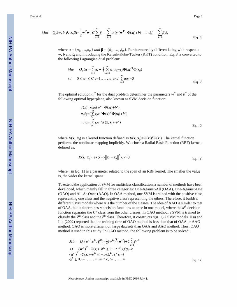
Discussion and ConclusionIn this paper, we developed an eMRF method, which first adds a potential function based onlocation information, then integrates the SVM and MRF for a more accurate and robustsegmentation of mouse brain MR images by taking the advantages of the two methods. MRFhas been used in the human brain image segmentation task because it utilizes the contextualinformation of a voxel, which describes the correlation of the voxel and its neighbors forsegmentation (Fischl et al., 2002). A similar algorithm has been successfully implemented forthe mouse brain (Ali et al., 2005). Other than contextual information and MR intensityinformation, Bae et al. (2008) recently studied the use of SVM based on MR intensityinformation and location information for mouse brain segmentation and a novel automatedsegmentation method, termed MRS-SVM, was proposed. Experimental results indicate thatthe MRF method outperforms the MRS-SVM method for smaller structures while the MRS-SVM method outperforms the MRF method for larger structures. The complementary natureof the two methods directs the development of eMRF. Specifically, other than using Gaussianprobability distribution to model the MR intensity signal, the eMRF method employs theposterior probability distribution obtained from the SVM to generate classification based onthe MR intensity information. Secondly, eMRF introduces a new potential function based onthe location information. Instead of considering the contributions from the three potentialfunctions – observation, location and contextual functions – equally, eMRF further appliesICM to optimally determine the contribution weights for each function.

To validate the proposed method, we conducted a comparison of the four different algorithms:MRF (Ali et al., 2005), MRS-SVM (Bae et al., 2008), atlas-based segmentation and eMRF forthe automate segmentation of mouse brain into 21 structures, using the same dataset. Our testresults show that the overall performance of the eMRF method is better than all the threesegmentation methods in terms of both the average VOP and average VDP, even though theMRS-SVM method is slightly better on a small number of large structures, and the atlas-basedsegmentation and MRF methods are slightly better on a few small structures.

In the future, we will extend and adapt the eMRF method to human brain segmentation andcompare the results with the existing study in literature (Powell et al., 2008). Furtherdevelopments of this work would also include obtaining higher resolution images and morelabels of neuroanatomical structures, which could provide more information to be incorporatedin atlases of the normal mouse brain. Moreover, we foresee that the automated segmentationmethod described in the paper will accelerate the study of brain images of large quantity, thushelp developing small animal disease models for many neurodegenerating disorders, such asAlzheimer disease and Parkinson disease.

AcknowledgmentsThe authors would like to thank the Duke Center for In Vivo Microscopy, an NCRR/NCI National BiomedicalTechnology Research Resource (P41 RR005959/U24 CA092656), for providing the images. They would also like tothank the Mouse Bioinformatics Research Network (MBIRN) (U24 RR021760) for providing support for this imagingstudy.

ReferencesAli AA, Dale AM, Badea A, Johnson GA. Automated segmentation of neuroanatomical structures in

multispectral MR microscopy of the mouse brain. NeuroImage 2005;27 (2):425–435. [PubMed:15908233]

Amato U, Larobina M, Antoniadis A, Alfano B. Segmentation of magnetic resonance images throughdiscriminant analysis. Journal of Neuroscience Methods 2003;131:65–74. [PubMed: 14659825]

Bae et al. Page 12

Neuroimage. Author manuscript; available in PMC 2010 July 1.

NIH

-PA Author Manuscript

NIH

-PA Author Manuscript

NIH

-PA Author Manuscript

Andersen AH, Zhang Z, Avison MJ, Gash DM. Automated segmentation of multispectral brain MRimages. Journal of Neuroscience Methods 2002;122:13–23. [PubMed: 12535761]

Ashburner J, Friston K. Multimodal image coregistration and partitioning – a unified framework.NeuroImage 1997;6:209–217. [PubMed: 9344825]

Bae, MH.; Wu, T.; Pan, R. Mix-Ratio Sampling: Classifying Multiclass Imbalanced Mouse Brain ImagesUsing Support Vector Machine. 2008. Technical Report available at http://swag.eas.asu.edu/vcie/

Besag J. On the statistical analysis of dirty pictures. Journal of Royal Statistical Society, Series B 1986;48(3):259–302.

Bock NA, Kovacevic N, Lipina TV, Roder JC, Ackerman SL, Henkelman RM. In vivo magneticresonance imaging and semiautomated image analysis extend the brain phenotype for cdf/cdf mice.The Journal of Neuroscience 2006;26 (17):4455–4459. [PubMed: 16641223]

Duta N, Sonka M. Segmentation and interpretation of MR brain images: an improved active shape model.IEEE Transactions on Medical Imaging 1998;16:1049–1062. [PubMed: 10048862]

Fischl B, Salat DH, Busa E, Albert M, Dieterich M, Haselgrove C, Van der Kouwe A, Killiany R, KennedyD, Klaveness S, et al. Whole brain segmentation: automated labeling of neuroanatomical structures inthe human brain. Neuron 2002;33:341–355. [PubMed: 11832223]

Geman S, Geman D. Stochastic relaxation, Gibbs distributions and the Bayesian restoration of images.IEEE Transactions on Pattern Analysis and Machine Intelligence 1984;6:721–741.

Gonzalez Ballester MA, Zisserman A, Brady M. Segmentation and measurement of brain structures inMRI including confidence bounds. Medical Image Analysis 2000;4:189–200. [PubMed: 11145308]

Heckemann RA, Hajnal JV, Aljabar P, Rueckert D, Hammers A. Automatic anatomical brain MRIsegmentation combining label propagation and decision fusion. NeuroImage 2006;33:115–126.[PubMed: 16860573]

Hsu CW, Lin CJ. A comparison of methods for multi-class support vector machines. IEEE Transactionson Neural Networks 2002;13(2):415–425. [PubMed: 18244442]

Kovacevic N, Lobaugh NJ, Bronskill MJ, Levine B, Feinstein A, Black SE. A robust method for extractionand automatic segmentation of brain images. NeuroImage 2002;17:1087–1100. [PubMed:12414252]

Kovacevic N, Henderson JT, Chan E, Lifshitz N, Bishop J, Evans AC, Henkelman RM, Chen XJ. Athree-dimensional MRI atlas of the mouse brain with estimates of the average and variability.Cerebral Cortex 2005;15 (5):639–645. [PubMed: 15342433]

Lee CH, Schmidt M, Murtha A, Bistritz A, Sander J, Greiner R. Segmenting brain tumors with conditionalrandom fields and support vector machines. Lecture Notes in Computer Science 2005;3765:469–478.

Li, SZ. Markov Random Field Modeling in Image Analysis. Springer-Verlag; Tokyo: 2001.Ma Y, Hof PR, Grant SC, Blackband SJ, Bennett R, Slatest L, Mcguigan MD, Benveniste H. A three-

dimensional digital atlas database of the adult C57BL/6J mouse brain by magnetic resonancemicroscopy. Neuroscience 2005;135 (4):1203–1215. [PubMed: 16165303]

Mazoyer N, Landeau B, Papathanassiou D, Crivello F, Etard O, Delcroix N, Mazoyer B, Joliot M.Automated anatomical labeling of activations in SPM using a macroscopic anatomical parcellationof the MNI MRI single-subject brain. NeuroImage 2002;15:273–289. [PubMed: 11771995]

Platt, J. Advances in Large Margin Classifiers. MIT Press; Cambridge, MA: 2000. Probabilistic outputsfor support vector machines and comparison to regularized likelihood methods.

Powell S, Magnotta VA, Johnson H, Jammalamadaka VK, Pierson R, Andreasen NC. Registration andmachine learning-based automated segmentation of subcortical and cerebellar brain structures.NeuroImage 2008;39:238–247. [PubMed: 17904870]

Reddick WE, Glass JO, Cook EN, Elkin TD, Deaton RJ. Automated segmentation and classification ofmultispectral magnetic resonance images of brain using artificial neural networks. IEEE Transactionson Medical Imaging 1997;16:911–918. [PubMed: 9533591]

Suri J. Two-dimensional fast Magnetic Resonance brain segmentation. IEEE Engineering in Medicineand Biology 2001 July/August;:84–95.

Vapnik, VN. The Nature of Statistical Learning Theory. Springer; Verlag: 1995.

Bae et al. Page 13

Neuroimage. Author manuscript; available in PMC 2010 July 1.

NIH

-PA Author Manuscript

NIH

-PA Author Manuscript

NIH

-PA Author Manuscript

Zavaljevski A, Dhawan AP, Gaskil M, Ball W, Johnson JD. Multi-level adaptive segmentation of multi-parameter MR brain images. Computerized Medical Imaging and Graphics 2000;24:87–98.[PubMed: 10767588]

Zhang Y, Smith S, Brady M. Segmentation of brain MR images through a hidden Markov random fieldmodel and the expectation–maximization algorithm. IEEE Transactions on Medical Imaging2001;20:45–57. [PubMed: 11293691]

Bae et al. Page 14

Neuroimage. Author manuscript; available in PMC 2010 July 1.

NIH

-PA Author Manuscript

NIH

-PA Author Manuscript

NIH

-PA Author Manuscript

Figure 1.SVM binary classification problem (adopted from Vapnik, 1995). The solid line between thetwo dashed lines is the optimal hyperplane. The squares represent the samples from the positiveclass and the circles represent the samples from the negative class. The samples representedas the filled squares and the filled circles are the support vectors.

Bae et al. Page 15

Neuroimage. Author manuscript; available in PMC 2010 July 1.

NIH

-PA Author Manuscript

NIH

-PA Author Manuscript

NIH

-PA Author Manuscript

Figure 2.Comparison of the relative performances of the eMRF, MRS-SVM, atlas-based segmentationand MRF methods based on the voxel overlap percent - VOP (top) and the volume differencepercent -VDP (bottom) indices

Bae et al. Page 16

Neuroimage. Author manuscript; available in PMC 2010 July 1.

NIH

-PA Author Manuscript

NIH

-PA Author Manuscript

NIH

-PA Author Manuscript

Figure 3.Coronal slices through the labeled brain at the level of anterior hippocampus and third ventricle(upper row), and pons and substantia nigra (lower row) show in a qualitative manner the relativesuperiority of eMRF compared to MRS-SVM. Note that eMRF segmentation better preservedthe shapes of striatum and corpus callosum (as seen in the manual labels), compared to MRS-SVM; and also that eMRF was able to segment a small CSF filled region in the center of PAG,while MRS-SVM missed it.

Bae et al. Page 17

Neuroimage. Author manuscript; available in PMC 2010 July 1.

NIH

-PA Author Manuscript

NIH

-PA Author Manuscript

NIH

-PA Author Manuscript

NIH

-PA Author Manuscript

NIH

-PA Author Manuscript

NIH

-PA Author Manuscript

Bae et al. Page 18Ta

ble

1Li

st o

f 21

segm

ente

d st

ruct

ures

and

thei

r abb

revi

atio

ns.

Stru

ctur

esA

bbre

v.St

ruct

ures

Abb

rev.

Stru

ctur

esA

bbre

v.

Cer

ebra

l cor

tex

CO

RT

Infe

rior c

ollic

ulus

INFC

Pont

ine

nucl

eiPO

N

Cer

ebra

l ped

uncl

eC

PED

Med

ulla

obl

onga

taM

EDSu

bsta

ntia

nig

raSN

R

Hip

poca

mpu

sH

CTh

alam

usTH

AL

Inte

rped

uncu

lar n

ucle

usIN

TP

Cau

date

put

amen

CPU

Mid

brai

nM

IND

Olfa

ctor

y bu

lbO

LFB

Glo

bus p

allid

usG

PA

nter

ior c

omm

issu

reA

CO

ptic

trac

tO

PT

Inte

rnal

cap

sule

ICA

PC

ereb

ellu

mC

BLM

Trig

emin

al tr

act

TRI

Peria

cque

duct

al g

ray

PAG

Ven

tricu

lar s

yste

mV

ENC

orpu

s cal

losu

mC

C

Neuroimage. Author manuscript; available in PMC 2010 July 1.

NIH

-PA Author Manuscript

NIH

-PA Author Manuscript

NIH

-PA Author Manuscript

Bae et al. Page 19Ta

ble

2A

ccur

acy

of th

e fou

r seg

men

tatio

n m

etho

ds (e

MRF

, MR

F-SV

M, a

tlas-

base

d se

gmen

tatio

n an

d M

RF)

for e

ach

of th

e 21

segm

ente

d br

ain

stru

ctur

es is

eva

luat

ed u

sing

the

VO

P (to

p ro

w) f

or e

ach

segm

enta

tion

and

VD

P (s

econ

d ro

w) m

etric

s. Th

e pe

rcen

tage

impr

ovem

ent i

nse

gmen

tatio

n ac

cura

cy is

com

pute

d fo

r eM

RF v

ersu

s MR

S-SV

M, e

MRF

ver

sus a

tlas-

base

d se

gmen

tatio

n, a

nd e

MRF

ver

sus M

RF.

The

impr

ovem

ents

in V

OP

and

VO

D a

re c

alcu

late

d se

para

tely

. A ‘+

’ sig

n al

way

s mea

ns th

at e

MRF

met

hod

outp

erfo

rms t

he o

ther

met

hods

for t

he sp

ecifi

c ne

uroa

nato

mic

al st

ruct

ure

and

‘−’ m

eans

that

eM

RF u

nder

perf

orm

s.

CO

RT

CPE

DH

CC

PUG

PIC

AP

PAG

INFC

ME

DT

HA

LM

IDB

eMRF

VO

P (%

)91

.10

73.1

586

.20

87.6

279

.64

73.1

490

.26

85.3

291

.93

93.5

393

.27

VD

P (%

)3.

348.

325.

563.

987.

5411

.05

3.55

5.26

7.12

2.48

2.97

MR

S-SV

MV

OP

(%)

93.4

663

.31

83.9

285

.72

74.4

763

.91

80.9

083

.21

90.2

792

.07

90.4

8

VD

P (%

)1.

6311

.50

5.87

3.89

11.3

412

.66

7.97

7.81

10.0

32.

783.

84

Impr

ovem

ent

VO

P (%

)−2

.53

15.5

52.

712.

226.

9514

.44

11.5

72.

541.

841.

593.

09

VD

P (%

)10

4.24

−27.

60−5

.33

2.16

−33.

51−1

2.78

−55.

44−3

2.64

−28.

98−1

0.61

−22.

57

Atla

s-ba

sed

segm

enta

tion

VO

P (%

)84

.19

64.3

184

.07

82.4

668

.19

60.8

384

.47

75.6

784

.24

91.1

688

.56

VD

P (%

)12

.24

11.7

611

.91

11.5

413

.51

11.4

011

.14

14.8

712

.50

11.5

712

.47

Impr

ovem

ent

VO

P (%

)8.

2013

.75

2.54

6.26

16.7

920

.25

6.85

12.7

69.

122.

605.

32

VD

P (%

)72

.74

29.2

053

.34

65.5

344

.16

3.13

68.1

164

.60

43.0

578

.54

76.1

8

MR

FV

OP

(%)

90.7

767

.69

87.6

988

.46

78.4

673

.85

85.3

883

.08

86.1

593

.08

90.7

7

VD

P (%

)4.

3512

.17

6.96

6.96

7.83

13.0

42.

614.

3510

.43

3.48

4.35

Impr

ovem

ent

VO

P (%

)0.

368.

06−1

.70

−0.9

51.

50−0

.96

5.71

2.70

6.70

0.49

2.76

VD

P (%

)23

.24

31.6

220

.08

42.8

43.

6115

.31

−36.

19−2

1.05

31.7

628

.58

31.6

8

AC

CB

LM

VE

NPO

NSN

RIN

TP

OL

FBO

PTT

RI

CC

Avg

.

eMRF

VO

P (%

)50

.76

92.6

871

.83

80.0

378

.98

71.6

182

.50

68.6

773

.83

65.7

580

.09

VD

P (%

)25

.55

3.73

16.8

312

.49

10.1

626

.09

10.7

95.

677.

3320

.57

9.54

MR

S-SV

MV

OP

(%)

25.4

796

.29

52.8

574

.38

60.7

958

.18

91.2

359

.25

69.7

257

.65

73.6

9

Neuroimage. Author manuscript; available in PMC 2010 July 1.

NIH

-PA Author Manuscript

NIH

-PA Author Manuscript

NIH

-PA Author Manuscript

Bae et al. Page 20

CO

RT

CPE

DH

CC

PUG

PIC

AP

PAG

INFC

ME

DT

HA

LM

IDB

VD

P (%

)68

.49

1.48

24.9

214

.30

25.6

562

.22

7.85

19.9

317

.27

24.2

816

.46

Impr

ovem

ent

VO

P (%

)99

.29

−3.7

535

.91

7.60

29.9

123

.08

−9.5

715

.90

5.89

14.0

48.

68

VD

P (%

)62

.70

−151

.51

32.4

812

.65

60.3

958

.06

−37.

4971

.58

57.5

715

.26

42.0

4

Atla

s-ba

sed

segm

enta

tion

VO

P (%

)50

.99

85.9

167

.30

70.6

873

.18

75.7

782

.19

44.7

459

.72

49.5

572

.77

VD

P (%

)11

.51

12.4

912

.40

14.5

512

.93

15.2

312

.40

12.0

512

.36

12.2

812

.53

Impr

ovem

ent

VO

P (%

)−0

.45

7.89

6.73

13.2

47.

92−5

.49

0.38

53.4

923

.62

32.6

910

.05

VD

P (%

)−1

21.9

870

.13

−35.

7014

.17

21.4

1−7

1.32

12.9

852

.99

40.7

1−6

7.49

23.8

4

MR

FV

OP

(%)

55.3

893

.08

70.7

773

.08

68.4

676

.92

84.6

253

.08

63.8

571

.54

77.9

1

VD

P (%

)19

.13

3.48

19.1

317

.39

15.6

513

.91

16.5

214

.78

10.4

322

.61

10.9

3

Impr

ovem

ent

VO

P (%

)−8

.35

−0.4

21.

509.

5215

.36

−6.9

1−2

.50

29.3

915

.63

−8.1

02.

79

VD

P (%

)−3

3.54

−7.2

212

.04

28.1

835

.09

−87.

5534

.68

61.6

829

.77

9.00

12.7

1

Neuroimage. Author manuscript; available in PMC 2010 July 1.