Automated map generalization with multiple operators: a simulated annealing approach

Research Article

Automated map generalization with multiple operators: a simulatedannealing approach

J. MARK WARE

School of Computing, University of Glamorgan, Pontypridd CF37 1DL, UK;e-mail: [email protected]

CHRISTOPHER B. JONES

Department of Computer Science, Cardiff University, Cardiff CF24 3XF,Wales, UK

and NATHAN THOMAS

School of Computing, University of Glamorgan, Pontypridd CF37 1DL,Wales, UK

(Received 2 March 2002; accepted 10 April 2003 )

Abstract. This paper explores the use of the stochastic optimization techniqueof simulated annealing for map generalization. An algorithm is presented thatperforms operations of displacement, size exaggeration, deletion and sizereduction of multiple map objects in order to resolve graphic conflict resultingfrom map scale reduction. It adopts a trial position approach in which each of ndiscrete polygonal objects is assigned k candidate trial positions that representthe original, displaced, size exaggerated, deleted and size reduced states ofthe object. This gives rise to a possible kn distinct map configurations; theexpectation is that some of these configurations will contain reduced levels ofgraphic conflict. Finding the configuration with least conflict by means of anexhaustive search is, however, not practical for realistic values of n and k. Weshow that evaluation of a subset of the configurations, using simulatedannealing, can result in effective resolution of graphic conflict.

1. IntroductionThe process of displaying map data at scales smaller than the source scale of the

data can result in graphic conflicts in which map objects overlap or become too

close together, or too small, to be clearly distinguishable. The cause of the conflicts

is a combination of the effects of geometric scale reduction, whereby features

decrease in size and increase in density on the map, and the fact that map symbols

are often larger than the true-scale representation of their associated real-world

feature. Thus with reduction in scale the map symbols may be regarded as

competing for occupation of the limited space on the map display. The solution to

such conflicts falls within the field of map generalization, whereby the content

International Journal of Geographical Information ScienceISSN 1365-8816 print/ISSN 1362-3087 online # 2003 Taylor & Francis Ltd

http://www.tandf.co.uk/journalsDOI: 10.1080/13658810310001596085

INT. J. GEOGRAPHICAL INFORMATION SCIENCE, 2003

VOL. 17, NO. 8, 743–769

of a map is adapted to meets the constraints of the scale and the purpose of the

map.

Typical operations performed in the course of map generalization include

reduction in the detail of lines, areas and surfaces; deletion of less important

features; exaggeration of the size of features that would otherwise be too small;

amalgamation of neighbouring features; collapse in the dimensionality of area

features to lines or points; caricature of the shape and pattern of simplified map

features to communicate their original form; and displacement in order to retain

adequate separation distances between neighbouring features. Solution of the

specific problems of graphic conflict is usually met through the application of

displacement, deletion and amalgamation operations, although all of the operations

referred to have the potential to assist in the process. A further operation that may

be employed in graphic conflict resolution is that of size reduction, though it is not

usually referred to as a standard map generalization operation.

Various efforts have been made to automate all of the map generalization

operations. Most of the early published procedures were developed to work on

individual features, and hence ignore the problems of graphic conflict resolution.

However, with increasing levels of use of map data in interactive and online

displays, there is a particular need to develop procedures that resolve graphic

conflicts fully automatically, without recourse to human intervention. Thus it may

be envisaged that arbitrary combinations of digital map features, which

approximate in level of detail to the users need, may be retrieved from a spatial

database, but that their successful display requires online conflict resolution that

must adapt to the user’s ad hoc requirements.Given a set of map features that is near to the required level of detail, the

primary conflict resolution procedure may be regarded as displacement, since, when

applied with care, this operator will not significantly reduce the information content

of the map. By itself it cannot of course be guaranteed to resolve conflicts if there is

insufficient map space available. Other operators such as deletion, amalgamation

and size reduction may then be required if constraints of separation distances are to

be met. There are several examples of the automation of displacement in local

contexts, notably Nickerson (1988) for linear features, Mackaness (1994) for sets of

points-referenced features and Jones et al. (1995) for area features.

A major challenge in automating displacement operations is to control the

propagation of conflict that arises when the movement of an object may introduce a

conflict with a feature that was not previously in conflict. This has given rise to a

number of approaches that can process multiple map features. One approach is to

formulate the problem as a set of mathematical constraints that can be solved

analytically, giving a continuous solution space. Prime examples of this approach

are Harrie (1999), who employed least squares methods, Højholt (2000) who

applied finite element analysis, and Burghardt and Meier (1997) who made use of a

method based on snakes. A second approach is to generate a discrete set of states

that are searched as part of an iterative improvement procedure. Examples of

discrete search methods are Ware and Jones (1998) who demonstrated the merits of

simulated annealing to a set of predetermined candidate states, and Lonergan and

Jones (2001) who applied a gradient descent procedure in combination with on the

fly generation of displacement actions.

Each of the methods described previously have demonstrated good potential in

744 J. M. Ware et al.

addressing the problem of conflict resolution, but none provides a method that can

be guaranteed to resolve all graphical conflict, as they are based on application of

displacement only. Harrie and Sarjakoski (2002) present a method that makes use

of multiple operators to resolve graphic conflict that arises subsequent to scale

reduction. The method, termed simultaneous graphic generalization, represents the

problem of line displacement, simplification, smoothing and exaggeration as a set of

linear constraints. Least squares adjustment is used to find a close to optimal

solution to the constraints. The reactive displacement technique presented by Ruas

(1998) is specifically aimed at building displacement. However, the method includes

an initial density analysis stage to check whether or not displacement is

appropriate; it has also been integrated into a more complete generalization tool

(i.e. Stratege), which allows for initial building and road removal, and building

aggregation based on density analysis.The AGENT project (e.g. Lamy et al. 1999, Haire and Hardy 2001) advocates

the use of intelligent software agents as a means of performing generalization. The

idea is to represent individual map features as active agents, each having its own set

of constraints that describe the way in which the feature should appear subsequent

to generalization. In addition, an agent has the ability to measure the extent to

which its constraints are met, and to suggest and try a range of conflict resolution

strategies (e.g. generalization operations) until an optimal solution is found. Low

level agents (e.g. buildings and road sections), are themselves under the control of

higher level agents that control larger scale compound features (e.g. road networks

and towns).

In this paper we show how simulated annealing (Kirkpatrick et al. 1983), an

example of an iterative improvement technique, can be applied to multiple

generalization operators of displacement, size exaggeration, deletion and size

reduction to guarantee that constraints of proximity and size are met in the course

of conflict resolution (figure 1). The methods presented use a trial position

approach, which is similar to that used in point feature label placement (Zoraster

1997), and to the work of Ware and Jones (1998) on displacement. Each of n

discrete polygonal objects is allocated k candidate trial positions into which it can

possibly move; these positions represent the original, displaced, enlarged, displaced

and enlarged, reduced, displaced and reduced, and deleted states of the object. This

results in a possible kn unique map configurations, some of which, it is assumed,

will contain less conflict than the original. Identifying the best (or, at least, an

Figure 1. Reducing scale causes conflict, which can be resolved by a combination of objectdisplacement, size enlargement, size reduction and deletion.

Automated map generalization with multiple operators 745

acceptable) configuration by means of an exhaustive search is, however, not

practical for realistic values of n and k and hence an optimization technique is

required. Simulated annealing search is a stochastic technique which has been

shown to be successful in solving large optimization problems quickly (Emden-

Weinert and Proksch, 1999), and we show here that it can be used successfully to

reduce the number of map configurations needing to be generated and evaluated.

In §2 we summarise existing methods of applying simulated annealing to

displacement of area objects, and highlight their shortcomings with regard to

inadequate performance for online application, combined with failure to guarantee

resolution of graphic conflict. In §3 we introduce techniques to improve significantly

the performance of simulated annealing, based on partitioning and on a two-stage

procedure, before introducing, in §4, the additional operators that when combined

with displacement can guarantee to resolve graphic conflict. Experiments are

described in §5 to show the importance of setting appropriate weights to control the

application of the individual operations. The paper concludes in §6 with a summary

of the results and a discussion of future work.

2. Conflict reduction by object displacement

In this section we present the problem of area object displacement in the context

of fixed linear features, following the approach of Ware and Jones (1998). A map

display D is regarded as made up of fixed linear objects F and n modifiable

detached polygonal objects M. Each modifiable object mi[M has k possible states,

providing a total of kn possible configurations of D.

2.1. Object states

At any given time a particular object mi exists in one of its k states (we will also

refer to these states as trial positions). An object’s initial map position is designated

as being trial position 1. Additional trial positions arise as a result of object

displacement only. (Additional generalization operators are considered in §4). It is

assumed that during the course of generalization, each object mi can be displaced

up to some maximum distance d from its original position (i.e. there is a continuous

space that extends from mi by a distance d into which it is permissible for mi to

move). The displacement trial positions associated with mi represent a discrete

approximation to this continuous space. Each object mi has k displacement trial

positions, which are distributed evenly about the object (figure 2).

2.2. Evaluation of map display

For a particular configuration Dj, each object mi has an associated cost. The

cost is determined by the extent to which mi is in conflict. Two categories of spatial

conflict are considered:

. PP-conflict. This involves conflict between a pair of polygonal objects (i.e. mi

and mj lie too close to each other to be distinguishable). This conflict occurs

when the minimum separating distance (in viewing coordinates) between mi

and mj is less than some predefined threshold dmin1. An occurrence of this type

of conflict carries a cost ppcost;. PL-conflict. This involves conflict between a polygonal object and a linear

object (i.e. mi and fj[F overlap or lie too close to each other to be


distinguishable). This conflict occurs when the minimum separating distance

(in viewing coordinates) between mi and fj is less than some predefined

threshold dmin2. An occurrence of this type of conflict carries a cost plcost.

The total cost C(Dj) associated with a realization Dj is found by summing the

costs associated with each object mi[M. Our goal is to find a minimum cost

configuration Dmin such that:

C Dminð Þ~MIN C Dj

� �, j~1,2 . . . kn

� �:

The set of all configurations is referred to as the search space. If the search space is

small enough then Dmin can be found by generating and evaluating each

configuration Dj (j~1, 2…kn) in turn. However, this is not practical for realistic

values of n and k. For example, a relatively simple display consisting of ten

modifiable objects each with eight trial positions, gives rise to approximately

1 000 000 000 configurations.

2.3. A simulated annealing solution

A well-established approach to solving large optimization problems of the kind

described is to adopt an iterative improvement algorithm. The concept of iterative

improvement can be illustrated by considering the search space (i.e. in our case, all

map configurations) to be laid out on the surface of a landscape. The elevation at

any point on the landscape represents the cost for the particular configuration

associated with that point. An iterative improvement algorithm will move around

the landscape in an attempt to find the lowest troughs, which correspond to low

cost configurations (Russel and Norvig 1995). Two major classes of iterative

improvement algorithms are gradient descent and simulated annealing.

Algorithm 1 describes a simple gradient descent implementation. The algorithm

accepts an initial map configuration Dinitial (i.e. each object in trial position 1),

which is immediately designated as being the current solution Dcurrent. Next, the

Figure 2. Displacement vector template for generating trial positions about a polygon.z~trial position, tpI~trial position 1. In this example, there are 28 displaced statetrial positions.


lowest cost successor Dnew to Dcurrent is found. A particular successor to Dcurrent is

found by moving a single object mi to an alternative trial position; the lowest cost

successor can be found by generating and evaluating all possible successors (of

which there are n(k-1)). If Dnew represents an improvement (in terms of cost) on

Dcurrent, then Dnew becomes Dcurrent and the next lowest cost successor is generated.

This process is repeated until a Dnew is generated that offers no improvement; at

this stage the algorithm terminates, with Dcurrent being returned as the solution. The

algorithm is quite straightforward, but is not guaranteed to find an optimal solution

since it is possible to arrive at a non-optimal current state from which no lower cost

state can be reached. This occurs when the search descends into a local minimum,

from which any single displacement generates a higher cost state. To use the

landscape analogy once more, a local minimum can be thought of as a trough in the

landscape that happens to be higher than the lowest point on the landscape. Several

ways of trying to deal with the problem of local minima are available (e.g. random-

restart, backtracking and multiple-moves). However, the exponential nature of

most realistic search spaces makes such remedies impractical.

function GradientDescentinput: Dinitial

DcurrentqDinitial

do

DnewqLowestCostSuccessor(Dcurrent)

if C(Dnew)§C(Dcurrent) then Return(Dcurrent)

DcurrentqDnew

end

Return(Dcurrent)Algorithm 1. Gradient Descent.

Searches based on simulated annealing (Algorithm 2) attempt to overcome the

problem of getting caught in local minima by sometimes allowing non-improving

configurations to be accepted. They achieve this by taking advantage of the

similarity between the way in which a metal cools from an initially high

temperature until it freezes into a minimum energy crystalline structure (called the

annealing process) and the search for a minimum in a more general system. As with

gradient descent, simulated annealing always accepts Dnew provided it offers a

better solution than Dcurrent. However, in cases where Dnew provides no

improvement, simulated annealing will accept the new configuration with some

probability P (Pv1). Like gradient descent, the algorithm begins by accepting an

initial map configuration Dinitial (i.e. each object in trial position 1); this is

immediately designated as being the current solution Dcurrent. Next a random

successor Dnew is generated by moving a randomly chosen object mi to a randomly

chosen trial positions kj. If the displacement results in a display configuration with a

lower cost (C(Dnew)vC(Dcurrent)), then the object remains in the chosen trial

position (DcurrentqDnew). If, however, the new display has a higher or equal cost

(i.e. C(Dnew)§C(Dcurrent)), then the object is either returned to its previous position

or remains in its new position, depending on probability P. The process of

attempting a random object displacement continues until stop conditions are met

(e.g. a solution that meets a target cost is found or a pre-defined maximum number

of iterations have taken place or a pre-defined maximum amount of time has

elapsed).


function SimulatedAnnealing

input: Dinitial, Schedule, Stop_Conditions

DcurrentqDinitial

TqinitialT(Schedule)while NotMet(StopConditions)

DnewqRandomSuccessor(Dcurrent)

DEqC(Dcurrent)-C(Dnew)

if DEw0 then DcurrentqDnew

else

P~e2DE/T

R~Random(0,1)

if (RvP) then DcurrentqDnew

end

TqUpdateT(Schedule)

end

Return(Dcurrent)

Algorithm 2. Simulated Annealing.

At each iteration the probability P is dependant on two variables: DE (the

change in conflict, measured by the difference in cost between the new and current

states); and T (the current ‘temperature’). P is defined as:

P~e{DE=T ð1ÞT is assigned a relatively high initial value; its value is decreased in stages

throughout the running of the algorithm. At high values of T poor displacements

(large negative DE) will often be accepted. At low values of T poor displacements

will tend to be rejected (although displacements resulting in small negative DEmight still sometimes be accepted). The acceptance of some poor displacements is

permitted so as to allow escape from locally optimal solutions. In practice, the

probability P is usually tested against a random number R (0ƒRƒ1). A value of

RvP results in the new state being accepted. For example, if P~1/3, then we

would expect, on average, for every third worse new state to be accepted. The initial

value of T and the rate by which it decreases is governed by what is called

the annealing schedule. Generally, the higher the initial value of T and the slower

the rate of change, the better the result (in cost reduction terms); however, the

processing overheads associated with the algorithm will increase as the rate of

change in T becomes more gradual.

Finding a minimum cost configuration Dmin by simulated annealing is

statistically guaranteed, provided that the reductions in T are small enough and

that for each value of T the number of configurations tested is large enough

(Zoraster 1997). However, most practical applications settle for near optimal

solutions, and make corresponding compromises in the annealing schedule; a

suitable schedule is usually decided upon after some preliminary experimentation.

2.4. Cost function

The viability of any iterative improvement algorithm depends heavily on it

having an efficient cost function, the purpose of which is to determine for any given

element of the search space (i.e. any map realization) a value that represents the

relative quality of that element. The cost function used here, C, is called repeatedly


and works by calculating and summing the costs associated with objects mi[M.

When invoked initially, C must calculate the cost associated with every object

mi[M. A record of these costs is maintained for future reference, meaning that, in

any further call, C has to consider only objects with costs affected by the most

recent displacement. Calculating the cost associated with a polygonal object mi

involves identifying all other polygonal objects lying within a distance dmin1 and all

linear objects lying within a distance dmin2. Identifying these conflicting objects

quickly requires the use of a spatial index of some kind. The current

implementation makes use a triangle-based data structure, together with an

associated search procedure (Jones and Ware 1998).

2.5. Initial results

Initial experiments reported by Ware and Jones (1998) demonstrated that both

gradient descent and simulated annealing approaches are successful in reducing

graphic conflict while limiting the number of realizations examined. When

compared against each other, the simulated annealing approach was clearly

superior with regard to the degree of conflict reduction achieved. The experiments

reported made use of IGN-France BDTopo data (1:25 000) consisting of 321

polygonal objects contained within 16 regions. In the experiments, PP-conflict is

deemed less serious than PL-conflict; the ppcost and plcost are set so as to reflect

this fact. The simulated annealing algorithm was implemented originally in C under

UNIX on a Sun Enterprise 2 model 2200 (26200MHz Ultrasparc).

A key factor determining the success or failure of simulated annealing is the

choice of annealing schedule and the one used was based on the format of

Christensen et al. (1995). This involves setting T to an initial value t. At each

temperature a maximum of vn object displacements (successful or unsuccessful) are

allowed. After every vn displacements T is decreased such that Tnew~Told2lt.Also, if more than fn successful displacements are made at any one temperature

then T is immediately decreased. If no successful displacements are made at a

particular temperature then the algorithm terminates. Finally, a limit on the

maximum number of temperature stages allowed is set to y (in practice the

maximum number of temperature stages is never reached). The annealing

parameters used were: t~3.0, l~0.1, v~100, f~30 and y~50. These values

were arrived at via experimentation. The other parameters used were: dmin1~7.5m,

dmin2~7.5m, d~7.5m, ppcost~1 and plcost~10. Note that the minimum

separating distance tolerance values used (together with the tolerance values used

in §5.2–5.5) were chosen so as to provide initial conflict sufficient to demonstrate

the usefulness of the approach. Tolerance values that reflect a specific cartographic

specification are used in the experiments presented in §5.6. Prior to annealing, there

were 236 occurrences of PP-conflict and 36 occurrences of PL-conflict. As can be

seen from the results given in table 1 and illustrated in figure 3, the simulated

annealing approach reduces the amount of graphic conflict by up to 90%. It

achieves this while at the same time limiting the number of realizations generated

and evaluated (approximately 340 000 out of a possible 29321).

2.6 Updated results for displacement-only conflict resolution

For the sake of valid comparison with results reported in this paper, the C

implementation referred to above has been run under LINUX on an 800MHz


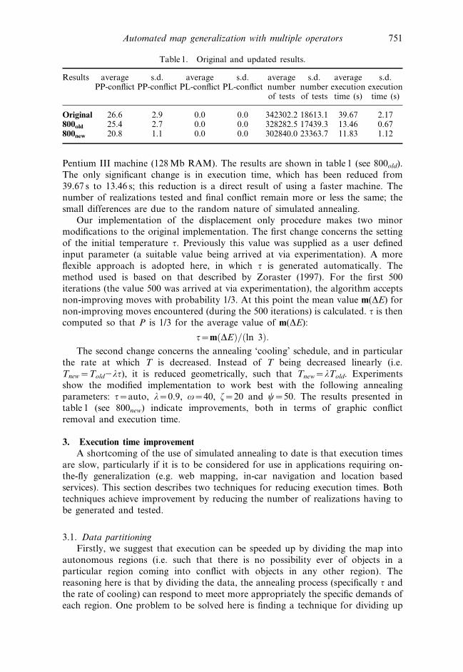
Pentium III machine (128Mb RAM). The results are shown in table 1 (see 800old).

The only significant change is in execution time, which has been reduced from

39.67 s to 13.46 s; this reduction is a direct result of using a faster machine. The

number of realizations tested and final conflict remain more or less the same; the

small differences are due to the random nature of simulated annealing.

Our implementation of the displacement only procedure makes two minor

modifications to the original implementation. The first change concerns the setting

of the initial temperature t. Previously this value was supplied as a user defined

input parameter (a suitable value being arrived at via experimentation). A more

flexible approach is adopted here, in which t is generated automatically. The

method used is based on that described by Zoraster (1997). For the first 500

iterations (the value 500 was arrived at via experimentation), the algorithm accepts

non-improving moves with probability 1/3. At this point the mean value m(DE) fornon-improving moves encountered (during the 500 iterations) is calculated. t is thencomputed so that P is 1/3 for the average value of m(DE):

t~m DEð Þ= ln 3ð Þ:The second change concerns the annealing ‘cooling’ schedule, and in particular

the rate at which T is decreased. Instead of T being decreased linearly (i.e.

Tnew~Told2lt), it is reduced geometrically, such that Tnew~lTold. Experiments

show the modified implementation to work best with the following annealing

parameters: t~auto, l~0.9, v~40, f~20 and y~50. The results presented in

table 1 (see 800new) indicate improvements, both in terms of graphic conflict

removal and execution time.

3. Execution time improvement

A shortcoming of the use of simulated annealing to date is that execution times

are slow, particularly if it is to be considered for use in applications requiring on-

the-fly generalization (e.g. web mapping, in-car navigation and location based

services). This section describes two techniques for reducing execution times. Both

techniques achieve improvement by reducing the number of realizations having to

be generated and tested.

3.1. Data partitioning

Firstly, we suggest that execution can be speeded up by dividing the map into

autonomous regions (i.e. such that there is no possibility ever of objects in a

particular region coming into conflict with objects in any other region). The

reasoning here is that by dividing the data, the annealing process (specifically t and

the rate of cooling) can respond to meet more appropriately the specific demands of

each region. One problem to be solved here is finding a technique for dividing up

Table 1. Original and updated results.

Results averagePP-conflict

s.d.PP-conflict

averagePL-conflict

s.d.PL-conflict

averagenumberof tests

s.d.numberof tests

averageexecutiontime (s)

s.d.executiontime (s)

Original 26.6 2.9 0.0 0.0 342302.2 18613.1 39.67 2.17800old 25.4 2.7 0.0 0.0 328282.5 17439.3 13.46 0.67800new 20.8 1.1 0.0 0.0 302840.0 23363.7 11.83 1.12


Figure 3. (a) Original BDTopo data. (b) BDTopo data after application of simulatedannealing algorithm. Objects shown in grey are involved in spatial conflict of some kind.


the map. In some instances it may be possible to make use of naturally occurring

regions, such as those formed by a road network or administrative boundaries.

Other situations will require analysis of the distribution of objects in order to find

groupings of objects that sustain no influence from objects external to their group.

We make use of a road network to divide data; the technique was used previously

by Ruas (1998). Using this approach, the BDTopo is divided into 16 regions

(figure 4). The simulated annealing algorithm can now be applied to regions

individually. In each case the annealing schedule used is the same as that used

previously (with initial temperature t set automatically). The results obtained are

given in table 2. It can be seen that, on average, the total number of realizations

tested has been reduced to 236935.6. The average execution time sees a

corresponding fall to 9.73 s, a reduction of approximately 18%. The conflict

remaining in the data has not changed significantly.

3.2. Two-stage approach

Some authors suggest that optimization can be made more efficient by adopting

a two-stage approach (Varanelli and Cohoon 1995). In two-stage simulated

annealing a faster heuristic algorithm is used to replace the simulated annealing

actions occurring at higher temperatures. This is followed by a conventional

simulated annealing approach initiated at lower temperatures in an attempt to

improve on the initial solution. The approach adopted in our implementation

differs slightly in that the faster heuristic algorithm is replaced by simulated

annealing in conjunction with an annealing schedule that involves an initial high

Figure 4. Division of BDTopo data into 16 autonomous regions.


temperature followed by rapid cooling. The second stage again makes use of

simulated annealing, this time with a much lower initial temperature followed by

much slower cooling. The annealing parameters used are given in table 3. For the

second stage, experiments showed that more consistent results were obtained by

reverting to a fixed value of t. Experimental results (table 4) show that execution

times are reduced by just less than 50% when adopting the two-stage approach.

Table 2. Data partitioning results.

Region Initial Results (averages)

PP-conflict PL-conflict PP-conflict PL-conflict numberof tests

executiontime (s)

1 2 1 0 0.0 94.8 0.00382 4 0 0 0.0 96.2 0.00393 16 1 0.8 0.0 17562.6 0.68494 6 7 0.4 0.0 21185.8 0.81995 8 1 2 0.0 10800.0 0.46446 12 2 0 0.0 9292.6 0.35317 24 0 2.4 0.0 21128.0 0.87318 18 4 0 0.0 21386.8 0.87479 10 7 2 0.0 16448.0 0.655810 6 0 0 0.0 4600.4 0.189511 12 2 2.4 0.0 18114.4 0.704612 0 1 0 0.0 5.4 0.000213 6 1 1.2 0.0 8189.2 0.352114 70 1 4.8 0.0 47488.0 2.151215 6 2 2 0.0 8624.0 0.352516 36 6 3.2 0.0 31919.4 1.2448Total 236 36 21.2 0.0 236935.6 9.7285

Table 3. Parameters used in two-stage annealing.

Stage t l v f y

1 auto 0.6 20 10 502 0.25 0.9 50 25 50

Table 4. Two-stage approach results and combined results (previous results also shown).

Results averagePP-conflict

averagePL-conflict

averagenumber of tests

averageexecution time (s)

Original 26.6 0.0 342302.2 39.67800old 25.4 0.0 328282.5 13.46800new 20.8 0.0 302840.0 11.83Partitioned 21.2 0.0 236935.6 9.73Two-stage 22.4 0.0 150749.2 6.13Combined 21.5 0.0 102539.4 4.1


3.3. Overall improvement

The two modifications described have been combined in a single implementation

(i.e. the two-stage procedure is applied to each of the 16 regions in turn).

Experimental results, shown in table 4, reveal an overall improvement of

approximately 65% with average execution times falling from 11.83 s to 4.1 s.

3.4. Displacement cost

Objects are displaced during the course of annealing, the overall aim being to

reduce graphic conflict. However, many of the displacements prove unnecessary

(i.e. they do not lead ultimately to a reduction in graphic conflict) and occur only as

a consequence of the algorithms occasional acceptance of neutral and negative

displacement. The result is a final display containing objects displaced from their

original location without benefit. In order to minimize displacement of this type, an

object displacement cost is introduced. If an object exists in a displaced state then a

cost is incurred:

. Displacing an object carries a cost ddispcost, where d represents the magnitude

of displacement.

The costs associated with graphic conflict and object displacement are combined

to give the overall cost associated with an object. For example, consider an object

mi that currently exists in a displaced state (cost~ddispcost) and lies in conflict with

two other polygonal objects (cost~2ppcost) and one linear object (cost~plcost). Itsassociated cost would equal (2ppcostzplcostzddispcost). Assigning appropriate

values to ppcost, plcost, and dispcost (i.e. 0vdispcostvppcost, plcost) creates an

incentive for displaced objects to return, during the course of annealing, as near to

their original location as is possible provided there is no resulting increase in

graphic conflict. Displays produced with and without consideration to displacement

cost are shown in figure 5.

4. Additional operatorsA further shortcoming of the initial algorithm is that it does not guarantee the

removal of all graphic conflict. For example, the best result obtained during

experiments was a final PP-conflict cost of 18. It is clear that displacement on its

own is not sufficient to resolve all graphic conflict and additional generalization

operators are required. We consider three additional operators:

. size exaggeration;

. deletion;

. size reduction.

Size exaggeration is required in situations where an object becomes too small to

be viewed adequately at the target scale. In situations where there is not enough

space for all objects to displayed, some objects have to be deleted. An alternative to

deletion is to reduce slightly the size of relatively large objects.

4.1. Object states

Again we consider a map display D made up of fixed linear objects F and n

modifiable detached polygonal objects M. Each modifiable object mi[M has k


Figure 5(a–b). Example of the effect of including displacement cost. (a) Original data. (b)Result obtained without consideration to displacement cost (original object locationsshown in background).


possible states providing us with kn possible configurations of D. At any given time

a particular object mi exists in one of its k possible states. An object’s (k-1) modified

states arise as a result of displacing the object, exaggerating the size of the object,

reducing the size of the object, displacing and exaggerating the object, displacing

and reducing the object, or deleting the object. In the current implementation the

possible object states are:

. Unmodified State. Each object mi has a single unmodified state;

. Displaced States. Each object mi has q displaced state trial positions that are

distributed evenly about the object;

. Enlarged States. Each object mi has qz1 enlarged state trial position; these

trial positions result from applying a scaling factor se (se§1.0) to the

unmodified state and displaced states of mi;

. Deleted State. An object mi has a single deleted state trial position; this trial

position represents the situation where the object has been removed from the

display;

. Reduced States. Each object mi has qz1 reduced state trial positions; these

trial positions result from applying a scaling factor sr (0.0vsrv1.0) to the

unmodified state and displaced states of mi.

There are therefore a total of (3qz4~k) trial positions. The object reduction

factor sr is provided as an input parameter to the algorithm. The object enlargement

Figure 5(c). Example of the effect of including displacement cost. (c) Result obtained whendisplacement cost is taken into account; unnecessary displacement has been reduced.


value se varies for each object and is dependant on object display area. For an

object with display area less than a minimum area tolerance amin, se is set so as to

increase object display area to amin. Objects with display area greater than or equal

to amin have se set to 1.0 (i.e. its application has no effect).

4.2. Evaluation of map display

For a particular configuration Dj, an object mi has an associated cost. This cost

is a measure of both the graphic conflict in which the object is involved and the

extent to which the object is modified. There are now three categories of graphic

conflict. The first two are the PP-conflict and PP-conflict types described previously.

The third is as follows:

. PA-conflict. Conflict involving a single polygonal object (i.e. mi is too small

for it to be seen clearly). This type of conflict occurs when the area of mi (in

viewing coordinates) is less than amin. An occurrence of this type of conflict

carries a cost pacost.

If an object exists in a modified state then a cost is incurred:

. Displacing an object carries a cost ddispcost, where d represents the magnitude

of displacement from the original position;

. Enlarging an object carries a cost ecost that is proportional to the scale of

enlargement, relative to the original size;

. Deleting an object carries a cost delcost;

. Reducing an object carries a cost rcost that is proportional to the scale of

reduction, relative to the original size.

The costs associated with graphic conflict and object modifications are

combined to give the overall cost associated with an object. For example, consider

an object mi that has been reduced in size and lies in conflict with two other

polygonal objects and one linear object. Its associated cost would equal

(2ppcostzplcostzrcost). As before, the total cost C(Dj) associated with a

realization Dj is found by summing the costs associated with each object mi; our

goal is to find a minimum cost configuration Dmin.

5. Implementation and testing

In implementation terms, introducing size enlargement, size reduction and

deletion capabilities is straightforward; these additional modified states of an object

are treated as additional trial positions for that object. Size reduction and size

enlargement are achieved by applying a suitable scaling factor (sr and se) to the

object, while deletion is accommodated by means of a simple Boolean flag (i.e. an

object is either deleted or not deleted). The cost function C is updated to take

account of the additional costs.

5.1. Cost setting

It is important to make sure that conflict costs (ppcost, plcost and pacost) and

object modification costs (dispcost, ecost, rcost and delcost) are set appropriately; it

is these costs that govern the likelihood of any given object/trial position pairing


being accepted should they be chosen during the annealing process. As such, the

cost values must be set so as to accommodate any orders of precedence that might

exist between the various operators and conflict types. For example, consider an

application that simply requires the removal of all graphic conflict (i.e. reducing

graphic conflict is the stated primary goal, and minimizing object modification is an

implied secondary goal). This might be achieved by assigning a relatively high value

to each of the conflict costs (e.g. ppcost~100, plcost~100 and pacost~100) and a

relatively low value to each of the object modification costs (e.g. dispcost~5,

ecost~5, rcost~5 and delcost~5). It could be the case, however, that the

modification operators have an order of precedence. For example, object

displacement might be preferred to size reduction, which in turn might be

preferred to deletion; the relevant cost value are changed accordingly (e.g.

dispcost~5, rcost~10 and delcost~15).

5.2. Displacement and deletion

Deletion was the first of the additional operators to be tested. The main thing to

note here is that care must be taken when setting the delcost value. If it is set too

high then, in some situations, not enough deletion takes place, and, as a

consequence, graphic conflict is not always removed (i.e. the cost of deleting is

greater than the cost associated with the graphic conflict). On the other hand, if

delcost is set too low, then too many deletions tend to occur (i.e. objects are

prematurely deleted in situations where displacement could have succeeded). An

example of each of the delcost setting scenarios is given in figure 6.

5.3. Reduction and enlargement

Object size enlargement and object size reduction operators are now introduced.

Again note that care must be taken when setting object modification costs and

regard must be given to any operator precedence that may exist. Figure 7 shows a

display produced with object displacement preferred to size reduction, and size

reduction preferred to deletion.

5.4. Cost weighting

When generalizing a map it is important to consider the relative importance of

objects; important objects should be less prone to modification than unimportant

objects. Consider a tourist map in which an object mm, representing a museum, lies

in conflict with an object mh, representing an ordinary house. In this context, mm

can be regarded as being more important than mh, and hence should be less

susceptible to generalization. In this situation there are a number of alternative

conflict resolution strategies that could be employed. For example, conflict

resolution could initially involve displacement and reduction of mh only; if this

failed, mh could be deleted. An alternative strategy might again involve the initial

displacement and reduction of mh only. If this failed then the next step would be

displace and reduce mh and mm in combination; continued failure at this stage

would result in the deletion of mh. Relative object importance is incorporated into

the simulated annealing procedure by assigning a cost weighting wi to each object

mi. Whenever an object mi and trial position kj pairing are chosen during the

annealing process, the cost associated with kj is multiplied by wi to give a modified


Figure 6(a–b). Application of deletion operator. (a) Original data. (b) Deletion cost set toohigh, not all spatial conflict removed.


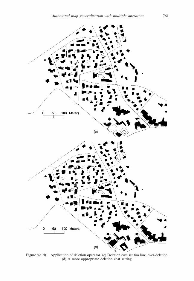
Figure 6(c–d). Application of deletion operator. (c) Deletion cost set too low, over-deletion.(d) A more appropriate deletion cost setting.


cost. A particular cost weighting value wi will be based on one or more attributes of

mi. In our experiments to date, and in the absence of any other measure of

importance, an object’s importance, and hence its cost weighting value, is assumed

to be proportional to object area (with large objects deemed more important than

small objects). Figure 8(a) shows output produced with no account taken of object

importance. The large object to the left has been deleted in order to resolve conflict.

If we consider large objects to be more important than small, then it would make

more sense to have deleted the smaller object to the right. This can be achieved by

making use of appropriate cost weightings, as shown in figure 8(b).

5.5. Performance

Initial experiments using the complete set of operators were shown to work well

with the following parameters: first-pass (t~auto, l~0.6, v~20, f~10 and

y~50); second-pass (t~5.0, l~0.9, v~40, f~20 and y~50). The example output

shown in figure 7 made use of the following costs: ppcost~5; plcost~50;

pacost~1.5; dispcost~0.1, ecost~0.5, rcost~0.5 and delcost~2.5. The other

values used were: dmin1~7.5m, dmin2~7.5m; amin~40m2; d~7.5m; and sr~0.8.

The average number of realizations tested was approximately 321421.7, with

average execution times of 12.75 s. All PP-conflict and PL-conflict was removed. On

average, 4.2 objects were deleted, 24.8 objects were size reduced and 114.3 objects

displaced.

Figure 7. Result obtained using displacement, size enlargement, size reduction and deletion.


Figure 8. The effect of cost weighting. (a) Result obtained without weighting – large objectdeleted. (b) Result obtained with area weighting – small object deleted.


5.6. Application to large scale ordnance survey data

The simulated annealing application has also been tested on large scale (1:1250)

Ordnance Survey (OS) data. The data consists of Mastermap building polygons

(pre-processed by OS staff using ArcInfo generalization tools) and OSCAR road

centre-lines. The tests assumed a map scale reduction to 1:10 000, with the road

centre-lines being assigned a symbol width of 14.0m (e.g. figures 9(a) and 10 (a)).

The annealing parameters and conflict cost values used were the same as those

given in §5.5. The other values used were: dmin1~1.0m, dmin2~7.0m (i.e. 14.0m/2);

amin~40m2; d~10.0m; and sr~0.9. Sample output, showing examples of

displacement, size enlargement and size reduction, is shown in figures 9(b) and

10 (b).

6. ConclusionThis paper has presented a simulated annealing based algorithm for map

generalization. The algorithm carries out map conflict reduction using displace-

ment, size enlargement, deletion and size reduction operators in combination.

Experimental results have shown the algorithm to be successful in reducing graphic

conflict within reasonable time. In more general terms, the work has further

highlighted the potential of iterative improvement techniques to act as a means of

orchestrating parts of the map generalization process.

A possible shortcoming of the existing approach is that it makes use of only a

fixed number of pre-defined trial positions; in some conflict situations the set of

available trial positions might not provide an appropriate solution. For example,

figure 9 shows how the algorithm can sometimes result in excessive displacement

and excessive reduction of building features. It may be possible to overcome this

problem by increasing the resolution of the search space by adding trial positions.

In the case of size reduction, the number of reduced states could be increased by

making use of a range of scaling values. This approach will be investigated as part

of the ongoing program of research. An alternative solution, which will also be

investigated, might be to adopt a continuous search space, as advocated by Strijk

and van Kreveld (2002) for the purpose of point labelling. The idea here would be

to generate random trial positions (i.e. randomly chosen operators together with the

appropriate randomly generated operator parameters) on the fly.

Future research will also focus on the development of additional operators, such

as simplification and aggregation. Conceptually this is seen as relatively

straightforward; each additional operator will produce additional trial positions

(either fixed or random) for any object to which it might be supplied. It is also the

intention to include operators that act upon line, point and textual data (i.e. line,

point and text objects will have associated operators and corresponding trial

positions).

In addition, the cost function will be expanded to take disruption to the

structure, form and density of map features into account. For example, displacing a

building might result in a row of buildings become misaligned (see figure 9 for

example). Attaching a high cost to such misalignment will stop the displacement

from taking place in the first place or encourage future displacements to realign the

buildings or stimulate some other remedial course of action (e.g. delete the

offending building).

In the current implementation, modification operators are applied to a single


object only at any given time. Other strategies could be accommodated. For

example, there is no reason why deletion could not be applied to groups of objects

en-mass, where groupings are determined by some attribute such as object class or

Figure 9(a). Large scale OS data example. (a) Graphic conflict arising due to scale reductionand road symbolization.


object area. The en-mass deletion could be treated as just another trial position for

the objects in question (i.e. the objects could be reintroduced as a group at some

later stage of the annealing process), or could be applied as a more permanent

Figure 9(b). Large scale OS data example. (b) Graphic conflict resolved by application ofdisplacement, size enlargement, size reduction and deletion.


culling of objects at pertinent stages of the generalization process (e.g. at the start

following an initial assessment of the problem or at certain stages during the

generalization process when it becomes apparent that the other operators will not

succeed in resolving conflict). Similarly an associated collection of objects, perhaps

representing a row of buildings, could be displaced (or enlarged or reduced) as a

group, so as to maintain, for example, feature alignment.

Another area for future work is the implementation and evaluation of

alternative optimization techniques. Those earmarked for evaluation include Tabu

Search and Genetic Algorithms.

In conclusion, it should be noted that the simulated annealing technique

presented is not being proposed as a complete solution to the map generalization

problem. Instead, the authors present it as a useful generalization tool to be used

Figure 10(a). Large scale OS data example. (a) Graphic conflict arising due to scalereduction and road symbolization.


within some kind of broader generalization framework. For example, it could be

used in a semi-automated setting by forming part of a set of generalization tools

made available via a GIS toolbar. Alternatively, it could contribute to a more

fully automated solution, maybe serving as a method available to certain object

classes within an AGENT-like system, or maybe by acting as just one step in a

pre-defined sequence of generalization operations (e.g. something akin to Bundy’s

‘internal agenda’ (Bundy 1996) or the ‘Global Master Plan’ of Ruas and Plazanet

(1996)).

Acknowledgments

Nathan Thomas is funded by EPSRC CASE Studentship 00802722, which is

carried out in collaboration with the Ordnance Survey. The authors express thanks

Figure 10(b). Large scale OS data example. (b) Graphic conflict resolved by application ofdisplacement, size enlargement, size reduction and deletion.


to the Institut Geographique National and the Ordnance Survey for permission to

use their data in parts of the work presented.

ReferencesBUNDY, G. L., 1996, Automated cartographic generalization with a triangulated spatial

model, PhD Thesis (available from The British Library).BURGHARDT, D., and MEIER, S., 1997, Cartographic displacement using the snakes concept.

In Smati ’97: Semantic Modelling for the Acquisition of Topographic Information fromImages and Maps, edited by W. Forstner and L. Plumer (Basel: Birkhauser)pp. 114–120.

CHRISTENSEN, J., MARKS, J., and SHIEBER, S., 1995, An empirical study of algorithms forpoint-feature label placement. ACM Transactions on Graphics, 14, 203–232.

EMDEN-WEINERT, T., and PROKSCH, M., 1999, Best practice simulated annealing for theairline crew scheduling problem. Journal of Heuristics, 5, 403–418.

HAIRE, K. R., and HARDY, P. G., 2001, Active agent based approaches to automatedgeneralization. Proceedings of 9th Annual GISRUK Conference, 319–320.

HARRIE, L. E., 1999, The constraint method for solving spatial conflicts in cartographicgeneralization. Cartography and Geographic Information Science, 26, 55–69.

HARRIE, L., and SARJAKOSKI, T., 2002, Simultaneous graphic generalization of vector datasets. GeoInformatica, 6, 233–261.

HøJOLT, P., 2000, Solving space conflicts in map generalization: Using a finite elementmethod. Cartography and GIS, 27, 65–73.

JONES, C. B., BUNDY, G. L., and WARE, J. M., 1995, Map generalization with a triangulateddata structure. Cartography and Geographic Information Systems, 22, 317–331.

JONES, C. B., and WARE, J. M., 1998, Proximity search with a triangulated spatial model.The Computer Journal, 41, 71–83.

KIRKPATRICK, S., GELATH, C. D., and VECCHI, M. P., 1983, Optimization by simulatedannealing. Science, 220, 671–680.

LAMY, S., RUAS, A., DEMAZEAU, Y., JACKSON, M., MACKANESS, W., and WEIBEL, R., 1999,The application of agents in automated map generalization. Proceedings of 19thInternational Cartographic Conference, 1225–1234.

LONERGAN, M. E., and JONES, C. B., 2001, An iterative displacement method for conflictresolution in map generalization. Algorithmica, 30, 287–301.

MACKANESS, W. A., 1994, An algorithm for conflict identification and feature displacementin automated map generalization. Cartography and Geographic Information Systems,21, 219–232.

NICKERSON, B. G., 1988, Automated cartographic generalization for linear features.Cartographica, 25, 15–66.

RUAS, A., 1998, A method for building displacement in automated map generalization.International Journal of Geographical Information Science, 12, 789–803.

RUAS, A., and PLAZANET, C., 1996, Strategies for automated generalization. Proceedings of7th International Symposium on Spatial Data Handling, 1, 6.1–6.18.

RUSSELL, S., and NORVIG, P., 1995, Artificial Intelligence: A Modern Approach (EnglewoodCliffs, New Jersey: Prentice-Hall), 1995.

STRIJK, T., and VAN KREVELD, M., 2002, Practical extensions of point labeling in the slidermodel. GeoInformatica, 6, 181–197.

VARANELLI, J., and COHOON, J. P., 1995, A two-stage simulated annealing methodology.Proceedings of 5th Great Lakes Symposium on VLSI, Buffalo NY, 50–53.

WARE, J. M., and JONES, C. B., 1998, Conflict reduction in map generalization using iterativeimprovement. Geoinformatica, 2, 383–407.

ZORASTER, S., 1997, Practical results using simulated annealing for point feature labelplacement. Cartography and Geographical Information Systems, 24, 228–238.


Automated map generalization with multiple operators: a simulated annealing approach

Documents

Transcript of Automated map generalization with multiple operators: a simulated annealing approach