Clemson UniversityTigerPrints

All Theses Theses

8-2019

Automated Deployment of an End-to-End Pipelineon Amazon Web Services for Real-Time VisualInspection using Fast Streaming High-DefinitionImagesAishwarya SrivastavaClemson University, aishsrivastava55@gmail.com

Follow this and additional works at: https://tigerprints.clemson.edu/all_theses

This Thesis is brought to you for free and open access by the Theses at TigerPrints. It has been accepted for inclusion in All Theses by an authorizedadministrator of TigerPrints. For more information, please contact kokeefe@clemson.edu.

Recommended CitationSrivastava, Aishwarya, "Automated Deployment of an End-to-End Pipeline on Amazon Web Services for Real-Time Visual Inspectionusing Fast Streaming High-Definition Images" (2019). All Theses. 3156.https://tigerprints.clemson.edu/all_theses/3156

Automated Deployment of an End-to-End Pipeline onAmazon Web Services for Real-Time Visual Inspection

using Fast Streaming High-Definition Images

A Thesis

Presented to

the Graduate School of

Clemson University

In Partial Fulfillment

of the Requirements for the Degree

Master of Science

Computer Science

by

Aishwarya Srivastava

August 2019

Accepted by:

Dr. Amy Apon, Committee Chair

Dr. Mashrur Chowdhury

Dr. Alexander Herzog

Abstract

This thesis investigates various degrees of freedom and deployment challenges of building

an end-to-end intelligent visual inspection system for use in automotive manufacturing. Current

methods of fault detection in automotive assembly are highly manual and labor intensive, and thus

prone to errors. An automated process can potentially be fast enough to operate within the real-time

constraints of the assembly line, and can reduce errors. In automotive manufacturing, components

of the end-to-end pipeline include capturing a large set of high definition images from a camera

setup at the assembly location, transferring and storing the images as needed, executing object

detection within a given time frame before the next car arrives in the assembly line, and notifying

a human operator when a fault is detected. As inference of object detection models is typically

very compute-intensive and memory-intensive, meeting the time, memory and resource constraints

requires a careful consideration of the choice of object detection model and model parameters along

with adequate hardware and environmental support. Some automotive manufacturing plants lack

floor space to set up the entire pipeline on an edge platform. Thus, we develop a template for Amazon

Web Services (AWS) in Python using the BOTO3 libraries that can deploy the entire end-to-end

scalable infrastructure in any region in AWS. In this thesis, we design, develop, and experimentally

evaluate the performance of system components, including the throughput and latency to upload

high definition images to an AWS cloud server, the time required by AWS components in the pipeline,

and the tradeoffs of inference time, memory and accuracy for twenty-four popular object detection

models on four hardware platforms.

ii

Acknowledgments

To begin with I would like to express my sincere gratitude to my advisor, Dr. Amy Apon.

This thesis would not have been possible without Dr. Apon’s continuous guidance, insightful sug-

gestions, constant encouragement and unfailing belief in me throughout the course of the project.

Secondly, I would like to thank my co workers, Siddhant Aggarwal and Dung Nguyen for

their major contributions to this project. I am also grateful to the collaborators at BMW, their

suggestions and ideas gave a direction to this project. I would also like to thank Dr. Mashrur

Chowdhury and Dr. Alexander Herzog for their support and for agreeing to be a part of my defense

committee.

Last but not least, I would like to express my deepest gratitude to my family and friends

for endless love and support throughout.

iii

Table of Contents

Title Page . . . . . . . . . . . . . . . . . . . . . . . . . . . . . . . . . . . . . . . . . . . . i

Abstract . . . . . . . . . . . . . . . . . . . . . . . . . . . . . . . . . . . . . . . . . . . . . ii

Acknowledgments . . . . . . . . . . . . . . . . . . . . . . . . . . . . . . . . . . . . . . . iii

List of Figures . . . . . . . . . . . . . . . . . . . . . . . . . . . . . . . . . . . . . . . . . . vi

Abbreviations . . . . . . . . . . . . . . . . . . . . . . . . . . . . . . . . . . . . . . . . . . viii

1 Introduction . . . . . . . . . . . . . . . . . . . . . . . . . . . . . . . . . . . . . . . . . 11.1 Problem Statement . . . . . . . . . . . . . . . . . . . . . . . . . . . . . . . . . . . . . 11.2 Work Flow . . . . . . . . . . . . . . . . . . . . . . . . . . . . . . . . . . . . . . . . . 3

2 Background and Literature Review . . . . . . . . . . . . . . . . . . . . . . . . . . . 52.1 Cloud Computing . . . . . . . . . . . . . . . . . . . . . . . . . . . . . . . . . . . . . . 5

2.1.1 Cloud Computing Basics . . . . . . . . . . . . . . . . . . . . . . . . . . . . . . 52.1.2 Amazon SDK: BOTO3 . . . . . . . . . . . . . . . . . . . . . . . . . . . . . . 6

2.2 Deep Learning . . . . . . . . . . . . . . . . . . . . . . . . . . . . . . . . . . . . . . . 72.2.1 Deep Learning Basics . . . . . . . . . . . . . . . . . . . . . . . . . . . . . . . 72.2.2 Layers in CNN . . . . . . . . . . . . . . . . . . . . . . . . . . . . . . . . . . . 8

2.3 Object Detection . . . . . . . . . . . . . . . . . . . . . . . . . . . . . . . . . . . . . . 92.3.1 Architecture . . . . . . . . . . . . . . . . . . . . . . . . . . . . . . . . . . . . 102.3.2 Datasets . . . . . . . . . . . . . . . . . . . . . . . . . . . . . . . . . . . . . . . 10

2.4 Degrees of Freedom for Object Detection . . . . . . . . . . . . . . . . . . . . . . . . . 112.4.1 Meta Architecture . . . . . . . . . . . . . . . . . . . . . . . . . . . . . . . . . 11

2.4.1.1 RCNN . . . . . . . . . . . . . . . . . . . . . . . . . . . . . . . . . . 112.4.1.2 SPP-Net . . . . . . . . . . . . . . . . . . . . . . . . . . . . . . . . . 122.4.1.3 Fast RCNN . . . . . . . . . . . . . . . . . . . . . . . . . . . . . . . . 122.4.1.4 Faster RCNN . . . . . . . . . . . . . . . . . . . . . . . . . . . . . . . 122.4.1.5 R-FCN . . . . . . . . . . . . . . . . . . . . . . . . . . . . . . . . . . 132.4.1.6 SSD . . . . . . . . . . . . . . . . . . . . . . . . . . . . . . . . . . . . 132.4.1.7 YOLO . . . . . . . . . . . . . . . . . . . . . . . . . . . . . . . . . . 132.4.1.8 RetinaNet . . . . . . . . . . . . . . . . . . . . . . . . . . . . . . . . 14

2.4.2 Feature Extractor . . . . . . . . . . . . . . . . . . . . . . . . . . . . . . . . . 142.4.2.1 VGG . . . . . . . . . . . . . . . . . . . . . . . . . . . . . . . . . . . 152.4.2.2 Inception/GoogleNet . . . . . . . . . . . . . . . . . . . . . . . . . . 152.4.2.3 MobileNet . . . . . . . . . . . . . . . . . . . . . . . . . . . . . . . . 152.4.2.4 ResNet . . . . . . . . . . . . . . . . . . . . . . . . . . . . . . . . . . 162.4.2.5 NAS . . . . . . . . . . . . . . . . . . . . . . . . . . . . . . . . . . . . 16

2.4.3 Batch Size . . . . . . . . . . . . . . . . . . . . . . . . . . . . . . . . . . . . . . 16

iv

2.4.4 Hardware . . . . . . . . . . . . . . . . . . . . . . . . . . . . . . . . . . . . . . 162.4.5 Other parameters . . . . . . . . . . . . . . . . . . . . . . . . . . . . . . . . . . 17

2.5 Frameworks . . . . . . . . . . . . . . . . . . . . . . . . . . . . . . . . . . . . . . . . . 17

3 Performance and Memory Trade-offs of Object Detection Models . . . . . . . . 183.1 System Architecture and Synthetic Workload . . . . . . . . . . . . . . . . . . . . . . 183.2 Object Detection Models . . . . . . . . . . . . . . . . . . . . . . . . . . . . . . . . . . 21

3.2.1 Meta Architecture . . . . . . . . . . . . . . . . . . . . . . . . . . . . . . . . . 223.2.2 Feature Extractor . . . . . . . . . . . . . . . . . . . . . . . . . . . . . . . . . 223.2.3 Mini batch size . . . . . . . . . . . . . . . . . . . . . . . . . . . . . . . . . . . 23

3.3 Hardware Platforms . . . . . . . . . . . . . . . . . . . . . . . . . . . . . . . . . . . . 233.3.1 Nvidia P100 . . . . . . . . . . . . . . . . . . . . . . . . . . . . . . . . . . . . . 233.3.2 Nvidia V100 PCIe . . . . . . . . . . . . . . . . . . . . . . . . . . . . . . . . . 233.3.3 Nvidia V100 SXM2 . . . . . . . . . . . . . . . . . . . . . . . . . . . . . . . . . 243.3.4 Nvidia Jetson TX2 . . . . . . . . . . . . . . . . . . . . . . . . . . . . . . . . . 243.3.5 CPU only . . . . . . . . . . . . . . . . . . . . . . . . . . . . . . . . . . . . . . 24

3.4 Performance Metrics . . . . . . . . . . . . . . . . . . . . . . . . . . . . . . . . . . . . 243.4.1 Inference Time . . . . . . . . . . . . . . . . . . . . . . . . . . . . . . . . . . . 253.4.2 GPU Memory Consumption . . . . . . . . . . . . . . . . . . . . . . . . . . . . 253.4.3 Model Accuracy . . . . . . . . . . . . . . . . . . . . . . . . . . . . . . . . . . 25

3.5 Results for Object Detection Models . . . . . . . . . . . . . . . . . . . . . . . . . . . 263.5.1 Inference Time as a Function of Mini Batch Size . . . . . . . . . . . . . . . . 263.5.2 Memory Consumption as a Function of Mini Batch Size . . . . . . . . . . . . 293.5.3 Inference Time and Memory for Different GPU Platforms . . . . . . . . . . . 313.5.4 Discussion of Real-Time Application Constraints . . . . . . . . . . . . . . . . 33

4 Pipeline Architecture . . . . . . . . . . . . . . . . . . . . . . . . . . . . . . . . . . . 374.1 Edge versus Cloud tradeoffs . . . . . . . . . . . . . . . . . . . . . . . . . . . . . . . . 374.2 AWS Components . . . . . . . . . . . . . . . . . . . . . . . . . . . . . . . . . . . . . 384.3 AWS Pipeline . . . . . . . . . . . . . . . . . . . . . . . . . . . . . . . . . . . . . . . . 404.4 Auto Deploy using BOTO3 . . . . . . . . . . . . . . . . . . . . . . . . . . . . . . . . 424.5 Results for End to End Pipeline . . . . . . . . . . . . . . . . . . . . . . . . . . . . . . 42

4.5.1 Upload time tradeoffs across different region . . . . . . . . . . . . . . . . . . . 434.5.2 Parallel upload using multiple machines . . . . . . . . . . . . . . . . . . . . . 454.5.3 Edge versus Cloud Upload Speed . . . . . . . . . . . . . . . . . . . . . . . . . 484.5.4 Time analysis for AWS components . . . . . . . . . . . . . . . . . . . . . . . 51

4.5.4.1 Timings for AWS components . . . . . . . . . . . . . . . . . . . . . 514.5.4.2 Time as a function of EC2 Instance . . . . . . . . . . . . . . . . . . 52

4.5.5 Cost Analysis . . . . . . . . . . . . . . . . . . . . . . . . . . . . . . . . . . . . 53

5 Discussion . . . . . . . . . . . . . . . . . . . . . . . . . . . . . . . . . . . . . . . . . . 56

6 Future Works . . . . . . . . . . . . . . . . . . . . . . . . . . . . . . . . . . . . . . . . 58

Bibliography . . . . . . . . . . . . . . . . . . . . . . . . . . . . . . . . . . . . . . . . . . . 59

v

List of Figures

1.1 Manual inspection process at BMW Assembly plant at Spartanburg [44] . . . . . . . 21.2 System Pipeline on Amazon Cloud . . . . . . . . . . . . . . . . . . . . . . . . . . . . 4

2.1 Deep Learning Basics . . . . . . . . . . . . . . . . . . . . . . . . . . . . . . . . . . . 72.2 Convolutional Layer . . . . . . . . . . . . . . . . . . . . . . . . . . . . . . . . . . . . 9

3.1 System Architecture Diagram [41] . . . . . . . . . . . . . . . . . . . . . . . . . . . . 203.2 The left side shows a sample synthetic image. Each image is composed of sixty-three

tiles. The complete visual view of a car in the synthetic workload is represented byninety-five images. The right side is zoomed in on four of the tiles and shows theobjects detected [41] . . . . . . . . . . . . . . . . . . . . . . . . . . . . . . . . . . . . 21

3.3 Inference time as a function of batch size on P100 [41] . . . . . . . . . . . . . . . . . 273.4 Inference time as a function of batch size on V100 SXM2 [41] . . . . . . . . . . . . . 283.5 Inference time as a function of batch size on V100 PCIe [41] . . . . . . . . . . . . . . 293.6 Inference time as a function of batch size using CPU only [41] . . . . . . . . . . . . . 303.7 Inference time as a function of batch size using TX2 [41] . . . . . . . . . . . . . . . . 313.8 Maximum GPU memory usage as a function of batch size on P100 [41] . . . . . . . . 323.9 Maximum GPU memory usage as a function of batch size on V100 PCIe [41] . . . . 333.10 Best inference time and max memory consumption of models on three GPU devices. The

labels used in this figure are shown in Fig. 9. For each point shown the mini batch size that

gives the best run time for that model is shown in parentheses. For example, C(64) shown

in the lower left of the left figure is the ssd mobilenet v1 ppn model run with a mini batch

size of 64, which is the fastest for that model on the P100. The left figure shows results for

P100, the middle figure shows results for V100 PCIe, and the right figure shows results for

V100 SXM2 [41]. . . . . . . . . . . . . . . . . . . . . . . . . . . . . . . . . . . . . . . . 343.11 List of models and IDs used in Fig. 3.10. . . . . . . . . . . . . . . . . . . . . . . . . 353.12 Inference times on V100 PCIe and V100 SXM2 platforms for representative models

from each of the five mAP groups [41]. . . . . . . . . . . . . . . . . . . . . . . . . . 36

4.1 Life cycle of SQS message in a queue [2] . . . . . . . . . . . . . . . . . . . . . . . . . 394.2 AWS Pipeline . . . . . . . . . . . . . . . . . . . . . . . . . . . . . . . . . . . . . . . 424.3 Throughput as a function of concurrent request in N. Virginia (us-east-1) for 100 images 444.4 Throughput as a function of concurrent request in Oregon (us-west-2) for 100 images 454.5 Throughput as a function of concurrent request in Ireland (eu-west-1) for 100 images 464.6 Throughput for all three regions for a concurrent request of 40 . . . . . . . . . . . . 474.7 Parallel upload using multiple machines. For 10 machines there are two network

switches. . . . . . . . . . . . . . . . . . . . . . . . . . . . . . . . . . . . . . . . . . . . 474.8 Cloud upload latency with variation of machine count . . . . . . . . . . . . . . . . . 484.9 There is a 95% probability of obtaining a per image (16MB) latency of less than

0.4631 seconds when using only a single machine to upload files. . . . . . . . . . . . 49

vi

4.10 There is a 95% probability of obtaining a per image (16MB) latency of less than 0.2866seconds when using three machines in a network. The CDF doesn’t make noticeablechanges when we further increase the number of machines, as shown in Fig. 13. . . . 50

4.11 Cloud timings for AWS components . . . . . . . . . . . . . . . . . . . . . . . . . . . 514.12 End-to-end time as a function of EC2 instances for two processes . . . . . . . . . . . 52

vii

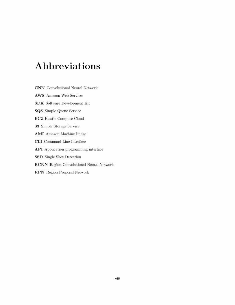
Abbreviations

CNN Convolutional Neural Network

AWS Amazon Web Services

SDK Software Development Kit

SQS Simple Queue Service

EC2 Elastic Compute Cloud

S3 Simple Storage Service

AMI Amazon Machine Image

CLI Command Line Interface

API Application programming interface

SSD Single Shot Detection

RCNN Region Convolutional Neural Network

RPN Region Proposal Network

viii

Chapter 1

Introduction

In recent years there have been several breakthroughs in the field of machine learning.

In particular, machine learning has proved to be highly effective in providing solution to wide

variety of challenging problems in several domains. It has impacted everything from transportation,

manufacturing, healthcare and natural disasters. Machine learning and Deep learning has several

potential application in automotive domain, both inside and outside the vehicle [30]. Inside here

refers to advanced driving assistance systems (ADAS), self driving cars while outside the vehicle

refers to manufacturing in the assembly plant systems.

Building an end-to-end system pipeline which facilitates continuous delivery requires careful

consideration. The pipeline should be responsive, scalable for different workloads, fault tolerant and

replicable. Much research lately focuses on optimization of machine learning algorithms, developing

frameworks for these algorithms, analyzing the tradeoffs of various parameters associated with these

models or developing a pipeline or system architecture for auto deploying the infrastructure. The

last two topics are main focus of this thesis.

1.1 Problem Statement

Visual inspection in the automotive manufacturing is highly labor intensive process and

is also prone to errors. Manually analyzing the defects in the automotive assembly plant is a time

taking process. The quality checks in the automotive manufacturing plant involve high quality visual

inspection to make sure that the parts are in correct locations, have the right shape and the product

1

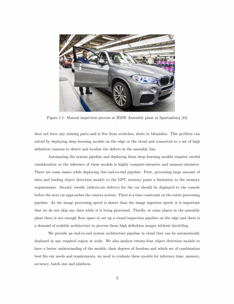
Figure 1.1: Manual inspection process at BMW Assembly plant at Spartanburg [44].

does not have any missing parts and is free from scratches, dents or blemishes. This problem can

solved by deploying deep learning models on the edge or the cloud and connected to a set of high

definition cameras to detect and localize the defects in the assembly line.

Automating the system pipeline and deploying these deep learning models requires careful

consideration as the inference of these models is highly compute-intensive and memory-intensive.

There are some issues while deploying this end-to-end pipeline. First, processing large amount of

data and loading object detection models to the GPU memory poses a limitation to the memory

requirements. Second, results (defects/no defects) for the car should be displayed to the console

before the next car approaches the camera system. There is a time constraint on the entire processing

pipeline. As the image processing speed is slower than the image ingestion speed, it is important

that we do not skip any data while it is being processed. Thirdly, at some places in the assembly

plant there is not enough floor space to set up a visual inspection pipeline on the edge and there is

a demand of scalable architecture to process those high definition images without throttling.

We provide an end-to-end system architecture pipeline in cloud that can be automatically

deployed in any required region at scale. We also analyze twenty-four object detection models to

have a better understanding of the models, their degrees of freedom and which set of combination

best fits our needs and requirements, we need to evaluate these models for inference time, memory,

accuracy, batch size and platform.

2

1.2 Work Flow

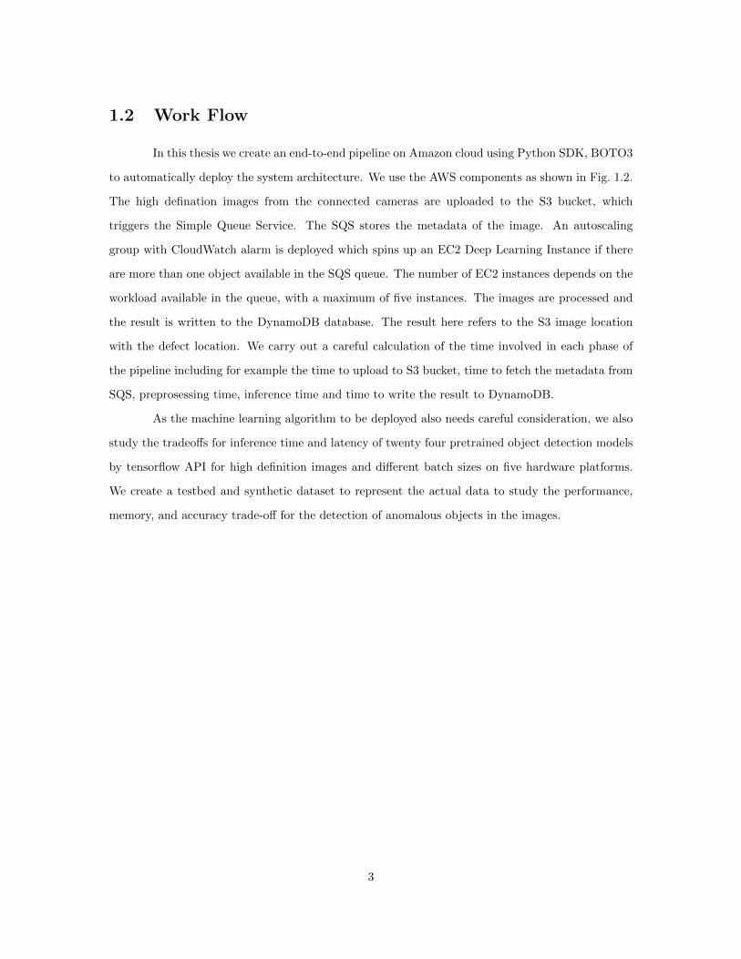
In this thesis we create an end-to-end pipeline on Amazon cloud using Python SDK, BOTO3

to automatically deploy the system architecture. We use the AWS components as shown in Fig. 1.2.

The high defination images from the connected cameras are uploaded to the S3 bucket, which

triggers the Simple Queue Service. The SQS stores the metadata of the image. An autoscaling

group with CloudWatch alarm is deployed which spins up an EC2 Deep Learning Instance if there

are more than one object available in the SQS queue. The number of EC2 instances depends on the

workload available in the queue, with a maximum of five instances. The images are processed and

the result is written to the DynamoDB database. The result here refers to the S3 image location

with the defect location. We carry out a careful calculation of the time involved in each phase of

the pipeline including for example the time to upload to S3 bucket, time to fetch the metadata from

SQS, preprosessing time, inference time and time to write the result to DynamoDB.

As the machine learning algorithm to be deployed also needs careful consideration, we also

study the tradeoffs for inference time and latency of twenty four pretrained object detection models

by tensorflow API for high definition images and different batch sizes on five hardware platforms.

We create a testbed and synthetic dataset to represent the actual data to study the performance,

memory, and accuracy trade-off for the detection of anomalous objects in the images.

3

Figure 1.2: System Pipeline on Amazon Cloud.

4

Chapter 2

Background and Literature Review

2.1 Cloud Computing

Cloud computing has become a vital part of business. Social networking, storage, streaming

videos, music everything nowadays is based on cloud platforms. Data intensive applications that are

spread geographically depend vastly on using the cloud environment. Rather than buying expensive

hardware and infrastructure for experimenting and business needs, people prefer using resources from

cloud computing service providers which provide upgraded infrastructure, hardware and softwares

with a ”pay as you go” system.

2.1.1 Cloud Computing Basics

A cloud service provider offers cloud computing services like infrastructure as a service

(IaaS), software as a service (SaaS) and platform as a service (PaaS) with high availability, security

and reliability. Some of the reason for the expansion of businesses from on premises to cloud are the

following:

1. Scalibility - Enterprises require an immediate increase and decrease of compute and

storage capacities according to the consumer requirements. Buying the maximum required capacity

of resources on the premises is expensive, instead shifting the resources to on-demand capacity using

cloud services is an effective solution.

2. Portability - Using Cloud, the system, data and application can be setup easily by

5

dropping the code into a robust Paas that provides infrastructure support. The data and the system

is globally accessible and can be setup in any region across the globe using few scripts.

3. Agility - Cloud offers flexibility and adaptability meeting the demands of rapid fluctua-

tions in the market. Cloud provides its users with the most updated technology by providing regular

updates.

4. Disaster Recovery - A small duration of power outage and unproductive downtime can

result in loss in revenue and can have a drastic negative impact on the companies reputation. Using

cloud, we can bundle the entire server including storage, applications, softwares and operating

systems into a single unit, a virtual server. This bundle can be spun up on any other virtual server

within minutes reducing the downtime by a large factor.

Our application focuses on the scalability, agility and portability across different regions in a

cloud. Sometimes in cases of large workloads or traffic the organizations run out of resources due to

limitations on capacity and power. Using cloud resources can provide vertical and horizontal scaling

of the infrastructure by using unlimited resources and paying per use basis. A lot of cloud platforms

are now offering machine learning services for model training and deployment. Some of the popular

cloud providers being Amazon, Microsoft’s Azure, Google Cloud Platform and IBM Watson.

For our experiments we use Amazon Web Services as the cloud provider as it is the most

stable and updated platform available at the time of this thesis.

2.1.2 Amazon SDK: BOTO3

AWS offers several APIs tailored to programming languages like Python, JAVA, Node.js

etc. Python SDK, BOTO3 is an open source package for configuring and deploying AWS cloud

resources. BOTO3 offers two ways of accessing cloud resources:

1. Client - low level service access

2. Resource - object oriented high level service access

Thus we aim at designing an end-to-end pipeline and provisioning the entire infrastructure

in the Amazon cloud environment using a simple python script. Using Python SDK, BOTO3 we

can deploy the pipeline in an automated manner anywhere across the geographical locations using

any Amazon account.

6

2.2 Deep Learning

In this chapter we will discuss about the basics of machine learning, deep learning, convolu-

tional neural network, model training and inference, followed by some of the popular tasks in deep

learning.

2.2.1 Deep Learning Basics

The term deep learning was first introduced to machine learning by Dechter in 1986 [10].

Goodfellow, et al [15] in his book, explained the relationship between deep learning, machine learning

and artificial intelligence.

Figure 2.1: Deep Learning Basics.

With the help of a Venn diagram in Fig 2.1 he explained that deep learning is a kind

of representation learning, which in turn is a type of machine learning. Machine learning is a

subset of artificial intelligence and there are other approaches based on knowledge learning that are

not included in machine learning. Deep learning significantly revolutionized the machine learning

7

community by providing some improved and excellent state-of-the-art algorithms in object detection,

object recognition, speech recognition and several others. Deep learning architecture provides a high

level abstraction of several layers, applying multiple linear and non-linear transformation on the

dataset.

LeCun et al. in [24] [25] developed the idea of Convolutional Neural Networks (CNN). CNN

or ConvNet is a type of feed forward neural network which is composed of neurons having trainable

weights and biases. The first CNN introduced was AlexNet [23] ConvNets work well in cases of

images. They make forward propagation easier with the use of less hyper-parameters. Every CNN

layer transforms 3D input matrix to a 3D output matrix by modulating the height, width and depth

of the image.

2.2.2 Layers in CNN

ConvNets are composed of sequence of layers where Convolution form the essence of CNNs.

In the Fig 2.2 below we see an image matrix of dimension (H x W x C) where C, number of channels

is 1. Next to it is a filter or kernel which performs convolutions using a sliding window approach

to produce the output. The kernel slides over the input image from the top-left to bottom-right

computing the weighted sum of input pixel with the kernel values. Combining the weighted sum of

outputs we get a feature map.

After getting familiar with how the convolutions work, we will briefly discuss the layers that

form the CNNs.

Input Layer contains pixel values of the image in (width x height x channels) dimensions.

Convolutional Layer computes the weighted sum of the dot product between the kernel

value and the input pixels using a sliding window technique to produce a feature map. It has k

number of filters/kernels of size (n x n x r) where r may vary according to the depth of the kernel.

Here the term stride specifies how much is the kernel moved at each step. Bigger strides make the

feature map smaller as we skip pixels in that case. We can also use padding to surround the input

in order to maintain same dimensionality and weigh every pixel equally.

RELU layer It appllies non-linear activation function to the input, like max(0,x) , without

changing the dimensionality.

Pooling layer it performs a downsampling operation on the input. It helps to prevent

overfitting and help reduce the number of parameters thereby reducing the cost. Some of the most

8

Figure 2.2: Convolutional Layer.

popular polling techniques used are Max pooling and Average pooling.

Fully Connected layer, as the name suggests connects every neuron in the previous layers

to every neuron in the next layer. It computes the class score or is connected to a softmax activation

function or some other function in the output layer.

2.3 Object Detection

To understand the whole image, merely classifying the image into a label from a set of labels

in not sufficient. We need to identify and localize all the objects within the image. Instead of saying

that a particular image contains a ‘cat’, it would be better if the model detects all the objects in the

image along with localization of objects. This task is referred to as object detection. The problem

of object detection is divided into two main tasks of object localization and object classification.

9

2.3.1 Architecture

The architecture of object detection models involves more that just the softmax probability

layer. Traditional object detection models can be divided into three stages.

Region Selection. Since the position of object can be anywhere in the image and can

be of any size or aspect ratio, multi-scale sliding window was used to scan the whole image. This

strategy is exhaustive, time consuming and affects the performance and speed of the entire process.

Feature Extraction. The goal of feature extraction is to reduce the image to a fixed

set of visual features. Visual features are extracted for each of the bounding boxes which help

in classification and identification of objects. Some of the traditional and representative feature

extractors are Scale Invariant Feature Transform (SIFT) [29] , Histogram of Oriented Gradients

(HOG) [9] and Haar features [26]. Choice of feature extractor is crucial as it effects the speed, memory

and performance of the object detector. We will be discussing some modern feature extractors in

section 2.3.2 in detail.

Classification. Labeling the bounding box provides information for visual recognition.

Comonly used classifiers are support vector machine classifier (SVM) [7] and Adaboost [12].

The generation of candidate boxes using sliding window is a redundant and time consum-

ing method. Simple detection tasks with small datasets can be solved efficiently using the above

technique. But to learn thousands of objects from millions of images, there is a need for model with

a large learning capacity. In 2012, A. Krizhevsky used a deep convolutional neural network in the

ImageNet large scale visual recognition challenge [45].

2.3.2 Datasets

COCO stands for Common Objects in Context. It is an object detection dataset developed

by Microsoft. COCO is a large-scale and rich for object detection, segmentation and captioning

dataset [27]. It contains 80 objects categories with approximately 2.5 million images. Tensorflow

provides pre-trained models that have been trained using the COCO dataset. These models are

useful for using pre-trained features as starting point for custom datasets.

Pascal VOC is also a large scale image classification and object detection dataset. The

dataset contains twenty classes of objects with 11,530 images as train/valdation data, containing

27,450 ROI annotated objects and 6,929 segmentations [11].

10

There are several other datasets for objects detection depending on the task as Open Images

Dataset, KITTI (autonomous driving dataset), Caltech Pedestrian Dataset, SUN (scene, places,

enviornment dataset), WIDER FACE dataset (face detection dataset).

2.4 Degrees of Freedom for Object Detection

In object detection there are several degrees of freedom associated with the entire process. In

real life applications we need to make choices to create a balance between performance and accuracy.

Some of the factors that impact the performance of object detectors are stated below.

2.4.1 Meta Architecture

Meta-architectures in object detection models can be categorized into two different classes:

single stage and two stage models. In two stage models the object proposals for the image is generated

and send to second stage where and a classifier or regressor is run through each box proposal. These

models are memory intensive and cannot be run on embedded devices. Whereas, single stage models

perform the detection process in one stage where the bounding boxes and regression is performed

in one pass.

Two stage models are accurate but have longer run times compared to the one stage models.

Some of the popular meta-architectures are described below.

2.4.1.1 RCNN

This was the first model to combined the concept of region proposal with convolutional

neural network [14]. Instead of using a sliding window strategy with large number regions, it uses

selective search to identify patterns and select 2000 proposals called region proposals. It then wraps

the region to a tight bounding box and passes it to the CNN, which extracts the features for each

region. The last layer of CNN is the SVM classifier which classifies the the object into a particular

class from a set of predefined classes. This model also considers the offset values which help to

predict the bounding boxes with precision.

RCNN comes with certain limitations. Training and inference of RCNN models is very slow.

This is because the meta architecture consist of three separate models; CNN for feature extraction,

11

SVM classifier and a regression model to tighten the bounding boxes. This makes the entire process

expensive.

2.4.1.2 SPP-Net

The computation time of RCNN architecture is improved by SPP-Net [17]. SPP-Net stands

for Spatial Pyramid Pooling in deep convolutional networks. This model adds a spatial pyramid

layer between the convolutional layers and fully connected layer to achieve multi-scale data input. In

RCNN, feature extraction is time consuming. SPP-Net computes the feature map of the image just

once and then divides it into sub-images to create fixed-length feature maps. This method prevents

repeated computation of convolutional features and is much faster than RCNN for object detection

with a comparable or greater accuracy. It can also handle multi scales images of different sizes as

well. SPP-Net also has a drawback of fixed convolutional layers, which cannot be updated.

2.4.1.3 Fast RCNN

Fast RCNN [13] fixes the drawbacks of RCNN and SPP-Net method and is also faster and

much more accurate than the two models mentioned above. Fast RCNN feeds the whole input

image to the convolutional and max pooling layers instead of feeding region proposals to the CNN.

This generates a convolutional feature map, from where the region proposal are identified and the

ROI pooling layer wraps the regions into standard size and each region is fed to the fully connected

layer. This layers is connected to a softmax classifier for predicting the class. Along with this, it

is parallelly connected to a linear regressor that predicts the four bounding box coordinates. Fast

RCNN model combines the three models into one for feature extraction, classification and bounding

box regression, which improves the speed and accuracy of the model.

Fast RCNN also has certain problems, as it depends on external box proposal selector, which

is time consuming.

2.4.1.4 Faster RCNN

First step used in finding the location of objects in the input image is using bounding boxes

to generate region of interest. This is done using selective search in the above mentioned models.

Faster RCNN [37] introduced the concept of Region proposal network (RPN). RPN takes the feature

map as input and for each anchor it predicts the object score (probability that the anchor is an object

12

or not) along with the bounding box regressor coordinates. Each proposal is then passed to the ROI

pooling layer which crops it to a fixed size and passes it to the fully connected layer. Embedding the

RPN in the already existing network increases the efficiency and performance of the architecture.

2.4.1.5 R-FCN

R-FCN [8] stands for Region-based Fully Convolutional Networks. It pre-computes the box

classifier features for the whole image. In this case the fully connected layers are replaced with

number of convolutional layers. R-FCN is composed of Convolutional RPN with the convolutional

region based classifier and it crops the features just before the last layer of the network making

it faster than Faster RCNN. In case of R-FCN the computational speed is weakly dependent on

number of proposals.

2.4.1.6 SSD

Single Shot Detector, is one of the fastest meta-architectures. SSD does not have box

proposal generation and feature resampling [28] instead it calculates the bounding boxes and object

classes in a single propagation through the neural network.

SSD predict off-sets based on grid cells rather than learning the box itself, it also predicts

boxes at multiple scales by taking outputs from many subsequent convolutional layers. However,

because it uses prior boxes at different scales but does not calculate the box proposals, SSD does

not have good performance on small objects . We have a light weight variant of SSD where all the

regular convolutions are replaced with separable convolutions in SSD prediction layers [38]. This

model is called SSD Lite and is faster than SSD.

2.4.1.7 YOLO

YOLO stands for ’You Look Only Once’ [34]. It is one of the single shot detectors. It

uses grid boxes on the image with different aspect ratios to localize objects instead of two stage

networks discussed above which used object proposal generators. It frames detection as a regression

problem and a single convolutional neural network is used to predict bounding boxes as well as class

probabilities from an image as a whole.

Because of its unified structure YOLO is considered very fast. But YOLO sufferes from

several drawbacks such as high localization error and low recall value. YOLOv2 [35] is the sec-

13

ond version of the YOLO, which improves upon the shortcomings of YOLO with the objective of

improving its accuracy and computation time.

YOLOv3 [36] variant of YOLO replaces the softmax function with logistic classifier and uses

binary cross entropy loss for each label. YOLOv3 also shows a lot of improvement in detecting small

objects and is faster than its previous versions.

2.4.1.8 RetinaNet

RetinaNet is a single stage detector which outperforms Faster RCNN in terms of accuracy

and is faster than the two stage detectors. One stage detectors suffered from the class imbalance

problem. To overcome this the cross entropy loss function is replaced by the focal loss function,

where the cross entropy loss is scaled and weighted less for well classified predictions and focuses

more on interesting cases.

It uses Feature Pyramid network (FPN) on top of ResNet as a backbone for multi-scale

feature pyramid from single resolution input image. The output of the backbone is fed to the

classification subnetwork which predicts the probability of the object present in each box. Here

focal loss is used as a loss function. Parallely there is a box regression sub network that regresses the

offset from the predicted box to the the ground truth box label. The structure of both the subnet

is similar except for their parameters. RetinaNet achieves state of the art in terms of accuracy and

speed.

2.4.2 Feature Extractor

Feature extraction in object detection is the process of extracting information from raw pix-

els and identifying local features based on the object of interest. Feature extraction is an important

stage in the object detection pipeline. After the features are extracted, a softmax layer is applied at

the end of network to calculate the probability of classes which allows for classification of objects.

AlexNet [23] was one of the pioneer networks to increase the accuarcy of ImageNet clas-

sification by a notabe stride after the traditional methods. AlexNet created Alex Krizhevsky, is

composed of five convolutional layers for feature extraction followed by three fully connected layer

to provide the classification probabilities along with ReLu(Rectified Linear Unit) layer. This network

also solved the problem of over-fitting by using Dropout layer after Fully connected layer. Some of

the popular feature extractors developed after AlexNet are mentioned below.

14

2.4.2.1 VGG

VGG [40] is a deep convolutional neural network for object recognition developed by the Vi-

sual Geometry Group (VGG) at Oxford University. VGG network unlike AlexNet contains multiple

3X3 small sized filters. Multiple small stacked filters are better than large size as they increase the

depth of the network. VGG is still used as a baseline model because of its simplicity and popularity.

2.4.2.2 Inception/GoogleNet

VGG is computationally expensive and is very slow to train. Szegedy et al created an

architecture, GoogleNet which has an Inception module that is able to process inputs in parallel.

Although the architecture has large number of convolutional layers, pooling layers along with a

softmax layer to predict the probability but it highly reduces the computational requirements by

minimizing the total number of parameters.

The inception architecture can be modified without effecting its performance. Inception

module developed in the GoogleNet convolutional architecture [43] was called Inception v1. Later

Ioffe et al. [21] refined the Inception architecture by introducing batch normalization. This was called

Inception v2. It uses two layers of 3 x 3 convolutions with 128 filters instead of 5 x 5 convolutional

layers.

Inception v3 introduces the use Factorization to reduce the overfitting problem. Inception

ResNet architecture are residual versions of Inception network which improve the training speed

of the Inception models. Szegedy et al. in [42] used cheaper Inception blocks and applied batch-

normalization only on top of the traditional layers and not on summations. Inception ResNet v2

achieves a slightly faster computational and training speed.

2.4.2.3 MobileNet

MobileNet [19] is an efficient deep neural network that is developed for mobile and embedded

vision applications. It is able to produce relatively light-weight networks but still has reasonable

performance. MobileNet utilizes a 1 by 1 convolution layer and a special type of convolutional layer

called depthwise convolution.

15

2.4.2.4 ResNet

ResNet stands for deep Residual Network. Instead of building networks based on single

neural units as is done with VGG, ResNet uses building blocks to construct its architecture. Each

building block is composed of several neural network units, and has its own structure, which is

called a micro-architecture. Several micro-architectures are proposed. The most important one is

the residual block. In that block, residual components are forwarded to a deeper layer of the micro-

architecture and are added to the result of the deeper layer to form a new value. ResNet creates a

very deep structure of neural networks. Popular variants of ResNet contain 50, 101 or 200 weight

layers. We test variations of ResNet with several variants of the R-CNN, Faster R-CNN, and R-FCN

meta-architectures.

2.4.2.5 NAS

Neural Architectural Search network [46] is an approach that uses the idea of recurrent

neural network to form an architecture. This approach has shown to exceed the accuracy of the best

human-invented architectures and to run up to 28% faster.

2.4.3 Batch Size

The batch size is the number of images fed into the network at a time. Larger batch sizes can

enable more efficient use of the GPU memory and cores. But depending on the system configuration,

if the model goes out of memory, a small batch size is preferred. The mini batch size is a parameter

to the models that specifies the number of tiles of a camera input image loaded and processed at

the same time. We will be carrying out the experiments for a mini batch size of 1, 2, 4, 8, 16, 32

and 64.

2.4.4 Hardware

Object detection in embedded systems is a challenging task as the embedded devices offer

low computational power and time constraints posed by the real time applications. The hardware

on which the model is running greatly affect the inference time and performance of the object

detection application. As object detection is very computationally intensive, we require GPU for its

processing. Therefore a good cost, performance and memory needs to be evaluated to make a fair

16

choice of hardware platform.

2.4.5 Other parameters

Other parameters that effect the performance of object detection model are listed below.

Data augmentaion We can apply data augmentation to images using techniques like

rotation, cropping, shifting and flipping. We can also apply color distortion like hue, saturation and

exposure shifts.

Box Proposals

Trained image size Two models we consider, R-FCN and Faster R-CNN are fixed at the

shorter edge. SSD is fixed at both edges.

2.5 Frameworks

This section breifly discusses the frameworks that are being used to solve Deep Learning

problems.

Tensorflow [3] is based on Theano and is an open source software developed by researchers

working on the Google Brain team within Google Machine Intelligence Reserach organization. Ten-

sorflow provides stable Python and C APIs and it uses the concept of static graph where the

computational graph has to be defined before running the model.

PyTorch [32] is based on Torch and is also open source framework developed by Facebook.

PyTorch uses dynamic graphs which helps in modification of graphs on the go.

Caffe [22] is based on C++ library with Python and MATLAB bindings. It was developed

by Berkeley Vision and Learning Center (BVLC) at UC Berkeley.

DarkNet [34] was developed by Joseph Redmon at the Univeristy of Washington. It is an

open source deep learning framework written in C and CUDA.

MXNet [4] is a deep learning framework designed for both efficiency and flexibility.

TensorFlow has a much bigger community than other frameworks and it has a great visual-

ization tool called TensorBoard which provides an edge over other frameworks. For our experiments

we use TensorFlow as it is production ready and better for production models and offers scalability.

17

Chapter 3

Performance and Memory

Trade-offs of Object Detection

Models

3.1 System Architecture and Synthetic Workload

Complete automated inspection of vehicles based on computer vision imposes requirements

on the data collection setup. The system must provide high resolution images that allow processing

of large number of features and information under within a time and memory constraint. For

example here the processing task is to identify anomalies in the images, such as a missing button or

a handle that is misaligned. We have designed a test bed and synthetic workload that allow us to

study the inference time, memory, and accuracy trade-offs for the detection of anomalous objects in

the images.

For the visual inspection application, we assume that a single pixel on the image is mapped

to 0.1 mm of the inspected area and that the minimal visible portion of the car on the assembly line

is approximately 1,300 mm, which can be covered by 13,000 pixels of vertical height. This number

of pixels may be achieved by either using a single very high resolution camera or with multiple lower

resolution cameras such that the whole height of the car is covered by several images.

Our application benefits from the latter solution for several reasons. First, it is more cost

18

effective to use several smaller resolution cameras than to use a single very high resolution camera

(at the 13,000 pixel level). Secondly, we have better control over lens distortion at small distance to

an object, and a higher frame rate is possible using cameras with a smaller resolution. In addition

to these advantages, a multiple camera setup enables much better insight into the depth information

for inspection of the geometry.

Given these parameters, we have designed a system that includes a set of cameras in a

vertical array that together cover the vertical visible portion of the car. Figure 3.1 illustrates our

system architecture. As a car moves through the assembly line at a fixed rate, camera images are

acquired and sent to the image processing infrastructure. A software broker (e.g., Kafka) directs

images from the cameras through the network to one or more image processing edge or cloud nodes,

each of which can have zero or more GPU processing units. The results of the object detection are

available to a human analyst. For real time processing, the results from a car must be available

before the next car reaches the inspection point in the assembly line. Images and object detection

results are also stored in persistent storage for later analysis.

We have designed a synthetic workload that is representative of the images that would be

obtained from real cameras in the car assembly application. Our design assumes that the application

includes five cameras with approximately 2,700 pixels of vertical resolution and 2,100 pixels of

horizontal resolution each. This resolution is the minimum required for our automotive assembly

application. We calculate that, minimally, nineteen camera shots by the five cameras are required

for visual inspection of the whole car, for a total of ninety-five images per car. We process each

image by dividing it into tiles with the size matching the smallest native input size of the object

detection methods that we consider, which is 300 pixels by 300 pixels. We note that different object

detection models, described in the next section, use different native image input sizes. However, to

keep the accuracy comparable across the different models, we use the same input size of 300x300

and the same input tiles for all testing of object detection methods. In this paper, we do not include

overlap between neighboring tiles, which may affect the accuracy of the detection of small objects.

The synthetic workload is constructed from a collection of images in which every image is composed

of tiles of images retrieved from the Common Objects in Context (COCO) data set [27]. Thus, each

“camera image” is a single image composed of a set of tiles on a nine by seven grid, providing a

consistent number of sixty-three tiles per image. Each tile is 300x300 pixels, creating images that

are each 2700x2100 pixels, and ninety-five such images are acquired to provide visual coverage of a

19

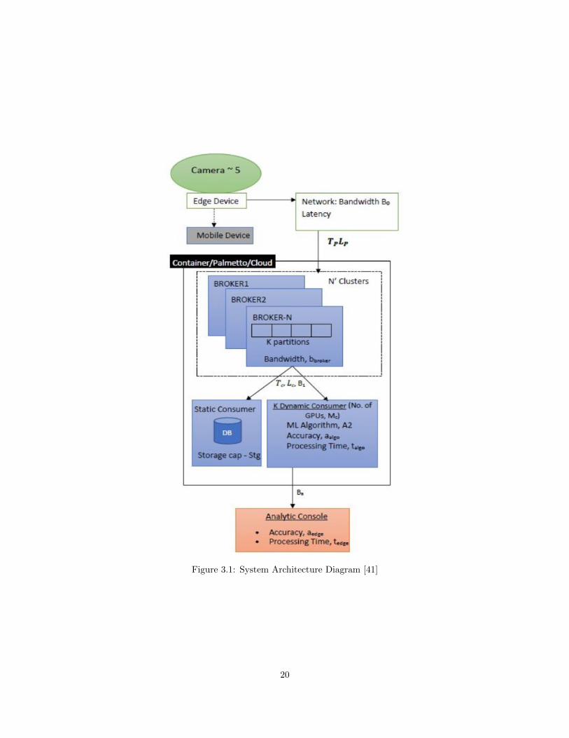
Figure 3.1: System Architecture Diagram [41]

20

Figure 3.2: The left side shows a sample synthetic image. Each image is composed of sixty-threetiles. The complete visual view of a car in the synthetic workload is represented by ninety-fiveimages. The right side is zoomed in on four of the tiles and shows the objects detected [41]

whole car. A sample synthetic image used for evaluation and performance testing is shown in Fig

Figure 3.2.

3.2 Object Detection Models

Traditionally, computer vision applications have required complex feature engineering tasks

to produce effective feature sets for different kinds of object detection applications. Today, deep

learning techniques can be applied directly to raw images without complex feature extraction algo-

rithms. Many common tasks such as object detection can be solved effectively using out-of-the-box

deep learning architectures. In our experimental environment, which includes a set of fixed-location

cameras, all images are the same size and all models are tested on the same images.

One challenge in object detection is that objects of interest may have different locations

within the image and may have different aspect ratios. In a naıve approach, the number of bounding

boxes that must be considered is exponentially large with respect to the size of the image. As a

21

result, many different object detection architectures have been proposed that reduce the size of the

search space for objects of interest or optimize the search in different ways. These different object

detection architectures have different characteristics as discussed above.

Some models are designed to achieve state-of-the-art performance in accuracy. Several

models aim to achieve reasonable accuracy within limited time and computational resources. There

are efforts to build deep learning models for special hardware systems, such as FPGAs, or for

resource-limited devices such as smartphones. There are multiple degrees of freedom in object

detection architectures that affect their accuracy, run time, and resource utilization as discussed in

Section 2.4. The literature provides many details about object detection architectures [20]. Here

we list some important degrees of freedom that we consider:

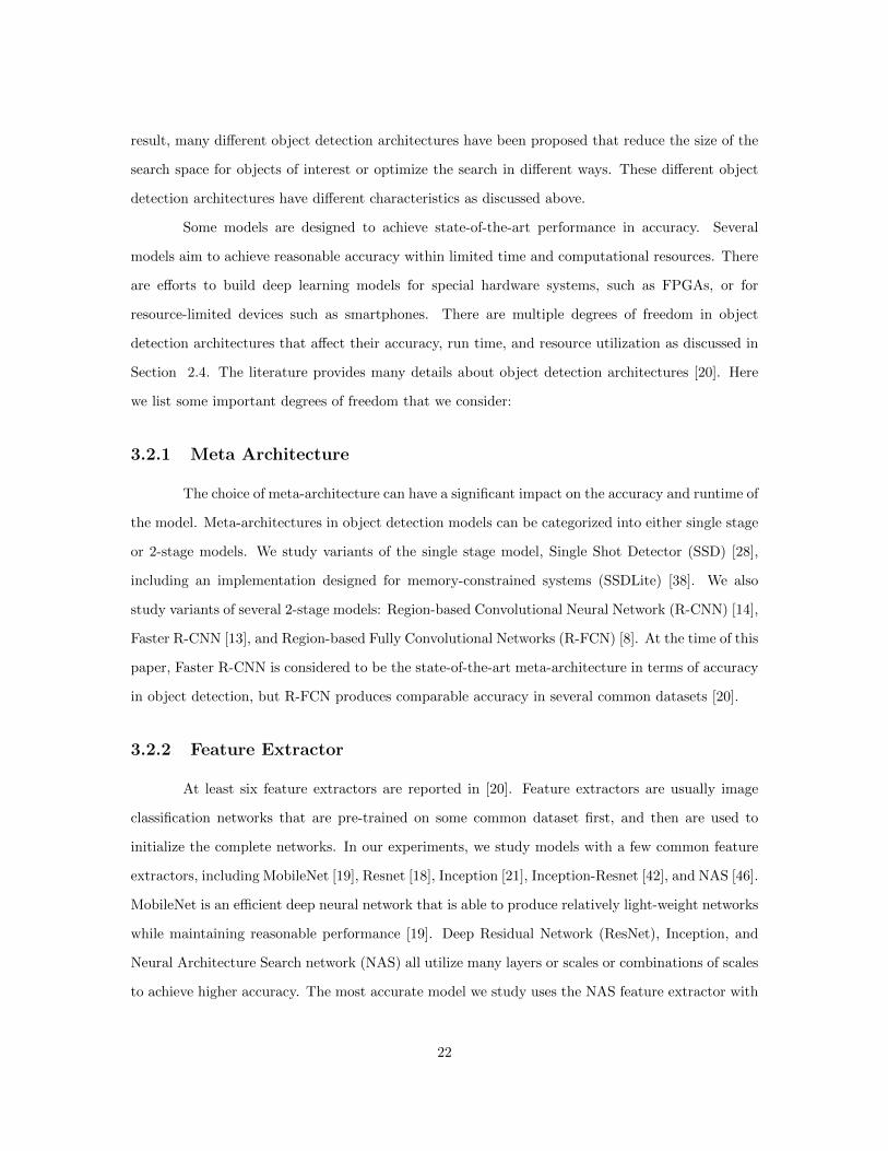
3.2.1 Meta Architecture

The choice of meta-architecture can have a significant impact on the accuracy and runtime of

the model. Meta-architectures in object detection models can be categorized into either single stage

or 2-stage models. We study variants of the single stage model, Single Shot Detector (SSD) [28],

including an implementation designed for memory-constrained systems (SSDLite) [38]. We also

study variants of several 2-stage models: Region-based Convolutional Neural Network (R-CNN) [14],

Faster R-CNN [13], and Region-based Fully Convolutional Networks (R-FCN) [8]. At the time of this

paper, Faster R-CNN is considered to be the state-of-the-art meta-architecture in terms of accuracy

in object detection, but R-FCN produces comparable accuracy in several common datasets [20].

3.2.2 Feature Extractor

At least six feature extractors are reported in [20]. Feature extractors are usually image

classification networks that are pre-trained on some common dataset first, and then are used to

initialize the complete networks. In our experiments, we study models with a few common feature

extractors, including MobileNet [19], Resnet [18], Inception [21], Inception-Resnet [42], and NAS [46].

MobileNet is an efficient deep neural network that is able to produce relatively light-weight networks

while maintaining reasonable performance [19]. Deep Residual Network (ResNet), Inception, and

Neural Architecture Search network (NAS) all utilize many layers or scales or combinations of scales

to achieve higher accuracy. The most accurate model we study uses the NAS feature extractor with

22

the Faster R-CNN meta-architecture (Faster R-CNN NAS).

3.2.3 Mini batch size

The mini batch size is a parameter to the models that specifies the number of tiles loaded

and processed by the model at the same time. Larger batch sizes can enable more efficient use of

the GPU memory and cores.

The original papers typically report a single combination of these options, with variants

such as different image resolutions, the numbers and positions of the candidate boxes, the layers

from which features are extracted and the number of layers. In this evaluation, we focus on popular

methods with different combinations of meta-architectures and feature extractors that have all been

pre-trained on the COCO dataset.

3.3 Hardware Platforms

Low cost embedded devices like Raspberry PI and mobile phones are used for the the

purpose of edge computing but are not suitable for high defination images. As our application has a

limitation of time constraint we leverage the growth in computational power and utilise four models

of GPU processor for our experiments. We also carry out experiments on CPU and few experiments

on Nvidia TX2.

3.3.1 Nvidia P100

Nvidia’s Tesla P100 (Pascal) architecture, introduced in 2016, contains 3,584 CUDA cores.

The card for our tests uses a PCIe bus, has 12GB of RAM, memory bandwidth of 732 GB/s, and a

GPU maximum clock rate of 1.33 GHz.

3.3.2 Nvidia V100 PCIe

The Tesla V100 (Volta), introduced in 2017, has 5,120 CUDA cores. The card is our tests

has 16 GB RAM, memory bandwidth of 900 GB/s, and a GPU maximum clock rate of 1.38 GHz.

In addition to the increased number of CUDA cores, an advantage of the V100 over the P100 is

the addition of 640 Tensor cores. A Tensor core uses a fused multiply add (FMA) operation in

23

which two half precision 4x4 matrices are multiplied together, and a half or single precision matrix

is added to the result. An FMA operation can be performed within one GPU clock cycle. Some

object detection models natively utilize reduced precision in some layers of the algorithms, which

can improve execution time without affecting accuracy.

3.3.3 Nvidia V100 SXM2

Though similar to PCIe in architecture and number of cores (5,120), Nvidia’s Tesla V100

SXM2 uses NVLink as the system interface. The card in our tests has 16 GB memory, memory

bandwith of 900 GB/s, and a GPU maximum clock rate of 1.53 GHz. It also has an interconnect

bandwidth of 300 GB/s, compared to the PCIe counterpart which offers 32 GB/s.

3.3.4 Nvidia Jetson TX2

The Nvidia Jetson TX2 has a Pascal GPU with 256 CUDA cores. Memory is shared with

main memory and is 8 GB with a bandwidth of 59.7 GB/s. The TX2, along with prior edge devices

TK1 and TX1, and the latest edge device Xavier, are designed to run pre-trained models. We

focuses on evaluating the less-resource demanding MobileNet models on the TX2. We use TX2 in

Max-N power mode, where both dual-core Denver processor and a quad-core ARM Cortex-A57 run

at maximum clock speed along with the GPU clock speed of 1.30 Ghz.

3.3.5 CPU only

CPU-only execution only tests were performed on a compute node with Intel Xeon Gold

6148 CPU at 2.40 GHz without the use of any GPU. Each test runs on all forty cores of a single

compute node.

3.4 Performance Metrics

There are many factors that can affect performance measure- ments, such as the executions

of other processes, the shared utilization of memory bandwidth, or environmental tasks. We set

up a clean and isolated environment with no processes that consume system resources other than

required system processes.

24

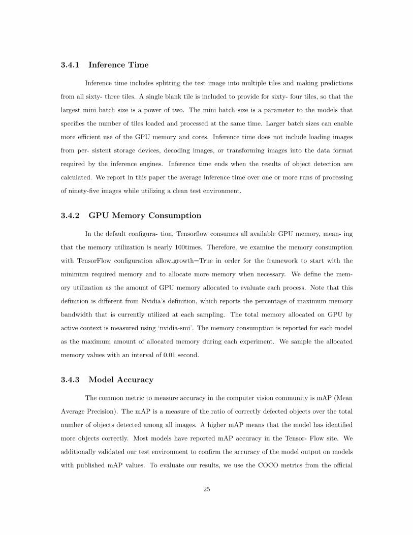
3.4.1 Inference Time

Inference time includes splitting the test image into multiple tiles and making predictions

from all sixty- three tiles. A single blank tile is included to provide for sixty- four tiles, so that the

largest mini batch size is a power of two. The mini batch size is a parameter to the models that

specifies the number of tiles loaded and processed at the same time. Larger batch sizes can enable

more efficient use of the GPU memory and cores. Inference time does not include loading images

from per- sistent storage devices, decoding images, or transforming images into the data format

required by the inference engines. Inference time ends when the results of object detection are

calculated. We report in this paper the average inference time over one or more runs of processing

of ninety-five images while utilizing a clean test environment.

3.4.2 GPU Memory Consumption

In the default configura- tion, Tensorflow consumes all available GPU memory, mean- ing

that the memory utilization is nearly 100times. Therefore, we examine the memory consumption

with TensorFlow configuration allow growth=True in order for the framework to start with the

minimum required memory and to allocate more memory when necessary. We define the mem-

ory utilization as the amount of GPU memory allocated to evaluate each process. Note that this

definition is different from Nvidia’s definition, which reports the percentage of maximum memory

bandwidth that is currently utilized at each sampling. The total memory allocated on GPU by

active context is measured using ‘nvidia-smi’. The memory consumption is reported for each model

as the maximum amount of allocated memory during each experiment. We sample the allocated

memory values with an interval of 0.01 second.

3.4.3 Model Accuracy

The common metric to measure accuracy in the computer vision community is mAP (Mean

Average Precision). The mAP is a measure of the ratio of correctly defected objects over the total

number of objects detected among all images. A higher mAP means that the model has identified

more objects correctly. Most models have reported mAP accuracy in the Tensor- Flow site. We

additionally validated our test environment to confirm the accuracy of the model output on models

with published mAP values. To evaluate our results, we use the COCO metrics from the official

25

COCO Python API [19]. These calculate the average precision over multiple Intersec- tion Over

Union (IOU) values ranging from 0.50 to 0.95 with a stride of 0.05. Note that the reported mAP

results were calculated on the COCO test data set, but the labels and annotations for the COCO test

data set are not available to the public. We performed accuracy tests using the COCO validation

data set. Since we have calculated mAP values using a different data set, the values are different,

but the results show that the relative accuracy of the models is the same with one exception. A

subset of the models was also hand inspected for accuracy. The list of models, sorted by accuracy,

is shown in Table I. The model names shown in Table I give the meta-architectures and feature

extractors as previously described. Models are grouped into five groups by mAP, as shown in Table

I, to facilitate comparative analysis.

3.5 Results for Object Detection Models

In this section, we discuss the experimental results. We tested the full range of models

and hardware choices. In a few cases, not all results are shown on the charts for space reasons.

The results shown are representative of the range of results and are the most likely combinations

of models and architecture to be selected for our application. Results for hardware platforms P100,

V100 PCIe, V100 SXM2, CPU-only, and TX2 are shown.

3.5.1 Inference Time as a Function of Mini Batch Size

We measure the inference time as a function of the TensorFlow mini batch size for each

platform. Mini batch size varies as a choice of 1, 2, 4, 8, 16, 32, and 64. The batch size of 64 loads all

tiles in the image as a single batch. The size of a mini batch indicates the size of the fourth dimension

of the input tensor supplied to the model’s computational graphs (the three other dimensions are

height, width, and color channels). Larger batch sizes require larger memory to store input tensors,

intermediate representations, and output tensors during computations. However, larger batch sizes

reduce the amount of communication between operations, thereby reducing inference time. The

inference time is reported in seconds and is shown in log scale on most charts. Some higher accuracy

models have an out-of-memory error with larger batch sizes and no result is shown in this case on

the chart.

Fig. 3.3 shows the inference time as a function of the mini batch size for selected models on

26

Figure 3.3: Inference time as a function of batch size on P100 [41]

the P100 hardware. In general, runtime decreases with larger batch sizes to about a mini batch size

of 8, where it tends to level off.

Note that Faster RCNN NAS runs out of memory with a batch size of 4 and above on the

P100 and on both V100 GPUs, but it is the most accurate model we tested. Some other models

with High or Medium accuracy also run out of memory at higher batch sizes. The more accurate

models build deeper neural networks that take more memory so fewer batches can fit into memory

at a time.

The four “low proposal” models are also shown in Fig. 3.3, but the accuracy of these is

Not Available. Note that these low proposal models have much faster run times than their non-low

proposal counterparts. Measuring the accuracy of these models for our application is an area of

future inquiry.

Fig. 3.5 and Fig. 3.4 show the inference time as a function of the mini batch sizes for the

V100 PCIe and V100 SXM2 platforms, respectively. Some similarities and differences can be noted

between execution on the P100 and execution on the V100 platforms. The out-of-memory errors for

some higher accuracy models occurs at the same batch sizes tested on all three platforms. However,

the run times for all models are faster on the V100 platforms than on the P100, and are somewhat

27

Figure 3.4: Inference time as a function of batch size on V100 SXM2 [41]

faster on the V100 SXM2 than on the V100 PCIe platform. These results are expected since the

faster memory bandwidth and clock rate and addition of tensor cores gives the V100 platforms a

significant advantage. The fastest models we test are the four MobileNet models. The fastest run

time we measure, of all models and hardware choices, is SSD MobileNet V2 with V100 SXM2 and

a mini batch size of 64. This model has a mean run time of 0.743 seconds to process a single image.

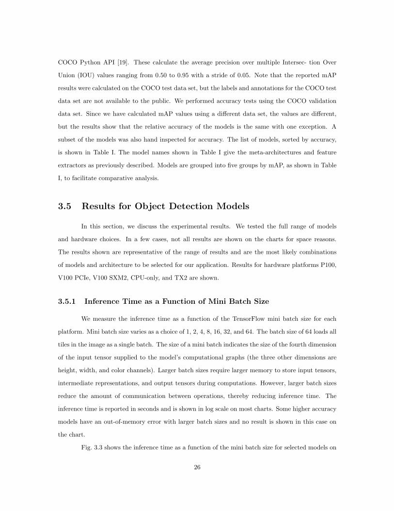
Figure 3.6 shows the inference time as a function of the mini batch sizes for CPU-only

execution. The relative ranking of models by run time is similar to the rankings by run time on the

GPU platforms. However, note the change of scale on the y-axis. The run times for CPU only are in

general much higher for all models than on the GPU platforms. For example, the best run time of

Faster RCNN NAS using V100 SXM2 is around 32 seconds as compared to the run time on the CPU-

only of around 256 seconds, a factor of 8 times slower. For real-time industrial applications, such as

ours, selection of hardware includes the ability of its performance to meet timing requirements and,

secondly, if the costs of using multiple hardware platforms in parallel to meet all workload demands

justify the use of the cheaper, slower platform. We study the costs comparisons separately.

Fig. 3.7 shows the inference time as a function of the mini batch sizes for TX2 execution.

Most models do not execute within our application run time constraints on the TX2, and we only

28

Figure 3.5: Inference time as a function of batch size on V100 PCIe [41]

show results for the MobileNet models. The SSD Mobilenet v1 FPN model runs out of memory for

batch sizes greater than one. The TX2 is designed to be inexpensive, having less memory and other

resources restrictions. The execution is much slower for the tested models than on the P100 and

V100 platforms, though the platform is less expensive and is useful for many application use cases.

3.5.2 Memory Consumption as a Function of Mini Batch Size

We measure the GPU memory consumption as a function of the TensorFlow mini batch size

using the same parameters as for measuring inference time. Memory consumption is reported in

MB for the GPU platforms. As before, higher accuracy models have an out-of-memory error with

larger batch sizes and no result is shown in this case on the chart.

Fig. 3.8 shows the memory consumption as a function of the mini batch size for selected

models on the P100 hardware. Fig. 3.9 shows the memory consumption as a function of the mini

batch size for selected models on the V100 PCIe hardware. Memory consumption on the V100

SXM2 hardware is the same as memory consumption on the V100 PCIe hardware and is not shown

for space reasons.

On both the P100 and V100 PCIe platforms the SSD models have the smallest memory

29

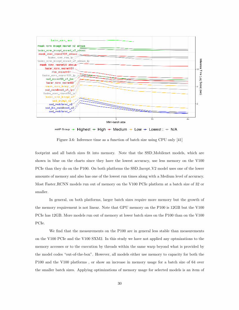
Figure 3.6: Inference time as a function of batch size using CPU only [41]

footprint and all batch sizes fit into memory. Note that the SSD Mobilenet models, which are

shown in blue on the charts since they have the lowest accuracy, use less memory on the V100

PCIe than they do on the P100. On both platforms the SSD Incept V2 model uses one of the lower

amounts of memory and also has one of the lowest run times along with a Medium level of accuracy.

Most Faster RCNN models run out of memory on the V100 PCIe platform at a batch size of 32 or

smaller.

In general, on both platforms, larger batch sizes require more memory but the growth of

the memory requirement is not linear. Note that GPU memory on the P100 is 12GB but the V100

PCIe has 12GB. More models run out of memory at lower batch sizes on the P100 than on the V100

PCIe.

We find that the measurements on the P100 are in general less stable than measurements

on the V100 PCIe and the V100 SXM2. In this study we have not applied any optmizations to the

memory accesses or to the execution by threads within the same warp beyond what is provided by

the model codes “out-of-the-box”. However, all models either use memory to capacity for both the

P100 and the V100 platforms , or show an increase in memory usage for a batch size of 64 over

the smaller batch sizes. Applying optimizations of memory usage for selected models is an item of

30

Figure 3.7: Inference time as a function of batch size using TX2 [41]

future study.

We do not show results for memory usage for the TX2 since the GPU does not have its own

memory on the TX2. It shares the system RAM and is wired to memory controller and generally

consumes most of the system memory. We do not break out those numbers in our charts.

3.5.3 Inference Time and Memory for Different GPU Platforms

In this section, we study the trade-offs of memory usage and interference time for three

different GPU platforms. For this part of the study with each model, we select the batch size that

provides the fastest execution time and report the memory usage for that model. Fig. 3.10 graphs

the inference time and memory usage for the models executed on the P100, V100 PCIe, and V100

SXM2 platforms. The reported values are labeled with an ID for each model. Fig. 3.11 lists the

models along with the ID that is used in Fig. 3.10. The values list the best inference time over all

the tested batch sizes and its relative memory usage for each model over every hardware.

The figures show that in general, bigger models with larger inference times achieve better

accuracies on both systems. Faster RCNN NAS is the model that both achieves highest accuracy

and has the longest run time. Also, because of its complex structure, we can only fit a maximum

31

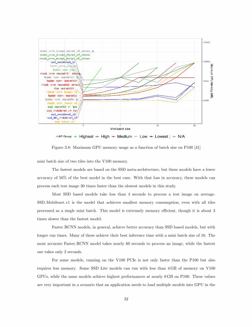
Figure 3.8: Maximum GPU memory usage as a function of batch size on P100 [41]

mini batch size of two tiles into the V100 memory.

The fastest models are based on the SSD meta-architecture, but these models have a lower

accuracy of 50% of the best model in the best case. With that loss in accuracy, these models can

process each test image 30 times faster than the slowest models in this study.

Most SSD based models take less than 4 seconds to process a test image on average.

SSD Mobilenet v1 is the model that achieves smallest memory consumption, even with all tiles

processed as a single mini batch. This model is extremely memory efficient, though it is about 3

times slower than the fastest model.

Faster RCNN models, in general, achieve better accuracy than SSD based models, but with

longer run times. Many of these achieve their best inference time with a mini batch size of 16. The

most accurate Faster RCNN model takes nearly 60 seconds to process an image, while the fastest

one takes only 2 seconds.

For some models, running on the V100 PCIe is not only faster than the P100 but also

requires less memory. Some SSD Lite models can run with less than 4 GB of memory on V100

GPUs, while the same models achieve highest performances at nearly 8 GB on P100. These values

are very important in a scenario that an application needs to load multiple models into GPU in the

32

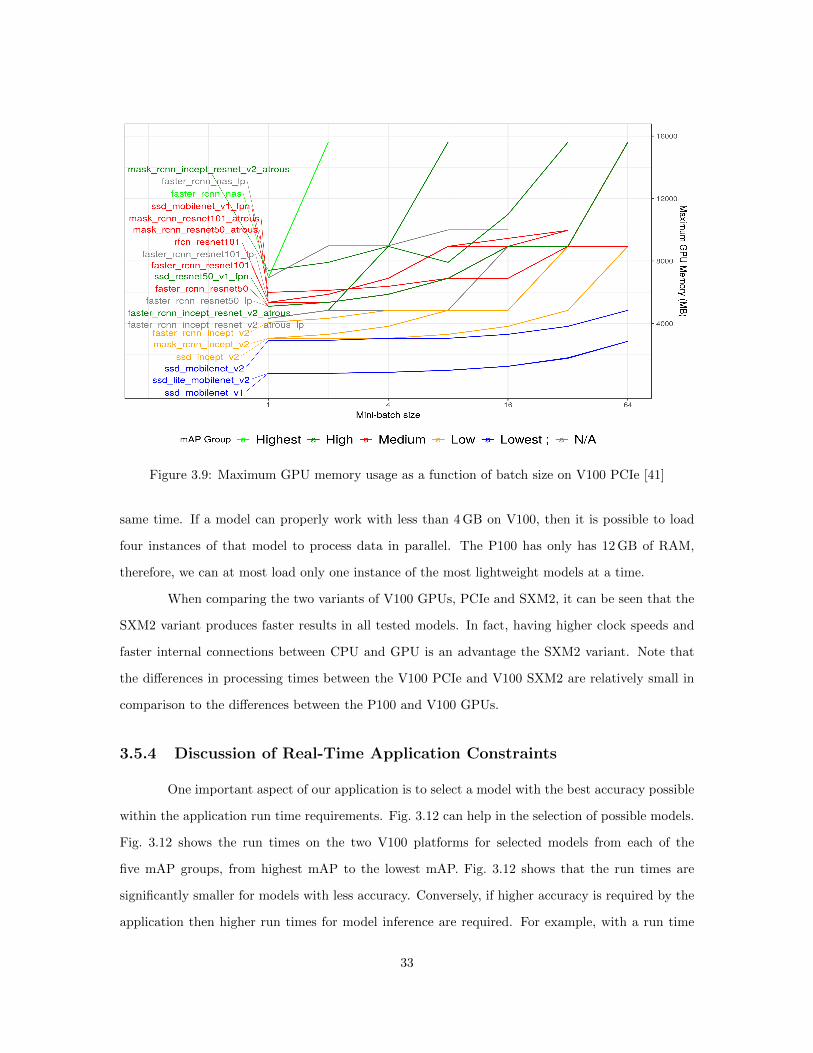
Figure 3.9: Maximum GPU memory usage as a function of batch size on V100 PCIe [41]

same time. If a model can properly work with less than 4 GB on V100, then it is possible to load

four instances of that model to process data in parallel. The P100 has only has 12 GB of RAM,

therefore, we can at most load only one instance of the most lightweight models at a time.

When comparing the two variants of V100 GPUs, PCIe and SXM2, it can be seen that the

SXM2 variant produces faster results in all tested models. In fact, having higher clock speeds and

faster internal connections between CPU and GPU is an advantage the SXM2 variant. Note that

the differences in processing times between the V100 PCIe and V100 SXM2 are relatively small in

comparison to the differences between the P100 and V100 GPUs.

3.5.4 Discussion of Real-Time Application Constraints

One important aspect of our application is to select a model with the best accuracy possible

within the application run time requirements. Fig. 3.12 can help in the selection of possible models.

Fig. 3.12 shows the run times on the two V100 platforms for selected models from each of the

five mAP groups, from highest mAP to the lowest mAP. Fig. 3.12 shows that the run times are

significantly smaller for models with less accuracy. Conversely, if higher accuracy is required by the

application then higher run times for model inference are required. For example, with a run time

33

Figure 3.10: Best inference time and max memory consumption of models on three GPU devices. The

labels used in this figure are shown in Fig. 9. For each point shown the mini batch size that gives the best

run time for that model is shown in parentheses. For example, C(64) shown in the lower left of the left figure

is the ssd mobilenet v1 ppn model run with a mini batch size of 64, which is the fastest for that model on

the P100. The left figure shows results for P100, the middle figure shows results for V100 PCIe, and the

right figure shows results for V100 SXM2 [41].

34

Figure 3.11: List of models and IDs used in Fig. 3.10.

requirement of 1 second, the best accuracy we can achieve for the calculation of an individual model

is in the “Lowest” range. However, with a run time requirement of 4 seconds, the best accuracy we

can achieve for the calculation of an individual model is a higher value in the “Medium” range. A

run time of about 32 seconds for the calculation of an individual model is required to obtain the

“Highest” accuracy.

35

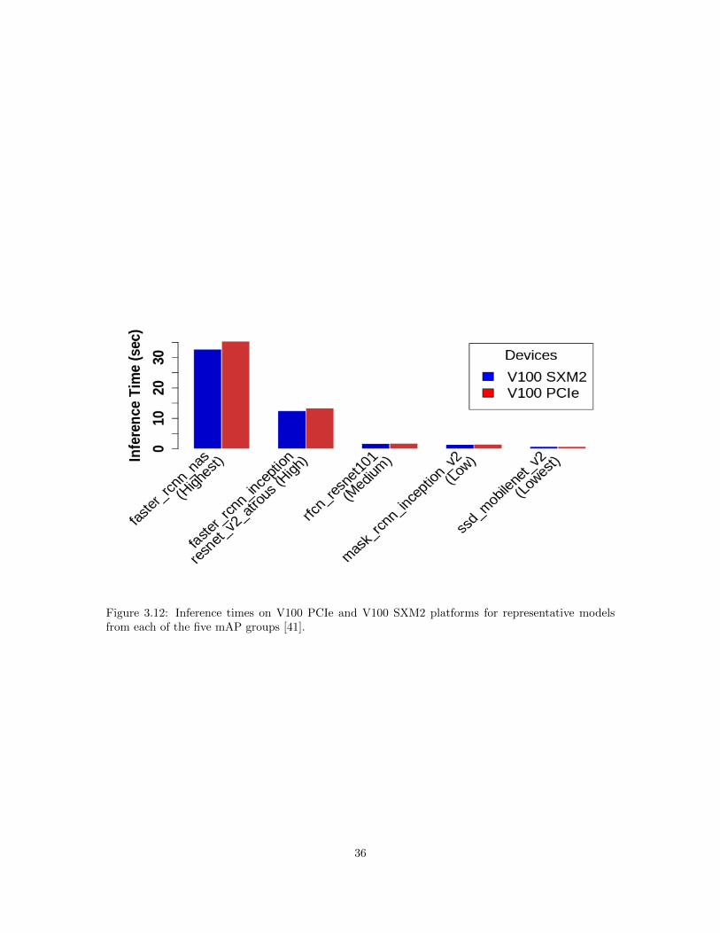
Figure 3.12: Inference times on V100 PCIe and V100 SXM2 platforms for representative modelsfrom each of the five mAP groups [41].

36

Chapter 4

Pipeline Architecture

In this section we present the implementation of end-to-end system pipeline using AWS

components. Tools like AWS Cloudformation, Azure Resource Manager (ARM) Templates and

Google Cloud deployement manager are some of the ways to define infrastructure as code. Deploying

softwares and architecture using these tools is transparent, reusable and can be modified with ease.

IaC provides th ability to iterate and change infrastructure faster and more efficiently [33].

In a few locations there is lack of floor space in the assembly plant to deploy and setup an

edge processing system that can support our defect detection problem in high definition images. To

achieve agility, flexibility and to overcome the inadequate space, we carry out our evaluations using

cloud environment. We describe the AWS components followed by how these components are used

to construct a data streaming and detection pipeline.

4.1 Edge versus Cloud tradeoffs

Although incorporating deep learning in our system is helpful for our visual inspection

problem, implementing the intelligent system in an efficient way is difficult. We can deploy a

streaming broker and deep learning models on the edge devices or on a cloud platform that is

connected to the assembly plant through a network. Edge and cloud computing have their own

benefits and limitations.

The cameras in the assembly line produce large amount of data which is required to be pro-

cessed in real time. This continuously increasing data needs to be processed and stored somewhere.

37

Cloud platforms may not be as efficient as edge platform for real-time scenarios, low latency, and

high quality of service (QoS) [6] for certain types of workloads. With this in mind, if we move the

compute of data on the edge, the network will no longer be a constraint but the storage of data on the

edge is unsecured and unmanageable. On the other hand, the cloud provides an excellent platform

for ubiquitous and on demand access to configurable compute and storage resources. EC2 instance

on the cloud provide GPUs suitable for performing compute intensive task, and these instances can

be provisioned as per the work load. Cloud computing and storage also comes in as a convenient

option in assembly plants where there is not enough floor space to set up a data center on the edge.

Then again, transferring large amount of data from the edge nodes to the cloud, involves a need for

a large bandwidth and network, which is an expensive resource [39].

A good connectivity with high bandwidth is the key feature for seamless processing in cloud

applications. In this chapter we study the end-to-end pipeline for real time visual inspection using

Amazon cloud and provisioning the entire infrastructure setup using AWS SDK, BOTO3.

4.2 AWS Components

We build an end-to-end pipeline for object detection for streaming high definition images

using Python SDK, BOTO3.

Some of the AWS services that we use are:

Simple Storage Service (S3) Amazon S3 is a cloud based storage system that stores

data in buckets. It allows read, write and delete operations on the data from anywhere, at any time

with any number of requests. We take advantage of S3 Transfer Acceleration which enables fast and

secure transfer of data across continents by utilizing the Amazon Cloudfront globally distributed

over the edge locations. The data is transferred to an edge location and travels over an optimized

network path. Transfer Acceleration is useful while transferring data across continents or in scenarios

when the entire bandwidth is not utilized.

Simple Queue Service (SQS) is a reliable queuing service that enables asynchronous

message based communication at scale. Amazon SQS supports both standard and FIFO (First In

First Out) queues. Order of messages send and received is strictly maintained in FIFO queues. As

FIFO queue is not available in all regions and order of messages is not a concern in our application

we use Standard SQS service.

38

Figure 4.1: Life cycle of SQS message in a queue [2]

Figure 4.1 shows the SQS life cycle diagram. The producer sends message A to the server,

which replicates on the SQS servers. The consumer consumes the messages from the queue and the

message A is returned and delete from the queue.

Messages in the queue can be processed using short polling and long polling. By default

SQS uses short polling, where messages are returned almost instantly, but it checks only few servers

based on weighted random distribution in which cases a lot of times the read request may not

return anything even when the queue has messages in a particular API call. In this case the

WaitTimeSeconds is set to 0. Unlike short polling, long polling is cost effective and efficient. It

reduces the cost by removing the empty responses and false empty responses. It tries to read

messages from the queue and returns atleast one or more messages as long as they are available to

be consumed. If the queue does not contain any messages, the read request waits till the timeout

period and then returns an empty response.

39

The image is uploaded to the S3 bucket, exploiting parallelism for data upload to S3. When

the image is uploaded to the bucket, an event trigger enable it to publish the metadata to SQS. The

consumer processes the message from the queue, and it remains in the queue until it is deleted by

the consumer. Messages which have been sent and not been deleted from the or have not reached

the end of visibility window are said to be in flight. SQS automatically delete the message if it has

been there for more than the maximum message retention period. The default retention period is 4

days.

Elastic Compute Cloud (EC2) provides a secure and re-sizable compute capacity. It

provides complete control of computing resources and machine learning workflow unlike Amazon

Sagemaker and Amazon Rekognition.

For our experimental pipeline we use Deep Learning AMI (Ubuntu) Version 12.0 which

comes with pre-installed CUDA9 and deep learning frameworks optimzed for Nvidia Volta GPUs.

We use P3 instances which are designed to handle deep learning workloads. Amazon P3 EC2 instance

comes with 8 NVIDIA V100 GPU and 100 Gbps of networking throughput. Careful cost and compute

consideration should be carried out while choosing P3 instance configuration. Autoscaling is enabled

to monitor the SQS messages and dynamically scale up/down the instances.

CloudWatch, is used to monitor the logs as well as define metrics and set custom alarms.

It is used to trigger alarm to spin up instances if the messages in the SQS queue reached a threshold

level. It also provides a visual representation for monitoring the existing usage of resources.

DynamoDB, is a fully managed, low latency No-SQL database. We use DynamoDB to

store the results obtained from object detection, which can be queried later if needed.

4.3 AWS Pipeline

Fig. 4.2 shows an end-to-end pipeline in Amazon cloud that uses the AWS components

described above. High definition images are sent over the network to S3 buckets using multiple con-

current requests. There are various factors that affect the latency and throughput of objects/images

to S3:

a. Region of S3 bucket

b. Connectivity/Bandwidth of network

c. Concurrency and the number of connections

40

S3 triggers notifications for certain events like creating, removal or restoring any object in

the S3 bucket. It publishes event messages to an SQS queue, SNS topic or an AWS lambda function.

In our experimental setup, we use S3 APIs, PUT, POST, COPY to enable a trigger whenever

any object is created in the S3 bucket. A trigger is fired to the Standard SQS, where the metadata

for the image is published in the queue.

We enable dynamic scaling of EC2 instances following the demand curve of our application.

A set Deep Learning AMI instances are spawned depending on the number of messages in the queue

at the given time.

These EC2 instances use the following services:

a. Security group, with ingress rules to restrict traffic.

b. Launch configuration, contains the Amazon Machine Image (AMI) ID, the instance type,

security group, instance type and other information about the instance.

c. Autoscaling group with scaling policies

d. Cloud watch alarm if the number of messages in queue are above threshold level

We create a new role to execute the userdata specified in launch configuration to spin

up an EC2 instance which is helpful in executing AWS CLI commands in EC2 instance without

authentication. EC2 userdata sets up the object detection module and fetches the metadata present

at a particular time from the SQS queue. If there is no message in the queue, the EC2 instance

waits for two minutes before terminating the instance. We set the WaitTimeSeconds to ten seconds

to enable long polling as explained above. The SQS queue fetches maximum ten messages at a time.

The metadata from the SQS is used to fetch the corresponding image from the S3 bucket.

We then use tensorflow to create a detection session where the image is divided into tiles and fed

into the model. The prediction of bounding box coordinates along with the class and score of the

particular object is written to the AWS DynamoDb in a JSON format.

After writing the result to the DynamoDB, the instance waits for another set of messages

from the queue. If the message does not arrive in the queue for two minutes the instance is termi-

nated.

41

Figure 4.2: AWS Pipeline

4.4 Auto Deploy using BOTO3

Developing, deployment and management of AWS services can be simplified by using an API

tailored to the programming language. AWS offers Software Development Kit(SDK) for Python,

JAVA, Node.js and several other languages. BOTO3 is an AWS SDK for Python. It provides a

platform for integration of Python scripts and libraries with a variety of AWS services.

BOTO3 has two distinct levels of API [1]. Client API or low level service access that maps

one to one with the service API and exposes the BotoCore client to the developer. Resource API

or high level object oriented API provides the resource object while hiding the underlying network

calls.

4.5 Results for End to End Pipeline

In this section, we discuss the experimental results. We examine different approaches for

reducing network latency. We issue PUT requests from a local machine in three different regions with

multiple concurrent request and then compare the measured throughput in each case for different

time of hour. Some of the scenarios are shown in the section below. We also measure the timings

for each component of Amazon Web Service for representative models.

In our transfer performance analysis, we use a local machine with a configuration of 1 Socket,

42

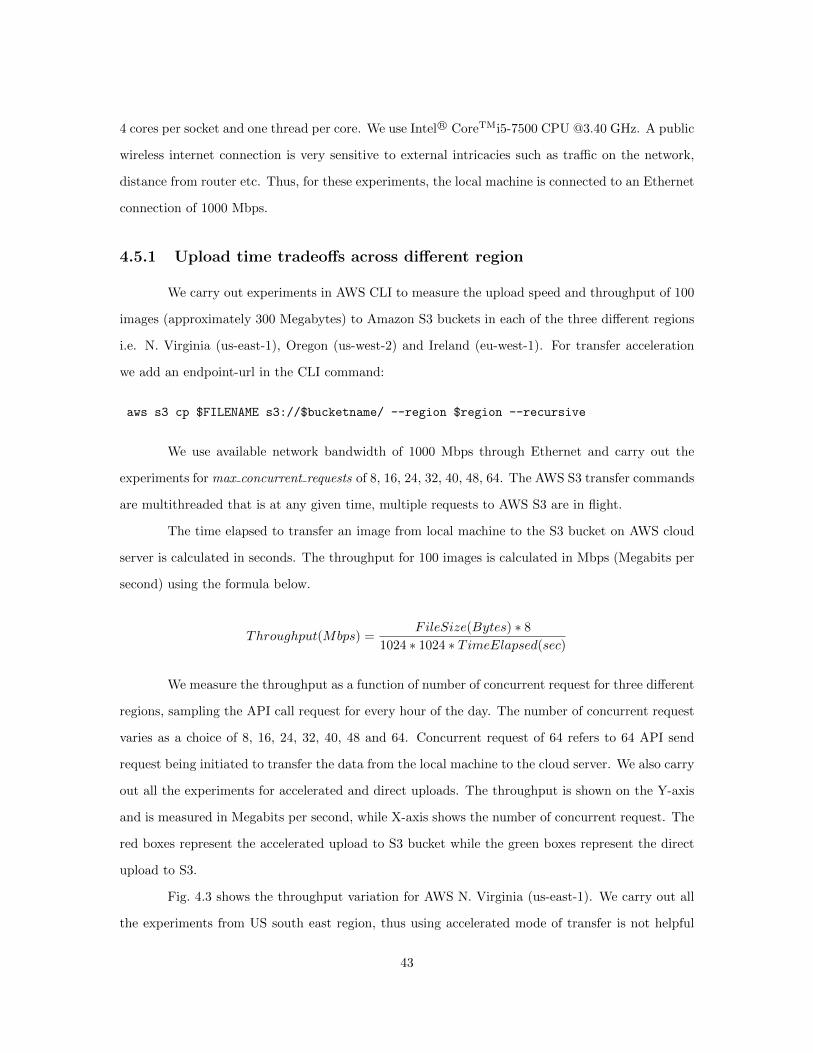
4 cores per socket and one thread per core. We use Intel R© CoreTMi5-7500 CPU @3.40 GHz. A public

wireless internet connection is very sensitive to external intricacies such as traffic on the network,

distance from router etc. Thus, for these experiments, the local machine is connected to an Ethernet

connection of 1000 Mbps.

4.5.1 Upload time tradeoffs across different region

We carry out experiments in AWS CLI to measure the upload speed and throughput of 100

images (approximately 300 Megabytes) to Amazon S3 buckets in each of the three different regions

i.e. N. Virginia (us-east-1), Oregon (us-west-2) and Ireland (eu-west-1). For transfer acceleration

we add an endpoint-url in the CLI command:

aws s3 cp $FILENAME s3://$bucketname/ --region $region --recursive

We use available network bandwidth of 1000 Mbps through Ethernet and carry out the

experiments for max concurrent requests of 8, 16, 24, 32, 40, 48, 64. The AWS S3 transfer commands

are multithreaded that is at any given time, multiple requests to AWS S3 are in flight.

The time elapsed to transfer an image from local machine to the S3 bucket on AWS cloud

server is calculated in seconds. The throughput for 100 images is calculated in Mbps (Megabits per

second) using the formula below.

Throughput(Mbps) =FileSize(Bytes) ∗ 8

1024 ∗ 1024 ∗ TimeElapsed(sec)

We measure the throughput as a function of number of concurrent request for three different

regions, sampling the API call request for every hour of the day. The number of concurrent request

varies as a choice of 8, 16, 24, 32, 40, 48 and 64. Concurrent request of 64 refers to 64 API send

request being initiated to transfer the data from the local machine to the cloud server. We also carry

out all the experiments for accelerated and direct uploads. The throughput is shown on the Y-axis

and is measured in Megabits per second, while X-axis shows the number of concurrent request. The

red boxes represent the accelerated upload to S3 bucket while the green boxes represent the direct

upload to S3.

Fig. 4.3 shows the throughput variation for AWS N. Virginia (us-east-1). We carry out all

the experiments from US south east region, thus using accelerated mode of transfer is not helpful

43

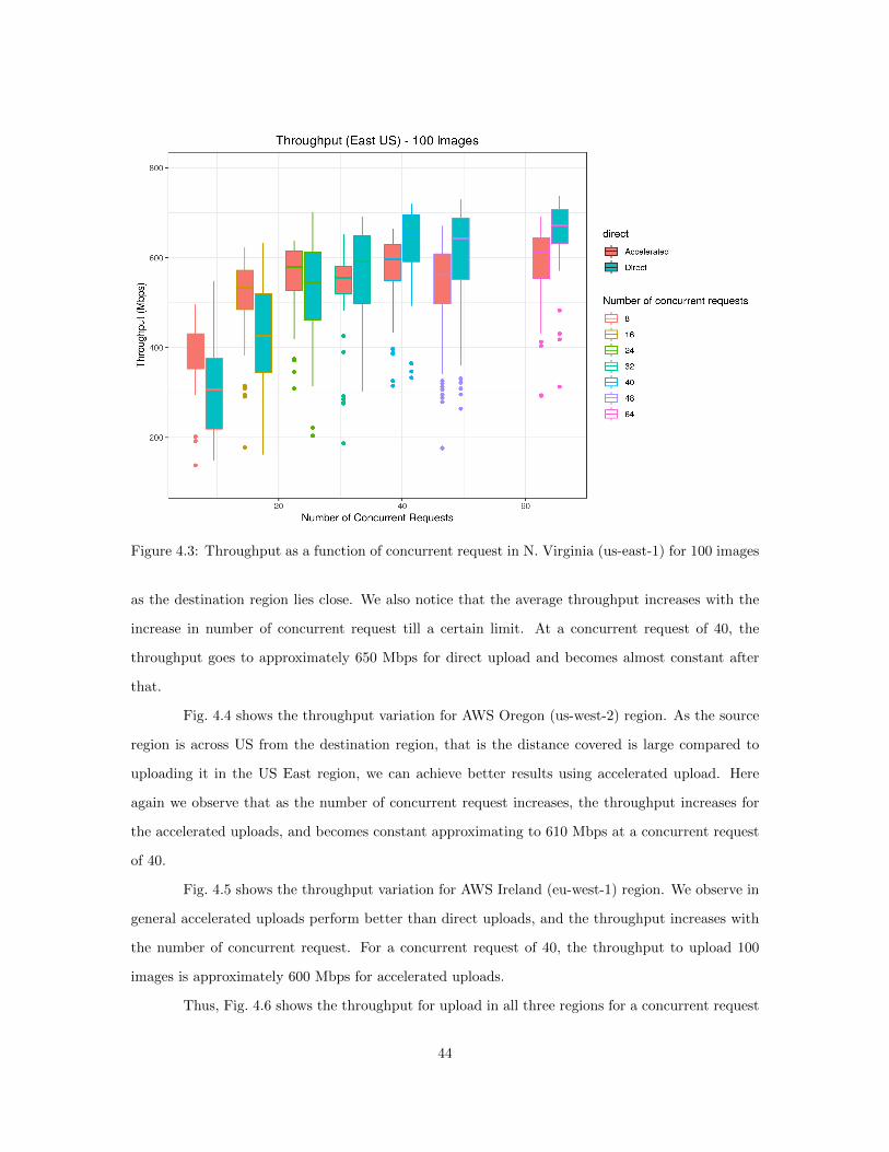
Figure 4.3: Throughput as a function of concurrent request in N. Virginia (us-east-1) for 100 images

as the destination region lies close. We also notice that the average throughput increases with the

increase in number of concurrent request till a certain limit. At a concurrent request of 40, the

throughput goes to approximately 650 Mbps for direct upload and becomes almost constant after

that.

Fig. 4.4 shows the throughput variation for AWS Oregon (us-west-2) region. As the source

region is across US from the destination region, that is the distance covered is large compared to

uploading it in the US East region, we can achieve better results using accelerated upload. Here

again we observe that as the number of concurrent request increases, the throughput increases for

the accelerated uploads, and becomes constant approximating to 610 Mbps at a concurrent request

of 40.

Fig. 4.5 shows the throughput variation for AWS Ireland (eu-west-1) region. We observe in

general accelerated uploads perform better than direct uploads, and the throughput increases with

the number of concurrent request. For a concurrent request of 40, the throughput to upload 100

images is approximately 600 Mbps for accelerated uploads.

Thus, Fig. 4.6 shows the throughput for upload in all three regions for a concurrent request

44

Figure 4.4: Throughput as a function of concurrent request in Oregon (us-west-2) for 100 images

of 40. As we carry out our experiment from south east region of US, the average throughput

in case of us-east-1 region is higher compared to other two regions, approximating to 650 Mbps

and the accelerated upload does not make a difference in scenarios when the destination of server

is closer to the source of upload. However, as Oregon and Ireland are far from our source, we

observe that accelerated upload to S3 performs better than the Direct upload. We also observe that

after a max concurrent requests of 40 the throughput becomes constant. Therefore for our further

experiments we choose max concurrent requests of 40 and N. Virginia (us-east-1) region as it is

closer to our location. Accelerated uploads to AWS edge locations in the United States, Europe,

and Japan costs $0.04 per GB, else it costs $0.08 per GB.

4.5.2 Parallel upload using multiple machines

In this section we report the results of using multiple whole computers at the same time to

upload the images to S3. In these experiments, the uploads are to the N. Virginia (us-east-1) region,

and each machine uses using 40 concurrent requests. The machine count varies as a choice of 3,

5, 10, 11 and 20. However, for all machines counts except for 10, all machines are connected to a

45

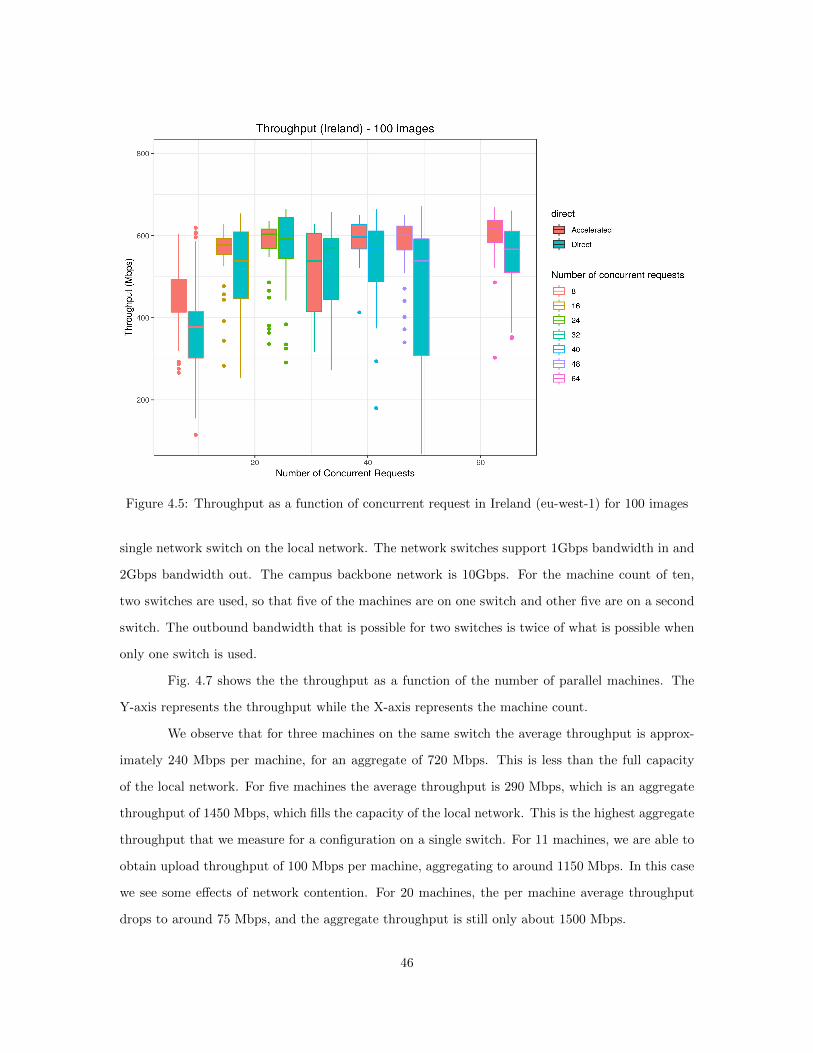
Figure 4.5: Throughput as a function of concurrent request in Ireland (eu-west-1) for 100 images

single network switch on the local network. The network switches support 1Gbps bandwidth in and

2Gbps bandwidth out. The campus backbone network is 10Gbps. For the machine count of ten,

two switches are used, so that five of the machines are on one switch and other five are on a second

switch. The outbound bandwidth that is possible for two switches is twice of what is possible when

only one switch is used.

Fig. 4.7 shows the the throughput as a function of the number of parallel machines. The

Y-axis represents the throughput while the X-axis represents the machine count.

We observe that for three machines on the same switch the average throughput is approx-

imately 240 Mbps per machine, for an aggregate of 720 Mbps. This is less than the full capacity

of the local network. For five machines the average throughput is 290 Mbps, which is an aggregate

throughput of 1450 Mbps, which fills the capacity of the local network. This is the highest aggregate

throughput that we measure for a configuration on a single switch. For 11 machines, we are able to

obtain upload throughput of 100 Mbps per machine, aggregating to around 1150 Mbps. In this case

we see some effects of network contention. For 20 machines, the per machine average throughput

drops to around 75 Mbps, and the aggregate throughput is still only about 1500 Mbps.

46

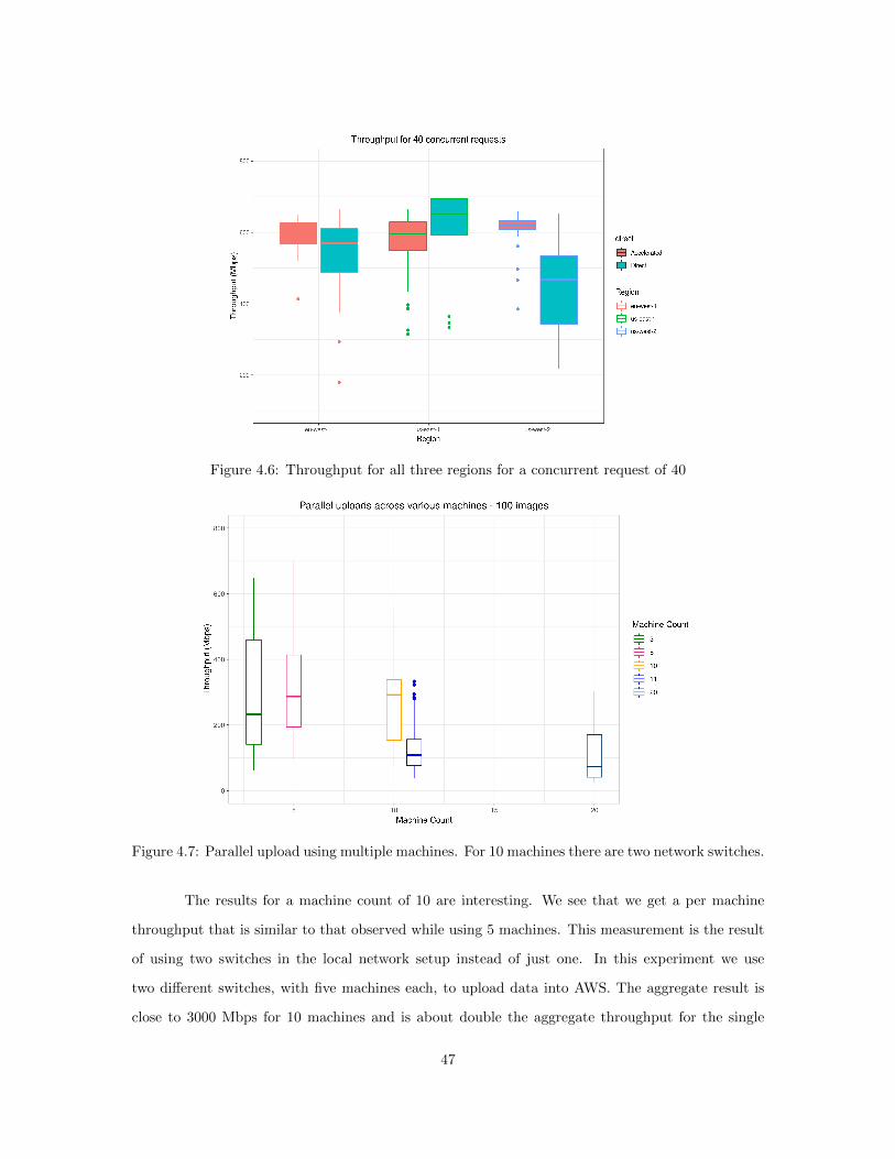
Figure 4.6: Throughput for all three regions for a concurrent request of 40

Figure 4.7: Parallel upload using multiple machines. For 10 machines there are two network switches.

The results for a machine count of 10 are interesting. We see that we get a per machine

throughput that is similar to that observed while using 5 machines. This measurement is the result

of using two switches in the local network setup instead of just one. In this experiment we use

two different switches, with five machines each, to upload data into AWS. The aggregate result is

close to 3000 Mbps for 10 machines and is about double the aggregate throughput for the single

47

switch configuration. This experiment illustrates that a component of the limitation to S3 upload

throughput is the local network configuration, and that upload throughput limitations cannot be

attributed only to AWS. The aggregate throughput using 10 machines connected via two switches

comes close double than when using 5 machines configured on a single switch, and the two-switch

configuration achieves the best throughput for our available hardware for our application testing.

4.5.3 Edge versus Cloud Upload Speed

We also measure the latency for uploading the images in our real-time visual inspection

application. We present results in this section as the time (latency) for the upload of a single image.

Figure 4.8: Cloud upload latency with variation of machine count

Latency is difficult to measure for an upload from the local machine to S3. The clocks are

different in the distributed systems, and sending a return message from S3 back to the local machine

for a round trip measurement requires the use of additional AWS services that add to the round

trip latency. We estimate the latency for the S3 upload by calculating it from the throughput of

the bulk upload of 100 images of size 16MB. Fig. 4.8 shows the average calculated latency for the

upload of a single image from the local machine to S3 in the N. Virginia region. The number of

machines used in parallel varies in the range of 3 to 20 as shown in the figure. We see that we

obtain a mean latency of around 0.15 seconds per 16MB image when we perform a parallel upload

48

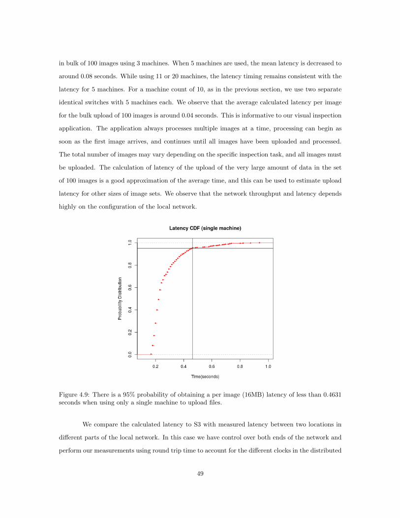
in bulk of 100 images using 3 machines. When 5 machines are used, the mean latency is decreased to

around 0.08 seconds. While using 11 or 20 machines, the latency timing remains consistent with the

latency for 5 machines. For a machine count of 10, as in the previous section, we use two separate

identical switches with 5 machines each. We observe that the average calculated latency per image

for the bulk upload of 100 images is around 0.04 seconds. This is informative to our visual inspection

application. The application always processes multiple images at a time, processing can begin as

soon as the first image arrives, and continues until all images have been uploaded and processed.

The total number of images may vary depending on the specific inspection task, and all images must

be uploaded. The calculation of latency of the upload of the very large amount of data in the set

of 100 images is a good approximation of the average time, and this can be used to estimate upload

latency for other sizes of image sets. We observe that the network throughput and latency depends

highly on the configuration of the local network.

Figure 4.9: There is a 95% probability of obtaining a per image (16MB) latency of less than 0.4631seconds when using only a single machine to upload files.

We compare the calculated latency to S3 with measured latency between two locations in

different parts of the local network. In this case we have control over both ends of the network and

perform our measurements using round trip time to account for the different clocks in the distributed

49

Figure 4.10: There is a 95% probability of obtaining a per image (16MB) latency of less than 0.2866seconds when using three machines in a network. The CDF doesn’t make noticeable changes whenwe further increase the number of machines, as shown in Fig. 13.

systems. The sending (source) machines are the same as in the previous S3 experiment, and the

receiving (sink) machines are located in a different building on a different set of network switches

across the campus backbone. We use secure copy protocol to send the images. Figure 14 shows the

CDF chart for the latency results across the local network. Figure 14(a) shows the CDF for the

use of single machine to upload the files. There is a 95% probability that the latency per image is

below 0.4631 for the bulk upload of 100 images in this case. Figure 14(b) shows the CDF for the

use of three machines configured on the same network switch to concurrently upload the files. There

is a 95% probability that the latency is below 0.2866 per image for the bulk upload of 100 images.

This measurement is comparable to the calculated latency for an upload to S3 for the case of 3

machines on a single switch. We can use this information to understand the tradeoffs of locating the

image processing in, say, a data center close to the visual inspection station as compared to locating

the processing of the images in AWS. The likelihood that network upload times will be a factor in

missing a deadline for the real-time visual inspection application depends on the configuration of

the local network. This likelihood is small for both a locally provisioned image processing system

and for one that is provisioned in the AWS cloud with an appropriately configured local network.

50

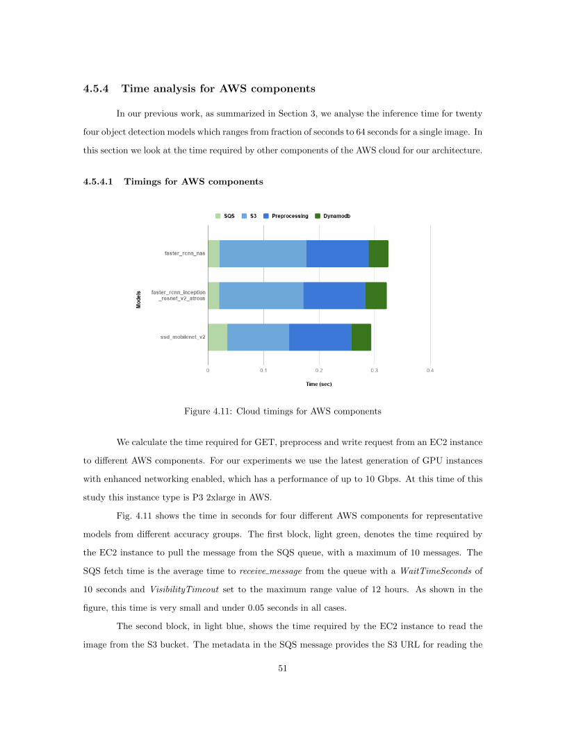
4.5.4 Time analysis for AWS components

In our previous work, as summarized in Section 3, we analyse the inference time for twenty

four object detection models which ranges from fraction of seconds to 64 seconds for a single image. In

this section we look at the time required by other components of the AWS cloud for our architecture.

4.5.4.1 Timings for AWS components

Figure 4.11: Cloud timings for AWS components

We calculate the time required for GET, preprocess and write request from an EC2 instance

to different AWS components. For our experiments we use the latest generation of GPU instances

with enhanced networking enabled, which has a performance of up to 10 Gbps. At this time of this

study this instance type is P3 2xlarge in AWS.

Fig. 4.11 shows the time in seconds for four different AWS components for representative

models from different accuracy groups. The first block, light green, denotes the time required by

the EC2 instance to pull the message from the SQS queue, with a maximum of 10 messages. The

SQS fetch time is the average time to receive message from the queue with a WaitTimeSeconds of

10 seconds and VisibilityTimeout set to the maximum range value of 12 hours. As shown in the

figure, this time is very small and under 0.05 seconds in all cases.

The second block, in light blue, shows the time required by the EC2 instance to read the

image from the S3 bucket. The metadata in the SQS message provides the S3 URL for reading the

51

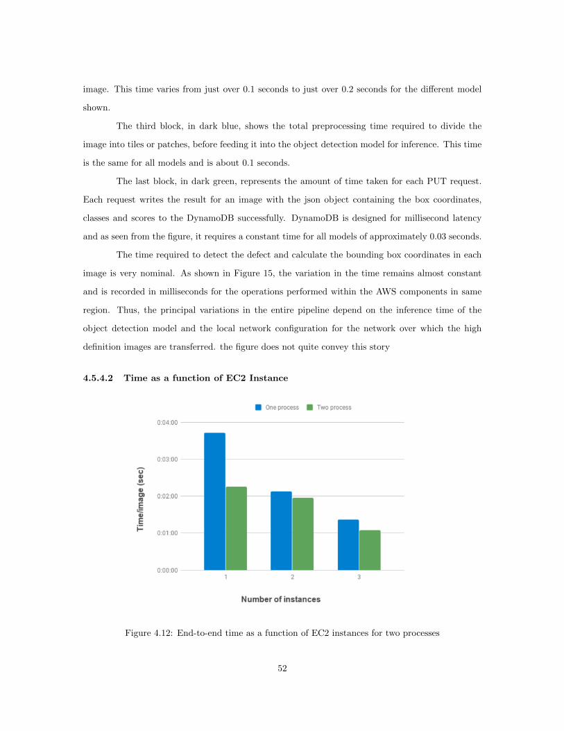
image. This time varies from just over 0.1 seconds to just over 0.2 seconds for the different model

shown.

The third block, in dark blue, shows the total preprocessing time required to divide the

image into tiles or patches, before feeding it into the object detection model for inference. This time

is the same for all models and is about 0.1 seconds.

The last block, in dark green, represents the amount of time taken for each PUT request.

Each request writes the result for an image with the json object containing the box coordinates,

classes and scores to the DynamoDB successfully. DynamoDB is designed for millisecond latency

and as seen from the figure, it requires a constant time for all models of approximately 0.03 seconds.

The time required to detect the defect and calculate the bounding box coordinates in each

image is very nominal. As shown in Figure 15, the variation in the time remains almost constant

and is recorded in milliseconds for the operations performed within the AWS components in same

region. Thus, the principal variations in the entire pipeline depend on the inference time of the

object detection model and the local network configuration for the network over which the high

definition images are transferred. the figure does not quite convey this story

4.5.4.2 Time as a function of EC2 Instance

Figure 4.12: End-to-end time as a function of EC2 instances for two processes

52

We calculate the end-to-end time for the entire visual inspection pipeline using the ssd mobilenet v2

model for a mini batch size of 64, for the entire car. The end-to-end time is measured from the time

required to upload, process and write the results to DynamoDb for 95 images of size 2,700 pixels by

2,100 pixels. This set of images forms the entire visual coverage of the car. The end-to-end time is

measured from the time it takes to upload images from the local host to the AWS S3 bucket to the

last time-stamp for the images that we receive on DynamoDb.

Figure 4.12 shows the time as a function of the count of p3 2xlarge EC2 instances used

in the experiments. The x-axis shows the number of p3 2xlarge instances ranging from 1, 2 and 3.

The blue block shows the timing for one process per EC2 instance while the green block shows the

timings for two processes running per instance. The y-axis shows the end-to-end time for 95 camera

images. We observe that for one instance count the time taken is approximately 223 seconds while

it reduces to 135 seconds when two processes are executed on one EC2 instance. Similarly, for three

instances, we see that it takes 82 seconds to process the set of images for the entire car by running

one process per instance. This is reduced to 63 seconds by running two parallel processes on one

EC2 instance.

We also observe that the end-to-end time using six instances reduces to approximately 38

seconds. This time is reduced by 82% as compared to the time taken by one EC2 instance.

As ssd mobilenet v2 model is not very memory intensive we are able to run two processes

of it parallelly on a p3 2xlarge instance. However, in case of memory intensive models such as the

two-shot models and some SSD variants, we cannot run two processes on the specified instance as

the V100 SXM2 offers a memory constraint of 32 GB.

4.5.5 Cost Analysis

Different types of AWS components lend themselves to different pricing models. AWS offers

different pricing methods such as on-demand, pay-as-you-go, and reservation-based payment models,

which enables the consumer to obtain the best return for their investment specific to different use

cases. There are three elemental drivers of cost with AWS and our research: compute, storage,

and outbound data transfer. In this section we will discuss the cost of each service and particular

scenarios.

Amazon EC2 pricing varies largely by the instance type, usage and region. For our experi-

ments we have used the p3 2xlarge, Deep learning (Ubuntu) instances as already stated. There are

53

four EC2 instances in AWS and each has a different pricing model : On-Demand Instances, Reserved

Instances, Spot Instances, and Dedicated Hosts. The on-demand pricing for a p3 2xlarge instance

is $ 3.060 per hour in us-east-1 (N. Virginia) and us-west-2 (Oregon) region, while $ 3.305 in the

eu-west-1 (Ireland) region. While the spot instances provide up to 90 percent off the On-Demand

price but are highly unstable. However, the reserved instances provide significant savings up to 75

percent but they require an upfront payment and are meant for steady users.

Other AWS components do not contribute much to the cost factor. The pricing for storage

in S3 for the first 50 TB per month is $ 0.023, while the next 450 TB per month cost $ 0.022 and

over 500 TB per month storage costs $ 0.021. GET and SELECT requests incur charges at different

rates than other requests, such as PUT and POST requests. S3 Request Pricing for PUT, COPY,

POST, LIST is $ 0.005 and for GET, SELECT is $ 0.004. While enabling S3 Transfer Acceleration

incurs an additional cost of $0.04 per GB. Pricing for S3 is similar in all regions.

For standard SQS, price per 1 million requests after free tier is $ 0.40 ($ 0.00000040 per

request). DynamoDb on demand write request costs for us-east-1 and us-west-2 region is $ 1.25 per

million write request units and for on demand read is $0.25 per million read request units. While

for eu-west-1 it is $1.4135 per million write request units and $0.283 per million read request units.

In our analysis, we choose on-demand AWS pricing. We do not consider free tier component

cost. We focus on the cost of EC2 instance, which is the most expensive component of the archi-

tecture. The cost for GET, PUT, SELECT, WRITE remains constant for every run, irrespective

of the model. The total cost for the visual inspection application depends on the selected model,

the real-time deadlines, and the number of EC2 instances needed to meet the application deadline

requirements. We consider two example scenarios with two different image processing models. The

first example uses a model with a moderate accurate and execution time, and the second model uses

a model that is one of the fastest, but also with lower accuracy, as shown in Figure ??.

In the first example scenario we consider ssd resnet v1 fpn with a mini batch size of 16. It is

the most accurate single shot model. With different real-time deadline to process the set of images

for the entire car we can calculate the costs as follows:

• A real-time deadline of 60 seconds require six P3 2xlarge instances to meet the deadline, which

costs approximately $18.36 per hour in the us-east-1 or us-west-2 region.

• A real-time deadline of 90 seconds require four P3 2xlarge instances to meet the deadline,

54

which costs approximately $12.24 per hour.

• A real time deadline of 120 seconds require three P3 2xlarge instances to meet the deadline,

which costs approximately $9.18 per hour.

For the second example scenarios we consider one of the fastest models, the ssd mobilenet v2

model, with a mini batch size of 64 with similar real-time deadlines as above. We calculate the

tradeoff as follows:

• A real time deadline of 60 seconds requires four P3 2xlarge instances to meet the deadline,

which costs approximately $12.24 per hour in the us-east-1 or us-west-2 region.

• A real time deadline of 90 seconds requires three P3 2xlarge instances with one process on

each instance to meet the deadline, which costs approximately $9.18 per hour.

• A real time deadline of 120 seconds requires two P3 2xlarge instances with two processes on

each instance to meet the deadline, which costs approximately $6.12 per hour.

For the visual inspection application there are tradeoffs between the cost, accuracy, and

ability to meet real-time deadlines. For example, using the faster rcnn inception resnet v2 atrous

model, the set of images for the entire car can be executed with an end-to-end time of 225 seconds

using six P3 2x large instances at a cost of $18.36 per hour. The most accurate faster rcnn nas

model, using a mini batch size of 2, takes approximately 9 minutes for the entire process using the

same number of instances and cost.

55

Chapter 5

Discussion

Edge inference is a critical component of every deep learning system enabling us to process

large amounts of data with low latencies while preserving privacy. On the other hand cloud inference

helps to provide agility and deploy the infrastructure at scale along with exploiting a higher degree

of parallelism by utilizing multiple nodes and GPUs.

The deployment of end-to-end deep learning system pipeline in production requires the

careful understanding of various trade-offs, in particular related to the computation and memory

requirements of the object detection models, their provided accuracies and the latency involved in

transferring high definition images over the network. In this thesis, we investigate the trade-offs to

guide the design of computer vision system for automated inspection.

Our results provide to us a selection of appropriate edge hardware. Not surprisingly, models

designed for embedded inference, such as MobileNet, are particularly well-suited for edge deployment.

However, the ability to deploy server- scale GPUs on the edge enables us to also utilize memory-

intensive models. We observe that V100 SXM2 is the most advanced GPU that provides stable and

high performance for memory and inference time compared to other hardware devices. Thus, we

select V100 SXM2 and carry out the experiments on AWS using deep learning EC2 instance with

one V100 SXM2 GPU.

In this thesis, we focus on time as a major constraint in the system pipeline. As observed

from the above experiments, the latency in the system pipeline is predominated with the inference

time and the time to upload the high definition images to cloud/edge device over the network.

We carry out the experiments to upload high definition images on the edge server using the

56

configurations discussed above and we obtain an average throughput of approximately 776 Mbps.

While the throughput to upload to AWS S3 bucket in the closest region, us-east-1 results in an

average throughput of 728 Mbps. Thus, the throughput to upload data on cloud is approximately

six percent more that that required to upload on an edge server. Consequently, to process 95 high

definition images, that is 263 MB of data, it requires 2.89 seconds to upload to an edge server while

it takes 2.71 seconds on a AWS S3 bucket.

If we have a requirement to process ninety five, 2100 x 2700 images, each within a time

limit of 30 seconds, we can make a choice from a set of models with their model parameters and

hardware platforms on cloud/edge location. For example, we select the ssd resnetv1 fpn, one of the

single shot variant which is reported to be the most accurate models and takes an inference time of

1.519 seconds for a mini batch size of 16 to process one camera input image aggregating to a total

of 144.305 seconds to process 95 such images, that provide an entire coverage of the car. Therefore,

to complete the entire process in 30 seconds, we need approximately five p3 2xlarge deep learning

instances on AWS.

Similarly, if we consider the fastest model that we tested, ssd mobilenet v2 which takes

an average of 0.743 seconds for a mini-batch size of 64 for one camera input, summing upto 70.585

seconds to process the entire car image. Thus we would need three p3 2xlarge deep learning instances

on AWS. However, if we consider the most accurate model that we tested, faster rcnn nas, takes

32.727 seconds for a batch size of two, and cannot be used to meet the desired time constraint of 30

seconds even on the edge.

57

Chapter 6

Future Works

In future we plan to exploit higher degree of parallelism and include other cloud services

for our experiments along with using scalable streaming services [31]. We envision various lines of

investigation for integrating other degrees of freedom in the system: (i) on a infrastructure-level edge

resource must be augmented with other hardware platforms by utilizing specialized cloud hardware,

such as Google’s TPUs [16] or Microsoft’s FPGA [5]; (ii) comparing performance across other cloud

services like Google cloud platform and Azure; (iii) explore other frameworks and multiple model

versions potentially trained on different datasets deployed on the edge and/or the cloud to magnify

the performance tradeoffs; (iv) To support active learning approaches, such as federated learning, to

provide the means to utilize decentralized training resources on the edge, and to combine the results

into a global model. (v) and to provide a complete cost analysis for the edge/cloud usage.

58

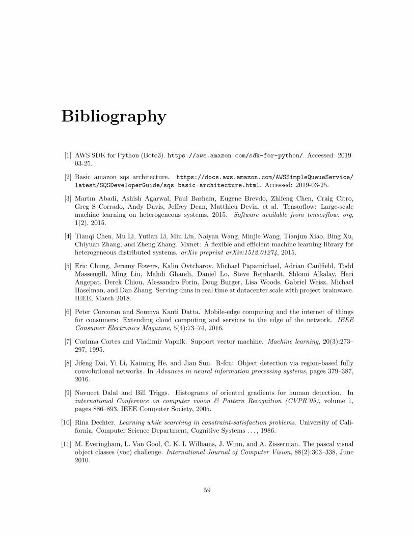
Bibliography

[1] AWS SDK for Python (Boto3). https://aws.amazon.com/sdk-for-python/. Accessed: 2019-03-25.

[2] Basic amazon sqs architecture. https://docs.aws.amazon.com/AWSSimpleQueueService/

latest/SQSDeveloperGuide/sqs-basic-architecture.html. Accessed: 2019-03-25.

[3] Martın Abadi, Ashish Agarwal, Paul Barham, Eugene Brevdo, Zhifeng Chen, Craig Citro,Greg S Corrado, Andy Davis, Jeffrey Dean, Matthieu Devin, et al. Tensorflow: Large-scalemachine learning on heterogeneous systems, 2015. Software available from tensorflow. org,1(2), 2015.

[4] Tianqi Chen, Mu Li, Yutian Li, Min Lin, Naiyan Wang, Minjie Wang, Tianjun Xiao, Bing Xu,Chiyuan Zhang, and Zheng Zhang. Mxnet: A flexible and efficient machine learning library forheterogeneous distributed systems. arXiv preprint arXiv:1512.01274, 2015.

[5] Eric Chung, Jeremy Fowers, Kalin Ovtcharov, Michael Papamichael, Adrian Caulfield, ToddMassengill, Ming Liu, Mahdi Ghandi, Daniel Lo, Steve Reinhardt, Shlomi Alkalay, HariAngepat, Derek Chiou, Alessandro Forin, Doug Burger, Lisa Woods, Gabriel Weisz, MichaelHaselman, and Dan Zhang. Serving dnns in real time at datacenter scale with project brainwave.IEEE, March 2018.

[6] Peter Corcoran and Soumya Kanti Datta. Mobile-edge computing and the internet of thingsfor consumers: Extending cloud computing and services to the edge of the network. IEEEConsumer Electronics Magazine, 5(4):73–74, 2016.

[7] Corinna Cortes and Vladimir Vapnik. Support vector machine. Machine learning, 20(3):273–297, 1995.

[8] Jifeng Dai, Yi Li, Kaiming He, and Jian Sun. R-fcn: Object detection via region-based fullyconvolutional networks. In Advances in neural information processing systems, pages 379–387,2016.

[9] Navneet Dalal and Bill Triggs. Histograms of oriented gradients for human detection. Ininternational Conference on computer vision & Pattern Recognition (CVPR’05), volume 1,pages 886–893. IEEE Computer Society, 2005.

[10] Rina Dechter. Learning while searching in constraint-satisfaction problems. University of Cali-fornia, Computer Science Department, Cognitive Systems . . . , 1986.

[11] M. Everingham, L. Van Gool, C. K. I. Williams, J. Winn, and A. Zisserman. The pascal visualobject classes (voc) challenge. International Journal of Computer Vision, 88(2):303–338, June2010.

59

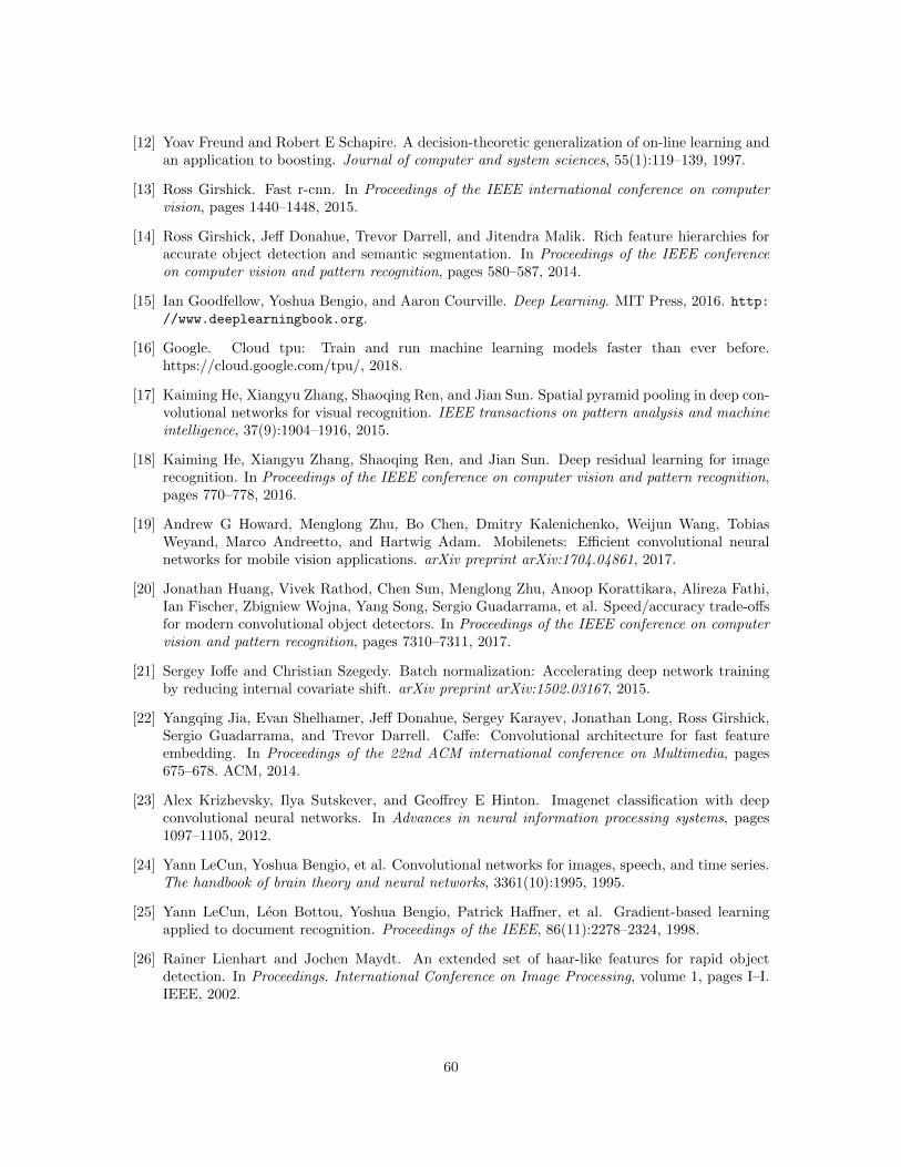
[12] Yoav Freund and Robert E Schapire. A decision-theoretic generalization of on-line learning andan application to boosting. Journal of computer and system sciences, 55(1):119–139, 1997.

[13] Ross Girshick. Fast r-cnn. In Proceedings of the IEEE international conference on computervision, pages 1440–1448, 2015.

[14] Ross Girshick, Jeff Donahue, Trevor Darrell, and Jitendra Malik. Rich feature hierarchies foraccurate object detection and semantic segmentation. In Proceedings of the IEEE conferenceon computer vision and pattern recognition, pages 580–587, 2014.

[15] Ian Goodfellow, Yoshua Bengio, and Aaron Courville. Deep Learning. MIT Press, 2016. http://www.deeplearningbook.org.

[16] Google. Cloud tpu: Train and run machine learning models faster than ever before.https://cloud.google.com/tpu/, 2018.

[17] Kaiming He, Xiangyu Zhang, Shaoqing Ren, and Jian Sun. Spatial pyramid pooling in deep con-volutional networks for visual recognition. IEEE transactions on pattern analysis and machineintelligence, 37(9):1904–1916, 2015.

[18] Kaiming He, Xiangyu Zhang, Shaoqing Ren, and Jian Sun. Deep residual learning for imagerecognition. In Proceedings of the IEEE conference on computer vision and pattern recognition,pages 770–778, 2016.

[19] Andrew G Howard, Menglong Zhu, Bo Chen, Dmitry Kalenichenko, Weijun Wang, TobiasWeyand, Marco Andreetto, and Hartwig Adam. Mobilenets: Efficient convolutional neuralnetworks for mobile vision applications. arXiv preprint arXiv:1704.04861, 2017.

[20] Jonathan Huang, Vivek Rathod, Chen Sun, Menglong Zhu, Anoop Korattikara, Alireza Fathi,Ian Fischer, Zbigniew Wojna, Yang Song, Sergio Guadarrama, et al. Speed/accuracy trade-offsfor modern convolutional object detectors. In Proceedings of the IEEE conference on computervision and pattern recognition, pages 7310–7311, 2017.

[21] Sergey Ioffe and Christian Szegedy. Batch normalization: Accelerating deep network trainingby reducing internal covariate shift. arXiv preprint arXiv:1502.03167, 2015.

[22] Yangqing Jia, Evan Shelhamer, Jeff Donahue, Sergey Karayev, Jonathan Long, Ross Girshick,Sergio Guadarrama, and Trevor Darrell. Caffe: Convolutional architecture for fast featureembedding. In Proceedings of the 22nd ACM international conference on Multimedia, pages675–678. ACM, 2014.

[23] Alex Krizhevsky, Ilya Sutskever, and Geoffrey E Hinton. Imagenet classification with deepconvolutional neural networks. In Advances in neural information processing systems, pages1097–1105, 2012.

[24] Yann LeCun, Yoshua Bengio, et al. Convolutional networks for images, speech, and time series.The handbook of brain theory and neural networks, 3361(10):1995, 1995.

[25] Yann LeCun, Leon Bottou, Yoshua Bengio, Patrick Haffner, et al. Gradient-based learningapplied to document recognition. Proceedings of the IEEE, 86(11):2278–2324, 1998.

[26] Rainer Lienhart and Jochen Maydt. An extended set of haar-like features for rapid objectdetection. In Proceedings. International Conference on Image Processing, volume 1, pages I–I.IEEE, 2002.

60

[27] Tsung-Yi Lin, Michael Maire, Serge Belongie, James Hays, Pietro Perona, Deva Ramanan,Piotr Dollar, and C Lawrence Zitnick. Microsoft coco: Common objects in context. In Europeanconference on computer vision, pages 740–755. Springer, 2014.

[28] Wei Liu, Dragomir Anguelov, Dumitru Erhan, Christian Szegedy, Scott Reed, Cheng-Yang Fu,and Alexander C Berg. Ssd: Single shot multibox detector. In European conference on computervision, pages 21–37. Springer, 2016.

[29] David G Lowe. Distinctive image features from scale-invariant keypoints. International journalof computer vision, 60(2):91–110, 2004.

[30] Andre Luckow, Matthew Cook, Nathan Ashcraft, Edwin Weill, Emil Djerekarov, and BennieVorster. Deep learning in the automotive industry: Applications and tools. In 2016 IEEEInternational Conference on Big Data (Big Data), pages 3759–3768. IEEE, 2016.

[31] Dung Nguyen, Andre Luckow, Edward Duffy, Ken Kennedy, and Amy Apon. Evaluation ofhighly available cloud streaming systems for performance and price. In 2018 18th IEEE/ACMInternational Symposium on Cluster, Cloud and Grid Computing (CCGRID), pages 360–363.IEEE, 2018.

[32] Adam Paszke, Sam Gross, Soumith Chintala, Gregory Chanan, Edward Yang, Zachary DeVito,Zeming Lin, Alban Desmaison, Luca Antiga, and Adam Lerer. Automatic differentiation inpytorch. 2017.

[33] Brandon Posey, Linh Bao Ngo, Mashrur Chowdhury, and Amy Apon. Infrastructure for trans-portation cyber-physical systems. In Transportation Cyber-Physical Systems, pages 153–171.Elsevier, 2018.

[34] Joseph Redmon, Santosh Divvala, Ross Girshick, and Ali Farhadi. You only look once: Unified,real-time object detection. In Proceedings of the IEEE conference on computer vision andpattern recognition, pages 779–788, 2016.

[35] Joseph Redmon and Ali Farhadi. Yolo9000: better, faster, stronger. In Proceedings of the IEEEconference on computer vision and pattern recognition, pages 7263–7271, 2017.

[36] Joseph Redmon and Ali Farhadi. Yolov3: An incremental improvement. arXiv preprintarXiv:1804.02767, 2018.

[37] Shaoqing Ren, Kaiming He, Ross Girshick, and Jian Sun. Faster r-cnn: Towards real-timeobject detection with region proposal networks. In Advances in neural information processingsystems, pages 91–99, 2015.

[38] Mark Sandler, Andrew Howard, Menglong Zhu, Andrey Zhmoginov, and Liang-Chieh Chen.Mobilenetv2: Inverted residuals and linear bottlenecks. In Proceedings of the IEEE Conferenceon Computer Vision and Pattern Recognition, pages 4510–4520, 2018.

[39] Shree Krishna Sharma and Xianbin Wang. Live data analytics with collaborative edge andcloud processing in wireless iot networks. IEEE Access, 5:4621–4635, 2017.

[40] Karen Simonyan and Andrew Zisserman. Very deep convolutional networks for large-scale imagerecognition. arXiv preprint arXiv:1409.1556, 2014.

[41] Aishwarya Srivastava, Dung Nguyen, Siddhant Aggarwal, Andre Luckow, Edward Duffy, KenKennedy, Marcin Ziolkowski, and Amy Apon. Performance and memory trade-offs of deeplearning object detection in fast streaming high-definition images. In 2018 IEEE InternationalConference on Big Data (Big Data), pages 3915–3924. IEEE, 2018.

61

[42] Christian Szegedy, Sergey Ioffe, Vincent Vanhoucke, and Alexander A Alemi. Inception-v4,inception-resnet and the impact of residual connections on learning. In Thirty-First AAAIConference on Artificial Intelligence, 2017.

[43] Christian Szegedy, Wei Liu, Yangqing Jia, Pierre Sermanet, Scott Reed, Dragomir Anguelov,Dumitru Erhan, Vincent Vanhoucke, and Andrew Rabinovich. Going deeper with convolutions.In Proceedings of the IEEE conference on computer vision and pattern recognition, pages 1–9,2015.

[44] Wikipedia,BMW Plant. Visual inspection, 2018. [Online; accessed Nov 25, 2018].

[45] Yanan Zhang, Hongyu Wang, and Fang Xu. Object detection and recognition of intelligentservice robot based on deep learning. In 2017 IEEE International Conference on Cyberneticsand Intelligent Systems (CIS) and IEEE Conference on Robotics, Automation and Mechatronics(RAM), pages 171–176. IEEE, 2017.

[46] Barret Zoph, Vijay Vasudevan, Jonathon Shlens, and Quoc V Le. Learning transferable ar-chitectures for scalable image recognition. In Proceedings of the IEEE conference on computervision and pattern recognition, pages 8697–8710, 2018.

62