Automaattisten segmentointialgoritmien analysointi

Fysiikan kandidaatti opinnäytetyö

Arttu Cowell

28.12.2019

Oheisessa tekstissä käsittelen viittä eri automaattista segmentointialgoritmia. Algoritmeja analysoitiin

Matlab skriptillä, joka laski Dice Similarity Coefficientit (DSC) ja ruston paksuus poikkeamista verrattuna

manuaalisesti segmentoiduista polvien magneettikuvista. DSC mittaa kuvien yhtäläisyyssuhdetta pikseli

kohtaisesti, kombinoituna paksuus analysoinnilla sain kvantitatiivisesti mitattua algoritmien pätevyyden ja

vertasin vastaavan tyyppisten tutkimusten tuloksiin. Saadusta datasta huomasin automaattisten

algoritmien potentiaalin laajassa kliinisessä polven nivelrikko -tutkimuksessa pienen lisäoptimoinnin

jälkeen.

Projekti alkoi Oulun yliopistollisen sairaalan Reasearch Unit of Medical Imaging, Physics and

Technology antamana ja ohjaamana kesätyöprojektina, mutta kahden kuukauden aikainen työaika ei

riittänyt suorittamaan projektia loppuun, joten sovittiin, että teen työn loppuun kandityönä. Projektia

ohjasi Eveliina Lammentausta ja työssä käytetty analysointi algoritmi oli Mikael Juntulan kirjoittama.

Paperissa kirjoitetut tekstit, johtopäätökset datasta, kuvat, kaaviot ja analysointiskriptin käyttö ovat kaikki

omaa tuotostani.

Evaluation of multiple automatic knee cartilage

segmentation algorithms

Abstract

Commonly in osteoarthritis studies, large

amounts of MRI data are acquired and cartilage is

manually delineated from the MRI data. We

investigate automatic segmentation frameworks

in order to obtain quantitative data on articular

cartilage morphology. We cover Mokkula, a

manual segmentation framework, atlas-based

automatic segmentation methodologies and a

patch-based technique comparing their

respective segmentation accuracies. Using

Laplace’s equation to calculate cartilage thickness

error (LTE), a vector thickness error method (VTE)

and Dice Similarity Coefficient (DSC) to assess the

accuracy of these techniques. The most accurate

segmentations reached DSC of 0,87 on both the

Femur and Tibia. The thickness analysis gave

avarage errors of 0,32mm over the Femur and

0,36mm over the Tibia. We feel these values are

reaching high enough stantards to be used in

large studies.

Introduction

Osteoarthritis (OA) is a joint disease affecting

significant populations worldwide [1]. Symptoms

of OA include swelling, pain, discomfort, and

locking of the joint [2]. It has been hypothesized

that OA is the result of multiple factors, e.g.

biomechanical stress and joint injury, eventually

leading to the degeneration of cartilage [3].

Cartilage has a limited ability to regenerate and

repair itself. This ability becomes less effective as

an individual ages making OA common amongst

the elderly [4]. Currently it is not understood

what causes OA to develop in young individual,

but genetics and obesity have been speculated to

have an effect [5][6]. Treatment of OA is highly

limited but knee joint replacement surgery can

help relieve pain and recover mobility [7]. The

use of Magnetic Resonance Imaging (MRI) in

clinical diagnosis of OA has increased recently

because MRI has the ability to detect signal and

morphologic changes of articular cartilage in 3D

[8].

Using MRI to study articular

cartilage is not straightforward. In order to study

the progression of OA one needs to follow the

cartilage borders closely. Morphological changes

in cartilage thickness are small in the span of a

few years, which means that the cartilage surface

changes its shape very slowly in a normal aging

patient [9].

Having a high contrast to noise ratio and high

signal to noise ratio (SNR) is important to

distinguish the bone-cartilage interface [10].

Turning the MR images into quantifiable research

data is a challenge. Segmenting articular cartilage

is currently performed manually by trained

experts. This process of manual segmentation can

be laborious and could take hours with 3D MRI

protocols. Recent studies have shown that

automatic segmentation methods, where a

computer analyses reference data to perform

segmentation using machine learning, for

instance, is a much faster process [11]. Automatic

segmentation methods could help in gathering

quantitative data in order to research and

development treatments for OA.

International workshop on

osteoarthritis imaging (IWOAI) Nordic segment

organized the knee cartilage segmentation

challenge in Oulu, Finland 2016, receiving entries

from five separate development teams. All

entries were atlas-based segmentation methods

and performed segmentation without expert

supervision. In this paper, we evaluated the

accuracy of these algorithms using manually

segmented images as the reference data.

Materials and Methods

Dataset

We gathered 44 knee MR images from the Oulu

Knee Osteoarthritis (OKOA) study [12] with the

criteria that the patients must have a Kellgren –

Lawrence score (KL) of 1 – 3 and a body mass

index (BMI) of 26.5 ± 2.5. The MR images were

T2-weighted images taken using the double echo

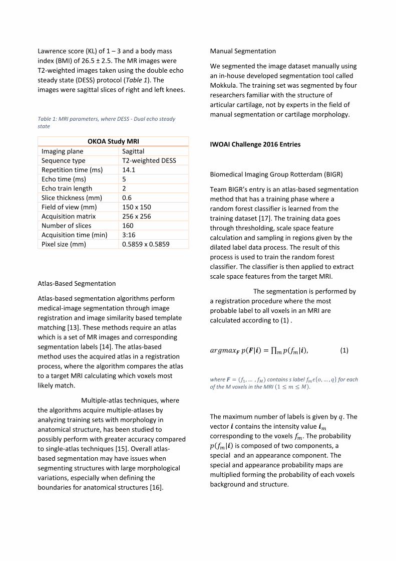
steady state (DESS) protocol (Table 1). The

images were sagittal slices of right and left knees.

Table 1: MRI parameters, where DESS - Dual echo steady state

OKOA Study MRI

Imaging plane Sagittal

Sequence type T2-weighted DESS

Repetition time (ms) 14.1

Echo time (ms) 5

Echo train length 2

Slice thickness (mm) 0.6

Field of view (mm) 150 x 150

Acquisition matrix 256 x 256

Number of slices 160

Acquisition time (min) 3:16

Pixel size (mm) 0.5859 x 0.5859

Atlas-Based Segmentation

Atlas-based segmentation algorithms perform

medical-image segmentation through image

registration and image similarity based template

matching [13]. These methods require an atlas

which is a set of MR images and corresponding

segmentation labels [14]. The atlas-based

method uses the acquired atlas in a registration

process, where the algorithm compares the atlas

to a target MRI calculating which voxels most

likely match.

Multiple-atlas techniques, where

the algorithms acquire multiple-atlases by

analyzing training sets with morphology in

anatomical structure, has been studied to

possibly perform with greater accuracy compared

to single-atlas techniques [15]. Overall atlas-

based segmentation may have issues when

segmenting structures with large morphological

variations, especially when defining the

boundaries for anatomical structures [16].

Manual Segmentation

We segmented the image dataset manually using

an in-house developed segmentation tool called

Mokkula. The training set was segmented by four

researchers familiar with the structure of

articular cartilage, not by experts in the field of

manual segmentation or cartilage morphology.

IWOAI Challenge 2016 Entries

Biomedical Imaging Group Rotterdam (BIGR)

Team BIGR’s entry is an atlas-based segmentation

method that has a training phase where a

random forest classifier is learned from the

training dataset [17]. The training data goes

through thresholding, scale space feature

calculation and sampling in regions given by the

dilated label data process. The result of this

process is used to train the random forest

classifier. The classifier is then applied to extract

scale space features from the target MRI.

The segmentation is performed by

a registration procedure where the most

probable label to all voxels in an MRI are

calculated according to (1) .

𝑎𝑟𝑔𝑚𝑎𝑥𝑭 𝑝(𝑭|𝒊) = ∏ 𝑝(𝑓𝑚|𝒊)𝑚 , (1)

where 𝑭 = (𝑓1, … , 𝑓𝑀) contains s label 𝑓𝑚𝜖{𝑜, … , 𝑞} for each of the M voxels in the MRI (1 ≤ 𝑚 ≤ 𝑀).

The maximum number of labels is given by 𝑞. The

vector 𝒊 contains the intensity value 𝒊𝑚

corresponding to the voxels 𝑓𝑚. The probability

𝑝(𝑓𝑚|𝒊) is composed of two components, a

special and an appearance component. The

special and appearance probability maps are

multiplied forming the probability of each voxels

background and structure.

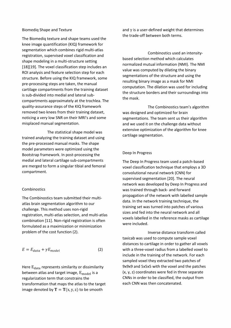
Biomediq Shape and Texture

The Biomediq texture and shape teams used the

knee image quantification (KIQ) framework for

segmentation which combines rigid multi-atlas

registration, supervised voxel classification and

shape modeling in a multi-structure setting

[18][19]. The voxel classification step includes an

ROI analysis and feature selection step for each

structure. Before using the KIQ framework, some

pre-processing steps are taken, the manual

cartilage compartments from the training dataset

is sub-divided into medial and lateral sub-

compartments approximately at the trochlea. The

quality-assurance steps of the KIQ framework

removed two knees from their training dataset,

noticing a very low SNR on their MRI’s and some

misplaced manual segmentation.

The statistical shape model was

trained analyzing the training dataset and using

the pre-processed manual masks. The shape

model parameters were optimized using the

Bootstrap framework. In post-processing the

medial and lateral cartilage sub-compartments

are merged to form a singular tibial and femoral

compartment.

Combinostics

The Combinostics team submitted their multi-

atlas brain segmentation algorithm to our

challenge. This method uses non-rigid

registration, multi-atlas selection, and multi-atlas

combination [11]. Non-rigid registration is often

formulated as a maximization or minimization

problem of the cost function (2).

𝐸 = 𝐸𝑑𝑎𝑡𝑎 + 𝛾𝐸𝑚𝑜𝑑𝑒𝑙 (2)

Here Edata represents similarity or dissimilarity

between atlas and target image, Emodel is a

regularization term that constrains the

transformation that maps the atlas to the target

image denoted by 𝐓 = 𝐓(x, y, z) to be smooth

and γ is a user-defined weight that determines

the trade-off between both terms.

Combinostics used an intensity-

based selection method which calculates

normalized mutual information (NMI). The NMI

value was computed by dilating the binary

segmentations of the structure and using the

resulting binary image as a mask for NMI

computation. The dilation was used for including

the structure borders and their surroundings into

the mask.

The Combinostics team’s algorithm

was designed and optimized for brain

segmentations. The team sent us their algorithm

and we used it on the challenge data without

extensive optimization of the algorithm for knee

cartilage segmentation.

Deep In Progress

The Deep In Progress team used a patch-based

voxel classification technique that employs a 3D

convolutional neural network (CNN) for

supervised segmentation [20]. The neural

network was developed by Deep In Progress and

was trained through back- and forward

propagation of the network with labelled sample

data. In the network training technique, the

training set was turned into patches of various

sizes and fed into the neural network and all

voxels labelled in the reference masks as cartilage

were included.

Inverse distance transform called

taxicab was used to compute sample voxel

distances to cartilage in order to gather all voxels

with a three-voxel radius from a labelled voxel to

include in the training of the network. For each

sampled voxel they extracted two patches of

9x9x9 and 5x5x5 with the voxel and the patches

(x, y, z) coordinates were fed in three separate

CNNs in order to be classified, the output from

each CNN was then concatenated.

The training periods were divided

into epochs, where batches of 150 voxels were

fed into the network, until all sampled voxels had

been used for training. Voxels were then

resampled in the same way, before training was

continued. From every fifth epoch the

parameters were saved and the best match

image used for evaluation. An optimal set of

parameters was then used to segment the full set

of training images and evaluation images. The

Deep In Progress team noticed issues in two of

the training set masks we provided and didn’t use

them in their segmentation training procedure.

The segmented images went

through post-processing where the training MRIs

were registered onto the evaluation MRIs. The

segmented images are then processed by a

largest connected component (LCC) method in

order to select three largest connected segments.

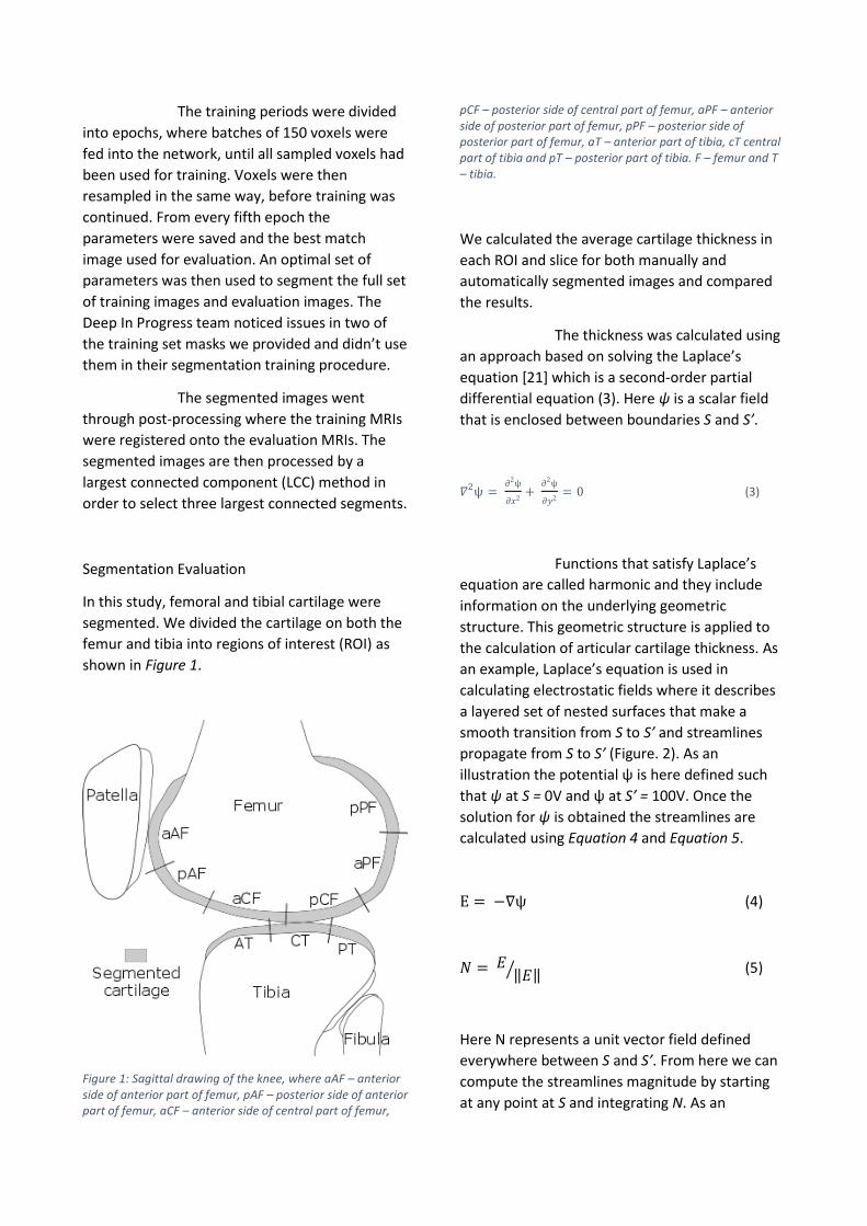
Segmentation Evaluation

In this study, femoral and tibial cartilage were

segmented. We divided the cartilage on both the

femur and tibia into regions of interest (ROI) as

shown in Figure 1.

Figure 1: Sagittal drawing of the knee, where aAF – anterior side of anterior part of femur, pAF – posterior side of anterior part of femur, aCF – anterior side of central part of femur,

pCF – posterior side of central part of femur, aPF – anterior side of posterior part of femur, pPF – posterior side of posterior part of femur, aT – anterior part of tibia, cT central part of tibia and pT – posterior part of tibia. F – femur and T – tibia.

We calculated the average cartilage thickness in

each ROI and slice for both manually and

automatically segmented images and compared

the results.

The thickness was calculated using

an approach based on solving the Laplace’s

equation [21] which is a second-order partial

differential equation (3). Here ѱ is a scalar field

that is enclosed between boundaries S and S’.

𝛻2ѱ = 𝜕2ѱ

𝜕𝑥2+

𝜕2ѱ

𝜕𝑦2= 0 (3)

Functions that satisfy Laplace’s

equation are called harmonic and they include

information on the underlying geometric

structure. This geometric structure is applied to

the calculation of articular cartilage thickness. As

an example, Laplace’s equation is used in

calculating electrostatic fields where it describes

a layered set of nested surfaces that make a

smooth transition from S to S’ and streamlines

propagate from S to S’ (Figure. 2). As an

illustration the potential ѱ is here defined such

that ѱ at S = 0V and ѱ at S’ = 100V. Once the

solution for ѱ is obtained the streamlines are

calculated using Equation 4 and Equation 5.

E = −∇ѱ (4)

𝑁 = 𝐸‖𝐸‖⁄ (5)

Here N represents a unit vector field defined

everywhere between S and S’. From here we can

compute the streamlines magnitude by starting

at any point at S and integrating N. As an

example, we can pick the point 𝑃1 and integrating

N takes us through the patch from 𝑃1 to 𝑃2 to 𝑃3

to… 𝑃𝑛. By using a very large amount of steps we

can calculate the streamlines with great accuracy

but computation time will increase significantly.

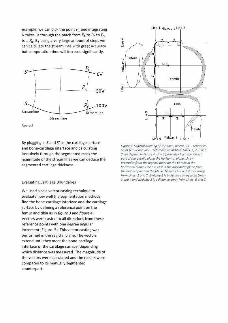
Figure 2

By plugging in S and S’ as the cartilage surface

and bone-cartilage interface and calculating

iteratively through the segmented mask the

magnitude of the streamlines we can deduce the

segmented cartilage thickness.

Evaluating Cartilage Boundaries

We used also a vector casting technique to

evaluate how well the segmentation methods

find the bone-cartilage interface and the cartilage

surface by defining a reference point on the

femur and tibia as in figure 3 and figure 4.

Vectors were casted to all directions from these

reference points with one degree angular

increment (Figure. 5). This vector casting was

performed in the sagittal plane. The vectors

extend until they meet the bone-cartilage

interface or the cartilage surface, depending

which distance was measured. The magnitude of

the vectors were calculated and the results were

compared to its manually segmented

counterpart.

Figure 3: Sagittal drawing of the knee, where RPF – reference point femur and RPT – reference point tibia. Lines- 1, 2, 6 and 7 are defined in Figure 4. Line 3 protrudes from the lowest part of the patella along the horizontal plane. Line 4 protrudes from the highest point on the patella in the horizontal plane. Line 5 is cast in the horizontal plane from the highest point on the fibula. Midway 1 is a distance away from Lines- 1 and 2, Midway 2 is b distance away from Lines- 3 and 4 and Midway 3 is c distance away from Lines- 6 and 7.

Figure 5: Sagittal drawing of the knee, where α – angle at which vectors are cast from RPF and φ – angle at which vectors are cast from RPT.

Dice Similarity Coefficient

The Dice similarity coefficient (DSC) is a

quantitative tool in validating segmentation

accuracy [22]. We used it to measure the overlap

between automatic and manual segmentations.

The DSC value range from 0 to 1 with 0 denoting

no overlap and 1 denoting total overlap (6). We

calculated the DSC for the entire segmentation of

tibia, femur, and for each ROI.

𝐷𝑆𝐶 = 2𝑁(𝐴∩𝑀)

𝑁(𝐴)+𝑁(𝑀) (6)

where A – automatic mask, M – manual mask and N – number of points in mask.

Results

BIGR Results Femur

The team’s highest average DSC came from the pCF (0,81) ROI and the lowest average DSC from the pPF

(0,62) (Table. 2). The smallest average Laplace Thickness Error (LTE) came from the aCF (0,36mm) ROI and

the largest average LTE (0,58mm) from aPF (Table. 3). The LTE Standard Deviation (SD) was the smallest in

the aCF (0,33mm) ROI and the largest LTE SD in the aAF (0,75mm) ROI (Table. 3). The average Vector

Thickness Error (VTE) value was the smallest in the aCF (0,6mm) ROI and the average VTE value was the

largest in the pPF (1,02mm) ROI (Table. 4). The VTE SD values was the smallest in the aCF (0,34mm) ROI and

the largest average VTE SD was found in the aAF (0,84mm) ROI (Table. 4).

BIGR Results Tibia

The team’s highest average DSC came from the cT (0,78) ROI and the lowest average DSC from the aT (0,71)

ROI (Table. 2). The smallest average LTE came from the (0,37mm) ROI and the largest average LTE pT (0,43)

ROI (Table. 3). The LTE average SD was the smallest in the aT and pT (0,44mm) ROI and the largest average

LTE SD was in the cT (0,54mm) ROI (Table. 3). The average VTE values was the smallest in the aT (0,74mm)

ROI and the average VTE values was the largest in the pT (0,9mm) ROI (Table. 4). The VTE SD values was the

smallest in the aT (0,36mm) ROI and the largest average VTE SD was in the cT (0,44mm) ROI (Table. 4).

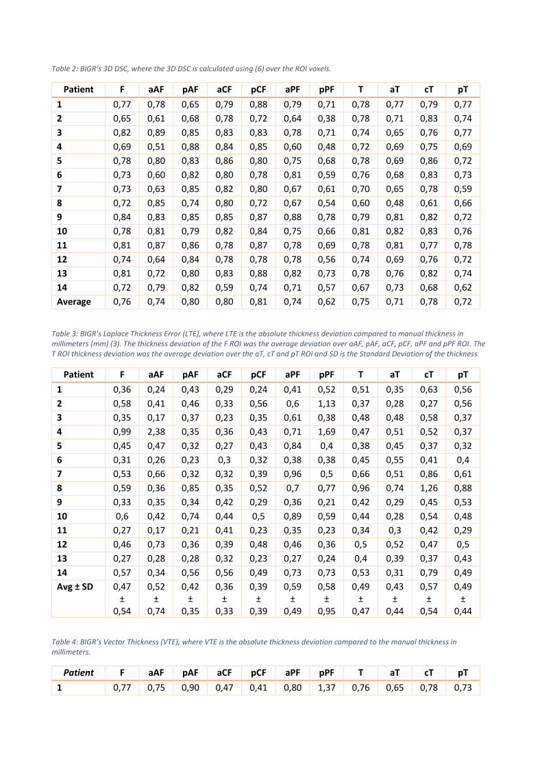
Table 2: BIGR’s 3D DSC, where the 3D DSC is calculated using (6) over the ROI voxels.

Patient F aAF pAF aCF pCF aPF pPF T aT cT pT

1 0,77 0,78 0,65 0,79 0,88 0,79 0,71 0,78 0,77 0,79 0,77

2 0,65 0,61 0,68 0,78 0,72 0,64 0,38 0,78 0,71 0,83 0,74

3 0,82 0,89 0,85 0,83 0,83 0,78 0,71 0,74 0,65 0,76 0,77

4 0,69 0,51 0,88 0,84 0,85 0,60 0,48 0,72 0,69 0,75 0,69

5 0,78 0,80 0,83 0,86 0,80 0,75 0,68 0,78 0,69 0,86 0,72

6 0,73 0,60 0,82 0,80 0,78 0,81 0,59 0,76 0,68 0,83 0,73

7 0,73 0,63 0,85 0,82 0,80 0,67 0,61 0,70 0,65 0,78 0,59

8 0,72 0,85 0,74 0,80 0,72 0,67 0,54 0,60 0,48 0,61 0,66

9 0,84 0,83 0,85 0,85 0,87 0,88 0,78 0,79 0,81 0,82 0,72

10 0,78 0,81 0,79 0,82 0,84 0,75 0,66 0,81 0,82 0,83 0,76

11 0,81 0,87 0,86 0,78 0,87 0,78 0,69 0,78 0,81 0,77 0,78

12 0,74 0,64 0,84 0,78 0,78 0,78 0,56 0,74 0,69 0,76 0,72

13 0,81 0,72 0,80 0,83 0,88 0,82 0,73 0,78 0,76 0,82 0,74

14 0,72 0,79 0,82 0,59 0,74 0,71 0,57 0,67 0,73 0,68 0,62

Average 0,76 0,74 0,80 0,80 0,81 0,74 0,62 0,75 0,71 0,78 0,72

Table 3: BIGR’s Laplace Thickness Error (LTE), where LTE is the absolute thickness deviation compared to manual thickness in millimeters (mm) (3). The thickness deviation of the F ROI was the average deviation over aAF, pAF, aCF, pCF, aPF and pPF ROI. The T ROI thickness deviation was the average deviation over the aT, cT and pT ROI and SD is the Standard Deviation of the thickness.

Patient F aAF pAF aCF pCF aPF pPF T aT cT pT

1 0,36 0,24 0,43 0,29 0,24 0,41 0,52 0,51 0,35 0,63 0,56

2 0,58 0,41 0,46 0,33 0,56 0,6 1,13 0,37 0,28 0,27 0,56

3 0,35 0,17 0,37 0,23 0,35 0,61 0,38 0,48 0,48 0,58 0,37

4 0,99 2,38 0,35 0,36 0,43 0,71 1,69 0,47 0,51 0,52 0,37

5 0,45 0,47 0,32 0,27 0,43 0,84 0,4 0,38 0,45 0,37 0,32

6 0,31 0,26 0,23 0,3 0,32 0,38 0,38 0,45 0,55 0,41 0,4

7 0,53 0,66 0,32 0,32 0,39 0,96 0,5 0,66 0,51 0,86 0,61

8 0,59 0,36 0,85 0,35 0,52 0,7 0,77 0,96 0,74 1,26 0,88

9 0,33 0,35 0,34 0,42 0,29 0,36 0,21 0,42 0,29 0,45 0,53

10 0,6 0,42 0,74 0,44 0,5 0,89 0,59 0,44 0,28 0,54 0,48

11 0,27 0,17 0,21 0,41 0,23 0,35 0,23 0,34 0,3 0,42 0,29

12 0,46 0,73 0,36 0,39 0,48 0,46 0,36 0,5 0,52 0,47 0,5

13 0,27 0,28 0,28 0,32 0,23 0,27 0,24 0,4 0,39 0,37 0,43

14 0,57 0,34 0,56 0,56 0,49 0,73 0,73 0,53 0,31 0,79 0,49

Avg ± SD 0,47 ±

0,54

0,52 ±

0,74

0,42 ±

0,35

0,36 ±

0,33

0,39 ±

0,39

0,59 ±

0,49

0,58 ±

0,95

0,49 ±

0,47

0,43 ±

0,44

0,57 ±

0,54

0,49 ±

0,44

Table 4: BIGR’s Vector Thickness (VTE), where VTE is the absolute thickness deviation compared to the manual thickness in millimeters.

Patient F aAF pAF aCF pCF aPF pPF T aT cT pT

1 0,77 0,75 0,90 0,47 0,41 0,80 1,37 0,76 0,65 0,78 0,73

2 1,18 1,30 0,84 0,66 0,83 1,05 2,55 0,67 0,55 0,58 0,85

3 0,69 0,42 0,60 0,50 0,52 0,94 1,35 0,96 1,12 0,84 0,86

4 2,80 3,30 0,57 0,54 0,67 1,18 1,77 1,03 0,91 0,93 1,09

5 1,06 0,95 0,52 0,46 0,71 1,02 1,32 0,63 0,72 0,53 0,69

6 0,77 0,99 0,51 0,51 0,59 0,64 1,03 0,75 0,80 0,58 0,97

7 0,89 1,05 0,51 0,66 0,69 1,27 1,25 1,09 0,92 1,06 1,12

8 1,01 0,66 1,09 0,62 0,99 1,10 1,77 1,43 1,42 1,67 0,94

9 0,68 0,74 0,60 0,59 0,49 0,59 0,97 0,73 0,64 0,71 0,83

10 0,91 0,81 0,98 0,70 0,71 1,03 1,41 0,75 0,47 0,73 0,88

11 1,07 0,52 0,44 0,58 0,37 0,57 1,62 0,56 0,49 0,62 0,52

12 0,84 1,08 0,64 0,64 0,77 0,77 1,39 0,83 0,55 0,84 0,92

13 0,58 0,72 0,50 0,49 0,42 0,47 0,92 0,57 0,53 0,51 0,67

14 1,01 0,89 0,83 0,95 0,82 1,05 1,72 1,19 0,63 1,13 1,47

Avg ± SD 1,02 ±

1,19

1,01 ±

0,84

0,68 ±

0,36

0,60 ±

0,34

0,64 ±

0,38

0,89 ±

0,49

1,46 ±

0,58

0,85 ±

0,37

0,74 ±

0,36

0,82 ±

0,44

0,90 ±

0,41

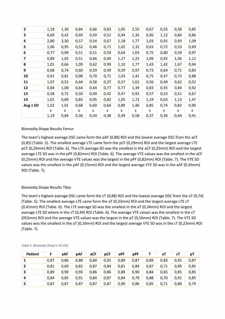
Biomediq Shape Results Femur

The team’s highest average DSC came form the pAF (0,88) ROI and the lowest average DSC from the aCF

(0,85) (Table. 5). The smallest average LTE came form the pCF (0,29mm) ROI and the largest average LTE

pCF (0,29mm) ROI (Table. 6). The LTE average SD was the smallest in the aCF (0,25mm) ROI and the largest

average LTE SD was in the pPF (0,82mm) ROI (Table. 6). The average VTE values was the smallest in the aCF

(0,25mm) ROI and the average VTE values was the largest in the pPF (0,82mm) ROI (Table. 7). The VTE SD

values was the smallest in the pAF (0,15mm) ROI and the largest average VTE SD was in the aAF (0,45mm)

ROI (Table. 7).

Biomediq Shape Results Tibia

The team’s highest average DSC came form the cT (0,88) ROI and the lowest average DSC from the aT (0,74)

(Table. 5). The smallest average LTE came form the aT (0,33mm) ROI and the largest average LTE cT

(0,41mm) ROI (Table. 6). The LTE average SD was the smallest in the aT (0,34mm) ROI and the largest

average LTE SD where in the cT (0,49) ROI (Table. 6). The average VTE values was the smallest in the cT

(052mm) ROI and the average VTE values was the largest in the pT (0,56mm) ROI (Table. 7). The VTE SD

values was the smallest in the aT (0,16mm) ROI and the largest average VTE SD was in the cT (0,23mm) ROI

(Table. 7).

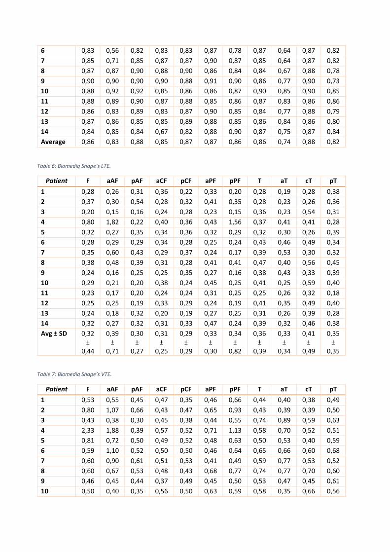
Table 5: Biomediq Shape’s 3D DSC.

Patient F aAF pAF aCF pCF aPF pPF T aT cT pT

1 0,87 0,86 0,88 0,84 0,91 0,89 0,87 0,89 0,83 0,91 0,87

2 0,81 0,69 0,82 0,87 0,84 0,81 0,84 0,87 0,71 0,89 0,85

3 0,89 0,90 0,93 0,86 0,86 0,88 0,90 0,84 0,65 0,85 0,85

4 0,84 0,85 0,91 0,84 0,87 0,84 0,79 0,88 0,70 0,91 0,85

5 0,87 0,87 0,87 0,87 0,87 0,90 0,86 0,85 0,71 0,88 0,79

6 0,83 0,56 0,82 0,83 0,83 0,87 0,78 0,87 0,64 0,87 0,82

7 0,85 0,71 0,85 0,87 0,87 0,90 0,87 0,85 0,64 0,87 0,82

8 0,87 0,87 0,90 0,88 0,90 0,86 0,84 0,84 0,67 0,88 0,78

9 0,90 0,90 0,90 0,90 0,88 0,91 0,90 0,86 0,77 0,90 0,73

10 0,88 0,92 0,92 0,85 0,86 0,86 0,87 0,90 0,85 0,90 0,85

11 0,88 0,89 0,90 0,87 0,88 0,85 0,86 0,87 0,83 0,86 0,86

12 0,86 0,83 0,89 0,83 0,87 0,90 0,85 0,84 0,77 0,88 0,79

13 0,87 0,86 0,85 0,85 0,89 0,88 0,85 0,86 0,84 0,86 0,80

14 0,84 0,85 0,84 0,67 0,82 0,88 0,90 0,87 0,75 0,87 0,84

Average 0,86 0,83 0,88 0,85 0,87 0,87 0,86 0,86 0,74 0,88 0,82

Table 6: Biomediq Shape’s LTE.

Patient F aAF pAF aCF pCF aPF pPF T aT cT pT

1 0,28 0,26 0,31 0,36 0,22 0,33 0,20 0,28 0,19 0,28 0,38

2 0,37 0,30 0,54 0,28 0,32 0,41 0,35 0,28 0,23 0,26 0,36

3 0,20 0,15 0,16 0,24 0,28 0,23 0,15 0,36 0,23 0,54 0,31

4 0,80 1,82 0,22 0,40 0,36 0,43 1,56 0,37 0,41 0,41 0,28

5 0,32 0,27 0,35 0,34 0,36 0,32 0,29 0,32 0,30 0,26 0,39

6 0,28 0,29 0,29 0,34 0,28 0,25 0,24 0,43 0,46 0,49 0,34

7 0,35 0,60 0,43 0,29 0,37 0,24 0,17 0,39 0,53 0,30 0,32

8 0,38 0,48 0,39 0,31 0,28 0,41 0,41 0,47 0,40 0,56 0,45

9 0,24 0,16 0,25 0,25 0,35 0,27 0,16 0,38 0,43 0,33 0,39

10 0,29 0,21 0,20 0,38 0,24 0,45 0,25 0,41 0,25 0,59 0,40

11 0,23 0,17 0,20 0,24 0,24 0,31 0,25 0,25 0,26 0,32 0,18

12 0,25 0,25 0,19 0,33 0,29 0,24 0,19 0,41 0,35 0,49 0,40

13 0,24 0,18 0,32 0,20 0,19 0,27 0,25 0,31 0,26 0,39 0,28

14 0,32 0,27 0,32 0,31 0,33 0,47 0,24 0,39 0,32 0,46 0,38

Avg ± SD 0,32 ±

0,44

0,39 ±

0,71

0,30 ±

0,27

0,31 ±

0,25

0,29 ±

0,29

0,33 ±

0,30

0,34 ±

0,82

0,36 ±

0,39

0,33 ±

0,34

0,41 ±

0,49

0,35 ±

0,35

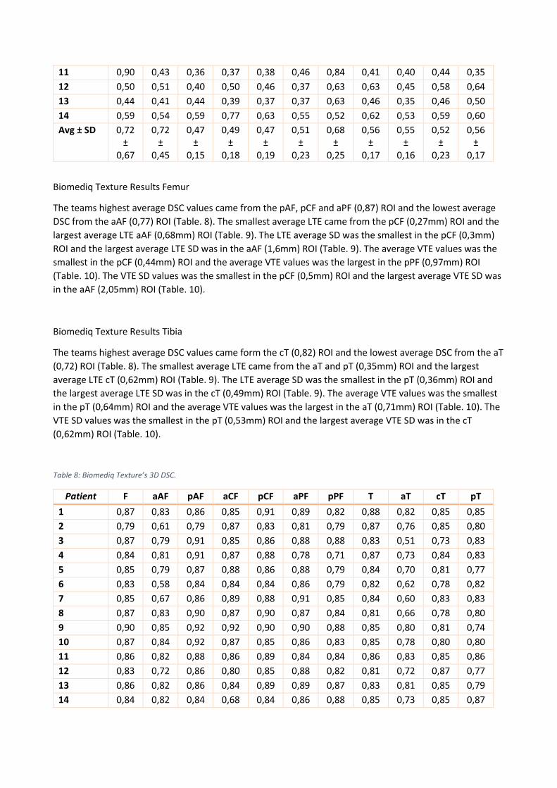
Table 7: Biomediq Shape’s VTE.

Patient F aAF pAF aCF pCF aPF pPF T aT cT pT

1 0,53 0,55 0,45 0,47 0,35 0,46 0,66 0,44 0,40 0,38 0,49

2 0,80 1,07 0,66 0,43 0,47 0,65 0,93 0,43 0,39 0,39 0,50

3 0,43 0,38 0,30 0,45 0,38 0,44 0,55 0,74 0,89 0,59 0,63

4 2,33 1,88 0,39 0,57 0,52 0,71 1,13 0,58 0,70 0,52 0,51

5 0,81 0,72 0,50 0,49 0,52 0,48 0,63 0,50 0,53 0,40 0,59

6 0,59 1,10 0,52 0,50 0,50 0,46 0,64 0,65 0,66 0,60 0,68

7 0,60 0,90 0,61 0,51 0,53 0,41 0,49 0,59 0,77 0,53 0,52

8 0,60 0,67 0,53 0,48 0,43 0,68 0,77 0,74 0,77 0,70 0,60

9 0,46 0,45 0,44 0,37 0,49 0,45 0,50 0,53 0,47 0,45 0,61

10 0,50 0,40 0,35 0,56 0,50 0,63 0,59 0,58 0,35 0,66 0,56

11 0,90 0,43 0,36 0,37 0,38 0,46 0,84 0,41 0,40 0,44 0,35

12 0,50 0,51 0,40 0,50 0,46 0,37 0,63 0,63 0,45 0,58 0,64

13 0,44 0,41 0,44 0,39 0,37 0,37 0,63 0,46 0,35 0,46 0,50

14 0,59 0,54 0,59 0,77 0,63 0,55 0,52 0,62 0,53 0,59 0,60

Avg ± SD 0,72 ±

0,67

0,72 ±

0,45

0,47 ±

0,15

0,49 ±

0,18

0,47 ±

0,19

0,51 ±

0,23

0,68 ±

0,25

0,56 ±

0,17

0,55 ±

0,16

0,52 ±

0,23

0,56 ±

0,17

Biomediq Texture Results Femur

The teams highest average DSC values came from the pAF, pCF and aPF (0,87) ROI and the lowest average

DSC from the aAF (0,77) ROI (Table. 8). The smallest average LTE came from the pCF (0,27mm) ROI and the

largest average LTE aAF (0,68mm) ROI (Table. 9). The LTE average SD was the smallest in the pCF (0,3mm)

ROI and the largest average LTE SD was in the aAF (1,6mm) ROI (Table. 9). The average VTE values was the

smallest in the pCF (0,44mm) ROI and the average VTE values was the largest in the pPF (0,97mm) ROI

(Table. 10). The VTE SD values was the smallest in the pCF (0,5mm) ROI and the largest average VTE SD was

in the aAF (2,05mm) ROI (Table. 10).

Biomediq Texture Results Tibia

The teams highest average DSC values came form the cT (0,82) ROI and the lowest average DSC from the aT

(0,72) ROI (Table. 8). The smallest average LTE came from the aT and pT (0,35mm) ROI and the largest

average LTE cT (0,62mm) ROI (Table. 9). The LTE average SD was the smallest in the pT (0,36mm) ROI and

the largest average LTE SD was in the cT (0,49mm) ROI (Table. 9). The average VTE values was the smallest

in the pT (0,64mm) ROI and the average VTE values was the largest in the aT (0,71mm) ROI (Table. 10). The

VTE SD values was the smallest in the pT (0,53mm) ROI and the largest average VTE SD was in the cT

(0,62mm) ROI (Table. 10).

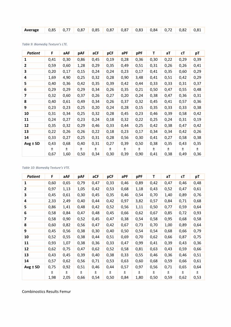
Table 8: Biomediq Texture’s 3D DSC.

Patient F aAF pAF aCF pCF aPF pPF T aT cT pT

1 0,87 0,83 0,86 0,85 0,91 0,89 0,82 0,88 0,82 0,85 0,85

2 0,79 0,61 0,79 0,87 0,83 0,81 0,79 0,87 0,76 0,85 0,80

3 0,87 0,79 0,91 0,85 0,86 0,88 0,88 0,83 0,51 0,73 0,83

4 0,84 0,81 0,91 0,87 0,88 0,78 0,71 0,87 0,73 0,84 0,83

5 0,85 0,79 0,87 0,88 0,86 0,88 0,79 0,84 0,70 0,81 0,77

6 0,83 0,58 0,84 0,84 0,84 0,86 0,79 0,82 0,62 0,78 0,82

7 0,85 0,67 0,86 0,89 0,88 0,91 0,85 0,84 0,60 0,83 0,83

8 0,87 0,83 0,90 0,87 0,90 0,87 0,84 0,81 0,66 0,78 0,80

9 0,90 0,85 0,92 0,92 0,90 0,90 0,88 0,85 0,80 0,81 0,74

10 0,87 0,84 0,92 0,87 0,85 0,86 0,83 0,85 0,78 0,80 0,80

11 0,86 0,82 0,88 0,86 0,89 0,84 0,84 0,86 0,83 0,85 0,86

12 0,83 0,72 0,86 0,80 0,85 0,88 0,82 0,81 0,72 0,87 0,77

13 0,86 0,82 0,86 0,84 0,89 0,89 0,87 0,83 0,81 0,85 0,79

14 0,84 0,82 0,84 0,68 0,84 0,86 0,88 0,85 0,73 0,85 0,87

Average 0,85 0,77 0,87 0,85 0,87 0,87 0,83 0,84 0,72 0,82 0,81

Table 9: Biomediq Texture’s LTE.

Patient F aAF pAF aCF pCF aPF pPF T aT cT pT

1 0,41 0,30 0,86 0,45 0,19 0,28 0,36 0,30 0,22 0,29 0,39

2 0,59 0,60 1,28 0,29 0,35 0,49 0,51 0,31 0,26 0,26 0,41

3 0,20 0,17 0,15 0,24 0,24 0,23 0,17 0,41 0,35 0,60 0,29

4 1,69 4,90 0,25 0,32 0,28 0,90 3,48 0,41 0,51 0,42 0,29

5 0,40 0,36 0,42 0,35 0,39 0,42 0,44 0,33 0,33 0,31 0,37

6 0,29 0,29 0,29 0,34 0,26 0,35 0,21 0,50 0,47 0,55 0,48

7 0,32 0,60 0,37 0,26 0,27 0,20 0,24 0,38 0,47 0,36 0,31

8 0,40 0,61 0,49 0,34 0,26 0,37 0,32 0,45 0,41 0,57 0,36

9 0,23 0,23 0,25 0,20 0,24 0,28 0,15 0,35 0,33 0,33 0,38

10 0,31 0,34 0,25 0,32 0,28 0,45 0,23 0,46 0,39 0,58 0,42

11 0,24 0,27 0,23 0,24 0,18 0,32 0,22 0,25 0,24 0,31 0,19

12 0,35 0,32 0,29 0,46 0,33 0,44 0,25 0,42 0,38 0,47 0,42

13 0,22 0,26 0,26 0,22 0,18 0,23 0,17 0,34 0,34 0,42 0,26

14 0,33 0,27 0,25 0,31 0,28 0,56 0,30 0,41 0,27 0,58 0,38

Avg ± SD 0,43 ±

0,67

0,68 ±

1,60

0,40 ±

0,50

0,31 ±

0,34

0,27 ±

0,30

0,39 ±

0,39

0,50 ±

0,90

0,38 ±

0,41

0,35 ±

0,38

0,43 ±

0,49

0,35 ±

0,36

Table 10: Biomediq Texture’s VTE.

Patient F aAF pAF aCF pCF aPF pPF T aT cT pT

1 0,60 0,65 0,79 0,47 0,33 0,46 0,89 0,42 0,47 0,46 0,48

2 0,97 1,13 1,05 0,42 0,53 0,68 1,18 0,43 0,52 0,47 0,61

3 0,45 0,61 0,30 0,45 0,35 0,46 0,54 0,70 1,40 0,89 0,76

4 2,33 2,49 0,40 0,44 0,42 0,97 3,82 0,57 0,84 0,71 0,68

5 0,86 1,41 0,48 0,42 0,52 0,56 1,11 0,50 0,77 0,59 0,64

6 0,58 0,84 0,47 0,48 0,45 0,66 0,62 0,67 0,85 0,72 0,93

7 0,58 0,90 0,52 0,45 0,47 0,38 0,54 0,58 0,95 0,68 0,58

8 0,60 0,82 0,56 0,47 0,42 0,67 0,73 0,70 1,00 0,89 0,64

9 0,45 0,56 0,38 0,30 0,40 0,50 0,54 0,54 0,68 0,66 0,79

10 0,52 0,55 0,38 0,44 0,51 0,69 0,70 0,62 0,66 0,87 0,75

11 0,93 1,07 0,38 0,36 0,33 0,47 0,99 0,41 0,39 0,43 0,36

12 0,62 0,75 0,47 0,62 0,52 0,58 0,81 0,63 0,43 0,59 0,66

13 0,43 0,45 0,39 0,40 0,38 0,33 0,55 0,46 0,36 0,46 0,51

14 0,57 0,62 0,56 0,71 0,53 0,63 0,60 0,68 0,59 0,66 0,61

Avg ± SD 0,75 ±

1,98

0,92 ±

2,05

0,51 ±

0,66

0,46 ±

0,54

0,44 ±

0,50

0,57 ±

0,84

0,97 ±

1,80

0,56 ±

0,50

0,71 ±

0,59

0,65 ±

0,62

0,64 ±

0,53

Combinostics Results Femur

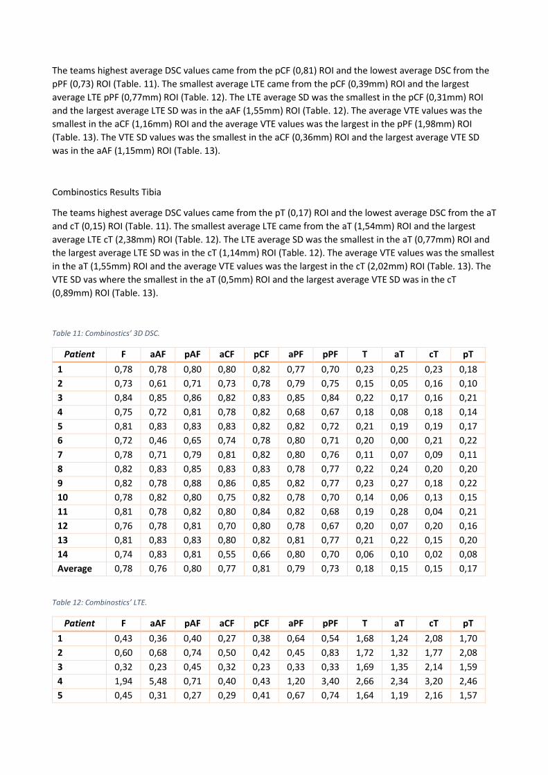
The teams highest average DSC values came from the pCF (0,81) ROI and the lowest average DSC from the

pPF (0,73) ROI (Table. 11). The smallest average LTE came from the pCF (0,39mm) ROI and the largest

average LTE pPF (0,77mm) ROI (Table. 12). The LTE average SD was the smallest in the pCF (0,31mm) ROI

and the largest average LTE SD was in the aAF (1,55mm) ROI (Table. 12). The average VTE values was the

smallest in the aCF (1,16mm) ROI and the average VTE values was the largest in the pPF (1,98mm) ROI

(Table. 13). The VTE SD values was the smallest in the aCF (0,36mm) ROI and the largest average VTE SD

was in the aAF (1,15mm) ROI (Table. 13).

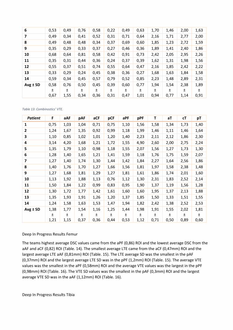
Combinostics Results Tibia

The teams highest average DSC values came from the pT (0,17) ROI and the lowest average DSC from the aT

and cT (0,15) ROI (Table. 11). The smallest average LTE came from the aT (1,54mm) ROI and the largest

average LTE cT (2,38mm) ROI (Table. 12). The LTE average SD was the smallest in the aT (0,77mm) ROI and

the largest average LTE SD was in the cT (1,14mm) ROI (Table. 12). The average VTE values was the smallest

in the aT (1,55mm) ROI and the average VTE values was the largest in the cT (2,02mm) ROI (Table. 13). The

VTE SD vas where the smallest in the aT (0,5mm) ROI and the largest average VTE SD was in the cT

(0,89mm) ROI (Table. 13).

Table 11: Combinostics’ 3D DSC.

Patient F aAF pAF aCF pCF aPF pPF T aT cT pT

1 0,78 0,78 0,80 0,80 0,82 0,77 0,70 0,23 0,25 0,23 0,18

2 0,73 0,61 0,71 0,73 0,78 0,79 0,75 0,15 0,05 0,16 0,10

3 0,84 0,85 0,86 0,82 0,83 0,85 0,84 0,22 0,17 0,16 0,21

4 0,75 0,72 0,81 0,78 0,82 0,68 0,67 0,18 0,08 0,18 0,14

5 0,81 0,83 0,83 0,83 0,82 0,82 0,72 0,21 0,19 0,19 0,17

6 0,72 0,46 0,65 0,74 0,78 0,80 0,71 0,20 0,00 0,21 0,22

7 0,78 0,71 0,79 0,81 0,82 0,80 0,76 0,11 0,07 0,09 0,11

8 0,82 0,83 0,85 0,83 0,83 0,78 0,77 0,22 0,24 0,20 0,20

9 0,82 0,78 0,88 0,86 0,85 0,82 0,77 0,23 0,27 0,18 0,22

10 0,78 0,82 0,80 0,75 0,82 0,78 0,70 0,14 0,06 0,13 0,15

11 0,81 0,78 0,82 0,80 0,84 0,82 0,68 0,19 0,28 0,04 0,21

12 0,76 0,78 0,81 0,70 0,80 0,78 0,67 0,20 0,07 0,20 0,16

13 0,81 0,83 0,83 0,80 0,82 0,81 0,77 0,21 0,22 0,15 0,20

14 0,74 0,83 0,81 0,55 0,66 0,80 0,70 0,06 0,10 0,02 0,08

Average 0,78 0,76 0,80 0,77 0,81 0,79 0,73 0,18 0,15 0,15 0,17

Table 12: Combinostics’ LTE.

Patient F aAF pAF aCF pCF aPF pPF T aT cT pT

1 0,43 0,36 0,40 0,27 0,38 0,64 0,54 1,68 1,24 2,08 1,70

2 0,60 0,68 0,74 0,50 0,42 0,45 0,83 1,72 1,32 1,77 2,08

3 0,32 0,23 0,45 0,32 0,23 0,33 0,33 1,69 1,35 2,14 1,59

4 1,94 5,48 0,71 0,40 0,43 1,20 3,40 2,66 2,34 3,20 2,46

5 0,45 0,31 0,27 0,29 0,41 0,67 0,74 1,64 1,19 2,16 1,57

6 0,53 0,49 0,76 0,58 0,22 0,49 0,63 1,70 1,46 2,00 1,63

7 0,49 0,34 0,41 0,52 0,31 0,71 0,64 2,16 1,71 2,77 2,00

8 0,49 0,48 0,48 0,34 0,37 0,69 0,60 1,85 1,23 2,72 1,59

9 0,35 0,29 0,33 0,37 0,27 0,46 0,36 1,89 1,41 2,40 1,86

10 0,68 0,64 0,81 0,58 0,42 0,91 0,73 2,42 2,05 2,95 2,26

11 0,35 0,31 0,44 0,36 0,24 0,37 0,39 1,62 1,31 1,98 1,56

12 0,55 0,37 0,51 0,74 0,55 0,64 0,47 2,16 1,85 2,42 2,22

13 0,33 0,29 0,24 0,45 0,38 0,36 0,27 1,68 1,63 1,84 1,58

14 0,59 0,34 0,45 0,57 0,79 0,52 0,85 2,23 1,48 2,89 2,31

Avg ± SD 0,58 ±

0,67

0,76 ±

1,55

0,50 ±

0,34

0,45 ±

0,36

0,39 ±

0,31

0,60 ±

0,47

0,77 ±

1,01

1,94 ±

0,94

1,54 ±

0,77

2,38 ±

1,14

1,89 ±

0,91

Table 13: Combinostics’ VTE.

Patient F aAF pAF aCF pCF aPF pPF T aT cT pT

1 0,75 1,03 1,04 0,71 0,75 1,10 1,56 1,58 1,34 1,73 1,40

2 1,24 1,67 1,35 0,92 0,99 1,18 1,99 1,46 1,11 1,46 1,64

3 1,10 0,85 1,02 1,01 1,20 1,40 2,23 2,11 2,12 1,86 2,30

4 3,14 4,20 1,68 1,21 1,72 1,55 4,90 2,60 2,00 2,75 2,24

5 1,35 1,79 1,10 0,98 1,18 1,55 2,07 1,56 1,27 1,73 1,30

6 1,28 1,40 1,65 1,21 1,41 1,59 1,18 1,76 1,75 1,59 2,07

7 1,27 1,40 1,74 1,30 1,44 1,42 1,84 2,27 1,64 2,56 1,86

8 1,40 1,76 1,70 1,27 1,66 1,56 1,81 1,97 1,58 2,38 1,48

9 1,27 1,68 1,81 1,29 1,27 1,81 1,61 1,86 1,74 2,01 1,60

10 1,13 1,92 1,88 1,13 0,76 1,12 1,30 2,31 1,83 2,52 2,14

11 1,50 1,84 1,22 0,99 0,83 0,95 1,90 1,37 1,19 1,56 1,28

12 1,30 1,72 1,77 1,42 1,61 1,60 1,60 1,95 1,37 2,13 1,88

13 1,35 1,93 1,91 1,26 1,20 1,37 1,85 1,50 1,33 1,51 1,55

14 1,24 1,58 1,63 1,53 1,47 1,94 1,82 2,42 1,38 2,52 2,53

Avg ± SD 1,38 ±

1,21

1,77 ±

1,15

1,54 ±

0,37

1,16 ±

0,36

1,25 ±

0,44

1,44 ±

0,53

1,98 ±

1,12

1,91 ±

0,71

1,55 ±

0,50

2,02 ±

0,89

1,81 ±

0,60

Deep In Progress Results Femur

The teams highest average DSC values came from the aPF (0,86) ROI and the lowest average DSC from the

aAF and aCF (0,82) ROI (Table. 14). The smallest average LTE came from the aCF (0,47mm) ROI and the

largest average LTE aAF (0,81mm) ROI (Table. 15). The LTE average SD was the smallest in the pAF

(0,37mm) ROI and the largest average LTE SD was in the pPF (1,2mm) ROI (Table. 15). The average VTE

values was the smallest in the aPF (0,58mm) ROI and the average VTE values was the largest in the pPF

(0,98mm) ROI (Table. 16). The VTE SD values was the smallest in the pAF (0,3mm) ROI and the largest

average VTE SD was in the aAF (1,12mm) ROI (Table. 16).

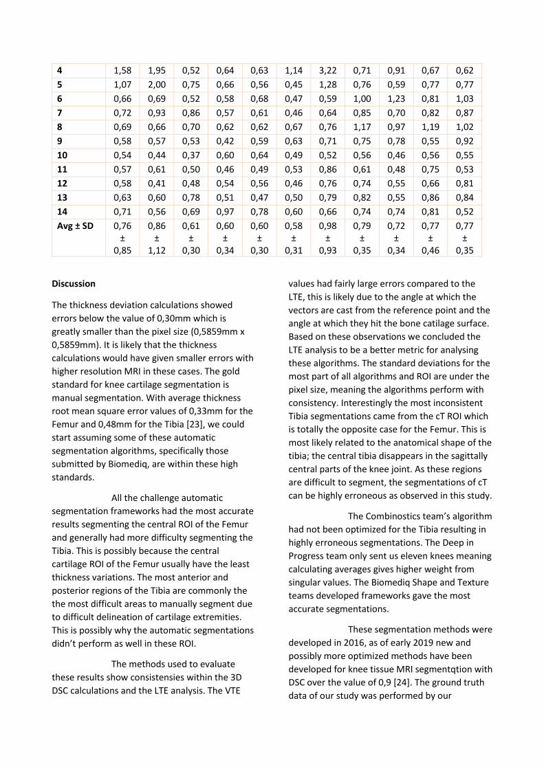
Deep In Progress Results Tibia

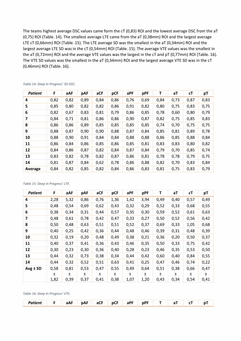
The teams highest average DSC values came form the cT (0,83) ROI and the lowest average DSC from the aT

(0,75) ROI (Table. 14). The smallest average LTE came from the aT (0,38mm) ROI and the largest average

LTE cT (0,66mm) ROI (Table. 15). The LTE average SD was the smallest in the aT (0,34mm) ROI and the

largest average LTE SD was in the cT (0,54mm) ROI (Table. 15). The average VTE values was the smallest in

the aT (0,72mm) ROI and the average VTE values was the largest in the cT and pT (0,77mm) ROI (Table. 16).

The VTE SD values was the smallest in the aT (0,34mm) ROI and the largest average VTE SD was in the cT

(0,46mm) ROI (Table. 16).

Table 14: Deep In Progress’ 3D DSC.

Patient F aAF pAF aCF pCF aPF pPF T aT cT pT

4 0,82 0,82 0,89 0,84 0,86 0,76 0,69 0,84 0,73 0,87 0,83

5 0,85 0,80 0,82 0,82 0,86 0,91 0,82 0,80 0,75 0,83 0,75

6 0,82 0,67 0,83 0,81 0,79 0,86 0,85 0,78 0,60 0,80 0,79

7 0,84 0,71 0,81 0,86 0,86 0,90 0,87 0,82 0,75 0,85 0,83

8 0,86 0,86 0,89 0,85 0,85 0,85 0,85 0,74 0,70 0,75 0,75

9 0,88 0,87 0,90 0,90 0,88 0,87 0,84 0,85 0,81 0,89 0,78

10 0,88 0,90 0,91 0,84 0,84 0,88 0,88 0,86 0,85 0,88 0,84

11 0,86 0,84 0,86 0,85 0,86 0,85 0,81 0,83 0,83 0,80 0,82

12 0,84 0,86 0,87 0,82 0,84 0,87 0,84 0,79 0,70 0,85 0,74

13 0,83 0,82 0,78 0,82 0,87 0,86 0,81 0,78 0,78 0,79 0,75

14 0,81 0,87 0,84 0,62 0,78 0,86 0,88 0,82 0,70 0,83 0,84

Average 0,84 0,82 0,85 0,82 0,84 0,86 0,83 0,81 0,75 0,83 0,79

Table 15: Deep In Progress’ LTE.

Patient F aAF pAF aCF pCF aPF pPF T aT cT pT

4 2,28 5,32 0,86 0,76 1,36 1,42 3,94 0,49 0,40 0,57 0,49

5 0,48 0,54 0,69 0,62 0,43 0,32 0,29 0,52 0,33 0,68 0,55

6 0,38 0,34 0,31 0,44 0,57 0,35 0,30 0,59 0,52 0,61 0,63

7 0,48 0,61 0,78 0,42 0,47 0,33 0,27 0,50 0,52 0,56 0,42

8 0,50 0,48 0,63 0,51 0,51 0,52 0,37 0,69 0,33 1,05 0,68

9 0,40 0,25 0,42 0,36 0,44 0,48 0,46 0,39 0,31 0,48 0,39

10 0,32 0,19 0,20 0,48 0,49 0,38 0,21 0,36 0,20 0,50 0,37

11 0,40 0,37 0,41 0,36 0,43 0,46 0,35 0,50 0,33 0,75 0,42

12 0,30 0,23 0,30 0,36 0,40 0,28 0,23 0,46 0,35 0,53 0,50

13 0,44 0,32 0,73 0,38 0,34 0,44 0,42 0,60 0,40 0,84 0,55

14 0,44 0,32 0,52 0,51 0,63 0,41 0,25 0,47 0,46 0,74 0,22

Avg ± SD 0,58 ±

1,82

0,81 ±

0,39

0,53 ±

0,37

0,47 ±

0,41

0,55 ±

0,38

0,49 ±

1,07

0,64 ±

1,20

0,51 ±

0,43

0,38 ±

0,34

0,66 ±

0,54

0,47 ±

0,41

Table 16: Deep In Progress’ VTE.

Patient F aAF pAF aCF pCF aPF pPF T aT cT pT

4 1,58 1,95 0,52 0,64 0,63 1,14 3,22 0,71 0,91 0,67 0,62

5 1,07 2,00 0,75 0,66 0,56 0,45 1,28 0,76 0,59 0,77 0,77

6 0,66 0,69 0,52 0,58 0,68 0,47 0,59 1,00 1,23 0,81 1,03

7 0,72 0,93 0,86 0,57 0,61 0,46 0,64 0,85 0,70 0,82 0,87

8 0,69 0,66 0,70 0,62 0,62 0,67 0,76 1,17 0,97 1,19 1,02

9 0,58 0,57 0,53 0,42 0,59 0,63 0,71 0,75 0,78 0,55 0,92

10 0,54 0,44 0,37 0,60 0,64 0,49 0,52 0,56 0,46 0,56 0,55

11 0,57 0,61 0,50 0,46 0,49 0,53 0,86 0,61 0,48 0,75 0,53

12 0,58 0,41 0,48 0,54 0,56 0,46 0,76 0,74 0,55 0,66 0,81

13 0,63 0,60 0,78 0,51 0,47 0,50 0,79 0,82 0,55 0,86 0,84

14 0,71 0,56 0,69 0,97 0,78 0,60 0,66 0,74 0,74 0,81 0,52

Avg ± SD 0,76 ±

0,85

0,86 ±

1,12

0,61 ±

0,30

0,60 ±

0,34

0,60 ±

0,30

0,58 ±

0,31

0,98 ±

0,93

0,79 ±

0,35

0,72 ±

0,34

0,77 ±

0,46

0,77 ±

0,35

Discussion

The thickness deviation calculations showed

errors below the value of 0,30mm which is

greatly smaller than the pixel size (0,5859mm x

0,5859mm). It is likely that the thickness

calculations would have given smaller errors with

higher resolution MRI in these cases. The gold

standard for knee cartilage segmentation is

manual segmentation. With average thickness

root mean square error values of 0,33mm for the

Femur and 0,48mm for the Tibia [23], we could

start assuming some of these automatic

segmentation algorithms, specifically those

submitted by Biomediq, are within these high

standards.

All the challenge automatic

segmentation frameworks had the most accurate

results segmenting the central ROI of the Femur

and generally had more difficulty segmenting the

Tibia. This is possibly because the central

cartilage ROI of the Femur usually have the least

thickness variations. The most anterior and

posterior regions of the Tibia are commonly the

the most difficult areas to manually segment due

to difficult delineation of cartilage extremities.

This is possibly why the automatic segmentations

didn’t perform as well in these ROI.

The methods used to evaluate

these results show consistensies within the 3D

DSC calculations and the LTE analysis. The VTE

values had fairly large errors compared to the

LTE, this is likely due to the angle at which the

vectors are cast from the reference point and the

angle at which they hit the bone catilage surface.

Based on these observations we concluded the

LTE analysis to be a better metric for analysing

these algorithms. The standard deviations for the

most part of all algorithms and ROI are under the

pixel size, meaning the algorithms perform with

consistency. Interestingly the most inconsistent

Tibia segmentations came from the cT ROI which

is totally the opposite case for the Femur. This is

most likely related to the anatomical shape of the

tibia; the central tibia disappears in the sagittally

central parts of the knee joint. As these regions

are difficult to segment, the segmentations of cT

can be highly erroneous as observed in this study.

The Combinostics team’s algorithm

had not been optimized for the Tibia resulting in

highly erroneous segmentations. The Deep in

Progress team only sent us eleven knees meaning

calculating averages gives higher weight from

singular values. The Biomediq Shape and Texture

teams developed frameworks gave the most

accurate segmentations.

These segmentation methods were

developed in 2016, as of early 2019 new and

possibly more optimized methods have been

developed for knee tissue MRI segmentqtion with

DSC over the value of 0,9 [24]. The ground truth

data of our study was performed by our

reaserchers who are not experts in the field of

manual segmentation.

Conclusion

The gap in the accuracy between segmentations

produced by automatic methods and experts has

been narrowing. The leaps in automatic

segmentation methods, i.e. deep learning, have

been great in the recent years, emphasizing their

future potential in the clinical realm. In this

study, the Biomediq Shape framework reached

accurate cartilage delineation with DSC values of

0,86 for Femur and Tibia, with thickness

quantification error falling below the pixel size of

the used MR protocol. We feel that the Biomediq

Shape framework has reached the accuracy

standards to be used in large knee osteoarthritis

studies. In order to gather further and more

accurate data about these types of methods we

need to start using higher resolution MRI images

as the ground truth data.

References

[1] A. M. Ogunbode, L. A. Adebusoye, O. O. Olowookere, and T. O. Alonge, “Physical functionality and self-rated health status of adulute patients with knee osteoarthritis presenting in a primary care clinic.”

[2] J. A. Buckwalter, H. J. Mankin, and A. J. Grodzinsky, “ArticuIarCartiIage and Osteoarthritis,” pp. 465–480, 2005.

[3] J. A. Buckwalter and J. A. Martin, “Osteoarthritis,” Adv. Drug Deliv. Rev., vol. 58, no. 2, pp. 150–167, 2006.

[4] G. S. Dulay, C. Cooper, and E. M. Dennison, “Knee pain, knee injury, knee osteoarthritis & work,” Best Pract. Res. Clin. Rheumatol., vol. 29, no. 3, pp. 454–461, 2015.

[5] H. Bliddal, A. R. Leeds, and R. Christensen, “Osteoarthritis, obesity and weight loss: Evidence, hypotheses and horizons - a scoping review,” Obes. Rev., vol. 15, no. 7,

pp. 578–586, 2014.

[6] F. J. Blanco, “Osteoarthritis year in review 2014: We need more biochemical biomarkers in qualification phase,” Osteoarthr. Cartil., vol. 22, no. 12, pp. 2025–2032, 2014.

[7] D. Dere, “Effect of body mass index on functional recovery after total knee arthroplasty in ambulatory overweight or obese women with osteoarthritis,” ACTA Orthop. Traumatol. Turc., vol. 48, no. 2, pp. 117–121, 2014.

[8] F. Cicuttini, J. Hankin, G. Jones, and A. Wluka, “Comparison of conventional standing knee radiographs and magnetic resonance imaging in assessing progression of tibiofemoral joint osteoarthritis,” Osteoarthr. Cartil., vol. 13, no. 8, pp. 722–727, 2005.

[9] Y. Li, X. Wei, J. Zhou, and L. Wei, “The age-related changes in cartilage and osteoarthritis,” Biomed Res. Int., vol. 2013, 2013.

[10] T. M. Link, Cartilage imaging : significance, techniques, and new developments. Springer, 2011.

[11] J. M. Lötjönen et al., “Fast and robust multi-atlas segmentation of brain magnetic resonance images,” Neuroimage, vol. 49, no. 3, pp. 2352–2365, 2010.

[12] J. Podlipská et al., “Erratum: Comparison of Diagnostic Performance of Semi-Quantitative Knee ULTErasound and Knee Radiography with MRI: Oulu Knee Osteoarthritis Study,” Sci. Rep., vol. 6, no. March, p. 33109, 2016.

[13] L. Shan, C. Zach, C. Charles, and M. Niethammer, “Automatic atlas-based three-label cartilage segmentation from MR knee images,” Med. Image Anal., vol. 18, no. 7, pp. 1233–1246, 2014.

[14] S. Egmentation, D. L. Pham, C. Xu, and J. L. Prince, “C m m i s,” 2000.

[15] T. Sekine et al., “Multi-Atlas-Based Attenuation Correction for Brain 18F-FDG

PET Imaging Using a Time-of-Flight PET/MR Scanner: Comparison with Clinical Single-Atlas- and CT-Based Attenuation Correction,” J. Nucl. Med., vol. 57, no. 8, pp. 1258–1264, 2016.

[16] C. Wachinger, K. Fritscher, G. Sharp, and P. Golland, “Contour-Driven Atlas-Based Segmentation,” IEEE Trans. Med. Imaging, vol. 34, no. 12, pp. 2492–2505, 2015.

[17] N. M. Hansson, H. Achterberg, A. Opbroek, and S. Klein, “IWOAI Challenge 2016 : Combined muLTEi-atlas and appearance segmentation model ( Team BIGR ),” pp. 1–9, 2016.

[18] E. B. Dam, “Knee Cartilage Segmentation Challenge Team : Biomediq Shape,” pp. 3–6.

[19] E. B. Dam, “Knee Cartilage Segmentation Challenge Team : Biomediq Texture,” pp. 2–3.

[20] D. I. Progress, “Tibial and Femoral Cartilage Segmentation with Deep 3D Convolutional Neural Networks.”

[21] A. I. Jones S.E., Buchbinder B.R., “Three-dimensional mapping of cortical thickness using Laplace's Equation” Hum. Brain Mapp., vol. 11, no. 1, pp. 12–32, 2000.

[22] N. H. Foley et al., “NIH Public Access,” Cell, vol. 18, no. 7, pp. 1089–1098, 2012.

[23] Zohara A. Cohen, Denise M. McCarthy, S. Daniel Kwak, Perrine Legrand, Fabian Fogarasi, Edward J. Ciaccio and Gerard A. Ateshian, ”Knee cartilage topography, thickness, and contact areas from MRI: in-vitro calibration and in-vivo measurements” Osteoarthritis and Cartilage (1999) 7, 95–109.

[24] Zhou Z, Zhao G, Kijowski R, Liu F. “Deep convolutional neural network for segmentation of knee joint anatomy.” Magn Reson Med. 2018 Dec;80(6):2759-2770. doi: 10.1002/mrm.27229. Epub 2018 May 17.