atom: A MATLAB PACKAGE FOR MANIPULATION OFMOLECULAR SYSTEMS

MICHAEL HOLMBOE*1Chemistry Department, Umeå University, SE-901 87 Umeå, Sweden

Abstract—This work presents Atomistic TopologyOperations inMATLAB (atom), an open source library of modularMATLAB routines whichcomprise a general and flexible framework for manipulation of atomistic systems. The purpose of the atom library is simply to facilitate commonoperations performed for construction, manipulation, or structural analysis. Due to the data structure used, atoms and molecules can be operatedupon based on different chemical names or attributes, such as atom- ormolecule-ID, name, residue name, charge, positions, etc. Furthermore, theBond Valence Method and a neighbor-distance analysis can be performed to assign many chemical properties of inorganic molecules. Apart fromreading and writing common coordinate files (.pdb, .xyz, .gro, .cif) and trajectories (.dcd, .trr, .xtc; binary formats are parsed via third-partypackages), the atom library can also be used to generate topology files with bonding and angle information taking the periodic boundaryconditions into account, and supports basic Gromacs, NAMD, LAMMPS, and RASPA2 topology file formats. Focusing on clay-mineral systems,the library supports CLAYFF (Cygan, 2004) but can also generate topology files for the INTERFACE forcefield (Heinz, 2005, 2013) for Gromacsand NAMD.

Keywords—CLAYFF . Gromacs . INTERFACE force field .MATLAB .Molecular dynamics simulations .Monte Carlo

INTRODUCTION

Molecular modeling is becoming increasingly important inmany different areas of fundamental and applied research(Cygan 2001; Lu et al. 2006; Medina, 2009). This is due notonly to the development of high-performance computing inrecent decades but also because of increasingly user-friendlymolecular modeling software, allowing for high-throughputscreening of large classes of molecules. This is especially truefor life-science related research, which traditionally hasspearheaded the development and design of molecular model-ing software and forcefield tools. However, due to the wide useof molecular modeling in different scientific disciplines,custom-made setup or analysis tools specifically tailored tothe user’s system are often required. This is because of theneed to perform specific tasks that topology tools aimed to-wards modeling of biomolecules normally do not offer. Exam-ples of this include the ability to perform: (1) automaticatomtype assignment for less common or system-specificforcefields; or (2) the ability to find bonds and angles acrossthe periodic boundary conditions (PBC) for periodic slabs orlayered molecules, such as graphene and graphite oxides,zeolites, clay minerals, layered double hydroxides, etc.

In this context and especially for scientists lackingcomprehensive programing skills, MATLAB, R, andsimilar software packages offer an attractive and versa-tile environment for scientific computing with simple yetrobust scripting languages, plotting capabilities, and thepossibility to display or copy data variables into spread-sheets. In fact, a handful of MATLAB and R packagesfor trajectory or statistical analysis focusing on biomol-ecules has been developed (Dien et al . 2014;

Dombrowsky et al. 2018; Kapla & Lindén 2018;Matsunaga & Sugita 2018). This work presents theAtomistic Topology Operations in MATLAB (atom) li-brary – a large collection of >100 modular MATLABscripts and sub-routines (e.g. functions) under an opensource license (simple BSD) which comprise a generalframework for construction, manipulation, and analysisof atomistic systems, with the option of incorporatingtopological and forcefield information. In contrast to theabove-mentioned MATLAB and R trajectory packages,the focus here lies not on the modeling of biomoleculesbut rather on the investigation of especially periodicinorganic structures, such as slabs and layers that havewell defined unit cells (UC) stretching over the PBC.

Because the atom function calls can be invoked fromthe command line as well as from within custom-madeMATLAB scripts and programs, the atom library is espe-cially well suited to batch-mode operations. In particular,the atom library may be useful for scientists with an interestin modeling inorganic and geochemical systems. This isbecause apart from parsing the input or output of basiccoordinate files (.pdb|.xyz|.gro|.cif), the atom library canalso be used to output basic molecular topology files(.lmp|.itp|.psf) for the CLAYFF forcefield (Cygan et al.2004) and INTERFACE (Heinz et al. 2005, 2013) forcertain geochemical systems/software, which are used inmolecular modeling software such as LAMMPS, Gromacs,NAMD and RASPA2 (Plimpton 1995; Phillips et al. 2005;Abraham et al. 2015; Dubbeldam et al. 2016).

METHODS

The unifying theme among the different library functions isthe atom (see Fig. 1), which is the default name of the variabletypically containing the molecular information from a coordi-nate file such as a .pdb file. In order to call the different library

* E-mail address of corresponding author: michael.holmboe@umu.seDOI: 10.1007/s42860-019-00043-y

Clays and Clay Minerals, Vol. 67, No. 5:419 426, 2019–

functions, i.e. to perform specific operations on the atomvariable, the following syntax is used:

atom ¼ operationf g atom argumentsf gð Þ

where examples of common {operations} are: composi-t ion , clayf f , copy, create , dist_matrix , element ,find_bonded, import, insert, interface, ionize, mass, radii,reorder, rotate, scale, slice, solvate, translate, update,wrap, write, etc. The {arguments} represent required func-tion input variables, which depend on the intended specif-ic {operations} to be made. It is normally a coordinatefilename, or the atom variable itself, followed by the UCor system size variable Box_dim (if such exists). Functionsrequiring additional arguments like limits (representing avolumetric region) are described in the documentation foreach function.

The properties of each individual atomistic particleare accessible by its atom-ID index (ranging from 1 tothe number of atomistic particles), because the atomvariable itself is an indexed data type called structurearray (denoted struct). The struct variable stores theindividual atom and molecule attributes (i.e. chemicalnames and properties) in so-called fields, where theassociated syntax is based on the so-called dot-notationas in [struct.field], or more generically [atom.attribute].One advantage of the dot-notation is that it enables aflexible syntax for advanced selections because individ-ual atoms and molecules can be filtered or selectivelymanipulated based on one or more specific attributes.This is done by using logical indexing (in the case offields with numeral data) or string comparison (in case of

fields containing text). A purposeful example is shown below,demonstrating how to select and delete (1) all atomsnamed Si that (2) belong to the molecule/molecule, (3)have the residue/molecule name MMT, and (4) have z coordi-nates of <10 Å (... only needed in case of line breaks).

atom ðstrcmpð atom:type½ �; 0Si0Þ&:::

strcmpð atom:resname½ �; 0MMT0Þ&:::

atom:molid½ �¼¼2&:::

atom:z½ � < 10Þ ¼ ½ �

Similar combined selections can be made on all the differ-ent struct attributes. The default attributes include the mole-cule-ID, atom-ID, atomtype names, residue names, and thecoordinates, and are denoted as molid, index, type, resname,x, y, z, respectively. If invoking other functions, the atom structwill expand to incorporate optional attributes, for instancestoring information on velocities, forces, neighbors, bonds,and angles, or strictly chemical properties like the atomic mass,partial charges, bond valence values, and so on.

Another benefit of the atom struct variable type is thatseveral structs can easily be merged:

atom123 ¼ atom1 atom2 atom3½ �

Although this notation works well for concatenating (i.e.stacking) molecules with the same attributes, theupdate_atom() function is generally superior as it also updatesthe atom- and molecule-ID indexes accordingly:

atom123 ¼ update atom atom1atom2atom3f gð Þ

The atom library provides several functions to create, ap-pend, duplicate, solvate, translate, rotate, and slice parts of orwhole molecules. Hence, in addition to the flexible selectionsyntax using the dot-notation described above, this library isideal for building or manipulating the structure of multicom-ponent systems by adding entire crystal slabs, molecules, ions,and solvent molecules.

HIGHLIGHTS

Construction of Multi-component Systems

Building basic configurations of multicomponent and/ormultilayered systems normally proceed by initially placingthe primary solute molecules, e.g. a protein or a crystallograph-ic mineral slab, into a pre-defined simulation box using func-tions such as place_atom(), center_atom(), translate_atom(),wrap_atom(), and so on.

Fig. 1 Schematic of the typical workflow using the atom library,illustrating various operations performed on the atom struct variable

Clays and Clay Minerals420

Ions can be added into a simulation box either randomly inspecified regions (but without atomic overlap of existing mol-ecules), on specified planes (in 3D), or with exponentiallydecaying concentrations from a surface with the functionionize_atom(). Other similar functions to add new or copyexisting solutes also exist.

In terms of solvation, the function solvate_atom() can solvatean entire simulation box or limited regions with generic three-,four-, or five-site water models, such as SPC/E or TIP3P/TIP4P/TIP5P, either as liquid water or hexagonal ice. Solvation withcustom solvents using unwrapped solvent boxes is also support-ed, as is scaling the solvent density to optimize solvent moleculepacking. Furthermore, one can solvate a solute by a certainsolvation thickness (Ex. around a centered protein).

VisualizationFor visualization one can make use of the function vmd() if

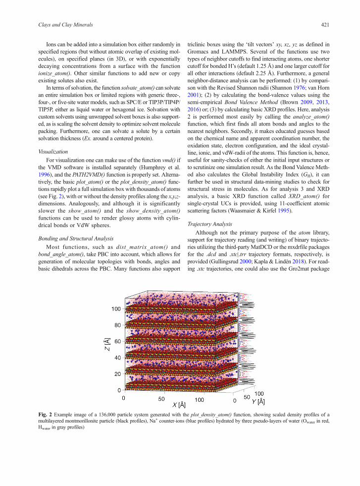
the VMD software is installed separately (Humphrey et al.1996), and the PATH2VMD() function is properly set. Alterna-tively, the basic plot_atom() or the plot_density_atom() func-tions rapidly plot a full simulation boxwith thousands of atoms(see Fig. 2), with or without the density profiles along the x,y,z-dimensions. Analogously, and although it is significantlyslower the show_atom() and the show_density_atom()functions can be used to render glossy atoms with cylin-drical bonds or VdW spheres.

Bonding and Structural AnalysisMost functions, such as dist_matrix_atom() and

bond_angle_atom(), take PBC into account, which allows forgeneration of molecular topologies with bonds, angles andbasic dihedrals across the PBC. Many functions also support

triclinic boxes using the ‘tilt vectors’ xy, xz, yz as defined inGromacs and LAMMPS. Several of the functions use twotypes of neighbor cutoffs to find interacting atoms, one shortercutoff for bonded H’s (default 1.25 Å) and one larger cutoff forall other interactions (default 2.25 Å). Furthermore, a generalneighbor-distance analysis can be performed: (1) by compari-son with the Revised Shannon radii (Shannon 1976; van Horn2001); (2) by calculating the bond-valence values using thesemi-empirical Bond Valence Method (Brown 2009, 2013,2016) or; (3) by calculating basic XRD profiles. Here, analysis2 is performed most easily by calling the analyze_atom()function, which first finds all atom bonds and angles to thenearest neighbors. Secondly, it makes educated guesses basedon the chemical name and apparent coordination number, theoxidation state, electron configuration, and the ideal crystal-line, ionic, and vdW-radii of the atoms. This function is, hence,useful for sanity-checks of either the initial input structures orto scrutinize one simulation result. As the Bond Valence Meth-od also calculates the Global Instability Index (GII), it canfurther be used in structural data-mining studies to check forstructural stress in molecules. As for analysis 3 and XRDanalysis, a basic XRD function called XRD_atom() forsingle-crystal UCs is provided, using 11-coefficient atomicscattering factors (Waasmaier & Kirfel 1995).

Trajectory Analysis

Although not the primary purpose of the atom library,support for trajectory reading (and writing) of binary trajecto-ries utilizing the third-party MatDCD or the mxdrfile packagesfor the .dcd and .xtc|.trr trajectory formats, respectively, isprovided (Gullingsrud 2000; Kapla & Lindén 2018). For read-ing .xtc trajectories, one could also use the Gro2mat package

Fig. 2 Example image of a 136,000 particle system generated with the plot_density_atom() function, showing scaled density profiles of amultilayered montmorillonite particle (black profiles), Na+ counter-ions (blue profiles) hydrated by three pseudo-layers of water (Owater in red,Hwater in gray profiles)

421Clays and Clay Minerals

(Dien et al. 2014). In addition to these third-party binarytrajectory packages, text-format trajectories in the.pdb|.xyz|.gro formats are also natively supported by the atomlibrary, where one special version written specifically for theMC code RASPA2 named import_mc_pdb_traj() can handletrajectories with non-constant numbers of atoms.

In order to import a trajectory into MATLAB as shownbelow, both a coordinate file and a trajectory file is needed.

atom;traj½ � ¼ import traj ð:::coordfile;trajfileÞ

Apart from the atom struct taken from the coordinate file,this command results in a data matrix called traj, of size3N×frames, where N represents the number of atoms in thetrajectory.

Case Study: A Hydrated Na+-montmorillonite NanoporeSystem with CLAYFF atomtypes

This example demonstrates the main steps needed tosetup a simulation box for MC or MD simulations of asystem representing the water–mineral interface to adefect mineral particle called MMT (as in Montmorillon-ite). MMT will describe a negatively charged smectitelayer, with an approximate thickness of 1 nm and beinginfinite in the lateral plane, due to the fact that PBC isused in MC or MD simulations and because the layer inthis example will have no edges in order to avoidcomplexity.

Preparation of the Mineral LatticeThe negative charge of MMT mainly originates from iso-

morphic substitution of octahedrally coordinated Al(III) withMg(II), which creates a charge defect which is smeared overthe nearest coordinating O(-II) in the lattice. In most caseswhen performing molecular modeling of inorganic or mineralparticles, initial UC data are available from either X-ray dif-fraction data or quantum mechanical calculations. For MMT,due to the isomorphic substitution, no precise UC data exist.Instead, one can use isostructural and defect-free UC data frompyrophyllite (Lee & Guggenheim 1981), and then replicate itto a mineral layer and subject it to isomorphic substitution.Hence, initially, a pyrophyllite UC structure must be imported:

Pyrox1 ¼ import atom 0Pyrophyllite:pdb0Þð

In many cases when UC information is taken from XRDdata, the number and positions of H atoms are somewhatunreliable. Hence, in this example both initial removal andaddition of H atoms to the clay lattice are demonstrated. First,all atoms with names starting with ‘H’ are removed.

Pyrox1 strncmpi Pyrox1:type½ �; 0H0; 1ÞÞ ¼ ½ �ðð

Then the remaining mineral lattice is analyzed for theresulting structure using the function analyze_atom().

properties ¼ analyze atom Pyrox1;Box dimð Þ

This function will output a separate properties struct withbonding information, as well as reveal which atoms needhealing by outputting a heal_ind variable. To protonate thoseindividual atoms, one would issue:

H atom ¼ protonate atom ð:::Pyrox1;Box dim;healindÞ

To simplify this example one could convert the triclinic UCto an orthogonal UC:

Pyrox1 ¼ orto atom ð:::Pyrox1H atom;Box dimÞ

Next, the UCmust be replicated into a layer, for instance by6×4 times in the X and Y-directions, respectively:

Pyrox6x4 ¼ replicate atom ð:::Pyrox1;orto Box dim; 64 1½ �Þ

From this pyrophyllite layer, aMMT layer can be generatedby performing isomorphic substitution by replacing Al latticeatoms with Mg in two-thirds of all the UCs (which is typicalfor natural MMT clay minerals). The last numerical argument(in Ångström units) sets the nearestMg–Mg neighbor distance,as charge defects are unlikely to be close to each other.

MMT ¼ substitute atom ðPyrox6x4; :::

Box dim; 6*4*2=3; 0Al0; 0Mg0; 5:5Þ

For consistency, one can at this point change the attributeMMT.resname from ‘PYR’ to ‘MMT’:

MMT:resname½ � ¼ deal 0MMT0f gð Þ

Here, the deal() is a nativeMATLABfunction.Next, the namesof all atoms (i.e. the atomtypes) in MMT can be set to a specificforcefield, such as the original CLAYFF (Cygan et al. 2004).

MMT ¼ clayff 2004 atom MMT;Box dim; 0clayff0Þð

This function will also output the layer net charge (–16from the isomorphic substitution), which must becounterbalanced by counter-cations such as Na+. In order toaccommodate these ions and later water molecules, the dimen-sions of the definitive simulation box should be defined, fromthe lateral dimensions of the MMT layer along X/Y (already setin the existing Box_dim variable) and an arbitrary height in Z,here set to 40 Å:

Clays and Clay Minerals422

Box dim 3ð Þ ¼ 40;%in Angstrom

Adding Counterions and Solvating with WaterIons can be added to an existing simulation box in several

ways using the ionize_atom() function. In this example, an Ionsstruct is created by adding ions close to the mineral surface (but>3 Å) of the wrapped MMT:

Ions ¼ ionize atom ð:::0Na0; 0Na0;Box dim; 16; 3; :::

wrap atom MMT;Box dimð Þ; 0surface0Þ

Note that wrapping the MMT layer into the box beforeadding the ions is important in order to avoid atomic overlap.Next, aWater struct is created in order to solvate the simulationbox. This is accomplished by placing 1000 SPC/E watermolecules with a relative density of 1.05 no nearer than 2 Åto any solute:

Water ¼ solvate atom ðBox dim; 1:05; :::

2; 1000;update atom MMT ;Ionsf gð ÞÞ

Finally, all components are merged together usingupdate_atom() into single System struct, which updates allatom- and molecular-ID indexes, and an ouput .pdb file iswritten. Note that because the different System struct compo-nents are stored in separate struct variables, the order of thecomponents can be changed arbitrarily.

System ¼ update atom fMMT Water Ionsgð Þwrite atom pdbðSystem; :::

Box dim; 0System:pdb0Þ

The following lines show example commands used to plotthe final System struct (see Fig. 3), where, for instance, theoptional last numerical in the plot_atom() function denotes theVdWradii scaling factor, whereas the 'vdw' in the show_atom()function sets the display style:

plot atom System;Box dim; 0:2ð Þshow atom ðSystem;Box dim; 0vdw0Þvmd System;Box dimð Þvmd 0System:pdb0Þð

Writing Molecular Topology Files

The atom library contains different flavors of both theCLAYFF and INTERFACE forcefields. The following exam-ples show how to write basic .psf, .lmp, and .itp topology filesaccording to the original CLAYFF to be used in the MDsoftware like NAMD2, LAMMPS, and Gromacs.

write atom psfðSystem;Box dim; 0System0Þwrite atom lmp ðSystem;Box dim; 0System0Þwrite atom itp MMT;Box dim; 0MMT0Þð

Note that when generating molecular topology files, onemust, in general, decide which components to include (i.e. theMMT, Ions, and Water) in the molecular topology, as differentMD and MC software may use different approaches on how toinclude molecular topologies in the total system topology. Forinstance, in Gromacs, separate molecular topology files areused commonly (.itp files) for different components; hence,the Ions and theWater in the current example would preferablynot be included in the same molecular topology as MMT.

On a separate note, because the original CLAYFF (norINTERFACE) does not contain all different oxygen atom typesneeded to model all minerals or, for instance, custom clay edgemodels, the atom library can also be used to derive partialcharges and molecular topologies for new oxygen atom typesnot part of the original CLAYFF forcefield. This is accom-plished by equation 1, which in fact can be used to calculate thepartial charge of any new or original oxygen atom type inCLAYFF (Tournassat et al. 2016; Lammers et al. 2017).

ZO ¼ −2− −∑n

Z fn−Z

pn

CNn

� �ð1Þ

In this equation, the partial charge of a CLAYFF oxygen type(ZO) is obtained from its formal charge (–2) minus the totalcharge needed to balance (hence the extra minus sign) the chargedistributed over all the n nearest coordinating cationic centers(including H). This distributed charge represented by the secondterm on the right hand side is, in turn, calculated from the

difference between the formal and partial charge Z fn and Zp

n

of each cation (hence the summation), divided by theirrespective number of coordinating oxygens, CNn. For amore extensive explanation, see Lammers et al. (2017).

Analyzing the Lattice Structure

In order to study the structural integrity of molecules sub-jected to molecular simulations, computing the root meansquare deviation of atomic positions (RMSD) from the posi-tions in the input structure is an often-used method. Thismethod is frequently used for large biomolecules; however,for crystalline inorganic lattice structures the semi-empiricalBond Valence Method can also be used. This method findsstrained atoms in a lattice by relating the so-called bondvalence values to the ideal semi-empirical bond distances(Brown 2016), as well as by comparing the total bond valencesum to the ideal atomic valence. In this example, this methodwas applied by invoking the analyze_atom() function on theaverage MMT lattice structure (Fig. 3) obtained from equili-brated simulations performed in Gromacs in the NVT ensem-ble over 1 ns. Six different forcefield implementations weretested in total, namely: (1–2) two implementations of theINTERFACE forcefield (Heinz et al. 2005, 2013), using theexperimental or pre-defined bond distance (with the 5%

423Clays and Clay Minerals

scaling factor) and angle values, respectively; (3) the originalunconstrained CLAYFF (Cygan et al. 2004), having no de-fined metal–oxygen bonds or angles; (4) CLAYFF with nobonds but all M–O angle terms defined by the experimentalvalues (as in 1); (5) a modified version of CLAYFF optimizedfor 1D-XRD modeling, using a larger basal O radius butsmaller Si radius (Szczerba & Kalinichev 2016); and lastly(6) the same modified version of CLAYFF, but with all angleterms defined as in (4).

The resulting average bond distances (Fig. 4A) from thesimulations generally agreed well among the various INTER-FACE forcefields, apart from the Mg bond distance forCLAYFF, which was found to relax considerably comparedto Al and the INTERFACE forcefields.

Average bond distances reveal little, however, about thestrain in lattices. The extended Mg–O bond distances foundwith the unconstrained CLAYFF but not with the constrainedINTERFACE forcefields is reasonable considering the bondvalence sum values. This is because a relaxed coordinatingoctahedron of the neighboring O atoms is needed in order to

maintain a physically reasonable atomic valence (+2 for Mg,see Fig. 4B). Nevertheless, the Global instability index, GII,which is a measure of the structural strain for the six differentforcefield implementations (1–6) were 0.257, 0.230, 0.366,0.233, 0.294, and 0.237, respectively. Overall this indicatesthat the implementations of the forcefields used are not perfect,as GII values >0.2 from experimentally determined structuresare found rarely (Brown 2009), and hence indicate unstablelattices. Simulations with pyrophyllite (not shown) resulted insimilar GII values, which can be compared to the input pyro-phyllite structure having a GII value of 0.09. Although theINTERFACE 2013 implementation resulted in the lowest GII

value and, hence, the best representation of the internal atomicUC positions, the CLAYFF implementations with definedangles perform almost as well, and are better suited for 1D-XRD modeling due to the larger radius of the basal O atoms(Ferrage et al. 2011; Szczerba & Kalinichev 2016). Still, theradii of the atom types in CLAYFF could likely be furtheroptimized to better represent the bond distances within theactual UC.

DOCUMENTATION

The entire atom library contains >100 unique functions thatare summarized in a self-contained html-based documentation,containing explanations for the most common variables andfunctions and include multiple examples which can be execut-ed interactively from within MATLAB, or be viewed in abrowser (also available at moleculargeo.chem.umu.se/codes/atom-scripts). Furthermore, each function describes examplesdemonstrating all available function arguments.

INSTALLATION

The latest version of the atom library can be downloadedfrom the MATLAB File Exchange or the GitHub repositorygithub.com/mholmboe/atom. No installation is needed, thelibrary files must only be added to the MATLAB path.Optional use of the visualization program VMD or the MD

Fig. 3 The final hydrated and unwrapped Na+-MMT System generatedby the plot_atom(). Note the legend which indicates the CLAYFF

Fig. 4 Results from the structural analysis comparing six different implementations of the INTERFACE and CLAYFF forcefields (as explained inthe text). (a) Average bond distances for the generic clay lattice atomtypes. (b) The corresponding bond valence sum, compared to the ideal atomicvalence, shown as gray lines

Clays and Clay Minerals424

package Gromacs (which must be installed separately) fromwithin the atom library is possible if the environmentalvariables in the functions called PATH2VMD() and PATH2GMX() are set. Binary trajectories can be imported with theimport_traj function, generating a trajectory matrix andseparate Box_dim variable. Supported formats are the .dcdformat using the MatDCD script, or the Gromacs formats .trrand .xtc by using mxdrfile (recommended for Gromacstrajectories) or Gro2mat (Gullingsrud 2000; Dien et al. 2014;Kapla & Lindén 2018).

CONCLUSIONS

A flexible MATLAB library for construction and manipula-tion of molecular models and systems is presented. This atomlibrary containsmany useful and time-saving functions that can beused by most researchers with even modest programming expe-rience, in order to setup and perform basic analysis of molecularsimulation systems. The main use of the library is to constructcustom-made molecular systems and generate topological bond-ing and angle information across the PBC from the command line,for modeling of geochemical systems such as hydrated claymodeled with the CLAYFF or INTERFACE forcefields in differ-ent molecular dynamics or Monte-Carlo simulation packages.

ACKNOWLEDGEMENTS

Open access funding provided by Umea University. The authoracknowledges useful comments by A. Ohlin, and funding from theFaculty of Science and Technology at Umeå University and theKempe foundation, as well as HPC resources provided by theSwedish National Infrastructure for Computing (SNIC) at HighPerformance Computing Center North (HPC2N), Umeå University.

Compliance with Ethical Standards

Conflict of InterestThe authors declare that they have no conflict of interest.

Open Access This article is licensed under a Creative Com-mons Attribution 4.0 International License, which permits use,sharing, adaptation, distribution and reproduction in any mediumor format, as long as you give appropriate credit to the originalauthor(s) and the source, provide a link to the Creative Commonslicence, and indicate if changes were made. The images or otherthird party material in this article are included in the article'sCreative Commons licence, unless indicated otherwise in a creditline to the material. If material is not included in the article'sCreative Commons licence and your intended use is not permittedby statutory regulation or exceeds the permitted use, you will needto obtain permission directly from the copyright holder. To view acopy of this l icence, visi t ht tp: / /creat ivecommons.org/licenses/by/4.0/.

REFERENCES

Abraham,M. J., Murtola, T., Schulz, R., Pall, S., Smith, J. C., Hess, B.,& Lindah, E. (2015). Gromacs: High performance molecular

simulations through multi-level parallelism from laptops to super-computers. SoftwareX, 1–2, 19–25. https://doi.org/10.1016/j.softx.2015.06.001.

Brown, I. D. (2009). Recent developments in the methods and appli-cations of the bond valence model. Chemical Reviews, 109(12),6858–6919. https://doi.org/10.1021/cr900053k.

Brown, I.D. (2013). Bond Valences in Education. In D. M. P. Mingos(Ed.), Structure and Bonding (Vol. 158, pp. 233–250). Springer. doi:https://doi.org/10.1007/430_2012_83.

Brown, I.D. (2016). Bond valence parameters. Retrieved November 3,2016, from www.iucr.org/resources/data/datasets/bond-valence-parameters

Cygan, R. T. (2001). Molecular modeling in mineralogy and geochem-istry. Reviews in Mineralogy and Geochemistry, 42(1), 1–35.https://doi.org/10.2138/rmg.2001.42.1.

Cygan, R. T., Liang, J. J., & Kalinichev, A. G. (2004). Molecularmodels of hydroxide, oxyhydroxide, and clay phases and the devel-opment of a general force field. Journal of Physical Chemistry B,108(4), 1255–1266.

Dien, H., Deane, C. M., & Knapp, B. (2014). Gro2mat: A package toefficiently read gromacs output in MATLAB. Journal ofComputational Chemistry, 35(20), 1528–1531. https://doi.org/10.1002/jcc.23650.

Dombrowsky, M., Jager, S., Schiller, B., Mayer, B. E., Stammler, S., &Hamacher, K. (2018). StreaMD : advanced analysis of moleculardynamics using R. Journal of Computational Chemistry, 39, 1666–1674. https://doi.org/10.1002/jcc.25197.

Dubbeldam,D., Calero, S., Ellis, D. E., & Snurr, R. Q. (2016). RASPA:molecular simulation software for adsorption and diffusion in flex-ible nanoporous materials. Molecular Simulation, 42(2), 81–101.https://doi.org/10.1080/08927022.2015.1010082.

Ferrage, E., Sakharov, B. A., Michot, L. J., Delville, A., Bauer, A., &Lanson, B. (2011). Hydration Properties and Interlayer Organizationof Water and Ions in Synthetic Na-Smectite with Tetrahedral LayerCharge. Part 2. Toward a Precise Coupling between MolecularSimulations and Diffraction Data. The Journal of PhysicalChemistry C, 115(5), 1867–1881. https://doi.org/10.1021/jp105128r.

Gullingsrud, J. (2000). MatDCD - MATLAB package DCD reading/w r i t i n g . R e t r i e v e d f r o m w w w . k s . u i u c .edu/Development/MDTools/matdcd/.

Heinz, H., Koerner, H., Anderson, K. L., Vaia, R. A., & Farmer, B. L.(2005). Force field for mica-type silicates and dynamics ofoctadecylammonium chains grafted to montmorillonite. Chemistryof Materials, 5, 5658–5669.

Heinz, H., Lin, T. J., Kishore Mishra, R., & Emami, F. S. (2013).Thermodynamically consistent force fields for the assembly ofinorganic, organic, and biological nanostructures: TheINTERFACE force field. Langmuir, 29, 1754–1765. https://doi.org/10.1021/la3038846.

Humphrey, W., Dalke, A., & Schulten, K. (1996). VMD – Visualmolecular dynamics. Journal of Molecular Graphics, 14, 33–38.

Kapla, J., & Lindén, M. (2018). Mxdrfile: read and write Gromacstrajectories with MATLAB. ArXiv:1811.03012 [Physics.Comp-Ph],1–3. Retrieved from http://arxiv.org/abs/1811.03012.

Lammers, L. N., Bourg, I. C., Okumura,M., Kolluri, K., Sposito, G., &Machida, M. (2017). Molecular dynamics simulations of cesiumadsorption on illite nanoparticles. Journal of Colloid and InterfaceScience, 490, 608–620. https://doi.org/10.1016/j.jcis.2016.11.084.

Lee, J. H., & Guggenheim, S. (1981). Single crystal X-ray refinementof pyrophyllite-1Tc. American Mineralogist, 66, 350–357.

Lu, D., Aksimentiev, A., Shih, A. Y., Cruz-Chu, E., Freddolino, P. L.,Arkhipov, A., & Schulten, K. (2006). The role of molecular model-ing in bionanotechnology. Physical Biology, 3, S40–S53. https://doi.org/10.1088/1478-3975/3/1/S05.

Matsunaga, Y., & Sugita, Y. (2018). Refining Markov state models forconformational dynamics using ensemble-averaged data and time-series trajectories. The Journal of Chemical Physics, 148(24),241731. https://doi.org/10.1063/1.5019750.

425Clays and Clay Minerals

Medina, G. M. (2009). Molecular and multiscale modeling: Review onthe theories and applications in chemical engineering. CienciaTecnologia y Futuro, 3, 205–224.

Phillips, J. C., Braun, R., Wang, W. E. I., Gumbart, J., Tajkhorshid, E.,& Villa, E. (2005). Scalable Molecular Dynamics with NAMD.Journal of Computational Chemistry, 26, 1781–1802. https://doi.org/10.1002/jcc.20289.

Plimpton, S. (1995). Fast parallel algorithms for short-range moleculardynamics. Journal of Computational Physics, 117, 1–42.

Shannon, R. D. (1976). Revised effective ionic radii and systematicstudies of interatomic distances in halides and chalcogenides. ActaCrystallographica Section A Foundations of Crystallography, A32,751–767.

Szczerba, M., & Kalinichev, A. G. (2016). Intercalation of ethyleneglycol in smectites: Several molecular simulationmodels verified byX-ray diffraction data. Clays and Clay Minerals, 64, 488–502.https://doi.org/10.1346/CCMN.2016.0640411.

Tournassat, C., Bourg, I., Holmboe, M., Sposito, G., & Steefel, C.(2016). Molecular dynamics simulations of anion exclusion in clayinterlayer nanopores. Clays and Clay Minerals, 64, 374–388.https://doi.org/10.1346/CCMN.2016.0640403.

van Horn, D. (2001). Electronic Table of Shannon Ionic Radii.Retrieved from http://v.web.umkc.edu/vanhornj/shannonradii.htm.

Waasmaier, D., & Kirfel, A. (1995). New analytical scattering-factorfunctions for free atoms and ions. Acta Crystallographica Section AFoundations of Crystallography, 51, 416–431. https://doi.org/10.1107/S0108767394013292.

Clays and Clay Minerals426