Elsevier Editorial System(tm) for Progress in Aerospace Sciences Manuscript Draft Manuscript Number: JPAS-D-12-00025 Title: Atmospheric Flow Field Models Applicable for Aircraft Endurance Extension Article Type: Review Paper Keywords: Atmospheric Phenomena; Flow Field; Modeling; UAV; Flight Endurance Corresponding Author: Mr. Ricardo Bencatel, Ph.D Corresponding Author's Institution: University of Michigan First Author: Ricardo Bencatel, Ph.D Order of Authors: Ricardo Bencatel, Ph.D; Anouck Girard, Ph.D; João B Sousa, M.D Abstract: We present a survey of atmospheric flow field phenomena models. The studied models are selected for their potential use towards extended aircraft endurance. This work describes several flow field phenomena, i.e., air flow currents and flow velocity variations. In particular, we discuss wind shear, thermal updrafts, and gusts. We study several wind shear models, such as the Surface, Layer, and Ridge Wind Shear models, comparing their characteristics. We also describe and compare thermal updraft models, such as the Chimney and the Bubble Thermal models. To close, we review different gust models. Throughout this work, we studied several existing models, but we also introduce new ones and improved versions of existing ones. The Bubble Thermal, Layer Wind Shear, and the Ridge Wind Shear models are examples of the new models presented. Furthermore, we present the Chimney Thermal model improvements, which take into account the phenomenon interaction with the prevailing winds.

Atmospheric Flow Field Models Applicable for Aircraft

Endurance Extension

Ricardo Bencatela,∗, Joao Tasso de Sousab, Anouck Girarda

aDepartment of Aerospace EngineeringUniversity of Michigan

Ann Arbor, Michigan, 48109, United StatesbDepartment of Electrical and Computer Engineering

University of Porto, School of EngineeringPorto, 4200-465, Portugal

Abstract

We present a survey of atmospheric flow field phenomena models. Thestudied models are selected for their potential use towards extended aircraftendurance. This work describes several flow field phenomena, i.e., air flowcurrents and flow velocity variations. In particular, we discuss wind shear,thermal updrafts, and gusts. We study several wind shear models, such asthe Surface, Layer, and Ridge Wind Shear models, comparing their charac-teristics. We also describe and compare thermal updraft models, such as theChimney and the Bubble Thermal models. To close, we review different gustmodels. Throughout this work, we studied several existing models, but wealso introduce new ones and improved versions of existing ones. The BubbleThermal, Layer Wind Shear, and the Ridge Wind Shear models are examplesof the new models presented. Furthermore, we present the Chimney Thermalmodel improvements, which take into account the phenomenon interactionwith the prevailing winds.

∗Corresponding author:Tel: +1 734 255 7450; Fax: +1 734 763 93002060 Francois Xavier Bagnoud Building1320 Beal AvenueAnn Arbor, Michigan 48109-2140United States

Email addresses: bencatel@umich.edu (Ricardo Bencatel), jtasso@fe.up.pt (JoaoTasso de Sousa), anouck@umich.edu (Anouck Girard)

Preprint submitted to Progress in Aerospace Sciences December 12, 2012

Main manuscript fileClick here to view linked References

Keywords: Atmospheric Phenomena, Flow Field, Modeling, UAV, FlightEndurance

1. Introduction

This survey focuses on atmospheric flow field phenomena. In particularwe describe models for thermal updrafts, wind shear and gusts. Thermal up-drafts appear due to temperature differences between air masses. Wind Shearis the variation in wind speed and direction. It appears in the transitionsbetween moving air masses, or between these and solid or liquid surfaces.Gusts are associated with atmospheric turbulence.

1.1. Motivation

The study we present is part of a wider effort to extend aircraft and, inparticular, Unmanned Aerial Vehicle (UAV) endurance.

Currently, UAVs are a key element in modern military. There is also aperception that the potential for UAV civil activities is enormous. A keydifference between UAVs and manned aircraft is that their endurance is notlimited by operator endurance. This allows us to take a completely differ-ent approach to UAVs’ endurance problems when compared with mannedaircraft.

The endurance extension may be achieved through several methods. Thestandard method is to increase the aircraft size and wing Aspect Ratio (AR).This leads to an increase in airframe aerodynamic efficiency and fuel capacity.Good examples are large UAVs, such as the Heron TP and the Global Hawk,which have endurances greater than 36 hours. Another possibility is to installsolar power panels in the aircraft. The collected energy can then be used topower the aircraft systems and propulsion, increasing its endurance.

We envision a system that is able to harvest energy from the airflow,without the need to redesign the aircraft. To produce such a result we need,for example, to evaluate the potential value of such a method, define how theaircraft should fly to harness the airflow energy, and know how to estimatethe airflow parameters of interest. But before we study all those problems,we are first required to know the airflow, i.e., to have models of the flow fieldphenomena.

This study is a survey on atmospheric flow field phenomena models, es-tablishing the basis for the development of all the tools necessary to harvestenergy from the airflow. The models discussed are not the large time-space

2

scale phenomena, widely studied by the atmospheric sciences community.The phenomena we discuss are the small set for which the characteristicsmatch the UAVs capabilities and requirements. The models should present alow computational load, to allow a timely handling by an onboard computer.Further, the current operation areas of an UAV are usually on the order ofmiles or tens of miles, narrowing the choice to small space scale phenomena.Another issue is the quick aircraft dynamics that may allow airflow energyharvesting, when compared with most atmospheric phenomena time scales.This requires the aircraft to maneuver in a small area, narrowing the compat-ible phenomena. As such, we focus on the three types of airflow phenomenathat show most potential: thermals, wind shear and gusts.

1.2. Literature Review

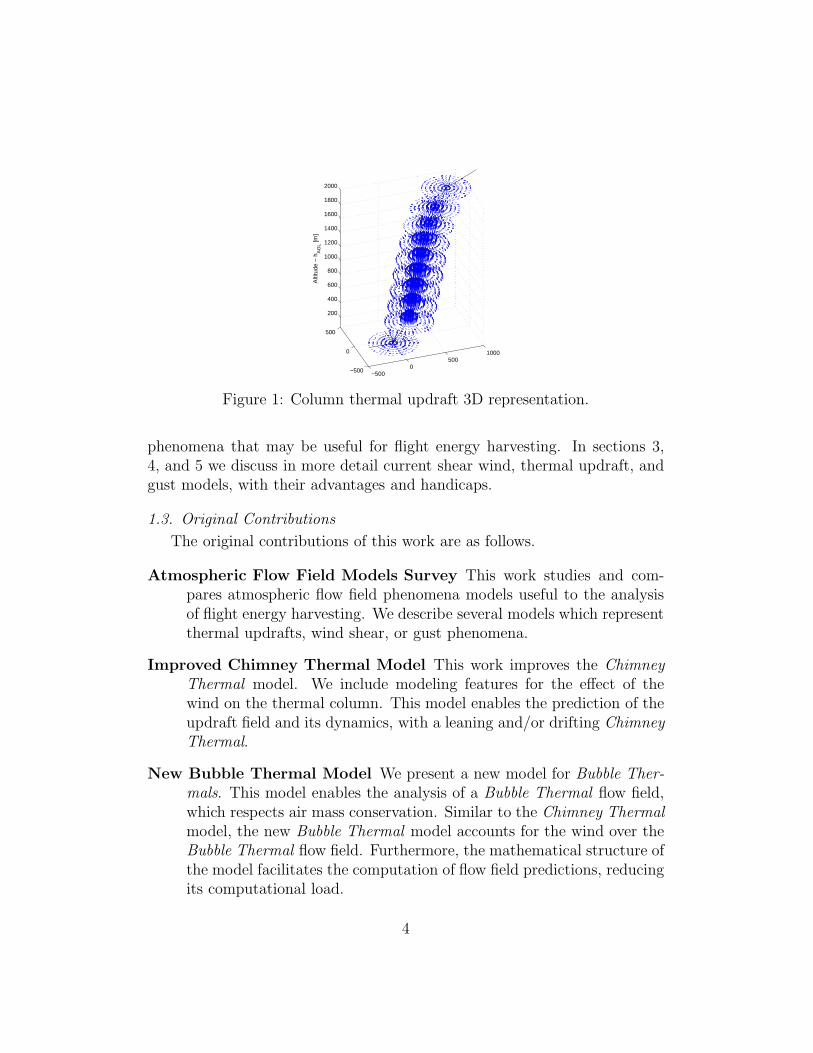
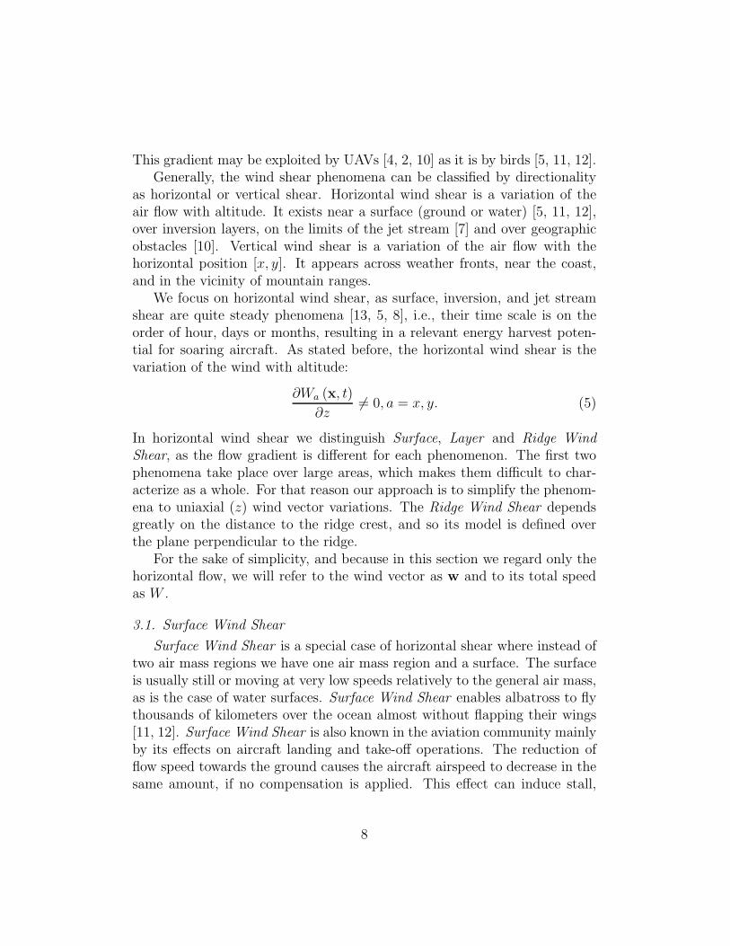
Thermals are updrafts (rising air masses) created by temperature vari-ations (fig. 1). Wind shear is an air layer which presents a flow gradient(fig. 2). It appears between fluid masses moving with different speeds orin different directions. Gusts are transitory phenomena associated with theatmospheric turbulence.

For thermals, there are simple models based on a Gaussian curve [1, 2] andmore detailed models describing Chimney Thermals [3] and Bubble Thermals[4]. None of these models predict the effects of the interaction of horizontalwind with the updraft flow field. Some are also unrealistic, in the sensethat they do not respect air mass conservation, predicting that more airascends than what descends. The studied atmospheric phenomena modelsare derived mainly from bird flight observations, glider pilot’s observationsand fluid dynamics theory.

There are several models for wind shear phenomena. The most widespreadis the Surface Wind Shear model [5, 6]. This model is mostly used to analyzethe effect of the wind gradient near the ground during takeoff and landingoperations. There are also general models [7, 8] for a constant wind gradientand quadratic models [9] that may represent either the constant wind gradi-ent or wind shear transitions with varying wind gradient. There is no modelto describe consistently the whole Layer Wind Shear with its transitions nearthe upper and lower air masses, and the core constant gradient. Also, thereis no model to predict the wind gradient generated at mountain ridges.

In the atmospheric modeling community, there is wealth of knowledgeprimarily about large scale phenomena, both in space and time. Nevertheless,we were unable to find a comprehensive survey of the particular flow field

3

−5000

5001000

−500

0

500

200

400

600

800

1000

1200

1400

1600

1800

2000

Alti

tude

− h

AG

L [m]

Figure 1: Column thermal updraft 3D representation.

phenomena that may be useful for flight energy harvesting. In sections 3,4, and 5 we discuss in more detail current shear wind, thermal updraft, andgust models, with their advantages and handicaps.

1.3. Original Contributions

The original contributions of this work are as follows.

Atmospheric Flow Field Models Survey This work studies and com-pares atmospheric flow field phenomena models useful to the analysisof flight energy harvesting. We describe several models which representthermal updrafts, wind shear, or gust phenomena.

Improved Chimney Thermal Model This work improves the ChimneyThermal model. We include modeling features for the effect of thewind on the thermal column. This model enables the prediction of theupdraft field and its dynamics, with a leaning and/or drifting ChimneyThermal.

New Bubble Thermal Model We present a new model for Bubble Ther-mals. This model enables the analysis of a Bubble Thermal flow field,which respects air mass conservation. Similar to the Chimney Thermalmodel, the new Bubble Thermal model accounts for the wind over theBubble Thermal flow field. Furthermore, the mathematical structure ofthe model facilitates the computation of flow field predictions, reducingits computational load.

4

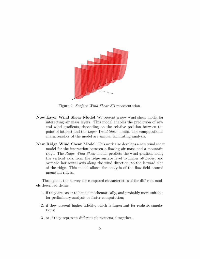
Figure 2: Surface Wind Shear 3D representation.

New Layer Wind Shear Model We present a new wind shear model forinteracting air mass layers. This model enables the prediction of sev-eral wind gradients, depending on the relative position between thepoint of interest and the Layer Wind Shear limits. The computationalcharacteristics of the model are simple, facilitating analysis.

New Ridge Wind Shear Model This work also develops a new wind shearmodel for the interaction between a flowing air mass and a mountainridge. The Ridge Wind Shear model predicts the wind gradient alongthe vertical axis, from the ridge surface level to higher altitudes, andover the horizontal axis along the wind direction, to the leeward sideof the ridge. This model allows the analysis of the flow field aroundmountain ridges.

Throughout this survey the compared characteristics of the different mod-els described define:

1. if they are easier to handle mathematically, and probably more suitablefor preliminary analysis or faster computation;

2. if they present higher fidelity, which is important for realistic simula-tions;

3. or if they represent different phenomena altogether.

5

We describe several thermal updraft models with different complexity andrealism levels. We compare the thermal updraft models over several charac-teristics, such as the updraft flow field shape and the relation between thethermal diameter and the updraft speed. The discussed model characteristicsare important to select adequate models for the analysis purpose and con-strains. As an example, if the analysis is only regarding the thermal updraftfield over a constant altitude horizontal plane, the full 3D structure of themodels may not be important, as well as the with influence on the verticalshape of the flow field.

We also present and compare several wind shear models. Some of thesemodels are more suitable for the analysis of general wind shear, others forwind shear affected by the terrain, and other for Layer Wind Shear. Similarto the thermal models, these models’ characteristics play a key role in theirselection to a certain analysis. As an example, one may prefer to use a generalwind shear model to characterize a short vertical range, due to its simplicity,or a more comprehensive model to capture the full vertical range gradient.

1.4. Paper structure

The remainder of this paper is as follows. We define a common nomen-clature for the flow field phenomena models in Section 2. Section 3 lays outthe wind shear models and compares them. We describe the thermal up-draft model in Section 4, where we also compare the models structures andfeatures. In Section 5 we discuss several gust models, with their advantagesand disadvantages. We close with the conclusions (Sec. 6) and an overviewof envisioned future work (Sec. 7).

1.5. Acronyms

AR Aspect Ratio

pdf probability density function

UAV Unmanned Aerial Vehicle

6

2. Atmospheric Phenomena

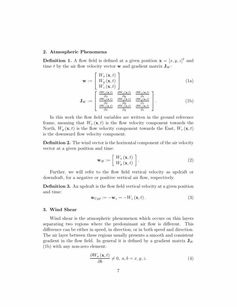
Definition 1. A flow field is defined at a given position x = [x, y, z]⊺ andtime t by the air flow velocity vector w and gradient matrix JW :

w :=

Wx (x, t)Wy (x, t)Wz (x, t)

(1a)

JW :=

∂Wx(x,t)∂x

∂Wx(x,t)∂y

∂Wx(x,t)∂z

∂Wy(x,t)∂x

∂Wy(x,t)∂y

∂Wy(x,t)∂z

∂Wz(x,t)∂x

∂Wz(x,t)∂y

∂Wz(x,t)∂z

. (1b)

In this work the flow field variables are written in the ground referenceframe, meaning that Wx (x, t) is the flow velocity component towards theNorth, Wy (x, t) is the flow velocity component towards the East, Wz (x, t)is the downward flow velocity component.

Definition 2. The wind vector is the horizontal component of the air velocityvector at a given position and time:

wH :=

[

Wx (x, t)Wy (x, t)

]

. (2)

Further, we will refer to the flow field vertical velocity as updraft ordowndraft, for a negative or positive vertical air flow, respectively.

Definition 3. An updraft is the flow field vertical velocity at a given positionand time:

wUpd := −wz = −Wz (x, t) . (3)

3. Wind Shear

Wind shear is the atmospheric phenomenon which occurs on thin layersseparating two regions where the predominant air flow is different. Thisdifference can be either in speed, in direction, or in both speed and direction.The air layer between these regions usually presents a smooth and consistentgradient in the flow field. In general it is defined by a gradient matrix JW(1b) with any non-zero element:

∂Wa (x, t)

∂b6= 0, a, b = x, y, z. (4)

7

This gradient may be exploited by UAVs [4, 2, 10] as it is by birds [5, 11, 12].Generally, the wind shear phenomena can be classified by directionality

as horizontal or vertical shear. Horizontal wind shear is a variation of theair flow with altitude. It exists near a surface (ground or water) [5, 11, 12],over inversion layers, on the limits of the jet stream [7] and over geographicobstacles [10]. Vertical wind shear is a variation of the air flow with thehorizontal position [x, y]. It appears across weather fronts, near the coast,and in the vicinity of mountain ranges.

We focus on horizontal wind shear, as surface, inversion, and jet streamshear are quite steady phenomena [13, 5, 8], i.e., their time scale is on theorder of hour, days or months, resulting in a relevant energy harvest poten-tial for soaring aircraft. As stated before, the horizontal wind shear is thevariation of the wind with altitude:

∂Wa (x, t)

∂z6= 0, a = x, y. (5)

In horizontal wind shear we distinguish Surface, Layer and Ridge WindShear, as the flow gradient is different for each phenomenon. The first twophenomena take place over large areas, which makes them difficult to char-acterize as a whole. For that reason our approach is to simplify the phenom-ena to uniaxial (z) wind vector variations. The Ridge Wind Shear dependsgreatly on the distance to the ridge crest, and so its model is defined overthe plane perpendicular to the ridge.

For the sake of simplicity, and because in this section we regard only thehorizontal flow, we will refer to the wind vector as w and to its total speedas W .

3.1. Surface Wind Shear

Surface Wind Shear is a special case of horizontal shear where instead oftwo air mass regions we have one air mass region and a surface. The surfaceis usually still or moving at very low speeds relatively to the general air mass,as is the case of water surfaces. Surface Wind Shear enables albatross to flythousands of kilometers over the ocean almost without flapping their wings[11, 12]. Surface Wind Shear is also known in the aviation community mainlyby its effects on aircraft landing and take-off operations. The reduction offlow speed towards the ground causes the aircraft airspeed to decrease in thesame amount, if no compensation is applied. This effect can induce stall,

8

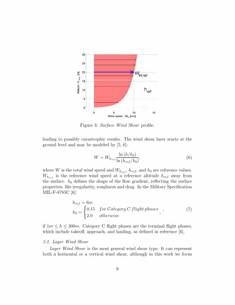
Figure 3: Surface Wind Shear profile.

leading to possibly catastrophic results. The wind shear layer starts at theground level and may be modeled by [5, 6]:

W =Whref

ln (h/h0)

ln (href/h0), (6)

where W is the total wind speed andWhref , href , and h0 are reference values.Whref is the reference wind speed at a reference altitude href away fromthe surface. h0 defines the shape of the flow gradient, reflecting the surfaceproperties, like irregularity, roughness and drag. In the Military SpecificationMIL-F-8785C [6]:

href = 6m

h0 =

0.15 for Category C flight phases

2.0 otherwise,, (7)

if 1m ≤ h ≤ 300m. Category C flight phases are the terminal flight phases,which include takeoff, approach, and landing, as defined in reference [6].

3.2. Layer Wind Shear

Layer Wind Shear is the most general wind shear type. It can representboth a horizontal or a vertical wind shear, although in this work we focus

9

on the horizontal shear. Two of the most common atmospheric phenom-ena associated with Layer Wind Shear are the Inversion Layer and the JetStream. An Inversion Layer is characterized by, as the name indicates, aninversion of the temperature gradient with altitude. Often the Convective orMixed-Layer, the lowest in the atmosphere, is separated from the upper Tro-posphere layers by an Inversion Layer. If the Inversion Layer is thin enoughand the flow of the separated air masses is different enough, the generatedgradient may be strong enough to provide aircraft with the energy necessaryto maintain flight. The Jet Stream phenomenon is characterized by a regionof high-speed winds. The regions between the Jet Stream core and slowerwind currents exhibit a wind gradient [8]. Glider pilots observe Layer WindShear sometimes above 3 knots per 1000 feet [13].

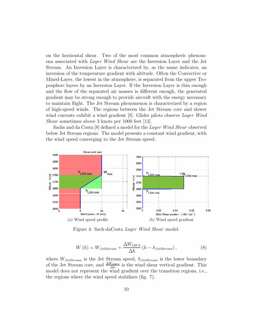
Sachs and da Costa [8] defined a model for the Layer Wind Shear observedbelow Jet Stream regions. The model presents a constant wind gradient, withthe wind speed converging to the Jet Stream speed:

(a) Wind speed profile (b) Wind speed gradient

Figure 4: Sach-daCosta Layer Wind Shear model.

W (h) =WJetStream +∆WLWS

∆h(h− hJetStream) , (8)

where WJetStream is the Jet Stream speed, hJetStream is the lower boundaryof the Jet Stream core, and ∆WLWS

∆his the wind shear vertical gradient. This

model does not represent the wind gradient over the transition regions, i.e.,the regions where the wind speed stabilizes (fig. 7).

10

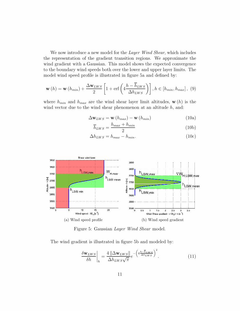
We now introduce a new model for the Layer Wind Shear, which includesthe representation of the gradient transition regions. We approximate thewind gradient with a Gaussian. This model shows the expected convergenceto the boundary wind speeds both over the lower and upper layer limits. Themodel wind speed profile is illustrated in figure 5a and defined by:

w (h) = w (hmin) +∆wLWS

2

[

1 + erf

(

4h− hLWS

∆hLWS

)]

, h ∈ [hmin, hmax] , (9)

where hmin and hmax are the wind shear layer limit altitudes, w (h) is thewind vector due to the wind shear phenomenon at an altitude h, and:

∆wLWS = w (hmax)−w (hmin) (10a)

hLWS =hmax + hmin

2(10b)

∆hLWS = hmax − hmin. (10c)

(a) Wind speed profile (b) Wind speed gradient

Figure 5: Gaussian Layer Wind Shear model.

The wind gradient is illustrated in figure 5b and modeled by:

δwLWS

δh

∣

∣

∣

∣

h

=4 ‖∆wLWS‖∆hLWS

√πe−

(

4h−hLWS∆hLWS

)2

. (11)

11

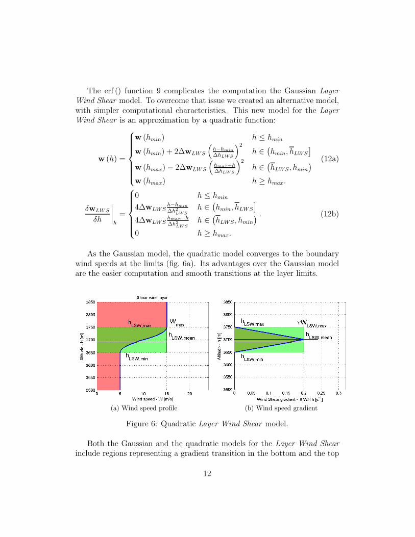
The erf () function 9 complicates the computation the Gaussian LayerWind Shear model. To overcome that issue we created an alternative model,with simpler computational characteristics. This new model for the LayerWind Shear is an approximation by a quadratic function:

w (h) =

w (hmin) h ≤ hmin

w (hmin) + 2∆wLWS

(

h−hmin

∆hLWS

)2

h ∈(

hmin, hLWS

]

w (hmax)− 2∆wLWS

(

hmax−h∆hLWS

)2

h ∈(

hLWS, hmin)

w (hmax) h ≥ hmax.

(12a)

δwLWS

δh

∣

∣

∣

∣

h

=

0 h ≤ hmin

4∆wLWSh−hmin

∆h2LWS

h ∈(

hmin, hLWS

]

4∆wLWShmax−h∆h2

LWS

h ∈(

hLWS, hmin)

0 h ≥ hmax.

. (12b)

As the Gaussian model, the quadratic model converges to the boundarywind speeds at the limits (fig. 6a). Its advantages over the Gaussian modelare the easier computation and smooth transitions at the layer limits.

(a) Wind speed profile (b) Wind speed gradient

Figure 6: Quadratic Layer Wind Shear model.

Both the Gaussian and the quadratic models for the Layer Wind Shearinclude regions representing a gradient transition in the bottom and the top

12

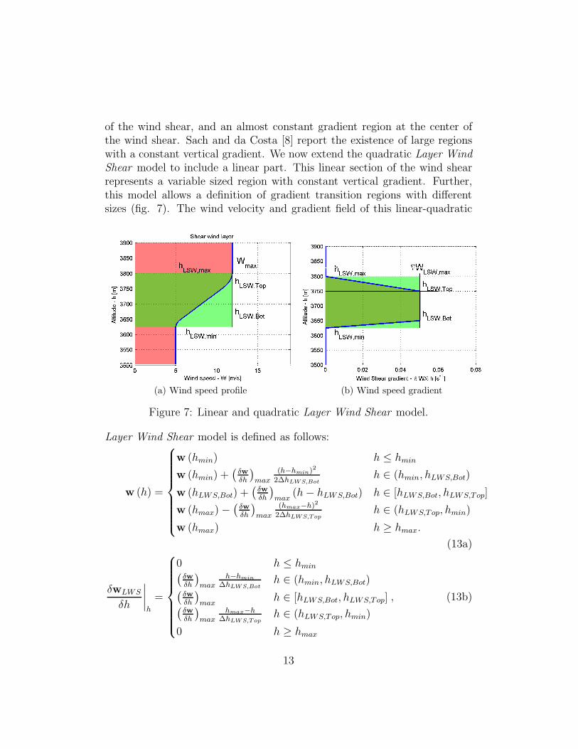
of the wind shear, and an almost constant gradient region at the center ofthe wind shear. Sach and da Costa [8] report the existence of large regionswith a constant vertical gradient. We now extend the quadratic Layer WindShear model to include a linear part. This linear section of the wind shearrepresents a variable sized region with constant vertical gradient. Further,this model allows a definition of gradient transition regions with differentsizes (fig. 7). The wind velocity and gradient field of this linear-quadratic

(a) Wind speed profile (b) Wind speed gradient

Figure 7: Linear and quadratic Layer Wind Shear model.

Layer Wind Shear model is defined as follows:

w (h) =

w (hmin) h ≤ hmin

w (hmin) +(

δwδh

)

max

(h−hmin)2

2∆hLWS,Both ∈ (hmin, hLWS,Bot)

w (hLWS,Bot) +(

δwδh

)

max(h− hLWS,Bot) h ∈ [hLWS,Bot, hLWS,Top]

w (hmax)−(

δwδh

)

max

(hmax−h)2

2∆hLWS,Toph ∈ (hLWS,Top, hmin)

w (hmax) h ≥ hmax.

(13a)

δwLWS

δh

∣

∣

∣

∣

h

=

0 h ≤ hmin(

δwδh

)

maxh−hmin

∆hLWS,Both ∈ (hmin, hLWS,Bot)

(

δwδh

)

maxh ∈ [hLWS,Bot, hLWS,Top]

(

δwδh

)

maxhmax−h

∆hLWS,Toph ∈ (hLWS,Top, hmin)

0 h ≥ hmax

, (13b)

13

where(

δwδh

)

maxis the maximum vertical gradient of the wind shear, hLWS,Bot

is the maximum altitude of the bottom gradient transition region, hLWS,Top

is the minimum altitude of the top gradient transition region, ∆hLWS,Bot

is the thickness of the bottom gradient transition region, ∆hLWS,Top is thethickness of the top gradient transition region, andw (hLWS,Bot) = w (hmin)+(

δwδh

)

max∆hLWS,Bot/2.

3.3. Ridge Wind Shear

The Ridge Wind Shear is a special case of the Layer Wind Shear, thatappears on the leeward side of a mountain. It is generated when the freemoving air finds a large obstacle (the ridge) and, while flowing over it, isnot capable of accelerating instantaneously the air mass behind the ridge.This wind shear type is the most used by radio controlled gliders, as it isstrong enough, maintains a constant position and the trajectory requiredto use it is safe enough to avoid ground collisions [10]. From Parle’s windvelocity measurements [10] it is clear that the vertical gradient appears overthe leeward side of the ridge.

We found no model in the literature representing the Ridge Wind Shearphenomenon. As such, we developed a new model based on Parle’s windvelocity measurements. The hypothetical model which approximately fitsParle’s data is defined as:

wRWS = w∞e−

λxW∞ +

(

1− e−λx

W∞

)

· wLWS (h)| hmin = hRidgehmax = hRidge + k1xw (hmin) = k2w∞

w (hmax) = w∞

, (14)

where wLWS (h) is the Layer Wind Shear gradient model. In this model thegradient strength varies as a first order response with the spatial coefficientλ. The gradient thickness is modeled as proportional (k1) to the distancefrom the ridge crest. The gradient bottom wind speed is proportional (k2)to the undisturbed wind speed (w∞). Note that this model has 3 degrees-of-freedom: λ, k1, and k2.

We now consider λ, k1, and k2 relationship with other physical variables.Given that we only have access to Parle’s wind velocity measurements, wecan only conjecture about this relationship. Our hypothetical interpretationis as follows. k1 is similar to the terrain slope on the windward side of theridge. Similarly, k2 is related with the terrain slope on the ridge leeward side.

14

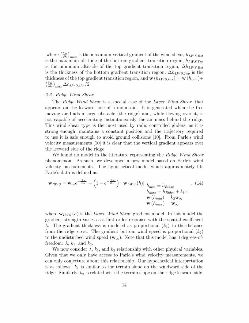
To the best of our knowledge, λ should depend on the ridge abruptness. Thismeans that a sharp ridge results in a larger λ.

(a) Wind speed profile (b) Wind speed gradient

Figure 8: Variation of wind speed over a Ridge Wind Shear with altitudeand distance to the ridge crest.

Figure 8 illustrates the wind speed variation within the Ridge Wind Shear.Notice the decrement of the minimum wind speed with the distance to theridge crest, modeled by the first order response. It is also clear that the windgradient is stronger closer to the ridge, indicating that this is the best areato harvest energy, as experienced by radio controlled glider pilots.

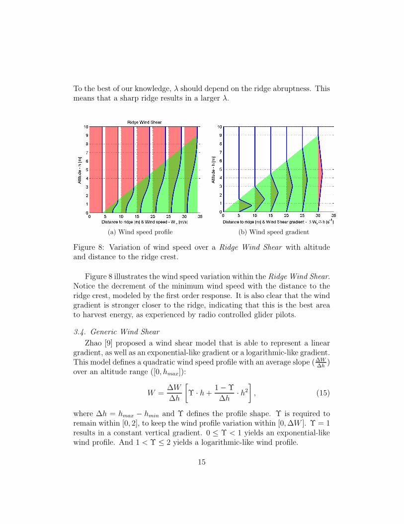
3.4. Generic Wind Shear

Zhao [9] proposed a wind shear model that is able to represent a lineargradient, as well as an exponential-like gradient or a logarithmic-like gradient.This model defines a quadratic wind speed profile with an average slope (∆W

∆h)

over an altitude range ([0, hmax]):

W =∆W

∆h

[

Υ · h+ 1−Υ

∆h· h2

]

, (15)

where ∆h = hmax − hmin and Υ defines the profile shape. Υ is required toremain within [0, 2], to keep the wind profile variation within [0,∆W ]. Υ = 1results in a constant vertical gradient. 0 ≤ Υ < 1 yields an exponential-likewind profile. And 1 < Υ ≤ 2 yields a logarithmic-like wind profile.

15

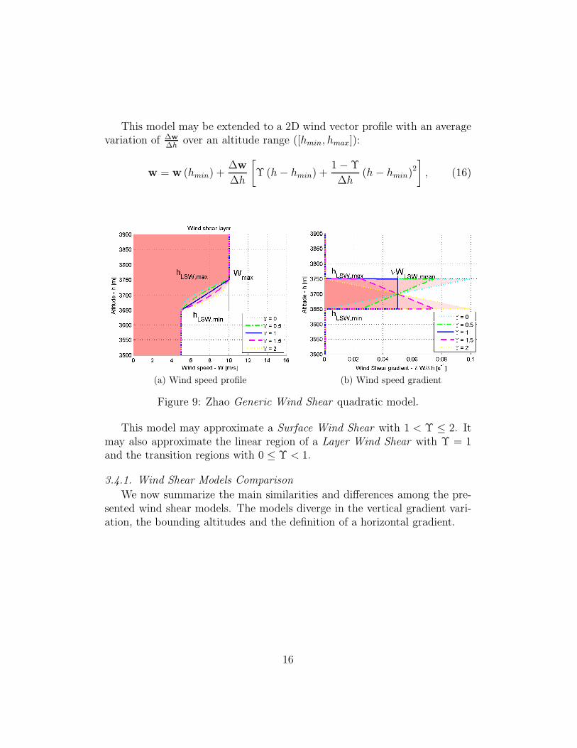
This model may be extended to a 2D wind vector profile with an averagevariation of ∆w

∆hover an altitude range ([hmin, hmax]):

w = w (hmin) +∆w

∆h

[

Υ (h− hmin) +1−Υ

∆h(h− hmin)

2

]

, (16)

(a) Wind speed profile (b) Wind speed gradient

Figure 9: Zhao Generic Wind Shear quadratic model.

This model may approximate a Surface Wind Shear with 1 < Υ ≤ 2. Itmay also approximate the linear region of a Layer Wind Shear with Υ = 1and the transition regions with 0 ≤ Υ < 1.

3.4.1. Wind Shear Models Comparison

We now summarize the main similarities and differences among the pre-sented wind shear models. The models diverge in the vertical gradient vari-ation, the bounding altitudes and the definition of a horizontal gradient.

16

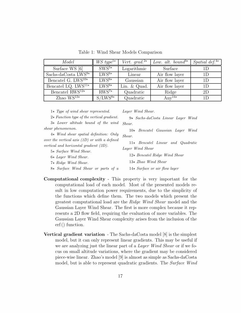
Table 1: Wind Shear Models Comparison

Model WS type1⋆ Vert. grad.2⋆ Low. alt. bound3⋆ Spatial def.4⋆

Surface WS [6] SWS5⋆ Logarithmic Surface 1DSachs-daCosta LWS9⋆ LWS6⋆ Linear Air flow layer 1DBencatel G. LWS10⋆ LWS6⋆ Gaussian Air flow layer 1DBencatel LQ. LWS11⋆ LWS6⋆ Lin. & Quad. Air flow layer 1DBencatel RWS12⋆ RWS7⋆ Quadratic Ridge 2D

Zhao WS13⋆ S/LWS8⋆ Quadratic Any14⋆ 1D

1⋆ Type of wind shear represented.

2⋆ Function type of the vertical gradient.

3⋆ Lower altitude bound of the wind

shear phenomenon.

4⋆ Wind shear spatial definition: Only

over the vertical axis (1D) or with a defined

vertical and horizontal gradient (2D).

5⋆ Surface Wind Shear.

6⋆ Layer Wind Shear.

7⋆ Ridge Wind Shear.

8⋆ Surface Wind Shear or parts of a

Layer Wind Shear.

9⋆ Sachs-daCosta Linear Layer Wind

Shear.

10⋆ Bencatel Gaussian Layer Wind

Shear.

11⋆ Bencatel Linear and Quadratic

Layer Wind Shear

12⋆ Bencatel Ridge Wind Shear

13⋆ Zhao Wind Shear

14⋆ Surface or air flow layer

Computational complexity - This property is very important for thecomputational load of each model. Most of the presented models re-sult in low computation power requirements, due to the simplicity ofthe functions which define them. The two models which present thegreatest computational load are the Ridge Wind Shear model and theGaussian Layer Wind Shear. The first is more complex because it rep-resents a 2D flow field, requiring the evaluation of more variables. TheGaussian Layer Wind Shear complexity arises from the inclusion of theerf () function.

Vertical gradient variation - The Sachs-daCosta model [8] is the simplestmodel, but it can only represent linear gradients. This may be useful ifwe are analyzing just the linear part of a Layer Wind Shear or if we fo-cus on small altitude variations, where the gradient may be consideredpiece-wise linear. Zhao’s model [9] is almost as simple as Sachs-daCostamodel, but is able to represent quadratic gradients. The Surface Wind

17

Shear may be represented by this quadratic approximation. Differ-ent parts of the Layer Wind Shear may also be represented by thismodel, but not the whole phenomenon. Zhao’s model may also be ad-equate when the goal is to observe a phenomenon for which there is nodetailed model, or parts of it. The Surface Wind Shear model [6] repre-sents the gradient through a logarithmic function, which is the widelyaccepted representation. The Ridge Wind Shear model uses the samegradient representation as the Layer Wind Shear model with a variablelayer thickness parameter, dependent on the horizontal distance to theridge. Both the Gaussian and Linear-Quadratic Layer Wind Shearmodels represent the whole Layer Wind Shear phenomenon, includingthe gradient variation at the bounding altitudes. The Linear-QuadraticLayer Wind Shear model is simpler to compute and allows the repre-sentation of regions with a linear gradient with an independent size,when compared to the global Layer Wind Shear thickness.

Model specificity - The only general models are the linear Sachs-daCostamodel [8] and Zhao’s quadratic model [9]. All other models are specificeither to Surface Layer or Ridge Wind Shear phenomena. Further,the Ridge Wind Shear model is the only one that defines a horizontalgradient together with the vertical gradient.

4. Updraft

Updrafts are upward moving air masses. These air masses can be smallupward gusts, created by turbulence, and ranging from centimeters to a fewmeters. Updrafts can also be the result of large rising air mass bodies, rangingfrom 50 meters to kilometers. These originate from terrain topography orfrom thermal flows. The first type, called orographic updrafts, are generatedwhen the wind hits a terrain slope, creating strong updrafts above the terrain.The thermal flows are generated by hot spots on the ground. These createa thermal gradient, heating the surrounding air. The density of the heatingair decreases, forcing an upward movement. Thermal updrafts don’t dependas much on topography or on wind as orographic updrafts.

Thermals are part of the convection flows that develop in the mixing-layerof the atmosphere, the lowest atmospheric layer, also called the convectivelayer. A thermal model may be characterized by three types of parameters:the atmosphere parameters, the internal parameters, and the terrain distri-bution. The atmosphere parameters characterize the regional environment

18

characteristics. These are the variables that are slow varying and very sim-ilar in adjacent flight areas. The internal parameters are individual to eachthermal. These parameters define the spatial effects of each specific thermal,and may be distinct for different adjacent thermals. The terrain distributionconcerns the sparsity among thermals, which affects the rate of appearanceof thermals in the aircraft flight path.

There are several types of thermals. Chimney Thermals, also designatedas Column Thermals, are continuous columns of rising air that extend fromthe ground surface right up to the mixing-layer maximum altitude. BubbleThermals are closed shells [14] of rising air. They are formed near the groundwhen the temperature differences are large enough to create buoyancy, likein a balloon. These shells then rise and depart from the ground. Cone[14] describes them as rising vortex rings, where there is a circulatory flowgenerated by a strong core updraft. This core updraft is fed by the buoyantair. When this air leaves the bubble core, it starts to cool down, becomingless buoyant. The cooled air then moves downward on the outside of thevortex ring, completing the cycle.

The main model features of a thermal are its position, the updraft field,representing how the vertical airspeed varies with the position relative to thethermal center, and its radius, defining where the updraft speed is null oralmost null. The models we will present next differ on three main modelingfeatures: the effect of altitude variation, the representation of the thermalskirt downdraft, and the interdependence among the updraft field and ther-mal radius.

4.1. Thermals

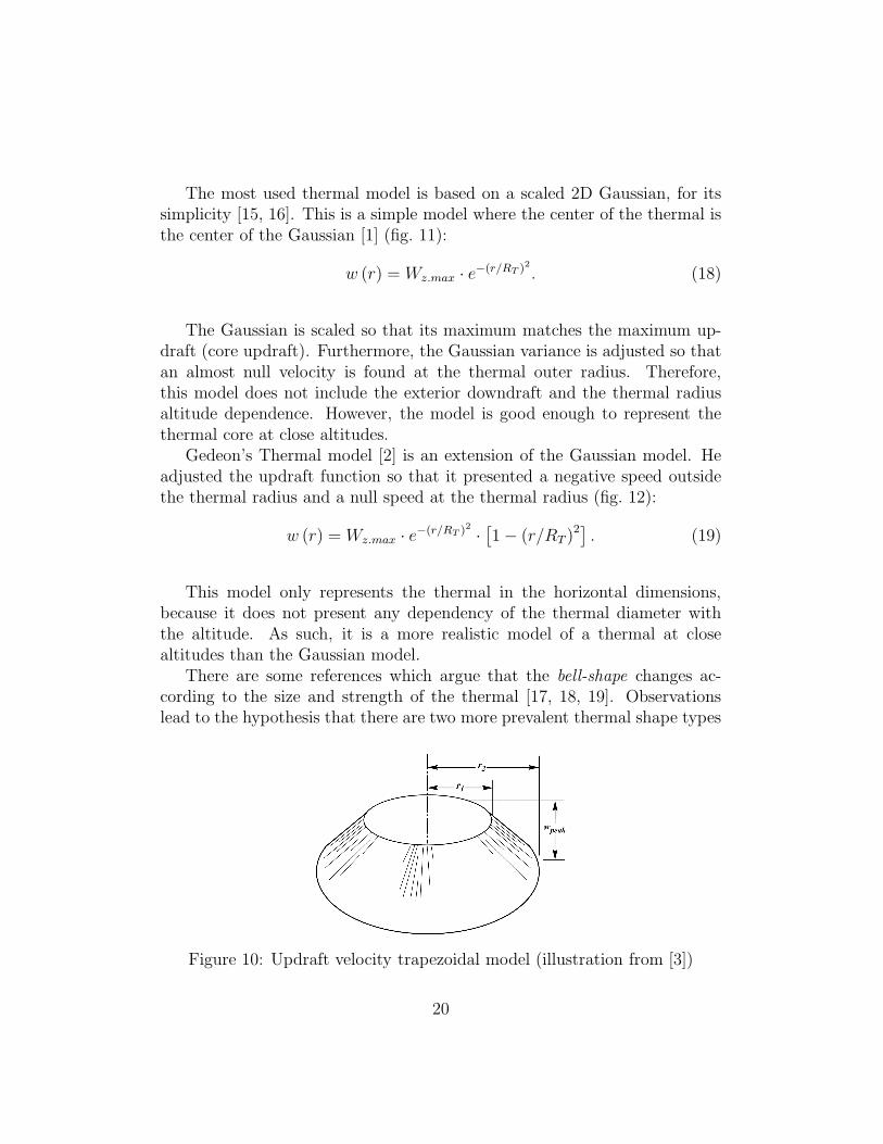
The simplest thermal model represents the updraft field as a 3D trapezoid,i.e., a conical trunk (Fig. 10). This model presents a core updraft, from thethermal center to its inner radius, and a decreasing updraft from the innerradius to the outer radius. Outside the thermal outer radius, there is novertical flow velocity. This model is defined by:

w (r) =

Wz.max r < r1

Wz.maxr2−rr2−r1

r ∈ [r1, r2]

0 otherwise

, (17)

where r is the distance from the thermal center, Wz.max is the core updraftspeed, r1 is the thermal inner radius, and r2 is the thermal outer radius.

19

The most used thermal model is based on a scaled 2D Gaussian, for itssimplicity [15, 16]. This is a simple model where the center of the thermal isthe center of the Gaussian [1] (fig. 11):

w (r) = Wz.max · e−(r/RT )2. (18)

The Gaussian is scaled so that its maximum matches the maximum up-draft (core updraft). Furthermore, the Gaussian variance is adjusted so thatan almost null velocity is found at the thermal outer radius. Therefore,this model does not include the exterior downdraft and the thermal radiusaltitude dependence. However, the model is good enough to represent thethermal core at close altitudes.

Gedeon’s Thermal model [2] is an extension of the Gaussian model. Headjusted the updraft function so that it presented a negative speed outsidethe thermal radius and a null speed at the thermal radius (fig. 12):

w (r) = Wz.max · e−(r/RT )2 ·[

1− (r/RT )2] . (19)

This model only represents the thermal in the horizontal dimensions,because it does not present any dependency of the thermal diameter withthe altitude. As such, it is a more realistic model of a thermal at closealtitudes than the Gaussian model.

There are some references which argue that the bell-shape changes ac-cording to the size and strength of the thermal [17, 18, 19]. Observationslead to the hypothesis that there are two more prevalent thermal shape types

Figure 10: Updraft velocity trapezoidal model (illustration from [3])

20

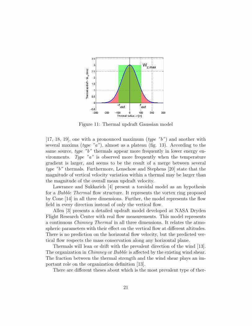
Figure 11: Thermal updraft Gaussian model

[17, 18, 19], one with a pronounced maximum (type ”b”) and another withseveral maxima (type ”a”), almost as a plateau (fig. 13). According to thesame source, type ”b” thermals appear more frequently in lower energy en-vironments. Type ”a” is observed more frequently when the temperaturegradient is larger, and seems to be the result of a merge between severaltype ”b” thermals. Furthermore, Lenschow and Stephens [20] state that themagnitude of vertical velocity variation within a thermal may be larger thanthe magnitude of the overall mean updraft velocity.

Lawrance and Sukkarieh [4] present a toroidal model as an hypothesisfor a Bubble Thermal flow structure. It represents the vortex ring proposedby Cone [14] in all three dimensions. Further, the model represents the flowfield in every direction instead of only the vertical flow.

Allen [3] presents a detailed updraft model developed at NASA DrydenFlight Research Center with real flow measurements. This model representsa continuous Chimney Thermal in all three dimensions. It relates the atmo-spheric parameters with their effect on the vertical flow at different altitudes.There is no prediction on the horizontal flow velocity, but the predicted ver-tical flow respects the mass conservation along any horizontal plane.

Thermals will lean or drift with the prevalent direction of the wind [13].The organization in Chimney or Bubble is affected by the existing wind shear.The fraction between the thermal strength and the wind shear plays an im-portant role on the organization definition [13].

There are different theses about which is the most prevalent type of ther-

21

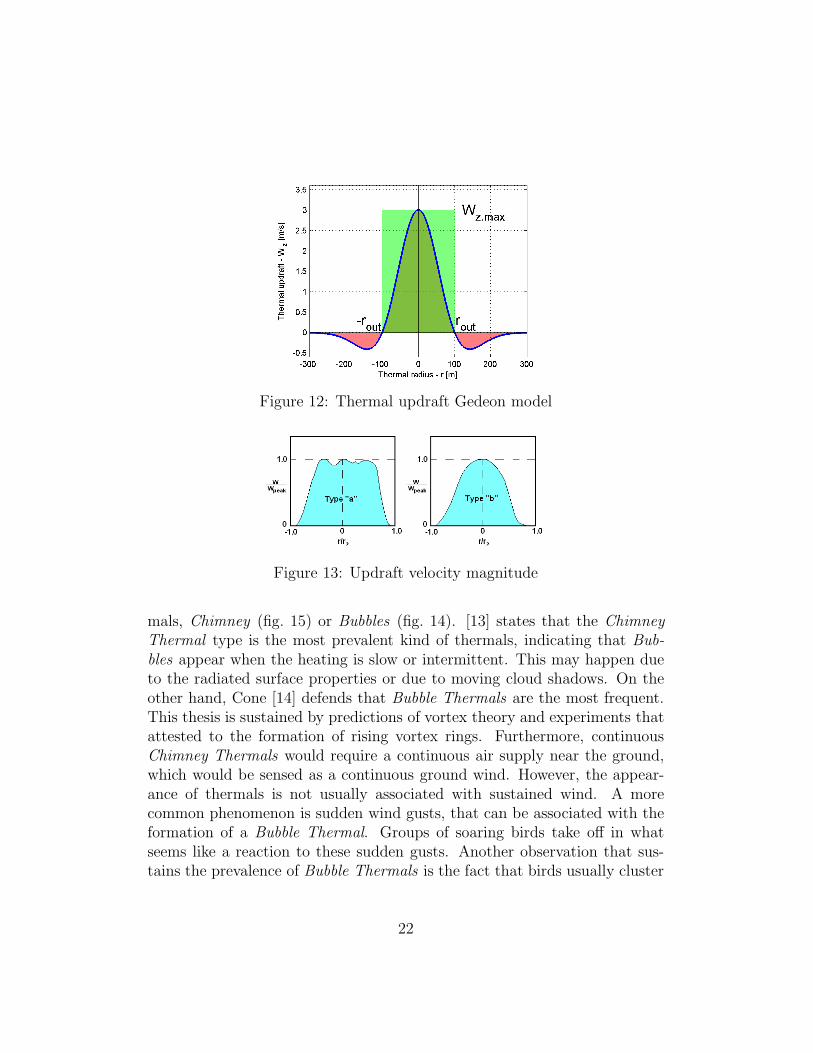
Figure 12: Thermal updraft Gedeon model

Figure 13: Updraft velocity magnitude

mals, Chimney (fig. 15) or Bubbles (fig. 14). [13] states that the ChimneyThermal type is the most prevalent kind of thermals, indicating that Bub-bles appear when the heating is slow or intermittent. This may happen dueto the radiated surface properties or due to moving cloud shadows. On theother hand, Cone [14] defends that Bubble Thermals are the most frequent.This thesis is sustained by predictions of vortex theory and experiments thatattested to the formation of rising vortex rings. Furthermore, continuousChimney Thermals would require a continuous air supply near the ground,which would be sensed as a continuous ground wind. However, the appear-ance of thermals is not usually associated with sustained wind. A morecommon phenomenon is sudden wind gusts, that can be associated with theformation of a Bubble Thermal. Groups of soaring birds take off in whatseems like a reaction to these sudden gusts. Another observation that sus-tains the prevalence of Bubble Thermals is the fact that birds usually cluster

22

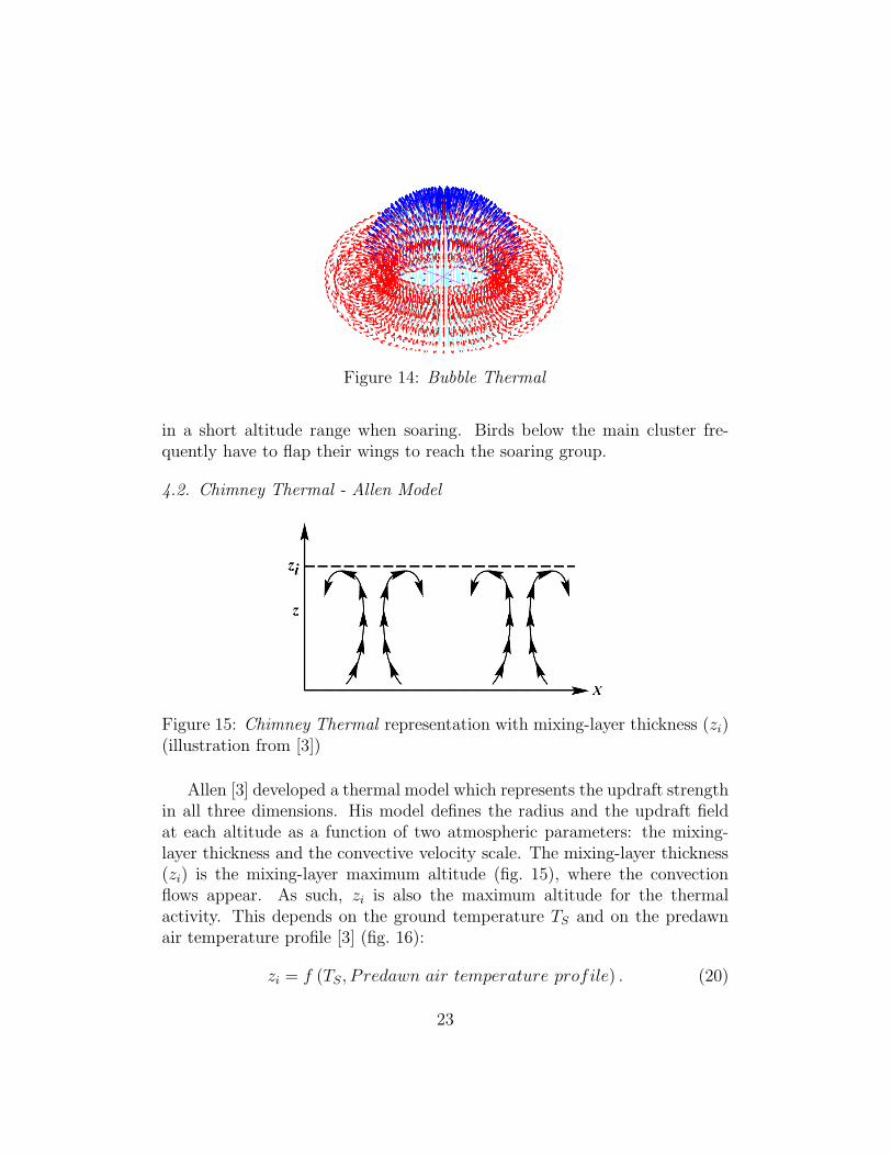
Figure 14: Bubble Thermal

in a short altitude range when soaring. Birds below the main cluster fre-quently have to flap their wings to reach the soaring group.

4.2. Chimney Thermal - Allen Model

Figure 15: Chimney Thermal representation with mixing-layer thickness (zi)(illustration from [3])

Allen [3] developed a thermal model which represents the updraft strengthin all three dimensions. His model defines the radius and the updraft fieldat each altitude as a function of two atmospheric parameters: the mixing-layer thickness and the convective velocity scale. The mixing-layer thickness(zi) is the mixing-layer maximum altitude (fig. 15), where the convectionflows appear. As such, zi is also the maximum altitude for the thermalactivity. This depends on the ground temperature TS and on the predawnair temperature profile [3] (fig. 16):

zi = f (TS, P redawn air temperature profile) . (20)

23

Table 2: Yearly convective lift statistical properties (from reference [3])

Description w⋆, m/s µzi − σzi , m µzi, m µzi + σzi , m

µw⋆ − 2σw⋆ 0.46 25.6 53.6 97.4µw⋆ − σw⋆ 1.27 150 210 1007

µw⋆ 2.56 767 1401 2319µw⋆ + σw⋆ 4.08 2134 2819 3638µw⋆ + 2σw⋆ 5.02 2913 3647 4495

The mixing-layer thickness (zi) varies slowly with the location, presentinga low spatial variation frequency. The thickness is usually 0 at dawn, rises tothe day maximum at late afternoon [17] and returns to 0 during the night.Therefore, the regional variation time constant should be high, on the orderof hours.

The convective velocity scale (w⋆) is a reference which indicates the pre-dicted velocity magnitudes in and around a thermal. Again reference [3]shows that this velocity is a function of the mixing-layer thickness (zi), thesurface virtual potential temperature flux (QOV ), the ground temperatureTS, and the static pressure at ground level (p) [3]. Furthermore, the virtualpotential temperature flux is a function of the net radiation at the surface(QS), the air relative humidity (rh), the saturated vapor pressure (es), andthe ground temperature TS.

w⋆ seems to have a spatial and temporal dependency similar to zi. Theonly extra factor is the wind speed, which seems to disrupt any thermal ifblowing above 12.87 m/s (in the Mojave Desert [3]), but also favors organizedthermal convection if above 5 m/s [13].

Allen [3] describes the yearly and monthly statistics for w⋆ and zi in DesertRock, Nevada. Table 2 show the yearly statistics. These statistics are im-portant to inference processes as a prior belief, e.g., for thermals parametersestimation.

The internal parameters are: the outer radius, and the vertical flow field,with:

wT ∼ w∗ (21a)

r2 ∼ zi. (21b)

The outer radius varies from thermal to thermal, and inside the thermal

24

Table 3: Shape constants for bell-shaped vertical velocity distribution [3]

r1r2

k1 k2 k3 k4

0.14 1.5352 2.5826 -0.0113 0.00080.25 1.5265 3.6054 -0.0176 0.00050.36 1.4866 4.8354 -0.0320 0.00010.47 1.2042 7.7904 0.0848 0.00010.58 0.8816 13.972 0.3404 0.00010.69 0.7067 23.994 0.5689 0.00020.80 0.6189 42.797 0.7157 0.0001

with the altitude above the ground. Lenschow and Stephens [20] state thatthe thermal radius average at a certain altitude is a direct function of themixing-layer thickness (zi), by (fig. 17):

r2 = max

[

10, 0.2513

(

z

zi

)1

3

(

1− 0.25z

zi

)

· zi]

. (22)

Note that multiplier 0.2513 is different from the one used by Allen [3], as thisauthor corrected the calculations later on.

The equation governing the vertical velocity is [3]:

w = wpeak

1

1 +∣

∣

∣k1

rr2+ k3

∣

∣

∣

k2+ k4

r

r2+ wD

(

1− wewpeak

)

+ we. (23)

The constants k1, k2, k3, and k4 are defined in table 3.The variables wpeak, wD, we, and r1 are defined next. We first define the

average updraft speed function (fig. 19):

w = w⋆(

z

zi

)1

3

(

1− 1.1z

zi

)

. (24)

Now, the radius for which the updraft speed is almost constant (r1) comesfrom

r1r2

=

0.0011r2 + 0.14 r2 < 600

0.8 otherwise. (25)

25

The maximum updraft speed (wpeak) is defined as

wpeak = w3r22 (r2 − r1)

r32 − r31. (26)

The skirt downdraft speed (wD) is computed by

wD =

w5π12

(

zzi− 0.5

)

sin(

πrr2

)

r ∈ (r1, 2r2) ∨ zzi∈ (0.5, 0.9)

0 otherwise. (27)

To maintain a null regional net vertical velocity, we have to define the naturalsink speed (we) as:

we = −w Nπr22Areg −Nπr22

·

[

1− 2.5(

zzi− 0.5

)]

zzi∈ (0.5, 0.9)

1 otherwise, (28)

where Areg is the affected region.

4.2.1. Chimney Thermal - Interaction with the Wind

There are three main effects the wind may have on Chimney Thermals.Wind seems to be fully disruptive for the thermals if blowing faster than 13m/s. If it is slower, it may lean the thermal, move it, or both. The thermaldrift depends both on the wind speed and on the terrain radiating properties.The drift velocity generally follows the prevailing wind, but not always [3].If the terrain radiating properties are very uneven there is a tendency forthe thermal to stay anchored to the most radiating points, usually calledhot-spots, such as rocks, building roofs, asphalt, etc. When the thermalsource, the lowest section of the thermal, is anchored to a hot spot or movesslower than the wind speed, the thermal has the tendency to lean to theleeward direction (fig. 20). During a thermal soaring flight thermal leaningis sometimes wrongly perceived as a drift by the whole thermal.

We now extend Allen’s Chimney Thermal to account for these wind effectson the 3D flow field structure and dynamics. In this model the movementdynamics of a Chimney Thermal are captured by:

xT = uT = VT cosψT (29a)

yT = vT = VT sinψT (29b)

VT ∼ N (µVT , σVT ) , µVT ∈ [0, ‖w‖] (29c)

ψT ∼ N (µψT, σψT

) , (29d)

26

where xT and yT are the Chimney Thermal source position coordinates, uTand vT are the Chimney Thermal source drift velocities, µVT and σVT are thethermal drift speed mean and standard deviation and µψT

and σψTare the

thermal drift direction probability parameters.The Chimney Thermal leaning may be characterized by the change in

the updraft core center for different altitudes:

xt (H) ≈ xT +

H∫

0

W x (h)− uT

W T,z (h)dh (30a)

yt (h) ≈ yT +

H∫

0

W y (h)− vT

W T,z (h)dh, (30b)

where xt (H) represents the updraft core center coordinates at an altitudeabove the ground H , W x (h) and W y (h) are the mean wind velocities awayfrom the thermal at each altitude h, and W T,z (h) = w is the updraft meanspeed at each altitude h. From this equation it is clear that the thermal willnot lean if the source is moving at the same velocity as the wind. As statedbefore, and because Chimney Thermal movements depend on the terrain,the thermal will present some leaning associated with some drift.

4.3. Bubble Thermal - Lawrance Model

Lawrance [4] developed a Bubble Thermal model. Unlike the ChimneyThermal model developed by Allen, this model describes an unsteady upwardmoving phenomenon. In this model the hotter air mass rises in a bubble likestructure, disconnected from the ground or the inversion layer. The modeldescribed in [4] defines a toroidal 3D flow field at a given instant (Fig. 21).The flow field model created by Lawrance is defined by:

wx = −wzz

(dH − R) · k2x

dH(31a)

wy = −wzz

(dH − R) · k2y

dH(31b)

wz =

wcore x = 0cos(1+ πz

k·R)2

R·wcore

πdHsin

(

πdHR

)

dH ∈ (0, 2R]

0 otherwise

, (31c)

(31d)

27

where dH =√

x2 + y2, wcore is the bubble core updraft speed, R is thedistance which limits the updraft area, i.e., the area around the bubble centerwhere the flow moves upwards, x, y, and z are positions relative to the bubblecenter, and k is the bubble eccentricity factor, i.e., k =

∆zflow2R

, where ∆zflowis the bubble height.

4.3.1. Bubble Thermal - Conservative Flow Model

The Lawrance Bubble Thermal model is not mass conservative, does notinclude any effects of the interaction with the prevailing wind, and does notpresent the possibility to represent an updraft core plateau described bysome authors. Figure 22 illustrates some of the models we developed to tryand overcome some of these issues. The bubble flow is only conservativeif the whole bubble region can be described by streamlines, i.e., the lines”followed” by air particles in the absence of disturbances. The first twomodels are adaptations of the toroid streamline model on which the Lawrancemodel is also based. The first model (fig. 22a) presents sharp flow directionchanges which are not realistic at all, as they would require infinite flowacceleration at those points. The second model (fig. 22b) presents morerealistic streamlines. The two main handicaps are the complex computationof some of the parameters, when taking a relative position as an input, andthe lack of flow near the top and the bottom of the bubble. In the nextstreamline model we drop the constraint for all the streamlines to be centeredat the toroid center, i.e., at the updraft outer radius on the mean bubblealtitude plane. Instead, we define the streamlines’ center to tend to the toroidcenter as they approach it. The third model (fig. 22c) presents nice propertiesin terms of parameter computation, when taking a relative position as aninput, but presents no flow near the bubble axis, when away from the centralplane. The final model (fig. 22d) presents a flow tending to vertical near thebubble axis, a vortex around the updraft outer radius, and is conservativein terms of mass exchange. The computation of the streamline parametersrequires an iterative process when the input to define those parameters is arelative position to the bubble center. This is shown below in equation (32).

The final model presents a flow tending to vertical near the bubble axis,as we define that the streamlines center should tend to infinite as those ap-proach the bubble axis. We also define that the streamlines’ direction shouldbe perpendicular to a circle at a distance RT from the bubble center (fig. 23),where RT is the Bubble Thermal updraft outer radius. The streamline pa-

28

rameters are then defined as:

rmax =R2T

rmin(32a)

rctr =rmax + rmin

2=

RT

cos ξ(32b)

Rstream =rmax − rmin

2= RT tan ξ (32c)

dH = rmax −∆z tan ζ (32d)

∆z = (dH − rmin) tan ζ (32e)

R2T

rmin+ rmin =

∆z2 + d2H +R2T

dH, (32f)

where rmin and rmax are the minimum and maximum distances of the stream-line to the Bubble Thermal axis, rctr is the streamline center distance to theBubble Thermal axis, Rstream is the streamline radius, dH =

√

∆x2 +∆y2

is the horizontal distance of a point to the Bubble Thermal axis, ∆x, ∆y,and ∆z are the coordinates of the relative position to the Bubble Thermalcenter, ξ is the ”exit” angle of the flow at a distance RT from the bubblecenter, and ζ is the angle of a point relative to the streamline center (fig. 24).The parameter iteration need arises from rmin being defined by the implicitfunction (32f).

We may also define the streamlines such that the flow is perpendicularto an ellipse, which crosses the bubble horizontal plane at the updraft outerradius RT . The streamline parameter may then be computed by solving:

rmax =R2T

(

1− e2 sin2 ξ)

rmin. (33)

To define the flow speed over each streamline, such that it presents amass conservative flow, the volume rate has to be constant through eachstreamline:

V = cst = vrπdA⇔ v1r1 = v2r2, (34)

where V is the volume rate, v is the flow total speed, and dA is an infinitesimalarea on the r − z plane centered at radius r(.). This yields a flow speed overa streamline defined by:

W2 =W1dH,2dH,1

, (35)

29

where W(.) are total flow speeds at points 1 and 2 with horizontal distancesdH,(.) from the bubble central axis. Combining (35) with the streamlineorientation at each point from (32), the flow velocity vector at each pointmay be defined as:

w = Wz,rmin,∆z=0rmindH

sin ζ∆xdh

sin ζ∆ydh

cos ζ

. (36)

To solve (36) and completely define the Bubble Thermal flow field one justneeds to define an updraft field at the bubble mean altitude (Wz,rmin,∆z=0).We considered three different hypotheses. The first is based on the flow fielddefined by Lawrance [4], constrained to dH ∈ [0, RT ] and ∆z = 0:

Wz,dH ,∆z=0 =

wcore dH = 0

wcore

π

(

RT

dH

)δFlat

sin

(

π(

RT

dH

)δFlat

)

dH ∈ (0, RT ], (37)

where wcore is a positive value defining the maximum updraft speed and δF latregulates the flatness of the updraft core and the abruptness of the updraftreduction towards to outer radius, as shown on figure 25.

The second model is based on the Gedeon updraft field [2], also con-strained to dH ∈ [0, RT ] and ∆z = 0:

Wz,dH ,∆z=0 = wcoree−(dH/RT )2δF lat ·

[

1− (dH/RT )2δFlat

]

, (38)

where wcore and δF lat are the same as in the first model.The last model, Plateau Updraft, is an extension of the second, with a

core constant updraft:

Wz,dH ,∆z=0 =

wcore dH ≤ RP lat

wcoree−δR · [1− δR] dH ∈ (RP lat, RT ]

(39a)

with δR =

(

dH − RP lat

RT −RP lat

)2δFlat

, (39b)

where RP lat is the core updraft plateau radius. This may be defined as inthe Chimney model by equation (25):

RP lat

RT

=

0.0011RT + 0.14 RT < 600

0.8 otherwise. (40)

30

Figure 26 illustrates all three models showing that there is almost no dif-ference between the Lawrance and the Gedeon models. It also shows thatthe plateau size control on the last model gives the user an extra degree-of-freedom, possibly allowing a better match between the model and realobservations.

The resulting Bubble Thermal flow field is depicted in figure 27. It isvery clear that the flow closest to the bubble axis is almost vertical, whilenear the updraft outer radius it turns into a vortex. The continuous natureof this model is also apparent. Figure 28 illustrates the main components ofthe Bubble Thermal, including the core updraft and the surrounding vortex,as proposed by Cone [14].

As Bubble Thermals are usually completely detached from the groundthey are more affected by the prevailing wind than the Chimney Thermals.The Bubble Thermals center velocity is defined as:

xT = uT = VT cosψT (41a)

yT = vT = VT sinψT (41b)

zT = wT (41c)

VT ∼ N (µVT , σVT ) , µVT = ‖w‖ (41d)

ψT ∼ N (µψT, σψT

) , (41e)

where xT , yT , and zT are the Bubble Thermal center coordinates, uT , vT ,and wT are the Bubble Thermal center drift velocities, µVT and σVT are thethermal drift speed mean and standard deviation and µψT

and σψTare the

thermal drift direction probability parameters.If the Bubble Thermal moves with a difference velocity from the prevailing

wind, its structure leans. The combined flow field from a Bubble Thermaland the prevailing wind is defined by:

w =Wz,rmin,∆z=0rmind′H

sin ζ ′∆x′

d′H

+ lx cos ζ′

sin ζ ′∆y′

d′H

+ ly cos ζ′

cos ζ ′

+

W x

W y

0

, (42)

where

lx =uT −W x

wT − wcore(43a)

lx =vT −W y

wT − wcore, (43b)

31

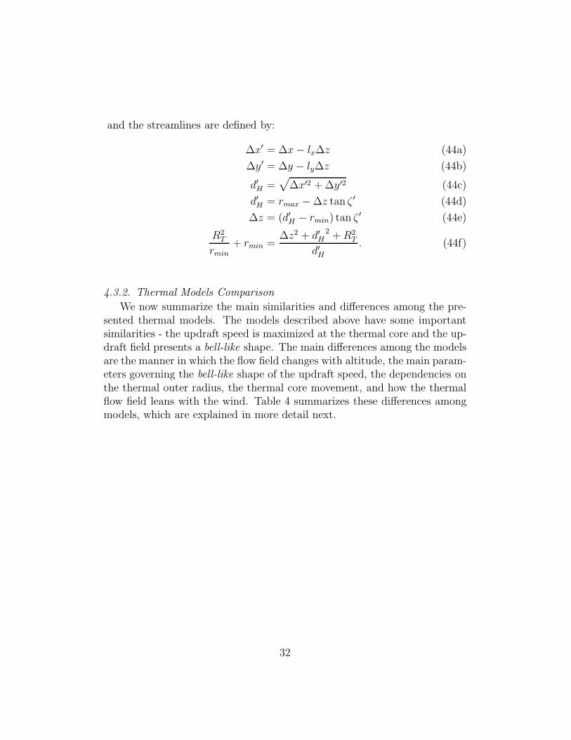
and the streamlines are defined by:

∆x′ = ∆x− lx∆z (44a)

∆y′ = ∆y − ly∆z (44b)

d′H =√

∆x′2 +∆y′2 (44c)

d′H = rmax −∆z tan ζ ′ (44d)

∆z = (d′H − rmin) tan ζ′ (44e)

R2T

rmin+ rmin =

∆z2 + d′H2 +R2

T

d′H. (44f)

4.3.2. Thermal Models Comparison

We now summarize the main similarities and differences among the pre-sented thermal models. The models described above have some importantsimilarities - the updraft speed is maximized at the thermal core and the up-draft field presents a bell-like shape. The main differences among the modelsare the manner in which the flow field changes with altitude, the main param-eters governing the bell-like shape of the updraft speed, the dependencies onthe thermal outer radius, the thermal core movement, and how the thermalflow field leans with the wind. Table 4 summarizes these differences amongmodels, which are explained in more detail next.

32

Table 4: Thermal models comparison

Model Dim Downdraft Flat core Mix. layer1⋆ Type

Toroidal [3] 2D No Yes Independent No type

Gaussian [1] 2D No No Independent No typeGedeon [2] 2D Constrained3⋆ No Independent No typeAllen [3] 3D Extended4⋆ Yes Dependent Chimney

Bencatel Mov. Chimn.6⋆ 3D Extended4⋆ Yes Dependent ChimneyLawrance [4] 3D Constrained3⋆ No Independent Bubble

Bencatel Cons. Bubb.7⋆ 3D Extended4⋆ Choice5⋆ Independent Bubble

Model Flow Field2⋆ Conservative Leaning Movement

Toroidal [3] Vertical No No No

Gaussian [1] Vertical No No NoGedeon [2] Vertical No No NoAllen [3] Vertical Yes No No

Bencatel Mov. Chimn.6⋆ Vertical Yes Yes YesLawrance [4] 3D No No No

Bencatel Cons. Bubb.7⋆ 3D Yes Yes Yes

1⋆ Mixing layer parameters - Thermal flow field dependence on the Mixing layer pa-

rameters.

2⋆ Flow Field representation: Only vertical component or full 3D flow field represen-

tation.

3⋆ Downdraft constrained to the thermal rim.

4⋆ Downdraft extended to the thermal surrounding area, beyond the thermal rim.

5⋆ The user can choose if there is a flat plateau and/or the flatness/abruptness of the

whole bell-shape updraft.

6⋆ Bencatel Moving Chimney

7⋆ Bencatel Conservative Bubble

Altitude handling - Both Chimney Thermal and Bubble Thermal modelsincorporate variation with altitude. By contrast, the Toroidal, theGaussian, and the Gedeon models are invariant with altitude, as shownin figure 30. The Allen model simulates a Chimney type thermal,where the thermal extends from the ground to the top of the mixing-layer (fig. 30a). In figure 30a it is possible to see the updraft speed andouter radius dependence over the altitude range. In the Bubble Thermal

33

models the updraft region is limited to the mixing-layer, but may notreach either the ground or the top of the mixing layer (fig. 30b). Inthe Allen Chimney Thermal model, the updraft speed depends on thealtitude. By contrast, the Lawrance Bubble Thermal model defines afixed outer radius. The conservative Bubble Thermal models present avariable outer updraft radius, but this variation is distinctly differentfrom the one defined by the Allen model.

Bell-like shape - All models present a Bell-like shape with some differ-ences. The Allen Chimney Thermal model (fig. 31a) presents an up-draft core with skirt downdrafts. In volumetric terms, the updraft anddowndraft cancel each other, presenting a conservative airmass flow.Further, it shows a flat core for large diameter thermals. This shape isbased on real observations as described by Irving [21]. The maximumupdraft is not constant, decreasing as the outer diameter increases.The Lawrance Bubble Thermal model (fig. 31b) also presents a centralupdraft and exterior downdrafts. Unlike the downdrafts from the othermodels, in this model the negative vertical flow is constrained to a dis-tance twice the outer radius. Moreover, the flow is only conservative atthe bubble mean altitude, no flat core is modeled, and the maximumupdraft only varies with altitude and not with the outer diameter. Theconservative Bubble Thermal models present a mass conservative flow,with the downdraft extending to infinity, but decreasing with the dis-tance to the bubble center. The core updraft also changes with altitude,although it covers different radii for both models. The conservativeBubble Thermal model with a Lawrance updraft field (fig. 31c) showsno flat core, while the one with the Plateau Updraft (fig. 31d) definesa near flat core. The Toroidal, the Gaussian-shape and the Gedeonmodels are simplifications which present the core updraft. The onlydifference between the Gaussian-shape and the Gedeon models is thepresence of a skirt downdraft on the last. These three models are notflow conservative and their maximum updraft is always constant, withrespect to the altitude and outer diameter.

34

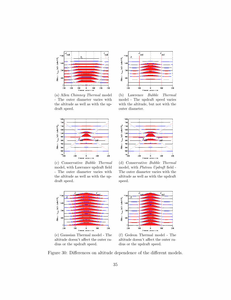
(a) Allen Chimney Thermal model- The outer diameter varies withthe altitude as well as with the up-draft speed.

(b) Lawrence Bubble Thermalmodel - The updraft speed varieswith the altitude, but not with theouter diameter.

(c) Conservative Bubble Thermalmodel, with Lawrance updraft field- The outer diameter varies withthe altitude as well as with the up-draft speed.

(d) Conservative Bubble Thermalmodel, with Plateau Updraft field -The outer diameter varies with thealtitude as well as with the updraftspeed.

(e) Gaussian Thermal model - Thealtitude doesn’t affect the outer ra-dius or the updraft speed.

(f) Gedeon Thermal model - Thealtitude doesn’t affect the outer ra-dius or the updraft speed.

Figure 30: Differences on altitude dependence of the different models.

35

Outer radius - For most of the models the outer radius represents the dis-tance to the core where the vertical flow is inverted, turning from up-draft to downdraft. That is the case for the Bubble Thermal models, theToroidal model, and the Gedeon model. Further, in the Bubble Ther-mal models the outer radius at the Bubble mean altitude also indicatesthe center for the toroid vortex. Both the Allen and the ConservativeBubble Thermal models have the mean updraft strength as a functionof the outer radius, and outer radius a function of the altitude. In theAllen model the flow field at the outer radius is almost null, but notquite. In the Gaussian model the outer radius is just a measure of theradial spread of the updraft.

36

(a) Allen Chimney Thermal model -Presents a constant updraft speed at thecore for large diameter thermals. Fur-ther, the updraft speed is inversely cor-related with the thermal diameter.

(b) Lawrance Bubble Thermal model -Presents a maximum updraft speed con-stant with the altitude and no flat corefor large diameter thermals.

(c) Conservative Bubble Thermal model,with Lawrance updraft field - Presentsa correlation between the updraft speedand the thermal diameter.

(d) Conservative Bubble Thermalmodel, with Plateau updraft field -Presents an almost constant updraftspeed at the core for large diameterthermals and a correlation betweenthe updraft speed and the thermaldiameter.

(e) Gaussian Thermal model - Presentsa constant maximum updraft speed andno flat core for large diameter thermals.

(f) Gedeon Thermal model - Presents aconstant maximum updraft speed andno flat core for large diameter thermals.

Figure 31: Updraft function shape among the different models.

37

(a) Allen Chimney Thermal model. (b) Lawrance Bubble Thermal model.

(c) Conservative Bubble Thermal model,with Lawrance updraft field.

(d) Conservatibe Bubble Thermalmodel, with Plateau updraft field.

(e) Gaussian Thermal model. (f) Gedeon Thermal model

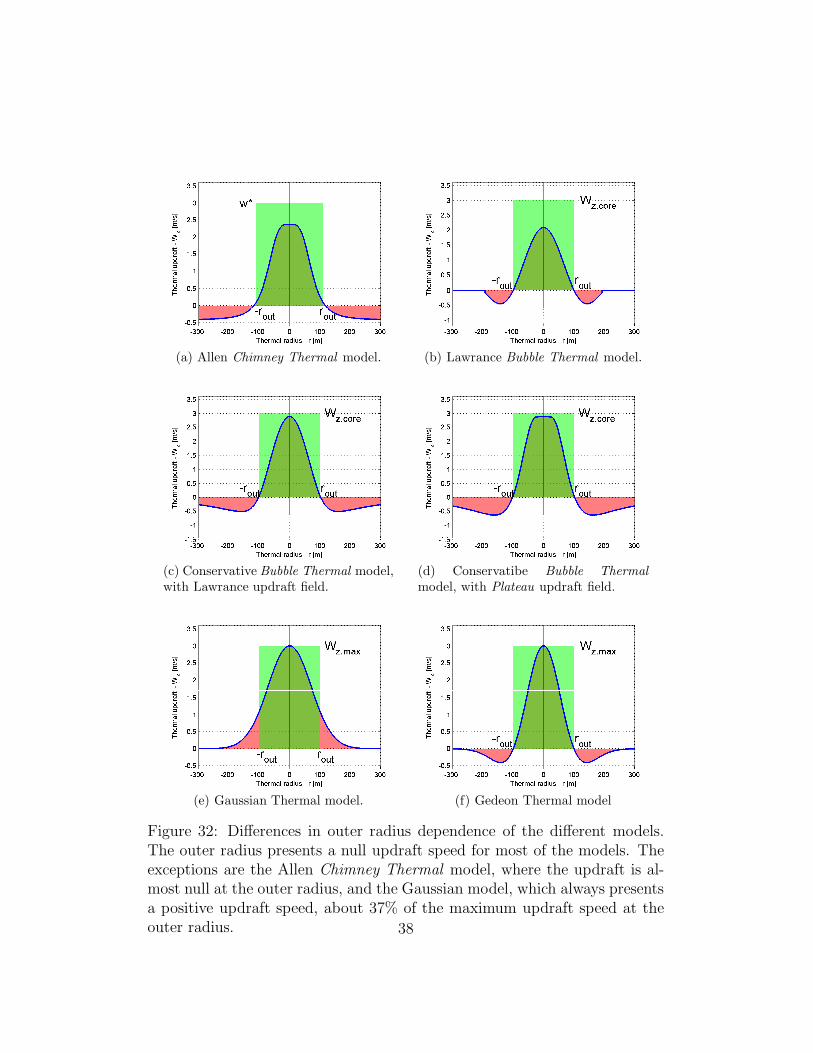
Figure 32: Differences in outer radius dependence of the different models.The outer radius presents a null updraft speed for most of the models. Theexceptions are the Allen Chimney Thermal model, where the updraft is al-most null at the outer radius, and the Gaussian model, which always presentsa positive updraft speed, about 37% of the maximum updraft speed at theouter radius. 38

We may extend the Gaussian and the Gedeon models into more realisticChimney models, if we use the Allen model’s outer radius function (22) andcore updraft function (26). This would make the outer radius a function ofaltitude and the updraft speed a function of both altitude and outer radius(fig. 33). Even so, these models would remain non conservative in terms ofair mass exchange.

(a) Allen-Gaussian Thermal model (b) Allen-Gedeon Thermal model

Figure 33: Adaptation of the Gaussian shape and Gedeon models to simulatea Chimney type thermal - The altitude affects the outer radius and themaximum updraft speed in the same manner as in the Allen model.

4.4. Thermals Development and Fading

Individual thermals’ appearance rate may be modeled by a Poisson dis-tribution. Based on Lenschow and Stephens’ data collected over the ocean[20], the average number of thermals encountered over a path of length s,normalized by the Mixed-Layer altitude zi, is

NT ≈ 1.2s

zi, z ∈

[

0.1zi, zi]

, (45)

where z is the measurement altitude. As such, the resulting Poisson distri-bution is

PThermal (s) = 1− e−λT ·s, λT ≈ 1.2

zi. (46)

Thermals present different strengths and sizes, even if they are devel-oped in the same region with the same environmental conditions. The sizeprobability distribution of an ensemble of thermals follows a Gamma distri-bution [22, 23]. Vulf’son and Borodin derived analytically the distribution

39

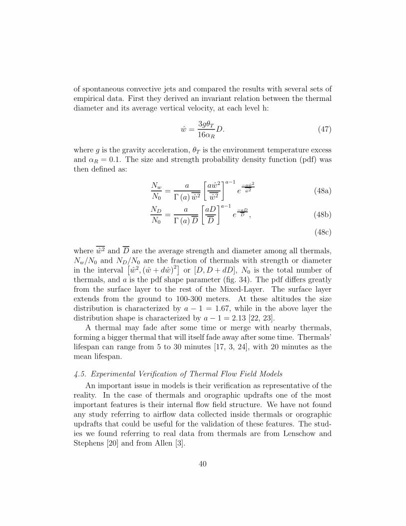
of spontaneous convective jets and compared the results with several sets ofempirical data. First they derived an invariant relation between the thermaldiameter and its average vertical velocity, at each level h:

w =3gθT16αR

D. (47)

where g is the gravity acceleration, θT is the environment temperature excessand αR = 0.1. The size and strength probability density function (pdf) wasthen defined as:

Nw

N0=

a

Γ (a) w2

[

aw2

w2

]a−1

e−aw2

w2 (48a)

ND

N0

=a

Γ (a)D

[

aD

D

]a−1

e−aD

D , (48b)

(48c)

where w2 and D are the average strength and diameter among all thermals,Nw/N0 and ND/N0 are the fraction of thermals with strength or diameterin the interval

[

w2, (w + dw)2]

or [D,D + dD], N0 is the total number ofthermals, and a is the pdf shape parameter (fig. 34). The pdf differs greatlyfrom the surface layer to the rest of the Mixed-Layer. The surface layerextends from the ground to 100-300 meters. At these altitudes the sizedistribution is characterized by a − 1 = 1.67, while in the above layer thedistribution shape is characterized by a− 1 = 2.13 [22, 23].

A thermal may fade after some time or merge with nearby thermals,forming a bigger thermal that will itself fade away after some time. Thermals’lifespan can range from 5 to 30 minutes [17, 3, 24], with 20 minutes as themean lifespan.

4.5. Experimental Verification of Thermal Flow Field Models

An important issue in models is their verification as representative of thereality. In the case of thermals and orographic updrafts one of the mostimportant features is their internal flow field structure. We have not foundany study referring to airflow data collected inside thermals or orographicupdrafts that could be useful for the validation of these features. The stud-ies we found referring to real data from thermals are from Lenschow andStephens [20] and from Allen [3].

40

Allen [3] studied the distribution of two environmental parameters thatinfluence the thermal size and strength, in Desert Rock, Nevada. Theseparameters are the maximum altitude a thermal may reach, i.e., the atmo-sphere mixing-layer altitude, and the convection intensity in the mixing-layer(zi), represented by the convective velocity scale (w⋆), which is related to thethermals’ updraft speed.

Lenschow and Stephens’s work [20] provides the best data to relate thealtitude with the average thermal horizontal size and the updraft speed.The data was collected from a thermal field over the ocean, flying long linesand averaging the airflow data among all detected thermals at each altitude.This method is good to obtain the general relations between altitude andthermal size and strength. However, it is not good enough to evaluate theevolution of the thermal diameter within individual thermals. That wouldbe important to evaluate the 3D shape of the thermals, identifying themas Chimney or Bubble Thermals and allowing the validation of the modelspresented in section 4.1. Furthermore, the averaging of the thermal airflowobservations makes it impossible to validate the internal thermal flow fieldpredicted by any thermal model.

4.6. Orographic Updrafts

Ridge lift - Ridge or slope lift appears along the windward side of moun-tain ridges. It is generated when the flowing air mass collides with themountain side and is forced to climb to overcome the obstacle. Lan-gelaan described a general model for the ridge flow field based on asemi-cylindric obstacle over a flat surface [25] (fig. 35):

w = w∞x− w∞

R2

r2(cos ηr+ sin ηη) (49a)

wx = w∞

[

1− R2

r2(

cos2 η − sin2 η)

]

(49b)

wz = 2w∞

R2

r2cos η sin η, (49c)

The updraft is generated if the general wind direction is within 30o

to 40o to the perpendicular to the ridge line [13]. Unlike thermals,the ridge updraft maintains a stable position, endures as long as thewind conditions are favorable, and can cover large areas, allowing longupward soaring legs. The main limitation of the ridge lift is that it isconstrained to a limited altitude above the ridge crest.

41

Wave lift - Wave lift is another effect of mountainous terrain. It developsafter the air mass has passed over the undulating terrain at high alti-tudes. ”This lift is part of a large scale deflection of air mass, whichis known as “lee wave” lift, first recognized in the 1930s and exploredscientifically in the early 1950s” [26]. The lee wave flow field structureis similar to a sinusoidal wave (fig. 35b). ”Lee wave field structuresthe air mass sink rates in parallel bands having high cross-stream co-herence” [27]. The wave length λW of this phenomenon depends onthe atmospheric conditions, in particular the atmosphere stability. ”Inthe atmosphere, [...] λW ∼ O (10n.mi.) for hydrostatic lee waves orλW ∼ O (1n.mi.) for nonhydrostatic lee waves” [27]. Wave lift devel-opment depends greatly on the presence of relatively high winds andstable atmosphere conditions.

5. Wind Gust Models

Among the studied phenomena in this work, gusts are the one most com-monly encountered by Aircraft. But, unlike wind shear and updrafts reviewedabove, the wind gusts are very short term phenomenon. This and the diffi-culty to predict gusts’ appearance makes them a lot harder to use for energyharvesting. For the sake of completeness, we include here a short review ofgust models.

Gusts may convey energy to an aircraft in a similar manner to the windshear phenomena. This energy is present in the wind velocity and directionvariations, i.e., airflow gradients [4, 2].

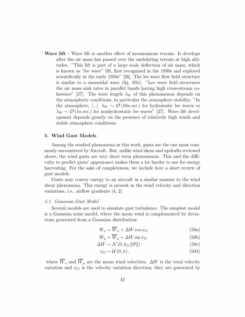
5.1. Gaussian Gust Model

Several models are used to simulate gust turbulence. The simplest modelis a Gaussian noise model, where the mean wind is complemented by devia-tions generated from a Gaussian distribution:

Wx =W x +∆W cosψG (50a)

Wy =W y +∆W sinψG (50b)

∆W ∼ N (0, kG ‖w‖) (50c)

ψG ∼ U (0, π) , (50d)

where W x and W y are the mean wind velocities. ∆W is the total velocityvariation and ψG is the velocity variation direction; they are generated by

42

the Normal distribution N (0, kG ‖w‖), with standard deviation proportionalto the total wind speed σG = kG ‖w‖, and the Uniform distribution U (0, π).

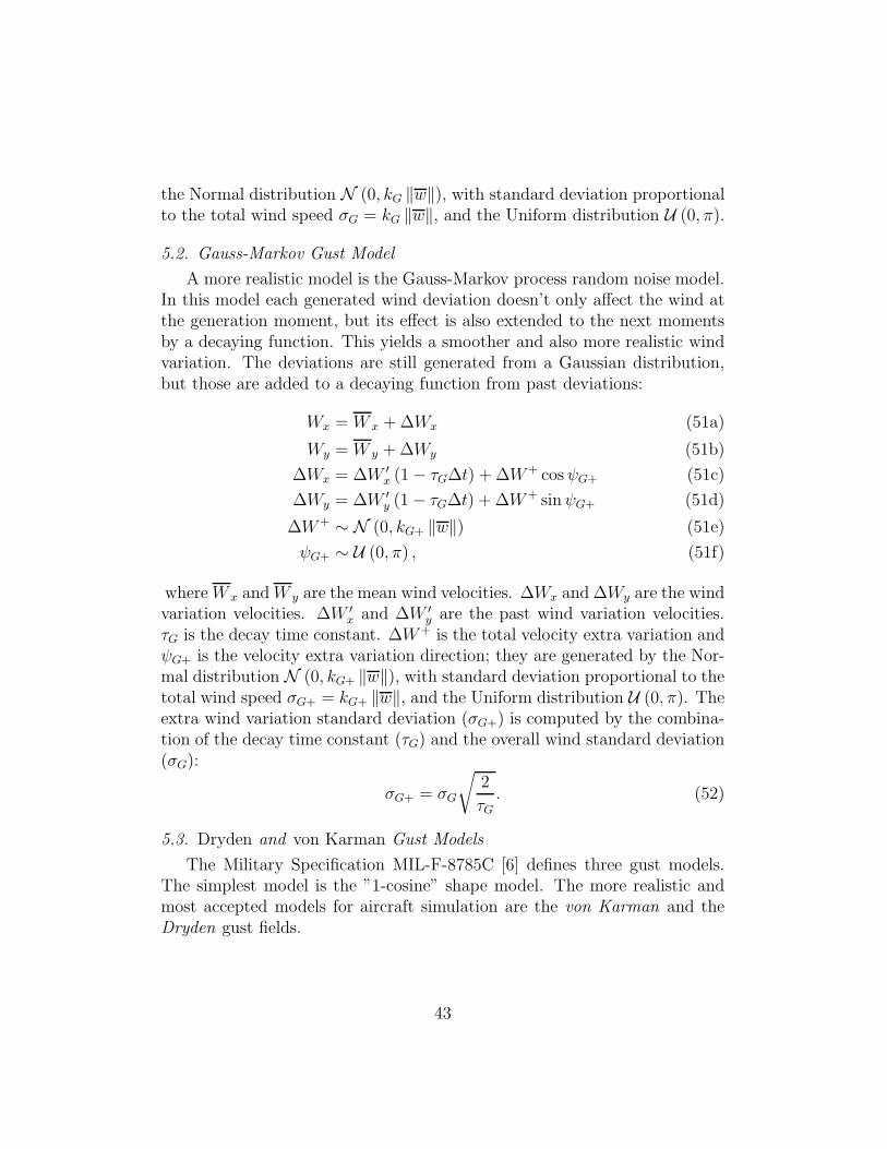
5.2. Gauss-Markov Gust Model

A more realistic model is the Gauss-Markov process random noise model.In this model each generated wind deviation doesn’t only affect the wind atthe generation moment, but its effect is also extended to the next momentsby a decaying function. This yields a smoother and also more realistic windvariation. The deviations are still generated from a Gaussian distribution,but those are added to a decaying function from past deviations:

Wx =W x +∆Wx (51a)

Wy =W y +∆Wy (51b)

∆Wx = ∆W ′

x (1− τG∆t) + ∆W+ cosψG+ (51c)

∆Wy = ∆W ′

y (1− τG∆t) + ∆W+ sinψG+ (51d)

∆W+ ∼ N (0, kG+ ‖w‖) (51e)

ψG+ ∼ U (0, π) , (51f)

whereW x andW y are the mean wind velocities. ∆Wx and ∆Wy are the windvariation velocities. ∆W ′

x and ∆W ′

y are the past wind variation velocities.τG is the decay time constant. ∆W+ is the total velocity extra variation andψG+ is the velocity extra variation direction; they are generated by the Nor-mal distribution N (0, kG+ ‖w‖), with standard deviation proportional to thetotal wind speed σG+ = kG+ ‖w‖, and the Uniform distribution U (0, π). Theextra wind variation standard deviation (σG+) is computed by the combina-tion of the decay time constant (τG) and the overall wind standard deviation(σG):

σG+ = σG

√

2

τG. (52)

5.3. Dryden and von Karman Gust Models

The Military Specification MIL-F-8785C [6] defines three gust models.The simplest model is the ”1-cosine” shape model. The more realistic andmost accepted models for aircraft simulation are the von Karman and theDryden gust fields.

43

5.4. Urban Gust Models

The gust models presented above are well suited for open area flow sim-ulation. However they don’t capture complex flow environments well, e.g.,a flow field in an urban grid. Models with more detail simulate those kindof environments better. For that, Cybyk et al [28] implemented a real-timephysics-based simulation tool to study UAV dynamics in a urban environ-ment.

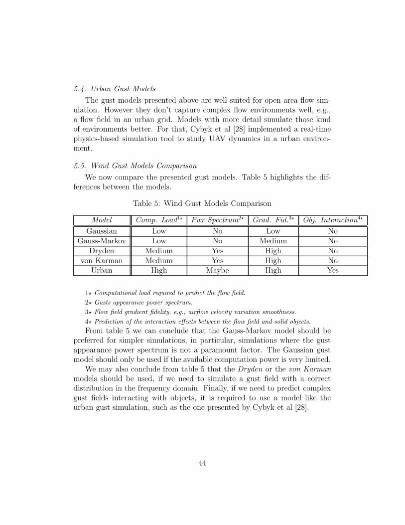
5.5. Wind Gust Models Comparison

We now compare the presented gust models. Table 5 highlights the dif-ferences between the models.

Table 5: Wind Gust Models Comparison

Model Comp. Load1⋆ Pwr Spectrum2⋆ Grad. Fid.3⋆ Obj. Interaction4⋆

Gaussian Low No Low NoGauss-Markov Low No Medium No

Dryden Medium Yes High Novon Karman Medium Yes High No

Urban High Maybe High Yes

1⋆ Computational load required to predict the flow field.

2⋆ Gusts appearance power spectrum.

3⋆ Flow field gradient fidelity, e.g., airflow velocity variation smoothness.

4⋆ Prediction of the interaction effects between the flow field and solid objects.

From table 5 we can conclude that the Gauss-Markov model should bepreferred for simpler simulations, in particular, simulations where the gustappearance power spectrum is not a paramount factor. The Gaussian gustmodel should only be used if the available computation power is very limited.

We may also conclude from table 5 that the Dryden or the von Karmanmodels should be used, if we need to simulate a gust field with a correctdistribution in the frequency domain. Finally, if we need to predict complexgust fields interacting with objects, it is required to use a model like theurban gust simulation, such as the one presented by Cybyk et al [28].

44

6. Conclusions

This survey lays out the basis for the development of flow field energy har-vesting by aircraft. This work studies an array of atmospheric flow field phe-nomena selected by their perceived exploitation potential to extend aircraftflight endurance. We studied several existing models for thermal updrafts,wind shear and gusts.

Further, we improved some of those models and created new ones tobetter capture some important features. Examples of this are the improvedChimney Thermal model and the new Bubble Thermal, Layer Wind Shear,and Ridge Wind Shear models.

The studied models represent the phenomena’s flow field shape in 1D,2D or 3D, the interaction with the steady wind flow, and the dynamics.For thermals we presented general 2D models, and 3D models for Chimneyand Bubble Thermals. The Bubble Thermal model is new and is based on thevortex shell hypothesis by Cone [14]. The extended Chimney Thermal modelis based on the Allen model [3], and includes the thermal core movement andthermal interactions with the surrounding flow field, e.g., its leeward leaningwhen there is wind. In terms of wind shear we presented existing models forgeneral wind shear and the Surface Wind Shear, and developed new modelsfor the Layer and the Ridge Wind Shear. For completeness, we closed thissurvey with a short review of gusts models.

7. Future Work

Most of the models presented in this work are based on the observationof bird flight and glider pilots observations. An important extension of thiswork will be the validation of the models through the measurement of thecorresponding flow fields. We plan to use a team of UAV flying in formation[29] to simultaneously collect air velocity data from several points in space.This data will then be compared to the model predictions to assert the fidelityof the models.

The flow field phenomena models presented in this work will support thedevelopment of estimators for the flow field phenomena. The combinationof simpler models and more realistic ones will allow the implementation oflow computational load estimators. These should use the simpler modelsto provide the initial convergence. Once an initial rough estimate exists,the higher fidelity models will allow the estimators to distinguish betweenphenomena types and provide more precise tracking and predictions.

45

The presented models will also serve to simulate UAVs’ flight throughflow field phenomena. Further, the flow field models will be the basis for thedefinition of flight controllers tailored for energy harvesting.

8. Acknowledgments

We are specially grateful to Professor Pierre Kabamba, from the Univer-sity of Michigan Aerospace Department, who carefully reviewed this manuscriptand provided precious insights. We gratefully acknowledge the support of theAerospace & Robotic Controls Laboratory researchers, in particular JustinJackson, Baro Hyun, Mariam Faied, and Zahid Hasan, at the University ofMichigan. We further acknowledge the support of the AsasF group and theresearchers from the Underwater Systems and Technology Laboratory, spe-cially Eduardo Oliveira, Rui Caldeira, Filipe Ferreira, and Gil Goncalves, andthe Portuguese Air Force Academy, specially Cap. Eloi Pereira and Lt. TiagoOliveira. The research leading to this work was funded in part by the UnitedStates Air Force under grant number FA 8650-07-2-3744, by Financiamentopluri-anual of the FEUP ISR Porto R&D unit, and by the FCT (Foundationfor Science and Technology) under PhD grant SFRH/BD/40764/2007.

References

[1] Wharington J. Autonomous control of soaring aircraft by reinforcementlearning. Ph.D. thesis; Royal Melbourne Institute of Technology, Facultyof Engineering, Department of Aerospace Engineering; 1998.

[2] Langelaan J. Gust energy extraction for mini and micro uninhab-ited aerial vehicles. Journal of Guidance, Control, and Dynamics2009;32(2):464–73. doi:10.2514/1.37735.

[3] Allen MJ. Updraft model for development of autonomous soaring un-inhabited air vehicles. In: 44rd AIAA Aerospace Sciences Meeting andExhibit. Reno, Nevada: AIAA; 2006,.

[4] Lawrance NR, Sukkarieh S. Wind energy based path planning for asmall gliding unmanned aerial vehicle. In: AIAA Guidance, Navigation,and Control Conference. Chicago, Illinois: AIAA; 2009,.

46

[5] Sachs G. Minimum shear wind strength required for dynamic soar-ing of albatrosses. Ibis - The International Journal of Avian Sci-ence 2005;147(1):1–10. doi:10.1111/j.1474-919x.2004.00295.x. URLhttp://dx.doi.org/10.1111/j.1474-919x.2004.00295.x.

[6] U.S. Military Specification MIL-F-8785C; 1980.

[7] Grenestedt JL, Spletzer JR. Optimal energy extraction during dynamicjet stream soaring. In: AIAA Guidance, Navigation, and Control Con-ference. Toronto, Ontario, Canada; 2010,.

[8] Sachs G, da Costa O. Dynamic soaring in altitude region below jetstreams. In: AIAA Guidance, Navigation, and Control Conference andExhibit. Keystone, Colorado; 2006,.

[9] Zhao YJ. Optimal patterns of glider dynamic soaring. Optimal ControlApplications and Methods 2004;25(2). doi:10.1002/oca.739.

[10] Parle J. Preliminary dynamic soaring research using a radio controlglider. In: 42nd AIAA Aerospace Sciences Meeting and Exhibit. Reno,Nevada, USA; 2004,.

[11] Sachs G, Traugott J, Holzapfel F. In-flight measurement of dynamicsoaring in albatrosses. In: AIAA Guidance, Navigation, and ControlConference. Toronto, Ontario, Canada; 2010,.

[12] Sachs G, Traugott J, Holzapfel F. Progress against the wind with dy-namic soaring: Results from in-flight measurements of albatrosses. In:AIAA Guidance, Navigation, and Control Conference and Exhibit. Port-land, Oregon, USA; 2011,.

[13] FAA . Aviation Weather. Aviation Supplies & Academics, Inc.; 1975.ISBN 1560270012. URL http://www.aviationweather.ws/.

[14] Cone CD. Thermal soaring of birds. American Scientist 1962;50(1):180–209.

[15] Andersson K, Kaminer I. Stability of a thermal centering controller. In:AIAA Guidance, Navigation, and Control Conference. Chicago, Illinois:AIAA; 2009,.

47

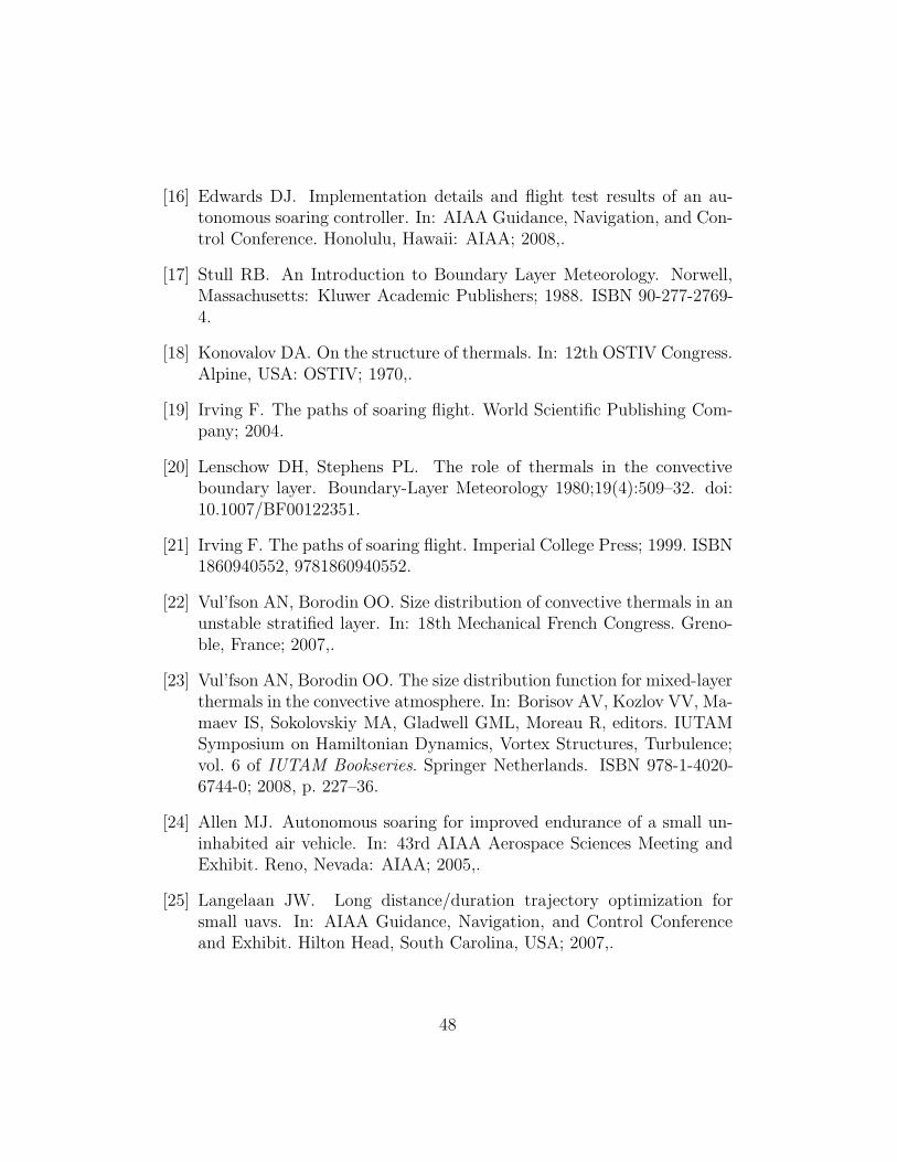
[16] Edwards DJ. Implementation details and flight test results of an au-tonomous soaring controller. In: AIAA Guidance, Navigation, and Con-trol Conference. Honolulu, Hawaii: AIAA; 2008,.

[17] Stull RB. An Introduction to Boundary Layer Meteorology. Norwell,Massachusetts: Kluwer Academic Publishers; 1988. ISBN 90-277-2769-4.

[18] Konovalov DA. On the structure of thermals. In: 12th OSTIV Congress.Alpine, USA: OSTIV; 1970,.

[19] Irving F. The paths of soaring flight. World Scientific Publishing Com-pany; 2004.

[20] Lenschow DH, Stephens PL. The role of thermals in the convectiveboundary layer. Boundary-Layer Meteorology 1980;19(4):509–32. doi:10.1007/BF00122351.

[21] Irving F. The paths of soaring flight. Imperial College Press; 1999. ISBN1860940552, 9781860940552.

[22] Vul’fson AN, Borodin OO. Size distribution of convective thermals in anunstable stratified layer. In: 18th Mechanical French Congress. Greno-ble, France; 2007,.

[23] Vul’fson AN, Borodin OO. The size distribution function for mixed-layerthermals in the convective atmosphere. In: Borisov AV, Kozlov VV, Ma-maev IS, Sokolovskiy MA, Gladwell GML, Moreau R, editors. IUTAMSymposium on Hamiltonian Dynamics, Vortex Structures, Turbulence;vol. 6 of IUTAM Bookseries. Springer Netherlands. ISBN 978-1-4020-6744-0; 2008, p. 227–36.

[24] Allen MJ. Autonomous soaring for improved endurance of a small un-inhabited air vehicle. In: 43rd AIAA Aerospace Sciences Meeting andExhibit. Reno, Nevada: AIAA; 2005,.

[25] Langelaan JW. Long distance/duration trajectory optimization forsmall uavs. In: AIAA Guidance, Navigation, and Control Conferenceand Exhibit. Hilton Head, South Carolina, USA; 2007,.

48

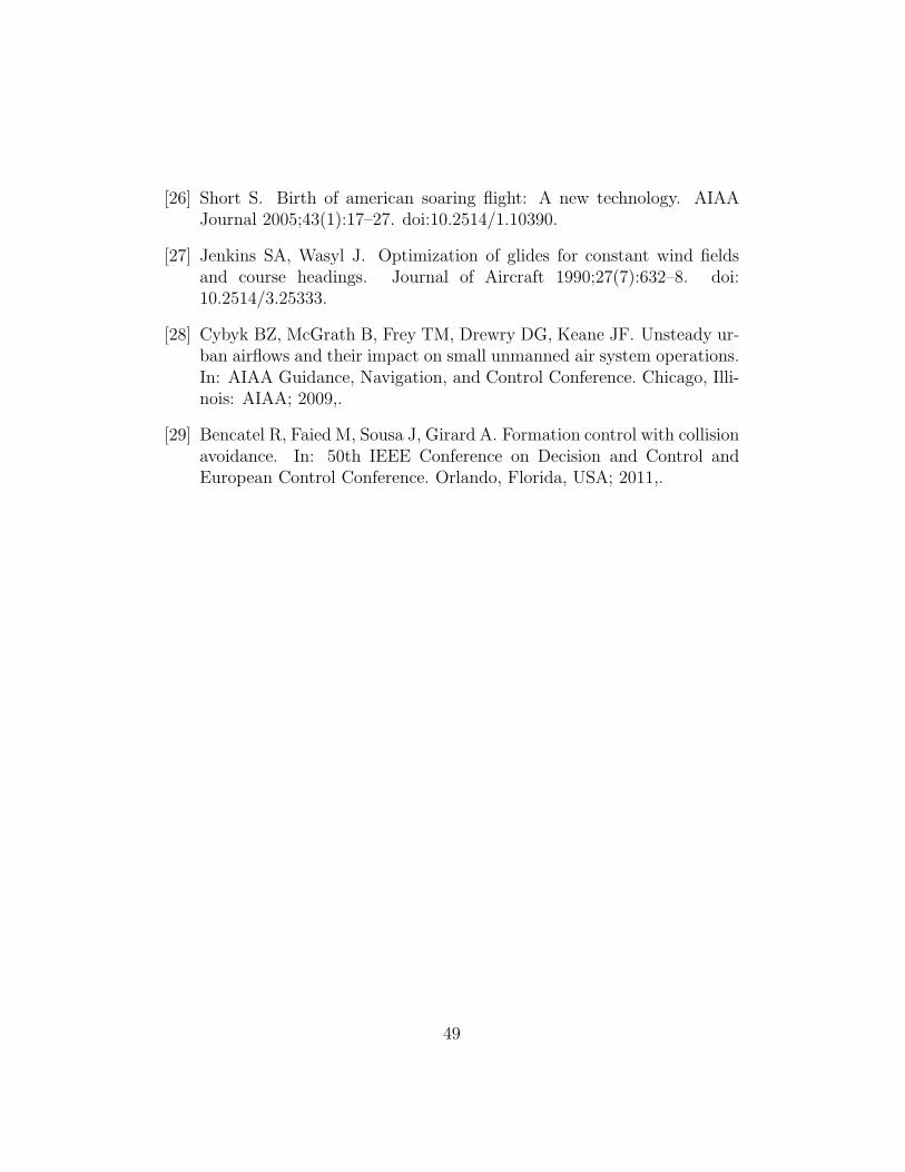
[26] Short S. Birth of american soaring flight: A new technology. AIAAJournal 2005;43(1):17–27. doi:10.2514/1.10390.

[27] Jenkins SA, Wasyl J. Optimization of glides for constant wind fieldsand course headings. Journal of Aircraft 1990;27(7):632–8. doi:10.2514/3.25333.

[28] Cybyk BZ, McGrath B, Frey TM, Drewry DG, Keane JF. Unsteady ur-ban airflows and their impact on small unmanned air system operations.In: AIAA Guidance, Navigation, and Control Conference. Chicago, Illi-nois: AIAA; 2009,.

[29] Bencatel R, Faied M, Sousa J, Girard A. Formation control with collisionavoidance. In: 50th IEEE Conference on Decision and Control andEuropean Control Conference. Orlando, Florida, USA; 2011,.

49

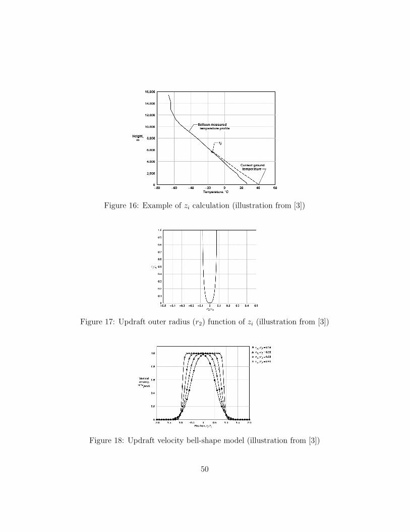
Figure 16: Example of zi calculation (illustration from [3])

Figure 17: Updraft outer radius (r2) function of zi (illustration from [3])

Figure 18: Updraft velocity bell-shape model (illustration from [3])

50

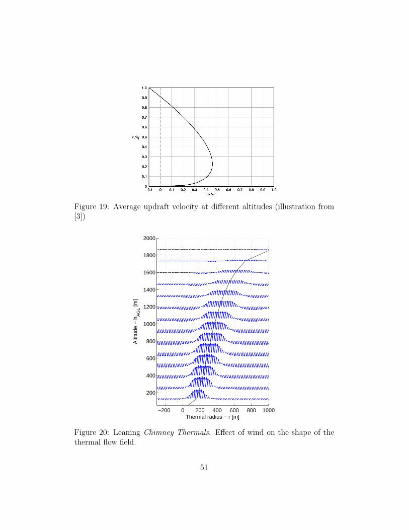
Figure 19: Average updraft velocity at different altitudes (illustration from[3])

−200 0 200 400 600 800 1000

200

400

600

800

1000

1200

1400

1600

1800

2000

Thermal radius − r [m]

Alti

tude

− h

AG

L [m]

Figure 20: Leaning Chimney Thermals. Effect of wind on the shape of thethermal flow field.

51

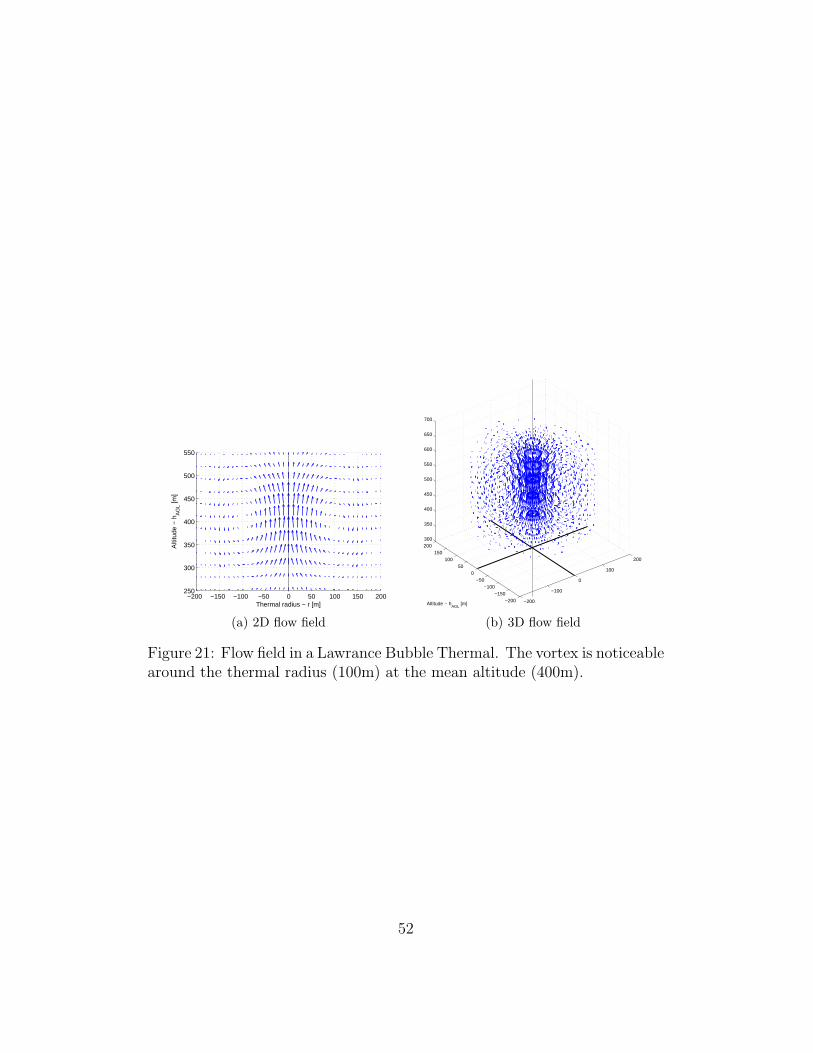
−200 −150 −100 −50 0 50 100 150 200250

300

350

400

450

500

550

Thermal radius − r [m]

Alti

tude

− h

AG

L [m]

(a) 2D flow field

−200

−100

0

100

200

−200−150

−100−50

050

100150

200300

350

400

450

500

550

600

650

700

Altitude − hAGL

[m]

(b) 3D flow field

Figure 21: Flow field in a Lawrance Bubble Thermal. The vortex is noticeablearound the thermal radius (100m) at the mean altitude (400m).

52

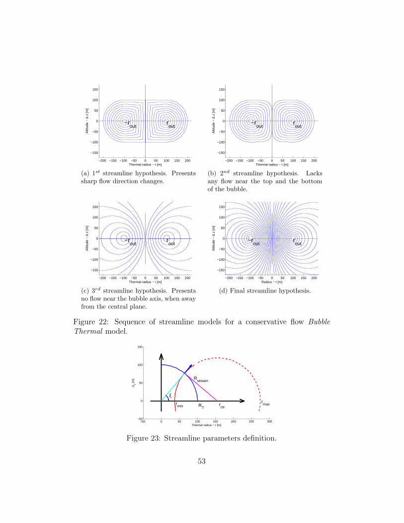
−200 −150 −100 −50 0 50 100 150 200

−150

−100

−50

0

50

100

150

Thermal radius − r [m]

Alti

tude

− ∆

z [m

]

−rout

rout

(a) 1st streamline hypothesis. Presentssharp flow direction changes.

−200 −150 −100 −50 0 50 100 150 200

−150

−100

−50

0

50

100

150

Thermal radius − r [m]

Alti

tude

− ∆

z [m

]

−rout

rout

(b) 2nd streamline hypothesis. Lacksany flow near the top and the bottomof the bubble.

−200 −150 −100 −50 0 50 100 150 200

−150

−100

−50

0

50

100

150

Thermal radius − r [m]

Alti

tude

− ∆

z [m

]

−rout

rout

(c) 3rd streamline hypothesis. Presentsno flow near the bubble axis, when awayfrom the central plane.

−200 −150 −100 −50 0 50 100 150 200

−150

−100

−50

0

50

100

150

Radius − r [m]

Alti

tude

− ∆

z [m

]

−rout

rout

(d) Final streamline hypothesis.

Figure 22: Sequence of streamline models for a conservative flow BubbleThermal model.

−50 0 50 100 150 200 250 300−50

0

50

100

150

Thermal radius − r [m]

∆ z [m]

RT

rctr

rmin

rmax

Rstream

ξ

Figure 23: Streamline parameters definition.

53

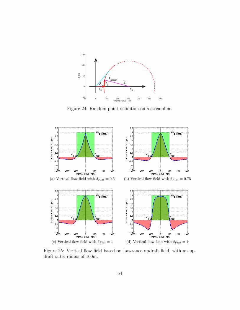
−50 0 50 100 150 200 250 300−50

0

50

100

150

Thermal radius − r [m]

∆ z [m]

rctr

Rstream

ξ

dH

∆z

ζ

Figure 24: Random point definition on a streamline.

(a) Vertical flow field with δFlat = 0.5 (b) Vertical flow field with δFlat = 0.75

(c) Vertical flow field with δFlat = 1 (d) Vertical flow field with δFlat = 4

Figure 25: Vertical flow field based on Lawrance updraft field, with an up-draft outer radius of 100m.

54

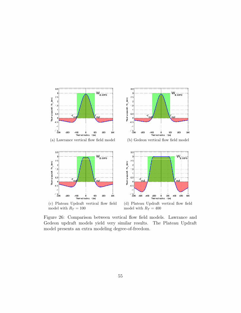
(a) Lawrance vertical flow field model (b) Gedeon vertical flow field model

(c) Plateau Updraft vertical flow fieldmodel with RT = 100

(d) Plateau Updraft vertical flow fieldmodel with RT = 400

Figure 26: Comparison between vertical flow field models. Lawrance andGedeon updraft models yield very similar results. The Plateau Updraftmodel presents an extra modeling degree-of-freedom.

55

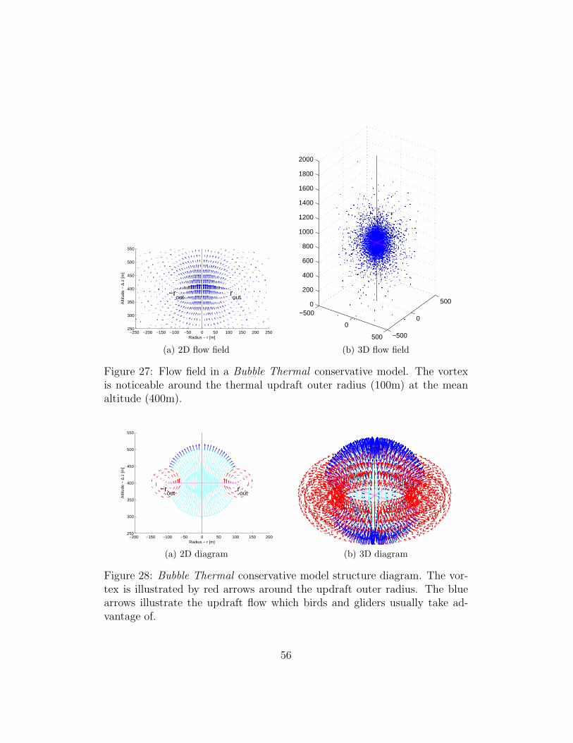
−250 −200 −150 −100 −50 0 50 100 150 200 250250

300

350

400

450

500

550

Radius − r [m]

Alti

tude

− ∆

z [m

]

−rout

rout

(a) 2D flow field

−500

0

500 −500

0

5000

200

400

600

800

1000

1200

1400

1600

1800

2000

(b) 3D flow field

Figure 27: Flow field in a Bubble Thermal conservative model. The vortexis noticeable around the thermal updraft outer radius (100m) at the meanaltitude (400m).

−200 −150 −100 −50 0 50 100 150 200250

300

350

400

450

500

550

Radius − r [m]

Alti

tude

− ∆

z [m

]

−rout

rout

(a) 2D diagram (b) 3D diagram

Figure 28: Bubble Thermal conservative model structure diagram. The vor-tex is illustrated by red arrows around the updraft outer radius. The bluearrows illustrate the updraft flow which birds and gliders usually take ad-vantage of.

56

−250 −200 −150 −100 −50 0 50 100 150 200 250250

300

350

400

450

500

550

Radius − r [m]

Alti

tude

− ∆

z [m

]

−rout

rout

(a) 2D flow field

−500

0

500 −500

0

5000

200

400

600

800

1000

1200

1400

1600

1800

2000

(b) 3D flow field

Figure 29: Flow field in a leaning Bubble Thermal. It is clear that the flowcrosses the bubble center at a certain angle, which depends both on thebubble and the wind velocity.

Figure 34: Diameter pdf with a− 1 = 5/3 (illustrations from [22])

57

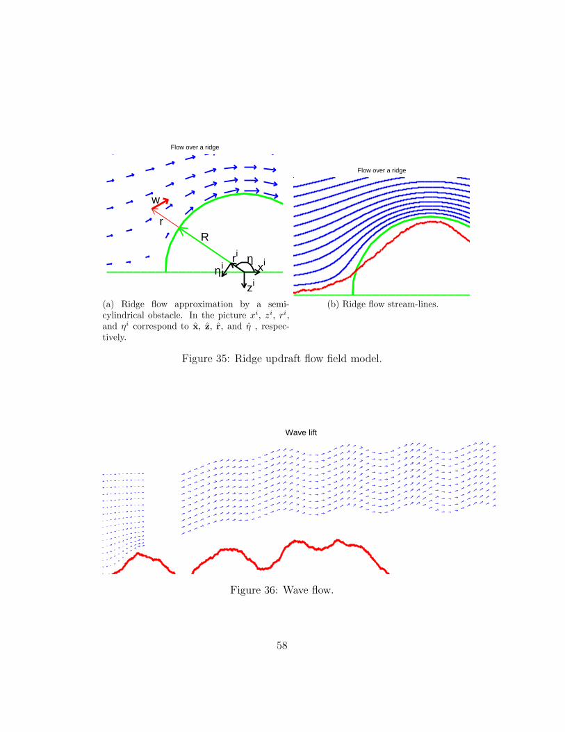
Flow over a ridge

xi

zi

ηri

ηi

Rr

w

(a) Ridge flow approximation by a semi-cylindrical obstacle. In the picture xi, zi, ri,and ηi correspond to x, z, r, and η , respec-tively.

Flow over a ridge

(b) Ridge flow stream-lines.

Figure 35: Ridge updraft flow field model.

Wave lift

Figure 36: Wave flow.

58