Atlas, a library for NWP and climate modelling - ESiWACE

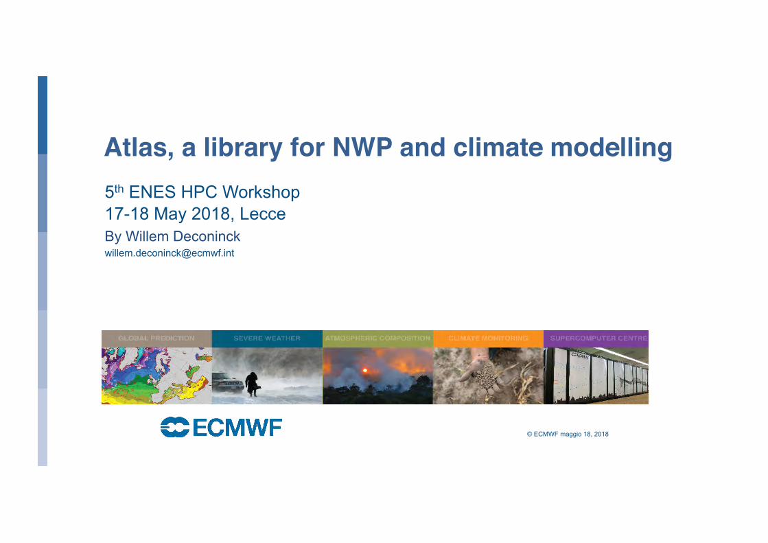
© ECMWF maggio 18, 2018

Atlas, a library for NWP and climate modelling

By Willem Deconinck

[email protected]

5th ENES HPC Workshop 17-18 May 2018, Lecce

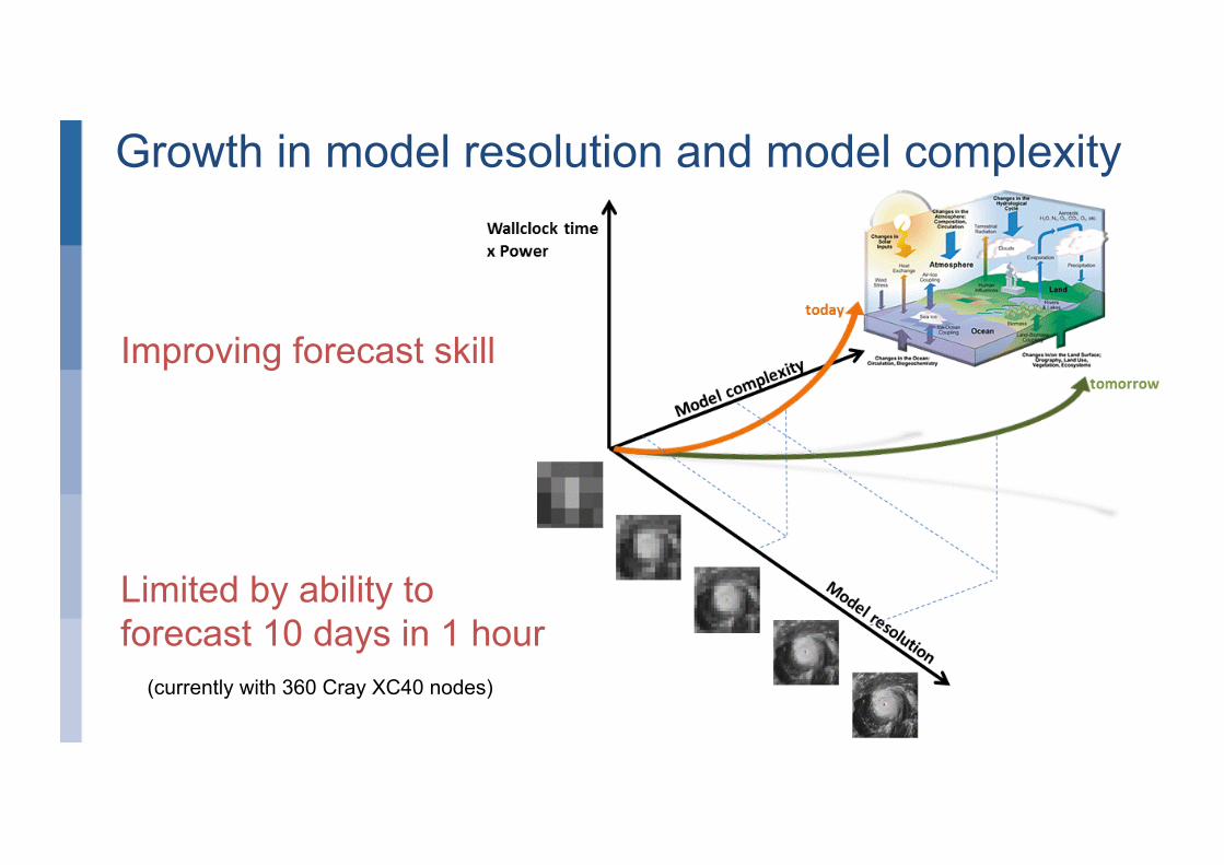
Growth in model resolution and model complexity

ESCAPE Technical Annex, Sections 1 – 3 Page 5 of 70

Figure 1.1a: In the next 10 years Earth-system forecast models will provide 1-5 km global resolution and include unprecedented complexity of physical and chemical processes in atmosphere, ocean, sea-ice, and land surface. The strict constraints on wall-clock execution time and power consumption will require drastic code redesign as proposed in ESCAPE.

Figure 1.1b: NWP consortia represented in ESCAPE: ECMWF, the world leading NWP centre, and its member and co-operating states; ALADIN/RC-LACE/SELAM, HIRLAM and COSMO, regional NWP consortia representing Western Europe and Northern Africa, Eastern Europe, Northern Europe and Scandinavia, and Central Europe.

Limited by ability to forecast 10 days in 1 hour

Improving forecast skill

(currently with 360 Cray XC40 nodes)

EUROPEAN CENTRE FOR MEDIUM-RANGE WEATHER FORECASTS

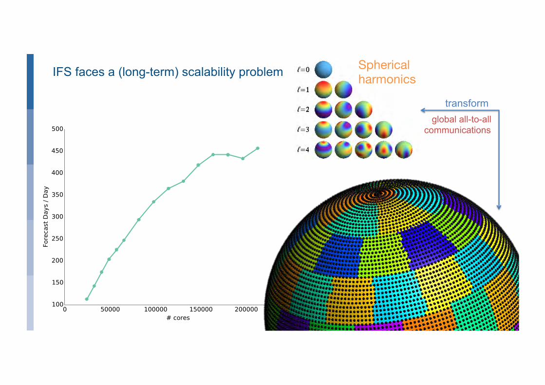
IFS faces a (long-term) scalability problem

7

Spherical harmonics

global all-to-all communications

transform

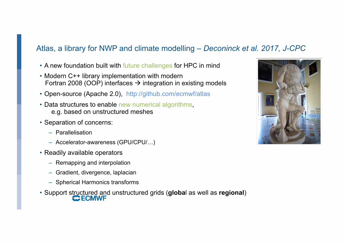
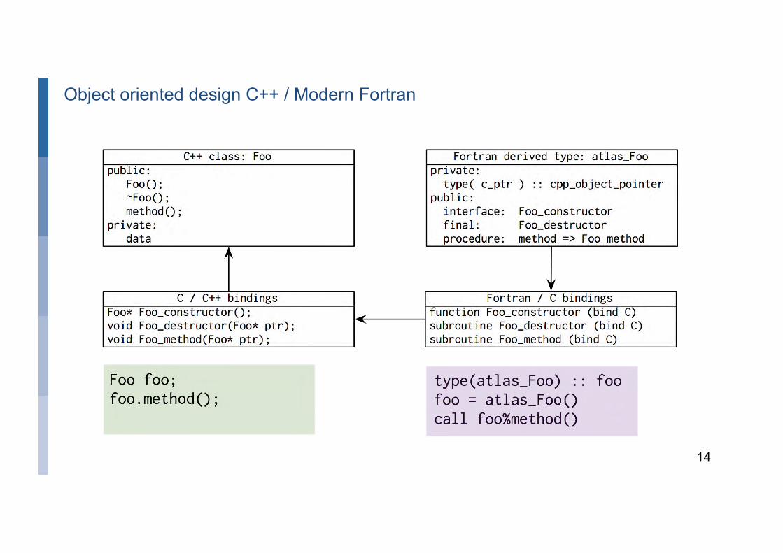
•  A new foundation built with future challenges for HPC in mind • Modern C++ library implementation with modern Fortran 2008 (OOP) interfaces à integration in existing models • Open-source (Apache 2.0), http://github.com/ecmwf/atlas •  Data structures to enable new numerical algorithms,

e.g. based on unstructured meshes •  Separation of concerns:

–  Parallelisation

–  Accelerator-awareness (GPU/CPU/…)

•  Readily available operators –  Remapping and interpolation

–  Gradient, divergence, laplacian

–  Spherical Harmonics transforms

•  Support structured and unstructured grids (global as well as regional)

Atlas, a library for NWP and climate modelling – Deconinck et al. 2017, J-CPC

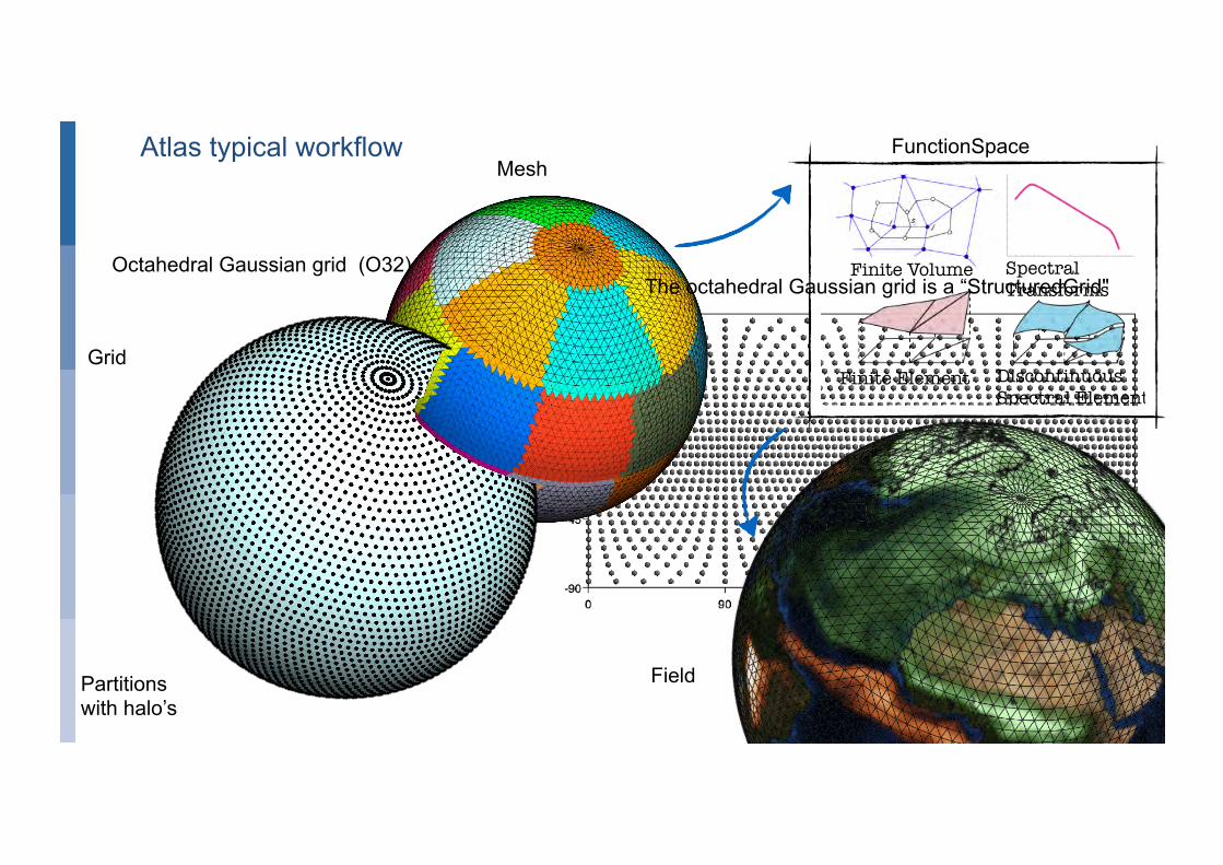
Mesh

Partitions with halo’s

Field

Finite Volume Spectral Transforms

Finite Element Discontinuous Spectral Element

FunctionSpace

Grid

Atlas typical workflow

Octahedral Gaussian grid (O32) The octahedral Gaussian grid is a “StructuredGrid"

14

Object oriented design C++ / Modern Fortran

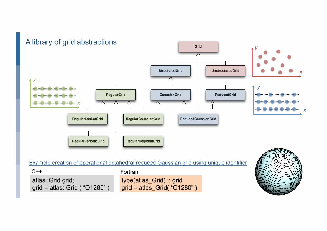
A library of grid abstractions Grid

StructuredGrid

ReducedGridGaussianGrid

ReducedGaussianGridRegularGaussianGridRegularLonLatGrid

RegularGrid

RegularPeriodicGrid RegularRegionalGrid

UnstructuredGrid x

y

x

y y

x

atlas::Grid grid; grid = atlas::Grid ( “O1280” )

type(atlas_Grid) :: grid grid = atlas_Grid( “O1280” )

Example creation of operational octahedral reduced Gaussian grid using unique identifier C++ Fortran

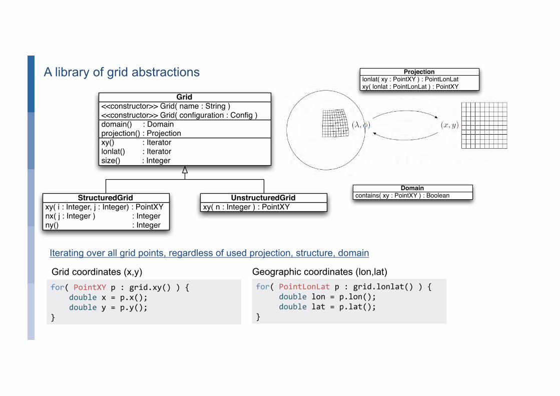
A library of grid abstractions

xy() : Iteratorlonlat() : Iteratorsize() : Integer

domain() : Domainprojection() : Projection

<<constructor>> Grid( name : String )<<constructor>> Grid( configuration : Config )

Grid

xy( i : Integer, j : Integer) : PointXYnx( j : Integer ) : Integerny() : Integer

StructuredGridxy( n : Integer ) : PointXY

UnstructuredGrid

lonlat( xy : PointXY ) : PointLonLatxy( lonlat : PointLonLat ) : PointXY

Projection

contains( xy : PointXY ) : BooleanDomain

Iterating over all grid points, regardless of used projection, structure, domain

for(PointXYp:grid.xy()){doublex=p.x();doubley=p.y();}

for(PointLonLatp:grid.lonlat()){doublelon=p.lon();doublelat=p.lat();}

Grid coordinates (x,y) Geographic coordinates (lon,lat)

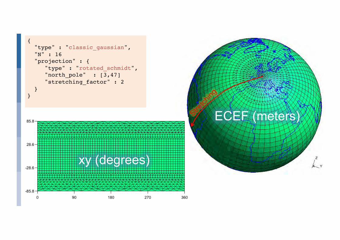
{ "type" : "classic_gaussian", "N" : 16 "projection" : { "type" : "rotated_schmidt", "north_pole" : [3,47] "stretching_factor" : 2 } }

ECEF (meters)

xy (degrees)

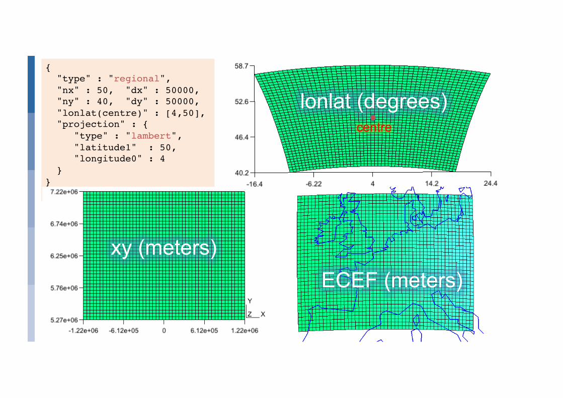
{ "type" : "regional", "nx" : 50, "dx" : 50000, "ny" : 40, "dy" : 50000, "lonlat(centre)" : [4,50], "projection" : { "type" : "lambert", "latitude1" : 50, "longitude0" : 4 } }

lonlat (degrees)

ECEF (meters) xy (meters)

centre

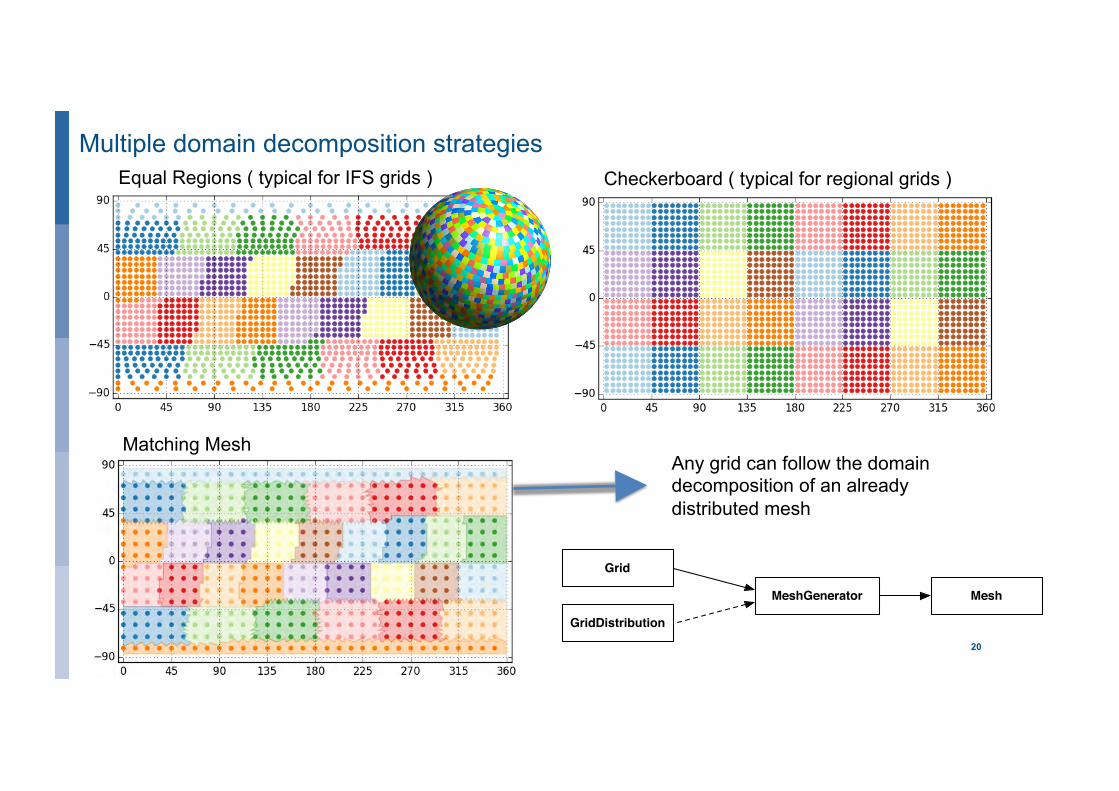
Multiple domain decomposition strategies

20 EUROPEAN CENTRE FOR MEDIUM-RANGE WEATHER FORECASTS

Checkerboard ( typical for regional grids ) Equal Regions ( typical for IFS grids )

Matching Mesh Any grid can follow the domain decomposition of an already distributed mesh

GridDistribution

MeshGenerator Mesh

Grid

Atlas architecture

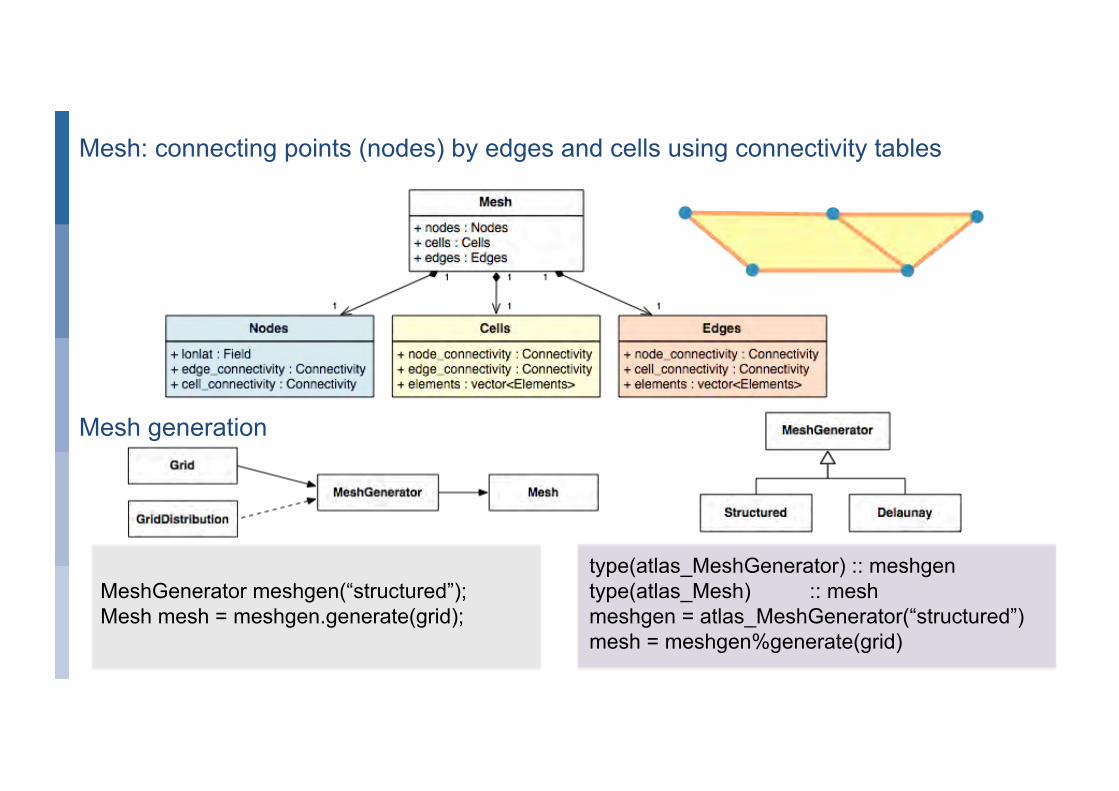
MeshGenerator meshgen(“structured”); Mesh mesh = meshgen.generate(grid);

type(atlas_MeshGenerator) :: meshgen type(atlas_Mesh) :: mesh meshgen = atlas_MeshGenerator(“structured”) mesh = meshgen%generate(grid)

Mesh: connecting points (nodes) by edges and cells using connectivity tables

Mesh generation

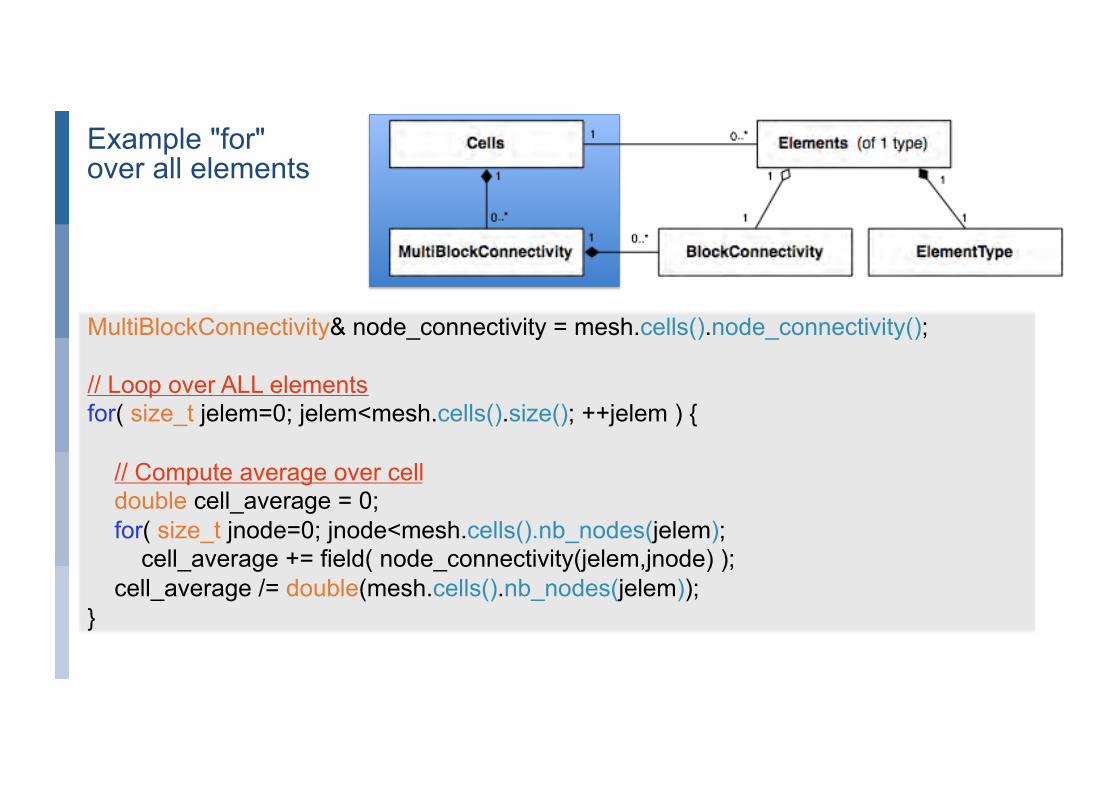
MultiBlockConnectivity& node_connectivity = mesh.cells().node_connectivity(); // Loop over ALL elements for( size_t jelem=0; jelem<mesh.cells().size(); ++jelem ) { // Compute average over cell double cell_average = 0; for( size_t jnode=0; jnode<mesh.cells().nb_nodes(jelem); cell_average += field( node_connectivity(jelem,jnode) ); cell_average /= double(mesh.cells().nb_nodes(jelem)); }

Example "for" over all elements

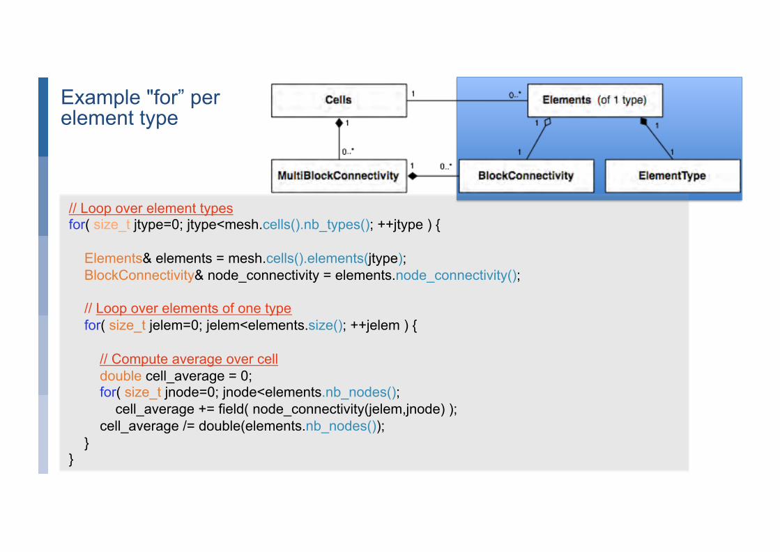
// Loop over element types for( size_t jtype=0; jtype<mesh.cells().nb_types(); ++jtype ) { Elements& elements = mesh.cells().elements(jtype); BlockConnectivity& node_connectivity = elements.node_connectivity(); // Loop over elements of one type for( size_t jelem=0; jelem<elements.size(); ++jelem ) { // Compute average over cell double cell_average = 0; for( size_t jnode=0; jnode<elements.nb_nodes(); cell_average += field( node_connectivity(jelem,jnode) ); cell_average /= double(elements.nb_nodes()); } }

Example "for” per element type

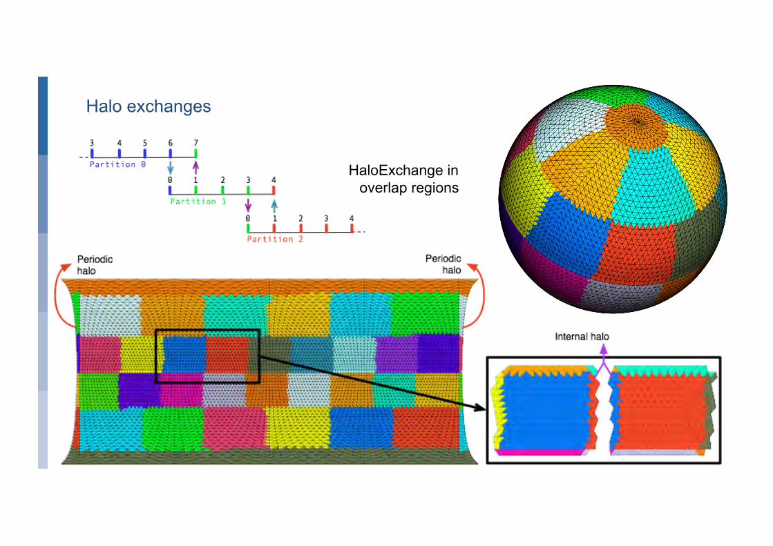
Halo exchanges

HaloExchange in overlap regions

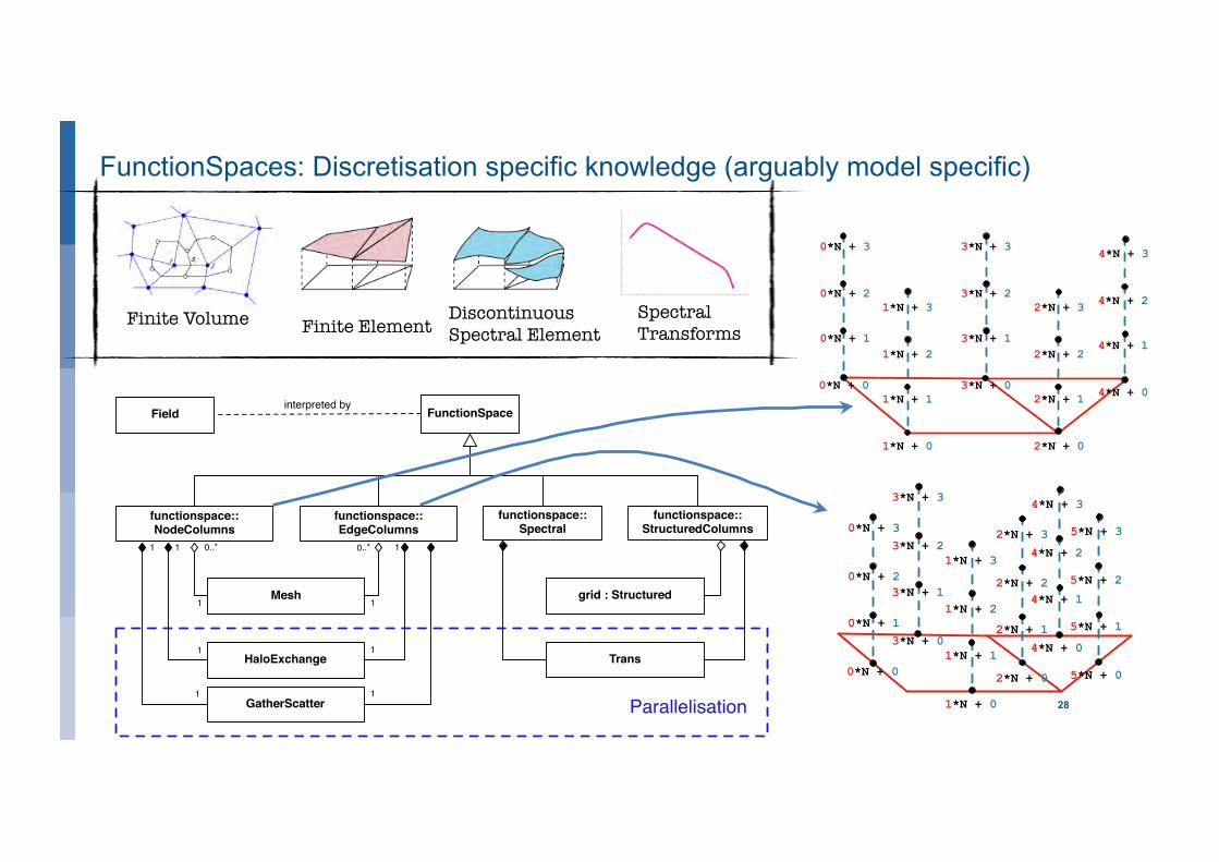
FunctionSpaces: Discretisation specific knowledge (arguably model specific)


Finite Volume Spectral Transforms Finite Element

Discontinuous Spectral Element

FunctionSpace

functionspace::NodeColumns

functionspace::EdgeColumns

Mesh

HaloExchange

GatherScatter

0..* 0..*1 1

1

1

1

1

1

1

1

functionspace::Spectral

functionspace::StructuredColumns

grid : Structured

Trans

Parallelisation

FunctionSpaceFieldinterpreted by

4*N + 0

4*N + 1

4*N + 2

4*N + 3

1*N + 0

1*N + 1

1*N + 2

1*N + 3

0*N + 0

0*N + 1

0*N + 2

0*N + 3

3*N + 0

3*N + 1

3*N + 2

3*N + 3

2*N + 0

2*N + 1

2*N + 2

2*N + 3

5*N + 0

5*N + 1

5*N + 2

5*N + 3

1*N + 0

1*N + 1

1*N + 2

1*N + 3

0*N + 0

0*N + 1

0*N + 2

0*N + 3

3*N + 0

3*N + 1

3*N + 2

3*N + 3

2*N + 0

2*N + 1

2*N + 2

2*N + 3

4*N + 0

4*N + 1

4*N + 2

4*N + 3

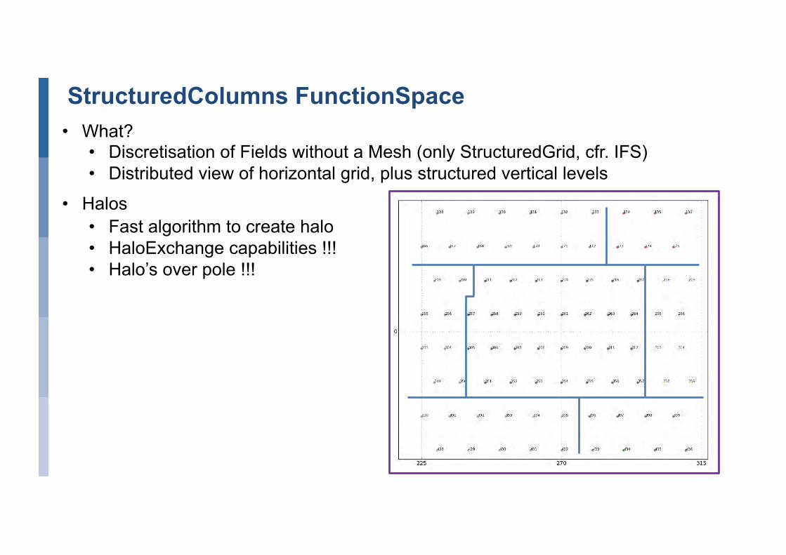
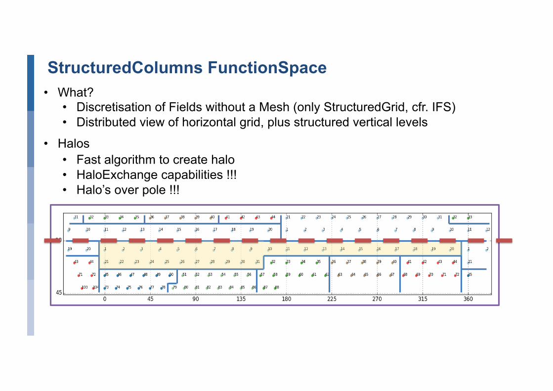
StructuredColumns FunctionSpace •  What?

•  Discretisation of Fields without a Mesh (only StructuredGrid, cfr. IFS) •  Distributed view of horizontal grid, plus structured vertical levels

•  Halos •  Fast algorithm to create halo •  HaloExchange capabilities !!! •  Halo’s over pole !!!

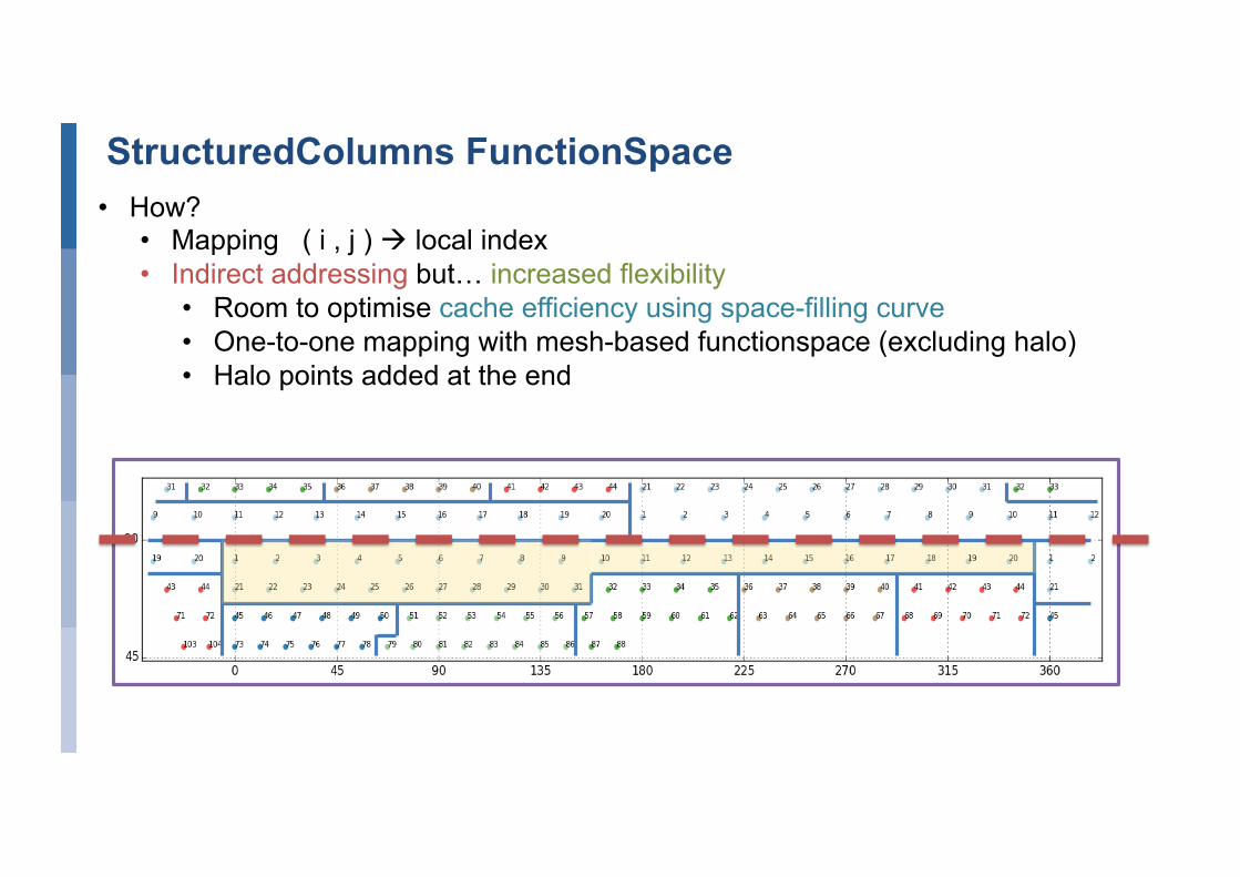
StructuredColumns FunctionSpace •  How?

•  Mapping ( i , j ) à local index •  Indirect addressing but… increased flexibility

•  Room to optimise cache efficiency using space-filling curve •  One-to-one mapping with mesh-based functionspace (excluding halo) •  Halo points added at the end

Atlas architecture

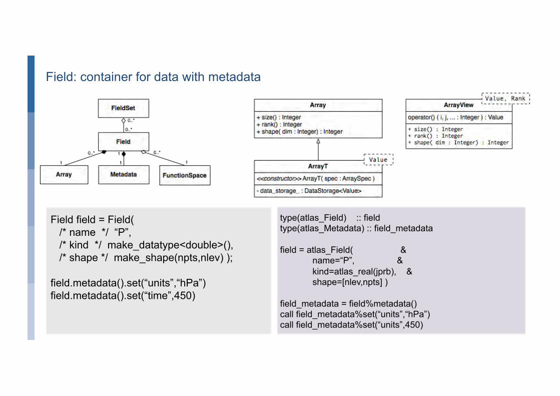
Field field = Field( /* name */ “P”, /* kind */ make_datatype<double>(), /* shape */ make_shape(npts,nlev) ); field.metadata().set(“units”,“hPa”) field.metadata().set(“time”,450)

type(atlas_Field) :: field type(atlas_Metadata) :: field_metadata field = atlas_Field( & name=“P”, & kind=atlas_real(jprb), & shape=[nlev,npts] ) field_metadata = field%metadata() call field_metadata%set(“units”,“hPa”) call field_metadata%set(“units”,450)

Field: container for data with metadata

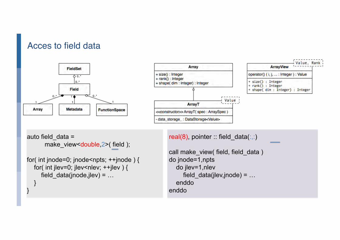
auto field_data = make_view<double,2>( field ); for( int jnode=0; jnode<npts; ++jnode ) { for( int jlev=0; jlev<nlev; ++jlev ) { field_data(jnode,jlev) = … } }

real(8), pointer :: field_data(:,:) call make_view( field, field_data ) do jnode=1,npts do jlev=1,nlev field_data(jlev,jnode) = … enddo enddo

Acces to field data

34

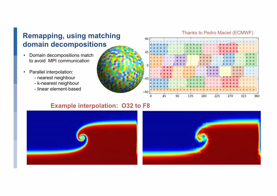
•  Domain decompositions match to avoid MPI communication

•  Parallel interpolation: - nearest neighbour - k-nearest neighbour - linear element-based

Example interpolation: O32 to F8

Remapping, using matching domain decompositions

Thanks to Pedro Maciel (ECMWF)

35

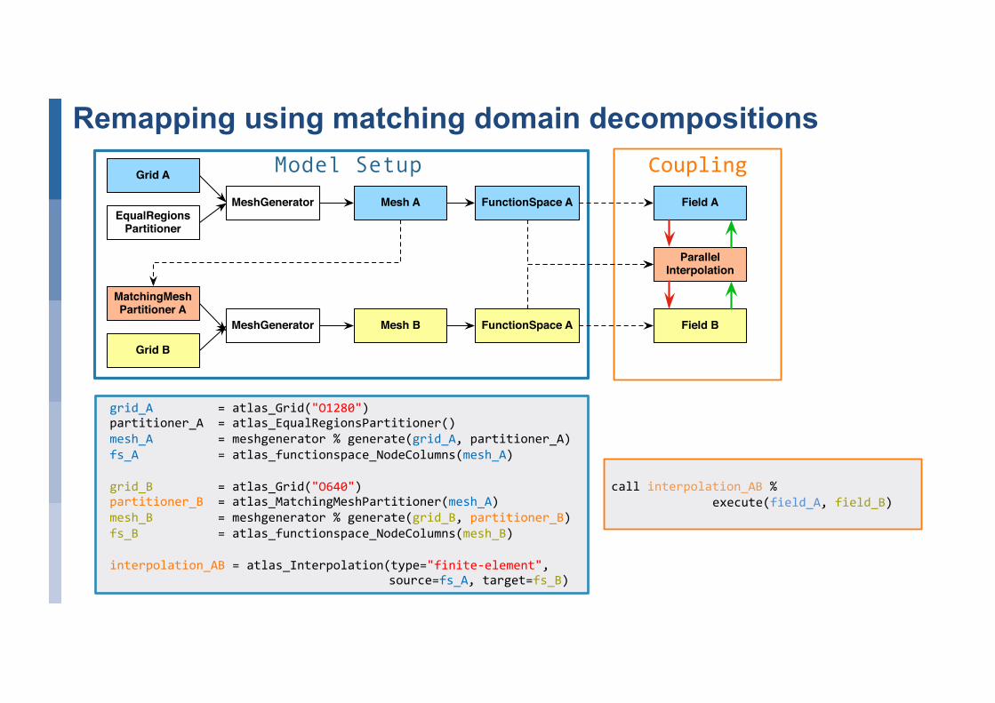
Remapping using matching domain decompositions

grid_A=atlas_Grid("O1280")partitioner_A=atlas_EqualRegionsPartitioner()mesh_A=meshgenerator%generate(grid_A,partitioner_A)fs_A=atlas_functionspace_NodeColumns(mesh_A)grid_B=atlas_Grid("O640")partitioner_B=atlas_MatchingMeshPartitioner(mesh_A)mesh_B=meshgenerator%generate(grid_B,partitioner_B)fs_B=atlas_functionspace_NodeColumns(mesh_B)interpolation_AB=atlas_Interpolation(type="finite-element",

source=fs_A,target=fs_B)

callinterpolation_AB%

execute(field_A,field_B)

Grid A

FunctionSpace AEqualRegions

Partitioner

MeshGenerator

Grid B

MatchingMeshPartitioner A

Mesh A

MeshGenerator Mesh B FunctionSpace A

ParallelInterpolation

Field A

Field B

Model Setup Coupling

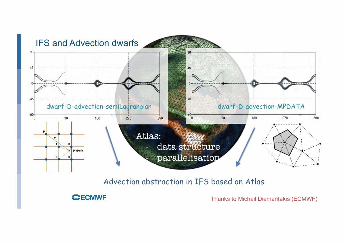
IFS and Advection dwarfs


Atlas: -  data structure -  parallelisation

Advection abstraction in IFS based on Atlas

dwarf-D-advection-semiLagrangian dwarf-D-advection-MPDATA

Thanks to Michail Diamantakis (ECMWF)

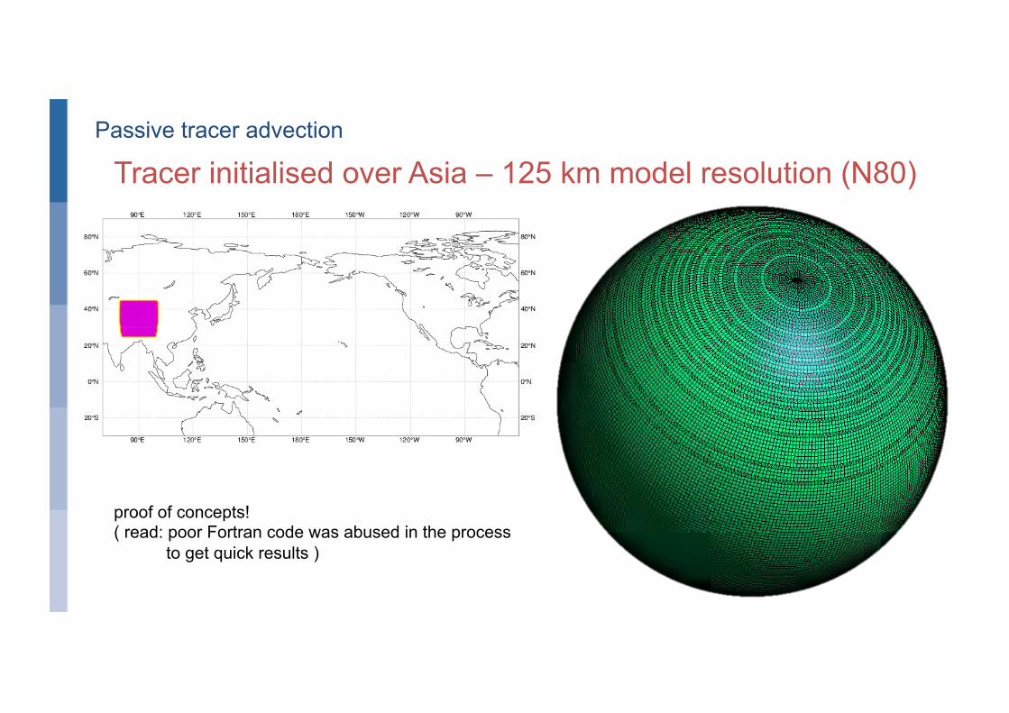
Passive tracer advection

Tracer initialised over Asia – 125 km model resolution (N80)

proof of concepts! ( read: poor Fortran code was abused in the process to get quick results )

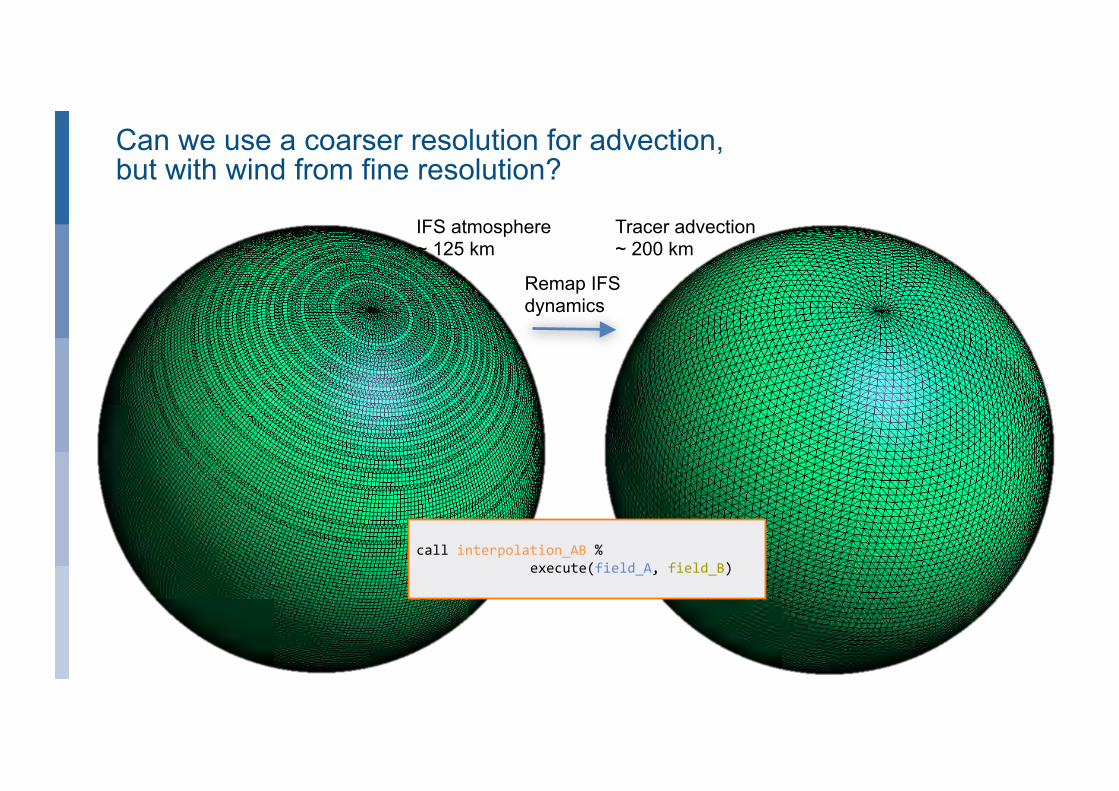
Can we use a coarser resolution for advection, but with wind from fine resolution?

IFS atmosphere ~ 125 km

Tracer advection ~ 200 km

Remap IFS dynamics

callinterpolation_AB%

execute(field_A,field_B)

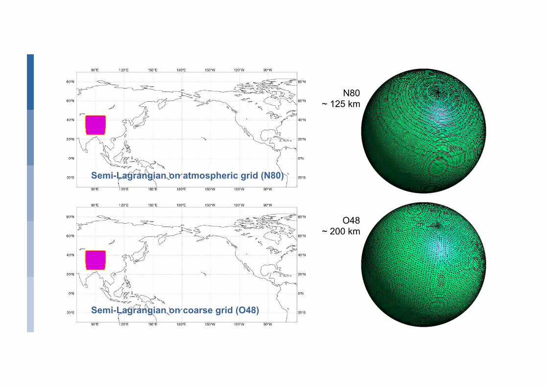
Semi-Lagrangian on atmospheric grid (N80)

Semi-Lagrangian on coarse grid (O48)

N80 ~ 125 km

O48 ~ 200 km

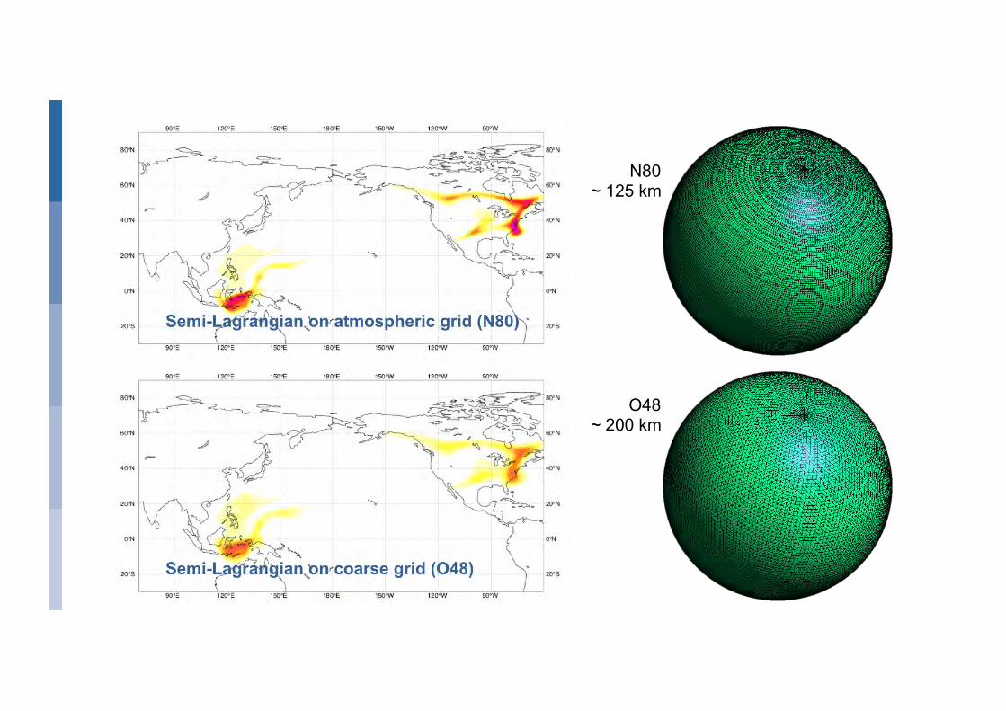
N80 ~ 125 km

O48 ~ 200 km

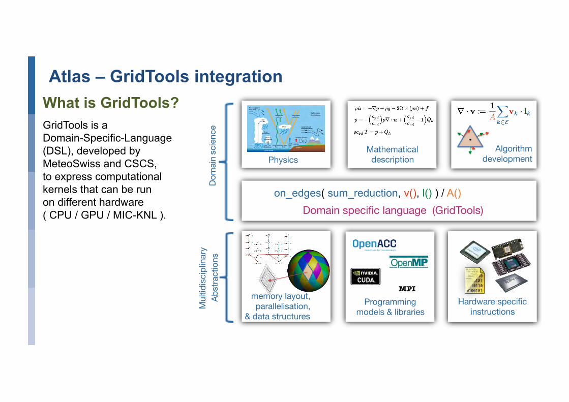
Atlas – GridTools integration What is GridTools?

GridTools is a Domain-Specific-Language (DSL), developed by MeteoSwiss and CSCS, to express computational kernels that can be run on different hardware ( CPU / GPU / MIC-KNL ).

Algorithmdevelopment Physics

Mathematicaldescription

on_edges( sum_reduction, v(), l() ) / A() Domain specific language (GridTools)

Dom

ain

scie

nce

Abst

ract

ions

memory layout, parallelisation,

& data structures Hardware specific

instructions Programming

models & libraries

MPI

Mul

tidis

cipl

inar

y

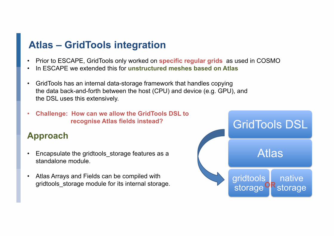
Atlas – GridTools integration •  Prior to ESCAPE, GridTools only worked on specific regular grids as used in COSMO •  In ESCAPE we extended this for unstructured meshes based on Atlas

•  GridTools has an internal data-storage framework that handles copying the data back-and-forth between the host (CPU) and device (e.g. GPU), and the DSL uses this extensively.

•  Challenge: How can we allow the GridTools DSL to recognise Atlas fields instead?

Approach •  Encapsulate the gridtools_storage features as a

standalone module.

•  Atlas Arrays and Fields can be compiled with gridtools_storage module for its internal storage.

GridTools DSL

Atlas

gridtools storage

native storage OR

October 29, 2014

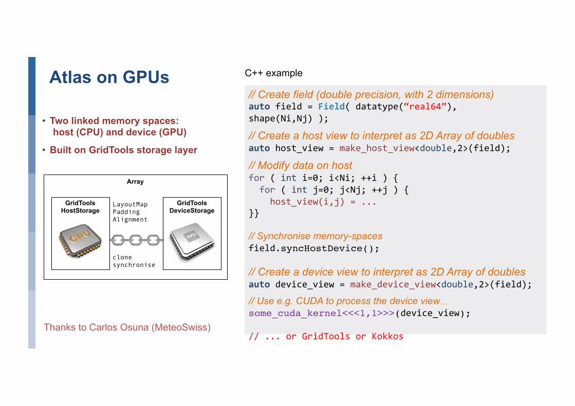
•  Two linked memory spaces: host (CPU) and device (GPU)

•  Built on GridTools storage layer

43

Atlas on GPUs

Array

LayoutMap Padding Alignment

clone synchronise

GridToolsHostStorage

GridToolsDeviceStorage

+ size() : Integer+ rank() : Integer+ shape( dim : Integer) : Integer+ valid() : Boolean

operator() ( i, j, ... : Integer ) : Value

ArrayViewValue, Rank

make_host_view<Value,Rank>make_device_view<Value,Rank>

// Create field (double precision, with 2 dimensions) autofield=Field(datatype(“real64”),shape(Ni,Nj));

// Create a host view to interpret as 2D Array of doubles autohost_view=make_host_view<double,2>(field);

// Modify data on host for(inti=0;i<Ni;++i){for(intj=0;j<Nj;++j){host_view(i,j)=...}}// Synchronise memory-spacesfield.syncHostDevice();// Create a device view to interpret as 2D Array of doubles autodevice_view=make_device_view<double,2>(field);

// Use e.g. CUDA to process the device view…some_cuda_kernel<<<1,1>>>(device_view);//...orGridToolsorKokkos

Thanks to Carlos Osuna (MeteoSwiss)

C++ example

October 29, 2014

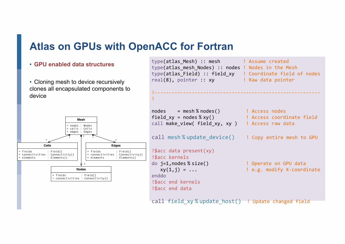
•  GPU enabled data structures

•  Cloning mesh to device recursively clones all encapsulated components to device

44

type(atlas_Mesh)::mesh!Assumecreatedtype(atlas_mesh_Nodes)::nodes!NodesintheMeshtype(atlas_Field)::field_xy!Coordinatefieldofnodesreal(8),pointer::xy!Rawdatapointer!----------------------------------------------------------!nodes=mesh%nodes()!Accessnodesfield_xy=nodes%xy()!Accesscoordinatefieldcallmake_view(field_xy,xy)!Accessrawdatacallmesh%update_device()!CopyentiremeshtoGPU!$accdatapresent(xy)!$acckernelsdoj=1,nodes%size()!OperateonGPUdataxy(1,j)=...!e.g.modifyX-coordinateenddo!$accendkernels!$accenddatacallfield_xy%update_host()!Updatechangedfield

+ nodes : Nodes+ cells : Cells+ edges : Edges

Mesh

+ fields : Field[]+ connectivities : Connectivity[]+ elements : Elements[]

Cells

+ fields : Field[]+ connectivities : Connectivity[]+ elements : Elements[]

Edges

+ fields : Field[]+ connectivities : Connectivity[]

Nodes

11 1

1

1

1

Atlas on GPUs with OpenACC for Fortran

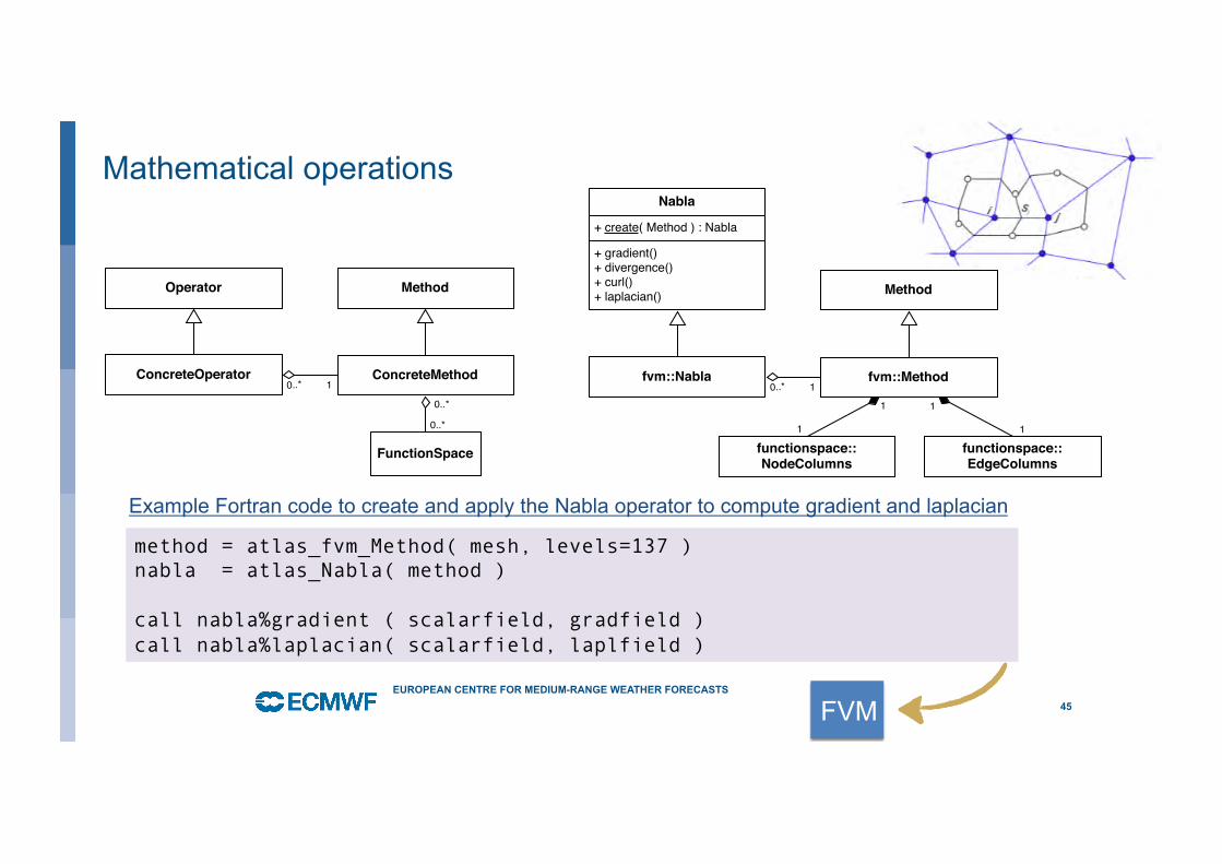
Mathematical operations

+ gradient()+ divergence()+ curl()+ laplacian()

Nabla

+ create( Method ) : Nabla

fvm::Nabla fvm::Method

Method

functionspace::NodeColumns

functionspace::EdgeColumns

1

1 1

1 1

0..*ConcreteOperator ConcreteMethod

Method

10..*

Operator

FunctionSpace

0..*

0..*


method = atlas_fvm_Method( mesh, levels=137 ) nabla = atlas_Nabla( method ) call nabla%gradient ( scalarfield, gradfield ) call nabla%laplacian( scalarfield, laplfield )

Example Fortran code to create and apply the Nabla operator to compute gradient and laplacian

FVM

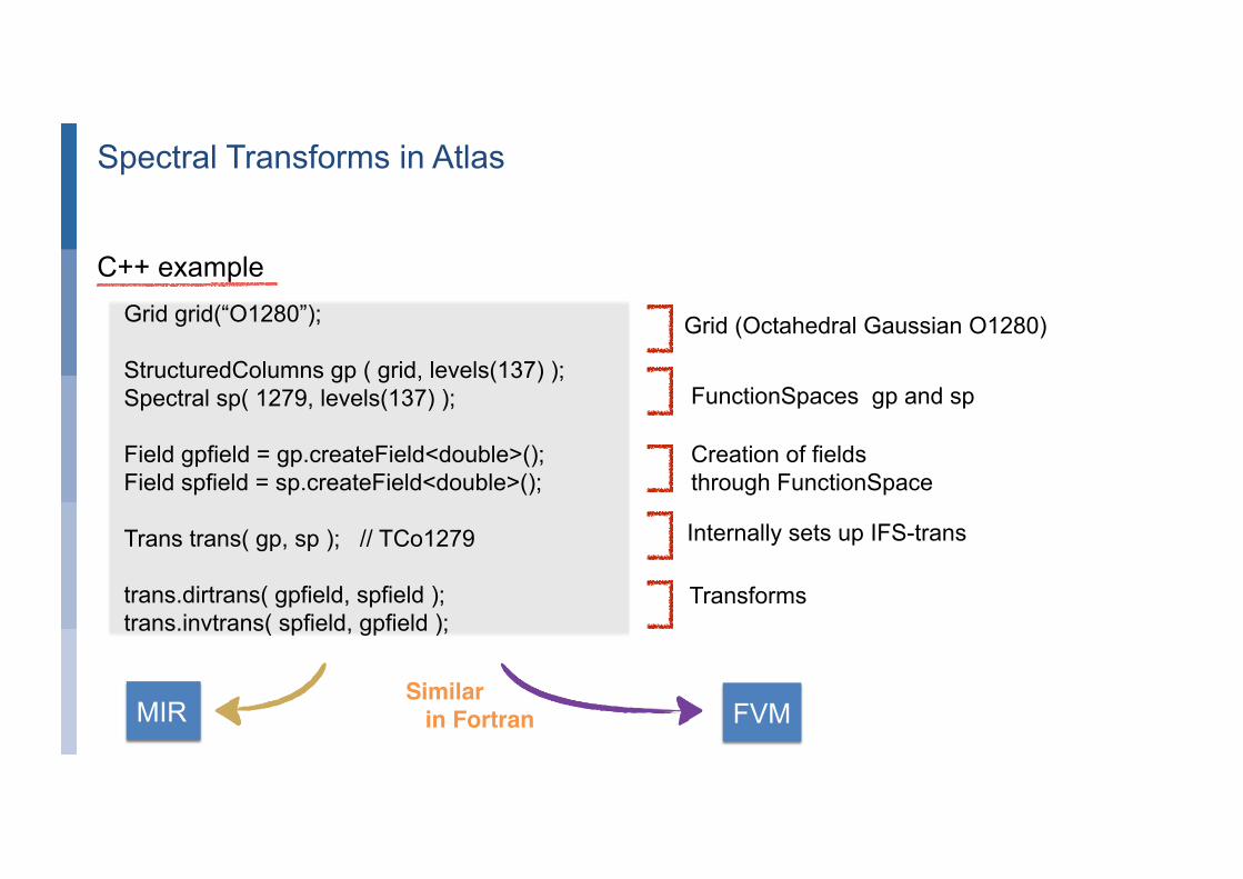
Spectral Transforms in Atlas

Grid grid(“O1280”); StructuredColumns gp ( grid, levels(137) ); Spectral sp( 1279, levels(137) ); Field gpfield = gp.createField<double>(); Field spfield = sp.createField<double>(); Trans trans( gp, sp ); // TCo1279 trans.dirtrans( gpfield, spfield ); trans.invtrans( spfield, gpfield );

FunctionSpaces gp and sp

Creation of fields through FunctionSpace

Transforms

Internally sets up IFS-trans

FVM

Grid (Octahedral Gaussian O1280)

C++ example

Similar in Fortran MIR

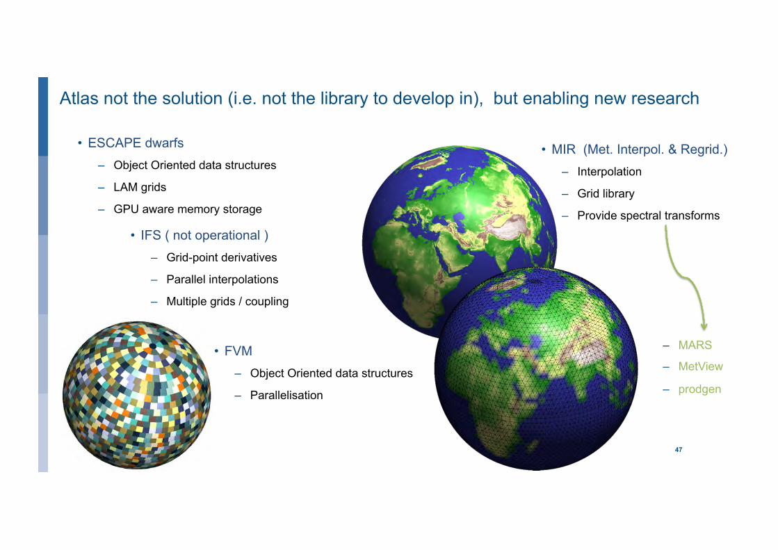
Atlas not the solution (i.e. not the library to develop in), but enabling new research

•  IFS ( not operational ) –  Grid-point derivatives

–  Parallel interpolations

–  Multiple grids / coupling

47

•  ESCAPE dwarfs –  Object Oriented data structures

–  LAM grids

–  GPU aware memory storage

•  MIR (Met. Interpol. & Regrid.) –  Interpolation

–  Grid library

–  Provide spectral transforms

•  FVM –  Object Oriented data structures

–  Parallelisation

–  MARS

–  MetView

–  prodgen

© ECMWF maggio 18, 2018

Thank you! ESCAPE has received funding from the European Union’s Horizon 2020 research and innovation programme under grant agreement no. 671627.

Atlas, a library for NWP and climate modelling

By Willem Deconinck

[email protected] OpenAccess

5th ENES HPC Workshop 17-18 May 2018, Lecce

Atlas, a library for NWP and climate modelling - ESiWACE

Documents

Transcript of Atlas, a library for NWP and climate modelling - ESiWACE