arX

iv:g

r-qc

/051

2057

v1 9

Dec

200

5

Asymptotic behavior of the warm inflation scenario with viscous

pressure

Jose P. Mimoso,1, ∗ Ana Nunes,2, † and Diego Pavon3, ‡

1Department of Physics, Faculdade de Ciencias da Universidade de Lisboa,

and Centro de Fısica Teorica e Computacional da Universidade de Lisboa,

Av. Prof. Gama Pinto 2, P-1649-003 Lisboa, Portugal

2Department of Physics, Faculdade de Ciencias da Universidade de Lisboa,

and Centro de Fısica Teorica e Computacional da Universidade de Lisboa,

Av. Prof. Gama Pinto 2, P-1649-003 Lisboa, Portugal

3Departamento de Fısica, Universidad Autonoma de Barcelona, Facultad de Ciencias

08193 Bellaterra (Barcelona) Spain

(Dated: February 7, 2008)

Abstract

We analyze the dynamics of models of warm inflation with general dissipative effects. We con-

sider phenomenological terms both for the inflaton decay rate and for viscous effects within matter.

We provide a classification of the asymptotic behavior of these models and show that the existence

of a late-time scaling regime depends not only on an asymptotic behavior of the scalar field poten-

tial, but also on an appropriate asymptotic behavior of the inflaton decay rate. There are scaling

solutions whenever the latter evolves to become proportional to the Hubble rate of expansion re-

gardless of the steepness of the scalar field exponential potential. We show from thermodynamic

arguments that the scaling regime is associated to a power-law dependence of the matter-radiation

temperature on the scale factor, which allows a mild variation of the temperature of the mat-

ter/radiation fluid. We also show that the late time contribution of the dissipative terms alleviates

the depletion of matter, and increases the duration of inflation.

PACS numbers: 98.80.Cq, 47.75+f

Keywords:

∗Electronic address: jpmimoso@cii.fc.ul.pt†Electronic address: anunes@lmc.fc.ul.pt

1

‡Electronic address: diego.pavon@uab.es

2

I. INTRODUCTION

There is a widespread belief that our Universe, or at least a sufficiently large part of

it causally connected to us, experienced an early period of accelerated expansion, called

inflation. This happened before the primordial nucleosynthesis era could take place and

likely after the Planck period. Many inflationary scenarios have been proposed over the

years (see [1] and references therein). Most of them rely on the dynamics of a self-interacting

scalar field (the “inflaton”), whose potential overwhelms all other forms of energy during

the relevant period. They generally share the unsatisfactory feature of driving the Universe

to such a super-cooled state that it becomes necessary to introduce an ad hoc mechanism

-termed “reheating”- in order to raise the temperature of the universe to levels compatible

with primordial nucleosynthesis. Therefore this reheating phase appears as a subsequent,

separate stage mainly justified by the need to recover from the extreme effects of inflation

[2] during which a rather elaborate process of multifield parametric resonances followed by

particle production [3, 4, 5] takes place.

As an alternative some authors have looked for inflationary scenarios leading the universe

to a moderate temperature state at the end of the superluminal stage so that the reheating

phase could be dispensed with altogether. It was advocated that this can be accomplished

by coupling the inflaton to the matter fields in such a way that the decrease in the energy

density of the latter during inflation is somewhat compensated by the decay of the inflaton

into radiation and particles with mass. This would happen when the inflaton rolls down its

potential, but keeping the combined pressure of the inflaton and radiation negative enough

to have acceleration. This kind of scenario, known as “warm inflation” as the radiation

temperature never drops dramatically, was first proposed by Berera [6, 7]. It now rests on

solid grounds since it has been forcefully argued in a series of papers that indeed the inflaton

can decay during the slow-roll (see, e.g. [8, 9, 10] and references therein). Besides, this

scenario has other advantages, namely: (i) the slow-roll condition φ2 ≪ V (φ) can be fulfilled

for steeper potentials, (ii) the density perturbations generated by thermal fluctuations may

be larger than those of quantum origin [11, 12, 13], and (iii) it may provide a very useful

mechanism for baryogenesis [14].

To simplify the study of the dynamics of warm inflation, previous works treated the par-

ticles created in the decay of the inflaton purely as radiation, thereby ignoring the existence

3

of particles with mass in the decay fluid. Here, we will go a step beyond by taking into

account the presence of of particles with mass as part of the decay products, and give a

hydrodynamical description of the mixture of massless and non-massless particles by an

overall fluid with equation of state p = (γ − 1)ρ, where the adiabatic index γ is bounded by

1 ≤ γ ≤ 2.

On very general grounds, this fluid is expected to have a negative dissipative pressure,

Π, that somewhat quantifies the departure of the fluid from thermodynamical equilibrium,

which we will consider to be small but still significant. This viscous pressure arises quite

naturally via two different mechanisms, namely: (i) the inter-particle interactions [15], and

(ii) the decay of particles within the matter fluid [16].

A well known example of mechanism (i) of prime cosmological interest is the radiative

fluid, a mixture of massless and non-massless particles, as it plays an essential role in the

description of the matter-radiation decoupling in the standard cosmological model [17, 18,

19].

A sizeable viscous pressure also arises spontaneously in mixtures of different particles

species, or of the same species but with different energies -a typical instance in laboratory

physics is the Maxwell-Boltzmann gas [20]. One may think of Π as the internal “friction”

that sets in as a consequence of the diverse cooling rates in the expanding mixture, something

to be expected in the matter fluid originated by the decay of the inflaton.

As for mechanism (ii), it is well known that the decay of particles within a fluid can be

formally described by a bulk dissipative pressure Π. This is only natural because the decay

is an entropy–producing scalar phenomenon associated with the spontaneous enlargement

of the phase space (we use the word “scalar” in the sense of irreversible thermodynamics)

and the bulk viscous pressure is also a scalar entropy–producing agent. There is an ample

body of literature on the cosmological applications of this analogy -see e.g. [16], [21]. In

the case of warm inflation, it is natural to expect that, at least, some species of particles

directly produced by the decay of the inflaton will, in turn, decay into other, lighter species.

In this connection, it has been proposed that the inflaton may first decay into a heavy boson

χ which subsequently decays in two light fermions ψd [22]. This is an obvious source of

entropy, and therefore it can be modelled by a dissipative bulk pressure Π.

Our purpose in this paper is to generalize the usual warm inflationary scenario by in-

troducing the novel elements mentioned above, namely the decay of the scalar field into a

4

fluid of adiabatic index γ rather than just radiation, and especially the dissipative pressure

of this fluid, irrespective of the underlying mechanism. We will not dwell on the difficult

question of the quantum, non–equilibrium thermodynamical problem underlying warm in-

flation [8, 23, 24, 25, 26, 27, 28], but rather take a phenomenological approach similar to

that considered in several works [29, 30, 31, 32, 33] (which can be traced back to the early

studies of inflation [34]). Instead of adopting a model building viewpoint and looking for

the implications of specific assumptions, we aim at identifying typical features of models

that yield interesting asymptotic behavior. We resort to a qualitative analysis of the corre-

sponding autonomous system of differential equations using the approach developed in [35]

that allows the consideration of arbitrary scalar field potentials. We will characterize the

implications of allowing for various forms of the rate of decay of the scalar field, as well

as for various forms for the dissipative pressure. We consider, for instance, models with

scalar field potentials displaying an asymptotic exponential behavior. These arise naturally

in generalized theories of gravity emerging in the low-energy limits of unification proposals

such as super-gravity theories or string theories [36]. On the one hand, after the dimen-

sional reduction to an effective 4-dimensional space-time and the subsequent representation

of the theories in the so-called Einstein frame typical polynomial potentials become expo-

nential [37, 38]. On the other hand, the theories are then characterised by the existence of a

scalar field that couples to all non-radiation fields, with the coupling depending, in general,

on the scalar field. The simplest example of these features can be found in the so-called

non-minimal coupling theories. We provide a classification of the relevant global dynamical

features of the cosmological model associated with those possible choices. A limited account

of some of the results of the present work was reported in [39].

One question we address is whether non-trivial scaling solutions [33, 35, 40, 41] (hereafter

simply termed scaling solutions) exist, i.e., solutions where the ratio of energies involving

the matter fluid and scalar field keep a constant ratio. Another class of solutions refered in

the literature as having a scaling asymptotic behavior are those for which both the energy

density of the scalar field and that of the matter fluid decay with different power laws of the

scale factor of the universe [40, 45, 46]. In this latter case one of the components eventually

dominates and thus the ratio of their energy densities becomes evanescent, in clear contrast

to the case of the non-trivial scaling solutions. We shall term these solutions as trivial scaling

solutions to contrast them with the previous ones sometimes dubbed tracker solutions. The

5

trivial case arises in association with scalar field potentials of a power-law type and, as we

shall see, they occur when the scalar field decays have the the same type of time-dependences

as those required by the (non-trivial, tracking) scaling solutions.

One of the reasons why non-trivial scaling solutions are important is that they provide an

asymptotic stationary regime for the energy transfer between the scalar field and radiation.

This stationary (sometimes termed “quasi-static”) regime is an assumption in the standard

treatment of warm inflation [11] to evaluate the temperature of matter in the final stages.

On the other hand, introducing this class of solutions in the kinetic analysis of interacting

fluids [42, 43] leads to an alternative to the usual Γ ≫ 3H case, generalizing the example of

Ref. [44] where temperature of the matter (radiation) bath is nearly constant.

We show that this class of scaling behavior depends not only on the asymptotic form of

the inflaton [35], but also on having an appropriate time-dependent rate for the scalar field

decay. The additional consideration of bulk viscosity, besides being a natural ingredient in

models with one or more matter components as well as in models with inter-particle decays,

facilitates the Universe to have a late time de Sitter expansion.

An outline of this work is as follows. Section II studies the model underlying the original

idea of the warm inflation proposal, namely the model in which the inflaton field decays into

matter during inflation thus avoiding the need for the post-inflationary reheating. This decay

is characterized by a rate Γ which we shall initially assume to be a constant. Our results

though will argue in favour of a varying Γ and we shall thus consider the case where Γ ∝ H .

This yields late time scaling solutions whenever the scalar field potentials asymptotes to an

exponential behavior. This happens regardless of the slope of the potential. Subsequently,

section IIII, analyses more realistic models where a bulk viscous pressure term Π is also

present in the equation of state of matter. We first envisage the usual form Π = −3ζH for

that pressure and, subsequently, analyse a general model with both a varying rate of decay

and a general form for the bulk viscosity Π = −3ζ ρα Hβ, where 2α+ β = 2 on dimensional

grounds. Finally, section IV provides a discussion of our results.

6

II. THE DYNAMICS OF WARM INFLATION

A. Warm inflation with constant Γ

We consider a spatially flat Friedmann-Robertson-Walker universe filled with a self-

interacting scalar field and a perfect fluid consisting of a mixture of matter and radiation,

such that the former decays into the latter at some constant rate Γ. For the time being

we ignore the dissipative pressure. We also neglect radiative corrections to the inflaton

potential [12, 24]. The corresponding system of equations reads

3H2 = ρ+φ2

2+ V (φ) , (1)

H = −12(φ2 + γρ) , (2)

φ = −(3H + Γ)φ− V ′(φ) , (3)

where here and throughout we use units in which 8πG = c = 1. The first two are Einstein’s

equations, the third describes the decay of the inflaton. From these, it follows the energy

balance for the matter fluid,

ρ = −3γ H ρ+ Γφ2 . (4)

As usual H ≡ a/a denotes the Hubble factor.

To cast the corresponding autonomous system of four differential equations it is expedient

to introduce the set of normalized variables

x2 =φ2

6H2(5)

y2 =V (φ)

3H2(6)

r =Γ

3H, (7)

along with the new time variable N = ln a. Thus we get

x′ = x (Q− 3(1 + r)) −W (φ) y2, (8)

y′ = (Q+W (φ) x) y , (9)

7

r′ = r Q , (10)

φ′ =√

6 x , (11)

where a prime means derivative with respect to N , and the definitions

W (φ) =

√

3

2

(

∂φV

V

)

(12)

and

Q =3

2

[

2x2 + γ (1 − x2 − y2)]

, (13)

as well as ρ/(3H2) = 1 − x2 − y2 were used. Equation (11) was first considered in [35],

and is crucial for the consideration of general potentials V (φ) besides the particular case of

the exponential potential. The function Q defined by Eq. (13) is related to the deceleration

parameter q = −aa/a2 by Q = 1 + q.

The special case where r = 0, naturally, corresponds to the absence of interaction between

the scalar field and the perfect fluid, and it is an invariant manifold of the dynamical

system (8)-(11). It is appropriate to refer here its major features in order to better appreciate

the implications of the decay of the scalar field (see Table I).

We distinguish the fixed points of the system into those occurring for finite values of φ

and those associated with the asymptotic limit, φ → ∞. In the former case, i.e., for finite

φ = φ∗, the fixed points always require the vanishing of the kinetic energy of the scalar field

(x = 0). They are located at the origin (x = y = 0), and at (x = 0, y = 1), on the frontier

of the phase space domain x2 + y2 = 1, which is an invariant manifold. For x = 0, y = 0,

the potential must have a vanishing critical point at φ∗, a case that cannot be dealt with

the variables in use, but it is well-know that if φ∗ is a minimum at the origin, then it is

a stable point and the scale factor evolves as a(t) ∝ t2/(3γ) [46, 50]. The fixed points on

x2 + y2 = 1 are given by x = 0, y = 1 and require that W = 0. This means that they can

only occur in association with extrema of the potential. Their stability is defined by the

sign of W ′(φ∗), where φ∗ is the value of φ where V ′(φ) (and hence W ) vanishes. When V

has a non-vanishing minimum and, hence W ′ > 0, the critical point is a stable node. When

V has a maximum and, hence W ′ < 0, we have a saddle point (an unstable fixed point).

These fixed points correspond to the de Sitter exponential behavior and are accompanied

by the depletion of the matter component (ρ = 0).

8

To study the critical points that occur at φ → ∞ (which we shall label φ∞), we carry

out the regularization produced by the change of variable ψ = 1/φ. Then Eq. (11) becomes

ψ′ = −√

6xψ2 , (14)

and the critical points correspond to either to x = 0, as previously seen, or ψ = 0. The

φ∞ critical points depend on the asymptotic behavior of V (φ) [35]. If V (φ) exhibits some

non-vanishing asymptotic value we have again x = 0, y = 1 corresponding to a cosmological

constant and, hence, to a de Sitter late-time behavior. If V (φ) asymptotes towards the

exponential potential, say V ∝ e−λφ, with λ constant, there are several possible fixed values

dependent on the ratio between λ2 and γ (see, for instance, [48] for details). There are

unstable fixed points on the invariant manifolds bounding the phase-space domain for all

possible choices of both W = −√

3/2λ and γ, namely: (i) a matter dominated solution at

x = 0 and y = 0, which is a saddle and corresponds to a(t) ∝ t2/(3γ), (ii) two solutions

dominated by the scalar field kinetic energy at x = ±1 and y = 0 which are either unstable

nodes or saddles, and correspond to the stiff behavior a(t) ∝ t1/3, φ∞(t) ∼ ln tK0 , where

K0 is an arbitrary constant defining the scalar field initial velocity. There is another fixed

point on the x2 + y2 = 1 boundary representing a scalar field dominated solution, when

W 2 < 9. This fixed point is stable when W 2 < 9γ/2, and unstable otherwise (saddle). Thus

for W 2 > 9γ/2 (i.e., λ2 > 3γ), there is a stable fixed point in the interior of the phase space

domain. This latter point corresponds to scaling behavior between the matter and scalar

field energy-densities [38, 40, 41, 47, 48, 49]. This attractor solution is characterized by

a(t) ∝ t2/3γ and φ− φ0 = ln t±2/λ.

There are also trivial scaling solutions for which ρφ ∝ a−n and ρ ∝ a−m, where n > m

are positive constants, when [46]

V (φ) = A2(

1 − n

m

)2 (6 − n

2n

)

(

φ

A

)

(15)

where

=2n

n−m. (16)

Coming back to the model that includes the interaction and thus letting r be non-

vanishing, we immediately see from Eq. (10) that, along the r-direction, all the points are

singular points if and only if Q = 0. For finite values of φ, as x = 0 at the fixed points, this

requires once more y2 = 1 so that the singular points are associated with ρ = 0, i.e., with the

9

depletion of the matter component. Moreover, as in the r = 0 case, these singular points are

extrema of the potential V (φ). They correspond to a de Sitter behavior (a(t) ∝ e√

V (φ0)/3) t,

φ = φ0 constant) and are either stable or unstable depending on the extremum being a

minimum (W ′ > 0) or a maximum (W ′ < 0). In fact, at the singular points corresponding

to extrema of the potential V (φ), the eigenvalues found in the linear stability analysis are

µy = −3γ , (17)

µx,φ = −3(1 + r)

2

1 ±

√

√

√

√1 − 4√

6W ′(φ0)

9(1 + r)2

. (18)

On the other hand, we no longer have fixed points at x = 0, y = 0 (unless γ = 0 which

corresponds to the perfect fluid being a cosmological constant). This happens because the

system then evolves along the r-axis towards r → ∞, a behavior that can only be prevented

by the existence of a positive minimum of the potential V (φ). At φ → ∞ the system does

not exhibit scaling solutions anymore. The only fixed points allowed in this asymptotic

limit are those associated with a non-vanishing, asymptotically flat potential, which thus

corresponds to the de Sitter exponential behavior.

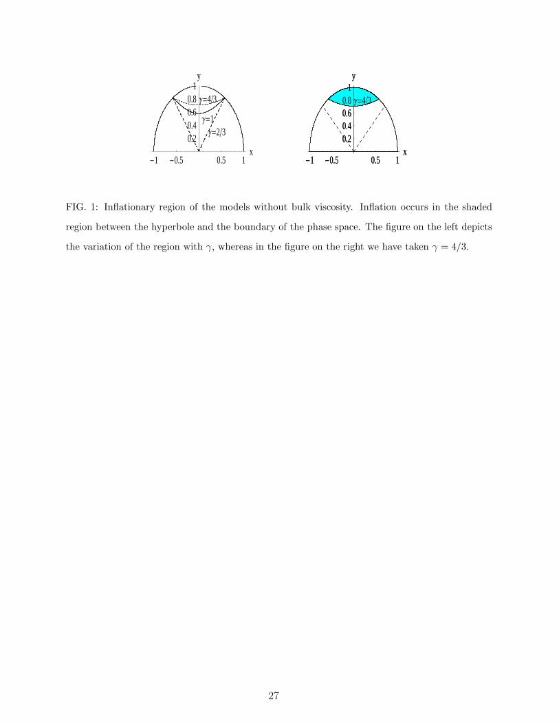
Accelerated expansion corresponds to the region of the phase space where Q < 1, so that

3γy2 − 3(2 − γ)x2 > 3γ − 2 . (19)

This condition does not carry any dependence either on r or φ. Thus we may restrict our

discussion to a (x, y) projection of the phase space. The condition (19) defines for 1 < γ < 2

the region between the upper branch of the hyperbolae 3γy2 − 3(2 − γ)x2 = (3γ − 2) and

the boundary x2 + y2 = 1 of the phase space domain (see Figure 1). The asymptotes of the

hyperbolae are y = ±√

(2 − γ)/γ, and we see that, as γ increases, the inflationary region

becomes progressively smaller. In fact the region shrinks vertically towards the x = 0, y = 1

point and it reduces to it in the limit case of γ = 2.

In Ref. [11] the end of inflation is given by the condition ρφ ≃ ργ and this event is

associated with the beginning of the matter (radiation) domination. As it becomes apparent

from the above discussion, the condition for the end of inflation, Q = 1, is more general and

does not strictly require matter domination. Taylor and Berera’s condition [11] corresponds

to the end of slow-roll inflation (i.e., φ2 ≃ 0 ≃ x) and is extended, in the present study, to

general γ-fluids as

ρm ≃ 2

3γ − 2ρφ . (20)

10

The independence on r of the size of inflationary region should not though be understood

as the interaction having no effect on inflation. From Eqs (17) and (18) we see that the

eigenvalues of the linearized system at the fixed points carry a dependence on r which is

such that it renders the minima of the potential more stable and the maxima less unstable

(as if the potential became shallower). Thus the transfer of energy from the scalar field to the

perfect fluid favors inflation in that the system spends a longer time in the neighborhood

of the extrema of the potential. This is exactly what is meant to happen in the warm

inflation scenario where it is assumed that slow roll holds and argued that r allows for

steeper potentials than those required in its absence. As discussed in [11], it is a simple

matter to see that the slow-roll condition on φ

φ = − V ′

3H(1 + r)≃ − V ′

3rH, (21)

is easier to satisfy if the scalar field decays, that is, if r > 1 and much easier if r ≫ 1.

The fact that r increases indefinitely in the present model is a consequence of its definition,

and merely translates the fact that, unless the system is trapped at a non-vanishing minimum

of V (φ), H decreases towards zero. Since this is a direct result of assuming a constant Γ, we

consider in the next section a more appropriate model where Γ decreases as the Universe’s

expansion proceeds.

B. Warm inflation with Γ ∝ H

We assume that Γφ = 3Γ∗H where Γ∗ is a dimensionless, positive constant. As H is

expected to be a non-increasing function of time in an expanding universe, this is a simple

choice for the time dependence of Γφ such that the decays have a stage of maximum intensity

(when inflation occurs) followed by a progressive attenuation until it vanishes altogether.

Now r = Γ∗ is a constant parameter and the dynamical system reduces to the three

equations

x′ = x [Q− 3(1 + r)] −W (φ) y2, (22)

y′ = [Q+W (φ) x] y , (23)

φ′ =√

6x , (24)

where Q is still given by Eq. (13) We see that these equations are analogous to those of

the r = 0 case of the previous section with a different coefficient on the linear term in x

11

of Eq. (22). Thus the basic qualitative dynamical features remain the same as those found

for that model (see Table II). The decay of the scalar field though introduces two major

consequences worthing to be emphasized.

Besides the fact that the origin x = 0, y = 0 is again a fixed point associated with the

vanishing of the scalar field’s energy and, hence, corresponds to the matter domination, the

interaction given by a non-vanishing r has the relevant effect (already found in the constant

Γ model) that the stability of the minima is reinforced and that the maxima become less

unstable. Moreover, the scalar field decay prevents the existence of the fixed points at

x = ±1, y = 0, that would correspond to a behavior completely dominated by the scalar

field’s kinetic energy (and which was, therefore, associated with a stiff behavior in the r = 0

case).

The other major effect of the interaction arises when we look for fixed points with x2+y2 <

1 at φ → ∞. Now, we find that there are always attracting scaling solutions for potentials

that have an asymptotic exponential behavior, that is, for potentials for which W → const

when φ → ∞ [35]. Moreover, this happens independently of the steepness of the late time

exponential behavior which is a remarkable effect of the present model for the transfer of

energy from the scalar field to the matter.

Indeed the latter solutions are given by the roots of the system of equations

(u− 1)(u− a

b) − ru = 0 , (25)

and

cos2 θ =λ2

6(1 + r)2ξ2 , (26)

where u = ξ2 and θ are polar coordinates, x = ξ cos θ and y = ξ sin θ, and where we have

defined

a =γ

2(27)

b =λ2

6(1 + r)2, (28)

as well asW∞ = −√

3/2λ. It is a simple matter to conclude that the effect of a non-vanishing

r is such that equations (25) and (26) always have one non-vanishing root within the range of

allowed values for ξ and for cos θ, and hence there are scaling solutions regardless of the ratio

between λ2 and 3γ. Furthermore linear stability analysis shows that the scaling solutions

12

are stable. It is important nevertheless to remark that although scaling solutions emerge

for any ratio of λ2/γ, the way that the γeff index associated with the effective equation of

state inducing the power-law scaling behavior is shifted from the corresponding γ value of

the scaling solutions in the absence of decays depend on λ2 being larger or smaller than γ.

Assuming the potential to be asymptotically given by V ∝ e−λφ, the latter solutions are

a(t) ∝ tA, φ− φ0 = ln t±2/λ, where A is given in implicit form by

3γ

(

A− 2

3γ

)

(

A− 2

λ2(1 + r)

)

− 4r

λ2= 0 . (29)

Notice that we can define γeff = 2/(3A). A linear expansion about r = 0 in the neighborhood

of the scaling solution (for λ2 6= 3γ) yields

A =2

3γ

1 +2λ2

(

23γ

− 2λ2

) r

, (30)

when λ2 6= 3γ. So the decays have the effect of increasing (resp. decreasing) the scale factor

rate of expansion with regard to the r = 0 case if λ2 > 3γ (resp. λ2 < 3γ). In particular

we can see that the scaling behavior can be inflationary, for cases where this would not

happen in the absence of decays. For instance, taking γ = 4/3 and λ2 > 4, the condition

for the scaling solution to be inflationary is 1 + r > λ2/4 > 1. Thus, in this model, the

solutions yield endless power-law inflation even for a modest scalar field decay, provided that

the asymptotic behavior of the potential is steep enough, i.e., λ2 > 3γ (> 4 in the present

example).

Naturally, besides the scaling solutions, there can also be fixed points corresponding to

de Sitter behavior x = 0, y = 1, whenever the scalar field potential exhibits an asymptotic,

non-vanishing constant value. However, when the potential is asymptotically exponential,

that there are no fixed points on the boundary x2+y2 = 1 at φ∞ in contrast to what happens

in the r = 0 case.

From a thermodynamical viewpoint, the above scaling solutions are particularly interest-

ing. In a universe with two components, it can be shown [42, 43] that the temperature of

each of the components satisfies the equation

Ti

Ti= −3

a

a

(

1 − Γi

3H

)

∂pi

∂ρi+

nisi

∂ρi/∂Ti, (31)

where i = 1 or 2, ni denotes the number density of particles of the i-species, Γi their rate

of decay, and Ti the temperature of this component. In the important case of particle

13

production with constant entropy per particle, si = 0, we also have (ρ1 + p1)Γ1 = −(ρ2 +

p2)Γ2. Thus, taking the first component to be the matter/radiation fluid and the second to

be the inflaton scalar field, we have

Γφ =(ρ+ p)

φ2Γm/r ∝ Γm/r . (32)

As (ρ + p)/φ2 = γ(1 − x2 − y2)/2x2 is a constant in the scaling solutions, Γφ = 3rH , with

r a constant, implies Γm/r = 3σH , where σ is another constant that depends both on r and

on the location of the scaling solution. This yields a temperature of the matter/radiation

component evolving as a power-law T ∝ a−3(γ−1)(1−σ). Thus for σ close to 1, the temperature

of the matter/radiation remains quasi-static, whereas for σ > 1 (resp. σ < 1), it increases

(resp. decreases). Notice also that for σ ≃ 0, we recover the temperature law for perfect

fluids without dissipative effects. Provided we guarantee enough inflation, r need not be

very large (contrary to what is usually assumed to facilitate slow-rolling). Indeed, the

temperature of the radiation at the end of inflation is

Tend = Tbeginning e−N(1−σ) , (33)

where N is the number of e-foldings. Thus, a value of sigma lower but sufficiently close to

1 has the potential to avoid a serious decrease of the temperature of the universe. As

σ =3x2

∗

2(1 − x2∗ − y2

∗)r , (34)

at the scaling solutions, we see that r need not be very large to ensure that σ ∼ 1.

Trivial scaling solutions generalizing those given Eq. (15) in the r = 0 case, arise in these

models for scalar field potentials of the form

V (φ) = A2(

1 − n

m

)2(

6(1 + r) − n

2n

) (

φ

A

)

, (35)

where is still given by Eq. (16) and A = Ar=0/√

1 + r. For the potential to be positive

one also requires 0 < m < n < 6(1 + r). The only difference with respect to the r = 0

case lies in the dependence on r of the constant factor multitplying φ, and translates the

fact that there is now a different distribution of the scalar field energy density between its

kinetic and potential parts. Indeed, we have that

V (φ) =

[

6(1 + r)

n− 1

]

φ2 (36)

14

which shows that the extra damping of the kinetic energy part when r 6= 0, as expected.

As in the r = 0 case, the possible emergence of the trivial scaling behavior in association

with monomial potentials (that might or not be part of double wells) happens when the

matter fluid is already dominating and is thus of a lesser importance in the context of warm

inflation.

III. WARM INFLATION WITH BULK VISCOSITY

One of the main purposes of the present work is to assess the implications for warm

inflation of the presence of a viscous pressure, Π, in the matter component, so that the total

fluid pressure is p = (γ − 1)ρ+ Π. We may assume the expression Π = −3ζH which, albeit

some causality caveats, is the simplest one may think of and has been widely considered in

the literature [51, 52, 53]. If the mixture of massive particles and radiation is taken as a

radiative fluid, it is admissible to adopt ζ ∝ ργτ , where τ denotes the relaxation time of the

dissipative process. For the hydrodynamic approach to apply the condition tcolH < 1 should

be fulfilled. Since τ ∝ tcol (a reasonable assumption) and the most obvious time parameter

in this description is H−1, one concludes that Π ≃ −β ργ , with 0 < β < 1.

This modifies the field equations (2) and (4) which now read

H = − φ2 + γρ+ Π

2(37)

ρ = −3

(

γ +Π

ρ

)

H ρ+ Γφ2 , (38)

while equations (1) and (3) remain in place and thus the dynamical system is now

x′ = x [Q− 3(1 + r)] −W (φ) y2, (39)

y′ = [Q+W (φ) x] y , (40)

χ′ = χ

[(

Π′

Π

)

+ 2Q

]

, (41)

r′ = rQ (42)

φ′ =√

6x , (43)

where

χ = Π/(3H2) , (44)

15

and

Q =3

2

[

2x2 + γ (1 − x2 − y2) + χ]

. (45)

Apart from raising the order of the system, the main difference with regard to the previous

cases lies in the modification introduced in Q. In fact the bulk viscosity term contributes

an additional term to it, and this changes the properties of some of the fixed points of the

warm inflation model. These implications naturally depend on the functional form of Π,

and next we consider some specific choices.

A. Warm inflation with bulk viscosity Π = −3ζH

Our first choice is the “classical” assumption already mentioned, Π = −3ζH , where ζ is

a positive constant ensuring that the second law of thermodynamics holds. We also assume

that Γφ is constant as in Subsection IIA.

Given the definition of χ in the dynamical system (39–43), we see that χ = −ζ/H ∝ r.

Therefore, defining the constant r = −Γ/3ζ so that we have r = rχ, not only Eq. (41)

considerably simplifies, but also we do not need the r equation (42). The resulting dynamical

system is

x′ = x [Q− 3(1 + r χ)] −W (φ) y2, (46)

y′ = [Q+W (φ) x] y , (47)

χ′ = χQ , (48)

φ′ =√

6x . (49)

We see from Eq. (48) that this system has fixed points with vanishing bulk viscosity,

χ = 0, which send us back to the cases already studied in section II. The novel situations,

however, arise when the fixed points occur with χ 6= 0, which requires Q = 0 (meaning that

H = H∗ is constant).

For finite values of φ, say at φ∗, the fixed points are defined by x∗ = 0, W (φ∗) y2∗ = 0. So

we have a fixed point at x∗ = 0, y∗ = 0, χ = χ∗, φ = φ∗, where χ∗ is given by

χ∗ = −γ . (50)

Being associated with the vanishing of both φ and V (φ), this is, remarkably, a matter domi-

nated de Sitter solution. It is stable if the potential has a vanishing minimum. Alternatively,

16

we have a line of fixed points given by x∗ = 0 and by γ(1− y2∗) = −χ∗, in accordance to the

Q∗ = 0 condition. This solution corresponds again to a de Sitter exponential behavior and

has the remarkable feature that the energy densities of the scalar field and of the matter

remain in a fixed proportion. It arises in association with an extremum of the potential V (φ)

and its stability depends on the extremum being a maximum or a minimum, the maximum

being unstable and the minimum stable. The presence of r = rχ will again contribute to

render the minima more stable and the maxima less unstable, as already found in the study

of the cases devoid of viscous pressure.

It is appropriate to emphasize that, for these classes of fixed points, the matter energy

density is not depleted by the inflationary behavior. This is due, of course, to the well-

known fact that the bulk viscosity contributes a negative pressure and induces inflationary

behavior.

Now, regarding the fixed points arising at φ→ ∞, the situation is similar to that consid-

ered in Subsection IIA. In fact the functional forms adopted both by Γ and Π prevent the

existence of scaling solutions. The only fixed points associated with the asymptotic behavior

of V (φ) are analogous to those at finite φ. If V (φ) has a vanishing asymptotic value, we

have again both the x = 0 and y = 0, χ = −γ de Sitter solutions dominated by matter,

and when V (φ) exhibits a non-vanishing asymptotic value at infinity, we have the x = 0,

χ = −γ(1− y2) de Sitter solutions characterized by a constant ratio between the energies of

matter and of the scalar field. Incidentally, one may remark that now the parameter r that

represents the decay of the scalar field takes a fixed value determined by the r = rχ relation

at the fixed points.

We conclude this Section commenting that if we were to assume the type of decay consid-

ered in Subsection IIB, i.e., a constant r, the features of the dynamical system would be the

same as in the case just considered. This means that the remarkable effect we found there

that attractor scaling solutions would always emerge when the potential has an asymptotic

exponential behavior is destroyed by the addition of bulk viscosity of the type Π = −3ζH .

B. Warm inflation with general bulk viscosity and decay terms

We now extend our previous analysis to ascertain the implications of more general func-

tional dependences of both Γφ and Π.

17

We assume, quite generally, Γφ = Γ(φ)Hδ and Π = −3ζ ραHβ, where δ > 0, ζ , α

and β are constants and moreover 2α + β − 2 = 0 on dimensional grounds. The latter

condition on the parameters α and β implies that the dimensionless variable χ becomes

χ = −3αζ (ρ/3H2)α and, hence, it reduces to χ = −3αζ (1 − x2 − y2)α, since, as previously,

we still have ρ/3H2 = 1−x2 − y2. The δ free parameter controls how fast Γφ decreases with

decreasing H during slow-roll inflation (see Eq.(37)). Moreover, for δ > 1, r decreases with

decreasing H , and that for δ < 1 it increases.

The dynamical system is 4-dimensional and reads

x′ = x (Q− 3(1 + r)) −W (φ) y2, (51)

y′ = (Q+W (φ) x) y , (52)

r′ = r

[√6

(

∂φΓ

Γ

)

x+Q(1 − δ)

]

(53)

φ′ =√

6 x , (54)

where Q is now given by

Q =3

2

[

2x2 + γ (1 − x2 − y2) − 3αζ (1 − x2 − y2)α]

. (55)

In what follows it seems reasonable to further assume that 0 < α < 1 so that β > 0 which

amounts to having a bulk viscosity pressure whose importance diminishes with the expansion

and with the dilution of matter.

Inspection of Eqs. (51–55) shows that it becomes possible to avoid the restrictive Q = 0

condition previously found in the Γ = constant and Π = −3ζ H models that implied a de

Sitter behavior at the fixed points. We have now a wider range of possibilities (our results

for the scaling solutions are summarised in Table III).

At finite values of φ we find a line of fixed points x = y = r = 0, and another line of

fixed points characterized by x = 0, φ = φ0, (1− y2)1−α = 3αζ/γ and any value of r. In the

latter case φ0 is the value of φ at an extremum of V (φ), i.e., where W (φ0) = 0, and in order

to guarantee that y2 ≤ 1 we require that

3αζ < γ . (56)

(Notice that this amounts to having ρ+ p+ Π > 0, hence ensuring ρ < 0, regardless of the

ratio ρ/(3H2). It is, thus, a condition akin to the usual weak energy condition).

18

The linear stability analysis shows that the singular points x = y = r = 0 corresponding

to matter domination are unstable. In fact the eigenvalues are

λφ = 0 (57)

λr =3

2(1 − δ) (γ − 3αζ) (58)

λy =3

2(γ − 3αζ) > 0 (59)

λx = 3

(

γ − 3αζ

2− (1 + r)

)

, (60)

and we see that λy is positive.

Regarding the line of singular points with r 6= 0, linear stability analysis reveals that,

besides the vanishing eigenvalue associated with r (λr = 0), the sability is once more deter-

mined by the nature of the extremum of V (φ). Indeed, the eigenvalue corresponding to y

is

λy = 2γ y2∗ (α− 1) < 0 , when α < 1 , (61)

where y∗ is a solution of (1 − y2∗)

1−α = 3αζ/γ, and the eigenvalues along x and φ are given

by

λx,φ = −3(1 + r)

2± 1

2

√

9(1 + r)2 − 4√

6 y2∗W

′(φ0) . (62)

We see from the latter equation that λx,φ > 0 requires that W ′(φ∗) < 0, that is a maximum

at V (φ∗). Otherwise, in the case of a minimum of V (φ), we have either a stable node (when

0 < W ′(φ0) < 9(1+ r)2/(4√

6 y2∗)) or a stable sink (when W ′(φ0) > 9(1+ r)2/(4

√6 y2

∗) > 0).

As is well-known, some authors have resorted to the cooperative action of many scalar

fields -the so-called“c inflation”-, both in cool inflation [54] and in warm inflation [55], to get

a sufficiently flat effective potential capable of driving power-law accelerated expansion. Here

we note that this can be achieved with just a single inflationary field provided the dissipative

bulk viscosity is not ignored. Indeed, this can be seen from from Eq. (62). An increase in the

parameter r as well as a decrease of y∗ induce an effective reduction of the steepness of the

potential at the maxima and a greater stability of the minima. Since y2∗ = 1−(3αζ/γ)1/(1−α),

a decrease in y∗ translates an increase in ζ within the admissible range (3αζ/γ < 1). The net

effect is that the system spends a longer time in the neighborhood of a fixed point associated

with a maximum of the potential (alternatively, the minima become more stable). This is

helpful for setting the conditions for slow-roll inflation. In fact, this alleviates the need for

a large rate of decay of the scalar field. We just need [3(1 + r)/y∗]2 > 1.

19

At φ → ∞, labelled φ∞, Eq. (53) shows that we may have the usual fixed points corre-

sponding to a non-vanishing, flat asymptotic asymptotic behavior of the potential (late-time

approach to a cosmological constant) if Q = 0, Γ′/Γ = 0 and Π′/Π = 0 simultaneously. How-

ever, we also find asymptotic scaling behavior in the case W (φ) approaches an exponential

behavior (W (φ∞) = −√

3/2λ, with constant λ > 0), provided

W (φ) =

√6

1 − δ

(

∂φΓ

Γ

)

, (63)

which amounts to having, at φ → ∞, Γ(φ) ∝ (V (φ))1−δ

2 and Γ must be asymptotically

exponential. Notice that for δ = 1 we recover the Γ ∝ H rate of decay considered in

section (IIB). The scaling solutions are then characterized in polar coordinates, x = ξ cos θ,

y = ξ sin θ, by

cos θ∗ =λ√

6(1 + r)

√u , (64)

where u ≡ ξ2 is a root of the equation

(1 − u) (a− bu) − rbu− 3αζ

2(1 − u)α = 0 . (65)

The quantities a and b were defined above.

We see from Eqs. (64) and (65) that there is always one (and only one) scaling solution,

provided the condition (56) holds. (Notice that this was precisely the condition that was

required for the existence of fixed points at finite φ). Indeed, the first two terms of Eq. (65)

are a second-order polynomial P2(u) with P2(0) > 0 and P2(1) < 0, so that it has one, and

only one zero, in that interval (0, 1). Thus the addition (subtraction) of the 3αζ2

(1−u)α has

the net effect of making the root of P2 approach the origin u = 0, and the latter remains

in the (0, 1) interval provided (56) is valid. We also find that the location of the singular

points corresponding to the scaling behavior is now closer to x2+y2 = 0, having a smaller y∞

value than in the models without bulk viscosity. Moreover, linear stability analysis reveals

that under the conditions (56) and α < 1 the scaling solutions are stable, i.e., are attractors.

These results mean that the late time contribution of the matter component is enhanced

by the viscous pressure. This is a most convenient feature for the warm inflation scenario,

since it further alleviates the depletion of matter during inflation and the subsequent need

for reheating.

20

The power law behavior of these solutions is a ∝ tA, φ ∼ ln t2/λ with A given in implicit

form by

(3γ A− 2)[

A− 2

λ2(1 + r)

]

=4

λ2r + 31+αζA2−α

[

A− 2

λ2(1 + r)

]α

, (66)

where r is here the asymptotic value of this parameter at the scaling solution (where, r ∝y

1−δ

2

∗ ). A linear expansion in both r and ζ in the neighborhood of the scaling solution when

r = 0, ζ = 0, and λ2 6= 3γ, yields

A(γ, λ; r, ζ) ≃ 2

3γ

1 +

(

2λ2

)

23γ

− 2λ2

r +31+α

2

(

2

3γ

)2−α (2

3γ− 2

λ2

)α−1

ζ

. (67)

Naturally, these equations reduce to the Eqs. (29) and (30) when δ = 1 and ζ = 0. As

found in subsection IIB, it is possible to define in the same manner a γeff = 2/(3A). We

see that now it might be possible to have λ2 < 3γ if α is, for instance, a rational of the type

α = m/(2n) with m(< 2n) and n integers. However for α = m/(2n + 1), λ2 can be both

larger or smaller than 3γ, rspectively, yielding γeff smaller or larger than γ. In other words,

larger or smaller values of A with regard to the case without either decays or bulk viscosity.

It is interesting to look at the modifications of the regions of the phase space that cor-

respond to inflationary behavior arising from the consideration of the viscous pressure. In

particular, it is important to assess how they depend on the choice of the parameters. From

Figure 2 we see that the size of the inflationary region is larger than in the corresponding

models without viscous pressure (models with the same γ). This was expected as the bulk

viscosity term amounts to a negative pressure. We also see, in good agreement with this,

that the size of the inflationary region decreases with decreasing ζ , as the importance of the

viscous pressure diminishes.

We conclude this section by briefly commenting on the trivial scaling solutions. The

scalar field potentials that yield trivial scaling solutions when the matter fluid dominates

are still given by Eq. (35). The requirement that r be a constant now translates into

Γ(φ) ∝[

(V (φ))δ−1

2

]2−

, (68)

and in addition we have a consistency condition

1

3

(

m− γ

3ζ

)1

α−1

= 1 . (69)

21

Once again, the inequalities 0 < m < n < 6(1 + r) must be satisfied if the potential is to

be positive. Moreover, as in the Γ ∝ H case, these scaling solutions happen when matter

dominates so that they are not important for warm inflation.

IV. DISCUSSION AND CONCLUSIONS

In this work we have analyzed the dynamical implications for the warm inflation scenario

of the existence of a viscous pressure in the matter content of the Universe. The dissipative

pressure may arise either because the fluid in which the inflaton decays may be treated as a

radiative fluid or because the different particles making up the fluid cool a different rates or

because the particles in which the inflaton decays experience a subsequent decay in another

particles species. We have adopted a phenomenological approach and have classified the

asymptotic behavior of models associated with possible choices of the inflaton potential, as

well as those arising from various functional dependences both of the rate of decay of the

scalar field and of the viscous pressure on the matter/radiation component. In general terms

we have considered Γφ = Γ(φ)Hδ, where δ is a constant, and Π = −3ζ ρα H2(1−α), α < 1

being a constant.

Relevant asymptotic regimes arise in association with maxima and minima of the inflaton

potential, at finite φ, and with the asymptotic exponential behavior of the potential at φ∞.

In the latter case, we have found that the existence of scaling solutions depends on the

form of the decay rate of the scalar field. Indeed, a necessary and sufficient condition to

have scaling solutions is that the rate of decay Γφ ∝ Γ(φ)Hδ becomes proportional to H

and, thus, Γ(φ) is required to become asymptotically exponential, as Γ∞ ∝ (V∞)δ−1

2 . In

contrast to the scaling solutions found in the models without decays (the r = 0 models),

here we find scaling solutions regardless of the steepness of the potential, that is for any

combination of V ′/V = −λ and γ. However the ratio between these values defines whether

the effective value of the γ-index characterising the scaling behavior, and hence the behavior

of the scalar field itself, is larger or smaller than the corresponding value of γ for the models

without decays. Indeed, γeff < γ when λ2 > 3γ and, conversely, γeff > γ when λ2 < 3γ.

Moreover inflation may be facilitated and is of the power-law type. On the one hand,

inflationary behavior emerges in association with small values of the r parameter. On the

other hand, the additional presence of bulk viscosity helps in avoiding a difficulty faced by

22

the warm inflation scenario that was raised by Yokoyama and Linde [24]. Their argument

was that if, on the one hand, to enhance slow-roll and simultaneously avoid the depletion

of matter, one should have a sufficiently high rate of decay of the scalar field, on the other

hand, this would make inflation stop earlier, since the transfer of energy from the scalar field

to matter would make the conditions for the domination of the scalar field cease swiftly.

Overall, the presence of dissipative pressure in the matter component (which arises on

very general physical grounds) lends strength to the warm inflationary proposal.

Acknowledgments

JPM and AN wish to acknowledge the financial support from “Fundacao de Ciencia e

Tecnologia” under the CERN grant POCTI/FNU/49511/2002 and the C.F.T.C. project

POCTI/ISFL/2/618, and are grateful to J.A.S. Lima for helpful discussions. DP is grate-

ful to the Centro de Fısica Teorica e Computacional da Universidade de Lisboa for warm

hospitality financial support. This research was partially supported by the old Spanish Min-

istry of Science and Technology under Grants BFM2003-06033 and the “Direccio General

de Recerca de Catalunya” under Grant No. 2001 SGR-00186.

[1] E. W. Kolb and M. S. Turner, The Early Universe (Addison-Wesley, Reading, Massachussetts,

1990); A. R. Liddle and D. Lyth, Cosmological Inflation and Large Scale Structure (Cambridge

University Press, Cambridge, 2000); A. Linde, “Particle Physics and Inflationary Cosmology”,

hep-th/0503203.

[2] A. Berera, “Dissipative dynamics of inflation, in Particles, Strings”, and Cosmology, Proceed-

ings of the Eighth International Conference, eds. P. Frampton and J. Ng (Rinton Press, 2001.,

p.393), hep-ph/0106310.

[3] L. Kofman, A.D. Linde and A.A. Starobinsky, Phys. Rev. D 56:3258 (1997), hep-ph/9704452.

[4] B.A. Bassett, D.I. Kaiser and R. Maartens, Phys. Lett. B, 455:84 (1999).

[5] T. Charters, A. Nunes and J. P. Mimoso, Phys. Rev. D71:083515 (2005), hep-ph/0502053.

[6] A. Berera, Phys. Rev. Lett., 75:3218 (1995).

[7] A. Berera and L.Z. Fang, Phys. Rev. Lett., 74:1912 (1995).

23

[8] A. Berera and R. O. Ramos, Phys. Rev. D 71:023513 (2005).

[9] L.M. Hall and I.G. Moss, Phys. Rev. D 71:023514 (2005).

[10] M. Bastero-Gil and A. Berera, Phys. Rev. D 71:063515 (2005).

[11] A. Berera, Nucl. Phys. B585:666 (2000); A.N. Taylor and A. Berera, Phys. Rev. D 62:083517

(2000).

[12] L.M.H. Hall, I.G. Moss and A. Berera, Phys. Rev. D 69:083525 (2004), astro-ph/0305015.

[13] S. Gupta et al, Phys. Rev. D 66:043510 (2002).

[14] R.H. Brandenberger and M. Yamaguchi, Phys. Rev. D 68:023505 (2003).

[15] L. Landau and E.M. Lifshitz, Mecanique des Fluides (MIR, Moscou, 1971); K. Huang, Statis-

tical Mechanics (J. Wiley, 1987).

[16] Ya. B. Zel’dovich, Sov. Phys. JETP Lett. 12:307 (1970); J.D. Barrow, Nucl. Phys. B 310:743

(1988).

[17] S. Weinberg, Gravitation and Cosmology, pp. 51-58 (J. Wiley, N.Y., 1972).

[18] N. Udey and W. Israel, Mon. Not. R. Astr. Soc. 199:1137 (1982).

[19] D. Jou and D. Pavon, Astrophys J., 291:447 (1983).

[20] S. Harris, An Introduction to the Theory of Boltzmann Equation (Holt, Reinhart and Winston,

N.Y., 1971); C. Cercignani, Theory and Applications of the Boltzmann Equation (Scottish

Academic Press, Edinburgh, 1975).

[21] W. Zimdahl and D. Pavon, Phys. Lett. A 176:57 (1993); W. Zimdahl and D. Pavon , Mon.

Not. R. Astron. Soc. 266:872 (1994); W. Zimdahl and D. Pavon , Gen. Relativ. Grav. 26:1259

(1994); W. Zimdahl, Mon. Not. R. Astron. Soc. 280:12 (1996), W. Zimdahl, Phys. Rev. D

53:5483 (1996).

[22] A. Berera and R.O. Ramos, Phys. Lett. B 567:294 (2003); A. Berera and R.O. Ramos, Phys.

Rev. D 71:023513 (2005).

[23] E. Calzetta, B.L. Hu, Phys. Rev. D37:2878 (1988).

[24] J. Yokoyama and A. Linde, Phys. Rev. D 60:083509 (1999).

[25] A.Berera, M. Gleiser, R.O. Ramos, Phys. Rev. D 58:123508 (1998), hep-ph/9803394.

[26] A. Berera, M. Gleiser, R. O. Ramos, Phys. Rev. Lett., 83:264-267 (1999), hep-ph/9809583.

[27] Ian G Moss, Nucl. Phys. B, 631:500 (2002), hep-ph/0103191.

[28] I.D. Lawrie, Phys. Rev. D 66:041702 (2002), hep-ph/0204184.

[29] H.P. de Oliveira and R.O. Ramos, Phys. Rev. D 57:741 (1998), gr-qc/9710093.

24

[30] M. Bellini, Phys. Lett. B, 428:31 (1998).

[31] J.M.F. Maia and J.A.S. Lima, Phys. Rev. D 60:101301 (1999), astro-ph/9910568).

[32] J. Yokoyama, K. Sato and H. Kodama, Phys. Lett. B, 196:129 (1987).

[33] A.P. Billyard and A.A. Coley, Phys. Rev. D 61:083503 (2000), astro-ph/9908224.

[34] A. Albrecht, P.J. Steinhardt, M.S. Turner and F. Wilczek , Phys. Rev. Lett., 48:1437 (1982).

[35] A. Nunes and J.P. Mimoso, Phys. Lett. B 488:423 (2000).

[36] K.A. Olive, Phys. Rep. 190:308 (1990); M.B. Green, J.H. Schwarz, and E. Witten, Superstring

Theory (Cambridge University Press, Cambridge, 1978); A. Salam and E. Sezgin, Phys. Lett

B 147:47 (1984).

[37] C. Wetterich, Astron. Astrophys. 301:321 (1995), J.J. Haliwell, Phys. Lett B 185:341 (1987).

[38] A. Nunes, J.P. Mimoso and T.C. Charters, Phys. Rev. D 63:083506 (2001).

[39] J.P. Mimoso, A. Nunes and D. Pavon, “Scaling Behaviour in Warm Inflation”, in Proceedings

of the AIP Conference Phi in the Sky. The Quest for Cosmological Scalar Fields (Porto,

Portugal, 2004).

[40] B. Ratra and P.J.E. Peebles, Phys. Rev. D 37:3406 (1988).

[41] D. Wands, E.J. Copeland and A.R. Liddle, Ann. N. Y. Acad. Sci., 688:647 (1993).

[42] W. Zimdahl, J. Triginer and D. Pavon, Phys. Rev. D 54:6101 (1996).

[43] W. Zimdahl and D. Pavon, Gen. Rel. Grav., 33:791 (2001), astro-ph/0005352.

[44] J.A.S. Lima and J.A. Espichan Carrillo, “Thermodynamic approach to warm inflation”,

astro-ph/0201168.

[45] I. Zlatev, L. Wang and P. J. Steinhardt, Phys. Rev. D59:123504 (1999).

[46] A. R. Liddle and R. J. Scherrer, Phys. Rev. D59:023509 (1999).

[47] P.G. Ferreira and M. Joyce, Phys. Rev. Lett., 79:4740 (1997).

[48] E.J. Copeland, A.R. Liddle and D. Wands, Phys. Rev. D 57 (1998) 4686.

[49] C. Wetterich, Nucl. Phys. B, 302:668 (1988) .

[50] V.A. Belinski, L.P. Grischuk, Ya. B. Zeldovich and I.M. Khalatnikov, Sov. Phys. JETP, 63:195

(1985).

[51] G. Murphy, Phys. Rev. D 8:423 (1973).

[52] S. Weinberg, Astrophys. J., 168:175 (1971).

[53] V.A. Belinski and I.M. Khalatnikov, Sov. Phys. JETP, 62:195 (1978).

[54] A.R. Liddle, A. Mazumdar, and F.E. Schunck, Phys. Rev. D 58:0661301 (1998); A.A. Coley

25

and R.J. van den Hoogen, Phys. Rev. D 62:023517 (2002).

[55] L.P. Chimento, A.S. Jakubi, D. Pavon and N. Zuccala, Phys. Rev. D 65:083510 (2002).

26

-1 -0.5 0.5 1x

0.20.40.60.8

1y

Γ=4�3

Γ=2�3Γ=1

-1 -0.5 0.5 1x

0.20.40.60.8

1y

Γ=4�3

-1 -0.5 0.5 1x

0.20.40.60.8

1y

FIG. 1: Inflationary region of the models without bulk viscosity. Inflation occurs in the shaded

region between the hyperbole and the boundary of the phase space. The figure on the left depicts

the variation of the region with γ, whereas in the figure on the right we have taken γ = 4/3.

27

-1 -0.5 0.5 1x

0.20.40.60.8

1y

Ζ=1�8

Ζ=1�5Ζ=1�3

Γ=1

-1 -0.5 0.5 1x

0.20.40.60.8

1y

FIG. 2: Inflationary region of the models with bulk viscosity for γ = 1. Inflation occurs in the

shaded regions between the border lines and the x2 + y2 = 1 boundary of the phase space. The

lowest line corresponds to ζ = 1/3, the intermediate line to ζ = 1/5 and the uppest line to ζ = 1/8.

We see that the size of the inflationary region decreases with ζ.

28

TABLE I: The properties of the asymptotic behavior of the Γ = 0 model. In this table, S stands

for stable, U for unstable, MD for matter dominated, SFD for scalar field dominated, Min for

minimum, Max for maximum, and Scal. Sol. for scaling solution.

r x∗ y∗ φ V (φ) Eq. state Stability

0 0 φ∗ V∗ = 0 Min(V ) – S/MD

0 0 φ∗ V∗ = 0 – U/MD

0 1 φ∗ V∗ 6= 0 Min(V ) γφ = 0 S/SFD

0 0 1 φ∗ V∗ 6= 0 Max(V ) γφ = 0 U/SFD

0 0 φ∞ V∞ = 0 – U /MD

0 1 φ∞ V∞ 6= 0 γφ = 0 S/SFD

±1 0 φ∞ V ∼ e−λφ γφ = 2 U. (saddle)/SFD

λ/√

6√

1 − λ2/6 φ∞ V ∼ e−λφ γφ = λ2/3 S (node)/SFD

λ/√

6√

1 − λ2/6 φ∞ V ∼ e−λφ γφ = λ2/3 U. (saddle)/SFD√

3

2

(

γ

λ

)

√

3(2 − γ)γ

2λ2φ∞ V ∼ e−λφ γ S/Scal. Sol., 3γ < λ2 < 24γ2

9γ−2

√

3

2

(

γ

λ

)

√

3(2 − γ)γ

2λ2φ∞ V ∼ e−λφ γ S/Scal. Sol., λ2 > 24γ2

9γ−2

29

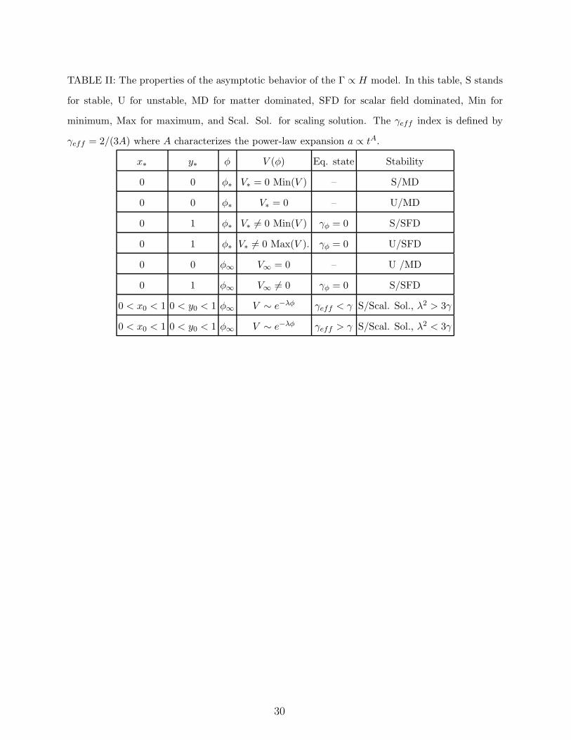
TABLE II: The properties of the asymptotic behavior of the Γ ∝ H model. In this table, S stands

for stable, U for unstable, MD for matter dominated, SFD for scalar field dominated, Min for

minimum, Max for maximum, and Scal. Sol. for scaling solution. The γeff index is defined by

γeff = 2/(3A) where A characterizes the power-law expansion a ∝ tA.

x∗ y∗ φ V (φ) Eq. state Stability

0 0 φ∗ V∗ = 0 Min(V ) – S/MD

0 0 φ∗ V∗ = 0 – U/MD

0 1 φ∗ V∗ 6= 0 Min(V ) γφ = 0 S/SFD

0 1 φ∗ V∗ 6= 0 Max(V ). γφ = 0 U/SFD

0 0 φ∞ V∞ = 0 – U /MD

0 1 φ∞ V∞ 6= 0 γφ = 0 S/SFD

0 < x0 < 1 0 < y0 < 1 φ∞ V ∼ e−λφ γeff < γ S/Scal. Sol., λ2 > 3γ

0 < x0 < 1 0 < y0 < 1 φ∞ V ∼ e−λφ γeff > γ S/Scal. Sol., λ2 < 3γ

30

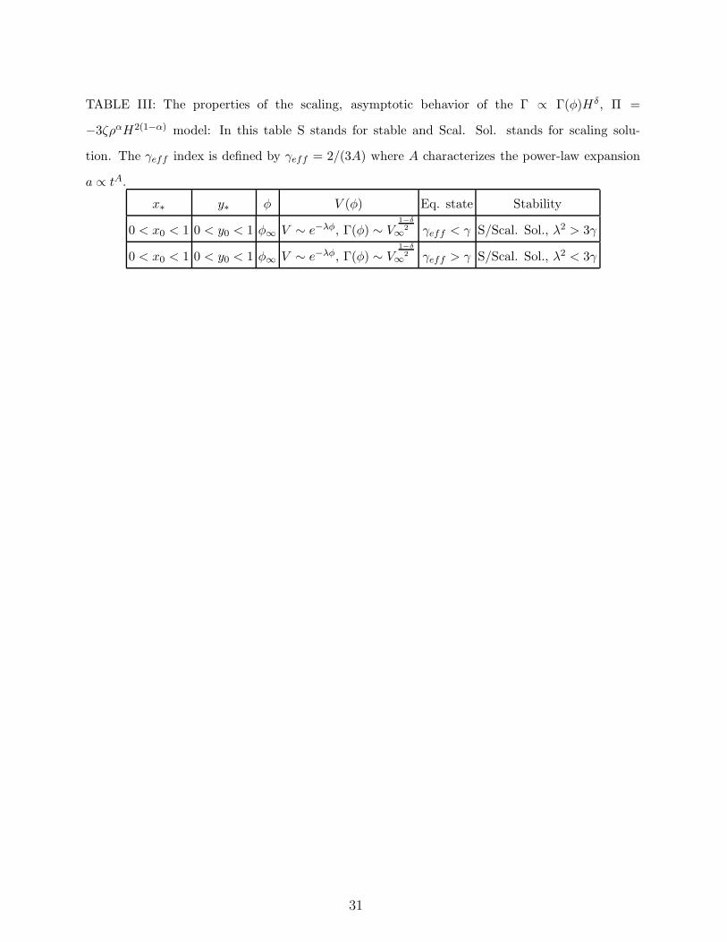
TABLE III: The properties of the scaling, asymptotic behavior of the Γ ∝ Γ(φ)Hδ , Π =

−3ζραH2(1−α) model: In this table S stands for stable and Scal. Sol. stands for scaling solu-

tion. The γeff index is defined by γeff = 2/(3A) where A characterizes the power-law expansion

a ∝ tA.

x∗ y∗ φ V (φ) Eq. state Stability

0 < x0 < 1 0 < y0 < 1 φ∞ V ∼ e−λφ, Γ(φ) ∼ V1−δ

2∞ γeff < γ S/Scal. Sol., λ2 > 3γ

0 < x0 < 1 0 < y0 < 1 φ∞ V ∼ e−λφ, Γ(φ) ∼ V1−δ

2∞ γeff > γ S/Scal. Sol., λ2 < 3γ

31