climate change adaptation action plan 2022–2026 - Engage ...
Upload
khangminh22Category
view
0download
0
ICAR-Central Research Institute for Dryland AgricultureSantoshnagar, Hyderabad 500059
Ph No. 040-24530157/177/163 Fax: 040-24531802Web: www.icar-crida.res.in
Section of Design and Analysis
ICAR-Central Research Institute for Dryland AgricultureSantoshnagar, Hyderabad 500059
Assessment of Vulnerability and Adaptation to Climate Change in Agriculture
ICAR short course on
28 November - 7 December 2018
C A Rama Rao, B M K Raju, R Nagarjuna Kumar, G NirmalaJ Samuel, M Srinivasa Rao, B Narsimlu and K Sammi Reddy
Compiled and Edited by
ICAR - Sponsored Short Course
on
Assessment of Vulnerability and Adaptation to
Climate Change in Agriculture
November 28 – December 7, 2018
Compendium of Lecture Notes
Compiled and Edited by
C.A. Rama Rao, B.M.K. Raju, R. Nagarjuna Kumar, G. Nirmala, J. Samuel,
M. Srinivasa Rao, B. Narsimlu and K. Sammi Reddy
Section of Design & Analysis
ICAR - Central Research Institute for Dryland Agriculture
Santoshnagar, Hyderabad – 500 059
Citation: Rama Rao, C.A., Raju, B.M.K., Nagarjuna Kumar, R., Josily Samuel, Nirmala, G.,
Srinivasa Rao, M., Narsimlu, B. and Sammi Reddy, K. 2018. Compendium of lectures on
“Assessment of Vulnerability and Adaptation to Climate Change in Agriculture”. ICAR-
Central Research Institute for Dryland Agriculture, Hyderabad – 500 059, pp 301.
© ICAR - Central Research Institute for Dryland Agriculture, 2018.
Course Director
C.A. Rama Rao
Co-Course Directors
B.M.K. Raju
R. Nagarjuna Kumar
G. Nirmala
Josily Samuel
M. Srinivasa Rao
B. Narsimlu
J. Rohit
Assistance
C.K. Durga
Y.L. Meghana
Acknowledgements
This document contains the notes of lectures delivered during the ICAR-sponsored short
course on “Assessment of Vulnerability and Adaptation to Climate Change in
Agriculture” held at ICAR-CRIDA, Hyderabad during 28 November to 7 December 2018.
The documents contains useful information on conceptual, methodological and computational
aspects in vulnerability assessment as well as the information on possible impacts of climate
change on agriculture, water, insect pests, etc. An over view of global climate models,
different scenarios used in the recent IPCC assessment reports, accessing climate projections
is also provided which is key to initiating climate change research. How various
technological approaches such as conservation agriculture, organic farming, agro-forestry,
water management, etc. are helpful in adaptation to climate change is also presented. Gender
issues, institutional aspects of transfer of technology, using digital tools for dissemination of
climate information are some other issues that were discussed during the short course. We are
grateful to all the resource persons for sharing useful information with the participants of the
short course.
We are thankful to the Education Division of the ICAR, New Delhi for providing financial
support to this short course. We are also grateful to Director and staff of ICAR-CRIDA for
supporting this activity.
Short Course Team

CONTENTS
S.No. Title Author Page No.
1. Vulnerability assessment: Concepts,
frameworks and methods
C.A. Rama Rao 01
2. Climate change, agriculture and
global climate models:
Fundamentals, sources and data
utilization
A.V.M. Subba Rao 12
3. Database and statistical issues in
construction of vulnerability index
B.M.K. Raju 23
4. National Innovations in Climate
Resilient Agriculture : A multi
sectoral approach to enhance farm
income under changing climate in
India
M. Prabhakar 33
5. Assessing agricultural vulnerability
using satellite-derived NDVI data
products
Kaushalya
Ramachandran
42
6. Impact of climate change on water
resources
K.V. Rao 61
7. Understanding climate change
impacts on crop growth and behavior
M. Vanaja 71
8. Impact assessment through
econometric methods
Josily Samuel 75
9. Impacts of climate change on
insect pests and prediction of
pest scenarios
M. Srinivasa Rao 85
10. Assessment of gender dimension of
vulnerability and adaptation to
climate change in agriculture
G. Nirmala 92
11. Developing insurance products P. Vijaya Kumar 103
12. Role of conservation agriculture in
climate change adaptation and
mitigation
K.L. Sharma 116
13. Adaptation and mitigation strategies
to climate change: Perspectives
G. Ravindra Chary 137
14. Potential role of resource
conservation technologies on
adaptation and mitigation of climate
change
G. Pratibha 158

S.No. Title Author Page No.
15. Agroforestry as an adaptation and
mitigation strategy for climate change
J.V.N.S. Prasad 173
16. Tank beds as source of fodder in
years of drought and need of policy
support – case studies of undivided
state of Andhra Pradesh
Mohammed Osman 184
17. Problem driven iterative adaptation
for solving developmental problems:
Monitoring, evaluation, feedback and
learning
A. Amarender Reddy 203
18. Belowground solutions to
aboveground problems: Plant roots as
mitigators of climate change
K. Srinivas 212
19. Institutional interventions and
capacity building for climate resilient
agriculture
K. Nagasree 233
20. Farmpond technology for enhancing
resilience to climate change/ climate
vulnerability
K. Sreenivas Reddy 244
21. Climate change adaptation and
mitigation potential of organic
farming
K.A. Gopinath 256
22. Building resilience of rainfed
production systems to climate
change: Livestock perspectives
D.B.V. Ramana 268
23. Rising atmospheric carbondioxide
and high temperature interactions
with food crops and their effect on
nutritional content
K. Sreedevi Shankar 275
24. Case studies for assessing climate
change using digital tools
R. Nagarjuna Kumar 289

ICAR-Sponsored Short Course on ‘Assessment of vulnerability and adaptation to climate change in
agriculture’, November 28 to December 07, 2018, ICAR-CRIDA, Hyderabad
1
1 Vulnerability assessment: Concepts, frameworks and methods
CA Rama Rao
Introduction
The last decade of the 20th century saw two important developments: the establishment of United Nations Framework Convention on Climate Change in 1992 and the commencement of the World Trade Organization in 1995. Both these 'events' have significant implications to the way the nations pursue their development goals, especially the developing countries. Various agencies involved in and concerned with economic development have these two aspects on their activity agenda and the researchers are no exception. An important area of research that received attention from different backgrounds is related to vulnerability and its assessment. The term 'vulnerability' has been used in many different contexts and with different meanings and often without even defining the world. Timmermann (1981) observed that “vulnerability is a term of such broad use as to be almost useless for careful description at the present, except as a rhetorical indicator of areas of greatest concern". The term is often used synonymously with susceptibility, fragility, resilience, adaptability, coping capacity, sensitivity, etc. It is important to have a clear understanding of the concept and meaning of vulnerability and its assessment given its importance in the context of climate change and agriculture.
Vulnerability – meaning and concepts
‘Vulnerability’ has emerged as a cross-cutting multidisciplinary theme of research in the current context, characterized by rapid changes in environmental, economic and social systems (O’Brien et al., 2004). The dictionary meaning of the word ‘vulnerable’ means propensity to be harmed. However, the word vulnerability has been used and vulnerability was assessed without actually being defined in many different contexts. Vulnerability is an ex ante concept in that what is likely to happen in future is the focus of analysis and thus the analysis has to lead to making decisions as to what is to be done in the present. Further, vulnerability of what to what are to be clearly defined along with the preference criteria for evaluation (Ionescu et al., 2009). Vulnerability and its assessment received attention in three important areas of research: disaster management, economic development and climate change. The disaster management literature sees vulnerability as susceptibility to a climatic disaster and is often concerned with the location of the system or entity. On the other hand, the vulnerability research in the broader area of economic development is concerned with vulnerability to, poverty for example, wherein the interest is to assess whether or not an economic decision making unit becomes worse off (in terms of outcomes) in the event of a climatic or non-climatic shock given its characteristics. Vulnerability is viewed both as a component of poverty as well as a determinant of poverty in the literature on poverty. Vulnerability is sometimes seen as a threshold value or tipping point which can be described as a degree of acceptable damage (Joakim et al., 2015). The shifting of the threshold or tipping points is seen as the responses to moderate or deal with vulnerability. Though there is a vast literature
ICAR-Sponsored Short Course on ‘Assessment of vulnerability and adaptation to climate change in
agriculture’, November 28 to December 07, 2018, ICAR-CRIDA, Hyderabad
2
on the theoretical development in the conceptualization and analysis of vulnerability, this discussion is limited to vulnerability and assessment in the context of climate change only.
Evolution of vulnerability assessment
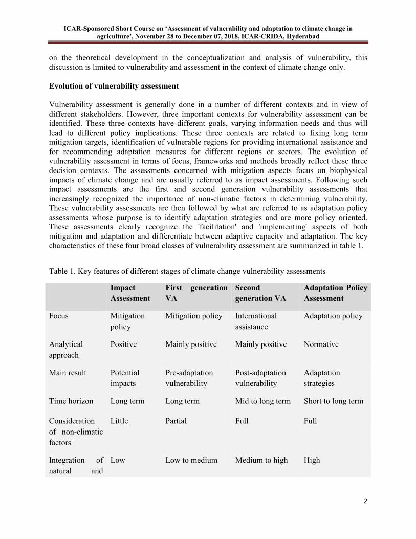
Vulnerability assessment is generally done in a number of different contexts and in view of different stakeholders. However, three important contexts for vulnerability assessment can be identified. These three contexts have different goals, varying information needs and thus will lead to different policy implications. These three contexts are related to fixing long term mitigation targets, identification of vulnerable regions for providing international assistance and for recommending adaptation measures for different regions or sectors. The evolution of vulnerability assessment in terms of focus, frameworks and methods broadly reflect these three decision contexts. The assessments concerned with mitigation aspects focus on biophysical impacts of climate change and are usually referred to as impact assessments. Following such impact assessments are the first and second generation vulnerability assessments that increasingly recognized the importance of non-climatic factors in determining vulnerability. These vulnerability assessments are then followed by what are referred to as adaptation policy assessments whose purpose is to identify adaptation strategies and are more policy oriented. These assessments clearly recognize the 'facilitation' and 'implementing' aspects of both mitigation and adaptation and differentiate between adaptive capacity and adaptation. The key characteristics of these four broad classes of vulnerability assessment are summarized in table 1.
Table 1. Key features of different stages of climate change vulnerability assessments
Impact
Assessment First generation
VA Second
generation VA Adaptation Policy
Assessment
Focus Mitigation policy
Mitigation policy International assistance
Adaptation policy
Analytical approach
Positive Mainly positive Mainly positive Normative
Main result Potential impacts
Pre-adaptation vulnerability
Post-adaptation vulnerability
Adaptation strategies
Time horizon Long term Long term Mid to long term Short to long term
Consideration of non-climatic factors
Little Partial Full Full
Integration of natural and
Low Low to medium Medium to high High

ICAR-Sponsored Short Course on ‘Assessment of vulnerability and adaptation to climate change in
agriculture’, November 28 to December 07, 2018, ICAR-CRIDA, Hyderabad
3
social sciences
Stakeholder consultation
Low Low Medium High
Typical question
What are biophysical impacts of CC?
What socioeconomic impacts are likely to result from CC?
How vulnerable are systems or entities to CC after after feasible adaptation?
What adaptation options can be recommended to reduce vulnerability?
Source: Fussel and Klein (2006)
Approaches to vulnerability assessment
‘Outcome vulnerability is conceptualized as ‘end point’ analysis where in the impact of climate change is examined on productivity or production of a particular crop or animal species either through simulation modeling or through physical experimentation. This is also referred to as biophysical impact assessment or first generation vulnerability assessment. Such assessments ‘superimpose future climate scenarios on an otherwise constant world to estimate the potential impacts of anthropogenic climate change on a climate-sensitive system’ (Fussel and Klein, 2006). The emphasis gradually shifted to derive policy lessons from vulnerability assessment as the purpose of such assessment was to identify strategies that reduce vulnerability of the systems or populations concerned. The socio-economic approach to vulnerability assessment proposes that the attributes of the system or entity of interest predispose it to the adverse impacts of an external shock (climate change or variability) (Adger and Kelly, 1999) and thus it is referred to as ‘starting point analysis’. In this case, vulnerability is regarded as a pre-existing condition (Alexandra Jurgilvech et al., 2017) in terms of health, education, wealth, etc. of the individuals and the differential endowments of individuals are responsible for varying vulnerability. The integrated approach combines both these approaches integrating bio-physical and socio-economic dimensions of vulnerability. As the vulnerability assessments evolved, more non-climatic data became a part of such assessments. Current vulnerability analyses the current risks to the system of interest whereas future
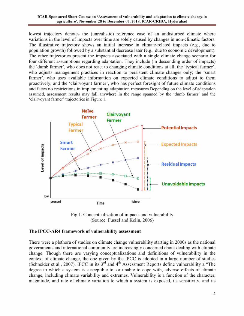
vulnerability assessments are concerned with future risks. Vulnerability assessment is considered static or dynamic whether the temporal changes in the predisposing conditions and/or risk are considered in the analysis. Conceptualization of impacts and vulnerability
Figure 1 depicts hypothetical trajectories for the level of climate-related impacts (caused by anthropogenic climate change as well as natural variability) on a climate-sensitive system. The
ICAR-Sponsored Short Course on ‘Assessment of vulnerability and adaptation to climate change in
agriculture’, November 28 to December 07, 2018, ICAR-CRIDA, Hyderabad
4
lowest trajectory denotes the (unrealistic) reference case of an undisturbed climate where variations in the level of impacts over time are solely caused by changes in non-climatic factors. The illustrative trajectory shows an initial increase in climate-related impacts (e.g., due to population growth) followed by a substantial decrease later (e.g., due to economic development). The other trajectories present the impacts associated with a single climate change scenario for four different assumptions regarding adaptation. They include (in descending order of impacts) the ‘dumb farmer’, who does not react to changing climate conditions at all; the ‘typical farmer’, who adjusts management practices in reaction to persistent climate changes only; the ‘smart farmer’, who uses available information on expected climate conditions to adjust to them proactively; and the ‘clairvoyant farmer’, who has perfect foresight of future climate conditions and faces no restrictions in implementing adaptation measures.Depending on the level of adaptation assumed, assessment results may fall anywhere in the range spanned by the ‘dumb farmer’ and the ‘clairvoyant farmer’ trajectories in Figure 1.
Fig 1. Conceptualization of impacts and vulnerability (Source: Fussel and Kelin, 2006)
The IPCC-AR4 framework of vulnerability assessment
There were a plethora of studies on climate change vulnerability starting in 2000s as the national governments and international community are increasingly concerned about dealing with climate change. Though there are varying conceptualizations and definitions of vulnerability in the context of climate change, the one given by the IPCC is adopted in a large number of studies (Schneider et al., 2007). IPCC in its 3rd and 4th Assessment Reports define vulnerability a “The degree to which a system is susceptible to, or unable to cope with, adverse effects of climate change, including climate variability and extremes. Vulnerability is a function of the character, magnitude, and rate of climate variation to which a system is exposed, its sensitivity, and its
ICAR-Sponsored Short Course on ‘Assessment of
agriculture’, November 28 to December 07, 2018, ICAR
adaptive capacity” (McCarthy et al., 2001vulnerability as a residual impact of climate change: the sensitivity and exposure together determine the potential impact which will be moderated by adaptation. Adaptation is the manifestation of adaptive capacity. Sensitivity is defined as “the degree to which a system is affected, either adversely or beneficially, by climate-related stimuli”. It is determined by demographic and environmental conditions of the region concerned. Esystem is exposed to significant climatic variations”. Thus, exposure relates to climate stress upon a particular unit of analysis (Gbetibouo and Ringler 2009). “A more complete measure of exposure to future climate change would require consideration of projected changes in climate in each analysis unit” (Eriyagama et al., 2012). Adaptive capacity is “the ability of a system to adjust to climate change, including climate variability and extremes, to modamages, to take advantage of opportunities, or to cope with the consequences. It is considered to be “a function of wealth, technology, education, information, skills, infrastructure, access to resources, stability and management capabili In this framework, adaptive capacity is largely consistent with socioeconomic approach and sensitivity with biophysical approach and both are internal dimensions. The component of exposure is viewed as an external dimension. vulnerability, higher adaptive capacity implies lower vulnerability and hence is inversely related to vulnerability. Although lack of standard methods for combining the biophysical and socioeconomic dimensions is a limitation to this approach, it can be helpful in making policy decisions (Deressa et al., 2008). This definition and framework of vulnerability is depicted in Figure
Fig 2. Components of vulnerability
3.1 Change of vulnerability assessment framework by IPCC with AR
The literature on vulnerability and its assessment is continually evolving drawing on works in different fields. The dynamic trait of vulnerability and its components is not adequately addressed in the Third and Fourth Assessment Reports of the IPCC. The rsuggests that the risks due to climate change are also a result of complex interactions among social and ecological systems and the hazards arising out of climate change rather than being
Sensitivity
Sponsored Short Course on ‘Assessment of vulnerability and adaptation to climate change in
agriculture’, November 28 to December 07, 2018, ICAR-CRIDA, Hyderabad
McCarthy et al., 2001, 2001, 2007). This conceptualization views vulnerability as a residual impact of climate change: the sensitivity and exposure together determine the potential impact which will be moderated by adaptation. Adaptation is the
anifestation of adaptive capacity.
Sensitivity is defined as “the degree to which a system is affected, either adversely or related stimuli”. It is determined by demographic and environmental
conditions of the region concerned. Exposure is defined as “the nature and degree to which a system is exposed to significant climatic variations”. Thus, exposure relates to climate stress upon a particular unit of analysis (Gbetibouo and Ringler 2009). “A more complete measure of
future climate change would require consideration of projected changes in climate in each analysis unit” (Eriyagama et al., 2012). Adaptive capacity is “the ability of a system to adjust to climate change, including climate variability and extremes, to modamages, to take advantage of opportunities, or to cope with the consequences. It is considered to be “a function of wealth, technology, education, information, skills, infrastructure, access to resources, stability and management capabilities” (McCarthy et al., 2001) In this framework, adaptive capacity is largely consistent with socioeconomic approach and
sensitivity with biophysical approach and both are internal dimensions. The component of exposure is viewed as an external dimension. While higher exposure and sensitivity mean higher vulnerability, higher adaptive capacity implies lower vulnerability and hence is inversely related to vulnerability. Although lack of standard methods for combining the biophysical and
ions is a limitation to this approach, it can be helpful in making policy
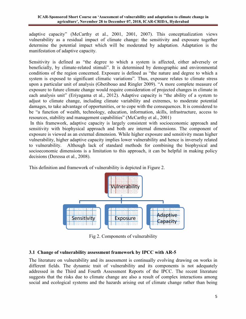
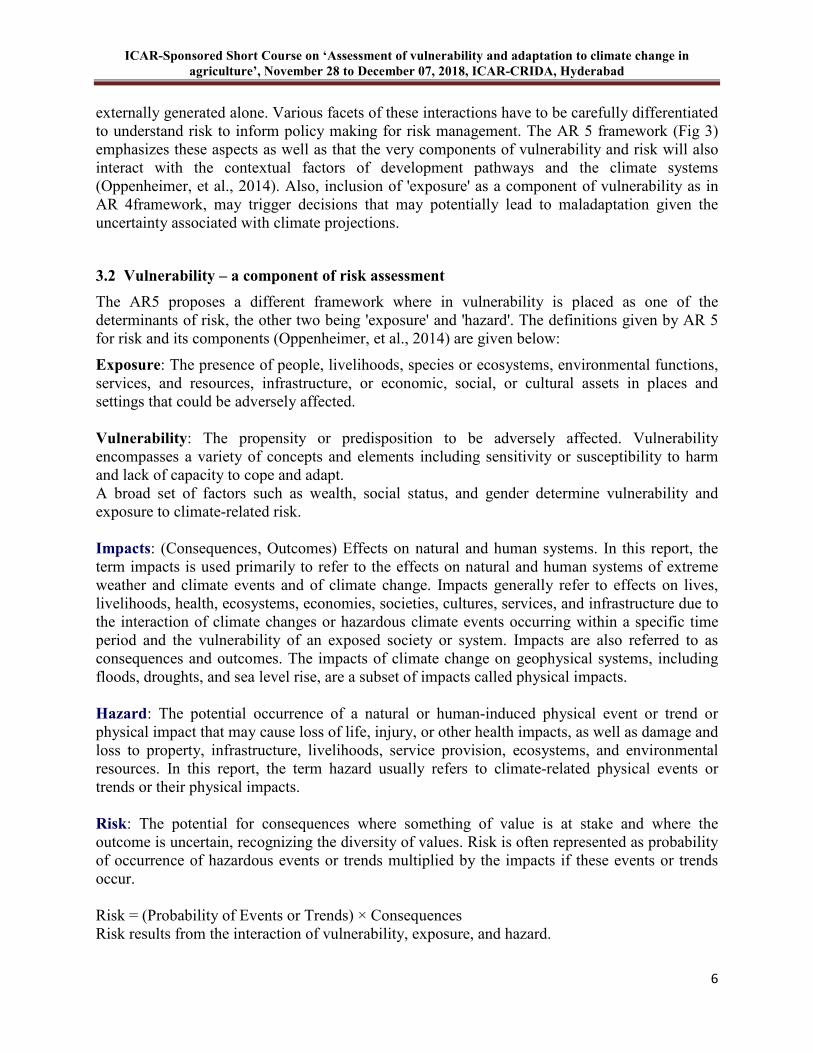
This definition and framework of vulnerability is depicted in Figure 2.
Fig 2. Components of vulnerability
assessment framework by IPCC with AR-5
The literature on vulnerability and its assessment is continually evolving drawing on works in different fields. The dynamic trait of vulnerability and its components is not adequately addressed in the Third and Fourth Assessment Reports of the IPCC. The rsuggests that the risks due to climate change are also a result of complex interactions among social and ecological systems and the hazards arising out of climate change rather than being
Vulnerability
Sensitivity ExposureAdaptive Capacity
vulnerability and adaptation to climate change in
CRIDA, Hyderabad
5
, 2001, 2007). This conceptualization views vulnerability as a residual impact of climate change: the sensitivity and exposure together determine the potential impact which will be moderated by adaptation. Adaptation is the
Sensitivity is defined as “the degree to which a system is affected, either adversely or related stimuli”. It is determined by demographic and environmental
xposure is defined as “the nature and degree to which a system is exposed to significant climatic variations”. Thus, exposure relates to climate stress upon a particular unit of analysis (Gbetibouo and Ringler 2009). “A more complete measure of
future climate change would require consideration of projected changes in climate in each analysis unit” (Eriyagama et al., 2012). Adaptive capacity is “the ability of a system to adjust to climate change, including climate variability and extremes, to moderate potential damages, to take advantage of opportunities, or to cope with the consequences. It is considered to be “a function of wealth, technology, education, information, skills, infrastructure, access to
In this framework, adaptive capacity is largely consistent with socioeconomic approach and sensitivity with biophysical approach and both are internal dimensions. The component of
While higher exposure and sensitivity mean higher vulnerability, higher adaptive capacity implies lower vulnerability and hence is inversely related to vulnerability. Although lack of standard methods for combining the biophysical and
ions is a limitation to this approach, it can be helpful in making policy
The literature on vulnerability and its assessment is continually evolving drawing on works in different fields. The dynamic trait of vulnerability and its components is not adequately addressed in the Third and Fourth Assessment Reports of the IPCC. The recent literature suggests that the risks due to climate change are also a result of complex interactions among social and ecological systems and the hazards arising out of climate change rather than being
ICAR-Sponsored Short Course on ‘Assessment of vulnerability and adaptation to climate change in
agriculture’, November 28 to December 07, 2018, ICAR-CRIDA, Hyderabad
6
externally generated alone. Various facets of these interactions have to be carefully differentiated to understand risk to inform policy making for risk management. The AR 5 framework (Fig 3) emphasizes these aspects as well as that the very components of vulnerability and risk will also interact with the contextual factors of development pathways and the climate systems (Oppenheimer, et al., 2014). Also, inclusion of 'exposure' as a component of vulnerability as in AR 4framework, may trigger decisions that may potentially lead to maladaptation given the uncertainty associated with climate projections.
3.2 Vulnerability – a component of risk assessment
The AR5 proposes a different framework where in vulnerability is placed as one of the determinants of risk, the other two being 'exposure' and 'hazard'. The definitions given by AR 5 for risk and its components (Oppenheimer, et al., 2014) are given below:
Exposure: The presence of people, livelihoods, species or ecosystems, environmental functions, services, and resources, infrastructure, or economic, social, or cultural assets in places and settings that could be adversely affected. Vulnerability: The propensity or predisposition to be adversely affected. Vulnerability encompasses a variety of concepts and elements including sensitivity or susceptibility to harm and lack of capacity to cope and adapt. A broad set of factors such as wealth, social status, and gender determine vulnerability and exposure to climate-related risk.
Impacts: (Consequences, Outcomes) Effects on natural and human systems. In this report, the term impacts is used primarily to refer to the effects on natural and human systems of extreme weather and climate events and of climate change. Impacts generally refer to effects on lives, livelihoods, health, ecosystems, economies, societies, cultures, services, and infrastructure due to the interaction of climate changes or hazardous climate events occurring within a specific time period and the vulnerability of an exposed society or system. Impacts are also referred to as consequences and outcomes. The impacts of climate change on geophysical systems, including floods, droughts, and sea level rise, are a subset of impacts called physical impacts. Hazard: The potential occurrence of a natural or human-induced physical event or trend or physical impact that may cause loss of life, injury, or other health impacts, as well as damage and loss to property, infrastructure, livelihoods, service provision, ecosystems, and environmental resources. In this report, the term hazard usually refers to climate-related physical events or trends or their physical impacts. Risk: The potential for consequences where something of value is at stake and where the outcome is uncertain, recognizing the diversity of values. Risk is often represented as probability of occurrence of hazardous events or trends multiplied by the impacts if these events or trends occur. Risk = (Probability of Events or Trends) × Consequences Risk results from the interaction of vulnerability, exposure, and hazard.

ICAR-Sponsored Short Course on ‘Assessment of
agriculture’, November 28 to December 07, 2018, ICAR
The AR4 and AR5 definitions and frameworks view the terms vulnerability and exposure differently. Exposure in the AR 4 terminology is related to climate related shocks that a system is exposed to whereas the AR 5 describes it being related to the individuals, systems, etc. being exposed to the 'hazard' which is a concept introduced in AR 5 framework. Vulnerability, as per AR5, is more a predisposition to an external shock and whether it will lead to risk depends on whether the vulnerable system is located (exposure) in a place wheoccur. Thus, a highly vulnerable system may not suffer risk due to climate change or a less vulnerable system may face risk if it is placed where severe hazard incidence is possible. Thus, the relationship between these threeThe AR5 vulnerability framework is closer to the disaster management conceptualization which is considered more appropriate in the context of climate change.
Fig 3. Framework of vulnerability and
Fig 4. Dimensions of risk and vulnerability
Vulnerability
SensitivityAdaptive capacity
Sponsored Short Course on ‘Assessment of vulnerability and adaptation to climate change in
agriculture’, November 28 to December 07, 2018, ICAR-CRIDA, Hyderabad
ons and frameworks view the terms vulnerability and exposure differently. Exposure in the AR 4 terminology is related to climate related shocks that a system is exposed to whereas the AR 5 describes it being related to the individuals, systems, etc. being exposed to the 'hazard' which is a concept introduced in AR 5 framework. Vulnerability, as per AR5, is more a predisposition to an external shock and whether it will lead to risk depends on whether the vulnerable system is located (exposure) in a place where the 'hazards' are likely to occur. Thus, a highly vulnerable system may not suffer risk due to climate change or a less vulnerable system may face risk if it is placed where severe hazard incidence is possible. Thus, the relationship between these three components of risk are more explicit and policy relevant. The AR5 vulnerability framework is closer to the disaster management conceptualization which is considered more appropriate in the context of climate change.
Fig 3. Framework of vulnerability and risk (Source: Oppenheimer et al., 2016)
Fig 4. Dimensions of risk and vulnerability
Risk
Adaptive capacity
Exposure Hazard
vulnerability and adaptation to climate change in
CRIDA, Hyderabad
7
ons and frameworks view the terms vulnerability and exposure differently. Exposure in the AR 4 terminology is related to climate related shocks that a system is exposed to whereas the AR 5 describes it being related to the individuals, systems, etc. being exposed to the 'hazard' which is a concept introduced in AR 5 framework. Vulnerability, as per AR5, is more a predisposition to an external shock and whether it will lead to risk depends on
re the 'hazards' are likely to occur. Thus, a highly vulnerable system may not suffer risk due to climate change or a less vulnerable system may face risk if it is placed where severe hazard incidence is possible. Thus,
components of risk are more explicit and policy relevant. The AR5 vulnerability framework is closer to the disaster management conceptualization which
risk (Source: Oppenheimer et al., 2016)
ICAR-Sponsored Short Course on ‘Assessment of vulnerability and adaptation to climate change in
agriculture’, November 28 to December 07, 2018, ICAR-CRIDA, Hyderabad
8
The AR5 risk conceptualization furthers the risk analysis by identifying two kinds of risk: key risks and emergent risks. Key risks are potentially severe consequences arising when systems with high vulnerability interact with severe hazards. Different criteria are suggested to categorize a risk as key which are based on the magnitude of the risk, high vulnerability of a particular group of population, criticality of the sector in the economy. Emergent risks are those that are not direct consequences of climate change hazard but are results of responses to climate change. For example, migration of population from a region due to climate change related hazards may increase the vulnerability and thus risk of receiving regions; similarly increased groundwater extraction during a drought may increase the vulnerability and risk in future. Thus, emergent risks are a result of spatial linkages and temporal dynamics related to responses to changing climate.
Thus AR5 framework places more emphasis on identifying and managing risk and thus views vulnerability as a determinant. Such conceptualization and framework will be more relevant to policy making.
Methods of vulnerability assessment
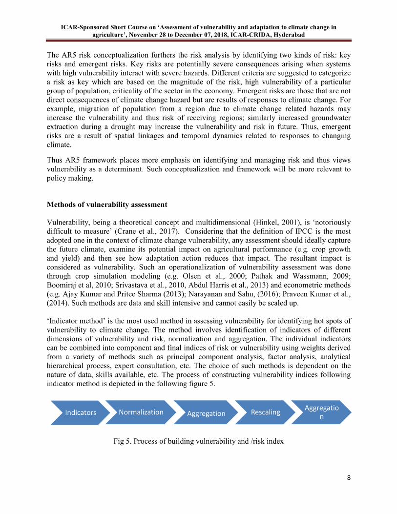
Vulnerability, being a theoretical concept and multidimensional (Hinkel, 2001), is ‘notoriously difficult to measure’ (Crane et al., 2017). Considering that the definition of IPCC is the most adopted one in the context of climate change vulnerability, any assessment should ideally capture the future climate, examine its potential impact on agricultural performance (e.g. crop growth and yield) and then see how adaptation action reduces that impact. The resultant impact is considered as vulnerability. Such an operationalization of vulnerability assessment was done through crop simulation modeling (e.g. Olsen et al., 2000; Pathak and Wassmann, 2009; Boomiraj et al, 2010; Srivastava et al., 2010, Abdul Harris et al., 2013) and econometric methods (e.g. Ajay Kumar and Pritee Sharma (2013); Narayanan and Sahu, (2016); Praveen Kumar et al., (2014). Such methods are data and skill intensive and cannot easily be scaled up. ‘Indicator method’ is the most used method in assessing vulnerability for identifying hot spots of vulnerability to climate change. The method involves identification of indicators of different dimensions of vulnerability and risk, normalization and aggregation. The individual indicators can be combined into component and final indices of risk or vulnerability using weights derived from a variety of methods such as principal component analysis, factor analysis, analytical hierarchical process, expert consultation, etc. The choice of such methods is dependent on the nature of data, skills available, etc. The process of constructing vulnerability indices following indicator method is depicted in the following figure 5.
Fig 5. Process of building vulnerability and /risk index
Indicators Normalization Aggregation RescalingAggregatio
n

ICAR-Sponsored Short Course on ‘Assessment of vulnerability and adaptation to climate change in
agriculture’, November 28 to December 07, 2018, ICAR-CRIDA, Hyderabad
9
Summary and conclusion
The term vulnerability has emerged as an area of multidisciplinary research in different thematic areas such as disaster management, poverty measurement and climate change. The term has been defined and interpreted in many different ways. In the context of climate change, the definitions and frameworks suggested by the IPCC have been often used and many different vulnerability assessments used these frameworks. Vulnerability assessments have over time became more multidisciplinary, more integrating in terms of climatic and non-climatic information, more stakeholder participatory and more policy oriented. Though many approached and methods of vulnerability are evident in the literature, the choice of such approach and method should be more determined by the context and purpose of vulnerability assessment.
References
Abdul Haris AV, Sandeep Biswas, Vandna Chhabra et al.2013. Impact of climate change on wheat and winter maize over a sub-humid climatic environment. Curr Sci 104 (2): p 206-214
Adger, Kelly. 1999. Social vulnerability to climate change and the architecture of entitlements. Miti and Adapt Stratg for Glob Change. 4: p 253-266
Ajay Kumar, Pritee Sharma. 2013. Impact of Climate Variation on Agricultural Productivity and Food Security in Rural India. Economics Discussion Papers. No 2013-43, Kiel Institute for the World Economy. http:// www.economics-ejournal.org/economics/discussionpapers/2013-43. Accessed on 20.08.2018
Alexandra Jurgilevich, Aleksi Rasanen, Fanny Groundstroem et al. 2017. A systematic review of dynamics in climate risk and vulnerability assessments. Environ Res Lett12. 013002 doi: 10.1088/1748-9326/aa5508
Boomiraj K, Chakrabarti B, Aggarwal PK et al.2010. Assessing the vulnerability of Indian mustard to climate change. Agric Ecosyst Environ 138: 265–273
Crane TA, Delaney A, Tamas PA et al. 2017. A systematic review of local vulnerability to climate change in developing country agriculture. WIREs Climt Change 8e464. doi: 10.1002/wcc.464
Deressa T, Hassen R, Alemu T, Yesuf M, Ringler C. 2008. ‘Analyzing the determinants of farmers’ choice of adaptation measures and perceptions of climate change in the Nile Basin of Ethiopia. International Food Policy Research Institute (IFPRI) Discussion Paper No. 00798, Washington
Eriyagama N, Smakhtin V, Chandrapala L et al.2012. Impacts of climate change on water resources and agriculture in Sri Lanka: A Review and Preliminary Vulnerability Mapping. IWMI Res Rep 135, 43
Fussel H M, Kelin R J T.2006. Climate Change Vulnerability Assessments: An Evolution of Conceptual Thinking. Clim Change 75: 301–329. DOI: 10.1007/s10584-006-0329-3
ICAR-Sponsored Short Course on ‘Assessment of vulnerability and adaptation to climate change in
agriculture’, November 28 to December 07, 2018, ICAR-CRIDA, Hyderabad
10
Gbetibouo GA, Ringler C. 2009. Mapping South African farming sector vulnerability to climate change and variability: A sub-national assessment, IFPRI Discussion Paper 00885. Washington, DC, USA: Int Food Poli Res Instit (IFPRI)
Hinkel J. 2011. Indicators of vulnerability and adaptive capacity: Towards a clarification of the science-policy interface, Glob Environ Change21: p 198-208
Ionescu C, Richard JTK, Jochen Hinkel et al.2008. Towards a Formal Framework of Vulnerability to Climate Change, Environ Model Assess
IPCC. 2007. Summary for Policymakers. In: Climate Change 2007: The Physical Science Basis. Contribution of Working Group I to the Fourth Assessment Report of the Intergovernmental Panel on Climate Change. Solomon, S., D. Qin, M., Manning, Z. Chen, M. Marquis, K.B. Averty, M. Tignor and H.L. Miller (eds). Cambridge University Press, Cambridge, United Kingdom and New York, NY, USA.
Joakim EP, Mortsch LOulahen G.2015. Using vulnerability and resilience concepts to advance climate change adaptation. Environ Hazard 14: 137-55
McCarthy JJ, Canziani OF, Lear NAY et al. 2001. Climate Change 2001: Impacts, Adaptation, and Vulnerability. Cambridge University, Press pp 1032
Narayanan K, Sahu SK.2016. Effects of climate change on household economy and adaptive responses among agricultural households in Eastern Coast of India. Curr Sci 110 (7): 1240-1250
O’Brien K, Leichenko R, Kelkar U et al.2004. Mapping Vulnerability to Multiple Stressors: Climate Change and Economic Globalization in India. Glob Environ Change 14 (4): 303-313
Olsen JE, Bocher PK, Jensen Y.2000. Comparison of scales of climate and soil data for aggregating simulated yields in winter wheat in Denmark. Agric Ecosyst Environ 82(3): 213–228
Oppenheimer M, Campos M, Warren R et al. 2014. Emergent risks and key vulnerabilities. In: Climate Change 2014: Impacts, Adaptation, and Vulnerability. Part A: Global and Sectoral Aspects. Contribution of Working Group II to the Fifth Assessment Report of the Intergovernmental Panel on Climate Change Field, C.B., V.R. Barros, D.J. Dokken, K.J. Mach, M.D. Mastrandrea, T.E. Bilir,M. Chatterjee, K.L. Ebi, Y.O. Estrada, R.C. Genova, B. Girma, E.S. Kissel, A.N. Levy, S. MacCracken, P.R. Mastrandrea, and L.L. White (eds). Cambridge University Press, Cambridge, United Kingdom and New York, NY, USA, pp. 1039-1099.
Praveen Kumar NS, Paul KSR, Krishna Reddy K et al. 2014. Assessment of Vulnerability and Impact of Climate Change on Crop Production in Krishna river basin of Andhra Pradesh. Int J Curr Agri Res 3(2): 62-66
Pathak H, Wassmann R.2009. Quantitative evaluation of climatic variability and risks for wheat yield in India Climatic Change. Doi: 10.1007/s10584-008-9463-4 93:157–175
Rama Rao CA, Raju BMK, Subba Rao AVM et al.2013. Atlas on Vulnerability of Indian Agriculture to Climate Change. Central Research Institute for Dryland Agriculture, Hyderabad P 116

ICAR-Sponsored Short Course on ‘Assessment of vulnerability and adaptation to climate change in
agriculture’, November 28 to December 07, 2018, ICAR-CRIDA, Hyderabad
11
Rama Rao CA, Raju BMK, Subba Rao AVM et al.2016. A District Level Assessment of Vulnerability of Indian Agriculture to Climate Change. Curr Sci 110(10): 1939-1946
Rama Rao CA, Raju BMK, Subba Rao AVM et al. 2017. Assessing vulnerability and adaptation of agriculture to climate change in Andhra Pradesh. Ind J Agri Econ 72(3): 375-384
Schneider S H, Semenov S, Patwardhan, A.2007. Assessing key vulnerabilities and the risk from climate change Climate Change 2007: Impacts, Adaptation and Vulnerability Contribution of Working Group II to the Fourth Assessment Report of the Intergovernmental Panel on Climate Change M L Parry et al (eds) Cambridge, UK: Cambridge University Press: 779–810
Srivastava A, Naresh Kumar S, Aggarwal PK.2010. Assessment on vulnerability of sorghum to climate change in India. Agric Ecosyst Environ 138: 160–169
Timmermann, P.1981.Vulnerability, Resilience and the Collapse of Society, No. 1 in Environmental 987 Monograph, Institute for Environmental Studies, University of Toronto, Toronto. 98
ICAR-Sponsored Short Course on ‘Assessment of vulnerability and adaptation to climate change in
agriculture’, November 28 to December 07, 2018, ICAR-CRIDA, Hyderabad
12
2 Climate change, Agriculture and Global Climate Models:
Fundamentals, Sources and Data utilization
AVM Subba Rao
Climate Change is one of the biggest global problem, requires local level action to control the emission of Green House Gases (GHGs) at global level to reduce the impacts on Human, Animal, Plant and other things on earth. Agriculture is the major looser under the climate change regime. Some major crops like rice, wheat and maize are showing impacts of temperatures on their yield levels. The projected increase in temperature, rainfall and CO2 & other gases along with likely increase in the occurrence of extreme events viz. droughts, floods and heat waves. There is also likely increase in the erratic monsoon rainfall distribution during the crop season leaving the crops perched for moisture to sustain. In order to identify the likely changes in different parts of the world we require some tools for simulating the future climates with reference to past. Global climate models or general circulation models (GCM) are the tools developed on the general principles of fluid dynamics and thermodynamics. They had their origin in numerical weather prediction and describe the dynamics of the atmosphere and ocean in an explicit way. The models facilitate numerical experiments of climate changes during the past, present, and future. History says that, numerical modeling of the atmosphere started since the beginning 20th Century. In 1904, the Norwegian meteorologist Vilhelm Bjerknes first proposed the possibility of the numerical prediction of weather if the initial state and the physical laws were known accurately. He showed how to compute large-scale weather dynamics using what are now known as the ‘primitive equations’ of motion and state. These equations include Newton’s laws of motion, the hydrodynamic state equation, mass conservation, and the thermodynamic energy equation. Bjerknes’s mathematical model described how mass, momentum, energy, and moisture are conserved in interactions among individual parcels of air. However, Bjerknes’ equations did not have closed-form solutions, and numerical techniques capable of approximate solutions did not yet exist. Then, the English scientist Lewis Fry Richardson made a weather prediction using equations describing the physics of the atmosphere that he calculated by hand. In the 1930s, Carl Gustav Rossby configured equations with reliable initial conditions as well as filtering high frequency waves. With the development of modern computers in the late 1940s, the idea of direct numerical modeling of the atmosphere could be revisited. At Princeton University's Institute for Advanced Studies, under the leadership of John von Neumann the construction of one of these early computers and using the same for weather forecasting has initiated. Presently a wide range of climate models available intended for the various simulation tasks associated with improving understanding of the climate system and predicting future (and past) climate changes. These models, based on knowledge of physics, chemistry, biology, as well as economics and social science, portray this understanding in simplified representations called parameterizations. The first atmospheric GCM were derived directly from numerical models of the atmosphere designed for short-term weather forecasting in 1950s (e.g. Charney et al., 1950; Smagorinsky, 1983). The advances in computer technology allowed more extensive simulations during 1960s, ideas were being formulated for long enough integrations of these numerical weather prediction schemes that they might be considered as climate models.
ICAR-Sponsored Short Course on ‘Assessment of vulnerability and adaptation to climate change in
agriculture’, November 28 to December 07, 2018, ICAR-CRIDA, Hyderabad
13
Predicting future climate change owing to emissions from human interactions initiate with the development of emission scenarios. These scenarios are not predictions, but represent plausible future environments under certain assumptions. On the basis of consistent set of assumptions, projections of population, demographics, economic growth, energy supply and demand, land use, and technological developments are developed. These projections are used as input to complex socio-economic models that estimate emissions of greenhouse gases resulting from human actions in various sectors, including agriculture, forestry, industry, commercial and residential transportation, energy and other sectors of the economy.
Climate change scenarios
The climate change scenarios are realistic portrayal of future climates generated from various climatological relationships and hypotheses of radioactive forcing (IPCC, 2007). Climate scenarios are portrayed by general circulation models (GCMs) and regional climate models (RCMs), which are advanced three-dimensional mathematical equations and relationships linking interactions between the atmosphere, land surface, oceans and sea ice which result from climate (Mearns, 2000). The Coupled Model Intercomparison Project (CMIP) was launched with a purpose for better understanding the past, present and future climatic changes evolved from natural, unforced variability or in response to changes in radiative forcing in a multi-model context. Idealized experiments are also applied to enhance the knowledge of the model responses. Apart of these long time experiments are conducted to study the predictability of the climate system on several space and time scales and performing simulations from observed climate system. It began in 1995 under the aegis of the Working Group on Coupled Modelling (WGCM). To make the multi-model output available to public in a standardized format is an important objective of CMIP. The first set of common experiments started by evaluating the model response to an idealized forcing like a constant rate of raise which was attained through increase in CO2 by 1% per year. It also included the integrations forced with estimates of the changes in the historical as well as future radiative forcing. The first phase of CMIP (CMIP1) was intended at collection and analysis of present day control runs from the coupled models. Its successor CMIP2 additionally collected model data from 1% yr–1 CO2 rise experiments from the coupled models (Meehl et al., 1997). A rapid growth in coupled-model development was prompted by IPCC-Fourth Assessment Report (AR4). The simulated output from the climate models was collected for the past, present and future climates, predominantly during the years 2005 and 2006, and this archived data comprises CMIP3. CMIP3 models have relied by many climate projections in the past (Delworth et al., 2006; Johnson and Sharma 2009). The reference standard for emission scenarios are the collections of scenarios established by an interdisciplinary group of integrated assessment modelers under the umbrella of the Intergovernmental Panel on Climate Change (IPCC). The IPCC provided a standard set of Integrated Science emission scenarios (IS92) in 1992 that have been used in a number of previous assessments (USGCRP, 2000; IPCC, 1992). However, these scenarios comprise a number of inconsistencies and assumptions that are considered limited in the face of current uncertainty as to how the world will develop over the next century. These scenarios failed to cover an adequate range of possible futures, in particular tending to under-estimate the results of a non-intervention policy towards climate change. In response to these issues, a new set of
ICAR-Sponsored Short Course on ‘Assessment of vulnerability and adaptation to climate change in
agriculture’, November 28 to December 07, 2018, ICAR-CRIDA, Hyderabad
14
emission scenarios were approved for use by the IPCC in 2000. These are called the SRES scenarios after the report entitled “Special Report on Emission Scenarios” (IPCC 2000). In these scenarios, unlike previous scenarios developed by the IPCC, sulfur emissions are consistent with current and anticipated air quality regulations. This eliminates the strong regional cooling patterns resulting from earlier scenarios used in the USGCRP reports. In addition, the two scenarios produce similar patterns of climate change over the next few decades consistent with recent findings by Knutti et al. (2002) and Stott & Kettle borough (2002). All of these scenarios are intended to represent the possible range for a business-as-usual situation with no significant policy intervention to reduce emissions in order to slow down climate change.
The SRES scenarios considered span the full range from ‘high’ (A1FI) through ‘mid-range’ (A2 and B2) to ‘low’ (B1) emissions (IPCC, 2000). • A1 – high end of range - where a rapid rate of temperature change is driven by a continued
dependence on fossil fuels and rapid economic growth throughout the next century. The A1 storyline and scenario family describes a future world of very rapid economic growth, global population that peaks in mid-century and declines thereafter, and the rapid introduction of new and more efficient technologies. Major underlying themes are convergence among regions, capacity building, and increased cultural and social interactions, with a substantial reduction in regional differences in per capita income. The A1 scenario family develops into three groups that describe alternative directions of technological change in the energy system. The three A1 groups are distinguished by their technological emphasis: fossil intensive (A1FI), non-fossil energy sources (A1T), or a balance across all sources.
• A2 – upper mid-range - for a very heterogeneous world where economic development is regionally-oriented and economic growth and technological change are relatively slow. The A2 storyline and scenario family describes a very heterogeneous world. The underlying theme is self-reliance and preservation of local identities. Fertility patterns across regions converge very slowly, which results in continuously increasing global population. Economic development is primarily regionally oriented and per capita economic growth and technological change are more fragmented and slower than in other storylines.
• B2 – lower mid-range – where the emphasises on local solutions to economic, social, and environmental sustainability with less rapid and more diverse technological change. The B2 storyline and scenario family describes a world in which the emphasis is on local solutions to economic, social, and environmental sustainability. It is a world with continuously increasing global population at a rate lower than A2, intermediate levels of economic development, and less rapid and more diverse technological change than in the B1 and A1 storylines. While the scenario is also oriented toward environmental protection and social equity, it focuses on local and regional levels.
• B1 – low end of range – where the focus is on global solutions to economic, social and environmental sustainability. Clean, efficient technology is introduced but no specific climate initiatives are taken. The B1 storyline and scenario family describes a convergent world with the same global population that peaks in mid century and declines thereafter, as in the A1 storyline, but with rapid changes in economic structures toward a service and information economy, with reductions in material intensity, and the introduction of clean and resource-efficient technologies. The emphasis is on global solutions to economic, social, and
ICAR-Sponsored Short Course on ‘Assessment of vulnerability and adaptation to climate change in
agriculture’, November 28 to December 07, 2018, ICAR-CRIDA, Hyderabad
15
environmental sustainability, including improved equity, but without additional climate initiatives.
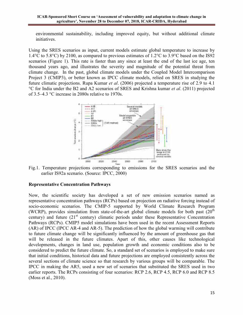
Using the SRES scenarios as input, current models estimate global temperature to increase by 1.4°C to 5.8°C) by 2100, as compared to previous estimates of 1.2°C to 3.9°C based on the IS92 scenarios (Figure 1). This rate is faster than any since at least the end of the last ice age, ten thousand years ago, and illustrates the severity and magnitude of the potential threat from climate change. In the past, global climate models under the Coupled Model Intercomparison Project 3 (CMIP3), or better known as IPCC climate models, relied on SRES in studying the future climatic projections. Rupa Kumar et al. (2006) projected a temperature rise of 2.9 to 4.1 °C for India under the B2 and A2 scenarios of SRES and Krishna kumar et al. (2011) projected of 3.5–4.3 °C increase in 2080s relative to 1970s.
Fig.1. Temperature projections corresponding to emissions for the SRES scenarios and the
earlier IS92a scenario. (Source: IPCC, 2000) Representative Concentration Pathways
Now, the scientific society has developed a set of new emission scenarios named as representative concentration pathways (RCPs) based on projection on radiative forcing instead of socio-economic scenarios. The CMIP-5 supported by World Climate Research Program (WCRP), provides simulation from state-of-the-art global climate models for both past (20th century) and future (21st century) climatic periods under these Representative Concentration Pathways (RCPs). CMIP5 model simulations have been used in the recent Assessment Reports (AR) of IPCC (IPCC AR-4 and AR-5). The prediction of how the global warming will contribute to future climate change will be significantly influenced by the amount of greenhouse gas that will be released in the future climates. Apart of this, other causes like technological developments, changes in land use, population growth and economic conditions also to be considered to predict the future climate. So, a standard set of scenarios is employed to make sure that initial conditions, historical data and future projections are employed consistently across the several sections of climate science so that research by various groups will be comparable. The IPCC in making the AR5, used a new set of scenarios that substituted the SRES used in two earlier reports. The RCPs consisting of four scenarios: RCP 2.6, RCP 4.5, RCP 6.0 and RCP 8.5 (Moss et al., 2010).
ICAR-Sponsored Short Course on ‘Assessment of vulnerability and adaptation to climate change in
agriculture’, November 28 to December 07, 2018, ICAR-CRIDA, Hyderabad
16
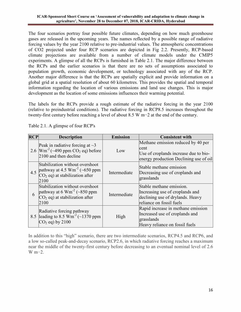
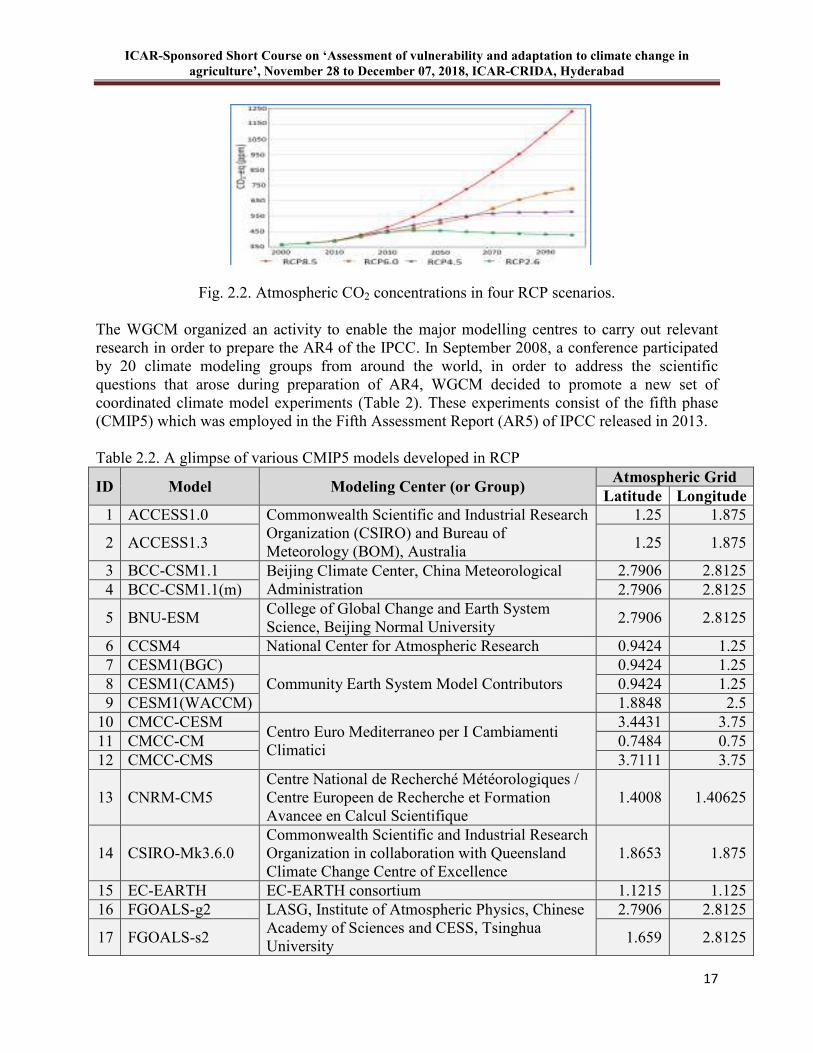
The four scenarios portray four possible future climates, depending on how much greenhouse gases are released in the upcoming years. The names reflected by a possible range of radiative forcing values by the year 2100 relative to pre-industrial values. The atmospheric concentrations of CO2 projected under four RCP scenarios are depicted in Fig 2.2. Presently, RCP-based climate projections are available from a number of climate models under the CMIP5 experiments. A glimpse of all the RCPs is furnished in Table 2.1. The major difference between the RCPs and the earlier scenarios is that there are no sets of assumptions associated to population growth, economic development, or technology associated with any of the RCP. Another major difference is that the RCPs are spatially explicit and provide information on a global grid at a spatial resolution of about 60 kilometres. This provides the spatial and temporal information regarding the location of various emissions and land use changes. This is major development as the location of some emissions influences their warming potential. The labels for the RCPs provide a rough estimate of the radiative forcing in the year 2100 (relative to preindustrial conditions). The radiative forcing in RCP8.5 increases throughout the twenty-first century before reaching a level of about 8.5 W m−2 at the end of the century. Table 2.1. A glimpse of four RCP's RCP Description Emission Consistent with
2.6 Peak in radiative forcing at ~3 Wm-2 (~490 ppm CO2 eq) before 2100 and then decline
Low
Methane emission reduced by 40 per cent Use of croplands increase due to bio-energy production Declining use of oil
4.5
Stabilization without overshoot pathway at 4.5 Wm-2 (~650 ppm CO2 eq) at stabilization after 2100
Intermediate Stable methane emission Decreasing use of croplands and grasslands
6
Stabilization without overshoot pathway at 6 Wm-2 (~850 ppm CO2 eq) at stabilization after 2100
Intermediate
Stable methane emission. Increasing use of croplands and declining use of drylands. Heavy reliance on fossil fuels
8.5 Radiative forcing pathway leading to 8.5 Wm-2 (~1370 ppm CO2 eq) by 2100
High
Rapid increase in methane emission Increased use of croplands and grasslands Heavy reliance on fossil fuels
In addition to this “high” scenario, there are two intermediate scenarios, RCP4.5 and RCP6, and a low so-called peak-and-decay scenario, RCP2.6, in which radiative forcing reaches a maximum near the middle of the twenty-first century before decreasing to an eventual nominal level of 2.6 W m−2.
ICAR-Sponsored Short Course on ‘Assessment of vulnerability and adaptation to climate change in
agriculture’, November 28 to December 07, 2018, ICAR-CRIDA, Hyderabad
17
Fig. 2.2. Atmospheric CO2 concentrations in four RCP scenarios.
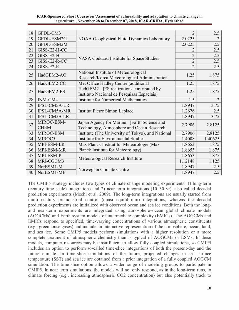
The WGCM organized an activity to enable the major modelling centres to carry out relevant research in order to prepare the AR4 of the IPCC. In September 2008, a conference participated by 20 climate modeling groups from around the world, in order to address the scientific questions that arose during preparation of AR4, WGCM decided to promote a new set of coordinated climate model experiments (Table 2). These experiments consist of the fifth phase (CMIP5) which was employed in the Fifth Assessment Report (AR5) of IPCC released in 2013.
Table 2.2. A glimpse of various CMIP5 models developed in RCP
ID Model Modeling Center (or Group) Atmospheric Grid
Latitude Longitude
1 ACCESS1.0 Commonwealth Scientific and Industrial Research Organization (CSIRO) and Bureau of Meteorology (BOM), Australia
1.25 1.875
2 ACCESS1.3 1.25 1.875
3 BCC-CSM1.1 Beijing Climate Center, China Meteorological Administration
2.7906 2.8125 4 BCC-CSM1.1(m) 2.7906 2.8125
5 BNU-ESM College of Global Change and Earth System Science, Beijing Normal University
2.7906 2.8125
6 CCSM4 National Center for Atmospheric Research 0.9424 1.25 7 CESM1(BGC)
Community Earth System Model Contributors 0.9424 1.25
8 CESM1(CAM5) 0.9424 1.25 9 CESM1(WACCM) 1.8848 2.5
10 CMCC-CESM Centro Euro Mediterraneo per I Cambiamenti Climatici
3.4431 3.75 11 CMCC-CM 0.7484 0.75 12 CMCC-CMS 3.7111 3.75
13 CNRM-CM5 Centre National de Recherché Météorologiques / Centre Europeen de Recherche et Formation Avancee en Calcul Scientifique
1.4008 1.40625
14 CSIRO-Mk3.6.0 Commonwealth Scientific and Industrial Research Organization in collaboration with Queensland Climate Change Centre of Excellence
1.8653 1.875
15 EC-EARTH EC-EARTH consortium 1.1215 1.125 16 FGOALS-g2 LASG, Institute of Atmospheric Physics, Chinese
Academy of Sciences and CESS, Tsinghua University
2.7906 2.8125
17 FGOALS-s2 1.659 2.8125
ICAR-Sponsored Short Course on ‘Assessment of vulnerability and adaptation to climate change in
agriculture’, November 28 to December 07, 2018, ICAR-CRIDA, Hyderabad
18
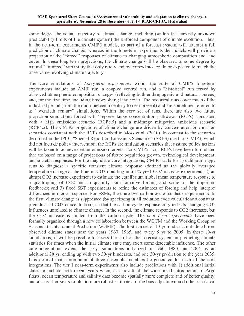
18 GFDL-CM3 NOAA Geophysical Fluid Dynamics Laboratory
2 2.5 19 GFDL-ESM2G 2.0225 2 20 GFDL-ESM2M 2.0225 2.5 21 GISS-E2-H-CC
NASA Goddard Institute for Space Studies
2 2.5 22 GISS-E2-H 2 2.5 23 GISS-E2-R-CC 2 2.5 24 GISS-E2-R 2 2.5
25 HadGEM2-AO National Institute of Meteorological Research/Korea Meteorological Administration
1.25 1.875
26 HadGEM2-CC Met Office Hadley Centre (additional HadGEM2 ]ES realizations contributed by Instituto Nacional de Pesquisas Espaciais)
1.25 1.875
27 HadGEM2-ES 1.25 1.875
28 INM-CM4 Institute for Numerical Mathematics 1.5 2 29 IPSL-CM5A-LR
Institut Pierre Simon Laplace 1.8947 3.75
30 IPSL-CM5A-MR 1.2676 2.5 31 IPSL-CM5B-LR 1.8947 3.75
32 MIROC-ESM-CHEM
Japan Agency for Marine ]Earth Science and Technology, Atmosphere and Ocean Research Institute (The University of Tokyo), and National Institute for Environmental Studies
2.7906 2.8125
33 MIROC-ESM 2.7906 2.8125 34 MIROC5 1.4008 1.40625 35 MPI-ESM-LR Max Planck Institut fur Meteorologie (Max
Planck Institute for Meteorology) 1.8653 1.875
36 MPI-ESM-MR 1.8653 1.875 37 MPI-ESM-P
Meteorological Research Institute 1.8653 1.875
38 MRI-CGCM3 1.12148 1.125 39 NorESM1-M
Norwegian Climate Centre 1.8947 2.5
40 NorESM1-ME 1.8947 2.5 The CMIP5 strategy includes two types of climate change modeling experiments: 1) long-term (century time scale) integrations and 2) near-term integrations (10–30 yr), also called decadal prediction experiments (Meehl et al. 2009). The long-term integrations are usually started from multi century preindustrial control (quasi equilibrium) integrations, whereas the decadal prediction experiments are initialized with observed ocean and sea ice conditions. Both the long- and near-term experiments are integrated using atmosphere–ocean global climate models (AOGCMs) and Earth system models of intermediate complexity (EMICs). The AOGCMs and EMICs respond to specified, time-varying concentrations of various atmospheric constituents (e.g., greenhouse gases) and include an interactive representation of the atmosphere, ocean, land, and sea ice. Some CMIP5 models perform simulations with a higher resolution or a more complete treatment of atmospheric chemistry than is typical of AOGCMs or ESMs. In these models, computer resources may be insufficient to allow fully coupled simulations, so CMIP5 includes an option to perform so-called time-slice integrations of both the present-day and the future climate. In time-slice simulations of the future, projected changes in sea surface temperature (SST) and sea ice are obtained from a prior integration of a fully coupled AOGCM simulation. The time-slice option allows a wider range of modeling groups to participate in CMIP5. In near term simulations, the models will not only respond, as in the long-term runs, to climate forcing (e.g., increasing atmospheric CO2 concentration) but also potentially track to
ICAR-Sponsored Short Course on ‘Assessment of vulnerability and adaptation to climate change in
agriculture’, November 28 to December 07, 2018, ICAR-CRIDA, Hyderabad
19
some degree the actual trajectory of climate change, including (within the currently unknown predictability limits of the climate system) the unforced component of climate evolution. Thus, in the near-term experiments CMIP5 models, as part of a forecast system, will attempt a full prediction of climate change, whereas in the long-term experiments the models will provide a projection of the “forced” responses of climate to changing atmospheric composition and land cover. In these long-term projections, the climate change will be obscured to some degree by natural “unforced” variability that only rarely and by coincidence could be expected to match the observable, evolving climate trajectory. The core simulations of Long-term experiments within the suite of CMIP5 long-term experiments include an AMIP run, a coupled control run, and a “historical” run forced by observed atmospheric composition changes (reflecting both anthropogenic and natural sources) and, for the first time, including time-evolving land cover. The historical runs cover much of the industrial period (from the mid-nineteenth century to near present) and are sometimes referred to as “twentieth century” simulations. Within the core set of runs, there are also two future projection simulations forced with “representative concentration pathways” (RCPs), consistent with a high emissions scenario (RCP8.5) and a midrange mitigation emissions scenario (RCP4.5). The CMIP5 projections of climate change are driven by concentration or emission scenarios consistent with the RCPs described in Moss et al. (2010). In contrast to the scenarios described in the IPCC “Special Report on Emissions Scenarios” (SRES) used for CMIP3, which did not include policy intervention, the RCPs are mitigation scenarios that assume policy actions will be taken to achieve certain emission targets. For CMIP5, four RCPs have been formulated that are based on a range of projections of future population growth, technological development, and societal responses. For the diagnostic core integrations, CMIP5 calls for 1) calibration type runs to diagnose a specific transient climate response (defined as the globally averaged temperature change at the time of CO2 doubling in a 1% yr−1 CO2 increase experiment; 2) an abrupt CO2 increase experiment to estimate the equilibrium global mean temperature response to a quadrupling of CO2 and to quantify both radiative forcing and some of the important feedbacks; and 3) fixed SST experiments to refine the estimates of forcing and help interpret differences in model response. For ESMs, there are two carbon cycle feedback experiments. In the first, climate change is suppressed (by specifying in all radiation code calculations a constant, preindustrial CO2 concentration), so that the carbon cycle response only reflects changing CO2 influences unrelated to climate change. In the second, the climate responds to CO2 increases, but the CO2 increase is hidden from the carbon cycle. The near term experiments have been formally organized through a new collaboration between the WGCM and the Working Group on Seasonal to Inter annual Prediction (WGSIP). The first is a set of 10-yr hindcasts initialized from observed climate states near the years 1960, 1965, and every 5 yr to 2005. In these 10-yr simulations, it will be possible to assess the skill of the forecast system in predicting climate statistics for times when the initial climate state may exert some detectable influence. The other core integrations extend the 10-yr simulations initialized in 1960, 1980, and 2005 by an additional 20 yr, ending up with two 30-yr hindcasts, and one 30-yr prediction to the year 2035. It is desired that a minimum of three ensemble members be generated for each of the core integrations. The tier 1 near-term experiments also include predictions with 1) additional initial states to include both recent years when, as a result of the widespread introduction of Argo floats, ocean temperature and salinity data become spatially more complete and of better quality, and also earlier years to obtain more robust estimates of the bias adjustment and other statistical
ICAR-Sponsored Short Course on ‘Assessment of vulnerability and adaptation to climate change in
agriculture’, November 28 to December 07, 2018, ICAR-CRIDA, Hyderabad
20
calculations; 2) volcanic eruptions removed from the hindcasts; 3) a hypothetical volcanic eruption imposed in one of the predictions of future climate; 4) different initialization methodologies; and 5) the option of performing time-slice experiments with high-resolution models or models with computationally expensive atmospheric chemistry treatments. Users of CMIP5 model output should take note that decadal predictions with climate models are in an exploratory stage. A number of different methods are being tried to assimilate ocean observations into the models, and no single method has gained widespread acceptance. Moreover, the quality and completeness of ocean observations may be insufficient to realize but a fraction of the predictability inherent in the system. Thus, the forecast systems being assembled for CMIP5 are clearly not considered operational, nor will they necessarily provide more realistic simulations than the long-term simulations. Rather, the experiments aim to advance understanding of predictability, expose the relative merits of various data assimilation approaches, and reveal the limitations of the existing ocean observational network. Overall predictive skill of a forecast system will be determined by the quality of the observations, the capabilities of the assimilation method, and the skill of the model itself.
The CMIP5 outputs are formatted in a common way in order to reduce shipment of huge data volumes, the data will be archived in data nodes distributed at modeling centers and data centers near where the model output is produced. The nodes will be linked together and the model output will be freely accessible through data portals (or gateways) integrated in a way that retains much of the convenience of a single repository. The international effort to create this “federated archive” was initiated under the Earth System Grid (ESG) project (http://esg-pcmdi.llnl.gov) and is being advanced through the Earth System Grid Federation (ESGF; http://esgf.org/wiki /ESGF_Overview;), established under the Global Organization for Earth System Science Portals (GO-ESSP; http://go-essp.gfdl.noaa .gov/). To obtain output from the CMIP5 archive, users must first register, indicating how the data will be used and agreeing to specific “terms of use” (see http://cmip-pcmdi.llnl.gov/cmip5/terms.html). Some of the modeling groups will release their data for “unrestricted” use, whereas others will limit use to “noncommercial research and educational” purposes. A user who is planning to engage in some commercial activity using the data will be given access only to model output that is meant for unrestricted use. Once registered, a user can access CMIP5 model output through the portal (http:// pcmdi3.llnl.gov/esgcet/home.htm) or through any of the other ESG federated gateways. A user may search using any combination of model, variable, experiment, frequency (e.g., monthly, daily, 3 hourly), and modeling realm (e.g., atmosphere, ocean, sea ice). Detailed step-by-step instructions on how to register and access CMIP5 model output are available (at http://cmip-pcmdi.llnl.gov/cmip5/data_getting_ started.html). CMIP5 data obey the Climate and Forecast (CF) conventions. Especially the CF Standard Names for variables have been used, e.g. "air temperature". This also facilitates search. Short variable names are also centralized. For example, the short name for air temperature is "ta". CMIP5 data are in NetCDF/CF format (Network Common Data Form, again obeying the CF conventions). This is a binary and header-based data format. Coordinate variables and data variable are defined in the file header. Each CMIP5 data file contains only one data variable, e.g. ta, and, of course, all necessary coordinate variables as longitude, latitude, altitude, time. Attributes in the header give additional information. In all NetCDF files, variable data are stored in multidimensional arrays. The sequence of the values is definition-controlled. The index set of the data variable is the Cartesian product of the index sets of the coordinate variables, in the same sequence as in the definition of the data variable.
ICAR-Sponsored Short Course on ‘Assessment of vulnerability and adaptation to climate change in
agriculture’, November 28 to December 07, 2018, ICAR-CRIDA, Hyderabad
21
Likely Impacts on Agriculture and allied sectors
After the development of GCMs as well as generation of future climate change scenarios, crop simulation modelling (CSM) experts incorporated the scenario weather data into CSMs and simulated different crop models to find out the likely impacts on crop yields and the other allies sectors like livestock and fisheries. Although increase in CO2 is likely to be beneficial to several crops, associated increase in temperatures, and increased variability of rainfall would considerably impact food production. Recent IPCC report indicates considerable probability of loss in crop production with increases in temperature in tropical regions. Indian studies do confirm this trend, although there is considerable disagreement among the studies on the magnitude of loss. Among cereal crops, important for food security, wheat is most sensitive to even small increase in temperature. Relatively rice has greater tolerance to increase in temperature. It is, however, possible for farmers to adapt to a limited extend and reduce the losses. Increasing climatic variability could, nevertheless, result in considerable seasonal/annual fluctuations in food production. All agricultural commodities are sensitive to such variability. Food production needs to be increased considerably in future to meet increasing demand associated with population and income growth. There is considerable biological yield gap still available for most crops that can be utilized for meeting these demands given the support of policy and economic development. Climate change, is however, likely to considerably reduce this biological gap. This could lead to stagnation in food production growth much sooner than otherwise expected. Increasing temperature in future is likely to reduce fertilizer use efficiency. This could lead to increased fertilizer requirement for meeting future food production demands (higher due to income and population growth). At the same time, greater fertilizer use leads to higher emissions of greenhouse gases. This could become a cause for concern, in case we have to reduce GHG emissions in future. Global warming in short-term is likely to favour agricultural production in temperate regions (largely Europe, north America) and negatively impact tropical crop production (South Asia, Africa). This is likely to have consequences on international food prices, trade, and could lead to a problem of food security. Small changes in temperature and rainfall could have significant effect on quality of fruits, vegetables, tea, coffee, aromatic, and medicinal plants. This needs to be quantified. If true, earnings from their trade, often dependent on their quality could decrease. Pathogens and insect populations are strongly dependent upon temperature and humidity. Any increase in the latter, depending upon their current base values, could significantly alter their population, which ultimately results in yield loss. Greater research is needed to understand population dynamics of pathogens and insects in relation to climate change. Droughts, floods, tropical cyclones, heavy precipitation events, hot extremes, and heat waves are known to negatively impact agricultural production, and farmers’ livelihood. The projected increase in these events could result in greater instability in food production, as well as further threaten livelihood security of farmers. Global warming could increase water, shelter, and energy requirement of livestock for meeting projected milk demands. Increasing sea and river water temperature is likely to affect fish breeding, migration, and harvests.

ICAR-Sponsored Short Course on ‘Assessment of vulnerability and adaptation to climate change in
agriculture’, November 28 to December 07, 2018, ICAR-CRIDA, Hyderabad
22
In conclusion, Climate change is unequivocal and requires action at local and global level for develop adaptation and mitigation strategies to reduce the impacts and increase the production with sustainability as main goal. To achieve this we need to bring Changes in land use and management, Development of resource conserving technologies, Improved land use and natural resource management policies and institutions and Improved risk management though early warning system and crop insurance. So act now, act global and think differently to save this world from the clutches of climate change problem.
References
Delworth TL, Broccoli AJ, Rosati A, Stouffer RJ, Balaji V and Beesley JA.2006. GFDL’s CM2 global coupled climate models. Part 1: Formulation and simulation characteristics. Journal of Climate, 19: 643-674.
IPCC (Intergovernmental Panel on Climate Change). 1992. IPCC Supplement, J.T. Houghton, B.A. Callander and S.K. Varney (eds.), Cambridge, Cambridge University Press.
IPCC (Intergovernmental Panel on Climate Change). 2000. Special Report on Emissions Scenarios, N. Nakicenovic (ed.), Cambridge, Cambridge University Press.
IPCC (Intergovernmental Panel on Climate Change). 2007. Summary for policymakers. In: Climate Change 2007: Impacts, Adaptation and Vulnerability. Contribution of Working Group II to the Fourth Assessment Report of the Knutti, R., T.F. Stocker, F. Joos, and G.-K. Plattner. 2002. Constraints on radiative forcing and future climate change from observations and climate model ensembles. Nature, 416, 719-723.
Johnson F and Sharma A. 2009. Measurement of GCM skill in predicting variables relevant for hydroclimatological assessments. Journal of Climate, 22: 4373-4382.
Mearns LO. 2000. Climate change and variability. In: "Climate Change and Global Crop Productivity". (Eds. K. R. Reddy and H. F. Hodges). Department of Plant and Soil Sciences, Mississippi State University, USA, pp 7-35.
Meehl GA, Boer GJ, Covey C, Latif M and Stouffer RJ. 1997. Intercomparison makes for a better climate model. Eos, 78 (41): 445–451.
Moss RH, Edmonds JA, Hibbard KA, Manning MR, Rose SK, Van Vuuren DP, Carter TR, Emori S, Kainuma M, Kram T, Meehl GA, Mitchell JFB, Nakicenovic N, Riahi K, Smith SJ, Stouffer RJ, Thomson AM, Weyant JP and Wilbanks TJ. 2010. The next generation of scenarios for climate change research and assessment. Nature, 463: 747–756
Stott PA and Kettleborough JA. 2002. Origins and estimates of uncertainty in predictions of twenty-first century temperature rise. Nature, 416, 723-726.
USGRP (United States Global Change Research Program). 2000. U.S. National Assessment
of the Potential Consequences of Climate Variability and Change: A detailed overview of the consequences of climate change and mechanisms for adaptation. www.usgcrp.gov/usgcrp/nacc/ Accessed 2002.
ICAR-Sponsored Short Course on ‘Assessment of vulnerability and adaptation to climate change in
agriculture’, November 28 to December 07, 2018, ICAR-CRIDA, Hyderabad
23
3 Database and Statistical Issues in Construction of Vulnerability Index
BMK Raju
1. Introduction
Fourth Assessment Report of IPCC defined vulnerability as a function of the character, magnitude, and rate of climate variation to which a system is exposed, its sensitivity, and its adaptive capacity (IPCC, 2007). It implies that assessment of vulnerability of a study unit involves integration of the three components viz., exposure, sensitivity and adaptive capacity. Further, each component is multi-faceted and not directly measurable. Several attributes together reflect a component. Data on an attribute has to be translated in to a meaningful indicator that enables comparison among study units. Identification of relevant indicators and choosing a few that together reflect the component is the most crucial step in construction of vulnerability index. Finally, the component is to be quantified by combining the indicators chosen. The data on different attributes may be available at varying spatial scales and temporal (year) scales. All these data are to be brought at the level of unit of analysis (study unit). This calls for development of a database to handle time-series data gathered on various spatial scales, say, grid, district, etc. 2. Some basic concepts of database
Database: The data congregated from various sources has to be compiled and stored in an electronic system which enables easy access, manipulation and updation. Database primarily refers to organizing data in a structured format. The structure usually follows a pre-defined architecture. Data are usually stored in tabular format. Each row of data is called a record; and each column a field. Primary key: Primary key is a field or a set of fields in a table that uniquely identifies all the records in the table. When information in one table is to linked to information in another table the values of primary key fields are used for joining the tables. Thus a primary key assumes significance in relational database management system (RDBMS). Normalization in database: Normalization is a technique of organizing the data in a database in order to avoid data redundancy, insertion anomaly, update anomaly & deletion anomaly. It can reduce number of fields in a table. It is easy to handle and analyze tables with lesser number of fields. Numeric codes: It is difficult to deal with the fields like state name, district name, crop name etc. in a database which are set as string variables on account of text contained in the data value. If someone enters upper case text or first letter of a word in upper case for a district or crop name it will be treated by the database as a ifferent entity. Similarly some people use blank space between two words of a district name or crop name and some do not. It is always advantageous to assign numeric codes to data values of such variables and set them as numeric variables which
ICAR-Sponsored Short Course on ‘Assessment of vulnerability and adaptation to climate change in
agriculture’, November 28 to December 07, 2018, ICAR-CRIDA, Hyderabad
24
are amenable for mathematical operations. Further, risk of spelling mistakes can be precluded in case of numeric codes. Joining tables in database: When some fields of one or more tables of a database are needed in another table it can be performed by using join function. It is implemented by equating the data values of a primary key or common fields among the tables. There are different types of joins. (i) Inner join: The output records include those for which the field in the first table matches the joining criterion of the field in the second table. (ii) Left join: The output records include all records from the first table and the records from the second table in which the joining criterion is met. (iii) Right join: The output records include all records from the second table and the records from the first table in which the joining criterion is met. (iv) Full join: It combines the results of both left and right joins. 3. Statistical issues in Construction of Vulnerability Index
3.1 Unit of analysis: District is the lowest administrative unit at which information for planning is available. Though certain states have planning data up to block level, studies planned at country level cannot consider block as a unit. If vulnerability of agriculture of a district to climate change is to be assessed, district may be considered as unit of analysis and set as primary key. Sometimes, units for which data available may be different from units of analysis. Data on future climate projections are often available at grid level, say at 0.5o x 0.5o latitude and longitude combination. In such cases, the climate projections are to be brought to district level. 3.2 Bringing climate projections from grid level to district level Thiessen polygon method is used to obtain influential area of a grid point. However, these polygons cut across the administrative boundaries of districts. The estimates at district level may be obtained with a consideration of area of different polygons falling in a district. If we have daily data for a number of years on climate projections, each grid point will have several records in climate data table. Similarly, a thiessen polygon corresponding to a grid point may cut across more than one district boundaries, which leads to more than one record per a grid point in district-grid point master table. These two tables can be joined by matching latitude and longitude fields as primary key. District level estimates may be obtained by using weighted average of data of polygons falling in a district with weight proportional to area of polygon falling in a district.
3.3 Reference period of data: Reference period of data is the time period for which the data are collected. Whenever the results are published they refer to the period for which the data are collected. The time period may be a calendar year (reference year) and even a day. Demographic data often refer to one specific time point, say March 1, 2011. It is called of date of reference. While constructing a composite index of vulnerability it is important to ensure that reference period of data of all study units is same. Similarly data used for building various indicators, to reflect a component, refer to same year. Therefore reference year may be fixed such that data for
ICAR-Sponsored Short Course on ‘Assessment of vulnerability and adaptation to climate change in
agriculture’, November 28 to December 07, 2018, ICAR-CRIDA, Hyderabad
25
majority of study units and most of the indicators are available for that year. If we are considering many indicators based on demographic data, it is better to take 2011 as reference year for which Census data were recently collected in India.
3.4 Apportioning and Unapportioning of data: Reorganisation of districts is a continuous activity in states. New districts are carved out from the existing districts. For some reasons, data may be available for new districts for year of reference though they do not exist during that year. For example Bemetara and Balod districts of Chhattisgarh were carved out from Durg district in 2012. But irrigation statistics for year 2011-12 were provided for 2 new districts and 1 residual district of Durg. In such cases irrigated area of Bemetara and Balod districts should be added to statistics furnished for residual Durg district. The process of computing statistics for study units (erstwhile or pre-divided districts) by adding the statistics of currently existing study units (new districts) is called apportioning. Sometimes data are available for pre-divided study units although they were reorganized as on reference date. In such cases the statistics for the study units are to be computed by dividing the statistics of pre-divided study units either in proportion of geographical area or population depending up on the context. This process is called unapportioning. 3.5 Triennium or quinquennium average of statistics: Agricultural statistics such as area sown and production tend to have year to year fluctuations on account of monsoon and distribution of rainfall. If the reference year happens to be a drought year for a particular state or region, the results based on the data would be misleading. It is therefore recommended to use 3 consecutive years’ average or five consecutive years' average for such statistics. One may consider 2009-2013 years for quinquennium average and 2010-2012 years for triennium average if 2011 is the reference year. These averages are expected to reflect the things that normally occur in a study unit and development planning based on them would be more reliable. 3.6 Unavailability of data for computing an indicator for a particular study unit and for a
particular year: In studies of larger dimension, data for an attribute may be unavailable for a particular study unit and for a particular year. In case of indicators where triennium or quinquennium average of statistics is used, unavailability leads to a missing data point. It may be ignored as long as an average value is obtained. In case of attributes like work force dependent on agriculture, which is obtained from a decennial census, an average of neighboring study units may be used as approximation for missing data point. 3.7 Identification of relevant indicators: Identification of relevant indicators should be guided by the theoretical considerations and causal processes of vulnerability. As per the framework of IPCC’s AR4, there are 3 sub-components of vulnerability, viz., exposure, sensitivity and adaptive capacity. A set of indicators that together reflect or describe the phenomenon of a sub-component as per its definition are to be identified. Proxies may be considered for certain indicators for which data are not available. Strength or weakness of the composite constructed depends on the relevance of the set of indicators used. Indicators are often selected based on literature review and data availability. However, the utility and acceptability of results improve if selection is based on stakeholder consultation through participatory methods. It is desirable to
ICAR-Sponsored Short Course on ‘Assessment of vulnerability and adaptation to climate change in
agriculture’, November 28 to December 07, 2018, ICAR-CRIDA, Hyderabad
26
have a comprehensive list of indicators and then screen them based on criteria such as relevance, correlation, data availability, relationship with the phenomenon, etc. for including in the analysis. Rama Rao et al. (2016) included indicators such as rainfall, degraded and wastelands, available water holding capacity of soil, etc. in sensitivity component. The indicators such as irrigation, nutrient use, density of livestock population, access to regulated markets, etc. were included in the component of adaptive capacity. Indicators that capture probable adversity of climate in future (projected) which has bearing on agricultural production were derived by computing change in rainfall, drought, dry-spells, temperature and extreme events such as heat wave, cold wave, frost, 99 percentile rainfall, etc. from baseline (1961-1990) to future period of 2021-2050. The details are available in Rama Rao et al. (2013). 3.8 Construction of a composite index for vulnerability
Construction of vulnerability index involves certain steps viz., normalization of indicators, assigning weights to different indicators, aggregation of indicators to build a composite index for a component of vulnerability, combining component indices to construct vulnerability index and grouping of study units based on composite scores or ranking based on them. 3.8.1 Normalization of indicators: Often data of different indicators used for construction of a composite index will have different units and measurement scales. For example rainfall is measured in mm or cm, drought is measured in percent probability, livestock population density in ACU/sqkm and nutrient use in kg/ha of sown area. If the indicators are combined ignoring the differential measurement scales of different indicators, the index built will have leverage towards indictors having larger values. Therefore it is necessary to bring a common scale among the indicators to be combined. Transforming the indicators in order to bring a common scale among indicators to be used in construction of a composite index is called normalization. Statistics offer a gamut of normalization techniques. Choice of normalization technique depends on the data properties, context of the study and objectives of the composite index. Important normalization techniques useful for constructing vulnerability index are described below. 3.8.1.1 Min-Max Method: This method rescales the data using range; and known as rescaling technique. If an individual indicator is positively associated with the component of vulnerability, the normalized value of the indicator is computed as N = (X-Min)/(Max-Min). Where X is original indicator value; Max is maximum of X values and Min is minimum of X values. It assigns zero score to lowest indicator value (min) and one to highest indicator value (max). Zero value of the normalized indicator implies that status of the component of vulnerability of the entity is the lowest among the study units with respect to the indicator. If an indicator is negatively associated with the component of vulnerability, normalized value for the indicator is computed as N = (Max-X)/(Min-Max). The unit with highest indicator value gets zero value in this case. The composite index built by aggregating the normalized values of various indicators using this method also carries similar interpretation. Therefore, this method is preferred if the objective is to assess relative vulnerability of an entity; but not absolute score. The indicators used for building human development index (HDI) were normalized using this kind of technique (UNDP, 2016). The only difference is that maximum and minimum values are set based on targets and future goals but not derived from data.
ICAR-Sponsored Short Course on ‘Assessment of vulnerability and adaptation to climate change in
agriculture’, November 28 to December 07, 2018, ICAR-CRIDA, Hyderabad
27
3.8.1.2 Standardization (Z score): This is statistically superior and most commonly used method. Deviations from mean are resclaed using standard deviation (SD). It is denoted by Z. Z score is computed as Z = (X-Mean)/SD. Where X is original indicator value, Mean is arithmetic mean of X values and SD is standard deviation in X. This transformation brings common scale in all the indicators with mean zero and standard deviation as one. If an indicator is negatively associated with the component of vulnerability, normalized value for the indicator is computed by multiplying the z score with -1. Zero mean of normalized indicator takes care of distortions that may arise while aggregating the indicators with different means. Indicators with extreme values will have greater bearing on the composite index Thus, this method may be preferred if exceptional behavior is to be rewarded or penalized (OECD, 2008). This method of normalization has been recommended for WHO index of health system performance (SPRG, 2001). 3.8.1.3 Ranking
This method ranks the study units on each indicator based on the relationship of the indicator with the component of vulnerability. If the indicator is positively (negatively) associated withthe component of vulnerability, the unit with highest indicator value is ranked first (last). This method is not sensitive to outliers. This method was adopted to build a composite index of development and application of information and communication technology (ICT) to evaluate countries (Fagerberg, 2001). One limitation of this method is loss of information on absolute level and eventually inability to quantify difference in vulnerability between study units. 3.8.1.4 Distance to a reference
Relative position of an indicator value vis-a-vis a specified reference point is considered for normalizing the indicator. The normalized indicator is computed as I = Xi/Xr, where I is normalized indicator; Xi is original indicator value of ith unit; Xr is reference value which could be a future target or external benchmark or value of an average study unit. This approach was used in environmental policy performance indicator (Adriaanse, 1993). 3.8.2 Assigning weights to different indicators Assigning weights to different indicators before aggregation is at the core of the composite index building. No universally agreed methodology exists to weight individual indicators for aggregating them into a composite index. Different weights may be assigned to different indicators to reflect their economic significance, reliability, statistical adequacy, etc. It is important to ensure that sum of weights given to the indicators used for constructing a composite index add up to unity. This makes valid the comparison among the component indices. Weights usually impact the composite index value and the resulting ranking. Hence, weighting models should be explicit and transparent. Weights are essentially value judgments to make explicit the objectives underlying the construction of a composite. The methods of weighting may be classified in to three groups: (a) Equal weights, (b) Differential weights based on statistical models and (c) Differential weights based on public/expert opinion.
ICAR-Sponsored Short Course on ‘Assessment of vulnerability and adaptation to climate change in
agriculture’, November 28 to December 07, 2018, ICAR-CRIDA, Hyderabad
28
3.8.2.1 Equal weights
In this method all individual indicators are given the same weight. It becomes the choice for lack of statistical or empirical ground for choosing a different scheme or sufficient knowledge of causal relationships or consensus on alternative solutions. Simple average (arithmetic mean) or geometric mean of normalized indicators results in an equal importance for all indicators. UNDP, 2016 used equal weights for the 3 components viz. health, education and income while constructing HDI.
3.8.2.2 Differential weights based on statistical models
Many a times, the indicators used for construction of a composite are correlated. With equal weights method there is a risk of double counting. There exist some statistical techniques in literature which are capable of adjusting weights by giving less weight to correlated indicators, if data set is found to have such correlations. Some important techniques used for generating weights are described below. Factor analysis using principal components is one of the popular statistical techniques used for deriving weights. Factor analysis groups together indicators that are collinear. Each factor reveals a set of indicators having the highest correlation with it. This method weights indicators such that overlapping information of two or more correlated indicators is addressed. The weights derived may not reflect theoretical or expected importance of the indicators. Principal components method is used to extract factors. Factors with eigen values more than 1, explaining at least 10% of total variation individually and more than 60% cumulatively are to be considered. Orthogonal rotation of factors (using varimax rotation) changes the factor loadings such that an indicator loads heavily one factor alone (rarely two factors). Square of factor loading represents the proportion of the total unit variance of the indicator captured by the factor. Finally weight of an indicator is determined by consideration of share of variance of the indicator in the factor (on which loading is high) and share of variance explained by the rotated factor out of the factors retained. Zurovec et. al. (2017) used this method to generate weights while assessing vulnerability of rural municipalities of Bosnia and Herzegovina to climate change.
Data envelopment analysis is another technique used for generating weights which uses linear programming to develop an efficiency frontier and uses this as benchmark to measure the performance of different entities. The distance of each entity with respect to the benchmark is determined by the location of the entity and its image position. This method was used in computing human development index (Mahlberg and Obersteiner, 2001).
3.8.2.3 Differential weights based on expert opinion
As mentioned earlier differential weights based on statistical models like factor analysis does not consider relative importance of the indicators while determining the weights. It just makes the correction for double counting or overlapping information. The method of factor analysis is based on correlation structure. If there exist indicators with spurious correlation, the method penalizes those indicators while assigning weights. Data driven weights are being used to eliminate the element of subjectivity. However, data do not know the priorities indeed. There
ICAR-Sponsored Short Course on ‘Assessment of vulnerability and adaptation to climate change in
agriculture’, November 28 to December 07, 2018, ICAR-CRIDA, Hyderabad
29
exist participatory approaches which take into account the opinion or judgment of experts to determine the weights. Budget allocation is one such method which asks experts to distribute N (usually 100) points over the indicators finalized. The experts have to give relatively more points for indicators whose importance they deem is high. Weight for an indicator is determined by computing arithmetic mean of points given by experts to the indicator divided by N. This method is expected to yield good results if the experts chosen possess wide spectrum of knowledge and experience. Rama Rao et al. (2013, 2016) assessed vulnerability of agriculture of Indian districts to climate change using this method. Analytic hierarchy process (AHP) is another such method which considers experts opinion while judging weights. It decomposes the complex problem into hierarchies and simpler groups using analytical approach. Experts systematically evaluate the elements in hierarchy by comparing them to each other two at a time, on a semantic scale of one (equality) to nine (9 times more important). Finally weights are computed using an eigen vector technique. Sehgal et al. (2013) used this technique while assessing vulnerability of agriculture to climate change at district level in Indo-Gangetic Plains. 3.8.3 Method of aggregation to construct a composite index
Method of aggregation also has a bearing on results. It is usual practice to use linear aggregation method. It proves to be a better choice if strength indicated in one attribute can compensate weakness indicated in another attribute which is known as compensability. If some degree of non-compensability is desired in the composite, multiplicative or geometric aggregation is a better choice. Geometric aggregation rewards those units with higher scores. UNDP (2016) used geometric aggregation to construct human development index (HDI), a composite of health, education and income. 3.8.4 Combining component indices to build vulnerability index
The composite indices need to be constructed for the components of sensitivity, exposure and adaptive capacity separately by following the above steps. Though these indices help us comparing the study units with respect to the component for which an index is built, do not necessarily possess common measurement scale. This entails a need for normalization of the component indices separately before combining them to construct vulnerability index. As done with individual indicators, the relationship of a component to vulnerability has to be kept in mind while normalizing the component indices. While sensitivity and exposure are directly related to vulnerability the component of adaptive capacity has an inverse relationship to vulnerability. Further, the steps of assigning weights to the three components and deciding up on method of aggregation are necessary to construct the composite index of vulnerability. In fact it is two tier model in which composite indices are constructed for the components in the first phase and the component indices are aggregated to build the vulnerability index in the second phase. It is not advisable to use data driven techniques like factor analysis to generate weights when number of indicators to be combined are very less. It is therefore suggested to consider weights based on expert opinion. Rama Rao et al. (2013, 2016) used expert based weights of 0.25, 0.40 and 0.35 to
ICAR-Sponsored Short Course on ‘Assessment of vulnerability and adaptation to climate change in
agriculture’, November 28 to December 07, 2018, ICAR-CRIDA, Hyderabad
30
exposure, sensitivity and adaptive capacity respectively. The method of aggregation, as stated earlier, may be determined by whether or not an element of compensability exists. One can expect an element of compensability among the 3 components of sensitivity, adaptive capacity and exposure and linear aggregation may be adopted. Rama Rao et al. (2013, 2016) used linear aggregation while assessing vulnerability of agriculture to climate change in India at district level. Fifth Assessment Report (AR5) of IPCC adopts a different framework where in vulnerability is conceptualized as predisposition of a system to be adversely affected. This framework views vulnerability as a component of risk management in larger context where in vulnerability along with two other components, namely, hazard and exposure determine the risk of a particular system or entity to climate change (Oppenheimer, et al., 2014). Exposure refers to presence of a system that could be adversely affected and hazard refers to potential occurrence of an event that may cause loss to a system. In this case composite indices are to be constructed for the three components viz., vulnerability, hazard and exposure in the first phase and resulting risk in the second phase. 3.8.5 Grouping or Categorization of study units
Planners and policy makers usually like to have the output in the form of groups of study units like poor, better, best; which indicate action. Categorization of study units into groups should be done with consideration of normalization technique used and the objectives of the composite index. The study units may be categorized for sensitivity, adaptive capacity, exposure and vulnerability separately. It helps us understand the components where certain study units are lagging behind and becoming highly vulnerable. This enables the policy makers to devise some interventions that help improve resilience and reduce vulnerability. If Min-Max normalization technique is used, the composite index serves as a measure of relative vulnerability. Composite score of zero implies lowest vulnerability and a score of one implies highest vulnerability among study units. In such cases, the units should be ranked based on composite score and be divided into equal groups and the number of groups may be determined from planning perspective. If the method of normalization used is z score, the units with composite score around zero may be regarded to have moderate vulnerability. Absolute value of composite score will have a meaning if distance to a reference is used as a normalization method. Vulnerability of the study units is measured in comparison to the reference. 3.9 Sensitivity analysis
There exists subjectivity due to judgment in selection of indicators by the constructors. Relative ranking of study units with respect to vulnerability may not be robust to indicator selection, normalization and aggregation methods. Sensitivity analysis is used to evaluate the influence of input data and parameters on output models. Uncertainty and sensitivity analysis of results will help improve the robustness and thus reliability of the resultant composite index (Saisana et al., 2005). It provides quantitative metrics to assess relative importance of different modeling methods and helps differentiate between those index construction stages that do have substantial bearing on output patterns of vulnerability and those that do not. It enables the modeler to focus data collection and methodology development on the choices that indeed matter and improves
ICAR-Sponsored Short Course on ‘Assessment of vulnerability and adaptation to climate change in
agriculture’, November 28 to December 07, 2018, ICAR-CRIDA, Hyderabad
31
the robustness of the model (Tate, 2012). One may consider using rank correlation between composite indices derived from various alternatives pair-wise with respect to selection of indicators, change of normalization, weighting and aggregation methods. Uncertainty can be measured by average shift in ranks. References
Adriaanse A. 1993. Environmental policy performance. A study on the development of
indicators for environmental policy in the Netherlands. SDV Publishers, The Hague Fagerberg J. 2001. Europe at the crossroads: The challenge from innovation-based growth in
the Globalising Learning Economy. Lundvall B and Archibugi D(ed) Oxford Press
https://www.techopedia.com
IPCC. 2007. Summary for Policymakers. In: Climate Change 2007: The Physical Science Basis. Contribution of Working Group I to the Fourth Assessment Report of the Intergovernmental Panel on Climate Change. Solomon, S., D. Qin, M., Manning, Z. Chen, M. Marquis, K.B. Averty, M. Tignor and H.L. Miller (eds). Cambridge University Press, Cambridge, United Kingdom and New York, NY, USA.
Mahlberg B, Obersteiner M. 2001. Remeasuring the HDI by data Envelopment analysis, Interim
report IR-01-069, Inter Instit for App Sys Analy, Laxenburg, Austria OECD. 2008. Handbook on Constructing Composite Indicators: Methodology and User Guide,
Organisation for Economic Co-operation and Development, Paris Oppenheimer M, Campos M, Warren R et al. 2014. Emergent risks and key vulnerabilities. In:
Climate Change 2014: Impacts, Adaptation, and Vulnerability. Part A: Global and Sectoral Aspects. Contribution of Working Group II to the Fifth Assessment Report of the Intergovernmental Panel on Climate Change Field, C.B., V.R. Barros, D.J. Dokken, K.J. Mach, M.D. Mastrandrea, T.E. Bilir,M. Chatterjee, K.L. Ebi, Y.O. Estrada, R.C. Genova, B. Girma, E.S. Kissel, A.N. Levy, S. MacCracken, P.R. Mastrandrea, and L.L. White (eds). Cambridge University Press, Cambridge, United Kingdom and New York, NY, USA, pp. 1039-1099.
Rama Rao CA, Raju BMK, Subba Rao AVM et al. 2013. Atlas on Vulnerability of Indian
Agriculture to Climate Change. Central Research Institute for Dryland Agriculture, Hyderabad, 116 pp.
Rama Rao CA, Raju BMK, Subba Rao AVM et al. 2016. A District Level Assessment of
Vulnerability of Indian Agriculture to Climate Change. Curr. Sci. 110(10): 1939-1946 Saisana M, Tarantola S, Saltelli A. 2005. Uncertainty and sensitivity techniques as tools for the
analysis and validation of composite indicators. J Royal Stat Soc 168(2): 307-323

ICAR-Sponsored Short Course on ‘Assessment of vulnerability and adaptation to climate change in
agriculture’, November 28 to December 07, 2018, ICAR-CRIDA, Hyderabad
32
Sehgal VK, Malti RS et al. 2013. Vulnerability of Indian Agriculture to Climate Change: District Level Assessment in the Indo-Gangetic Plains, Indian Agricultural Research Institute, Indian Council of Agricultural Research, New Delhi 110 012. http://www.nicra-icar.in/nicrarevised/images/Books/Vulnerability%20of%20agriculture%20to%20climate%20change.pdf (accessed on 28.11.2013)
SPRG. 2001. Report of the Scientific Peer Review Group on Health Systems Performance
Assessment, Scientific Peer Review Group (SPRG), WHO: Geneva Tate Eric. 2012. Social vulnerability indices: a comparative assessment using uncertainty and
sensitivity analysis. Natural Hazards, DOI 10.1007/s11069-012-0152-2 UNDP. 2016. Human Development Report 2016: Technical Notes, United Nations Development
Programme, 14 pp. Zurovec Ognjen, Sabrija Cadro, Bishal Kumar Sitaula. 2017. Quantitative Assessment of
Vulnerability to Climate Change in Rural Municipalities of Bosnia and Herzegovina Sustainability. 9, 1208; doi:10.3390/su9071208

ICAR-Sponsored Short Course on ‘Assessment of vulnerability and adaptation to climate change in
agriculture’, November 28 to December 07, 2018, ICAR-CRIDA, Hyderabad
33
4 National Innovations in Climate Resilient Agriculture : A Multi
Sectoral Approach to Enhance Farm Income under Changing Climate
in India
M Prabhakar
Introduction
Climate change projections suggest that an increase in temperature by 2 to 3.5°C would reduce net agricultural income by 25%. Although an increase in carbon dioxide is likely to be beneficial to several crops, associated increase in temperature and increased variability in rainfall would considerably affect food production. The AR-5 of IPCC indicates a probability of 10 to 40 percent loss in crop production by the year 2080-2100. It is also evident through modeling studies that loss of 4 to 5 million tons in wheat production in future with every 1°C rise in temperature. Climate change is likely to aggravate the heat stress in dairy animals and adversely affect their productive and reproductive capabilities. A preliminary estimate indicates that global warming is likely to reduce milk production in India to the tune of 1.6 million by 2020. Increasing sea and river water temperature is likely to affect fish breeding, migration and harvest. Indian coastline, which is about 7,517 km, is vulnerable to climate change impacts such as water intrusion and coastal salinity. A rise in temperature as low as 1°C could have a profound impact on survival and the geographical distribution of different fresh water &marine fish species. Therefore, it is very important for farmers and other stakeholders to adopt climate resilient technologies and reduce the losses. Simple adaptations such as change in planting dates and crop varieties could help reduce the adverse effects of climate change to some extent. In the recent past increased extreme weather events have been experienced in some or other parts of the country viz., droughts (2000-2004, 2006, 2009, 2011, 2012, 2014 & 2015), floods (2005, 2006, 2012, 2014 & 2015), cyclones (2012, 2015), heat wave (2003, 2004, 2005, 2007, 2010 & 2016), cold wave (2005, 2006, 2008, 2011, 2012, 2013 and 2017), hailstorm (2014, 2015). Increased number of mid-season droughts and high intensity rains that take away fertile soil leading to water stress reduced food production, stability and livelihoods of the farmers in the country. Small changes in temperature and rainfall would have significant effect on the quality of cereals, fruits, aromatic and medicinal plants. Pests and diseases are highly dependent upon temperature and humidity, and therefore will greatly be influenced by climate change. The recent outbreak of whitefly on cotton in northwest India and pink bollworm at several cotton growing areas of the country is attributed to aberrant changes in weather.
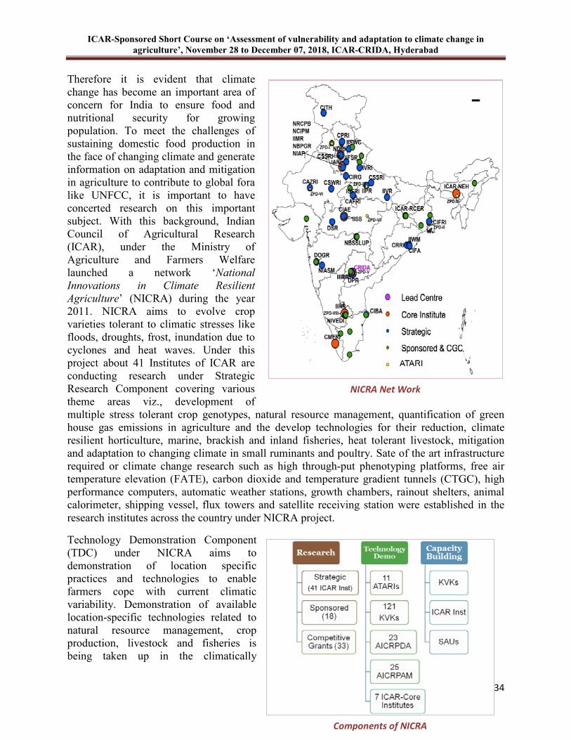
ICAR-Sponsored Short Course on ‘Assessment of vulnerability and adaptation to climate change in
agriculture’, November 28 to December 07, 2018, ICAR-CRIDA, Hyderabad
34
NICRA Net Work
Components of NICRA
Therefore it is evident that climate change has become an important area of concern for India to ensure food and nutritional security for growing population. To meet the challenges of sustaining domestic food production in the face of changing climate and generate information on adaptation and mitigation in agriculture to contribute to global fora like UNFCC, it is important to have concerted research on this important subject. With this background, Indian Council of Agricultural Research (ICAR), under the Ministry of Agriculture and Farmers Welfare launched a network ‘National
Innovations in Climate Resilient
Agriculture’ (NICRA) during the year 2011. NICRA aims to evolve crop varieties tolerant to climatic stresses like floods, droughts, frost, inundation due to cyclones and heat waves. Under this project about 41 Institutes of ICAR are conducting research under Strategic Research Component covering various theme areas viz., development of multiple stress tolerant crop genotypes, natural resource management, quantification of green house gas emissions in agriculture and the develop technologies for their reduction, climate resilient horticulture, marine, brackish and inland fisheries, heat tolerant livestock, mitigation and adaptation to changing climate in small ruminants and poultry. Sate of the art infrastructure required or climate change research such as high through-put phenotyping platforms, free air temperature elevation (FATE), carbon dioxide and temperature gradient tunnels (CTGC), high performance computers, automatic weather stations, growth chambers, rainout shelters, animal calorimeter, shipping vessel, flux towers and satellite receiving station were established in the research institutes across the country under NICRA project.
Technology Demonstration Component (TDC) under NICRA aims to demonstration of location specific practices and technologies to enable farmers cope with current climatic variability. Demonstration of available location-specific technologies related to natural resource management, crop production, livestock and fisheries is being taken up in the climatically
ICAR-Sponsored Short Course on ‘Assessment of vulnerability and adaptation to climate change in
agriculture’, November 28 to December 07, 2018, ICAR-CRIDA, Hyderabad
35
vulnerable districts for enhancing the adaptive capacity and resilience against climatic variability. Technologies with a potential to cope with climate variability are being demonstrated under Technology Demonstration Component (TDC) in 121 most vulnerable districts selected across the country through Krishi Vigyan Kendras (KVKs).
Institutional intervention Component under NICRA aims at creating enabling support system in the village comprising of strengthening of existing institutions or initiating new ones (Village Level Climate Risk Management Committees (VCRMC)), establishment and management of Custom Hiring Centers (CHCs) for farm implements, seed bank, fodder bank, creation of commodity groups, water sharing groups, community nursery and initiating collective marketing by tapping value chains. 100 custom hiring centers (CHCs) for farm machinery were setup under NICRA project, which are being managed by Village Climate Risk Management Committee (VCRMC) comprising of villagers. Module on use of ICT for knowledge empowerment of the communities in terms of climate risk management is also being planned in select KVKs for generation of locally relevant content and its dissemination in text and voice enabled formats. 121 KVKs associated under NICRA projects have also taken initiatives such as participatory village level seed production of short duration, drought and flood tolerant varieties, establishment of seed banks involving these varieties were established in the KVKs, demonstration and of improved varieties of fodder seeds and establishment of fodder bank in NICRA villages. Details about the research being carried out under this project is provided below.
Climate Smart Crop Varieties
Large number of germplasm screened for drought, heat, salinity, submergence tolerance etc. in different field and horticultural crops, for identifying donors for stress tolerance. Number of advance breeding materials was generated and evaluated at multi-locations for developing new cultivars. Germplasm lines of rice and wheat tolerant to drought and heat stress have been collected from different climatic hot-spot regions of India. So far a total of 184 rice accessions were collected. Evaluation of wheat germplasm for drought tolerance with 1485 accessions was conducted to identify drought tolerance lines based on 22 morpho-physiological traits. Based on the drought susceptible index a reference set will be developed for allele mining using micro satellite markers. Marker assisted back cross breeding was carried out using molecular markers link to the QTL governing drought tolerance into Pusa Basmati-1. rice varieties. Two rice genotypes for submergence tolerance was registered with National Bureau of Plant Genetic Resources (MBPGR), New Delhi. One salinity tolerant variety is in final year of All India Coordinated Research Project trials. Three superior heat tolerant hybrids were developed. Four drought tolerant rice varieties were released for Tripura. Two extra-early (50-55 days) green gram varieties were identified for summer cultivation (IPM 409-4, IPM 205-7) and one multiple stress tolerance redgram wild accession (C. scarabaeoides). A large number of soybean genotypes were evaluated for drought. Lines JS 97-52, EC 538828, EC 456548 and EC 602288 identified as relatively tolerant. These lines have been crossed among each other and with lines with superior agronomic background and are in F2-3 generations. Five heat tolerant and 12 drought tolerant genotypes in tomato. Number of mapping population in rice, wheat, maize were developed for identifying QTL for various abiotic stresses in these crops for utilization in maker assisted selection (MAS) breeding.
ICAR-Sponsored Short Course on ‘Assessment of vulnerability and adaptation to climate change in
agriculture’, November 28 to December 07, 2018, ICAR-CRIDA, Hyderabad
36
Natural Resource Management
GHG emissions (CO2, CH4& N2O) due to implementation of climate resilient interventions in various production systems (annual and/perennial crops, irrigated rice, inputs, livestock, forestry and land use change) were converted to an equivalent value (tonne CO2 equivalent) in 7 villages of Gujarat and Rajasthan, which were found to be negative suggesting a sink in GHG emissions. Direct-seeded rice (DSR) with mungbean residue incorporation, brown manuring (BM) with
sesbania, rice residue retention (RR) in zero till (ZT) wheat/rabi crops are important conservation agriculture (CA) practices. It was observed that mung bean residue (MBR) + DSR – ZTW – ZT summer mung bean (ZTSMB) gave highest system productivity, net return, water productivity and low GWP. In long term efforts to assess CA practices on productivity enhancement, nutrient use efficiency, soil health and quality, it was observed that seed (3.8 t ha-
1) and stover (5.6 t ha-1) yields in maize in CA were on par with conventional system (CT). Also, significantly higher grain (5.3 t ha-1), stover (6.5 t ha-1) yields and harvest index (0.44) were realized with balanced fertilization with NPKSZnB. Analysis of Resource Conservation Technologies (RCT) in NEH zone indicated that conventional Tillage (CT) has higher cumulative soil respiration (> 18%) compared to zero tillage. Agroforestry offset carbon dioxide from atmosphere is 0.77 tons of CO2ha-1 year-1and agroforestry system are estimated to mitigate 109.34 million tonnes CO2 annually from 142.0 million ha of agriculture land. Further, it is estimated to offset 33 per cent of total GHGs emissions from agriculture sector annually at country level. The net eco-system methane exchange during rice growth period was the highest between active tillering to maximum tillering stage in rice. The diurnal variations in mean Net Eco-system Exchange (NEE) in submerged rice eco-system in both dry and wet seasons varied from + 0.2 to - 1.2 and + 0.4 to - 0.8 mg CO2 m
-2 s-1. The cumulative seasonal methane emission was reduced by 75% in aerobic rice as compared to continuously flooded rice. The seasonal emissions were lower in slow release N fertilizer, especially, when applied on the basis of Customized Leaf Colour Chart (CLCC). Zero tillage in wheat lowered the GWP as compared to tilled wheat. Similarly, CO2, CH4 and N2O fluxes were influenced by tillage / anchored residue and anchored residues of 10 and 30 cm in zero till reduced the N2O emissions in rainfed pigeonpea-castor system. In efforts on mitigation strategies by reducing carbon foot prints through conservation agriculture in rainfed regions, carbon foot print from various practices like decomposition of crop residues, application of synthetic N fertilizers, field operations and input production indicated that there is a scope to reduce carbon foot prints by reducing one tillage operation with harvesting at 10 cm height with minimal impact on the crop yields. Long-term conservation horticultural practices in mango orchards improved the quality of soils through enhancing the organic carbon fraction and biological status, especially near the surface. Soil aggregates and water stability improved under conservation treatments. Cover crop, Mucuna, could conserve maximum moisture and reported higher Glomalin content in soil indicating the improvement in soil aggregation. Assessment of biochar on productivity, nutrient use efficiency and C sequestration potential of maize based cropping system in North-Eastern Hill region indicated a higher soil microbial biomass carbon (SMBC), dehydrogenase enzyme activity (DHA) and soil organic carbon (SOC) with application of biochar @ 5.0 t/ha along with 75% RDF + 4 t/ha FYM, while exchangeable aluminium and exchangeable acidity were reduced. GHG inventory for different cropping systems and production systems. GHG emissions quantified from Conservation Agriculture (CA) – 15 to 20% reduction, Resource conservation
ICAR-Sponsored Short Course on ‘Assessment of vulnerability and adaptation to climate change in
agriculture’, November 28 to December 07, 2018, ICAR-CRIDA, Hyderabad
37
technologies (Biochar, zero tillage, reduced tillage, mulching etc.). C Sequestration in different agroforestry systems (16-22 t C ha-1)
Greenhouse Gas Emission from Agriculture and Allied Sector
Under NICRA, emphasis has been placed on the development of technologies, which can reduce the green house gas emissions without compromising on yield. As part of this initiative, various ICAR institutes such as Indian Agricultural Research Institute (IARI), New Delhi, Indian Institute of Farming Systems Research (IIFSR), Modipuram, Indian Institute Soil Science (IISS), Bhopal, Central Arid Zone Research Institute (CAZRI), Jodhpur, ICAR Research Complex for NEH Region (ICAR-NEH), Umiam are working on various themes related to the GHG emissions. Facilities like, Eddy Covariance towers are established at IARI, New Delhi and National Rice Research Institute (NRRI), Cuttack for continuously monitoring the GHG emissions from the crop fields during growing season so as to quantify precisely the extent of GHG emissions from the paddy systems. Research Facilities like Rainout shelter, Carbon dioxide Temperature Gradient Chamber (CTGC), Free Air Carbon dioxide Enrichment (FACE), Free Air Temperature Enrichment (FATE) etc. have been established to understand the impact of elevated carbon dioxide (eCO2) and temperature and develop crop varieties that can withstand these stresses. Practices which can further reduce the GHG emissions such as improved systems of paddy cultivation, fertilizer management, improved fertilizer materials, crop diversification, etc. are explored for further reducing the GHG emissions from the paddy based systems. The proven mitigation practices, which can reduce the GHG emissions, are being demonstrated to farmers as part of the Technology Demonstration Component (TDC) of NICRA. The TDC of NICRA is being implemented in 121 climatically vulnerable districts of the country by taking one or cluster of villages in each of the vulnerable district.
Location specific, crop specific mitigation practices such as system of rice intensification, direct seeded rice cultivation (dry and wet methods of cultivation), soil test based fertiliser application, rational application of nitrogen, integration of trees especially fruit trees in the arable systems, efficient irrigation systems such as drip method and sprinkler method of application which can reduce the energy use while irrigating field crops, demonstration of zero tillage cultivation as an alternate to burning crop residues in rice-wheat systems of Punjab and Haryana where large quantities of rice residues are being burnt, integration of green manure crops in the existing cropping systems, promotion of green fodder crops and greater use of green fodder for livestock, etc. are being demonstrated as part of the technology demonstration component of NICRA in the 121 climatically vulnerable districts of the country. The proven resilient practices are being integrated in the development programs such as the Crop diversification in traditionally paddy growing regions as part of the National Food Security Mission (NFSM) wherein 1.02 lakh ha is being diversified from paddy to other less water consuming crops in the country during the year 2015-2016. Similarly the paddy systems of cultivation such as System of rice cultivation, direct seeded rice are being promoted by the development programs as part of the NFSM where in 1.63 lakh ha area was brought under these improved methods of paddy cultivation in the country during the year 2015-2016. Such kind of efforts would contribute to reduction of GHG emissions in the country.
ICAR-Sponsored Short Course on ‘Assessment of vulnerability and adaptation to climate change in
agriculture’, November 28 to December 07, 2018, ICAR-CRIDA, Hyderabad
38
Horticulture
Climate change impacts several horticultural crops in the country. Flooding for 24 hours severely affects tomato during flowering stage. Onion during blub stage is highly sensitive to flooding, where as warmer temperatures shorten the duration of onion bulb development leading to lower yields. Similarly, soil warming adversely affects several cucurbits. Reduction in chilling temperature in the recent years in Himachal Pradesh drastically affected apple production, and the farmers are shifting from apple to kiwi, pomegranate and other vegetables. More importantly, temperature and carbon dioxide are likely to alter the biology and forging behavior of pollinators that play key role in several horticulture crops. Under NICRA project research has been initiated at 5 ICAR Institutes viz., Indian Institute of Horticultural Research (IIHR), Bengaluru, Indian Institute of Vegetable Research (IIVR), Varanasi, Central Potato Research Institute (CPRI), Shimla, Central Institute of Temperate Horticulture (CITH), Srinagar and Directorate of Onion and Garlic Research (DOGR), Pune. High throughput screening of germplasm using plant Phenomics, Temperature Gradient Chambers, FATE Facility, Root imaging system, Environmental Chamber, TIR Facility, Photosynthetic System and Rainout shelter enabled to characterizes large number of germplasm lines and identify suitable donors for breeding against drought, heat stress and flooding in tomato, brinjal and onion. The technique for inter-specific grafting of tomato over brinjal has been standardized and large-scale demonstrations have been taken up to withstand drought and flooding in tomato. Environmentally safe protocol was developed for synchronizing flowering in mango, which is induced due to changing climate. A microbial inoculation with osmo tolerant bacterial strains have been developed to improve yield under limited moisture stress in tomato. Several resource conservation technologies viz., mulching, zero tillage, reduced tillage, biochar etc. have been demonstrated in climatically vulnerable districts across the country through Krishi Vigyan Kendras (KVKs). Large-scale adoption of this climate resilient technologies enable to adopt the changes associated with global warming and also keep pace with increasing demand for horticulture products in the country in the years to come.
Livestock
Under NICRA project climate change research facilities for livestock viz., CO2 Environmental Chambers, Thermal Imaging System, Animal Calorimeter, Custom Designed Animal Shed etc. have been established at ICAR-National Dairy Research Institute (NDRI), Karnal and ICAR-Indian Veterinary Research Institute (IVRI), Izatnagar. Biochemical, morphological and physiological characterization of indigenous cattle breeds were carried out and compared with exotic breeds. The traits identified in indigenous breed viz., heat shock proteins, air coat colour, wooly hair etc. that impart tolerance to heat stress could be used in future animal breeding programs to develop breeds that can withstand high temperature. Different feed supplements have been identified and tested successfully to withstand heat stress in cattle. Studies on prilled feeding in cattle showed that they help lowering stress levels and methane emission. Custom designed shelters system and feed supplementation with chromium propionate, mineral supplements (Cu, Mg, Ca and Zn) both in feed and fodder significantly improved the ability to withstand heat stress. At ICAR-North Eastern Hill Region, Umiam, the local birds of Mizoram are predominantly black in colour, small size, crown appearance on head, light pink comb with black, poorly develop wattle, small ear lobe, shank is brown to black and elongated. The average annual egg production of local birds is 45-55 eggs. Local birds are more tolerant to common
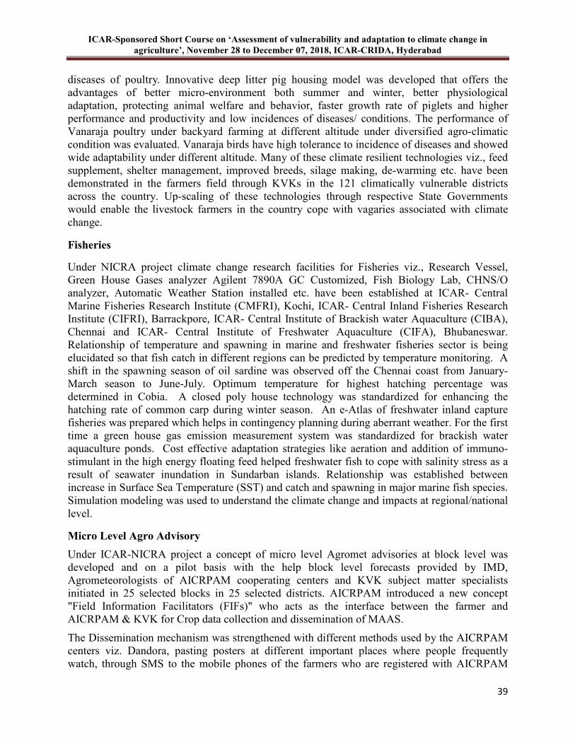
ICAR-Sponsored Short Course on ‘Assessment of vulnerability and adaptation to climate change in
agriculture’, November 28 to December 07, 2018, ICAR-CRIDA, Hyderabad
39
diseases of poultry. Innovative deep litter pig housing model was developed that offers the advantages of better micro-environment both summer and winter, better physiological adaptation, protecting animal welfare and behavior, faster growth rate of piglets and higher performance and productivity and low incidences of diseases/ conditions. The performance of Vanaraja poultry under backyard farming at different altitude under diversified agro-climatic condition was evaluated. Vanaraja birds have high tolerance to incidence of diseases and showed wide adaptability under different altitude. Many of these climate resilient technologies viz., feed supplement, shelter management, improved breeds, silage making, de-warming etc. have been demonstrated in the farmers field through KVKs in the 121 climatically vulnerable districts across the country. Up-scaling of these technologies through respective State Governments would enable the livestock farmers in the country cope with vagaries associated with climate change.
Fisheries
Under NICRA project climate change research facilities for Fisheries viz., Research Vessel, Green House Gases analyzer Agilent 7890A GC Customized, Fish Biology Lab, CHNS/O analyzer, Automatic Weather Station installed etc. have been established at ICAR- Central Marine Fisheries Research Institute (CMFRI), Kochi, ICAR- Central Inland Fisheries Research Institute (CIFRI), Barrackpore, ICAR- Central Institute of Brackish water Aquaculture (CIBA), Chennai and ICAR- Central Institute of Freshwater Aquaculture (CIFA), Bhubaneswar. Relationship of temperature and spawning in marine and freshwater fisheries sector is being elucidated so that fish catch in different regions can be predicted by temperature monitoring. A shift in the spawning season of oil sardine was observed off the Chennai coast from January-March season to June-July. Optimum temperature for highest hatching percentage was determined in Cobia. A closed poly house technology was standardized for enhancing the hatching rate of common carp during winter season. An e-Atlas of freshwater inland capture fisheries was prepared which helps in contingency planning during aberrant weather. For the first time a green house gas emission measurement system was standardized for brackish water aquaculture ponds. Cost effective adaptation strategies like aeration and addition of immuno-stimulant in the high energy floating feed helped freshwater fish to cope with salinity stress as a result of seawater inundation in Sundarban islands. Relationship was established between increase in Surface Sea Temperature (SST) and catch and spawning in major marine fish species. Simulation modeling was used to understand the climate change and impacts at regional/national level.
Micro Level Agro Advisory
Under ICAR-NICRA project a concept of micro level Agromet advisories at block level was developed and on a pilot basis with the help block level forecasts provided by IMD, Agrometeorologists of AICRPAM cooperating centers and KVK subject matter specialists initiated in 25 selected blocks in 25 selected districts. AICRPAM introduced a new concept "Field Information Facilitators (FIFs)" who acts as the interface between the farmer and AICRPAM & KVK for Crop data collection and dissemination of MAAS.
The Dissemination mechanism was strengthened with different methods used by the AICRPAM centers viz. Dandora, pasting posters at different important places where people frequently watch, through SMS to the mobile phones of the farmers who are registered with AICRPAM
ICAR-Sponsored Short Course on ‘Assessment of vulnerability and adaptation to climate change in
agriculture’, November 28 to December 07, 2018, ICAR-CRIDA, Hyderabad
40
center and KVKs. Special mobile applications were also developed by AICRPAM centers for dissemination of AAS. The feedback obtained from the farmers stated that many of them were satisfied with the timely Agromet advisories which are benefitted them a lot. some of the success stories presented below. In reality expansion of these services throughout the country will benefit of farming community and helps in doubling of their income.
Policy Support
Vulnerability assessment map prepared under NICRA is being used by different Ministries and several NGOs/CBOs.
• NICRA is also contributing to National missions like NMSA, Water mission, Green fund and INDC
• GHG inventory by NICRA partner institutes contributes to BUR reports • Outcome of NICRA project supported some of the policy issues in Sates of Maharashtra
(BBF Technology), Million farm ponds in the Sates of Andhra Pradesh and Telangana, ground water recharge initiatives (Southern states), drought proofing in Odisha, NABARD action plans, NICRA model village expansion in Assam etc.
• Contingency planning workshops organized every year in different States helps in preparedness to face weather aberrations.
Over all, NICRA project is contributing towards developing adaptation and mitigation strategies in the country and enabling to make Indian agriculture more resilient to climate change.
Conclusions
NICRA is a unique project, which brings all sectors of agriculture viz. crops, horticulture, livestock, fisheries, NRM and extension scientists on one platform for addressing climate concerns. It is very important to sustain the efforts made in the past few years and take forward the project for some more years. Over the past five years, the state of the art infrastructure facilities have been established, standardized and put in to function in core institutes of ICAR to undertake the climate change research. Manpower (Scientists, Research Associates, Research Fellows, Technical Officers etc.) have been trained to handle and operate these facilities. However, some of these precious research facilities are yet to be utilized to the full potential. In other words, a large platform related to climate change research has been created in the country. Crop improvement for multiple stresses takes several years of research and multi location testing. Efforts made under this project, in some cases resulted in development of varieties/hybrids ready for large-scale cultivation. Whereas, many are under different stages of development which may require few more years to be released as variety/hybrid/breed. Simulation modeling to assess the impact of climate change at regional level is still at initial stage. Standardization of minimum data sets and compilation of data from different sources have shown good progress. In the next phase, these data sets will be used for modeling. Capacity building for this activity will be emphasized and a dedicated group will be formulized. Research, essentially long term in nature, should continue further to achieve the intended outputs and outcomes
Though there are some positive lessons and experiences emerging out of technology demonstration component, there is still considerable need to continue this activity to identify and demonstrate technologies that help deal with climate change. In fact, the technologies found to
ICAR-Sponsored Short Course on ‘Assessment of vulnerability and adaptation to climate change in
agriculture’, November 28 to December 07, 2018, ICAR-CRIDA, Hyderabad
41
be performing well are getting fed into programs such as NMSA. There is still need to develop variety of adaptation options for different sub-sectors within agriculture, for different regions and for farmers with varying resource endowments. Such an effort is to be accompanied by identification of factors that help adopt technologies on a wider scale.
The commitments of the country to emission reductions require generate appropriate information and data on emissions as well as options that help reduce emissions. Techniques standardized so far under NICRA for estimation of GHG emissions from different management practices will be used for further reducing the carbon footprint of production systems in the country. Government of India has committed for the reduction of emission intensity of GDP by 32-35% by 2030 from 2005 levels, and the outputs of NICRA project contributing to several national project reports i.e., Intended Nationally Determined Contribution (INDC), Biennial Update Report (BUR), Nationally Appropriate Mitigation Action (NAMAs), National Mission on Sustainable Agriculture (NMSA) and several other Missions under National Action Plan on Climate Change. The system-wide impacts and responses to climate change need to be understood better and more comprehensively. The efforts in this direction, which have begun, recently have to be taken through their logical course for such an understanding is necessary to identify and prioritize various adaptation options. To sum up, the activities initiated few years back under NICRA should continue and expand in scope and content, and enable to develop multi location multi sector mitigation and adaptation strategies so that we combat major challenge posed due to climate change in Agriculture.
References
BUR. 2015. First Biennial Update Report to the United Nations Framework Convention on Climate Change. Ministry of Environment, Forest and Climate Change, Government of India, 184 p.
IPCC. 2014. Climate Change Synthesis Report. Contribution of Working Groups I, II and III to the Fifth Assessment Report of the Intergovernmental Panel on Climate Change [Core Writing Team, R.K. Pachauri and L.A. Meyer (eds.)]. IPCC, Geneva, Switzerland, 151 p.
National Innovations in Climate Resilient Agriculture (NICRA), Research Highlights (2016-18). ICAR-Central Research Institute for Dryland Agriculture, Hyderabad. 128 p.
ICAR-Sponsored Short Course on ‘Assessment of vulnerability and adaptation to climate change in
agriculture’, November 28 to December 07, 2018, ICAR-CRIDA, Hyderabad
42
5 Assessing Agricultural Vulnerability using Satellite-derived NDVI
Data Products
Kaushalya Ramachandran
1. Introduction
Climate change research has predominated political, economic, social and international discussions and dealings world over since the severe drought events of 1979 and 1987 which impacted human and livestock across several parts of the world. Scientific community opine that anthropogenic causes like increasing GHG emissions is the cause for growing weather aberrations (IPCC, 2007,2008) besides large scale change in Land Use - Land Cover (LULC) that impact the state and vigour of vegetation and crop adversely affecting agricultural potential of a region. A study was carried out under ICAR's national program - National Initiative on Climate Resilient Agriculture (NICRA) to gain an insight into sensitivity of rainfed agriculture in India to variability in climate using satellite derived Vegetation Index called Normalized Difference Vegetation Index (NDVI) as an indicator. Use of popular weather variables like precipitation and temperature as climate change indicators, help in understanding the genesis and impact of extreme weather events and resultant LULC and NDVI changes. The tools and techniques of remote sensing and GIS facilitate in examining the impacts of weather aberrations, abrupt extreme events and slow creeping changes on bio-physical cover of earth. In order to understand variations in weather and its attendant impact on Indian agriculture imparting degrees of vulnerability through its inherent sensitivity, a temporal study of NDVI variations was carried out using NDVI products from Advanced Very High Resolution Radiometer (NOAA-AVHRR) (15-day, 8km) and Moderate Resolution Imaging Spectro-radiometer (MODIS-TERRA) (16-day, 250m). Time-series NDVI datasets were downloaded from their respective websites and used for assessing sensitivity of cropping systems in various agro-eco-regions and mapping overall agricultural vulnerability to climate change in India. GIMMS (Global Inventory Modelling and Mapping Studies) dataset of NOAA- AVHRR with 8km resolution composited at 15-days interval, was used to analyse sensitivity of agricultural systems in India at state and agro-eco-sub-region (AESR) level for the period 1982-2006, while MODIS – TERRA NDVI data product with a higher spatial resolution of 250m was found useful to assess agricultural sensitivity at district–level for the period 2001-2012. Standard Precipitation Index (SPI) estimated from actual rainfall data was used to corroborate sensitivity of agriculture to climate variations and incidence of extreme weather events during the study period (Mckee et
al., 1993; Saikia and Kumar, 2011; Thenkabail et al., 2004; Dadhwal, 2011; SeshaSai et al., 2011; Murthy et al., 2010; Murthy and SeshaSai 2011).
ICAR-Sponsored Short Course on ‘Assessment of vulnerability and adaptation to climate change in
agriculture’, November 28 to December 07, 2018, ICAR-CRIDA, Hyderabad
43
2. Concepts Used For Analysing Agricultural Sensitivity For Spatial Vulnerability
Assessment
Normalized Difference Vegetation Index (NDVI)
The basis for remote sensing of vegetation is the sharp contrast in reflectivity of Visible (0.4 to 0.7 µm) and Near-Infrared (0.7-1.3 µm) spectra caused by the optical properties of chlorophyll and internal structures of green leaf cells. Several vegetation indices have been developed and are in use, however for current study NDVI has been used as it is strongly related to biomass. NDVI derived from 2-band information (Red and Near-infra Red) of multi-spectral imagery of a satellite data is a contrast–stretch ratio calculated from Red and Near–Infrared band (NIR) bands of sensors like LANDSAT – TM; AVHRR; IRS-1B, 1C, 1D, P6 satellite based sensors LISS-3 / LISS-4; and MODIS-TERRA besides several others. NDVI from AVHRR and MODIS data with Red reflectance in Band 1 and NIR reflectance in Band 2 is calculated as follows:(band 2-band
1) / (band 2 + band 1). NDVI takes advantage of typical low reflectance values of vegetation in the Red wavelength range which corresponds with chlorophyll absorption and high reflectance values in NIR range which signifies leaf structure, thereby enhancing the contrast between vegetated, un-vegetated and sparsely vegetated areas. Land Use-Land Cover (LULC) analysis facilitates the study of NDVI variations in various LULC classes like agriculture, plantation and forest besides open-scrubland (NRSC, 2011). Correlating rainfall pattern with NDVI time-series data helps in understanding the impact of increase / decrease in rainfall on vegetation cover in a given area over a period of time. Use of NDVI is particularly advantageous in sub-tropical regions especially in Asia and Africa where dependence on agriculture is high in the developing economies and study of vegetation response to rainfall and temperature in the event of scarce climate data, could help in drawing strategies to manage and adapt to weather aberrations. For the current study on impact of climate change on agriculture, other vegetation types like forest, plantation and scrub-land, mangroves, etc., were masked using multi-season data. Besides NDVI and LULC analysis, satellite data also provide information on other biophysical parameters viz., leaf area index (LAI), fraction of absorbed photo-synthetically active radiation (FPAR), crop/plant phenology, biomass, soil moisture and net primary productivity (NPP) which are of immense use to monitoring ecosystems and understanding their interactive roles (Gross, 2005). Conventional procedures to estimate and monitor these parameters although more accurate, are tedious and require more resources and hence Earth-Observation Satellites (EOS) play an important role in collection of these parameters in an object-oriented manner for accurate timely estimation (Dadhwal, 2011). Studies have been carried out to estimate LAI using MSS data from LANDSAT, NOAA-AVHRR, MODIS-TERRA and IRS-1D LISS-III sensor. LAI estimation using empirical method is based on regression between LAI and vegetation indices (VI) while physical estimation is based on inversion of canopy reflectance model. Statistical technique like Principal Component Inversion and Artificial Neural Network directly use band reflectance to predict LAI. The LAI-NDVI relation is logarithmic in nature and a significant positive relationship was seen while
ICAR-Sponsored Short Course on ‘Assessment of vulnerability and adaptation to climate change in
agriculture’, November 28 to December 07, 2018, ICAR-CRIDA, Hyderabad
44
estimating yield in several studies. NOAA/AVHRR data set have also been used to understand carbon storages and fluxes. As AVHRR-NDVI is available at global scale, it has been used effectively to monitor phenology of global vegetation which also facilitated study of inter-annual variations in NDVI that can reveal the response of vegetation to climate anomalies. Studies have demonstrated the linear relationship between NDVI during growing season and ground based observations of NPP in different biomes in North America. NDVI has been related to annual NPP at global-scale to study atmosphere-biosphere exchange of CO2. However, Nemani & Running (1989) found that NDVI could not reflect reduction in photosynthesis induced by summer drought in water-stressed areas implying that NDVI alone could not fully represent seasonal photosynthesis. NDVI can be simultaneously used to estimate both FPAR and LAI as FPAR is a linear function of NDVI while LAI is a curvilinear function of NDVI. The first global NPP images estimated using satellite NDVI were generated with Carnegie-Ames-Stanford Approach (CASA) model which had a spatial resolution of 1 degree. CASA model to investigate spatio-temporal processes of NPP over Indian sub-continent, used a 2-min spatial resolution derived from NOAA-AVHRR NDVI, weather inputs, soil and land cover maps. Study estimated an annual NPP of 1.57 PgC (2544 g C/m2, of which 56% was contributed by cropland, 18.5% by broad-leaved deciduous forests, 10% by broad-leaved evergreen forests and 8% by mixed shrub and grassland. There was a good agreement between the modelled NPP and ground-based crop land NPP estimates over western India. NDVI is used to understand vegetation condition, crop type and phenology and several derived information like area under agriculture and extent under various crop type and yield. Plants chlorophyll and pigmentation have high reflectance in red and near infrared section of electro-magnetic spectrum and stress in crop or physiological change causes variations in reflectance which helps in assessing vegetation condition. NDVI indicated as (NIR-R) / (NIR+R) thus ranges from -1 to 1 as reflectance from green vegetation in red spectrum is always lower than in near-infrared portion of spectrum due to absorption of light by chlorophyll. Hence NDVI value for vegetation cover can never be <0. It generally ranges from 0.1 to 0.6, the higher index values being associated with greater green leaf area and biomass. Time-series NDVI datasets facilitate study of start of growth of plant, peak growth and senescence (Sesha Sai et al., 2011). However, NDVI can be an indicator of crop development/condition only after significant spectral emergence of crops, which has a lag of 2-3 weeks after the completion of significant sowings in a region as stated by National Remote Sensing Centre (NRSC), a premier research institute under the Indian Space Research Organization (ISRO). Currently, NDVI data products are being generated from most of the satellite sensor systems viz., MODIS-NDVI of 250m and 1000m, SPOT VGT NDVI of 1000m, NOAA-AVHRR NDVI of 1000m and 8000m, and IRS AWiFS NDVI of 188m and AWiFS NDVI of 56m which are widely used for drought monitoring under India's National Agricultural Drought Assessment and Monitoring System (NADAMS) project because of the suitable spatial and temporal coverage of these products (Murthy et al., 2007).Murthy and Sesha Sai in their treaties Agricultural Drought Monitoring and Assessment in the form of an e-book in www.nrsc.gov.in have noted that NDVI shows a lag correlation of up to 4 weeks with rainfall and aridity anomaly; however, according to them this correlation is not unique for any season or
ICAR-Sponsored Short Course on ‘Assessment of vulnerability and adaptation to climate change in
agriculture’, November 28 to December 07, 2018, ICAR-CRIDA, Hyderabad
45
geographical area as rainfall use efficiency of crop or plant varies both in time and space, thus making direct satellite monitoring of vegetation growth essential for reliable and objective monitoring of agricultural drought situation. Hence they opine that complementary use of rainfall/aridity anomaly and vegetation index add to reliability of analysis of drought. Soil Moisture Variations
The thermal-infrared (TIR) range in EMS is sensitive to water-stress and hence used to study soil moisture status as it influences vegetation vigour and growth. Since 1980s, surface temperature (Ts) obtained from TIR has been used as a water-stress indicator based on a relationship between leaf temperature and transpiration. Numerous studies have suggested that a combination of surface temperature (Ts) and NDVI can provide information on vegetation stress and moisture condition on the land surface. Scatter plots of remotely sensed surface temperature and NDVI often exhibit triangular or trapezoidal shapes and are hence called NDVI Ts-shape. The primary basis for this relationship lies in the unique spectral reflectance-emittance properties of leaves in the red and infrared regions, in combination with the low thermal mass of plant leaves relative to soil surface. The slope of the NDVI-Ts is more or less closely related to surface evapo-transpiration (Boegh et al., 1998), surface soil moisture, stomatal conductance and Surface Bowen Ratio has suggested a no moisture index called the temperature / vegetation dryness index (TVDI) based on an interpretation of simplified NDVI-Ts space to assess surface moisture status. Later, many researchers have demonstrated the potential of the TVDI from Pathfinder data (8km) to assess the surface soil moisture status by using routine measurements of soil moisture at station-level or based on model simulations. In comparison with NOAA-AVHRR platform, MODIS-TERRA sensor has higher spectral (36 bands) and spatial (250-1000m) resolution, better viewing-time and calibration, which makes it superior for deriving parameters for various land surface properties. Standardized Precipitation Index (SPI)
Standardized Precipitation Index (SPI) represents total difference of precipitation for a given period of time from its climatic Mean and then normalized by Standard Deviation (SD) of precipitation for same period (Mckee et al., 1993; Saikia & Kumar, 2011). It provides an improved tool to assess variations in precipitation and associated impacts and hence, SPI instead of actual rainfall data was used for the present study. India Meteorological Department (IMD) provides daily rainfall data of more than 100 years for many stations from its archives. Daily girded rainfall data set for 1901–2007, developed by Rajeevan et al (2006) for 1384 stations was used for the present study. Girded rainfall data on a regular grid of 10 Latitude x 10 Longitude was used to calculate SPI using following formulae:
SPI = ���
��
Where,
a= current precipitation for a given period
A = long- term normal of precipitation for the same period
sd = Standard Deviation of precipitation for the given period
Long-term precipitation record was fitted to a probability distribution which was then transformed into a normal distribution so that Mean SPI for location and desired period is equal
ICAR-Sponsored Short Course on ‘Assessment of vulnerability and adaptation to climate change in
agriculture’, November 28 to December 07, 2018, ICAR-CRIDA, Hyderabad
46
to zero. Positive SPI values indicate greater than Median precipitation, while negative values indicate less than Median precipitation. As SPI is normalized, both wetter and drier climates can be presented in similar manner and both wet and dry periods denoting flood and drought could be monitored using SPI thus making it location and time independent. McKee et al (1993) used SPI values to define drought intensities in USA. Accordingly, SPI of ≤ 1.00 for any given period is considered as start of reduced rainfall period that could lead to drought, if prolonged. Thus, drought is said to occur at any time when SPI is continuously negative and reaches -1.0 or less. Drought event is said to end when SPI becomes positive. Computing SPI involves fitting a gamma probability density function to a given frequency distribution of precipitation totals for a given climate station. The gamma distribution is defined by its frequency or probability density function. In order to calculate SPI, a minimum of 30 years continuous daily rainfall data is required. The data may be summed as weekly or monthly averages as required for the study. In the absence of actual data, gridded rainfall data may be used for the same purpose as illustrated by Rajeevan et
al (2006). For the present study, both gridded and actual rainfall datasets were obtained from All-India Co-ordinated Research Program on Agro-Meteorology (AICRPAM) Data Bank at CRIDA and summed to arrive at monthly average for the months of June, July, August and September representing southwest monsoon season in India corresponding with Kharif cropping season as well as weekly total rainfall for 52 standard meteorological weeks for each year. Use of SPI is advantageous for analysis as it offers a flexible time-scale to assess the severity of a dry-spell in a given place. It can be calculated from weekly to 24-months or 2-year time scale depending on the purpose of the study and the suitable time-scale required for study. Studies have indicated that Weekly SPI provide accurate estimates as drought or dry spell start and end imperceptibly and hence weekly SPI may be the best time-scale and useful for early-warning and contingency planning for drought. Mckee et al (1993) has classified climatic variability based on SPI as follows:
SPI values Intensity of dry/wet spell
2.0 and > Extremely wet
1.5 to 1.99 Very wet
1.0 to 1.49 Moderately wet
-.99 to .99 Near normal
-1.0 to -1.49 Moderately dry
-1.5 to -1.99 Severely dry
-2.0 and < Extremely dry
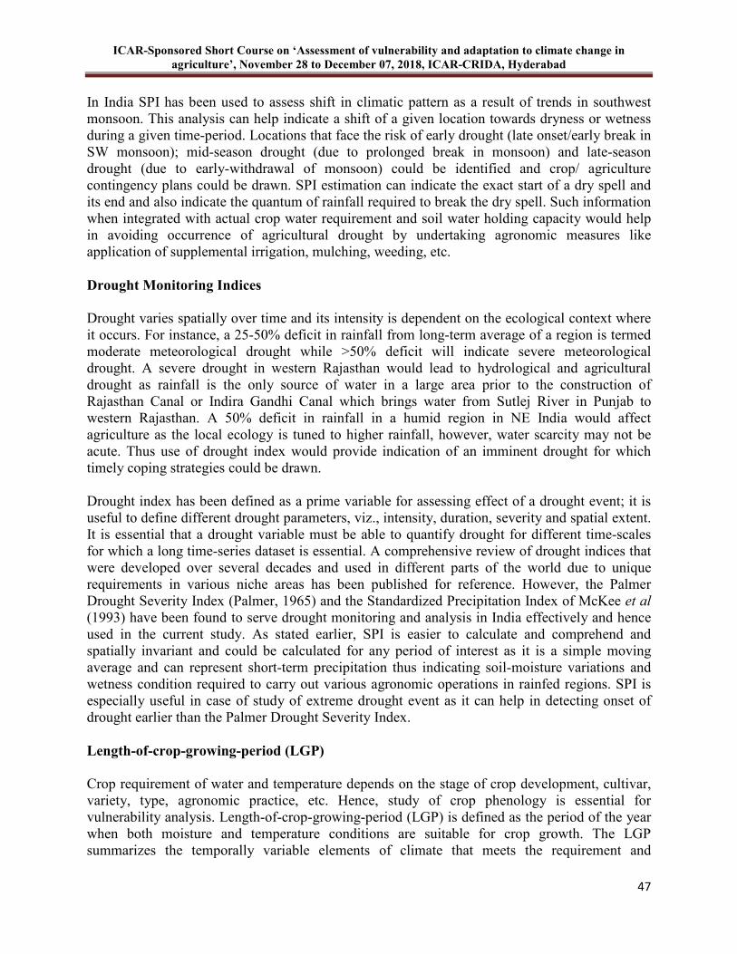
ICAR-Sponsored Short Course on ‘Assessment of vulnerability and adaptation to climate change in
agriculture’, November 28 to December 07, 2018, ICAR-CRIDA, Hyderabad
47
In India SPI has been used to assess shift in climatic pattern as a result of trends in southwest monsoon. This analysis can help indicate a shift of a given location towards dryness or wetness during a given time-period. Locations that face the risk of early drought (late onset/early break in SW monsoon); mid-season drought (due to prolonged break in monsoon) and late-season drought (due to early-withdrawal of monsoon) could be identified and crop/ agriculture contingency plans could be drawn. SPI estimation can indicate the exact start of a dry spell and its end and also indicate the quantum of rainfall required to break the dry spell. Such information when integrated with actual crop water requirement and soil water holding capacity would help in avoiding occurrence of agricultural drought by undertaking agronomic measures like application of supplemental irrigation, mulching, weeding, etc. Drought Monitoring Indices
Drought varies spatially over time and its intensity is dependent on the ecological context where it occurs. For instance, a 25-50% deficit in rainfall from long-term average of a region is termed moderate meteorological drought while >50% deficit will indicate severe meteorological drought. A severe drought in western Rajasthan would lead to hydrological and agricultural drought as rainfall is the only source of water in a large area prior to the construction of Rajasthan Canal or Indira Gandhi Canal which brings water from Sutlej River in Punjab to western Rajasthan. A 50% deficit in rainfall in a humid region in NE India would affect agriculture as the local ecology is tuned to higher rainfall, however, water scarcity may not be acute. Thus use of drought index would provide indication of an imminent drought for which timely coping strategies could be drawn. Drought index has been defined as a prime variable for assessing effect of a drought event; it is useful to define different drought parameters, viz., intensity, duration, severity and spatial extent. It is essential that a drought variable must be able to quantify drought for different time-scales for which a long time-series dataset is essential. A comprehensive review of drought indices that were developed over several decades and used in different parts of the world due to unique requirements in various niche areas has been published for reference. However, the Palmer Drought Severity Index (Palmer, 1965) and the Standardized Precipitation Index of McKee et al
(1993) have been found to serve drought monitoring and analysis in India effectively and hence used in the current study. As stated earlier, SPI is easier to calculate and comprehend and spatially invariant and could be calculated for any period of interest as it is a simple moving average and can represent short-term precipitation thus indicating soil-moisture variations and wetness condition required to carry out various agronomic operations in rainfed regions. SPI is especially useful in case of study of extreme drought event as it can help in detecting onset of drought earlier than the Palmer Drought Severity Index. Length-of-crop-growing-period (LGP)
Crop requirement of water and temperature depends on the stage of crop development, cultivar, variety, type, agronomic practice, etc. Hence, study of crop phenology is essential for vulnerability analysis. Length-of-crop-growing-period (LGP) is defined as the period of the year when both moisture and temperature conditions are suitable for crop growth. The LGP summarizes the temporally variable elements of climate that meets the requirement and
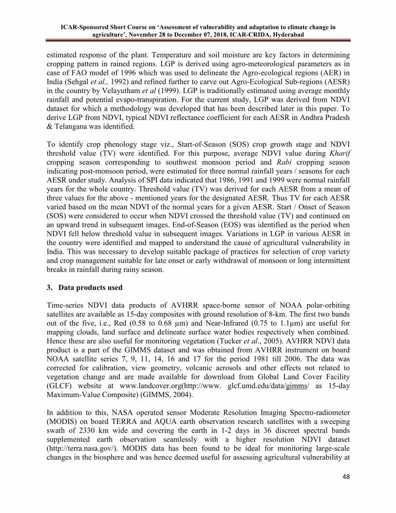
ICAR-Sponsored Short Course on ‘Assessment of vulnerability and adaptation to climate change in
agriculture’, November 28 to December 07, 2018, ICAR-CRIDA, Hyderabad
48
estimated response of the plant. Temperature and soil moisture are key factors in determining cropping pattern in rained regions. LGP is derived using agro-meteorological parameters as in case of FAO model of 1996 which was used to delineate the Agro-ecological regions (AER) in India (Sehgal et al., 1992) and refined further to carve out Agro-Ecological Sub-regions (AESR) in the country by Velayutham et al (1999). LGP is traditionally estimated using average monthly rainfall and potential evapo-transpiration. For the current study, LGP was derived from NDVI dataset for which a methodology was developed that has been described later in this paper. To derive LGP from NDVI, typical NDVI reflectance coefficient for each AESR in Andhra Pradesh & Telangana was identified. To identify crop phenology stage viz., Start-of-Season (SOS) crop growth stage and NDVI threshold value (TV) were identified. For this purpose, average NDVI value during Kharif cropping season corresponding to southwest monsoon period and Rabi cropping season indicating post-monsoon period, were estimated for three normal rainfall years / seasons for each AESR under study. Analysis of SPI data indicated that 1986, 1991 and 1999 were normal rainfall years for the whole country. Threshold value (TV) was derived for each AESR from a mean of three values for the above - mentioned years for the designated AESR. Thus TV for each AESR varied based on the mean NDVI of the normal years for a given AESR. Start / Onset of Season (SOS) were considered to occur when NDVI crossed the threshold value (TV) and continued on an upward trend in subsequent images. End-of-Season (EOS) was identified as the period when NDVI fell below threshold value in subsequent images. Variations in LGP in various AESR in the country were identified and mapped to understand the cause of agricultural vulnerability in India. This was necessary to develop suitable package of practices for selection of crop variety and crop management suitable for late onset or early withdrawal of monsoon or long intermittent breaks in rainfall during rainy season. 3. Data products used
Time-series NDVI data products of AVHRR space-borne sensor of NOAA polar-orbiting satellites are available as 15-day composites with ground resolution of 8-km. The first two bands out of the five, i.e., Red (0.58 to 0.68 µm) and Near-Infrared (0.75 to 1.1µm) are useful for mapping clouds, land surface and delineate surface water bodies respectively when combined. Hence these are also useful for monitoring vegetation (Tucker et al., 2005). AVHRR NDVI data product is a part of the GIMMS dataset and was obtained from AVHRR instrument on board NOAA satellite series 7, 9, 11, 14, 16 and 17 for the period 1981 till 2006. The data was corrected for calibration, view geometry, volcanic aerosols and other effects not related to vegetation change and are made available for download from Global Land Cover Facility (GLCF) website at www.landcover.org(http://www. glcf.umd.edu/data/gimms/ as 15-day Maximum-Value Composite) (GIMMS, 2004). In addition to this, NASA operated sensor Moderate Resolution Imaging Spectro-radiometer (MODIS) on board TERRA and AQUA earth observation research satellites with a sweeping swath of 2330 km wide and covering the earth in 1-2 days in 36 discreet spectral bands supplemented earth observation seamlessly with a higher resolution NDVI dataset (http://terra.nasa.gov/). MODIS data has been found to be ideal for monitoring large-scale changes in the biosphere and was hence deemed useful for assessing agricultural vulnerability at

ICAR-Sponsored Short Course on ‘Assessment of vulnerability and adaptation to climate change in
agriculture’, November 28 to December 07, 2018, ICAR-CRIDA, Hyderabad
49
a relatively finer-scale like district-level within the country. MODIS (16-day, 250m) NDVI composite products are freely available from Land Processes - Distributed Active Archive Centre
(LPDAAC) website of USGS <http://mrtweb.cr.usgs.gov/>. The Indian sub-continent is covered in 13 scenes and NDVI data is available from February 2000 onwards till date. 4. Methodology for Assessing Agricultural Vulnerability
Time-series NDVI data products of both AVHRR and MODIS were analysed to identify the spatial extent of agricultural vulnerability in India. AVHRR-NDVI data product which is available for whole of Indian sub-continent was sub-set from the global coverage in the form of one tile for each year starting from 1982. Bi-monthly NDVI images (15-day, 8km) were stacked and pre-processed, followed by identification of pixel-wise Max NDVI for arriving at Maximum Greenness for any pixel during corresponding year during the period 1982 to 2006. This was followed by estimation of Mean and Standard Deviation for Max NDVI. To understand variability in Greenness as an indicator of agricultural vulnerability, Coefficient of Variation (CV) of Max NDVI was calculated which formed the basis for analysis of agricultural vulnerability. Due to coarse resolution of AVHRR (8-km) dataset based on Max NDVI pattern, agricultural vulnerability was identified at AESR-level. The exercise helped in estimation of spatial extent of vulnerable regions in the whole country. Method for identifying and estimating extent of agricultural vulnerability is indicated in Figure1. Spatial pattern of rainfall (1982 and 2011) was mapped by interpolating 10 X 10 rainfall grid data using Kriging method as mentioned earlier. Standard Precipitation Index (SPI) was calculated from 110-year daily rainfall records for each grid point and trends analysed. As mentioned earlier, rainfall was highest during the months of July-August and corresponding Max NDVI occurred in the following months of Sept–October annually. Analysis of annual and southwest monsoon rainfall pattern was used for the study assuming 1982 as the base year.
5. Identification of Agriculturally Vulnerable Regions in India
Based on CV of Max NDVI as a result of decrease in rainfall illustrated by SPI and associated changes in length-of-crop-growing-period (LGP) discussed in a subsequent section, regional agricultural vulnerability was identified across India. Study indicated that drought and floods occurred simultaneously during several years since 1982. During typical years like in 1987 when drought occurred in the country, Gujarat and western Uttar Pradesh experienced severe drought with SPI<-2 denoting ‘extremely dry’ condition. During the year SPI ranged from -1.0 to -2.0 in Rajasthan which is termed ‘moderately to severely dry’ condition while moderate drought prevailed in central India with SPI ranging from -1 to -1.49. During this period Max NDVI in Gujarat ranged from 0.15 to 0.73 while Mean NDVI was 0.11 – 0.43.
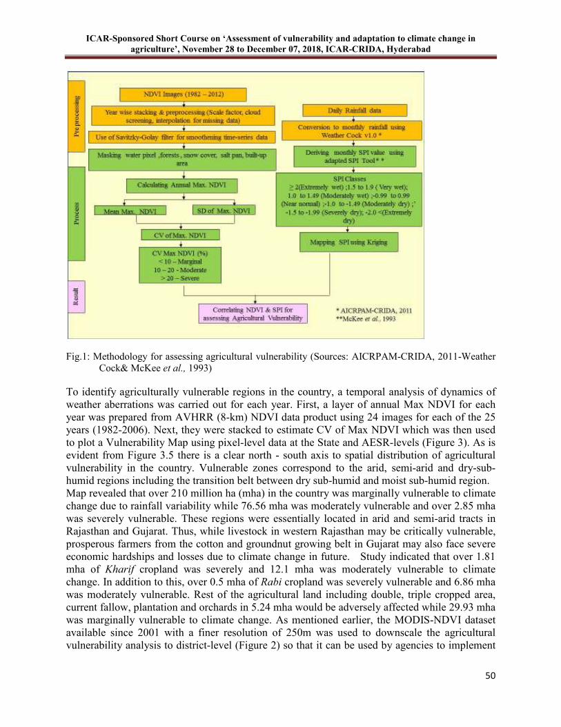
ICAR-Sponsored Short Course on ‘Assessment of vulnerability and adaptation to climate change in
agriculture’, November 28 to December 07, 2018, ICAR-CRIDA, Hyderabad
50
Fig.1: Methodology for assessing agricultural vulnerability (Sources: AICRPAM-CRIDA, 2011-Weather
Cock& McKee et al., 1993) To identify agriculturally vulnerable regions in the country, a temporal analysis of dynamics of weather aberrations was carried out for each year. First, a layer of annual Max NDVI for each year was prepared from AVHRR (8-km) NDVI data product using 24 images for each of the 25 years (1982-2006). Next, they were stacked to estimate CV of Max NDVI which was then used to plot a Vulnerability Map using pixel-level data at the State and AESR-levels (Figure 3). As is evident from Figure 3.5 there is a clear north - south axis to spatial distribution of agricultural vulnerability in the country. Vulnerable zones correspond to the arid, semi-arid and dry-sub-humid regions including the transition belt between dry sub-humid and moist sub-humid region. Map revealed that over 210 million ha (mha) in the country was marginally vulnerable to climate change due to rainfall variability while 76.56 mha was moderately vulnerable and over 2.85 mha was severely vulnerable. These regions were essentially located in arid and semi-arid tracts in Rajasthan and Gujarat. Thus, while livestock in western Rajasthan may be critically vulnerable, prosperous farmers from the cotton and groundnut growing belt in Gujarat may also face severe economic hardships and losses due to climate change in future. Study indicated that over 1.81 mha of Kharif cropland was severely and 12.1 mha was moderately vulnerable to climate change. In addition to this, over 0.5 mha of Rabi cropland was severely vulnerable and 6.86 mha was moderately vulnerable. Rest of the agricultural land including double, triple cropped area, current fallow, plantation and orchards in 5.24 mha would be adversely affected while 29.93 mha was marginally vulnerable to climate change. As mentioned earlier, the MODIS-NDVI dataset available since 2001 with a finer resolution of 250m was used to downscale the agricultural vulnerability analysis to district-level (Figure 2) so that it can be used by agencies to implement
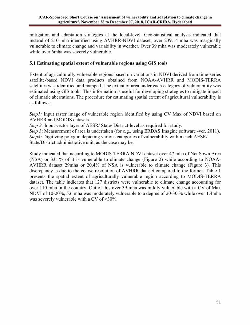
ICAR-Sponsored Short Course on ‘Assessment of vulnerability and adaptation to climate change in
agriculture’, November 28 to December 07, 2018, ICAR-CRIDA, Hyderabad
51
mitigation and adaptation strategies at the local-level. Geo-statistical analysis indicated that instead of 210 mha identified using AVHRR-NDVI dataset, over 239.14 mha was marginally vulnerable to climate change and variability in weather. Over 39 mha was moderately vulnerable while over 6mha was severely vulnerable. 5.1 Estimating spatial extent of vulnerable regions using GIS tools
Extent of agriculturally vulnerable regions based on variations in NDVI derived from time-series satellite-based NDVI data products obtained from NOAA-AVHRR and MODIS-TERRA satellites was identified and mapped. The extent of area under each category of vulnerability was estimated using GIS tools. This information is useful for developing strategies to mitigate impact of climatic aberrations. The procedure for estimating spatial extent of agricultural vulnerability is as follows:
Step1: Input raster image of vulnerable region identified by using CV Max of NDVI based on AVHRR and MODIS datasets. Step 2: Input vector layer of AESR/ State/ District-level as required for study. Step 3: Measurement of area is undertaken (for e.g., using ERDAS Imagine software -ver. 2011). Step4: Digitizing polygon depicting various categories of vulnerability within each AESR/ State/District administrative unit, as the case may be. Study indicated that according to MODIS-TERRA NDVI dataset over 47 mha of Net Sown Area (NSA) or 33.1% of it is vulnerable to climate change (Figure 2) while according to NOAA-AVHRR dataset 29mha or 20.4% of NSA is vulnerable to climate change (Figure 3). This discrepancy is due to the coarse resolution of AVHRR dataset compared to the former. Table 1 presents the spatial extent of agriculturally vulnerable region according to MODIS-TERRA dataset. The table indicates that 127 districts were vulnerable to climate change accounting for over 110 mha in the country. Out of this over 39 mha was mildly vulnerable with a CV of Max NDVI of 10-20%, 5.6 mha was moderately vulnerable to a degree of 20-30 % while over 1.4mha was severely vulnerable with a CV of >30%.
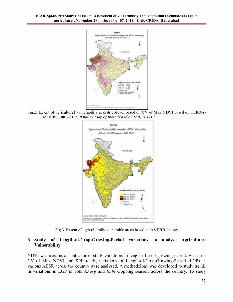
ICAR-Sponsored Short Course on ‘Assessment of vulnerability and adaptation to climate change in
agriculture’, November 28 to December 07, 2018, ICAR-CRIDA, Hyderabad
52
Fig.2. Extent of agricultural vulnerability at district-level based on CV of Max NDVI based on TERRA-
MODIS (2001-2012) (Outline Map of India based on SOI, 2012). \\
Fig.3. Extent of agriculturally vulnerable areas based on AVHRR dataset
6. Study of Length-of-Crop-Growing-Period variations to analyse Agricultural
Vulnerability
NDVI was used as an indicator to study variations in length of crop growing period. Based on CV of Max NDVI and SPI trends, variations of Length-of-Crop-Growing-Period (LGP) in various AESR across the country were analysed. A methodology was developed to study trends in variations in LGP in both Kharif and Rabi cropping seasons across the country. To study
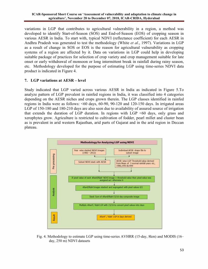
ICAR-Sponsored Short Course on ‘Assessment of vulnerability and adaptation to climate change in
agriculture’, November 28 to December 07, 2018, ICAR-CRIDA, Hyderabad
53
variations in LGP that contributes to agricultural vulnerability in a region, a method was developed to identify Start-of-Season (SOS) and End-of-Season (EOS) of cropping season in various AESR in India. To start with, typical NDVI (reflectance coefficient) for each AESR in Andhra Pradesh was generated to test the methodology (White et al., 1997). Variations in LGP as a result of change in SOS or EOS is the reason for agricultural vulnerability as cropping systems of a region are affected by it. Data on variations in LGP could help in developing suitable package of practices for selection of crop variety and crop management suitable for late onset or early withdrawal of monsoon or long intermittent break in rainfall during rainy season, etc. Methodology developed for the purpose of estimating LGP using time-series NDVI data product is indicated in Figure 4. 7. LGP variations at AESR – level
Study indicated that LGP varied across various AESR in India as indicated in Figure 5.To analyze pattern of LGP prevalent in rainfed regions in India, it was classified into 4 categories depending on the AESR niches and crops grown therein. The LGP classes identified in rainfed regions in India were as follows: <60 days, 60-90, 90-120 and 120-150 days. In irrigated areas LGP of 150-180 and 180-210 days are also seen due to availability of assured source of irrigation that extends the duration of LGP duration. In regions with LGP <60 days, only grass and xerophytes grow. Agriculture is restricted to cultivation of fodder, pearl millet and cluster bean as is prevalent in arid western Rajasthan, arid parts of Gujarat and in the arid region in Deccan plateau.
Fig. 4. Methodology to estimate LGP using time-series AVHRR (15-day, 8km) and MODIS (16–
day, 250 m) NDVI datasets
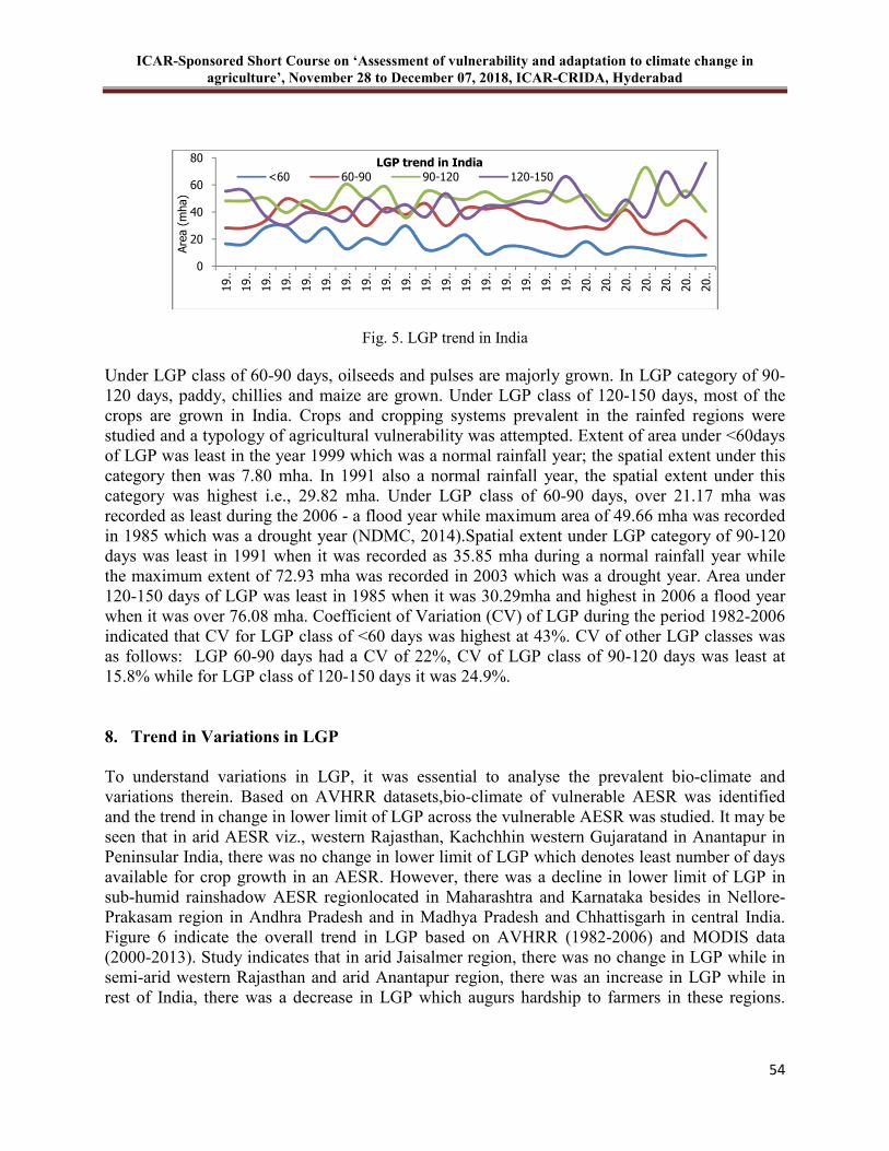
ICAR-Sponsored Short Course on ‘Assessment of vulnerability and adaptation to climate change in
agriculture’, November 28 to December 07, 2018, ICAR-CRIDA, Hyderabad
54
Fig. 5. LGP trend in India Under LGP class of 60-90 days, oilseeds and pulses are majorly grown. In LGP category of 90-120 days, paddy, chillies and maize are grown. Under LGP class of 120-150 days, most of the crops are grown in India. Crops and cropping systems prevalent in the rainfed regions were studied and a typology of agricultural vulnerability was attempted. Extent of area under <60days of LGP was least in the year 1999 which was a normal rainfall year; the spatial extent under this category then was 7.80 mha. In 1991 also a normal rainfall year, the spatial extent under this category was highest i.e., 29.82 mha. Under LGP class of 60-90 days, over 21.17 mha was recorded as least during the 2006 - a flood year while maximum area of 49.66 mha was recorded in 1985 which was a drought year (NDMC, 2014).Spatial extent under LGP category of 90-120 days was least in 1991 when it was recorded as 35.85 mha during a normal rainfall year while the maximum extent of 72.93 mha was recorded in 2003 which was a drought year. Area under 120-150 days of LGP was least in 1985 when it was 30.29mha and highest in 2006 a flood year when it was over 76.08 mha. Coefficient of Variation (CV) of LGP during the period 1982-2006 indicated that CV for LGP class of <60 days was highest at 43%. CV of other LGP classes was as follows: LGP 60-90 days had a CV of 22%, CV of LGP class of 90-120 days was least at 15.8% while for LGP class of 120-150 days it was 24.9%. 8. Trend in Variations in LGP
To understand variations in LGP, it was essential to analyse the prevalent bio-climate and variations therein. Based on AVHRR datasets,bio-climate of vulnerable AESR was identified and the trend in change in lower limit of LGP across the vulnerable AESR was studied. It may be seen that in arid AESR viz., western Rajasthan, Kachchhin western Gujaratand in Anantapur in Peninsular India, there was no change in lower limit of LGP which denotes least number of days available for crop growth in an AESR. However, there was a decline in lower limit of LGP in sub-humid rainshadow AESR regionlocated in Maharashtra and Karnataka besides in Nellore-Prakasam region in Andhra Pradesh and in Madhya Pradesh and Chhattisgarh in central India. Figure 6 indicate the overall trend in LGP based on AVHRR (1982-2006) and MODIS data (2000-2013). Study indicates that in arid Jaisalmer region, there was no change in LGP while in semi-arid western Rajasthan and arid Anantapur region, there was an increase in LGP while in rest of India, there was a decrease in LGP which augurs hardship to farmers in these regions.
0
20
40
60
80
19…
19…
19…
19…
19…
19…
19…
19…
19…
19…
19…
19…
19…
19…
19…
19…
19…
19…
20…
20…
20…
20…
20…
20…
20…
Area (mha)
<60 60-90 90-120 120-150
LGP trend in India
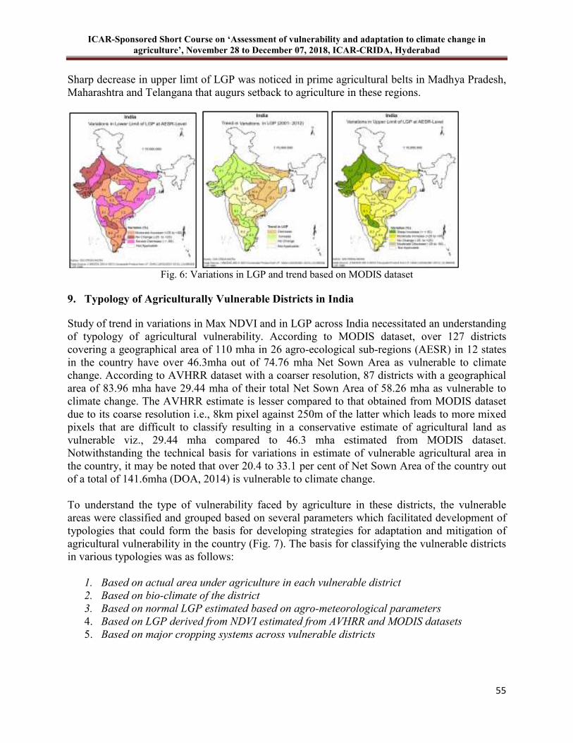
ICAR-Sponsored Short Course on ‘Assessment of vulnerability and adaptation to climate change in
agriculture’, November 28 to December 07, 2018, ICAR-CRIDA, Hyderabad
55
Sharp decrease in upper limt of LGP was noticed in prime agricultural belts in Madhya Pradesh, Maharashtra and Telangana that augurs setback to agriculture in these regions.
Fig. 6: Variations in LGP and trend based on MODIS dataset
9. Typology of Agriculturally Vulnerable Districts in India Study of trend in variations in Max NDVI and in LGP across India necessitated an understanding of typology of agricultural vulnerability. According to MODIS dataset, over 127 districts covering a geographical area of 110 mha in 26 agro-ecological sub-regions (AESR) in 12 states in the country have over 46.3mha out of 74.76 mha Net Sown Area as vulnerable to climate change. According to AVHRR dataset with a coarser resolution, 87 districts with a geographical area of 83.96 mha have 29.44 mha of their total Net Sown Area of 58.26 mha as vulnerable to climate change. The AVHRR estimate is lesser compared to that obtained from MODIS dataset due to its coarse resolution i.e., 8km pixel against 250m of the latter which leads to more mixed pixels that are difficult to classify resulting in a conservative estimate of agricultural land as vulnerable viz., 29.44 mha compared to 46.3 mha estimated from MODIS dataset. Notwithstanding the technical basis for variations in estimate of vulnerable agricultural area in the country, it may be noted that over 20.4 to 33.1 per cent of Net Sown Area of the country out of a total of 141.6mha (DOA, 2014) is vulnerable to climate change.
To understand the type of vulnerability faced by agriculture in these districts, the vulnerable areas were classified and grouped based on several parameters which facilitated development of typologies that could form the basis for developing strategies for adaptation and mitigation of agricultural vulnerability in the country (Fig. 7). The basis for classifying the vulnerable districts in various typologies was as follows:
1. Based on actual area under agriculture in each vulnerable district 2. Based on bio-climate of the district 3. Based on normal LGP estimated based on agro-meteorological parameters
4. Based on LGP derived from NDVI estimated from AVHRR and MODIS datasets 5. Based on major cropping systems across vulnerable districts
ICAR-Sponsored Short Course on ‘Assessment of vulnerability and adaptation to climate change in
agriculture’, November 28 to December 07, 2018, ICAR-CRIDA, Hyderabad
56
10. Conclusion
Satellite-based NDVI obtained from NOAA-AVHRR and MODIS-TERRA (1982-2012) was used to assess agricultural vulnerability in India. A methodology was developed to assess agricultural vulnerability by estimating CV of Max NDVI of AVHRR (16-day, 8km) data product for 1982-2006 period and MODIS NDVI dataset (15-day, 250m) from 2001 till 2012. In order to understand the trend in NDVI variations, Standard Precipitation Index (SPI) was estimated for the study period and results corroborated. Study indicated that over 127 districts covering 110 mha encompassing over 26 agro-ecological sub-regions (AESR) in 12 states in the country were vulnerable to climate change. Of the 74 mha under agriculture in these districts, MODIS dataset indicated that over 47 mha of net sown area was vulnerable to climate change. AVHRR dataset due to its coarse resolution indicated that over 29 mha of net sown area was vulnerable to climate change. This variation in estimation which was due to coarse resolution of the latter was a consequence of the mixed pixels in the image that are difficult to classify. Notwithstanding the variation in estimates of extent of agriculturally vulnerable region in India, it is notable that nearly 1/5th to 1/3rd net sown area in the country out of a total sown area of 142 mha, is vulnerable to climate change. Study revealed that NOAA-AVHRR and MODIS-TERRA based NDVI time-series data are useful for studying the slow process of climate change resulting due to variability in rainfall and its interaction with soil and micro-climate in a given region. Satellite based products provide an authentic spatial reference to analysis of agricultural vulnerability to climate change. As these data are readily available on the internet, their inclusion in planning for improving adaptation and mitigation strategies among farmers is essential. Due to pixel resolution of AVHRR data i.e., 8km, it was deemed appropriate to use it to estimate agricultural vulnerability at a regional level viz., AESR while MODIS (250m) NDVI data product was used to assess agricultural vulnerability at district-level. The comparatively finer resolution of NDVI data product makes it useful for drawing actual implementable strategy and plans for improving adaptation among farmers at local-level.

ICAR-Sponsored Short Course on ‘Assessment of vulnerability and adaptation to climate change in
agriculture’, November 28 to December 07, 2018, ICAR-CRIDA, Hyderabad
57
Fig.7. Change in lower-limit of LGP in comparison to normal LGP To identify agricultural vulnerability, trends in NDVI data were corroborated with SPI data. Year 1987 was a severe drought year when Gujarat and western Uttar Pradesh reeled under severe
ICAR-Sponsored Short Course on ‘Assessment of vulnerability and adaptation to climate change in
agriculture’, November 28 to December 07, 2018, ICAR-CRIDA, Hyderabad
58
drought. SPI corresponding to this region in 1987 was estimated at<-2 denoting extremely dry condition while in Rajasthan, the SPI was calculated as -1.0 to -2.0 denoting moderate to severe dry condition and in central India moderate drought prevailed with SPI ranging from -1 to -1.49.During the same year, Max NDVI in Gujarat was 0.15 while Mean NDVI was 0.11 while in Rajasthan it was lower, i.e., 0.11 and 0.08 and in western Uttar Pradesh, 0.48 and 0.31 respectively. In central India where moderate drought occurred, Max NDVI was 0.12 and Mean NDVI was 0.09. The NDVI ranges reflect the type of cropping systems prevalent in these regions. During 2005 when floods occurred extensively in erstwhile Andhra Pradesh, Karnataka, Tamil Nadu and south-western parts of Maharashtra, SPI ranged from very wet to extremely wet in former Andhra Pradesh with SPI >1.5 while Max NDVI in Andhra Pradesh and Karnataka ranged from 0.47 to 0.72 and Mean NDVI ranged from 0.30 to 0.55. To understand agricultural vulnerability, variations in LGP were studied for which a methodology was developed using NDVI of normal years to derive Threshold Value for each AESR in India. This value was in turn used to derive Start-of-Season and End-of-Season period of LGP for both cropping seasons in India namely, Kharif and Rabi. Change in LGP as a result of reduction in lower-limit or upper-limit of LGP was studied. Variability in LGP was seen to be high in regions having a LGP of <60 days and 120-150 days; it was lower in regions having 60-90 days of LGP and least in regions with90-120 days. There was a variation in identification of SOS and EOS of LGP while using AVHRR and MODIS-NDVI datasets with latter indicating longer LGP. Study also indicated a significant reduction in LGP during Rabi season. However increase in irrigation in several districts in central and southern India, have led to a negative correlation between SPI and NDVI. It was seen that there was an increase in area with LGP of 90 – 120 days during Kharif season in the country. It may be concluded that freely available NDVI data products developed from NOAA-AVHRR and MODIS-TERRA sensors were found useful to study the imperceptible change in vegetation cover especially agriculture in India. The methodology developed using CV of Max NDVI to identify spatial extent of agricultural vulnerability indicated that over 47 mha or 33% of net sown area in the country was vulnerable to climate change and weather aberrations.
References
AICRPAM-CRIDA .2011. Weather cock@ V 1.0. NICRA. Boegh E, Soegaard H, Hanan N, Kabat P and Lesch L. 1998. A remote sensing study of the
NDVI-Ts relationship and the transpiration from sparse vegetation in the Sahel based on high resolution satellite data. Remote Sensing of Environment 69: 224-240
DOA. 2014. Annual Report 2013-14. Ministry of Agriculture.Government of India. 1-200
ICAR-Sponsored Short Course on ‘Assessment of vulnerability and adaptation to climate change in
agriculture’, November 28 to December 07, 2018, ICAR-CRIDA, Hyderabad
59
Dadhwal VK. 2011. Retrieval of biophysical parameters from satellite data. (In): Agricultural drought: Climate change and rainfed agriculture (Eds. Rao, V.U.M., Rao, A.V.M.S., Kumar, P.V., Desai, S., Saikia, U.S., Srivastava, N.N. and B. Venkateswarlu). Lectures notes of the 5th SERC School, CRIDA 52-58
GIMMS..2004. Global Inventory Modelling and Mapping Studies http://www.glcf.umd.edu Gross D. 2005. Monitoring agricultural biomass using NDVI time series. Food and agriculture
organization of the United Nations.1-17. IPCC. 2007. Climate Change 2007: Impacts, Adaptation and Vulnerability. Contribution of
Working Group II to the Fourth Assessment Report of the Intergovernmental Panel on Climate Change, M.L. Parry, O.F. Canziani, J.P. Palutikof, P.J. van der Linden and C.E. Hanson, Eds., 976pp
IPCC. 2008. Climate Change 2007 – Synthesis report. WMO & UNEP Kaushalya Ramachandran, Rama Rao CA, Raju BMK, Rao VUM, Subba Rao AVM, Rao KV,
Ramana DBV, Nagasree K, Ravi Shankar K, Maheshwari M, Srinivasa Rao Ch, Venkateswarlu B and Sikka AK. 2015. Spatial Vulnerability Assessment using Satellite based NDVI for Rainfed Agriculture in India. ICAR-Central Research Institute of Dryland Agriculture, Hyderabad. P.192.
McKee TB, Doesken NJ and Kleist J. 1993. The relationship of drought frequency and duration
to time scales. 8th Conf. On Applied Climatology, 17-22 January, Anaheim, CA, pp.179-184
Murthy CS, Sesha Sai MVR, Bhanuja Kumari V and Roy PS. 2007. Agricultural drought assessment at disaggregated level using AwiFS/WiFS data of Indian Remote Sensing satellites. Geocarto International 22:127-140
Murthy CS, Sesha Sai MVR, Prabir Kumar Das, Naresh Kumar M, Abhishek Chakraborty and
Dwivedi RS. 2010. Assessing agricultural drought vulnerability using time series rainfall and NDVI. NNRMS Bulletin-2010. 65-71
Murthy CS and Sesha Sai MVR. 2011. Agricultural drought monitoring and Assessment. (In):
Remote Sensing Applications (Eds. Roy, P.S., Dwivedi, R.S. and Vijayan, D.) NRSC/ISRO, 303-330, www.nrsc.gov.in
NRSC. 2011. Land Use Land Cover Atlas of India (Based on Multi-temporal satellite data of
2005-06). LUD-RS&GIS Applications Area-NRSC (ISRO), Hyderabad, 128 p Palmer WC. 1965. Meteorological Drought. Office of Climatology, U.S. Bureau, Washington,
Research paper no. 65, 58p.

ICAR-Sponsored Short Course on ‘Assessment of vulnerability and adaptation to climate change in
agriculture’, November 28 to December 07, 2018, ICAR-CRIDA, Hyderabad
60
Rajeevan M, Jyoti Bhate, Kale JD and Lal B. 2006. High resolution daily gridded rainfall data for the Indian region: Analysis of break and active monsoon spells. Current Science 91(3): 296-306
Saikia US and Manoranjan Kumar. 2011. Standardized Precipitation Index (SPI): An effective
drought monitoring tool. 5th SERC School on Agricultural Drought: Climate Change and Rainfed Agriculture, pp.1-10
Sehgal J, Mandal DK, Mandal C and Vadivelu S. 1992. Agro-ecological regions of India, 2nd
edition, Tech. Bull., Publ. 24, pp 130, NBSS&LUP Sesha Sai MVR, Murthy CS and Ramana KV. 2011. Agricultural drought assessment &
monitoring. (In): Agricultural drought: Climate Change and rainfed agriculture (Eds.Rao, V.U.M., Rao, A.V.M. S., Kumar, P.V., Desai, S., Saikia, U.S., Srivastava, N.N. & B. Venkateswarlu), Lecture notes of the 5th SERC school, CRIDA, 80-87.
Thenkabail PS, Gamage MSDN and Smakhtin VU. 2004. The use of remote-sensing data for
drought assessment and monitoring in Southwest Asia. Research Rpt. 85. Future Harvest, IMWI, 25p
Tucker CJ, Pinzon JE, Brown ME, Slayback D, Pak EW, Mahoney R, Vermote E And Saleous
NEI. 2005. An extended AVHRR 8-km NDVI Data set Compatible with MODIS and SPOT vegetation NDVI Data. Int. J. of Remote Sensing, 26(20): 4485-4498
Velayutham M, Mandal DK, Champa Mandal and Sehgal J. 1999. Agro ecological sub regios of
India for planning and Development. NBSS&LUP, Nagpur, India.Pub., p - 372. White MA, Thornton PE and Running SW. 1997. A continental phenology model for monitoring
vegetation responses to inter-annual climatic variability. Global Biochemical Cycles, 11(2): 217-234
ICAR-Sponsored Short Course on ‘Assessment of vulnerability and adaptation to climate change in
agriculture’, November 28 to December 07, 2018, ICAR-CRIDA, Hyderabad
61
6 Impact of Climate change on Water Resources
KV Rao and R Rejani
Introduction
Earlier studies by Indian Meteorological Department (IMD) showed that mean annual temperature of India has increased by 0.50C during 1901-2003 whereas the maximum temperature increased by 0.70C. Climate change and global warming impacts all sectors of human life and agriculture is particularly vulnerable to it. The annual per capita water availability in India has decreased from 5177 m3 in 1951 to 1654 m3 in 2007 and it is projected to decrease to 1341 m3 by 2025 and 1140 m3 by 2050, approaching the water scarce condition. Climate change refers to the long-term changes in the components of climate such as temperature, precipitation, evapotranspiration, etc. causing the changes in hydrology of regions in terms of availability of surface and sub surface water resources. Among these parameters, the expected changes in precipitation pattern i.e number of rainy days, intensity of rain events, dryspellsetc may cause direct impact on the availability of water for drinking purpose as well as for agriculture. This in turn affects the runoff potential availability and irrigation requirement of crops. The effects could be more when coupled with manmade interventions on land use, artificial storage structures ( dams etc) and also the local level conservation measures. The changes in terms of availability of resources may vary spatially as the pattern of change of input parameters manifests differently across in time and spatial scales. Methodology
The climate change effects on water resources be estimated at farm scale, watershed scale and basin/sub basin scale. The effects could be understood through a modeling approach involving water balance computations. Based on the scale we are interested in, the processes which would get influenced could be used. The changes in water resource availability at farm scale could be estimated through a root zone soil water balance which would considers mostly the runoff from farm areas. On the other hand, at watershed scale/regional scale involves large tracts of area, routing of the surface flow also need to be considered. There are well established models which could be used for the purpose based on the data availability for the study regions. In order to understand the quantum of variability due to climate change, it is necessary to understand the variability in input parameters. There different Global Circulation Models available which estimate the variability for different input parameters at different spatial and temporal scales. These GCMs are physical process driven models and have certain assumptions in built into them due to which there is variability in the estimates of different parameters such as precipitation, temperature etc. Hence while understanding the effects of climate change on any sector; it is necessary to use more than one model’s data as input to assess the variability range among the outputs. Similarly, the water balance models also range from simple ones to a very complicated one in terms of processes depiction as well as input data intensity. Based on the purpose one needs to chose a more than one model to reduce the uncertainty in terms of models outputs. Combining
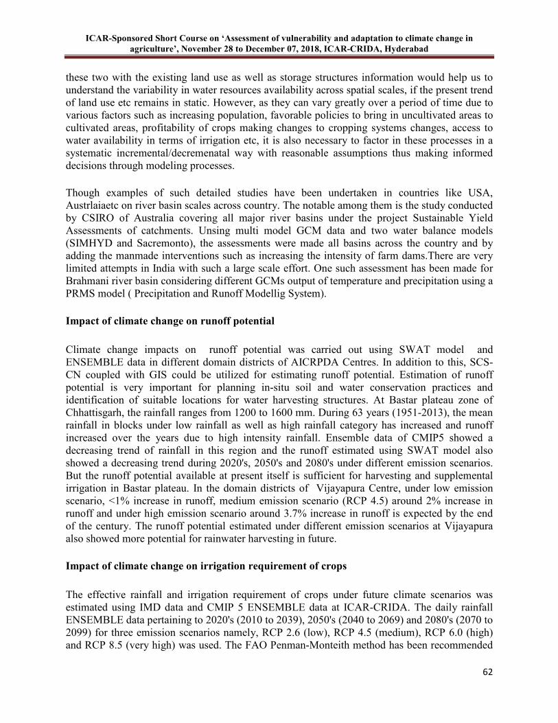
ICAR-Sponsored Short Course on ‘Assessment of vulnerability and adaptation to climate change in
agriculture’, November 28 to December 07, 2018, ICAR-CRIDA, Hyderabad
62
these two with the existing land use as well as storage structures information would help us to understand the variability in water resources availability across spatial scales, if the present trend of land use etc remains in static. However, as they can vary greatly over a period of time due to various factors such as increasing population, favorable policies to bring in uncultivated areas to cultivated areas, profitability of crops making changes to cropping systems changes, access to water availability in terms of irrigation etc, it is also necessary to factor in these processes in a systematic incremental/decremenatal way with reasonable assumptions thus making informed decisions through modeling processes. Though examples of such detailed studies have been undertaken in countries like USA, Austrlaiaetc on river basin scales across country. The notable among them is the study conducted by CSIRO of Australia covering all major river basins under the project Sustainable Yield Assessments of catchments. Unsing multi model GCM data and two water balance models (SIMHYD and Sacremonto), the assessments were made all basins across the country and by adding the manmade interventions such as increasing the intensity of farm dams.There are very limited attempts in India with such a large scale effort. One such assessment has been made for Brahmani river basin considering different GCMs output of temperature and precipitation using a PRMS model ( Precipitation and Runoff Modellig System). Impact of climate change on runoff potential
Climate change impacts on runoff potential was carried out using SWAT model and ENSEMBLE data in different domain districts of AICRPDA Centres. In addition to this, SCS-CN coupled with GIS could be utilized for estimating runoff potential. Estimation of runoff potential is very important for planning in-situ soil and water conservation practices and identification of suitable locations for water harvesting structures. At Bastar plateau zone of Chhattisgarh, the rainfall ranges from 1200 to 1600 mm. During 63 years (1951-2013), the mean rainfall in blocks under low rainfall as well as high rainfall category has increased and runoff increased over the years due to high intensity rainfall. Ensemble data of CMIP5 showed a decreasing trend of rainfall in this region and the runoff estimated using SWAT model also showed a decreasing trend during 2020's, 2050's and 2080's under different emission scenarios. But the runoff potential available at present itself is sufficient for harvesting and supplemental irrigation in Bastar plateau. In the domain districts of Vijayapura Centre, under low emission scenario, <1% increase in runoff, medium emission scenario (RCP 4.5) around 2% increase in runoff and under high emission scenario around 3.7% increase in runoff is expected by the end of the century. The runoff potential estimated under different emission scenarios at Vijayapura also showed more potential for rainwater harvesting in future. Impact of climate change on irrigation requirement of crops
The effective rainfall and irrigation requirement of crops under future climate scenarios was estimated using IMD data and CMIP 5 ENSEMBLE data at ICAR-CRIDA. The daily rainfall ENSEMBLE data pertaining to 2020's (2010 to 2039), 2050's (2040 to 2069) and 2080's (2070 to 2099) for three emission scenarios namely, RCP 2.6 (low), RCP 4.5 (medium), RCP 6.0 (high) and RCP 8.5 (very high) was used. The FAO Penman-Monteith method has been recommended

ICAR-Sponsored Short Course on ‘Assessment of vulnerability and adaptation to climate change in
agriculture’, November 28 to December 07, 2018, ICAR-CRIDA, Hyderabad
63
as a sole standard method for ETo calculation (Allen et al., 1998). However, the desired solar radiation data for the selected area for future climate scenarios is not available and hence the Hargreaves and Samani (1985) method was used for estimating ETo. This method requires extra terrestrial radiation, minimum temperature, maximum temperature and latitude of the area. The irrigation requirement of rabi crops at Vijayapurawas predicted to increase considerably whereas in kharif crops, the increase in irrigation requirement is negligible under low, medium and high emission scenarios (Table 1). At Vijayapura, the rainfall is predicted to increase from 590 mm during base line period to 611, 646 and 677 mm during 2020's, 2050's and 2080's under RCP 4.5, medium emission scenario. i.e., the rainfall would increase by 3.5, 9.5 and 14.7% respectively. Under high emission scenario (RCP 8.5), it is predicted as 617, 674 and 742 mm. i.e., the rainfall would increase by 4.5, 14.2 and 25.7% respectively. Compared to baseline period, the mean annual rainfall during RCP 2.6 would increase from 590 mm to 622, 645 and 646 mm and under RCP 6.0, the mean annual rainfall would increase from 590 mm to 602, 629 and 673 mm during 2020's, 2050's and 2080's.
At Vijayapura, the maximum temperature is predicted to increase by 0.8, 1.6, 2.00C under RCP 4.5 and 0.9, 2.0, 3.60C under RCP 8.5. The minimum temperature is also predicted to increase by 1.0, 1.8, 2.30C under RCP 4.5 and 1.1, 2.5, 4.20C under RCP 8.5 respectively. Correspondingly, the evapo-transpiration values (ET0) estimated showed an increasing trend from 1851 to 1877, 1900 and 1916 mm under RCP 4.5 and 1851 to 1876 , 1912 and 1958 mm under RCP 8.5. Similarly, the mean annual evapotranspiration would increase from 1851 to 1875, 1886 and 1896 mm respectively under RCP 2.6 and 1851 to 1879, 1897 and 1912 mm respectively under RCP 6.0.
Relatively higher temperatures predicted during future scenarios resulted in higher evapotranspiration. Eventhough higher mean annual rainfall was predicted, its variation during kharif season was less (CV=35 to 36%) compared to October to February and March to May (CV=70 to 77%). Hence, irrigation requirement of kharifcrops predicted under changing climatic scenarios are not rising considerably whereas rabi and summer crops are showing increasing trend. Main crops cultivated includes sunflower, pearl millet, pigeon pea, maize, chick pea, green gram, groundnut, onion, tomato and chilli. Results indicated that climate change may not have much impact on sustainability of prevailing cropping system as the crop seasonal water requirement of kharif crops are concerned. Based on water requirement under various climate change scenarios, appropriate strategies to cope up the climate change impact on rabi crops needs to be planned. Rainwater harvesting and artificial groundwater recharge need to be made mandatory in the study area for increasing the groundwater recharge and water availability. It is concluded that in order to ensure long-term and sustainable groundwater utilization in the region, proper estimation of crop water requirement and optimal water management are needed. Considerable spatial variation in the Irrigation requirement of kharif and rabi crops are noted at Akola (1951-2013) (Fig.1)
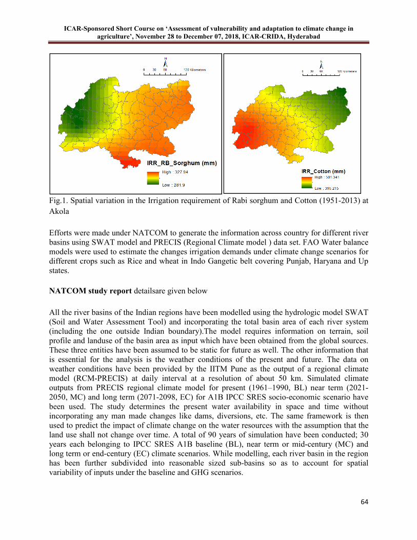
ICAR-Sponsored Short Course on ‘Assessment of vulnerability and adaptation to climate change in
agriculture’, November 28 to December 07, 2018, ICAR-CRIDA, Hyderabad
64
Fig.1. Spatial variation in the Irrigation requirement of Rabi sorghum and Cotton (1951-2013) at Akola Efforts were made under NATCOM to generate the information across country for different river basins using SWAT model and PRECIS (Regional Climate model ) data set. FAO Water balance models were used to estimate the changes irrigation demands under climate change scenarios for different crops such as Rice and wheat in Indo Gangetic belt covering Punjab, Haryana and Up states.
NATCOM study report detailsare given below All the river basins of the Indian regions have been modelled using the hydrologic model SWAT (Soil and Water Assessment Tool) and incorporating the total basin area of each river system (including the one outside Indian boundary).The model requires information on terrain, soil profile and landuse of the basin area as input which have been obtained from the global sources. These three entities have been assumed to be static for future as well. The other information that is essential for the analysis is the weather conditions of the present and future. The data on weather conditions have been provided by the IITM Pune as the output of a regional climate model (RCM-PRECIS) at daily interval at a resolution of about 50 km. Simulated climate outputs from PRECIS regional climate model for present (1961–1990, BL) near term (2021-2050, MC) and long term (2071-2098, EC) for A1B IPCC SRES socio-economic scenario have been used. The study determines the present water availability in space and time without incorporating any man made changes like dams, diversions, etc. The same framework is then used to predict the impact of climate change on the water resources with the assumption that the land use shall not change over time. A total of 90 years of simulation have been conducted; 30 years each belonging to IPCC SRES A1B baseline (BL), near term or mid-century (MC) and long term or end-century (EC) climate scenarios. While modelling, each river basin in the region has been further subdivided into reasonable sized sub-basins so as to account for spatial variability of inputs under the baseline and GHG scenarios.
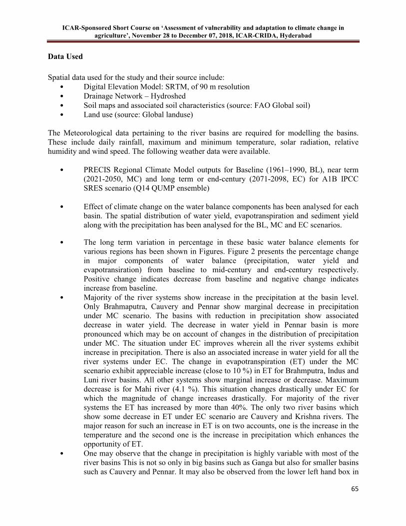
ICAR-Sponsored Short Course on ‘Assessment of vulnerability and adaptation to climate change in
agriculture’, November 28 to December 07, 2018, ICAR-CRIDA, Hyderabad
65
Data Used
Spatial data used for the study and their source include:
• Digital Elevation Model: SRTM, of 90 m resolution • Drainage Network – Hydroshed • Soil maps and associated soil characteristics (source: FAO Global soil) • Land use (source: Global landuse)
The Meteorological data pertaining to the river basins are required for modelling the basins. These include daily rainfall, maximum and minimum temperature, solar radiation, relative humidity and wind speed. The following weather data were available.
• PRECIS Regional Climate Model outputs for Baseline (1961–1990, BL), near term
(2021-2050, MC) and long term or end-century (2071-2098, EC) for A1B IPCC SRES scenario (Q14 QUMP ensemble)
• Effect of climate change on the water balance components has been analysed for each basin. The spatial distribution of water yield, evapotranspiration and sediment yield along with the precipitation has been analysed for the BL, MC and EC scenarios.
• The long term variation in percentage in these basic water balance elements for various regions has been shown in Figures. Figure 2 presents the percentage change in major components of water balance (precipitation, water yield and evapotransiration) from baseline to mid-century and end-century respectively. Positive change indicates decrease from baseline and negative change indicates increase from baseline.
• Majority of the river systems show increase in the precipitation at the basin level. Only Brahmaputra, Cauvery and Pennar show marginal decrease in precipitation under MC scenario. The basins with reduction in precipitation show associated decrease in water yield. The decrease in water yield in Pennar basin is more pronounced which may be on account of changes in the distribution of precipitation under MC. The situation under EC improves wherein all the river systems exhibit increase in precipitation. There is also an associated increase in water yield for all the river systems under EC. The change in evapotranspiration (ET) under the MC scenario exhibit appreciable increase (close to 10 %) in ET for Brahmputra, Indus and Luni river basins. All other systems show marginal increase or decrease. Maximum decrease is for Mahi river (4.1 %). This situation changes drastically under EC for which the magnitude of change increases drastically. For majority of the river systems the ET has increased by more than 40%. The only two river basins which show some decrease in ET under EC scenario are Cauvery and Krishna rivers. The major reason for such an increase in ET is on two accounts, one is the increase in the temperature and the second one is the increase in precipitation which enhances the opportunity of ET.
• One may observe that the change in precipitation is highly variable with most of the river basins This is not so only in big basins such as Ganga but also for smaller basins such as Cauvery and Pennar. It may also be observed from the lower left hand box in

ICAR-Sponsored Short Course on ‘Assessment of vulnerability and adaptation to climate change in
agriculture’, November 28 to December 07, 2018, ICAR-CRIDA, Hyderabad
66
Figure 3 that the average change in precipitation shown through the red cross bar reflecting increase in precipitation for majority of the river basins although there are few sub-basins within specific river basin that may be showing decrease in precipitation under MC scenario. The situation is further improved when we see the EC scenario for which there is increase in the average basin precipitation as compared to BL scenario. However even in this scenario many river systems such as Ganga, Indus, Luni, Godavari, Krishna etc,.have sub-basins which show decrease in precipitation.
• The implications of changes in precipitation have been quantified in the form of resulting water yields through the SWAT modelling. The response of water yield is dependent on combination of factors such as terrain, landuse, soil type and weather conditions. Despite the increase in precipitation from MC to EC scenario the Krishna river system is showing reduction in the water yield. This can be on account of higher ET (because of increased temperatures). It may also be observed that in the case of Cauvery river system although there is an improvement in the average water yield from MC to EC scenario yet there are some sub-basins that show reduction in water yield (also reflected in the bar chart – maximum reduction increasing from about 30% (MC) to more than 50% (EC).
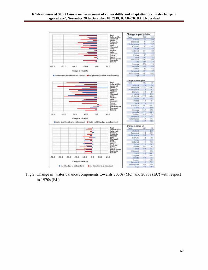
ICAR-Sponsored Short Course on ‘Assessment of vulnerability and adaptation to climate change in
agriculture’, November 28 to December 07, 2018, ICAR-CRIDA, Hyderabad
67
Fig.2. Change in water balance components towards 2030s (MC) and 2080s (EC) with respect to 1970s (BL)
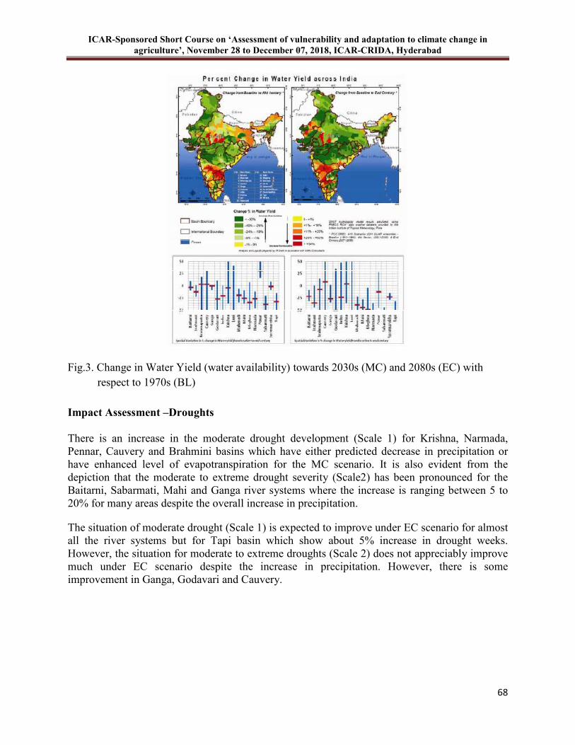
ICAR-Sponsored Short Course on ‘Assessment of vulnerability and adaptation to climate change in
agriculture’, November 28 to December 07, 2018, ICAR-CRIDA, Hyderabad
68
Fig.3. Change in Water Yield (water availability) towards 2030s (MC) and 2080s (EC) with respect to 1970s (BL)
Impact Assessment –Droughts
There is an increase in the moderate drought development (Scale 1) for Krishna, Narmada, Pennar, Cauvery and Brahmini basins which have either predicted decrease in precipitation or have enhanced level of evapotranspiration for the MC scenario. It is also evident from the depiction that the moderate to extreme drought severity (Scale2) has been pronounced for the Baitarni, Sabarmati, Mahi and Ganga river systems where the increase is ranging between 5 to 20% for many areas despite the overall increase in precipitation.
The situation of moderate drought (Scale 1) is expected to improve under EC scenario for almost all the river systems but for Tapi basin which show about 5% increase in drought weeks. However, the situation for moderate to extreme droughts (Scale 2) does not appreciably improve much under EC scenario despite the increase in precipitation. However, there is some improvement in Ganga, Godavari and Cauvery.
ICAR-Sponsored Short Course on ‘Assessment of vulnerability and adaptation to climate change in
agriculture’, November 28 to December 07, 2018, ICAR-CRIDA, Hyderabad
69
Conclusions
A comprehensive evaluation of the possible climate change impacts on the waterresources involves the understanding of the uncertainty of climate change predictions by different GCMs datasets as well as the water balance models. Inclusion of man made interventions/changes in land use , increase in number of dams etc would further increase the complexity of the problem.
References
Allen RG, Pereira LS, Raes D and Smith, M. 1998. Crop evapotranspiration- Guidelines for computing crop water requirements, FAO Irrigation and drainage paper 56. FAO, Rome, 300(9): D05109.
Hargreaves GH and Samani ZA. 1985. Reference crop evapotranspiration from temperature. Applied Engineering in Agriculture, 1(2): 96-99.
Rejani R, Rao KV, Shirahatti MS, Surakod VS, Yogitha P, Chary GR, Gopinath KA, Osman M, Sammi Reddy K and Srinivasa Rao Ch. 2016. Irrigation requirement of crops under changing climatic scenarios in a semi-arid region of Northern Karnataka. Indian J. Dryland Agric. Res. & Dev. 31(2): 51-60.
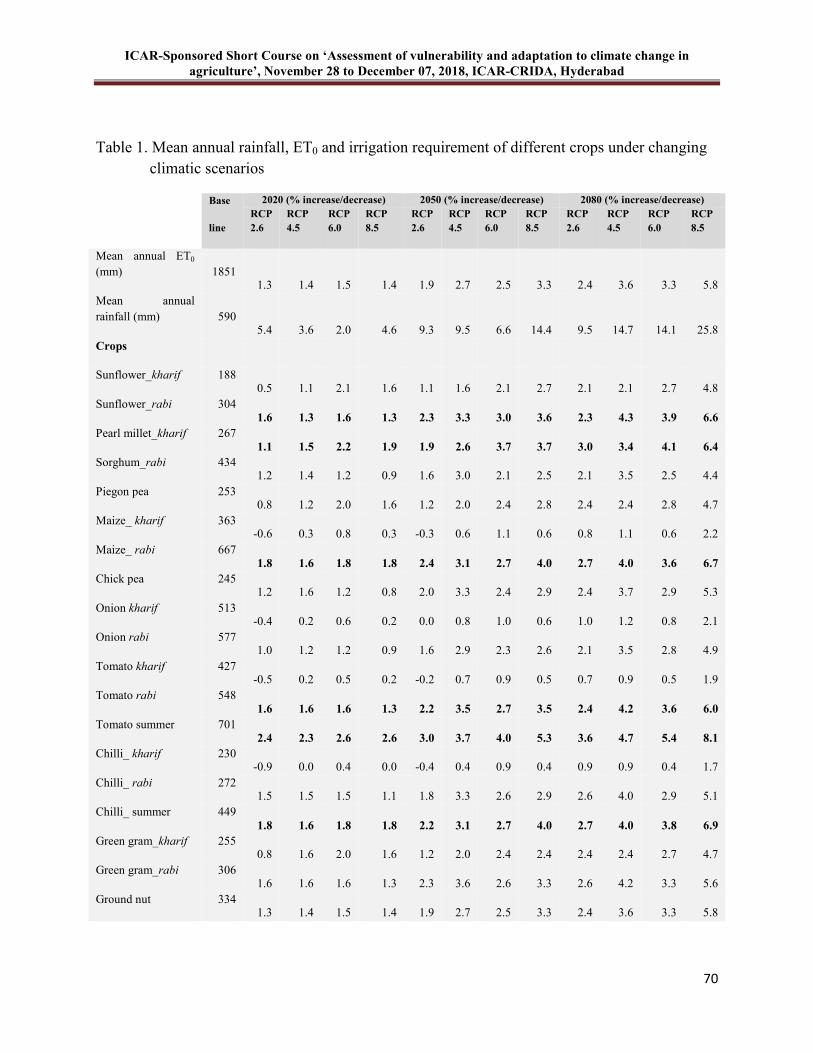
ICAR-Sponsored Short Course on ‘Assessment of vulnerability and adaptation to climate change in
agriculture’, November 28 to December 07, 2018, ICAR-CRIDA, Hyderabad
70
Table 1. Mean annual rainfall, ET0 and irrigation requirement of different crops under changing climatic scenarios
Base
line
2020 (% increase/decrease) 2050 (% increase/decrease) 2080 (% increase/decrease) RCP
2.6
RCP
4.5
RCP
6.0
RCP
8.5
RCP
2.6
RCP
4.5
RCP
6.0
RCP
8.5
RCP
2.6
RCP
4.5
RCP
6.0
RCP
8.5
Mean annual ET0 (mm) 1851
1.3 1.4 1.5 1.4 1.9 2.7 2.5 3.3 2.4 3.6 3.3 5.8 Mean annual rainfall (mm) 590
5.4 3.6 2.0 4.6 9.3 9.5 6.6 14.4 9.5 14.7 14.1 25.8 Crops
Sunflower_kharif 188
0.5 1.1 2.1 1.6 1.1 1.6 2.1 2.7 2.1 2.1 2.7 4.8 Sunflower_rabi 304
1.6 1.3 1.6 1.3 2.3 3.3 3.0 3.6 2.3 4.3 3.9 6.6 Pearl millet_kharif 267
1.1 1.5 2.2 1.9 1.9 2.6 3.7 3.7 3.0 3.4 4.1 6.4 Sorghum_rabi 434
1.2 1.4 1.2 0.9 1.6 3.0 2.1 2.5 2.1 3.5 2.5 4.4 Piegon pea 253
0.8 1.2 2.0 1.6 1.2 2.0 2.4 2.8 2.4 2.4 2.8 4.7 Maize_ kharif 363
-0.6 0.3 0.8 0.3 -0.3 0.6 1.1 0.6 0.8 1.1 0.6 2.2 Maize_ rabi 667
1.8 1.6 1.8 1.8 2.4 3.1 2.7 4.0 2.7 4.0 3.6 6.7 Chick pea 245
1.2 1.6 1.2 0.8 2.0 3.3 2.4 2.9 2.4 3.7 2.9 5.3 Onion kharif 513
-0.4 0.2 0.6 0.2 0.0 0.8 1.0 0.6 1.0 1.2 0.8 2.1 Onion rabi 577
1.0 1.2 1.2 0.9 1.6 2.9 2.3 2.6 2.1 3.5 2.8 4.9 Tomato kharif 427
-0.5 0.2 0.5 0.2 -0.2 0.7 0.9 0.5 0.7 0.9 0.5 1.9 Tomato rabi 548
1.6 1.6 1.6 1.3 2.2 3.5 2.7 3.5 2.4 4.2 3.6 6.0 Tomato summer 701
2.4 2.3 2.6 2.6 3.0 3.7 4.0 5.3 3.6 4.7 5.4 8.1 Chilli_ kharif 230
-0.9 0.0 0.4 0.0 -0.4 0.4 0.9 0.4 0.9 0.9 0.4 1.7 Chilli_ rabi 272
1.5 1.5 1.5 1.1 1.8 3.3 2.6 2.9 2.6 4.0 2.9 5.1 Chilli_ summer 449
1.8 1.6 1.8 1.8 2.2 3.1 2.7 4.0 2.7 4.0 3.8 6.9 Green gram_kharif 255
0.8 1.6 2.0 1.6 1.2 2.0 2.4 2.4 2.4 2.4 2.7 4.7 Green gram_rabi 306
1.6 1.6 1.6 1.3 2.3 3.6 2.6 3.3 2.6 4.2 3.3 5.6 Ground nut 334
1.3 1.4 1.5 1.4 1.9 2.7 2.5 3.3 2.4 3.6 3.3 5.8
ICAR-Sponsored Short Course on ‘Assessment of vulnerability and adaptation to climate change in
agriculture’, November 28 to December 07, 2018, ICAR-CRIDA, Hyderabad
71
7 Understanding Climate Change Impacts on Crop Growth and
Behavior
M Vanaja
Understanding the impact of climate change on agriculture is very crucial for the survival of mankind on the earth. Agriculture is sensitive to climate change at the same time it is one of the major driver for climate change. Understanding the weather variables over a period of time and setting the management practices for better harvest is required for the growth of agricultural sector as a whole.
The Fourth Assessment report of Intergovernmental Panel on Climate Change (2007) concluded that ‘there is high confidence that recent regional changes in temperature have had discernible impacts on many physical and biological systems’. Now it is evident from various studies that the human activities are contributing significantly for the change in climate compared to natural variability in climate. General circulation models predict temperature rises of 1.4-5.8°C by 2100, associated with carbon dioxide increases to 540-970 parts per million. The atmospheric concentration of carbon dioxide- the most important anthropogenic greenhouse gas increasing at alarming rates (1.9 ppm/ year) in recent years than the natural range concentration growth rate. This could be due to enhanced usage of fossil fuel and changed land use pattern to some extent.
Climate model predictions of CO2-induced global warming typically suggest that rising temperatures should be accompanied by increases in rainfall amounts and intensities, as well as enhanced variability. Both the number and intensity of heavy precipitation events are projected to increase in a warming world. Monsoon rainfall is an important socio-economic feature of India, and that climate models suggest that global averaged temperatures are projected to rise under all scenarios of future energy use (IPCC, 2001), leading to "increased variability and strength of the Asian monsoon." The analysis of observed data for the 131-year period (1871-2001) suggests no clear role of global warming in the variability of monsoon rainfall over India.
The climate sensitivity of agriculture is uncertain, as there is regional variation of rainfall, temperature, crops and cropping system, soils and management practices. The inter annual variations in temperature and precipitation were much higher than the predicted changes in temperature and precipitation. The crop losses may increase if the predicted climate change increases the climate variability. Different crops respond differently as the global warming will have a complex impact.
Though some of the projected changes in climate will have both beneficial and adverse effects on the environmental and socio-economic system, the larger changes will have effects that are more adverse. The expected changes in climate for India indicated that the increase in temperature is likely to be less in kharif than in rabi season and the rabi rainfall have larger uncertainty whereas kharif rainfall is likely to increase by as much as 10 per cent. Such global climate changes will affect agriculture considerably through its direct and indirect affect on
ICAR-Sponsored Short Course on ‘Assessment of vulnerability and adaptation to climate change in
agriculture’, November 28 to December 07, 2018, ICAR-CRIDA, Hyderabad
72
crops, livestock, pest and diseases and soils, thereby threatening the food security, an important problem for most of the developing countries.
Agriculture is one sector, which is immediately affected by climate change, and it is expected that the impact on global agricultural production may be small. However, regional vulnerabilities to food deficits may increase. Short or long-term fluctuations in weather patterns - climate variability and climate change - can influence crop yields and can force farmers to adopt new agricultural practices in response to altered climatic conditions. Climate variability / change, therefore, has a direct impact on food security.
Agricultural productivity is a function of many variables. The individual crop production is sensitive to different climate variables and in combination with edaphic conditions like the moisture and nutrient availability, the ultimate productivity would be regionally variable. Changes in climate will interact with stresses that result from actions to increase agricultural production, affecting crop yields and productivity in different ways, depending on the types of agricultural practices and systems in place. The main direct effects of climate change will be through changes in factors such as temperature, precipitation, length of growing season, and timing of extreme or critical threshold events relative to crop development, as well as through changes in atmospheric CO2 concentration.
The potential effect of climate change on agriculture is the shifts in the sowing time and length of growing seasons geographically, which would alter planting and harvesting dates of crops and varieties currently used in a particular area. Seasonal precipitation distribution patterns and amounts could change due to climate change. With warmer temperatures, evapotranspiration rates would rise, which would call for much greater efficiency of water use. Further, the water cycle is also very much influenced by the temperature regime. Increasing global temperature and resultant faster retreat of most glaciers is expected to affect the snow fed perennial water regimes feeding the IGP region. Himalayan Glaciers have shown a retreat /reduction of snow cover by 21% in last forty years. Accordingly, the vegetation status of catchments, magnitude and frequency of floods, precipitation, runoff and ground water recharge may all be affected. These changes may in turn may substantially affect hydropower generation, besides an increase in irrigation due to higher crop evaporation demand.
Rice, wheat, maize, sorghum, soybean and barley are the six major crops in the world and they are grown in 40% cropped area, 55% of non-meat calories and over 70% of animal feed. Since 1961, there is substantial increase in the yield of all the crops. The impact of warming was likely offset to some extent by fertilization effects of increased CO2 levels. At the global scale, the historical temperature- yield relationships indicate that warming from 1981 to 2002 very likely offset some of the yield gains from technological advance, rising CO2 and other non-climatic factors.
Carbon dioxide is the basic raw material that plants use in photosynthesis to convert solar energy into food, fiber, and other forms of biomass. . In the presence of chlorophyll, plants use sunlight to convert carbon dioxide and water into carbohydrates that, directly or indirectly, supply almost all animal and human needs for food; oxygen and some water are released as by-products of this process. Voluminous scientific evidence shows that if CO2 were to rise above its current ambient level of 365 parts per million, most plants would grow faster and larger because of more efficient
ICAR-Sponsored Short Course on ‘Assessment of vulnerability and adaptation to climate change in
agriculture’, November 28 to December 07, 2018, ICAR-CRIDA, Hyderabad
73
photosynthesis and a reduction in water loss. There are two important reasons for this productivity boost at higher CO2 levels. One is superior efficiency of photosynthesis. The other is a sharp reduction in water loss per unit of leaf area.
A related benefit comes from the partial closing of pores in leaves that is associated with higher CO2 levels. These pores, known as stomata, admit air into the leaf for photosynthesis, but they are also a major source of transpiration or moisture loss. By partially closing these pores, higher CO2 levels greatly reduce the plants' water loss--a significant benefit in arid and semi arid climates where water is limiting the productivity.
There are marked variations in response to CO2 among plant species. The biggest differences are among three broad categories of plants--C3, C4, and Crassulacean Acid Metabolism or CAM--each with a different pathway for photosynthetic fixation of carbon dioxide. Most green plants, including most major food crops use the C3 pathway respond most dramatically to higher levels of CO2. At current atmospheric levels of CO2, up to half of the photosynthate in C3 plants is typically lost and returned to the air by a process called photo-respiration, Elevated levels of atmospheric CO2 virtually eliminate photo-respiration in C3 plants, making photosynthesis much more efficient.
Corn, sugarcane, sorghum, millet, and some tropical grasses use the C4 pathway, also experience a boost in photosynthetic efficiency in response to higher carbon dioxide levels, but because there is little photo-respiration in C4 plants, the improvement is smaller than in C3 plants. Instead, the largest benefit C4 plants receive from higher CO2 levels comes from reduced water loss. Loss of water through leaf pores declines by about 33 percent in C4 plants with a doubling of the CO2 concentration from its current atmospheric level. Since these crops are frequently grown under drought conditions of high temperatures and limited soil moisture, this superior efficiency in water use may improve yields when rainfall is even lower than normal. When there was no stress, elevated CO2 reduced stomatal conductance by 21.3 and 16.0% for C3 and C4 species respectively. The lowest response to higher CO2 levels is usually from the CAM plants, which include pineapples, agaves, and many cacti and other succulents. CAM plants are also already well adapted for efficient water use.
The mean (average) response to a doubling of the CO2 concentration from its current level of 360 ppm is a 32 percent improvement in plant productivity, with varied manifestations in different species. In crop plants, a distinction has to be made between the increase in total biomass and increase in economic yield resulting from an elevated CO2 supply. When the dry mass production and yield increase of the world's ten most important crop species in response to elevated CO2 was analyzed from different experiments, it was found that in some species the relative increase of total biomass and in others that of economic yield is greater. Cereal grains with C3 metabolism, including rice, wheat, barley, oats, and rye, show yield increases ranging from 25 to 64 percent, resulting from a rise in carbon fixation and reduction in photo-respiration. Food crops with C4 metabolism, including corn, sorghum, millet, and sugarcane, show yield increases ranging from 10 to 55 percent, resulting primarily from superior efficiency in water use. Tuber and root crops, including potatoes and sweet potatoes, show dramatic increase in tuberization (potatoes) and growth of roots (sweet potatoes). Yield increases range from 18 to 75 percent. Legumes, including peas, beans, and soybeans, show yield increases of 28 to 46 percent.
ICAR-Sponsored Short Course on ‘Assessment of vulnerability and adaptation to climate change in
agriculture’, November 28 to December 07, 2018, ICAR-CRIDA, Hyderabad
74
Field crops under drought often experience two quite different but related and simultaneous stresses: soil water deficit and high temperature stresses. Elevated CO2 increase growth, grain yield and canopy photosynthesis while reducing evapotranspiration. During drought stress cycles, this water savings under elevated CO2 allow photosynthesis to continue for few more days compared with the ambient CO2 so that increase drought avoidance. Elevated atmospheric CO2 concentration ameliorates, to various degrees, the negative impacts of soil water deficit and high temperature stresses. Research on drought and heat tolerant genotypes needs to be enhanced. The impact of climate change on different crop management levels, viz., fertilizer, water management, increasing the rainwater management, through watershed development, increasing the water availability needs to be looked into it. Further, all the soil process with respect to changes in precipitation pattern and increased air and soil temperature can influence available soil water content, runoff and erosion and are need to be studied further.
The productivity reductions from climate change are far more permanent than with climate variability and require adaptation of more permanent solutions. Land-use/cover change is another climate driven factor due to resource scarcity leading to an increase in the pressure of production on resources.
Different research organizations including ICAR and SAUs have been working on developing of different strategies for sustainable agricultural production in the expected changes in climate. Some of the strategies could be the adoption of proper crop mix, changing the planting and harvest dates, irrigation scheduling, appropriate application and management of fertilizers and pesticides. Future trends in population growth, energy use, climate change, and globalization will confront to develop innovative production systems that are highly productive and environmentally sound. Furthermore, future agricultural production systems must possess an inherent capacity to adapt to change to be sustainable.
ICAR-Sponsored Short Course on ‘Assessment of vulnerability and adaptation to climate change in
agriculture’, November 28 to December 07, 2018, ICAR-CRIDA, Hyderabad
75
8 Impact assessment through econometric methods
Josily Samuel
Agriculture is the main source of livelihood for majority in India and also nearly 50 per cent of work force is employed in it. Agriculture is facing major challenges of feeding the growing populations across the globe. It is affected by a number of problems such as such as small and fragmented holding, lack of mechanisation, erosion, depletion and pollution leading to unhealthy soils, negligence of natural resources and so on. The needed increase in food availability has to be achieved in countering the changing climate and increased vulnerability. In order to overcome theses in the first place we should seek to have understanding and knowledge of the impact of climate change on agriculture. How we can increase crop productivity, propose interventions based on impact assessments to achieve food security without affecting our environment. There is need to estimate likely changes in productivity of crops and income and need to check the elements of adaptation for changing yields, income and has to address mitigation options. The importance of different tools and approaches for studying and estimating the impacts of climate change is inevitable. The various tools include mathematical programming, cost benefit analysis(CBA), Economic surplus, Econometrics, meta–analysis, spatial analysis through GIS and remote sensing, simulation modelling, etc., Each tools has its own pros and cons and efficiency under particular agricultural intervention/ technology. Here we would like to look into the various option and approaches of using econometric methods in assessing the impact of climate change (CC)
Econometrics and impact assessment
Econometrics means “economic measurement”. It is social science tool / quantitative analysis where in economic theory, mathematics, and statistical inference is applied in analysing situation. Econometric analysis helps us to numerical estimates of economic theory ie., expressing the theory in mathematical form. Methodology involved in econometrics includes the statement of theory, specifying the mathematical model and econometric model, data collection, estimation of econometric model, testing of hypothesis, forecasting or prediction,. In recent years, numerous econometric analyses have emerged to address this question by studying the effects of specific climatic conditions on different social and economic outcomes. Crop modelling approaches are based on controlled experimentations wherein a crop is exposed to varying degrees of temperature; and crop yields and compared across temperature level. Its main limitation is that it over-estimates the negative impacts and under-estimates the positive impacts and that it does not consider farmers’ responses or adaptations to changes in climate. Before selecting any particular analysis or model to study the impact it better if we find out what purpose does it have, and the economic decisions it help you with and can we evaluate it s quality in comparison with other models or methods.
ICAR-Sponsored Short Course on ‘Assessment of vulnerability and adaptation to climate change in
agriculture’, November 28 to December 07, 2018, ICAR-CRIDA, Hyderabad
76
NATURE AND SOURCES OF DATA:
The success of any econometric analysis ultimately depends on the avail ability of the appropriate data it is therefore essential that we spend some time discussing the nature. Sources. And limitation of the data that one may encounter in empirical analysis.
Types of data:
Three types of data may be available for empirical analysis : time series cross-section.And pooled i. E. Combination of time series and cross section data
Time series Data:
A time series is a set of observations on the values that a variable takes at different times Such data may be collected at regular time intervals such as daily e.g . stock prices. Weather reports weekly. Monthly e.g. the unemployment rate the consumer price index quarterly e.g. government budgets quinquennially that is every 5 years e. g. The census of manufactures or decennially e.g. the census of population sometime data are available both quarterly as well as annually as in the case of the data on GDP and consumer expenditure with the advent of high speed computers data can now be collected over an extremely short interval continuously the so-called real-time quote. Although time series data are used heavily in econometric studies they present special problems for econometricians as we will show in chapters on time series econometrics later on most empirical work based on time series data assumes that the underlying time series is stationary although it is too early to introduce the precise technical meaning of stationary at this juncture loosely speaking a time series is stationary if its mean and variance do not vary systematically over time. Cross-section data:
Cross –section data are data on one or more variables collected at the same point in time such as the census of population conducted by the census bureau every 10 years
Pooled data:
In pooled or combined data are elements of both time series and cross-section data
Panel. Longitudinal or micropanel data:
This is a special type of pooled data in which the some cross –sectional unit say a family or a firm is surveyed over time
ICAR-Sponsored Short Course on ‘Assessment of vulnerability and adaptation to climate change in
agriculture’, November 28 to December 07, 2018, ICAR-CRIDA, Hyderabad
77
Basic steps in econometrics:
Different econometrics methods:
Regression analysis is the main tool in econometrics and need of computers and statistical softwares to bring out results are inevitable. Ricardian approach assumes that in a perfectly competitive market reflects present value of future streams of profits (or rent) earned from paribus, a farmer maximises profits by allocating land in declining fertility and climate. The approach is similar to the hedonic price method wherein, all else remaining constant, regional differences in land value or productivity explained by the differences in climate. Regression analysis
Regression analysis is concerned with the study of the dependence of one variable, the dependent variable, on one or more other variables, the explanatory variables, with a view to estimating and/or predicting the (population) mean or average value of the former in terms of the known or fixed (in repeated sampling) values of the latter.
Single equation regression models
In these models, one variable, called the dependent variable, is expressed as a linear function of one or more other variables, called the explanatory variables
Multiple regression models
Adding more variables leads us to the discussion of multiple regression models, that is,models in which the dependent variable, or regress and, Y depends on two or more explanatory variables, or regressors. The simplest possible multiple regression model is three-variable regression, with one dependent variable and two explanatory variables. we are studying the dependence of one variable on more than one
Dummy variables regression models
In regression analysis the dependent variable, or regressand, is frequently influenced not only by ratio scale variables (e.g., income, output, prices, costs, height, temperature) but also by variables that are essentially qualitative, or nominal scale, in nature, such as sex, race, color, religion, nationality, geographical region, political upheavals, and party affiliation. Quantification of such attributes is done by constructing artificial variables that take on values of 1 or 0, 1 indicating the presence (or possession) of that attribute and 0 indicating the absence of that attribute. Variables that assume such 0 and 1 values are called dummy variables.
Economic theory Methematical model of theory Econometric model of theory Data Estimation of econometric model Hypothesis testing Forecasting or prediction Using the model for control or policy purposes
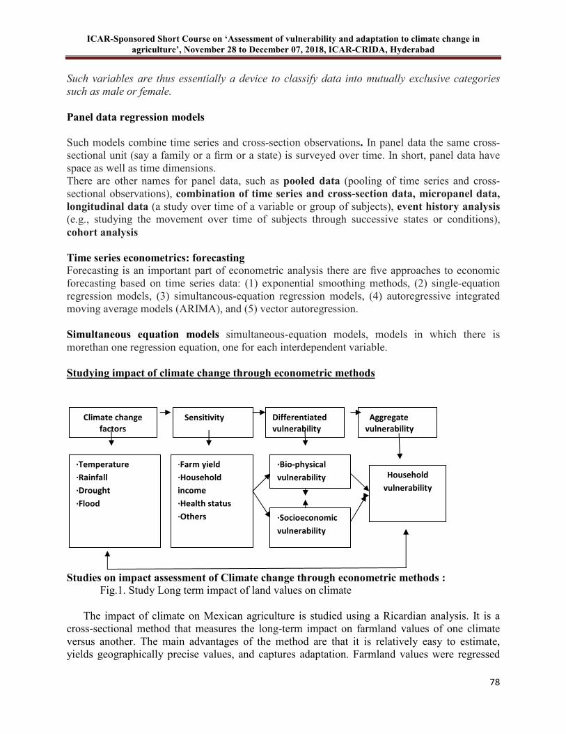
ICAR-Sponsored Short Course on ‘Assessment of vulnerability and adaptation to climate change in
agriculture’, November 28 to December 07, 2018, ICAR-CRIDA, Hyderabad
78
Such variables are thus essentially a device to classify data into mutually exclusive categories
such as male or female.
Panel data regression models
Such models combine time series and cross-section observations. In panel data the same cross-sectional unit (say a family or a firm or a state) is surveyed over time. In short, panel data have space as well as time dimensions. There are other names for panel data, such as pooled data (pooling of time series and cross-sectional observations), combination of time series and cross-section data, micropanel data,
longitudinal data (a study over time of a variable or group of subjects), event history analysis (e.g., studying the movement over time of subjects through successive states or conditions), cohort analysis Time series econometrics: forecasting
Forecasting is an important part of econometric analysis there are five approaches to economic forecasting based on time series data: (1) exponential smoothing methods, (2) single-equation regression models, (3) simultaneous-equation regression models, (4) autoregressive integrated moving average models (ARIMA), and (5) vector autoregression. Simultaneous equation models simultaneous-equation models, models in which there is morethan one regression equation, one for each interdependent variable.
Studying impact of climate change through econometric methods
Studies on impact assessment of Climate change through econometric methods :
Fig.1. Study Long term impact of land values on climate
The impact of climate on Mexican agriculture is studied using a Ricardian analysis. It is a cross-sectional method that measures the long-term impact on farmland values of one climate versus another. The main advantages of the method are that it is relatively easy to estimate, yields geographically precise values, and captures adaptation. Farmland values were regressed
Climate change
factors
Sensitivity Differentiated
vulnerability
Aggregate
vulnerability
∙Temperature
∙Rainfall
∙Drought
∙Flood
∙Farm yield
∙Household
income
∙Health status
∙Others
∙Bio-physical
vulnerability
∙Socioeconomic
vulnerability
Household
vulnerability
ICAR-Sponsored Short Course on ‘Assessment of vulnerability and adaptation to climate change in
agriculture’, November 28 to December 07, 2018, ICAR-CRIDA, Hyderabad
79
on climate and other control variables. The results reveal how farmland value varies with climate across the sample. Adaptation is captured because farmers have already adapted to the climate that they live in. By examining farmland values across climate, the Ricardian model captures these long-term adaptations in the analysis. Separate analyses were also conducted of different types of farms. One analysis tests whether rainfed and irrigated farms have similar climate sensitivity (climate co-efficients). A second analysis tests whether small versus large farms have similar climate sensitivity. The Ricardian results were then used to forecast how Mexican farmland value would change with different future climate scenarios. Cross-sectional observations across different climates can reveal the climate sensitivity of farms. The advantage of this empirical approach is that the method not only includes the direct effect of climate on productivitybut also the adaptation response by farmers to local climate. Including farm adaptation is important because farmers can take many actions to reduce the potential damages to their farms from climate change. For example, they can shift crops. Adaptation can explain the more optimistic results found with the Ricardian method compared to the generally more pessimistic results found in agronomic studies. Adaptation is clearly costly. The Ricardian model takes into account the costs of different farm choices. For example, if a farmer decides to introduce a new crop on his land as climate warms, the Ricardian model assumes the farmer will pay the costs normally associated with growing that new crop. The farmer will have to pay for new seeds and new equipment specific to the crop. The Ricardian model does not, however, measure transition costs. For example, if a farmer has crop failures for a year or two as he learns how to grow a new crop, this transition cost is not reflected in the analysis. Similarly, if the farmer makes the decision to move to a new crop suddenly, the model would not capture the cost of decommissioning capital equipment prematurely. Transition costs are clearly very important in sectors where there is extensive capital that cannot be easily changed. The Ricardian method is a cross-sectional approach to studying agricultural production (Mendelsohn et al., 1994). The method was named after Ricardo because of his original observation that the value of land would reflect its net productivity. Farmland net revenues (π) reflect net productivity. This principle is captured in the following equation: π = _ PiQi (X, F, Z) − _ PxX, (1) where Pi is the market price of crop i, Qi is output of crop i, X is a vector of purchased inputs (other than land), F is a vector of climate variables, Z is a vector of other control variables such as soil and market access, and Px is a vector of input prices. The farmer is assumed to choose X to maximize net revenues given the characteristics of the farm and market prices. Farmland value (V) is proportional to net revenue (V = π/r ) where r is the interest rate. The Ricardian model is a reduced form model that examines how several exogenous variables, F and Z, affect farmland value. We adopt a loglinear functional form for the Ricardian model with a quadratic formulation of climate: LnV = β0 + β1F + β2F 2 + β3Z + µ, (2) where β is an estimated coefficient and µ is an error term.. The change in annual welfare, _W, resulting from a climate change from C0 to C1 can be measured as follows: _W = V(C1) − V(C0). (4)
ICAR-Sponsored Short Course on ‘Assessment of vulnerability and adaptation to climate change in
agriculture’, November 28 to December 07, 2018, ICAR-CRIDA, Hyderabad
80
Changes that increase land value are beneficial and changes that decrease land value are harmful. This is a comparative static analysis. It is not a dynamic model. The Ricardian model is not measuring the effects of yearto-year changes in weather but rather long-term changes in climate. Cross-sectional observations across different climates can reveal the climate sensitivity of farms. The advantage of this empirical approach is that the method not only includes the direct effect of climate on productivity but also the adaptation response by farmers to local climate. Including farm adaptation is important because farmers can take many actions to reduce the potential damages to their farms from climate change. For example, they can shift crops etc., Econometric models have been widely used to measure the impact of climate change on agriculture in the united states and around the world. Using a cross-sectional data researchers regressed land values or net revenues against climate variables.
To assess the impacts due to the climate variability and climate change the relevant research are tobe answered like Is Indian agriculture likely to get adversely affected by climate change if so what is the extent of impact? And how to characterize the vulnerability of a farmer to climate change and climate variability which regions are relatively more vulnerable to climate variability and change and the effectiveness of adaptation options. One is interested in measuring vulnerability of a representative farmer to a climatic shock for the sake of illustration consider that the farmer s vulnerability the with regard to poor rice yield caused by potential changes in temperature the representative farmer s vulnerability can be meaningfully expressed by either of the two statements.
The vulnerability to poor rice yield due to temperature change or vulnerability to temperature change with reference to poor wheat yield in poverty literature non consideration of external stimulus causing vulnerability enables simple projection of the outcome of concern in severe states of the future the vulnerability metrics in climate change however should in question that is in the present example the analyst must identify how yield of rice changes due to temperature changes in other words the sensitivity of the entity must be assessed this is represented in the numerator of equation. the denominator captures the relative position of the yield with reference to the threshold finally using the probability of the future states the vulnerability is calculated as expected value as in note that in this formulation as expected with increase in outcome the vulnerability secretes however vulnerability also increases with sensitivity irrespective of the direction of change of the stimulus. Alternatively vulnerability to climate change can be interpret red as follows; continuing with the above example of farmer for each future state the shock (or stimulis) is assessed in terms of the change in temperature with respect to a present (or some normal) value with the help of sensitivity the change in the yield from which state specific yield can then be generated.
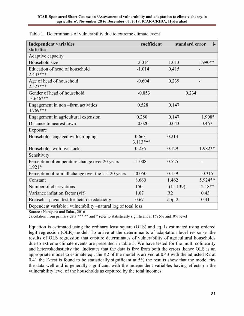
ICAR-Sponsored Short Course on ‘Assessment of vulnerability and adaptation to climate change in
agriculture’, November 28 to December 07, 2018, ICAR-CRIDA, Hyderabad
81
Table 1. Determinants of vulnerability due to extreme climate event
Independent variables coefficient standard error i-
statistics
Adaptive capacity Household size 2.014 1.013 1.990** Education of head of household -1.014 0.415 -2.443*** Age of head of household -0.604 0.239 -2.523*** Gender of head of household -0.853 0.234 -3.646*** Engagement in non –farm activities 0.528 0.147 3.769*** Engagement in agricultural extension 0.280 0.147 1.908* Distance to nearest town 0.020 0.043 0.467 Exposure Households engaged with cropping 0.663 0.213 3.113*** Households with livestock 0.256 0.129 1.982** Sensitivity Perception oftemperature change over 20 years -1.008 0.525 -1.921* Perception of rainfall change over the last 20 years -0.050 0.159 -0.315 Constant 8.660 1.462 5.924** Number of observations 150 f(11.139) 2.18** Variance inflation factor (vif) 1.07 R2 0.43 Breusch – pagan test for heteroskedasticity 0.67 abj r2 0.41 Dependent variable ; vulnerability –natural log of total loss Source : Narayana and Sahu., 2016 calculation from primary data *** ** and * refer to statistically significant at 1% 5% and10% level Equation is estimated using the ordinary least square (OLS) and eq. Is estimated using ordered legit regression (OLR) model. To arrive at the determinants of adaptation level response .the results of OLS regression that capture determinates of vulnerability of agricultural households due to extreme climate events are presented in table 5. We have tested for the multi colinearity and heteroskedasticity the Indicates that the data is free from both the errors .hence OLS is an appropriate model to estimate eq . the R2 of the model is arrived at 0.43 with the adjusted R2 at 0.41 the F-test is found to be statistically significant at 5% the results show that the model firs the data well and is generally significant with the independent variables having effects on the vulnerability level of the households as captured by the total incomes.
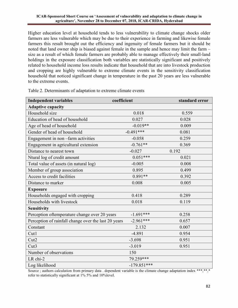
ICAR-Sponsored Short Course on ‘Assessment of vulnerability and adaptation to climate change in
agriculture’, November 28 to December 07, 2018, ICAR-CRIDA, Hyderabad
82
Higher education level at household tends to less vulnerability to climate change shocks older farmers are less vulnerable which may be due to their experience in farming and likewise female farmers this result brought out the efficiency and ingenuity of female farmers but it should be noted that land owner ship is biased against female in the sample and hence may limit the farm –size as a result of which female farmers are probably able to manage effectively their small-land holdings in the exposure classification both variables are statistically significant and positively related to household income loss results indicate that household that are into livestock production and cropping are highly vulnerable to extreme climate events in the sensitivity classification household that noticed significant change in temperature in the past 20 years are less vulnerable to the extreme events.
Table 2. Determinants of adaptation to extreme climate events
Independent variables coefficient standard error
Adaptive capacity
Household size 0.018 0.559 Education of head of household 0.027 0.028 Age of head of household -0.019** 0.009 Gender of head of household -0.491*** 0.081 Engagement in non –farm activities -0.058 0.259 Engagement in agricultural extension -0.761** 0.369 Distance to nearest town -0.027 0.192 Ntural log of credit amount 0.051*** 0.021 Total value of assets (in natural log) -0.005 0.008 Member of group association 0.895 0.499 Access to credit facilities 0.891** 0.392 Distance to marker 0.008 0.005
Exposure
Households engaged with cropping 0.418 0.289 Households with livestock 0.018 0.119
Sensitivity
Perception oftemperature change over 20 years -1.691*** 0.258 Perception of rainfall change over the last 20 years -2.961*** 0.657 Constant 2.132 0.007 Cut1 -4.891 0.954 Cut2 -3.698 0.951 Cut3 -3.019 0.951 Number of observations 150 LR chi-2 79.259*** Log likelihood -179.851*** Source ; authors calculation from primary data . dependent variable is the climate change adaptation index ***,**,* refer to statistically significant at 1% 5% and 10%level.
ICAR-Sponsored Short Course on ‘Assessment of vulnerability and adaptation to climate change in
agriculture’, November 28 to December 07, 2018, ICAR-CRIDA, Hyderabad
83
Source : Narayana and Sahu., 2016
OLR was estimated to determine the factors that affect the adaptation capacity of the agricultural households the factors that significantly influence the capacity of the households to adapt to climate change factors as reflected in the result are; significant change in temperature significant change in rainfall involvement in agricultural extensions age and gender of the head of the household availability of credit facilities and the credit amount the OLR for households not exposed to significant temperature and rainfall changes . Every INR increase in credit amount to given to CCAI by 0.051 the results in table 2.imp;y that availability of credit to households wil improve their adaptive skills however credit might hinder the adaptive capacity and this can be traced to diversion of funds for other uses rather than agri-business once again the experience of farmers by age and the female farmers are important factors that can be tapped to improve farmers adaptation to extreme climate events
Important steps for better outcome / results
The measurement of climate variables is a critical methodological step in identifying climate effects, regardless of the research design used. Early analyses concerned only with measuring whether climatic factors had a nonzero effect, or the sign of an effect, used simple measures of climate such as latitude or a single indicator variable that is one if a population is exposed to a predefined event (e.g., a drought) and is zero otherwise The key idea behind analysis is the statistical dependence of one variable the dependent variable on one or more other variables the explanatory variables .The objective of such analysis is to estimate and or predict the mean or average value of the dependent variable on the basis of the known or fired values of the explanatory variables. In practice the success of regression analysis depends on the avail ability of the appropriate data. Clearly state the sources of the data used in the analysis their definitions their methods of collection and any gaps or omissions in the data as well as any revisions in the data. Econometrics methods are only complementing the other tools and methods in assess impact of climate change and they are useful for more disaggregated and location specific studies not as simulation studies.
ICAR-Sponsored Short Course on ‘Assessment of vulnerability and adaptation to climate change in
agriculture’, November 28 to December 07, 2018, ICAR-CRIDA, Hyderabad
84
References
Gujarati DN. 2009. Basic Econometrics. Tata McGraw-Hill Education, New Delhi Palanisami K, Haileslassie A, Kakumanu Krishna Reddy, Ranganathan CR, Wani SP, Craufurd P and Kumar Shalander. 2015. Climate Change, Gender and Adaptation Strategies in Dryland Systems of South Asia. A Household Level Analysis in Andhra Pradesh, Karnataka and Rajasthan States of India. Patancheru 502 324, Telangana, India: International Crops Research Institute for the Semi-Arid Tropics. 36 pp. Hornbeck R, Keskin P. 2015. Does agriculture generate local economic spillovers? Short-run and long-runevidence from the Ogallala Aquifer. Am. Econ. J. Econ. Policy 7:192–213 Kurukulasuriya P, Mendelsohn RO. 2008. A Ricardian analysis of the impact of climate change on Africancropland. Afr. J. Agric. Resour. Econ. 2(1):105–26 Mendelsohn R, Emanuel K, Chonabayashi S, Bakkensen L. 2012. The impact of climate change on global tropical cyclone damage. Nat. Clim. Change 2:205–9 Deschênes O. and Greenstone M. 2007. The economic impacts of climate change: evidence from agricultural output and random fluctuations in weather. American Economic Review, 97(1), 354-385. Narayanan K. Sahu SK. 2016. Effects of climate change on household economy and adaptive responses among agricultural households in eastern coast of India. Current Science, 110(7), 1240.
ICAR-Sponsored Short Course on ‘Assessment of vulnerability and adaptation to climate change in
agriculture’, November 28 to December 07, 2018, ICAR-CRIDA, Hyderabad
85
9 Impacts of Climate Change on Insect Pests and Prediction Of Pest
Scenarios
M Srinivasa Rao and P Sreelakshmi
Introduction
Unequivocal evidences are available now about the impending impacts of climate change and the consequences thereof. Global Mean Surface Temperature (GMST) and Global atmospheric CO2 concentrations have been increasing at a significant rate since last 19th century. The projected increase in temperature by 2100 was set at by 1.4 – 5.8oC with the increase in the amount of CO2 in the atmosphere by about 40% when compared with pre-industrial levels. The increase in the amount of CO2 in the atmosphere will reach to 500 to 1000 ppm by the end of 21st century (IPCC, 2014). Though climate change is global phenomenon in its occurrence and consequences, it is the developing countries like India that face more adverse consequences. Climate change projections made up to 2100 for India indicate an overall increase in temperature by 2-4°C with no substantial change in precipitation quantity. However, different regions are expected to experience differential change in the amount of rainfall that is likely to be received in the coming decades. Last three decades, a sharp rise in all India mean annual temperature was reported (Venkateswarlu, 2009). Climatic variability together with increase in atmospheric carbon dioxide and temperature has lot of implications in agriculture sector influencing significantly the crops and insect pests. Insect herbivores are primary consumers and get energy from plants or plant products and impact of climate change on these insects can have far-reaching consequences and alter significantly. The two dimensions of climate change viz., elevated CO2 (eCO2) concentrations and increased temperatures which are cause and effect of climate change influence insect herbivores significantly and relevant information is discussed here under.
Increased temperature
Climate change resulting in increased temperature could impact crop pest insect populations in several complex ways. Although temperature effects might tend to depress insect populations, most researchers reported that warmer temperatures in temperate climates would result in more types and higher populations of insects. Insects are cold-blooded organisms - the temperature of their bodies is approximately the same as that of the environment. Therefore, temperature is probably the single most important environmental factor influencing their behavior, distribution, development, survival, and reproduction. Increased temperatures accelerate the development of several insect pests resulting in more number of generations (and crop damage) per year. In addition to the above observations some more predictions and generalizations were made by several researchers (Table.1). The documented information on impact of increased temperature on insect pests indicate the significant migration of insects, accelerated developmental rates and higher oviposition, out breaks, possibilities of introduction of invasive species etc., The effectiveness of insect bio-control by fungi, reliability of economic threshold levels, insect
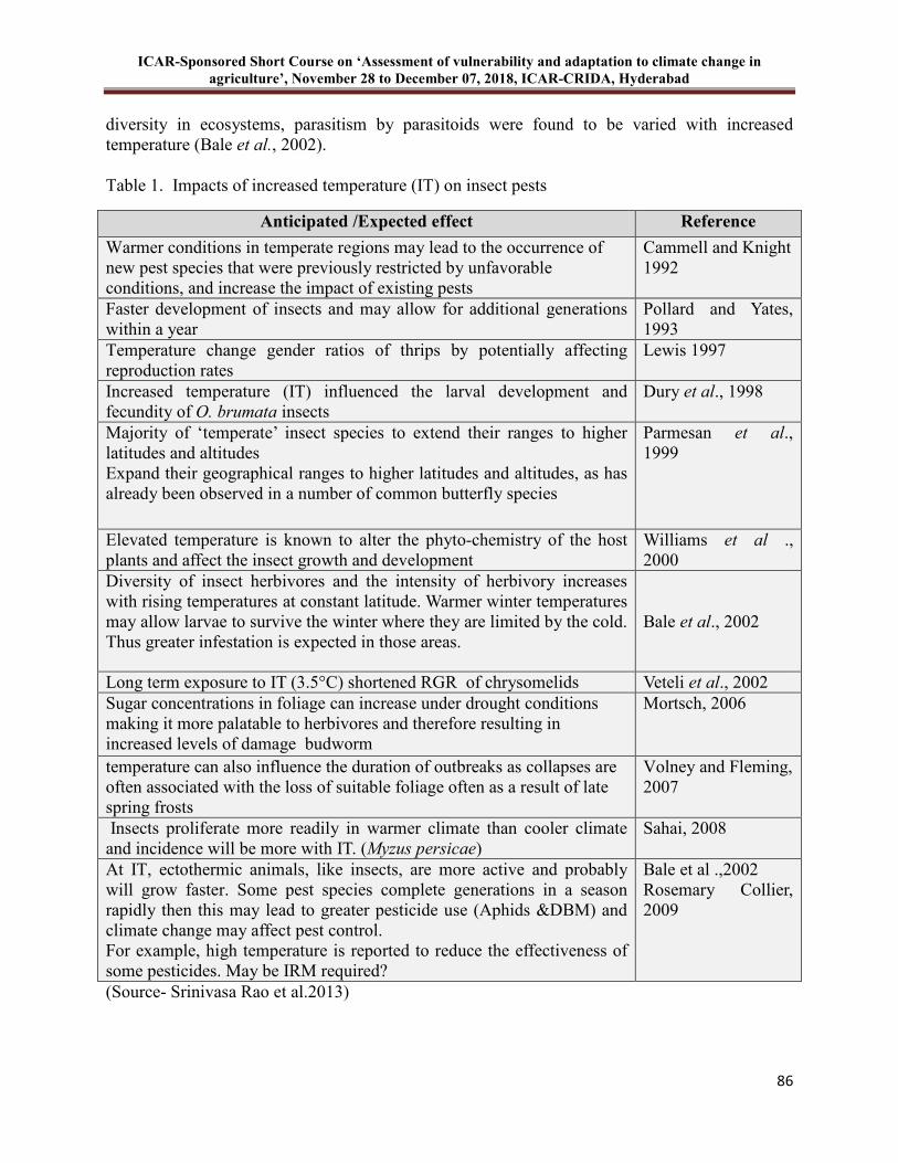
ICAR-Sponsored Short Course on ‘Assessment of vulnerability and adaptation to climate change in
agriculture’, November 28 to December 07, 2018, ICAR-CRIDA, Hyderabad
86
diversity in ecosystems, parasitism by parasitoids were found to be varied with increased temperature (Bale et al., 2002).
Table 1. Impacts of increased temperature (IT) on insect pests
Anticipated /Expected effect Reference
Warmer conditions in temperate regions may lead to the occurrence of new pest species that were previously restricted by unfavorable conditions, and increase the impact of existing pests
Cammell and Knight 1992
Faster development of insects and may allow for additional generations within a year
Pollard and Yates, 1993
Temperature change gender ratios of thrips by potentially affecting reproduction rates
Lewis 1997
Increased temperature (IT) influenced the larval development and fecundity of O. brumata insects
Dury et al., 1998
Majority of ‘temperate’ insect species to extend their ranges to higher latitudes and altitudes Expand their geographical ranges to higher latitudes and altitudes, as has already been observed in a number of common butterfly species
Parmesan et al., 1999
Elevated temperature is known to alter the phyto-chemistry of the host plants and affect the insect growth and development
Williams et al ., 2000
Diversity of insect herbivores and the intensity of herbivory increases with rising temperatures at constant latitude. Warmer winter temperatures may allow larvae to survive the winter where they are limited by the cold. Thus greater infestation is expected in those areas.
Bale et al., 2002
Long term exposure to IT (3.5°C) shortened RGR of chrysomelids Veteli et al., 2002 Sugar concentrations in foliage can increase under drought conditions making it more palatable to herbivores and therefore resulting in increased levels of damage budworm
Mortsch, 2006
temperature can also influence the duration of outbreaks as collapses are often associated with the loss of suitable foliage often as a result of late spring frosts
Volney and Fleming, 2007
Insects proliferate more readily in warmer climate than cooler climate and incidence will be more with IT. (Myzus persicae)
Sahai, 2008
At IT, ectothermic animals, like insects, are more active and probably will grow faster. Some pest species complete generations in a season rapidly then this may lead to greater pesticide use (Aphids &DBM) and climate change may affect pest control. For example, high temperature is reported to reduce the effectiveness of some pesticides. May be IRM required?
Bale et al .,2002 Rosemary Collier, 2009
(Source- Srinivasa Rao et al.2013)
ICAR-Sponsored Short Course on ‘Assessment of vulnerability and adaptation to climate change in
agriculture’, November 28 to December 07, 2018, ICAR-CRIDA, Hyderabad
87
It is well known that increase in the surface temperatures would allow polyvoltine species with accelerated developmental rates allowing the earlier completion of life cycle and thus resulting in additional number of generations within a season. In case of, Aphids (Yamamura, 1998), Plutella
xylostella, bark beetles Ips typographus , S. litura and H. armigera (Srinivasa Rao et al. 2016) increased number of generations was reported. Insect species diversity per area tends to decrease with higher latitude and altitude, meaning that rising temperatures could result in more insect species attacking more hosts in temperate climates. It is to conclude that the diversity of insect species and the intensity of their feeding have increased historically with increasing temperature.
Elevated CO2
Generally the impacts of CO2 on insects are found to be indirect through the changes in the host crop i.e., as a result of changes in plant physiology and biochemistry and is mainly referred as host mediated. Elevated CO2 (eCO2) levels generally lead to the accumulation of carbohydrates in the leaf tissue of plants through increased photosynthetic rates, causing an increase in leaf carbon (C) to nitrogen (N) ratio. Since N is considered a limiting nutrient for insects this dilution of N reduces the nutritional quality of the crops. In addition to decreases in leaf N concentration, changes in plant chemical defenses have been documented under eCO2 and these changes could further impact herbivore performance. As herbivores are affected, so are higher trophic levels organisms (secondary consumers) are also get affected. Atmospheric CO2 levels may affect the performance of natural enemies and/or susceptibility of prey directly or indirectly.Insect-host plant interactions will change in response to the effects of CO2 on nutritional quality and secondary metabolites of the host plants. Increased levels of CO2 will enhance plant growth, but may also increase the damage caused by some phytophagous insects. It was observed that in the enriched CO2 condition, the insect confront less nutritious host plants that may extend their larval developmental times. Increased CO2 may also cause a slight decrease in nitrogen-based defenses (e.g., alkaloids) and a slight increase in carbon-based defenses (e.g. tannins).Compensatory feeding is one way by which consumers may be able to mitigate some of negative effects of reduced plant quality under eCO2. Succinctly the information on CO2 impacts showed that the performance of the same insect vary from host to host-indicating host species specificity and the consumption by herbivores was related primarily to changes in nitrogen and carbohydrate levels. Several experiments were conducted at ICAR-CRIDA using various facilities to study the impact of eCO2 levels on insects of rainfed crops .i. Larval duration or time from hatching to pupation in larvae of both the species (Achaea janata and Spodoptera litura) was significantly influenced by the CO2.Larval duration of both species was extended by about two days when fed with eCO2 foliage. Thus, larvae fed with eCO2 foliage consumed more each day and over a longer period, resulting in considerably increased ingestion. (Srinivasa Rao et al. 2009). ii. Significant influence of eCO2 on life history parameters of S. litura on groundnut was observed. The percent variation of these parameters was significant under eCO2 compared with ambient CO2. iii. The percent reduction of nitrogen content and increased percent of carbon, C: N ratio and TAE (Tannic acid equivalents) was significant in groundnut and castor foliage under eCO2. iv. Increased population of aphids, Aphis craccivora was increased with reduced generation time on cowpea at eCO2. v. Helicoverpa armigera larvae consumed higher amount of chickpea foliage resulting increased larval weights under eCO2 conditions. These larvae extended their duration by two days.
ICAR-Sponsored Short Course on ‘Assessment of vulnerability and adaptation to climate change in
agriculture’, November 28 to December 07, 2018, ICAR-CRIDA, Hyderabad
88
Direct and indirect effects of climate change
Transgenic plants
Currently, Transgenic Bt (Bacillus thuringiensis) cotton has been adopted to control lepidopteran insect pests and is most notable achievement of biotechnology and addition of proteins from the bacterium (Bt) was done successfully. The proteins are nitrogen-based defenses that have a major impact on several common insect pests. Transgenic Bt cotton delayed larval – life span, reduced body weight and fecundity, and significantly reduced larval RGR and MRGR. The effects of transgenic Bt cotton on the growth and development of cotton bollworm were enhanced when grown under eCO2. Nearly 25% reduction of the expression of these proteins was observed under eCO2. This reduction allowed some lepidopteran larvae (Helicoverpa armigera and Spodoptera
litura) to survive on these plants, which would likely lead to the rapid selection of pest populations resistant to these proteins. The toxic effect of Bt in cotton leaves was diluted when plants were grown under eCO2 as evidenced by increased larval survival (H. armigera) than Bt cotton plants grown under ambient CO2.
Natural enemies
Climate change can have diverse effects on natural enemies of pest species. The fitness of natural enemies can be altered in response to changes in herbivore quality and size induced by temperature and CO2 effects on plants. The susceptibility of herbivores to predation and parasitism could be decreased through the production of additional plant foliage or altered timing of herbivore life cycles in response to plant phenological changes. Impacts of increased CO2 on plant-herbivore interaction may further influence the biological parameters of natural enemies at the third trophic level influencing the growth, development and reproduction, and predation/parasitization preference of natural enemies for herbivorous insects. Differential responses by natural enemies to climate change were reported by several authors. As with temperature, precipitation changes can impact insect pest predators, parasites, and diseases. Fungal pathogens of insects are favored by high humidity. Higher temperatures will favour parasitoids rather than their hosts.
Invasive pests and distribution
Invasive insect pest species is a non-native species which effects/threatens crop ecosystem or habitat and often these are referred as adventives or non-native species. These invasive pests will effect significantly the crop production and also the food security and buildup their population in the absence of natural enemies with favorable climatic conditions. Warmer conditions in temperate regions may lead to the occurrence of new pest species that were previously restricted by unfavorable conditions, and increase the impact of existing pests. Climate plays a major role in defining the distribution limits of an insect species. With changes in climate, these limits are shifting as species expand into higher latitudes and altitudes and disappear from areas that have become climatically unsuitable. Such shifts are occurring in species whose distributions are limited by temperature such as many temperate and northern species. It is estimated that there
ICAR-Sponsored Short Course on ‘Assessment of vulnerability and adaptation to climate change in
agriculture’, November 28 to December 07, 2018, ICAR-CRIDA, Hyderabad
89
would be shift in the crop cultivation due to shifts in the climate change which in turn may cause shifts in incidence of pests. It is observed that a northward shift in the production of rice and maize in the northern hemisphere—major uncertainties remain in the distribution and magnitude of climate change outcomes particularly the pattern of pests. It is well understood that the distribution of insect species is well impacted by the change in climate and unforeseen shifts in species is expected.
Extremes of Precipitation
Many pest species favour the warm and humid environment. Both direct and indirect effects of moisture stress on crops make them more vulnerable to be damaged by pests, especially in the early stages of plant growth. There are fewer scientific studies on the effect of precipitation on insects. Some insects are sensitive to precipitation and are killed or removed from crops by heavy rains (eg. onion thrips). A decrease in winter rainfall could result in reduced aphid developmental rates as drought- stressed tillering cereals reduce the reproductive capacity of overwintering aphids.
Pest Scenarios
The prediction of possible pest situation in the future period based on eCO2 and increase in temperature will indicate the expected possible pest scenarios. The predicted pest scenarios will improve the preparedness of the farmer to tackle the pest situation effectively. Prediction of pest scenarios using different approaches viz., thumb rules, simple pest models, accumulation of degree days and construction of life tables etc are being attempted.
The successful and standard ‘thumb rule’ developed for Helicoverpa by NCIPM was used to predict pest incidence during future climate change periods. Thumb rule indicates that “if rainfall during month of June-Sept is below the normal (500±25 mm) and rainfall during the month of November is above the normal (10±3 mm) then pest incidence will be severe on pulses”. The future climate data was down scaled for various areas of the country using PRECIS A1B Scenario data. Results indicated that the predicted pest incidence would be low during (2020) and moderate during 2050 and 2080 years at Gulbarga and Hyderabad regions. The projected temperature data was converted to daily and standard week wise and utilized for estimating the pest scenarios using ‘simple pest models’ which were developed at CRIDA. The predicted results indicated the incidences of Castor Semilooper and Helicoverpa would be severe during 2086 and 2100.
Studies were conducted to estimate the impact of increase in temperature on number of generations of tobacco caterpillar, S.litura on peanut for seven different locations of various agro ecological zones of the country for baseline (1961 to 1990), present (1991 to 2005), near future (2021 to 2050) and distant future (2071 to 2098) climate change (A1B) scenarios. The daily minimum and maximum temperature (MinT and MaxT) records were used to obtain cumulative ‘degree days’ –DD for each generation of insect using a temperature threshold of 10°C. Faster accumulation of degree days allowed S.litura to have one or two additional generations with shortened life cycle (completion of generation would be 5 to 6 days earlier) during near and distant-future climate change periods compared to baseline and present periods. Similarly prediction of pest scenarios using life table approach showed that Finite (λ) and intrinsic rates of
ICAR-Sponsored Short Course on ‘Assessment of vulnerability and adaptation to climate change in
agriculture’, November 28 to December 07, 2018, ICAR-CRIDA, Hyderabad
90
increase (rm), net reproductive rate (Ro), mean generation time (T) and doubling time (DT) of S.
litura varied significantly with temperature and CO2.The present results indicate that temperature and CO2 are vital in influencing the growth and life table parameters of S. litura and that pest incidence is likely to be higher in the future (Srinivasa Rao et al, 2014).
Summary
It is predicted that global-average surface temperature would increase considerably by 2100 with atmospheric carbon dioxide (CO2) concentrations expected to rise to between 500 to 1000 ppm and with varied rainfall in same period. Two major dimensions of climate change, eCO2 and increased temperatures impact crops and insect herbivores significantly. Elevated CO2 impact the lepidopteran insect pests to go for higher consumption, reduced growth rates, with extended larval duration. Increased temperatures influence insect survival, development, geographic range, no. of generations and population size etc. Significant variation in biochemical constituents of crop foliage i.e., lower leaf nitrogen, higher carbon, higher relative proportion of carbon to nitrogen (C:N) and higher polyphenols were observed in crop foliage grown under eCO2 levels. Climate change impacts the performance of the various lepidopteran and homopteran insect pests both directly and indirectly. Prediction of pest scenarios during future climate change periods indicate that incidence of insect pest is likely to be higher in future.
References
Bale Jeffery S, Gregory J Masters, Ian D Hodkinson, Caroline Awmack, T. Martijn Bezemer, Valeriek.
Brown, Jennifer Butterfield , Alan Buse, John C. Coulson, John Farrar, John E. G. Good, Richard Harrington, Susane Hartley, T. Hefin Jones, Richard L. Lindroth, Malcolm C. Press, Ilias Symrnioudis, Allan D. Watt and John B. Whittaker. 2002. Herbivory in global climate change research: Direct effects of rising temperature on insect herbivores, Global Change Biology 8: 1-16.
IPCC. 2014. In: Pachauri, R.K., Meyer, L.A. (Eds.), Climate Change: Synthesis Report.
Srinivasa Rao M, Srinivasa Rao CH and Venkateswarlu B. 2013. Impact of climate change on insect pests and possible adaptation strategies in ‘Climate change and Agriculture’ eds. Bhattacharya T, Pal DK, Dipak Sarkar and Wani SP, Studium Press India pvt ltd, New Delhi,110 002, pp145-158.
Srinivasa Rao M, Srinivas K, Vanaja M, Rao GGSN, Venkateswarlu B and Ramakrishna YS. 2009. Host plant (Ricinus communis Linn) mediated effects of elevated CO2 on growth performance of two insect folivores Current Science. 97:1047-1054.
Srinivasa Rao M, Manimanjari D, Rama Rao CA, Swathi P and Maheswari M. 2014. Effect of Climate Change on Spodoptera litura Fab. on peanut: A life table approach. Crop Protection 66(2014), 98-106
Srinivasa Rao M, Manimanjari D, Vennila S, Shaila O, Abdul K Biradar, Rao KV, Srinivas K, Raju BMK , Rama Rao CA , Srinivasa Rao Ch. 2016. Prediction of Helicoverpa armigera Hubner on pigeonpea during future climate change periods using MarkSim multimodel data. Agricultural
and Forest Meteorology, 228: 130-138.

ICAR-Sponsored Short Course on ‘Assessment of vulnerability and adaptation to climate change in
agriculture’, November 28 to December 07, 2018, ICAR-CRIDA, Hyderabad
91
Yamamura K and Kiritani K. 1998. A simple method to estimate the potential increase in the number of generations under global warming in temperate zones. Applied Entomology and Zoology, 33: 289-298.
Venkateswarlu B. 2009. Climate Change and Rainfed Agriculture: Research and development priorities. Key note address delivered in the International Conference on Nurturing Arid Zones for People and The Environment: Issues and Agenda for the 21st Century held at CAZRI, Jodhpur from November 24-28.

ICAR-Sponsored Short Course on ‘Assessment of vulnerability and adaptation to climate change in
agriculture’, November 28 to December 07, 2018, ICAR-CRIDA, Hyderabad
92
10 Assessment of Gender Dimension of Vulnerability and Adaptation to
Climate Change in Agriculture
G Nirmala, P K Pankaj, K Ravi Shanker, K Sammi Reddy and K Sindhu
Introduction
Climate change is predominant phenomenon occurring worldwide affecting various sectors such as energy, health, agriculture and livestock. The changes in average temperatures and rainfall, changes in intensity, timing, and distribution of rainfall and increase in frequency of droughts and floods account to negative impacts of climate change (IPCC, 2007). These impacts affect agriculture, which being main occupation of 60 percent of population of developing countries, its communities and also effect lives of men and women. Seventy percent of the 1.3 billion people in the developing world living below the threshold of poverty are women and are vulnerable to the impacts of climate change. It has been well documented that women play key role in environmental and natural resource management, which makes them more vulnerable to and also key stakeholders to the impacts of climate change (Denton 2002).
Women constitute 43 percent of agriculture labour work force as evidenced through their involvement in different activities as farmers, wage laborers and entrepreneurs. They play critical role in agriculture and increase of crop productivity which is usually unrecognized and underpaid when compared to rural men. According to Villareal, 2013, women’s progress towards development is hindered due to many constraints faced by them. Gender inequalities exists in literacy levels, wages, no. of working hours, access to productive resources, credit availability, access to inputs, information and extension services and technologies in comparison to urban men and women and also within rural settings. For example, women in Asia, Africa have low literacy levels, work for 11-12 hours, and low access to land, as possession of land bears social status and ownership lies with men leaving women with less or no land; women’s access to inputs restricted as credit denied.
Climate change impacts are gendered. Disadvantaged, marginal group and the poor are most affected from negative impacts of climate variability: increasing average temperatures and rainfall and its intensity. Poverty has many connotations and dimensions. Much common noted definition is as lack of income, lack of access to resources and productive assets. However, the latest concept of poverty widely recognized and accepted which meant deprivation of dignity, autonomy and vulnerability (Charlotte Wringley-Asante 2008). According to Dreze and Sen 2002 as cited in Charlotte Wringley-Asante 2008, proved poverty as a situation of malnutrition, persistent ill health, illiteracy, unemployment, lack of basic rights and services.
Evidences reported from studies indicated that women are marginalized in society from lack of access to resources, lack of information and extension services, technical guidance and knowledge and skills; the differences mainly occurring from unequal power distribution prevailing in society mostly from existing patriarchal nature, gender discrimination and social
ICAR-Sponsored Short Course on ‘Assessment of vulnerability and adaptation to climate change in
agriculture’, November 28 to December 07, 2018, ICAR-CRIDA, Hyderabad
93
inequities in society (Nelson and Stathers,2009) Poverty further aggravates vulnerability as experiences from poverty effects women more than men on account of dual responsibility and burdened with home and farming . Women are also being exploited in hands of their partners and employers and left with less decision making powers.
While men and women involved in agriculture occupation for livelihood as land owners, wage earners are constrained with resources and credit, majority are small and marginal farmers who are poor in socio economic status. Climate impacts have reduced opportunities of livelihood, increased migration of partners, lack of access to resources including maintenance of natural resources, poor access to credit facilities and less participation in decision making activities ( Charlotte Wrigley Asande 2008).
Vulnerability, as defined by Robert Watson, chair of the IPCC “Is the extent to which the natural or social system is susceptible to sustaining damage from climate change and is a function of the magnitude of climate change, the sensitivity of the system to changes in climate”. According to Denton 2000, who emphasized a gender dimension to climate change effects women’s status and activities that make them experience poverty different to men and more vulnerable than men to climate change effects? The extent of vulnerability to impacts of climate change depends on the exposure, sensitivity and adaptive capacity of the system and individual characteristics. However, adaptation and coping strategies are interchangeably used (Mamta Meher, 2016), As argued in literature coping strategies mean short term responses for experiences to climate variability of increased temperature and erratic rainfall, and ‘adaptation’ term mean responses to climate variabilities that that have long time being experienced and expected.(IPCC as cited in Mamta Meher, 2016). Decision making to adapt to or follow coping strategies to impacts of climate change is influenced with factors of gender, class, socio economic status and attributes of individuals in a community. Adaptation like vulnerability is also gendered. Recent studies on adaptation to climate variabilities have indicated that involvement of male members in decision making was higher than women followed by joint decision making by family (Mamta Meher 2016).This is attributed to low access to resources and poor economic status and marginalization of women in society (Denkelmann 2002) , UNFCC emphasizes mitigation as the major strategy to combat climate change impacts. Stern Review (2006), however, reported that adaptation is the only measure available over next few decades that could offset climate change impacts more than mitigation which can bring in some visible effect in long run. Some of the documented adaptation responses which has gendered impacts are presented in Table-1.
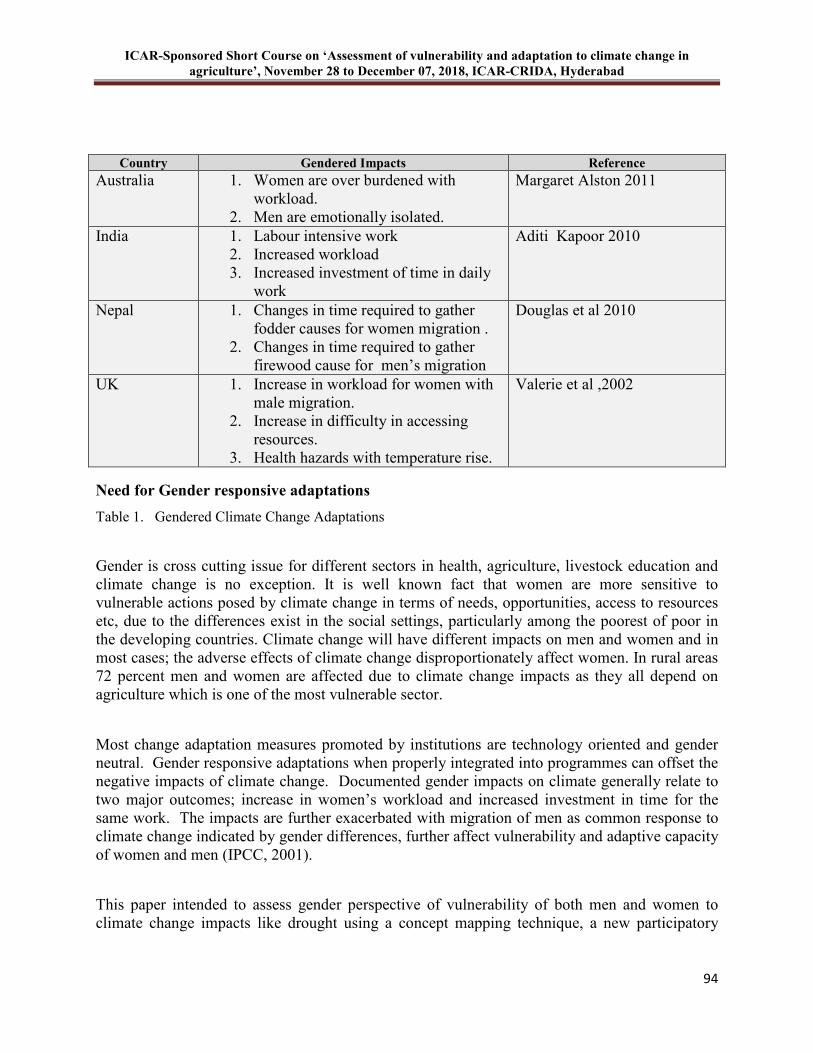
ICAR-Sponsored Short Course on ‘Assessment of vulnerability and adaptation to climate change in
agriculture’, November 28 to December 07, 2018, ICAR-CRIDA, Hyderabad
94
Need for Gender responsive adaptations
Table 1. Gendered Climate Change Adaptations
Gender is cross cutting issue for different sectors in health, agriculture, livestock education and climate change is no exception. It is well known fact that women are more sensitive to vulnerable actions posed by climate change in terms of needs, opportunities, access to resources etc, due to the differences exist in the social settings, particularly among the poorest of poor in the developing countries. Climate change will have different impacts on men and women and in most cases; the adverse effects of climate change disproportionately affect women. In rural areas 72 percent men and women are affected due to climate change impacts as they all depend on agriculture which is one of the most vulnerable sector.
Most change adaptation measures promoted by institutions are technology oriented and gender neutral. Gender responsive adaptations when properly integrated into programmes can offset the negative impacts of climate change. Documented gender impacts on climate generally relate to two major outcomes; increase in women’s workload and increased investment in time for the same work. The impacts are further exacerbated with migration of men as common response to climate change indicated by gender differences, further affect vulnerability and adaptive capacity of women and men (IPCC, 2001).
This paper intended to assess gender perspective of vulnerability of both men and women to climate change impacts like drought using a concept mapping technique, a new participatory
Country Gendered Impacts Reference
Australia 1. Women are over burdened with workload.
2. Men are emotionally isolated.
Margaret Alston 2011
India 1. Labour intensive work 2. Increased workload 3. Increased investment of time in daily
work
Aditi Kapoor 2010
Nepal 1. Changes in time required to gather fodder causes for women migration .
2. Changes in time required to gather firewood cause for men’s migration
Douglas et al 2010
UK 1. Increase in workload for women with male migration.
2. Increase in difficulty in accessing resources.
3. Health hazards with temperature rise.
Valerie et al ,2002

ICAR-Sponsored Short Course on ‘Assessment of vulnerability and adaptation to climate change in
agriculture’, November 28 to December 07, 2018, ICAR-CRIDA, Hyderabad
95
approach in social science. A participatory method employed to assess adaptation measures adopted by women
Assessment of gender dimension of vulnerability and adaptation to Climate variability – A
case study from Anantapur district
Concept mapping is a participatory text analysis that directly involves respondents or their proxies in the coding of the text (Jackson and Trochim, 2002). It is an effective methodology for working with groups for aggregating of ideas into a logical sequence. The maps generated will act as precursor for building evaluation criteria for future analysis.
The study was conducted in Chumuluru village of Anantapur district of Andhra Pradesh where NICRA project is active and therefore, is purposively selected. The rationale behind the selection is that adequate awareness to climate change impacts that might have been carried out by the project officials in the village and farmers are aware of the changing climate variability in the form of decreasing rainfall and increasing temperatures. Both women and men groups holding land ownership form the sample of the study. Each group was interviewed separately by the researcher. Concept mapping was conducted separately for men and women groups. Six key steps were followed such as brainstorming, card sorting, rating, point mapping, cluster mapping, labeling and conceptualization.
In brainstorming session it was started with a focus question “How have the households being affected with under adverse weather conditions like drought?” Question being common to both men and women groups. In response to the prompt question men found to have given 24 statements ranging from education, livelihood, health, water problems, institutional problems etc., and women responded with 34 statement problems ranging from education, health, livelihood, adaptiveness and institutional problems. Each statement was recorded on small cards.
In the second step of card sorting few card sorters who are key information sources of the village having in-depth knowledge of people’s perceptions, needs and coping strategies towards climate change impacts taken from their day to day living were selected. Card sorters then have sorted out the cards based on certain criteria in both sessions with men and women groups into different piles depending on similarity of meaning of statements .Usually 4-5 groups of piles are made for each group by each card sorter.
After card sorting exercise the same person would rate each statement on two dimensions: importance and feasibility. Likert 5 point continuum for importance namely; 1.Unimportant 2.Less important 3.Undecided 4.Important 5.More important. Doability (feasibility) 5 point scale comprised 1.Not doable 2.Less doable 3.Undecided 4.Doable 5. Highly doable; would be followed for each brainstormed statement.
After the participatory exercise statements are coded based on criteria of ‘similarity’. Statement with similar criteria are grouped together will be given code ‘1’and dissimilar statement as ‘0’. The data will be arranged as binary similarity matrix in SPSS data view. A multi dimensional scaling (MDS- PROXSCAL) will be run in SPSS which will position each statement in two dimensional spaces called point mapping. MDS generates X-Y coordinates which will facilitate
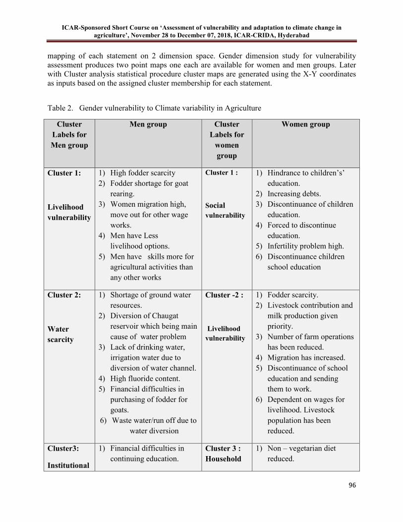
ICAR-Sponsored Short Course on ‘Assessment of vulnerability and adaptation to climate change in
agriculture’, November 28 to December 07, 2018, ICAR-CRIDA, Hyderabad
96
mapping of each statement on 2 dimension space. Gender dimension study for vulnerability assessment produces two point maps one each are available for women and men groups. Later with Cluster analysis statistical procedure cluster maps are generated using the X-Y coordinates as inputs based on the assigned cluster membership for each statement.
Table 2. Gender vulnerability to Climate variability in Agriculture
Cluster
Labels for
Men group
Men group Cluster
Labels for
women
group
Women group
Cluster 1:
Livelihood
vulnerability
1) High fodder scarcity 2) Fodder shortage for goat
rearing. 3) Women migration high,
move out for other wage works.
4) Men have Less livelihood options.
5) Men have skills more for agricultural activities than any other works
Cluster 1 :
Social
vulnerability
1) Hindrance to children’s’ education.
2) Increasing debts. 3) Discontinuance of children
education. 4) Forced to discontinue
education. 5) Infertility problem high. 6) Discontinuance children
school education
Cluster 2:
Water
scarcity
1) Shortage of ground water resources.
2) Diversion of Chaugat reservoir which being main cause of water problem
3) Lack of drinking water, irrigation water due to diversion of water channel.
4) High fluoride content. 5) Financial difficulties in
purchasing of fodder for goats.
6) Waste water/run off due to water diversion
Cluster -2 :
Livelihood
vulnerability
1) Fodder scarcity. 2) Livestock contribution and
milk production given priority.
3) Number of farm operations has been reduced.
4) Migration has increased. 5) Discontinuance of school
education and sending them to work.
6) Dependent on wages for livelihood. Livestock population has been reduced.
Cluster3:
Institutional
1) Financial difficulties in continuing education.
Cluster 3 :
Household
1) Non – vegetarian diet reduced.
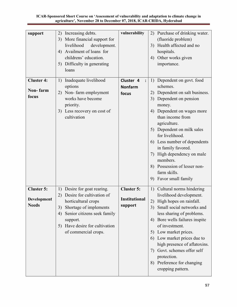
ICAR-Sponsored Short Course on ‘Assessment of vulnerability and adaptation to climate change in
agriculture’, November 28 to December 07, 2018, ICAR-CRIDA, Hyderabad
97
support 2) Increasing debts. 3) More financial support for
livelihood development. 4) Availment of loans for
childrens’ education. 5) Difficulty in generating
loans
vulnerability 2) Purchase of drinking water. (fluoride problem)
3) Health affected and no hospitals.
4) Other works given importance.
Cluster 4:
Non- farm
focus
1) Inadequate livelihood options
2) Non- farm employment works have become priority.
3) Less recovery on cost of cultivation
Cluster 4 :
Nonfarm
focus
1) Dependent on govt. food schemes.
2) Dependent on salt business. 3) Dependent on pension
money. 4) Dependent on wages more
than income from agriculture.
5) Dependent on milk sales for livelihood.
6) Less number of dependents in family favored.
7) High dependency on male members.
8) Possession of lesser non- farm skills.
9) Favor small family
Cluster 5:
Development
Needs
1) Desire for goat rearing. 2) Desire for cultivation of
horticultural crops 3) Shortage of implements 4) Senior citizens seek family
support. 5) Have desire for cultivation
of commercial crops.
Cluster 5:
Institutional
support
1) Cultural norms hindering livelihood development.
2) High hopes on rainfall. 3) Small social networks and
less sharing of problems. 4) Bore wells failures inspite
of investment. 5) Low market prices. 6) Low market prices due to
high presence of aflatoxins. 7) Govt. schemes offer self
protection. 8) Preference for changing
cropping pattern.
ICAR-Sponsored Short Course on ‘Assessment of vulnerability and adaptation to climate change in
agriculture’, November 28 to December 07, 2018, ICAR-CRIDA, Hyderabad
98
From Table 2 it was clearly reported that women vulnerabilities to drought conditions found to have many forms such as: Social Vulnerability (SV) : children’s education and family health; livelihood concerns are majorly influenced by increasing debts, migration of family members for wages and work; Household Vulnerability (HHV) is looked at from the angle of food habits: members diet due to non availability of protein diet (non vegetarian food) and poor quality drinking water mainly due to presence of high percentage of fluoride content in deep layers of groundwater; Institutional Vulnerability (IV) which was found to be high among women who generally hesitate to share problems with their neighbors and the reason stated was existence of small and restricted networks and strong cultural norms like casteism that hinder their development; and also tend to have preferences to small families and less number of dependents likely to lead to small families and that might increase gender gaps in future; Some of the nonfarm focused activities (NF) were of concern to women who under difficult circumstances opt in for petty businesses like salt businesses and prefer to migrate to long distances to jobs other than agriculture. According to Cannon (2010), women with poor access to health facilities, poor nutritious diet and less social protection are likely to be more vulnerable than men. vulnerability to climate change has affected men too but in different ways which are mostly centered on livelihoods having fewer options in job areas other than agriculture due to skill poverty. Researchers in cognitive science have consistently found that the knowledge learners possess a very strong determinant in what information they attend to, how that information is perceived, what learners’ judge to be important or relevant, and what they are able to understand and remember (Alexander, 1996).
This aspect had been conceptualized as Livelihood vulnerability (LV), common with men of which deserves attention of adaptive planners of climate change and their need to develop more skill diversification as adaptation measure for future. Male farmers have equipped with few skills and unable to shift to other occupations other than farming. Farming being the major livelihood in Anantapur district, farmers have high hopes on good rainfall; despite desire to cultivate commercial crops, horticulture crops etc. but unable to do due to poor water management that is causing major concern. It is general perception of male farmers that problem is so acute primarily due to poor management rather than availability of water itself. From the foregoing it is evident vulnerability to men mostly means lack of proper livelihood options other than agriculture. More skill development activities are required to withstand climate change impacts.
Assessment of adaptation to climate change impacts using pair wise ranking technique
Women farmers gave a different picture of the adaptation measures to climate change impact of drought in Anantapur district. Some of the measures are Efforts to reduce fodder scarcity, Application of FYM , Enhancement of livestock population and avoid migration, Drip Irrigation, Purchase of water tanker , Social and religious belief , Sheep rearing ,Selling of fuelwood, dryland horticulture, Borewell irrigation, Sorghum cultivation as alternative crop , Castor, pigeonpea as alternative crop to groundnut and Non forest timber produce .However the best four ranks were given to Borewell irrigation Sorghum cultivation as alternative crop,Castor,pigeonpea as alternative crop to groundnut and Non forest timber produce. (Table-4)

ICAR-Sponsored Short Course on ‘Assessment of vulnerability and adaptation to climate change in
agriculture’, November 28 to December 07, 2018, ICAR-CRIDA, Hyderabad
99
Adaptation measures reported by men were Gap filling with short duration crops, Sorghum, green gram as alternative crop to groundnut, Sowing across slope , Reduction of crop acreage , Rearing of milch cattle , Integrated farming system, Purchase of fodder , Support of government subsidy, Drip Irrigation , Farm bunding, Reduction of cost of production and Staggering sowing. Out of these measures given out by men farmers, IFA, Drip irrigation, Reduction of cost of production and staggering sowing received highest ranking.(Table-3)
Table 3. Pair-Wise Matrix Ranking of Adaptation strategies to impacts of drought- Men farmers in Chamuluru (Figures in parenthesis are ranks)
Adaptation measures
1
WH
2 M
3 BIRR
4 DIRR
5 DL&S
6 AFYM
7 UDI
8 AcR-VC
9
MC 10 LA -FC
Total
Score
(R)
1 WH 1 3 (VIII)
2 M 1 2 1 (X) 3 BIRR 1 3 3 2
(IX) 4 DIRR 4 4 4 4 4
(VII) 5 DL&S 5 5 5 5 5 9
(II) 6 AFYM 6 6 6 6 5 6 6 (V) 7 UDI 7 7 7 7 5 7 7 8
(III) 8 AcR-VC
8 8 8 8 5 8 7 8 7 (IV)
9 MC 9 9 9 9 5 6 7 8 9 5 (VI)
10 LA -FC
10 10 10 10 10 10 10 10 10 10 10 (I)
1- Water harvesting (WH) 2- Migration (M) 3- Bore well irrigation (BIRR) 4- Drip irrigation (DIRR) 5- Livestock and subsidies support (SL&S) 6- Application of Farm Yard Manure (AFYM) 7- Usage of dryland implements (UDI) 8- Vegetable cultivation alternative to rice (AcR-VC) 9- Millet cultivation (MC) 10- Land allocation for fodder cultivation (LA -FC)
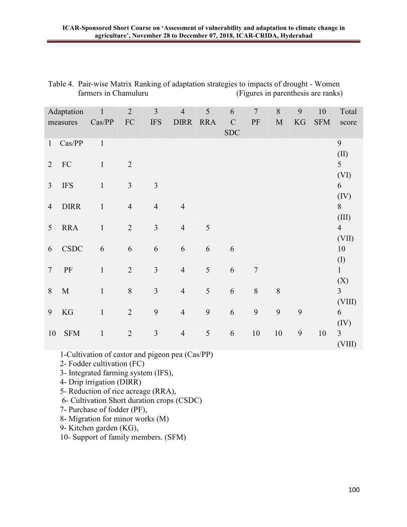
ICAR-Sponsored Short Course on ‘Assessment of vulnerability and adaptation to climate change in
agriculture’, November 28 to December 07, 2018, ICAR-CRIDA, Hyderabad
100
Table 4. Pair-wise Matrix Ranking of adaptation strategies to impacts of drought - Women farmers in Chamuluru (Figures in parenthesis are ranks)
Adaptation measures
1 Cas/PP
2 FC
3 IFS
4 DIRR
5 RRA
6 C
SDC
7 PF
8 M
9 KG
10 SFM
Total score
1 Cas/PP 1 9 (II)
2 FC 1 2 5 (VI)
3 IFS 1 3 3 6 (IV)
4 DIRR 1 4 4 4 8 (III)
5 RRA 1 2 3 4 5 4 (VII)
6 CSDC 6 6 6 6 6 6 10 (I)
7 PF 1 2 3 4 5 6 7 1 (X)
8 M 1 8 3 4 5 6 8 8 3 (VIII)
9 KG 1 2 9 4 9 6 9 9 9 6 (IV)
10 SFM 1 2 3 4 5 6 10 10 9 10 3 (VIII)
1-Cultivation of castor and pigeon pea (Cas/PP) 2- Fodder cultivation (FC) 3- Integrated farming system (IFS), 4- Drip irrigation (DIRR) 5- Reduction of rice acreage (RRA), 6- Cultivation Short duration crops (CSDC) 7- Purchase of fodder (PF), 8- Migration for minor works (M) 9- Kitchen garden (KG), 10- Support of family members. (SFM)
ICAR-Sponsored Short Course on ‘Assessment of vulnerability and adaptation to climate change in
agriculture’, November 28 to December 07, 2018, ICAR-CRIDA, Hyderabad
101
Conclusion
Agriculture is livelihood to 70 percent of population living in Rural India. This sector is more vulnerable to climate variabilities: increasing temperature, uneven and erratic rainfall and have prolonged dryspells etc., Climate impacts affect the most disadvantaged and poor farmers who have limited opportunities to adapt as they possess limited financial and physical resources, particularly women when compared to men who are marginalized and poorer in terms of access to land, capital and social status and bear dual responsibility of home and farm. Their adaptive capacity is low when compared to men. Vulnerability and adaptation to climate variabilities impacts are said to be gendered as vulnerability vary with men and women in terms of exposure and adaptive capacity, according to Denton 2000. The paper had studied the gender dimension of both vulnerabilities and gender adaptations to climate change impacts in Anantapur district through participatory approaches. Women vulnerabilities to climate change are related to specific indicators in respect of social, livelihood and institutional support and are related mostly to food, education, health and reduction of costs. Men have indicated vulnerability to generic aspects of livelihood development like technology, water management and institutional support. Similarly adaptation responses were gendered that varied with gender, age, class and land ownership. Women prepared short duration varieties, cultivation of drought resistant crops like castor or pigeon pea etc, while men are supporting and inclined towards livestock and fodder cultivation. This shows both men and women vary in perceptions and opinion on climate variabilities and livelihood goals.
References
Alexander, PA, 1996. The past, the present and future of knowledge research: A reexamination of the role of knowledge in learning and instruction, Educational Psychologist, v. 31, p. 89-92
Aditi Kapoor. 2011. Engendering the climate for change. Alternative futures. Aspire design publishers. New Delhi. 1-8
Cannon, Terry. 2010. Gender Impact of climate hazards in Bangladesh. Gender and development. 10:2: 45-50.
Charlotte Wringley –Asante. 2008. Men are poor but women are poorer: Gendered poverty and survival strategies in the Dangue West District of Ghana. Norwegian journal of geography 62. 161-170.
Denton, Fatma. 2000. ‘Gender impact of climate change: a human security dimension. In. Irene Dankelman (2002). Climate change: learning from gender analysis and women’s experiences of organizing for sustainable development. Gender and Development. 109(2): 21-29.
Denton, Fatma. 2002. ‘Gender impact of climate change: a human security dimension. In. Dankelman,I. (2002). Climate change: learning from gender analysis and women’s experiences of organizing for sustainable development. Gender and Development. 109(2): 21-29.
ICAR-Sponsored Short Course on ‘Assessment of vulnerability and adaptation to climate change in
agriculture’, November 28 to December 07, 2018, ICAR-CRIDA, Hyderabad
102
Dankelman I. 2002. Climate change: learning from gender analysis and women’s experiences of organizing for sustainable development. Gender and Development. 109(2): 21-29.
Dreze J and Sen, A. 2002. India- Development and participation. Oxford University Press.Oxford.
IPCC. 2007. Contribution of working groups I, II and III to the fourth assessment report of the Intergovernmental Panel on climate change. Geneva, Switzerland: Intergovernmental Panel on Climate change. URL hhtp://www.ipcc.ch/publications and data/ar4/syr/en/contents.html. (Accessed on 23 November 2011.)
Jackson M. Kristin and William M. K.Trochim. 2002. Concept Mapping as an Alternative Approach for the Analysis of Open-Ended Survey Responses. Organizational Research
methods. 5(4):307-336.
Trochim William MK. 1989. An Introduction to concept mapping and planning and evaluation. Evaluation and program planning, 12(1), 1-16.
Aditi Kapoor. 2011. Engendering the climate for change. Alternative futures.
Douglas S Massey, William G Axinn and Dirgha J Ghimire. 2010. Environmental Change and out migration: evidence from Nepal, Popul Environ 32: 109-136
FAO. 2007. Gender and Climate Change existing research and knowledge Gaps Rome. Gender and Population Division, FAO.
IPCC. 2001. Fourth Assessment report, In, Margaret Alston 2010 Gender and Climate Change in Australia Journal of Sociology. Vol 47 (1): 53-70.
Margaret Alston. 2011. Gender and Climate Change in Australia, Journal of Sociology 47:53
Stern N. 2006. The economics of climate change (the Stern review) Report of the cabinet office-
HM Treasury Cambridge University Press Cambridge
Thomas and Tom Mitchell. 2008. Introduction: Building the case for pro-poor adaptation IDS
Bulletin Volume 39 Number 4 September Institute of Development Studies
Valerie Nelson, Kate Meadows, Terry Cannon, John Morton, Adrienne martin.2002. Uncertain predictions, Invisible Impacts, and the Need to mainstream Gender in climate change adaptations. Gender and Development. 10(2): pp 51-59
Villarreal Marcela.2013. Decreasing Gender Inequality in Agriculture: Key to Eradicating Hunger .Brown Journal of World Affairs. 1(3) 169-177.
ICAR-Sponsored Short Course on ‘Assessment of vulnerability and adaptation to climate change in
agriculture’, November 28 to December 07, 2018, ICAR-CRIDA, Hyderabad
103
11 Developing Insurance Products
P Vijaya Kumar
Introduction
Agriculture contributes to 17% of the Indian GDP and supports the livelihood of 70% of the population (Statistics Times, 2017).In India around 59% of cultivable area is under rainfed cultivation, which is most vulnerable to vagaries of weather. Despite tremendous technological developments, vagaries of weather continue to plague the agriculture production. Any shortfall in agricultural production will have its cascading effect on the economy of the country. In recent times, climate change and variability are confounding the troubles already faced by Indian agriculture and the farming community. Loss in crop production and farm income due to unexpected weather hazards is beyond the carrying capacity of resource poor farmers of the country. With the growing commercialization of agriculture, the magnitude of crop loss due to unfavourable weather hazards is increasing leading to suicides of farmers. The State and National governments on their part are coming to the rescue of farming community by implementing various relief measures like reduction or suspension of land revenue taxes, loan waiving, relief from calamity relief fund etc.
As agricultural yields are highly variable due to weather aberrations, crops have to be covered under agriculture insurance for compensating yield losses and reduce the poverty of farming community. The agricultural insurance has evolved as an adaptation strategy in India since 1972 to mitigate / manage weather related risks in agriculture. However, experiences with traditional agricultural insurance schemes have shown that this approach is not often suitable in developing countries. In recent years, weather index insurance contracts in agriculture have emerged as an alternative to traditional agricultural (or crop) insurance.
1. Risks in Agriculture
The principal risks in agriculture are weather risks, biological risks and price risks (Hess et al.,2002; Bryla et al.,2003 and Skees et al.,2005). Agricultural risks can range from independent (like localized hail storms) to highly correlated or covariant (example: Price risks or widespread drought). Weather risks are broadly of two types viz. sudden, unforeseen events (thunder storms) and cumulative events occurring over extended period (example: drought). The adverse impacts of either of these two types vary according to the crop, crop variety and time of occurrence of the event. Some of the weather risks in agriculture are: Drought, excess rainfall or floods, high temperature, low temperature events like frost and freeze, high winds and hail storms etc.
1.1 Weather risk management
Farmers in developing countries have always been exposed to weather risks, and for a long time have developed a variety of weather risk management (WRM) techniques for reducing, mitigating and coping with weather risks (Dercon, 2002). Traditional risk management covers actions taken both before (ex-ante) and after (ex-post) the risky event occurs (Siegel and
ICAR-Sponsored Short Course on ‘Assessment of vulnerability and adaptation to climate change in
agriculture’, November 28 to December 07, 2018, ICAR-CRIDA, Hyderabad
104
Alwang, 1999). Mitigation,coping and transfer are the major strategies in agricultural risk management.
2. Agricultural Insurance
Agricultural insurance is a means of protecting the farmers against financial losses suffered due to unforeseen and non-preventable weather risks (AIC, 2008). It is a financial mechanism in which loss of crop yields suffered by farmers in a particular area are borne by farmers in other areas (as premiums), so that burden of loss can be distributed among a large number of farmers. In agricultural insurance the reserves of premiums accumulated in good years are used to pay the indemnities in bad years.
2.1 Crop insurance products
Crop insurance products can broadly be classified into two major groups: Indemnity-based insurance and Index insurance.
I. Indemnity-Based Crop Insurance
There are two main products in the Indemnity - based crop insurance. They are:
(i) Damage-based indemnity insurance (or named peril crop insurance): Damage-based indemnity insurance is the crop insurance in which the insurance claim is calculated by measuring the percentage damage in the field soon after the occurrence of the damage. The sum insured may be based on production costs or on the expected revenue. Where damage cannot be measured accurately and immediately after the loss, the assessment may be deferred until the end of the crop season. Damage-based indemnity insurance is best known for hail, frost, heat wave, deficit or excess rainfall.
(ii)Yield-based crop insurance (or Multiple Peril Crop Insurance, MPCI): Yield-based crop insurance is coverage in which insured crop yield is established as a percentage of the farmer’s historical average yield. The insured yield is mostly between 50 to 70 percent of the average farm yield. If the realized yield is less than the insured yield, an indemnity (the amount payable by the insurer to the insured) is paid equal to the difference between the actual yield and the insured yield, multiplied by a pre-agreed value. Yield-based crop insurance protects against multiple perils, meaning that it covers many different causes of yield loss (it is generally difficult to determine the exact cause of yield loss).
II. Index-Based Crop Insurance
Index based insurance products for agriculture represents an attractive alternative for managing weather risks. Currently there are two types of index insurance products viz., Area yield index insurance and weather index insurance (WII), as distinguished by Skees(2003)
(i) Area yield index insurance: In Area yield index insurance, the indemnity is based on the realized average yield of an area such as a block or district, not the actual yield of the insured farmer. The insured yield is established as a percentage of the average yield for the areaof the whole village or group of villages. An indemnity is paid if the realized yield for the area is less
ICAR-Sponsored Short Course on ‘Assessment of vulnerability and adaptation to climate change in
agriculture’, November 28 to December 07, 2018, ICAR-CRIDA, Hyderabad
105
than the insured yield regardless of the actual yield on a policyholder’s farm. This type of index insurance requires historical yield data of the area.
(ii) Weather Index Insurance (WII): In WII, the indemnity is based on realization of a specific weather parameter measured over a pre-specified period of time at a particular weather station. The insurance was structured to protect against realization of either very high or very low indices that are expected to cause crop losses. For example, the insurance can be structured to protect against either too much or too little rainfall. An indemnity is paid whenever the realized value of the index exceeds a pre-specified threshold (when protecting against excess rainfall) or when the index is less than the threshold (when protecting against deficit rainfall). The indemnity is calculated based on a pre-agreed sum insured per unit of the index.
Skees(2003) argues that weather based indices are usually preferred to yield based indices,as in developing countries the quality of historical weather datais better than quality of yield data, and weather events, especially deficit or excess rainfall, are the major sources of crop losses in many regions.
4. Main features of Weather Index-Based Insurance
The essential feature of WII is that the insurance contract responds to an objective parameter (e.g. rainfall or temperature) at a referred weather station during an agreed time period. The parameters of the contract are set so as to correlate, as accurately as possible, with the loss of yield of a specific crop suffered by the policyholder. All policyholders within a defined area receive payouts based on the same contract and measurement at the same weather station, eliminating the need for in-field assessment of yield loss.
In order for the underlying index to be a sound proxy for loss, it has to be based upon an objective measure (for example, rainfall, wind speed, temperature) that exhibits a strong cor-relation with the variable of interest (in this case, crop yield). Additionally, the weather variable that can form an index must satisfy the properties: i) Observable and easily measured, ii) Objective, iii) Transparent, iv) Independently verifiable, v) Reported in a timely manner, vi) Consistent over time and vii) Experienced over a wide area.
Important elements of a WII contract are: • A specific meteorological station is named as the reference weather station. • A strike or trigger weather measurement is set (e.g. cumulative rainfall), at which the
contract starts to pay out. • A lump sum or an incremental payment is made (e.g. Rupees per mm of rainfall above or
below the trigger). • A limit or exit of the measured parameter is set (e.g. cumulative rainfall), at which a
maximum payment is made. • The period of insurance is stated in the contract and coincides with the crop growth period; it
may be divided into phases (Maximum three), with each phase having its own triggers, increment and limit.
ICAR-Sponsored Short Course on ‘Assessment of vulnerability and adaptation to climate change in
agriculture’, November 28 to December 07, 2018, ICAR-CRIDA, Hyderabad
106
4.1 Advantages and disadvantages of weather index based insurance
Though the development and application of weather index insurance (WII) is still in its early stages, the advantages and disadvantages of WII were well-documented (World Bank, 2005;USAID, 2006; IFAD and WFP 2010). Some of the relative merits and demerits of the WII are presented below (IFAD, 2010). Advantages of WII
In comparison to the traditional damage based agricultural insurance, WII has advantages on the following aspects: Transparency: An Index Insurance contract usually allows the policyholder to have direct access to the information on which the payouts will be calculated. Hence, WII is more transparent to the clienteles. No on-farm loss adjustment: This is the primary advantage of index insurance, as on-farm loss adjustment is quite complex and costly. Lack of adverse selection: “Adverse selection” occurs when potential insured parties have hidden information about their risk exposure that is not available to the insurer, who then becomes more likely to erroneously assess the risk of the insured. As a result traditional insurance encourages high-risk producers to insure, while risk and premium are calculated on the average producer. However, in Weather Index based insurance all the insured farmers within the defined area have the same insurance payout conditions, regardless of their specific risk exposure (USAID, 2006). Hence, insurers and clients benefit from reduced adverse selection. Lack of moral hazard: “Moral hazard” refers to a phenomenon that the insured person’s optimal decision may change as a result of purchasing the insurance, because the insurance contract reduces the loss associated with the insured event. Such changes in behaviour will normally increase the probability of the insured event occurring or increased severity of loss (Ashan et al., 1982). In WII, individual farmers who are trying to influence claims will not get any benefit and all farmers in the defined area are treated equally for payment of pay outs or indemnity.
Addresses correlated risks: Index insurance works best where there are correlated and widespread risks like drought. In traditional insurance, perils such as drought are challenging to insure.
Low operational and transaction costs: Index insurance requires limited individual underwriting (Client assessment). It can be distributed, or sold out and claims can be settled, at relatively lower cost than in traditional insurance.
Rapid payout: Measurement of meteorological data from a reference weather station, with no field loss adjustment, allows for providing rapid payouts to the clients in WII than in traditional agricultural insurance.

ICAR-Sponsored Short Course on ‘Assessment of vulnerability and adaptation to climate change in
agriculture’, November 28 to December 07, 2018, ICAR-CRIDA, Hyderabad
107
Despite the merits of weather index based insurance mentioned above, acceptance WII by farmers is of slow due to the following disadvantages:
Disadvantages of WII
Basis risk: Basis risk is a key constraint in WII and it has suppressed the growth of WII. Basis risk is the difference between the actual crop yield at farm unit level and yield projected by the weather index. As a result of basis risk a farmer experiencing yield loss, may not receive a payout, and a payoutmay be triggered without any loss being experienced. Index insurance works best where losses are homogeneous in the defined area and highly correlated with the indexed peril. Diaz Nieto et al.(2006) mentioned three important types of basis risk, which are mentioned as under:
Spatial or geographical basis risk: A geographical basis risk represents the risk that result from the difference between weather patterns at reference weather stations and the locations of farmers. Local variations in the weather (e.g. rainfall) within the area surrounding a reference weather station are responsible for geographical basis risk. Temporal basis risk: It results from inter-annual variations in crop phases, and the insurance phases are not temporally aligned with the intended crop growth stage. Product or crop specific basis risk: It means that the sensitivity to weather events varies across crop types due to different crop characteristics. Crop losses can be caused by many factors including weather. Where there is no clear-cut and strong relationship between yield loss and the indexed weather peril, risk can be high. WII is most likely to work, for rainfed crops and at severe levels of the risk event, when losses may be more widespread and homogeneous. Limited perils: WII normally covers only one, or sometimes two, weather perils. Although this reduces the cost of operation compared to the multi-peril crop insurance (MPCI), the product may not provide broader and enough coverage to more number of weather risks that are affecting the crop loss. Replication or Scalability: The triggers, limits and increments of a specific product that were worked out for a reference weather station will not be valid for another reference weather station and they need to be adjusted to reflect the weather parameters of that new weather station. Different product designs are required for different crops (or at least generic crop types). Requirement of Technical expertise: WII requires considerable technical work in its implementation and sustaining. Technical capacity and expertise in agro-meteorology are required, particularly during the initial design phase for new products, and also in operationalising the products.
Lack of weather data: WII depends on the availability of quality weather data, which drastically vary from country to country. In developing countries, the shortage of historical and real-time weather data is often a major hurdle for design of WII products.
ICAR-Sponsored Short Course on ‘Assessment of vulnerability and adaptation to climate change in
agriculture’, November 28 to December 07, 2018, ICAR-CRIDA, Hyderabad
108
4.2 Collection of weather data for weather index based insurance
The data used for constructing the weather indices should satisfy quality requirements, including:
• Reliable and trustworthy ongoing daily collection and reporting procedures; • Periodic checks and quality control; • An independent source of data for verification (e.g. surrounding weather stations). The general criteria for weather data requirements for WII applications (ISMEA, 2006) are specified as follows:
• At least 20 years of historical weather data; • Limited missing values and out-of-range values (preferably less than 3 per cent missing data
from the entire dataset); • Availability of a nearby weather station for fall-back verification purposes; • Consistency of observation techniques – either manual or automated; • Limited changes in instrumentation/orientation/configuration; • Integrity of weather-data recording procedure; • Little potential for measurement tampering.
Beyond the quality of data, definition of the boundaries of the area(s) covered by the weather station(s) is critical, so that WII contracts can be written for specific areas tied to a specific weather station. A general rule of thumb is to consider a specific WII contract marketable within a 20-km radius of the weather station; but in many cases the applicable area is smaller. The more the terrain varies, the more the acceptable distance from a station decreases. Modalities must be defined for weather data collection and dissemination during the contract coverage period. Insurance and reinsurance industries tend to require the use of automated weather stations and availability of fallback verification measurements from nearby stations with comparable weather patterns. Manual measurement of weather variables (e.g. through manual rain gauges) is usually not regarded as sufficiently reliable and secure. As a result, low-cost, automatic weather stations are being implemented in some WII initiatives. Even if manual observation of weather risks are taken, all weather parameters should be taken at the same time for controlling hampering of weather data, as various weather variables are linked by specific relationship.
4.3 Collection of agricultural data
Agricultural information is the second most important component of the contract design equation of WII. The data on productivity (yield), and description of the agricultural production practices carried out in the areas is also necessary. Unfortunately, the availability of quality yield-data series of adequate length and at the appropriate spatial level is a major problem. However, lack of quality yield data does not pose as serious a problem as lack of good weather data, since it is still possible to find alternative approaches to estimate yield data. One possibility is to simulate synthetic yield-data series through crop growth simulation models. Information such as crop varieties adopted, planting dates, management practices, related costs, risk profiles, historical

ICAR-Sponsored Short Course on ‘Assessment of vulnerability and adaptation to climate change in
agriculture’, November 28 to December 07, 2018, ICAR-CRIDA, Hyderabad
109
recollection of the impact of the peril, and the most sensitive phases in crop life are essential in designing a meaningful WII contract. 4.4 Technical issues concerned to thedesign of weather index
Diaz Nieto et al.(2006) mentioned the following technical requirements for the index insurance scheme to have a positive impact on farmers’ livelihood.
• The weather index should be easily understood and well defined; • It should take account of crop sensitivity at different growth stages; • It should take account of the relationship between soil texture and rainfall effectiveness; • It should define a protocol that reflects the actual planting date as closely as possible; • It should ensure that the insured pays the price of spatial variation in risk; • It should enable accurate estimation of the probability of the risk event. • Reliability of the institution providing the weather data; • Transparency and absence of corruption; • Adaptation of the product to farmers’ needs; • Communication and training for farmers and field staff.
5. Design and validation of weather index based insurance products
The objective of the contract design is to define a structure that effectively captures the relationship between the weather variable and the potential crop loss and to select the index that is most effective in providing payouts when losses are experienced, eliminating basis risk as far as possible. The set of possible index combinations is unlimited, and numerous structures have been developed in the relatively short history of WII. Weather index-based contracts can be classified according to many different parameters (Table 1).
Table 1. Examples of parameters used for WII contracts Contract parameter Options
Triggering values of weather variable Cumulative
Average
Maximum
Minimum
Period covered by index Entire life cycle of crop
Fractions of crop life cycle
Number of phases into which covered period is divided Usually 1 to 3 phases
Start of coverage period Fixed
Dynamic
Payout structure Incremental
Lump sum (single value payout)
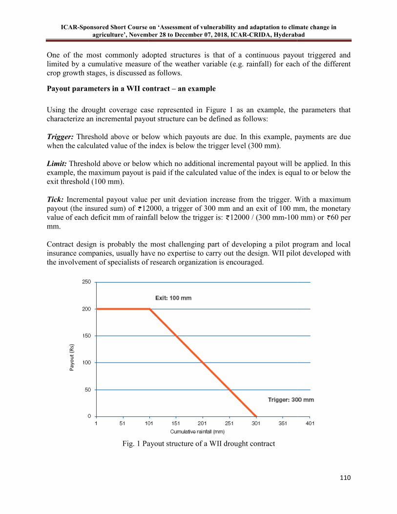
ICAR-Sponsored Short Course on ‘Assessment of
agriculture’, November 28 to December 07, 2018, ICAR
One of the most commonly adopted structures is that of a continuous payout limited by a cumulative measure of the weather variable (e.g. rainfall) for each of the different crop growth stages, is discussed as follows.
Payout parameters in a WII contract
Using the drought coverage case represented in characterize an incremental payout structure can be defined as follows: Trigger: Threshold above or below which payouts are due. In this example, payments are due when the calculated value of the index is below Limit: Threshold above or below which no additional incremental payout will be applied. In this example, the maximum payout is paid if the calculated value of the index is equal to or below the exit threshold (100 mm). Tick: Incremental payout value per unit deviation increase from the trigger. With a maximum payout (the insured sum) of 12000, a trigger of 300 mm and an exit of 100 mm, the monetary value of each deficit mm of rainfall below the trigger is: mm. Contract design is probably the most challenging part of developing a pilot program and local insurance companies, usually have no expertise to carry out the design. WII pilot developed with the involvement of specialists of research o
Fig. 1 Payout structure of a WII drought contract
Pa
yo
ut
(Rs)
Sponsored Short Course on ‘Assessment of vulnerability and adaptation to climate change in
agriculture’, November 28 to December 07, 2018, ICAR-CRIDA, Hyderabad
One of the most commonly adopted structures is that of a continuous payout limited by a cumulative measure of the weather variable (e.g. rainfall) for each of the different crop growth stages, is discussed as follows.
Payout parameters in a WII contract – an example
Using the drought coverage case represented in Figure 1 as an example, the parameters that characterize an incremental payout structure can be defined as follows:
Threshold above or below which payouts are due. In this example, payments are due when the calculated value of the index is below the trigger level (300 mm).
Threshold above or below which no additional incremental payout will be applied. In this example, the maximum payout is paid if the calculated value of the index is equal to or below the
ncremental payout value per unit deviation increase from the trigger. With a maximum 12000, a trigger of 300 mm and an exit of 100 mm, the monetary
value of each deficit mm of rainfall below the trigger is: 12000 / (300 mm-100
Contract design is probably the most challenging part of developing a pilot program and local insurance companies, usually have no expertise to carry out the design. WII pilot developed with the involvement of specialists of research organization is encouraged.
Fig. 1 Payout structure of a WII drought contract
vulnerability and adaptation to climate change in
CRIDA, Hyderabad
110
One of the most commonly adopted structures is that of a continuous payout triggered and limited by a cumulative measure of the weather variable (e.g. rainfall) for each of the different
Figure 1 as an example, the parameters that
Threshold above or below which payouts are due. In this example, payments are due
Threshold above or below which no additional incremental payout will be applied. In this example, the maximum payout is paid if the calculated value of the index is equal to or below the
ncremental payout value per unit deviation increase from the trigger. With a maximum 12000, a trigger of 300 mm and an exit of 100 mm, the monetary
100 mm) or 60 per
Contract design is probably the most challenging part of developing a pilot program and local insurance companies, usually have no expertise to carry out the design. WII pilot developed with
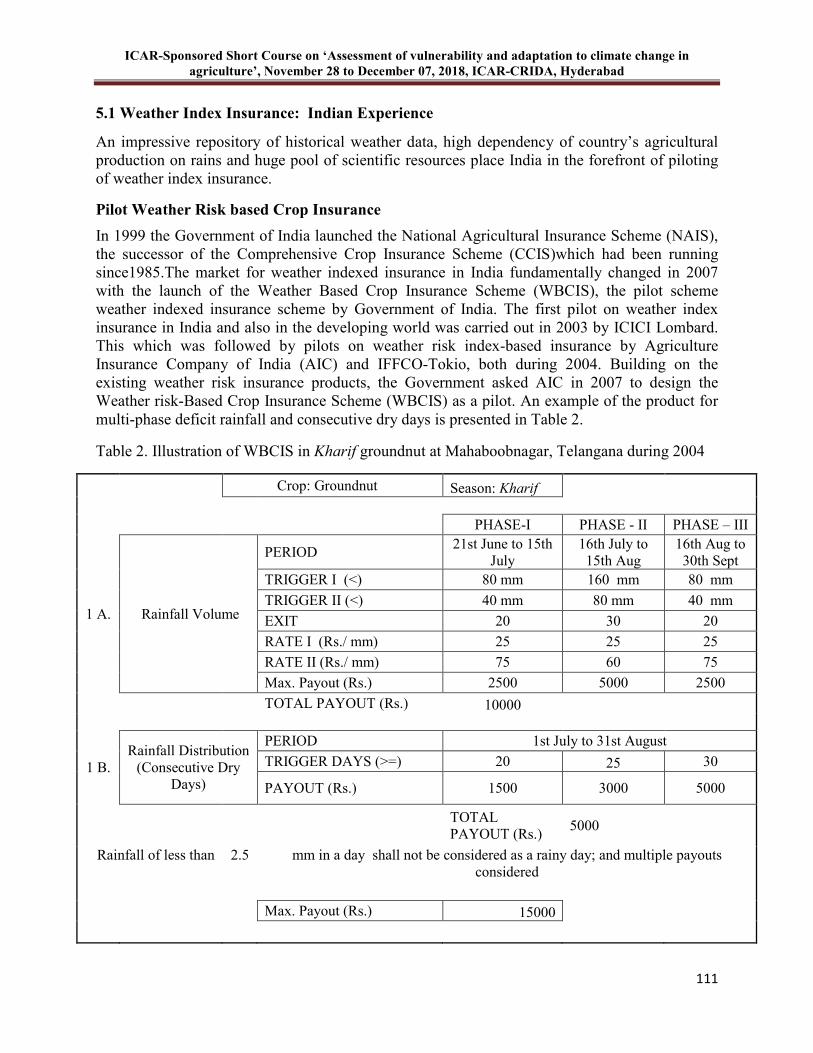
ICAR-Sponsored Short Course on ‘Assessment of vulnerability and adaptation to climate change in
agriculture’, November 28 to December 07, 2018, ICAR-CRIDA, Hyderabad
111
5.1 Weather Index Insurance: Indian Experience
An impressive repository of historical weather data, high dependency of country’s agricultural production on rains and huge pool of scientific resources place India in the forefront of piloting of weather index insurance.
Pilot Weather Risk based Crop Insurance
In 1999 the Government of India launched the National Agricultural Insurance Scheme (NAIS), the successor of the Comprehensive Crop Insurance Scheme (CCIS)which had been running since1985.The market for weather indexed insurance in India fundamentally changed in 2007 with the launch of the Weather Based Crop Insurance Scheme (WBCIS), the pilot scheme weather indexed insurance scheme by Government of India. The first pilot on weather index insurance in India and also in the developing world was carried out in 2003 by ICICI Lombard. This which was followed by pilots on weather risk index-based insurance by Agriculture Insurance Company of India (AIC) and IFFCO-Tokio, both during 2004. Building on the existing weather risk insurance products, the Government asked AIC in 2007 to design the Weather risk-Based Crop Insurance Scheme (WBCIS) as a pilot. An example of the product for multi-phase deficit rainfall and consecutive dry days is presented in Table 2.
Table 2. Illustration of WBCIS in Kharif groundnut at Mahaboobnagar, Telangana during 2004
Crop: Groundnut Season: Kharif
PHASE-I PHASE - II PHASE – III
1 A. Rainfall Volume
PERIOD 21st June to 15th
July 16th July to 15th Aug
16th Aug to 30th Sept
TRIGGER I (<) 80 mm 160 mm 80 mm
TRIGGER II (<) 40 mm 80 mm 40 mm
EXIT 20 30 20
RATE I (Rs./ mm) 25 25 25
RATE II (Rs./ mm) 75 60 75
Max. Payout (Rs.) 2500 5000 2500
TOTAL PAYOUT (Rs.) 10000
1 B. Rainfall Distribution
(Consecutive Dry Days)
PERIOD 1st July to 31st August
TRIGGER DAYS (>=) 20 25 30
PAYOUT (Rs.) 1500 3000 5000
TOTAL PAYOUT (Rs.)
5000
Rainfall of less than 2.5 mm in a day shall not be considered as a rainy day; and multiple payouts considered
Max. Payout (Rs.) 15000
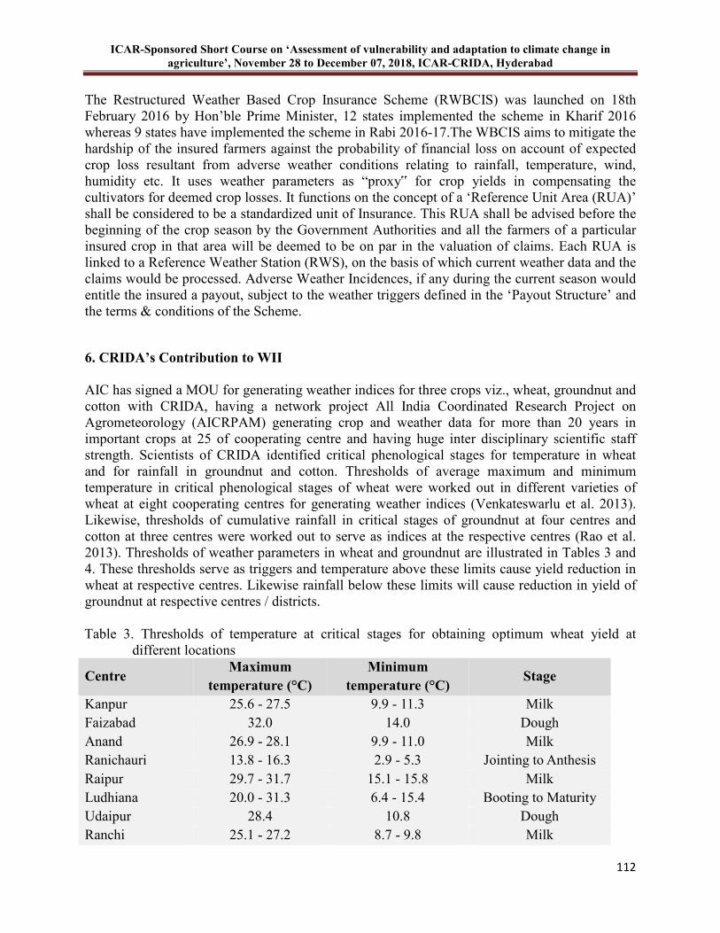
ICAR-Sponsored Short Course on ‘Assessment of vulnerability and adaptation to climate change in
agriculture’, November 28 to December 07, 2018, ICAR-CRIDA, Hyderabad
112
The Restructured Weather Based Crop Insurance Scheme (RWBCIS) was launched on 18th February 2016 by Hon’ble Prime Minister, 12 states implemented the scheme in Kharif 2016 whereas 9 states have implemented the scheme in Rabi 2016-17.The WBCIS aims to mitigate the hardship of the insured farmers against the probability of financial loss on account of expected crop loss resultant from adverse weather conditions relating to rainfall, temperature, wind, humidity etc. It uses weather parameters as “proxy‟ for crop yields in compensating the cultivators for deemed crop losses. It functions on the concept of a ‘Reference Unit Area (RUA)’ shall be considered to be a standardized unit of Insurance. This RUA shall be advised before the beginning of the crop season by the Government Authorities and all the farmers of a particular insured crop in that area will be deemed to be on par in the valuation of claims. Each RUA is linked to a Reference Weather Station (RWS), on the basis of which current weather data and the claims would be processed. Adverse Weather Incidences, if any during the current season would entitle the insured a payout, subject to the weather triggers defined in the ‘Payout Structure’ and the terms & conditions of the Scheme.
6. CRIDA’s Contribution to WII AIC has signed a MOU for generating weather indices for three crops viz., wheat, groundnut and cotton with CRIDA, having a network project All India Coordinated Research Project on Agrometeorology (AICRPAM) generating crop and weather data for more than 20 years in important crops at 25 of cooperating centre and having huge inter disciplinary scientific staff strength. Scientists of CRIDA identified critical phenological stages for temperature in wheat and for rainfall in groundnut and cotton. Thresholds of average maximum and minimum temperature in critical phenological stages of wheat were worked out in different varieties of wheat at eight cooperating centres for generating weather indices (Venkateswarlu et al. 2013). Likewise, thresholds of cumulative rainfall in critical stages of groundnut at four centres and cotton at three centres were worked out to serve as indices at the respective centres (Rao et al. 2013). Thresholds of weather parameters in wheat and groundnut are illustrated in Tables 3 and 4. These thresholds serve as triggers and temperature above these limits cause yield reduction in wheat at respective centres. Likewise rainfall below these limits will cause reduction in yield of groundnut at respective centres / districts.
Table 3. Thresholds of temperature at critical stages for obtaining optimum wheat yield at different locations
Centre Maximum
temperature (°C) Minimum
temperature (°C) Stage
Kanpur 25.6 - 27.5 9.9 - 11.3 Milk Faizabad 32.0 14.0 Dough Anand 26.9 - 28.1 9.9 - 11.0 Milk Ranichauri 13.8 - 16.3 2.9 - 5.3 Jointing to Anthesis Raipur 29.7 - 31.7 15.1 - 15.8 Milk Ludhiana 20.0 - 31.3 6.4 - 15.4 Booting to Maturity Udaipur 28.4 10.8 Dough Ranchi 25.1 - 27.2 8.7 - 9.8 Milk
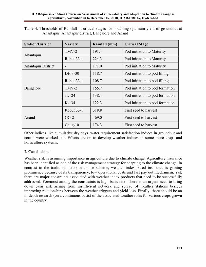
ICAR-Sponsored Short Course on ‘Assessment of vulnerability and adaptation to climate change in
agriculture’, November 28 to December 07, 2018, ICAR-CRIDA, Hyderabad
113
Table 4. Thresholds of Rainfall in critical stages for obtaining optimum yield of groundnut at Anantapur, Anantapur district, Bangalore and Anand
Station/District Variety Rainfall (mm) Critical Stage
Anantapur TMV-2 191.4 Pod initiation to Maturity
Robut 33-1 224.3 Pod initiation to Maturity
Anantapur District - 171.0 Pod initiation to Maturity
Bangalore
DH 3-30 118.7 Pod initiation to pod filling
Robut 33-1 108.7 Pod initiation to pod filling
TMV-2 155.7 Pod initiation to pod formation
JL -24 138.4 Pod initiation to pod formation
K-134 122.3 Pod initiation to pod formation
Anand
Robut 33-1 318.8 First seed to harvest
GG-2 469.0 First seed to harvest
Gaug-10 174.3 First seed to harvest
Other indices like cumulative dry days, water requirement satisfaction indices in groundnut and cotton were worked out. Efforts are on to develop weather indices in some more crops and horticulture systems.
7. Conclusions
Weather risk is assuming importance in agriculture due to climate change. Agriculture insurance has been identified as one of the risk management strategy for adapting to the climate change. In contrast to the traditional crop insurance scheme, weather index based insurance is gaining prominence because of its transparency, low operational costs and fast pay out mechanism. Yet, there are major constraints associated with weather index products that need to be successfully addressed. Foremost among the constraints is high basis risk. There is an urgent need to bring down basis risk arising from insufficient network and spread of weather stations besides improving relationships between the weather triggers and yield loss. Finally, there should be an in-depth research (on a continuous basis) of the associated weather risks for various crops grown in the country.
ICAR-Sponsored Short Course on ‘Assessment of vulnerability and adaptation to climate change in
agriculture’, November 28 to December 07, 2018, ICAR-CRIDA, Hyderabad
114
References
Agriculture Insurance Company of India Ltd. 2008.www.aicofindia.org accessed 2006 to 2008. Ashan Syed M, Ali AAG and Kurian NJ. 1982. Towards a theory of agricultural crop insurance.
Am. J. Agr. Econ64(3): 520-529. Bryla E, Dana, J, Hess, U and Varangis P. 2003. Risk Management: Pricing, Insurance,
Guarantees. The Use of Price and Weather Risk Management Instruments, prepared for the conference Paving the Way forward for Rural Finance, held in Washington D.C., June 2003.
Dercon S. 2002. Income Risk, Coping Strategies and Safety Nets, World Institute for
Development Economics Research Discussion Paper 2002/22, Oxford. Hess U, Richter K and Stoppa A. 2002. Weather Risk Management for Agriculture and Agri-
Business in Developing Countries, Climate Risk and the Weather Market Publication series, issue July 2002.
IFAD. 2010. Decision tools for rural finance, Rome. www.ifad.org/ruralfinance/dt/ index.htm. IFAD and WFP. 2010. Potential for scale and sustainability in weather index insurance for
agriculture and rural livelihoods, Rome.www.ifad.org/ruralfinance/pub/weather.pdf. ISMEA. 2006. Risk management in agriculture for natural hazards. Rome: Istituto di Servizi per
ilMercatoAgricoloAlimentare. Rao VUM, Bapuji Rao B, Rajkumar Dhakar, Vijaya Kumar P and Rao AVMS. 2013. National
Initiative on Climate Resilient Agriculture-AICRPAM Component,Annual Report 2012-2013, CRIDA, Hyderabad.
Seigel P and Alwang J. 1999. An Asset Based Approach to Social Risk Management: A Conceptual Framework, World Bank Social Protection Discussion Paper 9926, Washington, DC.
Skees JR. 2003. Risk Management Challenges in Rural Financial Markets: Blending Risk
Management Innovations with Rural Finance, paper prepared for presentation at Paving the Way Forward for Rural Finance: An International Conference on Best Practices, June 2-4, 2003, Washington DC.
Skees JR, Barnett B and Hartell J. 2005. Innovations in Government Responses to Catastrophic
Risk Sharing for Agriculture in Developing Countries, paper prepared for the workshop Innovations in Agricultural Production Risk Management in Central America: Challenges and Opportunities to Reach the Rural Poor, May 9-12, 2005, Antigua, Guatemala.
Statistics Times. 2017. Sector-wise contribution of GDP of India,
http://statisticstimes.com/economy/sectorwise-gdp-contribution-of-india.php.
ICAR-Sponsored Short Course on ‘Assessment of vulnerability and adaptation to climate change in
agriculture’, November 28 to December 07, 2018, ICAR-CRIDA, Hyderabad
115
USAID. 2006. Index insurance for weather risk in lower-income countries, (Eds. J Skees, A Goes, C Sullivan, R Carpenter, M Miranda and B Barnett),GlobalAgRisk Inc., Lexington, Kentucky, USA. Washington, DC: United States Agency for International Development, www.microlinks.org/ev_en.php? ID=14239_201&ID2=DO_TOPIC.
Venkateswarlu B, Maheswari M, Srinivasa Rao M, Rao VUM, Srinivasa Rao Ch, Reddy KS,
Ramana DBV, Rama Rao CA, Vijay Kumar P, Dixit S and Sikka AK. 2013. National Initiative on Climate Resilient Agriculture(NICRA),Research Highlights(2012-13), Central Research Institute for Dryland Agriculture,Hyderabad,111 p.
World Bank. 2005. Managing agricultural production risk: Innovations in developing
countries.Washington, DC: Agriculture and Rural Development Department(ARD), World Bank.
ICAR-Sponsored Short Course on ‘Assessment of vulnerability and adaptation to climate change in
agriculture’, November 28 to December 07, 2018, ICAR-CRIDA, Hyderabad
116
12 Role of Conservation Agriculture in Climate Change Adaptation and
Mitigation
KL Sharma
India is predominately, an agrarian Country. Out of its 329 m ha of total geographical area of the country , about 120.7 m ha of is under the severe grip of degradation, of which 73.3 m ha is affected by water erosion, 12.4 m ha by wind erosion, 6.73 m ha by salinity and alkalinity and 25 m ha by soil acidity ( Singh, 2010). Out of an estimated net cultivated area of about 142.2 m ha, only about 73 m ha is area is rainfed and is dependent on Rain God. The irrigated area produces about 56% of total food requirement of India. The remaining about 44% of the total food production is supported by rainfed agriculture. Most of the essential commodities such as coarse cereals (90%), pulses (87%), and oil seeds (74%) are produced from the rainfed agriculture. These statistics emphasise the role that rainfed regions play in ensuring food for the ever-rising population. Rainfall wise, 15 m ha area falls in a rainfall zone of <500mm, 15 m ha under 500 to 750 mm, 42 m ha under 750 to 1150 mm and 25 m ha under > 1150 mm rainfall. Predominant soil orders which represent semi-arid tropical region are Alfisols, Entisols, Vertisols and associated soils. Other soil orders such as Oxisols, Inceptisols and Aridisols also form a considerable part of rainfed agriculture. Most of the soils in rainfed regions are at the verge of degradation with low cropping intensity, relatively low organic matter status, poor soil physical health, low fertility, etc. The first predominant cause of soil degradation in rainfed regions undoubtedly is water erosion. The process of erosion sweeps away the topsoil along with organic matter and exposes the subsurface horizons. The second major indirect cause of degradation is loss of organic matter by virtue of temperature mediated fast decomposition of organic matter and robbing away of its fertility. Above all, the several other farming practices such as reckless tillage methods, harvest of every small component of biological produce and virtually no return of any plant residue back to the soil, burning of the existing residue in the field itself for preparation of clean seed bed, open grazing etc aggravate the process of soil degradation. Consequent to land degradation and deterioration of soil health, the productivity of crops, water use efficiency and water productivity have gone down in rainfed agriculture which is a matter of great concern.
The Major Causes of Land Degradation and Soil Quality Deterioration
The major reasons which degrade land, deteriorate soil quality and its productive capacity could be enumerated as: i) washing away of topsoil and organic matter associated with clay size fractions due to water erosion resulting in a ‘big robbery in soil fertility’, ii) intensive deep tillage and inversion tillage with moldboard and disc plough resulting in a) fast decomposition of remnants of crop residues which is catalyzed by high temperature, b) breaking of stable soil aggregates and aggravating the process of oxidation of entrapped organic C and c) disturbance to the habitat of soil micro flora and fauna and loss in microbial diversity, iii) dismally low levels of fertilizer application and widening of removal-use gap in plant nutrients, iv) mining and other commercial activities such as use of top soil for other than agricultural purpose, v) mono cropping without following any suitable rotation, vi) nutrient imbalance caused due to disproportionate use of primary, secondary and micronutrients, vii) no or low use of organic

ICAR-Sponsored Short Course on ‘Assessment of vulnerability and adaptation to climate change in
agriculture’, November 28 to December 07, 2018, ICAR-CRIDA, Hyderabad
117
manures such as FYM, compost, vermi-compost and poor recycling of farm based crop residues because of competing demand for animal fodder and domestic fuel, viii) no or low green manuring as it competes with the regular crop for date of sowing and other resources, ix) poor nutrient use efficiency attributing to nutrient losses due to leaching, volatilization and denitrification, x) indiscriminate use of other agricultural inputs such as herbicides, pesticides, fungicides, etc., resulting in poor soil and water quality, xi) water logging, salinity and alkalinity and acid soils. Consequent to all these reasons, soils encounter diversity of constraints broadly on account of physical, chemical and biological soil health and ultimately end up with poor functional capacity (Sharma et al., 2007). Amidst, likely climate change, the degradation of land resource may escalate. In order to restore the quality of degraded soils and to prevent them from some further degradation, it is of paramount importance to focus on conservation agriculture practices on long-term basis .
There is no doubt that, agricultural management practices such as crop rotations, inclusion of legumes in cropping systems, addition of animal based manures, adoption of soil water conservation practices, various permutations and combinations of deep and shallow tillage, mulching of soils with in-situ grown and externally brought plant and leafy materials always remained the part and parcel of agriculture in India. Despite all these efforts, the concept of conservation farming could not be followed in an integrated manner to expect greater impact in terms of protecting the soil resource from degradative processes.
Climate Change Versus Agricultural Productivity and Soil Health
There is a comprehensive report that the major weather related risks in Agriculture could be quite enormous (Rao et al (2010). These reports emphasize that Monsoons in India exhibits substantial inter-seasonal variations, associated with a variety of phenomena such as passage of monsoon disturbances associated with active phase and break monsoon periods whose periodicities vary from 3-5 and 10-15 days respectively. It is well noticed that summer monsoon rainfall in India varied from 604 to 1020 mm. The inter-seasonal variations in rainfall cause floods and droughts, which are the major climate risk factors in Indian Agriculture. The main unprecedented floods in India are mainly due to movement of cyclonic disturbances from Bay of Bengal and Arabian Sea on to the land masses during monsoon and post-monsoon seasons – and during break monsoon conditions in some parts of Uttar Pradesh and Bihar. The thunderstorms due to local weather conditions also damage agricultural crops in the form of flash floods. Beside floods, drought is a normal, repetitive feature of climate associated with deficiency of rainfall over extended period of time to different dryness levels describing its severity. During the period 1871 to 2009, there were 24 major drought years, defined as years with less than one standard deviation below the mean. Another important adverse effect of climate change could be unprecedented heat waves. Heat waves generally occur during summer season where the cropped land is mostly fallow, and therefore, their impact on agricultural crops is limited. However, these heat waves adversely affect orchards, livestock, poultry and rice nursery beds. The heat wave conditions during 2003 May in Andhra Pradesh and 2006 in Orissa are recent examples that have affected the economy to a greater extent. Also occurrence of heat waves in the northern parts during summer is common every year resulting in quite a good number of human deaths. Further, the water requirements of summer crops grown under irrigated conditions increase to a greater extent.
ICAR-Sponsored Short Course on ‘Assessment of vulnerability and adaptation to climate change in
agriculture’, November 28 to December 07, 2018, ICAR-CRIDA, Hyderabad
118
Another adverse effect of climate change is cold waves which mostly occur in northern states. The Northern states of Punjab, Haryana, U.P., Bihar and Rajasthan experience cold wave and ground frost like conditions during winter months of December and January almost every year. The occurrence of these waves has significantly increased in the recent past due to reported climatic changes at local, regional and global scales. Site-specific short-term fluctuations in lower temperatures and the associated phenomena of chilling, frost, fogginess and impaired sunshine may sometimes play havoc in an otherwise fairly stable cropping/farming system of a region.
i) Impact on soil quality
Climate change is likely to have a variety of impacts on soil quality. Soils vary depending on the climate and show a strong geographical correlation with climate. The key components of climate in soil formation are moisture and temperature. Temperature and moisture amounts cause different patterns of weathering and leaching. Wind redistributes sand and other particles especially in arid regions. The amount, intensity, timing, and kind of precipitation influence soil formation. Seasonal and daily changes in temperature affect moisture effectiveness, biological activity, rates of chemical reactions, and kinds of vegetation. Soils and climate are intimately linked. Climate change scenarios indicate increased rainfall intensity in winter and hotter, drier summers. Changing climate with prolonged periods of dry weather followed by intense rainfall could be a severe threat to soil resource. Climate has a direct influence on soil formation and cool, wet conditions and acidic parent material have resulted in the accumulation of organic matter. A changing climate could also impact the workability of mineral soils and susceptibility to poaching, erosion, compaction and water holding capacity. In areas where winter rainfall becomes heavier, some soils may become more susceptible to erosion. Other changes include the washing away of organic matter and leaching of nutrients and in some areas, particularly those facing an increase in drought conditions, saltier soils, etc.
Not only does climate influence soil properties, but also regulates climate via the uptake and release of greenhouse gases such as carbon dioxide, methane and nitrous oxide. Soil can act as a source and sink for carbon, depending on land use and climatic conditions. Land use change can trigger organic matter decomposition, primarily via land drainage and cultivation. Restoration and recreation of peat lands can result in increased methane emissions initially as soils become anaerobic, whereas in the longer term they become a sink for carbon as organic mater accumulates. Climatic factors have an important role in peat formation and it is thus highly likely that a changing climate will have significant impacts on this resource.
ICAR-Sponsored Short Course on ‘Assessment of vulnerability and adaptation to climate change in
agriculture’, November 28 to December 07, 2018, ICAR-CRIDA, Hyderabad
119
ii) Effect on soil organic carbon
In India, over two-thirds of the increase in atmospheric CO2 during the past 20 years is due to fossil fuel burning. The rest is due to land-use change, especially deforestation, and to a lesser extent, cement production. Global average surface temperature increased 0.6 (0.2)
oC in the 20th
century and will increase by 1.4 to 5.8 oC by 2100. Estimates indicate that India's climate could
become warmer under conditions of increased atmospheric carbon dioxide. The average temperature change is predicted to be in the range of 2.33oC to 4.78oC with a doubling in CO2 concentrations. Over the past 100 years, mean surface temperatures have increased by 0.3-0.8oC across the region. The 1990s have been the hottest decade for a thousand years. The time taken for CO2 to pass through the atmosphere varies widely, with a significant impact. It can take from 5 to 200 years to pass through the atmosphere, with an average of 100 years. This means that CO2 emission produced 50 years ago still linger in atmosphere today. It also means that current emissions won’t lose their deleterious effect until year 2104. Even though drastic measures to reduce climate emissions have been taken in recent years, climate change is impossible to prevent. As a result of increasing pressure from climate change on current key areas of food production, there might be a rising need for increased food production. The production of food more locally is also being promoted in an attempt to reduce food miles. To meet food production and security objectives, there might be the need to afford prime agricultural land more protection. The rise in temperatures will influence crop yields by shifting optimal crop growing seasons, changing patterns of precipitation and potential vapotranspiration, reducing winter storage of moisture in snow and glacier areas, shifting the habitat's of crops pests and diseases, affecting crop yields through the effects of carbon dioxide and temperature and reducing cropland through sea-level rise and vulnerability to flooding. iii) Influence on soil fertility
No comprehensive study has yet been made of the impact of possible climatic changes on soils. Higher temperatures could increase the rate of microbial decomposition of organic matter, adversely affecting soil fertility in the long run. But increases in root biomass resulting from higher rates of photosynthesis could offset these effects. Higher temperatures could accelerate the cycling of nutrients in the soil, and more rapid root formation could promote more nitrogen fixation. But these benefits could be minor compared to the deleterious effects of changes in rainfall. For example, increased rainfall in regions that are already moist could lead to increased leaching of minerals, especially nitrates. In the Leningrad region of the USSR a one-third increase in rainfall (which is consistent with the GISS 2 x CO2 scenario) is estimated to lead to falls in soil productivity of more than 20 per cent. Large increases in fertilizer applications would be necessary to restore productivity levels. Decreases in rainfall, particularly during summer, could have a more dramatic effect, through the increased frequency of dry spells leading to increased proneness to wind erosion. Susceptibility to wind erosion depends in part on cohesiveness of the soil (which is affected by precipitation effectiveness) and wind velocity.
Nitrogen availability is important to soil fertility, and N cycling is altered by human activity. Increasing atmospheric CO2 concentrations, global warming and changes in precipitation patterns are likely to affect N processes and N pools in forest ecosystems. Temperature,
ICAR-Sponsored Short Course on ‘Assessment of vulnerability and adaptation to climate change in
agriculture’, November 28 to December 07, 2018, ICAR-CRIDA, Hyderabad
120
precipitation, and inherent soil properties such as parent material may have caused differences in N pool size through interaction with biota. Keller et al., 2004 reported that climate change will directly affect carbon and nitrogen mineralization through changes in temperature and soil moisture, but it may also indirectly affect mineralization rates through changes in soil quality.
iv) Change in biodiversity
Climate change is having a major impact on biodiversity and in turn biodiversity loss (in the form of carbon sequestration trees and plants) is a major driver of climate change. Land degradation such as soil erosion, deteriorating soil quality and desertification are driven by climate variability such as changes in rainfall, drought and floods. Degraded land releases more carbon and greenhouse gases back into the atmosphere and slowly kills off forests and other biodiversity that can sequester carbon, creating a feed back loop that intensifies climate change.
What is the Significance of Organic in Soil
Soil organic matter, a most precious component of soil, is also considered as store house of many nutrients. It consists of a mixture of plant animal residues in various stages of decomposition, of substances synthesized chemically and biologically from the breakdown products, and of microorganisms and small animals and their decomposing remains. In simple terms, it can be classified into non-humic and humic substances. Non-humic substances include those with still recognizable physical and chemical characteristics such as carbohydrates, proteins, peptides, amino acids, fats, waxes, alkanes, and low molecular weight organic acids. Most of these compounds are attacked relatively readily by microorganisms in the soil and have a short survival period. The humic substances which form the major portion of organic matter in soil are characterized by amorphous, dark colored, hydrophilic, acidic, partly aromatic, chemically complex organic substances with molecular weight varying from few hundreds to several thousands. Humic substances are categorized into three parts: i) humic acid which is soluble in dilute alkali but is precipitated by acidification of the alkaline extract, ii) Fulvic acid which is the humic fraction that remains in solution when the alkaline extract is acidified and iii) humin, which is the humic fraction that cannot be extracted from the soil or sediment by dilute base and acid (Schnitzer, 1982). When plant and animal remains are recycled in soil, they undergo the various stages of microbial decomposition and humification. Since agricultural soils contain little litter and decomposed litter layers, SOM generally refers to non-humic substances which constitute 10-15% of total organic materials, and the humic substances which comprise the largest fraction (85-90%).
Organic matter (OM) is what makes the soil a living, dynamic system that supports all life. The significance of soil organic matter (SOM) accrues from the following facts:
� Organic matter is considered as a food /energy source for soil microorganisms and soil fauna. Without OM, the soil would be almost sterile and consequently, extremely infertile.
� It is the storehouse of many plant nutrients such as N, P, S and micronutrients and contributes significantly to the supply of these nutrients to higher plants. There is very little inorganic nitrogen in soils and much of it is obtained by transformation of the organic forms. Plants are

ICAR-Sponsored Short Course on ‘Assessment of vulnerability and adaptation to climate change in
agriculture’, November 28 to December 07, 2018, ICAR-CRIDA, Hyderabad
121
therefore, dependent either directly or indirectly, for their nutritional requirement of nitrogen on SOM.
� SOM also plays an important role in improving the majority of soil physical properties such as soil structure, water holding capacity, porosity, infiltration, soil drainage, etc.
� Soil organic matter also helps in improving various chemical properties of soil. For example, the increased cation exchange capacity and enhanced ligancy help in trapping nutrient cations like potassium, calcium, magnesium, zinc, copper, iron, etc. Improved soil buffering is its another important contribution.
� A part from the nutrients within the soil organics themselves, SOM contributes to nutrient release from soil minerals by weathering reactions, and thus helps in nutrient availability in soils.
� Plant growth and development are benefited by the physiological actions of some organic materials that are directly taken up by plants.
� The organic substances also influence various soil processes leading to soil formation. � Considering the importance of organic matter in improving majority of the soil functions, it is
considered as panacea to many productivity linked soil constraints. Hence, it plays important role to improve soil resilience.
Organic Matter - As Soil Structure Builder and as Store House of Essential Plant
Nutrients
It has been established that the organic matter content of agricultural soils is significantly correlated with their potential productivity, tilth and fertility. Although the amount of soil organic matter (SOM) in most semiarid dryland soils is relatively low ranging from typically less than 1%, its influence on soil properties is of major significance. Organic matter is the predominant material facilitating soil aggregation and structural stability even at low concentrations. Better soil structures helps in improved air and water relationships for root growth and in addition protect soils form wind and water erosion. The dark colour imparted by humic fraction of SOM increases the soils capacity to absorb heat and to warm rapidly in the spring. In semiarid regions with low or intermittent rainfall, organic matter is the major pool for some of the essential plant nutrients. The N, P, S contents of these soils average 0.12%, 0.05% and 0.03% respectively, with 95% of the N, 40% of the P and 90% of the S being associated with the organic matter component. Since the soil organic matter constitutes the predominant pool of plant nutrients, the decomposition and fluctuation within this pool are of major significance to nutrient storage and cycling. In many dryland cropping systems, depending on fertilizer additions and crop rotations, 50% or more of the nitrogen required by the crop comes from the mineralization of SOM. The microbial action that mediates this decomposition and nutrient release process is regulated by perturbations of the system such as wetting of dry soil, tillage, and addition and placement of residue. These types of perturbations affect the dynamics of SOM decomposition, the size of the microbial biomass pool and nutrient release (Smith and Elliott, 1990).

ICAR-Sponsored Short Course on ‘Assessment of vulnerability and adaptation to climate change in
agriculture’, November 28 to December 07, 2018, ICAR-CRIDA, Hyderabad
122
Conservation Agriculture - Definition, Concepts and Important Principles
Conservation agriculture is a practice that reduces soil erosion, sustains soil fertility, improves water management and reduces production costs, making inputs and services affordable to small-scale farmers. Conservation agriculture is defined as a set of practices aimed at achieving the following three principles simultaneously: i) maintaining adequate soil cover, ii) disturbing the soil minimally, and iii) ensuring crop rotation and intercropping. Conservation agriculture as defined by Food and Agricultural Organizations (FAO) of the United Nations is a concept for resource-saving agricultural crop production that strives to achieve acceptable profits together with high and sustained production levels while concurrently conserving the environment. It is based on enhancing natural biological processes above and below the ground. Interventions such as mechanical soil tillage are reduced to an absolute minimum, and the use of external inputs such as agrochemicals and nutrients of mineral or organic origin are applied at an optimum level and in a way and quantity that does not interfere with, or disrupt the biological processes (Philip et al., 2007). Conservation agriculture, in broader sense includes all those practices of agriculture, which help in conserving the land and environment while achieving desirably sustainable yield levels. Tillage is one of the important pillars of conservation agriculture which disrupts inter dependent natural cycles of water, carbon and nitrogen. Conservation tillage is a generic term encompassing many different soil management practices. It is generally defined as ‘any tillage system that reduces loss of soil or water relative to conventional tillage; mostly a form of non-inversion tillage allows protective amount of residue mulch on the surface (Mannering and Fenster, 1983).
Lal (1989) reported that the tillage system can be labeled as conservation tillage if it i) allows crop residues as surface mulch, ii) is effective in conserving soil and water, iii) maintains good soil structure and organic matter contents, iv) maintains desirably high and economic level of productivity, v) cut short the need for chemical amendments and pesticides, vi) preserves ecological stability and vii) minimizes the pollution of natural waters and environments. In order to ensure the above criteria in agriculture, there is a need to follow a range of cultural practices such as i) using crop residue as mulch, ii) adoption of non-inversions or no-tillage systems, iii) promotion of crop rotations by including cover crops, buffer strips, agroforestry, etc., iv) enhancement of infiltration capacity of soil through rotation with deep rooted perennials and modification of the root zone; v) enhancement in surface roughness of soil without jumping into fine tilth, vi) improvement in biological activity of soil fauna through soil surface management and vii) reducing cropping intensity to conserve soil and water resources and building up of soil fertility. The effects of conservation tillage on various soil properties, organic matter status, soil nutrient status and environmental quality have comprehensively reviewed by Blevins and Frye (1993), Lal (1989), Unger and McCalla (1980) and Unger (1990). From the various reviews, it is understood that no single tillage system is suitable for all soils and climatic conditions. The predominant advantages of the conservation tillage have been found in terms of soil erosion control, water conservation, less use of fossil fuels specifically for preparation of seed bed, reduced labour requirements, more timeliness of operations or greater flexibility in planting and harvesting operations that may facilitate double cropping, more intensive use of slopping lands and minimized risk of environmental pollution. Some of the discouraging and undesirable effects
ICAR-Sponsored Short Course on ‘Assessment of vulnerability and adaptation to climate change in
agriculture’, November 28 to December 07, 2018, ICAR-CRIDA, Hyderabad
123
of conservation tillage has been reported as: (1) Increase in use of herbicides and consequently increased cost, (2) problems and difficulties in controlling of some of the infested weeds, (3) difficulty in managing poorly drained soils, (3) slower warming of temperate soils due to surface residue layer during winter and springs which delays germination and early growth. However, in tropics this negative aspect can become an asset in helping in maintaining relatively lower temperature and thereby enhancing germination. It also helps in preserving soil and water resources.
How conservation agricultural practices are important in rainfed areas
As discussed in the foregoing section, soil quality degradation is more prominent in rainfed agro-eco-regions because of natural and human induced crop husbandry practices, which call for the adherence to the conservation agriculture management as top priority. Conservation agriculture has the main aim of protecting the soil from erosion and maintaining, restoring and improving soil organic carbon status in the various production systems, hence more suited and required in rainfed agriculture. Predominantly, this goal can be achieved through minimizing the soil tillage, inclusion of crop rotation or cover crops (mostly legumes) and maintaining continuous residue cover on soil surface. The former is governed by the amount of draft, a farmer is using and the latter by the produce amount, harvesting index and fodder requirements including open grazing. The crop rotations are induced by crop diversification, which has wider scopes in the rainfed agriculture than in irrigated agriculture. Diversification will help not only in minimizing the risk occurred due to failure of crops, improving total farm income but also in carbon sequestration.
Tillage, which is one of the predominant pillars of conservation agriculture, disrupts the inter-dependent natural cycles of water carbon and nitrogen. Tillage unlocks the potential microbial activity by creating more reactive surface area for gas exchange on soil aggregates that are exposed to higher ambient oxygen concentration (21%).Tillage also breaks the aggregate to expose fresh surfaces for enhanced gas exchange and perhaps, may lead to more carbon loss from the interior that may have higher carbon-dioxide concentration. Thus, an intensive tillage creates negative conditions for carbon sequestration and microbial activity. However, the main question is whether the intensity of tillage or length of cultivation of land which is an environment enemy in production agriculture in terms of loss of carbon-dioxide, soil moisture through evaporation and biota dwindling is a major production constraint to agriculture or not. The developed countries suffer from heavy-duty mechanization, while India is suffering from long use of plough without caring much about the maintenance of land cover. The major toll of organic C in slopping lands has been taken by water erosion due to faulty methods of up and down cultivation.
Soil Quality and its Indicators
Various research reports have emphasized that conservation agricultural practices play an important role in preventing the soils from further degradation and in restoring back the dynamic attributes of soil quality. According to Doran and Parkin (1994) and Karlen et al., (1997), soil quality is defined as the functional capacity of the soil. Seybold et al., (1998) defined the soil quality as ‘the capacity of a specific kind of soil to function, within natural or managed ecosystem boundaries, to sustain plant and animal productivity, maintain or enhance water and

ICAR-Sponsored Short Course on ‘Assessment of vulnerability and adaptation to climate change in
agriculture’, November 28 to December 07, 2018, ICAR-CRIDA, Hyderabad
124
air quality and support human health and habitation.’ Quality with respect to soil can be viewed in two ways: (1) as inherent properties of a soil; and (2) as the dynamic nature of soils as influenced by climate, and human use and management. This view of soil quality requires a reference condition for each kind of soil with which changes in soil condition are compared and is currently the focal point for the term ‘soil quality’. The soil quality as influenced by management practices can be measured quantitatively using physical, chemical and biological properties of soils as these properties interact in a complex way to give a soil its quality or capacity to function. Thus, soil quality cannot be measured directly, but must be inferred from measuring changes in its attributes or attributes of the ecosystem, referred to as ‘indicators’. Indicators of soil quality should give some measure of the capacity of the soil to function with respect to plant and biological productivity, environmental quality and human and animal health. Indicators are measurable properties of soil or plants that provide clues about how well the soil can function. They provide signal about desirable or undesirable changes in land and vegetation management that have occurred or may occur in the future.
Conservation Agriculture – Role in Influencing Soil Quality and Mitigation and
Adaptation of Climate Change
There are predictions that as a consequence of the climate change, there is high probability of increase in temperature, heavy rainfall, frequent drought, floods, higher rates of green house gas (GHG) emissions, etc. In this context, CA has a vital role to play as mitigation and adaptation for extreme events occurring due to climate change. CA will help in mitigating atmospheric GHGs, by reducing fuel emissions as a result of reduced tillage operation and more sequestering of organic C in soil. According to According to Baker et al.100, adoption of conservation tillage in all the crop land could potentially sequester 25 Gt C over the next 50 years, which is equivalent to 1833 Mt CO2- eq year–1. Thus, adoption of conservation tillage practices can provide a vital path for stabilization of GHG emissions globally. CA also acts as a strong adaptation strategy to manage extreme climatic events such as wind and water erosion, because in this system, soil is protected by crop residues, and not frequently loosened by tillage. Moreover, improved soil aggregation makes it more resistant towards wind and water erosion. Improved soil moisture status and decreased evaporation loss might mitigate drought situations. These practices also help in regulating the extreme temperature flow (heat/frost) in soil by covering the soil surface. Another important beneficial aspect of conservation agriculture is that it can help in improving water infiltration into soil and enhances groundwater recharge with rain water, consequently reducing flood and erosion problems during heavy rainfall. Thus conservation agriculture practices can contribute significantly to make crop systems more resilient to climate change.
Some of the specific advantage of conservation agriculture in protecting the soil from further degradation and improving its quality are as follows:
• Soil Temperature: Surface residues significantly affect soil temperature by balancing radiant energy and insulation action. Radiant energy is balanced by reflection, heating of soil and air and evaporation of soil water. Reflection is more from bright residue.
• Soil aggregation/ structure: It refers to binding together of soil particles into secondary units. Water stable aggregates help in maintaining good infiltration rate, good structure, protection from wind and water erosion. Aggregates binding substances are mineral substances and organic substances. Organic substances are derived from fungi, bacteria,
ICAR-Sponsored Short Course on ‘Assessment of vulnerability and adaptation to climate change in
agriculture’, November 28 to December 07, 2018, ICAR-CRIDA, Hyderabad
125
actinomycetes, earthworms and other forms through their feeding and other actions. Plants themselves may directly affect aggregation through exudates from roots, leaves and stems, leachates from weathering and decaying plant materials, canopies and surface residues that protect aggregates against breakdown with raindrop impact, abrasion by wind borne soil and dispersion by flowing water and root action. Aggregates with. 0.84 mm in diameter is non-erodable by wind and water action. Well-aggregated soil has greater water entry at the surface, better aeration, and more water-holding capacity than poorly aggregated soil.
• Aggregation is closely associated with biological activity and the level of organic matter in the soil. The gluey substances that bind components into aggregates are created largely by the various living organisms present in healthy soil. Therefore, aggregation is increased by practices that favor soil biota. Because the binding substances are themselves susceptible to microbial degradation, organic matter needs to be replenished to maintain aggregation. To conserve aggregates once they are formed, minimize the factors that degrade and destroy them.
• Well-aggregated soil also resists surface crusting. The impact of raindrops causes crusting on poorly aggregated soil by disbursing clay particles on the soil surface, clogging the pores immediately beneath, sealing them as the soil dries. Subsequent rainfall is much more likely to run off than to flow into the soil. In contrast, a well-aggregated soil resists crusting because the water-stable aggregates are less likely to break apart when a raindrop hits them. Any management practice that protects the soil from raindrop impact will decrease crusting and increase water flow into the soil. Mulches and cover crops serve this purpose well, as do no-till practices which allow the accumulation of surface residue.
• Soil density and porosity: Soil bulk density and porosity are inversely related. Tillage layer density is lower in ploughed than unploughed (area in grass, low tillage area etc). When residues are involved, tilled soils will reflect lower density. Mechanization with heavy machinery results in soil compaction, which is undesirable and is associated with increased bulk density and decreased porosity. Natural compaction occurs in soils, which are low in organic matter and requires loosening. But, practicing conservation tillage to offset the compaction will be effective only when there is adequate residue, while intensive tillage may adversely influence the soil fauna, which indirectly influence the soil bulk density and porosity.
• Influence on other physical properties: Tillage also influences crusting, hydraulic conductivity and water storage capacity. It has been understood that the textural influences and changes in proportion of sand, silt and clay occur due to inversion and mixing caused by different tillage instruments, tillage depth, mode of operation and effect of soil erosion. Soil crusting which severely affects germination and emergence of seedling is caused due to aggregate dispersion and soil particles resorting and rearrangement during rainstorm followed by drying. Conservation tillage and surface residue help in protecting the dispersion of soil aggregates and helps in increasing saturated hydraulic conductivity. Increased HC in conjunction with increased infiltration resulting from conservation tillage allows soil profile to be more readily filled with water. Further, less evaporation is also supported by conservation tillage, and profile can retain more water.
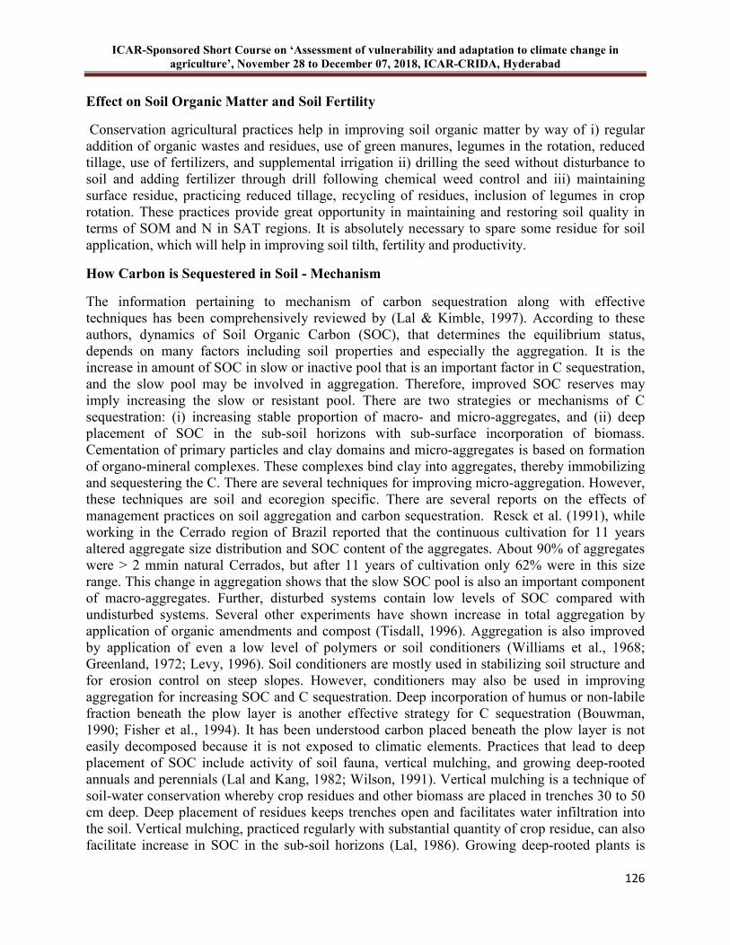
ICAR-Sponsored Short Course on ‘Assessment of vulnerability and adaptation to climate change in
agriculture’, November 28 to December 07, 2018, ICAR-CRIDA, Hyderabad
126
Effect on Soil Organic Matter and Soil Fertility
Conservation agricultural practices help in improving soil organic matter by way of i) regular addition of organic wastes and residues, use of green manures, legumes in the rotation, reduced tillage, use of fertilizers, and supplemental irrigation ii) drilling the seed without disturbance to soil and adding fertilizer through drill following chemical weed control and iii) maintaining surface residue, practicing reduced tillage, recycling of residues, inclusion of legumes in crop rotation. These practices provide great opportunity in maintaining and restoring soil quality in terms of SOM and N in SAT regions. It is absolutely necessary to spare some residue for soil application, which will help in improving soil tilth, fertility and productivity.
How Carbon is Sequestered in Soil - Mechanism
The information pertaining to mechanism of carbon sequestration along with effective techniques has been comprehensively reviewed by (Lal & Kimble, 1997). According to these authors, dynamics of Soil Organic Carbon (SOC), that determines the equilibrium status, depends on many factors including soil properties and especially the aggregation. It is the increase in amount of SOC in slow or inactive pool that is an important factor in C sequestration, and the slow pool may be involved in aggregation. Therefore, improved SOC reserves may imply increasing the slow or resistant pool. There are two strategies or mechanisms of C sequestration: (i) increasing stable proportion of macro- and micro-aggregates, and (ii) deep placement of SOC in the sub-soil horizons with sub-surface incorporation of biomass. Cementation of primary particles and clay domains and micro-aggregates is based on formation of organo-mineral complexes. These complexes bind clay into aggregates, thereby immobilizing and sequestering the C. There are several techniques for improving micro-aggregation. However, these techniques are soil and ecoregion specific. There are several reports on the effects of management practices on soil aggregation and carbon sequestration. Resck et al. (1991), while working in the Cerrado region of Brazil reported that the continuous cultivation for 11 years altered aggregate size distribution and SOC content of the aggregates. About 90% of aggregates were > 2 mmin natural Cerrados, but after 11 years of cultivation only 62% were in this size range. This change in aggregation shows that the slow SOC pool is also an important component of macro-aggregates. Further, disturbed systems contain low levels of SOC compared with undisturbed systems. Several other experiments have shown increase in total aggregation by application of organic amendments and compost (Tisdall, 1996). Aggregation is also improved by application of even a low level of polymers or soil conditioners (Williams et al., 1968; Greenland, 1972; Levy, 1996). Soil conditioners are mostly used in stabilizing soil structure and for erosion control on steep slopes. However, conditioners may also be used in improving aggregation for increasing SOC and C sequestration. Deep incorporation of humus or non-labile fraction beneath the plow layer is another effective strategy for C sequestration (Bouwman, 1990; Fisher et al., 1994). It has been understood carbon placed beneath the plow layer is not easily decomposed because it is not exposed to climatic elements. Practices that lead to deep placement of SOC include activity of soil fauna, vertical mulching, and growing deep-rooted annuals and perennials (Lal and Kang, 1982; Wilson, 1991). Vertical mulching is a technique of soil-water conservation whereby crop residues and other biomass are placed in trenches 30 to 50 cm deep. Deep placement of residues keeps trenches open and facilitates water infiltration into the soil. Vertical mulching, practiced regularly with substantial quantity of crop residue, can also facilitate increase in SOC in the sub-soil horizons (Lal, 1986). Growing deep-rooted plants is
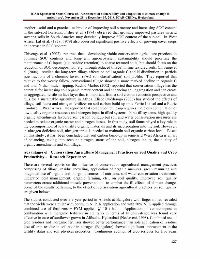
ICAR-Sponsored Short Course on ‘Assessment of vulnerability and adaptation to climate change in
agriculture’, November 28 to December 07, 2018, ICAR-CRIDA, Hyderabad
127
another useful and a practical technique of improving soil structure and increasing SOC content in the sub-soil horizons. Fisher et al. (1994) observed that growing improved pastures in acid savanna soils in South America may drastically improve SOC content of the sub-soil. In West Africa, Lal et al. (1978; 1979) also observed significant positive effects of growing cover crops on increase in SOC content.
Chivenge et al (2007) reported that developing viable conservation agriculture practices to optimize SOC contents and long-term agroecosystem sustainability should prioritize the maintenance of C inputs (e.g. residue retention) to coarse textured soils, but should focus on the reduction of SOC decomposition (e.g. through reduced tillage) in fine textured soils. Chivenge et al (2004) studied the long-term tillage effects on soil organic C and N distribution in particle size fractions of a chromic luvisol (FAO soil classification) soil profile. They reported that relative to the weedy fallow, conventional tillage showed a more marked decline in organic C and total N than mulch ripping. Rachid Marbet (2002) reported that conservation tillage has the potential for increasing soil organic matter content and enhancing soil aggregation and can create an aggregated, fertile surface layer that is important from a soil erosion reduction perspective and thus for a sustainable agriculture in Africa. Elisée Ouédraogo (2006) has studied the effects of tillage, soil fauna and nitrogen fertilizer on soil carbon build-up on a Ferric Lixisol and a Eutric Cambiso in West Africa. He reported that soil carbon build-up requires judicious combination of low quality organic resources and nitrogen input in tilled systems. In no-till systems, high quality organic amendments favoured soil carbon buildup but soil and water conservation measures are needed to reduce organic matter and nitrogen losses. In this study, soil fauna played a key role in the decomposition of low quality organic materials and its incorporation into the soil. However, in nitrogen deficient soil, nitrogen input is needed to maintain soil organic carbon level. Based on this study , it has been concluded that soil carbon build-up in semi-arid West Africa is an art of balancing, taking into account nitrogen status of the soil, nitrogen inputs, the quality of organic amendments and soil tillage.
Advantages of Conservation Agriculture Management Practices on Soil Quality and Crop
Productivity - Research Experiences
There are several reports on the influence of conservation agricultural management practices comprising of tillage, residue recycling, application of organic manures, green manuring and integrated use of organic and inorganic sources of nutrients, soil water conservation treatments, integrated pest management, organic farming, etc., on soil quality. Improved soil quality parameters create additional muscle power to soil to combat the ill effects of climate change. Some of the results pertaining to the effect of conservation agricultural practices on soil quality are given below:
The studies conducted over a 9 year period in Alfisols at Bangalore with finger millet, revealed that the yields were similar with optimum N, P, K application and with 50% NPK applied through combined use of fertilizers + FYM applied @ 10 t ha-1. Application of vermicompost in combination with inorganic fertilizer in 1:1 ratio in terms of N equivalence was found very effective in case of sunflower grown in Alfisol at Hyderabad (Neelaveni, 1998). Combined use of crop residues and inorganic fertilizer showed better performance than sole application of residue. Use of crop residue in soil poor in nitrogen (Bangalore) showed significant improvement in the fertility status and soil physical properties. Continuous addition of crop residues for five years
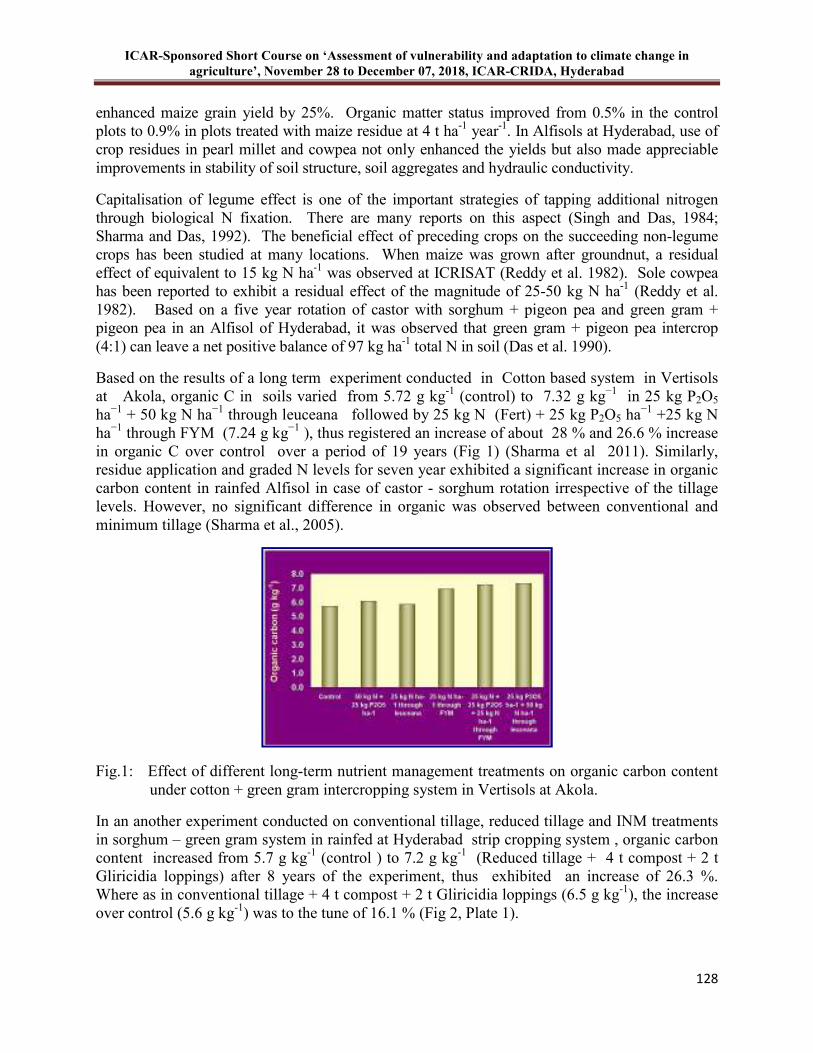
ICAR-Sponsored Short Course on ‘Assessment of vulnerability and adaptation to climate change in
agriculture’, November 28 to December 07, 2018, ICAR-CRIDA, Hyderabad
128
enhanced maize grain yield by 25%. Organic matter status improved from 0.5% in the control plots to 0.9% in plots treated with maize residue at 4 t ha-1 year-1. In Alfisols at Hyderabad, use of crop residues in pearl millet and cowpea not only enhanced the yields but also made appreciable improvements in stability of soil structure, soil aggregates and hydraulic conductivity.
Capitalisation of legume effect is one of the important strategies of tapping additional nitrogen through biological N fixation. There are many reports on this aspect (Singh and Das, 1984; Sharma and Das, 1992). The beneficial effect of preceding crops on the succeeding non-legume crops has been studied at many locations. When maize was grown after groundnut, a residual effect of equivalent to 15 kg N ha-1 was observed at ICRISAT (Reddy et al. 1982). Sole cowpea has been reported to exhibit a residual effect of the magnitude of 25-50 kg N ha-1 (Reddy et al. 1982). Based on a five year rotation of castor with sorghum + pigeon pea and green gram + pigeon pea in an Alfisol of Hyderabad, it was observed that green gram + pigeon pea intercrop (4:1) can leave a net positive balance of 97 kg ha-1 total N in soil (Das et al. 1990).
Based on the results of a long term experiment conducted in Cotton based system in Vertisols at Akola, organic C in soils varied from 5.72 g kg-1 (control) to 7.32 g kg−1 in 25 kg P2O5 ha−1 + 50 kg N ha−1 through leuceana followed by 25 kg N (Fert) + 25 kg P2O5 ha−1 +25 kg N ha−1 through FYM (7.24 g kg−1 ), thus registered an increase of about 28 % and 26.6 % increase in organic C over control over a period of 19 years (Fig 1) (Sharma et al 2011). Similarly, residue application and graded N levels for seven year exhibited a significant increase in organic carbon content in rainfed Alfisol in case of castor - sorghum rotation irrespective of the tillage levels. However, no significant difference in organic was observed between conventional and minimum tillage (Sharma et al., 2005).
Fig.1: Effect of different long-term nutrient management treatments on organic carbon content under cotton + green gram intercropping system in Vertisols at Akola.
In an another experiment conducted on conventional tillage, reduced tillage and INM treatments in sorghum – green gram system in rainfed at Hyderabad strip cropping system , organic carbon content increased from 5.7 g kg-1 (control ) to 7.2 g kg-1 (Reduced tillage + 4 t compost + 2 t Gliricidia loppings) after 8 years of the experiment, thus exhibited an increase of 26.3 %. Where as in conventional tillage + 4 t compost + 2 t Gliricidia loppings (6.5 g kg-1), the increase over control (5.6 g kg-1) was to the tune of 16.1 % (Fig 2, Plate 1).
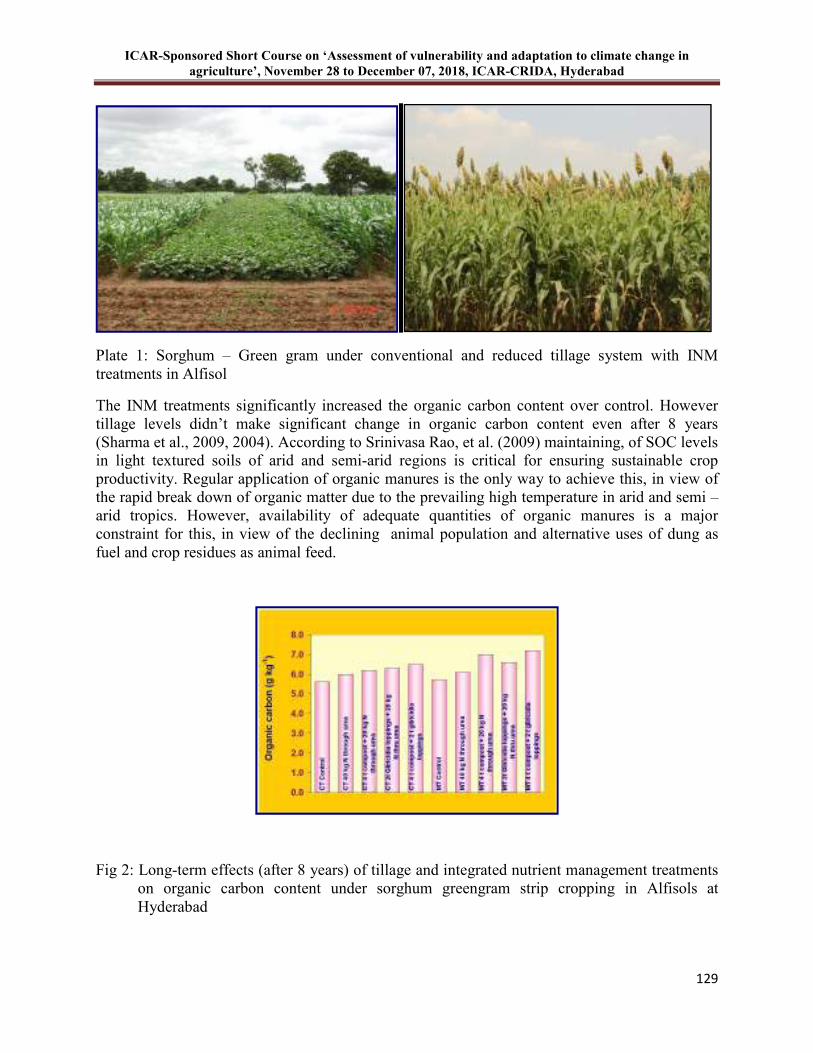
ICAR-Sponsored Short Course on ‘Assessment of vulnerability and adaptation to climate change in
agriculture’, November 28 to December 07, 2018, ICAR-CRIDA, Hyderabad
129
Plate 1: Sorghum – Green gram under conventional and reduced tillage system with INM treatments in Alfisol
The INM treatments significantly increased the organic carbon content over control. However tillage levels didn’t make significant change in organic carbon content even after 8 years (Sharma et al., 2009, 2004). According to Srinivasa Rao, et al. (2009) maintaining, of SOC levels in light textured soils of arid and semi-arid regions is critical for ensuring sustainable crop productivity. Regular application of organic manures is the only way to achieve this, in view of the rapid break down of organic matter due to the prevailing high temperature in arid and semi –arid tropics. However, availability of adequate quantities of organic manures is a major constraint for this, in view of the declining animal population and alternative uses of dung as fuel and crop residues as animal feed.
Fig 2: Long-term effects (after 8 years) of tillage and integrated nutrient management treatments on organic carbon content under sorghum greengram strip cropping in Alfisols at Hyderabad

ICAR-Sponsored Short Course on ‘Assessment of vulnerability and adaptation to climate change in
agriculture’, November 28 to December 07, 2018, ICAR-CRIDA, Hyderabad
130
Based on the network tillage experiment being carried out since 1999 at various centers of All India Coordinated Research Project on Dryland Agriculture (AICRPDA), it was observed that in arid (< 500 mm rainfall) region, low tillage was almost comparable to conventional tillage in terms of crop response and the weed management was not so difficult, whereas, in semi arid (500 – 1000 mm) region, conventional tillage was found superior. It is a well-established fact that infiltration of rainfall depends on soil loosening and its receptiveness and thus requires more surface disturbance. Success of crops depends on rainfall infiltration and soil moisture holding in the profile. For improving the carbon content in soil, apart from crop residues, the agro-forestry also becomes important. However, nothing comes free. The agro-forestry system comprising of perennial components depends on the sub-soil components. It has been observed that grasslands and tree system play an important role in improving soil properties such as bulk density, mean weight diameter, water stable aggregates and organic carbon. Apart from the above, other soil properties such as infiltration rate and hydraulic conductivity were also influenced due to agro forestry systems compared to agricultural systems Ramakrishna et al., (2005).
Based on a long term study, it was found that the tillage conventional tillage (CT) recorded 11.0% higher yields (1534 kg/ha) over the low tillage (LT) (1382 kg/ha) practice. Among the conjunctive nutrient management treatments, the application of 2 t Gliricidia loppings + 20 kg N through urea to sorghum crop recorded significantly highest grain yield of 1712 kg/ha followed by application of 4 t compost + 20 kg N through urea (1650 kg/ha) as well as 40 kg N through urea (1594 kg/ha). As in case of sorghum, CT showed a significant influence on mung bean grain yield (888 kg/ha) which was 6.7% higher compared to LT (832 kg/ha). Application of 2 t compost + 10 kg N through urea and 2 t compost + 1 t Gliricidia loppings performed significantly well and recorded higher mungbean grain yields of 960 kg/ha. In case of mung bean, the long-term trends revealed that, the performance of minimum tillage on an average, was near to that of conventional tillage with slight fluctuation depending upon the rainfall distribution during the cropping season. In both the crops, conventional tillage recorded significantly higher net returns compared to low tillage. In case of Sorghum, net returns obtained were significantly higher with 4 t compost + 20 Kg N/ha through urea (T3) (` 30,262) . The benefit-cost ratio (BCR) in sorghum crop was significantly higher (3.0) with application of 40 kg N through urea alone followed by 2 t Gliricidia loppings + 20 kg N through urea (2.77). Highest BCR (4.02) was observed with application of 2 t Gliricidia loppings + 20 kg N through urea under minimum tillage followed by recommended nitrogen dose of 40 kg/ha (through inorganic fertilizer) and application of 2 t compost + 10 kg N through urea (3.97) in mung bean. Low tillage recorded higher energy use efficiency (10.16, 5.05) compared to conventional tillage (7.21, 3.36) in case of Sorghum and mung bean, respectively (Sharma et al 2015). In an average, CT maintained 30.4 and 57.0% higher grain yields of sorghum and castor, respectively, over MT. Between two residues, GL performed well in both the crops. The highest yields of sorghum (1425 kg ha−1) and castor (876 kg ha−1) were recorded at 90 kg N ha−1. CT maintained higher SYI of 0.44 compared to MT (0.38) and higher agronomic efficiency (AE) of 13.5 and 6.76 kg grain kg−1 N for sorghum and castor crop, respectively. Use of crop residue as mulch had an advantage in increasing the yield of both the crops with increase in rainfall under CT even without N application (control), probably by making the soil more receptive to water infiltration, better moisture storage and by reducing the evaporative losses. Using response functions, the optimum fertilizer N requirement was also computed for a given set of tillage and residue combinations.
ICAR-Sponsored Short Course on ‘Assessment of vulnerability and adaptation to climate change in
agriculture’, November 28 to December 07, 2018, ICAR-CRIDA, Hyderabad
131
The revised optimum fertilizer N doses for sorghum and castor varied from 45 to 56 kg ha−1 and 46 to 74 kg ha−1, respectively, under different tillage and residue combinations and could be recommended depending upon the soil management practices. (J. Kusuma Grace et.al. 2013)
Strategies for Promoting Conservation Agricultural Practices
The following strategies are suggested to promote conservation agriculture in the future:
1) It is of paramount importance to create awareness among the communities about the importance of soil resources, organic matter build up in soil. Traditional practices such as burning of residues, clean cultivation, intensive tillage and pulverization of soil up to finest tilth need to be discouraged.
2) It has been felt that systems approach is essential for fitting conservation tillage in modern agriculture. In order to follow the principle of “grain is to man and a residue is to soil”, farming systems approach introducing alternative fodder crops is essential. Agroforestry systems with special emphasis on silvipastures systems need to be introduced. Unproductive livestock herds needs to be discouraged
3) The enhanced use of herbicides has become inevitable for adopting conservation tillage/conservation farming practices. The countries that use relatively higher amount of herbicides are already facing problem of non-point source pollution and environmental hazard. In order to reduce the herbicidal demand, there are scopes to study the allelopathic effects of cover crops and intercultural and biological method of weed control. In other words, due concentration is needed to do research on regenerative cropping systems to reduce dependence on inorganic chemicals.
4) For following conservation tillage, it is essential that complete package of practices may be identified based on intensive research for each agro ecological region.
5) Minimum tillage, crop rotation, cover crops, maintenance of residues on the surface, control of weeds through herbicides, are the key components of conservation farming. Therefore, it is essential that these themes must be studied in depth under diverse soil and climatic conditions across the country on long-term basis.
6) The additional objective of conservation farming is to minimize the inputs originating from non-renewable energy sources. Eg. Fertilizers and pesticides. Hence, research focus is required on enhancing fertilizer use efficiency and reduction in use of pesticides. This aspect can be strengthened by following integrated nutrient management and integrated pest management approach.
7) The past research experiences of conservation tillage reveal that the major toll of yield is taken by poor germination and poor crop stand because of poor microclimatic environment and hard setting tendencies of soil, excessive weed growth and less infiltration of water to the crop root zone. Therefore, the important aspects which need concentrated research focus include appropriate time of sowing, suitable seed rate, depth of seed placement and soil contact, row orientation, etc. Suitable cultivars having responsiveness to inputs also become important component of conservation farming.
8) The issues related to development of eco-friendly practices for tillage and residue recycling – appropriately for specific combination of soil-agro climatic cropping system – to alleviate physical constraints with higher water and nutrient use efficiency need to be addressed.

ICAR-Sponsored Short Course on ‘Assessment of vulnerability and adaptation to climate change in
agriculture’, November 28 to December 07, 2018, ICAR-CRIDA, Hyderabad
132
9) Inter-disciplinary research efforts are required to develop appropriate implements for seeding in zero tillage, residue incorporation and inter-cultural operations.
Research focus is needed on modeling of tillage dynamics and root growth, incorporation of soil-physical properties in crop-growth simulation models and relating it to crop yields under major cropping sequences.
Conclusions
Climate change is imminent. In order to protect the land from climatic extremes and to restore and improve the quality of soils, conservation tillage comprising of minimum or zero tillage in combination with appropriate mechanism of surface residue retention can play key role. Further, conservation tillage, a generic term implying all tillage methods that reduce runoff and soil erosion in comparison with plow-based tillage, is known to increase SOC content of the surface soil layer. Principal mechanisms of carbon sequestration with conservation tillage are increase in micro-aggregation and deep placement of SOC in the sub-soil horizons. Other useful agricultural practices associated with conservation tillage are those that increase biomass production (e.g., soil fertility enhancement, improved crops and species, cover crops and fallowing, improved pastures and deep-rooted crops). It is also important to adopt appropriate need based soil and crop management systems that accentuate humification and increase the passive fraction of SOC. Because of the importance of C sequestration, soil quality should be evaluated in terms of its SOC content. Beside this, conservation agricultural practices also play an important role in climate change mitigation by i) reducing the fuel requirement in tillage operations and consequently, the associated emissions due to fuel burning and ii) also by reducing the CO2 fluxes coming from soil by sequestering more C in soil profile an making the soil as net sink and not the emitter. Above all, CA and resource conservation practices directly and indirectly help in increasing crop productivity, water use efficiency and over all water productivity.
Thus, in the years to come, conservation agricultural practices can play a major role in increasing the organic C content in soil, improving crop and water productivity and in reducing the CO2
fluxes to the atmosphere.
References
Blevins RL and Frye WW. 1993. Conservation tillage: An ecological approach to soil management. Advances in Agronomy. 51: 33–78.
Bouwman AF. (ed). 1990. Soils and the Greenhouse Effect. J. Wiley & Sons, Chichester, U.K.
Chivenge PP, Murwira HK and Giller KE. 2004. Tillage Effects on Soil Organic Carbon and Nitrogen Distribution in Particle Size Fractions of a Red Clay Soil Profile in Zimbabwe. In: Managing nutrient cycles to sustain soil fertility in sub- saharam Africa. (eds.) Andre Bationo, Susan ikerra, Stephen kimani, Daniel Mugendi, Martins Odendo, Mary silver. Academy Science publishers (ASP). A division of the African Academy of Science (AAS).
ICAR-Sponsored Short Course on ‘Assessment of vulnerability and adaptation to climate change in
agriculture’, November 28 to December 07, 2018, ICAR-CRIDA, Hyderabad
133
Das SK, Sharma KL and Rao KPC. 1990. Response of castor bean (Ricinus communis) to fertilizer nitrogen under different crop rotation on dryland Alfisol. Accepted for XIV International Soil Science Congress held at Tokyo, Japan, August 1990.
Doran JW and Parkin TB. 1994. Defining and assessing soil quality. In: Defining Soil Quality for a Sustainable Environment. J. W. Doran, D. C. Coleman, D. F. Bezdicek, and B. A. Stewart (Eds.). Soil Science Society of America. Special Publication No.35, Madison, Wisconsin, USA, pp. 3-21.
Elisée Ouédraogo. 2006. Soil carbon build-up in semi-arid West Africa: An art of balancing. Conference paper No.54-8, presented in 18th World Congress of Soil Science July 9-15, - Philadelphia, Pennsylvania, USA.
Fisher MJ, Rao IM, Ayarza MA, Lascano CE, Sanz JI, Thomas RJ and Vera RR. 1994. Carbon storage by introduced deep-rooted grasses in the South American savannas. Nature 371: 236–238.
Greenland DJ. 1972. Adsorption of PVA by oxides and clays with non-expanding lattices. In M. De Boodt (ed) “Fundamentals of Soil Conditioning”, Symp. Proc. 17–21 April, 1972, Gent, Belgium.
Grace J Kusuma, Sharma KL, Sumachandrika D, Srinivas K, Mandal UK, Raju BMK, Korwar GR, Venkateswarlu B, Shalander Kumar, Maruthi Sankar GR, Munnalal, Satish Kumar T, Sammi Reddy K and Reshmashinde. 2013. Effect Of Long-Term Use Of Tillage, Residues and N Levels in Sorghum (Sorghum Vulgare (L)) –Castor (Ricinus Communis) Cropping System Under Rainfed Conditions – Crop Responses and Economic Performance – Part I Expl Agric. 49 (3) 395–415
Karlen DL, Mausbach MJ, Doran JW, Cline RG, Harres RF and Schuman GE. 1997. Soil quality: A concept definition, and framework for evaluation. Soil Science Society of America Journal. 61: 4-10.
Lal R. 1989. Conservation tillage for sustainable agriculture: tropics versus temperate environments. Advances of Agronomy. 42: 86–197.
Lal R. 1994. Date analysis and interpretation. In: Methods and Guidelines for Assessing Sustainable Use of Soil and Water Resources in the Tropics, R. Lal (Ed.). Soil Management Support Services Technical. Monograph. No. 21. SMAA/SCS/USDA, Washington D. C, pp. 59-64.
Lal R and Kang BT. 1982. Management of organic matter in soils of the tropics and sub- tropics. XII Cong. Int0l Society of Soil Science. New Delhi, India: 152–178.
Lal R and Kimble JM. 1997. Conservation tillage for carbon sequestration. Nutrient Cycling in Agroecosystems 49: 243–253, 1997. 243
ICAR-Sponsored Short Course on ‘Assessment of vulnerability and adaptation to climate change in
agriculture’, November 28 to December 07, 2018, ICAR-CRIDA, Hyderabad
134
Lal R. 1978. Influence of within- and between-row mulching on soil temperature, soil moisture, root development and yield of maize in a tropical soil. Field Crops Res. 1: 127–139.
Lal R. 1979. Influence of six years of no-tillage and conventional plowing on fertilizer response of maize on an Alfisol in the tropics. Soil Science Society of America Journal. 43: 399–403.
Lal R. 1986. Soil surface management in the tropics for intensive land use and high and sustained production. Advances of Soil Science. 5: 1–105.
Levey GJ. 1996. Soil stabilizers. In M. Agassi (ed) “Soil Erosion, Conservation and Rehabilitation”, Marcel Dekker, Inc., New York, 402 pp.
Mannering JV and Fenster CR. 1983. What is conservation tillage? J. Soil Water Conserv. 38, 141-143.
Neeleveni. 1998. Efficient use of organic matter in semi-arid environment through vermiculture composting and management. PhD Thesis submitted to ANGRAU, Rajendranagar, Hyderabad.
Philip B, Addo DB, Delali DG, Asare BE, Bernard T, Soren DL and John A. 2007. Conservation agriculture as practiced in Ghana. Nairobi: African Conservation Tillage Network; Paris, France:, Centre de cooperation international de recherche agronomique, pour le development ; Rome, Italy: Food and Agriculture, Organization of the United Nations. p 45.
Rachid Mrabet. 2002. Stratification of soil aggregation and organic matter under conservation tillage systems in Africa. Soil & Tillage Research 66: 119–128
Ramakrishna YS, Vittal KPR and Sharma KL. 2005. Conservation agriculture in rainfed semi-arid tropics-some past experiences, lessons learnt and future scope. In: Conservation Agriculture-Status and Prospects (eds: I.P. Abrol, R.K. Gupta., and R.K. Malik), Centre for Advancement of Sustainable Agriculture (CASA), PUSA campus, New Delhi. pp: 199-209.
Rao GGSN, Rao VUM, Vijaya Kumar P, Rao AVMS and Ravindra Chary G. 2010. Climate risk management and contingency crop planning. Lead papers. In: National Symposium on Climate Change and Rainfed Agriculture, 18-20 February, 2010, CRIDA, Hyderabad, India. Organized by Indian Society of Dryland Agriculture and Central Research Institute for Dryland Agriculture. Pp. 37.
Reddy MS, Rego TJ, Burford JR and Willey RW. 1982. Paper presented at the Expert Consultations on Fertilizer use under multiple cropping systems, organized by the FAO at IARI, New Delhi, February, 3-6.
Resck DVS, Pereia J and da Silva JE. 1991. Dinˆamica da mat´eria orgˆanica na Regiao dos Cerrados. Documentos 36. Planaltina, Brazil, EMBRAPA, CPAC.
ICAR-Sponsored Short Course on ‘Assessment of vulnerability and adaptation to climate change in
agriculture’, November 28 to December 07, 2018, ICAR-CRIDA, Hyderabad
135
Seybold CA, Mausbach MJ, Karlen DL, Rogers HH. 1998. Quantification of soil quality. In Lal R, Kimble JM, Follett RF, Stewart BA, eds. Soil Processes and the Carbon Cycle. Boca Raton, FL: CRC Press LLC, pp. 387–404.
Sharma KL, Grace J Kusuma, Mishra PK, Venkateswarlu B, Nagdeve MB, Gabhane VV, Sankar G Maruthi, Korwar GR, Chary G Ravindra, Rao C Srinivasa, Gajbhiye Pravin N, Madhavi M, Mandal UK, Srinivas K and Ramachandran Kausalya. 2011. Effect of Soil and Nutrient-Management Treatments on Soil Quality Indices under Cotton-Based Production System in Rainfed Semi-arid Tropical Vertisol', Communications in Soil Science and Plant Analysis, 42: 11, 1298 — 1315
Sharma KL and Das SK. 1992. Nitrogen and phosphorus management in dryland crops and cropping systems. In Dryland Agriculture in India - State of Art of Research in India (L.L. Somani., K.P.R. Vittal and B.Venkateswarlu eds). Scientific Publishers, P.O. Box 91, Jodhpur -342001, India pp 305-350.
Sharma KL, Vittal KPR, Ramakrishna YS, Srinivas K, Venkateswarlu B and Kusuma Grace J. 2007. Fertilizer use constraints and management in rainfed areas with special emphasis on nitrogen use efficiency. In: (Y. P. Abrol, N. Raghuram and M. S. Sachdev (Eds)), Agricultural Nitrogen Use and Its Environmental Implications. I. K. International Publishing House, Pvt., Ltd. New Delhi. Pp 121-138.
Sharma KL, Mandal UK, Srinivas K, Vittal KPR, Biswapati Mandal, Grace JK and Ramesh V. 2005. Long-term soil management effects on crop yields and soil quality in a dryland Alfisol. Soil-and-Tillage-Research. 83(2): 246-259.
Sharma KL, Srinivas K, Mandal UK, Vittal KPR, Kusuma Grace J and Maruthi Sankar G. 2004. Integrated Nutrient Management Strategies for Sorghum and Green gram in Semi arid Tropical Alfisols. Indian Journal of Dryland Agricultural Research and Development 19 (1): 13-23.
Sharma KL, Kusuma Grace J, Srinivas K, Ramakrishna YS, Korwar GR, Maruthi Sankar G, Uttam Kumar Mandal, Ramesh V, Hima Bindu V, Madhavi M and Pravin N Gajbhiye. 2009. Influence of Tillage and Nutrient Sources on Yield Sustainability and Soil Quality under Sorghum-Mung Bean System in Rainfed Semi-Arid Tropics. Communications in Soil Science and Plant Analysis, 40 (15): 2579-2602.
Sharma KL, Suma Chandrika D, Munna Lal, Srinivas K, Uttam Kumar Mandal, Indoria AK, Sanjeeva Reddy B, Srinivasa rao Ch, Sammi Reddy K, Osman M, Pushpanjali, Rajeshwar Rao G and Usha Rani K. 2015. Long Term Evaluation of Reduced Tillage and Low Cost Conjunctive Nutrient Management Practices on Productivity, Sustainability, Profitability and Energy Use Efficiency in Sorghum (Sorghum bicolor (L.) Moench) - Mung Bean (Vigna radiate (L.) Wilczek) System in Rainfed Semi-Arid Alfisol Indian J. Dryland Agric. Res. & Dev. 30(2) : 50-57
ICAR-Sponsored Short Course on ‘Assessment of vulnerability and adaptation to climate change in
agriculture’, November 28 to December 07, 2018, ICAR-CRIDA, Hyderabad
136
Singh RP and Das SK. 1984. Nitrogen management in cropping systems with particular reference to rainfed lands of India. In: Nutrient management in drylands with special reference to cropping systems and semi-arid red soils. All India Coordinated Research Project for Dryland Agriculture, Hyderabad, India. pp. 1-56.
Srinivasa Rao CH, Ravindra Chary G, Venkateswarlu B, Vittal KPR, Prasad JVNS, Sumanta Kundu, Singh, SR, Gajanan GN, Sharma RA, Deshpande, AN, Patel JJ and Balaguravaiah G. 2009. Carbon sequestration strategies in rainfed production systems of India. Central Research Institute for Dryland Agriculture, ICAR, Hyderabad – 500 059, India. p 102.
Tisdall JM. 1996. Formation of soil aggregates and accumulation of soil organic matter. In M.R. Carter and B.A. Stewart (eds) “Structure and Organic Matter Storage in Agricultural Soils”, CRC/Lewis Publisher, Boca Raton, Fl: 57–95.
Unger PW. 1990. Conservation tillage systems. Advance of Soil Science. 13, 27-68.
Unger PW and McCalla TM. 1980. Conservation tillage systems. Advance in Agronomy. 33: 1–58.
Williams BG, D.J. Greenland and Quirk JP. 1968. Water stability of natural clay aggregates containing polyvinyl alcohol. Australia Journal of Soil Research. 6: 59–66.
WilsonWS. (ed). 1991. Advances in Soil Organic Matter Research: The Impact of Agriculture and the Environment. Royal Society of Chemistry. Cambridge, U.K., 400 pp
ICAR-Sponsored Short Course on ‘Assessment of vulnerability and adaptation to climate change in
agriculture’, November 28 to December 07, 2018, ICAR-CRIDA, Hyderabad
137
Introduction
Climate change is considered as one of the major environmental problems of the 21st
Century. Climate change may be a change in average weather conditions, or in the distribution of weather around the average conditions (i.e., more or fewer extreme weather events). Recent debates focusing on the relationship between climate change stimuli and adaptation in agriculture recognize that climate change includes not only long term changes in mean conditions, but also a change in the year-to-year variation in growing season conditions, and the frequency and magnitude of extreme weather events. The Indian agriculture production system is challenged with the daunting task of feeding 17.5% of the global population with only 2.4% of land and 4% of water resources at its disposal. The warming trend in India over the past 100 years has indicated an increase of 0.6°C, which is likely to impact many crops, and thus affecting food security and livelihood. There are already evidences of negative impacts on yield of wheat and paddy in some parts of India due to increased temperature, water stress and reduction in number of rainy days. Since agriculture contributes currently <15% of India's Gross Domestic Product (GDP), a negative impact on production implies cost of climate change to roughly range from 0.7 to 1.35% of GDP per year. Enhancing agricultural productivity, therefore, is critical for ensuring food and nutritional security for all, particularly the resource poor small and marginal farmers who would be the most affected. In India, the estimated countrywide agricultural loss in 2030 will be over $7 billion that will severely affect the income of 10% of the population. However, this could be reduced by 80%, if cost-effective climate resilience measures are implemented.
Agricultural productivity is sensitive to direct effects due to changes in temperature, precipitation, and carbon dioxide concentrations and indirect effects through changes in soil moisture and the distribution and frequency of infestation by pests and diseases.
A microlevel study on climate variability on rainfed agriculture (Ravindra Chary et al. 2010) indicated that in Bhilwara district of Rajasthan, the annual rain fall is decreasing by 46 mm in the last 40 years, reduction in number of rainy days in last 10 years, in the last 45 years, 21 years found to be arid and 23 years found to be semi-arid. There was change in cropping pattern for the last 20 years i.e. declining area in the irrigated maize replaced with soybean, declined area in irrigated groundnut replaced by either soybean/ sesame/ cluster bean. Rainfed maize is replaced in the last 5 years by sesame, cluster bean and fodder sorghum. The area under fodder sorghum/ black gram/ sesame-fallow system has increased and area under maize-wheat has reduced and replaced in some areas with soybean- wheat/ maize-mustard/ taramira system. In rabi, area under mustard and taramira increased. In the last 15 years, shift in onset of monsoon observed, due to which the sowing window of maize shifted from 7th July to 20th July. This also impacted
13 Adaptation and Mitigation Strategies to Climate Change:
Perspectives
G Ravindra Chary, KA Gopinath and B Narsimlu
ICAR-Sponsored Short Course on ‘Assessment of vulnerability and adaptation to climate change in
agriculture’, November 28 to December 07, 2018, ICAR-CRIDA, Hyderabad
138
in high frequency of mid-season and terminal drought influencing change in varieties of kharif and rabi crops.
Adaptation to Climate Change: The Need
Adapting to climate change entails taking the right measures to reduce the negative effects of climate change (or exploit the positive ones) by making the appropriate adjustments and changes. Adaptation to climate change is a new process for both developed and developing nations, and concrete experience in applying an integrated approach to adaptation is limited (Parry et al.. 2005). Adaptation needs vary across geographical scales (local regional, global) temporal scales (coping with current impacts versus preparing for long-term change), and must be addressed within complex and uncertain conditions. Responding to this process hence calls for interdisciplinary and multiple expertise- a coalescing of researchers and practitioners in climatology, ecology, economics, and management of natural resources, public health, disaster risk reduction, and community development. The agricultural adaptation to climate change come from a various kinds of approaches, particularly research approaches, that consider geographic scales viz., plant, plot, field, farm, region, sector, nation and international ) employing several different perspectives (Smithers and Smit, 1997; Skinner et al. 2001).
Adaptation to Climate Change - Definitions
Many definitions of adaptation are found in the literature. Some of the straightforward definitions describe adaptation as involving “ changes in a system in response to some
force or perturbation, in our case related to climate” (Smithers and Smit, 1997) or as
an adjustment in individual, group and intuitional behavour in order to reduce society's
vulnerabilities to climate” (Pielke, 1998). Definitions of adaptation reviewed by Smit et al. (2000)
• Adaptation to climate is the process through which people reduce the adverse effects of climate on their health and well- being and take advantage of the opportunities that their climatic environment provides
• Adaptation involves adjustments to enhance the viability of social and economic activities and to reduce their vulnerability to climate, including its current variability and extreme events as well as longer- term climate change
• The term adaptation means any adjustment, wheather passive, reactive or anticipatory that is proposed as a means for ameliorating the anticipated adverse consequences associated with climate change
• Adaptation has been defined in different ways (http://www.vcccar.org.au/climate-change- adaptation-definitions)
• The UNFCCC defines it as actions taken to help communities and ecosystems cope with changing climate condition
ICAR-Sponsored Short Course on ‘Assessment of vulnerability and adaptation to climate change in
agriculture’, November 28 to December 07, 2018, ICAR-CRIDA, Hyderabad
139
• The IPCC describes it as adjustment in natural or human systems in response to actual or expected climatic stimuli or their effects, which moderates harm or exploits beneficial opportunities.
• The UN Development Program calls it a process by which strategies to moderate, cope with and take advantage of the consequences of climatic events are enhanced, developed, and implemented.
• The UK Climate Impacts Program defines it as the process or outcome of a process that leads to a reduction in harm or risk of harm, or realisation of benefits associated with climate variability and climate change
• NCCARF regards it as consisting of actions undertaken to reduce the adverse consequences of climate change, as well as to harness any beneficial opportunities.
• The Victorian Government says adapting to climate change is about taking deliberate and considered actions to avoid, manage or reduce the consequences of a hotter, drier and more extreme climate and to take advantage of the opportunities that such changes may generate
The definition used here is taken from IPCC (2001), where in adaptation refers to, “adjustments in ecological, social or economic systems in response to actual or
expected stimuli and their effects or impacts. This term refers to change in process,
practices and structures to moderate potential damages or to benefit from opportunities
associated with climate change”. Adaptation hence involves adjustments to decrease the vulnerability of communities, regions, and nations to climate variability and change and in promoting sustainable development.
Adaptation to Climate Change in Agriculture: The Approaches
Agriculture is inherently sensitive to climate conditions, and is amongst the most vulnerable sectors to the risks and impacts of climate change (Reilly, 1995). The literature indicates that without adaptation, climate change is generally problematic for agricultural production and for agricultural economies and communities; but with adaptation, vulnerability can be reduced and there are numerous opportunities to be realized (Fankhauser, 1996; Smith, 1996; Prasad Rao et al. 2011). Though adaptation is often considered as a government policy response in agriculture, it also involves decision-making by agri- business and producers at the farm-level (Smit, 1994; Adger and Kelly, 1999). Recent debates focusing on the relationship between climate change stimuli and adaptation in agriculture recognize that climate change includes not only long term changes in mean conditions, but also a change in the year-to-year variation in growing season conditions, and the frequency and magnitude of extreme weather events (IPCC, 2001). Understanding that climate change includes climatic variability and extreme events is important in analyses of adaptation. This is particularly so for agriculture, which is generally well adapted to mean or average conditions, but is susceptible to irregular or extreme conditions such as more frequent droughts and
ICAR-Sponsored Short Course on ‘Assessment of vulnerability and adaptation to climate change in
agriculture’, November 28 to December 07, 2018, ICAR-CRIDA, Hyderabad
140
deviations from 'normal' growing season conditions (Risbey et al. 1999.) Some of the approaches with respect to their main perspectives and approaches to adaptation as thought well by Smit and Mark (2002) are briefly presented below:
a. Climate Change Impact Assessment: The early (first generation) impact assessment models provided estimates of the overall agricultural impacts or damages of climate change based on the assumption that no adaptations would occur (Smit et
al. 1989), later (second-generation) impact assessment models arbitrarily assigned adaptations to climate change, assuming adaptive responses on the part of agricultural producers or the system as a whole with respect to changes in average temperature and moisture conditions (Mendelsohn et al.1994). More recently, impact assessments have recognized the importance of farm-level decision-making in the adaptation process, particularly when climatic extremes are considered, and studies have begun to focus on the role of human agency by researching farmer perceptions and risk management choices (Smit et al. 1997). The earlier focus on the potential biophysical impacts of climate change scenarios on agricultural production (i.e. plant growth and crop yields) now shifted to include possible adaptations by producers.
b. Agricultural Vulnerability and Adaptation: Vulnerability research identifies the
climatic attributes relevant to specific agricultural systems (Parry, 1985; Swart and Vellinga, 1994), examines how these attributes are experienced through the variability and extremes associated with climate change (Burton, 1997), and considers adaptation strategies in light of these climatic stimuli and the other conditions that influence decision-making. The vulnerability approach can identify differing sensitivities of specific agricultural systems, as a target for adaptation initiatives, and can indicate the types of adaptation that have been attempted with respect to climatic stimuli. This approach can provide insights into the conditions under which adaptive decision might be made.
c. Risk Management: Much attention is needed for farm-level risk management strategies in order to address uncertainties associated with conditions due to climate variability and change. Risk management research recognizes that decisions in agriculture involve both risk assessment and specific actions taken to reduce, hedge, transfer or mitigate risk. Within this field, adaptation is often considered a response to financial risk in agriculture (climatic or non-climatic).
d. Agricultural Systems and Farm Decision making: Agricultural systems research
has provided much useful information on the nature and dynamics of agricultural production systems and their responses to a myriad of climatic and non- climatic stimuli. This approach emphasizes the interconnections among the various levels within the agriculture system (i.e. field, farm, community, region and nation) and can describe change at aggregate scales and individual farm scales (Cocklin et al.. 1997). Models have been developed in this field to assess the economic impacts of climate related changes in agriculture based on simulations of farm decision-making at the regional (aggregate) scale studies have shown that decisions involving changes in
ICAR-Sponsored Short Course on ‘Assessment of vulnerability and adaptation to climate change in
agriculture’, November 28 to December 07, 2018, ICAR-CRIDA, Hyderabad
141
agriculture are made at different levels that are interrelated, and as a result, patterns of agricultural activity, including adaptation, are the product of many individual decisions (i.e. by government, agri-business and individual producers) (Smithers and Smit, 1997). Farm decision-making is seen as an on-going process, whereby producers are continually making short-term and long-term decisions to manage risks emanating external forces that affect the agricultural system at large (i.e. macro-economic policy, institutional frameworks).
e. Natural Hazards: Climate change studies of agriculture address adaptation as an
adjustment to the risks associated with changes in averages and, more recently, with recurring extreme events. These analyses can be informed by natural hazards research, especially by raising the questions of how farmers perceive the risks associated with climate change (Chiotti et al. 1997; Smit, 1996), and by recognizing that adaptation is directly related to the perception of risks and involves conscious (planned) decision-making.
f. Innovation Adoption: Innovation adoption research provides insights into the decision making process by which adaptations are implemented by producers and diffused among farming communities. Studies in this field focus on the characteristics of producers that influence their decisions about adaptation measures. Factors such as profitability, complexity and compatibility distinguish between innovations that are quickly up-taken and those that are not widely employed (Guerin and Guerin, 1994). This perspective informs an understanding of the processes by which adaptation options are implemented and their likelihood of adoption.
g. Agrarian Political Economy: Adaptation does not simply occur independently at the field or farm level, but it is a process greatly influenced by broader economic, political and social forces. In addition, policy initiatives by governments represent adaptations for the sector as a whole. The role of government policies, institutional arrangements, and macro-level social and economic conditions is increasingly recognized in adaptation studies (Smit, 1994).
Adaptation to Climate Change: Types
Depending on its timing, goal and motive of its implementation adaptation can either be reactive or anticipatory, private or public, planned or autonomous. Adaptation can also be short /long term localized or widespread (IPCC,2001). In unmanaged natural systems, adaptation is autonomous and reactive and is the means by which species respond to changed conditions. In these situations, adaptation assessment is essentially equivalent to natural system impact assessment. Adaptations undertaken by individuals/ communities is the focus here and can be classified as : a. Reactive or Anticipatory: Reactive adaptation takes place after the initial impacts
of climate change have occurred. Anticipatory adaptation takes place before impacts become apparent. In natural systems, there are is no anticipatory adaptation.
ICAR-Sponsored Short Course on ‘Assessment of vulnerability and adaptation to climate change in
agriculture’, November 28 to December 07, 2018, ICAR-CRIDA, Hyderabad
142
b. Private or Public: The distinction is based on whether adaptation is motivated by private (individual households and companies) or public interest (government).
c. Planned and Autonomous: Planned adaptation is consequence of deliberate policy decision, based awareness that conditions have changed or expected to change and that some form of action aids required to maintain a desired state. Autonomous adaptation involves changes that systems will undergo in response to changing climate irrespective of any policy, plan or decision. In summary, adaptation is important in the climate change debate in two ways relating to the development and evaluation of Impacts and vulnerabilities and response options (Smit and Pilifosova, 2001).
Adaptation to Climate Change - The Characteristics
A huge number and variety of measures or actions that could be undertaken in agriculture to adapt to climate change There also exist numerous characteristics by which adaptations can be distinguished, and which could serve as bases for a typology of agricultural adaptations . Smit and Skinner (2002) detailed about the distinguishing characteristics of adaptation such as intent and purposefulness, timing and duration; scale and responsibility; and form and are briefed below.
a. Intent and Purposefulness: Intent and purposefulness differentiate between adaptations that are undertaken spontaneously, or autonomously, as a regular part of on-going management from those that are consciously and specifically planned in light of a climate-related risks (Smit ef al., 2000). Within socio-economic systems, public sector adaptations are usually consciously planned strategies, such as investments in government programs, but private sector and individual adaptations can be autonomous, planned or a combination of the two. For example, the decisions of a producer who, over many years, gradually phases out one crop variety in favour of another that seems to do better in the climatic conditions, might be considered spontaneous and autonomous, but they are also consciously undertaken.
b. Timing and Duration: Timing of adaptation differentiates responses that are anticipatory (proactive), concurrent (during), or responsive (reactive). While logical in principle, this distinction is less clearcut in practice. For example, a producer who has experienced several droughts over recent years, and expects drought frequency to remain similar or increase in the future, may adjust certain production practices or financial arrangements to manage drought risks. The timing distinction is not helpful here, as this is both a reactive and proactive adaptation. Duration of adaptation distinguishes responses according to the time frame over which they apply, such as tactical (shorter-term) versus strategic (longer-term) (Smit et al.. 1996). In agriculture, tactical adaptations might include adjustments made within a season, that involve dealing with a climatic condition, such as drought, in the short term. Tactical adaptations might include selling of livestock, purchasing feed, plowing down a crop or taking out a bank loan. Strategic adaptations refer to structural changes in the farm
ICAR-Sponsored Short Course on ‘Assessment of vulnerability and adaptation to climate change in
agriculture’, November 28 to December 07, 2018, ICAR-CRIDA, Hyderabad
143
operation or changes in enterprises or management that would apply for a subsequent season, or a longer term. Thus, strategic adaptations might include changes in land use, enterprise mix, crop type or use of insurance.
c. Scale and Responsibility: In agriculture, adaptations occur at a variety of spatial scales, including plant, plot, field, farm, region and nation (Smithers and Smit, 1997). At the same time, responsibility can be differentiated among the various stakeholders that undertake or facilitate adaptations in agriculture including individual producers (farmers), agri-business (private industries), and governments (public agencies) (Smit et
al.. 2000). For example, a commonly addressed adaptation in agriculture is the use of crop development for changed climatic conditions. Such an adaptation would likely involve government agencies (encouraging this focus in breeding research), corporations (developing and marketing new crop varieties), and also producers (selecting and growing new crops). Any realistic assessment of adaptation options needs to systematically consider the roles of the various stakeholders.
d. Form: Adaptation in agriculture occurs via a variety of processes and can take many different forms at any given scale or with respect to any given stakeholder. Distinctions among adaptations based on form have been suggested (Carter et al.. 1994; Smithers and Smit, 1997). These studies indicated adaptations according to their administrative, financial, institutional, legal, managerial, organizational, political, practical, structural, and technological characteristics. The forms of adaptation at the farm-level, include changes in resource management, diversification, different forms of policy level adaptations (including aid for research and development) incentive strategies and infrastructure measures.
Adaptation to Climate Change - The Elements
A variety elements or steps are practiced / adopted world over to develop option menu for adaptation to climate change and variability An example of adaptation to climate change in drought prone areas in Bangladesh is illustrated (Asian Disaster Preparedness Centre, FAO). a. Assessing Current Vulnerability: Likely to address society's stand with respect to vulnerability to climate risks , what factors determine this society's current vulnerability and how successful are the efforts to adapt to current climate risks . The major steps to address these questions are to : i). assess natural resources (rainfall, water supply), socioeconomic conditions (agriculture and other land uses /farming systems, migration etc), ii). assess current climate risks (climate variability, soil variability ,cropping systems,spatio- temporal extent of drought, drought impacts), iii). assess local perceptions about climate risks and impacts (household level agricultural strategies like crop substitutions, replanting,in situ moisture conservation practices etc, individual level adjustments etc) , iv). document livelihood profiles in the pilot sites and v). assess institutional frameworks .
ICAR-Sponsored Short Course on ‘Assessment of vulnerability and adaptation to climate change in
agriculture’, November 28 to December 07, 2018, ICAR-CRIDA, Hyderabad
144
b. Assessing future climate risks: Focus on developing scenarios of future climate, vulnerability and environmental trends as a base for considering future climate risks. The major processes involved are : climate impact assessment and outlooks on agriculture ; local agro-meteorlrogical data collection and monitoring and downscaling climate change scenarios
c. Testing adaptation options: Identification and selection of viable adaptation options and the further formulation of these options into farmer-friendly adaptation menus in a participatory mode. The major steps involved are institutional and technical capacity building are: developing adaptation options and extension strategy; validation and selection of adaptation options and community mobilization and local awareness raising
d. Design development strategy: Preparation and dissemination and replication of successful field testing of adaptation options to current vulnerability and future climate risks. The key steps are: advocacy, broader awareness raising and networking ; economic feasibility studies; and field based demonstration and application.
Adaptation Options to Climate Change in Agriculture
The adaptation to refer to ‘adjustments in ecological-social-economic systems in response to actual or expected climatic stimuli, their effects or impacts’ (Smit et al.. 2000). As a result, the types of adaptations included are activities that represent changes in some attribute of the agricultural system directly related to reducing vulnerability to climate change. Smit and Skinner (2002) based on a sysnthesis of research on adaptation options in Canadian agriculture identified four main categories of agricultural adaptation options that are not mutually exclusive They are: (1) technological developments, (2) government programs and insurance, (3) farm production practices, and (4) farm financial management. The typology is based on the scale at which adaptations are undertaken and at which the stakeholders are involved. The first two categories are principally the responsibility of public agencies and agri-business, and adaptations included in these categories might be thought of as system-wide or macro-scale. Categories 3 and 4 mainly involve farm-level decision-making by producers. Of course, the categories are often interdependent. For example, an adaptation technology developed by government and the private sector (type 1), might be adopted to modify farm production practices (type 3). As another example, a producer may buy more crop insurance (type 4), when this insurance is supplied or subsidized by government (type 2). Category I: Technological Developments: Technological adaptations are developed through research programs undertaken or sponsored by public and or private sector. The technological adaptation options could be crop development (to increase their tolerance); weather and climate information systems (to provide forecasts); and resource management (to deal with of climate-related risks). The development of new crop varieties including types, cultivars and hybrids, has the potential to provide crop choices better suited to temperature, moisture and other conditions associated with climate change. This involves the development of plant varieties that are more tolerant to such
ICAR-Sponsored Short Course on ‘Assessment of vulnerability and adaptation to climate change in
agriculture’, November 28 to December 07, 2018, ICAR-CRIDA, Hyderabad
145
climatic conditions as heat or drought through conventional breeding, cloning and genetic engineering (Smithers and Blay-Palmer, 2000). Crop/cropping system based technologies will be mainly centered on promoting the cultivation of crops and varieties that fit into new cropping systems and seasons, development of varieties with changed duration that can overwinter the transient effects of change, release of varieties for high temperature, drought and submergence tolerance, evolving varieties which respond positively in growth and yield to high CO2. Improved and novel agronomic and crop production practices like adjustment of planting dates to minimize the effect of high temperature increase-induced spikelet sterility can be used to reduce yield instability, by avoiding flowering to coincide with the hottest period (Gadgil,1995). Adaptation measures to reduce the negative effects of increased climatic variability as normally experienced in arid and semi-arid tropics may include changing the cropping calendar to take advantage of the wet period and to avoid extreme weather events during the growing season. In addition, improved crop management through crop rotations and intercropping, integrated pest management, supplemented with agroforestry and afforestation schemes will be an important component in strategic adaptation to climate change in India. Intercropping is an efficient strategy that can be followed with desirable outcome in the present climate change scenario (Venkateswarlu and Shanker, 2009).
Another type of technological advance is the development of information systems capable of forecasting weather and climate conditions. Weather predictions over days or weeks have relevance to the timing of operations such as planting, spraying or harvesting. Seasonal forecasts have the potential to aid risk assessment and production decisions over several months. Information on longer- term climate change can inform farmers about future norms and variability, and the probability of extreme events. In these ways, weather and climate information systems can assist farm level adaptation. Farmers may use this information with respect to the timing of operations viz. planting and harvesting, the choice of production activities (i.e. crop varieties), the type of production (i.e. irrigation or dry-land agriculture), and financial management activities (i.e. use of crop insurance and water rights.
Category II: Farm Production Practices: Farm production adaptations include farm-level decisions with respect to farm production, land use, land topography, irrigation, and the timing of operations. Changing farm production activities have the potential to reduce exposure to climate-related risks and increase the flexibility of farm production to changing climatic conditions. Production adaptations could include the diversification of crop varieties, and changes to the intensity of production. Altering crop varieties, including the substitution of plant types, cultivars and hybrids designed for higher drought or heat tolerance, has the potential to increase farm efficiency in changing temperature and moisture stresses (Smit et al. 1996; Chiotti et al. 1997). Altering the intensity of chemical (i.e. fertilizers and pesticides), capital and labour inputs has the potential to reduce the risks in farm production (Hucg et al. 2000). Whether to reduce production risks or to increase productivity levels, the most common adaptations were switching crop types and altering harvest dates. Changing land use practices involves altering the location or nature of crop production. Rotating or shifting
ICAR-Sponsored Short Course on ‘Assessment of vulnerability and adaptation to climate change in
agriculture’, November 28 to December 07, 2018, ICAR-CRIDA, Hyderabad
146
production between crops and livestock, and shifting production away from marginal areas has the potential to reduce soil erosion and improve moisture and nutrient retention. The conservation of moisture and nutrients for drought mitigation can also be improved through the use of alternative fallow and tillage practices ( Hucq et al. 2000). Changing land topography involves land contouring and terracing, and the construction of diversions, reservoirs, and water storage and recharge areas (Easterling, 1996). This type of adaptation reduces farm production vulnerability by decreasing runoff and erosion, improves the retention of moisture and nutrients, and improves water uptake (de Loé et al. 1999). Water management could improve farm productivity and enable diversification of production with respect to climate-related changes (i.e. switching to crops that would otherwise not thrive in dryland agriculture). Changing the timing of operations involves production decisions, such as planting, spraying and harvesting, to take advantage of the changing duration of growing seasons and associated changes in temperature and moisture. Changing the timing of these farm practices has the potential to maximize farm productivity during the growing season and to avoid heat stresses and moisture deficiencies.
Category III: Farm Financial Management: Farm financial adaptations involve decisions with respect to crop insurance, crop shares and futures, income stabilization programs, and household income. Diversification of income sources has been identified as an adaptation option, including off-farm employment and other economic activities, which have the potential to reduce vulnerability to climate-related income loss (Smithers and Smit, 1997).
Category IV: Government Programs and Insurance: Government programs and insurance are institutional responses to the economic risks associated with climate change and have the potential to influence farm-level risk management strategies. These include government agricultural subsidy and support (to decrease the risk of climate-related income loss, and spread exposure to climate-related risks publicly); private insurance (to decrease the risk of climate related income loss, and spread exposure to climate-related risks privately); and resource management programs (to influence resource management in light of changing climate conditions) (Smit and Skinner, 2002). Resource management programs involve the development of government policies and programs that encourage or discourage changes in land use, water use and management practices. This type of adaptation includes the development of land use regulations. These policy instruments of governments represent adaptations at an aggregate scale and also influence farm-level adaptation decision-making. Policy initiatives in relation to access to banking, micro-credit/insurance services before, during and after a disaster event, access to communication and information services is imperative in the envisaged climate change scenario.
Mitigation to Climate Change
Agriculture releases to the atmosphere significant amounts of CO2, CH4, N2O (IPCC, 2001a). CO2 is released largely from microbial decay or burning of plant litter and soil organic matter (Smith, 2004; Janzen, 2004). CH4 is produced when organic materials
ICAR-Sponsored Short Course on ‘Assessment of vulnerability and adaptation to climate change in
agriculture’, November 28 to December 07, 2018, ICAR-CRIDA, Hyderabad
147
decompose in oxygen deprived conditions, notably from fermentive digestion by ruminant livestock, from stored manures, and from rice grown under flooded conditions (Mosier et al. 1998). N2O is generated by microbial transformation of nitrogen in soils and manures, and is often enhanced where available nitrogen (N) exceeds plant requirements, especially under wet conditions (Smith and Conen, 2004). Agricultural GHG fluxes are complex and heterogeneous, but the active management of agricultural systems offers possibilities for mitigation. Many of these mitigation opportunities use current technologies and can be implemented immediately (Smith et al. 2007).
Mitigation - Definition
Climate Change Mitigation refers to efforts to reduce or prevent emission of greenhouse gases. Mitigation can mean using new technologies and renewable energies, making older equipment more energy efficient, or changing management practices or consumer behavior. It can be as complex as a plan for a new city, or as a simple as improvements to a cook stove design. Efforts underway around the world range from high-tech subway systems to bicycling paths and walkways. Protecting natural carbon sinks like forests and oceans, or creating new sinks through silviculture or green agriculture are also elements of mitigation. UNEP takes a multifaceted approach towards climate change mitigation in its efforts to help countries move towards a low-carbon society (http://www.unep.org/climatechange/mitigation). Climate change mitigation are actions to limit the magnitude and/or rate of long-term climate change (Fischer et al. 2007) Climate change mitigation generally involves reductions in human (anthropogenic) emissions of greenhouse gases (GHGs) (IPCC, 2007). Mitigation may also be achieved by increasing the capacity of carbon sinks, e.g., through reforestation (IPCC, 2007) By contrast, adaptation to global warming are actions taken to manage the eventual (or unavoidable) impacts of global warming, e.g., by building dikes in response to sea level rise (Nicholls et al. 2007)
Mitigation - Technologies and Practices
Mitigation options include carbon sequestration in agriculture. Agriculture, provide in principle, a significant potential for greenhouse gases mitigation. The IPCC, estimates that the global technical mitigation potential for agriculture will be between 5,500 and 6,000 Mt CO2- equivalent per year by 2030, 89% of which are assumed to be from carbon sequestration in soils. Opportunities for migrating GHGs in agriculture fall into three broad categories based on the underlying mechanism: a. Reducing emissions: Agriculture releases to the atmosphere significant amounts of
CO2, CH4, N2O (IPCC, 2001a). The fluxes of these gases can be reduced by more efficient management of carbon and nitrogen flows in agricultural ecosystems. For example, practices that deliver added N more efficiently to crops often reduce N2O emissions (Bouwman, 2001), and managing livestock to make most efficient use of feeds often reduces amounts of CH4 produced (Clemens and Ahlgrimm, 2001). The approaches that best reduce emissions depend on local conditions, and therefore, vary from region to region.
ICAR-Sponsored Short Course on ‘Assessment of vulnerability and adaptation to climate change in
agriculture’, November 28 to December 07, 2018, ICAR-CRIDA, Hyderabad
148
b. Enhancing removals: Agricultural ecosystems hold large carbon reserves (IPCC, 2001a), mostly in soil organic matter. Historically, these systems have lost more than 50Pg C ( Lal, 1999, 2004a), but some of this carbon lost can be recovered through improved management, thereby withdrawing atmospheric CO2. Any practice that increases the photosynthetic input of carbon and/or slows the return of stored carbon to CO2 via respiration, fire or erosion will increase carbon reserves, thereby 'sequestering' carbon or building carbon 'sinks'. Many studies, worldwide, have now shown that significant amounts of soil carbon can be stored in this way, through a range of practices, suited to local conditions (Lal, 2004a). Significant amounts of vegetative carbon can also be stored in agro-forestry systems or other perennial plantings on agricultural lands (Albrecht and Kandji, 2003).
c. Avoiding (or displacing) emissions: Crops and residues from agricultural lands can be used as a source of fuel, either directly or after conversion to fuels such as ethanol or diesel (Schneider and McCarl, 2003; Cannell, 2003). These bio-energy feedstock still release CO2 upon combustion, but now the carbon is of recent atmospheric origin (via photosynthesis), rather than from fossil carbon. Often, a practice will affect more than one gas, by more than one mechanism, sometimes in opposite ways, so the net benefit depends on the combined effects on all gases (Schils et al. 2005).
Cropland Management
Mitigation practices in cropland management include the following , partly overlapping categories: a. Improved agronomic practices: Improved agronomic practices that increase yields
and generate higher inputs of carbon residue can lead to increased soil carbon storage. Examples of such practices include: using improved crop varieties; extending crop rotations, notably those with perennial crops that allocate more carbon below ground; and avoiding or reducing use of bare (unplanted) fallow (West and Post, 2002; Lal, 2003, 2004a); adding more nutrients, when deficient, can also promote soil carbon gains (Alvarez, 2005), but the benefits from N fertilizer can be offset by higher N,O emissions from the soils and CO2 from fertilizer manufacture (Gregorich et al. 2005); missions per hectare can also be reduced by adopting cropping systems with reduced reliance on fertilizers, (and therefore, the GHG cost of their production; Paustin et al. 2004), an example is the rotation with legume crops (West and Post, 2002 ), which reduce reliance on external inputs although legume derived N can also be a source of N2O (Rochette and Janzen, 2005); temporary vegetative cover between successive agricultural crops , or between rows of tree or vine crops (these 'catch' or'cover' crops add carbon to soils (Barthes et al.2004) and may also extract plant available N unused by the preceding crop, thereby reducing N2O emissions.
b. Nutrient management: Nitrogen applied in fertilizers, manures, biosolids, and other N sources is not always used efficiently by crops. Improving N use efficiency
ICAR-Sponsored Short Course on ‘Assessment of vulnerability and adaptation to climate change in
agriculture’, November 28 to December 07, 2018, ICAR-CRIDA, Hyderabad
149
can reduce N2O emissions and indirectly reduce GHG emissions from N fertilizer manufacture (Scanhlesinger,1999).Practices that improve N use efficiency include : adjusting application rates based on precise estimation of crop needs (e.g., precision farming); using slow or controlled release fertilizer forms or nitrification inhibitors(which slow the microbial processes leading to N2O formation); applying N when least susceptible to loss, often just prior to plant uptake (improved timing); placing the N more precisely into the soil to make it more accessible to crop roots; or avoiding N applications in excess of immediate plant requirements (Dalal et al. 2003; Monteny et al. 2006). Integrated Nutrient Management (INM) and Site-Specific Nutrient Management (SSNM) also have the potential to mitigate effects of climate change. Demonstrated benefits of these technologies are; increased rice yields and thereby increased net CO2 assimilation, 30-40% increase in nitrogen use efficiency. This offers important prospect for decreasing greenhouse gas emissions linked with N fertilizer use in rice systems. Judicious fertilizer application, a principal component of SSNM approach, thus has 2-fold benefit i.e. reducing GHG emissions; at the same time improving yields under high CO2 levels . CH4 oxidizers, and nitrifiers and denitrifiers in rice paddies which help in maintain the soil redox potential in a range where both N2O and CH4 emissions are low (Hou et al. 2000). The application of urease inhibitor, hydroquinone (HQ), and a nitrification inhibitor, dicyandiamide (DCD) together with urea also is an effective technology for reducing N,O and CH4 from paddy fields.
c. Tillage/residue management: Soil carbon sequestration is the mechanism responsible for most of the mitigation potential, with an estimated 89% contribution to the technical potential. Advances in weed control methods and farm machinery now allow many crops to be grown with minimal tillage (reduced tillage) or without tillage(no-till). These practices are now increasingly adopted throughout the world (e.g., Cerri et al. 2004). Since soil disturbance tends to stimulate soil carbon losses through enhanced decomposition and erosion (Madari et al. 2005), reduced or no tillage agriculture often results in soil carbon gain, but not always (West and Post, 2002; Ogle et al. 2005). The effect of reduced tillage on N2O emissions may depend on soil and climatic conditions. Systems that retain crop reduces also tend to increase soil carbon because these residues are the precursors for soil organic matter, the main carbon store in soil. Avoiding the burning of residues also avoids emissions of aerosols and GHGs generated from fire, although CO2 emissions from fuel use may increase.
d. Water management: Expanding area under irrigated agriculture or adoption of more efficient water management practices can enhance carbon storage in soils through enhanced yieds and residue returns (Lal, 2004a). But some of these gains may be CO2 from energy used to deliver the water (Mosier et al. 2005) or from N2O emissions from higher moisture and fertilizer N inputs (Liebig et al. 2005).
e. Agroforestry: The standing stock of carbon above ground is usually higher than the equivalent land use without trees, and planting trees may also increase soil carbon sequestration (Paul et al. 2003).
ICAR-Sponsored Short Course on ‘Assessment of vulnerability and adaptation to climate change in
agriculture’, November 28 to December 07, 2018, ICAR-CRIDA, Hyderabad
150
f. Land cover/use Change: Encouraging the reversion of crop land to another land cover, typically one similar to the native vegetation, is one of the most effective methods of reducing emissions. The conversion may be total land area or localized spots such as shelter belts (Freibauer et al. 2004; Lal, 2004b). Such land cover changes often increases carbon storage. The land cover/use conversion comes at the expense of lost agricultural productivity, it is usually an option only on surplus agricultural land or on croplands of marginal productivity (Smith et al. 2007).
Interaction of Adaptation and Mitigation Strategies
In the agricultural sector , there are interactions between mitigation and adaptation which may occur simultaneously, but differ in their spatial and geographic characteristics. The main climate change benefits of mitigation actions will emerge over decades, but there may also be short-term benefits if the drivers achieve other policy objectives. Conversely, actions to enhance adaptation to climate change impacts will have consequences in the short and long term. Most mitigations measures are likely robust to future climate change (e.g. nutrient management), but a subset will likely be vulnerable (e.g. irrigation in regions becoming more arid). Conclusion
Globally, the studies on climate change impacts and vulnerability in the agricultural sector is increasingly recognizing the important role of adaptation. The purpose of undertaking agricultural adaptation is to effectively manage potential climate risks over the coming decades as climate changes. Adaptation research undertaken now can help inform decisions by farmers, agribusiness, and policy makers with implications over a range of timeframes from short term tactical to long term strategic. However, it is particularly important to align the scales (spatial, temporal, and sectoral) and reliability of the information with the scale and nature of decision. There is an immense variety of potential and actual adaptation options available, including many different types which have been characterized into four main categories viz., technological developments, government programs and insurance, farm production practices and farm financial management. For specific farm systems, regions and producers, particular forms of adaptation measures would need to be tailored to local conditions and decision-making processes. Adaptation in agriculture involves various stakeholders who have different, but often inter- related roles. Agricultural adaptation options at all levels are part of a larger process, within which decisions are made continuously, in an on-going, 'incremental' fashion, in light of multiple (climatic and non-climatic) stimuli and conditions. There needs to be an understanding of the processes of decision-making in agriculture; of the ways in which potential climate change adaptation fits into real management decision-making of governments, private sector and producers; and of the constraints and stimuli for adaptation. At the same time, any effort to promote and encourage the implementation of adaptation options in agriculture should include an evaluation of options available. This necessitates the recognition of the stakeholder(s) involved in a particular adaptation option, and of how an adaptation relates to broader adaptation decision-making processes. A useful alternative to dealing with particular
ICAR-Sponsored Short Course on ‘Assessment of vulnerability and adaptation to climate change in
agriculture’, November 28 to December 07, 2018, ICAR-CRIDA, Hyderabad
151
'adaptations' is to work to enhance ‘adaptive capacity’, that is, the broader ability of a system (in this case, agricultural producers, regions or sectors) to cope with climate- related risks and opportunities.
Mitigation of GHG emissions associated with various agricultural activities and soil carbon sequestration could be achieved through best management practices, many of which are currently available for implementation. Recycling of agricultural byproducts, such as crop residues and animal manures, and production of energy crops provides opportunities for direct mitigation of GHG emissions from fossil fuel offsets. A number of agricultural mitigation options which have limited potential now have increased potential in the long term. Adoption of better practices like better use of fertilizer through precision farming, wider use of slow and controlled release fertilizers and o nitrification inhibitors, and other practices that reduce N application (and thus N2O emissions). Similarly, enhanced N use efficiency is achievable as technologies such as field diagnostics, fertilizer recommendations from expert/decision support systems and fertilizer placement technologies and water management systems in paddy rice are also likely in the long term.
References
Adger N and Kelly M. 1999. Social vulnerability to climate change and the architecture of entitlements. Mitigation and Adaptation Strategies for Global Change. 4: 253-266.
Albrecht A and Kandji ST. 2003. Carbon sequestration in tropical agroforestry systems.
Agriculture, Ecosystems and Environment, 99: 15-27. Alvarez R. 2005. A review of nitrogen fertilizer and conservation tillage effects on soil
organic storage. Soil Use and Management, 21: 38-52. Barthes BA, Azontonde E, Blanchart C, Girardin C, Villenave S, Lesaint R, Oliver and
Feller C. 2004. Effect of a legume crop (Mucuna pruriens var. utilis) on soil carbon in Ultisol under maize cultivation in southern Benin. Soil Use and Management. 20.231-239.
Bouwman A. 2001. Global Estimates of Gaseous Emissions from Agricultural land.
FAO, Rome.106. Burton 1.1997. Vulnerability and adaptive response in the context of climate and
climate change, Climate Change, 36: 185-196. Cannell MGR. 2003. Carbon sequestration and biomass energy offset: theoretical,
potential and achievable capacities globally, in Europe and the UK. Biomass & Bioenergy, 24: 97-116.
ICAR-Sponsored Short Course on ‘Assessment of vulnerability and adaptation to climate change in
agriculture’, November 28 to December 07, 2018, ICAR-CRIDA, Hyderabad
152
Carter TR, Parry ML, Harasawa H and Nishioka 8.1994. IPCC Technical Guidelines for Assessing Climate Change Impacts and Adaptations, London, Department of Geography, University College London.
Cerri CC, Bernoux M, Cerri CEP and Feller C. 2004. Carbon cycling and sequestration
opportunities in South America: the case of Brazil. Soil Use and Management, 20: 248-254.
Chiotti Q, Johnston TRR, Smit B and Ebel B.1997. Agricultural response to climate
change: A preliminary investigation of farm-level adaptation in southern Alberta' in Ilbery B, Chiotti Q and Rickard T (eds.), Agricultural Restructuring and Sustainability: A geographical perspective, Wallingford, CAB International, pp. 167-183.
Clemens J and Ahlgrimm HJ. 2001. Greenhouse gases from animal husbandry:
mitigation options. Nutrient Cycling in Agroecosystems, 60: 287-300. Cocklin C, Blunden G and Moran W.1997. Sustainability, spatial hierarchies and land-
based production, in Ilbery B, Chiotti Q and Rickard T (eds.), Agricultural Restructuringand Sustainability: A geographical perspective, Wallingford, CAB International, pp. 25-39.
Dalal RC, Wang W, Robertson, GP and Parton WJ. 2003. Nitrous oxide emission from
Australian agricultural lands and mitigation options: a review. Australian Journal of Soil Science. 11(3):335-350.
de Loé R, Kreutzwiser R and Mararu L.1999. Climate Change and the Canadian Water
Sector:Impacts and adaptation, Guelph, Natural Resources Canada. Easterling WE.1996. Adapting North American agriculture to climate change in
review', Agriculture and Forest Meteorology, 80:1-54 Fankhauser S.1996. The potential costs of climate change adaptation, in Smith JB,
BhattiN, Menzhulin G, Bennioff R, Budyko M, Campos M, Jallow B and Rijsberman F (eds.), Adapting to Climate Change: An International Perspective, New York, Springer, pp. 80- 96.
Freibauer A, Rounsevell M, Smith Pand VerhagenA. 2004. Carbon sequestration in the
agricultural soils of European. Geoderma. Pp.122 - 123. Fuseel HM and Klein RJT. 2002. Assessing the Vulnerability and Adaptation to
Climate Change:An Evolution of Conceptual Thinking.Paper Presented at the UNDP Expert Group Meeting on Integrating Disaster Reduction and Adaptation to Climate Change,Havana,Cuba, 17-19,June, 2002.
ICAR-Sponsored Short Course on ‘Assessment of vulnerability and adaptation to climate change in
agriculture’, November 28 to December 07, 2018, ICAR-CRIDA, Hyderabad
153
Gadgil, D. 1995. Climate change and agriculture: An Indian perspective. Current Science, 69(8): 649- 659.
Galloway JN, Dentener FJ, Capone DG, Boyer EW, Howrath, RW, Seizinger, SP,
Asner, GP, Cleveland CC, Green PA, Holland EA, Karl DM, Michaels AF, Porter JH, Townsend AR and Vorosmarty CJ. 2004. Nitrogen cycles: past , present, and uture. Biochemistry, 70: 153-226.
Goswami BN, Venugopal V, Sengupta D, Madhusoodhan,MS, Prince K, Xavier.2006.
Increasing Trend of Extreme Rain Events over India ina Warming Environment. Science, 314.5804, 1442-1445.
Gregorich EG, Rochette P, van den Bygaart AJ and Angers DA. 2005. Greenhouse gas
contributions of agricultural soils and potential mitigation practices in Eastern Canada. Soil and Tillage Research, 83: 53-72.
Guerin LJ and Guerin TR. 1994. Constraints to the adoption of innovations in
agricultural discussion on agriculture, Journal of Rural Study, 11(3): 335-350. Guhathkurta P and Rajeevan M. 2006. Trends in the rainall pattern over India. National
Climate Centre,Report No.2, India Meteorological Department,Pune, India. Houghton JT, Jenkins GJ and Ephrams JJ.1990. IPCC Scientific Assessment of Global
Climate Change, Geneva World Meteorological Organization and United Nations Environmental Plan.
Howden S Mark, Jean-Francois Soussana, Francesco N Tubiello, Netra Chhetri Michael Dunlop and Holger Meinke . 2007. www.pnas.orgcegidoil0.1073pnas.07018901
Hucq A, Kowalshi J, Gutek L and Gray R.2000. Achieving understanding in
agricultural GHG emission reduction, i Scott D, Jones B, Audrey J, Gibson R, Key P, Mortsch L and Warriner K (eds.), Climate Change Communication: Proceedings of an international conference, Kitchener-Waterloo, Canada, Environment Canada, pp. 9-17.
IPCC 2007. Summary for Policymakers. In: Climate Change: The Physical Science
Basis. Contribution of Working Group I to the Fourth Assessment Report of the Intergovernmental Panel on Climate Change (Solomon S, Qin D, Manning M, Chen Z, Marquis M, Averty KB, Tignor M and Miller HL (eds). Cambridge University Press.
IPCC. 2001. Climate Change 2001. Impacts, Adaptation and Vulnerability,
Contribution of Working Group II to the Third Intergovernmental Panel on Climate Change. In: McCarthy JJ, Canziani OF, Leary NA, Dokken DJ and White KS(Eds), Cambridge University Press, Cambridge, UK.

ICAR-Sponsored Short Course on ‘Assessment of vulnerability and adaptation to climate change in
agriculture’, November 28 to December 07, 2018, ICAR-CRIDA, Hyderabad
154
IPCC. 2001a. Climate Change : The Scientific basis. Contribution of Working Group I to the Third Assessment Report of the Intergovernmental Panel on Climate Change (Houghton JT, Ding Y, Griggs DJ, Noguer M, van der Linden PJ, Dai X, Mskell K and Johnson CA. Eds.). Cambridge University Press. pp. 881
Janzen HH. 2004. Carbon cycling in earth systems- a soil science perspective.
Agriculture, Ecosystems and Environment, 104: 399-417. Lal R. 1999. Soil management and restoration for C sequestration to mitigate the
accelerated greenhouse effect. Progress in 40 Adaptation and Mitigation Strategies for Climate Resilient Agriculture Environmental Science, 1: 3017-326.
Lal R. 2003. Global potential of soil carbon sequestration to mitigate the greenhouse
effect. Critical Reviews in Plant Science, 22: 151-184. Lal R. 2004a. Soil carbon sequestration impacts on global climate change and food
security. Science, 304: 1623-1627. Lal R.2004b. Soil carbon sequestration to mitigate climate change. Geoderma, 123: 1-
22. Liebig MA, Morgan JA, Reeder JD, Ellert BH, Gollany HT and Schuman GE. 2005. Greenhouse gas contribution and mitigation potential of agricultural practices in northwestern USA and western Canada. Soil and Tillage Research, 83-25-52.
Madari B, Machado PLOA, Torres E, Andrade AG and Valencia LIO. 2005. No tillage
and crop rotation effects on soil aggregation and organic carbon ina Fhodic erralsol from southern Brazil. Soil and Tillage Research, 80: 185-200.
Mendelsohn R, Nordaus WD and Shaw D.1994. 'The impact of global warming on
agriculture: A Ricardian analysis, American Economical Review, 84(4): 753-771. Monteny GJ, Groenestein CM and Hilhorst MA. 2006. Greenhouse gas abatement
strategies for animal husbandry. Agriculture, Ecosystems and Environment, 112: 163-170.
Mosier AR, Duxbury JM, Freney JR, Heinemeyer O, Minami K and Johnson DE. 1998.
Mitigating agricultural emissions of metahne. Climate Change, 40: 39-80. Mosier AR, Halvorson AD, Peterson GA, Robertson GP, and Sherrod L. 2005.
Measurementof net global warming potential in three agroecosystems. Nutrient Cycling in Agroecosystems, 72: 67-76
Nicholls RJ, et al. 2007. Coastal Systems and Low-Lying Areas", Table 6.11, in IPCC
AR4 WG2 2007, pp. 343
ICAR-Sponsored Short Course on ‘Assessment of vulnerability and adaptation to climate change in
agriculture’, November 28 to December 07, 2018, ICAR-CRIDA, Hyderabad
155
Ogle SM, Bredit FJ, Eve MD and Paustian K. 2005. Agricultural management impacts onsoilorganic carbon storage under moist and dry climatic conditions of temperate and tropical regions. Biochemistry. 72: 87-121.
Parry JE, Hammill A and Drexhage J. 2005. Climate Change and Adaptation, USD. Parry ML.1985. The impact of climatic variations on agricultural margins, in R.W.
Kates JH, Ausubel and Berberian M (eds.), Climate Impact Assessment: Scope 27, Chichester, John Wiley and Sons.
Paul EA, Morris SJ, Six J, Paustian K and Gregorich EG. 2003. Interpretation of soil
organic carbon and nitrogen dynamics in agricultural and afforested soils. Soil Society of America Journal, 67: 1620-1628.
Pielke RA. 1998. "Rethinking the role of adaptation in climate policy", Global
Environmental Change, 8: 159-170. Prasad Rao GSLHV, Kesava Rao, Krishna Kumar and Gopalkumar CS .2011. Climate
change projectionsand impacts on plantations in the humid tropics. In: Climate Change Adaptation Strategies in Agrciulture and Allied Sectors (GSLHV Prasad Rao Ed.)Scientific Publishers, Jodhpur,India).pp.20-31.
Ravindra Chary G, Maruthi Sankar GR, Vittal.KPR, Mishra PK, Venkateswarlu B and
Pratibha G. 2010. Assessment of changing rainfall trends in Agro-Climatic Zones of India: Strategies for prioritizationin Rainfed Agriculture. In : Extended Summaries. National Symposium on Climate Change and Rainfed Agriculture organized by Indian Society of Dryland Agriculture and CRIDA during 18-20 February 2010 at CRIDA, Hyderabad.pp.71.
Reilly J.1995. Climate change and global agriculture: Recent findings and issues,
American Journal of . Agricultural Economics, 77: 727-733. Risbey J, Kandlikar M and Dowlatabadi H. 1999. Scale, context, and decision making
in agricultural adaptation to climate variability and change, Miti. & Adapt. Strategy for Global Change, 4(2): 137-167.
Rochette P and Janzen HH. 2005. Towards a revised coefficient for estimating N,O
emissions from legumes. Nutrient Cycling in Agroecosystems. 73: 171-179. Scanhlesinger WH. 1999. Carbon sequestration in soils. Science. 284: pp. 2095. Schils RLM, Verhagen A, Aarts HFM, and Sebek LBJ. 2005. A farm level approach to
define successful mitigation strategies for ghg emissions rom ruminant livestock systems. Nutrient Cycling in Agroecosystems. 71: 163-175.
ICAR-Sponsored Short Course on ‘Assessment of vulnerability and adaptation to climate change in
agriculture’, November 28 to December 07, 2018, ICAR-CRIDA, Hyderabad
156
Schneider UA and McCarl BA. 2003. Economic potential of biomass based fuels for greenhouse gas emission mitigation. Environmental and Resource Economics, 24: 291-312.
Skinner MW, Smit B, Dolan AH, Bradshaw B and Bryant CR. 2001, Adaptation
Options. Smit B, Pilifosova O, Burton I, Challenger B, Huqs, Klein RJT and Yohe G. 2001. Adaptation to climate change in the context of sustainable development and equity.In: Climate Change 2001. Impacts, Adaptation and Vulnerability. McCarthy J, Canzianim O, Leary N, Dokken D and White K.. Eds) . Cambridge University Press. UK.
Smit B.1996. Climate, compensation and adaptation, in McCulloch Jand Etkin D (eds.),
Proceedings of a Workshop on Improving Responses to Atmospheric Extremes: The role of insurance and compensation, Toronto, Environment Canada/The Climate Institute, pp. 2.29-2.37.
Smit B and Pilifosova O. 2001. Adaptation to climate change in the context of
sustainable development and equity. In: Climate Change 2001: impacts,adaptation and vulnerability, Chapter 18,Cambridge:CambridgeUniversity Press.
Smit Barry and Mark W Skinner . 2002. Adaptation options in agriculture to climate
change: a typology. Mitigation and Adaptation Strategies for Global Change, 7: 85-114, 2002.
Smit B, Blain R, and Keddie P. 1997. Corn hybrid selection and climatic variability:
Gambling with nature Canadian Geography, 41: 429-38. Smit B, Brklacich M, Stewart RB, McBride R, Brown and Bond D. 1989. Sensitivity
ofcrop yields | and land resource potential to climatic change in Ontario, Climate Change, 14:153-174.
Smit B, Burton, I, Klein RJT and Wandel J.2000. An anatomy of adaptation to climate change and variability, Climate Change, 45: 223-251. 42 Adaptation and Mitigation Strategies for Climate Resilient Agriculture
Smit B.1994. Climate, compensation and adaptation’, in J. McCulloch and D. Etkin
(eds.), Proceedings of a Workshop on Improving Responses to Atmospheric Extremes: The role of insurance and compensation, Toronto, Environment Canada/The Climate Institute, pp. 2.29-2.37.
Smith KA and Conen F. 2004. Impacts of land mangement on fluxes of trace
greenhouse gases. Soil Use and Management, 20: 255-263. Smith P, Martino D, Cai Z, Gwary D, Janzen H, Kumar P, McCarl B, Ogle S, O'Mara F,
RiceC, ScholesBand -Sirotenko O. 2007. Agriculture. In: Climate Change 2007. Mitigation. Contribution of Working Group III to the ourth Assessment Report of the Intergovernmental Panel on Climate Change (B. Metz, OR Davidson, PR
ICAR-Sponsored Short Course on ‘Assessment of vulnerability and adaptation to climate change in
agriculture’, November 28 to December 07, 2018, ICAR-CRIDA, Hyderabad
157
Bosch, R Dave, LA Mayer. Eds.). Cambridge University Press, Cambridge, United Kingdom and New York,NY, USA.
Smith P. 2004. Engineereed biological sinks on land. In: Global Carbon Cycle.
Integrating humans, climate, and the natural world( Field CB, and Raupach MR. Eds). SCOPE 62: Island Press, Washington D.C. pp. 479-491.
Smith JB. 1996. Using a decision matrix to assess climate change adaptation'inSmithJB,
Bhatti N, Menzhulin G, Benioff R, Budyko MI, Campos M, Jallow B and Rijsberman F. (eds.),Adapting to Climate Change: An international Perspective, New York, Springer, pp. 68-79.
Smithers J and Smit B.1997. Agricultural system response to environmental stress, in
Ilbery B, Chiotti Q and Rickard T(eds.), Agricultural Restructuring and Sustainability: A geographical perspective, Wallingford, CAB International, pp. 167-183.
Smithers JA and Blay-Palmer A. 2000. Technology innovation as a strategy for climate
change adaptation in agriculture, forthcoming in Applied Geography. Swart RJ and Vellinga P. 1994. The “ultimate objective” of the framework convention
on climate change requires a new approach in climate change research, Climate Change, 26: 343-349.
Venkateswarlu B and Arun K Shanker . 2009. Climate change and agriculture:
Adaptation and mitigation strategies. Indian Journal of Agronomy, 54(2): 226-230.
West TO and Post WM. 2002. Soil organic carbon sequestration rates by tillage and
crop rotation: A global data analysis. Soil Science Society of America Journal, 66: 1930-1946.
ICAR-Sponsored Short Course on ‘Assessment of vulnerability and adaptation to climate change in
agriculture’, November 28 to December 07, 2018, ICAR-CRIDA, Hyderabad
158
14 Potential Role of Resource Conservation Technologies on
Adaptation and Mitigation of Climate Change
G Pratibha
Climate change is one of the most serious threat to sustainable development and is emerging as a major issue affecting many sectors in the world. Globally, an increase in greenhouse emissions has led to increased climate change impacts. Agriculture has shown to contribute immensely to climate change as it ranks third after energy consumption and chlorofluorocarbon production in enhancing green house emissions. In fact, agricultural contributes about 15% of today's anthropogenic greenhouse gas emissions. Land use changes, often made for agricultural purposes, contribute another 8% or so to the total. Impact of climate change on agriculture have become a serious concern globally; more particularly in developing countries like India. The warming trend in India over the past 100 years (1901 to 2007) was observed to be 0.510 C with accelerated warming of 0.210C per every 10 years since 1970 (Krishna Kumar 2009). A series of simulation studies by IPCC have shown that the increase in temperature was mainly due to rise in concentration of GHG.
A general warming trend has been predicted for India in future by all the global climate models, further the rate of warming would be much higher. A study carried out by Goswami (2006) indicated an increase in frequency of heavy rainfall events in last 50 years over Central India. Parts of Western Rajasthan, Southern Gujarat, Madhya Pradesh, Maharashtra, Northern Karnataka, Northern Andhra Pradesh, and Southern Bihar are likely to be more vulnerable in terms of extreme events (Mall et al. 2006). A long term analysis of rainfall trends in India (1901 to 2004) using Mann Kendall test of significance by CRIDA indicated that there is significant increase in rainfall trends in West Bengal, Central India, coastal regions, south western Andhra Pradesh and central Tamil Nadu. Whereas a significant decreasing trend was observed in central part of Jammu Kashmir, Northern MP, Central and western part of UP, northern and central part of Chattisgarh. Analysis of number of rainy days based on the IMD grid data from 1957 to 2007 showed declining trends in Chattisgarh, Madhya Pradesh, and Jammu Kashmir. In Chattisgarh and eastern Madhya Pradesh, both rainfall and number of rainy days are declining which is a cause of concern as this is a rainfed rice production system supporting large tribal population who has poor coping capabilities. In India 56 % of crop production is under rainfed. Nearly 85 m ha of India’s 141 m ha net sown area is rainfed. Rainfed farming area falls mainly in arid, semi-arid and dry sub- humid zones.Rainfed agriculture is likely to be more vulnerable in view of its high dependency on monsoon, the likelihood of increased extreme weather events due to aberrant behavior of south west monsoon. About 74% of annual rainfall occurs during southwest monsoon (June to September). SW monsoon exhibits high coefficient of variation particularly in arid and dry semi- arid regions. Skewed distribution has now
ICAR-Sponsored Short Course on ‘Assessment of vulnerability and adaptation to climate change in
agriculture’, November 28 to December 07, 2018, ICAR-CRIDA, Hyderabad
159
become more common with reduction on number of rainy days. Delay in onset, long dry spells and early withdrawal of monsoon are common abberations in SW monsoon, all the abberaations affect the crops, strongly influence the productivity levels (Lal 2001). These aberrations are likely to further increase in future. The risk of crop failure and poor yields always influence farmers’ decision on investing on new technologies and level of input use (Pandey et al. 2000). Numerous technological (e.g. cropping patterns, crop diversification, and shifts to drought-/salt-resistant varieties) and socio-economic (e.g. ownership of assets, access to services, and infrastructural support) factors will come into play in enhancing or constraining the current capacity of rainfed farmers to cope with climate change.
Impact of Climate Change
Impacts of climate change on agriculture and allied sectors directly or indirectly are being witnessed all over the world (Dhaka et al. 2010), but countries like India are more vulnerable of view of the high population depending on agriculture and excessive pressure on natural resources. The crop losses due to climate variability will vary from region to region depending on regional climate, cropping systems, soils and management practices. Rainfed crops are likely to be worst hit by climate change because of its high dependency on monsoon and the likelihood of increased extreme weather events furthermore there are limited options for coping with variability of rainfall and temperature. Temperature is another important variable influencing crop production in all seasons generally and particularly during winter season. Cereal productivity is projected to decrease anywhere between 10-40% by 2100 and greater loss is expected during winter. Furthermore for every one degree increase in temperature, yields of wheat, soybean, mustard, groundnut and potato are expected to decline by 3-7% . A 2° C increase in average temperatures would reduce world GDP by roughly 1%. ( Stern, 2007).
Decline in maize and sorghum yields in Nalgonda District, Telangana and Parbhani District, Maharashtra was reported during the last few years due to rise in temperatures (Jat et al. 2012). Furthermore, the length of the growing period has been reduced by 15 days, this resulted in yield reduction. In addition to hastening crop maturity and reducing crop yields, increased temperatures will also increase crop water requirement by increasing evapo-transpiration rates. In four major crops viz., wheat, maize, sorghum and pearl millet a 2.2 % increase in crop water requirement was observed by 2020 and 5.5 % by 2050 across all the crops/locations (Venkateswarlu 2010). The climate scenarios for 2020 and 2050 were obtained from Had CM3 model outputs using 1960-1990 as base line weather data. Besides the impact of climate change on crop growth and development, LGP, water availability, etc., there is a possibility of increased soil degradation and loss of soil organic matter due to increase in temperatures. This may also further enhance yield reduction than what is being predicted currently. Hence new technologies are required to enhance the WUE in agriculture.

ICAR-Sponsored Short Course on ‘Assessment of vulnerability and adaptation to climate change in
agriculture’, November 28 to December 07, 2018, ICAR-CRIDA, Hyderabad
160
In addition to direct effects of rainfall intensity on crop growth and yield, rainfall and temperature will increase both abiotic and biotic stresses. Increased rainfall intensity in some regions would cause more soil erosion leading to land degradation and reduced crop and soil productivity. Water requirement of crops is also likely to go up with projected warming: extreme events like floods, cyclones, heat wave and cold wave. The accelerated decomposition of organic matter releases the nutrients in short run, but may reduce the fertility and productivity of soils in the long run. Chemical reactions, that affect soil minerals and organic matter, are strongly influenced by higher soil and water temperature. The impact of climate change on these aspects needs to be studied in detail for sustaining agricultural production.
Adaptation Strategies for Resilience against Climate Change
Any significant change in climate will affect the food grain production and thus increase vulnerability of the large section of resource poor farmers. Hence both technology and policy options are required for adaptation to climate change to minimise the yield losses. Adaptation to climate change is adopting the right measures to reduce the negative effects of climate change (or exploit the positive ones) by making the appropriate adjustments and changes. Adaptation measures such as adjustment of time of planting and harvesting operations, substituting cultivars, crop diversification. The goal of the adaptation strategies is to stabilize agronomic production against the adverse impact of climate (Lal 2007). If the adaptation strategies are not developed and implemented, India, the may face some decline in food production in the long term. Automatic adaptation takes place on its own to progressive climate change; but both short term and long term strategies are required for planned adaptation strategies. Targeted research on adaptation strategies and mitigation is at nascent stage in India but based on existing knowledge, some options for adaptation to climate variability induced effects like droughts, high temperatures, floods and sea water inundation can be suggested (Fig1). These strategies fall into two broad categories viz., (i) crop based and (ii) resource management based. ‘Given the constraints of both current climate-induced production risk and the predicted change in nature of that risk in the future, it is now widely accepted that a two pronged approach, sometimes referred to as the “twin pillars” of adaptation to climate change, is needed. Such an approach recognizes short and medium-term adaptation strategies. There is a need to identify and recommend technologies to the farmers which respond well to climate change effects and give greater resilience against such shocks.
Crop Based Strategies The yield potential of the improved crop varieties is not attained in rainfed regions because of poor crop management practices (Reynolds and Tuberosa 2008). Hence development of crop management practices which improve the resilience of the system while reducing production costs is the need of the hour. Some of the improved management practices include crop diversification with climate resilient crops, changing planting time and varieties that fit into changed rainfall (Swearingen and

ICAR-Sponsored Short Course on ‘Assessment of vulnerability and adaptation to climate change in
agriculture’, November 28 to December 07, 2018, ICAR-CRIDA, Hyderabad
161
Bencherifa 2000, Mortimore and Adams 2001, Southworth et al. 2002, Howden et al. 2007, Phiri and Saka 2008), Growing early maturing, photo-insensitive, high tillering cultivars with optimal root traits which are tolerant to abiotic and biotic stresses; intercropping, mixed cropping, alternate land use system, land use diversification, mulching with crop residues; planting more seedling per hill for heat stress; better soil nutrient and water management, moisture conservation for late onset of monsoon and life-saving irrigation with stored rainwater for mid-season drought are few crop based and resource based strategies recommended to cope with the effects of climate change and variability on dryland agriculture.
Resilient Crops, Cropping Systems And Varieties Vulnerabilities to climate change depends on the region, hence region specific adaptation strategies need to be developed. Identification of climate resilient crops and varieties for different regions is essential for successful adaptation to climate changes and variability. There is a need to develop heat stress, drought and submergence tolerant varieties (Rosegrant and Cline 2003, Eckhardt et al. 2009); In addition to the heat and water stress tolerant varieties salinity and sea water inundation tolerant varieties, varieties which respond positively to high CO2., high fertilizer and radiation use efficiency varieties are required. Germplasm of wild relatives and local land races could prove valuable source of climate ready traits. Hence a re-visit to the earlier germplasm collections which have tolerance traits to heat and cold stresses but not made use in the past due to low yield potential is required. These promising new traits and varieties, which are mostly still in development stage, can emerge from traditional breeding techniques that make use existing germplasm as well as from more advanced techniques such as marker assisted selection and genetic modification. Modeling studies in Zimbabwe proved that retargeting long duration varieties of crops like pigeonpea and sorghum is a better strategy as they would still yield higher despite reduced duration due to warming as compared to short duration cultivars (Dimes et al. (2008). Simulation studies in groundnut at ICRISAT showed that in the warmer regions of India (northern, western and some parts of southern India), the negative effects of increased temperature are large as compared to increase in CO2 and rainfall, Hence, there is a need for temperature-tolerant cultivars, which fit well according to LGP (Jat et
al. 2012). Whereas in the relatively cooler regions the beneficial effects of increase in CO2 and rainfall are higher in terms of biomass production hence there is a need for cultivars with higher harvest index to take advantage of elevated CO2. Knowledge and understanding of photoperiod sensitivity, information on the genetic variation for transpiration efficiency, short duration varieties that escape the terminal drought and high-yielding, disease-resistant varieties will help dryland agriculture adapt to climate change. Some short duration cultivars, heat stress and drought-tolerant lines of chickpea (ICCV 96029 (super early 75–80 days), ICCV 2 (extra early 85–90 days) and KAK 2 (early 90–95 days);, groundnut, pigeonpea (ICPH 2671), pearl millet and sorghum have been identified for cultivation in semi-arid regions with short growing period. The
ICAR-Sponsored Short Course on ‘Assessment of vulnerability and adaptation to climate change in
agriculture’, November 28 to December 07, 2018, ICAR-CRIDA, Hyderabad
162
ICRISAT–NARS-developed improved groundnut variety ICGV 91114 which is more drought-tolerant, with larger seeds, uniform maturity, disease tolerance and better palatability of its straw for livestock, and produced 23% higher yield over the popular variety in Anantapur District (Birthal et al. 2011). In addition to this, some SAUs and NARS system have developed and identified short duration location specific varieties for cultivation in different regions. New varieties and traits can also lead to less intensive use of other inputs such as fertilizers and pesticides . In addition to increasing productivity generally, several new varieties and traits offer farmers greater flexibility in adapting to climate change.
Crop Diversification Crop Diversification towards high value crops is feasible in the medium to long term and is a high priority adaptation measure in both irrigated and non-irrigated areas. Furthermore, crop diversification can serve as insurance against rainfall variability. Crop substitution with a suitable crop can improve the yields by 15 -25 %. with change in rainfall due to climate change(Singh et al. 2007). Hence selection of crop and variety are most fundamental and important for adaptation of crops to dryland agriculture which in turn depends on the soil, rainfall intensity, quantity, temperature and LGP. Studies conducted in Chitoor district of Andhra Pradesh have revealed that groundnut and castor are profitable crops for normal onset of rainfall whereas pigeonpea cultivation is more profitable than groundnut for delayed onset of rainfall (Vineetha et
al. 2011). In India crop diversification by introduction of perennials like multipurpose trees shrubs, medicinal aromatic and dye plants, etc. also help in reducing the vulnerability. Studies conducted at CRIDA has revealed that crop diversification with medicinal aromatic and dye crops and several crops like henna, annatto, ashwagandha, senna, lemongrass were identified as suitable crops for semiarid tropical rainfed regions and were more profitable than the arable crops (Pratibha and Korwar 2002). Such perennials integrated with livestock production in agri pastoral system and horti pastoral systems can reduce the climate risks considerably.
Cropping System In rainfed regions the amount and distribution of rainfall dictates the effective growing season and cropping system. For example in a region 350 -600 mm rainfall and 20 weeks of effective growing season only single cropping season is possible in all the soils. Intercropping is a time tested efficient strategy to cope with climate variability and climate change. If one crop fails due to floods or droughts second crop gives some minimum assured returns for livelihood security. Various intercropping systems have been identified in the past. Grain-legume intercrops have many potential benefits such as stable yields, better resource use, weeds, pest and disease reductions, increased protein content of cereals, reduced N leaching as compared to sole cropping systems. Intercropping systems are recommended in areas receiving rainfall of 650-750mm with

ICAR-Sponsored Short Course on ‘Assessment of vulnerability and adaptation to climate change in
agriculture’, November 28 to December 07, 2018, ICAR-CRIDA, Hyderabad
163
20-30 weeks growing seasons. If the rain fall is above 750mm and effective growing season is more than 30 weeks double cropping is possible (Singh and Reddy 1986).
Crop Management Practices Kaur et al. (2012) observed that increased CO2, irrigation and nitrogen levels may not be able to outweigh the negative effect of temperature in maize, however, in wheat increased CO2 levels in the atmosphere and more of irrigation than the existing level may increase yield. Therefore for crops susceptible to climate change, the agro techniques like use of mulch, managing the light use by changing crop geometry which reduces the influence of temperature would increase the crop yields. The effect of dates of sowing wheat on the yield was simulated for different locations. Areas having higher yield potential of wheat had higher reduction in yield per day with delay in sowing from the optimal date. Whereas in few locations (north eastern parts) a small yield reduction with delayed sowing was observed. With the temperature rise, the adjustments in the date of sowing to have the similar weather conditions can be ensured, change in planting dates can imbalance the cropping system schedule, which is also important for developing countries where intensive cultivation is practiced on small and marginal lands. (Khan et al. 2009). Resource Conservation and Management Technologies
Resource conservation technologies (RCTs) increase natural and applied resource use efficiency in crop production. They indirectly contribute to adaptation and mitigation of climate change. However RCTs in isolation do not provide much advantage moreover the RCTs are location specific. There are large number of resource management options like soil, water and nutrient management strategies. (Kurukulasuriya and Rosenthal 2003). In situ moisture conservation, rainwater harvesting and recycling, efficient use of irrigation water, improving soil organic matter, conservation agriculture, energy efficiency in agriculture and use of poor quality water are some of the important rain water management which contribute to adaptation to climate change. Promotion of sustainable land management practices (SLM) has been suggested as another key adaptation strategy for countries in the developing world, to adapt to growing water shortages, worsening soil conditions, drought and desertification. Many earlier research in rainfed agriculture in India relates to soil and rain water conservation for drought proofing which is an ideal strategy for adaptation to climate change (Venkateswarlu et
al. 2009).
Conservation Agriculture Conservation agriculture (CA) with three principles of zero/minimum tillage, retaining soil cover through crop residues or cover crops and suitable crop rotations is a good concept of combining different RCTs for optimum benefit. CA systems improve the adaptive capacity by increasing water and nutrient use efficiency and increase soil organic matter. Studies conducted in Zimbabwe, have shown that conservation
ICAR-Sponsored Short Course on ‘Assessment of vulnerability and adaptation to climate change in
agriculture’, November 28 to December 07, 2018, ICAR-CRIDA, Hyderabad
164
agriculture has consistently increased average cereal yields by 50–200% in more than 40,000 farm households (Twomlow et al. 2008). In Indo-Gangetic plains rise in temperature during grain filling stage of wheat adversely affects the productivity. Conservation agriculture with zero tillage and residue retention helps in advancing of planting date by few days to a week and surface residue reduces the canopy temperature by 1-1.5 0C during grain filling stage, and increases soil moisture.
In situ and ex situ Rain Water Conservation
The rainfed farmers are more vulnerable since a particular zone might become wetter or drier in the coming decades, Hence soil and water conservation is central to farmers’ adaptation to climate change. It has been predicted that most of the rainfall will now occur in the form of high-intensity short-duration rain events due to global climate change (IPCC, 2007). At national level the water erosion results in an annual loss of 13.4 Mt of cereals, pulses and oil seeds. This loss is more in alfisols as compared to black soils or alluvial soils (Sharad et al. 2010). Hence in rainfed areas, two pronged strategy is needed to prevent land degradation and reduce erosion to a permissible limits. In-situ and ex-situ moisture conservation techniques of rainwater for recycling to rainfed crops is only alternative to sustain current agriculture activities.. Typical SLM technologies used in most developing countries include both agronomic and mechanical measures like the use of soil bunds, stone bunds, grass strips, waterways, trees planted at the edge of farms, contour farming, intercropping, strip cropping, mulching crop geometry, tillage, and supplemental irrigation. Sharma et al. (2010) estimated that about 28 m ha of rainfed area in eastern and central states has the potential to generate runoff of 114 billion cubic meters which can be used to provide one supplemental irrigation in about 25 m ha of rainfed area. For storing such quantum of rainwater about 50 million farm ponds are required. Watershed management is now considered an accepted strategy for development of rainfed agriculture. Watershed approach has many elements which help both in adaptation and mitigation. For example, soil and water conservation works, farm ponds, check dams etc. moderate the runoff and minimize floods during high intensity rainfall. Hence there is a need to quantify the adaptation potential of water shed management by quantifying benefits from each interventions made ridge to valley in terms of preventing carbon loss, C- Sequestration, drought proofing and livelihood resilience. Conserving water in the root zone and enhancing its use efficiency is possible through improved soil structure (Rockstrom et al. 2007). Soil conservation contributes to reduced carbon losses. Lal (2004) estimates that if water and wind erosion are arrested, it can contribute to 3 to 4.6 Tg year-1 of carbon in India. Research efforts have been made since last 4-5 decades and identified number of conservation technologies to reduce the risk of soil degradation, preserve the productive potential, and sustain agricultural productivity in the long run. Some of these erosion control measures include land shaping or mechanical measures, agronomic manipulations, vegetative barriers, alternate land use systems and run-off harvesting and recycling techniques Perennial grass strips of Khus (Vetiveria zizaniodes), reduces runoff velocity allowing
ICAR-Sponsored Short Course on ‘Assessment of vulnerability and adaptation to climate change in
agriculture’, November 28 to December 07, 2018, ICAR-CRIDA, Hyderabad
165
water to infiltrate and trap sediments and reduces runoff and soil loss by more than 18 % and 78 % respectively as compared to cultivated fallow (Bhardwaj 1991). Micro-irrigation, especially sub-surface drip irrigation, is a modern innovation to enhance water-use efficiency (Vishwanathan et al. 2002). On farm trials indicated that opening of furrow in alternate row at 30 -35 DAS increased the crop yields by 23 % and in sunflower in verisols (Reddy et al. 2005) and alfisols (Pratibha et al. 2006) respectively. Opening of conservation furrows and paired row planning with paired row planter at the time of sowing increased the yield by 20 % and reduced the runoff by 75 % in pigeonpea and castor. These adaptation strategies are especially important to resource-poor and small landholders of the tropics.
Soil Management Options Soil organic matter (SOM) plays a crucial role in climate resilience. SOM improves soil structure enabling soils absorb more rain water and reduce runoff and soil degradation. But soils in India are low in soil organic matter, Hence besides to soil and water conservation techniques equal emphasis should be on improving soil organic matter status. Gains of C by soil ecosystems is mainly through input of biomass in the form of crop residues (above and below ground), compost, manure, mulch, cover crops, and alluvial or aeolian deposition. Small farmers can use farm bunds for growing nitrogen- fixing shrubs and trees to generate nitrogen-rich loppings. For example, growing Gliricidia sepium at a close spacing of 75 cm on bunds could provide 28–30 kg N/ha in addition to valuable organic matter. Also, large quantities of farm residues and other organic wastes could be converted into valuable source of plant nutrients and organic matter through vermicomposting (Srinivasa Rao 2010). Long term studies conducted at CRIDA reveled that application of organics either FYM, or groundnut shells along with inorganic fertilizers improved the soil organic carbon in rainfed sorghum, soybean- safflower, and groundnut based cropping systems in SAT regions of India (Srinivasa Rao et al. 2012 a, b) These techniques not only build organic matter but also can minimize the climate change-induced water stress effects on crops by improving water-holding capacity.
Coping Strategies by Farmers Though climate change is global phenomena its impact at local and farm level are important for individual farms. Studies conducted at CRIDA, Hyderabad by Ravi Shankar et al. (2013) in three districts of Andhra Pradesh has revealed that farmers recognize climate change by increase in temperature, change in monsoon pattern, increase in pests and diseases and also failure in climate forecast with traditional knowledge. Furthermore to cope with climate variability, farmers have developed a wide range of management practices such as pre-monsoon dry seeding, stubble mulching, crop rotations, change in planting dates, and intercropping ( Ravi Shankar et
al.(2013) and Dhaka et al. (2010) ). Climate fluctuations such as drought had made the farmers to harvest rainwater for irrigation in dry days. Further they also indicated that the adoption process was influenced by experience, education, personal characteristics, extension and economic conditions. Several studies found that farming experience,
ICAR-Sponsored Short Course on ‘Assessment of vulnerability and adaptation to climate change in
agriculture’, November 28 to December 07, 2018, ICAR-CRIDA, Hyderabad
166
socioeconomic position, and access to resources, credit, and extension services increase the probability of uptake of adaptation measures to climate change (Maddison 2007, Nhemachena and Hassan 2007). Furthermore, the nature of farmers’ responses to climate change and variability also depends on the socioeconomic position of the household—poor farmers are likely to take measures to ensure their survival, while wealthier farmers make decisions to maximize profits (Ziervogel et al., 2006).
Mitigation Strategies
Agriculture is both victim as well as contributor to climate change. GHGs are emitted from agriculture. Modifying current management of agricultural systems could therefore greatly help to mitigate global anthropogenic emissions. The possible mitigation approaches in agriculture concentrate on either (or both) of two key components: (1) Carbon sequestration resulting in increased soil organic carbon (SOC) and (2) Reduction of greenhouse gas emissions to the atmosphere from agricultural operations. An important difference among the two options above is that soil carbon sequestration is ultimately finite. Positive manipulations in soil management will tend to increase the soil carbon pool by increasing C inputs into the soil or by slowing decay rates of soil organic matter. Conservation agriculture practices i.e reduction in tillage practices , surface cover and crop rotation helps in mittigation of climate change by reducing the GHG emissions and increase in carbon sequestration. Rain water and soil conservation techniques reduces the soil carbon loss and helps in carbon sequestration.
Interaction of Adaptation and Mitigation of Climate Change First, one should consider interactions between adaptation strategies, which will certainly be implemented by farmers as climate changes, and the mitigation potential of the adapted system. Some very specific adaptation practices may not be conducive to mitigation at all. If, for example, agricultural zonation shifts the earth’s potential agricultural limits polewards, increased cultivation in those previously marginal areas certainly seen as a boon by certain countries, might on the other hand lead to substantial losses of SOC in previously undisturbed lands. The same might be true under major shifts in rotation systems with very different production levels, occurring across regions over large areas. The majority of current agriculture adaptation practices may positively reinforce land mitigation potentials under specific conditions. For example, increased irrigation and fertilization necessary to maintain production in marginal semi-arid regions under climate change conditions, may also greatly enhance the ability of soils to sequester carbon. Interactions between mitigation strategies and adaptation measures may be important, although they are often overlooked. If the main avenue chosen for mitigation options related to soil carbon sequestration would be conversion of marginal agricultural lands to forestry, agro-forestry, grasslands, or bio-energy crops, competition for land and food would need to be considered as a function of specific socio-economic scenarios. many mitigation techniques implemented locally for soil carbon sequestration may also help
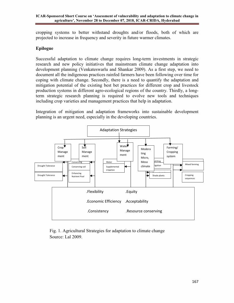
ICAR-Sponsored Short Course on ‘Assessment of vulnerability and adaptation to climate change in
agriculture’, November 28 to December 07, 2018, ICAR-CRIDA, Hyderabad
167
cropping systems to better withstand droughts and/or floods, both of which are projected to increase in frequency and severity in future warmer climates.
Epilogue Successful adaptation to climate change requires long-term investments in strategic research and new policy initiatives that mainstream climate change adaptation into development planning (Venkateswarlu and Shankar 2009). As a first step, we need to document all the indigenous practices rainfed farmers have been following over time for coping with climate change. Secondly, there is a need to quantify the adaptation and mitigation potential of the existing best bet practices for different crop and livestock production systems in different agro-ecological regions of the country. Thirdly, a long-term strategic research planning is required to evolve new tools and techniques including crop varieties and management practices that help in adaptation.
Integration of mitigation and adaptation frameworks into sustainable development planning is an urgent need, especially in the developing countries.
Fig. 1. Agricultural Strategies for adaptation to climate change
Source: Lal 2009.
Drought Tolerance
Drought Tolerance
Drought Tolerance
Conserving
water in the
root zone Conserving soil
Enhancing
Nutrient Pool
Water
Harvesting and
recycling Supplemental
irrigation
Mulching Irrigation
Row orientation Shade plants
Choice of
species Mixed farming
Cropping
sequences
.Flexibility .Equity
.Economic Efficiency .Acceptability
.Consistency .Resource conserving
Crop
Manage
ment
Soil
Manage
ment
Water
Manage
ment
Modera
ting
Micro,
Meso
climate
Farming/
Cropping
system
Adaptation Strategies
ICAR-Sponsored Short Course on ‘Assessment of vulnerability and adaptation to climate change in
agriculture’, November 28 to December 07, 2018, ICAR-CRIDA, Hyderabad
168
References
Bhardwaj SP. 1991. Study on live bunds for soil and water conservation and maize
yield on 4 % slope in Doon Valley. Pp 41-42. Annual Report, CSWCRTI, Dehradun, India.
Birthal PS, Nigam SN, Narayanan AV and Kareem KA. 2011. An economic assessment
of the potential benefits of breeding for drought tolerance in crops: a case of groundnut in India. Pp 44. Research Bulletin No. 25, ICRISAT, Patancheru, Andhra Pradesh. ISBN 978-92- 9066-539-7.
Cooper P, Rao KPC, Singh P, Dimes J, Traroe PS, Rap K, Dixit P and Twomlow SJ.
2009. Farming with current and future climate risk: Advancing hypothesis of Hope for rainfed agriculture in the semi arid tropics. SATe-J. 7: 1–19.
Dhaka BL, Chaya LK and Poonia MK. 2010. Analysis of farmers’ perception and
adaptation strategies to climate Change. Libyan Agriculture Research Center
Journal Internationl 6: 388-390. DOE. 2006. Carbon Sequestration. Department of Energy.
ttp://cdiac2.esd.ornl.gov/index.html. October 7, 2004 FAO. 2010. “Climate-Smart” Agriculture: Policies, Practices and Financing for Food
Security, Adaptation and Mitigation. Food and Agriculture Organization of the United Nations, Rome.
Goswami BN. 2006. Increasing trend of extreme rain events and possibility of extremes
of seasonal mean Indian monsoon in a warming world (http: saarc sdmc.nic.in/pdf/workshops/Kathmandu/pres16.pdf).
Howden SM, Soussana J, Tubiello FN, Chhetri N, Dunlop M and Meinke H. 2007.
Adapting agriculture to climate change. Proceedings of the National Academy of Sciences of the United States of America (PNAS) 104: 19691-19696.
IPCC. 2007. Summary for Policymakers. (in) Climate Change 2007: Impacts,
Adaptation and Vulnerability. Contribution of Working Group II to the Fourth Assessment Report of the Intergovernmental Panel on Climate Change. pp 7-22. Parry M L, Canziani O F, Palutikof J P, Van der Linden P J and Hanson C E (Eds). Cambridge University Press, UK.
Jat RA, Peter C, Kanwar LS and Wani SP. 2012. Climate change and resilient dryland
systems: experiences of ICRISAT in Asia and Africa. Current Science 102(12):1650-1659.
ICAR-Sponsored Short Course on ‘Assessment of vulnerability and adaptation to climate change in
agriculture’, November 28 to December 07, 2018, ICAR-CRIDA, Hyderabad
169
Kaur H, Jalota SK, Kanwar R and Vashisht BB. 2012. Climate change impacts on yield, evapo-transpiration and nitrogen uptake in irrigated maize (Zea mays) wheat (Triticum aestivum) cropping system: a simulation analysis. Indian Journal of
Agricultural Sciences 82(3):213-9. Khan SA, Kumar S, Hussain MZ and Kalra N. 2009. Climate Change, Climate
variability and Indian Agriculture: Impacts Vulnerability and Adaptation Strategies. (in) Climate Change and Crops, Environmental Science and Engineering. pp 19-38. S.N. Singh (Eds). Springer-Verlag Berlin Heidelberg.
Krishna Kumar. 2009. Impact of climate change on India’s monsoon climate and
development of high resolution climate change scenarios for India. Presented at MoEF, New Delhi on October 14, 2009 (http: moef.nic.in).
Kurukulasuriya P and Rosenthal S. 2003. Climate Change and Agriculture: A Review
of Impacts and Adaptations. Climate Change Series, Paper No. 91. pp 96. Published jointly with the Agriculture and Rural Development Department.
Lal M. 2007. Implications of climate change on agricultural productivity and food
security in South Asia. Key vulnerable regions and climate change – Identifying thresholds for impacts and adaptation in relation to Article 2 of the UNFCCC, Springer, Dordrecht.
Lal M, Nozawa T, Emori S, Harasawa H, Takahashi K, Kimoto M, Abe-Ouchi A,
Nakajima T, Takemura T and Numaguti A. 2001. Future climate change: Implications for Indian summer monsoon and its variability. Current Science 81: 1196–1207.
Lal R. 2004. Soil carbon sequestration in India. Climatic Change 65: 277–296. Lal R. 2009. Soil water management options for adaptations to climate change. (in)
Adapting agriculture to climate change. pp 117-136. Eaglesham A and Hardy R W F (Eds). National Agricultural Biotechnology Council, Ithaca, New York 14853.
Leggett M, Gleddie S and Holloway G. 2001. Phosphate-solubilising microorganisms
and their use. (in) Plant nutrient acquisition: New perspectives. pp 299-318. Ae N, Arihara J, Okada K and Srinivasan A (Eds). Springer-Verlag, Tokyo.
Mall RK, Singh R, Gupta A, Srinivasan G and Rathore LS. 2006. Impact of climate
change on Indian agriculture. A Review. Climate change 78: 445–478. McCarthy L, Lipper L and Branca G. 2011. Climate-Smart Agriculture: Smallholder
Adoption and Implications for Climate Change Adaptation and Mitigation. FAO working Paper. Mitigation of Climate Change in Agriculture (MICCA) Series: 4. www.fao.org/climatechange/micca/en 25.
ICAR-Sponsored Short Course on ‘Assessment of vulnerability and adaptation to climate change in
agriculture’, November 28 to December 07, 2018, ICAR-CRIDA, Hyderabad
170
Mortimore MJ and Adams WM. 2001. Farmer adaptation, change and 'crisis' in the
Sahel. Global Environmental Change 11(1): 49-57. Nhemachena C and Hassan R. 2007. Micro-level analysis of farmers’ adaptation to
climate change in southern Africa. International Food Policy Research Institute (IFPRI) Discussion Paper 00714. Washington D C.
Pratibha G and Korwar GR. 2002. Crop diversification through medicinal, aromatic
and dye yielding plants for sustainability in semi arid regions. (in) Proceedings of first national meet on medicinal and aromatic plants. pp 129-132. Mathur A K, Dwivedi S, Patra D D, Bagchi G D, Sangwan N S, Sharma A and Khanuja S P S (Eds). CIMAP, Lucknow.
Pratibha G, Korwar GR, Sharma KL and Reddy BN. 2006. Effect of nutrient
management and moisture conservation practices on yield and economics of sunflower cultivars. Journal of Oilseeds Research 23(1): 117-121.
Ravi Shankar K, Nagasree K, Prasad MS, Venkateswarlu B. 2013. Farmers’ knowledge
perceptions and adaptation measures towards climate change in south India and role of extension in climate change adaptation and mitigation. (in) Proceedings of the National Seminar on Futuristic Agricultural Extension for Livelihood Improvement and Sustainable Development. pp295-303. January 19-21, 2013. Acharya N G Ranga Agricultural University, Hyderabad, India.
Reynolds M and Tuberosa R. 2008. Translational research impacting on crop
productivity in drought-prone environments. Current Opinion in Plant Biology 11: 171–179.
Rockström J, Hatibu N, Oweis T, Wani SP. 2007. Managing Water in Rainfed
Agriculture. (in) Water for Food, Water for Life: A Comprehensive Assessment of Water Management in Agriculture. pp 315-348. Molden D (Eds). Earthscan, London, UK and International Water Management Institute, Colombo, Sri Lanka.
Rosegrant MW and Cline SA. 2003. Global food security: challenges and policies.
Science 302: 1917-1919. Sharma BR, Rao KV, Vittal KPR, Ramakrishna YS, Amarasinghe U. 2010. Estimating
the potential of rainfed agriculture in India. Prospects for water productivity improvements. Agricultural Water Management 97(1): 23-30.
Sharda V N, Dogra P and Prakash C. 2010. Assessment of production losses due to
water erosion in rainfed areas of India. Journal of Soil and Water Conservation, 65(2):79-91.
ICAR-Sponsored Short Course on ‘Assessment of vulnerability and adaptation to climate change in
agriculture’, November 28 to December 07, 2018, ICAR-CRIDA, Hyderabad
171
Singh HP, Sharma KD, Reddy GS and Sharma KL. 2007. Dryland agriculture in India. (in) Challenges and Strategies of Dryland Agriculture. pp 434. Rao C S and Ryan J (Eds). Scientific Publishers (India) Jodhpur.
Singh RP and Reddy GS. 1986. Research on drought problems in arid and semi-arid
tropics. ICRISAT, Patancheru, India. Srinivasa Rao Ch, Wani SP, Venkateswarlu B, Dixit S, Kundu S, Gayatri Devi K and
Rajesh C. 2010. Productivity enhancement and improved livelihood through participatory soil fertility management in tribal districts of Andhra Pradesh Indian Journal of Agricultural and Development 25(2): 23-32.
Srinivasa Rao Ch, Venkateswarlu B, Lal R, Singh AK, Kundu S, Vittal KPR, Gajanan
GN and Ramachandra B. 2012a. Long term effects of crop residues and fertility management on carbon sequestration and agronomic productivity of groundnut – fingermillet rotation on an Alfisol in southern India. International Journal of Agricultural Sustainability 10: 1-15.
Srinivasa Rao Ch, Deshpande AN, Venkateswarlu B, Lal R, Singh AK, Kundu S, Vittal
KPR, Mishra PK, Prasad JVNS, Mandal UK and Sharma KL. 2012b. Grain yield and carbon sequestration potential of post monsoon sorghum cultivation in Vertisols in the semi arid tropics of central India. Geoderma 175: 90-97.
Stern NH. 2007. The Economics of Climate Change: The Stern Review. pp 712.
Cambridge University Press, Cambridge, UK. Swearingen WD and Bencherifa A. 2000. An Assessment of the Drought Hazard in
Morocco. (in) Drought: A Global Assessment. pp 279-286. Wilhite D A (Eds). Routledge publication, New York.
Twomlow S, Urolov J C, Jenrich M and Oldrieve B. 2008. Lessons from the field –
Zimbabwe’s Conservation Agriculture Task Force. Journal of SAT Agriulture Research. 6: 1–11.
V and A programme 2009. Vulnerability and Adaptation experiences from Rajasthan
and Andhra Pradesh the system of rice intensification. SDC V and A program, India. pp 1-29.
Veneetha U, Maheswara Reddy P and Radha Kumari C. 2011. Studies on contigency
cropping in dry lands. Indian Journal of Dryland Agricultural Research and Development 26(2): 38-43.
Venkateswarlu B, Shankar AK and Gogoi AK. 2009. Climate change adaptation and
mitigation in Indian agriculture. (in) Proc. National Seminar on Climate Change Adaptation Strategies in Agriculture and Allied Sectors. pp 109-121. KAU, Trissur, India.
ICAR-Sponsored Short Course on ‘Assessment of vulnerability and adaptation to climate change in
agriculture’, November 28 to December 07, 2018, ICAR-CRIDA, Hyderabad
172
Venkateshwarlu B. 2010 Climate change: adaptation and mitigation of climate change.
The 21st Dr.S.P.Raychaudhuri Memorial Lecture during October 10-11, 2010, at BAU Ranchi organized by Ranchi chapter of Indian society of Soil Science .http://www.crida.in/Lecturers/Lect-Director.pdf
Venkateswarlu B and Shanker AK. 2009. Climate change and agriculture: Adaptation and
mitigation strategies. Indian Journal of Agronomy 54(2): 226 – 230. Viswanatha GB, Ramachandrappa BK and Nanjappa HV. 2002. Soil-plant water status
and yield of sweet corn (Zea mays L.) as influenced by drip irrigation and planting methods. Agricultural Water Management 55: 85–91.
Ziervogel G, Bharwani S and Downing TE. 2006. Adapting to climate variability:
Pumpkins, people and policy. Natural resources Forum: A United Nations Sustainable Development Journal 30(4): 294-305.
ICAR-Sponsored Short Course on ‘Assessment of vulnerability and adaptation to climate change in
agriculture’, November 28 to December 07, 2018, ICAR-CRIDA, Hyderabad
173
15 Agroforestry as an adaptation and mitigation strategy for
climate change
JVNS Prasad and B Ramakrishna
Introduction
The Intergovernmental Panel on Climate Change (IPCC) in its fifth assessment report (AR5) stated that warming of the climate system is unequivocal and is more pronounced since 1950s. The atmosphere and oceans have warmed, the amounts of snow and ice have diminished and sea level has risen. Each of the last three decades has been successively warmer at the Earth’s surface than any preceding decade since 1850 and the globally averaged combined land and ocean surface temperature data as calculated by a linear trend show a warming of 0.85°C over the period 1880 to 2012 (IPCC, 2013). In India, may states have experienced state wide warming in maximum and minimum temperatures over the last six decades (Rathore et al., 2013). Further it is projected that global mean surface temperature and sea level may rise by 0.3 to 1.50C and 0.26 to 0.54 m for RCP 2.6, 1.1 to 2.60C and 0.32 to 0.62 m for RCP 4.5, 1.4 to 3.1oC and 0.33 to 0.62 m for RCP 6.0 and 2.6 to 4.8oC and 0.45 to 0.81 m in RCP 8.5, respectively by 2080-2100. The impact would be particularly severe in tropical areas, which mainly consists of developing countries, including India.
Climate change impacts agricultural production and there are already evidences of negative impacts on yield of wheat and paddy in parts of India due to increased temperature, increasing water stress and reduction in number of rainy days. Modeling studies project a significant decrease in cereal production by the end of this century (Majumdar 2008). Parts of western Rajasthan, Southern Gujarat, Madhya Pradesh, Maharashtra, Northern Karnataka, Northern Andhra Pradesh, and Southern Bihar are likely to be more vulnerable in terms of extreme events (Mall et al. 2006). For every one degree increase in temperature, yields of wheat, soybean, mustard, groundnut and potato are expected to decline by 3-7% (Agarwal 2009). Similarly, rice yields may decline by 6% for every one degree increase in temperature (Saseendran et al. 2000). Water requirement of crops is also likely to go up with projected warming and extreme events are likely to increase. There is a need to minimize the impacts of climate variability on crop growth and production. Agriculture and forestry sectors though emits substantial quantities of GHG emissions, these sectors can be the only sinks for CO2 through carbon sequestration into biomass products and soil organic matter. There are multiple benefits of sequestering carbon in forest and agricultural soils and in vegetation besides the obvious benefit of offsetting CO2 emissions.
Agroforestry is defined as land-use system that involves the deliberate retention, introduction of mixture of trees or other woody perennials with agricultural crops, pastures and/or livestock to exploit the ecological and economic interactions of the different components for enhancing the productivity in unit area and time. Several studies have conclusively proved that the inclusion of trees in the agricultural
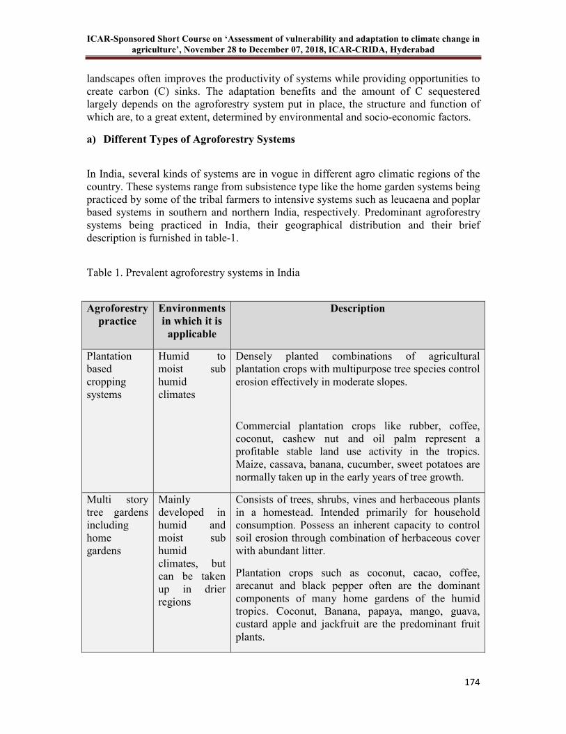
ICAR-Sponsored Short Course on ‘Assessment of vulnerability and adaptation to climate change in
agriculture’, November 28 to December 07, 2018, ICAR-CRIDA, Hyderabad
174
landscapes often improves the productivity of systems while providing opportunities to create carbon (C) sinks. The adaptation benefits and the amount of C sequestered largely depends on the agroforestry system put in place, the structure and function of which are, to a great extent, determined by environmental and socio-economic factors.
a) Different Types of Agroforestry Systems
In India, several kinds of systems are in vogue in different agro climatic regions of the country. These systems range from subsistence type like the home garden systems being practiced by some of the tribal farmers to intensive systems such as leucaena and poplar based systems in southern and northern India, respectively. Predominant agroforestry systems being practiced in India, their geographical distribution and their brief description is furnished in table-1.
Table 1. Prevalent agroforestry systems in India
Agroforestry
practice
Environments
in which it is
applicable
Description
Plantation based cropping systems
Humid to moist sub humid climates
Densely planted combinations of agricultural plantation crops with multipurpose tree species control erosion effectively in moderate slopes.
Commercial plantation crops like rubber, coffee, coconut, cashew nut and oil palm represent a profitable stable land use activity in the tropics. Maize, cassava, banana, cucumber, sweet potatoes are normally taken up in the early years of tree growth.
Multi story tree gardens including home gardens
Mainly developed in humid and moist sub humid climates, but can be taken up in drier regions
Consists of trees, shrubs, vines and herbaceous plants in a homestead. Intended primarily for household consumption. Possess an inherent capacity to control soil erosion through combination of herbaceous cover with abundant litter.
Plantation crops such as coconut, cacao, coffee, arecanut and black pepper often are the dominant components of many home gardens of the humid tropics. Coconut, Banana, papaya, mango, guava, custard apple and jackfruit are the predominant fruit plants.
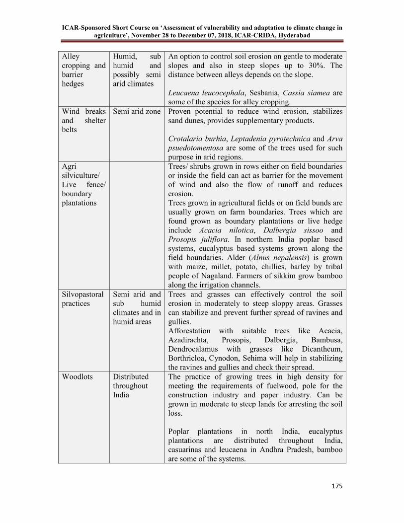
ICAR-Sponsored Short Course on ‘Assessment of vulnerability and adaptation to climate change in
agriculture’, November 28 to December 07, 2018, ICAR-CRIDA, Hyderabad
175
Alley cropping and barrier hedges
Humid, sub humid and possibly semi arid climates
An option to control soil erosion on gentle to moderate slopes and also in steep slopes up to 30%. The distance between alleys depends on the slope. Leucaena leucocephala, Sesbania, Cassia siamea are some of the species for alley cropping.
Wind breaks and shelter belts
Semi arid zone Proven potential to reduce wind erosion, stabilizes sand dunes, provides supplementary products. Crotalaria burhia, Leptadenia pyrotechnica and Arva
psuedotomentosa are some of the trees used for such purpose in arid regions.
Agri silviculture/ Live fence/ boundary plantations
Trees/ shrubs grown in rows either on field boundaries or inside the field can act as barrier for the movement of wind and also the flow of runoff and reduces erosion. Trees grown in agricultural fields or on field bunds are usually grown on farm boundaries. Trees which are found grown as boundary plantations or live hedge include Acacia nilotica, Dalbergia sissoo and Prosopis juliflora. In northern India poplar based systems, eucalyptus based systems grown along the field boundaries. Alder (Alnus nepalensis) is grown with maize, millet, potato, chillies, barley by tribal people of Nagaland. Farmers of sikkim grow bamboo along the irrigation channels.
Silvopastoral practices
Semi arid and sub humid climates and in humid areas
Trees and grasses can effectively control the soil erosion in moderately to steep sloppy areas. Grasses can stabilize and prevent further spread of ravines and gullies. Afforestation with suitable trees like Acacia, Azadirachta, Prosopis, Dalbergia, Bambusa, Dendrocalamus with grasses like Dicantheum, Borthricloa, Cynodon, Sehima will help in stabilizing the ravines and gullies and check their spread.
Woodlots Distributed throughout India
The practice of growing trees in high density for meeting the requirements of fuelwood, pole for the construction industry and paper industry. Can be grown in moderate to steep lands for arresting the soil loss. Poplar plantations in north India, eucalyptus plantations are distributed throughout India, casuarinas and leucaena in Andhra Pradesh, bamboo are some of the systems.
ICAR-Sponsored Short Course on ‘Assessment of vulnerability and adaptation to climate change in
agriculture’, November 28 to December 07, 2018, ICAR-CRIDA, Hyderabad
176
b) Agroforestry as an Adaptation Strategy
Trees on farms help adaptation to climate change by reducing vulnerability to climate impacts. Trees on farms can diminish the effects of weather extremes such as high temperatures and droughts. The important aspects of agroforestry that contribute towards adaptation consists of modification of micro climate in arid and semi arid regions, early crop vigor and growth due to enhancement of soil fertility, arresting soil erosion and land degradation, stability of income and enhancement of income through diversification from trees even under extremely low rainfall situations. In addition to the above, trees as components of landscapes also provides essential requirements of the communities such as fodder, fuel wood and other wood requirements for the rural communities.
i) Improvement in microclimate
Trees on farm can bring favourable changes in the microclimatic conditions in the form of windbreaks, shelter belts by influencing radiation flux, air temperature, wind speed, saturation deficit of under storey crops which will have a significant impact on the photosynthesis, transpiration, water use and plant growth (Monteith et al., 1991). Many shade loving crops like coffee, ginger, cardamom are grown under partial shade which is known to improve the micro climate favourably. Singh et al., (2002) found reduction of 1oC in air temperature and 1.6oC in soil temperature with Zizyphus
maurritiana+ Mungbean system which has found to increase the yield of Mungbean by 20%. Establishment of micro – shelterbelts in arable lands, by planting tall and fast growing plant species viz., castor on the windward side and shorter crop such as vegetables in the leeward side of tall plants helped to increase the yield of bhendi yield by 41 % and of cowpea by 21 % over the control (Venkateshwaralu, 1993).
ii) Enhancement of soil fertility
Trees in agroecosystems can enhance soil productivity through biological nitrogen fixation, efficient nutrient cycling, and capturing and recycling of nutrients from deeper layers of soils. Some of the non leguminous plants also found to enhance physical, chemical and biological properties of soils by adding significant amount of above (litter fall) and belowground (root turnover) organic matter and recycling nutrients. Land use systems such as agroforestry, agro-horticultural, agro-pastoral, and agro- silvipasture are more effective for soil organic matter restoration (Manna, et al. 2003). Significant improvement in soil biological activity has been reported under different tree based agroforestry systems and found that fluxes of C, N and P through microbial biomass were also significantly higher in P.cineraria based land use system followed by Dalbergia sissoo, Acacia leucophloea and Acacia nilotica in comparison to a no-tree control in Rajasthan (Yadav et al., 2011). Samra and Charan (2000) observed increase in soil organic carbon status of surface soil 0.39 % to 0.52 % under Acacia nilotica + Saccharum munja and 0.44% to 0.55% under Acacia nilotica+ Eulaliopsis binata after five years. Enhanced soil organic carbon coupled with improved nutrient status in soils
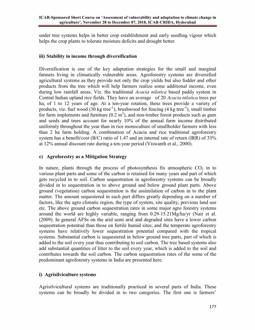
ICAR-Sponsored Short Course on ‘Assessment of vulnerability and adaptation to climate change in
agriculture’, November 28 to December 07, 2018, ICAR-CRIDA, Hyderabad
177
under tree systems helps in better crop establishment and early seedling vigour which helps the crop plants to tolerate moisture deficits and drought better.
iii) Stability in income through diversification
Diversification is one of the key adaptation strategies for the small and marginal farmers living in climatically vulnerable areas. Agroforestry systems are diversified agricultural systems as they provide not only the crop yields but also fodder and other products from the tree which will help farmers realize some additional income, even during low rainfall areas. Viz. the traditional Acacia nilotica based paddy system in Central Indian upland rice fields. They have an average of 20 Acacia nilotica trees per ha, of 1 to 12 years of age. At a ten-year rotation, these trees provide a variety of products, viz. fuel wood (30 kg tree-1), brushwood for fencing (4 kg tree-1), small timber for farm implements and furniture (0.2 m3), and non-timber forest products such as gum and seeds and trees account for nearly 10% of the annual farm income distributed uniformly throughout the year than in rice monoculture of smallholder farmers with less than 2 ha farm holding. A combination of Acacia and rice traditional agroforestry system has a benefit/cost (B/C) ratio of 1.47 and an internal rate of return (IRR) of 33% at 12% annual discount rate during a ten-year period (Viswanth et al., 2000).
c) Agroforestry as a Mitigation Strategy
In nature, plants through the process of photosynthesis fix atmospheric CO2 in to various plant parts and some of the carbon is retained for many years and part of which gets recycled in to soil. Carbon sequestration in agroforestry systems can be broadly divided in to sequestration in to above ground and below ground plant parts. Above ground (vegetation) carbon sequestration is the assimilation of carbon in to the plant matter. The amount sequestered in each part differs greatly depending on a number of factors, like the agro climatic region, the type of system, site quality, previous land use etc. The above ground carbon sequestration rates in some major agro forestry systems around the world are highly variable, ranging from 0.29-15.21Mg/ha/yr (Nair et al. (2009). In general AFSs on the arid semi arid and degraded sites have a lower carbon sequestration potential than those on fertile humid sites; and the temperate agroforestry systems have relatively lower sequestration potential compared with the tropical systems. Substantial carbon is sequestered in below ground tree parts, part of which is added to the soil every year thus contributing to soil carbon. The tree based systems also add substantial quantities of litter to the soil every year, which is added to the soil and contributes towards the soil carbon. The carbon sequestration rates of the some of the predominant agroforestry systems in India are presented here.
i) Agrisilviculture systems
Agrisilvicultural systems are traditionally practiced in several parts of India. These systems can be broadly be divided in to two categories. The first one is farmers’
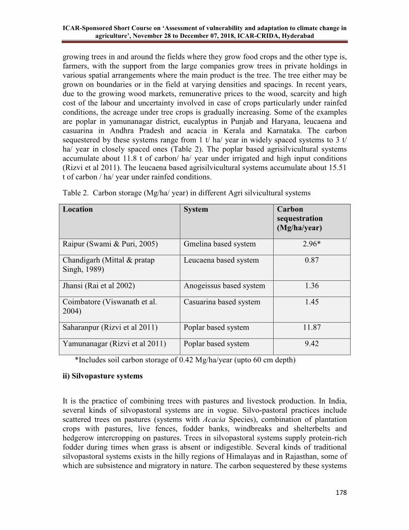
ICAR-Sponsored Short Course on ‘Assessment of vulnerability and adaptation to climate change in
agriculture’, November 28 to December 07, 2018, ICAR-CRIDA, Hyderabad
178
growing trees in and around the fields where they grow food crops and the other type is, farmers, with the support from the large companies grow trees in private holdings in various spatial arrangements where the main product is the tree. The tree either may be grown on boundaries or in the field at varying densities and spacings. In recent years, due to the growing wood markets, remunerative prices to the wood, scarcity and high cost of the labour and uncertainty involved in case of crops particularly under rainfed conditions, the acreage under tree crops is gradually increasing. Some of the examples are poplar in yamunanagar district, eucalyptus in Punjab and Haryana, leucaena and casuarina in Andhra Pradesh and acacia in Kerala and Karnataka. The carbon sequestered by these systems range from 1 t/ ha/ year in widely spaced systems to 3 t/ ha/ year in closely spaced ones (Table 2). The poplar based agrisilvicultural systems accumulate about 11.8 t of carbon/ ha/ year under irrigated and high input conditions (Rizvi et al 2011). The leucaena based agrisilvicultural systems accumulate about 15.51 t of carbon / ha/ year under rainfed conditions.
Table 2. Carbon storage (Mg/ha/ year) in different Agri silvicultural systems
Location
System
Carbon
sequestration
(Mg/ha/year)
Raipur (Swami & Puri, 2005) Gmelina based system 2.96*
Chandigarh (Mittal & pratap Singh, 1989)
Leucaena based system 0.87
Jhansi (Rai et al 2002) Anogeissus based system 1.36
Coimbatore (Viswanath et al. 2004)
Casuarina based system 1.45
Saharanpur (Rizvi et al 2011) Poplar based system 11.87
Yamunanagar (Rizvi et al 2011) Poplar based system 9.42
*Includes soil carbon storage of 0.42 Mg/ha/year (upto 60 cm depth)
ii) Silvopasture systems
It is the practice of combining trees with pastures and livestock production. In India, several kinds of silvopastoral systems are in vogue. Silvo-pastoral practices include scattered trees on pastures (systems with Acacia Species), combination of plantation crops with pastures, live fences, fodder banks, windbreaks and shelterbelts and hedgerow intercropping on pastures. Trees in silvopastoral systems supply protein-rich fodder during times when grass is absent or indigestible. Several kinds of traditional silvopastoral systems exists in the hilly regions of Himalayas and in Rajasthan, some of which are subsistence and migratory in nature. The carbon sequestered by these systems
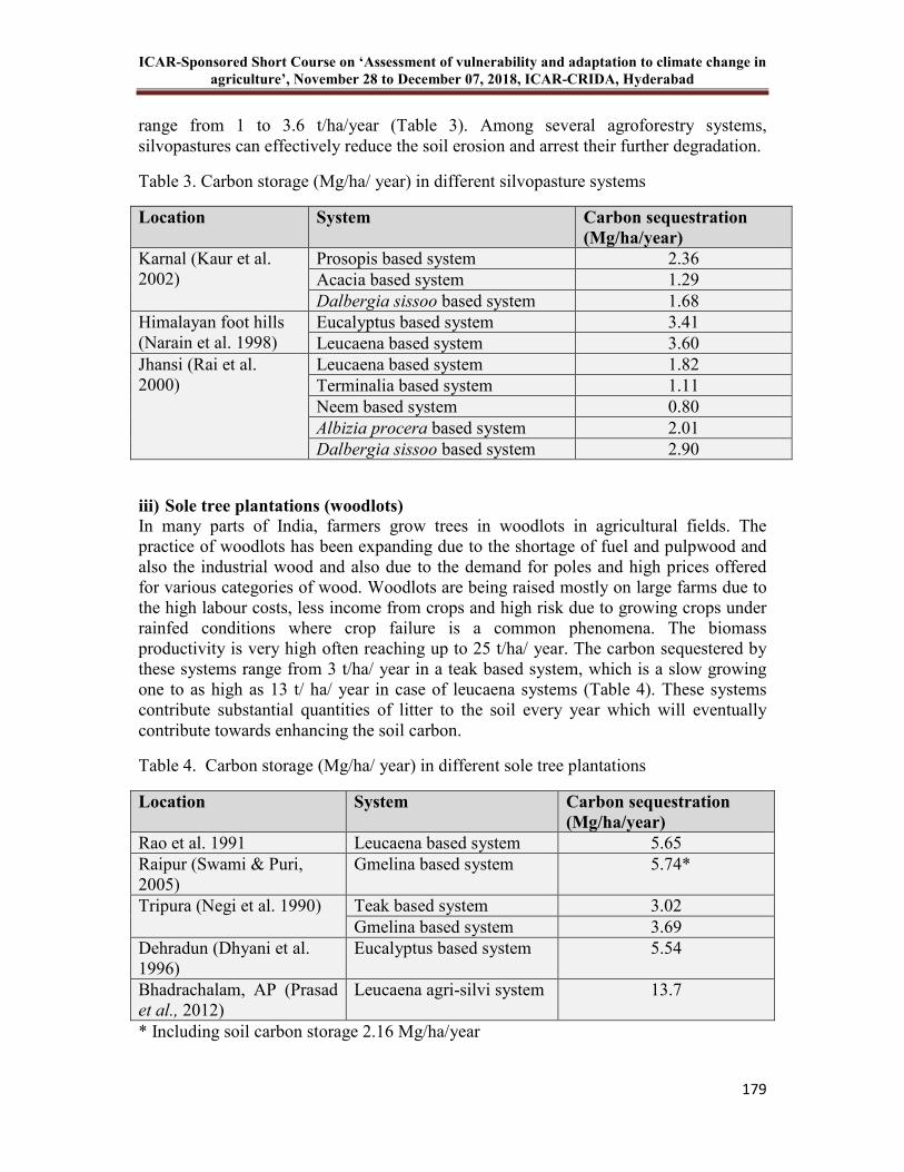
ICAR-Sponsored Short Course on ‘Assessment of vulnerability and adaptation to climate change in
agriculture’, November 28 to December 07, 2018, ICAR-CRIDA, Hyderabad
179
range from 1 to 3.6 t/ha/year (Table 3). Among several agroforestry systems, silvopastures can effectively reduce the soil erosion and arrest their further degradation.
Table 3. Carbon storage (Mg/ha/ year) in different silvopasture systems
Location
System
Carbon sequestration
(Mg/ha/year)
Karnal (Kaur et al. 2002)
Prosopis based system 2.36 Acacia based system 1.29 Dalbergia sissoo based system 1.68
Himalayan foot hills (Narain et al. 1998)
Eucalyptus based system 3.41 Leucaena based system 3.60
Jhansi (Rai et al. 2000)
Leucaena based system 1.82 Terminalia based system 1.11 Neem based system 0.80 Albizia procera based system 2.01 Dalbergia sissoo based system 2.90
iii) Sole tree plantations (woodlots)
In many parts of India, farmers grow trees in woodlots in agricultural fields. The practice of woodlots has been expanding due to the shortage of fuel and pulpwood and also the industrial wood and also due to the demand for poles and high prices offered for various categories of wood. Woodlots are being raised mostly on large farms due to the high labour costs, less income from crops and high risk due to growing crops under rainfed conditions where crop failure is a common phenomena. The biomass productivity is very high often reaching up to 25 t/ha/ year. The carbon sequestered by these systems range from 3 t/ha/ year in a teak based system, which is a slow growing one to as high as 13 t/ ha/ year in case of leucaena systems (Table 4). These systems contribute substantial quantities of litter to the soil every year which will eventually contribute towards enhancing the soil carbon.
Table 4. Carbon storage (Mg/ha/ year) in different sole tree plantations
Location
System
Carbon sequestration
(Mg/ha/year)
Rao et al. 1991 Leucaena based system 5.65 Raipur (Swami & Puri, 2005)
Gmelina based system 5.74*
Tripura (Negi et al. 1990) Teak based system 3.02 Gmelina based system 3.69
Dehradun (Dhyani et al. 1996)
Eucalyptus based system 5.54
Bhadrachalam, AP (Prasad et al., 2012)
Leucaena agri-silvi system 13.7
* Including soil carbon storage 2.16 Mg/ha/year
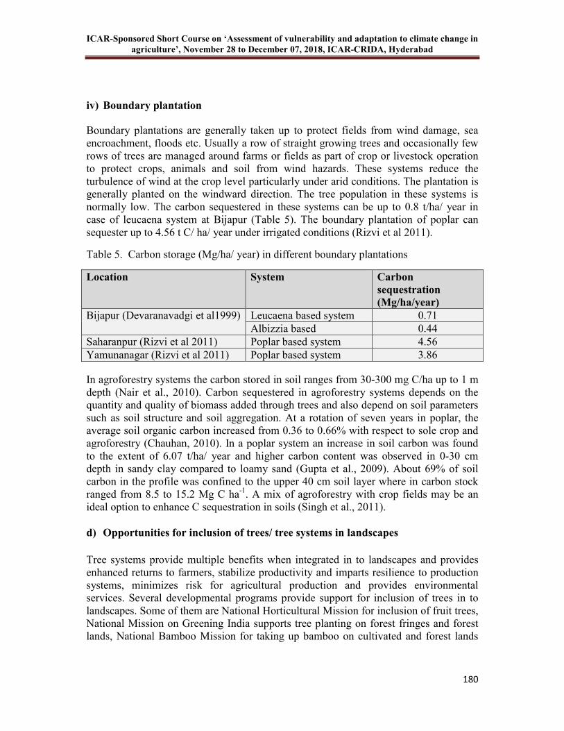
ICAR-Sponsored Short Course on ‘Assessment of vulnerability and adaptation to climate change in
agriculture’, November 28 to December 07, 2018, ICAR-CRIDA, Hyderabad
180
iv) Boundary plantation
Boundary plantations are generally taken up to protect fields from wind damage, sea encroachment, floods etc. Usually a row of straight growing trees and occasionally few rows of trees are managed around farms or fields as part of crop or livestock operation to protect crops, animals and soil from wind hazards. These systems reduce the turbulence of wind at the crop level particularly under arid conditions. The plantation is generally planted on the windward direction. The tree population in these systems is normally low. The carbon sequestered in these systems can be up to 0.8 t/ha/ year in case of leucaena system at Bijapur (Table 5). The boundary plantation of poplar can sequester up to 4.56 t C/ ha/ year under irrigated conditions (Rizvi et al 2011).
Table 5. Carbon storage (Mg/ha/ year) in different boundary plantations
Location
System
Carbon
sequestration
(Mg/ha/year)
Bijapur (Devaranavadgi et al1999) Leucaena based system 0.71 Albizzia based 0.44
Saharanpur (Rizvi et al 2011) Poplar based system 4.56 Yamunanagar (Rizvi et al 2011) Poplar based system 3.86
In agroforestry systems the carbon stored in soil ranges from 30-300 mg C/ha up to 1 m depth (Nair et al., 2010). Carbon sequestered in agroforestry systems depends on the quantity and quality of biomass added through trees and also depend on soil parameters such as soil structure and soil aggregation. At a rotation of seven years in poplar, the average soil organic carbon increased from 0.36 to 0.66% with respect to sole crop and agroforestry (Chauhan, 2010). In a poplar system an increase in soil carbon was found to the extent of 6.07 t/ha/ year and higher carbon content was observed in 0-30 cm depth in sandy clay compared to loamy sand (Gupta et al., 2009). About 69% of soil carbon in the profile was confined to the upper 40 cm soil layer where in carbon stock ranged from 8.5 to 15.2 Mg C ha-1. A mix of agroforestry with crop fields may be an ideal option to enhance C sequestration in soils (Singh et al., 2011).
d) Opportunities for inclusion of trees/ tree systems in landscapes
Tree systems provide multiple benefits when integrated in to landscapes and provides enhanced returns to farmers, stabilize productivity and imparts resilience to production systems, minimizes risk for agricultural production and provides environmental services. Several developmental programs provide support for inclusion of trees in to landscapes. Some of them are National Horticultural Mission for inclusion of fruit trees, National Mission on Greening India supports tree planting on forest fringes and forest lands, National Bamboo Mission for taking up bamboo on cultivated and forest lands
ICAR-Sponsored Short Course on ‘Assessment of vulnerability and adaptation to climate change in
agriculture’, November 28 to December 07, 2018, ICAR-CRIDA, Hyderabad
181
and under National Agroforestry Policy support is available for inclusion of trees on farmlands.
e) Conclusions
Diversification of arable cropping systems by integration of trees under rainfed conditions can stabilize income during the years of extreme rainfall which is the objective of any adaptation strategy besides sequestering carbon. Of the several tree based systems, short rotation intensive systems have the potential to sequester substantial quantities of carbon in a short time and can be taken up in degraded lands which are not suitable for intensive cropping. However, for such systems to be taken up in large areas, well established markets for the wood and wood based products are essential and the policy support from the government is also essential for price support.
References
Agarwal, PK. 2009. Global Climate change and Indian agriculture; Case studies from ICAR network project, Indian Council of Agricultural Research, pp 148.
Chauhan, SK, Sharma S C, Chauhan R, Naveen Gupta and Ritu.2010. Accounting poplar and wheat productivity for carbon sequestration in agri-silvicultural system. Indian Forester. 136. (9):1174-1182.
Devaranavadgi SB, Kalaghatagi SB, Guggari AK and Wali SY. 1999. Woody perennials on ansd as bunds in vertisols. Indian Journal of Agronomy: 44 (1):196-199.
Dhyani SK, Puri DN and Narain P. 1996. Biomass production and rooting behavior of Eucalyptus tereticornis SM. On deep soils and riverbed boulder lands of Doon valley, India. Indian Forester, 128-136.
IPCC. 2013. Climate Change 2013: The Physical Science Basis. Contribution of Working Group I to the Fifth Assessment Report of the Intergovernmental Panel on Climate Change [Stocker, T.F., D. Qin, G.-K. Plattner, M. Tignor, S.K. Allen, J. Boschung, A. Nauels, Y. Xia, V. Bex and P.M. Midgley (eds.)]. Cambridge University Press, Cambridge, 1535 pp doi:10.1017/CBO9781107415324.
Kaur B, Gupta SR and Singh G. 2002. Bioamelioration of a sodic soil by silvopastoral systems in northwestern India. Agroforestry Systems. 54(1):13-20.
Mall R, Singh Ranjeet, Gupta Akhilesh, Srinivasan G, Rathore L. 2006. Impact of
Climate Change on Indian Agriculture: A Review. Climatic Change, 78: 445-478
ICAR-Sponsored Short Course on ‘Assessment of vulnerability and adaptation to climate change in
agriculture’, November 28 to December 07, 2018, ICAR-CRIDA, Hyderabad
182
Mujumdar PP. 2008. Implications of climate change for sustainable water resources management in India, Physics and Chemistry of the Earth, Parts A/B/C, 33: 354-358
Manna MC, Ghoshand PK and Acharya CL. 2003. Sustainable crop production through management of soil organic carbon in semiarid and tropical India. Journal of Sustainable Agriculture, 21: 87-116
Mittal SP and Singh Pratap 1989. Intercropping field crops between rows of Leucaena
leucocephala under rainfed conditions in northern India. Agroforestry Systems, 8:165-172.
Monteith JL, Ong CK and Corlett JE. 1991. Microclimate interactions in agroforestry systems. Forest Ecol Manag 45: 31–44.
Nair PKR, Kumar BM and Nair VD. 2009. Agroforestry as a carbon sequestration .J.plant.Nut,Soil science .172,10-23.
Nair,P.K.R.;Vimala D.Nair,; B.Mohan kumar , and Julia M. Showalter ,2010.Carbon sequestration in Agroforestry systems .Advances in Agronomy ,pp:237-309.
Narain P, Singh RK, Sindhwal NS and Joshi P. 1998. Agroforestry for soil and water conservation in the western Himalayan valley region of India. Agroforestry systems, 39: 191-203.
Gupta N, Kukal SS, Bawa SS, Dhaliwal, GS. 2009. Soil organic carbon and aggregation under poplar based agroforestry system in relation to tree age and soil type. Agroforestry Systems ,76( 1 ): 27-35
Negi JDS, Bahuguna VK and Sharma DC. 1990. Biomass production and distribution of nutrients in 20 years old Teak (Tectona grandis) and Gamar (Gmelina
arborea) plantation in Tripura. Indian Forester, 116(9):681-686.
Prasad JVNS, Srinivas K, Srinivasarao Ch, Ramesh Ch, Venkatravamma K and Venkateswarlu B.2012. Biomass productivity and carbon stock of farm forestry and agroforestry systems of leucaena and eucalyptus in Khammam district of Andhra Pradesh. Current Science, 103 (5): 536-540.
Rao MR, Ong CK, Pathak P and Sharma MM. 1991. Productivity of annual cropping and agroforestry systems on a shallow Alfisol in semi-arid India. Agroforestry Systems, 15: 51-63
Rai AK, Solanki KR and Rai P. 2002. Performance of Anogeissus pendula Genotypes under Agrisilvicultural System. Indian Journal Agroforestry, 4(1): 71 -74.
Rai P, Rao GR and Solanki KR. 2000. Effect of multipurpose tree species on composition, dominance, yield and crude protein content in forage in natural grassland. Indian Journal of Forestry , 23(4): 380-385.
ICAR-Sponsored Short Course on ‘Assessment of vulnerability and adaptation to climate change in
agriculture’, November 28 to December 07, 2018, ICAR-CRIDA, Hyderabad
183
Rathore LS, Attri SD, Jaswal AK. 2013. State level climate change trends in India, India Meteorological Department, Government of India. 1-147.
Rizvi RH, Dhyani SK, Yadav RS and Ramesh Singh. 2011. Biomass production and carbon stock of poplar agroforestry systems in Yamunanagar and Saharanpur districts of North western India. Current Science, 100 (5): 736-742.
Samra JS and Charan SS. 2000. Silvipasture systems for soil, water and nutrient conservation on degraded lands of Shivalik foot hills (subtropical northern India). Indian Journal of Soil Conservation, 28(1): 35-42.
Saseendran ASK, Singh KK, Rathore LS, Singh SV and Sinha SK. 2000. Effects of climate change on rice production in the tropical humid climate of Kerala, India, Climate Change, 44 : 495-514
Singh H, Pathak, P, Kumar M and Raghubanshi AS. 2011. Carbon sequestration potential of Indo-Gangetic agroecosystem soils.Tropical Ecology. 52( 2):223-228.
Singh RS, Gupta JP and Rao AS. 2002. Impact of micro-meterological parameters on growth and productivity of mung bean under different agroforestry systems in arid Rajasthan. Journal of Agrometerology, 4(2): 105-112
Swamy SL and Puri Sunil. 2005. Biomass production and C-sequestration of Gmelina arborea in plantation and agroforestry system in India. Agroforestry systems, 64(3):181-195.
Venkateswarlu J. 1993. Problems and prospects in desertification control: Role of Central Arid Zone Research Institute. In: Desertification and its Control in the Thar, Sahara and Sahel Regions (Sen, A.K. and Kar, A. Eds.). pp. 249–267. (Jodhpur, India: Scientific Publishers).
Viswanath S, Nair PKR, Kaushik PK and Prakasam U. 2000. Acacia nilotica trees in rice fields: A traditional agroforestry system in central India. Agroforestry Systems, 50: 157–177.
Viswanath S, Peddappaiah RS, Subramoniam V, Manivachakam P and George M. 2004. Management of Casuarina equisetifolia in Wide-row Intercropping Systems for Enhanced Productivity. Indian Journal of Agroforestry, 6(2): 19-25.
Yadav RS, Yadav BL, Chhipa BR, Dhyani SK and Ram M. 2011. Soil biological properties under different tree based traditional agroforestry systems in a semi-arid region of Rajasthan, India. Agroforestry Systems, 81(3): 195-202.
ICAR-Sponsored Short Course on ‘Assessment of vulnerability and adaptation to climate change in
agriculture’, November 28 to December 07, 2018, ICAR-CRIDA, Hyderabad
184
16 Tank Beds As Source of Fodder in Years of Drought and Need
of Policy Support – Case Studies of Undivided State of Andhra
Pradesh
Mohammed Osman
Introduction
Tank fed irrigation in peninsular India in general and Andhra Pradesh in particular is a traditional practice but of late the shift has occurred from surface to ground water due to technological advancement (bore well) and policy changes. There is a breakdown of traditional tank management system and newly formed water user’s associations are active only where there is water. Often, water user associations (WUA) are denounced for lack of involvement of all the stakeholders as they mainly focus on water for irrigation and others are excluded. Most of the Panchayat Raj (PR) and Minor Irrigation (MI) tanks receive meager or no inflow, which is attributed to poor maintenance, rainfall, watershed development, change in cropping pattern and higher demand from various sectors. These tank beds are grossly under-utilized as most of them don’t get filled even in years of normal rainfall. There are about 70, 000+ PR and 10,000+ MI tanks in Andhra Pradesh whose tank-beds when efficiently made use may generate adequate fodder, fuel (bio fuel) and livelihoods for the poor. The current status of tanks and their irrigation potential is set out in Table 1. The total number of tanks in the state is 82443 but the proportion in use is mere 33% which is attributed to meager inflows due to poor maintenance of the feeder channels, inadequate rainfall, watershed structures like farm ponds, trench-cum-bunds, check dams and soil conservation structures like small cross section bunds, drainage line treatment, diversion drains, etc. An analysis across the districts indicates that the number of tanks available have varied from as low as 234 in Guntur to as high as 9518 in Vizianagaram while the proportion of tanks in use varies from 18% in Nalgonda to 98% in Srikakulam. The lowest level of tanks in use in Nalgonda is due to the reason that this district is constrained by low rainfall, sandy textured soils having high infiltration rate resulting in low runoff, siltation, encroachment and lack of funds for restoration. The other districts having similar such problems are Rangareddy, Anantapur, Mahabubnagar, Medak, Karimnagar and Cuddapah. The higher use of tanks in Srikakulam, Adilabad, Vizianagaram, Krishna, Vishakhapatnam, Khammam, East & West Godavari districts is attributed to high rainfall, higher density of river network and better runoff.
A great deal of information about inter-district variation in capacity and utilization of irrigation potential is presented in Table 1(a). A closer examination of the table reveals that Warangal is on the top of all districts in state with regard to irrigation potential capacity (288920 ha) created and has registered good utilization (64%), while Guntur has the least capacity (8763 ha) but good utilization (70%). Thus, both these districts come under the category of good capacity utilization irrespective of different capacities of irrigation potential. Nellore with higher capacity, Kurnool with lower capacity, and
ICAR-Sponsored Short Course on ‘Assessment of vulnerability and adaptation to climate change in
agriculture’, November 28 to December 07, 2018, ICAR-CRIDA, Hyderabad
185
West Godavari, Prakasam and Nizamabad with medium capacity fall under good capacity utilization of irrigation potential.
The districts having better capacity utilization irrespective of capacities created for irrigation potential are Srikakulam, Vizianagaram, Visakhapatnam, East Godavari, Krishna, Khammam and Adilabad which is attributed to the fact that these districts fall under river Krishna and Godavari basin and receive an annual average rainfall between 900 mm and 1100 mm. On the contrary, the districts having poor capacity utilization irrespective of varying capacities of irrigation potential are Chittoor, Medak, Karimnagar, Nalgonda, Cuddapah, Anantapur, Mahabubnagar and Rangareddy. The reasons for poor capacity utilization of irrigation potential of these districts are low rainfall (<900mm), less inflows, sandy textured soils, siltation and encroachment.
A study of rainfall pattern of Mahabubnagar district of Andhra Pradesh indicate only 50% probability of receiving ≥ 20mm rainfall during rainy season while there is a need of 30 mm in a day to generate runoff in alfisols (Table 2). Runoff is a function of rainfall intensity, land use, land cover, soil type, slope and antecedent moisture. The probability of receiving 30mm rainfall is much lower than 20 mm and runoff producing events are also quite a few. Further, it is evident from irrigated area covered by medium irrigation projects. Out of three medium irrigation projects in Mahabubnagar, only one could provide irrigation water to less than one-third of the registered ayacut (Table 3). Similarly, 654 MI tanks with an ayacut area of 1,47,331 acres could support irrigation to a meager total (both kharif and rabi) of 2510 acres and 2620 acres in 1994-95 and 2002-03, respectively (Table 4). The differences in area irrigated by MI tanks during kharif and rabi in two different years is attributed to distribution of rainfall. A higher area under rabi during 1994-95 is due to good rainfall during October 1994 (221 mm). The situation of PR tanks is no more different to that of medium and minor irrigation tanks as they are also prone to poor inflow. Most of the tanks that are not getting filled can be productively utilized by vegetation-based interventions. Fifty percent of the years, tanks are not getting filled and substantial area is left un-productive as water is confined to a fraction of the tank bed (Table 5).
Most of the districts of Telangana and Rayalaseema in Andhra Pradesh are not only prone to drought but also have large deficit of fodder in terms of supply and demand. These districts are also home for large number of poor people. Livestock rearing and migration is common drought coping strategies in these districts. Livestock productivity is low and is constrained by lack of fodder rather than market. Like any other common pool resource (CPR), tank beds are not only infested with non-browsable perennial weeds and Prosopis juliflora but encroachment is rampant. This is one of the major concerns, as only in the state of Andhra Pradesh there are 52,994 cases of encroachments and the state could remove temporarily in 40,979 cases. This indicates a higher possibility of rich cornering the share by excluding the rights of poor as they depend heavily on this common pool resource for variety of their needs. There are many initiatives by various agencies to overcome the short supply of fodder in poor rainfall years. An attempt has been made to compile the success stories and find out the area occupied by tanks in relation to geographical area to draw meaningful lessons.
ICAR-Sponsored Short Course on ‘Assessment of vulnerability and adaptation to climate change in
agriculture’, November 28 to December 07, 2018, ICAR-CRIDA, Hyderabad
186
Background of Study Areas
The locations of case study areas/mandals indicating both administrative and agro-climatic regions are setout in Fig. 1. A detailed description of agro-climatic zones of A.P. is presented in Table 6. The state has seven distinct zones and having varying rainfall, soil types and crops. The study areas fall in Southern Telangana (Zone V) and Scarce rainfall (Zone VI) of Andhra Pradesh.
Socio-Economic Profile of Study Areas
a) Population
Table 7 shows that all the four study areas/mandals have higher proportion of males than females in the total population. However, among the study areas/mandals, Roddam mandal in Anantapur district has higher proportion of males (66%) than others (each having 51% of males in total population).
Caste-wise distribution of total population reveals that the combined proportion of SCs and STs in the total population has registered as much as 49% in Roddam followed by 47,39 and 28% in Mahabubnagar, Wanaparthy and Ibrahimpatnam, respectively. It is therefore, obvious that other castes (72%) have dominated in Ibrahimpatnam than other study areas/mandals in the state.
b) Group-wise area of operational land holdings
As visualized in Table 8 that the semi-medium group (2-4 ha) has owned major portion of land in Ibrahimpatnam (about 32%) as well as Roddam (over 28%) mandals compared to other groups of size of operational land holdings. Similarly, small (28 to 29%) and marginal (26 to 27%) farmers have owned major portion of land in Wanaparthy and Mahabubnagar mandals.
c) Net area irrigated by different sources of irrigation
Tube wells are the major source of irrigation in all the four study areas/mandals in the three districts of Andhra Pradesh (Table 9). The net area irrigated under this source to the total sources of irrigation has ranged between 72% in Ibrahimpatnam in RR district and 100% in Roddam in Anantapur district during 2000-01. Other wells have covered

ICAR-Sponsored Short Course on ‘Assessment of vulnerability and adaptation to climate change in
agriculture’, November 28 to December 07, 2018, ICAR-CRIDA, Hyderabad
187
as high as 28% net area irrigated in total sources of irrigation in Ibrahimpatnam while as low as 2% in Wanaparthy. Tank irrigation is virtually nil in all the study areas during 2000-01. Area irrigated more than once has constituted higher in Wanaparthy (about 37%) followed by Ibrahimpatnam (over 26%) and Mahabubnagar (over 10%).
d) Cropping pattern
Cropping pattern followed in different mandals of the study area is presented in Table 10. It is evident from the table that paddy occupies major area during kharif, about 31% and over 54% of the total cropped area in Wanaparthy and Mahabubnagar mandals, respectively. Castor and jowar are the main crops in Ibrahimpatnam occupying about 39% and over 24% of total cropped area, respectively while groundnut is the major crop registering over 78% in Roddam mandal in Anantapur district.
Case Study 1: Area Occupied By Tanks And Scope For Greening In Wanaparthy
Mandal Of Mahabubnagar District, A.P.
There are total 61 tanks in the Wanaparthy mandal of Mahabubnagar district and occupies an area of 410.1 ha while the total area of the mandal is 17422 ha. The mandal occupies less than one per cent of the total area of the district (18,43,200 ha). Using Survey of India toposheet and GIS, area occupied by 61 tanks in the mandal was estimated which is about 2.4% of the total geographical area. Of the total 61 tanks, 17 belong to minor irrigation department and the rest to Panchayat. Area occupied by tanks was found to be higher in Warangal district of Andhra Pradesh, which is 6.4% (Dalai, 2006). The percent area occupied by tanks may vary from mandal to mandal, district to district depending upon the number of tanks, but will range anywhere from 2% to 6%, which is substantial.
The area estimated for MI tanks in Wanaparthy ranged between 7.0 ha and 40.0 ha while that of PR 0.12 ha and 7.5 ha. The average area of MI tanks estimated is 18.8 ha while that of PR is 2.1 ha (Table 11). Most of the PR tanks are dry while one-fourth area of MI tanks receives seasonal flows, the remaining three-fourth is underutilized. The total perimeter of 17 MI tanks excluding the length of embankment (bund) is 23616m while that of PR tanks is 17668m thus totaling 40834 m (~ 40 km). There are 82443 MI and PR tanks in Andhra Pradesh, which indicate that there is enough potential for trench and mound planting and also for foreshore planting. There is a scope for production of food and fodder crops in years with poor inflows.
A length of 40 km trench cum mound (1.0 m2 cross section) will support about 80000 plants of jatropha (Jatropha curcas) or agave (Agave sisalana) at 1.0 m spacing on either side of the mound in a staggered manner. About 8000 kg of seed can be produced from 3rd year onwards, which can yield about 20000 litres of biodiesel. The cost of trenching would be high but there is a possibility of recovering the cost in the long run but the

ICAR-Sponsored Short Course on ‘Assessment of vulnerability and adaptation to climate change in
agriculture’, November 28 to December 07, 2018, ICAR-CRIDA, Hyderabad
188
importance is not the economics per se but in situ generation of employment, reduction in migration and production of green fuel. Further, trench and mound will help in demarcating the tank boundaries and will prevent the encroachment, which is rampant. The intangible benefits will be enormous in terms of carbon sequestration and reduced siltation of reservoirs.
Case Study –2: People’s initiative for tank bed cultivation, Ibrahimpatnam
Mandal, Rr District, A.P.
Pedda Cheruvu located in Ibrahimpatnam mandal of Ranga Reddy district of Andhra Pradesh is one of the oldest tanks built by Ibrahim Quli Qutub Shah, about 400 years ago. The tank is located 25 km south of Hyderabad on the way to Nagarjuna Sagar Reservoir. The latitude is 170 11’ 59.8”N, longitude 780 37’ 41.9” E and is located at an altitude of 524m MSL. The total area which gets submerged under full tank level (FTL) is 466 ha; of that 380 ha is assigned (patta) and the rest 86 ha is owned by government. The length of tank bund is 2.5 km. There are two villages covered under the command area of 480 ha namely Ibrahimpatnam and Sheriguda. The tank is under the control of Minor Irrigation Department. The silt deposit is confined to 69 ha of the tank bed out of the total 86 ha. The depth of silt deposit varies from few centimeters to a maximum of 5 meters and the inward slope is about 4%. The tank has a catchment spread over 20 villages and has two feeder channels and one main stream known as “Firangi Kalva” which originates near Chevella, 60km away from the tank. One feeder channels covers about 8 villages namely Tatipatti, Kurmit, Mirkhanpet, Akula Mailaram, Gummadi velli, Madhapur, Yelminaidu, Pocharam and the other feeder channel covers 7 villages namely Kothur, Kandukur, Katkepally, Gudur, Lasloor, Begumpet, Thimmapur. There is no encroachment in the feeder channels but tank itself is under the threat of encroachment.
There are about 50 bore wells in the command area and 3 bore wells in the tank bed itself for supply of drinking water. The water table is shallow and water is available only upto 180 ft and beyond that groundwater prospects are poor because of rocky substrata. All the open dug wells have dried up in the past 20 years and have been replaced by bore wells indicating a shift from surface to ground water. In the past, water from the tank was supporting double cropping in the command area but for the last 4 years (2001-04) even a single crop of paddy could not be harvested. Few farmers in the command area have switched over to irrigated dry (ID) crops and few are growing paddy using ground water through bore well. The remaining area is fallow in anticipation of water from the tank for the last 4 years.
Impact of rainfall and watershed works on tank filling
In year 2004, Rangareddy district received 581 mm rainfall, which is 21% less than the normal (740 mm) and resulted in total drying of tank for the first time in 30 years. A high departure from the normal rainfall during the months of August to October made all the difference (Table 12) besides implementation of watershed programme in the
ICAR-Sponsored Short Course on ‘Assessment of vulnerability and adaptation to climate change in
agriculture’, November 28 to December 07, 2018, ICAR-CRIDA, Hyderabad
189
catchment area. Generally rains received during June and July help in saturating the soil profile while runoff starts from August onwards. The area receives rains in two peaks namely July and September while August mostly experiences dry spells. The year 2004 was different altogether and had deficit rainfall from August to October particularly September (-66%). Failure of September rains mostly resulted in hydrological drought. A possibility thus existed for raising fodder crops in tank beds after the month of October.
Cultivation of fodder crops
The farmers of mostly Sheriguda village, followed by Upperguda and Ibrahimpatnam had an apprehension about the availability of fodder during lean period because of prevailing dry period and ploughed the tank bed and sown the seeds of fodder crops. Farmers themselves procured seeds from the local market and cultivated three types of sorghum, viz; fodder sorghum (budda jonna), post monsoon sorghum (mahi jonna), and hybrid sorghum. Some innovative farmers have tried hybrid napier (paper gaddi) and para grass. All these crops fared well registering a good amount of yield. The biomass production by different crops is set out in Table 13. Conservative estimates indicate that an average of 3.0 kg of drymatter was produced in a square meter compared to 0.5 to 1.0 kg in normal soils. Thus, productivity of tank bed is three times higher than the normal soils because of rich fertile deposit of silt in the tank bed. However the farmers have spent about Rs. 1250 to 2,500 ha-1 on cultivation of fodder and are happy with their right decision and timely collective action. The farmers thus could anticipate and produced quality fodder on their own without any external support from any agency. There is a need to provide incentives to such initiatives and promote similar activities in other areas with suitable institutional and legal framework, at least in drought year.
Among perennial grasses, the hybrid napier was found to be highly productive followed by para grass. Among various sorghum types, fodder sorghum is preferred by the farmers, as more number of cuts are possible, while post-monsoon sorghum and hybrid sorghum are dual purpose varieties but harvested early for fodder rather than grain due to the problem of theft and demand of green fodder. There is no legume under cultivation and farmers are not aware of legumes. About 100 households cultivated an area of about 0.4 to 0.8 ha each in the tank bed but another 100 households are dependent on the resource by resorting to theft. On an average, each household is having three milch animals mostly buffaloes. There is no mechanism to share the tank bed. Those who tilled the land and invested the money are unhappy over the theft and the cases have been reported to the revenue officials and department of police. Tank bed being a CPR land, everyone is claiming the right and the problem is likely to grow in future and caste conflict is bound to emerge as people have witnessed a great success. Earlier the villagers were skeptical and expecting submergence considered this as a wasteful exercise. One farmer also tried chickpea but delayed sowing resulted in poor crop performance.
ICAR-Sponsored Short Course on ‘Assessment of vulnerability and adaptation to climate change in
agriculture’, November 28 to December 07, 2018, ICAR-CRIDA, Hyderabad
190
Case Study –3: Enabling access of poor to cprs: lessons from tank bed cultivation
in Zamistanpoor, Mahabubnagar District of A.P.
Despite the disappearance of most of the CPR lands in village due to illegal occupation and distribution to the poor by the Government, village tanks are one type of Common Pool Resources (CPR), which are still existing. The water is used mainly for irrigation and for drinking water for cattle, washing clothes and religious purposes. However, due to continuous siltation and reduced flows from the catchment areas, these tanks now remain dry most part of the year except for a few months in rainy season. In semi-arid areas, more than half the tank bed becomes empty as the water recedes due to evaporation or used up for cultivation. Due to silt deposition, these tank beds are fertile and retain adequate moisture in the soil profile for cultivation of short season crops. It is in this context that the scientists from CRIDA developed institutional arrangements for putting these tank beds to use by making them accessible to poor for crop and fodder cultivation.
Zamistanpoor is one of the four villages selected for implementation of the DFID-NRSP Project R8192 in Mahabubnagar mandal of Mahabubnagar District in Andhra Pradesh. The villagers demanded for raising of height of the crest (spillway) but it was observed that the tank known as “Varadaiah Cheruvu” was getting rarely filled and no overflow occurred in the past 25 years. The tank has a total area of 8 ha of bed, of which only 30% area gets filled with water even in year of normal rainfall. As a result of poor inflow, thorny bushes like Prosopis and weeds cover most of the tank bed.
It was thought that if this unused tank bed can be brought under cultivation and given to landless poor people, they can ekeout a living. The idea was discussed with the village Panchayat under whose jurisdiction the tank bed comes. The Panchayat responded positively for the proposal and permitted the use of tank bed by landless.
Four landless men came forward initially to cultivate 2.0 ha land, but they were reluctant to start cultivation as they were not sure of returns. At this stage, two landless women Smt. Venkatamma and Saraswathamma from the same village came forward. These women had high confidence of taking risk, because of their success in raising a nursery earlier. The project made contribution for cleaning the land and ploughing it and helped in procuring quality seeds of crops to be grown. The women contributed their labour for raising the crops. In one hectare of land, crops like fodder sorghum, maize, vegetables and chickpea crop were grown during rabi 2004.
The women could successfully grow short season vegetables, but the moisture was not adequate to get grain yield from sorghum and maize. Even for vegetables, they provided supplementary irrigation by using water from the tank through an improvised drip irrigation using plastic buckets. But in case of other crops like sorghum and maize they could get reasonable income by marketing it as green fodder within the village. Considering one season experience, the women believe that an open dug well in the tank bed if provided would be recharged with seepage and can be a good source for supplemental irrigation.
ICAR-Sponsored Short Course on ‘Assessment of vulnerability and adaptation to climate change in
agriculture’, November 28 to December 07, 2018, ICAR-CRIDA, Hyderabad
191
Case Study – 4: Facilitation by Satya Sai Grama Seva Trust for Cultivation of
Tank Bed, Roddam Mandal, Anantapur, A.P.
Roddam is one of the 63 mandals of Anantapur district in Andhra Pradesh. The average rainfall of the district and the mandal is about 550 mm. The district is classified as arid and is subjected to frequent droughts. The district ranks second in Andhra Pradesh in terms of livestock population. Most of the rainfall is received from June to October. The total geographical area of the mandal is 35837 ha and has 21 revenue villages. Of the total, cropped area is 59%, barren and unculturable land 14%, current fallows 12%, other fallows 6%, forest 4%, non-agricultural use 3%, cultivable waste 1% and tree crops 1%. Strikingly, there is no area under permanent pasture or grazing land. The mandal is deprived of natural mineral resources found in abundance in other mandals like granite, dolomite, quartz, white clay, barytes, limestone, asbestos, etc. The economy of the mandal is dependent mainly on agriculture and livestock. There are total 45 tanks in the mandal, 18 of them belong to MI department and the rest to Panchayat. The drought of 2002 was the eye opener as most of the livestock depended on cattle camps organized by department of animal husbandry. This motivated the youth of Satya Sai Grama Seva Trust to organize the community for cultivation of fodder in tank bed in 2003. Farmers from eight villages joined the programme and raised fodder in the bed of Cholamarri tank, which belong to MI department. The tank is located in Cholamarri village, Roddam mandal and has a catchment area of 720 ha. The tank receives hardly any runoff and gets filled only upto 20% even in years with normal rainfall. About 460 pairs of bullocks, one pair from each family tilled 0.4 ha of tank bed in December and raised Sudan grass through seed supplied by department of animal husbandry. Farmers could produce fodder worth of Rs. 4.75 lakhs and had three cuts. The fodder from tank bed supported the livestock throughout the entire summer. The community considered it as a unique event because the farmers from eight villages got together after 30 years for a common cause. But, the cultivation was not continued in the subsequent year, which is attributed to higher rainfall in 2004 and lack of facilitation. This calls for facilitation by an outside agency for taking up a collective action and guidelines from State government for initiating such activity instead of having cattle camps as drought relief measures and transport of fodder from long distances when in-situ solution is available.
Suggested Approach
There are several institutions having stakes in the tanks mainly Panchayat and minor irrigation department. As livelihoods of many landed and landless revolve around water bodies, Panchayat needs to play greater role as they are entrusted with this task through 73rd and 74th amendment. Water users associations (WUA) are mainly confined to large tanks managed by minor irrigation department while small tanks don’t have WUAs. The drawback of WUA is that they are mostly dominated by farming community while other stakeholders are left out. Panchayat can identify the poor and needy and lease out tank bed for short periods with flexible norms and fee. Other GO
ICAR-Sponsored Short Course on ‘Assessment of vulnerability and adaptation to climate change in
agriculture’, November 28 to December 07, 2018, ICAR-CRIDA, Hyderabad
192
and NGOs can facilitate the process of selection, monitoring and input supplies, if required.
Socio-Politico-Legal Framework
Institution: Village Panchayat to identify the landless poor and needy and lease out the tank bed.
Rights issue: On lines similar to tree patta scheme, rights over produce but not over the tank bed to be ensured by the Panchayat.
Cess: A nominal fee to the extent of 10-25% of net returns accrued from sale proceeds to be collected for use by Panchayat.
Selection: Panchayat to identify landless, preference be given to landless widows belonging to disadvantaged groups and facilitate formation of user group (UG) so that each individual get a sizeable area of one hectare.
Crops to be cultivated: Preference to be given to fodder crops as most areas are prone to drought and there is deficit of fodder. Other than fodder crops, vegetables and cucurbits, chickpea and safflower requiring little water need to be promoted.
Financial support: User groups need to be supported financially during initial years as the beds need clearance from bushes/weeds to make fit for cultivation. Additional funds may be needed for the purchase of inputs and support of credit institutions.
Lease period: The lease period to be of considerable duration of 4 to 5 years for retaining the interest of groups engaged in cultivation and need to be rotated among poor to avoid any conflict and rights issue over tank bed and the produce.
Conclusions
There are as many as 82,443 MI and PR tanks in Andhra Pradesh indicating enough potential for trench cum mound planting as well as foreshore planting. Substantial area of 2 to 5% exists under tanks, which can be accessed for cultivation by user groups of poor and landless for eking out their livelihood. This may help in checking migration of human as well as livestock in drought years. Therefore, there is a need of developing suitable guidelines for protecting user rights under varying levels of tank filling.
The case study one has amply demonstrated that there is enough potential for trench cum mound along the periphery of tank and green capping which will be also helpful in preventing encroachment. There is a scope for launch of comprehensive plantation programme that will benefit the livelihoods of poor. The second study has shown the strength and vision of community in taking-up proactive measure to mitigate the shortage of feed and fodder, which deserves encouragement from GO and NGOs. The

ICAR-Sponsored Short Course on ‘Assessment of vulnerability and adaptation to climate change in
agriculture’, November 28 to December 07, 2018, ICAR-CRIDA, Hyderabad
193
community action has resulted in improved feed/fodder availability and farm family income. The case study of Zamistanpur has indicated that the farmers’ aspiration of raising height of the spill way didn’t reflect the real need as they wanted the allocated budget to be spent irrespective of the requirement. The developmental programmes, therefore, should invariably study the tanks before rehabilitation and should focus on generating livelihoods for the poor. The fourth case study has reflected the importance of civil society organizations in group-building activities for common cause like cultivation of fodder where people from eight different villages joined and harvested fodder sufficient enough to overcome the lean period requirement.
Acknowledgement
Authors are thankful to farmers and Satya Sai Grama Seva Trust for sharing their views and also to Dr. Shaik Haffis (Agricultural Economist), CRIDA and Mr. Mohammed Irshad, Scientific Officer (GIS), ICRISAT for their input.
References
Dalai SK. 2006. A GIS approach: Restoration of tanks in Salivagu micro basin. Dialogue Bulletin, Issue No. 18, pp:22-23
GoAP 2000. 3rd Minor Irrigation Census, 2000-2001 of Andhra Pradesh, Directorate of Economics and Statistics, Government of Andhra Pradesh, Hyderabad, pp:126
Virmani SM, Siva Kumar MVK and Reddy SJ. 1982. Rainfall probability estimates for selected locations of semi-arid India, Research Bulletin No. 1, ICRISAT, Patancheru, India – 502 324
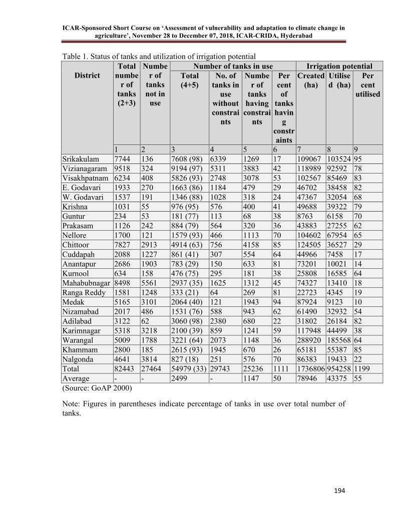
ICAR-Sponsored Short Course on ‘Assessment of vulnerability and adaptation to climate change in
agriculture’, November 28 to December 07, 2018, ICAR-CRIDA, Hyderabad
194
Table 1. Status of tanks and utilization of irrigation potential
District
Total
numbe
r of
tanks
(2+3)
Numbe
r of
tanks
not in
use
Number of tanks in use Irrigation potential
Total
(4+5)
No. of
tanks in
use
without
constrai
nts
Numbe
r of
tanks
having
constrai
nts
Per
cent
of
tanks
havin
g
constr
aints
Created
(ha)
Utilise
d (ha)
Per
cent
utilised
1 2 3 4 5 6 7 8 9 Srikakulam 7744 136 7608 (98) 6339 1269 17 109067 103524 95 Vizianagaram 9518 324 9194 (97) 5311 3883 42 118989 92592 78 Visakhpatnam 6234 408 5826 (93) 2748 3078 53 102567 85469 83 E. Godavari 1933 270 1663 (86) 1184 479 29 46702 38458 82 W. Godavari 1537 191 1346 (88) 1028 318 24 47367 32054 68 Krishna 1031 55 976 (95) 576 400 41 49688 39322 79 Guntur 234 53 181 (77) 113 68 38 8763 6158 70 Prakasam 1126 242 884 (79) 564 320 36 43883 27255 62 Nellore 1700 121 1579 (93) 466 1113 70 104602 67954 65 Chittoor 7827 2913 4914 (63) 756 4158 85 124505 36527 29 Cuddapah 2088 1227 861 (41) 307 554 64 44966 7458 17 Anantapur 2686 1903 783 (29) 150 633 81 73201 10021 14 Kurnool 634 158 476 (75) 295 181 38 25808 16585 64 Mahabubnagar 8498 5561 2937 (35) 1625 1312 45 74327 13410 18 Ranga Reddy 1581 1248 333 (21) 64 269 81 22723 4345 19 Medak 5165 3101 2064 (40) 121 1943 94 87924 9123 10 Nizamabad 2017 486 1531 (76) 588 943 62 61490 32932 54 Adilabad 3122 62 3060 (98) 2380 680 22 31802 26184 82 Karimnagar 5318 3218 2100 (39) 859 1241 59 117948 44499 38 Warangal 5009 1788 3221 (64) 2073 1148 36 288920 185568 64 Khammam 2800 185 2615 (93) 1945 670 26 65181 55387 85 Nalgonda 4641 3814 827 (18) 251 576 70 86383 19433 22 Total 82443 27464 54979 (33) 29743 25236 1111 1736806 954258 1199 Average - - 2499 - 1147 50 78946 43375 55 (Source: GoAP 2000)
Note: Figures in parentheses indicate percentage of tanks in use over total number of tanks.

ICAR-Sponsored Short Course on ‘Assessment of vulnerability and adaptation to climate change in
agriculture’, November 28 to December 07, 2018, ICAR-CRIDA, Hyderabad
195
Table 1a. Inter-district variation in capacity and utilization pattern of irrigation potential
Irrigation
capacity of tanks
in the district
Capacity utilization (%)
Poor (<40) Good (40-75) Better (>75)
Higher (>80,000 ha)
Chittoor, Medak, Karimnagar & Nalgonda
Nellore & Warangal
Srikakulam, Vizianagaram & Visakhapatnam
Medium (40,000 – 80,000 ha)
Kadapa, Anantapur & Mahabubnagar
West Godavari, Prakasam & Nizamabad
East Godavari, Krishna & Khammam
Lower (<40,000 ha)
Ranga Reddy Guntur & Kurnool Adilabad
Table 2. Mean weekly probability of rainfall of ≥ 20mm at Mahabubnagar during different months in the rainy season
Month
(Standard week)
Wet week
(W)
Wet week
followed by
wet (W/W)
Wet week
followed by dry
week (W/D)
Mean
June (22-25) 0.40 0.37 0.27 0.34 July (26-29) 0.65 0.62 0.53 0.60 August (30-33) 0.56 0.66 0.56 0.59 September (34-37) 0.53 0.57 0.49 0.53 October (38-42) 0.44 0.56 0.40 0.47 Mean 0.52 0.56 0.45 0.51
(Source: Virmani et.al. 1982)
Table 3. Area irrigated by medium irrigation project during the year 2001-02 in Mahabubnagar (686.5 mm rainfall)
S.
No
Name of the
project
Registered ayacut (acres) Actual area irrigated
(acres)
Kharif Rabi Kharif Rabi 1 Koilsagar 11,700 - - 3500 2 Saralsagar 4, 185 - - - 3 Ockachetti vagu 5,171 - - -
(Source: Hand Book of Statistics of Mahabubnagar 2003-04, Office of Chief Planning Officer, Mahabubnagar)
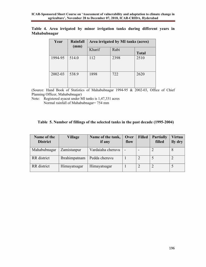
ICAR-Sponsored Short Course on ‘Assessment of vulnerability and adaptation to climate change in
agriculture’, November 28 to December 07, 2018, ICAR-CRIDA, Hyderabad
196
Table 4. Area irrigated by minor irrigation tanks during different years in
Mahabubnagar
Year Rainfall
(mm)
Area irrigated by MI tanks (acres)
Kharif Rabi Total
1994-95 514.0 112
2398
2510
2002-03 538.9 1898 722
2620
(Source: Hand Book of Statistics of Mahabubnagar 1994-95 & 2002-03, Office of Chief Planning Officer, Mahabubnagar) Note: Registered ayacut under MI tanks is 1,47,331 acres Normal rainfall of Mahabubnagar= 754 mm
Table 5. Number of fillings of the selected tanks in the past decade (1995-2004)
Name of the
District
Village Name of the tank,
if any
Over
flow
Filled Partially
filled
Virtua
lly dry
Mahabubnagar Zamistanpur Vardaiaha cheruvu - - 2 8
RR district Ibrahimpatnam Pedda cheruvu 1 2 5 2
RR district Himayatsagar Himayatsagar 1 2 2 5
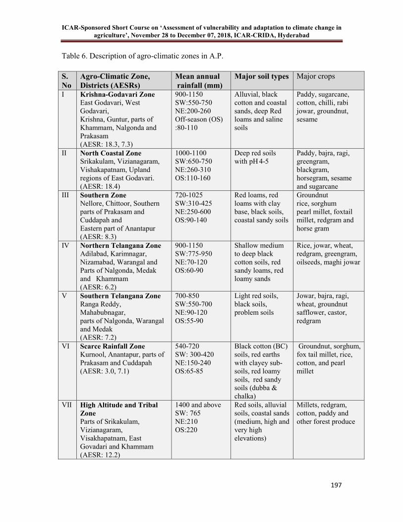
ICAR-Sponsored Short Course on ‘Assessment of vulnerability and adaptation to climate change in
agriculture’, November 28 to December 07, 2018, ICAR-CRIDA, Hyderabad
197
Table 6. Description of agro-climatic zones in A.P.
S.
No
Agro-Climatic Zone,
Districts (AESRs)
Mean annual
rainfall (mm)
Major soil types Major crops
I Krishna-Godavari Zone
East Godavari, West Godavari, Krishna, Guntur, parts of Khammam, Nalgonda and Prakasam (AESR: 18.3, 7.3)
900-1150 SW:550-750 NE:200-260 Off-season (OS) :80-110
Alluvial, black cotton and coastal sands, deep Red loams and saline soils
Paddy, sugarcane, cotton, chilli, rabi jowar, groundnut, sesame
II North Coastal Zone
Srikakulam, Vizianagaram, Vishakapatnam, Upland regions of East Godavari. (AESR: 18.4)
1000-1100 SW:650-750 NE:260-310 OS:110-160
Deep red soils with pH 4-5
Paddy, bajra, ragi, greengram, blackgram, horsegram, sesame and sugarcane
III Southern Zone
Nellore, Chittoor, Southern parts of Prakasam and Cuddapah and Eastern part of Anantapur (AESR: 8.3)
720-1025 SW:310-425 NE:250-600 OS:90-140
Red loams, red loams with clay base, black soils, coastal sandy soils
Groundnut rice, sorghum pearl millet, foxtail millet, redgram and horse gram
IV Northern Telangana Zone
Adilabad, Karimnagar, Nizamabad, Warangal and Parts of Nalgonda, Medak and Khammam (AESR: 6.2)
900-1150 SW:775-950 NE:70-120 OS:60-90
Shallow medium to deep black cotton soils, red sandy loams, red loamy sands
Rice, jowar, wheat, redgram, greengram, oilseeds, maghi jowar
V Southern Telangana Zone
Ranga Reddy, Mahabubnagar, parts of Nalgonda, Warangal and Medak (AESR: 7.2)
700-850 SW:550-700 NE:90-120 OS:55-90
Light red soils, black soils, problem soils
Jowar, bajra, ragi, wheat, groundnut safflower, castor, redgram
VI Scarce Rainfall Zone
Kurnool, Anantapur, parts of Prakasam and Cuddapah (AESR: 3.0, 7.1)
540-720 SW: 300-420 NE:150-240 OS:65-85
Black cotton (BC) soils, red earths with clayey sub-soils, red loamy soils, red sandy soils (dubba & chalka)
Groundnut, sorghum, fox tail millet, rice, cotton, and pearl millet
VII High Altitude and Tribal
Zone
Parts of Srikakulam, Vizianagaram, Visakhapatnam, East Govadari and Khammam (AESR: 12.2)
1400 and above SW: 765 NE:210 OS:220
Red soils, alluvial soils, coastal sands (medium, high and very high elevations)
Millets, redgram, cotton, paddy and other forest produce
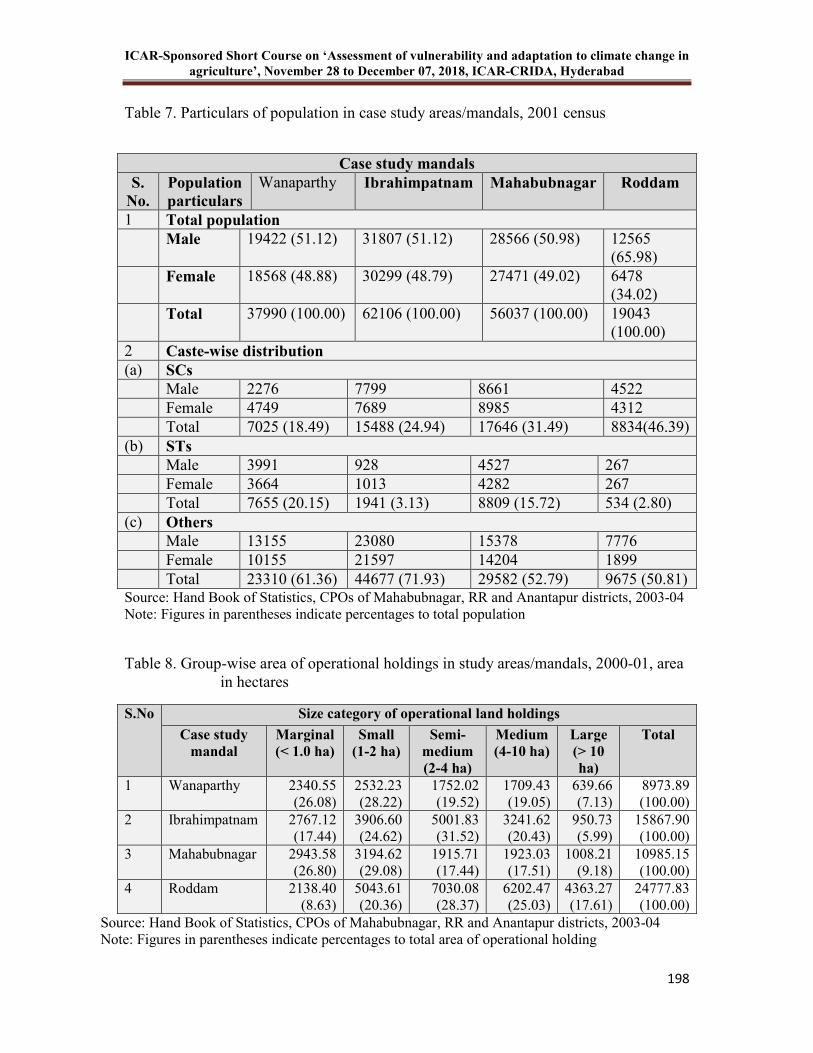
ICAR-Sponsored Short Course on ‘Assessment of vulnerability and adaptation to climate change in
agriculture’, November 28 to December 07, 2018, ICAR-CRIDA, Hyderabad
198
Table 7. Particulars of population in case study areas/mandals, 2001 census
Case study mandals
S.
No.
Population
particulars
Wanaparthy Ibrahimpatnam Mahabubnagar Roddam
1 Total population
Male 19422 (51.12) 31807 (51.12) 28566 (50.98) 12565 (65.98)
Female 18568 (48.88) 30299 (48.79) 27471 (49.02) 6478 (34.02)
Total 37990 (100.00) 62106 (100.00) 56037 (100.00) 19043 (100.00)
2 Caste-wise distribution (a) SCs
Male 2276 7799 8661 4522 Female 4749 7689 8985 4312 Total 7025 (18.49) 15488 (24.94) 17646 (31.49) 8834(46.39) (b) STs
Male 3991 928 4527 267 Female 3664 1013 4282 267 Total 7655 (20.15) 1941 (3.13) 8809 (15.72) 534 (2.80) (c) Others
Male 13155 23080 15378 7776 Female 10155 21597 14204 1899 Total 23310 (61.36) 44677 (71.93) 29582 (52.79) 9675 (50.81) Source: Hand Book of Statistics, CPOs of Mahabubnagar, RR and Anantapur districts, 2003-04 Note: Figures in parentheses indicate percentages to total population
Table 8. Group-wise area of operational holdings in study areas/mandals, 2000-01, area in hectares
S.No Size category of operational land holdings
Case study
mandal
Marginal
(< 1.0 ha)
Small
(1-2 ha)
Semi-
medium
(2-4 ha)
Medium
(4-10 ha)
Large
(> 10
ha)
Total
1 Wanaparthy 2340.55 (26.08)
2532.23 (28.22)
1752.02 (19.52)
1709.43 (19.05)
639.66 (7.13)
8973.89 (100.00)
2 Ibrahimpatnam 2767.12 (17.44)
3906.60 (24.62)
5001.83 (31.52)
3241.62 (20.43)
950.73 (5.99)
15867.90 (100.00)
3 Mahabubnagar 2943.58 (26.80)
3194.62 (29.08)
1915.71 (17.44)
1923.03 (17.51)
1008.21 (9.18)
10985.15 (100.00)
4 Roddam 2138.40 (8.63)
5043.61 (20.36)
7030.08 (28.37)
6202.47 (25.03)
4363.27 (17.61)
24777.83 (100.00)
Source: Hand Book of Statistics, CPOs of Mahabubnagar, RR and Anantapur districts, 2003-04 Note: Figures in parentheses indicate percentages to total area of operational holding

ICAR-Sponsored Short Course on ‘Assessment of vulnerability and adaptation to climate change in
agriculture’, November 28 to December 07, 2018, ICAR-CRIDA, Hyderabad
199
Table 9. Net area irrigated by different sources of irrigation in study areas/mandals during 2000-01, area in hectares
S.
No
Case
study
mandal
Canals Tanks Tube
wells
Other
wells
Lift irri
gation
Other
sources
Total Area
irrigate
d more
than
once
1 Wana parthy
- - 1670 (97.66)
40 (2.34)
- - 1710 (100.00)
629 (36.78)
2 Ibrahimpatnam
- - 1554 (72.01)
604 (27.99)
- - 2158 (100.00)
568 (26.32)
3 Maha bubnagar
- - 1450 (100.00)
- - - 1450 (100.00)
153 (10.55)
4 Roddam - - 3074 (100.00)
- - - 3074 (100.00)
0
Source: Hand Book of Statistics, CPOs of Mahabubnagar, RR and Anantapur districts, 2003-04 Note: Figures in parentheses indicate percentages of net area irrigated to total sources of irrigation
Table 10. Cropping pattern under kharif season in study areas/mandals in 2003-04, area in hectares
S.
No.
Principal
crops
Wanaparthy Ibrahimpatnam Mahabubnagar Roddam
1 Paddy 655 (30.66) 835 (10.32) 826 (54.27) 154 (0.72) 2 Jowar - 1949 (24.08) - 255 (1.20) 3 Bajra - 213 (2.63) - 14 (0.07) 4 Ragi - - - 255 (1.20) 5 Maize - 117 (1.45) - 298 (1.40) 6 Groundnut 17 (0.80) 2 (0.02) - 16719
(78.49) 7 Castor - 3133 (38.71) - 109 (0.51) 8 Sunflower - - - 851 (4.00) 9 Redgram - - - 1388 (6.52) 10 Chillies 9 (0.42) 17 (0.21) 7 (0.50) 151 (0.71) 11 Vegetables 15 (0.70) 814 (10.06) 4 (0.26) 0.18 Total cropped area under kharif and rabi seasons
2136 (100.00)
8094 (100.00) 1522 (100.00) 21301 (100.00)
Source: Hand Book of Statistics, CPOs of Mahabubnagar, RR and Anantapur districts, 2003-04 Note: Figures in parentheses indicate percentages to total cropped area under principal crops

ICAR-Sponsored Short Course on ‘Assessment of vulnerability and adaptation to climate change in
agriculture’, November 28 to December 07, 2018, ICAR-CRIDA, Hyderabad
200
Table 11.Number of tanks, area occupied and perimeter of tanks in Wanaparthy mandal
of Mahabubnagar district
Parameters MI tanks PR tanks Total
Number 17 44 61 Tank area (ha) 7 to 40 0.1 to 7.5 Total area (ha) 319.7 90.4 410.1 Dry area 248.2 Mostly dry Seasonal wet area 71.5 Partially wet Total perimeter (m) 32664 24135 56799 The length of bund (m) 9498 6467 15965 Perimeter available for plantation (m), excluding the length of the bund
23166 17668 40834
Table 12. Normal and actual rainfall of Ranga Reddy district in year 2004
Month Rainfall Departure from
normal (%) Normal Actual
January 5.9 19.7 233.9 February 7.5 0.0 -100 March 12.3 29.2 137.4 April 19.0 20.7 8.9 May 34.1 50.3 47.5 June 103.3 72.2 -30.1 July 125.8 205.0 63.0 August 150.4 51.7 -65.6 September 137.0 45.8 -66.2 October 104.9 84.8 -19.2 November 34.2 2.0 -94.2 December 5.6 0.0 -100 Total 740 581.4 -21.4
(Source: Hayathnagar Research Farm of CRIDA, Hyderabad)
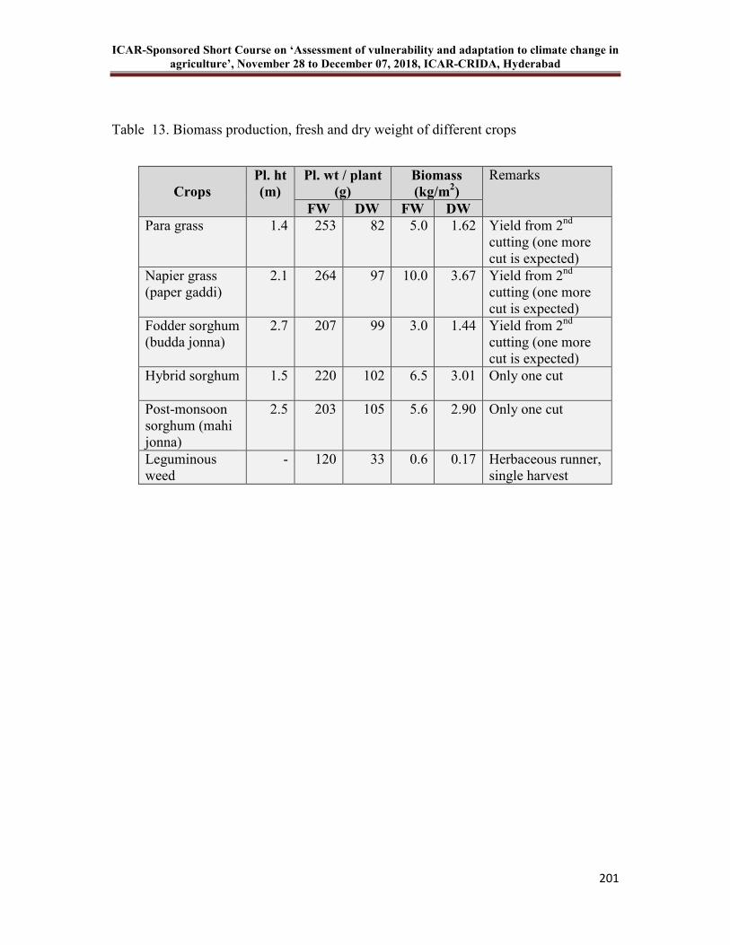
ICAR-Sponsored Short Course on ‘Assessment of vulnerability and adaptation to climate change in
agriculture’, November 28 to December 07, 2018, ICAR-CRIDA, Hyderabad
201
Table 13. Biomass production, fresh and dry weight of different crops
Crops
Pl. ht
(m)
Pl. wt / plant
(g)
Biomass
(kg/m2)
Remarks
FW DW FW DW
Para grass 1.4 253 82 5.0 1.62 Yield from 2nd cutting (one more cut is expected)
Napier grass (paper gaddi)
2.1 264 97 10.0 3.67 Yield from 2nd cutting (one more cut is expected)
Fodder sorghum (budda jonna)
2.7 207 99 3.0 1.44 Yield from 2nd cutting (one more cut is expected)
Hybrid sorghum 1.5 220 102 6.5 3.01 Only one cut
Post-monsoon sorghum (mahi jonna)
2.5 203 105 5.6 2.90 Only one cut
Leguminous weed
- 120 33 0.6 0.17 Herbaceous runner, single harvest
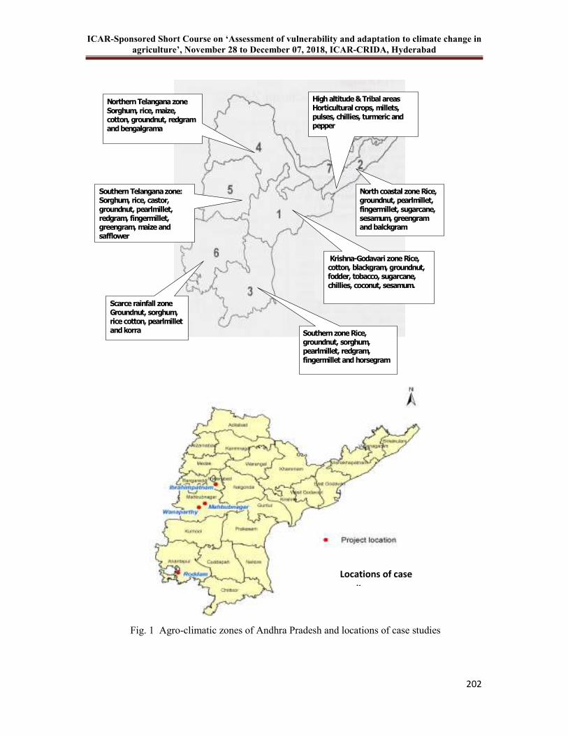
ICAR-Sponsored Short Course on ‘Assessment of vulnerability and adaptation to climate change in
agriculture’, November 28 to December 07, 2018, ICAR-CRIDA, Hyderabad
202
Krishna-Godavari zone Rice, cotton, blackgram, groundnut, fodder, tobacco, sugarcane, chillies, coconut, sesamum.
North coastal zone Rice, groundnut, pearlmillet, fingermillet, sugarcane, sesamum, greengram and balckgram
Southern zone Rice, groundnut, sorghum, pearlmillet, redgram, fingermillet and horsegram
Northern Telangana zone Sorghum, rice, maize, cotton, groundnut, redgram and bengalgrama
Southern Telangana zone: Sorghum, rice, castor, groundnut, pearlmillet, redgram, fingermillet, greengram, maize and safflower
Scarce rainfall zone Groundnut, sorghum, rice cotton, pearlmillet and korra
High altitude & Tribal areas Horticultural crops, millets, pulses, chillies, turmeric and pepper
Fig. 1 Agro-climatic zones of Andhra Pradesh and locations of case studies
Locations of case
studies

ICAR-Sponsored Short Course on ‘Assessment of
agriculture’, November 28 to December 07, 2018, ICAR
17 Problem Driven Iterative Ad
problems: Monitoring, evaluation, feedback and learning
A Amarender Reddy
A problem-driven, iterative approach to institutional reform involves (i) solving defined performance problems through (ii) creating an environment amenable to experimentation, (iii) creating tight feedback loops, and (iv) engaging a broad set of actors. Such an approach has recently been termed as PDIA (problemadaptation), with analysis suggesting that successful institutional reforms have mostly followed PDIA principles, though these may not have been acknowledged explicitly.PDIA (Problem Driven Iterative Adaptation) as an approach to building capability of state organizations while producing results. PDIA is implemnted through four principles given in figure 1.
Sponsored Short Course on ‘Assessment of vulnerability and adaptation to climate change in
agriculture’, November 28 to December 07, 2018, ICAR-CRIDA, Hyderabad
Problem Driven Iterative Adaptation for solving developmental
Monitoring, evaluation, feedback and learning
A Amarender Reddy
driven, iterative approach to institutional reform involves (i) solving defined performance problems through (ii) creating an environment amenable to experimentation, (iii) creating tight feedback loops, and (iv) engaging a broad set of
uch an approach has recently been termed as PDIA (problem-driven iterative adaptation), with analysis suggesting that successful institutional reforms have mostly followed PDIA principles, though these may not have been acknowledged
m Driven Iterative Adaptation) as an approach to building capability of state organizations while producing results. PDIA is implemnted through four principles given in figure 1.
Fig.1: Basic principles of PDIA
vulnerability and adaptation to climate change in
CRIDA, Hyderabad
203
tion for solving developmental
Monitoring, evaluation, feedback and learning
driven, iterative approach to institutional reform involves (i) solving defined performance problems through (ii) creating an environment amenable to experimentation, (iii) creating tight feedback loops, and (iv) engaging a broad set of
driven iterative adaptation), with analysis suggesting that successful institutional reforms have mostly followed PDIA principles, though these may not have been acknowledged
m Driven Iterative Adaptation) as an approach to building capability of state organizations while producing results. PDIA is implemnted through
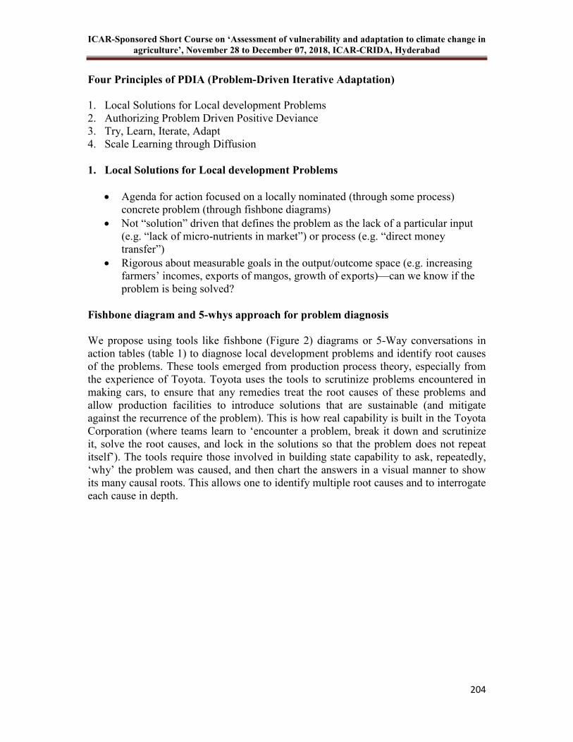
ICAR-Sponsored Short Course on ‘Assessment of vulnerability and adaptation to climate change in
agriculture’, November 28 to December 07, 2018, ICAR-CRIDA, Hyderabad
204
Four Principles of PDIA (Problem-Driven Iterative Adaptation)
1. Local Solutions for Local development Problems 2. Authorizing Problem Driven Positive Deviance 3. Try, Learn, Iterate, Adapt 4. Scale Learning through Diffusion 1. Local Solutions for Local development Problems
• Agenda for action focused on a locally nominated (through some process) concrete problem (through fishbone diagrams)
• Not “solution” driven that defines the problem as the lack of a particular input (e.g. “lack of micro-nutrients in market”) or process (e.g. “direct money transfer”)
• Rigorous about measurable goals in the output/outcome space (e.g. increasing farmers’ incomes, exports of mangos, growth of exports)—can we know if the problem is being solved?
Fishbone diagram and 5-whys approach for problem diagnosis
We propose using tools like fishbone (Figure 2) diagrams or 5-Way conversations in action tables (table 1) to diagnose local development problems and identify root causes of the problems. These tools emerged from production process theory, especially from the experience of Toyota. Toyota uses the tools to scrutinize problems encountered in making cars, to ensure that any remedies treat the root causes of these problems and allow production facilities to introduce solutions that are sustainable (and mitigate against the recurrence of the problem). This is how real capability is built in the Toyota Corporation (where teams learn to ‘encounter a problem, break it down and scrutinize it, solve the root causes, and lock in the solutions so that the problem does not repeat itself’). The tools require those involved in building state capability to ask, repeatedly, ‘why’ the problem was caused, and then chart the answers in a visual manner to show its many causal roots. This allows one to identify multiple root causes and to interrogate each cause in depth.
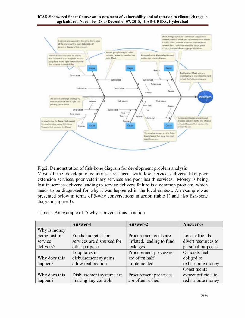
ICAR-Sponsored Short Course on ‘Assessment of vulnerability and adaptation to climate change in
agriculture’, November 28 to December 07, 2018, ICAR-CRIDA, Hyderabad
205
Fig.2. Demonstration of fish-bone diagram for development problem analysis Most of the developing countries are faced with low service delivery like poor extension services, poor veterinary services and poor health services. Money is being lost in service delivery leading to service delivery failure is a common problem, which needs to be diagnosed for why it was happened in the local context. An example was presented below in terms of 5-why conversations in action (table 1) and also fish-bone diagram (figure 3). Table 1. An example of ‘5 why’ conversations in action
Answer-1 Answer-2 Answer-3
Why is money being lost in service delivery?
Funds budgeted for services are disbursed for other purpose
Procurement costs are inflated, leading to fund leakages
Local officials divert resources to personal purposes
Why does this happen?
Loopholes in disbursement systems allow reallocation
Procurement processes are often half implemented
Officials feel obliged to redistribute money
Why does this happen?
Disbursement systems are missing key controls
Procurement processes are often rushed
Constituents expect officials to redistribute money
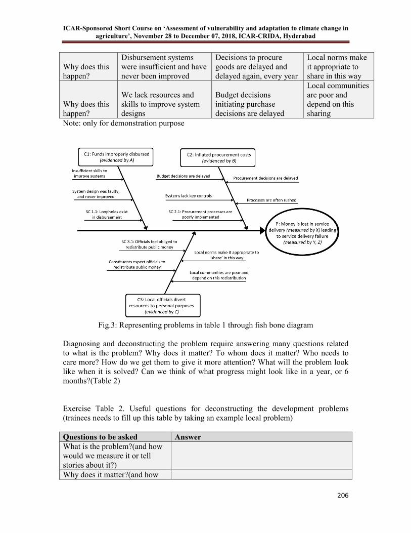
ICAR-Sponsored Short Course on ‘Assessment of vulnerability and adaptation to climate change in
agriculture’, November 28 to December 07, 2018, ICAR-CRIDA, Hyderabad
206
Why does this happen?
Disbursement systems were insufficient and have never been improved
Decisions to procure goods are delayed and delayed again, every year
Local norms make it appropriate to share in this way
Why does this happen?
We lack resources and skills to improve system designs
Budget decisions initiating purchase decisions are delayed
Local communities are poor and depend on this sharing
Note: only for demonstration purpose
Fig.3: Representing problems in table 1 through fish bone diagram
Diagnosing and deconstructing the problem require answering many questions related to what is the problem? Why does it matter? To whom does it matter? Who needs to care more? How do we get them to give it more attention? What will the problem look like when it is solved? Can we think of what progress might look like in a year, or 6 months?(Table 2)
Exercise Table 2. Useful questions for deconstructing the development problems (trainees needs to fill up this table by taking an example local problem) Questions to be asked Answer
What is the problem?(and how would we measure it or tell stories about it?)
Why does it matter?(and how
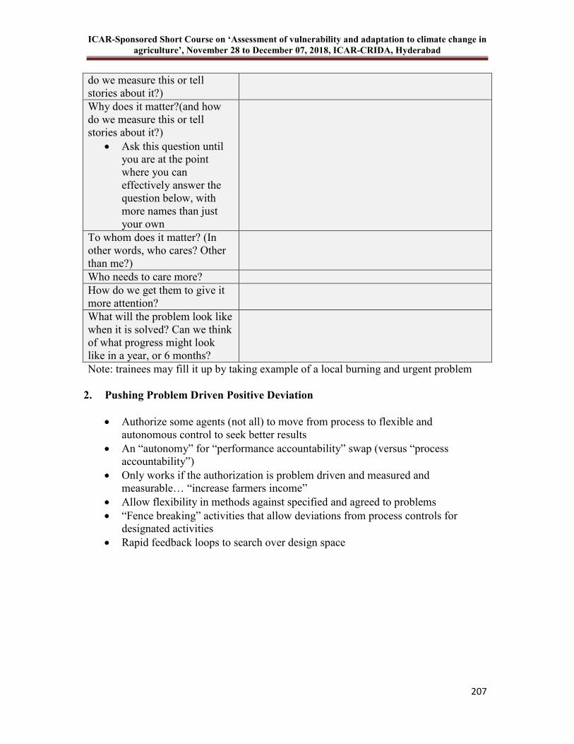
ICAR-Sponsored Short Course on ‘Assessment of vulnerability and adaptation to climate change in
agriculture’, November 28 to December 07, 2018, ICAR-CRIDA, Hyderabad
207
do we measure this or tell stories about it?) Why does it matter?(and how do we measure this or tell stories about it?)
• Ask this question until you are at the point where you can effectively answer the question below, with more names than just your own
To whom does it matter? (In other words, who cares? Other than me?)
Who needs to care more? How do we get them to give it more attention?
What will the problem look like when it is solved? Can we think of what progress might look like in a year, or 6 months?
Note: trainees may fill it up by taking example of a local burning and urgent problem
2. Pushing Problem Driven Positive Deviation
• Authorize some agents (not all) to move from process to flexible and autonomous control to seek better results
• An “autonomy” for “performance accountability” swap (versus “process accountability”)
• Only works if the authorization is problem driven and measured and measurable… “increase farmers income”
• Allow flexibility in methods against specified and agreed to problems • “Fence breaking” activities that allow deviations from process controls for
designated activities • Rapid feedback loops to search over design space
ICAR-Sponsored Short Course on ‘Assessment of
agriculture’, November 28 to December 07, 2018, ICAR
Sponsored Short Course on ‘Assessment of vulnerability and adaptation to climate change in
agriculture’, November 28 to December 07, 2018, ICAR-CRIDA, Hyderabad
vulnerability and adaptation to climate change in
CRIDA, Hyderabad
208
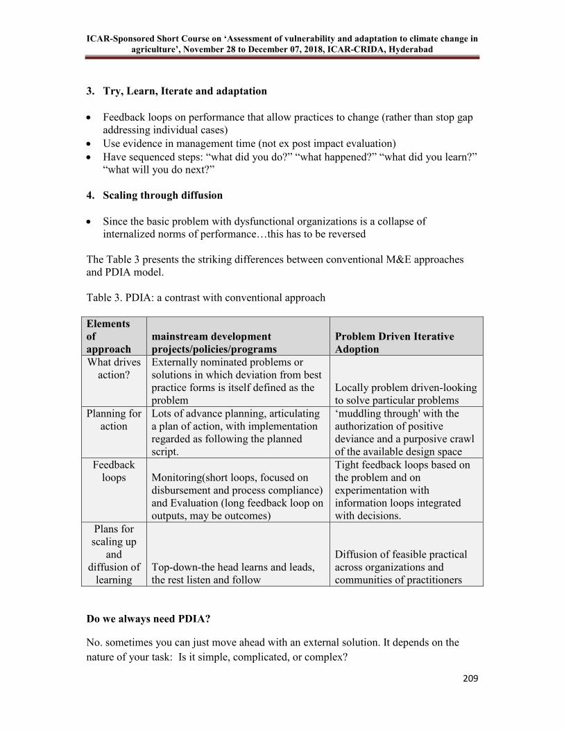
ICAR-Sponsored Short Course on ‘Assessment of vulnerability and adaptation to climate change in
agriculture’, November 28 to December 07, 2018, ICAR-CRIDA, Hyderabad
209
3. Try, Learn, Iterate and adaptation
• Feedback loops on performance that allow practices to change (rather than stop gap addressing individual cases)
• Use evidence in management time (not ex post impact evaluation) • Have sequenced steps: “what did you do?” “what happened?” “what did you learn?”
“what will you do next?”
4. Scaling through diffusion
• Since the basic problem with dysfunctional organizations is a collapse of internalized norms of performance…this has to be reversed
The Table 3 presents the striking differences between conventional M&E approaches and PDIA model. Table 3. PDIA: a contrast with conventional approach Elements
of
approach
mainstream development
projects/policies/programs
Problem Driven Iterative
Adoption
What drives action?
Externally nominated problems or solutions in which deviation from best practice forms is itself defined as the problem
Locally problem driven-looking to solve particular problems
Planning for action
Lots of advance planning, articulating a plan of action, with implementation regarded as following the planned script.
‘muddling through' with the authorization of positive deviance and a purposive crawl of the available design space
Feedback loops Monitoring(short loops, focused on
disbursement and process compliance) and Evaluation (long feedback loop on outputs, may be outcomes)
Tight feedback loops based on the problem and on experimentation with information loops integrated with decisions.
Plans for scaling up
and diffusion of
learning Top-down-the head learns and leads, the rest listen and follow
Diffusion of feasible practical across organizations and communities of practitioners
Do we always need PDIA?
No. sometimes you can just move ahead with an external solution. It depends on the nature of your task: Is it simple, complicated, or complex?

ICAR-Sponsored Short Course on ‘Assessment of vulnerability and adaptation to climate change in
agriculture’, November 28 to December 07, 2018, ICAR-CRIDA, Hyderabad
210
Where PDIA is applicable?
• We have done pretty well with the simple and complicated stuff • But complex tasks, problems, systems still confound us
o Challenges with adoption of a promising but complex technology o Gaps with adoption of crop insurance (PMFBY) o Getting civil servants to use shiny new systems, best practices
• So we need something like PDIA o To help us find and fit policy and management solutions o That fit the contexts in which we are working
References
Andrews M, Pritchett L and Woolcock M. 2015. Doing Problem Driven Work. HKS Working Paper No. 073, pp.47
Exercise on 5-Why and fishbone diagram
Annexure 1. Trainees example of ‘5 why’ conversations in action (please fill up this “5-why” to diagnose the local development problems in dryland agriculture
Answer-1 Answer-2 Answer-3
Problem: Why does this
happen?
Why does this happen?
Why does this
happen?
Why does this happen?
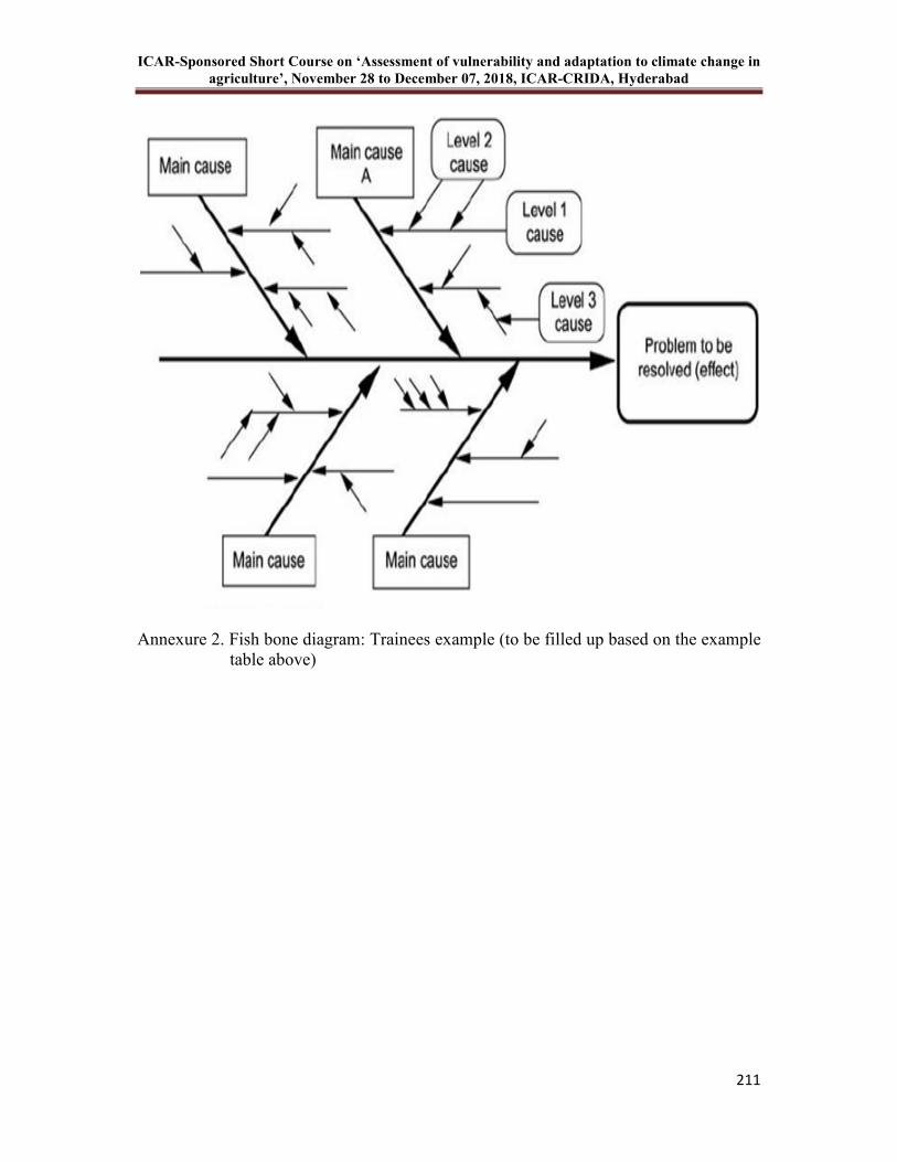
ICAR-Sponsored Short Course on ‘Assessment of vulnerability and adaptation to climate change in
agriculture’, November 28 to December 07, 2018, ICAR-CRIDA, Hyderabad
211
Annexure 2. Fish bone diagram: Trainees example (to be filled up based on the example table above)
ICAR-Sponsored Short Course on ‘Assessment of vulnerability and adaptation to climate change in
agriculture’, November 28 to December 07, 2018, ICAR-CRIDA, Hyderabad
212
18 Belowground Solutions to Aboveground Problems: Plant Roots
as Mitigators of Climate Change
K Srinivas
Recently, at a press encounter on climate change at the UN headquarters, New York on March 29, 2018, the United Nations secretary general, António Guterres, termed climate change “the most systemic threat to humankind” and urged world leaders to curb their countries’ greenhouse gas emissions. The global mean temperature in 2017 was approximately 1.1oC above the preindustrial era, more than half way towards the maximum limit of temperature increase of 2oC sought through the Paris Agreement, which further strives to limit the increase to 1.5°C above pre-industrial levels. The year 2017 was the warmest on record without an El Niño event, and one of the three warmest years, behind the record-setting 2016. The world’s nine warmest years have all occurred since 2005, and the five warmest since 2010. Extreme weather claimed lives and destroyed livelihoods in many countries in the recent years. It is no surprise that extreme weather events are identified as the most prominent risk facing humanity in the World Economic Forum’s Global Risks Report 2018 (World Economic Forum, 2018). Climate change has economic and societal impacts that disproportionately affect vulnerable nations through adverse effects on migration patterns, food security, health and other sectors. The United Nations in its annual report on food security and nutrition (FAO, 2018) noted that the number of hungry people in the world has reverted to levels last seen a decade ago. Nearly 821 million global citizens—or one out of every nine people—were undernourished in 2017, the third consecutive rise since 2015. Hunger affected 804 million people in 2016 and 784 million people in 2015. The rising rates of global hunger threaten the UN's Sustainable Development Goal (SDG) of ending all forms of hunger and malnutrition by 2030.
According to the report, the "key drivers" behind the rise in hunger include climate variability, which affects rainfall patterns and agricultural seasons, as well as climate extremes such as droughts and floods, which are a consequence of climate change. Climate change has already been shown to undermine production of staple crops such as wheat, rice and maize in tropical and temperate regions, and the predicted rise in global temperatures will reduce output even further. Notably, the countries that are the most exposed to climate extremes tend to have a higher prevalence and number of undernourished people.
Climate change is a consequence of warming of the earth’s climate attributed to elevated levels of greenhouse gases in the atmosphere resulting from anthropogenic emissions emanating from burning of fossil fuels, deforestation and land use changes, biomass burning, draining of wetlands, and inappropriate agricultural practices. Among the greenhouse gases emitted from human activities, CO2 is the single most important human-emitted greenhouse gas in the atmosphere, contributing 63.5% to the overall global radiative forcing of the climate since 1750 (WMO, 2009). The concentration of CO2 in the atmosphere has increased from the pre-industrial (before 1750) level of

ICAR-Sponsored Short Course on ‘Assessment of vulnerability and adaptation to climate change in
agriculture’, November 28 to December 07, 2018, ICAR-CRIDA, Hyderabad
213
about 280 ppmv (IPCC 2007) to 403 ppmv in 2016 (WMO, 2018). Any attempts towards arresting or reversing global warming must aim at stabilizing or reducing the concentration of CO2 in the atmosphere. This can be achieved either by reducing CO2 emissions to the atmosphere or by removing CO2 from the atmosphere. The process of transfer and secure storage of atmospheric CO2 into other long-lived C pools that would otherwise be emitted or remain in the atmosphere is called carbon sequestration (Lal, 2008). Carbon sequestration options can be grouped into two broad categories: abiotic and biotic sequestration. While abiotic sequestration is based on physical and chemical reactions and engineering techniques without intervention of living organisms, biotic sequestration, both oceanic and terrestrial, is based on managed intervention of higher plants and micro-organisms to remove CO2 from the atmosphere. Of the many options for terrestrial C sequestration, sequestering C in soil organic matter (SOM) is among the most preferred, as it offers a win-win solution to the problem of climate change. Transferring atmospheric C to relatively long-lived soil organic matter pools not only reduces atmospheric CO2 levels, but also enhances the productive capacity of the soil, which in turn enables greater C fixation and transfer, resulting in an atmospheric C negative (desirable) feedback loop. Soil organic carbon (SOC) sequestration involves putting C into the soil through the natural processes of humification. The fact that most soils under managed ecosystems contain a lower SOC pool than their counterparts under natural ecosystems, owing to the depletion of the SOC pool in cultivated soils, makes SOC sequestration possible and achievable. In general, cultivated soils normally contain 50–75% of the original SOC pool (Lal, 2008). The potential for C sequestration in soil organic matter in the world’s soils is estimated to be 0.6–1.2 Pg C yr-1 for up to 50 years, suggesting a sink capacity of 30-60 Pg C (Lal, 2004). The build-up of each Mg of soil organic matter removes 3.667 Mg of CO2 from the atmosphere. Increase in the SOC pool also has numerous ancillary benefits affecting local, regional and global processes.
The carbon fixed in plants by photosynthesis and added to soil as above and belowground litter is the primary source of C in ecosystems (Warembourg and Paul, 1977). Although most carbon enters ecosystems via leaves, and carbon accumulation is most obvious when it occurs in aboveground biomass, more than half of the assimilated carbon is eventually transported below ground via root growth and turnover and exudation of organic substances from roots. In many arable systems, since aboveground plant residues are grazed or removed, root-derived C provides a significant C input and is thus a major contributor to SOC (Heal et al., 1997), especially in the subtropical and tropical systems. The approximate similarity in the magnitude of variations in soil organic carbon content and root content in many soils may be regarded as evidence for the predominant role of roots in organic matter formation in soil (Kell, 2011).
Root Contribution to SOC
Belowground residues and root turnover represent direct inputs into the soil system, and as such have the potential to make major contributions to SOC stocks. The tight coupling between root distribution and SOC distribution with depth is often cited as evidence for the importance of root inputs in maintaining SOC stocks (Jackson et al.,
1996; Jobbagy and Jackson 2000). In addition to the spatial location within the mineral
ICAR-Sponsored Short Course on ‘Assessment of vulnerability and adaptation to climate change in
agriculture’, November 28 to December 07, 2018, ICAR-CRIDA, Hyderabad
214
soil, roots generally decay slower than aboveground residue (Rasse et al., 2005; Silver and Miya 2001) which has been attributed to both litter quality and environmental factors (Crow et al., 2009; Kogel-Knabner 2002).
Since shoots are the only primary carbon source in ecosystems apart from roots, comparisons between the contribution of shoots and roots to soil organic carbon are inevitable. Many studies suggest that the relative contribution of plant roots to soil organic C stocks is larger than that of plant shoots. Long-term residue management studies suggest that above ground material has a limited impact on SOM levels as compared to root systems. Campbell et al. (1991) reported that 30 years of returning wheat straw to soils did not modify the carbon content of the soils. They suggested that root inputs may be more important in maintaining soil organic matter. Results from a 30-year maize experiment indicated that restitution of maize stalks vs. removal for silage had no impact on SOC contents (Reicosky et al., 2002). Although some studies have observed a significant contribution of crop shoot residues to SOC content (Barber, 1979; Hooker et al., 1982), this contribution was comparatively smaller than that of roots (Barber, 1979). A simulation study by Molina et al. (2001) suggested that maize root systems contributed 1.8 times more C to soils than the corresponding aboveground biomass. Johnson et al. (2006) proposed that 1.5–3 times more root C than shoot C is stabilized in the SOC pool, which suggests that root biomass makes a greater contribution to soil C sequestration than aboveground residues. Root biomass has considerable value for SOC storage because of the amount of C contained in these residues and the fact that they are less easily mineralized, thus more likely to become chemically or physically stabilized in deeper soil layers (Bolinder et al. 1999). For roots to be preponderant contributors to the soil organic carbon pool, the belowground C additions have to be large, and/or belowground C has to be relatively more resistant to mineralization than aboveground C.
Carbon Allocation Belowground
Carbon taken up by plants through photosynthesis is termed gross primary production (GPP). CO
2 uptake during photosynthesis is only temporary – respiration returns about
half of the captured carbon to the atmosphere almost immediately. The remaining C is incorporated as structural material in shoots aboveground or allocated belowground. The fraction of GPP allocated belowground is significant. Heal et al. (1997) estimated that 16-33% of the C assimilated by plants through photosynthesis is transferred into the soil through the roots. Studies indicate that roughly 40% of net fixed C is allocated belowground (Jones et al., 2009). Cereals transfer 20-30% of assimilated C, while pasture plants transfer 30-50% C (Kuzyakov and Domanski, 2000). Based on analysis of several experiments, Amos and Walters (2006) conclude that, on average, the net belowground C at maize physiological maturity was 29% of shoot biomass C for maize. Carbon allocated belowground is lost as root respiration, incorporated in structural material as root biomass or released into the rhizosphere soil as rhizodeposition.
ICAR-Sponsored Short Course on ‘Assessment of vulnerability and adaptation to climate change in
agriculture’, November 28 to December 07, 2018, ICAR-CRIDA, Hyderabad
215
Rhizodeposited C
Rhizodeposition was first defined by Whipps and Lynch (1985) as all material lost from plant roots, including water-soluble exudates, secretions of insoluble materials, lysates, dead fine roots, and gases, such as CO2 and ethylene. The term rhizodeposition includes a wide range of processes by which C enters the soil including: (1) root cap and border cell loss, (2) death and lysis of root cells (cortex, root hairs etc), (3) flow of C to root-associated symbionts living in the soil (e.g. mycorrhizas), (4) gaseous losses, (5) leakage of solutes from living cells (root exudates), and (6) insoluble polymer secretion from living cells (mucilage) (Jones et al., 2009).
The amount of C inputs from the rhizodeposited C component is difficult to quantify under field conditions. Values of rhizodeposition, measured by 14C labeling technique, may range between 30-90% of the carbon transferred to belowground components of various plant-soil systems (Whipps 1990). For cereal crops, rhizodeposited C can represent 50% or more of the total amount of C allocated below-ground (Keith et al., 1986; Johansson, 1992; Swinnen et al., 1995). Common assumptions relating to rhizodeposited C are that it is equivalent to about 65 to 100% of the measurable root biomass (Bolinder et al., 1999; Bolinder et al., 2007; Rasse et al., 2005; Plénet et al., 1993). Some estimates suggest that rhizodeposition may be as much as 2.5 to 6 times the amount of C incorporated into root biomass (Johnen and Sauerbeck, 1977; Molina et
al., 2001).
Rhizodeposited C may not contribute significantly to soil C stocks, as much of the rhizodeposition is highly labile and therefore cycled through the soil food web during the growing season, with the respired portion of the C returned to the atmosphere as CO2. Root exudates have especially low residence times in soil. Typically, low molecular weight root exudates are believed to have a residence time of a few hours in soil solution as they are rapidly consumed by the C-limited rhizosphere microbial community (Nguyen and Guckert 2001; Van Hees et al. 2005). Boddy et al. (2007) found that these low molecular weight exudates had half-lives of only 20 to 40 minutes in soil. Although higher molecular weight rhizodeposits have a slightly longer persistence time in soil, they are still mineralized within a few days (Mary et al., 1992, 1993; Nguyen et al., 2008). Although most of the exuded materials are rapidly metabolized and respired by microorganisms (Kuzyakov and Cheng, 2001), some C is incorporated into the microbial biomass which has a slower turnover time (typically 30–90 days). However, some rhizodeposited C may become stabilized by adsorption on soil minerals. Also, rhizodeposits and the products of microbial decomposition of rhizodeposits play a significant role in formation of stable soil aggregates, in the process entrapping and protecting the organic carbon.
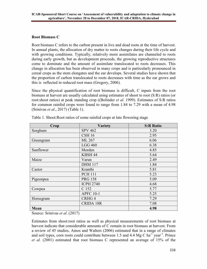
ICAR-Sponsored Short Course on ‘Assessment of vulnerability and adaptation to climate change in
agriculture’, November 28 to December 07, 2018, ICAR-CRIDA, Hyderabad
216
Root Biomass C
Root biomass C refers to the carbon present in live and dead roots at the time of harvest. In annual plants, the allocation of dry matter to roots changes during their life cycle and with growing conditions. Typically, relatively more assimilates are channeled to roots during early growth, but as development proceeds, the growing reproductive structures come to dominate and the amount of assimilate translocated to roots decreases. This change in allocation has been observed in many crops and is particularly pronounced in cereal crops as the stem elongates and the ear develops. Several studies have shown that the proportion of carbon translocated to roots decreases with time as the ear grows and this is reflected in reduced root mass (Gregory, 2006).
Since the physical quantification of root biomass is difficult, C inputs from the root biomass at harvest are usually calculated using estimates of shoot to root (S:R) ratios (or root:shoot ratios) at peak standing crop ((Bolinder et al. 1999). Estimates of S:R ratios for common rainfed crops were found to range from 1.84 to 7.29 with a mean of 4.98 (Srinivas et al., 2017) (Table 1).
Table 1. Shoot:Root ratios of some rainfed crops at late flowering stage
Crop Variety S:R Ratio Sorghum SPV 462 3.20 CSH 16 2.95 Greengram ML 267 6.06 LGG 460 6.38 Sunflower Morden 4.85 KBSH 44 5.64 Maize Varun 2.49 DHM 117 1.84 Castor Kranthi 5.81 PCH 111 5.23 Pigeonpea PRG 158 5.09 ICPH 2740 4.68 Cowpea C 152 5.77 APFC 10-1 5.25 Horsegram CRHG 4 7.29 CRIDA 18R 7.08 Mean 4.98
Source: Srinivas et al. (2017)
Estimates from shoot:root ratios as well as physical measurements of root biomass at harvest indicate that considerable amounts of C remain in root biomass at harvest. From a review of 45 studies, Amos and Walters (2006) estimated that in a range of climates and soil types, corn roots could contribute between 1.5 and 4.4 Mg C ha-1 year-1. Prince et al. (2001) estimated that root biomass C represented an average of 15% of the

ICAR-Sponsored Short Course on ‘Assessment of vulnerability and adaptation to climate change in
agriculture’, November 28 to December 07, 2018, ICAR-CRIDA, Hyderabad
217
aboveground biomass in maize. For cereals and grasses, about 50% of the C partitioned below ground (19% of net fixed C) is retained in root biomass (Kuzyakov and Domanski, 2000). Root biomass can represent up to 50% of residues incorporated into the soil from corn and soybean crops (Buyanovsky and Wagner, 1986).
Estimates made from data collected from long-term experiments and national crop yield data bases in the United States suggest that depending on tillage system and fertilizer rates, carbon inputs from irrigated and rainfed corn roots could range from 2.7 to 6.3 Mg C ha-1 year-1 (Allmaras et al., 2004, Wilts et al., 2004, Johnson et al., 2006). Similar estimates were made by Balesdent and Balabane (1996) in France, who reported a value of 5.4 Mg C ha-1 year-1 for a corn crop grown under cool temperate zone conditions. Hulugalle et al. (2010) quantified the carbon inputs by roots of irrigated corn in a Vertisol in Australia, and found that total root C of corn (C from root death + C remaining in roots at the end of the season) averaged 5.0 Mg ha-1 in cotton-corn system and 9.3 Mg ha-1 in corn monoculture system. Gan et al. (2009) quantified the carbon in different plant parts of wheat, oilseeds and pulses and found that while straw represented the largest stock of C, belowground C was considerable (Table 2)
Table 2. Carbon in plant parts of wheat, oilseeds and pulses at maturity, under rainfed and irrigated conditions in Saskatchewan, Canada
Crop/condition C (kg ha-1)
Grain Straw Roots
(0-100 cm)
Rhizodeposits
(65% of roots)
Rainfed Canola 343 1371 534 347 Mustard 324 1026 306 199 Flax 362 1212 314 204 Chickpea 495 743 330 214 Drypea 290 678 224 145 Lentil 439 853 380 247 Wheat 639 1491 449 292 Irrigated Canola 516 1548 535 348 Mustard 495 1273 365 237 Flax 418 1323 220 143 Chickpea 768 901 295 192 Drypea 424 861 203 132 Lentil 619 968 300 195 Wheat 1004 2133 606 394 Source: Gan et al. (2009)
From the foregoing discussion, it is clear that shoots have more biomass than roots, yet roots contribute more to SOC than shoots, indicating that there must be other mechanisms by which root derived C is preferentially preserved in soil over shoot derived C. Biochemical recalcitrance of root material (biochemical quality), physico-
ICAR-Sponsored Short Course on ‘Assessment of vulnerability and adaptation to climate change in
agriculture’, November 28 to December 07, 2018, ICAR-CRIDA, Hyderabad
218
chemical protection through the interaction with minerals, physical protection from microbial decomposers through aggregation and reduced decomposition of roots present in lower soil depths are mechanisms that explain the preferential preservation of root C in soil as SOC (Rasse et al., 2005).
Biochemical Recalcitrance (Biochemical Quality)
The importance of biochemical composition or ``quality'' in determining the rate of decomposition and mineralization of nutrients from plant materials has long been recognized (Swift et al., 1979). The chemical composition or quality of residues exerts a significant control over their decomposition (Vityakon and Dangthaisong, 2005). Plants generally contain the same classes of compounds, but the proportions of each, which depend upon the species and maturity, influence the degree and rate of decomposition (Kononova 1966). Residues typically consist of three fractions which differ in decomposition rate; 1. easily decomposable sugars and amino acids, 2. slowly decomposable compounds comprising cellulose and hemicellulose, and 3. recalcitrant materials such as lignin (Van Veen et al., 1984). When plant residues enter soil, some components decay quickly, while others decay slowly. Simple compounds such as sugars, amino acids and low molecular weight phenolics are quickly decomposed, while polymeric molecules such as celluloses, hemicelluloses and lignin decompose slowly (Berg and McClaugherty, 2003).
The chemical recalcitrance of plant litter material is largely ascribed to lignin (Tegelaar et al., 1989). Of all naturally produced organic chemicals, lignin is probably the most recalcitrant (Hammel, 1997). This is consistent with its biological functions, which are to give vascular plants the rigidity they need to stand upright, and to protect their structural polysaccharides (cellulose and hemicelluloses) from attack by other organisms. Lignin is known to inhibit microbial attack on holocellulose fraction physically, or by compounding the recalcitrant matrix by encrustation of cellulose (Adair et al., 2008; Berg and McClaugherty, 2003; Sinsabaugh and Linkins, 1989). Lignin is a polyphenolic molecule that has stable ether and C-C bonds. Microbial decomposition of this structure requires strong oxidation agents and only a few soil microorganisms, namely the white-rot fungi, are able to completely mineralize lignin (Hammel, 1997).
Biodegradability of plant litter material is often characterized through biochemical fractionation, such as the method of Goering and Van Soest (1970). This method leads to the quantification of a series of organic molecule fractions displaying decreasing biodegradability. Within a given species, the lignin content of roots obtained by the method of Goering and Van Soest (1970) is on average more than double that of shoots (Table 3).
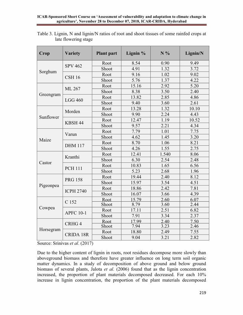
ICAR-Sponsored Short Course on ‘Assessment of vulnerability and adaptation to climate change in
agriculture’, November 28 to December 07, 2018, ICAR-CRIDA, Hyderabad
219
Table 3. Lignin, N and lignin/N ratios of root and shoot tissues of some rainfed crops at late flowering stage
Source: Srinivas et al. (2017)
Due to the higher content of lignin in roots, root residues decompose more slowly than aboveground biomass and therefore have greater influence on long term soil organic matter dynamics. In a study of decomposition of above ground and below ground biomass of several plants, Jalota et al. (2006) found that as the lignin concentration increased, the proportion of plant materials decomposed decreased. For each 10% increase in lignin concentration, the proportion of the plant materials decomposed
Crop Variety Plant part Lignin % N % Lignin/N
Sorghum SPV 462
Root 8.54 0.90 9.49 Shoot 4.91 1.32 3.72
CSH 16 Root 9.16 1.02 9.02 Shoot 5.76 1.37 4.22
Greengram ML 267
Root 15.16 2.92 5.20 Shoot 8.38 3.50 2.40
LGG 460 Root 13.82 2.85 4.86 Shoot 9.40 3.60 2.61
Sunflower Morden
Root 13.28 1.32 10.10 Shoot 9.90 2.24 4.43
KBSH 44 Root 12.47 1.19 10.52 Shoot 9.57 2.21 4.34
Maize Varun
Root 7.79 1.01 7.75 Shoot 4.62 1.45 3.20
DHM 117 Root 8.70 1.06 8.21 Shoot 4.26 1.55 2.75
Castor Kranthi
Root 12.41 1.540 8.06 Shoot 6.30 2.54 2.48
PCH 111 Root 10.83 1.65 6.56 Shoot 5.23 2.68 1.96
Pigeonpea PRG 158
Root 19.44 2.40 8.12 Shoot 15.97 3.54 4.51
ICPH 2740 Root 18.86 2.42 7.81 Shoot 16.07 3.66 4.39
Cowpea C 152 Root 15.79 2.60 6.07
Shoot 8.79 3.60 2.44
APFC 10-1 Root 17.11 2.51 6.82 Shoot 7.91 3.34 2.37
Horsegram CRHG 4 Root 17.99 2.40 7.50
Shoot 7.94 3.23 2.46
CRIDA 18R Root 18.80 2.49 7.55 Shoot 9.04 3.21 2.82
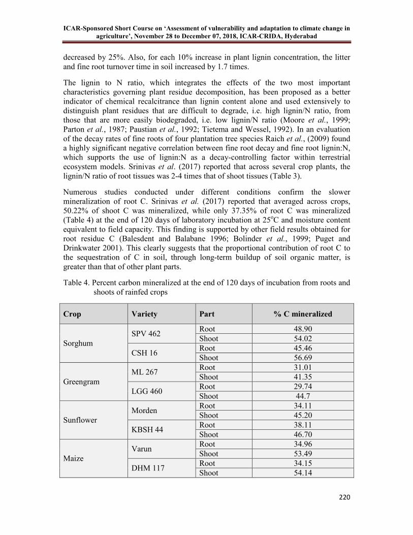
ICAR-Sponsored Short Course on ‘Assessment of vulnerability and adaptation to climate change in
agriculture’, November 28 to December 07, 2018, ICAR-CRIDA, Hyderabad
220
decreased by 25%. Also, for each 10% increase in plant lignin concentration, the litter and fine root turnover time in soil increased by 1.7 times.
The lignin to N ratio, which integrates the effects of the two most important characteristics governing plant residue decomposition, has been proposed as a better indicator of chemical recalcitrance than lignin content alone and used extensively to distinguish plant residues that are difficult to degrade, i.e. high lignin/N ratio, from those that are more easily biodegraded, i.e. low lignin/N ratio (Moore et al., 1999; Parton et al., 1987; Paustian et al., 1992; Tietema and Wessel, 1992). In an evaluation of the decay rates of fine roots of four plantation tree species Raich et al., (2009) found a highly significant negative correlation between fine root decay and fine root lignin:N, which supports the use of lignin:N as a decay-controlling factor within terrestrial ecosystem models. Srinivas et al. (2017) reported that across several crop plants, the lignin/N ratio of root tissues was 2-4 times that of shoot tissues (Table 3).
Numerous studies conducted under different conditions confirm the slower mineralization of root C. Srinivas et al. (2017) reported that averaged across crops, 50.22% of shoot C was mineralized, while only 37.35% of root C was mineralized (Table 4) at the end of 120 days of laboratory incubation at 25oC and moisture content equivalent to field capacity. This finding is supported by other field results obtained for root residue C (Balesdent and Balabane 1996; Bolinder et al., 1999; Puget and Drinkwater 2001). This clearly suggests that the proportional contribution of root C to the sequestration of C in soil, through long-term buildup of soil organic matter, is greater than that of other plant parts.
Table 4. Percent carbon mineralized at the end of 120 days of incubation from roots and shoots of rainfed crops
Crop Variety Part % C mineralized
Sorghum SPV 462
Root 48.90 Shoot 54.02
CSH 16 Root 45.46 Shoot 56.69
Greengram ML 267
Root 31.01 Shoot 41.35
LGG 460 Root 29.74 Shoot 44.7
Sunflower Morden
Root 34.11 Shoot 45.20
KBSH 44 Root 38.11 Shoot 46.70
Maize Varun
Root 34.96 Shoot 53.49
DHM 117 Root 34.15 Shoot 54.14
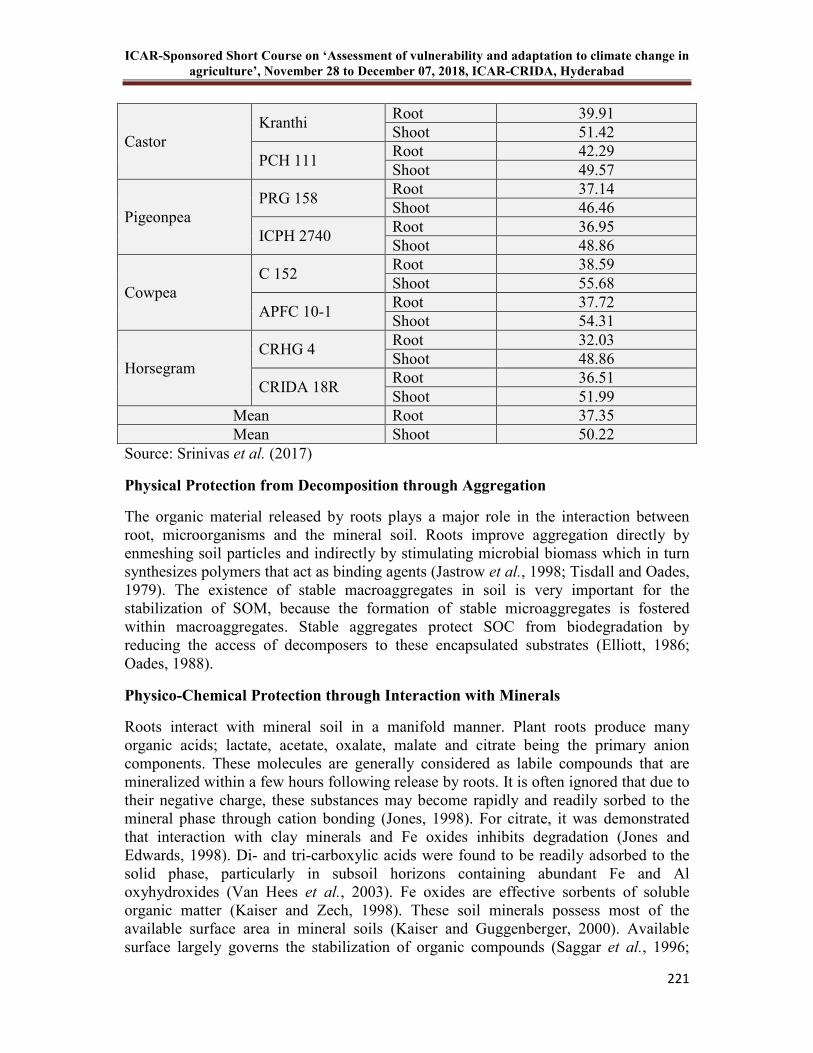
ICAR-Sponsored Short Course on ‘Assessment of vulnerability and adaptation to climate change in
agriculture’, November 28 to December 07, 2018, ICAR-CRIDA, Hyderabad
221
Castor Kranthi
Root 39.91 Shoot 51.42
PCH 111 Root 42.29 Shoot 49.57
Pigeonpea PRG 158
Root 37.14 Shoot 46.46
ICPH 2740 Root 36.95 Shoot 48.86
Cowpea C 152
Root 38.59 Shoot 55.68
APFC 10-1 Root 37.72 Shoot 54.31
Horsegram CRHG 4
Root 32.03 Shoot 48.86
CRIDA 18R Root 36.51 Shoot 51.99
Mean Root 37.35 Mean Shoot 50.22
Source: Srinivas et al. (2017)
Physical Protection from Decomposition through Aggregation
The organic material released by roots plays a major role in the interaction between root, microorganisms and the mineral soil. Roots improve aggregation directly by enmeshing soil particles and indirectly by stimulating microbial biomass which in turn synthesizes polymers that act as binding agents (Jastrow et al., 1998; Tisdall and Oades, 1979). The existence of stable macroaggregates in soil is very important for the stabilization of SOM, because the formation of stable microaggregates is fostered within macroaggregates. Stable aggregates protect SOC from biodegradation by reducing the access of decomposers to these encapsulated substrates (Elliott, 1986; Oades, 1988).
Physico-Chemical Protection through Interaction with Minerals
Roots interact with mineral soil in a manifold manner. Plant roots produce many organic acids; lactate, acetate, oxalate, malate and citrate being the primary anion components. These molecules are generally considered as labile compounds that are mineralized within a few hours following release by roots. It is often ignored that due to their negative charge, these substances may become rapidly and readily sorbed to the mineral phase through cation bonding (Jones, 1998). For citrate, it was demonstrated that interaction with clay minerals and Fe oxides inhibits degradation (Jones and Edwards, 1998). Di- and tri-carboxylic acids were found to be readily adsorbed to the solid phase, particularly in subsoil horizons containing abundant Fe and Al oxyhydroxides (Van Hees et al., 2003). Fe oxides are effective sorbents of soluble organic matter (Kaiser and Zech, 1998). These soil minerals possess most of the available surface area in mineral soils (Kaiser and Guggenberger, 2000). Available surface largely governs the stabilization of organic compounds (Saggar et al., 1996;

ICAR-Sponsored Short Course on ‘Assessment of vulnerability and adaptation to climate change in
agriculture’, November 28 to December 07, 2018, ICAR-CRIDA, Hyderabad
222
Torn et al., 1997). Sorption of root-derived organic acids to the mineral phase may be more effective in subsoils with low contents of organic matter because mineral surfaces are not yet saturated with organic matter. Thus, root-released compounds appear to have a selective advantage for stabilization through binding to the mineral phase, especially so in deep soil horizons.
Reduced Decomposition in Deeper Soil Layers
The recognition that substantial (possibly 10 or even 20 fold) decreases in atmospheric CO2 over geological time, especially during the Devonian (416.0–359.2 million years ago) may have largely been effected via the production of deep-rooted trees (Kell, 2011) can be taken as proof of the strong effect that deep roots can have on the terrestrial carbon cycle. Similarities in the depth distribution of roots and SOC (Olupot et al., 2010), further confirm this.
Depending on the plant species, roots can transfer C to considerable depth in the soil profile. There is considerable variation between both plant types and individual plant strains (cultivars) as to the maximum depth to which they produce roots, but 2 m for angiosperms (and much more for trees) is not at all uncommon (Kell, 2011). Plant root depths vary greatly in the same soil for different plants, for different cultivars of the same plant and even between different mutants of the same parent (Kell, 2001). Most presently cultivated agricultural crops have root depths that do not extend much beyond 1 m, but a few crop plants can produce roots exceeding 2 m (Kutschera et al., 2009). Roots of pigeonpea are deep and wide spreading in the soil, with well-developed lateral roots and may extend down to more than 2 m (Singh and Oswalt, 1992). Using data from experimental root measurements and modeling, Metselaar et al. (2009) estimated the rooting depths of globally important agricultural crops (Table 5) and found that averaged across all crops the depth within which 95% of roots were present (D95) was 90 cm, while depth within which 50% of roots were present (D50) was 19 cm. There was considerable variation in rooting depth of different crops, and D95 ranged from 32 cm for sunflower to 162 cm in cotton. Deeper root systems have the potential to sequester SOC (Smith, 2004) deeper in the soil profile, where SOC turnover times to atmospheric CO2 is slower due to unfavourable conditions for microbial activity with respect to moisture, temperature and nutrient availability.
Table 5. Average depth to 50% roots (D50) and depth to 95% roots (D95) of major agricultural crops
Crop D50 (cm) Weighted
D50 (cm)
D95 (cm) Weighted
D95 (cm)
Number of
observations
All crops 28 19 172 90 603 Barley 19 16 97 63 10 Rye 27 24 216 154 6 Rapeseed 16 14 99 73 30 Potato 33 30 125 83 50 Sugarbeet 47 45 154 129 11 Rice 11 10 53 25 91
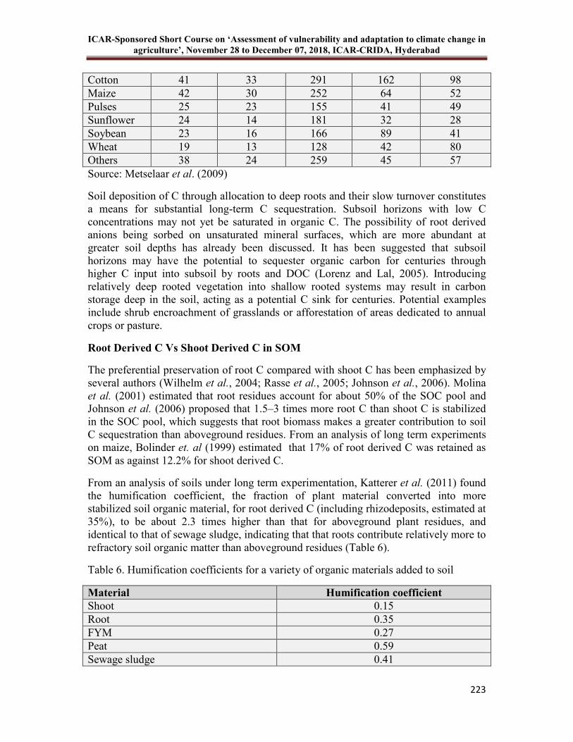
ICAR-Sponsored Short Course on ‘Assessment of vulnerability and adaptation to climate change in
agriculture’, November 28 to December 07, 2018, ICAR-CRIDA, Hyderabad
223
Cotton 41 33 291 162 98 Maize 42 30 252 64 52 Pulses 25 23 155 41 49 Sunflower 24 14 181 32 28 Soybean 23 16 166 89 41 Wheat 19 13 128 42 80 Others 38 24 259 45 57 Source: Metselaar et al. (2009)
Soil deposition of C through allocation to deep roots and their slow turnover constitutes a means for substantial long-term C sequestration. Subsoil horizons with low C concentrations may not yet be saturated in organic C. The possibility of root derived anions being sorbed on unsaturated mineral surfaces, which are more abundant at greater soil depths has already been discussed. It has been suggested that subsoil horizons may have the potential to sequester organic carbon for centuries through higher C input into subsoil by roots and DOC (Lorenz and Lal, 2005). Introducing relatively deep rooted vegetation into shallow rooted systems may result in carbon storage deep in the soil, acting as a potential C sink for centuries. Potential examples include shrub encroachment of grasslands or afforestation of areas dedicated to annual crops or pasture.
Root Derived C Vs Shoot Derived C in SOM
The preferential preservation of root C compared with shoot C has been emphasized by several authors (Wilhelm et al., 2004; Rasse et al., 2005; Johnson et al., 2006). Molina et al. (2001) estimated that root residues account for about 50% of the SOC pool and Johnson et al. (2006) proposed that 1.5–3 times more root C than shoot C is stabilized in the SOC pool, which suggests that root biomass makes a greater contribution to soil C sequestration than aboveground residues. From an analysis of long term experiments on maize, Bolinder et. al (1999) estimated that 17% of root derived C was retained as SOM as against 12.2% for shoot derived C.
From an analysis of soils under long term experimentation, Katterer et al. (2011) found the humification coefficient, the fraction of plant material converted into more stabilized soil organic material, for root derived C (including rhizodeposits, estimated at 35%), to be about 2.3 times higher than that for aboveground plant residues, and identical to that of sewage sludge, indicating that that roots contribute relatively more to refractory soil organic matter than aboveground residues (Table 6).
Table 6. Humification coefficients for a variety of organic materials added to soil
Material Humification coefficient
Shoot 0.15 Root 0.35 FYM 0.27 Peat 0.59 Sewage sludge 0.41
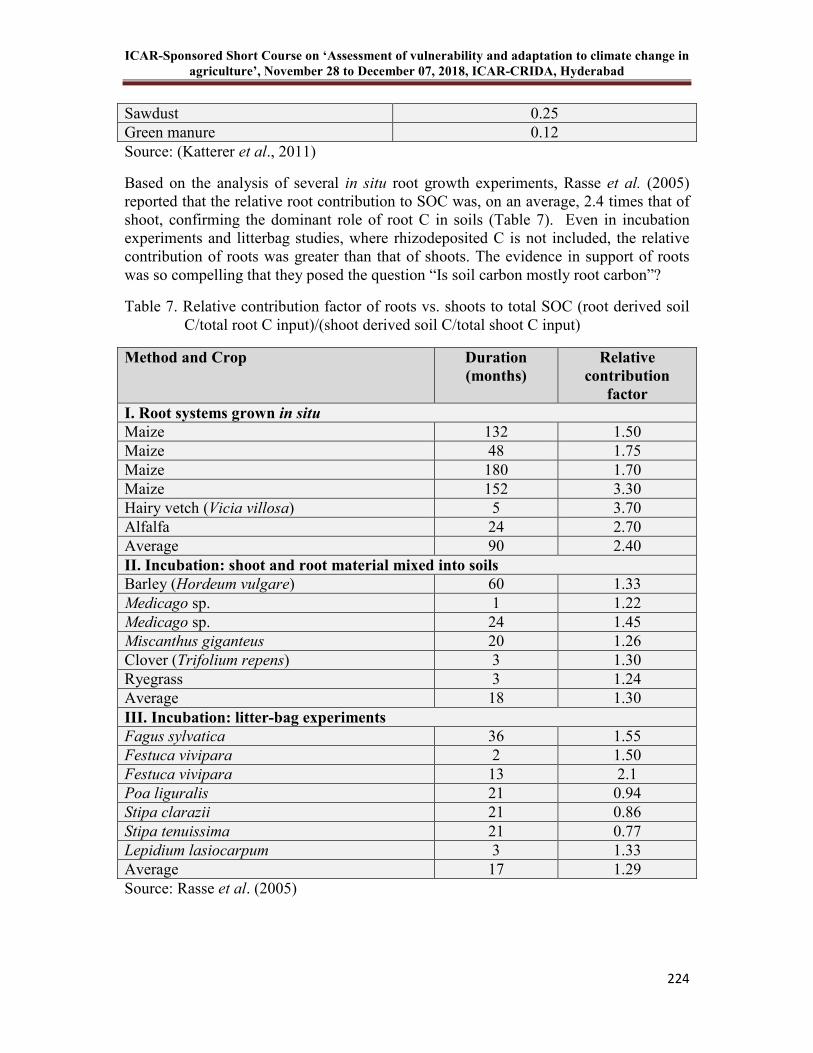
ICAR-Sponsored Short Course on ‘Assessment of vulnerability and adaptation to climate change in
agriculture’, November 28 to December 07, 2018, ICAR-CRIDA, Hyderabad
224
Sawdust 0.25 Green manure 0.12 Source: (Katterer et al., 2011)
Based on the analysis of several in situ root growth experiments, Rasse et al. (2005) reported that the relative root contribution to SOC was, on an average, 2.4 times that of shoot, confirming the dominant role of root C in soils (Table 7). Even in incubation experiments and litterbag studies, where rhizodeposited C is not included, the relative contribution of roots was greater than that of shoots. The evidence in support of roots was so compelling that they posed the question “Is soil carbon mostly root carbon”?
Table 7. Relative contribution factor of roots vs. shoots to total SOC (root derived soil C/total root C input)/(shoot derived soil C/total shoot C input)
Method and Crop Duration
(months)
Relative
contribution
factor
I. Root systems grown in situ
Maize 132 1.50 Maize 48 1.75 Maize 180 1.70 Maize 152 3.30 Hairy vetch (Vicia villosa) 5 3.70 Alfalfa 24 2.70 Average 90 2.40 II. Incubation: shoot and root material mixed into soils
Barley (Hordeum vulgare) 60 1.33 Medicago sp. 1 1.22 Medicago sp. 24 1.45 Miscanthus giganteus 20 1.26 Clover (Trifolium repens) 3 1.30 Ryegrass 3 1.24 Average 18 1.30 III. Incubation: litter-bag experiments
Fagus sylvatica 36 1.55 Festuca vivipara 2 1.50 Festuca vivipara 13 2.1 Poa liguralis 21 0.94 Stipa clarazii 21 0.86 Stipa tenuissima 21 0.77 Lepidium lasiocarpum 3 1.33 Average 17 1.29 Source: Rasse et al. (2005)
ICAR-Sponsored Short Course on ‘Assessment of vulnerability and adaptation to climate change in
agriculture’, November 28 to December 07, 2018, ICAR-CRIDA, Hyderabad
225
Strategies for Enhancing C Sequestration by Roots
The scope for sequestering atmospheric C into plant roots is substantial. Some analyses of existing grasslands and energy crops imply that at least 100 t ha-1 of steady-state carbon sequestration in roots is routinely attainable (Dondini et al., 2009; Silver et al., 2010). Any strategy that increases the quantity of C allocated belowground, enhances the recalcitrance of belowground inputs, or retards the decomposition of belowground C, will result in greater C sequestration in soil. In agroecosystems, such strategies include crop improvement through breeding or biotechnology, choice of cultivars, crops and cropping systems (intensive cropping, intercropping, mixed cropping, rotational cropping, alley cropping with tree components, etc.), and soil and crop management practices. Since potential for C sequestration in deeper soil layers is large, crop cultivars that express deeper and denser rooting characteristics will present greater opportunities for C sequestration. There is considerable scope for increasing the depth of roots by appropriate breeding strategies (Kell, 2011). Switching from annual crops to perennials or converting annual crops to perennials through breeding can also help sequester carbon as perennials have deeper and more extensive root systems that allow them to survive climatic extremes such as droughts and floods.
Subsoil C sequestration can be achieved by higher inputs of stable organic matter to deeper soil horizons. This can be achieved directly by selecting plants/cultivars with deeper and thicker root systems that are high in chemically recalcitrant compounds like suberin. Furthermore, recalcitrant compounds could be a target for plant breeding/biotechnology to promote C sequestration (Lorenz and Lal, 2005). Breeding crops that could cover present cropland areas but that had roots a metre deeper in the soil could double the amount of carbon captured from the environment (Kell, 2011). This could be a significant weapon in the fight against climate change.
Conclusions
The earth’s surface temperature is increasing at an alarming rate as a result of increase in concentration of greenhouse gases, among which CO2 is the most important. Sequestering atmospheric CO2 into soil organic matter can serve to mitigate global climate change while enhancing the productivity of crops through the beneficial effects of increased organic matter levels in soil. There is overwhelming evidence, that with equal or larger C contributions to soil of recalcitrant C than shoots, and the subsequent protection against decomposition, of root derived C, roots potentially contribute most of the organic C currently stored in soils of most ecosystems and will continue to do so in the future. Strategies that enhance the quantity and recalcitrance of belowground C inputs, particularly in deeper soil layers, and management practices that slow down the decomposition of SOC and its loss to the atmosphere can lead to sequestration of carbon and mitigation of global climate change.
ICAR-Sponsored Short Course on ‘Assessment of vulnerability and adaptation to climate change in
agriculture’, November 28 to December 07, 2018, ICAR-CRIDA, Hyderabad
226
References
Adair EC, Parton, WJ, Grosso, SD, Silver, WL, Harmon ME, Hall SA, Burke IC, Hart SC. 2008. Simple three-pool model accurately describes patterns of longterm litter decomposition in diverse climates. Global Change Biology, 14: 2636-2660.
Allmaras RR, Linden DR and Clapp CE. 2004. Corn residue transformations into root and soil carbon as related to nitrogen, tillage, and stover management. Soil Science Society of America Journal, 68: 1366-1375.
Amos B and Walters DT. 2006. Maize root biomass and net rhizodeposited carbon: An analysis of the literature. Soil Science Society of America Journal, 70:1489–1503.
Balesdent J and Balabane M. 1996. Major contribution of roots to soil carbon storage inferred from maize cultivated soils. Soil Biology and Biochemistry, 28: 1261–1263.
Barber SA. 1979. Corn residue management and soil organic matter. Agronomy Journal, 71: 625–627.
Berg B and McClaugherty CA. 2003. Plant Litter, Decomposition, Humus Formation, Carbon Sequestration. Springer-Verlag, Berlin, 338 pp.
Boddy E, Hill PW, Farrar J and Jones DL. 2007. Fast turnover of low molecular weight components of the dissolved organic carbon pool of temperate grassland field soils. Soil Biology and Biochemistry, 39: 827-835.
Bolinder MA, Angers DA, Giroux M and Laverdiere MR. 1999. Estimating C inputs retained as soil organic matter from corn (Zea mays L.). Plant and Soil, 215:85–91.
Bolinder MA, Janzen HH, Gregorich EG, Angers DA, Vanden-Bygaart AJ. 2007. An approach for estimating net primary productivity and annual carbon inputs to soil for common agricultural crops in Canada. Agriculture, Ecosystems and Environment, 118: 29–42.
Buyanovsky GA and Wagner GH. 1987. Carbon transfer in a winter wheat (Triticum
aestivum) ecosystem. Biology and Fertility of Soils, 5: 76-82.
Campbell CA, Lafond, GP, Zentner RP and Biederbeck V.O. 1991. Influence of fertilizer and straw baling on soil organic matter in a thin black chernozem in western Canada. Soil Biology and Biochemistry, 23: 443–446.
Crow SE, Lajtha K, Filley TR, Swanston CW, Bowden RD and Caldwell BA. 2009. Sources of plant-derived carbon and stability of organic matter in soil: Implications for global change. Global Change Biology.
ICAR-Sponsored Short Course on ‘Assessment of vulnerability and adaptation to climate change in
agriculture’, November 28 to December 07, 2018, ICAR-CRIDA, Hyderabad
227
Dondini M, Hastings A, Saiz, G, Jones MB, Smith P. 2009. The potential of Miscanthus to sequester carbon in soils: comparing field measurements in Carlow, Ireland, to model predictions. Global Change Biology Bioenergy, 1: 413–425.
Elliott ET. 1986. Aggregate structure and carbon, nitrogen, phosphorus in native and cultivated soils. Soil Science Society of America Journal, 50: 627–633.
FAO. 2018. The State of Food Security and Nutrition in the World 2018. Building climate resilience for food security and nutrition. FAO, Rome.
Gan YT, Campbell CA, Janzen HH, Lemke RL, Basnyat P and McDonald CL. 2009. Carbon input to soil from oilseed and pulse crops on the Canadian prairies. Agriculture, Ecosystems and Environment, 132: 290–297.
Goering HK and Van Soest PJ. 1970. Forage fiber analysis, apparatus, reagents, procedures, and some applications. Agriculture Handbook Vol. 379. ARS-USDA, Washington, DC.
Gregory PJ. 2006. Plant Roots: Growth, Activity and Interaction with Soils. Blackwell Publishing Ltd., Oxford, U.K. 318 pp.
Hammel KE. 1997. Fungal degradation of lignin. In G Cadisch and K E Giller (Eds.) “Driven by Nature: Plant Litter Quality and Decomposition”: 33–45. CAB International, Wallingford, U.K.
Heal OW, Anderson JW and Swift MJ. 1997. Plant litter quality and decomposition: An historical overview. In G. Cadisch, and K.E. Giller (Eds.) “Driven by Nature: Plant Litter Quality and Decomposition”, CAB International, Wallingford, U.K.: 3-45.
Hooker ML, Herron GM and Penas P. 1982. Effects of residue burning, removal and incorporation on irrigated cereal crop yields and soil chemical properties. Soil Science Society of America Journal, 46: 122–126.
Hulugalle NR, Weaver TB and Finlay LA. 2010. Carbon inputs by irrigated corn roots to a Vertisol. Plant Root 4: 18-21. www.plantroot.org.
IPCC. 2007. Climate Change 2007: The Physical Science Basis. Fourth Assessment Report (AR4) of the United Nations Intergovernmental Panel on Climate Change, Cambridge University Press, Cambridge, U.K., and New York, U.S.A..
Jackson RB, Canadell J, Ehleringer JR, Mooney HA, Sala OE and Shulze ED. 1996. A global analysis of root distributions for terrestrial biomes. Oecologia, 108: 389 411.
Jalota RK, Dalal RC, Harms BP, Page K, Mathers NJ and Wang WJ. Effects of litter and fine root composition on their decomposition in a Rhodic Paleustalf under different land uses. Communications in Soil Science and Plant Analysis, 37: 1859–1875.
ICAR-Sponsored Short Course on ‘Assessment of vulnerability and adaptation to climate change in
agriculture’, November 28 to December 07, 2018, ICAR-CRIDA, Hyderabad
228
Jastrow JD, Miller RM and Lussenshop J. 1998. Contribution of interacting biological mechanisms to soil aggregate stabilization in restored prairie. Soil Biology and Biochemistry, 30: 905–916.
Jobbagy EG and Jackson RB. 2000. The vertical distribution of soil organic carbon and its relation to climate and vegetation. Ecological Applications, 10: 423-436.
Johansson G. 1992. Release of organic C from growing roots of meadow fescue (Festucal pratensis L.). Soil Biology and Biochemistry, 24: 427-433.
Johnen G and Sauerbeck D. 1977. A tracer technique for measuring growth, mass and microbial breakdown of plant roots during vegetation.. In V. Lohm and T. Persson (Eds.) Soil Organisms as Components of Ecosystems. Proceedings of the International Soil Zoological Colloquium, 6th. Ecol. Bull., Stockholm, Sweden: 366–373.
Johnson JMF, Allmaras RR and Reicosky DC. 2006. Estimating source carbon from crop residues, roots and rhizodeposits using the national grain-yield database. Agronomy Journal, 98: 622-636.
Jones DL. 1998. Organic acids in the rhizosphere – A critical review. Plant and Soil 205, 25–44.
Jones DL and Edwards AC. 1998, Influence of sorption on the biological utilization of two simple carbon substrates. Soil Biology and Biochemistry, 30: 1895–1902.
Jones DL, Nguyen C and Finlay RD. 2009. Carbon flow in the rhizosphere: carbon trading at the soil–root interface. Plant Soil, 321: 5–33.
Kaiser K and Guggenberger, G. 2000. The role of DOM sorption to mineral surfaces in the preservation of organic matter in soils. Organic Geochemitrsy, 31: 711–725.
Kaiser K and Zech W. 1998. Soil dissolved organic matter sorption as influenced by organic and sesquioxide coatings and sorbed sulphate. Soil Science Society of America Journal, 62: 129–136.
Kätterer T, Bolinder MA, Andrén O, Kirchmann H, Menichetti L. 2011. Roots contribute more to refractory soil organic matter than aboveground crop residues, as revealed by a long-term field experiment. Agriculture Ecosystems and Environment, 141: 184–192.
Keith H, Oades JM Martin JK. 1986. Input of carbon to soil from wheat plants. Soil Biology and Biochemistry, 18: 445-449.
Kell DB. 2011. Breeding crop plants with deep roots: their role in sustainable carbon, nutrient and water sequestration. Annals of Botany, doi:10.1093/aob/mcr175, available online at www.aob.oxfordjournals.org.
ICAR-Sponsored Short Course on ‘Assessment of vulnerability and adaptation to climate change in
agriculture’, November 28 to December 07, 2018, ICAR-CRIDA, Hyderabad
229
Kogel-Knabner I. 2002. The macromolecular organic composition of plant and microbial residues as inputs to soil organic matter. Soil Biology and Biochemistry, 34: 139-162.
Kononova MM. 1966. Soil Organic Matter. Pergamon Press, New York, 544 pp.
Kutschera L, Lichtenegger E and Sobotik M. 2009. Wurzelatlas der Kulturpflanzen gemaßigter Gebiete mit Arten des Feldgemusebaues. Frankfurt/Main: DLG Verlag.
Kuzyakov Y and Cheng W. 2001. Photosynthesis controls of rhizosphere respiration and organic matter decomposition. Soil Biology and Biochemistry, 33: 1915-1925.
Kuzyakov Y and Domanski G. 2000. Carbon input by plants into the soil. Review. Journal of Plant Nutrition and Soil Science, 163: 421-431.
Lal R. 2004. Soil carbon sequestration to mitigate climate change. Geoderma, 123: 1–22.
Lal, R. 2008. Carbon sequestration. Philosohical Transactions of the Royal Society B, 363, 815–830.
Lorenz K and Lal R. 2005. The depth distribution of soil organic carbon in relation to land use and management and the potential of carbon sequestration in subsoil horizons. Advances in Agronomy, 88: 35-66.
Mary B, Fresneau C, Morel JL and Mariotti A. 1993. C-cycling and N-cycling during decomposition of root mucilage, roots and glucose in soil. Soil Biology and Biochemistry, 25:1005–1014.
Mary B, Mariotti A, Morel JL. 1992. Use of 13C variations at natural abundance for studying the biodegradation of root mucilage, roots and glucose in soil. Soil Biology and Biochemistry, 24: 1065–1072.
Metselaar K, Versace VL, Feddes RA. 2009. Root-depth profiles of important agricultural crops. Paper presented at the International Symposium “Root Research and Applications” RootRAP, 2–4 September 2009, Boku – Vienna, Austria.
Molina JAE, Clapp CE, Linden DR, Allmaras RR, Layese MF, Dowdy RH and Cheng HH. 2001. Modeling incorporation of corn (Zea mays L.) carbon from roots and rhizodeposition into soil organic matter. Soil Biology and Biochemistry, 33:83–92.
Moore TR, Trofymow JA, Taylor B, Prescott C, Camire C, Duschene L, Fyles J, Kozak L, Kranabetter M, Morrison I, Siltanen M, Smith S, Titus B, Visser S, Wein R and Zoltai S. 1999. Litter decomposition rates in Canadian forests. Global Change Biology, 5: 75–82.
ICAR-Sponsored Short Course on ‘Assessment of vulnerability and adaptation to climate change in
agriculture’, November 28 to December 07, 2018, ICAR-CRIDA, Hyderabad
230
Nguyen C, Froux F, Recous S, Morvan T, Robin C. 2008. Net N immobilization during the biodegradation of mucilage in soil as affected by repeated mineral and organic fertilization. Nutrient Cycling in Agroecosystems, 80: 39–47.
Nguyen C, Guckert A. 2001. Short-term utilisation of C-14-[U] glucose by soil microorganisms in relation to carbon availability. Soil Biology and Biochemistry, 33: 53 60.
Oades JM. 1988. The retention of organic matter in soils. Biogeochemistry, 5: 35–70.
Olupot G, Daniel H, Lockwood P, McHenry M and McLeod M. 2010. Root contributions to long-term storage of soil organic carbon: theories, mechanisms and gaps. 19th World Congress of Soil Science, Soil Solutions for a Changing World 1-6 August 2010, Brisbane, Australia. Published on DVD.
Parton WJ, Schimel CV, Cole CV and Ojima DS. 1987. Analysis of factors controlling soil organic matter levels in Great Plains grasslands. Soil Science Society of America Journal, 51: 1173–1179.
Paustian K, Parton WJ and Persson J. 1992. Modeling soil organic matter in organic amended and nitrogen-fertilized long-term plots. Soil Science Society of America Journal, 56: 476–488.
Plénet D, Lubet E, Juste C. 1993. Évolution à long terme du statut carboné du sol en monoculture non irriguée du maïs (Zea mays L.). Agronomie, 13 : 685–698.
Prince SD, Haskett J, Steininger M, Strand, H and Wright R. 2001. Net primary production of U.S. Midwest croplands from agricultural harvest yield data. Ecological Applications, 11: 1194–1205.
Puget P and Drinkwater LE. 2001. Short-term dynamics of root- and shoot-derived carbon from a leguminous green manure. Soil Science Society of America Journal 65: 771 -779.
Raich JW, Russell AE and Valverde-Barrantes O. 2009. Fine root decay rates vary widely among lowland tropical tree species. Oecologia, 161: 325–330.
Rasse DP, Rumpel C and Dignac MF. 2005. Is soil carbon mostly root carbon? Mechanisms for a specific stabilization. Plant and Soil, 269: 341–356.
Reicosky DC, Evans SD, Cambardella CA, Allmaras RR, Wilts AR and Huggins DR. 2002. Continuous corn with moldboard tillage: Residue and fertility effects on soil carbon. Journal of Soil and Water Conservation, 57: 277–284.
Saggar S, Parshotam A, Sparling GP, Feitham CW and Hart PBS. 1996. 14C labelled ryegrass turnover and residence time in soils varying in clay content and mineralogy. Soil Biology and Biochemistry, 28: 1677–1686.
Silver WL and Miya RK. 2001. Global patterns in root decomposition: comparisons of climate and litter quality effects. Oecologia, 129: 407-419.
ICAR-Sponsored Short Course on ‘Assessment of vulnerability and adaptation to climate change in
agriculture’, November 28 to December 07, 2018, ICAR-CRIDA, Hyderabad
231
Silver WL, Ryals R and Eviner V. 2010. Soil carbon pools in California’s annual grassland ecosystems. Rangeland Ecology and Management 63: 128–136.
Singh F and Oswalt DL. 1992. Pigeonpea Botany and Production Practices. Skill Development Series no. 9, Human Resource Development Program. ICRISAT, Hyderabad, India. pp. 38.
Sinsabaugh RL and Linkins AE. 1989. Cellulase mobility in decomposing leaf litter. Soil Biology and Biochemistry, 21: 205-209.
Smith P. 2004. Soils as carbon sinks: the global context. Soil Use and Management, 20: 212–218.
Srinivas K, Maruthi V, Ramana DBV, Vimala B, Nataraja KC, Sharma KL, Rao MS, Maheswari M, Prabhakar M and Reddy KS. 2017. Roots of Rainfed Crops: Biomass, Composition and Carbon Mineralization. Research Bulletin 01/2017. ICAR- Central Research Institute for Dryland Agriculture, Hyderabad, India. 68p.
Swift MJ, Heal O.W and Anderson JM. 1979. Decomposition in Terrestrial Ecosystems. Studies in Ecology, Vol. 5. Blackwell Scientific Publications, Oxford, U.K., 372 pp.
Swinnen J Van Veen JA, Merckx R. 1995. Carbon fluxes in the rhizosphere of winter wheat and spring barley with conventional vs integrated farming. Soil Biology and Biochemistry 27, 811-820.
Tegelaar EW, de Leeuw JW and Holloway PJ. 1989. Some mechanisms of flash pyrolysis in naturally occurring polyesters. Journal of Analytical and Applied Pyrolysis, 15: 289–295.
Tietema A and Wessel WW. 1992. Gross nitrogen transformations in the organic layer of acid forest ecosystems subjected to increased atmospheric nitrogen input. Soil Biology and Biochemistry, 24: 943–950.
Tisdall JM and Oades JM. 1979. Stabilization of soil aggregates by the root systems of ryegrass. Australian Journal of Soil Research, 17: 429–441.
Torn MS, Trumbore SE, Chadwick OA, Vitousek PM and Hendricks DM. 1997. Mineral control over soil carbon storage and turnover. Nature, 389: 170–173.
Van Hees PAW, Jones DL, Finlay R, Godbold DL and Lundström U. 2005. The carbon we do not see—the impact of low molecular weight compounds on carbon dynamics and respiration in forest soils: a review. Soil Biology and Biochemistry, 37: 1 13.
Van Hees PAW, Vinogradoff SI, Edwards AC, Godbold DL and Jones DL. 2003. Low molecular weight organic acid adsorption in forest soils: Effects on soil solution concentrations and biodegradation rates. Soil Biology and Biochemistry, 35: 1015–1026.
ICAR-Sponsored Short Course on ‘Assessment of vulnerability and adaptation to climate change in
agriculture’, November 28 to December 07, 2018, ICAR-CRIDA, Hyderabad
232
Van Veen JA, Ladd JN and Frissel MJ. 1984. Modeling C and N turnover through the microbial biomass in soil. Plant and Soil, 76: 257-274.
Vityakon P and Dangthaisong N. 2005 Environmental influences on nitrogen transformation of different quality tree litter under submerged and aerobic conditions. Agroforestry Systems, 63:225–236.
Warembourg FR and Paul EA. 1977. Seasional transfers of assimilated 14C in grassland: plant production and turnover, soil and plant respiration. Soil Biology and Biochemistry, 9: 295-301.
Whipps JM. 1990. Carbon economy. In J.M. Lynch (Ed.) “The Rhizosphere”. John Wiley and Sons, Chichester, U.K.
Whipps JM and Lynch JM. 1985. Energy losses by the plant in rhizodeposition. In K.W. Fuller and J.R. Gallon (Eds.) “Plant Products and the New Technology”, Annual Proceedings of the Phytochemical Society of Europe, 26: 59-71. Oxford University Press, U.K.
Wilhelm WW, Johnson JMF, Hatfield JL, Voorhees WB, Linden DR. 2004. Crop and soil productivity response to corn residue removal: A literature review. Agronomy Journal, 96: 1–17.
Wilts AR, Reicosky DC, Allmaras RR and Clapp CE. 2004. Long-term corn residue effects: Harvest alternatives, soil carbon turnover, and root-derived carbon. Soil Science Society of America Journal, 68: 1342-1351.
WMO. 2018. WMO Statement on the State of the Global Climate in 2017. WMO, Geneva, Switzerland.
WMO. 2009. World Meteorological Organization. WMO Greenhouse Gas Bulletin WMO No. 868.
World Economic Forum. 2018. The Global Risks Report 2018, 13th Edition, World Economic Forum, Geneva, Switzerland.

ICAR-Sponsored Short Course on ‘Assessment of vulnerability and adaptation to climate change in
agriculture’, November 28 to December 07, 2018, ICAR-CRIDA, Hyderabad
233
19 Institutional Interventions and Capacity Building for Climate
Resilient Agriculture
K Nagasree, JVNS Prasad, M Osman, CN Anshida Beevi, Jagriti Rohit, DBV Ramana and I Srinivas
Introduction
Agriculture has a high degree of sensitivity to both short-term weather changes and long term seasonal changes. Agricultural productivity is impacted by changes in temperature, precipitation and carbon dioxide levels as well as infestation by pests, diseases and weeds. Economically, it has an impact in terms of profitability, prices, supply, demand and trade. In the long run, such impacts could disturb development processes and food security. Efforts to reduce food insecurity must include building the resilience of rural communities to shocks and strengthening their adaptive capacity to cope with increased variability and slow onset changes. The agricultural and allied sectors (crops, livestock, forestry, fisheries etc.) must therefore transform themselves in order to feed a growing global population and provide the basis for economic growth and poverty reduction with channelized efforts of human and social capital. This requires a major shift in the way land, water, soil nutrients and genetic resources are managed to ensure that these resources are used more efficiently and sustainably through coordinated setup of institutions. Making this shift requires considerable changes in national and local governance, legislation, policies and financial mechanisms leading to efficient functioning of institutions and community based organizations at grass root level.
Institutional Frameworks
Institutions for information, dissemination and communication and capacity
development
Information is an important input in capacity development for climate resilient agriculture for farmers and other stakeholders. The dissemination of information provided by such R & D sectors, separate institutions with standard regulations should be incorporated in climate resilient agriculture management. These include institutions engaged in agricultural research, extension, agricultural production and marketing statistics and provision of climate-related information. Recently, International Institute for Environment and Development (IIED) has reported some key issues that need to be addressed in designing agricultural research programs that are responsive to climate change (Anderson et al. 2010). Improving the use of climate science data for agricultural planning can reduce the uncertainties generated by climate change and improve early warning systems.
ICAR-Sponsored Short Course on ‘Assessment of vulnerability and adaptation to climate change in
agriculture’, November 28 to December 07, 2018, ICAR-CRIDA, Hyderabad
234
Examples on field level Institutional services:
Climate Field Schools
For incorporating climate information within the farm, schools should be opened which will be beneficial for farmers on-farm decision making and substantial improvement subsequently generating early warning system. Following the successful Farmer Field School approach, experimental Climate Field Schools were set up in Indonesia. These aim to increase farmers’ knowledge on the climate and improve their response to it. Climate is another reason for building up resilience in farming systems, and this was built into the CFS curriculum. Farmers are now more aware of how to use climate information in managing their soil, water and crop resources for best effects.
Farmer Field Schools
This outreach strategy fills the gap of inadequate extension services, currently experienced by small-holder producers. It provides on-site guidance and participatory documentation, engaging farmers in discussions and studies of their own and neighbours’ plots, applying indigenous knowledge and scientific data. Women farmers are given special attention for they play a major role in agricultural operations.
Institutions to support financing and insurance
Climate-smart agriculture needs extended investments at the farm level to enhance the resilience under varying climate (McCarthy et al. 2011). So, there must be such institutions which could support farmers in financing and insurance needs. Capturing the synergies between mitigation and food security is a key opportunity for climate-smart agriculture requiring institutional capacity as well as reduced transaction costs.
Climate forecast and agri-management clinics
At each block and district level, climate forecast management clinics should be established to disseminate knowledge among big and smallholders. These clinics should have a group of scientists, skilled persons and self-help groups from diverse fields of agricultural sciences such as agronomy, pathology, soil science, plant physiology etc. It will also be helpful in explaining basic physiological, agronomical and pathological aspects through farm demonstrations. It should be used as agri clinics/ agri business and also as KVKs.
Weather-based locale-specific agroadvisories
With the support of data from Automated Weather Stations (AWS) located in villages, three days’ weather forecasts provided by the Indian Meteorological Department help generate locale- and crop-specific agro-advisories that are sent through SMS to farmers every three days. The pilot SMS by water organization trust (WOTR) service by has been launched with six crops – sorghum, gram, onion, rice, wheat, and groundnut, and feedback loops have been set up. A weekly ‘Krishi Salla’ (agriguidance) wall newspaper (for the main crops grown) is also displayed in villages. This helps farmers to respond appropriately to local climatic variations. Crop calendars have been prepared
ICAR-Sponsored Short Course on ‘Assessment of vulnerability and adaptation to climate change in
agriculture’, November 28 to December 07, 2018, ICAR-CRIDA, Hyderabad
235
for different crop varieties and crop growth stages for various meteorological conditions and soil types. The crop calendar helps prepare real-time, crop-specific agriculture advisories based on local weather conditions and in accordance with crop growth stage. Crop mapping helps in monitoring yearly seasonal changes in the cropping pattern at plot level.
Experiences from National Innovations on Climate Resilient agriculture (NICRA)
project
Enhancing the resilience of Indian agriculture to cope with climate variability and climate change is vital to the livelihood security at household and village level, and to meet the food requirements of the country. Planning for agricultural adaptation and mitigation has to lean on informed decision making and stakeholder involvement, integration of comprehensive information, and expertise for technology targeting. It is in this context, the crucial component of NICRA, technology demonstration which deals with the deployment of suitable extension methodologies and strategies for Adaptation and Resilience to Climate Change at grass root level for enhancing climate resilience at village level.
Partners
Technology demonstration component of NICRA was implemented in a village or a cluster of villages from each of selected 153 districts which are vulnerable to climate change impacts like droughts, floods, cyclones, heat wave, cold wave, frost and salinity. The program is piloted by the KVK or Farm Science Centre, under the supervision of Agricultural Technology Application and Research Institutes (ATARI). Indian Council of Agricultural Research (ICAR) Institutes and state agricultural university (SAU) systems located in that particular district supported the technology needs. Planning, coordination, implementation, and monitoring of the program at national level is done by Central Research Institute for Dryland Agriculture (CRIDA) in association with eight Agricultural Technology Application Research Institutes that coordinate the project in their respective zones. At the district level, the project is being implemented by selected KVK/ICAR institute/SAU and at the village level by institutions established in the villages through farmers’ participatory approach, such as Village Climate Risk Management committees (VCRMCs). Institutions facilitated and strengthened under ICAR-NICRA
The focus of the programme is not only to demonstrate the climate resilient agriculture technologies but also to institutionalize mechanisms at the village level for continued adoption of such practice in sustainable manner. This also results in strengthening the existing institutional mechanisms at the field level for successful technology adoption and up scaling. It is important to have appropriate institutional mechanism in place for successful implementation and sustainability of any agricultural development programme. Hence institutional interventions like community seed bank, fodder bank,

ICAR-Sponsored Short Course on ‘Assessment of vulnerability and adaptation to climate change in
agriculture’, November 28 to December 07, 2018, ICAR-CRIDA, Hyderabad
236
farm machinery custom hiring center etc. are being implemented under NICRA through active involvement of farmers /stake holders across the districts. The activities of these institutions are given below. Village Climate Risk Management Committee (VCRMC)
A VCRMC representing all the categories of farmers in the village is formed with the approval of gram sabha in all NICRA villages. This committee is fully involved in the NICRA programme and implementation of technological interventions VCRMC participates in all village level discussions including planning, finalizing interventions, selection of target farmers and area, and liaison with gram panchyat and local elected representatives. VCRMC maintains joint bank account which is used for all financial transactions under NICRA including maintaining farmer’s contributions for different activities, handling of payments recovered from custom hiring centres. Extensive capacity building of VCRMCS was taken up for post project sustainability. Besides VCRMC, user groups, custom hiring center, fodder bank, seed bank etc., have also been formed based on the needs of villages. A user group has been formed for each activity. The capacity of the group was built on how to manage and organize a particular activity like seed bank, fodder bank etc.
Custom Hiring Center
Timely access to farm machinery for sowing, harvesting etc. is an important component of adaptation strategy to deal with climatic variability. The sowing window in rainfed areas is most of the time very short and at the same time small farmers access to farm machinery is poor. As a result many farmers are not able to sow the crop timely and incur significant yield losses. Therefore an innovative institutional arrangement in the form of a farm machinery custom hiring center has been created in each of the 100 selected villages. Ferti-seed drill, zero-till drill, power weeders, harvesters, threshers, power tillers, sprayers, rotavators for residue incorporation, sprinklers, chaff cutting machine, weighing machine etc. are some of the important farm implements and machines which are part of the custom hiring center. There are some common implements across districts, but there are many district specific items included in every centre depending on the local needs. The rates for hiring the machines/ implements are decided by the VCRMC. Every farmer in the village can hire the machines from these centers; the modalities are decided by the committee members themselves and amended from time to time as per the local situation and needs. The revenue generated would be used for repair of farm implements and maintenance of custom hiring centre. Training of village youth as agri-service providers particularly on repair and maintenance of farm machinery of custom hiring center, maintenance of micro-irrigation systems, prophylaxis of animals, seed production, value addition of farm
ICAR-Sponsored Short Course on ‘Assessment of vulnerability and adaptation to climate change in
agriculture’, November 28 to December 07, 2018, ICAR-CRIDA, Hyderabad
237
produce, etc. is also envisaged. Hopefully these youth would be able to charge for their services eventfully and make their livelihood. Seed Bank as contingency measure
Provision timely seed for farmers (non hybrids but stress tolerant improved varieties) is one of the most relevant institutional interventions relevant to meet the goal of NICRA. This intervention was planned in the selected districts with more focus in the areas where timely supply of improved seed for major crops is a major constraint. In this process, a group of 20-25 farmers has been selected for seed production of relevant varieties for 2-4 major crops of the village in all the 100 districts. The farmers group is trained and given seed and money to organize the activity. Initially the group is being supplied with the foundation seed and training on seed production, processing and storage. In some districts, seed bins are provided for proper storage of seeds a part of this intervention. In other places the storage space is hired by the group. Fodder Bank for improving livestock productivity
Livestock is one of the most important components of dryland farming systems, which plays a stabilizing role during climatic shocks. Sharp reduction in fodder production from private as well as common lands due to either drought or flash floods is the key impact of climatic variability on livestock production. Hence, Fodder Bank is a very important institutional arrangement for enhancing climate resilience of livestock production systems in dry land/ rainfed regions. Enhancing production, conservation and storage of fodder by involving SHG’s / User groups is the objective. Contributory collection of fodder from the group members / villagers in the rainy season is encouraged.
Capacity building for climate resilience
Adaptation to climate change and mitigation efforts in agriculture, together with keeping up with production challenges, will require more skilful farmers, herders and fisher folk. Formal and informal training resources will need to be widely available to them. Training can be in the form of visits to communities from local agriculture, fisheries and natural resources institutes, regular training from extension services or NGOs or participation of producers in specific schemes outside their areas. Capacity development should include strategic thinking for identifying and managing risk and climate variability impacts, technical knowledge for climate-smart agricultural practices, ecosystem management and monitoring, business management decisions, all with a “problem solving” focus. Training programmes should also aim to attract younger generations to agriculture.
ICAR-Sponsored Short Course on ‘Assessment of vulnerability and adaptation to climate change in
agriculture’, November 28 to December 07, 2018, ICAR-CRIDA, Hyderabad
238
Successful Cases
Education strategies for farmers in Australia
The Australian Government DAFF and the National Farmers Federation work together to improve training opportunities for farmers, including:
• Promoting farm apprenticeships inclusion in Technical Colleges and Trade Training Centres and Skills incentive schemes
• Improving and providing training in the Institute for Trade Skills Excellence • Promoting enrolments in agricultural sciences in the universities • Making Farm Ready and Rural Skills Australia programmes compatible with
farmers needs
Building Capacity for Climate-Resilient Food Production in DRC
The project, 'Building Capacity in DRC to Respond to Threats Posed by Climate Change on Food Production and Security', was initiated by the UNDP to respond to the climate-change induced increased variability in agro-climatic conditions and its impacts on the agriculture sector in the DRC. The agriculture sector forms the basis of livelihood opportunities for the majority of the population. Although increased rainfall is expected in most parts of the country, model predictions of rainfall distribution (temporal) is uncertain. There is a high chance for longer intra-seasonal drought. The project tried to reduce vulnerability among rural populations in four selected sites by promoting: the renewal of agro-genetic material through provision of germplasm more suited for expected climate conditions, as well as the creation or strengthening of the agricultural chain of support (extension services, technological tools, agro-meteorological information and planning) from local to provincial and national levels. Building on current rehabilitation and reconstruction efforts, including efforts to promote decentralization and to reform the public sector, the project has facilitated the demonstration of adaptation measures relevant to planning at all levels, taking into account regional specificities. The project has enhanced the resilience of the agriculture sector by providing the tools, information, inputs and capacities to the main actors of agricultural development to enable them to adequately understand, analyse and react to climate risks.
o An operational supply chain for the production and diffusion of climate-tolerant
varieties of maize, cassava and rice o Adoption by farmers of adapted and sustainable farming techniques o Adoption of diversified climate-resilient livelihood activities o Updated crop calendars and technological packets o Updated skills on climate risk management o A Hydro-Agro-Climatic advisory network o An early warning system o Increased awareness on climate change and adaptation
ICAR-Sponsored Short Course on ‘Assessment of vulnerability and adaptation to climate change in
agriculture’, November 28 to December 07, 2018, ICAR-CRIDA, Hyderabad
239
Output of the project include improved climate resilience of crop systems used by the rural population, strengthened technical capacities of small farmers and agricultural institutions and the dissemination of best practices captured. Building Climate-Resilience and Adaptive Capacity in the Agricultural Sector of
Niger
'Implementing NAPA (National Adaptation Programmes of Action) Priority Interventions to Build Resilience and Adaptive Capacity of the Agriculture Sector to Climate Change', project was initiated by UNDP with an aim of building of adaptive capacity to climate change in the agricultural sector of Niger. At the national level, government, NGOs and business entities had strengthened the capacity to integrate climate change risk reduction strategies into development policies and programmes that support planned and autonomous adaptive strategies. Institutional mechanisms for integrating, monitoring and evaluating adaptation across sectors and scales will enhance the adaptive capacity of Niger to address climate change risks. Through better adaptation measures and alternative financing mechanisms, the government has implemented cost-effective measures of addressing climate change over the short terms and building foundation for middle and long terms measures. Capacity development of the National Meteorological Department has carried out to facilitate downscaling of seasonal weather forecasts and packaging of information in a manner appropriate for rural farmers to make informed farm management decisions. This information has been disseminated using communal radio by co-financing to mobilise installation of radio transmitters in areas that are currently out of range of the radio signal. At the local level, all the stakeholders have strengthened their adaptive capacity to respond to additional risks and uncertainties posed by climate change. In particular women and vulnerable groups, will have enhanced their livelihoods, spread financial risk, and have strengthened skill development and education, thereby reducing their vulnerability. Local governments and management institutions who are integrating climate change adaptation and disaster risk reduction into long-term development planning strategies are more accountable and transparent. The project has enhanced the resilience of food production systems in the context of climate change.
o Dissemination of seeds of tried and tested drought-resilient crop varieties o Undertook farm trials of drought-resilient crop varieties that are not tried and tested o Constructed and managed cereal banks, fodder banks and fertilizer/ pesticide shops o Constructed wells and supplied drinking water for both human and livestock use o Expanded the area under irrigation at a village level o Stabilise soils in agricultural and pastoral landscapes by constructing banquettes,
planting trees and sowing seeds of drought-resilient fodder species o Stabilise dunes around water basins o Gabions and weirs constructed where loss of river banks to floods is threatening
village infrastructure and agricultural land o Institutional capacity of the agricultural and water sector enhanced, including
information and extension services to respond to climate change, including
ICAR-Sponsored Short Course on ‘Assessment of vulnerability and adaptation to climate change in
agriculture’, November 28 to December 07, 2018, ICAR-CRIDA, Hyderabad
240
variability by developing institutional capacity to support climate risk management in pastoral and agricultural land management at the national, district and village level, to incorporate climate change risks into water supply and management and to create alternative climate-resilient livelihoods for farmers and pastoralists
o Knowledge and lessons learned to support implementation of adaptation measures compiled and disseminated
Capacity building of stakeholders under ICAR-NICRA project
Large-scale awareness on climate change, adaptation, and mitigation benefits through human resource development and capacity building of all stakeholders including officials, extension workers, and farmers for better adaptation to climate change is planned and implemented under the project. Hence, an integrated approach for organization of capacity building activities was taken up by the partners of strategic research with 40 participated institutions, 8 ATARIs, 121 KVKs, 25 AICRPDA –NICRA centres, 27 AICRPAM-NICRA centres and 30 competitive and sponsored research across the NICRA sites, all over the India. This huge capacity building network made efforts to cater the knowledge and skill requirement of 37,96,155 stakeholders till 2015 which led to enhancement of capacities for effective delivery of outputs.
These activities build the knowledge and capacity of stakeholders to change local practices and improve planning for adaptation to changing climatic conditions. Trainings were conducted on various aspects of climate change, impacts of climate change, adaptation to climate change, natural resource management for enhancing the adaptive capacity, efficient cultivars and cropping systems, livestock and fisheries, nutrient management, resource conservation technology, farm implements and machineries, livestock, feed and fodder management, nursery raising, vermincompost preparation and kitchen gardening for enhancing nutritional security, etc. in NICRA villages.
Strategies for capacity development of farmers for climate resilient agriculture
• There is an urgent need to improve farmer extension services to provide technical information and training on the best management practices for planting, harvesting and crop storage, to facilitate the adoption of new management practices and to encourage farmer-to-farmer learning. Strengthening extension services has been shown to be particularly effective at convincing farmers to change farming practices in response to climate change. For example, changes in crop planting schedules, management practices and varieties used, as well as the diversification of crops planted, are all low-cost options for reducing agricultural risk, which could be widely promoted through extension services and communication campaigns. Careful screening of these strategies and participatory action-oriented research with farmers will be needed to jointly identify and implement adaptation options that are feasible and effective and to ensure that these strategies do not have any negative or unexpected impacts on farmer livelihoods (CPED, 2017).
ICAR-Sponsored Short Course on ‘Assessment of vulnerability and adaptation to climate change in
agriculture’, November 28 to December 07, 2018, ICAR-CRIDA, Hyderabad
241
• Low-cost opportunity for policymakers is to invest in small-scale infrastructure, such as improved irrigation systems or crop storage facilities, which can help farmers to increase production and better protect their harvests. Smallholder farmers are very keen to build local infrastructure but rarely have the necessary capital to finance these activities. Governments and organizations working in remote areas should seek to further promote such small-scale infrastructure through the development of small-scale grants and credit to farmers or local farmer associations
• The third option for improving farmer livelihoods is to increase access to credit and safety nets during lean periods and following catastrophic events, such as extreme weather events or disease and pest outbreaks. In these extreme situations, many farmers currently depend on informal support from families and friends, as formal safety nets are lacking. There is a critical need to establish formal safety nets and also strengthen informal safety networks to ensure that farmers can access support when they need it
• New services, such as mobile telephone payment systems that are now available even in remote areas, provide an important new, cheap and secure way for family and friends to exchange money even when they are not physically close to each other. Community savings and loans groups in which members pool resources and lend to members in need are also a low-cost solution that could help to reduce the worst impacts of the lean season or extreme weather events, while creating local funds that farmers can tap into for other development activities (CPED, 2017).
Conclusion
NICRA initiative provided a conceptual framework for building resilience through enabling mechanisms created by village level institutional interventions which promoted adoption of climate resilient practices and technologies. Enhanced capacities with knowledge and skill gain helped farmers to cope with adverse weather conditions. Location specific integrated package of resilient technologies, including demonstrations and institutional interventions resulted in positive impacts at several locations. The state agriculture and line departments and other development agencies at NICRA field sites were stimulated to devise and implement local adaptation plans to combat and cope with the increasing threat of climate change and variability on agriculture production, productivity and livelihoods of the rural poor. References
Abdulai AN and Abdulai A. 2016. Allocative and scale efficiency among maize farmers in Zambia: a zero efficiency stochastic frontier approach. Applied Economics, 48(55): 5364–5378. https://doi.org/10.1080/00036846.2016.1176120
Adger WN. 2006. Vulnerability. Global Environmental Change, 16:268-281. Anderson S, Gundel S, Vanni M. 2010. The impacts of climate change on food security
in Africa: a synthesis of policy issues for Europe. IIED, London.
ICAR-Sponsored Short Course on ‘Assessment of vulnerability and adaptation to climate change in
agriculture’, November 28 to December 07, 2018, ICAR-CRIDA, Hyderabad
242
Anna Kalisch, Oliver Zemek and Susanne Schellhardt. 2011. Adaptation in Agriculture: 40-83. In: Adaptation to climate change with a focus on rural areas and India, a cooperative effort of Republic of India and Federal Republic of Germany, New Delhi: 230.
Centre for Population and Environmental Development.2017. Promoting climate
resilient agriculture and sustainable livelihoods for smallscale farmers in Niger Delta Communities: Example of Delta State CPED Policy Brief Series No. 5, 2017.
Chaturvedi AK, Chandran KM and Surendran U. 2018. Revisiting climate change
adaptation through proactive policy designing and institutional mechanism. Policy, 5(1), 14-18.
Chompolola A. and Kaonga O. 2016. Adoption of Conservation Agriculture in Zambia
– The Case of Chongwe District. Journal of Sustainable Development, 9(3): 77. https://doi.org/10.5539/jsd.v9n3p77
Golez R, and Dumangas II. 2012. Climate Field School: An Innovative Approach to Agricultural Adaptation. Agriculture and Development Notes, 2, 1-2.
Fussel, H. M. and Klein, R.J.T. (2006) Climate change vulnerability assessments: an evolution of conceptual thinking. Climatic Change, 75:301-329.
http://adaptation-undp.org/projects/ldcf-building-climate-resilience-and-adaptive-
capacity-agricultural-sector-niger. http://www.adaptation-undp.org/projects/ldcf-drc. McCarthy JJ, Canziani OF, Leary NA, Dokken DJ and White KS, IPCC. 2001. Climate
change 2001: impacts, adaptation and vulnerability, contribution of working group II to the third assessment report of the intergovernmental panel on climate change. Cambridge University Press, Cambridge, 1032 pp.
McCarthy L, Lipper L and Branca G. 2011. Climate-smart agriculture: smallholder
adoption and implications for climate change adaptation and mitigation. Mitigation of Climate Change in Agriculture Working Paper 3: 1– 37.
Prasad YG, Maheswari M, Dixit S, Srinivasarao Ch, Sikka AK, Venkateswarlu B,
Sudhakar N, Prabhu Kumar S, Singh AK, Gogoi AK, Singh AK, Singh YV and Mishra A. 2014. Smart Practices and Technologies for Climate Resilient Agriculture. Central Research Institute for Dryland Agriculture (ICAR), Hyderabad. 76 p.
ICAR-Sponsored Short Course on ‘Assessment of vulnerability and adaptation to climate change in
agriculture’, November 28 to December 07, 2018, ICAR-CRIDA, Hyderabad
243
Rama Rao CA, Raju BMK, Subba Rao AVM, Rao KV, Rao VUM, Kausalya Ramchandran, Venkateswarlu B and Sikka AK. 2013. Atlas on Vulnerability of Indian Agriculture to climate change. Central Research Institute for Dryland Agriculture, Hyderabad, 116p.
Smit B and Wandel J. 2006. Adaptation, adaptive capacity and vulnerability. Global
Environmental Change, 16: 282-292. Srinivasa Rao Ch, Prasad JVNS, Gopinath KA, Prasanna Kumar and Singh AK. 2016.
Climate Resilient Villages for Sustainable Food Security in Tropical India: Concept, Process, Technologies, Institutions, and Impacts. Advances in Agronomy,p. 140: 101-214.
Srinivasa Rao Ch, Prasad JVNS, Osman M, Prasad YG, Ramana DBV, Srinivas I,
Nagasree K, Rama Rao CA, Prabhakar M, Bhaskar S, Singh AK, Sikka AK and Alagusundaram K. 2016. Technology Demonstrations: Enhancing resilience and adaptive capacity of farmers to climate variability. National Innovations in Climate Resilient Agriculture (NICRA) Project, ICAR-Central Research Institute for Dryland Agriculture, Hyderabad, 129 p.
Swanson D, Henry David V, Christa Rust and Jennifer Medlock. 2008. Understanding
Adaptive Policy Mechanisms through Farm-Level Studies of Adaptation to Weather Events in Alberta, Canada. Published by the International Institute for Sustainable Development, Canada: pp.72.
Sulaiman RV. 2017. Enabling advisory services for climate-smart agriculture. Key elements to foster farmers’ adoption of CSA practices. Policy Brief. Rome, FAO. (also available at www.fao.org/3/a-bs940e.pdf)
Technical program of NICRA. 2011-12. All India Coordinated Research Project for
Dryland Agriculture, Central Research Institute for Dryland Agriculture, Santoshnagar, Hyderabad-500059, India. 132 p.
UNFCC - United Nations Framework Convention on Climate Change. 2011. Glossary
of Climate Change Acronyms. Bonn, Germany: UNFCC. http://unfcc.int/essential_background/glossary/items/3666.php#M (accessed 24 January, 2011).
Venkateswarlu B, Shalander Kumar, Sreenath Dixit, Srinivasa Rao Ch, Kokate KD and
Singh AK. 2012. Demonstration of Climate Resilient Technologies on Farmers’ Fields Action Plan for 100 Vulnerable Districts. Central Research Institute for Dryland Agriculture, Hyderabad. 163 p.
Watershed Organisation Trust. 2013. Towards Resilient Agriculture in a Changing
Climate Scenario, December 2013
ICAR-Sponsored Short Course on ‘Assessment of vulnerability and adaptation to climate change in
agriculture’, November 28 to December 07, 2018, ICAR-CRIDA, Hyderabad
244
20 Farmpond Technology for Enhancing Resilience to Climate
Change / Climate Vulnerability
K Sreenivas Reddy
Rainfed agriculture constitutes 55% of total net cultivable area in the country and contributes to production of major coarse cereals, pulses and oil seed production. The environment of rainfed agriculture is enrolled with regular climate constraints like long dryspells, high intensity rainfall, high evaporation losses, soil degradation etc. reducing the soil quality. Moreover the annual average rainfall varies from less than 100 mm to 2500 mm in different rainfed agro-ecological regions of the country. Its distribution is erratic with CV varying from 30 to 80 % during crop growth period and it varies in both space and time making the farmers more vulnerable due to the climate change/ variability. The present level of land productivity is about 1 t/ha in the country. Therefore, all the above vagaries of the climate necessitates for immediate measures for adaption of rainwater harvesting technologies for climate resilience by mitigating the drought in rainfed agriculture. Rainwater harvesting technologies like check dams, drop spillways, gabion structures, percolation tanks, sunken pits etc. have been implemented across the Indian states as a drought mitigation measures in the watershed programmes implemented by Govt. of India. These technologies have resulted in the increase of recharge potential of shallow wells and tube wells. However, in the hard rock areas and long distances for access to water by the farmers in the watersheds, it is imperative for on-farm rainwater harvesting through farm ponds is necessary for enhancing the field scale water productivity to basin level.
Rainwater harvesting is the collection and storage of excess runoff generated
from small scale farmers land, ephemeral streams and hill slopes in rainy season for productive purposes (Wang et al., 2011; Kahinda et al., 2007; Ngigi et al., 2005). Enhancing the water productivity in rainfed areas using supplemental small-scale irrigation is an important tool to increase green water flows (Fraiture et al., 2007). Many researchers around the world mentioned that, the rainwater harvesting concept has become key component in production technology to enhance livelihoods of rainfed farmers and reduce the yield gap between irrigated and rainfed agriculture with water scarcity under changing climate conditions (Oweis and Hachum, 2006; Stephen., 2009; Gunnell and Krishnamurthy, 2003; Pandey et al., 2003;).
The optimal design of rainwater storage structure, catchment command area ratio for giving supplemental irrigation to different cropping systems, depends on runoff potential of farm and the amount of water that is needed for supplementing irrigation at critical stages of rainy season crops and deficit irrigation to vegetable and rabi crops. A challenge in design and construction of on-farm water storage structures, such as farm ponds, is to minimize water losses (mainly due to seepage and evaporation) by way of linning (Ngigi et al., 2005). Evaporation rate and water spread area is directly relates to evaporation losses and it also depends on type of soil, climate and underlying formation material. The limited runoff collected in farm pond may not allow full
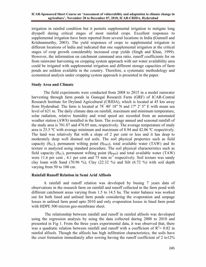
ICAR-Sponsored Short Course on ‘Assessment of vulnerability and adaptation to climate change in
agriculture’, November 28 to December 07, 2018, ICAR-CRIDA, Hyderabad
245
irrigation in rainfed condition but it permits supplemental irrigation to mitigate long dryspell during critical stages of most rainfed crops. Excellent responses to supplemental irrigation have been reported from several locations in India (Gunnell and Krishnamurthy, 2003). The yield responses of crops to supplemental irrigation in different locations of India and indicated that one supplemental irrigation at the critical stages of crop growth considerably increased crop yields (Singh and Khan, 1999). However, the information on catchment cammand area ratio, runoff coefficients for on from rainwater harvesting on cropping system approach with net water availability area could be irrigated with supplemental irrigation and different storage capacities of farm ponds are seldom available in the country. Therefore, a systematic methodology and economical analysis under cropping system approach is presented in the paper. Study Area and Climate
The field experiments were conducted from 2008 to 2015 in a model rainwater harvesting through farm ponds in Gunegal Research Farm (GRF) of ICAR-Central Research Institute for Dryland Agricultural (CRIDA), which is located at 45 km away from Hyderabad. The farm is located at 78º 40ʹ 18ʺ N and 17º 2ʹ 5ʺ E with mean sea level of 621 m. The daily climate data on rainfall, maximum and minimum temperature, solar radiation, relative humidity and wind speed are recorded from an automated weather station (AWS) installed in the farm. The average annual and seasonal rainfall of the study area is 701.87 and 478.05 mm, respectively. The average temperature of study area is 25.5 ºC with average minimum and maximum of 8.94 and 42.06 ºC respectively. The land was relatively flat with a slope of 2 per cent or less and it has deep to moderately deep well drained red soils. The soil physical properties such as field capacity (θFC), permanent wilting point (θPWP), total available water (TAW) and its texture is analyzed using standard procedure. The soil physical characteristics such as field capacity (θFC), permanent wilting point (θPWP) and total available water (TAW) were 11.6 per cent , 4.1 per cent and 75 mm m-1 respectively. Soil texture was sandy clay loam with Sand (70.96 %), Clay (22.32 %) and Silt (6.72 %) with soil depth varying from 50 to 100 cm.
Rainfall Runoff Relation in Semi Arid Alfisols
A rainfall and runoff relation was developed by busing 7 years data of observations in the research farm on rainfall and runoff collected in the farm pond with different catchment areas varying from 1.5 to 14.5 ha. The water balance was worked out for both lined and unlined farm ponds considering the evaporation and seepage losses in unlined farm pond upto 2010 and only evaporation losses in lined farm pond with HDPE 500 micron geo-membrane sheet.
The relationship between rainfall and runoff in rainfed alfisols was developed using the regression analysis by using the data collected during 2008 to 2010 and presented in Fig 1. From the three years experimental data, it was observed that, there was a quadratic relation between rainfall and runoff with a coefficient of R2= 0.82 in rainfed alfisols. Though the alfisols has high infiltration characteristics, the soils have the crust formation immediately after sowing having the runoff coefficient of 2 to12%
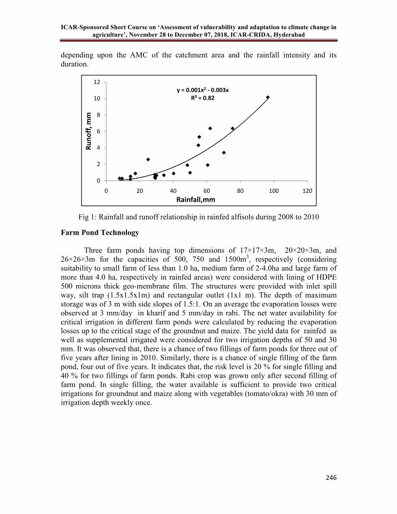
ICAR-Sponsored Short Course on ‘Assessment of vulnerability and adaptation to climate change in
agriculture’, November 28 to December 07, 2018, ICAR-CRIDA, Hyderabad
246
depending upon the AMC of the catchment area and the rainfall intensity and its duration.
Fig 1: Rainfall and runoff relationship in rainfed alfisols during 2008 to 2010
Farm Pond Technology
Three farm ponds having top dimensions of 17×17×3m, 20×20×3m, and 26×26×3m for the capacities of 500, 750 and 1500m3, respectively (considering suitability to small farm of less than 1.0 ha, medium farm of 2-4.0ha and large farm of more than 4.0 ha, respectively in rainfed areas) were considered with lining of HDPE 500 microns thick geo-membrane film. The structures were provided with inlet spill way, silt trap (1.5x1.5x1m) and rectangular outlet (1x1 m). The depth of maximum storage was of 3 m with side slopes of 1.5:1. On an average the evaporation losses were observed at 3 mm/day in kharif and 5 mm/day in rabi. The net water availability for critical irrigation in different farm ponds were calculated by reducing the evaporation losses up to the critical stage of the groundnut and maize. The yield data for rainfed as well as supplemental irrigated were considered for two irrigation depths of 50 and 30 mm. It was observed that, there is a chance of two fillings of farm ponds for three out of five years after lining in 2010. Similarly, there is a chance of single filling of the farm pond, four out of five years. It indicates that, the risk level is 20 % for single filling and 40 % for two fillings of farm ponds. Rabi crop was grown only after second filling of farm pond. In single filling, the water available is sufficient to provide two critical irrigations for groundnut and maize along with vegetables (tomato/okra) with 30 mm of irrigation depth weekly once.
y = 0.001x2 - 0.003x
R² = 0.82
0
2
4
6
8
10
12
0 20 40 60 80 100 120
Ru
no
ff,
mm
Rainfall,mm
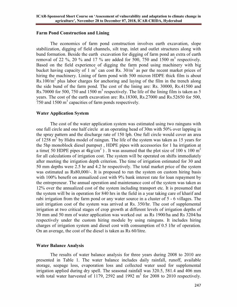
ICAR-Sponsored Short Course on ‘Assessment of vulnerability and adaptation to climate change in
agriculture’, November 28 to December 07, 2018, ICAR-CRIDA, Hyderabad
247
Farm Pond Construction and Lining
The economics of farm pond construction involves earth excavation, slope stabilization, digging of field channels, silt trap, inlet and outlet structures along with bund formation. Beside the earth excavation for digging of farm pond an extra of earth removal of 22 %, 20 % and 17 % are added for 500, 750 and 1500 m3 respectively. Based on the field experience of digging the farm pond using machinery with big bucket having capacity of 1 m3 can cost Rs. 30/m3 as per the recent market prices of hiring the machinery. Lining of farm pond with 500 micron HDPE thick film is about Rs.100/m2 plus labor charges for anchoring and laying of the film in the trench along the side bund of the farm pond. The cost of the lining are: Rs. 30000, Rs.41500 and Rs.70000 for 500, 750 and 1500 m3 respectively. The life of the lining film is taken as 5 years. The cost of the earth excavation are: Rs.18300, Rs.27000 and Rs.52650 for 500, 750 and 1500 m3 capacities of farm ponds respectively. Water Application System
The cost of the water application system was estimated using two rainguns with one full circle and one half circle at an operating head of 30m with 50% over lapping in the spray pattern and the discharge rate of 150 lph. One full circle would cover an area of 1258 m2 by Hidra model of raingun. The life of the system was taken as 15 years for the 5hp monoblock diesel pumpset , HDPE pipes with accessories for 1 ha irrigation at a time( 50 HDPE pipes at 4kg/cm2 ) . It was assumed that the plot size of 100 x 100 m2 for all calculations of irrigation cost. The system will be operated on shifts immediately after meeting the irrigation depth criterion. The time of irrigation estimated for 30 and 50 mm depths were 2.5 hr and 4.2 hr respectively. The total market price of the system was estimated as Rs80,000/-. It is proposed to run the system on custom hiring basis with 100% benefit on annualized cost with 9% bank interest rate for loan repayment by the entrepreneur. The annual operation and maintenance cost of the system was taken as 12% over the annualized cost of the system including transport etc. It is presumed that the system will be in operation for 840 hrs in the field in a year taking care of kharif and rabi irrigation from the farm pond or any water source in a cluster of 5 - 6 villages. The unit irrigation cost of the system was arrived at Rs. 350/hr. The cost of supplemental irrigation at two critical stages of crop growth at different levels of irrigation depths of 30 mm and 50 mm of water application was worked out as Rs 1900/ha and Rs 3204/ha respectively under the custom hiring module by using rainguns. It includes hiring charges of irrigation system and diesel cost with consumption of 0.5 l/hr of operation. On an average, the cost of the diesel is taken as Rs 60/litre.
Water Balance Analysis
The results of water balance analysis for three years during 2008 to 2010 are presented in Table 1. The water balance includes daily rainfall, runoff, available storage, seepage loss, evaporation loss and collected water used for supplemental irrigation applied during dry spell. The seasonal rainfall was 320.5, 581.4 and 406 mm with total water harvested of 1179, 2592 and 1992 m3 for 2008 to 2010 respectively.
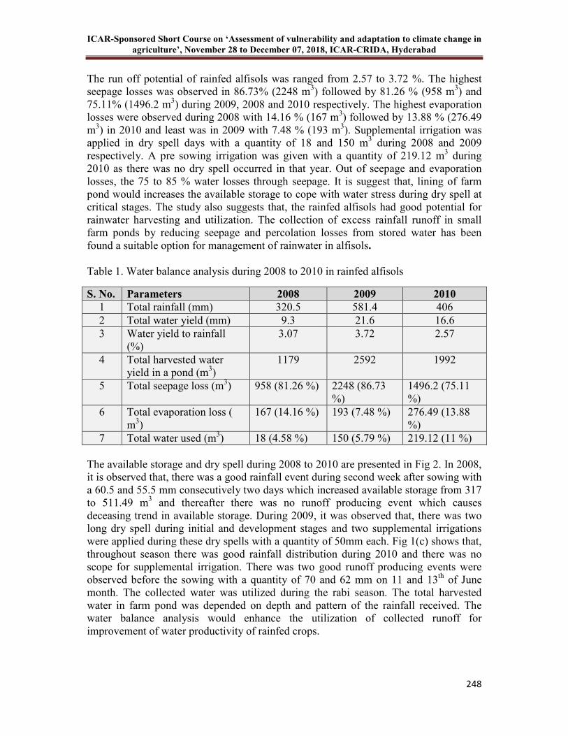
ICAR-Sponsored Short Course on ‘Assessment of vulnerability and adaptation to climate change in
agriculture’, November 28 to December 07, 2018, ICAR-CRIDA, Hyderabad
248
The run off potential of rainfed alfisols was ranged from 2.57 to 3.72 %. The highest seepage losses was observed in 86.73% (2248 m3) followed by 81.26 % (958 m3) and 75.11% (1496.2 m3) during 2009, 2008 and 2010 respectively. The highest evaporation losses were observed during 2008 with 14.16 % (167 m3) followed by 13.88 % (276.49 m3) in 2010 and least was in 2009 with 7.48 % (193 m3). Supplemental irrigation was applied in dry spell days with a quantity of 18 and 150 m3 during 2008 and 2009 respectively. A pre sowing irrigation was given with a quantity of 219.12 m3 during 2010 as there was no dry spell occurred in that year. Out of seepage and evaporation losses, the 75 to 85 % water losses through seepage. It is suggest that, lining of farm pond would increases the available storage to cope with water stress during dry spell at critical stages. The study also suggests that, the rainfed alfisols had good potential for rainwater harvesting and utilization. The collection of excess rainfall runoff in small farm ponds by reducing seepage and percolation losses from stored water has been found a suitable option for management of rainwater in alfisols.
Table 1. Water balance analysis during 2008 to 2010 in rainfed alfisols
S. No. Parameters 2008 2009 2010
1 Total rainfall (mm) 320.5 581.4 406 2 Total water yield (mm) 9.3 21.6 16.6 3 Water yield to rainfall
(%) 3.07 3.72 2.57
4 Total harvested water yield in a pond (m3)
1179 2592 1992
5 Total seepage loss (m3) 958 (81.26 %) 2248 (86.73 %)
1496.2 (75.11 %)
6 Total evaporation loss ( m3)
167 (14.16 %) 193 (7.48 %) 276.49 (13.88 %)
7 Total water used (m3) 18 (4.58 %) 150 (5.79 %) 219.12 (11 %)
The available storage and dry spell during 2008 to 2010 are presented in Fig 2. In 2008, it is observed that, there was a good rainfall event during second week after sowing with a 60.5 and 55.5 mm consecutively two days which increased available storage from 317 to 511.49 m3 and thereafter there was no runoff producing event which causes deceasing trend in available storage. During 2009, it was observed that, there was two long dry spell during initial and development stages and two supplemental irrigations were applied during these dry spells with a quantity of 50mm each. Fig 1(c) shows that, throughout season there was good rainfall distribution during 2010 and there was no scope for supplemental irrigation. There was two good runoff producing events were observed before the sowing with a quantity of 70 and 62 mm on 11 and 13th of June month. The collected water was utilized during the rabi season. The total harvested water in farm pond was depended on depth and pattern of the rainfall received. The water balance analysis would enhance the utilization of collected runoff for improvement of water productivity of rainfed crops.
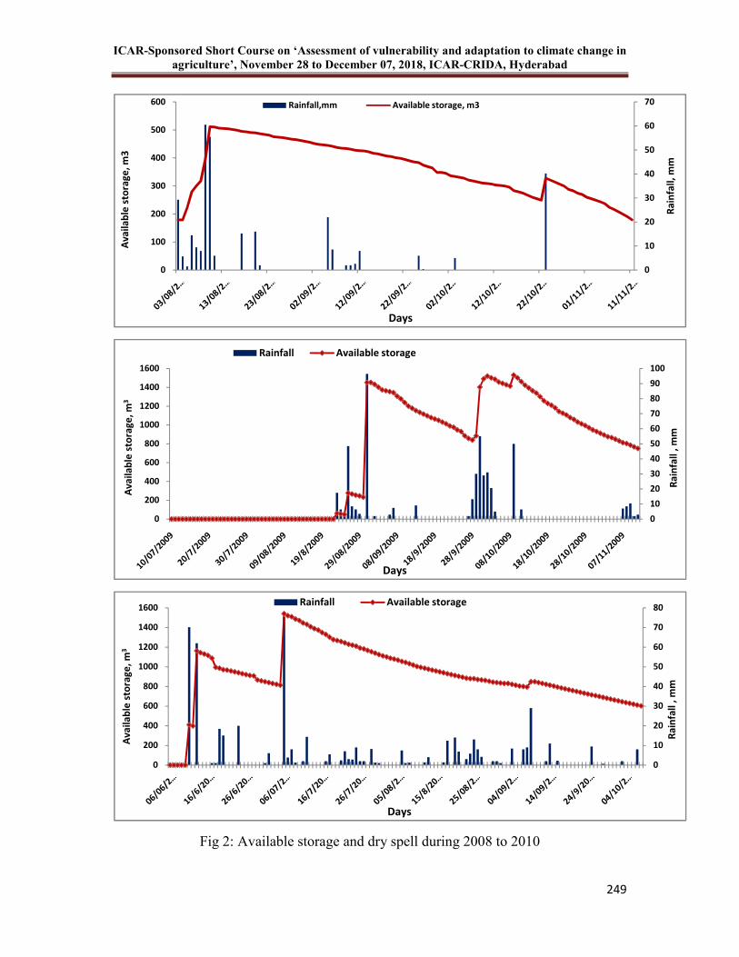
ICAR-Sponsored Short Course on ‘Assessment of vulnerability and adaptation to climate change in
agriculture’, November 28 to December 07, 2018, ICAR-CRIDA, Hyderabad
249
Fig 2: Available storage and dry spell during 2008 to 2010
0
10
20
30
40
50
60
70
0
100
200
300
400
500
600
Ra
infa
ll,
mm
Av
ail
ab
le s
tora
ge
, m
3
Days
Rainfall,mm Available storage, m3
0
10
20
30
40
50
60
70
80
90
100
0
200
400
600
800
1000
1200
1400
1600
Ra
infa
ll ,
mm
Av
ail
ab
le s
tora
ge
, m
3
Days
Rainfall Available storage
0
10
20
30
40
50
60
70
80
0
200
400
600
800
1000
1200
1400
1600
Ra
infa
ll ,
mm
Av
ail
ab
le s
tora
ge
, m
3
Days
Rainfall Available storage
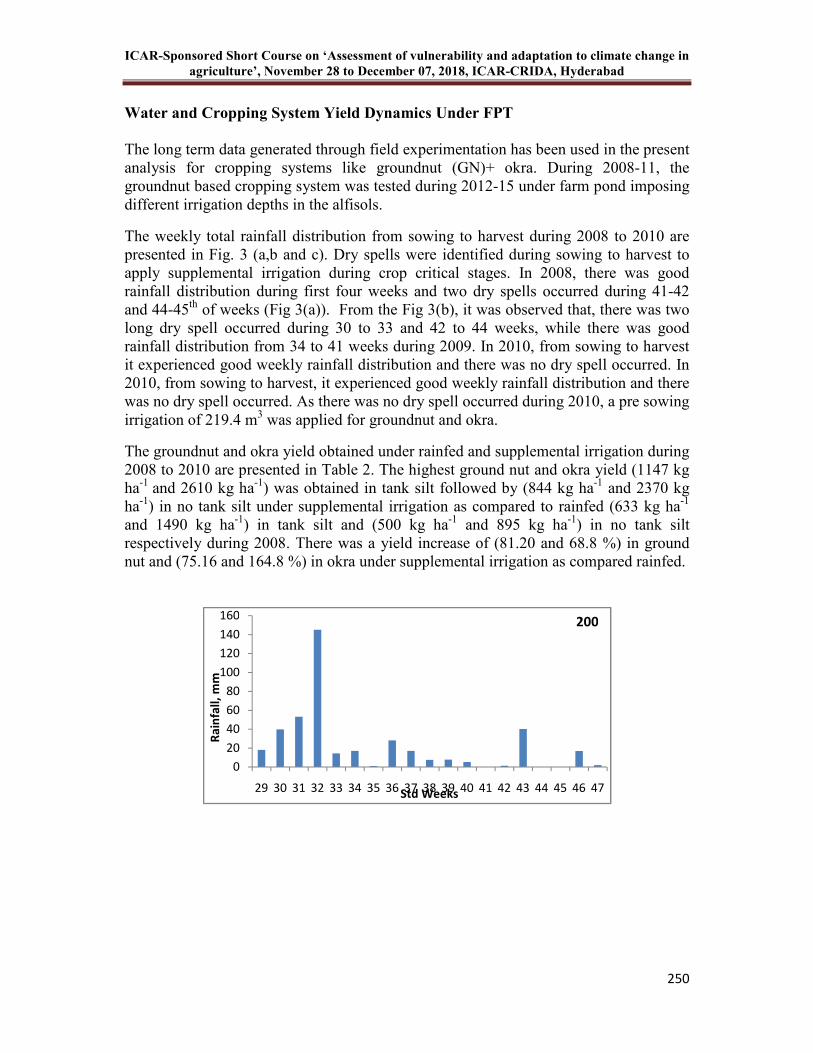
ICAR-Sponsored Short Course on ‘Assessment of vulnerability and adaptation to climate change in
agriculture’, November 28 to December 07, 2018, ICAR-CRIDA, Hyderabad
250
Water and Cropping System Yield Dynamics Under FPT
The long term data generated through field experimentation has been used in the present analysis for cropping systems like groundnut (GN)+ okra. During 2008-11, the groundnut based cropping system was tested during 2012-15 under farm pond imposing different irrigation depths in the alfisols.
The weekly total rainfall distribution from sowing to harvest during 2008 to 2010 are presented in Fig. 3 (a,b and c). Dry spells were identified during sowing to harvest to apply supplemental irrigation during crop critical stages. In 2008, there was good rainfall distribution during first four weeks and two dry spells occurred during 41-42 and 44-45th of weeks (Fig 3(a)). From the Fig 3(b), it was observed that, there was two long dry spell occurred during 30 to 33 and 42 to 44 weeks, while there was good rainfall distribution from 34 to 41 weeks during 2009. In 2010, from sowing to harvest it experienced good weekly rainfall distribution and there was no dry spell occurred. In 2010, from sowing to harvest, it experienced good weekly rainfall distribution and there was no dry spell occurred. As there was no dry spell occurred during 2010, a pre sowing irrigation of 219.4 m3 was applied for groundnut and okra.
The groundnut and okra yield obtained under rainfed and supplemental irrigation during 2008 to 2010 are presented in Table 2. The highest ground nut and okra yield (1147 kg ha-1 and 2610 kg ha-1) was obtained in tank silt followed by (844 kg ha-1 and 2370 kg ha-1) in no tank silt under supplemental irrigation as compared to rainfed (633 kg ha-1 and 1490 kg ha-1) in tank silt and (500 kg ha-1 and 895 kg ha-1) in no tank silt respectively during 2008. There was a yield increase of (81.20 and 68.8 %) in ground nut and (75.16 and 164.8 %) in okra under supplemental irrigation as compared rainfed.
0
20
40
60
80
100
120
140
160
29 30 31 32 33 34 35 36 37 38 39 40 41 42 43 44 45 46 47
Ra
infa
ll,
mm
Std Weeks
200
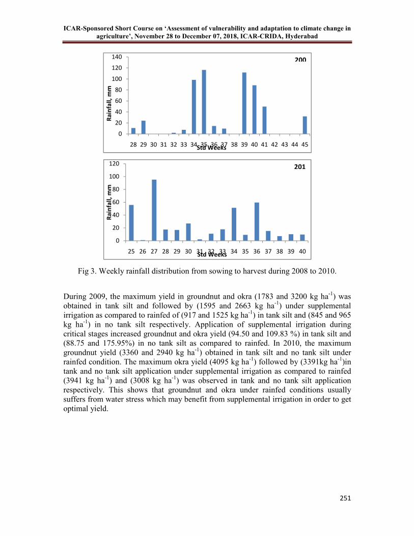
ICAR-Sponsored Short Course on ‘Assessment of vulnerability and adaptation to climate change in
agriculture’, November 28 to December 07, 2018, ICAR-CRIDA, Hyderabad
251
Fig 3. Weekly rainfall distribution from sowing to harvest during 2008 to 2010.
During 2009, the maximum yield in groundnut and okra (1783 and 3200 kg ha-1) was obtained in tank silt and followed by (1595 and 2663 kg ha-1) under supplemental irrigation as compared to rainfed of (917 and 1525 kg ha-1) in tank silt and (845 and 965 kg ha-1) in no tank silt respectively. Application of supplemental irrigation during critical stages increased groundnut and okra yield (94.50 and 109.83 %) in tank silt and (88.75 and 175.95%) in no tank silt as compared to rainfed. In 2010, the maximum groundnut yield (3360 and 2940 kg ha-1) obtained in tank silt and no tank silt under rainfed condition. The maximum okra yield (4095 kg ha-1) followed by (3391kg ha-1)in tank and no tank silt application under supplemental irrigation as compared to rainfed (3941 kg ha-1) and (3008 kg ha-1) was observed in tank and no tank silt application respectively. This shows that groundnut and okra under rainfed conditions usually suffers from water stress which may benefit from supplemental irrigation in order to get optimal yield.
0
20
40
60
80
100
120
140
28 29 30 31 32 33 34 35 36 37 38 39 40 41 42 43 44 45
Ra
infa
ll,
mm
Std Weeks
200
0
20
40
60
80
100
120
25 26 27 28 29 30 31 32 33 34 35 36 37 38 39 40
Ra
infa
ll,
mm
Std Weeks
201
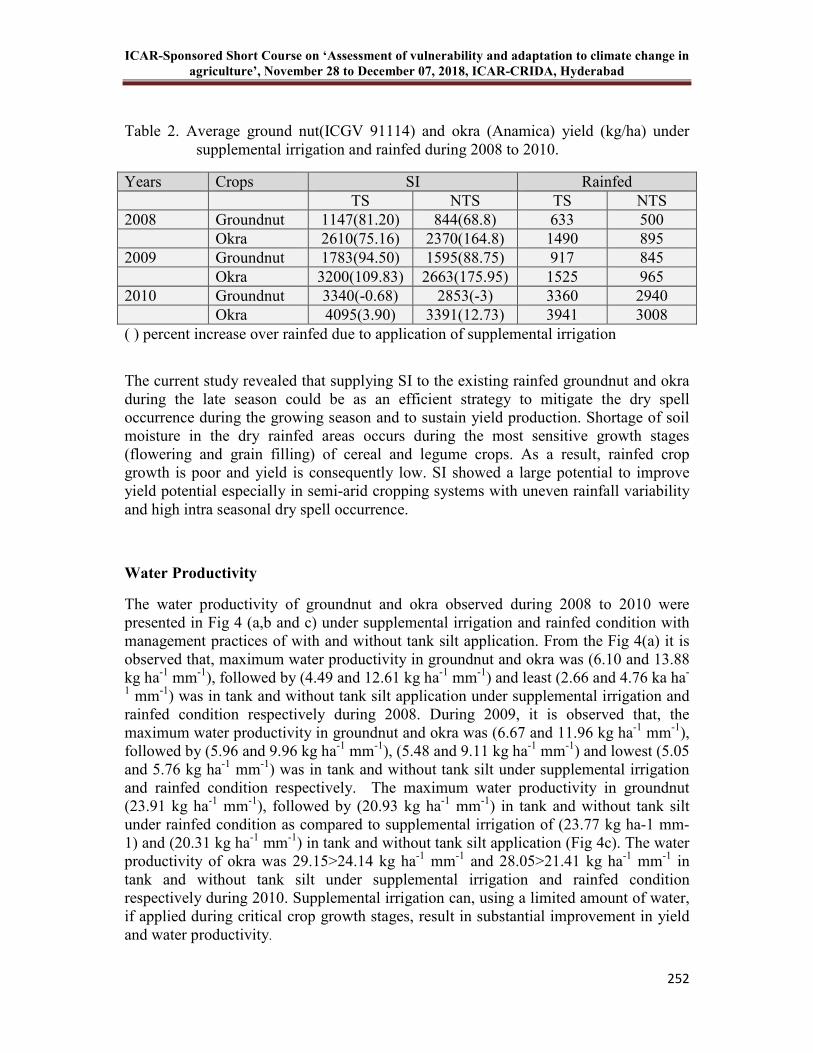
ICAR-Sponsored Short Course on ‘Assessment of vulnerability and adaptation to climate change in
agriculture’, November 28 to December 07, 2018, ICAR-CRIDA, Hyderabad
252
Table 2. Average ground nut(ICGV 91114) and okra (Anamica) yield (kg/ha) under
supplemental irrigation and rainfed during 2008 to 2010.
Years Crops SI Rainfed TS NTS TS NTS 2008 Groundnut 1147(81.20) 844(68.8) 633 500 Okra 2610(75.16) 2370(164.8) 1490 895 2009 Groundnut 1783(94.50) 1595(88.75) 917 845 Okra 3200(109.83) 2663(175.95) 1525 965 2010 Groundnut 3340(-0.68) 2853(-3) 3360 2940 Okra 4095(3.90) 3391(12.73) 3941 3008 ( ) percent increase over rainfed due to application of supplemental irrigation
The current study revealed that supplying SI to the existing rainfed groundnut and okra during the late season could be as an efficient strategy to mitigate the dry spell occurrence during the growing season and to sustain yield production. Shortage of soil moisture in the dry rainfed areas occurs during the most sensitive growth stages (flowering and grain filling) of cereal and legume crops. As a result, rainfed crop growth is poor and yield is consequently low. SI showed a large potential to improve yield potential especially in semi-arid cropping systems with uneven rainfall variability and high intra seasonal dry spell occurrence.
Water Productivity
The water productivity of groundnut and okra observed during 2008 to 2010 were presented in Fig 4 (a,b and c) under supplemental irrigation and rainfed condition with management practices of with and without tank silt application. From the Fig 4(a) it is observed that, maximum water productivity in groundnut and okra was (6.10 and 13.88 kg ha-1 mm-1), followed by (4.49 and 12.61 kg ha-1 mm-1) and least (2.66 and 4.76 ka ha-
1 mm-1) was in tank and without tank silt application under supplemental irrigation and rainfed condition respectively during 2008. During 2009, it is observed that, the maximum water productivity in groundnut and okra was (6.67 and 11.96 kg ha-1 mm-1), followed by (5.96 and 9.96 kg ha-1 mm-1), (5.48 and 9.11 kg ha-1 mm-1) and lowest (5.05 and 5.76 kg ha-1 mm-1) was in tank and without tank silt under supplemental irrigation and rainfed condition respectively. The maximum water productivity in groundnut (23.91 kg ha-1 mm-1), followed by (20.93 kg ha-1 mm-1) in tank and without tank silt under rainfed condition as compared to supplemental irrigation of (23.77 kg ha-1 mm-1) and (20.31 kg ha-1 mm-1) in tank and without tank silt application (Fig 4c). The water productivity of okra was 29.15>24.14 kg ha-1 mm-1 and 28.05>21.41 kg ha-1 mm-1 in tank and without tank silt under supplemental irrigation and rainfed condition respectively during 2010. Supplemental irrigation can, using a limited amount of water, if applied during critical crop growth stages, result in substantial improvement in yield and water productivity.
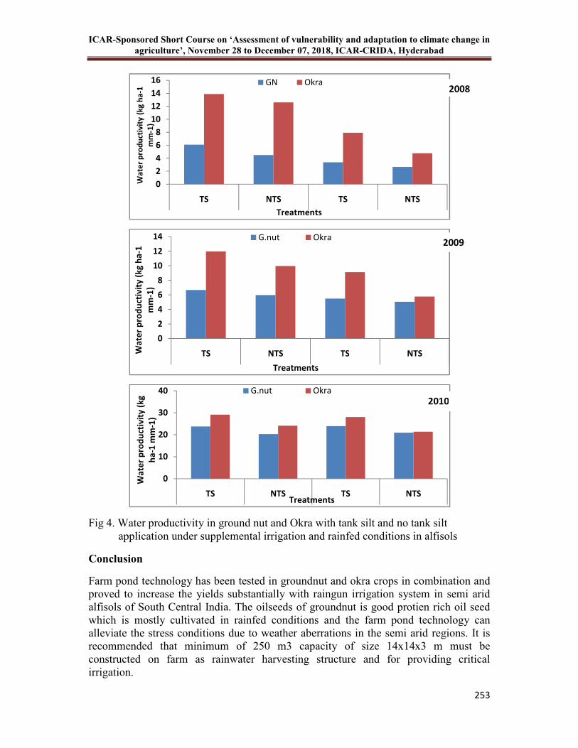
ICAR-Sponsored Short Course on ‘Assessment of vulnerability and adaptation to climate change in
agriculture’, November 28 to December 07, 2018, ICAR-CRIDA, Hyderabad
253
Fig 4. Water productivity in ground nut and Okra with tank silt and no tank silt application under supplemental irrigation and rainfed conditions in alfisols
Conclusion
Farm pond technology has been tested in groundnut and okra crops in combination and proved to increase the yields substantially with raingun irrigation system in semi arid alfisols of South Central India. The oilseeds of groundnut is good protien rich oil seed which is mostly cultivated in rainfed conditions and the farm pond technology can alleviate the stress conditions due to weather aberrations in the semi arid regions. It is recommended that minimum of 250 m3 capacity of size 14x14x3 m must be constructed on farm as rainwater harvesting structure and for providing critical irrigation.
0
2
4
6
8
10
12
14
16
TS NTS TS NTS
Wa
ter
pro
du
ctiv
ity
(k
g h
a-1
mm
-1)
Treatments
GN Okra
0
2
4
6
8
10
12
14
TS NTS TS NTSWa
ter
pro
du
ctiv
ity
(k
g h
a-1
mm
-1)
Treatments
G.nut Okra
0
10
20
30
40
TS NTS TS NTS
Wa
ter
pro
du
ctiv
ity
(k
g
ha
-1 m
m-1
)
Treatments
G.nut Okra
2010
2008
2009
ICAR-Sponsored Short Course on ‘Assessment of vulnerability and adaptation to climate change in
agriculture’, November 28 to December 07, 2018, ICAR-CRIDA, Hyderabad
254
References
Anbumozhi V, Matsumoto K, Yamaji E. 2002. Sustaining Agriculture through Modernization of Irrigation Tanks: An Opportunity and Challenge for Tamilnadu, India. Agricultural Engineering International: The CIGR J. Sci. Res. Dev. Manuscript LW 01 002. Vol. III.
Barron J. 2004. Dry spell mitigation to upgrade semi-arid rainfed agriculture: water
harvesting and soil nutrient management. PhD thesis, Natural Resources Management, Department of Systems Ecology, Stockholm University, Stockholm, Sweden.
Downing j A and others. 2006. The global abundance and size distribution of lakes,
ponds, and impoundments. Limnol. Oceanogr. 51: 2388–2397, doi:10.4319/lo.2006.51.5.2388.
Fraiture CD, Wichelns D, Rockström J, Benedict EK. 2007. Looking ahead to 2050:
scenarios of alternative investment approaches. In: Molden, D. (Ed.), Water for Food – Water for Life. A Comprehensive Assessment of water Management in Agriculture. Earthscan, pp. 91–145.
Gunnell Y, Krishnamurthy A. 2003. Past and present status of runoff harvesting
systems in dryland peninsular India: a critical review. Ambio 32 (4), 320–324. Kahinda JM, Rockström J Taigbenu AE, Dimes J. 2007. Rainwater harvesting to
enhance water productivity of rainfed agriculture in the semi-arid Zimbabwe. Physics and Chemistry of the Earth, 32, 1068-1073.
Li Q, Gowing J. 2005. A daily water balance model approach for simulating
performance of tank-based irrigation systems. Water Resources Management 19, 211–231.
Ngigi SN, Savenije HHG, Thome JN, Rockström J, de Vries FWTP. 2005. Agro
hydrological evaluation of on-farm rainwater storage systems for supplemental irrigation in Laikipia District, Kenya. Agric. Water Manag. 73 (1), 21e41.
Ngigi SN. 2003. What is the limit of up-scaling rainwater harvesting in a river basin?
Physics and Chemistry of the Earth 28, 943–956. Oweis T, Hachum A. 2006. Water harvesting and supplemental irrigation for improved
water productivity of dry farming systems in West Asia and North Africa. Agric. Water Manage. 80, 57–73.
Pandey DN, Gupta AK, Anderson DM. 2003. Rainwater harvesting as an adaptation to
climate change. Current Science 85 (1), 46–59.

ICAR-Sponsored Short Course on ‘Assessment of vulnerability and adaptation to climate change in
agriculture’, November 28 to December 07, 2018, ICAR-CRIDA, Hyderabad
255
Rockström J, Barron J. 2007. Water productivity in rainfed systems: overview of challenges and analysis of opportunities in water scarcity prone savannahs. Irrigation Science, 25, 299-311.
Rockström J, Karlberg L, Wani SP, Barron J, Hatibu N, Oweis T, Bruggeman A, Farahani J, Qiang Z. 2010. Managing water in rainfed agriculture––the need for a paradigm shift.
Singh RP and Khan MA. 1999 Rainwater management: water harvesting and its
efficient utilization. In: Singh, H.P., Ramakrishna, Y.S. and Venkateswaralu, B. (eds) Fifty Years of Dryland Agricultural ResearchIn India. Central Research Institute for Dryland Agriculture (CRIDA), Hyderabad, India, pp. 301–313.
Wang YJ Xie ZK, Malhi SS, Vera CL, Zhang YB, Guo ZH. 2011. Effects of gravel-
sand mulch, plastic mulch and ridge and furrow rainfall harvesting system combinations on water use efficiency, soil temperature and watermelon yield in a semi-arid Loess Plateau of northwestern China. Agricultural Water Management, 101, 88-92.
ICAR-Sponsored Short Course on ‘Assessment of vulnerability and adaptation to climate change in
agriculture’, November 28 to December 07, 2018, ICAR-CRIDA, Hyderabad
256
21 Climate Change Adaptation and Mitigation Potential of Organic
Farming
KA Gopinath, G Ravindra Chary, G Venkatesh, PS Prabhamani and V Visha Kumari
Introduction
Climate change and variability are a considerable threat to agricultural communities, particularly in India. This threat includes the likely increase of temperature, extreme weather conditions, increased water stress and drought, and desertification. Crop growth, development, water use and yield under normal conditions are largely determined by weather during the growing season. Seasonal variations in weather events may pose risks to traditional methods of crop production either due to water constraints or surplus of water and erosion. In this regard, soil stability will become crucial to store water in the soil profile, to resist extreme weather events and minimize soil erosion. Climate change is no longer a distant projection, but a contemporary reality demanding immediate attention. These changes will bring new challenges to farmers. Farmers need tools to help them adapt to these new conditions. Organic farming is one such option which is reported to have both climate change mitigation and adaptation potential particularly in rainfed agriculture.
The practice of farming described as ‘organic’ is promoted under many names (Merrill, 1983). Some of the descriptive names which are, or have been, used in reference to it are: humus farming, natural farming, bio-dynamic farming, biological farming, ecological farming, holistic farming, alternative farming, sustainable farming and scientific ecological farming. In general, these names are used interchangeably, the choice being determined by personal preference as much as by the audience for whom it is used. The only real exception to the general synonymity of these names is bio-dynamic which is used by and in reference to the methods developed by the agricultural followers of Rudolf Steiner. It is perhaps of interest to note that organic, which is used fairly widely, continues to carry the heaviest load of negative connotations.
The vast majority of rainfed farmers in remote areas still practice low external input or no external input farming which is well integrated with livestock, particularly small ruminants. Based on several surveys and reports, it is estimated that up to 30% of the rainfed farmers in many remote areas of the country do not use chemical fertilizers and pesticides. Thus, many resource poor farmers are practicing organic farming by default. The Government of India task force on organic farming and several other reviewers have identified rainfed areas and regions in north-east as more suitable for organic farming in view of the low input use (GOI, 2001; Dwivedi, 2005; Ramesh et al., 2005). Rainfed areas are reported to have relative advantage to go for organic farming primarily due to i) low level of input use, ii) shorter conversion period and iii) smaller yield reductions compared to irrigated areas, but no one can suggest any large scale conversion in view of several limitations particularly availability of organic amendments in required quantities (Venkateswarlu, 2008). Adoption of soil and water conservation measures, a key component of rainfed farming is also one of the pillars of
ICAR-Sponsored Short Course on ‘Assessment of vulnerability and adaptation to climate change in
agriculture’, November 28 to December 07, 2018, ICAR-CRIDA, Hyderabad
257
organic farming. Mulching or mulch cum manuring, residue management, green leaf manuring, cover cropping are other strategies that conserve moisture and improve nutrientuse efficiency in drylands which are also the essential components of organic production methods. The use of FYM or other organic nutrient sources during aberrant rainfall years in particular have an additional advantage of protecting the crop from drought besides the nutritional benefits, so critical in drylands. While there is no contradiction between these established rainfed farming technologies and the objectives of the organic farming, the only issue will be the labour and capital intensive nature of some of these technologies and its ultimate impact on the cost of production.
Definition of Organic Farming
There is no single definition for organic farming as it often refers to a movement rather than to a single policy. Organic farming was defined by USDA (1980) as “….Production systems which avoid or largely exclude the use of synthetically compounded fertilizers, pesticides, growth regulators and rely upon crop rotations, crop residues, animal manures, green manures, off-farm organic wastes, mechanical cultivation, mineral bearing rocks, and aspects of biological pest control to maintain soil productivity and tilth, to supply plant nutrients, and to control insects, weeds, and other pests”. Organic agriculture is defined in India’s National Programme for Organic Production (NPOP) as “a system of farm design and management to create an ecosystem, which can achieve sustainable productivity without the use of artificial external inputs such as chemical fertilizers and pesticides”.
Development and State of Organic Farming in India
There has been significant increase in the area under certified organic farming during the last 10 years. With less than 42,000 ha under certified organic farming during 2003-04, the area under organic farming grew by almost 25 fold, during the next 5 years, to 1.2 million ha during 2008-09. Later, however, the area under certified organic farming has fluctuated between 0.78-1.1 million ha. Presently (2016-17), about 1.44 million ha area is under certified organic cultivation and India ranks 9th in terms of total land under organic cultivation. Further, India has about 4.2 million ha under organic wild collection and non-agricultural areas. The countries with the largest areas of organic agricultural land are Australia, Argentina, China, USA, Spain, Italy, Uruguay, France, India and Germany (in that order) (Willer and Julia, 2018). During 2016-17, India had the largest number of organic producers of about 0.84 million and accounted for 1.18 million tons of certified organic produce. The total volume of export during 2015-16 was 263687 tons. The organic food export realization was around 298 million USD. Organic products are exported to European Union, US, Canada, Switzerland, Korea, Australia, New Zealand, South East Asian countries, Middle East, South Africa etc. Oilseeds (50%) lead among the products exported followed by processed food products (25%), cereals & millets (17%), tea (2%), pulses (2%), spices (1%), dry fruits (1%), and others.

ICAR-Sponsored Short Course on ‘Assessment of vulnerability and adaptation to climate change in
agriculture’, November 28 to December 07, 2018, ICAR-CRIDA, Hyderabad
258
Organic Farming and Climate Change
Agriculture is a major contributor to emissions of methane (CH4), nitrous oxide (N2O), and carbon dioxide (CO2). According to the Inter-governmental Panel on Climate Change (IPCC) agriculture accounts for 10-12% of global greenhouse gas (GHG) emissions and this figure is expected to rise further. GHGs attributed to agriculture by the IPCC include emissions from soils, enteric fermentation (GHG emissions from the digestion process of ruminant animals), rice production, biomass burning and manure management (Smith et al., 2007). There are other ‘indirect’ sources of GHG emissions that are not accounted for by the IPCC under agriculture such as those generated from land-use changes, use of fossil fuels for mechanization, transport and agro-chemical and fertilizer production (IFOAM, 2009).
Climate change and variability are a considerable threat to agricultural communities, particularly in India. This threat includes the likely increase of temperature, extreme weather conditions, increased water stress and drought, and desertification. Seasonal variations in weather events may pose risks to traditional methods of crop production either due to water constraints or surplus of water and erosion. In this regard, soil stability will become crucial to store water in the soil profile, to resist extreme weather events and minimize soil erosion. These changes will bring new challenges to farmers. Farmers need tools to help them adapt to these new conditions. Organic farming is one such option which is reported to have both climate change mitigation and adaptation potential particularly in rainfed agriculture.
Potential of Organic Farming to Mitigate Climate Change
There is considerable world-wide support at present in advocating organic agriculture for mitigating climate change (Kotschi and Miiller-Samann, 2004; Niggli, 2007; IFOAM, 2008; Goh, 2011). The potential of organic agriculture in mitigating climate change depends on its ability to reduce emissions of GHGs (nitrous oxide, carbon dioxide and methane), increase soil carbon sequestration, and enhance effects of organic farming practices which favour the above two processes (Goh, 2011).
Reduction of GHG Emissions
The global warming potential of conventional agriculture is strongly affected by the use of synthetic nitrogen fertilizers and by high nitrogen concentrations in soils. However, organic farming systems avoid the use of synthetic fertilizers, and rely on practices such as green manuring, crop rotation with legumes, efficient recycling of bioresidues and the use of organic manures. In addition, these systems avoid the use of synthetic pesticides and rely on practices such as crop rotations, use of bio-pesticides and increase beneficial insects for pest management. These restrictions on fossil-fuel based fertilizer and pesticide inputs can significantly reduce the overall GHG footprint of organic systems in comparison to conventional production systems (Sreejith and Sherief, 2011). Recent experimental results suggest that organic agriculture can significantly reduce GHG emissions.
ICAR-Sponsored Short Course on ‘Assessment of vulnerability and adaptation to climate change in
agriculture’, November 28 to December 07, 2018, ICAR-CRIDA, Hyderabad
259
Reduction of nitrous oxide emissions
N2O emissions are the most important source of agricultural emissions: 38% of agricultural GHG emissions (Smith et al., 2007). The IPCC attributes a default value of 1% to applied fertilizer nitrogen as direct N2O emissions (Eggleston et al., 2006). Similarly, emission factors of up to 3-5 kg N2O-N per 100 kg N-input have been reported by Crutzen et al. (2007). These higher values for global N2O budget are due to the consideration of both direct and indirect emissions, including also livestock production, NH3 and NO3 emissions, nitrogen leakage into rivers and coastal zones, etc (Scialabba and Muller-Lindenlauf, 2010). Nitrous oxide emissions are directly linked to the concentration of available mineral N (ammonium and nitrate) in soils arising from the nitrification and denitrification of available soil and added fertilizer N (Firestone and Davidson, 1989; Wrage et al., 2001). High emissions rates are detected directly after mineral fertilizer additions and are very variable (Bouwman, 1995).
In organic systems, the nitrogen input to soils, and hence the potential nitrous oxide emissions, are reduced. The share of reactive nitrogen that is emitted as N2O depends on a broad range of soil and weather conditions and management practices, which could partly foil the positive effect of lower nitrogen levels in top soil (Scialabba and Muller-Lindenlauf, 2010). One study found no significant differences between mineral and organic fertilization (Dambreville et al., 2007). In a study by Petersen et al. (2006), lower emission rates for organic compared to conventional farming were found for five European countries. In a long-term study in southern Germany, Flessa et al. (2002) also found reduced nitrous oxide emission rates in the organic farm, although yield-related emissions were not reduced.
Reduction of methane emissions
The reduction or avoidance of CH4 emissions is of special importance in global warming from the agricultural sector because two thirds of global CH4 emissions are of anthropogenic origin, mainly from enteric ruminant fermentation in animals (FAO, 2006) and in paddy rice production (Smith and Conan, 2004). In general, the CH4 emissions from ruminants and rice production are not significantly different between organic and conventional agriculture. Differences are due largely to the extent and intensity of various farming practices and their improvement used within different forms of agriculture.
Although research on CH4 emissions in organic and conventional paddy rice production is still in its infancy (Goh, 2011), employing better rice production techniques such as using low CH4-emitting varieties (Yagi et al., 1997; Aulakh et al., 2001), composted manures with low C/N ratio (Singh et al., 2003), adjusting the timing of organic residue additions (Xu et al., 2000; Cai and Xu, 2004) and using mid-season drainage or avoiding continuous flooding have been shown to reduce CH4 emissions (Smith and Conan, 2004). Further, as herbicides are not used in organic systems, aquatic weeds tend to be present in organic rice paddies and weeds have an additional decreasing effect on methane emissions (Inubushi et al., 2001). In organic farming systems, cropping depends on nutrient supply from livestock and the combination of cropping
ICAR-Sponsored Short Course on ‘Assessment of vulnerability and adaptation to climate change in
agriculture’, November 28 to December 07, 2018, ICAR-CRIDA, Hyderabad
260
and livestock provides an efficient means of mitigating GHG emissions especially CH4 (Goh, 2011). Efficient and direct recycling of manure and slurry is the best option to reduce GHG emissions as this practice avoids long-distance transport (Niggli, 2007).
Methane and N2O from manure account for about 7% of the agricultural GHG emissions. Methane emissions predominantly occur in liquid manure systems, while N2O emissions are higher in solid manure systems and on pastures (Smith et al., 2007). There is a very high variance for both gaseous emissions, depending on composition, coverage, temperature and moisture of the manure. Storing manure in solid form such as composting can suppress CH4 emissions but may result in more N2O emissions (Paustian et al., 2004).
Reduction of carbon dioxide emissions
Synthetic external inputs like fertilizers and pesticides are banned in organic farming. The energy used for the chemical synthesis of nitrogen fertilizers, which are totally excluded in organic systems, represent up to 0.4–0.6 Gt CO2 emissions (EFMA, 2005; Williams et al., 2006; FAOSTAT, 2009). This is as much as 10% of direct global agricultural emissions and around 1% of total anthropogenic GHG emissions. Further, CH4 and N2O from biomass burning account for 12% of the agricultural GHG emissions. Additionally, the carbon sequestered in the burned biomass is lost to the atmosphere. In organic agriculture, preparation of land by burning vegetation is restricted to a minimum (IFOAM, 2002). CO2‐e emissions are reported to be around 40‐60% lower in organic farming systems than conventional systems, largely because they don’t use synthetic nitrogen fertilizers which require large amounts of energy in their production and are associated with emissions of the powerful GHG nitrous oxide (Sayre, 2003, BFA 2007).
Soil Carbon Sequestration
Soil C sequestration is an important strategy and is a win–win option of producing more food per unit area besides mitigation of climate change (Lal, 2004). Although soils of the tropical regions have low C sequestration rate because of high temperatures, adoption of appropriate management practices can lead to higher rates particularly in high rainfall regions (Srinivasarao et al., 2012). Soil carbon sequestration at a global scale is considered the mechanism responsible for the greatest mitigation potential within the agricultural sector, with an estimated 90% contribution to the potential of what is technically feasible (Smith et al., 2007, 2008). Thus, improved agronomic practices that could lead to reduced carbon losses or even increased soil carbon storage are highly desired (Gattinger et al., 2012).
Soil carbon sequestration is enhanced through agricultural management practices (such as increased application of organic manures, use of intercrops and green manures, higher shares of perennial grasslands and trees or hedges, etc.), which promote greater soil organic matter (and thus soil organic carbon) content and improve soil structure (Niggli et al., 2008; Muller, 2009). There is strong scientific evidence that organic farming generally results in higher soil carbon levels in cultivated soils compared to chemical fertilizer based agriculture. Similarly, several field studies have proved the

ICAR-Sponsored Short Course on ‘Assessment of vulnerability and adaptation to climate change in
agriculture’, November 28 to December 07, 2018, ICAR-CRIDA, Hyderabad
261
positive effect of organic farming practices on soil carbon pools (Pimentel et al., 2005; Fliessbach et al., 2007; Kustermann et al., 2008). Gattinger et al. (2012) subjected datasets from 74 studies from pair-wise comparisons of organic vs. nonorganic farming systems to metaanalysis to identify differences in soil organic carbon (SOC). The analysis revealed significant differences and higher values for organically farmed soils of 0.18±0.06% points (mean±95% confidence interval) for SOC concentrations, 3.50±1.08 Mg C/ha for stocks, and 0.45±0.21 Mg C/ha/year for sequestration rates compared with nonorganic management. Leifeld and Fuhrer (2010) found in their review an average annual increase of the SOC concentration in organic systems by 2.2%, whereas in conventional systems, SOC did not change significantly.
Organic Agriculture as an Adaptation Strategy
Adaptation in agriculture is not new. Historically, farmers have developed several methods to adapt to changing climate including aberrant weather. However, the adaptation needs to occur at a much faster rate due to impending climate change. The Intergovernmental Panel on Climate Change (IPPC) defines adaptation to climate change as ‘adjustment in natural or human systems in response to actual or expected climatic stimuli or their effects, which moderates harm or exploits beneficial opportunities (IPCC, 2001). Long-term crop yield stability and the ability to buffer yields through climatic adversity are critical factors in agriculture's ability to support society in the future (Lotter et al., 2003). Several researchers have reported that organic farming systems perform better than their conventional counterparts during climate extremes including drought and excessive rainfall.
Several mechanisms may increase drought tolerance of organic cropping systems. Soil organic matter has positive effects on the water-capturing capacity of the soil. Numerous studies have shown soil organic carbon to be higher in organically managed systems (Reganold, 1995; Clark et al., 1998; Liebig and Doran, 1999; Gopinath et al., 2008, 2011). As a result, organically managed soils have high water holding capacity (Liebig and Doran, 1999; Wells et al., 2000). It was found that water capture in organic plots was twice as high as in conventional plots during torrential rains (Lotter et al., 2003). Similarly, Pimentel et al. (2005) reported that the amount of water percolating through the top 36 cm was 15-20% greater in the organic systems of the Rodale farming systems trial compared to conventional systems. In India, most of the organic cotton farmers stated that the capacity of their soils to absorb and retain water was increased after conversion to organic management (Eyhorn et al., 2009). Many farmers also said that they need less rounds of irrigation and the crops can sustain longer periods of drought. In the 21-year Rodale Farming Systems Trial, in which two organic and a conventional crop rotation were compared, the organic crop systems performed significantly better in 4 out of 5 years of moderate drought. In the severe drought year of 1999, three out of the four crop comparisons resulted in significantly better yields in the organic systems than the conventional (Lotter et al., 2003).
The mitigation of runoff, erosion and crop losses as a result of rainfall excess is also improved in organically managed systems (Lotter et al., 2003). Organic management of soils leads to improved soil stability and resistance to water erosion compared to
ICAR-Sponsored Short Course on ‘Assessment of vulnerability and adaptation to climate change in
agriculture’, November 28 to December 07, 2018, ICAR-CRIDA, Hyderabad
262
conventionally managed soils, due to higher soil C content and improved soil aggregation (Reganold, 1995; Clark et al., 1998; Liebig and Doran, 1999), permeability (Reganold et al., 2001) and lower bulk density as well as higher resistance to wind erosion (Jaenicke, 1998). Hence, organic crop management techniques will be a valuable resource in an era of climatic variability, providing soil and crop characteristics that can better buffer environmental extremes (Lotter et al., 2003).
Conclusion
Organic agricultural systems have an inherent potential to both mitigate climate change through reduced GHG emissions and higher carbon sequestration in the soil, and adapt to climate change. Farming practices such as organic agriculture that preserve soil fertility and maintain or even increase organic matter in soils are in a good position to maintain productivity in the event of drought, irregular rainfall events with floods, and rising temperatures. Soils in organic agriculture capture and store more water than soils of conventional cultivation. Therefore, organic agriculture is one of the adaptation strategies that can be targeted at improving the livelihoods of rural populations that are especially vulnerable to the adverse effects of climate change and variability.
References
Aulakh MS, Wassmann R and Rennenberg H. 2001. Methane emissions from rice fields quantification, mechanisms, role of management, and mitigation options. Advances in Agronomy, 70: 247-251.
BFA. 2007. Soil makes the carbon cut – BFA Press Release 13th December 2007, Biological Farmers of Australia, http://www.bfa.com.au/.
Bouwman AF. 1995. Uncertainties in the global source distribution of nitrous oxide. Journal of Geophysical Research, 100: 2785-2800.
Cai ZC and Xu H. 2004. Options for mitigating CH4 from rice fields in China. Journal of Geophysical Research, 105: 17231-17232.
Chhonkar PK. 2003. Organic farming: Science and belief. Journal of Indian Society of Soil Science, 51(4): 365-372.
Clark MS, Ferris H, Klonsky K, Lanini WT, vanBruggen AHC and Zalom FG. 1998. Agronomic, economic, and environmental comparison of pest management in conventional and alternative tomato and corn systems in northern California. Agriculture Ecosystems and Environment, 68(1-2): 51-71.
Crutzen PJ, Mosier AR, Smith KA and Winiwarter W. 2007. N2O release from agro-biofuel production negates global warming reduction by replacing fossil fuels. Atmospheric Chemistry and Physics Discussions, 7: 11191–11205.
Dambreville Ch, Morvan Th and German JC. 2007. N2O emission in maize crops fertilized with pig slurry, matured pig manure or ammonia nitrate in Brittany. Agriculture, Ecosystems and Environment, 123: 201-210.

ICAR-Sponsored Short Course on ‘Assessment of vulnerability and adaptation to climate change in
agriculture’, November 28 to December 07, 2018, ICAR-CRIDA, Hyderabad
263
Dwivedi Vandana 2005. Organic farming: Policy initiatives, Paper presented at the National Seminar on National Policy on Promoting Organic Farming, 10-11 March, 2005. pp.58-61.
EFMA. 2005. Understanding nitrogen and its use in agriculture. European Fertilizer Manufactures Association (EFMA), Brussels, Belgium.
Eggleston S, Buendia L, Miwa K, Ngara T and Tanabe K (Eds). 2006. IPCC Guidelines for National Greenhouse Gas Inventories. Volume 4: Agriculture, Forestry and Other Land Use. Prepared by the National Greenhouse Gas Inventories Programme (IGES), Hayama, Japan.
Eyhorn F, Mader P and Ramakrishnan M. 2009. The impact of organic cotton farming on the livelihoods of smallholders: Evidence from the Maikaal bioRe project in central India. Organic Farming Newsletter 5(1): 19-21.
FAO. 2006. Livestock's Long Shadow-Environmental Issues and Options, Food and Agriculture Organization of the United Nations (FAO), Rome, Italy.
FAOSTAT. 2009. FAO Statistical Database Domain on Fertilizers: ResourceSTAT-Fertilizers. Food and Agriculture Organisation of the United Nations (FAO) Rome, Italy.
Firestone MK and Davidson. 1989. Microbial basis of NO and N2O production and consumption in soil. In: Exchange of Trace Gases Between Terrestrial Ecosystems and the Atmosphere (MO Andreae and DS Schimel, Eds.), Wiley, New York, U.S.A. pp 2-21.
Fliessbach A, Oberholzer HR, Gunst L and Mader P. 2007. Soil organic matter and biological soil quality indicators after 21 years of organic and conventional farming. Agriculture, Ecosystems and Environment, 118: 273-284.
Gattinger A, Muller A, Haeni M, Skinner C, Fliessbach A, Buchmann N, Mäder P, Stolze M, Smith P, Scialabba N El-Hage and Niggli U. 2012. Enhanced top soil carbon stocks under organic farming. PANS, 109(44): 18226-18231.
Goh KM. 2011. Greater mitigation of climate change by organic than conventional agriculture: A review. Biological Agriculture & Horticulture, 27(2): 205-229.
GOI, 2001. The report of the working group on organic and biodynamic farming, Planning Commission, Government of India. pp.1-25.
Gopinath KA, Supradip Saha and Mina BL. 2011. Effects of organic amendments on productivity and profitability of bell pepper-french bean-garden pea system and on soil properties during transition to organic production. Communications in Soil Science and Plant Analysis, 42(21): 2572-2585.
ICAR-Sponsored Short Course on ‘Assessment of vulnerability and adaptation to climate change in
agriculture’, November 28 to December 07, 2018, ICAR-CRIDA, Hyderabad
264
Gopinath KA, Supradip Saha, Mina BL, Kundu S, Harit Pande and Gupta HS. 2008. Influence of organic amendments on growth, yield and quality of wheat and on soil properties during transition to organic production. Nutrient Cycling in Agroecosystems, 82: 51-60.
IFOAM. 2002. Basic Standards for Organic Production and Processing, International Federation of Organic Agricultural Movements, Bonn, Germany.
IFOAM. 2008. FAO Workshop on Organic Agriculture and Climate Change. Workshop at the 6th IFOAM Organic World Congress, Modena, Italy, June 18, 2008.
IFOAM. 2009. The contribution of organic agriculture to climate change mitigation. Available online at http:// classic.ifoam.org/growing_organic/ 1_arguments_for_oa/ environmental benefits/pdfs/ IFOAM-CC-Mitigation-Web.pdf.
Inubushi K, Sugii H, Nishino S and Nishino E. 2001. Effect of aquatic weeds on methane emission from submerged paddy soil. American Journal of Botany, 88(6): 975–979.
IPCC. 2001. Climate change 2001 synthesis report: a summary for policymakers. Wembley, UK, Intergovernmental Panel on Climate Change. Available at www.ipcc.ch/pub/un/syreng/spm.pdf.
Jaenicke EC. 1998. From the Ground Up: Exploring soil quality's contribution to environmental health. Policy Studies Report No. 10. Henry A. Wallace Center for Agricultural and Environmental Policy.
Kotschi, J., Müller-Sämann, K. (2004): The Role of Organic Agriculture in Mitigating Climate Change. International Federation of Organic Agriculture Movements (IFOAM), Bonn. 64 p.
Kustermann B, Kainz M and Hulsbergen KJ. 2008. Modelling carbon cycles and estimation of greenhouse gas emissions from organic and conventional farming systems. Renewable Agriculture and Food Systems, 23: 38-52.
Lal R. 2004. Soil carbon sequestration impacts on global climate change and food security. Science, 304: 1623-1627.
Leifeld J and Fuhrer J. 2010. Organic farming and soil carbon sequestration: What do we really know about the benefits? Ambio, 39: 585-599.
Liebig MA and Doran JW. 1999. Impact of organic production practices on soil quality indicators. Journal of Environmental Quality, 28(5): 1601-1609.
Lotter D, Seidel R and Liebhardt W. 2003. The performance of organic and conventional cropping systems in an extreme climate year. American Journal of Alternative Agriculture, 18: 146-154.
ICAR-Sponsored Short Course on ‘Assessment of vulnerability and adaptation to climate change in
agriculture’, November 28 to December 07, 2018, ICAR-CRIDA, Hyderabad
265
Merrill, M.C. 1983. Eco-agriculture: A review of its history and philosophy. Biological
Agriculture & Horticulture, 1: 181-210.
Muller A. 2009. Benefits of organic agriculture as a climate change adaptation and mitigation strategy for developing countries. EfD Discussion Paper 09, 19 p.
Niggli U, Fliessbach A, Hepperly P and Scialabba N. 2008. Low greenhouse gas agriculture: Mitigation and adaptation potential of sustainable farming systems, Rome: FAO.
Niggli U. 2007. Organic Farming and Climate Change. Available at www.intracen.org/ Organics/documents/Organic_Farming_and_Ciimate_Change.pdf.
Paustian K, Babcock BA, Hatfield J, Lal R, McCarl BA, McLaughlin C, Mosier A, Rice C, Robertson GP, Rosenberg NJ, Rosenzweig C, Schlesinger WH and Zilberman D. 2004. Agricultural mitigation of greenhouse gases: Science and policy options. CAST (Council on Agricultural Science and Technology) Report R141. Ames, IA, USA.
Petersen SO, Regina K, Pollinger A, Rigler E, Valli L, Yamulki S, Esala M, Fabbri C, Syviisalo, E and Vinther FP. 2005. Nitrous oxide emissions from organic and conventional crop rotations in five European countries. Agriculture, Ecosystems and Environment, 112: 200-206.
Pimentel D, Hepperly P, Hanson J, Douds D and Seidel R. 2005. Environmental, energetic and economic comparison of organic and conventional farming systems. Bioscience, 55: 573-582.
Ramesh P, Mohan Singh and Subba Rao A. 2005. Organic farming: Its relevance to the Indian context. Current Science 88(4): 561-568.
Reganold JP, Glover JD, Andrews PK and Hinman HR. 2001. Sustainability of three apple production systems. Nature, 410(6831): 926-930.
Reganold JP. 1995. Soil quality and profitability of biodynamic and conventional farming systems: A review. American Journal of Alternative Agriculture, 10(1): 36-46.
Sayre L. 2003. Organic farming combats global warming – big time, Rodale Institute, http://www.rodaleinstitute.org/ob_31.
Scialabba NE and Muller-Lindenlauf M. 2010. Organic agriculture and climate change. Renewable Agriculture and Food Systems, 25(2): 158-169.
Singh SN, Verma A and Tyagi L. 2003. Investigating options for attenuating methane emission from Indian rice fields. Environment International, 29: 547-553.
Smith KA and Conan F. 2004. Impacts of land management on fluxes of trace greenhouse gases. Soil Use and Management, 20: 255-263.
ICAR-Sponsored Short Course on ‘Assessment of vulnerability and adaptation to climate change in
agriculture’, November 28 to December 07, 2018, ICAR-CRIDA, Hyderabad
266
Smith P, Martino D, Cai Z, Gwary D, Janzen H, Kumar P, McCarl B, Ogle S, O'Mara F, Rice C, Scholes B, Sirotenko O, Howden M, McAllister T, Pan G, Romanenkov V, Schneider U, Towprayoon S, Wattenbach M and Smith J. 2008. Greenhouse gas mitigation in agriculture. Philosophical Transactions of the Royal Society of London. Series B, Biological sciences, 363: 789-813.
Smith P, Martino D, Cai Z, Gwary D, Janzen H, Kumar P, McCarl B, Ogle S, O’Mara F, Rice C, Scholes B and Sirotenko O. 2007. Agriculture. In: Climate Change
2007: Mitigation (B Metz, OR Davidson, PR Bosch, R Dave and LA Meyer, Eds.), Contribution of Working Group III to the Fourth Assessment Report of the Intergovernmental Panel on Climate Change. Cambridge University Press, Cambridge, UK. pp 497-450.
Sreejith A and Sherief AK. 2011. The wanted change against climate change: assessing
the role of organic farming as an adaptation strategy. In: Climate Change
Adaptation Strategies in Agriculture and Allied Sectors (GSLHV Prasad Rao, Ed.), Scientific Publishers, New Delhi, India. pp. 193-200.
Srinivasarao Ch, Venkateswarlu B, Lal R, Singh AK, Vittal KPR, Kundu S, Singh SR and Singh SP. 2012. Long-term effects of soil fertility management on carbon sequestration in a rice-lentil cropping system of the Indo-Gangetic plains. Soil Science Society of America Journal, 76(1): 168-178.
USDA, 1980. Report and recommendations on organic farming. USDA Study Team on Organic Farming, Washington, D.C.
Venkateswarlu B. 2008. Organic Farming in Rainfed Agriculture: Prospects and Limitations. In: Organic Farming in Rainfed Agriculture: Opportunities and Constraints. (B. Ventateswarlu, S.S. Balloli and Y.S. Ramakrishna, eds). Central Research Institute for Dryland Agriculture, Hyderabad. pp. 7-11.
Wells AT, Chan KY and Cornish PS. 2000. Comparison of conventional and alternative vegetable farming systems on the properties of a yellow earth in New South Wales. Agriculture Ecosystems and Environment, 80(1-2): 47-60.
Willer, H. and Julia, L. 2018. The World of Organic Agriculture - Statistics and Emerging Trends 2014. Research Institute of Organic Agriculture (FiBL), Frick, and International Federation of Organic Agriculture Movements (IFOAM), Bonn.
Williams AG, Audsley E and Sandars DL. 2006. Determining the environmental burdens and resource use in the production of agricultural and horticultural commodities. Main Report. Defra Research Project IS0205. Cranfield University, Bedford, and the Department for Environment, Food and Rural Affairs (Defra) of the United Kingdom Government, London. Available online at http://www.silsoe.cranfield.ac.uk, and www.defra.gov.uk.
ICAR-Sponsored Short Course on ‘Assessment of vulnerability and adaptation to climate change in
agriculture’, November 28 to December 07, 2018, ICAR-CRIDA, Hyderabad
267
Wrage NGL, Velthop GL, van Beusichem ML and Oenema O. 2001. Role of nitrifier denitrification in the production of nitrous oxide. Soil Biology and Biochemistry, 33: 1723-1732.
Xu H, Cai ZC, Jia ZJ and Tsuruta H. 2000. Effect of land management in winter crop season on CH4 emission during the following flooded and rice growing period. Nutrient Cycling in Agroecosystems, 58: 327-332.
Yagi K, Tsuruta H and Minami K. 1997. Possible options for mitigating methane emission from rice cultivation. Nutrient Cycling in Agroecosystems, 49: 213-220.
ICAR-Sponsored Short Course on ‘Assessment of vulnerability and adaptation to climate change in
agriculture’, November 28 to December 07, 2018, ICAR-CRIDA, Hyderabad
268
22 Building Resilience of Rainfed Production Systems to Climate
Change: Livestock Perspectives
DBV Ramana
Introduction
In tropical countries like India, climate change has been, and continues to be the most important cause of instability in rainfed production systems and the dependent livelihoods. Climatic related risks like extreme weather events (heat stress/cold stress), drought, floods etc., are expected to rise sharply in near future as global average surface temperature is predicted to increase 1.8 to 4.0° C by 2100. These changes would destabilize the rainfed production systems through crop failures, fodder scarcity, low livestock production and increased incidence of endemic animal diseases. Along with crops and tree plantations, livestock also contribute to human food supply. It converts low-value crop residues and byproducts, inedible or unpalatable for human, into milk, meat, and eggs and directly contributes to nutritional security. Nearly two-thirds of farm households are associated with livestock production as a resilient mechanism to the crop production and 80% of them are small landholders (≤2 ha). Besides contributing over one-fourth to the agricultural GDP, livestock provides employment to 18 million people in principal or subsidiary status in India.
At present, resource depletion and climate change in rainfed areas driving the farmers gradually towards more resilient livestock integrated farming systems. Climate change would also impact severely the economic viability and production of these integrated production systems. Drought and high ambient temperatures in particular, affects production of milk, meat and egg, reproduction, health of animals and condition of pastures. Changes in pasture and crop biomass availability and quality affect animal production through changes in daily or seasonal feed supplies. To mitigate the adverse affects of extreme weather events and cope with changing climate, much precised resilient basket of options suitable to local conditions and resources are needed. Hence, one should be critical in recommending resilient production systems in view of much diversified and heterogeneous group of farmers and the resources accessible to them in rainfed areas. This will help in sustaining the productivity in rainfed areas and profitability to the farmers even in the era of climate change.
Impact of Climate Change on Livestock Production Systems
Dry matter intake decreases especially in high yielding milch cattle and buffaloes exposed to heat stress. In addition, there can also be a decrease in the efficiency of nutrient utilization and increased loss of sodium and potassium electrolytes. Sudden changes in temperature, either a rise in T max (>4°C above normal) during summer i.e. heat wave or a fall in T min (<3°C than normal) during winter i.e. cold wave cause a decline in milk yield of crossbred cattle and buffaloes. The estimated annual loss due to
ICAR-Sponsored Short Course on ‘Assessment of vulnerability and adaptation to climate change in
agriculture’, November 28 to December 07, 2018, ICAR-CRIDA, Hyderabad
269
heat stress at the all-India level is 1.8 million tonnes, that is, nearly 2 percent of the total milk production in the country. Global warming is likely to lead to a loss of 1.6 million tonnes in milk production by 2020 and 15 million tons by 2050 from current level in business as usual scenario (Upadhyay et al., 2007). The decline in yield varies from 10-30% in first lactation and 5-20% in second and third lactation (Srivastava, A.K., 2010). Northern India is likely to experience more negative impact of climate change on milk production of both cattle and buffaloes due to higher variation in day and night temperatures. The decline in milk production will be higher in crossbreds (0.63%) followed by buffalo (0.5%) and indigenous cattle (0.4%). A rise of 2-6 °C due to global warming (time slices 2040-2069 and 2070-2099) projected to negatively impact growth, puberty and maturity of crossbreds and buffaloes (Naresh et al., 2012). Heat stress induced by climate change has also been reported to decrease reproductive performance in dairy animals. Time to attain puberty of crossbreds and buffaloes will increase by one to two weeks due to their higher sensitivity to temperature than indigenous cattle. The main effects include decrease in the length and intensity of the oestrus period, decreased fertility rate, decreased growth, size and development of ovarian follicles, increased risk of early embryonic deaths and decreased fetal growth and calf size. Decrease in weight gain and alterations in reproductive behaviour were also observed in small ruminants. Lack of prior conditioning to weather events most often results in catastrophic losses in the domestic livestock industry. Further, intensive livestock and poultry production systems rely heavily on food grains as their principal feed type will be the most affected. Since climate changes will have the potential to affect the crop production it will put pressure on livestock industry as a whole.
Besides the direct effects of climate change on animal production, there are profound indirect effects as well, which include climatic influences on quantity and quality of feed and fodder resources such as pastures, forages, grain and crop residues and the severity and distribution of livestock diseases and parasites. Climate change will have a substantial effect on global water availability in also. Not only this will affect livestock drinking water sources, but it will also have a bearing on livestock feed production systems and pasture yield. Rising temperatures increase lignifications of plant tissues and thus reduce the digestibility and the rates of degradation of plant species. Rainfed areas which receive relatively low rainfall are expected much reduction in herbage yields especially in dry seasons. Incessant rains during 2010 monsoon in India have indicated increased incidence of epidemics of blue tongue disease outbreak in costal districts of Tamilnadu, Karnataka, Andhra Pradesh due to heavy breeding of the vector Culicoides sp (Venkateswarlu et al., 2011). Temperature and humidity variations could have a significant effect on helminth infections also. Thus, in general, climate change-related aberrations will have adverse impacts on animal health and production systems.
Adaptation and Mitigation Strategies for Optimum Production from Animal
Production Systems
Adaptation helps in reducing vulnerability of animals and ecosystems to climatic changes, and mitigation reduces the magnitude of climate change impact in the long term. Livestock keepers, especially resource poor farmers have a key role to play in
ICAR-Sponsored Short Course on ‘Assessment of vulnerability and adaptation to climate change in
agriculture’, November 28 to December 07, 2018, ICAR-CRIDA, Hyderabad
270
promoting and sustaining a low-carbon rural path through good management practices. It is important to remember that the capacity of local communities to adapt to climate change and mitigate its impacts will also depend on their socio-economic and environmental conditions, and on the resources available and extent of accessibility for the resources.
Adaptation strategies
Adaptation strategies augment tolerance of livestock production systems and enhances ability to survive, grow and reproduce in conditions of deprived nutrition, high incidence of parasites and diseases under extreme weather events,. There is no one-size-fits-all solution for adaptation, measures need to be tailored to specific contexts, such as different species of animals, production level, ecological and socioeconomic patterns, and to geographical location and traditional practices. The foremost adaptation strategy that help in reducing the vulnerability of livestock production systems in rainfed areas include enhancing feed and fodder base both at household and community level. This can be achieved by intensive irrigated fodder production systems with high yielding perennial (hybrid Napier varieties like CO-3, CO-4, APBN-1 etc.,) and multicut fodders varieties (MP Chari, SSG etc.,), intensive rainfed fodder production systems by growing two or more annual fodder crops as sole crops in mixed strands of legume (Stylo or cow pea or hedge Lucerne etc) and cereal fodder crops like sorghum, ragi in rainy season followed by berseem or Lucerne etc., in rabi season, short duration fodder production from tank beds with sorghum and maize fodder, sowing Stylo hamata and Cenchrus
ciliaris in the inter spaces between the tree rows in orchards or plantations as hortipastoral and silvopastoral integrated fodder production systems, fodder production systems through alley cropping, perennial non-conventional fodder production systems with deep rooted top feed fodder trees and bushes such as Prosopis cineraria,
Hardwickia binata, Albizia species, Zizyphus numularia, Colospermum mopane,
Leucaena leucocephala, Azadirachta indica, Ailanthus excelsa, Acacia nilotica etc., use of unconventional resources form food industries like palm press fibre, fruit pulp waste, vegetable waste, brewers’ grain waste and all the cakes after expelling oil as feed.
Further, fodder production at homesteads through Azolla, hydroponic Fodder Production with barley, oats, lucerne and rye grass, year-round forage production with suitable perennial and annual forages like growing annual leguminous fodders like cowpea or horse gram etc inter-planted with perennial fodders like Co-3, CO-4, APBN-1 varieties of hybrid Napier in kharif and intercropping of the grasses with berseem, Lucerne, etc., during rabi season would also increases resilience of livestock production systems through continuous supply of nutritious fodder.
Substantial fodder can be produced through prior contingency planning. During early season drought, short to medium duration cultivated fodder crops like sorghum (Pusa Chari Hybrid-106 (HC-106), CSH 14, CSH 23 (SPH-1290), CSV 17 etc) or Bajra (CO 8, TNSC 1, APFB 2, Avika Bajra Chari (AVKB 19)etc.,) or Maize (African tall, APFM 8 etc.,) which are ready for cutting in 50-60 days and can be sown immediately after rains under rainfed conditions in arable lands during kharif season results in optimum fodder production. If a normal rain takes place in later part of the year, rabi crops like Berseem (Wardan, UPB 110, etc varieties), Lucerne (CO-1, LLC 3, RL 88, etc.) can be

ICAR-Sponsored Short Course on ‘Assessment of vulnerability and adaptation to climate change in
agriculture’, November 28 to December 07, 2018, ICAR-CRIDA, Hyderabad
271
grown as second crop with the available moisture during winter. In waste lands fodder varieties like Bundel Anjan 3, CO1 (Neela Kalu Kattai), Stylosanthes scabra, etc. can be sown for fodder production. In case of mid season drought, suitable fodder crops of short to long duration may be sown in kharif under rainfed conditions. Mid season drought affects the growth of the fodder crop. Once rains are received in later part of the season the crop revives and immediate fertilization help in speedy recovery. If sufficient moisture is available, rabi crops like Berseem (Wardan, UPB 110, etc. varieties), Lucerne (CO 1, LLC 3, RL 88, etc.) can be grown during winter. In waste lands fodder varieties like Bundel Anjan 3, CO-1 (Neela Kalu Kattai), Stylosanthes scabra etc., can be sown for fodder production. As late season drought affects seed setting, normal short duration fodder crops may be sown. Avoid multicut fodder varieties under rainfed conditions. All the available fodder must be harvested before drying out to preserve nutritive quality. Depending on availability of moisture, rabi fodder crops especially low water requiring varieties of lucerne may be planted. In wastelands, grasses like Cenchrus ciliaris, C. setigerus, Chloris gayana, Panicum maximum, Desmanthus virgatus, Stylosanthes scabra can be taken up to increase forage production. In areas that receive north east monsoon rains, multi-cut fodder varieties of sorghum (CO 27, Pant Chari-5 (UPFS- 32), COFS- 29 or pearl millet (Co-8) or maize (African tall) are recommended. In areas that receive summer rains, fodder crops like cowpea and maize are best suited.
The second most important in building the resilience of rainfed production systems is development and promotion of integrated farming systems. Integrated farming system besides generating higher productivity, it also produces sufficient food, fruits, vegetables etc., to the farm families. Several IFS models like (A) Conventional cropping; (B) crop + poultry (20) + goat (4); (C) crop + poultry (20) + goat (4) + dairy (1); (D) crop + poultry (20) + goat (4) + sheep (6); and (E) crop + poultry (20) + goat (4) + sheep (6) + dairy (1) were studied. Among the models examined, model (E) recorded a maximum net income of Rs 52794/ha, with maximum employment generation (389 man days/ha/year) (Solaiappan et al., 2007). Integrated farming system comprising enterprises viz. field and horticultural crops, poultry, fishery (0.20 ha) and apiary (5 bee hive boxes) in 0.6 ha area in Chintapalli of high altitude tribal zone of Andhra Pradesh recorded a net income of Rs.29,102 and B:C ratio of 1.83 with productivity of 14.40 (t ha-1) and 464 man days/ha/year over arable cropping returns (Rs.14500/ha) and B:C ratio (1.47) with less productivity (7.50 t ha-1) (Sekhar et al., 2014). Integration of field crops (Rice) + poultry + fish + horticultural crop (banana) resulted in highest system productivity (14.90 t ha- 1) in terms of rice grain equivalent yields. Further, integration of different farm components i.e., crops + horticultural crops (fruits & vegetables) and livestock along with vermi-composting as value addition practice has been found to have maximum gross and net returns with maximum net returns of Rs. 42,610 (51.7%) from livestock, including vermin-compost (AICRP-IFS,2013). Inclusion of 10-20 synthetic poultry breeds like Giriraja/Vanaraja/Gramapriya/Rajasree etc., at backyard with available food grain wastes/ grain byproducts (broken rice/rice bran etc.) from the cropping system will also provide additional income through sale of eggs and chicken. All these types of systems are suitable for the scarce rainfall zone where the rainfall is 500-750 mm.
ICAR-Sponsored Short Course on ‘Assessment of vulnerability and adaptation to climate change in
agriculture’, November 28 to December 07, 2018, ICAR-CRIDA, Hyderabad
272
Crop-livestock integrated systems are recommended for the areas having some irrigation facilities and or receiving above 1000mm rain fall with high yielding graded Murrah buffaloes and crossbred cows and crops. These areas generally produce surplus crop residues besides allocation of some cultivated land for fodder crops and purchase of feed supplements. In these systems inclusion of 10-20 synthetic poultry breeds like Giriraja/Vanaraja/Gramapriya/Rajasree etc., at backyard will further boost the income of the farmers. Crop- livestock- poultry - fishery integrated farming system are mostly suitable for high rainfall areas, where paddy is cultivated both in Kharif and Rabi seasons. Cows and or buffaloes are maintained at backyard with crop residues and supplements. Fish is reared in farm ponds and poultry is maintained in cages over the pond with grain and bran supplementation. The droppings of poultry serve as feed for the fish in the pond. Silvo-pastoral systems are efficient integrated land use management systems of agricultural crops, tree fodder species and or livestock simultaneously on the same unit of land which results in an increase of overall production. Inter spaces between fodder trees species (Leucaena leucocephala) are utilized for cultivation of grasses and grass legume mixtures (Cenchrus ciliaris and Stylosanthes hamata or scabra), which provides a two tier grazing under in situThis type of systems provide Rs.25000-30000 income per ha (Ramana, et al., 2000) and helps in reclamation of soil in waste lands and are more suitable for rearing small ruminants (10-12 animals/ha) in degraded waste lands under dryland conditions in Scarce rainfall zone. Horti-pastoral systems, the inter tree spaces in the mango/lemon/sweet orange orchards are utilized for cultivation of grasses and grass legume mixtures (Cenchrus ciliaris and Stylosanthes hamata or scabra) along with one side boundary plantation of fodder trees species (Leucaena
leucocephala). Cultivated fodder and weeds serve as feed for the animals. Integration of lambs provide Rs.4000-5000 additional income per ha through sale of animals, control weeds by grazing/browsing and also improve soil fertility through faeces and urine (Ramana, 2008 and Ramana et al., 2011).
Further, modifications in feeding, breeding and shelter management for different species of livestock would enhance resilience of livestock based production systems in rainfed areas. This includes, (i) modifying grazing practices (rotational grazing and or restricted grazing); (ii) introducing especially during lean period, such as stall-fed systems through cut and carry fodder production; (iii) better feeding management through conventional and unconventional feed resources (iv) providing proper shelter and adequate wholesome water throughout the year (v) identification and promotion of local high productive resilient breeds that have adapted to local climatic stress and feed sources; (vi) improvement of local animals through cross-breeding with heat and disease tolerant breeds and (vii) synchronization of oestrus based on the availability of feed resources and favourable climatic conditions, (viii) supplementation of micro minerals and vitamins especially during lean season, (ix) Eradication, containment and surveillance of endemic animal diseases
ICAR-Sponsored Short Course on ‘Assessment of vulnerability and adaptation to climate change in
agriculture’, November 28 to December 07, 2018, ICAR-CRIDA, Hyderabad
273
Mitigation strategies
Green house gas (GHG) emissions from animal production systems could be reduced through feeding optimum digestible feeds and fodders. More the digestibility, lesser the methane production and higher the productivity. Unless the emission reduction strategies are accompanied by increase in productivity they will not be in consonance with the sustainable development of livestock production systems. Increasing feed efficiency and improving the digestibility of feed intake are potential ways to reduce GHG emissions and maximize production and gross efficiency. Substitution of low digestibility feeds with high digestibility ones tends to reduce methane production, as with the improvement in digestibility same level of production can be achieved through lesser feed intake and hence the enteric emissions are reduced. A wide range of feed additives/ supplements like ionophores (monensin, lasalocid, salinomycin), propionate precursors (pyruvate, oxaloacetate, malate, fumarate and succinate) and dicarboxylic organic acids (fumarate and malate) would improve feed efficiency and increase livestock productivity. Further, strategic supplementation of protein and energy supplements (DORB, wheat bran, coconut cake, groundnut cake etc), deficient minerals and vitamins to animals on low quality feeds and use of molasses/urea multinutrient blocks (MNBs) and non-enzymatic antioxidants (selenium, chromium, zinc and vitamin E) has been found to reduce methane emissions by 25 to 27% (Robertson et al., 1994) and increase milk production.
Conclusions
Enhancing the fodder supply, integrated production systems, value addition, information and knowledge sharing through agro and animal advisories, crop cum livestock insurance, conservation and promotion of highly productive native breeds, contingent fodder-animal planning, mitigation of GHG emissions, scaling-up of proven resilient production systems to spread the adaptation options and innovations to a wider community with capacity building of small holders would certainly build the resilience of rainfed production systems in India.
References
Naresh Kumar S, Anil Kumar Singh, Aggarwal PK, Rao VUM and Venkateswarlu B. 2012. Climate Change and Indian Agriculture: Impact, Adaptation and Vulnerability – Salient Achievements from ICAR Network Project, IARI Publication, p. 32.
Ramana DBV. 2008. Silvopastoral and hortipastoral models for small ruminant production. In: Alternate land use systems for resource conservation, emerging market needs and mitigation of climate change in rainfed regions, 16th January-5h February 2009, CRIDA, Hyderabad, 239-249pp.
Ramana DBV, Rai P, Solanki KR and Singh UP. 2000. Comparative performance of lambs and kids under silvopastoral system.In: Proc. III Biennial ANA conference, Hissar.
ICAR-Sponsored Short Course on ‘Assessment of vulnerability and adaptation to climate change in
agriculture’, November 28 to December 07, 2018, ICAR-CRIDA, Hyderabad
274
Ramana DBV, Reddy NN and Rao G R. 2011. Hortipastoral systems for ram lamb production in rain fed areas. Annals of Biological Research, 2011, 2 (4) : 150-158.
Robertson TD, Ribeiro SA, Zodrow S and Breman JV. 1994. Assessment of Strategic Livestock Feed Supplementation as an Opportunity for Generating Income for Small-Scale Dairy Producers and Reducing Methane Emissions in Bangladesh, Appropriate Technology International, USA.
Sekhar DK, Tejeswara Rao N and Venugopala Rao. 2014. Studies on Integrated Farming Systems For Tribal Areas of Eastern Ghats In Andhra Pradesh. Indian Journal of Applied Research 4(10)14-15.
Solaiappan U, Subramanian V and Maruthi Sankar GR. 2007. Selection of suitable integrated farming system model for rainfed semi-arid vertic inceptisols in Tamil Nadu. Indian Journal of Agronomy 52 (3): 194-197.
Srivastava AK. 2010. Climate Change Impacts on Livestock and Dairy Sector: Issues and Strategies. In: National Symposium on Climate Change and Rainfed Agriculture, February 18-20, 2010, Indian Society of Dryland Agriculture, Central Research Institute for Dryland Agriculture, Hyderabad, India. Pp 127-135.
Upadhyay RC, Ashok Kumar, Ashutosh, SV Singh and Avtar Singh. 2007. Impact of climate change on milk production of crossbred cows. 4 th Congress of Federation of Indian Physiological Societies (FIPS), January 11-13, 2007, DIPAS, DRDO, Delhi.
Venkateswarlu B, Singh AK, Prasad YG, Ravindhra Chary G, Srinivasa Rao Ch, Rao KV, Ramana DBV, Rao VUM. 2011. District level Contingency Plans for Weather Aberrations in India. Central Research Institute for Dryland Agriculture, Natural Resource Management Division, ICAR, Hyderabad, India. 136p.
ICAR-Sponsored Short Course on ‘Assessment of vulnerability and adaptation to climate change in
agriculture’, November 28 to December 07, 2018, ICAR-CRIDA, Hyderabad
275
23 Rising atmospheric carbondioxide and high temperature
interactions with food crops and their effect on nutritional
content
K Sreedevi Shankar, M.Vanaja and Asma Siddiqua
Introduction
During the present century, atmospheric carbon dioxide (CO2) levels and higher temperatures are principally assumed to rise progressively, and the extent depends on the prevailing scenario, with around 1000 ppm at the end of the century being the upper limit. Elevated atmospheric CO2 concentration (eCO2, commonly 500–800 µmol mol −1) can promote plant photosynthesis and productivity, and enhance plant tolerance to environmental stresses (e.g. high temperatures or moisture stress). Hence, CO2 enrichment is also an effective practice to increase yield that has been widely adopted in vegetable cultivation in greenhouses. The yield increase can result from increased plant productivity and/or greater carbon allocation to sinks (i.e. seeds or fruits). The yield increase of food crops under eCO2 is largely attributed to the increased total plant productivity rather than harvest index. By contrast, it appears that eCO2 can promote the yield of food crops via both increased plant productivity and biomass allocation to grains. However, some of the recent studies reported that super-elevated CO2 (defined as >1000 µmol mol−1) decreases carbon fixation rates and yield of vegetables compared with commonly recommended CO2, resulting in the down regulation of photosynthesis or photosynthetic acclimation.
Increasing carbon dioxide concentration ([CO2]) in the atmosphere together with rising temperature and changes in rainfall amount and patterns are current concerns for agricultural crop production and crop quality in the near future (Miraglia et al. 2009). Under most emission scenarios atmospheric [CO2] (a[CO2])is expected increase to �550 _mol mol−1by 2050, causing global temperatures to increase by an average of 1.5–4.5◦C with more frequent occurrences of extreme climatic events such as heat waves and/or drought (Carter et al., 2007). Several studies have shown that wheat grain protein and mineral concentrations decrease under elevated [CO2] (e[CO2]) (Kimball et al., 2001; Taub et al., 2008; Hogy et al., 2009; Fernando et al., 2012b). As wheat is a staple food crop for almost half the world’s human population, and one of the main sources of minerals and protein in most developing countries (Cakmak, 2004), this is of concern for food security and human health. Grain protein concentration is also an important determinant of end product quality, because it influences dough properties and baking quality (Shewry and Halford, 2002).It has been suggested that reduction of grain protein at e[CO2] is associated with accumulation of excess carbohydrates compared to N acquisition (Loladze, 2002). This phenomenon is referred to as growth dilution or biomass dilution (Taub and Wang, 2008). In are view, Taub and Wang (2008), argued that reduction of grain protein at e[CO2] could not be fully explained by growth dilution. This hypothesis was further supported by the variability in changes in grain mineral nutrient concentration in response to e[CO2]. Several other mechanisms

ICAR-Sponsored Short Course on ‘Assessment of vulnerability and adaptation to climate change in
agriculture’, November 28 to December 07, 2018, ICAR-CRIDA, Hyderabad
276
have been suggested to explain the reduction of grain protein concentration under e[CO2] (Taub and Wang, 2008; Bloom et al., 2010). However, the underlying physiological mechanism is still fully understood. Better understanding how wheat grain quality changes under e[CO2] and its interaction with different growing conditions, is needed to underpin adaptation strategies. A study conducted in the AGFACE (Australian grains free air CO2 enrichment) facility within the major wheat production area of Australia (Mollah et al., 2009). The research site receives an average of 250–300 mm rainfall during the growing season making this the driest grain FACE experimental site in the world. Further more, high temperature (22–30◦C) often dominates during grain filling and even short period of 1–4 days above 32◦C can have detrimental effects on yield (Fischer, 2011). In the Australian wheat-belt, high temperatures and drought episodes occur frequently during the growing season (Nicolas et al., 1984), and are predicted to increase in the near future (Mpelasoka et al., 2008).
Yield and grain attributes towards climate change
There is increasing awareness of the impact of climate change on agriculture, arising from global warming and the implications for crops and food production (Hatfield et al., 2011). This has highlighted the importance of understanding the interactive effects of climate change including but not limited to eCO2, above optimal ambient temperature, varying rainfall and increased ozone concentrations. Increasing atmospheric CO2 stimulates photosynthesis in C3 plants resulting in greater biomass and increased grain yields (Ainsworth and Long, 2005; Kimball et al., 2001). Grain yield data from the Horsham AGFACE facility confirmed that mean grain yields increased by 14% due to eCO2 which was observed for the three cultivars reported here across all three years (Glenn Fitzgerald pers. comm.). In wheat, increased grain yields have been associated with higher biomass at maturity and increase in number of tillers and grains per spike rather than with spike number, grain size or harvest index (Bourgault et al., 2013). Reported in consistencies in physical grain attributes and yield response cannot be ascribed solely to eCO2 and logically sourceesink relationships are a major determinant of eCO2 plant response. An extensive review by Tausz et al. (2013) highlights the complexity of the relationship in C3 plants and the impact for carbon and nitrogen metabolism and it appears that pre anthesis conditions may affect plant response. Cultivars may respond differentially to eCO2 including tillering capacity depending on available soil moisture and nutrition levels. The cultivar Silverstar used in this study is known to produce a greater number of tillers, compared to other Australian cultivars under similar conditions. This can result in an increase in small grains if grain filling terminates early due to adverse seasonal conditions (R Eastwood pers. comm.). It is reported in three-year study conducted, grain size for Silverstar was least affected under eCO2 conditions. Change in Protein and carbohydrate content
Wheat cultivar, Silverstar had the greatest response to a decrease in grain protein concentration. The investigation of sourceesink relationships were not the aim of this study, however increased emphasis on the interaction between physiology and grain composition should be the focus of further studies. Herein we have reported for all
ICAR-Sponsored Short Course on ‘Assessment of vulnerability and adaptation to climate change in
agriculture’, November 28 to December 07, 2018, ICAR-CRIDA, Hyderabad
277
cultivars, a reduction in grain protein percentage confirming previous publications (Fernando et al., 2014; Kimball et al., 2001; Taub et al., 2008; Wieser et al., 2008). Wieser et al. (2008) also reported significant changes in protein composition: in addition to total glutenin concentration the glutenin/gliadin ratio decreased in the eCO2 treatment. This is in agreement with results reported in this study. It is likely that the decrease in total protein concentration and altered protein composition of both storage and metabolic proteins are linked due to eCO2. It is unclear whether the reduction in grain protein percentage is solely a dilution effect due to increased starch synthesis as grain weights and hectolitre weights were not significantly affected. Nor was there evidence of changes in starch composition determined by amylase and amylopectin ratios or percentage of A and B-type starch granules. Starch gelation properties are important for a wide range of food properties and are determined by granule size distribution, and amylose and amylopectin ratios. In this study, the between-cultivar variation in amylase and amylopectin was not significantly different and similarly there was no response to eCO2. Overall the amylograph pasting viscosity decreased under eCO2 indicating an increased amylolytic activity, which may in-part, have also contributed to the decrease in loaf volumes. These findings are interesting as eCO2 is known to increase structural and nonstructural carbohydrates measured as increased biomass and grain yield (Ainsworth and Long, 2005), yet carbohydrateconcentration within the grain has been reported in a number of reports to be unaffected (Tester et al., 1995; Dijkstra et al., 1999). The implications for cereal-derived products are positive as starch viscoelastic properties are important for a wide range of food products, in particular noodle cooking quality. Although the measured changes in either protein percentage or gluten-type proteins under eCO2 are consistent in each year, they were not reflected in the variation in dough rheology. Despite inconsistent effects in dough rheology properties, a significant reduction in loaf volume was measured in all cultivars and in each year in the eCO2 treatment. Fernando et al. (2012) indirectly showed, using algorithms derived from the Reomixer dough-mixing profile, that loaf volume for Janz and Yitpi were significantly reduced. Unequivocally, the most significant effects of eCO2 have been the reduction in protein percentage but the effect on dough rheology is less clear. It appears that at the CO2 concentration of 550 mmol mol_1, CO2 may not have the overriding effect on more complex quality traits such as protein and starch composition which then manifest as changes in endosperm hardness, milling quality or gluten or starch viscoelastic properties. The nonunilateral cultivar response to eCO2 is not surprising since plant physiological activity post anthesis in cereals is dependent on interactive environmental and genetic factors, thereby affecting sourceesink relationships for C and N. Grain quality is a complex trait and whilst highly heritable (Panozzo and Eagles, 2000), the final grain composition is affected by physiological processes which occur pre- and post anthesis (Panozzo and Eagles, 1999). In particular, the rate and duration of glutenin and gliadin synthesis and polymerisation of glutenin polymers are significantly affected by ambient temperature, available water and other environmental factors that may induce plant stress (Panozzo et al., 2001). Moreover, during grain filling and concomitantly with protein synthesis, the relative proportions of A and B-type starch granules and amylose and amylopectin are also dependent on environmental conditions particularly within 14 DAA (Panozzo and Eagles, 1998), which ultimately affect starch gelation properties. In the bread-making process, the final
ICAR-Sponsored Short Course on ‘Assessment of vulnerability and adaptation to climate change in
agriculture’, November 28 to December 07, 2018, ICAR-CRIDA, Hyderabad
278
quality (volume and texture) is determined by the synergistic balance between protein and starch functionality affecting dough mixing, fermentation and baking. It is therefore not surprising that some effects of eCO2 were significantly moderated by environmental conditions (between years), by cultivar or by the interaction of the two. Fernando et al. (2014) confirmed that eCO2 contributed to deleterious changes in wheat-product quality for wheat grown under different environmental conditions but could not identify a single environmental indicator that could explain changes in quality response to eCO2. Yet, despite such complex interactions, our study proved that CO2 had a consistently negative effect on end-product quality in terms of bread volumes. In this study we could not ascribe the measured changes in wheat quality traits solely to eCO2 nor was the experimental design capable of determining the relative contribution of each abiotic factor in quantifying the effect on each trait. Many crops in California depend on nitrate as their primary nitrogen source. As atmospheric carbon dioxide concentrations rise and nitrate assimilation diminishes, these cropswill be depleted of organic nitrogen, including protein, and food qualitywill suffer (Taub et al. 2008). Wheat, rice and potato provide 21%, 14% and 2%, respectively, of protein in the human diet (FAOSTAT 2007). At elevated carbon dioxide and standard fertilizer levels, wheat had 10% less grain protein (Fangmeier et al. 1999; Kimball etal. 2001). Similarly, grain protein in rice (Terao et al. 2005) and tuber nitrogen in potato (Fangmeier et al. 2002) declined by about 10% at elevated carbon dioxide concentrations. Several approaches could mitigate these declines in food quality under carbon dioxide enrichment. Increased yields may compensate to some degree for total protein harvested. Several-fold increases in nitrogen fertilization could eliminate declinesin food quality (Kimball et al. 2001), but such fertilization rates would not be economically or environmentally feasible given the anticipated higher fertilizer prices and stricter regulations on nitrate leaching and nitrous oxide emissions. Greater reliance on ammonium fertilizers and inhibitors of nitrification (microbial conversion of ammonium to nitrate) might counteract food quality decreases. Nevertheless, the wide spread adoption of such practices would require sophisticated management to avoid ammonium toxicity, which occurs when plants absorb more of this compound than they can assimilate into amino acids and free ammonium then accumulates in their tissues (Epstein and Bloom 2005). Lu et al. (1986) found that increases in the air’s CO2 concentration reduced the protein content of sweet potato (Ipomoea batatas L.) storage roots, Rogers et al. (1983, 1986) found that elevated levels of atmospheric CO2 had no effect on the protein composition of either maize (Zea mays L.) or soybean (Glycine max L. Merr.) seeds, and Biswas and Hileman (1985) found that atmospheric CO2 enrichment actually increased the nitrogen concentration of cowpea (Vigna unguiculata L. Walp.) seeds. The results of these three studies demonstrate that negative (decreasing), neutral (unchanging) and positive (increasing) responses of plant nitrogen and protein concentrations to increases in the air’s CO2 content are all possible. Different responses of grain protein concentration to atmospheric CO2 enrichment have also been observed for the same crop, and sometimes even within the same experiment. In an open-top chamber study of field-grown tropical rice (Oryza sati6a L.), for example, a 200 ppm increase in the air’s CO2 content had no
ICAR-Sponsored Short Course on ‘Assessment of vulnerability and adaptation to climate change in
agriculture’, November 28 to December 07, 2018, ICAR-CRIDA, Hyderabad
279
effect on grain protein concentrations, but an additional 100 ppm increase in CO2 caused an 8% reduction in this parameter (Ziska et al., 1997). With respect to the nitrogen and protein concentrations of wheat and barley (Hordeum 6ulgare L.) grains produced in CO2-enriched air, the response has generally been negative (Conroy, 1992; Conroy et al., 1994; Thompson and Woodward, 1994; Manderscheid et al., 1995; Blumenthal et al., 1996; Fangmeier et al., 1997; Hakala, 1998; Monje and Bugbee, 1998); and this phenomenon could well reduce the baking quality of flour produced from such grain (Conroy and Hocking, 1993). Nevertheless, Rudorff et al. (1996) observed a small increase in the milling and baking quality of wheat produced in air enriched with CO2, even in the presence of an 8% decrease in flour protein concentration. In addition, Saebo and Mortensen (1996) observed no CO2 effects on the protein contents of the grains of wheat and oats. Similarly, Havelka et al. (1984b) found atmospheric CO2 enrichment to have no effect on the nitrogen content of wheat grains; and Manderscheid et al. (1995) found that proportionally more protein was invested in essential amino acids in wheat grains produced in CO2 enriched air than in grains produced in ambient air. Some semblance of order was brought to this diverse array of findings by the study of Pleijel et al. (1999), who analyzed the results of 16 open top chamber experiments that were conducted on spring wheat in Denmark, Finland, Sweden and Switzerland between 1986 and 1996. In addition to CO2 enrichment of the air, these experiments also included increases and decreases in atmospheric ozone (O3) as treatments; and Pleijel et al. (1999) found that when increasing ozone pollution reduced wheat grain yield, it simultaneously increased the protein concentration of the grain. These investigators also found that when ozone was scrubbed from the air and grain yield was there by increased, the protein concentration of the grain was decreased. Moreover, this same relationship described the degree to which grain protein concentrations dropped when atmospheric CO2 enrichment increased grain yield. Hence, it became clear that whenever the grain yield of the wheat was changed — by carbon dioxide, ozone or even water stress, which was also a variable in one of the experiments — grain protein concentrations either moved up or down along a common linear relationship in the opposite direction to the change in grain yield elicited by the treatment, thus bringing some degree of order to what had previously been a confusing set of results. In an earlier study of CO2 effects on wheat grain yield and quality, Rudorff et al. (1996) obtained results that were essentially the same as those of Pleijel et al. (1999). They observed that ‘‘flour protein contents was reduced by elevated CO2’’ but that ‘‘the combined effect of these gases was minor.’’ Hence, they concluded that ‘‘it is likely that the concomitant increase of CO2 in the troposphere will have no significant impact on wheat grain quality.’’ The general relationship between grain yield and grain protein concentration that is responsible for the observations of Pleijel et al. (1999) and Rudorff et al. (1996) had been observed some years earlier by Evans (1993), who found similar relationships to exist for several other crops and observed them to be greatly affected by soil nitrogen availability. It is highly likely, therefore, that this latter factor, i.e. the differing availability of soil nitrogen, could also be responsible for some of the differing results observed in the many other studies reviewed in this section; and, in fact, that is precisely what the study of Rogers et al. (1996)
ICAR-Sponsored Short Course on ‘Assessment of vulnerability and adaptation to climate change in
agriculture’, November 28 to December 07, 2018, ICAR-CRIDA, Hyderabad
280
Although Rogers and his colleagues observed CO2 induced reductions in the protein concentration of flour derived from wheat plants growing at low soil nitrogen concentrations, no such reductions were evident when the soil nitrogen supply was increased to a higher rate of application. Hence, Pleijel et al. (1999) concluded that the observed negative impact of atmospheric CO2 enrichment on grain protein concentration would probably be alleviated by higher applications of nitrogen fertilizers; and a just completed study of this phenomenon by Kimball et al. (2001) seems to confirm their hypothesis. Kimball et al. studied the effects of a 50% increase in atmospheric CO2 concentration on wheat grain nitrogen concentration and the baking properties of the flour derived from that grain throughout 4 years of free-air CO2 enrichment experiments. In the first 2 years of their study, soil water content was an additional variable; and in the last 2 years, soil nitrogen content was varied. The most influential factor in reducing grain nitrogen concentration was determined to be low soil nitrogen; and under this condition, atmospheric CO2 enrichment further reduced grain nitrogen and protein concentrations, although the change was much less than that caused by low soil nitrogen. When soil nitrogen was not limiting, however, increases in the air’s CO2 concentration did not affect grain nitrogen and protein concentrations; neither did they reduce the baking properties of the flour derived from the grain. Hence, it would appear that given sufficient water and nitrogen, atmospheric CO2 enrichment can significantly increase grain yield without sacrificing grain protein concentration in the process.
Grain mineral concentration
In wheat reported by Nimesha Fernando et al., 2014, concentrations of most of the grain mineral nutrients were significantly decreased under e[CO2], irrespective of the cultivar. Grain Cu concentration decreased at e[CO2] only in cv.Yitpi (3.4%), while grain P concentration decreased only in cv. Janz (3.2%). Effects of e[CO2] on grain Zn, Mg and Na concentrations were only dependent on the growing environment. Grain Zn concentration significantly decreased under e[CO2] in 2008 (by 13%) and in 2009-TOS2 (by 20%), while grain Mg concentration decreased under all growing conditions except 2008. Relative reduction of grain S concentration at e[CO2] was strongly correlated with relative grain yield stimulation of e[CO2]. Relative decreased of other grain mineral nutrients (Fe, Zn, Mg, P, K) were also significantly correlated with yield stimulation of e[CO2]. However, the strength of the correlation was varied and dependent on the individual nutrients. Several studies have reported CO2 induced decreases in the mineral concentrations of the leaves of certain crops, including beans (Phaseolus vulgaris L.) by Porter and Grodzinski (1984, 1989), clover (Trifolium repens L.) by Heagle et al. (1993) and Overdieck (1993), cotton (Gossypium hirsutum L.) by Huluka et al. (1994), cucumbers (Peet et al., 1986), tomato (Lycopersicon esculentum Mill.) by Knecht and O’Leary (1974), wheat (Fangmeier et al., 1997), wheat and maize (Hocking and Meyer, Grotenhuis and Bugbee 1991a) and wheat and barley (Manderscheid et al., 1995). Loomis and Lafitte (1987), however, found atmospheric CO2 enrichment to have no
ICAR-Sponsored Short Course on ‘Assessment of vulnerability and adaptation to climate change in
agriculture’, November 28 to December 07, 2018, ICAR-CRIDA, Hyderabad
281
effect on the elemental composition of maize leaves. Likewise, Knecht and O’Leary (1983) found it to have no effect on the mineral nutrition of lettuce (Lactuca sativa L.); and (1997) found it to have no effect on either the macro- or micro-nutrient concentrations in the flag leaves of wheat. In addition, Penuelas et al. (1997b) observed that although the concentrations of most macro and micronutrients were somewhat reduced in the leaves of CO2 enriched sour orange trees at the three-year point of a long-term CO2 enrichment experiment (Gries et al., 1993), by the time 8 years had elapsed, most of these deficiencies had disappeared. With respect to the concentrations of mineral nutrients in the harvestable portions of crops, Grotenhuis and Bugbee (1997) found elevated CO2 to have no effect on either the macro- or micro-nutrient concentrations of wheat heads; while Manderscheid et al. (1995) documented increases in P and K in wheat grains produced under CO2 enrichment, but decreases in Ca and Mg as well as most micronutrients. What has been learned about nitrogen deficiency, however, suggests that such mineral deficiencies would also probably be relieved by larger fertilizer inputs in intensive agricultural settings. Maize genotypes were analysed to study, total mineral content (g/100g) of DHM 117, Harsha and Varun genotypes grown at 550 ppm was significantly higher compared to 380 ppm levels of CO2 concentration. Zinc content (mg/100g) of DHM 117 recorded significant increase in DHM 117 genotype grown in chamber control compared enriched CO2 levels of 550ppm. DHM 117 and Varun genotypes found to contain highly significant zinc content compared to Harsha genotype grown at ambient conditions. The effect of elevated CO2 on iron, copper, manganese, magnesium and crude fibre found to be non significant among the three maize genotypes (Sreedevi et.al., 2015).
Impact of eCO2 on cooking studies of maize
Among the four genotypes maximum (0.113 g water per seed) hydration capacity was seen with NK 6240 under irrigation conditions whereas minimum (0.073 g water per seed) with NK 6240 under moisture stress conditions. Regarding hydration index maximum (0.358 g) was recorded with 900M Gold under control whereas minimum (0.213 g) with NK 6240 under moisture stress conditions. Swelling capacity was seen more (0.240 ml per seed) with DHM – 117 under control whereas less (0.166 ml per seed) with NK 6240 and 900M Gold under moisture stress and elevated temperature and carbon dioxide conditions. Swelling index was recorded maximum (0.320 g) with DHM – 121 under control where least (0.170 g) with 900M Gold under elevated temperature and carbon dioxide conditions. Minimum cooking time (23 min) was seen with genotype DHM – 117 under irrigated conditions followed by DHM – 121 (27 min) under irrigated conditions whereas maximum (47.66 min) was seen DHM – 121 and NK 6240 under elevated temperature and carbon dioxide conditions.
Conclusion
Elevated [CO2] alone or in combination with heat stress affected grain quality significantly by carbohydrate content and reducing proteins, grain minerals and cooking
ICAR-Sponsored Short Course on ‘Assessment of vulnerability and adaptation to climate change in
agriculture’, November 28 to December 07, 2018, ICAR-CRIDA, Hyderabad
282
quality of nutrients. Grain mineral nutrient concentrations revealed negative relationship with chalkiness and positive association with grain protein content. Besides dilution effect of e[CO2], detailed mechanistic understanding of mineral uptake from root, distribution among different above ground plants parts and translocation in to the grains is needed to unravel the complex dynamics of mineral accumulation under e[CO2] and e[CO2] + HT interaction. Role of mineral elements in grain development and physiology is another aspect that warrants systematic investigation to simultaneously improve grain yield, quality and nutrition under future climate. Finally, exposure to heat stress even under e[CO2] would further exacerbate the negative impact on grain quality and mineral nutrient composition seen with the nutrient dilution effect when exposed to just e[CO2]. The research taken up till now will help the crop modeling community to further quantify the interactive effect of e[CO2] + HT on nutritional quality of food grains.
References
Ainsworth EA, Long SP. 2005. What have we learned from 15 years of free-air CO2
enrichment (FACE)? A meta-analytic review of the responses of photosynthesis, canopy properties and plant production to rising CO2. New. Phytol. 165, 351 - 372. http://dx.doi.org/10.1111/j.1469-8137.2004.01224.x
Biswas PK, Hileman DR. 1985. Response of Vegetation to Carbon Dioxide: Field Studies of Sweet Potatoes and Cowpeas in Response to Elevated Carbon Dioxide. Carbon Dioxide Research Division, Office of Energy Research, U.S. Department of Energy, Washington, DC.
Bloom AJ, Burger M, Rubio-Asensio, JS, Cousins AB. 2010. Carbon dioxide
enrichment inhibits nitrate assimilation in wheat and arabidopsis. Science 328, 899–903.
Blumenthal C, Rawson HM, McKenzie E, Gras PW, Barlow EWR, Wrigley CW. 1996.
Changes in wheat grain quality due to doubling the level of atmospheric CO2. Cereal Chem. 73, 762–766.
Bourgault M, Dreccer MF, James AT, Chapman SC. 2013. Genotypic variability in the
response to elevated CO2 of wheat lines differing in adaptive traits. Funct. Plant Biol. 40, 172 - 184. http://dx.doi.org/10.1071/FP12193
Cakmak I. 2004. Identification and correction of widespread zinc deficiency in
Turkey—a success story (a NATO-science for stability project). In: Proceedings—International Fertiliser Society, pp. 1–26.
ICAR-Sponsored Short Course on ‘Assessment of vulnerability and adaptation to climate change in
agriculture’, November 28 to December 07, 2018, ICAR-CRIDA, Hyderabad
283
Carter TR, Jones RN, Lu X. 2007. Contribution of working group II to the fourth assessment report of the intergovernmental panel on climate change. In: New Assessment Methods and Characterisation of Future conditions. In Climate Change 2007: Impacts, Adaptation and Vunerability. IPCC, Cambridge University Press, Cambridge, Uk. Pp 133-171.
Conroy JP. 1992. Influence of elevated atmospheric CO2 concentrations on plant nutrition. Aust. J. Bot. 40, 445 – 456.
Conroy JP, Seneweera S, Basra AS, Rogers G, Nissen Wooller B. 1994. Influence of
rising atmospheric CO2 concentrations and temperature on growth, yield, and grain quality of cereal crops. Aust. J. Plant Physiol. 21, 741–758.
Conroy JP, Hocking PJ. 1993. Nitrogen nutrition of C3 plants at elevated atmospheric
CO2 concentrations. Physiol. Plant 89, 570–576. Dijkstra P, Schapendonk AHMC. Groenwold, K.O., Jansen, M., Van De Geijn, S.C.,
1999. Seasonal changes in the response of winter wheat to elevated atmospheric CO2 concentration grown in Open-Top Chambers and field tracking enclosures. Glob. Change Biol. 5, 563 - 576. http://dx.doi.org/10.1046/j.1365- 2486.1999.00249.x
Epstein E, Bloom AJ. 2005. Mineral Nutrition of Plants: Principles and Perspectives,
2nd Edition. Sunderland, MA: Sinauer Assoc. 415 p. Evans LT. 1993. Crop Evolution, Adaptation and Yield. Cambridge University Press,
Cambridge, UK. .
Fangmeier A, De Temmerman L, Mortensen L, Kemp K, Burke J, Mitchell R, van Oijen M, Weigel H.J. 1999. Effects on nutrients and on grain quality in spring wheat crops grown under elevated CO2 concentrations and stress conditions in the European, multiple-site experiment ‘ESPACE-wheat ’ . Eur. J. Agron. 10, 215 – 229
Fangmeier A, Gruters U, Hogy P, Vermehren B, Jager HJ. 1997. Effects of elevated
CO2, nitrogen supply and tropospheric ozone on spring wheat-II. Nutrients (N, P, K, S, Ca, Mg, Fe, Mn, Zn). Environ. Poll. 96, 43–59.
Fangmeier A, De Temmerman L, Black C, et al. 2002. Effects of elevated CO2 and/or ozone on nutrient concentrations and nutrient uptake of potatoes. Eur J Agron 17:353–68.
Fernando N, Panozzo J, Tausz M, Norton RM, Fitzgerald GJ, Myers S, Walker C, Stangoulis J, Seneweera S. 2012b. Wheat grain quality under increasing atmospheric CO2 concentrations in a semi-arid cropping system. Journal of Cereal Science 56, 684–690.
ICAR-Sponsored Short Course on ‘Assessment of vulnerability and adaptation to climate change in
agriculture’, November 28 to December 07, 2018, ICAR-CRIDA, Hyderabad
284
Fernando N, Panozzo J, Tausz M, Norton, RM, Fitzgerald GJ, Myers S, Walker C,
Stangoulis J, Seneweera S. 2012. Wheat grain quality under increasing atmospheric CO2 concentrations in a semi-arid cropping system. J. Cereal Sci. 56, 684 - 690. http://dx.doi.org/10.1016/j.jcs.2012.07.010
Fernando N, Panozzo J, Tausz M, Norton RM, Neumann N, Fitzgerald GJ, Seneweera
S. 2014. Elevated CO2 alters grain quality of two bread wheat cultivars grown under different environmental conditions. Agric. Ecosyst. Environ. 185, 24 - 33. http://dx.doi.org/10.1016/j.agee.2013.11.023
Fischer RA. 2011. Wheat physiology: a review of recent developments. Crop and Pasture Science 62, 95–114.
Gries C, Kimball BA, Idso SB. 1993. Nutrient uptake during the course of a year by
sour orange trees growing in ambient and elevated atmospheric carbon dioxide concentrations.
J. Plant Nutr. 16, 129–147. Grotenhuis TP, Bugbee B. 1997. Super-optimal CO2 reduces seed yield but not
vegetative growth in wheat. Crop Sci. 37, 1215–1222. Hakala K. 1998. Growth and yield potential of spring wheat in a simulated changed
climate with increased CO2 and higher temperature. European J. Agron. 9, 41–52.
Hatfield JL, Boote KJ, Kimball BA, Ziska LH, Izaurralde RC, Ort D, Thomson AM,
Wolfe D. 2011. Climate impacts on agriculture: implications for crop production. Agron. J. 103, 351 – 370.
Heagle AS, Miller JE, Sherrill DE, Rawlings JO. 1993. Effects of ozone and carbon dioxide mixtures on two clones of white clover. New Phytol. 123, 751–762.
Högy P, Wieser H, Koehler P, Schwadorf K, Breuer J, Franzaring J, Muntifering R,
Fangmeier A. 2009. Effects of elevated CO2 on grain yield and quality of wheat: results from a 3-year free-air CO2 enrichment experiment. Plant Biology 11, 60–69.
Havelka UD, Wittenbach VA, Boyle MG. 1984b. CO2 enrichment effects on wheat
yield and physiology. Crop Sci. 24, 1163–1168. Hocking PJ, Meyer CP. 1991a. Effects of CO2 enrichment and nitrogen stress on growth
partitioning of dry matter and nitrogen in wheat and maize. Aust. J. Plant Physiol. 18, 339–356.

ICAR-Sponsored Short Course on ‘Assessment of vulnerability and adaptation to climate change in
agriculture’, November 28 to December 07, 2018, ICAR-CRIDA, Hyderabad
285
Huluka G, Hileman DR, Biswas PK, Lewin KF, Nagy J, Hendrey GR. 1994. Effects of elevated CO2 and water stress on mineral concentration of cotton. Agric. For. Meteorol. 70, 41–152.
Kimball BA, Morris CF, Pinter PJ, Wall, GW, Hunsaker DJ, Adamsen FJ, LaMorte RL,
Leavitt SW, Thompson TL, Matthias AD, Brooks TJ. 2001. Elevated CO2, drought and soil nitrogen effects on wheat grain quality. New Phytologist 150, 295–303.
Knecht GN, O’Leary JW. 1974. Increased tomato fruit development by CO2 enrichment. J. Amer. Soc. Hort. Sci. 99, 214–216.
Knecht GN, O’Leary JW. 1983. The influence of carbon dioxide on the growth, pigment, protein, carbohydrate, and mineral status of lettuce. J. Plant Nutr. 6, 301–312.
Loladze I. 2002. Rising atmospheric CO2 and human nutrition: toward globally
imbalanced plant stoichiometry? Trends in Ecology & Evolution 17, 457–461. Loomis RS, Lafitte HR. 1987. The carbon economy of a maize crop exposed to elevated
CO2 concentrations and water stress, as determined from elemental analysis. Field Crops Res. 17, 63–74.
Lu JY, Biswas PK, Pace RD. 1986. Effect of elevated CO2 growth conditions on the
nutritive composition and acceptability of baked sweet potatoes. J. Food Sci. 51, 358 – 359.
Manderscheid R, Bender J, Jager HJ, Weigel HJ. 1995. Effects of season long CO2
enrichment on cereals. II. Nutrient concentrations and grain quality. Agric. Ecosys. Environ. 54, 175–185.
Miraglia M, Marvin HJP, Kleter GA, Battilani P, Brera C, Coni E, Cubadda F, Croci L,
De Santis B, Dekkers S, Filippi L, Hutjes RWA, Noordam MY, Pisante M, Piva G, Prandini A, Toti L, vanden Born GJ, Vespermann A. 2009. Climate change and food safety: an emerging issue with special focus on Europe. Food and Chemical Toxicology 47, 1009–1021.
Mollah, M, Norton R, Huzzey J. 2009. Australian grains free-air carbon dioxide enrichment
(AGFACE) facility: design and performance. Crop & Pasture Science 60, 697–707.
Monje O, Bugbee B. 1998. Adaptation to high CO2 concentration in an optimal environment: radiation capture, canopy quantum yield and carbon use efficiency. Plant Cell Environ. 21, 315–324.
ICAR-Sponsored Short Course on ‘Assessment of vulnerability and adaptation to climate change in
agriculture’, November 28 to December 07, 2018, ICAR-CRIDA, Hyderabad
286
Mpelasoka F, Hennessy K, Jones R, Bates B. 2008. Comparison of suitable drought indices for climate change impacts assessment over Australia towards resource management. International Journal of Climatology 28, 1283–1292.
Nicolas M.E, Gleadow RM, Dalling MJ. 1984. Effects of drought and high temperature on
Grain growth in wheat. Australian Journal of Plant Physiology 11, 553.
Nimesha Fernandoa Joe Panozzob, Michael Tauszc, Robert M. Nortond,Nathan Neumannb, Glenn J. Fitzgeraldb, Saman Seneweeraa. 2014. Elevated CO2 alters grain quality of two bread wheat cultivars grownunder different environmental conditions. Agriculture, Ecosystems and Environment 185 24–33
Overdieck D. 1993. Elevated CO2 and the mineral content of herbaceous and woody plants. In: Rozema, J., Lambers, H., Van de Geijn, S.C., Cambridge, M.L. (Eds.), CO2 and Biosphere. Kluwer Academic Press, Dordrecht, The Netherlands, pp. 403–411.
Panozzo JF, Eagles H.A.1999. Rate and duration of grain filling and grain nitrogen
accumulation of wheat cultivars grown in different environments. Aust. J. Agric. Res. 50, 1007 -1015.
Panozzo JF, Eagles HA. 2000. Cultivar and environmental effects on quality characters
in wheat. II. Protein. Aust. J. Agric. Res. 51, 629 – 636. Panozzo JF, Eagles HA, Wootton M. 2001. Changes in protein composition during
grain development in wheat. Aust. J. Agric. Res. 52, 485 - 493.
Panozzo JF, Eagles HA. 1998. Cultivar and environmental effects on quality characters in wheat. I. Starch. Aust. J. Agric. Res. 49, 757 – 766
Peet MM, Huber SC, Patterson DT. 1986. Acclimation to high CO2 in monoecious
cucumbers. II. Carbon exchange rates, enzyme activities, and starch and nutrient concentrations. Plant Physiol. 80, 63–67.
Penuelas J, Idso SB, Ribas A, Kimball BA. 1997b. Effects of long-term atmospheric
CO2 enrichment on the mineral content of Citrus aurantium leaves. New Phytol. 135, 439–444.
Porter MA, Grodzinski B. 1984. Acclimation to high CO2 in bean. carbonic anhydrase
and ribulose bisphosphate carboxylase. Plant Physiol. 74, 413–416. Porter, M.M., Grodzinski, B., 1989. Growth of beans in high CO2: effects on shoot mineral composition. J. Plant Nutr.12, 129–144.
ICAR-Sponsored Short Course on ‘Assessment of vulnerability and adaptation to climate change in
agriculture’, November 28 to December 07, 2018, ICAR-CRIDA, Hyderabad
287
Pleijel H, Mortensen L, Fuhrer J, Ojanpera K, Danielsson H. 1999. Grain protein accumulation in relation to grain yield of spring wheat (Triticum aesti6um L.) grown in open-top chambers with different concentrations of ozone, carbon dioxide and water availability. Agric. Ecosys. Environ. 72, 265–270.
Rogers HH, Bingham GE, Cure JD, Smith JM, Surano KA. 1983. Responses of selected
plant species to elevated carbon dioxide in the field. J. Environ. Qual. 12, 569. Rogers HH, Cure JD, Smith JM. 1986. Soybean growth and yield response to elevated
carbon dioxide. Agric. Ecosys. Environ. 16, 113 – 128. Rogers GS, Milham PJ, Gillings M, Conroy JP. 1996. Sink strength may be the key to
growth and nitrogen responses in N-deficient wheat at elevated CO2. Austr. J. Plant Physiol. 23, 253–264.
.
Rudorff BFT, Mulchi CL, Fenny P, Lee EH, Rowland R. 1996. Wheat grain quality under enhanced tropospheric CO2 and O3 concentrations. J. Environ. Qual. 25, 1384–1388.
Saebo A, Mortensen LM. 1996. Growth, morphology and yield of wheat, barley and
oats grown at elevated atmospheric CO2 concentration in a cool, maritime climate. Agric. Ecosys. Environ. 57, 9–15.
Shewry PR, Halford NG. 2002. Cereal seed storage proteins: structures, properties and
role in grain utilization. Journal of Experimental Botany 53, 947–958. Sreedevi Shankar K, Vanaja M and Jyothi Lakshmi N. 2015. Effect of elevated
atmospheric CO2 concentration on nutrient quality of maize crop. Journal of Agrometerology. 17(1):124-126.
Taub DR, Miller B, Allen H. 2008. Effects of elevated CO2 on the protein concentration of Food crops: a meta-analysis. Global Change Biology 14, 565–575. Taub DR, Wang XZ. 2008. Why are nitrogen concentrations in plant tissues lower
under elevated CO2 ? A critical examination of the hypotheses. Journal of Integrative Plant Biology 50, 1365–1374.
Tausz, M, Tausz-Posch S, Norton RM, Fitzgerald GJ, Nicolas ME, Seneweera S.2013.
Understanding crop physiology to select breeding targets and improve crop management under increasing atmospheric CO2 concentrations. Environ. Exp. Bot. 88, 71- 80. http://dx.doi.org/10.1016/j.envexpbot.2011.12.005.
Tester RF, Morrison WR, Ellis RH, Piggott JR, Batts GR, Wheeter TR, Morison IL, Hadley P, Ledward DA. 1995. Effects of elevated growth temperature and carbon dioxide levels on some physiological properties of wheat starch. J. Cereal Sci. 22, 63 – 71.
ICAR-Sponsored Short Course on ‘Assessment of vulnerability and adaptation to climate change in
agriculture’, November 28 to December 07, 2018, ICAR-CRIDA, Hyderabad
288
Terao TS, Miura T, Yanagihara T, et al. 2005. Influence of free-air CO2 enrichment
(FACE) on the eating quality of rice. J Sci Food Ag 85:1861–8. Thompson GB, Woodward FI. 1994. Some influences of CO2 enrichment, nitrogen
nutrition and competition on grain yield and quality in spring wheat and barley. J. Exp. Bot. 45, 937–942.
Wieser H, Manderscheid R, Erbs M, Weigel HJ. 2008. Effects of elevated atmo-spheric
CO2 concentrations on the quantitative protein composition of wheat grain. J. Agric. Food Chem. 56, 6531- 6535. http://dx.doi.org/10.1021/jf8008603
Ziska LH, Namuco O, Moya T, Quilang J. 1997. Growth and yield response of field-
grown tropical rice to increasing carbon dioxide and air temperature. Agron. J. 89, 45 – 53.
.

ICAR-Sponsored Short Course on ‘Assessment of vulnerability and adaptation to climate change in
agriculture’, November 28 to December 07, 2018, ICAR-CRIDA, Hyderabad
289
24 Case studies for assessing climate change using digital tools
R Nagarjuna Kumar and B Sailaja 1. Introduction
Agriculture in developing countries must undergo significant transformation if it is to meet the growing and interconnected challenges of food insecurity and climate change (FAO, 2010). Climate change is the most severe challenge that affects development in 21st century. It is one of the major threats to humankind and affects many sectors like forestry, agriculture, environment and human lives as well. Climate change has brought about severe and possibly permanent alterations to our planet’s geological, biological and ecological systems. The croplands, pastures and forests that occupy approximately 60 per cent of the earth’s surface are progressively being exposed to threats from increased climatic variability. As climatic patterns change, there comes change in the distribution of agro-ecological zones, habitats, distribution patterns of plant diseases and pests, fish populations and ocean circulation patterns which can have significant impact on agriculture and food production. The challenge of rapidly boosting productivity is compounded by the current and expected impacts of climate change. Changes to precipitation and temperature, especially in marginal areas, are expected to reduce productivity and make production more erratic (Cline, 2008). Ensuring that agriculture becomes climate smart is a priority for addressing the need for adequate, nutritionally balanced food for a growing and more demanding population in a situation of resource limitations, and climate change and variability. Consequently, there is a need to simultaneously improve agricultural productivity and reduce yield variability over time under adverse climatic conditions. A proposed means to achieve this is increased adoption of a ‘Climate Smart Agriculture’ (CSA) approach (FAO, 2010). CSA, which is defined by its intended outcomes, rather than specific farming practices, is composed of three main pillars: sustainably increasing agricultural productivity and incomes; adapting and building resilience to climate change and reducing and/or removing greenhouse gas emissions relative to conventional practices (FAO, 2013a). So CSA is an important approach in agriculture to deal with the most challenging issue of the world. Much research has been conducted on the biophysical aspect of climate change but socio-economic research regarding the impact of these CSA practices is particularly lacking. So there is a need of strong ICT based extension network in climate-smart agriculture to change the behaviour of farmers or to provide them different location specific adaptation and mitigation strategies. 1.1. Climate Change and Agriculture
Agriculture is the backbone of economic system of most of the countries. In addition to food and raw material, agriculture also provides employment opportunities to large population. Climate change directly affects agricultural production as this sector is inherently sensitive to climatic conditions and is one of the most vulnerable sectors at the risk and impact of global climate change (Parry et al., 2005). Agricultural production has always been closely linked with variations in weather. Climate change is
ICAR-Sponsored Short Course on ‘Assessment of vulnerability and adaptation to climate change in
agriculture’, November 28 to December 07, 2018, ICAR-CRIDA, Hyderabad
290
projected to have significant impacts on conditions affecting agriculture, including temperature, carbon dioxide, glacial run-off, precipitation and interaction of these elements. These conditions determine the carrying capacity of the biosphere to produce enough food for the human population and domesticated animals. The overall effect of climate change on agriculture depends on the various measures adopted to balance these effects.
In general, climate change could affect agriculture in several ways:
• Productivity, in terms of quantity and quality of crops • Agricultural practices, through change of water use (irrigation) and agricultural
inputs such as herbicides, insecticides and fertilisers • Environmental effects, in particular, in relation of frequency and intensity of soil
drainage (leading to nitrogen leaching), soil erosion, reduction of crop diversity • Rural space, through the loss and gain of cultivated lands, land speculation, land
renunciation, and hydraulic amenities.
1.2. Impact of Climate Change on World Agriculture
Climate change has direct impact on food production across the globe. Increase in mean seasonal temperature can reduce the duration of many crops and hence reduce final yield. In areas where temperatures are already close to the physiological maxima for crops, warming will impact yields more immediately (IPCC, 2007). World agriculture faces a serious decline within this century due to global warming. Overall, agricultural productivity for the entire world is projected to decline between 3 and 16 % by 2080s. Developing countries, many of which have an average temperature that is already near or above crop tolerance levels, are predicted to suffer an average 10 to 25% decline in agricultural productivity by 2080s. Rich countries, which have typically lower average temperatures, will experience a much milder or even positive average effect, ranging from 8% increase in productivity to 6% decline. Individual developing countries face even larger declines. India, for example, could see a drop of 30 to 40% (Mahato, 2014). 1.3. Agriculture and Climate Change in India
India is an agriculture dependent country and more than two-third of its population depends on agriculture for their survival. Agriculture contributes to approximately 14% to India’s GDP. India is a large country with a diverse climate. Diverse seasons mean diverse crops and farming systems. There is a high dependency of agriculture on the monsoon rains and a close link exists between climate and water resources. The impacts of climate change are global, but countries like India are more vulnerable in view of the high population depending on agriculture. In India, significant negative impacts have been implied with medium-term (2010-2039) climate change, predicted to reduce yields by 4.5-9%, depending on the magnitude and distribution of warming. Since agriculture makes up roughly 16% of India’s GDP, a 4.5-9% negative impact on production implies a cost of climate change to be roughly up to 1.5% of GDP per year (Venkateswarlu et
al., 2013). People and their livelihood are directly or indirectly affected by climate change. Climate change poses a direct and growing threat to the livelihoods of millions of

ICAR-Sponsored Short Course on ‘Assessment of vulnerability and adaptation to climate change in
agriculture’, November 28 to December 07, 2018, ICAR-CRIDA, Hyderabad
291
people in India. Poor rural households, whose livelihoods depend predominantly on agriculture and natural resources, will bear a disproportionate burden of adverse impacts of climate change (Kates, 2000; Mendelssohn et al., 2007; Satapathy et al., 2011). 1.4. Climate Smart Agriculture and Rural Advisory Services
Agriculture, as both an area of human activity at risk from climate change as well as a driver of climate and environmental change, features prominently in the global climate change agenda. To alleviate some of the complex challenges posed by climate change, agriculture (including forestry and fisheries) has to become “climate smart”, that is, sustainably increase agricultural productivity and incomes, adapt and build resilience to climate change, and reduce and/or remove greenhouse gases emissions, where possible (FAO, 2013a). Climate-smart agriculture is defined as an approach for transforming and reorienting agricultural development under the new realities of climate change (Lipper et al., 2014). It is defined as “agriculture that sustainably increases productivity, enhances resilience (adaptation), reduces Green House Gases (GHGs) where possible and enhances achievement of national food security and development goals” (FAO, 2013b). CSA is an integrative approach to address these interlinked challenges of food security and climate change that explicitly aims for three objectives:
• Sustainably increasing agricultural productivity, to support equitable increases in farm incomes, food security and development;
• Adapting and building resilience of agricultural and food security systems to climate change at multiple levels;
• Reducing greenhouse gas emissions from agriculture (including crops, livestock and fisheries).
Achieving these objectives requires changes in the behaviour, strategies and agricultural practices of farming households by:
• Improving their access to climate resilient technologies and practices, knowledge and information for increasing productivity
• Inputs and market information and assistance with income diversification • Organising them better for collective action.
Rural Advisory Services (RAS) contribute to achieving climate-smart agriculture (CSA) by disseminating climate information and technologies and information on production practices for climate adaption through innovative approaches. There are various innovative approaches used worldwide to deal with the adverse impacts of climate change. One of them is ICT-supported network using digital tools.
2.1. Use of Digital Tools to Tackle Climate Change
Information and communication technologies (ICTs) are a combination of devices and services that capture, transmit and display data and information electronically. These
ICAR-Sponsored Short Course on ‘Assessment of vulnerability and adaptation to climate change in
agriculture’, November 28 to December 07, 2018, ICAR-CRIDA, Hyderabad
292
include personal computers (PCs) and peripherals, broadband telecom networks and devices, and data centres. With the rapidly increasing high-bandwidth content and applications on the Internet, there is a growing demand for higher-speed broadband connections as a catalyst for growth. ITU Secretary-General Hamadoun Touré has called broadband “the next tipping point, the next truly transformational technology” generating jobs, driving growth and productivity, and underpinning long-term economic competitiveness. The ITU Plenipotentiary Conference in Guadalajara in October 2010 (PP-10) adopted Resolution 182 “The role of Telecommunications/Information and Communication Technologies on Climate Change and the Protection of the Environment (Guadalajara, 2010). The Resolution identifies the need to assist developing countries to use ICTs to tackle climate change and commits the ITU to work with other stakeholders such as GeSI to develop tools to support developing country use of ICT. Studies such as the recent GeSI SMART 2020(GeSI, 2020) clearly show that a more effective use of ICTs can deliver tremendous CO2 e (carbon dioxide equivalent) savings. In October 2010, ITU reported that the number of Internet users worldwide had doubled in the past five years and would pass the two billion mark in 2010, with the majority of new users coming from developing countries. The number of people with Internet access at home had increased from 1.4 billion in 2009 to 1.6 billion in 2010, but only 13.5 per cent of these came from developing countries. Regional differences are significant:
ICTs can impact on climate change in three main ways: • by driving down emissions in the ICT sector itself through the introduction
of more efficient equipment and networks; • by reducing emissions and enabling energy efficiency in other sectors through,
for example, substituting for travel and replacing physical objects by electronic ones (dematerialization);.
• by helping both developed and developing countries adapt to the negative effects of climate change using ICT-based systems to monitor weather and the environment worldwide.
2.2. Actions on Adaptation to Climate Change
Adaptation involves taking action to tolerate the effects of climate change on a local or country level. Examples include remote sensing for monitoring of natural disasters such as earthquakes and tidal waves, and improved communications to help deal with natural disasters more effectively. ICTs in general and radio-based remote sensors in particular, are already the main tools for environmental observation, climate monitoring and climate change prediction on a global basis. The modern disaster prediction, detection and early warning systems based on the use of ICTs are essential for saving lives and should be proliferated in developing countries. ICTs are making available vital information on the changing environment to the mass population who need information and education to help sustain basic needs such as food and water. Ideally, this would be achieved through green technologies such as mobile devices and base stations powered by solar energy.
ICAR-Sponsored Short Course on ‘Assessment of vulnerability and adaptation to climate change in
agriculture’, November 28 to December 07, 2018, ICAR-CRIDA, Hyderabad
293
3.1. Using ICTs to monitor the global environment/ecosystem
There will be a predicted rise in average temperature of 1.1-6.4°C(IPCC,2007) during the 21st century the results will be uneven in their distribution, with low-lying coastal areas at risk because of rising sea levels and sub-Saharan Africa at risk due to desertification. There will be a growing number of environmental refugees and increased pressure on water sources and vulnerable ecosystems. ICT systems that are involved in environment and climate monitoring, data dissemination and early warning include: • Weather satellites that track the progress of hurricanes and typhoons; • Weather radars that track the progress of tornadoes, thunderstorms, and the effluent
from volcanoes and major forest fires; • Radio-based meteorological aid systems that collect and process weather data,
without which the current and planned accuracy of weather predictions would be seriously compromised;
• Earth observation-satellite systems that obtain environmental information such as atmosphere composition (e.g. CO2 , vapour, ozone concentration), ocean parameters (temperature, surface level change), soil moisture, vegetation including forest control, agricultural data and many others;
• Terrestrial and satellite broadcasting sound and television systems and different mobile radio communication systems that warn the public of dangerous weather events, and aircraft pilots of storms and turbulence;
• Satellite and terrestrial systems that are also used for dissemination of information concerning different natural and man-made disasters (early warning), as well as in mitigating negative effects of disasters.
3.2. Using ICTs to address food security
Climate change endangers the quality and availability of water and food. It is causing more frequent and more severe storms, heat waves, droughts and floods, while worsening the quality of our air. The impact will be most severe in poor countries. By 2020, up to a quarter of a billion Africans will experience increased water stress, and crop yields in some African countries are expected to drop by half. The first step to address food security is to systematically monitor world food supplies, including the mapping of agricultural production and food shortages ICTs that can be used include (ITU-2009)
• Machine-to-machine (M2M) connectivity that supports remote sensing infrastructure, with high-resolution radiometers and moderate-resolution imaging spectrometers used to monitor food and water resources.
• PCs, mobile devices, servers, mainframes and network databases used for food security analysis, modelling and mapping.
• Communications infrastructure, including the Internet, to distribute information to farmers and consumers.
ICAR-Sponsored Short Course on ‘Assessment of vulnerability and adaptation to climate change in
agriculture’, November 28 to December 07, 2018, ICAR-CRIDA, Hyderabad
294
Monitoring environmental and soil conditions using ICTs can make farming more profitable and sustainable. Better water management22 using ICTs can improve the overall efficiency of water use, providing significant savings and a more sustainable use of water resources23 Satellite imaging and global positioning systems (GPS) can be used to control the application of water and fertilizer. In the past a complete field would receive the same treatment, whereas precision farming makes it possible to split up the crop into sub-field management areas. Today it is possible to conduct spatial analysis of the crop in blocks as small as 20 x 20 metres. This allows local soil or climate conditions to be taken into consideration and encourages more efficient fertilizer application (Jacques Panchard, 2008). ICT tools used in agricultural and soil monitoring include sensors and telemetry units that measure and transmit parameters such as air temperature, humidity, leaf wetness and soil moisture over mobile networks to global databases. The deployment of ICTs will enable farmers to better forecast crop yields and production. This data can then be shared to increase the number of farmers profiting from the information
3.3. Using ICTs in education and to raise awareness on climate change
There are increased environmental risks caused by climate change, for example, floods causing mass displacement. Among the challenges are the need to gain ICT-based infrastructure (Internet backbone, electricity, community-based information access points, etc.), especially in vulnerable areas so that localized content can be provided and more specialist knowledge developed where it is most needed(ITU-2009).
Using ICTs, educational content can be delivered to students in their home communities thus saving travel costs. Radio and television have been used widely as educational tools since the 1920s and the 1950s, respectively in the following areas:
• Direct class teaching, where broadcast programming substitutes for teachers on a temporary basis;
• School broadcasting, where broadcast programming provides complementary teaching and learning resources not otherwise available; and
• General educational programming over community, national and international stations which provide general and informal educational opportunities.
Teleconferencing and audio conferencing are now used extensively in education. These involve the live (real-time) exchange of voice messages over a network. Text and images such as graphs, diagrams or pictures can be exchanged along with voice messages. Non-moving visuals are added using a computer keyboard or by drawing/writing on a graphics tablet or whiteboard. Videoconferencing allows the exchange of moving images. Web-based conferencing involves the transmission of text, and graphic, audio and visual media via the Internet. Teleconferencing is used in both formal and non-formal learning contexts to facilitate teacher-learner and learner-learner discussions, as well as to access experts and other
ICAR-Sponsored Short Course on ‘Assessment of vulnerability and adaptation to climate change in
agriculture’, November 28 to December 07, 2018, ICAR-CRIDA, Hyderabad
295
resources remotely. In open and distance learning, teleconferencing is a useful tool for providing direct instruction and learner support, minimizing learner isolation. Extensive broadband access now allows for educational content to be delivered direct to the students’ home thereby eliminating the need for student travel to distant schools when not required or when it is impractical. 4. Actions on Mitigation of Climate Change
In addition to reducing the direct effects of the ICT sector on climate change, and the indirect effects through using ICTs for displacement of carbon emissions, ICT-based technologies can also have a systemic impact on other sectors of the economy and of society, and can help in providing a basis for sustainable development. Climate change mitigation involves reductions in the concentrations of GHGs, either by reducing their sources or by increasing their sinks.
4.1. Using ICTs to reduce carbon emissions in other sectors
The GeSI Smart 2020 report (GeSI, 2020) provided examples of how the use of ICTs can reduce emissions in other sectors. These include: • Smart motor systems – through changes to the design of electric motors to allow
them to run at speeds optimized to the task. • Smart logistics – through efficiencies in transport and storage. • Smart buildings – through better building design, management and automation. • Smart grids – which would be of most benefit to countries such as India, where
reductions in emissions could be as high as 30 per cent.
Other examples include reducing emissions from the Healthcare sector through remote diagnosis and treatment, and the application of teleworking and telepresence to a range of sectors. Environmental load reduction may also come from ICT dematerialization, in particular, by substituting higher carbon products and activities with ICT-enabled lower carbon alternatives. These alternatives include:
• online media; • e-ticketing; • e-commerce; • E-paper;
4.2. Using ICTs to conduct Virtual Meetings
The need for travel can be reduced by using virtual meetings accessible to all users. The most common are web-based conferencing services that require Internet access and web-based software, allowing virtual meetings from different locations, including the sharing and exchanging of documents. Other services include teleconferencing that allows for multiple participants in one phone call, and videoconferencing with both audio and video transmission of meeting activities. Both of these can replace or complement face-to-face meetings. Telepresence, used especially by big companies and governmental organizations, provides
ICAR-Sponsored Short Course on ‘Assessment of vulnerability and adaptation to climate change in
agriculture’, November 28 to December 07, 2018, ICAR-CRIDA, Hyderabad
296
high-definition video, life-sized images, spatial audio, imperceptible latency and easy set up and use. This requires one or more display screens with microphones, speakers and cameras specially designed for the telepresence system. 5. Case studies shows the importance and role of ICT in adaptation, mitigation and
monitoring
The term Information and Communication Technologies (ICTs) played an important role as a medium of information and communication in climate change awareness, adaptation and mitigation strategies. However the availability and adoption of ICTs is varied between areas, developed and developing countries, urban and rural areas and within rural areas themselves. Farmers’ ability to perceive climate change is a key precondition for their choice to adapt (Gbetibouo, 2008). Use of mobile phones, videos, radios etc. was done to address the issue of climate change by creating awareness among the farmers about the availability of different adaptation and mitigation strategies.
These ICT technologies includes Geographical Information System (GIS), Wireless Sensor Networks (WSN), Mobile Technology (MT), Web based applications , Satellite Technology, Remote Sensing (RS).Weather patterns are changing intensively due to change in temperature globally. ICTs are enabling tools if integrated strategically can improve efficiency and effectiveness of efforts doing in climate change mitigation and adaptation. By using ICT in climate monitoring specially, provide real time observation, reduce cost, decrease power consumption, lively tracking, real time data processing and analysis etc. This review study evaluates how widely ICT and ICT based applications can be used in mitigation, adoption and monitoring of climate changes in developed and developing countries. Some case studies are included in this paper that shows the importance of role of ICT and the opportunities in climate change domain.
5.1. Case Study 1: e-Arik:
e-Arik (e-agriculture) was an ICT-based project initiated in 2007 in Arunachal Pradesh, India, Aimed to disseminate ‘Climate-smart agricultural practices’ and to achieve food security. Climate-smart farm practices were seen as those that were sustainable, low input and reliant on organic technologies; and focus was on the two major crops of the project area: paddy rice (Oriza sativa) and Khasi mandarin oranges (Citrus reticulate).The e-Arik project established a ‘Village Knowledge Centre’ with computer, internet link, printer, scanner, phone and TV at Yagrung village. Project facilitators (agricultural professionals, a computer instructor and farmer) were appointed at the centre to help farmers access ICT-based agricultural information. A project portal (www.earik.in) was also created, providing information on crop cultivation and other agricultural practices, baseline information from relevant agriculture and rural developmental departments of government (including information
ICAR-Sponsored Short Course on ‘Assessment of vulnerability and adaptation to climate change in
agriculture’, November 28 to December 07, 2018, ICAR-CRIDA, Hyderabad
297
on objectives, priority areas, administrative and technical personnel details and contacts for the departments of Agriculture, Horticulture, Fisheries, Animal Husbandry and Veterinary, Dairy and the district Rural Developmental Agency) specific information on government schemes such as farmers welfare programmes and day-to-day market information and weather forecasts. Farmers could obtain information directly from the portal, off line CDs or via the facilitator intermediaries to access ICT-based information or to engage in remote consultation with other agricultural experts. The e-Arik project used a wide variety of different ICTs in different ways. Thus, mobile technologies were used to record from the field. Radio and TV were used as a channel for raising general awareness about climate and agricultural issues but not for specific guidance. (Source: Saravanan, 2014) 5.2. Case Study 2: Vulnerability of Rice Yields under Changed Climate conditions
using Climate GIS and Climate models
Rice is an important cereal crop, adaptable in various types of land management systems in India. In this study, vulnerability of rice crop to increased temperatures and CO2concentration is examined using Oryza 2000 model. AICRIP data of plant physiology trials from locations namely viz., Pantnagar, Pattambi, Coimbatore, Karaikal, Umiam and Titabar was utilized to execute model with changing CO2
concentrations and also by increase in temperatures (+2, +4, +6oC). The model predicted that, elevated CO2resulted 1-3% increase in yield and is not uniform across the locations (PTB, UMM, PNR). On the other hand, temperature influence is more profound and also relatively more uniform ranging from 27 to 50% yield reduction as predicted by the model across geographical location
(Source: Sailaja, 2015)
5.3. Case Study 3: ATLAS on Vulnerability of Indian Agriculture to Climate Change
Keeping the need to make Indian agriculture more resilient to changing and increasingly variable climate, the Indian Council of Agricultural Research (ICAR) launched a megaproject “National Initiative on Climate Resilient Agriculture (NICRA)” during February 2011. This initiative, being coordinated by CRIDA, Hyderabad, is a collaborative and participatory effort by a number of institutes addressing the specific sub-sectors within agriculture. In order to develop and target appropriate adaptation measures, it is important to identify regions that are more affected by climate change. Hence, assessment of vulnerability of different regions was taken up as an important activity under NICRA. This publication presents the analysis of vulnerability of agriculture to climate change and variability at the district level considering the fact that most of the development planning and programme implementation is done at district level in India. Also, most of the non-climatic data that is integral to assessment of vulnerability to climate change and adaptation planning is also available at district level. Thus, this Atlas is useful in identifying the districts that are relatively more vulnerable to climate change so that the necessary investments can be targeted better. It is also useful in identifying sources of vulnerability that are critical to developing appropriate adaptation measures in terms of technologies, investments and policies.

ICAR-Sponsored Short Course on ‘Assessment of vulnerability and adaptation to climate change in
agriculture’, November 28 to December 07, 2018, ICAR-CRIDA, Hyderabad
298
(Source: Rama Rao et al., 2013)
5.4. Case Study 4: Climate Smart Villages in Haryana
The International Maize and Wheat Improvement Centre (CIMMYT), together with the CGIAR Research Programme on Climate Change Agriculture and Food Security (CCAFS), is working with a host of national partners and farmers’ organizations in Climate-Smart Villages in Haryana. In 2014, there were 27 Climate-Smart Villages being piloted in Karnal district of Haryana, in Nilokheri, Indri, Gharaunda and Nissing blocks. The project has seen farmers implement climate-smart agriculture practices such as laser-land levelling, zero-tillage, residue management, direct dry-seeded rice, alternate wetting and drying of rice, precision nutrient management decision-support tools (Nutrient Expert) and sensors (GreenSeeker), agro-forestry, crop diversification and climate information services among others. When used in combination, they show farmers that resource-saving practices can not only save water and energy and make soil healthy but are also economically viable. Farmers profit when they adapt to climate change. Climate-smart agriculture can prepare farmers to respond to the uncertainty that comes with climate change and its impacts on food security and livelihoods. (Source: CCAFS-CIMMYT, 2014) 5.5. Assessing Agricultural Vulnerability in India using NDVI Data Products
Impact of climate change on Indian rainfed agriculture was assessed using temporal NDVI data products from AVHRR and MODIS. Agricultural vulnerability was analysed using CV of Max NDVI from NOAA-AVHRR (15-day, 8km) and MODIS-TERRA (16-day, 250m) NDVI data products from 1982 - 2012. AVHRR dataset was found suitable for estimating regional vulnerability at state and agro-eco-sub-region (AESR) level while MODIS dataset was suitable for drawing district-level strategy for adaptation and mitigation. Methodology was developed to analyse NDVI variations with spatial pattern of rainfall using 10X 10 girded data and spatially interpolating it to estimate Standard Precipitation Index. Study indicated large variations in vegetation dynamics across India owing to bio-climate and natural resource base. IPCC framework of vulnerability and exposure was used to identify vulnerable region extending from arid western India to semi-arid and dry sub-humid regions in central India and southern peninsula. This is a major agricultural region in the country with sizable human and livestock population with millions of marginal and small farm holdings. Exposure to climatic variability at local and regional levels have national implications and study indicated that over 122 districts extending over 110 mha was vulnerable to climate change that spread across 26 typical AESR in 11 states in India. Of the 74 mha under agriculture in the region, MODIS dataset indicated 47 mha as agriculturally vulnerable while coarser resolution of AVHRR dataset indicated a conservative estimate of 29 mha. First ever estimates of agricultural vulnerability for India indicates 20.4 to 33.1% agricultural land under risk from climate change (Source: Kaushalya Ramachandran, 2014)
5.6. Case Study 6: Environmental Information System (ENVIS): This case study exhibits the potential use of ICT in developing strategies, development of laws and legislation regarding climate change, spreading and sharing valuable
ICAR-Sponsored Short Course on ‘Assessment of vulnerability and adaptation to climate change in
agriculture’, November 28 to December 07, 2018, ICAR-CRIDA, Hyderabad
299
information related to climate change impacts among the local community awareness and capacity building against climate change vulnerability. Like other developing countries India is seeking opportunities in integration and adoption latest technologies like ICT in the domain of climate change. In this regard India makes his first move towards Environmental Information System (ENVIS) in 1982 and gradually this system grown up till 2002 in association with World Bank Environmental Management Capacity Building Technical Assistance Project (EMCBTAP). ENVIS is distributed application. It is the central repository for collecting, storing, retrieving and disseminating climate related information to decision makers, researchers, engineers, policy makers and scientist etc. ENVIS consisting 76 network partners which are working and contributing on: i. Environment Law and Trade, ii. Ecology and Ecosystems, iii. Environment Education and Sustainable Development, iv. Environment and Energy Management, v. Flora, Fauna and Conservation, vi. Media, vii. Chemicals, viii. Wastes and Toxicology. India's National Informatics Centre (NIC), NIC is connected with different organizations through virtual private network (VPN). Other partners are collecting, storing, and updating, retrieving, sharing and dissemination of environmental information via VPN. Geographical Information System (GIS) and Remote Sensing Technologies are used by different partners to monitor different climate changes parameters
(Source: Madari, 2012)
Conclusion
Climate changes are impressive, impacts of climate changes are not negligible, in long terms theses impacts can be consequences for various types of destructive events like natural disasters. Technology adoption and integration in Climate Changes Monitoring, Mitigation and adaptation can help to save environment from destruction and degradation. ICT can play a pivotal role in monitoring, mitigation and adaptation of Climate changes challenges. By using these technologies which are very common, easily accessible and inexpensive we can replace the conventional system with more sophisticated and advance systems and get more accurate, fast, live and multidimensional data in lesser cost and efforts as compare to older one. Bridging the digital divide is essential to assist the developing world to plan for adaptation and to enable a rapid and fully informed response to extreme conditions. We have shown in this paper how the risks due to climate change can be assessed, mitigated or adapted with the help of ICTs and with the cooperation of ICT experts in all sectors. Therefore we stress the importance of including the carbon reduction benefits of ICT specifically in the negotiating text, along with the adoption of an agreed methodology for assessing the carbon impact of ICT equipment and services. The inclusion of ICTs in national adaptation and mitigation plans would provide an incentive to the ICT industry and its stakeholders to maximize the mitigation capabilities of ICTs.
ICAR-Sponsored Short Course on ‘Assessment of vulnerability and adaptation to climate change in
agriculture’, November 28 to December 07, 2018, ICAR-CRIDA, Hyderabad
300
References
CCAFS-CIMMYT. 2014. Climate-Smart Villages in Haryana, India. Copenhagen,
Denmark: CGIAR Research Program on Climate Change, Agriculture and Food Security (CCAFS).
Cline, W. (2008) ‘Global warming and agriculture’. Finance and Development, 45(1): 23-7.
FAO. (2013a). Sourcebook on Climate Smart Agriculture, Forestry and Fisheries, Food and Agriculture Organization of the United Nations (FAO), Rome, Italy. Retrieved from http://www.fao.org/ climatechange/37491-0c425f2caa2f5e6f3b9162d39c8507fa3.pdf
FAO. 2010 .Climate-Smart” Agriculture: Policies, Practices and Financing for Food Security, Adaptation and Mitigation’, Food and Agriculture Organization of the United Nations, Rome.
FAO. 2013b. Climate Smart Agriculture: Sourcebook. Food and Agriculture Organization of the United Nations, Rome, Italy.
Gbetibouo GA. 2008. Understanding Farmers’ Perceptions and Adaptations to Climate Change and Variability: The Case of the Limpopo Basin, South Africa. International Food Policy Research Institute (IFPRI) Discussion Paper, Washington, DC. pp. 1-2.
GeSI, 2012. Smart 2020 Report http://www.gesi.org/ReportsPublications/Smart2020/tabid/192/Default.aspx.
Guadalajara. 2010. Draft New ITU Resolution, the Role of Telecommunications/Information and Communication Technologies on Climate Change and the Protection of the Environment.
IPCC .2007. Assessment Report – available from www.ipcc.ch . IPCC. 2007. Climate Impact s, Adaptation and Vulnerability. Working Group II to the
Intergovernmental Panel on Climate Change Fourth Assessment Report, DRAFT technical summary 2006, Intergovernmental Panel on Climate Change, Geneva.
ITU-T Technology Watch report on ICTs and Food Security (July 2009) - http://www. itu.int/dms_pub/itu-t/oth/23/01/T230100000B0001MSWE.doc.
Jacques Panchard, 2008.Ecole Polytechnique Fédérale de Lausanne, Switzerland, http://commonsense.epfl.ch/Resources/thesis.pdf
Kates, R. 2000. Cautionary tales: Adaptation and the global poor. Climatic Change.45 (1): 5–17.
Kaushalya, R V. Praveen Kumar,, S. Shubhasmita,2014.Assessing Agricultural Vulnerability in India using NDVI Data. The International Archives of the Photogrammetry, Remote Sensing and Spatial Information Sciences, Volume XL-8, 2014,ISPRS Technical Commission VIII Symposium, 09 – 12 December 2014, Hyderabad, India.
Lipper, L., Thornton, P., Campbell, B.M. and Torquebiau, E.F. 2014. Climate –smart agriculture for food security. Nature Climate Change 4: 1068-1072. Retrieved from http://dx.doi.org/10.1038/nclimate2437.
ICAR-Sponsored Short Course on ‘Assessment of vulnerability and adaptation to climate change in
agriculture’, November 28 to December 07, 2018, ICAR-CRIDA, Hyderabad
301
Madari U., 2012. Supporting Strategic Decision Making on Climate Change Through Environmental Information Systems: The Case of ENVIS, Innovation and ICTs Project Centre for Development Informatics (CDI), University of Manchester, UK with the support of the International Development Research Centre (IDRC).
Mahato, A. 2014.Climate Change and its Impact on Agriculture International. Journal of Scientific and Research, 4(4):3.
Mendelssohn, R., A. Basist, F. Kogan, and P. Kurukulasuriya. 2007. Climate analysis with satellite versus weather station data. Climate Change, 81:71-83.
Parry, M., C. Rosenzweig, and M. Livermore, 2005: Climate change, global food supply and risk of hunger. Phil. Trans. Roy. Soc. B, 360, 2125-2138, doi:10.1098/rstb.2005.1751.
Rama Rao C A, Raju B M K, Subba Rao A V M, Rao K V, Rao V U M, Kausalya Ramachandran, Venkateswarlu B and Sikka A K .2013 Atlas on Vulnerability of Indian Agriculture to Climate Change. Central Research Institute for Dryland Agriculture, Hyderabad P 116.
Sailaja, B., Voleti, S.R., Gayatri, S, Subrahmanyam, D., Nagarjuna Kumar, R., Raghuveer Rao and Sahaik N Meera, 2015, Vulnerability of rice yields under changed climatic conditions, International Journal of Agricultural and Statistical Sciences: Vol 11(2) pp 523-526.
Saravanan, R. 2014. e-Arik: Using ICTs to Facilitate “Climate-Smart Agriculture” among Tribal Farmers of North-East India. Climate Change, Innovation and ICTs Project Case Studies, Centre for Development Informatics, University of Manchester, UK Http://www. Niccd. Org. Retrieved from http://www.niccd.org/NICCD_AgricAdapt_Case_Study_eArik.pdf.
Satapathy, S. 2011. Adaptation to Climate Change with a Focus on Rural Areas and India’ Deutsche Gesellschaft für Internationale Zusammenarbeit (GIZ) GmbH, India Project on Climate Change Adaptation in Rural Areas of India.
Venkateswarlu, B., Shalander Kumar, Sreenath Dixit, Srinivasa Rao, Ch., Kokate, K.D. and Singh, A.K. 2012. Demonstration of Climate Resilient Technologies on Farmers’ Fields Action Plan for 100 Vulnerable Districts. Central Research Institute for Dryland Agriculture, Hyderabad.
ICAR-Central Research Institute for Dryland AgricultureSantoshnagar, Hyderabad 500059
Ph No. 040-24530157/177/163 Fax: 040-24531802Web: www.icar-crida.res.in
Section of Design and Analysis
ICAR-Central Research Institute for Dryland AgricultureSantoshnagar, Hyderabad 500059
Assessment of Vulnerability and Adaptation to Climate Change in Agriculture
ICAR short course on
28 November - 7 December 2018
C A Rama Rao, B M K Raju, R Nagarjuna Kumar, G NirmalaJ Samuel, M Srinivasa Rao, B Narsimlu and K Sammi Reddy
Compiled and Edited by
Copyright © 2022 FDOKUMEN