ASSESSMENT OF THE GROUND SUBSIDENCE AND LINING FORCES

DUE TO TUNNEL ADVANCEMENT

A THESIS SUBMITTED TO THE GRADUATE SCHOOL OF NATURAL AND APPLIED SCIENCES

OF MIDDLE EAST TECHNICAL UNIVERSITY

BY

ÖMER KARAMANLI

IN PARTIAL FULFILLMENT OF THE REQUIREMENTS FOR

THE DEGREE OF MASTER OF SCIENCE IN

CIVIL ENGINEERING

AUGUST 2009

Approval of the thesis:

ASSESSMENT OF THE GROUND SUBSIDENCE AND LINING FORCES DUE TO TUNNEL ADVANCEMENT

submitted by ÖMER KARAMANLI in partial fulfillment of the requirements for the degree of Master of Science in Civil Engineering Department, Middle East Technical University by,

Prof. Dr. Canan Özgen ____________________ Dean, Graduate School of Natural and Applied Sciences Prof. Dr. Güney Özcebe ____________________ Head of Department, Civil Engineering Assoc Prof Dr. Kemal Önder Çetin ____________________

Supervisor, Civil Engineering Dept., METU

Examining Committee Members:

Prof. Dr. Erdal Çokça ____________________ Civil Engineering Dept., METU

Assoc. Prof. Dr. Kemal Önder Çetin ____________________ Civil Engineering Dept., METU

Inst. Dr. N. Kartal Toker ____________________ Civil Engineering Dept., METU

Inst. Dr. Nejan Huvaj Sarıhan ____________________ Civil Engineering Dept., METU

Assist. Prof. Dr. Nihat Sinan Işık ____________________ Techical Education Faculty, Gazi University

Date: 19.08.2009

iii

I hereby declare that all information in this document has been obtained and presented in accordance with academic rules and ethical conduct. I also declare that, as required by these rules and conduct, I have fully cited and referenced all material and results that are not original to this work.

Name, Last Name : ÖMER KARAMANLI

Signature :

iv

ABSTRACT

ASSESSMENT OF THE GROUND SUBSIDENCE AND LINING FORCES DUE TO TUNNEL ADVANCEMENT

Karamanlı, Ömer

M.S., Department of Civil Engineering

Supervisor: Assoc. Prof Dr. Kemal Önder Çetin

August 2009, 127 pages

The use of sprayed concrete lining is common in tunneling practice since it

allows the application of non-circular tunnel sections and complex tunnel

intersections. Low capital cost of construction equipment is also an important

factor for the selection of the sprayed concrete lining. In general the use of

sprayed concrete lining is referred as New Austrian Tunneling Method

(NATM). Depending on the requirements regarding tunnel heading stability

and limitations on tunneling induced soil displacements, tunnel cross sections

often advanced by different construction sequences and round lengths in

NATM. For the purpose of assessing the effects of excavation sequence, round

length, soil stiffness and tunnel depth on surface settlements and on tunnel

lining forces, a parametric study has been carried out, considering short-term

and long-term soil response. Three dimensional finite element analysis are

performed to model the excavation sequence and stress distribution around the

tunnel lining during excavation. The parameters used in the parametric study

can be listed as: tunnel diameter, tunnel depth, round length and soil stiffness.

v

Existing analytical and empirical solutions, which are used for prediction of

ground subsidence due to tunneling and forces on tunnel lining, are also

reviewed in this study; and their predictions are compared with the results

obtained from numerical analysis. This comparison also provides an

opportunity to evaluate the performance of the existing efforts. The variations

between the results obtained from different methods are discussed and it is

concluded that the limitations of the existing methods are the primary reason of

the variations between results.

Keywords: Excavation Sequence, Surface Settlement, Tunnel Lining, NATM

vi

ÖZ

TÜNEL İLERLEMESİNE BAĞLI YÜZEY

OTURMALARININ VE TÜNEL KAPLAMASI ÜZERİNDEKİ YÜKLERİN BELİRLENMESİ

Karamanlı, Ömer

Yüksek Lisans, İnşaat Mühendisliği Bölümü

Tez Yöneticisi: Doç. Dr. Kemal Önder Çetin

Ağustos 2009, 127 sayfa

Dairesel olmayan tünel kesitler ve karmaşık tünel kesişmelerinde

uygulanabilirliği sebebiyle, püskürtme beton ile kaplama uygulaması

tünelcilikte yaygın olarak kullanılmaktadır. Düşük inşaat ekipmanı maliyetleri

de bu uygulamanın tercih edilmesinde etkili olan bir diğer önemli faktördür.

Genel olarak, püskürtme beton ile kaplama uygulaması Yeni Avusturya

Tünelcilik Metodu (NATM) olarak ifade edilmektedir. NATM’da tünel ayna

duraylılığı ve yüzey oturmalarındaki sınırlamalara bağlı olarak tünel ilerlemesi

genellikle farklı tünel açım aşamaları ve açım uzunlukları ile yapılır. Kısa-

dönem ve uzun-dönem kil davranışlarını da göz önünde bulundurarak, tünel

açım aşamalarının, açım uzunluklarının, zemin rijitliğinin ve tünel derinliğinin,

yüzey oturmaları ve tünel kaplaması üzerindeki etkilerinin belirlenmesi

amacıyla parametrik bir çalışma yapılmıştır. Bu çalışmada, tünel açım

aşamaları ve tünel kaplaması üzerindeki gerilme dağılımlarının belirlenmesi

amacıyla üç boyutlu sonlu elemanlar yöntemine dayalı analizler

gerçekleştirilmiştir. Tünel çapı, tünel derinliği, açım uzunluğu ve zemin

vii

rijitliği, parametrik çalışmada kullanılan temel değişkenler olmuştur. Çalışma

kapsamında ayrıca, tünel açımı sonucu oluşan yüzey oturmalarının ve tünel

kaplaması üzerindeki yüklerin tahmini amacıyla kullanılan mevcut yöntemler

gözden geçirilmiş ve bu yöntemlerin verdiği tahminler, sayısal analizler sonucu

elde edilen sonuçlarla karşılaştırılmıştır. Bu karşılaştırma, mevcut yöntemlerin

performansının değerlendirilmesi için bir olanak sunmuştur. Mevcut

yöntemlerin sonuçları arasındaki farklılıkların nedenleri tartışılmış ve

yöntemlerdeki kısıtlamaların sonuçlar arasındaki farklılıkların temel nedeni

olduğu çıkarılmıştır.

Anahtar Kelimeler: Açım Aşamaları, Yüzey Oturmaları, Tünel Kaplaması,

NATM

viii

To My Family...

ix

ACKNOWLEDGEMENTS

I would like to express my special thanks to my dear supervisor, Assoc. Prof.

Dr. Kemal Önder Çetin, for his brilliant ideas, endless support and guidance

throughout this study. I am grateful that, he did not only provide support about

this study but also shared his invaluable experience about life.

I would like to express my gratitude to my family; my lovely mother, Nezahat,

my powered father Halil, and my ingenious brother, Ata Fırat.

I also express my gratefulness to Ali İhsan Karahan. Without his experience

and advice this work should never be possible.

It is with pleasure to express my deepest gratefulness to Edib Öztürel for being

an exceptional boss.

I also express my gratefulness to Habib Tolga Bilge for his contribution and

kindness.

I would like to offer my thanks to Bülend Erşahin, for his kindness and

support.

Sincere thanks to my friends for their precious friendship and continuous

support. Especially, the friends who look after me in bad times are invaluable.

x

TABLE OF CONTENTS

ABSTRACT ............................................................................................. iv 

ÖZ ........................................................................................................... vi 

ACKNOWLEDGEMENTS ..................................................................... ix 

TABLE OF CONTENTS .......................................................................... x 

LIST OF FIGURES ............................................................................... xiii 

LIST OF TABLES ................................................................................ xvii 

LIST OF ABBREVIATIONS ............................................................. xviii

CHAPTERS

1.  INTRODUCTION .......................................................................... 1 1.1  Research Statement .......................................................................... 1 

1.2  Research Significance ...................................................................... 2 

1.3  Scope of the Study ........................................................................... 3 

2.  LITERATURE REVIEW ............................................................... 5 2.1  Terminology in Tunnel Engineering ................................................ 5 

2.2  Tunneling methods ........................................................................... 6 

2.2.1  Open Faced Conventional Tunneling Method (NATM) .......... 6 

2.2.1.1  NATM Philosophy ............................................................... 7 

2.2.1.2  NATM Construction Technique .......................................... 8 

2.2.1.3  General NATM Excavation Patterns ................................... 8 

2.2.2  Open Faced Shield Tunnelling ............................................... 12 

2.2.3  Closed Faced Shield Tunneling .............................................. 13 

2.3  Analytical and Empirical Methods for Predicting Ground Movements ................................................................................................ 15 

2.3.1  Available Surface Settlement Methods .................................. 16 

2.3.1.1  Peck Method ...................................................................... 16 

xi

2.3.1.2  Sagaseta Method ................................................................ 18 

2.3.1.3  Gonzales and Sagaseta Method ......................................... 19 

2.3.1.4  Verruijt and Booker Method .............................................. 20 

2.3.1.5  Loganathan and Poulos Method ........................................ 21 

2.3.2  Ground Surface Settlement Parameters .................................. 22 

2.3.2.1  Settlement Through Parameter, i ....................................... 22 

2.3.2.2  Volume Loss Parameter, Vs ............................................... 23 

2.4  Analytical Methods for Predicting Lining Forces .......................... 25 

2.4.1  Plane Strain Continuum Models ............................................. 26 

2.4.2  Muir Wood Model .................................................................. 28 

2.4.3  Antonio Bobet Model ............................................................. 29 

2.4.4  Erdmann Model ...................................................................... 31 

2.5  2D and 3D Numerical Models Used in Tunneling ........................ 33 

3.  NUMERICAL MODELLING OF GENERIC CASES ............... 35 3.1  Introduction .................................................................................... 35 

3.2  Modeling Basics ............................................................................. 35 

3.2.1  Definition of the Excavation Sequences, Parametric Study and Analyzed Tunnel Sections .................................................................... 35 

3.2.2  Finite Element Mesh and Boundary Conditions ..................... 37 

3.2.3  Initial Stress Conditions .......................................................... 40 

3.2.4  Water Table Conditions .......................................................... 41 

3.2.5  Elastic Perfectly Plastic Constitutive Model with Mohr-Coulomb Failure Criterion ................................................................... 42 

3.3  Modeling Parameters ..................................................................... 46 

3.3.1  Notes on Soil Parameters ........................................................ 46 

3.3.2  Short and Long Term Clay Parameters .................................. 48 

3.3.3  Shotcrete Parameters .............................................................. 49 

3.4  Modeling of the Tunnel Advancement .......................................... 51 

4.  DISCUSSION OF THE RESULTS ............................................. 53 4.1  Introduction .................................................................................... 53 

xii

4.2  Short-Term Surface Settlements .................................................... 53 

4.2.1  Effect of Excavation Sequences ............................................. 53 

4.2.2  Effect of Round Length .......................................................... 55 

4.2.3  Effect of Soil Stiffness ............................................................ 57 

4.2.4  Effect of Depth ....................................................................... 58 

4.2.5  Comparison of FEM results with Closed Form Solutions ...... 59 

4.3  Short-Term and Long-Term Lining Responses ............................. 66 

4.3.1  Effect of Excavation Sequences ............................................. 66 

4.3.2  Effect of Round Length .......................................................... 69 

4.3.3  Effect of Soil Stiffness ............................................................ 71 

4.3.4  Effect of Depth ....................................................................... 73 

4.3.5  Comparison of FEM results with Closed Form Solutions ...... 74 

5.  CONCLUSION ............................................................................ 82 

BIBLIOGRAPHY ................................................................................... 87

APPENDIX

A. INTERACTION DIAGRAMS ........................................................... 92 

xiii

LIST OF FIGURES

FIGURES

Figure 2.1 Parts of a tunnel cross section (after Kolymbas, 2005) .................... 5 

Figure 2.2 Longitudinal sections of heading (Kolymbas, 2005) ........................ 6 

Figure 2.3 Cross and longitudinal section of full face drifts, Type A .............. 10 

Figure 2.4 Cross section and plan view of left and right side drifts, Type B ... 10 

Figure 2.5 Cross and longitudinal section of crown and bench drifts, Type C 11 

Figure 2.6 Left crown, right crown and bench drifts, Type D ......................... 12 

Figure 2.7 Left crown, left bench, right crown and right bench drifts, Type E 12 

Figure 2.8 Schematic view of open faced shield tunneling (after Tatiya, 2005)

.......................................................................................................................... 13 

Figure 2.9 Schematic view of the TBM ........................................................... 14 

Figure 2.10 Geometry of the tunnel induced settlement through (after Attewell

et al., 1986) ....................................................................................................... 16 

Figure 2.11 Gaussian curve for transverse settlement through and ground loss

Vl (after Möller, 2006) ..................................................................................... 17 

Figure 2.12 Components of deformation of the tunnel (Gonzales and Sagaseta,

2001) ................................................................................................................. 20 

Figure 2.13 Relation between width of settlement through, as represented by

i/R, and dimensionless depth of tunnel, H/2R, for various tunnels in different

materials (after Peck, 1969) .............................................................................. 23 

Figure 2.14 Different relations between stability number N and volume loss VL

(Lake et al. , 1992) ............................................................................................ 25 

Figure 2.15 Plane strain continuum model and characteristic distribution of

radial displacement, u, hoop forces, N, and bending moments, M (Duddeck &

Erdmann, 1985) ................................................................................................ 27 

xiv

Figure 2.16 Coefficient n0 for constant part of normal force (Erdmann, 1983) 32 

Figure 2.17 Coefficient n2 for non-constant part of normal force (Erdmann,

1983) ................................................................................................................. 32 

Figure 2.18 Coefficient m2 for bending moment (Erdmann, 1983) ................. 33 

Figure 3.1 Horse shoe shaped tunnel section used in the parametric study ..... 37 

Figure 3.2 15-node wedge elements nodes and stress points (Plaxis 3D Tunnel

version 2 Reference Manual, 2004) ................................................................. 38 

Figure 3.3 Mesh dimensions of the cross section of a typical 3D FE model ... 40 

Figure 3.4 Mesh dimensions of a typical 3D FE model ................................... 41 

Figure 3.5 Initial pore water pressures ............................................................. 42 

Figure 3.6 Pore water pressures after water table decrease .............................. 43 

Figure 3.7 The Mohr-Coulomb yield surface in principal stress space, c=0

(Plaxis 3D Tunnel version 2 Reference Manual, 2004) ................................... 44 

Figure 3.8 Assumed values of undrained unloading-reloading Young’s

Modulus for different depths ............................................................................ 50 

Figure 3.9 Assumed values of shear wave velocity for different depths ......... 50 

Figure 3.10 Cross section and plan view of left and right side drifts, Type B . 52 

Figure 4.1 Transverse surface settlement profile for different types of

excavation sequences in soft clay (D=5.0m, H=10.0m) .................................. 54 

Figure 4.2 Effect of round length on surface settlements ................................. 56 

Figure 4.3 Effect of tunnel depth on surface settlements of different round

lengths .............................................................................................................. 56 

Figure 4.4 Effect of soil stiffness on surface settlements ................................. 58 

Figure 4.5 Effect of tunnel depth on surface settlements ................................. 59 

Figure 4.6 Comparison of FEM results with closed form solutions for soft clay

.......................................................................................................................... 62 

Figure 4.7 Comparison of FEM results with closed form solutions for stiff clay

.......................................................................................................................... 62 

Figure 4.8 Surface settlement values obtained from closed form solutions and

FEM for soft clay ............................................................................................. 63 

xv

Figure 4.9 Surface settlement values obtained from closed form solutions and

FEM for stiff clay ............................................................................................. 63 

Figure 4.10 Plastic zones at the head of a tunnel in soft-clay (Type B, D=7.0m,

H=24.5m) ......................................................................................................... 66 

Figure 4.11 Interaction diagram for short-term lining forces in soft-clay

(D=7.0m, H=24.5m) ......................................................................................... 67 

Figure 4.12 Interaction diagram for long-term lining forces in soft clay

(D=7.0m, H=24.5m) ......................................................................................... 69 

Figure 4.13 Effect of round length on maximum bending moments ............... 70 

Figure 4.14 Effect of round length on maximum hoop forces ......................... 71 

Figure 4.15 Effect of soil stiffness on maximum bending moments ................ 72 

Figure 4.16 Effect of soil stiffness on maximum hoop forces ......................... 72 

Figure 4.17 Interaction diagram for long-term lining forces of soft clay and

stiff clay (D=7.0m, H=24.5m) .......................................................................... 73 

Figure 4.18 Interaction diagram for long-term lining forces of soft clay

(D=7.0m, H=24.5m) ......................................................................................... 74 

Figure 4.19 Comparison of FEM results with closed form solutions for short-

term bending moments ..................................................................................... 78 

Figure 4.20 Comparison of FEM results with closed form solutions for short-

term hoop forces ............................................................................................... 78 

Figure 4.21 Comparison of FEM results with closed form solutions for long-

term bending moments ..................................................................................... 79 

Figure 4.22 Comparison of FEM results with closed form solutions for long-

term hoop forces ............................................................................................... 79 

Figure 4.23 Bending moment values obtained from closed form solutions and

FEM for short-term .......................................................................................... 80 

Figure 4.24 Hoop force values obtained from closed form solutions and FEM

for short-term .................................................................................................... 80 

Figure 4.25 Bending moment values obtained from closed form solutions and

FEM for long-term ........................................................................................... 81 

xvi

Figure 4.26 Hoop force values obtained from closed form solutions and FEM

for long-term ..................................................................................................... 81 

xvii

LIST OF TABLES

TABLES

Table 2.1 Relations for settlement through parameter (after Dolzhenko, 2002)

.......................................................................................................................... 24 

Table 3.1 Variables of the parametric study ..................................................... 36 

Table 3.2 Radii of the arches defining horse shoe shaped tunnel section ........ 38 

Table 3.3 Material properties of Soft Clay ....................................................... 48 

Table 3.4 Material properties of Stiff Clay ...................................................... 49 

Table 3.5 Material properties of shotcrete ........................................................ 49 

Table 4.1 Soil and diameter properties of Plaxis runs according to run number

.......................................................................................................................... 60 

Table 4.2 Extreme values of Figure 4.10 and Figure 4.11 ............................... 70

xviii

LIST OF ABBREVIATIONS

As Area of cross section of liner

C Compressibility ratio

cu Undrained shear strength

d Round length

D Diameter of tunnel

eD Elastic material stiffness matrix

E Elastic modulus of the ground

Es Elastic modulus of liner

Eu Unloading elastic modulus of the gorund

F Flexibility ratio

g Undrained gap parameter

G Shear modulus

Gp Physical gap that represents the geometric clearance between the

outer skin of the shield and the lining

H Depth of center of tunnel below ground surface

h Distance from the tunnel centerline to the bottom mesh

boundary

hw Depth of center of tunnel below water table

xix

Is Moment of inertia of cross section of liner

i The horizontal distance from tunnel axis to the point of

inflection of the settlement through

Ko Coefficient of lateral earth pressure at rest

l Mesh length

M Bending moment

N Stability number

N Total hoop force

N0 Constatnt part of hoop force

N2 Non-constatnt part of hoop force changing with polar

coordinates

Nmax Maximum hoop force on the liner

PI Plasticity index

R Radius of tunnel

Shx Horizontal displacement in transverse direction

Shy Horizontal displacement in longitudinal direction

Scrown Vertical settlement at the crown of the tunnel

Smax Maximum vertical settlement above tunnel axis

Sv Vertical settlement

Sv,max Maximum vertical settlement above tunnel axis

u Radial displacement

xx

U3D Equivalent 3D elasto-plastic deformation at the tunnel face

Vl Volume of transverse settlement through

Vs Volume loss parameter

Vshear Shear wave velocity

w Gap between soil and liner

w Mesh width

W Parameter that takes into account the quality of workmanship

x Horizontal distance from tunnel axis in transverse direction

x’ Horizontal distance from tunnel axis normalized by tunnel depth

y Horizontal distance from tunnel axis in longitudinal direction

α Ratio of ground stiffness over bending stiffness

αv Exponent for volumetric compressibility

β Ratio of soil stiffness over the compressibility stiffness of the

lining

γ Total unit weight of soil

γb Buoyant unit weight of soil

γw Unit weight of water

δ Ovalization

ε Radial contraction

θ Polar coordinate in radians

λi Plastic multipliers

xxi

ν Poisson’s Ratio of ground

νs Poisson’s Ratio of liner

ρ Relative ovalization

σh Total horizontal pressure at tunnel axis level

σt Tunnel support pressure

σv Total overburden pressure at tunnel axis level

Φ Friction angle

ψ Dilatancy angle

ε Strain rate

eε Elastic strain rate

pε Plastic Strain rate

'σ Stress rate

1

CHAPTER 1

1. INTRODUCTION

1.1 Research Statement

The construction of tunnels for the purposes of transportation, sewage systems,

storage, civil defense and for other underground activities is a vital issue in

today’s urbanization because of space limitations, operation safety,

environmental and economic reasons. Various construction techniques are

available in practice and this field is still open to developments considering its

importance. Sprayed concrete lining technique, generally referred as New

Austrian Tunneling Method (NATM), has become very popular in tunneling

practice as it is applicable to non-circular tunnel sections and also complex

tunnel intersections.

Although NATM had been first applied at rock sites, today this method is also

applicable for soils. However, variations in site conditions require an

adjustment in tunnel advancement procedure to stabilize the tunnel heading.

Hence, understanding the effects of tunnel advancement on the short-term and

long-term soil response is crucial for this method. For the purpose of assessing

the effects of excavation sequence, round length, soil stiffness and tunnel depth

on surface settlements and forces on tunnel lining by also considering short-

term and long-term soil response, a parametric study has been carried out.

Three dimensional finite element analysis are performed to model the

excavation sequence and stress distribution around the tunnel lining during

2

excavation. The parameters used in the parametric study can be listed as:

tunnel diameter, tunnel depth and round length. At the end, results of numerical

analysis are also compared with the available analytical and empirical

solutions.

1.2 Research Significance

Excavation details have to be adjusted for different site conditions considering

their vital effects on the heading stability and surface settlements. Analytical

and empirically-based solutions have been used for a long time; however, as a

result of the developments in numerical methods and owing to limitations of

existing studies, their use has been reduced today. Easily accessible

commercial softwares, which are capable of modeling the non-linear soil

behavior and tunnel advancement sequences, also accelerate this process.

However, as pointed out by Sagaseta (1988), analytical and empirical solutions

are still valuable as they provide reference benchmarks for numerical analysis

results and they are useful for sensitivity analysis. However, the use of

analytical and empirical methods is not trivial as they require a number of

parameters that are not easily estimated. Maynar and Rodriguez (2005)

recently mentioned that depending on their assumptions, the existing methods

may result in different solutions even for same input parameters. The existing

methods also suffer from one or more of the following issues: i) they are

developed for simple circular tunnel cross-sections, ii) they are not able to

reflect the effects of excavation sequence, iii) variations in water table are

usually not considered, and iv) they do not take the long term soil response into

account.

3

Within the confines of this study, key parameters affecting the ground

subsidence and lining forces due to tunnel advancement have been

investigated. For this purpose 3D finite element analysis were performed and

the results are compared with the available analytical and empirical solutions to

check the viability of the assumptions of the existing methods.

1.3 Scope of the Study

Following this introduction,

Chapter 2 presents a literature review. Open-faced conventional tunneling

(NATM), open-faced shield tunneling and closed-faced shield tunneling

methods are explained first and then assumptions, limitations and theoretical

background of available empirical and analytical methods of predicting ground

subsidence are discussed. Next, the parameters required for prediction of

ground subsidence are introduced. Moreover, analytical methods of predicting

lining forces also are reviewed. This chapter is concluded by stating advantages

of 3D modeling of tunnel excavation and reviewing the methods of 2D

modeling of the 3D tunneling problem.

Chapter 3 gives details of the numerical modeling. First, it defines the

excavation sequences, parametric study and tunnel sections to be analyzed.

Then, details regarding finite element model, initial stress and water table

conditions and elastic perfectly plastic constitutive model are given. The

chapter is concluded by presenting the material properties and construction

stages used in the analysis.

4

Chapter 4 includes the discussion of the results. For the short-term surface

settlement calculations, effect of excavation sequence, round length, soil

stiffness, depth of tunnel is discussed and FEM results are compared to the

available analytical and empirical ground subsidence methods. For short-term

and long-term lining responses, effect of excavation sequence, round length,

soil stiffness, depth of tunnel is discussed and FEM results are compared to

available analytical methods.

Chapter 5 presents major research findings and conclusions.

5

CHAPTER 2

2. LITERATURE REVIEW

2.1 Terminology in Tunnel Engineering

In this section the terminology used in tunnel engineering is introduced for the

sake of completeness. The general notations used in tunnel engineering are

presented schematically in Figure 2.1 and 2.2 for a typical tunnel cross section

and a longitudinal section of tunnel heading, respectively.

Figure 2.1 Parts of a tunnel cross section (after Kolymbas, 2005)

crown

side

bench

invert

6

Figure 2.2 Longitudinal sections of heading (Kolymbas, 2005)

2.2 Tunneling methods

There exist a number of tunneling methods, which provide various advantages

depending on the site conditions. Economical considerations (e.g. capital cost

of construction equipments), time requirements and tunnel geometry are also

important factors while selecting tunneling method. Commonly used open-

faced and closed-faced methods are reviewed in this section.

2.2.1 Open Faced Conventional Tunneling Method (NATM)

A tunnel heading without any shield and permanent face support is described

as open faced conventional tunneling. Use of sprayed concrete lining (SCL) is

a characteristic of this method. Generally, conventional tunneling method or

the use of sprayed concrete lining is mentioned as New Austrian Tunneling

Method (NATM).

7

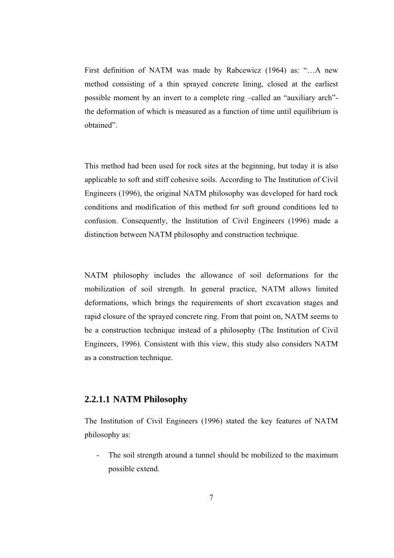
First definition of NATM was made by Rabcewicz (1964) as: “…A new

method consisting of a thin sprayed concrete lining, closed at the earliest

possible moment by an invert to a complete ring –called an “auxiliary arch”-

the deformation of which is measured as a function of time until equilibrium is

obtained”.

This method had been used for rock sites at the beginning, but today it is also

applicable to soft and stiff cohesive soils. According to The Institution of Civil

Engineers (1996), the original NATM philosophy was developed for hard rock

conditions and modification of this method for soft ground conditions led to

confusion. Consequently, the Institution of Civil Engineers (1996) made a

distinction between NATM philosophy and construction technique.

NATM philosophy includes the allowance of soil deformations for the

mobilization of soil strength. In general practice, NATM allows limited

deformations, which brings the requirements of short excavation stages and

rapid closure of the sprayed concrete ring. From that point on, NATM seems to

be a construction technique instead of a philosophy (The Institution of Civil

Engineers, 1996). Consistent with this view, this study also considers NATM

as a construction technique.

2.2.1.1 NATM Philosophy

The Institution of Civil Engineers (1996) stated the key features of NATM

philosophy as:

- The soil strength around a tunnel should be mobilized to the maximum

possible extend.

8

- Mobilization of the soil strength is provided by allowing deformation of

the ground.

- According to the site conditions, a primary support may be installed,

but the permanent support installation is normally carried out at a later

stage.

- Continuous monitoring of deformations and loads constitutes the basis

of selection of the primary support and adjusting the excavation

sequence.

2.2.1.2 NATM Construction Technique

The Institution of Civil Engineers (1996) stated the key features of construction

technique that is generally named as NATM as follows:

- The tunnel is excavated and supported sequentially. The excavation

sequence and face area should be adjusted according to site conditions.

- The primary support is provided by the combination of sprayed

concrete with steel mesh and/or steel arches and/or ground

reinforcement.

- The permanent support is generally (but not always) provided by a cast

in-situ concrete lining, which is designed separately.

2.2.1.3 General NATM Excavation Patterns

Excavation of the full face is not possible in most cases, especially in soft

ground. In practical applications, the tunnel is often advanced sequentially. The

excavation sequence mainly depends on the tunnel heading stability and

9

limitations on excavation induced ground displacements. The Institution of

Civil Engineers (1996) stated that many excavation patterns can be adopted to

satisfy one or more of the following objectives:

- Improvement on the control of the face stability, convergence and

surface settlements by reducing the exposed face area.

- Early support and closure of the ring by reducing the quantities of

excavation, reinforcement and sprayed concrete.

- Early invert closure.

- Better access for plant and operatives.

It is possible to follow different excavation sequences depending on site

conditions. Five different alternatives were selected and studied in numerical

analysis. Details of these alternatives are discussed in following paragraphs.

Full face drifts, Type A: If the tunnel diameter is small enough to satisfy the

tunneling objectives, full face excavation is a faster alternative compared to

sequential excavation. With the full face excavation, advance length is the only

parameter controlling tunneling-induced settlements and lining forces. A

typical cross and longitudinal section of a full face excavation is presented in

Figure 2.3.

Sidewall drifts, Type B: The face is divided into two parts by a temporary

wall. Starting from the left sidewall, advancement continues with the right

sidewall and there is some lag between these sidewall drifts while advancement

10

proceeds. As the tunnel enlarges, the central wall is broken out and sprayed

concrete is applied to the rest of the section to complete the ring. Cross section

and plan view of sidewall drifts are presented in Figure 2.4.

Figure 2.3 Cross and longitudinal section of full face drifts, Type A

Figure 2.4 Cross section and plan view of left and right side drifts, Type B

Crown and bench drifts, Type C: Advancement begins from the crown and

the enlargement proceeds by bench excavation. Similar to Type B, there is a

lag between advancement steps. The sprayed concrete is thickened at bench

advancement

advance step

unexcavated advances

advancement I

advance step

unexcavated advances

lag

advancement II I II

11

level to provide hunches for the crown arch. This procedure is generally

preferred for soft rock sites.

Figure 2.5 Cross and longitudinal section of crown and bench drifts, Type C

Left crown, right crown and bench drifts, Type D: The face is divided into

three parts and excavation begins from the left side of crown and proceeds with

right side. Full excavation is completed by bench drifts. The sequence of

excavation stages are presented in Figure 2.6. Lag is provided between the

excavation sequences and the sprayed concrete is thickened at bench level to

provide hunches for the crown arch.

advancement II

advance step

unexcavated advances

lag

advancement I I

II

12

Figure 2.6 Left crown, right crown and bench drifts, Type D

Left crown, left bench, right crown and right bench drifts, Type E: It is the

slowest method among the five alternatives used in this study. In this method,

excavation begins from the left crown and then left bench drifts. After the

completion of left sidewall, excavation proceeds with right crown and right

bench drifts and then the ring is completed. These excavation stages are

presented in Figure 2.7. Similar to the previous alternatives, lag is provided

between the excavation sequences and also thickness of the sprayed concrete is

increased at bench level to provide hunches for the crown.

Figure 2.7 Left crown, left bench, right crown and right bench drifts, Type E

2.2.2 Open Faced Shield Tunnelling

A tunnel heading that employs a shield, for temporary lining, without any

permanent face support is described as open faced shield tunneling. The

advancement of the shield is supplied with the reaction against the permanent

I II

III

Left Crown Drift

Right Crown Drift

Bench Drift

I

II

III

Left Crown Drift

Left Bench Drift

IV

Right Crown Drift

Right Bench Drift

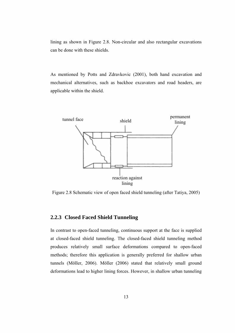
13

lining as shown in Figure 2.8. Non-circular and also rectangular excavations

can be done with these shields.

As mentioned by Potts and Zdravkovic (2001), both hand excavation and

mechanical alternatives, such as backhoe excavators and road headers, are

applicable within the shield.

Figure 2.8 Schematic view of open faced shield tunneling (after Tatiya, 2005)

2.2.3 Closed Faced Shield Tunneling

In contrast to open-faced tunneling, continuous support at the face is supplied

at closed-faced shield tunneling. The closed-faced shield tunneling method

produces relatively small surface deformations compared to open-faced

methods; therefore this application is generally preferred for shallow urban

tunnels (Möller, 2006). Möller (2006) stated that relatively small ground

deformations lead to higher lining forces. However, in shallow urban tunneling

tunnel face shield permanent

lining

reaction against lining

14

applications the main concern is surface settlements, and moreover the loads

are not significant.

Tunnel Boring Machines (TBM) are used in mechanized tunneling. TBM’s are

advanced in the ground by cutting wheels for rock or by teeth for soil, as

presented in Figure 2.9, and they are restricted with circular cross-sections.

While excavating, face support is provided mechanically by the TBM itself.

Potts and Zdravkovic (2001) pointed out that the face is supported by

controlling the applied thrust and the rate of removal of excavated material.

Figure 2.9 Schematic view of the TBM

Various face supports can be used depending on the site conditions. In addition

to the mechanical support, earth pressure balance (EPB), slurry shields and

compressed air can be selected.

Earth pressure balance shields use the excavated materials with additives to

support the face. Slurry shields use pressurized bentonite slurry to stabilize the

15

tunnel face and they are suitable for almost all types of soils. For less

permeable soils, compressed air is used to stabilize the tunnel face.

2.3 Analytical and Empirical Methods for Predicting Ground

Movements

Commercial softwares, allowing 3D modeling of tunnel advancement and

construction stages while incorporating non-linear soil response, are used

widely in today’s engineering practice. Hence, the demand for analytical and

empirical solutions has been reduced significantly, owing to their limitations

and the developments in numerical modeling tools. However, as pointed out by

Sagaseta (1998), analytical and empirical solutions can still play an important

role due to the following reasons: i) they are the reference benchmarks for the

numerical analysis results, ii) they can be used for sensitivity analysis and to

identify problem variables; and iii) they can provide simple and useful results if

they are corrected appropriately.

In fact, the use of analytical and empirical methods is difficult as they require a

number of parameters. The estimation of these parameters is not an easy task

and generally requires some experience. It is also noticed that even if the same

set of input parameters are used, the existing methods may give quite different

results as discussed by Maynar & Rodriguez (2005). The application of these

methods is limited for only circular cross-sections and they do not reflect the

possible effects of excavation sequence. Similarly, the variation in ground

water table and long-term clay behavior are not taken into account by these

methods. However, they can be used successfully if their assumptions and

shortcomings are known and corrected appropriately. The existing methods for

prediction of surface settlements will be reviewed in the following sections.

16

Common parameters for available surface settlement methods are settlement

through parameter (i) and volume loss parameter (Vs). Determination of these

parameters will be explained in Section 2.3.2

The notations used in this section and schematic view of tunneling-induced

settlement through are shown in Figure 2.10.

Figure 2.10 Geometry of the tunnel induced settlement through (after Attewell

et al., 1986)

2.3.1 Available Surface Settlement Methods

2.3.1.1 Peck Method

Peck (1969) proposed that the transverse settlement through over a single

tunnel can be represented by error function or Gaussian probability curve as

H

17

shown in Figure 2.11. Although the method has no theoretical basis, it is

widely used in the engineering practice. Peck’s method was developed based

on the settlement data obtained from 18 tunnels excavated by open faced

tunneling methods from both cohesive and granular soil sites.

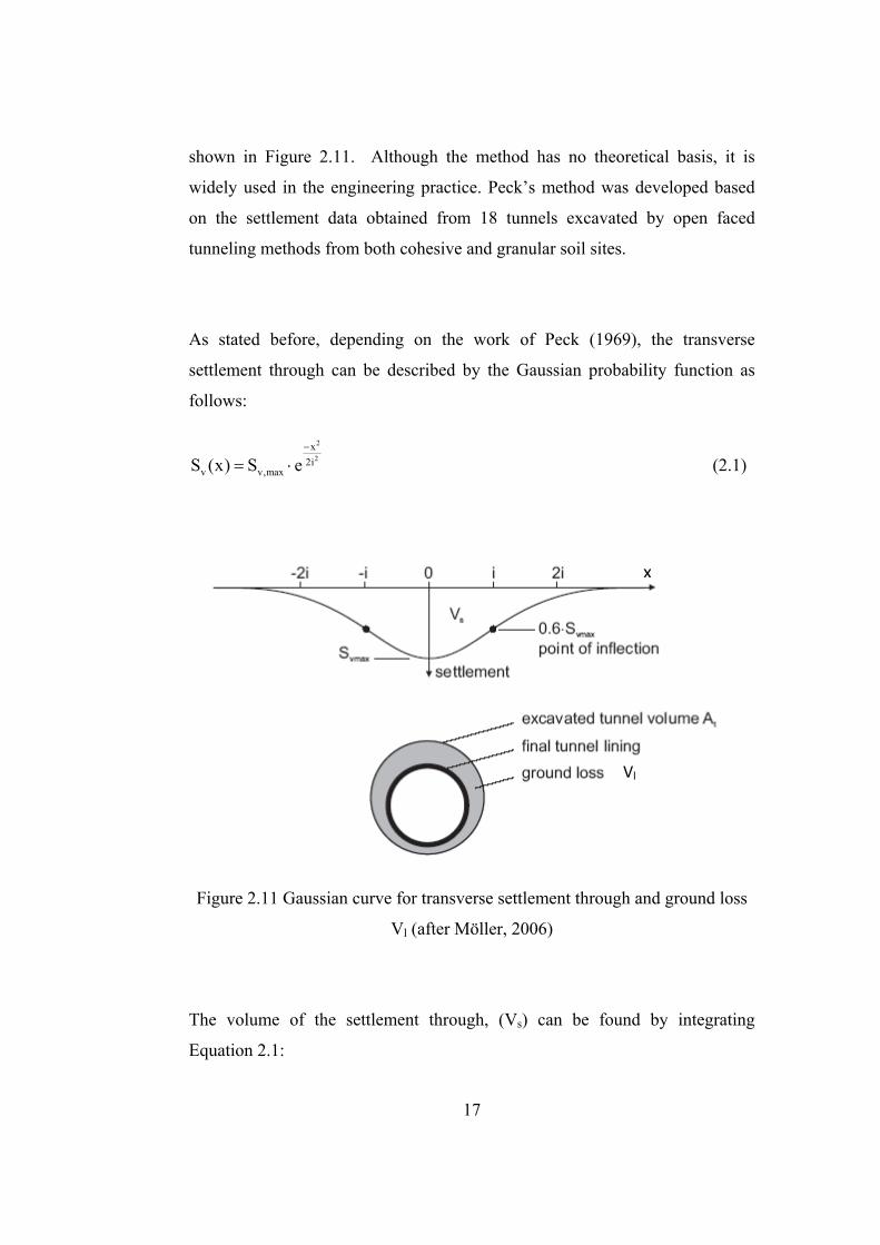
As stated before, depending on the work of Peck (1969), the transverse

settlement through can be described by the Gaussian probability function as

follows:

2

2x

2iv v,maxS (x) S e

−

= ⋅ (2.1)

Figure 2.11 Gaussian curve for transverse settlement through and ground loss

Vl (after Möller, 2006)

The volume of the settlement through, (Vs) can be found by integrating

Equation 2.1:

x

Vl 

18

v v,maxS (x) dx 2 i Sπ⋅ = ⋅ ⋅∫ (2.2)

and from Equation 2.2:

sv,max

VS2 iπ

=⋅

(2.3)

From Equations 2.1 to 2.3 the distribution of transverse surface settlements can

be formulized as:

2

2x

s 2iv

VS (x) e2 iπ

−

= ⋅⋅ (2.4)

In this study, for the estimation of through width parameter, i, the expression

proposed by Clough and Schmidt (1981) is used and a detailed discussion

regarding this parameter is presented in Section 2.3.2.1.

2.3.1.2 Sagaseta Method

The starting point of the study of Sagaseta (1987) stems from the solution for a

sink at an elastic infinite medium. As this solution is for the infinite medium,

by superposing the image solution at a point located symmetrically above the

soil surface, the shear stresses at the surface approaches to zero. To make

normal forces also zero, Boussinesq’s solution is added to the total solution.

The basis of the Sagaseta’s solution is incompressible soil layer assumption

and it is applicable only for undrained loading analysis. The surface settlements

19

in transverse and longitudinal directions are given in equations 2.5 and 2.6,

respectively.

sv 2 2

V HS (x)x Hπ

=+ (2.5)

sv 2 2

V yS (y) 12 H y Hπ

⎛ ⎞⎜ ⎟= +⎜ ⎟+⎝ ⎠

(2.6)

2.3.1.3 Gonzales and Sagaseta Method

Gonzales and Sagaseta (2001) proposed an extended version of Sagaseta

(1987) method. While predicting settlements, Sagaseta (1987) considers only

ground loss term for calculation of total deformation. In the study of Gonzales

and Sagaseta (2001), the total tunnel deformation is expressed as the sum of

several fundamental modes as shown in Figure 2.12. Solutions for ground loss,

ovalization and vertical movement due to soil compressibility or plastic strains

are summed up to obtain the total settlement as given in Equation 2.7.

v

v

2 1 2

v 2 2

D 1 1 x 'S (x) D 12H (1 x ' ) 1 x '

α

αε ρ− ⎛ ⎞−⎛ ⎞= +⎜ ⎟⎜ ⎟ + +⎝ ⎠ ⎝ ⎠ (2.7)

Ground loss solution is based on the assumptions of elastic and incompressible

media. For the ovalization, Kirsch (1898) solution is used by neglecting the

third order terms with the assumption of incompressible soil layer. Plastic

strains are taken into account with the assumption that the displacements in the

plastic zone attenuate with a power, αv ,of the distance.

20

Figure 2.12 Components of deformation of the tunnel (Gonzales and Sagaseta,

2001)

Equation 2.7 is given in terms of three parameters, ε, δ, and αv, the values of

which depend on soil conditions and excavation process. It is required to know

displacements at three different locations to predict these values. Sagaseta

recommended some values, such as i) for short term response of clayey soils αv

can be taken as 1, ii) for granular soils depending on the depth of tunnel axis αv

varies from 2 (for H<2D) to 1 (for H>4D), iii) the value of ρ generally varies

from 0 to 1, and it is greater than 1 if grouting is used to fill the gap.

When ovalization and volumetric compressibility omitted (i.e. ρ=1, αv=1),

Equation 2.7 is simplified and becomes equal to Equation 2.5

2.3.1.4 Verruijt and Booker Method

The method of Verruijt and Booker (1996) is an extension of the Sagaseta

(1987) solution. In this case, proposed solution is applicable not only for the

incompressible soil media but also for different values of Poisson’s ratio.

Besides this feature, in addition to the ground loss solution of Sagaseta,

21

Verruijt and Booker included the effect of ovalization into the solution as

follows:

( ) ( )( )

2 222

v 22 2 2 2

H x HH DS (x) D 1x H 2 x H

δε υ+

= − −+ +

(2.8)

For the incompressible case, i.e. δ=0 and ν=0; Equation 2.8 becomes equal to

Equation 2.5.

2.3.1.5 Loganathan and Poulos Method

Logonathan and Poulos (1998) redefined the traditional ground loss parameter

with respect to the gap parameter and implicated into the closed form solution

derived by Verruijt and Booker (1996), Equation 2.8. The solution of

Logonathan and Poulos (1998) is presented in Equation 2.9.

( ) ( )

2

21.38x

H 0.5D2v 2 2

HS (x) 1 (2gD g )ex H

υ

⎡ ⎤⎢ ⎥−⎢ ⎥+⎣ ⎦= − +

+ (2.9)

In equation 2.9, undrained gap parameter “g” is defined as the magnitude of the

equivalent 2D void formed around the tunnel due to the combined effects of

the 3D elasto-plastic ground deformation at the tunnel face, overexcavation of

soil around the periphery of the tunnel shield, and the physical gap related to

the tunneling machine, shield and lining geometry (Rowe and Kack, 1983).

The gap parameter is estimated using the theoretical based model of Lee et al.

(1992) as given in Equation 2.10:

22

(2.10)

where Gp is the physical gap that represents the geometric clearance between

the outer skin of the shield and the lining, U3D is the equivalent 3D elasto-

plastic deformation at the tunnel face and W is the parameter that takes into

account the quality of workmanship. 3D strains at the tunnel face may be

neglected and with the assumption of good workmanship, the gap parameter

becomes equal to the physical gap.

2.3.2 Ground Surface Settlement Parameters

Estimation of ground surface settlements with the available analytical and

empirical methods generally requires two parameters: settlement through

parameter (i) and volume loss parameter (Vs). Determination of these

parameters is discussed next.

2.3.2.1 Settlement Through Parameter, i

Settlement through parameter, i, determines the distance from tunnel axis to the

point of inflexion as shown in Figure 2.11. In other words, the width of

settlement through is determined by settlement through parameter.

Depending on the data obtained from 18 tunnels excavated in cohesive and

granular soils by using open faced tunneling methods, Peck (1969) proposed a

chart solution to determine the settlement through parameter (Figure 2.13).

p 3Dg G U W= + +

23

Figure 2.13 Relation between width of settlement through, as represented by

i/R, and dimensionless depth of tunnel, H/2R, for various tunnels in different

materials (after Peck, 1969)

After this study, various researchers have presented similar relations for

settlement through parameters and. some of them are presented in Table 2.1.

2.3.2.2 Volume Loss Parameter, Vs

The term, volume loss is sometimes referred as ground loss. Volume loss is the

ratio of excavated tunnel volume to the volume of the tunnel defined by final

tunnel lining (Figure 2.11). For the short-term settlements of clay, as shown in

Figure 2.11, volume of transverse settlement through is equal to the volume

loss as a result of the incompressible soil assumption.

i/R

24

Table 2.1 Relations for settlement through parameter (after Dolzhenko, 2002)

The volume loss depends on many factors such as: type of soil, rate of tunnel

advancement, round length, excavation sequence and tunnel size. The relations

for determination of the volume loss parameter are associated with the stability

number N which is defined by Broms and Bennermark (1967) as follows:

v t

u

Nc

σ σ−= (2.11)

Lake et al. (1992) summarized the available relationships between stability

number and volume loss and stated following conclusions; i) if N is less than 2,

the response is elastic and the tunnel face is stable, ii) if N is between 2 and 4,

local plastic zones develop around the tunnel, iii) if N is between 4 and 6,

plastic yielding zone produces large movements, and iv) if N is greater than 6,

face instability occurs. Lake et al. (1992) presented the relations between

volume loss and stability number proposed by several authors as in Figure

2.14.

25

Figure 2.14 Different relations between stability number N and volume loss VL

(Lake et al. , 1992)

Mair (1996) reported that, in stiff clays volume loss ranges between 1% and

2%. Conventional tunneling in London Clay results in volume losses between

0.5% and 1.5%.

Estimation of volume loss parameter is considered a difficult task. In this

study, volume loss parameters are obtained from finite element analysis in

which complete process of tunnel construction is simulated by 3D analysis.

2.4 Analytical Methods for Predicting Lining Forces

There exist a number of analytical methods for the prediction of lining forces.

They are generally simple methods and they can be applied easily; however

they suffer from some major limitations; i) they are generally applicable only

to circular cross-sections, ii) excavation procedures (i.e. sequences) are not

26

taken into account, iii) variations in soil strata and non-linear soil response are

not possibly implemented in these solutions.

Duddeck and Erdmann (1985) proposed a closed form solution for circular

sections; but they claimed that the results may also be valid for non-circular

cross sections. Basic assumptions of structural design models used in their

study can be listed as:

- the lining and the soil are assumed to be in plane-strain condition

- driving procedure and the placing of the supporting elements may affect

the active soil pressures on the lining but they are neglected

- both the soil and lining are assumed to behave elastically

The available closed form solutions are simple enough for practical application

and they are discussed next.

2.4.1 Plane Strain Continuum Models

Duddeck and Erdmann (1985) mentioned that methods presented by Windels

(1967), Curtis (1976), Einstein and Schwartz (1979) and Ahrens et al. (1982)

yields identical values. They all assumed that soil pressures on the lining are

equal to the initial stresses in the undisturbed soil, and the soil and lining

behavior is elastic. The authors give solutions for full bond (no slippage

between the ground and lining) and tangential slip (the shear force between

27

ground and lining is zero) conditions. Characteristic distribution of radial

displacement, hoop forces and bending moments are presented in Figure 2.15

Figure 2.15 Plane strain continuum model and characteristic distribution of

radial displacement, u, hoop forces, N, and bending moments, M (Duddeck &

Erdmann, 1985)

Most of the closed form solutions use the relative stiffness terms, α and β ,

which are stiffness against moments and hoop stresses, respectively:

3

s s

ERE I

α = (2.12)

s s

ERE A

β = (2.13)

Duddeck and Erdmann (1985) presented closed form solutions to summarize

the identical continuum models. Explicit formulae of bending moments, M and

Es

28

hoop forces, N of the tunnel lining for plane strain continuum models with the

assumption of full bond are given in Equations 2.14, 2.15 and 2.16,

respectively.

( )v 01M 1 K R

4 0.342σ

α= −

+ (2.14)

( ) ( )0 v 00

1N 1 K R2 1 K 2.69

σβ

= −+ −

(2.15)

( ) ( ) ( )max v 0 v 00

1 1N 1 K R 1 K R1.2 2 1 K 2.69228.1 1.8

σ σα βα

= − + −+ −+

+

(2.16)

2.4.2 Muir Wood Model

Muir Wood (1975) presented a continuum solution by assuming an elliptical

deformation mode. In this study, radial deformation due to the shear force

between soil and lining is omitted. Also the soil and lining are assumed to be

elastic.

Maximum bending moment, hoop force at crown and hoop force at axis are

given in Equations 2.17, 2.18 and 2.19 respectively .

( )

( )

2v 0 3

s s

1M 1 K R2 ER6

1 (5 6 ) E I

σ

ν ν

= −+

+ −

(2.17)

( )( )

( )

3

s s0 v 0 3

s s

ER1 0.556E IN 1 K R

ER3 1E I

νσ

ν

+ += −

+ + (2.18)

29

( )( )

( )

3

s smax v 0 3

s s

ER2 1 0.778E IN 1 K R

ER3 1E I

νσ

ν

+ += −

+ + (2.19)

2.4.3 Antonio Bobet Model

Bobet (2001) presented analytical solutions for shallow circular tunnels. In his

work, it is assumed that the tunnel is in plane-strain condition, and both tunnel

lining and soil behave elastically. Time dependent factors, such as swelling and

creep, are not considered in this solution. Also, it is assumed that the friction

between soil and lining is small, and full slippage condition is accepted. This

model is not valid for cases where depth to radius ratios are smaller than 1.5

Using the solution proposed by Timesoshenko and Goodier (1970), Bobet

(2001) extended the solution of Einstein and Schwartz (1979) for dry, partially

and fully saturated soils. The proposed solution is also applicable to short and

long term conditions.

To take into account the gap between the tail of the shield and liner, Bobet

(2001) included a gap parameter (w). Compressibility and flexibility ratios

used in the proposed model were defined as follows:

2s

2s s

ER(1 )CE A (1 )

νν

−=

− (2.20)

3 2s2

s s

ER (1 )FE I (1 )

νν−

=− (2.21)

30

In the finite element analysis of this study, for the short term conditions, the

soil on the tunnel is modeled as dry and no water pressure is assigned on the

tunnel lining. On the other hand, for long-term conditions water pressure

applied around the tunnel and drainage is not permitted between soil and

lining.

Short Term Analysis: For shallow tunnels in dry soil, hoop force and bending

moment are given as:

00

2

w2E H(1 K )(1 ) (C F)r1T R

2 (C F)(1 ) (1 )CF

γ ν

ν ν

⎡ ⎤− + + +⎢ ⎥

⎣ ⎦=+ + + −

03 3 4 H(1 K )R cos 22 (1 )F 3(5 6 )

ν γ θν ν

−− −

− + −2

03 4 (1 K )R sin 3

(1 )F 8(7 8 )ν γ θ

ν ν−

+ −− + −

(2.22)

20

3 3 4M H(1 K )R cos 22 (1 )F 3(5 6 )

ν γ θν ν

−= − −

− + −

30

3 4 (1 K )R sin 3(1 )F 8(7 8 )

ν γ θν ν

−+ −

− + − (2.23)

Long Term Analysis: The solutions for (i) saturated soil without water

pressure and (ii) water pressure only and no drainage, are considered separately

and summed up at the end for long term analysis. Solution for saturated soil

without water pressure condition is obtained by using γb as the unit weight in

31

Equations 2.22 and 2.23. Solution for water pressure only and no drainage

condition is given in Equations 2.24 and 2.25.

w wC FT h R

C F (1 )CFγ

υ+

=+ + −

(2.24)

M 0= (2.25)

Bobet (2001) stated that, solution for the short term analysis with water

pressure is the sum of (i) saturated soil without water pressure and (ii) water

pressure only. In the study of Bobet (2001), the solution for saturated soil

without water pressure condition is found by total stress analysis and then the

solution for only water pressure condition is added to obtain the complete

solution, which leads to taking water pressure into account twice.

2.4.4 Erdmann Model

Möller (2006) presented closed form solutions based on the charts given by

Erdmann (1983) for determination of hoop forces and bending moments as

follows:

0 2N N N= + (2.26)

v h0 0N Rn

2σ σ+

= (2.27)

22 v h2

2 2

RnNcos 2

M 2 R mσ σ θ

⎡ ⎤⎡ ⎤ += ⎢ ⎥⎢ ⎥

⎣ ⎦ ⎣ ⎦ (2.28)

32

Relative stiffness ratios in Equations 2.12 and 2.13 are used to determine the

coefficients n0, n2 and m2 from Figure 2.16, 2.17 and 2.18 respectively.

Figure 2.16 Coefficient n0 for constant part of normal force (Erdmann, 1983)

Figure 2.17 Coefficient n2 for non-constant part of normal force (Erdmann,

1983)

Q

33

Figure 2.18 Coefficient m2 for bending moment (Erdmann, 1983)

These figures are given for 3/ 3 10α β = ⋅ condition; however, Erdmann (1983)

stated that variations of /α β have little effects on the curves.

2.5 2D and 3D Numerical Models Used in Tunneling

By using 3D numerical models, the advancement of the tunnel can be correctly

simulated by also modeling the excavation sequence. Although 3D stress-strain

states can be fully simulated by 3D numerical models, Galli et al. (2004) stated

that 2D numerical models are generally preferred instead of 3D models.

It is important to consider the 3D redistribution of the stresses around heading,

in case tunnels are analyzed in 2D plane-strain conditions. Similarly, to take

into account the three dimensional arching effect with 2D numerical models,

34

there exist a number of alternatives, such as convergence-confinement method

(Panet and Guenot, 1982), gap method (Rowe et al.,1983; Lee and Rowe,

1991), disk calculation method (Schikora and Ostermeier, 1988), volume-loss

control method (Potts and Zdravkovic, 2001), and hypothetical modulus of

elasticity soft lining method (Powell et al.,1997; Karakus and Fowell, 2005).

35

CHAPTER 3

3. NUMERICAL MODELLING OF GENERIC CASES

3.1 Introduction

This study is focused on the assessment of the effects of tunnel advancement

on ground subsidence and on tunnel lining forces. A parametric study was

carried out for this purpose. Generic cases were studied to determine the effects

of various parameters, such as soil stiffness, short-term and long-term soil

response, tunnel geometry and construction procedures. Numerical analysis

performed as a part of this parametric study were carried out by Plaxis 3D

Tunnel geotechnical finite element package which is specifically preferred for

three-dimensional deformation and stability analysis of tunnels. This chapter is

devoted to introduce the details of material properties, finite element modeling,

constitutive models and construction procedures used in the performed

parametric study.

3.2 Modeling Basics

3.2.1 Definition of the Excavation Sequences, Parametric Study

and Analyzed Tunnel Sections

In practical applications, the tunnel is often advanced sequentially. The type of

excavation sequence mainly depends on the tunnel heading stability and

limitations on tunneling-induced ground displacements.

36

Sequence of excavation is considered as an important factor affecting the

tunneling-induced ground displacements and lining stresses. Owing to its

importance, five different excavation sequences are studied. Following are the

excavation sequences used in this study and their details were presented in

Section 2.2.1.3:

- Type A: Full face drifts

- Type B: Sidewall drifts

- Type C: Crown and bench drifts

- Type D: Left crown, right crown and bench drifts

- Type E: Left crown, left bench, right crown and right bench drifts

The parametric study considers the variations in soil stiffness, tunnel diameter,

type of excavation sequence, tunnel depth, and round length. The variables of

the parametric study are listed in Table 3.1

Table 3.1 Variables of the parametric study

Type of Soil

Diameter, D

Type of Excavation Sequence

Tunnel Depth, H

Round Length, d

Soft Clay Stiff Clay

5.0 m A, B, C 2.0D

3.5D

5.5D

1 m 2 m

7.0 m B, C, D, E

9.0 m D, E

37

A total of 108 different combinations are studied using the variables listed in

Table 3.1. For each finite element analysis, both short-term and long-term soil

responses are also investigated.

For 3D numerical models, a non-circular typical NATM horse shoe shaped

tunnel section is used (Figure 3.1). Three different equivalent diameters are

used to define tunnel sections such as, 5.0m, 7.0m and 9.0m. Equivalent

diameter is defined by considering a circular tunnel having an equal area. For

different diameters, the radii of the arches defining the horse shoe shaped

tunnel section are presented in Table 3.2.

Figure 3.1 Horse shoe shaped tunnel section used in the parametric study

3.2.2 Finite Element Mesh and Boundary Conditions

For 3D finite element analysis, 15 node wedge elements are used. These

elements are composed of 6 node triangular faces in two dimension and 8 node

R1

R5

R4

R3

R2

38

quadrilateral faces in third dimension (as shown in Figure 3.2). 8 node plate

elements are used to simulate the lining behavior.

Table 3.2 Radii of the arches defining horse shoe shaped tunnel section

Diameter (m) R1 (m) R2 (m) R3 (m) R4 (m) R5 (m) 5.0 3.29 1.41 2.81 2.57 2.67 7.0 4.6 1.96 3.93 3.59 3.73 9.0 5.92 2.53 5.05 4.62 4.8

Figure 3.2 15-node wedge elements nodes and stress points (Plaxis 3D Tunnel

version 2 Reference Manual, 2004)

At the bottom of the 3D finite element mesh, total fixities are used which

restrain the movements in horizontal and vertical directions. For upper part, the

mesh has no fixities. For right and left sides, roller supports are used which

restrain only the horizontal movements and vertical displacements are left free.

39

Mesh dimensions should be appropriately defined, to prevent the effects of

boundary conditions. Möller (2006) presented some guidance for the mesh

dimensions in his study, also summarizing the study of Meissner (1996) about

mesh dimensions.

Meissner (1996) reccommended mesh dimensions for 2D modelling of tunnels.

It was suggested to use (4 - 5) D from the tunnel centerline to the vertical mesh

boundaries, and (2 – 3) D from tunnel center line to the bottom mesh boundary.

For tunnel diameters between 4.0 m and 12.0 m, Möller (2006) recommended

mesh dimensions for 3D models. Equation 3.1 for total mesh width and (1.6 –

1.95) D from tunnel centerline to the bottom mesh boundary were suggested.

The correlation of mesh width with the ratio (H/D) is logical, as the depth of

tunnel increases the settlement through gets wider.

Hw 2D 1D

⎛ ⎞= +⎜ ⎟⎝ ⎠

(3.1)

The 2D mesh should be constructed before proceeding to the 3D mesh

extension. Typical 2-D and 3-D meshes used in this study are presented in

Figure 3.3 and 3.4, respectively. Mesh dimensions shown in Figure 3.3 are

calculated based on the recommendations of Meissner (1996) and Möller

(2006). To reduce the calculation time, mesh width is increased as the tunnel

gets deeper.

It is also important to check that boundary conditions are not affecting the

results. To assure that boundary effects are eliminated, plane-strain conditions

should be reached. In other words, the simulation of the tunnel advancement

procedure should be performed until steady state surface settlements and lining

40

forces are observed. The mesh length is coarser at both ends to minimize mesh

density while maximizing the mesh length. To minimize the boundary effects,

the excavation of the initial part (10D in Figure 3.4) is performed at once; then

the tunnel advancement proceeds. The simulation of the tunnel advancement is

repeated until the steady state conditions are reached.

Figure 3.3 Mesh dimensions of the cross section of a typical 3D FE model

3.2.3 Initial Stress Conditions

The initial stress distribution of the soil must be defined before simulating the

tunnel advancement procedure. The initial stresses in the soil are affected by

the weight of the soil and history of the soil formation. Stress state is

characterized by vertical and horizontal stresses. Initial vertical stress depends

on the weight of the soil and pore pressures; whereas initial horizontal stresses

are related to the vertical stresses by the coefficient of lateral earth pressure at

rest. This relation is provided by the K0-procedure in Plaxis 3D Tunnel

program.

w = 8D, 10D, 14D

2.0D 3.5D 5.5D

2.15D

H=

41

Figure 3.4 Mesh dimensions of a typical 3D FE model

In this study, it is assumed that the water table is at the ground surface and clay

formations are fully saturated; hence, initial stresses should be calculated in

terms of effective stresses. The relation between initial vertical and horizontal

stresses is given in Equation 3.2 and the coefficient of lateral earth pressure at

rest, K0, for normally consolidated soils can be calculated by Jacky (1944) ’s

formula as given in Equation 3.3.

' 'h 0 vKσ σ= (3.2)

'0K 1 sinφ= − (3.3)

3.2.4 Water Table Conditions

The water table is defined initially at the ground surface level. As the tunnel

advances, the water table around the opening should be decreased. The Plaxis

3D Tunnel package does not let changing the water table conditions along the

tunnel length. Because of this limitation the water table is decreased before the

10D

7D

8D

42

simulation of the excavation along the full length of the model. Deformations

due to the water table decrease are not considered in the tunnel advancement

by resetting the displacements before starting the tunnel construction stage.

Pore water pressure distributions corresponding to before and after ground

water table lowering are presented in Figures 3.5 and 3.6, respectively. While

modeling the decrease in ground water table permeability of the soil is not

taken into account and it is assumed that tunneling operations decrease the

water table within 2 diameters from the edge of the tunnel as shown in Figure

3.6.

Figure 3.5 Initial pore water pressures

3.2.5 Elastic Perfectly Plastic Constitutive Model with Mohr-

Coulomb Failure Criterion

Linearly Elastic perfectly plastic constitutive model with Mohr-Coulomb

failure criterion is used in this study. In these types of models, strains and strain

rates are composed of elastic and plastic components as shown in Equation 3.4.

43

Stress rates are related to the elastic strain rates by Hooke’s Law as in Equation

3.5.

e pε ε ε= + (3.4)

e e e p' D D ( )σ ε ε ε= = − (3.5)

Figure 3.6 Pore water pressures after water table decrease

In order to evaluate whether or not plastic deformations occur, yield surfaces

are defined as shown in Figure 3.7. For stress states located inside this yield

surface, all deformations are elastic and reversible. If the stress state touches

this yield surface, plastic, i.e. irreversible, deformations occur.

The Mohr-Coulomb yield condition is an extension of Coulomb’s friction law

to general states of stress. The Mohr-Coulomb yield condition consists of six

yield functions given in terms of principal stresses:

2D 2D

44

' ' ' '1a 2 3 2 3

1 1f ( ) ( )sin ccos 02 2σ σ σ σ φ φ= − + + − ≤ (3.6a)

' ' ' '1b 3 2 3 2

1 1f ( ) ( )sin ccos 02 2σ σ σ σ φ φ= − + + − ≤ (3.6b)

' ' ' '2a 3 1 3 1

1 1f ( ) ( )sin ccos 02 2σ σ σ σ φ φ= − + + − ≤ (3.6c)

' ' ' '2b 1 3 1 3

1 1f ( ) ( )sin ccos 02 2σ σ σ σ φ φ= − + + − ≤ (3.6d)

' ' ' '3a 1 2 1 2

1 1f ( ) ( )sin ccos 02 2σ σ σ σ φ φ= − + + − ≤ (3.6e)

' ' ' '3b 2 1 2 1

1 1f ( ) ( )sin ccos 02 2σ σ σ σ φ φ= − + + − ≤ (3.6f)

Figure 3.7 The Mohr-Coulomb yield surface in principal stress space, c=0

(Plaxis 3D Tunnel version 2 Reference Manual, 2004)

45

According to associated plasticity assumption, the derivative of the yield

function with respect to stresses is proportional to the plastic strain rates. Thus,

plastic strain rates are vectors perpendicular to the yield surface. The associated

plasticity assumption leads to an over predicted dilatancy in Mohr-Coulomb

yield functions. To overcome this overprediction, a plastic potential function,

g, is introduced which is called as non-associated plasticity. Plastic strain rates

are formulated by using non-associated plasticity as follows:

p 1 21 2

g g ...' '

ε λ λσ σ∂ ∂

= + +∂ ∂

(3.7)

where λ1, λ2… are plastic multipliers.

By the consistency condition:

ff ' 0'σ

σ∂

= =∂

(3.8)

Substituting Equation 3.5 and 3.7 into Equation 3.8, plastic multipliers can be

determined by using independent yield functions (f1, f2 …) as follows:

ei 1 2i 1 2

f g gf D ( ...) 0' ' '

ε λ λσ σ σ∂ ∂ ∂

= − − − =∂ ∂ ∂

(3.9)

The plastic potential functions are then defined as

' ' ' '1a 2 3 2 3

1 1f ( ) ( )sin2 2σ σ σ σ ψ= − + + (3.10a)

' ' ' '1b 3 2 3 2

1 1f ( ) ( )sin2 2σ σ σ σ ψ= − + + (3.10b)

46

' ' ' '2a 3 1 3 1

1 1f ( ) ( )sin2 2σ σ σ σ ψ= − + + (3.10c)

' ' ' '2b 1 3 1 3

1 1f ( ) ( )sin2 2σ σ σ σ ψ= − + + (3.10d)

' ' ' '3a 1 2 1 2

1 1f ( ) ( )sin2 2σ σ σ σ ψ= − + + (3.10e)

' ' ' '3b 2 1 2 1

1 1f ( ) ( )sin2 2σ σ σ σ ψ= − + + (3.10f)

Mohr-Coulomb constitutive model is summarized here for the sake of

completeness. More detailed information is available in Plaxis 3D Tunnel

version 2 Reference Manual (2004) and Möller (2006).

3.3 Modeling Parameters

Mohr-Coulomb Model needs five input parameters, modulus of elasticity (E)

and Poisson’s ratio (ν) to define elastic soil response; friction angle (Φ) and

cohesion (c) to define plastic response and angle of dilatancy (ψ). The

parametric study is carried out for both short-term and long-term behaviors of

soft clay and stiff clay layers. The parameters used in this study are presented

in the next section.

3.3.1 Notes on Soil Parameters

The soil stiffness depends on stress level and it generally increases with depth.

Lambe and Whitman (1969) stated that as the confining stress increases, the

modulus of elasticity also increases. In this study, a similar approach is used

47

and these values are presented in Section 3.3.2. As reviewed in Bowles (1996),

several researchers related undrained shear strength and modulus of elasticity.

It is also possible to determine modulus of elasticity based on shear wave

velocity value, as done in this study. Typical shear wave velocity values for

soft-clay and stiff-clay, obtained from literature, are shown in Figure 3.9.

Compared to initial loading, the soil stiffness is higher for unloading and

reloading. Therefore, it will be convenient to use the unloading modulus to

model tunnels as construction procedure includes excavation, i.e. unloading.

For practical purposes, unloading modulus can be simply determined by

multiplying the modulus of elasticity by 3 (Plaxis 3D Tunnel version 2

Material Models Manual, 2004).

To model the variation of undrained shear strength with depth, the correlation

given by Skempton and Bjerrum (1969) is used. Authors expressed the

undrained shear strength of normally consolidated clays as a function of

effective overburden stress and plasticity index as follows:

u'v

c 0.11 0.0037PIσ

= + (3.11)

To determine the friction angle, the equation given by Gibson (1953) is used.

This equation is given for drained loading conditions and expresses friction

angle as a function of plasticity index as follows:

2'drained 0.002283PI 0.3972851PI 35.724φ = − + (3.12)

48

Shear modulus of the soil is constant for short-term and long-term behaviour

but elastic modulus depends on Poisson’s ratio. Shear modulus is related to the

elasticity modulus, according to the Hooke’s law of isotropic elasticity as

follows:

EG2(1 )υ

=+

(3.13)

The dilatancy of the clay is not taken into account in this study and full bond

interface elements are used between soil and lining.

3.3.2 Short and Long Term Clay Parameters

Short and long term material properties for soft and stiff clay layers used in the

parametric study are presented in Table 3.3 and Table 3.4, respectively. The

increase in Young’s Modulus and shear wave velocity as a function of depth is

schematically represented in Figure 3.8 and Figure 3.9, respectively.

Table 3.3 Material properties of Soft Clay

49

Table 3.4 Material properties of Stiff Clay

3.3.3 Shotcrete Parameters

Tunnel lining is modeled using a linear elastic material model and the

corresponding material properties are given in Table 3.5. It should be noted

that, for tunnels having 5.0 m diameter, lining thickness is selected as 20 cm;

whereas for larger tunnel diameters 30 cm lining thickness is used.

Table 3.5 Material properties of shotcrete

Parameter Symbol Shotcrete Unit Type of Material Behaviour Elastic - Thickness t 20 - 30 cm

Weight wplate 24 kN/m3

Elastic modulus Eplate 28 500 000 kN/m2

Poisson's ratio ν 0.15 -

50

Figure 3.8 Assumed values of undrained unloading-reloading Young’s

Modulus for different depths

Figure 3.9 Assumed values of shear wave velocity for different depths

05

101520253035404550

0 100000 200000 300000 400000D

epth

bel

ow c

lay

surf

ace,

z (m

)Young's Modulus, Eu (kPa)

Soft Clay

Stiff Clay

05

101520253035404550

0 50 100 150 200 250

Dep

th b

elow

cla

y su

rfac

e, z

(m)

Shear Wave Velocity, Vshear (m/s)

Soft Clay

Stiff Clay

51

3.4 Modeling of the Tunnel Advancement

To assess the effects of excavation sequence on ground subsidence and lining

forces, 3D finite element simulations are performed for generic cases according

to the procedure described below.

i) Initial stresses are generated with long-term clay parameters according

to the K0 procedure.

ii) Short-term clay parameters are assigned to the model and water table is

decreased as described in Section 3.2.4.

iii) The ground deformations due to the water table decrease are reset.

iv) To minimize the boundary effects, the tunnel is excavated 10D away

from the front boundary and the tunnel lining is installed for 10D

simultaneously.

v) The tunnel advancement is started by performing the excavation of first

drift by an amount of round length, d. (two different round lengths are

used in the analysis, d=1.0 m and d=2.0 m)

vi) Excavation proceeds by another drift and the concrete lining is applied

to the previously excavated span

vii) The tunnel is advanced by repeating steps (v) and (vi) until having a lag

of 6.0 m between two drifts, then succeeding drifts are excavated till the

completion of the full tunnel section. Depending on the type of

excavation sequence, number of drifts to complete the full tunnel ring

varies. Section 2.2.1.3 presents the details of types of excavation

sequences used in this study. The temporary walls are cracked while

advancing the following drifts.

52

viii) Steps (v), (vi) and (vii) are repeated until the tunnel face gets 5D away

from the boundary.

ix) The water table is increased to the initial condition and long term clay

parameters are assigned to the model.

A cross section and plan view of Type B left and right side drifts is presented

as an example in Figure 3.10

Figure 3.10 Cross section and plan view of left and right side drifts, Type B

advancement I

round lenght, d

unexcavated advances

Lag = 6m

advancement II I II D

H

Ground Surface f

53

CHAPTER 4

4. DISCUSSION OF THE RESULTS

4.1 Introduction

This chapter is devoted to the presentation of the results of the parametric

study. A detailed discussion on important factors; such as excavation sequence,

round length, soil stiffness, affecting the tunneling induced ground subsidence

and lining forces are also presented. Moreover, the effects of short-term and

long-term soil response are emphasized in terms of variations in ground water

table level.

4.2 Short-Term Surface Settlements

For short-term ground conditions, water table is decreased within two

diameters of the edge of the tunnel as explained in Section 3.2.4 and for long-

term ground conditions the water table is increased to the surface level.

Increasing water table produces heave at ground surface instead of settlement.

Therefore, discussions about surface settlements include only short-term

ground conditions.

4.2.1 Effect of Excavation Sequences

The alternative excavation sequences used in this study have been introduced

in Section 2.2.1.3. Transverse surface settlement profile of different excavation

54

sequences for 5.0 m diameter tunnel at a depth of 10.0 m is presented in Figure

4.1 as a representative case. Type C (crown and bench drifts) excavation

procedure resulted in the largest surface settlements; whereas Type B (left and

right sidewall drifts) resulted in the lowest surface settlements. Type A (full

face drifts), on the other hand, produced intermediate levels of surface

settlements compared to types B and C.

Figure 4.1 Transverse surface settlement profile for different types of

excavation sequences in soft clay (D=5.0m, H=10.0m)

Tunnel advancement by subdividing the full tunnel area into smaller parts

should result a decrease in surface settlements. However, as revealed by Figure

4.1, as the number of drifts to complete the ring increases, surface settlement

do not always decrease. It is due to the ring closure problem. If the lining ring

is not closed, the lining is incapable of limiting the deformations inside the

tunnel excavation; and consequently, surface settlements increase. Considering

0.0

0.1

0.2

0.3

0.4

0.5

0.6

-4 -2 0 2 4

S max

/Scr

own

x/D

TYPE A, H/D=2, d/D=2/5TYPE B, H/D=2, d/D=2/5TYPE C, H/D=2, d/D=2/5

55

Type B, excavation begins with left side drifts and while the excavation of

right side starts the lining ring of the left side has been already closed.

However, for Type C, excavation starts with crown drifts and then proceeds

with bench drifts and as a result of this selection the lining ring can not be

closed until the end. It is the reason why Type A results in smaller surface

settlements compared to Type C, although it proceeds with full face drifts.

It can be concluded that the rapid closure of the tunnel ring is more important

than the type of excavation sequence owing to its effects on limiting the

surface settlements. Performing excavations sequentially do not decrease the

surface settlements unless the lining ring is closed. In some cases, sequential

excavation is required to stabilize the tunnel face and rapid closure of the ring

does not have significant effects.

4.2.2 Effect of Round Length

Two different round lengths, d=1.0m and d=2.0m, were used in these

parametric study. The effect of the round length on surface settlements is

presented in Figure 4.2. In this figure, d2 and d1 represent 2.0m and 1.0m round

lengths, respectively; whereas Smax,d2 and Smax,d1 represent the corresponding

maximum surface settlements due to tunnel advancements with these round

lengths, respectively and D is the diameter of the tunnel.

Using Figure 4.2, the surface settlement induced by any round length can be

estimated based on the known maximum surface settlement of a round length

for this study. The effect of round length on surface settlements varies from

20 % to 70 % for soft clay sites; whereas, for stiff clay sites, it varies between

15 % and 50 %. The round length loses its influence on surface settlements as

56

the round length to diameter ratio (d2/D) decreases. For higher round length to

diameter ratios, the effect of soil stiffness becomes more significant.

Figure 4.2 Effect of round length on surface settlements

Figure 4.3 Effect of tunnel depth on surface settlements of different round

lengths

00.20.40.60.8

11.21.41.61.8

2

0.2 0.25 0.3 0.35 0.4 0.45

S max

,d2/S

max

,d1

d2/D

Soft Clay

Stiff Clay

max,d2 2

max,d1

S d1.4413 0.9527S D

= +

max,d2 2

max,d1

S d0.7729 1.0576S D

= +

00.20.40.60.8

11.21.41.61.8

2

1.5 2.5 3.5 4.5 5.5 6.5

S max

,d2/S

max

,d1

H/D

Soft Clay

Stiff Clay

max,d2

max,d1

S H0.0384 1.5398S D

= − +

max,d2

max,d1

S H0.0342 1.4224S D

= − +

57

The cover depth ratio (H/D) is considered to be another significant factor

affecting the settlement ratio induced by different round lengths. According to

the results of the simulations, as the tunnel gets deeper, the effect of round

length on surface settlements decreases as shown in Figure 4.3.

4.2.3 Effect of Soil Stiffness

In order to show the effects of soil stiffness, analysis were preformed on both

soft and stiff clay sites using the material properties given in Section 3.3.2. The

findings are summarized in Figure 4.4, where Smax,soft and Smax,stiff represent

maximum surface settlements for soft and stiff soil sites, respectively and

(H/D) is the cover to depth ratio. It is observed that, Smax,soft/Smax,stiff ratio varies

between 5.3 and 13.8 and this ratio increases with increasing tunnel depth. This

observation can be explained by the fact that for stiff clay sites, soil stiffness

increases more with depth compared to soft clay sites. As the number of

excavation sequences increase, Smax,soft/Smax,stiff ratio increases too. Left crown,

left bench, right crown and right bench drifts (Type E) has the maximum

number of excavation sequences and it yields the highest Smax,soft/Smax,stiff ratio.

It means that with increasing soil stiffness, rapid closure of ring becomes less

important, and significant surface settlements are not expected for stiff clay

sites even for the cases when the tunnel ring is not closed.

58

Figure 4.4 Effect of soil stiffness on surface settlements

4.2.4 Effect of Depth

From the closed form solutions and site observations, it is known that as the

depth of tunnel increases, effects of tunneling operations are less significant for

the surface. Results of finite element analysis regarding this issue are presented

in Figure 4.5 where Smax is the maximum surface settlement, Scrown is the

settlement at the crown of the tunnel, H is tunnel depth and D is the diameter of

the tunnel. This figure reveals that effect of tunneling operations on surface

settlements (Smax/Scrown ratio) decreases with increasing tunnel depth. Also at

stiff clay sites, tunneling-induced ground settlements are smaller compared to

soft clay sites. For stiff clays (Smax/Scrown) ratio is approximately 40 % lower

compared to soft clays. Based on the variation of Smax/Scrown ratio with depth,

for this study it can be concluded that the effect of crown settlement on surface

settlements is negligible at a depth of 8.7 D for stiff clays, whereas it is 9.6 D

for soft clay sites.

0

2

4

6

8

10

12

14

16

1.5 2.5 3.5 4.5 5.5 6.5

S max

,soft/S

max

,stiff

H/D

Type A

Type B

Type C

Type D

Type E

59

Figure 4.5 Effect of tunnel depth on surface settlements

4.2.5 Comparison of FEM results with Closed Form Solutions

There exist a number of empirical and analytical solutions for prediction of

surface settlements in literature. A brief review of the methods, that were

decided to be used in this study, has been already given in Section 2.3.1. The

volume loss values required for these closed form solutions are obtained from

the results of numerical analysis. For each analysis, the difference between the

results of numerical analysis and existing closed-form solution is represented

by a normalized term, [ ]ClosedForm Plaxis Plaxis(S -S ) / S % , in Figures 4.6 and 4.7 for

soft and stiff soil sites, respectively. In these plots, SClosedForm and SPlaxis

represent the maximum surface settlements corresponding to existing closed

form solutions and results of numerical analysis, respectively. Numerical

analysis have been performed by Plaxis 3D Tunnel software as mentioned in

previous sections. A total number of 108 runs were performed in this

parametric study and these analysis are summarized in Table 4.1 by presenting

corresponding soil type and tunnel diameter. Surface settlement values

0

0.1

0.2

0.3

0.4

0.5

0.6

0.7

1.5 2.5 3.5 4.5 5.5 6.5

S max

/Scr

own

H/D

Soft Clay

Stiff Clay

max

crown

S H0.0663 0.6321S D

= − +

max

crown

S H0.0509 0.4412S D

= − +

60

obtained from closed form solutions and FEM is presented in Figure 4.8 and

Figure 4.9 for soft and stiff soil sites, respectively.

Table 4.1 Soil and diameter properties of Plaxis runs according to run number

Run# Type of

Soil Diameter1-18 Soft Clay 5.0m 19-42 Soft Clay 7.0m 43-54 Soft Clay 9.0m 55-72 Stiff Clay 5.0m 73-96 Stiff Clay 7.0m 97-108 Stiff Clay 9.0m

Based on the observations from Figures 4.6 and 4.7, it seems that difference

between the Peck (1969) method and FEM results is independent of tunnel

diameter. For soft clay, the difference is between 25.9% – 44.1%; whereas, for

stiff clay sites it is between 50.4% - 75.6%. For all diameters in both soft and

stiff clay sites, the Peck method always gives higher surface settlement values.

On the other hand, difference between the results of FEM and Sagaseta method

can be explained by the diameter of the tunnel. For soft clay sites, the Sagaseta

method overestimates the results by an amount of 99.6% to 154.9% for 5.0m

diameter. For 7.0 m tunnel diameter, there is still an overestimation in the

range of 2.6% to 25.5%, which is less significant; whereas, for tunnel diameter

of 9.0m, Sagaseta method underestimates the results in range of -27.0% to

-37.4%. The surface settlement predictions vary in a decreasing manner with

increasing diameter in soft clay sites. For stiff clays, the predictions of the

Sagaseta method is also diameter dependent and the predictions decrease with

the increase of diameter. In stiff clay the differences between the results of

61

FEM and Sagaseta method are found to vary in following ranges: 124.5% to

197.3%, 17.5% to 58.4% and -28.8% to -9.6%, for 5.0, 7.0 and 9.0 m tunnel

diameters, respectively.

Gonzales and Sagaseta proposed an extended version of the previous Sagaseta

solution as mentioned in previous chapters. The Sagaseta method considers

only ground loss term for the calculation of total deformation; whereas, the

Gonzales and Sagaseta method considers ovalization and plastic strains in

addition to the ground loss for the calculation of total ground loss. Both of

these methods assume that the soil layer is incompressible (ν=0.5). Hence it is

reasonable to expect higher settlement predictions from the Gonzales and

Sagaseta method. Figure 4.6 and Figure 4.7 reveal that for soft clay sites this

method may result in either higher or lower settlement predictions depending

on the tunnel diameter; whereas, for stiff clays this method always

overestimates the settlements. In soft clay sites, the difference between the

results of FEM and this method vary in following ranges: -5.9% and 232.3%,

-26.7% and 117.8%, -51.4% and 57.1%, for 5.0, 7.0 and 9.0m tunnel

diameters, respectively and the minus sign means underestimation. On the

other hand, at stiff clay sites, the difference between FEM results is between

73.6% and 334.3% for all diameters.

62

Figure 4.6 Comparison of FEM results with closed form solutions for soft clay

Figure 4.7 Comparison of FEM results with closed form solutions for stiff clay

-100

-50

0

50

100

150

200

250

0 10 20 30 40 50 60RUN#

Peck (1969)

Sagaseta (1987)

Gonzales & Sagaseta (2001)

Verruijt & Booker (1996)

Logonathan & Poulos (1998)

Clo

sedF

orm

Plax

is

Plax

is

SS

%S

−

-50

0

50

100

150

200

250

300

350

400

55 65 75 85 95 105 115

RUN#

Peck (1969)

Sagaseta (1987)

Gonzales & Sagaseta (2001)

Verruijt & Booker (1996)

Logonathan & Poulos (1998)

Clo

sedF

orm

Plax

is

Plax

is

SS

%S

−

D=5.0m D=9.0mD=7.0m

D=5.0m D=9.0mD=7.0m

63

Figure 4.8 Surface settlement values obtained from closed form solutions and

FEM for soft clay

Figure 4.9 Surface settlement values obtained from closed form solutions and

FEM for stiff clay

0

5

10

15

20

25

30

0 10 20 30 40 50 60

S max

(mm

)

RUN#

Peck (1969)

Sagaseta (1987)

Gonzales & Sagaseta (2001)

Verruijt & Booker (1996)

Logonathan & Poulos (1998)

Plaxis 3D Tunnel V2

0

0.5

1

1.5

2

2.5

3

3.5

55 65 75 85 95 105 115

S max

(mm

)

RUN#

Peck (1969)

Sagaseta (1987)

Gonzales & Sagaseta (2001)

Verruijt & Booker (1996)

Logonathan & Poulos (1998)

Plaxis 3D Tunnel V2

64

The Verrujit and Booker method has also been derived based on Sagaseta

method. In addition to the ground loss solution of Sagaseta, Verrujit and

Booker includes the effects of ovalization to the total settlement. Another

important difference is that Verrujit and Booker proposed a solution which is

valid not only for the incompressible soils but also for different values of

Poisson’s ratio. For soft and stiff clays, Poisson’s ratios are taken as 0.42 and

0.44, respectively for the further analysis. Since the compressibility of the soil

is taken into account in the Verrujit and Booker method, it is expected that the

Verrujit and Booker method gives higher settlement values compared to the

Gonzales and Sagaseta method; however the former method give smaller

settlement predictions contrary to initial expectation. This difference stems

mainly from the computation of settlement due to the ground loss. In the

Verrujit and Booker method, settlements due to ground loss are computed

based on the volume loss parameter and this parameter depends on the details

of the tunnel advancement; i.e. construction sequence and round length.

However, Gonzales and Sagaseta method predicts ground loss induced

settlements based on the shear modulus. For soft clays, the difference between

the results of FEM and Verrujit and Booker method varies between -19.8% and

89.4%, -27.9% and 39.9%, -38.4% and 10.7%, for tunnel diameters of 5.0, 7.0

and 9.0m, respectively; where the minus sign means under-estimation. For stiff

clay sites, the difference between FEM results and this solution varies between

4.9% and 100.5% for all diameters.

In the Logonathan and Poulos method, the traditional volume loss parameter is

redefined as gap parameter and it is inserted in the closed form solution of the

Verruijt and Booker. The gap parameter includes effects of the geometric

clearance between the outer skin of the support and lining, 3D elasto-plastic

deformation at the tunnel face and quality of workmanship. The FEM analysis

in this study do not consider the effect of workmanship and 3D strains at the

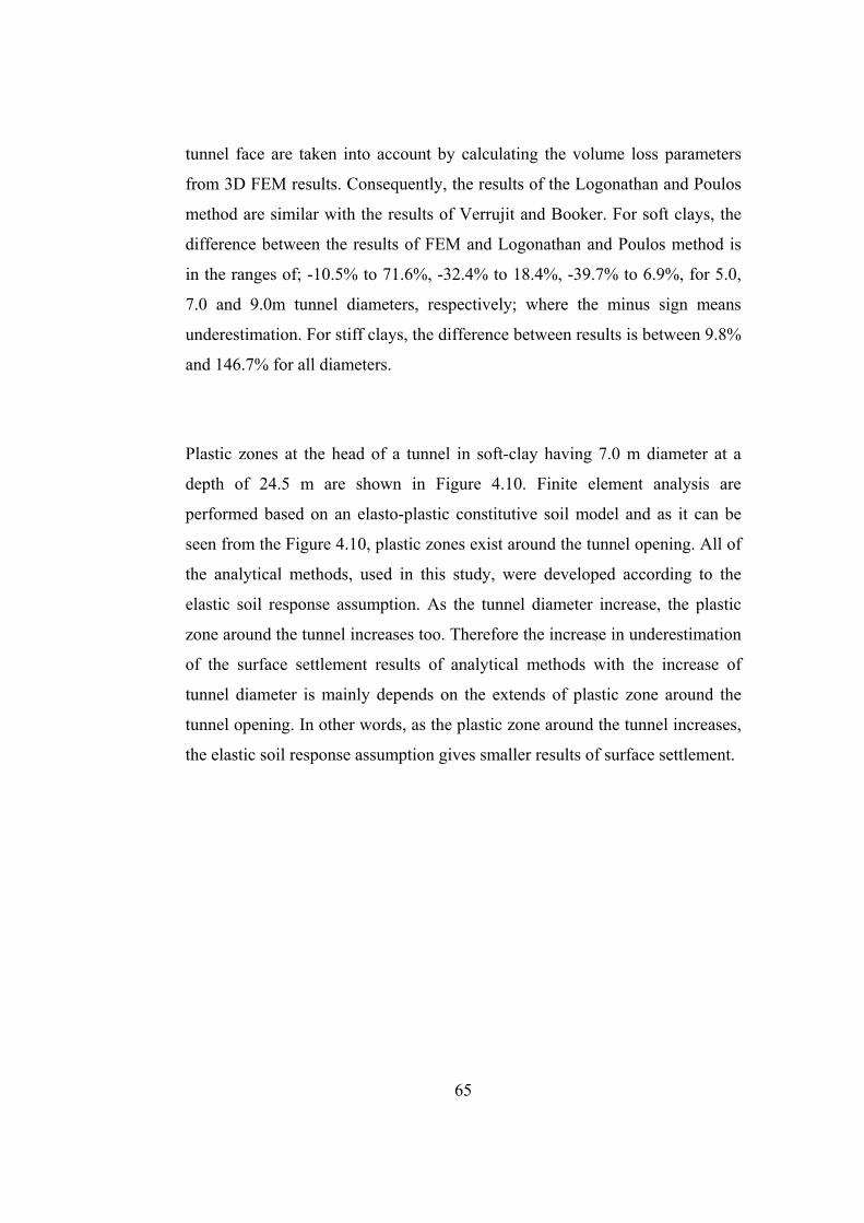
65

tunnel face are taken into account by calculating the volume loss parameters

from 3D FEM results. Consequently, the results of the Logonathan and Poulos

method are similar with the results of Verrujit and Booker. For soft clays, the

difference between the results of FEM and Logonathan and Poulos method is

in the ranges of; -10.5% to 71.6%, -32.4% to 18.4%, -39.7% to 6.9%, for 5.0,

7.0 and 9.0m tunnel diameters, respectively; where the minus sign means

underestimation. For stiff clays, the difference between results is between 9.8%

and 146.7% for all diameters.

Plastic zones at the head of a tunnel in soft-clay having 7.0 m diameter at a

depth of 24.5 m are shown in Figure 4.10. Finite element analysis are

performed based on an elasto-plastic constitutive soil model and as it can be

seen from the Figure 4.10, plastic zones exist around the tunnel opening. All of

the analytical methods, used in this study, were developed according to the

elastic soil response assumption. As the tunnel diameter increase, the plastic

zone around the tunnel increases too. Therefore the increase in underestimation

of the surface settlement results of analytical methods with the increase of

tunnel diameter is mainly depends on the extends of plastic zone around the

tunnel opening. In other words, as the plastic zone around the tunnel increases,

the elastic soil response assumption gives smaller results of surface settlement.

66

Figure 4.10 Plastic zones at the head of a tunnel in soft-clay (Type B, D=7.0m,

H=24.5m)

4.3 Short-Term and Long-Term Lining Responses

4.3.1 Effect of Excavation Sequences

The excavation sequence alternatives used in this study have been explained in

detail in Section 2.2.1.3. Interaction diagram corresponding to each scenario is

given in Appendix A. To discuss the effect of excavation sequence, bending

moment-hoop force pairs corresponding to different excavation sequences for

7.0 m diameter tunnels at a depth of 24.5 m is given in Figure 4.11 and Figure

4.12 for short-term and long-term conditions, respectively.

Short

advanc

the resu

with th

general

right be

crown,

and ben

from gr

C and T

Fig

The ho

number

-1,00

1,00

2,00

3,00

4,00

5,00

Axi

al F

orce

(kN

)

Term Re

cement resu

ults of para

he decrease

l, Type E e

ench drifts)

right crown

nch drifts) a

reatest to lo

Type A.

gure 4.11 In

op forces o

r of subsect

0

0

0

0

0

0

0

0

sponse: D

ults in differ

ametric stud

in number

excavation s

) results in t

n and bench

and Type A

owest as: Ty

nteraction di

btained from

tions to com

50B

67

Depending o

rent bending

dy, it can b

of drifts to

sequence (l

the largest

h drifts), Ty

A (full face

ype E excav

iagram for s

(D=7.0m, H

m analysis a

mplete the

100Bending Mom

7

on the ex

g moment a

e concluded

o complete

eft crown, l

hoop forces

ype B (side

drifts). Ben

vation seque

short-term l

H=24.5m)

are conside

full tunnel

150ment (kNm)

cavation s

and hoop fo

d that hoop

the full fac

left bench,

s, followed

wall drifts)

nding mome

ence, Type D

ining forces

red to be re

section inc

20

TYPE B H/TYPE C H/TYPE D H/TYPE E H/

equence, tu

force pairs.

p forces dec

ce excavatio

right crown

by Type D

, Type C (c

ent can be s

D, Type B,

s in soft-cla

easonable. A

creases, the

00

/D=3.5 d/D=2/D=3.5 d/D=2/D=3.5 d/D=2/D=3.5 d/D=2

unnel

From

crease

on. In

n and

D (left

crown

sorted

Type

ay

As the

hoop

250

2/72/72/7/7

68

force increases too; because the early installed lining is subjected to the loads

caused by the excavation of other subsections. On the other hand, greater

bending moments are observed in Type B and Type E procedures, in which

rings are completed during the excavation of subsections. For Types B and E,

first left side drifts are performed and while the right side drifts are going on,

lining ring of the left side has been already closed. However, for Types C and

D, first crown drifts are completed and while bench drifts are going on, the

crown ring remains open due to the excavation of bench. Early closure of the

lining ring limits the deformations inside the tunnel excavation and

consequently increases the bending moments on the lining. If the completion of

the ring is delayed until completion of the full tunnel excavation, the bending

moments become smaller.

As shown in Figure 4.11, in short-term, excavation sequence affects the lining

response.

Long Term Response: As shown for the selected sample case, from short-

term to long-term, hoop force and bending moment pairs converge to similar

values. In other words, in the long-term, excavation sequences do not have an

effect on lining response. The interaction diagram corresponding to each run is

presented in Appendix A.

It should be noted that, the long-term lining forces converge to same values

with linearly elastic perfectly plastic constitutive model with Mohr-Coulomb

failure criterion. Also the dilation and contraction of the soil is not modeled.

Fig

4.3.2

The lin

d=2.0m

round l

forces,

smaller

and ho

the max

with d1

The ex

summa

momen

-1,00

0

1,00

2,00

3,00

4,00

5,00A

xial

For

ce (k

N)

gure 4.12 In

Effect of

ning forces

m. The effe

length in F

respectivel

r round len

op force du

ximum ben

and D is th

xtreme val

arized in Ta

nts always in

0

0

0

0

0

0

0

0

nteraction di

f Round L

are evalua

ects of roun

igure 4.13

ly. In these

gth, Mmax,d2

ue to the tu

nding mome

he diameter

lues obser

able 4.2. It

ncrease wit

50B

69

iagram for l

(D=7.0m, H

Length

ted for two

nd length a

and Figure

e figures, d2

2 and Nmax,

unnel advan

ent and hoo

of the tunn

rved from

can be con

th decreasin

100Bending Mom

9

long-term li

H=24.5m)

o different r

are present

e 4.14 for b

2 is the gre

,d2 are the m

ncement wit

p force due

el.

Figure 4.

ncluded tha

ng round len

150ment (kNm)

ining forces

round lengt

ed in term

bending mo

ater round

maximum b

th d2, Mmax

e to the tunn

.13 and F

at, hoop for

ngth in undr

200

TYPE B HTYPE C HTYPE D TYPE E H

s in soft clay

ths, d=1.0m

ms of norma

oments and

length, d1 i

bending mo

,d1 and Nma

nel advance

Figure 4.14

ces and ben

rained cond

0 2

H/D=3.5 d/D=H/D=3.5 d/D=H/D=3.5 d/D=H/D=3.5 d/D=

y

m and

alized

hoop

is the

oment

ax,d1 is

ement

4 are

nding

itions

250

=2/7=2/7=2/7=2/7

70

independent of soil stiffness. Bending moments may decrease in soft clay with

decreasing round length under drained conditions; but it increases in stiff clay.

Normal forces are increasing with decreasing round length in both soft and stiff

clay independent of drainage conditions. With decreasing round length, the

hoop forces always increase irrespective of drainage conditions which mean as

the round length gets smaller the moment capacity of the lining increases.

Table 4.2 Extreme values of Figure 4.13 and Figure 4.14

Figure 4.13 Effect of round length on maximum bending moments

0

0.2

0.4

0.6

0.8

1

1.2

1.4

1.6

0.2 0.25 0.3 0.35 0.4 0.45

Mm

ax,d

2/Mm

ax,d

1

d2/D

Short Term Soft Clay

Long Term Soft Clay

Short Term Stiff Clay

Long Term Stiff Clay

71

Figure 4.14 Effect of round length on maximum hoop forces

4.3.3 Effect of Soil Stiffness

The properties assigned for soft and stiff clays have been introduced in Section

3.3.2. In order to see the effect of soil stiffness on bending moments, (H/D)

versus (Mmax,soft/Mmax,stiff) graph is prepared and presented in Figure 4.15 where

Mmax,soft and Mmax,stiff are the maximum bending moments for soft and stiff

clays, respectively. Effect of soil stiffness on hoop force is shown in Figure

4.16 where Nmax,soft and Nmax,stiff are the maximum hoop forces for soft and stiff

clay sites, respectively. The bending moments are higher at soft clay sites

compared to stiff clays in order of 25 % to 240 %.Considering hoop forces; this

difference may increase up to 215 %.

A representative interaction diagram corresponding to 7.0m diameter tunnel at

a depth of 24.5 m under drained loading conditions is given in Figure 4.17.

Although the hoop forces in soft clay is increasing with decreasing soil

stiffness, the increase in bending moment may be more significant as revealed

0

0.2

0.4

0.6

0.8

1

1.2

1.4

1.6

1.8

0.2 0.25 0.3 0.35 0.4 0.45

Nm

ax,d

2/Nm

ax,d

1

d2/D

Short Term Soft Clay

Long Term Soft Clay

Short Term Stiff Clay

Long Term Stiff Clay

72

by Figure 4.17. It is observed from Figure 4.17 that, the increase in bending

moment and hoop force decreases the factor of safety of the lining. Generally,

tunneling in soft clays results in using higher portion of lining capacity

compared to stiff clay, which reduces the factor of safety.

Figure 4.15 Effect of soil stiffness on maximum bending moments

Figure 4.16 Effect of soil stiffness on maximum hoop forces

0

0.5

1

1.5

2

2.5

3

3.5

4

0.2 1.2 2.2 3.2 4.2 5.2 6.2

Mm

ax,S

oft/M

max

,Stif

f

H/D

Short Term

Long Term

0

0.5

1

1.5

2

2.5

0.2 1.2 2.2 3.2 4.2 5.2 6.2

Nm

ax,S

oft/N

max

,Stif

f

H/D

Short Term

Long Term

Figur

4.3.4

To disc

corresp

present

deeper,

In Figu

reinforc

as the

increas

-1,00

1,00

2,00

3,00

4,00

5,00

Hoo

p Fo

rce

(kN

)

re 4.17 Inte

Effect of

cuss the eff

ponding to

ted in Figu

, the bendin

ure 4.18, th

cement deta

hoop forc

es too. But,

00

0

00

00

00

00

00

0

eraction diag

stiff

f Depth

fect of dept

a 7.0m diam

ure 4.18. A

ng moments

he presented

ails for all t

ce increase

, it is seen fr

50Be

73

gram for lon

clay (D=7.0

th on tunne

meter tunne

As revealed

and hoop f

d interactio

the depths.

s, the bend

from Figure

100ending Mome

3

ng-term lini

0m, H=24.5

el lining for

el at variou

from this

forces increa

n diagram

In general

ding mome

4.18 that as

150ent (kNm)

TYPE E

TYPE E

ing forces o

5m)

rces, an inte

us depth to

figure, as

ase.

is prepared

practice, it

ent capacit

s the tunnel

20

H/D=3.5 d/D=

H/D=3.5 d/D=

of soft clay a

eraction dia

cover ratio

the tunnel

d based on

t is accepted

ty of the l

l depth incre

00

=2/7 SOFT C

=2/7 STIFF C

and

agram

os are

l gets

same

d that

lining

eases,

250

CLAY

CLAY

the fact

are not

Fig

4.3.5

The clo

already

solution

4.20, F

diagram

values

4.23, F

-2,00

-1,00

1,00

2,00

3,00

4,00

5,00

Axi

al F

orce

(kN

)

tor of safety

always safe

gure 4.18 In

Compari

osed form s

y reviewed i

ns and Plax

igure 4.21 a

ms for each

obtained fr

igure 4.24,

00

00

0

00

00

00

00

00

0

y of the lini

fer than the s

nteraction di

ison of FE

solutions us

in Section 2

xis 3D Tunn

and Figure

h case and

rom closed

Figure 4.25

50

Be

74

ing decrease

shallow tun

iagram for l

(D=7.0m, H

EM result

sed for the

2.4. Differen

nel softwar

4.22. The re

they are pr

form soluti

5 and Figure

100

ending Mome

4

es. Therefor

nnels in term

long-term li

H=24.5m)

ts with Cl

calculation

nces betwee

re are prese

esults are al

resented in

ions and FE

e 4.26.

150 2

ent (kNm)

re, tunnels

ms of lining

ining forces

losed For

n of lining f

en the result

ented in Fig

lso compare

Appendix

EM are pre

200 2

TYPE E H

TYPE E H

TYPE E H

at greater d

capacities.

s of soft clay

m Solutio

forces have

ts of closed

gure 4.19, F

ed on intera

A. Lining

esented in F

250 30

H/D=5.5 d/D=2

H/D=3.5 d/D=2

H/D=2 d/D=2/7

depths

y

ons

been

d form

Figure

action

force

Figure

00

2/7

2/7

7

75

It should be noted that, among other methods only Antonio Bobet Model

considers the effects of water table while computing lining forces. For short-

term loading conditions, the soil above the tunnel is modeled as dry; therefore,

all methods can be used for short term. But for long-term solutions, water table

conditions should be taken into account and for this reason only Antonio Bobet

Model is used.

Closed form solutions are given for circular cross-sections, but in FEM, tunnel

sections are modeled as horse-shoe shaped and the shape of tunnel cross-

sections greatly change the forces acting on tunnel lining. Also, excavation

procedures (i.e. sequences, round lengths) can not be taken into account and

the lining and the soil are assumed to be in plane-strain condition in closed

form solutions; however, 3D stress distribution around tunnel opening is

different than plane-strain condition that produces the difference between

lining force results. Linear soil response assumption of the closed form

solutions is another important reason for the difference between lining force

results. Plastic zones at the head of a tunnel in soft clay having 7.0 m diameter

at a depth of 24.5 m are shown in Figure 4.10.

For the closed form solutions of surface settlement, excavation sequences and

round lengths are included in the solution by the volume loss parameters. But

in the closed form solutions of lining forces, there is no term in the calculations

for the inclusion of excavation sequence and round length effects. It is the main

reason of these differences between the results of existing models and

numerical analysis.

76

Short-term bending moments: The poorest performance relative to Plaxis is

exhibited by Muir Wood Model in terms of bending moment. Continuum

models and Muir Wood model are based on the same solution procedure, the

only difference between these models is that Muir Wood Model assumes

tangential slip (the shear force between ground and lining is zero) and ignores

the radial deformation due to the shear force between ground and lining,

whereas continuum models take into account the full bond (no slippage

between the ground and lining). Tangential slip assumption leads to small

bending moments compared to FEM solutions. For soft clay, all of the closed

form solutions both underestimate and overestimate results. As the soil gets

stiffer, closed form solutions tend to underestimate bending moment results.

Short-term hoop forces: The variation in results of closed form solutions and

FEM does not depend on soil stiffness. Closed form solutions generally

underestimate the result independent from soil stiffness. The differences

between FEM and closed form solutions are similar in Continuum Models,

Antonio Bobet Model and Erdmann Model. Muir Wood Model predicts

smaller hoop forces since it ignores the radial deformation due to the shear

force between soil and lining. Also excavation sequences and round lengths

can not be taken into account in the closed form solutions, which is the main

reason of the difference between FEM and closed form solutions.

Long-term bending moments: Bobet Model gives smaller values compared to

FEM up to -83% in soft clay and -93% in stiff clay. One of the reasons for this

difference is the assumption of elastic soil response as stated before. The other

reason is the circular tunnel section assumption. The increase in water table

does not produce any moment in the lining since the solution is for circular

77

linings. But for horseshoe shaped sections, high water pressures can produce

significant bending moments.

Long-term hoop forces: For soft clays, Antonio Bobet model underestimate

results up to -50% in soft clays and between -40% and 25% in stiff clays

compared to FEM.

78

Figure 4.19 Comparison of FEM results with closed form solutions for short-

term bending moments

Figure 4.20 Comparison of FEM results with closed form solutions for short-

term hoop forces

-150

-100

-50

0

50

100

150

0 20 40 60 80 100 120RUN#

Continuum Models Windels(1967) Curtis (1976) Einstein and Schwartz (1979) Aherens et al. (1982)

Muir Wood (1975)

Antonio Bobet (2001)

Erdmann (1983)

Clo

sedF

orm

Plax

is

Plax

is

MM

%M

−

-100

-80

-60

-40

-20

0

20

40

0 20 40 60 80 100 120RUN#

Continuum Models Windels(1967) Curtis (1976) Einstein and Schwartz (1979) Aherens et al. (1982)

Muir Wood (1975)

Antonio Bobet (2001)

Erdmann (1983)

Clo

sedF

orm

Plax

is

Plax

is

NN

%N

−

SOFT CLAY STIFF CLAY

SOFT CLAY STIFF CLAY

79

Figure 4.21 Comparison of FEM results with closed form solutions for long-

term bending moments

Figure 4.22 Comparison of FEM results with closed form solutions for long-

term hoop forces

-100

-90

-80

-70

-60

-50

-40

-30

-20

-10

0

0 20 40 60 80 100 120RUN#

Antonio Bobet (2001) (Long Term)

Clos

edFo

rmPl

axis

Plax

is

MM

%M

−

-60

-50

-40

-30

-20

-10

0

10

20

30

40

0 20 40 60 80 100 120RUN#

Antonio Bobet (2001) (Long Term)

Clos

edFo

rmPl

axis

Plax

is

NN

%N

−

SOFT CLAY STIFF CLAY

SOFT CLAY STIFF CLAY

80

Figure 4.23 Bending moment values obtained from closed form solutions and

FEM for short-term

Figure 4.24 Hoop force values obtained from closed form solutions and FEM

for short-term

0

50

100

150

200

250

300

350

0 20 40 60 80 100 120

M (k

N.m

)

RUN#

Continuum Models Windels(1967) Curtis (1976) Einstein and Schwartz (1979) Aherens et al. (1982)Muir Wood (1975)

Antonio Bobet (2001)

Erdmann (1983)

Plaxis 3D Tunnel V2

0

1000

2000

3000

4000

5000

6000

7000

8000

0 20 40 60 80 100 120

N (k

N)

RUN#

Continuum Models Windels(1967) Curtis (1976) Einstein and Schwartz (1979) Aherens et al. (1982)Muir Wood (1975)

Antonio Bobet (2001)

Erdmann (1983)

Plaxis 3D Tunnel V2

SOFT CLAY STIFF CLAY

SOFT CLAY STIFF CLAY

81

Figure 4.25 Bending moment values obtained from closed form solutions and

FEM for long-term

Figure 4.26 Hoop force values obtained from closed form solutions and FEM

for long-term

0

50

100

150

200

250

0 20 40 60 80 100 120

M (k

N.m

)

RUN#

Antonio Bobet (2001) (Long Term)

Plaxis 3D Tunnel V2

0

1000

2000

3000

4000

5000

6000

7000

8000

0 20 40 60 80 100 120

N (k

N)

RUN#

Antonio Bobet (2001) (Long Term)

Plaxis 3D Tunnel V2

SOFT CLAY STIFF CLAY

SOFT CLAY STIFF CLAY

82

CHAPTER 5

5. CONCLUSION

A parametric study has been carried out to assess the effects of tunnel

advancement on ground subsidence and on tunnel lining forces for short-term

and long-term clay behavior by using three dimensional finite element models.

For the numerical modeling of generic cases, Plaxis 3D Tunnel Version 2

geotechnical finite element package is used. Effects of excavation sequence,

round length, soil stiffness and tunnel depth on surface settlements and lining

forces are presented. The results obtained from finite element analysis are also

compared with the available analytical and empirical methods.

The followings are the main conclusion of this study:

- The rapid closure of the tunnel ring is more important than the type of

excavation sequence due to its effects on limiting the surface

settlements. If the lining ring is not closed, the lining is incapable of

limiting the deformations inside the tunnel excavation and surface

settlements increases.

- As the soil stiffness increases the rapid closure of the ring becomes less

significant and although the tunnel ring is not closed for tunnels in stiff

clay, significant surface settlements are not expected.

83

- The surface settlement due to an arbitrary round length for this study

can be estimated by using Figure 4.2 based on a known maximum

surface settlement and round length pair.

- As the tunnel gets deeper, the effect of round length on surface

settlements decreases.

- For this study, effect of crown settlement on surface settlements

becomes negligibly small at a depth of 9.6D in soft clay and 8.7D in

stiff clay.

- Using Figure 4.5, surface settlements can be predicted in case the

crown settlement is known for various depths to diameter ratios for this

study.

- Analytical surface settlement prediction methods may give smaller

surface settlement predictions in soft clay; however they result in higher

settlement predictions for stiff clays.

- Empirical method of Peck (1969) always results in higher surface

settlements compared to FEM for both soft and stiff clays. The

difference varies from 25.9% to 44.1% at soft clay and 50.4% to 75.6%

at stiff clay sites.

- The difference between surface settlement results of Sagaseta (1987)

method and FEM are depends on the diameter of the tunnel. As the

tunnel diameter increases, Sagaseta (1987) method underestimates the

surface settlement values as compared with FEM.

- The difference between settlement predictions of Gonzales and

Sagaseta (2001) method with FEM ranges between -50% and 230% for

soft clay. For stiff clay, it ranges between 70% and 330%.

84

- The difference between settlement predictions of Verruijt and Booker

(1996) method with FEM ranges between -40% and 90% for soft clay.

For stiff clay, it ranges between 5% and 100%.

- The difference between settlement predictions of Verruijt Logonathan

and Poulos (1998) method with FEM ranges between -40% and 70%

for soft clay. For stiff clay, it ranges between 10% and 145%.

- As the number of subsections to complete the full tunnel increases,

short-term hoop forces increases too; since the early installed lining is

subjected to the loads caused by the excavation of other subsections

- Short-term bending moments are higher for excavation sequences that

complete the ring during the excavation of subsections.

- As the ground conditions change from short-term to long-term, the

hoop forces and bending moments converge to the same values. In

other words, for long-term ground conditions, excavation sequences do

not have an effect on lining response with linearly elastic perfectly

plastic constitutive model with Mohr-Coulomb failure criterion by

ignoring the dilation and contraction of the soil.

- With decreasing round length, the short-term hoop forces on the lining

always increase which means as the round length gets smaller the lining

generally becomes safer in short-term.

- Closed form solutions for the calculation of bending moments and hoop

forces may underestimate the results obtained from FEM depending on

the construction sequence and soil and lining parameters.

- For the closed form solutions of surface settlement, excavation

sequences and round lengths are included in the solution by the volume

loss parameters. However, closed-form solutions given for lining forces

do not consider the effect of these parameters. Therefore, the analytical

85

methods given for estimation of lining forces are considered to be

suitable for shield tunneling.

- Comparison of FEM with closed form solutions are presented in

Figure 4.19 to Figure 4.22 in detail. The average differences between

FEM results and analytical solutions are as follows:

Short-term bending moments of Soft Clay: Continuum

Models underestimates the results of FEM -20% at average,

Muir Wood (1975) model underestimates the results of FEM

45% at average, Bobet (2001) model underestimates -10% at

average, Erdmann (1983) model overestimates the results of

FEM 20% at average.

Short-term bending moments of Stiff Clay: Continuum

Models underestimates the results of FEM -60% at average,

Muir Wood (1975) model underestimates the results of FEM

-75% at average, Bobet (2001) model underestimates the results

of FEM -60% at average, Erdmann (1983) model

underestimates the results of FEM -30% at average.

Short-term hoop forces of Soft Clay: Continuum Models

underestimates the results of FEM -35% at average, Muir Wood

(1975) model underestimates the results of FEM -70% at

average, Bobet (2001) model underestimates the results of FEM

-40% at average, Erdmann (1983) model underestimates the

results of FEM -30% at average.

Short-term hoop forces of Stiff Clay: Continuum Models

underestimates the results of FEM -25% at average, Muir Wood

(1975) model underestimates the results of FEM -70% at

average, Bobet (2001) model underestimates the results of FEM

86

-30% at average, Erdmann (1983) model underestimates the

results of FEM -10% at average.

Long-term bending moments of Soft Clay: Bobet (2001)

model underestimates the results the results of FEM -65% at

average.

Long-term bending moments of Stiff Clay: Bobet (2001)

model underestimates the results the results of FEM -85% at

average.

Long-term hoop forces of Soft Clay: Bobet (2001) model

underestimates the results the results of FEM -35% at average.

Long-term hoop forces of Stiff Clay: Bobet (2001) model

underestimates the results the results of FEM -10% at average.

87

BIBLIOGRAPHY

Ahrens, H., Linder, E., & Lux, K. H. (1982). Zur dimensionierung von tunnelasubauten nach den 'empfehlungen zur berechnung von tunnel im lockergestein (1980)'. Bautechnik .

Al Abram, I. (April 1998). Déplacements dans un modèle réduit bidimensionnel de creusement de tunnel, comparaison, mesures et calculs. XVIème Rencontres de l’AUGC à Reims, Les ouvrages dans leur environnement, (s. 410-417).

Atkinson, J. H., & Potts, D. M. (1977). Subsidence above shallow tunnels in soft ground. Journal of the Geotechnical Engineering Division ASCE GT4 , 307-325.

Attewell, P. B. (1977). Ground movements caused by tunnelling in soil. Conference on Large Ground Movments and (s. 812-984). cardiff.

Attewell, P. B., Yeates, J., & Selby, A. R. (1986). Soil movements induced by tunnelling and their effects on pipelines and structures. Glasgow: Blackie.

Bobet, A. (December 2001). Analytical solutions for shallow tunnels in saturated ground. Journal of engineering mechanics , 1258-1266.

Bowles, J. E. (1996). Foundation Analysis and Design. Singapore: Mc-Grawhill.

Broms, B. B., & Bennermark, H. (1967). Stability of clay at vertical openings. ASCE Soil Mechanics and Foundations Devision 93 .

Chapeau, C. (1991). Auscultation du sol pendant le creusement. Tunnels et ouvrages souterrains No 107 , 235-245.

Clough, W., & Schmidt, B. (1981). Design and performance of excavations and tunnels in soft clays. Amsterdam: Elsevier.

Curtis, D. J. (1976). Correspondence on the circular tunnel in elastic ground. Geotechnique 26 , 231-237.

88

Dolzhenko, N. (2002). Etude experimentale et numerique de modele reduit bidimensionnel du creusement d’un tunnel. developpement d’une loi de comportement specifique. Ph.D. Thesis, Universitat Stuttgart INSA Lyon.

Duddeck, H., & Erdmann, J. (1985). Structural design models for tunnels. Proceedings of tunnelling, vol.82, (pp. 83-91). London.

Dyer, M. R., Hutchinson, M. T., & Evans, N. (1996). Sudden valley sewer : a case history. Mair R.J., Taylor R.N. Eds. Geotechnical aspects of underground construction in soft ground, (pp. 671-676). Rotterdam.

Einstein, H. H., & Schwartz, C. W. (April 1979). Simplified analysis for tunnel supports. Journal of Geotechnical Engineering Division ASCE , 499-517.

Erdmann, J. (1983). Vergleich ebener und Entwicklung raumlicher Berechnungsverfahren fur Tunnel. Bericht nr. 83-40. Institut fur Statik, TU Braunschweig .

Galli, G., Grimaldi, A., & Leonardi, A. (2004). Three-dimensional modelling of tunnel excavation and lining. Computers and Geotechnics 31 , 171-183.

Gibson, R. E. (1953). Experimental determination of the true cohesion and true angle of internal friction in clays. Proceedings of 3rd International Conference on Soil Mechanics and Foundation Engineering, (pp. 126-130). Zurich.

Glossop, N. H. (1978). Soil deformation caused by soft ground tunnelling. Ph. D. Thesis, University of Durham.

Gonzales, C., & Sagaseta, C. (2001). Patterns of soil deformations around tunnels. Application to the extension of Madrid Metro. Computers and Geotechnics 28 , 445-468.

Hurrell, M. R. (1985). The empirical prediction of long-term surface settlements above shield-driven tunnels in soil. In Ground movements and structures (pp. 161-170). London: Pentech Press.

Institution of Civil Engineers (ICE). (1996). Sprayed concrete linings (NATM) for tunnels in soft ground. London: Thomas Telford.

Jacky, J. (1944). The coefficient of earth pressure at rest. Journal of the Society of Hungarian Architects and Engineers 78 (22) , 355–358.

89

Karakus, M., & Fowell, R. J. (2005). Back analysis for tunnelling induced ground movements and stress redistribution. Tunnelling and Underground Space Technology 20 , 514–524.

Kirsch, G. (1898). Die theorie der Elastizität und die bedürfnisse der festigkeitslehre. Zeit Ver Deut Ing J 42 , 797-807.

Kolymbas, D. (2005). Tunnelling and tunnel mechanics. Berlin Heidelberg: Springer-Verlag.

Lake, L. M., Rankin, W. J., & Hawley, J. (1992). Prediction and e®ects of ground movements caused by tunnelling in soft ground beneath urban areas. CIRIA Funders Report 5.

Lambe, T. W., & Whitman, R. V. (1969). Soil Mechanics. Singapore: John Wiley & Sons.

Lee, K. M., & Rowe, R. K. (1991). An analysis of three-dimensional ground movements: the Thunder Bay tunnel. Canadian Geotechnical Journal , 25-41.

Lee, K. M., Rowe, R. K., & Lo, K. Y. (1992). Subsidence owing to tunnelling. I: Estimating the gap parameter. Can. Geotech. J. 29 , 929-940.

Logonathan, L., & Poulos, H. G. (1998). Analytical prediction for tunnelling-induced ground movements in clays. Journal of Geotechnical and Geoenvironmental Engineering , 846-856.

Mair, R. J. (1996). Settlement effects of bored tunnels. In International Symposium on Geotechnical Aspects of Underground Construction in Soft Ground, (pp. 43-53). London.

Maynar, M. M., & Rodriguez, L. M. (2005). Predicted versus measured soil movements induced by shield tunnelling in the Madrid Metro Extension. Can. Geotech. J. 42 , 1160-1172.

Meissner, H. (1996). Tunnelbau unter Tage - Empfehlungen des Arbeitskreises 1.6 Numerik in der Geotechnik. Geotechnik , 99-108.

Möller, S. (2006). Tunnel induced settlements and structural forces in linings. Ph.D. Thesis, Universitat Stuttgart.

Muir Wood, A. M. (1975). The circular tunnel in elastic gorund. Geotechnique 25 , 115-127.

90

O'Reilly, M. P., & New, B. M. (1982). Settlements above tunnels in the United Kingdom - their magnitudes and prediction. Tunnelling' 82 , 173-181.

Oteo, C. S., & Sagaseta, C. (September 1982). Prediction of settlements due to underground openings. International Symposium on Numerical Models in Geomechanics, (pp. 653-659). Zurich.

Panet, M., & Guenot, A. (1982). Analysis of convergence behind the face of a tunnel. Tunnelling'82 (pp. 197-203). London: IMM.

Peck, R. B. (1969). Deep excavations and tunnelling in soft ground. Proc. of the 7th int. Conference on Soil Mechanics and Foundation Engineering (pp. 225-290). Sociedad Mexicnan de Mecanica de Suelos,A. C.

Plaxis 3D Tunnel version 2 Material Models Manual. (2004). Delft University of Technology & PLAXIS B.V.

Plaxis 3D Tunnel version 2 Reference Manual. (2004). Delft University of Technology & PLAXIS B.V.

Potts, D. M., & Zdravkovic, L. (2001). Finite element analysis in geotechnical engineering application. London: Thomas Telford Publisihng.

Powell, D. B., Sigl, O., & Beveridge, J. P. (1997). Heathrow-Express-design and performance of platform tunnels at Terminal 4. Tunnelling’97 (pp. 565-593). London: IMM.

Rabcewicz, L. (November 1964). The new austrian tunnelling method. Water Power , 453-457.

Rabcewicz, L. (December 1964). The new austrian tunnelling method, part two. Water Power , 511-515.

Rankin, W. J. (1987). Ground movements resulting from urban tunnelling : predictions and effects. Geological society engineering geology special publications no 5 , 79-92.

Rowe, R. K., & Kack, G. J. (1983). A theorotical examination of the settlements induced by tunnelling: Four case histories. Can. Geotech. J. 20 , 299-314.

Rowe, R. K., Lo, K. Y., & Kack, K. J. (1983). A method of estimating surface settlement above shallow tunnels constructed in soft ground. Canadian Geotechnical Journal 20 , 11-22.

91

Sagaseta, C. (1987). Analysis of undrained soil deformation due to ground loss. Geotechnique , 301-320.

Sagaseta, C. (1998). On the role of analytical solutions for the evaluation of soil deformation around tunnels. Application of numerical methods to geotechnical problems. Invited Lecture. CISM Courses and Lectures No.397 , 3-24.

Schikora, K., & Ostermeier, B. (1988). Two-dimensional calculation model in tunnelling. Verification by measurement results and by spatial calculation. Proceedings of the 6th International Conference on Numerical Methods in Geomechanics, (pp. 1499-1503). Innsbruck.

Schmidt, B. (1969). Settlements and ground movements associated with tunnelling in soil. Ph.D. Thesis, Imperial Collage, University of London.

Skempton, A. W., & Bjerrum, L. (1957). A contribution to the settlement analysis of foundations on clay. Geotechnique 7 , 168-178.

Tatiya, R. (2005). Civil excavations and tunnelling: a practical guide. London: Thomas Telford Publisihng.

Timesoshenko, S. P., & Goodier, J. N. (1970). Theory of elasticity. New York: McGraw-Hill.

Verruijt, A., & Booker, J. R. (1996). Surface settlements due to deformation of a tunnel in an elastic half plane. Geotechnique 46 , 753-756.

Windels, R. (1967). Kreisring im elastischen kontinuum. Bauingenieur 42 , 429-439.

92

APPENDIX A

INTERACTION DIAGRAMS

Figure A.1 Short-term lining forces of soft clay (D=5.0m)

Figure A.2 Long-term lining forces of soft clay (D=5.0m)

93

Figure A.3 Short-term lining forces of soft clay (D=5.0m)

Figure A.4 Long-term lining forces of soft clay (D=5.0m)

94

Figure A.5 Short-term lining forces of soft clay (D=5.0m)

Figure A.6 Long-term lining forces of soft clay (D=5.0m)

95

Figure A.7 Short-term lining forces of soft clay (D=5.0m)

Figure A.8 Long-term lining forces of soft clay (D=5.0m)

96

Figure A.9 Short-term lining forces of soft clay (D=5.0m)

Figure A.10 Long-term lining forces of soft clay (D=5.0m)

97

Figure A.11 Short-term lining forces of soft clay (D=5.0m)

Figure A.12 Long-term lining forces of soft clay (D=5.0m)

98

Figure A.13 Short-term lining forces of soft clay (D=7.0m)

Figure A.14 Long-term lining forces of soft clay (D=7.0m)

99

Figure A.15 Short-term lining forces of soft clay (D=7.0m)

Figure A.16 Long-term lining forces of soft clay (D=7.0m)

100

Figure A.17 Short-term lining forces of soft clay (D=7.0m)

Figure A.18 Long-term lining forces of soft clay (D=7.0m)

101

Figure A.19 Short-term lining forces of soft clay (D=7.0m)

Figure A.20 Long-term lining forces of soft clay (D=7.0m)

102

Figure A.21 Short-term lining forces of soft clay (D=7.0m)

Figure A.22 Long-term lining forces of soft clay (D=7.0m)

103

Figure A.23 Short-term lining forces of soft clay (D=7.0m)

Figure A.24 Long-term lining forces of soft clay (D=7.0m)

104

Figure A.25 Short-term lining forces of soft clay (D=9.0m)

Figure A.26 Long-term lining forces of soft clay (D=9.0m)

105

Figure A.27 Short-term lining forces of soft clay (D=9.0m)

Figure A.28 Long-term lining forces of soft clay (D=9.0m)

106

Figure A.29 Short-term lining forces of soft clay (D=9.0m)

Figure A.30 Long-term lining forces of soft clay (D=9.0m)

107

Figure A.31 Short-term lining forces of soft clay (D=9.0m)

Figure A.32 Long-term lining forces of soft clay (D=9.0m)

108

Figure A.33 Short-term lining forces of soft clay (D=9.0m)

Figure A.34 Long-term lining forces of soft clay (D=9.0m)

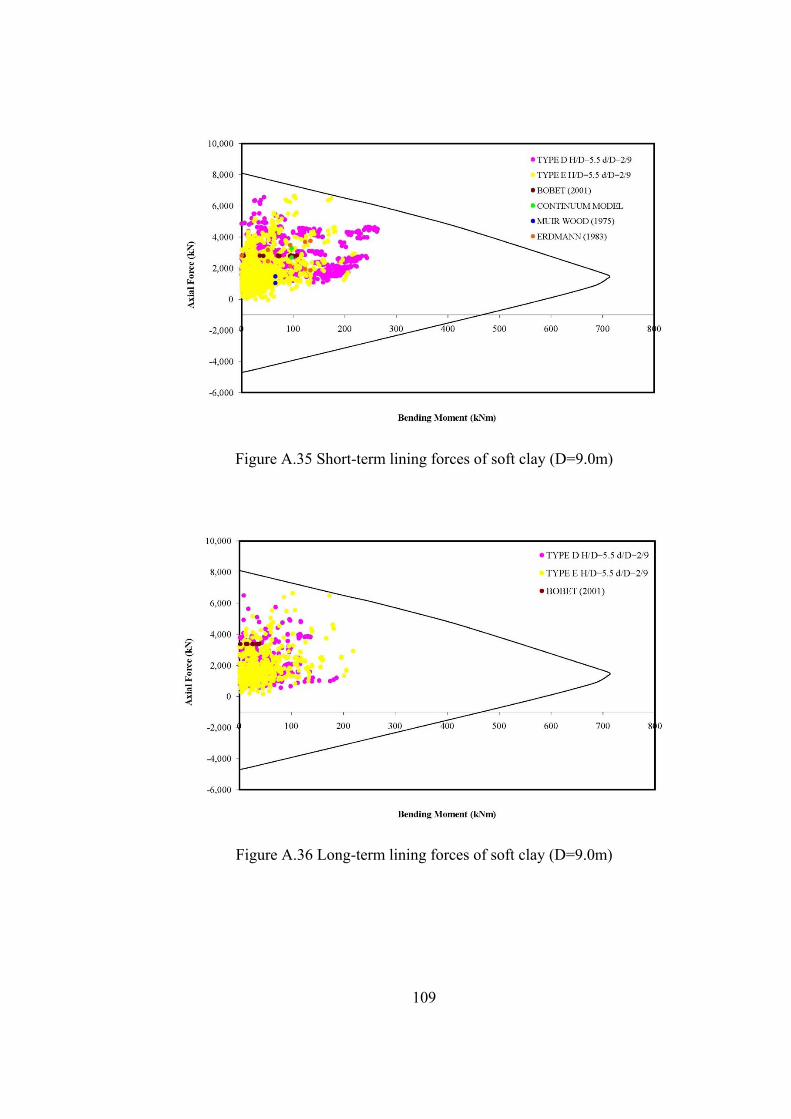
109

Figure A.35 Short-term lining forces of soft clay (D=9.0m)

Figure A.36 Long-term lining forces of soft clay (D=9.0m)

110

Figure A.37 Short-term lining forces of stiff clay (D=5.0m)

Figure A.38 Long-term lining forces of stiff clay (D=5.0m)

111

Figure A.39 Short-term lining forces of stiff clay (D=5.0m)

Figure A.40 Long-term lining forces of stiff clay (D=5.0m)

112

Figure A.41 Short-term lining forces of stiff clay (D=5.0m)

Figure A.42 Long-term lining forces of stiff clay (D=5.0m)

113

Figure A.43 Short-term lining forces of stiff clay (D=5.0m)

Figure A.44 Long-term lining forces of stiff clay (D=5.0m)

114

Figure A.45 Short-term lining forces of stiff clay (D=5.0m)

Figure A.46 Long-term lining forces of stiff clay (D=5.0m)

115

Figure A.47 Short-term lining forces of stiff clay (D=5.0m)

Figure A.48 Long-term lining forces of stiff clay (D=5.0m)

116

Figure A.49 Short-term lining forces of stiff clay (D=7.0m)

Figure A.50 Long-term lining forces of stiff clay (D=7.0m)

117

Figure A.51 Short-term lining forces of stiff clay (D=7.0m)

Figure A.52 Long-term lining forces of stiff clay (D=7.0m)

118

Figure A.53 Short-term lining forces of stiff clay (D=7.0m)

Figure A.54 Long-term lining forces of stiff clay (D=7.0m)

119

Figure A.55 Short-term lining forces of stiff clay (D=7.0m)

Figure A.56 Long-term lining forces of stiff clay (D=7.0m)

120

Figure A.57 Short-term lining forces of stiff clay (D=7.0m)

Figure A.58 Long-term lining forces of stiff clay (D=7.0m)

121

Figure A.59 Short-term lining forces of stiff clay (D=7.0m)

Figure A.60 Long-term lining forces of stiff clay (D=7.0m)

122

Figure A.61 Short-term lining forces of stiff clay (D=9.0m)

Figure A.62 Long-term lining forces of stiff clay (D=9.0m)

123

Figure A.63 Short-term lining forces of stiff clay (D=9.0m)

Figure A.64 Long-term lining forces of stiff clay (D=9.0m)

124

Figure A.65 Short-term lining forces of stiff clay (D=9.0m)

Figure A.66 Long-term lining forces of stiff clay (D=9.0m)

125

Figure A.67 Short-term lining forces of stiff clay (D=9.0m)

Figure A.68 Long-term lining forces of stiff clay (D=9.0m)

126

Figure A.69 Short-term lining forces of stiff clay (D=9.0m)

Figure A.70 Long-term lining forces of stiff clay (D=9.0m)

127

Figure A.71 Short-term lining forces of stiff clay (D=9.0m)

Figure A.72 Long-term lining forces of stiff clay (D=9.0m)