assessing the shallow groundwater system as a potential

ASSESSING THE SHALLOW GROUNDWATER SYSTEM AS A POTENTIAL

FACTOR IN GENERATING STORM-WATER RUNOFF ON A NORTH CAROLINA

BARRIER ISLAND

By:

Michael S. Sisco

May 2013

Director of Thesis: Alex K. Manda

Major Department: Geological Sciences

The town of Emerald Isle, located in North Carolina’s Outer Banks, experiences

significant storm-water runoff and flooding problems during the fall and winter months. The

topography of the island influences drainage patterns as well as the position of the water table.

The goal of this study was to determine if the shallow groundwater system is responsible for

storm-water runoff on the island. Two hypotheses were developed to test the relationship

between the water table and storm-water runoff. The first hypothesis states: the water table rises

above the land surface during periods of high precipitation, which leads to storm-water runoff in

the town. The second hypothesis states: low infiltration rates in the swales of the island impede

water from recharging the Surficial aquifer. The first hypothesis was tested by monitoring the

position of the water table in the Surficial aquifer over a 12-month period using a network of 15

shallow groundwater monitoring wells. Potentiometric surface maps of the aquifer show that the

water table does breach the land surface during storm events that produce at least 25 mm of

precipitation. The second hypothesis was tested by conducting infiltrometer tests to determine if

low infiltration rates were retarding natural recharge to the groundwater system. These tests

reveal that the soils located in small portions of the swales have the lowest infiltration rates on

the island, making it more likely for storm-water runoff to be generated. A 3D finite-difference

groundwater model was then used to determine if pumping water from the aquifer during

extreme storm events (e.g., hurricanes) would alleviate an elevated water table. Numerical and

analytical modeling results suggest that pumping water from the aquifer may be impractical for

the town to employ because it is only a short-term solution to the storm-water problem.

Therefore, several structural best management practices (BMP’s) are presented as alternative

measures to reduce storm-water runoff. These structural BMP’s are ideal for the needs of the

town, and they include bioretention, level spreader-vegetative filter strips, and infiltration

basins/trenches.



BARRIER ISLAND

A Thesis

Presented To the Faculty of the Department of Geological Sciences

East Carolina University

In Partial Fulfillment of the Requirements for the Degree

Master of Science in Geology

By:

Michael S. Sisco

May 2013

© Copyright

Michael S. Sisco

May 2013

All Rights Reserved



BARRIER ISLAND

By:

Michael S. Sisco

APPROVED BY:

DIRECTOR OF THESIS: _______________________________________________________

Alex K. Manda, PhD

COMMITTEE MEMBER: _______________________________________________________

Richard K. Spruill, PhD


Michael O’Driscoll, PhD


Charles Humphrey, PhD

CHAIR OF THE DEPARTMENT

OF GEOLOGICALSCIENCES: ___________________________________________________

Stephen J. Culver, PhD

DEAN OF THE GRADUATE SCHOOL: ___________________________________________

Paul J. Gemperline, PhD

DEDICATION

This thesis is dedicated to my late grandmother, Norma Sisco. Although you passed before I

began this journey, I know you would have been proud.

ACKNOWLEDGEMENTS

First and foremost, I would like to thank my family for giving me a seamlessly never-

ending amount of support throughout this entire process. To my mother, father, and sister: you

helped me more than you will ever know.

I could not have completed this thesis paper without my advisor, Dr. Alex Manda. You

kept me on track when I was hopelessly overwhelmed during portions of this project. I was

continually amazed at how broad your knowledge spanned, and how much you were willing to

share that knowledge with me.

Thank you to the rest of my committee members for providing your expertise in this field

of research. Dr. Richard Spruill, Dr. Michael O’Driscoll, and Dr. Charlie Humphrey: I’m

grateful to have chosen you for this committee, and to have your help guiding me along this path.

Thank you to my fellow graduate students and professors who helped me along the way

with problems that arose and fieldwork: Dr. David Mallinson, Justin Nixon, Angela Giuliano,

Alex Culpepper, and David Szynal. To John Woods and Jim Watson: this department wouldn’t

run without the two of you. Thank you for all of your help during this process.

I would like to thank Frank Rush and the Town of Emerald Isle for help funding this

project, and allowing us to conduct research on a truly beautiful island. I hope these findings will

benefit the town in the future.

Finally, I would like to thank the Department of Geological Sciences as a whole. Through

my academic experience, I learned what an incredibly talented group of faculty, staff, graduates,

and undergraduates we really have. Help was never too far away, and for that, I thank you all.

TABLE OF CONTENTS

DEDICATION .................................................................................................................. vii

ACKNOWLEDGEMENTS ............................................................................................. viii

LIST OF TABLES ............................................................................................................ xii

LIST OF FIGURES ......................................................................................................... xiii

LIST OF SYMBOLS AND ABBREVIATIONS ............................................................. xv

CHAPTER 1: INTRODUCTION ....................................................................................... 2

1.1 Purpose .............................................................................................................. 4

1.2 Significance....................................................................................................... 4

1.3 Background ....................................................................................................... 5

1.3.1 Previous work .................................................................................... 5

1.3.2 Hydrogeology .................................................................................... 7

1.3.3 Soils.................................................................................................. 11

1.3.3 Physiography.................................................................................... 12

1.4 Climate ............................................................................................................ 13

CHAPTER 2: METHODS ................................................................................................ 16

2.1 Well Installation .............................................................................................. 16

2.2 Groundwater Monitoring ................................................................................ 18

2.3 Geospatial Analysis ........................................................................................ 20

2.4 Aquifer Properties ........................................................................................... 21

2.5 Water Budget .................................................................................................. 23

2.6 Groundwater Modeling ................................................................................... 24

CHAPTER 3: RESULTS AND DISCUSSION ................................................................ 26

3.1 Hydrogeologic Analysis.................................................................................. 26

3.2 Changes in Water Levels ................................................................................ 29

3.3 Groundwater Flow .......................................................................................... 43

3.4 Hydrologic Components ................................................................................. 45

3.5 Groundwater Flow Model ............................................................................... 48

3.5.1 Conceptual model ............................................................................ 48

3.5.2 Model calibration ............................................................................. 49

3.5.3 Simulation of groundwater pumping ............................................... 52

3.5.4 Analytical solution to test feasibility of numerical model ............... 54

CHAPTER 4: STORM-WATER BEST MANAGEMENT PRACTICES ....................... 56

4.1 Overview ......................................................................................................... 56

4.2 Structural Examples for Reducing Storm-water Runoff ................................. 57

4.2.1 Bioretention...................................................................................... 58

4.2.2 Level spreader-vegetative filter strip ............................................... 60

4.2.3 Infiltration basins/trenches ............................................................... 61

CHAPTER 5: CONCLUSIONS ....................................................................................... 64

REFERENCES ................................................................................................................. 67

APPENDIX A: ADDITIONAL FIELD WORK .............................................................. 73

APPENDIX B: MODFLOW PUMPING SIMULATIONS ............................................. 78

APPENDIX C: GROUNDWATER RESPONSE TIME PLOTS ..................................... 89

APPENDIX D: MODFLOW CALIBRATION PLOTS ................................................. 101

APPENDIX E: GEOPHYSICAL METHODS AND RESULTS ................................... 119

LIST OF TABLES

1. Geologic framework of the North Carolina Coastal Plain, and their respective hydrogeologic

units ..................................................................................................................................... 9

2. Climate data for Morehead City over a 20-year period. Swansboro data are used in 2011. The

year 2011 is not included in the 20 year average .............................................................. 14

3. Well characteristics derived from groundwater monitoring wells in Emerald Isle ...... 19

4. Horizontal hydraulic conductivity results from slug test data ...................................... 28

5. Calculated recharge rates of the monitoring wells using the Water Table Fluctuation (WTF)

method. Healy and Cook’s (2002) specific yield values for similar grain-size were used in this

table ................................................................................................................................... 29

6. Examples of response and land times for monitoring wells in the study area during Tropical

Storm Beryl ....................................................................................................................... 43

7. Water level data for the beginning and end of the study period ................................... 46

8. Hydrologic parameters used for each Visual MODFLOW run during calibration of the model

........................................................................................................................................... 50

9. Errors for each run that was conducted to calibrate the numerical model .................... 51

10. Errors for each run that was conducted to calibrate the numerical model. Wells EIC1, EIC2,

and EIC3 are not included................................................................................................. 52

11. Results of simulating groundwater pumping in the numerical model ........................ 54

LIST OF FIGURES

1. Map showing the Town of Emerald Isle on Bogue Banks. Inset: Arrow indicates the location

of Bogue Banks off the coast of North Carolina................................................................. 2

2. Map showing the study area on the western part of Emerald Isle in the vicinity of Coast Guard

Road. Inset: Bogue Banks with a red outline identifying the study area ............................ 3

3. Hydrogeologic section showing the aquifer system of the North Carolina Coastal Plain

............................................................................................................................................. 8

4. Hydrogeologic well logs of A) Test Well 12 and B) Mallard Road Test Well. C) Shows the

locations of the wells on Emerald Isle .............................................................................. 10

5. Soil distribution on the western side of Emerald Isle ................................................... 12

6. LiDAR map of the western side of Emerald Isle .......................................................... 13

7. Map of the western part of Emerald Isle showing locations of water table monitoring wells

within the study area ......................................................................................................... 16

8. Observation well design utilized on Emerald Isle ........................................................ 17

9. Core logs from the northern transect of wells ............................................................... 26

10. Infiltration rates for the study area .............................................................................. 27

11. Groundwater levels in monitoring wells where the water table is shallow ................ 32

12. Groundwater levels in monitoring wells where the water table is moderately deep .. 33

13. Groundwater levels in monitoring wells where the water table is deep ..................... 34

14. Depth to the water table prior to Hurricane Irene ....................................................... 35

15. Depth to the water table for an intermediate storm event on March 5, 2012 ............. 36

16. Depth to the water table following Hurricane Irene ................................................... 37

17. Plot of the ground elevation versus water level during a period of no recharge (A) and

recharge (B) ...................................................................................................................... 39

18. Plots showing water level, hydraulic gradient variation in wells EIS2-D and EIS2-S, and

precipitation recorded in the study area ............................................................................ 40

19. Groundwater hydrographs for wells EIN2 (A), EIS3 (B), EIC3 (C), and a bar graph of

precipitation (D) ................................................................................................................ 42

20. Groundwater flow patterns for the study area during pre-hurricane conditions (A), an

intermediate storm event (B), and post-hurricane conditions (C)..................................... 44

21. Components of the water budget within the study area .............................................. 47

22. Conceptual flow model of groundwater in the Surficial aquifer on Emerald Isle ...... 48

23. Locations of sites chosen to simulate groundwater pumping at to lower the water table

........................................................................................................................................... 53

24. Design of a bioretention cell. ...................................................................................... 58

25. Bioretention garden built in a residential property. .................................................... 59

26. Design of a level spreader – vegetative filter strip ..................................................... 60

27. Design of an infiltration basin..................................................................................... 61

28. Design of an infiltration trench ................................................................................... 62

LIST OF SYMBOLS AND ABBREVIATIONS

m Meters

r2 Coefficient of determination

Sy Specific yield

Δh Change in hydraulic head

Δt Change in time

Kx Hydraulic conductivity in the x (horizontal) direction

Ky Hydraulic conductivity in the y (horizontal) direction

Kz Hydraulic conductivity in the z (vertical) direction

ΔS Change in groundwater storage

ΔWL Change in water level

GPM Gallons per minute

CHAPTER 1: INTRODUCTION

The town of Emerald Isle, which is located on Bogue Banks (Fig. 1), experiences

significant storm-water runoff during the fall and winter months. This is primarily a function of

increased precipitation, the position of the water table, topography, geology, and the

development of more impervious surfaces. A previous study by Moffat & Nichol Engineers

(1997) found that the topography characterized by dunes and swales directly influences the

hydrology and drainage patterns on the island. The construction of impervious surfaces such as

roads, houses, and gutters has significantly altered the natural drainage patterns in Emerald Isle,

(Moffat & Nichol Engineers, 1997). This increase in impervious area can reduce infiltration to

the shallow aquifer system and lead to more storm-water runoff (Arnold and Gibbons, 1996).

Rather than focusing solely on the storm-water runoff that Emerald Isle experiences, this study

sets out to determine the influence of the shallow groundwater system on storm-water

generation, as well as the relationship between the water table and the topography on the island.

Figure 1: Map showing the Town of Emerald Isle on Bogue Banks. Inset: Arrow indicates the location of

Bogue Banks off the coast of North Carolina.

3

Light Detection And Ranging (LiDAR) data show that the elevation of the island ranges

from 0 m to 16.5 m (45 feet) above mean sea level (AMSL). The higher elevations represent

dunes that lie parallel to the long axis of the island, while lower elevation swales are present in

between these longitudinal dunes. The largest dunes are located in the south whereas the smallest

dunes are in the northern parts of the island. According to studies conducted by other workers,

the swales act as the natural discharge zones for the island (e.g., along Coast Guard Road)

(Moffat & Nichol Engineers, 1997). These areas, particularly those located along Coast Guard

Road (Fig. 2), experience periodic flooding events that impact the residents in that part of the

town.

Figure 2: Map showing the study area on the western part of Emerald Isle in the vicinity of Coast Guard

Road. Inset: Bogue Banks with a red outline identifying the study area.

4

1.1 Purpose and Scope

The goal of this study is to characterize the shallow groundwater system on the western

side of Bogue Banks and determine how the system contributes to storm-water generation within

the study area. Through the collection of water level, precipitation, and hydrogeologic data, the

research will seek to accomplish the following objectives:

1) Derive and evaluate the physical properties of the Surficial aquifer.

2) Monitor the position of the water table and characterize groundwater flow patterns.

3) Estimate components of a water budget for the study area.

4) Determine the influence of the water table fluctuations on storm-water runoff.

5) Assess alternatives of managing storm-water problems and/or lowering groundwater.

The data that were collected were used to test two hypothesis related to the position of the

water table and storm-water runoff. The hypotheses that were tested in the study are as follows:

(1) the shallow water table rises above the land surface, particularly in the lower-lying swales,

during periods of significant recharge, and (2) the infiltration rates of the soils reduce the

recharge potential during storm events in low-lying areas. When infiltration rates impede the

natural recharge of the soil, storm-water runoff has the potential to be generated.

1.2 Significance

Previous work (Moffat & Nichol Engineers, 1997) that looked at the groundwater system

on the island did not utilize time-series data of groundwater level measurements, which are

important for understanding spatial and temporal variations of groundwater flow. Not having

these data can in turn affect the accuracy of a model that is created for characterizing the

Surficial aquifer and providing solutions for storm-water management (Taylor and Alley, 2001).

5

Studying the configuration of the water table and the properties of the Surficial aquifer can

reveal potential areas where flooding induced by a shallow water table may be expected. In

addition to the groundwater table characteristics, other factors influencing groundwater levels in

the Surficial aquifer must be considered. These include precipitation, evapotranspiration, runoff,

and topography.

Depth-to-groundwater measurements are important to study for two main reasons:

determining the groundwater flow pattern for the study area, and estimating the amount of

interaction between groundwater and surface water. This relationship is important for

understanding how long it would take rain events to naturally drain into the ground, ultimately

discharging into the ocean or any large body of water (Heath, 1994). Due to the presence of

dunes and swales on Bogue Banks, the percolation rate is a major limiting factor for the recharge

rate of precipitation (Heath, 1994). Other primary controls on recharge and water table elevations

that will be investigated include infiltration rate, land cover, evapotranspiration, water-table

depth, and soil type. This study will characterize how groundwater levels may influence storm-

water generation, as well as how possible solutions to alternative storm-water management

practices can be addressed.

1.3 Background

1.3.1 Previous work

There have been several studies conducted where hydrogeologic characteristics of barrier

islands have been investigated. For example, Winner (1975) and Heath (1988) characterized the

available ground-water resources, hydraulic properties, and salt-water encroachment on Hatteras

Island for the Cape Hatteras Water Association. Working on the same island, Anderson (2000)

6

calculated hydraulic properties of the island and investigated the relationship between

progradational barrier island morphology and water-table elevations in the underlying

stratigraphy. In particular, Anderson found that this progradation influences the soil properties in

locations where lower-permeability swales have been covered up by dunes over time. Burkett

(1996) estimated several hydrogeologic parameters within the Buxton Woods surficial aquifer at

Cape Hatteras. The hydrogeologic parameters estimated in these studies, particularly hydraulic

conductivity, were vital to the current study, and were used to verify slug tests results conducted

on Bogue Banks. The hydraulic conductivity of the Surficial aquifer on Hatteras Island was very

similar to those estimated within Bogue Banks.

Other regional studies have been conducted on the shallow groundwater system. Harden

et al., (2003) studied the hydrogeology and groundwater quality of the Surficial aquifer in

Brunswick County, NC, located southwest of the study area. A water budget conceptualized for

Brunswick County estimated a similar ratio of precipitation to groundwater recharge to the

surficial aquifer. Harden et al. (2003) also found no evidence of long-term trends in water level

data. An absence of trends in regional water resources of the Surficial aquifer should implore

further research to be conducted. This report, along with Anderson’s (2000) on Hatteras Island,

reported on similar parameters measured in this study. These parameters helped justify values

calculated in the study area. An analytical study conducted on strip-islands used the Dupuit-

Ghyben-Herzberg analysis to estimate the position of the water table and salt-water interface on

islands based on their geometry, distribution of hydraulic conductivity, and recharge variability

(Vacher, 1988).

Moffat & Nichol (M&N) Engineers conducted a site study in Emerald Isle in 1996. The

focus of this study was to identify alternative solutions to mitigate flooding problems under the

7

current storm-water regulations. The solutions were then put through a cost/damage ratio

analysis to determine which solutions would reduce the damages the most. However, the M&N

report did not address two important issues: 1) the shallow groundwater system was not

monitored over time, and 2) the alternatives did not include conservative non-structural and

structural Best Management Practices (BMP’s) that would benefit residential properties within

the study area. The present study addresses these concerns in greater detail and in so doing, will

improve our understanding of the role that shallow groundwater systems play in influencing

storm-water runoff on barrier islands.

1.3.2 Hydrogeology

The hydrogeologic framework of eastern North Carolina is divided into nine aquifers.

Nine confining units separate the aquifers, which range in age from Holocene to Cretaceous

(Winner and Coble, 1996). The aquifers, which gradually increase in dip and thickness towards

the east (Fig. 3), are part of a series of obliquely stacked marine terraces (Brown et al., 1972). A

basement complex of Paleozoic age rocks lies beneath the terraces, which run parallel to the

Atlantic Coast (Clark et al., 1912; Nelson, 1964; Lautier, 2009). An escarpment, the Suffolk

scarp, bounds this hydrogeologic region to the west, which runs north to south from Washington

County to the western edge of the study area (Brown, 1985; Mallinson et al., 2008).

The stratigraphic column of this region is subdivided into geologic formations based

upon their depositional environment, with sediments, lithology, and faunal composition

separating the varying members (Brown, et al., 1972). These deposits have been characterized

into aquifers and their respective confining units by the delineation of non-permeable versus

hydraulically connected permeable units, with some boundaries not always corresponding to

certain geologic boundaries (Table 1) (Lautier, 2009). The names of the aquifers are (from

8

youngest to oldest) the Surficial, the Yorktown, the Castle Hayne, the Beaufort, the Peedee, the

Black Creek, the Upper Cape Fear, the Lower Cape Fear, and the Lower Cretaceous and/or

Undifferentiated (Winner and Coble, 1996).

Figure 3: Hydrogeologic section showing the aquifer system of the North Carolina Coastal Plain

(Adapted from Winner and Coble, 1996 and Heath and Spruill, 2003).

The Surficial aquifer is a water table aquifer, meaning that it is an unconfined aquifer that

is in direct communication with the atmosphere (Fig. 3). The aquifer is the upper layer of

sediments, which overlies much of the North Carolina Coastal Plain. The sediments, ranging in

thickness from ~6 m to ~60 m, consist mostly of sand with some minor deposits of silt, clay, and

peat beds (Ingram, 1987). The Surficial aquifer also consists of older sediments, which depend

on the stratigraphic position of the underlying formation these sediments were deposited on

(Wilder, et al., 1978).

9

Table 1: Geologic framework of the North Carolina Coastal Plain, and their respective hydrogeologic

units (Adapted from Lautier, 2009).

North Carolina East Central Coastal Plain

Geologic Units

North Carolina East Central

Coastal Plain Hydrogeologic Units

System Series Formation (Fm.) Aquifers, stratigraphically below their

respective confining units (not shown)

Quaternary

Holocene

Undifferentiated Surficial Aquifer

Pleistocene

Tertiary

Pliocene Yorktown Fm.

Yorktown Aquifer

Miocene

Pungo River Fm.

Eocene Castle Hayne Fm. Castle Hayne Aquifer

Paleocene Beaufort Fm. Beaufort Aquifer

Upper

Cretaceous

Peedee Fm. Peedee Aquifer

Black Creek Fm. Black Creek Aquifer

Cape Fear Fm.

Upper Cape Fear Aquifer

Lower Cape Fear Aquifer/Lower

Cretaceous Aquifer Undifferentiated Lower Cretaceous

Even though the Surficial aquifer is one of the thinnest of all the aquifers, it is an

extremely important aquifer because it receives direct recharge from precipitation and in some

places is the major source of water for underlying aquifers and baseflow to streams in the Coastal

Plain (Giese et al., 1997). Since there are no streams within the study area, the Surficial aquifer

groundwater would likely discharge to canals, ponds, estuaries, and the ocean. Along the coast

and the Outer Banks, the Surficial aquifer is an important groundwater resource because salt-

10

water intrusion affects the water quality in the deeper aquifers in these areas (Heath and Spruill,

2003). However, in Emerald Isle, the deeper Castle Hayne aquifer is the source of potable water.

The water from the Castle Hayne aquifer may eventually recharge the Surficial aquifer via onsite

wastewater treatment systems.

Figure 4: Hydrogeologic well logs of A) TW 12 (Test Well 12) and B) MRTW (Mallard Road Test Well).

C) Shows the locations of the wells on Emerald Isle (Adapted from NC DWR, 2012).

Data from the North Carolina Department of Water Resources (NC DWR) reveal that the

Bogue Banks Water Corporation (BBWC) has two wells on the western end of Bogue Banks.

11

These wells have hydrogeologic logs of the aquifers and confining units present in the

subsurface, as well as their relative thicknesses (Fig. 4). The approximate thickness of the

Surficial aquifer in the study area is 17.4 m (57 feet) (NC DWR, 2012). However, it appears the

aquifer is thinner to the east with a thickness of 10.7 m (35 feet) at the Mallard Road Test Well

(MRTW). At both sites, the Surficial aquifer is underlain by the Yorktown confining unit, which

also increases in thickness to the east from 5-8 m (16-26 feet)

1.3.3 Soils

The United States Department of Agriculture’s Soil Conservation Service classified soils

within Carteret County in 1982 (NCSS, 1987). Within the study area, the soil series and soil

complexes include: coastal beaches (Be), Carteret sand (CH), Carteret sand – low (CL), Corolla

fine sand (Co), Corolla-Urban land complex (Cu), Duckston fine sand (Du), Fripp fine sand (Fr),

Newhan-Corolla complex (Nc), Newhan-Urban land complex (Ne), and Newhan fine sand (Nh).

Of the 10 soil series and complexes located on the western end of Bogue Banks, 6 of them

encompass the majority of the study area.

The Duckston fine sand (Du) and beach sand (Be) are described as poorly drained sands

that frequently flood. The Corolla fine sand (Co) and Newhan-Urban land complex (Nc) soils

drain at moderate amounts leading to much lower flooding frequency. The Fripp fine sand (Fr)

and Newhan fine sand (Nh) are described as being excessively drained and rarely flood. These

last two soil types, Fripp fine sand (Fr) and Newhan fine sand (Nh), also represent the largest

area of drainage class within the study area. Therefore, the majority of the study area is well-

drained, according to the soil survey. The spatial distribution of these soils revealed a pattern of

soil series that were generally oriented parallel with the long-axis of the island (Fig. 5).

12

Figure 5: Soil distribution on the western side of Emerald Isle. Be = beach sand, CH = Carteret sand, CL

= Carteret sand, low, Co = Corolla fine sand, Cu = Corolla-Urban land fine sand, Du = Duckston fine

sand, Fr = Fripp fine sand, Nc = Newhan-Corolla fine sand, Ne = Newhan-Urban land fine sand, Nh =

Newhan fine sand.

1.3.4 Physiography

The physiography of Bogue Banks is characterized by a series of dunes and inter-dunal

troughs (or swales), which run nearly parallel to the coastline (Fig. 6). The dune fields closest to

the southern shoreline are present at some of the highest elevations on this part of Bogue Banks,

whereas the smaller dunes are near the northern shoreline. Lower elevation swales, which are the

primary areas of concern in this study, are located on the interior portions of the island.

It is evident from Figure 6 that regions with low elevations constitute a much larger

surface area than the high elevation dunes. This would imply that the majority of the island has

the potential for flooding in response to a shallow water table. The swales can also create

discontinuous sections of the longitudinal dune fields, further complicating the drainage patterns

within Emerald Isle. The topography to the south of the large dunes and north of the smaller

13

dunes levels out to the Atlantic Ocean and Bogue Sound, respectively. The elevation within the

study area ranges from 0 m along the shoreline to 13.7 m (45 feet) above sea level on the high

southern dunes.

Figure 6: LiDAR map of the western side of Emerald Isle.

1.4 Climate

Precipitation and air temperature data for a 20 year period (1991-2011) leading up to the

study window were collected from a weather station in Morehead City, North Carolina,

approximately 32 km (20 miles) east of Emerald Isle (Table 2). The station was selected due to

the availability of long term records and continuity of data, which were used to derive long-term

averages for the region. Annual data were summarized from June to May of the following year.

For the study period (2011-2012), weather data from the NCDWR station NC-ON-4 in

Swansboro, North Carolina were used because the weather station in Morehead City did not

14

record any data during Hurricane Irene. The Swansboro weather station is located 10 km (6.6

miles) north-northwest of the study area.

Table 2: Climate data for Morehead City over a 20 year period. Swansboro data are used in 2011. The

year 2011 is not included in the 20 year average.

The average temperature for the 20-year period was 17.5 ° C (63.7° F), with annual

temperatures ranging from 16.1 ° C (61° F) to 20.5 ° F (69° F). Average precipitation for the 20-

year period was 998 mm (39.30 inches), with annual amounts ranging from 138 mm (5.44

inches) to 1669 mm (65.7 inches). During the 2011-2012 study period, annual precipitation and

Year Precipitation (mm) Mean Temperature (°F) Mean Temperature (°C)

1991 1621 65 18.3 1992 1440 63 17.2

1993 916 69 20.5

1994 473 65 18.3

1995 621 63 17.2

1996 349 63 17.2

1997 138 63 17.2

1998 182 65 18.3

1999 386 63 17.2

2000 921 61 16.1

2001 757 63 17.2

2002 1669 63 17.2

2003 1504 62 16.7

2004 1077 63 17.2

2005 1634 64 17.8

2006 1011 63 17.2

2007 1234 65 18.3

2008 1108 62 16.7

2009 1645 63 17.2

2010 1277 63 17.2

2011 987 66 18.9

Mean 998 63.5 17.5

15

temperature were 987 mm (38.88 inches) and 18.9° C (66° F), respectively. The mean

temperature for 2011-2012 was the highest since 1993 (20.5° C). The precipitation during the

study period was only 2% lower than the 20-year annual average (1991-2010), but was

significantly lower than six of the previous nine years. During 2011, the months of August,

September, and October combined to receive 45% of the yearly total. The high volume of sub-

tropical and extra-tropical cyclones during these months yielded these elevated levels of rainfall.

CHAPTER 2: METHODS

2.1 Well Installation

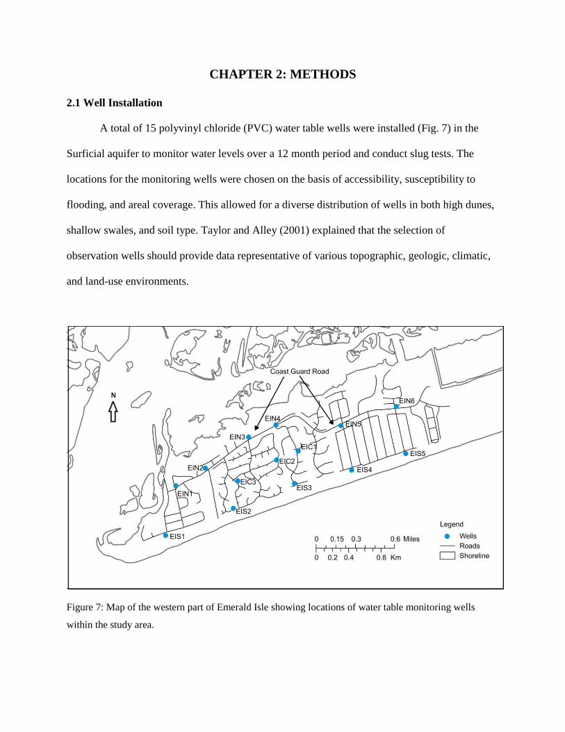
A total of 15 polyvinyl chloride (PVC) water table wells were installed (Fig. 7) in the

Surficial aquifer to monitor water levels over a 12 month period and conduct slug tests. The

locations for the monitoring wells were chosen on the basis of accessibility, susceptibility to

flooding, and areal coverage. This allowed for a diverse distribution of wells in both high dunes,

shallow swales, and soil type. Taylor and Alley (2001) explained that the selection of

observation wells should provide data representative of various topographic, geologic, climatic,

and land-use environments.

Figure 7: Map of the western part of Emerald Isle showing locations of water table monitoring wells

within the study area.

17

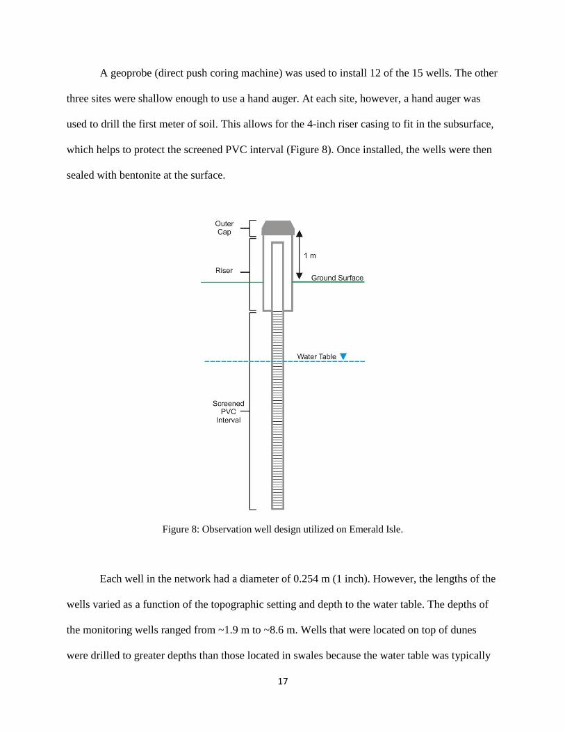
A geoprobe (direct push coring machine) was used to install 12 of the 15 wells. The other

three sites were shallow enough to use a hand auger. At each site, however, a hand auger was

used to drill the first meter of soil. This allows for the 4-inch riser casing to fit in the subsurface,

which helps to protect the screened PVC interval (Figure 8). Once installed, the wells were then

sealed with bentonite at the surface.

Figure 8: Observation well design utilized on Emerald Isle.

Each well in the network had a diameter of 0.254 m (1 inch). However, the lengths of the

wells varied as a function of the topographic setting and depth to the water table. The depths of

the monitoring wells ranged from ~1.9 m to ~8.6 m. Wells that were located on top of dunes

were drilled to greater depths than those located in swales because the water table was typically

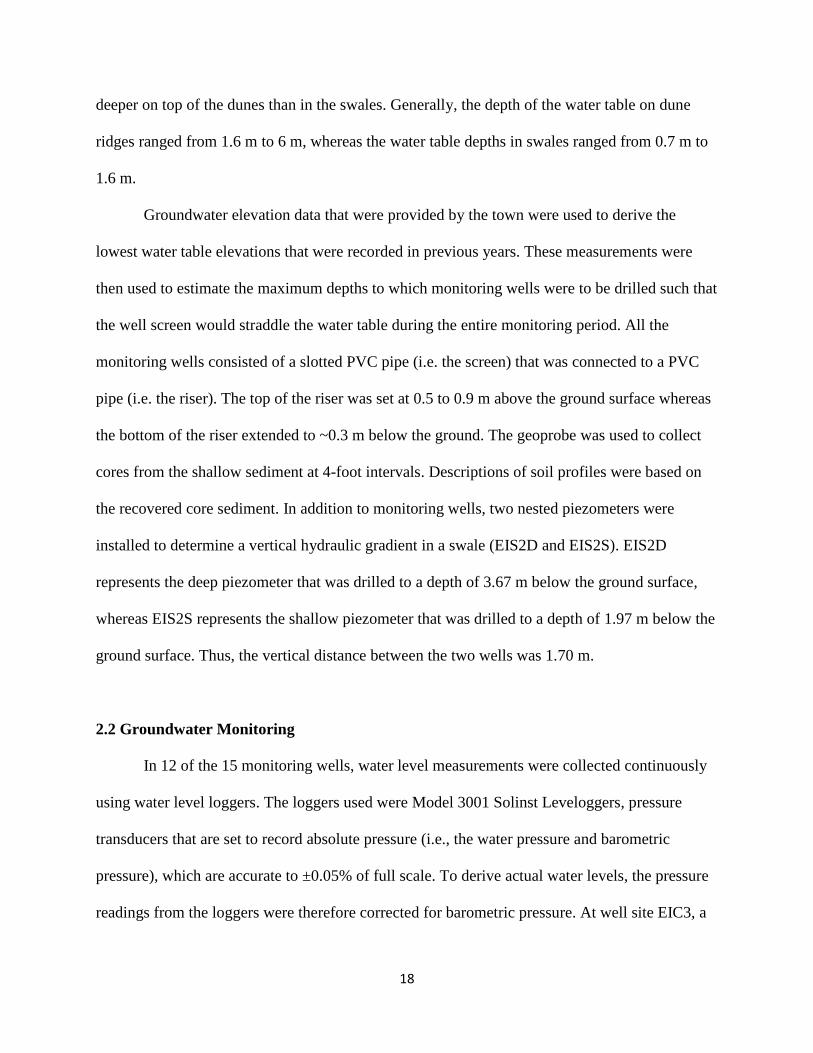
18

deeper on top of the dunes than in the swales. Generally, the depth of the water table on dune

ridges ranged from 1.6 m to 6 m, whereas the water table depths in swales ranged from 0.7 m to

1.6 m.

Groundwater elevation data that were provided by the town were used to derive the

lowest water table elevations that were recorded in previous years. These measurements were

then used to estimate the maximum depths to which monitoring wells were to be drilled such that

the well screen would straddle the water table during the entire monitoring period. All the

monitoring wells consisted of a slotted PVC pipe (i.e. the screen) that was connected to a PVC

pipe (i.e. the riser). The top of the riser was set at 0.5 to 0.9 m above the ground surface whereas

the bottom of the riser extended to ~0.3 m below the ground. The geoprobe was used to collect

cores from the shallow sediment at 4-foot intervals. Descriptions of soil profiles were based on

the recovered core sediment. In addition to monitoring wells, two nested piezometers were

installed to determine a vertical hydraulic gradient in a swale (EIS2D and EIS2S). EIS2D

represents the deep piezometer that was drilled to a depth of 3.67 m below the ground surface,

whereas EIS2S represents the shallow piezometer that was drilled to a depth of 1.97 m below the

ground surface. Thus, the vertical distance between the two wells was 1.70 m.

2.2 Groundwater Monitoring

In 12 of the 15 monitoring wells, water level measurements were collected continuously

using water level loggers. The loggers used were Model 3001 Solinst Leveloggers, pressure

transducers that are set to record absolute pressure (i.e., the water pressure and barometric

pressure), which are accurate to ±0.05% of full scale. To derive actual water levels, the pressure

readings from the loggers were therefore corrected for barometric pressure. At well site EIC3, a

19

barologger was deployed to record atmospheric pressure, which was used to compensate the

readings from the water level loggers.

The water levels were referenced to the North America Vertical Datum of 1988 (NAVD

88) using the National Geodetic Survey station markers located on the island. A Topcon Total

Station was used to survey elevations of well sites via line-of sight from the geodetic markers.

Once ground elevations were derived, elevations for the top of casings and water level loggers

were calculated for each well. A Trimble Global Position System (GPS) unit was used to

determine the geographic coordinates of the monitoring wells. The GPS unit has a horizontal

accuracy of less than 5 meters. Data from the survey and additional well characteristics are listed

in Table 3.

Table 3: Well characteristics derived from groundwater monitoring wells in Emerald Isle. TOC = Top of

casing. Elevation is in reference to mean sea level.

Well

ID Latitude Longitude

Elevation of

TOC (m)

Elevation

of

ground

(m)

Well

depth

(m)

Length

of string

and

probe

(m)

Elevation

of probe

(m)

Length

of casing

above

ground

(m)

EIC1 34.6548 -77.077 4.11 3.24 3.40 3.81 0.31 0.87

EIC2 34.6531 -77.079 2.88 2.26 1.82 2.20 0.69 0.62

EIC3 34.6515 -77.085 7.91 7.36 8.60 8.84 -0.93 0.55

EIN1 34.651 -77.093 3.53 2.96 3.11 3.28 0.26 0.57

EIN2 34.6528 -77.089 2.77 2.08 2.36 2.67 0.11 0.69

EIN3 34.6562 -77.083 2.54 1.99 3.53 2.85 -0.30 0.55

EIN4 34.6577 -77.079 2.46 1.55 3.05 - - 0.91

EIN5 34.6576 -77.071 6.15 5.66 4.99 5.09 1.06 0.49

EIN6 34.6594 -77.063 4.14 3.53 4.88 5.08 -0.93 0.61

EIS1 34.6459 -77.094 3.86 3.29 3.19 - - 0.57

EIS2D 34.6488 -77.085 2.25 1.37 3.67 3.59 -1.33 0.88

EIS2S 34.6488 -77.085 2.26 1.37 1.97 1.92 0.35 0.89

EIS3 34.6513 -77.077 7.54 6.67 6.24 6.81 0.74 0.87

EIS4 34.6526 -77.069 5.64 5.06 4.90 4.76 0.89 0.58

EIS5 34.6544 -77.062 3.43 2.86 1.87 - - 0.57

20

Groundwater level, pressure, and precipitation data were collected from May 2011 to

June 2012 so all seasons could be represented during the monitoring period. The water level

loggers and barologger were set to take readings at 10-minute intervals. Periodic water level

measurements were collected from all wells using a water level meter. These measurements were

used to ensure the accuracy of the readings of the water level loggers. The software program,

Surfer 8, was then used to create potentiometric surface maps of the Surficial aquifer.

2.3 Geospatial Analysis

Geospatial layers, representing physiography, hydrography, soil types, and man-made

features were either created or acquired from the NC One-Map or NC Department of

Transportation websites. Geospatial layers for the installed wells were created from the

geographic coordinates taken from the Trimble GPS unit. A 2007 LiDAR digital elevation model

was used to create a topographic map of the study area. The LiDAR data had a vertical accuracy

of 0.25 m and a spatial resolution of 6.1 m. The shoreline, roads, and surface water bodies for

Emerald Isle were created from existing geospatial layers acquired from NC One-Map.

Previous reports of storm-water runoff within the study area reveal that the areas prone to

flooding are along Coast Guard Road (Moffat & Nichol Engineers, 1997). Using three different

periods of water table elevation, flood potential maps were created to indicate where storm-water

buildup would be observed on the western part of the island. The water table periods that were

used to estimate flood potential maps include a pre-hurricane low, an intermediate rain event,

and an extreme precipitation event (i.e., Hurricane Irene). A contour map representing each

period was created using Geographic Information Systems (GIS) to show the position of the

water table. The map calculator in ArcGIS was used to subtract water level data from elevation

21

data to yield the flood potential maps. Areas with negative values would suggest that the water

table was above the land surface and vice versa.

2.4 Aquifer Properties

To estimate the hydraulic conductivity (K) of the Surficial aquifer, falling-head slug tests

were conducted in all wells in the study area. Falling-head slug tests involve quickly inserting a

large displacement object into a well and then recording the rate at which the water levels return

to equilibrium (Bouwer and Rice, 1976). A long steel rod of known volume (slug) was added to

the well, while a pressure transducer measured the rate at which the water level recovered to the

starting value.

The slug test data collected in the field were imported into Aquifer Test Solve

(AQTESOLV) software program to derive the hydraulic conductivity of the Surficial aquifer.

Multiple slug test solutions are available in the program; however, two were chosen to best

represent the data. The Hvorslev (1951) and Bouwer and Rice (1976) method are ideal for

unconfined, water table aquifers. Both methods account for a variety of well geometries and

aquifer conditions (Campbell et al., 1990). These methods match a straight-line solution to

displacement data derived from quickly inserting the slug. Well characteristics from Table 3

were also required for the derivation of hydraulic conductivity. The results from the slug tests

were compared to values calculated in previous studies that were conducted on nearby barrier-

islands to determine whether the hydraulic conductivity measurements from the Surficial aquifer

were within acceptable ranges.

Since specific yield was not directly measured, grain size and core analyses were used to

derive estimates for this parameter (Healy and Cook, 2002). Johnson (1966) and Healy and Cook

22

(2002) characterized average specific yield values based on sediment type, which have been

assigned based on the grain-sizes in a given location. Averages for coarse, medium, and fine-

grained sand are 0.27, 0.26, and 0.21, respectively. The value used for specific yield was 0.20.

This is due to the predominant grain size being fine-grained sand with portions of silt and clay.

The Water-Table Fluctuation (WTF) method was then used to derive an estimate of annual

groundwater recharge by using the following equation:

Eq. (1)

where R is recharge, Sy is specific yield, Δh is the change in water-table height, and Δt is the

change in time (Healy and Cook, 2002). This method is based on the premise that rises in

groundwater levels in unconfined aquifers are due to recharge water arriving at the water table

(Scanlon, et al, 2002). The WTF method is best applied to relatively short periods (≤1 year) in

locations where there is a shallow water table that experiences sharp rises and declines in water

levels (Healy and Cook, 2002). The equation requires the total amount of head change in each

well during the time period.

A double ring infiltrometer was also used to determine the infiltration rates of the

different soils at the site of each monitoring well (Fig. 5). The infiltration rate was derived by

measuring the amount of water that was drained in dry soil during a 20-minute period. During

single storm events, as the soil becomes more saturated, it is assumed the infiltration rates will

become lower as the soil moisture content increases (Akan, 1993). All of the soil classes were

represented at the various well sites, so none of the soil types described above were excluded in

the analysis. Infiltration capacities were also looked at using the Carteret County Soil Survey

(NCSS, 1987). The saturated hydraulic conductivity of the soils is likely very similar to the

23

infiltration capacity, thus the permeability of the soils were used as the maximum rate of water

absorption.

2.5 Water Budget

A water budget for Emerald Isle was derived using parameters acquired from field data,

modeling programs, and a literature review. The water balance for the study area is derived using

the following (Thornthwaite, 1948; Thornthwaite and Mather, 1955):

Eq. (2)

where G is natural groundwater recharge, P is precipitation, I is artificial recharge, RO is direct

runoff, ET is estimated actual evapotranspiration, and ∆S is the change in groundwater storage.

Since the basis for the water budget is the shallow groundwater system, natural groundwater

recharge is considered an outflow (Shade, 1995). Artificial recharge in this area is predominantly

from onsite wastewater treatment systems and other domestic water uses (e.g., irrigation). This

value is derived from the volume of water extracted from the Castle Hayne aquifer system,

assuming that this water eventually recharges to the Surficial aquifer via artificial inflows.

Groundwater withdrawals from the Castle Hayne aquifer were obtained from Bogue Banks

Water Corporation. The water budget equation has been arranged to solve for ET, since this

value was not directly measured or calculated during the study period. Estimating for ET

algebraically would assume a range of values from the parameters required in the calculation.

Using the time-series data from each well, the difference in water level between June 1,

2011 and May 31, 2012 was used to calculate change in storage for the period of record. This

was achieved by multiplying the difference between initial water level (June 1, 2011) and the

final water level (May 31, 2012) by specific yield (Eq. 1). Change in storage, or net recharge,

24

takes into account the specific yield of the material, owing to the fact that only a percentage of

the recharge is capable of being stored in the pore spaces of a material (Healy and Cook, 2002).

Precipitation values were taken from a nearby weather station (Swansboro, NC), while recharge

was calculated using the WTF method. The ‘Simple Method’ to calculate urban storm-water

loads was used to estimate direct runoff (Schueler, 1987). Using the Simple Method, direct

runoff is computed as follows:

Eq. (3a)

Eq. (3b)

where R is the annual runoff, P is the annual rainfall, Pj is the fraction of annual rainfall events

that produce runoff, Rv is the runoff coefficient, and IA is the proportion of land cover that is

impervious area. Impervious area was estimated to be 0.30 based on the predominant residential

land use of the island (Cappiella and Brown, 2001), whereas Pj was estimated to be 90%

(Schueler, 1987). The direct runoff within the study area is likely within a range of values that

the island experiences in a given year.

2.6 Groundwater Modeling

The software program Visual MODFLOW was used to simulate groundwater flow in the

Surficial aquifer on the western side of Emerald Isle under steady state conditions. Groundwater

flow was simulated in a 3-dimensional model using a finite-difference method that numerically

solves the groundwater flow equation (Harbaugh et al., 2000). The one layer model that was

created was discretized into 499 columns by 250 rows representing a volume consisting of 50 m

x 50 m x 17 m cells (L x W x H). Cells that were not superimposed over the island were made

inactive for computational efficiency.

25

A geospatial layer was input into the modeling program to represent the shoreline of

Bogue Banks. The layer served as a constant head boundary, set to sea level (i.e., head = 0 m). A

digital elevation model of the island was imported to simulate the topography during the

modeling process. Observation wells monitored during the study period were included in the

model. Recharge to the model was applied via a United States Geological Survey (USGS)

geospatial shape file. Hydrogeologic characteristics acquired from other aspects of this study

were used as input parameters in the groundwater model. These parameters include hydraulic

conductivity (x, y and z directions), specific yield, effective porosity, total porosity, recharge,

evapotranspiration, and extinction depth. The extinction depth is the point in the subsurface at

which evapotranspiration from the water table ceases. This is directly related to the depth of the

roots of plants, which were assumed to be at a maximum of 3 m.

CHAPTER 3: RESULTS AND DISCUSSION

3.1 Hydrogeological Analysis

Analysis of geologic maps and drill cores reveal that the sediments studied in the upper

18 meters of the subsurface comprise the Surficial aquifer (Fig. 4, Table 1). Sediments logged

from the geoprobe cores are primarily fine to medium sands, but there were lenses of rich

organic materials and clay in some locales (Figs. 9). The sediments derived from the northern

wells consisted of gray, well-sorted sands, with occasional low permeability sediments near the

surface (e.g., at EIN2 and EIN4). The sediments derived from the central wells were also

composed of mostly fine to-medium sand, but had small amounts of shell fragments near the

bottom of each section. Low percentages of silt were also mixed into the finer-grained sand. The

southern transect of wells, located mostly in the dune fields near the shoreline, were slightly

more coarse-grained than the other transects. Aside from thin organic layers near the top of the

sediments derived from EIS3 and EIS5, the rest of the cores revealed the presence of medium-

grained sand in these areas.

Figure 9: Core logs from the northern transect of wells.

Cores taken indicate that the clay and organic rich units are not very thick, ranging from

0.15 to 0.3 meters (0.5 to 1.0 feet). The presence of these clay lenses in the lower lying swales

are likely to reduce the infiltration rates of surface water into the shallow groundwater system.

This is particularly a problem during storm events, which may lead to flooding due to the

perching of the water table (e.g., sites EIN2, EIN3 and EIN4) (Moffat & Nichol Engineers,

1997). Observations made in the field reveal that these sites were inundated with water during

storm events during the monitoring period. Flooding from perching typically occurs when a thin

layer of soil close to the surface gets saturated and prevents water from seeping into the ground

to the water table below. Several sites in the study area have been identified where low

infiltration rates of the soil may cause perching of the water table. These sites, represented by red

in Figure 10, are areas that should be targeted for managing storm-water runoff.

Figure 10: Infiltration rates for the study area.

28

The results of the infiltrometer tests show that the lowest infiltration rates occur in the

elongated soil sections, which overlap with some of the swales on the western part of the island

(Fig. 10). These data suggest that the second hypothesis is partially supported; low infiltration

rates are impeding groundwater recharge in these swales during storm events, but not to the

entire extent which was postulated. The ranges where intermediate and high infiltration rates are

observed are associated with the dunes and dune slopes identified on the LiDAR map (Fig. 6).

Table 4: Horizontal hydraulic conductivity results from slug tests data.

Hydraulic Conductivity (x 10-5

m/s)

Well ID Hvorslev method Bouwer and Rice method

EIC1 1.4 1.5

EIC2 2.9 3.2

EIC3 1.3 1.5

EIN1 3.2 3.8

EIN2 3.0 3.4

EIN3 0.9 0.9

EIN4 1.1 1.2

EIN5 5.1 6.0

EIN6 2.5 3.8

EIS1 3.4 4.5

EIS2 0.6 0.7

EIS3 3.0 3.4

EIS4 3.5 3.9

EIS5 1.0 1.1

Slug tests in the monitoring wells revealed that the horizontal hydraulic conductivity in

the Surficial aquifer ranged from 8.6 x 10-6

to 6.0 x 10-5

m/s (Table 4). Smith and Chapman

(2005) used constant-rate pumping tests at three locations within the Little Contentnea Creek

Basin, North Carolina to estimate hydraulic properties of the Surficial aquifer. Their results show

that the hydraulic conductivity ranges from 1.2 x 10-5

to 7.4 x 10-5

m/s. Anderson (2000)

estimated that the Buxton Woods aquifer on Hatteras Island, NC also had a horizontal hydraulic

conductivity (6.5 x 10-5

m/s) similar to those estimated in this study.

29

Table 5: Calculated recharge rates of the monitoring wells using the Water Table Fluctuation method

(WTF). Healy and Cook’s (2002) specific yield values for similar grain-size were used in this table.

Well ID Mean specific yield

Sy

Total head change

(mm/year)

Recharge

(mm/year)

EIC1 0.20 3,050 610

EIC2 0.19 4,480 851

EIC3 0.20 2,120 424

EIN1 0.20 3,110 622

EIN2 0.16 5,600 896

EIN3 0.20 4,310 862

EIN5 0.19 2,320 441

EIN6 0.19 3,820 726

EIS3 0.20 2,350 470

EIS4 0.19 3,240 616

Mean 0.20 3,440 688

From Healy and Cook’s (2002) estimations, specific yields were likely to be higher in

wells that had continuous sections of coarse-grained material, and lower in drill cores where

sections of mud and organic material were present. Due to the predominant grain size being fine-

grained sand, the average specific yield was estimated to be 0.20. Thus, recharge rates computed

using the WTF method ranged from 424 mm/year to 896 mm/year with an average groundwater

recharge of 688 mm/year (Table 5). Giese et al. (1997) estimated recharge to the Surficial aquifer

to vary between 300 and 550 mm/year. The variance is due to the difference in infiltration rates,

depths to the water table, and vegetative cover contributing to evapotranspiration.

3.2 Changes in Water Levels

Low barometric pressures and high precipitation rates that occurred in August 2011 and

May 2012 were a result of Hurricane Irene and Tropical Storm Beryl, respectively. Hurricane

Irene was a significant storm event that occurred in the study region, and provided further insight

about how the shallow groundwater system responded to extreme flooding events. Groundwater

30

levels in the monitoring wells responded quickly to such precipitation events. However, the rate

of response was not the same in each well. This variance is most likely a function of the

infiltration rate of the soil, soil moisture, and depth to the water table prior to precipitation

events. The depth of the water table controls the amount of storage between the land surface and

water table. The monitoring wells located in areas where the water table was shallow (swales)

responded quicker than those wells where the water table was deeper (ridges and dunes).

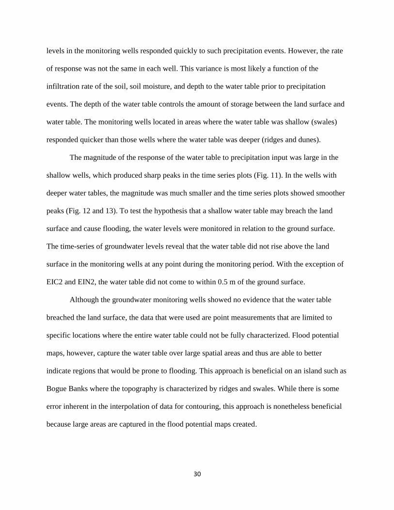
The magnitude of the response of the water table to precipitation input was large in the

shallow wells, which produced sharp peaks in the time series plots (Fig. 11). In the wells with

deeper water tables, the magnitude was much smaller and the time series plots showed smoother

peaks (Fig. 12 and 13). To test the hypothesis that a shallow water table may breach the land

surface and cause flooding, the water levels were monitored in relation to the ground surface.

The time-series of groundwater levels reveal that the water table did not rise above the land

surface in the monitoring wells at any point during the monitoring period. With the exception of

EIC2 and EIN2, the water table did not come to within 0.5 m of the ground surface.

Although the groundwater monitoring wells showed no evidence that the water table

breached the land surface, the data that were used are point measurements that are limited to

specific locations where the entire water table could not be fully characterized. Flood potential

maps, however, capture the water table over large spatial areas and thus are able to better

indicate regions that would be prone to flooding. This approach is beneficial on an island such as

Bogue Banks where the topography is characterized by ridges and swales. While there is some

error inherent in the interpolation of data for contouring, this approach is nonetheless beneficial

because large areas are captured in the flood potential maps created.

31

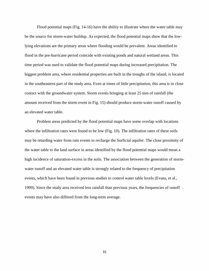
Flood potential maps (Fig. 14-16) have the ability to illustrate where the water table may

be the source for storm-water buildup. As expected, the flood potential maps show that the low-

lying elevations are the primary areas where flooding would be prevalent. Areas identified to

flood in the pre-hurricane period coincide with existing ponds and natural wetland areas. This

time period was used to validate the flood potential maps during increased precipitation. The

biggest problem area, where residential properties are built in the troughs of the island, is located

in the southeastern part of the study area. Even at times of little precipitation, this area is in close

contact with the groundwater system. Storm events bringing at least 25 mm of rainfall (the

amount received from the storm event in Fig. 15) should produce storm-water runoff caused by

an elevated water table.

Problem areas predicted by the flood potential maps have some overlap with locations

where the infiltration rates were found to be low (Fig. 10). The infiltration rates of these soils

may be retarding water from rain events to recharge the Surficial aquifer. The close proximity of

the water table to the land surface in areas identified by the flood potential maps would mean a

high incidence of saturation-excess in the soils. The association between the generation of storm-

water runoff and an elevated water table is strongly related to the frequency of precipitation

events, which have been found in previous studies to control water table levels (Evans, et al.,

1999). Since the study area received less rainfall than previous years, the frequencies of runoff

events may have also differed from the long-term average.

32

Figure 11: Groundwater levels in monitoring wells where the water table is shallow. The dashed black line represents the ground surface.

33

Figure 12: Groundwater levels in monitoring wells where the water table is moderately deep. The dashed black line represents the ground surface.

34

Figure 13: Groundwater levels in monitoring wells where the water table is deep. The dashed black line represents the ground surface.

35

Figure 14: Depth to the water table prior to Hurricane Irene. Red areas are where the water table breaches the land surface.

36

Figure 15: Depth to the water table for an intermediate storm event on March 5, 2012. Red areas are where flooding is modeled to have occurred.

37

Figure 16: Depth to the water table following Hurricane Irene. Red areas are where flooding is modeled to have occurred.

38

The NCSCS Soil Survey (1986) for Carteret County estimated infiltration capacities of

the soils within the study area to range from 150 to 500 mm/hour (6 to 20 in/hour). Even during

Hurricane Irene, rainfall intensity would not have exceeded this capacity. The soil survey likely

generalizes soils across a large area. As evidenced by the soil logs, the spatial variability of

similar soils may include layers of clay and organic material. These layers tend to lower the

infiltration capacities in certain areas. Infiltration capacities estimated by the soil survey have not

accounted for soil compaction and vegetation removal over time, which are a result of residential

and urban development. Emerald Isle and Bogue Banks as a whole have experienced

development over the years that could have the potential to lower the infiltration capacity of the

soil. Soil compaction has the potential to reduce infiltration properties by up to 70% (Gregory et

al., 2006).

It is likely that in some areas not identified to flood in Figs. 14-16, the low infiltration

excess of the soil from development (i.e., impervious surfaces, compaction, etc.) is the main

concern for storm-water generation. These areas are not able to be identified in the flood

potential maps, because they are not associated with the shallow groundwater system. If the

compacted surface soils and the road network are unable to soak up precipitation, then those soils

and impervious areas will cause the storm-water to runoff towards lower-lying soils. Thus, it is

in these areas of storm-water convergence that the soil properties and water table (infiltration

capacity and saturation excess) are creating a flooding problem. Future efforts of soil

classification should include a much more detailed look at the spatial variability of infiltration

capacities within the same soil series, as well as how this has changed as the island has

developed over time. These data can further link the groundwater system characterized in this

paper to storm-water generation from soil properties in other areas of the island. In addition,

39

flood potential maps can be verified during rainfall events and the areas of major storm-water

generation can be mapped and overlain on the flood potential maps.

Figure 17: Plot of ground elevation versus water level during a period of no recharge (A) and recharge

(B).

40

The data also reveal that during periods of low recharge, there is a positive association

between the elevation of the ground surface at the location of a well and the depth to the water

table at that site (Fig. 17). This association means that a deeper groundwater table should be

observed on ridges than in the swales. During periods of higher recharge, this association is not

as strong, due to the water table being much closer to the land surface in all of the observation

wells.

Figure 18: Plots showing water level, hydraulic gradient variation in wells EIS2-D and EIS2-S, and

precipitation recorded in the study area. Positive hydraulic gradient values represent upward flow

(discharge), whereas negative values represent downward flow (recharge).

Time-series data of groundwater levels from the nested piezometers indicate that the

shallow piezometer (EIS2-S) predominantly has a higher hydraulic head than the deep

piezometer (EIS2-D) (Fig. 18). This reveals that the vertical groundwater flow direction at this

location is downwards. During most precipitation events over the study period, the magnitude of

41

the downward flow increases. This is represented by sharp troughs evident in the hydraulic

gradient plot (Fig. 18). The hydraulic gradient derived from these piezometers also indicates that

the flow of groundwater may on occasion reverse, by flowing upwards instead of downwards.

The month of May, in both 2011 and 2012, experiences a substantial directional change in

vertical movement compared to other months. These results suggest that although the low lying

areas on Emerald Isle may act as recharge zones for the majority of the year, certain hydrologic

conditions can periodically vary such that the areas begin to act as a discharge zones. Flood

potential is therefore at its highest during periods when discharge is likely.

Water level data from Tropical Storm Beryl were used to show how long it takes for the

groundwater system to respond to a rainfall event (Fig. 19). The time-series plots show the

response time between initial rainfall and peak water levels. Shallower wells within the study

area, such as well EIN2 (Fig. 19a), have sharper peaks of groundwater levels. Following storm

events, shallow wells return to background water levels much faster than the deeper wells. Well

EIC2 (Fig. 19b), which is a moderately shallow well, exhibits a sharp rising limb, but a much

more gradual falling limb once the storm passes. The deepest wells have a much more gradual

water level rise and decline, such as well EIS3 (Fig. 19c). The primary control on these

magnitudes of response is the depth to water table and infiltration rate of the soil.

Table 6 lists the lag times for each well in the study area. Response time in Table 6 is

defined as the time elapsed from initial rainfall (red-dashed line) to initial head rise in the well

(above pre-storm conditions), whereas the lag time is the elapsed time from initial rainfall to

peak water level. Due to one weather station being used for rainfall amounts over the entire

town, the actual initial time of rainfall and total rainfall amounts may be different from well to

42

well. Shallower wells (EIC1, EIC2, EIN1, EIN2 and EIN6) experience an exceedingly short lag

time during their period of recharge.

Figure 16: Groundwater hydrographs for wells EIN2 (A), EIS3 (B), EIC3 (C), and bar graph of

precipitation (D). The red dashed line represents time of initial rainfall.

43

The deeper wells experience the opposite: a delayed lag time and much steadier rates of recharge

over longer periods of time. Longer lag times are due to low infiltration rates and hydraulic

conductivity, which increase the time required for the water to reach the water table. The

topography may also play a role in regards to anomalous response times, as runoff from

impervious surfaces and dunes may affect the timing of infiltration. Trends can be identified with

respect to the location of each well site (Fig. 7). Wells located along the southern dune field had

the lowest rates of recharge, whereas the wells located adjacent to the dunes experienced

significantly higher recharge rates.

Table 6: Examples of response and lag times for monitoring wells in the study area during Tropical Storm

Beryl.

Well ID Response

time

Water level

rise (mm) Lag time

EIC1 0.9 hours 210 6.5 hours

EIC2 1.0 hour 270 9.5 hours

EIC3 2.3 hours 100 39.3 hours

EIN1 2.5 hours 170 23.5 hours

EIN2 1.0 hour 700 4.2 hours




EIS3 6.3 hours 90 36.3 hours

EIS4 3.6 hours 100 39.6 hours

3.3 Groundwater Flow

Time-series data show how water levels vary at specific locations, whereas contour maps

of the water table show groundwater levels on selected dates across the study region (Fig. 20).

The dates used here were selected to encompass a diverse representation of the water table

44

fluctuations. The selected dates include a minimum water level, which preceded Hurricane Irene,

a common rain event in March, 2012, and a maximum water level directly following Hurricane

Irene. Within the study area, there are two to three groundwater mounds where the water table is

at its highest within the Surficial aquifer. One mound is generally to the west towards the center

of the study area, while the other two are located to the east, adjacent to each other near Coast

Guard Road.

Figure 20: Groundwater flow patterns for the study area during pre-hurricane conditions (A), an

intermediate storm event (B), and post-hurricane conditions (C). Red lines represent groundwater flow.

Flow lines on each of the contour maps divulge two patterns. First, the groundwater

mounds create radial flow patterns away from the mounds. During periods of high precipitation

45

(e.g., during Hurricane Irene), this radial flow increases as the mounds grow in size. This is

evidenced by the compressed water table contours seen in the contour map representing the

conditions after the hurricane (Fig. 20c). Second, the lateral flow patterns show convergence of

flow lines in several locations. These patterns indicate that the groundwater may perhaps collect

in areas of low-lying elevation. The presence of the groundwater mounds suggests that these

mounds are the primary recharge zones for the Surficial aquifer. The mounds also appear to shift

position during periods of increased precipitation. The mounds shift towards the southeast along

the high elevation dune ridge that was identified in the ground surface elevation map. These

results support Hubbert’s (1940) principle that a topography driven water table will create

groundwater divides and divergent flow.

3.4 Hydrologic Components

Recharge data indicate that the summer months received the most recharge, whereas the

winter months received considerably less recharge (Appendix A). This difference for this

particular year can be attributed to increased precipitation from Hurricane Irene. The small

average change in groundwater storage for the wells (-0.8 cm), indicates that the shallow

groundwater system can be considered to be in a steady-state condition over the monitoring

period (Table 7). In general, steady-state conditions mean that water levels do not change

through time. This has implications on the groundwater flow model constructed to simulate flow

in the Surficial aquifer, and was the justification behind running the model under steady-state

conditions.

46

Table 7: Water level data for the beginning and end of the study period. Change in storage = ΔWL x Sy.

WL = water level.

Well ID 6/1/2011

WL (cm)

5/31/2012

WL (cm)

ΔWL

(cm/year)

ΔS

(cm/year)

EIC1 126.95 118.97 -7.97 -1.67

EIC2 100.47 102.44 1.97 0.45

EIC3 133.25 125.72 -7.53 -1.58

EIN1 49.89 63.92 14.03 3.65

EIN2 85.1 96.85 11.75 2.46

EIN3 87.49 96.65 9.15 2.10

EIN5 175.92 166.88 -9.04 -1.89

EIN6 225.95 194.19 -31.1 -7.15

EIS3 121.1 108 -13.1 -3.01

EIS4 162.71 156.52 -6.19 -1.43

Mean - - -3.22 -0.81

Using the Simple Method (Eq. 3), the annual runoff in the study area was estimated to be

284 mm/year. Due to the shallow nature of the water table, septic systems and other man-made

pipes/inflows are likely contributing to the hydrologic system. Data from the BBWC wells

estimates artificial recharge to the Surficial aquifer to be 216 mm/year. This may vary due to

evaporative losses of irigation water. The summer months, when tourism significantly boosts the

population, is likely when the majority of this volume plays a role in raising the water table

elevation. BBWC estimates usage of onsite wastewater systems increase nearly tenfold during

this period, as large amounts of tourists occupy the island and use water for a wide variety of

reasons (pools, lawns, septic systems, etc.). Using Eq. (2) the estimated actual evapotranspiration

was calculated to be 223 mm/year (Fig. 21). Frank and Inouye (1994) estimated

evapotranspiration in the coastal plain of North and South Carolina to be between 821 mm/year

and 1363 mm/year. This variance between the estimated actual evapotranspiration and coastal

47

plain values is likely due to the limited availability of input (precipitation and artificial recharge)

during the study year, which experienced drought-like conditions compared to previous years.

Figure 21: Components of the water budget within the study area. Blue text represents inflows, while red

text represents outflows.

Long term records (20 years) of climatic data near Emerald Isle reveal two important

factors that may have implications on long-term trends of the water budget:

1) Based on a mean temperature of 17.5 °C (63.5 °) and mean precipitation of 998 mm

(39.3 inches), the town can be characterized as a humid subtropical climate (Peel et

al., 2007).

2) The previous decade brought greater (~20%) rainfall than in 2011. These years may

have had higher instances of flooding than the study year.

The significant differences in both precipitation and temperature for the past decade play a large

role in regards to the water table influencing future flooding. If there is less recharge coming into

the shallow groundwater system, then the water table may see a diminished elevation and reduce

48

the flood potential for certain areas on the island. Conversely, if there is more recharge, then the

storm-water problem could potentially be worse during those periods.

3.5 Groundwater Flow Model

3.5.1 Conceptual model

The Surficial aquifer of the North Carolina Coastal Plain is a shallow, unconfined,

ground-water system which overlies the Yorktown confining unit in the study area (Winner and

Coble, 1996). The Surficial aquifer receives most of the recharge from precipitation, due to

direct areal exposure. No water is received as recharge from the underlying system, which is

impeded by the Yorktown confining unit. The conceptual model describes a water table that is

controlled by the overlying topography and soil properties (Fig. 22). In the groundwater model,

we expect to see a deep water table on the dunes and a shallow water table in the troughs. In

certain low-lying areas, the water table is expected to come very close to intersecting or

exceeding the land surface. The flow regime is such that groundwater flows from the dunes

towards the troughs and surface water bodies (i.e., the Atlantic Ocean and Bogue Sound). Runoff

from the dunes would exacerbate the high water table in the low-lying troughs.

Figure 22: Conceptual flow model of groundwater in the Surficial aquifer of Emerald Isle.

49

Tide data were assessed to determine whether the ranges of tidal fluctuations would

affect the model results. National Oceanic and Atmospheric Administration (NOAA) tidal

records from Beaufort, NC were the closest to the field site that were found. The average

monthly ranges of low and high tide were between 0.456 m and 0.706 m. Martin (2008) found

that tidal fluctuations influencing Cape Cod Bay were up to 3.505 m. This range is five times as

high as that found near Emerald Isle. These data suggest that the study area (Atlantic Ocean and

Bogue Sound) is not heavily influenced by normal tides. Observed water levels near the

shoreline verify that a high mean tide would not reverse groundwater flow on Emerald Isle, and

that the surrounding water bodies act as discharge zones for the Surficial aquifer.

3.5.2 Model calibration

Simulated heads were calibrated against average observed head values in the model.

These values take into account typical storms the groundwater system experiences throughout

the year, so flooding will still be evident during model simulation. Ranges of hydraulic

parameters (Table 8), based on field calculations and literature review, were used in the model to

minimize the difference between simulated and observed head values. All hydraulic

conductivities were based on slug test results in the monitoring wells and nested piezometer.

Vertical hydraulic conductivity (Kz) was estimated to be about one order of magnitude less than

horizontal conductivity (Kx/Ky). Eight runs were simulated during calibration of the model. The

parameters that gave the best calibration are Run #8 (Table 8).

During the calibration process, each cell was designated a value for every hydraulic

parameter the model required. These parameters were uniform throughout the entire model. The

only input that had any variance was recharge. A recharge layer, which designates 32 recharge

50

zones based on groundcover, was applied to the model to account for the variability of recharge

in the study area. This variability is a result of land-cover, soil data, and vegetation classes.

Table 8: Hydrologic parameters used for each Visual MODFLOW run during calibration of the model.

Kx/Ky = horizontal hydraulic conductivity, Kz = vertical hydraulic conductivity, Sy = specific yield, ET =

evapotranspiration.

Table 9 lists the statistical results during each simulation. The residual statistics are the

maximum, minimum, and average distance of the calculated data from the observed data. This

can further be quantified as an absolute value (distance from zero) to yield the absolute residual

mean. The standard error of estimate is the standard deviation of all the wells in the calibration.

Root mean squared (RMS) error measures the accuracy of the calculated head values

against the observed head values. The normalized RMS error, which is the RMS error divided by

the range of values found in the calibration, was used to ensure the model was as accurate as

possible. Lower percentages of the normalized RMS error mean that there is less residual

variance in each model run. The model was considered calibrated when the statistical analysis

revealed there was little measurable variance in the errors. Ideally, the residuals and errors for a

calibrated model should be a small percentage of the actual head values, in this case below 0.25

Run

#

Kx/Ky

(m/s) Kz (m/s)

Sy

(%)

Effective

Porosity

(%)

Total

Porosity

(%)

ET

(m/d)

Extinction

Depth (m)

1 1.1 x 10-5

1.1 x 10-6

0.20 0.22 0.25 0.00232 3

2 1.5 x 10-5

1.5 x 10-6

0.21 0.22 0.25 0.00239 3

3 2.0 x 10-5

2.0 x 10-6

0.21 0.22 0.25 0.00246 3

4 2.5 x 10-5

2.5 x 10-6

0.21 0.22 0.25 0.00246 3

5 3.0 x 10-5

3.0 x 10-6

0.22 0.22 0.25 0.00253 3

6 3.5 x 10-5

3.5 x 10-6

0.23 0.22 0.25 0.00253 3

7 4.0 x 10-5

4.0 x 10-6

0.23 0.22 0.25 0.00256 3

8 4.5 x 10-5

4.5 x 10-6

0.23 0.22 0.25 0.00256 3

51

m. The coefficient of determination (r2) should be as close to 1 as possible to be deemed

plausible. The target threshold for the RMS error was < 10%.

Table 9: Errors for each run that was conducted to calibrate the numerical model.

During the calibration, wells EIC1, EIC2, and EIC3 consistently had calculated head

values higher than observed head values. This was most likely a result of the hydrologic

parameters being overly sensitive in those areas. Although the normalized RMS error was 25%,

which is 15% higher than ideal, the model was still calibrated enough with these wells included

in the model. During the next phase of calibration, wells EIC1, EIC2, and EIC3 were turned off

to determine the statistical influence the wells had on the model (Table 10). Each run maintained

identical hydrologic parameters simulated during the last calibration that included the three

wells. The statistics of the calibration without the three wells were significantly better, with most

values improving by up to 75%. The normalized RMS error was computed to 6.2%, which is

below acceptable thresholds for groundwater models (< 10%) (Lutz et al., 2009).

Run

#

Maximum

Residual

(m)

Minimum

Residual

(m)

Residual

Mean

(m)

Absolute

Residual

Mean (m)

Standard

Error (m)

RMS

(m)

Normalized

RMS (%) r2

1 3.240 0.431 1.997 1.997 0.290 2.178 134.425 0.883

2 2.498 0.289 1.135 1.395 0.226 1.551 95.768 0.867

3 1.952 0.165 1.001 1.001 0.190 1.152 71.098 0.855

4 1.631 0.088 0.795 0.795 0.168 0.941 58.111 0.860

5 1.326 0.010 0.583 0.583 0.149 0.734 45.317 0.861

6 1.117 -0.043 0.453 0.461 0.135 0.607 37.474 0.867

7 0.920 0.005 0.325 0.344 0.123 0.492 30.345 0.871

8 0.755 -0.003 0.224 0.273 0.113 0.407 25.131 0.876

52

Table 10: Errors for each run that was conducted to calibrate the numerical model. Wells EIC1, EIC2, and

EIC3 are not included.

3.5.3 Simulation of groundwater pumping

During the study period, the highest observed head rise for a single storm event was 1

meter for Hurricane Irene. This is considered to be the maximum height of water in the model

that would need to be removed to diminish a flood event. This conservative estimate is used in

deducing where pumping wells should be placed, and how much should be pumped to achieve

the ideal drawdown. Using the calibrated steady state model, five scenarios were envisioned to

test the effects of pumping on the water table at various locations. These locations were

identified from the flood potential maps as areas that are prone to flooding (Fig. 23).

To successfully reduce the water table back to normal values, a pumping well was

simulated at each location, and would run for the entire duration of the steady-state simulation.

The wells were designed to have a fully penetrating well screen for the model’s single layer.

Pumping well diameters were set at 0.51 meters (20 inches), which are used in industry

production wells for similar pumping rates (Amsbaugh, 1996). The groundwater contour maps

acquired from Visual MODFLOW representing extreme events were used to determine the

drawdown required to lower the water table such that flooding potential would be reduced in the

Run

#

Maximum

Residual

(m)

Minimum

Residual

(m)

Residual

Mean

(m)

Absolute

Residual

Mean (m)

Standard

Error (m)

RMS

(m)

Normalized

RMS (%) r2

1 2.372 0.431 1.554 1.554 0.262 1.681 103.778 0.968

2 1.772 0.289 1.037 1.037 0.187 1.133 69.960 0.955

3 1.310 0.165 0.683 0.683 0.139 0.763 47.088 0.952

4 1.005 0.088 0.501 0.501 0.107 0.566 34.944 0.963

5 0.732 0.010 0.316 0.316 0.083 0.376 23.197 0.969

6 0.528 -0.043 0.203 0.215 0.065 0.258 15.913 0.977

7 0.345 0.005 0.094 0.121 0.051 0.156 9.617 0.982

8 0.192 -0.003 0.009 0.079 0.041 0.101 6.229 0.986

53

problem area. Thus, no more than this amount is needed to lower the water table to reduce the

flooding potential from a shallow water table (Table 11).

Figure 23: Locations of sites chosen to simulate groundwater pumping at to lower the water table.

The results for each pumping scenario are shown in Appendix B. In each of the figures,

the water level contours associated with the non-pumping, steady-state simulation are compared

to the stressed water level conditions after pumping. The first four pumping scenarios simulated

a relatively low pumping rate of 500 m3/day (92 gpm), while the last was doubled to assess the

effects pumping would have on drawdown. This volume was deemed suitable to reduce a high

water table during a storm event, while not extracting unnecessary volumes of water from the

aquifer. The cone of the depression was also monitored closely, so that the cone did not reach

any major surface water body such as Bogue Sound or the Atlantic Ocean. Interaction of the

54

cone of depression with the major water bodies would not be desirable as this would induce

saltwater intrusion in to the shallow aquifer. Although scenario 5 would create a larger area of

influence to reduce an elevated water table, the results suggest that the potential for drawing in

saltwater from Bogue Sound to the north would be considerably high.

Table 11: Results of simulating groundwater pumping in the numerical model.

Scenario Subdivision Pumping rate

(m3/day)

1 m drawdown

radius (m)

Cone of

depression

diameter (m)

1 Ocean Oaks 500 115 750

2 Eastern Lands End 500 175 975

3 Point Emerald Villas 500 170 775

4 Dolphin Ridge 500 150 875

5 Emerald Isle Woods Park 1000 250 1150

3.5.4 Analytical solution to test feasibility of numerical model

An analytical solution was used to assess whether the results of the numerical model were

practical. Using Neuman’s (1972) equation for unconfined aquifers:

Eq. (4)

where h is the drawdown, Q is the pumping rate, T is transmissivity, and W(uA, uB, Γ) is the

well function for the water-table aquifer. Variables used in the numerical model were input to

solve for the drawdown. Results from the analytical solution show that a well pumping at 500

m3/day for the entire day will produce a drawdown of less than the 1 meter requirement (Table

12). At a distance of 50 m, which is the cell size of the numerical model, the drawdown

estimated using the analytical solution would be 0.43 m. This reduced drawdown in relation to

those estimated by the numerical model is due to the assumptions inherent when pumping from

an unconfined aquifer. The Neuman equation assumes that water pumped from an unconfined

55

aquifer will behave in two manners. First, that the early stage of water withdrawal will be a

result of the decline in pressure because of the elastic storage of the aquifer storativity (uB), and

second, the later stage of withdrawal will be a result of the water draining under the gravity of

the sediments, or specific yield (uA) (Fetter, 2000). This lower estimate of water withdrawal may

be more accurate due to the assumptions in Neuman’s equation. However, the pumping of the

Surficial aquifer may be impracticable for two reasons: cost benefit, and an excess volume of

water the town will have to safely discharge of elsewhere.

Pumping scenarios proposed in this chapter were meant to show the possibility of

withdrawing water during storm conditions to reduce flooding. Although the likely cost for the

installation and running of these shallow pumps would be practicable, the pumps would not

solve the infiltration problems that the soil analysis revealed. To better address the storm-water

issue, broader, more conservative measures must be taken to ensure current and future

development minimizes flooding potential. Urban storm-water can best be controlled in this

manner by various Best Management Practices (BMPs) (Wossink and Hunt, 2003, Wahl, 2009).

These methods can not only be considered for future alterations to the island, but can be applied

to existing areas to enhance the natural infiltration of water in to the subsurface.

CHAPTER 4: STORM-WATER BEST MANAGEMENT PRACTICES

4.1 Overview

As discussed in previous sections, the urban development of Emerald Isle has increased

the relative percentage of impervious cover over the last few decades. This development, along

with the natural dune and swale topography, has created flooding problems in several locations

within the study area. When this storm-water is not properly managed, the surrounding

environment may be adversely affected in two ways. First, the changes in volume, timing, and

location of discharge will be altered. Second, the movement of pollutants from the site to nearby

water bodies and the underlying groundwater system will be a threat to the water quality

(Wossink and Hunt, 2003). Although the water quality effects will not be detailed in this

discussion, the suggestions will lead to safer management of possible pollutants on the island.

Storm-water Best Management Practices (BMPs) can be broken down into two

categories: non-structural and structural. Typically, the state of North Carolina prefers non-

structural methods of reducing runoff (NCDENR, 2007). However, structural methods may have

greater benefits on Emerald Isle since much of the study area is already developed. The North

Carolina Division of Environment and Natural Resources (NCDENR, 2007) cite the following as

preferred, non-structural methods for storm-water management:

Public education and participation

Land-use planning and management (vegetative controls, reduced and/or

disconnected impervious areas)

Material use controls (housekeeping practices, pesticide and fertilizer use)

Spill prevention and cleanup (vehicle spill control, aboveground tank spill

control

57

Connection controls (illicit connection detection, removal, and prevention,

leaking sanitary sewer control)

Street and storm drain maintenance (roadway cleaning, catch basin cleaning,

vegetation controls, storm drain flushing, roadway/bridge maintenance)

Many of these non-structural methods target source pollutants. As mentioned before,

water quality was not looked at, only flood potential of storm-water. However, the structural

methods looked at in this study do have strengths in the reduction/removal of suspended solids,

particulates, metals, bacteria, and excess nutrients. The methods which outline land-use planning

are important for future development proposals, particularly to consider storm-water runoff in

early stages of implementation.

4.2 Structural Examples for Reducing Storm-water Runoff

Although the primary concerns of this study have been focused on the shallow

groundwater system, low infiltration rates and increased rainfall leading to surface runoff can be

a contributing factor to excess storm-water runoff. Infiltration rates can be controlled with the

addition of structural BMP’s. Structural BMPs include physical structures that reduce

downstream erosion, provide significant flood control from storm-water runoff, and help runoff

naturally recharge into the subsurface (NCDENR, 2007). Some structural BMPs perform better

under certain conditions. These factors include the size of the watershed or catchment, the

impervious cover of the area, and the amount of available land (Wossink and Hunt, 2003). The

structural BMPs detailed in this chapter are bioretention areas (rain gardens), level spreaders, and

infiltration basins/trenches. These BMPs are some of the simplest and most feasible within the

study area to implement, based on current land-use and goals of the study. Other methods may

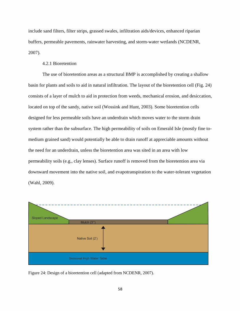
58

include sand filters, filter strips, grassed swales, infiltration aids/devices, enhanced riparian

buffers, permeable pavements, rainwater harvesting, and storm-water wetlands (NCDENR,

2007).

4.2.1 Bioretention

The use of bioretention areas as a structural BMP is accomplished by creating a shallow

basin for plants and soils to aid in natural infiltration. The layout of the bioretention cell (Fig. 24)

consists of a layer of mulch to aid in protection from weeds, mechanical erosion, and desiccation,

located on top of the sandy, native soil (Wossink and Hunt, 2003). Some bioretention cells

designed for less permeable soils have an underdrain which moves water to the storm drain

system rather than the subsurface. The high permeability of soils on Emerald Isle (mostly fine to-

medium grained sand) would potentially be able to drain runoff at appreciable amounts without

the need for an underdrain, unless the bioretention area was sited in an area with low

permeability soils (e.g., clay lenses). Surface runoff is removed from the bioretention area via

downward movement into the native soil, and evapotranspiration to the water-tolerant vegetation

(Wahl, 2009).

Figure 24: Design of a bioretention cell (adapted from NCDENR, 2007).

59

Bioretention cells are intended in areas where the seasonal high water table is at least 0.6

m (2 feet) below the land surface, and which receive runoff from a nearby impervious surface

(i.e., lawns next to roads, adjacent to sidewalks, parking lots) (Fig.25). The main reason these

locations are ideal is to prevent the concentration of flow so the entry velocity is reduced

(NCDENR, 2007). The two greatest disadvantages of the bioretention method are that the area

drained by the cell can be small, and the cells require constant mulch and vegetation for upkeep

(Schueler, 1992). There are three primary factors that make bioretention areas an ideal choice for

the study area. First, due to the high volume of residential properties on the western end of

Emerald Isle, the small land requirement for bioretention areas could be utilized in most areas.

Second, the sandy soil that dominates beneath the subsurface is ideal for drainage in designated

problem areas. Last, the landscaping value inherent in these bioretention cells will greatly

increase property values and beautification of properties. Bioretention cells are also characterized

as a low impact development (LID) (Hunt et al., 2010).

Figure 25: Bioretention garden built in a residential property (from AWPA, 2008)

60

4.2.2 Level spreader – vegetative filter strip system

A level spreader – vegetative filter strip (LS-VFS) is designed to disperse concentrated

storm-water flows, maintain non-erosive flow, and promote higher infiltration/evapotranspiration

rates (NCDENR, 2007). The LS-VFS is another example of a structural, low impact

development method to remediate runoff problems. However, as bioretention requires a

mandatory water table depth, LS-VFS’s are able to be constructed in a much wider variety of

locations due to no water table constraints. Although some LS-VFS systems encompass fairly

large areas of land, the size of them is dependent on the typical flow rate that is directed nearby

(Hunt et al., 2010).

Figure 26: Design of a level spreader - vegetative filter strip (adapted from NCDENR, 2007)

The design of the LS-VFS is separated in into two parts, the level spreader, and the

vegetative filter strip (Fig. 26). The level spreader is a concrete structure that acts as a temporary

stopper for high volumes of flow. The water is held in the swale until either 1) the water is

dispersed and diffused onto the VFS at a manageable rate or 2) the water infiltrates in the swale

itself. The size of both the level spreader and vegetative filter strip is determined based on the

61

estimated overland flow the area receives. The higher the volume of runoff, the longer the level

spreader length and bigger the vegetative filter strip are.

The application of the LS-VFS as a structural BMP is meant primarily as a component in

a larger storm-water management system, not a stand-alone solution (NCDENR, 2007). Case

studies in the Charlotte area have shown that these structures can reduce the runoff volume by up

to 85% (Hunt et al., 2009). Due to the simple design, low cost of construction, minimal upkeep

required, and high community acceptance (NCDENR, 2007), LS-VFS can have a large impact in

problem areas within the study area.

4.2.3 Infiltration basins/trenches

Areas along the Coast Guard Road corridor and low-lying swales in residential

neighborhoods were found to be the most problematic for storm-water runoff during the study.

Infiltration basins and trenches can be used in these areas due to their variability in size, but may

be of limited effectiveness in areas with a shallow water table. Both systems are designed to

capture runoff from nearby impervious surfaces and channel the water into their respective

catchment. The primary difference in application between infiltration basins and trenches is the

availability of space.

Figure 27: Design of an infiltration basin (adapted from NCDENR, 2007).

62

Infiltration basins are designed as a shallow depression that captures and stores storm-

water until it can infiltrate into the subsurface (Fig. 27) (NJDEP, 2004). They typically provide

runoff management for drainage basins 5 to 50 acres in area (Schueler, 1992). Inflow is received

from a pipe which collects runoff from nearby impervious surfaces. Once stored for exfiltration,

water is discharged via infiltration into the underlying soil, spilled over the embankment, or out

of the system during severe events using an underdrain. Infiltration basins are applicable in

locations where the soil permeability is high enough and there is sufficient land to construct one.

In cases where an infiltration basin would be ideal, but required space is not available,

infiltration trenches work well in their place.

Figure 28: Design of an infiltration trench (adapted from NCDENR, 2007).

Similar to infiltration basins, infiltration trenches are shallow excavated areas designed to

create a storm-water reservoir from runoff (APWA, 2008). They are typically filled in with

coarse, granular material which creates a highly permeable conduit for infiltration (Fig. 28).

Since they are much smaller than basins, their lower storage volumes in smaller catchments are

designed to easily capture the first wave of runoff during storm events. Areas where infiltration

63

trenches would be the most effective on Emerald Isle would be in residential lots where flooding

is a frequent occurrence. When infiltration trenches are used in combination with other structural

BMP’s, the negative side effects of storm-water runoff can be minimized by allowing for

increased infiltration potential (Schueler, 1987).

CHAPTER 5: CONCLUSIONS

The results of this study show that the shallow groundwater system may play a significant

role in generating storm-water runoff in Emerald Isle on Bogue Banks. Through the creation and

analysis of potentiometric maps, the water table did appear to rise to levels at or above the

ground surface during storm events. These potentiometric maps reveal that even during times of

little precipitation, the water table may have breached the land surface in several locations within

the study area. These data confirmed the first of the two hypotheses proposed, that an elevated

water table was contributing to storm-water ponding.

The second hypothesis, that infiltration capacities impede natural recharge in low-lying

areas, was partially confirmed by analyzing sediment properties of the Surficial aquifer. Low

infiltration capacities likely contribute to storm-water runoff in small, elongated soil sections

(Fig. 10). Due to the close proximity of the water table to the ground surface (as shown in the

flood potential maps), storm-water generation in these areas is likely a result of saturation excess

throughout the majority of the year. Therefore, if more areas of the island observe a rise in water

levels, storm-water runoff should be more widespread than found during the study year. High

water tables and storm-water generation are influenced by the frequency and duration of rain

events, which directly control water table levels in the Surficial aquifer. Other conclusions drawn

from this study are as follows:

1) Geological analyses of core samples show that the island is composed predominantly

of fine to-medium-grained sand. Some horizons of silt, clay and organic material,

similar to those found by Anderson (2000) on Hatteras Island, are present close to the

surface, suggesting that the infiltration rates may be retarded in these horizons. These

reduced infiltration rates should not be ruled out as a major factor contributing

65

to the storm-water runoff problem. Slug tests performed indicate that the sediment is

moderately permeable; with horizontal hydraulic conductivities ranging from 8.6 x

10-6

to 6.0 x 10-5

m/s. Vertical hydraulic conductivity was estimated to be on the

order of one magnitude less than the average horizontal conductivity.

2) Contour maps of the water table divulge a flow regime that is dominated by several

mounds on the western part of the island. Groundwater flow is radial from these

mounds, and is moving water from the dunes to the low-lying swales which were

identified to have a water table near the surface and low infiltration rates impeding

recharge.

3) The components of the water budget were estimated to be 223 mm/year for

evapotranspiration, 987 mm/year for precipitation, 284 mm/year for surface runoff,

688 mm/year for natural groundwater recharge, -8 mm/year for the change in

groundwater storage, and 216 mm/year for artificial recharge. Although the natural

recharge is approximately 70% of the precipitation, the permeability of the sediments

within the study area would recharge water at appreciable amounts. The change in

storage was low enough (-8 mm/year) to assume that the Surficial aquifer can be

considered in steady-state conditions.

Pumping was simulated both numerically and analytically to assess storm-water

mitigation during extreme rain events. The effects of Hurricane Irene, which brought a maximum

water level increase of 1 meter in the observation wells, were used as the baseline data. An

analytical solution (Neuman, 1972), which takes into account the behavior of the unconfined

aquifer when pumped, showed that the numerical model may be overestimating the drawdown.

66

This could be a potential short term solution to alleviate flooding, but is likely impracticable and

broader, long-term remedies for the town should be considered.

Storm-water Best Management Practices (BMP’s) provide a much more conservative

approach to reducing runoff. These include structural methods such as bioretention, level

spreader-vegetated filter strips, and infiltration basins and trenches. Current and future

development should consider the addition of structural BMP’s as a sustainable way to mitigate

problematic flooding. Not only are most BMP’s cost effective, but they can also add aesthetically

pleasing landscapes to the area.

This study highlights the need for more studies to be conducted on barrier islands to

improve our understanding of the Surficial aquifer. For example, because drainage patterns

continue to be altered with the addition of impervious surfaces such as roads and buildings,

changes in groundcover can in turn alter the locations and volumes of recharge to the Surficial

aquifer, as well as the intensity of runoff. As the island continues to develop, further studies

should look into quantifying how this impervious cover changes over time, and how this

development has affected infiltration capacities of the soils.

67

REFERENCES

Akan, A. O. (1993). Urban stormwater hydrology - a guide to engineering calculations.

Lancaster, PA: Technomic Publishing.

Alley, W. M., Reilly, T. E., & Franke, O. L. (1999). Sustainability of ground-water resources.

U.S Geological Survey Circular 1186.

American Public Works Assocation (APWA). (2012). Manual of Best Management Practices for

storm-water quality. Kansas City, MO: Mid-America Regional Council.

Amsbaugh, M. B. (1996). Hydrogeology of the Castle Hayne aquifer system in eastern Onslow

County, North Carolina. Master's Thesis - East Carolina University.

Anderson, W. P., Evans, D. G., & Snyder, S. W. (2000). The effects of holocene barrier-island

evolution on water-table elevations, Hatteras Island, North Carolina, USA. Hydrogeology

Journal, 8, 390-404.

Annan, P. A. (2005). GPR Methods for Hydrogeophysical Studies. In Hydrogeophysics (pp. 185-

213). New Delhi, India: CSB Publishers.

Arnold, C. L., & Gibbons, C. J. (1996). Impervious surface coverage. Journal of the American

Planning Association, 62, 243-259.

Bobba, A. G. (2009). Numerical modeling of salt-water intrusion due to human activites and sea-

level change in the Godavari Delta, India. Hydrogeological Sciences Journal, 47, 67-80.

Bouwer, H., & Rice, R. C. (1976). A slug test method for determining hydraulic conductivity of

unconfined aquifers with competely or partically penetrating wells. Water Resources

Research, 12, 423-428.

Bouwer, R. (1989). The Bouwer and Rice slug test - an update. Ground Water, 27, 304-309.

Brendle, D. L. (2002). Evaluation of possible alternatives to lower the high water table of St.

Charles Mesa, Pueblo County, Colorado. U.S. Geological Survey Water Resources

Investigations Report 01-4190.

Brown, P. M. (1985). Geologic map of North Carolina. North Carolina Department of Natural

Resources, Geological Survey Section.

Brown, P. M., Miller, J. A., & Swain, F. M. (1972). Structural and stratigraphic framework, and

spatial distribution of permeability of the Atlantic Coastal Plain, North Carolina to New

York. U.S. Geological Survey Professional Paper 796.

68

Burkett, C. A. (1996). Estimating the hydrogeologic characteristics of the Buxton Woods

aquifer, Hatteras Island, North Carolina. Master's Thesis - North Carolina State

University.

Campbell, M. D., Starrett, M. S., Fowler, J. D., & Klein, J. J. (1990). Slug tests and hydraulic

conductivity in processing petroleum hydrocarbons, and organic chemicals in

groundwater. API/NWWA Conference, (pp. 85-99). Houston, Texas.

Cappiella, K., & Brown, K. (2000). Derivations of impervious cover for suburban land uses in

the Chesapeake Bay Watershed. Ellicott City, MD: United States Environmental

Protection Agency Chesapeake Bay Program.

Christenson, S., Osborn, N. I., Neel, C. R., Faith, J. R., Blome, C. D., Puckette, J., et al. (2011).

Hydrogeology and simulation of groundwater flow in the Arbuckle-Simpson Aquifer,

South Central Oklahoma. U.S. Geological Survey Scientific Investigations Report 5029.

Clark, W. B., Miller, B. L., Stephenson, L. W., Parker, H. N., & Johnson, B. L. (1912). The

water resources of the Coastal Plain of North Carolina. North Carolina Geological and

Economic Survey, 3, 333-509.

Domenico, P. A., & Schwartz, F. W. (1990). Physical and Chemical Hydrogeology. Hoboken,

NJ: Wiley Publishing.

Evans, M. G., Burt, T. P., Holden, J., & Adamson, J. K. (1999). Runoff generation and water

table fluctuations in blanket peat: evidence from UK data spanning the dry summer of

1995. Journal of Hydrology, 221, 141-160.

Fetter, C. W. (2000). Applied Hydrogeology. Upper Saddle River, NJ: Prentice Hall.

Frank, D. A., & Inouye, R. S. (1994). Temporal variation in actual evapotranspiration of

terrestrial ecosystems: patterns and ecological implications. Journal of Biogeography, 21,

401-411.

Giese, G. L., Eimers, J. L., & Coble, R. W. (1997). Simulation of groundwater flow in the

coastal plain aquifer system of North Carolina. U.S. Geological Survey Professional

Paper 1404-M.

Gregory, J., Dukes, M., Jones, P., & Miller, G. (2006). Effects of urban soil compaction on

infiltration rate. Journal of Soil and Water Conservation, 61, 117-124.

Harbaugh, A. W., Banta, E. R., Hill, M. C., & McDonald, M. G. (2000). MODFLOW-2000, the

U.S. Geological Survey modular groundwater flow model - user guide to modularization

concepts and the groundwater flow process. U.S. Geological Survey Open-File Report

00-92.

69

Harden, S. L., Fine, J. M., & Spruill, T. B. (2003). Hydrogeology and groundwater quality of

Brunswick County, North Carolina. U.S. Geological Survey Water Resources

Investigations Report 2003-4051.

Healy, R. W., & Cook, P. G. (2002). Using grounwater levels to estimate recharge.

Hydrogeology Journal, 10, 91-109.

Heath, R. C. (1983). Basin groundwater hydrology. U.S Geological Survey Water Supple Paper

2220.

Heath, R. C. (1988). Groundwater resources of the Cape Hatteras area of North Carolina. Report

to the Cape Hatteras Water Association.

Heath, R. C. (1994). Groundwater recharge in North Carolina. Groundwater Section - North

Carolina Division of Environmental Health and Natural Resources.

Heath, R. C., & Spruill, R. K. (2003). Cretaceous aquifers in North Carolina: analysis of safe

yield based on historical data. Hydrogeology Journal, 11, 249-258.

Hubbert, M. K. (1940). The theory of groundwater motion. Journal of Geology, 48, 785-944.

Hunt, W. F., & Doll, B. A. (2000). Urban waterways: designing stormwater wetlands for small

watersheds. North Carolina Cooperative Extension Servie Factsheet AG-588-2.

Hunt, W. F., Hathaway, J. M., Winston, R. J., & Jadlocki, S. J. (2010). Runoff volume reduction

by level spreader - vegetated filter strip system in suburban Charlotte, NC. Journal of

Hydrologic Engineering, 15, 499-503.

Hutchings, W. C., & Tarbox, D. L. (2003). A model of seawater intrusion in surficial and

confined aquifers of Northeast Florida. Conference on Saltwater Intrusion and Coastal

Aquifers - Monitoring, Modeling, and Management, (pp. 1-17). Yucatan, Mexico.

Hvorslev, M. J. (1951). Time lag and soil permeability in groundwater observations. Waterways

Experts State Corps of Engineers, U.S. Army Bulletic No. 36, 1-50.

Ingram, R. L. (1987). Peat deposits in NOrth Carolina. North Carolina Geological Survey

Section Bulletin 88.

Jackson, J. M. (2007). Hydrogeology and groundwater flow model, central catchment of Bribie

Island, Southeast Queensland. Master's Thesis - Queensland University of Technology.

Johnson, A. I. (1966). Specific yield - compilation of specific yields for various materials. U.S

Geological Survey Water Supply Paper 1662-D.

Kadlec, R. H., & and Knight, R. L. (1996). Treatment Wetlands. Boca Raton, FL: CRC Press.

70

Konikow, L. F., & Hornberger, G. Z. (2006). Use of Multi-Node Well (MNW) package when

simulating solute transport with the MODFLOW groundwater transport process. U.S.

Geological Survey Techniques and Methods Paper 6-A15.

Lautier, J. C. (2009). Hydrogeologic framework and ground water conditions in the North

Carolina Central Coastal Plain. North Carolina DENR: Division of Water Resources.

Lawrence, D. P., & Hoffman, C. W. (1993). Geology of basement rocks beneath the North

Carolina Coastal Plain. North Carolina Geological Survey Bulletin 95.

Lutz, A., Thomas, J. M., Pohll, G., McKay, W. A., & Keita, M. (2009). Sustainability of

groundwater in Mali, West Africa. Environmental Geology, 58, 1441-1450.

Mallinson, D. J., Burdette, K., Mahan, S., & Brook, G. (2008). Optically stimulated

luminescence age controls on late Pleistocene and Holocene coastal lithosomes, North

Carolina, USA. Quaternary Geology, 69, 97-109.

Martin, L. (2008). Simulation of groundwater flow at Beach Point, Cape Cod, Massachusetts.

Fort Collins, Colorado: Natural Resource Technical Report, National Park Service.

Meinzer, O. E. (1923). Outline of groundwater hydrology with definitions. U.S. Geological

Survey Water Supple Paper 494.

Moffatt and Nichol Engineers. (1997). Engineering analysis for the FEMA storm-water hazard

mitigation application - Coast Guard Road Area. Emerald Isle, NC: North Carolina

Hazard Mitigation Grant.

Nelson, P. F. (1964). Geology and groundwater resources of the Swanquarter Area, North

Carolina. North Carolina Department of Water Resources Ground Water Bulletin No. 4.

Neuman, S. P. (1972). Theory of unconfined aquifers considering delayed response of the water

table. Water Resources Research, 8, 1031-1045.

North Carolina Department of Environment and Natural Resources (NCDENR). (2007). Storm-

water Best Management Practices manual. North Carolina Division of Water Quality.

North Carolina Division of Water Resources (NC DWR). (2012). Hydrogeologic Framework

Database. Retrieved June 2012, from

http://www.ncwater.org/Data_and_Modeling/Ground_Water_Databases/frametable.php?

countyname=CARTERET

North Carolina Soil Conservation Service (NCSCS). (1987). Soil Survey of Carteret County,

North Carolina. United States Department of Agriculture.

71

Peel, M. C., Finlayson, B. L., & McMahon, T. A. (2007). Updated world map of the Koppen-

Geiger climate classification. Hydrology and Earth System Sciences, 115, 270-276.

Scanlon, B. R., Healy, R. W., & Cook, P. G. (2002). Choosing appropriate techniques for

quantifying groundwater recharge. Hydrogeology Journal, 10, 18-39.

Schueler, T. R. (1987). Controlling urban runoff: a practical manual for planning and designing

urban BMP's. Washington, DC: Metropolitian Washington Council of Governments.

Schueler, T. R. (1992). Design of storm-water wetlands: guidelines for creating diverse and

effective storm-water wetland systems in the Mid-Atlantic Region. Washington, DC:

Anacostia Restoration Team - Department of Environmental Programs.

Shade, P. J. (1995). Water budget for the island of Kauai, Hawaii. U.S. Geological Survey Water

Resources Investigation 95-4128.

Smith, D. G., & Chapman, M. J. (2005). Hydraulic properties of the Surficial aquifer at five

selected sites in the Little Contentnea Creek Basin, North Carolina. U.S. Geological

Survey Scientific Investigations Report 2005-5238.

Taylor, C. J., & Alley, W. M. (2001). Groundwater level monitoring and the importance of long-

term water level data. U.S Geological Survey Circular 1217.

Thornthwaite, C. W. (1948). An approach toward a rational classification of climate.

Geographical Review, 38, 55-94.

Thornthwaite, C. W., & Mather, J. R. (1955). The water balance. Climatology, 8, 1-104.

Toth, J. (1963). A theoretical analysis of groundwater flow in small drainage basins. Journal of

Geophysical Research, 68, 4795-4812.

Vacher, H. L. (1988). Dupuit-Ghyben-Herzberg analysis of strip-island lenses. Geological

Society of America Bulletin 100, 580-591.

van Overmeeren, P. A. (1998). Radar facies of unconsolidated sediments in the Netherlands: a

radar stratigraphy interpretation method for hydrogeology. Journal of Applied

Geophysics, 40, 1-18.

Wahl, S. (2009). Stormwater Best Managements Practices: a first guide for landscape architects.

Department of Urban and Rural Development.

Wiegand, C., Schueler, T. R., Chittenden, W., & Jellick, D. (1986). Cost of urban runoff

controls. Engineering Foundation Conference, Urban Water Resources, (pp. 366-380).

Henniker, NH.

72

Wilder, H. B., Robinson, T. M., & Lindskov, K. L. (1978). Water resources of Northeast North

Carolina. U.S. Geological Survey Water Resources Investigation 77-81.

Winner, M. D. (1975). Groundwater resources of the Cape Hatteras National Seashore, North

Carolina. U.S. Geological Survey Hydrologic Investigation HA-450.

Winner, M. D. (1981). An observation well network concept as applied to North Carolina. U.S.

Geological Survey Water Resources Investigations Report 81-13.

Winner, M. D., & Coble, R. W. (1996). Hydrogeologic framework of the North Carolina Coastal

Plain. U.S. Geological Survey Professional Paper 1401-I.

Wossink, A., & Hunt, B. (2003). The economics of structural stormwater BMP's in North

Carolina. North Carolina Urban Water Consortium.

assessing the shallow groundwater system as a potential

Documents

Transcript of assessing the shallow groundwater system as a potential