at SciVerse ScienceDirect

Applied Geography 34 (2012) 38e46

Contents lists available

Applied Geography

journal homepage: www.elsevier .com/locate/apgeog

Assessing resolution and source effects of digital elevation models on automatedfloodplain delineation: A case study from the Camp Creek Watershed, Missouri

Richard Charrier a,b, Yingkui Li c,*aDepartment of Geography, University of Missouri, Columbia, MO 65211, USAbCenter for Applied Research and Environmental Systems, University of Missouri, Columbia, MO 65211, USAcDepartment of Geography, University of Tennessee, Knoxville, TN 37996, USA

Keywords:Digital elevation model (DEM)GISAutomated floodplain delineationResolution and data source effectsCamp Creek Watershed

* Corresponding author. Tel.: þ1 865 974 0595; faxE-mail address: yli32@utk.edu (Y. Li).

0143-6228/$ e see front matter � 2011 Elsevier Ltd.doi:10.1016/j.apgeog.2011.10.012

a b s t r a c t

Digital elevation models (DEMs) have been widely used in automated floodplain modeling to determinefloodplain boundaries. However, the effects of DEM resolution and data source on floodplain delineationare not well quantified. This paper presents a case study to assess these effects from the Camp CreekWatershed, Missouri, using two sets of DEMs. One is the Light Detection and Ranging (LiDAR) DEMs re-sampled from 1-m to 3, 5, 10, 15, and 30-m resolutions. The other is 5, 10, and 30-m DEMs obtained fromthe U.S. Geological Survey (USGS). Floodplain boundaries are delineated using a combination of hydro-logical, hydraulic and floodplain delineation models under the Federal Emergency Management Agency’s(FEMA) guideline. Model outputs including stream network, watershed and floodplain boundaries arecompared to 1-m LiDAR DEM outputs (as the reference) to assess the uncertainty. Results indicate thatre-sampled 3 or 5-m LiDAR DEMs produce similar streams and floodplain boundaries within 10%difference of the reference. In contrast, coarser LiDAR DEMs (such as the 10-m resolution) are moreappropriate for watershed boundary delineation because higher DEM resolutions are likely moresensitive to minor topographic changes and may introduce erroneous boundaries. For different datasources, uncertainties introduced by USGS DEMs are much higher than LiDAR DEMs with a distinctrelationship between uncertainties and DEM resolutions. Uncertainties of LiDAR DEMs consistentlyincrease with decreasing resolutions, whereas similar levels of uncertainty are observed for differentUSGS DEM resolutions. This difference is probably due to the inherited difference in their original datasource resolutions to make these two types of DEMs.

� 2011 Elsevier Ltd. All rights reserved.

Introduction

Water is essential to life on Earth, but it can also cause disasters.Water-related disasters, such as flooding, hurricanes, cyclones,tsunamis, mudslides, and blizzards, account for approximately 60%of all disasters worldwide (Frech, 2006; Ibarra, 2011; Vinet, 2008).Flooding itself is the largest natural disaster (about 40% of alldisasters) in the United States with an estimated property damageof about $4 billion and approximate 200 deaths each year (Pielke,Downton, & Miller, 2002). Therefore, understanding the extent offlooding is critical to prevent property damage and life loss. Sincethe 1970s, the Federal Emergency Management Agency (FEMA) ofthe United States has conducted considerable effort to mapnationwide floodplain areas, especially for the 100 year flooding

: þ1 865 974 6025.

All rights reserved.

event (Blanchard-Boehm, Berry, & Showalter, 2001). Early methodsto delineate floodplain boundaries are primarily manual andrequire considerable amount of time and effort (Norman, Nelson, &Zundel, 2001). With the development of numerical modeling,geographic information systems (GIS), and digital elevation models(DEMs), automated techniques and methods become available andhave been widely used in floodplain delineation.

The automated method significantly reduces the time andimproves the accuracy of the floodplain delineation. However,uncertainties still exist. First, automated floodplain modelingusually includes a combination of hydrological, hydraulic, andfloodplain delineation models (FEMA, 2005) and each model canhave different choices with strengths and weaknesses (Normanet al., 2001). Therefore, uncertainties can be introduced due todifferent combinations of models and/or parameters (Wheater,2002; Yang, Townsend, & Daneshfar, 2006). Second, automatedfloodplain modeling requires a DEM to represent topography,calculate flood elevation, and delineate floodplain boundaries. The

R. Charrier, Y. Li / Applied Geography 34 (2012) 38e46 39

source and resolution of the DEM would affect many steps of thefloodplain modeling. With technological advances, DEMs can becreated at much higher resolutions. For example, the use of LightDetection and Ranging (LiDAR) allows for the creation of <1-mresolution DEMs (National Academy of Sciences, 2009; Tate,Maidment, Olivera, & Anderson, 2002). Higher resolution DEMsprovide more accurate terrain representation and would result inmore accurate floodplain delineation. However, gathering higherresolution DEMs can be expensive and require considerabledemands of data storage space and computation ability. In addition,DEMs can be created using different data sources such as syntheticaperture radar, topographic maps, LiDAR, and field surveys. As allDEMs introduce errors, examining the effects of DEM resolutionand data source on floodplain delineation is critical to floodmanagement and disaster prevention.

The effects of DEM resolution and data source have beenexamined for many processes such as soil erosion (Zhang, Chang, &Wu, 2008), landslide (Claessens, Heuvelink, Schoorl, & Veldkamp,2005), solar radiation (Cebecauer, Huld, & Suri, 2007), watershed,and hydrological (Chaubey, Cotter, Costello, & Sorens, 2005;Vazquez & Feyen, 2007; Wu, Li, & Huang, 2006) models to test ifan optimum DEM resolution exists so the model output can beaccurate enough without the need to significantly increase datastorage space and computation ability. The goal of this paper is toassess the effects of DEM resolution and data source on automatedfloodplain delineation through a case study from the Camp CreekWatershed, Missouri. The results of this study would provideinsights into the determination of an optimum DEM resolutionneeded for accurate floodplain modeling.

Study area and datasets

The Camp Creek Watershed is located in Saline County, Mis-souri, with a drainage area of about 46 km2 (Fig. 1A). The portion ofthe Camp Creek used for this study consists of approximately19.3 km of the stream flowing from its headwaters southward toabout 1.5 km upstream from the Salt Fork River. The watershed

Fig. 1. (A) The shaded relief map of the Camp Creek Watershed. (B) The land use/land cov(MoRAP) 2005 data).

belongs to a relatively flat topography (<10% in slope) and consistsof silt loam soils. The land use of the watershed is dominated byagricultural land (66%), grassland (18%), and forest (15%) (Fig. 1B).

Two sets of DEMs are used for this study. One is a set of DEMsderived from an original 1-m LiDAR dataset obtained by a jointproject between the United States Army Corps of Engineers, KansasCity District, and United States Department of Agriculture, NaturalResource Conservation Service (USDA-NRCS) in 2007. The originaldataset covers four counties in Missouri (Lafayette, Saline, Carroll,and Chariton) and was verified using 304 ground control points (17points from forest covered areas) with a vertical accuracy of<0.13 m. To examine the effect of DEM resolution on floodplaindelineation, this original dataset is re-sampled to a set of DEMswith resolutions of 3, 5, 10, 15, and 30 m. The other is USGS DEMswith resolutions of 5, 10 and 30 m. The 30-m DEM is retrieved fromthe Missouri State Data Repository (MSDIS, http://misdisweb.missouri.edu) and was developed for the USGS in 1998 by theGeographic Resource Center (GRC) at the University of Missouriusing 7.5 min quadrangle topographic maps. The 5 and 10-m DEMswere developed for the USGS by the Center for Applied Researchand Environmental Systems (CARES) at the University of Missouriin 2005. These DEMs were developed based on 1:24,000 topog-raphy maps and are obtained directly from CARES with thepermission of the USGS.

Methods

Automated floodplain modeling

Following the FEMA guidelines, the floodplain model used inthis study includes three portions: hydrological, hydraulic, andfloodplain delineation models (Fig. 2). The hydrological portiondetermines the discharge of a flooding event at a stream crosssection. The hydraulic portion calculates the flood elevation cor-responding to the discharge at each cross section. The final portiondelineates floodplain boundaries based on calculated flood eleva-tion at each cross section and the DEM.

er (LULC) map of the study area (based on Missouri Resource Assessment Partnership

DEMDEM

StreamNetwork

Manning’s‘n’ Value

HEC-RAS(3.1.3)

FloodSurface

Elevations

Manning’s‘n’ Value

HEC-RAS(3.1.3)

FloodSurface

Elevations

HEC-RAS

FloodElevations

CARESDelineation

Model

Stre

m a

nd w

ater

shed

Del

inea

tion

Hyd

raul

icM

odel

ing

Flo

odpl

ain

Del

inea

tion

GIS EnvironmentNon-GIS

Environment

Hyd

rolo

gica

lM

odel

ing

RegressionEquation

CrossSections

CARESHydrological

Model

Slope Discharge

Input Data/Variable

Model or Process

Derived Data/Variable

Workflow

FloodplainPolygon

ArcGISD8 Method

Watersheds

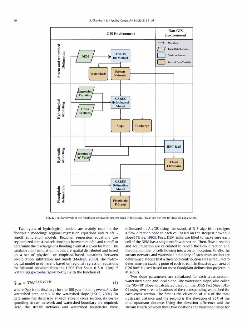
Fig. 2. The framework of the floodplain delineation process used in this study. Please see the text for detailed explanation.

R. Charrier, Y. Li / Applied Geography 34 (2012) 38e4640

Two types of hydrological models are mainly used in thefloodplain modeling: regional regression equations and rainfall-runoff simulation models. Regional regression equations useregionalized statistical relationships between rainfall and runoff todetermine the discharge of a flooding event at a given location. Therainfall-runoff simulation models are spatial distributed and basedon a set of physical- or empirical-based equations betweenprecipitation, infiltration and runoff (Madsen, 2000). The hydro-logical model used here is based on regional regression equationsfor Missouri obtained from the USGS Fact Sheet 015-01 (http://water.usgs.gov/pubs/fs/fs-015-01/) with the function of

Q100 ¼ 376A0:652S0:346 (1)

where Q100 is the discharge for the 100 year flooding event, A is thewatershed area, and S is the watershed slope (USGS, 2001). Todetermine the discharge at each stream cross section, its corre-sponding stream network and watershed boundary are required.Here, the stream network and watershed boundaries were

delineated in ArcGIS using the standard D-8 algorithm (assignsa flow direction code to each cell based on the steepest downhillslope) (Tribe, 1992). First, DEM sinks are filled to make sure eachcell of the DEM has a single outflow direction. Then, flow directionand accumulation are calculated to record the flow direction andthe total number of cells flowing into a certain location. Finally, thestream network and watershed boundary of each cross section aredetermined. Notice that a threshold contribution area is required todetermine the starting point of each stream. In this study, an area of0.26 km2 is used based on most floodplain delineation projects inMissouri.

Two slope parameters are calculated for each cross section:watershed slope and local slope. The watershed slope, also calledthe “85e10” slope, is calculated based on the USGS Fact Sheet 015-01 using two stream locations of the corresponding watershed foreach cross section. The first is the elevation of 10% of the totalupstream distance and the second is the elevation of 85% of thetotal upstream distance. Using the elevation difference and thestream length between these two locations, thewatershed slope for

R. Charrier, Y. Li / Applied Geography 34 (2012) 38e46 41

each cross section can be determined. The local slope for eachsection is calculated using the elevation difference between thecross section and 1000 feet downstream from the cross section.

Hydraulic models include backwater and normal flood depthmodels. A backwater model, such as the HEC-RAS (Hydrology Engi-neering Centere River Analysis System) model developed by the USArmy Corps of Engineers, considers the connectivity of differentstream cross sections and calculated upstream flood elevations arealways higher than downstream calculations. In contrast, a normalflooddepthmodel calculates theflood elevationof each cross sectionindependently, allowing for the possibility that downstream floodelevations might be higher than upstream calculations. Here, wechose the HEC-RAS model because it is the most widely usedhydraulic model in automated floodplain modeling.

The HEC-RAS model requires an input file including the locationof stream and cross section vertexes, elevation profiles, discharge,watershed and local slopes of all cross sections. All these variablesare determined by the previous hydrological model. One additionalvariable required in the HEC-RAS model is the Manning’s ‘n’roughness coefficient. For floodplain mapping, values of 0.065 forbanks and 0.040 for channels are generally used in this region.Although these values may not be appropriate for the entirewatershed, they are consistently used in the floodplain modeling ofall DEMs in order to compare model outputs. If there is any effectdue to the selection of these values, all model outputs would beaffected equally. Once all variables are input and verified, the HEC-RAS steady flow analysis is used to calculate the flood elevation foreach cross section. The calculated flood elevations of all crosssections are exported to ArcGIS files for further floodplaindelineation.

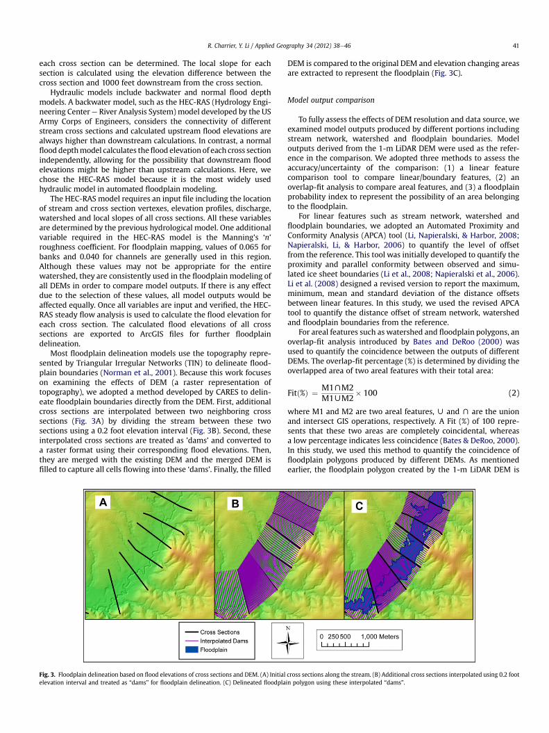
Most floodplain delineation models use the topography repre-sented by Triangular Irregular Networks (TIN) to delineate flood-plain boundaries (Norman et al., 2001). Because this work focuseson examining the effects of DEM (a raster representation oftopography), we adopted a method developed by CARES to delin-eate floodplain boundaries directly from the DEM. First, additionalcross sections are interpolated between two neighboring crosssections (Fig. 3A) by dividing the stream between these twosections using a 0.2 foot elevation interval (Fig. 3B). Second, theseinterpolated cross sections are treated as ’dams’ and converted toa raster format using their corresponding flood elevations. Then,they are merged with the existing DEM and the merged DEM isfilled to capture all cells flowing into these ‘dams’. Finally, the filled

Fig. 3. Floodplain delineation based on flood elevations of cross sections and DEM. (A) Initialelevation interval and treated as “dams” for floodplain delineation. (C) Delineated floodpla

DEM is compared to the original DEM and elevation changing areasare extracted to represent the floodplain (Fig. 3C).

Model output comparison

To fully assess the effects of DEM resolution and data source, weexamined model outputs produced by different portions includingstream network, watershed and floodplain boundaries. Modeloutputs derived from the 1-m LiDAR DEM were used as the refer-ence in the comparison. We adopted three methods to assess theaccuracy/uncertainty of the comparison: (1) a linear featurecomparison tool to compare linear/boundary features, (2) anoverlap-fit analysis to compare areal features, and (3) a floodplainprobability index to represent the possibility of an area belongingto the floodplain.

For linear features such as stream network, watershed andfloodplain boundaries, we adopted an Automated Proximity andConformity Analysis (APCA) tool (Li, Napieralski, & Harbor, 2008;Napieralski, Li, & Harbor, 2006) to quantify the level of offsetfrom the reference. This tool was initially developed to quantify theproximity and parallel conformity between observed and simu-lated ice sheet boundaries (Li et al., 2008; Napieralski et al., 2006).Li et al. (2008) designed a revised version to report the maximum,minimum, mean and standard deviation of the distance offsetsbetween linear features. In this study, we used the revised APCAtool to quantify the distance offset of stream network, watershedand floodplain boundaries from the reference.

For areal features such as watershed and floodplain polygons, anoverlap-fit analysis introduced by Bates and DeRoo (2000) wasused to quantify the coincidence between the outputs of differentDEMs. The overlap-fit percentage (%) is determined by dividing theoverlapped area of two areal features with their total area:

Fitð%Þ ¼ M1XM2M1WM2

� 100 (2)

where M1 and M2 are two areal features, W and X are the unionand intersect GIS operations, respectively. A Fit (%) of 100 repre-sents that these two areas are completely coincidental, whereasa low percentage indicates less coincidence (Bates & DeRoo, 2000).In this study, we used this method to quantify the coincidence offloodplain polygons produced by different DEMs. As mentionedearlier, the floodplain polygon created by the 1-m LiDAR DEM is

cross sections along the stream. (B) Additional cross sections interpolated using 0.2 footin polygon using these interpolated “dams”.

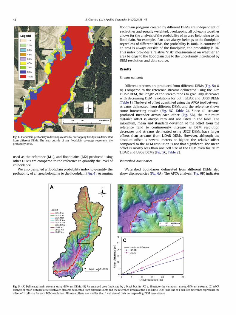
Fig. 4. Floodplain probability index map created by overlapping floodplains delineatedfrom different DEMs. The area outside of any floodplain coverage represents theprobability of 0%.

R. Charrier, Y. Li / Applied Geography 34 (2012) 38e4642

used as the reference (M1), and floodplains (M2) produced usingother DEMs are compared to the reference to quantify the level ofcoincidence.

We also designed a floodplain probability index to quantify theprobability of an area belonging to the floodplain (Fig. 4). Assuming

Fig. 5. (A) Delineated main streams using different DEMs. (B) An enlarged area (indicatedanalysis of mean distance offsets between streams delineated from different DEMs and the roffset of 1 cell size for each DEM resolution. All mean offsets are smaller than 1 cell size o

floodplain polygons created by different DEMs are independent ofeach other and equally weighted, overlapping all polygons togetherallows for the analysis of the probability of an area belonging to thefloodplain. For example, if an area always belongs to the floodplainregardless of different DEMs, the probability is 100%. In contrast, ifan area is always outside of the floodplain, the probability is 0%.This index provides a relative “risk” measurement on whether anarea belongs to the floodplain due to the uncertainty introduced byDEM resolution and data source.

Results

Stream network

Different streams are produced from different DEMs (Fig. 5A &B). Compared to the reference streams delineated using the 1-mLiDAR DEM, the length of the stream tends to gradually decreaseswith decreasing DEM resolutions for both LiDAR and USGS DEMs(Table 1). The level of offset quantified using the APCA tool betweenstreams delineated from different DEMs and the reference showssome interesting results (Fig. 5C, Table 2). Since all streamsproduced meander across each other (Fig. 5B), the minimumdistance offset is always zero and not listed in the table. Themaximum, mean and standard deviation of the offset from thereference tend to continuously increase as DEM resolutiondecreases and streams delineated using USGS DEMs have largeroffsets than streams from LiDAR DEMs. However, although theabsolute offset is several meters or higher, the relative offsetcompared to the DEM resolution is not that significant. The meanoffset is mostly less than one cell size of the DEM even for 30 mLiDAR and USGS DEMs (Fig. 5C, Table 2).

Watershed boundaries

Watershed boundaries delineated from different DEMs alsoshow discrepancies (Fig. 6A). The APCA analysis (Fig. 6B) indicates

by a black box in (A)) to illustrate the variations among different streams. (C) APCAeference stream of the 1-m LiDAR DEM (The line of 1 cell size difference represents thef their corresponding DEM resolutions).

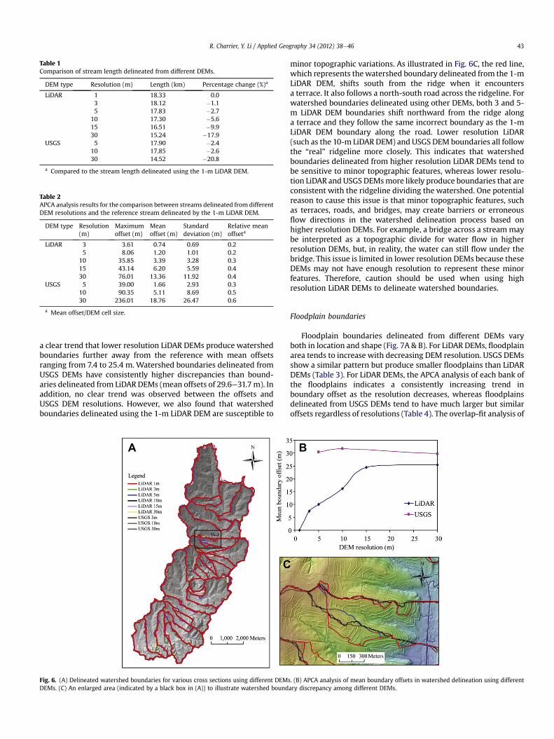
Table 1Comparison of stream length delineated from different DEMs.

DEM type Resolution (m) Length (km) Percentage change (%)a

LiDAR 1 18.33 0.03 18.12 �1.15 17.83 �2.7

10 17.30 �5.615 16.51 �9.930 15.24 �17.9

USGS 5 17.90 �2.410 17.85 �2.630 14.52 �20.8

a Compared to the stream length delineated using the 1-m LiDAR DEM.

Table 2APCA analysis results for the comparison between streams delineated from differentDEM resolutions and the reference stream delineated by the 1-m LiDAR DEM.

DEM type Resolution(m)

Maximumoffset (m)

Meanoffset (m)

Standarddeviation (m)

Relative meanoffseta

LiDAR 3 3.61 0.74 0.69 0.25 8.06 1.20 1.01 0.2

10 35.85 3.39 3.28 0.315 43.14 6.20 5.59 0.430 76.01 13.36 11.92 0.4

USGS 5 39.00 1.66 2.93 0.310 90.35 5.11 8.69 0.530 236.01 18.76 26.47 0.6

a Mean offset/DEM cell size.

R. Charrier, Y. Li / Applied Geography 34 (2012) 38e46 43

a clear trend that lower resolution LiDAR DEMs produce watershedboundaries further away from the reference with mean offsetsranging from 7.4 to 25.4 m. Watershed boundaries delineated fromUSGS DEMs have consistently higher discrepancies than bound-aries delineated from LiDAR DEMs (mean offsets of 29.6e31.7 m). Inaddition, no clear trend was observed between the offsets andUSGS DEM resolutions. However, we also found that watershedboundaries delineated using the 1-m LiDAR DEM are susceptible to

Fig. 6. (A) Delineated watershed boundaries for various cross sections using different DEMsDEMs. (C) An enlarged area (indicated by a black box in (A)) to illustrate watershed bound

minor topographic variations. As illustrated in Fig. 6C, the red line,which represents thewatershed boundary delineated from the 1-mLiDAR DEM, shifts south from the ridge when it encountersa terrace. It also follows a north-south road across the ridgeline. Forwatershed boundaries delineated using other DEMs, both 3 and 5-m LiDAR DEM boundaries shift northward from the ridge alonga terrace and they follow the same incorrect boundary as the 1-mLiDAR DEM boundary along the road. Lower resolution LiDAR(such as the 10-m LiDAR DEM) and USGS DEM boundaries all followthe “real” ridgeline more closely. This indicates that watershedboundaries delineated from higher resolution LiDAR DEMs tend tobe sensitive to minor topographic features, whereas lower resolu-tion LiDAR and USGS DEMsmore likely produce boundaries that areconsistent with the ridgeline dividing the watershed. One potentialreason to cause this issue is that minor topographic features, suchas terraces, roads, and bridges, may create barriers or erroneousflow directions in the watershed delineation process based onhigher resolution DEMs. For example, a bridge across a stream maybe interpreted as a topographic divide for water flow in higherresolution DEMs, but, in reality, the water can still flow under thebridge. This issue is limited in lower resolution DEMs because theseDEMs may not have enough resolution to represent these minorfeatures. Therefore, caution should be used when using highresolution LiDAR DEMs to delineate watershed boundaries.

Floodplain boundaries

Floodplain boundaries delineated from different DEMs varyboth in location and shape (Fig. 7A & B). For LiDAR DEMs, floodplainarea tends to increase with decreasing DEM resolution. USGS DEMsshow a similar pattern but produce smaller floodplains than LiDARDEMs (Table 3). For LiDAR DEMs, the APCA analysis of each bank ofthe floodplains indicates a consistently increasing trend inboundary offset as the resolution decreases, whereas floodplainsdelineated from USGS DEMs tend to have much larger but similaroffsets regardless of resolutions (Table 4). The overlap-fit analysis of

. (B) APCA analysis of mean boundary offsets in watershed delineation using differentary discrepancy among different DEMs.

Fig. 7. (A) Delineated floodplains using different DEMs. (B) An enlarged area (indicated by a black box in (A)) to illustrate floodplain boundary discrepancy among different DEMs.(C) Overlapping percentage of the floodplain probability index created from all DEMs. (D) Overlapping percentage of the floodplain probability index created just from LiDAR DEMs.

R. Charrier, Y. Li / Applied Geography 34 (2012) 38e4644

floodplain areas (Table 5) represents a distinct relationshipbetween overlapped percentage and LiDAR DEM resolution. AsLiDAR DEM resolution decreases, the overlapped percentage alsodecreases. For floodplains delineated from USGS DEMs, the over-lapped percentage also increases as resolution decreases, but theentire change is just <5%. The floodplain probability index created

Table 3Comparison between floodplain areas delineated from different DEMs.

DEM type Resolution(m)

Floodplainarea (km2)

Area difference(%)a

LiDAR 1 2.47 e

3 2.52 2.05 2.56 3.6

10 2.54 2.815 2.64 6.830 2.64 6.8

USGS 5 2.16 �12.610 2.24 �9.330 2.44 �1.2

a Compared to the floodplain area delineated using the 1-m LiDAR DEM.

by overlapping floodplains delineated by all DEMs indicates 48.7%of cells fell within the floodplain (100% probability) regardless ofDEM resolutions and data sources (Fig. 7C). In addition, the flood-plain probability index seems to be more affected by data sources.

Table 4APCA analysis results for the comparison between floodplain boundaries delineatedfrom different DEM resolutions and floodplain boundaries delineated by the 1-mLiDAR DEM.

DEM type Resolution(m)

Right bank Left bank

Maximumoffset (m)

Meanoffset (m)

Maximumoffset (m)

Meanoffset (m)

LiDAR 3 103.0 4.8 56.8 3.65 121.6 7.2 72.1 5.7

10 109.6 9.9 119.4 8.215 126.6 15.1 104.7 11.330 138.8 18.7 108.0 15.7

USGS 5 124.0 25.9 112.7 17.410 123.4 27.1 100.2 17.330 145.3 26.1 99.0 18.1

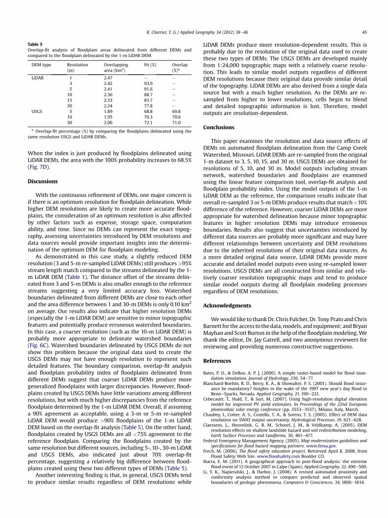
Table 5Overlap-fit analysis of floodplain areas delineated from different DEMs andcompared to the floodplain delineated by the 1-m LiDAR DEM.

DEM type Resolution(m)

Overlappingarea (km2)

Fit (%) Overlap(%)a

LiDAR 1 2.47 e e

3 2.42 93.9 e

5 2.41 91.6 e

10 2.36 88.7 e

15 2.33 83.7 e

30 2.24 77.8 e

USGS 5 1.89 68.8 69.810 1.95 70.3 70.630 2.06 72.1 71.0

a Overlap-fit percentage (%) by comparing the floodplains delineated using thesame resolution USGS and LiDAR DEMs.

R. Charrier, Y. Li / Applied Geography 34 (2012) 38e46 45

When the index is just produced by floodplains delineated usingLiDAR DEMs, the area with the 100% probability increases to 68.5%(Fig. 7D).

Discussions

With the continuous refinement of DEMs, one major concern isif there is an optimum resolution for floodplain delineation. Whilehigher DEM resolutions are likely to create more accurate flood-plains, the consideration of an optimum resolution is also affectedby other factors such as expense, storage space, computationability, and time. Since no DEMs can represent the exact topog-raphy, assessing uncertainties introduced by DEM resolutions anddata sources would provide important insights into the determi-nation of the optimum DEM for floodplain modeling.

As demonstrated in this case study, a slightly reduced DEMresolution (3 and 5-m re-sampled LiDAR DEMs) still produces>95%stream length match compared to the streams delineated by the 1-m LiDAR DEM (Table 1). The distance offset of the streams delin-eated from 3 and 5-m DEMs is also smaller enough to the referencestreams suggesting a very limited accuracy loss. Watershedboundaries delineated from different DEMs are close to each otherand the area difference between 1 and 30-m DEMs is only 0.10 km2

on average. Our results also indicate that higher resolution DEMs(especially the 1-m LiDAR DEM) are sensitive to minor topographicfeatures and potentially produce erroneous watershed boundaries.In this case, a coarser resolution (such as the 10-m LiDAR DEM) isprobably more appropriate to delineate watershed boundaries(Fig. 6C). Watershed boundaries delineated by USGS DEMs do notshow this problem because the original data used to create theUSGS DEMs may not have enough resolution to represent suchdetailed features. The boundary comparison, overlap-fit analysisand floodplain probability index of floodplains delineated fromdifferent DEMs suggest that coarser LiDAR DEMs produce moregeneralized floodplains with larger discrepancies. However, flood-plains created by USGS DEMs have little variations among differentresolutions, but with much higher discrepancies from the referencefloodplain determined by the 1-m LiDAR DEM. Overall, if assuminga 90% agreement as acceptable, using a 3-m or 5-m re-sampledLiDAR DEM would produce >90% floodplains of the 1-m LiDARDEM based on the overlap-fit analysis (Table 5). On the other hand,floodplains created by USGS DEMs are all <75% agreement to thereference floodplain. Comparing the floodplains created by thesame resolution but different sources, including 5-,10-, 30-m LiDARand USGS DEMs, also indicated just about 70% overlap-fitpercentage, suggesting a relatively big difference between flood-plains created using these two different types of DEMs (Table 5).

Another interesting finding is that, in general, USGS DEMs tendto produce similar results regardless of DEM resolutions while

LiDAR DEMs produce more resolution-dependent results. This isprobably due to the resolution of the original data used to createthese two types of DEMs. The USGS DEMs are developed mainlyfrom 1:24,000 topographic maps with a relatively coarse resolu-tion. This leads to similar model outputs regardless of differentDEM resolutions because their original data provide similar detailof the topography. LiDAR DEMs are also derived from a single datasource but with a much higher resolution. As the DEMs are re-sampled from higher to lower resolutions, cells begin to blendand detailed topographic information is lost. Therefore, modeloutputs are resolution-dependent.

Conclusions

This paper examines the resolution and data source effects ofDEMs on automated floodplain delineation from the Camp CreekWatershed, Missouri. LiDAR DEMs are re-sampled from the original1-m dataset to 3, 5, 10, 15, and 30 m. USGS DEMs are obtained forresolutions of 5, 10, and 30 m. Model outputs including streamnetwork, watershed boundaries and floodplains are examinedusing the linear feature comparison tool, overlap-fit analysis andfloodplain probability index. Using the model outputs of the 1-mLiDAR DEM as the reference, the comparison results indicate thatoverall re-sampled 3 or 5-mDEMs produce results that match<10%difference of the reference. However, coarser LiDAR DEMs are moreappropriate for watershed delineation because minor topographicfeatures in higher resolution DEMs may introduce erroneousboundaries. Results also suggest that uncertainties introduced bydifferent data sources are probably more significant and may havedifferent relationships between uncertainty and DEM resolutionsdue to the inherited resolutions of their original data sources. Asa more detailed original data source, LiDAR DEMs provide moreaccurate and detailed model outputs even using re-sampled lowerresolutions. USGS DEMs are all constructed from similar and rela-tively coarser resolution topographic maps and tend to producesimilar model outputs during all floodplain modeling processesregardless of DEM resolutions.

Acknowledgments

Wewould like to thankDr. Chris Fulcher, Dr. Tony Prato and ChrisBarnett for the access to the data,models, and equipment; andBryanMayhan and Scott Burton in the help of the floodplainmodeling.Wethank the editor, Dr. Jay Gatrell, and two anonymous reviewers forreviewing and providing numerous constructive suggestions.

References

Bates, P. D., & DeRoo, A. P. J. (2000). A simple raster-based model for flood inun-dation simulation. Journal of Hydrology, 236, 54e77.

Blanchard-Boehm, R. D., Berry, K. A., & Showalter, P. S. (2001). Should flood insur-ance be mandatory? Insights in the wake of the 1997 new year’s day flood inRenoeSparks, Nevada. Applied Geography, 21, 199e221.

Cebecauer, T., Huld, T., & Suri, M. (2007). Using high-resolution digital elevationmodel for improved PV yield estimates. In Proceedings of the 22nd Europeanphotovoltaic solar energy conference (pp. 3553e3557), Milano, Italy, March.

Chaubey, I., Cotter, A. S., Costello, T. A., & Sorens, T. S. (2005). Effect of DEM dataresolution on SWAT output uncertainty. Hydrological Processes, 19, 621e628.

Claessens, L., Heuvelink, G. B. M., Schoorl, J. M., & Veldkamp, A. (2005). DEMresolution effects on shallow landslide hazard and soil redistribution modeling.Earth Surface Processes and Landforms, 30, 461e477.

Federal Emergency Management Agency. (2005). Map modernization guidelines andspecifications for flood hazard mapping partners. www.fema.gov.

Frech, M. (2006). The flood safety education project. Retrieved April 8, 2008, fromFlood Safety Web Site. www.floodsafety.com Boulder CO.

Ibarra, E. M. (2011). A geographical approach to post-flood analysis: the extremeflood event of 12 October 2007 in Calpe (Spain). Applied Geography, 32, 490e500.

Li, Y. K., Napieralski, J., & Harbor, J. (2008). A revised automated proximity andconformity analysis method to compare predicted and observed spatialboundaries of geologic phenomena. Computers & Geosciences, 34, 1806e1814.

R. Charrier, Y. Li / Applied Geography 34 (2012) 38e4646

Madsen, H. (2000). Automatic calibration of a conceptual rainfall-runoff modelusing multiple objectives. Journal of Hydrology, 235, 276e288.

Napieralski, J., Li, Y. K., & Harbor, J. (2006). Comparing predicted and observedspatial boundaries of geological phenomena: Automated Proximity andConformity Analysis (APCA) applied to ice sheet reconstructions. Computers &Geosciences, 32, 124e134.

National Academy of Sciences. (2009). More accurate FEMA flood maps could helpavoid significant damages and losses. Science Daily Retrieved April 10, 2009from. www.sciencedailly.com/releases/2009/01/090123111515.htm.

Noman, N., Nelson, J., & Zundel, A. (2001). Review of automated floodplain delin-eation from digital terrain models. Journal of Water Resources Planning andManagement, Nov.eDec., 394e402.

Pielke, R. A., Jr., Downton, M. W., & Miller, J. Z. B. (2002). Flood damage in the UnitedStates, 1926e2000: A reanalysis of national weather service estimates. Boulder,CO: UCAR.

Tate, E., Maidment, D., Olivera, F., & Anderson, D. (2002). Creating a terrain modelfor floodplain mapping. Journal of Hydrologic Engineering, MareApr, 100e108.

Tribe, A. (1992). Automated recognition of valley lines and drainage networks fromgrid digital elevation models: a review and a new method. Journal of Hydrology,139, 263e293.

United States Geological Survey. (2001). The national flood frequency program-methods for estimating flood magnitude and frequency in rural and urban areasin Missouri. USGS Fact Sheet 015e01. http://pubs.usgs.gov/fs/fs-015-01/.

Vazquez, R. F., & Feyen, J. (2007). Assessment of the effects of DEM gridding on thepredictions of basin runoff using MIKE SHE and a modeling resolution of 600m.Journal of Hydrology, 334, 73e87.

Vinet, F. (2008). Geographical analysis of damage due to flash floods in southernFrance: the cases of 12e13 November 1999 and 8e9 September 2002. AppliedGeography, 28, 323e336.

Wheater, H. (2002). Progress in and prospects for fluvial flood modeling. Philo-sophical Transactions of the Royal Society of London, 360, 1409e1431.

Wu, S., Li, J., & Huang, G. H. (2006). Modeling the effects of elevation data resolutionon the performance of topography-based watershed runoff simulation. Envi-ronmental Modeling & Software, 22, 1250e1260.

Yang, J., Townsend, R., & Daneshfar, B. (2006). Applying the HEC-RAS model and GIStechniques in river network floodplain delineation. Canadian Journal of CivilEngineering, 33, 19e28.

Zhang, J. X., Chang, K. T., & Wu, J. Q. (2008). Effects of DEM resolution and source onsoil erosion modeling: a case study using the WEPP model. International Journalof Geographical Information Science, 22, 925e942.