Assessing Human Error Against a Benchmark of Perfection

Ashton AndersonMicrosoft Research

Jon KleinbergCornell University

Sendhil MullainathanHarvard University

ABSTRACTAn increasing number of domains are providing us with detailedtrace data on human decisions in settings where we can evaluate thequality of these decisions via an algorithm. Motivated by this de-velopment, an emerging line of work has begun to consider whetherwe can characterize and predict the kinds of decisions where peopleare likely to make errors.

To investigate what a general framework for human error predic-tion might look like, we focus on a model system with a rich historyin the behavioral sciences: the decisions made by chess players asthey select moves in a game. We carry out our analysis at a largescale, employing datasets with several million recorded games, andusing chess tablebases to acquire a form of ground truth for a subsetof chess positions that have been completely solved by computersbut remain challenging even for the best players in the world.

We organize our analysis around three categories of features thatwe argue are present in most settings where the analysis of humanerror is applicable: the skill of the decision-maker, the time avail-able to make the decision, and the inherent difficulty of the deci-sion. We identify rich structure in all three of these categories offeatures, and find strong evidence that in our domain, features de-scribing the inherent difficulty of an instance are significantly morepowerful than features based on skill or time.

1. INTRODUCTIONSeveral rich strands of work in the behavioral sciences have been

concerned with characterizing the nature and sources of human er-ror. These include the broad of notion of bounded rationality [25]and the subsequent research beginning with Kahneman and Tver-sky on heuristics and biases [26]. With the growing availabilityof large datasets containing millions of human decisions on fixed,well-defined, real-world tasks, there is an interesting opportunity toadd a new style of inquiry to this research — given a large streamof decisions, with rich information about the context of each deci-sion, can we algorithmically characterize and predict the instanceson which people are likely to make errors?

This genre of question — analyzing human errors from largetraces of decisions on a fixed task — also has an interesting relation

Permission to make digital or hard copies of all or part of this work for personal orclassroom use is granted without fee provided that copies are not made or distributedfor profit or commercial advantage and that copies bear this notice and the full citationon the first page. Copyrights for components of this work owned by others than theauthor(s) must be honored. Abstracting with credit is permitted. To copy otherwise, orrepublish, to post on servers or to redistribute to lists, requires prior specific permissionand/or a fee. Request permissions from permissions@acm.org.KDD ’16, August 13 - 17, 2016, San Francisco, CA, USAc� 2016 Copyright held by the owner/author(s). Publication rights licensed to ACM.

ISBN 978-1-4503-4232-2/16/08. . . $0.00DOI: http://dx.doi.org/10.1145/2939672.2939803

to the canonical set-up in machine learning applications. Typically,using instances of decision problems together with “ground truth”showing the correct decision, an algorithm is trained to producethe correct decisions in a large fraction of instances. The analy-sis of human error, on the other hand, represents a twist on thisformulation: given instances of a task in which we have both thecorrect decision and a human’s decision, the algorithm is trainedto recognize future instances on which the human is likely to makea mistake. Predicting human error from this type of trace data hasa history in human factors research [14, 24], and a nascent line ofwork has begun to apply current machine-learning methods to thequestion [16, 17].

Model systems for studying human error. As the investigationof human error using large datasets grows increasingly feasible, itbecomes useful to understand which styles of analysis will be mosteffective. For this purpose, as in other settings, there is enormousvalue in focusing on model systems where one has exactly the datanecessary to ask the basic questions in their most natural formula-tions.

What might we want from such a model system?(i) It should consist of a task for which the context of the human

decisions has been measured as thoroughly as possible, andin a very large number of instances, to provide the trainingdata for an algorithm to analyze errors.

(ii) So that the task is non-trivial, it should be challenging evenfor highly skilled human decision-makers.

(iii) Notwithstanding the previous point (ii), the “ground truth”— the correctness of each candidate decision — should befeasibly computable by an algorithm.

Guided by these desiderata, we focus in this paper on chess asa model system for our analysis. In doing so, we are proceedingby analogy with a long line of work in behavioral science usingchess as a model for human decision-making [4, 5, 6]. Chess is anatural domain for such investigations, since it presents a humanplayer with a sequence of concrete decisions — which move toplay next — with the property that some choices are better thanothers. Indeed, because chess provides data on hard decision prob-lems in such a pure fashion, it has been described as the “drosophilaof psychology” [7, 10]. (It is worth noting our focus here on hu-man decisions in chess, rather than on designing algorithms to playchess [22]. This latter problem has also, of course, generated a richliterature, along with a closely related tag-line as the “drosophila ofartificial intelligence” [19].)

Chess as a model system for human error. Despite the cleanformulation of the decisions made by human chess players, we still

must resolve a set of conceptual challenges if our goal is to as-semble a large corpus of chess moves with ground-truth labels thatclassify certain moves as errors. Let us consider three initial ideasfor how we might go about this, each of which is lacking in somecrucial respect for our purposes.

First, for most of the history of human decision-making researchon chess, the emphasis has been on focused laboratory studies atsmall scales in which the correct decision could be controlled bydesign [4]. In our list of desiderata, this means that point (iii), theavailability of ground truth, is well under control, but a significantaspect of point (i) — the availability of a vast number of instances— is problematic due to the necessarily small scales of the studies.

A second alternative would be to make use of two importantcomputational developments in chess — the availability of databaseswith millions of recorded chess games by strong players; and thefact that the strongest chess programs — generally referred to aschess engines — now greatly outperform even the best human play-ers in the world. This makes it possible to analyze the moves ofstrong human players, in a large-scale fashion, comparing theirchoices to those of an engine. This has been pursued very effec-tively in the last several years by Biswas and Regan [2, 3, 23]; theyhave used the approach to derive interesting insights including pro-posals for how to estimate the depth at which human players areanalyzing a position.

For the current purpose of assembling a corpus with ground-trutherror labels, however, engines present a set of challenges. The basicdifficulty is that even current chess engines are far from being ableto provide guarantees regarding the best move(s) in a given posi-tion. In particular, an engine may prefer move m to m

0 in a givenposition, supplementing this preference with a heuristic numericalevaluation, but m0 may ultimately lead to the same result in thegame, both under best play and under typical play. In these cases,it is hard to say that choosing m

0 should be labeled an error. Morebroadly, it is difficult to find a clear-cut rule mapping an engine’sevaluations to a determination of human error, and efforts to labelerrors this way would represent a complex mixture of the humanplayer’s mistakes and the nature of the engine’s evaluations.

Finally, a third possibility is to go back to the definition of chessas a deterministic game with two players (White and Black) whoengage in alternating moves, and with a game outcome that is either(a) a win for White, (b) a win for Black, or (c) a draw. This meansthat from any position, there is a well-defined notion of the outcomewith respect to optimal play by both sides — in game-theoreticterms, this is the minimax value of the position. In each position, itis the case that White wins with best play, or Black wins with bestplay, or it is a draw with best play, and these are the three possibleminimax values for the position.

This perspective provide us with a clean option for formulatingthe notion of an error, namely the direct game-theoretic definition:a player has committed an error if their move worsens the mini-max value from their perspective. That is, the player had a forcedwin before making their move but now they don’t; or the playerhad a forced draw before making their move but now they don’t.But there’s an obvious difficulty with this route, and it’s a com-putational one: for most chess positions, determining the minimaxvalue is hopelessly beyond the power of both human players andchess engines alike.

We now discuss the approach we take here.

Assessing errors using tablebases. In our work, we use minimaxvalues by leveraging a further development in computer chess —the fact that chess has been solved for all positions with at most kpieces on the board, for small values of k [18, 21, 15]. (We will

refer to such positions as k-piece positions.) Solving these po-sitions has been accomplished not by forward construction of thechess game tree, but instead by simply working backward from ter-minal positions with a concrete outcome present on the board andfilling in all other minimax values by dynamic programming untilall possible k-piece positions have been enumerated. The result-ing solution for all k-piece positions is compiled into an objectcalled a k-piece tablebase, which lists the game outcome with bestplay for each of these positions. The construction of tablebases hasbeen a topic of interest since the early days of computer chess [15],but only with recent developments in computing and storage havetruly large tablebases been feasible. Proprietary tablebases withk = 7 have been built, requiring in excess of a hundred terabytesof storage [18]; tablebases for k = 6 are much more manageable,though still very large [21], and we focus on the case of k = 6 inwhat follows.1

Tablebases and traditional chess engines are thus very differentobjects. Chess engines produce strong moves for arbitrary posi-tions, but with no absolute guarantees on move quality in mostcases; tablebases, on the other hand, play perfectly with respectto the game tree — indeed, effortlessly, via table lookup — for thesubset of chess containing at most k pieces on the board.

Thus, for arbitrary k-piece positions, we can determine min-imax values, and so we can obtain a large corpus of chess moveswith ground-truth error labels: Starting with a large database ofrecorded chess games, we first restrict to the subset of k-piecepositions, and then we label a move as an error if and only it wors-ens the minimax value from the perspective of the player makingthe move. Adapting chess terminology to the current setting, wewill refer to such an instance as a blunder.

This is our model system for analyzing human error; let us nowcheck how it lines up with desiderata (i)-(iii) for a model systemlisted above. Chess positions with at most k = 6 pieces arise rela-tively frequently in real games, so we are left with many instanceseven after filtering a database of games to restrict to only these po-sitions (point (i)). Crucially, despite their simple structure, theycan induce high error rates by amateurs and non-trivial error rateseven by the best players in the world; in recognition of the inherentchallenge they contain, textbook-level treatments of chess devotea significant fraction of their attention to these positions [9] (point(ii)). And they can be evaluated perfectly by tablebases (point (iii)).

Focusing on k-piece positions has an additional benefit, madepossible by a combination of tablebases and the recent availabil-ity of databases with millions of recorded chess games. The mostfrequently-occurring of these positions arise in our data thousandsof times. As we will see, this means that for some of our analyses,we can control for the exact position on the board and still haveenough instances to observe meaningful variation. Controlling forthe exact position is not generally feasible with arbitrary positionsarising in the middle of a chess game, but it becomes possible withthe scale of data we now have, and we will see that in this case ityields interesting and in some cases surprising insights.

Finally, we note that our definition of blunders, while concreteand precisely aligned with the minimax value of the game tree, isnot the only definition that could be considered even using table-base evaluations. In particular, it would also be possible to consider“softer” notions of blunders. Suppose for example that a playeris choosing between moves m and m

0, each leading to a position

1There are some intricacies in how tablebases interact with certainrules for draws in chess, particularly threefold-repetition and the50-move rule, but since these have essentially negligible impact onour use of tablebases in the present work, we do not go into furtherdetails here.

whose minimax value is a draw, but suppose that the position aris-ing after m is more difficult for the opponent, and produces a muchhigher empirical probability that the opponent will make a mistakeat some future point and lose. Then it can be viewed as a kindof blunder, given these empirical probabilities, to play m

0 ratherthan the more challenging m. This is sometimes termed specula-tive play [12], and it can be thought of primarily as a refinement ofthe coarser minimax value. This is an interesting extension, but forour work here we focus on the purer notion of blunders based onthe minimax value.

2. SETTING UP THE ANALYSISIn formulating our analysis, we begin from the premise that for

analyzing error in human decisions, three crucial types of featuresare the following:

(a) the skill of the decision-maker;(b) the time available to make the decision; and(c) the inherent difficulty of the decision.

Any instance of the problem will implicitly or explicitly containfeatures of all three types: an individual of a particular level ofskill is confronting a decision of a particular difficulty, with a givenamount of time available to make the decision.

In our current domain, as in any other setting where the questionof human error is relevant, there are a number of basic genres ofquestion that we would like to ask. These include the following.

• For predicting whether an error will be committed in a giveninstance, which types of features (skill, time, or difficulty)yield the most predictive power?

• In which kinds of instances does greater skill confer the largestrelative benefit? Is it for more difficult decisions (where skillis perhaps most essential) or for easier ones (where there isthe greatest room to realize the benefit)? Are there particu-lar kinds of instances where skill does not in fact confer anappreciable benefit?

• An analogous set of questions for time in place of skill: Inwhich kinds of instances does greater time for the decisionconfer the largest benefit? Is additional time more benefi-cial for hard decisions or easy ones? And are there instanceswhere additional time does not reduce the error rate?

• Finally, there are natural questions about the interaction ofskill and time: is it higher-skill or lower-skill decision-makerswho benefit more from additional time?

These questions motivate our analyses in the subsequent sec-tions. We begin by discussing how features of all three types (skill,time, and difficulty) are well-represented in our domain.

Our data comes from two large databases of recorded chess games.The first is a corpus of approximately 200 million games from theFree Internet Chess Server (FICS), where amateurs play each otheron-line2. The second is a corpus of approximately 1 million gamesplayed in international tournaments by the strongest players in theworld. We will refer to the first of these as the FICS dataset, andthe second as the GM dataset. (GM for “grandmaster,” the highesttitle a chess player can hold.) For each corpus, we extract all occur-rences of 6-piece positions from all of the games; we record themove made in the game from each occurrence of each position, anduse a tablebase to evaluate all possible moves from the position (in-cluding the move that was made). This forms a single instance for2This data is publicly available at ficsgames.org.

our analysis. Since we are interested in studying errors, we excludeall instances in which the player to move is in a theoretically los-ing position — where the opponent has a direct path to checkmate— because there are no blunders in losing positions (the minimaxvalue of the position is already as bad as possible for the player tomove). There are 24.6 million (non-losing) instances in the FICSdataset, and 880,000 in the GM dataset.

We now consider how feature types (a), (b), and (c) are associ-ated with each instance. First, for skill, each chess player in thedata has a numerical rating, termed the Elo rating, based on theirperformance in the games they’ve played [8, 11]. Higher numbersindicate stronger players, and to get a rough sense of the range:most amateurs have ratings in the range 1000-2000, with extremelystrong amateurs getting up to 2200-2400; players above 2500-2600belong to a rarefied group of the world’s best; and at any time thereare generally about fewer than five people in the world above 2800.If we think of a game outcome in terms of points, with 1 point fora win and 0.5 points for a draw, then the Elo rating system has theproperty that when a player is paired with someone 400 Elo pointslower, their expected game outcome is approximately 0.91 points— an enormous advantage.3

For our purposes, an important feature of Elo ratings is the factthat a single number has empirically proven so powerful at predict-ing performance in chess games. While ratings clearly cannot con-tain all the information about players’ strengths and weaknesses,their effectiveness in practice argues that we can reasonably usea player’s rating as a single numerical feature that approximatelyrepresents their skill.

With respect to temporal information, chess games are generallyplayed under time limits of the form, “play x moves in y minutes”or “play the whole game in y minutes.” Players can choose howthey use this time, so on each move they face a genuine decisionabout how much of their remaining allotted time to spend. TheFICS dataset contains the amount of time remaining in the gamewhen each move was played (and hence the amount of time spenton each move as well); most of the games in the FICS dataset areplayed under extremely rapid time limits, with a large fraction ofthem requiring that the whole game be played in 3 minutes for eachplayer. To avoid variation arising from the game duration, we fo-cus on this large subset of the FICS data consisting exclusively ofgames with 3 minutes allocated to each side.

Our final set of features will be designed to quantify the difficultyof the position on the board — i.e. the extent to which it is hard toavoid selecting a move that constitutes a blunder. There are manyways in which one could do this, and we are guided in part by thegoal of developing features that are less domain-specific and moreapplicable to decision tasks in general. We begin with perhaps thetwo most basic parameters, analogues of which would be presentin any setting with discrete choices and a discrete notion of error— these are the number of legal moves in the position, and thenumber of these moves that constitute blunders. Later, we will alsoconsider a general family of parameters that involve looking moredeeply into the search tree, at moves beyond the immediate movethe player is facing.

To summarize, in a single instance in our data, a player of a givenrating, with a given amount of time remaining in the game, faces aspecific position on the board, and we ask whether the move theyselect is a blunder. We now explore how our different types of

3In general, the system is designed so that when the rating differ-ence is 400d, the expected score for the higher-ranked player underthe Elo system is 1/(1 + 10�d).

0

5

10

15

20

0 5 10 15 20

Number of legal moves

Num

ber o

f pos

sibl

e bl

unde

rs

0.1

0.2

0.3

Blunderrate

Figure 1: A heat map showing the empirical blunder rateas a function of the two variables (n(P ), b(P )), for the FICSdataset.

features provide information about this question, before turning tothe general problem of prediction.

3. FUNDAMENTAL DIMENSIONS

3.1 DifficultyWe begin by considering a set of basic features that help quantify

the difficulty inherent in a position. There are many features wecould imagine employing that are highly domain-specific to chess,but our primary interest is in whether a set of relatively genericfeatures can provide non-trivial predictive value.

Above we noted that in any setting with discrete choices, one canalways consider the total number of available choices, and partitionthese into the number that constitute blunders and the number thatdo not constitute blunders. In particular, let’s say that in a givenchess position P , there are n(P ) legal moves available — theseare the possible choices — and of these, b(P ) are blunders, in thatthey lead to a position with a strictly worse minimax value. Notethat it is possible to have b(P ) = 0, but we exclude these positionsbecause it is impossible to blunder. Also, by the definition of theminimax value, we must have b(P ) n(P ) � 1; that is, there isalways at least one move that preserves the minimax value.

A global check of the data reveals an interesting bimodality inboth the FICS and GM datasets: positions with b(P ) = 1 andpositions with b(P ) = n(P )� 1 are both heavily represented. Theformer correspond to positions in which there is a unique blunder,and the latter correspond to positions in which there is a uniquecorrect move to preserve the minimax value. Our results will coverthe full range of (n(P ), b(P )) values, but it is useful to know thatboth of these extremes are well-represented.

Now, let us ask what the empirical blunder rate looks like as abivariate function of this pair of variables (n(P ), b(P )). Over allinstances in which the underlying position P satisfies n(P ) = n

and b(P ) = b, we define r(n, b) to be the fraction of those in-stances in which the player blunders. How does the empirical blun-der rate vary in n(P ) and b(P )? It seems natural to suppose thatfor fixed n(P ), it should generally increase in b(P ), since there aremore possible blunders to make. On the other hand, instances withb(P ) = n(P ) � 1 often correspond to chess positions in whichthe only non-blunder is “obvious” (for example, if there is onlyone way to recapture a piece), and so one might conjecture that theempirical blunder rate will be lower for this case.

●●● ● ●

●

●

●●

●

0.00

0.05

0.10

0.15

0.20

0.1 0.4 0.7 1.0

Blunder potential

Empi

rical

blu

nder

rate

●

●

●

●

●

●●

●●

●

0.0001

0.0100

1.0000

0.1 0.4 0.7 1.0

Blunder potential

(a) GM data

●

●

●

●

●

●

●

●

●

●

0.0

0.1

0.2

0.3

0.4

0.1 0.4 0.7 1.0

Blunder potential

Empi

rical

blu

nder

rate

●

●

●

●

●

●

●

●

●

●

0.01

0.10

1.00

0.1 0.4 0.7 1.0

Blunder potential

(b) FICS data

Figure 2: The empirical blunder rate as a function of the blun-der potential, shown for both the GM and the FICS data. Onthe left are standard axes, on the right are logarithmic y-axes.The plots on the right also show an approximate fit to the �-value defined in Section 3.1.

In fact, the empirical blunder rate is generally monotone in b(P ),as shown by the heatmap representation of r(n, b) in Figure 1.(We show the function for the FICS data; the function for the GMdata is similar.) Moreover, if we look at the heavily-populated lineb(P ) = n(P )� 1, the blunder rate is increasing in n(P ); as thereare more blunders to compete with the unique non-blunder, it be-comes correspondingly harder to make the right choice.

Blunder Potential. Given the monotonicity we observe, there isan informative way to combine n(P ) and b(P ): by simply takingtheir ratio b(P )/n(P ). This quantity, which we term the blunderpotential of a position P and denote �(P ), is the answer to thequestion, “If the player selects a move uniformly at random, whatis the probability that they will blunder?”. This definition will proveuseful in many of the analyses to follow. Intuitively, we can thinkof it as a direct measure of the danger inherent in a position, sinceit captures the relative abundance of ways to go wrong.

In Figure 2 we plot the function y = r(x), the proportion ofblunders in instances with �(P ) = x, for both our GM and FICSdatasets on linear as well as logarithmic y-axes. The striking reg-ularity of the r(x) curves shows how strongly the availability ofpotential mistakes translates into actual errors. One natural startingpoint for interpreting this relationship is to note that if players weretruly selecting their moves uniformly at random, then these curveswould lie along the line y = x. The fact that they lie below thisline indicates that in aggregate players are preferentially selectingnon-blunders, as one would expect. And the fact that the curve forthe GM data lies much further below y = x is a reflection of themuch greater skill of the players in this dataset, a point that we willreturn to shortly.

The �-value. We find that a surprisingly simple model qualita-tively captures the shapes of the curves in Figure 2 quite well. Sup-pose that instead of selecting a move uniformly at random, a playerselected from a biased distribution in which they were preferen-

●

●

●

●●

0.00

0.01

0.02

0.03

2300 2400 2500 2600 2700

Skill (Elo rating)

Empi

rical

blu

nder

rate

●●

●

●

●●●

●

●

●

●

0.000

0.025

0.050

0.075

0.100

0.125

1000 1200 1400 1600 1800 2000

Skill (Elo rating)

Empi

rical

blu

nder

rate

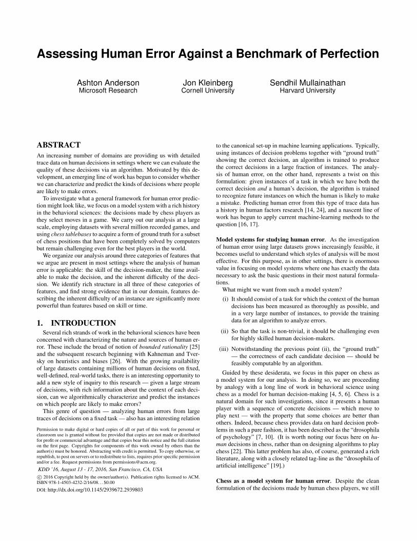
Figure 3: The empirical blunder rate as a function of playerrating, shown for both the (top) GM and (bottom) FICS data.

tially c times more likely to select a non-blunder than a blunder, fora parameter c > 1.

If this were the true process for move selection, then the empiri-cal blunder rate of a position P would be

�

c

(P ) =b(P )

c(n(P )� b(P )) + b(P ).

We will refer to this as the �-value of the position P , with param-eter c. Using the definition of the blunder potential �(P ) to writeb(P ) = �(P )n(P ), we can express the �-value directly as a func-tion of the blunder potential:

�

c

(P ) =�(P )n(P )

c(n(P )� �(P )n(P )) + �(P )n(P )=

�(P )c� (c� 1)�(P )

.

We can now find the value of c for which �

c

(P ) best approximatesthe empirical curves in Figure 2. The best-fit values of c are c ⇡ 15for the FICS data and c ⇡ 100 for the GM data, again reflecting theskill difference between the two domains. These curves are shownsuperimposed on the empirical plot in the figure (on the right, withlogarithmic y-axes).

We note that in game-theoretic terms the �-value can be viewedas a kind of quantal response [20], in which players in a game se-lect among alternatives with a probability that decreases accordingto a particular function of the alternative’s payoff. Since the mini-max value of the position corresponds to the game-theoretic payoffof the game in our case, a selection rule that probabilistically favorsnon-blunders over blunders can be viewed as following this princi-ple. (We note that our functional form cannot be directly mappedonto standard quantal response formulations. The standard formu-lations are strictly monotonically decreasing in payoff, whereas wehave cases where two different blunders can move the minimaxvalue by different amounts — in particular, when a win changesto a draw versus a win changes to a loss — and we treat these thesame in our simple formulation of the �-value.)

●

●●●

●

●

●

●

●

●●

●

●

●

●

●

●●

●

●

●

●

●

●

●

●●●

●

●

●

●

●●

●

●

●

●

●

●●

●

●

●

●

0.000

0.025

0.050

0.075

0.100

2300 2400 2500 2600 2700

Skill (Elo rating)

Empi

rical

blu

nder

rate

Blunderpotential●

●

●

●

●

●

●

●

●

0.10.20.30.40.50.60.70.80.9

●

●

●

●●

●

●

●

●

●●

●●

●

●●

●

●

●

●

●●

●

●

●

●

●●

●

●

●●

●

●

●

●

●●

●

●

●

●

●

●

●

●

●

●

●

●

●●

●

●●

●

●

●

●

●

●

●

●

0.0

0.1

0.2

1200 1400 1600 1800

Skill (Elo rating)

Empi

rical

blu

nder

rate

Blunderpotential●

●

●

●

●

●

●

●

●

0.10.20.30.40.50.60.70.80.9

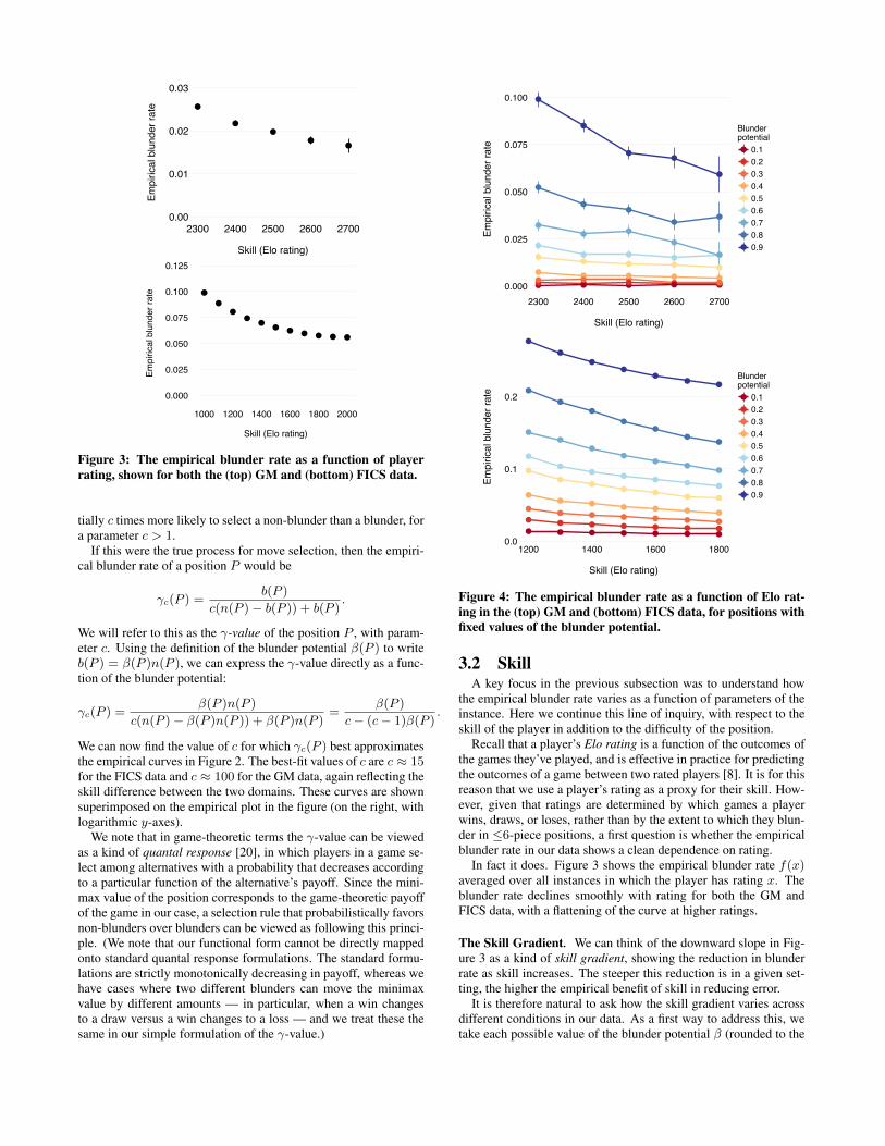
Figure 4: The empirical blunder rate as a function of Elo rat-ing in the (top) GM and (bottom) FICS data, for positions withfixed values of the blunder potential.

3.2 SkillA key focus in the previous subsection was to understand how

the empirical blunder rate varies as a function of parameters of theinstance. Here we continue this line of inquiry, with respect to theskill of the player in addition to the difficulty of the position.

Recall that a player’s Elo rating is a function of the outcomes ofthe games they’ve played, and is effective in practice for predictingthe outcomes of a game between two rated players [8]. It is for thisreason that we use a player’s rating as a proxy for their skill. How-ever, given that ratings are determined by which games a playerwins, draws, or loses, rather than by the extent to which they blun-der in 6-piece positions, a first question is whether the empiricalblunder rate in our data shows a clean dependence on rating.

In fact it does. Figure 3 shows the empirical blunder rate f(x)averaged over all instances in which the player has rating x. Theblunder rate declines smoothly with rating for both the GM andFICS data, with a flattening of the curve at higher ratings.

The Skill Gradient. We can think of the downward slope in Fig-ure 3 as a kind of skill gradient, showing the reduction in blunderrate as skill increases. The steeper this reduction is in a given set-ting, the higher the empirical benefit of skill in reducing error.

It is therefore natural to ask how the skill gradient varies acrossdifferent conditions in our data. As a first way to address this, wetake each possible value of the blunder potential � (rounded to the

●

●●

●

●

●

●

●

●

●

●

●

●●

●●● ●

●

●

●

●

●●●●

●●

●● ●

●

●●

●

●●

●

●●

● ●

●●

●● ●

●●

● ●● ●

● ●

●

●

●●

●●

●●

●●

●

●

● ●

●

2 3

4 5

0.00

0.05

0.10

0.15

0.00

0.05

0.10

0.15

0.20

0.000.050.100.150.20

0.000.050.100.150.20

1200 1400 1600 1800 1200 1400 1600 1800

Skill (Elo rating)

Empi

rical

blu

nder

rate

Number of blunders ● ● ● ●1 2 3 4

Figure 5: The empirical blunder rate as a function of Elorating in the FICS data, for positions with fixed values of(n(P ), b(P )).

nearest multiple of 0.1), and define the function f

�

(x) to be theempirical error rate of players of rating x in positions of blunderpotential �. Figure 4 shows plots of these curves for � equal toeach multiple of 0.1, for both the GM and FICS datasets.

We observe two properties of these curves. First, there is remark-ably little variation among the curves. When viewed on a logarith-mic y-axis the curves are almost completely parallel, indicating thesame rate of proportional decrease across all blunder potentials.

A second, arguably more striking, property is how little the curvesoverlap in their ranges of y-values. In effect, the curves form a kindof “ladder” based on blunder potential: for every value of the dis-cretized blunder potential, every rating in 1200-1800 range on FICShas a lower empirical blunder rate at blunder potential � than thebest of these ratings at blunder potential � + 0.2. In effect, eachadditional 0.2 increment in blunder potential contributes more, av-eraging over all instances, to the aggregate empirical blunder ratethan an additional 600 rating points, despite the fact that 600 ratingpoints represent a vast difference in chess performance. We see asimilar effect for the GM data, where small increases in blunderpotential have a greater effect on blunder rate than the enormousdifference between a rating of 2300 and a rating of 2700. (Indeed,players rated 2700 are making errors at a greater rate in positionsof blunder potential 0.9 than players rated 1200 are making in po-sitions of blunder potential 0.3.) And we see the same effects whenwe separately fix the numerator and denominator that constitute theblunder potential, b(P ) and n(P ), as shown in Figure 5.

To the extent that this finding runs counter to our intuition, itbears an interesting relation to the fundamental attribution error —the tendency to attribute differences in people’s performance to dif-ferences in their individual attributes, rather than to differences inthe situations they face [13]. What we are uncovering here is that abasic measure of the situation — the blunder potential, which as wenoted above corresponds to a measure of the danger inherent in theunderlying chess position — is arguably playing a larger role thanthe players’ skill. This finding also relates to work of Abelson onquantitative measures in a different competitive domain, baseball,where he found that a player’s batting average accounts for verylittle of the variance in their performance in any single at-bat [1].

●

●

●

●

●

●

●

●

●

●

●

●

●

●

●

●

●

●

●

●

●

●

●

●●

●

●

●

●

●

● ●●

●

●

●

●

● ●●

●

●

●●

●

●

●

●

●

●●

●

●

●

●

●

●●

●

●

● ●

●

8/1k6/8/1PK5/8/8/8/8−0 2k5/8/1K6/2P5/8/8/8/8−1 1k6/8/K7/1P6/8/8/8/8−1

1k6/8/1P6/2K5/8/8/8/8−0 8/1k6/8/K7/1P6/8/8/8−0 2k5/8/2P5/2K5/8/8/8/8−0

2k5/8/1P6/2K5/8/8/8/8−1 1k6/8/2P5/1K6/8/8/8/8−1 7k/8/6P1/6K1/8/8/8/8−1

0.10.20.30.40.5

0.25

0.50

0.75

0.2

0.4

0.6

0.8

0.150.200.250.300.350.40

0.0

0.1

0.2

0.3

0.4

0.10

0.15

0.20

0.25

0.2

0.3

0.4

0.5

0.10.20.30.40.5

0.1

0.2

0.3

0.4

0.5

1200 1400 1600 1800 1200 1400 1600 1800 1200 1400 1600 1800

Skill (Elo rating)

Empi

rical

blu

nder

rate

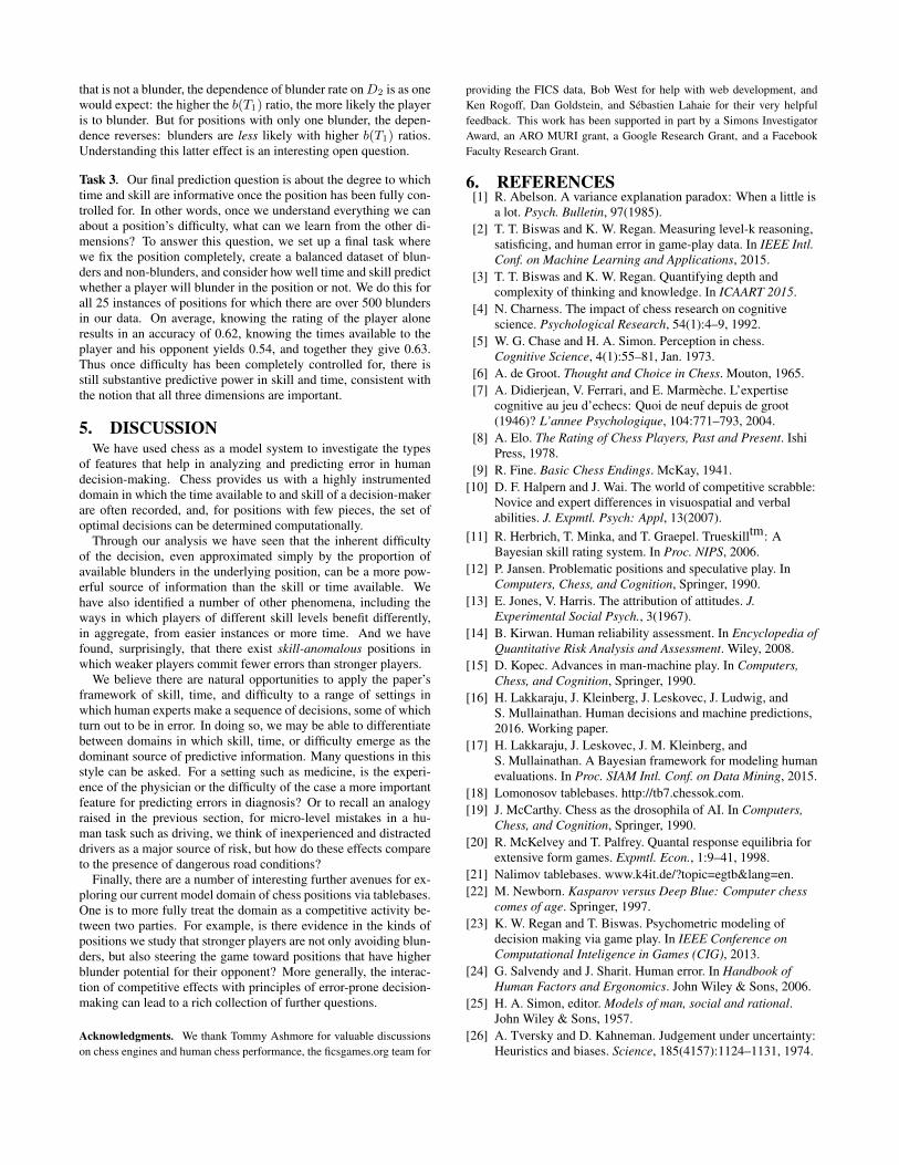
Figure 6: The empirical blunder rate as a function of Elo rat-ing, for a set of frequently-occurring positions.

We should emphasize, however, that despite the strong effect ofblunder potential, skill does play a fundamental role role in ourdomain, as the analysis of this section has shown. And in generalit is important to take multiple types of features into account inany analysis of decision-making, since only certain features may beunder our control in any given application. For example, we maybe able to control the quality of the people we recruit to a decision,even if we can’t control the difficulty of the decision itself.

The Skill Gradient for Fixed Positions. Grouping positions to-gether by common (n(P ), b(P )) values gives us a rough sense forhow the skill gradient behaves in positions of varying difficulty.But this analysis still aggregates together a large number of differ-ent positions, each with their own particular properties, and so itbecomes interesting to ask — how does the empirical blunder ratevary with Elo rating when we fix the exact position on the board?

The fact that we are able to meaningfully ask this question isbased on a fact noted in Section 1, that many non-trivial 6-piecepositions recur in the FICS data, exactly, several thousand times.4

For each such position P , we have enough instances to plot thefunction f

P

(x), the rate of blunders committed by players of ratingx in position P .

Let us say that the function f

P

(x) is skill-monotone if it is de-creasing in x — that is, if players of higher rating have a lowerblunder rate in position P . A natural conjecture would be that ev-ery position P is skill-monotone, but in fact this is not the case.Among the most frequent positions, we find several that we termskill-neutral, with f

P

(x) remaining approximately constant in x, aswell as several that we term skill-anomalous, with f

P

(x) increas-ing in x. Figure 6 shows a subset of the most frequently occurring

4To increase the amount of data we have on each position, we clus-ter together positions that are equivalent by symmetry: we can ap-ply a left-to-right reflection of the board, or we can apply a top-bottom reflection of the board (also reversing the colors of thepieces and the side to move), or we can do both. Each of the fourresulting positions is equivalent under the rules of chess.

●

●● ● ●●●

●

●

●

●

●● ●

●

●

●

●

●●

●

●● ●

●

● ● ●●● ●

0.00

0.02

0.04

0.06

0.08

0.10

0.12

0 10 20 30

Time remaining (sec.)

Empi

rical

blu

nder

rate

Figure 7: The empirical blunder rate as a function of time re-maining.

positions in the FICS data that contains examples of each of thesethree types: skill-monotone, skill-neutral, and skill-anomalous.5

The existence of skill-anomalous positions is surprising, sincethere is a no a priori reason to believe that chess as a domain shouldcontain common situations in which stronger players make moreerrors than weaker players. Moreover, the behavior of players inthese particular positions does not seem explainable by a strategyin which they are deliberately making a one-move blunder for thesake of the overall game outcome. In each of the skill-anomalousexamples in Figure 6, the player to move has a forced win, and theposition is reduced enough that the worst possible game outcomefor them is a draw under any sequence of moves, so there is nolong-term value in blundering away the win on their present move.

3.3 TimeFinally, we consider our third category of features, the time that

players have available to make their moves. Recall that playershave to make their own decisions about how to allocate a fixed bud-get of time across a given number of moves or the rest of the game.The FICS data has information about the time remaining associatedwith each move in each game, so we focus our analysis on FICS inthis subsection. Specifically, as noted in Section 2, FICS gamesare generally played under extremely rapid conditions, and for uni-formity in the analysis we focus on the most commonly-occurringFICS time constraint — the large subset of games in which eachplayer is allocated 3 minutes for the whole game.

As a first object of study, let’s define the function g(t) to be theempirical blunder rate in positions where the player begins consid-ering their move with t seconds left in the game. Figure 7 showsa plot of g(t); it is natural that the blunder rate increases sharplyas t approaches 0, though it is notable how flat the value of g(t)becomes once t exceeds roughly 10 seconds.

The Time Gradient. This plot in Figure 7 can be viewed as abasic kind of time gradient, analogous to the skill gradient, showingthe overall improvement in empirical blunder rate that arises fromhaving extra time available. Here too we can look at how the timegradient restricted to positions with fixed blunder potential, or fixedblunder potential and player rating.

We start with Figure 8, which shows g�

(t), the blunder rate forplayers within a narrow skill range (1500-1599 Elo) with t secondsremaining in positions with blunder potential �. In this sense, it isa close analogue of Figure 4, which plotted f

�

(x), and for values

5For readers interested in looking at the exact positions in question,each position in Figure 6 is described in Forsyth-Edwards notation(FEN) above the panel in which its plot appears.

● ● ●

● ●●

●

●●

●

●

●

●

●●

●

●

●

●

●

● ●●

●●

●

●

●

●

●

●

●

● ●

● ●

●

●

●

●

●

●

●

●

●

●● ●

●

●

●

●

●

●

●

●

●●

●

●

●

●

●

●

●

●

●

●

●

●

●

●

●

●

●

●

●

●

●

●

●

● ●

●

●

●

●

●

●

●

0.0

0.1

0.2

0.3

[0,2

]

(2,5

]

(5,8

]

(8,1

2]

(12,

17]

(17,

24]

(24,

32]

(32,

43]

(43,

59]

(59,

176]

Time remaining (sec.)

Empi

rical

blu

nder

rate

Blunderpotential●

●

●

●

●

●

●

●

●

0.10.20.30.40.50.60.70.80.9

Figure 8: The empirical blunder rate as a function of the timeremaining, for positions with fixed blunder potential values.

of t above 8 seconds, it shows a very similar “ladder” structure inwhich the role of blunder potential is dominant. Specifically, forevery �, players are blundering at a lower rate with 8 to 12 secondsremaining at blunder potential � than they are with over a minuteremaining at blunder potential �+0.2. A small increase in blunderpotential has a more extensive effect on blunder rate than a largeincrease in available time.

We can separate the instances further both by blunder potentialand by the rating of the player, via the function g

�,x

(t) which givesthe empirical blunder rate with t seconds remaining when restrictedto players of rating x in positions of blunder potential �. Figure 9plots these functions, with a fixed value of � in each panel. We cancompare curves for players of different rating, observing that forhigher ratings the curves are steeper: extra time confers a greaterrelative empirical benefit on higher-rated players. Across panels,we see that for higher blunder potential the curves become some-what shallower: more time provides less relative improvement asthe density of possible blunders proliferates. But equally or morestriking is the fact that all curves retain a roughly constant shape,even as the empirical blunder rate climbs by an order of magnitudefrom the low ranges of blunder potential to the highest.

Comparing across points in different panels helps drive home therole of blunder potential even when considering skill and time si-multaneously. Consider for example (a) instances in which playersrated 1200 (at the low end of the FICS data) with 5-8 seconds re-maining face a position of blunder potential 0.4, contrasted with(b) instances in which players rated 1800 (at the high end of theFICS data) with 42-58 seconds remaining face a position of blun-der potential 0.8. As the figure shows, the empirical blunder rateis lower in instances of type (a) — a weak player in extreme timepressure is making blunders at a lower rate because they’re dealingwith positions that contain less danger.

Time Spent on a Move. Thus far we’ve looked at how the empir-ical blunder rate depends on the amount of time remaining in thegame. However, we can also ask how the probability of a blundervaries with the amount of time the player actually spends consider-ing their move before playing it. When a player spends more timeon a move, should we predict they’re less likely to blunder (becausethey gave the move more consideration) or more likely to blunder(because the extra time suggests they didn’t know what do)?

●

●● ● ●

●

●

●●

●

●●

● ● ●

●

● ●●

●

●

●

●

● ●

●

●

●● ●

●

●

●●

●

● ●

●

● ●●

●● ●

●

●

●●

●

●

●

●

●

●●

●

●● ● ●●

●

●

●

●

● ●● ●● ●

●

● ●

●

●●

●

●

●

●

●

●● ●

●

●

●●

●

●

●

● ● ●

●

●●

●

●

●

●

●●●

●

●●

● ●●

●

●

●

●

●

●

●

●●

●

●

●

●● ●

●

●

●

●

●●

●

●

●

●

●●

●

●

●

●

●●

●●

●●

●

●●● ●●

●

●

●

●

●●

●

●●

●●

●●

●

●

●

●●

●●

●

●

●●

●

●●

●●

●

●

●● ●

●

●

●●

●●

●

●●

●

●●

●

●

●

●

● ●●

●

●

●

●●

●

●

●

● ●●

●●●

●

●

●

●

●

●●●

●

●●

●

●● ●

●

● ● ●●

●

●

●●●●

●

●

●

●

● ●

●

●

●

●

●●●

●

● ●●

●

●●

●

●

●

●●

●

●

●

●●●●

●

0.2 0.4

0.6 0.8

0.00

0.02

0.04

0.06

0.00

0.04

0.08

0.12

0.00

0.05

0.10

0.15

0.20

0.0

0.1

0.2

0.3

[0,2

](2

,5]

(5,8

](8

,12]

(12,

17]

(17,

23]

(23,

31]

(31,

42]

(42,

58]

(58,

176]

[0,2

](2

,5]

(5,8

](8

,12]

(12,

17]

(17,

23]

(23,

31]

(31,

42]

(42,

58]

(58,

176]

Time remaining (sec.)

Empi

rical

blu

nder

rate

Elo●

●

●

●

●

●

●12001300

14001500

16001700

1800

Figure 9: The empirical blunder rate as a function of time re-maining, fixing the blunder potential and player rating.

The data turns out to be strongly consistent with the latter view:the empirical blunder rate is higher in aggregate for players whospend more time playing a move. We find that this property holdsacross the range of possible values for the time remaining and theblunder potential, as well as when we fix the specific position.

4. PREDICTIONWe’ve now seen how the empirical blunder rate depends on our

three fundamental dimensions: difficulty, the skill of the player,and the time available to them. We now turn to a set of tasks thatallow us to further study the predictive power of these dimensions.

4.1 Greater Tree DepthIn order to formulate our prediction methods for blunders, we

first extend the set of features available for studying the difficultyof a position. Once we have these additional features, we will beprepared to develop the predictions themselves.

Thus far, when we’ve considered a position’s difficulty, we’veused information about the player’s immediate moves, and then in-voked a tablebase to determine the outcome after these immedi-ate moves. We now ask whether it is useful for our task to con-sider longer sequences of moves beginning at the current position.Specifically, if we consider all d-move sequences beginning at thecurrent position, we can organize these into a game tree of depth d

with the current position P as the root, and nodes representing thestates of the game after each possible sequence of j d moves.Chess engines use this type of tree as their central structure in de-termining which moves to make; it is less obvious, however, howto make use of these trees in analyzing blunders by human players,given players’ imperfect selection of moves even at depth 1.

Let us introduce some notation to describe how we use this in-formation. Suppose our instance consists of position P , with n

legal moves, of which b are blunders. We will denote the moves by

m1,m2, ...,mn

, leading to positions P1, P2, . . . , Pn

respectively,and we’ll suppose they are indexed so that m1,m2, . . . ,mn�b

arethe non-blunders, and m

n�b+1, . . . ,mn

are the blunders. We writeT0 for the indices of the non-blunders {1, 2, . . . , n� b} and T1 forthe indices of the blunders {n� b+ 1, . . . , n}. Finally, from eachposition P

i

, there are n

i

legal moves, of which b

i

are blunders.The set of all pairs (n

i

, b

i

) for i = 1, 2, . . . , n constitutes a po-tentially useful source of information in the depth-2 game tree fromthe current position. What might it tell us?

First, suppose that position P

i

, for i 2 T1, is a position reachablevia a blunder m

i

. Then if the blunder potential �(Pi

) = b

i

/n

i

islarge, this means that it may be challenging for the opposing playerto select a move that capitalizes on the blunder m

i

made at theroot position P ; there is a reasonable chance that the opposing willinstead blunder, restoring the minimax value to something larger.This, in turn, means that it may be harder for the player in the rootposition of our instance to see that move m

i

, leading to positionP

i

, is in fact a blunder. The conclusion from this reasoning is thatwhen the blunder potentials of positions P

i

for i 2 T1 are large, itsuggests a larger empirical blunder rate at P .

It is less clear what to conclude when there are large blunderpotentials at positions P

i

for i 2 T0 — positions reachable bynon-blunders. Again, it suggests that player at the root may have aharder time correctly evaluating the positions P

i

for i 2 T0; if theyappear better than they are, it could lead the player to favor thesenon-blunders. On the other hand, the fact that these positions arehard to evaluate could also suggest a general level of difficulty inevaluating P , which could elevate the empirical blunder rate.

There is also a useful aggregation of this information, as follows.If we define b(T1) =

Pi2T1

b

i

and n(T1) =P

i2T1n

i

, and anal-ogously for b(T0) and n(T0), then the ratio �1 = b(T1)/n(T1) isa kind of aggregate blunder potential for all positions reachable byblunders, and analogously for �0 = b(T0)/n(T0) with respect topositions reachable by non-blunders.

In the next subsection, we will see that the four quantities b(T1),n(T1), b(T0), n(T0) indeed contain useful information for predic-tion, particularly when looking at families of instances that havethe same blunder potential at the root position P . We note that onecan construct analogous information at greater depths in the gametree, by similar means, but we find in the next subsection that thesedo not currently provide improvements in prediction performance,so we do not discuss greater depths further here.

4.2 Prediction ResultsWe develop three nested prediction tasks: in the first task we

make predictions about an unconstrained set of instances; in thesecond we fix the blunder potential at the root position; and in thethird we control for the exact position.

Task 1. In our first task we formulate the basic error-predictionproblem: we have a large collection of human decisions for whichwe know the correct answer, and we want to predict whether thedecision-maker will err or not. In our context, we predict whetherthe player to move will blunder, given the position they face and thevarious features of it we have derived, how much time they have tothink, and their skill level. In the process, we seek to understandthe relative value of these features for prediction in our domain.

We restrict our attention to the 6.6 million instances that oc-curred in the 320,000 empirically most frequent positions in theFICS dataset. Since the rate of blundering is low in general, wedown-sample the non-blunders so that half of our remaining in-stances are blunders and the other half are non-blunders. This re-sults in a balanced dataset with 600,000 instances, and we evaluate

Feature Description

�(P ) Blunder potential (b(P )/n(P ))a(P ), b(P ) # of non-blunders, # of blundersa(T0), b(T0) # of non-blunders and blunders available to

opponent following a non-blundera(T1), b(T1) # of non-blunders and blunders available to

opponent following a blunder�0(P ) Opponent’s aggregate � after a non-blunder�1(P ) Opponent’s aggregate � after a blunderElo, Opp-elo Player ratings (skill level)t Amount of time player has left in game

Table 1: Features for blunder prediction.

model performance with accuracy. For ease of interpretation, weuse both logistic regression and decision trees. Since the relativeperformance of these two classifiers is virtually identical, but deci-sion trees perform slightly better, we only report the results usingdecision trees here.

Table 1 defines the features we use for prediction. In additionthe notation defined thus far, we define: S = {Elo,Opp-elo} tobe the skill features consisting of the rating of the player and theopponent; a(P ) = n(P )�b(P ) for the number of non-blunders inposition P ; D1 = {a(P ), b(P ),�(P )} to be the difficulty featuresat depth 1; D2 = {a(T0), b(T0), a(T1), b(T1),�0(P ),�1(P )} asthe difficulty features at depth 2 defined in the previous subsection;and t as the time remaining.

In Table 2, we show the performance of various combinations ofour features. The most striking result is how dominant the diffi-culty features are. Using all of them together gives 0.75 accuracyon this balanced dataset, halfway between random guessing andperfect performance. In comparison, skill and time are much lessinformative on this task. The skill features S only give 55% ac-curacy, time left t yields 53% correct predictions, and neither addspredictive value once position difficulty features are in the model.

The weakness of the skill and time features is consistent with ourfindings in Section 3, but still striking given the large ranges overwhich the Elo ratings and time remaining can extend. In particular,a player rated 1800 will almost always defeat a player rated 1200,yet knowledge of rating is not providing much predictive power indetermining blunders on any individual move. Similarly, a playerwith 10 seconds remaining in the entire game is at an enormousdisadvantage compared to a player with two minutes remaining,but this too is not providing much leverage for blunder predictionat the move level. While these results only apply to our particulardomain, it suggests a genre of question that can be asked by analogyin many domains. (To take one of many possible examples, onecould similarly ask about the error rate of highly skilled drivers indifficult conditions versus bad drivers in safe conditions.)

Another important result is that most of the predictive powercomes from depth 1 features of the tree. This tells us the immediatesituation facing the player is by far the most informative feature.

Finally, we note that the prediction results for the GM data (wherewe do not have time information available) are closely analogous;we get a slightly higher accuracy of 0.77, and again it comes en-tirely from our basic set of difficulty features for the position.

Human Performance on a Version of Task 1. Given the accuracyof algorithms for Task 1, it is natural to consider how this comparesto the performance of human chess players on such a task.

To investigate this question, we developed a version of Task 1as a web app quiz and promoted it on two popular Internet chess

Model Accuracy

Random guessing 0.50�(P ) 0.73D1 0.73D2 0.72D1 [D2 0.75S 0.55S [D1 [D2 0.75{t} 0.53{t} [D1 [D2 0.75S [ {t} [D1 [D2 0.75

Table 2: Accuracy results on Task 1.

forums. Each quiz question provided a pair of 6-piece instanceswith White to move, each showing the exact position on the board,the ratings of the two players, and the time remaining for each. Thetwo instances were chosen from the FICS data with the propertythat White blundered in one of them and not the other, and the quizquestion was to determine in which instance White blundered.

In this sense, the quiz is a different type of chess problem fromthe typical style, reflecting the focus of our work here: rather than“White to play and win,” it asked “Did White blunder in this posi-tion?”. Averaging over approximately 6000 responses to the quizfrom 720 participants, we find an accuracy of 0.69, non-triviallybetter than random guessing but also non-trivially below our model’sperformance of 0.79.6

The relative performance of the prediction algorithm and the hu-man forum participants forms an interesting contrast, given that thehuman participants were able to use domain knowledge about prop-erties of the exact chess position while the algorithm is achievingalmost its full performance from a single number – the blunder po-tential — that draws on a tablebase for its computation. We alsoinvestigated the extent to which the guesses made by human par-ticipants could be predicted by an algorithm; our accuracy on thiswas in fact lower than for the blunder-prediction task itself, withthe blunder potential again serving as the most important featurefor predicting human guesses on the task.

Task 2. Given how powerful the depth 1 features are, we now con-trol for b(P ) and n(P ) and investigate the predictive performanceof our features once blunder potential has been fixed. Our strat-egy on this task is very similar to before: we compare differentgroups of features on a binary classification task and use accuracyas our measure. These groups of features are: D2, S, S [D2, {t},{t}[D2, and the full set S [ {t}[D2. For each of these models,we have an accuracy score for every (b(P ), n(P )) pair. The rela-tive performances of the models are qualitatively similar across all(b(P ), n(P )) pairs: again, position difficulty dominates time andrating, this time at depth 2 instead of depth 1. In all cases, the per-formance of the full feature set is best (the mean accuracy is 0.71),but D2 alone achieves 0.70 accuracy on average. This further un-derscores the importance of position difficulty.

Additionally, inspecting the decision tree models reveals a veryinteresting dependence of the blunder rate on the depth 1 structureof the game tree. First, recall that the most frequently occurring po-sitions in our datasets have either b(P ) = 1 or b(P ) = n(P ) � 1.In so-called “only-move” situations, where there is only one move6Note that the model performs slightly better here than in our basicformulation of Task 1, since there instances were not presented inpairs but simply as single instances drawn from a balanced distri-bution of positive and negative cases.

that is not a blunder, the dependence of blunder rate on D2 is as onewould expect: the higher the b(T1) ratio, the more likely the playeris to blunder. But for positions with only one blunder, the depen-dence reverses: blunders are less likely with higher b(T1) ratios.Understanding this latter effect is an interesting open question.

Task 3. Our final prediction question is about the degree to whichtime and skill are informative once the position has been fully con-trolled for. In other words, once we understand everything we canabout a position’s difficulty, what can we learn from the other di-mensions? To answer this question, we set up a final task wherewe fix the position completely, create a balanced dataset of blun-ders and non-blunders, and consider how well time and skill predictwhether a player will blunder in the position or not. We do this forall 25 instances of positions for which there are over 500 blundersin our data. On average, knowing the rating of the player aloneresults in an accuracy of 0.62, knowing the times available to theplayer and his opponent yields 0.54, and together they give 0.63.Thus once difficulty has been completely controlled for, there isstill substantive predictive power in skill and time, consistent withthe notion that all three dimensions are important.

5. DISCUSSIONWe have used chess as a model system to investigate the types

of features that help in analyzing and predicting error in humandecision-making. Chess provides us with a highly instrumenteddomain in which the time available to and skill of a decision-makerare often recorded, and, for positions with few pieces, the set ofoptimal decisions can be determined computationally.

Through our analysis we have seen that the inherent difficultyof the decision, even approximated simply by the proportion ofavailable blunders in the underlying position, can be a more pow-erful source of information than the skill or time available. Wehave also identified a number of other phenomena, including theways in which players of different skill levels benefit differently,in aggregate, from easier instances or more time. And we havefound, surprisingly, that there exist skill-anomalous positions inwhich weaker players commit fewer errors than stronger players.

We believe there are natural opportunities to apply the paper’sframework of skill, time, and difficulty to a range of settings inwhich human experts make a sequence of decisions, some of whichturn out to be in error. In doing so, we may be able to differentiatebetween domains in which skill, time, or difficulty emerge as thedominant source of predictive information. Many questions in thisstyle can be asked. For a setting such as medicine, is the experi-ence of the physician or the difficulty of the case a more importantfeature for predicting errors in diagnosis? Or to recall an analogyraised in the previous section, for micro-level mistakes in a hu-man task such as driving, we think of inexperienced and distracteddrivers as a major source of risk, but how do these effects compareto the presence of dangerous road conditions?

Finally, there are a number of interesting further avenues for ex-ploring our current model domain of chess positions via tablebases.One is to more fully treat the domain as a competitive activity be-tween two parties. For example, is there evidence in the kinds ofpositions we study that stronger players are not only avoiding blun-ders, but also steering the game toward positions that have higherblunder potential for their opponent? More generally, the interac-tion of competitive effects with principles of error-prone decision-making can lead to a rich collection of further questions.

Acknowledgments. We thank Tommy Ashmore for valuable discussionson chess engines and human chess performance, the ficsgames.org team for

providing the FICS data, Bob West for help with web development, andKen Rogoff, Dan Goldstein, and Sébastien Lahaie for their very helpfulfeedback. This work has been supported in part by a Simons InvestigatorAward, an ARO MURI grant, a Google Research Grant, and a FacebookFaculty Research Grant.

6. REFERENCES[1] R. Abelson. A variance explanation paradox: When a little is

a lot. Psych. Bulletin, 97(1985).[2] T. T. Biswas and K. W. Regan. Measuring level-k reasoning,

satisficing, and human error in game-play data. In IEEE Intl.Conf. on Machine Learning and Applications, 2015.

[3] T. T. Biswas and K. W. Regan. Quantifying depth andcomplexity of thinking and knowledge. In ICAART 2015.

[4] N. Charness. The impact of chess research on cognitivescience. Psychological Research, 54(1):4–9, 1992.

[5] W. G. Chase and H. A. Simon. Perception in chess.Cognitive Science, 4(1):55–81, Jan. 1973.

[6] A. de Groot. Thought and Choice in Chess. Mouton, 1965.[7] A. Didierjean, V. Ferrari, and E. Marmèche. L’expertise

cognitive au jeu d’echecs: Quoi de neuf depuis de groot(1946)? L’annee Psychologique, 104:771–793, 2004.

[8] A. Elo. The Rating of Chess Players, Past and Present. IshiPress, 1978.

[9] R. Fine. Basic Chess Endings. McKay, 1941.[10] D. F. Halpern and J. Wai. The world of competitive scrabble:

Novice and expert differences in visuospatial and verbalabilities. J. Expmtl. Psych: Appl, 13(2007).

[11] R. Herbrich, T. Minka, and T. Graepel. Trueskilltm: ABayesian skill rating system. In Proc. NIPS, 2006.

[12] P. Jansen. Problematic positions and speculative play. InComputers, Chess, and Cognition, Springer, 1990.

[13] E. Jones, V. Harris. The attribution of attitudes. J.Experimental Social Psych., 3(1967).

[14] B. Kirwan. Human reliability assessment. In Encyclopedia ofQuantitative Risk Analysis and Assessment. Wiley, 2008.

[15] D. Kopec. Advances in man-machine play. In Computers,Chess, and Cognition, Springer, 1990.

[16] H. Lakkaraju, J. Kleinberg, J. Leskovec, J. Ludwig, andS. Mullainathan. Human decisions and machine predictions,2016. Working paper.

[17] H. Lakkaraju, J. Leskovec, J. M. Kleinberg, andS. Mullainathan. A Bayesian framework for modeling humanevaluations. In Proc. SIAM Intl. Conf. on Data Mining, 2015.

[18] Lomonosov tablebases. http://tb7.chessok.com.[19] J. McCarthy. Chess as the drosophila of AI. In Computers,

Chess, and Cognition, Springer, 1990.[20] R. McKelvey and T. Palfrey. Quantal response equilibria for

extensive form games. Expmtl. Econ., 1:9–41, 1998.[21] Nalimov tablebases. www.k4it.de/?topic=egtb&lang=en.[22] M. Newborn. Kasparov versus Deep Blue: Computer chess

comes of age. Springer, 1997.[23] K. W. Regan and T. Biswas. Psychometric modeling of

decision making via game play. In IEEE Conference onComputational Inteligence in Games (CIG), 2013.

[24] G. Salvendy and J. Sharit. Human error. In Handbook ofHuman Factors and Ergonomics. John Wiley & Sons, 2006.

[25] H. A. Simon, editor. Models of man, social and rational.John Wiley & Sons, 1957.

[26] A. Tversky and D. Kahneman. Judgement under uncertainty:Heuristics and biases. Science, 185(4157):1124–1131, 1974.