Hindawi Publishing CorporationInternational Journal of Forestry ResearchVolume 2012, Article ID 961576, 8 pagesdoi:10.1155/2012/961576

Research Article

Assessing Forest Production Using Terrestrial Monitoring Data

Hubert Hasenauer and Chris S. Eastaugh

Department of Forest and Soil Sciences, Institute of Silviculture, BOKU University of Natural Resources and Life Sciences,Vienna, Peter Jordan Street 82, A-1190 Vienna, Austria

Correspondence should be addressed to Hubert Hasenauer, hubert.hasenauer@boku.ac.at

Received 20 October 2011; Revised 12 December 2011; Accepted 5 January 2012

Academic Editor: Timo Pukkala

Copyright © 2012 H. Hasenauer and C. S. Eastaugh. This is an open access article distributed under the Creative CommonsAttribution License, which permits unrestricted use, distribution, and reproduction in any medium, provided the original work isproperly cited.

Accurate assessments of forest biomass are becoming an increasingly important aspect of natural resource management. Besidestheir use in sustainable resource usage decisions, a growing focus on the carbon sequestration potential of forests means thatassessment issues are becoming important beyond the forest sector. Broad scale inventories provide much-needed information,but interpretation of growth from successive measurements is not trivial. Even using the same data, various interpretation methodsare available. The mission of this paper is to compare the results of fixed-plot inventory designs and angle-count inventories withdifferent interpretation methods. The inventory estimators that we compare are in common use in National Forest Inventories. Nomethod should be described as “right” or “wrong”, but users of large-scale inventory data should be aware of the possible errorsand biases that may be either compensated for or magnified by their choice of interpretation method. Wherever possible, severalinterpretation methods should be applied to the same dataset to assess the possibility of error.

1. Introduction

National forest inventories are an expensive and time-consuming operation, particularly in large, remote, andinhospitable regions. There is therefore great interest inalternative measures to estimate forest growth, such asremote sensing [1] or mechanistic process modeling [2].These methods, however, are not a direct measurement ofthe same physical characteristics as in an inventory, andit is reasonable to suggest that estimates made with thesealternatives should be shown to be unbiased with referenceto ground data.

In the near future, national forest inventories will forman integral part of the way that many nations determine theirnational carbon balance, and inventories are used to estimateforest increment as a means of monitoring their value asa carbon sink. Relatively minor errors in current standingvolume estimates may have little practical or policy impact,but these may translate to substantial errors and biases inthe estimate of forest increment. In some cases, these biasesmay mean the difference between forest areas being assessedas a sink or a source of CO2 or could result in erroneous

(but substantial) financial penalties to countries signing upto successor agreements to the Kyoto protocol. Conversely,countries may claim carbon credits for a degree of forestsequestration that does not in fact exist.

Until recently, inventories were conducted solely as ameans of measuring the timber resource present in a region,generally in order to determine its immediate extractivecapacity. The inventories were optimized to most efficientlyestimate a particular forest parameter, current standingvolume. This was and still is important, as it describesa crucial aspect of forested landscapes. The carbon sinkstrength of forests is not, however, directly related to standingvolume, but is a function of forest increment. Mathemati-cally, increment is simply the difference in standing volumebetween two periods, plus the volume of any removals fromthe growing stock. In practice however this is not so simple,as sample designs or locations may vary between increments,forest area may change and some inventory designs use anonadditive method of increment estimation (where, at theindividual plot level, increment does not equal the differencein standing volumes) [3].

2 International Journal of Forestry Research

In recent decades, regular forest inventories have beenestablished in many countries using a permanent plot designto reduce the sampling error of the resulting incrementcalculations [4]. Remeasurement intervals range from 5 to 10years and either fixed area plots or angle-count sampling [5]may be used. In the latter case, three common methods maybe applied to repeated measurements in order to estimateforest increment: the difference, starting value or end-valuemethods. Upscaling plot-level increments from fixed-plotinventories or using any three of the angle-count estimationmethods produces mathematically unbiased estimates ofincrement [6–8]. It has been shown, however, that mea-surement error affects the various estimators differently, andthus different estimators will produce different results [6]. Ithas been suggested that comparing the results of differentestimators can indicate the presence of measurement errorand thus be used as an inventory auditing tool [6, 9].

In a theoretical simulation study using plausible esti-mates of measurement errors Eastaugh and Hasenauer [6]reported possible biases in angle count-derived incrementestimates of up to ±0.4–1.0 m3/ha/yr when averaged over30 years, depending on the nature of the error and theestimation method used. The key findings of that study werethat errors can result in different magnitudes of incrementbias and may manifest in the either the period in whichthe error occurred or in subsequent periods, depending onthe increment estimation method used. Thomas and Roesch[9] applied different interpretation methods to large-scaleinventory data from the southern United States and foundthat an up to 48% difference in increment estimation waspresent between methods, which they attributed to treesbeing missed (not counted) in the first inventory period.The Eastaugh and Hasenauer [6] study found that a 44.3%increment difference could result from inventories errors thatgave rise to an only 4.6% error in volume estimation.

Applying several methods to the same dataset can,however, give substantially different results due to samplingvariation, even in the absence of error. The different resultsare all equally valid estimators, but precision may be poorif relatively few plots are sampled. In such cases, it maybe difficult to determine which (if either) of the estimatorsmay be error affected and doubts can be raised over whichestimated value should be accepted. Similarly, if inventorydata is to be used as a baseline to compare against modeledor remote-sensed estimates of forest characteristics, then itis important to first ensure the integrity of the inventoryestimate. This can be done by applying more than oneestimation method and ensuring that the final results arewithin a predetermined range of each other.

In this study, we mimic a large scale forest inventorythrough simulating 12 000 fixed area and angle countsamples inside a large long term forest monitoring plotat Hirschlacke in northern Austria, over 7 measurementperiods from 1977 to 2007. We are interested in how sucherrors may be detectable in mean increment estimates withhigh variance. Our primary purpose is to confirm the non-biased nature of each of the increment estimators in theabsence of measurement error and determine the minimum

50 100 150 200 250 300

50

100

150

200

250

300

“y”

coor

din

ate

(met

res)

“x” coordinate (metres)

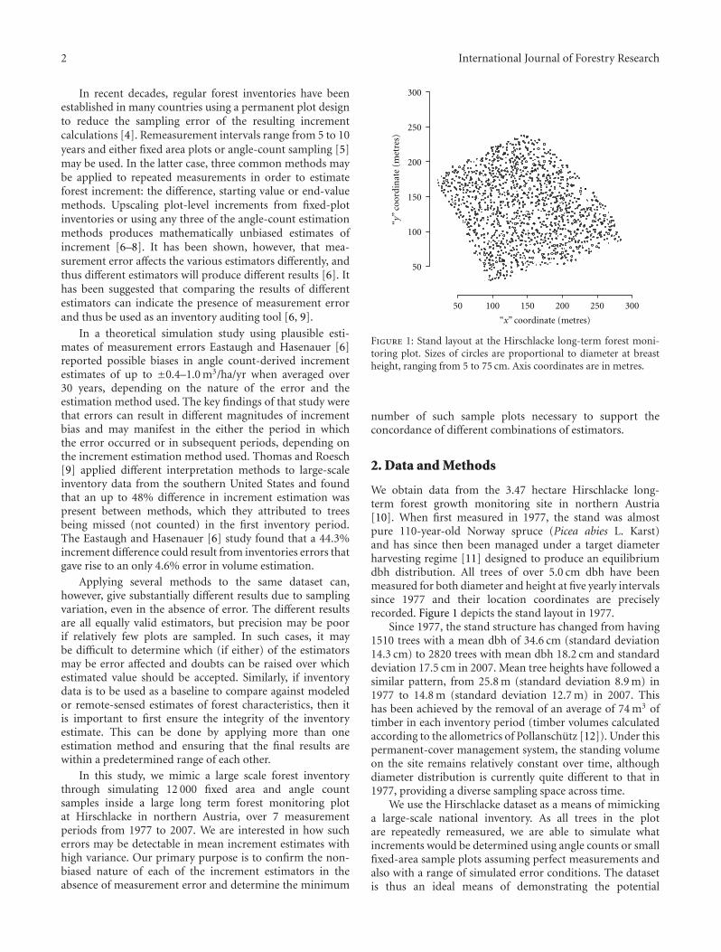
Figure 1: Stand layout at the Hirschlacke long-term forest moni-toring plot. Sizes of circles are proportional to diameter at breastheight, ranging from 5 to 75 cm. Axis coordinates are in metres.

number of such sample plots necessary to support theconcordance of different combinations of estimators.

2. Data and Methods

We obtain data from the 3.47 hectare Hirschlacke long-term forest growth monitoring site in northern Austria[10]. When first measured in 1977, the stand was almostpure 110-year-old Norway spruce (Picea abies L. Karst)and has since then been managed under a target diameterharvesting regime [11] designed to produce an equilibriumdbh distribution. All trees of over 5.0 cm dbh have beenmeasured for both diameter and height at five yearly intervalssince 1977 and their location coordinates are preciselyrecorded. Figure 1 depicts the stand layout in 1977.

Since 1977, the stand structure has changed from having1510 trees with a mean dbh of 34.6 cm (standard deviation14.3 cm) to 2820 trees with mean dbh 18.2 cm and standarddeviation 17.5 cm in 2007. Mean tree heights have followed asimilar pattern, from 25.8 m (standard deviation 8.9 m) in1977 to 14.8 m (standard deviation 12.7 m) in 2007. Thishas been achieved by the removal of an average of 74 m3 oftimber in each inventory period (timber volumes calculatedaccording to the allometrics of Pollanschutz [12]). Under thispermanent-cover management system, the standing volumeon the site remains relatively constant over time, althoughdiameter distribution is currently quite different to that in1977, providing a diverse sampling space across time.

We use the Hirschlacke dataset as a means of mimickinga large-scale national inventory. As all trees in the plotare repeatedly remeasured, we are able to simulate whatincrements would be determined using angle counts or smallfixed-area sample plots assuming perfect measurements andalso with a range of simulated error conditions. The datasetis thus an ideal means of demonstrating the potential

International Journal of Forestry Research 3

biases that may be apparent in angle-count-based inventoriescontaining error [6], or in this study, comparing the resultsof different increment estimation methods.

We construct a pattern of 12 000 points at a 1 × 1 meterspacing within the Hirschlacke plot, such that no point iswithin 30 meters of the plot boundary. We then simulate afixed area plot of 200 m2 and an angle-count sample witha basal area factor of 4 at each point in each of the sevenmeasurement periods. This mimics the plot size used as partof the Swiss National Forest Inventory [13] and the basal areafactor used in Austria [14].

Increments are estimated four ways.

(1) Differences between time 1 and time 2 volumesdetermined from fixed-area plots, plus removals(fixed-plot method).

(2) Differences between time 1 and time 2 volumesdetermined from angle-count plots, plus removals(difference method).

(3) The recorded increment of the trees within the angle-count sample multiplied by the estimated numberof trees of that size in the stand in time 1, plus thevolume of the new trees entering the stand. (startingvalue method).

(4) The recorded increment of the trees within the angle-count sample multiplied by the estimated numberof trees of that size in the stand in time 2. (endvalue method). This method requires the estimationof prior dimensions of trees which (in a practicalinventory situation) may not have been recorded attime 1.

Much of the published literature on deriving incre-ments from angle-count sampling distinguishes between“survivors”, “ingrowth”, “ongrowth”, and “nongrowth” trees(cf. Martin 1982 [15]), depending on whether they wereabove or below a particular diameter at breast height in theperiod preceding the current measuring period and whetherthey were counted “in” or “out” of the angle count in thepreceding period (Table 1).

Defining the following variables.

Z = volume increment per hectare, with superscripts Ffor fixed are plots, D for difference method, S forstarting value method, and E for end value method;

m = Number of sample plots;

nj= Number of trees in each sample j;

vi = volume of individual tree i;

aj = area of fixed area plot j;

K = basal area factor;

gi = basal area of individual tree i. and denoting measure-ments made in a subsequent inventory period by (∗),ignoring tree removals from the plots and followingHradetzky (1995) [16] and Eastaugh and Hasenauer[6], the mathematical form of the four methods maybe presented as:

ZF = 10000m

m∑

j=1

nj∑

i=1

v∗jia j− 10000

m

m∑

j=1

nj∑

i=1

vjiaj

, (1)

ZD = K

m

m∑

j=1

nj∑

i=1

v∗jig∗ji− K

m

m∑

j=1

nj∑

i=1

vjig ji

+K

m

m∑

j=1

n∗ji∑

i=n+1

v∗jig∗ji

, (2)

ZS = K

m

m∑

j=1

nj∑

i=1

v∗jig ji− K

m

m∑

j=1

nj∑

i=1

vjig ji

+K

m

m∑

j=1

n∗j ,gji<19.63i∑

i=nj+1

v∗jig∗ji

,

(3)

ZE = K

m

m∑

j=1

nj∑

i=1

v∗jig∗ji− K

m

m∑

j=1

nj∑

i=1

vjig∗ji

+K

m

m∑

j=1

n∗j∑

i=nj+1

v∗jig∗ji

− K

m

m∑

j=1

n∗j∑

i=nj+1

vjig∗ji

.

(4)

The term∑n∗j

i=nj+1 in (2) and (4) describes the “new” treesentering a sample in the subsequent measurement periodand includes nongrowth, ongrowth, and ingrowth. In thisformulation of the difference and end value methods, thethree types of new tree need not be distinguished. Thestarting value method does not include nongrowth, so onlythose new trees with a previous dbh of less than 5.0 cm (basalarea less than 19.63 cm2) are included in (3).

Mean per hectare volume and increment estimates(without errors) for each plot across each and all timeperiods are compared with paired t-tests. In these examples,we use 84 000 paired data points for volume calculationsand 72 000 for increment, thus even very small differencesmay be deemed to be statistically “significant”. In practicalapplications, however, given the large variances in incrementestimation, the null hypothesis (that the means are thesame) is difficult to reject even if the mean values appearquite different. If differences due to measurement errorswere present, we are interested to determine a minimumnumber of samples necessary to detect that difference. Todo this, we estimate the population mean increment andstandard deviation through lumping data from all periodsand applying standard statistical procedures [17] to find theminimum number of paired samples that will give a t-testwith 90% confidence that the means are within 5%, with 95%power.

n = s2d

δ2

(tα(2),v + tβ(1),v

)2, (5)

where: n= required minimum sample size, s2d = variance of

the differences, δ = maximum allowable error, tα(2),v = tstatistic at significance α, two tailed, and degrees of freedomv, tβ(1),v = t statistic for power 1-β, one tailed, and degrees offreedom v.

These minimum sample sizes are then tested by drawingthat many random plots from the data and comparing theappropriate increment estimators with a paired t-test. Thisis repeated 1000 times, and we report the number of timeswhere a statistically significant difference of greater than 5%

4 International Journal of Forestry Research

Table 1: Components of growth in angle-count sampling.

Tree classificationdbh in measurement

period 1dbh in measurement

period 2

Presence inAngle-count sample,

period 1

Presence inAngle-count sample,

period 2

Survivors >threshold >threshold IN IN

Ingrowth <threshold >threshold IN IN

Ongrowth <threshold >threshold OUT IN

Nongrowth >threshold >threshold OUT IN

appears to be present. These routines are implemented in the“sample size” package in the “R” programming environment[18]. Users of this package should note that it assumes one-sided tests, thus the value of α must be adapted to the two-tailed equivalent.

3. Results

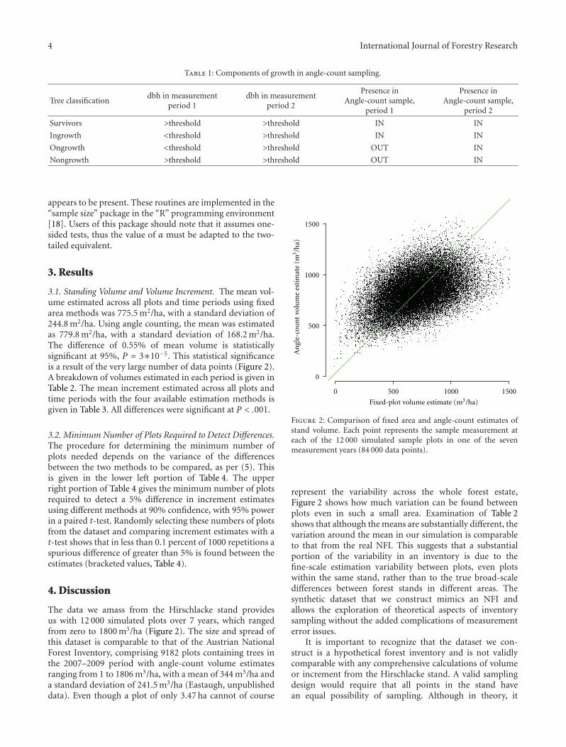
3.1. Standing Volume and Volume Increment. The mean vol-ume estimated across all plots and time periods using fixedarea methods was 775.5 m2/ha, with a standard deviation of244.8 m2/ha. Using angle counting, the mean was estimatedas 779.8 m2/ha, with a standard deviation of 168.2 m2/ha.The difference of 0.55% of mean volume is statisticallysignificant at 95%, P = 3∗10−5. This statistical significanceis a result of the very large number of data points (Figure 2).A breakdown of volumes estimated in each period is given inTable 2. The mean increment estimated across all plots andtime periods with the four available estimation methods isgiven in Table 3. All differences were significant at P < .001.

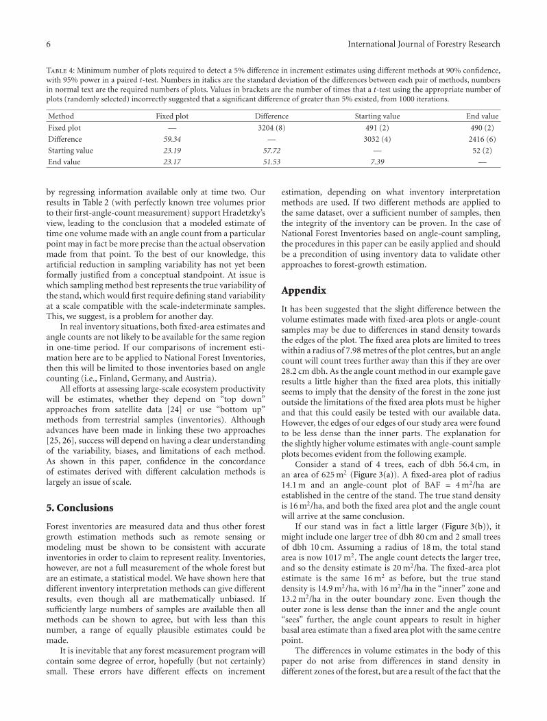
3.2. Minimum Number of Plots Required to Detect Differences.The procedure for determining the minimum number ofplots needed depends on the variance of the differencesbetween the two methods to be compared, as per (5). Thisis given in the lower left portion of Table 4. The upperright portion of Table 4 gives the minimum number of plotsrequired to detect a 5% difference in increment estimatesusing different methods at 90% confidence, with 95% powerin a paired t-test. Randomly selecting these numbers of plotsfrom the dataset and comparing increment estimates with at-test shows that in less than 0.1 percent of 1000 repetitions aspurious difference of greater than 5% is found between theestimates (bracketed values, Table 4).

4. Discussion

The data we amass from the Hirschlacke stand providesus with 12 000 simulated plots over 7 years, which rangedfrom zero to 1800 m3/ha (Figure 2). The size and spread ofthis dataset is comparable to that of the Austrian NationalForest Inventory, comprising 9182 plots containing trees inthe 2007–2009 period with angle-count volume estimatesranging from 1 to 1806 m3/ha, with a mean of 344 m3/ha anda standard deviation of 241.5 m3/ha (Eastaugh, unpublisheddata). Even though a plot of only 3.47 ha cannot of course

0

500

1000

1500

0 500 1000 1500

Fixed-plot volume estimate (m3/ha)

An

gle-

cou

nt

volu

me

esti

mat

e (m

3/h

a)

Figure 2: Comparison of fixed area and angle-count estimates ofstand volume. Each point represents the sample measurement ateach of the 12 000 simulated sample plots in one of the sevenmeasurement years (84 000 data points).

represent the variability across the whole forest estate,Figure 2 shows how much variation can be found betweenplots even in such a small area. Examination of Table 2shows that although the means are substantially different, thevariation around the mean in our simulation is comparableto that from the real NFI. This suggests that a substantialportion of the variability in an inventory is due to thefine-scale estimation variability between plots, even plotswithin the same stand, rather than to the true broad-scaledifferences between forest stands in different areas. Thesynthetic dataset that we construct mimics an NFI andallows the exploration of theoretical aspects of inventorysampling without the added complications of measurementerror issues.

It is important to recognize that the dataset we con-struct is a hypothetical forest inventory and is not validlycomparable with any comprehensive calculations of volumeor increment from the Hirschlacke stand. A valid samplingdesign would require that all points in the stand havean equal possibility of sampling. Although in theory, it

International Journal of Forestry Research 5

Table 2: Comparison of fixed-area and angle-count estimates of stand volume, for the 12 000 plots simulated in each measurement year.

Measurement yearFixed-area volume estimate Angle-count volume estimate

Mean (m3/ha) Std. dev. Mean (m3/ha) Std. dev.

1977 759.0 231.3 762.5 172.4

1982 769.3 226.3 774.6 161.9

1987 772.7 225.3 775.2 155.1

1992 818.2 241.2 822.4 163.9

1997 798.6 242.5 806.0 158.7

2002 775.5 259.0 780.8 168.0

2007 735.3 275.5 737.1 181.9

Table 3: Comparison of fixed-area and angle-count estimates of stand increment per 5 years, for the 72 000 data points simulated in eachmeasurement year.

MethodIncrement estimate, m3/ha/5 years

Mean Std. dev.

Fixed-area plots 67.88 28.14

Angle counts, difference method 69.01 56.97

Angle counts, starting Value method 68.23 21.89

Angle counts, end Value method 68.24 21.13

would be possible to extend our sample grid to encompassthe whole stand, problems then arise with the boundaryoverlap problem, where some sample plots extend to outsidethe stand. Solutions to this may exist [19] but would becomputationally extremely expensive to institute in oursimulation. Our purpose in this paper, however, is not toassess the accuracy of each inventory method in estimatingthe values of a true stand, but to compare the estimates madewith different methods from the same set of points.

The apparent statistical significant differences in volumeresults from different methods arise from the large numberof plots. However, at 0.55% of volume and a maximum of1.66% of increment, these differences are not functionallysignificant [20]. This difference does not arise in a properlyconducted inventory, as both fixed-area plots and angle-count plots are unbiased sampling procedures. In thisrespect, our hypothetical inventory may slightly flawed, aswe effectively sample from a forest stand without edges andthe population sampled with angle counts is slightly differentto that sampled with fixed-area plots, even though both usethe same plot centres. Nevertheless, significance testing withsufficiently large samples will always find “some” significantdifference, even if the null hypothesis that the sample meansare equal is actually true [21]. Given that the effect size is sosmall, we believe that this difference does not invalidate oursample collection for the purposes of this paper. Moreover,the (hypothetical) populations sampled for analysis with thethree angle-count-based increment estimators are identicaland thus validly comparable.

A single fixed-plot will measure different trees to an anglecount with the same centre and thus high variance in thedifference between each individual plot is to be expected.Interestingly, the behaviour at the extremes appears to bequite different, as the fixed plot estimates appear to give

higher values than the angle counts in denser portions ofthe forest bur lower values in regions with lower density(Figure 2).

The difference method of increment estimation has veryhigh variance in itself (ref. Table 3), as it is dependentmostly on how many new trees (either ingrowth, ongrowthor nongrowth) enter a sample in a remeasurement period.Multimethod estimation comparisons involving either ofthese two methods will thus require a large number ofplots (Table 4). When comparing the starting value andend value methods, most trees that make up the incrementestimate are the same trees, the only difference in the sampleis due to the nongrowth trees that enter the sample inthe remeasurement. This explains the plotwise intermethodvariance of only 7.39 m3/ha/5 years. It is important, however,to note that the end value method requires knowing orestimating the dimensions of nongrowth trees in the periodprior to when they entered the sample. In our examplestudied here this information was known from the long-term monitoring records, but in real inventories it is usuallyestimated with regression equations. This may change thevariance in the estimates in comparison with other methods.The inclusion of nongrowth trees enlarges the sample and soin principle the estimate should be more precise. This effectis, however, lessened by the fact that the covariance is greateras the survivor estimates are calculated using their inclusionprobabilities at time 2, when the basal areas are larger [16].Hradetzky [16] derived equations showing that incrementsderived from the end value method would have “slightly”less variance than the starting value method, if prior treedimensions were known. Roesch et al. [22] and Heikkinenand Henttonen [23] however give details of empirical studiesshowing that the standing volume at the time of firstmeasurement can be substantially more precisely estimated

6 International Journal of Forestry Research

Table 4: Minimum number of plots required to detect a 5% difference in increment estimates using different methods at 90% confidence,with 95% power in a paired t-test. Numbers in italics are the standard deviation of the differences between each pair of methods, numbersin normal text are the required numbers of plots. Values in brackets are the number of times that a t-test using the appropriate number ofplots (randomly selected) incorrectly suggested that a significant difference of greater than 5% existed, from 1000 iterations.

Method Fixed plot Difference Starting value End value

Fixed plot — 3204 (8) 491 (2) 490 (2)

Difference 59.34 — 3032 (4) 2416 (6)

Starting value 23.19 57.72 — 52 (2)

End value 23.17 51.53 7.39 —

by regressing information available only at time two. Ourresults in Table 2 (with perfectly known tree volumes priorto their first-angle-count measurement) support Hradetzky’sview, leading to the conclusion that a modeled estimate oftime one volume made with an angle count from a particularpoint may in fact be more precise than the actual observationmade from that point. To the best of our knowledge, thisartificial reduction in sampling variability has not yet beenformally justified from a conceptual standpoint. At issue iswhich sampling method best represents the true variability ofthe stand, which would first require defining stand variabilityat a scale compatible with the scale-indeterminate samples.This, we suggest, is a problem for another day.

In real inventory situations, both fixed-area estimates andangle counts are not likely to be available for the same regionin one-time period. If our comparisons of increment esti-mation here are to be applied to National Forest Inventories,then this will be limited to those inventories based on anglecounting (i.e., Finland, Germany, and Austria).

All efforts at assessing large-scale ecosystem productivitywill be estimates, whether they depend on “top down”approaches from satellite data [24] or use “bottom up”methods from terrestrial samples (inventories). Althoughadvances have been made in linking these two approaches[25, 26], success will depend on having a clear understandingof the variability, biases, and limitations of each method.As shown in this paper, confidence in the concordanceof estimates derived with different calculation methods islargely an issue of scale.

5. Conclusions

Forest inventories are measured data and thus other forestgrowth estimation methods such as remote sensing ormodeling must be shown to be consistent with accurateinventories in order to claim to represent reality. Inventories,however, are not a full measurement of the whole forest butare an estimate, a statistical model. We have shown here thatdifferent inventory interpretation methods can give differentresults, even though all are mathematically unbiased. Ifsufficiently large numbers of samples are available then allmethods can be shown to agree, but with less than thisnumber, a range of equally plausible estimates could bemade.

It is inevitable that any forest measurement program willcontain some degree of error, hopefully (but not certainly)small. These errors have different effects on increment

estimation, depending on what inventory interpretationmethods are used. If two different methods are applied tothe same dataset, over a sufficient number of samples, thenthe integrity of the inventory can be proven. In the case ofNational Forest Inventories based on angle-count sampling,the procedures in this paper can be easily applied and shouldbe a precondition of using inventory data to validate otherapproaches to forest-growth estimation.

Appendix

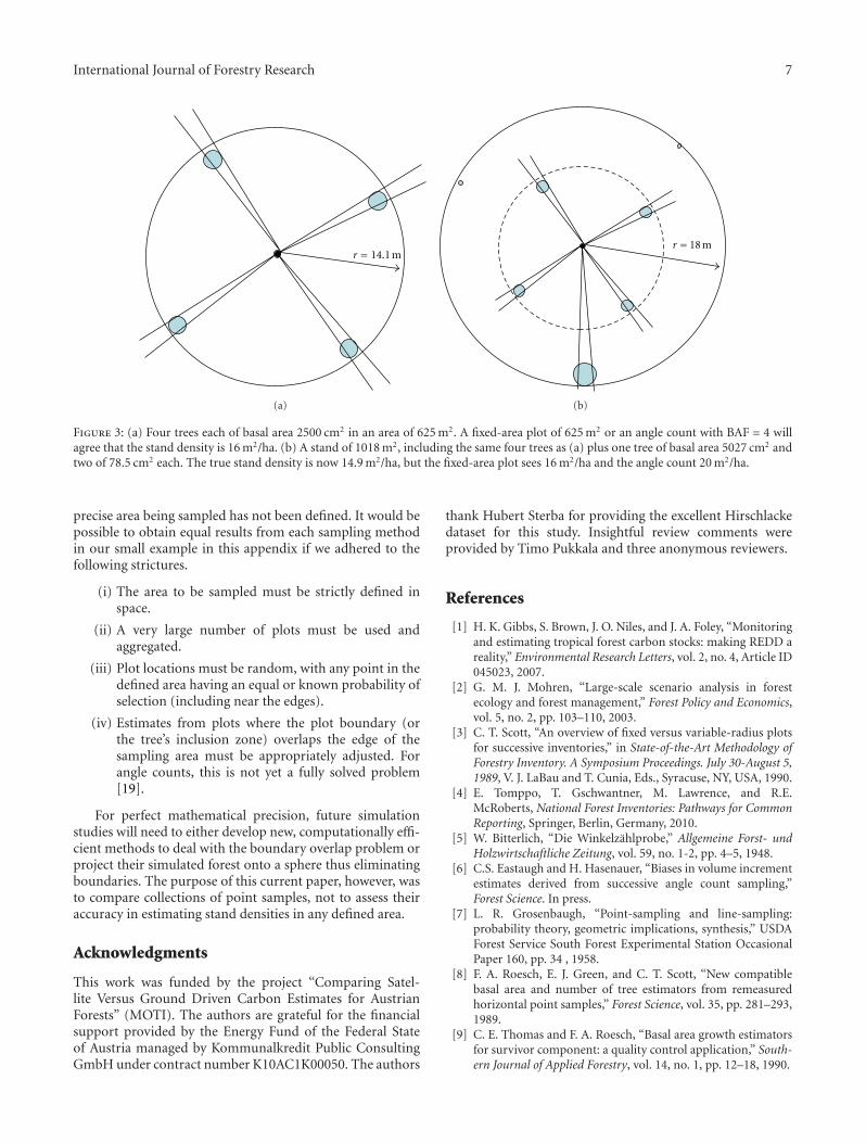
It has been suggested that the slight difference between thevolume estimates made with fixed-area plots or angle-countsamples may be due to differences in stand density towardsthe edges of the plot. The fixed area plots are limited to treeswithin a radius of 7.98 metres of the plot centres, but an anglecount will count trees further away than this if they are over28.2 cm dbh. As the angle count method in our example gaveresults a little higher than the fixed area plots, this initiallyseems to imply that the density of the forest in the zone justoutside the limitations of the fixed area plots must be higherand that this could easily be tested with our available data.However, the edges of our edges of our study area were foundto be less dense than the inner parts. The explanation forthe slightly higher volume estimates with angle-count sampleplots becomes evident from the following example.

Consider a stand of 4 trees, each of dbh 56.4 cm, inan area of 625 m2 (Figure 3(a)). A fixed-area plot of radius14.1 m and an angle-count plot of BAF = 4 m2/ha areestablished in the centre of the stand. The true stand densityis 16 m2/ha, and both the fixed area plot and the angle countwill arrive at the same conclusion.

If our stand was in fact a little larger (Figure 3(b)), itmight include one larger tree of dbh 80 cm and 2 small treesof dbh 10 cm. Assuming a radius of 18 m, the total standarea is now 1017 m2. The angle count detects the larger tree,and so the density estimate is 20 m2/ha. The fixed-area plotestimate is the same 16 m2 as before, but the true standdensity is 14.9 m2/ha, with 16 m2/ha in the “inner” zone and13.2 m2/ha in the outer boundary zone. Even though theouter zone is less dense than the inner and the angle count“sees” further, the angle count appears to result in higherbasal area estimate than a fixed area plot with the same centrepoint.

The differences in volume estimates in the body of thispaper do not arise from differences in stand density indifferent zones of the forest, but are a result of the fact that the

International Journal of Forestry Research 7

r = 14.1 m

(a)

r = 18 m

(b)

Figure 3: (a) Four trees each of basal area 2500 cm2 in an area of 625 m2. A fixed-area plot of 625 m2 or an angle count with BAF = 4 willagree that the stand density is 16 m2/ha. (b) A stand of 1018 m2, including the same four trees as (a) plus one tree of basal area 5027 cm2 andtwo of 78.5 cm2 each. The true stand density is now 14.9 m2/ha, but the fixed-area plot sees 16 m2/ha and the angle count 20 m2/ha.

precise area being sampled has not been defined. It would bepossible to obtain equal results from each sampling methodin our small example in this appendix if we adhered to thefollowing strictures.

(i) The area to be sampled must be strictly defined inspace.

(ii) A very large number of plots must be used andaggregated.

(iii) Plot locations must be random, with any point in thedefined area having an equal or known probability ofselection (including near the edges).

(iv) Estimates from plots where the plot boundary (orthe tree’s inclusion zone) overlaps the edge of thesampling area must be appropriately adjusted. Forangle counts, this is not yet a fully solved problem[19].

For perfect mathematical precision, future simulationstudies will need to either develop new, computationally effi-cient methods to deal with the boundary overlap problem orproject their simulated forest onto a sphere thus eliminatingboundaries. The purpose of this current paper, however, wasto compare collections of point samples, not to assess theiraccuracy in estimating stand densities in any defined area.

Acknowledgments

This work was funded by the project “Comparing Satel-lite Versus Ground Driven Carbon Estimates for AustrianForests” (MOTI). The authors are grateful for the financialsupport provided by the Energy Fund of the Federal Stateof Austria managed by Kommunalkredit Public ConsultingGmbH under contract number K10AC1K00050. The authors

thank Hubert Sterba for providing the excellent Hirschlackedataset for this study. Insightful review comments wereprovided by Timo Pukkala and three anonymous reviewers.

References

[1] H. K. Gibbs, S. Brown, J. O. Niles, and J. A. Foley, “Monitoringand estimating tropical forest carbon stocks: making REDD areality,” Environmental Research Letters, vol. 2, no. 4, Article ID045023, 2007.

[2] G. M. J. Mohren, “Large-scale scenario analysis in forestecology and forest management,” Forest Policy and Economics,vol. 5, no. 2, pp. 103–110, 2003.

[3] C. T. Scott, “An overview of fixed versus variable-radius plotsfor successive inventories,” in State-of-the-Art Methodology ofForestry Inventory. A Symposium Proceedings. July 30-August 5,1989, V. J. LaBau and T. Cunia, Eds., Syracuse, NY, USA, 1990.

[4] E. Tomppo, T. Gschwantner, M. Lawrence, and R.E.McRoberts, National Forest Inventories: Pathways for CommonReporting, Springer, Berlin, Germany, 2010.

[5] W. Bitterlich, “Die Winkelzahlprobe,” Allgemeine Forst- undHolzwirtschaftliche Zeitung, vol. 59, no. 1-2, pp. 4–5, 1948.

[6] C.S. Eastaugh and H. Hasenauer, “Biases in volume incrementestimates derived from successive angle count sampling,”Forest Science. In press.

[7] L. R. Grosenbaugh, “Point-sampling and line-sampling:probability theory, geometric implications, synthesis,” USDAForest Service South Forest Experimental Station OccasionalPaper 160, pp. 34 , 1958.

[8] F. A. Roesch, E. J. Green, and C. T. Scott, “New compatiblebasal area and number of tree estimators from remeasuredhorizontal point samples,” Forest Science, vol. 35, pp. 281–293,1989.

[9] C. E. Thomas and F. A. Roesch, “Basal area growth estimatorsfor survivor component: a quality control application,” South-ern Journal of Applied Forestry, vol. 14, no. 1, pp. 12–18, 1990.

8 International Journal of Forestry Research

[10] H. Sterba, “20 Years target diameter thinning in the“Hirscblacke”, forest of the monastery of Schagl,” AllgemeineForst- und Jagdzeitung, vol. 170, no. 9, pp. 170–175, 1999.

[11] H. Sterba and A. Zingg, “Target diameter harvesting—astrategy to convert even-aged forests,” Forest Ecology andManagement, vol. 151, no. 1–3, pp. 95–105, 2001.

[12] J. Pollanschutz, “Formzahlfunktionen der HauptbaumartenOsterreichs,” Allgemeine Forstzeitung, vol. 85, pp. 341–343,1974.

[13] P. Brassel and H. Lischke, Swiss National Forest Inventory:Methods and Models of the Second Assessment, WSL SwissFederal Research Institute, Birmansdorf, Switzerland, 2001.

[14] K. Gabler and K. Schadauer, Methoden der OsterreichischenWaldinventur 2000/02, vol. 135 of BFW Berichte,Bundesforschungs- und Ausbildungszentrum fur Wald,Naturgefahren und Landschaft, Vienna, Austria, 2006.

[15] G. L. Martin, “A method for estimating ingrowth on perma-nent horizontal sample points,” Forest Science, vol. 28, no. 1,pp. 110–114, 1982.

[16] J. Hradetzky, “Concerning the precision of growth estimationusing permanent horizontal point samples,” Forest Ecology andManagement, vol. 71, no. 3, pp. 203–210, 1995.

[17] J. H. Zar, Biostatistical Analysis, Prentice Hall, EnglewoodCliffs, NJ, USA, 1999.

[18] R Development Core Team, R: A Language and Environmentfor Statistical Computing, R Foundation for Statistical Com-puting, Vienna, Austria, 2011.

[19] M. J. Ducey, J. H. Gove, and H. T. Valentine, “A walkthroughsolution to the boundary overlap problem,” Forest Science, vol.50, no. 4, pp. 427–435, 2004.

[20] S. T. Ziliak and D. N. McCloskey, The Cult of StatisticalSignificance: How the Standard Error Costs Us Jobs, Justice andLives, University of Michigan Press, Ann Arbor, Mich, USA,2008.

[21] J. Cohen, “The earth is round (P < 0.05 ),” AmericanPsychologist, vol. 49, no. 12, pp. 997–1003, 1994.

[22] F. A. Roesch, E. J. Green, and C. T. Scott, “A test of alternativeestimators for volume at time 1 from remeasured pointsamples,” Canadian Journal of Forest Research, vol. 23, pp. 598–604, 1993.

[23] J. Heikkinen and H. Henttonen, “Re-measured relascope plotsin the assessment of inventory update methods,” in NordicTrends in Forest Inventory, Management Planning and Mod-elling. Proceedings of SNS meeting in Solvalla, Finland. April17–19, 2001, J. Heikkinen, K. T. Korhonen, M. Siitonen, M.Strandstrom, and E. Tomppo, Eds., Finnish Forest ResearchInstitute, 2001, Research Papers 860.

[24] R. Paivinen and P. Anttila, “How reliable is a satellite forestinventory?” Silva Fenica, vol. 35, no. 1, pp. 125–127, 1998.

[25] R. Petritsch, C. Boisvenue, S. W. Running, and H. Hasenauer,“Assessing forest productivity: satellite versus terrestrial data-driven estimates in Austria,” in Forest Growth and TimberQuality: Crown Models and Simulation Methods for SustainableForest Management Proceedings of an International Conference,Portland, OR, USA, August 7–10, 2007, Dennis P. Dykstraand Robert A. Monserud, Eds., pp. 211–216, United StatesDepartment of Agriculture Forest Service Pacific NorthwestResearch Station, 2009, General Technical Report PNW-GTR-791.

[26] R. A. Houghton, D. Butman, A. G. Bunn, O. N. Krankina, P.Schlesinger, and T. A. Stone, “Mapping Russian forest biomasswith data from satellites and forest inventories,” EnvironmentalResearch Letters, vol. 2, no. 4, Article ID 045032, 2007.