Supplier Quality Assurance Handbook - GF Machining Solutions
Upload
khangminh22Category
view
1download
0
Arithmetic Architectures for Finite FieldsGF (pm) with Cryptographic Applications
DISSERTATION
zur Erlangung des Grades einesDoktor-Ingenieurs
der Fakultat fur Elektrotechnik und Informationstechnikan der Ruhr-Universitat Bochum
von
Jorge Guajardo Merchanaus Caracas, Venezuela
Bochum, 2004

Copyright c© 2004 Jorge Guajardo Merchan. All Rights Reserved.The author hereby grants to the Ruhr-Universitat Bochum permission to reproduce and distrib-ute publicly paper and electronic copies of this thesis document in whole or in part. The authorcan be contacted [email protected]
Dissertation submitted on: May 20th, 2004Dissertation defended on: July 16th, 2004Dissertation Advisor: Prof. Dr.-Ing. Christof PaarDissertation Reader: Prof. Dr. Colin D. Walter

To the memory of my father,Jorge Guajardo Plantamura (1929–1997),
To my mother and sister who always have supported me,and to my loves, Kathy and Matteo.


Dissertation Abstract
Finite fields are essential building blocks of many cryptographic schemes. Traditionally, crypto-graphic applications developed on hardware have tried to take advantageof the ease of implementationof fields of the formGF (2n) to reduce costs and increase performance. In recent years, however, therehas been a renewed interest on the implementation of cryptographic systems based on odd characteristicfinite fieldsGF (pm), p a prime, which have found applications in areas such as elliptic curve cryptog-raphy, identity-based encryption, and short signature schemes, to namea few. There are several reasonswhy these fields have become attractive. First, they provide for greater diversity at the time of imple-mentation and this is directed related to security. For example, certain attacks which have been shown tobe successful against elliptic curves defined over composite binary fieldsGF ((2n)m) may not carry overto elliptic curves defined overGF ((pn)m) wherep is an odd prime. Thus, by considering alternativeimplementation options, we are, in a way, safeguarding against future attacks. Second, and perhaps moreappealing to the practitioner, in certain cases fields of odd characteristic offer advantages, such as shortersignature sizes, which simply can not be achieved with fields of characteristic two. Thus, the need toprovide hardware architectures for their efficient implementation. We tacklethis problem in this thesis.In particular, we focus on the implementation of hardware architectures foraddition, multiplication, andinversion in fieldsGF (pm).
The first part of the dissertation surveys previous architectures usedto implement addition and mul-tiplication overGF (p) as such operations are the basic building blocks used to implementGF (pm)multipliers. We make particular emphasis on architectures forsmallGF (p) fields wherep < 32. At theend of this section, we propose a new method to designGF (p) multipliers which can achieve up to a30% improvement over previous architectures. For completeness, we alsosurvey previous architecturesfor largeGF (p) fields such as those used in DL-based and RSA-based systems.
The second part of this thesis is concerned with multiplier architectures for fields GF (pm). Wegeneralize architectures originally proposed for fieldsGF (2n) to the odd characteristic case. BothLeast Significant Digit (LSD) multiplier architectures and Most Significant Digit (MSD) architecturesare introduced and their time and area complexities compared. We implemented an arithmetic unitfor GF (3m) fields on an FPGA and compared its performance to previous implementations and to ourtheoretical complexity models which agree with our practical results. In addition, we provide a thoroughtreatment of the cubing operation in fields of characteristic three and propose irreducible polynomialswhich reduce both the complexity of the multiplier and the cubing unit. In the appendix, we provideexhaustive lists of irreducible trinomials overGF (3). Although LSD and MSD multiplier architecturesallow the designer to trade area and performance according to his/her needs, these architectures sufferfrom several drawbacks: they use global signals and they are not very regular, thus not very suitable forVLSI systems. As a result, we developed systolic designs forGF (pm) fields based on our previouslyproposed LSD multipliers. In addition, for fixedp, we incorporate the notion of scalability, which hasbeen extensively studied in the context ofGF (2n) andGF (p) based systems. Here by scalability wemean the ability to process fieldsGF (pm), for constantp and different values ofm without recurringto changing the hardware or to reconfigurability, as in the case of FPGAs.We implemented the basiccell of an LSD-based systolic multiplier on 0.18µm CMOS technology and provided time and areacomplexities.
Finally, we tackle the problem of inversion in fieldsGF (qm), q = pn, by giving a generalization ofthe Itoh and Tsujii inversion algorithm to fields of odd characteristic and a standard basis representation.We introduce families of irreducible polynomials which reduce the complexity of exponentiating to the

ii Dissertation Abstract
q-th power whereq = pn andp is the field characteristic. By reducing the complexity of this operation,we also reduce the overall time required to compute an inverse inGF (qm).

Kurzdarstellung der Dissertation
Endliche Korper sind ein wesentlicher Bestandteil kryptographischer Verfahren. Konventionelle kryp-tographische Anwendungen in Hardware benutzen BinarkorperGF (2n) um den Rechenaufwand zu re-duzieren und die Rechengeschwindigkeit zu steigern. In den vergangenen Jahren haben jedoch endlichenKorper ungerader CharakteristikGF (pm), wobeip eine Primzahl ist, stark an Bedeutung gewonnen.Einsatzgebiete dieser Korper sind beispielsweise kryptographische Verfahren basierend auf elliptischenKurven, identitatsbezogene Verschlusselung sowie kurze digitale Signaturen. Die Grunde fur das In-teresse an diesen Korpern sind vielseitig. Einerseits stellen sie einen wichtigen zusatzlichen System-parameter dar, welcher sich direkt auf die kryptographische Sicherheit auswirkt. Beispielsweise sindbestimmte Angriffe gegen kryptographische Verfahren basierend auf elliptischen Kurven, welcheuberBinarkorpern definiert sind,uber Erweiterungskorpern mit ungerader Charakteristik moglicherweisenicht erfolgreich. Andererseits weisen diese Korper in bestimmten Fallen praktische Vorteile gegenuberBinarkorpern auf. So konnen z.B. basierend auf diesen Korpern kurzere digitale Signaturen erzeugtwerden. Um eine effiziente Implementierung zu gewahrleisten, ist die Entwicklung geeigneter Hard-warearchitekturen unabdingbar. Diese Dissertation beschaftigt sich mit dem Entwurf solcher Architek-turen. Insbesondere werden Implementierungen von Hardwarearchitekturen fur Addition, Multiplika-tion und Inversion in KorpernGF (pm) entwickelt.
Der erste Teil der Dissertation untersucht bereits bekannte Architekturen fur Addition und Multip-likation in KorpernGF (p), welche als grundlegende Funktionsbausteine fur die Implementierung vonMultiplizierern in GF (pm) dienen. Insbesondere stehen Architekturen fur kleineKorperGF (p) mitp < 32, im Mittelpunkt. Am Ende dieses Abschnitts wird eine neue Methode fur den Entwurf von Mul-tiplizierern vorgestellt, welche bis zu 30% effizienter als bisherige Multiplizierer sind. DieUbersichtumfasst auch Architekturen fur große KorperGF (p), wie sie in DL-basierten und RSA-basierten Sys-temen eingesetzt werden.
Der zweite Teil der Arbeit behandelt Architekturen fur Multiplizierer fur KorperGF (pm). Die furdie Multiplikation in KorpernGF (2n) vorgeschlagenen Architekturen werden fur den Fall ungeraderCharakteristik verallgemeinert. Es werden die Strukturen der LSD- (Least Significant Digit) und derMSD- (Most Significant Digit) Multiplizierer vorgestellt und deren Aufwandbezuglich Flache undLaufzeit verglichen. Schließlich wird die Realisierung einer Arithmetikeinheitfur KorperGF (3m) aufeinem FPGA beschreiben und deren Merkmale mit bekannten Implementierungen verglichen. Bei demVergleich mit dem theoretisch hergeleiteten Komplexitatsmodell ist eine grundlegendeUbereinstimmungzu verzeichnen. Des Weiteren wird eine sorgfaltige Analyse von Cubing-Einheiten in Korpern derCharakteristik Drei durchgefuhrt und irreduzibles Polynome vorgestellt, welche sowohl die Komplexitatdes Multiplizierers als auch die der Cubing-Einheit reduzieren. Obwohl die Architekturen von LSD-und MSD-Multiplizierern dem Anwender die Wahl der Flache und Durchsatzrate erlauben, leiden dieseArchitekturen an Einschrankungen: Es werden globale und unregelmaßige Verbindungen verwendet,welche fur VLSI-Implementierungen nicht wunschenswert sind. Aus diesem Grund wird eine systolis-che Architektur fur KorperGF (pm) basierend auf den existierenden Ansatzen fur LSD-Multiplizierervorgestellt. Fur festesp wird zusatzlich noch der Begriff der Skalierbarkeit berucksichtigt, welcher imKontext vonGF (2n) undGF (p) basierten Architekturen in der Literatur detailliert untersucht wurde.Mit Skalierbarkeit ist hier die Moglichkeit gemeint, in KorpernGF (pm) mit verschiedenen Wertenm zurechnen, ohneAnderungen an der Hardware oder, im Fall von FPGAs, Rekonfigurationen vornehmen zumussen. Die grundlegende Struktur eines LSD-basierten systolischen Multiplizierers wurde fur 0.18µmCMOS Technologie entworfen und dessen Zeit- und Flachenaufwand dargestellt.

iv Kurzdarstellung der Dissertation
Schließlich wird das Problem der Inversion in KorpernGF (qm), q = pn, durch eine Verallge-meinerung des Inversions-Algorithmus von Itoh und Tsujii fur Korper allgemeiner Charakteristik undPolynomialbasen-Reprasentation gelost. Es werden Familien von irreduziblen Polynomen zur Reduk-tion des Aufwands von Exponentiationen mit Potenzenq = pn vorgestellt, wobeip die Charakteristikdes Korpers ist. Durch die Reduktion der Komplexitat dieser Operation wird auch die gesamte benotigteZeit zur Berechnung einer Inversen inGF (qm) verringert.

Contents
List of Tables ix
List of Figures xi
List of Algorithms xiii
Preface xv
1 Introduction 11.1 Hardware Complexity Considerations. . . . . . . . . . . . . . . . . . . . . . . . . . . 31.2 Summary of Research Contributions and Dissertation Outline. . . . . . . . . . . . . . . 61.3 Notes and Further References. . . . . . . . . . . . . . . . . . . . . . . . . . . . . . . . 8
2 Mathematical Background 92.1 Groups. . . . . . . . . . . . . . . . . . . . . . . . . . . . . . . . . . . . . . . . . . . . 102.2 Rings and Fields . . . . . . . . . . . . . . . . . . . . . . . . . . . . . . . . . . . . . . 122.3 Polynomial Rings. . . . . . . . . . . . . . . . . . . . . . . . . . . . . . . . . . . . . . 142.4 Construction of Finite FieldsGF (pm) . . . . . . . . . . . . . . . . . . . . . . . . . . . 162.5 Polynomial, Normal, and Dual Bases. . . . . . . . . . . . . . . . . . . . . . . . . . . . 192.6 Irreducible Polynomials. . . . . . . . . . . . . . . . . . . . . . . . . . . . . . . . . . . 21
2.6.1 Preliminaries. . . . . . . . . . . . . . . . . . . . . . . . . . . . . . . . . . . . 222.6.2 Irreducible Binomials. . . . . . . . . . . . . . . . . . . . . . . . . . . . . . . . 242.6.3 Irreducible Trinomials. . . . . . . . . . . . . . . . . . . . . . . . . . . . . . . 252.6.4 Irreducible AOPs and ESPs. . . . . . . . . . . . . . . . . . . . . . . . . . . . 30
2.7 Notes and Further References. . . . . . . . . . . . . . . . . . . . . . . . . . . . . . . . 30
3 Architectures for Arithmetic in SmallGF (p) Fields 333.1 Integer Adders . . . . . . . . . . . . . . . . . . . . . . . . . . . . . . . . . . . . . . . 33
3.1.1 Ripple-Carry Adders (RCA). . . . . . . . . . . . . . . . . . . . . . . . . . . . 343.1.2 Carry-Lookahead Adders (CLA). . . . . . . . . . . . . . . . . . . . . . . . . . 363.1.3 Carry-Save Adders (CSA). . . . . . . . . . . . . . . . . . . . . . . . . . . . . 373.1.4 Carry-Delayed Adders (CDA). . . . . . . . . . . . . . . . . . . . . . . . . . . 39

vi Contents
3.1.5 Summary and Comparison. . . . . . . . . . . . . . . . . . . . . . . . . . . . . 413.2 GF (p) Adders . . . . . . . . . . . . . . . . . . . . . . . . . . . . . . . . . . . . . . . 43
3.2.1 Table Look-Up Based Architectures. . . . . . . . . . . . . . . . . . . . . . . . 433.2.2 Combinatorial Architectures. . . . . . . . . . . . . . . . . . . . . . . . . . . . 443.2.3 Hybrid Architectures. . . . . . . . . . . . . . . . . . . . . . . . . . . . . . . . 513.2.4 Summary and Comparison. . . . . . . . . . . . . . . . . . . . . . . . . . . . . 52
3.3 GF (p) Multipliers . . . . . . . . . . . . . . . . . . . . . . . . . . . . . . . . . . . . . 563.3.1 Table Look-Up and Hybrid Based Architectures. . . . . . . . . . . . . . . . . . 563.3.2 Combinatorial Architectures. . . . . . . . . . . . . . . . . . . . . . . . . . . . 593.3.3 NewGF (p) Multipliers for p < 25 . . . . . . . . . . . . . . . . . . . . . . . . 60
3.4 Notes and Further References. . . . . . . . . . . . . . . . . . . . . . . . . . . . . . . . 67
4 Algorithms for Arithmetic in LargeGF (p) Fields 694.1 Basic Methods . . . . . . . . . . . . . . . . . . . . . . . . . . . . . . . . . . . . . . . 70
4.1.1 School-book Method for Modular Multiplication. . . . . . . . . . . . . . . . . 704.1.2 Interleaved Multiplication Reduction Method. . . . . . . . . . . . . . . . . . . 73
4.2 Advanced Algorithms. . . . . . . . . . . . . . . . . . . . . . . . . . . . . . . . . . . . 744.2.1 Sedlak Modular Reduction. . . . . . . . . . . . . . . . . . . . . . . . . . . . . 744.2.2 Barret Modular Reduction. . . . . . . . . . . . . . . . . . . . . . . . . . . . . 754.2.3 Brickell’s Modular Reduction. . . . . . . . . . . . . . . . . . . . . . . . . . . 774.2.4 Quisquater’s Modular Reduction. . . . . . . . . . . . . . . . . . . . . . . . . . 79
4.3 Montgomery Modular Reduction. . . . . . . . . . . . . . . . . . . . . . . . . . . . . . 814.3.1 Towards Higher Radix Montgomery Multipliers. . . . . . . . . . . . . . . . . . 844.3.2 Avoiding Quotient Determination in High Radix Montgomery. . . . . . . . . . 864.3.3 High-Radix Montgomery Exponentiation on FPGAs. . . . . . . . . . . . . . . 894.3.4 Performance. . . . . . . . . . . . . . . . . . . . . . . . . . . . . . . . . . . . 90
4.4 Notes and Further References. . . . . . . . . . . . . . . . . . . . . . . . . . . . . . . . 92
5 Semi-Systolic Architectures for Arithmetic inGF (pm) 935.1 PreviousGF (pm) Multipliers . . . . . . . . . . . . . . . . . . . . . . . . . . . . . . . 94
5.1.1 Non-general Multipliers. . . . . . . . . . . . . . . . . . . . . . . . . . . . . . 945.1.2 General Multipliers. . . . . . . . . . . . . . . . . . . . . . . . . . . . . . . . . 95
5.2 Adder Architectures forGF (pm) . . . . . . . . . . . . . . . . . . . . . . . . . . . . . . 975.3 Serial Multipliers forGF (pm) . . . . . . . . . . . . . . . . . . . . . . . . . . . . . . . 97
5.3.1 Least Significant Element (LSE) First Multiplier. . . . . . . . . . . . . . . . . 985.3.2 Most Significant Element First Multiplier (MSE). . . . . . . . . . . . . . . . . 985.3.3 Modular Reduction. . . . . . . . . . . . . . . . . . . . . . . . . . . . . . . . . 995.3.4 Area/Time Complexity of LSE and MSE Multipliers. . . . . . . . . . . . . . . 100
5.4 Digit-Serial/Parallel Multipliers forGF (pm) . . . . . . . . . . . . . . . . . . . . . . . 1015.4.1 Least Significant Digit-Element (LSDE) Multipliers. . . . . . . . . . . . . . . 1025.4.2 Most Significant Digit-Element First Multiplier (MSDE). . . . . . . . . . . . . 1035.4.3 Modular Reduction for LSDE and MSDE Multipliers. . . . . . . . . . . . . . . 1045.4.4 Area/Time Complexity of LSDE Multipliers for Optimal Irreducible Polynomials1055.4.5 Area/Time Complexity of MSDE Multipliers for Optimal Irreducible Polynomials1075.4.6 Comments on Irreducible Polynomials of Degreem overGF (p) . . . . . . . . . 108

Contents vii
5.5 Case Study:GF (3m) Arithmetic . . . . . . . . . . . . . . . . . . . . . . . . . . . . . . 1095.5.1 GF (3) Arithmetic Implementation on FPGAs. . . . . . . . . . . . . . . . . . . 1095.5.2 Cubing inGF (3m) . . . . . . . . . . . . . . . . . . . . . . . . . . . . . . . . . 1105.5.3 Irreducible Polynomials overGF (3) . . . . . . . . . . . . . . . . . . . . . . . . 111
5.6 GF (3m) Prototype Implementation and Comparisons. . . . . . . . . . . . . . . . . . . 1125.6.1 GF (3m) Complexity Estimates. . . . . . . . . . . . . . . . . . . . . . . . . . 1135.6.2 Results . . . . . . . . . . . . . . . . . . . . . . . . . . . . . . . . . . . . . . . 115
5.7 Notes and Further References. . . . . . . . . . . . . . . . . . . . . . . . . . . . . . . . 116
6 Systolic and Scalable Architectures for Digit-Serial Multiplication in FieldsGF (pm) 1176.1 Related Work. . . . . . . . . . . . . . . . . . . . . . . . . . . . . . . . . . . . . . . . 1186.2 Systolic Least-Significant Element (LSE) First Architecture. . . . . . . . . . . . . . . . 119
6.2.1 Architecture. . . . . . . . . . . . . . . . . . . . . . . . . . . . . . . . . . . . . 1206.3 Systolic Least-Significant Digit Element (LSDE) First Architecture. . . . . . . . . . . . 1236.4 Architecture Description. . . . . . . . . . . . . . . . . . . . . . . . . . . . . . . . . . 129
6.4.1 Complexity and Performance. . . . . . . . . . . . . . . . . . . . . . . . . . . 1316.5 Prototypes Description. . . . . . . . . . . . . . . . . . . . . . . . . . . . . . . . . . . 1336.6 Notes and Further References. . . . . . . . . . . . . . . . . . . . . . . . . . . . . . . . 133
7 An Inversion Algorithm for FieldsGF (qm) 1357.1 Preliminaries . . . . . . . . . . . . . . . . . . . . . . . . . . . . . . . . . . . . . . . . 1357.2 The Itoh-Tsujii Algorithm overGF (qm), q = pn . . . . . . . . . . . . . . . . . . . . . 1397.3 Itoh-Tsujii Inversion in Standard Basis. . . . . . . . . . . . . . . . . . . . . . . . . . . 1417.4 Field Types with Low Complexity Inversion. . . . . . . . . . . . . . . . . . . . . . . . 143
7.4.1 FieldsGF ((2n)m) with Binary Field Polynomials . . . . . . . . . . . . . . . . 1437.4.2 FieldsGF (qm) with Binomials as Field Polynomials. . . . . . . . . . . . . . . 1457.4.3 FieldsGF (qm) with Binarys-ESP Field Polynomials . . . . . . . . . . . . . . 146
7.5 Notes and Further References. . . . . . . . . . . . . . . . . . . . . . . . . . . . . . . . 148
8 Discussion 1498.1 Summary and Conclusions. . . . . . . . . . . . . . . . . . . . . . . . . . . . . . . . . 1498.2 Recommendations for Further Research. . . . . . . . . . . . . . . . . . . . . . . . . . 151
A Irreducible Polynomials overGF (p) 153A.1 Irreducible Binomials overGF (p) . . . . . . . . . . . . . . . . . . . . . . . . . . . . . 153
A.1.1 C++ Source Code Used to Generate Table A.1. . . . . . . . . . . . . . . . . . 155A.2 Irreducible Trinomials and Quadrinomials overGF (3) . . . . . . . . . . . . . . . . . . 158
A.2.1 C++ Source Code Used to Generate Irreducible Trinomials. . . . . . . . . . . . 161
B GF (p) Adder Complexities 163
C FPGAs and Their Complexity Model 167C.1 Virtex Architecture . . . . . . . . . . . . . . . . . . . . . . . . . . . . . . . . . . . . . 167C.2 Complexity Considerations for the Virtex FPGA. . . . . . . . . . . . . . . . . . . . . . 169
D Standard Cell Library Data 171

viii Contents
Bibliography 173
Index 199

List of Tables
1.1 Normalized time and area complexities of basic building blocks. . . . . . . . . . . . . 5
2.1 Notation for common group operations, whereα ∈ G andn andm are integers.. . . . . 102.2 Representation ofGF (24) elements.. . . . . . . . . . . . . . . . . . . . . . . . . . . . 172.3 Elements ofGF (33) in polynomial representation.. . . . . . . . . . . . . . . . . . . . 182.4 Possible degrees for irreducible binomialsxm − ω overF7 . . . . . . . . . . . . . . . . 252.5 Values ofn andk for which the trinomials overF3 have an odd number of irreducible
factors. Here for an integers, v2(s) implies thats = 2v2(s)s1 wheres1 is odd. . . . . . . 28
3.1 Asymptotic area/time complexities of differentn-bit adders. . . . . . . . . . . . . . . . 413.2 Area/time complexities of RCA, CSA, and CLA according to [NIO96]. Area and delay
are normalized with respect to estimated FA delay.. . . . . . . . . . . . . . . . . . . . 423.3 Area/time complexities ofn-bit RCA, CLA, CSA, and CDA.. . . . . . . . . . . . . . . 433.4 Recommended implementation approaches for different types of moduli according to
[BJM87b]. LT : Look-Up Table, BA: Binary Adder, HY: Hybrid.. . . . . . . . . . . . . 443.5 Area-time complexities of the implementation of [Dug92] in 2 µm CMOS technology.
Times are given in nsec and area in square microns×103 . . . . . . . . . . . . . . . . . 483.6 Area/time complexities of differentGF (p) adders. We writen = ⌈log2(m−1)⌉, where
m is the modulus.. . . . . . . . . . . . . . . . . . . . . . . . . . . . . . . . . . . . . . 533.7 Truth table representation ofC = A ·B mod 3. The element 0 is represented as′00′ or
′01′, 1 as′10′, and 2 as′11′ . . . . . . . . . . . . . . . . . . . . . . . . . . . . . . . . . 623.8 don’t caredistribution of best encoding forp = 13 . . . . . . . . . . . . . . . . . . . . 643.9 Area (transistors) complexity of proposedGF (p) multipliers with given encodings.. . . 66
4.1 CLB usage and execution time for a full modular exponentiation. . . . . . . . . . . . . 914.2 Application to RSA: Encryption. . . . . . . . . . . . . . . . . . . . . . . . . . . . . . 914.3 Application to RSA: Decryption. . . . . . . . . . . . . . . . . . . . . . . . . . . . . . 92
5.1 Area complexity and critical path delay of LSE multiplier.. . . . . . . . . . . . . . . . 1015.2 Area complexity and critical path delay of MSE multiplier.. . . . . . . . . . . . . . . . 1015.3 Area complexity and critical path delay of LSDE multiplier with optimal irreducible
polynomials.. . . . . . . . . . . . . . . . . . . . . . . . . . . . . . . . . . . . . . . . . 107

x List of Tables
5.4 Area complexity and critical path delay of MSDE multiplier with optimal irreduciblepolynomials.. . . . . . . . . . . . . . . . . . . . . . . . . . . . . . . . . . . . . . . . . 108
5.5 Truth table representing multiplication inGF (3). . . . . . . . . . . . . . . . . . . . . . 1105.6 GF (3m) AU complexity estimates. . . . . . . . . . . . . . . . . . . . . . . . . . . . . 1145.7 AU estimated vs. measured complexity for prototypes (D = 16) . . . . . . . . . . . . . 1155.8 Comparison of multiplication time forGF (2151), GF (2241), andGF (397) prototypes
(D = 16) and the AU from [PS02] . . . . . . . . . . . . . . . . . . . . . . . . . . . . . 115
6.1 Characteristics of LSE/LSDE multipliers. . . . . . . . . . . . . . . . . . . . . . . . . . 1326.2 Area and Frequency of the basic cell for an LSDE multiplier. . . . . . . . . . . . . . . 133
A.1 Irreducible binomials of the formxm−ω overGF (p), for all m such that2160 ≤ pm ≤2256 and3 ≤ p ≤ 521 with n = ⌊log2 p⌋. . . . . . . . . . . . . . . . . . . . . . . . . . 154
A.2 Optimal irreducible trinomials of the formxm +ptxt +p0 overGF (3), for m prime and
2 ≤ m ≤ 255. . . . . . . . . . . . . . . . . . . . . . . . . . . . . . . . . . . . . . . . . 158A.3 Irreducible trinomials of the formxm + xt + 2 overGF (3), 2 ≤ m ≤ 255 . . . . . . . 159A.4 Irreducible trinomials of the formxm + 2xt + 1 overGF (3), 3 ≤ m ≤ 255 . . . . . . . 159A.5 Irreducible trinomials of the formxm + 2xt + 2 overGF (3), 2 ≤ m ≤ 255 . . . . . . . 159A.6 Irreducible quadrinomialsxm + pt1x
t1 + pt2xt2 + p0 overGF (3) for degrees with no
trinomials. . . . . . . . . . . . . . . . . . . . . . . . . . . . . . . . . . . . . . . . . . . 160
B.1 Normalized area complexity of differentGF (p) adders for3 ≤ p ≤ 521 . . . . . . . . . 164B.2 Normalized time complexity of differentGF (p) adders for3 ≤ p ≤ 521 . . . . . . . . . 165B.3 Normalized area/time product of differentGF (p) adders for3 ≤ p ≤ 521 . . . . . . . . 166
C.1 Virtex FPGA Family Members. . . . . . . . . . . . . . . . . . . . . . . . . . . . . . . 168
D.1 Area and time complexities of different circuits for three different standard cell libraries. 171D.2 Normalized area and time complexities of different components in differentstandard cell
libraries. Normalization done with respect to the area/delay of a 2-input NAND gate inthe given library. . . . . . . . . . . . . . . . . . . . . . . . . . . . . . . . . . . . . . . 172

List of Figures
3.1 Half-adder cell . . . . . . . . . . . . . . . . . . . . . . . . . . . . . . . . . . . . . . . 353.2 Full-adder cell. . . . . . . . . . . . . . . . . . . . . . . . . . . . . . . . . . . . . . . . 353.3 n-bit carry-ripple adder. . . . . . . . . . . . . . . . . . . . . . . . . . . . . . . . . . . 353.4 n-bit carry-save adder. . . . . . . . . . . . . . . . . . . . . . . . . . . . . . . . . . . . 383.5 n-bit carry-delayed adder. . . . . . . . . . . . . . . . . . . . . . . . . . . . . . . . . . 403.6 Binary adder-based RNS adder from Bayoumi [BJM87b] . . . . . . . . . . . . . . . . . 453.7 Type II modulo adder with feedback register from Dugdale [Dug92] . . . . . . . . . . . 473.8 Type III modulo adder with overflow detection circuit from Dugdale [Dug92] . . . . . . 483.9 Binary-based RNS adder from Hiasat [Hia02] . . . . . . . . . . . . . . . . . . . . . . . 493.10 Addition4 + 5 mod 7 according to Banerji [Ban74] . . . . . . . . . . . . . . . . . . . . 513.11 Normalized area complexity comparison of differentGF (p) adders. (a) ROM only vs.
hybrid-base, (b) Hybrid-based vs. binary-adder-based and (c)Detail of binary-adder-based543.12 Normalized time complexity comparison of differentGF (p) adders. . . . . . . . . . . . 553.13 Index calculus multiplier. . . . . . . . . . . . . . . . . . . . . . . . . . . . . . . . . . 573.14 Index calculus modulo 19 multiplier from [Jul80] with zero encoding from [Dug94] and
moduli set{6, 7}. . . . . . . . . . . . . . . . . . . . . . . . . . . . . . . . . . . . . . . 583.15 RNS multiplier from [RY92] with m = m1 ·m2 · · ·mr . . . . . . . . . . . . . . . . . . 59
5.1 GF (3m) Arithmetic Unit Architecture. . . . . . . . . . . . . . . . . . . . . . . . . . . 113
6.1 Dependency graph forAα mod q(α) . . . . . . . . . . . . . . . . . . . . . . . . . . . . 1216.2 Dependency graph for the LSE algorithm. . . . . . . . . . . . . . . . . . . . . . . . . 1226.3 Dependency graph for LSDE multiplication (d = 4) . . . . . . . . . . . . . . . . . . . . 1306.4 LSDE scalable multiplier (e = 2) . . . . . . . . . . . . . . . . . . . . . . . . . . . . . . 132
C.1 Virtex FPGA . . . . . . . . . . . . . . . . . . . . . . . . . . . . . . . . . . . . . . . . 167

xii List of Figures

List of Algorithms
3.1 5-stage algorithm for CSA RNS addition from [EB90] and [BJS94] . . . . . . . . . . . 46
4.1 Multiplication . . . . . . . . . . . . . . . . . . . . . . . . . . . . . . . . . . . . . . . . 704.2 Restoring Shift/Subtract Division. . . . . . . . . . . . . . . . . . . . . . . . . . . . . . 714.3 Non-restoring Shift/Subtract Division. . . . . . . . . . . . . . . . . . . . . . . . . . . 724.4 Interleaved Multiplication Reduction Method. . . . . . . . . . . . . . . . . . . . . . . 734.5 Modular Reduction for Step 4 of Algorithm 4.4. . . . . . . . . . . . . . . . . . . . . . 744.6 Barret Modular Reduction. . . . . . . . . . . . . . . . . . . . . . . . . . . . . . . . . 764.7 Brickell’s Modular Reduction. . . . . . . . . . . . . . . . . . . . . . . . . . . . . . . . 784.8 Interleaved Multiplication Reduction Method for General Radixb . . . . . . . . . . . . 804.9 Montgomery Reduction. . . . . . . . . . . . . . . . . . . . . . . . . . . . . . . . . . . 824.10 Montgomery Multiplication. . . . . . . . . . . . . . . . . . . . . . . . . . . . . . . . . 834.11 Modified Montgomery Multiplication according to [EW93] . . . . . . . . . . . . . . . . 834.12 Montgomery Multiplication Avoiding Quotient Determination [Oru95] . . . . . . . . . 874.13 Improved Montgomery Multiplication with Quotient Pipelining [Oru95] . . . . . . . . . 88
5.1 LSE Multiplier . . . . . . . . . . . . . . . . . . . . . . . . . . . . . . . . . . . . . . . 985.2 MSE Multiplier . . . . . . . . . . . . . . . . . . . . . . . . . . . . . . . . . . . . . . . 995.3 LSDE Multiplier . . . . . . . . . . . . . . . . . . . . . . . . . . . . . . . . . . . . . . 1035.4 MSDE Multiplier . . . . . . . . . . . . . . . . . . . . . . . . . . . . . . . . . . . . . . 103
6.1 LSE Multiplier . . . . . . . . . . . . . . . . . . . . . . . . . . . . . . . . . . . . . . . 1196.2 Low Level LSE Multiplier . . . . . . . . . . . . . . . . . . . . . . . . . . . . . . . . . 1206.3 Modified LSDE Multiplier . . . . . . . . . . . . . . . . . . . . . . . . . . . . . . . . . 1246.4 Low Level Modified LSDE Multiplier . . . . . . . . . . . . . . . . . . . . . . . . . . . 128
7.1 Multiplicative inverse computation inGF (2n) with n = 2r + 1 [IT88, Theorem 1] . . . 136

xiv List of Algorithms

Preface
This thesis describes much of the work that I conducted while completing my Ph.D. degree at the Ruhr-
Universitat Bochum. I have attempted to make the treatment of architectures for finite fields of odd
characteristic as complete and self-contained as possible. It is my hope thatmy contributions to the field
and the extensive bibliographic material will make this thesis into a useful reference work for academia
and industry professionals alike.
I would like to thank the following people for their support throughout the months that I worked on
this thesis. First and foremost, I would like to thank my advisor Prof. ChristofPaar for all his help,
patience, and support throughout my graduate work at the RUB and at WPI. This work would certainly
not have been possible without his help and guidance. I would also like to thank Prof. Paar for two other
reasons: first for his friendship, camaraderie, and advice during difficult times in my life and, second, for
introducing me, back in 1995, to the exciting field of applied cryptography and its engineering aspects,
both of which I love and feel passionate about. I am also grateful to Prof. Colin Walter for taking the
time to read this manuscript and for his valuable suggestions, comments, and constructive feedback, all
of which helped improve the presentation of this thesis. Any errors that remain, of course, are entirely
my own.

xvi Preface
I would like thank Guido Bertoni, Gerardo Orlando, Andre Weimerskirch, and Thomas Wollinger for
our fruitful discussions and friendship. Much of the work in this thesis was joint work with Guido and
Gerardo. I learned a lot from their insights into what is useful and efficient in the hardware world. I
must say that working in two different continents and three different geographic locations was definitely
a challenge but also a lot of fun. I would also like to thank the members of the COSY Lab at the
time. In alphabetical order they are: Marcus Heitmann, Irmgard Kuhn, Sandeep Kumar, Jan Pelzl, Kai
Schramm, Andre Weimerskirch, and Thomas Wollinger. Thanks for making the COSY Lab such a fun
place to work, for your patience and understanding when I talked in my broken German, for your insights
into the German culture, for your friendship, and for the many wonderfultimes we had together.
I must also thank Ari Juels for giving me the chance to work at RSA Laboratories in the summer of
2001. Working at the Labs was a lot of fun. Thanks for always being willing to listen to and answer
my questions, for giving me the chance to learn about security protocols, and for believing in me. I
am also grateful to Prof. J. E. Stine for providing me with the delay and areadata for his standard cell
library. My most sincere thanks to Jean-Pierre Seifert for his supportand encouragement during the time
of writing my thesis at Infineon. Had it not been for him, I might still be writing. Finally, I would like
to give special thanks to Kathy Kreitner Guajardo, my loving wife, for proof reading my English in the
manuscript that you are about to read and for her unconditional support and love.
To all of you my most sincere thanks!

CHAPTER 1
Introduction
Before 1976, Galois fields and their hardware implementation received considerable attention because of
their applications in coding theory and the implementation of error correcting codes. In 1976, Diffie and
Hellman [DH76] invented public-key cryptography1 and single-handedly revolutionized a field which,
until then, had been the domain of intelligence agencies and secret government organizations. In addi-
tion to solving the key management problem and allowing for digital signatures, public-key cryptogra-
phy provided a major application area for finite fields. In particular, the Diffie-Hellman key exchanged
is based on the difficulty of the Discrete Logarithm (DL) problem in finite fields.It is apparent, however,
that most of the work on arithmetic architectures for finite fields only appeared after the introduction of
two public-key cryptosystems based on finite fields: elliptic curve cryptosystems, introduced by Miller
and Koblitz [Mil86, Kob87], and hyperelliptic cryptosystems, a generalization of elliptic curves intro-
duced by Koblitz in [Kob89].
Both, prime fields and extension fields, have been proposed for use in such cryptographic systems
but until a few years ago the focus was mainly on fields of characteristic 2.This is due to two main
reasons. First, even characteristic fields naturally offer a straight forward manner in which field elements
can be represented. In particular, elements ofGF (2) can be represented by the logical values “0”
and “1” and thus, elements ofGF (2n) can be represented as vectors of zeros and ones. For these
types of fields, both software implementations (see [HMV92, SOOS95, DBV+96, HHM00, LD00]) and

2 1. Introduction
hardware architectures (see [YP82, Mas89, HWB92, AMV93, ABMV93, FBT96, SP98, PFR99]) have
been extensively studied. Second, until 1997 applications of fieldsGF (pm) for oddp were scarce in the
literature.
In 1997, Mihalescu [Mih97] and independently Bailey and Paar [BP98, BP01a] introduced the con-
cept of Optimal Extension Fields (OEFs) in the context of elliptic curve cryptography. OEFs are fields
GF (pm) wherep is odd and bothp andm are chosen to fit the particular hardware platform where the
cryptosystem is being implemented. A major observation in [BP98, BP01a] is that matching of field
parameters to hardware platform allows for optimized field arithmetic and an overall efficient imple-
mentation. Notice that the treatment in [Mih97, BP98, BP01a] and that of other works based on OEFs
[Kob00, WBP00, Mul01] has only been concerned with efficient software implementations. Fields
GF (pm) have also been proposed for cryptographic applications in [Kob98, Sma99]. In particular,
[Kob98] describes an implementation of ECDSA over fields of characteristic 3 and 7.The author in
[Sma99] describes a method to implement elliptic curve cryptosystems over fields ofsmallodd charac-
teristic, only consideringp < 24 in the results section.
More recently, Boneh and Franklin [BF01] introduced a practical identity-based encryption scheme
which is based on the application of the Weil and Tate pairings. Similarly, [BBS01] described a short sig-
nature scheme based on the Weil and Tate pairings (see [BB04a, BB04b] for the corresponding schemes
not based on the random oracle model). Other applications include [Jou00, Ver01]. All of these appli-
cations of the Weil and Tate pairings consider elliptic curves defined over fields of characteristic 2 and
3. Because characteristic 2 field arithmetic has been extensively studied in the literature, authors have
concentrated their efforts to improve the performance of systems based oncharacteristic 3 arithmetic2.
For example, [BKLS02, GHS02a] describe algorithms to improve the efficiency of the pairing compu-
tations. In addition, [GHS02a] introduces some clever tricks to improve the efficiency of the underlying
arithmetic insoftwarebased solutions.
Although, there have been several dissertations dealing with the problem of finite field arithmetic
overGF (2) and their hardware implementation, (see for example [Mas91, Has92, Gei93, Paa94, Wu98,
Olo02]), to our knowledge there has not been a systematic treatment of finite field arithmetic in fields
GF (pm) wherep is odd andm > 1, and, in fact, very little work in general. Thus, this thesis focuses on

1.1 Hardware Complexity Considerations 3
the development of techniques to implement addition, multiplication, and inversion infieldsGF (pm)
for oddp andm > 1. We end this section by emphasizing that the efficient implementation of finite
field arithmetic, whether in hardware or software, is key to the performanceof the overall system and,
in fact, will dictate the final performance of the system. A poor finite field implementation will result in
bad system performance and vice versa. Thus, the importance of studying techniques for the efficient
implementation of finite fields.
1.1 Hardware Complexity Considerations
As in the case of characteristic two finite field hardware architectures, we can also classify architectures
for fieldsGF (pm), wherep > 2, according to the way the finite field elements are processed as: array
(also known as serial), digit, or parallel multipliers [SP98]. In this thesis, we consider only array and digit
architectures for multipliers inGF (pm) which include both combinatorial and memory elements such as
registers. Parallel architectures and, in particular, parallel multipliers would require immense hardware
resources for cryptographic applications and, thus, they do not seemrealistic in this context. Notice,
however, that in building architectures for fieldsGF (pm), it is first required to implement arithmetic
in GF (p). Thus, we also consider the complexity of adders and multipliers for arithmetic inGF (p),
wherep is small (we will make our definition of small more exact in Chapter3). For such adders and
multipliers, we consider parallel architectures.
In evaluating hardware architectures, there are several factors which need to be considered, including
but not limited to:
• Space complexity (chip area)
• Time complexity (circuit performance or delay)
• Power dissipation
• Architecture regularity and modularity
Traditionally, both the area and time complexities have been the most important criteria to evaluate and
compare hardware architectures for finite field arithmetic3 (see for example [Paa94, Wu98, Olo02]). We

4 1. Introduction
will use primarily theoretical VLSI time and area complexities to evaluate and compare the architectures
studied and proposed in this thesis. As mentioned previously, two differenttypes of architectures are
studied in this thesis: architectures to implement arithmetic in smallGF (p) fields and architectures to
implement arithmetic inGF (pm) fields. For the first case, we have chosen to measure the space and
time complexities according to:
1. The number of inverters as well as 2-input and 3-input AND, OR, andXOR gates and their corre-
sponding delays.
2. In terms of normalized gate area and delay, where we have normalized withrespect to the area
and delay of a 2-input NAND gate.
The first measure has been widely used in other works where arithmetic architectures for characteristic
two fields are studied [Paa94, Wu98] but limited to 2-input XOR and AND gates as it is possible to
implementGF (2) arithmetic using only these two types of gates. We extend the model to include OR
gates and 3-input gates because these are used regularly throughoutthe Residue Number System (RNS)
literature (for example in[CPO95, PKS01]) to estimate the complexity ofGF (p) adders and multipliers.
Such adders and multipliers are essential building blocks ofGF (pm) multipliers. In addition, by giving
the area of a circuit in terms of the number of gates, we remain somewhattechnology independent.
In other words, anyone can take the number of gates required to implement aGF (p) multiplier, for
fixed p, and estimate the total area used given a standard cell library and CMOS technology. Notice,
however, that the above measure does not allow us to perform comparisons among different designs.
For example, consider a circuit which requires five 2-input XOR gates, three 2-input AND gates and six
2-input OR gates versus a circuit which requires three 2-input XOR gates and fifteen 2-input OR gates.
How can we establish which circuit has the largest area? We simply can not. We need to map our gates
to transistors, to equivalent gates, to their size inµm2, or to other similar measure which allows us to
compare area (time delay) in a more exact manner. We chose our measure to be the normalized area of
all components with respect to the size and delay of a 2-input NAND gate. This is also known as the
equivalent gate measure. Table1.1 summarizes the assumed normalized area and delay characteristics
of all basic components used in the architectures presented in this thesis.

1.1 Hardware Complexity Considerations 5
Table 1.1.Normalized time and area complexities of basic building blocks
Component Abbreviation Normalized NormalizedArea Delay
Inverter NOT 0.7 1.02-input AND gate AND2 1.3 1.02-input NAND gate NAND2 1.0 1.03-input AND gate AND3 2.0 1.13-input NAND gate NAND3 1.5 1.12-input OR gate OR2 1.3 0.82-input NOR gate NOR2 1.0 1.03-input OR gate OR3 2.0 1.13-input NOR gate NOR3 1.5 1.12-input XOR gate XOR2 2.3 1.02-input XNOR gate XNOR2 2.3 1.0Complex gate implementing((A ∧B) ∨ C) AO21 1.3 1.0Complex gate implementing((A ∧B) ∨ (C ∧D)) AO22 1.7 1.0Complex gate implementing((A ∨B) ∧ C) OA21I 1.0 1.0Complex gate implementing((A ∨B) ∧ (C ∨D)) OA22I 1.7 1.0D Flip-Flop FF 4.0 1.0Latch LAT 2.0 1.01-bit 2:1 Multiplexer MUX21 2.0 1.01-bit Full Adder FA 5.0 1.11-bit Half Adder HA 2.2 1.02n ×W -bit ROM table ROMn,W (2n ×W )· OR2 n· TFA
The normalized area complexity provided in Table1.1 has been obtained based on the normalized
area characteristics of the components in the standard cell libraries from [GS03b, VLS03] which are
summarized in TableD.2. We notice that the delays of most components in TableD.2 do not vary by
more than 10% except for the OR2 and the FA cells. Thus, we assume that thedelay of all components
is the same except for the OR2, the 3-input gates, and FA cells. The delay of the OR2 gate is slightly
better than other gates and the delay of the 3-input gates and FA cells is slightly worse. We notice that
in our model, we assumed that 3-input gates require an area which is 1.5 times that of the corresponding
2-input gate. This is in agreement with the model of [PKS01]. We also assume that a latch requires
about half the area of a flip-flop. For the delay and time complexities of ROM tables and 1-bit half adder
cells, we have taken into consideration the VLSI complexity model used in [CPO95, PKS01]4. Thus, in
agreement with [PKS01], we have assumed that a HA is about 0.43 times as large as a FA. Similarly, we
have adopted the ROM-complexity model from [CPO95] according to which a2n ×W -bit table has an
area complexity of2n ×W OR2 gates and a delay ofn 1-bit FA. We hope that by consideringactual

6 1. Introduction
gate sizes and delays our area and delay estimates will be more accurate.
For theGF (pm) architectures, we have chosen a single complexity measure: The number ofGF (p)
multipliers and adders and their corresponding delays. We emphasize that the delay and area are given
in terms ofGF (p) multipliers, adders, and, for certain designs, also registers. This measure provides us
with technology and design independence. By design independence, wemean that it is very probable
that in the future there will be a new and betterGF (p) adder or multiplier optimized according to certain
measure which we might want to combine with theGF (pm) architectures proposed in this thesis. This
measure, thus, allows an easy estimate of the area in terms of this futureGF (p) arithmetic design.
We end this section by noticing that, in some cases, we have also synthesized and simulated the
proposed architectures on FPGAs. For these cases, we provide a theoretical framework to evaluate the
area complexity of our FPGA designs. Our FPGA model is based on the complexity measures of [Orl02]
and it is briefly described in AppendixC.
1.2 Summary of Research Contributions and Dissertation
Outline
Given the research community’s interest in cryptographic systems based on fields of odd characteristic
and the lack of hardware architectures for general odd characteristicfields, we try to close this gap in
this dissertation. We begin with an overview of the mathematics of Galois fields in Chapter2. This
introduction is meant to make the thesis self-contained and, thus, it provides the readers with facts on
finite fields and construction of irreducible polynomials, all of them without proofs. We end Chapter2
with references to other works which would provide in-depth treatment (and proofs) of the mathematical
concepts here described. The remainder of the dissertation is organizedinto three main themes: adders
and multipliers inGF (p), multipliers inGF (pm), and inversion inGF (pm).
In Chapters3 and4, we thoroughly investigate adders and multipliers inGF (p) for both small and
large values ofp. For small values ofp, we consider architectures which have been presented in the
context of digital signal processing (DSP) applications and, in particular, of residue number systems

1.2 Summary of Research Contributions and Dissertation Outline 7
(RNS). At the end of Chapter3, we propose a new method to designGF (p) multipliers which can
achieve up to a 30% area improvement over previous architectures. For the sake of completeness, in
Chapter4 we survey multipliers for large values ofp (between 160-bit and 2000-bit long primes) which
have been proposed mainly in the context of RSA [RSA78], Discrete Logarithm (DL) systems [DH76],
and, more recently, elliptic curves [Mil86, Kob87].
Chapters5 and6 investigate multipliers inGF (pm) and constitute the heart of this dissertation. In
Chapter5, we first generalize the work in [SP98] to fieldsGF (pm), p odd. In particular, we develop
semi-systolic architectures for Most Significant Digit (MSD) and Least Significant Digit (LSD) multi-
pliers. Second, we study the complexity of the architectures previously proposed for the particular case
of GF (3m) and propose optimizations to the computation of the cubing operation in these fields. Fields
of characteristic three are of interest for cryptographic applications such as identity-based encryption
[BF01] and short signature schemes [BBS01]. As a result of the optimizations for characteristic three
fields, we also provide tables of irreducible polynomials for which the complexity of the multipliers is
reduced. We end this chapter by describing an implementation of an arithmetic unit used to perform
operations inGF (3m) and compare it to a similar unit used to perform arithmetic over binary fields.
The methods described in Chapter5 have the drawback of using global signals and long wires and
they require reconfigurability to achieve their full potential. Thus, these solutions lack flexibility in
platforms such as ASICs. In Chapter6, we move a step forward towards the design of scalable and
flexible hardware architectures for oddGF (pm) fields. In particular, we propose new systolic and
scalable architectures for arithmetic inGF (pm) fields. On the one hand, the systolic nature of our
architectures provides for ease of design and offers functional andlayout modularity all of which are
properties envisioned in good VLSI designs. On the other hand, with scalability, we are able to perform
a multiplication for any value ofm in GF (pm), with fixedp and fixed digit size. Thus, we can support
multiple irreducible polynomials without turning to the use of reconfigurability in FPGAs, solving one
of the major disadvantages of the architectures presented in Chapter5. We end Chapter6 with an
implementation of the basic cell of the systolic architecture described in a 0.18µm CMOS standard cell
library.
In Chapter7, we tackle the problem of inversion in fieldsGF (qm), q = pn, by giving a generalization

8 1. Introduction
of the Itoh and Tsujii inversion algorithm to fields of odd characteristic and astandard basis representa-
tion. We introduce families of irreducible polynomials which reduce the complexityof exponentiating
to theq-th power whereq = pn andp is the field characteristic. By reducing the complexity of this
operation, we also reduce the overall time required to compute an inverse inGF (qm).
1.3 Notes and Further References
1. The discovery of public-key cryptography in the intelligence community is attributed in [Ell97]
to John H. Ellis in 1970. Reference [Ell97], attributes to John H. Ellis a theorem which proves the
existence of a method to establish a secure communication channel between twoparties who previously
do not share a common secret-key. The discovery of the equivalent ofthe RSA cryptosystem [RSA78]
is attributed to Clifford Cocks in 1973 while the equivalent of the Diffie-Hellmankey exchange was
discovered by Malcolm J. Williamson, in 1974. All of the authors worked at CESG at the time of their
inventions and thus, their inventions were not in the public-domain at the time when Diffie and Hellman
or Rivest, Shamir and Adleman published their results. In addition, it is believed (although the issue
remains open) that these British scientists did not realize the practical implications of their discoveries
at the time of their publication within CESG (see for example [Sch98, Dif99]).
2. The use of characteristic 3 fields is preferred in some applications due tothe improved bandwidth
requirements implied by the security parameters. For example, signatures resulting from pairing cryp-
tography will be smaller in characteristic 3 than in characteristic 2.
3. Recently, power consumption has become a third important factor to evaluate the performance of
hardware architectures, however, in this thesis power consumption will not be considered.
4. The standard cell library from [GS03b, VLS03] provides a 1-bit half adder cell but it is different from
the definition that we use throughout this thesis. Thus, we have not consider it.

CHAPTER 2
Mathematical Background
A more appropriate name for this chapter would probably have been “A Short Introduction to Finite
Fields”, as we have tried to be as concise and thorough as possible. The aim was two fold. First, we
wanted to make the thesis self-contained presenting all results in the theory offinite fields that were
used to develop the architectures presented in this work. Second, we have found during the course of
writing the present document that in the past couple of years there were several results on irreducible
polynomials and their applications which were scattered throughout the literature and had not been
included in previous overview articles. Thus, we wanted this chapter to be used as a reference which
summarized all such results. We also hope that this chapter will be of interestnot only to people working
on arithmetic architectures for finite fields (the subject of the present thesis) but to a wider audience.
We notice that finite fields are, by far, the most widely used algebraic structure in the construction
of cryptographic schemes. Examples include: the Advanced Encryption Standard (AES) [U.S01], the
Diffie-Hellman key exchange protocol [DH76] and those systems based on the difficulty of solving the
Discrete Logarithm (DL) problem over finite fields [U.S00] and over elliptic curves [Mil86, Kob87]
such as the Elliptic Curve Digital Signature Algorithm (ECDSA) [MJ99, U.S00]. We refer the reader to
[LN97] for a comprehensive treatment of finite fields1.
Definition 2.1. Let S be a set. Then, the mapping fromS × S to S is called a binary operation onS. In
particular, a binary operation is a rule that assigns ordered pairs(s, t), with s, t ∈ S, to an element of

10 2. Mathematical Background
S. Notice that under this definition the image of the mapping is require to be also inS. This is known
as theclosure property.
2.1 Groups
Definition 2.2. A group is a setG together with a binary operation∗ on the set, such that the following
properties are satisfied:
(i) The group operation is associative. That isα ∗ (β ∗ γ) = (α ∗ β) ∗ γ, for all α, β, γ ∈ G.
(ii) There is an elementǫ ∈ G, called the identity element, such thatǫ ∗ α = α ∗ ǫ = α for all α ∈ G.
(iii) For all α ∈ G, there is an elementα−1 ∈ G, such thatα ∗ α−1 = α−1 ∗ α = ǫ. The elementα−1
is called the inverse ofα.
If the group also satisfiesα ∗ β = β ∗ α for all α, β ∈ G, then the group is said to becommutative
or abelian. In the remainder of this work, we will only consider abelian groups unlesswe explicitly
say something to the contrary. Note that we have used a multiplicative group notation for the group
operation. If the group operation is written additively, then we talk about anadditive group, the identity
element is often associated with the the zero(0) element, and the inverse element ofα is written as−α.
Notation conventions are shown in Table2.1.
Table 2.1.Notation for common group operations, whereα ∈ G andn andm are integers.
Multiplicative Notation Additive Notation
αn = α ∗ α ∗ · · · ∗ α (n factors ofα) nα = α + α + · · ·+ α (α added to itselfn times)α−n = (α−1)n −nα = n(−α)
αn ∗ αm = αn+m nα + mα = (n + m)α(αn)m = αnm n(mα) = (nm)α
Example 2.1. (i) The set of integersZ forms an additive group with identity element 0.
(ii) The set of realsR forms a group under the addition operation with identity element 0 and under
the multiplication operation with identity element 1.

2.1 Groups 11
(iii) The integers modulom, denoted byZm, form a group under addition modulom with identity
element 0. Notice that the groupZm is, in general, not a group under multiplication modulom,
since not all its elements have multiplicative inverses.
Definition 2.3. A groupG is finite if the number of elements in it is finite, i.e., if its order, denoted|G|,
is finite.
Definition 2.4. For n ≥ 1, letφ(n) denote the number of integers in the range[1, n] which are relatively
prime (or co-prime) ton (i.e. an integer a is co-prime ton if gcd(a, n) = 1). The functionφ(n) is
called the Euler phi function or the Euler totient function. The Euler phi functionsatisfies the following
properties:
(i) If p is prime thenφ(p) = p− 1.
(ii) The Euler phi function is multiplicative. In other words, ifgcd(p, q) = 1, thenφ(pq) = φ(p)φ(q).
(iii) If n = pe11 pe2
2 · · · pek
k , is the prime factorization ofn, thenφ(n) can be computed as:
φ(n) = n
(1−
1
p1
)(1−
1
p2
)· · ·
(1−
1
pk
)
Example 2.2.Let the set of non-zero integers modulom which are co-prime tom be denoted byZ∗m.
Then, the setZ∗m under the operation of multiplication modulom forms a group of orderφ(m) with
identity element 1. In particular, ifm is prime thenφ(m) = m− 1.
Definition 2.5. A groupG is cyclic if there is an elementα ∈ G such that for eachβ ∈ G, there is
an integeri such thatβ = αi. Such an element is called a generator ofG and we writeG =< α >.
The order ofβ ∈ G is defined to be the least positive integert such thatβt = ǫ, whereǫ is the identity
element inG.
Notice the difference between the order of an elementβ ∈ G, written ord(β), and the order of the
groupG, written |G|.
Example 2.3. (i) The multiplicative group of integers modulo 11,Z∗11, is a cyclic group with gener-
ators 2,23 ≡ 8 mod 11, 27 ≡ 7 mod 11, and29 ≡ 6 mod 11. Notice that the powers of two

12 2. Mathematical Background
which result in generators are co-prime to the order ofZ∗11, i.e., 10. In fact, it can be shown that
given a generatorα ∈ Z∗m, β ≡ αi mod m is also a generator if and only ifgcd(i, φ(m)) = 1.
(ii) The additive group of integers modulo 6,Z6, has generators 1 and 5.
2.2 Rings and Fields
Definition 2.6. A ring, (R, +, ∗), is a setR together with two binary operations onR, arbitrarily de-
noted+ (addition) and∗ (multiplication), which satisfy the following properties:
(i) (R, +) is an abelian group with identity element denoted by 0.
(ii) The operation∗ is associative, that is,α ∗ (β ∗ γ) = (α ∗ β) ∗ γ, for all α, β, γ ∈ R.
(iii) There is a multiplicative identity element denoted by 1, with0 6= 1, such that for allα ∈ R,
α ∗ 1 = 1 ∗ α = α.
(iv) The operation∗ is distributive over the+ operation. In other words,α∗(β+γ) = (α∗β)+(α∗γ)
and(β + γ) ∗ α = (β ∗ α) + (γ ∗ α) for all α, β, γ ∈ R.
If the operation∗ is also commutative, i.e.,α ∗ β = β ∗ α, then the ring is said to be commutative.
Example 2.4. (i) The set of integersZ with the usual addition and multiplication operations is a com-
mutative ring. Similarly, the set of rational numbersQ, the set of realsR, and the complex numbers
C are all examples of commutative rings with the usual addition and multiplication operations.
(ii) The setZm of residues modulom with the addition and multiplication modulom operations is a
commutative ring.
Definition 2.7. A fieldF is a commutative ring in which every non-zero element (i.e., all elements except
for the additive identity element) have multiplicative inverses. A subsetS of a fieldF which itself is a
field with respect to operations inF is called a subfield ofF . In this caseF is said to be an extension
field ofS.

2.2 Rings and Fields 13
Definition 2.7 implies that a fieldF is a set on which two binary operations are defined, called addi-
tion and multiplication, and which contains two elements, 0 and 1, which satisfy0 6= 1. In particular,
(F, +, 0) is an abelian group with additive identity 0 and(F ∗, ∗, 1) is an abelian group under the mul-
tiplication operation with 1 as its multiplicative identity. The two operations of addition and multipli-
cation are related to each other via the distributivity law, i.e.,α ∗ (β + γ) = (α ∗ β) + (α ∗ γ), and
(β + γ) ∗ α = α ∗ (β + γ) = (β ∗ α) + (γ ∗ α) follows automatically from the fact that(F ∗, ∗, 1) is an
abelian group under multiplication.
Example 2.5. (i) The set of integersZ with the usual addition and multiplication operations isnot a
field since not all its elements have multiplicative inverses. In fact, only 1 and -1 have multiplica-
tive inverses.
(ii) The set of rational numbersQ, the set of realsR, and the complex numbersC are all examples of
fields.
(iii) The setZm of residues modulom with the addition and multiplication modulom operations is a
field if and only ifm is prime. For example,Z2, Z3, Z5, etc., are all fields.
Definition 2.8. The characteristic of a field is said to be 0 if
m times︷ ︸︸ ︷1 + 1 + · · ·+ 1 is never equal to 0 for
any value ofm ≥ 1. Otherwise, the characteristic of a field is the least positive integerm such that∑m
i=0 1 = 0. It can be shown that if the characteristicm of a field is not 0 thenm is a prime.
We end this section by noticing thatZ2, Z3, Z5, . . . , Zp, wherep is prime, are fields of characteristicp.
We notice in particular that they are fields with a finite number of elements and, thus, they have received
the name of finite fields or Galois fields after its discoverer Evariste Galois, French mathematician of
the 18th century. The number of elements in the field is called theorder of the field. Finally, it is worth
mentioning thatZp, for p prime, are just but a few of the existing finite fields. To provide constructions
for other finite fields we introduce the concept of polynomial rings.
Example 2.6. (i) If p is prime then we can find the inverse of any integera modulop via Fermat’s
Little theorem which states that ifgcd(a, p) = 1, (this is always true ifp is prime anda < p) then
ap−1 = 1 mod p. It follows thatap−2 is the inverse ofa modulop.

14 2. Mathematical Background
(ii) The inverse of 3 modulo 7 (3−1 mod 7) can be found as35 = 243 ≡ 5 mod 7. A quick check
verifies our assertion:3 · 5 = 15 ≡ 1 mod 7.
(iii) A second way to find the inverse of an integer modulop is to use the extended Euclidean algorithm
which guarantees that we can find integersu andv such thata · v + p · u = d = gcd(a, p). It
follows that if gcd(a, p) = 1, we can find the inverse ofa mod p asa · v + p · u = 1 ⇒ a · v ≡
1 mod p⇒ a−1 ≡ v mod p.
2.3 Polynomial Rings
Definition 2.9. If R is a commutative ring, then a polynomial in the indeterminatex overR is an ex-
pression of the form:A(x) = anxn + an−1xn−1 + · · · + a2x2 + a1x + a0 where eachai ∈ R and
n ≥ 0. As in classical algebra, the elementai is called the coefficient ofxi in A(x) and the largestn
for whichan 6= 0 is called the degree ofA(x), denoted bydeg(A(x)). The coefficientan is called the
leading coefficient ofA(x). If an = 1 thenA(x) is said to be a monic polynomial. IfA(x) = a0 then
the polynomial is a constant polynomial and has degree 0 whereas ifA(x) = 0 (i.e. all coefficients of
A(x) are equal to 0), thenA(x) is called the zero polynomial and for mathematical convenience is said
to have degree−∞. Two polynomialsA(x) =∑n
i=0 aixi andB(x) =
∑ni=0 bix
i overR are said to be
equal if and only ifai = bi for 0 ≤ i ≤ n.
Example 2.7. (i) The sum of two polynomials is realized in the familiar way as:
A(x) + B(x) =n∑
i=0
(ai + bi)xi
(ii) The product of two polynomialsA(x) =∑n
i=0 aixi andB(x) =
∑mj=0 bjx
j overR is defined as
follows:
C(x) = A(x) ·B(x) =n+m∑
k=0
ckxk

2.3 Polynomial Rings 15
where
ck =∑
i+j=k0≤i≤n0≤j≤m
aibj
and addition and multiplication of coefficients is performed inR. Together with the operations of
addition and multiplication defined as above it is easily seen that the set of polynomials overR
forms a ring.
Definition 2.10.Let R be a commutative ring. Then the set of polynomials overR with addition and
multiplication of polynomials defined as in Example2.7 is called a polynomial ring and we denote it by
R[x].
Notice the difference in notation between the set of all polynomials overR, together with the operations
of addition and multiplication of polynomials, denoted byR[x] (square brackets) and one element of
R[x], sayA(x), which we denote also with capital letters but round parenthesis. In the remainder of this
work we will only consider polynomial ringsF [x] defined overF , whereF is a field.
Elements ofF [x] share many properties with the integers. Thus, it is possible to talk about divisibility
of a polynomial by other polynomial. In particular, a polynomialB(x) ∈ F [x] is said to divide another
polynomialA(x) ∈ F [x] if there exists a polynomialC(x) ∈ F [x] such thatA(x) = B(x) · C(x).
We say thatB(x) is a divisor ofA(x) or thatA(x) is a multiple ofB(x), or thatA(x) is divisible by
B(x). The idea of divisibility leads to a division algorithm for polynomials. In fact, we can prove that
for anyB(x) 6= 0 in F [x], and for anyA(x) ∈ F [x], we can find polynomialsQ(x) andR(x) such that
A(x) = Q(x) ·B(x) + R(x) wheredeg(R(x)) < deg(B(x)) andQ(x) andR(x) are unique.
Definition 2.11.A polynomialP (x) ∈ F [x] is said to be irreducible overF if P (x) has positive degree
and writingP (x) = B(x) ·C(x) implies that eitherB(x) or C(x) is a constant polynomial. Otherwise
P (x) is said to be reducible.
Much in the same way as with the integers, we say that ifA(x), B(x) ∈ F [x], thenA(x) is said
to be congruent toB(x) moduloT (x) if T (x) dividesA(x) − B(x), written T (x)|(A(x) − B(x)).
The congruency relation is denoted asA(x) ≡ B(x) mod T (x). For a fixed polynomialT (x), the
equivalence class of a polynomialA(x) ∈ F [x] is the set of all polynomials inF [x] congruent to

16 2. Mathematical Background
A(x) moduloT (x). It can be shown that the relation of congruency moduloT (x) partitionsF [x] into
equivalence classes. In particular, we can find a unique representative for each equivalence class as
follows. From the division algorithm for polynomials we know that given anytwo polynomialsA(x)
andT (x) we can find unique polynomialsQ(x) andR(x) wheredeg(R(x)) < deg(T (x)). Hence, every
polynomialA(x) is congruent moduloT (x) to a unique polynomialR(x) of degree less thanT (x). Now,
we can choose the unique polynomialR(x) to be the unique representative for the equivalence class of
polynomials containingA(x). We denote byF [x]/(T (x)) the set of equivalence classes of polynomials
in F [x] of degree less thanm = deg(T (x)). It turns out thatF [x]/(T (x)) is a commutative ring and if
T (x) is irreducible overF , thenF [x]/(T (x)) is a field.
Definition 2.12.An elementα ∈ F , is said to be a root (or zero) of the polynomialP (x) ∈ F [x] if
P (α) = 0.
2.4 Construction of Finite FieldsGF (pm)
In previous sections, we saw howZp, for p prime, was an example of a finite field (also called Galois
field GF (p) or Fp) with p elements where addition and multiplication where the standard addition and
multiplication modulop operations and inversion could be achieved via Fermat’s Little theorem or using
the extended Euclidean algorithm for integers. In this section, we construct the remaining finite fields.
Definition 2.13.Let m be a positive integer andP (x) be an irreducible polynomial of degreem over
GF (p). Moreover, letα be a root ofP (x), i.e., P (α) = 0. Then, the Galois field of orderpm and
characteristicp, denotedGF (pm) or Fpm , is the set of polynomialsam−1αm−1 + am−2α
m−2 + · · ·+
a2α2 + a1α + a0, with ai ∈ GF (p) together with the addition and multiplication operations defined
as follows. LetA(α), B(α), C(α) ∈ GF (pm), with A(α) =∑m−1
i=0 aiαi, B(α) =
∑m−1i=0 biα
i, and
C(α) =∑m−1
i=0 ciαi, whereai, bi, ci ∈ GF (p) then:
(i) C(α) = A(α) + B(α) =∑m−1
i=0 (ai + bi)αi
(ii) DefineC(α) to be the result of multiplyingA(α) byB(α) via standard polynomial multiplication
as described in Example2.7. Thus,C(α) is a polynomial withdeg(C(α)) ≤ 2m − 1. Then, we

2.4 Construction of Finite FieldsGF (pm) 17
defineC(α) to beC(α) moduloP (α), i.e.,C(α) ≡ C(α) mod P (α). Notice thatC(α) can be
found since the division algorithm guarantees that we can writeC(α) asC(α) = P (α)Q(α) +
C(α) wheredeg(C(α)) < m.
Example 2.8.Let p = 2 andP (x) = x4 + x + 1. Then,P (x) is irreducible overGF (2). Let α be a
root of P (x), i.e.,P (α) = 0, then the Galois fieldGF (24) is defined byGF (24) = {a3α3 + a2α
2 +
a1α+a0|ai ∈ GF (2)} together with addition and multiplication as defined in Definition2.13. The field
GF (24) is of characteristic 2 and it has order24 = 16, in other words, it has 16 elements. The elements
of GF (24) can be written as shown in Table2.2.
Table 2.2.Representation ofGF (24) elements.
As a 4-tuple As a polynomial As a power ofα0000 0 00001 1 α15 ≡ 10010 α α0011 α + 1 α4
0100 α2 α2
0101 α2 + 1 α8
0110 α2 + α α5
0111 α2 + α + 1 α10
1000 α3 α3
1001 α3 + 1 α14
1010 α3 + α α9
1011 α3 + α + 1 α7
1100 α3 + α2 α6
1101 α3 + α2 + 1 α13
1110 α3 + α2 + α α11
1111 α3 + α2 + α + 1 α12
To addα3 +1 andα3 +α2 +1 we simply perform polynomial addition and reduce the coefficients of
the resulting polynomial modulo 2. Thus,(α3 +1)+(α3 +α2 +1) ≡ α2. Similarly,(α3 +1) multiplied
by (α3 + α2 + 1) is obtained as
(α3 + 1)(α3 + α2 + 1) = α6 + α5 + α3 + α3 + α2 + 1 ≡ α3 + α2 + α + 1
Notice thatGF (24)∗, in other wordsGF (24) \ {0} is a cyclic group of order 15 generated byα, thus
we can writeGF (24)∗ =< α >.

18 2. Mathematical Background
Example 2.9.Let p = 3. ThenP (x) = x3 + 2x + 2 is irreducible overGF (3). Let β be a root ofP (x).
Then, the elements ofGF (33) can be written as polynomialsa2β2 + a1β + a0 with ai ∈ GF (3). The
order ofGF (33) is 33 = 27 and the elements ofGF (33) are shown in Table2.3.
Table 2.3.Elements ofGF (33) in polynomial representation.
0 β2 2β2
1 β2 + 1 2β2 + 12 β2 + 2 2β2 + 2β β2 + β 2β2 + β2β β2 + 2β 2β2 + 2β
β + 1 β2 + β + 1 2β2 + β + 1β + 2 β2 + β + 2 2β2 + β + 22β + 1 β2 + 2β + 1 2β2 + 2β + 12β + 2 β2 + 2β + 2 2β2 + 2β + 2
Before ending this section with some basic facts about finite fields, we introduce an important mapping
between an extension fieldGF (qk) and its ground fieldGF (q) which we will use in the construction of
some irreducible polynomials. We would like to notice that such mapping has beenwidely used on the
efficient implementation of DL-based systems such as XTR [LV00].
Definition 2.14.For α ∈ E = GF (qm) and F = GF (q), the trace ofα from E to F , denoted by
TrE/F (α), is defined as
TrE/F (α) = α + αq + αq2+ · · ·+ αqm−1
The trace function satisfies the following properties:
1. TrE/F (α + β) = TrE/F (α) + TrE/F (β) for all α, β ∈ E.
2. TrE/F (cα) = cTrE/F (α) for all c ∈ F andα ∈ E.
3. TrE/F (c) = mc for all c ∈ F .
4. TrE/F (αq) = TrE/F (α) for all α ∈ E.
If F is the prime subfield ofE, thenTrE/F (α) is called theabsolute traceof α and simply denoted by
TrE(α).
The following are some basic properties of finite fields:

2.5 Polynomial, Normal, and Dual Bases 19
(i) (Existence and uniqueness of finite fields) IfF is a finite field thenF containspm elements for
some primep and positive integerm ≥ 1. For every prime powerpm, there is a unique, up to
isomorphism, finite field of orderpm. Informally speaking, two finite fields are isomorphic if they
are structurally the same, although the representation of their field elements maybe different.
(ii) If GF (q) is a finite field of orderq = pm, p a prime, then the characteristic ofGF (q) is p. In
addition,GF (q) contains a copy ofGF (p) as a subfield. Hence,GF (q) can be viewed as an
extension ofGF (p) of degreem.
(iii) Let GF (q) a finite field of orderq = pm, then every subfield ofGF (q) has orderpn for some
positive divisorn of m. Conversely, ifn is a positive divisor ofm, then there is exactly one
subfield ofGF (q) of orderpn. An elementA ∈ GF (q) is in the subfieldGF (pn) if and only
if Apn≡ A. The non-zero elements ofGF (q) form a group under multiplication called the
multiplicative group ofGF (q), denotedGF (q)∗. In factGF (q)∗ is a cyclic group of orderq− 1.
Thus,Aq = A for all A ∈GF (q). A generator ofGF (q)∗ is called a primitive element ofGF (q).
(iv) Let A ∈ GF (q), with q = pm, then the multiplicative inverse ofA can be computed asA−1 ≡
Aq−2. Alternatively, one can use the extended Euclidean algorithm for polynomials to find poly-
nomialsS(α) andT (α) such thatS(α)A(α) + T (α)P (α) = 1, whereP (x) is an irreducible
polynomial of degreem overGF (p). Then,A−1 = S(α).
(v) If A, B ∈ GF (q), with GF (q) a finite field of characteristicp, then
(A + B)pt
= Apt
+ Bpt
for all t ≥ 0.
2.5 Polynomial, Normal, and Dual Bases
Notice that in Table2.2, we have shown two different representations of the elements ofGF (24). In one
case we represent the elements ofGF (24) as polynomials, in the other case we represent the elements as

20 2. Mathematical Background
powers of a suitable element, say a primitive element. In this section we describedifferent types of bases
which can be used to represent the elements of a finite fieldGF (qm). Before continuing, we define the
concept of conjugates.
Definition 2.15.Let GF (qm) be an extension ofGF (q) and let α ∈ GF (qm). Then the elements
αq, αq2, . . . , αqm−1
are called the conjugates ofα with respect toGF (q).
Following Example2.8, one can use different basis to represent the elements of a finite field. Inpartic-
ular, the two different representations from Table2.2 lead to the ideas of polynomial basis and normal
basis.
Definition 2.16.LetE = GF (qm) andF = GF (q). Then a basis ofE overF of the form{1, α, α2, . . . ,
αm−2, αm−1}
is called a polynomial basis, whereα ∈ GF (qm) and it is often taken to be a primitive
element. Similarly a basis ofE over F of the form{α, αq, αq2, . . . , αqm−1
} receives the name of a
normal basis for a suitable elementα ∈ GF (qm).
It can be shown that for any fieldGF (q) and any extension fieldGF (qm), there exists always a normal
basis ofGF (qm) over GF (q) [LN97, Theorem 2.35]. There has been a lot of work done on finding
normal basis which areoptimal to perform arithmetic operations. Such normal basis have received the
name ofoptimal normal basis [MOVW89] because they allow efficient implementations of arithmetic
operations in fieldsGF (pm). Notice that although there exist always a normal basis for every field, the
same is not true in the case of optimal normal bases2. Another type of basis which has received attention
in the literature is the dual basis.
Definition 2.17.E = GF (qm) andF = GF (q). Then two bases{α0, α1, . . . , αm−1} and{β0, β1, . . . , βm−1}
of E overF are said to be dual or complementary bases if for0 ≤ i, j ≤ m− 1 we have:
TrE/F (αiβj) =
0 for i 6= j
1 for i = j
References [MKW89, WB90] define the concept of a weakly dual basis as follows:
Definition 2.18.Let E, F , be defined as in Definition2.17. Then two bases{α0, α1, . . . , αm−1} and
{β0, β1, . . . , βm−1} of E overF are said to be weakly dual to each other if for0 ≤ i, j ≤ m − 1 we

2.6 Irreducible Polynomials 21
have:
TrE/F (γαiβj) =
0 for i 6= j
1 for i = j
for γ ∈ E \ {0}.
Reference [WHB02] used weakly dual basis to build finite field multipliers for fieldsGF (qm), where
q is an odd prime power. Finally, it is important to point out that given a basis{α0, α1, . . . , αm−1} of
GF (qm) overGF (q), one can always represent an elementβ ∈ GF (qm) as:
β = b0α0 + b1α1 + · · ·+ bm−1αm−1
wherebi ∈ GF (q).
2.6 Irreducible Polynomials
This section summarizes numerous and recent advances on irreducible polynomials. This is interesting
for two reasons. First, the results on irreducible polynomials are very dispersed throughout the literature,
specially when the finite field is of odd characteristic. Second and probablymore importantly, in recent
years there have been improvements on generation of irreducible trinomials which are of interest to
the research community since they provide efficient implementations of finite field arithmetic which
in turn is the basis for numerous applications in cryptography and error correcting codes. In addition,
as seen from the literature, there has been a lot of work done on fields ofcharacteristic two but the
same statement is not true when we consider fields of odd characteristic. Finally, we use some of the
theorems presented in this section to generate tables and alternative construction methods for irreducible
polynomials which are of interest on their own right. We use [LN97] as a convenient reference for results
well established in the literature3. In this section, we will use the notationFq, q a prime power, to refer
to a finite fieldGF (q), simply because it seems less overwhelming to writeFq[x] to refer to the ring of
polynomials overFq, for example, than its equivalent with theGF (·) notation.

22 2. Mathematical Background
2.6.1 Preliminaries
Let Fq denote the finite field withq = pm elements, for some primep, andFq[x] denote the set of
polynomials overFq. As implied by Definition2.11, we say that a polynomialP (x) ∈ Fq is irreducible
if it can not be factored into a non-trivial product of lower degree polynomials inFq[x].
Definition 2.19.The order (or exponent or period) of a non-zero polynomialP (x) ∈ Fq[x], withP (0) 6=
0, is defined to be the least positive integere for which P (x) dividesxe − 1, and it is denoted by
ord(P ) = ord(P (x)). If P (0) = 0, thenP (x) = xhG(x) for someh ∈ N andG(x) ∈ Fq[x], with
G(0) 6= 0, andord(P ) is defined to be ord(G).
Notice that ifP (x) is irreducible overFq[x] thenP (0) 6= 0 by definition. A polynomialP (x) is
called primitive if it has degreen andord(P ) = qn − 1. It is sometimes convenient to define the notion
of the index ofP (x) asqn − 1/e, wheree = ord(P ).
We denote byIq,n the number of irreducible polynomials of degreen overFq. Then, it can be shown
(see [LN97, Theorem 3.25]) that
Iq,n =1
n
∑
d|n
µ(n
d
)qd =
1
n
∑
d|n
µ(d)qn/d (2.1)
where∑
d|n means the summation over all positive integersd divisors ofn andµ(·) is the Moebius
function defined as follows
Definition 2.20.The Moebius functionµ is the function onN defined by
µ(n) =
1 if n = 1,
(−1)k if n is the product ofk distinct primes,
0 if n is divisible by the square of a prime.
Example 2.10.The number of irreducible polynomials of degree 6 overFq is given by
Iq,6 =1
6
(µ(1)q6 + µ(2)q3 + µ(3)q2 + µ(6)q
)=
1
6
(q6 − q3 − q2 + q
)

2.6 Irreducible Polynomials 23
Notice that fields of the formF36m have been proposed for cryptographic applications with36m ≥ 21024
in [Jou00, Ver01, BF01, BBS01, BKLS02, GHS02a, PS02].
As a side remark, notice that (2.1) can be used to show the well-known fact that for every finite fieldFq
and every integern ∈ N there exists an irreducible polynomial inFq[x] of degreen [LN97].
Next, we define the concept of the discriminant of a polynomial. Before, wedo this, we introduce the
notion of the splitting field of a polynomial.
Definition 2.21.LetF ∈ K[x] be of positive degree andE an extension field ofK. Then,F splits inE if
F can be written as a product of linear factors inE[x], that is if there exists elementsα1, α2, . . . , αn ∈ E
such that
F (x) = a(x− α1)(x− α2) · · · (x− αn),
wherea is the leading coefficient ofF . The fieldE is the splitting field ofF overK if F splits inE and
if, moreover,E = K(α1, α2, . . . , αn).
In other words,E is the field formed by adjoining all the roots ofF to K . It can be shown, that the
splitting field ofF over K always exists and it is unique up to isomorphism. Now, we can define the
discriminant ofF .
Definition 2.22.LetF ∈ K be a polynomial of degreen ≥ 2 and suppose thatF (x) = a(x− α1)(x−
α2) · · · (x − αn) with α1, α2, . . . , αn in the splitting field ofF overK. Then the discriminantD(F ) of
F is defined by
D(F ) = a2n−2∏
1≤i<j≤n
(αi − αj)2
From the definition, one can deduce thatD(F ) = 0 if and only if the polynomial has multiple roots.
Notice, also that although theαi’s are all inE, the splitting field ofF , one can show thatD(F ) ∈ K.
For small values ofn, this can be seen by explicit calculation, as Example2.11shows.
Example 2.11.Let F (x) = ax2 + bx + c = a(x − α1)(x − α2) ∈ K[x] with n = 2. Then, from the
definition of the discriminantD(F ) = a2(α1−α2)2 = a2((α1 +α2)
2− 4α1α2) = a2(b2a−2− 4ca−1)

24 2. Mathematical Background
(the last equality was obtained by comparing coefficients ofax2 +bx+c anda(x−α1)(x−α2)). Thus,
D(F ) = b2 − 4ac
In general, it is not possible to determine an explicit formula for the discriminant of a polynomial over a
field. However, for the case of trinomials Dalen Swan [Swa62] have found an explicit formula.
Theorem 2.1.[Swa62] Let F (x) = xn + axk + b ∈ Fq[x], for oddq, n > k > 0, andd = gcd(n, k)
with n = n1d, k = k1d, then
D(F ) = (−1)n(n−1)/2 · bk−1 ·[nn1 · bn1−k1 − (−1)n1 · (n− k)n1−k1 · kk1 · an1
]d
2.6.2 Irreducible Binomials
It is well known that choosing an irreducible polynomial with the least numberof non-zero coefficients
leads to a more efficient implementations of finite field arithmetic. Thus, this section isdevoted en-
tirely to known results regarding irreducible binomials, which in a sense are an optimal choice with
respect to efficient arithmetic in odd characteristic fields, and irreducible trinomials, which for the char-
acteristic two case are optimal since binomials are never irreducible overGF (2). As we can see from
Theorem2.2, the existence of irreducible binomials is entirely established.
Theorem 2.2.[LN97, Theorem 3.75] Letm ≥ 2 be an integer andω ∈ F∗q . Then the binomialxm − ω
is irreducible inFq[x] if and only if the following two conditions are satisfied: (i) each prime factor of
m divides the ordere of ω ∈ F∗q , but not(q − 1)/e; (ii) q ≡ 1 mod 4 if m ≡ 0 mod 4.
Notice that the first condition in Theorem2.2 implies thatgcd(m, (q − 1)/e) = 1. An interesting
corollary is given in [Men93].
Corollary 2.1. [Men93] Let r be a prime factor ofq−1 andω ∈ Fq have ordere such thatr ∤ (q−1)/e.
Assume thatq ≡ 1 mod 4 if r = 2 andk ≥ 2. Then for any integerk ≥ 0,
xrk
− ω
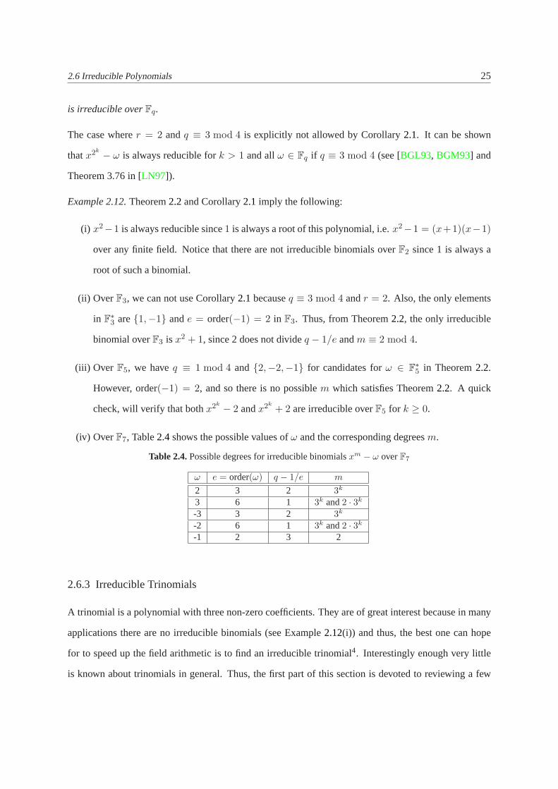
2.6 Irreducible Polynomials 25
is irreducible overFq.
The case wherer = 2 andq ≡ 3 mod 4 is explicitly not allowed by Corollary2.1. It can be shown
thatx2k− ω is always reducible fork > 1 and allω ∈ Fq if q ≡ 3 mod 4 (see [BGL93, BGM93] and
Theorem 3.76 in [LN97]).
Example 2.12.Theorem2.2and Corollary2.1 imply the following:
(i) x2−1 is always reducible since1 is always a root of this polynomial, i.e.x2−1 = (x+1)(x−1)
over any finite field. Notice that there are not irreducible binomials overF2 since 1 is always a
root of such a binomial.
(ii) Over F3, we can not use Corollary2.1becauseq ≡ 3 mod 4 andr = 2. Also, the only elements
in F∗3 are{1,−1} ande = order(−1) = 2 in F3. Thus, from Theorem2.2, the only irreducible
binomial overF3 is x2 + 1, since 2 does not divideq − 1/e andm ≡ 2 mod 4.
(iii) Over F5, we haveq ≡ 1 mod 4 and{2,−2,−1} for candidates forω ∈ F∗5 in Theorem2.2.
However, order(−1) = 2, and so there is no possiblem which satisfies Theorem2.2. A quick
check, will verify that bothx2k− 2 andx2k
+ 2 are irreducible overF5 for k ≥ 0.
(iv) OverF7, Table2.4shows the possible values ofω and the corresponding degreesm.
Table 2.4.Possible degrees for irreducible binomialsxm − ω overF7
ω e = order(ω) q − 1/e m
2 3 2 3k
3 6 1 3k and2 · 3k
-3 3 2 3k
-2 6 1 3k and2 · 3k
-1 2 3 2
2.6.3 Irreducible Trinomials
A trinomial is a polynomial with three non-zero coefficients. They are of great interest because in many
applications there are no irreducible binomials (see Example2.12(i)) and thus, the best one can hope
for to speed up the field arithmetic is to find an irreducible trinomial4. Interestingly enough very little
is known about trinomials in general. Thus, the first part of this section is devoted to reviewing a few

26 2. Mathematical Background
“classical” results as well as recursive constructions to obtain irreducible polynomials from known ones.
In the second part, we treat the recent results from von zur Gathen [vzG03].
Classical Results
As mentioned in Section2.6.2, binomials of the formx2k− ω over Fq are always reducible overFq
for all ω ∈ Fq if q ≡ 3 mod 4. However, it is possible to construct irreducible trinomials as shown in
[BGM93].
Theorem 2.3.[BGM93, Theorem 1] Letp ≡ 3 mod 4 be a prime andv the largest integer such that
2v|(p + 1). Defineav recursively by the formula
ai =
±(
ai−1+12
)(p+1)/4for 2 ≤ i ≤ v − 1
±(
ai−1−12
)(p+1)/4for i = v
with the initiala1 = 0 and at each step one can choose either+ sign or− sign. Then
x2k
− 2avx2k−1− 1
is irreducible overFp for every integerk ≥ 1.
Before we continue we introduce a well known result on how to constructan irreducible polynomial
over an extension fieldFqk given one which is irreducible overFq.
Theorem 2.4.[LN97, Theorem 3.46] An irreducible polynomial overFq of degreen remains irreducible
overFqk if and only ifgcd(k, n) = 1.
Example 2.13.The polynomialP (x) = x11 + x2 + 1 is irreducible overF2. Thus, by Theorem2.4
it remains irreducible overF22r for any r ≥ 1, sincegcd(2r, 11) = 1. This construction was used in
[DBV+96] and [GP97] to perform efficient field arithmetic in the fieldF2176∼= GF ((216)11) in the
context of elliptic curve based cryptography.
Reference [BGL93] noticed that ifq = pm ≡ 3 mod 4, for p a prime,m must be odd and thus,
combining this result with Theorem2.4, we see thatx2k− 2avx
2k−1− 1 is also irreducible overFq

2.6 Irreducible Polynomials 27
for every integerk ≥ 1. The previous statement together with Theorems2.2 and2.3 prove that when
q is odd there is always an irreducible binomial or trinomial of degree2k over Fq [BGL93]. Another
classical result on irreducible trinomials is the following:
Theorem 2.5.[LN97, Theorem 3.78] Letb ∈ Fq and letp be the characteristic ofFq. Then the trinomial
xp − x− b is irreducible inFq[x] if and only if theTrFq(b) 6= 0
Corollary 2.2. For a, b ∈ F∗q , the trinomialxp − ax − b is irreducible overFq if and only ifa = Ap−1
for someA ∈ Fq andTrFq(b/Ap) 6= 0
There are several recursive constructions of irreducible polynomialswhich lead to new irreducible
polynomials. We refer to [Men93, Chapter 3] for a nice treatment of such constructions. Here we
include one result which we will use in Chapter7 and which itself leads to new irreducible trinomials
given an irreducible trinomial. Notice that ifF (x) is a trinomial, thenF (xt) is also a trinomial.
Theorem 2.6.[LN97, Theorem 3.35] LetF1(x), F2(x), . . . , FN (x) be all the distinct monic irreducible
polynomials inFq[x] of degreem and ordere, and lets ≥ 2 be an integer whose prime factors dividee
but notqm − 1/e. Assume also thatqm ≡ 1 mod 4 if s ≡ 0 mod 4. ThenF1(xs), F2(x
s), . . . , FN (xs)
are all the distinct monic irreducible polynomials inFq[x] of degreems and orderes.
Corollary 2.3. [BGL93, Corollary 10] LetF (x) ∈ Fq[x] a polynomial of degreem with exponente and
let r be a prime factor ofe such thatr does not divideqm − 1/e. Assume also thatqm ≡ 1 mod 4 if
r = 2. ThenF (xrk) is irreducible overFq[x] for every integerk ≥ 1.
New Results on Trinomials
FieldsF3m have received a lot of attention in the past couple of years because of their applications in
cryptography. This section summarizes the results from [Loi00] and [vzG03] which we use to derive
optimized cubing architectures well suited for FPGAs in Chapter5 as well as to provide tables of irre-
ducible polynomials over fields of odd characteristic. In the following discussion we use a theorem due
to Swan [Swa62]

28 2. Mathematical Background
Theorem 2.7.[Swa62] Let Fq be a finite field of odd characteristic,n > k ≥ 1 are integers,F (x) =
xn + axk + b ∈ Fq[x] with a, b ∈ F∗q , r is the number of irreducible factors ofF in Fq[x], andD ∈ Fq
is the discriminant ofF . Then ifF is square free, thenr ≡ n mod 2 if and only ifD is a square inFq.
In [Loi00], Loidreau studies trinomialsP (x) = xn ± xk ± 1 over F3 and finds congruences for
n andk which together with the number of times that 2 dividesn andk characterize the property of
P (x) being square free and having an odd number of irreducible factors. Notice that any irreducible
polynomial always satisfies such property but the converse is not true [vzG03]. OverF3 there are four
monic trinomials of degreen overF3, i.e.,xn+xk +1, xn+xk−1, xn−xk +1, andxn−xk−1 and the
polynomialxn+xk +1 is always reducible overF3 since 1 is always a root of it. Using Theorem2.7and
the expression for the discriminant of trinomial (Theorem2.1), reference [Loi00] computes explicitly
for which values ofn andk, a trinomialP (x) overF3 has an odd number of irreducible factors. These
results are summarized in Table2.5together with the corrections pointed out in [vzG03].
Table 2.5.Values ofn andk for which the trinomials overF3 have an odd number of irreducible factors. Here foran integers, v2(s) implies thats = 2v2(s)s1 wheres1 is odd.
n mod 12 xn + xk + 1 xn + xk − 1 xn − xk + 1 xn − xk − 1
0 — k ≡ 2, 4 mod 6 — k ≡ 2, 4 mod 61 k ≡ 4, 5 mod 6 k ≡ 0, 1 mod 3 k ≡ 0, 1 mod 3 k ≡ 0, 1 mod 32 k ≡ 0, 2 mod 3 k ≡ 1 mod 6 k ≡ 0, 2 mod 3 k ≡ 1 mod 6
k ≡ 4 mod 63 k ≡ 0, 1 mod 3 k ≡ 2 mod 3 k ≡ 1, 2 mod 3 k ≡ 1 mod 34 — k ≡ 0, 1 mod 3 — k ≡ 0, 1 mod 3
k ≡ 2 mod 6, v2(k) 6= v2(n) k ≡ 2 mod 6, v2(k) ≤ v2(n)5 — k ≡ 4 mod 6 k ≡ 1 mod 3 k ≡ 1 mod 66 k ≡ 1, 2 mod 3 k ≡ 1, 5 mod 6 k ≡ 1, 2 mod 3 k ≡ 1, 5 mod 67 — k ≡ 2 mod 6 k ≡ 2, 5 mod 6 k ≡ 5 mod 68 — k ≡ 0, 2 mod 3 — k ≡ 0, 2 mod 3
k ≡ 4 mod 6, v2(k) 6= v2(n) k ≡ 4 mod 6, v2(k) ≤ v2(n)9 k ≡ 1, 2 mod 6 k ≡ 1 mod 3 k ≡ 4, 5 mod 6 k ≡ 2 mod 310 k ≡ 0, 1 mod 3 k ≡ 5 mod 6 k ≡ 0, 1 mod 3 k ≡ 5 mod 6
k ≡ 2 mod 6, v2(k) ≥ v2(n)11 k ≡ 0, 2 mod 3 k ≡ 0, 2 mod 3 k ≡ 0, 2 mod 3 k ≡ 0, 2 mod 3
Reference [vzG03] further generalizes the work in [Loi00]. In particular, von zur Gathen [vzG03]
gives a necessary condition (but not sufficient) for trinomials overFq for q an odd prime power to be
irreducible. This result is summarized in Theorem2.8. Before stating the theorem, we make a definition
which we will use in the theorem.
Definition 2.23.We say that a polynomialF ∈ Fq[x] satisfies property(S) if F is square free and it has
an odd number of irreducible factors
Theorem 2.8.Let q be a power of the odd primep, F (x) = xn + axk + b with a, b ∈ F∗q , n > k ≥ 1,

2.6 Irreducible Polynomials 29
d = gcd(n, k), n1 = n/d, k1 = k/d, m2 = p(q − 1), andm1 = lcm(4, m2). Then the discriminant of
F and property(S) depend only on the following residues:
n mod m1, k mod m2, n1 mod q − 1 and k1 mod q − 1
In order to minimize the search for irreducible polynomials, [vzG03] notices the following useful trans-
formations:
1. Lets, k0 = 0 < k1 < · · · < ks−1 = n be non-negative integers and
R =
∑
0≤i<s
aixki : all ai ∈ F∗
q , an = 1
⊆ Fq[x]
be the set of monic polynomials with support{k0, . . . , ks−1}. Notice that eachF ∈ R is s-sparse.
Then itsmonic reversal, denotedF , is defined by
F = a−10 xnf(x−1) = a−1
0
∑
0≤i<s
aixn−ki
and it is alsos-sparse. This transformation preserves square freeness and the number of irreducible
factors.
2. Let u ∈ F∗q andF ∈ R, setFu = u−nF (ux). Then,Fu ∈ R and the transformation preserves
square freeness and the number of irreducible factors.
3. Assume the notation as in Theorem2.8, and1 ≤ k∗ < n∗ with n∗ ≡ −n mod m1, k∗ ≡ −k mod
m2, n∗1 ≡ −n1 mod (q − 1), k∗
1 ≡ −k1 mod (q − 1), andF ∗ = xn∗+ axk∗
+ b. ThenF has
property(S) if and only if F ∗ does.
Notice that the concept ofs-sparse refers to the number of non-zero coefficients in a given polynomial.
Thus, in the above transformations if you begin with a trinomial after the transformation you still have
a trinomial. Similarly, a transformation which preserves square freeness and the number of irreducible
factors implies that ifF ∈ Fq[x] satisfies property(S) then the transformed polynomial will also satisfy
this property.

30 2. Mathematical Background
2.6.4 Irreducible AOPs and ESPs
Irreducible All One Polynomials (AOPs) and Equally Spaced Polynomials (ESPs) have been repeatedly
proposed in the literature to optimize arithmetic in fields of characteristic two [IT89, Ito91, HWB92,
cKKS98, WH98, LLL01] as well as arithmetic in fields of odd characteristic [GP02]. In the following,
we formally define AOPs and ESPs and show two constructions for irreducible AOPs and ESPs. These
definitions and constructions are used in Chapter7 to instantiate fields which allow for an efficient
implementation of the Itoh and Tsujii algorithm for inversion [IT88].
Definition 2.24. [WW84] A polynomialF (x) = xk + xk−1 + · · ·+ x + 1 overGF (q) is called an All
One Polynomial (AOP) of degreek.
Definition 2.25. [ IT89] A polynomialG(x) = xsk + xs(k−1) + · · · + xs + 1 = F (xs) over GF (q),
whereF (x) is an AOP of degreek overGF (q) is called a binarys-Equally Spaced Polynomial (s-ESP)
of degreesk.
We have abused the original definitions which were for the caseq = 2 and generalized them toq = pn,
p an odd prime. Notice that AOPs are just a special case of binarys-ESPs in whichs = 1. Theorem2.9
describes the cases when irreducible AOPs exist.
Theorem 2.9.[Men93, Chapter 5] The polynomialf(x) = xm + xm−1 + · · · + x + 1 is irreducible
overGF (q) if and only ifm + 1 is prime andq is primitive inGF (m + 1)
We can use Theorem2.6 to construct an irreducibles-ESP given an irreducible AOP. In particular,
by choosingGF (q) andm such that any of theFi(x) in Theorem2.6 is a binary AOP, we immediately
obtain a binary irreducibles-ESP, wheres satisfies the conditions in Theorem2.6. Notice, also, that if
we construct an irreducibles-ESP of degreesm overGF (q) using Theorem2.6, call it P (x), thenP (x)
is also irreducible overGF (qk), for k satisfyinggcd(k, sm) = 1 by Theorem2.4.
2.7 Notes and Further References
1. McEliece [McE89] also provides a nice introduction to the theory of finite fields as well as to their
applications in engineering. The books by Lidl and Niederreiter [LN97] and Jungnickel [Jun93] provide

2.7 Notes and Further References 31
comprehensive treatments of the subject. It is also worth mentioning the book by Menezes [Men93]
which has extensive treatment of topics such as constructions of normal and optimal normal bases.
2. Optimal normal bases were introduced in [MOVW89] as a way of implementing discrete logarithm-
based systems over binary fieldsGF (2n) with n ≥ 1000 which at the time seemed infeasible using
only normal basis. Although the authors in [MOVW89] make emphasis on binary fields, their work also
applies to fieldsGF (pm), for odd primesp. Reference [GL92] showed that the normal bases found
in [MOVW89] were essentially all the normal bases. Gao and Vanstone [GV95] provide experimental
results on the multiplicative orders of optimal normal basis generators inGF (2n) overGF (2) for n ≤
1200. See also [Men93, Chapters 4 and 5] for a nice overview of optimal normal basis and some
constructions. Normal and optimal normal bases have been repeatedly proposed for efficient arithmetic
in finite fields of characteristic two with applications to discrete logarithm based systems [AMOV91] as
well for elliptic curves [AMV93, MV93]. Parallel architectures for multiplication using normal basis
have been proposed in [WTS+85, MO86, cKKS98, ScKK01, RMH02a, Kwo03]. Reference [RMH03a]
offers multiplier architectures for composite fieldsGF ((2n)m) using normal basis while [RMH02b] and
[RMH03b] propose digit-serial and sequential multipliers using normal basis, respectively. References
[HTDR88, JB92, PL95] offer comparisons between binary finite field architectures based on thechosen
basis for small fields while [GG90] compares polynomial and normal basis architectures for field sizes
of interest in cryptography. We refer to Section7.5 in Chapter7 for uses of normal bases for inversion
in finite fields.
3. Lidl and Niederreiter [LN97] provide a comprehensive treatment of irreducible polynomials. Ref-
erences [BGL93, Men93] also give interesting overviews of known results on irreducible polynomials
until the year 1993. In addition, reference [BGL93] extends the tables of irreducible trinomials over
GF (2) in [ZB68, ZB69] up to degreem ≤ 2000. Reference [Zie69] provides tables of primitive trino-
mials of degreep such that2p− 1 is known to be prime andp ≤ 11213. Tables of irreducible trinomials
overGF (2) are also found in [MvOV97] for degree up tom ≤ 1478 and for primitive trinomials over
GF (2n) of degreem ≤ 229. Reference [CQS01] proved that ifp is a prime andp ≡ 13 mod 24 or
p ≡ 19 mod 24 then there is no irreducible trinomial of degreep overGF (2). References [Loi00] and
[vzG03] used the work of Swan [Swa62] to describe necessary conditions (but not sufficient) for trinomi-

32 2. Mathematical Background
als to be irreducible overGF (3). Vishne [Vis97] provides some sufficient conditions for a trinomial over
a field of characteristic two to be reducible. For example, [Vis97] shows thatxm+axk +b ∈ GF (2n)[x]
is reducible if bothm, n are even except possibly whenm = 2k andk is odd.
4. There has been a great deal of research done on the arithmetic advantages of irreducible polynomials
of special form overGF (2). In [IT89], AOPs and ESPs overGF (2) are introduced. The authors show
necessary and sufficient conditions for ESPs to be irreducible overGF (2) and propose a new configu-
ration of parallel multipliers for fieldsGF (2m), based on irreducible AOPs and ESPs overGF (2). In
[Ito91], necessary and sufficient conditions are given for a family of infinitelymany ESPs to be irre-
ducible overGF (2). In addition, a uniqueness criteria which characterizes all irreducible ESPs over
GF (2) in a strict sense is presented.

CHAPTER 3
Architectures for Arithmetic in SmallGF (p)
Fields
In this chapter, we survey previous hardware architectures for performing addition operations inZ and
addition and multiplication inGF (p) fields, wherep is odd, prime, andsmall. Section3.1 deals with
integer adders which will be fundamental building blocks for theGF (p) multipliers presented in Chap-
ter 4. The remaining of the material presented in this chapter comes from the literature on Residue
Number Systems (RNS) which is particularly useful in Digital Signal Processing (DSP) applications.
However, we depart from these traditional applications. In Chapter5, we use the architectures presented
here to build multipliers forGF (pm) fields, forp odd, and large enough for cryptographic applications,
i.e., withpm ≥ 2160. At the end of this chapter, we describe newGF (p) multipliers, forp > 2, specially
suited forGF (pm) multiplication. Parts of this chapter appear in [GWP02].
3.1 Integer Adders
It is well known that adders constitute the basic building blocks for more complicated arithmetic oper-
ators such as multipliers. Thus, this section surveys adder architectures which we will used in future
sections to implement more complicated operators. Our focus, rather than comprehensive, is on those

34 3. Architectures for Arithmetic in SmallGF (p) Fields
adders to which we will refer in future chapters as we survey architectures forGF (p) arithmetic in
the context of cryptographic applications. For more detailed treatments of hardware architectures and
computer arithmetic, we refer the reader to [Kor93, Par99].
In what follows, we consider the addition of twon-bit integersA =∑n−1
i=0 ai2i andB =
∑n−1i=0 bi2
i,
with S = cout2n +
∑n−1i=0 si2
i = A + B being possibly an(n + 1)-bit integer. We refer toA andB
as the inputs (and to their bitsai andbi as the input bits) and toS as the sum (and to its bitssi for
i = 0 · · ·n− 1 as the sum bits). The last bit of the sumcout receives the special name of carry-out bit.
3.1.1 Ripple-Carry Adders (RCA)
Single-bit half-adders (HA) and full-adders (FA) are the basic buildingblocks used to synthesize more
complex adders. A HA accepts two input bitsa andb and outputs a sum-bits and a carry-out bitcout
following (3.1) and (3.2)
s = a⊕ b (3.1)
cout = a ∧ b (3.2)
A half-adder can be seen as a single-bit binary adder that produces the 2-bit binary sum of its inputs,
i.e.,a + b = (cout s)2. In a similar manner, a full-adder accepts a 3-bit inputa, b and a carry-in bitcin,
and outputs two bits: a sum-bits and a carry-out bitcout, according to (3.3) and (3.4)
s = a⊕ b⊕ cin (3.3)
cout = (a ∧ b) ∨ (cin ∧ (a ∨ b))
= (a ∧ b) ∨ (a ∧ cin) ∨ (b ∧ cin) (3.4)
Pictorially, we can view half-adders and full-adders as depicted in Figures 3.1 and3.2. We notice that
because of the importance of the FA as an arithmetic building block, there are many optimized FA
designs for a variety of implementation technologies [Par99]. An n-bit ripple-carry adder (RCA) can
be synthesized by concatenatingn single-bit FA cells, with the carry-out bit of theith-cell used as the

3.1 Integer Adders 35
outc HA
a
s
b
Figure 3.1.Half-adder cell
outc cinFA
a b
s
Figure 3.2.Full-adder cell
carry-in bit of the(i + 1)th-cell. The resultingn-bit adder outputs ann-bit long sum and a carry-out bit.
This is depicted in Figure3.3. The total latency of ann-bit RCA can be approximated byn ·TFA, where
cinoutcc0
2s 1s 0s
c1
0a 0b1bb2 1a2a
c3cn−1
n−1bn−1a
cn c2
n−1
FA
s
FA FA FA. . .
Figure 3.3.n-bit carry-ripple adder
TFA refers to the delay of a single full-adder cell. Designingn-bit RCAs for any value ofn is a rather
simple task: simply, concatenate as many FA cells as bits of precision are required. In addition, although
not directly relevant to the treatment here, RCA-based designs have two other advantages: (1) easy sign
detection if one uses 2’s complement arithmetic, and (2) subtraction is accomplished by first converting
the subtrahend to its 2’s complement representation and then adding the result to the original minuend.
However, the delay of the RCA grows linearly withn, making it undesirable for large values ofn or
for high-speed applications, as it is the case in many cryptographic systems. Thus, the need to explore
other designs to improve the performance of the adder without significantly increasing area-resource
requirements.

36 3. Architectures for Arithmetic in SmallGF (p) Fields
3.1.2 Carry-Lookahead Adders (CLA)
As it name indicates a carry lookahead adder (CLA) computes the carries generated during an addition
before the addition process takes place, thus, reducing the total time delay of the RCA at the cost of
additional logic. We next make some definitions that will help us in developing a CLA.
Definition 3.1. Letai, bi be two operand digits in radix-r notation andci be the carry-in digit. Then, we
define the generate signalgi, the propagate signalpi, and the annihilate (absorb) signalvi as:
gi = 1 if ai + bi ≥ r
pi = 1 if ai + bi = r − 1
vi = 1 if ai + bi < r − 1
whereci, gi, pi, vi ∈ {0, 1} and 0 ≤ ai, bi < r.
Notice that Definition3.1is independent of the radix used which allows one to treat the carry propagation
problem independently of the number system [Par99]. Specializing to the binary case and using the
signals from Definition3.1, we can re-writegi, pi, andvi as:
gi = ai ∧ bi (3.5)
pi = ai ⊕ bi (3.6)
vi = ai ∧ bi = ai ∨ bi (3.7)
Relations (3.5), (3.6), and (3.7) have very simple interpretations. Ifai, bi ∈ GF (2), then a carry will
be generated whenever bothai andbi are equal to one, a carry will be propagated if eitherai or bi are
equal to one, and a carry will be absorbed whenever both input bits areequal to zero. In some cases it
is also useful to define a transfer signal (ti = ai ∨ bi) which denotes the event that the carry-out will
be one given that the carry-in is equal to one1. Combining (3.4), (3.5), and (3.6) we can write the
carry-recurrence relation as follows:
ci+1 = gi ∨ (ci ∧ ti) = gi ∨ (ci ∧ pi) (3.8)

3.1 Integer Adders 37
Proof.
ci+1 = gi ∨ (ci ∧ ti) = gi ∨ (ci ∧ (a ∨ b))
= gi ∨ (ci ∧ ((a ∨ b) ∧ (a ∨ a))) = gi ∨ (ci ∧ (a ∨ (a ∧ b)))
= gi ∨(ci ∧
((a ∧ (b ∨ b)) ∨ (a ∧ b)
))
= gi ∨(ci ∧
((a ∧ b) ∨
((a ∧ b) ∨ (a ∧ b)
)))
= gi ∨ (ci ∧ ((a ∧ b) ∨ (a⊕ b)))
= gi ∨ (ci ∧ gi) ∨ (ci ∧ pi) = gi ∨ (ci ∧ pi)
where we have made use of the fact thata ∨ b = (a ∨ (a) ∧ (a ∨ b). ⊓⊔
Intuitively, (3.8) says that there will be a non-zero carry at stagei + 1 if either the generate signal is
equal to one or there was a carry at stagei and it was propagated (or transfered) by this stage. Notice
that implementing the carry-recurrence using the transfer signal leads to slightly faster adders than using
the propagate signal, since an OR gate is easier to produce than an XOR gate[Par99]. Finally, notice
that from (3.3) and (3.6), it follows that
si = pi ⊕ ci (3.9)
3.1.3 Carry-Save Adders (CSA)
A CSA is simply a parallel ensemble ofn full-adders without any horizontal connection, i.e., the carry bit
from adderi is not fed to adderi + 1 but rather, stored asc′i. In particular given threen-bit integersA =
∑n−1i=0 ai2
i, B =∑n−1
i=0 bi2i, andC =
∑n−1i=0 ci2
i, their sum produces two integersC ′ =∑n
i=0 c′i2i and
S =∑n−1
i=0 si2i such that
C ′ + S = A + B + C

38 3. Architectures for Arithmetic in SmallGF (p) Fields
where:
si = ai ⊕ bi ⊕ ci (3.10)
c′i+1 = (ai ∧ bi) ∨ (ai ∧ ci) ∨ (bi ∧ ci) (3.11)
wherec′0 = 0 (notice that (3.10) and (3.11) are nothing else but (3.1) and (3.2) re-written for different
inputs and outputs). Ann-bit CSA is shown in Figure3.4. We point out that since the inputsA, B, and
n−1bn−1a cn−1
n−1sc’n
FA
2s
2a b2 c2
c’3
FA
1s
1a 1b c1
2c’
FA
0s
0a 0b c0
c’1
. . . FA
0c’ = 0
Figure 3.4.n-bit carry-save adder
C are all applied in parallel the total delay of a CSA is equal to that of a full-adder cell (i.e. the delay
of (3.10) and (3.11)). On the other hand, the area of the CSA is justn-times the area of a FA cell and
it scales very easily by adding more FA-cells in parallel. Subtraction can be accomplished by using 2’s
complement representation of the inputs. However, CSAs have two major drawbacks:
• Sign detection is hard. In other words, when an integer is represented asa carry-save pair(C ′, S)
such that its actual value isC ′ + S, we may not know the sign of the total sumC ′ + S unless the
addition is performed in full length. In [KH91] a method for fast sign estimation is introduced and
applied to the construction of modular multipliers.
• CSAs do not solve the problem of adding two integers and producing a single output. Instead, it
adds three integers and produces two outputs.
We end this section with an example that illustrates the operation of a CSA.
Example 3.1.Let A = 59 = (1 1 1 0 1 1)2, B = 61 = (1 1 1 1 0 1)2, andC = 43 = (1 0 1 0 1 1)2. Then,

3.1 Integer Adders 39
S andC ′ follow from (3.10) and (3.11) as:
A = 59 = 1 1 1 0 1 1
B = 61 = 1 1 1 1 0 1
C = 43 = 1 0 1 0 1 1
A + B + C = 163 = 1 0 1 0 0 0 1 1
S = 45 = 1 0 1 1 0 1
C ′ = 118 = 1 1 1 0 1 1 0
S + C ′ = 163 = 1 0 1 0 0 0 1 1
3.1.4 Carry-Delayed Adders (CDA)
Carry-delayed adders (CDAs) were originally introduced in [NS81] as a modification to the CSA par-
adigm. In particular, a CDA is a two-level CSA. Thus, addingA =∑n−1
i=0 ai2i, B =
∑n−1i=0 bi2
i, and
C =∑n−1
i=0 ci2i, we obtain the sum-pair(D, T ), such thatD + T = A + B + C, where
si = ai ⊕ bi ⊕ ci (3.12)
c′i+1 = (ai ∧ bi) ∨ (ai ∧ ci) ∨ (bi ∧ ci) (3.13)
ti = si ⊕ c′i (3.14)
di+1 = si ∧ c′i (3.15)
with c′0 = d0 = 0. Notice that (3.14) and (3.15) are exactly the same equations that define a half-adder,
thus ann-bit CDA is nothing else but ann-bit CSA plus a row ofn half-adders. The overall latency is
equal to the delay of a full-adder and a half-adder cascaded in series,whereas the total area is equal ton
times the area of a full-adder and a half adder. The CDA scales in same manner as the CSA. Figure3.5
depicts ann-bit CDA. We notice thatti anddi+1 satisfy
di+1 ∧ ti = 0 (3.16)

40 3. Architectures for Arithmetic in SmallGF (p) Fields
0d = 0
HA
n−1tdn
HA
3t4d
HA
2d t1
HA
0t1d
HA
t3d
c’3
0a 0b c0
FA
1a 1b c1
FA
2a b2 c2
FA
n−1b cn−1n−1a
FA
0c’ = 0c’n c’n−1 2c’ c’1
0s1s2s3sn−1s
2
. . .
. . .
. . .
Figure 3.5.n-bit carry-delayed adder
for all 0 ≤ i < n. This property is easily proved as follows:
di+1 ∧ ti = (si ∧ c′i) ∧ (si ⊕ c′i) = si ∧ c′i ∧((si ∧ c′i) ∨ (si ∧ c′i)
)=
= (si ∧ c′i ∧ c′i) ∨ (si ∧ si ∧ c′i) = 0
where we made use of fact that
si ⊕ c′i = (si ∧ c′i) ∨ (si ∧ c′i)
and of some basic Boolean algebra theorems. Property (3.16) of the CDA implies that eitherdi+1 or
ti or both are equal to zero, is exploited by Brickell in [Bri82] to reduce the complexity of a modular
multiplier. We end this section with an example.
Example 3.2.Let A = 43 = (1 0 1 0 1 1)2, B = 53 = (1 1 0 1 0 1)2, andC = 62 = (1 1 1 1 1 0)2. Then,

3.1 Integer Adders 41
S andC ′ follow from (3.10) and (3.11) as:
A = 43 = 1 0 1 0 1 1
B = 53 = 1 1 0 1 0 1
C = 62 = 1 1 1 1 1 0
A + B + C = 158 = 1 0 0 1 1 1 1 0
S = 32 = 1 0 0 0 0 0
C ′ = 126 = 1 1 1 1 1 1 0
A + B + C = 158 = 1 0 0 1 1 1 1 0
T = 94 = 1 0 1 1 1 1 0
D = 64 = 1 0 0 0 0 0 0
ti ∧ di+1 = 0 0 0 0 0 0 0
T + D = 158 = 1 0 0 1 1 1 1 0
3.1.5 Summary and Comparison
Section3.1 described four different integer adders: ripple-carry adders, carry-lookahead adders, carry-
save adders, and carry-delayed adders. The asymptotic complexity of the above adders is summarized
in Table3.1and it is well known.
Table 3.1.Asymptotic area/time complexities of differentn-bit adders.
Adder Type Abbreviation Area Time
Ripple-Carry Adder RCA O(n) O(n)Carry-Lookahead Adder CLA O(n log n) O(log n)Carry-Save Adder CSA O(n) O(1)Carry-Delayed Adder CDA O(n) O(1)
We, however, are interested in providing actual area estimates and, thus,asymptotics are not the right
measure for this work. In terms of the components in Table1.1, the area and delay of the RCA, CSA,
and CDA are straight forward to estimate. However, the area of a CLA is very dependent on the actual
implementation. Thus, we have used [NIO96] as a way of estimating the size and time delay of the
CLA with respect to the RCA and CSA sizes2. The authors in [NIO96] have performed their study with
the purpose of giving the practitioner insight into design trade-offs that can save power and enhance

42 3. Architectures for Arithmetic in SmallGF (p) Fields
performance. As transistors shrink and wireless devices take over ourdaily lives, it is our opinion that
power will probably be the optimization criteria of choice in most applications andthus, the relative
size of the CLA with respect to RCA and CDA designs will be representativeof current and future
implementations. In addition, [NIO96] point out that by reducing area, power consumption is in general
also reduced and therefore, area considerations are not completely left out in this study. Table3.2
provides the area and delay characteristics of the RCA, CSA, CLA in [NIO96] for 16-bit, 32-bit, and
64-bit designs.
Table 3.2.Area/time complexities of RCA, CSA, and CLA according to [NIO96]. Area and delay are normalizedwith respect to estimated FA delay.
Adder Area (transistors) Area (normalized) Time (nsec) Time (normalized)Type 16-bit 32-bit 64-bit 16-bit 32-bit 64-bit 16-bit 32-bit 64-bit 16-bit 32-bit 64-bit
RCA 596 1204 2420 15.9 32.0 64.4 26.3 52.5 105 16.0 32.0 64.0CLA 1038 2132 4348 27.6 56.7 115.6 11.0 14.2 15.8 6.7 8.7 9.6CSA 1176 2360 4728 31.3 62.8 125.7 5.0 5.0 5.0 3.0 3.0 3.0FA 37.6 1.0 1.64 1.0(estimate)
We make the following observations regarding Table3.2:
• We estimate the delay of one FA by dividing the 16-bit, 32-bit, and 64-bit RCA areas and delays
by 16, 32, and 64, respectively, and averaging out the results. Our estimated FA delay is shown in
the last row of Table3.2. Based on these estimates, we calculate the normalized area and delay of
the other designs.
• The area and delay of ann-bit RCA can be approximated asn FA andn TFA, respectively.
• The CSA design of [NIO96] includes two levels of FA. We assume that asimpleCSA as the one
presented in Section3.1.3requires the same resources as a RCA but half the delay of the CSA in
[NIO96]. Thus, the area and delay of asimpleCSA can be approximated asn FA and1.5 TFA,
respectively.
• The area and delay of ann-bit CLA can be approximated as0.36n⌈log2 n⌉FA and1.67⌈log2 n⌉TFA,
respectively.
Table3.3 summarizes the above discussion and includes the time and area complexities which will be
assumed in the following sections when integers adders are used.
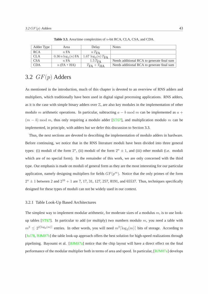
3.2GF (p) Adders 43
Table 3.3.Area/time complexities ofn-bit RCA, CLA, CSA, and CDA.
Adder Type Area Delay Notes
RCA n FA nTFACLA 0.36n log2(n) FA 1.67 log2(n)TFACSA n FA 1.5TFA Needs additional RCA to generate final sumCDA n (FA + HA) TFA + THA Needs additional RCA to generate final sum
3.2 GF (p) Adders
As mentioned in the introduction, much of this chapter is devoted to an overview of RNS adders and
multipliers, which traditionally have been used in digital signal processing applications. RNS adders,
as it is the case with simple binary adders overZ, are also key modules in the implementation of other
modulom arithmetic operations. In particular, subtractinga − b mod m can be implemented asa +
(m − b) mod m, thus only requiring a modulo adder [ST67], and multiplication modulom can be
implemented, in principle, with adders but we defer this discussion to Section3.3.
Thus, the next sections are devoted to describing the implementation of modulo adders in hardware.
Before continuing, we notice that in the RNS literature moduli have been divided into three general
types: (i) moduli of the form2n, (ii) moduli of the form2n ± 1, and (iii) other moduli (i.e. moduli
which are of no special form). In the remainder of this work, we are only concerned with the third
type. Our emphasis is made on moduli of general form as they are the most interesting for our particular
application, namely designing multipliers for fieldsGF (pm). Notice that the only primes of the form
2n ± 1 between 2 and216 + 1 are 7, 17, 31, 127, 257, 8191, and 65537. Thus, techniques specifically
designed for these types of moduli can not be widely used in our context.
3.2.1 Table Look-Up Based Architectures
The simplest way to implement modular arithmetic, for moderate sizes of a modulusm, is to use look-
up tables [ST67]. In particular to add (or multiply) two numbers modulom, you need a table with
m2 ≤ 22⌈log2(m)⌉ entries. In other words, you will needm2⌈log2(m)⌉ bits of storage. According to
[Jul78, BJM87b] the table look-up approach offers the best solution for high-speed realizations through
pipelining. Bayoumi et al. [BJM87a] notice that the chip layout will have a direct effect on the final
performance of the modular multiplier both in terms of area and speed. In particular, [BJM87a] develops

44 3. Architectures for Arithmetic in SmallGF (p) Fields
a design methodology to obtain an optimized layout for table look-up-based modulo adders and multi-
pliers. Reference [BJM87b] expands on the work of [BJM87a] and compares the table look-up based
implementation to binary adder based and hybrid (combining table look-ups andcombinatorial circuits)
design methods and concludes that table look-up based methods are, both interms of area and time
performance, optimal forgeneralmoduli which can be represented with at most 5 bits. Table3.4sum-
marizes the recommended implementation approach for moduli of different sizeaccording to [BJM87b].
Table 3.4.Recommended implementation approaches for different types of moduli according to [BJM87b]. LT :Look-Up Table, BA: Binary Adder, HY: Hybrid.
Modulo size 2–3 4 5 6 7 8 and up(bits)Modulo type Area Time Area Time Area Time Area Time Area Time Area Time2n ± 1 LT LT LT LT BA LT BA HY BA HY BA HYgeneral LT LT LT LT LT LT HY HY HY HY HY HY
3.2.2 Combinatorial Architectures
Combinatorial architectures are based on the fact that the additionA + B mod m can be performed as:
A + B mod m =
A + B if A + B < m
A + B −m if A + B ≥ m(3.17)
Such realization was already known in [Ban74] and it seems to date at least to 1967 [ST67]. Reference
[BJM87b] reports on a VLSI implementation of this approach using twon-bit binary adders, where
m ≤ 2n: the first adder computesA + B while the second computesA + B −m. The carry bits of the
first and second adders are combined together with an OR gate and this result is used by the multiplexer
to select the correct output. The adders are implemented according to the carry-look-ahead paradigm.
Figure3.6shows the structure of this adder and provides the reader with an example3.
In [EB90], the authors propose a modulo adder based on carry-saved adderswhich accomplishes
modular addition in constant time independently of the number of bits in the modulus.In particular, it
requires at most 5 stages ofn-bit CSA adders (for ann-bit modulus). Reference [BJS94] provides a

3.2GF (p) Adders 45
Adder 1
7 = (0111)2
212 = (1100)
Adder 2
2 − m = 5n
21 = (0001)
Mux
212 = (1100)
Adder 1
Adder 2
10 = (1010)2
2 − m = 5n
3 = (0011)2
28 = (1000)
3 = (0011)2
Adder 1
Adder 2
Mux
A + B mod m
carry 2 = 1
carry 1 = 0
5
Example 1:
A=7, B=5, m=11, n=4
5 + 7 = 1 mod 11
carry 2 = 0
carry 1 = 1
25 = (0101)
A=9, B=10, m=11, n=49 = (1001)
2
5
9 + 10 = 8 mod 11
B
carry 2
carry 1
Mux0 1
Example 2:
2 − mn
n
nn
1n
n
n
n
1
A
Figure 3.6.Binary adder-based RNS adder from Bayoumi [BJM87b]
formal proof of the previous statement. The adder is designed for medium tolarge size moduli. One
problem with this adder is that it does not consider how to convert back from the CSA representation
to the binary representation which, in general, requires a ripple carry-adder, thus incurring in additional
delay. This fact effectively renders the advantages of the CSA approach from [EB90] impractical for
normal RNS applications. It seems that it might only be convenient if one performs several additions
while in CSA form before transforming back to the regular binary representation or in the final stage of
a fast signal processing application for decoding and/or automatic errorcorrection [BJS94].
We would like to point out that the same idea as in [EB90], was developed independently by [BJS94]
but, this time, it is applied to an implementation of RNS arithmetic using a systolic array in the context
of conversion from RNS to binary representation conversions, i.e., implementation of the Chinese Re-
mainder Theorem (CRT). Finally, notice that a key characteristic of these architectures is the fact that
certain residues modulom do not have a unique representation. In other words, bothA andA + m are

46 3. Architectures for Arithmetic in SmallGF (p) Fields
considered valid representations ofA mod m as long asA + m < 2n, with n = ⌈log2(m)⌉. Algo-
rithm 3.1summarizes the ideas of [EB90]. This type of adder seems well suited to large moduli as the
delay will remain constant (i.e. 5 CSA stages [BJS94]).
Algorithm 3.1 5-stage algorithm for CSA RNS addition from [EB90] and [BJS94]
Input: A = (AC , AS), B = (BC , BS), andm with A = AC + AS , B = BC + BS , 2n−1 < m ≤ 2n,and0 ≤ A, B < 2n.
Output: R = (RC , RS) = A + B mod m with R = RC + RS and0 ≤ R < 2n.1: (c1, DC , DS)← AS + (BC , BS)2: (c2, RC , RS)← AC + (DC , DS)3: if c1 = 0 AND c2 = 0 then4: Return((RC , RS)5: else ifc1 + c2 = 1 then6: (c3, RC , RS)← (2n −m) + (RC , RS)7: else {if c1 = 1 AND c2 = 1}8: (c3, RC , RS)← 2(2n −m) + (RC , RS)9: end if
10: if c3 = 0 then11: Return((RC , RS)12: else13: (c4, RC , RS)← (2n −m) + (RC , RS)14: end if15: if c4 = 0 then16: Return((RC , RS)17: else18: (RC , RS)← (2n −m) + (RC , RS)19: Return((RC , RS)20: end if
Reference [Dug92] implements and compares three approaches to the layout of modulo adders based
on binary adders. The first approach is the one described by [BJM87b]. The second approach is shown
in Figure3.7. In this approach only one binary adder is used to perform two cycles ofaddition. In the
first cycle, the input multiplexers select inputsA andB to be added and, both, the sum and the carry
which result from the addition are stored in the latch. In the second cycle ofthe addition, the input
multiplexers pass the sumA + B, together with correction factor. The correct result is chosen, as in
the modular adder from [BJM87b], based on the output of a gate which ORs the carries from the two
additions. The third layout approach is shown in Figure3.8. As in the second design, the modular adder
uses only one binary adder for two cycles of addition. The second cycleof addition, however, needs

3.2GF (p) Adders 47
2 − mn
nn
n
n
n
n
n n n
1
1
Adder
Latch
MuxMux
BA
Mux
A + B mod m
sum 1
sum 2
sum 1
carry 2
carry 1
carry 1
Figure 3.7.Type II modulo adder with feedback register from Dugdale [Dug92]
to be performed only if necessary. An ”add signal” selects inputsA andB to be added during the first
cycle of addition. The sum and the carry of this addition are fed to an overflow detection. The add signal
is disabled and the overflow signal now controls the output of the multiplexersto be added during the
second cycle of addition. If an overflow is detected then the sum which resulted from the first addition
cycle together with the correction factor are added together. Otherwise, the original inputs are added a
second time. However, [Dug92] noticed that this approach could be modified to avoid performing the
second addition if unnecessary. All adders in [Dug92] are implemented as carry-lookahead adders.
Table3.5summarizes the area and timing results from [Dug92] for the three designs. The author used
2 µm, single poly, double metal, static CMOS. In Table3.5, Type I, Type II, and Type III correspond to
the three different layouts that Dugdale describes in [Dug92]. We have added two columns to the this
table which we have labeledAT for area-time product and(AT )N for normalized area-time product.
The(AT )N values are obtained by dividing theAT values for the Type I and Type III layout approaches
by theAT product of the Type II layout approach which is the one with the minimumAT value. We

48 3. Architectures for Arithmetic in SmallGF (p) Fields
2 − mn
nn
n
n
n n n
1
n1
addsignal
Adder
Latch
MuxMux
BA
A + B mod m
sum 1
Comparator
carry 1
sum 1carry 1
Figure 3.8.Type III modulo adder with overflow detection circuit from Dugdale [Dug92]
see that the Type II layout approach gives, on average, a 25 % improvement on theAT product over
the Type I layout approach (i.e. the design from [BJM87b]) and an 8 % improvement over the Type III
approach.
Table 3.5.Area-time complexities of the implementation of [Dug92] in 2 µm CMOS technology. Times are givenin nsec and area in square microns×103
Modulo Number of Type I Type II Type IIIbits A T AT (AT )N A T AT (AT )N A T AT (AT )N
5 3 261 34 8874 1.22 187 39 7293 1 183 43 7869 1.0813 4 374 41 15334 1.25 267 46 12282 1 262 51 13362 1.0929 5 452 51 23052 1.24 331 56 18536 1 324 61 19764 1.0761 6 545 63 34335 1.27 399 68 27132 1 392 74 29008 1.0797 7 643 69 44367 1.28 467 74 34558 1 456 82 37392 1.08193 8 754 72 54288 1.28 550 77 42350 1 541 87 47067 1.11
Hiasat [Hia02] introduces a new design of modulo adder based on (3.17) and builds on ideas intro-
duced by Piestrak [Pie94]. . The binary-based adder from [Hia02] is depicted in Figure3.9. In [Pie94],
the author notices that ifA + B < m thenA + B + 2n − m < 2n whereas ifA + B ≥ m then
A + B + 2n−m ≥ 2n, where0 ≤ A, B < m and2n−1 < m < 2n. Thus, based on the carry-out (cout)

3.2GF (p) Adders 49
Mux
Carry Propagate andGenerate Unit
Sum and Carry Unit
n
Summation UnitCLA and
CLA forcarry out
1
n
nn n + 1n + 1c’i + 1
ci + 1 s’ s
ai i
i i
b
nnnn
n n
A + B mod m
A B
SCS’C’
n
HAL cell
G P G’P’
Figure 3.9.Binary-based RNS adder from Hiasat [Hia02]
of the operationA + B + 2n−m (if A + B + 2n−m < 2n thencout = 0, otherwisecout = 1) one can
decide whetherA+B or A+B +2n−m is the right result forA+B mod m. Piestrak [Pie94] imple-
ments this idea in the context of residue-to-binary conversion circuits for RNS applications and uses a
CSA and two CLA adders for his circuitry. Hiasat modifies this design and achieves significant savings
in area and performance. The basic observation in [Hia02] is that if we use a CLA adder to implement
the idea of [Pie94] we only need two sets of propagate, generate, and carry signals and asingle adder
circuit. In addition, one can further reduce the required hardware resources by sharing circuitry between
the two Carry Propagate and Generate (CPG) units (the one corresponding to addingX +Y and the one
addingX + Y + Z). We make these ideas more explicit in the following.
The adder in [Hia02] consists of a Sum and Carry (SAC) unit, a CPG unit, a multiplexing unit, a
CLA for cout, and a CLA and Summation (CLAS) unit. In the following discussion we will denote by
Z =∑n−1
i=0 zi2i the constant2n − m, A =
∑n−1i=0 ai2
i, andB =∑n−1
i=0 bi2i. The SAC unit outputs
4 signals corresponding to the carry and sum signals fromA + B, denoted byC =∑n
i=0 ci2i, with
c0 = 0, andS =∑n−1
i=0 Si2i and the carry and sum signals resulting from addingA + B + Z which
we denoteC ′ =∑n
i=0 c′i2i, with c′0 = 0, andS′ =
∑n−1i=0 s′i2
i. Reference [Hia02] notices that based on

50 3. Architectures for Arithmetic in SmallGF (p) Fields
(3.3) and (3.4), one can write ifzi = 0,
si = ai ⊕ bi, ci = ai ∧ bi
and ifzi = 1
s′i = ai ⊕ bi, c′i = ai ∨ bi
A circuit which can produce the sum and carry, in both cases, i.e. whenzi = 0 and whenzi = 1,
requires one XOR gate, one AND gate, and one Exclusive-NOR gate. Such a cell receives the name
of half-adder-like (HAL) cell and it is also depicted in Figure3.9. Hiasat also notices that the number
of such cells will depend on the hamming weight ofZ, thus, the SAC unit needsHW (Z) HAL cells
and(n−HW (Z)) normal half adder cells, whereHW (·) denotes the hamming weight of the operand.
The CPG unit is designed as explained in Section3.1.2. Notice that the circuit in Figure3.9 requires
two CLA circuits, one for the sumA + B and the second for the sumA + B + Z. The propagate and
generate signals corresponding to the first sum are labeledP andG, whereas the ones corresponding
to the second sum are labeledP ′ andG′. A maximum of2n − 2 half-adder (HA) cells are required
to realize the CPG unit. However, as in the case of the SAC unit, the exact number depends on the
hamming weight ofZ. The more zeros in the binary representation ofZ the more HA cells that can be
shared betweenG andG′ andP andP ′. The CLA for the carry-out bit receives as inputsP ′ andG′ and
outputs one bit, the carry-out. The MUX requires a maximum of(n − 1) 2 × 1 multiplexers to select
betweenP andP ′ and similarly forG andG′. The number of multiplexers can be reduced depending on
how many HA cells are shared by the CPG unit. The CLAS unit receivesn carry bits andn propagate
bits which can be combined according to (3.9) to form the final sum. We estimate the overall hardware
complexity of Hiasat’s adder as: one CLA,(2HW (Z)− 1) MUX21, (HW (Z)− 1) HA4, andHW (Z)
2-input OR gates and inverters5.

3.2GF (p) Adders 51
3.2.3 Hybrid Architectures
In hybrid architectures the modulo adder is constructed using a combination of combinatorial circuits
and table-lookups. One of the earliest modulo adder designs is due to Banerji [ Ban74]. The author in
[Ban74] notices that the set of residues modulom form a finite cyclic group under addition modulom
and, thus, givenS = {0, 1, . . . , m − 1}, addingk ∈ S to any value inS corresponds to a permutation
of S by k positions to the left. The area complexity of the adder can be further reduced by performing
rotations only by powers of 2. In other words, ifk =∑⌈log2(m)⌉
i=0 ki2i, whereki ∈ {0, 1}, then you
can perform a rotation by2i positions to the left wheneverki 6= 0 and achieve the same final result.
This reduction in area complexity is at the cost of a slower modular adder. The design is optimized for
MSI/LSI technology. The operation of the adder is illustrated in the following example.
Example 3.3.Suppose that you want to add4 + 5 mod 7. Notice that5 = 22 + 1 and assume the
availability of a register that has been preloaded with all residues modulo 7 asshown in Figure3.10.
Then, we successively rotate by one and by four positions to the left andobtain the final result of
9 ≡ 2 mod 7 in register position number four. This operation is depicted in Figure3.10.
1 2 3 4 5 6
0 1 2 3 4 5 6Position #
Register contents 0
Position #
Register contents
Position #
Register contents
Result
0 1 2 3 4 5 6
1 52 63 04
0 1 2 3 4 5 6
5 6 0 1 2 3 4
2
Cyclically shift left by 1
Cyclically shift left by 4
Figure 3.10.Addition 4 + 5 mod 7 according to Banerji [Ban74]
The time complexity of this adder is estimated at(⌈log2(m)⌉ + 1)∆, where∆ denotes a single gate
delay. This is essentially given by the complexity of the shifter circuit. Although,the author does not

52 3. Architectures for Arithmetic in SmallGF (p) Fields
give area estimates ingeneral6, it is easy to verify that barrel shifters have an area complexity which
increases asO(m log2(m)) (see for example [PSW02] for a nice overview of barrel shifters alternative
hardware implementations and their corresponding time and area complexities).A subtracter can be
implemented in a similar way but instead of using left shifters, one uses right shifters [Ban74].
To the author’s knowledge, the only other reference which refers to thehybrid approach of imple-
menting modulo adders is [BJM87b]. In [BJM87b], the authors use the binary adder to realize regular
addition and table-lookup to correct the states which are larger thanm. According to [BJM87b], this
hybrid approach is only preferred for moduli which use more than six bits for their representation, as
shown in Table3.4.
3.2.4 Summary and Comparison
We summarize the complexity of the adders presented in this section. We notice that we will assume two
possible table look-up implementations. The first one, referred here to as the full custom (FC) approach,
allows the designer to implement ROM tables whose size is not a power of two, following [BJM87a].
The second one assumes that only ROMs whose size increases as a power of two are available. We
refer to the second approach as the semi-custom (SC) approach. The SC approach is what most authors
assume throughout the literature when estimating and comparing the costs of differentGF (p) architec-
tures. Obviously, the second approach is faster to implement (there are already ROMs available so the
engineer must only use them) but also more expensive in terms of area as there can be many unused
entries. The second approach allows the practitioner to save in area but requires a lot of time in design
work. We assume that a3 : 1 multiplexer requires twice as much area and delay as a2 : 1 multiplexer.
All the other component complexities are taken from Table1.1and Table3.3. Table3.6summarizes the
complexities of theGF (p) adder architectures discussed in this section.
Figures3.11and3.12show the area and time complexity behavior of theGF (p) adders considered
in this section. The area complexity increases exponentially for ROM-basedadders whereas it increases
logarithmically for combinatorial designs. Exception is the hybrid design from[BJM87b] whose behav-
ior depends on the size of the prime moduli. The closer2n −m is to zero, the more the area complexity
of the adder behaves logarithmically. On the other hand, the closer2n − m is to 2n, the area com-

3.2G
F(p
)A
dders53
Table 3.6.Area/time complexities of differentGF (p) adders. We writen = ⌈log2(m− 1)⌉, wherem is the modulus.Adder Type Building blocks Area Delay
Components Normalized Components Normalized
n–bit table look-upGF (p) adder (SC) (22nn)–bit ROM 22nn OR2 1.3 22nn nTFA 1.1nn–bit table look-upGF (p) adder (FC) (m2n)–bit ROM m2n OR2 1.3 m2n nTFA 1.1nn–bit hybridGF (p) adder from [BJM87b] 1 n–bit CLA +
(2n −m)n–bit ROM0.36 n log2(n) FA+ (2n −m)n OR2
1.8 n log2(n)+ 1.3(2n −m)n
TCLA +nTFA
1.84 log2(n)+ 1.1n
n–bit CLA-based GF (p) adder from[BJM87b]
2 n–bit CLAs +1 n–bit 2:1 MUX +1 OR2
0.72 n log2(n) FA+ n MUX21 +1 OR2
3.6n log2(n)+ 2n + 1.3
2TCLA +TMUX21 +TOR2
3.67 log2(n)+ 1.8
n–bit 5-stage CSA-basedGF (p) adder from[EB90, BJS94]
5 n–bit CSAs +1 n–bit 3:1 MUX +2 n–bit MUX21
5n FA +4n MUX21
33n 4 TMUX21 +7.5 TFA
12.25
n–bit type II binary GF (p) adder from[Dug92]
1 n–bit CLA +3 n–bit MUX21 +n 1–bit LAT +1 OR2
0.36n log2(n) FA+ 3 n–bit MUX21+ n 1–bit LAT +1 OR2
1.8n log2(n)+ 8n + 1.3
3TMUX21 +2TCLA +2TLAT +TOR2
3.67 log2(n)+ 5.8
n–bit binaryGF (p) adder from [Hia02] 1 n–bit CLA +(2HW (2n −m) + 1)MUX21 +(HW (2n −m)− 1)HA + HW (2n −m)(OR2 + NOT)
0.36n log2(n) FA+ (2HW (2n −m)+1) MUX21 +(HW (2n −m)−1)HA + HW (2n
−m)(OR2 + NOT)
1.8n log2(n)+8.2HW (2n−m) -0.2
TCLA +TMUX21 +TNOT
1.84 log2(n)+ 2

54 3. Architectures for Arithmetic in SmallGF (p) Fields
0
500000
1e+06
1.5e+06
2e+06
2.5e+06
3e+06
3.5e+06
0 100 200 300 400 500
Nor
mal
ized
are
a co
mpl
exity
Moduli
ROM GF(p) adder (semi-custom)ROM GF(p) adder (full-custom)Hybrid GF(p) adder [BJM87b]
(a)
0
500
1000
1500
2000
2500
3000
0 100 200 300 400 500
Nor
mal
ized
are
a co
mpl
exity
Moduli
Hybrid GF(p) adder [BJM87b]GF(p) CLA-based adder [BJM87b]GF(p) CSA-based adder [EB90]GF(p) type II binary adder [Dug92]GF(p) binary adder [Hia02]
(b)
0
50
100
150
200
250
300
0 100 200 300 400 500
Nor
mal
ized
are
a co
mpl
exity
Moduli
GF(p) CLA-based adder [BJM87b]GF(p) CSA-based adder [EB90]GF(p) type II binary adder [Dug92]GF(p) binary adder [Hia02]
(c)
Figure 3.11.Normalized area complexity comparison of differentGF (p) adders. (a) ROM only vs. hybrid-base,(b) Hybrid-based vs. binary-adder-based and (c)Detail of binary-adder-based

3.2GF (p) Adders 55
0
5
10
15
20
0 100 200 300 400 500
Nor
mal
ized
tim
e co
mpl
exity
Moduli
ROM GF(p) adder (semi-custom)ROM GF(p) adder (full-custom)Hybrid GF(p) adder [BJM87b]GF(p) CLA-based adder [BJM87b]GF(p) CSA-based adder [EB90]GF(p) type II binary adder [Dug92]GF(p) binary adder [Hia02]
Figure 3.12.Normalized time complexity comparison of differentGF (p) adders.
plexity of the adder behaves exponentially, as expected. It can also be seen from Figure3.11(c) that
the area complexities of the CLA-based adder from [BJM87b], the type II binary adder from [Dug92],
and the binary adder from [Hia02] are all comparable. Notice, however, that for most values ofm the
adder from [Hia02] has the best area complexity. With regards to time complexity, ROM-based designs
together with the CLA-based design from [Hia02] show the best behaviors compared to otherGF (p)
adders discussed in this section. Form < 128, ROM-based designs have the same or better time com-
plexity than the design from [Hia02] whereas form ≥ 128, the adder from [Hia02] is the clear winner.
Finally, notice that for the adders considered, the area/time product is essentially given by the area com-
plexity of the adders. Thus, [Hia02] provides the best area/time trade-off of all the designs considered.
For completeness, AppendixB includes tables where the normalized area, time, and area/time product
complexities for all prime moduli3 ≤ p ≤ 521 are provided.
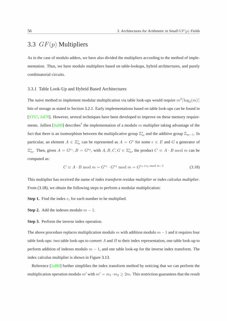
56 3. Architectures for Arithmetic in SmallGF (p) Fields
3.3 GF (p) Multipliers
As in the case of modulo adders, we have also divided the multipliers according to the method of imple-
mentation. Thus, we have modulo multipliers based on table-lookups, hybrid architectures, and purely
combinatorial circuits.
3.3.1 Table Look-Up and Hybrid Based Architectures
The naive method to implement modular multiplication via table look-ups would requirem2⌈log2(m)⌉
bits of storage as stated in Section3.2.1. Early implementations based on table look-ups can be found in
[ST67, Jul78]. However, several techniques have been developed to improve on these memory require-
ments. Jullien [Jul80] describes7 the implementation of a modulom multiplier taking advantage of the
fact that there is an isomorphism between the multiplicative groupZ∗m and the additive groupZm−1. In
particular, an elementA ∈ Z∗m can be represented asA = Ge for somee ∈ E andG a generator of
Z∗m. Then, givenA = Ge1 , B = Ge2 , with A, B, C, G ∈ Z∗
m, the productC ≡ A · B mod m can be
computed as:
C ≡ A ·B mod m = Ge1 ·Ge2 mod m = Ge1+e2 mod m−1 (3.18)
This multiplier has received the name ofindex transform residue multiplieror index calculus multiplier.
From (3.18), we obtain the following steps to perform a modular multiplication:
Step 1. Find the indexei for each number to be multiplied.
Step 2. Add the indexes modulom− 1.
Step 3. Perform the inverse index operation.
The above procedure replaces multiplication modulom with addition modulom−1 and it requires four
table look-ups: two table look-ups to convertA andB to their index representation, one table look-up to
perform addition of indexes modulom− 1, and one table look-up for the inverse index transform. The
index calculus multiplier is shown in Figure3.13.
Reference [Jul80] further simplifies the index transform method by noticing that we can perform the
multiplication operation modulom′ with m′ = m1 ·m2 ≥ 2m. This restriction guarantees that the result
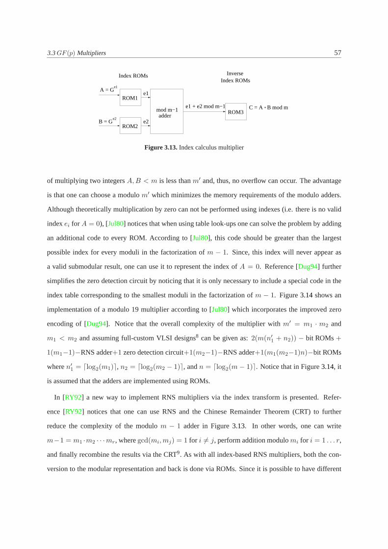
3.3GF (p) Multipliers 57
e2
Inverse
ROM2
ROM1
ROM3
Index ROMs
e2
e1
addermod m−1
e1 + e2 mod m−1 *C = A B mod m
A = G
B = G
e1
Index ROMs
Figure 3.13.Index calculus multiplier
of multiplying two integersA, B < m is less thanm′ and, thus, no overflow can occur. The advantage
is that one can choose a modulom′ which minimizes the memory requirements of the modulo adders.
Although theoretically multiplication by zero can not be performed using indexes (i.e. there is no valid
indexei for A = 0), [Jul80] notices that when using table look-ups one can solve the problem by adding
an additional code to every ROM. According to [Jul80], this code should be greater than the largest
possible index for every moduli in the factorization ofm − 1. Since, this index will never appear as
a valid submodular result, one can use it to represent the index ofA = 0. Reference [Dug94] further
simplifies the zero detection circuit by noticing that it is only necessary to include a special code in the
index table corresponding to the smallest moduli in the factorization ofm − 1. Figure3.14shows an
implementation of a modulo 19 multiplier according to [Jul80] which incorporates the improved zero
encoding of [Dug94]. Notice that the overall complexity of the multiplier withm′ = m1 · m2 and
m1 < m2 and assuming full-custom VLSI designs8 can be given as:2(m(n′1 + n2)) − bit ROMs+
1(m1−1)−RNS adder+1 zero detection circuit+1(m2−1)−RNS adder+1(m1(m2−1)n)−bit ROMs
wheren′1 = ⌈log2(m1)⌉, n2 = ⌈log2(m2 − 1)⌉, andn = ⌈log2(m− 1)⌉. Notice that in Figure3.14, it
is assumed that the adders are implemented using ROMs.
In [RY92] a new way to implement RNS multipliers via the index transform is presented. Refer-
ence [RY92] notices that one can use RNS and the Chinese Remainder Theorem (CRT)to further
reduce the complexity of the modulom − 1 adder in Figure3.13. In other words, one can write
m−1 = m1 ·m2 · · ·mr, wheregcd(mi, mj) = 1 for i 6= j, perform addition modulomi for i = 1 . . . r,
and finally recombine the results via the CRT9. As with all index-based RNS multipliers, both the con-
version to the modular representation and back is done via ROMs. Since it is possible to have different

58 3. Architectures for Arithmetic in SmallGF (p) Fields
e2 + e1 mod 7
0 1 6
2 2 0 6
3 1 3 5
1 5 0 4
4 3 2
00
0 1 2 3
4
8
12
16
6 0 1 1
2 4 2 0
3 2 5 0
3 5 1 5
4 4 3
0 1 2 3
12
8
4
16
0
e2B = G mod 19
6 0 1 1
2 4 2 0
3 2 5 0
3 5 1 5
4 4 3
0 1 2 3
12
8
4
16
0
0 1 6
2 2 0 6
3 1 3 5
1 5 0 4
4 3 2
00
0 1 2 3
4
8
12
16
e1A = G mod 19
0 1 2 3 4 5 6
0 1 2 3 4 5 6
1 2 3 4 5
2 3 4 5
3 4 5
4 5
5
6
6
6
6
6
6
0
0
0
0
0
0
1
1
1
1
1
2
2
2
2
3
3
3
4
4 5
0
1
2
3
4
5
6
0 1 2 3 4 5 6
1 2 3 4 5 0 6
6
6
6
6
2 3 4 5 0 1
3 4 5 0 1 2
4 5 0 1 2 3
5 0 1 2 3 4
6 666666
0
1
2
3
4
5
6
0 1 2 3 4 5 6
1 14 6 8 1710 0
0
0
0
0
0
0
1 2 9 121615
11 2 4 18 5 13
7 3 4 8 1710
1
11
7
14
2
3
6
9
4
8
12
18
16
16
5
15
13
13
0 1 2 3 4 5 6
0
1
2
3
4
5
6
*C = A B mod 19
Index ROMsInverse
Index ROMs
e1 mod 6
e2 mod 6
e1 mod 7
e2 mod 7
e1+ e2 mod 6
Figure 3.14.Index calculus modulo 19 multiplier from [Jul80] with zero encoding from [Dug94] and moduli set{6, 7}.
decompositions ofm − 1 in terms of the relatively prime modulimi’s, [RY92] uses the following cost
function to minimize the area/delay of the resulting RNS multiplier:∑r
i=1⌈log2(mi − 1)⌉. Notice that
minimizing the value of∑r
i=1⌈log2(mi − 1)⌉ reduces the size of the index and inverse index ROMs.
Similarly, smaller⌈log2(mi − 1)⌉ imply smaller and faster adders. Depending on the design require-
ments one moduli set might be chosen over another. Moreover, certain moduli decompositions might
result in minimum area but not minimum delay and vice versa. Figure3.15 shows a diagram of the
multiplier in [RY92]. The overall cost area cost of the multiplier in Figure3.15can now be estimated
as: 2(m(∑r
i=1 ni)) − bit ROMs+ 1(mi − 1) − adder for eachi + 1((m − 1)n) − bit ROM where
ni = ⌈log2(mi − 1)⌉.
We end this section by pointing out a second general methodology to implement ROM-based mul-
tipliers. This is known as thequarter square residue multiplier. Attributed in [Tay84] to [VP73] and
independently discovered in [SF77], it is based on the observation that given a modulom, multiplying

3.3GF (p) Multipliers 59
ROM2
ROM1
2
addermod m − 1
1
addermod m − 1
mod m − 1 r
adder
ROM3
A = Ge1
B = G e2
C = A B mod m*
Index ROMs InverseIndex ROM
Figure 3.15.RNS multiplier from [RY92] with m = m1 ·m2 · · ·mr
A ·B mod m can be accomplished as:
C = A ·B mod m
=[(
(A + B)2 · 4−1 mod m)−((A−B)2 · 4−1 mod m
)]mod m
wherem is assumed to be odd and the quantity(·)2 · 4−1 mod m is stored in a look-up table. However,
from the literature it is apparent that other designs are better both in terms ofarea and time delay and,
thus, the quarter square multiplier is not considered any further in this work.
3.3.2 Combinatorial Architectures
This section considers modulo multipliers based on combinational logic forfixedmoduli. We emphasize
that only architectures for fixed moduli have been considered. In addition, it would not be fair to com-
pare architectures which can process multiple moduli to architectures optimizedfor a single modulus.
To our knowledge, the best architectures for variable moduli in the context of RNS10 is the one pre-
sented in [CPO95]. In [CPO95] Di Claudio et al. introduced the pseudo-RNS representation. This new
representation is similar in flavor to the Montgomery multiplication technique as it defines an auxiliary
modulusA relatively-prime top. The technique allows building reprogrammable modulo multipliers,

60 3. Architectures for Arithmetic in SmallGF (p) Fields
systolization, and simplifies the computation of DSP algorithms. Nevertheless, ROM-based solutions
seem to be more efficient for small modulip < 26 [CPO95].
In [SPSG97] Soudris et al. present full-adder (FA) based architectures for RNSmultiply-add oper-
ations which adopt the carry-save paradigm. The paper concludes thatfor moduli p > 25, FA based
solutions outperform ROM ones. Finally, [PKS01] introduces a new design which takes advantage of
the non-occurring combinations of input bits to reduce certain 1-bit FAs to OR gates and, thus, reduce
the overall area complexity of the multiplier. The multiplier outperforms in terms of area all previous
designs. However, in terms of time complexity, the designs in [CPO95, RY92] as well as ROM-based
ones outperform the multiplier proposed in [PKS01] for most prime modulip < 27. Nevertheless, the
combined time/area product in [PKS01] is always less than that of other designs.
Hiasat [Hia96] is the first to propose the design of modulo multipliers using the combinatorial logic
approach by taking advantage of the fact that for any primep there will always be2n−p don’t-careposi-
tions in the truth table that defines the multiplier (wheren = ⌈log2 p⌉). In particular, one can build a truth
table whose inputs are the bits of the multiplicand and multiplier and whose output corresponds to the
output bits of the modular product. The truth table can then be given as inputto Boolean minimization
tools, such as ESPRESSO [BHH+82, BHMS84] and SIS [SSL+92], which, in turn, will output a two
level logic implementation of the truth table. Reference [Hia96] only considers thenormalapproach to
code the elements ofGF (p). For example, one considers the bit-strings{′000′,′ 001′,′ 010′,′ 011′,′ 100′}
to represent the numbers modulo 5, and the bit strings{′101′,′ 110′,′ 111′} are simply used asdon’t care
terms. We noticed, however, that one can choose a different representation. In other words, we could
use the code words{′100′,′ 101′,′ 110′,′ 111′} to represent the set of integers{1,2,3,4}, and use the
remainingunusedbit-strings to represent the integer zero. Section3.3.3examines this idea in detail.
3.3.3 NewGF (p) Multipliers for p < 25
The following two sections are devoted to describing the methodology used to design area optimized
GF (p) multipliers forp < 25. The first part will concentrate exclusively on theGF (3) case, which is of
great interest as demonstrated by recent applications in the crypto community[Kob98, Sma99, BF01].
Our design methodology is generalized for odd prime fields, wherep < 25. The work presented in this

3.3GF (p) Multipliers 61
section appears in [GWP02]11.
Notation
We briefly present some basic notation and definitions used in the sequel. Let I = {0, 1} andO =
{0, 1,−}, then a logic functionf in t input variablesxt−1, xt−2, . . . , x1, x0 and s output variables
ys−1, ys−2, . . . , y1, y0 can be defined as:
f : It → Os
whereX = [xt−1, xt−2, . . . , x1, x0] ∈ It is the input andY = [ys−1, ys−2, . . . , y1, y0] ∈ Os is the
output. We notice that in addition to the usual values of 0 and 1, the outputsyi can also take on adon’t
carevalue−. Such functions are called incompletely specified logic functions.
An elementA ∈ GF (p), will be represented as a binary string[an−1, an−2, . . . , a1, a0] of length
n = ⌈log2 p⌉. We point out that the binary encoding ofA does not necessarily imply a positional
number system. Whenever we imply the representation ofA in radix-2 notation we write(A)2 =
(an−1, an−2, . . . , a1, a0)2 explicitly. We refer to the radix-2 representation ofA as thenaturalor normal
encoding ofA interchangeably throughout the text. For the purposes of this section, multiplication in
GF (p), is an incompletely specified logic function fromI2n to On. HereX = [an−1, an−2, . . . , a1, a0,
bn−1, bn−2, . . . , b1, b0] ∈ I2n is the concatenation of the encodings ofA, B ∈ GF (p) andC = [cn−1,
cn−2, . . . , c1, c0] ∈ On, with C = A·B mod p. Finally, we represent the logical AND and OR operators,
by∧, ∨, and we will use a bar over a binary variable to denote logical negation (i.e.NOT(a) = a).
GF (3) Multiplier
As previously mentioned, [Hia96] only considers thenatural encoding forGF (p) elements. It is possi-
ble, however, to choose a different representation. We illustrate our approach by considering the case of
p = 3.
Example 3.4.Let p = 3, then we have thatn = 2 bits are required to represent any element ofGF (3).
Using Hiasat’s approach, one obtains the following Boolean equations to represent the productC =

62 3. Architectures for Arithmetic in SmallGF (p) Fields
(c1, c0)2 = A ·B mod 3 with A = (a1, a0)2, B = (b1, b0)2 andA, B, C ∈ GF (3).
c1 = (a1 ∧ b0) ∨ (a0 ∧ b1), c0 = (a0 ∧ b0) ∨ (a1 ∧ b1) (3.19)
This method allows for the implementation of this boolean function with four AND gates and two OR
gates. However, one can do better. Notice that the above equations wereobtained with the natural en-
coding. If instead we encode the integers 1 and 2 using the binary strings′10′ and ′11′, respectively,
and allow the binary strings{′00′,′ 01′} to both represent the integer 0, we can represent modulo 3 mul-
tiplication as shown in Table3.7. Applying logic minimization to Table3.7, one obtains the following
Table 3.7.Truth table representation ofC = A ·B mod 3. The element 0 is represented as′00′ or ′01′, 1 as′10′,and 2 as′11′
A B C A B C[a1, a0] [b1, b0] [c1, c0] [a1, a0] [b1, b0] [c1, c0]
00 00 0− 10 00 0−00 01 0− 10 01 0−00 10 0− 10 10 1 000 11 0− 10 11 1 101 00 0− 11 00 0−01 01 0− 11 01 0−01 10 0− 11 10 1 101 11 0− 11 11 1 0
Boolean equations
c1 = a1 ∧ b1, c0 = (a0 ∧ b0) ∨ (a0 ∧ b0) (3.20)
Equation (3.20) can be realized with two NOT gates, three AND gates, and one OR gate. Thisrepresents
an improvement of about 30% with respect to [Hia96] in the gate count if one does not take into account
the circuits required to convert to and from our modified representation. At the end of this section, it is
argued that for our particular application we can ignore such cost.
The optimized encoding of Example3.4 was obtained by trying out all twelve possible encodings for
GF (3) elements in which we allow a redundant representation for the element 0 (i.e. one allows the
element 0 to be represented by two different bit-strings12). In general, one has(
2n
2n−p+1
)choices to en-
code the zero element ofGF (p) and(p−1)! possible encodings for the non-zero elements. Multiplying
these two numbers out one gets 2n!(2n−p+1)! possible encodings.

3.3GF (p) Multipliers 63
Once an encoding has been chosen, one creates the corresponding truth table which is used as input
to the well known Boolean minimization program ESPRESSO [BHH+82, BHMS84]. We use the SIS
[SSL+92] program and itsscript.algebraicto find common terms in the Boolean functions obtained as
output from ESPRESSO. One lesson we learned while performing this exhaustive search approach is
that the encoding of the non-zero elements ofGF (3) does not matter for minimization purposes. Thus,
for example, whether we encode the element 1 as′10′ and 2 as′11′ or vice versa, the same number
of gates are required to implement the resulting Boolean functions. Assuming that the encoding of the
non-zero elements ofGF (p) does not influence the complexity of the minimized Boolean functions, we
are left with only(
2n
2n−p+1
)possibilities to encode the zero element. This means, for example, that we
would have to perform 70 Boolean minimizations forp = 5, 728 minimizations forp = 11, etc. It is
obvious from the start that such a methodology is only applicable for the smallest of primes. It is, thus,
necessary to develop efficient heuristics (or design criteria) that wouldallow a designer to choosegood
encodings, in other words, encodings that minimize our Boolean equations.The next section introduces
a set of rules that allows one to findgood encodingswithout trying out all possible ones.
Modular Multipliers forp < 25
Example3.4 considered the particular case ofp = 3 which is of the form2k + 1. Notice that the
encoding that produced the best results corresponded to representing an elementA ∈ GF (3) \ {0}
using thenormalbinary representation ofA′ such thatA′ = A + 1 and the element zero is encoded as
′00′ or ′01′. Forp = 5, we foundA′ = A + 4 to be optimum forA ∈ GF (5) \ {0} and we represent
zero with the strings in the set{′000′,′ 001′,′ 010′, ′011′}. A similar procedure can be applied to find a
good encoding for the elements ofGF (17). This allows us to give our first heuristics.
Design Criterion 1 Let p = 2k + 1 be a prime. Then, we can decrease the area complexity of a
combinatorialGF (p) multiplier by encodingA ∈ GF (p) \ {0} using the binary representation ofA′
with A′ = A + 2n − 1, n = ⌈log2(p)⌉, and letting the remaining unused encodings to all represent the
element zero. In addition, wheneverA and/orB, in the multiplicationC = A · B mod p, assume any
of the encodings of zero, the resultC should be written as′0 − · · · −′︸ ︷︷ ︸
n don′t cares
.
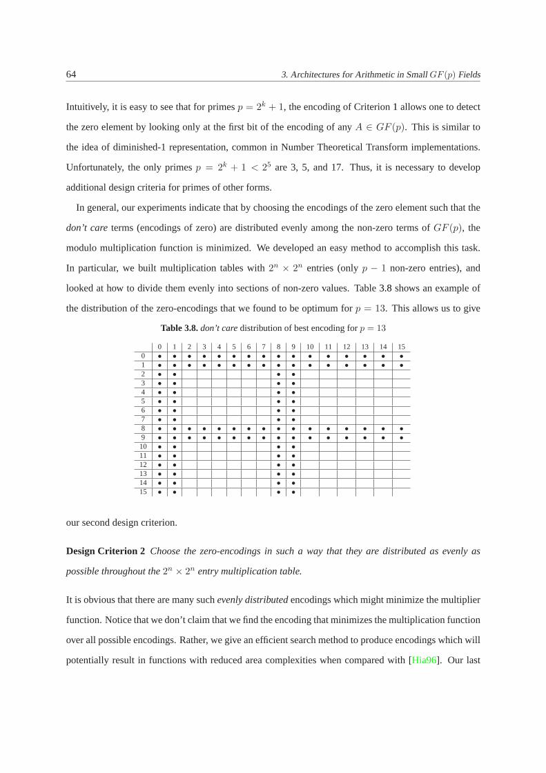
64 3. Architectures for Arithmetic in SmallGF (p) Fields
Intuitively, it is easy to see that for primesp = 2k + 1, the encoding of Criterion1 allows one to detect
the zero element by looking only at the first bit of the encoding of anyA ∈ GF (p). This is similar to
the idea of diminished-1 representation, common in Number Theoretical Transform implementations.
Unfortunately, the only primesp = 2k + 1 < 25 are 3, 5, and 17. Thus, it is necessary to develop
additional design criteria for primes of other forms.
In general, our experiments indicate that by choosing the encodings of thezero element such that the
don’t care terms (encodings of zero) are distributed evenly among the non-zero termsof GF (p), the
modulo multiplication function is minimized. We developed an easy method to accomplish this task.
In particular, we built multiplication tables with2n × 2n entries (onlyp − 1 non-zero entries), and
looked at how to divide them evenly into sections of non-zero values. Table 3.8 shows an example of
the distribution of the zero-encodings that we found to be optimum forp = 13. This allows us to give
Table 3.8.don’t caredistribution of best encoding forp = 13
0 1 2 3 4 5 6 7 8 9 10 11 12 13 14 150 • • • • • • • • • • • • • • • •1 • • • • • • • • • • • • • • • •2 • • • •3 • • • •4 • • • •5 • • • •6 • • • •7 • • • •8 • • • • • • • • • • • • • • • •9 • • • • • • • • • • • • • • • •10 • • • •11 • • • •12 • • • •13 • • • •14 • • • •15 • • • •
our second design criterion.
Design Criterion 2 Choose the zero-encodings in such a way that they are distributed as evenly as
possible throughout the2n × 2n entry multiplication table.
It is obvious that there are many suchevenly distributedencodings which might minimize the multiplier
function. Notice that we don’t claim that we find the encoding that minimizes the multiplication function
over all possible encodings. Rather, we give an efficient search method to produce encodings which will
potentially result in functions with reduced area complexities when compared with [Hia96]. Our last

3.3GF (p) Multipliers 65
heuristic is related to the way of choosing the encoding of the result of a multiplication by zero.
It is clear, that the encoding of a multiplication by zero has to belong to the set of zero encodings.
However, which of the2n − p + 1 possible encodings should one choose? This is particular interesting
in the case in which the number of possible encodings is not a power of two. Criteria 3 and 4 provide us
with guidelines to choose such encodings.
Design Criterion 3 Let D = 2n − p + 1 be equal to2s for somes. Then, choose sets of2s zero
encodings by fixings of then possible bits to be equal to 0 and setting the remaining ones to be don’t
cares (−). If settings bits equal to 0 does not reduce the area complexity of the resulting function,then
set them equal to 1. If that still does not work, try combinations of 0’s and 1’s.
Design Criterion 4 AssumeD = 2n − p + 1 6= 2s . Then choose a set of2s < D zero encodings for
the largest possibles and follow Criterion 3. Choose the remaining don’t cares (D− 2s) so as to satisfy
Design Criterion 2. The encoding for any multiplication by zero result will correspond to the encoding
of the set with2s elements.
As a final remark, we notice that in some cases setting thedon’t caresto zero, can further minimize the
area complexity of the resulting function.
Complexity of ProposedGF (p) Multipliers
The criteria of Section3.3.3was used to find encodings that would reduce the complexity ofGF (p)
multipliers for p < 25. Once the possible encodings were chosen13, we used ESPRESSO and SIS
as explained in Section3.3.3. After Boolean minimization, we used SIS once more for technology
mapping with thestdcell22.genlibCMOS cell library. Then, we chose the encoding that realizes the
multiplier with the least area. The area reported by SIS is a relative figure obtained from the layout of the
standard cells. We divided this value by the relative size of a pull-down or pull-up (a pull-down/pull-up
is implemented withonetransistor) according to thestdcell22.genliblibrary to obtain transistor counts.
The number of transistors required to implement the logic functions for2 < p < 25, together with the
encoding that gave the best results are summarized in Table3.9. We have also implemented and mapped
the modulo multipliers proposed in [Hia96] using thestdcell22.genliblibrary of SIS. We observe that

66 3. Architectures for Arithmetic in SmallGF (p) Fields
Table 3.9.Area (transistors) complexity of proposedGF (p) multipliers with given encodings.
p Area Area % ZERO element Zero Encoding[Hia96] new Encoding of Result
3 14 9 35.7 (0)2, (1)2 ′0−′
5 65 42 35.4 (0)2, (1)2, (2)2, (3)2 ′0−−′
7 114 111 2.6 (0)2, (7)2 ′0 0 0′
11 445 375 15.7 (8)2, (9)2(10)2, ′1−1−′
(11)2, (14)2(15)2,13 566 520 8.1 (0)2, (1)2(8)2, (9)2 ′−00−′
17 1048 907 13.5 (0)2, (1)2(2)2, (3)2, (4)2 ′0−−−−′
(5)2, (6)2(7)2, (8)2, (9)2(10)2, (11)2(12)2, (13)2(14)2, (15)2
19 1450 1343 7.4 (0)2, (2)2(4)2, (6)2, (8)2 ′0−−−0′
(10)2, (12)2, (14)2(16)2,(18)2, (20)2, (22)2(24)2,(26)2
23 1984 1830 7.3 (0)2, (3)2, (7)2, (11)2, ′−−−11′
(15)2, (19)2, (23)2,(27)2, (30)2, (31)2
29 3272 3136 4.2 (4)2, (12)2, (20)2, (28)2 ′00100′
31 3806 3689 3.1 (0)2, (31)2 ′00000′
in all cases our new encoding reduces the area complexity of the multiplier when compared to [Hia96].
Although, we do not do so explicitly here, when compared to other multipliers in the literature, our new
design outperforms all previous ones except for the one presented in [PKS01].
Other Considerations
We notice that we have also implemented and mapped the circuits required to convert to/from our mod-
ified representation. The area requirements indicate that our design will only be area efficient in cases
where several modulop multipliers (for constantp) are needed but only a few conversion circuits are
implemented. One such application isGF (pm) multipliers for cryptographic applications where one
requires 160–1024 bit long operands. For example, the cryptosystem in[Kob98] works over the field
GF (3163). In such a field, one would require 163GF (3) multipliers to implement aGF (3163) serial
multiplier. If one uses a single conversion circuit, the conversion circuit would contribute less than one
transistor perGF (3) multiplier and thus, we could ignore it. Another important consideration is that in
implementing aGF (pm) multiplier, we only need to change to and from our modified representation
at the beginning and at the end of the field multiplication (i.e. at system input/output times). Addi-
tion and subtraction which are also required in aGF (pm) multiplier can also be done in our modified
representation at no extra area penalty when compared to a normalGF (p) adder/subtracter.
3.4 Notes and Further References 67
3.4 Notes and Further References
1. Notice that different authors use different definitions. We have followed the definitions of [Par99],
however [Kor93] only defines two types of signals a generate signal, which is the same as the generate
signal from [Par99], and a propagate signal which is equivalent to [Par99] transfer signal. The resulting
carry recurrence relations are nevertheless the same.
2. The CDA is not considered in the study of [NIO96].
3. The design shown in Figure3.6 is a modification of the original design in [BJM87b] due to Dugdale
[Dug92]. In the original design instead of adding the constant2n−m in the second adder, one subtracts
the modulusm (so the second adder acts as a subtracter), and only the carry from thesecond adder is
considered by the multiplexer to choose the correct result.
4. These HAs come from the CPG unit and correspond to computing the propagate and generate signals
for the sumX + Y + Z. It is (HW (Z) − 1) and notHW (Z) because we don’t need to compute
P0, p0, G0, g0 since by definitionP0 = s0, p0 = s′0 andG0 = g0 = 0.
5. These OR2 gates and inverters correspond to the HAL cells.
6. The author in [Ban74] does provide area estimates in terms of equivalent gates for certain modulim.
7. The idea of index table look-ups is attributed to Pollard [Pol71] by Jullien [Jul80]. Reference [RY92]
attributes this idea to [Nak62] and [JL77] introduces the idea as background material without references.
8. If one can not use full-custom ROM designs, then it is assumed that onlyROMs with2kr-bits are
available for somek andr. Thus, the overall area complexity of the multiplier in [Jul80] is 2(2n(n′1 +
n2)) − bit ROMs+ 1(m1 − 1) − RNS adder+ 1 zero detection circuit+ 1(m2 − 1) − RNS adder+
(2⌈log2(m1(m2−1))⌉n)− bit ROM.
9. The only primesp for which this method can not be applied are those of the form2n +1. In the range
2 ≤ p ≤ 216 + 1, 17, 257, and216 + 1 are the only primes of this form.
10. Architectures for large and variable moduli such as those used in cryptographic applications are
discussed in Chapter4.
11. After presenting [GWP02], the author found out that a similar idea had been presented in [MGM99].
Interestingly enough, encoding symmetry is a key factor leading to area reduction in both works.

68 3. Architectures for Arithmetic in SmallGF (p) Fields
12. This is not to be confused with the technique of Redundant Number Representation used to limit
carry propagation inherent in adder-based solutions for multipliers.
13. Following the design criteria of Section3.3.3, we never had to try more than 25 encodings before
finding one that was better than the encoding of [Hia96].

CHAPTER 4
Algorithms for Arithmetic in LargeGF (p)
Fields
Most public-key schemes are based on modular exponentiation or repeated point addition. Both op-
erations are in their most basic forms performed via the binary method for exponentiation or one of
its variants [Gor98]. The atomic operation in the binary method for exponentiation is either modular
multiplication, in the case of RSA and DL-based systems, or point addition, in thecase of ECC, which
in turn is performed through a combination of doublings and additions in the fieldof definition of the
elliptic curve. In all cases, it is required that the moduli be at least 160-bitlong for ECC-based systems
or between 1024 and 2048-bit long for DL and RSA-based systems. Thus, this chapter surveys known
methods and architectures to perform modular arithmetic with large moduli (160-bit to 2048-bit long
integers). The purpose is just completeness as Chapter3 dealt with a similar problem but for small
moduli. Our focus is on algorithm developments rather than on specific architectures although, we also
discuss certain implementations as examples of certain architectures.
Notation
We will refer to multi-precision integers with capital letters and to their digits in radix-b representation
with lower-case letters. For example, we would write ann-digit integer in baseb asA =∑n−1
i=0 aibi

70 4. Algorithms for Arithmetic in LargeGF (p) Fields
with b ≥ 2 and0 ≤ ai < b. Notice that unless otherwise stated we always assume unsigned operands.
4.1 Basic Methods
4.1.1 School-book Method for Modular Multiplication
The most naive method to perform modular multiplication is known as the multiply first and then divide
method. In other words, to compute the productZ = X · Y mod M , one first computesZ ′ = X · Y
and then computesZ = Z ′ mod M = Z ′ − ⌊Z ′/M⌋M .
Multiplication
A multiplication algorithm can be derived by observing that forX andY =∑n−1
i=0 yibi, the product
X · Y can be written as:
X · Y =n−1∑
i=0
(X · yi)bi = b(· · · (b(0 + X · yn−1) + X · yn−2) + · · · ) + X · y0 (4.1)
Algorithm 4.1summarizes the multiplication operation (See [MvOV97, Section 14.2.3] for a more soft-
ware oriented multiplication algorithm description). Algorithm4.1 requires in every step a digit multi-
Algorithm 4.1 Multiplication
Input: X, Y =∑n−1
i=0 yibi
Output: Z = X · Y1: Z ← 02: for i = 0 to n− 1 do3: Z ← b · Z + X · yn−1−i
4: end for5: Return(Z)
plication (X · yi), a multiplication1 by b, and an adder. Forb = 2 the algorithm reduces to left shifts
by one bit and addition ofX or 0, depending on the bityi. We also point out that if instead of ini-
tializing Z to 0 in Step1 of Algorithm 4.1 we initialize it to A2−(n−1), then, the final result will be
Z = X · Y + A. This operation is useful in certain applications and it is obtained at virtually no extra
cost. Finally, we notice that Algorithm4.1 can also be re-written in terms of right-shift operations but

4.1 Basic Methods 71
we refer to [Kor93, Par99] for this and other hardware multipliers as these are not the most common
methods to perform modular multiplication.
Division
Division can be fully characterized by the basic division equation
X = Q ·M + R, 0 ≤ R < M (4.2)
whereX is the dividend,M is the divisor,Q is the quotient, andR is the residue. Just like multiplication
can be expressed in terms of repeated additions and shifts, division can be written in terms of subtractions
and shifts. Thus, our first version of division is called Shift/Subtract Division and it is summarized in
Algorithm 4.2. At this point, several remarks are in order. First, the conditionX < 2nM ensures
Algorithm 4.2 Restoring Shift/Subtract Division
Input: M =∑n−1
i=0 mi2i, X =
∑2n−1i=0 xi2
i < 2nMOutput: X = Q ·M + R with 0 ≤ R < M andQ =
∑n−1i=0 qi2
i
1: R← X2: for i = 0 to n− 1 do3: R← 2 ·R4: S ← R− 2nM5: if S < 0 then6: qn−i ← 07: else8: qn−i ← 19: R← S
10: end if11: end for12: R← R/2n
13: Return(Q, R)
thatQ < 2n. This is necessary since division of a2n-bit number by ann-bit number can generate a
quotient which is larger thann-bits. This basically implements an overflow check. Second, the name
restoringrefers to the fact that if one guesses the next bit of the quotient wrong (by executing Step4
of Algorithm 4.2and obtaining a negative result), then one restores the residueR to its previous value.
Restoring-dividers have timing issues which can be avoided by using non-restoring dividers [Par99].

72 4. Algorithms for Arithmetic in LargeGF (p) Fields
In a non-restoring divider, one always performs Step4 of Algorithm 4.2, however, depending on
whether the result is negative or positive, one adds or subtracts2nM . The result is shown in Algo-
rithm 4.3. It is easy to see that Algorithm4.3 produces the same result as Algorithm4.2. For sup-
Algorithm 4.3 Non-restoring Shift/Subtract Division
Input: M =∑n−1
i=0 mi2i, X =
∑2n−1i=0 xi2
i < 2nMOutput: X = Q ·M + R with 0 ≤ R < M andQ =
∑n−1i=0 qi2
i
1: R← X2: for i = 0 to n− 1 do3: if R < 0 then4: qn−i ← 05: R← 2 ·R + 2nM6: else7: qn−i ← 18: R← 2 ·R− 2nM9: end if
10: end for11: R← R/2n
12: Return(Q, R)
pose that in iterationi of Algorithm 4.3, R(i) = 2 · R(i−1) − 2nM < 0 (i.e. Algorithm 4.2 would
have generatedR(i) = 2 · R(i−1) as a result), then in iteration(i + 1), R(i+1) = 2 · R(i) + 2nM =
2(2 · R(i−1) − 2nM) + 2nM = 22 · R(i−1) − 2nM which is the same result that Algorithm4.2would
have generated.
It is natural, to try to generalize Algorithms4.2 and4.3 to higher radixes. In this case, we could
characterized the value ofR at iterationi as:
R(i) = b ·R(i−1) − qk−i(bnM) with R(0) = X, R(n) = bnR
whereQ =∑n−1
i=0 qibi and0 ≤ qi < b. The problem with higher-radix division methods is that of
estimatingqi correctly. However, higher-radix division is outside the scope of this work and thus we
refer to [Kor93, Par99] for a thorough treatment of the subject (See also [Knu81, MvOV97] for more
software oriented descriptions).

4.1 Basic Methods 73
4.1.2 Interleaved Multiplication Reduction Method
The details of this method are sketched in [Bla83, Slo85]. The method is based on combining (4.1)
with modular reduction and making use of the distributivity property of modular reduction. Thus, (4.1)
becomes:
X · Y mod M =n−1∑
i=0
(X · yi)2i mod M (4.3)
= 2(· · · (2(0 + X · yn−1 mod M) + X · yn−2 mod M) +
· · · ) + X · y0 mod M
where we have specialized (4.1) to theb = 2 case. Algorithm4.4 follows easily from (4.3). We notice
Algorithm 4.4 Interleaved Multiplication Reduction Method
Input: X, M , Y =∑n−1
i=0 yi2i with X, Y < M
Output: Z = X · Y mod M1: Z ← 02: for i = 0 to n− 1 do3: Z ← 2 · Z + X · yn−1−i
4: Z ← Z mod M5: end for6: Return(Z)
that restrictingX, Y < M does not have any practical impact as in most cryptographic applications that
is a requirement. In addition, sinceZ, X, Y < M at the beginning of every loop iterationi, we obtain
thatZ in Step3 of Algorithm 4.4 is
Z(i) = 2 · Z(i−1) + X · yn−1−i ≤ 2(M − 1) + (M − 1) ≤ 3M − 3
Thus, in Step4 we need to subtractM at most twice fromZ to obtainZ mod M . Step4 can be easily
achieved following Algorithm4.5. The computation ofZ = X · Y mod M following Algorithm 4.4
requiresn steps. At each steps the following operations are performed:
• A left shift (2 · Z) in Step3 and the conditional addition ofA depending on whetheryn−1−i is
equal to zero or one. Notice that the left shift operation can be simply achieved by wiring.

74 4. Algorithms for Arithmetic in LargeGF (p) Fields
Algorithm 4.5 Modular Reduction for Step4 of Algorithm 4.4Input: X, M , 0 ≤ X ≤ 3M − 3Output: Z = X mod M
1: Z ← X −M2: if Z ≥ 0 then3: Y ← Z −M4: if Y ≥ 0 then5: Z ← Y6: end if7: else8: Z ← X9: end if
10: Return(Z)
• At most two subtractions for the computation ofZ mod M as indicated in Algorithm4.5.
The crucial computations are the addition and subtraction operations, i.e., they need to be performed
fast. They can be achieved following Omura’s method [Omu90] introducingO(n) delay or using a
CSA which only introducesO(1) delay. However, because in CSA sign information is not immediately
available, one needs to perform fast sign detection in order to determine whether the product needs to be
reduced moduloM or not. One such technique is introduced in [KH91].
4.2 Advanced Algorithms
4.2.1 Sedlak Modular Reduction
Originally introduced by Sedlak in [Sed87], this algorithm is used by Siemens, in the SLE44C200 and
SLE44CR80S microprocessors, to perform modular reduction [NM96]. In the algorithm comparisons
of X with 1/3, 1/6, · · · of M play an important role in the final computation ofX mod M . Assume
that during the division ofX by M , M was already shifted and subtracted fromX several times. Fur-
thermore, assume that the remainder has been stored inX. Sedlak’s algorithm ensures that|X| ≤M/3.

4.2 Advanced Algorithms 75
This will also be true of the following steps. By assumption,M falls into one of the following ranges:
Range j=2M
2 · 3< |X| ≤
M
3
Range j=3M
22 · 3< |X| ≤
M
2 · 3...
...
Range j=iM
2(i−1) · 3< |X| ≤ 2−(i−2) M
2(i−2) · 3
for somei > 1. Now M is shiftedi bits to the right and forM ′ = M/2i, we obtain:
2iM ′
2(i−1) · 3< |X| ≤
2iM ′
2(i−2)3⇒−M ′
3< |X| −M ′ ≤
M ′
3(4.4)
Equation4.4 implies thatX ′ = X ±M ′ ≤ M ′/3 is satisfied again. Since, the above argument proves
that the above condition is always met,M can always be shifted by at leastj = 2 bits in every step of
the algorithm. Sedlak notices that the expected value ofi is 3 and therefore, the algorithm improves the
reduction complexity by an average factor of1/3 when compared to the basic bit-by-bit reduction.
4.2.2 Barret Modular Reduction
Barret reduction was originally introduced in [Bar86], in the context of implementing RSA on a DSP
processor. Algorithm4.6 summarizes Barret’s modular reduction. To clarify Algorithm4.6, consider
re-writing X asX = Q ·M + R with 0 ≤ R < M , which is a well known identity from the division
algorithm [MvOV97, Definition 2.82]. Thus
R = X mod M = X −Q ·M (4.5)
Barret’s basic idea is that one can writeQ in (4.5) as:
Q = ⌊X/M⌋ =⌊(
X/bn−1) (
b2n/M) (
1/bn+1)⌋
(4.6)

76 4. Algorithms for Arithmetic in LargeGF (p) Fields
Algorithm 4.6 Barret Modular Reduction
Input: X =∑2n−1
i=0 xibi, M =
∑n−1i=0 mib
i, with mn−1 6= 0, µ = ⌊b2n/M⌋, b > 3Output: R = X mod M
1: Q1 ← ⌊X/bn−1⌋2: Q2 ← Q1 · µ3: Q3 ← ⌊Q2/bn+1⌋4: R1 ← X mod bn+1
5: R2 ← Q3 ·M mod bn+1
6: R← R1 −R2
7: if R < 0 then8: R← R + bn+1
9: end if10: while R ≥M do11: R← R−M12: end while13: Return(R)
and in particularQ can be approximated by
Q = Q3 =⌊⌊(
X/bn−1)⌋ (
b2n/M) (
1/bn+1)⌋
We notice thatQ3 can be at most 2 smaller thanQ [MvOV97, Fact 14.43] and that the quantityµ =
b2n/M can be precomputed when performing many modular reductions with the same modulus, as is the
case in cryptographic algorithms. Finally, Step11 in Algorithm 4.6 is repeated at most twice [Bar86].
From the efficiency point of view, notice that all divisions by a power ofb are simply performed
by right-shifts and modular reduction modulobi, is equivalent to truncation. The complexity of Algo-
rithm 4.6 is basically given by the number of multiplications. We notice that there are only two multi-
precision multiplications: one to computeQ2 (Step2) and one to computeR2 (Step5). Both are “partial”
multiplications, i.e., we don’t need to compute all digits of the result. In the case ofQ2 then−1 least sig-
nificant digits need not to be computed and in the case ofR2 only then+1 significant digits are needed.
It can be shown that Algorithm4.6needs at most(n2+5n+2)
2 +(n+1
2
)+n = n2 +4n+1 single-precision
multiplications (where single-precision multiplication means multiplication of two digits)[MvOV97,
Note 14.45]. We refer to [MvOV97, Section 14.3.3] for further discussion of implementation issues
regarding Barret reduction.

4.2 Advanced Algorithms 77
Improved Barret Algorithm
Barret’s algorithm can be further improved as shown in [Dhe94, Dhe98]. The basic idea is to re-write
the quotient in (4.6) as:
Q = ⌊X/M⌋ =
⌊X
2n+β2n+α
M
2α−β
⌋
where Barret’s algorithm in radixb = 2 corresponds to the caseα = n andβ = −1. Then, the quotient
can be estimated as
Q =
⌊
X2n+β
⌋ ⌊2n+α
M
⌋
2α−β
Then, for a given modulusM , µ = 2n+α
M can be precomputed. It is shown in [Dhe98], that
⌊X
M
⌋− 2γ−α − 2β+1 − 1 + 2β−α < Q ≤
⌊X
M
⌋(4.7)
for someγ > 0. Equation4.7implies that the estimated quotientQ is always smaller or equal to the real
quotient and that one needs to chooseα, β, andγ to minimize the error of the estimateQ. In particular,
[Dhe98] shows that to minimize the error one must chooseβ ≤ −2 andα > γ. Following [Dhe98], the
error is at most 1, thus improving over Barret’s algorithm (Algorithm4.6) whereQ could be at most 2.
4.2.3 Brickell’s Modular Reduction
Brickell’s method, originally introduced in [Bri82], is dependent on the utilization of carry-delayed
adders (CDAs) as introduced in Section3.1.4. Assume thatX is in CDA form, then it can be written as:
X =
n−1∑
i=0
(xdi + xti) 2i (4.8)
wherexd0 = 0. It follows thatZ = X · Y can be computed as:
Z = X · Y = Y ·n−1∑
i=0
(xdi + xti) 2i
= (xt0 · Y ) 20 + (xt1 · Y + xd1 · Y ) 21 + · · ·+ (xtn−1 · Y + xdn−1 · Y ) 2n−1

78 4. Algorithms for Arithmetic in LargeGF (p) Fields
Re-grouping terms, we obtain:
Z =(20 · xt0 · Y + 21 · xd1 · Y
)+(21 · xt1 · Y + 22 · xd2 · Y
)+ · · ·
+(2n−2 · xtn−2 · Y + 2n−1 · xdn−1 · Y
)+(2n−1 · xtn−1 · Y
)
Finally, using (3.16), we see that at each step we will only need to add a shifted version ofY to the
accumulated valueZ. Reduction moduloM can be accomplished by subtracting shifted versions of
M from the resultZ. However, Brickell suggests to interleave multiplication and reduction steps.The
result is shown in Algorithm4.7. We make the following remarks about Algorithm4.7:
Algorithm 4.7 Brickell’s Modular Reduction
Input: X = (Xd, Xt)CDA =∑n
i=0 xdi2i +
∑n−1i=0 xti2
i with xd0 = 0, K = 2n −M with 2n−1 ≤M < 2n, b1, b2 ∈ {0, 1}, R = (Rd, Rt)CDA =
∑n+10i=0 (rdi + rti)2
i with rd0 = 0Output: R = X · Y mod M
1: R← 0, t1 ← 0, t22: for j = 1 to n + 10 do3: B′ ← xtn−1 ·B + xdn · 2B4: K ′ ← b2 · 2
11K + b1 · 210K
5: R← 2 · (R + B′ + K ′)6: X ← 2 ·X7: Add the 4 MSbits ofR to the 4 MSbits of211K8: if overflow is detectedthen9: b2 ← 1
10: else11: b2 ← 012: end if13: Add the 4 MSbits ofR to the 3 MSBits of210K.14: if overflow is detected ANDt2 = 0 then15: b1 ← 116: else17: b2 ← 018: end if19: end for20: Return(R)
• In Algorithm 4.7, the notationX = (Xd, Xt)CDA implies thatX is represented in the carry-
delayed manner, as explained in Section3.1.4.
• Brickell’s reduction method uses basically a combination of a sign estimation technique (See for

4.2 Advanced Algorithms 79
example [KH91]) and Omura’s modular reduction [Omu90]. In particular, one estimates the sign
of the accumulatorR by looking at its four most significant bits. Since the sign is used to decide
whether or not to subtract a multiple ofM , the error is only by a factor ofM which can be later
corrected.
• Omura’s method is based on the following observation. When performing a modular addition,
say moduloM , one can allow a temporary registerR to grow larger thanM but keep it always
less than an upper bound2k. Whenever the sumR + C ≥ 2k with R, C < 2k, one can instead
compute(R + C mod 2k) + K, whereK = 2k −M is a pre-computed constant. In other words,
whenever there is a carry-out from the sumR + C, one can ignore it and simply add the constant
K.
• b1 andb2 are two bits used as control bits to subtracts multiples ofK from the accumulatorR.
• Carry-delayed registerX, consists of ann-bit registerXt and an(n + 1)-bit registerXd, so that
bit xdn can be stored during the left shift operation in Step6.
• R, the accumulator, is an(n+11)-bit carry-delayed register. In Step5, it is possible that overflow
occurs. However, it is shown in [Bri82] that if the overflow bits are ignored, one still obtains
R ≡ 2 · (R + B′ + K ′) mod M , which is the purpose of the algorithm in the end.
• Algorithm 4.7, assumes2n−1 ≤ M < 2n. If M < 2n−1, [Bri82] shows how to computeX ·
Y mod M as follows. Let2s−1 ≤ M < 2s ande = n − s. To findX · Y mod M , simply find
R ≡ A · (B · 2e) mod (2eM). This is possible since2n−1 ≤ 2eM < 2n. It can be shown that
2e|R and thatD/2e ≡ X · Y mod M .
4.2.4 Quisquater’s Modular Reduction
Quisquater’s algorithm, originally introduced in [Qui90, Qui92], can be thought of as an improved
version of Barret’s reduction algorithm. [BD95, Wal91] have proposed similar methods. In addition,
the method is used in the Phillips smart-card chips P83C852 and P83C855, which use the CORSAIR

80 4. Algorithms for Arithmetic in LargeGF (p) Fields
crypto-coprocessor [DQ90, NM96] and the P83C858 chip, which uses the FAME crypto-coprocessor
[FMM+96].
Quisquater’s algorithm, as presented in [DQ90], is a combination of the interleaved multiplication
reduction method (Algorithm4.4) and a method that makes easier and more accurate the estimation of
the quotientQ in (4.5). We re-write Algorithm4.4for the case of general radixb as Algorithm4.8.
Algorithm 4.8 Interleaved Multiplication Reduction Method for General Radixb
Input: X, M , Y =∑n−1
i=0 yibi with X, Y < M and0 ≤ yi < b
Output: R = X · Y mod M1: R← 02: for i = 0 to n− 1 do3: R← b ·R + X · yn−1−i
4: R← R mod M5: end for6: Return(R)
Step4 of Algorithm 4.8can then be performed following (4.5). In particular, assume that we want to
computeR = X mod M = X −Q ·M , then the quotientQ can be written as:
Q =
⌊X
M
⌋=
⌊X
2n+c·2n+c
M
⌋
From the above, we can write
Qδ =
(⌊X
2n+c
⌋)·
(⌊2n+c
M
⌋)(4.9)
whereQ is an approximation of the quotientQ. Thus, (4.9) allows us to write an approximation for
R = X mod M as
R = X − Q ·M ′ = X −
⌊X
2n+c
⌋·M ′
where we effectively are performing a reduction moduloM ′ = δM = ⌊2n+c/M⌋M . We notice that
M ′ has its most significantc bits equal to 1 and that the computation of the approximate quotientQ is
immediate, i.e., it is just the most significant bits ofX. Since the objective of the modular reduction
is to obtainR = X mod M , we need a way to obtainR from R which is known in the literature as
de-normalization2.
Since we have reduced moduloM ′ = δM , a multiple ofM , we have thatR = X mod M =

4.3 Montgomery Modular Reduction 81
R mod M = (X mod M ′) mod M . Notice that we can writeδR mod M ′ as:
δR mod M ′ =
[δ
(X −
⌊X
M ′
⌋M ′
)]mod M ′ = δX −
⌊δX
M ′
⌋M ′ = δX −
⌊X
M
⌋(δM) (4.10)
Thus, from (4.10), we obtain the following relation to obtainR from R:
R =
(δ · R
)mod M ′
δ
The only step that is left is to computeδ = ⌊2n+c/M⌋. It is shown in [DJQ97] that one can approximate
δ within 1 as indicated in Theorem4.1.
Theorem 4.1.[DJQ97] Let k = n− c− 2 and letM =∑n−1
i=0 mi2i. PuttingM =
∑n−1i=k mi2
i−k if we
define
δ =
⌊22c+2
M
⌋
thenδ ≤ δ < δ + 1.
Theorem4.1 implies that with only one test we can obtain the exact value of the constantδ and, more
importantly, we only need the(c + 2) most significant bits ofM to do so. Further, details about the
algorithm and the choice ofδ can be found in [Dhe98].
4.3 Montgomery Modular Reduction
The Montgomery algorithm, originally introduced in [Mon85], is a technique that allows efficient imple-
mentation of the modular multiplication without explicitly carrying out the modular reduction step. The
Montgomery reduction algorithm is shown in Algorithm4.9. The idea behind Montgomery’s algorithm
is to transform the integers inM -residues and compute the multiplication with theseM -residues. At
the end, one transforms back to the normal representation. As with Quisquater’s method, this approach
is only beneficial if we compute a series of multiplications in the transform domain (for example, in
the case of modular exponentiation). Notice that Algorithm4.9 is just the reduction step involved in a
modular multiplication. The multiplication step can be accomplished, for example, with Algorithm 4.1.

82 4. Algorithms for Arithmetic in LargeGF (p) Fields
Algorithm 4.9 Montgomery Reduction
Input: 0 ≤ T < R ·M , R > M , gcd(R, M) = 1, andR ·R−1 −M ·M ′ = 1Output: Z = T ·R−1 mod M
1: Q← (T mod R) M ′ mod R2: Z ← T+Q·M
R3: if Z ≥M then4: Z ← Z −M5: end if6: Return(Z)
To see thatZ in Step2 is an integer, observe thatQ = T ·M ′ + k · R andM ·M ′ = −1 + l · R, for
some integersk andl. Then,(T + Q ·M)/R = (T + (T ·M ′ + k ·R)M)/R = l · T + k ·M .
In practiceR in Algorithm 4.9is a multiple of the word size of the processor and a power of two. This
means thatM , the modulus, has to be odd (because of the restrictiongcd(M, R) = 1) but this does not
represent a problem asM is a prime or the product of two primes (RSA) in most practical cryptographic
applications. In addition, choosingR a power of 2 simplifies Steps1 and2 in Algorithm 4.9, as they
become simply truncation (modular reduction byR in Step1) and right shifting (division byR in Step2).
Notice thatM ′ ≡ −M−1 mod R. In [DK90] it is shown that ifM =∑n−1
i=0 mibi, for some radixb
typically a power of two, andR = bn, thenM ′ in Step1 of Algorithm 4.9 can be substituted by
m′0 = −M−1 mod b. The authors of [DK90] notice that although the resulting sumT + A ·M (in
Step2 of Algorithm 4.9) might not be the same, the effect is, namely makingT + A ·M a multiple of
R.
As with previous algorithms, one can interleave multiplication and reduction steps. The result is
Algorithm 4.10where the trick from [DK90] is also used. In Algorithm4.10, we have made use of the
fact thatm′0 = −M−1 mod b ≡ (b −m0)
−1 mod b ≡ −m−10 mod b, where usuallyb = 2k for some
k > 0. Similarly to Algorithm 4.9, one can see thatZ in Step4 of Algorithm 4.10 is an integer by
substitutingq = (z0 + xi · y0) m′ + l · b, for some integerl, in the expression(Z + xi · Y + q ·M) /b.
Finally, we notice that0 ≤ Z < 2M − 1. To justify this, assume that0 ≤ Z < 2M − 1 at iteration
i of Algorithm 4.10. Then, Step4 of Algorithm 4.10 replacesZ with (Z + xi · Y + q · M)/b ≤
((2M − 2) + (b − 1)(M − 1) + (b − 1)M)/b = 2M − 1 − (1/b) < 2M − 1. This justifies Steps6
through8 of Algorithm 4.10and guarantees that the output of the Algorithm is less thanM .

4.3 Montgomery Modular Reduction 83
Algorithm 4.10 Montgomery Multiplication
Input: X =∑n−1
i=0 xibi, Y =
∑n−1i=0 yib
i, M =∑n−1
i=0 mibi, with 0 ≤ X, Y < M , b > 1, m′ =
−m−10 mod b, R = bn, gcd(b, M) = 1
Output: Z = X · Y ·R−1 mod M1: Z ← 0 {whereZ =
∑ni=0 zib
i}2: for i = 0 to n− 1 do3: q ← (z0 + xi · y0) m′ mod b4: Z ← (Z + xi · Y + q ·M) /b5: end for6: if Z ≥M then7: Z ← Z −M8: end if9: Return(Z)
In contrast to previous algorithms, Montgomery’s algorithm reverses the processing order of the digits
of multiplicandX, performs a shift down instead of up on each iteration, and does an addition rather
than a subtraction. These changes are used in [EW93] to simplify the combinatorial logic needed to
implement Montgomery reduction. The algorithm as modified in [EW93] is shown as Algorithm4.11.
Algorithm 4.11 Modified Montgomery Multiplication according to [EW93]
Input: X =∑n−1
i=0 xibi, Y =
∑n−1i=0 yib
i, M =∑n−1
i=0 mibi, with 0 ≤ X, Y < M , b > 1 m′ =
−m−10 mod b , R = bn, gcd(b, M) = 1
Output: Z = X · Y ·R−1 mod M1: Z ← 0 {whereZ =
∑ni=0 zib
i}2: q ← 03: for i = 0 to n + 1 do4: Z ←
(Z + xi · (b
2Y ) + q ·M)/b
5: q ← z0 ·m′ mod b
6: end for7: if Z ≥M then8: Z ← Z −M9: end if
10: Return(Z)
The idea in [EW93], is to shift Y by two digits (i.e., multiplyY by b2) thus makingq in Step3 of
Algorithm 4.10independent ofY . Notice that one could have multipliedY by b instead ofb2 and have
also obtained aq independent ofY . However, by multiplyingY by b2, one getsq to be dependent only
on the partial productZ and on the lowest two digits3 of the multiple ofM (i.e. q ·M ). The price of such
a modification is two extra iterations of the for-loop for which the digits ofX are zero. The architecture
84 4. Algorithms for Arithmetic in LargeGF (p) Fields
proposed by [EW93] is only considered for the caseb = 2 and estimated to be twice as fast as previous
modular multiplication architectures at the time of publication.
4.3.1 Towards Higher Radix Montgomery Multipliers
Reference [SV93] describes the implementation of modular exponentiation architectures on FPGAs.
They utilized an array of 16 XILINX 3090 FPGAs. Their design uses several speed-up methods [SV93]
including the Chinese remainder theorem, asynchronous carry completion adder, and a windowing ex-
ponentiation method. This section describes in some detail their implementation as theirs appears to
be the firstworking hardware implementationof the RSA algorithm using Montgomery’s method for
multiplication.
The algorithm used in [SV93] is basically Algorithm4.10. Notice that since0 ≤ Z < 2M − 1,
one only needsn + 1 digits4 to representZ as noted in Step1 of Algorithm 4.10. However, [SV93]
avoids having to perform a subtraction after every modular product of the exponentiation algorithm by
letting all intermediate results havetwo extra bitsof precision. [SV93] also shows that even allowing
for the two extra bits of precision, one can always manage to work with intermediate results no larger
thann-digits if M < bn/4 andX, Y ≤ 2M . A second improvement over previous implementations is
the use of a radixb > 2. In particular, they useb = 22 as a radix which permits for a trivial computation
of the quotientq in Step3 of Algorithm 4.10and it allows for the use of Booth recoded multiplications
(this doubles the multipliers performance compared tob = 2 at an approximate 1.5 increase in hardware
complexity). Higher radixes, which would offer better performance, were dismissed since they involve
too great of a hardware cost and the computation of the quotient digits is no longer trivial. As in other
hardware implementations and to reduce the carry-propagation time, [SV93] use carry-save adders.
Upon completion of each modular multiplication stage they convert back to the non-redundant form
in order to feed this result back into the modular multiplier in the next exponentiation step. In some
implementations, the operands are always kept in carry-save form but this doubles the size of radix-4
multiplier compared to a non-redundant one. [SV93] solution is to convert back to the non-redundant
representation by using an asynchronous carry completion detection circuit and clock the final result for
as many cycles as needed to fully propagate all carries. They notice thaton average5, the circuit will

4.3 Montgomery Modular Reduction 85
only need to propagate throughlog2(k) bits (wherek is the number of bits in the result). The technique
provides a valuable saving in multiplier area for a small increase in the number of cycles needed per
modular multiplication. Finally, we notice that they re-write Montgomery’s Algorithmin a similar way
to Algorithm 4.11, to allow for pipeline execution, basically getting rid off of theq dependency on the
least significant digit of the partial productZ. The cost ford levels of pipelining isd extra bits of
precision andd more cycles in the computation of the final product.
RSA Implementation
The authors in [SV93] implement RSA [RSA78] in what they call a PAM (Programmable Active Mem-
ory), basically a universally configurable hardware co-processorbased on FPGA technology and closely
coupled to a standard host computer. For decryption (signature generation) they make use of the Chi-
nese Remainder Theorem (CRT), since the private-key is known (i.e. thefactorization of the modulus
M = P ·Q, whereP, Q are primes). The CRT provides their implementation with a factor of 4 speedup.
This factor of 4 is achieved by using the reconfigurability capabilities of the PAM. In particular, two
hardware multipliers of sizek/2 bits each (whereM is k-bits long) are instantiated in the PAM together
with one of the following solutions used to recombine the output of the two multipliersinto one:
1. Compute the CRT recombination in software. A 40 MIPS machine performs thisoperation at 600
Kbits/sec on a pair of 512-bit primes.
2. Assist a slower host computer with a fast enough hardware multiplier, running in parallel with the
two exponentiators.
3. Design the twok/2-bit moduloP andQ multipliers so that they can be reconfigured quickly
enough into one singlek-bit multiplier moduloM which can be used for the recombination step
in the CRT.
For the encryption (signature verification) operation, a short exponent such as216+1 is assumed. Finally,
for the exponentiation they use them-ary method [MvOV97, Gor98] with windows of size five bits for
a 512-bit modulus (i.e. exponentiations modulo 256-bit primes) and windows of size 6-bits for 1024-bit

86 4. Algorithms for Arithmetic in LargeGF (p) Fields
modulus. The average number of multiplications is then1.24k and1.22k for k = 512 bits andk = 1024
bits, respectively, compared to1.5k operations in the case of the binary method for exponentiation.
The result of all these speedup methods, is an RSA secret decryption rate of over 600 Kbits/sec for a
512-bit modulus and of 165 Kbits/sec for a 1024-bit modulus. While the previous results make full use
of the PAM reconfigurability, they derive a single gate-array specification whose size is estimated under
100K gates and speed over 1Mbit/sec for RSA 512-bit keys.
4.3.2 Avoiding Quotient Determination in High Radix Montgomery
The main obstacle to the use of higher radixes in the Montgomery algorithm is thatof the quotient
determination. In [Oru95], the author presents a method which avoids quotient determination all together
and makes higher-radix Montgomery practical.
In what follows we assume the radixb to be of the formb = 2k. Our starting point for the improve-
ments is Algorithm4.10. Step3 is the determination of the quotientq and it looks like
q ← (z0 + xi · y0)m′ mod 2k (4.11)
Step4 is the computation of the partial productZ as
Z ← (Z + xi · Y + q ·M) /2k (4.12)
[Oru95] first notices that ifk = 1, thenm′ = 1 and the multiplication bym′ in (4.11) can be avoided.
Thus, the idea is to makem′ always equal to 1 independent of the modulus. To this end, [Oru95] defines
a new modulusM = (M ′ mod 2k)M which satisfiesM ≡ −1 mod 2k and, thus, the desired property.
Equations (4.11) and (4.12) become
q ← (z0 + xi · y0) mod 2k (4.13)
Z ←(Z + xi · Y + q · M
)/2k (4.14)
Thus, we have replaced multiplication bym′ in every step of the algorithm by a single multiplication

4.3 Montgomery Modular Reduction 87
(computingM ) done once at the beginning of the algorithm. The penalty of these modifications is that
Z requires more precision and the loop has increased its size by at most one.Similarly to [EW93], the
quotient computation in (4.13) can be further reduced by replacingY by 2kY . Then, (4.13) and (4.14)
are reduced to
q ← z0 mod 2k (4.15)
Z ←(Z + q · M
)/2k + xi · Y (4.16)
The price to pay is one more iteration in the for-loop to compensate for the extra2k factor. The resulting
algorithm is shown as Algorithm4.12. Reference [Oru95] notices6 thatM + 1 is divisible byb = 2k.
Algorithm 4.12 Montgomery Multiplication Avoiding Quotient Determination [Oru95]
Input: b = 2k, M > 2 with gcd(2, M) = 1, M = (M ′ mod b)M , with 4M < bn andR = bn andM
satisfyingR ·R−1 −M ·M ′ = 1, X =∑n
i=0 xibi, xn = 0, and0 ≤ X < 2M , 0 ≤ Y < 2M
Output: Z = X · Y ·R−1 mod M and0 ≤ Z < 2M1: Z ← 02: for i = 0 to n do3: q ← Z mod b
4: Z ←(Z + q · M
)/b + xi · Y
5: end for6: Return(Z)
Thus, Step4 of Algorithm 4.12can be simplified as follows:
(Z + q · M)
2k+ xi · Y =
Z − (Z mod 2k)
2k+
q · M + (Z mod 2k)
2k+ xi · Y (4.17)
=Z
2k+
q · (M + 1)
2k+ xi · Y
where we have made use of the fact thatq = Z mod 2k and that(Z − (Z mod 2k))/2k = Z/2k if we
see division by2k as right shiftingZ to the rightk positions. Notice that theM + 1 is a constant which
can be pre-computed at the beginning of an exponentiation with a new valueM . With the simplification
of (4.17), we do not need to calculate the carry-out from thek least significant bits ofZ + q · M .
The final improvement in [Oru95] is the use of quotient pipelining, similar to [SV93], the idea is

88 4. Algorithms for Arithmetic in LargeGF (p) Fields
to delay the use of quotient digitqi−d determined from information available in iterationi − d, by d
iterations. The result is thatd iterations are available for determining a quotient. In [SV93] the price to
pay isd extra iterations and an increased in the quotient range, i.e.,qi−d ∈ {0, 1, · · · , 2k(d+1)−1}. Orup
improves over this by not increasing the quotient range but only increasing the number of iterations.
This has the advantage of not requiring more complex hardware to compute the productsqi−d · (M +1).
The result is presented as Algorithm4.13.
Algorithm 4.13 Improved Montgomery Multiplication with Quotient Pipelining [Oru95]
Input: b = 2k, M > 2 with gcd(2, M) = 1, M = (M ′ mod bd+1)M , with 4M < bn, R−1 such thatbn · R−1 mod M = 1 andM ′ satisfying−M ·M ′ mod bd+1 = 1, X =
∑n+di=0 xib
i, xi = 0 fori ≥ n, and0 ≤ X < 2M , 0 ≤ Y < 2M
Output: Z = X · Y ·R−1 mod M and0 ≤ Z < 2M1: Z ← 02: q−d ← 0, q−d+1 ← 0, · · · , q−1 ← 03: for i = 0 to n + d do4: qi ← Z mod b5: Z ← Z/b + qi−d · (M + 1)/2k(d+1) + xi · Y6: end for7: Return(Z)
An example architecture is also considered in [Oru95] with 3 pipeline stages and a radixb = 28. The
author estimates the critical path of the architecture to be no more than 5 nsec assuming 1995 CMOS
technology. It is also assumed the use of a redundant representation for the intermediate values of the
Montgomery multiplier. However, the outputs have to be converted back to non-redundant representation
using a carry-ripple adder with an asynchronous carry completions detection circuit as proposed in
[SV93]. With these techniques, the author estimates the time of one 512-bit modular multiplication at
415 nsec. Using the binary method for exponentiation, one 512-bit exponentiation would take 319µsec
which corresponds to a 1.6 Mbit/sec throughput. Modifying the binary algorithm so as to read the bits
of the exponent from the least significant bit to the most significant bit7, one can perform multiplications
and squarings in parallel as shown in [OK91], thus achieving a factor of two speedup, i.e., more than 2.4
Mbit/sec throughput. This is four times faster than the implementation of [SV93] which at the time was
the fastest. Furthermore, if the modulus is composite, as in the RSA case, and itsprime factorization is
known, it is possible to obtain a factor of four speedup through the use ofthe CRT as in [SV93]. The

4.3 Montgomery Modular Reduction 89
author estimates that the architecture would require no more than 300000 transistors for 512 operands.
4.3.3 High-Radix Montgomery Exponentiation on FPGAs
This section presents the work introduced in [BP99, BP01b] which extends [Oru95] to reconfigurable
hardware and a systolic array architecture as presented in [Kor94]. There have been a number of propos-
als for systolic array architectures for modular arithmetic. However, to ourknowledge [BP99, BP01b]
were the first implementations that have been reported.
In [BP99], the authors presented a version of Montgomery’s algorithm optimized fora radix two
hardware implementation. The version shown below is based on Algorithm4.12, which is suitable for
high radix hardware implementations of modular exponentiation. The goal of the new architecture was
to design a speed efficient architecture using a systolic array which realizes Algorithm4.12. As target
devices [BP99, BP01b] use the XILINX XC4000 family [Xil96]. An XC4000 CLB consists of three
look–up tables, two flip–flops and programmable multiplexers. Two Boolean functions of four inputs
can be computed in one CLB. Note that Altera, Lucent, and Actel have FPGAfamilies with related
architectures and it is expected that the design from [BP01b] will be suitable for those FPGAs as well.
For a more detailed description and timing diagrams of the design described in thissection, we refer to
[Blu99].
Design Overview
One of the major problems when implementing Algorithm4.12is computing multiples ofY andM in
Step4. Reference [Oru95] proposes a multiplexer network. This approach is not suitable for a systolic
array implementation in FPGAs because of the following reasons:
1. For a radix of22 the multiplexer could be implemented in one CLB per bit length. However, for
b = 24, the design would require more than four CLBs per bit. This would result in unrealistically
large CLB counts for secure bit lengths in cryptographic applications.
2. In a systolic array, one typically computesk bits per processing element. With a multiplexer
solution the internal bit length becomes2k resulting in twice the cost for adders and registers.

90 4. Algorithms for Arithmetic in LargeGF (p) Fields
To avoid the doubling of the internal bit length of a unit the following approach which is optimized
for the CLB architectures at hand can be taken:
• Pre-compute the multiples ofY andM at the beginning of Montgomery’s algorithm execution
and store the results for later use.
• Let the carries of this pre-computations propagate to the units to the left.
If a unit processesk bits, the stored multiples will also havek bits and the internal bit length will not
exceedk + 2 bits (addition of 3 operands). The cost is2k additional clock cycles for calculating the2k
multiples ofY . For smallk values, this expense is negligible compared to the total amount of2(n + 1)
cycles for the whole algorithm. As storage elements, one can either use registers or RAM elements. For
k larger than 2, registers are not suitable as they utilize one CLB per 2 storedbits. RAM elements are
very efficient up to an address width of 4 bits [Xil96]. Their implementation requires only one CLB per
two bits data width (2 CLBs for a16×4 bit RAM). The resource requirements grow rapidly, though, for
larger address width. A64×6 bit implementation (k = 6) utilizes 18 CLBs, a256×8 bit implementation
(k = 8) utilizes 96 CLBs. Both would result in unrealistically large CLB counts for secure bit lengths.
Additionally the26−1 or even28−1 clock cycles for pre-computing the multiples ofY are not negligible
any more. Thus, to achieve an optimal time–area product, [BP01b] implemented an architecture with
a radixb = 24 and computed4 bits per processing element. Similar to the approaches in [Kor94], the
architectures presented in [BP01b] use the binary method for exponentiation and compute squares and
multiplications in parallel.
4.3.4 Performance
As target devices, [BP99, BP01b] used the XILINX XC40250XV, speed grade -09, 8464 CLBs, for
the larger designs (> 5000 CLBs), and the XC40150XV, speed grade -08, 5184 CLBs, for the smaller
designs. The designs were developed in VHDL and synthesized with Synopsis Design Compiler (version
1998.08). The place and route process of the synthesized designs wasaccomplished with the XILINX
Design Manager tools (version M1.5.9). The timing results were computed by the XILINX timing
analyzer from the placed and routed designs, and verified by the Synopsis VHDL debugger. They

4.3 Montgomery Modular Reduction 91
were not verified with an actual chip. Note that the XILINX tools assume the absolute worst possible
operating conditions — highest possible operating temperature, lowest possible supply voltage, and
worst-case fabrication tolerance for the speed grade of the FPGA [Alf99].
Table4.1 shows the results from [BP99, BP01b] for a full length modular exponentiation, i.e., an
exponentiation where base, exponent, and modulus have all the same bit length. We notice that [BP99,
BP01b] both use the right-to-left method for exponentiation. Table4.2 shows RSA encryption perfor-
Table 4.1.CLB usage and execution time for a full modular exponentiation
512 bit 768 bit 1024 bitRadix C T C T C T
(CLBs) (msec) (CLBs) (msec) (CLBs) (msec)2 [BP99] 2555 9.38 3745 22.71 4865 40.05
16 [BP01b] 3413 2.93 5071 6.25 6633 11.95
mance and resource requirements according to [BP99, BP01b]. The encryption time is calculated for
the Fermat primeF4 = 216 + 1 exponent [Knu81], requiring2 · 19(n + 2) clock cycles for the radix
2 design [BP99], and2 · 19(n + 8) clock cycles if the radix 16 design is used, where the modulus has
n− 2 bits.
Table 4.2.Application to RSA: Encryption
512 bit 1024 bitRadix C T C T
(CLBs) (msec) (CLBs) (msec)2 [BP99] 2555 0.35 4865 0.75
16 [BP01b] 3413 0.11 6633 0.22
For decryption, [BP01b] apply the Chinese remainder theorem. They either decryptm bits with an
m/2 bit architecture serially, or with twom/2 bit architectures in parallel. The first approach uses only
half as many resources, the latter is almost twice as fast. A little time is lost here because of the slower
delay specifications of the larger devices.

92 4. Algorithms for Arithmetic in LargeGF (p) Fields
Table 4.3.Application to RSA: Decryption
512 bit 512 bit 1024 bit 1024 bit2× 256 serial 2× 256 parallel 2× 512 serial 2× 512 parallel
Radix C T C T C T C T(CLBs) (msec) (CLBs) (msec) (CLBs) (msec) (CLBs) (msec)
2 [BP99] 1307 4.69 2614 2.37 2555 18.78 5110 10.1816 [BP01b] 1818 1.62 3636 0.79 3413 5.87 6826 3.10
4.4 Notes and Further References
1. b is in general a power of two and, thus, multiplication byb can be implemented through left shifts.
2. Notice that Quisquater’s algorithm is intended for cases in which many modular reductions have to
be performed such as in the case of an RSA exponentiation, thus the de-normalization is only performed
at the end of the exponentiation.
3. We emphasize thatq depends on the lowest two digits ofM and not just on the lowest digit ofM as at
first sight might appear. The value ofz(i+1)0 at iterationi+1 equals((z(i)
1 b+z(i)0 )+q(i)·(m1b+m0))/b =
z(i)1 + m1.
4. More precisely, one needsn digits plus 1 bit to representZ in Algorithm 4.10.
5. [Knu81] predicts this average and the authors measurements support the theoretical result.
6. The same observation is made in [Kor94] for a systolic Montgomery architecture in radix 2.
7. This is known as the right-to-left binary exponentiation algorithm [MvOV97]. The binary method is
also known as the left-to-right binary exponentiation algorithm since it processes the bits of the exponent
from left to right.

CHAPTER 5
Semi-Systolic Architectures for Arithmetic
in GF (pm)
In recent years, there has been increased interest in cryptographicsystems based on fields of odd char-
acteristic [PS95, Mih97, BP98, BP01a, Kob98, Sma99, LV00]. Nevertheless, there is a lack of hardware
architectures for general odd characteristic fields, and thus, in this chapter we try to close this gap. Our
approach is different from previous ones, in that, we proposegeneralarchitectures which are suitable for
fieldsGF (pm). In particular, we generalize the work in [SP98] to fieldsGF (pm) for odd primesp. We,
then, study carefully the case ofGF (3m) due to its cryptographic significance. In addition, we focused
on finding irreducible polynomials overGF (3) to improve the performance of the multiplier. For the
problem of efficientGF (p) arithmetic, we refer the reader to Chapters3 and4. We begin this chapter
by surveying previous architectures forGF (pm) fields. Parts of this chapter appear in [BGK+03].
Notation
In the following, we will consider the fieldGF (pm) generated by an irreducible polynomialq(x) =
xm + Q(x) = xm +∑m−1
i=0 qixi overGF (p) of degreem. We assumeα to be a root ofq(x), thus for
A, B, C ∈ GF (pm), we writeA =∑m−1
i=0 aiαi, B =
∑m−1i=0 biα
i, C =∑m−1
i=0 ciαi, andai, bi, ci ∈
94 5. Semi-Systolic Architectures for Arithmetic inGF (pm)
GF (p). Notice that by assumptionq(α) = 0 sinceα is a root ofq(x). Therefore,
αm = −Q(α) =
m−1∑
i=0
(−qi)αi (5.1)
gives an easy way to perform modulo reduction whenever we encounterpowers ofα greater thanm−1.
Addition in GF (pm) can be achieved as shown in (5.2)
C(α) ≡ A(α) + B(α) =m−1∑
i=0
(ai + bi)αi (5.2)
where the additionai + bi is done inGF (p). Multiplication of two elementsA, B ∈ GF (pm) is written
asC(α) =∑m−1
i=0 ciαi ≡ A(α) · B(α), where the multiplication is understood to happen in the finite
field GF (pm) and allαt, with t ≥ m can be reduced using (5.1). Notice that we abuse our notation and
throughout the text we will writeA mod q(α) to meanexplicitly the reduction step described previously.
Finally, we refer toA as the multiplicand and toB as the multiplier.
5.1 PreviousGF (pm) Multipliers
In contrast to theGF (p) case, there has not been a lot of work done onGF (pm) architectures. Our lit-
erature search yielded [PB95] and more recently [BINP03, GS03a] as the only references that explicitly
treated the general case ofGF (pm) multipliers,p odd1. Reference [OKPK99] treats explicitly the case
of GF ((3n)3). We do not discuss [OKPK99] and [WHB02], who introduced parallel multipliers for
GF (pm), as parallel multipliers are not well suited to cryptographic applications due totheir excessive
hardware requirements.
5.1.1 Non-general Multipliers
In [PB95], GF (pm) multiplication is computed in two stages:
1. The polynomial product is computed modulo a highly factorisable degreeS polynomial,M(x),
with S ≥ 2m − 1. This restriction comes from the fact that the product of two polynomials of

5.1 PreviousGF (pm) Multipliers 95
maximum degreem − 1 is at most2m − 1. Then, the product is computed using a polynomial
residue number system (PRNS), originally introduced in [ST91]. This involves converting back
and forth between the normal representation and the PRNS representation.
2. The second step involves reducing modulo the irreducible polynomialq(x) over whichGF (pm)
is defined.
In order to further simplify the complexity of these multipliers, [PB95] suggests to limit the form of
M(x) to being fully factorisable into degree-one polynomials. [PB95] shows that this is equivalent to
requiring that the inequality2m < p be satisfied. This restriction implies that for all primesp < 67,
these multipliers can not be implemented if intended for use in cryptographic applications2. A second
optimization in [PB95] is to consider only fieldsGF (pm) for which an irreducible binomial of degree
m overGF (p) exists. As it can be seen from TableA.1, the second optimization reduces significantly
the number of fields for which these multipliers are of interest. We notice that thenumber of fields
for which these multipliers are feasible might be increased by considering higher-dimensional PRNS as
suggested in [PB95]. However, this technique requires thatm be a composite integer which in many
cryptographic applications is seen with skepticism because of security considerations. Thus, we do not
consider this method any further in this work. The architectures presentedin [BINP03] are similarly
constrained, i.e., they can only be implemented forp ≥ 67 if the desired group size is2160, however,
there are no restrictions similar to [PB95].
5.1.2 General Multipliers
To our knowledge, [PS02] is the first to describeGF (3m) architectures for applications of cryptographic
significance. The authors introduce a representation similar to the one usedby [GHS02a] to represent
their polynomials. In particular, they combine all the least significant bits of thecoefficients of an
element, sayA, into one value and all the most significant bits of the coefficients ofA into a second
value (notice the coefficients ofA are elements ofGF (3) and thus 2 bits are needed to represent each
of them). Thus,A = (a1, a0) wherea1 anda0 arem-bit long each. Addition of two polynomials

96 5. Semi-Systolic Architectures for Arithmetic inGF (pm)
A = (a1, a0), B = (b1, b0) with C = (c1, c0) ≡ A + B is achieved as:
t = (a1 ∨ b0)⊕ (a0 ∨ b1) (5.3)
c1 = (a0 ∨ b0)⊕ t
c2 = (a1 ∨ b1)⊕ t
where∨ and⊕mean the logical OR and exclusive OR operations, respectively. Page and Smart [PS02]
notice that subtraction and multiplication by 2 are equivalent in characteristic 3and that they can be
achieved as2 · A = 2 · (a1, a0) = −A = −(a1, a0) = (a0, a1). Multiplication is achieved in
the bit-serial manner, by repeatedly shifting the multiplier down by one bit position and shifting the
multiplicand up by one bit position. The multiplicand is then added or subtracted depending on whether
the least significant bit of the first or second word of the multiplier is equal toone. The authors do
not mention what methods were used to perform modular reduction in the field.Reference [PS02] also
notices that with this representation a cubing operation can only be as fast as a general multiply, whereas,
using other implementation methods the cubing operation could be much faster. The implementation of
multiplication in GF ((3m)6) is also discussed using the irreducible polynomialQ(y) = y6 + y + 2.
They use the normal method to multiply polynomials of degree 5 with coefficients inGF (3m) and then
reduce moduloQ(y) using 10 additions and 4 doublings inGF (3m). In addition, they suggest that
using the Karatsuba algorithm for multiplication [KO63], performance can be improved at the cost of
additional area. They provide timings which we further discuss in Section5.6.2.
In [SP98] a new approach for the design of digit-serial/parallelGF (2k) multipliers is introduced.
Their approach combines both array-type and parallel multiplication algorithms, where the digit-type
algorithms minimize the latency for one multiplication at the expense of extra hardware inside each
digit cell. In addition, the authors consider special types of polynomials which allow for efficiency in
the moduloq(x) reduction operation. These architectures are generalized in Section5.3to theGF (pm)
case, wherep is odd.

5.2 Adder Architectures forGF (pm) 97
5.2 Adder Architectures forGF (pm)
This section is concerned with hardware architectures for addition and multiplication in GF (pm). In-
version can be performed through the Euclidean algorithm or by exponentiation based techniques (see
for example [GP02]). We notice that in many cases inversion is avoided through the use of projective
coordinates in elliptic curve based systems and through the use of explicit formulas in the hyperelliptic
curve case. Thus, we do not treat inversion any further in this paper.
Addition in GF (pm) is performed according to (5.2). A parallel adder requiresm GF (p) adders and
its critical path delay is oneGF (p) adder. In some multiplier architectures, such as the Most Signifi-
cant Digit-Element (MSDE) first multiplier described in Section5.4.2, the addition of two intermediate
polynomials of degree larger thanm might need to be performed. In these cases, a parallel adder will
require(m + D) GF (p) adders but the critical path delay will remain that of oneGF (p) adder.
5.3 Serial Multipliers forGF (pm)
There are three different types of architectures used to buildGF (pm) multipliers: array-, digit-, and
parallel-multipliers [SP98]. Array-type (or serial) multipliers process all coefficients of the multiplicand
in parallel in the first step, while the coefficients of the multiplier are processed serially. Array-type
multiplication can be performed in two different ways, depending on the order in which the coefficients
of the multiplier are processed: Least Significant Element (LSE) first multiplier and Most Significant
Element (MSE) first multiplier, described in this section. We also discuss digit-multipliers which are also
divided in Most Significant and Least Significant Digit-Element first multipliers, depending on the order
in which the coefficients of the polynomial are processed. Parallel-multipliershave a high critical path
delay but only require one clock cycle to complete a whole multiplication. Thus, parallel-multipliers
exhibit high throughput and they are best suited for applications requiring high-speed and relatively
small finite fields. However, they are expensive in terms of area when compared to serial multipliers
and, thus, often prohibitive for cryptographic applications. We do not discuss parallel-multipliers any
further in this thesis.

98 5. Semi-Systolic Architectures for Arithmetic inGF (pm)
5.3.1 Least Significant Element (LSE) First Multiplier
The LSE scheme processes first coefficientb0 of the multiplier and continues with the remaining co-
efficients one at the time in ascending order. Hence, multiplication according tothis scheme can be
performed in the following way:
C ≡ AB mod q(α)
≡ b0A + b1(Aα mod q(α)) + b2(Aα2 mod q(α)) + . . . + bm−1(Aαm−1 mod q(α))
The accumulation of the partial product has to be performed with a polynomialadder. This multiplier
computes the operation according to Algorithm5.1. The counterpart of the LSE multiplier is the Most
Algorithm 5.1 LSE Multiplier
Input: A =∑m−1
i=0 aiαi, B =
∑m−1i=0 biα
i, whereai, bi ∈ GF (p)Output: C ≡ A ·B =
∑m−1i=0 ciα
i, whereci ∈ GF (p)1: C ← 02: for i = 0 to m− 1 do3: C ← biA + C4: A← Aα mod q(α)5: end for6: Return (C)
Significant Element (MSE) first multiplier which is considered in the next section.
5.3.2 Most Significant Element First Multiplier (MSE)
The most significant element multiplication starts with the highest coefficient of the multiplier polyno-
mial. Hence, the multiplication can be performed in the following way:
C ≡ AB mod q(α)
≡ (. . . (bm−1Aα mod q(α) + bm−2A)α mod q(α) + . . . + b1A)α mod q(α) + b0A
Algorithm 5.2 describes the operation of the MSE multiplier. Notice that in Step3 of Algorithm 5.2
the computation ofbm−1−iA andCα mod q(α) can be performed in parallel as they are independent
of each other. However, the value ofC in each iteration depends on both the value ofC at the previous

5.3 Serial Multipliers forGF (pm) 99
Algorithm 5.2 MSE Multiplier
Input: A =∑m−1
i=0 aiαi, B =
∑m−1i=0 biα
i, whereai, bi ∈ GF (p)Output: C ≡ A ·B =
∑m−1i=0 ciα
i, whereci ∈ GF (p)1: C ← 02: for i = 0 to m− 1 do3: C ← Cα mod q(α) + bm−1−iA4: end for5: Return(C)
iteration and on the value ofbm−1−iA. This dependency has the effect of making the MSE multiplier
have a longer critical path than that of the LSE multiplier.
5.3.3 Modular Reduction
In both LSE and MSE multipliers a quantityWα, whereW =∑m−1
i=0 wiαi ∈ GF (pm), wi ∈ GF (p),
has to be reducedmod q(α). Multiplying W by α, we obtain
Wα =m−1∑
i=0
wiαi+1 = wm−1α
m +m−2∑
i=0
wiαi+1
Using (5.1) and re-writing the index of the second summation,Wα mod q(α) can then be calculated as
follows:
Wα mod q(α) =m−1∑
i=0
(−qiwm−1)αi +
m−1∑
i=1
wiαi = (−q0wm−1) +
m−1∑
i=1
(wi−1 − qiwm−1)αi (5.4)
where all coefficient arithmetic is done modulop. From (5.4) and the definitions ofA, B, andC, we can
write expressions forA andC in Algorithm 5.1at iterationi as follows:
C(i) =m−1∑
j=0
c(i)j αj = biA
(i) + C(i−1) =m−1∑
j=0
(bia
(i)j + c
(i−1)j
)αj , C(−1) = 0
A(i) =m−1∑
j=0
a(i)j αj ≡ A(i−1)α mod q(α) =
(−q0a
(i−1)m−1
)+
m−1∑
j=1
(a
(i−1)j−1 − qja
(i−1)m−1
)αj , A(−1) = A

100 5. Semi-Systolic Architectures for Arithmetic inGF (pm)
Similarly, we can write an expression forC at iterationi of Algorithm 5.2as
C(i) =m−1∑
j=0
c(i)j αj ≡ C(i−1)α mod q(α) + bm−1−iA
=(a0bm−1−i − q0c
(i−1)m−1
)+
m−1∑
j=1
(c(i−1)j−1 − qjc
(i−1)m−1 + ajbm−1−i
)αj , C(−1) = 0
where in both cases the loop indexi runs from0 to m−1. As a final remark, notice that if one initializes
C to a value different from0, sayI, then Algorithms5.1and5.2computeC ≡ A·B+I mod q(α). This
multiply-accumulate operation turns out to be very useful in elliptic curve systems and it is obtained at
no extra cost.
5.3.4 Area/Time Complexity of LSE and MSE Multipliers
The LSE multiplier takesm iterations to output the productC ≡ A · B mod q(α). In each iteration,
the following operations are performed: 1 multiplication of aGF (p) element by aGF (pm) element
(requiresm GF (p) multipliers), 1GF (pm) addition (requiresm GF (p) adders), 1 multiplication by
α (implemented as aGF (p) coefficient shift), and 1 moduloq(α) reduction. This last operation could
be implemented according to (5.4), and thus, it would require(r − 1) GF (p) multipliers and(r − 2)
adders for a fixedr-nomial (wherer is the number of non-zero coefficients in the irreducible polynomial
q(x)). However, one could envision a chip in which the modulus is loaded on demand, thus, requiring
m GF (p) multipliers and(m − 1) adders. A similar analysis for Algorithm5.2 yields the following.
The MSE multiplier takesm iterations to output the productC ≡ A · B mod q(α). In each iteration,
one has to perform 1 multiplication of aGF (p) element by aGF (pm) element, 1 multiplication byα, 1
moduloq(α) reduction, and the addition of twoGF (pm) elements. Notice that this last addition makes
the critical path of the MSE multiplier oneGF (p) adder longer. The reduction in the MSE case can be
implemented in the same manner as for the LSE multiplier.
Both the area and time complexities of Algorithms5.1 and 5.2 are summarized in Table5.1 and
Table5.2, respectively, in terms ofGF (p) adders and multipliers, for two types of irreducible polyno-
mials. We chose this unusual measure because it is independent of technology and thus most general.

5.4 Digit-Serial/Parallel Multipliers forGF (pm) 101
Table 5.1.Area complexity and critical path delay of LSE multiplier.
Irreducible Area Critical Path Latencypolynomial Complexity Delay (# clocks)
r-nomial (m + r − 2) ADD + (m + r − 1) MUL 1 ADD + 1 MUL mGeneral (2m− 1) ADD + 2m MUL 1 ADD + 1 MUL m
One immediate advantage of estimating area in terms ofGF (p) adders (multipliers) is that we do not
need to care about the way these are implemented. In particular, there are many implementation choices
depending on the application, design criteria, and size of the modulus as shown in Chapter3. Sec-
tion 5.5gives specific complexity numbers for an FPGA implementation ofGF (3m) arithmetic in terms
of both, Look-Up Tables3 (LUTs) and Configurable Logic Blocks (CLBs), thus taking into accountthe
wayGF (p) arithmetic is implemented and the target technology.
Table 5.2.Area complexity and critical path delay of MSE multiplier.
Irreducible Area Critical Path Latencypolynomial Complexity Delay (# clocks)
r-nomial (m + r − 2) ADD + (m + r − 1) MUL 2 ADD + 1 MUL mGeneral (2m− 1) ADD + 2m MUL 2 ADD + 1 MUL m
In Tables5.1 and5.2, ADD and MUL refer to the area and delay of aGF (p) adder and multiplier,
respectively. We have not taken into account the delays or area requirements of storage elements (such as
those needed to implement a shift register) or routing elements (such as thoseused for interconnections in
FPGAs). In addition, we do not make any distinction between general and constantGF (p) multipliers,
i.e., we assume their complexities are the same. General irreducible polynomials refer to the case in
which one wants to be able to change the irreducible polynomial on demand. Finally, notice that the
complexity for LSE and MSE multipliers when using anr-nomial withr = m+1 non-zero coefficients
reduces to the complexity of the multipliers when using general polynomials, as expected.
5.4 Digit-Serial/Parallel Multipliers forGF (pm)
Both LSE and MSE multipliers process the coefficients ofA in parallel while the coefficients ofB
are processed in a serial manner. Hence, these multipliers are area-efficient and suitable for low-speed
applications. Digit multipliers, introduced in [SP98] for fields GF (2k), are a trade-off between speed,

102 5. Semi-Systolic Architectures for Arithmetic inGF (pm)
area, and power consumption. This is achieved by processing severalof B’s coefficients at the same
time. The number of coefficients that are processed in parallel is defined tobe the digit-size and we
denote it with the letterD.
For a digit-sizeD, we can denote byd = ⌈m/D⌉ the total number of digits in a polynomial of degree
m− 1. Then, we can re-write the multiplier asB =∑d−1
i=0 BiαDi, where
Bi =D−1∑
j=0
bDi+jαj 0 ≤ i ≤ d− 1 (5.5)
and we assume thatB has been padded with zero coefficients such thatbi = 0 for m − 1 < i < d ·D
(i.e. the size ofB is d ·D coefficients butdeg(B) < m). Hence,
C ≡ AB mod q(α) = Ad−1∑
i=0
BiαDi mod q(α) (5.6)
In the following, two generalized digit-serial/parallel multiplication algorithms are introduced. These
algorithms are classified as Least Significant Digit-Element first multiplier (LSDE) and Most Significant
Digit-Element first multiplier (MSDE). Here, we have introduced the wordelementto clarify that the
digits correspond to groups ofGF (p) coefficients in contrast to [SP98] where the digits were groups of
bits.
5.4.1 Least Significant Digit-Element (LSDE) Multipliers
The LSDE is an extension of the LSE multiplier. Using (5.6), the product in this scheme can be calcu-
lated as follows
C ≡ AB mod q(α)
≡ [B0A + B1(AαD mod q(α)) + B2(AαDαD mod q(α))
+ . . . + Bd−1(AαD(d−2)αD mod q(α))] mod q(α)

5.4 Digit-Serial/Parallel Multipliers forGF (pm) 103
This is summarized in Algorithm5.3. A similar derivation, is performed for MSDE multipliers in
Algorithm 5.3 LSDE Multiplier
Input: A =∑m−1
i=0 aiαi, whereai ∈ GF (p), B =
∑⌈mD⌉−1
i=0 BiαDi, whereBi is as defined in (5.5)
Output: : C ≡ A ·B =∑m−1
i=0 ciαi, whereci ∈ GF (p)
1: C ← 02: for i = 0 to ⌈m
D ⌉ − 1 do3: C ← BiA + C4: A← AαD mod q(α)5: end for6: Return (C mod q(α))
the next section. We end this section by noticing that, as in Algorithm5.1, if C is initialized to I
in Algorithm 5.3, then we can obtain as an output the quantityA · B + I mod q(α) at no additional
(hardware or delay) cost. This operation, known as a multiply/accumulate operation, is very useful in
elliptic curve cryptosystems.
5.4.2 Most Significant Digit-Element First Multiplier (MSDE)
In analogy to LSDE multipliers, one can obtain an MSDE by re-writing (5.6) as
C ≡ AB mod q(α)
≡ ((((. . . (((ABd−1 mod q(α))αD + ABd−2) mod q(α))αD + · · · )αD)
+AB1) mod q(α))αD + AB0) mod q(α)
where, we start processing the digit-elements ofB from the most significant element to the least sig-
nificant. Algorithm5.4 summarizes this result. Notice that in both LSDE and MSDE multipliers, the
Algorithm 5.4 MSDE Multiplier
Input: A =∑m−1
i=0 aiαi, whereai ∈ GF (p), B =
∑⌈mD⌉−1
i=0 BiαDi, whereBi is as defined in (5.5)
Output: C ≡ A ·B =∑m−1
i=0 ciαi, whereci ∈ GF (p)
1: C ← 02: for i = 0 to ⌈m
D ⌉ − 1 do3: C ← ABd−1−i + (C mod q(α))αD
4: end for5: Return (C mod q(α))

104 5. Semi-Systolic Architectures for Arithmetic inGF (pm)
intermediate resultC is of degree larger thanm = deg(q(α)). This fact has two consequences: (i) both
LSDE and MSDE multipliers require a number of storage elements which is largerthan the degree of the
irreducible polynomialq(α) and (ii) afterd loop iterations, one must perform one additional reduction.
5.4.3 Modular Reduction for LSDE and MSDE Multipliers
In both LSDE and MSDE a product of the formWαD mod q(α) occurs. As in the LSE multiplier
case, one can derive equations for the modular reduction forparticular irreducibleq(α) polynomials.
However, it is more interesting to search forfamiliesof polynomials that minimize the complexity of the
reduction operation. In coming up with these optimum irreducible polynomials we use two theorems
from [SP98], adapted to the case ofGF (pm) fields withp odd.
Theorem 5.1.[SP98, Theorem 1] Assume thatq(α) = αm + qkαk +
∑k−1j=0 qjα
j , with k < m. For
t ≤ m − 1 − k, the degree ofαm+t can be reduced to be less thanm in one step with the following
equation:
αm+t mod q(α) = −k∑
j=0
qjαj+t (5.7)
Proof. The result follows from (5.1), the assumed form ofq(α), and the fact that forαk+t where
t + k ≤ m− 1 no modular reduction is necessary. ⊓⊔
Theorem 5.2.[SP98, Theorem 2] For digit multipliers with digit-element size D, whenD ≤ m− k the
degree of the intermediate results in Algorithms5.3 and 5.4 can be reduced to be less thanm in one
step.
Proof. Looking at Algorithms5.3 and5.4 there are two terms which will require modular reduction:
one isA ·Bi with highest degree(m−1)+(D−1) = m+D−2 and the other isCαD with maximum
degreem + D − 1. So assume that the intermediate value is as follows:
W = wm+D−1αm+D−1 + · · ·+ wmαm + wm−1α
m−1 + · · ·+ w0 (5.8)
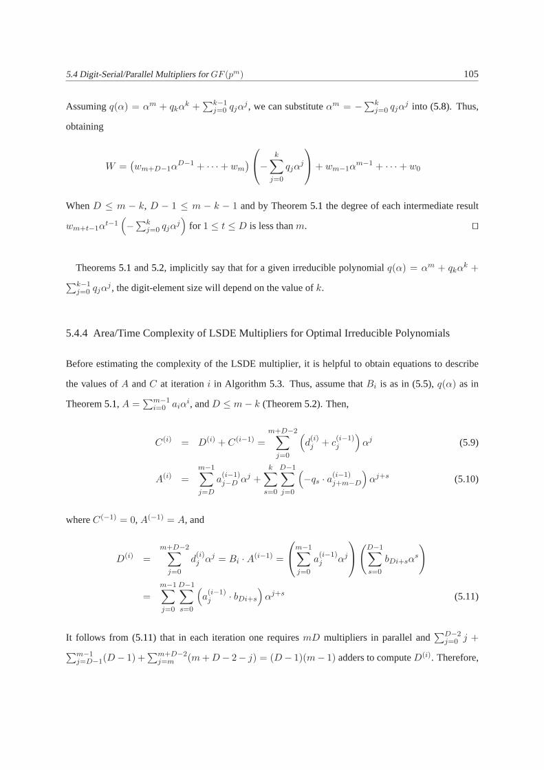
5.4 Digit-Serial/Parallel Multipliers forGF (pm) 105
Assumingq(α) = αm + qkαk +
∑k−1j=0 qjα
j , we can substituteαm = −∑k
j=0 qjαj into (5.8). Thus,
obtaining
W =(wm+D−1α
D−1 + · · ·+ wm
)−
k∑
j=0
qjαj
+ wm−1α
m−1 + · · ·+ w0
WhenD ≤ m − k, D − 1 ≤ m − k − 1 and by Theorem5.1 the degree of each intermediate result
wm+t−1αt−1(−∑k
j=0 qjαj)
for 1 ≤ t ≤ D is less thanm. ⊓⊔
Theorems5.1 and5.2, implicitly say that for a given irreducible polynomialq(α) = αm + qkαk +
∑k−1j=0 qjα
j , the digit-element size will depend on the value ofk.
5.4.4 Area/Time Complexity of LSDE Multipliers for Optimal Irreducible Polynomials
Before estimating the complexity of the LSDE multiplier, it is helpful to obtain equations to describe
the values ofA andC at iterationi in Algorithm 5.3. Thus, assume thatBi is as in (5.5), q(α) as in
Theorem5.1, A =∑m−1
i=0 aiαi, andD ≤ m− k (Theorem5.2). Then,
C(i) = D(i) + C(i−1) =m+D−2∑
j=0
(d
(i)j + c
(i−1)j
)αj (5.9)
A(i) =m−1∑
j=D
a(i−1)j−D αj +
k∑
s=0
D−1∑
j=0
(−qs · a
(i−1)j+m−D
)αj+s (5.10)
whereC(−1) = 0, A(−1) = A, and
D(i) =m+D−2∑
j=0
d(i)j αj = Bi ·A
(i−1) =
m−1∑
j=0
a(i−1)j αj
(
D−1∑
s=0
bDi+sαs
)
=m−1∑
j=0
D−1∑
s=0
(a
(i−1)j · bDi+s
)αj+s (5.11)
It follows from (5.11) that in each iteration one requiresmD multipliers in parallel and∑D−2
j=0 j +
∑m−1j=D−1(D− 1) +
∑m+D−2j=m (m + D− 2− j) = (D− 1)(m− 1) adders to computeD(i). Therefore,

106 5. Semi-Systolic Architectures for Arithmetic inGF (pm)
in total we need(D− 1)(m− 1)+m+D− 1 = mD adders to computeC(i) according to (5.9). Using
a ripple adder architecture, the critical path is given byD − 1 adder delays from the computation of
D(i), one adder delay from the computationd(i)j + c
(i−1)j in (5.9), and one multiplier. Notice, however,
that it is possible to improve the critical path delay of the LSDE multiplier by using a binary tree of
adders4. Using this technique one would reduce the length of the critical path fromD GF (p) adders
and oneGF (p) multiplier delays to⌈log2(D +1)⌉ adders and one multiplier delays. We use this, as our
complexity for the critical path. The computation of (5.10) requires onlyD(k + 1) multipliers (notice
that the second term of (5.10) looks exactly the same asD(i) in (5.11), except that the limits in the
summation are changed) and at most(D − 1)k + k = Dk adders (where the(D − 1)k term comes
from the double summation and thek other adders come from adding the single summation term to the
double summation one in (5.10)).
If q(α) is anr-nomial, the complexity of computing (5.10) is reduced to(r − 1)D multipliers and
at most(r − 2)D adders (notice that the first summation in (5.10) starts atj = D, thus, the firstD
coefficients resulting from the second summation do not need to be added to anything). We sayat most
because depending on the values ofD andr and the distribution of the non-zero coefficients ofq(α),
some adders may be saved. Last, we should consider the final reduction inStep6 of Algorithm 5.3. In
Step6, we get as inputC(d−1) =∑m+D−2
j=0 c(d)j αj and we want to obtainC(d) such thatdeg(C(d)) < m.
This is accomplished in a similar way to (5.10) as follows
C(d) =m−1∑
j=0
c(d)j αj =
m−1∑
j=0
c(d−1)j αj +
(k∑
s=0
(−qs)αs
)
D−2∑
j=0
c(d−1)j+m αj
=m−1∑
j=0
c(d−1)j αj +
k∑
s=0
D−2∑
j=0
(−qsc
(d−1)j+m
)αj+s (5.12)
Equation (5.12) requires in general(k + 1)(D − 1) multipliers andk(D − 2) + k + D − 2 + 1 = (k +
1)(D−1) adders. If we use anr-nomial, the number of multipliers will be(D−1)(r−1) but the number
of adders will vary, as in the case of (5.10), depending on the valuesi for whichqi 6= 0. To give an upper
bound, we assume that a general optimalr-nomialq(x) = xm+qsr−2xsr−2 +qsr−3x
sr−3 +· · ·+qs1x+q0
with sr−2 > sr−3 > · · · > s1 > 0 andsr−2 ≤ m − D also satisfiessi = si−1 + 1 with s1 = 1. It

5.4 Digit-Serial/Parallel Multipliers forGF (pm) 107
is easy to see that this assumption will provide us with the maximum number of adders (simply look at
how to compute the final product in (5.12)). Then, computing (5.12) with an r-nomial will require at
most(r+D−3)+(D−2)(r−2) = (D−1)(r−1) adders. These results are summarized in Table5.3
Table 5.3.Area complexity and critical path delay of LSDE multiplier with optimal irreducible polynomials.
Irreducible Area Critical Path Latencypolynomial Complexity Delay (# clocks)
r-nomial [(m + r − 2)D + (D − 1)(r − 1)] ADD + ⌈log2(D + 1)⌉ ADD ⌈mD⌉+
[(m + r − 1)D + (D − 1)(r − 1)] MUL + 1 MUL 1− δ(D, 1)General [(m + k)D + (k + 1)(D − 1)] ADD + ⌈log2(D + 1)⌉ ADD ⌈m
D⌉+
[(m + k + 1)D + (k + 1)(D − 1)] MUL + 1 MUL 1− δ(D, 1)
In Table5.3, δ(D, 1) is equal to 1 ifD = 1 and 0 otherwise. The extra clock cycle whenD > 1 comes
from the modular reduction in Step6 of Algorithm 5.3 which is necessary because the intermediate
results are of degree larger thanm − 1. Table5.3makes the same assumptions as for the LSE case. In
other words, ADD and MUL refer to the area and delay of aGF (p) adder and multiplier, respectively,
delay or area of storage elements are not taken into account, and no distinction is made between general
and constantGF (p) multipliers. We end by noticing that an LSDE multiplier withD = 1 is equivalent
to an LSE multiplier. Our complexity estimates verify this if one letsD = 1 andk = m−1 in Table5.3.
5.4.5 Area/Time Complexity of MSDE Multipliers for Optimal Irreducible Polynomials
As in the LSDE case, we first find expressions forC in Algorithm 5.4at iterationi. Thus,
C(i) = A ·Bd−1−i +(C(i−1) mod q(α)
)αD (5.13)
The termA · Bd−1−i is of the same complexity as (5.10), thus requiringmD parallel multipliers and
(m−1)(D−1) parallel adders. ComputingC(i−1) mod q(α) is the same operation described in (5.12),
except that now we need to reduce a polynomial of degree≤ m+D−1 instead of a polynomial of degree
≤ m+D− 2. For general optimal polynomials this implies an area complexity of(k +1)D multipliers
and(k + 1)D adders. Forr-nomials this means(r − 1)D multipliers and at most(r − 1)D adders. In
addition, we require an additionalm− 1 adders to addA ·Bd−1−i and(C(i−1) mod q(α)
)αD. Finally,
notice that since we multiply and modulo reduce all in one step, the number of adders in the critical path

108 5. Semi-Systolic Architectures for Arithmetic inGF (pm)
is at most doubled. Table5.4summarizes these results.
Table 5.4.Area complexity and critical path delay of MSDE multiplier with optimal irreducible polynomials.
Irreducible Area Critical Path Latencypolynomial Complexity Delay (# clocks)
r-nomial [(m + r − 2)D + (D − δ(D, 1))(r − 1)] ADD + ⌈log2(2D + 1)⌉ ADD ⌈mD⌉+
[(m + r − 1)D + (D − δ(D, 1))(r − 1)] MUL + 1 MUL 1− δ(D, 1)General [(m + k)D + (k + 1)(D − δ(D, 1))] ADD + ⌈log2(2D + 1)⌉ ADD ⌈m
D⌉+
[(m + k + 1)D + (k + 1)(D − δ(D, 1))] MUL + 1 MUL 1− δ(D, 1)
5.4.6 Comments on Irreducible Polynomials of Degreem overGF (p)
From Theorems5.1 and5.2, it is obvious that choosing an irreducible polynomial should be carefully
done. In this section, we give some guidelines regarding the selection of irreducible polynomials.
For fieldsGF (pm) with odd prime characteristic it is often possible to choose irreducible binomials
q(α) = xm − ω, ω ∈ GF (p). This is particularly interesting since binomials are never irreducible in
characteristic 2 fields. Another interesting property of binomials is that they are optimum from the point
of view of Theorem5.1. In particular, for any irreducible binomialq(α) = xm − ω, it holds thatk = 0
andD ≤ m in Theorem5.2. This implies that even in the degenerate case whereD = m (parallel
multiplier case) one is able to perform the reduction in one step. In addition, reduction is virtually for
free, corresponding to just a fewGF (p) multiplications (this follows from the fact thatαm = ω). A
specific sub-class of these fields whereq is a prime of the formq = p = 2n − c, c “small”, has recently
been proposed for cryptographic applications in [BP01a]. We notice that the existence of irreducible
binomials has been exactly established as Theorem5.3shows5.
Theorem 5.3.[LN97] Let m ≥ 2 be an integer andω ∈ F ⋆q . Then the binomialxm − ω is irreducible
in Fq[x] if and only if the following two conditions are satisfied: (i) each prime factor ofm divides the
ordere of ω in F ⋆q , but not(q − 1)/e; (ii) q ≡ 1 mod 4 if m ≡ 0 mod 4.
When irreducible binomials can not be found, one searches in incrementalorder for irreducible trino-
mials, quadrinomials, etc. In [vzGN00] von zur Gathen and Nocker conjecture that the minimal number
of termsσq(m) in irreducible polynomials of degreem overGF (q), q a power of a prime, is form ≥ 1,
σ2(m) ≤ 5 andσq(m) ≤ 4 for q ≥ 3. This conjecture has been verified forq = 2 andm ≤ 10000

5.5 Case Study:GF (3m) Arithmetic 109
[BGL93, Gol67, vzGN00, Zie70, ZB68, ZB69] and forq = 3 andm ≤ 539 [vzG01].
By choosing irreducible polynomials with the least number of non-zero coefficients, one can reduce
the area complexity of the LSDE multiplier (this follows directly from Table5.3). We point out that
by choosing irreducible polynomials such that their non-zero coefficientsare all equal top− 1 one can
further reduce the complexity since all the multiplications by−qs in (5.10) reduce to multiplication
by 1. We point out that there is no existence criteria for irreducibility of trinomials over any field
GF (pm). The most recent advances in this area are the results of Loidreau [Loi00], where a table that
characterizes the parity of the number of factors in the factorization of a trinomial overGF (3) is given,
and the necessary (but not sufficient) irreducibility criteria for trinomials introduced by von zur Gathen
in [vzG01]. Neither reference provides tables of irreducible polynomials.
5.5 Case Study:GF (3m) Arithmetic
5.5.1 GF (3) Arithmetic Implementation on FPGAs
Field Programmable Gate Arrays (FPGAs) are reconfigurable hardwaredevices whose basic logic ele-
ments are Look-Up Tables (LUTs), sometimes also called Configurable LogicBlocks (CLBs), flip-flops
(FFs), and, for modern devices, memory elements [Act01, Alt01, Xil00]. The LUTs are used to im-
plement Boolean functions of their inputs, that is, they are used to implement functions traditionally
implemented with logic gates. In the particular case of the XCV1000E-8-FG1156 and the XC2VP20-7-
FF1156, their basic building blocks are 4-bit input/1-bit output LUTs. Thismeans that all basic arith-
metic operations inGF (3) (add, subtract, and multiply) can be done with 2 LUTs, where each LUT
generates one bit of the output. This follows from the fact that any of these arithmetic operations over
GF (3) can be thought of as logic functions in 4 input variablesa1, a0, b1, b0 and 2 output variablesc1, c2
as:
f : I4 −→ O2
whereI = {0, 1} andO = {0, 1}. Then, given three elementsa = (a1, a0)2, b = (b1, b0)2, c =
(c1, c0)2 ∈ GF (3), we can write the function “multiplication inGF (3)” as Table5.5. In Table5.5,

110 5. Semi-Systolic Architectures for Arithmetic inGF (pm)
Table 5.5.Truth table representing multiplication inGF (3).
a1 a0 b1 b0 c1 c0 a1 a0 b1 b0 c1 c00 0 0 0 0 0 1 0 0 0 0 00 0 0 1 0 0 1 0 0 1 1 00 0 1 0 0 0 1 0 1 0 0 10 0 1 1 0 0 1 0 1 1 0 00 1 0 0 0 0 1 1 0 0 0 00 1 0 1 0 1 1 1 0 1 0 00 1 1 0 1 0 1 1 1 0 0 00 1 1 1 0 0 1 1 1 1 0 0
we have assumed that(1, 1) is an alternate representation for0 ∈ GF (3). Notice that it is possible
to choose different representations as shown in [GWP02]. This might minimize the complexity of the
GF (3) multiplier in ASIC-based designs. However, in FPGA based designs, a different encoding has
no advantages because of the LUT-based structure of the FPGA.
5.5.2 Cubing inGF (3m)
It is well known that forA ∈ GF (pm) the computation ofAp (also known as the Frobenius map) is
linear. In the particular case ofp = 3, we can write the Frobenius map as:
A3 mod q(α) =
(m−1∑
i=0
aiαi
)3
mod q(α) =m−1∑
i=0
aiα3i mod q(α) = (5.14)
Equation (5.14) can in turn be written as the sum of three terms (notice that here we have re-written the
indexes in the summation):
A3 mod q(α) =
3(m−1)∑
i=0i≡0 mod 3
a i3αi mod q(α) = T + U + V mod q(α) = (5.15)
=
m−1∑
i=0i≡0 mod 3
a i3αi
+
2m−1∑
i=mi≡0 mod 3
a i3αi
+
3(m−1)∑
i=2mi≡0 mod 3
a i3αi
mod q(α)
Notice that onlyU andV need to be reducemod q(α). We further assume thatq(x) = xm + qtxt + q0
and thatt < m/3. This assumption proves to be a valid one in terms of the existence of such irreducible

5.5 Case Study:GF (3m) Arithmetic 111
trinomials as we show in Section5.5.3. Then, we obtain:
U =2m−1∑
i=mi≡0 mod 3
a i3αi mod q(α) =
2m−1∑
i=mi≡0 mod 3
a i3αi−m
(−qtα
t − q0
)mod q(α)
V =
3(m−1)∑
i=2mi≡0 mod 3
a i3αi mod q(α) =
3(m−1)∑
i=2mi≡0 mod 3
a i3αi−2m
(α2t − qtq0α
t + 1)
mod q(α)
where we have made use of the fact that(−qtαt − q0)
2 = (α2t − qtq0αt + 1) in GF (3). It can be
shown thatU andV can be reduced to be of degree less thanm in one extra reduction step. To estimate
the complexity of this cubing circuit, we assume thatq(α) is a trinomial witht < m/3, and that the
circuit is implemented for fixed irreducible trinomials, i.e., that multiplications inGF (3) (for example
multiplying by−ptp0) can be handled by adders and subtracters. Then, it can be shown that one needs
in the order of2m adders/subtracters to perform a cubic operation inGF (3m).
5.5.3 Irreducible Polynomials overGF (3)
If we follow the criteria of Section5.4.6 for choosing irreducible polynomials, we would try to find
irreducible binomials first. Unfortunately, the only irreducible binomial overGF (3) is x2 + 1, thus we
have to consider irreducible trinomials. Notice thatxm + xt + 1 is never irreducible overGF (3) since
1 is always a root of it. Therefore, we only need to search for irreducible trinomials of the following
forms: xm − xt − 1 or xm ± xt ∓ 1. For2 ≤ m ≤ 255, we exhaustively searched for trinomials. Our
results are provided in TablesA.3, A.4, andA.5 in AppendixA.2. There are only 23 degreesm in the
range above, for which we were unable to find trinomials (this agrees with thefindings in [vzG01]) and
thus, we provide quadrinomials for them in TableA.6. Of these quadrinomials, only 4 correspond tom
prime (149, 197, 223, 233). Primem is the most commonly used degree in cryptographic applications.
Another criteria to choose irreducible polynomials is based on the value of thenon-zero coefficients
of q(x) and on the degree of the second-highest non-zero coefficient inq(x). From our discussion in
Section5.4.6, follows that choosing irreducible polynomials whose non-zero coefficients are all equal to
−1 might be advantageous, thus we make emphasis on trinomials of the formxm − xt − 1. In addition,
from our cubing circuit discussion follows that polynomialsxm + qtxt + q0, with t < m/3 are also

112 5. Semi-Systolic Architectures for Arithmetic inGF (pm)
desirable. Putting all these criteria together we come up with theoptimumpolynomials of TableA.2. In
doing so, we follow these rules:
1. For allm, whenever a trinomialxm − xt − 1 with t < m/3 exists we include it in TableA.2.
2. If there is no trinomial as in 1 but there is a trinomial(s) witht < m/3, we include them in
TableA.2.
3. If both 1 and 2 fail, we write all available trinomials for that degree.
As a final remark, we notice that of the 50 primes in the range2 ≤ m ≤ 255 which had trinomials, we
were not able to find trinomials witht < m/3 for 9 of them (18 %).
5.6 GF (3m) Prototype Implementation and Comparisons
Figure5.1shows a block diagram of the prototyped6 arithmetic unit (AU). In Figure5.1, all bus-widths
correspond to how manyGF (3) elements can be carried by the bus. In other words, if we writem, then
it is understood that the bus is2m-bit wide.
The AU consists of an LSDE multiplier and a cubic circuit. The multiplier and the cubic circuit
support the computation of field additions, squares, multiplications, and inversions. For addition and
subtraction we take advantage of the multiply/accumulate capabilities of the LSDE multiplier and cubing
circuit. In other words, the additionC = A+B is done by first computingA ·1 and then adding to it the
productB · 1. This takes two clock cycles. However, if operandA is already in the accumulator of the
multiplier one can computeC = B · 1 + A in one clock. This addition eliminates the need for an adder.
Subtractions are computed in a similar manner. The subtractionC = A−B is done by first computing
A · 1 and then adding to it the product(−1) ·B or alternatively asC = (−1) ·B + A.
AU prototypes were developed to verify the suitability of the architecture shown in Figure5.1 for
reconfigurable FPGA logic and compare the efficiency ofGF (3m) andGF (2m) AUs. The prototypes
were coded in VHDL at a very low level. The VHDL code was synthesized using Synopsis FPGA Com-
piler 3.7.1 and the component placement and routing was done using XILINXDesign Manager 4.2.03i.

5.6GF (3m) Prototype Implementation and Comparisons 113
�� � � � � � �� � �
� � � � � � � � � �� �
� � � � �� � � � �� �� � � � �� � � � � � � � �� ���� � �� � � � � � � � ! �� ��" � �� � � � �� � � �� # � �
� �$ � ! %" � �� � � � ��
��
� � & �� � � � ��
� ' � � � � �� ��(" � )Figure 5.1.GF (3m) Arithmetic Unit Architecture
The prototypes were synthesized and routed for the XILINX XCV1000-8-FG1156 and XC2VP20-7-
FF1156 FPGAs. The XCV1000E-8-FG1156 prototype allowed us to compare our AU implementations
against the AU forGF (2m) used in the elliptic curve processor (ECP) documented in [OP00]. The
XC2VP20-7-FF1156 prototype allowed us to verify the speed of our AU for one of the newest families of
XILINX FPGAs. Three implementation were developed which support the fields GF (397), GF (2151),
andGF (2241). The fieldsGF (397) andGF (2241) are used in Weil and Tate pairing schemes for sys-
tems with comparable degrees of security (see [GHS02a, BKLS02, PS02]). The fieldGF (2151) offers
security comparable to that ofGF (397) for cryptosystems based on the elliptic curve discrete logarithm
problem (ECDLP).
5.6.1 GF (3m) Complexity Estimates
Table5.6 shows the complexity estimates for the AU shown in Figure5.1. The estimates assume the
use of optimum irreducible polynomials. The estimates give the register complexityin terms of the
number of flip-flops. Note that the register estimates do not account for registers used to reduce the

114 5. Semi-Systolic Architectures for Arithmetic inGF (pm)
critical path delay of a multiplier, a technique known as pipelining. This technique was used to reduce
the critical path delay of the prototype implementations. The complexity estimates arebased on the
Table 5.6.GF (3m) AU complexity estimates
Circuit Area ComplexityGF (397)(q(x) = x97 + x12 + 2)
LSE Mult. (4mD + 2m + 6D) LUT + 6m + 2D + 4 FFCubic 4m LUTMux 2m LUT
AU (total) (4mD + 8m + 6D) LUT + 6m + 2D + 4 FF
following assumptions:
1. A GF (3) adder, subtracter, or multiplier requires two LUTs, including adders that add weighted
inputs, for example, adders that compute(ai ∗ c) + (bi ∗ d) wherec andd are fixed constants. In
addition, a 2:1 multiplexer requires one LUT.
2. From Table5.3 the digit multiplication core and the accumulator circuits requiremD GF (3)
multipliers andmD GF (3) adders. This circuit stores the result in two(m+D− 1)-bit registers.
An m-bit register requiresm flip-flops (FFs).
3. The estimates for theAαDi mod q(α) circuit assume that the circuit contains twom-bit multi-
plexers that select between the elementA and the elementAαDi mod q(α). An m-bit multiplexer
requiresm LUTs. For programmable optimum irreducible trinomials, the circuitry that generates
AαDi mod q(α) requires2D GF (3) multipliers andD adders (see Table5.3). This circuit stores
the result in twom-bit registers and the coefficients ofq(x) in two 2r-bit registers (r = 3 for
trinomials).
4. The estimates assume that the coefficients ofB are fed in by twom-bit parallel in/serial out shift
registers. Each of these shift registers containsm 2:1 multiplexers andm registers.
5. The cubic circuit requires2m GF (3) adders.
6. The complexity for theGF (2m) AU is done accordingly to the models in [Orl02]. We have also
assumed that theGF (2m) AU contains an LSD multiplier and a squarer.

5.6GF (3m) Prototype Implementation and Comparisons 115
Table 5.7.AU estimated vs. measured complexity for prototypes (D = 16)
Circuit ⌊log2(pm)⌋ Estimated Measured LUT Estimate
complexity complexity Error(incl. pipelining ((actual-est.)/est.)registers & I/O)
GF (2151) 151 2366 LUT + 453 FF 2239 LUT + 1092 FF -5.4 %(15.7m LUT + 3m FF) (14.3m LUT + 7.2m FF)
GF (2241) 241 3705 LUT + 723 FF 3591 LUT + 1722 FF -3.1 %(14.9m LUT + 3m FF) (15.4m LUT + 7.1m FF)
GF (397) 153 7080 LUT + 618 FF 7122 LUT + 2790 FF 1.0 %(73.0m LUT + 6.4m FF) (73.4m LUT + 7.2m FF)
We observe that the estimates obtained from our models are very accurate when compared to the actual
measured complexities. This validates our models and assumptions.
5.6.2 Results
Table5.8presents the timings obtained for our three prototypes. We have tried to implement our designs
in such a way that we can make a meaningful comparison. Thus, although, the clock rates are not
exactly the same between the different designs (this is due to the fact that theclock rate depends on the
critical path of the AU which is different for each circuit), they are not more than 10 % different. The
platforms are the same and we chose same digit sizes for bothGF (2m) andGF (3m) architectures. The
results make sense, for the same digit size (D = 16) we obtain that theGF (397) design is about twice
as big as theGF (2241) design and more than 3 times the size of theGF (2151) AU. This of course is
offset by the gain in performance. At similar clock rates theGF (397) design is 2.7 times faster than the
correspondingGF (2241) AU and 1.4 times faster than theGF (2151) one.
Table 5.8. Comparison of multiplication time forGF (2151), GF (2241), andGF (397) prototypes (D = 16) andthe AU from [PS02]
Circuit Mult. time for Mult. time foroptimized mult. prototypes
[PS02] XCV1000-8-FG1156 XC2VP20-7-FF1156(in µsec) (in µsec) (in µsec)
GF (2151) N/A 0.139 (@ 71.7 MHz) 0.100 (@ 100.2 MHz)GF (2241) 37.32 0.261 (@ 61.3 MHz) 0.150 (@ 107 MHz)GF (397) 50.68 0.097 (@ 72 MHz) 0.074 (@ 94.4 MHz)
It is clear that by using more hardware resources forGF (397) we can achieve better performance than

116 5. Semi-Systolic Architectures for Arithmetic inGF (pm)
fields of characteristic 2. In particular, we point out that by choosing thesame digit size for both types
of fields, we are implicitly processing twice as many bits of the multiplier inGF (397) as in theGF (2m)
cases (remember that is why we introduced the notation of LSDE, where the Erefers to elements of
GF (p) and not bits as in theGF (2m) case). Table5.8 also includes the results presented in [PS02].
Unfortunately, the authors in [PS02] used the Celoxica Handel-C hardware compilation system [Cel02]
and a PCI resident XILINX4000XL FPGA based prototyping device. The Handel-C language allows the
designer to describe hardware in a high-level language similar to C and usea compiler to map this code
to synthesizable VHDL code. Thus, we do not think it is possible to make a meaningful comparison,
other than point out that by coding directly in VHDL, one can improve the performance of FPGA based
implementations.
5.7 Notes and Further References
1. There has been a lot work done, however, on finite field architectures for characteristic two fields. See
for example [YP82, Mas89, HWB92, AMV93, ABMV93, FBT96, SP98, PFR99].
2. It is widely accepted that for cryptosystems against which the Pollard’srho algorithm or one of its
variants are the best available attacks, such as elliptic curve cryptosystems, the group order should be
greater or equal to2160. Thus, solving2m < p andpm ≥ 2160 for p andm, one obtainsp ≥ 67. Notice
that the value ofp grows as the size of the desired group grows. For groups with|G| ≥ 2192, |G| ≥ 2223,
and|G| ≥ 521, the primep satisfiesp ≥ 67, p ≥ 79, andp ≥ 157, respectively.
3. Look-Up Tables are the basic building blocks of most common FPGAs [Act01, Alt01, Xil00].
4. Binary trees have been used both in [SP98] and [Orl02] in the context ofGF (2n) arithmetic to reduce
delay and power consumption.
5. Reference [LN97] is used in this setting as a convenient reference for well established results.
6. The synthesis was joint work General Dynamics Communication Systems, USA. The design and the
running of the tools were performed at General Dynamics Communication Systems. Special thanks to
Dr. Gerardo Orlando.

CHAPTER 6
Systolic and Scalable Architectures for
Digit-Serial Multiplication in FieldsGF (pm)
The research community’s interest in cryptographic systems based on fields of odd characteristic and
the lack of hardware architectures for general odd characteristic fields is evident. Reference [BGK+03]
has given a partial answer to this problem but their methods have the drawback of using global signals
and long wires and they require reconfigurability to achieve their full potential (for example, [BGK+03]
uses irreducible trinomial specific circuitry to perform modular reduction onFPGAs), and thus, these
solutions lack flexibility in other hardware platforms such as ASICs. Hence,in this chapter, we move a
step forward towards the design of scalable and flexible hardware architectures for oddGF (pm) fields.
In particular, we propose systolic architectures for arithmetic inGF (pm) fields. Systolic architectures
solve the previously mentioned problems in several ways. First, by using a systolic design we use
localized routing, thus avoiding the need for global control signals and long wires. In addition, this
methodology allows for ease of design and offers functional and layoutmodularity all of which are
properties envisioned in good VLSI designs. Second, we modify the design of [BGK+03] to allow
for scalability as introduced in [TcKK99]. In other words, for a fixed value of the digit-sizeD [SP98,
BGK+03] and parameterd, we can perform a multiplication for any value ofm in GF (pm), with fixed
p, i.e., we support multiple irreducible polynomials making unnecessary the use of reconfigurability in

118 6. Systolic and Scalable Architectures for Digit-Serial Multiplication in FieldsGF (pm)
FPGAs. Thus, these architectures are well suitable for very large multipliers and a large number of
hardware platforms, including FPGAs and ASICs. Parts of this chapter appear in [BGO03].
6.1 Related Work
There has been significant work on systolization of modular multiplication (i.e. multiplication inGF (p)).
The first attempt to provide systolic architectures for modular multiplication was presented in [KH91].
However, these architectures suffered from excessive latency anda slow clock as a result of the unsuit-
ability of the regular multiply–and–then–reduce algorithm to systolization. The first systolic architec-
tures for Montgomery multiplication were introduced in [Wal93]. In particular, [Wal93], takes advantage
of simplifications to the Montgomery algorithm presented in [EW93] to minimize the complexity of the
array cells and their execution time. Throughout the years, several systolic architecture designs of the
binary type (using radix 2 to represent and process operands) havebeen introduced, including both 1D-
based arrays [Kor94, CHCW99, TSW00] and 2D-based arrays [JB97]. Higher-radix systolic arrays have
also been proposed, as for example [Tak92, Wal97, FP00, BP01b]. Notice that the previously mentioned
works include both Montgomery and non-Montgomery based architectures.
We also build on the concept of scalability presented in [TcKK99] and further generalized to higher
radix Montgomery multipliers in [STcKK00, TcKK01]. Notice that [TcKK99, STcKK00, TcKK01] are
only concerned with Montgomery multiplication overGF (2k) andGF (p). Scalability, as defined in
[TcKK99], means that an arithmetic unit (AU) (in our case an AU to perform arithmetic operations in
GF (pm)) can be used or replicated in order to generate long-precision1 results independently of the data
path precision for which the unit was originally designed. A very important design choice in [TcKK99] is
the use of a word-based algorithm. Rather than processing one of the inputs (multiplier or multiplicand)
in a bitwise manner, [TcKK99] uses circuits which process multiple bits of the operands at a time. Based
on the data dependencies of the Montgomery algorithm, the authors define processing units which, when
combined with pipelining and word-operand processing, result in scalablearchitectures for modular
multiplication. The authors in [TcKK99] also examine trade-offs among desired performance, area,
number of processing units, operand word-length, and precision.

6.2 Systolic Least-Significant Element (LSE) First Architecture 119
6.2 Systolic Least-Significant Element (LSE) First Architecture
The LSE scheme from Chapter5 processes first coefficientb0 of the multiplier and continues with the
remaining coefficients one at a time in ascending order. This multiplier computes the operation ac-
cording to Algorithm5.1 which we reproduce here as Algorithm6.1 for ease of presentation. Step3
Algorithm 6.1 LSE Multiplier
Input: A =∑m−1
i=0 aiαi, B =
∑m−1i=0 biα
i, q(α) = αm +∑m−1
i=0 qiαi whereai, bi, qi ∈ GF (p)
Output: C ≡ A ·B mod q(α) =∑m−1
i=0 ciαi, whereci ∈ GF (p)
1: C ← 02: for i = 0 to m− 1 do3: C ← biA + C4: A← Aα mod q(α)5: end for6: Return (C)
in Algorithm 6.1 requires the accumulation of the partial product which is achieved via a polynomial
adder. In Step4 of Algorithm 6.1 the quantityAα mod q(α), has to be computed. Thus,Aα =
∑m−1i=0 aiα
i+1 = am−1αm +
∑m−2i=0 aiα
i+1. Then, using (5.1) and re-writing the index of the second
summation,Aα mod q(α) can be calculated as follows:
Aα mod q(α) ≡ (−q0am−1) +
m−1∑
i=1
(ai−1 − qiam−1)αi (6.1)
where all coefficient arithmetic is done modulop. Using (6.1) we can write expressions forA andC in
Algorithm 6.1at iterationi as follows:
C(i) =m−1∑
j=0
c(i)j αj ≡ biA
(i) + C(i−1) =m−1∑
j=0
(bia(i)j + c
(i−1)j )αj , (6.2)
A(i) =m−1∑
j=0
a(i)j αj ≡ A(i−1)α ≡ (−q0a
(i−1)m−1 ) +
m−1∑
j=1
(a(i−1)j−1 − qja
(i−1)m−1 )αj (6.3)
with C(−1) = 0 andA(−1) = A. Notice that ifC is initialized to a value different from0, sayI, before
beginning the algorithm, Algorithm6.1computesC ≡ A ·B + I mod q(α). This multiply-accumulate
operation turns out to be very useful in elliptic curve systems and it is obtainedat no extra cost. Using

120 6. Systolic and Scalable Architectures for Digit-Serial Multiplication in FieldsGF (pm)
(6.2) and (6.3), one can define Algorithm6.2, which is a low-level version of Algorithm6.1.
Algorithm 6.2 Low Level LSE Multiplier
Input: A =∑m−1
i=0 aiαi, B =
∑m−1i=0 biα
i, q(α) = αm +∑m−1
i=0 qiαi whereai, bi, qi ∈ GF (p)
Output: C ≡ A ·B mod q(α) =∑m−1
i=0 ciαi whereci ∈ GF (p)
1: C ← 02: for i = 0 to m− 1 do3: for j = m− 1 to 0 do4: cj ← biaj + cj
5: end for6: for j = m− 1 to 0 do7: aj ← aj−1 − qjam−1 {Note:a−1 = 0}8: end for9: end for
10: Return (C)
6.2.1 Architecture
In this section, we analyze data dependencies of Algorithm6.2. Steps4 and7 in Algorithm 6.2 are
completely independent of each other. In other words, at iterationi, one can calculate coefficientcj
of C and, at the same time, computeaj for iteration i + 1 of the outer loop. To best study the data
dependencies in Algorithm6.2, two dependency graphs (DG) are used. Figure6.1shows the DG for the
computation ofAα mod q(α). Every square corresponds to the computation of Step7 in Algorithm 6.2.
Thus, each cell contains oneGF (p) multiplier and aGF (p) adder2. Each column corresponds to a new
iteration of the outer loop (i-loop). Notice that because of the dependence ofa(i)j on a
(i−1)j−1 , there is a
two cycle delay between the processing of a column at iterationi andi + 1 (this can be better seen on
Figure6.2, where thebi’s are labeled). Figure6.2 shows the DG for Algorithm6.2 as a whole. This
figure is obtained by superimposing the computation of Step4 on Figure6.1. To make this clearer, we
have used dotted lines to indicate the inputs and outputs corresponding to Step4 while using solid lines
for those that correspond to Step7 of Algorithm 6.2. Figure6.2, contains two types of cells. The white
cells can compute the values ofcj andaj for the nexti iteration. The black cells can computec(i)m−1
andc(i)m−2 given the values ofc(i−1)
m−1 andc(i−1)m−2 , respectively. In other words, they compute one morecj
value than the white cells. Thus, the white cells contain twoGF (p) multipliers and twoGF (p) adders
while the black cells contain threeGF (p) multipliers and threeGF (p) adders. The critical path for

6.2 Systolic Least-Significant Element (LSE) First Architecture 121
am−1
am−1
am−2
am−2
am−2
am−1
am−3
am−4
am−5
am−6
am−7
am−3
am−4
am−5
am−6
am−3
am−4
am−1
am−2
m−1q
m−1q
m−1q
m−2q
m−2q
m−2q
m−3q
m−3q
m−4q
m−4q
m−5q
m−6q
Figure 6.1.Dependency graph forAα mod q(α)
both types of cells is just the delay corresponding to oneGF (p) adder and oneGF (p) multiplier. As
in Figure6.1, there is a two cycle delay between columns which is a result of the dependence ofa(i)j on
a(i−1)j−1 . Similarly to [TcKK99], each column in Figure6.2 may be computed by a different processing
element (PE) and the data generated by one PE may be passed to another PEin a pipeline manner.

122 6. Systolic and Scalable Architectures for Digit-Serial Multiplication in FieldsGF (pm)
m−3
am−5
am−4am−2
am−3
am−1
am−2
cm−1 cm−2
am−1
am−1
am−1cm−1
cm−2
cm−1cm−2
am−2
am−3
am−4
am−5
am−6
am−7
cm−3
cm−3
cm−3
cm−4
cm−5
cm−6
cm−7
cm−4
cm−5
cm−1cm−2
b0
b1
b2
m−1q
m−1q
m−1q
m−2q
m−2q
m−2q
qm−3
qm−3
qm−4
qm−4 m−6
q
m−5q
a
Figure 6.2.Dependency graph for the LSE algorithm

6.3 Systolic Least-Significant Digit Element (LSDE) First Architecture 123
6.3 Systolic Least-Significant Digit Element (LSDE) First
Architecture
This section develops the theory for the systolic Least-Significant Digit Element (LSDE) First multi-
plier. Digit multipliers, introduced in [SP98] in the context of fieldsGF (2k) and later generalized in
[BGK+03], are a trade-off between speed, area, and power consumption. Thisis achieved by processing
several ofB’s coefficients at the same time. The number of coefficients that are processed in parallel is
defined to be the digit-size and we denote it byD. For a digit-sizeD, we can denote byd = ⌈m/D⌉
the total number of digits in a polynomial of degreem − 1. Thus, we can re-write the multiplier as
B =∑d−1
i=0 BiαDi, whereBi =
∑D−1j=0 bDi+jα
j with 0 ≤ i ≤ d − 1 and we assume thatB has been
padded with zero coefficients such thatbi = 0 for m− 1 < i < d ·D (i.e. B’s size isd ·D coefficients
butdeg(B) < m). Hence,
C ≡ AB mod q(α) = Ad−1∑
i=0
BiαDi mod q(α) (6.4)
≡ [B0A + B1(AαD mod q(α)) + . . . + Bd−1(AαD(d−2)αD mod q(α))] mod q(α)
Using (6.4), one can derive an algorithm similar to Algorithm6.1, substitutingbi in Step3 by Bi (we
process nowD coefficients as opposed to just one coefficient ofB) and multiplyingA by αD. The au-
thors in [BGK+03] define optimal irreducible polynomials of the formq(α) = αm +qkαk +∑k−1
i=0 qiαi
as those which satisfy the constraint3 k ≤ m −D. These polynomials allow one to perform the reduc-
tion of AαD moduloq(α) in one clock cycle. We illustrate the reductionAαD mod q(α) with a small
example.
Example 6.1.Although not shown in (6.4), one can also processA in digits of sizeD. Let A =
∑d−1i=0 Aiα
Di ∈ GF (pm) with d = ⌈m/D⌉, Ai a digit (i.e., a group ofD GF (p) coefficients), and
q(α) = αm + qkαk +∑k−1
i=0 qiαi an optimum irreducible polynomial in the sense of [BGK+03]. Notice

124 6. Systolic and Scalable Architectures for Digit-Serial Multiplication in FieldsGF (pm)
thatA is written in digit-form whereasq(α) is written in terms of its coefficients. Then,
AαD ≡ αDd−1∑
i=0
AiαDi mod q(α) = Ad−1α
Dd +d−1∑
i=1
Ai−1αDi mod q(α)
AαD ≡ Ad−1αDd−mαm +
d−1∑
i=1
Ai−1αDi mod q(α) = Ad−1α
Dd−m
(−qkα
k −k−1∑
i=0
qiαi
)+
d−1∑
i=1
Ai−1αDi
Notice that the first term in the reduced result depends on the value ofm, in other words on the field size.
In fact, one needs to multiply byαDd−m, which can be instantiated as avariable shifter in hardware.
This might be undesirable if scalability of the multiplier is desired.
Before we continue we prove a small proposition, the result of which will beused in the development of
new architectures.
Proposition 6.1.Let A, B ∈ GF (pm), q(α) = αm +∑m−1
i=0 qiαi, be an irreducible polynomial over
GF (p), and d = ⌈m/D⌉. Then,A · B mod q(α) ≡ [A · B mod q(α)] mod q(α), whereq(α) =
αDd−mq(α).
Proof. If Dd = m, then the result is immediate, so let’s consider the caseDd > m. DefineR ≡
A · B mod q(α). Then,A · B = Qq(α) + R = Q(αDd−mq(α)) + R. Thus, we can writeR =
A ·B −Q(αDd−mq(α)), which impliesR ≡ A ·B mod q(α). ⊓⊔
Intuitively, Proposition6.1 says that we can perform reductions moduloq(α) = αDd−mq(α) and still
obtain a result which when reduced moduloq(α) returns the correct value. We make this more formal
by first introducing Algorithm6.3.
Algorithm 6.3 Modified LSDE Multiplier
Input: A =∑d−1
i=0 AiαDi with Ai =
∑D−1j=0 aDi+jα
j , B =∑d−1
i=0 BiαDi with Bi =
∑D−1j=0 bDi+jα
j ,
q(α) = αDd−mq(α), ai, bi ∈ GF (p), andd = ⌈mD ⌉
Output: C ≡ A ·B mod q(α) =∑d
i=0 CiαDi with Ci =
∑D−1j=0 cDi+jα
j , ci ∈ GF (p), andd = ⌈mD ⌉
1: C ← 02: for i = 0 to d− 1 do3: C ← BiA + C4: A← AαD mod q(α)5: end for6: Return (C mod q(α))

6.3 Systolic Least-Significant Digit Element (LSDE) First Architecture 125
Algorithm 6.3 suggests the following computation strategy. Given two inputsA, B ∈ GF (pm) one
can computeC ≡ A · B mod q(α) by first computingC ≡ A · B mod q(α) using Algorithm6.3
and, then, computingC ≡ C mod q(α). The second step follows as a consequence of Proposition6.1.
In practice, the second step can be performed at the end of a long rangeof computations, similar to
the procedure used when performing Montgomery multiplication. Step4 in Algorithm 6.3 requires a
modular multiplication. There, it would be desirable to reduceAαD in just one iteration as in [BGK+03]
and, at the same time, make the reduction process independent of the value of m and, thus, of the field
GF (pm). Givenq(α) = αm +∑m−1
i=0 qiαi, we define
q(α) = αDd−mq(α) = αDd + αDd−mm−1∑
i=0
qiαi = αDd +
m−1∑
i=0
qiαDd+i−m
= αDd +Dd−1∑
i=0
qiαDd+i−m = αDd +
d−1∑
i=0
QiαDi (6.5)
whereqi = 0 for 0 ≤ i < Dd−m, qi = qi+m−Dd for Dd−m ≤ i < Dd, andQi =∑D−1
j=0 qDi+jαj .
Then, we can computeAαD mod q(α) as follows:
αDA mod q(α) = αDd−1∑
i=0
AiαDi mod q(α) = Ad−1α
Dd +d−2∑
i=0
AiαD(i+1) mod q(α)
Using (6.5), we obtain
αDA mod q(α) = Ad−1
(−
d−1∑
i=0
QiαDi
)+
d−2∑
i=0
AiαD(i+1) mod q(α)
=d−2∑
i=0
AiαD(i+1) −
d−1∑
i=0
(Ad−1Qi
)αDi mod q(α) (6.6)
In (6.6), we have kept themod q(α) because it is possible thatdeg(Ad−1Qd−1α
D(d−1))≥ Dd, in
which case it would require a further reduction. This problem might be solved by defining M-LSDE
optimal polynomials as those in whichQd−1 = 0 or Qd−1 = 1. Theorem6.1 summarizes the above
discussion.
Theorem 6.1.LetA =∑d−1
i=0 AiαDi be as defined in Algorithm6.3andq(α) = αDd−mq(α) = αDd +

126 6. Systolic and Scalable Architectures for Digit-Serial Multiplication in FieldsGF (pm)
∑d−1i=0 Qiα
Di be as defined in (6.5), in particular q(α) is irreducible overGF (p) of degree m. Then, if
Qd−1 = 0 or Qd−1 = 1, AαD mod q(α) can be computed in one reduction step. Moreover,Qd−1 = 0
implies that forq(α) = αm +∑m−1
i=0 qiαi, coefficientsqm−1 = qm−2 = · · · = qm−D = 0. Similarly,
whenQd−1 = 1 thenqm−1 = qm−2 = · · · = qm−D+1 = 0.
Proof. Notice thatαDA mod q(α) =∑d−2
i=0 AiαD(i+1) −
∑d−1i=0
(Ad−1Qi
)αDi mod q(α) from (6.6).
The first summation does not require any further reduction, thus we concentrate on the second one. If
Qd−1 = 1, then the largest degree possible in (6.6) would correspond to the termAd−1Qd−1αD(d−1)
anddeg(Ad−1Qd−1α
D(d−1))≤ (D−1)+D(d−1) ≤ Dd−1 < Dd. On the other hand, ifQd−1 = 0,
(6.6) becomes
αDA mod q(α) =d−2∑
i=0
AiαD(i+1) −
d−2∑
i=0
(Ad−1Qi
)αDi (6.7)
Now it is easy to verify thatdeg(Ad−1Qd−2α
D(d−2))≤ (D−1)+(D−1)+(Dd−2D) = Dd−2 < Dd.
This proves the first part of the theorem. The second part is just a consequence of the definition ofQi in
terms of the coefficients ofq(α). ⊓⊔
Notice that Theorem6.1 implies that ifq(α) = αm + qkαk +
∑k−1i=0 qiα
i is to be an optimal M-LSDE
polynomial, thenk ≤ m − D, which agrees with the findings in [SP98, BGK+03]. Notice also that
(6.7), which defines the way modular reduction is performed in Step4 of Algorithm 6.3, is independent
of the value ofm and thus of the field. The price of this field independence is that now we do not obtain
anymore the value ofA · B mod q(α) but ratherA · B mod q(α) thus, requiring one more reduction
at the end of the whole computation. In addition, we need to multiplyonceat initializationq(α) by
αDd−m. This, however, can be thought of as analogous to the Montgomery initialization, and thus, can
be neglected when considering the total costs of complex computations which iscustomary practice in
cryptography. In addition, notice that multiplication byα can be easily implemented in hardware via
left shifts. In the remainder of this chapter, we only consider M-LSDE optimal polynomials unless we
explicitly say something to the contrary.
In what follows, we re-write the steps in Algorithm6.3 to make it suitable to a systolic implementa-
tion. The beginning of our work is (6.6), assuming thatQd−1 = 0 or Qd−1 = 1, which we re-write in

6.3 Systolic Least-Significant Digit Element (LSDE) First Architecture 127
(6.8) as a recurrence. We also re-write the limits of the summation for convenience.
A(i)αD mod q(α) =d−1∑
j=1
A(i−1)j−1 αDj −
d−1∑
j=0
(A
(i−1)d−1 Qj
)αDj (6.8)
Unfortunately, (6.8) is not entirely in terms of digits. In particular, we can writeA(i−1)d−1 Qj as
A(i−1)d−1 Qj = R
(i−1)j αD + S
′(i−1)j (6.9)
whereR(i−1)j is a polynomial of maximum degreeD − 2 andS
′(i−1)j is of maximum degreeD − 1.
Plugging (6.9) into (6.8), we get:
A(i)αD mod q(α) =d−1∑
j=1
A(i−1)j−1 αDj −
d−1∑
j=0
(R
(i−1)j αD + S
′(i−1)j
)αDj
=
d−1∑
j=1
A(i−1)j−1 αDj −
d−1∑
j=0
S′(i−1)j αDj −
d−1∑
j=0
R(i−1)j αD(j+1)
which after re-writing the index of the last summation becomes
A(i)αD mod q(α) =d−1∑
j=1
A(i−1)j−1 αDj −
d−1∑
j=0
S′(i−1)j αDj −
d−1∑
j=1
R(i−1)j−1 αDj (6.10)
where we have made use of the fact that given thatQd−1 is either 0 or 1 for optimal M-LSDE polyno-
mials,R(i−1)d−1 = 0 (i.e. when the indexj of the last summation is equal tod, the termR
(i−1)j−1 vanishes)
always, and thus the last summation in (6.10) need only run tod− 1. Similarly, we can write an expres-
sion for Step3 of Algorithm 6.3at iterationi as:
C(i)
= BiA(i−1) + C
(i−1)=
d−1∑
j=0
(BiA
(i−1)j
)αDj +
d∑
j=0
C(i−1)j αDj (6.11)

128 6. Systolic and Scalable Architectures for Digit-Serial Multiplication in FieldsGF (pm)
Notice thatBiA(i−1)j is of the same form as (6.9), thus we can writeBiA
(i−1)j = R′
j,i,(i−1)αD+S′′
j,i,(i−1)
which when plugged back into (6.11), gives us
C(i)
=
d−1∑
j=0
(R′
j,i,(i−1)αD + S′′
j,i,(i−1)
)αDj +
d∑
j=0
C(i−1)j αDj
=d∑
j=1
R′j−1,i,(i−1)α
Dj +d−1∑
j=0
S′′j,i,(i−1)α
Dj +d∑
j=0
C(i−1)j αDj (6.12)
In a similar manner, we can derive an expression for the last reduction (C mod q(α)) of Algorithm 6.3.
In particular,
C mod q(α) =
d−1∑
j=0
CjαDj −
d−1∑
j=1
R′′j−1,dα
Dj −
d−1∑
j=0
S′′′j,dα
Dj (6.13)
whereCdQj = R′′j,dα
D + S′′′j,d and because of the use of optimal M-LSDE polynomialsR′′
d−1,d = 0.
Using (6.10), (6.12), and (6.13) we readily obtain Algorithm6.4. Notice that thefor -loop starting on
Algorithm 6.4 Low Level Modified LSDE Multiplier
Input: A =∑d−1
i=0 AiαDi with Ai =
∑D−1j=0 aDi+jα
j , B =∑d−1
i=0 BiαDi with Bi =
∑D−1j=0 bDi+jα
j ,
q(α) = αDd−mq(α) = αDd +∑d−1
i=0 QiαDi andQd−1 = 0 or Qd−1 = 1
ai, bi ∈ GF (p), andd = ⌈mD ⌉
Output: C ≡ A ·B mod q(α) =∑d
i=0 CiαDi with Ci =
∑D−1j=0 cDi+jα
j , ci ∈ GF (p), andd = ⌈mD ⌉
1: C ← 02: for i = 0 to d− 1 do3: for j = d to 0do4: R′
j−1αD + S′′
j−1 ← BiAj−1 { A−1 = 0}
5: Cj ← R′j−1 + S′′
j + Cj {S′′d = 0}
6: end for7: for j = d to 0do8: Rj−1α
D + S′j−1 ← Ad−1Qj−1 {Q−1 = 0}
9: Aj ← Aj−1 − S′j −Rj−1 { A−1 = 0, S′
d = Ad−1}10: end for11: end for12: Return (C mod q(α)) {Reduction performed according to (6.13)}
line 7 can start atd− 1 for optimal M-LSDE polynomials since thenAd = 0 always.

6.4 Architecture Description 129
6.4 Architecture Description
The previous section introduced scalable LSE/LSDE multiplier architectures for fieldsGF (pm). These
architectures are adaptations of the scalable architecture introduced in [TcKK99] to multiplication in
fieldsGF (pm) and for multiplication algorithms that employ most significant digit reduction. Note that
the architecture introduced in [TcKK99] was developed for Montgomery multiplication, which is a form
of least significant digit reduction.
Addition in fieldsGF (pm) are carry free operations, therefore digit addition is also carry free.Two
digits result from the multiplication of two digits; for example,Aj ·Bi = RαD +S′. One can considerR
as a carry. Due to carry free addition, carries are consumed in the nextdigit position without generating
further carries. This operation can be transformed so that carries flowtowards the least significant
digit positions using the following primitive:Aj · Bi/αD = (RαD + S′)/αD. These principles are
used by the architectures presented here to perform scalar multiplications ina most significant to least
significant digit order. Scalar multiplications refer to the multiplication of aGF (pm) field element by a
digit. Figure6.3shows a dependency graph for LSDE multiplication ford = 4. In this graph the flow of
execution progresses horizontally in thei dimension from left to right and vertically in thej dimension
from top to bottom. The cut set lines, shown with dotted lines, show the timing boundaries used here
to develop a systolic architecture. In general, data propagation in thei dimension need to be registered
once, while data in thej direction needs to be registered twice. Data traveling diagonally need to be
registered once. Dots at the top of the graphs represent the delays required to synchronize inputs with
array execution. The dependency graph shows two types of cells. In the following discussion, the term
type 1 refers to the cells with rounded corners and the term type 2 refers tothe cells with right angle
corners. Type 1 cells are used to compute Steps2 through11of Algorithm 6.4and type 2 cells are used
to compute Step12of the same algorithm.
By folding the dependency graph along thei dimension one obtains a digit-serial multiplier where
each processing unit processes a row of the dependency graph. Ifone then folds again along thej
dimension, one obtains a scalable architecture, where processing unitx performs the functions in rows
x mod e, wheree represents the number of processing units in the circuit. The folding just described

130 6. Systolic and Scalable Architectures for Digit-Serial Multiplication in FieldsGF (pm)
i
A 3 A 3 A 3 A 3A 3A 3
A 3 A 3 A 3 A 3A 3A 3
A 3 A 3 A 3 A 3A 3A 3
A 3 A 3 A 3 A 3A 3A 3
C1 C0C4 C3 C2Q 3 Q2 Q1 Q0 Q−1
A4 C4 Q 3 A 3 C3 Q2 A2 C2 Q1 A1 C1 Q0 A0 C0 Q−1 A−1
A4 C4 Q 3 A 3 C3 Q2 A2 C2 Q1 A1 C1 Q0 A0 C0 Q−1 A−1
A4 C4 Q 3 A 3 C3 Q2 A2 C2 Q1 A1 C1 Q0 A0 C0 Q−1 A−1
A4 C4 Q 3 A 3 C3 Q2 A2 C2 Q1 A1 C1 Q0 A0 C0 Q−1 A−1
C4 Q 3 C3 Q2 C2 Q1 C1 C0Q0 Q−1
C4C4 C4 C4 C4 C4
B0B0B0 B0 B0 B0
B1B1 B1 B1 B1 B1
B2B2 B2 B2 B2 B2
B3B3 B3 B3 B3 B3
S’4S’3 S’2 S’1 S’0 S’−1
S’4S’3 S’2 S’1 S’0 S’−1
S’4S’3 S’2 S’1 S’0 S’−1
S’4S’3 S’2 S’1 S’0 S’−1
S’’4 S’’3 S’’2 S’’1 S’’0 S’’−1
S’’4 S’’3 S’’2 S’’1 S’’0 S’’−1
S’’4 S’’3 S’’2 S’’1 S’’0 S’’−1
S’’4 S’’3 S’’2 S’’1 S’’0 S’’−1
S’’4 S’’3 S’’2 S’’1 S’’0 S’’−1(4,4) (4,3) (4,2) (4,1) (4,0)
(3,4) (3,3) (3,2) (3,1) (3,0)
(2,4) (2,3) (2,2) (2,1) (2,0)
(1,4) (1,3) (1,2) (1,1) (1,0)
(0,4) (0,3) (0,2) (0,1) (0,0)
j
Figure 6.3.Dependency graph for LSDE multiplication (d = 4)

6.4 Architecture Description 131
requires that one of the processing units be able to perform the functionsof both type 1 and type 2
cells. LSE multipliers do not need to compute the reduction in the last row, and thus require processing
units to perform the functions of type 1 cells only. Figure6.4shows a block diagram of an LSE/LSDE
multiplier that uses two processing units (e = 2). Processing unit 0 performs the function of type 1 cells.
Processing unit 1 performs the functions of type 2 cells. For this work we developed a single processing
unit that can perform the functions of cells of type 1 and 2.
For the LSDE multipliers, the data lines, represented with solid lines, transportD elements (width of
data paths isD times the width of an element). For LSE multipliers the data lines carry one element.
Dotted lines represent control signals. Note that control is sent from one cell to another in a way that
allows data synchronization in the processing units. The figure shows the set of inputs to processing
unit 0 with the subscript 0. The same scheme is used for processing unit 1.The scheduling of operands
for the LSE/LSDE algorithms require that operandsQi be fed one digit or element at time in a cyclic
manner. The rotator (Rot) in the block diagram performs this function. The digits fromQi are bypassed
by processing unit 0. Shift registers load the operandsB andA into the multiplier. The multiplicandA is
loaded into the multiplier through a multiplexer during the computation of the top row in the dependency
graph. Thereafter, processing unit 0 gets operands from processing unit 1.
Even though it is not shown, theC0 input can be enhanced with a circuit similar to one used to
multiplex A. This circuit would allow the multiplier to perform multiply-and-accumulate operations.
The FIFOs are the main components that support scalability. These FIFOs allow processing unit 1 to
buffer data destined for processing unit 0. For example, if processingunit 0 is working on row 0 and
processing unit 1 is working on row 1 in the dependency graph, the partial results from processing unit
1 corresponding to row 1 are stored in the FIFOs. When processing unit0 starts working on row 2, it
starts consuming the partial results corresponding to row 1 of the dependency graph. Note that partial
results from processing unit 0 to processing unit 1 require one or two register delays.
6.4.1 Complexity and Performance
Table6.1 summarizes the most significant characteristics of LSE/LSDE multipliers. The results in the
table assume thatd is a multiple ofe for LSE multipliers and thatd + 1 is a multiple ofe for LSDE

132 6. Systolic and Scalable Architectures for Digit-Serial Multiplication in FieldsGF (pm)
ProcUnit 0
ProcUnit
1
SR
SR
Rot
ctrl 0
Q
B 0
Q0
A 0
C 0 C 1
Q1
A 1
B 1
ctrl 1
FIFO
FIFO
A
B
C
Figure 6.4.LSDE scalable multiplier (e = 2)
multipliers. This arrangement aligns the data so that results can be gathered from the the last processing
unit in the pipeline. Note that the LSDE algorithm involves extra iterations in its processing loops.
The table identifies two cases ford. Whend = e the multiplication does not involve the feedback
path. This is analogous to having a digit-serial systolic multiplier. Whend ≥ 2e the feedback path is
used. The timing metrics shown in the table can be deduced from the LSDE dependency graph.
In Table6.1, M , A, R, andX represent, respectively,GF (p) digit/element multiplier, adder, register,
and multiplexer.TM andTA represent, respectively, the delay of aGF (p) digit/element multiplier and
adder.
Table 6.1.Characteristics of LSE/LSDE multipliers
Parameter Condition LSE LSDEThroughput d ≥ e d2/e (d + 1)2/e
(# clocks/1 mult.)Latency d ≥ 2e (d/e)d ((d + 1)/e)(d + 1) + 1
(# clocks) d = e 2e 2e + 1FIFO storage d ≥ 2e d− 2e (d + 1)− 2e
(# digits) d = e 0 0Critical path delay d ≥ e TM + TA TM + TA
Cell complexity d ≥ e 2M + 4A + 11R + 5X 2M + 4A + 11R + 5X

6.5 Prototypes Description 133
6.5 Prototypes Description
Since the multiplier is scalable, we report synthesis4 results for only one processing unit. The complex-
ity of a scalar multiplier is a function of the number of processing units it contains. The prototyped
processing units were synthesized with Synopsys Design Compiler and theywere mapped on a 0.18µm
technology library from ST Microelectronics. For comparisons with other technology libraries, a gate
density of 85Kgate/mm2 can be assumed for the ST Microelectronics library. The frequency of oper-
ation reported represents worst environment conditions (80 ◦C).
Table6.2presents results for ground fieldsGF (2) andGF (3) and for digit sizesD = 4, 8, 16. One
and two bits respectively were used to represent elements of the fieldsGF (2) andGF (3). The results
Table 6.2.Area and Frequency of the basic cell for an LSDE multiplier
GF (3) GF (2)
Digit size Frequency Area Frequency Area(MHz) (µm2) (MHz) (µm2)
4 333 23900 454 62008 256 61600 357 1490016 181 181000 344 43400
show that increases in digit size result in increases in the critical path delayand, thus, a reduction of
the maximum frequency. In addition, theGF (2m) processing units exhibit superior time-area products,
even when considering inputs to the processing units of the same width (for example, compare the results
for GF (2) with D = 16 and the results forGF (3) with D = 8).
6.6 Notes and Further References
1. In our context long-precision refers to polynomials which require morethan one word to be repre-
sented.
2. In Step7 of Algorithm 6.2, the quantityaj−1− qjam−1 must be computed which, in principle, would
require aGF (p) subtracter. However, we can re-write the last operation asaj−1 + qjam−1, where
qj = −qj = p − qj . For fixedp this is just a re-write of the coefficients of the irreducible polynomial

134 6. Systolic and Scalable Architectures for Digit-Serial Multiplication in FieldsGF (pm)
q(x). Thus, an adder can be used instead of a subtracter.
3. This in general does not seem to be a problem. For example, 80% of irreducible polynomials over
GF (2) in [P1300] satisfy this requirement for practical values ofD and similar results have been found
in [BGK+03] for polynomials overGF (3).
4. The synthesis was joint work with General Dynamics Communication Systems, USA and the Po-
litecnico di Milano, Italy. Part of the design was coded by Gerardo Orlando at General Dynamics
Communication Systems. The other part and the synthesis were performed byGuido Bertoni in Italy.
Special thanks to both of them.

CHAPTER 7
An Inversion Algorithm for FieldsGF (qm)
This chapter is concerned with a generalization of Itoh and Tsujii’s algorithmfor inversion in extension
fieldsGF (qm). Unlike the original algorithm, the method introduced here uses a standard (or polyno-
mial) basis representation. The inversion method is generalized for standard basis representation and
relevant complexity expressions are established, consisting of the numberof extension field multiplica-
tions and exponentiations. In addition, for three important classes of fieldswe show that the Frobenius
map can be explored to perform the exponentiations required for the inversion algorithm efficiently.
Thus, Itoh and Tsujii’s inversion method shows almost the same practical complexity for standard basis
as for normal basis representation for the field classes considered. Parts of this chapter appear in [GP02]
and [Gua03].
7.1 Preliminaries
The two most popular methods for large finite field inversion are based on theextended Euclidean algo-
rithm or one of its derivatives (e.g., the almost inverse algorithm [SOOS95]), the extended binarygcd,
also known as Stein’s algorithm [Ste67], or on Fermat’s little theorem. The Itoh and Tsujii algorithm
(ITA) [ IT88] is an exponentiation-based inversion algorithm which reduces the complexity of comput-
ing the inverse of a non-zero element inGF (2n), when using a normal basis representation, fromn− 2
multiplications inGF (2n) andn− 1 cyclic shifts using the binary method for exponentiation to at most

136 7. An Inversion Algorithm for FieldsGF (qm)
2⌊log2(n− 1)⌋ multiplications inGF (2n) andn− 1 cyclic shifts.
Itoh and Tsujii proposed in [IT88] three algorithms. The first two algorithms describe addition chains
for exponentiation-based inversion in fieldsGF (2n) while the third one describes a method based on
subfield inversion. The first algorithm is only applicable to values ofn such thatn = 2r + 1, for some
positiver, and it is based on the observation that the exponent2n− 2 can be re-written as(2n−1− 1) · 2.
Thus ifn = 2r + 1, we can computeA−1 ≡ (A22r−1)2. Furthermore, we can re-write22r
− 1 as
22r
− 1 =(22r−1
− 1)
22r−1+(22r−1
− 1)
(7.1)
Equation (7.1) and the previous discussion lead to Algorithm7.1. Notice that Algorithm7.1 performs
Algorithm 7.1 Multiplicative inverse computation inGF (2n) with n = 2r + 1 [IT88, Theorem 1]
Input: A ∈ GF (2n), A 6= 0, n = 2r + 1Output: C = A−1
C ← Afor i = 0 to r − 1 do
D ← C22i
{NOTE:2i cyclic shifts}C ← C ·D
end forC ← C2
Return (C)
r = log2(n − 1) iterations. In every iteration, one multiplication andi cyclic shifts, for0 ≤ i < r, are
performed which leads to an overall complexity oflog2(n− 1) multiplications andn− 1 cyclic shifts.
Example 7.1.Let A ∈ GF (217), A 6= 0. Then according to Algorithm7.1 we can computeA−1 with
the following addition chain:
A2 ·A = A3
(A3)221
·A3 = A15
(A15)222
·A15 = A255
(A255
)223
·A255 = A65535
(A65535
)2= A131070

7.1 Preliminaries 137
A quick calculation verifies that217 − 2 = 131070. Notice that in accordance with Algorithm7.1 we
have performed four multiplications inGF (217) and, if using a normal basis, we would also require
24 = 16 cyclic shifts.
Algorithm 7.1can be generalized to any value ofn [IT88]. First, we writen− 1 as
n− 1 =t∑
i=1
2ki , where k1 > k2 > · · · > kt (7.2)
Using the fact thatA−1 ≡ (A2n−1−1)2 and (7.2), one can write the inverse ofA as:
(A2n−1−1)2 =
(A22kt −1)
(
A22kt−1
−1
)· · ·
[(A22k2−1)(A22k1−1)2
2k2]22k3
· · ·
22kt
2
(7.3)
An important feature of (7.3) is that in computingA22k1−1 all other quantities of the formA22ki−1 for
ki < k1 have been computed. Thus, the overall number of multiplications required in (7.3) is equal
to the number of multiplications required to computeA22k1−1 which according to (7.1) is justk1 plus
the multiplications required to multiply out all the terms of the formA22ki−1 in (7.1) which is equal to
t− 1 = HW (m− 1)− 1. Similarly, the number of cyclic shifts to computeA22k1−1 are just1 2k1 − 1
and therefore the overall number of cyclic shifts is found as(2k1−1)+2k2 + · · · 2kt +1 = n−1. These
results are summarized in Theorem7.1
Theorem 7.1.[ IT88, Theorem 2] LetA ∈ GF (2n), A 6= 0. Then, there exists an algorithm which can
computeA−1 with the following complexity
#MUL = ⌊log2(n− 1)⌋+ HW (n− 1)− 1
#CSH = n− 1
whereHW (·) denotes the hamming weight of the operand, MUL refers to multiplications inGF (2n),
and CSH refers to cyclic shifts overGF (2) when using a normal basis.
1Notice that in Algorithm7.1we are computingA−1 which requires one extra squaring at the end of the loop.

138 7. An Inversion Algorithm for FieldsGF (qm)
Example 7.2.Let A ∈ GF (223), A 6= 0. Then according to (7.2) we can writen−1 = 22 = 24 +22 +2
wherek1 = 4, k2 = 2, andk3 = 1. It follows that we can computeA−1 ≡ A223−2 with the following
addition chain:
A2 ·A = A22−1
(A3)22
·A3 = A24−1
(A15)24
·A15 = A28−1
(A255
)28
·A255 = A216−1
(A22−1 ·
(A24−1 ·
(A216−1
)24)22)2
= A223−2
The above addition chain requires 6 multiplications and 22 cyclic shifts which agrees with the complex-
ity of Theorem7.1.
In [IT88], the authors also notice that the previous ideas can be applied to extensionfieldsGF (qm),
q = 2n. Although this algorithm does not perform a complete inversion, it reducesextension field
inversion to inversion inGF (q). It is assumed that subfield inversion can be done relatively easily, e.g.,
through table look-up or with one of the general methods mentioned earlier. The ITA is applicable to
finite fieldsGF (2m) given in a normal basis representation. In particular, the original reference deals
with composite fieldsGF ((2n)m). In this chapter, we apply the idea of Itoh and Tsujii to fieldsGF (qm)
given in standard basis (or polynomial or canonical) basis representation. Although the exponentiations
required in the algorithm make it rather inefficient for general fields in a standard basis representation,
it can be shown that for certain classes of finite fields, the exponentiationscan be computed with a very
low complexity. The field classes for which efficient inversion algorithms arepossible include composite
fieldsGF (qm), q = 2n, with a binary extension field polynomial; fieldsGF (qm) whereq = pn, p is an
odd prime, and the field polynomial is a binomial; and fieldsGF (qm) whereq is a prime power and the
field polynomial is an equally spaced polynomial with binary coefficients.
The remainder of this chapter is organized as follows. Section7.2 revisits the ITA for inversion in
composite fieldsGF ((2n)m) and generalizes it to fields of any characteristic. Unlike the original algo-

7.2 The Itoh-Tsujii Algorithm overGF (qm), q = pn 139
rithm, we consider the ITA in standard (or polynomial) basis representation inSection7.3. In addition,
the number of extension field multiplications and exponentiations required to perform an inverse op-
eration is established. Finally, in Section7.4 we show that for three important classes of fields, the
Frobenius map can be explored to perform the exponentiations required for the inversion algorithm
efficiently.
7.2 The Itoh-Tsujii Algorithm overGF (qm), q = pn
In [IT88], the authors also propose a method for reducing inversion inGF (qm) to inversion inGF (q),
whereq = 2n. As in the case of the previous ones, this algorithm was studied in the contextof a
normal basis representation of the fieldsGF (2n) andGF ((2n)m). In the following we will review this
algorithm with a new notation. Our presentation will be slightly more general as we do not require a
subfield of the formGF (2n) but allow general subfieldsGF (q), q = pn, andp any prime.
Theorem 7.2.[ IT88] Let A ∈ GF (qm), A 6= 0 and r = (qm − 1)/(q − 1). Then, the multiplicative
inverse of an elementA can be computed as
A−1 = (Ar)−1Ar−1.
Computing the inverse through Theorem7.2requires four steps:
Step 1. Exponentiation inGF (qm), yieldingAr−1.
Step 2. Multiplication of A andAr−1, yieldingAr ∈ GF (q).
Step 3. Inversion inGF (q), yielding(Ar)−1.
Step 4. Multiplication of (Ar)−1Ar−1.
Steps 2 and 4 are trivial since bothAr, in Step 2, and(Ar)−1, in Step 4, are in the subfieldGF (q).
Both operations can, in most cases, be done with a complexity that is well belowthat of one single
extension field multiplication. The complexity of Step 3, subfield inversion, depends heavily on the type

140 7. An Inversion Algorithm for FieldsGF (qm)
and order of the subfieldGF (q) and will not be discussed here. However, in many practical scenarios,
such as in the case of cryptographic applications, the subfield can be smallenough to perform inver-
sion very efficiently, for example, through table look-up [GP97, DBV+96], or by using the Euclidean
algorithm which can be applied with relatively low processing times for small subfield orders [BP01a].
What remains is Step 1, exponentiation to the(r − 1)th power in the extension fieldGF (qm).
First, we notice that the exponent can be expressed inq-adic representation as
r − 1 = qm−1 + · · ·+ q2 + q = (1 · · · 110)q
This exponentiation can be computed through repeated raising of intermediateresults to theq-th power
and multiplications. The number of multiplications inGF (qm) can be minimized by using the addition
chain proposed by Itoh and Tsujii [IT88]. Thus:
#MUL = ⌊log2(m− 1)⌋+ HW (m− 1)− 1 (7.4)
The number of exponentiations to theq-th power is given by
#q-EXP = m− 1
The original paper assumes a normal basis representation of the field elements of GF (qm), q = 2n,
in which the exponentiations to theq-th power are simply cyclic shifts of them coefficients that rep-
resent an individual field element. In standard basis, however, these exponentiations are, in general,
considerably more expensive. Standard basisq-th power exponentiation will be considered in detail in
Section7.3 below. Notice that the algorithm performs alternating exponentiations and multiplications
with previous results. For the treatment in Section7.3 it is important to observe that in general several
exponentiations to theqth power are performed between two multiplications.

7.3 Itoh-Tsujii Inversion in Standard Basis 141
7.3 Itoh-Tsujii Inversion in Standard Basis
In the following, we will consider the fieldGF (qm) generated by an irreducible polynomialP (x) =
xm +∑m−1
i=0 pixi overGF (q) of degreem. Let α be a root ofP (x), then we representA ∈ GF (qm)
asA(α) =∑m−1
i=0 aiαi, ai ∈ GF (q).
We will now establish the complexity of raisingA to theqe-th power, wheree is a positive integer.
This is theeth iterate of the Frobenius automorphism:
Aqe
=
(m−1∑
i=0
aiαi
)qe
=
m−1∑
i=0
aiαi qe
This exponentiation is aGF (q)-linear mapping for all integerse > 0. We can explicitly construct
the matrix which describes the mapping by considering the standard basis representations ofαi qe, i =
1, 2, . . . , m− 1:
αi qe
≡ s(e)0,i + s
(e)1,iα + · · ·+ s
(e)m−1,iα
m−1, i = 1, 2, . . . , m− 1 (7.5)
together with the identityP (α) = 0. Notice that the superscripts “(e)” are mere indexes. The matrix
follows now as
Aqe
=
1 s(e)0,1 s
(e)0,2 · · · s
(e)0,m−1
0 s(e)1,1 s
(e)1,2 · · · s
(e)1,m−1
......
..... .
...
0 s(e)m−1,1 s
(e)m−1,2 · · · s
(e)m−1,m−1
a0
a1
...
am−1
(7.6)
In general, theeth iterate of the Frobenius map has a complexity ofm(m − 1) multiplications and
m(m− 2)+1 = (m− 1)2 additions inGF (q). We note that this complexity is roughly the same as one
GF (qm) multiplication, which requiresm2 subfield multiplications if we do not assume fast convolution
techniques (e.g., Karatsuba’s algorithm [KO63]).
An adaptation of the ITA to standard basis is straightforward. In fact, the description above is in-
dependent of the basis representation. We observe, however, that instandard basis theeth iterate of

142 7. An Inversion Algorithm for FieldsGF (qm)
the Frobenius map, wheree > 1, is as costly as a single exponentiation to theqth power. Thus, we
change the algorithm slightly by performing as many subsequent exponentiations to theqth power in
one step between multiplications. This yields the same multiplication complexity as givenin (7.4), but
we perform noweth iterates of the Frobenius map with the following complexity:
Theorem 7.3.LetA ∈ GF (qm). One can computeAr−1 wherer− 1 = q + q2 + · · ·+ q(m−1) with no
more than
#MUL = ⌊log2(m− 1)⌋+ HW (m− 1)− 1
#qe-EXP = ⌊log2(m− 1)⌋+ HW (m− 1)
operations, where#MUL and#qe-EXP refer to multiplications and exponentiations to theqeth power
in GF (qm), respectively.
Proof. First, consider the computation ofAsk wheresk =∑2k
i=1 qi = q + q2 + · · · + q2k. Notice
that Ask = (Ask−1)q2k−1
Ask−1 . If we denote byM(k) the number of multiplications and byE(k)
the number of exponentiations to theqeth power required to computeAsk , then it is easy to see that
M(k) = M(k − 1) + 1 andE(k) = E(k − 1) + 1. Notice also thatAs0 = Aq, thusM(k = 0) = 0
andE(k = 0) = 1. It follows thatM(k) = k andE(k) = k + 1. Furthermore, in computingAsk , we
have also computedAsi for si < sk. We now apply a similar procedure as in the proof of Theorem 2 in
[IT88]. Let m− 1 =∑t
u=1 2ku with k1 > k2 > · · · > kt. Then, one can re-writeAr−1 as follows:
Ar−1 = Aqm−1+···+q2+q = (Askt )
· · · (Ask3 )
[(Ask2 )(Ask1 )q2k2
]q2k3
· · ·
q2kt
Sincek1 > ki for i = 2, · · · , t then if we computeAsk1 as above, all theAski for i = 2, · · · , t
will also be computed. From our previous results we see thatM(k1) = k1 = ⌊log2(m − 1)⌋ and
E(k1) = k1 + 1 = ⌊log2(m− 1)⌋+ 1. Also notice that we go throught− 1 = HW (m− 1)− 1 mul-
tiplications andeth iterates of the Frobenius after computingAsk1 . Adding up the partial complexities,
one obtains the result in Theorem7.3. ⊓⊔

7.4 Field Types with Low Complexity Inversion 143
We would like to stress that Theorem7.3 is just an upper bound on the complexity of this exponen-
tiation. Thus, it is possible to find addition chains which yield better complexity as shown in [CSL00].
In addition, we see from Theorem7.3 that Step 1 of the ITA requires about as many exponentiations
to theqeth power as multiplications inGF (qm) if a standard basis representation is being used. In the
discussion earlier in this section it was established thateth iterates of the Frobenius map are roughly
as costly as multiplications. Hence, if it is possible to make exponentiations to theqeth power more
efficient, considerable speed-ups of the algorithm can be expected. Inthe remainder of the paper we will
introduce three classes of finite fields for which the complexity of theeth iterates of the Frobenius map
is in fact substantially lower than that of a general multiplication inGF (qm).
7.4 Field Types with Low Complexity Inversion
This section introduces three types of finite fields for whicheth iterates of the Frobenius map are sub-
stantially less costly than general field multiplications. All three field families have been proposed for
use in public-key cryptosystems, mainly in the context of elliptic curve cryptosystems.
7.4.1 FieldsGF ((2n)m) with Binary Field Polynomials
Fields of characteristic two with two field extensionsGF (qm), q = 2n, sometimes referred to as
composite fields, had been proposed repeatedly for applications in elliptic curve cryptosystems [HMV92,
DBV+96, GP97]. We notice that Gaudry et al. [GHS02b] have shown an attack on these types of curves.
However, it is not entirely certain how plausible the attack is and if it is practical at all (see for example
[CQS01, MQ01, MMT02]). Even if these fields were not usable to construct applications based on
elliptic curve cryptosystems, composite fields have also proved useful in theimplementation of error
correcting codes [Paa96] and in the implementation of power and space efficient architectures for the
Advanced Encryption Standard (AES) [MS02].
Let the field polynomialP (x) be irreducible overGF (2) and of degreem. Then, according to
Theorem2.4, P (x) will also be irreducible overGF (2n) if and only if gcd(n, m) = 1. Notice that
sinceP (x) is binary, all the powersαiqein (7.5) can also be represented as binary polynomials. Hence,

144 7. An Inversion Algorithm for FieldsGF (qm)
the matrix coefficientssi,j are elements ofGF (2) and no general multiplications are required in the
matrix multiplication shown in (7.6). Assuming on average an equal number of ones and zeros in the
matrix, aneth iterate of the Frobenius map can be computed with an average complexity of
(m− 1
2− 1
)m + 1 =
(m− 1)(m− 2)
2≤
m2
2
additions inGF (2n) and noGF (2n) multiplications. SinceGF ((2n)m) multiplications require (in a
straight forward realization)m2 subfield multiplications and(m− 1)2 subfield additions, the dominant
complexity for computingAr−1 in GF ((2n)m) is now determined by the number of extension field
multiplications as given in (7.4).
Example 7.3.As an example we consider the special case wheren = 16 andm = 11 which is of
interest for cryptographic systems that are based on the discrete logarithm problem for elliptic curves
[DBV+96, GP97]. We chose as field polynomial the trinomialP (x) = x11 +x2 +1. We can now apply
Theorem7.3 to computeAr−1 = A216+22·16+···+210·16. Note thatm − 1 = 10 = 23 + 2 = 2k1 + 2k2
and thatq = 2n. Then
Ar−1 = (Ask2 ) (Ask1 )q2k2
= (A2n+22n
)(A2n+22n+···+28n
)22n
= A2n+22n+···+210n
Ask1 can be computed using the following addition chain:
A
A2n
(A2n
)2n
= A22n
A2n
A22n
= A2n+22n
(A2n+22n
)22n
= A23n+24n
A2n+22n
A23n+24n
= A2n+22n+23n+24n
(A2n+22n+23n+24n
)24n
= A25n+26n+27n+28n
A2n+22n+23n+24n
A25n+26n+27n+28n
= Ask1

7.4 Field Types with Low Complexity Inversion 145
Notice that in computingAsk1 , we also computedAsk2 = A2n+22nand that in the overall process
we performed⌊log2(10)⌋ + HW (10) − 1 = 3 + 2 − 1 = 4 multiplications and 5 exponentiations to
a power2ne as predicted by Theorem7.3. Furthermore, each exponentiation to a power2ne will only
require(m− 1)(m− 2)/2 = 10× 9/2 = 45 additions inGF (2n) on average.
7.4.2 FieldsGF (qm) with Binomials as Field Polynomials
For extension fields with odd prime characteristic it is often possible to chooseirreducible binomials
P (x) = xm − ω, ω ∈ GF (q). A specific sub-class of these fields whereq is a prime of the form
q = p = 2n− c, c “small”, has recently been proposed for cryptographic applications in [BP98, LKL98,
KMKH99, BP01a, Kob00] (Also see [BP01a] for tabulated tables with values forn, c, m, andω). We
will show that for the general case of fieldsGF (qm) with binomials as field polynomials, theeth iterates
of the Frobenius map in the ITA are computationally inexpensive. [LN97, Theorem 3.75] describes
the conditions necessary for irreducible binomials to exist. The computationalsavings are due to the
following theorem:
Theorem 7.4.Let P (x) be an irreducible polynomial of the formP (x) = xm − ω overGF (q), e an
integer,P (α) = 0, and it is understood thatq = pn, p ≥ 3. Then:
αe ≡ ωtαs
wheres ≡ e mod m andt = e−sm
Proof. First, notice that sinceP (α) = 0, thenαm ≡ ω. Now αe = αtm+s, wheret ands are as defined
above. Then,αe = αtmαs ≡ ωtαs ⊓⊔
It follows immediately from Theorem7.4 that (7.5) has only one non-zero coefficients(e)i,j and thus, the
exponentiation matrix in (7.6) has also only one non-zero entry per column. Moreover, the theorem also
provides an efficient method for computing these entries. Again, the dominant complexity of Step 1 of
the ITA algorithms is determined by the number of extension field multiplications as given in (7.4).
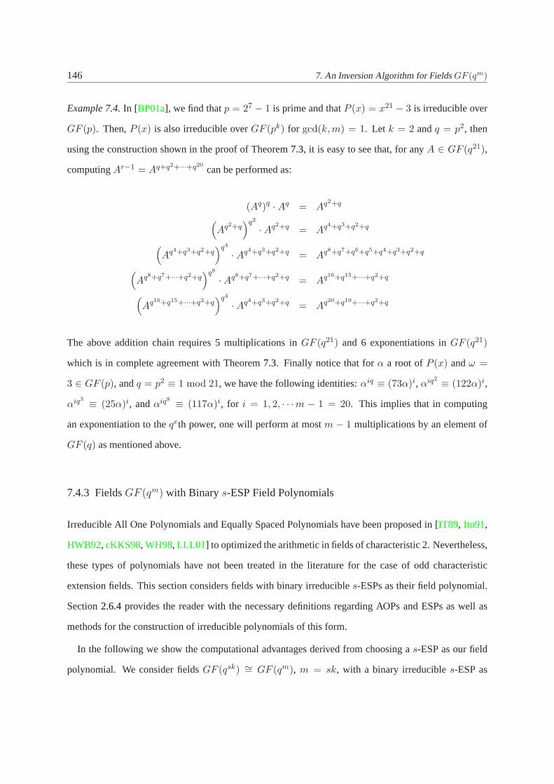
146 7. An Inversion Algorithm for FieldsGF (qm)
Example 7.4.In [BP01a], we find thatp = 27 − 1 is prime and thatP (x) = x21 − 3 is irreducible over
GF (p). Then,P (x) is also irreducible overGF (pk) for gcd(k, m) = 1. Let k = 2 andq = p2, then
using the construction shown in the proof of Theorem7.3, it is easy to see that, for anyA ∈ GF (q21),
computingAr−1 = Aq+q2+···+q20can be performed as:
(Aq)q ·Aq = Aq2+q
(Aq2+q
)q2
·Aq2+q = Aq4+q3+q2+q
(Aq4+q3+q2+q
)q4
·Aq4+q3+q2+q = Aq8+q7+q6+q5+q4+q3+q2+q
(Aq8+q7+···+q2+q
)q8
·Aq8+q7+···+q2+q = Aq16+q15+···+q2+q
(Aq16+q15+···+q2+q
)q4
·Aq4+q3+q2+q = Aq20+q19+···+q2+q
The above addition chain requires 5 multiplications inGF (q21) and 6 exponentiations inGF (q21)
which is in complete agreement with Theorem7.3. Finally notice that forα a root ofP (x) andω =
3 ∈ GF (p), andq = p2 ≡ 1 mod 21, we have the following identities:αiq ≡ (73α)i, αiq2≡ (122α)i,
αiq3≡ (25α)i, andαiq8
≡ (117α)i, for i = 1, 2, · · ·m − 1 = 20. This implies that in computing
an exponentiation to theqeth power, one will perform at mostm − 1 multiplications by an element of
GF (q) as mentioned above.
7.4.3 FieldsGF (qm) with Binarys-ESP Field Polynomials
Irreducible All One Polynomials and Equally Spaced Polynomials have been proposed in [IT89, Ito91,
HWB92, cKKS98, WH98, LLL01] to optimized the arithmetic in fields of characteristic 2. Nevertheless,
these types of polynomials have not been treated in the literature for the caseof odd characteristic
extension fields. This section considers fields with binary irreducibles-ESPs as their field polynomial.
Section2.6.4provides the reader with the necessary definitions regarding AOPs and ESPs as well as
methods for the construction of irreducible polynomials of this form.
In the following we show the computational advantages derived from choosing as-ESP as our field
polynomial. We consider fieldsGF (qsk) ∼= GF (qm), m = sk, with a binary irreducibles-ESP as
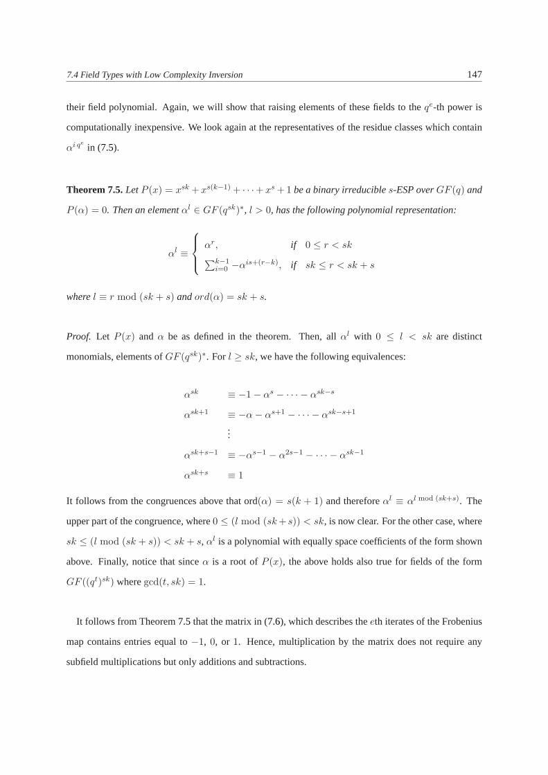
7.4 Field Types with Low Complexity Inversion 147
their field polynomial. Again, we will show that raising elements of these fields to the qe-th power is
computationally inexpensive. We look again at the representatives of the residue classes which contain
αi qein (7.5).
Theorem 7.5.LetP (x) = xsk + xs(k−1) + · · ·+ xs + 1 be a binary irreducibles-ESP overGF (q) and
P (α) = 0. Then an elementαl ∈ GF (qsk)∗, l > 0, has the following polynomial representation:
αl ≡
αr, if 0 ≤ r < sk
∑k−1i=0 −αis+(r−k), if sk ≤ r < sk + s
wherel ≡ r mod (sk + s) andord(α) = sk + s.
Proof. Let P (x) and α be as defined in the theorem. Then, allαl with 0 ≤ l < sk are distinct
monomials, elements ofGF (qsk)∗. For l ≥ sk, we have the following equivalences:
αsk ≡ −1− αs − · · · − αsk−s
αsk+1 ≡ −α− αs+1 − · · · − αsk−s+1
...
αsk+s−1 ≡ −αs−1 − α2s−1 − · · · − αsk−1
αsk+s ≡ 1
It follows from the congruences above that ord(α) = s(k + 1) and thereforeαl ≡ αl mod (sk+s). The
upper part of the congruence, where0 ≤ (l mod (sk +s)) < sk, is now clear. For the other case, where
sk ≤ (l mod (sk + s)) < sk + s, αl is a polynomial with equally space coefficients of the form shown
above. Finally, notice that sinceα is a root ofP (x), the above holds also true for fields of the form
GF ((qt)sk) wheregcd(t, sk) = 1.
It follows from Theorem7.5that the matrix in (7.6), which describes theeth iterates of the Frobenius
map contains entries equal to−1, 0, or 1. Hence, multiplication by the matrix does not require any
subfield multiplications but only additions and subtractions.

148 7. An Inversion Algorithm for FieldsGF (qm)
7.5 Notes and Further References
Reference [WTS+85] examines the hardware implementation of a Massey-Omura parallel multiplier
using a normal basis representation and apply their design to the computation of the inverse inGF (2n),
using a pipeline design. However, the inversion algorithm in [WTS+85] is impractical for sizes ofn
needed in cryptographic applications. The treatment in [IT88] is concerned only with fields of charac-
teristic two and a normal basis representation of the field elements. Feng [Fen89] proposes an algorithm
for inversion in fieldsGF (2n) using normal basis which requires⌋ log2(n− 1)⌋+ HW (n− 1) multi-
plications and a number of cyclic shifts which are not considered by the author. The method in [Fen89]
yields addition chains which are similar to the ones of the ITA. Reference [MK00] notice that in a hard-
ware implementation the latency of the ITA can be reduced from⌊log2(m− 1)⌋+ HW (m− 1)− 1 in
a fieldGF (2m) to ⌊log2(m− 1)⌋− 1 by performing certain operations in parallel. Reference [HWB92]
applies parallel multipliers to efficiently compute the inverse of elements inGF (2n) using a variant
of Fermat’s Little Theorem. Finally, [GP97] describes a version of the ITI algorithm applied to fields
GF ((2n)m) in a polynomial basis representation applied to elliptic curve cryptosystems.
Both [HWB92] and [WH98] use irreducible AOPs and ESPs overGF (2) to implement efficient
parallel multipliers. The complexity of the proposed multipliers in both of these contributions is less
than that of the parallel multiplier proposed in [IT89]. Furthermore, since inversion can be achieved
by repeated multiplications, [HWB92] applies parallel multipliers to efficiently compute the inverse of
elements inGF (2m) using a variant of Fermat’s Little Theorem.
Other possibilities to compute the inverse of an element in a finite field have also been extensively
explored. For example, non-systolic hardware implementations based on theextended Euclidean algo-
rithm have been proposed [AFM89, BCH93] as well as systolic implementations [GW98b, GW98a],
and VLSI algorithms based on the extended binarygcd algorithm [WTT02, WmWSH02]. Notice that
all of the above techniques except for [GP02] study inversion in binary fields only.
CHAPTER 8
Discussion
8.1 Summary and Conclusions
In this thesis, we have focused on the development of hardware architectures for addition, multiplication,
and inversion in fieldsGF (pm). In studying arithmetic inGF (pm) fields we have taken a bottom-up
approach. First, we discussed thoroughly architectures to implement addition and multiplication over
GF (p). We make particular emphasis on architectures forsmall GF (p) fields wherep < 32. In
particular, we proposed a new method to design smallGF (p) multipliers which can achieve up to a
30% improvement over previous architectures. The method is based on two observations: (i) for moduli
which can be represented with less than 5 bits, it is very efficient to implement the modulo arithmetic
operations as Boolean equations of the input bits and (ii) if the implementation method of (i) is assumed,
then it is possible to reduce the complexity of the resulting Boolean equations byusing a redundant
encoding of the value zero.
The second part of this thesis is concerned with multiplier architectures for fields GF (pm). We
investigated two strategies towards the implementation of these architectures. First, we explored a gen-
eralization of digit architectures originally proposed for fieldsGF (2n) to the odd characteristic case.
Both Least Significant Digit (LSD) multiplier architectures and Most Significant Digit (MSD) architec-
tures were considered. As in the case of characteristic two, Most Significant Digit architectures tend to

150 8. Discussion
have increased area and delay requirements. We implemented an arithmetic unitfor GF (3m) fields on
an FPGA and compared its performance to previous implementations and to our theoretical complexity
models which agreed with our practical results. Not surprisingly, we find that in odd characteristic fields,
it is possible to achieve comparable performance to binary fields at twice the hardware cost. The result
is particularly interesting because fields of characteristic three allow for shorter signatures than binary
fields (at twice the hardware cost but with comparable performance). Wealso showed that in character-
istic three the cubing operation can be implemented using a number of adders/subtracters linear on the
degreem of the irreducible polynomial defining the field. Finally, we introduced optimal irreducible
polynomials in the sense that they optimize the reduction operation during the normal operation of the
multiplication algorithm as well as when a cubing operation is being computed.
The second approach that we investigated towards the implementation of architectures for fields
GF (pm) was based on systolization and scalability. In other words, we proposed architectures which
are able to process fieldsGF (pm), for constantp and different values ofm without recurring to chang-
ing the hardware or to reconfigurability, as in the case of FPGAs. To achieve scalability we introduced
a new algorithm, which at the cost of initial and final pre-computations, allowsus to perform modular
reductions for any irreducible polynomial which satisfies a certain optimality criteria. The criteria is
analogue to the definition optimal irreducible polynomials in Chapter5 and does not constitute a ma-
jor restriction for choosing suitable irreducible polynomials in practical applications. Notice that the
method is also analogue to the Montgomery method of multiplication in the sense that both require ini-
tial and final computation stages. We implemented the basic cell of an LSD-based systolic multiplier on
0.18µm CMOS technology and provided time and area complexities.
Finally, we tackle the problem of inversion in fieldsGF (qm), q = pn, by giving a generalization of
the Itoh and Tsujii inversion algorithm to fields of odd characteristic and a standard basis representation.
We introduce families of irreducible polynomials which reduce the complexity of exponentiating to
the q-th power whereq = pn and p is the field characteristic. By reducing the complexity of this
operation, we also reduce the overall time required to compute an inverse inGF (qm). In particular,
for the families of fields proposed, the inverse computation time complexity is essentially given by
⌊log2(m− 1)⌋+ HW (m− 1)− 1 multiplications.

8.2 Recommendations for Further Research 151
8.2 Recommendations for Further Research
During the research which lead to this thesis, several questions and openproblems remained unanswered.
This section summarizes these questions and suggests several avenues toextend the results presented in
this work.
• Finite field hardware implementation. One natural avenue for further research is to generalize
the Montgomery method forGF (2n) fields toGF (pm) fields and compare it to our previously
proposed architectures. The main contribution here would be to allow for scalable support of any
field GF (pm), for any value ofm. In previous work, it is assumed that the ground field is fixed,
which for small values ofp (by small values, we meanp < 32) means arithmetic done through
table-lookups. For larger values ofp, it would be interesting to investigate how the Montgomery
technique (for fieldsGF (p)) compares to RNS-based techniques. A second possibility is to in-
vestigate the cost of incorporatingGF (pm) into unified architecture units which already support
GF (p) andGF (2n)arithmetic. Such architectures are important since standards support ECC
based on fieldsGF (p), GF (2n), andGF (pm), for p odd and prime.
• Elliptic curves and Pairing-based cryptosystems. A logical next step to this thesis would be
to implement ECC and pairing-based crypto-processors based onGF (pm) arithmetic. These
processors are important since the main application of finite field arithmetic and,in particular, of
GF (pm) fields (in this context) is the implementation of ECC and of ID-based encryption and
short signature schemes based on parings. To the author’s knowledgethere are not documented
hardware implementations of such schemes in the literature. Although, throughput is always a
main factor in such hardware implementations, it would be also important to consider implemen-
tations which can trade-off power, throughput, and area according to application requirements.
Another, interesting area of further research is the implementation of the above cryptographic
processors on systems which combine programmable cores and reconfigurable logic. This is
specially interesting for schemes based onGF (pm) arithmetic because it is conceivable that one
could take advantage of the programmable cores to implement the basicGF (p) arithmetic and use
the reconfigurable logic to implement the polynomial arithmetic required to support operations in

152 8. Discussion
GF (pm). Such implementations have not been studied yet in the research community.
• Hyperelliptic curves cryptosystems (HECC). Recently, there has been a lot of work on HECC
because they use smaller operands than ECC and thus, they might be better suited to constrained
environments. There is already some hardware implementations of HECC overGF (2n)as well
as the first embedded processor implementations overGF (2n). Because of HECC’s smaller
operands, it seems natural to extend the work of OEFs on ECC to HECC andto examine im-
plementation aspects on systems which combine programmable cores and reconfigurable compo-
nents. Notice that no work on hardware or embedded processor implementations of HECC over
odd characteristic fields has been documented in the literature. Similarly, it would be interesting
to explore the performance of OEF-based HECC on general purpose processors and embedded
processors, since OEFs where originally introduced as a way of obtaining fast implementations of
cryptographic systems on software platforms.

APPENDIX A
Irreducible Polynomials overGF (p)
A.1 Irreducible Binomials overGF (p)
The generation of irreducible binomials overGF (p) follows easily from Theorem2.2as their existence
is entirely established. Reference [BP01a] provides an algorithm based on Theorem2.2which on input
accepts a field order and the approximate prime size and as output providesa prime of the formp =
2n − c, for smallc, and an irreducible binomial of the formxm − 2. We used a modification of such
algorithm whose implementation is shown in SectionA.1.1 of this appendix. Differences include: the
generation of the primep of special form, which in our case does not apply since we are interestedin
irreducible polynomials for all primes in the range of interest and not limiting the irreducible binomial
to the formxm−2 but rather accepting binomials of the formxm−ω for the smallestω possible. Notice
that [BP01a] also provides tables with irreducible binomials in the range3 ≤ p ≤ 521, p prime, but
only for somep, whereas TableA.1 does the same forall primes in this range. The number theory and
multi-precision library NTL [Sho01] was used to implement the search algorithm in C++.

154A
.IrreducibleP
olynomials
overGF
(p)
Table A.1. Irreducible binomials of the formxm − ω overGF (p), for all m such that2160 ≤ pm ≤ 2256 and3 ≤ p ≤ 521 with n = ⌊log2 p⌋.p n m n · m ω p n m n · m ω p n m n · m ω p n m n · m ω p n m n · m ω
3 1 — — — 101 6 32 192 2 211 7 27 189 2 337 8 21 168 2 449 8 28 224 35 2 128 256 2 40 240 2 30 210 4 8 24 192 10 32 256 37 2 81 162 2 103 6 27 162 2 35 245 2 8 27 216 2 457 8 24 192 1311 3 — — — 34 204 2 223 7 27 189 3 8 28 224 5 27 216 313 3 54 162 2 107 6 — — — 227 7 — — — 8 32 256 5 32 256 5
64 192 2 109 6 27 162 3 229 7 24 168 6 347 8 — — — 461 8 20 160 272 216 2 32 192 2 27 189 3 349 8 24 192 2 23 184 281 243 2 36 216 6 32 224 2 8 27 216 2 25 200 2
17 4 64 256 3 113 6 28 168 3 36 252 6 8 29 232 2 32 256 219 4 54 216 4 32 192 3 233 7 29 203 2 8 32 256 2 463 8 21 168 223 4 — — — 127 6 27 162 3 32 224 3 353 8 22 176 3 22 176 2
49 196 2 42 252 9 239 7 34 238 2 8 32 256 3 27 216 256 224 2 131 7 25 175 2 241 7 24 168 7 359 8 — — — 467 8 — — —64 256 2 26 182 3 25 175 3 367 8 27 216 2 479 8 — — —
31 4 45 180 3 137 7 32 224 3 27 189 2 373 8 24 192 2 487 8 27 216 250 200 2 34 238 3 30 210 7 8 27 216 2 491 8 25 200 254 216 5 139 7 23 161 2 32 224 7 8 31 248 2 499 8 27 216 5
37 5 32 160 2 27 189 2 36 252 7 8 32 256 2 503 8 — — —36 180 2 149 7 32 224 2 251 7 25 175 3 379 8 21 168 2 509 8 32 256 248 240 2 151 7 25 175 3 257 8 32 256 3 8 27 216 2 521 8 20 160 3
41 5 32 160 3 27 189 2 263 8 — — — 383 8 — — — 25 200 240 200 6 30 210 5 269 8 32 256 2 389 8 32 256 2 26 208 350 250 6 157 7 24 168 5 271 8 25 200 2 397 8 22 176 2
43 5 42 210 9 26 182 2 27 216 2 8 24 192 549 245 2 27 189 3 30 240 2 8 27 216 3
47 5 46 230 2 32 224 2 277 8 23 184 2 8 32 256 253 5 32 160 2 36 252 5 24 192 5 401 8 20 160 359 5 — — — 163 7 27 189 2 27 216 3 8 25 200 261 5 32 160 2 167 7 — — — 32 256 2 8 32 256 3
36 180 2 173 7 32 224 2 281 8 20 160 3 409 8 24 192 740 200 2 179 7 — — — 25 200 2 8 27 216 245 225 2 181 7 24 168 2 28 224 3 8 32 256 748 240 2 25 175 2 32 256 3 419 8 22 176 350 250 2 27 189 2 283 8 27 216 3 421 8 20 160 2
67 6 27 162 2 30 210 2 292 8 32 256 2 8 21 168 233 198 2 32 224 2 307 8 27 216 5 8 24 192 2
71 6 35 210 2 36 252 2 311 8 25 200 2 8 25 200 273 6 27 162 2 191 7 25 175 2 31 248 2 8 27 216 2
32 192 5 193 7 24 168 5 313 8 24 192 10 8 28 224 236 216 5 27 189 2 26 208 7 8 30 240 2
79 6 27 162 2 32 224 5 27 216 2 8 32 256 239 234 2 36 252 5 32 256 5 431 8 25 200 5
83 6 41 246 2 197 7 28 196 2 317 8 32 256 2 433 8 24 192 589 6 32 192 3 32 224 2 331 8 22 176 5 8 27 216 397 6 27 162 2 199 7 27 189 2 25 200 2 8 32 256 5
32 192 5 33 231 2 27 216 2 439 8 27 216 536 216 5 211 7 25 175 2 30 240 4 443 8 26 208 3
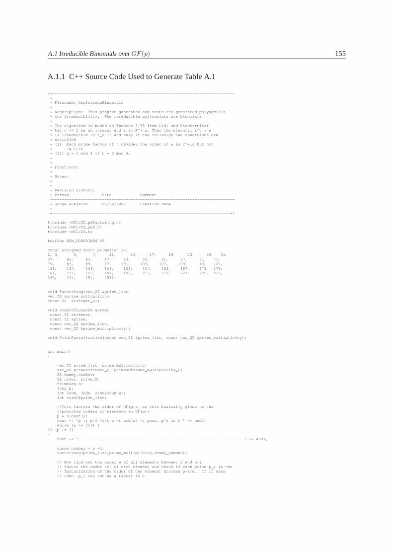
A.1 Irreducible Binomials overGF (p) 155
A.1.1 C++ Source Code Used to Generate TableA.1
/ * --------------------------------------------------- --------------------------
** Filename: GenIrreducBinomials
** Description: This program generates and tests the generate d polynomials
* for irreducibility. The irreducible polynomials are binom ials
** The algorithm is based on Theorem 3.75 from Lidl and Niederre iter
* Let t >= 2 be an integer and a in Fˆ * _q. Then the binomial xˆt - a
* is irreducible in F_q if and only if the follwoign two conditi ons are
* satisfied
* (i) Each prime factor of t divides the order of a in Fˆ * _q but not
* (q-1)/e
* (ii) q = 1 mod 4 if t = 0 mod 4.
*** Functions:
** Notes:
*** Revision History:
* Person Date Comment
* --------------------------------------------------- --------------------------
* Jorge Guajardo 06/26/2002 Creation date
** --------------------------------------------------- ------------------------ * /
#include <NTL/ZZ_pXFactoring.h>#include <NTL/ZZ_pEX.h>#include <NTL/ZZ.h>
#define NUM_ODDPRIMES 55
const unsigned short primelist[]={2, 3, 5, 7, 11, 13, 17, 19, 23, 29, 31,37, 41, 43, 47, 53, 59, 61, 67, 71, 73,79, 83, 89, 97, 101, 103, 107, 109, 113, 127,131, 137, 139, 149, 151, 157, 163, 167, 173, 179,181, 191, 193, 197, 199, 211, 223, 227, 229, 233,239, 241, 251, 257};
void FactorLong(vec_ZZ &prime_list,vec_ZZ &prime_multiplicity,const ZZ &integer_Z);
void orderOfLong(ZZ &order,const ZZ &element,const ZZ &prime,const vec_ZZ &prime_list,const vec_ZZ &prime_multiplicity);
void PrintFactorization(const vec_ZZ &prime_list, const vec_ZZ &prime_multiplicity);
int main(){
vec_ZZ prime_list, prime_multiplicity;vec_ZZ primesOforder_L, primesOforder_multiplicity_L;ZZ dummy_number;ZZ order, prime_Z;PrimeSeq s;long p;int indx, jndx, commaCounter;int sizeOfprime_list;
//This factors the order of GF(p) * , so this basically gives us the//possible orders of elements in GF(p) *p = s.next();cout << "p \t p-1 \t\t a \t ord(a) \t poss. p’s in t " << endl;while (p <= 259) {
if (p != 2){
cout << "-------------------------------------------- --------------------------" << endl;
dummy_number = p -1;FactorLong(prime_list,prime_multiplicity,dummy_numb er);
// Now find out the order e of all elements between 2 and p-1// Factor the order (e) of each element and check if each prime p_i in the// factorization of the order of the element divides p-1/e. I f it does// then p_i can not be a factor in t
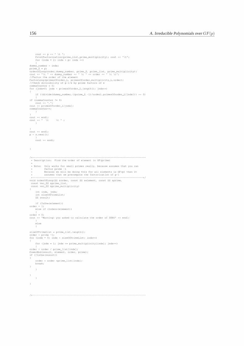
156 A. Irreducible Polynomials overGF (p)
cout << p << " \t ";PrintFactorization(prime_list,prime_multiplicity); c out << "\t";for (indx = 2; indx < p; indx ++){
dummy_number = indx;prime_Z = p;orderOfLong(order,dummy_number, prime_Z, prime_list, p rime_multiplicity);cout << "\t " << dummy_number << " \t " << order << " \t \t";//Factor the order of the elementFactorLong(primesOforder_L, primesOforder_multiplici ty_L,order);//Check divisibility of p-1/e by prime factors of ecommaCounter = 0;for (jndx=0; jndx < primesOforder_L.length(); jndx++){
if ((divide(dummy_number,((prime_Z -1)/order),primesO forder_L[jndx])) == 0){
if (commaCounter != 0)cout << ",";
cout << primesOforder_L[jndx];commaCounter++;
}}cout << endl;cout << " \t \t " ;
}
}cout << endl;p = s.next();
}cout << endl;
}
/ * --------------------------------------------------- --------------------------
* Description: Find the order of element in GF(prime)
** Note: Only works for small primes really, because assumes th at you can
* factor prime -1
* Because we will be doing this for all elements is GF(p) then it
* assumes that we precompute the factorization of p-1
* --------------------------------------------------- ------------------------ * /void orderOfLong(ZZ &order, const ZZ &element, const ZZ &pr ime,
const vec_ZZ &prime_list,const vec_ZZ &prime_multiplicity)
{int indx, jndx;int sizeOfPrimeList;ZZ result;
if (IsOne(element))order = 1;
else if (IsZero(element)){
order = 0;cout << "Warning: you asked to calculate the order of ZERO" << endl;
}else{
sizeOfPrimeList = prime_list.length();order = prime -1;for (indx = 0; indx < sizeOfPrimeList; indx++){
for (jndx = 1; jndx <= prime_multiplicity[indx]; jndx++){
order = order / prime_list[indx];PowerMod(result, element, order, prime);if (!IsOne(result)){
order = order * prime_list[indx];break;
}}
}}
}
/ * --------------------------------------------------- --------------------------

A.1 Irreducible Binomials overGF (p) 157
* Description: Factor integers less than 259 by dividing by li st of primes
* less than 259
* prime_list = p_1 p_2 p_3 ... p_n
* prime_multiplicity = e_1 e_2 ... e_n
** where integer = p_1ˆe_1 p_2ˆe_2 ... p_nˆe_n
** Note: Only works for small primes
** --------------------------------------------------- ------------------------ * /
void FactorLong(vec_ZZ &prime_list,vec_ZZ &prime_multiplicity,const ZZ &integer_Z){
ZZ dummy_Z;ZZ quotient_Z;int flag = 1;int indx = 0;int counter_numPrimes;int counter_multiplicity;long remainder;
/ * Just make sure that we don’t try to factor bigger numbers for n ow * /if (integer_Z > 259)
Error("The integer you are trying to factor is greater than 2 59\n");
dummy_Z = integer_Z;counter_numPrimes = 0;while(flag){
if (IsOne(dummy_Z))flag = 0;
//Tests if dummy_Z is prime, if the function returns 1//then dummy_Z is primeelse if (ProbPrime(dummy_Z) == 1){
prime_list.SetLength(counter_numPrimes+1);prime_multiplicity.SetLength(counter_numPrimes+1);prime_list[counter_numPrimes] = dummy_Z;prime_multiplicity[counter_numPrimes] = 1;flag = 0; //end the big while loop
}else{
//This takes care of dividing by the small primes and multipl icitiesremainder = DivRem(quotient_Z, dummy_Z ,primelist[indx] );
if (remainder == 0){
dummy_Z = quotient_Z;prime_list.SetLength(counter_numPrimes+1);prime_multiplicity.SetLength(counter_numPrimes+1);prime_list[counter_numPrimes] = primelist[indx];counter_multiplicity = 1;while (remainder == 0){
remainder = DivRem(quotient_Z, dummy_Z ,primelist[indx] );if (remainder == 0){
dummy_Z = quotient_Z;counter_multiplicity++;//cout << counter_multiplicity << endl;
}else
prime_multiplicity[counter_numPrimes] = counter_multi plicity;}counter_numPrimes++;
}else
indx++;}
}//end big while
}
/ * --------------------------------------------------- --------------------------
* Description: Print Factorization of a number given its prim e factors and
* their multiplicity
** --------------------------------------------------- ------------------------ * /
void PrintFactorization(const vec_ZZ &prime_list, const vec_ZZ &prime_multiplicity){
long sizeOfprime_list;int indx;
sizeOfprime_list = prime_list.length();

158 A. Irreducible Polynomials overGF (p)
for (indx=0; indx < sizeOfprime_list; indx++){
cout << prime_list[indx];if (prime_multiplicity[indx] != 1)
cout << "ˆ" << prime_multiplicity[indx] << " ";else
cout << " ";}
}
A.2 Irreducible Trinomials and Quadrinomials overGF (3)
The irreducible polynomials shown in TablesA.3, A.4, A.5, andA.6 were generated as explained in
Section5.5.3performing an exhaustive search. Notice that this exhaustive search could be improved by
including the irreducibility criteria described in [vzG01]. In the range2 ≤ m ≤ 255, there are only
23 degreesm for which we were unable to find trinomials (this agrees with the findings in [vzG01])
and thus, we provide irreducible quadrinomials for them in TableA.6. Finally, TableA.2 corresponds
to optimal irreducible polynomials, where optimality is defined as described in Section 5.5.3. Example
of the code used to generate TablesA.3, A.4, A.5, andA.6 is shown in SectionA.2.1. The code was
written by Guido Bertoni of the Politecnico di Milano and it uses the NTL library [Sho01].
Table A.2.Optimal irreducible trinomials of the formxm+ptxt+p0 overGF (3), for m prime and2 ≤ m ≤ 255.
m (pt, t, p0) m (pt, t, p0) m (pt, t, p0)
2 (2,1,2) 67 (1,2,2),(2,2,1),(2,11,2) 157 (1,22,2),(2,22,1)3 (2,1,2) 71 (1,20,2),(2,20,1) 163 (2,59,2)5 (2,1,2) 73 (2,1,2) 167 (2,71,2)7 (1,2,2),(2,2,1) 79 (1,26,2),(2,26,1) 173 (2,7,2)11 (1,2,2),(2,2,1),(2,3,2) 83 (2,27,2) 179 (2,59,2)13 (2,1,2) 89 (2,13,2) 181 (2,37,2)17 (2,1,2) 97 (1,12,2),(2,12,1) 191 (2,71,2)19 (1,2,2),(2,2,1) 101 (2,31,2) 193 (1,12,2),(2,12,1)23 (2,3,2) 103 (2,47,2) 197 —29 (2,4,1),(1,4,2) 107 (2,3,2) 199 (2,35,2)31 (2,5,2) 109 (2,9,2) 211 (2,89,2)37 (1,6,2),(2,6,1) 113 (2,19,2) 223 —41 (2,1,2) 127 (1,8,2),(2,8,1) 229 (1,72,2),(2,72,1)43 (2,17,2) 131 (2,27,2) 233 —47 (2,15,2) 137 (2,1,2) 239 (2,5,2)53 (2,13,2) 139 (2,59,2) 241 (1,88,2),(2,88,1), (2,117,2)59 (2,17,2) 149 — 251 (2,9,2)61 (2,7,2) 151 (1,2,2),(2,2,1)

A.2 Irreducible Trinomials and Quadrinomials overGF (3) 159
Table A.3. Irreducible trinomials of the formxm + xt + 2 overGF (3), 2 ≤ m ≤ 255
m t m t m t m t m t m t m t m t m t m t m t
2 1 22 5 43 26 71 20 93 70 117 52 143 108 167 92 187 8 211 122 238 53 2 23 8 44 3 72 28 95 48 119 2 144 56 168 28 188 11 214 65 239 244 1 24 4 45 28 73 30 96 16 120 4 145 24 169 24 191 116 215 36 240 85 4 25 6 46 5 76 9 97 12 121 40 147 8 170 43 192 32 216 4 241 886 1 26 7 47 32 77 16 99 74 124 25 148 3 171 20 193 12 217 132 242 1157 2 27 20 48 8 78 13 100 25 125 52 150 73 172 19 194 55 219 26 243 1228 2 28 2 51 50 79 26 101 70 126 49 151 2 173 166 195 26 220 15 244 319 4 29 4 52 7 80 2 102 25 127 8 152 18 174 73 196 79 222 89 245 14811 2 30 1 53 22 81 40 103 50 128 6 153 94 176 12 198 29 224 12 246 1312 2 31 20 54 1 83 32 104 5 131 48 155 12 177 52 199 164 225 16 247 12213 4 32 5 55 26 84 14 107 32 133 88 156 26 178 11 200 3 227 68 248 5014 1 33 28 56 3 85 16 108 2 134 61 157 22 179 104 201 88 228 14 249 7615 2 35 2 59 20 86 13 109 88 135 44 158 61 180 38 203 8 229 72 251 2616 4 36 14 60 2 87 26 111 2 136 57 159 32 181 40 204 50 230 73 252 9817 16 37 6 61 30 88 6 112 6 137 136 160 4 182 25 205 78 232 30 253 1218 7 39 26 63 26 89 64 113 70 139 80 162 19 183 2 206 61 234 91 254 7319 2 40 1 64 3 90 19 114 7 140 59 163 80 184 20 208 10 235 26 255 2620 5 41 40 67 2 91 74 115 32 141 64 164 15 185 64 209 40 236 921 16 42 7 69 52 92 10 116 15 142 65 165 22 186 47 210 7 237 70
Table A.4. Irreducible trinomials of the formxm + 2xt + 1 overGF (3), 3 ≤ m ≤ 255
m t m t m t m t m t m t m t m t
3 1 31 5 62 10 93 23 126 52 159 32 191 71 227 115 1 33 5 63 26 94 30 127 8 162 80 193 12 229 726 2 34 2 66 10 95 47 131 27 163 59 194 24 230 647 2 35 2 67 2 97 12 133 15 165 22 195 26 234 1049 4 37 6 69 17 99 19 134 4 166 54 198 38 235 2610 2 38 4 70 4 101 31 135 44 167 71 199 35 237 7011 2 39 7 71 20 102 2 137 1 169 24 201 88 238 413 1 41 1 73 1 103 47 138 34 170 32 202 62 239 514 4 42 10 74 12 106 26 139 59 171 20 203 3 241 8815 2 43 17 77 16 107 3 141 5 173 7 205 9 242 217 1 45 17 78 14 109 9 142 40 174 52 206 94 243 12118 8 46 6 79 26 110 22 143 35 177 52 209 40 245 9719 2 47 15 81 40 111 2 145 24 178 26 211 89 247 12221 5 50 6 82 2 113 19 146 2 179 59 214 6 249 5922 4 51 1 83 27 115 32 147 8 181 37 215 36 250 10423 3 53 13 85 16 117 52 151 2 182 34 217 85 251 925 3 54 14 86 34 118 34 153 59 183 2 218 18 253 726 2 55 11 87 26 119 2 154 32 185 64 219 25 254 1627 7 58 8 89 13 121 1 155 12 186 46 222 4 255 2629 4 59 17 90 34 122 14 157 22 187 8 225 1630 4 61 7 91 17 125 52 158 52 190 94 226 38
Table A.5. Irreducible trinomials of the formxm + 2xt + 2 overGF (3), 2 ≤ m ≤ 255
m t m t m t m t m t m t m t m t m t m t m t
2 1 22 5 43 17 71 51 93 23 117 65 143 35 167 71 187 65 211 89 238 53 1 23 3 44 3 72 28 95 47 119 3 144 56 168 28 188 11 214 65 239 54 1 24 4 45 17 73 1 96 16 120 4 145 73 169 37 191 71 215 59 240 85 1 25 3 46 5 76 9 97 81 121 1 147 43 170 43 192 32 216 4 241 1176 1 26 7 47 15 77 25 99 19 124 25 148 3 171 151 193 81 217 85 242 1157 5 27 7 48 8 78 13 100 25 125 73 150 73 172 19 194 55 219 25 243 1218 2 28 2 51 1 79 53 101 31 126 49 151 125 173 7 195 49 220 15 244 319 5 29 25 52 7 80 2 102 25 127 119 152 18 174 73 196 79 222 89 245 9711 3 30 1 53 13 81 41 103 47 128 6 153 59 176 12 198 29 224 12 246 1312 2 31 5 54 1 83 27 104 5 131 27 155 129 177 83 199 35 225 209 247 12513 1 32 5 55 11 84 14 107 3 133 15 156 26 178 11 200 3 227 11 248 5014 1 33 5 56 3 85 31 108 2 134 61 157 69 179 59 201 113 228 14 249 5915 7 35 17 59 17 86 13 109 9 135 91 158 61 180 38 203 3 229 79 251 916 4 36 14 60 2 87 37 111 13 136 57 159 127 181 37 204 50 230 73 252 9817 1 37 13 61 7 88 6 112 6 137 1 160 4 182 25 205 9 232 30 253 718 7 39 7 63 37 89 13 113 19 139 59 162 19 183 181 206 61 234 91 254 7319 11 40 1 64 3 90 19 114 7 140 59 163 59 184 20 208 10 235 83 255 22920 5 41 1 67 11 91 17 115 83 141 5 164 15 185 121 209 49 236 921 5 42 7 69 17 92 10 116 15 142 65 165 77 186 47 210 7 237 167

160 A. Irreducible Polynomials overGF (p)
Table A.6. Irreducible quadrinomialsxm + pt1xt1 + pt2x
t2 + p0 overGF (3) for degrees with no trinomials.
m t1 t2 (pt1, pt2
, p0)
49 3 2 (−1, ±1, ±1)57 7 2 (1, ±1, ∓1)65 5 3 (1, 1, ±168 3 2 (±1, 1, 1)75 5 4 (−1, ±1, ±1)98 4 3 (1, ±1, 1)105 6 2 (±1, ±1, ±1)123 7 4 (1, ±1, ∓1)129 3 2 (−1, ±, ±1)130 10 6 (1, 1, 1)132 10 1 (1, ±1, 1)149 11 10 (−1, ±1, ±1)161 9 5 (1, 1, ±1)175 10 8 (±1, ±1, ±1)189 9 7 (1, 1, ±1)197 9 4 (−1, ±1, ±1)207 11 8 (−1, ±1, ±1)212 14 3 (1, ±1, 1)213 12 1 (±1, 1, ∓1)221 12 2 (±1, ±1, ±1)223 8 5 (±1, −1, ±1)231 8 7 (±1, 1, ∓1)233 6 2 (±1, ±1, ±1)

A.2 Irreducible Trinomials and Quadrinomials overGF (3) 161
A.2.1 C++ Source Code Used to Generate Irreducible Trinomials
/ * --------------------------------------------------- --------------------------
** Filename: GenIrreducTrinom.C
** Description: This program generates and tests the generate d polynomials
* for irreducibility. The irreducible polynomials are trino mials
**** Revision History:
* Person Date Comment
* --------------------------------------------------- --------------------------
* Guido Bertoni 06/26/2002 Creation date
** --------------------------------------------------- ------------------------ * /
#include <NTL/ZZ_pXFactoring.h>
#define MAX_DEGREE_MINE 256;
//#define debug_interactive
int main(){
ZZ p;//cin >> p;p=3;
ZZ_p::init(p);
ZZ_pX degree,d,coeffzero,poly_sum;vec_pair_ZZ_pX_long factors;long irreducibile;int counter,counter2,flag;
flag=0;
SetCoeff(degree,2,1);SetCoeff(d,1,1);
SetCoeff(coeffzero,0,2);
for(counter=2;counter<256;counter++){//cout << "cycle" << counter << "\n";degree=0;d=0;SetCoeff(degree,counter,1);SetCoeff(d,0,1);for(counter2=1;counter2<counter;counter2++){
poly_sum=0;LeftShift(d,d,1);poly_sum=degree+d;poly_sum=poly_sum+coeffzero;irreducibile=DetIrredTest(poly_sum);
#ifdef debug_interactivecout << "d ";cout << d << "\n";cout << "irre " << poly_sum << "\n";cout << "degree d" << counter2 << "\n";cout << "irreduc ???" << irreducibile << "\n";
#endif
if(irreducibile!=0){flag=1;cout << counter << " " << counter2 << "\n";break;
}}
}cout <<"\n any irr: " << flag;
}

162 A. Irreducible Polynomials overGF (p)

APPENDIX B
GF (p) Adder Complexities

164B
.G
F(p
)A
dderC
omplexities
Table B.1.Normalized area complexity of differentGF (p) adders for3 ≤ p ≤ 521p n ROM ROM [BJM87b] [BJM87b] [EB90] [Dug92] [Hia02] p n ROM ROM [BJM87b] [BJM87b] [EB90] [Dug92] [Hia02]
(SC) (FC) (hybrid) (CLA) (CSA) (type II) (SC) (FC) (hybrid) (CLA) (CSA) (type II)3 2 41 18 7 13 66 21 12 239 8 681574 456968 220 104 264 109 605 3 249 75 21 25 99 34 25 241 8 681574 464648 200 104 264 109 767 3 249 147 13 25 99 34 17 251 8 681574 504008 96 104 264 109 6011 4 1331 484 41 39 132 48 31 257 9 3067084 594441 3035 123 297 125 11713 4 1331 676 30 39 132 48 31 263 9 3067084 622521 2965 123 297 125 10117 5 6656 1445 119 54 165 63 54 269 9 3067084 651249 2895 123 297 125 10119 5 6656 1805 106 54 165 63 46 271 9 3067084 660969 2872 123 297 125 9323 5 6656 2645 80 54 165 63 38 277 9 3067084 690561 2801 123 297 125 10129 5 6656 4205 41 54 165 63 38 281 9 3067084 710649 2755 123 297 125 10131 5 6656 4805 28 54 165 63 29 283 9 3067084 720801 2731 123 297 125 9337 6 31948 8214 239 70 198 78 61 293 9 3067084 772641 2614 123 297 125 10141 6 31948 10086 208 70 198 78 61 307 9 3067084 848241 2450 123 297 125 9343 6 31948 11094 192 70 198 78 53 311 9 3067084 870489 2404 123 297 125 8447 6 31948 13254 161 70 198 78 45 313 9 3067084 881721 2380 123 297 125 9353 6 31948 16854 114 70 198 78 53 317 9 3067084 904401 2333 123 297 125 8459 6 31948 20886 67 70 198 78 45 331 9 3067084 986049 2170 123 297 125 9361 6 31948 22326 52 70 198 78 45 337 9 3067084 1022121 2099 123 297 125 10167 7 149094 31423 591 87 231 93 77 347 9 3067084 1083681 1982 123 297 125 8471 7 149094 35287 555 87 231 93 68 349 9 3067084 1096209 1959 123 297 125 8473 7 149094 37303 536 87 231 93 77 353 9 3067084 1121481 1912 123 297 125 10179 7 149094 43687 482 87 231 93 60 359 9 3067084 1159929 1842 123 297 125 8483 7 149094 48223 445 87 231 93 68 367 9 3067084 1212201 1748 123 297 125 7689 7 149094 55447 391 87 231 93 68 373 9 3067084 1252161 1678 123 297 125 8497 7 149094 65863 318 87 231 93 77 379 9 3067084 1292769 1608 123 297 125 76101 7 149094 71407 282 87 231 93 68 383 9 3067084 1320201 1561 123 297 125 68103 7 149094 74263 263 87 231 93 60 389 9 3067084 1361889 1491 123 297 125 101107 7 149094 80143 227 87 231 93 60 397 9 3067084 1418481 1397 123 297 125 93109 7 149094 83167 209 87 231 93 60 401 9 3067084 1447209 1351 123 297 125 101113 7 149094 89383 172 87 231 93 68 409 9 3067084 1505529 1257 123 297 125 93127 7 149094 112903 45 87 231 93 44 419 9 3067084 1580049 1140 123 297 125 93131 8 681574 137288 1344 104 264 109 93 421 9 3067084 1595169 1117 123 297 125 93137 8 681574 150152 1281 104 264 109 93 431 9 3067084 1671849 1000 123 297 125 76139 8 681574 154568 1260 104 264 109 84 433 9 3067084 1687401 976 123 297 125 93149 8 681574 177608 1156 104 264 109 84 439 9 3067084 1734489 906 123 297 125 76151 8 681574 182408 1136 104 264 109 76 443 9 3067084 1766241 859 123 297 125 76157 8 681574 197192 1073 104 264 109 76 449 9 3067084 1814409 789 123 297 125 101163 8 681574 212552 1011 104 264 109 84 457 9 3067084 1879641 695 123 297 125 93167 8 681574 223112 969 104 264 109 76 461 9 3067084 1912689 649 123 297 125 84173 8 681574 239432 907 104 264 109 76 463 9 3067084 1929321 625 123 297 125 76179 8 681574 256328 844 104 264 109 76 467 9 3067084 1962801 578 123 297 125 84181 8 681574 262088 824 104 264 109 76 479 9 3067084 2064969 438 123 297 125 68191 8 681574 291848 720 104 264 109 60 487 9 3067084 2134521 344 123 297 125 76193 8 681574 297992 699 104 264 109 93 491 9 3067084 2169729 298 123 297 125 76197 8 681574 310472 657 104 264 109 84 499 9 3067084 2241009 204 123 297 125 76199 8 681574 316808 636 104 264 109 76 503 9 3067084 2277081 157 123 297 125 68211 8 681574 356168 512 104 264 109 76 509 9 3067084 2331729 87 123 297 125 68223 8 681574 397832 387 104 264 109 60 521 10 13631488 2714410 6599 141 330 142 126227 8 681574 412232 345 104 264 109 76 — — — — — — — — —229 8 681574 419528 324 104 264 109 76 — — — — — — — — —233 8 681574 434312 283 104 264 109 76 — — — — — — — — —
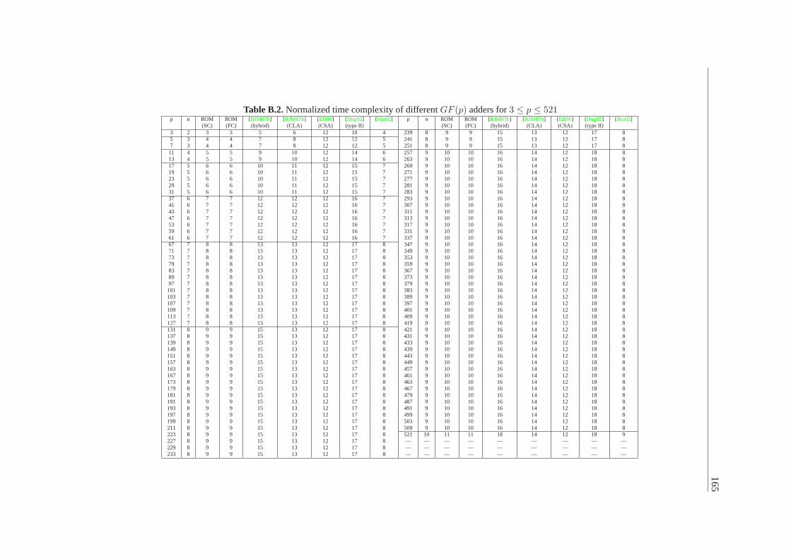
165
Table B.2.Normalized time complexity of differentGF (p) adders for3 ≤ p ≤ 521p n ROM ROM [BJM87b] [BJM87b] [EB90] [Dug92] [Hia02] p n ROM ROM [BJM87b] [BJM87b] [EB90] [Dug92] [Hia02]
(SC) (FC) (hybrid) (CLA) (CSA) (type II) (SC) (FC) (hybrid) (CLA) (CSA) (type II)3 2 3 3 5 6 12 10 4 239 8 9 9 15 13 12 17 85 3 4 4 7 8 12 12 5 241 8 9 9 15 13 12 17 87 3 4 4 7 8 12 12 5 251 8 9 9 15 13 12 17 811 4 5 5 9 10 12 14 6 257 9 10 10 16 14 12 18 813 4 5 5 9 10 12 14 6 263 9 10 10 16 14 12 18 817 5 6 6 10 11 12 15 7 269 9 10 10 16 14 12 18 819 5 6 6 10 11 12 15 7 271 9 10 10 16 14 12 18 823 5 6 6 10 11 12 15 7 277 9 10 10 16 14 12 18 829 5 6 6 10 11 12 15 7 281 9 10 10 16 14 12 18 831 5 6 6 10 11 12 15 7 283 9 10 10 16 14 12 18 837 6 7 7 12 12 12 16 7 293 9 10 10 16 14 12 18 841 6 7 7 12 12 12 16 7 307 9 10 10 16 14 12 18 843 6 7 7 12 12 12 16 7 311 9 10 10 16 14 12 18 847 6 7 7 12 12 12 16 7 313 9 10 10 16 14 12 18 853 6 7 7 12 12 12 16 7 317 9 10 10 16 14 12 18 859 6 7 7 12 12 12 16 7 331 9 10 10 16 14 12 18 861 6 7 7 12 12 12 16 7 337 9 10 10 16 14 12 18 867 7 8 8 13 13 12 17 8 347 9 10 10 16 14 12 18 871 7 8 8 13 13 12 17 8 349 9 10 10 16 14 12 18 873 7 8 8 13 13 12 17 8 353 9 10 10 16 14 12 18 879 7 8 8 13 13 12 17 8 359 9 10 10 16 14 12 18 883 7 8 8 13 13 12 17 8 367 9 10 10 16 14 12 18 889 7 8 8 13 13 12 17 8 373 9 10 10 16 14 12 18 897 7 8 8 13 13 12 17 8 379 9 10 10 16 14 12 18 8101 7 8 8 13 13 12 17 8 383 9 10 10 16 14 12 18 8103 7 8 8 13 13 12 17 8 389 9 10 10 16 14 12 18 8107 7 8 8 13 13 12 17 8 397 9 10 10 16 14 12 18 8109 7 8 8 13 13 12 17 8 401 9 10 10 16 14 12 18 8113 7 8 8 13 13 12 17 8 409 9 10 10 16 14 12 18 8127 7 8 8 13 13 12 17 8 419 9 10 10 16 14 12 18 8131 8 9 9 15 13 12 17 8 421 9 10 10 16 14 12 18 8137 8 9 9 15 13 12 17 8 431 9 10 10 16 14 12 18 8139 8 9 9 15 13 12 17 8 433 9 10 10 16 14 12 18 8149 8 9 9 15 13 12 17 8 439 9 10 10 16 14 12 18 8151 8 9 9 15 13 12 17 8 443 9 10 10 16 14 12 18 8157 8 9 9 15 13 12 17 8 449 9 10 10 16 14 12 18 8163 8 9 9 15 13 12 17 8 457 9 10 10 16 14 12 18 8167 8 9 9 15 13 12 17 8 461 9 10 10 16 14 12 18 8173 8 9 9 15 13 12 17 8 463 9 10 10 16 14 12 18 8179 8 9 9 15 13 12 17 8 467 9 10 10 16 14 12 18 8181 8 9 9 15 13 12 17 8 479 9 10 10 16 14 12 18 8191 8 9 9 15 13 12 17 8 487 9 10 10 16 14 12 18 8193 8 9 9 15 13 12 17 8 491 9 10 10 16 14 12 18 8197 8 9 9 15 13 12 17 8 499 9 10 10 16 14 12 18 8199 8 9 9 15 13 12 17 8 503 9 10 10 16 14 12 18 8211 8 9 9 15 13 12 17 8 509 9 10 10 16 14 12 18 8223 8 9 9 15 13 12 17 8 521 10 11 11 18 14 12 18 9227 8 9 9 15 13 12 17 8 — — — — — — — — —229 8 9 9 15 13 12 17 8 — — — — — — — — —233 8 9 9 15 13 12 17 8 — — — — — — — — —

166B
.G
F(p
)A
dderC
omplexities
Table B.3.Normalized area/time product of differentGF (p) adders for3 ≤ p ≤ 521p n ROM ROM [BJM87b] [BJM87b] [EB90] [Dug92] [Hia02] p n ROM ROM [BJM87b] [BJM87b] [EB90] [Dug92] [Hia02]
(SC) (FC) (hybrid) (CLA) (CSA) (type II) (SC) (FC) (hybrid) (CLA) (CSA) (type II)3 2 123 54 35 78 792 210 48 239 8 6134166 4112712 3300 1352 3168 1853 4805 3 996 300 147 200 1188 408 125 241 8 6134166 4181832 3000 1352 3168 1853 6087 3 996 588 91 200 1188 408 85 251 8 6134166 4536072 1440 1352 3168 1853 48011 4 6655 2420 369 390 1584 672 186 257 9 30670840 5944410 48560 1722 3564 2250 93613 4 6655 3380 270 390 1584 672 186 263 9 30670840 6225210 47440 1722 3564 2250 80817 5 39936 8670 1190 594 1980 945 378 269 9 30670840 6512490 46320 1722 3564 2250 80819 5 39936 10830 1060 594 1980 945 322 271 9 30670840 6609690 45952 1722 3564 2250 74423 5 39936 15870 800 594 1980 945 266 277 9 30670840 6905610 44816 1722 3564 2250 80829 5 39936 25230 410 594 1980 945 266 281 9 30670840 7106490 44080 1722 3564 2250 80831 5 39936 28830 280 594 1980 945 203 283 9 30670840 7208010 43696 1722 3564 2250 74437 6 223636 57498 2868 840 2376 1248 427 293 9 30670840 7726410 41824 1722 3564 2250 80841 6 223636 70602 2496 840 2376 1248 427 307 9 30670840 8482410 39200 1722 3564 2250 74443 6 223636 77658 2304 840 2376 1248 371 311 9 30670840 8704890 38464 1722 3564 2250 67247 6 223636 92778 1932 840 2376 1248 315 313 9 30670840 8817210 38080 1722 3564 2250 74453 6 223636 117978 1368 840 2376 1248 371 317 9 30670840 9044010 37328 1722 3564 2250 67259 6 223636 146202 804 840 2376 1248 315 331 9 30670840 9860490 34720 1722 3564 2250 74461 6 223636 156282 624 840 2376 1248 315 337 9 30670840 10221210 33584 1722 3564 2250 80867 7 1192752 251384 7683 1131 2772 1581 616 347 9 30670840 10836810 31712 1722 3564 2250 67271 7 1192752 282296 7215 1131 2772 1581 544 349 9 30670840 10962090 31344 1722 3564 2250 67273 7 1192752 298424 6968 1131 2772 1581 616 353 9 30670840 11214810 30592 1722 3564 2250 80879 7 1192752 349496 6266 1131 2772 1581 480 359 9 30670840 11599290 29472 1722 3564 2250 67283 7 1192752 385784 5785 1131 2772 1581 544 367 9 30670840 12122010 27968 1722 3564 2250 60889 7 1192752 443576 5083 1131 2772 1581 544 373 9 30670840 12521610 26848 1722 3564 2250 67297 7 1192752 526904 4134 1131 2772 1581 616 379 9 30670840 12927690 25728 1722 3564 2250 608101 7 1192752 571256 3666 1131 2772 1581 544 383 9 30670840 13202010 24976 1722 3564 2250 544103 7 1192752 594104 3419 1131 2772 1581 480 389 9 30670840 13618890 23856 1722 3564 2250 808107 7 1192752 641144 2951 1131 2772 1581 480 397 9 30670840 14184810 22352 1722 3564 2250 744109 7 1192752 665336 2717 1131 2772 1581 480 401 9 30670840 14472090 21616 1722 3564 2250 808113 7 1192752 715064 2236 1131 2772 1581 544 409 9 30670840 15055290 20112 1722 3564 2250 744127 7 1192752 903224 585 1131 2772 1581 352 419 9 30670840 15800490 18240 1722 3564 2250 744131 8 6134166 1235592 20160 1352 3168 1853 744 421 9 30670840 15951690 17872 1722 3564 2250 744137 8 6134166 1351368 19215 1352 3168 1853 744 431 9 30670840 16718490 16000 1722 3564 2250 608139 8 6134166 1391112 18900 1352 3168 1853 672 433 9 30670840 16874010 15616 1722 3564 2250 744149 8 6134166 1598472 17340 1352 3168 1853 672 439 9 30670840 17344890 14496 1722 3564 2250 608151 8 6134166 1641672 17040 1352 3168 1853 608 443 9 30670840 17662410 13744 1722 3564 2250 608157 8 6134166 1774728 16095 1352 3168 1853 608 449 9 30670840 18144090 12624 1722 3564 2250 808163 8 6134166 1912968 15165 1352 3168 1853 672 457 9 30670840 18796410 11120 1722 3564 2250 744167 8 6134166 2008008 14535 1352 3168 1853 608 461 9 30670840 19126890 10384 1722 3564 2250 672173 8 6134166 2154888 13605 1352 3168 1853 608 463 9 30670840 19293210 10000 1722 3564 2250 608179 8 6134166 2306952 12660 1352 3168 1853 608 467 9 30670840 19628010 9248 1722 3564 2250 672181 8 6134166 2358792 12360 1352 3168 1853 608 479 9 30670840 20649690 7008 1722 3564 2250 544191 8 6134166 2626632 10800 1352 3168 1853 480 487 9 30670840 21345210 5504 1722 3564 2250 608193 8 6134166 2681928 10485 1352 3168 1853 744 491 9 30670840 21697290 4768 1722 3564 2250 608197 8 6134166 2794248 9855 1352 3168 1853 672 499 9 30670840 22410090 3264 1722 3564 2250 608199 8 6134166 2851272 9540 1352 3168 1853 608 503 9 30670840 22770810 2512 1722 3564 2250 544211 8 6134166 3205512 7680 1352 3168 1853 608 509 9 30670840 23317290 1392 1722 3564 2250 544223 8 6134166 3580488 5805 1352 3168 1853 480 521 10 149946368 29858510 118782 1974 3960 2556 1134227 8 6134166 3710088 5175 1352 3168 1853 608 — — — — — — — — —229 8 6134166 3775752 4860 1352 3168 1853 608 — — — — — — — — —233 8 6134166 3908808 4245 1352 3168 1853 608 — — — — — — — — —

APPENDIX C
FPGAs and Their Complexity Model
C.1 Virtex Architecture
This section gives a brief overview of the XILINX Virtex FPGA architecture which are the devices used
in this thesis for prototyping. The XILINX Virtex family is the most used FPGA series in academia
concerning cryptographic implementations [WGP03].
I/O Blocks
Configurable Logic Block
InterconnectionMatrix
Figure C.1.Virtex FPGA
Three logic components are common in modern FPGAs: Configurable Logic Blocks (CLBs), inter-

168 C. FPGAs and Their Complexity Model
connections, and I/O blocks as shown in FigureC.1. In addition, certain FPGA families and, in particular
the Virtex family, contain embedded memory blocks. The I/O blocks of FPGAs are very similar to the
I/O pads in an ASIC and act as buffers to the outside world. The CLBs arethe core logic element in
an FPGA. The main block in a Virtex CLB is the logic cell. Each Virtex CLB containsfour logic cells
organized in two similar slices. A logic cell includes a 4-input function generator, carry logic, and a
storage element. The output from the function generator in each logic cell drives both the CLB output
and the D-input of the flip-flop. The function generators in the slice can bethought of as 4-input look-up
tables (LUTs). Each LUT can be configured to provide a16×1-bit synchronous RAM or the two LUTs
within a slice can be combined to create a16×2-bit, 32×1-bit synchronous RAM, or a16×1-bit dual-port
synchronous RAM. The F5 multiplexer provides the ability to combine the function generator outputs,
either to a function generator (implementing any 5-input function), to a 4:1 multiplexer, or to selected
functions of up to nine inputs. The F6 multiplexer combines the outputs of all four function generators
in the CLB by selecting one of the F5-multiplexer outputs. This permits the implementation of any
6-input function, an 8:1 multiplexer, or selected functions of up to 19 inputs.The XOR gate provides
the possibility to implement a 1-bit full adder in one LC and the AND gate allows a efficient multiplier
implementation.
In addition, large blocks of RAM memories which are organized in columns areprovided. Virtex
devices have two columns that extend the full height of the chip. Each memoryblock is four CLBs high,
and consequently, a Virtex device 64 CLBs high contains 16 memory blocks per column, and a total of
32 blocks. A summary of the number of system gates, CLBs, LC, available I/Oand RAM for the Virtex
devices considered in this thesis can be found in TableC.1.
Table C.1.Virtex FPGA Family Members
Device System CLB Logic Maximum Block MaximumGates Array Cells I/O RAM Bits RAM Bits
XCV 1000 1, 124, 022 64x96 27, 648 512 131, 072 393, 216

C.2 Complexity Considerations for the Virtex FPGA 169
C.2 Complexity Considerations for the Virtex FPGA
The main focus of this thesis is on providing architectures forGF (pm) fields, amenable to VLSI imple-
mentations. However, in order to validate our designs, we have in some cases implemented prototypes
on FPGAs. To this end, we also provide size complexity estimates which we compare to the actual size
of the circuit after synthesis by the FPGA tools. We do not provide delay estimates for several reasons,
which include the lack of an accurate delay model for FPGAs as pointed outin [Orl02] and the fact that
our implementation of the circuits on FPGAs is mainly for verification purposes rather than as target
technology.
We have used extensively the area models for FPGAs introduced in [Orl02], since we have used
similar architectures to the ones introduced in [Orl02] to implement theGF (pm) multipliers presented
in this thesis and, more importantly, because the models in [Orl02] turn out to be remarkably accurate.
Notice that the prototype implementations presented in this work correspond to fields GF (2n) and
GF (3m), i.e., fields of characteristic two and three respectively. Thus, the models and assumptions set
out in this section are specific to these two fields (although they can probablybe easily generalized to
other fields).
The following assumptions have been made in coming up with the FPGA area estimates throughout
this thesis. We notice that the models from [Orl02] have been extended to account for the characteristic
three case.
• A GF (2) adder, subtracter, or multiplier requires one LUT.
• A GF (3) adder, subtracter, or multiplier requires two LUTs, including adders that add weighted
inputs, for example, adders that compute(ai ∗ c) + (bi ∗ d) wherec andd are fixed constants.
• A 2:1 multiplexer requires one LUT. A 2:1 multiplexer that handlesm-bit inputs requiresm 2:1
multiplexers and thusm LUTs
• A shift-register cell requires one LUT and one flip-flop (FF). Thus, anm-bit shift-register requires
m LUTs andm flip-flops. Alternatively, anm-bit shift-register can be thought of as containingm
2:1 multiplexers andm registers.

170 C. FPGAs and Their Complexity Model
• An m-bit register requiresm flip-flops.
• The register estimates do not account for registers used to reduce the critical path delay of a
multiplier through pipelining.

APPENDIX D
Standard Cell Library Data
Table D.1.Area and time complexities of different circuits for three different standard cell libraries.
Function [GS03b, VLS03] [GS03b, VLS03]0.25µm CMOS 0.18µm CMOS
A (µm2) T (nsec) A (µm2) T (nsec)
A 36 0.9 16 0.7(A ∧B) 72 — 32 0.6(A ∧B) 54 0.9 24 0.7(A ∧B ∧ C) 81 1.0 36 0.7(A ∨B) 72 0.8 32 0.5(A ∨B) 54 0.8 24 0.6(A ∨B ∨ C) 144 0.8 64 0.6(A⊕B) 126 0.8 56 0.6(A⊕B) 126 0.8 56 0.6((A ∧B) ∨ C) 72 0.8 32 0.6((A ∧B) ∨ (C ∧D)) 90 0.8 40 0.6((A ∨B) ∧ C) 51 0.9 23 0.7((A ∨B) ∧ (C ∨D)) 90 0.9 40 0.7D Flip-Flop 216 0.8 96 0.62:1 Multiplexer 108 0.8 48 0.6Full Adder 270 1.0 120 0.7
Notes:
• The standard cell library from [GS03b, VLS03] has a half adder cell, but the definition of the
half adder cell is different from the one that we have used throughoutthis work, thus we do not
include it in TableD.1. Similarly, we have not included delay for the 2-input AND gate in [GS03b,

172 D. Standard Cell Library Data
VLS03] because in the documentation there is only delay data for an AND gate designed with an
output driving strength which is twice as large as all other components included in TableD.1.
• Timings reported for the 0.25µm CMOS library from [GS03b, VLS03] are worst case delay
assuming a 0.3 pF load.
• Timings reported for the 0.18µm CMOS library from [GS03b, VLS03] are worst case delay
assuming a 0.15 pF load.
Table D.2.Normalized area and time complexities of different components in different standard cell libraries.Normalization done with respect to the area/delay of a 2-input NAND gate in the given library.
Component [VLS03] [VLS03]0.25µm CMOS 0.18µm CMOS
A T A T
Inverter 0.7 1.0 0.7 1.02-input AND gate 1.3 — 1.3 0.92-input NAND gate 1.0 1.0 1.0 1.03-input NAND gate 1.5 1.1 1.5 1.02-input OR gate 1.3 0.9 1.3 0.72-input NOR gate 1.0 0.9 1.0 0.93-input NOR gate 2.7 0.9 2.7 0.92-input XOR gate 2.3 0.9 2.3 0.92-input XNOR gate 2.3 0.9 2.3 0.9Complex gate implementing((A ∧B) ∨ C) 1.3 0.9 1.3 0.9Complex gate implementing((A ∧B) ∨ (C ∧D)) 1.7 0.9 1.7 0.9Complex gate implementing((A ∨B) ∧ C) 0.9 1.0 1.0 1.0Complex gate implementing((A ∨B) ∧ (C ∨D)) 1.7 1.0 1.7 1.0D Flip-Flop 4.0 0.9 4.0 0.92:1 Multiplexer 2.0 0.9 2.0 0.9Full Adder 5.0 1.1 5.0 1.0

Bibliography
[ABMV93] G. Agnew, T. Beth, R. Mullin, and S. Vanstone. Arithmetic operations in GF (2m).
Journal of Cryptology, 6:3–13, 1993.
[Act01] Actel Corporation.Actel’s ProASIC Family, The Only ASIC Design Flow FPGA, 2001.
[AFM89] K. Araki, I. Fujita, and M. Morisue. Fast inverters over finite field based on Euclid’s
algorithm.Transactions of the IEICE, E-72(11):1230–1234, November 1989.
[Alf99] P. Alfke. Xilinx M1 Timing Parameters. Electronic Mail Personal Correspondance,
December 1999.
[Alt01] Altera Corporation.APEX 20KC Programmable Logic Device Data Sheet, 2001.
[AMOV91] G. B. Agnew, R. C. Mullin, I. M. Onyschuk, and S. A. Vanstone. An implemenation for
a fast public-key cryptosystem.Journal of Cryptology, 3:63–79, 1991.
[AMV93] G. B. Agnew, R. C. Mullin, and S. A. Vanstone. An implementation ofelliptic curve cryp-
tosystems overF2155 . IEEE Journal on Selected areas in Communications, 11(5):804–
813, June 1993.

174 Bibliography
[Ban74] D.K. Banerji. A Novel Implementation Method for Addition and Subtraction in Residue
Number Systems.IEEE Transactions on Computers, pages 106–108, January 1974.
[Bar86] P. Barrett. Implementing the Rivest Shamir and Adleman Public Key Encryption Al-
gorithm on a Standard Digital Signal Processor. In A. M. Odlyzko, editor, Advances
in Cryptology – CRYPTO ’86, volume LNCS 263, pages 311–323, Berlin, Germany,
August 1986. Springer-Verlag.
[BB04a] D. Boneh and X. Boyen. Short Signatures Without Random Oracles. In C. Cachin and
J. Camenisch, editors,Advances in Cryptology — EUROCRYPT 2004, volume LNCS
3027, pages 56–73. Springer-Verlag, 2004.
[BB04b] D. Boneh and X. Boyen. Short Signatures Without Random Oracles. In M. Franklin,
editor,Advances in Cryptology — CRYPTO 2004, volume LNCS 3152, pages 443–459.
Springer-Verlag, 2004.
[BBS01] D. Boneh, B.Lynn, and H. Shacham. Short signatures from the Weil pairing. In J. Boyd,
editor,Advances in Cryptology — Asiacrypt 2001, volume LNCS 2148, pages 514–532.
Springer-Verlag, 2001.
[BCH93] H. Brunner, A. Curiger, and M. Hofstetter. On Computing Multiplicative Inverses in
GF (2m). IEEE Transactions on Computers, 42(8):1010–1015, August 1993.
[BD95] J. Benaloh and W. Dai. Fast modular reduction. Rump session of CRYPTO ’95, 1995.
[BF01] D. Boneh and M. Franklin. Identity-Based Encryption from the Weil Pairing. In J. Kilian,
editor,Advances in Cryptology — CRYPTO 2001, volume LNCS 2139, pages 213–229.
Springer-Verlag, 2001.
[BGK+03] G. Bertoni, J. Guajardo, S. Kumar, G. Orlando, C. Paar, and T. Wollinger. Efficient
GF (pm) Arithmetic Architectures for Cryptographic Applications. In M. Joye, editor,
Topics in Cryptology — CT-RSA 2003, volume LNCS 2612, pages 158–175. Springer-
Verlag, April 13-17, 2003.

Bibliography 175
[BGL93] Blake, Gao, and Lambert. Constructive problems for irreducible polynomials over finite
fields. In T.A. Gulliver and N.P. Secord, editors,Information Theory and Applications,
volume LNCS 793, pages 1–23. Springer-Verlag, 1993.
[BGM93] I. F. Blake, S. Gao, and R. C. Mullin. Explicit factorization ofx2k+1 overfp with prime
p ≡ 3 mod 4. Applicable Algebra in Engineering, Communication, and Computation,
4:89–94, 1993.
[BGO03] G. Bertoni, J. Guajardo, and G. Orlando. Systolic and ScalableArchitectures for Digit-
Serial Multiplication in FieldsGF (pm). In T. Johansson and S. Maitra, editors,Progress
in Cryptology — INDOCRYPT 2003, volume LNCS 2904, pages 349–362. Springer-
Verlag, December 8-10, 2003.
[BHH+82] R.K. Brayton, G.D. Hachtel, L. Hemanchandra, R. Newton, and A. Sangiovanni-
Vincentelli. A Comparison of Logic Minimization Strategies Using ESPRESSO:
An APL Program Package for Partitioned Logic Minimization. InProceed-
ings of the International Symposium on Circuits and Systems, pages 42–48,
April 1982. Latest version of the ESPRESSO software is available from
http://www-cad.eecs.berkeley.edu/software.html .
[BHMS84] R. Brayton, G. Hachtel, C. McMullen, and A. Sangiovanni. ESPRESSO-II: A New Logic
Minimizer for Programmable Logic Arrays. InProc. 1984 Custom Integrated Circuits
Conference, May 1984.
[BINP03] J.-C. Bajard, L. Imbert, C. Negre, and T. Plantard. Efficient Multiplication inGF (pk)
for Elliptic Curve Cryptography. In J.-C. Bajard and M. Schulte, editors,Proceedigns
of the 16th IEEE Symposium on Computer Arithmetic (ARITH-16), pages 181–187, June
15-18, 2003.
[BJM87a] M.A. Bayoumi, G.A. Jullien, and W.C. Miller. A Look-Up Table VLSIDesign Method-
ology for RNS Structures Used in DSP Applications.IEEE Transactions on Circuit and
Systems, CAS-34(6):604–616, June 1987.

176 Bibliography
[BJM87b] M.A. Bayoumi, G.A. Jullien, and W.C. Miller. A VLSI Implementation of Residue
Adders.IEEE Transactions on Circuit and Systems, CAS-34(3):284–288, March 1987.
[BJS94] S. Bandyopadhyay, G.A. Jullien, and A. Sengupta. A Fast VLSI Systolic Array for Large
Modulus Residue Addition.Journal of VLSI Signal Processing, 8:305–318, 1994.
[BKLS02] P. S. L. M. Barreto, H. Y. Kim, B. Lynn, and M. Scott. Efficient Algorithms for Pairing-
Based Cryptosystems. In M. Yung, editor,Advances in Cryptology — CRYPTO 2002,
volume LNCS 2442, pages 354–368. Springer-Verlag, 2002.
[Bla83] G. R. Blakley. A computer algorithm for the product AB modulo M.IEEE Transactions
on Computers, 32(5):497–500, May 1983.
[Blu99] T. Blum. Modular exponentiation on reconfigurable hardware. Master’s thesis, ECE De-
partment, Worcester Polytechnic Institute, Worcester, Massachusetts, USA, May 1999.
[BP98] D. V. Bailey and C. Paar. Optimal Extension Fields for Fast Arithmeticin Public-Key
Algorithms. In H. Krawczyk, editor,Advances in Cryptology — CRYPTO ’98, volume
LNCS 1462, pages 472–485, Berlin, Germany, 1998. Springer-Verlag.
[BP99] T. Blum and C. Paar. Montgomery modular multiplication on reconfigurable hardware.
In Proceedigns of the 14th IEEE Symposium on Computer Arithmetic (ARITH-14), pages
70–77, 1999.
[BP01a] D. V. Bailey and C. Paar. Efficient Arithmetic in Finite Field Extensions with Application
in Elliptic Curve Cryptography.Journal of Cryptology, 14(3):153–176, 2001.
[BP01b] T. Blum and C. Paar. High radix Montgomery modular exponentiation on reconfigurable
hardware.IEEE Transactions on Computers, 50(7):759–764, July 2001.
[Bri82] E. F. Brickell. A fast modular multiplication algorithm with applications to twokey
cryptography. In D. Chaum and R. L. Rivest and A. T. Sherman, editor, Advances in
Cryptology — CRYPTO ’82, pages 51–60, New York, USA, 1982. Plenum Publishing.

Bibliography 177
[Cel02] Celoxica. Celoxica Handel-C Language Overview, 2002. Manual available from
http://www.celoxica.com .
[CHCW99] C.Y.Su, S.A. Hwang, P.S. Chen, and C.W. Wu. An improved Montgomery’s algorithm
for high-speed RSA public-key cryptosystems.IEEE Transactions on VLSI Systems,
7(2):282–286, 1999.
[cKKS98] C. K. Koc and B. Sunar. Low Complexity Bit-Parallel Canonical and Normal Basis
Multipliers for a Class of Finite Fields.IEEE Transactions on Computers, 47(3):353–
356, March 1998.
[CPO95] E. D. Di Claudio, F. Piazza, and G. Orlandi. Fast CombinatorialRNS Processors for DSP
Applications.IEEE Transactions on Computers, 44(5):624–633, May 1995.
[CQS01] M. Ciet, J.-J. Quisquater, and F. Sica. A Secure Family of Composite Finite Fields
Suitable for Fast Implementation of Elliptic Curve Cryptography. In C.P. Rangan and
C. Ding, editors,Progress in Cryptology — Indocrypt 2001, volume LNCS 2247, pages
108–116, Berlin, December 16-20, 2001. Springer-Verlag.
[CSL00] Jae Wook Chung, Sang Gyoo Sim, and Pil Joong Lee. Fast Implementation of Ellip-
tic Curve Defined overGF (pm) on CalmRISC with MAC2424 Coprocessor. In Cetin
K. Koc and Christof Paar, editors,Workshop on Cryptographic Hardware and Embedded
Systems — CHES 2000, volume LNCS 1965, pages 57–70, Berlin, August 17-18, 2000.
Springer-Verlag.
[DBV+96] E. De Win, A. Bosselaers, S. Vandenberghe, P. De Gersem, and J. Vandewalle. A fast
software implementation for arithmetic operations inGF (2n). In Kim, K. and Mat-
sumoto, T., editor,Advances in Cryptology — Asiacrypt ’96, volume LNCS 1233, pages
65–76. Springer-Verlag, 1996.
[DH76] W. Diffie and M. E. Hellman. New directions in cryptography.IEEE Transactions on
Information Theory, IT-22:644–654, 1976.

178 Bibliography
[Dhe94] J.-F. Dhem. Modified version of the Barret modular multiplication algorithm. UCL
Technical Report CG-1994/1, Universite catholique de Louvain, July 18, 1994.
[Dhe98] J.-F. Dhem.Design of an efficient public-key cryptographic library for RISC-based smart
cards. PhD thesis, UCL — Universite catholique de Louvain, Louvain-la-Neuve, Bel-
gium, May 1998.
[Dif99] W. Diffie. Subject: Authenticity of Non-Secret Encryption documents. World
Wide Web, October 6, 1999. Email message sent to John Young. Available at
http://cryptome.org/ukpk-diffie.htm .
[DJQ97] J.-F. Dhem, M. Joye, and J.-J. Quisquater. Normalisation in diminished-radix modulus
transform.Electronic Letters, 33(23):1931, 1997.
[DK90] S. R. Dusse and B. S. Kaliski. A Cryptographic Library for the Motorola DSP56000.In
I. B. Damgard, editor,Advances in Cryptology — EUROCRYPT ’90, volume LNCS 473,
pages 230–244, Berlin, Germany, May 1990. Springer-Verlag.
[DQ90] D. De Waleffe and J.-J. Quisquater. CORSAIR: A smart card for public key cryptosys-
tems. In A. J. Menezes and S. A. Vanstone, editors,Advances in Cryptology - CRYPTO
’90, volume LNCS 537, pages 502–514, Berlin, 1990. Springer-Verlag.
[Dug92] M. Dugdale. VLSI Implementeation of Residue Adders Based on Binary Adders.
IEEE Transactions on Circuits and Systems II: Analog and Digital Signal Processing,
39(5):325–329, May 1992.
[Dug94] M. Dugdale. Residue Multipliers Using Factored Decomposition.IEEE Transactions on
Circuits and Systems II: Analog and Digital Signal Processing, 41(9):623–627, Septem-
ber 1994.
[EB90] K. M. Elleithy and M. A. Bayoumi. AΘ(1) Algorithm for Modulo Addition. IEEE
Transactions on Circuits and Systems, 37(5):628–631, May 1990.

Bibliography 179
[Ell97] J. H. Ellis. The story of non-secret encryption. Available at
http://jya.com/ellisdoc.htm , December 16th, 1997.
[EW93] S. E. Eldridge and C. D. Walter. Hardware implementation of Montgomery’s modular
multiplication algorithm.IEEE Transactions on Computers, 42(6):693–699, July 1993.
[FBT96] S. T. J. Fenn, M. Benaissa, and D. Taylor.GF (2m) multiplication and division over the
dual base.IEEE Transactions on Computers, 45(3):319–327, March 1996.
[Fen89] G. L. Feng. A VLSI Architecture for Fast Inversion inGF (2m). IEEE Transactions on
Computers, C-38(9):1989, October 1989.
[FMM+96] R. Ferreira, R. Malzahn, P. Marissen, J.-J. Quisquater, and T. Wille. FAME: A 3rd gen-
eration coprocessor for optimising public key cryptosystems in smart card applications.
In P. H. Hartel, P. Paradinas, and J.-J. Quisquater, editors,Proceedings of CARDIS 1996,
Smart Card Research and Advanced Applications, pages 59–72, CWI, Amsterdam, The
Netherlands, September 16–18, 1996. Stichting Mathematisch Centrum.
[FP00] W.L. Frecking and K. K. Parhi. Performance-Scalable Array Architectures for Modu-
lar Multiplication. In IEEE International Conference on Application-Specific Systems,
Architectures, and Processors — ASAP’00, pages 149–162, July 10 - 12, 2000.
[Gei93] W. Geiselmann.Algebraische Algorithmenentwicklung am Beispiel der Arithmetik in
Endlichen Korpern. PhD thesis, Universitat Karlsruhe, Fakultat fur Informatik, Institut
fur Algorithmen und Kognitive Systeme, Karlsruhe, Germany, 1993.
[GG90] W. Geiselmann and D. Gollmann. VLSI design for exponentiation inGF (2n). In J. Se-
berry and J. Pieprzyk, editors,Advances in Cryptology — AUSCRYPT ’90, volume LNCS
453, pages 398–405, Sydney, Australia, January 1990. Springer-Verlag.
[GHS02a] S. D. Galbraith, K. Harrison, and D. Soldera. Implementing the Tate Pairing. In C. Fieker
and D. Kohel, editors,Algorithmic Number Theory — ANTS-V, volume LNCS 2369,
pages 324–337. Springer-Verlag, 2002.

180 Bibliography
[GHS02b] P. Gaudry, F. Hess, and N. Smart. Constructive and Destructive Facets of Weil Descent
on Elliptic Curves.Journal of Cryptology, 15(1):19–46, January 2002.
[GL92] S. Gao and H. W. Lenstra, Jr. Optimal normal bases.Designs, Codes and Cryptography,
2:315–323, 1992.
[Gol67] S.W. Golomb.Shift Register Sequences. Holden-Day, San Francisco, USA, 1967.
[Gor98] D. M. Gordon. A survey of fast exponentiation methods.Journal of Algorithms, 27:129–
146, 1998.
[GP97] J. Guajardo and C. Paar. Efficient Algorithms for Elliptic Curve Cryptosystems. In
B. Kaliski, Jr., editor,Advances in Cryptology — CRYPTO ’97, volume LNCS 1294,
pages 342–356, Berlin, Germany, August 1997. Springer-Verlag.
[GP02] J. Guajardo and C. Paar. Itoh-Tsujii Inversion in Standard Basis and Its Application in
Cryptography and Codes.Design, Codes, and Cryptography, 25(2):207–216, February
2002.
[GS03a] W. Geiselmann and R. Steinwandt. A Redundant Representation of GF (qn) for Design-
ing Arithmetic Circuits.IEEE Transactions on Computers, 52(7):848–853, July 2003.
[GS03b] J. Grad and J. E. Stine. A Standard Cell Library for Student Projects. InInternational
Conference on Microelectronic Systems Education, pages 98–99. IEEE Computer Soci-
ety, 2003.
[Gua03] J. Guajardo. Itoh-Tsujii Inversion Algorithm. In H.C.A. van Tilborg, editor,Encyclope-
dia of Cryptography and Security. Kluwer Academic Publishers, 2003. To appear.
[GV95] S. Gao and S.A. Vanstone. On Orders of Optimal Basis Generators. Mathematics of
Computation, 64(211):1227–1233, July 1995.
[GW98a] J.-H. Guo and C.-L. Wang. Hardware-efficient systolic architecture for inversion and di-
vision inGF (2m). IEE Proceedings — Computers and Digital Techniques, 145(4):272–
278, July 1998.

Bibliography 181
[GW98b] J.-H. Guo and C.-L. Wang. Systolic Array Implementation of Euclid’s Algorithm for
Inversion and Division inGF (2m). IEEE Transactions on Computers, 145(4):272–278,
July 1998.
[GWP02] J. Guajardo, T. Wollinger, and C. Paar. Area EfficientGF (p) Architectures forGF (pm)
Multipliers. In Proceedings of the 45th IEEE International Midwest Symposium on Cir-
cuits and Systems — MWSCAS 2002, August 2002.
[Has92] M. A. Hasan.Efficient Computations in Galois Fields. PhD thesis, Department of ECE,
University of Victoria, Canada, April 1992.
[HHM00] D. Hankerson, J. Lopez Hernandez, and A. Menezes. Software Implementation of Ellip-
tic Curve Cryptography Over Binary Fields. In C. Koc and C. Paar, editors,Workshop on
Cryptographic Hardware and Embedded Systems — CHES 2000, volume LNCS 1965,
pages 1–24, Berlin, August 17-18, 2000. Springer-Verlag.
[Hia96] A. A. Hiasat. Semi-Custom VLSI Design for RNS Multipliers Using Combinatorial
Logic Approach. InThird IEEE International Conference on Electronics, Circuits, and
Systems — ICECS ’96, pages 935–938, October 13–16, 1996.
[Hia02] A. A. Hiasat. High-Speed and Residue-Area Modular Adder Structures for RNS.IEEE
Transactions on Computers, 51(1):84–89, January 2002.
[HMV92] G. Harper, A. Menezes, and S. Vanstone. Public-key cryptosystems with very small key
lengths. In R. A. Rueppel, editor,Advances in Cryptology — EUROCRYPT ’92, volume
LNCS 658, pages 163–173, Berlin, Germany, May 1992. Springer-Verlag.
[HTDR88] I. S. Hsu, T. K. Truong, L. J. Deutsch, and I. S. Reed. Acomparison of VLSI architecture
of finite field multipliers using dual-, normal-, or standard bases.IEEE Transactions on
Computers, 37(6):735–739, June 1988.
[HWB92] M. A. Hasan, M. Wang, and V. K. Bhargava. Modular construction of low complexity

182 Bibliography
parallel multipliers for a class of finite fieldsGF (2m). IEEE Transactions on Computers,
41(8):962–971, August 1992.
[IT88] T. Itoh and S. Tsujii. A Fast Algorithm for Computing Multiplicative Inverses inGF (2m)
Using Normal Bases.Information and Computation, 78:171–177, 1988.
[IT89] T. Itoh and S. Tsujii. Structure of parallel multipliers for a class of fieldsGF (2k). Inform.
and Comp., 83:21–40, 1989.
[Ito91] T. Itoh. Characterization for a family of infinitely many irreducible equally spaced poly-
nomials.Information Processing Letters, 37(5):273–277, March 1991.
[JB92] Y. Jeong and W. Burleson. Choosing VLSI algorithms for finite field arithmetic. InIEEE
Symposium on Circuits and Systems, pages 799–802. IEEE, Inc., 1992.
[JB97] Y.J. Jeong and W.P. Burleson. VLSI array algorithms and architectures for RSA modular
multiplication. IEEE Transactions on VLSI Systems, 5(2):211–217, 1997.
[JL77] W.K. Jenkins and B.J. Leon. The Use of Residue Number Systems inthe Design of
Finite Impulse Response Digital Filters.IEEE Transactions on Circuits and Systems,
CAS-24(4):191–201, April 1977.
[Jou00] A. Joux. A one-round protocol for tripartite Diffie-Hellman. InW. Bosma, editor,Al-
gorithmic Number Theory — ANTS-IV, volume LNCS 1838, pages 385–394. Springer-
Verlag, 2000.
[Jul78] G. A. Jullien. Residue number scaling and other operations using ROM arrays. IEEE
Transactions on Computers, C-27:325–337, April 1978.
[Jul80] G. A. Jullien. Implementation of Multiplication, Modulo a Prime Number, with Ap-
plications to Number Theoretic Transforms.IEEE Transactions on Computers, C-
29(10):899–905, October 1980.
[Jun93] D. Jungnickel.Finite Fields. B.I.-Wissenschaftsverlag, Mannheim, Pennsylvania, USA,
1993.

Bibliography 183
[KH91] C. K. Koc and C. Y. Hung. Bit-level systolic arrays for modular multiplication. Journal
of VLSI Signal Processing, 3(3):215–223, 1991.
[KMKH99] T. Kobayashi, H. Morita, K. Kobayashi, and F. Hoshino. Fast Elliptic Curve Algorithm
Combining Frobenius Map and Table Reference to Adapt to Higher Characteristic. In
Advances in Cryptology — EUROCRYPT ’99, Berlin, Germany, 1999. Springer-Verlag.
[Knu81] D. E. Knuth.The Art of Computer Programming. Volume 2: Seminumerical Algorithms.
Addison-Wesley, Reading, Massachusetts, USA, 2nd edition, 1981.
[KO63] A. Karatsuba and Y. Ofman. Multiplication of multidigit numbers on automata. Sov.
Phys. Dokl. (English translation), 7(7):595–596, 1963.
[Kob87] N. Koblitz. Elliptic curve cryptosystems.Mathematics of Computation, 48:203–209,
1987.
[Kob89] N. Koblitz. Hyperelliptic cryptosystems.Journal of Cryptology, 1(3):129–150, 1989.
[Kob98] N. Koblitz. An elliptic curve implementation of the finite field digital signature algorithm.
In H. Krawczyk, editor,Advances in Cryptology — CRYPTO 98, volume LNCS 1462,
pages 327–337. Springer-Verlag, 1998.
[Kob00] T. Kobayashi. Base–φ Method for Elliptic Curves over OEF.IEICE Transaction on
Fundamentals of Electronics, Communications and Computer Sciences, E83-A(4):679–
686, April 2000.
[Kor93] I. Koren. Computer Arithmetic Architectures. Prentice-Hall, 1993.
[Kor94] P. Kornerup. A systolic, linear-array multiplier for a class of right-shift algorithms.IEEE
Transactions on Computers, 43(8):892–898, August 1994.
[Kwo03] S. Kwon. A Low Complexity and a Low Latency Bit Parallel Systolic Multiplier over
GF(2m) Using an Optimal Normal Basis of Type II. In J.-C. Bajard and M. Schulte,
editors,Proceedigns of the 16th IEEE Symposium on Computer Arithmetic (ARITH-16),
pages 196–203, June 15-18, 2003.

184 Bibliography
[LD00] J. Lopez and R. Dahab. High-Speed Software Multiplication inF2m . In — Indocrypt
2000, volume LNCS, Berlin, 2000. Springer-Verlag.
[LKL98] E. Lee, D. Kim, and P. Lee. Speed-up ofFpm Arithmetic for Elliptic Curve Cryptosys-
tems. InProceedings of ICICS ’98, Berlin, Germany, 1998. Springer Verlag, Lecture
Notes in Computer Science.
[LLL01] C.-Y. Lee, E.-H. Lu, and J.Y. Lee. Bit-Parallel Systolic Multipliersfor GF (2m) Fields
Defined by All-One and Equally Spaced Polynomials.IEEE Transactions on Computers,
50(5):385–393, May 2001.
[LN97] R. Lidl and H. Niederreiter.Finite Fields, volume 20 ofEncyclopedia of Mathematics
and its Applications. Cambridge University Press, Cambridge, Great Britain, second
edition, 1997.
[Loi00] P. Loidreau. On the Factorization of Trinomials overF3. Rapport de recherche no. 3918,
INRIA, April 2000.
[LV00] A. Lenstra and E. Verheul. The XTR Public-Key Cryptosystem. In M. Bellare, edi-
tor, Advances in Cryptology — CRYPTO 2000, volume LNCS 1423, pages 1–19, Berlin
Heidelberg, 2000. Springer-Verlag.
[Mas89] E. D. Mastrovito. VLSI design for multiplication over finite fieldsGF (2m). In Lec-
ture Notes in Computer Science 357, pages 297–309, Berlin, Germany, March 1989.
Springer-Verlag.
[Mas91] E. D. Mastrovito. VLSI Architectures for Computation in Galois Fields. PhD thesis,
Linkoping University, Department of Electrical Engineering, Linkoping, Sweden, 1991.
[McE89] R. J. McEliece.Finite Fields for Computer Scientists and Engineers. Kluwer Academic
Publishers, 2nd edition, 1989.
[Men93] A. J. Menezes, editor.Applications of Finite Fields. Kluwer Academic Publishers,
Boston, Massachusetts, USA, 1993.

Bibliography 185
[MGM99] M.N. Mahesh, S. Gupta, and M. Mehendale. Improving Area Efficiency of Residue
Number System based Implementation of DSP Algorithms. InProceedings of the Inter-
national Conference on VLSI Design (VLSID), Goa, India, 1999.
[Mih97] P. Mihailescu. Optimal Galois Field Bases which are not Normal. Recent Results Session
— FSE ’97, 1997.
[Mil86] V. Miller. Uses of elliptic curves in cryptography. In H. C. Williams, editor, Advances in
Cryptology — CRYPTO ’85, volume LNCS 218, pages 417–426, Berlin, Germany, 1986.
Springer-Verlag.
[MJ99] A. Menezes and D. Johnson. The elliptic curve digitial signature algorithm (ECDSA).
Technical report CORR 99-34, Department of C& O, University of Waterloo, Ontario,
Canada, August 1999.
[MK00] S. Morioka and Y. Katayama.O(log2 m) Iterative Algorithm for Multiplicative Inversion
in GF (2m). In Proceedings of the 2000 IEEE International Symposium on Information
Theory, page 449, June 25-30, 2000.
[MKW89] M. Morii, M. Kasahara, and D.L. Whiting. Efficient bit-serial multiplication and discrete-
time Wiener-Hoph equation over finite fields.IEEE Transactions on Information Theory,
IT-35:1177–1184, November 1989.
[MMT02] M. Maurer, A. Menezes, and E. Teske. ANALYSIS OF THE GHS WEIL DESCENT
ATTACK ON THE ECDLP OVER CHARACTERISTIC TWO FINITE FIELDS OF
COMPOSITE DEGREE.LMS Journal of Computation and Mathematics, 5:127–174,
November 2002.
[MO86] J. L. Massey and J. K. Omura. Computational method and apparatus for finite field
arithmetic. United States Patent, Patent Number 4587627, May 6, 1986. Filed September
14, 1982.

186 Bibliography
[Mon85] P. L. Montgomery. Modular multiplication without trial division.Mathematics of Com-
putation, 44(170):519–521, April 1985.
[MOVW89] R. C. Mullin, I. M. Onyszchuk, S. A. Vanstone, and R. M. Wilson. Optimal normal bases
in GF (pn). Discrete Applied Mathematics, North Holland, 22:149–161, 1988/89.
[MQ01] A. Menezes and M. Qu. Analysis of the Weil Descent Attack of Gaudry, Hess and Smart.
In D. Naccache, editor,Topics in Cryptology - CT-RSA 2001, volume LNCS 2020, pages
308–318, Berlin, April 8-12 2001. Springer-Verlag.
[MS02] S. Morioka and A. Satoh. An Optimized S-Box Circuit Architecture for Low Power AES
Design. In B. S. Kaliski, Jr., C. K. Koc, and C. Paar, editors,Workshop on Cryptographic
Hardware and Embedded Systems — CHES 2002, volume LNCS 2523, pages 172–186.
Springer-Verlag, 2002.
[Mul01] V. Muller. Efficient Point Multiplication for Elliptic Curves over Special Optimal Exten-
sion Fields. In Walter de Gruyter, editor,Public-key Cryptography and Computational
Number Theory, pages 197–207, September 2001.
[MV93] A. Menezes and S. Vanstone. Elliptic curve cryptosystems and their implementation.
Journal of Cryptology, 6:209–224, 1993.
[MvOV97] A. J. Menezes, P. C. van Oorschot, and S. A. Vanstone.Handbook of Applied Cryptog-
raphy. CRC Press, Boca Raton, Florida, USA, 1997.
[Nak62] A. Nakl, editor. Decimal Arithmetic Unit. Stroje Na Zprocovani, Prague, CSAU,
Czechoslovakia, 1962.
[NIO96] C. Nagendra, M.J. Irwin, and R.M. Owens. Area-Time-PowerTradeoffs in Parallel
Adders. IEEE Transactions on Circuits and Systems II: Analog and Digital Signal
Processing, 43(10):689–702, October 1996.
[NM96] D. Naccache and D. M’Raıhi. Cryptographic smart cards.IEEE Micro, 16(3):14–24,
1996.

Bibliography 187
[NS81] M. J. Norris and G. J. Simmons. Algorithms for high-speed modular arithmetic. Con-
gressus Numeratium, 31:153–163, 1981.
[OK91] H. Orup and P. Kornerup. A High-Radix Hardware Algorithm for Calculating the Expo-
nentialME Modulo N . In P. Kornerup and D. W. Matula, editors,Proceedigns of the
10th IEEE Symposium on Computer Arithmetic (ARITH 10), pages 51–56, 1991.
[OKPK99] Jin Young Oo, Young-Gern Kim, Dong-Young Park, and Heung-Su Kim. Efficient Mul-
tiplier Architecture Using Optimized Irreducible Polynomial overGF ((3n)3). In Pro-
ceedings of the IEEE Region 10 Conference – TENCON 99. ”Multimedia Technology for
Asia-Pacific Information Infrastructure”, volume 1, pages 383–386, 1999.
[Olo02] M. Olofsson. VLSI Aspects on Inversion in Finite Fields. PhD thesis, Department of
Electrical Engineering — Linkopings universitet, Linkopings, Sweden, 2002.
[Omu90] J. K. Omura. A public key cell design for smart card chips. InInternational Symposium
on Information Theory and its Applications, pages 983–985, USA, November 27-30,
1990.
[OP00] G. Orlando and C. Paar. A High-Performance ReconfigurableElliptic Curve Processor
for GF (2m). In C. K. Koc and C. Paar, editors,Workshop on Cryptographic Hardware
and Embedded Systems — CHES 2000, volume LNCS 1965, pages 41–56. Springer-
Verlag, August 17-18, 2000.
[Orl02] G. Orlando. Efficient Elliptic Curve Processor Architectures for Field Programmable
Logic. PhD thesis, Dept. of ECE, Worcester Polytechnic Institute, March 2002.
[Oru95] H. Orup. Simplifying quotient determination in high-radix modular multiplication. In
Proceedigns of the 12th IEEE Symposium on Computer Arithmetic (ARITH 12), pages
193–9, 1995.
[P1300] IEEE P1363-2000: IEEE Standard Specifications

188 Bibliography
for Public Key Cryptography, 2000. Available at
http://standards.ieee.org/catalog/olis/busarch.html .
[Paa94] C. Paar.Efficient VLSI Architectures for Bit-Parallel Computation in Galois Fields. PhD
thesis, (Engl. transl.), Institute for Experimental Mathematics, University ofEssen, Es-
sen, Germany, June 1994. ISBN 3–18–332810–0.
[Paa96] C. Paar. A new architecture for a parallel finite field multiplier with lowcomplexity based
on composite fields.IEEE Transactions on Computers, 45(7):856–861, July 1996.
[Par99] B. Parhami.COMPUTER ARITHMETIC — Algorithms and Hardware Designs. Oxford
University Press, New York, USA, 1999.
[PB95] M. G. Parker and M. Benaissa.GF (pm) Multiplication Using Polynomial Residue Num-
ber Systems.IEEE Transactions on Circuits and Systems II: Analog and Digital Signal
Processing, 42(11):718–721, November 1995.
[PFR99] C. Paar, P. Fleischmann, and P. Soria Rodriguez. Fast arithmetic for public-key algo-
rithms in Galois fields with composite exponents.IEEE Transactions on Computers,
48(10):1025–1034, October 1999.
[Pie94] S.J. Piestrak. Design of High-Speed Residue-to-Binary NumberSystem Converter Based
on Chinese Remainder Theorem. InProceedings of the International Conference on
Computer Design — ICCD’94, pages 508–511. IEEE Computer Society Press, October
14-16, 1994.
[PKS01] V. Paliouras, K. Karagianni, and T. Stouraitis. A Low-ComplexityCombinatorial RNS
Multiplier. IEEE Transactions on Circuits and Systems II: Analog and Digital Signal
Processing, 48(7):675–683, July 2001.
[PL95] C. Paar and N. Lange. A comparative VLSI synthesis of finite field multipliers. In3rd
International Symposium on Communication Theory and its Applications, Lake District,
UK, July 10–14 1995.

Bibliography 189
[Pol71] J.M. Pollard. The fast Fourier transform in a finite field.Mathematics of Computation,
25:365–374, April 1971.
[PS95] P.Smith and C. Skinner. A public-key cryptosystem and a digital signature system based
on the lucas function analogue to discrete logarithms. In J. Pieprzyk and R. Safavi-Naini,
editors,Advances in Cryptology — ASIACRYPT’94, volume LNCS 917, pages 357–364,
Berlin, 1995. Springer-Verlag.
[PS02] D. Page and N. P. Smart. Hardware implementation of finite fields of characteristic
three. In B. S. Kaliski, Jr., C. K. Koc, and C. Paar, editors,Workshop on Cryptographic
Hardware and Embedded Systems — CHES 2002, volume LNCS 2523, pages 529–539.
Springer-Verlag, 2002.
[PSW02] M.R. Pillmeier, M.J. Schulte, and E.G. Walters III. Design alternatives for barrel shifters.
In F.T. Luk, editor,Proceedings of SPIE — Advanced Signal Processing Algorithms, Ar-
chitectures, and Implementations XII, volume 4791, pages 436–447, Seattle, Washing-
ton, USA, July, 2002. SPIE - The International Society for Optical Engineering.
[Qui90] J.-J. Quisquater. Fast modular exponentiation without division. Rump session of EURO-
CRYPT ’90, 1990.
[Qui92] J.-J. Quisquater. Encoding system according to the so-called RSA method, by means of a
microcontroller and arrangement implementing this system. United States Patent, Patent
Number 5166978, November 24 1992.
[RMH02a] A. Reyhani-Masoleh and M.A. Hasan. A New Construction of Massey-Omura Parallel
Multiplier overGF (2m). IEEE Transactions on Computers, 51(5):511–520, May 2002.
[RMH02b] A. Reyhani-Masoleh and M.A. Hasan. Efficient Digit-Serial Normal Basis Multipliers
over GF (2M ). In IEEE International Symposium on Circuits and Systems — ISCAS
2002, pages 781–784, May 2002.
[RMH03a] A. Reyhani-Masoleh and M.A. Hasan. Efficient Multiplication Beyond Optimal Normal

190 Bibliography
Bases.IEEE Transactions on Computers. Special Section on Cryptographic Hardware
and Embedded Systems, 52(4):428–439, April 2003.
[RMH03b] A. Reyhani-Masoleh and M.A. Hasan. Low Complexity Sequential Normal Basis Mul-
tipliers overGF (2m). In J.-C. Bajard and M. Schulte, editors,Proceedigns of the 16th
IEEE Symposium on Computer Arithmetic (ARITH-16), pages 188–195, June 15-18,
2003.
[RSA78] R. L. Rivest, A. Shamir, and L. Adleman. A Method for Obtaining Digital Signatures
and Public-Key Cryptosystems.Communications of the ACM, 21(2):120–126, February
1978.
[RY92] D. Radhakrishnan and Y. Yuan. Novel Approaches to the Design of VLSI RNS Multipli-
ers. IEEE Transactions on Circuits and Systems II: Analog and Digital Signal Process-
ing, 39(1):52–57, January 1992.
[Sch98] B. Schneier. Crypto-Gram Newsletter. World Wide Web, May 15, 1998. Available at
http://www.schneier.com/crypto-gram-9805.html .
[ScKK01] B. Sunar and C. K. Koc. An Efficient Optimal Normal Basis Type II Multiplier. IEEE
Transactions on Computers, 50(1):83–87, January 2001.
[Sed87] H. Sedlak. The rsa cryptography processor. In D. Chaumand W. L. Price, editors,
Advances in Cryptology – EUROCRYPT ’87, volume LNCS 304, pages 95–105, Berlin,
Germany, 1987. Springer-Verlag.
[SF77] M.A. Soderstrand and E.L. Fields. Multipliers and residue number arithmetic digital
filters. Electronic Letters, 13(6):164–166, March 1977.
[Sho01] V. Shoup. NTL: A Library for doing Number Theory, version5.1, July 19th, 2001.
Available athttp://www.shoup.net/ntl/ .
[Slo85] K. R. Sloan, Jr. Comments on “A computer algorithm for the productAB modulo M”.
IEEE Transactions on Computers, 34(3):290–292, March 1985.

Bibliography 191
[Sma99] N. Smart. Elliptic Curve Cryptosystems over Small Fields of Odd Characteristic.Journal
of Cryptology, 12(2):141–151, Spring 1999.
[SOOS95] R. Schroeppel, H. Orman, S. O’Malley, and O. Spatscheck.Fast key exchange with
elliptic curve systems. In D. Coppersmith, editor,Advances in Cryptology — CRYPTO
’95, volume LNCS 963, pages 43–56, Berlin, Germany, 1995. Springer-Verlag.
[SP98] L. Song and K. K. Parhi. Low energy digit-serial/parallel finite field multipliers.Journal
of VLSI Signal Processing, 19(2):149–166, June 1998.
[SPSG97] D. J. Soudris, V. Paliouras, T. Stouraitis, and C. E. Goutis. AVLSI Design Methodology
for RNS Full Adder-Based Inner Product Architectures.IEEE Transactions on Circuits
and Systems II: Analog and Digital Signal Processing, 44(4):315–318, April 1997.
[SSL+92] E. M. Sentovich, K. J. Singh, L. Lavagno, C. Moon, R. Murgay, A. Saldanha, H. Savoj,
P. R. Stephan, R. K. Brayton, and A. Sangiovanni-Vincentelli. SIS: A System for Sequen-
tial Circuit Synthesis. Electronics Research Laboratory Memorandum No. UCB/ERL
M92/41, University of California, Berkeley, May 4th 1992.
[ST67] N. Szabo and R. Tanaka.Residue Arithmetic and its Applications to Computer Technol-
ogy. McGraw-Hill, New York, 1967.
[ST91] A. Skavantzos and F.J. Taylor. On the polynomial residue numbersystem.IEEE Trans-
actions on Signal Processing, 39:376–382, February 1991.
[STcKK00] E. Savas, A. F. Tenca, and C K. Koc. A Scalable and Unified Multiplier Architecture
for Finite FieldsGF (p) andGF (2m). In C K. Koc and C. Paar, editors,Workshop on
Cryptographic Hardware and Embedded Systems — CHES 2000, volume LNCS 1965,
pages 277–292, Berlin, Germany, August 17-18, 2000. Springer-Verlag.
[Ste67] J. Stein. Computational problems associated with Racah algebra.Journal of Computa-
tional Physics, 1:397–405, 1967.

192 Bibliography
[SV93] M. Shand and J. Vuillemin. Fast implementations of RSA cryptography. In E. Swartz-
lander, Jr., M. J. Irwin, and G. Jullien, editors,Proceedigns of the 11th IEEE Symposium
on Computer Arithmetic (ARITH-11), pages 252–259, 1993.
[Swa62] R.G. Swan. Factorization of trinomials over finite fields.Pacific Journal of Mathematics,
12:1099–1106, 1962.
[Tak92] N. Takagi. A radix-4 modular multiplication hardware algorithm for modular exponen-
tiation. IEEE Transactions on Computers, 41(8), 1992.
[Tay84] F. Taylor. Residue Arithmetic: A tutorial with examples.IEEE Transactions on Com-
puters, C-32:50–62, May 1984.
[TcKK99] A. F. Tenca and C K. Koc. A Scalable Architecture for Montgomery Multiplication. In
C K. Koc and C. Paar, editors,Workshop on Cryptographic Hardware and Embedded
Systems — CHES’99, volume LNCS 1717, pages 94–108, Berlin, Germany, August 12-
13, 1999. Springer-Verlag.
[TcKK01] A. F. Tenca and G. Todorov C K. Koc. High-Radix Designof a Scalable Modular Mul-
tiplier. In C K. Koc, D. Naccache, and C. Paar, editors,Workshop on Cryptographic
Hardware and Embedded Systems — CHES 2001, volume LNCS 2162, pages 185–201,
Berlin, Germany, May 14-16, 2001. Springer-Verlag.
[TSW00] W.C. Tsai, C.B. Shung, and S.J. Wang. Two systolic architectures for modular multipli-
cation. IEEE Transactions on VLSI Systems, 8(1):103–110, 2000.
[U.S00] U.S. Department of Commerce/National Institute of Standard and Technology.
FIPS 186-2, Digital Signature Standard (DSS), February 2000. Available at
http://csrc.nist.gov/encryption .
[U.S01] U.S. Department of Commerce/National Institute of Standard and Technology. FIPS
PUB 197, Specification for the Advanced Encryption Standard (AES), November 2001.
Available athttp://csrc.nist.gov/encryption/aes .

Bibliography 193
[Ver01] E. Verheul. Self-blindable Credential Certificates from the WeilPairing. In C. Boyd,
editor,Advances in Cryptology — Asiacrypt 2001, volume LNCS 2248, pages 533–551.
Springer-Verlag, 2001.
[Vis97] U. Vishne. Factorization of Trinomials over Galois Fields of Characterisitic 2. Finite
Fields and Their Applications, 3(4):370–377, 1997.
[VLS03] VLSI Computer Architecture, Arithmetic, and CAD Research Group — Department of
Electrical and Computer Engineering, IIT, Chicago, IL 60616, USA.IIT Standard Cells
for AMI 0.5µm and TSMC 0.25µm/0.18µm (Version 1.6.0), 2003. Library and docu-
mentation available fromhttp://www.ece.iit.edu/ ∼cad/ .
[VP73] V.A. Vyshysky and V.D. Petushchak. Algorithms for Determination of the Reciprocal of
a Number in a Residue Class System.Soviet Automatic Control, 6(3):58–61, May 1973.
[vzG01] J. von zur Gathen. Irreducible Trinomials over Finite Fields. In B. Mourrain, editor,Pro-
ceedings of the 2001 International Symposium on Symbolic and AlgebraicComputation
— ISSAC2001, pages 332–336. ACM Press, 2001.
[vzG03] J. von zur Gathen. Irreducible Trinomials over Finite Fields.Mathematics of Computa-
tion, posted on February 3, 2003. PII: S 0025-5718(03)01515-1 (to appear in print).
[vzGN00] J. von zur Gathen and M. Nocker. Exponentiation in Finite Fields: Theory and Practice.
In T. Mora and H. Mattson, editors,Applied Algebra, Agebraic Algorithms and Error
Correcting Codes — AAECC-12, volume LNCS 1255, pages 88–113. Springer-Verlag,
2000.
[Wal91] C. D. Walter. Faster modular multiplication by operand scaling. In J. Feigenbaum, editor,
Advances in Cryptology - CRYPTO ’91, volume LNCS 576, pages 313–323, Berlin,
1991. Springer-Verlag.
[Wal93] C. D. Walter. Systolic Modular Multiplication. IEEE Transactions on Computers,
42(3):376–378, March 1993.

194 Bibliography
[Wal97] C. D. Walter. Space/time trade-offs for higher radix modular multiplication using re-
peated addition.IEEE Transactions on Computers, 46(2), 1997.
[WB90] M. Wang and I.F. Blake. Bit serial multiplication in finite fields.SIAM Discrete Mathe-
matics, 3(1):140–148, 1990.
[WBP00] A. Woodbury, D. V. Bailey, and C. Paar. Elliptic curve cryptography on smart cards
without coprocessors. InIFIP CARDIS 2000, Fourth Smart Card Research and Advanced
Application Conference, Bristol, UK, September 20–22 2000. Kluwer.
[WGP03] T. Wollinger, J. Guajardo, and C. Paar. Security on FPGAs: State of the Art — Imple-
mentations and Attacks.ACM Transactions on Embedded Systems, 2003. To appear.
[WH98] H. Wu and M.A. Hasan. Low Complexity Bit-Parallel Multipliers for a Class of Finite
Fields. IEEE Transactions on Computers, 47(8):883–887, August 1998.
[WHB02] H. Wu, M.A. Hasan, and I.F. Blake. Low Complexity Parallel Multiplier in Fqn OverFq.
IEEE Transactions on Circuits and Systems I: Fundamental Theory andApplications,
49(7):1009–1013, July 2002.
[WmWSH02] C.-H. Wu, C. m. Wu, M.-D. Shieh, and Y.-T. Hwang. Novel Algorithms and VLSI
Design for Division overGF (2m). IEICE Transactions on Fundamentals of Electronics,
Communications and Computer Sciences, E85-A(5):1129–1139, May 2002.
[WTS+85] C. C. Wang, T. K. Truong, H. M. Shao, L. J. Deutsch, J. K. Omura, and I. S. Reed. VLSI
Architectures for Computing Multiplications and Inverses inGF (2m). IEEE Transac-
tions on Computers, C-34:709–717, August 1985.
[WTT02] Y. Watanabe, N. Takagi, and K. Takagi. A VLSI Algorithm for Division in GF (2m)
Bassed on Extended Binary GCD Algorithm.IEICE Transactions on Fundamentals of
Electronics, Communications and Computer Sciences, E85-A(5):994–999, May 2002.
[Wu98] H. Wu. Efficient Computations in Finite Fields with Cryptographic Significance. PhD

Bibliography 195
thesis, Department of Electrical Engineering — University of Waterloo, Waterloo, On-
tario, Canada, 1998.
[WW84] P.K.S. Wah and M.Z. Wang. Realization and application of the Massey-Omura lock. In
Proc. International Zurich Seminar, Switzerland, 1984.
[Xil96] Xilinx, Inc., San Jose, California, USA.The Programmable Logic Data Book, 1996.
[Xil00] Xilinx, Inc. The Programmable Logic Data Book, 2000.
[YP82] K. Yiu and K . Peterson. A single-chip VLSI implemenation of the discrete exponential
public-key distribution system.IBM Systems Journal, 15(1):102–116, 1982.
[ZB68] N. Zierler and J. Brillhart. On Primitive Trinomials(mod2). Information and Control,
13:541–554, 1968.
[ZB69] N. Zierler and J. Brillhart. On Primitive Trinomials(mod2), II. Information and Con-
trol, 14:566–569, 1969.
[Zie69] N. Zierler. Primitive Trinomials Whose Degree is a Mersenne Exponent. Information
and Control, 15:67–69, 1969.
[Zie70] N. Zierler. Onxn + x + 1 overGF (2). Information and Control, 16:67–69, 1970.

Curriculum Vitae
Personal Data
Born on August 1st, 1973 in Caracas, Venezuela. Venezuelan Citizen.
Secondary Education
09.1985 - 13.07.1990 Colegio Champagnat, Caracas, Venezuela. Degree: High School Diploma.09.1990 - 01.06.1991 South Kent School, South Kent, CT 06785, USA English and Science Language
Courses.08.1991 - 20.05.1995 Worcester Polytechnic Institute, Worcester, MA 01609, USA. Degree: B.S. in
Electrical and Computer Engineering and Physics.09.1995 - 24.05.1997 Worcester Polytechnic Institute, Worcester, MA 01609, USA. Degree: M.S. in
Electrical and Computer Engineering.09.1998 - 28.09.2001 Worcester Polytechnic Institute, Worcester, MA 01609, USA. Research assistant
and Ph.D. candidate.
Professional Experience
08.1993 - 03.1995 Teaching assistant, WPI, Worcester, MA 01609, USA.08.1994 - 05.1995 Senior tutor, WPI, Worcester, MA 01609, USA.07.1995 - 08.1995 Instructor for the 1995 STRIVE program, WPI,Worcester, MA 01609, USA.07.1995 - 06.1997 Research and teaching assistant, WPI, Worcester, MA 01609, USA.05.1996 - 08.1996 Engineer intern, General Dynamics, Needham, MA 02494, USA.08.1997 - 08.1998 Systems/Software engineer, Baltimore Technologies, Needham, MA 02494,
USA.05.2000 - 08.2000 Engineer intern, cv cryptovision gmbh, 45886 Gelsenkirchen, Germany.09.1998 - 05.2001 Research assistant, WPI, Worcester, MA 01609, USA.06.2001 - 08.2001 Research intern, RSA Laboratories, Bedford, MA 01730, USA.10.2001 - 07.2003 Research assistant at the Lehrstuhl Kommunikationssicherheit, 44807 Bochum,
Germany.08.2003 - present Member of the Technical Staff, Infineon Technologies AG, Secure Mobile Solu-
tions Division, 81609 Munich, Germany.
Publications
Journals
• T. Wollinger, J. Guajardo, C. Paar, Security on FPGAs: State of the Art Implementations andAttacks, ACM Transactions on Embedded Computing Systems — Special Issue on EmbeddedSystems Security, 2004. To appear.

Curriculum Vitae 197
• J. Guajardo, C. Paar, Itoh-Tsujii Inversion in Standard Basis and Its Applications to Cryptography,Design, Codes and Cryptography,25(2):207-216, February, 2002.
Book Chapters
• J. Guajardo, Itoh-Tsujii Inversion Algorithm, In H.C.A. van Tilborg, editor, Encyclopedia of Cryp-tography and Security,Kluwer Academic Publishers, 2004. To appear.
• G. Bertoni, J. Guajardo, C. Paar, Architectures for Advanced Cryptographic Systems, In C. Bel-lettini and M. G. Fugini, editors,Information Security Policies and Actions in Modern IntegratedSystems,Idea Group Publishing, 2004. To appear.
Conferences
• G. Bertoni, J. Guajardo, G. Orlando, Systolic and Scalable Architecturesfor Digit-Serial Mul-tiplication in FieldsGF (pm), In T. Johansson and S. Maitra (Eds.):Progress in Cryptology —INDOCRYPT 2003, volume LNCS 2904, pp. 349–362, New Delhi, India, December 8-10, 2003.
• J. Pelzl, T. Wollinger, J. Guajardo, C. Paar, Hyperelliptic Curve Cryptosystems: Closing the Per-formance Gap to Elliptic Curves. In C. D. Walter, C. K. Koc, and C. Paar(Eds.): Workshopon Cryptographic Hardware and Embedded Systems — CHES 2003, volume LNCS 2779, pp.351-365, Cologne, Germany, September 7-10, 2003.
• G. Bertoni, J. Guajardo, S. Kumar, G. Orlando, C. Paar, T. Wollinger, Efficient GF (pm) Arith-metic Architectures for Cryptographic Applications, In Marc Joye (Ed.):The Cryptographers’Track at the RSA Conference - CT-RSA 2003,volume LNCS 2612, pp. 158-175, San Francisco,CA, USA, April 13-17, 2003.
• T. Wollinger, J. Guajardo, C. Paar, Cryptography in Embedded Systems:An Overview (InvitedPaper), Inproceedings of the Embedded World 2003 Exhibition and Conference,pp.735-744,Design & Elektronik, Nuernberg, Germany, February 18-20, 2003.
• J. Guajardo, T. Wollinger, C. Paar, Area EfficientGF (p) Architectures forGF (pm) Multipli-ers. In proceedings ofthe 45th IEEE International Midwest Symposium on Circuits and Systems,Tulsa, Oklahoma, August 4-7, 2002.
• A. Juels, J. Guajardo, RSA Key Generation with Verifiable Randomness, In D. Naccache and P.Paillier (Eds.),Fifth International Workshop on Practice and Theory in Public Key Cryptography— PKC 2002, volume LNCS 2274, February 12-14 2002, Paris, France.
• J. Guajardo, R. Bluemel, U. Krieger, C. Paar, Efficient Implementation of Elliptic Curve Cryp-tosystems on the TI MSP430x33x Family of Microcontrollers, In Kwangjo Kim (Ed.), FourthInternational Workshop on Practice and Theory in Public Key Cryptography - PKC 2001,volumeLNCS 1992, February 13-15 2001, Cheju Island, Korea.
• T. Wollinger, M. Wang, J. Guajardo, C. Paar, How Well Are High-End DSPs Suited for the AESAlgorithms?: AES Algorithms on the TMS320C6x DSP,The Third Advance Encryption Stan-dard (AES3) Candidate Conference, April 13-14, 2000, New York, USA. (Also published as TIApplication Report SPRA740, February 2001).

198 CurriculumVitae
• D. V. Bailey, W. Cammack, J. Guajardo, C. Paar, Cryptography in Modern Communication Sys-tems (Extended Abstract),Wireless Symposium,TI DSPS FEST ’99,Houston, Texas, August1999, USA.
• J. Guajardo, C. Paar Fast Inversion in Composite Galois FieldsGF ((2n)m), 1998 IEEE Interna-tional Symposium on Information Theory,MIT, August 16-21, 1998, Cambridge, MA, USA.
• J. Guajardo, C. Paar, Efficient Algorithms for Elliptic Curve Cryptosystems, In Burton Kaliski,editor,Advances in Cryptology - CRYPTO ’97,volume LNCS 1294, August 17-21 1997, SantaBarbara, CA, USA.
Other Manuscripts
• J. Bomer, J. Guajardo, V. Krummel, Provably Secure Masking of AES, Cryptology ePrint Archive,Report 2004/101. April 30th, 2004.
• J. Guajardo, C. Paar, A Modified Squaring Algorithm. 1998.
Patents
• C. Paar, J. Guajardo, Method and system for point multiplication in elliptic curve cryptosystems.US Patent No. 6,252,959. Issue Date: June 26, 2001.
Honors and Awards
• Scholarship received from the Venezuelan government in 1990 to studyin the United States forfive years. Selected among 3500 applicants.
• Second place 1995 ECE Senior Project Competition.
• 1995 Salisbury Prize Award given to the best senior projects in each academic department.
• Graduated with High Honors from WPI in 1995.
• GTE Fellowship to sponsor my second year of graduate studies at WPI. (Fall 1996-Spring 1997)
• USENIX Scholars Fellowship awarded for one year (9.2000 - 9.2001)
Professional Society Memberships and Activities
• Refereed Papers for: the Workshop on Cryptographic Hardware and Embedded Systems (CHES’99), CHES 2000, CHES 2001, CHES 2003, CHES 2004, the RSA Conference’s Cryptographers’Track (CT-RSA 2003), the IEEE Transactions on Computers, the IEEE Transactions on Circuitsand Systems I, IEE Proceedings: Computers and Digital Techniques, TheComputer Journal, andInternational Journal of Computers and Applications.
• Member of the IACR (International Association for: Cryptographic Research), Tau Beta Pi (Na-tional Engineering Honor Society), Sigma Pi Sigma (Physics Honor Society),and Eta Kappa Nu(Electrical Engineering Honor Society - WPI Chapter President Fall 94-Spring 95)

Index
Abelian groupsee Group
Adderasymptotic complexity of integer adders,41carry-delayed adder,39, 78carry-lookahead adder,36carry-save adder,37full-adder,34
complexity of,5half-adder,34
complexity of,5modular adders
asymptotic complexity of,52binary adder and register based,46, 47binary adder based,44, 49carry-saved adder based,44comparison of,46, 52hybrid,51normalized complexity of,163table look-up based,43
ripple-carry adder,34
Basisdual,20normal,20optimal normal,20, 31polynomial,20weakly dual,20
Binary operation,9Binomial
see Polynomial
Boolean function,61
Characteristic of a fieldsee Field
Classical modular multiplicationsee Multiplication
Divisionnon-restoring method of,72restoring shift/subtract method of,71
Extension fieldsee Field
Fermat’s Little theorem,13Field,12, 16
characteristic of,13extension field,12, 19, 20
irreducible polynomial over,26finite, 13
properties of,18Galois field,13, 16multiplicative group of a finite field,19order of,13see also Basissplitting field,23subfield,12
Galois fieldGF (pm) multipliersbased on polynomial residue number sys-
tem (PRNS),94bit-serial overGF (3), 95

200 Index
digit multipliers,101comparison ofGF (2m) andGF (3m) mul-
tipliers,113complexity of,105, 107, 109, 113least significant digit-element (LSDE),102,
115, 123modified least significant digit-element (M-
LSDE),124most significant digit-element (MSDE),
103optimum irreducible polynomials,104, 112,
125systolic,123
digit size,102least significant element (LSE),98, 119
complexity of,100data dependencies,120low level,120
most significant element (MSE),98complexity of,100
scalability for,117, 124, 129systolic architectures for,117
Group,10Abelian,10
example of,12, 13cyclic, 11
generator,11
Integer addersee Adder
Inversionsee Multiplicative inverse
Irreducible polynomialsee Polynomial
Itoh and Tsujii’s algorithm for inversion,135complexity of,137in standard basis,141
complexity of,142complexity of Frobenius computation,141
overGF (qm), 139complexity of,140
Logic function,61
Modular addersee Adder
Modular multipliersee Multiplier
Modular reductionBarret,75, 77Brickell, 77Montgomery,81
see also Montgomery multiplicationQuisquater,79Sedlak,74see also Multiplicationsee also Multiplier
Moebius function,22Monic polynomial,14Montgomery multiplication,82
architecture,88avoiding quotient determination,87hardware implementation of,84on reconfigurable hardware,89radix two hardware implementation,89simplified,83with quotient pipelining,88
Multi-precision integers,69Multiplication
modular multiplication,70interleaved,73
School-book method of,70see also Multiplier
Multiplicative groupof a finite field,19
Multiplicative inverse,19see also Itoh and Tsujii’s algorithm for in-
versionMultiplier
modular multipliers,56area optimized combinatorial,60combinational,59index transform based,56, 57quarter square residue multiplier,58table lookup-based,56
Orderof a finite field,13of a group,11of a group element,11of a polynomial,22

Index 201
PolynomialAll One Polynomial,30, 146, 148
arithmetic advantages,32irreducible,30
discriminant of,23discriminant of trinomials,24irreducible,15, 21, 31
minimal number of non-zero terms,108number of,22
irreducible binomialsoverGF (3), 111applications of,108, 145existence of,24table of,153
irreducible trinomials,25overGF (3), 111construction of,26irreducibility criteria,109tables of trinomials overGF (3), 158
monic,14number of irreducible factors
overFq, 28overF3, 28
order of,22primitive, 22splitting field of,23
Ring,12commutative,12, 16polynomial,15
Splitting fieldsee Field
Subfieldsee Field
Trace function,18properties of,18
Trinomialsee Polynomial
Copyright © 2022 FDOKUMEN