Jean-Marc Spaggiari & Kevin O'Dell

Architecting HBase ApplicationsA GUIDEBOOK FOR SUCCESSFUL DEVELOPMENT AND DESIGN

www.allitebooks.com

www.allitebooks.com

Jean-Marc Spaggiari and Kevin O’Dell

Architecting HBase ApplicationsA Guidebook for Successful Development

and Design

Boston Farnham Sebastopol TokyoBeijing Boston Farnham Sebastopol TokyoBeijing

www.allitebooks.com

978-1-491-91581-3

[LSI]

Architecting HBase Applicationsby Jean-Marc Spaggiari and Kevin O’Dell

Copyright © 2016 Jean-Marc Spaggiari and Kevin O’Dell. All rights reserved.

Printed in the United States of America.

Published by O’Reilly Media, Inc., 1005 Gravenstein Highway North, Sebastopol, CA 95472.

O’Reilly books may be purchased for educational, business, or sales promotional use. Online editions arealso available for most titles (http://safaribooksonline.com). For more information, contact our corporate/institutional sales department: 800-998-9938 or corporate@oreilly.com.

Editor: Marie BeaugureauProduction Editor: Nicholas AdamsCopyeditor: Jasmine KwitynProofreader: Amanda Kersey

Indexer: WordCo Indexing Services, Inc.Interior Designer: David FutatoCover Designer: Karen MontgomeryIllustrator: Rebecca Demarest

August 2016: First Edition

Revision History for the First Edition2016-07-14: First Release

See http://oreilly.com/catalog/errata.csp?isbn=9781491915813 for release details.

The O’Reilly logo is a registered trademark of O’Reilly Media, Inc. Architecting HBase Applications, thecover image, and related trade dress are trademarks of O’Reilly Media, Inc.

While the publisher and the authors have used good faith efforts to ensure that the information andinstructions contained in this work are accurate, the publisher and the authors disclaim all responsibilityfor errors or omissions, including without limitation responsibility for damages resulting from the use ofor reliance on this work. Use of the information and instructions contained in this work is at your ownrisk. If any code samples or other technology this work contains or describes is subject to open sourcelicenses or the intellectual property rights of others, it is your responsibility to ensure that your usethereof complies with such licenses and/or rights.

www.allitebooks.com

To my father. I wish you could have seen it...—Jean-Marc Spaggiari

To my mother, who I think about every day; my father, who has always been there for me;and my beautiful wife Melanie and daughter Scotland, for putting up with all my com‐

plaining and the extra long hours.—Kevin O’Dell

www.allitebooks.com

www.allitebooks.com

Table of Contents

Foreword. . . . . . . . . . . . . . . . . . . . . . . . . . . . . . . . . . . . . . . . . . . . . . . . . . . . . . . . . . . . . . . . . . . . . xi

Preface. . . . . . . . . . . . . . . . . . . . . . . . . . . . . . . . . . . . . . . . . . . . . . . . . . . . . . . . . . . . . . . . . . . . . . xiii

Part I. Introduction to HBase

1. What Is HBase?. . . . . . . . . . . . . . . . . . . . . . . . . . . . . . . . . . . . . . . . . . . . . . . . . . . . . . . . . . . . . 3Column-Oriented Versus Row-Oriented 5Implementation and Use Cases 5

2. HBase Principles. . . . . . . . . . . . . . . . . . . . . . . . . . . . . . . . . . . . . . . . . . . . . . . . . . . . . . . . . . . 7Table Format 7

Table Layout 8Table Storage 9

Internal Table Operations 15Compaction 15Splits (Auto-Sharding) 17Balancing 19

Dependencies 19HBase Roles 20

Master Server 21RegionServer 21Thrift Server 22REST Server 22

3. HBase Ecosystem. . . . . . . . . . . . . . . . . . . . . . . . . . . . . . . . . . . . . . . . . . . . . . . . . . . . . . . . . . 25Monitoring Tools 25

v

www.allitebooks.com

Cloudera Manager 26Apache Ambari 28Hannibal 32

SQL 33Apache Phoenix 33Apache Trafodion 33Splice Machine 34Honorable Mentions (Kylin, Themis, Tephra, Hive, and Impala) 34

Frameworks 35OpenTSDB 35Kite 36HappyBase 37AsyncHBase 37

4. HBase Sizing and Tuning Overview. . . . . . . . . . . . . . . . . . . . . . . . . . . . . . . . . . . . . . . . . . . 39Hardware 40Storage 40Networking 41OS Tuning 42Hadoop Tuning 43HBase Tuning 44Different Workload Tuning 46

5. Environment Setup. . . . . . . . . . . . . . . . . . . . . . . . . . . . . . . . . . . . . . . . . . . . . . . . . . . . . . . . 49System Requirements 50

Operating System 50Virtual Machine 50Resources 52Java 53

HBase Standalone Installation 53HBase in a VM 56Local Versus VM 57

Local Mode 57Virtual Linux Environment 58QuickStart VM (or Equivalent) 58

Troubleshooting 59IP/Name Configuration 59Access to the /tmp Folder 59Environment Variables 59Available Memory 60

First Steps 61Basic Operations 61

vi | Table of Contents

www.allitebooks.com

Import Code Examples 62Testing the Examples 66

Pseudodistributed and Fully Distributed 68

Part II. Use Cases

6. Use Case: HBase as a System of Record. . . . . . . . . . . . . . . . . . . . . . . . . . . . . . . . . . . . . . . 73Ingest/Pre-Processing 74Processing/Serving 75User Experience 79

7. Implementation of an Underlying Storage Engine. . . . . . . . . . . . . . . . . . . . . . . . . . . . . . 83Table Design 83

Table Schema 84Table Parameters 85Implementation 87

Data conversion 88Generate Test Data 88Create Avro Schema 89Implement MapReduce Transformation 89

HFile Validation 94Bulk Loading 95Data Validation 96

Table Size 97File Content 98

Data Indexing 100Data Retrieval 104Going Further 105

8. Use Case: Near Real-Time Event Processing. . . . . . . . . . . . . . . . . . . . . . . . . . . . . . . . . . 107Ingest/Pre-Processing 110Near Real-Time Event Processing 111Processing/Serving 112

9. Implementation of Near Real-Time Event Processing. . . . . . . . . . . . . . . . . . . . . . . . . . 115Application Flow 117

Kafka 117Flume 118HBase 118Lily 120Solr 120

Table of Contents | vii

www.allitebooks.com

Implementation 121Data Generation 121Kafka 122Flume 123Serializer 130HBase 134Lily 136Solr 138Testing 139

Going Further 140

10. Use Case: HBase as a Master Data Management Tool. . . . . . . . . . . . . . . . . . . . . . . . . . 141Ingest 142Processing 143

11. Implementation of HBase as a Master Data Management Tool. . . . . . . . . . . . . . . . . . 147MapReduce Versus Spark 147Get Spark Interacting with HBase 148

Run Spark over an HBase Table 148Calling HBase from Spark 148

Implementing Spark with HBase 149Spark and HBase: Puts 150Spark on HBase: Bulk Load 154Spark Over HBase 156

Going Further 160

12. Use Case: Document Store. . . . . . . . . . . . . . . . . . . . . . . . . . . . . . . . . . . . . . . . . . . . . . . . . 161Serving 163Ingest 164Clean Up 166

13. Implementation of Document Store. . . . . . . . . . . . . . . . . . . . . . . . . . . . . . . . . . . . . . . . 167MOBs 167

Storage 169Usage 170Too Big 170

Consistency 172Going Further 173

viii | Table of Contents

www.allitebooks.com

Part III. Troubleshooting

14. Too Many Regions. . . . . . . . . . . . . . . . . . . . . . . . . . . . . . . . . . . . . . . . . . . . . . . . . . . . . . . . 177Consequences 177Causes 178

Misconfiguration 178Misoperation 179

Solution 179Before 0.98 179Starting with 0.98 185

Prevention 187Regions Size 187Key and Table Design 189

15. Too Many Column Families. . . . . . . . . . . . . . . . . . . . . . . . . . . . . . . . . . . . . . . . . . . . . . . . 191Consequences 192

Memory 192Compactions 193Split 193

Causes, Solution, and Prevention 193Delete a Column Family 194Merge a Column Family 194Separate a Column Family into a New Table 196

16. Hotspotting. . . . . . . . . . . . . . . . . . . . . . . . . . . . . . . . . . . . . . . . . . . . . . . . . . . . . . . . . . . . . 197Consequences 197Causes 198

Monotonically Incrementing Keys 198Poorly Distributed Keys 198Small Reference Tables 199Applications Issues 200Meta Region Hotspotting 200

Prevention and Solution 200

17. Timeouts and Garbage Collection. . . . . . . . . . . . . . . . . . . . . . . . . . . . . . . . . . . . . . . . . . . 203Consequences 203Causes 206

Storage Failure 206Power-Saving Features 206Network Failure 207

Solutions 207Prevention 207

Table of Contents | ix

Reduce Heap Size 208Off-Heap BlockCache 208Using the G1GC Algorithm 209Configure Swappiness to 0 or 1 210Disable Environment-Friendly Features 211Hardware Duplication 211

18. HBCK and Inconsistencies. . . . . . . . . . . . . . . . . . . . . . . . . . . . . . . . . . . . . . . . . . . . . . . . . 213HBase Filesystem Layout 213Reading META 214Reading HBase on HDFS 215General HBCK Overview 217Using HBCK 218

Index. . . . . . . . . . . . . . . . . . . . . . . . . . . . . . . . . . . . . . . . . . . . . . . . . . . . . . . . . . . . . . . . . . . . . . . 223

x | Table of Contents

Foreword

Throughout my 25 years in the software industry, I have experienced many disruptivechanges: the Internet, the World Wide Web, mainframes, the client–server model,and more. I once worked on a team that was implementing software to make oilrefineries safer. Our 40-person team shared a single DEC VAX—a machine no morepowerful than the cell phone I use today.

I still remember a day in the early 90s when we were scheduled to receive newmachines. The machines being replaced were located on the third floor, and werelarge, heavy, washing machine–sized behemoths. A bunch of us waited inside the“machine room” to see how they would heave the new machines up all those flights ofstairs. We imagined a giant crane, the street outside being blocked off…in short, a bigoperation!

But what actually happened was quite different. A man entered the room carrying asmall box under his arm. He placed it on top of one of the old “washing machines,”switched some cables around, did some tests, and left. That was it? Wow. Thingschange!

That is the joy of being part of the tech industry: if we are willing to learn new thingsand move with it, we will never be bored, and will never cease to be amazed. Whatseemed impossible just a few years ago is suddenly commonplace.

Big data is such a change. Big data is everywhere. The revolution started by Googlewith the Google File System and BigTable has now reached almost every tech com‐pany, bank, government, and startup. Directly or indirectly, for better or for worse,these systems touch the lives of almost every human being on the planet.

Apache HBase, like BigTable before it, has a unique place in this ecosystem: it pro‐vides an updatable view into essentially unlimited datasets stored in an immutable,distributed filesystem. As such, it bridges the gap between pure file storage andOLTP/OLAP databases.

xi

HBase is everywhere: Facebook, Apple, Salesforce.com, Adobe, Yahoo!, Bloomberg,Huawei, The Gap, and many other companies use it. Google adopted the HBase APIfor its public cloud BigTable offering, a testament to the popularity of HBase.

Despite its ubiquity, HBase is not plug and play. Distributed systems are hard. Termssuch as partition tolerance, consistency, and availability inevitably creep into every dis‐cussion, soon followed by even more esoteric terms such as hotspotting and salting.Scaling to hundreds or thousands of machines requires painful trade-offs, and thesetrade-offs make it harder to use these systems optimally. HBase is no exception.

In my years in the HBase and Hadoop communities, I have experienced these chal‐lenges firsthand. Use cases must be designed and architected carefully in order to playto the strengths of HBase.

This book, written by two insiders who have been on the ground supporting custom‐ers, is a much needed guide that details how to architect applications that will workwell with HBase and that will scale to thousands of machines.

If you are building or are planning to build new applications that need highly scalableand reliable storage, this book is for you. Jean-Marc and Kevin have seen it all: the usecases, the mistakes people make, the assumptions from single-server systems that nolonger hold. But most importantly, they know what works well, how to fix whatdoesn’t, and how to make sense of it all

— Lars Hofhansl,Committer and member of the HBase

Project Management CommitteeApache Foundation member VP at

Salesforce.com

xii | Foreword

Preface

As Hadoop has grown into mainstream popularity, so has its vibrant ecosystem,including widely used tools such as Hive, Spark, Impala, and HBase. This book focu‐ses on one of those tools: Apache HBase, a scalable, fault-tolerant, low-latency datastore that runs on top of the Hadoop Distributed Filesystem (HDFS). HBase mergesHadoop scalability with real-time data serving. At scale, HBase allows for millions ofread and write operations per second from a single cluster, while still maintaining allof Hadoop’s availability guarantees. HBase quickly grew in popularity and now pow‐ers some of the largest Hadoop deployments on the planet—it is used by companiessuch as Apple, Salesforce.com, and Facebook.

However, getting started with HBase can be a daunting task. While there are numer‐ous resources that can help get a developer started (including mailing lists, an onlinebook, and Javadocs), information about architecting, designing, and deploying real-world applications using Apache HBase is quite limited. That’s where this book comesin.

The goal of the book is to bring to life real-world HBase deployments. Each use casediscussed in this book has been deployed and put into production. This doesn’t meanthere isn’t room for improvement, or that you won’t need to modify for your particu‐lar task, but it does show how things have actually been done.

The book also includes robust coverage of troubleshooting (Part III). Our goal is tohelp you avoid common deployment mistakes. Part III will also offer insight intooften overlooked tuning such as garbage collection and region allocations.

Who Should Read This Book?Architecting HBase Applications is designed for architects, developers, and those look‐ing to get a better idea of big data application deployment in general. You should havebasic knowledge about Hadoop, including the components needed for setting up andinstalling a successful Hadoop cluster. We will not spend time on Hadoop configura‐

xiii

tions or NodeManager actions. Architects reading this book are not required to havea full working knowledge of Java, but it will be necessary to fully grasp the deploy‐ment chapters. The book is designed to cover multiple vertical use cases and designedto assist enterprises and startups alike.

Architects will appreciate the detail-oriented use case chapters, which outline theindividual components being deployed and how they are all tied together. The devel‐opment chapters offer developers a quick look at detailed code examples to speed upproduction deployments. The deployment chapters will offer insight into the specificAPIs being used, along with performance enhancement tips that can save hours oftroubleshooting. Those curious about big data will find both the architecture anddeployment chapters useful, and also gather insight into the HBase ecosystem andwhat it takes to deploy HBase.

How This Book Is OrganizedArchitecting HBase Applications is organized into three parts: Part I, the introductionto HBase, covers topics such as what HBase is, what its ecosystem looks like, and howto deploy it. Part II, which covers the use cases, is the heart of the book. We hope thiswill be the part you refer back to most frequently, as it contains tips and tricks thatwill prove useful to you. Finally, Part III discusses troubleshooting—you should referto this part frequently. We hope this will be the second-most referenced section (in aproactive manner, not a reactive one). This part offers insights about controlling yourregion count, properly tuning garbage collection, and avoiding hotspots.

Additional ResourcesThis book is not designed to cover the internals of HBase. Our good friend LarsGeorge has taken HBase internals to a whole new level with HBase: The DefinitiveGuide (O’Reilly, 2011). We recommend reading his book as a precursor to ours. It willhelp you better understand some terminology that we only gloss over with a para‐graph or two.

While we spend a fair bit of time discussing the details of deploying HBase, our bookwill not cover much of the theory behind deploying HBase. Nick Dimiduk andAmandeep Khurana’s HBase in Action (Manning, 2013) covers the practicalities ofdeploying HBase. Their book is less focused on the total application development andspends more time on production best practices.

xiv | Preface

Conventions Used in This BookThe following typographical conventions are used in this book:

ItalicIndicates new terms, URLs, email addresses, filenames, and file extensions.

Constant width

Used for program listings, as well as within paragraphs to refer to program ele‐ments such as variable or function names, databases, data types, environmentvariables, statements, and keywords.

Constant width bold

Shows commands or other text that should be typed literally by the user.

Constant width italic

Shows text that should be replaced with user-supplied values or by values deter‐mined by context.

This element signifies a tip or suggestion.

This element signifies a general note.

This element indicates a warning or caution.

Using Code ExamplesSupplemental material (code examples, exercises, etc.) is available for download athttps://github.com/ArchitectingHBase/examples.

This book is here to help you get your job done. In general, if example code is offeredwith this book, you may use it in your programs and documentation. You do notneed to contact us for permission unless you’re reproducing a significant portion ofthe code. For example, writing a program that uses several chunks of code from this

Preface | xv

book does not require permission. Selling or distributing a CD-ROM of examplesfrom O’Reilly books does require permission. Answering a question by citing thisbook and quoting example code does not require permission. Incorporating a signifi‐cant amount of example code from this book into your product’s documentation doesrequire permission.

We appreciate, but do not require, attribution. An attribution usually includes thetitle, author, publisher, and ISBN. For example: “Architecting HBase Applications byJean-Marc Spaggiari and Kevin O’Dell (O’Reilly). Copyright 2016 Jean-Marc Spag‐giari and Kevin O’Dell, 978-1-491-91581-3.”

If you feel your use of code examples falls outside fair use or the permission givenabove, feel free to contact us at permissions@oreilly.com.

Safari® Books OnlineSafari Books Online is an on-demand digital library that deliv‐ers expert content in both book and video form from theworld’s leading authors in technology and business.

Technology professionals, software developers, web designers, and business and crea‐tive professionals use Safari Books Online as their primary resource for research,problem solving, learning, and certification training.

Safari Books Online offers a range of plans and pricing for enterprise, government,education, and individuals.

Members have access to thousands of books, training videos, and prepublicationmanuscripts in one fully searchable database from publishers like O’Reilly Media,Prentice Hall Professional, Addison-Wesley Professional, Microsoft Press, Sams, Que,Peachpit Press, Focal Press, Cisco Press, John Wiley & Sons, Syngress, Morgan Kauf‐mann, IBM Redbooks, Packt, Adobe Press, FT Press, Apress, Manning, New Riders,McGraw-Hill, Jones & Bartlett, Course Technology, and hundreds more. For moreinformation about Safari Books Online, please visit us online.

How to Contact UsPlease address comments and questions concerning this book to the publisher:

O’Reilly Media, Inc.1005 Gravenstein Highway NorthSebastopol, CA 95472800-998-9938 (in the United States or Canada)707-829-0515 (international or local)

xvi | Preface

707-829-0104 (fax)

We have a web page for this book, where we list errata, examples, and any additionalinformation. You can access this page at http://bit.ly/architecting-hbase-applications.

To comment or ask technical questions about this book, send email to bookques‐tions@oreilly.com.

For more information about our books, courses, conferences, and news, see our web‐site at http://www.oreilly.com.

Find us on Facebook: http://facebook.com/oreilly

Follow us on Twitter: http://twitter.com/oreillymedia

Watch us on YouTube: http://www.youtube.com/oreillymedia

AcknowledgmentsKevin and Jean-Marc would like to thank everyone who made this book a reality forall of their hard work: our amazing editor Marie Beaugureau; the exceptional staff atO’Reilly Media; Lars Hofhansl for composing the foreword; our primary reviewersNate Neff, Suzanne McIntosh, Jeff “Jeffrey” Holoman, Prateek Rungta, Jon Hsieh,Sean Busbey, and Nicolae Popa; fellow authors for their unending support and guid‐ance; Ben Spivey, Joey Echeverria, Ted Malaska, Gwen Shapira, Lars George, EricSammer, Amandeep Khurana, and Tom White. We would also like to thank LindenHillenbrand, Eric Driscoll, Ron Beck, Paul Beduhn, Matt Jackson, Ryan Blue, Aaron“ATM” Meyers, Dave Shuman, Ryan Bosshart (thank you for all the hoops you jum‐ped through), Jean-Daniel “JD” Cryans, St. Ack, Elliot Clark, Harsh J Chouraria, AmyO’Connor, Patrick Angeles, and Alex Moundalexis. Finally, we’d like to thank every‐one at Cloudera and Rocana for their support, advice, and encouragement along theway.

From KevinI would like to thank my best friends and brothers for the lifetime of support andencouragement: Matthew “Kabuki” Langrehr, Scott Hopkins, Paul Bernier, ZackMyers, Matthew Ring, Brian Clay, Chris Holt, Cole Sillivant, Viktor “Shrek” Skowro‐nek, Kyle Prawdzik, and Master Captain Matt Jones. I would also like to thank myfriends, coworkers, partners, and customers who helped along the way: Ron Kent,John “Over the Top” Lynch, Brian Burton, Mark Schnegelberger, David Hackett,Sekou McKissick, Scott Burkey, David Rahm, Steve Williams, Nick Preztak, Steve“Totty” Totman, Brock Noland, Josh “Nooga” Patterson, Shawn Dolley, Stephen Fritz,Richard Saltzer, Ryan P, and Sam Heywood. A special thanks to everyone who helpedby publishing their use case or consulting on content: Kathleen DeValk, Kevin

Preface | xvii

Farmer, Raheem Daya, Tomas Mazukna, Chris Ingrassia, Kevin Sommer, and JeremyUlstad.

A special thanks goes to Mike Olson and Angus Klein for taking a chance and hiringme at Cloudera. Eric Sammer, Omer Trajman, and Marc “Boat Ready” Degenkolb forbringing me onto Rocana. A begrudging thanks to Don “I am a millennial-hatingbaby” Brown. One final thank you to Jean-Marc, I can’t thank you enough for askingme to be your coauthor.

From Jean-MarcI would like to thank everyone who supported me over the journey.

xviii | Preface

PART I

Introduction to HBase

Welcome to Part I of Architecting HBase Applications. Before we dive into architectingand deploying production use cases, it is important to level set on general HBaseknowledge. Part I will be a high-level review for anyone who has read either of theamazing books HBase: The Definitive Guide (O’Reilly) or HBase In Action (Manning).If it has been awhile since reading these books, or if Architecting HBase Applications isyour first foray into HBase, it is recommended that you read Part I.

We will start with a high-level overview of general HBase principles. Next, we willlook at the surrounding HBase ecosystem. The goal is not to cover every HBaserelated technology, but to give you an understanding of the options and integrationpoints surrounding HBase. After the ecosystem, we will cover one of the harder top‐ics surrounding HBase: sizing and tuning of a general HBase cluster. The goal is tohelp you avoid upfront mistakes around improper node sizing, while providing tun‐ing best practices to prevent performance issues before they happen. Finally, we willwrap up with an HBase deployment overview. This will allow you to set up your ownstandalone HBase instance to follow along with the examples in the books.

CHAPTER 1

What Is HBase?

Back in the 1990s, Google started to index the Web, and rapidly faced somechallenges.

The first challenge was related to the size of the data to store: the Web was quicklygrowing from a few tens of millions of pages to the more than one billion pages wehave today. Indexing the Web was becoming harder and harder with each passingday.

This led to the creation of the Google File System (GFS), which Google used inter‐nally, and in 2006, the company published “Bigtable: A Distributed Storage Systemfor Structured Data,” a white paper on GFS. The open source community saw anopportunity and within the Apache Lucene search project started to implement a GFSequivalent filesystem, Hadoop. After some months of development as part of theApache Lucene project, Hadoop became its own Apache project.

As Google began to store more and more data, it soon faced another challenge. Thistime it was related to the indexing of mass volumes of data. How do you store agigantic index spread over multiple nodes, while maintaining high consistency, fail-over, and low-latency random reads and random writes? Google created an internalproject known as BigTable to meet that need.

Yet again, the Apache open source community saw a great opportunity for leveragingthe BigTable white paper and started the implementation of HBase. Apache HBasewas originally started as part of the Hadoop project.

Then, in May 2010, HBase graduated to become its own top-level Apache project.And today, many years after its founding, the Apache HBase project continues toflourish and grow.

3

According to the Apache HBase website, HBase “is the Hadoop database, a dis‐tributed, scalable, big data store.” This succinct description can be misleading if youhave a lot of experience with databases. It’s more accurate to say it is a columnar storeinstead of a database.

This book should help to clarify expectations forming in your head right now.

To get even more specific, HBase is a Java-based, open source, NoSQL, non-relational, column-oriented, distributed database built on top of the Hadoop Dis‐tributed Filesystem (HDFS), modeled after Google’s BigTable paper. HBase brings tothe Hadoop eccosystem most of the BigTable capabilities.

HBase is built to be a fault-tolerant application hosting a few large tables of sparsedata (billions/trillions of rows by millions of columns), while allowing for very lowlatency and near real-time random reads and random writes.

HBase was designed with availability over consistency and offers high availability ofall its services with a fast and automatic failover.

HBase also provides many features that we will describe later in this book, including:

• Replication• Java, REST, Avro, and Thrift APIs• MapReduce over HBase data framework• Automatic sharding of tables• Load balancing• Compression• Bloom filters• Server-side processing (filters and coprocessors)

Another major draw for HBase is the ability to allow creation and usage of a flexibledata model. HBase does not force the user to have a strong model for the columnsdefinition, which can be created online as they are required.

In addition to providing atomic and strongly consistent row-level operations, HBaseachieves consistency partition tolerance for the entire dataset.

However, you also need to be aware of HBase’s limitations:

• HBase is not an SQL RDBMS replacement.• HBase is not a transactional database.• HBase doesn’t provide an SQL API.

4 | Chapter 1: What Is HBase?

1 For in-depth discussions of these implementations, see “The Underlying Technology of Messages,” “ApacheHBase at Yahoo! – Multi-Tenancy at the Helm Again,” and “HBase: The Use Case in eBay Cassini,” respec‐tively.

Column-Oriented Versus Row-OrientedAs previously stated, HBase is a column-oriented database, which greatly differs fromlegacy, row-oriented relational database management systems (RDBMSs). This differ‐ence greatly impacts the storage and retrieval of data from the filesystem. In acolumn-oriented database, the system stores data tables as sparse columns of datarather than as entire rows of data. The columnar model was chosen for HBase toallow next-generation use cases and datasets to be quickly deployed and iterated on.Traditional relational models, which require data to be uniform, do not suit the needsof social media, manufacturing, and web data. This data tends to be sparse in nature,meaning not all rows are created equal. Having the ability to quickly store and accesssparse data allows for rows with 100 columns to be stored next to rows with 1,000columns without being penalized. HBase’s data format also allows for loosely definedtables. To create a table in HBase, only the table name and number of column familiesare needed. This enables dynamic column allocation during write, which is invaluablewhen dealing with nonstatic and evolving data.

Leveraging a column-oriented format impacts aspects of applications and use casedesign. Failing to properly understand the limitations can lead to degrading perfor‐mance of specific HBase operations, including reads, writes, and check and swap(CAS) operations. We will allude to these nuances as we explain properly leveragingthe HBase API and schema design around successful deployments.

Implementation and Use CasesHBase is currently deployed at different scales across thousands of enterprises world‐wide. It would be impossible to list them all in this book. As you begin or refine yourHBase journey, consider the following large-scale, public HBase implementations:1

• Facebook’s messaging platform• Yahoo!• eBay

In Part II, we will focus on four real-world use cases currently in production today:

• Using HBase as an underlying engine for Solr• Using HBase for real-time event processing• Using HBase as a master data management (MDM) system

Column-Oriented Versus Row-Oriented | 5

• Using HBase as a document store replacement

As HBase has evolved over time, so has its logo. Today’s HBase logo has adopted asimplified and modern text representation. Since all other projects in the Hadoopeccosystem have adopted a mascot, HBase recently voted to choose an orca represen‐tation (Figure 1-1).

Figure 1-1. HBase logos from past to present, including the mascot

6 | Chapter 1: What Is HBase?

CHAPTER 2

HBase Principles

In the previous chapter, we provided a general HBase overview, and we will now gointo more detail and look at HBase principles and internals. Although it is veryimportant to understand HBase principles in order to create a good design, it is notmandatory to know all of the internals in detail. In this chapter, we will focus the dis‐cussion on describing those HBase internals that will steer you toward good designdecisions.

Table FormatLike traditional databases, HBase stores data in tables and has the concept of rowkeys and column names. Unlike traditional databases, HBase introduces the conceptof column families, which we will describe later. But compared to RDBMSs, while thenomenclature is the same, tables and columns do not work the same way in HBase. Ifyou’re accustomed to traditional RDBMSs, most of this might seem very familiar, butbecause of the way it is implemented, you will need to hang up your legacy databaseknowledge and put your preconceptions aside while learning about HBase.

In HBase, you will find two different types of tables: the system tables and the usertables. Systems tables are used internally by HBase to keep track of meta informationlike the table’s access control lists (ACLs), metadata for the tables and regions, name‐spaces, and so on. There should be no need for you to look at those tables. User tablesare what you will create for your use cases. They will belong to the default name‐space unless you create and use a specific one.

7

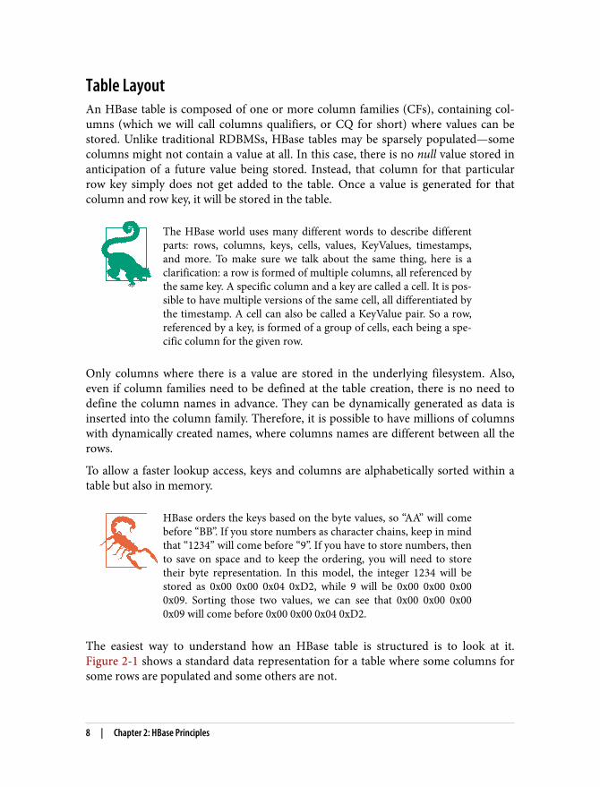
Table LayoutAn HBase table is composed of one or more column families (CFs), containing col‐umns (which we will call columns qualifiers, or CQ for short) where values can bestored. Unlike traditional RDBMSs, HBase tables may be sparsely populated—somecolumns might not contain a value at all. In this case, there is no null value stored inanticipation of a future value being stored. Instead, that column for that particularrow key simply does not get added to the table. Once a value is generated for thatcolumn and row key, it will be stored in the table.

The HBase world uses many different words to describe differentparts: rows, columns, keys, cells, values, KeyValues, timestamps,and more. To make sure we talk about the same thing, here is aclarification: a row is formed of multiple columns, all referenced bythe same key. A specific column and a key are called a cell. It is pos‐sible to have multiple versions of the same cell, all differentiated bythe timestamp. A cell can also be called a KeyValue pair. So a row,referenced by a key, is formed of a group of cells, each being a spe‐cific column for the given row.

Only columns where there is a value are stored in the underlying filesystem. Also,even if column families need to be defined at the table creation, there is no need todefine the column names in advance. They can be dynamically generated as data isinserted into the column family. Therefore, it is possible to have millions of columnswith dynamically created names, where columns names are different between all therows.

To allow a faster lookup access, keys and columns are alphabetically sorted within atable but also in memory.

HBase orders the keys based on the byte values, so “AA” will comebefore “BB”. If you store numbers as character chains, keep in mindthat “1234” will come before “9”. If you have to store numbers, thento save on space and to keep the ordering, you will need to storetheir byte representation. In this model, the integer 1234 will bestored as 0x00 0x00 0x04 0xD2, while 9 will be 0x00 0x00 0x000x09. Sorting those two values, we can see that 0x00 0x00 0x000x09 will come before 0x00 0x00 0x04 0xD2.

The easiest way to understand how an HBase table is structured is to look at it.Figure 2-1 shows a standard data representation for a table where some columns forsome rows are populated and some others are not.

8 | Chapter 2: HBase Principles

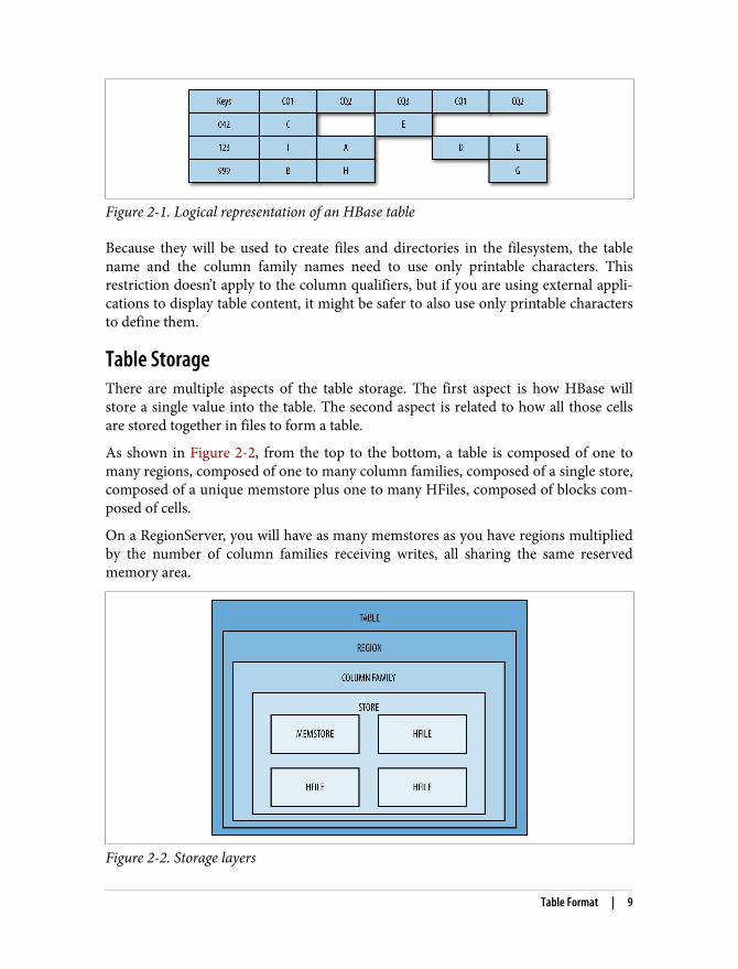
Figure 2-1. Logical representation of an HBase table

Because they will be used to create files and directories in the filesystem, the tablename and the column family names need to use only printable characters. Thisrestriction doesn’t apply to the column qualifiers, but if you are using external appli‐cations to display table content, it might be safer to also use only printable charactersto define them.

Table StorageThere are multiple aspects of the table storage. The first aspect is how HBase willstore a single value into the table. The second aspect is related to how all those cellsare stored together in files to form a table.

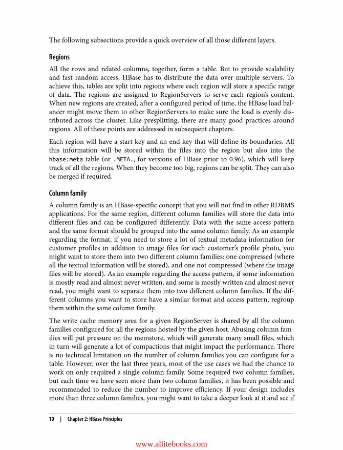
As shown in Figure 2-2, from the top to the bottom, a table is composed of one tomany regions, composed of one to many column families, composed of a single store,composed of a unique memstore plus one to many HFiles, composed of blocks com‐posed of cells.

On a RegionServer, you will have as many memstores as you have regions multipliedby the number of column families receiving writes, all sharing the same reservedmemory area.

Figure 2-2. Storage layers

Table Format | 9

The following subsections provide a quick overview of all those different layers.

RegionsAll the rows and related columns, together, form a table. But to provide scalabilityand fast random access, HBase has to distribute the data over multiple servers. Toachieve this, tables are split into regions where each region will store a specific rangeof data. The regions are assigned to RegionServers to serve each region’s content.When new regions are created, after a configured period of time, the HBase load bal‐ancer might move them to other RegionServers to make sure the load is evenly dis‐tributed across the cluster. Like presplitting, there are many good practices aroundregions. All of these points are addressed in subsequent chapters.

Each region will have a start key and an end key that will define its boundaries. Allthis information will be stored within the files into the region but also into thehbase:meta table (or .META., for versions of HBase prior to 0.96), which will keeptrack of all the regions. When they become too big, regions can be split. They can alsobe merged if required.

Column familyA column family is an HBase-specific concept that you will not find in other RDBMSapplications. For the same region, different column families will store the data intodifferent files and can be configured differently. Data with the same access patternand the same format should be grouped into the same column family. As an exampleregarding the format, if you need to store a lot of textual metadata information forcustomer profiles in addition to image files for each customer’s profile photo, youmight want to store them into two different column families: one compressed (whereall the textual information will be stored), and one not compressed (where the imagefiles will be stored). As an example regarding the access pattern, if some informationis mostly read and almost never written, and some is mostly written and almost neverread, you might want to separate them into two different column families. If the dif‐ferent columns you want to store have a similar format and access pattern, regroupthem within the same column family.

The write cache memory area for a given RegionServer is shared by all the columnfamilies configured for all the regions hosted by the given host. Abusing column fam‐ilies will put pressure on the memstore, which will generate many small files, whichin turn will generate a lot of compactions that might impact the performance. Thereis no technical limitation on the number of column families you can configure for atable. However, over the last three years, most of the use cases we had the chance towork on only required a single column family. Some required two column families,but each time we have seen more than two column families, it has been possible andrecommended to reduce the number to improve efficiency. If your design includesmore than three column families, you might want to take a deeper look at it and see if

10 | Chapter 2: HBase Principles

www.allitebooks.com

all those families are really required; most likely, they can be regrouped. If you do nothave any consistency constraints between your two columns families and data willarrive into them at a different time, instead of creating two column families for a sin‐gle table, you can also create two tables, each with a single column family. This strat‐egy is useful when it comes time to decide the size of the regions. Indeed, while it wasbetter to keep the two column families almost the same size, by splitting them accrosstwo different tables, it is now easier to let me grow independently.

Chapter 15 provides more details regarding the column families.

StoresWe will find one store per column family. A store object regroups one memstore andzero or more store files (called HFiles). This is the entity that will store all the infor‐mation written into the table and will also be used when data needs to be read fromthe table.

HFilesHFiles are created when the memstores are full and must be flushed to disk. HFilesare eventually compacted together over time into bigger files. They are the HBase fileformat used to store table data. HFiles are composed of different types of blocks (e.g.,index blocks and data blocks). HFiles are stored in HDFS, so they benefit fromHadoop persistence and replication.

BlocksHFiles are composed of blocks. Those blocks should not be confused with HDFSblocks. One HDFS block might contain multiple HFile blocks. HFile blocks are usu‐ally between 8 KB and 1 MB, but the default size is 64 KB. However, if compression isconfigured for a given table, HBase will still generate 64 KB blocks but will then com‐press them. The size of the compressed block on the disk might vary based on thedata and the compression format. Larger blocks will create a smaller number of indexvalues and are good for sequential table access, while smaller blocks will create moreindex values and are better for random read accesses.

If you configure block sizes to be very small, it will create manyHFiles block indexes, which ultimately will put some pressure onthe memory, and might produce the opposite of the desired effect.Also, because the data to compress will be small, the compressionratio will be smaller, and data size will increase. You need to keepall of these details in mind when deciding to modify the defaultvalue. Before making any definitive changes, you should run someload tests in your application using different settings. However, ingeneral, it is recommended to keep the default value.

Table Format | 11

The following main block types can be encountered in an HFile (because they aremostly internal implementation details, we will only provide a high-level description;if you want to know more about a specific block type, refer to the HBase sourcecode):

Data blocksA data block will contain data that is either compressed, or uncompressed, butnot a combination of both. A data block includes the delete markers as well asthe puts.

Index blocksWhen looking up a specific row, index blocks are used by HBase to quickly jumpto the right location in an HFile.

Bloom filter blockThese blocks are used to store bloom filter index related information. Bloom fil‐ter blocks are used to skip parsing the file when looking for a specific key.

Trailer blockThis block contains offsets to the file’s other variable-sized parts. It also containsthe HFile version.

Blocks are stored in reverse order. It means that instead of having the index at thebeginning of the file followed by the other blocks, the blocks are written in reverseorder. Data blocks are stored first, then the index blocks, then the bloom filter blocks;the trailer blocks are stored at the end.

CellsHBase is a column-oriented database. That means that each column will be storedindividually instead of storing an entire row on its own. Because those values can beinserted at different time, they might end up in different files in HDFS.

Figure 2-3 represents how HBase will store the values from Figure 2-1.

12 | Chapter 2: HBase Principles

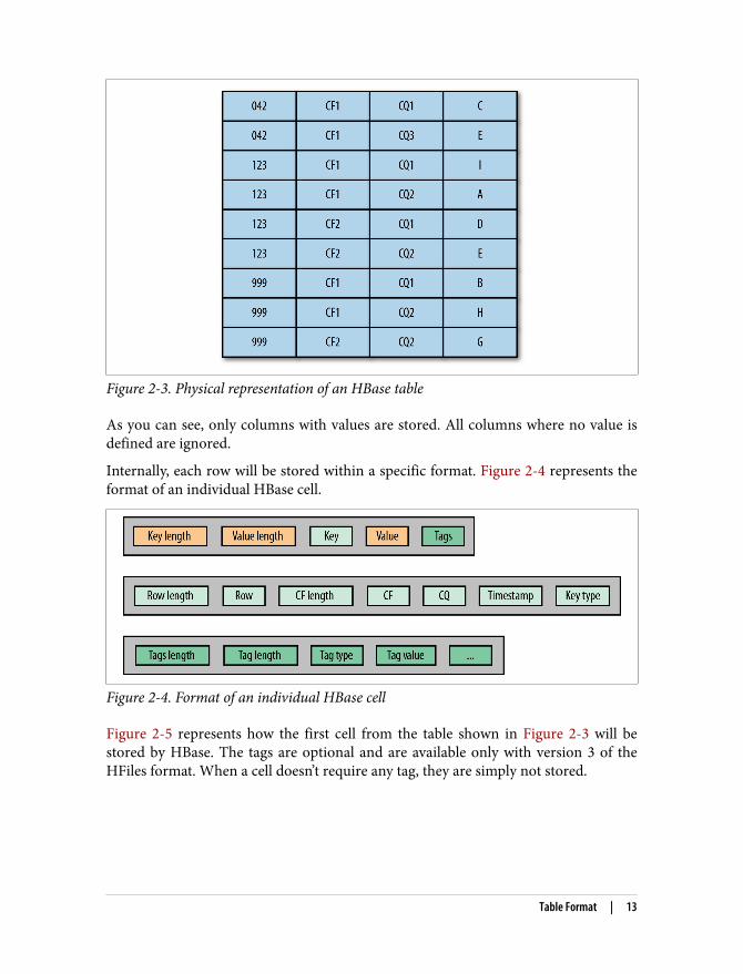
Figure 2-3. Physical representation of an HBase table

As you can see, only columns with values are stored. All columns where no value isdefined are ignored.

Internally, each row will be stored within a specific format. Figure 2-4 represents theformat of an individual HBase cell.

Figure 2-4. Format of an individual HBase cell

Figure 2-5 represents how the first cell from the table shown in Figure 2-3 will bestored by HBase. The tags are optional and are available only with version 3 of theHFiles format. When a cell doesn’t require any tag, they are simply not stored.

Table Format | 13

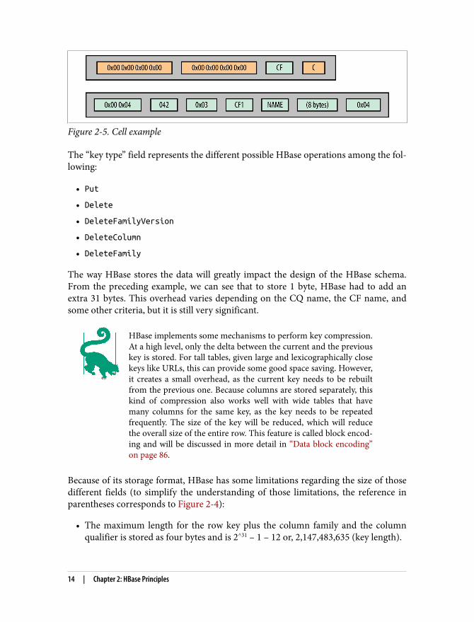
Figure 2-5. Cell example

The “key type” field represents the different possible HBase operations among the fol‐lowing:

• Put

• Delete

• DeleteFamilyVersion

• DeleteColumn

• DeleteFamily

The way HBase stores the data will greatly impact the design of the HBase schema.From the preceding example, we can see that to store 1 byte, HBase had to add anextra 31 bytes. This overhead varies depending on the CQ name, the CF name, andsome other criteria, but it is still very significant.

HBase implements some mechanisms to perform key compression.At a high level, only the delta between the current and the previouskey is stored. For tall tables, given large and lexicographically closekeys like URLs, this can provide some good space saving. However,it creates a small overhead, as the current key needs to be rebuiltfrom the previous one. Because columns are stored separately, thiskind of compression also works well with wide tables that havemany columns for the same key, as the key needs to be repeatedfrequently. The size of the key will be reduced, which will reducethe overall size of the entire row. This feature is called block encod‐ing and will be discussed in more detail in “Data block encoding”on page 86.

Because of its storage format, HBase has some limitations regarding the size of thosedifferent fields (to simplify the understanding of those limitations, the reference inparentheses corresponds to Figure 2-4):

• The maximum length for the row key plus the column family and the columnqualifier is stored as four bytes and is 2^31 – 1 – 12 or, 2,147,483,635 (key length).

14 | Chapter 2: HBase Principles

• The maximum length for the value is stored as four bytes and is 2^31 – 1 or2,147,483,647 (value length).

• The maximum length for the row key is stored as two signed bytes and is 32,767(row length).

• Because it is stored in one signed byte, the maximum length for the column fam‐ily is 127 (CF length).

• The maximum length for all the tags together is stored as two bytes and is 65,535(tags length).

Internal Table OperationsHBase scalability is based on its ability to regroup data into bigger files and spread atable across many servers. To reach this goal, HBase has three main mechanisms:compactions, splits, and balancing. These three mechanisms are transparent for theuser. However, in case of a bad design or improper usage, it might impact the perfor‐mance of servers. Therefore, it is good to know about these mechanisms to under‐stand server reactions.

CompactionHBase stores all the received operations into its memstore memory area. When thememory buffer is full, it is flushed to disk (see “Memory” on page 192 for furtherdetails about the memstore and its flush mechanisms). Because this can create manysmall files in HDFS, from time to time, and based on specific criteria that we will seelater, HBase can elect files to be compacted together into a bigger one. This will bene‐fit HBase in multiple ways. First, the new HFile will be written by the hosting Region‐Server, ensuring the data is stored locally on HDFS. Writing locally will allow theRegionServer local lookups for the file rather than going over the network. Second,this will reduce the number of files to look at when a user is requesting some data.That will allow HBase to do faster lookups and will reduce the pressure on HDFS tokeep track of all the small files. Third, it allows HBase to do some cleanup on the datastored into those files. If the time to live (TTL) causes some cells to expire, they willnot be rewritten in the new destination file. The same applies for the deletes undercertain conditions that are detailed momentarily.

There exist two types of compactions.

Minor compactionA compaction is called minor when HBase elects only some of the HFiles to be com‐pacted but not all. The default configurable threshold triggers HBase compactionwhen there are three files (HFiles) or more in the current region. If the compaction is

Internal Table Operations | 15

triggered, HBase will elect some of those files based on the compaction policy. If allthe files present in the store are elected, the compaction will be promoted into amajor compaction.

Minor compactions can perform some cleanup on the data, but not everything can becleaned. When you perform a delete of a cell, HBase will store a marker to say that allidentical cells older than that one have been deleted. Therefore, all the cells with thesame key but a previous timestamp should be removed. When HBase performs thecompaction and finds a delete marker, it will make sure that all older cells for thesame key and column qualifier will be removed. However, because some cells mightstill exist in other files that have not been elected for compaction, HBase cannotremove the marker itself, as it still applies and it cannot make sure no other cells needto be removed. The same thing is true if the delete marker is present on a file that hasnot been elected for compaction. If that’s the case, cells that should have been deletedbecause of the marker will still remain until a major compaction is performed.Expired cells based on the TTL defined on the column family level will be deletedbecause they don’t depend on the content of the other non-elected files, except if thetable has been configured to keep a minimal number of versions.

It is important to understand the relationship of cell version countand compactions. When deciding the number of versions to retain,it is best to treat that number as the minimum version count avail‐able at a given time. A great example of this would be a table with asingle column family configured to retain a maximum versioncount of 3. There are only two times that HBase will remove extraversions. The first being on flush to disk, and the second on majorcompaction. The number of cells returned to the client are nor‐mally filtered based on the table configuration; however, whenusing the RAW => true parameter, you can retrieve all of the ver‐sions kept by HBase. Let’s dive deeper into a few scenarios:

• Doing four puts, followed immediately by a scan without aflush, will result in four versions being returned regardless ofversion count.

• Doing four puts, followed by a flush and then a scan, willresult in three versions being returned.

• Doing four puts and a flush, followed by four puts and a flush,and then a scan, will result in six versions being returned.

• Doing four puts and a flush, followed by four puts and a flush,and then a major compaction followed by a scan, will result inthree versions being returned.

16 | Chapter 2: HBase Principles

Major compactionWe call it a major compaction when all the files are elected to be compacted together.A major compaction works like a minor one except that the delete markers can beremoved after they are applied to all the related cells and all extra versions of thesame cell will also be dropped. Major compactions can be manually triggered at thecolumn family level for a specific region, at the region level, or at the table level.HBase is also configured to perform weekly major compactions.

Automatic weekly compactions can happen at any time dependingon when your cluster was started. That means that it can be over‐night when you have almost no HBase traffic, but it also means thatit can be exactly when you have your peak activity. Because theyneed to read and rewrite all the data, major compactions are veryI/O intensive and can have an impact on your cluster response timeand SLAs. Therefore, it is highly recommended to totally disablethose automatic major compactions and to trigger them yourselfusing a cron job when you know the impact on your cluster will beminimal. We also recommend that you do not compact all thetables at the same time. Instead of doing all the tables once a weekon the same day, spread the compactions over the entire week. Last,if you really have a very big cluster with many tables and regions, itis recommended to implement a process to check the number offiles per regions and the age of the oldest one and trigger the com‐pactions at the region level only if there are more files than youwant or if the oldest one (even if there is just one file) is older thana configured period (a week is a good starting point). This willallow to keep the region’s data locality and will reduce the I/O onyour cluster.

Splits (Auto-Sharding)Split operations are the opposite of compactions. When HBase compacts multiplefiles together, if not too many values are dropped over the compaction process, it willcreate a bigger file. The bigger the input files, the more time it takes to parse them, tocompact them, and so on. Therefore, HBase tries to keep them under a configurablemaximum size. In HBase 0.94 and older, this default maximum size was 1 GB. Later,this value was increased to 10 GB. When one of the column families of a region rea‐ches this size, to improve balancing of the load, HBase will trigger a split of the givenregion into two new regions. Because region boundaries apply to all the column fami‐lies of a given region, all the families are split the same way even if they are muchsmaller than the configured maximum size. When a region is split, it is transformedinto two new smaller regions where the start key of the first one is the start key of theoriginal region, and the end key of the second one is the end key of the originalregion. The keys for the end of the first region and the beginning of the second one

Internal Table Operations | 17

are decided by HBase, which will choose the best mid-point. HBase will do its best toselect the middle key; however we don’t want this to take much time, so it is not goingto split within an HFile block itself.

There are a few things you need to keep in mind regarding the splits. First, HBase willnever split between two columns of the same row. All the columns will stay togetherin the same region. Therefore, if you have many columns or if they are very big, asingle row might be bigger than the maximum configured size and HBase will not beable to split it. You want to avoid this situation where an entire region will serve onlya single row.

You also need to remember that HBase will split all the column families. Even if yourfirst column reached the 10 GB threshold but the second one contains only a fewrows or kilobytes, both of them will be split. You might end up with the second familyhaving only very tiny files in all the regions. This is not a situation you want to findyourself in, and you might want to review your schema design to avoid it. If you arein this situation and you don’t have a strong consistency requirement between yourtwo column families, consider splitting them into two tables.

Finally, don’t forget that splits are not free. When a region is balanced after beingsplit, it loses its locality until the next compaction. This will impact the read perfor‐mance because the client will reach the RegionServer hosting the region, but fromthere, the data will have to be queried over the network to serve the request. Also, themore regions you have, the more you put pressure on the master, the hbase:metatable, and the region services. In the HBase world, splits are fine and normal, but youmight want to keep an eye on them.

Figure 2-6 shows a two-column family table before and after a split. As you will notein the figure, one CF is significantly bigger than the other.

Figure 2-6. A two-column family table, before and after a split

18 | Chapter 2: HBase Principles

BalancingRegions get split, servers might fail, and new servers might join the cluster, so at somepoint the load may no longer be well distributed across all your RegionServers. Tohelp maintain a good distribution on the cluster, every five minutes (default config‐ured schedule time), the HBase Master will run a load balancer to ensure that all theRegionServers are managing and serving a similar number of regions.

HBase comes with a few different balancing algorithms. Up to version 0.94, HBaseused the SimpleLoadBalancer, but starting with HBase 0.96, it uses theStochasticLoadBalancer. Although it is recommended to stay with the default con‐figured balancer, you can develop you own balancer and ask HBase to use it.

When a region is moved by the balancer from one server to a newone, it will be unavailable for a few milliseconds, and it will lose itsdata locality until it gets major compacted.

Figure 2-7 shows how the master reassigns the regions from the most loaded serversto the less loaded ones. Overloaded servers receive the instruction from the master toclose and transition the region to the destination server.

Figure 2-7. Example migration from overworked RegionServer

DependenciesTo run, HBase only requires a few other services and applications to be available. LikeHDFS, HBase is written in Java and will require a recent JDK to run. As we have seen,HBase relies on HDFS. However, some work has been done in the past to run it ontop of other filesystems, including Amazon S3.

Dependencies | 19

HBase will need HDFS to run on the same nodes as the HBase nodes. It doesn’t meanthat HBase needs to run on all the HDFS nodes, but it is highly recommended, as itmight create very unbalanced situations. HBase also relies on ZooKeeper to monitorthe health of its servers, to provide high-availability features, and to keep track ofinformation such as replication progress, current active HBase Master, the list ofexisting tables, and so on.

There is work in progress in HBase 2.0 to reduce its dependency on ZooKeeper.

HBase RolesHBase is composed of two primary roles: the master (also sometime called HBaseMaster, HMaster, or even just HM) and the RegionServers (RS). It is also possible torun Thrift and REST servers to access HBase data using different APIs.

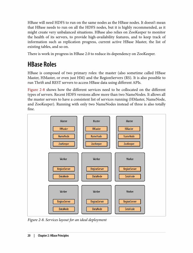
Figure 2-8 shows how the different services need to be collocated on the differenttypes of servers. Recent HDFS versions allow more than two NameNodes. It allows allthe master servers to have a consistent list of services running (HMaster, NameNode,and ZooKeeper). Running with only two NameNodes instead of three is also totallyfine.

Figure 2-8. Services layout for an ideal deployment

20 | Chapter 2: HBase Principles

Master ServerThe HBase master servers are the head of the cluster and are responsible for few aoperations:

• Region assignment• Load balancing• RegionServer recovery• Region split completion monitoring• Tracking active and dead servers

For high availability, it is possible to have multiple masters in a single cluster. How‐ever, only a single master will be active at a time and will be responsible for thoseoperations.

Unlike HBase RegionServers, the HBase Master doesn’t have much workload and canbe installed on servers with less memory and fewer cores. However, because it is thebrain of your cluster, it has to be more reliable. You will not lose your cluster if youlose two RegionServers, but losing your two Masters will put you at high risk. Becauseof that, even though RegionServers are usually built without disks configured asRAID or dual power supplies, etc., it is best to build more robust HBase Masters.Building HBase Masters (and other master services like NameNodes, ZooKeeper, etc.)on robust hardware with OS on RAID drives, dual power supply, etc. is highly recom‐mended. To improve overall cluster stability, there is work in progress in HBase 2.0 tolet the master track some of the information currently tracked by Zookeeper.

A cluster can survive without a master server as long as there is no RegionServer fail‐ing nor regions splitting.

RegionServerA RegionServer (RS) is the application hosting and serving the HBase regions andtherefore the HBase data. When required (e.g., to read and write data into a specificregion), calls from the Java API can go directly to the RegionServer. This is to ensurethe HBase master or the active ZooKeeper server are not bottlenecks in the process.

A RegionServer will decide and handle the splits and the compactions but will reportthe events to the master.

Even if it is technically doable to host more than one RegionServer on a physical host,it is recommended to run only one server per host and to give it the resources youwill have shared between the two servers.

HBase Roles | 21

When a client tries to read data from HBase for the first time, itwill first go to ZooKeeper to find the master server and locate thehbase:meta region where it will locate the region and RegionServerit is looking for. In subsequent calls from the same client to thesame region, all those extra calls are skipped, and the client will talkdirectly with the related RegionServer. This is why it is important,when possible, to reuse the same client for multiple operations.

Thrift ServerA Thrift server can be used as a gateway to allow applications written in other lan‐guages to perform calls to HBase. Even if it is possible to use Java to call HBasethrough the Thrift server, it is recommended to directly call the Java API instead.HBase provides the Apache Thrift schema that you will have to compile for the lan‐guage you want to use. There are currently two versions of the Thrift schema. Version1 is the legacy schema and is kept for compatibility for external applications builtagainst it. Version 2 is the new version and includes an updated schema. The twoschemas can be found in the HBase code under the following locations:

Version 1 (legacy)hbase-thrift/src/main/resources/org/apache/hadoop/hbase/thrift/Hbase.thrift

Version 2hbase-thrift/src/main/resources/org/apache/hadoop/hbase/thrift2/hbase.thrift

Unlike the Java client that can talk to any RegionServer, a C/C++ client using a Thriftserver can talk only to the Thrift server. This can create a bottleneck, but startingmore than one Thrift server can help to reduce this point of contention.

Not all the HBase Java API calls might be available through theThrift API. The Apache HBase community tries to keep them as upto date as possible, but from time to time, some are reported miss‐ing and are added back. If the API call you are looking for is notavailable in the Thrift schema, report it to the community.

REST ServerHBase also provides a REST server API through which all client and administrationoperations can be performed. A REST API can be queried using HTTP calls directlyfrom client applications or from command-line applications like curl. By specifyingthe Accept field in the HTTP header, you can ask the REST server to provide results indifferent formats. The following formats are available:

22 | Chapter 2: HBase Principles

• text/plain (consult the warning note at the end of this chapter for more infor‐mation)

• text/xml

• application/octet-stream

• application/x-protobuf

• application/protobuf

• application/json

Let’s consider a very simple table created and populated this way:

create 't1', 'f1'put 't1', 'r1', 'f1:c1', 'val1'

Here is an example of a call to the HBase REST API to retrieve in an XML format thecell we have inserted:

curl -H "Accept: text/xml" http://localhost:8080/t1/r1/f1:c1

This will return the following output:

<?xml version="1.0" encoding="UTF-8" standalone="yes"?><CellSet> <Row key="cjE="> <Cell column="ZjE6YzE=" timestamp="1435940848871">dmFsMQ==</Cell> </Row></CellSet>

where values are base64 encoded and can be decoded from the command line:

$ echo "dmFsMQ==" | base64 -dval1

If you don’t want to have to decode XML and based64 values, you can simply use theoctet-stream format:

curl -H "Accept: application/octet-stream" http://localhost:8080/t1/r1/f1:c1

which will return the value as it is:

val1

Even if the HBase code makes reference to the text/html format, itis not implemented and cannot be used.Because it is not possible to represent the responses in all the for‐mats, some of the calls are implemented for only some of the for‐mats. Indeed, even if you can call the /version or the /t1/schemaURLs for the text/plain format, it will fail with the /t1/r1/f1:c1call. Therefore, before choosing a format, make sure all the callsyou will need work with it.

HBase Roles | 23

CHAPTER 3

HBase Ecosystem

As we know, HBase is designed as part of the Hadoop ecosystem. The good news isthat when creating new applications, HBase comes with a robust ecosystem. Thisshould come as no surprise, as HBase is typically featured in a role of serving produc‐tion data or powering customer applications. There are a variety of tools surroundingHBase, ranging from SQL query layers, ACID compliant transactional systems, man‐agement systems, and client libraries. In-depth coverage of every application forHBase will not be provided here, as the topic would require a book in and of itself.We will review the most prominent tools and discuss some of the pros and consbehind them. We will look at a few of the most interesting features of the top ecosys‐tem tools.

Monitoring ToolsOne of the hottest topics around Hadoop, and HBase in general, is management andmonitoring tools. Having supported both Hadoop and HBase for numerous years, wecan testify that any management software is better than none at all. Seriously, take theworst thing you can think of (like drowning in a vat of yellow mustard, or whateverscares you the most); then double it, and that is debugging a distributed systemwithout any support. Hadoop/HBase is configured through XML files, which you cancreate manually. That said, there are two primary tools for deploying HBase clustersin the Hadoop ecosystem. The first one is Cloudera Manager, and the second isApache Ambari. Both tools are capable of deploying, monitoring, and managing thefull Hadoop suite shipped by the respective companies. For installations that choosenot to leverage Ambari or Cloudera Manager, deployments typically use automatedconfiguration management tools such as Puppet or Chef in combination with moni‐toring tools such as Ganglia or Cacti. This scenario is most commonly seen wherethere is an existing infrastructure leveraging these toolsets. There is also an interest‐

25

ing visualization out there called Hannibal that can help visualize HBase internalsafter a deployment.

Cloudera ManagerThe first tool that comes to mind for managing HBase is Cloudera Manager (yeah, wemight be a little biased). Cloudera Manager (CM) is the most feature-complete man‐agement tool available. Cloudera Manager has the advantage of being first to marketand having a two-year lead on development over Apache Ambari. The primarydownside commonly associated with CM is its closed source nature. The good newsis that CM has numerous amazing features, including a point-and-click install inter‐face that makes installing a Hadoop cluster trivial. Among the most useful features ofCloudera Manager are parcels, the Tsquery language, and distributed log search.

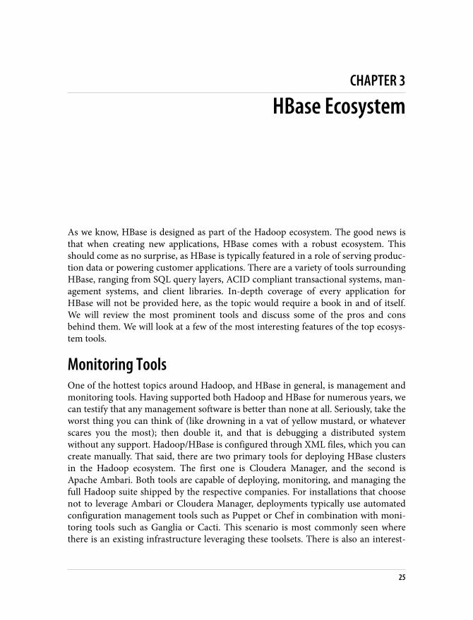
Parcels are an alternative method for installing Cloudera Distribution of ApacheHadoop (CDH). Parcels, in their simplest form, are “glorified tarballs.” What isimplied by tarballs is that Cloudera packages up all the necessary start/stop scripts,libs/jars, and other files necessary for CM functions. Cloudera Manager will use thissetup to easily manage the deployed services. Figure 3-1 shows an example of Clou‐dera Manager listing available and installed packages. Parcels allow for full stack roll‐ing upgrades and restarts without having to incur downtime between minor releases.They also contain the necessary dependencies to make deploying Hadoop cleanerthan using packages. CM will take advantage of the unified directory structure togenerate and simplify classpath and configuration management for the differentprojects.

Figure 3-1. Listing of available and currently deployed parcels

26 | Chapter 3: HBase Ecosystem

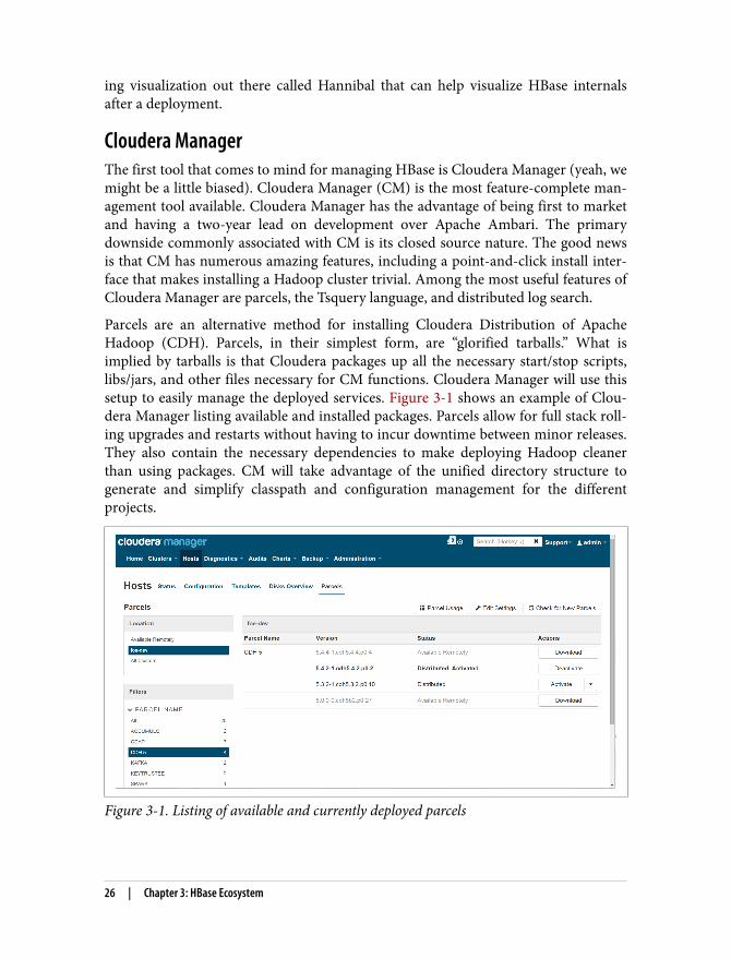
Monitoring is key to any successful Hadoop or HBase deployment. CM has impres‐sive monitoring and charting features built in, but it also has an SQL-like languageknown as “Tsquery.” As shown in Figure 3-2, administrators can use Tsquery to buildand share custom charts, graphs, and dashboards to monitor and analyze clusters’metrics.

Figure 3-2. Executed query showing average wait time per disk

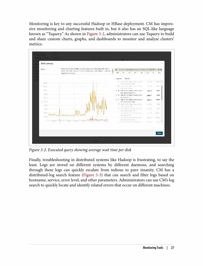
Finally, troubleshooting in distributed systems like Hadoop is frustrating, to say theleast. Logs are stored on different systems by different daemons, and searchingthrough these logs can quickly escalate from tedious to pure insanity. CM has adistributed-log search feature (Figure 3-3) that can search and filter logs based onhostname, service, error level, and other parameters. Administrators can use CM’s logsearch to quickly locate and identify related errors that occur on different machines.

Monitoring Tools | 27

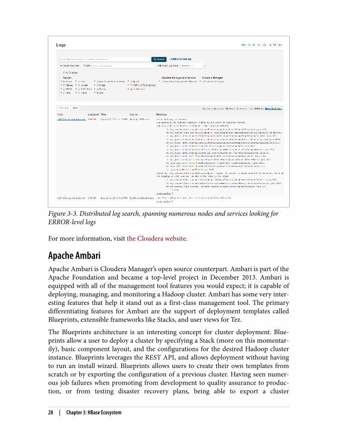
Figure 3-3. Distributed log search, spanning numerous nodes and services looking forERROR-level logs

For more information, visit the Cloudera website.

Apache AmbariApache Ambari is Cloudera Manager’s open source counterpart. Ambari is part of theApache Foundation and became a top-level project in December 2013. Ambari isequipped with all of the management tool features you would expect; it is capable ofdeploying, managing, and monitoring a Hadoop cluster. Ambari has some very inter‐esting features that help it stand out as a first-class management tool. The primarydifferentiating features for Ambari are the support of deployment templates calledBlueprints, extensible frameworks like Stacks, and user views for Tez.

The Blueprints architecture is an interesting concept for cluster deployment. Blue‐prints allow a user to deploy a cluster by specifying a Stack (more on this momentar‐ily), basic component layout, and the configurations for the desired Hadoop clusterinstance. Blueprints leverages the REST API, and allows deployment without havingto run an install wizard. Blueprints allows users to create their own templates fromscratch or by exporting the configuration of a previous cluster. Having seen numer‐ous job failures when promoting from development to quality assurance to produc‐tion, or from testing disaster recovery plans, being able to export a cluster

28 | Chapter 3: HBase Ecosystem

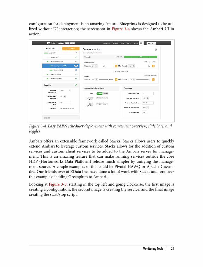
configuration for deployment is an amazing feature. Blueprints is designed to be uti‐lized without UI interaction; the screenshot in Figure 3-4 shows the Ambari UI inaction.

Figure 3-4. Easy YARN scheduler deployment with convenient overview, slide bars, andtoggles

Ambari offers an extensible framework called Stacks. Stacks allows users to quicklyextend Ambari to leverage custom services. Stacks allows for the addition of customservices and custom client services to be added to the Ambari server for manage‐ment. This is an amazing feature that can make running services outside the coreHDP (Hortonworks Data Platform) release much simpler by unifying the manage‐ment source. A couple examples of this could be Pivotal HAWQ or Apache Cassan‐dra. Our friends over at ZData Inc. have done a lot of work with Stacks and sent overthis example of adding Greenplum to Ambari.

Looking at Figure 3-5, starting in the top left and going clockwise: the first image iscreating a configuration, the second image is creating the service, and the final imagecreating the start/stop script.

Monitoring Tools | 29

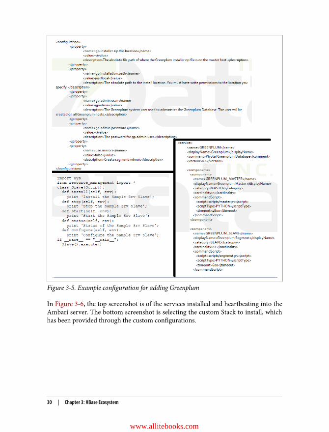
Figure 3-5. Example configuration for adding Greenplum

In Figure 3-6, the top screenshot is of the services installed and heartbeating into theAmbari server. The bottom screenshot is selecting the custom Stack to install, whichhas been provided through the custom configurations.

30 | Chapter 3: HBase Ecosystem

www.allitebooks.com

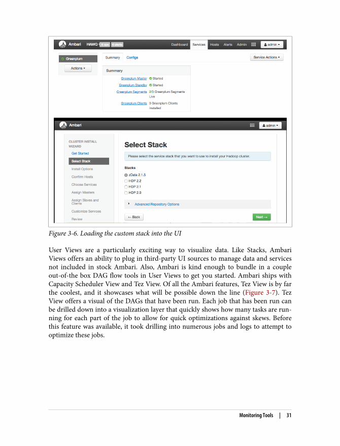
Figure 3-6. Loading the custom stack into the UI

User Views are a particularly exciting way to visualize data. Like Stacks, AmbariViews offers an ability to plug in third-party UI sources to manage data and servicesnot included in stock Ambari. Also, Ambari is kind enough to bundle in a coupleout-of-the box DAG flow tools in User Views to get you started. Ambari ships withCapacity Scheduler View and Tez View. Of all the Ambari features, Tez View is by farthe coolest, and it showcases what will be possible down the line (Figure 3-7). TezView offers a visual of the DAGs that have been run. Each job that has been run canbe drilled down into a visualization layer that quickly shows how many tasks are run‐ning for each part of the job to allow for quick optimizations against skews. Beforethis feature was available, it took drilling into numerous jobs and logs to attempt tooptimize these jobs.

Monitoring Tools | 31

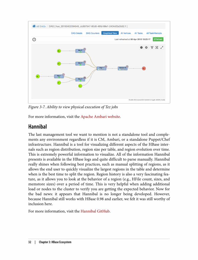
Figure 3-7. Ability to view physical execution of Tez jobs

For more information, visit the Apache Ambari website.

HannibalThe last management tool we want to mention is not a standalone tool and comple‐ments any environment regardless if it is CM, Ambari, or a standalone Puppet/Chefinfrastructure. Hannibal is a tool for visualizing different aspects of the HBase inter‐nals such as region distribution, region size per table, and region evolution over time.This is extremely powerful information to visualize. All of the information Hannibalpresents is available in the HBase logs and quite difficult to parse manually. Hannibalreally shines when following best practices, such as manual splitting of regions, as itallows the end user to quickly visualize the largest regions in the table and determinewhen is the best time to split the region. Region history is also a very fascinating fea‐ture, as it allows you to look at the behavior of a region (e.g., HFile count, sizes, andmemstore sizes) over a period of time. This is very helpful when adding additionalload or nodes to the cluster to verify you are getting the expected behavior. Now forthe bad news: it appears that Hannibal is no longer being developed. However,because Hannibal still works with HBase 0.98 and earlier, we felt it was still worthy ofinclusion here.

For more information, visit the Hannibal GitHub.

32 | Chapter 3: HBase Ecosystem

SQLOne of hottest topics for Big Data is SQL on Hadoop. HBase, with numerous offer‐ings, is never one to be left out of the mix. The vast majority of the tools that bringSQL functionality to the Hadoop market are mostly aimed at providing businessintelligence functionality. With HBase, there are a few tools that focus on businessintelligence, but on an arguably more interesting side, there are a few that focus onfull-blown transactional systems. There are three main solutions we will look at:Apache Phoenix, Trafodion, and Splice Machine.

Apache PhoenixApache Phoenix was contributed by our friends at Salesforce.com. Phoenix isdesigned as a relational database layer set on top of HBase designed to handle SQLqueries. It is important to note that Phoenix is for business intelligence rather thanabsorbing OLTP workloads. Phoenix is still a relatively new project (it reached incu‐bator status in December 2013 and recently graduated to a top-level project in May2014). Even with only a couple years in the Apache Foundation, Phoenix has seen anice adoption rate and is quickly becoming the de facto tool for SQL queries. Phoe‐nix’s main competitors are Hive and Impala for basic SQL on HBase. Phoenix hasbeen able to establish itself as a superior tool through tighter integration by leveragingHBase coprocessors, range scans, and custom filters. Hive and Impala were both builtfor full file scans in HDFS, which can greatly impact performance because HBase wasdesigned for single point gets and range scans.

Phoenix offers some interesting out-of-the-box functionality. Secondary indexes areprobably the most popular request we receive for HBase, and Phoenix offers threedifferent types: functional indexing, global indexing, and local indexing. Each indextype targets a different type of workload; whether it is read heavy, write heavy, orneeds to be accessed through expressions, Phoenix has an index for you. Phoenix willalso help to handle the schema, which is especially useful for time series records. Youjust have to specify the number of salted buckets you wish to add to your table. Byadding the salted buckets to the key and letting Phoenix manage the keys, you willavoid very troublesome hot spots that tend to show their ugly face when dealing withtime series data.

For more information, visit the Apache Phoenix website.

Apache TrafodionTrafodion is an open source tool and transactional SQL layer for HBase beingdesigned by HP and currently incubating in Apache. Unlike Phoenix, Trafodion ismore focused on extending the relational model and handling transactional pro‐cesses. The SQL layer offers the ability to leverage consistent secondary indexes for

SQL | 33

faster data retrieval. Trafodion also offers some of its own table structure optimiza‐tions with its own data encoding for serialization and optimized column family andcolumn names. The Trafodion engine itself has implemented specific technology tosupport large queries as well as small queries. For example, during large joins andgrouping, that Trafodion will repartition the tables into executor server processes(ESPs), outside of the HBase RegionServers, then the queries will be performed inparallel. An added bonus is Trafodion will optimize the SQL plan execution choicesfor these types of queries. Another interesting feature is the ability to query and joinacross data sources like Hive and Impala with HBase. Like Phoenix, Trafodion doesnot offer an out-of the-box UI, but expects BI tools or custom apps built on ODBC/JDBC to connect to Trafodion.

For more information, visit the Apache Trafodion website.

Splice MachineSplice Machine is a closed source offering targeting the OLTP market. Splice Machinehas leveraged the existing Apache Derby framework for its foundation. SpliceMachine’s primary goal is to leverage the transaction and SQL layer to port previousrelational databases on to HBase. Splice Machine has also developed its own customencoding format for the data which heavily compresses the data and lowers storageand retrieval costs. Similar to the previously discussed SQL engines, the paralleltransaction guarantees are handled through custom coprocessors, which enables thehigh level of throughput and scalability these transactional systems are able to ach‐ieve. Like Trafodion, Splice Machine can also just leverage the SQL layer for businessreporting from not just HBase, but Hive and Impala as well.

For more information, visit Splice Machine’s website.

Honorable Mentions (Kylin, Themis, Tephra, Hive, and Impala)There are also numerous other systems out there to bring SQL and transaction func‐tionality to HBase:

• Apache Kylin (originally contributed by eBay) is designed for multidimensionalonline analytical processing (MOLAP) and relational online analytical processing(ROLAP). Kylin is interesting because the data cubes have to be pre-created inHive and then pushed over to HBase. Kylin is designed for large-scale reportingas opposed to real-time ingest/serving systems.

• Themis is a cross row/cross table transaction built on top of HBase sponsored byXiaoMi.

• Tephra is another transaction system brought to us by the team at Cask.

34 | Chapter 3: HBase Ecosystem

• Finally, Hive and Apache Impala are storage engines both designed to run fulltable or partitioned scans against HDFS. Hive and Impala both have HBase stor‐age handlers allowing them to connect to HBase and perform SQL queries. Thesesystems tend to pull more data than the other systems, which will greatly increasequery times. Hive or Impala make sense when a small set of reference data livesin HBase, or when the queries are not bound by SLAs.

FrameworksAnother interesting aspect of the HBase ecosystem is frameworks. There are manydifferent types of frameworks available on the market for HBase. Some frameworksspecialize in handling time series data, while others focus on codifying best practices,handling the use of different languages, or moving to an asynchronous client model.We will take a deeper look at the OpenTSDB framework, which is really almost astandalone application, before moving on to discuss Kite, HappyBase, andAsyncHBase.

OpenTSDBOpenTSDB is one of the most interesting applications we will talk about. OpenTSDBis not a framework itself, but it takes the place of a custom framework for handlingtime series data. OpenTSDB is designed as a time series database on top of HBase. Ithas a full application layer integrated for querying and presenting the data, as well asframeworks written on top of it for ingesting the time series data. It is a prettystraightforward system, where individual, stateless collectors called time series dae‐mons (TSDs) receive the time series data from the servers. Those TSDs then act asclients and write the data to HBase using a schema designed for fetching the seriesdata over a period of time in an efficient manner. The end user never directly accessesHBase for any of the data. All necessary calls are funneled through the TSDs.OpenTSDB also has a basic UI (Figure 3-8) built into it for graphing the differentmetrics from the time series data. The TSDs can also expose an HTTP API for easilyquerying data to be consumed by third-party monitoring frameworks or reportingdashboards.

Frameworks | 35

Figure 3-8. OpenTSDB offers a fully functional UI out of the box

For more information, visit OpenTSDB’s website.

KiteThere are quite a few different frameworks that either replace or alter the HBase cli‐ent’s behavior. Kite is a whole SDK designed to codify Hadoop best practices. Kitealso comes with a prebuilt transformation, aggregation, and extract library set calledMorphlines. Kite on HBase is relatively new and still flagged as experimental. Theportion of Kite designed for HBase is in heavy use in Cloudera for its CustomerOperations Tools Team. It is being based on the internal library known as HBase-common. The goal is to codify how the records should be stored in HBase columns to

36 | Chapter 3: HBase Ecosystem

optimize for storage and performance efficiency. Kite offers the ability to map specificHBase columns, and has many different flexible options. The column mapping isstored in JSON and is used to write the Avro records into the HBase table structure.Kite also offers a simple way to load data into the cluster. Once the configuration hasbeen stored, all Kite writers know exactly how to put the data into the dataset withouthaving to reconfigure each writer. Kite also leverages the concept of datasets. Thedataset used can be Hadoop, Hive, or HBase. By pre-creating these datasets, Kiteknows how and where to write the data into Hadoop, thus saving many hours ofdirect coding.

For more information, visit Kite’s website.

HappyBaseThe HappyBase framework is designed to allow the end user to leverage the HBaseclient through the use of Python. HappyBase is designed to allow Python to access theHBase system by leveraging the Thrift gateway. HappyBase supports the vast majorityof functions an HBase application needs in order to flourish, right down to atomiccounters and batch mutations. HappyBase is great for getting an application up andrunning, but leveraging the Thrift interface brings a few different issues to light. Youshould consider how you are going to load balance and handle failovers (pro tip:HAProxy is your friend), and the thrift interface will be slower than the direct JavaAPI.

For more information visit the HappyBase website.

AsyncHBaseFinally, the AsyncHBase project (which happens to be part of OpenTSDB) is one werun into out in the field constantly. AsyncHBase is a client replacement that offersbetter throughput and performance if your data can be processed asynchronously.One of the coolest features of AsyncHBase is the ease of deploying a multithreadedapplication using the single client. You should keep in mind that it is not a trivial mat‐ter to switch back and forth between the clients, as they require almost a completerewrite. This is a very popular library for handling time series data without fullydeploying OpenTSDB.

For more information, visit the OpenTSDB’s GitHub.

Frameworks | 37

CHAPTER 4

HBase Sizing and Tuning Overview

The two most important aspects of building an HBase appplication are sizing andschema design. This chapter will focus on the sizing considerations to take intoaccount when building an application. We will discuss schema design in Part II.

In addition to negatively impacting performance, sizing an HBase cluster incorrectlywill reduce stability. Many clusters that are undersized tend to suffer from client time‐outs, RegionServer failures, and longer recovery times. Meanwhile, a properly sizedand tuned HBase cluster will perform better and meet SLAs on a consistent levelbecause the internals will have less fluctuation, which in turn means fewer compac‐tions (major and minor), fewer region splits, and less block cache churn.

Sizing an HBase cluster is a fine art that requires an understanding of the applicationneeds prior to deploying. You will want to make sure to understand both the read andthe write access patterns before attempting to size the cluster. Because it involves tak‐ing numerous aspects into consideration, proper HBase sizing can be challenging.Before beginning cluster sizing, it’s important to analyze the requirements for theproject. These requirements should be broken down into three categories:

WorkloadThis requires understanding general concurrency, usage patterns, and ingress/egress workloads.

Service-level agreements (SLAs)You should have an SLA that guarantees fully quantified read and write latencies,and understanding the tolerance for variance.

CapacityYou need to consider how much data is ingested daily, the total data retentiontime, and total data size over the lifetime of the project.

39

After fully understanding these project requirements, we can move on to cluster siz‐ing. Because HBase relies on HDFS, it is important to take a bottom-up approachwhen designing an HBase cluster. This means starting with the hardware and thenthe network before moving on to operating system, HDFS, and finally HBase.

HardwareThe hardware requirements for an HBase-only deployment are cost friendly com‐pared to a large, multitenant deployment. HBase currently can use about 16–24 GB ofmemory for the heap, though that will change with Java 7 and the G1GC algorithm.The initial testing with the G1GC collector has shown very promising results withheaps over 100 GB is size. This becomes especially important when attempting to ver‐tically scale HBase, as we will see later in our discussion of the sizing formulas.

When using heaps larger than 24 GB of allocated heap space, garbage collection pau‐ses will become so long (30 seconds or more) that RegionServers will start to time outwith ZooKeeper causing failures. Currently, stocking the DataNodes with 64–128 GBof memory will be sufficient to cover the RegionServers, DataNodes, and operatingsystem, while leaving enough space to allow the block cache to assist with reads. In aread-heavy environment looking to leverage bucketcache, 256 GB or more of RAMcould add significant value. From a CPU standpoint, an HBase cluster does not needa high core count, so mid-range speed and lower-end core count is quite sufficient.As of early 2016, standard commodity machines are shipping with dual octacore pro‐cessors on the low end, and dual dodecacore processors with a clock speed of about2.5 GHz. If you are creating a multitenant cluster (particularly if you plan to utilizeMapReduce), it is beneficial to use a higher core count (the exact number will be dic‐tated by your use case and the components used). Multitenant use cases can be verydifficult, especially when HBase is bound by tight SLAs, so it is important to test withboth MapReduce jobs as well as an HBase workload. In order to maintain SLAs, it issometimes necessary to have a batch cluster and a real-time cluster. As the technol‐ogy matures, this will become less and less likely. One of the biggest benefits ofHBase/Hadoop is that a homogenous environment is not required (though it is rec‐ommended for your sanity). This allows for flexibility when purchasing hardware,and allows for different hardware specifications to be added to the cluster on anongoing basis whenever they are required.

StorageAs with Hadoop, HBase takes advantage of a JBOD disk configuration. The benefitsoffered by JBOD are two-fold: first, it allows for better performance by leveragingshort-circuit reads (SCR) and block locality; and second, it helps to control hardwarecosts by eliminating expensive RAID controllers. Disk count is not currently a majorfactor for an HBase-only cluster (where no MR, no Impala, no Solr, or any other

40 | Chapter 4: HBase Sizing and Tuning Overview

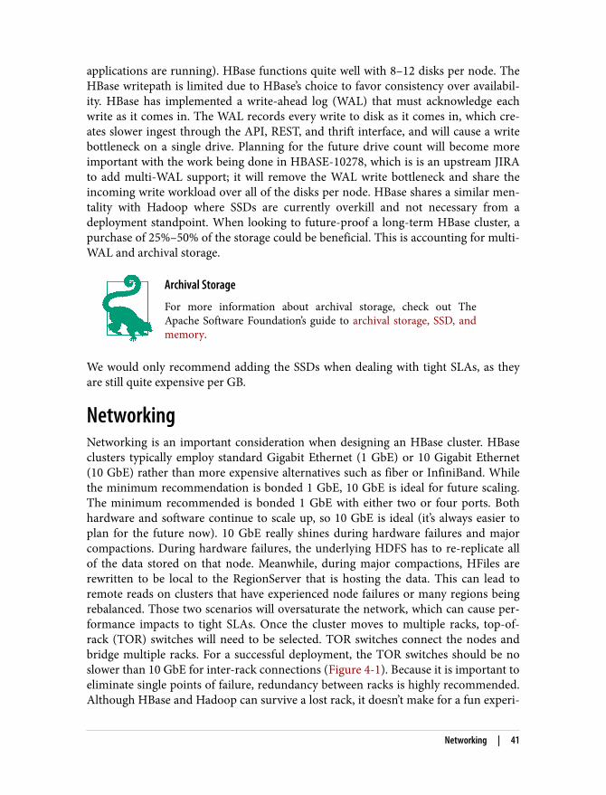
applications are running). HBase functions quite well with 8–12 disks per node. TheHBase writepath is limited due to HBase’s choice to favor consistency over availabil‐ity. HBase has implemented a write-ahead log (WAL) that must acknowledge eachwrite as it comes in. The WAL records every write to disk as it comes in, which cre‐ates slower ingest through the API, REST, and thrift interface, and will cause a writebottleneck on a single drive. Planning for the future drive count will become moreimportant with the work being done in HBASE-10278, which is is an upstream JIRAto add multi-WAL support; it will remove the WAL write bottleneck and share theincoming write workload over all of the disks per node. HBase shares a similar men‐tality with Hadoop where SSDs are currently overkill and not necessary from adeployment standpoint. When looking to future-proof a long-term HBase cluster, apurchase of 25%–50% of the storage could be beneficial. This is accounting for multi-WAL and archival storage.

Archival Storage

For more information about archival storage, check out TheApache Software Foundation’s guide to archival storage, SSD, andmemory.

We would only recommend adding the SSDs when dealing with tight SLAs, as theyare still quite expensive per GB.

NetworkingNetworking is an important consideration when designing an HBase cluster. HBaseclusters typically employ standard Gigabit Ethernet (1 GbE) or 10 Gigabit Ethernet(10 GbE) rather than more expensive alternatives such as fiber or InfiniBand. Whilethe minimum recommendation is bonded 1 GbE, 10 GbE is ideal for future scaling.The minimum recommended is bonded 1 GbE with either two or four ports. Bothhardware and software continue to scale up, so 10 GbE is ideal (it’s always easier toplan for the future now). 10 GbE really shines during hardware failures and majorcompactions. During hardware failures, the underlying HDFS has to re-replicate allof the data stored on that node. Meanwhile, during major compactions, HFiles arerewritten to be local to the RegionServer that is hosting the data. This can lead toremote reads on clusters that have experienced node failures or many regions beingrebalanced. Those two scenarios will oversaturate the network, which can cause per‐formance impacts to tight SLAs. Once the cluster moves to multiple racks, top-of-rack (TOR) switches will need to be selected. TOR switches connect the nodes andbridge multiple racks. For a successful deployment, the TOR switches should be noslower than 10 GbE for inter-rack connections (Figure 4-1). Because it is important toeliminate single points of failure, redundancy between racks is highly recommended.Although HBase and Hadoop can survive a lost rack, it doesn’t make for a fun experi‐

Networking | 41

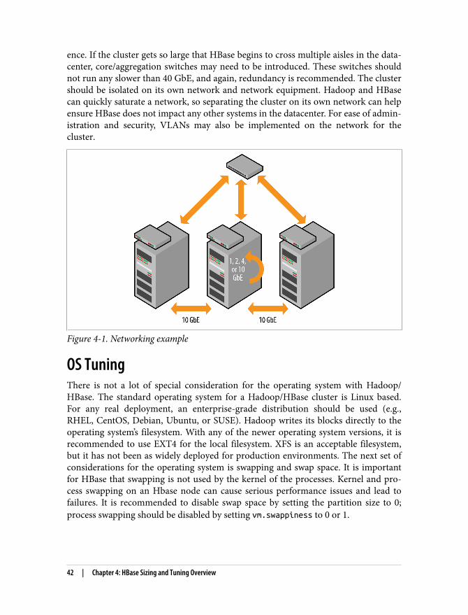
ence. If the cluster gets so large that HBase begins to cross multiple aisles in the data‐center, core/aggregation switches may need to be introduced. These switches shouldnot run any slower than 40 GbE, and again, redundancy is recommended. The clustershould be isolated on its own network and network equipment. Hadoop and HBasecan quickly saturate a network, so separating the cluster on its own network can helpensure HBase does not impact any other systems in the datacenter. For ease of admin‐istration and security, VLANs may also be implemented on the network for thecluster.

Figure 4-1. Networking example

OS TuningThere is not a lot of special consideration for the operating system with Hadoop/HBase. The standard operating system for a Hadoop/HBase cluster is Linux based.For any real deployment, an enterprise-grade distribution should be used (e.g.,RHEL, CentOS, Debian, Ubuntu, or SUSE). Hadoop writes its blocks directly to theoperating system’s filesystem. With any of the newer operating system versions, it isrecommended to use EXT4 for the local filesystem. XFS is an acceptable filesystem,but it has not been as widely deployed for production environments. The next set ofconsiderations for the operating system is swapping and swap space. It is importantfor HBase that swapping is not used by the kernel of the processes. Kernel and pro‐cess swapping on an Hbase node can cause serious performance issues and lead tofailures. It is recommended to disable swap space by setting the partition size to 0;process swapping should be disabled by setting vm.swappiness to 0 or 1.

42 | Chapter 4: HBase Sizing and Tuning Overview

Hadoop TuningApache HBase 0.98+ only supports Hadoop2 with YARN. It is important to under‐stand the impact that YARN (MR2) can have on an HBase cluster. Numerous caseshave been handled by Cloudera support where MapReduce workloads were causingHBase to be starved of resources. This leads to long pauses while waiting for resour‐ces to free up.

Hadoop2 with YARN adds an extra layer of complexity, as resource management hasbeen moved into the YARN framework. YARN also allows for more granular tuningof resources between managed services. There is some work upstream to integrateHBase within the YARN framework (HBase on YARN, or HOYA), but it is currentlyincomplete. This means YARN has to be tuned to allow for HBase to run smoothlywithout being resource starved. YARN allows for specific tuning around the numberof CPUs utilized and memory consumption. The three main functions to take intoconsideration are:

yarn.nodemanager.resource.cpu-vcores

Number of CPU cores that can be allocated for containers.

yarn.nodemanager.resource.memory-mb

Amount of physical memory, in megabytes, that can be allocated for containers.When using HBase, it is important not to over allocate memory for the node. It isrecommended to allocate 8–16 GB for the operating system, 2–4 GB for theDataNode, 12–24 GB for HBase, and the rest for the YARN framework (assum‐ing there are not other workloads such as Impala or Solr).

yarn.scheduler.minimum-allocation-mb

The minimum allocation for every container request at the RM, in megabytes.Memory requests lower than this won’t take effect, and the specified value will getallocated at minimum. The recommended value is between 1–2 GB of data.

When performing the calculations, it is important to remember that the vast majorityof servers use an Intel chip set with hyper-threading enabled. Hyper-threading allowsthe operating system to present two virtual or logical cores for every physical corepresent. Here is some back-of-the-napkin tuning for using HBase with YARN (thiswill vary depending on workloads—your mileage may vary):

physicalCores * 1.5 = total v-cores

We also must remember to leave room for HBase:

Total v-cores – 1 for HBase – 1 for DataNode – 1 for NodeManager – 1 for OS ...– 1 for any other services such as Impala or Solr

Hadoop Tuning | 43

For an HBase and YARN cluster with a dual 10-core processor, the tuning would lookas follows:

20 * 1.5 = 30 virtual CPUs30 – 1 – 1 – 1 – 1 = 26 total v-cores

Some sources recommend going one step further and dividing the 26 v-cores in halfwhen using HBase with YARN. You should test your application at production levelsto determine the best tuning.

HBase TuningAs stated at the beginning of the chapter, HBase sizing requires a deep understandingof three project requirements: workload, SLAs, and capacity. Workload and SLAs canbe organized into three main categories: read, write, or mixed. Each of these cate‐gories has its own set of tunable parameters, SLA requirements, and sizing concernsfrom a hardware-purchase standpoint.

The first one to examine is the write-heavy workload. There are two main ways to getdata into HBase: either through an API (Java, Thrift, or REST) or by using bulk load.This is an important distinction to make, as the API will use the WAL and memstore,while bulk load is a short-circuit write and bypasses both. As mentioned in “Hard‐ware” on page 40, the primary bottleneck for HBase is the WAL followed by thememstore. There are a few quick formulas for determining optimal write perfor‐mance in an API-driven write model.

To determine region count per node:

HBaseHeap * memstoreUpperLimit = availableMemstoreHeapavailableMemstoreHeap / memstoreSize = recommendedActiveRegionCount

(This is actually column family based. The formula is based on one CF.)

To determine raw space per node:

recommendedRegionCount * maxfileSize * replicationFactor = rawSpaceUsed

To determine the number of WALs to keep:

availableMemstoreHeap / (WALSize * WALMultiplier) = numberOfWALs

44 | Chapter 4: HBase Sizing and Tuning Overview

Here is an example of this sizing using real-world numbers:

HBase heap = 16 GBMemstore upper limit = 0.5*Memstore size = 128 MBMaximum file size = 20 GBWAL size = 128 MBWAL rolling multiplier = 0.95

First, we’ll determine region count per node:

16,384 MB * 0.5 = 8,192 MB8,192 MB / 128 MB = 64 activeRegions

Next, we’ll determine raw space per node:

64 activeRegions * 20 GB * 3 = 3.75 TB used

Finally, we need to determine the number of WALs to keep:

8,192 GB / (128 MB * 0.95) = 67 WALs

When using this formula, it is recommended to have no more than 67 regions perRegionServer while keeping a total of 67 WALs. This will use 3.7 TB (with replica‐tion) of storage per node for the HFiles, which does not include space used for snap‐shots or compactions.

Bulk loads are a short-circuit write and do not run through the WAL, nor do they usethe memstore. During the reduce phase of the MapReduce jobs, the HFiles are cre‐ated and then loaded using the completebulkload tool. Most of the region count lim‐itations come from the WAL and memstore. When using bulkload, the region countis limited by index size and response time. It is recommended to test read responsetime scaling up from 100 regions; it is not unheard of for successful deployments tohave 150–200 regions per RegionServer. When using bulk load, it is important toreduce the upper limit (hbase.regionserver.global.memstore.upper limit) andlower limit (hbase.regionserver.global.memstore.lower limit) to 0.11 and 0.10,respectively, and then raise the block cache to 0.6–0.7 depending on available heap.Memsore and block cache tuning will allow HBase to keep more data in memory forreads.

It is important to note these values are percentages of the heapdevoted to the memstore and the block cache.

HBase Tuning | 45

The same usable space from before per node calculation can be used once the desiredregion count has been determined through proper testing.

Again, the formula to determine raw space per node is as follows:

recommendedRegionCount * maxfileSize * replicationFactor = rawSpaceUsed

Using this formula, we’d calculate the raw space per node as follows in this instance:

150 activeRegions * 20 GB * 3 = 9 TB used

Capacity is the easiest portion to calculate. Once the workload has been identifiedand properly tested (noticing a theme with testing yet?), it is a simple matter of divid‐ing the total amount of data by capacity per node. It is important to leave scratchspace available (the typical recommendation is 20%–30% overhead). This space willbe used for MapReduce scratch space, extra space for snapshots, and major compac‐tions. Also, if using snapshots with high region counts, testing should be done toensure there will be enough space for the desired backup pattern, as snapshots canquickly take up space.

Different Workload TuningFor primary read workloads, it is important to understand and test the SLA require‐ments. Rigorous testing is required to determine the best settings. The primary set‐tings that need to be tweaked are the same as write workloads (i.e., loweringmemstore settings and raising the block cache to allow for more data to be stored inmemory). In HBase 0.96, bucket cache was introduced. This allows for data to bestored either in memory or on low-latency disk (SSD/flash cards). You should use0.98.6 or higher for this feature due to HBASE-11678.

In a mixed workload environment, HBase bucket cache becomes much more inter‐esting, as it allows HBase to be tuned to allow more writes while maintaining a higherread response time. When running in a mixed environment, it is important to over‐provision your cluster, as doing so will allow for the loss of a RegionServer or two. Itis recommended to allow one extra RegionServer per rack when sizing the cluster.This will also give the cluster better response times with more memory for reads andextra WALs for writes. Again, this is about finding the perfect balance to fit the work‐load, which means tuning the number of WALs, memstore limits, and total allocatedblock cache.

HBase can run into multiple issues when leveraging other Hadoop components. Wewill cover deploying HBase with Impala, Solr, and Spark throughout Part II. Unfortu‐nately, there really isn’t a great answer for running HBase with numerous compo‐nents. The general concerns that arise include the following:

46 | Chapter 4: HBase Sizing and Tuning Overview

• CPU contention• Memory contention• I/O contention

The first two are reasonably easy to address with proper YARN tuning (this meansrunning Spark in YARN mode) and overprovisioning of resources. What we meanhere is if you know your application needs W GB for YARN containers, Impala willuse X memory, HBase heap needs Y to meet SLAs, and I want to save Z RAM for theOS, then my formula should be:

W + X + Y + Z = totalMemoryNeeded

This formula makes sense at first glance, but unfortunately it rarely works out to be asstraightforward. We would recommend upgrading to have at least 25%–30% freememory. The benefits of this approach are twofold: first, when it’s time to purchaseadditional nodes, it will give you room to vertically grow until those new nodes areadded to the cluster; and second, the OS will take advantage of the additional mem‐ory with OS buffers helping general performance across the board.

The I/O contention is where the story really starts to fall apart. The only viableanswer is to leverage control groups (cgroups) in the Linux filesystem. Setting upcgroups can be quite complex, but they provide the ability to assign specific processsuch as Impala, or most likely YARN/MapReduce, into specific I/O-throttled groups.

Most people do not bother with configuring cgroups or other throttle technologies.We tend to recommend putting memory limits on Impala, container limits on YARN,and memory and heap limits on Solr. Then properly testing your application at scalewill allow for fine-tuning of the components working together.

Our colleague Eric Erickson, who specializes in all things Solr, has trademarked thephrase “it depends” when asked about sizing. He believes that back-of-the-napkinmath is a great starting point, but only proper testing can verify the sizing estimates.The good news with HBase and Hadoop is that they provide linear scalability, whichallows for testing on a smaller level and then scaling out from there. The key to a suc‐cessful HBase deployment is no secret—you need to utilize commodity hardware,keep the networking simple using Ethernet versus more expensive technologies suchas fiber or InfiniBand, and maintain detailed understanding of all aspects of theworkload.

Different Workload Tuning | 47

CHAPTER 5

Environment Setup

To be able to test locally and see how HBase behaves, we will install and configure astandalone HBase environment that will be used to run the given examples. HBasecan run in three modes, each of which offers different behaviors (the first two modesare mainly for testing purposes, while the last one is the mode you will use for yourproduction HBase cluster):

Standalone modeThis mode starts all of the HBase processes in a single virtual machine (VM).Standalone mode uses the local disk for HBase storage and does not require anyspecific configuration. Data will be stored in the current user-configured tempo‐rary folder (usually /tmp) in a folder named hbase-$USERNAME. Removing thisfolder when HBase is down will remove all HBase data. This is the simplest modefor running HBase, and it’s the one we will use for our testing. Using this modeallows the end user to easily clear all HBase content and restart with a blankinstallation. This mode doesn’t require running any other external service (e.g.,ZooKeeper or HDFS).

Pseudodistributed modeIn pseudodistributed mode, HBase will run the same processes as in fully dis‐tributed mode, but as a single node cluster. HBase will start the ZooKeeper pro‐cess and both the HBase Master and RegionServer processes.

Fully distributed modeLast, fully distributed mode is when HBase runs on multiple machines with allrequired services (ZooKeeper, Hadoop, etc.).

49

System RequirementsWhether you are choosing a standalone, pseudo-distributed, or fully distributeddeployment, the choices made around the environment will be key for its success.There will be choices around using bare metal or VMs for the core infrastructure;which OS should you install; what Hadoop distribution you should use; the Java ver‐sion to deploy on; and the most important question, what system resources are goingto be needed for success. The following sections will help guide and answer thesequestions for you.

Operating SystemAll example outputs provided in this book are captured from a Linux shell terminalusing HBase 1.0.1 (some on Debian, some on CentOS). In order to reproduce ourresults, try to use the same Linux version that we have used. The examples can be runin a Linux environment running on either a physical or virtual machine. Commandsmight also work in other environments (Windows, Mac OS X, etc.) or on Cygwin,but we have not tested them.

If you want to install a Linux environment, you can download and install one of thefollowing distributions:

• Debian 7+• Ubuntu 14.04+• RedHat 6.6+• CentOS 6.6

This is a nonexhaustive list—there are many other distributions and versions avail‐able today, and any of them should work. You should choose and install the one youare most comfortable working with. If you decide to use an Apache Hadoop distribu‐tion, make sure to validate which Linux distribution and version it is compatible with.

Virtual MachineAs described in the following subsections, there are multiple ways to use a VM to runa pseudodistributed HBase environment. Let’s take a look at each of these options.

VM modes

Local VMYou can install a virtual machine support (e.g., VirtualBox) on your local com‐puter and then create a Linux VM into which you can install HBase and run it ineither standalone or pseudodistributed mode.

50 | Chapter 5: Environment Setup

Public cloudThis is similar to the previous option, except that you create the Linux VM(instance) on a public cloud such as Amazon EC2. You then install the HBasesoftware and run it in standalone or pseudodistributed mode. You can also provi‐sion multiple virtual nodes and run HBase in a fully distributed mode. Be carefulwith running a production HBase cluster in a public cloud, as some specific con‐figuration might be required.

Local virtual distributionInstall a virtual machine support (e.g., VirtualBox) on your local computer andinstead of installing software manually, simply download the Cloudera Quick‐Start VM, which includes a fully functional HBase installation in pseudodistrib‐uted mode (no manual installation required).

Linux environmentIf you don’t have a computer available on which to install a Linux distribution,you can run one on your local environment by running it in a local VM. The fol‐lowing applications will help you to run a Linux environment in a local VM:

• VirtualBox• VMWare• KVM

Hadoop distributionThis book covers HBase application design and development, but to be fully imple‐mented, some use cases might require other external applications, such as Solr orFlume. Installing, configuring, and running those tools is outside the scope of thisbook. If you want to implement those integration examples, you will need to have aVM with an entire Hadoop distribution already installed. A Hadoop distribution is abundle, usually packaged by a Hadoop vendor, including most if not all of theHadoop-related applications. This is usually easier to install, as all the applications areconfigured to work together and they usually come with some setup scripts to pre‐pare them all.

For simplicity and because it already contains all the applications we need (HDFS,HBase, Solr, Flume, etc.), you can use the Cloudera QuickStart VM. We used version5.4.2 of this VM to build all those use cases, and all the examples are tested with it. Ifyou are not familiar with Linux or HBase and Hadoop installation, it might be easierfor you to follow the same path and use the QuickStart VM.

All of the examples in the book are built for HBase 1.0.1. If you choose to use anotherHadoop distribution in a virtual environment or if you decide to install HBase locally,you’ll need to make sure that the distribution you choose comes with the same HBase

System Requirements | 51

version. While the examples might work with more recent versions, most of them willfail with older ones.

If you choose to use a Hadoop distribution, we still recommend reading the followingsections so that you can become familiar with HBase, its constraints, and itsinstallation.

In order to make the most of HBase’s capabilities, all of the examples in this book aretested against a local Linux standalone HBase server and the Cloudera QuickStartVM. If you have access to a Hadoop test cluster (physical or virtual), you can also useit. That will allow you to choose the environment with which you are the most com‐fortable to run your tests.

ResourcesThe necessary resources are an important choice when choice when starting downthe HBase path. Having enough resources will decide early success or failure.

MemoryWhether you are working in your local environment or on a VM, you need enoughmemory for provide to HBase and the other services to run. A standalone HBaseenvironment running locally will require a minimum of 1 GB memory. However, ifpossible, we recommend allocating more memory, as doing so will allow you to runthe tests on bigger datasets and to have a better view of the results and the behaviorsof the application. If you are testing the examples directly in a Hadoop distributionrunning in a virtual environment, you should allocate a minimum of 4 GB to the VM.Here again, giving more memory to the environment will allow you to have a betterresponse time from your applications and to run on bigger datasets. That’s why werecommend allocating at least 8 GB to your virtual machine.

You should allocate as much memory as possible to your virtualmachine. If you have 32 GB or more in your environment, makesure to allocate as much as you can to your VM. We ran most of theexamples on a 12 GB VirtualBox virtual environment.

Disk spaceThe HBase installation file takes less than 100 MB (and the examples require just afew megabytes), so you can run all of the examples with less than 1 GB of availabledisk space. However, if you want to see all of the features in the examples pushed fur‐ther, you’ll need to create bigger datasets—and that requires more space for you totest. Therefore, we recommend allowing for at least 10 GB of available disk space.

52 | Chapter 5: Environment Setup

If you want to run in a virtual environment, you will need at least 4 GB of availabledisk space to download the VM and another 4 GB to extract it. The Cloudera Quick‐Start VM is configured to allow its virtual disk to grow up to 64 GB. Creating bigdatasets and running HBase for a long period will create a lot of data in your virtualenvironment. As a result, you will easily use up to 50 GB of disk space. Although it’spossible to start with less, we recommend that you to have this space available beforeyou start.

JavaHBase is written in Java and therefore it depends on specific versions of the JDK. Itsupports version 7 since HBase 0.94 and version 8 since HBase 0.99, while Java 6 sup‐port has been dropped starting with HBase 1.0. To run your local HBase version andthe given examples, we recommend using the most up-to-date Java 7 version avail‐able. The VM we used for the examples runs with Java 1.7.0_67, so you should usethat version to ensure that you will get the same results.

Be careful when choosing your JVM version—you need to makesure it is bug free. As an example, JDK 1.7.0_75 has some issueswith the jps command when running it in sudo mode.

Version Recommended JDK Other JDKs1.x JDK 7 JDK 8

0.98 JDK 7 JDK 6, JDK 8

0.96 JDK 7 JDK 6

0.94 JDK 6 JDK 7

HBase Standalone InstallationThis section will describe the steps necessary for installing HBase on metal or on aVM running Linux.

Running a standalone HBase installation should be a straightforward process—yousimply need to download the HBase binary, extract it, and finally, run it.

At the time of this writing, the last stable Apache HBase version from the stablebranch is version 1.0.1. We recommend using a mirror to download the release. Onceyou have found the best mirror to download the HBase release, the file to downloadshould be named something like hbase-1.0.x-bin.tar.gz, where x is the last subreleasenumber. Take the downloaded file and extract it to the directory of your choice usingtar -xzf from the command line. The instructions that follow will assume that

HBase Standalone Installation | 53

HBase has been extracted or is accessible from the ~/hbase directory and that thehbase/bin folder has been added to the user path.

Using the Unix command line, the steps just described can be achieved as follows:

#:~$ cd ~#:~$ wget \"http://www.us.apache.org/dist/hbase/hbase-1.0.1/hbase-1.0.1-bin.tar.gz"#:~$ tar -xzf hbase-1.0.1-bin.tar.gz#:~$ ln -s hbase-1.0.1 hbase#:~$ rm hbase-1.0.1-bin.tar.gz#:~$ cd hbase#:~/hbase$ export PATH=$PATH:~/hbase/bin

Because this is based on HBase release 1.0.1, the download of thebinaries might fail if this release is replaced by a more recent one.Go to http://www.apache.org/dyn/closer.cgi/hbase/ to check for thelast available version, and update the preceding command ifnecessary.

The next step is to specify which JDK should be used to run HBase (we recommendconfiguring the same JDK that will be used in the development environment). Onceyou’ve specified the JDK, you will need to let HBase know about the location of yourJDK. First, identify the version and the location using the java -version and whichjava commands. When you have identified the location of your JDK, you can exportthe JAVA_HOME variable. Here are two examples of potential Java locations:

#:~$ export JAVA_HOME=/usr # If using your Linux distribution JDK#:~$ export JAVA_HOME=/usr/local/jdk1.7.0_60/ # If installed manually

When your JAVA_HOME variable has been defined correctly, the HBase standaloneserver can simply be started using the following command:

#:~$ start-hbase.sh

Instead of exporting the JAVA_HOME variable each time you start theserver, you can also edit the conf/hbase-env.sh file to get this valueautomatically defined when the HBase command is launched.

At this point, the HBase environment should be running locally. There are multipleways to verify that HBase is functioning correctly. In the later examples, we will seehow to do that using Java code. As a matter of simplicity, we will use the HBase shellfor now.

To start the HBase shell, run the following command:

#:~$ hbase shell

54 | Chapter 5: Environment Setup

The output should look something like this:

HBase Shell; enter 'help<RETURN>' for list of supported commands.Type "exit<RETURN>" to leave the HBase ShellVersion 1.1.5, r239b8045640b2e562a5568b5c744252e,\Sun May 8 20:29:26 PDT 2016

hbase(main):001:0>

You might encounter some informational messages with warningsabout deprecated properties or missing native libraries. For thisexample, it is safe to ignore them (and for brevity, we removedthem from the code displayed here). The warnings could impactperformance in a fully distributed system, but for a standaloneHBase server they are not a cause for concern.

While in the HBase shell, simply run the status command to see HBase statistics:

hbase(main):001:0> status1 servers, 0 dead, 2.0000 average load

The output from the status command explains that there is one HBase server run‐ning, with an average of two HBase regions per RegionServer. At this point, if yourenvironment is not running correctly, refer to “Troubleshooting” on page 59.

Even if you just installed HBase, it already contains two regions:one for the hbase:meta table (which contains all information for allother table regions) and another for the hbase:namespace table(which contains the details of the available namespaces). Those twotables are HBase system tables and therefore belong to the hbasenamespace (for more information regarding namespaces, refer to“HBase Filesystem Layout” on page 213).

The HBase standalone server is now available for the next set of tests. tests. If any‐thing is not as expected, refer to “Troubleshooting” on page 59.

Now that the environment is running, it can be accessed by its web interface at http://localhost:16010 or you can replace localhost by the local machine hostname or IP.

The HBase cluster can be stopped by calling the stop-hbase.sh script as follows:

#:~$ stop-hbase.shstopping hbase..........

Depending on server performance and the state of the environment, it might takesome time for HBase to properly shut down.

HBase Standalone Installation | 55

HBase in a VMTo install and run a virtual machine, you first need to have a virtualization environ‐ment (e.g, VirtualBox, KVM, or VMWare) installed and running locally. Because thecomputer we used to build the examples runs on Debian, and because it is available asa Debian distribution package, we used VirtualBox for our tests. The next step is todownload the QuickStart VM file and extract it where you have enough space avail‐able. Then import it into your virtualization environment. For VirtualBox users, thiscan be done by navigating to the File menu and selecting “Import virtual application”(it can take some time to complete the import). The last step is to configure yournewly imported virtual environment to have enough memory.

When all of those steps are completed, you can start your environment. The first timeyou run it, it will take some time to perform initialization steps that are not requiredfor subsequent restarts. When the VM is started and ready to be used, a browsershould automatically open and be visible in the VM with some useful links and infor‐mation on the home page.

To validate that HBase is already correctly installed, configured, and running, simplyopen a terminal and proceed with the same steps as the standalone installation.

Open the HBase shell:

#:~$ hbase shell

And use the status command to make sure it is running:

hbase(main):001:0> status1 servers, 0 dead, 2.0000 average load

Then you can close the terminal you just opened. Congratulations! You have a pseu‐dodistributed (cluster features but with a single node) HBase, HDFS, YARN, etc.installation running.

If HBase is not running but was running correctly before, it might have been killedbecause you paused your VM. You can use the sudo jps command to list all of therunning Java processes:

[cloudera@quickstart ~]$ sudo jps3097 HMaster2820 ResourceManager1915 DataNode2270 SecondaryNameNode51994914 Bootstrap52251844 QuorumPeerMain2137 NameNode4380 Worker2050 JournalNode

56 | Chapter 5: Environment Setup

3629 RunJar4054 HistoryServer6242 Jps4151 Master3445 RunJar3346 ThriftServer5171 Bootstrap2397 Bootstrap3213 RESTServer4278 HRegionServer4026 Bootstrap2452 JobHistoryServer2547 NodeManager

This lists all of the Java processes currently running on your environment. What weare looking for here is 3097 HMaster and 4278 HRegionServer. The former is theHBase master server process, while the latter is the RegionServer process. The num‐ber before the process name is the process ID, which might change after each restart.If you don’t see either of those processes running, restart your HBase server using thehbase-start.sh command or your manager web interface.

Local Versus VMIf you are still are still deciding which mode to run (e.g., local mode, a virtual Linuxenvironment, or a QuickStart VM), consider the pros and cons for each. Keep inmind that whichever mode you decide to run HBase in, you can always move toanother one by exporting the examples again.

Local ModeThis mode is the fastest to run, and requires the least amount of memory. However, ifyou are not running a Linux environment or if you are not savvy at the Linux shell,you might prefer to run another mode.

Pros

• Requires less than 1 GB of disk space and only a few gigabytes of memory• Very fast to stop and start

Cons

• Does not allow running of complex use cases where other tools are required• Needs to run on a Linux-like environment

Local Versus VM | 57

Virtual Linux EnvironmentThis mode is a good compromise between the local mode and the QuickStart VMmode. Choose this mode if you are not running a local Linux environment but arecomfortable with the command line and don’t need the other applications (Solr, etc.)to be running.

Pros

• Allows you to easily run HBase on non-Linux systems• Avoid conflicts with already-installed applications

Cons

• Requires at least 3 GB of memory (2 GB for the operating system and 1 GB forHBase)

• Slower to start compared to the local mode

QuickStart VM (or Equivalent)This is the most resource-demanding mode. It will start slowly and will use more diskspace and memory. However, it comes preconfigured with all of the applications youwill need to fully run the examples in this book. If you want to skip all of the installa‐tion steps but still have a powerful enough environment, choose this option—it’s theone we used to develop this book’s examples.

Pros

• Allows you to easily run HBase and other related applications (Solr, HDFS,YARN, etc.)

• Avoid conflicts with already installed applications

Cons

• Requires more memory than the two other modes (4 GB minimum, with 8+ GBrecommended)

• Slowest mode to start/restart

58 | Chapter 5: Environment Setup

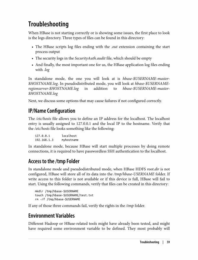
TroubleshootingWhen HBase is not starting correctly or is showing some issues, the first place to lookis the logs directory. Three types of files can be found in this directory:

• The HBase scripts log files ending with the .out extension containing the startprocess output

• The security logs in the SecurityAuth.audit file, which should be empty• And finally, the most important one for us, the HBase application log files ending

with .log

In standalone mode, the one you will look at is hbase-$USERNAME-master-$HOSTNAME.log. In pseudodistributed mode, you will look at hbase-$USERNAME-regionserver-$HOSTNAME.log in addition to hbase-$USERNAME-master-$HOSTNAME.log

Next, we discuss some options that may cause failures if not configured correctly.

IP/Name ConfigurationThe /etc/hosts file allows you to define an IP address for the localhost. The localhostentry is usually assigned to 127.0.0.1 and the local IP to the hostname. Verify thatthe /etc/hosts file looks something like the following:

127.0.0.1 localhost192.168.1.3 myhostname

In standalone mode, because HBase will start multiple processes by doing remoteconnections, it is required to have passwordless SSH authentication to the localhost.

Access to the /tmp FolderIn standalone mode and pseudodistributed mode, when HBase HDFS root.dir is notconfigured, HBase will store all of its data into the /tmp/hbase-USERNAME folder. Ifwrite access to this folder is not available or if this device is full, HBase will fail tostart. Using the following commands, verify that files can be created in this directory:

mkdir /tmp/hbase-$USERNAMEtouch /tmp/hbase-$USERNAME/test.txtrm -rf /tmp/hbase-$USERNAME

If any of those three commands fail, verify the rights in the /tmp folder.

Environment VariablesDifferent Hadoop or HBase-related tools might have already been tested, and mighthave required some environment variable to be defined. They most probably will

Troubleshooting | 59

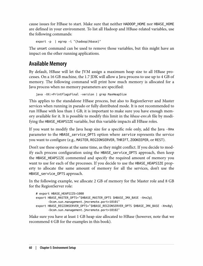
cause issues for HBase to start. Make sure that neither HADOOP_HOME nor HBASE_HOMEare defined in your environment. To list all Hadoop and HBase-related variables, usethe following commands:

export -p | egrep -i "(hadoop|hbase)"

The unset command can be used to remove those variables, but this might have animpact on the other running applications.

Available MemoryBy default, HBase will let the JVM assign a maximum heap size to all HBase pro‐cesses. On a 16 GB machine, the 1.7 JDK will allow a Java process to use up to 4 GB ofmemory. The following command will print how much memory is allocated for aJava process when no memory parameters are specified:

java -XX:+PrintFlagsFinal -version | grep MaxHeapSize

This applies to the standalone HBase process, but also to RegionServer and Masterservices when running in pseudo or fully distributed mode. It is not recommended torun HBase with less than 1 GB; it is important to make sure you have enough mem‐ory available for it. It is possible to modify this limit in the hbase-env.sh file by modi‐fying the HBASE_HEAPSIZE variable, but this variable impacts all HBase roles.

If you want to modify the Java heap size for a specific role only, add the Java -Xmxparameter to the HBASE_service_OPTS option where service represents the serviceyou want to configure (e.g., MASTER, REGIONSERVER, THRIFT, ZOOKEEPER, or REST).

Don’t use these options at the same time, as they might conflict. If you decide to mod‐ify each process configuration using the HBASE_service_OPTS approach, then keepthe HBASE_HEAPSIZE commented and specify the required amount of memory youwant to use for each of the processes. If you decide to use the HBASE_HEAPSIZE prop‐erty to allocate the same amount of memory for all the services, don’t use theHBASE_service_OPTS approach.

In the following example, we allocate 2 GB of memory for the Master role and 8 GBfor the RegionServer role:

# export HBASE_HEAPSIZE=1000export HBASE_MASTER_OPTS="$HBASE_MASTER_OPTS $HBASE_JMX_BASE -Xmx2g\ -Dcom.sun.management.jmxremote.port=10101"export HBASE_REGIONSERVER_OPTS="$HBASE_REGIONSERVER_OPTS $HBASE_JMX_BASE -Xmx8g\ -Dcom.sun.management.jmxremote.port=10102"

Make sure you have at least 1 GB heap size allocated to HBase (however, note that werecommend 4 GB for the examples in this book).

60 | Chapter 5: Environment Setup

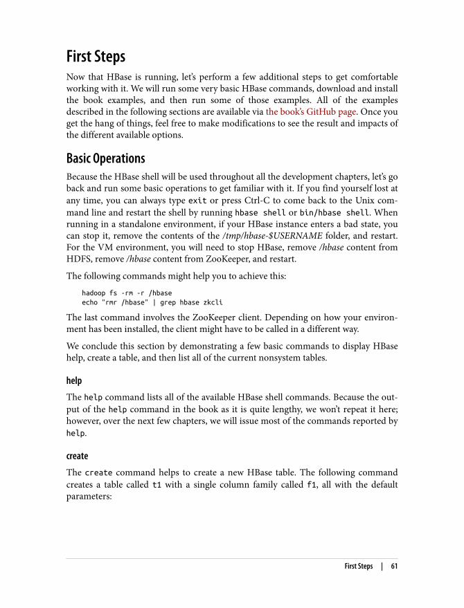
First StepsNow that HBase is running, let’s perform a few additional steps to get comfortableworking with it. We will run some very basic HBase commands, download and installthe book examples, and then run some of those examples. All of the examplesdescribed in the following sections are available via the book’s GitHub page. Once youget the hang of things, feel free to make modifications to see the result and impacts ofthe different available options.

Basic OperationsBecause the HBase shell will be used throughout all the development chapters, let’s goback and run some basic operations to get familiar with it. If you find yourself lost atany time, you can always type exit or press Ctrl-C to come back to the Unix com‐mand line and restart the shell by running hbase shell or bin/hbase shell. Whenrunning in a standalone environment, if your HBase instance enters a bad state, youcan stop it, remove the contents of the /tmp/hbase-$USERNAME folder, and restart.For the VM environment, you will need to stop HBase, remove /hbase content fromHDFS, remove /hbase content from ZooKeeper, and restart.

The following commands might help you to achieve this:

hadoop fs -rm -r /hbaseecho "rmr /hbase" | grep hbase zkcli

The last command involves the ZooKeeper client. Depending on how your environ‐ment has been installed, the client might have to be called in a different way.

We conclude this section by demonstrating a few basic commands to display HBasehelp, create a table, and then list all of the current nonsystem tables.

help

The help command lists all of the available HBase shell commands. Because the out‐put of the help command in the book as it is quite lengthy, we won’t repeat it here;however, over the next few chapters, we will issue most of the commands reported byhelp.

create

The create command helps to create a new HBase table. The following commandcreates a table called t1 with a single column family called f1, all with the defaultparameters:

First Steps | 61

hbase(main):002:0> create 't1', 'f1'0 row(s) in 1.2860 seconds

=> Hbase::Table - t1

list

The list command shows the newly created table:

hbase(main):003:0> listTABLEt11 row(s) in 0.0100 seconds

=> ["t1"]hbase(main):004:0>

list only reports user tables. User tables are nonsystem tables (i.e., they are tablesthat are explicitly created by the user).

If everything has been installed and is running correctly, you should have been able torun those three commands with outputs very similar to what has been reported.

Import Code ExamplesThe examples presented in this book are available in full via the book’s GitHub repos‐itory. For the sake of brevity and to focus on the most important parts of the code,the examples presented here have been condensed. The names of the examples usedin the book match the names of the files in the GitHub repository. Package namescorrespond to this book’s chapter numbering. This naming convention will allow youto easily and quickly find the code you are looking for in the example repository. Forexample, the TestInstallation sample code that we will use in Example 5-1 is avail‐able in package com.architecting.ch05 under the name TestInstallation.java.

Also, because many examples depend on others (e.g., scan dependson table creation and data generation), some examples will reuseother examples, and some helper classes are used to prepare theenvironment and make results predictable. You are invited to mod‐ify those helpers and those examples to create different environ‐ments and test different scenarios, such as generating more data,bigger values, or even corrupted information to test failurehandling.

To download, build, and modify the examples, you will need the following tools to beinstalled and configured (if you are running the examples in the QuickStart VM, allthose tools are already installed for you; if you are running the examples in a Linux

62 | Chapter 5: Environment Setup

VM, you will need to use package management tools such as APT or yum to installthem):

Text editorTo look at the examples and modify them, you will need a text editor. It can be viin a terminal, xemacs, or any other kind of editor you want as long as you arecomfortable with it. For simplicity, we built all the examples and code usingEclipse.

GitAs stated on its website, “Git is a free and open source distributed version controlsystem designed to handle everything from small to very large projects withspeed and efficiency.” You will need Git to retrieve the source code for the exam‐ples. It is available on all major Linux distributions.

This book’s examples are hosted on GitHub, which provides an online public Gitservice. You can also access and download the examples using a web browser.

MavenThe Apache website defines Maven as “a software project management and com‐prehension tool. Based on the concept of a project object model (POM), Mavencan manage a project’s build, reporting and documentation from a central pieceof information.” The Architecting HBase Applications source code is configured tobuild using Maven. The instructions for building and packaging the examples areprovided in the following subsections.

If you choose to use the Cloudera QuickStart VM 5.4.0 or older todevelop, you will need to use the command line to retrieve the Gitrepository. Indeed, the Eclipse version provided with the VM is notcompatible with the Eclipse m2e-egit plugin. If you prefer to useEclipse in the VM and use the import wizard, you will need toupgrade it to a more recent version.

Download from command lineThe first thing we need to do is download the source repository. As we explained inthe previous section, examples are hosted on a Git repository. If you prefer to useEclipse for all those operations, refer to “Download and build using Eclipse” on page65.

The following Git command will download a copy of the examples into a local folder:

git clone https://github.com/ArchitectingHBase/examples.git ~/ahae

This will create a directory called architecting-hbase-applications-examples, whichlooks like this:

First Steps | 63

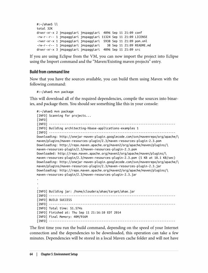
#:~/ahae$ lltotal 32Kdrwxr-xr-x 2 jmspaggiari jmspaggiari 4096 Sep 11 21:09 conf-rw-r--r-- 1 jmspaggiari jmspaggiari 11324 Sep 11 21:09 LICENSE-rwxr-xr-x 1 jmspaggiari jmspaggiari 5938 Sep 11 21:09 pom.xml-rw-r--r-- 1 jmspaggiari jmspaggiari 38 Sep 11 21:09 README.mddrwxr-xr-x 3 jmspaggiari jmspaggiari 4096 Sep 11 21:09 src

If you are using Eclipse from the VM, you can now import the project into Eclipseusing the Import command and the “Maven/Existing maven projects” entry.

Build from command lineNow that you have the sources available, you can build them using Maven with thefollowing command:

#:~/ahae$ mvn package

This will download all of the required dependencies, compile the sources into binar‐ies, and package them. You should see something like this in your console:

#:~/ahae$ mvn package[INFO] Scanning for projects...[INFO][INFO] ------------------------------------------------------------------------[INFO] Building architecting-hbase-applications-examples 1[INFO] ------------------------------------------------------------------------Downloading: http://onejar-maven-plugin.googlecode.com/svn/mavenrepo/org/apache/\maven/plugins/maven-resources-plugin/2.3/maven-resources-plugin-2.3.pomDownloading: http://repo.maven.apache.org/maven2/org/apache/maven/plugins/\maven-resources-plugin/2.3/maven-resources-plugin-2.3.pomDownloaded: http://repo.maven.apache.org/maven2/org/apache/maven/plugins/\maven-resources-plugin/2.3/maven-resources-plugin-2.3.pom (5 KB at 18.1 KB/sec)Downloading: http://onejar-maven-plugin.googlecode.com/svn/mavenrepo/org/apache/\maven/plugins/maven-resources-plugin/2.3/maven-resources-plugin-2.3.jarDownloading: http://repo.maven.apache.org/maven2/org/apache/maven/plugins/\maven-resources-plugin/2.3/maven-resources-plugin-2.3.jar...[INFO] Building jar: /home/cloudera/ahae/target/ahae.jar[INFO] ------------------------------------------------------------------------[INFO] BUILD SUCCESS[INFO] ------------------------------------------------------------------------[INFO] Total time: 51.574s[INFO] Finished at: Thu Sep 11 21:16:10 EDT 2014[INFO] Final Memory: 40M/916M[INFO] ------------------------------------------------------------------------

The first time you run the build command, depending on the speed of your Internetconnection and the dependencies to be downloaded, this operation can take a fewminutes. Dependencies will be stored in a local Maven cache folder and will not have

64 | Chapter 5: Environment Setup

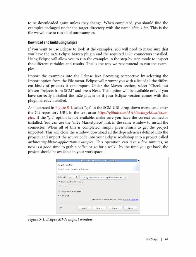
to be downloaded again unless they change. When completed, you should find theexamples packaged under the target directory with the name ahae-1.jar. This is thefile we will use to run all of our examples.

Download and build using EclipseIf you want to use Eclipse to look at the examples, you will need to make sure thatyou have the m2e Eclipse Maven plugin and the required EGit connectors installed.Using Eclipse will allow you to run the examples in the step-by-step mode to inspectthe different variables and results. This is the way we recommend to run the exam‐ples.

Import the examples into the Eclipse Java Browsing perspective by selecting theImport option from the File menu. Eclipse will prompt you with a list of all the differ‐ent kinds of projects it can import. Under the Maven section, select “Check outMaven Projects from SCM” and press Next. This option will be available only if youhave correctly installed the m2e plugin or if your Eclipse version comes with theplugin already installed.

As illustrated in Figure 5-1, select “git” in the SCM URL drop-down menu, and enterthe Git repository URL in the text area: https://github.com/ArchitectingHBase/examples. If the “git” option is not available, make sure you have the correct connectorinstalled. You can use the “m2e Marketplace” link in the same window to install theconnector. When all of this is completed, simply press Finish to get the projectimported. This will close the window, download all the dependencies defined into theproject, and import the source code into your Eclipse workshop into a project calledarchitecting-hbase-applications-examples. This operation can take a few minutes, sonow is a good time to grab a coffee or go for a walk—by the time you get back, theproject should be available in your workspace.

Figure 5-1. Eclipse MVN import window

First Steps | 65

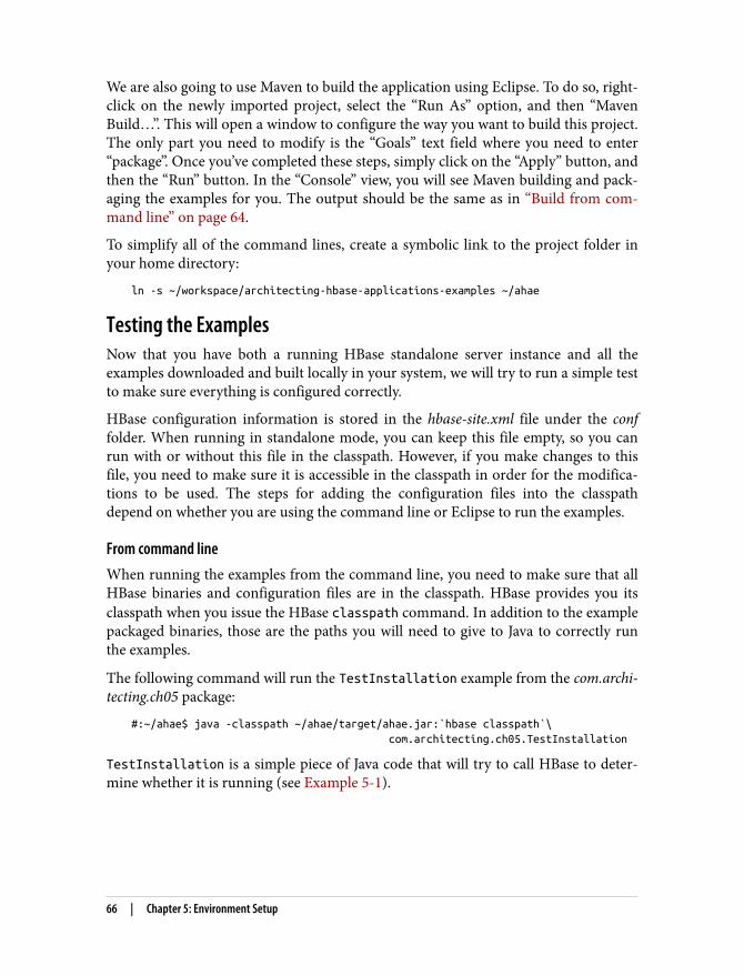
We are also going to use Maven to build the application using Eclipse. To do so, right-click on the newly imported project, select the “Run As” option, and then “MavenBuild…”. This will open a window to configure the way you want to build this project.The only part you need to modify is the “Goals” text field where you need to enter“package”. Once you’ve completed these steps, simply click on the “Apply” button, andthen the “Run” button. In the “Console” view, you will see Maven building and pack‐aging the examples for you. The output should be the same as in “Build from com‐mand line” on page 64.

To simplify all of the command lines, create a symbolic link to the project folder inyour home directory:

ln -s ~/workspace/architecting-hbase-applications-examples ~/ahae

Testing the ExamplesNow that you have both a running HBase standalone server instance and all theexamples downloaded and built locally in your system, we will try to run a simple testto make sure everything is configured correctly.

HBase configuration information is stored in the hbase-site.xml file under the conffolder. When running in standalone mode, you can keep this file empty, so you canrun with or without this file in the classpath. However, if you make changes to thisfile, you need to make sure it is accessible in the classpath in order for the modifica‐tions to be used. The steps for adding the configuration files into the classpathdepend on whether you are using the command line or Eclipse to run the examples.

From command lineWhen running the examples from the command line, you need to make sure that allHBase binaries and configuration files are in the classpath. HBase provides you itsclasspath when you issue the HBase classpath command. In addition to the examplepackaged binaries, those are the paths you will need to give to Java to correctly runthe examples.

The following command will run the TestInstallation example from the com.archi‐tecting.ch05 package:

#:~/ahae$ java -classpath ~/ahae/target/ahae.jar:`hbase classpath`\ com.architecting.ch05.TestInstallation

TestInstallation is a simple piece of Java code that will try to call HBase to deter‐mine whether it is running (see Example 5-1).

66 | Chapter 5: Environment Setup

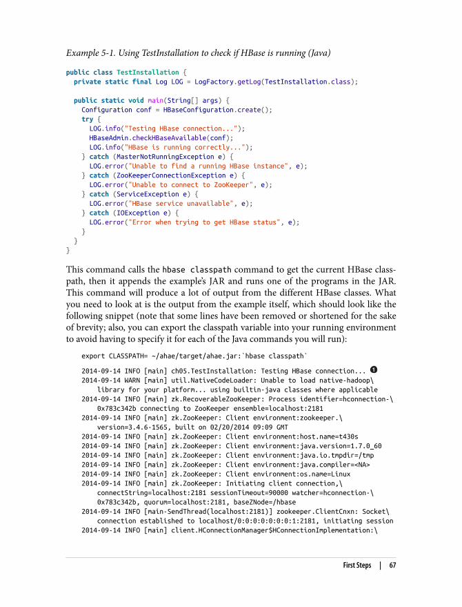
Example 5-1. Using TestInstallation to check if HBase is running (Java)

public class TestInstallation { private static final Log LOG = LogFactory.getLog(TestInstallation.class);

public static void main(String[] args) { Configuration conf = HBaseConfiguration.create(); try { LOG.info("Testing HBase connection..."); HBaseAdmin.checkHBaseAvailable(conf); LOG.info("HBase is running correctly..."); } catch (MasterNotRunningException e) { LOG.error("Unable to find a running HBase instance", e); } catch (ZooKeeperConnectionException e) { LOG.error("Unable to connect to ZooKeeper", e); } catch (ServiceException e) { LOG.error("HBase service unavailable", e); } catch (IOException e) { LOG.error("Error when trying to get HBase status", e); } }}

This command calls the hbase classpath command to get the current HBase class‐path, then it appends the example’s JAR and runs one of the programs in the JAR.This command will produce a lot of output from the different HBase classes. Whatyou need to look at is the output from the example itself, which should look like thefollowing snippet (note that some lines have been removed or shortened for the sakeof brevity; also, you can export the classpath variable into your running environmentto avoid having to specify it for each of the Java commands you will run):

export CLASSPATH= ~/ahae/target/ahae.jar:`hbase classpath`

2014-09-14 INFO [main] ch05.TestInstallation: Testing HBase connection... 2014-09-14 WARN [main] util.NativeCodeLoader: Unable to load native-hadoop\ library for your platform... using builtin-java classes where applicable2014-09-14 INFO [main] zk.RecoverableZooKeeper: Process identifier=hconnection-\ 0x783c342b connecting to ZooKeeper ensemble=localhost:21812014-09-14 INFO [main] zk.ZooKeeper: Client environment:zookeeper.\ version=3.4.6-1565, built on 02/20/2014 09:09 GMT2014-09-14 INFO [main] zk.ZooKeeper: Client environment:host.name=t430s2014-09-14 INFO [main] zk.ZooKeeper: Client environment:java.version=1.7.0_602014-09-14 INFO [main] zk.ZooKeeper: Client environment:java.io.tmpdir=/tmp2014-09-14 INFO [main] zk.ZooKeeper: Client environment:java.compiler=<NA>2014-09-14 INFO [main] zk.ZooKeeper: Client environment:os.name=Linux2014-09-14 INFO [main] zk.ZooKeeper: Initiating client connection,\ connectString=localhost:2181 sessionTimeout=90000 watcher=hconnection-\ 0x783c342b, quorum=localhost:2181, baseZNode=/hbase2014-09-14 INFO [main-SendThread(localhost:2181)] zookeeper.ClientCnxn: Socket\ connection established to localhost/0:0:0:0:0:0:0:1:2181, initiating session2014-09-14 INFO [main] client.HConnectionManager$HConnectionImplementation:\

First Steps | 67

Closing master protocol: MasterService2014-09-14 INFO [main] client.HConnectionManager$HConnectionImplementation:\ Closing zookeeper sessionid=0x1487467e621000a2014-09-14 INFO [main] zk.ZooKeeper: Session: 0x1487467e621000a closed2014-09-14 INFO [main-EventThread] zookeeper.ClientCnxn: EventThread shut down2014-09-14 INFO [main] ch05.TestInstallation: HBase is running correctly...

and are two lines printed by the example.

If you don’t see the “HBase is running correctly…” line, you’ll need to make sure yourHBase server is running correctly and examples have been built as expected.

From EclipseTo run an example from Eclipse, you simply need to right-click on it, select “Run As”and then “Java Application”. Output of the same TestInstallation example runfrom Eclipse should be shorter and should include the HBase outputted logs. Youshould see the following lines printed in the console:

2014-09-14 18:45:34 INFO ch05.TestInstallation: Testing HBase connection......2014-09-14 18:45:35 INFO ch05.TestInstallation: HBase is running correctly...

When running examples from Eclipse, the hbase-site.xml file thatwas used for the configuration is the default one embedded in thedependencies. Modifications of your local configuration file willnot be used by your examples running in Eclipse unless you specif‐ically add your HBase configuration directory into your projectclasspath. You can do this in your project properties. In the JavaBuild Path section, go to the Libraries tab, click on “Add ExternalClass Folder…” and add the directory where your hbase-site.xml fileis. If you installed HBase in standalone mode, the file should beunder ~/hbase/conf; otherwise, the file should be under /etc/hbase/conf/. We also recommend doing the same thing for the Hadoopconfiguration files.

Pseudodistributed and Fully DistributedRunning and managing an HBase cluster in distributed mode is beyond the scope ofthis book and will not be discussed here. To better understand how to configure andrun HBase in this mode, we recommend referring to the Apache HBase ReferenceGuide. We will, however, provide a few configuration hints for running in pseudo-distributed mode.

To configure your HBase instance to run in pseudodistributed or distributed mode,add the following required configuration parameters into the conf/hbase-site.xml:

68 | Chapter 5: Environment Setup

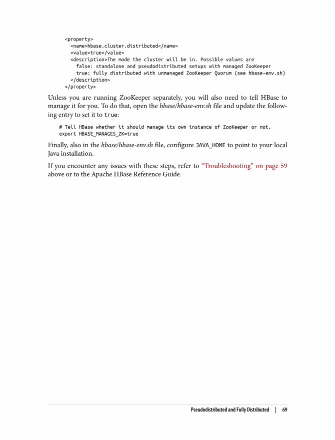
<property> <name>hbase.cluster.distributed</name> <value>true</value> <description>The mode the cluster will be in. Possible values are false: standalone and pseudodistributed setups with managed ZooKeeper true: fully distributed with unmanaged ZooKeeper Quorum (see hbase-env.sh) </description> </property>

Unless you are running ZooKeeper separately, you will also need to tell HBase tomanage it for you. To do that, open the hbase/hbase-env.sh file and update the follow‐ing entry to set it to true:

# Tell HBase whether it should manage its own instance of ZooKeeper or not.export HBASE_MANAGES_ZK=true

Finally, also in the hbase/hbase-env.sh file, configure JAVA_HOME to point to your localJava installation.

If you encounter any issues with these steps, refer to “Troubleshooting” on page 59above or to the Apache HBase Reference Guide.

Pseudodistributed and Fully Distributed | 69

PART II

Use Cases

It is important to have a solid understanding of HBase principles before jumping intothe use-case section. After reviewing Part I, we can start to look at how HBase can beused in real-life use cases. We will be looking at four core uses for HBase: usingHBase with Solr, near real-time serving system with HBase, using HBase for MasterData Management, and using HBase as a document store.

Throughout Part II we will describe the business need, the way data is coming in, theway data is retrieved, and how it is processed. We will also provide draft solutions andcode examples to implement those use cases. The goal here is to greatly reduce timeto value for HBase applications by enabling you through detailed code examples.When specific aspects are approached, we will also detail how they impact the usecase and why, while diving deeper into HBase internals when required.

It is impossible to cover all HBase use cases in a single book, so we have selected whatwe think covers the majority of HBase usage. We hope by going through all thedescribed scenarios, you will attain a sense of HBase best practices, and then you willbe able to apply the same thinking to your specific use case.

CHAPTER 6

Use Case: HBase as a System of Record

The first use case that we will examine is from Omneo (a division of Camstar, a Sie‐mens Company). Omneo is a big data analytics platform that assimilates data fromdisparate sources to provide a 360-degree view of product quality data across the sup‐ply chain. Manufacturers of all sizes are confronted with massive amounts of data,and manufacturing datasets comprise the key attributes of big data. These datasets arehigh volume, rapidly generated, and come in many varieties. When tracking productsbuilt through a complex, multitier supply chain, the challenges are exacerbated by thelack of a centralized data store and because there is no unified data format. Omneoingests data from all areas of the supply chain, such as manufacturing, test, assembly,repair, service, and field.

Omneo offers this system to its end customers as a software-as-a-service (SaaS)model. This platform must provide users the ability to investigate product qualityissues, analyze contributing factors, and identify items for containment and control.The ability to offer a rapid turnaround for early detection and correction of problemscan result in greatly reduced costs and significantly improved consumer brand confi‐dence. Omneo starts by building a unified data model that links the data sources sousers can explore the factors that impact product quality throughout the product life‐cycle. Furthermore, Omneo provides a centralized data store, and applications thatfacilitate the analysis of all product quality data in a single, unified environment.

Omneo evaluated numerous NoSQL systems and other data platforms. Its parentcompany, Camstar, has been in business for over 30 years, giving Omneo a well-established IT operations system. When Omneo was created, the team was givencarte blanche to build its own system. Knowing the daunting task of handling all ofthe data at hand, Omneo decided against building a traditional EDW. Although otherbig data technologies such as Cassandra and MongoDB were considered, Hadoopwas ultimately chosen as the foundation for the Omneo platform. The primary rea‐

73

son for this decision came down to ecosystem or lack thereof from the other technol‐ogies. The fully integrated ecosystem that Hadoop offered with MapReduce, HBase,Solr, and Impala allowed Omneo to handle the data in a single platform without theneed to migrate the data between disparate systems.

The solution must be able to handle the data of numerous products and customersbeing ingested and processed on the same cluster. This can make handling data vol‐umes and sizing quite precarious, as one customer could provide 80%–90% of thetotal records. At the time of writing, Omneo hosts multiple customers on the samecluster for a rough record count of 6+ billion records stored in ~50 nodes. The totalcombined set of data in the HDFS is approximately 100 TBs. Importantly, as we getinto the overall architecture of the system, we will note where duplicating data ismandatory and where savings can be introduced by using a unified data format.

Omneo has fully embraced the Hadoop ecosystem for its overall architecture, andalso takes advantage of Hadoop’s Avro data serialization system. Avro is a popular fileformat for storing data in the Hadoop world. Avro allows for a schema to be storedwith data, making it easier for different processing systems (e.g., MapReduce, HBase,and Impala/Hive) to easily access the data without serializing and deserializing thedata over and over again.

The high-level Omneo architecture consists of the following phases:

• Ingest/pre-processing• Processing/serving• User experience

Ingest/Pre-ProcessingThe ingest/pre-processing phase includes acquiring the flat files, landing them inHDFS, and converting the files into Avro. As illustrated in Figure 6-1, Omneo cur‐rently receives all files in a batch manner. The files arrive in a CSV format or in anXML file format. The files are loaded into HDFS through the HDFS API. Once thefiles are loaded into Hadoop, a series of transformations are performed to join the rel‐evant datasets together. Most of these joins are done based on a primary key in thedata (in the case of electronic manufacturing, this is normally a serial number toidentify the product throughout its lifecycle). These transformations are all handledthrough the MapReduce framework. Omneo wanted to provide a graphical interfacefor consultants to integrate the data rather than code custom MapReduce. To accom‐plish this, Omneo partnered with Pentaho to expedite time to production. Once thedata has been transformed and joined together, it is then serialized into the Avroformat.

74 | Chapter 6: Use Case: HBase as a System of Record

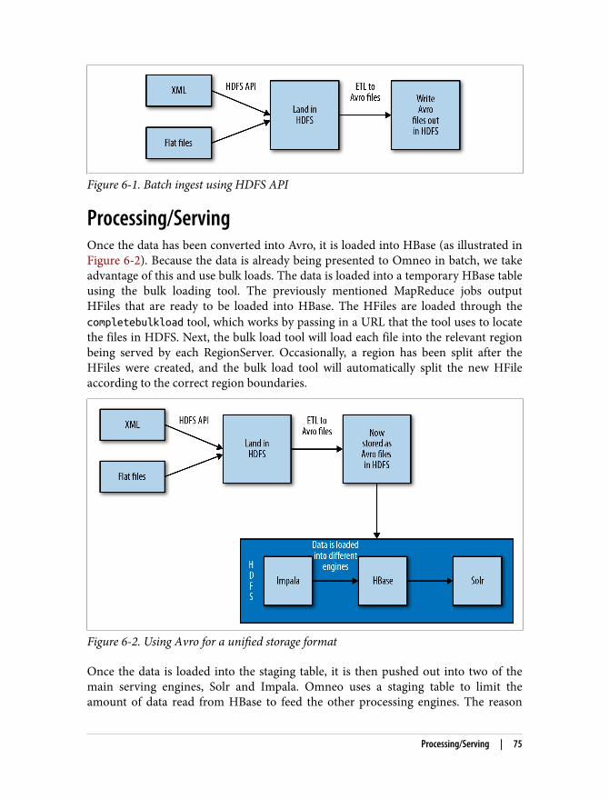
Figure 6-1. Batch ingest using HDFS API

Processing/ServingOnce the data has been converted into Avro, it is loaded into HBase (as illustrated inFigure 6-2). Because the data is already being presented to Omneo in batch, we takeadvantage of this and use bulk loads. The data is loaded into a temporary HBase tableusing the bulk loading tool. The previously mentioned MapReduce jobs outputHFiles that are ready to be loaded into HBase. The HFiles are loaded through thecompletebulkload tool, which works by passing in a URL that the tool uses to locatethe files in HDFS. Next, the bulk load tool will load each file into the relevant regionbeing served by each RegionServer. Occasionally, a region has been split after theHFiles were created, and the bulk load tool will automatically split the new HFileaccording to the correct region boundaries.

Figure 6-2. Using Avro for a unified storage format

Once the data is loaded into the staging table, it is then pushed out into two of themain serving engines, Solr and Impala. Omneo uses a staging table to limit theamount of data read from HBase to feed the other processing engines. The reason

Processing/Serving | 75

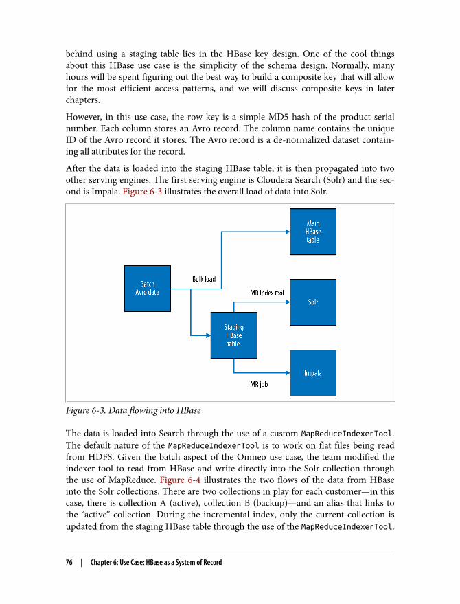
behind using a staging table lies in the HBase key design. One of the cool thingsabout this HBase use case is the simplicity of the schema design. Normally, manyhours will be spent figuring out the best way to build a composite key that will allowfor the most efficient access patterns, and we will discuss composite keys in laterchapters.

However, in this use case, the row key is a simple MD5 hash of the product serialnumber. Each column stores an Avro record. The column name contains the uniqueID of the Avro record it stores. The Avro record is a de-normalized dataset contain‐ing all attributes for the record.

After the data is loaded into the staging HBase table, it is then propagated into twoother serving engines. The first serving engine is Cloudera Search (Solr) and the sec‐ond is Impala. Figure 6-3 illustrates the overall load of data into Solr.

Figure 6-3. Data flowing into HBase

The data is loaded into Search through the use of a custom MapReduceIndexerTool.The default nature of the MapReduceIndexerTool is to work on flat files being readfrom HDFS. Given the batch aspect of the Omneo use case, the team modified theindexer tool to read from HBase and write directly into the Solr collection throughthe use of MapReduce. Figure 6-4 illustrates the two flows of the data from HBaseinto the Solr collections. There are two collections in play for each customer—in thiscase, there is collection A (active), collection B (backup)—and an alias that links tothe “active” collection. During the incremental index, only the current collection isupdated from the staging HBase table through the use of the MapReduceIndexerTool.

76 | Chapter 6: Use Case: HBase as a System of Record

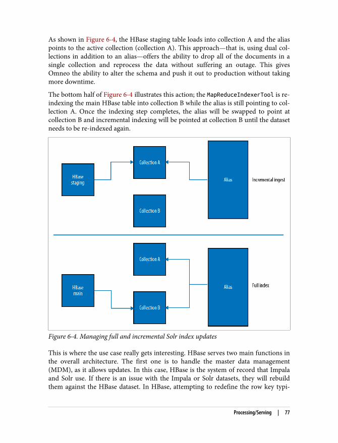
As shown in Figure 6-4, the HBase staging table loads into collection A and the aliaspoints to the active collection (collection A). This approach—that is, using dual col‐lections in addition to an alias—offers the ability to drop all of the documents in asingle collection and reprocess the data without suffering an outage. This givesOmneo the ability to alter the schema and push it out to production without takingmore downtime.

The bottom half of Figure 6-4 illustrates this action; the MapReduceIndexerTool is re-indexing the main HBase table into collection B while the alias is still pointing to col‐lection A. Once the indexing step completes, the alias will be swapped to point atcollection B and incremental indexing will be pointed at collection B until the datasetneeds to be re-indexed again.

Figure 6-4. Managing full and incremental Solr index updates

This is where the use case really gets interesting. HBase serves two main functions inthe overall architecture. The first one is to handle the master data management(MDM), as it allows updates. In this case, HBase is the system of record that Impalaand Solr use. If there is an issue with the Impala or Solr datasets, they will rebuildthem against the HBase dataset. In HBase, attempting to redefine the row key typi‐

Processing/Serving | 77

cally results in having to rebuild the entire dataset. Omneo first attempted to tacklefaster lookups for secondary and tertiary fields by leveraging composite keys. It turnsout the end users enjoy changing the primary lookups based on the metrics they arelooking at. For example, they may look up by part time, test, date, or any other arbi‐tary field in the data. This is one of the reasons Omneo avoided leveraging compositekeys, and used Solr to add extra indexes to HBase. The second and most importantpiece is HBase actually stores all of the records being served to the end user. Let’s lookat a couple sample fields from Omneo’s Solr schema.xml:

<schema name="example" version="1.5"><fields> <field name="id" type="string" indexed="true" stored="true" required="true" multiValued="false" /> <field name="rowkey" type="binary" indexed="false" stored="true" omitNorms="true" required="true"/> <field name="eventid" type="string" indexed="true" stored="false" omitNorms="true" required="true"/> <field name="docType" type="string" indexed="true" stored="false" omitNorms="true"/> <field name="partName" type="lowercase" indexed="true" stored="false" omitNorms="true"/> <field name="partNumber" type="lowercase" indexed="true" stored="false" omitNorms="true"/>… <field name="_version_" type="long" indexed="true" stored="true"/></fields>

Looking at some of the fields in this schema.xml file, we can see that Omneo is onlyflagging the HBase row key and the required Solr fields (id and _version_) as Stored,which will directly write these results to HDFS. The other fields are flagged asIndexed; which will store the data in a special index directory in HDFS. The indexedattribute makes a field searchable, sortable, and facetable; it is also stored in memory.The stored attributes make the fields retrievable through search and persisted toHDFS. Omneo ingests records that can have many columns present, ranging fromhundreds to thousands of fields depending on the product being ingested. For thepurposes of faceting and natural language searching, typically only a small subset ofthose fields are necessary. The amount of fields indexed will vary per customer anduse case. This is a very common pattern, as the actual data results displayed to thecustomer are being served from the application calling scans and multigets fromHBase based on the stored data. Just indexing the fields serves multiple purposes:

• All of the facets are served out of memory from Solr, offering tighter and morepredictable SLAs.

• The current state of Solr Cloud on HDFS writes the data to HDFS per shard andreplica. If HDFS replication is set to the default factor of 3, then a shard with tworeplicas will have nine copies of the data on HDFS. This will not normally affect a

78 | Chapter 6: Use Case: HBase as a System of Record

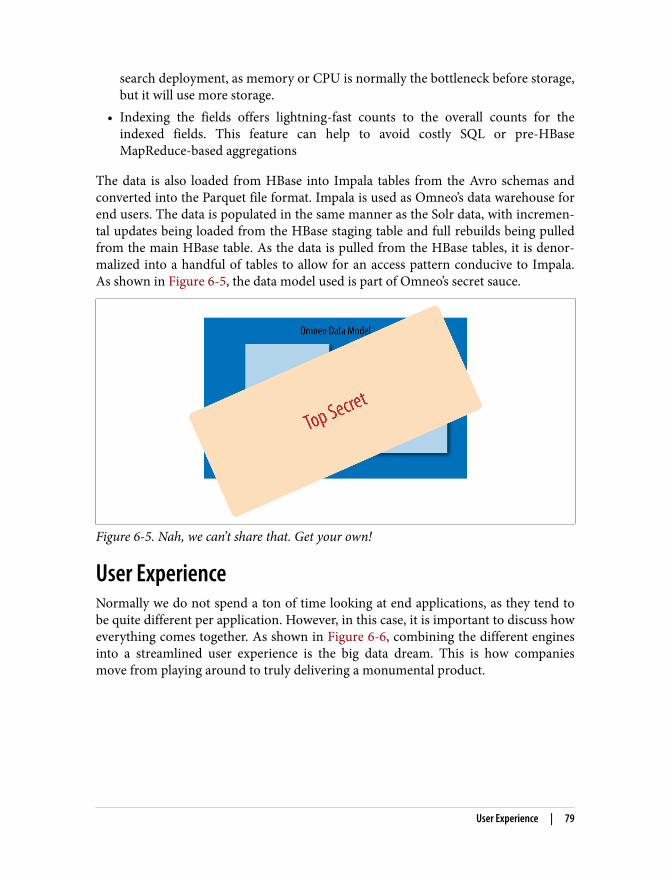
search deployment, as memory or CPU is normally the bottleneck before storage,but it will use more storage.

• Indexing the fields offers lightning-fast counts to the overall counts for theindexed fields. This feature can help to avoid costly SQL or pre-HBaseMapReduce-based aggregations

The data is also loaded from HBase into Impala tables from the Avro schemas andconverted into the Parquet file format. Impala is used as Omneo’s data warehouse forend users. The data is populated in the same manner as the Solr data, with incremen‐tal updates being loaded from the HBase staging table and full rebuilds being pulledfrom the main HBase table. As the data is pulled from the HBase tables, it is denor‐malized into a handful of tables to allow for an access pattern conducive to Impala.As shown in Figure 6-5, the data model used is part of Omneo’s secret sauce.

Figure 6-5. Nah, we can’t share that. Get your own!

User ExperienceNormally we do not spend a ton of time looking at end applications, as they tend tobe quite different per application. However, in this case, it is important to discuss howeverything comes together. As shown in Figure 6-6, combining the different enginesinto a streamlined user experience is the big data dream. This is how companiesmove from playing around to truly delivering a monumental product.

User Experience | 79

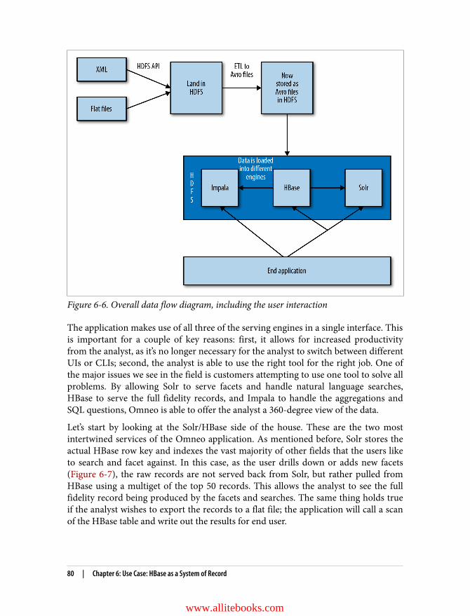
Figure 6-6. Overall data flow diagram, including the user interaction

The application makes use of all three of the serving engines in a single interface. Thisis important for a couple of key reasons: first, it allows for increased productivityfrom the analyst, as it’s no longer necessary for the analyst to switch between differentUIs or CLIs; second, the analyst is able to use the right tool for the right job. One ofthe major issues we see in the field is customers attempting to use one tool to solve allproblems. By allowing Solr to serve facets and handle natural language searches,HBase to serve the full fidelity records, and Impala to handle the aggregations andSQL questions, Omneo is able to offer the analyst a 360-degree view of the data.

Let’s start by looking at the Solr/HBase side of the house. These are the two mostintertwined services of the Omneo application. As mentioned before, Solr stores theactual HBase row key and indexes the vast majority of other fields that the users liketo search and facet against. In this case, as the user drills down or adds new facets(Figure 6-7), the raw records are not served back from Solr, but rather pulled fromHBase using a multiget of the top 50 records. This allows the analyst to see the fullfidelity record being produced by the facets and searches. The same thing holds trueif the analyst wishes to export the records to a flat file; the application will call a scanof the HBase table and write out the results for end user.

80 | Chapter 6: Use Case: HBase as a System of Record

www.allitebooks.com

Figure 6-7. Check out this Solr goodness

On the Impala side of the house, also known as performance analytics, models arebuilt and managed to handle SQL-like workloads. These are workloads that wouldnormally be forced into HBase or Solr. Performance analytics was designed to run aset of pre-packed application queries that can be run against the data to calculate keyperformance indicators (KPIs), as shown in Figure 6-8. The solution does not allowfor random free-form SQL queries to be utilized, as long-running rogue queries cancause performance degradation in a multitenant application. In the end, users canselect the KPIs they want to look at, and add extra functions to the queries (sums, avg,max, etc.).

Figure 6-8. Leveraging Impala for custom analytics

User Experience | 81

CHAPTER 7

Implementation of an UnderlyingStorage Engine

In the previous chapter, we described how Omneo uses the different Hadoop technol‐ogies to implement its use case. In this chapter, we will look more closely at all thedifferent parts involving HBase. We will not discuss each and every implementationdetail, but will cover all the required tools and examples to help you understand whatis important during this phase.

As usual when implementing an HBase project, the first consideration is the tableschema, which is the most important part of every HBase project. Designing anHBase schema can be straightforward, but depending on the use case, can also bequite complex and require significant planning and testing. It is a good practice toalways start with this task, keeping in mind how data is received from your applica‐tion (write path) and how you will need to retrieve it (read path). Read and writeaccess patterns will dictate most of the table design.

Table DesignAs we said and we will continue to say all over the book, table design is one of themost important parts of your project. The table schema, the key you will choose touse, and the different parameters you will configure will all have an impact on notonly the performances of your application but also on the consistency. This is why forall the use cases we will describe, we are going to spend a lot of time on the table’sdesign. After your application is running for weeks and storing terabytes of data,moving back from a bad table design to a good one will require duplicating the entiredataset, a lot of time, and usually an update to the client application. Those are allcostly operations that you might want to avoid by spending the right amount of timein this phase.

83

Table SchemaTable design for the Omneo use case is pretty easy, but let’s work through the steps soyou can apply a similar approach to your own table schema design. We want bothread and write paths to be efficient. In Omneo’s case, data is received from externalsystems in bulk. Therefore, unlike other ingestion patterns where data is inserted onesingle value at a time, here it can be processed directly in bulk format and doesn’trequire single random writes or updates based on the key. On the read side, the userneeds to be able to retrieve all the information for a specific sensor very quickly bysearching on any combination of sensor ID, event ID, date, and event type. There isno way we can design a key to allow all those retrieval criteria to be efficient. We willneed to rely on an external index, which given all of our criteria, will return a key thatwe will use to query HBase. Because the key will be retrieved from this external indexand we don’t need to look up or scan for it, we can simply use a hash of the sensor ID,with the column qualifier being the event ID. You can refer to “Generate Test Data”on page 88 to see a preview of the data format.

Sensors can have very similar IDs, such as 42, 43, and 44. However, sensor IDs canalso have a wide range (e.g., 40,000–49,000). If we use the original sensor ID as thekey, we might encounter hotspots on specific regions due to the keys’ sequentialnature. You can read more about hotspotting in Chapter 16.

Hashing keysOne option for dealing with hotspotting is to simply presplit the table based on thosedifferent known IDs to make sure they are correctly distributed accross the cluster.However, what if distribution of those IDs changes in the future? In that case, splitsmight not be correct anymore, and we might again end up with hot spots on someregions. If today all IDs are between 40xxxx and 49xxxx, regions will be split from thebeginning to 41, 41 to 42, 42 to 43, and so on. But if tomorrow a new group of sen‐sors is added with IDs from 40xxx to 39xxx, they will end up in the first region.Because it is not possible to forecast what the future IDs will be, we need to find asolution to ensure a good distribution whatever the IDs will be. When hashing data,even two initially close keys will produce a very different result. In this example, 42will produce 50a2fabfdd276f573ff97ace8b11c5f4 as its md5 hash, while 43 will pro‐duce f0287f33eba7192e2a9c6a14f829aa1a. As you can see, unlike the original sensorIDs 42 and 43, sorting those two md5 hashes puts them far from one another. Andeven if new IDs are coming, because they are now translated into a hexadecimalvalue, they will always be distributed between 0 and F. Using such a hashing approachwill ensure a good distribution of the data across all the regions, while given a specificsensor ID, we still have direct access to its data.

84 | Chapter 7: Implementation of an Underlying Storage Engine

The hash approach cannot be used when you need to scan yourdata keeping the initial order of the key, as the md5 version of thekey disrupts the original ordering, distributing the rows through‐out the table.

Column qualifierRegarding the column qualifier, the event ID will be used. The event ID is a hashvalue received from the downstream system, unique for the given event for this spe‐cific sensor. Each event has a specific type, such as “alert”, “warning”, or “RMA”(which stands for return merchandise authorization). At first, we considered usingthe event type as a column qualifier. However, a sensor can encounter a single eventtype multiple times. Each “warning” a sensor encountered would overwrite the previ‐ous “warning”, unless we used HBase’s “versions” feature. Using the unique event IDas the column qualifier allows us to have multiple events with the same type for thesame sensor being stored without having to code extra logic to use HBase’s “versions”feature to retrieve all of a sensor’s events.

Table ParametersTo get the best peformances possible, we have to look at all the parameters and makesure to set them as required depending on our need and usage. However, only theparameters that apply to this specific use case are listed in this section.

CompressionThe first parameter we’ll examine is the compression algorithm used when writingtable data to disk. HBase writes the data into HFiles in a block format. Each block is64 KB by default, and is not compressed. Blocks store the data belonging to oneregion and column family. A table’s columns usually contain related information,which normally results in a common data pattern. Compressing those blocks canalmost always give good results. As an example, it will be good to compress columnfamilies containing logs and customer information. HBase supports multiple com‐pression algorithms: LZO, GZ (for GZip), SNAPPY, and LZ4. Each compression algo‐rithm will have its own pros and cons. For each algorithm, consider the performanceimpact of compressing and decompressing the data versus the compression ratio (i.e.,was the data sufficiently compressed to warrant running the compression algo‐rithm?).

Snappy will be very fast in almost all operations but will have a lower compressionratio, while GZ will be more resource intensive but will normally compress better.The algorithm you will choose depends on your use case. It is recommended to test afew of them on a sample dataset to validate compression rate and performance. As anexample, a 1.6 GB CSV file generates 2.2 GB of uncompressed HFiles, while from the

Table Design | 85

exact same dataset, it uses only 1.5 GB with LZ4. Snappy compressed HFiles for thesame dataset take 1.5 GB, too. Because read and write latencies are important for us,we will use Snappy for our table. Be aware of the availability of the various compres‐sion libraries on different Linux distributions. For example, Debian does not includeSnappy libraries by default. Due to licensing, LZO and LZ4 libraries are usually notbundled with common Apache Hadoop distributions, and must be installedseparately.

Keep in mind that compression ratio might vary based on the datatype. Indeed, if you try to compress a text file, it will compressmuch better than a PNG image. For example, a 143,976 byte PNGfile will only compress to 143,812 bytes (a space savings of only2.3%), whereas a 143,509 byte XML file can compress as small as6,284 bytes (a 95.7% space savings!) It is recommended that youtest the different algorithms on your dataset before selecting one. Ifthe compression ratio is not significant, avoid using compressionand save processor overhead.

Data block encodingData block encoding is an HBase feature where keys are encoded and compressedbased on the previous key. One of the encoding options (FAST_DIFF) asks HBase tostore only the difference between the current key and the previous one. HBase storeseach cell individually, with its key and value. When a row has many cells, much spacecan be consumed by writing the same key for each cell. Therefore, activating the datablock encoding can allow important space saving. It is almost always helpful to acti‐vate data block encoding, so if you are not sure, activate FAST_DIFF. The current usecase will benefit from this encoding because a given row can have thousands ofcolumns.

Bloom filterBloom filters are useful in reducing unnecessary I/O by skipping input files fromHBase regions. A Bloom filter will tell HBase if a given key might be or is not in agiven file. But it doesn’t mean the key is definitively included in the file.

However, there are certain situations where Bloom filters are not required. For thecurrent use case, files are loaded once a day, and then a major compaction is run onthe table. As a result, there will almost always be only a single file per region. Also,queries to the HBase table will be based on results returned by Solr. This means readrequests will always succeed and return a value. Because of that, the Bloom filter willalways return true, and HBase will always open the file. As a result, for this specificuse case, the Bloom filter will be an overhead and is not required.

86 | Chapter 7: Implementation of an Underlying Storage Engine

Because Bloom filters are activated by default, in this case we will need to explicitlydisable them.

PresplittingPresplits are not really table parameters. Presplit information is not stored within themetadata of the table and is used only at the time of table creation. However, it’simportant to have an understanding of this step before moving on the implementa‐tion. Presplitting a table means asking HBase to split the table into multiple regionswhen it is created. HBase comes with different presplit algorithms. The goal of pre‐splitting a table is to make sure the initial load will be correctly distributed across allthe regions and will not hotspot a single region. Granted, data would be distributedover time as region splits occur automatically, but presplitting provides the distribu‐tion from the onset.

ImplementationNow that we have decided which parameters we want to set for our table, it’s time tocreate it. We will keep all the default parameters except the ones we just discussed.Run the following command in the HBase shell to create a table called “sensors” witha single column family and the parameters we just discussed, presplit into 15 regions(NUMREGIONS and SPLITALGO are the two parameters used to instruct HBase to pre-split the table):

hbase(main):001:0> create 'sensors', {NUMREGIONS => 15,\ SPLITALGO => 'HexStringSplit'}, \ {NAME => 'v', COMPRESSION => 'SNAPPY',\ BLOOMFILTER => 'NONE',\ DATA_BLOCK_ENCODING => 'FAST_DIFF'}

When your table is created, you can see its details using the HBase WebUI interfaceor the following shell command:

hbase(main):002:0> describe 'sensors'Table sensors is ENABLEDsensorsCOLUMN FAMILIES DESCRIPTION{NAME => 'v', DATA_BLOCK_ENCODING => 'FAST_DIFF', BLOOMFILTER => 'NONE',REPLICATION_SCOPE => '0', VERSIONS => '1', COMPRESSION => 'SNAPPY',MIN_VERSIONS => '0', TTL => 'FOREVER', KEEP_DELETED_CELLS => 'FALSE',BLOCKSIZE => '65536', IN_MEMORY => 'false', BLOCKCACHE => 'true'}1 row(s) in 0.1410 seconds

The NUMREGIONS and SPLITALGO parameters are used for the tablecreation but are not stored within the metadata of the table. It isnot possible to retrieve this information after the table has beencreated.

Table Design | 87

As you can see, the parameters we specified are listed in the output, along with thedefault table parameters. The default parameters might vary based on the HBase ver‐sion you are using. However, BLOOMFILTER, DATA_BLOCK_ENCODING, and COMPRESSIONshould be configured as we specified here.

Now that we have our table ready, we can move forward with the data preparation.

Data conversionTo be able to implement and test the described use case, we will need to have ingestdata into our system. Therefore, it will be required to generated some testing data thatwe will later process and transform.

Generate Test DataThe next goal is to generate a set of representative test data to run through our pro‐cess and verify the results. The first thing we will create is some data files with testvalues. The goal is to have a dataset to allow you to run the different commands andprograms.

In the examples, you will find a class called CSVGenerator, which creates data resem‐bling the code shown here:

1b87,58f67b33-5264-456e-938a-9d2e9c5f4db8,ALERT,NE-565,0-0000-000,1,ECEGYFFL ...3244,350cee9e-55fc-409d-b389-6780a8af9e76,RETURNED,NE-382,0-0000-000,1,OOQTY ...727d,b97df483-f0bd-4f24-8ff3-6988d8eff88c,ALERT,NE-858,0-0000-000,1,MSWOCQXM ...53d4,d8c39bf8-6f5f-4311-8ee5-9d3bce3e18d7,RETURNED,NE-881,0-0000-000,1,PMKMW ...1fa8,4a0bf5b3-680d-4b87-8d9e-e55f06614ae4,ALERT,NE-523,0-0000-000,1,IYIZSHKA ...

Each line contains a random sensor ID comprised of four characters (0 to 65535, rep‐resented in hexadecimal), then a random event ID, document type, part name, partnumber, version, and a payload formed of random letters (64 to 128 characters inlength). To generate a different workload, you can rerun the CSVGenerator code anytime you want. Subsequent parts of the example code will read this file from the~/ahae/resources/ch07 folder. This class will create files relative to where it’s run;therefore we need to run the class from the ~/ahae folder. If you want to increase orreduce the size of the dataset, simply update the following line:

for (int index = 0; index < 1000000; index++) {

You can run this data generator directly from Eclipse without any parameter or fromthe shell into the ~/ahae folder using the following command:

hbase -classpath ~/ahae/target/ahae.jar com.architecting.ch07.CSVGenerator

This will create a file called omneo.csv in ~/ahae/resources/ch07/omneo.csv.

88 | Chapter 7: Implementation of an Underlying Storage Engine

Create Avro SchemaNow that we have some data to start with, we need to define an Avro schema that willreflect the format of the data generated. Based on the search schema provided in theprevious chapter, we will need the following Avro schema:

{"namespace": "com.architecting.ch07", "type": "record", "name": "Event", "fields": [ {"name": "id", "type": "string"}, {"name": "eventid", "type": "string"}, {"name": "docType", "type": "string"}, {"name": "partName", "type": "string"}, {"name": "partNumber", "type": "string"}, {"name": "version", "type": "long"}, {"name": "payload", "type": "string"} ]}

You can find the schema in the omneo.avsc file, which is available in the resources/ch07 directory. Because it has already been compiled and imported into the project, itis not required to compile it. However, if you want to modify it, you can recompile itusing the following command:

java -jar ~/ahae/lib/avro-tools-1.7.7.jar compile schema omneo.avsc ~/ahae/src/

This creates the file ~/ahae/src/com/architecting/ch07/Event.java containing the Eventobject that will be used to store the Event Avro object into HBase.

Implement MapReduce TransformationAs shown in Example 7-1, the first steps of the production process is to parse thereceived CSV file to generate HBase HFiles, which will be the input to the next step.They will map the format of the previously created table.

Our production data will be large files, so we will implement this transformationusing MapReduce to benefit from parallelism. The input of this MapReduce job willbe the text file, and the output will be the HFiles. This dictates the way you shouldconfigure your MapReduce job.

Example 7-1. Convert to HFiles example

Table table = connection.getTable(tableName);

Job job = Job.getInstance(conf, "ConvertToHFiles: Convert CSV to HFiles");

HFileOutputFormat2.configureIncrementalLoad(job, table, connection.getRegionLocator(tableName)); job.setInputFormatClass(TextInputFormat.class);

Data conversion | 89

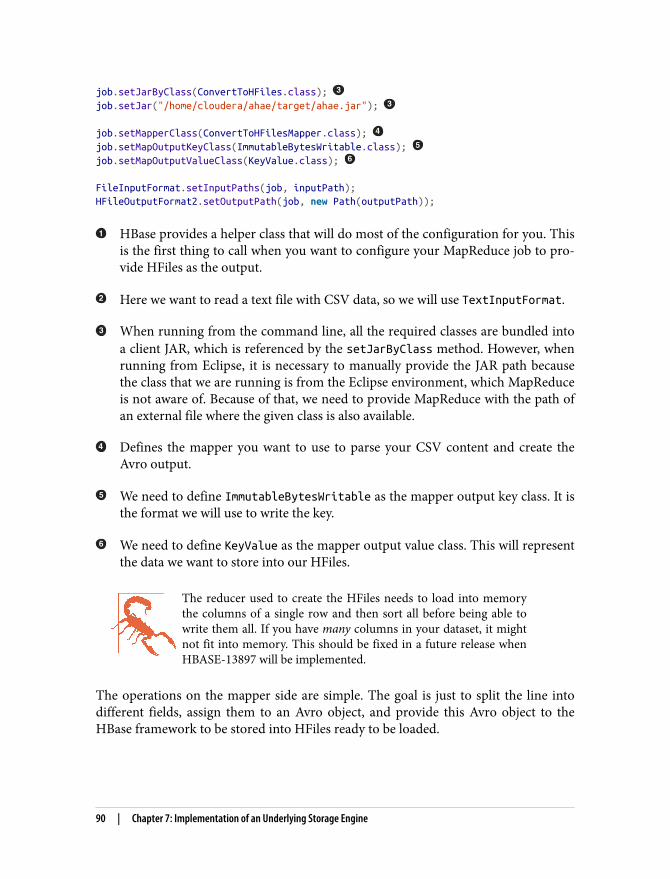
job.setJarByClass(ConvertToHFiles.class); job.setJar("/home/cloudera/ahae/target/ahae.jar");

job.setMapperClass(ConvertToHFilesMapper.class); job.setMapOutputKeyClass(ImmutableBytesWritable.class); job.setMapOutputValueClass(KeyValue.class);

FileInputFormat.setInputPaths(job, inputPath);HFileOutputFormat2.setOutputPath(job, new Path(outputPath));

HBase provides a helper class that will do most of the configuration for you. Thisis the first thing to call when you want to configure your MapReduce job to pro‐vide HFiles as the output.

Here we want to read a text file with CSV data, so we will use TextInputFormat.

When running from the command line, all the required classes are bundled intoa client JAR, which is referenced by the setJarByClass method. However, whenrunning from Eclipse, it is necessary to manually provide the JAR path becausethe class that we are running is from the Eclipse environment, which MapReduceis not aware of. Because of that, we need to provide MapReduce with the path ofan external file where the given class is also available.

Defines the mapper you want to use to parse your CSV content and create theAvro output.

We need to define ImmutableBytesWritable as the mapper output key class. It isthe format we will use to write the key.

We need to define KeyValue as the mapper output value class. This will representthe data we want to store into our HFiles.

The reducer used to create the HFiles needs to load into memorythe columns of a single row and then sort all before being able towrite them all. If you have many columns in your dataset, it mightnot fit into memory. This should be fixed in a future release whenHBASE-13897 will be implemented.

The operations on the mapper side are simple. The goal is just to split the line intodifferent fields, assign them to an Avro object, and provide this Avro object to theHBase framework to be stored into HFiles ready to be loaded.

90 | Chapter 7: Implementation of an Underlying Storage Engine

As shown in Example 7-2, the first thing we need to do is define a set of variables thatwe will reuse for each and every iteration of the mapper. This is done to reduce thenumber of objects created.

Example 7-2. Convert to HFiles mapper

public static final ByteArrayOutputStream out = new ByteArrayOutputStream(); public static final DatumWriter<Event> writer = new SpecificDatumWriter<Event> (Event.getClassSchema()); public static final BinaryEncoder encoder = encoderFactory.binaryEncoder(out,null); public static final Event event = new Event(); public static final ImmutableBytesWritable rowKey = new ImmutableBytesWritable();

Those objects are all reused on the map method shown in Example 7-3.

Example 7-3. Convert to HFiles mapper

// Extract the different fields from the received line. String[] line = value.toString().split(",");

event.setId(line[0]); event.setEventId(line[1]); event.setDocType(line[2]); event.setPartName(line[3]); event.setPartNumber(line[4]); event.setVersion(Long.parseLong(line[5])); event.setPayload(line[6]);

// Serialize the AVRO object into a ByteArray out.reset(); writer.write(event, encoder); encoder.flush();

byte[] rowKeyBytes = DigestUtils.md5(line[0]); rowKey.set(rowKeyBytes); context.getCounter("Convert", line[2]).increment(1);

KeyValue kv = new KeyValue(rowKeyBytes, CF, Bytes.toBytes(line[1]), out.toByteArray()); context.write (rowKey, kv);

First, we split the line into fields so that we can have individual direct access toeach of them.

Instead of creating a new Avro object at each iteration, we reuse the same objectfor all the map calls and simply assign it the new received values.

Data conversion | 91

This is another example of object reuse. The fewer objects you create in yourmapper code, the less garbage collection you will have to do and the faster yourcode will execute. The map method is called for each and every line of your inputfile. Creating a single ByteArrayOutputStream and reusing it and its internalbuffer for each map iteration saves millions of object creations.

Serialize the Avro object into an array of bytes to store them into HBase, reusingexisting objects as much as possible.

Construct our HBase key from the sensor ID.

Construct our HBase KeyValue object from our key, our column family, our eventid as the column qualifier and our Avro object as the value.

Emit our KeyValue object so the reducers can regroup them and write therequired HFiles. The row key will only be used for partitioning the data. Whendata will be written into the underlying files, only the KeyValue data will be usedfor both the key and the value.

When implementing a MapReduce job, avoid creating objectswhen not required. If you need to access a small subset of fields in aString, it is not recommended to use the string split() method toextract the fields. Using split() on 10 million strings having 50fields each will create 500 million objects that will be garbage col‐lected. Instead, parse the string to find the few fields’ locationsand use the substring() method. Also consider using thecom.google.common.base.Splitter object from Guava libraries.

Again, the example can be run directly from Eclipse or from the command line. Inboth cases, you will need to specify the input file, the output folder, and the tablename as the parameters. The table name is required for HBase to find the region’sboundaries to create the required splits in the output data, but also to look up the col‐umn family parameters such as the compression and the encoding. The MapReducejob will produce HFiles in the output folder based on the table regions and the col‐umn family parameters.

The following command will create the HFiles on HDFS (if because you are runningon the standalone version you need the files to be generated on local disk, simplyupdate the destination folder):

hbase -classpath ~/ahae/target/ahae.jar:`hbase classpath` \com.architecting.ch09.ConvertToHFiles \ file:///home/cloudera/ahae/resources/ch09/omneo.csv \ hdfs://localhost/user/cloudera/ch09/hfiles/ sensors

92 | Chapter 7: Implementation of an Underlying Storage Engine

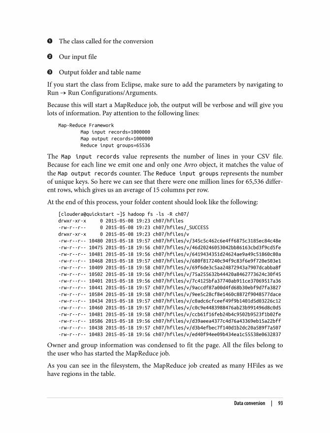
The class called for the conversion

Our input file

Output folder and table name

If you start the class from Eclipse, make sure to add the parameters by navigating toRun → Run Configurations/Arguments.

Because this will start a MapReduce job, the output will be verbose and will give youlots of information. Pay attention to the following lines:

Map-Reduce Framework Map input records=1000000 Map output records=1000000 Reduce input groups=65536

The Map input records value represents the number of lines in your CSV file.Because for each line we emit one and only one Avro object, it matches the value ofthe Map output records counter. The Reduce input groups represents the numberof unique keys. So here we can see that there were one million lines for 65,536 differ‐ent rows, which gives us an average of 15 columns per row.

At the end of this process, your folder content should look like the following:

[cloudera@quickstart ~]$ hadoop fs -ls -R ch07/drwxr-xr-x 0 2015-05-08 19:23 ch07/hfiles-rw-r--r-- 0 2015-05-08 19:23 ch07/hfiles/_SUCCESSdrwxr-xr-x 0 2015-05-08 19:23 ch07/hfiles/v-rw-r--r-- 10480 2015-05-18 19:57 ch07/hfiles/v/345c5c462c6e4ff6875c3185ec84c48e-rw-r--r-- 10475 2015-05-18 19:56 ch07/hfiles/v/46d20246053042bb86163cbd3f9cd5fe-rw-r--r-- 10481 2015-05-18 19:56 ch07/hfiles/v/6419434351d24624ae9a49c51860c80a-rw-r--r-- 10468 2015-05-18 19:57 ch07/hfiles/v/680f817240c94f9c83f6e9f720e503e1-rw-r--r-- 10409 2015-05-18 19:58 ch07/hfiles/v/69f6de3c5aa24872943a7907dcabba8f-rw-r--r-- 10502 2015-05-18 19:56 ch07/hfiles/v/75a255632b44420a8462773624c30f45-rw-r--r-- 10401 2015-05-18 19:56 ch07/hfiles/v/7c4125bfa37740ab911ce37069517a36-rw-r--r-- 10441 2015-05-18 19:57 ch07/hfiles/v/9accdf87a00d4fd68b30ebf9d7fa3827-rw-r--r-- 10584 2015-05-18 19:58 ch07/hfiles/v/9ee5c28cf8e1460c8872f9048577dace-rw-r--r-- 10434 2015-05-18 19:57 ch07/hfiles/v/c0adc6cfceef49f9b1401d5d03226c12-rw-r--r-- 10460 2015-05-18 19:57 ch07/hfiles/v/c0c9e4483988476ab23b991496d8c0d5-rw-r--r-- 10481 2015-05-18 19:58 ch07/hfiles/v/ccb61f16feb24b4c9502b9523f1b02fe-rw-r--r-- 10586 2015-05-18 19:56 ch07/hfiles/v/d39aeea4377c4d76a43369eb15a22bff-rw-r--r-- 10438 2015-05-18 19:57 ch07/hfiles/v/d3b4efbec7f140d1b2dc20a589f7a507-rw-r--r-- 10483 2015-05-18 19:56 ch07/hfiles/v/ed40f94ee09b434ea1c55538e0632837

Owner and group information was condensed to fit the page. All the files belong tothe user who has started the MapReduce job.

As you can see in the filesystem, the MapReduce job created as many HFiles as wehave regions in the table.

Data conversion | 93

When generating the input files, be careful to provide the correctcolumn family. Indeed, it a common mistake to not provide theright column family name to the MapReduce job, which will createthe directory structure based on its name. This will cause the bulkload phase to fail.

The folder within which the files are stored is named based on the column familyname we have specified in our code—“v” in the given example.

HFile ValidationThroughout the process, all the information we get in the console is related to theMapReduce framework and tasks. However, even if they succeed, the content theyhave generated might not be good. For example, we might have used the wrong col‐umn family, forgotten to configure the compression when we created our table, ortaken some other misstep.

HBase comes with a tool to read HFiles and extract the metadata. This tool is calledthe HFilePrettyPrinter and can be called by using the following command line:

hbase hfile -printmeta -f ch07/hfiles/v/345c5c462c6e4ff6875c3185ec84c48e

The only parameter this tool takes is the HFile location in HDFS.

Here we show part of the output of the previous command (some sections have beenomitted, as they are not relevant for this chapter):

Block index size as per heapsize: 161264reader=ch07/hfiles/v/345c5c462c6e4ff6875c3185ec84c48e, compression=snappy, cacheConf=CacheConfig:disabled, firstKey=7778/v:03afef80-7918-4a46-a903-f6e35b629926/1432004229936/Put, lastKey=8888/v:fc69a89f-4a78-4e2d-ae0a-b22dc93c962c/1432004229936/Put, avgKeyLen=53, avgValueLen=171, entries=666591, length=104861200

Let’s now take a look at the important parts of this output:

This shows you the compression format used for your file, which should reflectwhat you have configured when you created the table (we initially chose to useSnappy, but if you configured a different one, you should see it here).

Key of the first cell of this HFile, as well as column family name.

94 | Chapter 7: Implementation of an Underlying Storage Engine

The last key contained in the HFile (only keys between 7778 and 8888 are presentin the file; it is used by HBase to skip entire files when the key you are looking foris not between the first and last key).

Average size of the keys.

Average size of the values.

Number of cells present in the HFile.

Total size of the HFile.

Using the output of this command, you can validate that there is data in the files youhave generated and that the format of the data is according to your expectations(compression, bloom filters, average key size, etc.).

Bulk LoadingBulk loading inserts multiple pre-generated HFiles into HBase instead of performingputs one by one using the HBase API. Bulk loads are the most efficient way to insert alarge quantity of values into the system. Here we will show you how to perform a bulkload.

The HDFS content of your table should look as follows (to fit the page width, file per‐missions and owner information was removed, and /hbase/data/default/sensorswas abbreviated to …/s):

0 2015-05-18 19:46 .../s/.tabledesc287 2015-05-18 19:46 .../s/.tabledesc/.tableinfo.0000000001 0 2015-05-18 19:46 .../s/.tmp 0 2015-05-18 19:46 .../s/0cc853926c7c10d3d12959bbcacc55fd 58 2015-05-18 19:46 .../s/0cc853926c7c10d3d12959bbcacc55fd/.regioninfo 0 2015-05-18 19:46 .../s/0cc853926c7c10d3d12959bbcacc55fd/recovered.edits 0 2015-05-18 19:46 .../s/0cc853926...3d12959bbcacc55fd/recovered.edits/2.seqid 0 2015-05-18 19:46 .../s/0cc853926c7c10d3d12959bbcacc55fd/v

If your table is empty, you will still have all the region folders, because we have pre-split the table. HFiles might be present in the regions folders if data already existedprior to loading. We show only one region’s directory in the preceding snippet, andyou can see that this region’s column family v is empty because it doesn’t contain anyHFiles.

Our HFiles have been generated by the MapReduce job, and we now need to tellHBase to place the HFiles into the given table. This is done using the followingcommand:

Bulk Loading | 95

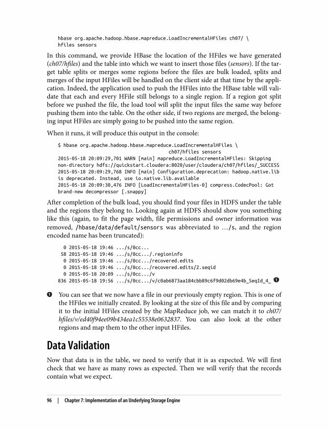
hbase org.apache.hadoop.hbase.mapreduce.LoadIncrementalHFiles ch07/ \hfiles sensors

In this command, we provide HBase the location of the HFiles we have generated(ch07/hfiles) and the table into which we want to insert those files (sensors). If the tar‐get table splits or merges some regions before the files are bulk loaded, splits andmerges of the input HFiles will be handled on the client side at that time by the appli‐cation. Indeed, the application used to push the HFiles into the HBase table will vali‐date that each and every HFile still belongs to a single region. If a region got splitbefore we pushed the file, the load tool will split the input files the same way beforepushing them into the table. On the other side, if two regions are merged, the belong‐ing input HFiles are simply going to be pushed into the same region.

When it runs, it will produce this output in the console:

$ hbase org.apache.hadoop.hbase.mapreduce.LoadIncrementalHFiles \ ch07/hfiles sensors2015-05-18 20:09:29,701 WARN [main] mapreduce.LoadIncrementalHFiles: Skippingnon-directory hdfs://quickstart.cloudera:8020/user/cloudera/ch07/hfiles/_SUCCESS2015-05-18 20:09:29,768 INFO [main] Configuration.deprecation: hadoop.native.libis deprecated. Instead, use io.native.lib.available2015-05-18 20:09:30,476 INFO [LoadIncrementalHFiles-0] compress.CodecPool: Gotbrand-new decompressor [.snappy]

After completion of the bulk load, you should find your files in HDFS under the tableand the regions they belong to. Looking again at HDFS should show you somethinglike this (again, to fit the page width, file permissions and owner information wasremoved, /hbase/data/default/sensors was abbreviated to …/s, and the regionencoded name has been truncated):

0 2015-05-18 19:46 .../s/0cc... 58 2015-05-18 19:46 .../s/0cc.../.regioninfo 0 2015-05-18 19:46 .../s/0cc.../recovered.edits 0 2015-05-18 19:46 .../s/0cc.../recovered.edits/2.seqid 0 2015-05-18 20:09 .../s/0cc.../v836 2015-05-18 19:56 .../s/0cc.../v/c0ab6873aa184cbb89c6f9d02db69e4b_SeqId_4_

You can see that we now have a file in our previously empty region. This is one ofthe HFiles we initially created. By looking at the size of this file and by comparingit to the initial HFiles created by the MapReduce job, we can match it to ch07/hfiles/v/ed40f94ee09b434ea1c55538e0632837. You can also look at the otherregions and map them to the other input HFiles.

Data ValidationNow that data is in the table, we need to verify that it is as expected. We will firstcheck that we have as many rows as expected. Then we will verify that the recordscontain what we expect.

96 | Chapter 7: Implementation of an Underlying Storage Engine

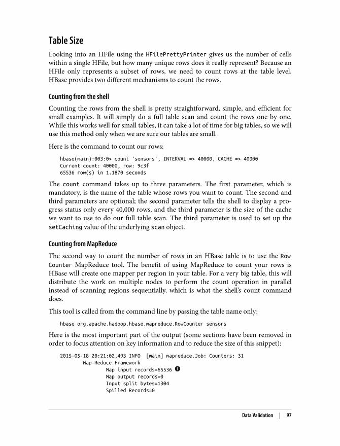
Table SizeLooking into an HFile using the HFilePrettyPrinter gives us the number of cellswithin a single HFile, but how many unique rows does it really represent? Because anHFile only represents a subset of rows, we need to count rows at the table level.HBase provides two different mechanisms to count the rows.

Counting from the shellCounting the rows from the shell is pretty straightforward, simple, and efficient forsmall examples. It will simply do a full table scan and count the rows one by one.While this works well for small tables, it can take a lot of time for big tables, so we willuse this method only when we are sure our tables are small.

Here is the command to count our rows:

hbase(main):003:0> count 'sensors', INTERVAL => 40000, CACHE => 40000Current count: 40000, row: 9c3f65536 row(s) in 1.1870 seconds

The count command takes up to three parameters. The first parameter, which ismandatory, is the name of the table whose rows you want to count. The second andthird parameters are optional; the second parameter tells the shell to display a pro‐gress status only every 40,000 rows, and the third parameter is the size of the cachewe want to use to do our full table scan. The third parameter is used to set up thesetCaching value of the underlying scan object.

Counting from MapReduce

The second way to count the number of rows in an HBase table is to use the RowCounter MapReduce tool. The benefit of using MapReduce to count your rows isHBase will create one mapper per region in your table. For a very big table, this willdistribute the work on multiple nodes to perform the count operation in parallelinstead of scanning regions sequentially, which is what the shell’s count commanddoes.

This tool is called from the command line by passing the table name only:

hbase org.apache.hadoop.hbase.mapreduce.RowCounter sensors

Here is the most important part of the output (some sections have been removed inorder to focus attention on key information and to reduce the size of this snippet):

2015-05-18 20:21:02,493 INFO [main] mapreduce.Job: Counters: 31 Map-Reduce Framework Map input records=65536 Map output records=0 Input split bytes=1304 Spilled Records=0

Data Validation | 97

Failed Shuffles=0 Merged Map outputs=0 GC time elapsed (ms)=2446 CPU time spent (ms)=48640 Physical memory (bytes) snapshot=3187818496 Virtual memory (bytes) snapshot=24042749952 Total committed heap usage (bytes)=3864526848 org.apache.hadoop.hbase.mapreduce.RowCounter$RowCounterMapper$Counters ROWS=65536

Let’s now take a look at the important fields to consider here:

Because the input records of this job are the HBase rows, we will have as manyinput records as we have rows.

The number of rows we have in the table, which will match the number of inputrecords. Indeed, this MapReduce job simply increments a ROWS counter for eachinput record.

HBase also provides a MapReduce tool called CellCounter tocount not just the number of rows in a table, but also the numberof columns and the number of versions for each of them. However,this tool needs to create a Hadoop counter for each and everyunique row key found in the table. Hadoop has a default limit of120 counters. It is possible to increase this limit, but increasing it tothe number of rows we have in the table might create some issues.If you are working on a small dataset, this might be useful to testyour application and debug it. This tool generally cannot be run ona big table. Some work have been done on the Apache repository tofix this limitation. Please refer to HBASE-15773 for more details.

File ContentWe have our table with the number of lines we expected and the format we asked. Butwhat does the data in the table really look like? Are we able to read what we wrote?Let’s see two ways to have a look at our data.

Using the shellThe easiest and quickest way to read data from HBase is to use the HBase shell. Usingthe shell, you can issue commands to retrieve the data you want. The first commandis get, which will give you a single row. If you specify a column family, only the col‐umns for that family are returned. If you specify both a column family and a columnqualifier (separated with a colon), it will return only the specific value if it exists. Thesecond option is to use scan, which will return a certain number of rows that we canlimit using the LIMIT parameter or the STARTROW and STOPROW parameters. Both of

98 | Chapter 7: Implementation of an Underlying Storage Engine

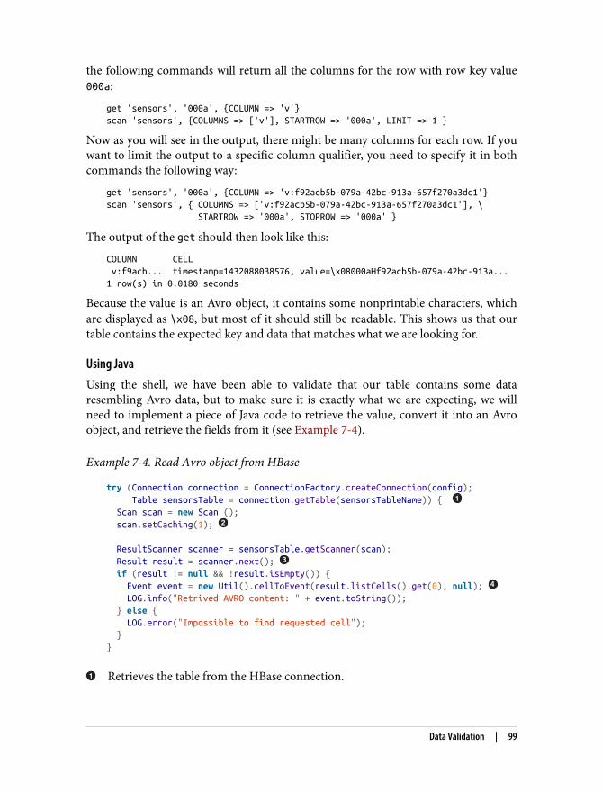
the following commands will return all the columns for the row with row key value000a:

get 'sensors', '000a', {COLUMN => 'v'}scan 'sensors', {COLUMNS => ['v'], STARTROW => '000a', LIMIT => 1 }

Now as you will see in the output, there might be many columns for each row. If youwant to limit the output to a specific column qualifier, you need to specify it in bothcommands the following way:

get 'sensors', '000a', {COLUMN => 'v:f92acb5b-079a-42bc-913a-657f270a3dc1'}scan 'sensors', { COLUMNS => ['v:f92acb5b-079a-42bc-913a-657f270a3dc1'], \ STARTROW => '000a', STOPROW => '000a' }

The output of the get should then look like this:

COLUMN CELL v:f9acb... timestamp=1432088038576, value=\x08000aHf92acb5b-079a-42bc-913a...1 row(s) in 0.0180 seconds

Because the value is an Avro object, it contains some nonprintable characters, whichare displayed as \x08, but most of it should still be readable. This shows us that ourtable contains the expected key and data that matches what we are looking for.

Using JavaUsing the shell, we have been able to validate that our table contains some dataresembling Avro data, but to make sure it is exactly what we are expecting, we willneed to implement a piece of Java code to retrieve the value, convert it into an Avroobject, and retrieve the fields from it (see Example 7-4).

Example 7-4. Read Avro object from HBase

try (Connection connection = ConnectionFactory.createConnection(config); Table sensorsTable = connection.getTable(sensorsTableName)) { Scan scan = new Scan (); scan.setCaching(1);

ResultScanner scanner = sensorsTable.getScanner(scan); Result result = scanner.next(); if (result != null && !result.isEmpty()) { Event event = new Util().cellToEvent(result.listCells().get(0), null); LOG.info("Retrived AVRO content: " + event.toString()); } else { LOG.error("Impossible to find requested cell"); } }

Retrieves the table from the HBase connection.

Data Validation | 99

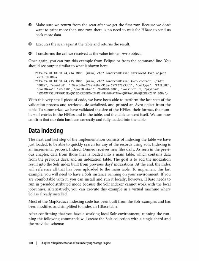
Make sure we return from the scan after we get the first row. Because we don’twant to print more than one row, there is no need to wait for HBase to send usback more data.

Executes the scan against the table and returns the result.

Transforms the cell we received as the value into an Avro object.

Once again, you can run this example from Eclipse or from the command line. Youshould see output similar to what is shown here:

2015-05-20 18:30:24,214 INFO [main] ch07.ReadFromHBase: Retrieved Avro object with ID 000a2015-05-20 18:30:24,215 INFO [main] ch07.ReadFromHBase: Avro content: {"id": "000a", "eventid": "f92acb5b-079a-42bc-913a-657f270a3dc1", "docType": "FAILURE", "partName": "NE-858", "partNumber": "0-0000-000", "version": 1, "payload": "SXOAXTPSIUFPPNUCIEVQGCIZHCEJBKGWINHKIHFRHWHNATAHAHQBFRAYLOAMQEGKLNZIFM 000a"}

With this very small piece of code, we have been able to perform the last step of thevalidation process and retrieved, de-serialized, and printed an Avro object from thetable. To summarize, we have validated the size of the HFiles, their format, the num‐bers of entries in the HFiles and in the table, and the table content itself. We can nowconfirm that our data has been correctly and fully loaded into the table.

Data IndexingThe next and last step of the implementation consists of indexing the table we havejust loaded, to be able to quickly search for any of the records using Solr. Indexing isan incremental process. Indeed, Omneo receives new files daily. As seen in the previ‐ous chapter, data from those files is loaded into a main table, which contains datafrom the previous days, and an indexation table. The goal is to add the indexationresult into the Solr index built from previous days’ indexations. At the end, the indexwill reference all that has been uploaded to the main table. To implement this lastexample, you will need to have a Solr instance running on your environment. If youare comfortable with it, you can install and run it locally; however, HBase needs torun in pseudodistributed mode because the Solr indexer cannot work with the localjobrunner. Alternatively, you can execute this example in a virtual machine whereSolr is already installed.

Most of the MapReduce indexing code has been built from the Solr examples and hasbeen modified and simplified to index an HBase table.

After confirming that you have a working local Solr environment, running the run‐ning the following commands will create the Solr collection with a single shard andthe provided schema:

100 | Chapter 7: Implementation of an Underlying Storage Engine

export PROJECT_HOME=~/ahae/resources/ch07/searchrm -rf $PROJECT_HOMEsolrctl instancedir --generate $PROJECT_HOMEmv $PROJECT_HOME/conf/schema.xml $PROJECT_HOME/conf/schema.oldcp $PROJECT_HOME/../schema.xml $PROJECT_HOME/conf/solrctl instancedir --create Ch07-Collection $PROJECT_HOMEsolrctl collection --create Ch07-Collection -s 1

In a production environment, to scale your application, you might want to considerusing more shards.

The most important file to define your index is its schema.xml file. This file is avail‐able in the book’s GitHub repository and contains many tags. The most importantsection of the schema is the following:

<field name="id" type="string" indexed="true" stored="true" required="true" multiValued="false" /><field name="rowkey" type="binary" indexed="false" stored="true" omitNorms="true" required="true"/><field name="eventId" type="string" indexed="true" stored="false" omitNorms="true" required="true"/><field name="docType" type="string" indexed="true" stored="false" omitNorms="true"/><field name="partName" type="lowercase" indexed="true" stored="false" omitNorms="true"/><field name="partNumber" type="lowercase" indexed="true" stored="false" omitNorms="true"/><field name="version" type="long" indexed="true" stored="false" required="true" multiValued="false" /><field name="payload" type="string" indexed="true" stored="false" required="true" multiValued="false" /><field name="_version_" type="long" indexed="true" stored="true"/>

Because this book is focused on HBase, we won’t go into all the details of this file andall its fields, but invite you to look at the Solr online documentation.

The following commands will create the required index for the examples:

export PROJECT_HOME=~/ahae/resources/ch07/searchrm -rf $PROJECT_HOMEsolrctl instancedir --generate $PROJECT_HOMEmv $PROJECT_HOME/conf/schema.xml $PROJECT_HOME/conf/schema.oldcp $PROJECT_HOME/../schema.xml $PROJECT_HOME/conf/solrctl instancedir --create Ch07-Collection $PROJECT_HOMEsolrctl collection --create Ch07-Collection -s 1

If, for any reason, you want to delete your collection, use the following commands:

solrctl collection --delete Ch07-Collectionsolrctl instancedir --delete Ch07-Collectionsolrctl instancedir --delete search

Data Indexing | 101

The steps to get the table indexed are pretty straightforward. The first thing we needto do is to scan the entire HBase table using MapReduce to create Solr index files. Thesecond step is to bulk load those files into Solr similar to how we bulk loaded ourHFiles into HBase. The entire code will not be shown here due to size, however thereare few pieces we want to show you here.

Example 7-5 demonstrates how we need to configure our MapReduce job in thedriver class.

Example 7-5. Index HBase Avro table to Solr using MapReduce driver

scan.setCaching(500); scan.setCacheBlocks(false);

TableMapReduceUtil.initTableMapperJob( options.inputTable, // Input HBase table name scan, // Scan instance to control what to index HBaseAvroToSOLRMapper.class, // Mapper to parse cells content Text.class, // Mapper output key SolrInputDocumentWritable.class, // Mapper output value job);

FileOutputFormat.setOutputPath(job, outputReduceDir);

job.setJobName(getClass().getName() + "/" + Utils.getShortClassName(HBaseAvroToSOLRMapper.class)); job.setReducerClass(SolrReducer.class); job.setPartitionerClass(SolrCloudPartitioner.class); job.getConfiguration().set(SolrCloudPartitioner.ZKHOST, options.zkHost); job.getConfiguration().set(SolrCloudPartitioner.COLLECTION, options.collection); job.getConfiguration().setInt(SolrCloudPartitioner.SHARDS, options.shards);

job.setOutputFormatClass(SolrOutputFormat.class); SolrOutputFormat.setupSolrHomeCache(options.solrHomeDir, job);

job.setOutputKeyClass(Text.class); job.setOutputValueClass(SolrInputDocumentWritable.class); job.setSpeculativeExecution(false);

By default, scans cache only one row at a time. To reduce remote procedure calls(RPC) calls and improve throughput, we want to increase the size of the cache.

Because we are going to scan the entire table once and only once, caching theblocks is not required and will just put pressure on the RegionServers’ blockc‐ache. It is always recommended to disable the blockcache when running a Map‐Reduce job over a table.

102 | Chapter 7: Implementation of an Underlying Storage Engine

Again, we are using HBase utility classes to configure required MapReduce inputformats and output formats as well as the required mapper.

Use the default Apache Solr reducer class.

Also use the default apache Solr partitioner class.

Everything on the class should be pretty straightforward to understand.

Now let’s have a look at the mapper. The goal of the mapper is to read the contentfrom HBase and translate it for Solr. We have already written a class to create an Avroobject from an HBase cell. We reuse the same code here, as this is exactly what wewant to achieve. We want to read each cell, convert it back to an Avro object, and pro‐vide to Solr the data we want to index (Example 7-6).

Example 7-6. Index HBase Avro table to Solr using MapReduce mapper

event = util.cellToEvent(cell, event);

inputDocument.clear(); inputDocument.addField("id", UUID.randomUUID().toString()); inputDocument.addField("rowkey", row.get()); inputDocument.addField("eventId", event.getEventId().toString()); inputDocument.addField("docType", event.getDocType().toString()); inputDocument.addField("partName", event.getPartName().toString()); inputDocument.addField("partNumber", event.getPartNumber().toString()); inputDocument.addField("version", event.getVersion()); inputDocument.addField("payload", event.getPayload().toString());

context.write(new Text(cell.getRowArray()), new SolrInputDocumentWritable(inputDocument));

Transform the received cell into an Avro object reusing the event instance toavoid creation of new objects.

Here again we want to reuse existing objects as much as possible and thereforewill simply reinitialize and reuse the Solr input document.

Assign to the Solr input document all the fields we want to index or store fromthe Avro event object.

Write the Solr document to the context for indexing.

If you want to run the indexing from the command line, you will have to use the fol‐lowing command:

hbase -classpath ~/ahae/target/ahae.jar:`hbase classpath` \com.architecting.ch07.MapReduceIndexerTool

Data Indexing | 103

You can also execute it from Eclipse without any specific parameter.

Data RetrievalAt this point, we have generated test data, transformed it into Avro format stored intoHFiles, loaded it into a table, and indexed it into Solr. The only remaining piece is tomake sure we can query Solr to find what we are looking for and then retrieve therelated information from HBase. The HBase retrieval part is the same as what wehave already seen before. You can query Solr using the code shown in Example 7-7.

Example 7-7. Retrieve Avro data from HBase based on Solr

CloudSolrServer solr = new CloudSolrServer("localhost:2181/solr"); solr.setDefaultCollection("Ch09-Collection"); solr.connect();

ModifiableSolrParams params = new ModifiableSolrParams(); params.set("qt", "/select"); params.set("q", "docType:ALERT AND partName:NE-555");

QueryResponse response = solr.query(params); SolrDocumentList docs = response.getResults();

LOG.info("Found " + docs.getNumFound() + " matching documents."); if (docs.getNumFound() == 0) return; byte[] firstRowKey = (byte[]) docs.get(0).getFieldValue("rowkey"); LOG.info("First document rowkey is " + Bytes.toStringBinary(firstRowKey));

// Retrieve and print the first 10 columns of the first returned document Configuration config = HBaseConfiguration.create(); try (Connection connection = ConnectionFactory.createConnection(config); Admin admin = connection.getAdmin(); Table sensorsTable = connection.getTable(sensorsTableName)) { Get get = new Get(firstRowKey);

Result result = sensorsTable.get(get); Event event = null; if (result != null && !result.isEmpty()) { for (int index = 0; index < 10; index++) { // Print first 10 columns if (!result.advance()) break; // There are no more columns and we have not reached 10 event = new Util().cellToEvent(result.current(), event); LOG.info("Retrieved AVRO content: " + event.toString()); } } else { LOG.error("Impossible to find requested cell"); } }

104 | Chapter 7: Implementation of an Underlying Storage Engine

Connect to your Solr cluster. Adjust this if you are not running Solr on the samecluster as HBase.

Define the Solr collection you want to use.

Configure the request you want Solr to execute. Here we ask it for all the ALERTdocuments for the NE-555 part.

Execute the Solr request and retrieve the response from the server.

Call HBase, specifying the row key of the first document sent back by Solr.

Iterate over the columns for the given key and display the first 10 Avro objectsretrieved from those columns.

Going FurtherIf you want to extend the examples presented in this chapter, the following list offerssome options you can try based on our discussions from this chapter:

Bigger input fileTo make sure examples run pretty fast, the dataset we worked with was prettysmall. What about using a bigger dataset? Depending on the available disk spaceyou have and the performance of your environment, try to create a significantlybigger input file and verify it’s processed the exact same way.

Single region tableBecause it’s a good practice to avoid hotspotting, we have created a table withmultiple regions split based on the key we used. Therefore the different Map‐Reduce jobs have generated multiple files, one per region. What if we create atable with a single region instead? Try to modify the create table statement tohave a single region and load more than 10 GB of data into it. You should see theregion splitting after the data is inserted; however, since we are using bulk load,you should still not see any hotspotting on this region. You can validate yourtable splits and the content of each region by looking in HDFS, as discussed in“Bulk Loading” on page 95.

Impact on table parametersWe have created our table using the parameters that are good for our current usecase. We recommend modifying the various parameters and rerunning the pro‐cess to measure the impact.

Going Further | 105

CompressionTry to use different types of compression and compare. If you used Snappy(which is fast), try to configure LZ4 (which is slower, but compresses better),and compare the overall time it takes to process everything in relation to thesize of your files.

Block encodingBecause of the format of the key we store into this table, we configured it touse the FAST_DIFF data block encoding. Here again, look at the performanceand the overall data size at the end.

Bloom filterWhen doing reads, Bloom filters are useful for skipping HBase store fileswhere we can confirm the key we are looking for is not present. However,here we knew that the data we are looking for will always be present in thefile, so we disabled the Bloom filters. Create a list of tens of keys and columnsthat you know are present in the table and measure how long it takes to readthem all. Activate the Bloom filter on the table and run a major compaction,which will create the Bloom filters. There should be no noticeable perfor‐mance gain on subsequent tests for this specific use case.

It is almost always good to have Bloom filters activated. We dis‐abled them here because this use case is very specific. If you are notsure, just keep them on.

106 | Chapter 7: Implementation of an Underlying Storage Engine

CHAPTER 8

Use Case: Near Real-Time Event Processing

This next use case focuses on handling claims records for the healthcare industry.The claims processor utilizes a software-as-a-service (SaaS) model to act as a bridgefor patients, hospitals, and doctor’s offices. Because medical claims are quite difficultto manage for many hospitals and healthcare providers, the claims processor (alsoknown as a clearinghouse) accepts claims from customers (i.e., hospitals and doctor’soffices) and then formats those claims to send to the payer. This is a difficult and tedi‐ous process, as most hospitals and doctor’s offices did not traditionally use a standar‐dized format for claims. This is where the clearinghouse comes in to submit all claimsin a unified format designed specifically for the payer.

Compared to the previous use cases, the clearinghouse has a few extra layers of com‐plexity. For example, this data is not just machine-generated data to be loaded inbatch; the incoming data has to be processed inflight. In addition, because the data isclassified as personally identifiable information (PII) or protected health information(PHI), and thus protected under the Health Insurance Portability and AccountabilityAct (HIPAA), it requires numerous layers of security. This use case focuses on elec‐tronic medical claims records and creating a system to process these records. The endobjective for this system is to lower the typical claims processing time from 30 days toeventually processing the claims in real time, by optimizing the claim to ensure all ofthe necessary information is present, and instantly rejecting claims before sendingthem to the insurance provider. The ideal service-level agreement (SLA) behind a sys‐tem like this is to have the claim ready for review from the system in less than 15 sec‐onds to be available for lookup and reference from the customer, claims processor,and payers. Because the system needs to serve external requests in real time, the clus‐ter is required to have a 99.9% uptime, which weighed heavily into the decision to useHadoop and HBase. There is also a concept of milestones, which require the ability toupdate the current claims record on the fly without knowing the number of updates a

107

single record may receive. This plays right into HBase’s strengths with the ability tohandle sparse data and add thousands of columns without thinking twice.

The claims provider looked at numerous other systems to solve this use case. Whenevaluating the technologies for this project, the provider was lucky that this was a netnew project. This gave a clean slate for technologies to choose from. The first tech‐nology looked at was Oracle RAC, which was at the time the current incumbent data‐base. The provider performed some load testing at the volumes of data expected, butunfortunately RAC was not able to keep up. Next up was Netezza, which was nixedfor lack of small files and total cost of ownership. Finally, Cassandra was evaluated.Because the use case required access to different processing layers, it was ruled out infavor of the complete Hadoop ecosystem. The current cluster houses roughly 178 TBof data in HDFS with 40 TB of that data living in the HBase instance, which is sizedto handle roughly 30,000 events per second, and serve roughly 10 requests per secondfrom Solr.

As mentioned earlier, this cluster currently contains PHI data. The overall require‐ments for storing this type of protected data are not only limited to technology, but toprocess as well. We will briefly focus on the technical requirements for storing thisdata in the system. These strict guidelines also weighed heavily in the choice of tech‐nology. These guidelines are taken very seriously, as the administrators of the systemcan incur large fines as well as jail time if they are found to be in violation of the law.When dealing with PHI, the claims provider is required to offer a strong layer ofauthentication, authorization, and encryption.

This claims provider wanted to ensure all levels were properly met before deployingthe system. For the authentication layer, the provider went with the industry standardof Kerberos. Authorization is controlled from a few different places; the first is lever‐aging HBase’s built-in ACLs, the second is through HDFS ACLs, and finally, Sentryfor the Search and Impala layer. The encryption layer started out with Vormetric,which did not seem to include a large performance hit, but later the provider movedto Gazzang encryption to leverage the integrated KeyStore and AES-NI for offloadingthe processing to the CPU. The claims provider also leverages Cloudera Navigator forauditing, data lineage, and metadata tagging.

Figure 8-1 illustrates the overall architecture. This diagram might be a bit daunting atfirst, as it contains a few Hadoop ecosystem technologies that we have not yetreviewed. Before diving into the different layers, let’s spend a minute looking a littledeeper into Kafka and Storm, which play a major role in the near real-time pipeline.

108 | Chapter 8: Use Case: Near Real-Time Event Processing

Figure 8-1. Architecture overview

Kafka is going to be a recurring component in the wonderful world of real-timeingest. Kafka maintains different streams of messages referred to as topics. The pro‐cesses that publish messages to a Kafka topic are called producers. There are numer‐ous pre-created producers (similar to Flume Sources), or you can always write yourown producer depending on use case requirements. The processes reading from thetopics are known as consumers. Consumers are also typically responsible for writingto the downstream applications. Kafka is traditionally run as a cluster comprised ofone or more nodes, each of which is called a broker. These consumers are broken upinto consumer groups, each of which handle their own offset allowing for consumersto be able to easily subscribe and unsubscribe without affecting other consumersreading for the same topic. Kafka allows for very high read and write throughputthrough the use of partitions that can be tuned to take advantage of numerous spin‐dles inside the Kafka nodes.

Use Case: Near Real-Time Event Processing | 109

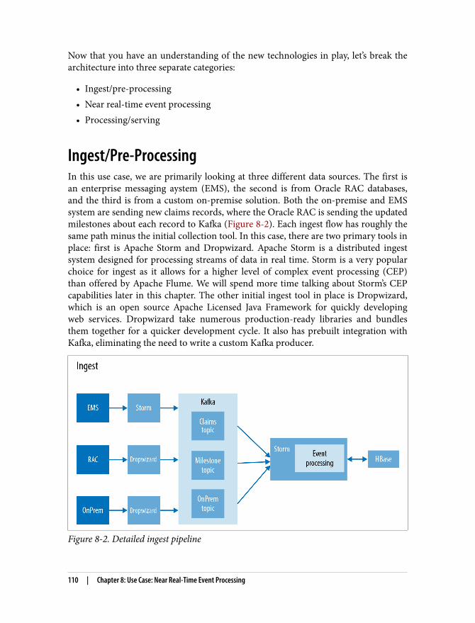
Now that you have an understanding of the new technologies in play, let’s break thearchitecture into three separate categories:

• Ingest/pre-processing• Near real-time event processing• Processing/serving

Ingest/Pre-ProcessingIn this use case, we are primarily looking at three different data sources. The first isan enterprise messaging aystem (EMS), the second is from Oracle RAC databases,and the third is from a custom on-premise solution. Both the on-premise and EMSsystem are sending new claims records, where the Oracle RAC is sending the updatedmilestones about each record to Kafka (Figure 8-2). Each ingest flow has roughly thesame path minus the initial collection tool. In this case, there are two primary tools inplace: first is Apache Storm and Dropwizard. Apache Storm is a distributed ingestsystem designed for processing streams of data in real time. Storm is a very popularchoice for ingest as it allows for a higher level of complex event processing (CEP)than offered by Apache Flume. We will spend more time talking about Storm’s CEPcapabilities later in this chapter. The other initial ingest tool in place is Dropwizard,which is an open source Apache Licensed Java Framework for quickly developingweb services. Dropwizard take numerous production-ready libraries and bundlesthem together for a quicker development cycle. It also has prebuilt integration withKafka, eliminating the need to write a custom Kafka producer.

Figure 8-2. Detailed ingest pipeline

110 | Chapter 8: Use Case: Near Real-Time Event Processing

In this use case, we are using three separate topics, one for each ingest path. Thisallows for the end user to be able to add other systems to read from an individualtopic without having to receive all of the other unwanted data. In this case, thenumerous topics are being used simply for ease of management and future extensibil‐ity. From Kafka, we have a single Storm topology pulling from the three main Kafkatopics.

Near Real-Time Event ProcessingThe main portion of the ETL work all resides inside this Storm topology. The Stormtopology includes the concept of Bolts, which enable us to perform the CEP tasks thatneed to be done. The consumers in this case will be Kafka spouts for Storm. TheStorm Bolt will receive the events from the Kafka Spout where the event enrichmentwill occur (Figure 8-3). We have two streams that need to be processed: the newclaims records and milestones. They both need some separate processing, whichStorm makes easy by allowing numerous streams to occur in a single topology. As theclaims come in, they need to be enriched with previously stored data or messages.This process includes adding missing traits, such as name, doctor, hospital, address,the internal claim IDs, and the external claim ID. It is important to remember that thenaming structure might differ from one claim provider to the next. It is important forclaim providers to be able to identify the same claim every time. The milestones areenriching claims with updated data, and new status levels that are going to be used inthe serving layer.

Figure 8-3. Inflight event processing

The HBase row key design has to be carefully considered when dealing with PII data.One of the most important requirements around handling healthcare information isthe ability to guarantee never exposing the wrong customer information. In this case,

Near Real-Time Event Processing | 111

the row key is a concatenation of the customerID and a random hash. Looking at thethree relevant tables:

• Lookups - InternalID• ClaimsID - claimsID• Claims - CustomerID|random hash

The customer ID must be the first part of the key as this guarantees that when theapplication does a look up in HBase, only that record is served back. The problem ismost customer IDs tend to increment in the system and are usually just a series ofnumbers. By adding the random hash to the end of the key, it allows for additionallexicographic sort split purposes. The most ideal row key distribution would be asimple MD5 hash, which has an astronomically low collision rate—this would spreadthe keys around evenly and make for a smoother write path. However, when dealingwith PII data, it is a gamble to use the MD5 hash, no matter how low the risk.Remember, people win the lottery every day!

Processing/ServingWe have taken a look at the ingest and CEP layer of the pipeline. Everything we havediscussed occurs outside the cluster, except for the Storm bolts calling Gets and Putsfor HBase. The claims provider uses a combination of Impala, Spark, Solr, and thealmighty HBase (it is the focal point of the book). HBase in this case is used innumerous ways: in addition to being the record of truth for claims, it is also used torebuild Solr indexes and Impala tables when the data shifts, and to enrich and updateincoming claims and milestones. The data coming into HBase is all being loadedthrough the Java API inside the Storm Bolts through the use of Gets, Puts, and checkand swap operations. Once the data is written to HBase, the claims provider then lev‐erages the Lily Indexer to write the new records and updates to Solr. The Lily Indexeris an interesting piece of software, as it allows indexing into SolrCloud without hav‐ing do any custom coding. The Lily Indexer works by acting as a replication sink forHBase. As with HBase replication, the Indexer processes the write asynchronously asto not interrupt other incoming writes.

One of the coolest features of the Lily Indexer is that it piggybacks on the previouslybuilt HBase replication functionality. This means the progress is stored in ZooKeeperand it leverages the HBase HLogs. By using the previously built replication frame‐work, the Lily Indexer is fault tolerant and can survive region and Solr Server failureswithout having data loss. This is very important when storing medical claims, asaccuracy and data protection are two of the top concerns. As discussed in the previ‐ous chapter, Solr is not only housing the data being searched, but the HBase row keyas well. This row key is going to be used later when we discuss the Spark processinglayer. Once the data is in Solr, it can be accessed two different ways (Figure 8-4). The

112 | Chapter 8: Use Case: Near Real-Time Event Processing

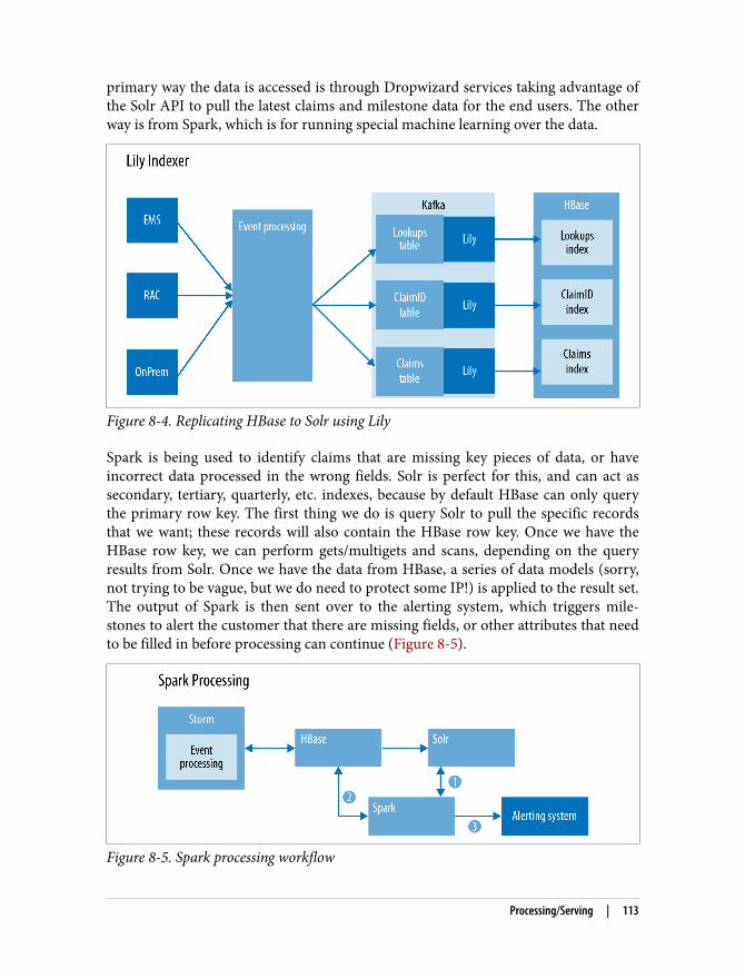
primary way the data is accessed is through Dropwizard services taking advantage ofthe Solr API to pull the latest claims and milestone data for the end users. The otherway is from Spark, which is for running special machine learning over the data.

Figure 8-4. Replicating HBase to Solr using Lily

Spark is being used to identify claims that are missing key pieces of data, or haveincorrect data processed in the wrong fields. Solr is perfect for this, and can act assecondary, tertiary, quarterly, etc. indexes, because by default HBase can only querythe primary row key. The first thing we do is query Solr to pull the specific recordsthat we want; these records will also contain the HBase row key. Once we have theHBase row key, we can perform gets/multigets and scans, depending on the queryresults from Solr. Once we have the data from HBase, a series of data models (sorry,not trying to be vague, but we do need to protect some IP!) is applied to the result set.The output of Spark is then sent over to the alerting system, which triggers mile‐stones to alert the customer that there are missing fields, or other attributes that needto be filled in before processing can continue (Figure 8-5).

Figure 8-5. Spark processing workflow

Processing/Serving | 113

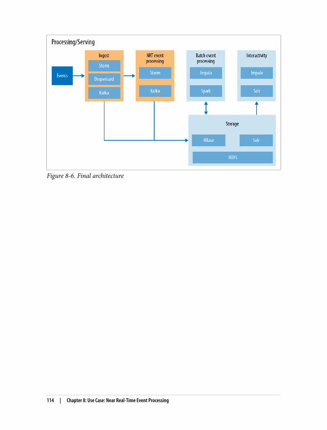
Figure 8-6. Final architecture

114 | Chapter 8: Use Case: Near Real-Time Event Processing

1 http://blog.acolyer.org/2015/06/15/twitter-heron-stream-processing-at-scale/

CHAPTER 9

Implementation of Near Real-TimeEvent Processing

In the previous chapter, we introduced many tools that we did not use in the previoususe case implementation, including Storm, Spark, and Kafka. This book is focused onHBase usage, so we will not review the installation of all these new tools, and we willassume that they are correctly installed and running on your environment. In addi‐tion, because Twitter decommissioned Storm and identified flaws in its design andscalability,1 the examples here are implemented using Flume.

Because the Cloudera QuickStart VM already comes with Flume, Kafka, Spark, Solr,Lily Indexer, and HBase, we used it to develop and test this use case. Because we usedonly standard applications and APIs, if you are able to install all those tools locallyoutside of a VM, or if you have any other VM with all those tools available, it shouldwork exactly the same way.

Keep in mind that the more services you are running, the more memory you need.We assigned 12 GB to our virtual machine to run these examples. If you are lackingmemory, you can stop some of those services and run the different steps one by onewith the services you have running.

Again, we will not discuss each and every implementation detail, but will cover all therequired tools and examples to help you understand what is important during thisphase.

Before we begin, you’ll need to make sure that all services are running correctly.

115

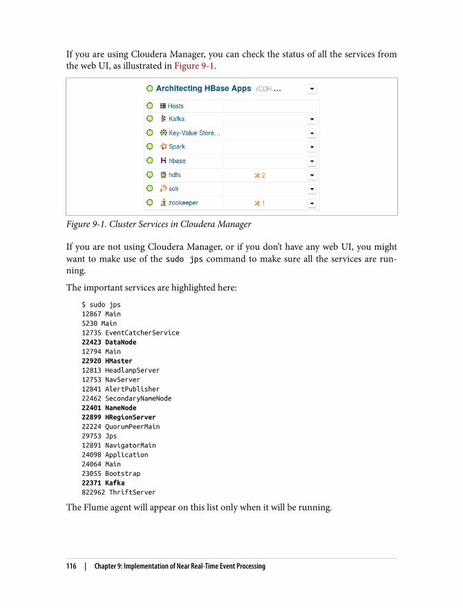
If you are using Cloudera Manager, you can check the status of all the services fromthe web UI, as illustrated in Figure 9-1.

Figure 9-1. Cluster Services in Cloudera Manager

If you are not using Cloudera Manager, or if you don’t have any web UI, you mightwant to make use of the sudo jps command to make sure all the services are run‐ning.

The important services are highlighted here:

$ sudo jps12867 Main5230 Main12735 EventCatcherService22423 DataNode12794 Main22920 HMaster12813 HeadlampServer12753 NavServer12841 AlertPublisher22462 SecondaryNameNode22401 NameNode22899 HRegionServer22224 QuorumPeerMain29753 Jps12891 NavigatorMain24098 Application24064 Main23055 Bootstrap22371 Kafka822962 ThriftServer

The Flume agent will appear on this list only when it will be running.

116 | Chapter 9: Implementation of Near Real-Time Event Processing

Application FlowAs described in Chapter 8, Flume will pick up data from external data sources andstore that into Kafka for queuing. Then another Flume agent will read the differentKafka queues, process the data if required, then send it into HBase for storage wherethe Lily Indexer will pick it up and send it into Solr for indexation. This is what weare going to implement here. We will not implement all the sources nor all the real-time processing options, but we will make sure we have an entire data flow goingfrom the initial Flume event up to the Solr indexation. To have an easy way to ingesttesting events into our flow, we will make Flume read the events from a Kafka queuewhere we will insert test data from the kafka-console-producer command line.

Figure 9-2 shows a simplified version of the data flow.

Figure 9-2. Data flow

For the purpose of this example, we will consider the incoming data to be XML filesthat we will transform over the process into Avro objects that we will insert intoHBase and get all the fields separately indexed into Solr.

KafkaBecause Kafka will be the entry point for all our data, it is the first thing we need toget running and configured. Kafka will be used for two purposes. It will first be usedto queue all the data received from the external sources and make it available for thedownstream consumers. Then it will also be used for the Flume channel.

To populate the Kafka queue, we will build our own data generator script using asmall Java application to create random XML documents. We will use the Kafka com‐mand line to load them into Kafka. To read and process all those events, we will con‐figure a Flume agent that we will enhance with an interceptor to perform the XML toAvro transformation.

Application Flow | 117

FlumeFlume is a stream engine commonly used to stream data from a source to a sink,applying small modifications if required. It also needs to have a channel configured.The channel is where Flume will store incoming data until it’s sent to the destination.

Storm was initially selected in the original project implementation; however, we feel itis better to use Flume, which is widely adopted and used by the community.

For the examples, we will use Flume to read the events from Kafka source, transformand enrich them, and push them to HBase. We will need to use a Kafka source, aKafka channel, an interceptor, and an HBase sink.

HBaseAs we saw in Chapter 8, the HBase key has been initially designed to be the customerID followed by a random hash. For better distribution, we also talked about theoption to use an MD5 hash. In the current implementation, we will not follow exactlythe same key pattern, and we will build one that will achieve the same goal, a bit dif‐ferently. Here is the reasoning and how we are going to implement it.

The end goal for this use case is to get the XML documents indexed into Solr but alsostored into HBase so they can easily be retrieved. Each document represents medicalinformation for a specific person. Therefore, one person can be assigned multipledocuments. A natural ID to identify a person is by insurance number or customer ID.However, the distribution of this ID cannot be guaranteed and might result in someregions being more loaded than others. For this reason (and because scanning byinsurance number is untenable), we want to look at the option to hash this number.As we have seen in the previous use case, hashing a key allows it to have a better dis‐tribution. So our key can be an MD5 of the insurance number. Even if MD5s havevery low risk of collisions, the risk nonetheless still exists. What if when retrieving amedical record for a patient, because of an MD5 collision, we also retrieve the recordsfor another patient? This can create confusion, can result in bad diagnostics, and canhave very dramatic consequences, including legal ramifications. Data collisions in themedical world are simply not acceptable. That means we need to find a way to pre‐serve the distribution of the MD5 and to be absolutely certain that there will never beany collision. The easiest way to achieve this goal is to simply append the customer orinsurance ID at the end of the MD5. Therefore, even if two different IDs result in thesame MD5, they can still be used as a differentiator for the key and each person willthen have its own row into HBase. For a row to be returned, it needs the ID and itsMD5 to both match the key, which makes it unique. In comparison to the key pro‐posed in the previous chapter, this option allows a better distribution of the dataaccross the table, but at the cost of a bigger footprint. Indeed, an MD5 plus the IDwill be bigger than the ID plus some random bytes. However this extra cost can prove

118 | Chapter 9: Implementation of Near Real-Time Event Processing

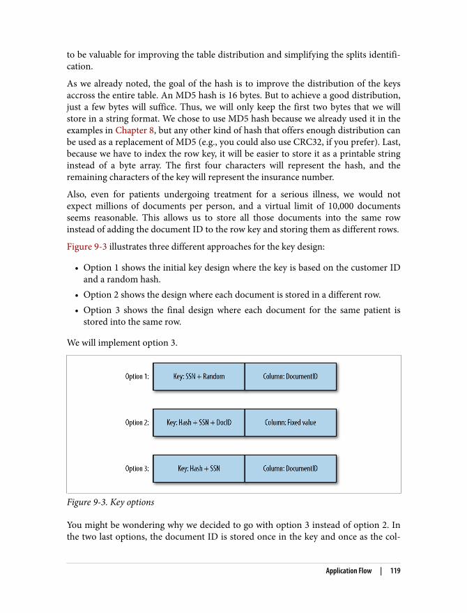
to be valuable for improving the table distribution and simplifying the splits identifi‐cation.

As we already noted, the goal of the hash is to improve the distribution of the keysaccross the entire table. An MD5 hash is 16 bytes. But to achieve a good distribution,just a few bytes will suffice. Thus, we will only keep the first two bytes that we willstore in a string format. We chose to use MD5 hash because we already used it in theexamples in Chapter 8, but any other kind of hash that offers enough distribution canbe used as a replacement of MD5 (e.g., you could also use CRC32, if you prefer). Last,because we have to index the row key, it will be easier to store it as a printable stringinstead of a byte array. The first four characters will represent the hash, and theremaining characters of the key will represent the insurance number.

Also, even for patients undergoing treatment for a serious illness, we would notexpect millions of documents per person, and a virtual limit of 10,000 documentsseems reasonable. This allows us to store all those documents into the same rowinstead of adding the document ID to the row key and storing them as different rows.

Figure 9-3 illustrates three different approaches for the key design:

• Option 1 shows the initial key design where the key is based on the customer IDand a random hash.

• Option 2 shows the design where each document is stored in a different row.• Option 3 shows the final design where each document for the same patient is

stored into the same row.

We will implement option 3.

Figure 9-3. Key options

You might be wondering why we decided to go with option 3 instead of option 2. Inthe two last options, the document ID is stored once in the key and once as the col‐

Application Flow | 119

umn qualifier. Since we are storing the same information at the end whatever optionis chosen, the storage size of the two options will be the same. Again, in both cases,when retrieving a document, we will query HBase given the customer ID and itsMD5, and the document ID. So for both cases again, the access pattern will be direct,and identical.

The main difference here is that storing the documents together allows you to benefitfrom HBase row-level consistency. Indeed, if your upstream system wants to uploadtwo documents at the same time, with the guarantee that they will both go, or bothfail, having them in the same line will allow you to achieve this goal. However, havingthem on two different rows can potentially land the documents into two differentregions. This can be problematic in case of a partial failure. If you do not have anyconsistency constraint, to improve the scalability, it is totally fine, and even preferred,to use the design described in version 2.

Last, keep in mind that HBase will never split within a row. So this approach workswell only if your rows are a decent limited size. This is why we have estimated themaximum number of columns a row might realistically have. If we consider that wecan have a maximum of 10,000 columns of small 10 KB Avro objects, this is onlyabout 100 MB of data for this specific row. Given that HBase regions can easily growabove 10 GB, that gives us plenty of space to store those outlier rows.

LilyThe goal of the Lily Indexer is to replicate into Solr all the mutations received intoHBase. We will not go into all the technical details, but Lily is built on top of theHBase replication framework. Therefore, all mutations are guaranteed to be forwar‐ded to Solr, even in case of a node failure where the region and the related HLogs areassigned to another RegionServer. Because the indexer will receive the data that isstored into HBase, it will be accountable to translate it into a Solr document. In ouruse case, we are going to store Avro objects into HBase. The indexer will have to mapthe fields of the Avro objects to the fields of the Solr document we want to index. Thismapping is defined using a Morphlines script. As described on the project’s website,“Morphlines is an open source framework that reduces the time and skills necessaryto build and change Hadoop ETL stream processing applications that extract, trans‐form and load data into Apache Solr, Enterprise Data Warehouses, HDFS, HBase orAnalytic Online Dashboards.”

SolrWe already discussed Solr in Chapter 8, so we will not repeat the details here. Part ofthe Solr schema that we will use is the following:

<field name="id" type="string" indexed="true" stored="true" required="true" multiValued="false" />

120 | Chapter 9: Implementation of Near Real-Time Event Processing

<field name="rowkey" type="binary" indexed="false" stored="true" omitNorms="true" required="true"/><field name="documentId" type="string" indexed="true" stored="true"\ omitNorms="true" required="true"/><field name="payload" type="text_general" indexed="true" stored="false" required="true" multiValued="false" /><field name="_version_" type="long" indexed="true" stored="true"/>

And again, the complete schema is available in the book’s example files.

ImplementationNow that we have defined all of our main components (Kafka, Flume, HBase, Lily,and Solr), it is time to make sure data can flow from the entry point up to the Solrindex. To allow you to test the examples as you advance into this chapter, we willimplement the different required parts in the same order as the data flow.

Before going into all the details, we recommend creating the HBase table right fromthe beginning. Indeed, having the table available will allow you to test the examples aswe describe them. Later, we will review the details of this table creation and provide amore efficient creation script, but to quickly start, simply type the following into theHBase shell:

create 'documents', 'c'

Data GenerationFirst of all, if we want to test our examples, we need to make sure we have data tosend into our flow. Because we are going to ingest XML documents into Kafka, wewill need a small XML documents generator. Because it doesn’t add much value to thebook, the code for this generator will not be printed here, but it is available in theexample files. The generated data will follow the following format:

<ClinicalDocument> <PatientRecord> <FirstName></FirstName> <LastName></LastName> <SIN></SIN> </PatientRecord> <MedicalRecord> <Comments></Comments> </MedicalRecord></ClinicalDocument>

Of course, a real-world medical document will contain way more fields than what weare generating here; however, the few fields we’re using here are enough to implementthe examples. The social insurance number is a mandatory field, but the other fieldsmight not always be populated. When a field is missing, at the ingestion time, HBasewill try to look up the missing information.

Implementation | 121

The first thing we do to generate those documents is to create a random social insur‐ance number (SIN). We want the same SIN to always represent the same person.Therefore, we will generate a first name and a last name based on this number. Thatway, the same number will always return the same name. However, because we alsowant to demonstrate the use of an interceptor, we are going to generate some of themessages without the first name or the last name. Leveraging a Flume interceptor, wecan add missing field detection. This will not only transform the message from XMLto Avro, but will allow HBase to perform a Get to retrieve previous messages that maycontain the missing fields. This would allow us to fully populate the document.

To run the XML document generator, from the command line, simply use the follow‐ing command:

java -classpath ~/ahae/target/ahae.jar com.architecting.ch09.XMLGenerator

KafkaNow that we have our messages ready to enter our flow, we need to prepare Kafka toaccept them.

Make sure that Kafka is configured with the zookeeper.chrootproperty pointing to the /kafka zookeeper path. Indeed, by default,some distributions will keep the Kafka folder as being the rootZooKeeper path. If the default is used, you will end up with all theKafka folders created under the root path, which could becomeconfusing when it’s time to differentiate those Kafka folders fromother applications folders. Also, not setting the value could result inthe following error: Path length must be > 0.

The first step is to create a Kafka queue, which can be achieved as follows:

[cloudera@quickstart ~]$ kafka-topics --create --topic documents --partitions 1 \ --zookeeper localhost/kafka --replication-factor 1Created topic "documents".

In production, you will most probably want more partitions and abigger replication factor. However, in a local environment with asingle Kafka server running, you will not be able to use any biggernumber.

To learn more about the different parameters this command accepts, refer to theonline Kafka documentation.

When the queue is created, there are multiple ways to add messages into it. The mostefficient approach is to use the Kafka Java API. However, to keep the examples sim‐

122 | Chapter 9: Implementation of Near Real-Time Event Processing

ple, we will use the command-line API for now. To add a message into the newly gen‐erated Kafka queue, use the following command:

java -classpath ~/ahae/target/ahae.jar com.architecting.ch09.XMLGenerator | \kafka-console-producer --topic documents --broker-list localhost:9092

This method will call the XMLGenerator we have implemented earlier and will use itsoutput as the input for the kafka-console-producer. At the end of this call, one newXML message will have been created and pushed into the Kafka queue.

To validate that your topic now contains the generated messages, you can make use ofthe following command:

kafka-console-consumer --zookeeper localhost/kafka --topic documents \ --from-beginning

This command will connect to the documents topic and will output all the eventspresent in this topic, starting from the first available one.

The output of this last command should look like this:

<ClinicalDocument>\n<PatientRecord>\n<FirstName>Tom</FirstName>\n<LastName>...

This shows you that at least one event is available into the Kafka topic.

Also, because we configured Flume to use Kafka as a channel, we also need to createthe Flume Kafka channel using the following:

[cloudera@quickstart ~]$ kafka-topics --create --topic flumechannel \ --partitions 1 --zookeeper localhost/kafka --replication-factor 1Created topic "flumechannel".

FlumeNow that our topic is getting events, we will need something to consume them andstore them into HBase.

The configuration of Flume is done via a property file where we define all the parts tobe put in place together. Flume parameters are in the following form:

<agent-name>.<component-type>.<component-name>.<parameter> = <value>

We will use ingest as the agent name for all the configuration.

For more details about how Flume works and all of its parameters, check out theproject’s online documentation or Hari Shreedharan’s book Using Flume (O’Reilly,2014). For all Kafka plus Flume-specific parameters, refer to the blog post “Flafka:Apache Flume Meets Apache Kafka for Event Processing” on the Cloudera Engineer‐ing Blog.

Implementation | 123

Flume Kafka sourceFlume can be configured with many different sources, most of them being alreadydeveloped. If the source you are looking for is not already built, you can develop yourown. Were are looking here for a Kafka source. We will inform Flume about thissource using the following parameter:

ingest.sources = ingestKafkaSource

This tells Flume that the ingest agent has only one source called ingestKafkaSource. Now that we have told Flume that we have a source, we have to configure it:

ingest.sources.ingestKafkaSource.type = \ org.apache.flume.source.kafka.KafkaSourceingest.sources.ingestKafkaSource.zookeeperConnect = localhost:2181/kafkaingest.sources.ingestKafkaSource.topic = documentsingest.sources.ingestKafkaSource.batchSize = 10ingest.sources.ingestKafkaSource.channels = ingestKafkaChannel

Again, this provides Flume with all the details about the source that we are defining.

Flume Kafka channelA Flume channel is a space that Flume uses as a buffer between the source and thesink. Flume will use this channel to store events read from the source and waiting tobe sent to the sink. Flume comes with a few different channel options. The memorychannel is very efficient, but in case of server failure, data stored into this channel islost. Also, even if servers have more and more memory, they still have a limitedamount compared to what disks can store. The disk channel allows data to be persis‐ted in case of a server failure. However, this will be slower than the other channels,and data lost still exists in case the disk used to store the channel cannot be restored.Using a Kafka channel will use more network than the other channels, but data willbe persisted in a Kafka cluster and therefore cannot be lost. Kafka will store the infor‐mation mainly in memory before returning to Flume, which will reduce the disk’slatency impact on the application. Also, in case the source provides events way fasterthan what the sink can handle, a Kafka cluster can scale bigger than a single diskchannel and will allow to store more of the backlogs to be processed later when thesource will slow down. In our use case, we are storing healthcare information, and wecannot afford to lose any data. For this reason, we will use a Kafka queue as ourFlume channel.

The channel configuration is similar to the source configuration:

ingest.channels = ingestKafkaChannelingest.channels.ingestKafkaChannel.type = org.a.f.channel.kafkaingest.channels.ingestKafkaChannel.brokerList = localhost:9092ingest.channels.ingestKafkaChannel.topic = flumechannelingest.channels.ingestKafkaChannel.zookeeperConnect = localhost:2181/kafka

124 | Chapter 9: Implementation of Near Real-Time Event Processing

This tells our ingest agent to use a channel called ingestKafkaChannel backed byKafka.

Flume HBase sinkThe goal of the Flume sink is to take events from the channel and store them down‐stream. Here, we are looking at HBase as the storage platform. Therefore, we willconfigure an HBase Flume sink. Flume comes with a few default serializers to pushthe data into HBase. The goal of a serializer is to transform a Flume event into anHBase event (and nothing else). However, even if they can be used most of the time,those serializers don’t give you full control over the row key and the column names.We will have to implement our own serializer to be able to extract our row key fromour Avro object.

The sink configuration can be done using the following:

ingest.sinks = ingestHBaseSinkingest.sinks.ingestHBaseSink.type = hbaseingest.sinks.ingestHBaseSink.table = documentsingest.sinks.ingestHBaseSink.columnFamily = cingest.sinks.ingestHBaseSink.serializer = \ com.architecting.ch09.DocumentSerializeringest.sinks.ingestHBaseSink.channel = ingestKafkaChannel

InterceptorA Flume interceptor is a piece of code that can update a Flume event before it is sentto the sink or dropped.

In our case, we want to transform our XML source into an Avro object and performsome HBase lookups to enrich the event before sending it back to HBase. Indeed, ifthe first name or the last name is missing, we need to perform a lookup into HBasefor already existing events to see if it is possible to enrich the current event with theinformation.

The interceptor is where this transformation and this enrichment takes place. Thisprocess should be executed as fast as possible to the table to return the event to Flumevery quickly. Taking too much time or performing too much processing in the inter‐ceptor will result in Flume processing events performing slower than when theyarrived and might end up overwhelming the channel queue.

The interceptor is configured similarly to what has been done for the source, the sink,and the channel:

ingest.sources.ingestKafkaSource.interceptors = ingestInterceptoringest.sources.ingestKafkaSource.interceptors.ingestInterceptor.type = \ com.architecting.ch09.DocumentInterceptor$Builder

Implementation | 125

Instead of building your own XmlToAvro interceptors, it is possibleto apply the transformation using the Morphlines interceptor.However, for simplicity, to be able to update HBase records and tonot have to go over all the Morphlines details, we chose to imple‐ment our own Java interceptor.

Conversion. The first step of the interceptor is to convert the event into an Avroobject. Like in the previous chapter, we will need to define an Avro schema:

{"namespace": "com.architecting.ch09", "type": "record", "name": "Document", "fields": [ {"name": "sin", "type": "long"}, {"name": "firstName", "type": "string"}, {"name": "lastName", "type": "string"}, {"name": "comment", "type": "string"} ]}

The related Java class is also generated the same way:

java -jar ~/ahae/lib/avro-tools-1.7.7.jar compile schema\ ~/ahae/resources/ch09/document.avsc ~/ahae/src/

Code similar to what has been done in the previous chapter will be used to serializeand de-serialize the Avro object. We will use the XPath method to parse the XMLdocument to populate the Avro object. The code in Example 9-1, extracted from thecomplete example available on the GitHub repository, shows you how to extract thoseXML fields.

Example 9-1. XML extraction

expression = "/ClinicalDocument/PatientRecord/FirstName";nodes = getNodes(xpath, expression, inputSource);if (nodes.getLength() > 0) firstName = nodes.item(0).getTextContent();

expression = "/ClinicalDocument/PatientRecord/LastName";inputAsInputStream.reset();nodes = getNodes(xpath, expression, inputSource);if (nodes.getLength() > 0) lastName = nodes.item(0).getTextContent();

expression = "/ClinicalDocument/PatientRecord/SIN";inputAsInputStream.reset();nodes = getNodes(xpath, expression, inputSource);if (nodes.getLength() > 0) SIN = Long.parseLong(nodes.item(0).getTextContent());

expression = "/ClinicalDocument/MedicalRecord/Comments";inputAsInputStream.reset();

126 | Chapter 9: Implementation of Near Real-Time Event Processing

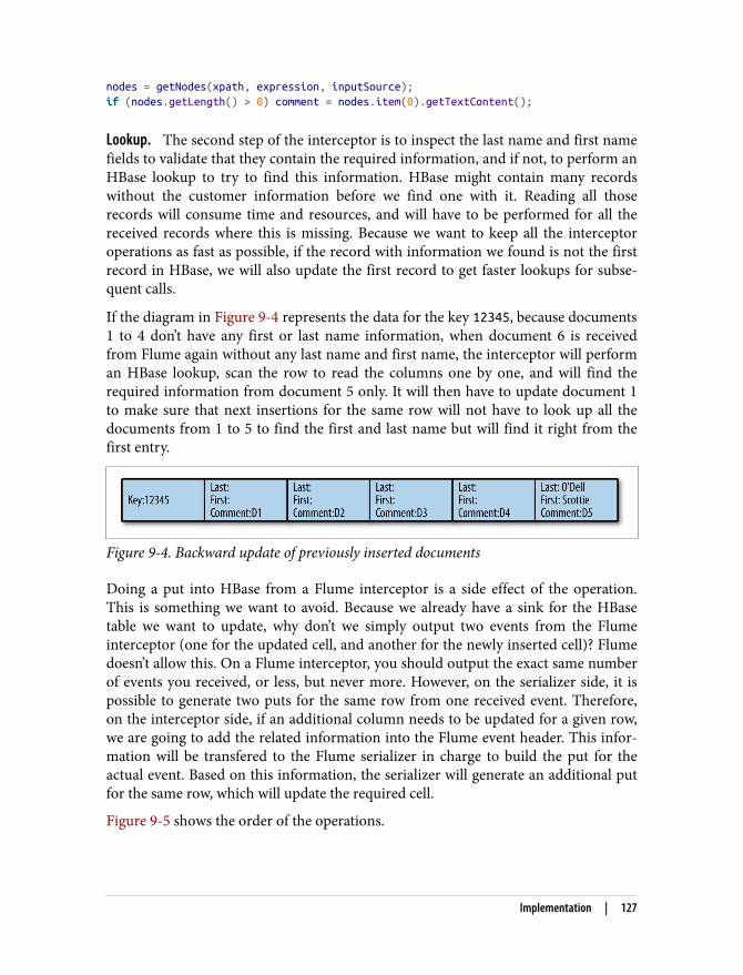
nodes = getNodes(xpath, expression, inputSource);if (nodes.getLength() > 0) comment = nodes.item(0).getTextContent();

Lookup. The second step of the interceptor is to inspect the last name and first namefields to validate that they contain the required information, and if not, to perform anHBase lookup to try to find this information. HBase might contain many recordswithout the customer information before we find one with it. Reading all thoserecords will consume time and resources, and will have to be performed for all thereceived records where this is missing. Because we want to keep all the interceptoroperations as fast as possible, if the record with information we found is not the firstrecord in HBase, we will also update the first record to get faster lookups for subse‐quent calls.

If the diagram in Figure 9-4 represents the data for the key 12345, because documents1 to 4 don’t have any first or last name information, when document 6 is receivedfrom Flume again without any last name and first name, the interceptor will performan HBase lookup, scan the row to read the columns one by one, and will find therequired information from document 5 only. It will then have to update document 1to make sure that next insertions for the same row will not have to look up all thedocuments from 1 to 5 to find the first and last name but will find it right from thefirst entry.

Figure 9-4. Backward update of previously inserted documents

Doing a put into HBase from a Flume interceptor is a side effect of the operation.This is something we want to avoid. Because we already have a sink for the HBasetable we want to update, why don’t we simply output two events from the Flumeinterceptor (one for the updated cell, and another for the newly inserted cell)? Flumedoesn’t allow this. On a Flume interceptor, you should output the exact same numberof events you received, or less, but never more. However, on the serializer side, it ispossible to generate two puts for the same row from one received event. Therefore,on the interceptor side, if an additional column needs to be updated for a given row,we are going to add the related information into the Flume event header. This infor‐mation will be transfered to the Flume serializer in charge to build the put for theactual event. Based on this information, the serializer will generate an additional putfor the same row, which will update the required cell.

Figure 9-5 shows the order of the operations.

Implementation | 127

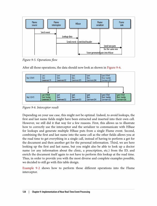
Figure 9-5. Operations flow

After all those operations, the data should now look as shown in Figure 9-6.

Figure 9-6. Interceptor result

Depending on your use case, this might not be optimal. Indeed, to avoid lookups, thefirst and last name fields might have been extracted and inserted into their own cell.However, we still did it that way for a few reasons. First, this allows us to illustratehow to correctly use the interceptor and the serializer to communicate with HBasefor lookups and generate multiple HBase puts from a single Flume event. Second,combining the first and last name into the same cell as the other fields allows you atthe read time to get everything in a single call, instead of having to perform a get forthe document and then another get for the personal information. Third, we are herelooking up the first and last name, but you might also be able to look up a doctorname (or any information about the clinic, a prescription, etc.) from the ID, andenrich the document itself again to not have to perform this lookup at the read time.Thus, in order to provide you with the most diverse and complete examples possible,we decided to still go with this table design.

Example 9-2 shows how to perform those different operations into the Flumeinterceptor.

128 | Chapter 9: Implementation of Near Real-Time Event Processing

Example 9-2. HBase lookup

byte[] rowKeyBytes = Bytes.add(DigestUtils.md5("" + SIN), Bytes.toBytes((int) SIN)); if (StringUtils.isBlank(firstName) || StringUtils.isBlank(lastName)) { LOG.info("Some personal information is missing. Lookup required"); Table documentsTable = connection.getTable(tableName); Get get = new Get(rowKeyBytes); Result result = documentsTable.get(get); if (!result.isEmpty()) { result.advance(); Cell firstCell = result.current(); Cell currentCell = firstCell; while (true) { document = cellToAvro(currentCell, document); if (document.getFirstName() != null) firstName = document.getFirstName().toString(); if (document.getLastName() != null) lastName = document.getLastName().toString(); if ((!"".equals(firstName) && !"".equals(lastName)) || (!result.advance())) break; currentCell = result.current(); } if ((firstCell != currentCell) && StringUtils.isNotBlank(lastName) && StringUtils.isNotBlank(firstName)) { LOG.info("Need to update first cell. Updating headers."); document = cellToAvro(firstCell, document); document.setFirstName(firstName); document.setLastName(lastName); byte[] qualifier = Bytes.copy(firstCell.getQualifierArray(), firstCell.getQualifierOffset(), firstCell.getQualifierLength()); Map<String, String> headers = event.getHeaders(); headers.put(COLUMN, Base64.encodeBytes(qualifier)); headers.put(PAYLOAD, Base64.encodeBytes(avroToBytes(document))); } } }

To improve performances, it is important to reuse a single connection to retrievethe table.

Get the current customer row and prepare to iterate across all its documents.

Iterate until we found both customer last and first names.

If we found the information we were looking for and it is not coming from thefirst cell of the row, update the first cell to make subsequent requests faster.

Implementation | 129

We have decided to give the entire document into the header. Doing that willallow us to not have to lookup the table again on the serializer side but justdirectly create the related Put object. You might want to avoid doing that if yourdocuments are too big.

The last part of the code, shown in Example 9-3, is to make sure modified informa‐tion is applied back to the Avro object, which will be serialized and sent back toFlume.

Example 9-3. Avro enrichment

document.setFirstName(firstName); document.setLastName(lastName); document.setSin(SIN); document.setComment(comment);

All those classes are going to be run by the Flume agent. Therefore,it is important for Flume to have access to the project JAR. Flumehas a plugin.d directory where each project should create its ownsubdirectories with a specific structure. The Flume documentationprovides more details about how this directory is structured.

Build those classes using Maven the same way you are building the other examples(using Eclipse or the command line) and copy the generated JAR into the Flumeplugin directory. To simplify the process for the examples, we will just give everyoneaccess to this directory (in a production environment, you should make sure thatonly required people have access to it):

sudo mkdir -p /var/lib/flume-ng/plugins.d/ahae/libsudo chmod a+rwx /var/lib/flume-ng/plugins.d/ahae/libcp ~/ahae/target/ahae.jar /var/lib/flume-ng/plugins.d/ahae/lib/

You will need to restart Flume for this JAR to be taken into consideration by theapplication. You will also have to restart the Flume agent each time you deploy a newversion of your JAR.

SerializerA Flume serializer is a class that given a Flume event, serializes the required outputfor a given sink. In our example, we will need to build an HBase Flume serializer. Thisserializer will receive our Avro objects generated by the interceptor plus the requiredheaders, and will transform that into one HBase Put operation. Depending on whatwe will receive on the headers, our single put operations might impact one or twocolumns.

130 | Chapter 9: Implementation of Near Real-Time Event Processing

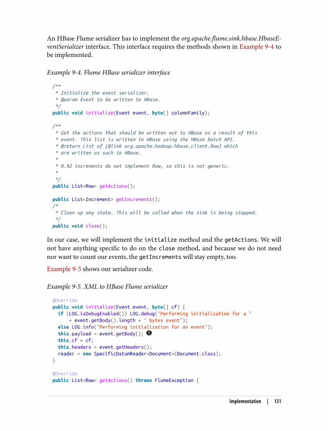
An HBase Flume serializer has to implement the org.apache.flume.sink.hbase.HbaseE‐ventSerializer interface. This interface requires the methods shown in Example 9-4 tobe implemented.

Example 9-4. Flume HBase serializer interface

/** * Initialize the event serializer. * @param Event to be written to HBase. */ public void initialize(Event event, byte[] columnFamily);

/** * Get the actions that should be written out to HBase as a result of this * event. This list is written to HBase using the HBase batch API. * @return List of {@link org.apache.hadoop.hbase.client.Row} which * are written as such to HBase. * * 0.92 increments do not implement Row, so this is not generic. * */ public List<Row> getActions();

public List<Increment> getIncrements(); /* * Clean up any state. This will be called when the sink is being stopped. */ public void close();

In our case, we will implement the initialize method and the getActions. We willnot have anything specific to do on the close method, and because we do not neednor want to count our events, the getIncrements will stay empty, too.

Example 9-5 shows our serializer code.

Example 9-5. XML to HBase Flume serializer

@Override public void initialize(Event event, byte[] cf) { if (LOG.isDebugEnabled()) LOG.debug("Performing initialization for a " + event.getBody().length + " bytes event"); else LOG.info("Performing initialization for an event"); this.payload = event.getBody(); this.cf = cf; this.headers = event.getHeaders(); reader = new SpecificDatumReader<Document>(Document.class); }

@Override public List<Row> getActions() throws FlumeException {

Implementation | 131

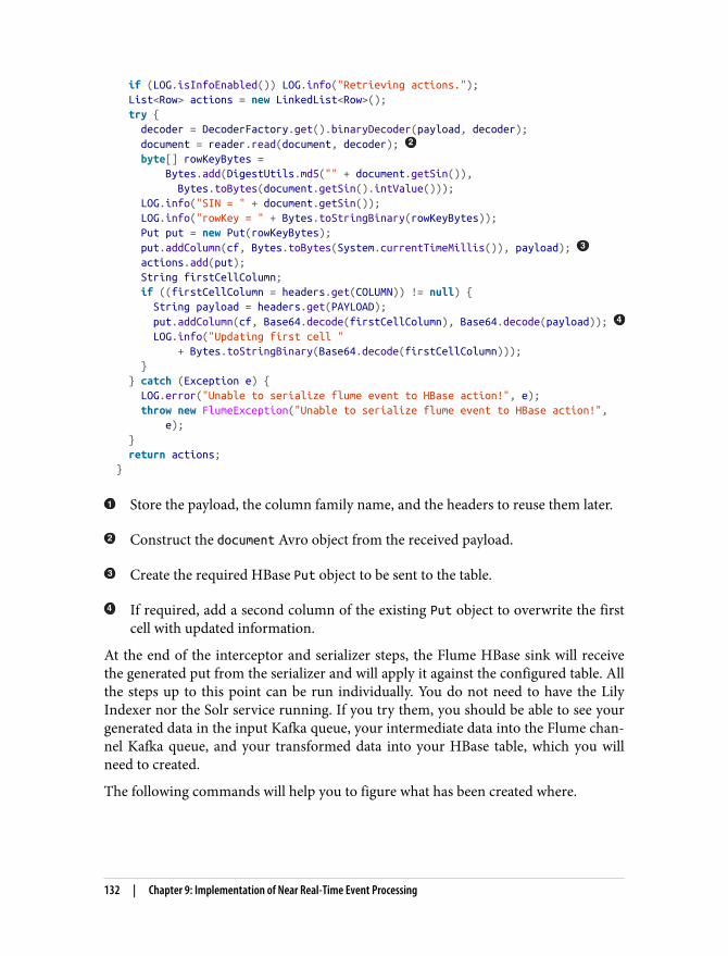
if (LOG.isInfoEnabled()) LOG.info("Retrieving actions."); List<Row> actions = new LinkedList<Row>(); try { decoder = DecoderFactory.get().binaryDecoder(payload, decoder); document = reader.read(document, decoder); byte[] rowKeyBytes = Bytes.add(DigestUtils.md5("" + document.getSin()), Bytes.toBytes(document.getSin().intValue())); LOG.info("SIN = " + document.getSin()); LOG.info("rowKey = " + Bytes.toStringBinary(rowKeyBytes)); Put put = new Put(rowKeyBytes); put.addColumn(cf, Bytes.toBytes(System.currentTimeMillis()), payload); actions.add(put); String firstCellColumn; if ((firstCellColumn = headers.get(COLUMN)) != null) { String payload = headers.get(PAYLOAD); put.addColumn(cf, Base64.decode(firstCellColumn), Base64.decode(payload)); LOG.info("Updating first cell " + Bytes.toStringBinary(Base64.decode(firstCellColumn))); } } catch (Exception e) { LOG.error("Unable to serialize flume event to HBase action!", e); throw new FlumeException("Unable to serialize flume event to HBase action!", e); } return actions; }

Store the payload, the column family name, and the headers to reuse them later.

Construct the document Avro object from the received payload.

Create the required HBase Put object to be sent to the table.

If required, add a second column of the existing Put object to overwrite the firstcell with updated information.

At the end of the interceptor and serializer steps, the Flume HBase sink will receivethe generated put from the serializer and will apply it against the configured table. Allthe steps up to this point can be run individually. You do not need to have the LilyIndexer nor the Solr service running. If you try them, you should be able to see yourgenerated data in the input Kafka queue, your intermediate data into the Flume chan‐nel Kafka queue, and your transformed data into your HBase table, which you willneed to created.

The following commands will help you to figure what has been created where.

132 | Chapter 9: Implementation of Near Real-Time Event Processing

First, to perform a lookup into the Kafka topic used as a source for the entire process,use the following command:

kafka-console-consumer --zookeeper localhost/kafka --topic ingest \ --from-beginning

This should show you all the events that you have inserted into the topic to be pickedup by Flume. To start and to simplify the debugging, make sure to insert only fewevents.

If the Flume agent is running and the Flume source is correctly configured, youshould also see all those events being picked up and inserted into the Flume Kafkachannel topic. To inspect this specific topic, use the following command:

kafka-console-consumer --zookeeper localhost/kafka --topic flumechannel\ --from-beginning

If everything is working correctly, the content of this topic should be the same as thecontent of the ingest topic, and therefore the output of the two commands should bethe same. At this point, you confirmed that both your Kafka service and your Flumeservice are running correctly. The next step is to validate that the interceptor and theserializer are working fine, too. Because the Flume sink is the HBase sink, the resultof our operations should be visible in HBase. Performing the following scan in theHBase shell against the previously created table should show you as many cells asthere was events in the ingest Kafka topic:

hbase(main):001:0> scan 'documents'

If you have inserted millions of events into your Kafka input topic,there will be millions of entries in the two topics as well as millionsof lines into HBase. If this is the case, make sure to use the LIMITkeyword of the HBase scan and use | more or | less in conjonc‐tion with the kafka-console-consumer commands.

The produce.sh file into the resources/ch09/ folder will produce five events (fourwithout last name and first name, and one with the first and last name). At the end ofthe process, you should see into HBase the first cell being updated, the fourth eventbeing populated with its own first and last name, and the fifth event being enrichedwith the last name and first name for the other events.

There are different places where those steps might fail. If you do not see your data inthe ingest topic, check the logs and the code of your data generation steps, and try topush some data from the command line. If you do not see your data in theflumechannel topic, your Flume agent might not be running or it might be incor‐rectly configured. Check the logs of your Flume agent and its configuration. If you donot see your data in the HBase table, there might be an issue with your interceptor

Implementation | 133

or your serializer code. Check the logs of your Flume agent and your Java code,and make sure it has been deployed and is accessible for Flume.

HBaseEven if HBase is probably the most important part of this design, its implementationis the smallest one. Indeed, even if everything here is related to HBase, there is notany specific HBase code required. There are two things we will have to look into onthe HBase side.

Table designAs usual, the first and most important one is the table and key design. As we said pre‐viously, to have a very good distribution of our keys, we are going to use an MD5hash of the social insurance number as a prefix, followed by the number itself. AnMD5 hash is represented by a byte array, values of those bytes being anythingbetween 0 of 255. This information is what we need to correctly presplit the table andchoose the correct logic to calculate the split points. Because we are going to generatebinary keys, we will make use of the UniformSplit algorithm here. The number ofregions we will create depends on the size of the cluster and on the size of the datasetwe expect to have. For our example, we will create an eight-region table calleddocuments with a single column family called c:

create 'documents', { NUMREGIONS => 8, SPLITALGO => 'UniformSplit' }, \ { NAME => 'c' }

Presplitting TablesAs we have suggested many times, it is always recommended to presplit your tableinto multiple regions. This is to avoid hotspotting a RegionServer at the time of theingestion, and will help by reducing huge region splits and compactions. However,how many regions is a good number to start with? There are two good numbers tostart with. The first is based on the expected size of your table after it is fully loaded. Ifthe ingestion will occur over a long period (say, a few months), consider the size aftera few weeks. You want to make sure you have at least 1 GB per region.

Therefore, on a 20-RegionServer cluster, if you expect your table to be only 15 GBafter a month, only create 15 splits to start. The second number is based on the num‐ber of RegionServers you have. As your data becomes more distributed, the reads andwrites will become more efficient. Again, on the same 20-RegionServer clusters, youwould like to have, for a specific table, at least twice the number of regions as youhave RegionServers. If your cluster hosts only very few tables (two or three), youmight want to have at least four regions per table. However, make sure to alwaysrespect the first recommendation, which is to have at least 1 GB regions.

134 | Chapter 9: Implementation of Near Real-Time Event Processing

As another example, if you have a 30 GB table on a 20-RegionServer cluster, based onthe number of RegionServers, you will want to have 40 regions for your table. But thiswill create regions under 1 GB, which we want to avoid. Therefore, we will use thesize as our splitting factor and will presplit this table in 30 regions only.

Table parametersThe second most important part of the HBase design is the table parameters. Indeed,as we have already seen, there are many different values and parameters we can adjuston a table. First, we want to activate the compression for XML. Since XML is textbased, it normally compresses quite well. Also, because the SLA regarding the readlatency for this project is high (documents needs to be returned within one second),we will choose a compression algorithm that will provide a better compression ratiothan the others.

To activate the compaction for this table column family, use the following command:

alter 'documents', { NAME => 'c', COMPRESSION => 'GZ' }

In addition to the compression, we want to disable the Bloom filters. All the readsdone into the HBase table will be base on the key returned by Solr. Therefore, theywill all always succeed. Bloom filters might still be useful if there are many files withina single region; however, major compactions being scheduled daily at night, most ofthe regions will have only a single file, and the Bloom filters are going to be anoverhead.

If you are not sure about using Bloom filters or not, it’s better tokeep them activated. There are very few use cases for which it isadvisable to disable them. If your reads always succeed (e.g., incases when they are looked up from an external index) or if there isonly one file (or very few files) per region, then Bloom filters canbe disabled. However, for all other use cases, Bloom filters will helpto skip reading some files and will improve the read latency.

To disable the Bloom filters, use the following command:

alter 'documents', { NAME => 'c', BLOOMFILTER => 'NONE' }

This example will also work very well if you keep Bloom filters acti‐vated and compression disabled.

Implementation | 135

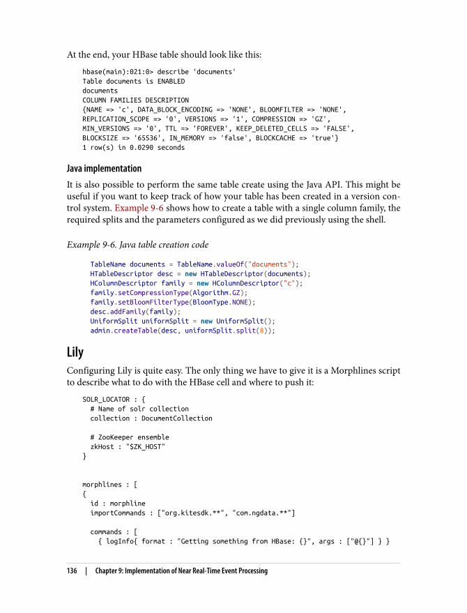
At the end, your HBase table should look like this:

hbase(main):021:0> describe 'documents'Table documents is ENABLEDdocumentsCOLUMN FAMILIES DESCRIPTION{NAME => 'c', DATA_BLOCK_ENCODING => 'NONE', BLOOMFILTER => 'NONE',REPLICATION_SCOPE => '0', VERSIONS => '1', COMPRESSION => 'GZ',MIN_VERSIONS => '0', TTL => 'FOREVER', KEEP_DELETED_CELLS => 'FALSE',BLOCKSIZE => '65536', IN_MEMORY => 'false', BLOCKCACHE => 'true'}1 row(s) in 0.0290 seconds

Java implementationIt is also possible to perform the same table create using the Java API. This might beuseful if you want to keep track of how your table has been created in a version con‐trol system. Example 9-6 shows how to create a table with a single column family, therequired splits and the parameters configured as we did previously using the shell.

Example 9-6. Java table creation code

TableName documents = TableName.valueOf("documents"); HTableDescriptor desc = new HTableDescriptor(documents); HColumnDescriptor family = new HColumnDescriptor("c"); family.setCompressionType(Algorithm.GZ); family.setBloomFilterType(BloomType.NONE); desc.addFamily(family); UniformSplit uniformSplit = new UniformSplit(); admin.createTable(desc, uniformSplit.split(8));

LilyConfiguring Lily is quite easy. The only thing we have to give it is a Morphlines scriptto describe what to do with the HBase cell and where to push it:

SOLR_LOCATOR : { # Name of solr collection collection : DocumentCollection

# ZooKeeper ensemble zkHost : "$ZK_HOST"}

morphlines : [{ id : morphline importCommands : ["org.kitesdk.**", "com.ngdata.**"]

commands : [ { logInfo{ format : "Getting something from HBase: {}", args : ["@{}"] } }

136 | Chapter 9: Implementation of Near Real-Time Event Processing

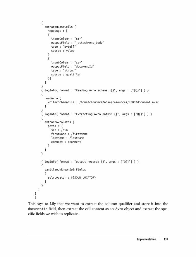
{ extractHBaseCells { mappings : [ { inputColumn : "c:*" outputField : "_attachment_body" type : "byte[]" source : value } { inputColumn : "c:*" outputField : "documentId" type : "string" source : qualifier }] } } { logInfo{ format : "Reading Avro schema: {}", args : ["@{}"] } } { readAvro { writerSchemaFile : /home/cloudera/ahae/resources/ch09/document.avsc } } { logInfo{ format : "Extracting Avro paths: {}", args : ["@{}"] } } { extractAvroPaths { paths : { sin : /sin firstName : /firstName lastName : /lastName comment : /comment } } }

{ logInfo{ format : "output record: {}", args : ["@{}"] } } { sanitizeUnknownSolrFields { solrLocator : ${SOLR_LOCATOR} } } ]}]

This says to Lily that we want to extract the column qualifier and store it into thedocumentId field, then extract the cell content as an Avro object and extract the spe‐cific fields we wish to replicate.

Implementation | 137

2 https://github.com/NGDATA/hbase-indexer/wiki/Indexer-configuration

We also need an XML file to configure the indexer. This file will be given as a param‐eter to the command line. It defines what kind of mapper we want to use and pro‐vides some parameters for this mapper:

<?xml version="1.0"?><indexer table="documents" mapper="com.ngdata.hbaseindexer.morphline.MorphlineResultToSolrMapper" mapping-type="column" row-field="rowkey">

<!-- The relative or absolute path on the local file system to the morphline --><!-- configuration file. Use relative path "morphlines.conf" for morphlines --><!-- managed by Cloudera Manager --><param name="morphlineFile" value="morphlines.conf"/>

</indexer>

The XML will configure Lily to use the MorphlineResultToSolrMapper. It will alsoconfigure this mapper to process the HBase cells at the column lever (instead of thedefault row-level mode). Last, it will also configure Lily to provide the HBase row keyinto the rowkey field. More information regarding the XML file content is availableon the NGData GitHub page.2

The last step is to enable to the indexer using the following command:

hbase-indexer add-indexer --name myIndexer --indexer-conf indexer-config.xml \ --connection-param solr.zk=quickstart/solr \ --connection-param solr.collection=DocumentCollection \ --zookeeper localhost:2181

If you want to disable and remove the indexer (because you want to try another oneor if something goes wrong with the configuration), use the following command:

hbase-indexer delete-indexer --name myIndexer

After this step, Lily will create a Solr document for each cell inserted into HBase byFlume. However, because Solr is not yet configured, this will probably fail. Continueto the next section to configure Solr and test Lily.

SolrThe implementation part of Solr is straightforward. We simply need to create a Solrcollection based on the schema that we have defined previously. To do so, we will fol‐low the exact same steps described in Chapter 7.

To create the collection, use the following commands:

export PROJECT_HOME=~/ahae/resources/ch09/searchrm -rf $PROJECT_HOME

138 | Chapter 9: Implementation of Near Real-Time Event Processing

3 http://quickstart.cloudera:8983/solr/DocumentCollection_shard1_replica1/select?q=rowkey%3A+%22827c12345%22&wt=json&indent=true

solrctl instancedir --generate $PROJECT_HOMEmv $PROJECT_HOME/conf/schema.xml $PROJECT_HOME/conf/schema.oldcp $PROJECT_HOME/../schema.xml $PROJECT_HOME/conf/solrctl instancedir --create DocumentCollection $PROJECT_HOMEsolrctl collection --create DocumentCollection -s 1

When this is done, the collection should be visible on the web UI: http://quick‐start.cloudera:8983/solr/#/DocumentCollection_shard1_replica1

TestingNow that all the parts are installed and implemented, any data inserted into the Kafkaqueue should be visible in both HBase and Solr. A Solr query such as the followingshould return all the records indexed by Solr: http://quickstart.cloudera:8983/solr/DocumentCollection_shard1_replica1/select?q=%3A&wt=json&indent=true. All thoserecords should also be into HBase and can be viewed using the shell.

Inserting this XML:

<?xml version=\"1.0\" encoding=\"UTF-8\"?><ClinicalDocument> <PatientRecord> <SIN>12345</SIN> <FirstName>Scottie</FirstName> <LastName>O'Dell</LastName> </PatientRecord> <MedicalRecord> <Comments>Scottie is doing well.</Comments> </MedicalRecord></ClinicalDocument>

Will produce this entry in HBase:

hbase(main):002:0> get 'documents', '827c12345'COLUMN CELLc:1448998062581 timestamp=1448998062683 value=\xF2\xC0\x01\x0EScottie\x0CO'Dell6Scottie is doing well.1 row(s) in 0.0290 seconds

And this output in Solr:3

{ "responseHeader":{ "status":0, "QTime":0, "params":{ "indent":"true", "q":"rowkey: \"827c12345\"",

Implementation | 139

"wt":"json"}}, "response":{"numFound":1,"start":0,"docs":[ { "id":"827c12345-c-1448998450634", "lastName":"O'Dell", "rowkey":"827c12345", "firstName":"Scottie", "documentId":"1448998450634", "_version_":1519384999917256704}] }}

You can now query Solr by any of the indexed fields, and using the returned informa‐tion, query HBase given a specific row and a specific column qualifier to get a direct,low-latency random access to the record.

Going FurtherIf you want to extend the examples presented in this chapter, the following list offerssome options you can try based on our discussions from this chapter:

Bigger input fileHere again we tried our workflow by ingesting one document at a time and onlya few. Try to ingest way more documents. Also try to ingest documents with verybig fields. When producing documents bigger than one MB, you can also eventry the HBase MOB features.

Extract patient recordExtract the patient name from the document and store it separately in a specificcolumn. Modify the lookup to populate only this column and only if informationis missing. Then, instead of storing the Avro object inside of HBase, only storethe comment field.

Duplicate flowsProduce two kinds of documents in two different topics and two Flume agents.Merge those two streams into a single HBase table and a single Solr index.

Row keyThe row key for a new document is calculated twice (once in the interceptor, andonce in the serializer). Using the event header, store, transfer, and reuse thisinformation.

Change Solr schemaTo make things easier, in the current schema, we store, index, and return the rowkey. However, the Solr document ID (stored in the ID field) already contains therow key as well as the column family and the column qualifier. Update the Solrschema to only index the row key and the document ID but not store them.

140 | Chapter 9: Implementation of Near Real-Time Event Processing

CHAPTER 10

Use Case: HBase as a Master DataManagement Tool

Next, we will take a look at the New York–based digital advertising company Collec‐tive. Collective is an advertising technology company that helps companies impactthe bottom line by connecting brands and customers together. This approach isknown as customer 360, and to execute efficiently, it requires numerous data sourcesand boatloads of data. Collective leverages Hadoop and HBase to help offer their cli‐ents a unified view of the consumer and allowing brands to seamlessly message acrosschannels and devices, including PCs, tablets, and smartphones.

When looking at customer 360, Hadoop is the obvious choice. A solid customer 360implementation gets better and better as data sources are added. Most data sourcesthat customers interact with on a regular basis tend to create unstructured data. Someof the typical data sources seen in a customer 360 are clickstream through offeringslike Adobe Omniture or IBM Tealeaf and social media data either directly throughTwitter and Facebook, or more often, from curated data services providers such asGnip and Datasift; these data sources are then joined with the all-powerful (andhomegrown) customer profile. Maintaing an up-to-date, complete customer profileon an immutable filesystem like HDFS is not a trival task. Collective needed a systemthat could combine these numerous data sources, which fit poorly into a relationalsystem, into a unified customer—and that’s where HBase comes in.

At first, Collective tried a couple standalone relational systems and was attempting topush the data from the Hadoop ETL jobs. The company started to run into problemsof serving the data to end users when the cache on a node or two became full. Thiscaused the disks to start thrashing, and would require a major hardware overhaul tohandle the data in a traditional manner. Most of these relational systems require ver‐tical scalability as opposed to horizontal scalability. These relational systems typically

141

require more memory and leverage expensive solid-state drives (SSDs). On the flipside, HBase utilizes commodity hardware and SATA drives. This is what led Collec‐tive to start looking at HBase. Luckily, Collective already had a Hadoop cluster inplay, and had the advantage of seamlessly integrating HBase into the existing infra‐structure with minor development and cost overhead.

Collective currently has 60 RegionServers deployed serving 21 TBs of data out ofHBase alone. Collective’s HBase deployment is pretty straightforward. For this usecase, there is a single table that handles the user profile data. The table is broken intothree column families consisting of visitor, export, and edge. The “visitor” CF con‐tains the metadata about the user. This will consist of information such as date ofbirth, behavior information, and any third-party lookup IDs. The “export” CF con‐tains the segment information (an example of a segment would be male, 25 years old,likes cars), and any relevant downstream syndication information needed for pro‐cessing. The “edge” CF contains the activity information of the user, along with any ofthe additional data that may come in from the batch imported data:

COLUMN CELL

edge:batchimport ts=1391769526303, value=\x00\x00\x01D\x0B\xA3\xE4.export:association:cp ts=1390163166328, value=6394889946637904578export:segment:13051 ts=1390285574680, value=\x00\x00\x00\x00\x00\x00\x00\x00export:segment:13052 ts=1390285574680, value=\x00\x00\x00\x00\x00\x00\x00\x00export:segment:13059 ts=1390285574680, value=\x00\x00\x00\x00\x00\x00\x00\x00…visitor:ad_serving_count ts=1390371783593, value=\x00\x00\x00\x00\x00\x00\x1Avisitor:behavior:cm.9256:201401 ts=1390163166328, value=\x00\x00\x00\x0219visitor:behavior:cm.9416:201401 ts=1390159723536, value=\x00\x00\x00\x0119visitor:behavior:iblocal.9559:2 ts=1390295246778, value=\x00\x00\x00\x020140120visitor:behavior:iblocal.9560:2 ts=1390296907500, value=\x00\x00\x00\x020140120visitor:birthdate ts=1390159723536, value=\x00\x00\x01C\xAB\xD7\xC4(visitor:retarget_count ts=1390296907500, value=\x00\x00\x00\x00\x00\x00\x00\x07

As already mentioned, Collective is a digital advertising company that enhancesoffers and profiles through consumer interactions. Each user is tracked through acustom cookie ID that is generated upstream in the process. The row key is a reverseof that cookie ID. This begs the question of why to reverse a generated UUID. Thereare two primary offenders that require reverse keys: websites and time series data. Inthis case, the beginning of the cookie ID has the timestamp on it. This would lead tomonotonically increasing row keys; by simply reversing the row key, the randomlygenerated portion now occurs first in the row key.

IngestIn Chapters 8 and 9, we looked at near real-time ingest pipelines and batch loadingprocesses. Next, we are going to look at combining the two while using HBase as thesystem of record, which is sometimes referred to as master data management

142 | Chapter 10: Use Case: HBase as a Master Data Management Tool

(MDM); a system of record is used as the “golden copy” of the data. The records con‐tained in HBase will be used to rebuild any Hive or other external data sources in theevent of bad or wrong data. The first piece we will examine is batch processing. Forthis system, Collective built a tool that pulls in third-party data sources from numer‐ous data sources covering S3, SFTP sites, and a few proprietary APIs (Figure 10-1).The tool pulls from these data sources on an hourly basis and loads the data into anew HDFS directory using the Parquet file format. A new Hive partition is then cre‐ated on top of the newly loaded data, and then linked to the existing archive table.

Figure 10-1. Ingest dataflow

The other side of the house is the near real-time processing, which is currently beinghandled by Flume. Flume brings in data from different messaging services, which ispushed into a system known as Parquetify. The Parquetify system, which runs hourly,prepares the data into a unified file format, wraps a temporary table around the data,and then inserts the data into the main archive Hive tables. In this case, the file for‐mat used for this data is Parquet files. Once the data is loaded into the system, theaptly named preprocessor Harmony is run every hour in a custom workflow fromCelos. Harmony collects and preprocesses the necessary data from the previously lis‐ted sources. This is used to normalize the output together for the formal transforma‐tion stages. Currently this runs in a series of Flume dataflows, MapReduce jobs, andHive jobs. Collective is in the process of porting all of this to Kafka and Spark, whichwill make processing both easier and faster.

ProcessingOnce Harmony has joined the inbound data together, it is then sent for final process‐ing into another internal system that coordinates a series of MapReduce jobs togetherknown as Pythia (Figure 10-2). The MapReduce jobs create a write-ahead log (WAL)

Processing | 143

for maintaining data consistency in case of failures. There are three total steps in thisprocess:

• Aggregator• ProfileMod• Update MDM system

Figure 10-2. Processing dataflow

Both the Aggregator and ProfileMod steps in the pipeline also represent backed andpartitioned Hive/Impala tables. The first thing done is to read the output of the Har‐mony job into an Avro file for our Aggregator job. Once new edits (Harmony) andprevious hour of data (HDFS) are read and grouped in the mapper, they are passed tothe reducer. During the Reduce phase, numerous HBase calls are made to join the fullprofile together for the next hourly partition. The reducer will pull the full HBaserecord for each record that has an existing profile. The Aggregator job then outputs aset of differences (typically known as diffs) that is applied during the ProfileModstage. These diffs are used as a sort of WAL that can be used to rectify the changes ifany of the upstream jobs fail.

Next, the ProfileMod job is executed. ProfileMod will be a Map job because wealready extracted the data we needed from HBase in the reducer from the Aggregatorflow. The mapper will read all of the data from the previous output and rectify thediffs. Once the diffs are all combined together, ProfileMod will use these as the actualdiffs that need to be written back to HBase. The final output of this job is a newhourly partition in the ProfileMod Hive table.

144 | Chapter 10: Use Case: HBase as a Master Data Management Tool

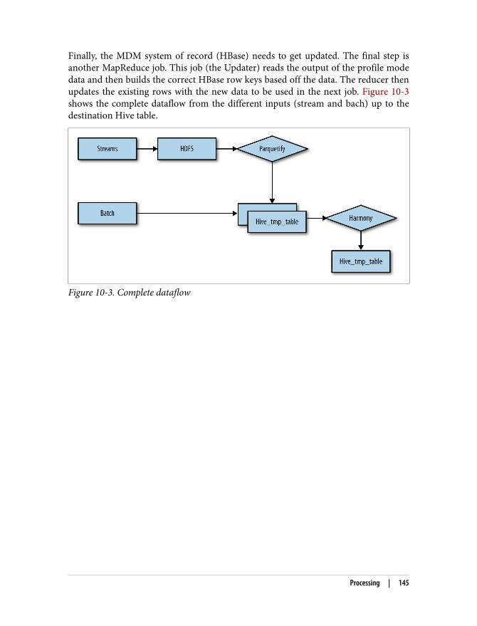
Finally, the MDM system of record (HBase) needs to get updated. The final step isanother MapReduce job. This job (the Updater) reads the output of the profile modedata and then builds the correct HBase row keys based off the data. The reducer thenupdates the existing rows with the new data to be used in the next job. Figure 10-3shows the complete dataflow from the different inputs (stream and bach) up to thedestination Hive table.

Figure 10-3. Complete dataflow

Processing | 145

CHAPTER 11

Implementation of HBase as a Master DataManagement Tool

In Chapter 10, we reviewed the implementation of a customer 360 solution. In addi‐tion to HBase, it uses several different applications, including MapReduce and Hive.On the HBase side, we described how MapReduce is used to do lookups or to gener‐ate HBase files. In addition, as discussed in the previous chapter, Collective plans toimprove its architecture by using Kafka. None of this should be new for you, as wecovered it in detail in previous chapters. However, Collective is also planning to useSpark, and this is where things start to be interesting. Indeed, over the last severalyears, when applications needed to process HBase data, they have usually used Map‐Reduce or the Java API. However, with Spark becoming more and more popular, weare seeing people starting to implement solutions using Spark on top of HBase.

Because we already covered Kafka, MapReduce, and the Java API in previous chap‐ters, instead of going over all those technologies again to provide you with very simi‐lar examples, we will here focus on Spark over HBase. The example we are going toimplement will still put the customer 360 description in action, but as for the otherimplementation examples, this can be reused for any other use case.

MapReduce Versus SparkBefore we continue, we should establish the pros and cons of using Spark versususing MapReduce. Although we will not provide a lengthy discussion on this topic,we will briefly highlight some points for you to consider as you narrow down yourchoice.

Spark is a recent technology, while MapReduce has been used for years. AlthoughSpark has been proven to be stable, you might be more comfortable with a technol‐

147

ogy deployed in hundreds of thousands of production applications—if so, you shouldbuild your project around MapReduce. On the other hand, if you prefer to rely onrecent technologies, then Spark will be a good fit.

For companies with good MapReduce knowledge that already have many MapReduceprojects deployed, it might be easier, faster, and cheaper to stay with something theyknow well. However, if they start a brand-new project and are planning manyprojects, they might want to consider Spark.

Some use cases require fast and efficient data processing. MapReduce comes with abig overhead. It gives you reliability and many other benefits, but at the price of a per‐formance hit. If your use case has tight SLAs, you might want to consider Spark.Otherwise, MapReduce is still a good option.

One last consideration is the development language. Spark is compatible with bothJava and Scala code, while MapReduce is mostly for Java developers.

So which one should you choose? If you are still deciding between the two, we recom‐mend trying Spark, as it has nice benefits over MapReduce.

Get Spark Interacting with HBaseAs with MapReduce, there are two main ways for Spark to interact with HBase. Thefirst is to run a Spark application on top of an HBase table. The second is to interactwith HBase while running Spark on other data. We will assume that you have at leastbasic spark knowledge. Refer to the Spark website for more information.

Run Spark over an HBase TableWhen we are running a MapReduce job on top of an HBase table, each mapper pro‐cess a single region. You can also run a simple Java application that will scan theentire HBase table. This will be very similar with Spark. The HBase Spark API canreturn you an RDD representing your entire HBase table. But you partition this RDDto get it processed over multiple executors where each of them will process a singleregion

Calling HBase from SparkThe HBase Java API is accessible from the Spark code. Therefore, you can performlookups like what we did when implementing our Flume interceptor. You can also useSpark to enrich and store data into HBase leveraging Puts and Increments. Last, thesame way you can use MapReduce to generate HFiles for BulkLoads, you can useSpark to generate the same kind of files that you will later BulkLoad into HBase.

148 | Chapter 11: Implementation of HBase as a Master Data Management Tool

Implementing Spark with HBaseTo illustrate using Spark with HBase, we will begin by implementing a Spark job toprocess a text file where each line is a record that we will use to enrich HBase data.Later, we will process another source of data that we will use to create HFiles to Bulk‐Load into HBase tables. Finally, we will implement a Spark job over the same HBasetable to perform data aggregation.

You might find different versions of the Spark HBase API. The onewe will use here is extracted from the Apache HBase 2.0 project. Ifyou are using another version of the Spark HBase API, you mightface some compilation issues, but the logic behind it will still be thesame. You might be able to adjust the examples to compile withyour code and run them.

All the operations we are going to implement will be done over the same table. Usethe following command to create this table:

create 'user', {NAME => 'edge', BLOOMFILTER => 'NONE',\ COMPRESSION => 'SNAPPY', DATA_BLOCK_ENCODING => 'FAST_DIFF'},\ {NAME => 'segment', BLOOMFILTER => 'NONE',\ COMPRESSION => 'SNAPPY', DATA_BLOCK_ENCODING => 'FAST_DIFF'},\ {NAME => 'visitor', BLOOMFILTER => 'NONE',\ COMPRESSION => 'SNAPPY', DATA_BLOCK_ENCODING => 'FAST_DIFF'}

Let’s take a closer look at the table creation command and the reason for the differentoptions we have chosen. First, we disabled the Bloom filters. Indeed, every time wequery HBase for a row, we will use its rowID so that we can be sure that it exists. Also,most of the time, the entire dataset will be processed and not just a single line. There‐fore, having to look at the Bloom filter just to confirm that the row exists is an over‐head. Most of the time, it is a good idea to keep the Bloom filters on. If you are notsure, just keep them.

Second, we enabled the Snappy compression. Even if the compression ratio it gives isless efficient compared to some other algorithm, Snappy allows quick compressionwith very small impact on the CPU. Unless you are storing data like compressedimages or sound, it is always a good idea to enable it.

Last, we enabled data block encoding. Data block encoding is very useful to reducethe overhead of storing the key for every column of the same row. Given that a usercan have many columns, and given that the row key can be pretty long, activating theFAST_DIFF block encoding will provide us with extra savings.

Implementing Spark with HBase | 149

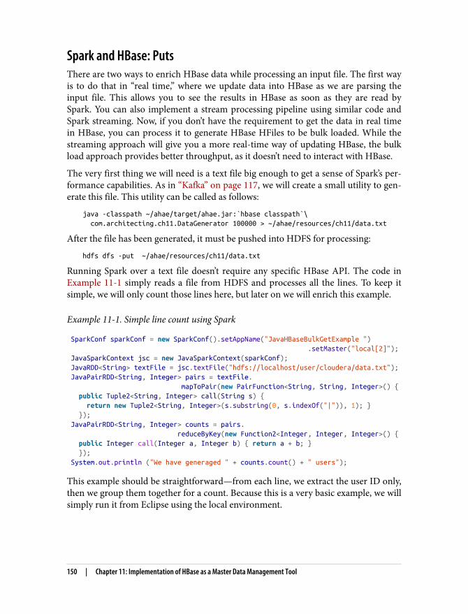
Spark and HBase: PutsThere are two ways to enrich HBase data while processing an input file. The first wayis to do that in “real time,” where we update data into HBase as we are parsing theinput file. This allows you to see the results in HBase as soon as they are read bySpark. You can also implement a stream processing pipeline using similar code andSpark streaming. Now, if you don’t have the requirement to get the data in real timein HBase, you can process it to generate HBase HFiles to be bulk loaded. While thestreaming approach will give you a more real-time way of updating HBase, the bulkload approach provides better throughput, as it doesn’t need to interact with HBase.

The very first thing we will need is a text file big enough to get a sense of Spark’s per‐formance capabilities. As in “Kafka” on page 117, we will create a small utility to gen‐erate this file. This utility can be called as follows:

java -classpath ~/ahae/target/ahae.jar:`hbase classpath`\ com.architecting.ch11.DataGenerator 100000 > ~/ahae/resources/ch11/data.txt

After the file has been generated, it must be pushed into HDFS for processing:

hdfs dfs -put ~/ahae/resources/ch11/data.txt

Running Spark over a text file doesn’t require any specific HBase API. The code inExample 11-1 simply reads a file from HDFS and processes all the lines. To keep itsimple, we will only count those lines here, but later on we will enrich this example.

Example 11-1. Simple line count using Spark

SparkConf sparkConf = new SparkConf().setAppName("JavaHBaseBulkGetExample ") .setMaster("local[2]"); JavaSparkContext jsc = new JavaSparkContext(sparkConf); JavaRDD<String> textFile = jsc.textFile("hdfs://localhost/user/cloudera/data.txt"); JavaPairRDD<String, Integer> pairs = textFile. mapToPair(new PairFunction<String, String, Integer>() { public Tuple2<String, Integer> call(String s) { return new Tuple2<String, Integer>(s.substring(0, s.indexOf("|")), 1); } }); JavaPairRDD<String, Integer> counts = pairs. reduceByKey(new Function2<Integer, Integer, Integer>() { public Integer call(Integer a, Integer b) { return a + b; } }); System.out.println ("We have generaged " + counts.count() + " users");

This example should be straightforward—from each line, we extract the user ID only,then we group them together for a count. Because this is a very basic example, we willsimply run it from Eclipse using the local environment.

150 | Chapter 11: Implementation of HBase as a Master Data Management Tool

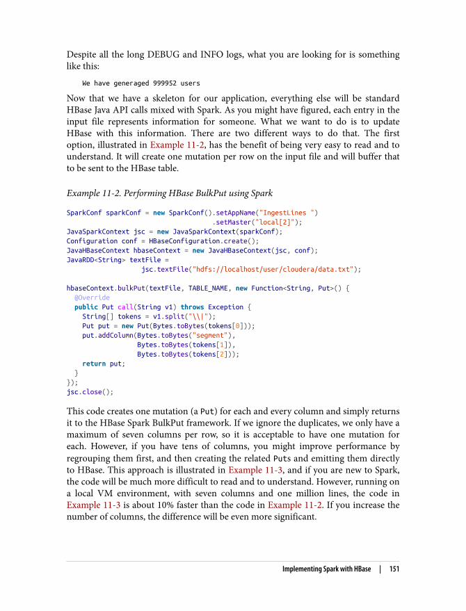
Despite all the long DEBUG and INFO logs, what you are looking for is somethinglike this:

We have generaged 999952 users

Now that we have a skeleton for our application, everything else will be standardHBase Java API calls mixed with Spark. As you might have figured, each entry in theinput file represents information for someone. What we want to do is to updateHBase with this information. There are two different ways to do that. The firstoption, illustrated in Example 11-2, has the benefit of being very easy to read and tounderstand. It will create one mutation per row on the input file and will buffer thatto be sent to the HBase table.

Example 11-2. Performing HBase BulkPut using Spark

SparkConf sparkConf = new SparkConf().setAppName("IngestLines ") .setMaster("local[2]");JavaSparkContext jsc = new JavaSparkContext(sparkConf);Configuration conf = HBaseConfiguration.create();JavaHBaseContext hbaseContext = new JavaHBaseContext(jsc, conf);JavaRDD<String> textFile = jsc.textFile("hdfs://localhost/user/cloudera/data.txt");

hbaseContext.bulkPut(textFile, TABLE_NAME, new Function<String, Put>() { @Override public Put call(String v1) throws Exception { String[] tokens = v1.split("\\|"); Put put = new Put(Bytes.toBytes(tokens[0])); put.addColumn(Bytes.toBytes("segment"), Bytes.toBytes(tokens[1]), Bytes.toBytes(tokens[2])); return put; }});jsc.close();

This code creates one mutation (a Put) for each and every column and simply returnsit to the HBase Spark BulkPut framework. If we ignore the duplicates, we only have amaximum of seven columns per row, so it is acceptable to have one mutation foreach. However, if you have tens of columns, you might improve performance byregrouping them first, and then creating the related Puts and emitting them directlyto HBase. This approach is illustrated in Example 11-3, and if you are new to Spark,the code will be much more difficult to read and to understand. However, running ona local VM environment, with seven columns and one million lines, the code inExample 11-3 is about 10% faster than the code in Example 11-2. If you increase thenumber of columns, the difference will be even more significant.

Implementing Spark with HBase | 151

Example 11-3. Text file to HBase Spark processing

SparkConf sparkConf = new SparkConf().setAppName("IngestLines ") .setMaster("local[2]");JavaSparkContext jsc = new JavaSparkContext(sparkConf);Configuration conf = HBaseConfiguration.create();JavaHBaseContext hbaseContext = new JavaHBaseContext(jsc, conf);JavaRDD<String> textFile = jsc.textFile("hdfs://localhost/user/cloudera/data.txt");

PairFunction<String, String, String> linesplit = new PairFunction<String, String, String>() { public Tuple2<String, String> call(String s) { int index = s.indexOf("|"); return new Tuple2<String, String>(s.substring(0, index), s.substring(index + 1)); }};

JavaPairRDD<String, String> pairs = textFile.mapToPair(linesplit);Function<String, List<String>> createCombiner =new Function<String, List<String>>() { public List<String> call(String s) { List<String> list = new ArrayList<String>(); list.add(s); return list; }};

Function2<List<String>, String, List<String>> mergeValue =new Function2<List<String>, String, List<String>>() { @Override public List<String> call(List<String> v1, String v2) throws Exception { v1.add(v2); return v1; }};

Function2<List<String>, List<String>, List<String>> mergeCombiners =new Function2<List<String>, List<String>, List<String>>() { @Override public List<String> call(List<String> v1, List<String> v2) throws Exception { v2.addAll(v1); return v2; }};

JavaPairRDD<String, List<String>> keyValues = pairs.combineByKey(createCombiner, mergeValue, mergeCombiners);

JavaRDD<Put> keyValuesPuts = keyValues.map( new Function<Tuple2<String, List<String>>, Put>() {

152 | Chapter 11: Implementation of HBase as a Master Data Management Tool

@Override public Put call(Tuple2<String, List<String>> v1) throws Exception { Put put = new Put(Bytes.toBytes(v1._1)); ListIterator<String> iterator = v1._2.listIterator(); while (iterator.hasNext()) { String colAndVal = iterator.next(); int indexDelimiter = colAndVal.indexOf("|"); String columnQualifier = colAndVal.substring(0, indexDelimiter); String value = colAndVal.substring(indexDelimiter + 1); put.addColumn(COLUMN_FAMILY, Bytes.toBytes(columnQualifier), Bytes.toBytes(value)); } return put; }});

hbaseContext.foreachPartition(keyValuesPuts, new VoidFunction<Tuple2<Iterator<Put>, Connection>>() { @Override public void call(Tuple2<Iterator<Put>, Connection> t) throws Exception { Table table = t._2().getTable(TABLE_NAME); BufferedMutator mutator = t._2().getBufferedMutator(TABLE_NAME); while (t._1().hasNext()) { Put put = t._1().next(); mutator.mutate(put); }

mutator.flush(); mutator.close(); table.close(); } });jsc.close();

Extract the key from the lines to create pairs that can be regrouped together.

Combine all the entries based on the key so each key will have a list of “columnqualifier|value” strings associated.

Transform one key and all its related “column qualifier|value” strings to a singleHBase put object.

Emit all the puts to HBase.

Basically, what we are doing here is regrouping all the lines based on the key that weextract from the string, then we transform them into a single put for this line that wethen send to HBase.

You can run this example directly from Eclipse.

Implementing Spark with HBase | 153

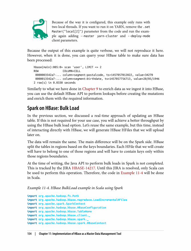
Because of the way it is configured, this example only runs withtwo local threads. If you want to run it on YARN, remove the .setMaster("local[2]") parameter from the code and run the exam‐ple again adding --master yarn-cluster and --deploy-modeclient parameters.

Because the output of this example is quite verbose, we will not reproduce it here.However, when it is done, you can query your HBase table to make sure data hasbeen processed:

hbase(main):005:0> scan 'user', LIMIT => 2ROW COLUMN+CELL 0000003542a7-... column=segment:postalcode, ts=1457057812022, value=34270 0000013542a7-... column=segment:birthdate, ts=1457057756713, value=20/05/19462 row(s) in 0.0330 seconds

Similarly to what we have done in Chapter 9 to enrich data as we ingest it into HBase,you can use the default HBase API to perform lookups before creating the mutationsand enrich them with the required information.

Spark on HBase: Bulk LoadIn the previous section, we discussed a real-time approach of updating an HBasetable. If this is not required for your use case, you will achieve a better throughput byusing the HBase bulk load option. Let’s reuse the same example, but this time, insteadof interacting directly with HBase, we will generate HBase HFiles that we will uploadlater on.

The data will remain the same. The main difference will be on the Spark side. HBasesplit the tables in regions based on the keys boundaries. Each HFile that we will createwill have to belong to one of those regions and will have to contain keys only withinthose regions boundaries.

At the time of writing, the Java API to perform bulk loads in Spark is not completed.This is tracked by the JIRA HBASE-14217. Until this JIRA is resolved, only Scala canbe used to perform this operation. Therefore, the code in Example 11-4 will be donein Scala.

Example 11-4. HBase BulkLoad example in Scala using Spark

import org.apache.hadoop.fs.Pathimport org.apache.hadoop.hbase.mapreduce.LoadIncrementalHFilesimport org.apache.spark.SparkContextimport org.apache.hadoop.hbase.HBaseConfigurationimport org.apache.hadoop.hbase.TableNameimport org.apache.hadoop.hbase.client._import org.apache.hadoop.hbase.spark._import org.apache.hadoop.hbase.spark.HBaseContext

154 | Chapter 11: Implementation of HBase as a Master Data Management Tool

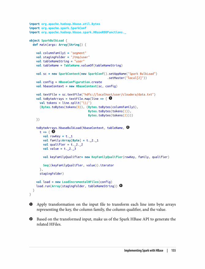
import org.apache.hadoop.hbase.util.Bytesimport org.apache.spark.SparkConfimport org.apache.hadoop.hbase.spark.HBaseRDDFunctions._

object SparkBulkLoad { def main(args: Array[String]) {

val columnFamily1 = "segment" val stagingFolder = "/tmp/user" val tableNameString = "user" val tableName = TableName.valueOf(tableNameString)

val sc = new SparkContext(new SparkConf().setAppName("Spark BulkLoad") .setMaster("local[2]")) val config = HBaseConfiguration.create val hbaseContext = new HBaseContext(sc, config)

val textFile = sc.textFile("hdfs://localhost/user/cloudera/data.txt") val toByteArrays = textFile.map(line => { val tokens = line.split("\\|") (Bytes.toBytes(tokens(0)), (Bytes.toBytes(columnFamily1), Bytes.toBytes(tokens(1)), Bytes.toBytes(tokens(2)))) })

toByteArrays.hbaseBulkLoad(hbaseContext, tableName, t => { val rowKey = t._1 val family:Array[Byte] = t._2._1 val qualifier = t._2._2 val value = t._2._3

val keyFamilyQualifier= new KeyFamilyQualifier(rowKey, family, qualifier)

Seq((keyFamilyQualifier, value)).iterator }, stagingFolder)

val load = new LoadIncrementalHFiles(config) load.run(Array(stagingFolder, tableNameString)) }}

Apply transformation on the input file to transform each line into byte arraysrepresenting the key, the column family, the column qualifier, and the value.

Based on the transformed input, make us of the Spark HBase API to generate therelated HFiles.

Implementing Spark with HBase | 155

Describe how bytes arrays are going to be transformed into the format requiredby the bulk load.

After HFiles are generated, make use of the LoadIncrementalHFiles API to loadgenerated files into the target table.

There are a few steps required to run this application. First, because you will mostprobably not run this application as the Spark user, you will need permission to writein the applicationhistory directory. Use the following command to help you with this(you might need to set a password for HDFS):

sudo -u hdfs hadoop fs -chmod 1777 /user/spark/applicationHistory

Another important consideration to keep in mind is that, on a nonsecured cluster,HBase LoadIncrementalHFiles has to run with the HBase user. Indeed, it will pushfiles into the /hbase tree, which will be read and written by the HBase processes.Pushing a file there with another user will end up with HBase not able to delete thisfile after compaction and fail.

You can run this small example using the following command:

su -l hbase -- spark-submit --class com.architecting.ch11.SparkBulkLoad \ --master local ~/ahae/target/ahae.jar

Then add the following content into your HBase table:

hbase(main):013:0> scan 'user', LIMIT =>ROW COLUMN+CELL 0000123542a7-... column=segment:postalcode, ts=1457567998199, value=34270 0000153542a7-... column=segment:lastname, ts=1457567998199, value=Smith 0000173542a7-... column=segment:birthdate, ts=1457567998199, value=06/03/1942 0000173542a7-... column=segment:status, ts=1457567998199, value=maried

Spark stream is typically viewed as a micro batch processingengine. It will process a couple of entries at a time, then take thenext batch, and so on. The bulk load approach creates HFiles. Thebigger the files, the better throughput we will have. Because it willcreate HFiles for each small batch, using Spark streaming with bulkload will not make sense and is not recommended.

Spark Over HBaseThe final example we will look at for using Spark and HBase will process the contentof an HBase table using Spark. As we have done MapReduce over an HBase table, wewill do Spark over an HBase table. The concept for Spark is similar; it will process thedifferent regions in parallel.

156 | Chapter 11: Implementation of HBase as a Master Data Management Tool

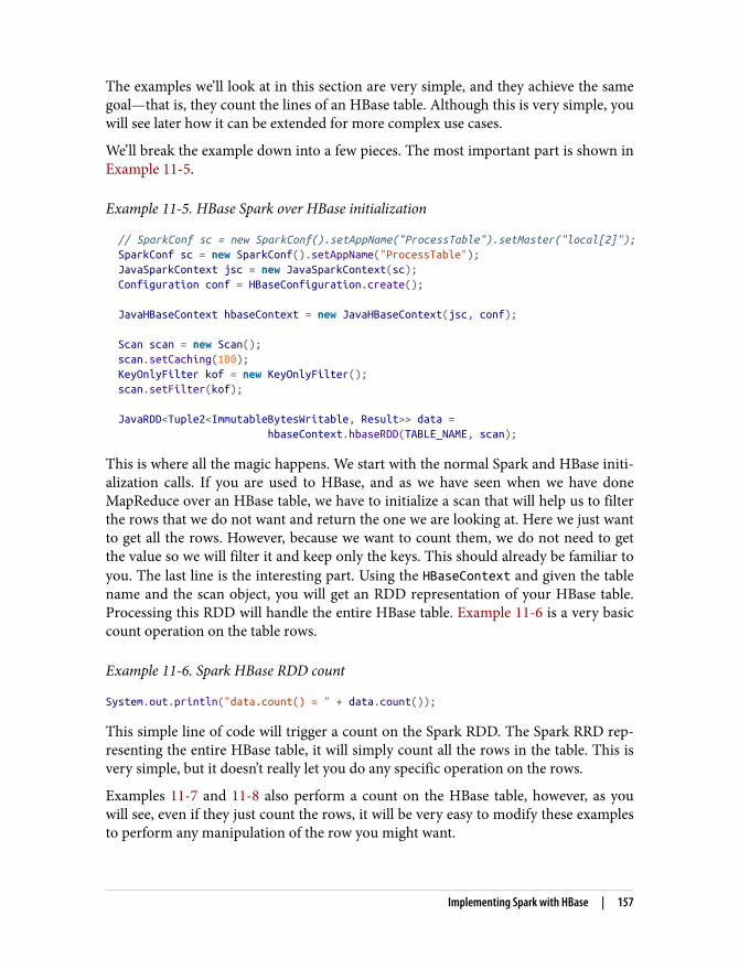
The examples we’ll look at in this section are very simple, and they achieve the samegoal—that is, they count the lines of an HBase table. Although this is very simple, youwill see later how it can be extended for more complex use cases.

We’ll break the example down into a few pieces. The most important part is shown inExample 11-5.

Example 11-5. HBase Spark over HBase initialization

// SparkConf sc = new SparkConf().setAppName("ProcessTable").setMaster("local[2]"); SparkConf sc = new SparkConf().setAppName("ProcessTable"); JavaSparkContext jsc = new JavaSparkContext(sc); Configuration conf = HBaseConfiguration.create();

JavaHBaseContext hbaseContext = new JavaHBaseContext(jsc, conf);

Scan scan = new Scan(); scan.setCaching(100); KeyOnlyFilter kof = new KeyOnlyFilter(); scan.setFilter(kof);

JavaRDD<Tuple2<ImmutableBytesWritable, Result>> data = hbaseContext.hbaseRDD(TABLE_NAME, scan);

This is where all the magic happens. We start with the normal Spark and HBase initi‐alization calls. If you are used to HBase, and as we have seen when we have doneMapReduce over an HBase table, we have to initialize a scan that will help us to filterthe rows that we do not want and return the one we are looking at. Here we just wantto get all the rows. However, because we want to count them, we do not need to getthe value so we will filter it and keep only the keys. This should already be familiar toyou. The last line is the interesting part. Using the HBaseContext and given the tablename and the scan object, you will get an RDD representation of your HBase table.Processing this RDD will handle the entire HBase table. Example 11-6 is a very basiccount operation on the table rows.

Example 11-6. Spark HBase RDD count

System.out.println("data.count() = " + data.count());

This simple line of code will trigger a count on the Spark RDD. The Spark RRD rep‐resenting the entire HBase table, it will simply count all the rows in the table. This isvery simple, but it doesn’t really let you do any specific operation on the rows.

Examples 11-7 and 11-8 also perform a count on the HBase table, however, as youwill see, even if they just count the rows, it will be very easy to modify these examplesto perform any manipulation of the row you might want.

Implementing Spark with HBase | 157

Example 11-7. HBase Spark over HBase partitions reduce count

FlatMapFunction<Iterator<Tuple2<ImmutableBytesWritable, Result>>, Integer> setup = new FlatMapFunction<Iterator<Tuple2<ImmutableBytesWritable, Result>>, Integer>() { @Override public Iterable<Integer> call(Iterator<Tuple2<ImmutableBytesWritable, Result>> input) { int a = 0; while (input.hasNext()) { a++; input.next(); } ArrayList<Integer> ret = new ArrayList<Integer>(); ret.add(a); return ret; } }; Function2<Integer, Integer, Integer> combine = new Function2<Integer, Integer, Integer>() { @Override public Integer call(Integer a, Integer b) { return a+b; } };

System.err.println("data.mapPartitions(setup).reduce(combine) = " + data.mapPartitions(setup).reduce(combine)); long time3 = System.currentTimeMillis(); System.err.println("Took " + (time3 - time2) + " milliseconds");

For each Spark partition, we simply increment a counter for each line we found.Here, it will be very easy to accumulate a value extracted from the HBase cell ordo any other kind of aggregation we want.

Now that all the partitions are aggregated, to combine them, we simply need tosum all the values.

Example 11-7 looks very close to what we were doing in previous chapters with Map‐Reduce. Because it doesn’t really map by partition, Example 11-8 is a bit different, butthe output will again be the same.

Example 11-8. HBase Spark over HBase aggregate count

Function2<Integer, Tuple2<ImmutableBytesWritable, Result>, Integer> aggregator = new Function2<Integer, Tuple2<ImmutableBytesWritable, Result>, Integer>() { @Override public Integer call(Integer v1, Tuple2<ImmutableBytesWritable, Result> v2) throws Exception { return v1 + 1; }

158 | Chapter 11: Implementation of HBase as a Master Data Management Tool

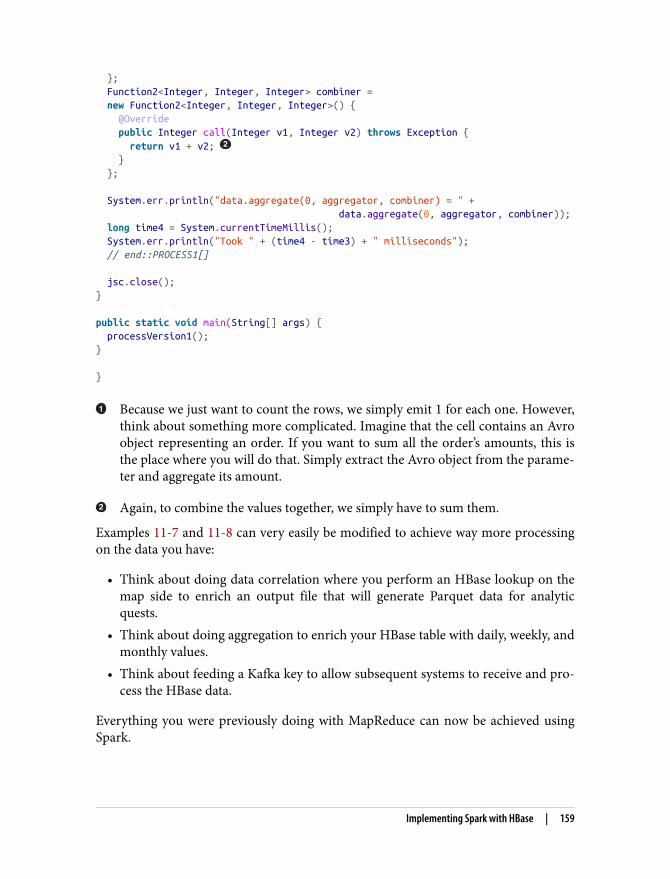
}; Function2<Integer, Integer, Integer> combiner = new Function2<Integer, Integer, Integer>() { @Override public Integer call(Integer v1, Integer v2) throws Exception { return v1 + v2; } };

System.err.println("data.aggregate(0, aggregator, combiner) = " + data.aggregate(0, aggregator, combiner)); long time4 = System.currentTimeMillis(); System.err.println("Took " + (time4 - time3) + " milliseconds"); // end::PROCESS1[]

jsc.close();}

public static void main(String[] args) { processVersion1();}

}

Because we just want to count the rows, we simply emit 1 for each one. However,think about something more complicated. Imagine that the cell contains an Avroobject representing an order. If you want to sum all the order’s amounts, this isthe place where you will do that. Simply extract the Avro object from the parame‐ter and aggregate its amount.

Again, to combine the values together, we simply have to sum them.

Examples 11-7 and 11-8 can very easily be modified to achieve way more processingon the data you have:

• Think about doing data correlation where you perform an HBase lookup on themap side to enrich an output file that will generate Parquet data for analyticquests.

• Think about doing aggregation to enrich your HBase table with daily, weekly, andmonthly values.

• Think about feeding a Kafka key to allow subsequent systems to receive and pro‐cess the HBase data.

Everything you were previously doing with MapReduce can now be achieved usingSpark.

Implementing Spark with HBase | 159

Going FurtherIf you want to extend the examples presented in this chapter, the following list offerssome options you can try based on our discussion:

PartitionsTo clearly see the benefit of partitioning the RRDs, create a bigger HBase tablewith multiple regions and try to create two version of your Spark code: one thatruns over all the data with a single executor, and another that partitions the datato run it over multiple executors. Instead of a single executor processing theentire table, you should see one executor per HBase region on your table. Thedifference in execution time should be significant.

StreamingTry to convert the put example into Spark streaming. Instead of processing theentire file at once, try to process it by micro batches. This should allow you tostart seeing results into HBase sooner than with the entire puts bulked at once.

Scan modificationTry to modify the scanner initialization to sort only certain rows, or extract onlycertain columns from your table. The scan object you give to your Spark RDDwill determine what data you are going to receive on the subsequent calls.

160 | Chapter 11: Implementation of HBase as a Master Data Management Tool

CHAPTER 12

Use Case: Document Store

The final use case focuses on leveraging HBase as a document store. This use case isimplemented by a large insurance company, which will henceforth be referred to as“the firm.” The information the firm collects is used to determine accident at faults,payouts, and even individual net worth. This particular use case involves data man‐agement and curation at a massive scale.

The firm needed to build a document store that would allow it to serve differentdocuments to numerous business units and customers. A company of this size willend up having hundreds to thousands of different business units and millions of endusers. The data from these different business units creates massive amounts of infor‐mation that needs to be collected, aggregated, curated, and then served to internaland external consumers. The firm needed the ability to serve hundreds of millions ofdocuments over thousands of different logical collections. That is a challenge for anyplatform, unless that platform is HBase.

Leveraging HBase as a document store is a relatively new use case for HBase. Previ‐ously, documents larger than a few 100 KB were not recommended for consumption.The competition to earn the production deployment was against a major RDBMSsystem. In this bake off, reads, writes, and file sizes were tested. The incumbent ven‐dor performed well against HBase. HBase writes were slightly faster on smaller docu‐ments (ranging in size from 4 to 100 KB). Yet, the incumbent vendor managed tooutperform HBase on larger documents by showing almost twice the write through‐put with large documents of 300+ MB. HBase shined through with the reads, which ismost important to the end users for this use case. HBase was 4 times faster whenreading small files and 3.5 times faster with the large documents over 300 MB in size.Finally, HBase was tested with documents up to 900 MB in size and performed well,though the production deployment will not have any 900 MB cells floating around.

161

This use case would have been problematic in earlier versions of HBase. Luckily, theMedium Object (MOB) storage feature was introduced in HBASE-11339. OriginallyHBase struggled with cells up to 100 KB to 1 MB or larger in size. When using theselarger sized cells without the MOB feature enabled, HBase suffered from somethingknown as write amplification. This occurs when HBase compactions have to rewritethese larger cells over and over again potentially causing flush delays, blockedupdates, disk I/O to spike, and latencies to shoot through the roof. This may be finein batch-based systems using HBase as a system of record, updating large sets of datain Spark or MR jobs, but real-time systems with SLAs would suffer the most.

The MOB feature allowed HBase to accommodate larger cells with an official recom‐mendation of 100 KB to 10 MB, but we have seen reasonable success with documentsover 100 MB. MOB solves this issue by writing the MOB files into a special region.The MOB files are still written to the WAL and block cache to allow for normal repli‐cation and faster retrieval. Except when flushing a memstore containing a MOB file,only a reference is written into the HFile. The actual MOB file is written into an off‐line MOB region to avoid being compacted over and over again during major com‐pactions causing write amplification. Figure 12-1 highlights the read path whenleveraging MOB.

Figure 12-1. Understanding the MOB read path

To accomplish the deployment, the firm needed to have the ability to store 1 PB onthe primary cluster and 1 PB on the disaster recovery cluster, while maintaining theability to stay cost-effective. Staying cost-effective means enabling greater verticalscalability to keep the total node count down. To achieve this, we had to push HBasebeyond the known best practices. We leveraged 40 GB for our region size and had

162 | Chapter 12: Use Case: Document Store

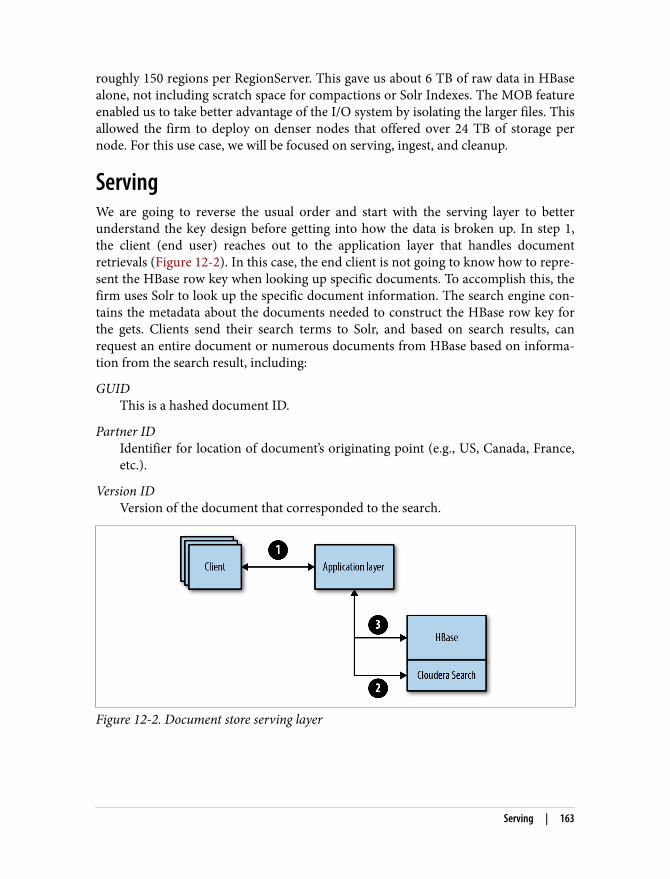
roughly 150 regions per RegionServer. This gave us about 6 TB of raw data in HBasealone, not including scratch space for compactions or Solr Indexes. The MOB featureenabled us to take better advantage of the I/O system by isolating the larger files. Thisallowed the firm to deploy on denser nodes that offered over 24 TB of storage pernode. For this use case, we will be focused on serving, ingest, and cleanup.

ServingWe are going to reverse the usual order and start with the serving layer to betterunderstand the key design before getting into how the data is broken up. In step 1,the client (end user) reaches out to the application layer that handles documentretrievals (Figure 12-2). In this case, the end client is not going to know how to repre‐sent the HBase row key when looking up specific documents. To accomplish this, thefirm uses Solr to look up the specific document information. The search engine con‐tains the metadata about the documents needed to construct the HBase row key forthe gets. Clients send their search terms to Solr, and based on search results, canrequest an entire document or numerous documents from HBase based on informa‐tion from the search result, including:

GUIDThis is a hashed document ID.

Partner IDIdentifier for location of document’s originating point (e.g., US, Canada, France,etc.).

Version IDVersion of the document that corresponded to the search.

Figure 12-2. Document store serving layer

Serving | 163

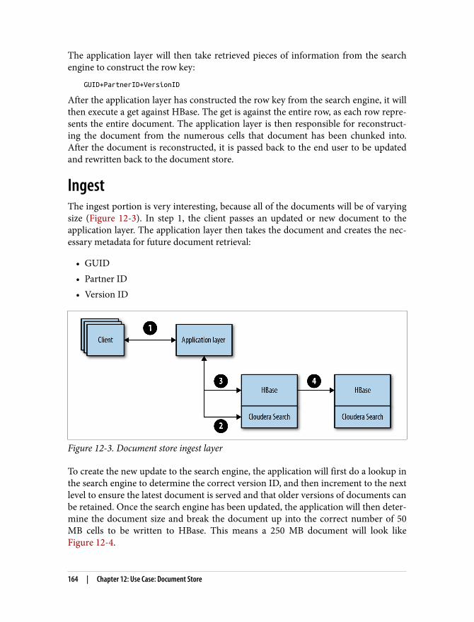
The application layer will then take retrieved pieces of information from the searchengine to construct the row key:

GUID+PartnerID+VersionID

After the application layer has constructed the row key from the search engine, it willthen execute a get against HBase. The get is against the entire row, as each row repre‐sents the entire document. The application layer is then responsible for reconstruct‐ing the document from the numerous cells that document has been chunked into.After the document is reconstructed, it is passed back to the end user to be updatedand rewritten back to the document store.

IngestThe ingest portion is very interesting, because all of the documents will be of varyingsize (Figure 12-3). In step 1, the client passes an updated or new document to theapplication layer. The application layer then takes the document and creates the nec‐essary metadata for future document retrieval:

• GUID• Partner ID• Version ID

Figure 12-3. Document store ingest layer

To create the new update to the search engine, the application will first do a lookup inthe search engine to determine the correct version ID, and then increment to the nextlevel to ensure the latest document is served and that older versions of documents canbe retained. Once the search engine has been updated, the application will then deter‐mine the document size and break the document up into the correct number of 50MB cells to be written to HBase. This means a 250 MB document will look likeFigure 12-4.

164 | Chapter 12: Use Case: Document Store

Figure 12-4. Cell layout while chunking large documents

The final HBase schema was different than what was tested during the bake off.HBase showed the best performance when the documents were broken out intochunks, as illustrated in Figure 12-4. The chunking also helps to keep total memstoreusage under control, as we can flush numerous chunks at a time without having tobuffer the entire large document. Once the HBase application has written the data toboth the search engine and HBase, the document is the made available for retrievalfrom the client.

Once the data has been written to HBase, the Lily Indexer picks up the metadataabout each document and writes it into Cloudera Search. While the search engine isindexing some metadata in step 4, HBase is also replicating the data to the disasterrecovery cluster, which in turn is also writing the metadata to Cloudera Searchthrough the Lily Indexer (Figure 12-5). This is actually a very clever way to do veryquick document counts without having to utilize HBase resources to issue scans tocount the total number of documents. Cloudera Search can quickly give back a totalcount of documents in both sites, ensuring that the document counts stays the same.

Figure 12-5. Disaster recovery layout

Ingest | 165

Clean UpFor those of you following along at home, you may be thinking “Hey! Great schema,but how do you control versions?” Normally versions are handled through individualHBase cells and are configurable on the column family level. However, the portion ofthe row key known as “VersionID” is used to control the versioning. This allows theclient to be able to easily pull the latest, or the last X versions with a single scan. If thefirm wished to keep all copies of a single document, this would be fine; but dependingon the delta rate of the documents, this could balloon out of control fast. Seriously,think about how many times you have changed a sentence, got busy and saved thedocument, then came changed another sentence, then repeat. To combat this, thefirm has written a clean up job that will iterate through the table and delete unneededversions of their documents.

For the current RDBMS-based solution, the cleanup process runs constantly in orderto minimize storage and contain costs on their expensive RDBMS. Because HBase islower cost, storage is less of an issue, and cleanups can run less frequently. To do this,the firm fires off a Spark job daily.

The Spark job has two primary tasks. First, it collects the version count of each docu‐ment from the search system. This is an easy way to eliminate the documents that donot exceed the maximum version count. In this case, the firm retains up to the last 10versions of a document. Once the document list has been built, the Spark job will usethe response to build the necessary row keys to issue the deletes. Finally, the job willfire off a series of deletes to HBase, followed by a major compaction to age off all ofthe tombstones.

166 | Chapter 12: Use Case: Document Store

1 http://blog.cloudera.com/blog/2015/06/inside-apache-hbases-new-support-for-mobs/

CHAPTER 13

Implementation of Document Store

As you might have guessed, this use case again utilizes most if not all of what we haveseen before—that is, replication for backup, Lily and Solr for real-time indexing andsearch, Spark for fast processing, and of course the Java API. The only thing that wedon’t really have look at is the MOB aspect. Therefore, we will focus on that over thenext sections. Because consistency is also one important aspect of the use case, we willalso address it.

As you will see next, there is not that much to do on the implementation side, but wewill mostly focus on the key concepts to keep in mind when designing your ownapplication.

MOBsHBase works very well with small to average size cell values, but bigger ones, becauseof the compactions, create write amplification. MOBs have been implemented toavoid this.

MOBs require HFiles format v3. You will have to make sure yourHBase version is configured for that. The Apache version of HBasehas HFile configured to v3 since version 1.0. However, for compati‐bility purposes, some distributions still keep the v2. To make sureyour version is configured to v3, add hfile.format.versionparameter to your config file and set it to 3.1

167

In the following section, we will see how to configure a table to use the MOB featureand how to push some data into it. You will need to decide the cut off point for whendata will be considered a regular cell, or if the entry is too large and needs to bemoved into a MOB region.

For testing purposes, we will keep this value pretty small:

create 'mob_test', {NAME => 'f', IS_MOB => true, MOB_THRESHOLD => 104857}

MOB have been implemented as part of HBASE-11339, which hasbeen commited into the HBase 2.0 branch. Is had not been back‐ported into the 1.0 branch by the community. Therefore, if youwant to try the MOB feature, you have to use a 2.0+ version ofHBase or a distribution where this has been backported. Becausethe Cloudera QuickStart VM includes this implementation, we willuse it for testing in this chapter.

This command will create a table called mod_test with a single column family calledf where all cells over tens of a megabyte will be considered to be a MOB. From theclient side, there is no specific operation or parameter to add. Therefore, the Putcommand will transfer the entire cell content to the RegionServer. Once there, theRegionServer will decide whether to store the document as a normal cell or a MOBregion.

The following two puts against our mob_test table are very similar from a client pointof view, but will be stored differently on the server side:

byte[] rowKey = Bytes.toBytes("rowKey");byte[] CF = Bytes.toBytes("f");byte[] smallCellCQ = Bytes.toBytes("small");byte[] bigCellCQ = Bytes.toBytes("big");byte[] smallCellValue = new byte(1024);byte[] bigCellValue = new byte(110000);Put smallPut = new Put(rowKey);smallPut.addColumn(CF, smallCellCQ, smallCellValue);table.put (smallPut);

Put bigPut = new Put(rowKey);bigPut.addColumn(CF, bigCellCQ, bigCellValue);table.put (bigPut);

Those two puts for the same row key of the same table will both go into the sameregion. However, after flushing the memstore, the small one will go in a regular HFilewhile the big one will go as a separate MOB file.

168 | Chapter 13: Implementation of Document Store

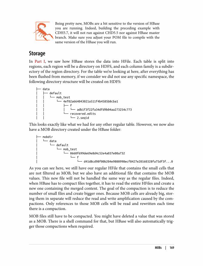
Being pretty new, MOBs are a bit sensitive to the version of HBaseyou are running. Indeed, building the preceding example withCDH5.7, it will not run against CHD5.5 nor against HBase masterbranch. Make sure you adjust your POM file to compile with thesame version of the HBase you will run.

StorageIn Part I, we saw how HBase stores the data into HFile. Each table is split intoregions, each region will be a directory on HDFS, and each column family is a subdir‐ectory of the region directory. For the table we’re looking at here, after everything hasbeen flushed from memory, if we consider we did not use any specific namespace, thefollowing directory structure will be created on HDFS:

├── data│ ├── default│ │ └── mob_test│ │ └── 4ef02a664043021a511f4b4585b8cba1│ │ ├── f│ │ │ └── adb1f3f22fa34dfd9b04aa273254c773│ │ └── recovered.edits│ │ └── 2.seqid

This looks exactly like what we had for any other regular table. However, we now alsohave a MOB directory created under the HBase folder:

├── mobdir│ └── data│ └── default│ └── mob_test│ └── 0660f699de69e8d4c52e4a037e00a732│ └── f│ └── d41d8cd98f00b204e9800998ecf8427e20160328fa75df3f...0

As you can see here, we still have our regular HFile that contains the small cells thatare not filtered as MOB, but we also have an additional file that contains the MOBvalues. This new file will not be handled the same way as the regular files. Indeed,when HBase has to compact files together, it has to read the entire HFiles and create anew one containing the merged content. The goal of the compaction is to reduce thenumber of small files and create bigger ones. Because MOB cells are already big, stor‐ing them in separate will reduce the read and write amplification caused by the com‐pactions. Only references to those MOB cells will be read and rewritten each timethere is a compaction.

MOB files still have to be compacted. You might have deleted a value that was storedas a MOB. There is a shell command for that, but HBase will also automatically trig‐ger those compactions when required.

MOBs | 169

If most of what you are doing with HBase is writes of big cells and almost no deletes,MOB will give you a very good improvement compared to the regular format.

UsageAt this point, you might be wondering what constitutes a big cell versus a small one.HBase performs very well with cells up to 1 MB. It is also able to process cells up to 5MB. However, above that point, regular write path will start to have some perfor‐mance challenges. The other thing you have to consider is how many times you aregoing to write big cells versus regular ones. MOBs required some extra work forHBase. When you are reading a cell, we first need to lookup into the related HFileand then into the MOB file. Because of this extra call, latency will be slightly impac‐ted. Now, if your MOB is 50 MB, the time to transfer it to the client versus the extraread access on HBase might not be significant. The extra read access on the HBaseside will add few milliseconds to your call. But transferring 50 MB of data to yourclient might take more than that and might just hide the extra milliseconds for theadditional read.

The main question you will need to ask yourself is how often are you going to insertbig cells into HBase. If you expect to do so only, once in a while, and not more thanonce per row, a cell that might be a big bigger than the others, like up to 5 MB, youmight just be able to use the regular put API. That will save you the extra manage‐ment of the MOB files and HBase will be able to handle that. Because there will beonly a few big cells, the read and write amplification will be limited. However, if youare planning to have multiple big cells per row, if some of your cells are going to bebigger than 5 MB, or if most of your puts are big, you might want to consider usingthe MOBs.

Keep in mind that even if MOB reduces the rewrite amplificationof the regular HFiles, if you have to perform many puts and deletesof big cells, you will still have to perform many compactions of theMOB files.

Too BigAs we have just seen, it’s fine for regular HBase cells to occasionally grow up to 5 MBcells. MOBs will allow you to easily handle cells up 20 MB. Even if it is not necessarilyrecommended, some people have pushed it a bit further and are using MOBs with 50MB cells.

Now, if your use case is to store only very big cells, like 100 MB cells or more, you arebetter off using a different approach.

170 | Chapter 13: Implementation of Document Store

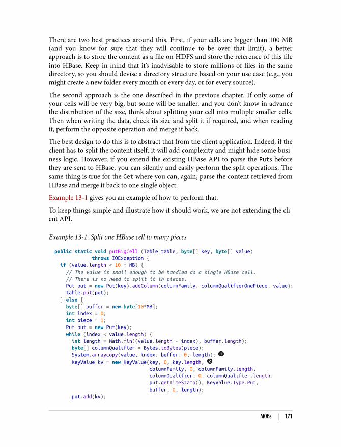
There are two best practices around this. First, if your cells are bigger than 100 MB(and you know for sure that they will continue to be over that limit), a betterapproach is to store the content as a file on HDFS and store the reference of this fileinto HBase. Keep in mind that it’s inadvisable to store millions of files in the samedirectory, so you should devise a directory structure based on your use case (e.g., youmight create a new folder every month or every day, or for every source).

The second approach is the one described in the previous chapter. If only some ofyour cells will be very big, but some will be smaller, and you don’t know in advancethe distribution of the size, think about splitting your cell into multiple smaller cells.Then when writing the data, check its size and split it if required, and when readingit, perform the opposite operation and merge it back.

The best design to do this is to abstract that from the client application. Indeed, if theclient has to split the content itself, it will add complexity and might hide some busi‐ness logic. However, if you extend the existing HBase API to parse the Puts beforethey are sent to HBase, you can silently and easily perform the split operations. Thesame thing is true for the Get where you can, again, parse the content retrieved fromHBase and merge it back to one single object.

Example 13-1 gives you an example of how to perform that.

To keep things simple and illustrate how it should work, we are not extending the cli‐ent API.

Example 13-1. Split one HBase cell to many pieces

public static void putBigCell (Table table, byte[] key, byte[] value) throws IOException { if (value.length < 10 * MB) { // The value is small enough to be handled as a single HBase cell. // There is no need to split it in pieces. Put put = new Put(key).addColumn(columnFamily, columnQualifierOnePiece, value); table.put(put); } else { byte[] buffer = new byte[10*MB]; int index = 0; int piece = 1; Put put = new Put(key); while (index < value.length) { int length = Math.min((value.length - index), buffer.length); byte[] columnQualifier = Bytes.toBytes(piece); System.arraycopy(value, index, buffer, 0, length); KeyValue kv = new KeyValue(key, 0, key.length, columnFamily, 0, columnFamily.length, columnQualifier, 0, columnQualifier.length, put.getTimeStamp(), KeyValue.Type.Put, buffer, 0, length); put.add(kv);

MOBs | 171

index += length + 1; piece ++; } table.put(put); } }

We do not want to create a new 10 MB object each time we read a new slice, sowe keep reusing the same buffer array.

The HBase Put object doesn’t allow you to give a byte array or to specify thelength of your value, so we have to make use of the KeyValue object.

To make sure you don’t create rows that are too big, HBase vali‐dates the size of the cells you are trying to store. If you are trying tostart 10 MB cells, you might want to make sure hbase.client.key‐value.maxsize is not set to a lower number. This is a relativelyunknown setting that can cause lots of headaches when dealingwith large cells.

ConsistencyLet’s take a small example to really get the sense of what is the consistency in HBase.Imagine you are writing a website order into HBase. Let’s consider you are writing allthe entries one by one with a different key formed by the order ID and the entry ID.Each line in the order will have a different entry ID and so will be a different HBaserow. Most of the time, it will all go well and at once into HBase. But what if this issplit over two different regions hosted on two different servers? And what if the sec‐ond server just failed before storing the entries? Some will make it, and some otherswill have to be retried until the region is reassigned and the data finally makes it in. Ifa client application tries to read the entire order while this is happening, it willretrieve a partial view of the order. If we use Lily to index the data coming into thistable, a query to the index will return partial results.

This is where consistency awareness is important.

Let’s see how this applies to the current use case.

Documents are received by the application where a modified HBase client split themin 10 MB slices and sends all the slices plus the metadata into HBase. All the slicesand the metadata have to go together. If you send the slices as different HBase rows, itmay take some time for each part to make its way into HBase and therefore an appli‐cation trying to read it might get only a partial file. Because it is important for all theslices to be written in a single write and be read at once, they will have to be storedinto a single row. Metadata also needs to be part of the consistency equation. Because

172 | Chapter 13: Implementation of Document Store

it will be indexed and used for the document retrieval, the metadata is tightly coupledto the file. It will have to go with the same row, at the same time.

There are cases where consistency is not an issue. As an example, if you receive a listof tweets from a user, all those tweets are not linked together. Therefore, retrievingjust a subset of them might not impact your results.

Consistency is a very important concept in HBase. It’s not always required to haveconsistency within an operation. But if you have to, it is very important to keep yourdata together to make sure it makes it together into HBase, or not at all.

Stay away from cross-references. Let’s imagine you have a row Awhere you store the key and the value of a reference called row BWhen you will update the value of row B, you will also have toupdate the value of row A. However, they can be on differentregions, and consistency of those update operations cannot beguaranteed. If you need to get the value of row B when reading rowA, you are much better off keeping row B key in row A values anddoing another call based on that. This will require an extra call toHBase, but will save you the extra burden of having to rebuild yourentire table after a few failures.

Going FurtherIf you want to extend the examples presented in this chapter, the following list offerssome options you can try based on our discussions from this chapter:

Single cellTry to push HBase to its maximum capability. Instead of splitting cells into 10MB chunks, try to create bigger and bigger chunks and see how HBase behaves.Try to read and write those giant cells and validate their content.

Deletes impactsTo gain a better understanding of how deletes are handled with MOBs, updatethe example to generate some big MOB cells, flush them onto disk, and then exe‐cute a delete. Then look at the underlying filesystem storage. Later, flush the tableagain and run a compaction to see what happens.

ReadThis chapter illustrated how to split a huge cell into a smaller one and write it toHBase. But we leave it to you to write the read path. Based on how we have splitthe cell into multiple pieces, build a method that will read it, back and re-createthe initial document. To help you get started, you will have to find the last col‐umn, read it and get its size. The size of the document will be the number of col‐umns minus one, multiplied by 10 MB plus the size of the last one. As an

Going Further | 173

example, if you have three columns and the last one is 5 MB, the document sizewill be (3 - 1) * 10 MB + 5 MB, which is 25 MB.

174 | Chapter 13: Implementation of Document Store

PART III

Troubleshooting

There are many different gotchas that can occur when deploying an HBase use case.This upcoming section is all about HBase issues we have run into over the years ofusing it. Ideally, you should read this section before deploying HBase, as recoveringfrom some of these mistakes in production can be quite difficult.

This section will cover the typical issues we run into, such as too many regions or col‐umn familes, hotspotting, issues with region time outs, or worst-case scenario, havingto recover from metadata or filesystem corruption. We will go over the typical causeand recovery from these issues. We will also highlight some best practices aroundJava tuning that can enable greater vertical scalability.

CHAPTER 14

Too Many Regions

ConsequencesHaving too many regions can impact your HBase application in many ways.

The most common consequence is related to HFile compactions. Regions are sharingthe memstore memory area. Therefore, the more regions there are, the smaller thememstore flushes will be. When the memstore is full and forced to flush to disk, itwill create an HFile containing data to be stored in HDFS. This means the moreregions you have, the smaller the generated HFiles will be. This will force HBase toexecute many compaction operations to keep the number of HFiles reasonably low.These compactions will cause excessive churn on the cluster, affecting performance.When specific operations are triggered (automatic flush, forced flush, and user callfor compactions), if required, HBase will start compactions. When many compac‐tions run in tandem, it is known as a compaction storm.

Compactions are normal HBase operations. You should expectthem, and there is nothing to worry about when minor compac‐tions are running. However, it is recommended to monitor thenumber of compactions. The compaction queue should not be con‐stantly growing. Spikes are fine, but the key needs to stay close tozero most of the time. Constant compactions can be a sign of poorproject design or a cluster sizing issue. We call constant compac‐tions a situation where the compaction queue for a given Region‐Server never goes down to zero or is constantly growing.

Certain operations can timeout as a result of having too many regions. HBase com‐mands like splits, flushes, bulkloads, and snapshots (when using flush) perform oper‐ations on each and every region. As an example, when the flush <table> command

177

is called, HBase needs to store a single HFile into HDFS for each column family ineach region of <table> where there are pending writes in the memstore. The moreregions you have, the more files will be created in the filesystem. Because all of thosenew file creations and data transfers will occur at the same time, this can overwhelmthe system and impact SLAs. If the time taken to complete the operation is greaterthan the configured timeout for your operation, you will start to see some timeoutfailures.

Here is a quick summary of the problems you might encounter on your cluster as aresult of having too many regions:

• Snapshots timeout• Compaction storms• Client operations can timeout (like flush)• Bulk load timeouts (might be reported as RegionTooBusyException)

CausesThere are multiple root causes for having too many regions, ranging from misconfi‐guration to misoperation. These root causes will be discussed in greater detail in thissection:

• Maximum region size set too low• Configuration settings not updated following an HBase upgrade• Accidental configuration settings• Over-splitting• Improper presplitting

MisconfigurationIn previous HBase versions, 1 GB was the default recommendation for region size.HBase can now easily handle regions ranging in size from 10 to 40 GB, thanks tooptimizations in HBase and ever-increasing default memory size in hardware. Formore details on how to run HBase with more memory, refer to Chapter 17. When anolder HBase cluster is migrated into a recent version (0.98 or greater), a commonmistake is to retain previous configuration settings. As a result, HBase tries to keepregions under 1 GB when it will be better letting them grow up to 10 GB or more.Also, even if the cluster has not been migrated from an older version, the maximumregion size configuration might have been mistakenly modified to a smaller value,resulting in too many regions.

178 | Chapter 14: Too Many Regions

MisoperationThere are also multiple manual operations that might cause HBase to have too manyregions to serve.

Over-splittingThe first one is a misuse of the split feature. HBase’s “Table Details” Web UI allowsadministrators to split all the regions of a given table. HBase will split the regionseven if they are small, as long as the amount of data in the region meets the minimumsize required to qualify for manual splitting. This option can sometimes be very use‐ful, but abusing it can easily create too many regions for a single table. Take as anexample a 128 region table on a four-node cluster where each RegionServer hostsonly 32 regions. This is a correct load for a cluster of that size. The use of the splitoption three times will create up to 1,024 regions, which represents 256 regions perserver!

Improper presplittingIt is also possible to create too many regions when using the presplit HBase feature.Presplitting is very important to help spread the load across all the RegionServers inthe cluster; however, it needs to be well thought out beforehand. There should be afundamental understanding of row key design, HBase writes, and desired regioncount to correctly presplit a table. A poorly split table can result in many regions(hundreds or even thousands) with only a few of them being used.

SolutionDepending on the HBase version you use, there are different ways to address the issueof having too many regions. But in both scenarios, the final goal is to reduce the totalnumber of regions by merging some of them together. What differs between theHBase versions is the ways to achieve this.

Before 0.98Before version 0.98, there are two main options to merge regions together: copyingthe table to a new presplit table or merging regions. Before HBase 0.98, regions couldbe merged offline only.

The first option is to create a new table with the same definitions as the existing tablebut with a different table name. Copy the data from the original table into this table.To complete the process, drop the original table and then rename the new table to theoriginal table name. In this method, we will use the HBase snapshot feature so HBase0.94.6 or above is required. Also, you will need to run the MapReduce CopyTable jobon top of the HBase cluster, so you will need to make sure that the MapReduce frame‐

Solution | 179

work is available and running. Last, this method will require a temporary suspensionof data ingestion. This interruption will be short but is the important part of theprocess.

Because this method will duplicate the initial table, it will consumespace on your cluster equal to the original tables size. Ensure theextra space is available before starting. It is also important tounderstand the impact of running MapReduce on the HBasecluster.

The new table should be presplit with the expected newly merged region boundaries.Figure 14-2 illustrates this. Once the presplit step is completed, use the CopyTablecommand to copy data from the original table to the new table. The CopyTable toolaccepts a date range as an argument and will then copy data from time t0 to t1directly into the target table, into the correct regions. This will allow you to transferthe oldest data first and rerun the tool again to transfer newly created data.CopyTable also allows you to rename or drop unnecessary column families, whichcan be very useful in case of table redesign.

As illustrated in Figure 14-1, if you are doing puts and deletes withmodified timestamps, you might want to avoid this method, assome of your deletes and puts might not be copied correctly if anycompaction occurs on the source side between the two CopyTablecalls. It is almost never a good idea to be modifying internal HBasetimestamps. In Figure 14-1, CopyTable is done between t0 and t1 tocopy data from one table to another. By the time CopyTable is runfor data between t1 and current time, some data with old time‐stamps is inserted into the source table. Because only data with atimestamp greater than t1 will be consider by the second run ofCopyTable, this newly inserted data in the past will be ignored (i.e.,it will not be copied over to the new table and will be lost if thesource table is dropped).

180 | Chapter 14: Too Many Regions

Figure 14-1. Risk when performing updates with timestamp of cells in the past

Figure 14-2 is an example to better understand how this can be done. Consider thatyou built an application that stores transactions into a table using the transaction IDas the row key. Your initial assumption was that the transaction ID would be a uniquerandomly generated readable string. Based on this assumption, the initial table wassplit into 26 regions from A to Z. However, after running the application for a fewweeks, you notice that the transaction ID is a hexadecimal ID. Therefore, instead ofgoing from A to Z, it goes from 0 to F. With the new distribution, regions greater thanF will never be used, while the first region will get way more data than the others(puts from 0 to A) and will split into many new regions as it grows. In this case, we’reonly moving 26 region to 8 regions; but if you scale this example, you can easily seehow hundreds of regions may have been initially created to handle more load andhow the same issue of data balancing can occur.

Solution | 181

Figure 14-2. Regions redesign

In order to fix this, we will create a new table where regions are already presplit onhexadecimal boundaries. Using the CopyTable command, we will copy data from theexisting table to the new table, from t0 to the current day:

hbase org.apache.hadoop.hbase.mapreduce.CopyTable --starttime=0 \--endtime=1411264757000 --new.name=new_table previous_table

The goal of the starttime and endtime parameters is to make sure we copy a specificand controlled section of the source table. Because this operation might take sometime, before going to the next steps, and to reduce the input table downtime, we wantto copy as much data as possible; but we also want to make sure we will be able torestart the copy from a specific point in time.

Depending on the size of your dataset, this copy might take several hours to a fewdays. While the copy is running, normal operations can continue on the cluster andon the initial table.

Once the first CopyTable operation is done, the new table contains almost all of theexisting data except what has been added between when your previous operation wasstarted (t=141126475700, in this example) and now. Depending on the time it takesto run the first copy, this can represent a considerable amount of data. Because ofthat, and to make sure the next steps are going to be as short as possible, we willrerun the CopyTable command again. Because the endtime parameter that we used inthe previous command is exclusive, we will use it for our current starttime:

hbase org.apache.hadoop.hbase.mapreduce.CopyTable --starttime=1411264757000 \--endtime=1411430414000 --new.name=new_table previous_table

182 | Chapter 14: Too Many Regions

This second operation should be faster, as most of the data was copied in the initialoperation. When the two CopyTable operations are done and before doing the lastrun, to not lose any data, you will have to stop the ingestion to your existing tablewhile you are performing the following operations. In production environments, it issometimes very sensitive to stop data ingestion. If that is the case, you can thinkabout mitigation solutions. One of them consists of pushing the data into the newlycreated table. Another is to design the ingestion such that it can accept those pauses.Applications such as Kafka and Flume can be used to queue the data being ingestedto HBase and can be paused without losing any information. Typically, the remainingsteps might be accomplished in less than one hour. It is hard to quantify how long itwill take to bring in the delta. It can be computed from the previous runs, but it canvary widely.

Finally, you will need to do one last run of the CopyTable tool to copy the remainingdata. The time between the end of the last run and when you disabled the data inges‐tion is only a couple minutes, so it should run even faster. This time, because we wantto copy all the remaining data, we will again use the last endtime value as thestarttime parameter, but we will not specify any endtime:

hbase org.apache.hadoop.hbase.mapreduce.CopyTable --starttime=1411264757000 \--new.name=new_table previous_table

This should run for a few seconds up to a few minutes. At the end of this operation,we will have a duplicate of the original table in our new table, with the new regionsboundaries. The last step is to run some snapshot commands to rename the newlycreated table:

disable 'events_table'drop 'events_table'disable 'new_events_table'snapshot 'new_events_table', 'snap1'clone_snapshot 'snap1', 'events_table'delete_snapshot 'snap1'drop 'new_events_table'

At the end of all those operations, you will have a table containing the exact same databut with a reduced number of regions.

Offline mergesThe second option to reduce the number of regions you have is to perform offlinemerges. To be able to perform the following steps, you will need to run HBase 0.94.13or higher. Offline merge before 0.94.13 can fail and can leave corrupted files in yoursystem (see HBASE-9504). One major constraint with offline merges is that theyrequire total cluster downtime.

Solution | 183

The steps to perform offline merges are as follows (we’ll look at the details momen‐tarily):

1. Stop the cluster.2. Perform one or more merge operations.3. Start the cluster.

To stop and start your HBase cluster, you can use the bin/stop-hbase.sh and bin/start-hbase.sh commands. If you are using a management tool such as Cloudera Manager,you will find the HBase actions in the HBase service management page.

Using HBase command

Performing an offline merge is done using the HBase Merge class called from thecommand line:

bin/hbase org.apache.hadoop.hbase.util.Merge testtable \ "testtable,,1411948096799.77873c05283fe40822ba69a30b601959."\ "testtable,11111111,1411948096800.e7e93a3545d36546ab8323622e56fdc4."

This command takes three parameters: the first is the table name, and the other twoare the regions to merge. You can capture the region names from the HBase webinterface. However, depending on the key design, it can be very difficult to run fromthe command line. Your key may contain some reserved characters (e.g., $, ^, etc.),which can make the formatting a bit difficult. If that’s the case and you are not able toformat the command, it may be prudent to use the Java API method described next.Once the command has been run, HBase will first test that the cluster is stopped.HBase will then perform many operations to merge all the content of those tworegions into a single region. This will also create a new region with the new bound‐aries, create the related directory structure, move content into this new region, andupdate the HBase .META. information. The duration of the operation will depend onthe size of the regions you are merging.

Using the Java APITo perform the same operation using the Java API, we will make use of the HBasemerge utility class and call it while giving the correct parameters. This example is spe‐cific to HBase 0.94 and 0.96, and will not compile with later HBase versions. We haveomitted parts of this code here, but provide a snippet in Example 14-1.

Example 14-1. Java merge for HBase 0.94

public int mergeRegion (Configuration config, String tableName, String region1, String region2) { String[] args = {tableName, region1, region2}; int status = -1;

184 | Chapter 14: Too Many Regions

try { status = ToolRunner.run(config, \ new org.apache.hadoop.hbase.util.Merge(), args); } catch (Exception e) { e.printStackTrace(); } return status; }

This method allows you to bypass the command line parsing challenge by directlypassing the table and region names. It is still available in HBase 1.0, but becauseonline merge is also available, it is no longer the recommended approach.

Because this method requires a running ZooKeeper instance, youwill not be able to test the offline merge operation with an HBase0.94 standalone server. You will need to run it in a pseudodistrib‐uted or distributed mode.

Starting with 0.98HBASE-7403 introduces online merge into HBase starting at version 0.98. Onlinemerge allows you to concatenate two regions into a single one without having to shutdown the HBase cluster or disable the target table. This is a big improvement in themerge process. Assuming a high enough version of HBase, this is currently the pre‐ferred way to solve the issue of too many regions.

Using HBase shell

Using the HBase shell, you will need to use the merge_region command. This com‐mand simply takes the two region-encoded names as parameters:

merge_region 'ENCODED_REGIONNAME', 'ENCODED_REGIONNAME'

The region-encoded name is the last token of the entire region name. From theregion testtable,22222222,1411566070443.aaa5bdc05b29931e1c9e9a2ece617f30.“testtable” is the table name, “22222222” is the start key, “1411566070443” is thetimestamp, and finally, “aaa5bdc05b29931e1c9e9a2ece617f30” is the encoded name(note that the final dot is part of the encoded name and is sometimes required, butnot for the merge command).

Command call and output should look like this:

hbase(main):004:0> merge_region 'cec1ed0e20002c924069f9657925341e',\ '1d61869389ae461a7971a71208a8dbe5'0 row(s) in 0.0140 seconds

Solution | 185

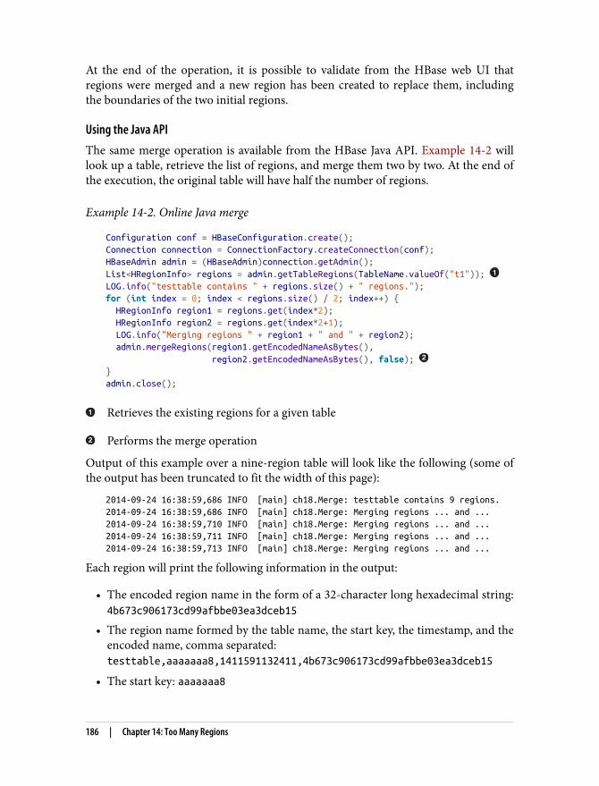
At the end of the operation, it is possible to validate from the HBase web UI thatregions were merged and a new region has been created to replace them, includingthe boundaries of the two initial regions.

Using the Java APIThe same merge operation is available from the HBase Java API. Example 14-2 willlook up a table, retrieve the list of regions, and merge them two by two. At the end ofthe execution, the original table will have half the number of regions.

Example 14-2. Online Java merge

Configuration conf = HBaseConfiguration.create(); Connection connection = ConnectionFactory.createConnection(conf); HBaseAdmin admin = (HBaseAdmin)connection.getAdmin(); List<HRegionInfo> regions = admin.getTableRegions(TableName.valueOf("t1")); LOG.info("testtable contains " + regions.size() + " regions."); for (int index = 0; index < regions.size() / 2; index++) { HRegionInfo region1 = regions.get(index*2); HRegionInfo region2 = regions.get(index*2+1); LOG.info("Merging regions " + region1 + " and " + region2); admin.mergeRegions(region1.getEncodedNameAsBytes(), region2.getEncodedNameAsBytes(), false); } admin.close();

Retrieves the existing regions for a given table

Performs the merge operation

Output of this example over a nine-region table will look like the following (some ofthe output has been truncated to fit the width of this page):

2014-09-24 16:38:59,686 INFO [main] ch18.Merge: testtable contains 9 regions.2014-09-24 16:38:59,686 INFO [main] ch18.Merge: Merging regions ... and ...2014-09-24 16:38:59,710 INFO [main] ch18.Merge: Merging regions ... and ...2014-09-24 16:38:59,711 INFO [main] ch18.Merge: Merging regions ... and ...2014-09-24 16:38:59,713 INFO [main] ch18.Merge: Merging regions ... and ...

Each region will print the following information in the output:

• The encoded region name in the form of a 32-character long hexadecimal string:4b673c906173cd99afbbe03ea3dceb15

• The region name formed by the table name, the start key, the timestamp, and theencoded name, comma separated: testtable,aaaaaaa8,1411591132411,4b673c906173cd99afbbe03ea3dceb15

• The start key: aaaaaaa8

186 | Chapter 14: Too Many Regions

• The end key: c71c71c4

Keys used in the example table are string based and can be printed by HBase. How‐ever, when your keys contain nonprintable characters, HBase will format them inhexadecimal form. A key containing a mix of printable and nonprintable characters,represented by the byte array [42, 73, 194] will be printed *I\xC2.

PreventionThere are multiple ways to prevent an HBase cluster from facing issues related to thenumber of regions.

Keep in mind that you need to consider not only the number ofregions, but also the number of column families in each of thoseregions. Indeed, for each column family within a region, HBase willkeep track of it in memory and in the hbase:meta table. Therefore,having 400 regions of two column families is not better than having800 regions of a single column family. Having too many columnfamilies in a table also creates problems, as we will explore inChapter 15.

Regions SizeFirst, you will want to make sure the maximum file size is set to at least 10 GB. It isnot an issue to have regions smaller than that, but you want to make sure that whenrequired, regions can get as big as 10 GB. Presplitting is discussed later in this section.It is recommended to monitor region sizes using a visualization tool such as Hanni‐bal. Watch for regions that are growing faster than others, and look to split them dur‐ing off-peak usage times. Figure 14-3 illustrates how Hannibal helps you to view thesize of each region.

Prevention | 187

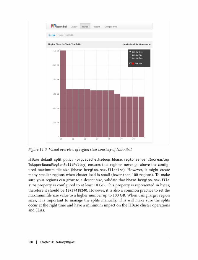
Figure 14-3. Visual overview of region sizes courtesy of Hannibal

HBase default split policy (org.apache.hadoop.hbase.regionserver.IncreasingToUpperBoundRegionSplitPolicy) ensures that regions never go above the config‐ured maximum file size (hbase.hregion.max.filesize). However, it might createmany smaller regions when cluster load is small (fewer than 100 regions). To makesure your regions can grow to a decent size, validate that hbase.hregion.max.filesize property is configured to at least 10 GB. This property is represented in bytes;therefore it should be 10737418240. However, it is also a common practice to set themaximum file size value to a higher number up to 100 GB. When using larger regionsizes, it is important to manage the splits manually. This will make sure the splitsoccur at the right time and have a minimum impact on the HBase cluster operationsand SLAs.

188 | Chapter 14: Too Many Regions

We do not recommend disabling splits or setting the split size tovery big values like 200 GB or more. A region can easily grow to anunwieldy size if there’s a spike in volume, if there are uncleansedrecords, or if the admin takes a vacation. If a region does not getsplit and continues to grow up to a very big size, it might crash theRegionServer. Upon failure, all regions from the server will be reas‐signed to another server, which will cause a cascading effect ofcrashes because of the size. From RegionServer to RegionServer,the culprit region will be reassigned and each time it will cause thetarget host to fail. If this is not recognized early, the entire clustermight go down.

Even if you expect your table to be small, you can still presplit it to increase distribu‐tion across RegionServers or manually trigger the splits to make sure you have up toas many regions as you have RegionServers. However, because HBase works betterwith bigger regions, make sure all your regions are at least 1 GB.

Key and Table DesignThe second thing you want to look at is how your application has been designed. Oneof the most common mistakes in HBase application design is to abuse the number ofcolumn families. Because a memstore for a specific region will be divided between thedifferent column families, having too many of them will reduce the size of the mem‐ory available for each and might result in very small flushes for some column fami‐lies. Also, because of the size of the flushed files, it will generate extra compactions.Reducing the number of column families will allow more memory per region for theremaining column families, will reduce the required flushes and compactions, andwill allow you to host more regions per server.

Another common mistake on table design is related to presplitting. Based on yourkey design and the size of the dataset, you will want to make sure that the table iscorrectly presplit before starting to inject data into the cluster. If the table has notbeen presplit correctly, you may end up with many unused or underutilized regions.Unused and underutilized regions still require resources such as memory and CPU,and still require periodic compactions. If your data is not evenly distributed but thetable is evenly split, you will also end up with some regions being heavily used andsome others being almost not used.

Prevention | 189

CHAPTER 15

Too Many Column Families

Many HBase users start to design HBase tables before reading about it and beforeknowing about all the HBase features and behaviors. People coming from theRDBMS world, with no knowledge of the differences between a column family and acolumn qualifier, will be tempted to create a column family for each column theyhave of a table they want to migrate to HBase. As a result, it is common to see tablesdesigned with too many column families.

For years, it has been recommended to keep the number of column families underthree. But there is no magic number like this. Why not two? Why not four? Techni‐cally, HBase can manage more than three of four column families. However, you needto understand how column families work to make the best use of them. The conse‐quences explained here will give you a very good idea of what kind of pressure col‐umn families are putting on HBase. Keep in mind that column families are built toregroup data with a similar format or a similar access pattern. Let’s look at these twofactors and how they affect the number of column families:

Regarding the formatIf you have to store large text data, you will most probably want to have this col‐umn family compressed. But if for the same row you also want to store a picture,then you most probably do not want this to be compressed because it will useCPU cycles to not save any space so will have negative impact on the performan‐ces. Using separate column families make sense here.

Regarding the access patternThe best way to describe this is to consider a real-world example. Imagine youhave a table storing customer information. A few huge columns store the cus‐tomer metadata. They contain a lot and are a few kilobytes in size. Then anothercolumn is a counter that stores each time the customer clicks on a page on thewebsite. The metadata columns will almost never change, while the counter col‐

191

umn will be updated many times a day. Over time, because of all the operationson the counters, the memstore will be flushed into disk. This will create files thatmostly contain only counter operations, which at some point will be compacted.However, when the compaction is performed, it will most probably select HFilesthat contain customer metadata. The compaction will rewrite all those huge cellsof customer metadata as well as the small counters. As a result, the vast majorityof the I/O will be wasted rewriting files with little to no change just to update orcompact the small counters. This creates an overhead on the I/Os. HBase triggerscompactions at the column family level. By separating the customer metadataand the customer counters into two different columns families, we will avoidunnecessarily rewriting the static information. It will lower the total IOPs on theRegionServers and therefore will improve the overall performances of the appli‐cations.

So how many column families is too many? We will not be able to give you a magicnumber. If it makes sense to separate them from the access pattern or from the for‐mat, separate them. But if you read and write them almost the same way and data hasalmost the same format, then simply keep it together in the same column family.

ConsequencesAbusing column families will impact your application’s performance and the wayHBase reacts in different ways. Depending how hard you are pushing HBase, it mightalso impact its stability because timeouts can occur, and RegionServers can get killed.

MemoryThe first impact of too many column families is on the memory side. HBase shares itsmemstore (write cache) among all the regions. Because each region is allowed a max‐imum configurable cache size of 128 MB, this section has to be shared between all thecolumn families of the same region. Therefore, the more column families you have,the smaller the average available size in the memstore will be for each of them. Whenone column family’s bucket is full, all of the other column families in that region mustbe flushed to disk as well, even if they have relatively little data. This will put a lot ofpressure on the memory, as many objects and small files will get created again andagain, but it will also put some pressure on the disks because those small files willhave to be compacted together.

Some work over HBASE-3149 and HBASE-10201 has been done toflush only the column families that are full instead of flushing all ofthem. However, this is not yet available in HBase 1.0. Once this fea‐ture is available, the memory impact of having too many columnfamilies will be drastically reduced, as will the impact on thecompactions.

192 | Chapter 15: Too Many Column Families

CompactionsThe number of column families affects the number of store files created duringflushes, and subsequently the number of compactions that must be performed. If atable has eight column families, and region’s 128 MB memstore is full, the data fromthe eight families is flushed to separate files. Over time, more flushes will occur.When more than three store files exist for a column family, HBase considers thosefiles for compaction. If a table has one column family, one set of files would need tobe compacted. With eight column families, eight sets of files need to be compacted,affecting the resources of the RegionServers and HDFS. Configuring fewer columnfamilies allows you to have larger memstore size per family; therefore fewer store filesneed to be flushed, and most importantly, fewer compactions need to occur, reducingthe I/Os on the underlying HDFS system. When a table needs to be flushed (likebefore taking a snapshot, or if administrators trigger flushes from the shell), all thememstores are flushed into disk. Depending on the previous operations, it is possiblethat doing this will make HBase reach yet another compaction trigger and will startcompactions for many if not all the regions and column families. The more columnfamilies, the more compactions will go into the queue and the more pressure will beput on HBase and HDFS.

SplitHBase stores columns families’ data into separate files and directories. When one ofthose directories become bigger than the configured region size, a split is triggered.

Splits affect all column families in a region, not only the column family whose datagrew beyond the maximum size. As a result, if some column families are pretty bigwhile others are pretty small, you might end up with column families containing onlya few cells. RegionServers allocate resources like memory and CPU threads perregion and column family. Very small regions and column families can create unnec‐essary pressure on those resources. The HBase master will also need to manage moreentries in the hbase:meta table and the underlying HDFS system. The HDFSDataNodes and NameNodes will also need to manage more I/Os for the small col‐umn family files. If you expect some column families to contain much more data thanothers, you might want to separate that data into other tables, producing fewer butlarger files.

Causes, Solution, and PreventionThe cause of having too many column families is always related to schema design.HBase will not create too many column families on your behalf; there’s no automatic-split behavior that can cause too many column families. Thus, to prevent this prob‐lem, you need to carefully consider HBase principles before you begin designing yourschema so that you can determine an appropriate number of column families.

Causes, Solution, and Prevention | 193

Several solutions exist for the issue of having too many column families. Understand‐ing the data in the column families and the access pattern is critical. Sometimes thecolumn families are not required and can simply be dropped—for example, if thedata is duplicated/denormalized and is available in another table. Sometimes the col‐umn family is present due to the access pattern (i.e., rollups or summary column-families). In that case, maybe the column family can simply be de-coupled from thetable and moved to its own table. Other times, the data in the separate column familycan be merged together with larger column families.

All the operations in the next sections can be done using the Java API, but they canalso very simply be done using the HBase shell or the command line. Because the JavaAPI will not really add any benefit to those operations, we have not documented it.

Delete a Column FamilyIf you have decided that you don’t need a specific column family, simply remove thiscolumn family from the table META information. The following method will deletethe picture column family from the sensors table:

alter 'sensors', NAME => 'picture', METHOD => 'delete'

This operation might take some time to execute because it will be applied in all theregions one by one. At the end, related files in HDFS will be removed, and thehbase:meta table will be updated to reflect the modification.

Merge a Column FamilyBecause of a flaw in the original schema design, or a shift in scope in the original usecase, you might have separated the data in two different column families but nowwant to merge it back into a single column family. As we discussed in “Solution” onpage 179, CopyTable allows you to copy data from one table into another one.CopyTable will help us in the current situation. The idea is that CopyTable willrequire a source table and a destination table; however, those two tables don’t neces‐sarily need to be different. Also, CopyTable allows us to rename one column familyinto a new one (Figure 15-1).

194 | Chapter 15: Too Many Column Families

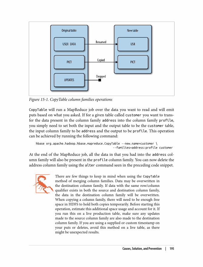
Figure 15-1. CopyTable column families operations

CopyTable will run a MapReduce job over the data you want to read and will emitputs based on what you asked. If for a given table called customer you want to trans‐fer the data present in the column family address into the column family profile,you simply need to set both the input and the output table to be the customer table,the input column family to be address and the output to be profile. This operationcan be achieved by running the following command:

hbase org.apache.hadoop.hbase.mapreduce.CopyTable --new.name=customer \ --families=address:profile customer

At the end of the MapReduce job, all the data in that you had into the address col‐umn family will also be present in the profile column family. You can now delete theaddress column family using the alter command seen in the preceding code snippet.

There are few things to keep in mind when using the CopyTablemethod of merging column families. Data may be overwritten inthe destination column family. If data with the same row/columnqualifier exists in both the source and destination column family,the data in the destination column family will be overwritten.When copying a column family, there will need to be enough freespace in HDFS to hold both copies temporarily. Before starting thisoperation, estimate this additional space usage and account for it. Ifyou run this on a live production table, make sure any updatesmade to the source column family are also made to the destinationcolumn family. If you are using a supplied or custom timestamp onyour puts or deletes, avoid this method on a live table, as theremight be unexpected results.

Causes, Solution, and Prevention | 195

It is also possible to merge back multiple column families into a single column family.You simply need to specify them all by separating them with a comma:

--families=address:profile,phone:profile,status:profile

Separate a Column Family into a New TableSeparating data into different tables might be desired for various reasons. Perhapsatomicity of operations between a table’s column families is not needed or there aresignificant differences in data size or access patterns between column families. Per‐haps it just makes more logical sense to have separate tables. Again, we will make useof CopyTable to perform the operations.

The following command copies the data from column family picture of thecustomer table to the map table in the same column family:

hbase org.apache.hadoop.hbase.mapreduce.CopyTable --families=picture \ --new.name=map customer

Here again, as long as you want to transfer multiple column families into the samedestination table, you can specify each desired column family by separating themwith a comma.

Both the destination table and the destination column family should exist before youstart the MapReduce job.

All the warnings from the previous paragraph also apply to the cur‐rent one.

196 | Chapter 15: Too Many Column Families

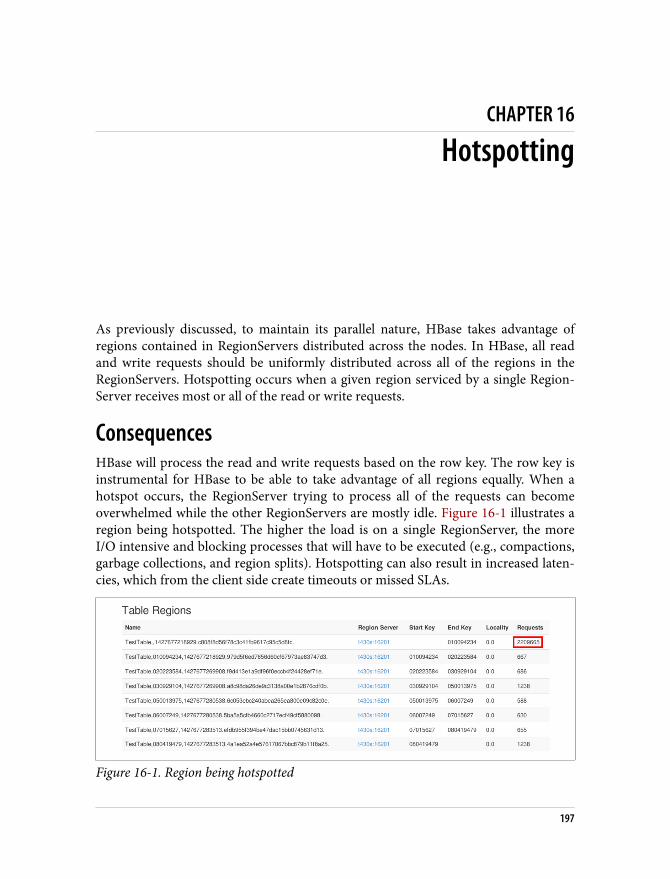
CHAPTER 16

Hotspotting

As previously discussed, to maintain its parallel nature, HBase takes advantage ofregions contained in RegionServers distributed across the nodes. In HBase, all readand write requests should be uniformly distributed across all of the regions in theRegionServers. Hotspotting occurs when a given region serviced by a single Region‐Server receives most or all of the read or write requests.

ConsequencesHBase will process the read and write requests based on the row key. The row key isinstrumental for HBase to be able to take advantage of all regions equally. When ahotspot occurs, the RegionServer trying to process all of the requests can becomeoverwhelmed while the other RegionServers are mostly idle. Figure 16-1 illustrates aregion being hotspotted. The higher the load is on a single RegionServer, the moreI/O intensive and blocking processes that will have to be executed (e.g., compactions,garbage collections, and region splits). Hotspotting can also result in increased laten‐cies, which from the client side create timeouts or missed SLAs.

Figure 16-1. Region being hotspotted

197

CausesThe main cause of hotspotting is usually an issue in the key design. In the followingsections, we will look at some of the most common causes of hotspotting, includingmonotonically incrementing or poorly distributed keys, very small reference tables,and applications issues.

Monotonically Incrementing KeysMonotonically incrementing keys are keys where only the last bits or bytes are slowlyincrementing. This means that most of the new key being written to or read fromHBase is extremely similar to the previously written or read key. The most commonlyseen monotonically incrementing key occurs when the timestamp is used as the key.When timestamp is used as the row key, the key will slowly increment from the firstput. Let’s take a look at a quick example: in HBase, keys are stored ordered in lexico‐graphical order. Our row keys will update as shown here:

1424362829142436283014243628311424362832...14243629001424362901142436290214243629031424362904

If requests are writes, each of the preceding updates is going to go into the sameregion until it reaches the key of the next region or its maximum configured size. Atthat point, the region will split, and we will begin incrementally updating the nextregion. Notice that most of the write operations are against the same region, therebyburdening a single RegionServer. Unfortunately, when this issue is detected after adeployment, there is nothing you can do to prevent hotspotting. The only way toavoid this kind of issue is to prevent it with a good key design.

Poorly Distributed KeysAs stated before, key design is very important, as it will impact not only the scalabilityof your application, but also its performance. However, in the first iteration of schemadesign in a use case, it is not uncommon for keys to be poorly designed and thereforewrongly distributed. This can occur due to a lack of information at the time of theschema design but also because of issues when implementing the application. A goodexample of a poorly distributed key is when you expect the source data to send youkeys with digits distributed between “0” and “9”; but you end up receiving keysalways prefixed with value before the expected “0” to “9” values. In this case, the

198 | Chapter 16: Hotspotting

application expects to receive “1977” and “2001” but gets “01977” and “02001”instead. In this example, if you had properly presplit the table into 10 regions (up to“1”, “1” to “2”, “2” to “3”, etc.), then all the values you received and stored in HBasewould be written to the first region (up to “1”) while all of the other regions wouldremain un-touched. In this case, even though we had the right intentions with theschema design, the data will never get fully distributed. This issue should be discov‐ered during proper testing, but if you discover this issue after the application has beendeployed, don’t despair—all is not lost. It is recommended to split the hotspottingregion into multiple regions. This should restore the expected distribution. In thisexample, you will have to split the first region into 10 regions to account for the lead‐ing zero. The new region range distribution being “00”, then “00” to “01”, “01 to “02”,and so on. The other regions, after “1”, will not be used if the keys are always prefixedby “0” and can be merged together one by one through region “10”.

Small Reference TablesThis common hotspotting issue refers to the bottleneck that results from the use ofsmall reference tables typically to perform joins in HBase. For this example, we havetwo reference tables consisting of a single region defining postal codes and citynames. In this case, we perform a MapReduce join over a billion-row orders table. Allthe generated mappers are going to query those two tables to perform the lookups. Asa result, the two RegionServers hosting the two reference regions will be over‐whelmed by calls from all the other servers in the cluster. If you are really unlucky,those two regions will be served by the same RegionServer. This kind of contention/bottleneck will increase latency and create delays that can lead to job failures due totimeouts. The good news is that there are multiple ways to avoid this situation. Thefirst and easiest option is to presplit your reference tables. The goal would be to haveclose to as many regions as you have RegionServers. Presplitting the reference tablemay not be an option if the table is too small or if you have too many RegionServerson HBase at the current time.

The other option here would be to distribute this table to all the nodes before per‐forming the join. The distribution of this data will be done using the MapReduce dis‐tributed cache mechanism. The distributed cache framework will copy the data to theslave node before any tasks are executed. The efficiency of this approach stems fromthe fact that the files are copied only once per job.

When all servers have a local copy of the data, and if the data is small enough to fitinto memory, it can then be loaded from the setup method of the MapReduce code,and lookups can now be performed into memory instead of reading from the disk.

This will increase performance, while also fixing the hotspotting issue.

Causes | 199

If MapReduce also updates or enriches the reference table, the dis‐tributed cache is not a viable option. Indeed, distributing a copy ofthe table at the beginning means the content is fixed for the dura‐tion of the job. If updates to the reference table are required in youruse case, then the best option is to presplit your reference table toensure even distribution of the table across the RegionServers.

Applications IssuesThe final example of region hotspotting is related to application design or implemen‐tation issues. When a region is hotspotting, it is very important to identify the rootcause. To accomplish this, we need to determine the source of the offending calls. Ifthe data is very well distributed into the table, the hotspotting may be coming from abug causing writes to always land in the same region. This is where mistakenly addedprefix fields, double or triple writes, or potentially badly converted data types canmanifest themselves as application issues. Let’s imagine the system is expected toreceive a four-byte integer value, but the backend code converts that to a height bytevalue. The four initial bytes might have been very well distributed over the entirerange of data, however, adding four empty bytes to this value will create a neverincrementing prefix of four empty bytes [0x00, 0x00, 0x00, 0x00] all landing into thesame HBase region and creating the hotspot.

Meta Region HotspottingAnother commonly seen issue is applications hotspotting the META region. Whencreating a connection to an HBase cluster, the application’s first stop is ZooKeeper toacquire HBase Master and the META region location. The application will cache thisinformation, and will then query the META table to send read and write requests tothe proper region. Each time a new connection is created, the application will againgo to ZooKeeper, and to META. To avoid having all those calls to ZooKeeper and theMETA table each time you perform a request to HBase, it is recommended to create asingle connection and to share it across your application. For a web service applica‐tion, it is recommended to create a pool of a few HBase connections and share themwith all the threads on the application side.

Prevention and SolutionThe best way to solve hotspotting is to prevent it from happening. This starts right atthe beginning of the project with a well-tested key design (refer back to “Key andTable Design” on page 189 if you need a refresher on how to do this). It is also impor‐tant to keep an eye on all your region metrics to have early detection of potential hot‐spotting. On the HBase Master web interface, the table page shows the number ofrequests received for each of the table’s regions. Requests column represents the num‐

200 | Chapter 16: Hotspotting

ber of read and write requests received by the region since it has been online. Whenregions are moved to other RegionServers, or when a table is disabled, the regionmetrics are reset. So when a region shows a very high number compared to the oth‐ers, it might be hotspotting but could also be due to very recent balancing of theregion between two servers. The only way to determine if it is from hotspotting orregion transitions is by looking through the logs or monitoring the suspect regionover time. The best way to avoid these issues in production is to put your applicationthrough proper testing and development cycles.

Prevention and Solution | 201

CHAPTER 17

Timeouts and Garbage Collection

Garbage collection (GC) is the process that cleans up the memory no longer refer‐enced by Java objects. This is done to free up the memory and make it available againto the application. Garbage collections are a normal, unavoidable occurrence in Java,but they can be managed. Depending on the garbage collection algorithm used, theremight be one or more garbage collection events going. The most impactful garbagecollection event for an HBase server is when the Java Virtual Machine needs to per‐form a full garbage collection (full GC). Such an operation is known as a “stop-the-world pause” and will pause the JVM while it is cleaning enough memory to allocaterequired objects. During this operation, the current running threads are in a holdingpattern until the JVM completes its GC. Long-running GC pauses are usually themain cause of timeouts on an HBase server, but we will also look at a few other risks.

ConsequencesAs stated before, full GCs are a “stop-the-world pause,” meaning any operation run‐ning on an HBase server will be paused until GC completion. These pauses can mani‐fest themselves externally as visible big spikes in the reads and writes latencies, oreven in the worst cases as false server failures. There are other issues that can reflectsimilar performance spikes in the RegionServer. The sources of these spikes shouldalways be clearly identified before starting to treat GC issues. The JVM will be pausedwhile performing the garbage collection cleanup, during this time all read and writeoperations will be queued by the client, which must wait for the server to becomeresponsive again. Garbage collection should always complete before the configuredtimeout values. Once complete, the reads and writes will resume to the server and beprocessed. However, if the Java tunings are not properly configured, the garbage col‐lection can last longer than the configured timeouts. There are a few different actionsthat can occur when the garbage collection exceeds the configured timeout values. If

203

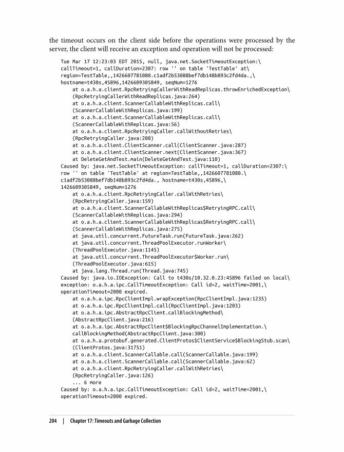
the timeout occurs on the client side before the operations were processed by theserver, the client will receive an exception and operation will not be processed:

Tue Mar 17 12:23:03 EDT 2015, null, java.net.SocketTimeoutException:\callTimeout=1, callDuration=2307: row '' on table 'TestTable' at\region=TestTable,,1426607781080.c1adf2b53088bef7db148b893c2fd4da.,\hostname=t430s,45896,1426609305849, seqNum=1276 at o.a.h.a.client.RpcRetryingCallerWithReadReplicas.throwEnrichedException\ (RpcRetryingCallerWithReadReplicas.java:264) at o.a.h.a.client.ScannerCallableWithReplicas.call\ (ScannerCallableWithReplicas.java:199) at o.a.h.a.client.ScannerCallableWithReplicas.call\ (ScannerCallableWithReplicas.java:56) at o.a.h.a.client.RpcRetryingCaller.callWithoutRetries\ (RpcRetryingCaller.java:200) at o.a.h.a.client.ClientScanner.call(ClientScanner.java:287) at o.a.h.a.client.ClientScanner.next(ClientScanner.java:367) at DeleteGetAndTest.main(DeleteGetAndTest.java:110)Caused by: java.net.SocketTimeoutException: callTimeout=1, callDuration=2307:\row '' on table 'TestTable' at region=TestTable,,1426607781080.\c1adf2b53088bef7db148b893c2fd4da., hostname=t430s,45896,\1426609305849, seqNum=1276 at o.a.h.a.client.RpcRetryingCaller.callWithRetries\ (RpcRetryingCaller.java:159) at o.a.h.a.client.ScannerCallableWithReplicas$RetryingRPC.call\ (ScannerCallableWithReplicas.java:294) at o.a.h.a.client.ScannerCallableWithReplicas$RetryingRPC.call\ (ScannerCallableWithReplicas.java:275) at java.util.concurrent.FutureTask.run(FutureTask.java:262) at java.util.concurrent.ThreadPoolExecutor.runWorker\ (ThreadPoolExecutor.java:1145) at java.util.concurrent.ThreadPoolExecutor$Worker.run\ (ThreadPoolExecutor.java:615) at java.lang.Thread.run(Thread.java:745)Caused by: java.io.IOException: Call to t430s/10.32.0.23:45896 failed on local\exception: o.a.h.a.ipc.CallTimeoutException: Call id=2, waitTime=2001,\operationTimeout=2000 expired. at o.a.h.a.ipc.RpcClientImpl.wrapException(RpcClientImpl.java:1235) at o.a.h.a.ipc.RpcClientImpl.call(RpcClientImpl.java:1203) at o.a.h.a.ipc.AbstractRpcClient.callBlockingMethod\ (AbstractRpcClient.java:216) at o.a.h.a.ipc.AbstractRpcClient$BlockingRpcChannelImplementation.\ callBlockingMethod(AbstractRpcClient.java:300) at o.a.h.a.protobuf.generated.ClientProtos$ClientService$BlockingStub.scan\ (ClientProtos.java:31751) at o.a.h.a.client.ScannerCallable.call(ScannerCallable.java:199) at o.a.h.a.client.ScannerCallable.call(ScannerCallable.java:62) at o.a.h.a.client.RpcRetryingCaller.callWithRetries\ (RpcRetryingCaller.java:126) ... 6 moreCaused by: o.a.h.a.ipc.CallTimeoutException: Call id=2, waitTime=2001,\operationTimeout=2000 expired.

204 | Chapter 17: Timeouts and Garbage Collection

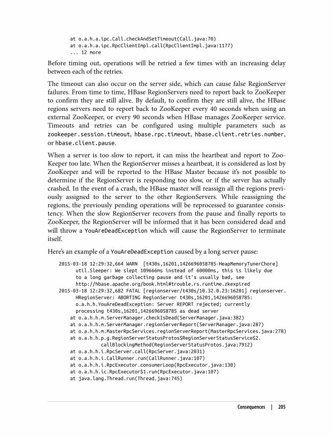
at o.a.h.a.ipc.Call.checkAndSetTimeout(Call.java:70) at o.a.h.a.ipc.RpcClientImpl.call(RpcClientImpl.java:1177) ... 12 more

Before timing out, operations will be retried a few times with an increasing delaybetween each of the retries.

The timeout can also occur on the server side, which can cause false RegionServerfailures. From time to time, HBase RegionServers need to report back to ZooKeeperto confirm they are still alive. By default, to confirm they are still alive, the HBaseregions servers need to report back to ZooKeeper every 40 seconds when using anexternal ZooKeeper, or every 90 seconds when HBase manages ZooKeeper service.Timeouts and retries can be configured using multiple parameters such aszookeeper.session.timeout, hbase.rpc.timeout, hbase.client.retries.number,or hbase.client.pause.

When a server is too slow to report, it can miss the heartbeat and report to Zoo‐Keeper too late. When the RegionServer misses a heartbeat, it is considered as lost byZooKeeper and will be reported to the HBase Master because it’s not possible todetermine if the RegionServer is responding too slow, or if the server has actuallycrashed. In the event of a crash, the HBase master will reassign all the regions previ‐ously assigned to the server to the other RegionServers. While reassigning theregions, the previously pending operations will be reprocessed to guarantee consis‐tency. When the slow RegionServer recovers from the pause and finally reports toZooKeeper, the RegionServer will be informed that it has been considered dead andwill throw a YouAreDeadException which will cause the RegionServer to terminateitself.

Here’s an example of a YouAreDeadException caused by a long server pause:

2015-03-18 12:29:32,664 WARN [t430s,16201,1426696058785-HeapMemoryTunerChore] util.Sleeper: We slept 109666ms instead of 60000ms, this is likely due to a long garbage collecting pause and it's usually bad, see http://hbase.apache.org/book.html#trouble.rs.runtime.zkexpired2015-03-18 12:29:32,682 FATAL [regionserver/t430s/10.32.0.23:16201] regionserver. HRegionServer: ABORTING RegionServer t430s,16201,1426696058785: o.a.h.h.YouAreDeadException: Server REPORT rejected; currently processing t430s,16201,1426696058785 as dead server at o.a.h.h.m.ServerManager.checkIsDead(ServerManager.java:382) at o.a.h.h.m.ServerManager.regionServerReport(ServerManager.java:287) at o.a.h.h.m.MasterRpcServices.regionServerReport(MasterRpcServices.java:278) at o.a.h.h.p.g.RegionServerStatusProtos$RegionServerStatusService$2. callBlockingMethod(RegionServerStatusProtos.java:7912) at o.a.h.h.i.RpcServer.call(RpcServer.java:2031) at o.a.h.h.i.CallRunner.run(CallRunner.java:107) at o.a.h.h.i.RpcExecutor.consumerLoop(RpcExecutor.java:130) at o.a.h.h.ic.RpcExecutor$1.run(RpcExecutor.java:107) at java.lang.Thread.run(Thread.java:745)

Consequences | 205

CausesWhen dealing with Java-based platforms, memory fragmentation is typically themain cause of full garbage collection and pauses. In a perfect world, all the objectswould be the same size, and it would be very easy to track, find, and allocate freememory without causing heavy memory fragmentation. Unfortunately, in the realworld this is not the case, and puts received by the servers are almost never the samesize. Also, the compressed HFiles blocks and many other HBase objects are alsoalmost neither never the same size. The previously mentioned factors will create frag‐mentation of the available memory. The more the JVM memory is fragmented, themore it will need to run garbage collection to release unused memory. Typically, thelarger the heap is, the longer a full GC will take to complete. This means raising theheap too high without (or even sometimes) with proper tuning can lead to timeouts.

Garbage collection is not the only contributing factor to timeouts and pauses. It ispossible to create a scenario where the memory is overallocated (giving to HBase orother applications more memory than available physical memory), the operating sys‐tem will need to swap some of the memory pages to the disks. This is one of the leastdesirable situations in HBase. Swapping is guaranteed to cause issues with cluster,which in turn will create timeouts and drastically impact the latencies.

The final risk is improper hardware behaviors or failures. Network failures and harddrives are good examples of such risks.

Storage FailureFor multiple reasons, a storage drive can fail and become unresponsive. When thisoccurs, the operating system will try multiple times before reporting the error to theapplication. This might create delays and general slowness, which again will impactthe latency and might trigger timeouts or failures. HDFS is designed to handle suchfailures and no data will be lost, however failures on the operating system drive myimpact the entire host availability.

Power-Saving FeaturesTo reduce energy consumption, some disks have energy-saving features. When thisfeature is activated, if a disk is not accessed for a certain period of time, it will go onsleep and will stop spinning. As soon as the system needs data stored on that disk, itneeds first to start spinning the disk back, wait for it to reach its full speed, and thenonly start to read from it. When HBase makes any request to the I/O layer, the totaltime it takes the energy-saving drives to spin back up can contribute to timeouts andlatency spikes. In certain circumstances, those timeouts can even cause serverfailures.

206 | Chapter 17: Timeouts and Garbage Collection

Network FailureOn big clusters, servers are assigned into racks, connected together using top-of-the-rack switches. Such switches are powerful and come with many features, but like anyother hardware they can have small failures and can pause because of them. Thosepauses will cause communications between the servers to fail for a certain period oftime. Here again, if this period of time extends beyond the configured timeout,HBase will consider those servers as lost and will kill them if they come back online,with all the impacts on the latencies that you can imagine.

SolutionsWhen a server crashes or has been closed because of a timeout issue, the only solu‐tion is to restart it. The source of such a failure can be a network, configuration, orhardware issue (or something else entirely). Whatever the source of this failure is, itneeds to be identified and addressed to avoid similar issues in the future. When yourserver fails for any reason, if not addressed, the chances of this occurring again onyour cluster are very high and other failures are to be expected. The best place to startwith to identify issues are the servers logs, both HBase Master and the culprit Region‐Server; however, it might also be good to have a look at the system logs (/var/log/messages), the network interfaces statistics (in particular, the drop packages), and theswitch monitoring interface. It is also a very good practice to validate your networkbandwidth between multiple nodes at the same time across different racks using toolslike iperf. Testing the network performances and stability will allow you to detect bot‐tleneck in the configuration, but will miss configured interfaces (like, configured tobe 1 Gbps instead of 10 Gbps, etc.).

Hardware duplication and new generation network management tools like Aristaproducts can help to avoid network and hardware issues and will be looked at in thefollowing section.

Last, Cloudera Manager and other cluster management applications can automati‐cally restart the services when they exit (RegionServers, Masters, ThriftServers, etc.),however, it might be good to not activate such features, as you want to identify theroot cause of the failures before restarting the services.

There are multiple ways to prevent such situations from occurring, and the next sec‐tion will review them one by one.

PreventionAs we have just seen, timeouts and garbage collection can occur for multiple differentreasons. In this section, we identify what those situations might be, and provide waysto prevent them from happening.

Solutions | 207

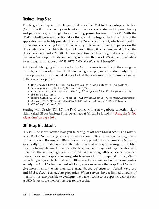
Reduce Heap SizeThe bigger the heap size, the longer it takes for the JVM to do a garbage collection(GC). Even if more memory can be nice to increase cache size and improve latencyand performance, you might face some long pauses because of the GC. With theJVM’s default garbage collection algorithms, a full garbage collection will freeze theapplication and is highly probable to create a ZooKeeper timeout, which will result inthe RegionServer being killed. There is very little risks to face GC pauses on theHBase Master server. Using the default HBase settings, it is recommended to keep theHBase heap size under 20 GB. Garbage collection can be configured inside the conf/hbase-conf.sh script. The default setting is to use the Java CMS (Concurrent MarkSweep) algorithm: export HBASE_OPTS="-XX:+UseConcMarkSweepGC".

Additional debugging information for the GC processes is avalable in the configura‐tion file, and is ready to use. In the following example, we are adding only one ofthese options (we recommend taking a look at the configuration file to understand allof the available options):

# This enables basic GC logging to its own file with automatic log rolling.# Only applies to jdk 1.6.0_34+ and 1.7.0_2+.# If FILE-PATH is not replaced, the log file(.gc) would still be generated in# the HBASE_LOG_DIR .# export CLIENT_GC_OPTS="-verbose:gc -XX:+PrintGCDetails -XX:+PrintGCDateStamps\# -Xloggc:<FILE-PATH> -XX:+UseGCLogFileRotation -XX:NumberOfGCLogFiles=1\# -XX:GCLogFileSize=512M"

Starting with Oracle JDK 1.7, the JVM comes with a new garbage collection algo‐rithm called G1 for Garbage First. Details about G1 can be found in “Using the G1GCAlgorithm” on page 209 .

Off-Heap BlockCacheHBase 1.0 or more recent allows you to configure off-heap BlockCache using what iscalled BucketCache. Using off-heap memory allows HBase to manage the fragmenta‐tion on its own. Because all HBase blocks are supposed to be the same size (except ifspecifically defined differently at the table level), it is easy to manage the relatedmemory fragmentation. This reduces the heap memory usage and fragmentation andtherefore, the required garbage reduction. When using off-heap cache, you canreduce the default heap size memory, which reduces the time required for the JVM torun a full garbage collection. Also, if HBase is getting a mix load of reads and writes,as only the BlockCache is moved off heap, you can reduce the heap BlockCache togive more memory to the memstore using hbase.regionserver.global.memstoreand hfile.block.cache.size properties. When servers have a limited amount ofmemory, it is also possible to configure the bucket cache to use specific devices suchas SSD drives as the memory storage for the cache.

208 | Chapter 17: Timeouts and Garbage Collection

Using the G1GC AlgorithmThe Default JVM garbage collection algorithm in Java 6, 7, and 8 tends to strugglewith large heaps running full GC. These full GCs will pause the JVM until memory iscleaned. As seen in the previous section, this might negatively impact the server avail‐ability. Java 1.7_u60+ is the first stable release of the G1GC algorithm. G1GC is agarbage collection algorithm that stands for garbage first collection. G1 breaks mem‐ory into 1–32 MB regions depending on the heap size. Then when running cleanupattempts to clean the regions that are no longer being used first, G1 frees up morememory without having to perform stop-the-world pauses. G1GC also heavily lever‐ages mixed collections that occur on the fly, again helping to avoid the stop-the-worldpauses that can be detrimental to HBase latency.

Tuning the G1GC collector can be daunting and require some trial and error. Onceproperly configured, we have used the G1GC collector with heaps as large as 176 GB.Heaps that large are beneficial to more than just read performance. If you are lookingfor strictly for read performance, off-heap caching will offer the performance bumpwithout the tuning headaches. A benefit of having large heaps with G1GC is that itallows HBase to scale better horizontally by offering a large memstore pool forregions to share.

Must-use parameters

• -XX:+UseG1GC

• -XX:+PrintFlagsFinal

• -XX:+PrintGCDetails

• -XX:+PrintGCDateStamps

• -XX:+PrintGCTimeStamps

• -XX:+PrintAdaptiveSizePolicy

• -XX:+PrintReferenceGC

Additional HBase settings while exceeding 100 GB heaps

-XX:-ResizePLAB

Promotion local allocation buffers (PLABs) avoid the large communication costamong GC threads, as well as variations during each GC.

-XX:+ParallelRefProcEnabled

When this flag is turned on, GC uses multiple threads to process the increasingreferences during young and mixed GC.

Prevention | 209

-XX:+AlwaysPreTouch

Pre-touch the Java heap during JVM initialization. That means every page of theheap is demand-zeroed during initialization rather than incrementally duringapplication execution.

-XX:MaxGCPauseMillis=100

Max pause will attempt to keep GC pauses below the referenced time. Thisbecomes critical for proper tuning. G1GC will do its best to hold to the number,but will pause longer if necessary.

Other interesting parameters

-XX:ParallelGCThreads=X

Formula: 8 + (logical processors – 8) (5/8)

-XX:G1NewSizePercent=X

Eden size is calculated by (heap size * G1NewSizePercent). The default value ofG1NewSizePercent is 5 (5% of total heap). Lowering this can change the totaltime young GC pauses take to complete.

-XX:+UnlockExperimentalVMOptions

Unlocks the use of the previously referenced flags.

-XX:G1HeapWastePercent=5

Sets the percentage of heap that you are willing to waste. The Java HotSpot VMdoes not initiate the mixed garbage collection cycle when the reclaimable per‐centage is less than the heap waste percentage. The default is 10%.

-XX:G1MixedGCLiveThresholdPercent=75

Sets the occupancy threshold for an old region to be included in a mixed garbagecollection cycle. The default occupancy is 65%. This is an experimental flag.

The primary goal from the tuning is to be running many mixed GC collections andavoiding the full GCs. When properly tuned, we should see very repeatable GCbehavior assuming the workload stays relatively uniform. It is important to note thatoverprovisioning of the heap can help avoid the full GCs by leaving headroom for themixed GCs to continue in the background. For further reading, check out Oracle’scomprehensive documentation.

Configure Swappiness to 0 or 1HBase might not be the only application running on your environment, and at somepoint memory might have been over allocated. By default, Linux will try to anticipatethe lack of memory and will start to swap to disk some memory pages. This is finebecause it will allow the operating system to avoid being out of memory; however,writing such pages into disk takes time and will, here again, impact the latency. When

210 | Chapter 17: Timeouts and Garbage Collection

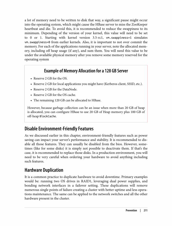
a lot of memory need to be written to disk that way, a significant pause might occurinto the operating system, which might cause the HBase server to miss the ZooKeeperheartbeat and die. To avoid this, it is recommended to reduce the swappiness to itsminimum. Depending of the version of your kernel, this value will need to be setto 0 or 1. Starting with kernel version 3.5-rc1, vm.swappiness=1 simulatesvm.swappiness=0 from earlier kernels. Also, it is important to not over commit thememory. For each of the applications running in your server, note the allocated mem‐ory, including off heap usage (if any), and sum them. You will need this value to beunder the available physical memory after you remove some memory reserved for theoperating system

Example of Memory Allocation for a 128 GB Server• Reserve 2 GB for the OS.• Reserve 2 GB for local applications you might have (Kerberos client, SSSD, etc.).• Reserve 2 GB for the DataNode.• Reserve 2 GB for the OS cache.• The remaining 120 GB can be allocated to HBase.

However, because garbage collection can be an issue when more than 20 GB of heapis allocated, you can configure HBase to use 20 GB of Heap memory plus 100 GB ofoff-heap BlockCache.

Disable Environment-Friendly FeaturesAs we discussed earlier in this chapter, environment-friendly features such as powersaving can impact your server’s performance and stability. It is recommended to dis‐able all those features. They can usually be disabled from the bios. However, some‐times (like for some disks) it is simply not possible to deactivate them. If that’s thecase, it is recommended to replace those disks. In a production environment, you willneed to be very careful when ordering your hardware to avoid anything includingsuch features.

Hardware DuplicationIt is a common practice to duplicate hardware to avoid downtime. Primary exampleswould be: running two OS drives in RAID1, leveraging dual power supplies, andbonding network interfaces in a failover setting. These duplications will removenumerous single points of failure creating a cluster with better uptime and less opera‐tions maintenance. The same can be applied to the network switches and all the otherhardware present in the cluster.

Prevention | 211

CHAPTER 18

HBCK and Inconsistencies

HBase Filesystem LayoutLike any database or filesystem, HBase can run into inconsistencies between what itbelieves its metadata looks like and what its filesystem actually looks like. Of course,the inverse of the previous statement can be true as well. Before getting into debug‐ging HBase inconsistencies, it is important to understand the layout of HBase’s meta‐data master table known as hbase:meta and the how HBase is laid out on HDFS.Looking at the meta table name hbase:meta, the hbase before the : indicates thenamespace the table lives in, and after the : is the name of the table, which is meta.Namespaces are used for logical grouping of similar tables, typically utilized in multi‐tenant environments. Out of the box, two namespaces are used: default and hbase.default is where all tables without a namespace specified are created, and hbase isused for HBase internal tables. For right now, we are going to focus on hbase:meta.HBase’s meta table is used to store important pieces of information about the regionsin the HBase tables. Here is a sample output of an HBase instance with one user tablenamed odell:

hbase(main):002:0> describe 'hbase:meta'DESCRIPTION 'hbase:meta', {TABLE_ATTRIBUTES => {IS_META => 'true', coprocessor$1 => '|org.apache.hadoop.hbase.coprocessor.MultiRowMutation Endpoint|536870911|'}, {NAME => 'info', DATA_BLOCK_ENCODING => 'NONE', BLOOMFILTER => 'NONE', REPLICATION_SCOPE => '0', COMPRESSION => 'NONE', VERSIONS => '10', TTL => 'FOREVER', MIN_VERSIONS => '0', KEEP_DELETED_CELLS => 'false', BLOCKSIZE => '8192', IN_MEMORY => 'true', BLOCKCACHE => 'true'}

213

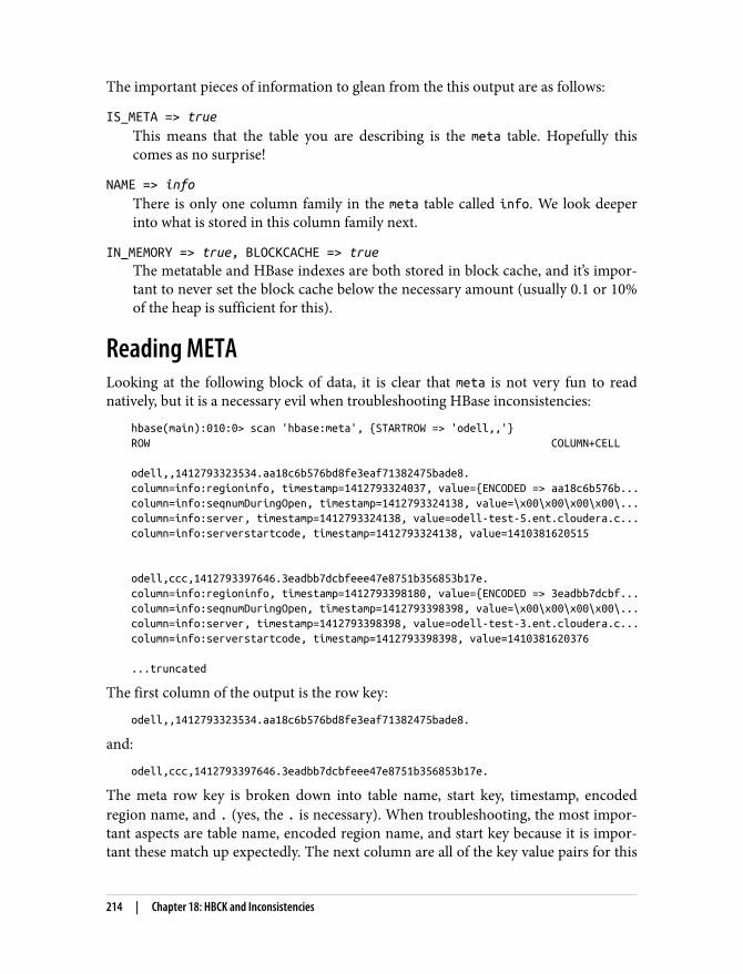
The important pieces of information to glean from the this output are as follows:

IS_META => true

This means that the table you are describing is the meta table. Hopefully thiscomes as no surprise!

NAME => info

There is only one column family in the meta table called info. We look deeperinto what is stored in this column family next.

IN_MEMORY => true, BLOCKCACHE => true

The metatable and HBase indexes are both stored in block cache, and it’s impor‐tant to never set the block cache below the necessary amount (usually 0.1 or 10%of the heap is sufficient for this).

Reading METALooking at the following block of data, it is clear that meta is not very fun to readnatively, but it is a necessary evil when troubleshooting HBase inconsistencies:

hbase(main):010:0> scan 'hbase:meta', {STARTROW => 'odell,,'}ROW COLUMN+CELL

odell,,1412793323534.aa18c6b576bd8fe3eaf71382475bade8.column=info:regioninfo, timestamp=1412793324037, value={ENCODED => aa18c6b576b...column=info:seqnumDuringOpen, timestamp=1412793324138, value=\x00\x00\x00\x00\...column=info:server, timestamp=1412793324138, value=odell-test-5.ent.cloudera.c...column=info:serverstartcode, timestamp=1412793324138, value=1410381620515

odell,ccc,1412793397646.3eadbb7dcbfeee47e8751b356853b17e.column=info:regioninfo, timestamp=1412793398180, value={ENCODED => 3eadbb7dcbf...column=info:seqnumDuringOpen, timestamp=1412793398398, value=\x00\x00\x00\x00\...column=info:server, timestamp=1412793398398, value=odell-test-3.ent.cloudera.c...column=info:serverstartcode, timestamp=1412793398398, value=1410381620376

...truncated

The first column of the output is the row key:

odell,,1412793323534.aa18c6b576bd8fe3eaf71382475bade8.

and:

odell,ccc,1412793397646.3eadbb7dcbfeee47e8751b356853b17e.

The meta row key is broken down into table name, start key, timestamp, encodedregion name, and . (yes, the . is necessary). When troubleshooting, the most impor‐tant aspects are table name, encoded region name, and start key because it is impor‐tant these match up expectedly. The next column are all of the key value pairs for this

214 | Chapter 18: HBCK and Inconsistencies

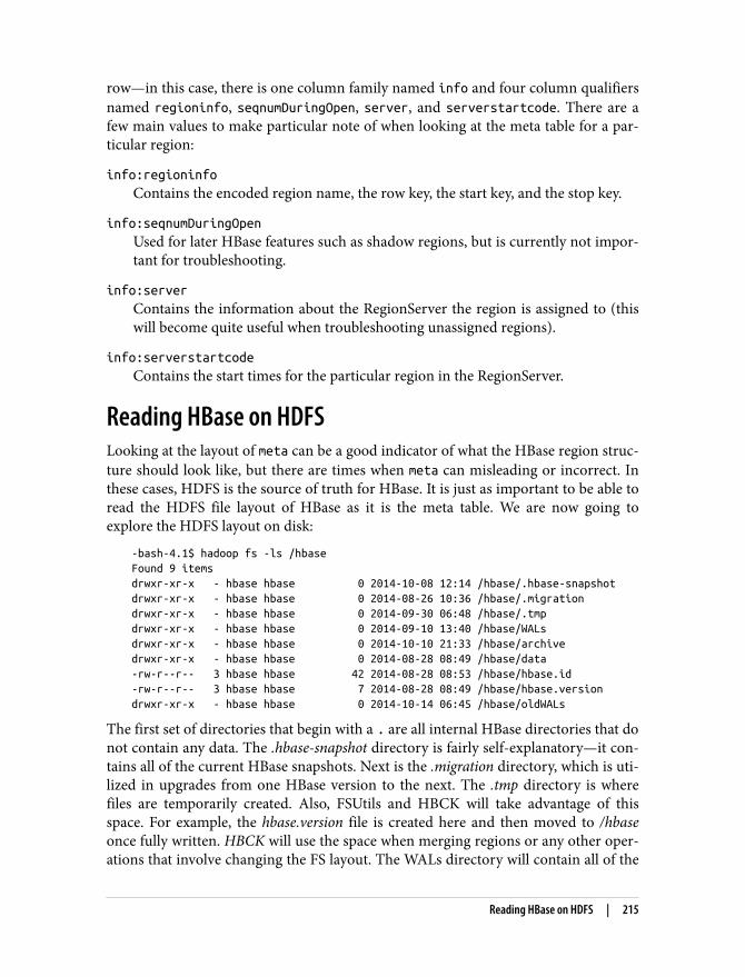
row—in this case, there is one column family named info and four column qualifiersnamed regioninfo, seqnumDuringOpen, server, and serverstartcode. There are afew main values to make particular note of when looking at the meta table for a par‐ticular region:

info:regioninfo

Contains the encoded region name, the row key, the start key, and the stop key.

info:seqnumDuringOpen

Used for later HBase features such as shadow regions, but is currently not impor‐tant for troubleshooting.

info:server

Contains the information about the RegionServer the region is assigned to (thiswill become quite useful when troubleshooting unassigned regions).

info:serverstartcode

Contains the start times for the particular region in the RegionServer.

Reading HBase on HDFSLooking at the layout of meta can be a good indicator of what the HBase region struc‐ture should look like, but there are times when meta can misleading or incorrect. Inthese cases, HDFS is the source of truth for HBase. It is just as important to be able toread the HDFS file layout of HBase as it is the meta table. We are now going toexplore the HDFS layout on disk:

-bash-4.1$ hadoop fs -ls /hbaseFound 9 itemsdrwxr-xr-x - hbase hbase 0 2014-10-08 12:14 /hbase/.hbase-snapshotdrwxr-xr-x - hbase hbase 0 2014-08-26 10:36 /hbase/.migrationdrwxr-xr-x - hbase hbase 0 2014-09-30 06:48 /hbase/.tmpdrwxr-xr-x - hbase hbase 0 2014-09-10 13:40 /hbase/WALsdrwxr-xr-x - hbase hbase 0 2014-10-10 21:33 /hbase/archivedrwxr-xr-x - hbase hbase 0 2014-08-28 08:49 /hbase/data-rw-r--r-- 3 hbase hbase 42 2014-08-28 08:53 /hbase/hbase.id-rw-r--r-- 3 hbase hbase 7 2014-08-28 08:49 /hbase/hbase.versiondrwxr-xr-x - hbase hbase 0 2014-10-14 06:45 /hbase/oldWALs

The first set of directories that begin with a . are all internal HBase directories that donot contain any data. The .hbase-snapshot directory is fairly self-explanatory—it con‐tains all of the current HBase snapshots. Next is the .migration directory, which is uti‐lized in upgrades from one HBase version to the next. The .tmp directory is wherefiles are temporarily created. Also, FSUtils and HBCK will take advantage of thisspace. For example, the hbase.version file is created here and then moved to /hbaseonce fully written. HBCK will use the space when merging regions or any other oper‐ations that involve changing the FS layout. The WALs directory will contain all of the

Reading HBase on HDFS | 215

currently active WALs that have not yet been rolled or need to be split during arestart. The archive directory is related directly to the .hbase-snapshots and is reservedfor snapshot use only. The archive directly holds the HFiles that are being protectedby the HBase snapshot, rather than being deleted. The hbase.id file contains theunique ID of the cluster. The hbase.version file holds a string representation of thecurrent version of HBase. The oldWALs directory is used in direct correlation withHBase replication. Any WALs that still need to be replayed to the destination clusterare written here rather than deleted when rolled. This backup typically happenswhenever there is communication issues between the source and destination cluster.For the exercise of troubleshooting inconsistencies, we will be focused on the datadirectory. The data directory is aptly named—it contains the data for HBase. Let’stake a deeper look at the the directory structure for data:

-bash-4.1$ hadoop fs -ls /hbase/dataFound 2 itemsdrwxr-xr-x - hbase hbase 0 2014-10-08 11:31 /hbase/data/defaultdrwxr-xr-x - hbase hbase 0 2014-08-28 08:53 /hbase/data/hbase

The next layer is where the namespaces for the HBase are contained. In the precedingexample, there are only two namespaces—default and hbase:

-bash-4.1$ hadoop fs -ls /hbase/data/defaultFound 1 itemsdrwxr-xr-x - hbase hbase 0 2014-10-08 11:40 /hbase/data/default/odell-bash-4.1$ hadoop fs -ls /hbase/data/hbaseFound 2 itemsdrwxr-xr-x - hbase hbase 0 2014-08-28 08:53 /hbase/data/hbase/metadrwxr-xr-x - hbase hbase 0 2014-08-28 08:53 /hbase/.../namespace

The next level down will show the tables’ names. As in the preceding code snippet, wehave a table called odell in our default namespace, and we have two tables, meta, andnamespace, in the hbase namespace. We are going to focus on what odell looks likegoing forward:

-bash-4.1$ hadoop fs -ls /hbase/data/default/odellFound 5 itemsdrwxr-xr-x 2014-10-08 11:31 /hbase/data/default/odell/.tabledescdrwxr-xr-x 2014-10-08 11:31 /hbase/data/default/odell/.tmpdrwxr-xr-x 2014-10-08 11:36 /hbase/data/default/odell/3eadbb7dcbfeee47e875...drwxr-xr-x 2014-10-08 11:36 /hbase/data/default/odell/7450bb77ac287b9e77ad...drwxr-xr-x 2014-10-08 11:35 /hbase/data/default/odell/aa18c6b576bd8fe3eaf71...

The .tabledesc directory contains a file typically named .tableinfo.000000xxxx where xis a count for the number of tables. The tableinfo file contains a listing of the sameinformation presented when running a describe from the HBase shell. This includesinformation such as meta, data block encoding type, bloomfilter used, version count,compression, and so on. It is important to maintain the tableinfo file when attemptingto duplicate tables using distcp (we highly recommend using snapshots instead).The .tmp directory is used to write the tableinfo file which is then moved to

216 | Chapter 18: HBCK and Inconsistencies

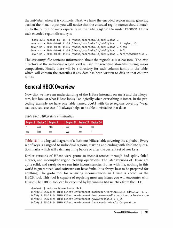
the .tabledesc when it is complete. Next, we have the encoded region name; glancingback at the meta output you will notice that the encoded region names should matchup to the output of meta especially in the info:regioninfo under ENCODED. Undereach encoded region directory is:

-bash-4.1$ hadoop fs -ls -R /hbase/data/default/odell/3ead...-rwxr-xr-x 2014-10-08 11:36 /hbase/data/default/odell/3ead.../.regioninfodrwxr-xr-x 2014-10-08 11:36 /hbase/data/default/odell/3ead.../.tmpdrwxr-xr-x 2014-10-08 11:36 /hbase/data/default/odell/3ead.../cf1-rwxr-xr-x 2014-10-08 11:36 /hbase/data/default/odell/3ead.../cf1/5cadc83fc35d...

The .regioninfo file contains information about the region’s <INFORMATION>. The .tmpdirectory at the individual region level is used for rewriting storefiles during majorcompactions. Finally there will be a directory for each column family in the table,which will contain the storefiles if any data has been written to disk in that columnfamily.

General HBCK OverviewNow that we have an understanding of the HBase internals on meta and the filesys‐tem, let’s look at what HBase looks like logically when everything is intact. In the pre‐ceding example we have one table named odell with three regions covering “–aaa,aaa–ccc, ccc–eee, eee–”. It always helps to be able to visualize that data:

Table 18-1. HBCK data visualization

Region 1 Region 2 Region 3 … Region 24 Region 25 Region 26“ aaa bbb … xxx yyy zzz

aaa bbb ccc … yyy zzz ”

Table 18-1 is a logical diagram of a fictitious HBase table covering the alphabet. Everyset of keys is assigned to individual regions, starting and ending with absolute quota‐tion marks which will catch anything before or after the current set of row keys.

Earlier versions of HBase were prone to inconsistencies through bad splits, failedmerges, and incomplete region cleanup operations. The later versions of HBase arequite solid, and rarely do we run into inconsistencies. But as with life, nothing in thisworld is guaranteed, and software can have faults. It is always best to be prepared foranything. The go-to tool for repairing inconsistencies in HBase is known as theHBCK tool. This tool is capable of repairing most any issues you will encounter withHBase. The HBCK tool can be executed by by running hbase hbck from the CLI:

-bash-4.1$ sudo -u hbase hbase hbck14/10/15 05:23:24 INFO Client environment:zookeeper.version=3.4.5-cdh5.1.2--1,...14/10/15 05:23:24 INFO Client environment:host.name=odell-test-1.ent.cloudera.com14/10/15 05:23:24 INFO Client environment:java.version=1.7.0_5514/10/15 05:23:24 INFO Client environment:java.vendor=Oracle Corporation

General HBCK Overview | 217

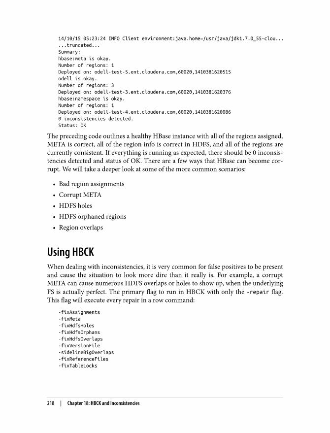
14/10/15 05:23:24 INFO Client environment:java.home=/usr/java/jdk1.7.0_55-clou......truncated...Summary:hbase:meta is okay.Number of regions: 1Deployed on: odell-test-5.ent.cloudera.com,60020,1410381620515odell is okay.Number of regions: 3Deployed on: odell-test-3.ent.cloudera.com,60020,1410381620376hbase:namespace is okay.Number of regions: 1Deployed on: odell-test-4.ent.cloudera.com,60020,14103816200860 inconsistencies detected.Status: OK

The preceding code outlines a healthy HBase instance with all of the regions assigned,META is correct, all of the region info is correct in HDFS, and all of the regions arecurrently consistent. If everything is running as expected, there should be 0 inconsis‐tencies detected and status of OK. There are a few ways that HBase can become cor‐rupt. We will take a deeper look at some of the more common scenarios:

• Bad region assignments• Corrupt META• HDFS holes• HDFS orphaned regions• Region overlaps

Using HBCKWhen dealing with inconsistencies, it is very common for false positives to be presentand cause the situation to look more dire than it really is. For example, a corruptMETA can cause numerous HDFS overlaps or holes to show up, when the underlyingFS is actually perfect. The primary flag to run in HBCK with only the -repair flag.This flag will execute every repair in a row command:

-fixAssignments-fixMeta-fixHdfsHoles-fixHdfsOrphans-fixHdfsOverlaps-fixVersionFile-sidelineBigOverlaps-fixReferenceFiles-fixTableLocks

218 | Chapter 18: HBCK and Inconsistencies

This is great when you are working with an experimental or development instance,but might not be ideal when dealing with production or pre-production instances.One of the primary reasons to be careful with executing just the -repair flag is the-sidelineBigOverlaps flag. If there are overly large overlaps, HBase will sidelineregions outside of HBase, and they will have to be bulk loaded back into the correctregion assignments. Without a full understanding of every flag’s implication, it is pos‐sible to make the issue worse than it is. It is recommended to take a pragmaticapproach and start with the less impactful flags.

Log Everything

Before you start running any HBCK, make sure you are either log‐ging to an external file or your terminal is logging all commandsand terminal outputs

The first two flags we typically prefer to run are -fixAssignments and -FixMeta. The-fixAssignments flag repairs unassigned regions, incorrectly assigned regions, orregions with multiple assignments. HBase uses HDFS as the underlying source oftruth for the correct layout of META. The -fixMeta flag removes meta rows whencorresponding regions are not present in HDFS and adds new meta rows if theregions are present in HDFS while not in META. In HBase, the region assignmentsare controlled through the Assignment Manager. The Assignment Manager keeps thecurrent state of HBase in memory, if the region assignments were out of sync withHBase and META, it is safe to assume they are out of sync in the Assignment Man‐ager. The fastest way to update the Assignment Manager to the correct values pro‐vided by HBCK is to rolling restart your HBase Master nodes. After restarting theHBase Master nodes, it is time to run HBCK again.

If after rerunning HBCK the end result is not “0 inconsistencies detected,” then it istime to use some heavier-handed commands to correct the outstanding issues. Thethree other major issues that could still be occurring are HDFS holes, HDFS overlaps,and HDFS orphans.

If running the -FixMeta and the -FixAssignments flag, we would recommend con‐tacting your friendly neighborhood Hadoop vendor for more detailed instructions. If,on the other hand, you are handling this yourself, we would recommend using the-repair flag at this point. It is important to note that numerous passes may need tobe run. We recommend running the -repair flag in a cycle similar to this:

-bash-4.1$ sudo -u hbase hbase hbck

-bash-4.1$ sudo -u hbase hbase hbck -repair

-bash-4.1$ sudo -u hbase hbase hbck

Using HBCK | 219

-bash-4.1$ sudo -u hbase hbase hbck -repair

-bash-4.1$ sudo -u hbase hbase hbck

-bash-4.1$ sudo -u hbase hbase hbck -repair

-bash-4.1$ sudo -u hbase hbase hbck

If you have run through this set of commands and are still seeing inconsistencies, youmay need to start running through individual commands depending on the output ofthe last HBCK command. Again, at this point, we cannot stress enough the impor‐tance of contacting your Hadoop vendor or the Apache mailing lists—there areexperts available who can help with situations like this. In lieu of that, here is a list ofother commands that be found in HBCK:

-fixHdfsHoles

Try to fix region holes in HDFS.

-fixHdfsOrphans

Try to fix region directories with no .regioninfo file in HDFS.

-fixTableOrphans

Try to fix table directories with no .tableinfo file in HDFS (online mode only).

-fixHdfsOverlaps

Try to fix region overlaps in HDFS.

-fixVersionFile

Try to fix missing hbase.version file in HDFS.

-sidelineBigOverlaps

When fixing region overlaps, allow to sideline big overlaps.

-fixReferenceFiles

Try to offline lingering reference store files.

-fixEmptyMetaCells

Try to fix hbase:meta entries not referencing any region (empty REGIONINFO_QUALIFIER rows).

-maxMerge <n>

When fixing region overlaps, allow at most <n> regions to merge (n=5 bydefault).

-maxOverlapsToSideline <n>

When fixing region overlaps, allow at most <n> regions to sideline per group(n=2 by default).

220 | Chapter 18: HBCK and Inconsistencies

The preceding list is not inclusive, nor is it meant to be. There arelots of dragons ahead when messing with Meta and the underlyingHDFS structures. Proceed at your own risk!

Using HBCK | 221

Index

AApache Ambari, 28-32Apache Impala, 35, 77-79Apache Kylin, 34Apache Phoenix, 33Apache Thrift server, 22Apache Trafodion, 33AsyncHBase, 37auto-sharding, 17

(see also splits)available memory, troubleshooting, 60Avro, 74

application flow, 117, 120data retrieval, 104for unified storage format, 75indexing, 102Java and, 99schema, 89, 126

Bbalancing, 19BigTable, 3blocks, HFile, 11Bloom filter, 86, 106Bloom filter block, 12Blueprints cluster deployment architecture, 28bulk loading

for underlying storage engine, 95Spark on HBase, 154-156

Ccells

HBase definition, 8table storage, 12

CFs (see column families)cloud, VM and, 51Cloudera Manager (CM), 26-28cluster sizing (see sizing)code examples

building from command line, 64downloading from command line, 63importing, 62-66testing from command line, 66testing from Eclipse, 68using Eclipse to download/build, 65

Collective, HBase as a master data managementtool for, 141-145

column families (CFs)cause of having too many, 193compactions, 193consequences of having too many, 192deleting, 194memory and, 192merging, 194-196separating into new table, 196solutions for having too many, 194splits, 18, 193table layout, 8table storage, 10too many, 191-196

column qualifier (CQ)and table layout, 8and table schema, 85

column-oriented databases, row-oriented data‐bases vs., 5

columns, split operations and, 18commands

create, 61

223

help, 61list, 62

compactionmajor, 17minor, 15tables, 15-17

compressionkey, 14table data, 85

CQ (see column qualifier)create command, 61

Ddata blocks, 12, 86data conversion

Avro schema, 89for storage engine, 88-94MapReduce transformation, 89-94test data generation, 88

data indexingfor underlying storage engine, 100-104Phoenix and, 33

data retrieval, 104-105data validation

counting rows from MapReduce, 97counting rows from shell, 97file content, 98-100for underlying storage engine, 96-100Java and, 99reading data from shell, 98table size, 97

databases, column-oriented vs. row-oriented, 5dependencies, 19disk space, for HBase installation file, 52distributed log search, 27document store, 161-174

clean up, 166consistency, 172implementation, 167-174ingest phase, 164-165MOBs and, 167-172serving layer, 163

EEclipse

downloading/building code examples, 65running code examples, 68

ecosystem, HBase, 25-37frameworks, 35-37

monitoring tools, 25-32SQL, 33-35

environment setup, 49-69available memory, 60basic operations, 61-62create command, 61disk space, 52environment variables, 59first steps, 61-68fully distributed mode, 68HBase in a VM, 56-57HBase standalone installation, 53-55help command, 61importing code examples, 62-66IP/name configuration, 59Java, 53list command, 62local mode, 57local mode vs. vm, 57memory, 52operating system, 50pseudodistributed mode, 68QuickStart VM, 58resources, 52standalone mode, 49-68system requirements, 50-53/tmp folder access, 59troubleshooting, 59-60virtual Linux environment, 58virtual machine, 50-52

environment variables, 59event processing (see near real-time event pro‐

cessing)

Ffields, size limitations for, 14Flume

configuration, 118HBase sink, 125interceptor, 125-130Kafka channel, 124Kafka source, 124near real-time event processing, 123-130serializer, 130-134

frameworks, 35-37AsyncHBase, 37HappyBase, 37Kite, 36OpenTSDB, 35

224 | Index

GG1GC garbage collection algorithm, 209-210

HBase settings while exceeding 100 GBheaps, 209

parameters for, 209garbage collection (GC), 203-211

and G1GC algorithm, 209-210causes, 206consequences, 203-205heap size and, 208off-heap BlockCache and, 208prevention, 207-211

Gitdownloading code from command line, 63for retrieving source code, 63

Google File System (GFS), 3

HHadoop

distribution for virtual machine, 51HBase as part of ecosystem, xiiiorigins of, 3tuning, 43

Hadoop Distributed Filesystem (HDFS)dependencies and, 19HBase and, xiiireading HBase on, 215-217

Hannibal, 32HappyBase, 37hardware

and sizing, 40duplication to prevent timeouts, 211

hashing keys, 84HBase

about, 3-6implementation and use cases, 5

(see also use cases)logo, 6origins of, 3principles, 7-23roles, 20-23

HBase Master, 20(see also master server)

HBCK, 217-221overview, 217using, 218-221

HDFS (see Hadoop Distributed Filesystem)help command, 61HFiles

table storage and, 11validation, 94

Hive, 35HM, 20HMaster, 20

(see also master server)hotspotting, 197-201

applications issues, 200causes, 198-200consequences, 197META region, 200monotonically incrementing keys, 198poorly distributed keys, 198prevention and solution, 200small reference tables, 199

IImpala, 35, 77-79inconsistencies, 213-221

HBase filesystem layout, 213HBCK tool, 217-221reading HBase on HFDS, 215-217reading META, 214

index block, 12indexes/indexing

data for underlying storage engine, 100-104Phoenix and, 33

ingest/pre-processing phasedocument store, 164-165near real-time event processing use case,

110Omneo (use case), 74

interceptor, 125-130conversion, 126lookup, 127-130

IP/name configuration troubleshooting, 59

JJava

data validation, 99for HBase environment setup, 53implementation for near real-time event

processing, 136offline merges using Java API, 184

KKafka

channel for Flume, 124

Index | 225

configuration, 117queue/channel for near real-time event pro‐

cessing, 122source for Flume, 124

key compression, 14keys

monotonically incrementing, 198ordering of, 8poorly distributed, 198

KeyValue pair, 8(see also cells)

Kite, 36Kylin, 34

LLily, 136-138Lily Indexer, 112, 120Linux, 51, 58list command, 62logo, HBase, 6

Mmajor compaction, 17MapReduce

counting rows from, 97Spark vs., 147transformation implementation for data

conversion, 89-94master data management tool, 141-145,

147-160implementation, 147-160ingest phase, 142MapReduce vs. Spark, 147processing phase, 143-145Spark and HBase: Puts, 150-154Spark on HBase: bulk load, 154-156Spark over HBase, 156-159

master server, 20Maven, 63Medium Objects (see MOBs)memory

environment setup, 52troubleshooting, 60

METAand inconsistencies, 214corrupt, 218hotspotting, 200

minor compaction, 15MOBs (Medium Objects)

document store and, 167-172storage, 169storage of cells above limits of, 170-172usage, 170

monitoring tools, 25-32Apache Ambari, 28-32Cloudera Manager, 26-28Hannibal, 32

monotonically incrementing keys, 198

Nnear real-time event processing, 107-113,

115-140application flow, 117-121checking status of services, 115conversion, 126data generation, 121Flume configuration, 118, 123-130Flume HBase sink, 125Flume Kafka channel, 124Flume Kafka source, 124HBase implementation, 134-136HBase key design, 118-120implementation, 121-140inflight event processing, 111ingest/pre-processing phase, 110interceptor, 125-130Kafka configuration, 117Kafka queue/channel, 122Lily configuration, 136-138Lily Indexer, 120processing/serving phase, 112-113serializer, 130-134Solr implementation, 138Solr schema, 120testing, 139

network failure, as cause of timeouts, 207networking, sizing and, 41

OOmneo, 73-81OpenTSDB, 35, 37operating system, HBase environment setup, 50OS tuning (see tuning)

Pparcels, 26Phoenix, 33

226 | Index

power-saving features, as cause of timeouts, 206pre-processing phase (see ingest/pre-processing

phase)pre-splitting

about, 87hotspotting and, 199improper, 179, 189number of regions for, 134

processing/serving phasenear real-time event processing, 112-113Omneo use case, 75-81

public cloud, VM and, 51Puts, 150-154

QQuickStart VM, 58

Rreference tables, 199regions

about, 10splitting, 17

regions, too many, 177-189causes, 178consequences, 177file size settings to prevent, 187-189improper pre-splitting, 179key and table design, 189misconfiguration, 178misoperation, 179offline merge to address, 183-185offline merge using HBase command, 184offline merge using Java API, 184online merge with HBase shell, 185online merge with Java API, 186over-splitting, 179prevention, 187-189solutions before version 0.98, 179-185solutions starting with version 0.98, 185-187

RegionServer (RS), 21REST server, 22roles

HBase, 20-23master server, 20RegionServer, 21REST server, 22Thrift server, 22

row-oriented databases, column-oriented data‐bases vs., 5

rowscounting from MapReduce, 97counting from shell, 97HBase definition, 8

RS (RegionServer), 21

Ssecondary indexes, 33servers

HBase, 20-23master, 20region, 21REST, 22Thrift, 22

serving phase (see processing/serving phase)shell

counting rows from, 97reading data from, 98

single region table, 105sizing, 39-42

hardware, 40networking, 41storage, 40

Solrdata indexing, 100-103, 113data retrieval, 104-105event processing implementation, 138event processing schema, 120HBase datasets and, 76-80Lily Indexer and, 112, 120load of data into, 76sizing, 47

Sparkcalling HBase from, 148HBase bulk load option and, 154-156implementing with HBase, 149-159interacting with HBase, 148MapReduce vs., 147processing content of HBase table with,

156-159Puts with HBase, 150-154running over HBase table, 148

Splice Machine, 34splits, 17

(see also pre-splitting)cells, 171column families and, 18, 193file size for, 188hotspotting and, 199

Index | 227

misuse of, 179tables, 17

SQL, 33-35Apache Phoenix and, 33Apache Trafodion and, 33Splice Machine and, 34

Stacks extensible framework, 29storage, 40

(see also table storage)basics, 40failures, 206MOBs, 169

storage engine, underlying (see underlyingstorage engine)

store object, 11system of record, HBase as a, 73-81

ingest/pre-processing phase, 74processing/serving phase, 75-81user experience, 79

system requirements, HBase, 50-53systems tables, 7

Ttable design

for underlying storage engine, 83-88implementation, 87near real-time event processing, 134parameters, 85-87single region table, 105table schema, 84uneven region usage caused by, 189

table format, HBase, 7-15layout, 8-9storage, 9-15

table parameters, 85-87block encoding, 106Bloom filters, 86compression, 85, 106data block encoding, 86for near real-time event processing, 135presplits and, 87

table schema, 84column qualifier, 85hashing keys, 84

table storage, 9-15blocks, 11cells, 12-15column families, 10HFiles, 11

regions, 10stores, 11

tablesbalancing, 19compaction, 15-17internal operations, 15-19major compaction, 17minor compaction, 15splits, 17

Tephra, 34test data, 88text editor, 63Themis, 34Thrift server, 22timeouts, 203-211

causes, 206garbage collection and, 203-211hardware duplication to prevent, 211network failure and, 207power-saving features as cause of, 206, 211prevention, 207-211solutions, 207storage failure, 206swappiness configuration and, 210

/tmp folder access, 59Trafodion, 33trailer block, 12troubleshooting

environment setup, 59-60HBCK and inconsistencies, 213-221hotspotting, 197-201timeouts and garbage collection, 203-211too many column families, 191-196too many regions, 177-189

troubleshooting, environment setup, 59-60Tsquery language, 27tuning, 42-47

for primary read workloads, 46Hadoop, 43HBase, 44-46in mixed workload environment, 46

Uunderlying storage engine, 83-106

bulk loading, 95data conversion, 88-94data indexing, 100-104data retrieval, 104-105data validation, 96-100

228 | Index

HFile validation, 94implementation, 83-106table design, 83-88testing options, 105

use casesdocument store, 161-174master data management tool, 141-145,

147-160near real-time event processing, 107-113,

115-140system of record, 73-81underlying storage engine implementation,

83-106user tables, 7

Vversion count, compactions and, 16

virtual Linux environment, 58virtual machine

environment setup, 50-52, 56-57Hadoop distribution, 51Linux environment, 51local mode vs., 57local virtual distribution, 51local vm, 50modes, 50public cloud, 51

Wweekly major compaction, 17

Index | 229

About the AuthorsJean-Marc Spaggiari, an HBase contributor since 2012, works as an HBase specialistSolutions Architect for Cloudera to support Hadoop and HBase through technicalsupport and consulting work. He has worked with some of the biggest HBase users inNorth America.

Jean-Marc’s prime role is to support HBase users over their HBase cluster deploy‐ments, upgrades, configuration and optimization, as well as to support them regard‐ing HBase-related application development. He is also a very active HBasecommunity member, testing every release from performance and stability stand‐points.

Prior to Cloudera, Jean-Marc worked as a Project Manager and as a Solution Archi‐tect for CGI and insurance companies. He has almost 20 years of Java developmentexperience. In addition to regularly attending HBaseCon, he has spoken at variousHadoop User Group meetings and many conferences in North America, usuallyfocusing on HBase-related presentations and demonstration.

Kevin O’Dell has been an HBase contributor since 2012 where he has been active inthe community. Kevin has spoken at numerous Big Data conferences and eventsincluding Hadoop User Groups, Hadoop Summits, Hadoop Worlds, and HBaseCons.Kevin currently works at Rocana serving in a Sales Engineering position. In this role,Kevin specializes in solving IT monitoring issues at scale while applying inflightadvanced anomaly detection. Kevin previously worked as a Systems Engineer forCloudera, building Big Data applications with a specialization in HBase. In this roleKevin worked to architect, size, and deploy Big Data applications across a wide vari‐ety of verticals in the industry. Kevin was also on the Cloudera support team wherehe was the team lead for HBase and supported some of the largest HBase deploy‐ments in the known universe.

Prior to Cloudera, Kevin worked at EMC/Data Domain and was the Global SupportLead for Hardware/RAID/SCSI where he ran a global team and supported many ofthe Fortune 500 customers. Kevin also worked at Netapp, where he specialized in per‐formance support on NetApp SAN and NAS deployments, leveraging the WAFL filesystem.

ColophonThe animal on the cover of Architecting HBase Applications is a killer whale or orca(Orcinus orca). Killer whales have black and white coloring, including a distinctivewhite patch above the eye. Males can grow up to 26 feet in length and can weigh up to6 tons. Females are slightly smaller, growing to 23 feet and 4 tons in size.

Killer whales are toothed whales, and feed on fish, sea mammals, birds, and evenother whales. Within their ecosystem they are apex predators, meaning they have nonatural predators. Groups of killer whales (known as pods) have been observed spe‐cializing in what they eat, so diets can vary from one pod to another. Killer whales arehighly social animals, and develop complex relationships and hierarchies. They areknown to pass knowledge, such as hunting techniques and vocalizations, along fromgeneration to generation. Over time, this has the effect of creating divergent behav‐iors between different pods.

Killer whales are not classified as a threat to humans, and have long played a part inthe mythology of several cultures. Like most species of whales, the killer whale popu‐lation was drastically reduced by commercial whaling over the last several centuries.Although whaling has been banned, killer whales are still threatened by human activ‐ities, including boat collisions and fishing line entanglement. The current populationis unknown, but is estimated to be around 50,000.

Many of the animals on O’Reilly covers are endangered; all of them are important tothe world. To learn more about how you can help, go to animals.oreilly.com.

The cover image is from British Quadrapeds. The cover fonts are URW Typewriterand Guardian Sans. The text font is Adobe Minion Pro; the heading font is AdobeMyriad Condensed; and the code font is Dalton Maag’s Ubuntu Mono.