Information Sciences 292 (2015) 143–161

Contents lists available at ScienceDirect

Information Sciences

journal homepage: www.elsevier .com/locate / ins

Approximate TF–IDF based on topic extraction from massivemessage stream using the GPU

http://dx.doi.org/10.1016/j.ins.2014.08.0620020-0255/� 2014 Elsevier Inc. All rights reserved.

⇑ Corresponding author.E-mail addresses: ugo.erra@unibas.it (U. Erra), ssenatore@unisa.it (S. Senatore), fernando.minnella@unibas.it (F. Minnella), giuseppe.caggian

bas.it (G. Caggianese).

Ugo Erra a, Sabrina Senatore b,⇑, Fernando Minnella a, Giuseppe Caggianese c

a Dipartimento di Matematica, Informatica ed Economia, Universitá della Basilicata, Potenza, Italyb Dipartimento di Informatica, Universitá degli Studi di Salerno, 84084 Fisciano, SA, Italyc Scuola di Ingegneria, Universitá della Basilicata, Potenza, Italy

a r t i c l e i n f o

Article history:Received 17 May 2013Received in revised form 30 June 2014Accepted 29 August 2014Available online 16 September 2014

Keywords:TwitterTF–IDFGPUTopic extractionFrequent itemsMassive data stream

a b s t r a c t

The Web is a constantly expanding global information space that includes disparate typesof data and resources. Recent trends demonstrate the urgent need to manage the largeamounts of data stream, especially in specific domains of application such as critical infra-structure systems, sensor networks, log file analysis, search engines and more recently,social networks. All of these applications involve large-scale data-intensive tasks, oftensubject to time constraints and space complexity. Algorithms, data management and dataretrieval techniques must be able to process data stream, i.e., process data as it becomesavailable and provide an accurate response, based solely on the data stream that hasalready been provided. Data retrieval techniques often require traditional data storageand processing approach, i.e., all data must be available in the storage space in order tobe processed. For instance, a widely used relevance measure is Term Frequency–InverseDocument Frequency (TF–IDF), which can evaluate how important a word is in a collectionof documents and requires to a priori know the whole dataset.

To address this problem, we propose an approximate version of the TF–IDF measure suit-able to work on continuous data stream (such as the exchange of messages, tweets andsensor-based log files). The algorithm for the calculation of this measure makes twoassumptions: a fast response is required, and memory is both limited and infinitely smallerthan the size of the data stream. In addition, to face the great computational powerrequired to process massive data stream, we present also a parallel implementation ofthe approximate TF–IDF calculation using Graphical Processing Units (GPUs).

This implementation of the algorithm was tested on generated and real data stream andwas able to capture the most frequent terms. Our results demonstrate that the approxi-mate version of the TF–IDF measure performs at a level that is comparable to the solutionof the precise TF–IDF measure.

� 2014 Elsevier Inc. All rights reserved.

1. Introduction

Over the past twenty years technological advances in communication infrastructure, the miniaturization of computingdevices, and Web networking platforms have led to the growth of data at an astonishing rate. Data comes from varioussources: Internet-based companies acquire vast amounts of information about their customers and suppliers, network

ese@uni-

144 U. Erra et al. / Information Sciences 292 (2015) 143–161

sensors are embedded in physical devices such as smart phones and capture physical or environmental information, andmore recently, user-generated content is growing faster than ever. This explosive increase in information is most evidenton the Web: every day, millions of new documents, posts, messages, and web pages are added by users to the data space.

The management of large pools of information is becoming crucial for several sectors of the global economy. The chal-lenge is to capture, aggregate, store, and analyze this huge amount of data that exceeds available storage space (volume),comes from different sources (variety) and requires immediate, real-time solutions (velocity). For example, data from sensornetworks or monitoring systems must be processed, and the correct action provided, as soon as possible, especially in criticalsituations. Recent studies predict that in the future, the behavior of individual customers will be tracked by Internet clickstreams, used to update their preferences, and predict their behavior in real time [21]. The term ‘big data’ is widely usedto refer to the explosion in the amount of digital data that is increasing in terms of volume, variety and velocity worldwide.Big data offers new opportunities that affect how the global economy makes decisions, how it responds to customers’requests, and how it identifies new markets and monitors operations. Hence, big data mining relates to the extraction ofknowledge structures represented by continuous streams of information. The real-time consumption of data streams isincreasingly important and requires continuously updated data processing; an example is data from the last hour’s newsfeed, which must be made available and ranked at the top of the results that search engines provide to users’ queries.

In the data mining domain, a well-known measure that is often used for scoring and ranking the relevance of documentsis the Term Frequency–Inverse Document Frequency, commonly referred to as the TF–IDF measure [30]. It provides a simplemodel to evaluate the relevance of keywords within a corpus or large collection of documents. Although the TF–IDF measureis a relatively old weighting factor, its simplicity makes it a popular starting point for more sophisticated ranking algorithms.It is widely used in information retrieval and text mining, and its variants are used in many other domains of applicationwhere it is important to know the relevance of a term. A recent use of the TF–IDF measure is in business and content mar-keting for advertising campaigns and return on investment tracking [34]. However, the TF–IDF measure requires a traditionaldata storage and processing approach, i.e. the whole corpus must be available in the storage space in order to be processed.The problem is that big data often takes the form of massive data streams that require real-time computation, i.e., data canonly be examined in a few passes (typically just one) and then it is no longer available.

Stream processing has recently been recognized as an emerging paradigm in data-intensive applications. Data is modeledas a transient stream consisting of relational tuples [3]. This paradigm forces us to rethink traditional algorithms and intro-duces new challenges. Input data streams arrive at a very high rate; they require intense computation and consume highlevels of resources. The rate at which data must be produced means that it must be temporarily captured and consumedat the same rate it arrives, as the cost of archiving it on a long-term basis is usually prohibitive. One way to build workablesystems that can meet these challenges is to use parallelism. As computations can be performed independently for each dataitem in the stream, a high degree of parallelism is possible, i.e., the same function can be applied to all items of an inputstream simultaneously. Stream processing has increased in recent years thanks to new programmable processors such asGraphics Processing Units (GPUs) [5] and Field Programmable Gate Arrays (FPGAs) [19], which make it easy to exploit thecharacteristics of data stream using low-cost parallel architectures.

This paper describes a parallel implementation of an algorithm to process massive data streams using GPUs. The algo-rithm takes its inspiration from the TF–IDF measure, and provides an approximate ranking of terms from a continuousstream in real-time. In nutshell, our contribution is twofold:

� An approximate TF–IDF measure for streamed data processing.� A parallel implementation of the calculation of this measure based on programmable Graphics Processing Units.

The proposal has been tested on generated and real datasets. Particularly, the real dataset is composed of a large Twittercollection. The results of the case studies are used to assess the speed up with respect to the sequential implementation. Wethen compare the results of the approximate TF–IDF measure with its exact counterpart, and demonstrate that our imple-mentation is both efficient and effective.

The remainder of the paper is structured as follows. Section 2 provides an overview of related work; it addresses the roleof the TF–IDF measure (and its variants) in information retrieval and data mining. Section 3 presents the theoretical back-ground and the formalization of the problem. Section 4 describes the approximate version of the TF–IDF measure. Implemen-tation and configuration details are given in Section 5. A comparison of the performance of GPUs vs. CPUs is presented inSection 6, which also provides details of the experiments. We end our paper with some final remarks and future directionsfor our research.

2. Related work

Automatic topic/term extraction is a crucial activity in many knowledge-based processes such as automatic indexing,knowledge discovery, text mining, and monitoring. Other emerging domains such as biomedicine or news broadcasting alsohave an interest, as new terms emerge continuously.

Most research on topic extraction takes two distinctive approaches: the first looks at the distributional properties ofterms, such as frequency and the TF–IDF measure, and the second aims for a deeper textual analysis based on Natural Lan-

U. Erra et al. / Information Sciences 292 (2015) 143–161 145

guage Processing (NLP) principles [22]. Our work reflects the first approach, as it returns the most relevant terms found inthe data stream through the modeling of an approximate version of the TF–IDF measure.

The following work has similarities to our algorithm (particularly with respect to the use of the TF–IDF measure). To thebest of our knowledge, there has been no other work that aims to compute the TF–IDF measure from a massive data stream.

The approach described in [6] shares certain similarities with our work, although the research goals are different. It pro-vides a weekly summary of the main topics found in archived newswire sources on the Web. The approach can analyze asmany channels as there are newswire sources. It uses a modified version of the TF–IDF measure, called the TF-PDF (TermFrequency–Proportional Document Frequency) that gives significant weight to terms related to the hot topics carried bythe main channels. The measure reflects the weight of a term taken from a data channel; it is linearly proportional to thefrequency of the term in the channel, and exponentially proportional to the ratio of documents containing the term foundin the channel. Unlike our approximate TF–IDF measure, the TF-PDF measure depends on the number of channels: the morechannels, the more accurately the TF-PDF measure is able to recognize terms that reflect emerging topics. The TF-PDF is aprecise measure, computed from the entire data stream composed of all channels. Once the TF-PDF measure has been com-puted, the approach builds sentence clusters in order to create a summary of the relevant topics. Experiments were carriedout on samples of around a thousand news documents, and performed well in terms of recall and precision.

An approach closer to deep textual analysis is described in [36]. Linguistic and temporal features are exploited toextract topic-level conversations in text message streams; the approach uses the cosine measure to calculate the degreeof content similarity between messages. It demonstrates that when the TF–IDF measure is used to represent message con-tent, similarities between messages may be lost because of the sparsity of terms. The approach was tested on a sample ofaround ten thousand instant messages, subject to limited memory and CPU resources. The results were good in terms ofthe F-measure.

An interesting approach is described in [28], which addresses a real-time unsupervised document clustering problem. Thecomputation of the TF–IDF measure on streamed documents is translated into a new term weighting scheme, called the TF-ICF measure (where C stands for Corpus) that takes advantage of empirical evidence. The authors demonstrate that the doc-ument frequency distribution derived from a training dataset can be approximated to that of an unknown data stream; con-sequently, the IDF (in this case, the ICF) computation can be applied to a carefully chosen static corpus that makes it possibleto approximate information about unknown documents. At the same time, benefits are derived in terms of algorithmic andcomputational complexity. However, the traditional IDF computation needs a priori knowledge of the entire static collectionof documents; the authors overcome this problem by defining an ICF measure that is not dependent on any of the globalfeatures of the set. We address the same issue in our work, but in our case, we compute an approximate TF–IDF measurefrom a continuous, dynamic data stream.

There are other notable examples in the literature that exploit the TF–IDF measure (or variants thereof) to achieve differ-ent results: in [35] two parallel streaming algorithms are used to classify HTTP requests in order to detect attacks on web-sites. Their algorithms are based on machine learning techniques, and implement a real-time document similarity classifierthat is based on the TF–IDF measure to separate malicious HTTP requests from normal ones. They are shown to be highlyaccurate and achieve optimal throughput. Other algorithms, implemented on a GPU, exploit the TF–IDF measure to achievemassive document clustering [37,33] and document searching [10]. For example, the latter implements an algorithm that,along with the TF–IDF measure, exploits Latent Semantic Analysis (LSA), Multi-objective algorithms, Genetic algorithmsand Quad Tree Pareto Dominance techniques. Notably, it is able to parallelize mathematical operations typically used inthe TF–IDF and LSA techniques, as a result of its CUDA-based implementation.

Although most of these approaches have some similarities with our method, in that they address research issues using theTF–IDF measure (or variants), the evaluation of the measure is accurate and requires a priori knowledge of the data. In theera of big data, handling streaming high-rate data as well as real-time (or at least rapid) interactions with large datasets is anopen problem which requires a rethinking of traditional data storage approaches to fit data-intensive applications, whichnowadays are increasingly widespread.

3. Background

This section introduces the frequent items problem and briefly presents the algorithm detailed in [11] that, like well-known counter-based algorithms, provides an approximate solution with a preset memory size.

3.1. Frequent items problem

The frequent items problem [7] is one of the most studied questions in data stream mining. It is a popular and interestingproblem that is simple to explain informally: given a sequence of items, find those items that occur most frequently. It can bemore formally expressed, according to [7] as: given a stream S of n items t1 . . . tn, the frequency of an item i is f i ¼ jftj ¼ igj.The exact /-frequent items comprise the set fijf i > /ng, where the parameter / is called the frequency threshold. For example,given a stream S ¼ ðw; x;w;u; y;w; x;uÞ, we have f w ¼ 3; f x ¼ 2; f y ¼ 1, and f u ¼ 2. If we set / ¼ 0:2, the exact /-frequentitems is the set fw; x;ug. Since the frequent items problem requires a space that is proportional to the length of the stream[7], an approximate version is defined, based on an error tolerance �. The �-approximate problem returns a set F of items so

146 U. Erra et al. / Information Sciences 292 (2015) 143–161

that 8i 2 F; f i > ð/� �Þn and there is no i R F such that f i > /n. As a consequence, there can be false positives but no falsenegatives.

Most algorithms for frequent items in data stream mining are classified as counter-based algorithms. FREQUENT and SPACE-

SAVING [7] are two well-known examples. They maintain a small subset of items together with relative counters that store theapproximate frequency of these items in the stream. For each new, incoming item the algorithm decides whether to store theitem or not, and if so, what counter value to associate with it. Both algorithms maintain a set T entries that represent themost frequent items computed so far. Specifically, given a data stream of n items, the set T stores k� 1 hitem; counteri pairsin the FREQUENT algorithm and k hitem; counteri pairs in the SPACESAVING algorithm, while processing all incoming items. At run-time, each new item is compared against the stored items in T. If the item exists, the corresponding counter is incrementedby 1. Otherwise, the new item is stored and the corresponding counter is set to 1. If the set T is full, the two algorithms takedifferent strategies. The FREQUENT algorithm decrements all counters by 1, while in the SPACESAVING algorithm, thehitem; counteri pair with the smallest count is replaced by the new item, whose counter is incremented by 1.

3.2. Sort-based frequent items

Algorithm 1. SORT-BASED FREQUENT ITEMS(k)

1. B ;2: for all S do3: for i 1 to jSj do4: Bkþi:item Si:item5: Bkþi:counter 16: end for7: min Bk:counter8: for i 1 to k do9: Bi:counter Bi:counter �min

10: end for11: Sort_by_key(B:item)12: Reduce_by_key(B:item)13: Sort_by_key(B:counter)14: for i 1 to k do15: Bi:counter Bi:counter þmin16: end for17: end for

In order to provide a comprehensive view of our approach, first we briefly present the approach outlined in [11] thatinspired the solution to the problem described in this paper. The pseudo-code of the Sort-based Frequent Items algorithm(Algorithm 1) provides an approximate solution to the discovery of frequent items, when buffer memory is limited. It mustbe emphasized that simply counting the number of items is not feasible with limited memory; as we stated before, the fre-quent items problem requires a space proportional to the length of the stream [7].

The algorithm processes the continuous stream of data as blocks of sub-stream S. In order to compute the frequency ofeach item, a buffer B is created to contain the hitem; counteri pairs where, counter is the number of times that the item hasappeared. The buffer B is split into two parts. The first part of size k holds the most frequent items found in the items receivedso far and the number of occurrences. The second part of size jSj contains the incoming sub-stream S to be processed. Foreach new sub-stream S that is received, its items are copied into the buffer B, starting from position kþ 1 (line 4). As eachnew incoming item occurs exactly once, each relative counter value is initialized to 1 (line 5).

Next, the item with minimum counter value (that is in the k-th position of buffer B) is selected (line 7). This value is sub-tracted from the first k items (lines 8–10). Sorting and reduction by key operations, called respectively Sort_by_key andReduce_by_key are used to update the current k most-frequent items (lines 11–13). The reduction operation bringstogether identical elements and sums their counter values. Consequently, buffer B is ordered in descending order andreduced with respect to the item (lines 11–12). Then, in order to calculate the k most-frequent items, a further descendingsort operation is applied on buffer B, with respect to the counter (line 13). Finally, the previously subtracted minimum isadded to all items in the first k positions (lines 14–16).

Therefore, while previously the minimum was subtracted from the first k-items, by allowing new items to be candidatesfor the first k most-frequent items, the last for loop (lines 14–16) restores the correct values of the counter once new items inthe incoming sub-stream S have been evaluated. Specifically, the basic idea behind the algorithm is that the frequency of newitems is overestimated by the minimum value min of all counters of items in the first k positions. Each new item could havealready occurred anywhere between 0 and min times. This is true because if it has occurred more than min times, the secondSort_by_key operation places it in a position such that is not substituted by new items, and thus cannot be a new item. As

U. Erra et al. / Information Sciences 292 (2015) 143–161 147

we do not know the exact number of occurrences in the range ½0;min�, we overestimate the frequency by choosing the valuemin. By overestimating frequencies, the genuinely frequent items satisfy the condition counter > �n. As demonstrated by[11], the frequency estimation error is negligible.

3.3. Term Frequency–Inverse Document Frequency

TF–IDF (Term Frequency–Inverse Document Frequency) [30] is a well-known measure that is often used to construct avector space model in information retrieval. It evaluates the importance of a word in a document. The importance increasesproportionally with the number of times that a word appears in a document, compared to the inverse proportion of the sameword in the whole collection of documents. Roughly speaking, the TF–IDF measure associated with a term t takes:

� a higher value when the term t appears several times within a small number of documents;� a lower value when the term t occurs fewer times in a document, or occurs in many documents;� a lower value if the term t appears in almost all documents.

More formally, let D ¼ fd1; d2; . . . ; dng be a comprehensive collection of documents and t a term in the collection. The termfrequency-inverse document measure is computed as follows:

tf � idf ðt;d;DÞ ¼ tf ðt;dÞ � idf ðt;DÞ ð1Þ

Specifically, tf ðt; dÞ represents the frequency of term t in a document d (i.e., the number of times a term occurs in a docu-ment), expressed by:

tf ðt;dÞ ¼ f ðt;dÞjdj ð2Þ

where f ðt; dÞ is the number of times the term t appears in the document d and the denominator is the dimension of d,expressed as the cardinality of its own terms. The inverse document frequency idf ðt;DÞ is described as follows:

idf ðt;DÞ ¼ logjDj

jfdjt 2 dgj ð3Þ

where the denominator represents the number of documents in which the term t appears.

4. The approximate TF–IDF measure

The definition of the TF–IDF measure described in the previous section requires a complete knowledge of the number ofdocuments to process and consequently all the terms appearing in those documents. In real data stream problems, theseconditions are not always practicable due to environmental constraints. Limitations on the size of memory available to storethe stream of terms prevent the computation of the exact TF–IDF measure, and requires an approximate solution. This sec-tion introduces the formal implementation of the calculation of the approximate TF–IDF measure on a continuous datastream.

4.1. A high level abstraction description

The Sort-Based Frequent Items algorithm (Algorithm 1) is the first step of our implementation. It is described in [11],where it is used in the frequent items computation. However, different constrains led to a different design. The main differ-ence is in how the item is represented. The calculation of the TF–IDF measure requires each item in a data stream to be com-posed of two elements: the term and the document in which it appears (rather than a simple numeric stream). Consequently,Algorithm 1 was revised to work with buffer B that contains pairs of the form hðt; idÞ; counteri, where ðt; idÞ represents the‘‘atomic’’ item, composed of the document identifier id and the term t that appears in the document id; the counter representsthe number of times that the item has appeared so far. In practice, B contains triples. Thus, the first step of the TF–IDF imple-mentation is to compute the most frequent k items, as shown in Fig. 1, assuming that B already contains ordered pairs.

Let us notice that the pseudocode presented in Algorithm 1 has been thought to be easily translated in a parallel imple-mentation code. Moreover, there are many parallel implementations of the two algorithms that we named Sort_by_keyand Reduce_by_key, such as, for example, the parallel implementation available in the Thrust library (that will be describedin Section 5).

We assume that at time s, we have the most frequent pairs ti; dj� �

with i ¼ 1; . . . ;n and j ¼ 1; . . . ;m, computed by Algo-rithm 1. Let D0 ¼ fd1; d2; . . . ; dng and T 0 ¼ ft1; t2; . . . ; tmg be the set of documents and terms from these pairs, with D0 # D andT 0 # T, where D and T are respectively the comprehensive collection of documents and the set of all the terms that are in D.We note that memory size constraints mean that we can only maintain a part of the data flow.

Let count be a function that associates a numeric value with each (term, document) pair. Expressed more formally:count : T 0 � D0 ! N, such that 8ðt; dÞ with t 2 T 0 and d 2 D0; countðt; dÞP 0. The value countðt; dÞ represents the number of

Fig. 1. Example computation of approximate term frequency values A� tf ðt;dÞ.

148 U. Erra et al. / Information Sciences 292 (2015) 143–161

occurrences of term t in a document d : countðt; dÞ is equal to 0 when the term t does not appear in the document d. We notethat countðt; dÞ corresponds to the numerator of the ratio in Eq. (2). Therefore, taking the approximate version of the TF–IDFmeasure, Eqs. (2) and (3) can be rewritten respectively in the following form:

A� tf ðt; dÞ ¼ countðt;dÞPmi¼1countðti;dÞ

ð4Þ

A� idf ðt;D0Þ ¼ logjD0jPn

j¼1djð5Þ

where

dj ¼1 if countðt;djÞ > 00 otherwise

�ð6Þ

Eq. (4) is the ratio between the occurrence of term t in document d and the total number of terms that appear in the doc-ument (in other words, its cardinality). Eq. (5) differs from Eq. (3) in the denominator: the set of all the documents containingthe term t in Eq. (3) is computed by summing the value (0 or 1) returned by the binary function d that determines whether aterm t appears (or not) in a certain document.

Algorithm 2. APPROXIMATE TF–IDF (B; k)

1: V Sort_by_keyðB:idÞ2: C Reduce_by_keyðV :idÞ3: for i 1 to k do

4: id ¼ Bi:id5: TFi ¼ Bi:counter / Get_totalðC; idÞ6: end for

7: for i 1 to k do

8: Ci:total ¼ 19: end for

10: D CountðC:idÞ

11: V Sort_by_keyðB:tÞ12: for i 1 to k do

13: Ci:t ¼ Vi:t14: Ci:total ¼ 115: end for

16: C Reduce_by_keyðC:tÞ

17: for i 1 to k do

18: t ¼ Bi:t19: IDFi ¼ logðD / Get_totalðC; tÞÞ20: end for

21: for i 1 to k do

22: TFIDFi TFi � IDFi

23: end for

U. Erra et al. / Information Sciences 292 (2015) 143–161 149

4.2. Computing the approximate TF–IDF measure

Algorithm 2 shows the pseudo-code for computing the approximate TF–IDF measure. Like Algorithm 1, the approximateTF–IDF measure is created on-demand in buffer B and returns the k items ðt; idÞ with the highest TF–IDF values in the givendata stream. The algorithm has two phases. In the first phase, it computes A� tf and in the second phase A� idf . These val-ues are used to compute A� tf � idf . Note that the pseudo-code assumes a parallel implementation. We discuss this furtherin the implementation section, where we use parallel for each loops and parallel sorting and reduction.

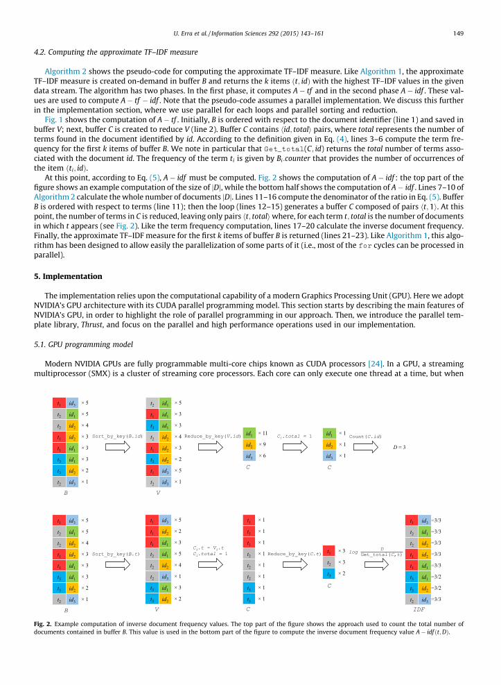
Fig. 1 shows the computation of A� tf . Initially, B is ordered with respect to the document identifier (line 1) and saved inbuffer V; next, buffer C is created to reduce V (line 2). Buffer C contains hid; totali pairs, where total represents the number ofterms found in the document identified by id. According to the definition given in Eq. (4), lines 3–6 compute the term fre-quency for the first k items of buffer B. We note in particular that Get_total(C; id) returns the total number of terms asso-ciated with the document id. The frequency of the term ti is given by Bi:counter that provides the number of occurrences ofthe item ðti; idÞ.

At this point, according to Eq. (5), A� idf must be computed. Fig. 2 shows the computation of A� idf : the top part of thefigure shows an example computation of the size of jDj, while the bottom half shows the computation of A� idf . Lines 7–10 ofAlgorithm 2 calculate the whole number of documents jDj. Lines 11–16 compute the denominator of the ratio in Eq. (5). BufferB is ordered with respect to terms (line 11); then the loop (lines 12–15) generates a buffer C composed of pairs ht;1i. At thispoint, the number of terms in C is reduced, leaving only pairs ht; totaliwhere, for each term t; total is the number of documentsin which t appears (see Fig. 2). Like the term frequency computation, lines 17–20 calculate the inverse document frequency.Finally, the approximate TF–IDF measure for the first k items of buffer B is returned (lines 21–23). Like Algorithm 1, this algo-rithm has been designed to allow easily the parallelization of some parts of it (i.e., most of the for cycles can be processed inparallel).

5. Implementation

The implementation relies upon the computational capability of a modern Graphics Processing Unit (GPU). Here we adoptNVIDIA’s GPU architecture with its CUDA parallel programming model. This section starts by describing the main features ofNVIDIA’s GPU, in order to highlight the role of parallel programming in our approach. Then, we introduce the parallel tem-plate library, Thrust, and focus on the parallel and high performance operations used in our implementation.

5.1. GPU programming model

Modern NVIDIA GPUs are fully programmable multi-core chips known as CUDA processors [24]. In a GPU, a streamingmultiprocessor (SMX) is a cluster of streaming core processors. Each core can only execute one thread at a time, but when

Fig. 2. Example computation of inverse document frequency values. The top part of the figure shows the approach used to count the total number ofdocuments contained in buffer B. This value is used in the bottom part of the figure to compute the inverse document frequency value A� idf ðt;DÞ.

150 U. Erra et al. / Information Sciences 292 (2015) 143–161

a thread performs an operation with high latency it is put into a waiting state and another thread executes. This feature, andthe application of a scheduling policy means that the core can run many threads at the same time. In the current generationof GPUs (code named Kepler), the number of SMXs ranges from 1 to 14. The GPU used in our experiments (GK110) consistedof 14 SMXs, each containing 192 single-precision CUDA cores. Because each SMX is capable of supporting up to 2048 threads,this GPU manages up to 28,672 resident threads. All thread management, including creation, scheduling and barrier synchro-nization is performed entirely in hardware by the SMX with virtually zero overheads.

In terms of the software model, CUDA [25] provides software developers with facilities to execute parallel programs onthe GPU. To use CUDA, a programmer needs to write their code as special functions called kernels, which are executed acrossa set of parallel threads. The programmer organizes these threads into a hierarchy of blocks and grids. A thread block is a setof concurrent threads that can cooperate via shared memory (which has a latency similar to that of registers) and can becoordinated using synchronization mechanisms. A thread grid is a set of thread blocks executed independently. All threadshave access to the same global memory space. Each thread block is mapped to an SMX and executes concurrently. SMXresources (registers and shared memory) are split across the mapped thread block. As a consequence, this limits the numberof thread blocks that can be mapped onto one SMX.

5.2. Sorting on the GPU

We use a GPU in the implementation of our approach because of its excellent performance in parallel sorting and reduc-tion. Following the introduction of programmable GPUs and NVIDIA’s CUDA framework, many sorting algorithms have beensuccessfully implemented on the GPU in order to exploit its computational power. The first programmable GPUs were suitedto implement sorting algorithms [12,27] although they were far from optimal in terms of execution time Oðnlog2nÞ. Succes-sive improvements in GPU technology have enabled the implementation of other comparison sorts with algorithmic com-plexity below Oðn log nÞ, such as the merge sort and the radix sort [31].

The radix sort is currently the fastest approach to sorting 32- and 64-bit keys on both CPU and GPU processors [32]. It isbased on a positional representation of keys, where each key is an ordered sequence of digits. For a given input sequence, thismethod produces a lexicographic ordering iteration over the digit-places from the least significant to the most significant.Given an n-element sequence, the algorithmic complexity of radix sorting is OðnÞ. In [23], the authors demonstrate a radixsorting approach that is able to exceed 1 billion 32-bit keys/s on a single GPU microprocessor.

Reduction has also been successfully implemented on the GPU. In general, reduction is any operation that computes asingle result from a set of data. Examples include min/max, average, sum, product, or any other user-defined function. Sev-eral implementations has been developed in past years, such as [14,29].

5.3. Detailed implementation: the Thrust Library

Thrust [4] is a parallel template library that implements high performance applications with minimal programmingeffort. It is based on CUDA and the Standard Template Library (STL). Thanks to Thrust, developers can take advantage of acollection of fundamental high-level parallel algorithms such as scan, sort, and reduction. For instance, the radix sort dis-cussed above has been implemented. One of the greatest benefits of Thrust is that it exploits the computational capabilityof the GPU without making fine-grained decisions about how computations are decomposed into parallel threads, and howthey are executed on the target architecture. Moreover, its parallel algorithms are generic and can be used with arbitraryuser-defined types and operators. There are many features in the Thrust Library; here we only explain those functions thatare directly relevant to our implementation.

According to the description of the algorithm for the approximate TF–IDF measure, the main structures to maintain the datastream are vector containers. Thrust provides two types of vector container: host_vector and device_vector. Declaring acontainer as a host_vector means that it resides on the CPU host memory; otherwise, the device_vector container is res-ident in the GPU device memory. These vectors are generic containers that are able to store any data type and can be resizeddynamically, simplifying the data exchange process between the CPU and the GPU. Depending on which vector containers thealgorithms use, Thrust can automatically map computational tasks onto the CPU or the GPU. In this way, changing the type ofthe container enables developers to write executable code for either the GPU or the CPU with minimal effort.

In our implementation, each item in the data stream corresponds to a pair hðid; tÞ; counti; we store these values in threeseparate containers using a Structure of Arrays (SoA) layout. The SoA is a parallel design pattern that promotes the optimi-zation of parallel data access inside the arrays, by using separate arrays for each element of a data structure. The advantage ofthe SoA technique is that it gives all threads access to contiguous global memory addresses, in order to maximize memorybandwidth [24]. Thrust provides a design pattern that can traverse one or more containers that exploit the SoA layout. In ourapproach, the aforementioned buffer B (see Algorithm 2) is allocated on the GPU device memory as an SoA layout, and eachincoming sub-stream is copied to GPU memory. Therefore, the CPU manages each sub-stream as three separate arrays beforethe host-to-device memory transfer.

A Thrust program acts on the containers by adopting the STL convention of describing a vector position through an iter-ator. The iterator works like a pointer that can point to any element in the array. Each algorithm typically takes a pair ofiterators as arguments that define the range on which the algorithm must act. Thrust provides some standard iterators, thatare defined as primitive types (e.g., char, int, float, and double).

U. Erra et al. / Information Sciences 292 (2015) 143–161 151

As we have three separate ints containers, we need three iterators. Two of these iterators must have simultaneous accessto the key ðt; idÞ (through the SoA layout); therefore, we need a way to parallel-iterate over the two containers. To achievethis, Thrust provides a zip_iterator, which is composed of a tuple of iterators and enables it to parallel-iterate over two ormore containers simultaneously. Thus, by increasing the zip_iterator, all the iterators in the tuple are increased in par-allel. We note that through using the zip_iterator design pattern, we logically encapsulate the elements of each containerinto a single entity. It is clear that our key ðid; tÞ is implemented by the zip-iterator.

Thrust’s functionality is derived from four fundamental parallel algorithms: for_each, reduce, scan and sort. In ourimplementation we use the sort_by_key algorithm to perform a key-value sort and a reduce_by_key algorithm to obtain,for each group of consecutive keys, a single value reduction by using a sum operator over the corresponding values. As forsorting, Thrust statically selects a highly optimized radix sort algorithm for sorting primitive types, while it uses a generalmerge sort algorithm for user-defined data types. We also use a Count algorithm, which is an additional Thrust functionbased on the reduce algorithm: it returns the number of occurrences of a specific value in a given sequence (e.g., we usedCount to obtain the total number of documents in buffer B, see Algorithm 2).

Moreover, Thrust provides several algorithms that can perform parallel operations over each element of one or moreinput containers. For instance, the sequence algorithm is designed to fill a container with a sequence of numbers, whilea more general transform operation applies a binary function to each pair of elements from two input containers. Thesealgorithms are generic in both the type of data to be processed, and the operations to be applied to the input containers. Theycan easily handle all the loop iterators presented in the pseudo-code of Algorithm 2; moreover, they can be efficiently exe-cuted in parallel.

6. Evaluation

In order to evaluate the performance of our algorithm, we have performed the experimentation on a generated and a realdataset. Precisely, we assess the quality of the approximate TF–IDF measure for both the datasets. In particular, for the realdataset, we consider the performance when applied to topic extraction from a Twitter data stream. Moreover, on the realdataset we also evaluate the CPU vs. GPU performance. To the best of our knowledge, there is no standardized benchmark.

The quality of our approximate TF–IDF measure has been estimated by comparing the results of the exact TF–IDF and ourapproximate version. Precisely, we compared the most frequent term-document pairs ht; idi ranked by our approach withthose calculated by the brute force approach.

For this purpose, we consider two measures: the Kendall rank correlation coefficient [15] and the recall measure.The Kendall coefficient, also referred to as Kendall’s tau (s) coefficient is a statistical measure that evaluates the degree of

similarity between two sets of ranked data. Specifically, it considers all possible pairwise combinations of a first set of values,and compares them with a second set of values. Given two sets of size n, the Kendall coefficient measures the differencebetween the number nc of concordant pairs and the number nd of discordant pairs, as a ratio of the total number of possiblepairings, based on the following formula:

s ¼ nc � nd

nðn� 1Þ=2

Kendall’s coefficient s ranges from ½�1;1�. The value is 1 if the agreement between the two rankings is perfect (perfect posi-tive correlation). On the other hand, a value of �1 means there is total disagreement (perfect negative correlation). This coef-ficient allows us to assess the correlation between the most frequent pairs ht; idi, resulting from our approximate solutionand those from the brute force approach.

A typical measure of Information Retrieval is instead, the recall: it returns the retrieved pairs that are relevant, from thereturned pairs. In our context it measures the number of coincidences of the top-k terms.

More formally, we define recallðkÞ as the intersection between the top-k terms, defined as follows:

recallðkÞ ¼ topðkÞtf�idf \ topðkÞA�tf�idf

where topðkÞtf�idf and topðkÞA�tf�idf are the top-k terms computed by the exact TF–IDF algorithm and the approximate TF–IDFalgorithm, respectively.

These two measures supply two different criteria to estimate how much the results provided by our approximate TF–IDFversion are comparable to that exact.

The hardware configuration was based on a CPU Intel Core i7-3820@3.6 GHz (quad-core HT) with 16 GB of RAM and aGPU NVIDIA GeForce GTX TITAN (2688 CUDA cores) with 6 GB of RAM running Microsoft Windows 8.1. The code was com-piled using Microsoft’s Visual Studio 2012 and the NVIDIA CUDA Toolkit 5.5. Thrust version 1.7.0 was used.

6.1. Generated datasets

The generated data stream has been designed as a sequence of term-document pairs ht; idi. Specifically, we have consid-ered a maximum number of unique documents and unique terms: 100 documents and 100 terms. This way, The maximumnumber of possible distinct pairs ht; idi is 10,000. Without loss of generality, we have assumed a uniform distribution for the

152 U. Erra et al. / Information Sciences 292 (2015) 143–161

documents. For the terms generation instead, a Zipf distribution has been used. It is shown that the distribution of word fre-quencies for randomly generated texts is very similar to Zipf’s law observed in natural languages such as English [18]. More-over Zipf’s law governs many others domains: email archives, newsgroups [16], caching [13], hypermedia-basedcommunication [17], web accesses [9] and many other Internet features [2]. In addition, massive data streams are rarely uni-form, and real data sources typically exhibit significant skewness. They lend themselves well to be modeled by Zipf distri-butions, which are characterized by a parameter that captures the amount of skew [8].

6.1.1. Methodology and evaluationWe have generated several datasets, by considering three different sizes: 10 K, 100 K, and 1000 K; then, the terms have

been generated from a skewed distribution, varying the skew from 0.8 to 2 (in order to obtain meaningful distributions thatproduce at least one heavy hitter per run), with a step equal to 0.2. In total, we had 21 datasets (7 for each dataset size).

The dataset size affects the input stream size: with the dataset of size 10 K, we consider a stream size s = 1 K; with thedataset of size 100 K, we consider two streams with size s = 1 K and 10 K. Finally, with a 1000 K dataset, the conceivablestream sizes are s = 1 K, 10 K, and 100 K. In total, there are six different (dataset, stream) size-configurations.

For each (dataset, stream) size-configurations, there are 7 datasets (by varying the skew value); consequently, there are42 (7 datasets � 6 (dataset, stream) size-configurations) experiments. Finally, since for each experiment, we use three dif-ferent sizes for the most k frequent items: 50, 100, and 1000, we have in total as many as 126 (42 experiments � 3 k-size)experiments.

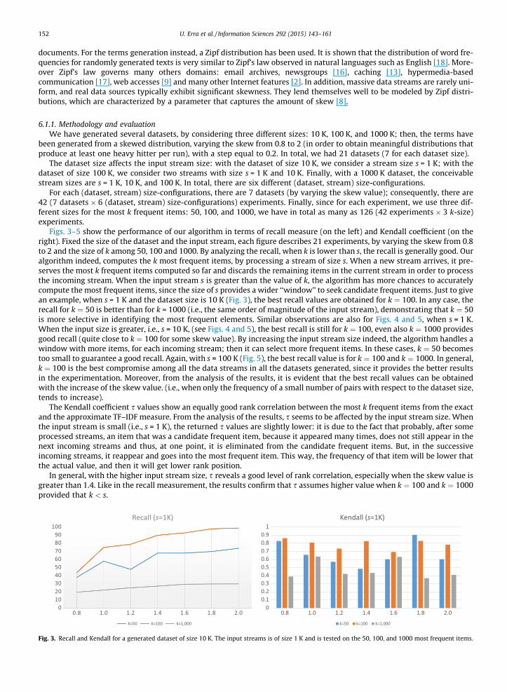
Figs. 3–5 show the performance of our algorithm in terms of recall measure (on the left) and Kendall coefficient (on theright). Fixed the size of the dataset and the input stream, each figure describes 21 experiments, by varying the skew from 0.8to 2 and the size of k among 50, 100 and 1000. By analyzing the recall, when k is lower than s, the recall is generally good. Ouralgorithm indeed, computes the k most frequent items, by processing a stream of size s. When a new stream arrives, it pre-serves the most k frequent items computed so far and discards the remaining items in the current stream in order to processthe incoming stream. When the input stream s is greater than the value of k, the algorithm has more chances to accuratelycompute the most frequent items, since the size of s provides a wider ‘‘window’’ to seek candidate frequent items. Just to givean example, when s = 1 K and the dataset size is 10 K (Fig. 3), the best recall values are obtained for k ¼ 100. In any case, therecall for k ¼ 50 is better than for k = 1000 (i.e., the same order of magnitude of the input stream), demonstrating that k ¼ 50is more selective in identifying the most frequent elements. Similar observations are also for Figs. 4 and 5, when s = 1 K.When the input size is greater, i.e., s = 10 K, (see Figs. 4 and 5), the best recall is still for k ¼ 100, even also k ¼ 1000 providesgood recall (quite close to k ¼ 100 for some skew value). By increasing the input stream size indeed, the algorithm handles awindow with more items, for each incoming stream; then it can select more frequent items. In these cases, k ¼ 50 becomestoo small to guarantee a good recall. Again, with s = 100 K (Fig. 5), the best recall value is for k ¼ 100 and k ¼ 1000. In general,k ¼ 100 is the best compromise among all the data streams in all the datasets generated, since it provides the better resultsin the experimentation. Moreover, from the analysis of the results, it is evident that the best recall values can be obtainedwith the increase of the skew value. (i.e., when only the frequency of a small number of pairs with respect to the dataset size,tends to increase).

The Kendall coefficient s values show an equally good rank correlation between the most k frequent items from the exactand the approximate TF–IDF measure. From the analysis of the results, s seems to be affected by the input stream size. Whenthe input stream is small (i.e., s = 1 K), the returned s values are slightly lower: it is due to the fact that probably, after someprocessed streams, an item that was a candidate frequent item, because it appeared many times, does not still appear in thenext incoming streams and thus, at one point, it is eliminated from the candidate frequent items. But, in the successiveincoming streams, it reappear and goes into the most frequent item. This way, the frequency of that item will be lower thatthe actual value, and then it will get lower rank position.

In general, with the higher input stream size, s reveals a good level of rank correlation, especially when the skew value isgreater than 1.4. Like in the recall measurement, the results confirm that s assumes higher value when k ¼ 100 and k ¼ 1000provided that k < s.

0102030405060708090

100

0.8 1.0 1.2 1.4 1.6 1.8 2.0

Recall (s=1K)

k=50 k=100 k=1,000

00.10.20.30.40.50.60.70.80.9

1

0.8 1.0 1.2 1.4 1.6 1.8 2.0

Kendall (s=1K)

k=50 k=100 k=1,000

Fig. 3. Recall and Kendall for a generated dataset of size 10 K. The input streams is of size 1 K and is tested on the 50, 100, and 1000 most frequent items.

0102030405060708090

100

0.8 1.0 1.2 1.4 1.6 1.8 2.0

Recall (s=1K)

k=50 k=100 k=1,000

00.10.20.30.40.50.60.70.80.9

1

0.8 1.0 1.2 1.4 1.6 1.8 2.0

Kendall (s=1K)

k=50 k=100 k=1,000

0102030405060708090

100

0.8 1.0 1.2 1.4 1.6 1.8 2.0

Recall (s=10K)

k=50 k=100 k=1,000

00.10.20.30.40.50.60.70.80.9

1

0.8 1.0 1.2 1.4 1.6 1.8 2.0

Kendall (s=10K)

k=50 k=100 k=1,000

Fig. 4. Recall and Kendall for a generated dataset of size 100 K. The input streams are of size 1 K and 10 K. Each input stream is tested on the 50, 100, and1000 most frequent items.

U. Erra et al. / Information Sciences 292 (2015) 143–161 153

6.2. Real dataset

Other experiments were carried out on a Twitter dataset.1 Twitter is a social network that connects people through theexchange of tweets, which are small messages of up to 140 characters. Its popularity has increased dramatically in recent years,and it has become one of most well-known ways to chat, microblog and discuss current topics. Each tweet can contain one ormore hashtags i.e., the # symbol used to mark keywords or topics. Through this mechanism, a conversation about a specifictopic can be identified by one or more hashtags associated with a message.

We extracted a dataset composed of 4 million public tweets posted by users from August 2012 to September 2012 in thecities of Washington, New York, and San Francisco. The dataset was transferred to a local machine using the command linetool cURL [1].

All tweets were in English and could have one or more hashtags. Tweets with the same hashtag were grouped to repre-sent a document about a specific topic, identified by the hashtag. Consequently, tweets without hashtags were discardedbecause they could not be associated with a document. The dataset was preprocessed to discard ‘‘noise’’ using simpleNLP principles [20]. We used the Porter stemming algorithm [26] to obtain the stem or base forms of each term, thenstop-words were removed. Irregular syntactic slang and non-standard vocabulary (widespread in phone text messagingdue to the necessary brevity) was not discarded and was included in the data to be processed.

Finally, to facilitate data processing, a hash function was defined in order to map each hashtag to a numeric identifier (asshown in Fig. 6). Likewise, all the terms that remained following text processing were mapped into a numeric identifier. Thepair, composed of the document identifier and the term identifier (Fig. 6) represents the minimal unit to process. A total of40 million hterm; documenti pairs were generated.

6.2.1. Methodology and evaluationThe analysis of the dataset led to the creation of 40 million pairs. These pairs were split into four batches of input stream

of size s = 1 M, 5 M, 10 M, and 20 M. For each of these batches, k (the number of most frequent items) was varied with k = 1 K,10 K, 100 K, and 1,000 K. Once we had computed the most frequent items for all s and all k, we applied the approximate TF–IDF algorithm. In total, we performed 16 experiments.

We assessed our approach on three criteria:

� Speed up and memory footprint: the CPU implementation was compared with the GPU implementation. We exploited theThrust portability between GPUs and multicore CPUs to obtain a running version of the approximate TF–IDF measure forboth architectures.

1 Source and data are available at http://graphics.unibas.it/atfidf.

0102030405060708090

100

0.8 1.0 1.2 1.4 1.6 1.8 2.0

Recall (s=1K)

k=50 k=100 k=1,000

00.10.20.30.40.50.60.70.80.9

1

0.8 1.0 1.2 1.4 1.6 1.8 2.0

Kendall (s=1K)

k=50 k=100 k=1,000

0102030405060708090

100

0.8 1.0 1.2 1.4 1.6 1.8 2.0

Recall (s=10K)

k=50 k=100 k=1,000

00.10.20.30.40.50.60.70.80.9

1

0.8 1.0 1.2 1.4 1.6 1.8 2.0

Kendall (s=10K)

k=50 k=100 k=1,000

0102030405060708090

100

0.8 1.0 1.2 1.4 1.6 1.8 2.0

Recall (s=100K)

k=50 k=100 k=1,000

00.10.20.30.40.50.60.70.80.9

1

0.8 1.0 1.2 1.4 1.6 1.8 2.0

Kendall (s=100K)

k=50 k=100 k=1,000

Fig. 5. Recall and Kendall for a generated dataset of size 1000 K. The input streams are of size 1 K, 10 K, and 100 K. Each input stream is tested on the 50,100, and 1000 most frequent items.

154 U. Erra et al. / Information Sciences 292 (2015) 143–161

� Frequent items similarity: the output of the CPU brute force approach was compared with the output of the approximateTF–IDF measure. In particular, we compared the most highly ranked term; document pairs resulting from our approximatesolution to those of the brute force approach.� TF–IDF quality: the TF–IDF measure calculated using the approximate solution was compared with values calculated

using the brute force approach, which provides the exact frequency of each pair. For all k, we compared the output ofa percentage of the overall corpus of tweets.

GPU vs. CPU performance. We analyzed performance in two steps. In the first step, we measured the total time and theamount of memory required to process all of the 40 M document-term pairs, based on input streams of size s and a calcu-lation of the k most frequent items, as illustrated in Table 1. These times include both memory transfer time (CPU to GPU)and Thrust execution time. The results show that execution times were not affected by the size of the input stream. In par-ticular, execution time remained stable when the input stream was equal to or greater than 5 M, and was independent on itssize. In the second step, we measured the time required to compute the approximate TF–IDF measure with different values ofk. We evaluated the performance of GPU and CPU implementations by comparing how long each call to the approximate TF–IDF algorithm took on buffer B returned by the Sort-Based Frequent Item of the previous step. Fig. 7 compares performancewith different sizes of k. With k greater than 10,000 the GPU implementation is more efficient than the CPU implementation.With lower values of k the CPU implementation is more efficient due to overheads that dominate overall performance.

Finally, in Fig. 8 we report the total GPU speed up compared to the CPU implementation, by summing the times obtainedin the two steps. For a 1 M input stream, the speed up ranges from 5� to 8�, and when it is equal to or greater than 5 M it isaround 10�.

@Tony has a nice #job and a bad #car!!!

@Tony nice #job bad #car

23456 3572 56995 2598 117522

56995 23456

56995 3572

56995 2598

117522 23456

117522 3572

117522 2598

Stemming and stop words

Hashing

Tuples genera�on

Fig. 6. Tuple generation from a tweet. The green label represents the document and the blue label the word. (For interpretation of the references to color inthis figure legend, the reader is referred to the web version of this article.)

Table 1GPU performance for input streams of size s, and k most frequent items. In all experiments, we measured the totaltime to process all 40 M document-term pairs. Times include CPU to GPU data transfers (and vice versa).

s (M) k Times (s) Memory (MB)

1 1000 1.062 30.5410,000 0.982 30.82

100,000 1.070 33.561,000,000 1.342 61.03

5 1000 0.773 152.6110,000 0.814 152.89

100,000 0.795 155.641,000,000 0.886 183.10

10 1000 0.802 305.2010,000 0.768 305.48

100,000 0.801 308.221,000,000 0.857 335.69

20 1000 0.788 610.3810,000 0.774 610.65

100,000 0.827 613.401,000,000 0.791 640.86

U. Erra et al. / Information Sciences 292 (2015) 143–161 155

Let us observe that the size of input stream is very important for guaranteeing a high speed up: in our experiments, whenthe input stream size is 1 M, there are many ‘‘CPU to GPU’’ data transfers; precisely, on our dataset composed of 40 M doc-ument-term pairs, there are as many as 40 data transfers. As stated above, the high number of transfers produces high over-head, penalizing the GPU performance. The number of data transfers required for the input streams of 5 M, 10 M and 20 M,instead considerably drops to 8, 4, and 2 respectively, guaranteeing an high speed up (around 10�). Therefore, when inputstreams are large, the GPU offers stable and better performance than the CPU. This is due to the fact that GPUs perform betteron repetitive tasks using large data blocks, and when data transfers are limited.

The importance of these results is twofold. First, the time to compute the approximate TF–IDF measure on the GPU is notaffected by the type of data source (it may be a stream of tweets, a news feed, etc.) and second, the parallel implementation

020406080

100120140160180

1K 10K 100K 1,000K

Tim

e in

ms

Top frequent k-items

GPU CPU

Fig. 7. GPU vs. CPU scalability with varying sizes of most frequent k items.

0

2

4

6

8

10

12

1K 10K 100K 1,000K 1K 10K 100K 1,000K 1K 10K 100K 1,000K 1K 10K 100K 1,000K

Spee

d U

p

Total Time Speed Up: GPU vs CPU

1M

5M

10M

20M

Fig. 8. GPU speed up compared to the CPU implementation with input streams of 1 M, 5 M, 10 M, and 20 M. Each input stream is tested on the 1 K, 10 K,100 K, and 1000 K most frequent items.

156 U. Erra et al. / Information Sciences 292 (2015) 143–161

works well when GPU or graphic card memory is limited. In general, with input stream size equals or greater than 5 M, ourGPU implementation fully exploits the benefits of the data buffering and performs much better than the CPU implementa-tion. Moreover, the GPU performance evidences a good scalability with varying the input data stream. The obtained values ofspeed up indeed, outline the validity of our parallel implementation for the calculation of the approximate TF–IDF, when thedata collection is a real-time continuous data stream.

Rank correlation. As stated above, we use the Kendall coefficient to assess the correlation between the most frequent pairsht; idi, resulting from our approximate solution and those from the brute force approach.

Table 2 shows the results computed for different sizes of input stream s, and the k most frequent items. The table showsthat our approach performs well: its accuracy in identifying the most frequent items is comparable with that of the bruteforce approach. In particular, we note that when k ¼ 1000, the s coefficient is very close to 1 (i.e., greater than 0.9), evenas the size of the input data stream grows to 20 M. We also note that as k increases, the Kendall coefficient tends to decrease.

TF–IDF quality. As stated, the analysis of TD-IDF quality is based on a comparison of the approximate TF–IDF valuesreturned by our implementation and the exact values returned by the brute force algorithm. We use the Spearman’s rankcorrelation coefficient q, to measure the strength of the relationship between the two variables. This coefficient providesa nonparametric measure of statistical dependence between paired data, in our case, the TD-IDF values computed by thetwo algorithms. Thus, we calculate the number of coincidences of the k most frequent terms obtained by the exact bruteforce algorithm with those found using the approximate TF–IDF measure.

We exploit the recall defined in Section 6, to compute the top-k terms common to the exact and approximate TF–IDF ver-sion. Once the top-k common terms are obtained, Spearman’s rank correlation coefficient q can be computed.

Tables 3–7 illustrate the results from the Twitter dataset, with the 20%, 40%, 60%, 80%, and 100% of the k most frequentterms. In total, 16 experiments have been carried out. Given k and s, each experiment has been analyzed for the 20%, 40%,60%, 80%, and 100% of the k most frequent terms. Just to give an example, with k ¼ 1000 and s = 1 M, the results (expressed interms of recall and q) of the corresponding experiment is described by the first column and the first row of the each of thefive tables (with varying the percentage). Increasing the percentage allows enlarging the ‘‘window’’ of the top terms from themost k frequent items, in order to better evaluate how many terms are in common with the exact TF–IDF, with varying thedimension of the window.

We note in general, that, given k, the recall value tends to decrease with the increase of the percentage of terms taken intoaccount. Fig. 9 shows the recall trend for each input stream size s, by varying the k frequent items. It is a summary view of therecall values described in Tables 3–7.

Moreover, we also note that in general, recall is lower for smaller sizes of s (i.e., s equal to 1 M and 5 M), compared to 10 Mand 20 M. This result is due to the fact that the accurate identification of frequent items is affected by the size of the inputstream. Our algorithm computes the k most frequent items, by processing a stream of size s. As stated, when a new streamarrives, it discards the items in the current stream in order to process the incoming stream. For small input streams, it is

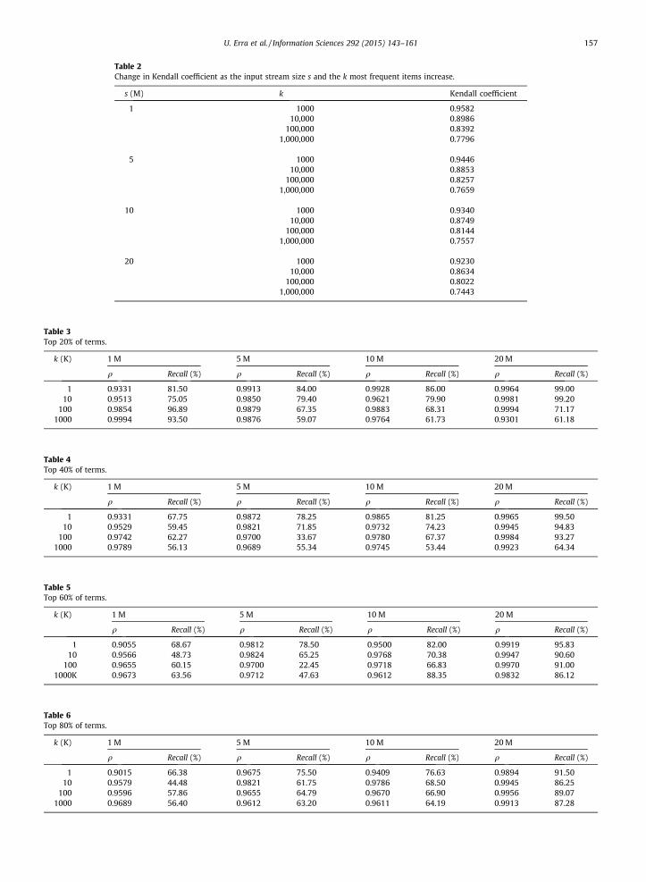
Table 2Change in Kendall coefficient as the input stream size s and the k most frequent items increase.

s (M) k Kendall coefficient

1 1000 0.958210,000 0.8986

100,000 0.83921,000,000 0.7796

5 1000 0.944610,000 0.8853

100,000 0.82571,000,000 0.7659

10 1000 0.934010,000 0.8749

100,000 0.81441,000,000 0.7557

20 1000 0.923010,000 0.8634

100,000 0.80221,000,000 0.7443

Table 3Top 20% of terms.

k (K) 1 M 5 M 10 M 20 M

q Recall (%) q Recall (%) q Recall (%) q Recall (%)

1 0.9331 81.50 0.9913 84.00 0.9928 86.00 0.9964 99.0010 0.9513 75.05 0.9850 79.40 0.9621 79.90 0.9981 99.20

100 0.9854 96.89 0.9879 67.35 0.9883 68.31 0.9994 71.171000 0.9994 93.50 0.9876 59.07 0.9764 61.73 0.9301 61.18

Table 4Top 40% of terms.

k (K) 1 M 5 M 10 M 20 M

q Recall (%) q Recall (%) q Recall (%) q Recall (%)

1 0.9331 67.75 0.9872 78.25 0.9865 81.25 0.9965 99.5010 0.9529 59.45 0.9821 71.85 0.9732 74.23 0.9945 94.83

100 0.9742 62.27 0.9700 33.67 0.9780 67.37 0.9984 93.271000 0.9789 56.13 0.9689 55.34 0.9745 53.44 0.9923 64.34

Table 5Top 60% of terms.

k (K) 1 M 5 M 10 M 20 M

q Recall (%) q Recall (%) q Recall (%) q Recall (%)

1 0.9055 68.67 0.9812 78.50 0.9500 82.00 0.9919 95.8310 0.9566 48.73 0.9824 65.25 0.9768 70.38 0.9947 90.60

100 0.9655 60.15 0.9700 22.45 0.9718 66.83 0.9970 91.001000K 0.9673 63.56 0.9712 47.63 0.9612 88.35 0.9832 86.12

Table 6Top 80% of terms.

k (K) 1 M 5 M 10 M 20 M

q Recall (%) q Recall (%) q Recall (%) q Recall (%)

1 0.9015 66.38 0.9675 75.50 0.9409 76.63 0.9894 91.5010 0.9579 44.48 0.9821 61.75 0.9786 68.50 0.9945 86.25

100 0.9596 57.86 0.9655 64.79 0.9670 66.90 0.9956 89.071000 0.9689 56.40 0.9612 63.20 0.9611 64.19 0.9913 87.28

U. Erra et al. / Information Sciences 292 (2015) 143–161 157

Table 7Top 100% of terms.

k (K) 1 M 5 M 10 M 20 M

q Recall (%) q Recall (%) q Recall (%) q Recall (%)

1 0.8996 61.60 0.9630 70.40 0.9423 71.60 0.9881 87.6010 0.9577 43.23 0.9807 59.14 0.9785 66.34 0.9941 81.94

100 0.9566 54.23 0.9639 63.86 0.9667 66.30 0.9944 87.771000 0.9632 56.42 0.9523 62.84 0.9632 56.09 0.9432 79.83

158 U. Erra et al. / Information Sciences 292 (2015) 143–161

probable that some items that are discarded from the current stream also appear in the following stream, but in both cases,the occurrence is not high enough to included in the k most frequent items. By increasing the size of the stream, it is possiblethat these items appear in the same stream; in this case, the number of occurrences make them appropriate candidates toone of the top k items. In other words, when the input stream is large, the exact item count may be more accurate, becausemore items are kept in memory before they are discarded. Therefore, when s is small, the algorithm can only accuratelycount a few items. The recall indeed, is very good in the top 20% of the terms (see Table 3). As this percentage increases, recallvalues tend to decrease, as shown in Tables 4–7. Increasing the size of the input stream overcomes this problem for streamsof size 10 M or 20 M.

There is some result that deserves to be further explored: the output generated by the experiment with input streams = 5 M and k = 100,000 (Tables 3–7: second column, third row) shows a decreasing recall value, from the initial discreterecall value (67.35% on 20% of terms) until to get a very low recall, at 40% and 60% of the top terms (Tables 4 and 5). It seemsthat by enlarging the percentage of the top k terms, the recall is lower, i.e., the common terms are dispersed. In other words,the common terms are mainly concentrate in the first 20%. The recall improves when the top percentage of terms is close tok = 100,000 (i.e., 80%, 100% of the top terms). From the analysis of the recall results of this experiment, it seems that the topmost frequent items are accurately computed. Perhaps due to an unhappy sequence of data stream, the recall degrades (withmiddle percentages) and then back to acceptable values when it is calculated on the whole k size.

It also is interesting to notice that, fixed the input stream s = 20 M, the recall tends to decrease, by varying the size of k(Tables 3–7). This fact outlines that, in general, the algorithm can correctly identify the most frequent items that appear inthe top portion of the k frequent items. Yet, when the size of k is big (i.e., k = 1,000,000), the first 20% of terms is not enoughto gather the most frequent items, that are in common with the precise TF–IDF measure. Just increase the percentage of k, inorder to improve the recall (Tables 4–7). This situation emphasizes the fact that when k < s, the recall values are generallymore accurate. Completely opposite situation happens for s = 1 M: the recall tends to increase by varying k (for example, seeTable 3, but it hold also for Tables 4–7).

0%10%20%30%40%50%60%70%80%90%

100%

Top 20% Top 40% Top 60% Top 80% Top 100%

k=1K

s=1M s=5M s=10M s=20M

0%10%20%30%40%50%60%70%80%90%

100%

Top 20% Top 40% Top 60% Top 80% Top 100%

k=10K

s=1M s=5M s=10M s=20M

0%10%20%30%40%50%60%70%80%90%

100%

Top 20% Top 40% Top 60% Top 80% Top 100%

k=100K

s=1M s=5M s=10M s=20M

0%10%20%30%40%50%60%70%80%90%

100%

Top 20% Top 40% Top 60% Top 80% Top 100%

k=1,000K

s=1M s=5M s=10M s=20M

Fig. 9. Recall computed for the top 20%, 40%, 60%, 80% and 100%, for the sizes of the input streams s = 1 M, 5 M, 10 M, and 20 M, by varying k = 1 K, 10 K,100 K, and 1000 K.

Table 8From top to bottom: the most frequent hashtags contained in tweets for the period August 2012–September 2012. From left to right: theterms used most often in tweets with same hashtags.

Hashtag Terms

#VMA Tweet mtv vote lead video shareworthi#bing Tweet mtv vote lead video shareworthi#votebieber Justinbieb time hit bed button difficult morn#rageofbahamut Tweet card ref code free friend#voteonedirection Home daniellepeaz#StopChildAbuse Donat tweet join campaign twitter#Gameinsight Play start paradis island#Kiss Excit list track reveal carlyraejepsen#fashion Show largest voguemagazin#votebeyonce Tweet vote mtv lead

U. Erra et al. / Information Sciences 292 (2015) 143–161 159

Tables 3–7 show also the values of the Spearman correlation coefficient q. It is always around 0.90, evidencing that a goodpositive correlation exists between the exact and approximate TF–IDF measure. In particular, for input stream size s = 20 M,iq is close to 1, showing a strong correlation.

Additionally, Tables 3–7 seem to show that bigger recall values cause better correlation value. To confirm this, we haveassessed how the correlation varies using different recall values. For each experiment of the top-k common terms, we takeinto account the minimum and maximum recall. Using this data, we have performed a Wilcoxon rank sum test to check if thedifferences are or not significant. The test yields a p-value of 1.8165e�04, thus rejecting the null hypothesis (the medians areequal) and confirming the alternative hypothesis at the default 5% significance level, i.e., bigger recall values result in a bettercorrelation.

The experiments confirm the validity of our implementation of the approximate TF–IDF measure, evidencing that, in gen-eral, the algorithm works well by varying the size s of input stream (as stated, the results are better for larger s). Moreover,the results computed for the different execution of the approximate TF–IDF outlines the effectiveness of our implementationchoices (parallel GPU computation), supported also by a good efficacy.

6.2.2. Analysis of trending topicsTable 8 shows an ordered list of the most frequent document–term pairs. Hashtags represent documents. For each hash-

tag in the first column of Table 8, the second column shows the associated terms. Their order reflects the ranking of the mostfrequent hashtag–term pairs. It is interesting to note that the same terms often appear in the top positions of the ranked list,although they are associated with different hashtags. This is seen most clearly at the top of the list; they become more scat-tered as they appear lower down.

The tweets dataset was posted in the period August 2012–September 2012 in the cities of Washington, New York, and SanFrancisco. We note that the most frequent hashtags were VMA (Video Music Awards), bing, votebieber, etc., these correspondto the 2012 MTV Video Music Awards that took place in the United States at the time. This emphasizes the coherence andrelevance of our results. For example, our analysis showed that the hashtags VMA and bing always appeared together intweets. This is clearly shown in Table 8, where these hashtags appear in the first two positions with the same terms (secondcolumn of the table).

Our results so far are rough, and our experiments could be improved with further textual processing and refinements.

7. Conclusions

The exact TF–IDF measure is typically used to retrieve relevant terms from a corpus of documents, given that the contentsof the entire corpus are a priori known for the purposes of the calculation. This paper presents a revised TF–IDF measure,which can be used for processing continuous data streams. Specifically, our contribution is twofold: we provide (1) anapproximate TF–IDF measure and (2) a parallel implementation of the calculation of the approximate TF–IDF, based on GPUs.The parallel GPU architecture meets fast response requirements and overcomes storage constraints when processing a con-tinuous flow of data stream in real time.

The proposal was tested on both generated and real datasets. The generated dataset is composed of pairs ht; idi and it hasbeen created from a skewed and uniform distribution in order to study in details how our approximate TF–IDF works under aknow distribution of terms and documents, respectively. The real dataset instead, was composed of a large Twitter collection,where it detected trending topics in the data stream. Both experimentations evidence that the approximate version of TF–IDF yields good results. We notice that the best results are when k is smaller (some order of magnitude) than the inputstream size. We think that this is due to the frequency of distinct pairs inside the datasets. From the analyze of generatedand real datasets, we think that when the data distribution presents a skew value close to 2 (a few pairs that appear manytimes, with respect to the dataset size), it preferable to choose a small k, in order to capture all the actual frequent items. Fora large k, the most k frequent items will enclose also terms with a low frequency, that, in the successive input streams havebeen encountered, but are not effectively relevant.

160 U. Erra et al. / Information Sciences 292 (2015) 143–161

In terms of performance, our approximate TF–IDF measure performs satisfactorily. One interesting aspect is the GPUimplementation is stable and performs well even with limited memory. We found good scalability and a significant speedup of the GPU over the CPU implementation in computing the approximate TF–IDF. Furthermore, the time to computethe approximate TF–IDF measure on the GPU is not affected by the data source. In terms of quality, we correlated our resultswith those computed using the exact TF–IDF measure. Here again, the approximate solution is reasonably good when used indata mining scenarios.

With respect to future developments, we are working on an implementation using multiple GPUs. This may provide manybenefits, although it is not immediately possible as the Thrust library is designed for a single GPU. To achieve this requires acomplete software architecture redesign, in order to exploit multiple GPUs during the computation of the approximatemeasure.

In a nutshell, our approximate TF–IDF measure can be considered as an extension of the exact version. It can be applied indata stream data contexts: for instance, from sophisticated sensors, batch query processing in search engines, and in textstream classification techniques applied to social networks, news feeds, chat, and e-mail.

References

[1] cURL and libcurl <http://http://curl.haxx.se/>.[2] L.A. Adamic, B.A. Huberman, Zipf’s law and the internet, Glottometrics 3 (2002) 143–150.[3] Brian Babcock, Shivnath Babu, Mayur Datar, Rajeev Motwani, Jennifer Widom, Models and issues in data stream systems, in: Proceedings of the

Twenty-First ACM SIGMOD-SIGACT-SIGART Symposium on Principles of Database Systems, PODS ’02, ACM, New York, NY, USA, 2002, pp. 1–16.[4] Nathan Bell, Jared Hoberock, Thrust: a productivity-oriented library for CUDA, GPU Comput. Gems Jade Ed. 2 (2011) 359–371.[5] Ian Buck, Tim Foley, Daniel Horn, Jeremy Sugerman, Kayvon Fatahalian, Mike Houston, Pat Hanrahan, Brook for GPUs: stream computing on graphics

hardware, ACM Trans. Graph. (TOG) 23 (3) (2004) 777–786.[6] Khoo Khyou Bun, Mitsuru Ishizuka, Topic extraction from news archive using TF⁄PDF algorithm, in: Proceedings of the 3rd International Conference on

Web Information Systems Engineering, WISE ’02, IEEE Computer Society, Washington, DC, USA, 2002, pp. 73–82.[7] Graham Cormode, Marios Hadjieleftheriou, Finding the frequent items in streams of data, Commun. ACM 52 (2009) 97–105.[8] Graham Cormode, S. Muthukrishnan, Summarizing and mining skewed data streams, in: SIAM Conference on Data Mining (SDM), 2005, pp. 44–55.[9] Mark E. Crovella, Murad S. Taqqu, Azer Bestavros, A Practical Guide to Heavy Tails, Chapter Heavy-tailed Probability Distributions in the World Wide

Web, Birkhauser Boston Inc., Cambridge, MA, USA, 1998.[10] Jason P. Duran, Sathish A.P. Kumar, CUDA based multi objective parallel genetic algorithms: adapting evolutionary algorithms for document searches,

in: Proceedings of the 2011 International Conference on Information and Knowledge Engineering, (IKE 2011), vol. 52(29), 2011, pp. 36–49.[11] Ugo Erra, Bernardino Frola, Frequent items mining acceleration exploiting fast parallel sorting on the GPU, Proc. Comput. Sci. 9 (0) (2012) 86–95.

Proceedings of the International Conference on Computational Science, ICCS 2012.[12] Naga K. Govindaraju, Nikunj Raghuvanshi, Dinesh Manocha, Fast and approximate stream mining of quantiles and frequencies using graphics

processors, in: Proceedings of the 2005 ACM SIGMOD International Conference on Management of Data, SIGMOD ’05, ACM, New York, NY, USA, 2005,pp. 611–622.

[13] Raffaella Grieco, Delfina Malandrino, Vittorio Scarano, A scalable cluster-based infrastructure for edge-computing services, World Wide Web 9 (3)(2006) 317–341.

[14] Daniel Horn, Stream reduction operations for GPGPU applications, in: Matt Pharr (Ed.), GPU Gems 2, Addison-Wesley, 2005.[15] M.G. Kendall, A new measure of rank correlation, Biometrika 30 (1/2) (1938) 81–93.[16] Mark Kot, Emily Silverman, Celeste A. Berg, Zipf’s law and the diversity of biology newsgroups, Scientometrics 56 (2) (2003) 247–257.[17] V.V. Kryssanov, K. Kakusho, E.L. Kuleshov, M. Minoh, Modeling hypermedia-based communication, Inform. Sci. 174 (1–2) (2005) 37–53.[18] W. Li, Random texts exhibit Zipf’s-law-like word frequency distribution, IEEE Trans. Inform. Theory 38 (6) (1992) 1842–1845.[19] K.F. Lysakov, M.Yu. Shadrin, FPGA-based hardware accelerator for high-performance data-stream processing, Patt. Recog. Image Anal. 23 (1) (2013)

26–34.[20] Christopher D. Manning, Hinrich Schütze, Prabhakar Raghavan, Introduction to Information Retrieval, Cambridge University Press, New York, NY, USA,

2008.[21] James Manyika, Michael Chui, Brad Brown, Jacques Bughin, Richard Dobbs, Charles Roxburgh, Angela Hung Byers, Big Data: The Next Frontier for

Innovation, Competition, and Productivity, Technical report, McKinsey Global Institute, June 2011.[22] Diana Maynard, Yaoyong Li, Wim Peters, NLP techniques for term extraction and ontology population, in: Proceedings of the 2008 Conference on

Ontology Learning and Population: Bridging the Gap Between Text and Knowledge, IOS Press, Amsterdam, The Netherlands, The Netherlands, 2008, pp.107–127.

[23] Duane Merrill, Andrew Grimshaw, High performance and scalable radix sorting: a case study of implementing dynamic parallelism for GPUcomputing, Paral. Process. Lett. 21 (02) (2011) 245–272.

[24] NVIDIA Corporation, NVIDIA’s Next Generation CUDA Compute Architecture: Fermi, Technical report, Nvidia Corporation, 2009.[25] NVIDIA Corporation, NVIDIA CUDA C Programming Guide 5.5, NVIDIA Corporation, 2010.[26] Martin F. Porter, An algorithm for suffix stripping, Program 14 (3) (1980) 130–137.[27] Timothy J. Purcell, Craig Donner, Mike Cammarano, Henrik Wann Jensen, Pat Hanrahan, Photon mapping on programmable graphics hardware, in:

Proceedings of the ACM SIGGRAPH/EUROGRAPHICS Conference on Graphics Hardware, HWWS ’03, Eurographics Association, Aire-la-Ville,Switzerland, Switzerland, 2003, pp. 41–50.

[28] Joel W. Reed, Yu Jiao, Thomas E. Potok, Brian A. Klump, Mark T. Elmore, Ali R. Hurson, TF-ICF: a new term weighting scheme for clustering dynamicdata streams, in: Proceedings of the 5th International Conference on Machine Learning and Applications, ICMLA ’06, IEEE Computer Society,Washington, DC, USA, 2006, pp. 258–263.

[29] David Roger, Ulf Assarsson, Nicolas Holzschuch, Efficient stream reduction on the GPU, in: David Kaeli, Miriam Leeser (Eds.), Workshop on GeneralPurpose Processing on Graphics Processing Units, 2007.

[30] Gerard Salton, Christopher Buckley, Term-weighting approaches in automatic text retrieval, Inform. Process. Manage. 24 (5) (1988) 513–523.[31] Nadathur Satish, Mark Harris, Michael Garland, Designing efficient sorting algorithms for many core GPUs, in: Proceedings of the 2009 IEEE

International Symposium on Parallel & Distributed Processing, IPDPS ’09, IEEE Computer Society, Washington, DC, USA, 2009, pp. 1–10.[32] Nadathur Satish, Changkyu Kim, Jatin Chhugani, Anthony D. Nguyen, Victor W. Lee, Daehyun Kim, Pradeep Dubey, Fast sort on CPUs and GPUs: a case

for bandwidth oblivious SIMD sort, in: Proceedings of the 2010 International Conference on Management of Data, SIGMOD ’10, ACM, New York, NY,USA, 2010, pp. 351–362.

[33] Benjamin E. Teitler, Jagan Sankaranarayanan, Hanan Samet, Marco D. Adelfio, Online document clustering using GPUs, in: Barbara Catania, TaniaCerquitelli, Silvia Chiusano, Giovanna Guerrini, Mirko Kämpf, Alfons Kemper, Boris Novikov, Themis Palpanas, Jaroslav Pokorny, Athena Vakali (Eds.),New Trends in Databases and Information Systems, Advances in Intelligent Systems and Computing, vol. 241, Springer International Publishing, 2014,pp. 245–254.

U. Erra et al. / Information Sciences 292 (2015) 143–161 161

[34] S. Thomaidou, M. Vazirgiannis, Multiword keyword recommendation system for online advertising, in: 2011 International Conference on Advances inSocial Networks Analysis and Mining (ASONAM), 2011, pp. 423–427.

[35] Craig Ulmer, Maya Gokhale, Brian Gallagher, Philip Top, Tina Eliassi-Rad, Massively parallel acceleration of a document-similarity classifier to detectweb attacks, J. Paral. Distrib. Comput. 71 (2) (2011) 225–235. Data Intensive Computing.

[36] Le Wang, Yan Jia, Yingwen Chen, Conversation extraction in dynamic text message stream, JCP 3 (10) (2008) 86–93.[37] Yongpeng Zhang, Frank Mueller, Xiaohui Cui, Thomas Potok, Data-intensive document clustering on graphics processing unit (GPU) clusters, J. Paral.

Distrib. Comput. 71 (2) (2011) 211–224. Data Intensive Computing.