REGULAR ARTICLE

Approaching the serpentine factor at a local scale—a studyin an ultramafic area in northern Greece

Ioannis Tsiripidis & Athanasios Papaioannou &

Vasilios Sapounidis & Erwin Bergmeier

Received: 23 June 2009 /Accepted: 29 July 2009 /Published online: 18 August 2009# Springer Science + Business Media B.V. 2009

Abstract We explore factors responsible for vegetationdifferentiation in a small-scale serpentine area, andattempt to provide new insights in the complexity ofthe serpentine factor at community level. We sampled 49quadrats. From each quadrat physical and chemical soilparameters were measured and species composition,altitude, inclination, aspect and coordinates were re-corded. Quadrats were classified and ordination analyseswere used to explore the environmental gradients and toestimate the explanatory power of the variables. Gener-alized linear models were used to investigate theresponse of species to environmental factors. Variancepartitioning was applied to calculate the proportion ofvariance attributed to different groups of explanatoryvariables. The gradients revealed were related to soil

texture, nutrient contents, calcium deficiency, chromiumcontent, climatic parameters and grazing and disturbanceintensity. Variance partitioning showed that the highestproportions of variance were attributed to the nutrientsand physiographic (including soil texture) variables,while smaller but notable proportions of variance wereattributed to geographical coordinates and to metalcontents. Our study shows that vegetation differentiationat a local scale is determined by a complex factor of soilproperties and climatic parameters, together with varia-tion in disturbance and succession.

Keywords Plant communities . Alyssumchalcidicum . Serpentine vegetation . Heavy metals .

Variance partitioning

Introduction

Ultramafic soils host a specific flora often characterizedby local or regional endemic species (Whittaker 1954;Brooks 1987; Chiarucci et al. 2001; Constantinidis et al.2002; Stevanović et al. 2003; Proctor 2003; Chiarucciand Baker 2007; Grace et al. 2007). Species growing onultramafic soils have evolved morphological as well asphysiological adaptations (Constantinidis et al. 2002;Brady et al. 2005), of which nickel hyperaccumulationis among the most frequently studied (Baker and Brooks1989; Reeves and Adigüzel 2004). Plant communitiesfound on ultramafic soils are usually significantlydistinct from adjacent communities on “normal” soils(Brooks 1987; Robinson et al. 1996).

Plant Soil (2010) 329:35–50DOI 10.1007/s11104-009-0132-9

Responsible Editor: Henk Schat.

I. Tsiripidis (*) :V. SapounidisDepartment of Botany, School of Biology,Aristotle University of Thessaloniki,Thessaloniki GR-54124, Greecee-mail: tsiripid@bio.auth.gr

A. PapaioannouSchool of Forestry and Natural Environment,Aristotle University of Thessaloniki,Thessaloniki GR-54124, Greece

E. BergmeierDepartment of Vegetation and Phytodiversity Analysis,Albrecht von Haller Institute of Plant Sciences,University of Göttingen, Untere Karspüle 2,Göttingen 37073, Germany

The term ultramafic characterises rocks with at least70% ferromagnesian, or mafic minerals (Kruckeberg2002). Soils derived from ultramafic rocks are diverse,but share a number of common characteristics, such ashigh concentrations of Mg, Cr, Co and Ni and lowconcentrations of macronutrients such as P, K, N andCa (Kruckeberg 1985; Brooks 1987; Robinson et al.1997; Proctor 2003). Furthermore, ultramafic soilsprovide physical properties that are unfavourable forplant life, such as shallowness, coarse texture, widerange of diurnal temperature fluctuations and low waterholding capacity (Brooks 1987; Huenneke et al. 1990;Robinson et al. 1997; Kruckeberg 2002; Gram et al.2004; Brady et al. 2005).

Sometimes in literature, the term serpentine is used asa synonym to the term ultramafic. Actually, serpentinesoils constitute a subgroup of ultramafic soils which arerich in serpentine minerals. The term has also been usedto describe the peculiar characteristics of plant life onultramafic soils, which are summarized as “serpentineproblem”, “serpentine factor” or “serpentine syndrome”(Brooks 1987; Brady et al. 2005). Many studiesattributed the serpentine problem to the toxic concen-trations of metals such as Ni, Cr and Co. Nickel isbelieved to play a major role in determining the floraand vegetation in many serpentine areas (Brooks 1987;Vergnano Gambi 1992; Robinson et al. 1997) becauseof its relatively high availability in the range of pHvalues of serpentine soils and the discovery of a highnumber of taxa that accumulate Ni in their tissues(Brooks 1987; Bani et al. 2007). Although relativelyhigh concentrations of Co are available to plants onultramafic soils, the phenomenon of its accumulationin plant tissues is rare (Robinson et al. 1997).Chromium, on the other hand, has very low exchange-able concentrations in the soil and no plants are knownthat hyperaccumulate this element (Brooks 1987;Robinson et al. 1997; Chiarucci 2003). Anotherpossible serpentine factor is the high concentration ofMg or the deficiency of Ca or the unfavourableratio of Mg to Ca in serpentine soils. Strong effectsof the Mg/Ca ratio (Brooks 1987; Proctor andWoodell 1975; Kruckeberg 2002; Roberts andProctor 1992) and for the toxic influence of Mg(Proctor 1971; Brooks and Yang 1984; Bani et al.2007) were found in several studies, and the additionof Ca to serpentine soils may reverse the unfavorableconditions of these soils to some extent (Proctor1971; Brooks 1987; Brady et al. 2005).

A third hypothesis concerning the serpentine problemis the low nutrient content of these soils (Brooks 1987;Proctor and Nagy 1992; Chiarucci et al. 1998b).Fertilization with P, K or N enhanced cover andproductivity and resulted in a change in the floristiccomposition of serpentine plant communities (Huennekeet al. 1990; Proctor and Nagy 1992; Chiarucci et al.1999; Chiarucci and Maccherini 2007; Bani et al. 2007).

While many studies stressed the importance of one ormore of the above-mentioned chemical properties,physical properties of serpentine soils should not beneglected. The low water holding capacity of these soilsis believed to contribute to the serpentine factor(Huenneke et al. 1990; Angelone et al. 1993; Chiarucciet al. 1998b).

The present study uses an explorative approach toinvestigate the environmental gradients in a serpentinegrassland onMt Vermio (north-central Greece). Distinctspecies assemblages of grassland vegetation wereobserved, differing in structure and cover as well as infloristic composition. The environmental factors con-sidered in this study are those known to influencespecies distribution and composition on a local scale.The aim of the study is to explore which factors areresponsible for vegetation differentiation, and thus toprovide new insights in the complexity of the serpentinefactor at community level and within a small-scaleserpentine area.

Material and methods

Study area

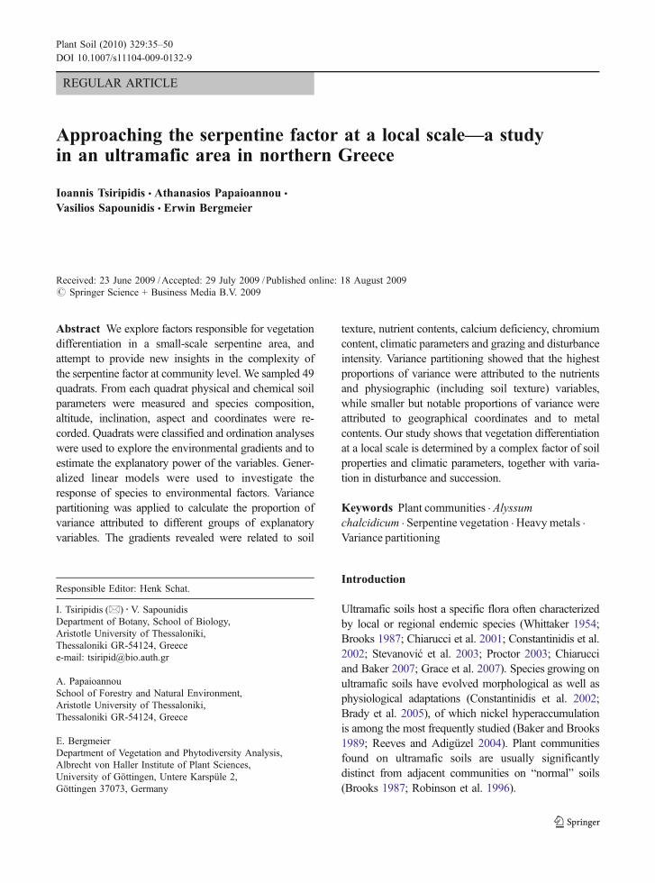
The study area is located at the north-eastern slopes ofMt Vermio, in the vicinity of the village Arkochorion(Fig. 1; longitude 22o 04’ to 22o 08’ E, latitude 40o

34’ to 40o 37’ N) and it comprises three subareas. Thealtitude ranges from 260 to 560 m a.s.l. Thegeological substrate is peridotite. Ground inclinationin the sampled areas does not exceed 35%. The soilsare shallow and the texture is mainly sandy-clayeyloam but in some sites sandy loam or clayey loam.

The climate is transitional between mediterraneanand submediterranean with annual precipitationaround 600 mm, mean annual temperature approxi-mately 15°C and a xerothermic period of almost fourmonths (Chochliouros 2005). The vegetation of thewider area, especially where the substrate is not

36 Plant Soil (2010) 329:35–50

peridotite, but flysch or schist, is comprised of forestsof Quercus frainetto, which at lower altitudes and indrier and/or more disturbed areas are replaced byQuercus pubescens and Carpinus orientalis scrub. Allthree subareas are grazed but the first two moreintensively so.

Vegetation and soil data

In total 49 quadrats (each 1 m2) were selected torepresent all vegetation types visually recognized inthe study area. The sampling was done during the endof spring of 2005. In all selected quadrats at least oneindividual of Alyssum chalcidicum occurred. Thisregional serpentinophyte indicates serpentine vegeta-tion (Stevanović et al. 2003, Bergmeier et al. 2009).Species cover and bare soil were measured using thepoint-quadrat method, with a density of 100 pins m−2

(Moore and Chapman 1986). In each quadrat,altitude, inclination and aspect were measured andthe coordinates recorded using a GPS device.

From each quadrat a composite soil sample wastaken (merging four subsamples) representing theupper 10 cm of the topsoil (humus layer and surfacelitter were excluded). The following soil parameterswere measured: acidity (determined electrometricallyin a 1:1 soil-water slurry), organic matter (wet

oxidation method; Nelson and Sommers 1982) andnitrogen content (Kjeldahl method; Bremmer andMulvaney 1982), particle size distribution (pipettemethod; Gee and Bauder 1982), available phosphorus(Olsen method; Olsen and Sommers 1982), exchange-able potassium, magnesium, calcium, sodium(extracted by 1 N ammonium acetate at pH 7; Thomas1982). Exchangeable cations were determined byatomic absorption spectrophotometry. Exchangeablequantities of elements were measured becausethey represent much better the concentrations avail-able to plants in comparison with total concentrations(Robinson et al. 1996; Chiarucci et al. 1998b).Available zinc, iron, manganese, copper, nickel,cobalt (extracted by DTPA solution; 0.005 MDTPA+0.01 M CaCl2+0.1 M TEA, pH 7.3; Lindsayand Norvell 1978) and chromium (extracted byHNO3, 2 M; Reisenauer 1982), were also determinedby using atomic absorption spectrophotometry (Bakerand Amacher 1982). Cobalt concentration was belowthe limit of detectability and thus was not used in dataanalysis.

Data analysis

All the soil variables (except pH and particle sizedistribution) were expressed in μg/g and were

Fig. 1 Map of the study area, showing the three subareas sampled

Plant Soil (2010) 329:35–50 37

logarithmically transformed by means of the formulabij=log(xij+d)—c, where bij is the transformed valueof xij, c is order of magnitude constant and is equal toInt(log(Min(x)) (with Min(x) being the smallest non-zero value in the data and Int(x) a function thattruncates x to an integer by dropping digits afterdecimal point), and d is a decimal constant equal tolog−1(c) (see McCune and Grace 2002: 69 for furtherdetails). Soil acidity (pH) was first transformed to H+

concentration and then subjected to the above-mentioned transformation. This treatment of pHvariable should be noted when reading the results ofthis study, as a positive relation with H+ correspondsto a positive relation to more acidic conditions.Inclination, aspect and coordinates from each relevéwere used to calculate the potential annual directincident radiation and heat load by applying the thirdequation from McCune and Keon (2002). Thesevariables reflect site microclimatic variation.

TWINSPAN (Hill 1979) was applied for the classi-fication of quadrats, using the following percentageabundances as cut levels: 0, 1, 5, 15, 30. Differentialspecies were determined by applying the algorithmproposed by Tsiripidis et al. (2009). Species wereconsidered as differential when the phi coefficient wasequal or higher than 0.4. Phi coefficient was calculatedfor the groups that are positively differentiated vs. thegroups found to be differentiated negatively, positively-negatively or not differentiated at all.

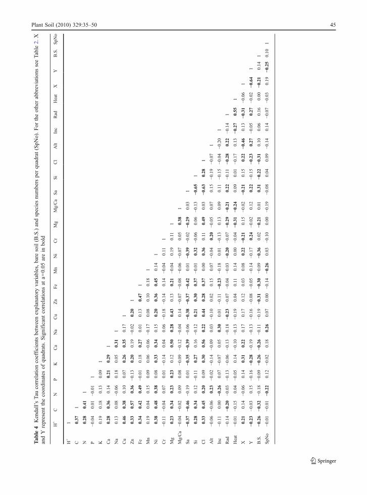
Ordination diagrams of quadrats were made usingDetrended Correspondence Analysis (DCA; Hill andGauch 1980). As (passive) explanatory variables thesoil parameters together with altitude, inclination,coordinates (in the form of X and Y distances froma zero point), annual direct incident radiation and heatload were used. Kendall’s Tau correlation coefficientswere calculated between the explanatory variablesand the scores of the quadrats on the first two DCAaxes as well as the bare soil cover. Kendall’s Taucorrelation coefficients were also calculated betweenthe explanatory variables.

Canonical Correspondence Analysis (CCA; terBraak 1986) was applied in order to test whichvariables have a significant unique contribution to theexplanation of species data variance. For this reason astepwise forward selection of the explanatory varia-bles was applied in CCA and only the variablessignificant at the 0.05 probability level (using MonteCarlo test with 999 permutations) were considered.

Two CCAs were applied, one with the X and Ycoordinates included in the explanatory data set and asecond with the coordinates excluded.

In order to facilitate the interpretation of the DCAand CCA results, the response of species to theexplanatory variables was explored using generalizedlinear models. Only the differential species occurringat least in 7 quadrats and the non-differential occur-ring at least in 10 quadrats were considered. For thenon-differential species occurring at least in 25quadrats (these were also the species recorded withthe highest cover values) the Poisson distribution witha log link function was applied. For the other speciesthe Bernoulli distribution (i.e., a binomial distributionwhere the response variable is converted to binary)with a logit link function was used. In order tosimplify interpretation and to avoid overfitting onlythe models with a linear form were considered, whichwere significant at the 0.05 probability level.

Mann-WhitneyU test with Bonferroni correction formultiple comparisons was applied in order to comparethe values of the explanatory variables between thevegetation units and the sampling subareas.

Finally, variance partitioning was applied in orderto calculate the proportion of variance explained bydifferent groups of explanatory variables. The algo-rithm of Økland (2003) for variance partitioningbetween n groups of explanatory variables wasapplied. The explanatory variables were grouped asfollows. The first group includes the coordinates, thesecond the nutrients (organic matter, organic nitrogen,N, K, Ca, Na, Cu, Zn, Fe and Mn), the third thefactors that are considered toxic (Ni, Cr, Mg, Mg/Ca),and the fourth the factors related to physical soilproperties and physiography (soil texture, inclination,altitude, annual direct incident radiation and heatload). The first group includes differentiation thatcannot be attributed to measured variables, while thelatter reflects microclimate and indirectly soil waterholding capacity. Soil acidity was not used in anygroup, as it influences both the availability ofnutrients and the solubility of toxic metals. In orderto avoid overexplanation of variance, firstly fourCCAs were applied, each having one of the fourgroups as the only explanatory variables. From theseCCAs only the variables presenting a significantunique contribution to variance explanation were usedin variance partitioning. Following the instructions ofØkland (2003) the proportion of variance attributed

38 Plant Soil (2010) 329:35–50

uniquely to each group of variables as well as theshared variance attributed to all the combinations oftwo, three and four groups were calculated.

TWINSPAN was applied using PC-ORD (ver. 5)(McCune and Mefford 1999) and ordination analysesas well as species response curves were calculatedusing CANOCO (ver. 4.5) (ter Braak and Šmilauer2002). Correlation coefficients were calculated withthe help of SPSS (ver. 12) (Anon. 2003).

Results

Classification

The TWINSPAN classification and the DCA dia-grams revealed four species assemblages. Eachassemblage is differentiated by unique differentialtaxa. Additionally, there is a group of differential taxacommon to the first and second group, as well as onecommon to the third and fourth groups. Few otherspecies, differentiating other combinations of assemb-lages, also exist (Table 1).

The first assemblage appears exclusively in sub-area 2. This subarea is strongly affected by grazing andtrampling, particularly so around watering troughs.Although the quadrats are overgrazed they present thesecond highest vegetation cover (median value of baresoil equal to 23). Subarea 2 is a small plateau with gentleinclination which may be the reason for the relativelyhigh vegetation cover. This assumption is supported bythe relatively high percentage of clay in the soils of thisgroup (Table 2). The nitrogen content in this assem-blage is the highest, most likely due to the livestock.The higher amount of organic matter of topsoil may beattributed to the higher vegetation cover.

The second assemblage occurs mainly in thesubareas 1 and 2, and is represented in subarea 3 byonly one quadrat. This assemblage occurs on soilspoor in organic matter and its vegetation cover issmall (Table 2). Plants are very small (5–15 cm) andthis type of vegetation dries very early, at thebeginning of summer.

The third assemblage occurs mainly in subarea 3and with few quadrats in the other two subareas. Thisassemblage presents the lowest vegetation cover. Thesoil is relatively poor in organic matter and nitrogenand other nutrients (e.g. K, Ca, Na, Fe) and it is ofcoarse texture (Table 2).

The fourth assemblage has the highest vegetationcover in the study area. It is characterized by thedominance of Chrysopogon gryllus and its structureand composition resembles those of the typical drygrasslands on “normal” soils in the wider area. Thesoils of this vegetation type are the richest in organicmatter and nutrients. Better soil moisture conditionsmay be assumed due to the finer texture of the soil(higher percentages of silt and clay and smaller ofsand) and the lower direct annual radiation and heatload (Table 2).

DCA

Along the first DCA axis (Fig. 2), the first and secondassemblages are separated from the third and fourth.The second axis discriminates the first and fourthassemblages from the second and third.

Most variables present higher and significant corre-lations with the second DCA axis (Table 3, Fig. 3).Variables significantly correlated with the first axiscomprise only the percentage of bare soil, the Ycoordinate and the potassium content. The formervariable is more strongly correlated with the secondaxis, while the other two variables are significantlycorrelated between each other and reveal the K-poorsoils of the third assemblage, spatially confined tosubarea 3. Therefore, the first axis probably reflectsdifferences in soil conditions of the third assemblage,plus possibly other variables not quantified in thisstudy. Based on our observations, we may say thatthese variables concern grazing intensity, degree ofdisturbance and the vegetation succession stage. This isalso indirectly derived from the fact that the quadrats ofthe first and fourth assemblages co-occur in subarea 1and their floristic differentiation indicates a differentdisturbance intensity as well as succession stage.

The second DCA axis reflects the texture of thesoil and the nutrient content. Quadrats with nutrient-rich soils and of finer texture appear on the lower partof the second DCA axis. Clay proportion is signifi-cantly correlated with most nutrients (Table 4).

CCA and species responses to environmental factors

The variance that each variable explains is presentedin Table 5. The Y coordinate and the percentage ofclay explain the highest proportions of variance, whilethe magnesium content and the sand fraction follow.

Plant Soil (2010) 329:35–50 39

Table 1 Synoptic table of the distinguished assemblages 1–4. The second column (C) gives the absolute constancy of species in thewhole data set (n=49), the third column indicates the phi coefficient multiplied by 100, and fourth to seventh columns specify therelative constancy of species in each assemblage. In the latter columns bold typescript indicates positive differentiation, italictypescript indicates negative differentiation, bold-italic typescript indicates positive-negative differentiation and regular typescriptindicates non-differentiation. Phi coefficient was calculated between the assemblages differentiated positively vs. those differentiatednegatively, positively-negatively or non-differentiated

Assemblage number C Phi 1 2 3 4

Quadrats per assemblage 7 14 19 9

Differential species

Veronica arvensis 6 72 71 0 0 11

Crepis setosa 3 60 43 0 0 0

Galium divaricatum 17 41 71 29 37 11

Filago vulgaris 23 86 100 93 11 11

Anthemis arvensis ssp. incrassata 14 77 100 50 0 0

Vulpia ciliata 10 54 71 29 5 0

Sherardia arvensis 10 51 57 36 5 0

Plantago lagopus 8 47 29 43 0 0

Plantago bellardii 9 56 0 50 11 0

Trifolium arvense 16 56 14 71 26 0

Daucus broteri 3 41 0 21 0 0

Cerastium brachypetalum ssp. roeseri 6 51 0 0 32 0

Haplophyllum coronatum 5 46 0 0 26 0

Crupina vulgaris 16 41 0 14 58 33

Melica ciliata 4 41 0 0 21 0

Dorycnium germanicum 13 77 0 0 26 89

Thymus longicaulis ssp. chaubardii 31 62 14 36 95 78

Hypericum rumeliacum 22 60 0 14 84 44

Allium stamineum 13 49 0 7 37 56

Asphodeline liburnica 13 47 0 7 42 44

Aira elegantissima 9 42 0 0 37 22

Prunella laciniata 16 71 29 14 16 100

Carex caryophyllea 15 63 29 7 21 89

Polygala nicaeensis ssp. mediterranea 5 56 0 0 5 44

Danthonia alpina 3 52 0 0 0 33

Filipendula vulgaris 3 52 0 0 0 33

Centaurium erythraea 10 44 14 7 16 56

Poa timoleontis 21 52 86 50 42 0

Crepis neglecta ssp. neglecta 18 43 43 71 26 0

Linum trigynum 30 48 14 71 68 67

Teucrium capitatum 28 42 14 64 68 56

Trifolium angustifolium 13 46 0 57 11 33

Plantago lanceolata 17 53 71 7 26 67

Festuca valesiaca 15 43 57 0 32 56

Centaurea spec. 9 44 29 0 37 0

Non-differential species

Alyssum chalcidicum 49 100 100 100 100

Aegilops triuncialis 40 57 100 84 67

Table 1 Synoptic table of the distinguished assemblages 1–4. Thesecond column (C) gives the absolute constancy of species in thewhole data set (n=49), the third column indicates the phicoefficient multiplied by 100, and fourth to seventh columnsspecify the relative constancy of species in each assemblage. In thelatter columns bold typescript indicates positive differentiation,

italic typescript indicates negative differentiation, bold-italictypescript indicates positive-negative differentiation and regulartypescript indicates non-differentiation. Phi coefficient was calcu-lated between the assemblages differentiated positively vs. thosedifferentiated negatively, positively-negatively or non-differentiated

40 Plant Soil (2010) 329:35–50

Table 1 (continued)

Assemblage number C Phi 1 2 3 4

Quadrats per assemblage 7 14 19 9

Chrysopogon gryllus 36 43 50 89 100

Potentilla detommasii 36 71 79 79 56

Sanguisorba minor 33 57 50 84 67

Convolvulus cantabrica 30 37 29 86 68 33

Trachynia distachya 30 71 71 58 44

Dichanthium ischaemum 27 57 79 42 44

Trifolium campestre 22 28 71 57 37 22

Trifolium squamosum 16 39 43 64 11 22

Cynosurus elegans 12 14 36 16 33

Geranium columbinum 10 28 29 7 16 44

Anagallis arvensis 9 32 43 29 11 0

Medicago minima 9 32 43 29 11 0

Arenaria serpyllifolia 9 30 43 21 16 0

Silene paradoxa 8 39 0 0 32 22

Crepis foetida ssp. rhoeadifolia 8 39 0 36 16 0

Cistus creticus 8 36 0 14 32 0

Trifolium phleoides 8 33 14 36 11 0

Ornithogalum comosum 8 23 0 21 21 11

Nigella arvensis ssp. arvensis 7 34 0 21 21 0

Hieracium caespitosum 7 21 14 0 21 22

Allium guttatum ssp. sardoum 6 20 14 7 21 0

Xeranthemum annuum 6 14 14 11 11

Anchusa officinalis 5 29 0 21 11 0

Leontodon crispus 5 28 0 0 21 11

Trifolium cherleri 5 17 14 21 0 11

Minuartia recurva ssp. condensata 5 0 14 16 0

Cynodon dactylon 4 25 14 21 0 0

Cerastium pumilum ssp. glutinosum 4 14 7 5 11

Logfia arvensis 4 0 7 16 0

Logfia gallica 4 0 14 11 0

Taeniatherum caput-medusae 4 0 7 11 11

Bupleurum praealtum 3 35 0 0 5 22

Genista carinalis 3 35 0 0 5 22

Bellis perennis 3 14 0 11 0

Cuscuta approximata 3 0 0 11 11

Dactylis glomerata 3 0 0 11 11

Dasypyrum villosum 3 0 14 0 11

Moenchia mantica 3 0 14 5 0

Ornithogalum umbellatum 3 14 7 0 11

Petrorhagia illyrica ssp. haynaldiana 3 0 0 11 11

Salvia viridis 3 14 14 0 0

Scabiosa tenuis 3 0 14 0 11

Plant Soil (2010) 329:35–50 41

Tab

le2

Medianvalues

ofexplanatoryvariables,percentage

ofbare

soil(B.S)andspeciesnu

mbers

ofqu

adrats(SpN

o)forallqu

adrats,each

assemblageandthethreesampling

subareas.The

lastnine

columns

presenttheresults

ofpair-w

isecomparisons

(Mann-Whitney

Utest)betweenthevegetatio

nun

itsandthesamplingsubareas

(one

asterisk

indicates

sign

ificantdifferencesat

a=0.05

andtwoasterisksat

a=0.00

8forthevegetatio

nun

itsandat

a=0.01

7forthesamplingsubareas—

thelast

twosign

ificance

levels

wereadjusted

accordingto

theBon

ferron

icorrectio

nformultip

lecomparisons).Ratio

Mg/Cawas

calculated

onthebasisof

themeq/100

gconcentrations

oftheseelem

ents.Sa:sand

,Si:silt,

Cl:

clay,A

lt:altitud

e,Inc:inclination,

Rad:annu

aldirectincident

radiationandHeat:annu

alheatload;As1

toAs4

correspo

ndto

theassemblages

inTable1;

Ar1

toAr3

correspo

ndto

samplingareas1to

3

Exp

lan.

Var.

AllQuad

-rats

As1

As2

As3

As4

Sub-area1

Sub-area2

Sub-area3

As1vs.

As2

As1vs.

As3

As1vs.

As4

As2vs.

As3

As2vs.

As4

As3vs.

As4

Ar1

vs.

Ar2

Ar1

vs.

Ar3

Ar2

vs.

Ar3

pH6.64

6.63

6.65

6.67

6.60

6.63

6.63

6.67

*

C(μg/g)

41924

5208

137

213

40848

53833

4210

241

589

4191

3*

***

N(μg/g)

2873

4949

2639

2835

3263

2568

3397

2873

**

*

P(μg/g)

18.3

17.6

18.2

17.7

18.6

18.3

19.0

17.0

K(μg/g)

153

162

173

134

170

177

160

131

**

****

Ca(μg/g)

1386

1731

1395

1281

1658

1521

1418

1172

**

*

Na(μg/g)

31.2

36.5

29.2

28.5

32.2

31.5

34.0

27.5

****

Cu(μg/g)

1.34

1.43

1.33

1.22

1.45

1.41

1.15

1.22

*

Zn(μg/g)

1.44

1.86

1.38

1.26

1.86

1.50

1.44

1.22

*

Fe(μg/g)

37.2

43.2

33.7

36.4

43.8

34.8

43.3

34.6

**

****

Mn(μg/g)

55.6

51.9

58.0

54.6

55.9

55.9

58.7

53.2

Ni(μg/g)

558

653

574

447

554

580

623

405

Cr(μg/g)

45.9

50.8

39.6

50.1

45.5

42.2

50.8

50.1

***

****

Mg(μg/g)

2068

2392

1687

1892

2459

2112

2068

1892

***

**

Mg/Ca

2.19

2.26

2.18

2.12

2.19

2.18

2.28

2.12

Sa(%

)51

.851

.851

.554

.638

.444

.851

.854

.6*

**

Si(%

)19

.217

.920

.118

.426

.320

.917

.917

.4*

*

Cl(%

)30

.133

.027

.428

.935

.332

.430

.927

.4*

***

***

**

Alt(m

)40

045

036

541

032

532

046

541

0**

****

****

**

Inc(%

)20

1515

2020

2010

20

Rad

0.95

0.92

0.96

0.95

0.88

0.88

0.92

0.96

**

*

Heat

0.93

0.94

0.95

0.92

0.88

0.88

0.94

0.92

**

B.S.(%

)28

2333

3610

2623

37*

****

**

SpN

o21

2123

2121

2421

20

42 Plant Soil (2010) 329:35–50

In the forward selection seven variables were foundhaving a significant contribution to the explanation ofspecies data variance. These variables explain 28.2 %of total variance (Table 5). In the CCA where thecoordinates were not included in the explanatoryvariables set, eight variables were found with asignificant unique contribution to the explanation ofvariance. In the latter CCA, 28.9 % of species datavariance was explained (Table 5). In this latter CCAthe clay percentage and the altitude were chosen asthe first two variables. Additionally, in the absence ofcoordinates, K and Cr appear among the significantvariables. Conclusively, both CCAs reveal: a) aspatial gradient that accounts for the variance notrepresented by the measured variables as well as forthe differences in K and Cr content between thesubareas, b) a gradient related to soil texture, c)another related to altitude and thus to climaticparameters, and d) one or more gradients related tonutrients (K, Zn, Na), the calcium deficiency (ormagnesium surplus), and the Cr content.

The analysis of species response to the measuredvariables provides a more detailed picture of thespecies-environment relations (Table 6). No specieswere found significantly correlated with the variablesinclination, Mn and P. Several species are significant-ly correlated to the coordinates, revealing a spatiallystructured ecological differentiation. Potassium alsoexplains a significant proportion of variance for ahigh number of species. Silt, although explainingrelatively small proportions of variance, does so for alot of species. The absolute differential species of theassemblages 1 to 3 are infrequent in the data set and

therefore poorly represented in Table 6. The commondifferential taxa of assemblages 1 and 2 are mainlycorrelated to the coordinates and the K content. Thecommon differential taxa of the assemblages 3 and 4have a significant proportion of their variance explainedby different variables. Moreover, three species (out ofsix) are significantly related to the Y coordinate and twospecies to the X coordinate, K and altitude. The absolutedifferential taxa of the fourth group are significantlycorrelated to organic matter, soil texture (positively toclay and silt, and negatively to sand percentages), aswell as to nutrients such as Cu, Fe, Mg and Zn. From theFig. 2 DCA diagram of quadrats’ scores on the first two axes.

Eigenvalue and length of 1st axis: 0.401 and 3.331, respective-ly; corresponding values of 2nd axis: 0.225 and 2.328; totalinertia: 2.975

Table 3 Variance explained by each variable singly in CCAand Kendall’s Tau correlation coefficients between samplescores on the first two DCA axes, percentage of bare soil andexplanatory variables; two asterisks indicate significance at a=0.01 and one asterisk at a=0.05

Variables VE DCA axis1 DCA axis2 Bare Soil

DCA axis1 −0.21*DCA axis2 0.42**

Bare Soil −0.21* 0.42**

Cl 6.39 −0.53** −0.31**Y 6.39 0.29**

Mg 5.38 −0.45** −0.21*Sa 5.38 0.38** 0.31**

X 4.71 −0.21*Ca 4.37 −0.36** −0.26**Fe 4.37 −0.44** −0.30**K 4.37 −0.22* −0.26**C 4.03 −0.42** −0.32**Cu 4.03 −0.32**Zn 4.03 −0.30** −0.31**Alt 3.7

H+ 3.7 −0.35** −0.26**N 3.7 −0.33**Ni 3.7 −0.32** −0.36**Si 3.7 −0.22*Mg/Ca 3.36

P 3.36

Rad 3.36 0.28**

Na 3.03 −0.30**Cr 2.69

Heat 2.69

Inc 2.02

Mn 1.68

Plant Soil (2010) 329:35–50 43

remaining differential taxa as well as the common non-differential species a high proportion (more than 20%)of their variance is attributed to variables such asaltitude (Convolvulus cantabrica), Ca (Dichanthiumischaemum), clay (Plantago lanceolata), K (Aegilopstriuncialis, Trifolium squamosum), Mg (Festucavalesiaca), N (Festuca valesiaca), Na (Dichanthiumischaemum), Ni (Geranium columbinum) and geo-graphical coordinates (Potentilla detommasii, Trifoliumsquamosum, Cynosurus elegans).

Variance partitioning

From each group of explanatory variables at least twovariables were found with a significant uniquecontribution to the explanation of variance. Both Xand Y coordinates were found significant in the groupof spatial variables; K, Ca and Fe were foundsignificant in the group of nutrients; altitude, sandand clay from the group of physiographic variables;and Mg and Ni from the group of metals. All thesevariables explain 33.7 % of the total variance. Theresults of variance partitioning showed that the high-est proportions of variance were attributed to thenutrients and physiographic variables (7.8 and 7.6%,respectively), while 6.7 % of the variance is attribut-able to geographical coordinates and 5.0% to metals.

The shared variances were small, and those whichexplained more than 1% of variance were coordinatesand physiography (1.92 %), and nutrients, physiogra-phy and metals (2.12 %).

Discussion

Alyssum chalcidicum, a species of the A. muralecomplex, is a Ni-hyperaccumulator found with highfrequency and abundance in serpentine areas of NorthGreece (Konstantinou 1992; Bergmeier et al. 2009). Itis the only obligate serpentinophyte occurring in thefour classified assemblages. The relatively strongfloristic differentiation of the four assemblages aswell as the considerable length of DCA axes revealhigh beta diversity in the study area, despite of itssmall size. Harrison and Inouye (2002) found thatserpentine areas in California have a comparativelyhigh diversity of biotic communities, perhaps due toclimatic differences among the serpentine “islands”.Whittaker (1954; 1960) also found a more rapidturnover in species composition along an altitudinalgradient in serpentine areas compared to non-serpentine areas. Our findings suggest high sensitivityof serpentine vegetation to other factors as well,namely nutrients and disturbances.

The variance explained in both CCAs is relativelysmall if we take into account the small size of thestudy area. Chiarucci et al. (2001) found a similarlysmall proportion of explained variance (around 20%),which they attributed to stochastic variation of speciesdistribution. In our case, however, part of theunexplained variance is possibly related to grazingor other disturbance intensities as well as differentsuccession stages. The impact of grazing is partlyrepresented by the Y coordinate as the subareas 1 and2 (assemblages 1 and 2) are more heavily grazed thansubarea 3 (assemblage 3). In the subareas 1 and 2there are also patches much less disturbed by grazing,where the quadrats of the fourth assemblage weresampled. Grace et al. (2007) found that the secondaxis of their ordination diagram for the serpentinevegetation of California was not related to climatic orsoil variables, but expressed successional history andin particular the histories of fire and livestock grazing.The lack of any correlation of Tuscan garigues withenvironmental factors was also attributed to the effect

Fig. 3 Environmental variables (arrows) passively projectedinto the DCA diagram of the first and second DCA axes; forabbreviations of explanatory variables see Tables 2 and 4

44 Plant Soil (2010) 329:35–50

Tab

le4

Kendall’sTau

correlationcoefficientsbetweenexplanatoryvariables,bare

soil(B.S.)andspeciesnu

mbers

perqu

adrat(SpN

o).For

theotherabbreviatio

nsseeTable

2.X

andY

representthecoordinatesof

quadrats.Significant

correlations

ata=

0.05

arein

bold

H+

CN

PK

Ca

Na

Cu

Zn

Fe

Mn

Ni

Cr

Mg

Mg/Ca

Sa

Si

Cl

Alt

Inc

Rad

Heat

XY

B.S.

SpN

o

H+

1

C0.37

1

N0.28

0.41

1

P−0

.04

0.01

−0.01

1

K0.19

0.18

0.13

0.09

1

Ca

0.28

0.36

0.14

0.21

0.29

1

Na

0.13

0.08

−0.06

0.18

0.05

0.31

1

Cu

0.46

0.38

0.10

0.07

0.26

0.35

0.17

1

Zn

0.33

0.57

0.36

−0.13

0.20

0.19

−0.02

0.20

1

Fe

0.34

0.42

0.49

−0.01

0.18

0.27

0.01

0.13

0.47

1

Mn

0.19

0.04

0.15

0.09

0.06

−0.06

−0.17

0.08

0.10

0.18

1

Ni

0.38

0.48

0.38

0.08

0.33

0.34

0.15

0.20

0.36

0.45

0.14

1

Cr

−0.11

−0.04

0.07

0.01

−0.14

0.04

0.06

−0.18

−0.14

0.14

−0.04

0.11

1

Mg

0.23

0.34

0.23

0.23

0.12

0.50

0.28

0.43

0.13

0.21

−0.04

0.19

0.11

1

Mg/Ca

−0.04

−0.02

0.09

0.08

−0.09

−0.12

−0.04

0.14

−0.07

−0.08

−0.06

−0.07

0.05

0.38

1

Sa

−0.37

−0.46

−0.19

0.01

−0.35

−0.39

−0.06

−0.38

−0.37

−0.42

0.01

−0.39

−0.02

−0.29

0.03

1

Si

0.28

0.34

0.12

−0.11

0.27

0.16

−0.12

0.21

0.30

0.37

−0.01

0.32

−0.06

0.06

−0.13

−0.65

1

Cl

0.33

0.45

0.20

0.09

0.30

0.56

0.22

0.44

0.28

0.37

0.00

0.36

0.11

0.49

0.03

−0.63

0.28

1

Alt

−0.06

−0.06

0.23

−0.02

−0.14

−0.09

0.03

−0.10

0.02

0.15

0.07

−0.04

0.20

−0.05

0.07

0.15

−0.19

−0.07

1

Inc

−0.11

0.00

−0.26

0.07

−0.07

0.05

0.30

0.01

−0.11

−0.23

−0.18

0.01

−0.13

0.13

0.09

0.11

−0.15

−0.04

−0.20

1

Rad

−0.14

−0.20

−0.03

−0.13

−0.06

−0.13

−0.18

−0.23

−0.07

−0.04

−0.03

−0.20

−0.07

−0.29

−0.21

0.22

−0.11

−0.28

0.22

−0.14

1

Heat

−0.01

−0.15

0.04

−0.05

0.14

−0.10

−0.13

−0.19

0.04

0.11

0.14

0.00

−0.04

−0.31

−0.24

0.09

0.01

−0.17

0.13

−0.27

0.55

1

X0.21

0.14

−0.06

0.14

0.31

0.22

0.17

0.17

0.12

0.03

0.08

0.22

−0.21

0.15

−0.02

−0.21

0.15

0.22

−0.46

0.13

−0.31

−0.06

1

Y−0

.23

−0.03

0.15

−0.16

−0.28

−0.19

−0.13

−0.16

−0.08

−0.05

−0.14

−0.17

0.24

−0.02

0.12

0.22

−0.15

−0.23

0.27

−0.05

0.27

−0.02

−0.64

1

B.S.

−0.26

−0.32

−0.18

−0.09

−0.26

−0.26

−0.11

−0.19

−0.31

−0.30

−0.09

−0.36

0.02

−0.21

0.01

0.31

−0.22

−0.31

0.10

0.06

0.16

0.00

−0.21

0.14

1

SpN

o−0

.01

−0.01

−0.22

0.12

−0.02

0.18

0.26

0.07

0.00

−0.14

−0.26

0.03

−0.10

0.00

−0.19

−0.08

0.04

0.09

−0.14

0.14

−0.07

−0.03

0.19

−0.25

0.10

1

Plant Soil (2010) 329:35–50 45

of human disturbance (Chiarucci et al. 1998b;Chiarucci 2003).

The CCA results revealed that among the mostimportant soil variables influencing the floristiccomposition of the assemblages are those concerningthe soil texture. Clay percentage presents also thehighest correlation to the second DCA axis. Finer soiltexture increases the water holding capacity as well asthe cation exchange capacity (clay and silt arepositively correlated to most of the measurednutrients; see Table 4). Important factors affectingspecies composition in serpentine areas are drought(Walker 1954; Proctor and Woodell 1975; Kruckeberg2002; Chiarucci et al. 1998b; Chiarucci 2003; Gramet al. 2004) and nutrient deficiency (Proctor and Nagy1992; Chiarucci et al. 2001). Small additionalamounts of N, P and K induced vegetation coverand biomass production and in some cases asubstantial change in species composition (Huennekeet al. 1990; Proctor and Nagy 1992; Chiarucci et al.1998a; 1999). The combined effect of drought andnutrient deficiency has been considered an importantlimiting factor in serpentine soils (Chiarucci 2003).Higher nutrient availability may alleviate the effectsof drought (Grime 1990). Chiarucci and Maccherini(2007) observed that the dry Mediterranean climate ofTuscany affects species richness and vegetation coverof serpentine communities only in fertilized plots,while it has non-significant effects in unfertilizedones. Our study corroborates findings that serpentine

communities are subject to a combination of climaticand nutritional stress which prevents, or delays,succession.

The soil conditions of the most evolved assem-blage (4) in our study area affect in a combined waysoil water and nutrients availability. As the soil ismoister in this assemblage, plant growth is stimulated.This increases the deposition of dead organic matterand soil organic content, thus improving soil waterholding capacity. Furthermore, wetter conditions andhumus decay cause soil acidification. Indeed, the pHin the fourth assemblage is somewhat lower than inthe other assemblages. The increase of organic mattercontent provides a bigger nutrients pool and thedecrease of pH increases nutrients availability (Angeloneet al. 1993; Chiarucci 2003).

Another interesting finding of this study is that theconcentration of toxic metals is higher in the soils ofthe more evolved assemblages. For instance, magne-sium is significantly higher in assemblages 1 and 4(see Table 2), and nickel is also higher in theseassemblages (see Fig. 3), albeit not significantly. Boththese two metals are significantly and positivelycorrelated to the concentration of hydrogen cations(Table 4). This corroborates annotations of Chiarucci(1998b), Chiarucci et al. (2001) and Chiarucci (2003)that the available fraction of metals is higher in thesoils under the more developed and structuredcommunities. Note, however, that the available Crdoes not follow the same pattern.

Table 5 Variables that entered the model in the forward selection of CCA. In the first CCA, on the left, X and Y coordinates wereincluded in the explanatory data set, while in the second one, on the right, coordinates were excluded from the analysis. AVE:additional proportion of variance that each variable explains at the time of its inclusion in the model, P: significance level of variables,F: F−ratio, TVE: proportion of total variance explained by the significant explanatory variables, Or: inclusion order of variables in themodel

Variable AVE P F Or AVE P F Or

Y 6.39 0.001 3.22 1

Cl 5.38 0.001 2.73 2 6.39 0.001 3.22 1

Alt 4.03 0.002 2.19 3 4.03 0.005 1.98 2

Zn 3.36 0.005 1.94 4 3.70 0.006 1.9 4

Mg/Ca 3.36 0.004 1.74 5 3.03 0.028 1.54 5

Na 2.69 0.024 1.58 6 2.69 0.029 1.57 8

Sa 3.03 0.013 1.61 7 2.69 0.008 1.65 6

K 3.36 0.008 1.91 3

Cr 3.03 0.015 1.59 7

TVE 28.24 28.91

Table 5 Variables that entered the model in the forwardselection of CCA. In the first CCA, on the left, X and Ycoordinates were included in the explanatory data set, while inthe second one, on the right, coordinates were excluded from theanalysis. AVE: additional proportion of variance that each

variable explains at the time of its inclusion in the model, P:significance level of variables, F: F−ratio, TVE: proportion oftotal variance explained by the significant explanatory variables,Or: inclusion order of variables in the model

46 Plant Soil (2010) 329:35–50

Tab

le6

Species

having

asign

ificant(0.05

:regular

fonts,0.01

:boldfonts)prop

ortio

nof

theirvariance

explainedby

anexplanatoryvariable.O

nlydifferentialspecies

occurringin

atleast7

quadratsandtheno

n-differentialspecies

occurringin

atleast1

0qu

adratswereconsidered.N

umbersin

thetablecorrespo

ndto

thepercentage

ofthetotalv

arianceof

aspecies

explainedby

themod

el.A

negativ

esign

before

thenu

mbers

indicatesanegativ

eregression

coefficient

Species

H+

CN

KCa

Na

Cu

Zn

Fe

Ni

Cr

Mg

Mg/Ca

Sa

Si

Cl

Alt

Rad

Heat

XY

Galium

divaricatum

8.8

−11

11

Fila

govulgaris

13.7

6.1

14.5

−29

Anthemisarvensisssp.

incrassata

11.2

7.1

−22

Vulpia

cilia

ta15.4

−11

Sherardiaarvensis

12.4

−19

Plantagolagopus

14.4

9.8

−17

Plantagobella

rdii

−8.8

−19

−11

10.1

−17

13.2

Crupina

vulgaris

−15

−7.2

−15

−16.6

20.9

Dorycnium

germ

anicum

12.7

15.9

−10

−17

−24

−12

Thymus

longicaulis

ssp.

chaubardii

−8.8

−11

11

Hypericum

rumeliacum

−14

−6.3

−6.2

−19.2

27.9

Allium

stam

ineum

10.4

7.3

Asphodelin

elib

urnica

−9.1

17

Airaelegantissima

11.5

8.5

Prunella

laciniata

8.2

20.2

11.9

11.4

10.3

7.3

8.3

31.2

6.8

−26

6.9

29.4

−16

−14

7.2

− 7.9

Carex

caryophyllea

22.7

9.5

7.1

8.5

21.6

7.8

15.3

−27

11.1

23.1

Centaurium

erythraea

10−9

.713.5

Poa

timoleontis

−9.9

10.3

10.6

Crepisneglecta

ssp.

neglecta

−9.2

−9.5

−13

Linum

trigynum

−11

−13

9.7

Teucrium

capitatum

−8.5

Trifo

lium

angustifo

lium

14.5

−8.9

−17

11.8

−16

19.9

−17

Plantagolanceolata

6.7

13.5

7.4

6.4

10.5

7.5

14.4

9.9

8.1

−13

27.6

−11

−6.8

Festuca

valesiaca

7.6

11.7

228.7

1022

13.3

29.8

9.4

18.5

−14

Centaurea

species

−18

13.2

Aegilo

pstriuncialis

29.5

−9.8

11.9

−18

Chrysopogon

gryllus

7.1

9.3

15.2

10.9

9.9

−912.1

Potentilla

detommasii

−12

10.3

12.3

−11

−8.1

−12

7.4

25.3

−23

Sanguisorbaminor

−14

Convolvulus

cantabrica

−9.7

−11

−24

9.3

Dichanthium

ischaemum

29.4

38.1

16.4

11.6

−9.7

Trifo

lium

campestre

7.4

6.2

−6.6

Trifo

lium

squamosum

36.2

−12

−12

10.9

20.2

−39

Cynosurus

elegans

12.2

7−1

28.7

24.2

−43

Geranium

columbinum

11.8

14.3

8.2

16.7

20.8

−13

13.3

Plant Soil (2010) 329:35–50 47

From the variables considered responsible fortoxicity effects (Ni, Mg, Cr, Mg/Ca), Mg explainsthe highest proportion of variance in the CCA.However, as mentioned above this element presentsthe highest concentration in the more developedassemblages. In the forward selection procedure thevariable explaining a significant, unique proportion ofvariance is the ratio Mg/Ca. This variable was notfound significantly different among the four assemb-lages and among the three subareas. Additionally, theratio is relatively small in our study area compared towhat is given in other serpentine areas of the world(Brooks 1987; Chiarucci 2003). Chromium, althoughexplaining a small proportion of variance in the CCA,was found to explain a significant unique proportion ofvariance in the CCAwithout coordinates. This elementis significantly lower in subarea 1 in comparison to theother two subareas. Several authors noticed the limitedimportance of metal toxicity for the serpentine factor(e.g. Carter et al. 1987; Kruckeberg 1992), and Proctorand Nagy (1992) mentioned that many assumptionsabout the importance of nickel in determining theserpentine vegetation were unfounded.

A more detailed picture of the dependence ofspecies distribution is obtained by the analysis ofspecies response to the measured variables. Mainlypositive correlations with species occurrences werefound for both Mg and Ni, and thus we may notassume toxic effects of these elements. Chromiumshows negative correlations with some species, but itexplains a low proportion of their variance. Plantagobellardii is an exception. This small annual occursalmost exclusively in subarea 1 where chromium isleast concentrated. Also the remaining species corre-lated negatively with chromium occur mainly in thissubarea or are more abundant there.

Another interesting finding is that there is goodcongruence in the response of species within thedifferential species groups. Huenneke et al. (1990)observed individualistic responses within speciesgroups (e.g. groups of growth form) to the additionof nutrients. The results of this study, and specificallythe fact that the common differential taxa of assemb-lages 1 and 2 as well as the absolute differential taxaof assemblage 4, showed similar responses to com-mon explanatory variables, indicate that a generaliza-tion of certain species responses to environmentalfactors in serpentine areas may be possible throughdifferential species groups obtained by classification.

The results of variance partitioning provide a directanswer to the question of which factors are maindrivers of the vegetation differentiation in the studyarea. The combined use of explanatory variables andcovariables reveals the unique proportion of variancethat each group of variables explains (Borcard et al.1992; Legendre and Legendre 1998; Økland 2003).We conclude that a combination of factors isresponsible for the vegetation differentiation at a localscale, notably soil properties and climatic parameters,together with variation in disturbance and succession.Our results show that nutrients and physiographicvariables are chiefly responsible for vegetation differ-entiation, but the other two groups of variables(coordinates and concentration of metals) are alsoresponsible for notable proportions of explainedvariance. In the group of physiographic variables soiltexture plays the major role, while in the group ofnutrients, K and Ca were found to be relatively moreimportant. Explorative and explanatory studies atdifferent scales are essential to improve our under-standing of ecological phenomena in serpentine areas.

Acknowledgements The authors would like to acknowledgeProf. Dimitrios Alifragis for his help and advice during the soillaboratory analyses and two anonymous reviewers for theirvaluable comments and suggestions.

References

Angelone M, Vaselli O, Bini C, Coradossi N (1993) Pedogeo-chemical evolution and trace elements availability toplants in ophiolitic soils. Sci Total Environ 129:291–309

Anon. (2003) SPSS for Windows, Rel. 12.0.0. SPSS Inc.,Chicago, IL, US

Baker DE, Amacher MC (1982) Nickel, copper, zinc, andcadmium. In: Page AL et al. (eds) Methods of soilanalysis, Part 2: Chemical and microbiological properties.2nd edn., Madison, pp 323–336

Baker AJM, Brooks RR (1989) Terrestrial higher plants whichhyperaccumulate metallic elements—review of their dis-tribution, ecology and phytochemistry. Biorecovery 1:81–126

Bani A, Echevarria G, Sulçe S, Morel JL, Mullai A (2007) In-situ phytoextraction of Ni by a native population ofAlyssum murale on an ultramafic site (Albania). Plant Soil293:79–89

Bergmeier E, Konstantinou M, Tsiripidis I, Sykora K (2009)Plant communities on metalliferous soils in northernGreece. Phytocoenologia (in press)

Borcard D, Legendre P, Drapeau P (1992) Partialling out thespatial component of ecological variation. Ecology73:1045–1055

48 Plant Soil (2010) 329:35–50

Brady KU, Kruckeberg AR, Bradshaw HD (2005) Evolutionaryecology of plant adaptation to serpentine soils. Annu RevEcol Evol Syst 36:243–266

Bremmer JM, Mulvaney CS (1982) Nitrogen-total. In: Page ALet al. (eds) Methods of soil analysis. Part 2: Chemical andmicrobial properties, 2nd edn., ASA and SSSA, Madison,pp 595–624

Brooks RR (1987) Serpentine and its vegetation: a multidisciplinaryapproach. Dioscorides Press, Portland, Oregon, USA

Brooks RR, Yang XH (1984) Elemental levels and relationshipsin the endemic serpentine flora of the Great Dyke,Zimbabwe and their significance as controlling factorsfor this flora. Taxon 33:392–399

Carter SP, Proctor J, Slingsby DR (1987) Soil and vegetation ofthe Keen of Hamar serpentine, Shetland. J Ecol 75:21–42

Chiarucci A (2003) Vegetation ecology and conservation onTuscan ultramafic soils. Bot Rev 69(3):252–268

Chiarucci A, Baker AJM (2007) Advances in the ecology ofserpentine soils. Plant Soil 293:1–2

Chiarucci A, Maccherini S (2007) Long-term effects of climateand phosphorus fertilisation on serpentine vegetation.Plant Soil 293:133–144

Chiarucci A, Maccherini S, Bonini I, De Dominicis V (1998a)Effects of nutrient addition on species diversity and coveron “serpentine” vegetation. Plant Biosyst 132:143–150

Chiarucci A, Maccherini S, Bonini I, De Dominicis V (1999)Effects of nutrient addition on community productivityand structure of serpentine vegetation. Plant Biol 1:121–126

Chiarucci A, Robinson BH, Bonini I, Petit D, Brooks RR, DeDominicis V (1998b) Vegetation of Tuscan ultramaficsoils in relation to edaphic and physical factors. FoliaGeobot 33:113–131

Chiarucci A, Rocchini D, Leonzio C, De Dominicis V (2001) Atest of vegetation-environment relationships in serpentinesoils of Tuscany, Italy. Ecol Res 16:627–639

Chochliouros SP (2005) Floristic and phytosociological re-search of Mt Vermio—An ecological approach. Universityof Patra, Greece, Dissertation

Constantinidis T, Bareka EP, Kamari G (2002) Karyotaxonomyof Greek serpentine angiosperms. Bot J Linn Soc139:109–124

Gee GW, Bauder JW (1982) Particle-size analysis. In: Klute A(ed) Methods of soil analysis, Part 1: Physical andmineralogical methods, 2nd edn. ASA and SSSA, Madison,pp 383–412

Grace JB, Safford HD, Harrison S (2007) Large-scale causes ofvariation in the serpentine vegetation of California. PlantSoil 293:121–132

Gram WK, Borer ET, Cottingham KL, Seabloom EW, BoucherVL, Goldwasser L, Micheli F, Kendall BE, Burton RS(2004) Distribution of plants in a California serpentinegrassland: are rocky hummocks spatial refuges for nativespecies? Plant Ecol 172:159–71

Grime JP (1990) Mechanisms promoting floristic diversity incalcareous grasslands. In: Hillier SH, Walton DWH, WellsDA (eds) Calcareous grasslands: Ecology and manage-ment. Bluntisham Books, Bluntisham, England, pp 51–56

Harrison S, Inouye BD (2002) High b diversity in the flora ofCalifornian serpentine ‘islands’. Biodivers Conserv11:1869–1876

Hill MO (1979) TWINSPAN—a FORTRAN program forarranging multivariate data in an ordered two way tableby classification of the individuals and the attributes.Cornell University, Ithaca, NY, US, Ecology & Systematics

Hill MO, Gauch HG (1980) Detrended correspondenceanalysis: an improved ordination technique. Vegetatio42:47–58

Huenneke LF, Hamburg SP, Koide R, Mooney HA, VitousekPM (1990) Effects of soil resources on plant invasion andcommunity structure in Californian serpentine grassland.Ecology 71:478–491

Konstantinou M (1992) Phytosociological studies of thevegetation on metalliferous soils in northern Greece.Aristotle University of Thessaloniki, Greece, Dissertation

Kruckeberg AR (1985) California serpentines: flora, vegetation,geology, soils, and management problems. Univ. Calif.Press, Berkeley

Kruckeberg AR (1992) Plant life of western North Americanultramafics. In: Roberts BA, Proctor J (eds) The ecologyof areas with serpentinized rocks: A world view. KluwerAcademic Publishers, The Netherlands, pp 31–74

Kruckeberg AR (2002) Geology and plant life: the effects ofland forms and rock types on plants. University ofWashington Press, Seattle, USA

Legendre P, Legendre L (1998) Numerical ecology, 2nd,Englishth edn. Elsevier Science, Amsterdam, NL

Lindsay WL, Norvell WA (1978) Development of a DTPA soiltest for zinc, iron, manganese, and copper. Soil Sci SocAm J 42:421–428

McCune B, Grace JB (2002) Analysis of ecological communities.MJM Press, Gleneden Beach, Oregon, USA

McCune B, Keon D (2002) Equations for potential annualdirect incident radiation and heat load. J Veg Sci 13:603–606

McCune B, MeffordMJ (1999) PC-ORD—Multivariate analysisof ecological data. Version 5.0. MjM Software, GlenedenBeach, Oregon, USA

Moore PD, Chapman SB (1986) Methods in plant ecology.Blackwell Scientific Publications, Oxford

Nelson DW, Sommers LE (1982) Total carbon, organic carbonand organic matter. In: Page AL et al. (eds) Methods ofsoil analysis. Part 2: Chemical and microbial properties,2nd edn., ASA and SSSA, Madison, pp 39–579

Økland RH (2003) Partitioning the variation in a plot-by-species data matrix that is related to n sets of explanatoryvariables. J Veg Sci 14(5):693–700

Olsen SR, Sommers LE (1982) Phosphorus. In: Page AL et al.(eds) Methods of soil analysis. Part 2: Chemical andmicrobial properties, 2nd edn., ASA and SSSA, Madison,pp 401–430

Proctor J (1971) The plant ecology of serpentine. III. Theinfluence of a high magnesium/calcium ratio and highnickel and chromium levels in some British and Swedishserpentine soils. J Ecol 59:827–842

Proctor J (2003) Vegetation and soil and plant chemistry onultramafic rocks in the tropical Far East. Perspect PlantEcol 6:105–124

Proctor J, Nagy L (1992) Ultramafic rocks and their vegetation:an overview. In: Baker AJM, Proctor J, Reeves RD (eds)The vegetation of ultramafic (serpentine) soils. KluwerAcademic Publishers, Dordrecht, pp 469–494

Plant Soil (2010) 329:35–50 49

Proctor J, Woodell SRJ (1975) The ecology of serpentine soils.Adv Ecol Res 9:255–366

Reeves RD, Adigüzel N (2004) Rare plants and nickelaccumulators from Turkish serpentine soils, withspecial reference to Centaurea species. Turk J Bot28:147–153

Reisenauer HM (1982) Chromium. In: Page AL et al. (eds)Methodsof soil analysis. Part 2: Chemical and microbiologicalproperties. 2nd edn., Madison, pp 323–336

Roberts BA, Proctor J (1992) The ecology of areas withserpentinized rocks: a world view. Kluwer, Dordrecht,Netherlands

Robinson BH, Brooks RR, Kirkman JH, Gregg PEH, AlvarezHV (1997) Edaphic influences on a New Zealandultramafic (“serpentine”) flora: a statistical approach. PlantSoil 188:11–20

Robinson BH, Brooks RR, Kirkman JH, Gregg PEH,Gremigni P (1996) Plant-available elements in soilsand their influence on the vegetation over ultramafic(‘Serpentine’) rocks in New Zealand. J R Soc NewZeal 26:457–458

Stevanović V, Tan K, Iatrou G (2003) Distribution of theendemic Balkan flora on serpentine I.—obligate serpentineendemics. Plant Syst Evol 242:149–170

ter Braak CJF (1986) Canonical correspondence analysis: anew eigenvector technique for multivariate direct gradientanalysis. Ecology 67:1167–1179

ter Braak CJF, Šmilauer P (2002) CANOCO reference manualand CanoDraw for Windows user’s guide: Software forcanonical community ordination (version 4.5). Microcom-puter Power, Ithaca, NY, US

Thomas GW (1982) Exchangable cations. In: Page AL et al. (eds)Methods of soil analysis. Part 2: Chemical and microbialproperties, 2nd edn., ASA and SSSA, Madison, pp 154–157

Tsiripidis I, Bergmeier E, Fotiadis G, Dimopoulos P (2009) Anew algorithm for the determination of differential taxa. JVeg Sci 20:233–240

Vergnano Gambi O (1992) The distribution and ecology of thevegetation of ultramafic soils of Italy. In: Roberts BA,Proctor J (eds) The Ecology of Areas with SerpentinizedRocks: AWorld View. Kluver, Dordrecht, NL, pp 217–247

Walker RB (1954) The ecology of serpentine soils: Asymposium. II. Factors affecting plant growth on serpentinesoils. Ecology 35:259–66

Whittaker RH (1954) The vegetational responses to serpentinesoils. Ecology 35:275–288

Whittaker RH (1960) Vegetation of the Siskiyou Mountains,Oregon and California. Ecol Monogr 30:279–338

50 Plant Soil (2010) 329:35–50