Forest Ecology and Management 258 (2009) 2439–2449

Applying spatial conservation prioritization software and high-resolution GISdata to a national-scale study in forest conservation

Joona Lehtomaki a,*, Erkki Tomppo b, Panu Kuokkanen c, Ilkka Hanski a, Atte Moilanen a

a Metapopulation Research Group, Dept. of Biological and Environmental Sciences, P.O. Box 65, University of Helsinki, FI-00014 Helsinki, Finlandb Finnish Forest Research Institute, Vantaa Research Unit, Vantaa Unit, P.O. Box 18, FI-01301 Vantaa, Finlandc Metsahallitus Natural Heritage, Kalevankatu 8, FI-40100 Jyvaskyla, Finland

A R T I C L E I N F O

Article history:

Received 29 January 2009

Received in revised form 15 August 2009

Accepted 20 August 2009

Keywords:

Boreal forest

Zonation

Connectivity

Conservation planning

GIS

A B S T R A C T

We apply a recently developed conservation prioritization method (Zonation algorithm) to a national-

scale conservation planning task. The Finnish Forest and Park Service (Metsahallitus) was given the

mandate to expand the current protected areas in southern Finland by 10 000 ha. The question is which

areas should be selected out of the total area of 1 760 000 ha. The data available include a nation-wide

GIS data set describing general features of forests at the resolution of 25 m � 25 m for entire Finland and

another data set about biodiversity features within the current state-managed conservation areas.

Ecologically, the key information includes forest age and the volume of growing stock for 20 forest types

representing different productivity classes and dominant tree species. Our analysis employs four

different connectivity components to identify forest areas that are (i) locally of high quality and

internally well connected, (ii) well connected to surrounding high-quality forests, (iii) well connected to

existing conservation areas, and (iv) large enough to allow efficient implementation. Expert evaluation of

the results suggested that the present quantitative analysis was helpful in identifying areas with high

conservation value systematically across southern Finland. Our analysis also showed that the highest

forest conservation potential in Finland is located on privately owned land. The present techniques can

be applied to many large-scale planning and management projects.

� 2009 Elsevier B.V. All rights reserved.

Contents lists available at ScienceDirect

Forest Ecology and Management

journa l homepage: www.e lsevier .com/ locate / foreco

1. Introduction

Boreal forests comprise the most important habitat type inFinland both in terms of the area covered and overall biodiversity(Hilden et al., 2005). Although the volume of the growing stock ofFinnish forests has increased in the past decades and is stillincreasing (Finnish Forest Research Institute, 2008), intensiveforestry practices have led to adverse ecological changes in forests(Tikkanen et al., 2006). The most important threat to forestbiodiversity is the small area and low quality of the remainingnatural and semi-natural forests that potentially host largenumbers of specialized species (Puumalainen et al., 2003; Hanski,2005). Although forestry practices have been somewhat modifiedduring the past 20 years, timber production-oriented manage-ment has created forest structures that are far from natural: even-aged stands largely established with a single tree species, which insouthern Finland is mostly the Scots pine (Pinus sylvestris L.). Themain difference between forests available for wood supply

* Corresponding author. Tel.: +358 9 191 57753; fax: +358 9 191 57694.

E-mail addresses: joona.lehtomaki@helsinki.fi (J. Lehtomaki),

erkki.tomppo@metla.fi (E. Tomppo), panu.kuokkanen@metsa.fi (P. Kuokkanen),

ilkka.hanski@helsinki.fi (I. Hanski), atte.moilanen@helsinki.fi (A. Moilanen).

0378-1127/$ – see front matter � 2009 Elsevier B.V. All rights reserved.

doi:10.1016/j.foreco.2009.08.026

(FAWS) and natural forests is the homogeneous structure ofand low volume of dead wood in the former, which furthermoreare typically <100 years in age (Rassi et al., 2001; Penttila et al.,2004).

Strictly protected areas cover 4.5% of the forested land inFinland, but most of the protected forests are in northern Finland(16% of the forested land) with climate and soils not favourable forforest growth, while only 2.2% of forests in southern Finland areprotected (Hanninen et al., 2006; Finnish Forest Research Institute,2008). The most significant deficiency in the Finnish forest reservenetwork is the low level of protection in hemiboreal and southernand middle-boreal forest vegetation zones (Virkkala et al., 2000). Inthese zones, only 0.4% of the forests are protected and classified assemi-natural old forests (140 years or older with featuresindicating naturalness; Punttila, 2008, pers. comm.). Much hopehas been placed on achieving an adequate level of conservationthrough a network of small woodland key habitats (Annila, 1998).However, ecological studies show that these hopes are unwar-ranted (Hanski, 2006), because of high local extinction rates(Pykala, 2004), edge effects (Murcia, 1995), and very lowconnectivity (Aune et al., 2005). In the future, climate change(Soja et al., 2007) and biomass harvesting for energy production(Lundmark, 2006; Antikainen et al., 2007) are likely to exertadditional pressures on forest biodiversity.

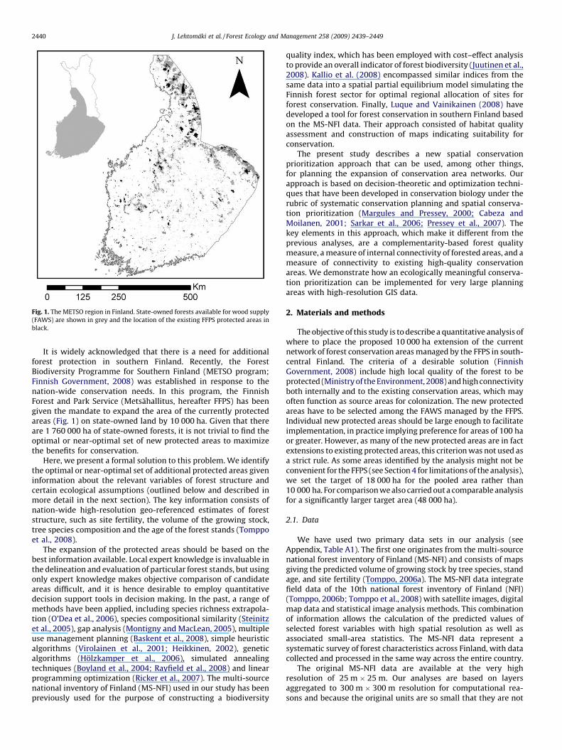
Fig. 1. The METSO region in Finland. State-owned forests available for wood supply

(FAWS) are shown in grey and the location of the existing FFPS protected areas in

black.

J. Lehtomaki et al. / Forest Ecology and Management 258 (2009) 2439–24492440

It is widely acknowledged that there is a need for additionalforest protection in southern Finland. Recently, the ForestBiodiversity Programme for Southern Finland (METSO program;Finnish Government, 2008) was established in response to thenation-wide conservation needs. In this program, the FinnishForest and Park Service (Metsahallitus, hereafter FFPS) has beengiven the mandate to expand the area of the currently protectedareas (Fig. 1) on state-owned land by 10 000 ha. Given that thereare 1 760 000 ha of state-owned forests, it is not trivial to find theoptimal or near-optimal set of new protected areas to maximizethe benefits for conservation.

Here, we present a formal solution to this problem. We identifythe optimal or near-optimal set of additional protected areas giveninformation about the relevant variables of forest structure andcertain ecological assumptions (outlined below and described inmore detail in the next section). The key information consists ofnation-wide high-resolution geo-referenced estimates of foreststructure, such as site fertility, the volume of the growing stock,tree species composition and the age of the forest stands (Tomppoet al., 2008).

The expansion of the protected areas should be based on thebest information available. Local expert knowledge is invaluable inthe delineation and evaluation of particular forest stands, but usingonly expert knowledge makes objective comparison of candidateareas difficult, and it is hence desirable to employ quantitativedecision support tools in decision making. In the past, a range ofmethods have been applied, including species richness extrapola-tion (O’Dea et al., 2006), species compositional similarity (Steinitzet al., 2005), gap analysis (Montigny and MacLean, 2005), multipleuse management planning (Baskent et al., 2008), simple heuristicalgorithms (Virolainen et al., 2001; Heikkinen, 2002), geneticalgorithms (Holzkamper et al., 2006), simulated annealingtechniques (Boyland et al., 2004; Rayfield et al., 2008) and linearprogramming optimization (Ricker et al., 2007). The multi-sourcenational inventory of Finland (MS-NFI) used in our study has beenpreviously used for the purpose of constructing a biodiversity

quality index, which has been employed with cost–effect analysisto provide an overall indicator of forest biodiversity (Juutinen et al.,2008). Kallio et al. (2008) encompassed similar indices from thesame data into a spatial partial equilibrium model simulating theFinnish forest sector for optimal regional allocation of sites forforest conservation. Finally, Luque and Vainikainen (2008) havedeveloped a tool for forest conservation in southern Finland basedon the MS-NFI data. Their approach consisted of habitat qualityassessment and construction of maps indicating suitability forconservation.

The present study describes a new spatial conservationprioritization approach that can be used, among other things,for planning the expansion of conservation area networks. Ourapproach is based on decision-theoretic and optimization techni-ques that have been developed in conservation biology under therubric of systematic conservation planning and spatial conserva-tion prioritization (Margules and Pressey, 2000; Cabeza andMoilanen, 2001; Sarkar et al., 2006; Pressey et al., 2007). Thekey elements in this approach, which make it different from theprevious analyses, are a complementarity-based forest qualitymeasure, a measure of internal connectivity of forested areas, and ameasure of connectivity to existing high-quality conservationareas. We demonstrate how an ecologically meaningful conserva-tion prioritization can be implemented for very large planningareas with high-resolution GIS data.

2. Materials and methods

The objective of this study is to describe a quantitative analysis ofwhere to place the proposed 10 000 ha extension of the currentnetwork of forest conservation areas managed by the FFPS in south-central Finland. The criteria of a desirable solution (FinnishGovernment, 2008) include high local quality of the forest to beprotected (Ministry of the Environment, 2008) and high connectivityboth internally and to the existing conservation areas, which mayoften function as source areas for colonization. The new protectedareas have to be selected among the FAWS managed by the FFPS.Individual new protected areas should be large enough to facilitateimplementation, in practice implying preference for areas of 100 haor greater. However, as many of the new protected areas are in factextensions to existing protected areas, this criterion was not used asa strict rule. As some areas identified by the analysis might not beconvenient for the FFPS (see Section 4 for limitations of the analysis),we set the target of 18 000 ha for the pooled area rather than10 000 ha. For comparison we also carried out a comparable analysisfor a significantly larger target area (48 000 ha).

2.1. Data

We have used two primary data sets in our analysis (seeAppendix, Table A1). The first one originates from the multi-sourcenational forest inventory of Finland (MS-NFI) and consists of mapsgiving the predicted volume of growing stock by tree species, standage, and site fertility (Tomppo, 2006a). The MS-NFI data integratefield data of the 10th national forest inventory of Finland (NFI)(Tomppo, 2006b; Tomppo et al., 2008) with satellite images, digitalmap data and statistical image analysis methods. This combinationof information allows the calculation of the predicted values ofselected forest variables with high spatial resolution as well asassociated small-area statistics. The MS-NFI data represent asystematic survey of forest characteristics across Finland, with datacollected and processed in the same way across the entire country.

The original MS-NFI data are available at the very highresolution of 25 m � 25 m. Our analyses are based on layersaggregated to 300 m � 300 m resolution for computational rea-sons and because the original units are so small that they are not

J. Lehtomaki et al. / Forest Ecology and Management 258 (2009) 2439–2449 2441

relevant in forest conservation planning. Furthermore, using theresolution of 9 ha (300 m � 300 m) rather than 0.0625 ha(25 m � 25 m) decreases the root mean square errors of theestimates and makes the analysis more reliable. The pixel level(25 m � 25 m) quantities are predictions and hence includeprediction error, but the predictions are nearly unbiased in thesense that when the aggregated area increases the error decreases(Tomppo et al., 2008).

The second primary data set is the FFPS nature type inventory(NTI), which includes detailed stand and habitat level informationabout forest type, vegetation cover, the amount of dead wood andgeneral ‘‘naturalness’’ of the forest plot. These data are availableonly for the current protected areas (611 000 ha in the METSOregion, see Fig. 1). Though these data are not available for the areasamong which the new protected areas must be selected, theyprovide relevant information about connectivity to high-qualityforest areas that may serve as source areas for colonization to thenew protected areas. Only those NTI features were selected thathave been consistently surveyed across all the FFPS areas and arerelevant for the conservation of biodiversity (Table A1). Thesefeatures were used to provide a ranking of the FFPS conservationareas, but also to calculate connectivity from the FFPS areas to thesurrounding landscape.

The study area is south-central Finland, as defined by theMETSO programme, covering approximately two-thirds of Finland(Fig. 1). Within this area, the MS-NFI data cover ca 15 million ha offorest land and the NTI data cover 611 000 ha, including forests,peatlands and small water bodies. Following the aggregation of theMS-NFI data up to the resolution of 300 m � 300 m, the dataconsisted of a matrix of 2.3 million informative locations. Thevector form NTI data were converted to raster data and sampled tothe same resolution as the MS-NFI data. Aggregation inevitablyleads to loss of some spatial information, but the originalinformation about various forest features in the 25 m � 25 m cellsis retained as averages in the aggregated data.

2.2. The Zonation framework for conservation prioritization

Conservation prioritization is concerned with efficient alloca-tion of limited resources for conservation. The Zonation frameworkand software are intended for quantitative conservation prior-itization across large landscapes using data sets that describe thedistribution of biodiversity features such as species, habitat types,etc. (Moilanen et al., 2005; Moilanen and Kujala, 2008). The inputdata may be derived from various sources, including remotelysensed habitat mapping, empirical data on the distribution ofspecies and statistical species distribution models (Elith et al.,2006). Zonation generates a ranked prioritization of the landscapevia iterative removal of the least important remaining site,accounting for factors such as multiple biodiversity features andvariable local habitat quality, priorities (weights) given to thefeatures, land cost, and the locations of existing conservation areas.Important features of Zonation for the present work include theability to handle species-specific connectivity requirements(Moilanen et al., 2005; Moilanen and Wintle, 2006, 2007) andthe ability to include interactions between the forest features inthe analysis (Rayfield et al., 2009). It is also important thatZonation can handle species-specific connectivity requirements ongrids of millions of elements, which allows high-resolutionanalyses across very large areas. In the forest context Zonationhas previously been used for targeting of habitat restoration inAustralia (Thomson et al., 2009). Other major Zonation applica-tions include conservation prioritization of biodiversity hotspot inMadagascar (Kremen et al., 2008) and the evaluation of theplanned marine protection areas of New Zealand (Leathwick et al.,2008b).

2.3. Connectivity

Connectivity is a fundamental variable in spatial ecology. Thereis a large literature demonstrating that connectivity influencesboth local and regional population dynamics, including the risk ofextinction (Murcia, 1995; Hanski, 2000; Rolstad et al., 2004;Moilanen and Wintle, 2006). In the case of networks of protectedareas, regional viability of species may depend critically onconnectivity (Aune et al., 2005). In this study, we took into accountthree components of connectivity, (1) the internal connectivity offorest areas, that is connectivity among different parts (grid cells)of the forest area, (2) connectivity to current high-qualityconservation areas that may function as sources of immigrantsto any new conservation areas, and (3) structural compactness ofnew conservation areas that would facilitate the implementationof conservation. The spatial scale of connectivity is selected tocorrespond to the likely dispersal capacity of the more specializedforest-dwelling species that are of main conservation concern.There are no data to rigorously estimate the spatial scale, but basedon expert opinion and existing empirical studies (discussed below)we used the exponential kernel with mean dispersal distance of2 km for internal connectivity within forested areas and 5 km forthe connectivity to current high-quality conservation areas.

The internal connectivity of forest areas was calculated using avariant of the kernel-type metapopulation connectivity measure(Hanski, 1994; Moilanen and Nieminen, 2002), which takes intoaccount multiple features (habitat types) that contribute to theconnectivity of each other. For example, spruce forest maycontribute to the connectivity of species living in pine forest,because there is some overlap in the species composition of therespective communities. Multi-feature connectivity was imple-mented as a many-to-one generalization of the distributionsmoothing and interaction connectivity techniques (Moilanenet al., 2005; Moilanen and Kujala, 2008; Rayfield et al., 2009),which have been previously applied to single features. To constructthe multi-feature measure, we re-compute the value of feature k atlocation (grid cell) i via a transformation, in which the value offeature k is multiplied by its connectivity,

p0ik ¼ pikCik; (1)

where Cik is the connectivity of feature k in cell i, and pik and p0ik arethe original and transformed values of the feature. Importantly, Cik

is defined (below) so that it accounts not only for the distribution ofthe feature k but also for the distributions of all features that maycontribute to the connectivity of feature k. In the Zonationalgorithm, pik is first normalized to the fraction of the fulldistribution of feature k in cell I (see Moilanen et al., 2005).

The connectivity component of transform (1) is described by

Cik ¼XF

n¼1

Snk

XJ

j¼1

p jn exp �akdði; jÞ½ �

8<:

9=;; (2)

where F is the total number of features, J is the total number ofcells, d(i,j) is the geographical distance between cells i and j, and ak

is the parameter giving the spatial scale for feature k. We used ak

= 0.001, corresponding to the mean dispersal distance of 2 km. Snk

is a coefficient specifying how much feature n contributes to theconnectivity of feature k. Table A2 specifies the matrix of Snk

coefficients used for the 20 MS-NFI feature layers in this study.The mean dispersal distance of 2 km is a reasonable value for

species like the Capercaillie (Tetrao urogallus) (Storch and Segelba-cher, 2000) and the Siberian flying squirrel (Pteromys volans)(Selonen and Hanski, 2004), which require relatively large areas ofsuitable habitat and high level of landscape connectivity (Kurki et al.,2000; Reunanen et al., 2000). Many less mobile forest species do not

J. Lehtomaki et al. / Forest Ecology and Management 258 (2009) 2439–24492442

necessarily require equally large areas, but are specialized onephemeral resources such as dead wood that are scattered unevenlyacross the landscape. Studies conducted on two polypore species,Fomitopsis rosea and Phlebia centrifuga, have concluded that wood-decaying fungi regularly disperse over distances of 1–3 km in borealforests (Norden and Larsson, 2000; Edman et al., 2004).

Turning to the second connectivity component, we note thatonly small fragments of forests of high conservation value remainin southern and central Finland (Hanninen et al., 2006) and manyspecies living in natural forests have low dispersal ability (e.g.Komonen et al., 2000). This observation suggests that connectivityin general is an important feature of reserve networks (Hanski,2006) and that the present FFPS conservation areas may functionas sources of immigrants to any new conservation areas. Toconstruct the relevant connectivity measure, a second copy of theMS-NFI layers (Fig. 2, step 5) was transformed by connectivity toexisting high-quality conservation areas. This step was imple-mented using the interaction connectivity method (Moilanen andKujala, 2008; Rayfield et al., 2009), which was applied between

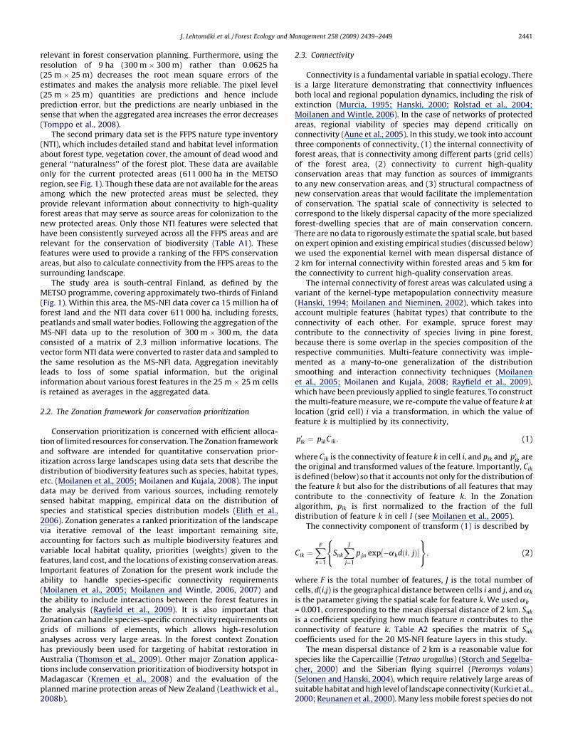
Fig. 2. A flow chart of the analysis. Numbered steps in the flow chart indicate m

particular forest types present both in the existing conservationareas and in their neighbourhood (Section 2.4, step 5). Theparameter of the negative exponential dispersal kernel wasselected to correspond to the mean dispersal distance of 5 km.The rational for using here a longer spatial scale than in thecalculation of connectivity within forest stands is that uncommondispersal events from the existing high-quality conservation areasmay lead to successful colonization of the new conservation areas.

The third connectivity component was added to address therequirement that the new protected areas should preferably belarge enough for practical implementation. We applied theboundary length penalty technique to increase the structuralcompactness of the selected forest areas (Possingham et al., 2000;Moilanen and Wintle, 2007).

2.4. The course of the analysis

Fig. 2 outlines the course of the analysis. The primary aim is toarrive at a recommendation as to where the new protected areas

ain analysis phases and correspond to the steps described in Section 2.4.

J. Lehtomaki et al. / Forest Ecology and Management 258 (2009) 2439–2449 2443

should be located. The primary data are the MS-NFI data, whichcover the entire country and therefore allow unbiased treatment ofall forested areas. The additional data from the currently protectedareas (Fig. 1) are helpful in identifying likely source areas forcolonization to the candidate new protected areas. The analysisinvolves the following steps:

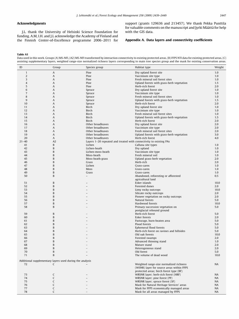
(1) Construction of the MS-NFI feature layers. Twenty feature layerswere extracted from the MS-NFI data, combining five forestproductivity classes and four dominant tree species. Each cell inthe grid was assigned to a combination layer AB if itrepresented productivity class A and dominant tree species B

(see Appendix, Table A1 for all the combinations). These gridswere then aggregated by summing up the values in individualgrid cells to achieve the resolution of 300 m. At this resolution,each grid cell can contribute to multiple forest types. To assessthe conservation value of each feature we calculated indexlayers using the formula

ffiffiffiffiffiffiffiffiffiffiffiffiffiffiffiffiffiffiffiffiffiffiffiffiffiffiffiffiffiage� volume

p, where age is given in

years and volume is total volume. This formula gives weight toforest areas with large volume of old trees.

(2) Weighting of the habitat types. Weights were assigned tofeatures in both the MS-NFI and NTI data sets based on theirconservation value as determined by experts. Highest weightswere given to highly productive forests areas and deciduousforests with a dominant tree species other than birch(Table A1). These criteria were used because species-richforest types are underrepresented in the current conservationnetwork and represent focal habitats in Finnish forestconservation (Virkkala and Toivonen, 1999).

(3) Quality of existing forest reserves as source areas for colonization.

We had additional data for the current reserves in the form ofnature type inventory (NTI) reflecting the quality of theconservation areas. Here we employed weighted, range-sizenormalized richness layers, which represent the fraction of thetotal known biodiversity features that occurs in each cell.Technically, these fractions are calculated as ai ¼

Pjw j f i j,

where w j is the weight of feature j, fij is the fraction of thedistribution of feature j in cell i, and the summation is takenacross the relevant features j (Moilanen and Kujala, 2008).Source quality was estimated separately for the classescorresponding to the four dominant tree species (layers 72–75 in Appendix Table A1). NTI features contributed to thequality of one or more of these source quality layers.

(4) Connectivity within the forest area. One copy of the MS-NFIlayers was entered into the analysis and transformed using themulti-feature connectivity operation to model internal con-nectivity of the forest area (Table A2; see also Section 2.3).Importantly, this operation accounts for partial similarity offorests that have different nominal classifications.

(5) Connectivity to current reserves. Another copy of the MS-NFIlayers was first transformed by internal connectivity (previousstep) and next by interaction connectivity to the currentconservation areas (Rayfield et al., 2009) This transformationincreases the value of the forest areas in the MS-NFI layers thatare well connected to high-quality current protected areas. Theweighted, range-size normalized richness layers (step 3) wereused as source area quality in the interaction connectivitymethod (Rayfield et al., 2009), meaning that connectivity wascalculated between similar habitat types inside and outside thecurrent conservation areas.

(6) Complementarity-based iterative hierarchical analysis of spatial

conservation priority. This analysis was conducted with theZonation software that was run in the additive benefit mode(Moilanen, 2007), with value z = 0.25 for the parameter of thepower function that scales conservation value as a function ofrepresentation. The boundary length penalty was used for extra

structural connectivity (Moilanen and Wintle, 2007; penaltyparameter b = 0.00003).

(7) Forcing the selection to the state-owned FAWS. A two-level maskfile was produced, with the current protected areas given thehighest priority and the FFPS FAWS the second-highest priority.No extra priority was given to privately owned forests,meaning that the cell removal order in Zonation was forcedto be first private land, then the FFPS FAWS and lastly the FFPSprotected areas. Within each of these three classes, the cellremoval order was free and determined by the rule of stepwiseminimization of marginal loss of conservation value.

(8) Post-processing and output. Post-processing analyses were doneto identify optimal extensions of the current protected areasbased on the priority rank maps produced by each Zonationrun. The optimal set of new conservation areas is the highest-ranked set of areas outside the current conservation areas.

The present analysis with 71 informative layers (Table A1) offeature data in a matrix of 2.3 million informative grid cells wasclose to the memory limit using the present version of Zonationoperating on a 32-bit Windows platform. Computation times on anordinary desktop PC were around 2 h per analysis.

3. Results

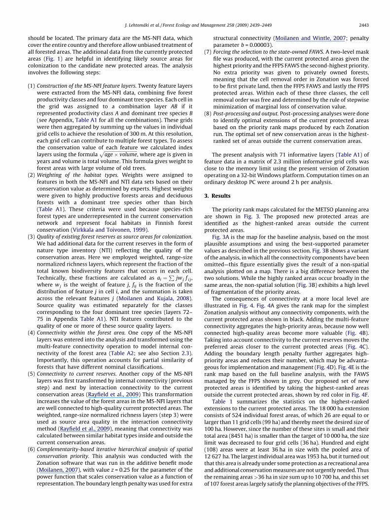
The priority rank maps calculated for the METSO planning areaare shown in Fig. 3. The proposed new protected areas areidentified as the highest-ranked areas outside the currentprotected areas.

Fig. 3A is the map for the baseline analysis, based on the mostplausible assumptions and using the best-supported parametervalues as described in the previous section. Fig. 3B shows a variantof the analysis, in which all the connectivity components have beenomitted—this figure essentially gives the result of a non-spatialanalysis plotted on a map. There is a big difference between thetwo solutions. While the highly ranked areas occur broadly in thesame areas, the non-spatial solution (Fig. 3B) exhibits a high levelof fragmentation of the priority areas.

The consequences of connectivity at a more local level areillustrated in Fig. 4. Fig. 4A gives the rank map for the simplestZonation analysis without any connectivity components, with thecurrent protected areas shown in black. Adding the multi-featureconnectivity aggregates the high-priority areas, because now wellconnected high-quality areas become more valuable (Fig. 4B).Taking into account connectivity to the current reserves moves thepreferred areas closer to the current protected areas (Fig. 4C).Adding the boundary length penalty further aggregates high-priority areas and reduces their number, which may be advanta-geous for implementation and management (Fig. 4D). Fig. 4E is therank map based on the full baseline analysis, with the FAWSmanaged by the FFPS shown in grey. Our proposed set of newprotected areas is identified by taking the highest-ranked areasoutside the current protected areas, shown by red color in Fig. 4F.

Table 1 summarizes the statistics on the highest-rankedextensions to the current protected areas. The 18 000 ha extensionconsists of 524 individual forest areas, of which 26 are equal to orlarger than 11 grid cells (99 ha) and thereby meet the desired size of100 ha. However, since the number of these sites is small and theirtotal area (8451 ha) is smaller than the target of 10 000 ha, the sizelimit was decreased to four grid cells (36 ha). Hundred and eight(108) areas were at least 36 ha in size with the pooled area of12 627 ha. The largest individual area was 1953 ha, but it turned outthat this area is already under some protection as a recreational areaand additional conservation measures are not urgently needed. Thusthe remaining areas>36 ha in size sum up to 10 700 ha, and this setof 107 forest areas largely satisfy the planning objectives of the FFPS.

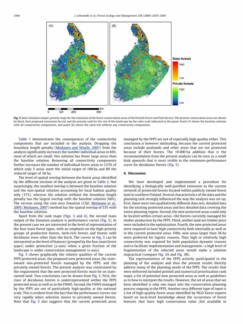
Fig. 3. Basic Zonation output, priority maps for the extension of the forest conservation areas of the Finnish Forest and Park Service. The present conservation areas are shown

by black, best proposed extensions by red, and the priority rank for the rest of the landscape by the color scale indicated in the panel. Panel (A) shows the baseline solution

with all connectivity components, and panel (B) shows the same but without any connectivity components.

J. Lehtomaki et al. / Forest Ecology and Management 258 (2009) 2439–24492444

Table 1 demonstrates the consequences of the connectivitycomponents that are included in the analysis. Dropping theboundary length penalty (Moilanen and Wintle, 2007) from theanalysis significantly increases the number individual areas to 845,most of which are small; this solution has fewer large areas thanthe baseline solution. Removing all connectivity componentsfurther increases the number of individual forest areas to 1270, ofwhich only 5 areas meet the initial target of 100 ha and 80 thereduced target of 36 ha.

The level of spatial overlap between the forest areas identifiedby the different versions of the analysis are given in Table 2. Notsurprisingly, the smallest overlap is between the baseline solutionand the non-spatial solution accounting for local habitat qualityonly (37%), whereas the solution without the boundary lengthpenalty has the largest overlap with the baseline solution (66%).The version using the core-area Zonation (CAZ; Moilanen et al.,2005; Moilanen, 2007) method has the spatial overlap of 53% withthe baseline solution.

Apart from the rank maps (Figs. 3 and 4), the second mainoutput of the Zonation analysis is performance curves (Fig. 5). Inthe present case we are interested in the level of representation ofthe four main forest types, with an emphasis on the high-prioritygroups of productive forests, herb-rich forests and forests withdeciduous trees other than the birch. The curves in Fig. 5 can beinterpreted as the level of features (grouped by the four main foresttypes) under protection (y-axis) when a given fraction of thelandscape is under conservation management (x-axis).

Fig. 5 shows graphically the relative qualities of the currentFFPS protected areas, the proposed new protected areas, the state-owned non-protected forests managed by the FFPS, and theprivately owned forests. The present analysis was constrained bythe requirement that the new protected forests must be on state-owned land. Two conclusions can be drawn from Fig. 5. First, theclass of deciduous forests is underrepresented within the FFPSprotected areas as well as in the FAWS. Second, the FAWS managedby the FFPS are not of particularly high-quality at the nationalscale. This is evident from the fact that the performance curves risevery rapidly when selection moves to privately owned forests.Note that Fig. 5 also suggests that the current protected areas

managed by the FFPS are not of especially high quality either. Thisconclusion is however misleading, because the current protectedareas include peatlands and other areas that are not protectedbecause of their forests. The 10 000 ha addition that is therecommendation from the present analysis can be seen as a smallkink upwards that is most visible in the minimum-performancecurve for deciduous forests (Fig. 5).

4. Discussion

We have developed and implemented a procedure foridentifying a biologically well-justified extension to the currentnetwork of protected forests located within publicly owned forestland in southern Finland. Several characteristics of the data and theplanning task strongly influenced the way the analysis was set up.First, there were two qualitatively different data sets, detailed datafor the existing protected areas and less detailed data covering theentire planning region. Second, the new protected areas could onlybe located within certain areas—the forests currently managed fortimber production by the FFPS. Third, neither land nor timber pricewere included in the optimization. Fourth, the new protected areaswere required to have high connectivity both internally as well asto the current protected areas. Fifth, new areas larger than 36 hawere preferred for logistic reasons. Thus high or relatively highconnectivity was required for both population dynamic reasonsand to facilitate implementation and management—a high level offragmentation of the selected areas would make a solutionimpractical (compare Fig. 3A and Fig. 3B).

The representatives of the FFPS actively participated in theplanning of the analysis and thus the present results directlyaddress many of the planning needs of the FFPS. The results thatwere delivered included printed and numerical prioritization rankmaps, a list of potential new protected areas as well as guidelinesas to how to interpret the results. However, the set of areas that wehave identified is only one input into the conservation planningprocess ongoing in the FFPS. Another very different type of input isa list of high-quality forest areas identified by NGO forest expertsbased on local-level knowledge about the occurrence of forestfeatures that have high conservation value (list available in

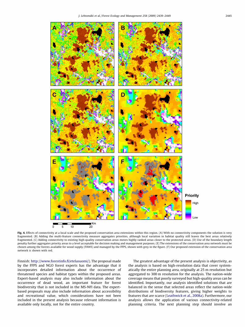
Fig. 4. Effects of connectivity at a local scale and the proposed conservation area extensions within this region. (A) With no connectivity components the solution is very

fragmented. (B) Adding the multi-feature connectivity measure aggregates priorities, although local variation in habitat quality still leaves the best areas relatively

fragmented. (C) Adding connectivity to existing high-quality conservation areas moves highly ranked areas closer to the protected areas. (D) Use of the boundary length

penalty further aggregates priority areas to a level acceptable for decision making and management purposes. (E) The extensions of the conservation area network must be

chosen among the forests available for wood supply (FAWS) and managed by the FFPS, shown with grey in the figure. (F) Our proposed extension of the conservation area

network is shown with red.

J. Lehtomaki et al. / Forest Ecology and Management 258 (2009) 2439–2449 2445

Finnish: http://www.forestinfo.fi/etelasuomi/). The proposal madeby the FFPS and NGO forest experts has the advantage that itincorporates detailed information about the occurrence ofthreatened species and habitat types within the proposed areas.Expert-based analysis may also include information about theoccurrence of dead wood, an important feature for forestbiodiversity that is not included in the MS-NFI data. The expert-based proposals may also include information about accessibilityand recreational value, which considerations have not beenincluded in the present analysis because relevant information isavailable only locally, not for the entire country.

The greatest advantage of the present analysis is objectivity, asthe analysis is based on high-resolution data that cover system-atically the entire planning area, originally at 25 m resolution butaggregated to 300 m resolution for the analysis. The nation-widecoverage means that poorly surveyed but high-quality areas can beidentified. Importantly, our analysis identified solutions that arebalanced in the sense that selected areas reflect the nation-widedistributions of biodiversity features, giving higher weights tofeatures that are scarce (Leathwick et al., 2008a). Furthermore, ouranalysis allows the application of various connectivity-relatedplanning criteria. The next planning step should involve an

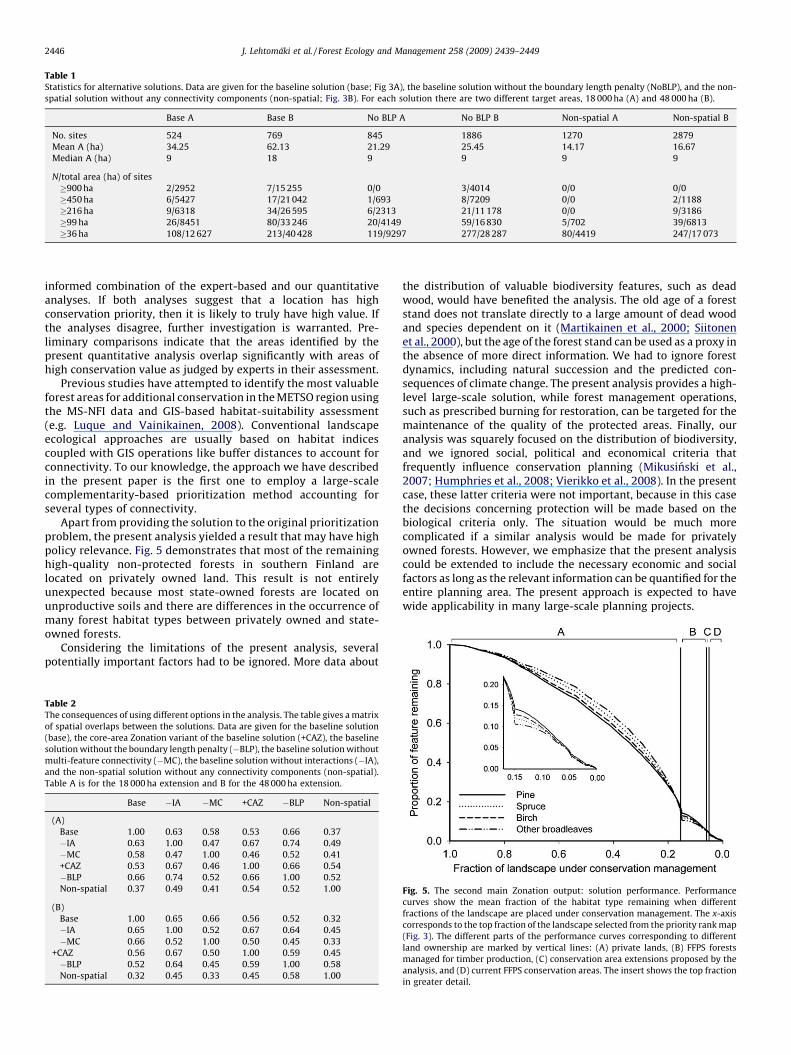
Table 1Statistics for alternative solutions. Data are given for the baseline solution (base; Fig 3A), the baseline solution without the boundary length penalty (NoBLP), and the non-

spatial solution without any connectivity components (non-spatial; Fig. 3B). For each solution there are two different target areas, 18 000 ha (A) and 48 000 ha (B).

Base A Base B No BLP A No BLP B Non-spatial A Non-spatial B

No. sites 524 769 845 1886 1270 2879

Mean A (ha) 34.25 62.13 21.29 25.45 14.17 16.67

Median A (ha) 9 18 9 9 9 9

N/total area (ha) of sites

�900 ha 2/2952 7/15 255 0/0 3/4014 0/0 0/0

�450 ha 6/5427 17/21 042 1/693 8/7209 0/0 2/1188

�216 ha 9/6318 34/26 595 6/2313 21/11 178 0/0 9/3186

�99 ha 26/8451 80/33 246 20/4149 59/16 830 5/702 39/6813

�36 ha 108/12 627 213/40 428 119/9297 277/28 287 80/4419 247/17 073

J. Lehtomaki et al. / Forest Ecology and Management 258 (2009) 2439–24492446

informed combination of the expert-based and our quantitativeanalyses. If both analyses suggest that a location has highconservation priority, then it is likely to truly have high value. Ifthe analyses disagree, further investigation is warranted. Pre-liminary comparisons indicate that the areas identified by thepresent quantitative analysis overlap significantly with areas ofhigh conservation value as judged by experts in their assessment.

Previous studies have attempted to identify the most valuableforest areas for additional conservation in the METSO region usingthe MS-NFI data and GIS-based habitat-suitability assessment(e.g. Luque and Vainikainen, 2008). Conventional landscapeecological approaches are usually based on habitat indicescoupled with GIS operations like buffer distances to account forconnectivity. To our knowledge, the approach we have describedin the present paper is the first one to employ a large-scalecomplementarity-based prioritization method accounting forseveral types of connectivity.

Apart from providing the solution to the original prioritizationproblem, the present analysis yielded a result that may have highpolicy relevance. Fig. 5 demonstrates that most of the remaininghigh-quality non-protected forests in southern Finland arelocated on privately owned land. This result is not entirelyunexpected because most state-owned forests are located onunproductive soils and there are differences in the occurrence ofmany forest habitat types between privately owned and state-owned forests.

Considering the limitations of the present analysis, severalpotentially important factors had to be ignored. More data about

Table 2The consequences of using different options in the analysis. The table gives a matrix

of spatial overlaps between the solutions. Data are given for the baseline solution

(base), the core-area Zonation variant of the baseline solution (+CAZ), the baseline

solution without the boundary length penalty (�BLP), the baseline solution without

multi-feature connectivity (�MC), the baseline solution without interactions (�IA),

and the non-spatial solution without any connectivity components (non-spatial).

Table A is for the 18 000 ha extension and B for the 48 000 ha extension.

Base �IA �MC +CAZ �BLP Non-spatial

(A)

Base 1.00 0.63 0.58 0.53 0.66 0.37

�IA 0.63 1.00 0.47 0.67 0.74 0.49

�MC 0.58 0.47 1.00 0.46 0.52 0.41

+CAZ 0.53 0.67 0.46 1.00 0.66 0.54

�BLP 0.66 0.74 0.52 0.66 1.00 0.52

Non-spatial 0.37 0.49 0.41 0.54 0.52 1.00

(B)

Base 1.00 0.65 0.66 0.56 0.52 0.32

�IA 0.65 1.00 0.52 0.67 0.64 0.45

�MC 0.66 0.52 1.00 0.50 0.45 0.33

+CAZ 0.56 0.67 0.50 1.00 0.59 0.45

�BLP 0.52 0.64 0.45 0.59 1.00 0.58

Non-spatial 0.32 0.45 0.33 0.45 0.58 1.00

the distribution of valuable biodiversity features, such as deadwood, would have benefited the analysis. The old age of a foreststand does not translate directly to a large amount of dead woodand species dependent on it (Martikainen et al., 2000; Siitonenet al., 2000), but the age of the forest stand can be used as a proxy inthe absence of more direct information. We had to ignore forestdynamics, including natural succession and the predicted con-sequences of climate change. The present analysis provides a high-level large-scale solution, while forest management operations,such as prescribed burning for restoration, can be targeted for themaintenance of the quality of the protected areas. Finally, ouranalysis was squarely focused on the distribution of biodiversity,and we ignored social, political and economical criteria thatfrequently influence conservation planning (Mikusinski et al.,2007; Humphries et al., 2008; Vierikko et al., 2008). In the presentcase, these latter criteria were not important, because in this casethe decisions concerning protection will be made based on thebiological criteria only. The situation would be much morecomplicated if a similar analysis would be made for privatelyowned forests. However, we emphasize that the present analysiscould be extended to include the necessary economic and socialfactors as long as the relevant information can be quantified for theentire planning area. The present approach is expected to havewide applicability in many large-scale planning projects.

Fig. 5. The second main Zonation output: solution performance. Performance

curves show the mean fraction of the habitat type remaining when different

fractions of the landscape are placed under conservation management. The x-axis

corresponds to the top fraction of the landscape selected from the priority rank map

(Fig. 3). The different parts of the performance curves corresponding to different

land ownership are marked by vertical lines: (A) private lands, (B) FFPS forests

managed for timber production, (C) conservation area extensions proposed by the

analysis, and (D) current FFPS conservation areas. The insert shows the top fraction

in greater detail.

J. Lehtomaki et al. / Forest Ecology and Management 258 (2009) 2439–2449 2447

Acknowledgments

J.L. thank the University of Helsinki Science Foundation forfunding. A.M, I.H. and J.L acknowledge the Academy of Finland andthe Finnish Center-of-Excellence programme 2006–2011 for

Table A1Data used in this work. Groups (A) MS-NFI, (A2) MS-NFI transformed by interaction conne

assisting supplementary layers, weighted range-size normalized richness layers corres

ID Group Species group

1 A Pine

2 A Pine

3 A Pine

4 A Pine

5 A Pine

6 A Spruce

7 A Spruce

8 A Spruce

9 A Spruce

10 A Spruce

11 A Birch

12 A Birch

13 A Birch

14 A Birch

15 A Birch

16 A Other broadleaves

17 A Other broadleaves

18 A Other broadleaves

19 A Other broadleaves

20 A Other broadleaves

21–40 A2 Layers 1–20 repeated and treat

41 B Lichen

42 B Lichen-heath

43 B Lichen-moss-heath

44 B Moss-heath

45 B Moss-heath-grass

46 B Grass

47 B Lichen

48 B Moss

49 B Grass

50 B –

51 B –

52 B –

53 B –

54 B –

55 B –

56 B –

57 B –

58 B –

59 B –

60 B –

61 B –

62 B –

63 B –

64 B –

65 B –

66 B –

67 B –

68 B –

69 B –

70 B –

71 B –

Additional supplementary layers used during the analysis

72 C –

73 C –

74 C –

75 C –

76 C –

77 C –

78 C –

support (grants 129636 and 213457). We thank Pekka Punttilafor valuable comments on the manuscript and Jyrki Maatta for helpwith the GIS data.

Appendix A. Data layers and connectivity coefficients

ctivity to existing protected areas, (B) FFPS NTI data for existing protected areas, (C)

ponding to main tree species group and the mask for existing conservation areas.

Habitat type Weight

Dry upland forest site 1.0

Vaccinium site type 1.0

Fresh mineral soil forest sites 1.0

Upland forests with grass-herb vegetation 1.5

Herb-rich forest 2.0

Dry upland forest site 1.0

Vaccinium site type 1.0

Fresh mineral soil forest sites 1.0

Upland forests with grass-herb vegetation 1.5

Herb-rich forest 2.0

Dry upland forest site 1.0

Vaccinium site type 1.0

Fresh mineral soil forest sites 1.0

Upland forests with grass-herb vegetation 1.5

Herb-rich forest 2.0

Dry upland forest site 2.0

Vaccinium site type 2.0

Fresh mineral soil forest sites 2.0

Upland forests with grass-herb vegetation 3.0

Herb-rich forest 4.0

ed with connectivity to existing PAs

Calluna site types 1.0

Dry upland 1.0

Vaccinium site type 1.0

Fresh mineral soil 1.0

Upland grass-herb vegetation 2.0

Herb-rich 2.0

Grass-carex 1.0

Grass-carex 1.0

Grass-carex 1.0

Abandoned, reforesting or afforested

agricultural land

0.5

Esker islands 10.0

Forested dunes 2.0

Limy rocky outcrops 10.0

Silicate rocky outcrops 2.0

Pioneer vegetation on rocky outcrops 2.0

Natural forests 5.0

Hardwood forests 10.0

Primary succession vegetation on

postglacial rebound ground

5.0

Herb-rich forest 5.0

Esker forests 2.0

Pasturage, burn-beaten area 5.0

Flood forests 5.0

Ephemeral flood forests 5.0

Herb-rich forest on ravines and hillsides 5.0

Old oak forests 10.0

Forested swamps 2.0

Advanced thinning stand 1.0

Mature stand 2.0

Heterogeneous stand 2.0

Old forest 5.0

The volume of dead wood 10.0

Weighted range-size normalized richness

(WSNR) layer for source areas within FFPS

protected areas; birch forest type (BF)

NA

WRSNR layer; herb-rich forest (HRF) NA

WRSNR layer; pine forest (PF) NA

WRSNR layer; spruce forest (SF) NA

Mask for Natural Heritage Services’ areas NA

Mask for FFPS economically managed areas NA

Mask for all areas managed by FFPS NA

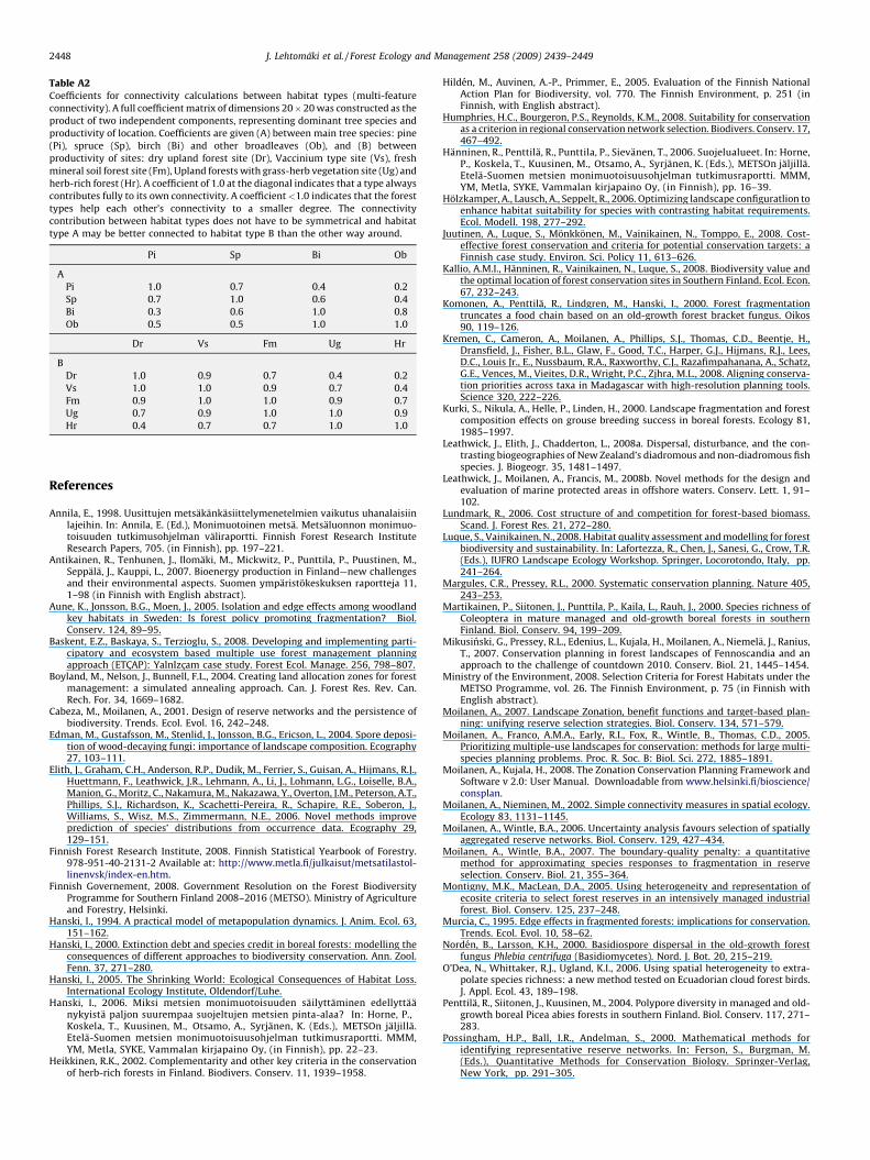
Table A2Coefficients for connectivity calculations between habitat types (multi-feature

connectivity). A full coefficient matrix of dimensions 20�20 was constructed as the

product of two independent components, representing dominant tree species and

productivity of location. Coefficients are given (A) between main tree species: pine

(Pi), spruce (Sp), birch (Bi) and other broadleaves (Ob), and (B) between

productivity of sites: dry upland forest site (Dr), Vaccinium type site (Vs), fresh

mineral soil forest site (Fm), Upland forests with grass-herb vegetation site (Ug) and

herb-rich forest (Hr). A coefficient of 1.0 at the diagonal indicates that a type always

contributes fully to its own connectivity. A coefficient<1.0 indicates that the forest

types help each other’s connectivity to a smaller degree. The connectivity

contribution between habitat types does not have to be symmetrical and habitat

type A may be better connected to habitat type B than the other way around.

Pi Sp Bi Ob

A

Pi 1.0 0.7 0.4 0.2

Sp 0.7 1.0 0.6 0.4

Bi 0.3 0.6 1.0 0.8

Ob 0.5 0.5 1.0 1.0

Dr Vs Fm Ug Hr

B

Dr 1.0 0.9 0.7 0.4 0.2

Vs 1.0 1.0 0.9 0.7 0.4

Fm 0.9 1.0 1.0 0.9 0.7

Ug 0.7 0.9 1.0 1.0 0.9

Hr 0.4 0.7 0.7 1.0 1.0

J. Lehtomaki et al. / Forest Ecology and Management 258 (2009) 2439–24492448

References

Annila, E., 1998. Uusittujen metsakankasiittelymenetelmien vaikutus uhanalaisiinlajeihin. In: Annila, E. (Ed.), Monimuotoinen metsa. Metsaluonnon monimuo-toisuuden tutkimusohjelman valiraportti. Finnish Forest Research InstituteResearch Papers, 705. (in Finnish), pp. 197–221.

Antikainen, R., Tenhunen, J., Ilomaki, M., Mickwitz, P., Punttila, P., Puustinen, M.,Seppala, J., Kauppi, L., 2007. Bioenergy production in Finland—new challengesand their environmental aspects. Suomen ymparistokeskuksen raportteja 11,1–98 (in Finnish with English abstract).

Aune, K., Jonsson, B.G., Moen, J., 2005. Isolation and edge effects among woodlandkey habitats in Sweden: Is forest policy promoting fragmentation? Biol.Conserv. 124, 89–95.

Baskent, E.Z., Baskaya, S., Terzioglu, S., 2008. Developing and implementing parti-cipatory and ecosystem based multiple use forest management planningapproach (ETCAP): YalnIzcam case study. Forest Ecol. Manage. 256, 798–807.

Boyland, M., Nelson, J., Bunnell, F.L., 2004. Creating land allocation zones for forestmanagement: a simulated annealing approach. Can. J. Forest Res. Rev. Can.Rech. For. 34, 1669–1682.

Cabeza, M., Moilanen, A., 2001. Design of reserve networks and the persistence ofbiodiversity. Trends. Ecol. Evol. 16, 242–248.

Edman, M., Gustafsson, M., Stenlid, J., Jonsson, B.G., Ericson, L., 2004. Spore deposi-tion of wood-decaying fungi: importance of landscape composition. Ecography27, 103–111.

Elith, J., Graham, C.H., Anderson, R.P., Dudik, M., Ferrier, S., Guisan, A., Hijmans, R.J.,Huettmann, F., Leathwick, J.R., Lehmann, A., Li, J., Lohmann, L.G., Loiselle, B.A.,Manion, G., Moritz, C., Nakamura, M., Nakazawa, Y., Overton, J.M., Peterson, A.T.,Phillips, S.J., Richardson, K., Scachetti-Pereira, R., Schapire, R.E., Soberon, J.,Williams, S., Wisz, M.S., Zimmermann, N.E., 2006. Novel methods improveprediction of species’ distributions from occurrence data. Ecography 29,129–151.

Finnish Forest Research Institute, 2008. Finnish Statistical Yearbook of Forestry.978-951-40-2131-2 Available at: http://www.metla.fi/julkaisut/metsatilastol-linenvsk/index-en.htm.

Finnish Governement, 2008. Government Resolution on the Forest BiodiversityProgramme for Southern Finland 2008–2016 (METSO). Ministry of Agricultureand Forestry, Helsinki.

Hanski, I., 1994. A practical model of metapopulation dynamics. J. Anim. Ecol. 63,151–162.

Hanski, I., 2000. Extinction debt and species credit in boreal forests: modelling theconsequences of different approaches to biodiversity conservation. Ann. Zool.Fenn. 37, 271–280.

Hanski, I., 2005. The Shrinking World: Ecological Consequences of Habitat Loss.International Ecology Institute, Oldendorf/Luhe.

Hanski, I., 2006. Miksi metsien monimuotoisuuden sailyttaminen edellyttaanykyista paljon suurempaa suojeltujen metsien pinta-alaa? In: Horne, P.,Koskela, T., Kuusinen, M., Otsamo, A., Syrjanen, K. (Eds.), METSOn jaljilla.Etela-Suomen metsien monimuotoisuusohjelman tutkimusraportti. MMM,YM, Metla, SYKE, Vammalan kirjapaino Oy, (in Finnish), pp. 22–23.

Heikkinen, R.K., 2002. Complementarity and other key criteria in the conservationof herb-rich forests in Finland. Biodivers. Conserv. 11, 1939–1958.

Hilden, M., Auvinen, A.-P., Primmer, E., 2005. Evaluation of the Finnish NationalAction Plan for Biodiversity, vol. 770. The Finnish Environment, p. 251 (inFinnish, with English abstract).

Humphries, H.C., Bourgeron, P.S., Reynolds, K.M., 2008. Suitability for conservationas a criterion in regional conservation network selection. Biodivers. Conserv. 17,467–492.

Hanninen, R., Penttila, R., Punttila, P., Sievanen, T., 2006. Suojelualueet. In: Horne,P., Koskela, T., Kuusinen, M., Otsamo, A., Syrjanen, K. (Eds.), METSOn jaljilla.Etela-Suomen metsien monimuotoisuusohjelman tutkimusraportti. MMM,YM, Metla, SYKE, Vammalan kirjapaino Oy, (in Finnish), pp. 16–39.

Holzkamper, A., Lausch, A., Seppelt, R., 2006. Optimizing landscape configuratlion toenhance habitat suitability for species with contrasting habitat requirements.Ecol. Modell. 198, 277–292.

Juutinen, A., Luque, S., Monkkonen, M., Vainikainen, N., Tomppo, E., 2008. Cost-effective forest conservation and criteria for potential conservation targets: aFinnish case study. Environ. Sci. Policy 11, 613–626.

Kallio, A.M.I., Hanninen, R., Vainikainen, N., Luque, S., 2008. Biodiversity value andthe optimal location of forest conservation sites in Southern Finland. Ecol. Econ.67, 232–243.

Komonen, A., Penttila, R., Lindgren, M., Hanski, I., 2000. Forest fragmentationtruncates a food chain based on an old-growth forest bracket fungus. Oikos90, 119–126.

Kremen, C., Cameron, A., Moilanen, A., Phillips, S.J., Thomas, C.D., Beentje, H.,Dransfield, J., Fisher, B.L., Glaw, F., Good, T.C., Harper, G.J., Hijmans, R.J., Lees,D.C., Louis Jr., E., Nussbaum, R.A., Raxworthy, C.J., Razafimpahanana, A., Schatz,G.E., Vences, M., Vieites, D.R., Wright, P.C., Zjhra, M.L., 2008. Aligning conserva-tion priorities across taxa in Madagascar with high-resolution planning tools.Science 320, 222–226.

Kurki, S., Nikula, A., Helle, P., Linden, H., 2000. Landscape fragmentation and forestcomposition effects on grouse breeding success in boreal forests. Ecology 81,1985–1997.

Leathwick, J., Elith, J., Chadderton, L., 2008a. Dispersal, disturbance, and the con-trasting biogeographies of New Zealand’s diadromous and non-diadromous fishspecies. J. Biogeogr. 35, 1481–1497.

Leathwick, J., Moilanen, A., Francis, M., 2008b. Novel methods for the design andevaluation of marine protected areas in offshore waters. Conserv. Lett. 1, 91–102.

Lundmark, R., 2006. Cost structure of and competition for forest-based biomass.Scand. J. Forest Res. 21, 272–280.

Luque, S., Vainikainen, N., 2008. Habitat quality assessment and modelling for forestbiodiversity and sustainability. In: Lafortezza, R., Chen, J., Sanesi, G., Crow, T.R.(Eds.), IUFRO Landscape Ecology Workshop. Springer, Locorotondo, Italy, pp.241–264.

Margules, C.R., Pressey, R.L., 2000. Systematic conservation planning. Nature 405,243–253.

Martikainen, P., Siitonen, J., Punttila, P., Kaila, L., Rauh, J., 2000. Species richness ofColeoptera in mature managed and old-growth boreal forests in southernFinland. Biol. Conserv. 94, 199–209.

Mikusinski, G., Pressey, R.L., Edenius, L., Kujala, H., Moilanen, A., Niemela, J., Ranius,T., 2007. Conservation planning in forest landscapes of Fennoscandia and anapproach to the challenge of countdown 2010. Conserv. Biol. 21, 1445–1454.

Ministry of the Environment, 2008. Selection Criteria for Forest Habitats under theMETSO Programme, vol. 26. The Finnish Environment, p. 75 (in Finnish withEnglish abstract).

Moilanen, A., 2007. Landscape Zonation, benefit functions and target-based plan-ning: unifying reserve selection strategies. Biol. Conserv. 134, 571–579.

Moilanen, A., Franco, A.M.A., Early, R.I., Fox, R., Wintle, B., Thomas, C.D., 2005.Prioritizing multiple-use landscapes for conservation: methods for large multi-species planning problems. Proc. R. Soc. B: Biol. Sci. 272, 1885–1891.

Moilanen, A., Kujala, H., 2008. The Zonation Conservation Planning Framework andSoftware v 2.0: User Manual. Downloadable from www.helsinki.fi/bioscience/consplan.

Moilanen, A., Nieminen, M., 2002. Simple connectivity measures in spatial ecology.Ecology 83, 1131–1145.

Moilanen, A., Wintle, B.A., 2006. Uncertainty analysis favours selection of spatiallyaggregated reserve networks. Biol. Conserv. 129, 427–434.

Moilanen, A., Wintle, B.A., 2007. The boundary-quality penalty: a quantitativemethod for approximating species responses to fragmentation in reserveselection. Conserv. Biol. 21, 355–364.

Montigny, M.K., MacLean, D.A., 2005. Using heterogeneity and representation ofecosite criteria to select forest reserves in an intensively managed industrialforest. Biol. Conserv. 125, 237–248.

Murcia, C., 1995. Edge effects in fragmented forests: implications for conservation.Trends. Ecol. Evol. 10, 58–62.

Norden, B., Larsson, K.H., 2000. Basidiospore dispersal in the old-growth forestfungus Phlebia centrifuga (Basidiomycetes). Nord. J. Bot. 20, 215–219.

O’Dea, N., Whittaker, R.J., Ugland, K.I., 2006. Using spatial heterogeneity to extra-polate species richness: a new method tested on Ecuadorian cloud forest birds.J. Appl. Ecol. 43, 189–198.

Penttila, R., Siitonen, J., Kuusinen, M., 2004. Polypore diversity in managed and old-growth boreal Picea abies forests in southern Finland. Biol. Conserv. 117, 271–283.

Possingham, H.P., Ball, I.R., Andelman, S., 2000. Mathematical methods foridentifying representative reserve networks. In: Ferson, S., Burgman, M.(Eds.), Quantitative Methods for Conservation Biology. Springer-Verlag,New York, pp. 291–305.

J. Lehtomaki et al. / Forest Ecology and Management 258 (2009) 2439–2449 2449

Pressey, R.L., Cabeza, M., Watts, M.E., Cowling, R.M., Wilson, K.A., 2007. Conserva-tion planning in a changing world. Trends Ecol. Evol. 22, 583–592.

Puumalainen, J., Kennedy, P., Folving, S., 2003. Monitoring forest biodiversity: aEuropean perspective with reference to temperate and boreal forest zone. J.Environ. Manage. 67, 5–14.

Pykala, J., 2004. Effects of new forestry practices on rare epiphytic macrolichens.Conserv. Biol. 18, 831–838.

Rassi, P., Alanen, A., Kanerva, T., Mannerkoski, I., 2001. The 2000 Red List of FinnishSpecies. Ministry of Environment, Helsinki.

Rayfield, B., James, P.M.A., Fall, A., Fortin, M.J., 2008. Comparing static versusdynamic protected areas in the Quebec boreal forest. Biol. Conserv. 141,438–449.

Rayfield, B., Moilanen, A., Fortin, M.-J., 2009. Incorporating consumer–resourcespatial interactions in reserve design. Ecol. Modell. 220, 725–733.

Reunanen, P., Monkkonen, M., Nikula, A., 2000. Managing boreal forest landscapesfor flying squirrels. Conserv. Biol. 14, 218–226.

Ricker, M., Ramirez-Krauss, I., Ibarra-Manriquez, G., Martinez, E., Ramos, C.H.,Gonzalez-Medellin, G., Gomez-Rodriguez, G., Palacio-Prieto, J.L., Hernandez,H.M., 2007. Optimizing conservation of forest diversity: a country-wideapproach in Mexico. Biodivers. Conserv. 16, 1927–1957.

Rolstad, J., Saetersdal, M., Gjerde, I., Storaunet, K.O., 2004. Wood-decaying fungiin boreal forest: are species richness and abundances influenced by small-scale spatiotemporal distribution of dead wood? Biol. Conserv. 117, 539–555.

Sarkar, S., Pressey, R.L., Faith, D.P., Margules, C.R., Fuller, T., Stoms, D.M., Moffett, A.,Wilson, K.A., Williams, K.J., Williams, P.H., Andelman, S., 2006. Biodiversityconservation planning tools: present status and challenges for the future. Ann.Rev. Environ. Resour. 31, 123–159.

Selonen, V., Hanski, I.K., 2004. Young flying squirrels (Pteromys volans) dispersing infragmented forests. Behav. Ecol. 15, 564–571.

Siitonen, J., Martikainen, P., Punttila, P., Rauh, J., 2000. Coarse woody debris andstand characteristics in mature managed and old-growth boreal mesic forests insouthern Finland. Forest Ecol. Manage. 128, 211–225.

Soja, A.J., Tchebakova, N.M., French, N.H.F., Flannigan, M.D., Shugart, H.H., Stocks,B.J., Sukhinin, A.I., Parfenova, E.I., Chapin Iii, F.S., Stackhouse, J.P.W., 2007.

Climate-induced boreal forest change: predictions versus current observations.Glob. Planet. Change 56, 274–296.

Steinitz, O., Heller, J., Tsoar, A., Rotem, D., Kadmon, R., 2005. Predicting regionalpatterns of similarity in species composition for conservation planning. Con-serv. Biol. 19, 1978–1988.

Storch, I., Segelbacher, G., 2000. Genetic correlates of spatial population structure incentral European capercaillie Tetrao urogallus and black grouse T-tetrix: aproject in progress. Wildl. Biol. 6, 305–310.

Thomson, J.R., Moilanen, A.J., Vesk, P.A., Bennett, A.F., Mac Nally, R., 2009. Where andwhen to revegetate: a quantitative method for scheduling landscape recon-struction. Ecol. Appl. 19, 817–828.

Tikkanen, O.P., Martikainen, P., Hyvarinen, E., Junninen, K., Kouki, J., 2006. Red-listedboreal forest species of Finland: associations with forest structure, tree species,and decaying wood. Ann. Zool. Fenn. 43, 373–383.

Tomppo, E., 2006a. The Finnish multi-source National Forest Inventory—small areaestimation and map production. In: Kangas, A., Maltamo, M. (Eds.), Forestinventory: Methodology and Applications (Managing Forest Ecosystems).Springer, Dordrecht, pp. 195–224.

Tomppo, E., 2006b. The Finnish National Forest Inventory. In: Kangas, A., Maltamo,M. (Eds.), Forest inventory: Methodology and applications (Managing ForestEcosystems). Springer, Dordrecht, pp. 179–194.

Tomppo, E., Haakana, M., Katila, M., Perasaari, J., 2008. Multi-source National ForestInventory—Methods and Applications. Springer.

Vierikko, K., Vehkamaki, S., Niemela, J., Pellikka, J., Linden, H., 2008. Meeting theecological, social and economic needs of sustainable forest management at aregional scale. Scand. J. Forest Res. 23, 431–444.

Virkkala, R., Korhonen, K.T., Haapanen, R., Aapala, K., 2000. Protected Forests andMires in Forest and Mire Vegetation Zones in Finland based on the 8th NationalForest Inventory, vol. 395. Finnish Environment, 1–49 (in Finnish with Englishabstract).

Virkkala, R., Toivonen, H., 1999. Maintaining Biological Diversity in Finnish forests,vol. 278. Finnish Environment, p. 56.

Virolainen, K.M., Nattinen, K., Suhonen, J., Kuitunen, M., 2001. Selecting herb-richforest networks to protect different measures of biodiversity. Ecol. Appl. 11,411–420.