Applying evolutionary computing methods for

decision support: towards optimizing technical

trading strategies on the Johannesburg Stock

Exchange.

The final project report for HONPR2C.

Johann G. Muller,

Student Number: 3114-696-1

Johannesburg16 December 2010

Abstract

This project is aimed at testing the Efficient Market Hypothesisthrough the use of genetic algorithms to simulate the application oftechnical trading rules on the Johannesburg Stock Exchange.

1 Introduction

1.1 Background

The stock market has attracted and repelled many investors since the DutchEast India Company became the first company to issue shares and bondson the Amsterdam Stock Exchange in 1602 [Wik]. Since then investors havebeen continuously seeking for ways to “beat the market” and obtain superiorreturns on their investments. Most academics favour the Efficient MarketHypothesis in this regard, which simplistically states that individuals arenot able to consistently outperform the market. The project explores thishypothesis in more detail.

1.2 Scope

This project is aimed at illustrating the use of genetic algorithms and sim-ple artificial neural networks to develop a decision support system, writtenin C#, for optimal technical trading strategies, and it did not venture toinvestigate the particularly onerous task of forecasting future stock prices

1

The initial approach was focused on a number of high volume stocks tradedon the Johannesburg Stock Exchange. In the end, the analysis was focusedon the share price information of Anglo American PLC with share codeAGL trading on the Johannesburg Stock Exchange over the period 1 January2003 to 31 December 2006.

1.3 Approach

The approach followed in this project was to use a genetic algorithm togenerate successive populations of trading agents that used a simple neuralnetwork to select a set of trading rules and triggers to generate buy and sellsignals for near optimal returns, based on historical data. The model wasthen used to generate buy and sell signals for an out of sample set of dataand the performance of the algorithm was evaluated against a traditional‘buy and hold’ strategy.

2 Overview of Stock Markets

This overview is an attempt to summarize some of the key academic studiesthat pertain to stock market behaviour and the randomness thereof. Itstarts off with a general discussion of the approaches to share trading andthen briefly state the main hypothesis and models used in academic analysisof the stock market behaviour.

2.1 Stock Market Basics

In its simplest form stock markets are marketplaces where public companies(those trading on the stock market or exchange) list their shares in orderto raise capital from investors. This capital is then used to increase theearnings potential of the company. The investor essentially buys a stake inthe company and carries the risk and reward associated with the stake orshare in the company. If the company performs well it will return some ofthe profits in the form of dividends to the investors (shareholders), and theshare price (capital value of the stake) will typically increase. In the samemanner the share price of a company that performs poorly will decline andbecome a less attractive investment to buy.

2.2 Trading Strategies

Investors in the stock market have different motives for investing and basedon their motives, they often follow different strategies and exhibit differentbehaviours. Broadly investors can be divided into long term and short terminvestors. Long term investors are often investing for sustainable cash flows

2

from reputable companies and are more concerned with the long term re-turns in the form of cash dividends and any capital growth is of secondaryconcern to them.On the other hand, short term investors are often speculative in nature andthey are looking for short term capital gains and aim to exploit the underly-ing volatility in the share price to their advantage. The short term investoroften perceives the long term investor as conservative and naive, whilst thelatter often perceive the short term investors as speculative, gambling andfoolish. Obviously, most stock market investors are somewhere in betweenthe extremes. The profit motive of the stock market investor often leadsto them adopting either a fundamental or technical analysis approach toinvestment decision making.

2.2.1 Fundamental Analysis

Fundamental analysis is named as such, because the determination of thefuture growth of the share price as based on tangible or “fundamental”financial information, such as the underlying well being of the economy,supply and demand trends, the performance of industry groups, the com-pany’s financial statements, the management team, the business model, thecompetition in the market and many other tangible factors. The premiseof fundamental analysis is that the share price of a company reflects its fu-ture earnings potential, which in turn is determined by the aforementionedfactors. Fundamental analysis is most likely the strategy of choice for longterm investors in the stock market.

2.2.2 Technical Analysis

Technical analysis in its simplest definition is the forecasting of future pricemovements based on the examination of previous price movements. It usesa number of technical trading rules and strategies developed over a numberof years, based on mathematical, statistical and heuristic models of stockprice movements. It discounts the notion that share price movements arerandom in nature, and that future share price movements are independentof the past prices. Technical analysis is most likely the strategy of choicefor short term investors in the stock market.Technical analysis relies on ‘charting’ of the historic price information ofstocks in order to determine various trends which are claimed to provideinvestors with the ability to forecast trend changes. This information is thenused to determine whether the current market price is signalling whether aspecific stock has to be bought or sold. Due to the vast number of technicaltrading rules that exist in popular investment, it is not feasible to evaluate alland most approaches, including this proposal, focus on a sub-set of technicaltrading rules in their research and investigations.

3

A detailed description of the technical trading rules employed in this studyand their key characteristics are covered in Appendix A to this report.

2.3 Random Walk Hypothesis

In his 1900 thesis titled The Theory of Speculation, Louis Bachelier arguablylaid the foundation for many of the theories governing the academic descrip-tion of stock markets including the Random Walk Hypothesis. The theorythat stock prices move randomly was proposed by Maurice Kendall [Ken53]in 1953 and this was developed in more detail by Cootner in his book titled“The Random Character of Stock Market Prices” published in 1964 [Coo64].Fama used this reference in his publication titled “Random Walks in StockMarket Prices” [Fam65] which together with Burton Malkiel’s book “A Ran-dom Walk Down Wall Street” institutionalized the term. one of the earliestworks in literature which gave formal mathematical context to the move-ment of share prices, is Osborne’s “Brownian Motion in the Stock Market”which postulates that stock market prices contains all known information ofthe stock at any point in time and that the next movement in the price ofthe stock is random and follows a Brownian motion, after Robert Brown’sobservations of pollen grains in 1827. This random movement is not depen-dant on any previous movement of the stock price and hence the RandomWalk Hypothesis states that share prices cannot be predicted.To test the hypothesis, Malkiel did an experiment, documented in his book[Mal73] where he flipped a coin to represent random movements in the stockprice. The resultant stock price graph was then given to some technical an-alysts which made suggestion based on information they perceived to becontained in the graphs. Understandably they were not impressed whentold that the share price movements was created by the flipping of a coin.On the other side of the spectrum, Lo and MacKinley wrote a book called“A Non-Random Walk Down Wall Street” [LM99] in which they postulatethat the random walk hypothesis is incorrect and they propose an AdaptiveMarket Hypothesis which states that the stock market a great measure ofpredictability. In reality the Random Walk Hypothesis has not conclusivelybeing proven true or false on the basis of sound reasoning, and most au-thors tried to use empirical test to prove their points for and against thehypothesis.

2.4 Efficient Market Hypothesis

Louis Bachelier arguably also laid the foundation for the Efficient-MarketHypothesis formally postulated by Eugene Fama in his Ph.D thesis and sum-marized in his submission to the Twenty-Eight Annual Meeting of the Amer-ican Finance Association New York at the end of December 1969 [Fam70].This hypothesis was very eloquently summarized by Schlater, Haugen and

4

Wichern [SHW80] as follows:

A perfectly efficient capital market is one in which all availablerelevant information is fully reflected in the market prices of se-curities. The proponents of market efficiency argue that while itmay be nearly impossible for any one individual to obtain andefficiently analyse all relevant information, sophisticated and in-formed investors exist in sufficient numbers to make today’s mar-ket price approximate the best estimate of the true intrinsic valueof any security. In their continuing search for under and over-valued issues, these investors price away any opportunities forabnormally large profits that may exist in the marketplace. Insuch a market no trading rule is able to distinguish between prof-itable and unprofitable investments, and it should be impossiblefor any investor to ‘beat the market’ in the sense of earning arate of return that consistently exceeds the average rate of returnon other investments of comparable risk.

This hypothesis therefore essentially states that no one individual can out-perform the market at any given point in time, because the stock price atany specific point in time is a fair price, due to the assumption that allknown information has been discounted in by investors. This hypothesiswas the subject of much academic debate and led to a flurry of publicationsdiscussing the merits of the claims made therein.The Efficient-Market Hypothesis probably led to the biggest divide betweenacademic finance and industry practice, which is arguably the gap that existsbetween technical analysts and their academic critics [LMW02]. The prac-tical reality is that most investors practice an element of technical analysisin their investment strategies, and various authors [LMW02] have proventhat there is merit in evaluating technical trading rules in stock markets toproduce higher than expected profits.Research unearthed a number of studies attempting to validate [CY97] orinvalidate [SHW80],[MYR06] the hypothesis. The use of evolutionary com-puting methods, such as genetic algorithms, genetic programming and arti-ficial neural networks, to forecast stock prices and gain some form of advan-tage over the general market, appeared to be prevalent and has biased theapproach proposed taken in this project submission.

2.5 Capital Asset Pricing Model

The Capital Asset Pricing Model is an economic model for the valuation ofstocks, securities, derivatives and/or assets in a diversified portfolio. It wasdeveloped independently by a number of economists, but Sharpe, Markowitzand Merton Miller jointly received the Nobel prize in economics for theirwork toward formulating it. The model proposes a theoretical expected

5

return of an asset, given the market risk or systemic risk, the expected returnof the market or the asset class and the expected return of a theoretical risk-free asset. The Capital Asset Pricing Model assumes that an investor wouldinvest in a specific asset or security if the ratio of return to risk of thegiven asset is at least as good as the market return to risk ratio. For largemarkets, the market risk β is assumed to be unity. Therefore the CapitalAsset Pricing Model can be formulated as follows[Sha64]:

E[Ri]−Rf

βim= E[Rm]−Rf

Solving for E[Ri]: E[Ri] = Rf + βim(E[Rm]−Rf ).

Where:

• E[Ri] is the expected return of the security or asset under considera-tion,

• Rf is the risk free rate of interest,

• βim is the sensitivity of the expeced return in relation to the expectedmarket return and βim = Cov(Ri,Rm)

V arRm

• E[Rm] is the expected market returns

• E[Rm]−Rf is often referred to as the market premium or risk premium

The Capital Asset Pricing Model is only valid within a special set of as-sumptions [Per04]:

• Investors are risk averse and maximise their investments at the end ofa single period.

• All investors in the market have the same information and observe thesame beliefs.

• The expected asset returns adheres to the normal distribution.

• A risk free asset exists and investors can borrow or lend unlimitedamounts at the risk free rate.

• There is a set number of assets and they remain fixed in the period ofthe model.

• All assets are perfectly divisible and are priced competitively.

• The borrowing rate is equal to the lending rate and information doesnot cost money.

• There are no market imperfections such as taxes, restrictions or regu-lations for short-selling.

6

Although the Capital Asset Pricing Model has its limitations, it forms theunder lying theory to the Sharpe Ratio and consequently the Modigliani RiskAdjusted Ratio used in this project to evaluate solutions.

3 Theoretical Foundation of Genetic Algorithms

In order to illuminate the approach followed in this project, a basic summaryof genetic algorithm theory is provided here.

3.1 Introduction

Genetic Algorithms were derived as an analogy of the biological evolutionprocess. It is essentially a computational search technique that uses evolu-tionary biological concepts such as inheritance, recombination (or crossover),mutation and selection to improve results from generation to generation ofpotential matches. These techniques are typically used to find exact orapproximate answers to optimization and search problems. Genetic tech-niques have gained popularity in recent years due to the increasing amountof computing power available, the ability to conduct parallel processing,and the relative ease of programming the techniques in modern computinglanguages.

3.2 History

Various computer scientists, including Box, Friedman, Bledsoe, Bremer-mann, Reed, Toombs and Baricelli developed algorithms for application inoptimization problems in the 1950s and 1960s. Genetic Algorithms were in-vented by John Holland in the 1960s, and further developed by Holland, hisstudents and colleagues at the University of Michigan in the 1960s and 1970s.Their aim was to develop ways in which the natural adaptation processescould be used in the design of generic computer algorithms, which can beused to solve a range of different problems. Holland published a book titledAdaptation in Natural and Artificial Systems in 1975 in which he presenteda theoretical framework which abstracts the process of biological evolutionthus giving birth to the Genetic Algorithm.[Hol92]

3.3 Biological Terminology

All living organisms’ cells contain genetic material in the form of specific pro-teins called DNA. The DNA are organised in strands called chromosomes.The chromosomes consist of specific blocks of DNA that can transcribe orsynthesize proteins that manifests in the organism having certain traits (e.g.varying eye colour). These blocks of DNA are referred to as genes. The genesin turn contains alleles which encodes the specific variations in specific traits

7

(e.g. blue eyes, brown eyes, etc.). These terms are depicted in Figure 1.The collection of all the chromosomes in an organism is called its genome,and the set of genes contained in the genome is called the genotype of the or-ganism. Organisms with identical genotypes, will have traits that manifestit differently due to different alleles, this is called the organism’s phenotypeand ensures that virtually no two organisms are identical.Organisms’ DNA are either arranged in a double strand format called diploidor in a single stranded format called haploid. Sexual reproduction resultsin the exchange of genes between the chromosomes of the parent chromo-somes. The two parent chromosomes recombine or crossover at a certainpoint, called a locus, to form two new chromosomes with mixed portions ofgenetic material from each parent’s chromosome.The chances that an organism will survive (fitness) depends on the geneticmakeup inherited from the process described above, in the same mannerdoes it affect the probability that the organism will reproduce (viability)and the number of offspring it will have (fertility).In the biological evolution process organisms develop and adapt to their en-vironments through the processes of natural selection, mutation, inversionand recombination. Natural selection refers to the fact that certain organ-ism has a better chance of survival and reproduction due to their acquiredgenetic makeup, whilst others do not reproduce or become naturally extinctdue to a lesser fit to their environment. The fact that certain genetic traitsincrease the chances of certain members of a population of organisms toreproduce or survive is called natural selection.In nature mutation takes place through the seemingly random occurrence of

Figure 1: Graphical Representation of Genes

transcription errors when genetic material is reproduced, resulting in traits

8

that differ from the original genetic makeup of the organism’s parents. Mu-tations can either improve or decrease the chances for survival and/or re-production, thereby either improving or decreasing the fit of the organismto its environment.Inversion is the process where the genetic code or makeup of parts of anorganism’s genetic material is inverted (reversed in order). This has similarresults to mutation, either increasing or decreasing the organism’s chancesto reproduce.

3.4 The Biological Analogy - Genetic Algorithms

In genetic algorithms the chromosomes represents potential solutions to aspecific search or optimization problem candidate solution and the potentialsolutions are typically encoded in bit strings or numbers. The “genes” aretypically blocks of bits or numbers, representing part of the solution and“alleles” is a bit in a gene which can either be 0 or 1. Sometimes the encod-ing can be characters other than bits.[Mit96]Genetic algorithms generally only considers haploid chromosomes, but somevery complex problems can only be represented by diploid chromosomes. Ge-netic algorithm techniques apply the principles of the biological evolutionaryprocesses described above to improve the fit of the resultant offspring to thesolution space.

3.5 Fitness Functions

In order for genetic algorithms to function properly, the testing criterianeeds to be defined in a manner to compare individuals in a populationwith each other to determine which individuals are of “higher quality” or abetter fit. The testing criteria are incorporated in a test function f(x) whichrepresents the degree of fit of the individual x compared to other individualsin the population. f(x) is normally expressed as a number.The testing criteria f(x) is normally linked to a solutions space which is acollection of candidate solutions to the problem. The solutions space can beplotted in a (l + 1)-dimensional plot, where l is the length of the genotype.This plot, called the fitness landscape, can be examined with numericalmethods to understand if a candidate solution is better than another, bydetermining whether it is located at an absolute or relative maximum.[Mit96]

3.6 Genetic Algorithm Operators

In keeping with the origins of the genetic algorithm in biological evolution,a number of genetic algorithm operators were defined by Holland, which arestill in use today. The most commonly used forms of these are discussedbelow:[Mit96]

9

3.6.1 Selection Operator

This operator uses the fitness criteria f(x) to assign probabilities to individ-uals in the population and determines which members are thus selected forreproduction or for inclusion in the next generation. The different selectionoperators typically employed are as follows:

Elitist Selection is a method where the individuals of the current gener-ation with the best fitness are guaranteed to be selected.

Fitness Proportionate Selection is a method where the individuals ofthe current generation with the best fitness are more likely, but notguaranteed, to be selected.

Roulette Wheel Selection is a form of fitness proportionate selectionwhere the likelihood that an individual is selected is proportional tothe amount by which its fitness exceeds or follows its competitors’ fit-ness. This is analogous to a roulette wheel where each individual getsa slice on the wheel and where the size of the slice is proportional tothe individual’s relative fitness. The selection process is then akin tothe wheel being spun and the individual on which the wheel selectorstops is then selected.

Scaling Selection is a form of selection where the fitness function becomesmore and more discriminating as the average fitness of the populationincreases. This ensures that the population do not converge too quicklyaround sub-optimal solutions by including a variety of individuals forselecting when the population is fairly diverse. When the individualsare converging it has the advantage that selection is based on smalldifferences, thereby increasing effectiveness.

Tournament Selection is a selection process that takes sub groups of in-dividuals from the population. Individuals from the subgroup thencompete against each other based on fitness and only a single individ-ual from each subgroup is selected.

Rank Selection is a process which assigns a rank to each individual basedon their fitness. Selection then takes place on the rank of the individ-uals and not on the absolute differences in the fitness. This preventsearly dominance of higher fitness individuals which might reduce thepopulation’s genetic diversity hindering attempts to find an acceptablesolution.

Generational Selection is a process where the offspring of the selectedindividuals of one generation become the new generation. No retentionof individuals between generations takes place.

10

Steady-State Selection is a selection process where the offspring fromselected individuals in a generation go back into the previous genera-tion’s gene pool, thereby replacing some of the less fit members of theprevious generation. Therefore some individuals are retained betweengenerations.

Hierarchical Selection takes place when individuals of a population gothrough multiple rounds of fitness evaluation of increasing discrimina-tion. This has the advantage that less fit individuals can be excludedfrom selection at relatively lower computational expense than thosethat survive higher levels of fitness evaluation.

Truncated Selection is a form of rank selection where individuals that arein the best half, third or some other fraction is selected for reproductionor for inclusion into the next generation.

3.6.2 Crossover Operator

The crossover or recombination operator is analogous to the sexual repro-duction process in biology. The operator selects one or more loci in thechromosome (between genes) and this locus or loci are then used to ex-change genetic material between the parents to produce offspring. The lociare normally randomly chosen. The probability that the crossover operatoris invoked pc is normally varied in the implementation of genetic algorithms,but typical values are pc = 0.6 to pc = 0.8.In the classical definition of genetic algorithms [Hol92], the genes are nor-mally represented by binary strings. As an example in this case the par-ents are represented by the binary strings Pi1 = {10110111} and Pi2 ={01110101}. If the crossover operator then uses the third locus to conducta single crossover operation, the resultant offspring will be represented bythe binary strings P(i+1)i = {10110101} and P(i+1)j = {01110111}.Mitchell [Mit96] has shown that more complex representations, using in-

Figure 2: Illustration of the crossover operator

11

tegers or arrays are often required to represent real life problems. In orderto provide a more generic definition of the crossover operator, consider twoindividuals Pix and Piy in the current population Pi chosen for reproduction.Each of these can be represented as shown below

Pix = {Gx0, Gx1, . . . , Gxn} andPiy = {Gy0, Gy1, . . . , Gyn},

where Gx and Gy represents the phenotype of each parent with a total ofn + 1 genes. Assume the crossover operator is then invoked to performcrossover at two loci a and b such that

a < b wherea > 0 andb < n.

The resultant offspring denoted by P(i+1)p and P(i+1)q are then defined as

P(i+1)p = {Gx0, Gx1, . . . , Gx(a−1), Gya, . . . , Gy(b−1), Gxb, . . . , Gxn}, and

P(i+1)q = {Gy0, Gy1, . . . , Gy(a−1), Gxa, . . . , Gx(b−1), Gyb, . . . , Gyn}.

A single locus crossover operation of the generic definition is graphicallyshown in Figure 2.

3.6.3 Mutation Operator

In the classical definition of genetic algorithms [Hol92], the mutation op-erator inverts a bit, or stated differently it converts a 1 to a 0 and viceversa. The operator is invoked to act on any bit or numerous bits in thegenetic code of an individual, normally with a very small probability suchas pm = 0.001. For example if the string {10110110} is mutated at the thirdlocus the resultant string will be {10010110}.In order to provide a more generic definition of the crossover operator, againconsider an individual Pix in the current population Pi chosen for mutation.This individual can be represented as shown below

Pix = {Gx0, Gx1, . . . , Gxn},

where Gx represent the phenotype of the individual. Assume the mutationoperator is then invoked to perform mutation at two loci a and b such that

a < b witha ≥ 0 andb ≤ n.

12

Then the resultant phenotype denoted by Pmix is then defined as

Pmix = {Gx0, Gx1, . . . , G

′xa, Gx(a+1), . . . , Gx(b−1), G

′xb, Gx(b+1) . . . , Gxn},

where G′xj denotes a mutated gene at position j. In complex representations

the mutation is normally the replacement of an integer value or array witha randomly generated value or values that are in the valid range or rangesfor the gene.

3.6.4 Inversion Operator

In the classical definition of genetic algorithms [Hol92], the inversion oper-ator inverts each bit in the gene. The operator is generally invoked witha very small probability pi = 0.001. For example if the string {10110110}is inverted the resultant string will be {01001001}. The inversion operatorcan therefore be thought of as a special case of the mutation operator whereeach locus in the gene is guaranteed to be mutated.This observation is useful to formulate the more generic definition of theinversion operator. Again consider an individual Pix in the current popula-tion Pi that is chosen for inversion. This individual can be represented asshown below

Pix = {Gx0, Gx1, . . . , Gxn},

where Gx represent the phenotype of the individual. Assume the inversionoperator is then invoked on this individual, the resultant phenotype denotedby P i

ixis then defined as

P iix = {G′

x0, G′x1, . . . , G

′xn},

where G′xj denotes a mutated gene at position j.

4 Theoretical foundation of Artificial Neural Net-works

In order to illuminate the approach followed in this project, a basic summaryof neural network theory is provided here.

4.1 History

The first artificial neural network was built by Marvin L. Minsky [Joh93] atPrinceton university in 1951, but a number of academics laid the founda-tion for him to achieve this feat. It arguably started when William Jamespublished the first articles about brain activity patterns in 1890. The firstmodel for the artificial neural network was developed by McCulloch and

13

Pitts [MP43] in 1943. This model is still used in teaching the foundationsof artificial neural networks. Donald Hebb published The Organization ofBehaviour [Heb49] in 1949, which described a learning approach which isstill used for learning in artificial neural networks today. Since then manyacademics have contributed to our understanding of artificial neural net-works.

4.2 Biological Terminology

The biological neuron shown in Figure 3 has three main components thatare of interest in comparing biological neural networks to artificial neuralnetworks. These three components are the soma or body of the neuron, theaxon and the dendrites. The axon transmits electric impulses from the soma

Figure 3: Biological Neuron

to the telodendritic zone, where the axon of the neuron connects with vari-ous dendrites from other cells via connections called synapses. In the samemanner, other axons connect to the neuron’s dendrites to convey impulsesfrom other neurons. The electric impulse that traverses the axon is trans-ferred via a chemical process over the synaptic gap at the synapses. Thechemicals have a modifier effect on the electric impulse being transmitted,either amplifying it or dampening it. The soma or cell body summates theinput signals and the sum of the input signals reaches a certain thresholdthe cell “fires” or transmits an electrical impulse via its axon. It is oftensupposed that a cell fires or does not at a given point in time [Fau94] so thatthe outputs can be treated as binary. In reality the frequency at which thecell fires often varies, which can be translated in to a specific signal strengthover the period of time over which the neuron fires, or over a predeterminedperiod of time.There are several key features of biological neurons which are used to char-acterize artificial neural networks [Fau94], such as

1. The neuron process input from many other cells.

14

2. Signals are affected by the chemical action of the receiving synapses.

3. The soma sums the input received.

4. When an appropriate threshold is reached, the cell transmits a singleoutput via its axon.

5. The output from a specific neuron may reach a number of other neu-rons via the terminal axon branches connected to other neurons’ den-dritic networks.

Fausett [Fau94] indicates a number of artificial neural network features aresuggested by biological neurons such as:

6. Information processed at the soma is a local process, although evidenceof overall process control via hormones is suggested.

7. Memory is distributed in the network:

(a) Long-term memory resides in the neuron’s synapses.

(b) Short-term memory is the signals sent by the neurons.

8. Experience alters the effect or strength of a synapse.

9. The chemicals or neurotransmitters at a synapse may act as excitatoryor inhibitory.

10. Fault tolerance is built into biological networks due to the large numberof interconnections between neurons. Fault tolerance can take on oneof two formats:

(a) Recognition of input signals that differs from previous inputsthrough association is possible.

(b) The system can tolerate damage (loss of neurons) to the systemwithout significant impact on the system, and without losing theability to learn.

4.3 The Analogy - Artificial Neural Networks

Artificial neural networks have been developed as mathematical generaliza-tions or models of human neural biology. Therefore, an artificial neuralnetwork can be seen as an information processing system that shares thefollowing characteristics with biological neural networks such as the humanbrain [Fau94]:

• Information is processed in simple nodes called neurons.

15

• The results of the information processing at a node is passed as asignal to other neurons in the network over connection links akin toa biological neuron’s axon. It is important to note that a neuron canonly send a single output signal.

• The signal travelling over each connection has an associated weight,which is typically multiplies the transmitted signal. This is analogousto the way synapses operate in biological neurons.

• Every neuron can receive multiple input signals from other neurons,analogous to biological neurons that has many dendrites that connectto other neurons’ axons.

• Each neuron has an activation function, usually non-linear, that isapplied to the sum of its weighted input signals to determine whetherthe neuron “fires” and what signal is being transmitted.

Artificial neural networks are typically categorized by three main character-istics, namely:

1. Its architecture, which relates to the pattern of connections betweenits neurons.

2. The training or learning algorithm which relates to the method ofdetermining the weights on the connections.

3. Its activation or trigger function that translates inputs to outputs.

A typical artificial neural network consists of many interconnected elementsreferred to as neurons, units, nodes or cells. Each element has an internalactivation state determined by the activation function as described above.This activation signal is transmitted to all other neurons connected to thesaid neuron. The neuron can only broadcast a single activation signal at anypoint in time. In order to conceptualise this further a simple artificial neuralnetwork is shown in Figure 4. In this network, node X10 receives inputs fromnodes X00, X01, X02, X03 and X04. The output signals or activation levelsof each of these neurons are x00, x01, x02, x03 and x04, respectively. Theweights of the interconnections from nodes X00, X01, X02, X03 and X04 tonode X10 are w0

00, w001, w0

02, w003 and w0

04, respectively. The input into nodeX10, y10 is the sum of the weighted signals from the connected neurons, i.e.

y10 =5∑

i=1

x0iw0i0.

The activation x10 of neuron X10 is then calculated by applying some func-tion to the weighted input y10, such that x10 = f(y10). A number of ac-tivation functions f(x) are used in the implementation of artificial neural

16

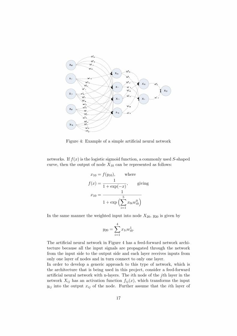
Figure 4: Example of a simple artificial neural network

networks. If f(x) is the logistic sigmoid function, a commonly used S-shapedcurve, then the output of node X10 can be represented as follows:

x10 = f(y10), where

f(x) =1

1 + exp(−x), giving

x10 =1

1 + exp( 5∑

i=1

x0iw0i0

)

In the same manner the weighted input into node X20, y20 is given by

y20 =4∑

i=1

x1iw1i0.

The artificial neural network in Figure 4 has a feed-forward network archi-tecture because all the input signals are propagated through the networkfrom the input side to the output side and each layer receives inputs fromonly one layer of nodes and in turn connect to only one layer.In order to develop a generic approach to this type of network, which isthe architecture that is being used in this project, consider a feed-forwardartificial neural network with n-layers. The ith node of the jth layer in thenetwork Xij has an activation function fij(x), which transforms the inputyij into the output xij of the node. Further assume that the ith layer of

17

nodes has mi nodes. The output of the ath node in the second layer x1a canthen be defined as follows, using the notation in Figure 4

x1a = f1a

( m0∑

p1=0

x0p1w0p1a

). (1)

In the same manner, can the output of the bth node of the second layer x2b

be defined as

x2b = f2b

( m1∑

p2=0

x1p2w1p2b

). (2)

Replacing (1) into (2) yields

x2b = f2b

( m1∑

p2=0

f1p2

( m0∑

p1=0

x0p1w0p1p2

)w1

p2b

). (3)

Continuing in the same manner, the general case for the output of the jthnode in the ith layer Xij , xij is

xij = fij

(m(i−1)∑

pi=0

f(i−1)pi

(· · ·

m1∑

p2=0

f1p2

( m0∑

p1=0

x0p1w0p1p2

)w1

p2p3

)· · ·w(i−1)

pij

).

The weightings of the connections between this node and the node in thenext layer, the (j + 1)th layer, is wi0, wi1, wi2, . . . , wim(j+1)

assuming thatthere are m(j+1) nodes in the (j + 1)th layer.

4.4 Neural Network Architectures

An artificial neural network is classified in terms of its architecture or itsorganization of nodes. The most straight forward architecture is the feedforward network, which allows signals to flow through the network from theinput to the output nodes without any recurring loops. These networksnormally have hidden nodes, so called because they are not accessible fromthe input or output nodes. This form of artificial neural network is the onlyarchitecture considered in this study.

4.5 Trigger Functions

The most commonly used trigger functions are the sigmoid and unity func-tions, which are covered elsewhere in this document.

5 Design of the Model

The design approach taken was to define an artificial stock trading frame-work with artificial trading agent that use technical trading rules to make

18

decisions on whether to buy, hold or sell a single stock trading on the Jo-hannesburg Stock Exchange. A genetic algorithm is used to improve onan initial population of randomly selected artificial trading agents throughthe application of various genetic operators, with the aim to maximise prof-itability over the learning period. A simple artificial neural network is thenused to generate the final decision to buy, hold or sell the shares at the endof each day. This decision is then executed, based on the trigger function,at the closing price of each day under review. Once the genetic algorithmconverges, the most profitable individual is selected to execute its trad-ing strategy over a period not covered in the original learning period, theso called out-of-range period. The model was refined through an iterativeprocess to determine the most optimal set of parameters for the genetic al-gorithm.The trading framework mechanisms are covered in Section 5.1, followed bythe genetic encoding of the artificial trading agents in Section 5.2. The de-sign parameters of the genetic algorithm is covered in Section 5.3, followedby the design of the artificial neural network in Section 5.4, the model designdiscussion is concluded with the evaluation approach followed to determinethe success of the chosen trading agents in Section 5.5.

5.1 Agent Trading Framework

The model was setup to generate a fixed number of artificial trading agentsduring each iteration to form a population of trading agents. At the endof each trading day, each agent makes a decision on whether to buy or sellshares conditional upon the status of the agent’s market exposure and theparameters of the technical trading rules encoded in the individual. Thetotal capital available for investment and the total number of shares boughtin previous transactions, the share holding, is tracked for each agent andupdated at the end of the day once the agent executed the transactionbased on its investment decision.The model has been designed to incorporate realistic transaction fees for thebuy and sell transactions. These are configurable for each simulation run ofthe model. The model makes provision for the following transaction fees inthe trading framework:

Amount under consideration is the ruling share price multiplied by thenumber of shares being considered in the transaction.

Value Added Tax (VAT) is a government tax charged on goods and ser-vices in South Africa. it is calculated as a percentage of the relevantservices or goods being traded and is payable by the buyer of theservices or goods.

Brokerage fees is normally calculated as a percentage of the amount under

19

consideration with most institutions setting a minimum amount pertransaction. This fee is subjected to VAT.

Investor protection levy (IPL) is a minimal charge to insure the investoragainst anomalies that might arise during trading and insures theamount under consideration. This fee is subjected to VAT.

Securities Transfer Tax (STT) is a form of duty charged by the SouthAfrican Government on all share sales. It is calculated as a percentageof the amount under consideration.

STRATE is an abbreviation for Share Transactions Totally Electronic, theSouth African licensed central securities depository. The STRATE feeis fixed charge per transaction and is subjected to VAT.

The total transaction fees for a buy and sell transaction, fbuy(x) and fsell(x)respectively, is thus dependent on the Value Added Tax fvat, SecuritiesTransfer Tax fstt, Investor Protection Levy fipl, the STRATE fee fstr, thebrokerage fees fbr and the minimum brokerage charge fmin

br . The fee calcu-lation for each type of transaction, based on the closing share price Pt onday t and the number of shares being considered in the transaction x is then

fbuy(x) = Ptx((

fbr + fipl

)(1 + fvat

)+ fstt

)+ fstr

(1 + fvat

), if

Ptxfbr ≥ fminbr , else

fbuy(x) = Ptx(fipl

(1 + fvat

)+ fstt

)+

(fmin

br + fstr

)(1 + fvat

), if

Ptxfbr ≤ fminbr , and

fsell(x) = Ptx(fbr + fipl

)(1 + fvat

)+ fstr

(1 + fvat

).

The default values in the model have been configured courtesy of StandardBank’s Online Share Trading platform.

5.2 Genetic Encoding of the Trading Agents

5.2.1 Technical Trading Rules

This study is concerned with the effectiveness of a strategy using geneticalgorithms and technical trading rules to deliver superior market returns. Inorder to effectively encode the trading agents as individuals in a populationof a genetic algorithm the technical trading rules and parameters needsto be identified upfront. There are literally hundreds of technical tradingrules being used today by investors in the stock market, and any attempt toinclude a representative set in this study would have made it too cumbersometo illustrate the principles of genetic algorithms.The approach used in this study is to focus on six of the most commonlyused technical trading rules. In practice, these rules will often be used in

20

conjunction with each other, which can be effectively implemented usinggenetic programming techniques. Again, because this study is concernedwith the use of genetic algorithms, the technical trading rules are consideredin isolation to each other when buy, hold or sell signals are generated. Thetrading rules on which this study focus are as follows:

• The Moving Average indicator.

• The Relative Strength Indicator.

• The Full Stochastic Oscillator set of indicators.

• The Moving Average Convergence Divergence indicator.

• The Price Rate-of-Change indicator.

• The Bollinger Bands set of indicators.

A full description on each of these indicators, there use, calculation and de-cision logic as implemented in this project, is discussed in Appendix A.subsubsectionTrading Agent Genome Design The genome of each agent con-sists of 25 genes each containing an integer value. These values represent theweightings for each of the technical trading rules, to be used for the artificialneural network, as well as the different parameters for each of those rules.The genome structure implemented for the trading agents is represented inthe table below:

Gene Range Description of GeneG1 0-100 Short-term Moving Average WeightingG2 0-100 Long-term Moving Average WeightingG3 0-100 Relative Strength Indicator WeightingG4 0-100 Stochastic Oscillator WeightingG5 0-100 Moving Average Convergence Divergence WeightingG6 0-100 Price Rate-of-Change WeightingG7 0-100 Bollinger Bands WeightingG8 5-30 Short-term MA time period valueG9 30-300 Long-term MA time period valueG10 10-50 RSI time period valueG11 10-30 RSI Buy signal valueG12 70-90 RSI Sell signal valueG13 2-100 SO time period valueG14 1-10 SO tempo indicatorG15 5-30 SO Buy signal valueG16 70-95 SO Sell signal valueG17 20-50 MACD long-term time period value

Continued on next page ...

21

... continued from previous pageGene Range Description of GeneG18 5-20 MACD short-term time period valueG19 5-20 MACD signal line valueG20 5-30 ROC short-term time period valueG21 20-100 ROC long-term time period valueG22 5-20 ROC buy signal line valueG23 5-20 ROC sell signal line valueG24 9-30 BB time period valueG25 10-400 BB standard deviations value (100x)

Table 1: Trading Agent genome structure

The parameters of the technical trading rules can be thought of as thetrue genetic material of the individuals and the weightings of the differentrules to be applied in the neural network can be thought of as the instinct orbuilt in bias of the individual to prefer one rule over the other. Alternativeapproaches for the implementation of the neural network weightings arediscussed in Section 6.4.

Figure 5: Ranges for Technical Trading Rule Parameters being set

Genes 1 to 7 represent the percentage weighting for each technical tradingfunction at the input of the neural network. It is essentially the biasof the input at each of input nodes one to seven of the neural networkthat determines the output of the agents’ decision process.

Genes 8 to 10, 13, 17, 18, 20, 21 and 24 are place holders for the pe-riod, in number of trading days, for each of the technical trading in-dicators as list in Table 1.

Genes 11 and 12 represent the buy and sell signal values for the RelativeStrength Indicator.

22

Gene 14 represents the tempo indicator of the Stochastic Oscillator, whichis the period of the exponential moving average applied to the %K and%D values.

Genes 15 and 16 represent the buy and sell signal values for the Stochas-tic Oscillator.

Gene 19 represents the signal line period for the Moving Average Conver-gence Divergence indicator, which is the period of the moving averageapplied to the Moving Average Convergence Divergence indicator val-ues.

Genes 22 and 23 represent the buy and sell signal values for the PriceRate of Change indicator.

Gene 25 represents the number of standard deviations that the upper andlower Bollinger Bands are from the middle band. The value needs tobe divided by 100 to obtain the actual number of standard deviations.

Figure 5 shows how the different technical trading rule ranges are configuredin the simulation program.

5.3 Genetic Algorithm Design

The genetic algorithm design in this project is described in terms of thefitness function, the genetic operators implemented and the design thereof aswell as the key parameters that govern the algorithm during the simulation.

5.3.1 The Fitness Function

The aim of this project is to maximise profit returned based on share trans-actions, and hence the immediate candidate for the fitness function to opti-mize is the over profitability of the trading agent. This function is easy toimplement in the C# language and was preferred for this project. Alterna-tive fitness functions based on metrics such as the Sharpe Ratio [Sha64] isdiscussed in Section 6.4.

5.3.2 Crossover Operator Design

The implemented genetic algorithm made use of crossover reproduction.The crossover operator was limited to crossover in a single locus and thecrossover was in between gene boundaries. This ensured the integrity ofthe parameters of the technical trading rules and further limited irrationalbehaviour from the trading agents.

23

5.3.3 Mutation Operator Design

The simulation program allowed for the mutation probability to be adjustedbetween 0 and 1. The mutation operator is invoked after the cross overreproduction took place. When invoked, the mutation operator mutatesbetween zero and five of the genes at random and sets the value to a randominteger between 0 and 300.

5.3.4 Selection Operator Design

The selection operator was based on a combination of three different selec-tion strategies, evaluated against the fitness function as described in Section5.3.1. The implementation of the selection operator can be summarized inthe three steps approach below;

Step 1 : Elitist selection takes place on the individuals of the current pop-ulation. The percentage of individuals carried forward to the nextgeneration is adjustable in the simulation program, and the actualsimulations varied the parameter between 0% and 10%.

Step 2 : Truncated selection takes place on the individuals of the currentpopulation. The percentage of individuals thus selected for reproduc-tion (crossover) is adjustable in the simulation program, and the actualsimulations varied the parameter between 10% and 60%. It should benoted that the truncated group included the group of individuals se-lected in Step 1.

Step 3 : The percentage of the next population that is replaced by newindividuals is adjustable in the simulation program, and the actualsimulations varied the parameter n between 25% and 75%. The effectof this strategy is that the individuals selected in Step1 to be includedin the next population, plus the offspring generated in Step 2 madeup (100− n)% of the next generation, with the rest of the individualsbeing randomly generated.

5.3.5 Parameters for Simulations

The other parameters of the genetic algorithm that were adjustable was thepopulation size which was varied between 100 and 5000 and the number ofpopulations (or iterations) which was varied between 15 and 30.

5.3.6 Algorithm Implemented

Figure 6 shows the implemented algorithm, the pseudo code of which follows:

24

Figure 6: Genetic Algorithm Flow Chart

10 Initialize Parameters20 Set Population = 020 Generate a random population with size N.30 Evaluate each individual against fitness function F(X).40 Select top X% of Population and add to Next Population50 Determine top Y% of Population for Reproduction60 Select 2 individuals at random from top Y%65 Cross over at random locus70 Mutate the individual at random loci80 Include offspring in Next Population90 IF Next Population = M individuals THEN 100 ELSE 60

25

100 Generate N-M new individuals and add to next population110 Population = Population +1120 IF Population = Max Population THEN END ELSE 30

5.4 Artificial Neural Network Design

The simulation iterates or steps through each trading day in a sequentialmanner, for each population being evaluated, evaluating the investment de-cisions each individual makes based on the closing price of the stock. Thesimulation was designed such that the various technical trading rules eachgenerate a buy, hold or sell signal. These are then viewed as inputs into asimple artificial neural network to compute the overall decision for the day.The following sections cover the design and reasons for the design approachof this neural network.

5.4.1 The Architecture of the Artificial Neural Network

The artificial neural network employed to calculate the investment decisionat the end of each trading day, for each individual, is shown in Figure 7. It isa feed forward network with no hidden nodes. This, very simple architecturewas selected due to the fact that it needs to be computationally efficient, as itis the most frequently executed step in the simulation. For example, a typicalsimulation run consists of a population size of 5000 individuals, evaluatedover 122 trading days and iterated through 30 generations, resulting in thecode for this neural network being executed 18.3 million times during thesimulation run.The design is not only computationally efficient, but it accurately reflects

an architecture where each individual has a set instinct or decision logicin terms of making their investment decision. This architecture does notallow the agents to learn through experience, which is a shortcoming that iselaborated upon in Section 6.4.Each technical trading rule generates a BUY, HOLD or SELL signal at the endof each trading day. The values of these are 1, 0 and −1 respectively. Thesevalues are presented as the input values xi to the neural network and aremultiplied by the weights wi for each technical trading rule in the genomeof the individual, resulting in a weighted sum y, that is then applied to thetrigger function of the final node, to generate the individual’s investmentdecision for the day under consideration.

5.4.2 Trigger Functions

The design considered a number of the popular trigger functions for thefinal node, such as the sigmoidal function and the unity function. The finalsimulation design implemented two trigger functions, the results of whichare compared in Section 6. These trigger functions are shown in Figures 8

26

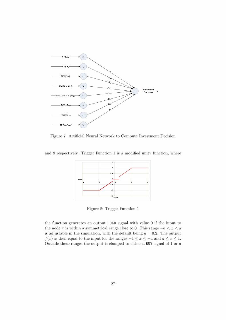
G1G2G6G7Figure 7: Artificial Neural Network to Compute Investment Decision

and 9 respectively. Trigger Function 1 is a modified unity function, where

-1.5-1-0.500.511.5-2 -1 0 1 2Input OutputFigure 8: Trigger Function 1

the function generates an output HOLD signal with value 0 if the input tothe node x is within a symmetrical range close to 0. This range −a < x < ais adjustable in the simulation, with the default being a = 0.2. The outputf(x) is then equal to the input for the ranges −1 ≤ x ≤ −a and a ≤ x ≤ 1.Outside these ranges the output is clamped to either a BUY signal of 1 or a

27

SELL signal of −1. This is mathematically represented by

f(x) = 0 when − a < x < a, andf(x) = x when − 1 ≤ x ≤ −a and a ≤ x ≤ 1, withf(x) = 0 when x < −1, andf(x) = 1 when x > 1.

Trigger Function 2 is a binary function, with a threshold zone where the

-1.5-1-0.500.511.5-2 -1 0 1 2Input OutputFigure 9: Trigger Function 2

function generates an output f(x) HOLD signal with value 0 if the input x tothe node x is within a symmetrical range close to 0. This range −a < x < ais also adjustable in the simulation, with the default also being set such thata = 0.2. This function is mathematically represented by

f(x) = 0 when − a < x < a, andf(x) = −1 when − 1 ≤ x ≤ −a andf(x) = 1 when a < x < 1.

5.5 Evaluation Approach

At the end of a simulation run an individual is selected with the best ge-netic fit to optimize the profits over the learning period. In order to evaluatewhether this artificial trading agent actually has the ability to return supe-rior investments when compared with the market it needs to be evaluatedover a range of inputs it was not selected or trained upon (no actual train-ing takes place in the implemented neural network, but it is stated for thegeneral case).One way to determine whether this artificial agent performs better thanthe market, is to compare its profits at the end of a test period with anequivalent buy and hold strategy. However, this is not sufficient in itself,since the artificial trading agent could perform worse than the market formost of the evaluation period just to make a single good decision at the end,

28

that results in profits that exceeds the market at the end of the evaluationperiod. An example, from one of the simulation runs are shown in Figure10 to illustrate this point.

In Figure 10 it is clear that the trading agent return less profits than a

-8%-6%-4%-2%0%2%4%6%8%10%12%14%16%Return on InvestmentOut of Range Performance - Good Individual

Buy & Hold Good IndividualFigure 10: Example of Trading Agent compared with Market

buy and hold strategy for the bulk of the period under review, but that itstarts to deliver superior returns from the week of 5 September 2006 on-wards and at the end of the evaluation period is exceeds the market returnsby 2,68%. Most investors would be delighted to exceed the market returnsby that margin over a three month period, such as this example, since it bereasonably expected that the trend will continue and that annualised profitscould exceed the market returns by 10% or more.However, a more discriminating approach is required to evaluate the per-formance of the trading agents. From the work done by Sharpe [Sha64]and others in the definition and application of the Capital Asset PricingModels (see Section 2.5), Modigliani and Modigliani developed a risk ad-justed performance model [MM97] that is used in this project to evaluatethe performance of the trading agent returns over the evaluation period.

5.5.1 Modigliani Risk Adjusted Performance measure

The Nobel laureate Franco Modigliani and his granddaughter Leah devel-oped the Modigliani Risk Adjusted Performance measure or M2 in 1999based on the well known Sharpe ratio [Sha64] which is a dimensionless mea-sure of relative asset returns when comparing two investment strategies.The benefit of the Modigliani Risk Adjusted Performance measure is that it

29

is measured in the same dimension of the investments being evaluated, andtherefore is can be represented as a more intuitive percentage measure whencomparing investment strategies with each other.To define the Modigliani Risk Adjusted Performance measure in context ofthis work, a number of concepts need to be reviewed. Firstly, it is assumedthat the investor has a risk free investment available that offers some posi-tive return on investment over the time period t under review. In the caseof this project the RSA retail savings bonds issued and guaranteed by theSouth African government was considered as the risk free investment option.Secondly, the measure calls for a benchmark investment strategy as part ofthe comparison. In the case of this project the benchmark was taken to bethe market returns over the period under review.The Modigliani Risk Adjusted Performance measure can then be defined incontext of this project such that

Dt = RPt −RFt

where RPt is the return of the trading agent investment strategy for sometime period t and RFt is then the risk free investment returns over thesame period. The difference, Dt is then excess return of the trading agentinvestment compared with the risk free investment option over that period.The Sharpe Ratio S can then be defined as

S =D

σD, with

D =

N∑

t=1

Dt

N, and

σD =

√√√√√√N∑

t=1

(Dt)2

N − 1.

In this case D is the average excess returns of the trading agent comparedwith the risk free investment over the evaluation period, and σD is the stan-dard deviation of D. The Modigliani Risk Adjusted Performance measureM2 is then defined as

M2 = SσB + RF

= DσB

σD+ RF ,

30

where RF is the average risk free returns for the evaluation period, definedby

RF =

N∑

t=1

RFt

N,

and where σB is the standard deviation of the benchmark market returnsRBt compared with the risk free returns RFt , defined by

σB =

√√√√√√N∑

t=1

(RPt −RBt)2

N − 1,

The M2 measure therefore adjusts the average gain D of the returns com-pared with risk free investment, with the ratio of the risk of the benchmarkand the investment strategy followed. In this case the standard deviationsσD and σB are representative of the risk of the investments.Returning back to Figure 10, the M2 measure for the trading agent over theevaluation period, compared with a risk free return of 7,5% per annum is0,3%. This an order of magnitude less than the absolute difference betweenthe two options. Clearly indicating that the trading agent in Figure refEV isonly marginally better than the market and that more extensive evaluationis required.

6 Simulation Results

Text goes here Simulation period, share price, learning period out of rangeperiods.

6.1 Random Number Generator

In order to execute effective simulations a good random number generatoris required. During the simulation model implementation, it was found thatthe C# random generator returned inconsistent results. A program was thendeveloped to explore the random number generator using the first 100 000seeds of the Math.Random function in C#, and the results were analysedin Microsoft Excel.The approach followed in the program was to generate 1 million integers

between 0 and 1000 for each seed. The dataset was divided in 20 equalintervals to analyse the frequency of the random numbers. The χ2-test with19 degrees of freedom was then used to test whether the random numbergenerator-seed combination generated a uniform distribution. An extract ofthe results of this test is shown in Table 2. The simulation runs in the restof this Section used the most uniformly random seed.

31

Seed χ2 Prob Seed χ2 Prob Seed χ2 Prob

57940 3.00 0.99999 99643 18.32 0.50090 17213 49.36 0.0001624565 3.47 0.99997 99651 18.33 0.50011 68065 50.14 0.0001348084 3.52 0.99996 6347 18.34 0.49985 75148 50.22 0.0001264894 3.53 0.99996 99045 18.38 0.49720 2892 50.51 0.0001170174 4.04 0.99988 1852 18.41 0.49509 69105 50.53 0.00011

Table 2: Evaluation of different seeds in C# Math.Random Object

6.2 Tuning the Genetic Algorithm

The implementation of the genetic algorithm design, discussed in Section5.3, required that a number of parameters of the genetic algorithm be finetuned to deliver optimal results during the simulation runs. A manual trial-and-error approach was followed to optimize the parameters of the geneticalgorithm. All the parameters, except the parameter to be optimised, werekept constant with the following defaults:

• The elitist selection operator was set to select the top 5% by default.

• The truncated selection operator was set to select the top 25% bydefault.

• The parameter for new individuals was set to 25% by default.

• The probability of mutation was set to 10% by default.

The results of the optimization iterations are discussed in the next Sections.

6.2.1 Elitist Selection Operator

The output of the simulation runs to search for an optimal elitist selectionoperator value is shown in Table 3.

MetricElitist Selection Parameter

0% 1% 2% 4% 5% 6% 10%

Best Ind. 194,190 190,108 192,741 196,540 217,960 186,151 198,563Market 132,662 132,662 132,662 132,662 132,662 132,663 132,662Net % 61.53% 57.45% 60.08% 63.88% 85.30% 53.49% 65.90%Diff. % -3.23% -2.63% -12.96% -8.25% 2.31% -10.48% -19.95%M2 250.09 284.69 -111.50 37.04 289.40 0.09 -371.41M2 (%) 0.25% 0.28% -0.11% 0.04% 0.29% 0.00% -0.37%

Table 3: Optimization runs for the Elitism Selection Parameter

32

Table 3 shows partial results for stepping the elitist selection operator pa-rameter from 0% to 10%. The first row in the table title Best Ind. shows thebest individual’s return in the training period based on initial investment ofR100,000. The second row indicates the market return over the same periodalso assuming the same level of investment. The third row titled Net %shows the percentage that the best individual beat the market with. Row4 titled Diff. % indicates the percentage that the best individual beat themarket within the out of range simulation. The last two rows shows theabsolute value and the percentage of the M2 measure for each iteration.From these results it is clear that, given the other settings, the most likelyoptimal setting for the elitist selection operator was 5%.

6.2.2 Truncation Selection Operator

The output of the simulation runs to search for an optimal truncated selec-tion operator value is shown in Table 4. Table 4 shows partial results for

MetricTruncation Selection Parameter

10% 20% 25% 30% 40% 50%

Best Ind. 205,205 193,577 217,960 215,691 192,285 196,127Market 132,662 132,662 132,662 132,662 132,662 132,663Net % 72.54% 85.30% 85.30% 83.03% 59.62% 63.46%Diff. % -4.44% -6.49% 2.31% -2.45% -11.99% -14.05%M2 186.24 178.85 289.40 213.62 -79.52 -49.08M2 (%) 0.19% 0.18% 0.29% 0.21% -0.08% -0.12%

Table 4: Optimization runs for the Truncation Selection Parameter

stepping the truncation selection operator parameter from 10% to 50%. Thefirst row in the table title Best Ind. shows the best individual’s return inthe training period based on initial investment of R100,000. The second rowindicates the market return over the same period also assuming the samelevel of investment. The third row titled Net % shows the percentage thatthe best individual beat the market with. Row 4 titled Diff. % indicates thepercentage that the best individual beat the market within the out of rangesimulation. The last two rows shows the absolute value and the percentageof the M2 measure for each iteration.From these results it is clear that, given the other settings, the most likelyoptimal setting for the truncation selection operator was 25%.

6.2.3 New Individuals Parameter

The output of the simulation runs to search for an optimal parameter for thepercentage of new individuals introduced in each new population is shownin Table 5. Table 5 shows partial results for stepping the “new individualsparameter” from 15% to 60%. The first row in the table title Best Ind.

33

MetricNew Individuals Parameter

15% 25% 35% 50% 60%

Best Ind. 192,222 217,960 193,132 189,929 190,734Market 132,662 132,662 132,662 132,662 132,662Net % 59.56% 85.30% 60.47% 57.27% 58.07%Diff. % 0.95% 2.31% -2.99% -2.60% 1.39%M2 265.42 289.40 262.64 284.69 275.75M2 (%) 0.27% 0.29% 0.26% 0.28% 0.28%

Table 5: Optimization runs for the New Individuals Parameter

shows the best individual’s return in the training period based on initialinvestment of R100,000. The second row indicates the market return overthe same period also assuming the same level of investment. The third rowtitled Net % shows the percentage that the best individual beat the marketwith. Row 4 titled Diff. % indicates the percentage that the best individualbeat the market within the out of range simulation. The last two rows showsthe absolute value and the percentage of the M2 measure for each iteration.From these results it is clear that, given the other settings, the most likelyoptimal setting for the “new individuals parameter” was 25%, but it isworth noting that simulation was not particularly sensitive to the value ofthe parameter.

6.2.4 Mutation Probability

The output of the simulation runs to search for an optimal parameter for theprobability that an individual will be mutated is shown in Table 6. Table 6

MetricMutation Probability

1% 2% 5% 7.5% 10% 12.5%

Best Ind. 200,019 197,127 193,078 196,442 217,960 184,047Market 132,662 132,662 132,662 132,662 132,662 132,662Net % 67.36% 64.46% 60.42% 63.78% 85.30% 51.38%Diff. % -5.70% 2.00% -6.49% 0.48% 2.31% -9.25%M2 113.12 287.90 182.14 252.46 289.40 13.38M2 (%) 0.11% 0.29% 0.18% 0.25% 0.29% 0.01%

Table 6: Optimization runs for the Mutation Probability

shows partial results for stepping the ‘mutation probability from 15% to 60%.The first row in the table title Best Ind. shows the best individual’s return inthe training period based on initial investment of R100,000. The second rowindicates the market return over the same period also assuming the samelevel of investment. The third row titled Net % shows the percentage thatthe best individual beat the market with. Row 4 titled Diff. % indicates thepercentage that the best individual beat the market within the out of range

34

simulation. The last two rows shows the absolute value and the percentageof the M2 measure for each iteration.From these results it is clear that, given the other settings, the most likelyoptimal setting for the mutation probability was 10%.

6.2.5 Number of Generations

The number of generations for which the genetic algorithm is iterated for, isdependent on how fast the results are converging. The speed of convergenceis dependent on the level of diversity in the initial generation and the levelof diversity introduced in each new generation.Experiments with the implemented simulation program showed that pop-ulations with less than 250 individuals did not explore the solutions spaceadequately and converged very quickly to the most dominant individual inthe initial generation. Further experiments shown that the model convergessufficiently after approximately 19 generations when the population size was500. Predictably the number of generations before convergence was achievedincreased with the number of individuals in the population and when thenumber of new individuals in each new generation was increased to a valuelarger than 60%.

The total execution time of the simulation also increased rapidly as the

0%20%40%60%80%100%120%140%1 2 3 4 5 6 7 8 9 10 11 12 13 14 15 16 17 18 19 20 21 22 23 24 25 26 27 28 29 30Return on Investment Generations

Model Performance - Population Size=1000(3 Jan '06 to 31 Jul '06)Best Individual Average (Top 75%) Buy & Hold

Figure 11: Example of Simulation Model Convergence

number of individuals in the population increased. The total simulation ex-ecution time for the simulation with a population size set to 5000 and 100generations, was more than 90 minutes, and it yielded marginally better re-sults than simulation runs with the initial population set at 1000 individuals

35

over 30 generations. The latter took approximately 12 minutes to executeand all results discussed in this project used the latter settings. Figure 11shows how the simulation model converges with an initial population set at1000 individuals, with 25% new individuals introduced in each new genera-tion. Convergence in this case is measured as the difference in performanceof the optimal solution compared with the average of the best 75% of thesolutions.subsubsectionTrigger Function selection The two trigger functions consid-ered in Section 5.4.2 were also compared during the various simulation runsexecuted in the previous sections, and Trigger Function 1 consistently out-performed Trigger Function 2 by approximately 25%. Therefore TriggerFunction 1 was used in all the comparisons and results shown in this report.

6.3 Optimized Results

Once the simulation model was optimized as described in Sections 6.1 and6.2, fifty simulation runs were executed and the best solution found had thefollowing genome

• The short term moving average time period was 193 days with aweighting of 257%.

• The long term moving average time period was 289 days with a weight-ing of 27%.

• The Relative Strength Indicator time period was 19 days with a weight-ing of 99%. The buy level was set at 43 and the sell level set at 70.

• The Stochastic Oscillator time period was 56 days with a weighting of250%. The tempo value was set at 5 days, with the buy level set at18 and the sell level set at 73.

• The Moving Average Convergence Divergence indicator long term timeperiod was 30 days, with the short term time period set at 11 days,and the weighting was 7%. The signal line time period was set at 10days.

• The short term price rate of change time period was 12 days and thelong term price rate of change time period was 134 days, both hada weighting of 231%. The buy signal value was set at 3 and the sellsignal value was set at 146.

• The Bollinger Bands indicator time period was 25 days with a weight-ing of 24%. The standard deviation value was set at 3,85.

36

It is worth noticing that some of the technical trading rule values in thebest solution, were outside of the parameters set in the initial genome de-sign. This clearly shows the value that the mutation operator added to thesimulation model.

6.3.1 Performance in Learning Range

The performance of the optimal solution in the “Learning range” is shownin Figure 12, where the trading agent’s normalized profitability is comparedwith that of the “buy and hold” strategy.The corresponding BUY and SELL signals (the output of Trigger Function 1)

-20%0%20%40%60%80%100%120%03/01/2006 03/02/2006 03/03/2006 03/04/2006 03/05/2006 03/06/2006

Best Individual Performance in Learning RangeBuy & Hold Best Individual

Figure 12: Best Solution Performance in Learning Range

is depicted in Figure 13, together with the input into the trigger function.The corresponding closing prices of the share are depicted in Figure 14.

-3-2-10123

03/01/2006 03/02/2006 03/03/2006 03/04/2006 03/05/2006 03/06/2006 Best Individual - Buy and Sell Signals

Input OutputFigure 13: Trigger Function signals for Best Solution

37

Comparing the share price trends with the signals, it is clear that manysignals are generated when the share price has sideways movement, but thatthe trading agent makes very sensible decisions when the share prices aretrending up or down.

260002700028000290003000031000320003300034000Closing Price (ZA cents)AGL Closing Prices - Learning Period

Figure 14: Closing Price of Anglo American Shares during Learning Period

6.3.2 Out of Range Performance

The ultimate test for any simulation model is to understand whether thesimulation proves or disprove the original hypothesis. In this case the per-formance of the best trading agent generated by the simulation is evaluatedover a range of data which it has not seen before, in an attempt to provethe hypothesis that trading agents which exclusively use technical tradingrules can outperform a conservative “buy and hold” strategy.Figure 15 shows the result when the best trading agent is presented with

the share price information for the period 1 July 2006 to 30 September 2006,the three months following the “Learning Period”. The trading agent de-livered 2,13% more return on investment than the “buy and hold” strategy,but the instantaneous performance varied between 4,88% worse to 7,02%better than the “buy and hold” strategy. The M2 value however shows thatthe comparative risk adjusted performance of the trading agent is a mere0,29% better than the market returns.

6.4 Improvements Proposed to Simulation Model

During the simulation model design, implementation and analysis, a numberof short comings of the implemented simulation model were identified. Themain improvements as a result of these shortcomings, as listed below, withthe reasons for suggesting it. The majority of these potential improvements

38

-6.00%-4.00%-2.00%0.00%2.00%4.00%6.00%8.00%10.00%12.00%14.00%16.00%Return on Investment

Best Individual Performance - New DataBuy & Hold Best Individual

Figure 15: Performance of Best Solution on New Period

were ratified in discussions with academics and experienced modellers con-sulted as part of the project. In the interest of brevity, references to theseare not included in this document.

6.4.1 Artificial Neural Network Weights

The implemented simulation model encoded the artificial neural networktraining weights in the genome of the agent. This ensured that the artificialneural network could not be optimized on its own, resulting in a sub-optimalneural network implementation. It is therefore suggested that the artificialneural network weights be decoupled from the genome of the trading agent,thereby ensuring that the trading agents can improve through experienceand are not forced to act “instinctively” based on its genetic makeup.

6.4.2 Artificial Neural Network Architecture

The simulation model implemented a very simplistic feed forward neural net-work without any hidden nodes. If the neural network is expanded to includehidden nodes, the performance thereof could arguably be improved becausemore complex patterns in the share price movement can conceptually beidentified. No learning takes place in the implemented neural network, andthe “experience” gained by the artificial trader is lost in subsequent gener-ations. The model can be significantly improved by the introduction of aback propagation learning algorithm to capture this “experience”.

39

6.4.3 Optimization Approach

Experienced modellers suggest that profitability is a sub-optimal fitnessfunction to base optimization of the genetic algorithm on for share trading.Most modellers suggested that improved results are achieved if optimizationis based on the prediction of the next day’s closing price or on the Sharperatio [Sha64]. The model can thus be improved if the prediction of the nextday’s share price or the Modigliani Risk Adjusted Ratio is used to optimizethe genetic algorithm with.Another potential improvement is the use of genetic algorithms to optimizethe parameters of the genetic algorithm itself. This will ensure that thesimulation model is optimized for the problem it tries to solve.

7 Conclusion

In conclusion the results discussed in Section 6.3 supports the EfficientMarket Theory due to the fact that the most optimal solution for an ar-tificial trading agent that uses technical trading rules for decision making,could not outperform the market over various evaluation and learning peri-ods. Promising results for specific periods were uncovered, based on abso-lute gains achieved, but when adjusted for risk over the entire period, theModigliani Risk Adjusted Ratio proved that the finding were not signifi-cant.Finally, the author gained significant experience in the use of simulationmodels to solve real life problems.

References

[Coo64] Paul H. Cootner. The random character of stock market prices.MIT Press, 1964.

[CY97] Shu-Heng Chen and Chia-Hsuan Yeh. Toward a computable ap-proach to the efficient market hypothesis: An application of ge-netic programming. Journal of Economic Dynamics and Control,21:1043–1063, 1997.

[Fam65] Eugene F. Fama. Random Walks in Stock Market Prices. Finan-cial Analysts Journal, 21:55–59, 1965.

[Fam70] Eugene F. Fama. Efficient Capital Markets: A Review of Theoryand Empirical Work. The Journal of Finance, 25:383–417, 1970.

[Fau94] Laurene V. Fausett. Fundamentals of neural networks : architec-tures, algorithms, and applications. Upper Saddle River, N.J. :Prentice Hall, 1994.

40

[Heb49] Donald O. Hebb. The organization of behavior: a neuropsycho-logical theory. Wiley-Interscience, New York, 1949.

[Hol92] John H. Holland. Adaptation in natural and artificial systems :an introductory analysis with applications to biology, control, andartificial intelligence. MIT Press, 1st edition, 1992.

[Joh93] Horgan John. Profile: Marvin l. minsky: The mastermind ofartificial intelligence. Scientific American, 5:14–15, 1993.

[Ken53] Maurice G. Kendall. The analysis of economic tie-series - parti:Price. Journal of the Royal Statistical Society, 116:11–34, 1953.

[LM99] Andrew W. Lo and Craig A. MacKinley. A Non-Random WalkDown Wall Street. Princeton University Press, 5 edition, 1999.

[LMW02] Andrew W. Lo, Harry Mamaysky, and Jiang Wang. AdvancedTrading Rules. Prentice Hall, 2nd edition, 2002.

[Mal73] Burton G. Malkiel. A random walk down Wall street. W.W.Norton and Company Inc., 1973.

[Mit96] M. Mitchell. An Introduction to Genetic Algorithms. MIT Press,1st edition, 1996.

[MM97] Franco Modigliani and Leah Modigliani. Risk-adjusted perfor-mance. Journal of Portfolio Management, 23:19–27, 1997.

[MP43] Warren S. McCulloch and Walter Pitts. A logical calculus ofthe ideas immanent in nervous activity. Bulletin of MathematicalBiophysics, 7:115–133, 1943.

[MYR06] Ben R. Marshall, Martin R. Young, and Lawrence C. Rose. Can-dlestick technical trading strategies: Can they create value forinvestors? Journal of Banking and finance, 30:2303–2323, 2006.

[Per04] Andre F. Perold. The capital asset pricing model. Journal ofEconomic Perspectives, 18:3–24, 2004.

[Sha64] William F. Sharpe. Asset prices: A theory of market equilibriumunder conditions of risk. Journal of Finance, 19:425–442, 1964.

[SHW80] John E. Schlater, Robert A. Haugen, and Dean W. Wichern.Trading based on forecasts of earnings per share : A test of theefficient market hypothesis. Journal of Banking and Finance,4:197–211, 1980.

41

[Stk] Relative Strength Indicator (RSI) - StockCharts.com. Availablefrom: http://stockcharts.com/help/doku.php?id=chart_school:technical_indicators:relative_strength_in [cited22 November 2010].

[Wik] Stock exchange. Available from: http://en.wikipedia.org/wiki/Stock_exchange [cited 01 Ju1 2010].

42

A Appendix: Technical Trading Rules

This appendix provides the background information, calculation, decisionlogic, parameters and usage of the technical trading rules used in the project.

A.1 Notation

This sub section will introduce the mathematical notation used to describeand calculate the technical trading rules.Let the closing price of a share on the stock exchange on day t be representedby Pt. The series of closing prices of the stock up to that date can then berepresented as:

P = {P0, P1, P2, . . . , Pt}.The gain Gt or loss Lt of a share price on day t is calculated based on thedifference between the previous day’s share price Pt−1 and the current day’sshare price Pt. This calculation is represented as follows:

if Pt > Pt−1,

then Gt = Pt − Pt−1 and Lt = 0,

otherwise if Pt < Pt−1,

then Lt = Pt−1 − Pt and Lt = 0,

for all t ≥ 0.

Notice that the value of the loss Lt or gain Gt on day t is always positiveor equal to zero. The series of losses and gains up to day t are thereforerepresented by

G = {G1, G2, . . . , Gt},and L = {L1, L2, . . . , Lt}.

A.2 Simple Moving Average

A.2.1 Background

Moving averages provides a smoothing effect to the share price, which oftenexhibits volatile behaviour. The moving average line provides an indica-tion of the trend of the share price over the past number of periods and istherefore a trend following or lagging indicator of the share price. It doesnot provide any information to base price predictions on, but it can provideclues to potential trend changes when the share price crosses the movingaverage line. Most technical traders use the moving average in conjunctionwith other indicators to predict price trend changes.In Figure 16 the red arrows indicate potential sell signals when the closingprice moves below the 10-day moving average line, whilst the green arrowsindicate potential sell signals when the closing price moves above the 10-daymoving average line.

43

A.2.2 Parameters

The simple moving average has a single parameter N which indicates theperiod, in number of days, of the moving average. That is the number ofdays including the current day that the moving average will be calculatedon.

15000175002000022500250002750030000325003500037500CentsAnglo American PLC AGL:JSE (Jan to Dec 2006)

Closing Price MA(10) MA(60)Figure 16: Anglo American share price with 10-day and 60-day simple mov-ing average plots

A.2.3 Calculation

The simple moving average of a share price P with a period of N days, atthe close of day t is calculated as follows:

Pt(N) =

t∑

i=t−N

Pi

N

A.2.4 Decision Logic

The pseudo code below illustrates how the moving average indicator is usedin conjunction with the current closing price Pt and the previous day’s clos-ing price Pt−1 to generate BUY, SELL and HOLD signals.

Calculate MA_T(N)Retrieve P_T and P_T-1IF P_T > MA_T(N)THEN

44

IF P_T-1 < MA_T(N) THENSignal=BUY

ELSESignal=HOLD

ENDIFENDIFIF P_T < MA_T(N)THEN

IF P_T-1 > MA_T(N) THENSignal=SELL

ELSESignal=HOLD

ENDIFENDIF

A.3 Relative Strength Indicator

A.3.1 Background

The Relative Strength Indicator was developed by J. Welles Wilder in 1978[Stk]. It is momentum oscillator that varies between zero and 100 and itmeasures the speed and size of price changes. Traditionally a rise in the in-dicator above 70 is considered an overbought signal and technical investorsbelieve that a correction is eminent. Conversely, when the indicator dropsbelow 30 it is considered oversold, and a positive trend is believed to beeminent.In recent times the overbought and oversold thresholds vary from one tech-nical investor to another, but typically values are between 70 and 80 forthe overbought signal line and between 20 and 30 for the oversold signalline remains common. Figure 17 shows an overbought area above 70 andan oversold area below 30. It further depicts potential buy signals by greenarrows, and potential sell signals by red arrows.

A.3.2 Parameters

The Relative Strength Indicator has a single parameter N which indicatesthe period, in number of days, of the moving average.

A.3.3 Calculation

The calculation of the Relative Strength Indicator of period N days on dayt is based on the relationship between the average gains Gt(N) and averagelosses Lt(N) of the closing share price P over the said period. Since G and Lare sets of exponential moving averages, the calculation starts by calculatingthe mean of the losses and gains for the initial N days. The initial average

45

gain and average loss is thus defined as

G0(N) =

N∑

i=0

Gi

Nand

L0(N) =

N∑

i=0

Li

Nwhere t = N.

The average gains and average losses for the remaining periods are thencalculated based on an exponential average and are defined below:

Gt(N) =(N − 1)Gt−1 + Gt

Nand

Lt(N) =(N − 1)Lt−1 + Lt

Nwhere t > N.

Once the average gains and losses at the close of day t have been calculated,the Relative Strength Indicator RSI can be calculated as follows:

RSIt(N) = 100− 1001 + RSt

where

RSt(N) =Gt(N)Lt(N)

.

15,00017,50020,00022,50025,00027,50030,00032,50035,00037,500 Anglo American PLC AGL:JSE (Jan to Dec 2006)Closing Price0102030405060708090100 Relative Strength Indicator

Figure 17: Anglo American share price with 9-day RSI plot

46

A.3.4 Decision Logic

The pseudo code below illustrates in what manner the Relative StrengthIndicator RSIt(N) is used to generate BUY, SELL and HOLD signals.

Calculate RSI_T(N) and RSI_T-1(N)SET BUY_S=30, SET SELL_S=7-IF RSI_T(N) > BUY_S THEN

IF RSI_T-1(N) < BUY_S THENSignal=BUY

ELSESignal=HOLD

ENDIFENDIFIF RSI_T(N) < SELL_S THEN

IF RSI_T-1(N) > SELL_S THENSignal=SELL

ELSESignal=HOLD

ENDIFENDIF

A.4 Stochastic Oscillator

A.4.1 Background

The Stochastic Oscillator was developed by George C. Lane in the late 1950s[Stk]. It is a momentum oscillator that varies between zero and 100 and itmeasures the relative value of the closing price at the end of a specific dayin terms of the highest and lowest values over a preceding period. Typicallywhen the indicator’s signal line rises above 80 it is considered overboughtand technical investors believe that a correction is eminent. Conversely,when the indicator’s signal line drops below 20 it is considered oversold, anda positive trend is believed to be eminent. Figure 18 shows an overboughtarea above 80 and an oversold area below 20. It further depicts potentialbuy signals by green arrows, and potential sell signals by red arrows.

A.4.2 Parameters

The Stochastic Oscillator has the following parameters that are required tocalculate the indicator (%K) and signal (%D) lines that characterize theindicator:

1. The number of days or the period that the oscillator is consideringpast closing prices, denoted by N .

47

2. The number of days or the period that is used for the calculation ofthe moving average of the two lines, denoted by M .

Three basic variants of the Stochastic Oscillator has been developed overtime, these are listed below with their parameters:

1. The fast Stochastic Oscillator does not apply a moving average to%K and %D is a 3-day simple moving average of %K, where %K iscalculated over N previous periods.

2. The slow Stochastic Oscillator applies a 3-day simple moving averageto %K and %D in turn is a 3-day simple moving average of %K, where%K is calculated over N previous periods.

3. The full Stochastic Oscillator applies a M-day simple moving averageto %K and %D in turn is a M-day simple moving average of %K,where %K is calculated over N previous periods.

15,00017,50020,00022,50025,00027,50030,00032,50035,00037,500 Anglo American PLC AGL:JSE (Jan to Dec 2006) Closing Price020406080100

SO K(14) SO D(3)Figure 18: Anglo American share price with Stochastic Oscillator (N=14,M=3)

A.4.3 Calculation

This project uses the full Stochastic Oscillator, and the calculations for thetwo values at the close of each day t, namely %Kt and %Dt, are defined as

48

follows:

%Kt =

t∑

i=t−M

100Pi − Pmin(N, t)

Pmax(N, t)− Pmin(N, t)

Mand

%Dt =

t∑

i=t−M

%Kt

Mwith M < N where

Pmax(N, t) = max(Pt−N , Pt−N+1, . . . , Pt) and

Pmin(N, t) = min(Pt−N , Pt−N+1, . . . , Pt).

The minimum Pmin(N, t) and maximum Pmax(N, t) above is calculated overthe last N trading days, whilst %D is calculated as the mean average of %Kover a period of M days.

A.4.4 Decision Logic

The pseudo code below illustrates how the Stochastic Oscillator SOt(N) isused in conjunction with the current closing price Pt and the previous day’sclosing price Pt−1 to generate BUY, SELL and HOLD signals.

Calculate SO_T(N)Retrieve P_T and P_T-1IF P_T > SO_T(N)THEN

IF P_T-1 < SO_T(N) THENSignal=BUY

ELSESignal=HOLD

ENDIFENDIFIF P_T < SO_T(N)THEN

IF P_T-1 > SO_T(N) THENSignal=SELL

ELSESignal=HOLD

ENDIFENDIF

49

A.5 Moving Average Convergence Divergence

A.5.1 Background

The Moving Average Convergence Divergence indicator was developed byGerald Appel in the late 1970s [Stk]. It is a very simple momentum indi-cator that tracks the difference between two exponential moving averagesof different periods. The signal line that indicates potential buy and sellsignals is the exponential moving average of the indicator. Traditionallythe Moving Average Convergence Divergence indicator is calculated as thedifference between the 12-day exponential moving average and the 26-dayexponential moving average, with the signal line as the 9-day exponentialmoving average of the indicator.Technical investors often experiment with the parameters and have slightlydifferent values that they use to calculate potential buy and sell signals.Figure 19 depicts potential buy signals by green arrows, and potential sellsignals by red arrows. These are generated where the signal line crosses theindicator line.

A.5.2 Parameters

The Moving Average Convergence Divergence indicator has three parame-ters, as follows:

1. The period of the shorter term exponential moving average is N days.

2. The period of the longer term exponential moving average is M days.

3. The period of the signal line is S days.

A.5.3 Calculation

The Moving Average Convergence Divergence indicator on day t, MACDt

is the difference between a shorter term exponential average ST t and longerterm exponential moving average LT t. This line is compared with a signalline which is an exponential average of the Moving Average ConvergenceDivergence indicator with a period of S. The calculation can be described

50

as follows:

MACDt = ST t(N)− LT t(M) where

ST t(N) =(N − 1)Pt−1 + Pt

Nwith t > N where

ST 0(N) =

N∑

i=0

Pi

Nand

LT t(M) =(M − 1)Pt−1 + Pt

Mtextwith t > M where

LT 0(M) =

M∑

i=0

Pi

Mwith M > N.

The signal line SLt is then defined as:

SLt(S) =(S − 1)MACDt−1 + MACDt

Swith t > S where

SL0(S) =

S∑

i=0

MACDi

S.

A.5.4 Decision Logic

The pseudo code below illustrates how the Moving Average ConvergenceDivergence indicator MACDt(N) is used in conjunction with the signal lineSLT (N) to generate BUY, SELL and HOLD signals.

Calculate MACD_T(N)Calculate Signal_T(N)IF MACD_T > Signal_T(N)THEN

Signal=BUYELSE

IF MACD_T < Signal_T(N)THENSignal=SELL

ELSESignal=HOLD

ENDIFENDIF

51

15,00017,50020,00022,50025,00027,50030,00032,50035,00037,500 Anglo American PLC AGL:JSE (Jan to Dec 2006) Closing PriceEMA(12)EMA(26)-20002004006008001,0001,2001,4001,600

MACD Signal LineFigure 19: Anglo American share price with MACD and signal line (N=12,M=26, S=9)

A.6 Price Rate of Change

A.6.1 Background

The Price Rate of Change or Rate of Change indicator is a momentumindicator that measures the percentage change at the close of the currentday compared to the closing period a number of days ago. Technical tradersoften determine their own overbought and oversold limits (5% to 10% oreven more), upon which the determine likely buy and sell signals.Figure 20 shows an overbought area above 5% and an oversold area below-5%. It further depicts potential buy signals by green arrows, and potentialsell signals by red arrows.

A.6.2 Parameters

The Price Rate of Change indicator has a single parameter N which is theperiod N days ago with which the share price is compared with at close ofthe current day t.

A.6.3 Calculation

As stated above, the Price Rate of Change indicator ROCt(N) is a simpleindicator that expresses the difference between the closing price on day twith the closing price N days ago as a percentage of the closing price at the

52

former date. It can be expressed as follows:

ROCt(N) =Pt − Pt−N

Pt−N× 100.

15,00017,50020,00022,50025,00027,50030,00032,50035,00037,500 Anglo American PLC AGL:JSE (Jan to Dec 2006) Closing Price-15-10-5051015202530 ROC(12)

Figure 20: Anglo American share price with ROC plot (N=12)

A.6.4 Decision Logic

The pseudo code below illustrates how the Price Rate of Change indicatorROCt(N) is used in conjunction with the selected buy and sell signal linesto generate BUY, SELL and HOLD signals.

Calculate ROC_T(N)SET BUY_S = -5%, SET SELL_S = 5%IF ROC_T(N) > BUY_S THEN

IF ROC_T-1(N) < BUY_S THENSignal=BUY

ELSESignal=HOLD

ENDIFENDIFIF ROC_T(N) < SELL_S THEN

IF ROC_T-1(N) > SELL_S THENSignal=SELL

53

ELSESignal=HOLD

ENDIFENDIF

A.7 Bollinger Bands

A.7.1 Background

Developed by John Bollinger, Bollinger Bands are volatility bands placedabove and below a moving average [Stk]. The volatility bands are based onthe standard deviation of the closing price. Typically the upper and lowerbands of the Bollinger Bands indicator are two standard deviations aboveand below a simple moving average, the middle band. The simple movingaverage period varies from one technical trader to another. Potential buyand sell signals are generated when the closing price is above the upperband, or below the lower band. Figure 21 depicts potential buy signals asgreen arrows and potential sell signals as red arrows.

A.7.2 Parameters

The Bollinger Bands indicators have the following two parameters:

1. The simple moving average has a period of N days.

2. The standard deviation parameter determines the width of the bandsand is represented by M , the number of standard deviations that theupper and lower bands are from the middle band.

A.7.3 Calculation

The Bollinger Bands indicators consist of the values for a specific day t.These value are plotted on a graph to form three bands, the middle bandBBM , the upper band BBU and the lower band BBL. The values of each

54

of these are calculated as follows:

BBMt(N) =

t∑

i=t−N

Pi

Nand

BBUt(N) = BBMt(N) + M × St(N) and

BBLt(N) = BBMt(N)−M × St(N) where

St(N) =

√√√√√√

t∑

i=t−N

(Pi −BBMt(N))2

N − 1

is the standard deviation of the closing price with period N as calculatedon day t.

15000175002000022500250002750030000325003500037500CentsAnglo American PLC AGL:JSE (Jan to Dec 2006)

Closing Price MA(20) Upper Band Lower BandFigure 21: Anglo American share price with Bollinger Bands (N=20, M=2)

A.7.4 Decision Logic

The pseudo code below illustrates how the Bollinger Bands upper bandBBUt(N) and lower band BBLt(N) indicators are used in conjunction withthe current closing price Pt and the previous day’s closing price Pt−1 togenerate BUY, SELL and HOLD signals.

55

Calculate BBU_T(N) and BBL_T(N)Retrieve P_T and P_T-1IF P_T > BBU_T(N)THEN

IF P_T-1 < BBU_T(N) THENSignal=BUY

ELSESignal=HOLD

ENDIFENDIFIF P_T < BBL_T(N)THEN

IF P_T-1 > BBL_T(N) THENSignal=SELL

ELSESignal=HOLD

ENDIFENDIF

Declaration

I declare that this project is my own, unaided work, except where otherwiseacknowledged. It is being submitted to the University of South Africa forthe degree of B.Sc.(Hons)(Operational Research). It has not been submittedbefore for any degree or examination at any other university.Johann G. Muller, Johannesburg, 16 December 2010.

Acknowledgements

I dedicate this work to my children who patiently supported me duringmy studies. Special acknowledgement goes to Lucy Joanne Montague, mysupportive wife, for her support, dedication and assistance with the finaldocument preparation.

56