1

Applied Mathematics & Econometrics Honors Thesis

ARE THE PARAMETERS IN FUNDAMENTAL FACTOR MODELS TIME-INVARIANT?

Joseph Mickel

May 2012

Thesis Advisor

Dr. Russ Wermers

2

1. Introduction

Mathematical models are at the heart of investment decisions in quantitative investment

management. Well known mutual funds and hedge funds throughout the United States often employ

such quantitative methodologies, with notable examples including the Vanguard Quantitative Equity

Group, the Fidelity Quantitative Equity Group, and Blackrock Global Funds. Mathematical models can

enhance a fund’s performance by facilitating diversification, optimizing trade flows to reduce

transaction costs, and even identifying investment opportunities arising from equity market anomalies.

In this thesis, I examine the temporal stability of parameters in a specific kind of quantitative model, the

Fundamental Factor Model.

The Fundamental Factor Model is a stock screening and selection tool used by investment firms.

It uses observable and measurable firm characteristics and attributes, the factor exposures, to estimate

factor premia, the marginal stock returns associated with each additional unit of factor exposure. In the

model, factor premia are empirically determined, whereas the factor exposures are exogenously

determined (Connor, 1995). Therefore, a quantitative fund manager using a Fundamental Factor Model

obtains historical equity data and decomposes stock returns into a linear combination of factor

exposures and factor premia. With the model parameters estimated, the manager then predicts future

stock returns from currently available information on the associated factor exposures. These predicted

returns are then used to generate a long-short equity portfolio with the intent to outperform a

benchmark.

The number of funds using quantitative investment management has grown over the years at a

faster pace than qualitative funds. Further, as of 2009, the assets-under-management of quantitative

funds was approximately 25% more than the total amount invested in pure qualitative strategies

(Chincarini, 2010). Hence, a large amount of wealth is made or lost based upon the validity of

assumptions and analysis used to generate predictions of asset returns. For the Fundamental Factor

3

Model, a necessary assumption is that the estimated parameters, the factor premia, are time-invariant.

Should these estimated parameters actually vary with time, significant forecasting errors may occur as a

result of model misspecification. Therefore, the existence and frequency of structural breaks is the

primary concern in this analysis.

This paper uses a nested cross-sectional Fundamental Factor Model within a larger pooled OLS

factor model estimated over subsets of twenty years of data. The data consist of corporate accounting

and stock performance metrics contained in the CRSPsift database on US equities listed on US indices.

After constructing factor exposures and a return variable, the model is tested via Wald and Sup-Wald

tests on exogenously determined subsets of the data. All tests in this paper reject the null hypothesis of

parameter stability at the 1% significance level, indicating that structural breaks not only exist, but are

pervasive in the model on this dataset.

2. Review of Literature

As of writing this thesis, I have not been able to find a paper on structural breaks in

Fundamental Factor Models. While some papers acknowledge that factors seem to unexpectedly

change during some estimation periods (Jegadeesh et al., 2004), there is no financial literature that tests

for significant parameter changes over time. However, there is a large body of research involving the

significance of different factor exposures which are commonly used in the Fundamental Factor Model.

Therefore, the selection of factors in this analysis is entirely based upon this established body of

research.

For momentum-based factors, Chan et al. (1999) suggest that earnings momentum related to

analyst recommendations is a unique signal in financial markets that drives cross sectional returns. The

paper examines twenty years of returns from portfolios constructed via price momentum and earnings

momentum factors. The authors constructed zero-investment portfolios based upon individual factors

4

and weighted combinations of the factors. They perform in-sample and out-of-sample back-tests using

the model parameters and observe high portfolio returns in each test. In a similar paper by Jegadeesh

et al. (2004), the predictive power of the level and change in consensus recommendations is compared

against twelve previously established factors. The authors conclude that the change in consensus

recommendations is a unique signal which supplements the other factors in predicting cross sectional

returns. The authors demonstrate the effectiveness of this signal through a series of regressions. In

both papers, the authors establish a set of factors as unique signals by comparison to previously studied

factors from the financial literature.

Finally, Campbell, Lo, and Mackinlay (1999, ch. 6) extensively cover factor models in their book.

They discuss factor identification and the issues that arise when determining the source of deviation

from exact factor pricing. They assert a common assumption that omitted variables are the cause of

deviations whenever such issues arise in practice; but, they also state that with finite sample sizes,

additional factors can always be added to reduce residual error. However, the addition of more factors

implicitly assumes that the deviations arise as a result of omitted factors and not another source.

Consequently, this paper employs a comprehensive set of factors from many factor classes, several of

which were discussed in Chan et al. (1999) and Jegadeesh et al. (2004), including: momentum, size,

growth rate, value, industry level, financial risk, operating efficiency, and market liquidity.

3. Models and Tests

a. Models:

For k distinct factors, M distinct industries containing all firms in the sample space, and T distinct

quarters, we have the following two types of factor models:

5

The Fundamental Factor Model in pooled OLS, predicting 2 quarters ahead:

𝑹𝒕+𝟐 = ��𝜹𝒋,𝒕𝑰𝒋𝑫𝒕

𝑴

𝒋=𝟏

𝑻−𝟐

𝒕=𝟏

+ �𝜷𝒊 ∗ 𝑿𝒊,𝒕

𝒌

𝒊=𝟏

+ 𝒖𝒕+𝟐

The Fundamental Factor Model using T-2 cross-sections individually, predicting 2 quarters ahead:

𝑹𝒕+𝟐 = ��𝜹𝒋,𝒕𝑰𝒋𝑫𝒕

𝑴

𝒋=𝟏

𝑻−𝟐

𝒕=𝟏

+ �𝜷𝒊,𝒕 ∗ 𝑿𝒊,𝒕

𝒌

𝒊=𝟏

+ 𝒖𝒕+𝟐

• 𝑿𝒊,𝒕 denotes the factor exposure of factor i at quarter t. These factors are observable firm level

characteristics.

• 𝛃𝒊 in the pooled model denotes the factor premium to the factor 𝑿𝒊,𝒕. It is the return associated

with a unit of exposure to the associated factor, 𝑿𝒊,𝒕.

• 𝛃𝒊,𝒕 in the cross sectional model denotes the factor premium to factor i at time t.

• 𝑹𝒕+𝟐 denotes the conditional expectation of return two quarters ahead of the observation date.

• 𝒖𝒕+𝟐 denotes the residual at time t+2.

• 𝜹𝒋,𝒕𝑰𝒋𝑫𝒕 denotes the Industry-Quarter indicator term in both the cross-sectional and the pooled OLS

model. This allows for variance in return between industries during a given quarter and within a

single industry across time. Hence, I allow for factor premia associated with industry exposures to

vary with time. 𝜹𝒋,𝒕 is the estimated return to industry j at time t. 𝑰𝒋 is the indicator or characteristic

function for industry j. 𝑫𝒕 is the indicator or characteristic function for time t.

The Fundamental Factor Model in pooled OLS with a nested cross-section (used in testing):

𝑹𝒕+𝟐 = ��𝜹𝒋,𝒕𝑰𝒋𝑫𝒕

𝑴

𝒋=𝟏

𝑻−𝟐

𝒕=𝟏

+ ��𝜷𝒊 ∗ 𝑿𝒊,𝒕�𝒌

𝒊=𝟏

+ ��𝜷𝒊,𝒕′ ∗ 𝑿𝒊,𝒕′�𝒌

𝒊=𝟏

+ 𝒖𝒕+𝟐

6

• The inference for all parameters except 𝜷𝒊,𝒕′ is the same as previously mentioned. The first set of

bracketed terms corresponds to the pooled OLS model. The second bracketed set of terms

corresponds to a single cross section during the specified quarter: t’.

• For 𝜷𝒊,𝒕′, the new inference is the difference between the factor premia over the tested time

periods and the factor premia at quarter t’ factor premia. Hence, no structural break during quarter

t’ is equivalent to the statement ∀𝒊 ∈ [𝟏,𝒌],𝜷𝒊,𝒕′ = 0. This inference occurs because I do not

subtract 𝑿𝒊,𝒕′ from 𝑿𝒊,𝒕 in the pooled model before estimating the factor premia.

• Note 1: All standard errors in the pooled model are clustered by firm. This is done in order to

mitigate the effect of intra-firm return autocorrelations.

• Note 2: In the following section on hypothesis tests, 𝜷𝒊,𝒕′ will be denoted as 𝜷𝒊,𝒕 for simplicity.

b. Hypothesis Tests:

The first structural break tests are performed over the entire dataset. Additional tests are

conducted within exogenously determined or pre-specified subsets of the dataset. Analytically, we have

the following hypotheses:

The null hypothesis is that all parameters are time invariant over the observation period. H0: ∀𝒕 ∈ [𝟏,𝑻 − 𝟐], ∀𝒊 ∈ [𝟏,𝒌], 𝜷𝐢,𝐭 = 𝟎 Define the sets for the hypothesis tests as follow: 𝑻𝒋′ 𝑑𝑒𝑛𝑜𝑡𝑒 𝑡ℎ𝑒 𝑞𝑢𝑎𝑟𝑡𝑒𝑟 𝑡ℎ𝑎𝑡 𝑎 𝑏𝑢𝑠𝑖𝑛𝑒𝑠𝑠 𝑐𝑦𝑐𝑙𝑒 𝑑𝑜𝑤𝑛𝑡𝑢𝑟𝑛 𝑏𝑒𝑔𝑖𝑛𝑠. 𝑻𝒋′′ 𝑑𝑒𝑛𝑜𝑡𝑒 𝑡ℎ𝑒 𝑞𝑢𝑎𝑟𝑡𝑒𝑟 𝑡ℎ𝑎𝑡 𝑎 𝑏𝑢𝑠𝑖𝑛𝑒𝑠𝑠 𝑐𝑦𝑐𝑙𝑒 𝑑𝑜𝑤𝑛𝑡𝑢𝑟𝑛 𝑒𝑛𝑑𝑠.

Define a recession interval: 𝝉𝒋 = �𝑻𝒋′ ,𝑻𝒋′′�. Denote the recession periods: (⋃ 𝝉𝒋)𝒋 . De�ine the growth periods: 𝚪 = [𝟏,𝑻 − 𝟐] ∖ (⋃ 𝝉𝒋)𝒋 . Thus, 𝚪 defines the observation period less the recession intervals. Finally, let 𝑚(𝜏𝑗) will denote the length of a recession period 𝜏𝑗.

7

I now consider the following alternative hypotheses:

I. A. A structural break exists in the dataset for some parameter. Ha: ∃𝐭 ∈ [𝟏,𝐓 − 𝟐] ∧ ∃𝐢 ∈ [𝟏,𝐤] ∋ 𝛃𝐢,𝐭 ≠ 𝟎

This is the simplest test I will conduct. It will be performed via a Sup-Wald test.

II. A. A structural break exists in any interval about a recession: Ha: ∃𝒕 ∈ [𝑻𝒋′ − 𝑚(𝜏𝑗),𝑻𝒋′′ + 𝑚(𝜏𝑗)] ∧ ∃𝒊 ∈ [𝟏,𝒌] ∋ 𝛃𝒊,𝒕 ≠ 𝟎

Rejection of the null indicates that factor model parameters are unstable during

the periods around or within recessions. This test is performed via a Sup-Wald test

on each interval.

III. A. A structural break exists within the growth model. Ha: ∃𝒕 ∈ 𝚪 ∧ ∃𝒊 ∈ [𝟏,𝒌] ∋ 𝛃𝒊,𝒕 ≠ 𝟎

Rejection of the null in this test indicates that factor models, even after accounting

for recessions, still have unstable parameters. This test will be performed using a

single Sup-Wald test.

IV. A structural break exists on six quarter time intervals. Ha: ∀𝐭′ ∈ [𝟏,𝐓 − 𝟖] ∃𝐭 ∈ [𝐭′, 𝐭′ + 𝟔] ∧ ∃𝐢 ∈ [𝟏,𝐤] ∋ 𝛃𝐢,𝑡 ≠ 𝟎

Depending on the number of intervals with structural breaks, rejection of the null

in this test might indicate anything from an isolated event to excessive parameter

instability. Without prior knowledge of the data, I would expect that a Sup-Wald

test would fail to reject the null on most, if not all intervals. An excessive number

of statistically significant breaks would suggest this model has unstable parameters

even when estimated over small time scales. This test will be performed via a Sup-

Wald test on each six-quarter interval in the dataset.

8

c. Methodology

This paper employs two associated tests for structural breaks. The first is a Wald-type test, a

generalized version of the Chow test. The second, based upon the Wald test, is the Sup-Wald test; this

test compares the supremum of a set of Wald statistics to the asymptotic critical values of its

distribution, which is the supremum of a squared, standardized tied-down Bessel process (Andrews,

1993). The data analysis program used in this analysis, Stata 12.1, computes joint significance tests in

regression models via the Wald test, as opposed to the Chow test, since a Wald-type test accounts for

estimated standard errors. The statistics and distributions follow:

The Wald Test Statistic

𝑭𝑾𝒂𝒍𝒅(𝒕) = �𝛃� − 𝛃�𝑻𝑽�𝛃��

−𝟏�𝛃� − 𝛃�

Where: 𝛃 ∈ ℝ𝒌 are parameter values, 𝛃� ∈ ℝ𝒌 is an estimator of 𝛃, and

𝑽�𝛃�� is the variance − covariance matrix of 𝛃�

The Distribution of the Wald Statistic

𝑭𝑾𝒂𝒍𝒅(𝒕)~𝝌𝟐(𝒌) ⟹ for large sample size n,𝑭𝑾𝒂𝒍𝒅(𝒕)

𝒌~𝐅(𝐤,𝐧 − 𝐤)

The Sup-Wald Test Statistic

For 𝝉 time periods, 𝝉 ∈ ℕ; a trimming value 𝜶 ∈ �𝟎, 𝟏𝟐� ; and, index 𝒔 ∈ [𝜶, (𝟏 − 𝜶)],

𝑭𝒔𝒖𝒑 = 𝒔𝒖𝒑{𝑭𝑾𝒂𝒍𝒅(𝒕) | 𝒕 ∈ [𝜶𝝉, (𝟏 − 𝜶)𝝉]}

9

The Sup-Wald Distribution and Asymptotic Critical Values

𝜷 ∈ ℝ𝒌 a 𝐤 − dimensional Wiener process ⇒ ‖𝜷‖2~Bessel(k), where (‖𝜷(𝒔)‖𝟐)𝟐 = �[𝜷𝒊(𝒔)]𝟐𝒌

𝒊=𝟏

Andrews (1993) laid out the Sup-Wald, Sup-LM, and Sup-LR tests in his original paper. The asymptotic critical values (right) of the Sup-Wald distribution (below) were derived in his corrigendum (Andrews, 2003).

The Sup-Wald Distribution

𝑭𝒔𝒖𝒑 = 𝐒𝐮𝐩𝒔∈[𝜶,(𝟏−𝜶)]

�𝟏𝒌�

�𝛃�𝒊(𝒔) − 𝛃𝒊(𝒔)�𝟐

𝒔

𝒌

𝒊=𝟏

�

The below table values have not been divided by p,

denoted as “k” in the Sup-Wald distribution.

This analysis uses the 1% significance level

4. Data

The raw dataset in this analysis came from CRSPsift, a joint research database derived

from the CRSP (Center for Research in Security Prices) and Compustat databases. This raw dataset is an

unbalanced panel on all US equity returns listed on the NYSE, Amex, NASDAQ, and Arca indices with

512,659 firm-quarter observations spanning 14,193 firms and 92 quarters. From this dataset, factor

exposures and the dependent variable, equity returns, are constructed. All unusable observations due

to missing data are then list-wise deleted. The remaining data that is used in the analysis is an

unbalanced panel with 330,090 complete observations on 11,647 firms and 79 quarters. This dataset

covers the quarterly periods from 1989Q4 to 2009Q2. The factors used in this analysis are based upon

those in Jegadeesh (2004), Barra1 Factor models, and Chincarini and Kim (2006). Information on the

1 http://www.msciindia.com/research/articles/barra/Barra_Risk_Models.pdf

10

CRSP and Compustat data variables used in constructing equity returns and factor exposures may be

found in the appendix.

Factor Definitions from CRSPsift Data

Auxiliary Variable Constructions

Variable Definition Comments

Recession 𝛘𝑅𝑒𝑐𝑒𝑠𝑠𝑖𝑜𝑛 = �1, 𝑖𝑓 𝑑𝑎𝑡𝑒 ∈ ⋃ 𝝉𝒋𝒋0, 𝑖𝑓 𝑜𝑡ℎ𝑒𝑟𝑤𝑖𝑠𝑒 �

The set ⋃ 𝝉𝒋𝒋 is the set of business cycle contractions listed in the

NBER business cycle expansion and contraction dates

IndustryDate 𝛘𝐼𝑛𝑑𝑢𝑠𝑡𝑟𝑦𝐷𝑎𝑡𝑒𝒋,𝒕 = �1, 𝑖𝑓 𝑖𝑛𝑑𝑢𝑠𝑡𝑟𝑦 = 𝑗 ∧ 𝑑𝑎𝑡𝑒𝑛𝑢𝑚 = 𝑡0, 𝑖𝑓 𝑜𝑡ℎ𝑒𝑟𝑤𝑖𝑠𝑒 �

Categorical levels of interacted NAICS code and Date number

DateNumber 𝐃𝑡 = 𝑡 ∀𝑡 ∈ [1,𝑇 − 2] An integer valued date number.

T-2 corresponds to the number 86 in this dataset.

The Dependent Variable Construction

Variable Definition Label

𝐶𝐶𝑅𝑛𝑒𝑥𝑡6 Ln�𝑃𝑟𝑖𝑐𝑒𝑡+2 + 𝐴𝑑𝑗𝐷𝑖𝑣𝑡+2 + 𝐴𝑑𝑗𝐷𝑖𝑣𝑡+1

𝐹𝑎𝑐𝑃𝑟𝑐𝑡+2𝑃𝑟𝑖𝑐𝑒𝑡

� Continuously Compounded

6-month Return for the next 6 months

11

Factor Exposure Constructions

Variable Definition Label

Mom6 Ln�𝑃𝑟𝑖𝑐𝑒𝑡 + 𝐴𝑑𝑗𝐷𝑖𝑣𝑡 + 𝐴𝑑𝑗𝐷𝑖𝑣𝑡−1

𝐹𝑎𝑐𝑃𝑟𝑐𝑡𝑃𝑟𝑖𝑐𝑒𝑡−2

� 6 Month lagged CCRnext6

Mom12 Ln�𝑃𝑟𝑖𝑐𝑒𝑡−2 + 𝐴𝑑𝑗𝐷𝑖𝑣𝑡−2 + 𝐴𝑑𝑗𝐷𝑖𝑣𝑡−3

𝐹𝑎𝑐𝑃𝑟𝑐𝑡−2𝑃𝑟𝑖𝑐𝑒𝑡−4

� 12 Month lagged CCRnext6

SGR ∑ 𝑆𝑎𝑙𝑒𝑠𝑖𝑡𝑖=𝑡−3

∑ 𝑆𝑎𝑙𝑒𝑠𝑖𝑡−4𝑖=𝑡−7

Sales Growth Ratio

LnMktCap Ln (1000 ∗ 𝑀𝑎𝑟𝑘𝑒𝑡𝐶𝑎𝑝𝑡) Natural Log of Market Cap

PBratio 𝐶𝑃𝑟𝑖𝑐𝑒𝑡 ∗ 𝐶𝑜𝑚𝑚𝑜𝑛𝑆ℎ𝑎𝑟𝑒𝑠𝑡

𝐸𝑞𝑢𝑖𝑡𝑦𝑡 Price to Book ratio

EPavg ∑ 𝐸𝑃𝑆𝑘𝑡𝑘=𝑡−3

4 ∗ 𝐶𝑃𝑟𝑖𝑐𝑒𝑡 Average Earnings-to-Price ratio

TAT ∑ 𝑆𝑎𝑙𝑒𝑠𝑖𝑡𝑖=𝑡−3

�4 ∗ ∑ 𝐴𝑠𝑠𝑒𝑡𝑠𝑖𝑡𝑖=𝑡−3 �

Totat Asset Turnover

DEratio ∑ 𝐷𝑒𝑏𝑡𝑖𝑡𝑖=𝑡−3

∑ 𝐸𝑞𝑢𝑖𝑡𝑦𝑖𝑡𝑖=𝑡−3

Debt to Equity ratio

TURN 𝑉𝑜𝑙𝑢𝑚𝑒 𝑡 90

Average Daily Turnover

Volume

DIV �𝐴𝑑𝑗𝐷𝑖𝑣𝑡 + ∑

𝐴𝑑𝑗𝐷𝑖𝑣(𝑡−𝑖)

�∏ 𝐹𝑎𝑐𝑃𝑟𝑐(𝑡−𝑘+1)𝑖𝑘=1 �

3𝑖=1 �

𝑃𝑟𝑖𝑐𝑒𝑡

Dividend Yield

12

Mathematical Definitions of Data Transformations

For 𝑝 ∈ �0, 12�, an increasing ordering of X={𝑋1,𝑋2, … ,𝑋𝑁−1,𝑋𝑁}, an index “j” and total number “M” of

industries, an index “h” and total number “N” of observations, I define the data transform functions

𝐹0:ℝ → ℝ, 𝐹1:ℝ × �0, 12� → ℝ and 𝐹2 :ℝ × �0, 1

2� → ℝ as follows:

• The identity transform for the “regular” model, 𝑭𝟎:

𝐹0(𝑿) ≝ 𝑿

• The winsor transform, 𝑭𝟏:

𝐹1(𝑿,𝑝) ≝ �𝑋𝑁∗𝑝 ,𝑋ℎ ,

𝑋[𝑁∗(1−𝑝)] , �

𝑖𝑓 ℎ < 𝑁𝑝𝑖𝑓 𝑁𝑝 < ℎ < 𝑁(1 − 𝑝)

𝑖𝑓 𝑁(1 − 𝑝) < ℎ� �

• The normalization transform, 𝑭𝟐: (by industry and time levels)

𝐹2(𝑿,𝑝) ≝𝐹1�𝑿𝒋,𝒕,𝑝� − 𝜇�𝐹1�𝑿𝒋,𝒕,𝑝��

𝜎��𝐹1�𝑿𝒋,𝒕,𝑝��� ∀𝑡 ∈ [1,𝑇 − 2], ∀𝑗 ∈ [1,𝑀], 𝑤ℎ𝑒𝑟𝑒 𝑿 = ��𝑿𝒋,𝒕

𝑀

𝑗=1

𝑇−2

𝑡=1

The winsor transform is employed to mitigate the effect of outliers in the dataset. A number of

factors contained very large outliers, several magnitudes different from the mean. Plots of all regular

factors are shown in the appendix. Factors with extreme outliers include Sales Growth Ratio (SGR), Debt

to Equity ratio (Deratio), Price to Book ratio (PBratio), and Earnings to Price ratio (EPavg). Results from

using winsorized data appeare similar to those obtained from a median regression; however, due to the

excessive computing time required to run regressions on the median in Stata, this data transform is

applied as an alternative.

The normalization transform is used to mitigate the effects of outliers and the variance among

factor exposures that are correlated with industry, such as price-to-earnings ratio. An observation is

included in a particular industry-date subset if the observed firm belongs to that industry during that

quarter. The inclusion of the time dimension standardizes the transformation method across time

periods and allows for testing within the nested model.

13

5. Results:

At the one percent significance level, all tests rejected the null hypothesis of parameter stability.

Graphics and tables of the computed test statistics follow.

Test of alternative I: The Sup-Wald test on the entire dataset, 15% 2-tail trimming

A point represents a Wald statistic.

The suprema of the Wald statistics for regular, winsorized, and normalized models are: 63.03, 75.81,

and 71.34 respectively. The 1% alpha and 15% 2-tail trimming critical value for the Sup-Wald test is

3.23. Based upon the graph, considering the large number of Wald statistics above the 1% Sup-Wald

rejection line for each model, we can reasonably conclude that a structural break exists. However, due

to the excessive number of statistically significant breaks, it is difficult to determine where the structural

break(s) are located or how many breaks exist.

14

Test of alternative II: The Sup-Wald test about recessions. Respective 2-tail trim: 10%, 15%, and 15%

Regular Winsor Normalized1990Q1 8.40 6.52 6.14 3.31990Q2 25.41 24.27 25.23 3.31990Q3 6.82 9.42 10.76 3.31990Q4 16.19 16.40 16.26 3.31991Q1 1.56 3.36 2.57 3.31991Q2 7.20 13.04 14.06 3.31991Q3 11.78 11.51 11.99 3.32000Q3 60.20 48.39 41.65 3.232000Q4 26.67 25.21 23.97 3.232001Q1 19.11 11.22 10.08 3.232001Q2 11.43 10.68 9.45 3.232001Q3 4.65 8.88 9.26 3.232001Q4 22.49 21.41 19.19 3.232002Q1 31.03 33.52 34.33 3.232002Q2 5.93 8.19 8.71 3.232006Q3 16.85 6.02 5.60 3.232006Q4 3.89 2.54 2.43 3.232007Q1 7.15 4.92 3.93 3.232007Q2 6.03 7.12 7.46 3.232007Q3 5.64 7.99 7.21 3.232007Q4 6.94 5.38 3.23 3.232008Q1 11.45 14.53 13.53 3.232008Q2 17.79 19.87 19.57 3.232008Q3 7.94 14.52 11.07 3.232008Q4 37.18 47.63 52.36 3.23

1% Critical value

Date

1990Q3 to

1991Q1

2001Q1 to

2001Q4

2007Q4 to

2009Q2

Wald Statistics from Chow TestAssociated Recession

Sup-Wald statistics are displayed in red.

All three recession models have, for all recession intervals, Sup-Wald statistics well over the 1%

Sup-Wald critical values of 3.3, 3.23, and 3.23 respectively. Notably, among all three models, only two

periods have at least one Wald statistic that does not exceed the Sup-Wald critical value; hence, these

statistics indicate a structural break is present in nearly every quarter. The results of this test imply that

Fundamental Factor Models have unstable parameters during transitions between periods of growth

and business cycle downturns. Due to the excessive number of statistics over the Sup-Wald critical

value, it is difficult to determine where a structural break begins and ends.

15

Test of alternative III: The Sup-Wald test on the business cycle growth periods, 15% 2-tail trimming

A point represents a Wald statistic.

The suprema of the Wald statistics for regular, winsorized, and normalized models are: 60.39,

80.16, and 71.23 respectively. The associated 1% Sup-Wald critical value is 3.23. From these statistics, it

is clear that a structural break exists during growth periods, as nearly all of the Wald statistics exceed

the Sup-Wald rejection value. This indicates that the each model is highly unstable even over the

growth periods. The excessive number of statistically significant structural breaks makes it difficult to

ascertain exactly where or how any breaks are contained within this time period.

16

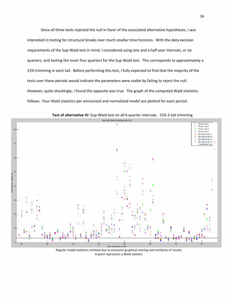
Since all three tests rejected the null in favor of the associated alternative hypotheses, I was

interested in testing for structural breaks over much smaller time horizons. With the data excision

requirements of the Sup-Wald test in mind, I considered using one and a half year intervals, or six

quarters, and testing the inner four quarters for the Sup-Wald test. This corresponds to approximately a

15% trimming in each tail. Before performing this test, I fully expected to find that the majority of the

tests over these periods would indicate the parameters were stable by failing to reject the null.

However, quite shockingly, I found the opposite was true. The graph of the computed Wald statistics

follows. Four Wald statistics per winsorized and normalized model are plotted for each period.

Test of alternative IV: Sup-Wald test on all 6 quarter intervals. 15% 2-tail trimming

Regular model statistics omitted due to excessive graphical overlap and similarity of results.

A point represents a Wald statistic.

17

This test rejected the null hypothesis, as every interval contained a Sup-Wald statistic over the

critical value. A list of Wald statistics below the Sup-Wald critical value for this graph may be found in

the appendix. Approximately one out of every six time periods contained a test statistic for either

model below the Sup-Wald value. Hence, five out of every six Wald statistics were in the Sup-Wald

rejection region. This test also leads me to conclude that the Fundamental Factor Model is highly

unstable, even with estimation windows as short as six quarters.

6. Conclusion:

My findings indicate that, with half year holding periods, the factor premia of commonly-

modeled factors in a Fundamental Factor Model are highly unstable with respect to time. In every

model, parameter instability was more the norm than the exception; even in the models with one and a

half year time horizons, the majority of the computed Wald statistics were in the 1% significance Sup-

Wald rejection region. Hence, the factor premia appear non-stationary with any estimation window.

These results suggest that a large number of investment funds could be employing a

misspecified model with questionable predictive power. As Fundamental Factor Models can be used

with a variety of holding periods and any number of unique factor exposures, I cannot generalize my

conclusion to all possible variants of the Fundamental Factor Model; however, my results do suggest

that any model variant which uses commonly modeled factors from financial literature with a similar

holding period is likely subject to significant parameter instability over time.

In spite of this unsettling conclusion, it is possible that high magnitude within-industry cross-

autocorrelations of equity returns are affecting the statistical tests used in this analysis. It is also

possible that factor premia differ between industries, but are constant within industries; hence,

structural breaks observed in this analysis could be driven by changes in the composition of industries

over time. This question may be considered in a future paper.

18

Sources Cited

• N. Jegadeesh, J. Kim, S. Krische and Charles M. C. Lee. “Analyzing the Analysts: When Do

Recommendations Add Value?” The Journal of Finance, Vol. 59, No. 3 (Jun., 2004), pp. 1083-

1124

• L. Chan, N. Jegadeesh, J. Lakonishok. “The Profitability of Momentum Strategies.” Financial

Analysts Journal. 1999. Vol. 55, No. 6, Behavioral Finance (Nov. - Dec., 1999), pp.80-90

• G Connor. “The Three Types of Factor Models: A Comparison of Their Explanatory Power.”

Financial Analysts Journal, Vol. 51, No. 3 (May - Jun., 1995), pp. 42-46

• John Y. Campbell, Andrew W. Lo, A. Craig MacKinlay. THE ECONOMETRICS OF FINANCIAL

MARKETS. Princeton University Press, 1997

• L. Chincarini, “A Comparison of Quantitative and Qualitative Hedge Funds.” Pomona College

Working Paper. Pomona College Working Paper, (Jan. 2010)

• D. Andrews, “TESTS FOR PARAMETER INSTABILITY AND STRUCTURAL CHANGE WITH UNKNOWN

CHANGE POINT”, Econometrica, Vol. 63, No. 4 (July, 1993), pp. 821-856

• D. Andrews, “TESTS FOR PARAMETER INSTABILITY AND STRUCTURAL CHANGE WITH UNKNOWN

CHANGE POINT: A CORRIGENDUM”, Econometrica, Vol. 71, No. 1 (Jan., 2003), pp. 395-397

19

Appendix

Factor premia estimated over all periods

Factor premia estimated over growth periods

Factor premia estimated over recession periods

20

Alternative IV: Table of Wald statistics below the Sup-Wald critical value

Winsorized Normalized Winsorized Normalized10 15 13 2.79 2.44 63 68 67 2.07 3.2816 21 20 2.89 3.78 64 69 66 2.88 3.2617 22 21 3.06 3.72 64 69 67 2.00 2.9918 23 21 2.74 3.59 65 70 67 2.10 2.6518 23 22 1.60 1.37 66 71 67 1.58 2.2819 24 22 2.60 2.63 66 71 69 2.36 2.5020 25 22 2.21 2.20 66 71 70 2.26 2.9721 26 22 2.50 2.08 67 72 69 2.82 2.7621 26 25 3.50 3.10 67 72 70 2.41 2.8222 27 25 2.45 1.96 67 72 71 2.65 3.4423 28 25 2.64 2.25 69 74 70 2.99 3.2525 30 26 3.03 4.07 70 75 71 3.02 4.0525 30 27 3.10 2.80 70 75 74 3.63 3.1727 32 31 2.93 3.27 71 76 74 2.87 2.3229 34 31 2.97 2.54 71 76 75 2.22 2.3432 37 36 1.99 2.06 72 77 74 1.63 1.1633 38 36 1.98 1.56 72 77 76 1.20 1.8134 39 35 3.02 3.09 73 78 74 2.35 2.3034 39 36 1.88 1.29 73 78 76 1.03 1.7735 40 36 1.15 0.74 74 79 76 1.91 3.0658 63 62 3.22 3.33 75 80 76 1.98 3.6861 66 64 2.85 3.25 75 80 77 3.18 3.3362 67 63 3.56 3.14 76 81 77 2.81 2.7762 67 64 1.57 1.28 76 81 78 2.62 3.1763 68 64 2.45 2.30 77 82 78 2.11 3.1863 68 66 2.96 3.83

Index WaldWald StatisticsTstart Tend Index Tstart Tend

The test intervals in this table are defined by the set of indices in the set [Tstart+1, Tend-1]. As

is evident from the table, no test interval has all four Wald Statistics listed. This occurs only if at least

one index has a corresponding Wald statistic above the 1% significance Sup-Wald critical value.

21

Sources of the quarterly Data Variables used in Factor Construction:

CRSP Variables

Price: “adjprice “

Facprc: “facprc”

Volume: “adjvol”

MarketCap: “cap”

AdjDiv: “adjdiv”

Compustat Variables

Sales: “saleq”

Debt: “ltq”

Equity: “ceqq”

CommonShares: “cshoq”

EPS: “epspxq”

CPrice: “price”

Assets: “atq”

Naics code: “naics”

Plots of regular factor exposures vs. time The following are plots are taken over the entire dataset. Note the outliers in some graphs.

Returns vs. Time

22

Natural Log of Market Capitalization vs. Time

Prior 6 month Returns Momentum vs. Time

23

Prior 12 to 6 month Returns Momentum vs. Time

Total Asset Turnover vs. Time

24

Sales Growth Ratio vs. Time

Debt to Equity Ratio vs. Time

25

Adjusted Average Daily Volume vs. Time

Price to Book Ratio vs. Time

26

Earnings to Price Ratio vs. Time

Dividend Yield vs. Time

27

Summary statistics of regular data

within .0759342 -4.692295 15.93388 T-bar = 28.3412 between .0788563 0 4.705118 n = 11647DIV overall .0128227 .0870443 0 19.23077 N = 330090 within 153.9074 -11763.52 63459.03 T-bar = 28.3412 between 129.6485 .0271677 11781.09 n = 11647DEratio overall 3.979764 165.3874 .001056 69231 N = 330090 within .081776 -1.309798 3.488691 T-bar = 28.3412 between .2133991 0 2.963348 n = 11647TAT overall .2625893 .2254904 0 5.306439 N = 330090 within 59.15526 -6757.771 20265.22 T-bar = 28.3412 between 67.54025 0 6765.157 n = 11647SGR overall 1.597242 65.3512 0 27028.78 N = 330090 within .2779586 -115.1175 13.49402 T-bar = 28.3412 between .2692261 -13.85271 1.980056 n = 11647EPavg overall -.0183501 .3001202 -118.3453 15.49242 N = 330090 within 200.813 -3313.132 101069 T-bar = 28.3412 between 44.36919 .0824635 3317.638 n = 11647PBratio overall 4.24708 203.5891 .0189279 102478.1 N = 330090 within .7352949 12.7808 23.35111 T-bar = 28.3412 between 1.883639 12.83233 25.97695 n = 11647LnMktCap overall 19.07941 2.094817 11.68621 27.12424 N = 330090 within 13882.41 -289581.8 3157440 T-bar = 28.3412 between 12861.49 .1590278 487832.1 n = 11647TURN overall 4076.957 23256.7 0 3322031 N = 330090 within .3778661 -3.310242 5.679092 T-bar = 28.3412 between .2447774 -2.807713 2.784478 n = 11647Mom12 overall .0008323 .3950725 -4.153661 5.908147 N = 330090 within .3883649 -4.228867 4.135431 T-bar = 28.3412 between .2568274 -2.685577 2.097141 n = 11647Mom6 overall -.0110231 .4075402 -4.290459 4.190496 N = 330090 within .4540304 -7.819571 4.051639 T-bar = 28.3412 between .3968147 -7.294717 1.642745 n = 11647CCRnext6 overall -.0173998 .4807335 -8.174703 4.190496 N = 330090 Variable Mean Std. Dev. Min Max Observations

28

Summary statistics of winsorized data

within .0110855 -.0885973 .1311436 T-bar = 28.3412 between .0151148 0 .1221053 n = 11647DIV overall .010584 .0187607 0 .1221053 N = 330090 within 2.127588 -19.67986 34.39335 T-bar = 28.3412 between 4.734654 .047489 32.71814 n = 11647DEratio overall 2.902778 4.584336 .047489 32.71814 N = 330090 within .0714359 -.6014877 1.208815 T-bar = 28.3412 between .2041928 .0019785 1.195833 n = 11647TAT overall .2608828 .2129883 .0019785 1.195833 N = 330090 within .4685093 -3.064714 6.30837 T-bar = 28.3412 between .496526 .1701427 6.006501 n = 11647SGR overall 1.17382 .5423698 .1701427 6.006501 N = 330090 within .0774865 -.8766053 .678017 T-bar = 28.3412 between .1106891 -.8545455 .0733333 n = 11647EPavg overall -.0132923 .0963662 -.8545455 .0733333 N = 330090 within 2.904608 -25.91024 37.32603 T-bar = 28.3412 between 3.842162 .2139904 36.50642 n = 11647PBratio overall 2.895137 3.954607 .2139904 36.50642 N = 330090 within .7297016 12.78004 23.35035 T-bar = 28.3412 between 1.870978 14.54193 24.92134 n = 11647LnMktCap overall 19.07865 2.080567 14.54193 24.92134 N = 330090 within 4616.842 -67041.06 89909.69 T-bar = 28.3412 between 7166.603 1.366667 94029.83 n = 11647TURN overall 3395.252 10278.93 1.366667 94029.83 N = 330090 within .3636287 -1.736109 1.89196 T-bar = 28.3412 between .2238177 -1.481605 1.244644 n = 11647Mom12 overall .0010169 .3799221 -1.481605 1.244644 N = 330090 within .3740957 -1.957286 2.066974 T-bar = 28.3412 between .2379111 -1.564986 1.241713 n = 11647Mom6 overall -.0107728 .3923491 -1.564986 1.241713 N = 330090 within .4540304 -7.819571 4.051639 T-bar = 28.3412 between .3968147 -7.294717 1.642745 n = 11647CCRnext6 overall -.0173998 .4807335 -8.174703 4.190496 N = 330090 Variable Mean Std. Dev. Min Max Observations

29

Summary statistics of normalized data

between .7539986 -2.457027 12.19361 n = 11647NDIV overall 8.46e-10 .9972454 -2.55548 14.82217 N = 330090 within .3780099 -5.466204 11.46131 T-bar = 28.3412 between .6859714 -.8216292 10.33942 n = 11647NTURN overall -2.29e-10 .9972454 -1.129668 19.86789 N = 330090 within .722734 -9.278238 18.66465 T-bar = 28.3412 between .9523942 -1.914443 20.00147 n = 11647NPBratio overall 2.72e-10 .9972454 -2.763816 21.10627 N = 330090 within .7939418 -20.38017 9.306662 T-bar = 28.3412 between 1.069475 -13.65239 1.560367 n = 11647NEPavg overall -1.11e-10 .9972454 -23.47325 4.926731 N = 330090 within .6420565 -9.579826 16.00106 T-bar = 28.3412 between 1.002571 -2.185102 11.71153 n = 11647NDEratio overall -1.19e-09 .9972454 -2.185102 17.84907 N = 330090 within .4489305 -5.542224 8.558899 T-bar = 28.3412 between .9457634 -2.64264 9.000388 n = 11647NTAT overall 3.22e-09 .9972454 -2.754076 10.84011 N = 330090 within .8639982 -8.421585 16.0297 T-bar = 28.3412 between .8777673 -3.062694 17.17064 n = 11647NSGR overall 6.52e-09 .9972454 -5.957483 17.71057 N = 330090 within .3209713 -3.042282 1.965051 T-bar = 28.3412 between .8941637 -2.891855 3.35686 n = 11647NLnMkt~p overall -2.17e-10 .9972454 -3.373385 4.358819 N = 330090 within .9529175 -9.075345 9.718304 T-bar = 28.3412 between .5613808 -5.599185 3.621288 n = 11647NMom12 overall 7.76e-11 .9972454 -9.403751 9.21301 N = 330090 within .9492542 -8.38606 8.436458 T-bar = 28.3412 between .6005179 -7.78686 3.919336 n = 11647NMom6 overall -7.77e-10 .9972454 -8.756555 7.67023 N = 330090 within .4540304 -7.819571 4.051639 T-bar = 28.3412 between .3968147 -7.294717 1.642745 n = 11647CCRnext6 overall -.0173998 .4807335 -8.174703 4.190496 N = 330090 Variable Mean Std. Dev. Min Max Observations