Application of Highway Capacity Manual 2010 Level-of ...

University of Tennessee, Knoxville University of Tennessee, Knoxville

TRACE: Tennessee Research and Creative TRACE: Tennessee Research and Creative

Exchange Exchange

Masters Theses Graduate School

12-2012

Application of Highway Capacity Manual 2010 Level-of-Service Application of Highway Capacity Manual 2010 Level-of-Service

Methodologies for Planning Deficiency Analysis Methodologies for Planning Deficiency Analysis

James Oliver Ensley [email protected]

Follow this and additional works at: https://trace.tennessee.edu/utk_gradthes

Part of the Civil Engineering Commons, and the Other Civil and Environmental Engineering Commons

Recommended Citation Recommended Citation Ensley, James Oliver, "Application of Highway Capacity Manual 2010 Level-of-Service Methodologies for Planning Deficiency Analysis. " Master's Thesis, University of Tennessee, 2012. https://trace.tennessee.edu/utk_gradthes/1373

This Thesis is brought to you for free and open access by the Graduate School at TRACE: Tennessee Research and Creative Exchange. It has been accepted for inclusion in Masters Theses by an authorized administrator of TRACE: Tennessee Research and Creative Exchange. For more information, please contact [email protected].

https://trace.tennessee.edu/

https://trace.tennessee.edu/

https://trace.tennessee.edu/utk_gradthes

https://trace.tennessee.edu/utk-grad

https://trace.tennessee.edu/utk_gradthes?utm_source=trace.tennessee.edu%2Futk_gradthes%2F1373&utm_medium=PDF&utm_campaign=PDFCoverPages

http://network.bepress.com/hgg/discipline/252?utm_source=trace.tennessee.edu%2Futk_gradthes%2F1373&utm_medium=PDF&utm_campaign=PDFCoverPages

http://network.bepress.com/hgg/discipline/257?utm_source=trace.tennessee.edu%2Futk_gradthes%2F1373&utm_medium=PDF&utm_campaign=PDFCoverPages

mailto:[email protected]

To the Graduate Council:

I am submitting herewith a thesis written by James Oliver Ensley entitled "Application of

Highway Capacity Manual 2010 Level-of-Service Methodologies for Planning Deficiency

Analysis." I have examined the final electronic copy of this thesis for form and content and

recommend that it be accepted in partial fulfillment of the requirements for the degree of

Master of Science, with a major in Civil Engineering.

Lee D. Han, Major Professor

We have read this thesis and recommend its acceptance:

Christopher Cherry, Stephen Richards

Accepted for the Council:

Carolyn R. Hodges

Vice Provost and Dean of the Graduate School

(Original signatures are on file with official student records.)

Application of Highway Capacity Manual 2010 Level-of-Service Methodologies for Planning

Deficiency Analysis

A Thesis Presented for the

Master of Science Degree

The University of Tennessee, Knoxville

James Oliver Ensley

December 2012

i

DEDICATION

I dedicate this work to my family and the love of my life, thank you for your support

through it all.

Philippians 4:13

ii

ACKNOWLEDGMENTS

I would like to acknowledge Dr. Lee Han, thank you for your patience and guidance.

Thank you Dr. Chris Cherry and Dr. Steve Richards for your guidance during my time

here at the University of Tennessee. I would also like to thank Stephanie Hargrove for

setting a guideline for me to follow. Thank you to my fellow classmates, I knew I could

always depend on you in a time of need. Thank you to Joseph Roach, Tom Eldridge,

Irina Ponarovskaya, and all of those who helped me from the Tennessee Department of

Transportation offices.

iii

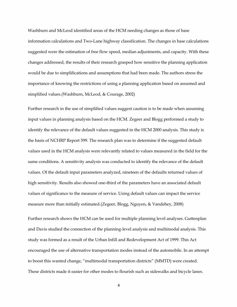
ABSTRACT

Influence on investment in the infrastructure is critical for decision-making by State

planning departments. Judgments which are made for funding purposes and are based

on limited data analysis by states can results in economic disasters for the state and

nation. The Tennessee Department of Transportation (TDOT) uses the Evaluation of

Roadway Efficiency (EVE) database to prioritize the importance of roadway projects in

the state. In addition, EVE is also used as a method to provide deficiency analysis

results for roadways in the state. This study will add support to the methodology of the

current decision-making process in regards to Tennessee roadways for planning.

Updating the current deficiency analysis program (EVE) with the methodologies of the

Highway Capacity Manual (HCM) 2010 is the foundation for improving the decision-

making abilities of those using EVE for such efforts. New algorithms have been

developed based upon the procedures in the HCM 2010 for the following sections:

Freeway, Two-Lane Highways, Multilane Highways, and Urban Arterials. Using these

algorithms and data from Washington County in Tennessee, level-of-service results

were analyzed and compared to previous deficiency analysis results. Some of these

results were found to be better and other were found to be worse than the previous. The

new method of the HCM 2010 applied in this procedure changed 60% of the level of

service ratings based on the comparable data. This proves to show the update of the

deficiency analysis method currently used will be beneficial in the assistance of the

decision-making process.

iv

Table of Contents

Chapter I – Introduction ............................................................................................................................... 1

Chapter II – Literature Review ..................................................................................................................... 3

Chapter III - Highway Capacity Manual ................................................................................................... 11

Evolution of HCM (History) ............................................................................................................... 11

HCM 2000 .............................................................................................................................................. 12

HCM 2010 .............................................................................................................................................. 12

Freeway Segments ........................................................................................................................... 18

Multilane Highway Segments ........................................................................................................ 20

Urban Arterial Segments ................................................................................................................. 21

Two-Lane Highway Segments ....................................................................................................... 21

Chapter IV - Methodologies for Deficiency Analysis ................................................................................. 25

Deficiency Analysis ............................................................................................................................. 25

TDOT Deficiency Analysis ................................................................................................................. 25

TRIMS ................................................................................................................................................ 25

EVE ..................................................................................................................................................... 29

Chapter V - Procedures ............................................................................................................................... 31

Freeway Segment Analysis ................................................................................................................. 31

Multilane Highway Analysis ............................................................................................................. 40

Bicycle Analysis ................................................................................................................................ 46

Urban Arterial Segment Analysis ...................................................................................................... 50

Two-Lane Highway Analysis ............................................................................................................. 62

Chapter VI – Findings and Discussion ...................................................................................................... 81

Study Methodology ............................................................................................................................. 81

Task .................................................................................................................................................... 81

Assumptions ..................................................................................................................................... 81

Newly Created Algorithms ................................................................................................................ 82

Data Contributions .............................................................................................................................. 87

Example Calculations .......................................................................................................................... 88

Two-Lane Highway ......................................................................................................................... 89

Multilane Highways: ....................................................................................................................... 91

v

Urban Arterial Segment: ................................................................................................................. 93

Freeway Analysis: ............................................................................................................................ 95

RESULTS ............................................................................................................................................... 96

Comparison ....................................................................................................................................... 98

Chapter VII – Conclusion ......................................................................................................................... 107

Summary ............................................................................................................................................. 107

Suggestions ......................................................................................................................................... 108

APPENDIX .............................................................................................................................................. 109

Capacity Analysis Procedures for Eve 4.0 ...................................................................................... 110

fn/dp,PTSF Charts .................................................................................................................................... 157

List of References ...................................................................................................................................... 160

VITA ......................................................................................................................................................... 162

vi

List of Tables

Table 1: Two-Lane Highway Comparison Results .............................................................................. 24

Table 2: ET and ER Values based on Terrain ....................................................................................... 33

Table 3: Reduction due to Lane Width (National Research Council . Transportation Research,

2010) ........................................................................................................................................................... 34

Table 4: Reduction due to Right-Side Lateral Clearance(National Research Council .

Transportation Research, 2010) .............................................................................................................. 35

Table 5: Freeway Segment LOS Criteria ............................................................................................... 38

Table 6: ET and ER Values based on Terrain (National Research Council . Transportation

Research, 2010) ......................................................................................................................................... 41


2010) ........................................................................................................................................................... 42

Table 8: Reduction due to Total Lateral Clearance (National Research Council . Transportation

Research, 2010) ......................................................................................................................................... 42

Table 9: Reduction due to Presence of Median (National Research Council . Transportation

Research, 2010) ......................................................................................................................................... 42

Table 10: Reduction due to Access-Point Density (National Research Council . Transportation

Research, 2010) ......................................................................................................................................... 43

Table 11: LOS Criteria for Multilane Highways .................................................................................. 45

Table 12: Bicycle Level of Service Score Criteria (National Research Council . Transportation

Research, 2010) ......................................................................................................................................... 49

Table 13: Through Vehicle Delay (National Research Council . Transportation Research, 2010) 55

Table 14: Level of Service Criteria Urban Arterial (National Research Council . Transportation

Research, 2010) ......................................................................................................................................... 60

Table 15: Two-Lane Highway Classifications ...................................................................................... 64

Table 16: Reduction due to Grade for ATS ........................................................................................... 67

Table 17: ET for specific Upgrades (ATS) (National Research Council . Transportation Research,

2010) ........................................................................................................................................................... 68

Table 18: ER for specific Upgrades (ATS) (National Research Council . Transportation Research,

2010) ........................................................................................................................................................... 69

Table 19: Reduction due to Grade for PTSF ......................................................................................... 71

Table 20: ET and ER Values for Specific Grades (National Research Council . Transportation

Research, 2010) ......................................................................................................................................... 72

Table 21: Reduction due to No-Passing Zones for ATS (fnp,ATS) (National Research Council .


Table 22: Reduction due to No-Passing Zone and Directional Distribution for PTSF (fnp/dp,PTSF) 79

Table 23: Level of Service Criteria for Two-Lane Highways (National Research Council .


Table 24: Portion of LOS Values ............................................................................................................ 99

vii

Table 25: New LOS Percentage Results ................................................................................................ 99

Table 26: Same as EVE Results by Roadway Class ........................................................................... 102

viii

List of Figures

Figure 1: Basic Freeway Segment Algorithm (National Research Council . Transportation

Research, 2010) ......................................................................................................................................... 14

Figure 2: Multilane Highway Algorithm (National Research Council . Transportation Research,

2010) ........................................................................................................................................................... 15

Figure 3: Two-Lane Highway Algorithm (National Research Council . Transportation Research,

2010) ........................................................................................................................................................... 16

Figure 4: Urban Arterial Segment Algorithm (National Research Council . Transportation

Research, 2010) ......................................................................................................................................... 17

Figure 5: HCM 2000 Basic Freeway Segments Speed-Flow Curve (National Research Council .




Figure 7: Sample of Two-Lane Highway Classification Comparison .............................................. 23

Figure 8: TRIMS Information Type Selection ....................................................................................... 26

Figure 9: TRIMS - Washington County Road Segment Query .......................................................... 28

Figure 10: Screenshot of EVE Summary ............................................................................................... 30

Figure 11: Freeway Segment Speed-Flow Curve (National Research Council . Transportation

Research, 2010) ......................................................................................................................................... 32

Figure 12: Multilane Highway Speed-Flow Curve (National Research Council . Transportation

Research, 2010) ......................................................................................................................................... 40

Figure 13: Freeway Segment Algorithm ............................................................................................... 83

Figure 14: Multilane Highway Algorithm ............................................................................................ 84

Figure 15: Two-Lane Highway Algorithm ........................................................................................... 85

Figure 16: Urban Arterial Segment Algorithm .................................................................................... 86

Figure 17: Bicycle Analysis Algorithm .................................................................................................. 87

Figure 18: LOS Comparison results ..................................................................................................... 101

Figure 19: LOS Comparison Results for Two-Lane Highways ....................................................... 103

Figure 20: Urban Arterial Segment LOS Comparison Percentages ................................................ 104

Figure 21: Multilane Highway LOS Comparison Percentages ........................................................ 105

ix

List of Equations

Equation 1: Flow Rate .............................................................................................................................. 32

Equation 2: Reduction due to Heavy Vehicles ..................................................................................... 33

Equation 3: FFS Calculation .................................................................................................................... 34

Equation 4: Total Ramp Density for Longer Segments ...................................................................... 35

Equation 5: Total Ramp Density for Shorter Segments ...................................................................... 36

Equation 6: Capacity Equation for FFS less than 70 mph ................................................................... 36

Equation 7: Freeway Operation Speed Calculation (FFS = 75mph) .................................................. 37

Equation 8: Freeway Operation Speed for FFS > 70 mph .................................................................. 37

Equation 9: Freeway Operation Speed for FFS > 65 mph .................................................................. 37

Equation 10: Freeway Operation Speed for FFS > 60 mph ................................................................ 38

Equation 11: Freeway Operation Speed for FFS > 55 mph ................................................................ 38

Equation 12: Freeway and Multilane Highway Segment Density .................................................... 38

Equation 13: Multilane Highway FFS ................................................................................................... 41

Equation 14: Access-Point Density Calculation ................................................................................... 43

Equation 15: Multilane Highway Capacity less than 60 mph............................................................ 44

Equation 16: Multilane Operation Speed for FFS > 55 mph .............................................................. 44

Equation 17: Multilane Operation Speed for FFS between 50-55 mph ............................................. 45

Equation 18: Multilane Operation Speed for FFS between 45-50 mph ............................................. 45

Equation 19: Multilane Operation Speed for FFS = 45 mph .............................................................. 45

Equation 20: Flow Rate based on Outside Lane width ...................................................................... 46

Equation 21: Width as a function of Traffic Volume for V > 160 vph .............................................. 47

Equation 22: Width as a function of Traffic Volume ........................................................................... 47

Equation 23: Average effective width (SW > 8 feet) ........................................................................... 47

Equation 24: Average effective width (4 ft. < SW < 8 ft.) ................................................................... 48

Equation 25: Average Effective Width (SW < 4 ft.) ............................................................................. 48

Equation 26: Effective Speed Factor ...................................................................................................... 48

Equation 27: Bicycle Level of Service Score .......................................................................................... 48

Equation 28: Urban Arterial Segment Flow Rate ................................................................................ 51

Equation 29: Midsegment Volume ........................................................................................................ 52

Equation 30: Arterial FFS Calculation ................................................................................................... 52

Equation 31: Arterial BFFS ...................................................................................................................... 53

Equation 32: Arterial Access Point Adjustment .................................................................................. 53

Equation 33: Cross Section adjustment ................................................................................................. 54

Equation 34: Signal Spacing Adjustment .............................................................................................. 54

Equation 35: Vehicle Proximity Adjustment ........................................................................................ 55

Equation 36: Running Time Estimation ................................................................................................ 56

Equation 37: Arterial Capacity ............................................................................................................... 56

Equation 38: v/c ratio .............................................................................................................................. 57

x

Equation 39: Average Delay per Vehicle: ............................................................................................. 58

Equation 40: Uniform Delay ................................................................................................................... 58

Equation 41: Incremental Delay ............................................................................................................. 58

Equation 42: Initial Queue Delay ........................................................................................................... 58

Equation 43: Average Travel Speed ...................................................................................................... 60

Equation 44: ATS Flow Rate ................................................................................................................... 65

Equation 45: Directional Demand Flow Rate ....................................................................................... 66

Equation 46: PTSF Flow Rate.................................................................................................................. 70

Equation 47: Directional Flow Rate ....................................................................................................... 73

Equation 48: Opposing Flow Rate ......................................................................................................... 73

Equation 49: Two-Lane Highway FFS .................................................................................................. 74

Equation 50: Adjustment due to Lane Width and Shoulder Width ................................................. 74

Equation 51: Adjustment due to Access-Point Density ...................................................................... 74

Equation 52: Average Travel Speed (Two-Lane) ................................................................................. 75

Equation 53: Percent Time Spent Following (Two-Lane) ................................................................... 77

Equation 54: Base Percent Time Spent Following (Two-Lane) .......................................................... 77

Equation 55: Percent Free Flow Speed (Two-Lane) ............................................................................ 79

1

Chapter I – Introduction

The many state transportation organizations maintain an understanding of current and future

roadways quality of service. These understanding may be based on the use of deficiency

analysis. Deficiency analysis is used to determine weaknesses found in a system. This is found

true in many types of systems, especially in roadway systems. Deficiency analysis is used by

some as a method of appropriating funding for projects. This is the case when it comes to the

Tennessee Department of Transportation. In order to provide assistance to TDOT’s efforts for

deficiency analysis, an improvement of the model they currently use will be established in this

study. Using the Highway Capacity Manual (HCM) 2010 and the Tennessee Roadway

Information Management System (TRIMS) developed by TDOT, this study will modernize the

program for better Planning-Level analysis and quality of service. Planning-level analysis is

beneficial for gaining understanding of roadway operations without the use of detailed

information. Many developers use planning-level analysis to visualize necessary design ideas.

Planning-level analyses are common in the transportation industry. Many engineers utilize the

Highway Capacity Manual (HCM) methods of level-of service determination to assist them in

planning efforts.

Level-of-service (LOS) is the best known measure for qualitatively assessing the quality of a

roadway. In order to assist TDOT in projecting the level-of-service (LOS) of roadways in the

state of Tennessee, updates have to be made to the structure of their current deficiency analysis

program. The program developed by TDOT used for deficiency analysis is known as the

Evaluation of Roadway Efficiency, EVE.

2

The most recent version of EVE is based on the methodologies of the HCM 2000. In order for

EVE to remain most effective in its analysis, the methodologies used as a basis need to remain

updated with those of the most current version of the HCM. The changes from HCM 2000 to

HCM 2010 are a factor in the modification of EVE methodologies and will be presented in this

study.

Planning-level analysis is beneficial for the appropriation of funding within the state as well as

other forms of decision-making. Since the EVE database is used to prioritize projects in the state

by level of importance, the methodologies must be kept up-to-date. The connection of the HCM

and EVE is vitally important to maintain the principles on which EVE has been based. With the

use of the algorithms from HCM 2010 Level of Service (LOS) analysis, planning efforts are made

to help improve the accuracy of the deficiency analysis in Tennessee Roadway Systems. The

new methods will be tested on data from Washington County in Tennessee and compared to

results from the same location provided by TDOT researchers. The proposal of a newer version

of the EVE database will be presented and suggested based on the results of the findings.

3

Chapter II – Literature Review

This chapter reviews previous research conducted in areas related to this thesis. Those areas are

separated into sections for planning analysis using the Highway Capacity Manual (HCM),

improvements of levels of service, and Investment decision for highways. This chapter is to

provide an idea of the issues this thesis desires to address. The research described below

provides important perspective to the ideas formulated in this thesis.

HCM for Planning

Using the HCM for planning level analysis is the basis of this study. It is important to

understand the ideas of previous researchers and their use of the Highway Capacity Manual for

planning or operational analysis. Researchers believe the HCM is a “principal guide in

transportation decision-making, planning, and design. (Kittelson & Roess)” Research shows the

importance of using the HCM for planning; however they understand the difficulties in this as

well.

Washburn and McLeod studied the planning methods of HCM 2000 in order to create a with

planning-analysis capabilities for two-lane and multilane highways. The software developed by

the Florida Department of Transportation (FDOT) is known as HIGHPLAN. Creating this

software based on the methods of the HCM is a difficult task. Difficulty arose when attempting

to remain connected to the specific methods in the HCM while also having to make necessary

assumptions for planning analysis.

4

Washburn and McLeod identified areas of the HCM needing changes as those of base

information calculations and Two-Lane highway classification. The changes in base calculations

suggested were the estimation of free flow speed, median adjustments, and capacity. With these

changes addressed, the results of their research grasped how sensitive the planning application

would be due to simplifications and assumptions that had been made. The authors stress the

importance of knowing the restrictions of using a planning application based on assumed and

simplified values.(Washburn, McLeod, & Courage, 2002)

Further research in the use of simplified values suggest caution is to be made when assuming

input values in planning analysis based on the HCM. Zegeer and Blogg performed a study to

identify the relevance of the default values suggested in the HCM 2000 analysis. This study is

the basis of NCHRP Report 599. The research plan was to determine if the suggested default

values used in the HCM analysis were relevantly related to values measured in the field for the

same conditions. A sensitivity analysis was conducted to identify the relevance of the default

values. Of the default input parameters analyzed, nineteen of the defaults returned values of

high sensitivity. Results also showed one-third of the parameters have an associated default

values of significance to the measure of service. Using default values can impact the service

measure more than initially estimated.(Zegeer, Blogg, Nguyen, & Vandehey, 2008)

Further research shows the HCM can be used for multiple planning level analyses. Guttenplan

and Davis studied the connection of the planning-level analysis and multimodal analysis. This

study was formed as a result of the Urban Infill and Redevelopment Act of 1999. This Act

encouraged the use of alternative transportation modes instead of the automobile. In an attempt

to boost this wanted change, “multimodal transportation districts” (MMTD) were created.

These districts made it easier for other modes to flourish such as sidewalks and bicycle lanes.

5

Research revealed a connection between land use development and transportation modes. The

evaluation of the MMTD was based on level-of-service techniques and the application of those

techniques in the HCM. The results from this study provided the government with a developed

template for current and future development enhancement of multimodal

planning.(Guttenplan, Davis, Steiner, & Miller, 2003)

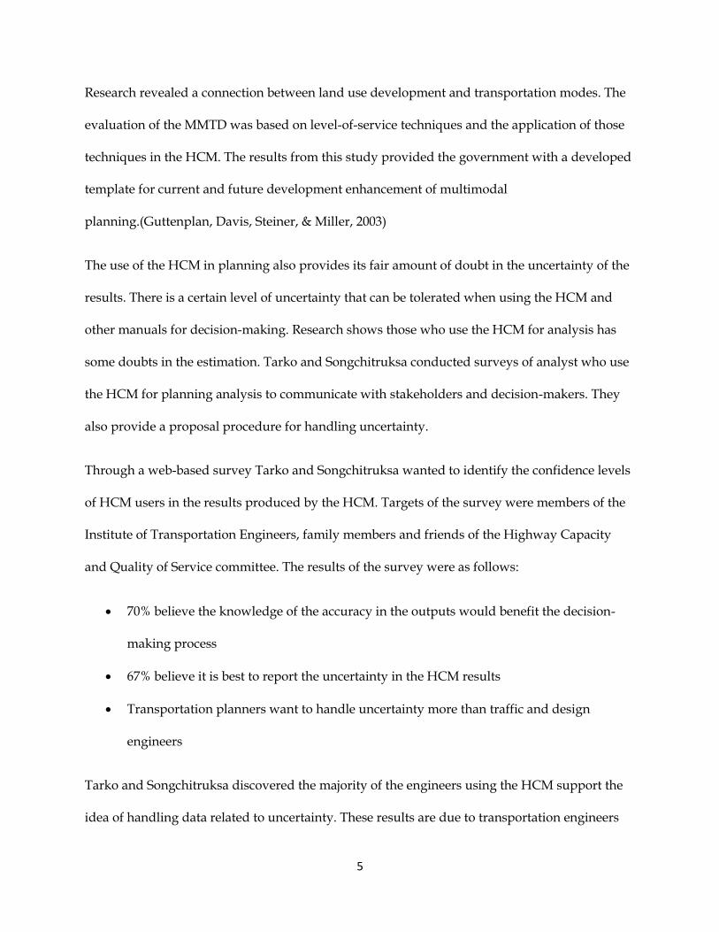
The use of the HCM in planning also provides its fair amount of doubt in the uncertainty of the

results. There is a certain level of uncertainty that can be tolerated when using the HCM and

other manuals for decision-making. Research shows those who use the HCM for analysis has

some doubts in the estimation. Tarko and Songchitruksa conducted surveys of analyst who use

the HCM for planning analysis to communicate with stakeholders and decision-makers. They

also provide a proposal procedure for handling uncertainty.

Through a web-based survey Tarko and Songchitruksa wanted to identify the confidence levels

of HCM users in the results produced by the HCM. Targets of the survey were members of the

Institute of Transportation Engineers, family members and friends of the Highway Capacity

and Quality of Service committee. The results of the survey were as follows:

70% believe the knowledge of the accuracy in the outputs would benefit the decision-

making process

67% believe it is best to report the uncertainty in the HCM results

Transportation planners want to handle uncertainty more than traffic and design

engineers

Tarko and Songchitruksa discovered the majority of the engineers using the HCM support the

idea of handling data related to uncertainty. These results are due to transportation engineers

6

believing the uncertainty reports will result in better decision-making based on the HCM

analysis. They also heed that reporting uncertainty can be beneficial but first must be

researched to identify the non-engineering impacts as well as formatted to the understanding of

transportation decision-makers and stakeholders.(Tarko & Songchitruksa, 2003)

Level of Service Improvements

The next topic of research related to this study is improvements of level of service (LOS). The

HCM is used to provide the best measure of quality of service for a roadway with given

conditions. The HCM methods for estimating level of service are directly related decision-

making purposes based on quality analysis. Meaning, any efforts at improving the level of

service methods can results in improvements in the planning analysis of the HCM.

Research shows the HCM levels of service are based on different measures of effectiveness

(MOEs). However, these MOEs are selected by the Highway Capacity and Quality of Service

Committee (HCQSC) as to which would best represent the LOS for the type of roadway. Many

researchers have found that travelers perceive the LOS for roadway differently than what the

HCQS believe.

Washburn, Ramlackhan, and McLeod performed a study to identify new measures of quality of

service. Previous measures were based on the Highway Capacity Quality of Service Committee

(HCQSC) and what they deemed was suitable to measure quality. Some committee members

felt it was necessary for an alternative measure related to traveler perceptions. Therefore, a

survey was conducted for travelers near a rural freeway in Florida. The idea of the study was to

7

gain information regarding the trip, personal information of the travelers, and overall traveler

opinion of the trip on the freeway.

Washburn, Ramlackhan, and McLeod identified what the study refers to as the “cruise-control

factor” to be the most important factor based on traveler opinion. This factor is related to the

ability for travelers to maintain their desired travel speeds with deceleration. Other important

factors were found to be freeway density, pavement quality, the percent of travel at the free

flow speed, etiquette of fellow drivers on the road, and construction zone presence. Research

also showed that there roadway quality is not solely based on one factor. Many factors were

found to be significant, some of these factors are related to traffic and some are not. However, it

is important to take each of these factors into account when assessing a roadway. (Washburn,

Ramlackhan, & McLeod, 2004)

Another study conducted by Pechaux, Pietrucha, and Jovanis displayed the assessment

of LOS at signalized intersections based on the HCM LOS methods from a user

perspective and factors affecting user LOS perceptions. A model was created to estimate

the LOS based on user perceptions. This model included factors pertaining to time-of-

day, location, trip putrpose, personal characteristics, value of time and time use,

temporal urgency, delay, signal characteristics, and user experience expectations.

Results showed that users were more adherent to delay than the HCM originally

believed. The reuslts showed that user classifed their LOS beliefs into four levels of

service as opposed to six. The estimation of delay for users at signalized intersections

were found to “accurate but variable.” Results further determined that traveler

8

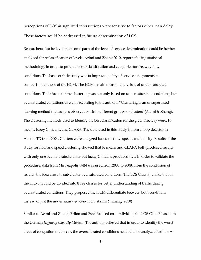
perceptions of LOS at signlized intersections were sensitve to factors other than delay.

These factors sould be addressed in future determination of LOS.

Researchers also believed that some parts of the level of service determination could be further

analyzed for reclassification of levels. Azimi and Zhang 2010, report of using statistical

methodology in order to provide better classification and categories for freeway flow

conditions. The basis of their study was to improve quality of service assignments in

comparison to those of the HCM. The HCM’s main focus of analysis is of under saturated

conditions. Their focus for the clustering was not only based on under saturated conditions, but

oversaturated conditions as well. According to the authors, “Clustering is an unsupervised

learning method that assigns observations into different groups or clusters”(Azimi & Zhang).

The clustering methods used to identify the best classification for the given freeway were: K-

means, fuzzy C-means, and CLARA. The data used in this study is from a loop detector in

Austin, TX from 2004. Clusters were analyzed based on flow, speed, and density. Results of the

study for flow and speed clustering showed that K-means and CLARA both produced results

with only one oversaturated cluster but fuzzy C-means produced two. In order to validate the

procedure, data from Minneapolis, MN was used from 2008 to 2009. From the conclusion of

results, the idea arose to sub cluster oversaturated conditions. The LOS Class F, unlike that of

the HCM, would be divided into three classes for better understanding of traffic during

oversaturated conditions. They proposed the HCM differentiate between both conditions

instead of just the under saturated condition.(Azimi & Zhang, 2010)

Similar to Azimi and Zhang, Brilon and Estel focused on subdividing the LOS Class F based on

the German Highway Capacity Manual. The authors believed that in order to identify the worst

areas of congestion that occur, the oversaturated conditions needed to be analyzed further. A

9

proposal of dividing the LOS Class F into four classes (F1-F4) was given. The study was done

using freeway analysis. Given that the results are sensitive, the use of software is suggested to

evaluate the methods further. The purpose of this study is to better identify the most

problematic areas for congestion. The identification of bottlenecks is very important to planning

procedures. If results are provided in the range of those similar to bottlenecks, planning

adjustment could be made to the roadway to help improve the quality.(Brilon & Estel, 2010)

Highway Investment Decisions

The final topic of research related to this study is those of highway investment decisions. The

ultimate scope of this study is for the development and use of a deficiency analysis program as

a selector for highway investment. Sharma, Al-Hussein, Safouhi, and Bouferguene conducted a

study of the use of an asset LOS (ALOS) determination methodology with the inclusion of a

decision support system (DSS) to assess a roadway infrastructure. The model is based on the

analytical hierarchy method and is believed to determine LOS in regards to more qualitative

measures in comparison to quantitative. This model returned a combined LOS determination

for an urban road based on vehicle, pedestrian, and bicyclist users, as well as information

regarding safety and appearance of the road. The resulted framework for ALOS determination

is primarily believed to provide assistance in decision-making regarding the infrastructure. This

research further shows that use of current methods of level of service for decision-making

purposes need to be modified in order to fully grasp all of the appropriate service measures.

Calculating the asset LOS in this study provided a more general result of analysis based not

10

only on quantitative measure but qualitative measure as well.(Sharma, Al-Hussein, Safouhi, &

Bouferguene, 2008)

11

Chapter III - Highway Capacity Manual

The Highway Capacity Manual (HCM) is a guide used to determine the quality of service and

capacity for given roadway segments and facilities. The structural basis of the deficiency

analysis method in this study is from the HCM 2010. The ideologies in the method are taken

directly from the HCM. Before diving into the methods of the HCM 2010, here is a brief history

of the HCM.

Evolution of HCM (History)

The Highway Capacity Manual was first published by the Transportation Research Board in 1950.

There have been five major editions of the manual published in 1950, 1965, 1985, 2000, and 2010.

Every edition brought forth something that the previous had not. It began as a way of

determining the capacity and quality of service for roadways. “The first edition of the Highway

Capacity Manual in 1950 did not contain any significant material on uninterrupted flow

facilities. Freeways were not common, as the National System of Interstate and Defense

Highways had not yet been initiated”(Roess, 2011). Therefore the 1965 edition included

freeway chapters in addition to modification of previous methods in the first edition in

1950. The next major edition in 1985 introduced more focus into signalized analysis

utilizing data collection from the early 80’s. The update to the 1985 manual came in 1994

with the addition of new chapters following the addition of Multilane Highway analysis

previously. The HCM 2000 was focused more into the connection of micro simulation and

12

software application. The HCM 2010 added new analysis sections regarding multimodal

facilities and roundabouts. Each edition provided something new based on research studies

conducted. The most beneficial studies that brought about changes in the HCM were those of

the National Cooperative Highway Research Program (NCHRP) project reports. The Highway

Capacity Manual provides the best and most effective methods for calculating the appropriate

results given specific conditions. As the nature of transportation grew, so has the ideology of

the manual. The earlier models were not as detail specific as the one today and the future

editions will be more complex in comparison to those today.

HCM 2000

The methodologies taken from the HCM 2000 for Multilane Highway, Two-Lane Highway,

Freeway, and Urban Street chapters have been previously used for deficiency analysis

programs for TDOT. The deficiency analysis program known as EVE was developed according

to the HCM 2000 just as the program is being developed in this method is based from the HCM

2010.

HCM 2010

The HCM 2010 is the cornerstone of this entire study. For the purpose of this study specific

chapters of the HCM 2010 were targeted. Those chapters, just like the ones from previous

analysis, are: Freeway Segments, Multilane Highways, Two-Lane Highways, and Urban Street

Segments. The algorithms in each section of the HCM 2010 provided the guideline for proper

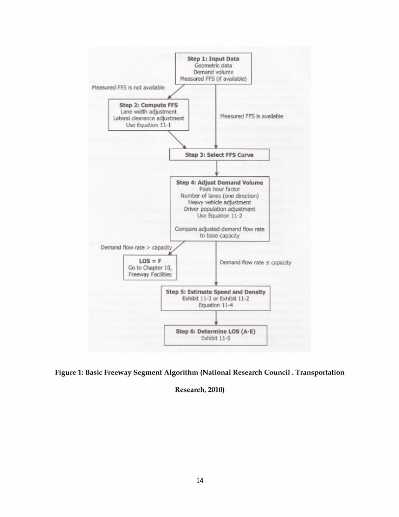
estimation of the quality of service amongst other values. Each chapter’s algorithm can be found

13

below. Each of the figures below are from the HCM 2010 (National Research Council .

Transportation Research (2010).

This study focuses on segment analysis of the HCM 2010. Even though the manual contains

sections for both segments and facilities, segment analysis was selected due to constraints of the

data by TDOT through the TRIMS database. Also, the previous version of the deficiency

analysis program was segment based.

For this study it is necessary to identify the changes affecting the analysis. Each of the chapters

used for analysis has been update from the 2000 edition to the 2010 edition. The changes for

each of the chapters are provided in the sections below.

14

Figure 1: Basic Freeway Segment Algorithm (National Research Council . Transportation

Research, 2010)

15

Figure 2: Multilane Highway Algorithm (National Research Council . Transportation

Research, 2010)

16

Figure 3: Two-Lane Highway Algorithm (National Research Council . Transportation

Research, 2010)

17

Figure 4: Urban Arterial Segment Algorithm (National Research Council . Transportation

Research, 2010)

18

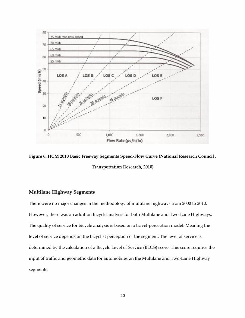
Freeway Segments

The methodology of the Freeway Segments remains similar to the HCM 2000. However, the

major change is the modification of the speed-flow curve. Speed-flow curves have been used to

depict the relationship of speed and flow rate for given free flow speeds (FFS). The curves are a

critical part of level of service estimation. The speed-flow curve from the 2000 edition of the

HCM is shown in Figure 5: HCM 2000 Basic Freeway Segments Speed-Flow Curve (National

Research Council . Transportation Research, 2000). Figure 6: HCM 2010 Basic Freeway

Segments Speed-Flow Curve (National Research Council . Transportation Research, 2010)

shows the speed-flow curve provided in the HCM 2010. The differences in these curves are the

breakpoints of each free flow speed curve. The 2000 edition shows its breakpoints on its curve;

however the 2010 edition does not. The values of the breakpoints for the 2010 edition are 1000,

1200, 1400, 1600, and 1800 correlating to order of the curves starting with the 75 mph curve. The

breakpoint changes affect the operation speed (S) for segments with free flow speeds within the

range of 55-75 mph. the average FFS on a freeway segment falls within this range, therefore this

methodology change is small.

Other changes from the HCM 2000 are found in the method for calculation of the Free Flow

Speed (FFS). This change adds in the factor Total Ramp Density (TRD) which is similar to

Interchange Density (ID) found in the 2000 edition. Whereas ID was used as a reduction factor,

the new calculation uses TRD to directly estimate FFS. The previous FFS calculation also

estimated the Base Free Flow Speed, but now in the 2010 edition an assumed value of 75.4 mph

is used instead of a calculation based on the posted speed limit. The FFS calculation in the 2010

edition also removed the reduction due to lane width.

19


Transportation Research, 2000)

20



Multilane Highway Segments

There were no major changes in the methodology of multilane highways from 2000 to 2010.

However, there was an addition Bicycle analysis for both Multilane and Two-Lane Highways.

The quality of service for bicycle analysis is based on a travel-perception model. Meaning the

level of service depends on the bicyclist perception of the segment. The level of service is

determined by the calculation of a Bicycle Level of Service (BLOS) score. This score requires the

input of traffic and geometric data for automobiles on the Multilane and Two-Lane Highway

segments.

21

Urban Arterial Segments

The change to the Urban Street Segment analysis was the removal of Arterial Classification. The

2000 edition categorized for different types of arterials: High-Speed, Suburban, Urban, and

Intermediate. All four of these arterial types are now analyzed using the same method.

Two-Lane Highway Segments

From 2000 to 2010 there was a significant change of the methodology of the Two-Lane Highway

Analysis. The method in the 2010 HCM focuses on one directional analysis. This means two-

lane roadways are now to be analyzed based on one direction of traffic and include inputs

related to the opposing direction of traffic.

In addition to the methodology change, there was also an addition made to the Highway

Classifications. The new method adopts a Class III Highway which is for developed areas that

may travel through small towns. These highways also have a higher number of access points on

the segment as compared to Class I and Class II highways.

Classification is a strong factor in the necessary level of service analysis. In order to understand

how important a change in the highway class can be in the LOS results, a comparison was

conducted. The comparison is of the data collected from two-lane highway segments in

Washington County. Each segment is analyzed as if it is considered a Class I, Class II, or Class

III highway. Since there are so many segments used in the analysis, samples of the results are

shown in Figure 7: Sample of Two-Lane Highway Classification Comparison. Table 1: Two-

Lane Highway Comparison Results shows the comparison of results by percentages. From

the results, it shows that Class III provides the best results for LOS Classes A, B, and C. Class I

22

has the most results with LOS Classes D, E, and F. From this, consideration is made that Class

III is the best for LOS results, next is Class II, and Class I is the worst in comparison to the other

classes.

23

BLM ELM Road Name AADT Spd LimitLOS if

Class I

LOS if

Class II

LOS if

Class III

0.716 1.35 TELFORD RD. 2100 35 E C B

0 1.07 GLENDALE RD. 340 35 E A A

1.07 4.55 GLENDALE RD. 890 35 E B A

0 2.48 BUMPUS COVE RD. 420 20 E A B

0.96 0.99 OLD SR-34 1040 45 D B A

3 3.05 OLD SR-34 1040 45 C B A

4 4.138 OLD SR-34 1040 30 E B B

4.138 4.59 OLD SR-34 530 30 E B A

4.59 4.72 S. CLEAR SPRINGS RD. 530 30 E B A

0 1.538 BOWMANTOWN RD. 530 35 E B A

1.538 3.64 BOWMANTOWN RD. 540 35 E B A

1.94 3.34 ARNOLD RD. 920 40 E C A

8.511 8.559 DRY CREEK RD. 780 40 E B A

8.559 8.59 LONE OAK RD. 780 40 E B A

1.76 4.77 CONKLIN RD. 500 45 D B A

4.77 6.57 CONKLIN RD. 3420 45 D D B

0.19 0.36 W. MAIN ST. 6600 20 E D E

0.36 0.45 E. MAIN ST. 6600 20 E D E

0.49 0.548 FOX AVE. 3060 20 E D D

0.548 0.62 WOODROW AVE. 3060 20 E D E

1.047 1.126 S. CHEROKEE ST. 3060 20 E D E

1.438 1.462 OLD EMBREEVILLE RD. 3060 20 E D E

2.84 4 OLD EMBREEVILLE RD. 3060 35 E D C

4 5.68 BILL JONES RD. 500 30 E B A

4.14 4.19 OLD STAGECOACH RD. 460 40 E B A

8.347 8.38 HAIRETOWN RD. 1820 40 E C B

9.049 11.363 BOONES STATION RD. 1820 35 E C B

11.8 11.839 BOONES STATION RD. 90 35 E A A

11.839 12.08 LAKE PARK DR. 90 35 E A A

0.07 0.139 E. OAKLAND AVE. 5380 30 E D C

2.045 2.2 E. OAKLAND AVE. 5380 30 E D D

0 1.68 DUCKTOWN RD. 160 35 E A A

0 1.08 MAPLE SWAMP RD. 380 30 E A A

1.529 1.791 LIBERTY CHURCH DR. 380 30 E A A

1.791 2.83 HONEYSUCKLE LN. 380 30 E A A

Figure 7: Sample of Two-Lane Highway Classification Comparison

24

Table 1: Two-Lane Highway Comparison Results

Highway Class Type

Percent “Good” (Class A, B, C) (%)

Percent “Bad” (Class D, E, F) (%)

Class I 0.7 99.3

Class II 43.1 56.9

Class III 73.2 26.8

25

Chapter IV - Methodologies for Deficiency Analysis

Deficiency Analysis

Deficiency Analysis is a method used to determine weaknesses in a system. This is useful when

it comes to analyzing roadway weaknesses. Many state transportation organizations run

deficiency analyses in order to identify where appropriate funding should be going. This

analysis can be run for current roadway conditions as well as future roadway conditions. With

this in mind, the model to be presented is beneficial to the State of Tennessee’s deficiency

analysis of its roadways. Without the necessary change to the current deficiency analysis

program, current methods will remain inconsistent with current state of the practice.

TDOT Deficiency Analysis

The Tennessee Department of Transportation (TDOT) maintains the state’s current deficiency

analysis program. With the assistance of TDOT, this study will provide reasonable and current

methodologies for updating the deficiency analysis program.

TRIMS

In order to run an accurate deficiency analysis of Tennessee roadways, TDOT has provided data

from its Tennessee Roadway Information Management System (TRIMS) database. The TRIMS

database contains information regarding every roadway in the state. Much of the input data

needed to run a proper analysis can be located within this database. Specific queries were run in

26

TRIMS in order to locate the appropriate data for the roadways. Data in TRIMS is separated by

a combination of City or County and Route. From here one must select from data sets already

presented in TRIMS. The information types are shown below in Error! Reference source not

ound..

Figure 8: TRIMS Information Type Selection

27

Of these information types, the most beneficial information for the analysis was located within

the following sets:

- Roadway Segment

- Roadway Description

- Roadway Geometrics

- Route Feature

- Traffic

28

Any combination of these information types could be run in an advanced query. An

example of the query ran for Washington County Road Segments is shown in Figure 9.

From here the result of the query are tabulated.

Figure 9: TRIMS - Washington County Road Segment Query

Using the advanced query, each information type above was selected and filtered to provide

data for Washington County only. The data was then exported into excel and trimmed in order

to establish all of the necessary parameters needed for the deficiency analysis.

29

EVE

Evaluation of Roadway Efficiency (EVE) is the program TDOT uses to run it Deficiency

Analysis. This program was developed by Dr. Lee Han and Dr. Fred Wegmann of The

University of Tennessee at Knoxville and adopted for use by TDOT. The current version of EVE

is based on the methodologies of the 2000 Highway Capacity Manual. Since the version of the

HCM used in EVE is now outdated, this study will provide a current version of its basic

methodologies based now on the HCM 2010.

EVE takes input data from the TRIMS database and run its deficiency analysis as shown in

Figure 10. EVE in addition to providing current roadway analysis would also provide

forecasted analysis for future conditions. Keeping this analysis as current as possible is the

reason for this study.

30

Figure 10: Screenshot of EVE Summary

31

Chapter V - Procedures

Now with an understanding of deficiency analysis and the TRIMS system, the following

procedure is used to estimate deficiency analysis based from the algorithms in the HCM 2010.

This procedure has been developed to provide methodologies for future deficiency analysis

programs, such as EVE. The procedure consists of Freeway Segments, Multilane Highways,

Two-Lane Highways, and Urban Arterial Segments sections. As previously stated, the

foundation of this procedure comes from the Capacity Analysis Procedure for Eve 4.0, which

can be found in the Appendix.

Freeway Segment Analysis

The data inputs have collected are necessary for proper analysis of the freeway segments.

Specific inputs to be taken from the TRIMS database for Freeway Segments are: Annual

Average Daily Traffic (AADT), K Factor, D Factor, Peak Hour Factor (PHF), Lane Width, Lateral

Clearance, Rural/Urban Classification, Terrain, Truck Percentage, and Posted Speed. The

respective output results of the freeway segments are: Operational Speed (S), Capacity (c), v/c

ratio, Density (D), and Level of Service (LOS). Each of these inputs and outputs are necessary to

determine the density of the segments, which is needed to estimate the appropriate LOS.

This procedure is based on Chapter 11: Basic Freeway Segments of the HCM 2010. The heart of

the methodology is the speed-flow relationship depicted in the figure below. The speed-flow

curve depicted is used to determine the appropriate values of operation speed. Upon obtaining

the flow rate and the operation speed of the vehicles on the segment, the LOS can be derived.

32

Figure 11: Freeway Segment Speed-Flow Curve (National Research Council . Transportation

Research, 2010)

The first step in estimating the LOS of a segment, is the calculation of the flow rate (or, more

appropriately, demand if the flow rate turns out to be higher than the capacity) for the segment.

Equation 1: Flow Rate

P HV P

AADT K Factor D Factorv

PHF N f f

Equation 1: Flow Rate shows the flow rate calculation for freeway segments. The values for

AADT, K and D factors are found in TRIMS data, as well as the PHF. However if the PHF is not

33

available in TRIMS, the PHF is 0.94 as a default. The value N is the number of lanes in one

direction of traffic, and fP is the driver population adjustment. This value is usually 1.0; however

for drivers who are not mostly commuters, the value is 0.85. The reduction due to heavy

vehicles (fHV) can be calculated using Equation 2: Reduction due to Heavy Vehicles.

Equation 2: Reduction due to Heavy Vehicles

HVT T R R

1f

1 P(E 1) P(E 1)

The inputs used in Equation 2: Reduction due to Heavy Vehicles are the percentage of multi-

and single unit trucks from TRIMS (PT and PR). The values for ET and ER are determined based

on the type of terrain for the segment. These values can be determined from the following table.

Table 2: ET and ER Values based on Terrain

Vehicle Level Rolling Mountainous

ET 1.5 2.5 4.5

ER 1.2 2.0 4.0

In order to get the v/c ratio, first we must determine Capacity (c) of the segment. Capacity is a

function of FFS, free-flow speed, according to the method in the HCM 2010. FFS can be

34

measured in the field. It is suggested that if FFS is measured in the field, then it is best to use the

measured FFS. However if FFS is not directly measured in the field, which is often the case, use

the new model suggested by HCM 2010 as shown in Equation 3: FFS Calculation.

Equation 3: FFS Calculation

FFS = 75.4 – fLW – fLC – 3.22TRD0.84

The values in the FFS calculation are reductions in lane width (fLW), lateral clearance, and Total

Ramp Density. The values for lane width reduction are given in Table 3. The values for right-

side lateral clearance are given in Table 4. Total ramp Density is described in the next section.


2010)

35

Table 4: Reduction due to Right-Side Lateral Clearance(National Research Council .


Total Ramp Density (TRD) has a large impact on calculating FFS. It is defined as the number of

on-ramps, off-ramps, and interchanges in one direction of travel over a certain length. The Total

Ramp Density is based on a length of 6 miles. The TRD is determined in one of two methods.

For segments longer than 6 miles, the TRD is the number of ramps within the length of the

segment divided by the length of the segment (LS) in miles.

Equation 4: Total Ramp Density for Longer Segments

TRD =

For segments shorter than 6 miles, the length of study areas upstream and downstream

changes. Now, the number of ramps are those within upstream and downstream of ((6–LS)/2),

36

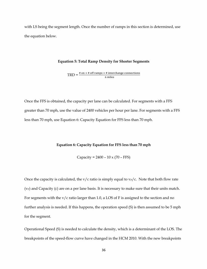
with LS being the segment length. Once the number of ramps in this section is determined, use

the equation below.

Equation 5: Total Ramp Density for Shorter Segments

TRD =

Once the FFS is obtained, the capacity per lane can be calculated. For segments with a FFS

greater than 70 mph, use the value of 2400 vehicles per hour per lane. For segments with a FFS

less than 70 mph, use Equation 6: Capacity Equation for FFS less than 70 mph.

Equation 6: Capacity Equation for FFS less than 70 mph

Capacity = 2400 – 10 x (70 – FFS)

Once the capacity is calculated, the v/c ratio is simply equal to vP/c. Note that both flow rate

(vP) and Capacity (c) are on a per lane basis. It is necessary to make sure that their units match.

For segments with the v/c ratio larger than 1.0, a LOS of F is assigned to the section and no

further analysis is needed. If this happens, the operation speed (S) is then assumed to be 5 mph

for the segment.

Operational Speed (S) is needed to calculate the density, which is a determinant of the LOS. The

breakpoints of the speed-flow curve have changed in the HCM 2010. With the new breakpoints

37

of the curves, the ranges of flow rates (vp) as well as the FFS are used to determine the

appropriate Operational Speed (S). For segments with flow rates less than 1000 vphpl the

operation speed is the same as the free flow speed. For segments with flow rates between 1000-

2400 vphpl and have a FFS equal to 75 mph, use Equation 7: Freeway Operation Speed

Calculation (FFS = 75mph). For segments with flow rates between 1200-2400 vphpl and have a

FFS between 70-75 mph, use Equation 8: Freeway Operation Speed for FFS > 70 mph. For

segments with flow rates between 1400-2350 vphpl and have a FFS between 65-70 mph, use

Equation 9: Freeway Operation Speed for FFS > 65 mph. For segments with flow rates

between1600-2300 vphpl and have a FFS between 60-65 mph, use Equation 10: Freeway

Operation Speed for FFS > 60 mph. For segments with flow rates between 1800-2250 vphpl and

have a FFS between 55-60 mph, use Equation 11: Freeway Operation Speed for FFS > 55 mph.

Equation 7: Freeway Operation Speed Calculation (FFS = 75mph)

S = FFS – 0.00001107 (vP – 1000)2

Equation 8: Freeway Operation Speed for FFS > 70 mph

S = FFS – 0.00001160 (vP – 1200)2


S = FFS – 0.00001418 (vP – 1400)2

38


S = FFS – 0.00001816 (vP – 1600)2


S = FFS – 0.00002469 (vP – 1800)2

Now with the flow rate, capacity, and operation speed (S) calculated the LOS can be

determined. The density based on the lesser value of either the flow rate or the capacity. The

density calculation is shown in Equation 12: Freeway and Multilane Highway Segment Density.

To complete this analysis use Table 5 to determine the LOS. Once calculated, the analysis is

complete.

Equation 12: Freeway and Multilane Highway Segment Density

Density = Min (vP, c)/S

Table 5: Freeway Segment LOS Criteria

LOS A B C D E F

Density 0 – 11 >11 – 18 >18 – 26 >26 – 35 >35 – 45 >45

40

Multilane Highway Analysis

The analysis for Multilane Highways is similar to Freeway Segment analysis. The same input

data is used from TRIMS just as the Freeway segment analysis. The outputs of the Multilane

Highway analysis are also the same as the Freeway segment analysis. This Multilane Highway

procedure is based on Chapter 14 of the HCM 2010. The speed-flow relationship shown below

is the basis of this chapter methodology. After determining the Operational Speed of passenger

cars and the flow rate, LOS can be derived.

Figure 12: Multilane Highway Speed-Flow Curve (National Research Council .


41

Similar to the analysis procedure for freeway segments, the flow rate (or, more appropriately,

demand if the flow rate turns out to be higher than the capacity) needs to be calculated first.

This calculation is shown in Equation 1: Flow Rate. The difference between this calculation and

the one for Freeway segments is the default value of for PHF is now 0.88. This is only to be used

if TRIMS does not provide the PHF value. The remaining inputs are the same. This includes the

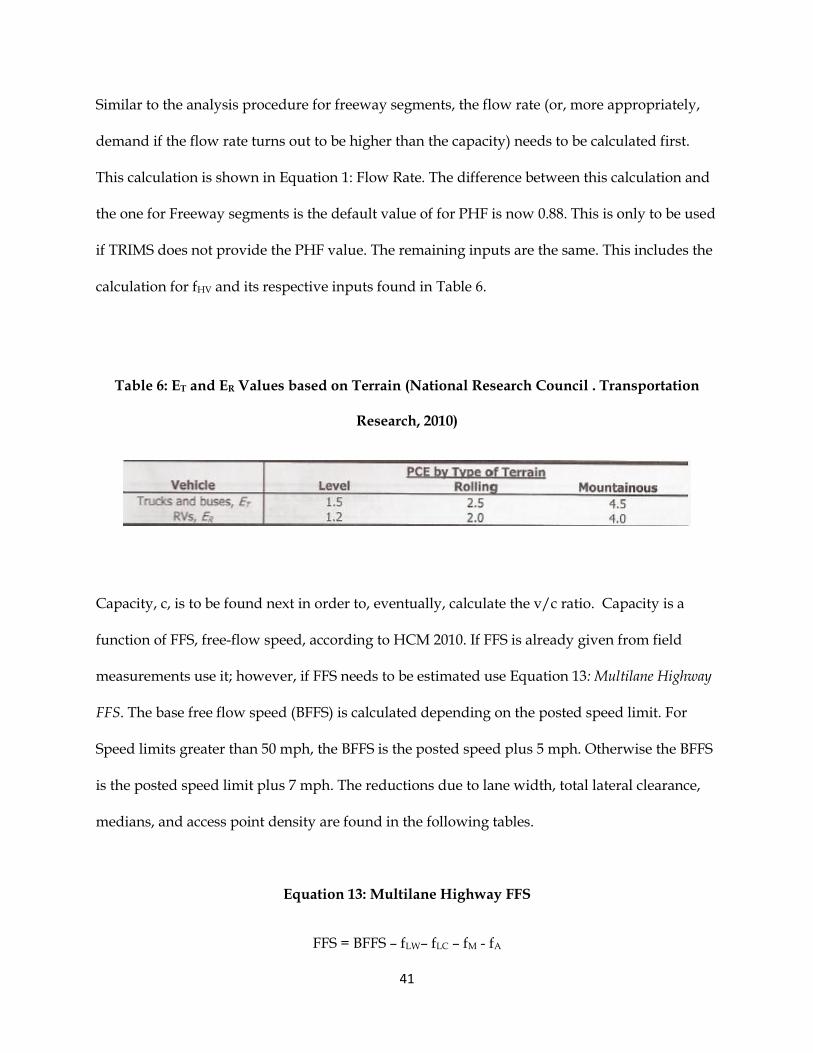
calculation for fHV and its respective inputs found in Table 6.

Table 6: ET and ER Values based on Terrain (National Research Council . Transportation

Research, 2010)

Capacity, c, is to be found next in order to, eventually, calculate the v/c ratio. Capacity is a

function of FFS, free-flow speed, according to HCM 2010. If FFS is already given from field

measurements use it; however, if FFS needs to be estimated use Equation 13: Multilane Highway

FFS. The base free flow speed (BFFS) is calculated depending on the posted speed limit. For

Speed limits greater than 50 mph, the BFFS is the posted speed plus 5 mph. Otherwise the BFFS

is the posted speed limit plus 7 mph. The reductions due to lane width, total lateral clearance,

medians, and access point density are found in the following tables.

Equation 13: Multilane Highway FFS

FFS = BFFS – fLW– fLC – fM - fA

42


2010)

Total Lateral Clearance (TLC) = LCR + LCL

Table 8: Reduction due to Total Lateral Clearance (National Research Council .


Table 9: Reduction due to Presence of Median (National Research Council . Transportation

Research, 2010)

43

The method for calculating access point density still remains the same from EVE 4.0. Use the

following equation to determine the access points per mile if the information is provided in

TRIMS. Continually, 20 access points per mile has to be used as a default value when data is

unavailable. Once the Access Points per mile have been determined, use Table 10.

Equation 14: Access-Point Density Calculation

Access Points/Mile =

Table 10: Reduction due to Access-Point Density (National Research Council . Transportation

Research, 2010)

Once the FFS is determined, the capacity, c, can be calculated. For segments with FFS greater

than 60 mph, the capacity is 2200 vehicles per hour per lane. For segments with a FFS less than

60 mph, use Equation 15: Multilane Highway Capacity less than 60 mph.

44

Equation 15: Multilane Highway Capacity less than 60 mph

Capacity = 2200 – 20 x (60 – FFS)

Once capacity is determined, the v/c ratio can be calculated. This ratio is simply equal to vP/c.

The flow rate and capacity are on an on per lane basis. At this point if the v/c ratio is larger

than 1.0, we can readily assign a LOS of F to the section and move on and save calculation time.

In addition to this, the operation speed for a segment with a v/c ratio greater than 1.0 is 5 mph.

Next operation speed, S, is calculated for FFS between 45-60 mph. Each of the operation speed

calculations are based on a flow greater than 1400 vphpl. For segments with a FFS > 55 mph use

Equation 16: Multilane Operation Speed for FFS > 55 mph. For segments with a FFS between 50-

55 mph use Equation 17: Multilane Operation Speed for FFS between 50-55 mph. For segments

with a FFS between 45-50 mph use Equation 18: Multilane Operation Speed for FFS between 45-

50 mph. For segments with a FFS equal to 45 mph, use Equation 19: Multilane Operation Speed

for FFS = 45 mph. For segments with a FFS less than 45 mph, the operation speed is equal to the

FFS. Upon determining the operation speed, the density can be calculated using Equation 12:

Freeway and Multilane Highway Segment Density. The density is then used to determine the

LOS for the segment from Table 11.

Equation 16: Multilane Operation Speed for FFS > 55 mph

S = FFS – [5.00 x (

) 1.31]

45

Equation 17: Multilane Operation Speed for FFS between 50-55 mph

S = FFS – [3.78 x (

) 1.31]

Equation 18: Multilane Operation Speed for FFS between 45-50 mph

S = FFS – [3.49 x (

) 1.31]

Equation 19: Multilane Operation Speed for FFS = 45 mph

S = FFS – [2.78 x (

) 1.31]

Table 11: LOS Criteria for Multilane Highways

LOS A B C D E F

Density 0 – 11 >11 – 18 >18 – 26 >26 – 35 >35 – DFFS >DFFS

DFFS = 0.00133333 FFS3 – 0.2 FFS2 + 9.566667 FFS – 102

46

Bicycle Analysis

An addition to Level of Service Analysis in the HCM 2010 is the analysis of the Bicycle Mode for

Multilane and Two-Lane highways. The result of the LOS for bicycles is based on a Bicycle

Level of Service score. This score is based on roadway geometrics and travel for automobiles on

the segment. The score ranges from 0.5 to 6.5. Following the procedure below establishes the

Level of Service for the segment.

In order to determine the bicycle score for the segment, the flow rate must first be determined.

Using Equation 20: Flow Rate based on Outside Lane width, the flow rate is based on data

taken from TRIMS.

Equation 20: Flow Rate based on Outside Lane width

vOL =

Once the flow rate is determined, the effective width is estimated. The effective width depends

on the width of the outside lane and shoulder width. The default value of the shoulder width is

6 feet, if unavailable in TRIMS. The effective width (We) is based on paved shoulder width (Ws)

and directional hourly volume, as shown in the equations below. For segments with a flow

greater than 160 vph, the effective width as a function of traffic volume is estimated in Equation

21: Width as a function of Traffic Volume for V > 160 vph. For all other segments, use Equation

22: Width as a function of Traffic Volume to determine the effective width as a function of traffic

volume.

47

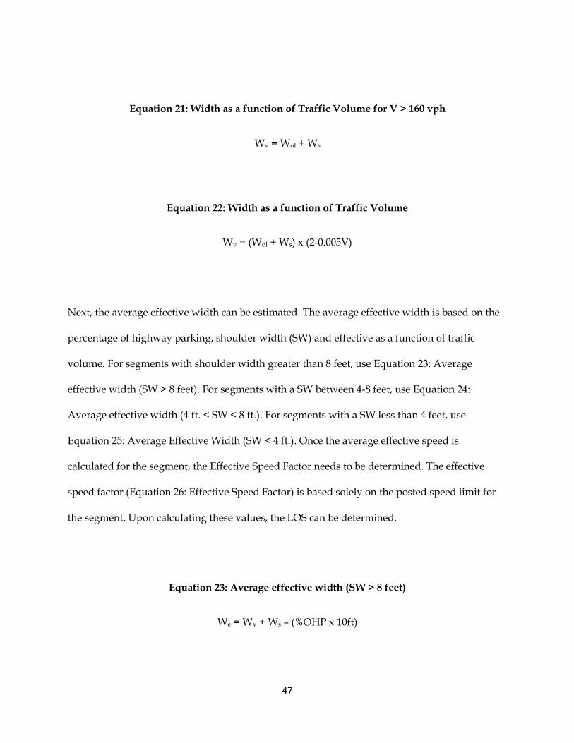
Equation 21: Width as a function of Traffic Volume for V > 160 vph

Wv = Wol + Ws

Equation 22: Width as a function of Traffic Volume

Wv = (Wol + Ws) x (2-0.005V)

Next, the average effective width can be estimated. The average effective width is based on the

percentage of highway parking, shoulder width (SW) and effective as a function of traffic

volume. For segments with shoulder width greater than 8 feet, use Equation 23: Average

effective width (SW > 8 feet). For segments with a SW between 4-8 feet, use Equation 24:

Average effective width (4 ft. < SW < 8 ft.). For segments with a SW less than 4 feet, use

Equation 25: Average Effective Width (SW < 4 ft.). Once the average effective speed is

calculated for the segment, the Effective Speed Factor needs to be determined. The effective

speed factor (Equation 26: Effective Speed Factor) is based solely on the posted speed limit for

the segment. Upon calculating these values, the LOS can be determined.

Equation 23: Average effective width (SW > 8 feet)

We = Wv + Ws – (%OHP x 10ft)

48

Equation 24: Average effective width (4 ft. < SW < 8 ft.)

We = Wv + Ws – 2 x (%OHP (2ft + Ws))

Equation 25: Average Effective Width (SW < 4 ft.)

We = Wv + (%OHP (2 ft. + Ws))

Equation 26: Effective Speed Factor

St = 1.1199ln (Sp – 20) + 0.8103

The Bicycle Level of Service is based upon a traveler-perception model. In order to determine

the appropriate LOS for bicycles, the inputs are combined into a traveler score. The equation is

shown in Equation 27: Bicycle Level of Service Score. This score is based on previous

determined values, as well as the percentage of Heavy Vehicles, and the FHWA’s 5-point

surface rating. The percent of heavy vehicles on the roadway is set at a maximum of 50% for a

flow less than 200 vph. The default value for the surface rating is set as 4.

Equation 27: Bicycle Level of Service Score

BLOS = 0.507 x ln (vOL) + 0.1999St (1 + 10.38HV)2 + 7.066 (1/P)2 – 0.005(We)2 + 0.057

49

Once the BLOS score is obtained use Table 12 to determine the appropriate LOS. This procedure

is used for both Multilane Highways and Two-Lane Highways.

Table 12: Bicycle Level of Service Score Criteria (National Research Council . Transportation

Research, 2010)

50

Urban Arterial Segment Analysis

This procedure is for the analysis of urban and suburban streets with traffic signal spacing of 2.0

miles or less. The analysis should be conducted for sections 2 miles or longer, and at least one

mile in the urban area. The section we are referring to is defined as a portion of a roadway of

which the AADT and/or roadway geometry do not change significantly. The analysis is meant

to be performed for directional traffic. The inputs taken from the TRIMS database are as

follows: AADT, K Factor, D Factor, PHF, Rural/Urban, Number of Lanes (N), Signals, Cross

Streets, Functional Class, and Length of Segments. The outputs for Arterial segments are

different than those of Freeway and Multilane Highway segments. The outputs to be

determined are: Average Travel Speed (SA or ATS), Running Time (TR), Capacity (c), v/c ratio,

Estimated Delay, and Level of Service (LOS).

The urban arterial analysis procedure is the most complicated analysis as compared to the other

analysis procedures. It is based on Chapters 17 and 18 of HCM 2010. The nature and purpose of

Highway Capacity Manual is for detailed operational assessment. Due to the planning emphasis

of TRIMS, certain input parameters for HCM 2010 are not readily available. These parameters

include:

- Signal Timing Plans

- Coordination of Signals along the Roadway

- Actuation/Detectors at Intersections

- Turning Movements

- Public Transit Demand and Service Information

- Parking Activities

- Pedestrian Demand

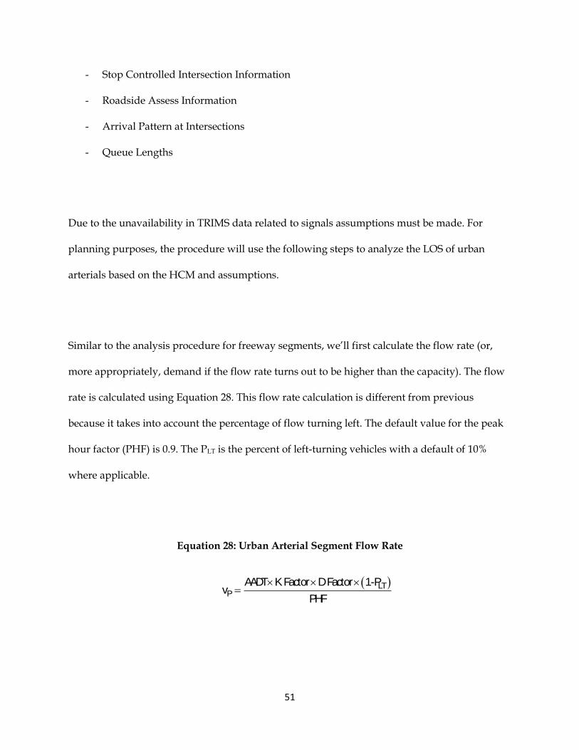
51

- Stop Controlled Intersection Information

- Roadside Assess Information

- Arrival Pattern at Intersections

- Queue Lengths

Due to the unavailability in TRIMS data related to signals assumptions must be made. For

planning purposes, the procedure will use the following steps to analyze the LOS of urban

arterials based on the HCM and assumptions.

Similar to the analysis procedure for freeway segments, we’ll first calculate the flow rate (or,

more appropriately, demand if the flow rate turns out to be higher than the capacity). The flow

rate is calculated using Equation 28. This flow rate calculation is different from previous

because it takes into account the percentage of flow turning left. The default value for the peak

hour factor (PHF) is 0.9. The PLT is the percent of left-turning vehicles with a default of 10%

where applicable.

Equation 28: Urban Arterial Segment Flow Rate

LT

P

AADT K Factor D Factor 1-Pv

PHF

52

Equation 29: Midsegment Volume

vm = (AADT x K x D)/PHF

The flow rate, vp ,accounts for the volume of vehicles that travel through the intersection as well

as turn from the direction of travel. It takes account for the left turning vehicles and combines

the right turning vehicles into the account of the thru vehicles. The midsegment volume (vm) is

the volume of vehicles along the middle of the segment. It however does not account for

turning vehicles. All vehicles in the midsegment calculation are assumed to travel through the

intersection. The midsegment volume is calculated in Equation 29. Both the flow rate and

volume are necessary for this analysis.

In the HCM 2000 the arterials were separated into sub categories. These subcategories were

High-Speed, Suburban, Urban, and Intermediate arterials. The removal of the classifications

allows the LOS determination method to be the same for all arterial types.

The next step in estimating the LOS, is determining the arterial segment the running time, TR.

This is to be estimated based on signal spacing, vehicle proximity, delay and FFS. Since FFS is

rarely available in TRIMS, it must be calculated with Equation 30. Before FFS can be calculated,

the inputs must first be determined.

Equation 30: Arterial FFS Calculation

FFS = (BFFS) x fLS

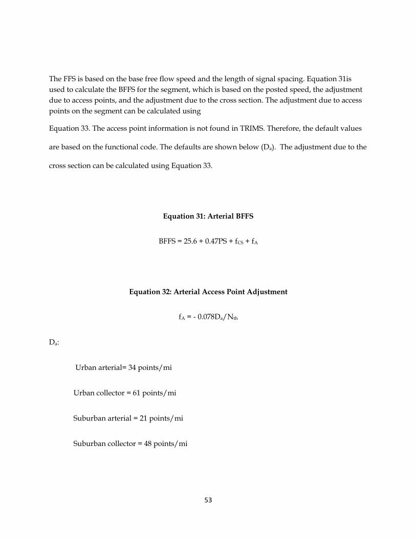
53

The FFS is based on the base free flow speed and the length of signal spacing. Equation 31is

used to calculate the BFFS for the segment, which is based on the posted speed, the adjustment

due to access points, and the adjustment due to the cross section. The adjustment due to access

points on the segment can be calculated using

Equation 33. The access point information is not found in TRIMS. Therefore, the default values

are based on the functional code. The defaults are shown below (Da). The adjustment due to the

cross section can be calculated using Equation 33.

Equation 31: Arterial BFFS

BFFS = 25.6 + 0.47PS + fCS + fA

Equation 32: Arterial Access Point Adjustment

fA = - 0.078Da/Nth

Da:

Urban arterial= 34 points/mi

Urban collector = 61 points/mi

Suburban arterial = 21 points/mi

Suburban collector = 48 points/mi

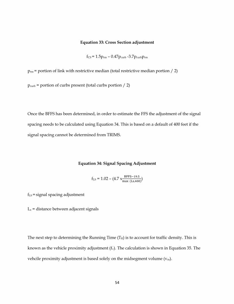
54

Equation 33: Cross Section adjustment

fCS = 1.5prm – 0.47pcurb -3.7pcurbprm

prm = portion of link with restrictive median (total restrictive median portion / 2)

pcurb = portion of curbs present (total curbs portion / 2)

Once the BFFS has been determined, in order to estimate the FFS the adjustment of the signal

spacing needs to be calculated using Equation 34. This is based on a default of 400 feet if the

signal spacing cannot be determined from TRIMS.

Equation 34: Signal Spacing Adjustment

fLS = 1.02 – (4.7 x

)

fLS = signal spacing adjustment

Ls = distance between adjacent signals

The next step to determining the Running Time (TR) is to account for traffic density. This is

known as the vehicle proximity adjustment (fv). The calculation is shown in Equation 35. The

vehcile proximity adjustment is based solely on the midsegment volume (vm).

55

Equation 35: Vehicle Proximity Adjustment

fv =

Following this step, is the calculation of the delay caused by turning vehicles. This accounts for

vehicles turning into the flow of traffic as well turn out of the flow of traffic. Based on the

number of through of lanes and the midsegment volume for the segment, use the table below to

determine the delay due to turning vehicles (dTV).

Table 13: Through Vehicle Delay (National Research Council . Transportation Research,

2010)

Running time is based on running time, FFS, length of the segment,through movement control,

and delays. For our analysis of arterial sections, we are to assume each segment in the analysis

has a signalized intersection. Given the assunmption, there are default values for through

movement control, as well as start-up lost time.

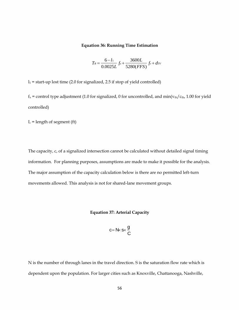
56

Equation 36: Running Time Estimation

16 3600

0.0025 5280( )R x v TV

l LT f f d

L FFS

l1 = start-up lost time (2.0 for signalized, 2.5 if stop of yield controlled)

fx = control type adjustment (1.0 for signalized, 0 for uncontrolled, and min(vth/cth, 1.00 for yield

controlled)

L = length of segment (ft)

The capacity, c, of a signalized intersection cannot be calculated without detailed signal timing

information. For planning purposes, assumptions are made to make it possible for the analysis.

The major assumption of the capacity calculation below is there are no permitted left-turn

movements allowed. This analysis is not for shared-lane movement groups.

Equation 37: Arterial Capacity

g

c N sC

N is the number of through lanes in the travel direction. S is the saturation flow rate which is

dependent upon the population. For larger cities such as Knoxville, Chattanooga, Nashville,

57

and Memphis the S = 1900 pcphpl only if the classification of the roadway is Urban. For all

other roadways, S = 1750 pcphpl. The green ratio (g

C) is assumed to be 0.5 when the cross road

is a state route and 0.67 otherwise. Given such, the capacity would be:

c = 950N or 1273N (Urban in Knoxville, Nashville, Chattanooga, Memphis)

c = 875N or 1172.5N (otherwise)

With the unit in vehicles/hour, one may also calculate X or the v/c ratio as:

Equation 38: v/c ratio

PvXc

Signal delay at each intersection has to be estimated. The delay needed for this analysis is the

through delay. For signalized intersections, the delay computed is the control delay. The

through delay is the sum of control delay and geometric delay. Geometric delay can be

disregarded since there is no effective change through intersections. For each intersection, the

average delay per vehicle can be calculated as:

58

Equation 39: Average Delay per Vehicle:

d = d1 + d2 + d3

d1 = uniform delay (s/veh)

d2 = incremental delay (s/veh)

d3 = initial queue delay (s/veh)

Equation 40: Uniform Delay

d1 = (

)

Equation 41: Incremental Delay

d2 = √

Equation 42: Initial Queue Delay

d3 =

59

The other values are shown above are described below.

Incremental Delay factor (k) = 0.5

Analysis Period (T) = 0.25 hour

Cycle Length (C) = 90 sec

Effective Green Time over cycle length (g/C) = 0.5 if the cross street is a state route and

otherwise 0.67

Upstream Filtering Adjustment Factor (I) = 1.0 if signal is >= 0.6 miles from the nearest

upstream signal and I = 1.0 – 0.91X2.68 otherwise.

d3 = 0.0 sec

The initial queue delay (d3) is a new addition to the delay calculation in HCM 2010 for

signalized intersections. However due to the lack of queue estimation information in

TRIMS the value for d3 is zero.

Since delay is incurred at all signalized intersections along the section, we define the

cumulative delay per vehicle as:

SAll Signals

d d

60

The next calculation is the Average Travel Speed as shown in Equation 43. This is based on the

segment length (in feet), Running Time, and estimated signal delay.

Equation 43: Average Travel Speed

3600

5280( )t

R S

LS

T d

Based on the travel speed determined previously and the base free flow speed of the section, the

LOS can be determined from Table 14.

% = ATS / BFFS

Table 14: Level of Service Criteria Urban Arterial (National Research Council .


62

Two-Lane Highway Analysis

This final procedure of this entire analysis is of two-lane roads with no or only isolated traffic

signals (spaced at least 2 miles apart). The updated HCM 2010 analysis method is for one-

directional traffic as opposed to analyzing both directions. The inputs taken from the TRIMS

database are: AADT, K Factor, D Factor, PHF, Rural/Urban, Terrain, Number of Lanes (N),

Signals, Truck %, RV %, Functional Class, Length of Segments, Posted Speed, Directional Split,

Grade, Lane Width, and Shoulder Width. The outputs that this analysis is estimating are:

Average Travel Speed (ATS), Percent Time Spent Following (PTSF), Percent Free Flow Speed

(PFFS), Capacity (c), v/c ratio, and Level of Service (LOS).

The two-lane highway analysis has been modified since the method used in the HCM 2000. The

procedure in the HCM 2010 now provides a method for one directional analysis. The procedure

to be implemented is based on Chapters 15 of HCM 2010. This procedure includes the addition

of a new Highway Class. The main considerations of this procedure are the average travel

speed, the percent time spent following, and the percent of the free flow speed on two lane

highways. The presence of a passing lane or a directional climbing lane makes a difference to

the LOS of a roadway segment and requires different analysis procedures. Both procedures can

be found in this section, but the first procedure is for the segments without passing or climbing

lanes.

It should be noted that two-lane roads exist in both rural and urban areas. HCM 2010 provides

different standards and classifications for the three classes of such roadways as following.

63

Class I – These are two-lane highways on which motorists expect to travel at relatively high

speeds. Two-lane highways that are major intercity routes, primary arterials connecting major

traffic generators, daily commuter routes, or primary links in state or national highway

networks generally are assigned to Class I. Class I facilities most often serve long-distance trips

or provide connecting links between facilities that serve long-distance trips.

Class II – These are two-lane highways on which motorists do not necessarily expect to travel at

high speeds. Two-lane highways that function as access routes to Class I facilities, serve as

scenic or recreational routes that are not primary arterials, or pass through rugged terrain

generally are assigned to Class II. Class II facilities most often serve relatively short trips, the

beginning and ending portions of longer trips, or trips for which sightseeing plays a significant

role.

Class III – These are two-lane highways that serve as moderately developed areas. These

highways may be portions of Class I and Class II highways that pass through small towns or

developed recreational areas. On these segments, local traffic is mixed with through traffic; the

density of un-signalized roadside access points is noticeably higher than in normal rural areas.

Class III segments may be longer, passing through more spread-out recreational area, with

increased roadside densities.

The first step is to identify the Two-Lane Highway. All of the following should be true to use

this procedure.

64

A total of two lanes for the two directions of the roadway(or 3 if the third lane is a

passing lane or climbing lane) and

The length of the segment between two signals is larger than 2 miles.

The next step is to classify the highway. In order to discover the appropriate LOS for the

segment the classification of the highway is important. Because LOS considerations and

analysis procedures are not exactly the same for the three classes of two-lane roads, it is

essential to classify a roadway segment first. Being that some Class I and Class II highways can

be designated as Class III Highways, we will classify Class I first. The descriptions of each

highway class can be found in Table 15.

Table 15: Two-Lane Highway Classifications

Class I Highway with relatively high speeds, major intercity routes, daily commuter

routes, major links in highway networks, major traffic generator.

Class

II

Not at high speeds, access routes, scenic or recreational routes, passing

through rugged terrain, sight-seeing

Class

III

Developed areas, local traffic mixed with through traffic, segments with higher

access densities than in average rural areas

These steps must be followed in order to classify the highways accordingly.

1. A segment is classified as Class I if one of the following conditions is true:

65

It has a SR or NHS designation;

It’s FC code is 02, 06, 12, 14, or 16;

A speed limit greater than 45 mph

2. Class III segments for this classification are dependent of Access-Point Density.

If the access-point density is >= 12/mi for one side of traffic.

3. Otherwise, we classify the segment as Class II.

4. There might be exceptions based on the terrain, scenic route designation, and posted

speed.

The next step is to determine the flow rate of the Two-Lane segment. Similar to other analysis

procedures, we’ll first calculate the flow rate for the section. This analysis requires a different

flow rate calculation for Average Travel Speed and Percent Time Spent Following. Although the

equations are similar, the factors within the equations correspond to different values.

Equation 44: ATS Flow Rate

,

, ,

( )

( )( )P ATS

g ATS HV ATS

AADT Kv

PHF f f

vp is total flow rate for the section in vph; include the “D-factor” to find the directional demand

flow rate (d);

66

AADT and K factor should come from TRIMS;

PHF has default of 0.88 if unavailable from TRIMS;

fg,ATS is grade adjustment factor, method described below; and

fHV,ATS is heavy vehicle adjustment factor.

The grade adjustment factor for Average Travel Speed calculations, fg,ATS, defined in HCM 2010

is separated into two sections. The first is based upon Level and Rolling Terrains and the other

is based upon the grade percentage (G) of the segment. In order to find the adjustment factor for

Level and Rolling Terrain sections, the one directional demand flow rate should be calculated as

such:

Equation 45: Directional Demand Flow Rate

vvph = V/PHF

The equation below is used to determine the fg,ATS for level and rolling terrains is given

below. In order to find the fg,ATS for Mountainous terrains use Table 16.

fg,ATS (level) = 1.0

fg,ATS (rolling) = 0.274(vvph)0.1946

67

Table 16: Reduction due to Grade for ATS

Grade (%) fg,ATS Equation:

>= 3 0.76655-0.013924*GradeLength + 0.00033188*vvph

>= 3.5 0.694256-0.023495*GradeLength+0.00043896*vvph




The heavy vehicle adjustment factor for ATS, fHV,ATS, is defined as the following in HCM 2010. It

can be calculated using Equation 2: Reduction due to Heavy Vehicles, just as like the other

sections. Use the equations and charts below to find the appropriate values for ET and ER. For

segment with specific upgrades, use Table 17 for ET and Table 18 for ER.

ET and ER are:

Level: ET = 6.7057vvph-0.277

ER = 1.0

Rolling: ET = .000001vvph2- 0.0026vvph + 2.8643

ER = 1.1

68

For segments with specific upgrades use the charts below:

ET (ATS):

Table 17: ET for specific Upgrades (ATS) (National Research Council . Transportation

Research, 2010)

69

ER (ATS):

Table 18: ER for specific Upgrades (ATS) (National Research Council . Transportation

Research, 2010)

We will use TRIMS truck percentage information for following calculations:

PT = (TRIMS Combo Trucks %) + fRU (TRIMS Single Unit Trucks %)

PR = (1-fRU) (TRIMS Single Unit Truck %)

Where:

fRU is 1.00 for urban areas and 0.67 for rural areas.

Once this base information is determined for Average Travel Speed, the base information for

the Percent Time Spent Following flow rate can be estimated using Equation 46.

70

Equation 46: PTSF Flow Rate

,

, ,

( )

( )( )P PTSF

g PTSF HV PTSF

AADT Kv

PHF f f

where:

vP is the total flow rate in vph;


PHF has default of 0.88 if unavailable from TRIMS;

fG,PTSF is grade adjustment factor, method described below; and

fHV,PTSF is heavy vehicle adjustment factor.

The grade adjustment factor for the Percent Time Spent Following calculation, fG,PTSF, is defined

in HCM 2010 just as the method for ATS. As previously noted, the first is based upon Level and

Rolling Terrains and the other is based upon the grade percentage (G) of the segment. In order

to find the adjustment factor for Level and Rolling Terrain sections, the one directional demand

flow rate should be calculated using Equation 45. Once determined, use the equations below to

determine the grade adjustment based on terrain.

Level: fg,PTSF = 1.0

Rolling: fg,PTSF = -0.0000005vvph2 + 0.0008vvph + 0.6493

71

For specific upgrades use the equations provided below:

Table 19: Reduction due to Grade for PTSF

Grade (%) fg,PTSF

>= 3 0.986265+0.011273*GradeLength-8.25E-5*vvph

>= 3.5 0.988419+0.009734*GradeLength-4.375E-5*vvph

>= 4.5 0.992222+0.035556*GradeLength-2E-5*vvph

>= 5.5 1.0

The heavy vehicle adjustment factor for PTSF, fHV,PTSF, can be calculated using Equation 2. Use

the charts below to find the appropriate values for ET and ER.

Level: ET = 1.1 If vvph <= 400

ET = 1.0 If vvph > 400

ER = 1.0

Rolling: ET = 0.000000005vvph3 – 0.000007vvph2 + 0.0013vvph + 1.8048

ER = 1.0

72

For segments with specific upgrades use the charts below:

Table 20: ET and ER Values for Specific Grades (National Research Council . Transportation

Research, 2010)



where :

73

fRU is 1.00 for urban areas and 0.67 for rural areas.

Analysis further in this section requires the use of directional split demands for both ATS and

PTSF. Using the Directional Split provided in TRIMS, calculate the opposing demand of flow

(vo) and the analysis directional demand of flow (vp). The TRIMS database contains the

directional distribution as a percentage, assume the value given is the analysis directional

demand and the remaining is the opposing demand. The equations below apply to both ATS

and PTSF demand estimation. Use the appropriate values of vp whether it is vp,ATS or vp,PTSF.

Equation 47: Directional Flow Rate

vd = vp x D-factor

Equation 48: Opposing Flow Rate

vo = vp - vd

The next step in this procedure is to estimate the Free Flow Speed (FFS). In order to find the

Average Travel Speed and Percent Time Spent Following, the FFS must be calculated.. If FFS is

can be provided from direct field measurements, then it should be utilized. We’ll use the

following procedure from the HCM 2010 Chapter 15. The FFS is based on the base free flow

speed, lane and shoulder widths, and access points. The base free flow speed is determined

74

using the posted speed and adding 10 mph. The factor fLS, representing the reduction in FFS

due to lane width and shoulder width restrictions, is found using Equation 50 where both

inputs are in feet. The access point factor, fA, which also causes reduction in FFS, is provided by

Equation 51.

Equation 49: Two-Lane Highway FFS

FFS = BFFS – fLS – fA

Equation 50: Adjustment due to Lane Width and Shoulder Width

fLS = 12.69 - 0.73(LW) - 0.70(SW)

Equation 51: Adjustment due to Access-Point Density

4

Mileper Points- AccessAf

The default numbers for access-point density depend of highway classification. The access point

reduction defaults for Class I and II are 4 and Class III is 8 for both directions. This is based

upon the default values for access-point density being 8/mi and 16/mi for one directional

traffic for Class I/II and Class III highways, respectively.

75

Upon determining the FFS, the Average Travel Speed can be obtained. Average Travel Speed,

ATS, is a function of FFS, directional flow rate, and existence of passing zone. This is necessary

for LOS determination of Class I and Class III highways. This value depends on the directional

and opposing flow rate as well as the adjustment due to no-passing zones. Use the method

described earlier to determine the values of vd,ATS and vo,ATS.

Equation 52: Average Travel Speed (Two-Lane)

ATS = FFS – 0.00776(vd,ATS + vo,ATS) – fnp,ATS

The adjustment factor for no-passing zones, fnp,ATS, is specific to the direction of analysis. If the

percentage of no-passing zone is known, Table 21 should be used. However, the percentage no-

passing zone information is currently unavailable in TRIMS. For our analysis we are going to

assume 20, 50 and 80% no-passing zones for Level, Rolling, and Mountainous segments. With

the Table 21, use the values coordinated with the previously determined no-passing zone

percentages for level, rolling, and mountainous and FFS to determine the appropriate

adjustment factor.

76

Table 21: Reduction due to No-Passing Zones for ATS (fnp,ATS) (National Research Council .


Once the Average Travel Speed is determined, the Percent Time Spent Following must be

decided. A HCM 2010 based model is adopted for the estimation of PTSF (percent time-spent-

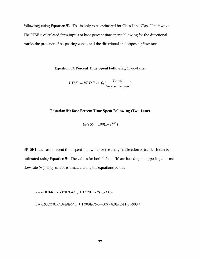
77

following) using Equation 53. This is only to be estimated for Class I and Class II highways.

The PTSF is calculated form inputs of base percent time spent following for the directional

traffic, the presence of no-passing zones, and the directional and opposing flow rates.

Equation 53: Percent Time Spent Following (Two-Lane)

,

, ,

( )D PTSF

D D np

D PTSF O PTSF

VPTSF BPTSF f

V V

Equation 54: Base Percent Time Spent Following (Two-Lane)

100(1 )b

davBPTSF e

BPTSF is the base percent time-spent-following for the analysis direction of traffic. It can be

estimated using Equation 54. The values for both "a" and "b" are based upon opposing demand

flow rate (vo). They can be estimated using the equations below.

a = -0.001461 - 3.4702E-6*vo + 1.7708E-9*(vo-900)2

b = 0.9003701-7.3849E-5*vo + 1.308E-7(vo-900)2 - 8.049E-11(vo-900)3

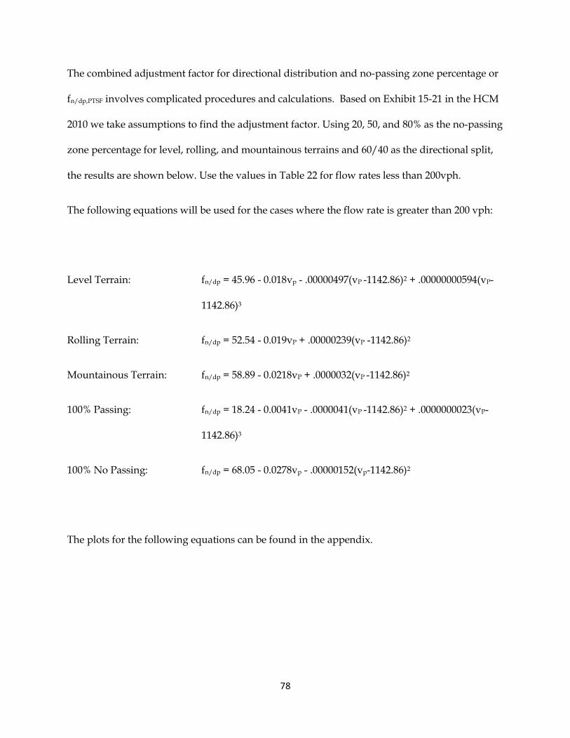
78

The combined adjustment factor for directional distribution and no-passing zone percentage or

fn/dp,PTSF involves complicated procedures and calculations. Based on Exhibit 15-21 in the HCM

2010 we take assumptions to find the adjustment factor. Using 20, 50, and 80% as the no-passing

zone percentage for level, rolling, and mountainous terrains and 60/40 as the directional split,

the results are shown below. Use the values in Table 22 for flow rates less than 200vph.

The following equations will be used for the cases where the flow rate is greater than 200 vph:

Level Terrain: fn/dp = 45.96 - 0.018vp - .00000497(vP -1142.86)2 + .00000000594(vP-

1142.86)3

Rolling Terrain: fn/dp = 52.54 - 0.019vP + .00000239(vP -1142.86)2

Mountainous Terrain: fn/dp = 58.89 - 0.0218vP + .0000032(vP -1142.86)2

100% Passing: fn/dp = 18.24 - 0.0041vP - .0000041(vP -1142.86)2 + .0000000023(vP-

1142.86)3

100% No Passing: fn/dp = 68.05 - 0.0278vp - .00000152(vp-1142.86)2

The plots for the following equations can be found in the appendix.

79

Table 22: Reduction due to No-Passing Zone and Directional Distribution for PTSF

(fnp/dp,PTSF)

Terrain: fnp/dp,PTSF

Level 30.6

Rolling 46.1

Mountainous 52.3

The next step is to calculate the Percent Free Flow Speed (PFFS). This is necessary to determine

to LOS for Class III highways. Use the equation below to determine PFFS, which is based on

Average Travel Speed (ATS) and free flow speed (FFS). The ATS is based on the analysis

direction, ATSd.

Equation 55: Percent Free Flow Speed (Two-Lane)

PFFS = ATSd/FFS

Prior to determining the v/c ratio one must first discover the capacity in the analysis direction.

The v/c ratio is easily obtained as vp/c where c is 3,200 vph for two-way directional traffic and

1,700 vph for one-way one-directional cases. Under non-ideal conditions the analysis direction

capacity for ATS and PTSF is provided below. These equations are be use only if the demand

adjustment factors are based upon a flow rate > 900 vehicles/hour.

80

cATS = 1700 x fg,ATS x fHV,ATS

cPTSF = 1700 x fg,PTSF x fHV,PTSF

Once the ATS, PTSF, and PFFS are calculated the LOS can be estimated. It should be noted that

whenever the v/c ratio is greater than 1.00, the LOS is considered F. Otherwise, LOS of the

two-lane roadway segment may be determined depending on if it is a Class I, Class II, or Class

III roadway. For Class I cases, both PTSF, percent time-spent-following, and ATS, average

travel speed, values will be used to determine the level of service of the roadway segment. If the

results differ and the ATS results as a LOS C and the PTSF results as LOS B, use the worse of the

two LOS classes. Only LOS Classes A-E has been listed in the table, LOS F exists only when the

volume exceeds the capacity or when v/c ratio is greater than 1.00. For Class II cases, only PTSF

will be used. For Class III cases, the PFFS will be used. Again, only when v/c ratio is greater

than 1.00 would LOS F result. The LOS can be estimated using Table 23.

Table 23: Level of Service Criteria for Two-Lane Highways (National Research Council .


81

Chapter VI – Findings and Discussion

Study Methodology

Task

Here is the timeline of tasks conducted to complete this study.

- Research the changes between HCM 2000 and HCM 2010

- Create new algorithms based from HCM 2010

- Collect Input Data from TRIMS for Analysis

- Discover which changes of the HCM are applicable to the analysis

- Regress and simplify the charts from the HCM 2010

- Run the analysis of the given segments

- Discuss the analysis results

- Identify the segments needing further analysis

Assumptions

Planning-level analyses are based on provided information as well as assumptions that are

made for analysis. The assumptions made in this analysis are based on default values in the

HCM 2010 as well as values believed to be beneficial to the methodology. These assumptions

provide constraints to the newly created algorithms, and permit them to be planning-level

analysis methods. Here is a list of assumptions and changes for this deficiency analysis:

- Base Free Flow Speed Calculations ( Urban Arterial, Two-Lane Highways)

82

- Access-Point Densities (Urban Arterial, Two-Lane Highways)

- Signalized Intersections Delay Estimation (Urban Arterials)

- Saturation Flow Rates for larger cities (Urban Arterial)

- Initial Queue Delay (d3) cannot be applicable due to lack of signal information (Urban

Arterial)

- Class I Highways have travel speeds higher than 45 mph

- Class III Highways have 12 access-points/mi or greater per side of traffic (Two-Lane)

- No-Passing Zone Percentages for Level, Rolling, and Mountainous Terrains are 20%,

50%, and 80% respectively

Newly Created Algorithms

The following algorithms are based on the algorithms provided in the HCM 2010, as shown in

the previous chapter. A simplistic methodology for planning the quality of service for a

roadway is obtained with each algorithm. Before the developed algorithms can be used, the

input data for each segment must be known. Upon obtaining the input data, the algorithms

then can be used for analysis. In addition to the roadway class specific algorithms, the

algorithm for Bicycle Analysis on Two-Lane and Multilane Highways is provided.

83

Figure 13: Freeway Segment Algorithm

84

Figure 14: Multilane Highway Algorithm

85

Figure 15: Two-Lane Highway Algorithm

86

Figure 16: Urban Arterial Segment Algorithm

87

Figure 17: Bicycle Analysis Algorithm

Data Contributions

Making the analysis methods more manageable for programmers became is an important task.

Regression analyses were conducted for the charts within Chapter 15: Two-Lane Highways of

the Highway Capacity Manual 2010. These charts are as follows:

88

- Exhibit 15-7

- Exhibit 15-9

- Exhibit 15-10

- Exhibit 15-11

- Exhibit 15-16

- Exhibit 15-17

- Exhibit 15-18

- Exhibit 15-20

- Exhibit 15-21

With the use of the software programs JMP and Microsoft Excel, statistical regression equations

were formulated to simplify the charts. In order to determine whether some regressions were

statistically stable, the mean absolute percentage error (MAPE) was calculated. For Exhibit 15-

17, the MAPE values were all within 2% error; meaning the regression equation is only a 2%

error away from the actual value. Devoid of a preset determinant for a sufficient MAPE value,

the assumption was made that such as small error percentage is sufficient.

Example Calculations

Thousands of roadway segments were provided for the analysis. Given the amount data for

these segments, it would be difficult to demonstrate the calculations for each segment provided

in this thesis. Therefore, this section contains example calculations using the deficiency analysis

procedures developed in this study. Data used in the example calculations is the same data

89

from Washington County as the rest of the data used in the overall analysis. The calculations

are separated by roadway class. The desired results of each section can be found in bold print.

Two-Lane Highway

Analysis Results:

- Average Travel Speed - Percent Time Spent Following - v/c ratio - Percent Free Flow Speed - Capacity - Level of Service (LOS)

TRIMS DATA:

- Segment Length: 1.35 miles - Road Name: Telford Rd. - AADT: 2100 - K-Factor: 0.12 - D-Factor: 0.65 - PHF: 0.9 - PT (Multi-Unit Trucks): 0% - PR (Single-Unit Trucks): 2% - Right Shoulder Width: 2 feet - Lane Width: 10 feet - Number Lanes: 2 - Terrain: Rolling - Speed Limit: 35 mph - Functional Class: 08 - Rural

Assumptions:

- Access-Point Density (APD): 8 access-points/mile - Based on APD, Highway Class Type: Class II - fRU: 0.67

Average Travel Speed Estimation:

90

Vvph = (AADT x K x D)/PHF = (2100 x 0.12 x 0.65)/ 0.9 = 182 vph

fg,ATS = 0.274 x (Vvph)0.1946 = 0.274 x (182)0.1946 = 0.754

ET = 0.000001*(Vvph)2 - 0.0026*( Vvph) + 2.8643 = 0.000001*(182)2 - 0.0026*(182) + 2.8643 = 2.424

ER = 1.1

PT = PT + fRU (ER ) = 0% + 0.67 (2%) = 0.134

PR =(1 – fRU) * (ER) = (1 – 0.67) *(2%) = 0.0066

fHV = 1/((1+PT*(ET-1)+PR*(ER-1)) = 1/((1+0.134*(2.424-1)+0.0066*(1.1-1)) = 0.981

vP = (AADT x K) / (PHF x fg,ATS x fHV) = (2100 x 0.12) / (0.9 x 0.754 x 0.981) = 378.52 vph

vD = 378.52 * (D- FACTOR) = 378.52 * (0.65) = 246.04 vph

vO = 378.52 – 246.04 = 132.48 vph

BFFS = 35 mph +10 mph = 45 mph

FLS = 12.69 – 0.73*(10 feet)-0.7*(2) = 3.99

FA = Maximum (4, 8/4) = 4

FFS = BFFS – fLS – fA = 45 mph – 3.99 – 4 = 37.01 mph

fnp = 2.3

ATS = FFS – 0.00776*(vP)- fnp = 37.01 mph – 0.00776*(378.52 vph) – 2.3 = 31.89 mph

Percent Time Spent Following Estimation:

Vvph = 182 vph

fg,PTSF = -0.0000005*(Vvph)2 +0.0008*( Vvph )+0.6493 = -0.0000005*(182)2 +0.0008*(182)+0.6493 = 0.778

ET = 0.000000005*(Vvph)3-0.000007*(Vvph )2 +0.0013*(Vvph )+1.8048 = 0.000000005*(182)3-0.000007*(182)2+0.0013*(182)+1.8048 = 1.84

ER = 1

PT = 0.134

PR = 0.0066

fHV = 1/((1+PT*(ET-1)+PR*(ER-1)) = 1/((1+0.134*(1,84-1)+0.0066*(1-1)) = 0.989

vp = (AADT x K)/(PHF x fg,PTSF x fHV) = (2100 x 0.12)/(0.9 x 0.778 x 0.989) = 363.79 v/h

91

vD = 363.79*(D-factor) = 363.79 x 0.65 = 236.46 v/h

vO = 363.79 – 236.46 = 127.33 v/h

BFFS = 45 mph

FLS = 3.99

FA = 4

FFS = 37.01 mph

a = -.00187

b = 1.01

BPTSFd = 100*(1-e-0.00187*(236.46)^1.01) = 36.77 %

fNP = 47.08

PTSF (%) = BPTSF + fnp*(vd/vp) = 36.77% +47.08*(236.46/363.79) = 67.37 %

PFFS (%) = ATS/FFS = 86.16 %

Capacity: 1700 v/h

Vats/c = 378.52/1700 = 0.223

Vptsf/c = 363.79/1700 = 0.214

The LOS criterion for this segment is based on Percent Time Spent Following because it is

considered a Class II Highway. The LOS determination for this segment is LOS Class C.

Multilane Highways:

Results:

- Density - Operational Speed (S) - Capacity (c) - v/c ratio - Level of Service (LOS)

TRIMS DATA:

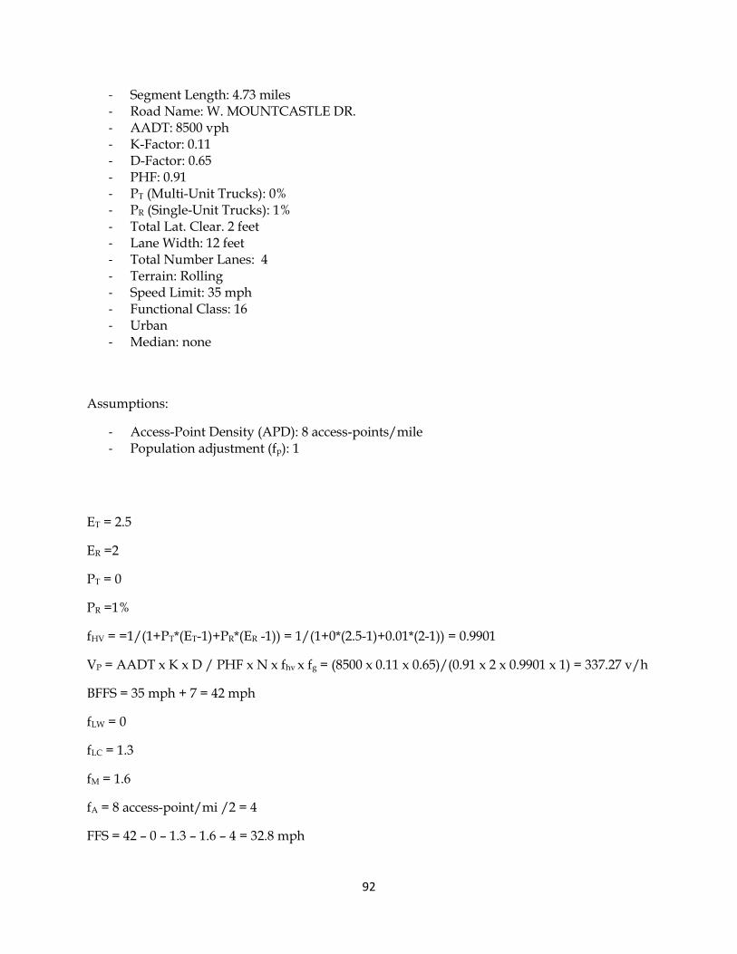
92

- Segment Length: 4.73 miles - Road Name: W. MOUNTCASTLE DR. - AADT: 8500 vph - K-Factor: 0.11 - D-Factor: 0.65 - PHF: 0.91 - PT (Multi-Unit Trucks): 0% - PR (Single-Unit Trucks): 1% - Total Lat. Clear. 2 feet - Lane Width: 12 feet - Total Number Lanes: 4 - Terrain: Rolling - Speed Limit: 35 mph - Functional Class: 16 - Urban - Median: none

Assumptions:

- Access-Point Density (APD): 8 access-points/mile - Population adjustment (fp): 1

ET = 2.5

ER =2

PT = 0

PR =1%

fHV = =1/(1+PT*(ET-1)+PR*(ER -1)) = 1/(1+0*(2.5-1)+0.01*(2-1)) = 0.9901

VP = AADT x K x D / PHF x N x fhv x fg = (8500 x 0.11 x 0.65)/(0.91 x 2 x 0.9901 x 1) = 337.27 v/h

BFFS = 35 mph + 7 = 42 mph

fLW = 0

fLC = 1.3

fM = 1.6

fA = 8 access-point/mi /2 = 4

FFS = 42 – 0 – 1.3 – 1.6 – 4 = 32.8 mph

93

Capacity = 2200 – 20*(60-32.8) = 1080 v/h

v/c ratio = 337.27/1080 = 0.31

Operational Speed = FFS = 32.8

Density = 337.27 / 32.8 = 10.28 v/mi

The criterion for LOS determination in the segment is based on Density. The resulting density of

this segment describes as LOS Class A.

Urban Arterial Segment:

Results:

- Average Travel Speed (ATS) - Estimated Delay (DS) - Running Time (TR) - Capacity (c) - v/c ratio - Level of Service (LOS)

TRIMS DATA:

- Segment Length: 0.28 miles - Total Segment Length: 2.1 miles - Road Name: King Springs Rd - AADT: 2900 - K-Factor: 0.12 - D-Factor: 0.65 - PHF: 0.9 - PT (Multi-Unit Trucks): 0% - PR (Single-Unit Trucks): 1% - Right Shoulder Width: 1 foot - Lane Width: 12 feet - Number Lanes: 2 - Terrain: Rolling - Speed Limit: 30 mph - Functional Class: 16 - Urban

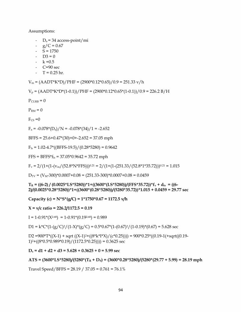
94

Assumptions:

- Da = 34 access-point/mi - g/C = 0.67 - S = 1750 - D3 = 0 - k =0.5 - C=90 sec - T = 0.25 hr.

Vm = (AADT*K*D)/PHF = (2900*0.12*0.65)/0.9 = 251.33 v/h

Vp = (AADT*K*D*(1-0.1))/PHF = (2900*0.12*0.65*(1-0.1))/0.9 = 226.2 B/H

PCURB = 0

PRM = 0

FCS =0

Fa = -0.078*(Da)/N = -0.078*(34)/1 = -2.652

BFFS = 25.6+0.47*(30)+0+-2.652 = 37.05 mph

Fls = 1.02-4.7*((BFFS-19.5)/(0.28*5280) = 0.9642

FFS = BFFS*fls = 37.05*0.9642 = 35.72 mph

Fv = 2/(1+(1-(vm/(52.8*N*FFS)))0.21 = 2/(1+(1-(251.33/(52.8*1*35.72)))0.21 = 1.015

DTV = (VM-300)*0.0007+0.08 = (251.33-300)*0.0007+0.08 = 0.0459

TR = ((6-2) / (0.0025*LS*5280))*1+((3600*(LS*5280))/(FFS*35.72))*fv + dtv = ((6-2)/(0.0025*0.28*5280))*1+((3600*(0.28*5280))/(5280*35.72))*1.015 + 0.0459 = 29.77 sec

Capacity (c) = N*S*(g/C) = 1*1750*0.67 = 1172.5 v/h

X = v/c ratio = 226.2/1172.5 = 0.19

I = 1-0.91*(X2.68) = 1-0.91*(0.192.68) = 0.989

D1 = k*C*(1-(g/C)2/(1-X)*(g/C) = 0.5*0.67*(1-(0.67)2/(1-0.19)*(0.67) = 5.628 sec

D2 =900*T*((X-1) + sqrt ((X-1)2+((8*k*I*X)/(c*0.25)))) = 900*0.25*((0.19-1(+sqrt((0.19-1)2+((8*0.5*0.989*0.19)/(1172.5*0.25)))) = 0.3625 sec

Ds = d1 + d2 + d3 = 5.628 + 0.3625 + 0 = 5.99 sec

ATS = (3600*LS*5280)/(5280*(TR + DS) = (3600*0.28*5280)/(5280*(29.77 + 5.99) = 28.19 mph

Travel Speed/BFFS = 28.19 / 37.05 = 0.761 = 76.1%

95

The LOS criterion for this segment is based on the percentage of travel speed to base free flow

speed. The LOS determination for this segment is LOS Class B.

Freeway Analysis:

Results:

- Density - Operational Speed (S) - Capacity (c) - v/c ratio - Level of Service (LOS)

TRIMS DATA:

- Segment Length: 3.22 miles - Road Name: JAMES H. QUILLEN PKWY. - AADT: 46050 - K-Factor: 0.11 - D-Factor: 0.51 - PHF: 0.91 - PT (Multi-Unit Trucks): 5% - PR (Single-Unit Trucks): 3% - Total Lateral Clearance: 2 feet - Lane Width: 12 feet - Total Number Lanes: 4 - Terrain: Rolling - Speed Limit: 70 mph

Assumptions:

- Ramps: 4 ramps/mile - fp = 1

TRD = 4/6 = 0.6667

ET = 2.5

ER =2

96

PT = 5%

PR =3%

fHV = =1/(1+PT*(ET-1)+PR*(ER -1)) = 1/(1+.05*(2.5-1)+0.03*(2-1)) = 0.905

VP = AADT x K x D / PHF x N x fhv x fg = (46050 x 0.11 x 0.51)/(0.91 x 2 x 0.905 x 1) = 1419.5 v/h

fLW = 0

fLC = 0

FFS = 75.4 – fLW – fLC – 3.22*TRD0.84 = 75.4 – 0 -0 – 3.22*(0.6667)0.84 = 73.11 mph

Capacity > 70 c = 2400 v/h

v/c ratio = 1419.5/2400 = 0.59

Operational Speed (S) = FFS - 0.0000116*(vp-1200)2 = 73.11 – 0.0000116*(1419.5-1200)2 = 72.55 mph

Density = vp / S = 1419.5/72.55 = 19.56 v/mi

The LOS criterion for this segment is based on density of the roadway. The LOS determination

for this segment is LOS Class C.

RESULTS

Before the comparison part of the deficiency analysis, the results must first be analyzed for

patterns and key changes to the LOS. Specific factors were found to affect the level of service

more than others. For the Freeway segment analysis the important factor appeared to be Total

Ramp density (TRD). The TRD affects the free flow speed, which is always relatively high for

freeway segments. Since TRD is based on the number of ramps within six miles, a high or low

number of ramps on the segment will not affect the LOS in a major way. Multilane Highway

analysis and Freeway analysis are similar. The number of ramps and interchanges on a freeway

97

are similar to access points on a multilane highway. The results of the multilane highway

analysis reveal the importance of access-point densities, which can result in a change of the

Level of Service by an entire grade. Access point densities are also a factor in the Two-Lane

Highway analysis, and also effect the LOS in the manner described for Multilane Highways.

The most important factor in Two-lane Highways analysis is highway classification. The level of

service criterion is different for each of the three classes. In correctly classifying a highway can

produce results that are inaccurate. The complexity of the Two-Lane Highway analysis is

comparable to that of the Urban Arterial Segment analysis. Unlike two-lane analysis, segment

length is important and can result in level of services grade changes. In order to improve the

results of segments less than 0.1 miles during the analysis, said segments were added to

adjacent segments with similar input data (i.e. AADT, Number of Lanes, etc.). Thus increasing

the segment lengths of the adjacent segment and improving the overall level of service. Later in

the comparison of results, the segments were reverted back to their original lengths.

Annual Average Daily Traffic (AADT) was very important for each of the analyses because it is

a part of the flow rate calculation. Segments returning the LOS Class F results were due to the

higher AADT values. Multilane Highways with very high AADT values can result the demand

on segments exceeding the capacity, resulting in a LOS Class F. Two-lane Highways with a

combination of high AADT values and shorter segment lengths results in lower LOS Classes.

Two-Lane highway results also show that segments with more than 5,000 vph resulted in LOS

Classes D, E, and F.

Other reasons two-lane highway segments resulted in low LOS classes are as follows. The

change in functional class codes from an urban segment to a rural segment can result in

different LOS results on the same segment for different links on the segment. This is because the

98

analysis calculations for rural and urban segments differ in specific values. Change in Speed

Limits also affects the LOS Class. Highway Class I is based on high speeds and if the segment

has a speed limit less than 45 mph then the highway classification is changed. This results in a

change of LOS criterion as described previously. Now that these results have been analyzed,

next is comparison section of the deficiency analysis.

Comparison

In order for this study to be considered a proper deficiency analysis, a comparison of current

results and past results must occur to identify the changes. Using results from a previous EVE

analysis, a comparison of the same roadway segments were conducted. The percentage of LOS

changes in the results from EVE and the new method can be shown in Table 24. These

percentages are based on a total of 256 comparable segments As shown in the table LOS Class A

decreased by more than half, LOS Class B increased and produced the most values, LOS Class C

remained about the same, LOS Class D increased by more than half, LOS Class E decreased, and

LOS Class F increased from nothing previously.

The change of methodologies results in a higher percentage of bad LOS grades for the roadway

segments as compared to EVE. There are 42 segments with the LOS Classes of D, E, and F.

These segments will be highlighted and further analyzed to discover possible improvement

methods.

Table 25 shows the percentages of the results that are either the same, better, or worse than

those from EVE. There are 35 segments with better levels of service results than those provided

by EVE. The reason for these results are because of the changes from the in the HCM

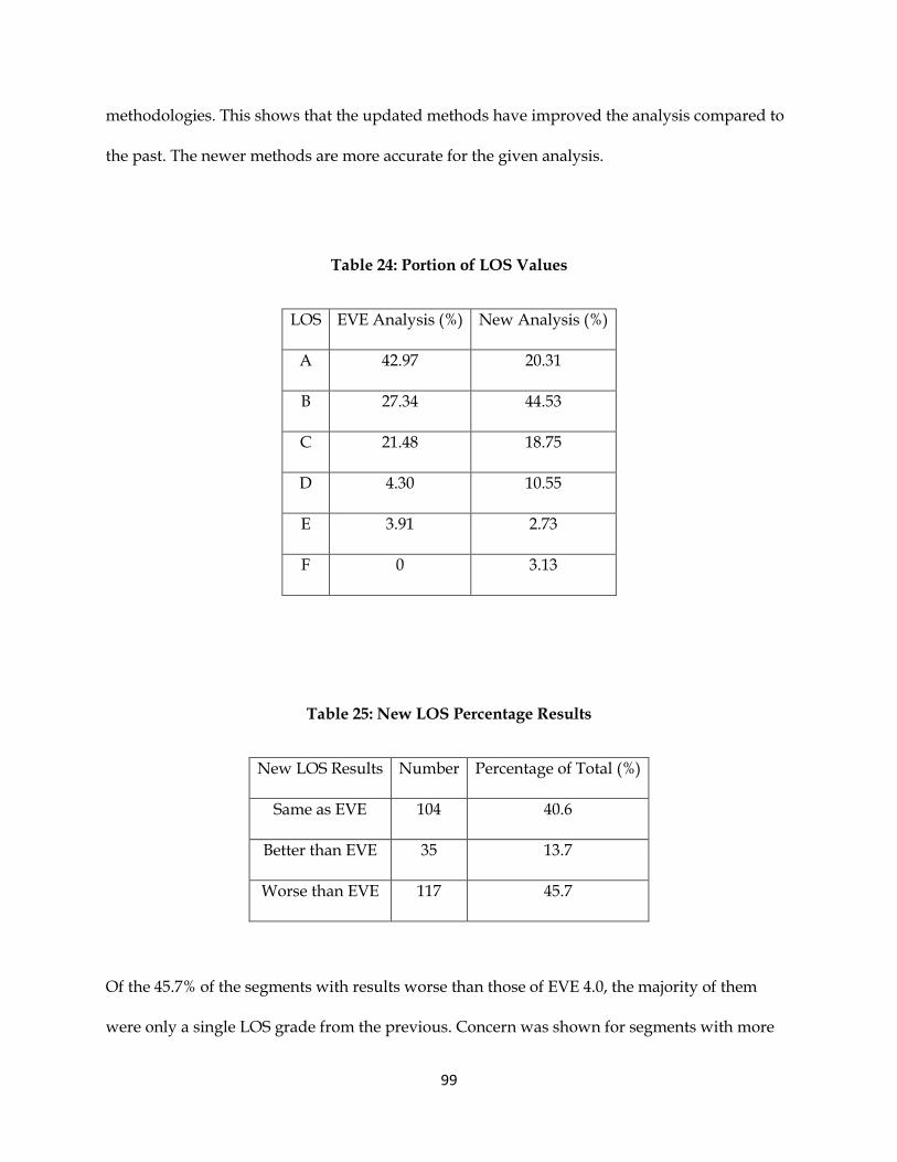
99

methodologies. This shows that the updated methods have improved the analysis compared to

the past. The newer methods are more accurate for the given analysis.

Table 24: Portion of LOS Values

LOS EVE Analysis (%) New Analysis (%)

A 42.97 20.31

B 27.34 44.53

C 21.48 18.75

D 4.30 10.55

E 3.91 2.73

F 0 3.13

Table 25: New LOS Percentage Results

New LOS Results Number Percentage of Total (%)

Same as EVE 104 40.6

Better than EVE 35 13.7

Worse than EVE 117 45.7

Of the 45.7% of the segments with results worse than those of EVE 4.0, the majority of them

were only a single LOS grade from the previous. Concern was shown for segments with more

100

than one LOS grade change, more importantly segments going from a “good” LOS grade (A-C)

to a “poor” LOS grade (D-F). There were 16 segments fitting this description. Of these 16

segments, the most concerning was the Two-Lane segment that changed from a LOS Class B to

a LOS Class E. This resulted from the roadway having a lane drop and changing the LOS

analysis type. Segments prior to this one had 4 lanes and then this segment went down to 2

lanes, thus changing the analysis from Multilane to two-Lane analysis. The remaining 15

segments resulted as they are due to changes in Two-Lane Highway classification. Highway

classification is very sensitive and as shown can result in changes in the LOS.

In order to gain a better understanding of the connection between EVE 4.0 results and result of

the newly proposed method, bubble diagrams were used. The use of the diagrams is to show

how much deviation from previous results had been made. As shown in Figure 18, the results

of this new method are similar to those of the results of the EVE method.

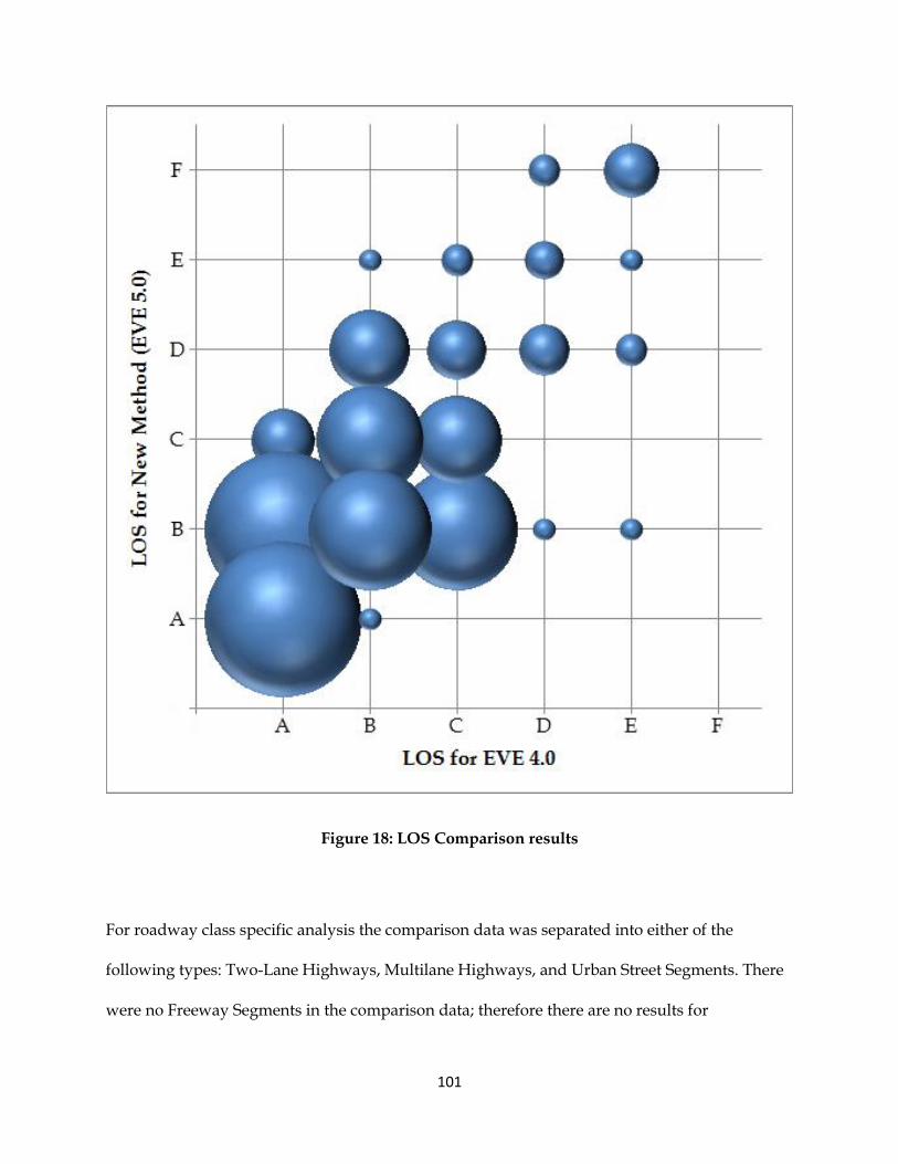
101

Figure 18: LOS Comparison results

For roadway class specific analysis the comparison data was separated into either of the

following types: Two-Lane Highways, Multilane Highways, and Urban Street Segments. There

were no Freeway Segments in the comparison data; therefore there are no results for

102

comparison. Out of the results provided above, roughly 86% of the results were Two-Lane

Highways, 11% are Urban Arterial Segments, and the remaining 4% are Multilane Highways.

The comparison results of each of these roadway classes are provided in the tables below. Table

26 shows the number of segments with results similar to that of EVE.

Table 26: Same as EVE Results by Roadway Class

Roadway Class Number Percentage Total Same as EVE (%)

Two-Lane Highways 86 82.7

Urban Arterial Segments 12 11.5

Multilane Highways 6 5.8

In comparison to EVE, the following figures show bubble diagrams according to roadway class.

The results shown are based on 219 Two-lane highway segments, 28 Urban Arterial Segments,

and 9 Multilane Segments. Of the segments for Two-Lane, Urban Arterial, and Multilane

highways the percentages of values worse than EVE 4.0 are 47%, 40%, and 33% respectively.

The values on the Urban Arterial and Multilane segments only change by one LOS Class. The

values change on the Two-Lane Highway segments due to the reasons previously discussed.

103

Figure 19: LOS Comparison Results for Two-Lane Highways

104

Figure 20: Urban Arterial Segment LOS Comparison Percentages

105

Figure 21: Multilane Highway LOS Comparison Percentages

Given these results, segments with LOS Classes D, E, and F need to be analyzed further to

identify methods of improvement. There are 42 segments that need to be analyzed further out

of this data set. Some things that may need improvement on these segments are lane width,

106

speed, segment length. The deficiency analysis program will analyze the roadways with poor

LOS grades. From there it is up to the analyst to determine the next step.

107

Chapter VII – Conclusion

Summary

This study was conducted to benefit those using deficiency analyses for decision-making

purposes in the transportation field. Since deficiency analysis is used for funding based

decisions the method of the deficiency analysis for Tennessee had to be updated. This new

method is based on the HCM 2010 methodologies and algorithms. With the use of the HCM

2010 a new procedure was established to determine the quality of service on Freeway, Multilane

Highway, Two-Lane Highway, and Urban Arterial segments of roadway. The study was taking

from a planning-level view for the analysis. Therefore, many assumptions were to be made if

the data was not provided. This study used TRIMS, a database provide by TDOT for input data.

The inputs that were not in TRIMS had to be assumed. Using data from Washington County,

some of the findings of the analysis show the importance of access-point density on Multilane

and Two-Lane highways as well as proper classification for Two-Lane highways. A comparison

of Two-Lane highways was conducted and it shows that in comparison to the others, Class III

highways provide the best LOS. Another comparison was conducted in order to identify

problem areas in comparison to EVE database results. Of the 256 segments compared to EVE, 42

of these segments results in a LOS Class D, E, or F. These 42 results will be further analyzed to

resolve any potential issues resulting in a poor LOS. The updating in the deficiency analysis

method used for decision-making is beneficial for future project estimation and must be

continually updated with information selected from the most recent edition of Highway Capacity

Manual.

108

Suggestions

In order to provide the best results from this deficiency analysis procedure and future

deficiency analyses it is believed that the following suggestions must be considered. Careful

attention must be paid to the classification of Two-Lane highways. Each highway class bases its

level of service determination on a different service measure. Thus an incorrect classification

will result in an incorrect LOS determination. The use of a deficiency analysis program in

association with an information database (such as TRIMS) must conduct analyses whenever

there is new information in the database related to the program. In addition to running

analyses, it is beneficial to develop methods of gathering information related to other modes of

transportation into such information databases. The addition of the bicycle analysis for this

program will provide a gateway for other alternative modes to be added. This addition of a

multimodal analysis method to determine deficiency analysis is dependent upon the

information database. If the information database does not contain the necessary information,

the alternative modes cannot be assessed. Additional measures of effectiveness (MOEs) on a

roadway should be considered for each roadway for future deficiency analysis efforts.

Developing an analysis considering safety as a service measure will provide benefit to both the

users as well as the planners. If safety is to be added a starting point of research should be

NCHRP Report 546. The use of the most accurate input data will be beneficial to the analysis of

the segment.

109

APPENDIX

110

Capacity Analysis Procedures for Eve 4.0

Roadway Class Sorting Procedure

INPUT: from TRIMS database:

FC Code, Route Name, Number of Lanes, Direction, Lane Type, AADT,

Terrain

OUTPUT: Roadway Class (RC) and, hence, procedures to be used for analysis.

RC = 1 for Freeway, 2 for Arterial, 3 for Two-Lane Road, or 4 for

Multilane Road

Step 1. Identify Interstate and Freeways

IF FC Code = 01 or 11 THEN

RC = 1 for freeway/Interstate

EXIT

ELSE IF Road Name = “Interstate …” THEN

RC = 1

EXIT

END IF

Step 2. Identify Arterials

111

IF Signal Spacing is less or equal to 2.0 miles THEN

RC = 2 for arterial

EXIT

END IF

Step 3. Identify Two-Lane Roads

IF Number of Lanes = 2 THEN

IF Directions = 2 THEN

RC = 3 for two-lane road

EXIT

END IF

ELSE Number of Lanes = 3 THEN

IF Directions = 2 THEN

IF Pavement Width <= 28 THEN

RC = 3

EXIT

ELSE IF Lane Type = 0, 2, 3, 6, 8, or 12 THEN

RC = 3

EXIT

112

END IF

END IF

END IF

Step 4. The Rest Are Multilane Roads

RC = 4

113

Section I - Freeway Segment Analysis Procedure


AADT, K Factor, D Factor, PHF, Lane Width, Lateral Clearance,

Rural/Urban, Terrain,

Truck Percentage,

OUTPUT: Operational Speed (S)

Capacity (c)

v/c ratio

Density (D)

Level of Service (LOS)

This procedure is based on Chapter 23 of HCM 2000. At the heart of the

methodology is the speed-flow relationship depicted in the figure below. Once the flow

rate and the average passenger-car speed are obtained, the LOS can be derived.

114

First calculate the flow rate (or, more appropriately, demand if the flow rate turns

out to be higher than the capacity) entering the segment:

P HV P


PHF N f f

where:

AADT, K and D factors should come from TRIMS;

PHF is 0.9 by default but can be changed if TRIMS has it;

N is the number of lanes in one direction;

fP is usually 1.0 but can be changed if the drivers are not mostly commuters;

fHV can be estimated from the following procedure:

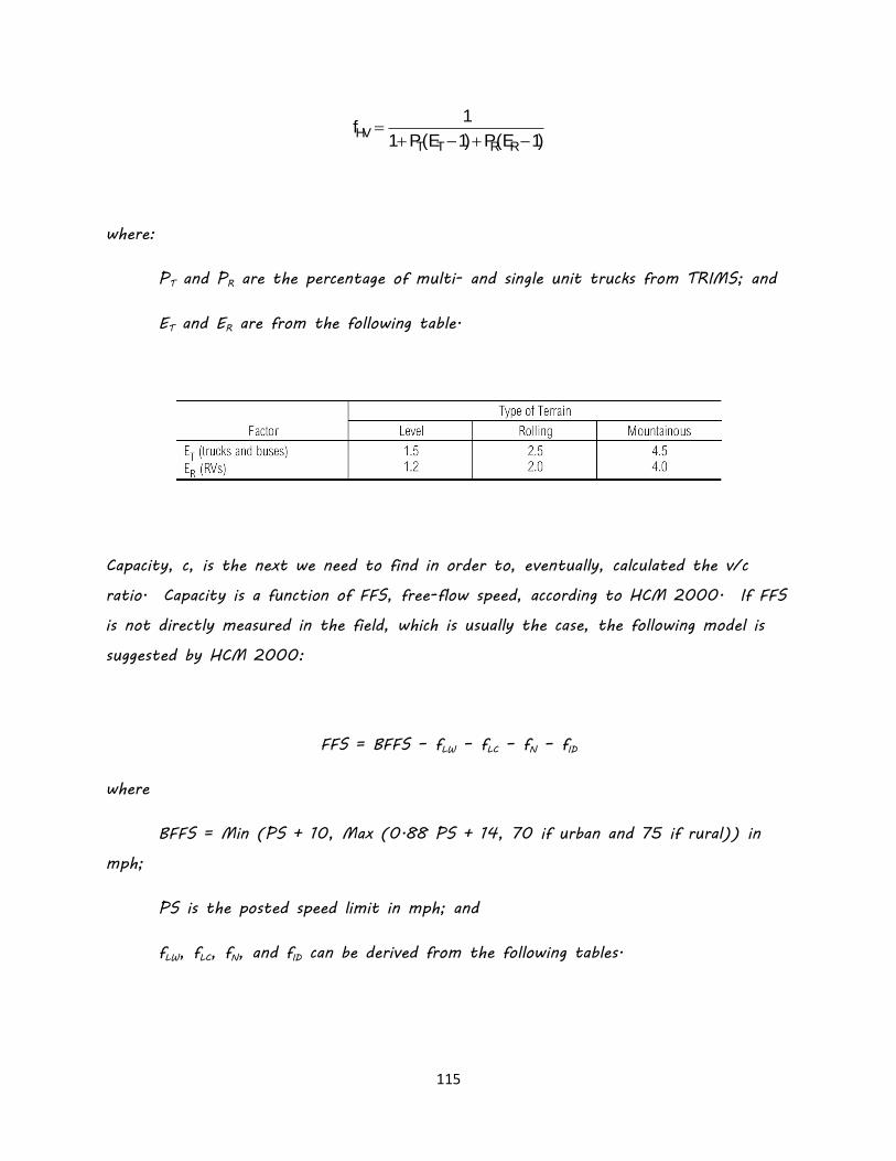
115

HVT T R R

1f

1 P(E 1) P(E 1)

where:

PT and PR are the percentage of multi- and single unit trucks from TRIMS; and

ET and ER are from the following table.

Capacity, c, is the next we need to find in order to, eventually, calculated the v/c

ratio. Capacity is a function of FFS, free-flow speed, according to HCM 2000. If FFS

is not directly measured in the field, which is usually the case, the following model is

suggested by HCM 2000:

FFS = BFFS – fLW – fLC – fN – fID

where

BFFS = Min (PS + 10, Max (0.88 PS + 14, 70 if urban and 75 if rural)) in

mph;

PS is the posted speed limit in mph; and

fLW, fLC, fN, and fID can be derived from the following tables.

116

In calculating fID we do have to figure out the number of Interchanges per Mile first,

which may be tricky. Obviously it is not always easy to find out the number of

117

interchanges in a mile in TRIMS due to data “breakdown” at county boundaries, etc.

The number of Interchanges per Mile, nevertheless, can be approximated as:

1

Distance between Adjacent Interchanges

If the segment been analyzed does not have any “artificial” boundaries, such as county

lines, rural/urban changes, and lane add/drop cutting, then the length of the segment,

or LS, is the same as the distance between two adjacent interchanges. Even if there

were rural/urban or lane add/drop cases, we should be able to find the distance between

adjacent interchanges. The only time we will have some challenges is when the county

line cuts between two interchanges. For such cases, we would simplify the process by

using the following defaults:

fID = 0.0 for rural and 1.5 for urban

We will not use Model 1 for FFS for now. The final FFS results from Models 2 and 3:

FFS = Max (FFS from Model 2, FFS from Model 3)

Once we have FFS, the capacity per lane can be calculated as:

Capacity = 2400 pcphpl, if FFS 70 mph

= 2400 10 (70 FFS) pcphpl, otherwise

118

Then the v/c ratio is simply equal to vP/c. Note that both vP and c here are on a per

lane basis. Make sure they match. At this point if the v/c ratio is larger than 1.0,

we can readily assign a LOS of F to the section and move on and save calculation time.

Therefore:

IF vP/c > 1.0 THEN

LOS = F

S = 5 mph

EXIT

END IF

We can also calculate the operation speed, S, according to the following procedure:

IF (3400 – 30FFS) < vP THEN

IF 70 < FFS THEN

ELSE

END IF

ELSE

119

S = FFS

END IF

And the density can be calculated also as:


With density, we can calculate the level of service, LOS:

LOS A B C D E F

Density 0 – 11 >11 – 18 >18 –

26

>26 –

35

>35 –

45

>45

Note though, if vP/c > 1.0 then LOS automatically becomes F no matter what density,

S, etc. are.

120

Section II - Multilane Segment Analysis Procedure


AADT, K Factor, D Factor, PHF, Lane Width, Lateral Clearance,

Rural/Urban, Terrain,

Truck Percentage,

OUTPUT: Operational Speed (S)

Capacity (c)

v/c ratio

Density (D)


This procedure is based on Chapter 21 of HCM 2000. At the center of the

methodology is the speed-flow relationship depicted in the figure below. Once the flow

rate and the average passenger-car speed are obtained, the LOS can be derived.

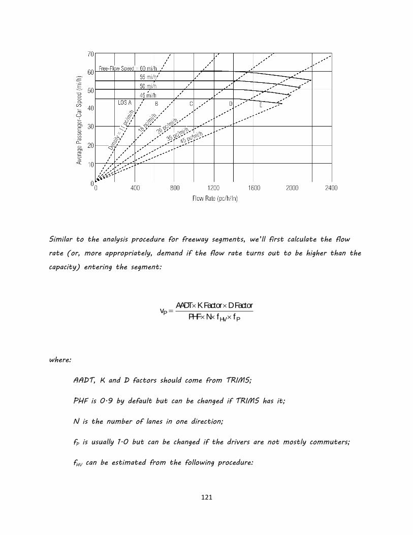
121

Similar to the analysis procedure for freeway segments, we’ll first calculate the flow

rate (or, more appropriately, demand if the flow rate turns out to be higher than the

capacity) entering the segment:

P HV P


PHF N f f

where:


PHF is 0.9 by default but can be changed if TRIMS has it;

N is the number of lanes in one direction;

fP is usually 1.0 but can be changed if the drivers are not mostly commuters;

fHV can be estimated from the following procedure:

122

HVT T R R

1f

1 P(E 1) P(E 1)

where:

PT and PR are the percentage of multi- and single unit trucks from TRIMS; and

ET and ER are from the following table.

Capacity, c, is the next we need to find in order to, eventually, calculated the v/c

ratio. Capacity is a function of FFS, free-flow speed, according to HCM 2000. We

have developed a model for implementing HCM 2000.

FFS = Max (45, Min (60, BFFS – fLW – fLC – fM – fA))

Where,

FFS is bound between 45 and 60 mph;

BFFS = –8×10-5 PS3 + 0.0121 PS2 + 0.3926 PS + 14.718 mph; and

fLW, fLC, fM, and fA can be derived from the following tables.

123

It is rather difficult to figure out the actual number of access points (intersections as

well as driveways) per mile in a segment since such information is not always collected

and/or coded in TRIMS. However, if such information is available, one could calculate it

with the following equation. In the past, 20 access points per mile has been used when

data is not available.

124

No of Access PointsAccess Points/Mile =

Length of the Segment

Once we have FFS, the capacity, c, can be calculated as:

Capacity = 2200 pcphpl, if FFS 60 mph

= 2200 20 (60 FFS) pcphpl, otherwise

Then the v/c ratio is simply equal to vP/c. Note that both vP and c are on per lane

basis. At this point if the v/c ratio is larger than 1.0, we can readily assign a LOS of

F to the section and move on and save calculation time. Therefore:

IF vP/c > 1.0 THEN

LOS = F

S = 5 mph

EXIT

END IF

We can also calculate the operation speed, S, according to the following procedure:

IF vP > 1400 THEN

IF FFS > 55 THEN

125

ELSE IF 55 ≥ FFS > 50 THEN

ELSE IF 50 ≥ FFS > 45 THEN

ELSE

FFS = 45

END IF

ELSE

S = FFS

END IF

And the density can be calculated also as:


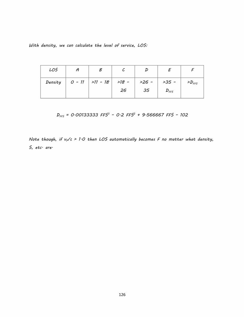
126

With density, we can calculate the level of service, LOS:

LOS A B C D E F

Density 0 – 11 >11 – 18 >18 –

26

>26 –

35

>35 –

DFFS

>DFFS

DFFS = 0.00133333 FFS3 – 0.2 FFS2 + 9.566667 FFS – 102

Note though, if vP/c > 1.0 then LOS automatically becomes F no matter what density,

S, etc. are.

127

Section III - Urban Arterial Analysis Procedure

This procedure is for the analysis of urban and suburban streets with traffic signal

spacing of 2.0 miles or less. The analysis should be conducted for sections 2 miles or

longer, and at least one mile in the downtown area1. A section is defined as a portion

of a roadway where the AADT and/or roadway geometry do not change significantly.

The analysis is meant to be performed for directional traffic.


AADT, K Factor, D Factor, PHF, Rural/Urban, Number of Lanes (N),

Signals, Cross

Streets, Functional Class, Length of Segments

OUTPUT: Average Travel Speed (SA)

Capacity (c)

v/c ratio


The urban arterial analysis procedure is more complicated than the analysis procedures

for freeways and multilane highways. It is based on Chapters 10, 15, and 16 of HCM

2000.

1 The procedure may be applied to shorter segments also.

128

The nature and purpose of Highway Capacity Manual is for detailed operational

assessment. Due to the planning emphasis of TRIMS, certain input parameters for

HCM 2000 are not readily available. These parameters include:

Signal Timing Plans

Coordination of Signals along the Roadway

Actuation/Detectors at Intersections

Turning Movements

Public Transit Demand and Service Information

Parking Activities

Pedestrian Demand

Stop Controlled Intersection Information

Roadside Assess Information

Arrival Pattern at Intersections

For planning purposes, EVE will use the following steps to analysis the LOS of urban

arterials.

Step 1. Demand Calculation/Estimation

Similar to the analysis procedure for freeway segments, we’ll first calculate the

flow rate (or, more appropriately, demand if the flow rate turns out to be

higher than the capacity) entering the section:

129

LT

P

AADT K Factor D Factor 1-Pv

PHF

where:


PHF is 0.9 by default but can be changed if TRIMS has it; and

PLT is the percent of left-turning vehicles with a default of 10% where

applicable.

Step 2. Arterial Classification

HCM 2000 defines LOS for arterials based on the operational speed on different

classes of roadways. Therefore, it is important to classify the arterial type at

an early stage of the analysis procedure.

130

For the purpose of EVE analysis, we’ll use TRIMS parameters to determine the

functional category. The parameters from TRIMS include:

Functional Classification (FC)

Speed Limit (SL)

FC Code Procedure for Arterial Type (CA)

131

Determination

02 CA = 1

06 CA = 2

07 CA = 3

08

IF SL > 30 THEN

CA = 3

ELSE

CA = 4

END IF

Default = 4

09 CA = 4

12

IF SL ≥ 45 THEN

CA = 1

ELSE

CA = 2

END IF

Default = 2

14 CA = 2

16

IF SL ≥ 40 THEN

CA = 2

ELSE IF SL ≥ 35 THEN

CA = 3

ELSE

Default = 4

132

CA = 4

END IF

17

IF SL ≥ 30 THEN

CA = 3

ELSE

CA = 4

END IF

Default = 4

19 CA = 4 Default = 4

CA is Arterial Class

Step 3. Average Running Time Estimation

For the arterial segment the running time, TR, is to be estimated based on

arterial class and FFS. Since FFS is rarely available in TRIMS, we’ll use the

following equations. Note though the Speed_Lmt, or speed limit, term should

be greater than 0.0.

Variable SD is signal density within the section and can be calculated as the

number of traffic signals divided by the length, L, of the section. Note that

these equations were resultant from linear regressions with R2 > 0.95 based on

HCM 2000 methodology.

133

Arterial

Class Equation for TR (sec)

I TR = L Max[3600/Speed_Lmt,

(9.8545SD+60.907)]

Eq.

Xa

II TR = L Max[3600/Speed_Lmt,

(6.7430SD+80.958)]

Eq.

Xb

III TR = L Max[3600/Speed_Lmt,

(3.9518SD+106.64)]

Eq.

Xc

IV TR = L Max[3600/Speed_Lmt,

(5.9188SD+111.74)]

Eq.

Xd

Based on Akcelik model with Tennessee calibration, running speed for the segment

is calculated as:

y = 5.9188x + 111.74

R2 = 0.9822

y = 3.9518x + 106.64

R2 = 0.9587

y = 6.743x + 80.958

R2 = 0.9649

y = 9.8545x + 60.907

R2 = 0.9809

0

50

100

150

200

250

300

0.00 5.00 10.00 15.00 20.00 25.00

Traffic Signals per Mile

Run

ning

Tim

e (s

ec)

I

II

III

IV

Linear (IV)

Linear (III)

Linear (II)

Linear (I)

134

2R

RAT v v v 8J

T 3,600 1 13600 c c c Q

where

J = 1.00 and

Q = 900 vpl

Step 4. Capacity Estimation

The capacity, c, of a signalized intersection cannot be calculated without detailed

signal timing information. For planning purposes, assumptions are made to make

it possible for the analysis.

g

c N sC

N is the number of through lanes in the travel direction, s is the saturation flow

rate (1,900 vph), and g

C is green ratio, which is assumed to be 0.5 when the

cross road is a state route and 0.65 otherwise. Given such, the capacity would

be:

c 1,235 N or 950 N

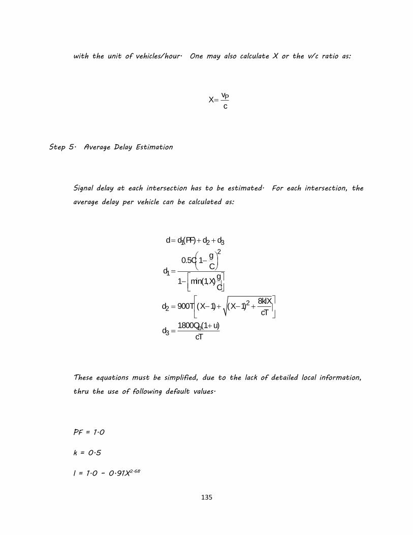
135

with the unit of vehicles/hour. One may also calculate X or the v/c ratio as:

PvXc

Step 5. Average Delay Estimation

Signal delay at each intersection has to be estimated. For each intersection, the

average delay per vehicle can be calculated as:

1 2 3

2

1

22

b3

d d(PF) d d

g0.5C 1

Cd

g1 min(1,X)

C

8klXd 900T (X 1) (X 1)

cT

1800Q (1 u)d

cT

These equations must be simplified, due to the lack of detailed local information,

thru the use of following default values.

PF = 1.0

k = 0.5

l = 1.0 – 0.91X2.68

136

T = 0.25 hour

d3 = 0.0 sec

C = 90 sec

g/C = 0.5 if the cross street is a state route and 0.67 otherwise

Therefore, if the signal is at an intersection with a state route (or higher class

road), the average delay per vehicle, in seconds, at this intersection would be:

245 l Xd 225 X 1 (X 1)

4 2 min(1,X) 60 N

If the cross road has a lesser classification, then

215 l Xd 225 X 1 (X 1)

3 2 min(1,X) 80 N

where I = 1.0 if X > 1.0 and I = 1.0 – 0.91X2.68 otherwise.

Since delay is incurred at all signalized intersections along the section, we define

the cumulative delay per vehicle as:

SAll Signals

d d

137

Step 6. Average Travel Speed Estimation

ARA S

3600LS

T d

where SA is the average speed in mph and L is the section length in miles.

Step 7. LOS Assessment

Based on the average travel speed and arterial class, LOS can be determined:

138

Section IV - Two-Lane Highway Analysis Procedure

This procedure is for the analysis of two-lane roads with no or only isolated traffic

signals (spaced at least 2 miles apart). The analysis can be performed for two- or one-

directional traffic.


AADT, K Factor, D Factor, PHF, Rural/Urban, Terrain, Number of Lanes

(N), Signals,

Truck %, RV %, Functional Class, Length of Segments, Posted Speed, Safe

Operational Speed (from IHSDM)

OUTPUT: Average Travel Speed (SA)

Percent Time Spent Following

Capacity (c)

v/c ratio


The two-lane highway analysis procedure is an improved and complicated one in

comparison with its earlier versions prior to 1997. The procedure to be implemented is

based on Chapters 12 and 20 of HCM 2000. The main considerations of this

procedure are passing opportunities and the average travel speed. The presence of a

passing lane or a directional climbing lane makes a marked difference to the LOS of a

139

roadway segment and requires different analysis procedures. The following is the

procedure for the sections without passing or climbing lanes.

It should be noted that two-lane roads exist in both rural and urban areas. HCM

2000 provides different standards for the two classes of such roadways as following.

Class I – These are two-lane highways on which motorists expect to travel at relatively

high speeds. Two-lane highways that are major intercity routes, primary arterials

connecting major traffic generators, daily commuter routes, or primary links in state or

national highway networks generally are assigned to Class I. Class I facilities most often

serve long-distance trips or provide connecting links between facilities that serve long-

distance trips.

Class II – These are two-lane highways on which motorists do not necessarily expect to

travel at high speeds. Two-lane highways that function as access routes to Class I

facilities, serve as scenic or recreational routes that are not primary arterials, or pass

through rugged terrain generally are assigned to Class II. Class II facilities most often

serve relatively short trips, the beginning and ending portions of longer trips, or trips

for which sightseeing plays a significant role.

Step 1. Identification of a Two-Lane Highway

All of the following should be true to use this procedure.

A total of two lanes for the two directions of the roadway(or 3 if the third

lane is a passing lane or climbing lane) and

140

The length of the segment between two signals is larger than 2 miles.

141

Step 2. Roadway Classification

Because LOS considerations and analysis procedures are not exactly the same for

the two classes of two-lane roads, it is essential to classify a roadway segment

first.

Table 4.1

1. A segment is classified as Class I if one of the following conditions is true:

It has a SR or NHS designation;

It’s FC code is 02, 06, 12, 14, or 16;

2. Otherwise, we classify the segment as Class II.

3. There might be exceptions based on the terrain, scenic route designation, and

posted speed.

Step 3. Demand Estimation

142

Similar to other analysis procedures, we’ll first calculate the demand for the

section:

P

G HV

AADT K Factorv

PHF f f

where:

vP is the two-way flow rate in pc/h;


PHF is 0.88 for rural area and 0.92 for urban area if unavailable from

TRIMS;

fG is grade adjustment factor; and

fHV is heavy vehicle adjustment factor.

The grade adjustment factor, fG, is defined as the following in HCM 2000.

Table 4.2

Rang of vP

Two-Way Flow

(pc/h)

Type of Terrain

Level Rolling Mountainous

>0000 - 0600 1.00 0.71 0.57

>0600 - 1200 1.00 0.93 0.85

143

>1200 - 0000 1.00 0.99 0.99

It should be noted that since vP and fG are both unknown an iterative process

has to be used here. We probably start with an fG value of 1.00, 0.93, or

0.85 depending on the terrain type and solve for vP.

The heavy vehicle adjustment factor, fHV, is defined as the following in HCM

2000.

HVT T R R

1f

1 P(E 1) P(E 1)

Table 4.3

Vehicle

Type

Rang of vP

Two-Way Flow

(pc/h)

Type of Terrain


Trucks, ET

>0000 -

0600 1.7 2.5 7.2

>0600 - 1200 1.2 1.9 7.2

>1200 - 0000 1.1 1.5 7.2

RVs, ER All 1.0 1.1 3.2

We will use TRIMS truck percentage information for following calculations:

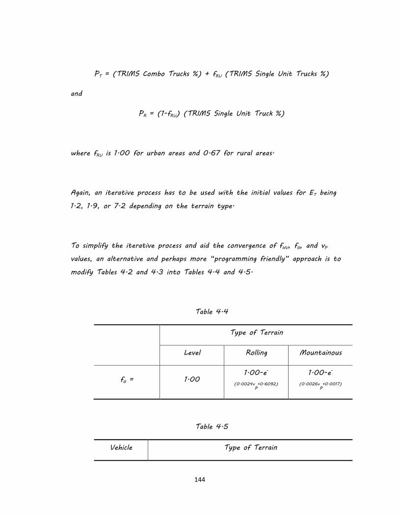
144


and


where fRU is 1.00 for urban areas and 0.67 for rural areas.

Again, an iterative process has to be used with the initial values for ET being

1.2, 1.9, or 7.2 depending on the terrain type.

To simplify the iterative process and aid the convergence of fHV, fG, and vP

values, an alternative and perhaps more “programming friendly” approach is to

modify Tables 4.2 and 4.3 into Tables 4.4 and 4.5.

Table 4.4

Type of Terrain


fG = 1.00 1.00-e-

(0.0024vP+0.6092)

1.00-e-

(0.0026vP+0.0017)

Table 4.5

Vehicle Type of Terrain

145

Type Level Rolling Mountainous

Trucks, ET -0.0004vP+1.7458 -0.0007vP+2.6389 7.2

RVs, ER 1.0 1.1 3.2

Use the same iterative process with same initial values and stop when vP < 10

vph

Step 4. Estimate Free Flow Speed (FFS)

Research has established relationships of FFS, posted speed limit, and the safe

operational speed from geometric design perspective. We’ll use the following

procedure, which is a combination of research findings from HCM 2000, IHSDM,

and UT studies.

FFS = Max(25, Min(65, V85 – fLS – fA))

The following pseudo-code is provided to explain the calculation process for V85.

IF (PS is available in TRIMS) THEN

V85 = –8×10-5 PS3 + 0.0121 PS2 + 0.3926 PS + 14.718 mph;

ELSE IF (DC and G are available in TRIMS and DC ≠ 0) THEN

V85 = CA – CB/R or

V85 = CA – 0.00017455 CB DC

146

because R = DC/5,729.58 or 0.00017455 DC

Grade Range CA CB

-9% ≤ G < -4% 63.81 6309.73

-4% ≤ G < -0% 66.24 7607.24

-0% ≤ G < -4% 65.51 7329.62

-4% ≤ G < -9% 60.38 5643.43

ELSE

V85 = 60 mph for Class I or 45 mph for Class II segments

END IF

Where,

PS is posted speed limit in mph;

V85 is the 85th percentile speed or base free flow speed in mph;

G is grade in %;

R is radius in feet;

DC is the degree of curvature, which is stored in TRIMS

CA is a coefficient for speed prediction model; and

CB is a coefficient for speed prediction model.

The factor fLS, which represents the reduction in FFS due to lane width and

shoulder width restrictions has the following values:

147

The access point factor, fA, which also causes reduction in FFS is tabulated below.

4

Mile per Points AccessfA

where the default numbers of access points per mile in rural and urban areas is 0

and 10, respectively.

Step 5. Determine Average Travel Speed

Average Travel Speed, ATS, is a function of FFS, flow rate, and existence of

passing zone.

ATS = FFS – 0.00776vP – fnp

where fnp is the adjustment factor for no-passing zones. If the percentage of

no-passing zone is known, the HCM 2000 table should be used. However, the

148

percentage no-passing zone information is currently unavailable in TRIMS.

Therefore, the following presents an alternative set of default values for fnp

based on terrain types.

149

Two-Way Demand Flow

Rate, vP (pc/h)

Type of Terrain


0 0.00 0.00 0.00

200 0.60 1.90 2.60

400 1.70 3.10 3.90

600 1.60 2.70 3.40

800 1.40 2.15 2.70

1000 1.10 1.80 2.20

1200 0.80 1.40 1.90

1400 0.60 1.05 1.40

1600 0.60 0.95 1.30

1800 0.50 0.85 1.10

2000 0.50 0.75 1.00

2200 0.50 0.75 0.90

2400 0.50 0.70 0.90

2600 0.50 0.70 0.90

2800 0.50 0.65 0.80

3000 0.50 0.65 0.70

3200 0.50 0.60 0.60

Step 6. Decide Percent Time Spent Following

150

A HCM 2000 based model is adopted for the estimation of PTSF (percent

time-spent-following). Note that the range of PTSF is between 0 and 100.

PTSF = Max(BPTSF + fn/dp, 0)

BPTSF is the base percent time-spent-following for both directions of traffic. It

can be estimated as:

BPTSF = 100 (1 – e-0.000879 vp) or

= 100 (1 – 1/e0.000879 vp)

The combined adjustment factor for directional distribution and no-passing zone

percentage or fn/dp involves complicated procedures and calculations. Based on

HCM 2000 procedures and simplifications for the state of Tennessee with

directional split being 60/40 during the peak hour and 20, 50, and 80% being

the no-passing zone percentage for level, rolling, and mountainous terrains.

Note that if Medium_Width > 0, then 100% No Passing equation should be

used. On the other hand if Number_of_Lane = 3 and Lane_Type = 0, then

100% Passing Zone equation below should be used.

The following equations will be used for the cases of:

151

Level Terrain: fn/dp = 13.422 – 0.0077 vp + 0.000001 vp2

Rolling Terrain: fn/dp = 21.935 – 0.0132 vp + 0.000002 vp2

Mountainous Terrain: fn/dp = 25.499 – 0.0152 vp + 0.000002 vp2

100% No Passing: fn/dp = 28.210 – 0.0181 vp + 0.000003 vp2

100% Passing: fn/dp = 1.3422 – 0.0008 vp + 0.0000001 vp2

The following trend-line analysis plot is provided to show the approximation

process in deriving these equations.

153

Step 7. Calculate v/c ratio

The v/c ratio is easily obtained as vp/c where c is equal to 3,200 vph for two-

way traffic and 1,700 vph for one-way one-direction cases.

Step 8. Determine LOS

It should be noted that whenever the v/c ratio is greater than 1.00, the LOS

should be F. Otherwise, LOS of the two-lane roadway segment may be

determined depending on if it is a Class I or Class II roadway.

For Class I cases, both PTSF, percent time-spent-following, and ATS, average

travel speed, values will be used to determine the level of service of the roadway

segment. Note that only LOS A through E are listed in the table. LOS F

exists only when the volume exceeds the capacity or when v/c ratio is greater

than 1.00.

For Class II cases, only PTSF will be used. Again, only when v/c ratio is greater

than 1.00 would LOS F result.

155

APPENDICIES

HIGHWAY FUNCTIONAL CLASS CODE

FC Code Functional Class

Rural Area

01 Principal Arterial Interstate

02 Other Principal Arterial

06 Minor Arterial

07 Major Collector

08 Minor Collector

09 Local

Urban Area

11 Principal Arterial Interstate

12 Principal Arterial, Other Freeways &

Expressways

14 Other Principal Arterial

16 Minor Arterial

17 Collector

19 Local

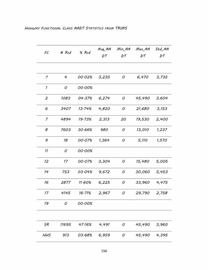
156

HIGHWAY FUNCTIONAL CLASS AADT STATISTICS FROM TRIMS

FC # Rcd % Rcd Avg_AA

DT

Min_AA

DT

Max_AA

DT

Std_AA

DT

? 4 00.02% 3,235 0 6,470 3,735

1 0 00.00%

2 1083 04.37% 6,274 0 45,490 3,604

6 3407 13.74% 4,820 0 21,680 3,153

7 4894 19.73% 2,313 20 19,530 2,400

8 7603 30.66% 980 0 13,010 1,237

9 18 00.07% 1,364 0 5,110 1,570

11 0 00.00%

12 17 00.07% 3,304 0 15,480 5,005

14 753 03.04% 9,672 0 30,060 5,453

16 2877 11.60% 6,225 0 33,960 4,475

17 4145 16.71% 2,967 0 29,790 2,758

19 0 00.00%

SR 11695 47.16% 4,491 0 45,490 3,960

NHS 913 03.68% 6,959 0 45,490 4,395

157

fn/dp,PTSF Charts

Level Terrain (20% No-Passing Zone)

Rolling Terrain (50% No-Passing Zone)

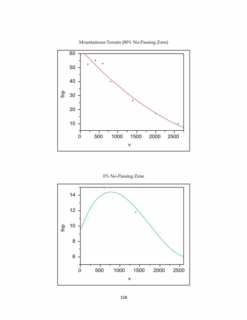
158

Mountainous Terrain (80% No-Passing Zone)

0% No-Passing Zone

159

100% No-Passing Zone

160

List of References

161

Azimi, Mehdi, & Zhang, Yunlong. (2010). Categorizing freeway flow conditions by using clustering methods. Transportation Research Record(2173), 105-114. doi: 10.3141/2173-13

Brilon, Werner, & Estel, Anja. (2010). Differentiated analysis of level of service f within the German highway capacity manual. Transportation Research Record(2173), 36-44. doi: 10.3141/2173-05

Dowling, Richard G., Reinke, David, National Cooperative Highway Research, Program, National Research Council . Transportation Research, Board, American Association of State, Highway, & Transportation, Officials. (2008). Multimodal level of service analysis for urban streets. Washington, D.C.: Transportation Research Board.

Guttenplan, Martin, Davis, Beverly, Steiner, Ruth, & Miller, Demian. (2003). Planning-Level Areawide Multimodal Level-of-Service Analysis: Performance Measures for Congestion Management.

Kittelson, Wayne K., & Roess, Roger P. (2001). Highway capacity analysis after Highway Capacity Manual 2000. Transportation Research Record(1776), 10-16.

National Research Council . Transportation Research, Board. (2000). Highway capacity manual. Washington, D.C.: Transportation Research Board, National Research Council.

National Research Council . Transportation Research, Board. (2010). HCM 2010 : highway capacity manual. Washington, D.C.: Transportation Research Board.

Roess, Roger P. (2011). Speed-flow curves for freeways in Highway Capacity Manual 2010. Transportation Research Record(2257), 10-21. doi: 10.3141/2257-02

Sharma, V., Al-Hussein, M., Safouhi, H., & Bouferguene, A. (2008). Municipal infrastructure asset levels of service assessment for investment decisions using analytic hierarchy process. J. Infrastruct. Syst. Journal of Infrastructure Systems, 14(3), 193-200.

Tarko, A., & Songchitruksa, P. (2003). Reporting uncertainty in the highway capacity manual-survey results. Transportation Research Board.

Washburn, Scott S., McLeod, Douqlas S., & Courage, Kenneth G. (2002). Adaptation of highway capacity manual 2000 for planning-level analysis of two-lane and multilane highways in Florida. Transportation Research Record(1802), 62-68.

Washburn, Scott S., Ramlackhan, Kirby, & McLeod, Douglas S. (2004). Quality-of-service perceptions by rural freeway travelers: Exploratory analysis.

Washington, Simon, National Cooperative Highway Research, Program, National Research Council . Transportation Research, Board, American Association of State, Highway, & Transportation, Officials. (2006). Incorporating safety into long-range transportation planning. Washington, D.C.: Transportation Research Board.

Zegeer, John D., Blogg, Miranda, Nguyen, Khang, & Vandehey, Mark. (2008). Default values for highway capacity and level-of-service analyses. Transportation Research Record(2071), 35-43. doi: 10.3141/2071-05

162

VITA

James Ensley was born and raised in Nashville, TN. He graduated from Antioch High School in

May 2007. He began his Undergraduate career at the University of Tennessee in August 2007.

He graduated from the University of Tennessee with a Bachelors of Science in Civil Engineering

in December 2011. The following semester, he continued with his Masters of Science in Civil

Engineering with a Concentration in Transportation Engineering. Upon graduation, he plans to

gain employment within the Transportation Industry.

Application of Highway Capacity Manual 2010 Level-of ...

Documents

Transcript of Application of Highway Capacity Manual 2010 Level-of ...