2013 Status of the Nation’s H

ighways, Bridges, and Transit:

Conditions &

Performance

2013 Status of the Nation’s Highways, Bridges, and Transit:

REPORT TO CONGRESS

Conditions & Performance

U.S. Departmentof Transportation

Federal HighwayAdministration

Federal TransitAdministration

Table of Contents iii

Table of Contents

List of Exhibits ......................................................................................................................................xi

Abbreviations ................................................................................................................................... xxiii

Introduction ....................................................................................................................................... xxix

Executive Summary ..........................................................................................................................ES-1

Chapter OverviewsPart I: Description of Current System ...............................................................................CO-1Chapter 1: Household Travel ..............................................................................................CO-2Chapter 1: Freight Movement .............................................................................................CO-3Chapter 2: System Characteristics: Highways and Bridges .............................................CO-4Chapter 2: System Characteristics: Transit .......................................................................CO-5Chapter 3: System Conditions: Highways .........................................................................CO-6Chapter 3: System Conditions: Transit ..............................................................................CO-7Chapter 4: Safety: Highways ..............................................................................................CO-8Chapter 4: Safety: Transit ...................................................................................................CO-9Chapter 5: System Performance: Highways ....................................................................CO-10Chapter 5: System Performance: Transit .........................................................................CO-11Chapter 6: Finance: Highways .........................................................................................CO-12Chapter 6: Finance: Transit ...............................................................................................CO-13Part II: Investment/Performance Analysis ......................................................................CO-14Chapter 7: Potential Capital Investment Impacts: Highways..........................................CO-16Chapter 7: Potential Capital Investment Impacts: Transit ...............................................CO-17Chapter 8: Selected Capital Investment Scenarios: Highways ......................................CO-18Chapter 8: Selected Capital Investment Scenarios: Transit ...........................................CO-19Chapter 9: Supplemental Scenario Analysis: Highways .................................................CO-20Chapter 9: Supplemental Scenario Analysis: Transit ......................................................CO-21Chapter 10: Sensitivity Analysis: Highways ....................................................................CO-22Chapter 10: Sensitivity Analysis: Transit .........................................................................CO-23Chapter 11: Transportation Serving Federal and Tribal Lands .......................................CO-24Chapter 12: Center for Accelerating Innovation ..............................................................CO-25Chapter 13: National Fuel Cell Bus Program ...................................................................CO-26

Part I: Description of Current System ............................................................................................... I-1Introduction ................................................................................................................................ I-2

U.S. DOT Strategic Plan ............................................................................................................ I-2Performance Management ........................................................................................................ I-3

Chapter 1: Household Travel and Freight Movement ........................................................... 1-1

Household Travel ............................................................................................................ 1-2Trends in Our Nation’s Travel ................................................................................................... 1-3

Geographic Trends in Trip Rates and Trip Lengths ................................................................. 1-4The Determinants of Travel ...................................................................................................... 1-6Travel by Time of Day ............................................................................................................... 1-7

Usual and Actual Commute: A Typical Day Versus a Specific Day ........................................ 1-7Baby Boomer Travel Trends ..................................................................................................... 1-8Travel of Millennials .................................................................................................................. 1-9

Table of Contentsiv

Aging of the Household Vehicle Fleet ................................................................................... 1-10Some Myths and Facts About Daily Travel ............................................................................ 1-11

Myth 1: The majority of personal travel is for commuting to work ........................................ 1-11Myth 2: Americans love their cars, and that’s why they don’t walk or take transit ............... 1-11Myth 3: Households without vehicles rely completely on transit, walk, and bike ................. 1-12Myth 4: When elderly drivers give up their driver’s license they maintain mobility by using transit or walking instead of using private vehicles ................................................ 1-15Myth 5: We can solve congestion by having people shift noncommuting trips outside of peak periods.......................................................................................................... 1-16

Gas Prices and the Public’s Opinions ................................................................................... 1-16Number One Issue for the Public: Price of Travel .................................................................. 1-17

Freight Movement ......................................................................................................... 1-18Freight Transportation System ............................................................................................... 1-18Freight Transportation Demand ............................................................................................. 1-18Freight Challenges ................................................................................................................. 1-26

Chapter 2: System Characteristics ....................................................................................... 2-1

Highway System Characteristics .................................................................................... 2-2Roads by Ownership ................................................................................................................ 2-2Roads by Purpose .................................................................................................................... 2-3

Review of Functional Classification Concepts ......................................................................... 2-3System Characteristics ............................................................................................................. 2-5Highway Travel ......................................................................................................................... 2-8

Federal-Aid Highways ............................................................................................................ 2-11National Highway System ...................................................................................................... 2-12Interstate System .................................................................................................................... 2-14Highway Freight System ........................................................................................................ 2-14

Changes under MAP-21 ......................................................................................................... 2-15

Bridge System Characteristics ...................................................................................... 2-17Bridges by Owner ................................................................................................................... 2-17Interstate, STRAHNET, and NHS Bridges .............................................................................. 2-18Bridges by Roadway Functional Classification .................................................................... 2-19Bridges by Traffic Volume ...................................................................................................... 2-21

Transit System Characteristics ...................................................................................... 2-22System History........................................................................................................................ 2-22System Infrastructure ............................................................................................................. 2-23

Urban Transit Agencies .......................................................................................................... 2-23Transit Fleet ............................................................................................................................ 2-27Track, Stations, and Maintenance Facilities ........................................................................... 2-28

Rural Transit Systems (Section 5311 Providers) .................................................................. 2-29Transit System Characteristics for Americans With Disabilities and the Elderly ................ 2-29Transit System Characteristics: Alternative Fuel Vehicles ................................................... 2-31

Chapter 3: System Conditions .............................................................................................. 3-1

Highway System Conditions ........................................................................................... 3-2Pavement Terminology and Measurements ............................................................................ 3-2Factors Impacting Pavement Performance ............................................................................. 3-3Implications of Pavement Condition for Highway Users ........................................................ 3-3Pavement Ride Quality on the National Highway System ...................................................... 3-5Pavement Ride Quality on Federal-Aid Highways .................................................................. 3-5

Pavement Ride Quality by Functional Classification ............................................................... 3-7

Table of Contents v

Lane Width ................................................................................................................................ 3-9Roadway Alignment .................................................................................................................. 3-9

Bridge System Conditions ............................................................................................. 3-11Bridge Ratings ........................................................................................................................ 3-11

Condition Ratings ................................................................................................................... 3-12Appraisal Ratings ................................................................................................................... 3-14

Bridge Conditions ................................................................................................................... 3-16Bridge Conditions on the NHS ............................................................................................... 3-16Bridge Conditions by Functional Classification ..................................................................... 3-18Bridge Conditions by Owner .................................................................................................. 3-18

Bridges by Age ....................................................................................................................... 3-20

Transit System Conditions ............................................................................................. 3-23The Replacement Value of U.S. Transit Assets ..................................................................... 3-24Bus Vehicles (Urban Areas) ................................................................................................... 3-25Other Bus Assets (Urban Areas) ........................................................................................... 3-27Rail Vehicles ........................................................................................................................... 3-27Other Rail Assets .................................................................................................................... 3-29Rural Transit Vehicles and Facilities ...................................................................................... 3-31

Chapter 4: Safety .................................................................................................................... 4-1

Highway Safety ................................................................................................................. 4-2Overall Fatalities and Injuries .................................................................................................. 4-3Highway Fatalities: Roadway Contributing Factors ................................................................ 4-5

Focus Area Safety Programs ................................................................................................... 4-5Roadway Departures ................................................................................................................ 4-6Intersections ............................................................................................................................. 4-7Pedestrians and Other Nonmotorists ....................................................................................... 4-8Fatalities by Roadway Functional Class .................................................................................. 4-9Behavioral ............................................................................................................................... 4-11

Transit Safety .................................................................................................................. 4-13Incidents, Fatalities, and Injuries ........................................................................................... 4-13

Chapter 5: System Performance ........................................................................................... 5-1

Highway System Performance ........................................................................................ 5-2Transportation Systems and Livable Communities ................................................................ 5-2

Fostering Livable Communities ................................................................................................ 5-3Advancing Environmental Sustainability .................................................................................. 5-6

Economic Competitiveness ..................................................................................................... 5-8System Reliability ..................................................................................................................... 5-9System Congestion ................................................................................................................ 5-10Effect of Congestion and Reliability on Freight Travel ........................................................... 5-11Congestion Mitigation and Reliability Improvement .............................................................. 5-13

Transit System Performance ......................................................................................... 5-16Average Operating (Passenger-Carrying) Speeds ............................................................... 5-16Vehicle Use ............................................................................................................................. 5-17

Vehicle Occupancy................................................................................................................. 5-17Revenue Miles per Active Vehicle (Service Use) ................................................................... 5-18

Frequency and Reliability of Service ..................................................................................... 5-19System Coverage: Urban Directional Route Miles ............................................................... 5-21System Capacity ..................................................................................................................... 5-21Ridership ................................................................................................................................. 5-23

Table of Contentsvi

Chapter 6: Finance ................................................................................................................. 6-1

Highway Finance .............................................................................................................. 6-2Revenue Sources for Highways............................................................................................... 6-2

Revenue Trends ........................................................................................................................ 6-5Highway Expenditures ............................................................................................................. 6-7

Types of Highway Expenditures ............................................................................................... 6-7Historical Expenditure and Funding Trends ............................................................................ 6-8

Highway Capital Outlay .......................................................................................................... 6-12Capital Outlays on Federal-Aid Highways ............................................................................. 6-16Capital Outlays on the National Highway System ................................................................. 6-17Capital Outlays on the Interstate System ............................................................................... 6-18

Innovative Finance ................................................................................................................. 6-18Public-Private Partnerships .................................................................................................... 6-19Federal Credit Assistance ...................................................................................................... 6-19Debt Financing Tools .............................................................................................................. 6-20

Transit Finance ............................................................................................................... 6-21Level and Composition of Transit Funding ........................................................................... 6-21

Federal Funding ..................................................................................................................... 6-22State and Local Funding ........................................................................................................ 6-24System-Generated Funds ...................................................................................................... 6-24

Trends in Funding ................................................................................................................... 6-25Funding in Current and Constant Dollars .............................................................................. 6-25

Capital Funding and Expenditures ........................................................................................ 6-26Operating Expenditures ......................................................................................................... 6-29

Operating Expenditures by Transit Mode .............................................................................. 6-30Operating Expenditures by Type of Cost ............................................................................... 6-31Operating Expenditures per Vehicle Revenue Mile ............................................................... 6-31Operating Expenditures per Passenger Mile ......................................................................... 6-33Farebox Recovery Ratios ....................................................................................................... 6-33

Rural Transit ............................................................................................................................ 6-34

Part II: Investment/Performance Analysis ......................................................................................... II-1Introduction ............................................................................................................................... II-2Capital Investment Scenarios. ................................................................................................. II-3

Highway and Bridge Investment Scenarios ............................................................................. II-3Transit Investment Scenarios ................................................................................................... II-4Comparisons Between Report Editions ................................................................................... II-5

The Economic Approach to Transportation Investment Analysis .......................................... II-6The Economic Approach in Theory and Practice .................................................................... II-6Measurement of Costs and Benefits in “Constant Dollars” ..................................................... II-8Multimodal Analysis ................................................................................................................. II-9Uncertainty in Transportation Investment Modeling ................................................................ II-9

Chapter 7: Potential Capital Investment Impacts ................................................................. 7-1

Potential Highway Capital Investment Impacts .............................................................. 7-2Types of Capital Spending Projected by HERS and NBIAS ................................................... 7-2Alternative Levels of Future Capital Investment Analyzed ..................................................... 7-4Highway Economic Requirements System ............................................................................. 7-5

HPMS Database ....................................................................................................................... 7-6Operations Strategies............................................................................................................... 7-7

Table of Contents vii

HERS Treatment of Traffic Growth ........................................................................................... 7-8Travel Demand Elasticity ........................................................................................................ 7-10

Impacts of Federal-Aid Highway Investments Modeled by HERS ....................................... 7-10Selection of Investment Levels for Analysis ........................................................................... 7-10Investment Levels and BCRs by Funding Period .................................................................. 7-12Impact of Future Investment on Highway Pavement Ride Quality ........................................ 7-13Impact of Future Investment on Highway Operational Performance .................................... 7-16Impact of Future Investment on Highway User Costs ........................................................... 7-19

Impacts of NHS Investments Modeled by HERS .................................................................. 7-22Impact of Future Investment on NHS Pavement Ride Quality ............................................... 7-23Impact of Future Investment on NHS Travel Times and User Costs ..................................... 7-24

Impacts of Interstate System Investments Modeled by HERS ............................................ 7-26Impact of Future Investment on Interstate Pavement Ride Quality ....................................... 7-26Impact of Future Investment on Interstate System Travel Times and User Costs ................ 7-27

National Bridge Investment Analysis System ....................................................................... 7-28Performance Measures .......................................................................................................... 7-29

Impacts of Systemwide Investments Modeled by NBIAS .................................................... 7-30Impacts of Federal-Aid Highway Investments Modeled by NBIAS ...................................... 7-31Impacts of NHS Investments Modeled by NBIAS ................................................................. 7-32Impacts of Interstate Investments Modeled by NBIAS ......................................................... 7-34

Potential Transit Capital Investment Impacts ............................................................... 7-35Types of Capital Spending Projected by TERM .................................................................... 7-35

Preservation Investments ....................................................................................................... 7-35Expansion Investments .......................................................................................................... 7-36Recent Investment in Transit Preservation and Expansion ................................................... 7-37

Impacts of Systemwide Investments Modeled by TERM ..................................................... 7-37Impact of Preservation Investments on Transit Backlog and Conditions .............................. 7-37Impact of Expansion Investments on Transit Ridership......................................................... 7-40

Impacts of Urbanized Area Investments Modeled by TERM ................................................ 7-41Urbanized Areas Over 1 Million in Population ....................................................................... 7-42Other Urbanized and Rural Areas .......................................................................................... 7-44

Chapter 8: Selected Capital Investment Scenarios .............................................................. 8-1

Selected Highway Capital Investment Scenarios ........................................................... 8-2Scenarios Selected for Analysis .............................................................................................. 8-2Scenario Spending Levels ....................................................................................................... 8-4

Spending Levels Assuming Forecast Growth in VMT ............................................................. 8-4Spending Levels Assuming Trend Growth in VMT .................................................................. 8-7

Scenario Spending Patterns and Conditions and Performance Projections ........................ 8-7Systemwide Scenarios ............................................................................................................. 8-7Federal-Aid Highway Scenarios ............................................................................................. 8-11Scenarios for the National Highway System and the Interstate Highway System ................ 8-18

HIghway and Bridge Investment Backlog ............................................................................. 8-21

Selected Transit Capital Investment Scenarios ............................................................ 8-23Sustain 2010 Spending Scenario ........................................................................................... 8-25

Preservation Investments ....................................................................................................... 8-26Expansion Investments .......................................................................................................... 8-27

State of Good Repair Benchmark .......................................................................................... 8-29SGR Investment Needs .......................................................................................................... 8-29Impact on the Investment Backlog ........................................................................................ 8-30Impact on Conditions ............................................................................................................. 8-30Impact on Vehicle Fleet Performance .................................................................................... 8-31

Table of Contentsviii

Low and High Growth Scenarios ........................................................................................... 8-31Low Growth Assumption ........................................................................................................ 8-32High Growth Assumption ....................................................................................................... 8-32Low and High Growth Scenario Needs ................................................................................. 8-32Impact on Conditions and Performance ................................................................................ 8-33

Scenario Benefits Comparison .............................................................................................. 8-34Scorecard Comparisons ........................................................................................................ 8-36

Chapter 9: Supplemental Scenario Analysis ........................................................................ 9-1

Highway Supplemental Scenario Analysis ..................................................................... 9-2Comparison of Scenarios With Previous Reports .................................................................. 9-2

Comparison With 2010 C&P Report ........................................................................................ 9-2Comparison of Implied Funding Gaps ..................................................................................... 9-3

Comparison of Scenario Projections in 1991 C&P Report to ActualExpenditures, Conditions, and Performance .......................................................................... 9-4

1991 C&P Report Scenario Definitions .................................................................................... 9-4Comparison of Scenario Projections in 1991 C&P Report to Actual Spending ...................... 9-5Comparison of Scenario Projections in 1991 C&P Report to Actual Outcomes ..................... 9-6

Accounting for Inflation ............................................................................................................ 9-7Timing of Investment .............................................................................................................. 9-10

Alternative Timing of Investment in HERS ............................................................................. 9-10Alternative Timing of Investment in NBIAS ............................................................................ 9-13

Transit Supplemental Scenario Analysis ...................................................................... 9-15Asset Conditions Forecasts and Expected Useful Service Life Consumed for All Transit Assets Under Four Scenarios ......................................................................... 9-15

Alternative Methodology ........................................................................................................ 9-18Comparison of 2010 to 2013 TERM Results ......................................................................... 9-19Comparison of Passenger Miles Traveled (PMT) Growth Rates .......................................... 9-20

MPO Growth Compared to Historical Growth for All Urbanized and Rural Areas ................ 9-20UZAs Over 1 Million in Population ......................................................................................... 9-21UZAs Under 1 Million in Population and Rural Areas ............................................................ 9-21

Impact of New Technologies on Transit Investment Needs ................................................. 9-22Impact of Compressed Natural Gas and Hybrid Buses on Future Needs ............................ 9-23Impact on Costs ..................................................................................................................... 9-23Impact on Needs .................................................................................................................... 9-23Impact on Backlog ................................................................................................................. 9-24

Forecasted Expansion Investment ........................................................................................ 9-25

Chapter 10: Sensitivity Analysis .......................................................................................... 10-1

Highway Sensitivity Analysis ......................................................................................... 10-2Alternative Economic Analysis Assumptions ....................................................................... 10-2

Value of Travel Time ............................................................................................................... 10-2Growth in the Value of Time ................................................................................................... 10-5Value of a Statistical Life ......................................................................................................... 10-7Discount Rate ......................................................................................................................... 10-8Alternative Future Fuel Price Assumptions .......................................................................... 10-10

Alternative Strategies ........................................................................................................... 10-11Alternative Bridge Maintenance, Repair, and Rehabilitation Strategies .............................. 10-11Accelerating Operations/ITS Deployments .......................................................................... 10-12

Transit Sensitivity Analysis .......................................................................................... 10-15Changes in Asset Replacement Timing (Condition Threshold) ......................................... 10-15

Table of Contents ix

Changes in Capital Costs .................................................................................................... 10-16Changes in the Value of Time .............................................................................................. 10-16Changes to the Discount Rate ............................................................................................. 10-17

Part III: Special Topics ...................................................................................................................... III-1Introduction .............................................................................................................................. III-2

Chapter 11: Transportation Serving Federal and Tribal Lands .......................................... 11-1

Transportation Serving Federal and Tribal Lands ....................................................... 11-2Types of Federal and Tribal Lands ......................................................................................... 11-2Accessing Tribal Communities .............................................................................................. 11-3Resources Served within Federal Lands ............................................................................... 11-3Role of Transportation in the Use of Federal and Tribal Lands ............................................ 11-4Role of Federal Lands in U.S. Economy ................................................................................ 11-5Condition and Performance of Roads Serving Federal and Tribal Lands ........................... 11-6

Forest Service ......................................................................................................................... 11-7National Park Service ............................................................................................................. 11-7Fish and Wildlife Service ........................................................................................................ 11-9Bureau of Land Management .............................................................................................. 11-10Bureau of Reclamation ......................................................................................................... 11-11Bureau of Indian Affairs ........................................................................................................ 11-11Department of Defense ........................................................................................................ 11-11United States Army Corps of Engineers .............................................................................. 11-12

Transportation Funding for Federal and Tribal Lands ........................................................ 11-13Increasing Walking, Biking, and Transit Use on Federal and Tribal Lands ....................... 11-14The Future of Transportation on Federal and Tribal Lands ................................................ 11-15

Chapter 12: Center for Accelerating Innovation ................................................................. 12-1

Center for Accelerating Innovation .............................................................................. 12-2Highways for LIFE: Improving the American Driving Experience ........................................ 12-2Every Day Counts: Creating a Sense of Urgency ................................................................. 12-3

Accelerating Technology and Innovation Deployment .......................................................... 12-5Accelerating Project Delivery Methods .................................................................................. 12-7Shortening Project Delivery Toolkit ........................................................................................ 12-9Every Day Counts Round Two ............................................................................................. 12-10

A New Way of Doing Business ............................................................................................ 12-12

Chapter 13: National Fuel Cell Bus Program ...................................................................... 13-1

National Fuel Cell Bus Program .................................................................................... 13-2Value and Challenges of Fuel Cell Electric Propulsion for Transit Buses ........................... 13-2History and Status of FCEB Research .................................................................................. 13-4Research Accomplishments .................................................................................................. 13-5

Part IV: Recommendations for HPMS Changes .............................................................................. IV-1

Recommendations for HPMS Changes ......................................................................... IV-2Background.............................................................................................................................. IV-2Changes to HPMS ................................................................................................................... IV-3

Part V: Appendices: ........................................................................................................................... V-1Introduction ............................................................................................................................... V-2

Table of Contentsx

Appendix A: Highway Investment Analysis Methodology ...................................................A-1

Highway Investment Analysis Methodology ...................................................................A-2Highway Economic Requirements System .............................................................................A-2Highway Operational Strategies ..............................................................................................A-3

Current Operations Deployments ............................................................................................A-4Future Operations Deployments ..............................................................................................A-4Operations Investment Costs ...................................................................................................A-4

Impacts of Operations Deployments .......................................................................................A-5HERS Improvement Costs ....................................................................................................... A-7

Allocating HERS Results Among Improvement Types ............................................................A-7Costs of Air Pollutant Emissions .............................................................................................A-8

Greenhouse Gas Emissions ....................................................................................................A-8Emissions of Criteria Air Pollutants .........................................................................................A-9Effects on HERS Results ........................................................................................................A-10

Valuation of Travel Time Savings ...........................................................................................A-10

Appendix B: Bridge Investment Analysis Methodology .......................................................B-1

Bridge Investment Analysis Methodology ......................................................................B-2General Methodology ...............................................................................................................B-2Determining Functional Improvement Needs .........................................................................B-3Determining Repair and Rehabilitation Needs .......................................................................B-3

Predicting Bridge Element Composition .................................................................................B-3Calculating Deterioration Rates ...............................................................................................B-4Forming of the Optimal Preservation Policy ............................................................................B-4Applying the Preservation Policy .............................................................................................B-5

Appendix C: Transit Investment Analysis Methodology ......................................................C-1

Transit Investment Analysis Methodology ......................................................................C-2Transit Economic Requirements Model ..................................................................................C-2

TERM Database ....................................................................................................................... C-2Investment Categories ............................................................................................................ C-4Asset Decay Curves ................................................................................................................ C-6Benefit-Cost Calculations ........................................................................................................ C-8

Appendix D: Crosscutting Investment Analysis Issues .......................................................D-1

Crosscutting Investment Analysis Issues.......................................................................D-2Conditions and Performance ...................................................................................................D-2

Pavement Condition .................................................................................................................D-2Transit Asset Reporting ............................................................................................................D-3Vehicle Operating Costs ...........................................................................................................D-4Bridge Performance Issues ......................................................................................................D-6Transit Conditions, Reliability, and Safety ................................................................................D-7Transit Vehicle Crowding by Agency-Mode .............................................................................D-7

Transportation Supply and Demand ........................................................................................D-7Cost of Travel Time ...................................................................................................................D-7Construction Costs .................................................................................................................D-13Travel Demand .......................................................................................................................D-14

Productivity and Economic Development .............................................................................D-15

List of Exhibits xi

List of Exhibits

Introduction

Summary of Recovery Act Funding Received by DOT, by Appropriation Title ...............................................xxxv

Executive Summary

Key Findings ...................................................................................................................................................ES-1

Chapter Overviews

Chapter 1

Average Annual Person Miles per Household by Trip Purpose .................................................................... CO-2

Age of Household Vehicles ............................................................................................................................ CO-2

Weight of Shipments by Transportation Mode (Millions of Tons) ................................................................. CO-3

Chapter 2

2010 Mileage and Bridges by Owner ............................................................................................................ CO-4

2010 Percentage of Highway Miles, Bridges, and Vehicle Miles Traveled by Functional System ............... CO-4

Annual U.S. Unlinked Transit Passenger Trips, 1995–2011 .......................................................................... CO-5

Chapter 3

Percent of Federal-aid Highway VMT on Pavements With Good and Acceptable Ride Quality .................. CO-6

Percentage of NHS Bridges Classified as Deficient, 2000–2010 .................................................................. CO-6

Distribution of Asset Physical Conditions by Asset Type for All Rail ............................................................. CO-7

Chapter 4

Highway Fatality Rates, 2000 to 2010 ........................................................................................................... CO-8

Highway Fatalities by Crash Type, 2000 to 2010 .......................................................................................... CO-8

Annual Transit Fatality Rates by Highway Mode, 2002–2010 ....................................................................... CO-9

Annual Transit Fatality Rates by Rail Mode, 2002–2010 ............................................................................... CO-9

Chapter 5

Sources of Congestion ................................................................................................................................ CO-10

Rail and Nonrail Vehicle Revenue Miles, 2000–2010 .................................................................................. CO-11

Chapter 6

Revenue Sources for Highways, 2010 ........................................................................................................ CO-12

Highway Expenditure by Type, 2010 ........................................................................................................... CO-12

Applications of Federal Funds for Transit Operating and Capital Expenditures, 2000–2010 ..................... CO-13

List of Exhibitsxii

Chapter 7

Projected Change in 2030 Average Delay per VMT Compared With 2010 Levels, for Various Spending Levels Under Forecast and Trend VMT Growth ......................................................................... CO-16

Comparison of Current and Needed Annual Investment to Support Asset Preservation and Capacity Expansion in All Urbanized and Rural Areas ........................................................................ CO-17

Impact of Preservation Investment on 2030 Transit State of Good Repair Backlog in All Urbanized and Rural Areas ..................................................................................................................... CO-17

Chapter 8

Average Annual Cost by Investment Scenario (Billions of 2010 Dollars) ................................................... CO-18

Annual Average Cost by Investment Scenario (2010–2030) ....................................................................... CO-19

Chapter 9

Gap Between Average Annual Investment Scenarios and Base Year Spending, as Identified in the 1997 to 2013 C&P Reports .......................................................................................................................... CO-20

Illustration of Potential Impact of Inflation on the Improve Conditions and Performance Scenario ........... CO-20

Causes of the Increase in the SGR Backlog between the 2010 C&P Report and the 2013 C&P Report .. CO-21

Hybrid and Alternative Fuel Vehicles: Share of Total Bus Fleet, 2000–2010 .............................................. CO-21

Chapter 10

Impact of Alternative Assumptions on Highway Scenario Average Annual Investment Levels (Billions of 2010 Dollars) .............................................................................................................................. CO-22

Impact of Alternative Replacement Condition Thresholds on Transit Preservation Investment Needs by Scenario (Excludes Expansion Impacts) ................................................................. CO-23

Chapter 11

Economic Benefits of Federal Lands ........................................................................................................... CO-24

Roads Serving Federal Lands ..................................................................................................................... CO-24

Chapter 12

Selected Every Day Counts Initiatives ......................................................................................................... CO-25

Chapter 13

Fuel Cell Electric Buses Operating in the United States, 2006–2012 ......................................................... CO-26

Fuel Cell Electric Bus Demonstration Sites ................................................................................................. CO-26

Main Report

Exhibit I-1 Performance Management Planning and Programming Elements ......................................... I-5

Exhibit 1-1 VMT by Type of Travel .............................................................................................................1-3

Exhibit 1-2 Summary Statistics on Total Travel, 1990–2009 NHTS (Millions) ...........................................1-3

Exhibit 1-3 Total Annual Household VMT (Billions) ...................................................................................1-4

Exhibit 1-4 Summary of Daily Travel Statistics, 1969–2009 NHTS ............................................................1-4

Exhibit 1-5 Annual Person Trips and Person Miles per Capita by Urban/Rural Residence ......................1-5

List of Exhibits xiii

Exhibit 1-6 Average Annual Person Miles and Person Trips per Household by Trip Purpose .................1-6

Exhibit 1-7 Number of Vehicle Trips by Start Time and Trip Purpose .......................................................1-7

Exhibit 1-8 Percentage Agreement Between Usual Mode to Work and Actual Commute Mode on Travel Day ................................................................................................................................1-8

Exhibit 1-9 Average Daily Person Trips and Miles per Person ..................................................................1-8

Exhibit 1-10 Average Daily Miles and Daily Trips per Person by Age .........................................................1-9

Exhibit 1-11 Household Size and Vehicles Owned over Time, 1969–2009 NHTS ...................................1-10

Exhibit 1-12 Age of Household Vehicles ...................................................................................................1-10

Exhibit 1-13 Annual VMT per Person by Trip Purpose, Age, and Worker Status .....................................1-11

Exhibit 1-14 Impact of Population Density on Transportation Mode ........................................................1-12

Exhibit 1-15 Walk and Transit Rates by Area Type ....................................................................................1-13

Exhibit 1-16 Distribution of Person Trips and Person Miles by Mode and Household Vehicles ..............1-13

Exhibit 1-17 Characteristics of Zero-Vehicle Households .........................................................................1-14

Exhibit 1-18 Person Miles by Private Vehicle, Transit, and Walk by Age and Travel Disability .................1-15

Exhibit 1-19 Percent of Person Trips by Selected Purpose During Peak and Off-Peak Hours ................1-16

Exhibit 1-20 Average Gas Price per Month and Daily VMT per Driver, 2001–2002 and 2008–2009 ........1-17

Exhibit 1-21 Goods Movement by Mode, 2007 .........................................................................................1-19

Exhibit 1-22 Tonnage on Highways, Railroads, and Inland Waterways, 2007 ..........................................1-19

Exhibit 1-23 Average Daily Long-Haul Freight Truck Traffic on the National Highway System, 2007 ......1-20

Exhibit 1-24 Weight of Shipments by Transportation Mode (Millions of Tons) .........................................1-21

Exhibit 1-25 Average Daily Long-Haul Freight Truck Traffic on the National Highway System, 2040 ......1-21

Exhibit 1-26 The Spectrum of Freight Moved in 2007 ...............................................................................1-22

Exhibit 1-27 Major Truck Routes on the National Highway System, 2007 ................................................1-23

Exhibit 1-28 Trucks and Truck Miles by Range of Operations ..................................................................1-23

Exhibit 1-29 U.S. Ton-Miles of Freight (BTS Special Tabulation) (Millions) ...............................................1-24

Exhibit 2-1 Highway Miles by Owner and by Size of Area, 2000–2010 ....................................................2-3

Exhibit 2-2 Revised Highway Functional Classification .............................................................................2-4

Exhibit 2-3 Cumulative Percentage Distributions of Mileage by AADT Volume, by Functional System ..............................................................................................................2-5

Exhibit 2-4 Percentage of Highway Miles, Lane Miles, and VMT by Functional System ..........................2-6

Exhibit 2-5 Highway Route Miles by Functional System, 2000–2010 .......................................................2-7

Exhibit 2-6 Highway Lane Miles by Functional System and by Size of Area, 2000–2010 ........................2-8

Exhibit 2-7 Annual VMT Growth Rates, 1990–2010 ...................................................................................2-9

Exhibit 2-8 Vehicle Miles Traveled (VMT) and Passenger Miles Traveled (PMT), 2000–2010 ..................2-9

Exhibit 2-9 Highway Travel by Functional System and by Vehicle Type, 2008–2010 .............................2-10

Exhibit 2-10 Federal-Aid Highway Miles, Lane Miles, and VMT, 2000–2010.............................................2-11

Exhibit 2-11 Highway Route Miles, Lane Miles, and VMT on the NHS Compared With All Roads, by Functional System, 2010 ..................................................................................................2-13

List of Exhibitsxiv

Exhibit 2-12 Interstate Highway Miles, Lane Miles, and VMT, 2000–2010 ................................................2-14

Exhibit 2-13 National Network for Conventional Combination Trucks, 2009 ............................................2-15

Exhibit 2-14 Bridges by Owner, 2000–2010 ..............................................................................................2-17

Exhibit 2-15 Bridge Inventory Characteristics for Ownership, Traffic, and Deck Area, 2010 ...................2-18

Exhibit 2-16 Interstate, STRAHNET, and NHS Bridges Weighted by Numbers, ADT, and Deck Area, 2010 .............................................................................................................2-18

Exhibit 2-17 Number of Bridges by Functional System, 2000–2010 ........................................................2-20

Exhibit 2-18 Bridges by Functional System Weighted by Numbers, ADT, and Deck Area, 2010 ............2-20

Exhibit 2-19 Number of Bridges by Functional Class and ADT Group, 2010 ...........................................2-21

Exhibit 2-20 Rail Modes Serving Urbanized Areas ...................................................................................2-25

Exhibit 2-21 Transit Active Fleet by Vehicle Type, 2010 ...........................................................................2-27

Exhibit 2-22 Composition of Urban Transit Road Vehicle Fleet, 2010 ......................................................2-27

Exhibit 2-23 Maintenance Facilities for Directly Operated Services, 2010 ...............................................2-28

Exhibit 2-24 Transit Rail Mileage and Stations, 2010 ................................................................................2-28

Exhibit 2-25 Rural Transit Vehicles, 2010 ..................................................................................................2-29

Exhibit 2-26 Urban Transit Operators’ ADA Vehicle Fleets by Mode, 2010 ..............................................2-30

Exhibit 2-27 Urban Transit Operators’ ADA-Compliant Stations by Mode, 2010 ......................................2-30

Exhibit 2-28 Percentage of Urban Bus Fleet Using Alternative Fuels, 2000–2010 ...................................2-31

Exhibit 2-29 Hybrid Buses as a Percentage of Urban Bus Fleet, 2005–2010 ...........................................2-31

Exhibit 3-1 Pavement Condition Criteria ....................................................................................................3-2

Exhibit 3-2 Percent of NHS VMT on Pavements With Good and Acceptable Ride Quality, 2000–2010 ...............................................................................................................................3-5

Exhibit 3-3 Percent of VMT on Pavements with Good and Acceptable Ride Quality, by Functional System, 2000–2010 ..........................................................................................3-6

Exhibit 3-4 Percent of Mileage with Acceptable and Good Ride Quality, by Functional System, 2000–2010 ..........................................................................................3-8

Exhibit 3-5 Lane Width by Functional Class, 2008 ....................................................................................3-9

Exhibit 3-6 Rural Alignment by Functional Class, 2008 ..........................................................................3-10

Exhibit 3-7 Bridge Condition Rating Categories .....................................................................................3-13

Exhibit 3-8 Bridge Condition Ratings, 2010 ............................................................................................3-14

Exhibit 3-9 Bridge Appraisal Rating .........................................................................................................3-14

Exhibit 3-10 Bridge Appraisal Ratings Based on Geometry and Function, 2010 .....................................3-15

Exhibit 3-11 Systemwide Bridge Deficiencies, 2000–2010 .......................................................................3-16

Exhibit 3-12 NHS Bridge Deficiencies, 2000–2010 ...................................................................................3-17

Exhibit 3-13 STRAHNET-Deficient Bridges ................................................................................................3-18

Exhibit 3-14 Bridge Deficiencies by Functional Class, 2000–2010 ...........................................................3-19

Exhibit 3-15 Bridge Deficiencies by Owner, 2010 .....................................................................................3-20

Exhibit 3-16 Bridges by Age Range, as of 2010 ........................................................................................3-20

List of Exhibits xv

Exhibit 3-17 Bridge Deficiencies by Period Built, as of 2010 ....................................................................3-21

Exhibit 3-18 Definitions of Transit Asset Conditions ..................................................................................3-23

Exhibit 3-19 Distribution of Asset Physical Conditions by Asset Type for All Modes ...............................3-24

Exhibit 3-20 Estimated Replacement Value of the Nation’s Transit Assets, 2010 ....................................3-24

Exhibit 3-21 Urban Transit Bus Fleet Count, Age, and Condition, 2000–2010 .........................................3-25

Exhibit 3-22 Age Distribution of Buses and Vans, 2010 ............................................................................3-26

Exhibit 3-23 Distribution of Estimated Asset Conditions by Asset Type for Bus ......................................3-27

Exhibit 3-24 Urban Transit Rail Fleet Count, Age, and Condition, 2000–2010 .........................................3-28

Exhibit 3-25 Age Distribution of Rail Transit Vehicles, 2010 ......................................................................3-29

Exhibit 3-26 Distribution of Asset Physical Conditions by Asset Type for All Rail ....................................3-30

Exhibit 3-27 Distribution of Asset Physical Conditions by Asset Type for Heavy Rail ..............................3-30

Exhibit 3-28 Age Distribution of Rural Transit Vehicles, 2010 ...................................................................3-31

Exhibit 4-1 Crashes by Severity, 2000–2010 .............................................................................................4-3

Exhibit 4-2 Summary of Fatality and Injury Rates, 1966–2010 ..................................................................4-4

Exhibit 4-3 Fatalities Related to Motor Vehicle Operation, 1980–2010 .....................................................4-4

Exhibit 4-4 Fatality Rates, 1980–2010 ........................................................................................................4-5

Exhibit 4-5 Highway Fatalities by Crash Type, 2000–2010 .......................................................................4-6

Exhibit 4-6 Intersection-Related Fatalities by Functional System, 2010 ...................................................4-7

Exhibit 4-7 Pedestrian and Other Nonmotorist Traffic Fatalities, 2000–2010 ............................................4-8

Exhibit 4-8 Fatalities by Functional System, 2000–2010 ...........................................................................4-9

Exhibit 4-9 Fatalities by Functional System, 2000–2010 (per 100 Million VMT) .....................................4-10

Exhibit 4-10 Annual Transit Fatalities Excluding Suicides, 2002–2010 .....................................................4-14

Exhibit 4-11 Transit Fatality Rates by Person Type, 2002–2010, per 100 Million PMT .............................4-15

Exhibit 4-12 Annual Transit Fatalities Including Suicides, 2002–2010 ......................................................4-16

Exhibit 4-13 Transit Injury Rates by Person Type, 2002–2010, per 100 Million PMT ................................4-16

Exhibit 4-14 Annual Transit Fatality Rates by Highway Mode, 2002–2010 ...............................................4-17

Exhibit 4-15 Annual Transit Fatality Rates by Rail Mode, 2002–2010 .......................................................4-17

Exhibit 4-16 Transit Incidents and Injuries by Mode, 2004–2010..............................................................4-18

Exhibit 4-17 Commuter Rail Fatalities, 2002–2010 ....................................................................................4-18

Exhibit 4-18 Commuter Rail Incidents, 2002–2010 ...................................................................................4-19

Exhibit 4-19 Commuter Rail Injuries, 2002–2010 ......................................................................................4-19

Exhibit 5-1 Potential Livability Performance Measures .............................................................................5-5

Exhibit 5-2 Sources of Congestion ..........................................................................................................5-10

Exhibit 5-3 Peak-Period Congestion on High-Volume Truck Portions of the National Highway System, 2007 .........................................................................................................................5-11

Exhibit 5-4 Average Truck Speeds on Selected Interstate Highways, 2010 ...........................................5-12

List of Exhibitsxvi

Exhibit 5-5 Peak-Period Congestion on High-Volume Truck Portions of the National Highway System, 2040 .........................................................................................................................5-13

Exhibit 5-6 Average Speeds for Passenger-Carrying Transit Modes, 2010 ............................................5-17

Exhibit 5-7 Unadjusted Vehicle Occupancy: Passengers per Transit Vehicle, 2000–2010 ....................5-18

Exhibit 5-8 Average Seat Occupancy Calculations for Passenger-Carrying Transit Modes, 2010 ........5-18

Exhibit 5-9 Vehicle Service Utilization: Vehicle Revenue Miles per Active Vehicle by Mode ..................5-19

Exhibit 5-10 Distribution of Passengers by Wait-Time ...............................................................................5-19

Exhibit 5-11 Share of Working-Age Residents With Access to Transit, 100 Metropolitan Areas ..............5-20

Exhibit 5-12 Mean Distance Between Failures, 2004–2010 ......................................................................5-20

Exhibit 5-13 Transit Urban Directional Route Miles, 2000–2010 ...............................................................5-21

Exhibit 5-14 Rail and Nonrail Vehicle Revenue Miles, 2000–2010 ............................................................5-22

Exhibit 5-15 Capacity-Equivalent Factors by Mode ..................................................................................5-22

Exhibit 5-16 Capacity-Equivalent Vehicle Revenue Miles, 2000–2010 .....................................................5-23

Exhibit 5-17 Unlinked Passenger Trips (Total in Billions and Percent of Total) by Mode, 2010 ...............5-23

Exhibit 5-18 Passenger Miles Traveled (Total in Billions and Percent of Total) by Mode, 2010 ...............5-24

Exhibit 5-19 Transit Urban Passenger Miles, 2000–2010 ..........................................................................5-24

Exhibit 5-20 Transit Ridership versus Employment, 2006–2011 ...............................................................5-25

Exhibit 5-21 Washington, DC, Transit Mode Share, 2007–2011 ...............................................................5-25

Exhibit 6-1 Government Revenue Sources for Highways, 2010 ...............................................................6-2

Exhibit 6-2 Disposition of Highway-User Revenue by Level of Government, 2010 ..................................6-3

Exhibit 6-3 Highway Trust Fund Highway Account Receipts and Outlays, Fiscal Years 2000–2011 .......6-5

Exhibit 6-4 Government Revenue Sources for Highways, 2000–2010 .....................................................6-6

Exhibit 6-5 Percent of Highway Revenue Derived From User Charges, Each Level of Government, 2000–2010 ...............................................................................................................................6-7

Exhibit 6-6 Direct Expenditures for Highways, by Expending Agencies and by Type, 2010 ...................6-8

Exhibit 6-7 Expenditures for Highways by Type, All Units of Government, 2000–2010 ...........................6-8

Exhibit 6-8 Funding for Highways by Level of Government, 2000–2010 ..................................................6-9

Exhibit 6-9 Highway Capital, Noncapital, and Total Expenditures in Current and Constant 2010 Dollars, All Units of Government, 1990–2010 ..............................................................6-10

Exhibit 6-10 Highway Expenditures Funded by Federal and Non-Federal Sources, in Current and Constant 2010 Dollars, 1990–2010 .......................................................................................6-11

Exhibit 6-11 Comparison of Inflation Indices (Converted to a 2003 Base Year), 1990–2010 ...................6-12

Exhibit 6-12 Highway Capital Outlay by Improvement Type, 2010 ...........................................................6-13

Exhibit 6-13 Distribution of Capital Outlay by Improvement Type and Functional System, 2010 ............6-14

Exhibit 6-14 Capital Outlay on All Roads by Improvement Type, 2000–2010 ..........................................6-15

Exhibit 6-15 Comparison of FHWA Expenditures by Type, Prior to and During the Recovery Act ..........6-16

Exhibit 6-16 Capital Outlay on Federal-Aid Highways, by Improvement Type, 2000–2010 .....................6-17

List of Exhibits xvii

Exhibit 6-17 Capital Outlay on the NHS, by Improvement Type, 2000–2010 ...........................................6-17

Exhibit 6-18 Capital Outlay on the Interstate System, by Improvement Type, 2000–2010 .......................6-18

Exhibit 6-19 2010 Revenue Sources for Transit Funding ..........................................................................6-21

Exhibit 6-20 2010 Public Transit Revenue Sources (Billions of Dollars) ...................................................6-21

Exhibit 6-21 Mass Transit Account Receipts and Outlays, Fiscal Years 2000–2011 ................................6-22

Exhibit 6-22 Recovery Act Funding Awards Compared to Other FTA Fund Awards ................................6-23

Exhibit 6-23 State and Local Sources of Transit Funding (Millions of Dollars) .........................................6-24

Exhibit 6-24 Average Fares and Costs per Mile—Top 10 Transit Systems, 2000–2010 (Constant Dollars) ..................................................................................................................6-24

Exhibit 6-25 Funding for Transit by Government Jurisdiction, 2000–2010 ...............................................6-25

Exhibit 6-26 Current and Constant Dollar Funding for Public Transportation (All Sources) ....................6-26

Exhibit 6-27 Applications of Federal Funds for Transit Operating and Capital Expenditures, 2000–2010 .............................................................................................................................6-26

Exhibit 6-28 Sources of Funds (Billions of Dollars) for Transit Capital Expenditures, 2000–2010 ...........6-27

Exhibit 6-29 2010 Transit Capital Expenditures by Mode and Type .........................................................6-28

Exhibit 6-30 Sources of Funds for Transit Operating Expenditures, 2000–2010 ......................................6-29

Exhibit 6-31 Transit Operating Expenditures by Mode, 2000–2010 ..........................................................6-30

Exhibit 6-32 Operating Expenditures by Mode and Type of Cost, 2010 ...................................................6-31

Exhibit 6-33 Rail Operating Expenditures by Type of Cost, Millions of Dollars ........................................6-31

Exhibit 6-34 2010 Nonrail Operating Expenditures by Type of Cost, Millions of Dollars ..........................6-31

Exhibit 6-35 Operating Expenditures per Vehicle Revenue Mile, 2000–2010 (Constant Dollars) ............6-32

Exhibit 6-36 Growth in Operating Costs—UZAs over 1 million, 2000–2010 .............................................6-32

Exhibit 6-37 Operating Expenditures per Capacity-Equivalent Vehicle Revenue Mile by Mode, 2000–2010 (Constant Dollars) ....................................................................................6-33

Exhibit 6-38 Operating Expenditures per Passenger Mile, 2000–2010 (Constant Dollars) ......................6-33

Exhibit 6-39 Farebox Recovery Ratio by Mode, 2004–2010 .....................................................................6-34

Exhibit 6-40 Rural Transit Funding Sources for Operating Expenditures, 2010 .......................................6-34

Exhibit 7-1 Distribution of 2010 Capital Expenditures by Investment Type (Billions of Dollars) ...............7-4

Exhibit 7-2 Annual Projected Highway VMT Based on HPMS Forecasts or Actual 15-Year Average Growth Trend ................................................................................................7-9

Exhibit 7-3 Description of Ten Alternative HERS-Modeled Investment Levels Selected for Further Analysis .....................................................................................................................7-11

Exhibit 7-4 Benefit-Cost Ratio Cutoff Points Associated With Different Possible Funding Levels for Federal-Aid Highways ......................................................................................................7-12

Exhibit 7-5 Minimum and Average Benefit-Cost Ratios (BCRs) for Different Possible Funding Levels for Federal-Aid Highways ...........................................................................................7-13

Exhibit 7-6 Projected 2030 Average Pavement Roughness on Federal-Aid Highways Compared with Base Year, for Different Possible Funding Levels ..........................................................7-14

List of Exhibitsxviii

Exhibit 7-7 Projected 2030 Pavement Ride Quality Indicators on Federal-Aid Highways Compared with 2010, for Different Possible Funding Levels ................................................7-15

Exhibit 7-8 Projected Changes in 2030 Highway Travel Delay and Speed on Federal-Aid Highways Compared with Base Year, for Different Possible Funding Levels .......................7-17

Exhibit 7-9 Projected Changes in 2030 Highway Travel Delay and Speed on Federal-Aid Highways Compared with Base Year, for Different Possible Funding Levels, Assuming Trend-Based VMT Growth ....................................................................................7-18

Exhibit 7-10 Projected 2030 Average Total User Costs and VMT on Federal-Aid Highways Compared with Base Year, for Different Possible Funding Levels ........................................7-20

Exhibit 7-11 Projected Changes in 2030 Average Highway User Costs on Federal-Aid Highways Compared With Base Year, for Different User Cost Components and Different Possible Funding Levels ........................................................................................................7-21

Exhibit 7-12 Projected 2030 Pavement Ride Quality Indicators on the NHS Compared with 2010, for Different Possible Funding Levels ....................................................................................7-24

Exhibit 7-13 Projected Changes in 2030 Delay, Speed, and Highway User Costs on the NHS Compared with 2030 for Different Possible Funding Levels .................................................7-25

Exhibit 7-14 Projected 2030 Pavement Ride Quality Indicators on the Interstate System Compared with 2010, for Different Funding Levels .................................................................................7-27

Exhibit 7-15 Projected Changes in 2030 Speed, Delay, and Highway User Costs on the Interstate System Compared with 2010, for Different Possible Funding Levels ...................................7-28

Exhibit 7-16 Projected 2030 Bridge Condition Indicators for All Bridges, for Different Funding Scenarios ...............................................................................................................................7-31

Exhibit 7-17 Projected 2030 Bridge Condition Indicators for Bridges on Federal-Aid Highways, for Different Possible Funding Levels ....................................................................................7-32

Exhibit 7-18 Projected 2030 Bridge Condition Indicators for Bridges on the NHS, for Different Possible Funding Levels ........................................................................................................7-33

Exhibit 7-19 Projected 2030 Bridge Condition Indicators for Bridges on the Interstate System, for Different Funding Levels ...................................................................................................7-34

Exhibit 7-20 2010 Transit Capital Expenditures (Billions of Dollars) .........................................................7-37

Exhibit 7-21 Impact of Preservation Investment on 2030 Transit State of Good Repair Backlog in All Urbanized and Rural Areas ...........................................................................................7-38

Exhibit 7-22 Impact of Preservation Investment on 2030 Transit Conditions in All Urbanized and Rural Areas .....................................................................................................................7-39

Exhibit 7-23 New Ridership Supported in 2030 by Expansion Investments in All Urbanized and Rural Areas .....................................................................................................................7-41

Exhibit 7-24 Impact of Level of Preservation Investment on 2030 Transit Conditions in Urbanized Areas Over 1 Million in Population ........................................................................................7-42

Exhibit 7-25 Impact of Preservation Investment on 2030 Transit State of Good Repair Backlog in Urbanized Areas Over 1 Million in Population ...................................................................7-43

Exhibit 7-26 New Ridership Supported in 2030 by Expansion Investments in Urbanized Areas Over 1 Million in Population ...................................................................................................7-44

Exhibit 7-27 Impact of Preservation Investment on 2030 Transit Conditions in Urbanized Areas Under 1 Million in Population ......................................................................................7-45

List of Exhibits xix

Exhibit 7-28 Impact of Preservation Investment on 2030 Transit State of Good Repair Backlog in Urbanized Areas Under 1 Million in Population ................................................................7-46

Exhibit 7-29 New Ridership Supported in 2030 by Expansion Investments in Urbanized Areas Under 1 Million in Population ......................................................................................7-47

Exhibit 8-1 Capital Investment Scenarios for Highways and Bridges, Derviation of Components ..........8-3

Exhibit 8-2 Summary of Average Annual Investment Levels, by Scenario ...............................................8-5

Exhibit 8-3 Systemwide Highway Capital Investment Scenarios for 2011 through 2030: Derivation and Distribution ......................................................................................................8-8

Exhibit 8-4 Systemwide Highway Capital Investment Scenarios for 2011 through 2030: Derivation and Distribution, Assuming Lower Trend-Based VMT Growth ..............................8-9

Exhibit 8-5 Systemwide Highway Capital Investment Scenarios for 2011 through 2030: Distribution by Capital Improvement Type Compared to 2010 Spending ............................8-10

Exhibit 8-6 Projected Impact of Systemwide Capital Investment Scenarios on Average Bridge Sufficiency Rating in 2030 .........................................................................................8-11

Exhibit 8-7 Federal-Aid Highway Capital Investment Scenarios for 2011 through 2030: Derivation, Distribution, and Projected Impacts ....................................................................8-12

Exhibit 8-8 Federal-Aid Highway Capital Investment Scenarios for 2011 through 2030: Derivation, Distribution, and Projected Impacts, Assuming Lower Trend-Based VMT Growth ...........................................................................................................................8-13

Exhibit 8-9 Sustain 2010 Spending Scenario for Federal-Aid Highways: Distribution of Average Annual Investment for 2011 Through 2030 Compared With Actual 2010 Spending, by Functional Class and Improvement Type .......................................................8-14

Exhibit 8-10 Maintain Conditions and Performance Scenario for Federal-Aid Highways: Distribution of Average Annual Investment for 2011 Through 2030 Compared With Actual 2010 Spending, by Functional Class and Improvement Type ...................................8-15

Exhibit 8-11 Intermediate Improvement Scenario for Federal-Aid Highways: Distribution of Average Annual Investment for 2011 Through 2030, Compared With Actual 2010 Spending, by Functional Class and Improvement Type .........................................................................8-16

Exhibit 8-12 Improve Conditions and Performance Scenario for Federal-Aid Highways: Distribution of Average Annual Investment for 2011 Through 2030 Compared With Actual 2010 Spending, by Functional Class and Improvement Type .......................................................8-17

Exhibit 8-13 NHS Capital Investment Scenarios for 2011 through 2030: Derivation, Distribution, and Projected Impacts ..........................................................................................................8-19

Exhibit 8-14 Interstate System Capital Investment Scenarios for 2011 through 2030: Derivation, Distribution, and Projected Impacts ......................................................................................8-20

Exhibit 8-15 Estimated Highway and Bridge Investment Backlog as of 2010 ..........................................8-22

Exhibit 8-16 2010 C&P Analysis Scenarios for Transit ..............................................................................8-23

Exhibit 8-17 Annual Average Cost by Investment Scenario (2010–2030) ................................................8-24

Exhibit 8-18 Annual Transit Capital Expenditures, 2004 to 2010 (Billions of Current-Year Dollars) ............................................................................................8-25

Exhibit 8-19 Sustain 2010 Spending Scenario: Average Annual Investment by Asset Type, 2010–2030 (Billions of 2010 Dollars) .....................................................................................8-25

List of Exhibitsxx

Exhibit 8-20 Sustain 2010 Spending Scenario: Over-Age Forecast by Asset Category, 2010–2030 .............................................................................................................................8-26

Exhibit 8-21 Investment Backlog: Sustain 2010 Spending ($10.3 Billion Annually) .................................8-27

Exhibit 8-22 Sustain 2010 Spending Scenario: Capacity Utilization by Mode Forecast, 2010–2030 .............................................................................................................................8-28

Exhibit 8-23 Projected Versus Currently Supported Ridership Growth ....................................................8-28

Exhibit 8-24 SGR Benchmark: Average Annual Investment by Asset Type, 2010–2030 (Billions of 2010 Dollars) ........................................................................................................8-29

Exhibit 8-25 Investment Backlog: State of Good Repair Benchmark ($18.5 Billion Annually) .................8-30

Exhibit 8-26 Proportion of Transit Assets Not in State of Good Repair (Excluding Tunnel Structures) ...8-31

Exhibit 8-27 Percent Reduction in Revenue Service Disruptions Relative to 2010 for State of Good Repair Benchmark .......................................................................................................8-31

Exhibit 8-28 Low and High Growth Scenarios: Average Annual Investment by Asset Type, 2010–2030 (Billions of 2010 Dollars) .....................................................................................8-33

Exhibit 8-29 Scenario Investment Benefits Scorecard ..............................................................................8-35

Exhibit 9-1 Selected Highway Investment Scenario Projections Compared With Comparable Data From the 2010 C&P Report (Billions of Dollars) .............................................................9-3

Exhibit 9-2 Comparison of Average Annual Highway and Bridge Investment Scenario Estimates With Base Year Spending, 1997 to 2013 C&P Reports ...........................................................9-4

Exhibit 9-3 1991 C&P Report Highway and Bridge Investment Scenario Estimates and Cumulative Spending, 1990 Through 2009 ............................................................................9-5

Exhibit 9-4 Selected Pavement, Bridge, and Congestion Metrics, 1989, 2008, and 2010 .......................9-7

Exhibit 9-5 Illustration of Potential Impact of Alternative Inflation Rates on Selected Systemwide Investment Scenarios ..............................................................................................................9-9

Exhibit 9-6 Distribution of Spending Among 5-Year HERS Analysis Periods and Projected Impacts on Average IRI and Average Delay, for Alternative Approaches to Investment Timing ........9-11

Exhibit 9-7 Distribution of Spending Among 5-Year Periods in NBIAS and Projected Impacts on the Average Bridge Sufficiency Rating, for Alternative Approaches to Investment Timing ........9-13

Exhibit 9-8 Asset Condition Forecast for All Existing and Expansion Transit Assets .............................9-16

Exhibit 9-9 SGR Baseline Scenario: Asset Percent of Useful Life Consumed ........................................9-16

Exhibit 9-10 Sustain 2010 Spending Scenario: Asset Percent of Useful Life Consumed .......................9-17

Exhibit 9-11 Low Growth Scenario: Asset Percent of Useful Life Consumed ...........................................9-17

Exhibit 9-12 High Growth Scenario: Asset Percent of Useful Life Consumed ..........................................9-18

Exhibit 9-13 Asset Condition Forecast for All Existing and Expansion Transit Assets Under Alternative Methodology ........................................................................................................9-18

Exhibit 9-14 Causes of the Increase in the Backlog between the 2010 C&P Report and the 2013 C&P Report ...................................................................................................................9-19

Exhibit 9-15 Comparison of Projected Investment Needs for 2010 and 2013 C&P Report Investment Scenarios ............................................................................................................9-19

List of Exhibits xxi

Exhibit 9-16 Passenger Miles Traveled, All Urbanized and Rural Areas ...................................................9-20

Exhibit 9-17 Passenger Miles Traveled, UZAs over 1 Million in Population ..............................................9-21

Exhibit 9-18 Passenger Miles Traveled, UZAs Under 1 Million in Population ...........................................9-22

Exhibit 9-19 Hybrid and Alternative Fuel Vehicles: Share of Total Bus Fleet, 2000–2030 ........................9-23

Exhibit 9-20 Impact of Shift to Vehicles Using Hybrid and Alternative Fuels on Investment Needs: Low Growth Scenario ............................................................................................................9-24

Exhibit 9-21 Impact of Shift from Diesel to Alternative Fuels and Hybrid Vehicles on Annual Investment Needs ..................................................................................................................9-24

Exhibit 9-22 Impact of Shift to Vehicles Using Hybrid and Alternative Fuels on Backlog Estimate: Sustain 2010 Spending Scenario .........................................................................................9-25

Exhibit 9-23 Projection of Fleet Size by Scenario .....................................................................................9-25

Exhibit 9-24 Projection of Guideway Route Miles by Scenario .................................................................9-26

Exhibit 9-25 Projection of Stations by Scenario ........................................................................................9-26

Exhibit 9-26 Stock of Fixed Guideway Miles by Year Under Low Growth Scenario, 2010–2030 .............9-27

Exhibit 10-1 Impact of Alternative Value of Time Assumptions on Highway Investment Scenario Average Annual Investment Levels ........................................................................10-3

Exhibit 10-2 Impact of Alternative Assumptions About Growth in the Real Value of Time on Highway Investment Scenario Average Annual Investment Levels ......................................10-6

Exhibit 10-3 Impact of Alternative Value of Life Assumptions on Highway Investment Scenario Average Annual Investment Levels .......................................................................................10-8

Exhibit 10-4 Impact of Alternative Discount Rate Assumption on Highway Investment Scenario Average Annual Investment Levels .......................................................................................10-9

Exhibit 10-5 Impact of Alternative Future Fuel Price Assumption on Highway Investment Scenario Average Annual Investment Levels .....................................................................................10-10

Exhibit 10-6 Impact of Alternative Bridge Maintenance, Repair, and Rehabilitation Strategies on the Economic Bridge Investment Backlog and Future Capital Investment Scenarios .............10-12

Exhibit 10-7 Impact of Alternative Operations Strategies Deployment Rate Assumptions on Selected Performance Indicators and Highway Investment Scenarios ..............................10-13

Exhibit 10-8 Impact of Alternative Replacement Condition Thresholds on Transit Preservation Investment Needs by Scenario (Excludes Expansion Impacts) .........................................10-15

Exhibit 10-9 Impact of an Increase in Capital Costs on Transit Investment Estimates by Scenario ......10-16

Exhibit 10-10 Impact of Alternative Value of Time Rates on Transit Investment Estimates by Scenario..10-17

Exhibit 10-11 Impact of Alternative Discount Rates on Transit Investment Estimates by Scenario .........10-17

Exhibit 11-1 Major Federal Lands ..............................................................................................................11-2

Exhibit 11-2 Types of Lands Managed by Federal Land Management Agencies ....................................11-3

Exhibit 11-3 Summary of Annual Recreation Use and Visits ....................................................................11-4

Exhibit 11-4 Federal Land Use ..................................................................................................................11-5

Exhibit 11-5 Economic Benefits of Federal Lands ....................................................................................11-6

List of Exhibitsxxii

Exhibit 11-6 Roads Serving Federal Lands ...............................................................................................11-6

Exhibit 11-7 Forest Roads Pavement Condition (Paved Roads Only) ......................................................11-7

Exhibit 11-8 Park Roads and Parkways Pavement Condition (Paved Roads Only) .................................11-8

Exhibit 11-9 Wildlife Refuge Roads Condition ...........................................................................................11-9

Exhibit 11-10 BLM Roads Pavement Condition (Paved Roads Only) .......................................................11-10

Exhibit 11-11 U.S. Army Corps of Engineers Road Condition ..................................................................11-13

Exhibit 11-12 FLHP Annual Authorizations ($M) .......................................................................................11-14

Exhibit 12-1 Selected Every Day Counts Initiatives ...................................................................................12-4

Exhibit 12-2 Every Day Counts State-Based Structure .............................................................................12-5

Exhibit 12-3 Design-Build Process ............................................................................................................12-8

Exhibit 12-4 Construction-Manager–General Contractor Process ............................................................12-8

Exhibit 12-5 Diverging Diamond Interchange .........................................................................................12-11

Exhibit 12-6 3D Modeling ........................................................................................................................12-12

Exhibit 12-7 Intelligent Compaction.........................................................................................................12-13

Exhibit 13-1 Diagram of Fuel Cell Operation .............................................................................................13-3

Exhibit 13-2 Progress Toward Achieving Technical Performance Objectives ...........................................13-6

Exhibit 13-3 Fuel Cell Electric Buses Operating in the United States, 2006–2012 ...................................13-6

Exhibit 13-4 Fuel Cell Electric Bus Demonstration Sites ...........................................................................13-7

Exhibit 13-5 Fuel Cell Bus Configurations .................................................................................................13-7

Exhibit A-1 Types of Operations Strategies Included in Each Scenario .................................................. A-5

Exhibit A-2 Impacts of Operations Strategies in HERS ............................................................................ A-6

Exhibit A-3 Typical Costs per Lane Mile Assumed in HERS, by Type of Improvement ........................... A-8

Exhibit A-4 Estimated 2010 Values of Travel Time by Vehicle Type ....................................................... A-11

Exhibit C-1 Definitions of Transit Asset Conditions ................................................................................... C-4

Exhibit C-2 Scale for Determining Asset Condition Over Time, From Acquisition to Replacement ........ C-5

Exhibit C-3 Distribution of Asset Physical Condition by Asset Type for All Modes .................................. C-6

Exhibit C-4 Weighted Average by Asset Category, 2010–2029 ................................................................ C-7

Exhibit C-5 Assets in Marginal or Poor Condition, 2010–2029 ................................................................. C-7

Exhibit C-6 TERM Asset Decay Curve for 40-Foot Buses ......................................................................... C-8

Abbreviations xxiii

Abbreviations

AADT average annual daily trafficAADTT average annual daily truck trafficAARP American Association of Retired PersonsAASHTO American Association of State Highway and Transportation OfficialsACE Altamont Commuter ExpressACS American Community SurveyAC Transit Alameda-Contra Costa Transit DistrictADA Americans with Disabilities Act of 1990ADT annual daily traffic; average daily trafficADTT average daily truck travelAEO Annual Energy OutlookAPTA American Public Transportation AssociationAPU auxiliary power unitATDM active transportation and demand managementATM Active Traffic ManagementATS alternative transportation systemsBAB Build America BondBAC blood alcohol contentBART San Francisco Bay Area Rapid Transit DistrictBay Area San Francisco Bay AreaB/C benefit-costBCR benefit-cost ratioBIRM Bridge Inspector’s Reference ManualBLM Bureau of Land ManagementBPI Bid Price IndexC-TIP Cross-Town Improvement ProjectC&P Conditions and PerformanceCAFE Corporate Average Fuel EconomyCARB California Air Resources BoardCATA Central Arkansas Transit AuthorityCATS Charlotte Area Transit SystemCDOT Connecticut Department of TransportationCFR U.S. Code of Federal RegulationsCFS Commodity Flow SurveyCMAQ Congestion Mitigation and Air QualityCM-GC construction manager-general contractorCMTA Capital Metropolitan Transportation AuthorityCNG compressed natural gas

Abbreviationsxxiv

CO2 carbon dioxideCombo combination (trucks)CPI Consumer Price IndexCRR Corps Recreation RoadsCTA Chicago Transit AuthorityCTE Center for Transportation and the EnvironmentDART Dallas Area Rapid TransitDB design-buildDBB design-bid-buildDC direct currentDHS Department of Homeland SecurityDO directly operatedDOD Department of DefenseDOE Department of EnergyDOI Department of the InteriorDOT Department of TransportationDR Demand ResponseDRM directional route mileDTS City and County of Honolulu Department of Transportation ServicesEDC Every Day CountsEERE Efficiency and Renewable EnergyEIA Energy Information AdministrationEPA Environmental Protection AgencyFAF Freight Analysis FrameworkFARS Fatality Analysis Reporting SystemFCEB fuel cell electric busFH Forest HighwaysFHWA Federal Highway AdministrationFLH Office of Federal Lands HighwayFLHP Federal Lands Highway ProgramFLMA Federal Land Management AgencyFMCSA Federal Motor Carrier Safety AdministrationFPM freight performance measuresFS USDA Forest Service FTA Federal Transit AdministrationFWS Fish and Wildlife ServiceFY fiscal yearg/dL gram per deciliterGARVEE Grant Anticipation Revenue VehicleGCRTA The Greater Cleveland Regional Transit AuthorityGDP gross domestic productGHG greenhouse gasGIS geographic information systemGPS global positioning systemGRS-IBS geosynthetic reinforced soil integrated bridge systemHART Hillsborough Area Regional Transit AuthorityHBP Highway Bridge ProgramHERS Highway Economic Requirements SystemHERS-ST HERS State Version

Abbreviations xxv

HFCS Highway Functional Classification SystemHPMS Highway Performance Monitoring SystemHPMS-AP HPMS Analytical ProcessHR Heavy RailHSIP Highway Safety Improvement ProgramHTF Highway Trust FundHUD Department of Housing and Urban DevelopmentIC intelligent compactionIDAS ITS Deployment Analysis SystemINVEST Infrastructure Voluntary Evaluation Sustainability ToolIRI International Roughness IndexIRR Indian Reservation RoadsISIP Intersection Safety Implementation PlanISTEA Intermodal Surface Transportation Efficiency Act of 1991IT Island TransitITS intelligent transportation system(s)King County Metro King County Department of TransportationKT Kenosha TransitLACMTA Los Angeles County Metropolitan Transportation AuthorityLNG liquefied natural gasLR Light RailLPG liquefied petroleum gasMAP-21 Moving Ahead for Progress in the 21st Century ActMARTA Metropolitan Atlanta Rapid Transit AuthorityMATA Memphis Area Transit AuthorityMB MotorbusMBTA Massachusetts Bay Transportation AuthorityMDT Miami-Dade TransitME-PDG Mechanistic Empirical Pavement Design GuideMetra Northeast Illinois Regional Commuter Railroad CorporationMETRO Bi-State Development Agency; Metropolitan Transit Authority of Harris County, TexasMetrolink Southern California Regional Rail AuthorityMIR Military Installation RoadsMOU Memorandum of UnderstandingMOVES Motor Vehicle Emission Simulatormpg miles per gallonMPO metropolitan planning organizationMR&R maintenance, repair, and replacement; maintenance, repair, and rehabilitation MSA Metropolitan Statistical AreaMTA Mass Transit Account; Maryland Transit AdministrationMTA LIRR MTA Long Island Rail RoadMTA-MNCR Metro-North Commuter Railroad Company MTS San Diego Metropolitan Transit System MTSI mean time to service interruptionMUNI San Francisco Municipal RailwayMUTCD Manual of Uniform Traffic Control DevicesNAVC Northeast Advanced Vehicle ConsortiumNASS GES National Automotive Sampling System General Estimates SystemNBER National Bureau of Economic Research

Abbreviationsxxvi

NBI National Bridge InventoryNBIAS National Bridge Investment Analysis SystemNBIS National Bridge Inspection StandardsNCHRP National Cooperative Highway Research ProgramNCTD North County Transit DistrictNEPA National Environmental Policy ActNFS National Forest SystemNFSR National Forest System RoadsNFCBP National Fuel Cell Bus ProgramNFT Metro Niagara Frontier Transportation Authority NHCCI National Highway Construction Cost Index NHPP National Highway Performance ProgramNHS National Highway SystemNHTS National Household Travel SurveyNHTSA National Highway Traffic Safety Administration NICTD Northern Indiana Commuter Transportation District NJ TRANSIT New Jersey Transit CorporationNLCS National Landscape Conservation SystemNNEPRA Northern New England Passenger Rail AuthorityNOx nitrogen oxideNORTA New Orleans Regional Transit AuthorityNPS National Park ServiceNTD National Transit DatabaseNTPP Nonmotorized Transportation Pilot ProgramNWRS National Wildlife Refuge SystemNYCT MTA New York City TransitO&M operations and maintenanceOF&E Other Freeway and ExpresswayOMB Office of Management and BudgetOPA Other Principal ArterialP3 Public-Private PartnershipPAB Private Activity BondPATCO Port Authority Transit CorporationPATH Port Authority Trans-Hudson CorporationPCJPB Peninsula Corridor Joint Powers BoardPEL Planning and Environmental LinkagesPENNDOT Pennsylvania Department of TransportationPLDR&T public lands development roads and trailsPLHD Public Lands Highway Discretionary ProgramPM-10 particulate matter of 10 microns in diameter or smallerPMT passenger miles traveled; person miles of travelPort Authority Port Authority of Allegheny CountyPRHTA Puerto Rico Highway and Transportation AuthorityPRP park roads and parkwaysPSR Present Serviceability Rating; Pavement Serviceability Rating PT purchased transportationPV passenger vehicleRAIRS Rail Accident/Injury Reporting SystemReclamation Bureau of Reclamation

Abbreviations xxvii

Recovery Act American Recovery and Reinvestment ActRMRTD Rio Metro Regional Transit DistrictRR Refuge RoadsRSDP Roadway Safety Data ProgramRTA Regional Transportation AuthorityRTD Denver Regional Transportation DistrictRVD recreation visitor daysSacramento RT Sacramento Regional Transit DistrictSAFETEA-LU Safe, Accountable, Flexible, Efficient Transportation Equity Act: A Legacy for UsersSEPTA Southeastern Pennsylvania Transportation AuthoritySGR state of good repairSHRP2 Strategic Highway Research Program 2SHSP Strategic Highway Safety PlanSIB State Infrastructure BankSIRTOA Staten Island Rapid Transit Operating AuthoritySQC Synthesis, Quantity, and ConditionSRTS Safe Routes to SchoolS/TIP State/Transportation Improvement ProgramST Central Puget Sound Regional Transit AuthoritySTAA Surface Transportation Assistance Act of 1982STP Surface Transportation ProgramSTRAHNET Strategic Highway NetworkSTURAA Surface Transportation and Uniform Relocation Assistance Act of 1987SU single-unit (truck)TEA-21 Transportation Equity Act for the 21st CenturyTEAM Transit Electronic Award ManagementTERM Transit Economic Requirements ModelTEU Twenty-foot equivalent unit TIFIA Transportation Infrastructure and Finance Innovation ActTIGER Transportation Investment Generating Economic RecoveryTMC traffic management centerTMG Traffic Monitoring GuideTRB Transportation Research BoardTRDF Texas Research and Development FoundationTriMet Tri-County Metropolitan Transportation District of OregonTRIP Transit in the ParksTRI-Rail South Florida Regional Transportation AuthorityTTI Texas Transportation InstituteTVT Traffic Volume TrendsUCR Urban Congestion ReportUN United NationsUPT unlinked passenger tripsU.S. United StatesUSACE U.S. Army Corps of EngineersUSAGE United States Applied General EquilibriumU.S.C. United States CodeUSDA U.S. Department of Agriculture USFS U.S. Forest Service UTA Utah Transit Authority

Abbreviationsxxviii

UZA urbanized areaVII Vehicle Infrastructure IntegrationVIUS Vehicle Inventory and Use SurveyVMR Valley Metro Rail, Inc.VMS variable message signsVMT vehicle miles traveledVRE Virginia Railway ExpressVRM vehicle revenue mileV/SF volume/service flowVSL value of a statistical life; variable speed limitVTA Santa Clara Valley Transportation AuthorityVTTS value of travel time savingsWMA warm mix asphaltWMATA Washington Metropolitan Area Transit AuthorityWSDOT Washington Department of TransportationZEBA Zero Emission Bay Area

Introduction xxix

Introduction

This is the tenth in a series of combined documents prepared by the U.S. Department of Transportation (DOT) to satisfy requirements for reports to Congress on the condition, performance, and future capital investment needs of the Nation’s highway and transit systems. This report incorporates highway, bridge, and transit information required by 23 U.S.C. §503(b)(8), as well as transit system information required by 49 U.S.C. §308(e). Beginning in 1993, the Department combined two separate existing report series that covered highways and transit to form this report series; prior to this, 11 reports had been issued on the condition and performance of the Nation’s highway systems, starting in 1968. Five separate reports on the Nation’s transit systems’ performance and conditions were issued beginning in 1984.

This 2013 Status of the Nation’s Highways, Bridges, and Transit: Conditions and Performance report to Congress (C&P report) draws primarily on 2010 data, which reflect funds from the American Recovery and Reinvestment Act of 2009 (Recovery Act) (Pub.L. 111–5). The 2010 C&P Report, transmitted on March 15, 2012, was based primarily on 2008 data.

In assessing recent trends, many of the exhibits presented in this report present statistics for the 10 years from 2000 to 2010. Other charts and tables cover different time periods depending on data availability and years of significance for particular data series. The prospective analyses presented in this report generally cover the 20-year period ending in 2030.

Report PurposeThis document is intended to provide decision makers with an objective appraisal of the physical conditions, operational performances, and financing mechanisms of highways, bridges, and transit systems based both on the current state of these systems and on their projected future state under a set of alternative future investment scenarios. This report offers a comprehensive, data-driven background context to support the development and evaluation of legislative, program, and budget options at all levels of government. It also serves as a primary source of information for national and international news media, transportation associations, and industry.

This C&P report consolidates conditions, performance, and financial data provided by States, local governments, and public transit operators to provide a national-level summary. Some of the underlying data are available through the U.S. DOT’s regular statistical publications. The future investment scenario analyses are developed specifically for this report and provide national-level projections only.

Report OrganizationThis report begins with an Executive Summary that highlights key findings of the overall report, which is followed by Chapter Overviews that summarize the key findings in each individual chapter.

The main body of the report is organized into four major sections. The six chapters in Part I, “Description of Current System,” contain the core retrospective analyses of the report. Chapters 2 through 6 each include separate highway and transit sections discussing each mode in depth. This structure is intended to accommodate report users who may primarily be interested in only one of the two modes. The Introduction to Part I provides background information on the Recovery Act and performance management.

Introductionxxx

■ Chapter 1 provides information on household travel and highway freight movement. ■ Chapter 2 describes recent trends in highway, bridge, and transit system characteristics. ■ Chapter 3 depicts the current physical conditions of highways, bridges, and transit systems. ■ Chapter 4 discusses issues relating to the safety of highways and transit. ■ Chapter 5 presents information on various aspects of the current system performance for highways and

transit, including sustainability and operational performance. ■ Chapter 6 discusses highway and transit revenue sources and expenditure patterns for all levels of

government. The four chapters in Part II, “Investment/Performance Analysis,” contain the core prospective analyses of the report, including 20-year future capital investment scenarios. The Introduction to Part II provides critical background information and caveats that should be considered while interpreting the findings presented in Chapters 7 through 10.

■ Chapter 7 projects the potential impacts of different levels of future highway, bridge, and transit capital investment on the future performance of various components of the system.

■ Chapter 8 describes selected capital investment scenarios in more detail and relates these scenarios to the current levels of capital investment for highways, bridges, and transit.

■ Chapter 9 provides supplemental analysis relating to the primary investment scenarios, comparing the future investment scenario findings to previous reports and discussing scenario implications.

■ Chapter 10 discusses how the future highway and transit investment scenarios would be affected by changing some of the underlying technical assumptions.

Part III, “Special Topics,” explores some topics related to the primary analyses in the earlier sections of the report.

■ Chapter 11 examines the transportation systems serving Federal and Tribal lands. ■ Chapter 12 describes the FHWA Center for Accelerating Innovation. ■ Chapter 13 discusses FTA’s National Fuel Cell Bus Program. The report also contains three technical appendices that describe the investment/performance methodologies used in the report for highways, for bridges, and for transit. A fourth appendix describes ongoing research activities and identifies potential areas for improvement in the data and analytical tools used to produce the analyses contained in this report.

Highway Data SourcesHighway conditions and performance data are derived from the Highway Performance Monitoring System (HPMS), a cooperative data/analytical effort dating from the late 1970s that involves the Federal Highway Administration (FHWA) and State and local governments. The HPMS includes a statistically drawn sample of more than 100,000 highway sections containing data on current physical and operating characteristics, as well as projections of future travel growth on a section-by-section basis. All HPMS data are provided to FHWA through State DOTs from existing State or local government databases or transportation plans and programs, including those of metropolitan planning organizations.

The HPMS data are collected in accordance with the Highway Performance Monitoring System Field Manual for the Continuing Analytical and Statistical Database. This document is designed to create a uniform and consistent database by providing standardized collection, coding, and reporting instructions for the various data items. The FHWA reviews the State-reported HPMS data for completeness, consistency, and adherence to reporting guidelines. Where necessary, and with close State cooperation, data may be adjusted to improve

Introduction xxxi

uniformity. The HPMS data also serve as a critical input to other studies that are cited in various parts of this report, such as the Texas Transportation Institute’s 2010 Urban Mobility Report.

State and local finance data are derived from the financial reports provided by the States to FHWA in accordance with A Guide to Reporting Highway Statistics. These are the same data used in compiling the annual Highway Statistics report. The FHWA adjusts these data to improve completeness, consistency, and uniformity. Highway safety performance data are drawn from the Fatality Analysis Reporting System (FARS).

Bridge Data SourcesThe FHWA collects bridge inventory and inspection data from the States annually and incorporates the data into the National Bridge Inventory (NBI). The NBI contains information from all bridges covered by the National Bridge Inspection Standards (Title 23, Code of Federal Regulations, Part 650) located on public roads throughout the United States and Puerto Rico. Inventory information for each bridge includes descriptive identification data, functional characteristics, structural design types and materials, location, age and service, geometric characteristics, navigation data, and functional classifications; conditions information includes inspectors’ evaluations of the primary components of a bridge, such as the deck, superstructure, and substructure. Most bridges are inspected once every 24 months. The archival NBI data sets represent the most comprehensive uniform source of information available on the conditions and performance of bridges located on public roads throughout the United States.

Transit Data SourcesTransit data are derived from the National Transit Database (NTD) and transit agency asset inventories. The NTD provides comprehensive data on the revenue sources, capital and operating expenses, basic asset holdings, service levels, annual passenger boardings, and safety data of the more than 700 urban and 1,500 rural transit operators that receive annual funding support through the Federal Transit Administration’s (FTA’s) Section 5307 (Urbanized Area) and Section 5311 (Rural Area) Formula Programs. However, with the exception of fleet vehicle holdings (where NTD provides comprehensive data on the composition and age of transit fleets), NTD does not provide the data required to assess the current physical condition of the Nation’s transit infrastructure.

To meet this need, FTA collects transit asset inventory data from a sample of the Nation’s largest rail and bus transit operators. In direct contrast to the data in either NTD or HPMS—which local and State funding grantees are required to report to FTA and FHWA, respectively, and which are subject to standardized reporting procedures—the transit asset inventory data used to assess current transit conditions have been provided to FTA in response to direct requests submitted to grantees and have not been subject to any reporting requirements. Although there are no current reporting requirements or reporting standards for asset inventory data, the Moving Ahead for Progress in the 21st Century Act (MAP-21) transportation bill requires that grantees submit this information to NTD. Once rules for collecting this data are formalized in regulation and grantees start submitting it, FTA will have much better data on which to base its forecasts.

In recent practice, data requests have mostly been made to the Nation’s 20 to 30 largest transit agencies because these agencies account for roughly 85 percent of the Nation’s total transit infrastructure by value. Considering the slow rate of change in transit agency asset holdings over time (excluding fleet vehicles and major expansion projects), FTA has requested these data from any given agency only every 3 to 5 years. The asset inventory data collected through these requests document the age, quantity, and replacement costs of the grantees’ asset holdings by asset type. The nonvehicle asset holdings of smaller operators have been estimated using a combination of (1) the fleet-size and facility-count data reported to NTD and (2) the

Introductionxxxii

actual asset age data of a sample of smaller agencies that respond to previous asset inventory requests. This method of obtaining asset data has served FTA well in the past (and the quality of the reported data has improved over time), but the accuracy and comprehensiveness of FTA’s estimates of current asset conditions and capital reinvestment needs will benefit from the standardized reporting requirements to be developed as per the requirements of MAP-21.

Other Data SourcesThis report also relies on data from a number of other sources. For example, the National Household Travel Survey (NHTS) collected by the FHWA provides information on the characteristics, volume, and proportion of passenger travel across all modes of transportation. Information on freight activity is collected by the Census Bureau through the Commodity Flow Survey, and then merged with other data in FHWA’s Freight Analysis Framework.

Investment/Performance Analytical ProceduresThe earliest versions of the reports in this combined series relied exclusively on engineering-based estimates for future investment/performance analysis, which considered only the costs incurred by transportation agencies. This approach failed to adequately consider another critical dimension of transportation programs, such as the impacts of transportation investments on the costs incurred by the users of the transportation system. Executive Order 12893, Principles for Federal Infrastructure Investments, dated January 1994, directs each executive department and agency with infrastructure responsibilities to base investments on “. . . systematic analysis of expected benefits and costs, including both quantitative and qualitative measures . . .” New approaches have been developed to address the deficiencies in earlier versions of this report and to meet this Executive Order. The analytical tools now used in this report have added an economic overlay to the development of future investment scenarios.

The highway investment scenarios presented in this report are developed in part from the Highway Economic Requirements System (HERS), which uses benefit-cost analysis to optimize highway investment. The HERS model quantifies user, agency, and societal costs for various types and combinations of improvements, including travel time and vehicle operating, safety, capital, maintenance, and emissions costs. Bridge investment scenario estimates are developed from the National Bridge Investment Analysis System (NBIAS) model. Unlike earlier bridge models (and similar to HERS), NBIAS incorporates benefit-cost analysis into the bridge investment/performance evaluation.

The transit investment analysis is based on the Transit Economic Requirements Model (TERM). The TERM consolidates older engineering-based evaluation tools and introduces a benefit-cost analysis to ensure that investment benefits exceed investment costs. TERM identifies the investments needed to replace and rehabilitate existing assets, improve operating performance, and expand transit systems to address the growth in travel demand.

The HERS, NBIAS, and TERM models have not yet evolved to the point where direct multimodal analysis is possible. While the three models all utilize benefit-cost analysis, their methods for implementing this analysis are very different. The highway, transit, and bridge models are all based on separate databases that are very different from one another. Each model makes use of the specific data available for its part of the transportation system and addresses issues unique to each mode. For example, HERS assumes that when lanes are added to a highway, this causes highway user costs to fall, resulting in additional highway travel. Under this assumption, some of this increased traffic would be newly generated travel and some could be the result of travel shifting from transit to highways. However, HERS does not distinguish between different sources of additional highway travel. At present, there is no truly accurate method for predicting the impact

Introduction xxxiii

that a given level of highway investment would have on the future performance of transit systems. Likewise, TERM’s benefit-cost analysis assumes that some travel shifts from automobile to transit as a result of transit investments, but cannot project these investments’ impact on highways.

In interpreting the findings of this report, it is important to recognize the limitations of these analytical tools and the potential impacts of different assumptions that have been made as part of the analysis. Appendix D and the Introduction to Part II both contain information critical to contextualizing the future investment scenarios, and these issues are also discussed in Q&A boxes located in Chapters 7 through 10.

Changes to C&P Report Scenarios from 2010 EditionThe selected capital investment scenarios presented in Chapter 8 are framed somewhat differently from those presented in the 2010 edition of the C&P report. While the transit scenario definitions have remained largely unchanged, the highway and bridge scenarios have been revised.

The 2010 C&P Report presented a single version of each highway and bridge scenario in Chapter 8, based on modeled projections of future vehicle miles of travel (VMT) for individual highway sections provided by the States to the HPMS. This edition includes some scenarios that assume lower future VMT growth based on the historic trend over the past 15 years; these alternative analyses are referred to as “Trend-Based” in this report.

The 2010 C&P Report introduced Low Growth and High Growth scenarios for transit, which are retained in this edition. The former is based on modeled transit ridership projections developed by Metropolitan Planning Organizations (MPOs), while the latter assumes higher future ridership based on the historic trend over the last 15 years.

The Maintain Conditions and Performance scenario for highways and bridges presented in the 2010 C&P Report used average speed and the economic bridge investment backlog as primary indicators. This edition instead targets average pavement roughness, average delay per VMT, and the average bridge sufficiency rating in defining this scenario.

The highway and bridge components of the Intermediate Improvement scenario presented in the 2010 C&P Report used the same annual growth in spending, based on HERS analysis. For this edition, the highway and bridge components were derived independently, with the bridge component based on achieving half of the improvement to average bridge sufficiency rating projected by NBIAS for the Improve Conditions and Performance scenario.

Cautionary Notes on Using This ReportIn order to correctly interpret the analyses presented in this report, it is important to understand the framework in which they were developed and to recognize their limitations. This document is not a statement of Administration policy, and the future investment scenarios presented are intended to be illustrative only. The report does not endorse any particular level of future highway, bridge, or transit investment. It does not address what future Federal surface transportation programs should look like, or what level of future surface transportation funding can or should be provided by the Federal government, State governments, local governments, the private sector, or system users. Making recommendations on policy issues such as these would go beyond the legislative mandate for the report and would violate its objectivity. Outside analysts can and do make use of the statistics presented in the C&P report to draw their own conclusions, but any analysis attempting to use the information presented in this report to determine a target Federal program size would require a whole series of additional policy and technical assumptions that go well beyond what is reflected in the report itself.

Introductionxxxiv

The investment scenario estimates presented in this report are estimates of the performance that could be achieved with a given level of funding, not necessarily what would be achieved with it. The analytical tools used in the development of these estimates combine engineering and economic procedures, determining deficiencies based on engineering standards while applying benefit-cost analysis procedures to identify potential capital improvements to address deficiencies that may have positive net benefits. Although the models generally assume that projects are prioritized based on their benefit-cost ratios, that assumption deviates somewhat from actual patterns of project selection and funding distribution that occur in the real world. Consequently, the level of investment identified as the amount required to maintain a certain performance level should be viewed as illustrative only, and should not be considered a projection or prediction of actual condition and performance outcomes likely to result from a given level of national spending.

As in any modeling process, simplifying assumptions have been made to make analysis practical and to report within the limitations of available data. Because the ultimate decisions concerning highways, bridges, and transit systems are primarily made by their operators at the State and local levels, they have a much stronger business case for collecting and retaining detailed data on individual system components. The Federal government collects selected data from States and transit operators to support this report, as well as a number of other Federal activities, but these data are not sufficiently robust to make definitive recommendations concerning specific transportation investments in specific locations. Improvements are evaluated based on benefit-cost analysis, but not all external costs (such as noise pollution or construction-related loss of wildlife habitat) or external benefits (such as the productivity gains that may result from transportation improvements opening up markets to competition) are fully considered. Across a broad program of investment projects, such external effects may cancel each other; but, to the extent that they do not, the true “needs” may be either higher or lower than would be predicted by the models.

Recovery Act: Overview and ImpactsIn February 2009, the American Recovery and Reinvestment Act authorized $48.1 billion for programs administered by the U.S. Department of Transportation (DOT). The U.S. DOT’s broad recovery goals reflect those of the Recovery Act, primarily (1) creating and preserving jobs and promoting economic recovery and (2) investing in infrastructure that has long-term economic benefits. Supporting the former goal required that Recovery Act funds be spent quickly on projects that would contribute to the Federal government’s larger efforts to promote economic recovery. Supporting the latter goal required that Recovery Act funds be invested in projects that provide long-term benefits for the Nation’s transportation systems. Of most relevance to the transportation modes reflected in the C&P report are the $27.5 billion appropriated for programs administered by FHWA and $8.4 billion appropriated for programs administered by FTA. In addition, highway, bridge, and transit projects were eligible to compete for Office of the Secretary of Transportation’s Supplemental Discretionary Grant for a National Surface Transportation System program, later referred to as the TIGER I program.

The short-term goal of the Recovery Act was to support jobs in the economy. The States and transit agencies were required to report the number of labor hours worked on projects supported by Recovery Act expenditures. Reported labor hours were converted to full-time job year equivalents by dividing hours worked by 2080 (40 hours multiplied by 52 weeks). Each job-year could reflect one person working full time for a whole year or two people working 6 months each. The “1201 (c) Report as of January 30, 2011” submitted to Congress in December 2011 indicated that the cumulative total number of jobs-years report for Recovery Act-funded highway and transit projects were 54,686 and 21,368, respectively. In addition to the direct jobs reported, jobs are also supported in industries that supply construction materials, transportation, and other services to the construction sector, referred to as indirect jobs. These were estimated to be 97,557

Introduction xxxv

for highways and 25,368 for transit. The wages earned from these jobs are spent to buy consumer goods and services, inducing jobs in other sectors. The total number of jobs (direct, indirect, induced) were estimated to be 195,325 for highways and 57,467.

The longer-term goal of the Recovery Act, which is more directly relevant to the C&P report, was to invest in infrastructure to produce long-term economic benefits. Through December 31, 2010, the Recovery Act had funded a total of 12,931 highway projects covering 41,840 miles of roadway. This included 7,632 pavement improvement projects (covering 33,340 miles), 421 pavement widening projects (covering 1,076 miles), and 173 new construction projects (covering 429 miles). Also included were 663 bridge replacement projects, 574 bridge improvement projects, and 61 new bridge construction projects. The Recovery Act also supported 970 projects (covering 3,775 miles) focused on safety or traffic management, 1,645 transportation enhancement projects (covering 2,194 miles), and 792 projects (covering 1,027 miles) involving other types of highway improvements. These investments will yield economic benefits through their lifetimes; having addressed these specific needs in the short term will allow a greater share of future investment to be targeted at other system needs.

Consistent with the operation of the regular Federal-aid program funds as a reimbursement program, the Recovery Act funds were obligated to specific projects up front, but the actual transfer of Federal dollars to the grant recipients occurs more gradually over the life of the projects. Through the end of 2010, approximately $17.3 billion of Recovery Act funding had been expended for highway projects, and approximately $3.5 billion had been expended for transit projects. Consequently the 2010 conditions and performance data presented in this report do not yet fully reflect the results of the Recovery Act investments. Recovery Act investments will continue to impact future financial data, as well as condition and performance data.

Because the financial statistics presented in the C&P report are cash-based, the Recovery Act funding is accounted for at the time that States and transit agencies are reimbursed, and appears in the revenue figures as support from Federal general funds. During 2010, $11.9 billion of funding appropriated under the Recovery Act funds were expended for highway purposes and $2.4 billion were expended for transit capital investments.

12/18/2013 94X_A R1.xlsx

Operating AdministrationBudget Authority

($Billions) Program NameFederal Highway Administration 27.5 Highway Infrastructure InvestmentFederal Transit Administration 6.9 Transit Capital Assistance

0.75 Capital Investment Grants0.75 Fixed Guideway Infrastructure Investment

Office of the Secretary of Transportation1.5

Supplemental Discretionary Grants for a National Surface transportation System (TIGER)

Federal Aviation Administration 0.2 Facilities and Equipment

1.1 Grants-in-Aid to AirportsFederal Railroad

1.3Capital Grants to the National Railroad Passenger Corporation

8.0 Capital Assistance for High Speed Rail CorridorsMaritime Administration 0.1 Assistance to Small ShipyardsOffice of inspector General 0.02 Salaries and Expenses Transportation Total 48.12

Summary of Recovery Act Funding Received by DOT, by Appropriation Title

Source: U.S. DOT American Recovery and Reinvestment Act of 2009, Pub.L. 111-5

Introductionxxxvi

What are the Implications of the Recovery Act for the C&P report?

The Recovery Act significantly affects the financial and other data presented in Part I of the C&P Report and the future investment scenarios in Part II. The Recovery Act impacts are particularly visible in the financial data presented in Chapter 6.

The financial data are presented on a cash basis, so that Recovery Act funding is not reflected in the year it was authorized or obligated, but instead in the year it was expended. Although $27.5 billion and $8.4 billion were authorized for highways and transit investments in 2009 and the deadline set for the obligation of these funds was September 30, 2010, only the funds that were actually expended in 2010 will show up in this report.

In 2010, the Recovery Act funded $11.9 billion of the expenditures for highways and $2.4 billion of the expenditures for transit. Since Recovery Act funding was not drawn from the user charges that support the Federal Highway Trust Fund, these amounts shows up as General Fund revenues, which reduces the national percentage of spending supported by user changes in 2010, relative to most previous years. States and transit agencies were given tight deadlines to obligate Recovery Act funding, and encouraged to select projects that could proceed quickly, in order to produce a short-term impact on employment, particularly in the construction industry. This influenced the types of projects selected and increased the National share of highway capital spending directed toward system rehabilitation spending significantly compared to recent years. Although the long-term effects of this shift are unclear, given a set program of planned and prioritized potential future investments, transportation agencies may shift the focus of their future investment toward other types of investments that did not receive significant amounts of funding from the Recovery Act. While not directly attributable to the Recovery Act, there has been some degree of slowdown in the spending rate from regular Federal highway and transit program funds in recent years compared to some earlier years.

Spending supported by the Recovery Act also impacts the conditions, safety, and performance data presented in Chapters 3, 4, and 5. However, the full effects of the Recovery Act are not yet reflected in the data, since some of the funds have not yet been expended. In addition, while projects are underway, they can have a temporary negative impact on system users (in terms of pavement condition, delays, etc.) until they are completed. Given the number of projects underway in 2010, this could have had an impact on the national-level statistics.

Caution should be taken in evaluating the scenario findings presented in Chapters 7 through 10 of this report given the impact of Recovery Act funding on spending in 2010, which was used as the base year for the 20-year scenarios presented. Sustaining spending at 2010 levels may prove more challenging than would be the case for a more typical base year. To emphasize this point, the scenario identified as “Sustain Current Spending” in previous C&P reports was renamed as “Sustain 2010 Spending” for this report.

Q A&

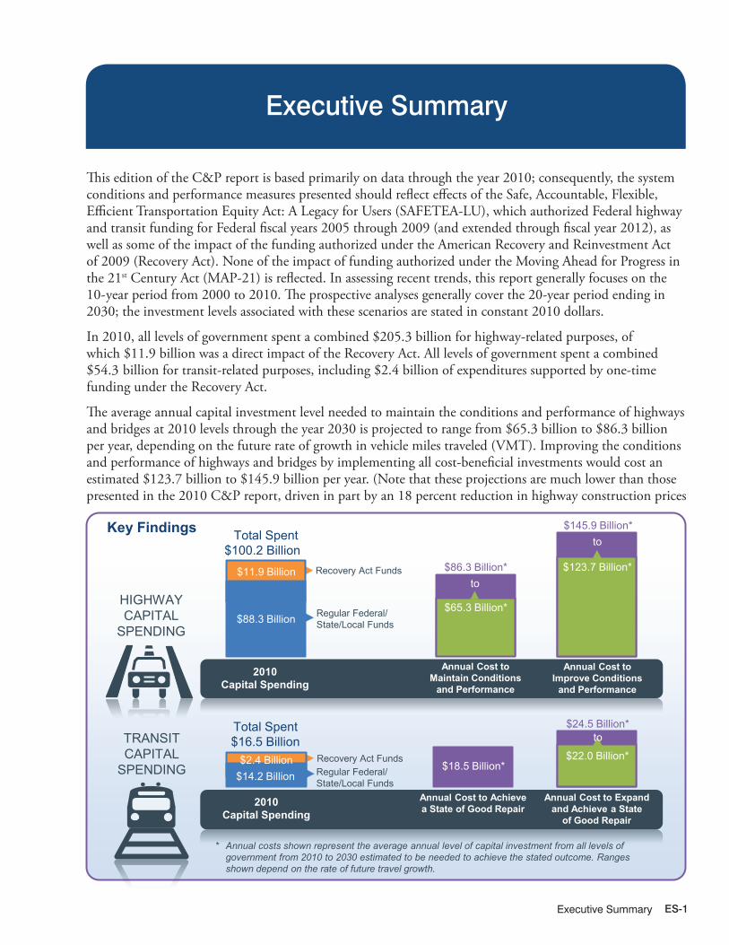
Executive Summary ES-1

Executive Summary

This edition of the C&P report is based primarily on data through the year 2010; consequently, the system conditions and performance measures presented should reflect effects of the Safe, Accountable, Flexible, Efficient Transportation Equity Act: A Legacy for Users (SAFETEA-LU), which authorized Federal highway and transit funding for Federal fiscal years 2005 through 2009 (and extended through fiscal year 2012), as well as some of the impact of the funding authorized under the American Recovery and Reinvestment Act of 2009 (Recovery Act). None of the impact of funding authorized under the Moving Ahead for Progress in the 21st Century Act (MAP-21) is reflected. In assessing recent trends, this report generally focuses on the 10- year period from 2000 to 2010. The prospective analyses generally cover the 20-year period ending in 2030; the investment levels associated with these scenarios are stated in constant 2010 dollars.

In 2010, all levels of government spent a combined $205.3 billion for highway-related purposes, of which $11.9 billion was a direct impact of the Recovery Act. All levels of government spent a combined $54.3 billion for transit-related purposes, including $2.4 billion of expenditures supported by one-time funding under the Recovery Act.

The average annual capital investment level needed to maintain the conditions and performance of highways and bridges at 2010 levels through the year 2030 is projected to range from $65.3 billion to $86.3 billion per year, depending on the future rate of growth in vehicle miles traveled (VMT). Improving the conditions and performance of highways and bridges by implementing all cost-beneficial investments would cost an estimated $123.7 billion to $145.9 billion per year. (Note that these projections are much lower than those presented in the 2010 C&P report, driven in part by an 18 percent reduction in highway construction prices

Annual Cost to Improve Conditions

and Performance

Annual Cost to Maintain Conditions

and Performance

2010 Capital Spending

HIGHWAY CAPITAL

SPENDING

Recovery Act Funds

123.7

Total Spent

$100.2 Billion3 $11.9 Billion

$145.9 Billion

$123.7

123.7

$65.3

Key Findings

TRANSIT CAPITAL

SPENDING

$65.3 Billion*

$86.3 Billion* $123.7 Billion*

$145.9 Billion*

to

to

Regular Federal/ State/Local Funds $88.3 Billion

Annual Cost to Expand and Achieve a State

of Good Repair

Annual Cost to Achieve a State of Good Repair 2010

Capital Spending

Recovery Act Funds

123.7 $18.5 Billion*

Total Spent $16.5 Billion

$11.9 Billion $14.2 Billion $2.4 Billion

123.7

$24.5 Billion*

Depending on Future Rate of Growth in VMT

to

$22.0 Billion*

* Annual costs shown represent the average annual level of capital investment from all levels of government from 2010 to 2030 estimated to be needed to achieve the stated outcome. Ranges shown depend on the rate of future travel growth.

Regular Federal/ State/Local Funds

Executive SummaryES-2

between 2008 and 2010). In 2010, all levels of government spent a combined $100.2 billion for capital improvements to highways and bridges.

Bringing existing transit assets up to a state of good repair would require an annualized investment level of $18.5 billion through the year 2030. The estimated combined costs associated with accommodating future increases in transit ridership and addressing system preservation needs when it is cost-beneficial to do so, would range from $22.0 billion to $24.5 billion per year. In 2010, all levels of government spent a combined $16.5 billion for transit capital improvements.

Highlights: Highways and Bridges

Extent of the System � The Nation’s road network includes more than

4,083,768 miles of public roadways and more than 604,493 bridges. In 2010, this network carried almost 2.985 trillion vehicle miles traveled (VMT).

� The 1,007,777 miles of Federal-aid highways (25 percent of total mileage) carried 2.525 trillion VMT (85 percent of total travel) in 2010.

� While the 162,698 miles on the National Highway System (NHS) make up only 4 percent of total mileage, the NHS carried 1.305 trillion VMT in 2010, just under 44 percent of total travel.

� The 47,182 miles on the Interstate System carried 0.731 trillion VMT in 2010, constituting a bit over 1 percent of mileage and just over 24 percent of total VMT.

Spending on the System � All levels of government spent a combined $205.3 billion for highway-related purposes in 2010.

About half of total highway spending ($100.2 billion) was for capital improvements to highways and bridges; the remainder included expenditures for physical maintenance, highway and traffic services, administration, highway safety, and debt service.

� In nominal dollar terms, highway spending increased by 67.3 percent between 2000 and 2010; adjusting for inflation this equates to a 35.9 percent increase. Highway capital expenditures increased by 63.4 percent between 2000 and 2010, equaling a 36.6 percent increase when adjusted for inflation.

� The portion of total highway capital spending funded by the Federal government increased from 42.6 percent in 2000 to 44.3 percent in 2010. The average annual increase in Federally funded highway capital outlay grew by 5.4 percent per year over this period, compared to a 4.7 annual increase in capital spending funded by State and local governments.

Constant Dollar Conversions for Highway Expenditures

This report uses the Federal Highway Administration’s (FHWA’s) National Highway Construction Cost Index (NHCCI) and its predecessor, the Composite Bid Price Index (BPI), for inflation adjustments to highway capital expenditures and the Consumer Price Index (CPI) for adjustments to other types of highway expenditures.

Highway System Terminology“Federal-aid Highways” are roads that are generally eligible for Federal funding assistance under current law. (Note that certain Federal programs do allow the use of Federal funds on other roadways.)

The “National Highway System” (NHS) includes those roads that are most important to interstate travel, economic expansion, and national defense. It includes the entire Interstate System. MAP-21 directed that the NHS system be expanded. The statistics presented for 2010 reflect the NHS as it existed then. The 20-year scenarios have been adjusted to approximate the NHS after expansion.

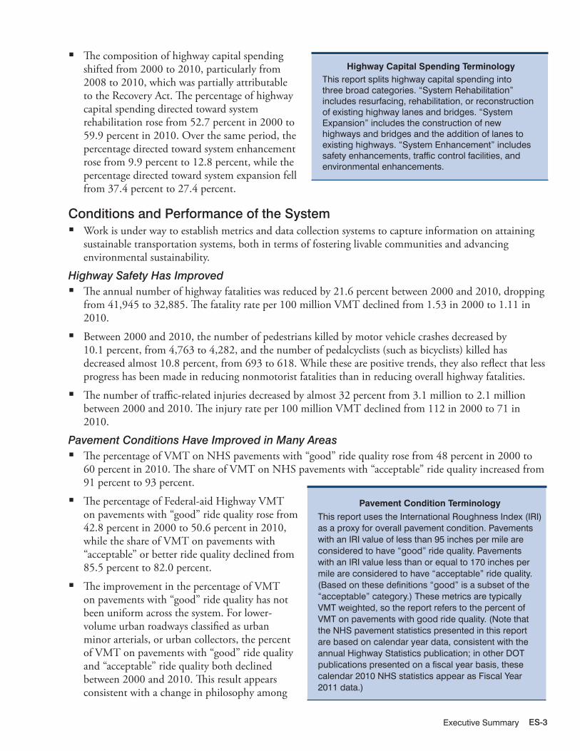
Executive Summary ES-3

Highway Capital Spending TerminologyThis report splits highway capital spending into three broad categories. “System Rehabilitation” includes resurfacing, rehabilitation, or reconstruction of existing highway lanes and bridges. “System Expansion” includes the construction of new highways and bridges and the addition of lanes to existing highways. “System Enhancement” includes safety enhancements, traffic control facilities, and environmental enhancements.

� The composition of highway capital spending shifted from 2000 to 2010, particularly from 2008 to 2010, which was partially attributable to the Recovery Act. The percentage of highway capital spending directed toward system rehabilitation rose from 52.7 percent in 2000 to 59.9 percent in 2010. Over the same period, the percentage directed toward system enhancement rose from 9.9 percent to 12.8 percent, while the percentage directed toward system expansion fell from 37.4 percent to 27.4 percent.

Conditions and Performance of the System � Work is under way to establish metrics and data collection systems to capture information on attaining

sustainable transportation systems, both in terms of fostering livable communities and advancing environmental sustainability.

Highway Safety Has Improved � The annual number of highway fatalities was reduced by 21.6 percent between 2000 and 2010, dropping

from 41,945 to 32,885. The fatality rate per 100 million VMT declined from 1.53 in 2000 to 1.11 in 2010.

� Between 2000 and 2010, the number of pedestrians killed by motor vehicle crashes decreased by 10.1 percent, from 4,763 to 4,282, and the number of pedalcyclists (such as bicyclists) killed has decreased almost 10.8 percent, from 693 to 618. While these are positive trends, they also reflect that less progress has been made in reducing nonmotorist fatalities than in reducing overall highway fatalities.

� The number of traffic-related injuries decreased by almost 32 percent from 3.1 million to 2.1 million between 2000 and 2010. The injury rate per 100 million VMT declined from 112 in 2000 to 71 in 2010.

Pavement Conditions Have Improved in Many Areas � The percentage of VMT on NHS pavements with “good” ride quality rose from 48 percent in 2000 to

60 percent in 2010. The share of VMT on NHS pavements with “acceptable” ride quality increased from 91 percent to 93 percent.

� The percentage of Federal-aid Highway VMT on pavements with “good” ride quality rose from 42.8 percent in 2000 to 50.6 percent in 2010, while the share of VMT on pavements with “acceptable” or better ride quality declined from 85.5 percent to 82.0 percent.

� The improvement in the percentage of VMT on pavements with “good” ride quality has not been uniform across the system. For lower-volume urban roadways classified as urban minor arterials, or urban collectors, the percent of VMT on pavements with “good” ride quality and “acceptable” ride quality both declined between 2000 and 2010. This result appears consistent with a change in philosophy among

Pavement Condition TerminologyThis report uses the International Roughness Index (IRI) as a proxy for overall pavement condition. Pavements with an IRI value of less than 95 inches per mile are considered to have “good” ride quality. Pavements with an IRI value less than or equal to 170 inches per mile are considered to have “acceptable” ride quality. (Based on these definitions “good” is a subset of the “acceptable” category.) These metrics are typically VMT weighted, so the report refers to the percent of VMT on pavements with good ride quality. (Note that the NHS pavement statistics presented in this report are based on calendar year data, consistent with the annual Highway Statistics publication; in other DOT publications presented on a fiscal year basis, these calendar 2010 NHS statistics appear as Fiscal Year 2011 data.)

Executive SummaryES-4

many transportation agencies leading them to move away from a simple strategy of addressing assets on a “worst first” basis toward more comprehensive strategies aimed at targeting investment where it will benefit the most users.

Bridge Conditions Have Improved � Based directly on bridge counts, the share of

NHS bridges classified as structurally deficient declined from 6.0 percent in 2000 to 5.1 percent in 2010. Over this period, the share classified as functionally obsolete declined from 17.7 percent to 16.3 percent, so the total share classified as deficient declined from 23.7 percent to 21.4 percent.

� Weighted by deck area, the share of NHS bridges classified as structurally deficient declined from 8.7 percent in 2000 to 8.3 percent in 2010. Over this period, the share classified as functionally obsolete declined from 22.0 percent to 20.3 percent, so the total share classified as deficient declined from 30.7 percent to 28.7 percent.

� Systemwide, based on bridge counts, the share of bridges classified as structurally deficient declined from 15.2 percent to 11.7 percent from 2000 to 2010, the functionally obsolete share declined from 15.5 percent to 14.2 percent, and the total percentage of deficient bridges declined from 30.7 percent to 25.9 percent.

� The reductions in bridge deficiencies have not been uniform across the system. The share of rural interstate bridges classified as structurally deficient rose from 4.0 percent in 2000 to 4.5 percent in 2010; over the same period, the share of urban collector bridges classified as functionally obsolete was not reduced below the 2000 level of 28.1 percent.

Future Capital Investment Scenarios – SystemwideThe scenarios that follow pertain to spending by all levels of government combined for the 20-year period from 2010 to 2030 (reflecting the impacts of spending from 2011 through 2030); the funding levels associated with all of these analyses are stated in constant 2010 dollars. Rather than assuming an immediate jump to a higher (or lower) investment level, each of these analyses assume that spending will grow by a uniform annual rate of increase (or decrease) in constant dollar terms using combined highway capital spending by all levels of government in 2010 as the starting point. As noted in the Introduction, caution should be taken in evaluating the scenario findings, given the impact of the Recovery Act funding on 2010 spending.

Bridge Condition TerminologyBridges are considered “structurally deficient” if significant load-carrying elements are found to be in poor or worse condition due to deterioration and/or damage, or the adequacy of the waterway opening provided by the bridge is determined to be extremely insufficient to the point of causing intolerable traffic interruptions due to high water. That a bridge is deficient does not imply that it is likely to collapse or that it is unsafe.

Functional obsolescence is a function of the geometrics (i.e., lane width, number of lanes on the bridge, shoulder width, presence of guardrails on the approaches, etc.) of the bridge in relation to the geometrics required by current design standards. As an example, a bridge designed in the 1930s would have shoulder widths in conformance with the design standards of the 1930s, but could be deficient relative to current design standards, which are based on different criteria and require wider bridge shoulders to meet current safety standards. The magnitude of these types of deficiencies determines whether a bridge is classified as “functionally obsolete.”

These classifications are often weighted by bridge deck area, in recognition of the fact that bridges are not all the same size and, in general, larger bridges are more costly to rehabilitate or replace to address deficiencies. They are also sometimes weighted by annual daily traffic (ADT).

Executive Summary ES-5

Sustain 2010 Spending Scenario � The Sustain 2010 Spending scenario assumes

that capital spending by all levels of government is sustained in constant dollar terms at the 2010 level ($100.2 billion systemwide) through 2030.

� At this level of spending, the average sufficiency rating for the Nation’s bridges is projected to improve from 81.7 to 84.1 (on a scale of 0 to 100).

� Assuming a higher forecast-based future VMT growth (of 1.85 percent per year), average pavement ride quality on Federal-aid highways is projected to improve by 11.5 percent while average delay per VMT on Federal-aid highways worsens by 1.9 percent. Assuming lower trend-based VMT growth (of 1.36 percent per year), average pavement ride quality is projected to improve by 17.7 percent, while average delay improves by 7.8 percent.

� Note that 2010 capital spending was supplemented by one-time funding under the Recovery Act, which would make it more challenging to sustain this level of spending in the future.

Maintain Conditions and Performance Scenario � The Maintain Conditions and Performance scenario assumes that capital investment gradually changes

in constant dollar terms over 20 years to the point at which selected measures of future conditions and performance in 2030 are maintained at 2010 levels.

� The average annual level of investment associated with this scenario is $86.3 billion systemwide assuming higher future VMT growth and $65.3 billion systemwide assuming lower future VMT growth.

� The annual investment levels for both versions of this systemwide scenario fall below the base year (2010) spending level. In previous editions of this report, the estimated costs of this scenario have typically been higher than base year spending, under most or all alternative versions of the scenario presented.

Improve Conditions and Performance Scenario � The Improve Conditions and Performance scenario assumes that capital investment gradually rises to

the point at which all potential highway and bridge investments that are estimated to be cost-beneficial (i.e., those with a benefit-cost ratio of 1.0 or higher) could be funded by 2030.

� Assuming higher future VMT growth, the average annual level of systemwide investment associated with this scenario is $145.9 billion. This is 45.7 percent higher than actual 2010 spending; a gap that could be closed if spending rose by 3.46 percent per year faster than the rate of future inflation.

� Assuming lower future VMT growth brings the annual cost of this systemwide scenario down to $123.7 billion, 23.4 percent higher than 2010 spending; a 1.96 percent annual increase in constant dollar spending would be sufficient to close this gap.

� The State of Good Repair benchmark represents the subset of this scenario that is directed toward addressing deficiencies of existing highway and bridge assets. The average annual investment level associated with this benchmark is $78.3 billion, assuming higher future VMT growth, and $72.9 billion, assuming lower future VMT growth.

Highway Investment/Performance AnalysesIn order to provide an estimate of the costs that might be required to maintain or improve system performance, this report includes a series of investment/performance analyses that examine the potential impacts of alternative levels of future combined investment levels by all levels of government on highways and bridges for different subsets of the overall system.

Drawing upon these investment/performance analyses, a series of illustrative scenarios were selected for further exploration and presentation in more detail. The scenario criteria were applied separately to the Interstate System, the NHS, all Federal-aid highways, and the overall road system.

Recognizing that one of the major factors influencing future highway investment needs will be future travel demand, two sets of illustrative scenarios are presented for Federal-aid Highways and the overall system. One set incorporates travel forecasts provided by the States for individual highway sections (averaging to 1.85 percent growth per year), while the other assumes lower travel growth based on a continuation of national trends over the last 15 years (1.36 percent growth per year).

Executive SummaryES-6

Intermediate Improvement Scenario � The highway component of the Intermediate Improvement scenario assumes that combined spending

gradually rises to a point at which potential highway investments with a benefit-cost ratio of 1.5 or higher can be implemented; the bridge component represents the cost of achieving half of the gains in bridge sufficiency computed under the Improve Conditions and Performance scenario.

� The average annual level of systemwide investment associated with this scenario is $111.9 billion (11.7 percent higher than 2010 spending, which was 10.8 percent higher than 2008 spending due to the Recovery Act), assuming higher future VMT growth, and $93.9 billion (6.3 percent lower than 2010 spending), assuming lower future VMT growth.

Highlights: TransitExtent of the System � Of the transit agencies that submitted data to the National Transit Database (NTD) in 2010, 728

provided service to urbanized areas and 1,582 provided service to rural areas. Urban agencies operated 612 bus systems, 587 demand response systems, 18 heavy rail systems, 30 commuter rail systems, and 33 light rail systems. There were also 70 transit vanpool systems, 20 ferryboat systems, 5 trolleybus systems, 3 automated guideway systems, 3 inclined plane systems, and 1 cable car system.

� Bus and heavy rail modes continue to be the largest segments of the industry, providing 35.6 percent and 51.6 percent of all transit trips, respectively. Commuter rail supports a relatively high share of passenger miles (20.0 percent). Light rail is the fastest-growing rail mode (with passenger miles growing at 5.0 percent per year between 2000 and 2010) but it still provides only 4.1 percent of transit passenger miles. Vanpool growth during that period was 10.3 percent per year, with vanpools accounting for only 2.1 percent of all transit passenger miles.

� Urban transit operators reported 9.9 billion unlinked passenger trips on 3.9 billion vehicle revenue miles. Rural transit operators reported 123 million unlinked passenger trips on 570 million vehicle revenue miles.

Bus, Rail, and Demand Response: Transit ModesPublic transportation is provided by several different types of vehicles that are used in different operational modes. The most common is fixed-route bus service, which uses different sizes of rubber-tired buses that run on scheduled routes. Commuter bus service is similar but uses over-the-road buses and runs longer distances between stops. Bus rapid transit is high-frequency bus service that emulates light rail service. Publicos and jitneys are small owner-operated buses or vans that operate on less-formal schedules along regular routes.

Larger urban areas are often served by one or more varieties of fixed-guideway (rail) service. These include heavy rail (often running in subway tunnels) which is primarily characterized by third-rail electric power and exclusive dedicated guideway. Extended urban areas may have commuter rail, which often shares track with freight trains and usually uses overhead electric power (but may also use diesel power). Light rail systems are common in large- and medium-sized urban areas; they feature overhead electric power and run on track that is entirely or in part on city streets that are shared with pedestrian and automobile traffic. Streetcars are small light rail systems, usually with only one or two cars per train. Cable cars, trolley buses, monorail, and automated guideway systems are less-common rail variants.

Demand response transit service is usually provided by vans, taxicabs, or small buses that are dispatched to pick up passengers upon request. This mode is mostly used to provide paratransit service as required by the Americans with Disabilities Act. They do not follow a fixed schedule or route.

Spending on the System � All levels of government spent a combined $54.3 billion to provide public transportation and maintain

transit infrastructure. Of this, 26.1 percent was system-generated revenue, of which most came from

Executive Summary ES-7

passenger fares. 19 percent of revenues came from the Federal government while the remaining funds came from State and local sources.

� Public transit agencies spent $16.6 billion on capital investments in 2010. Annually authorized Federal funding made up 26.6 percent of these capital expenditures. One-time funds from the Federal American Recovery and Reinvestment Act provided another 14.5 percent.

� Federal funding is primarily targeted for capital assistance; however, Federal funding for operating expenses at public transportation agencies has increased from 19 percent of all Federal funding in 2000 to 35 percent in 2010. Virtually all of the increase is due to the 2004 change making “preventative maintenance” eligible for reimbursement from 5307 grant funds. Maintenance is an operating expense. Meanwhile, farebox recovery ratios, representing the share of operating expenses that come from passenger fares, have remained close to the 2000 value of 35.5 percent throughout this period.

� Recent investments in system expansion have been adequate to keep pace with ridership growth (the average number of passengers per vehicle has not increased). Furthermore, continuing these investment levels will support projected growth in demand that falls between the low- and high-growth projections in this report. Investments in system preservation, however, still fall short of current and projected needs.

Conditions and Performance of the SystemTransit Remains Safe � There has been no significant increase in the

rate of transit fatalities since 2004. Excluding suicides, that fatality rate hovers around one fatality for each 250 million passenger miles traveled (0.4 per 100 million).

� In 2010, one in four transit-related fatalities was classified as a suicide. In 2002, the rate was just one in 13. The rate of suicides on transit facilities has gone up every year since 2005.

Some Aspects of System Performance Have Improved � Between 2000 and 2010, transit agencies have

provided substantially more service. The annual rate of growth in route miles ranged from 0.4 percent for heavy rail to 6.0 percent for light rail. This has resulted in 21 percent more route miles available to the public.

� Between 2000 and 2010, the number of annual service miles per vehicle (vehicle productivity) increased steadily and the average number of miles between breakdowns (mean distance between failures) decreased by 14 percent. Thus, transit operators are getting more use out of their vehicles.

Federal Transit Funding Urban and RuralFederal Transit Administration (FTA) Urbanized Area Formula Funds are apportioned to urbanized areas (UZAs), as defined by the Census Bureau. UZAs in this report were defined by the 2000 census. Data from the 2010 census will be used in the 2013 apportionment and beyond. Each UZA has a designated recipient, usually a Metropolitan Planning Organization (MPO) or large transit agency, which then sub-allocates FTA funds in its area according to local policy. In small urban and rural areas, FTA apportions funds to the State, which allocates them according to State policy. Indian tribes receive their funds directly. All funds then become available, on a reimbursement basis, through application to the FTA.

Unlinked Passenger Trips, Passenger Miles, Route Miles, and Revenue Miles

Unlinked passenger trips (UPT), also called boardings, count every time a person gets on an in-service transit vehicle. Each transfer to a new vehicle or route is considered another unlinked trip, so a person’s commute to work may count as more than one trip if that person transferred between routes.

Passenger miles traveled (PMT) simply count how many miles a person travels. UPT and PMT are both commonly used measures of transit service consumed.

Directional route miles (DRM) measure the number of miles of transit route available to customers. They are directional because each direction counts separately; thus, a one-mile-out and one-mile-back bus route would be two DRM. Vehicle Revenue Miles (VRM) count the miles of revenue service, and are typically much greater than the DRM because many trips are taken over each route (and each DRM). These are commonly used measures of transit service provided.

Executive SummaryES-8

� Growth in service offered was nearly in accordance with growth in service consumed. In spite of steady growth in route miles and revenue miles, average vehicle occupancy levels did not decrease. Passenger miles traveled grew at a 1.6-percent annual pace while the number of trips grew at a 1.3-percent annual pace. This is significantly faster than the growth in the U.S. population during this period (0.93 percent), suggesting that transit has been able to attract riders who previously used other modes of travel. Increased availability of transit service has undoubtedly been a factor in this success.

Future Capital Investment Scenarios – SystemwideAs in the highway discussion, the transit investment scenarios that follow pertain to spending by all levels of government combined for the 20-year period from 2010 to 2030 (reflecting the impacts of spending from 2011 through 2030); the funding levels associated with all of these analyses are stated in constant 2010 dollars. Unlike the highway scenarios, these transit scenarios assume an immediate jump to a higher (or lower) investment level that is maintained in constant dollar terms throughout the analysis period.Included in this section for comparison purposes is an assessment of the investment level needed to replace all assets that are currently past their useful life or that will be over the forecast period. This would be necessary to achieve and maintain a state of good repair (SGR) but would not address any increases in demand during that period. Although not a realistic scenario, this does provide a benchmark for infrastructure preservation.Sustain 2010 Spending Scenario � The Sustain 2010 Spending scenario assumes that capital spending by all levels of government is

sustained in constant dollar terms at the 2010 level ($16.5 billion systemwide), including Recovery Act funds, through 2030. Assuming that the current split between expansion and preservation investments is maintained, this will allow for enough expansion to meet medium growth expectations but will fall far short of meeting system preservation needs. By 2030, this will result in roughly $142 billion in deferred system preservation projects.

Low-Growth Scenario � The Low-growth scenario assumes that transit ridership will grow at an annual rate of 1.4 percent

between 2010 to 2030, as projected by the Nation’s metropolitan planning organizations. During that period, it also attempts to pay down the current $85.9 billion system preservation backlog (subject to a cost-benefit constraint). The annualized cost of this scenario is $22.0 billion. In 2010, all levels of government spent a combined $16.5 billion for transit capital improvements.

High-Growth Scenario � The High-growth scenario assumes that transit ridership will grow at an annual rate of 2.2 percent

between 2010 and 2030, the average annual rate of growth experienced between 1995 and 2010. It also attempts to pay down the current $85.9-billion system preservation backlog (subject to the same cost-benefit constraint). The annualized cost of this scenario is $24.5 billion.

State of Good Repair – Expansion vs. PreservationState of Good Repair (SGR) is defined in this report as all transit capital assets being within their average service life. This is a general construct that allows FTA to estimate system preservation needs. The analysis looks at the age of all transit assets and adds the value of those that are past the age at which that type of asset is usually replaced to a total reinvestment needs estimate. Some assets may continue to provide reliable service well past the average replacement age and others will not; over the large number of assets nationally, the differences average out. Some assets will need to be replaced, some will just get refurbished. Both types of cost are included in the reinvestment total. SGR is a measure of system preservation needs, and failure to meet these needs results in increased operating costs and poor service.

Expansion needs are treated separately in this analysis. They result from the need to add vehicles and route miles to accommodate more riders. Estimates of future demand are, by their nature, speculative. Failure to meet this type of need results in crowded vehicles and represents a lost opportunity to provide the benefits of transit to a wider customer base.

CHAPTER OVERVIEWS

Description of Current System CO-1

PART IDescription of Current System

Part I of this report summarizes the current state of highways, bridges and transit systems, based primarily on data through the year 2010 unless otherwise noted. Chapter 1 discusses trends in personal travel, drawing upon the 2009 National Household Travel Survey, and presents data and issues relating to highway freight movement. Chapter 2 describes the characteristics of the highway, bridge, and transit systems, and Chapter 6 provides data on the revenue collected and expended for highways and transit.

U.S. Department of Transportation (DOT) Strategic Plan, FY 2012–16The latest U.S. DOT Strategic Plan presents five strategic goals for America’s transportation system:

�� Safety – Improve public health and safety by reducing transportation-related fatalities and injuries.

�� State of Good Repair – Ensure that the United States proactively maintains its critical transportation infrastructure in a state of good repair.

�� Economic Competitiveness – Promote transportation policies and investments that bring lasting and equitable economic benefits to the Nation and its citizens.

�� Livable Communities – Foster livable communities through place-based policies and investments that increase the transportation choices and access to transportation services.

�� Environmental Sustainability – Advance environmentally sustainable policies and investments that reduce carbon and other harmful emissions from transportation sources.

Chapter 3 addresses issues relating to the State of Good Repair goal, presenting data on the physical conditions of highways, bridges, transit systems, and transit vehicles. Chapter 4 addresses issues pertaining to the Safety goal. Chapter 5 covers topics relating to the goals for Livable Communities, Environmental Sustainability, and Economic Competitiveness.

Performance ManagementTransportation Performance Management is a strategic approach that uses system information to make investment and policy decisions to achieve national performance goals. A typical performance management process would include the following elements: (1) establish a set of goals/objectives; (2) define measures that support achievement of the goal or objective; (3) establish specific future targets for the measures; (4) develop specific plans, budgets, and programs to achieve the target outcome; and (5) after the programs are implemented, assess their results against the desired target. Any discrepancy between the planned and actual outcomes can be addressed by altering strategies. Performance management is a continual improvement process.

In July 2012, the Moving Ahead for Progress into the 21st Century Act (MAP-21) introduced specific requirements for performance management for highway and transit investments, establishing national goals for safety, infrastructure condition, congestion reduction, system reliability, freight movement and economic activity, environmental sustainability, and reduced project delivery time.

Federal Agencies are required to define the measures and standards for achieving the goals identified, unless defined in MAP-21. The States are to determine their own targets, while minimum standards may be established by Federal agencies where appropriate. States are to report progress toward the targets established. Failure to meet targets or develop plans has specific penalties for States: reduction in funding or requirements to spend more on the specific goal area. States are to report progress toward the targets within 4 years of enactment of MAP-21, and biennially thereafter.

Transit agencies that receive FTA grant funds are similarly required to maintain asset management plans, to set goals for achieving a state of good repair, and to report asset inventory condition data to FTA along with metrics demonstrating their progress toward meeting their goals.

CHAPTER OVERVIEWS

Description of Current SystemCO-2

Household Travel

CHAPTER 1

To fully understand daily travel, one must look at it through the lens of the 300 million Americans who use the transportation system to connect to jobs, stores, schools, friends, relatives, healthcare, recreational places, and more. The National Household Travel Survey (NHTS) is the only national source of travel data that connects daily travel behavior with the characteristics of the household and the individual making the trip.

The NHTS data reflect daily travel behavior of the American public, and do not include freight movement or commercial driving. Americans drove 30 billion fewer vehicle miles in 2008-2009 than in the 2001-2002 NHTS survey period despite a nearly 10 percent population increase over that time. There are many factors that could be causing this decline, including: the recession, high gas prices during the summer of 2008, changing demographics (e.g., the aging of the population and smaller household sizes) changing lifestyles of Americans (e.g., the increases in telecommuting and cyber shopping or different travel preferences), an increase in the availability of quality transit service and other alternatives

By 2050, about one in four members of the U.S. population will be over the age of 65. Maintaining the mobility of this group is a major quality of life issue. This group is increasing in average age over time, which may explain the recent decreases in their per capita trips and miles traveled.

Like the population as a whole, the household vehicle fleet is also aging, with the average age of household vehicles now reaching an all-time high of 9.4 years. Because more than half of the household vehicles are now older than 9 years, recent automotive advances in energy efficiency, air quality, and safety are not fully represented in the vehicles on the road.

12/18/2012 ESX01H_A R1

6,397 7,005

10,579 9,989

11,567 9,754

6,701 6,256

0

10,000

20,000

30,000

40,000

2001 2009

Ave

rage

Ann

ual P

erso

n M

iles

Year

To/From Work

Shopping/Errands

Social/Recreation

Other

Average Annual Person Miles per Household by Trip Purpose

to driving, or roadway congestion. The NHTS results also show that transit ridership increased by 16 percent between the two survey periods; most of the increase was in the shopping and social/recreational activities categories. For all modes of travel combined, average daily person miles of travel per household dropped from 96.6 to 90.4.

10/23/2012 ESX01H_B R1.xlsx

Model Years Percent of Total<1 Year 5.7%2-5 Years 28.6%6-10 Years 32.2%11-20 Years 26.9%>20 Years 6.7%

Age of Household Vehicles

Much attention has been given to changes in the travel behavior of the Millennial generation, generally defined as those born between 1982 and 2000. The NHTS results indicate that youth travel is declining as they are driving less, traveling less, and taking shorter trips compared with previous generations. Recent research has identified several contributing factors to this trend, including: �� Technology influences travel and how youth get

their information. �� Youth concerns for the environment play a role in

their travel decisions.�� More youth prefer to live in high-density areas

where there are more modal options and shorter trip lengths.

�� High unemployment and personal income constraints limit resources for travel and cause youth to live with parents longer.

�� Increases in driver’s licensing restrictions have resulted in more youth waiting longer to get their license.

CHAPTER OVERVIEWS

Description of Current System CO-3

Freight MovementCHAPTER 1

The freight transportation system plays a major role in promoting and sustaining the economic vitality of the United States. Various businesses, ranging from companies that mine raw materials that are used to manufacture goods to retail companies selling household goods or office products, rely on the U.S. freight transportation system to have their products picked-up and/or delivered.

Though the system includes a variety of transportation modes (highway, railroad, waterway, aviation, and pipeline), some of which are publicly owned and others of which are privately owned, most of the system has a high degree of connectivity. This allows freight carriers to operate more efficiently and shippers to use the most economically effective mode or modes for shipping their goods.

The well-developed transportation system currently handles over 50 million tons of freight each day, with over two-thirds of that amount being carried by trucks. This high volume of freight movement, which has grown steadily over the last few decades due to the ease of transport in the United States and an increase in interregional domestic and international trade, is putting increasing stress on the transportation system. Freight volumes are expected to continue to increase across all modes in the coming years, challenging the transportation system even more.

Based on projections from the FHWA Freight Analysis Framework, combined tonnage for all freight modes is projected to increase by 1.4 percent per year over the next 30 years to 27.4 billion in 2040. The weight of shipments carried by trucks is projected to increase by 1.3 percent per year during this period, rising from 12.5 billion tons to 18.5 billion tons.

Though trucking typically is considered a faster mode and handles a large volume (87 percent) of high-value, time-sensitive goods, it also hands a surprising share (71 percent) of lower-value bulk tonnage. This share includes movement of

agricultural products from farms, local distribution of gasoline, and pickup of municipal solid waste.

The growth in freight shipments will make it more difficult for freight carriers to continue to operate efficiently, particularly if capacity expansions and/or operational improvements are not implemented on major freight corridors and at major freight nodes. In turn, decreased operational efficiency would increase transportation costs, negatively impacting carriers, shippers, and ultimately consumers.

The increased focus on freight transportation needs in the Moving Ahead for Progress in the 21st Century (MAP-21) surface transportation reauthorization legislation should help address the growing freight needs in the United States. By designating a national freight network, requiring the formulation of a national freight strategic plan, and refining transportation investment and planning tools to evaluate freight projects, among other requirements, freight transportation needs should become more easily identifiable, and transportation funding decisions should become more strategic in nature. These legislative changes will likely help enhance the U.S. freight transportation system in the long term.

12/15/2013 ESX01F_A R2.xlsx

Mode 20102040

Projected

Average Annual Growth,

2010–2040Truck 12,490 18,503 1.3%Rail 1,776 2,353 0.9%Water 860 1,263 1.3%Air, Air & Truck* 12 43 4.4%Multiple Modes & Mail 1,380 2,991 2.6%

Pipeline 1,494 1,818 0.7%Other & Unknown 302 514 1.8%Total 18,313 27,484 1.4%

*Includes air cargo movements that are shipped via truck at the ends of the trips.

Weight of Shipments by Transportation Mode (Millions of Tons)

CHAPTER OVERVIEWS

Description of Current SystemCO-4

System Characteristics: Highways and Bridges

CHAPTER 2

Spanning more than 4.08 million miles and including 604,493 bridges, the Nation’s public road network facilitated slightly less than three trillion VMT in 2010. Local governments owned 77.5 percent of the Nation’s public road mileage and 50.2 percent of the Nation’s bridges in 2010; States owned 19.1 percent of mileage and 48.2 percent of bridges; the Federal government owned 3.4 percent of mileage and 1.3 percent of bridges.

Rural mileage (in areas with population less than 5,000) decreased an at an average annual rate of 0.4 percent between 2000 and 2010, in part due to the expansion of urban area boundaries following the 2000 Census. Urban mileage increased at a rate of 2.5 percent annually during this period.

Roads are functionally classified based on the purpose they serve in terms of providing mobility and access. Almost half of the Nation’s road mileage is classified as rural local, but these roads carry only 4.5 percent of VMT.

11/19/2012 ESX02H_A R2.xlsx

Federal 3.4%

State 19.1%

Local 77.5%

Highway Miles

Federal 1.3%

State 48.2%

Local 50.2%

Other 0.3%

Bridges

2010 Mileage and Bridges by Owner

As of 2010, the National Highway System (NHS) included 162,876 miles of the Nation’s key corridors (4.0 percent of total mileage) which carried 43.0 percent of VMT. The revised NHS criteria in MAP-21 will add to the NHS most of the principal arterial mileage that is not currently part of the system. If all principal arterial mileage were added, this would cover 5.5 percent of the Nation’s route miles and 55.2 percent of VMT. (This estimate of the extent of the enhanced NHS is used in Chapters 7 and 8 in developing 20-year NHS investment/performance projections.)

MAP-21 requires the creation and definition of a new National Freight Network, which is intended to include the most important urban, rural, and intercity routes for commercial truck movements. This network will include a Primary Freight Network of up to 27,000 miles to be designated by the U.S. DOT, other Interstate highways not included in the Primary Freight Network, and Critical Rural Freight Corridors to be designated by the States.

11/26/2012 ESX02H_B R2.xlsx

Functional System Miles VMT BridgesRural Areas

Interstate 0.7% 8.2% 4.2%Other Freeway and Expressway 0.1% 0.6%

Other Principal Arterial 2.2% 6.8% 6.0%Minor Arterial 3.3% 5.1% 6.5%Major Collector 10.2% 6.0% 15.4%Minor Collector 6.4% 1.8% 7.9%Local 49.7% 4.5% 34.0%

Subtotal Rural 72.7% 32.9% 73.9%Urban Areas

Interstate 0.4% 16.0% 5.0%Other Freeway and Expressway 0.3% 6.7% 3.3%

Other Principal Arterial 1.6% 15.5% 4.5%Minor Arterial 2.6% 13.0% 4.6%Major Collector 2.8% 6.1% 3.4%Minor Collector 0.0% 0.1%Local 19.6% 9.7% 5.3%

Subtotal Urban 27.3% 67.1% 26.1%Total 100.0% 100.0% 100.0%

2010 Percentage of Highway Miles, Bridges, and Vehicle Miles Traveled by Functional System

Bridges on rural other freeway and expressway included under rural other principal arterial. Bridges on urban minor collector included under urban major collector.

The term “Federal-aid Highways” refers to the subset of the road network that is generally eligible for Federal funding assistance under most programs; this excludes roads functionally classified as rural minor collector, rural local or urban local. Federal-aid highways make up 24.7 percent of the nation’s mileage, but carry 84.6 percent of VMT.

CHAPTER OVERVIEWS

Description of Current System CO-5

System Characteristics: TransitCHAPTER 2

Between 2000 and 2010, transit system coverage, capacity, and use in the United States all experienced steady growth. In 2010, there were 728 agencies (709 public agencies) in urbanized areas required to submit data to the National Transit Database (NTD). All but 148 of these agencies operated more than one mode. There were also 1,582 rural transit operators that reported. Urban reporters operated 612 motor bus systems, 587 demand response systems, 18 heavy rail systems, 30 commuter rail systems, and 33 light rail systems. There were also 70 transit vanpool systems, 20 ferryboat systems, 5 trolleybus systems, 3 automated guideway systems, 3 inclined plane systems, and 1 cable car system.

U.S. transit systems operated 74,319 motor buses, 33,458 vans, 11,434 heavy rail vehicles, 7,072 commuter rail cars, and 2,118 light rail cars. Transit providers operated 12,438 miles of track and served 3,175 stations. Almost all transit providers are included in these counts, excepting those that do not receive FTA grant funds and choose not to report to NTD.

Motor bus and heavy rail modes continue to be the largest segments of the industry, providing 51.6 percent and 35.6 percent of all transit trips, respectively. Commuter rail, with 4.6 percent of trips, supports a relatively high share of passenger miles (20.0 percent) due to its greater average trip length (23.4 miles compared with 4.0 for bus, 4.6 for heavy rail, and 4.8 for light rail). Light rail

is the fastest-growing rail mode (with passenger miles traveled [PMT] growing at 5.0 percent per year between 2000 and 2010) but still provided only 4.1 percent of transit PMT in 2010. Vanpool growth during that period was 10.3 percent per year, substantially outpacing the 0.9-percent growth in motor bus passenger miles; however, while motor buses provided 39.1 percent of all PMT, vanpools accounted for only 2.1 percent.

Transit systems are concentrated in the 42 urbanized areas with populations of more than 1 million people. These areas contain about half of the U.S. population, but their higher population densities and long-term investments in transit infrastructure support 89 percent of all transit trips on 77 percent of the vehicle revenue miles.

Rural transit operators reported 123.2 million unlinked passenger trips on 570 million vehicle revenue miles. This included 61 Indian tribes that provided 1,008,701 unlinked passenger trips. Rural systems provide both traditional fixed-route and demand response services. In 2010, there were 1,180 demand response systems, including 30 systems added since 2008, and 530 motor bus systems, including 36 added since 2008. Sixteen rural systems reported vanpool operations.

Rural service is provided in every State, and 327 urbanized area agencies reported providing service to rural areas as well.

12/31/2012 ESX02T_B R1

7.50 7.56 7.98 8.12

8.52 8.72

9.01 9.02 8.88 8.94 9.18

9.38

9.95 10.26 10.13 9.96 10.09

7

8

9

10

11

1995 1996 1997 1998 1999 2000 2001 2002 2003 2004 2005 2006 2007 2008 2009 2010 2011

Bill

ions

of P

asse

nger

s

Year

Annual U.S. Unlinked Transit Passenger Trips, 1995–2011

CHAPTER OVERVIEWS

Description of Current SystemCO-6

System Conditions: HighwaysCHAPTER 3

Highway users are economically impacted by the conditions of the highways and bridges they utilize. Users are more likely to incur higher vehicle maintenance costs for travel on roads with poor pavement conditions, particularly on higher speed roads like Interstate highways. Poor pavement conditions may also increase travel time due to drivers slowing down and avoiding risks like potholes, which can also escalate the level of congestion on the Nation’s most traveled roadways.

Urban centers facilitate more than two-thirds of VMT on the Nation’s highway system. Pavement conditions in urban settings tend to deteriorate at a faster rate because of the higher usage. Replacing pavement in urban centers is also challenging because roadwork can exacerbate congestion.

The Highway Performance Monitoring System (HPMS) includes data on pavement ride quality on Federal-aid highways, which includes about one-quarter of the Nation’s mileage. Between 2000 and 2010, the percentage of rural VMT on pavements classified as having acceptable ride quality declined from 93.8 percent to 87.8 percent. However, the percent of rural VMT on pavements with good ride quality (a subset of the acceptable ride quality classification) increased from 55.2 percent to 64.6 percent. The share of urban VMT on pavements with good ride quality rose from 35.0 percent in 2000 to 44.0 percent in 2010, while the share on pavements with acceptable ride quality declined from 80.3 percent to 79.4 percent.

11/30/2012 ESX03H_A R1Ax

Ride Quality 2000 2008 2010Good (IRI < 95)Rural 55.2% 62.5% 64.6%Urban 35.0% 38.9% 44.0%Total 42.8% 46.4% 50.6%Acceptable (IRI ≤ 170)Rural 93.8% 94.8% 87.8%Urban 80.3% 81.0% 79.4%Total 85.5% 85.4% 82.0%

Calendar Year

Percent of Federal-aid Highway VMT on Pavements With Good and Acceptable Ride Quality

The share of National Highway System (NHS) VMT on pavements with good ride quality rose from 48 percent in 2000 to 60 percent in 2010.

Bridges are another vital component for the Nation’s highway system. Two terms used to summarize bridge deficiencies are “structurally deficient” and “functionally obsolete.” Structural deficiencies are characterized by deteriorated conditions of significant bridge elements and potentially reduced load-carrying capacity, but do not necessarily imply safety concerns. Functional obsolescence is characterized by bridges not meeting current design standards, such as lane width or number of lanes, relative to the traffic volume carried by the bridge.

The percentage of NHS bridges classified as deficient decreased from 23.7 percent in 2000 to 21.4 percent in 2010. Of the 116,669 bridges on the NHS in 2010, 5.1 percent of bridges were classified as structurally deficient while 16.3 percent of bridges were classified as functionally obsolete.

6.0% 5.9% 5.7% 5.5% 5.4% 5.1%

17.7% 17.2% 16.9% 16.8% 16.9% 16.3%

23.7% 23.1% 22.6% 22.3% 22.3% 21.4%

0%

5%

10%

15%

20%

25%

30%

2000 2002 2004 2006 2008 2010

Structurally DeficientFunctionally ObsoleteTotal Deficient

Percentage of NHS Bridges Classified as Deficient, 2000–2010

12/19/2013 ESX03H_B R3.xlsx

Almost 68.5 percent of the Nation’s 604,493 bridges were 26 years old or older as of 2010, up from 67.2 percent in 2000. The share of total bridges classified as structurally deficient as of 2010 was 11.5 percent, and 12.8 percent of bridges were functionally obsolete.

CHAPTER OVERVIEWS

Description of Current System CO-7

System Conditions: TransitCHAPTER 3

This edition of the C&P report discusses levels of investment needed to achieve a “state of good repair” benchmark. The FTA uses a numerical condition rating scale ranging from 1 to 5 (detailed in Chapter 3) to describe the relative condition of transit assets as estimated by the Transit Economic Requirements Model (TERM). Assets are considered to be in a state of good repair when the physical condition of that asset is at or above a condition rating value of 2.5 (the mid-point of the marginal range). An entire transit system is considered to be in a state of good repair when all of its assets are rated at or above the 2.5 threshold rating. This report estimates the cost of replacing all assets in the national inventory that are past their useful life (that is, below the 2.5 condition rating) to be a total of $85.9 billion. This is 13 percent of the estimated total asset value of $678.9 billion for the entire U.S. transit industry.

The cost-weighted average condition rating over all bus types is at the bottom of the adequate range (3.0), slightly lower than it has been for the past decade. The full-size bus fleet shows decreases in average age and percentage of vehicles that are below the state of good repair replacement threshold. The average age of the bus fleet is now 6.1 years.

A reduction of 1.2 percent in the number of full-sized buses may indicate that older vehicles are being removed from the fleet. If so, this represents a welcome reversal of trends seen in the 2010 edition of this report. The total number of vehicles reported is up 14 percent over the last 4 years. This is driven by a 46-percent increase in the number of vans and a 42-percent increase in the number of articulated buses (extra-long buses with two connected passenger compartments) during this 4-year period.

The cost-weighted average condition rating for all rail vehicles is near the middle of the adequate range (3.5), where it has been without appreciable change for the past decade. With

average conditions and ages being quite stable over the last 5 years, the most significant aspect of the rail vehicle data presented here is the steady growth in the size of the fleet, which increased at an average annual rate of 2.1 percent between 2000 and 2010. By comparison, the U.S. population increased at an average annual rate of only 0.93 percent.

Non-vehicle transit rail assets represent the biggest challenge to achieving a state of good repair. The estimated replacement value of guideway elements (track, ties, switches, ballast, tunnels, and elevated structures) is $213.0 billion, of which $35.8 billion is for assets in poor condition (17 percent) and $22.6 billion is for assets in marginal condition. The replacement value of train systems (power, communication, and train control equipment) is estimated at $93.6 billion, of which $13.7 billion is for systems in poor condition (15 percent) and $15.3 billion is for systems in marginal condition. The relatively large proportion of guideway and systems assets that are in poor condition, and the magnitude of the $49.5-billion investment required to replace them, represents a major challenge to the rail transit industry.

11/9/2012 ESX03T_A R1.xlsx

$0

$50

$100

$150

$200

$250

Guideway Elements

Facilities Systems Stations Vehicles

Rep

lace

men

t Val

ue in

Bill

ions

of D

olla

rs

4.8–5.0 Excellent 4.0–4.7 Good 3.0–3.9 Adequate 2.0–2.9 Marginal 1.0–1.9 Poor

Distribution of Asset Physical Conditions by Asset Type for All Rail

CHAPTER OVERVIEWS

Description of Current SystemCO-8

CHAPTER 4Safety: Highways

10/30/2012 ESX04H_A R1

1.53 1.51 1.45 1.42 1.26

1.11

0.0

0.5

1.0

1.5

2.0

2000 2002 2004 2006 2008 2010

Fata

litie

s pe

r 100

Mill

ion

VM

T

Year

Highway Fatality Rates, 2000 to 2010

There has been considerable improvement in highway safety since Federal legislation first addressed the issue in 1966; in that year alone, 50,894 Americans lost their lives in crashes. Traffic deaths reached their highest point in 1972 with 54,589 fatalities, then declined sharply following the implementation of a national speed limit, reaching a low of 39,250 fatalities in 1992. Between 1992 and 2006, there was more limited progress in reducing the number of fatalities, and by 2006 the annual number of fatalities had risen to 42,708. The annual number of traffic deaths has subsequently declined; there were 32,885 fatalities in 2010, a record low in the post-1966 era.

The fatality rate per VMT provides a metric that allows transportation professionals to consider fatalities in terms of the additional exposure associated with driving more miles. In 1966, the fatality rate was 5.50 fatalities per 100 million VMT. By 2010, the fatality rate had declined to 1.11 per 100 million VMT. It is also worth noting that the number of fatalities decreased by 23 percent between 2006 and 2010, coinciding with the timing of the implementation of FHWA’s Highway Safety Improvement Program (HSIP).

At the same time that the overall number of fatalities dropped by more than 26 percent in 20 years (between 1990 and 2010), the overall number of traffic-related injuries also decreased by almost

35 percent (from 3.2 million to 2.1 million). Injuries increased between 1992 and 1996, but have steadily declined since then. In 1990, the injury rate was 151 per 100 million VMT; by 2010, the number had dropped by almost 53 percent to 71 per 100 million VMT.

FHWA has three focus areas related to the reduction of crashes: roadway departures, intersections, and pedestrian crashes. These three focus areas have been selected because they account for a noteworthy portion of overall fatalities and represent an opportunity to significantly impact the overall number of fatalities and serious injuries. In 2010, roadway departure, intersection, and pedestrian fatalities accounted for 52.9 percent, 20.3 percent, and 13.0 percent, respectively, of all crash fatalities.

10/30/2012 ESX04H_B R1.xlsx

2000 2010Percent Change

Roadway Departures 23,046 17,389 -24.5%Intersection-Related 8,689 6,758 -22.2%Pedestrian-Related 4,763 4,280 -10.1%

Highway Fatalities by Crash Type, 2000 to 2010

In 2010, there were 17,389 roadway departure fatalities. In some cases, the vehicle crossed the centerline and struck another vehicle, hitting it head-on or sideswiping it. In other cases, the vehicle left the roadway and struck one or more manmade or natural objects, such as utility poles, embankments, guardrails, trees, or parked vehicles.

Of the 32,885 fatalities that occurred in 2010, 6,673 occurred at intersections. Rural intersections accounted for 38.3 percent of intersection fatalities and urban accounted for 61.7 percent.

The number of pedestrian fatalities decreased 10.1 percent, from 4,763 in 2000 to 4,280 in 2010. Total nonmotorist fatalities (including pedestrians, bicyclists, etc.) decreased from 5,597 in 2000 to an 11-year low of 4,888 in 2009 before rising to 5,080 in 2010.

CHAPTER OVERVIEWS

Description of Current System CO-9

CHAPTER 4Safety: Transit

Based on the number of fatalities and injuries reported on an annual basis, public transportation generally experiences lower rates of incident, fatality, and injury than other modes of transportation in the same year. However, serious incidents do occur, and the potential for catastrophic events remains. Several transit agencies in recent years have had major accidents that resulted in fatalities, injuries, and significant property damage. The National Transportation Safety Board (NTSB) has investigated a number of these accidents and has issued reports identifying their probable causes and the factors that contributed to them. Since 2004, the NTSB has reported on nine transit accidents that, collectively, resulted in 15 fatalities, 297 injuries, and over $30 million in property damage.

Since 2002, there has been no significant decrease in the rate of transit fatalities, excluding suicides. From 2002 to 2010, the number of fatalities has remained relatively flat while the rate per 100 million passenger miles has declined slightly due to increasing ridership. Unlike other modes, such as highway travel, public transportation has not achieved a consistent decrease in fatalities.

Transit interaction with pedestrians, cyclists, and motorists at rail grade crossings, pedestrian crosswalks, and intersections largely drives overall transit safety performance. The majority of fatalities and injuries in public transportation result from interaction with the public on busy city streets, from suicides, and from trespassing on transit right-of-way and facilities. Pedestrian fatalities accounted for 29 percent of all transit fatalities in 2010.

Although public fatalities have been decreasing in recent years, suicides have steadily increased. This change could be attributed to improvements arising

from clarifications to the procedures for reporting and distinguishing between trespasser fatalities and suicides, or it could indicate a rising trend of suicides in public transportation environments. On average, fatalities involving suicides and persons who are not transit passengers or patrons (usually pedestrians and drivers) account for about 75 percent of all public transportation fatalities.

12/19/2012 ESX04T_A R1.xlsx

0.0

0.5

1.0

1.5

2.0

2002 2004 2006 2008 2010

Fata

litie

s pe

r 100

Mill

ion

PM

T Motor Bus Demand Response

Note: Fatality totals include both Directly Operated (DO) and Purchased Transportation (PT) service types.

Annual Transit Fatality Rates by Highway Mode, 2002–2010

11/20/2012 ESX04T_B R1

0.00

0.25

0.50

0.75

1.00

1.25

1.50

1.75

2.00

2.25

2002 2004 2006 2008 2010

Fata

litie

s pe

r 100

Mill

ion

PM

T Heavy Rail Light Rail

Annual Transit Fatality Rates by Rail Mode, 2002–2010

Note: Fatality totals include both Directly Operated (DO) and Purchased Transportation (PT) service types.

CHAPTER OVERVIEWS

Description of Current SystemCO-10

System Performance: HighwaysCHAPTER 5

This chapter relates to three of the goals in the U.S. DOT Strategic Plan FY 2012–FY2016: (1) to “Foster livable communities through place-based policies and investments that increase transportation choices and access to transportation services;” (2) to “Advance environmentally sustainable policies and investments that reduce carbon and other harmful emissions from transportation sources;” and (3) to “Promote transportation policies and investments that bring lasting and equitable economic benefits to the Nation and its citizens.”

Sustainable Transportation SystemsTransportation systems that balance the access and mobility needs of all users—motorists, truckers, emergency vehicles, bicyclists, pedestrians, and transit riders—are an important aspect of livable communities. Incorporating community input and other livability considerations into transportation, land use, and housing policies can help improve public health and safety, lower infrastructure costs, reduce combined household transportation and housing costs, reduce vehicle miles traveled, and improve air and water quality, among many other benefits. Sustainability emphasizes the natural environment, the economic efficiency of the transportation system, and societal needs (e.g., mobility, accessibility, and safety). Transportation agencies currently address sustainability through a wide range of initiatives, such as Intelligent Transportation Systems, linking transportation and land use decision-making, linking planning and environment, and addressing requirements of the National Environmental Policy Act. From an environmental sustainability perspective, FHWA helps ensure that regions continue to make progress towards their air-quality standards through the Congestion Mitigation and Air Quality Improvement (CMAQ) Program, promoting strategies to reduce greenhouse gas emissions, and assisting transportation agencies in adapting to the impacts of climate change and extreme weather events.

Economic CompetitivenessMaintaining economic competitiveness means increasing and maximizing the contribution of the transportation system to economic growth.

Heavy congestion has an adverse impact on the American economy. The problem is of particular concern to firms involved in logistics and distribution. As just-in-time delivery increases, firms need an integrated transportation network that allows for the reliable, predictable shipment of goods. If travel time were to increase or reliability were to decrease, businesses would need to increase average inventory levels to compensate, which increases storage costs and adds to the final costs of goods.

Congestion results when traffic demand approaches or exceeds the available capacity of the system. Recurring congestion occurs in roughly the same place and time on the same days of the week if the physical infrastructure is not adequate to accommodate demand during peak periods. Nonrecurring congestion is caused by temporary disruptions that take away part of the roadway from use. The three main causes of nonrecurring congestion are: incidents ranging from a flat tire to an overturned hazardous material truck, work zones, and weather.

Inadequate Physical Capacity (Bottle- necks) 40%

Traffic Incidents

25%

Bad Weather

15%

Work Zones 10%

Poor Signal Timing

5%

Special Events/ Other 5%

Sources of Congestion

12/11/2013 ESX05H_B R1.xlsx

CHAPTER OVERVIEWS

Description of Current System CO-11

System Performance: TransitCHAPTER 5

The transit industry has been successful at meeting the growing demand for its services in communities across the country. While many transit agencies experienced budget reductions during the last decade, analyses of transit data from the end of the last decade show steady increases in service provided. This is accompanied by improvements in a number of efficiency indicators and in ridership.Between 2000 and 2010, transit route miles of service and vehicle revenue miles on those routes have steadily increased for all the major transit modes. This has been done without significant decreases in vehicle occupancy. In addition, the mean distance transit vehicles operated between mechanical breakdowns has decreased (by 14 percent).Between 2000 and 2010, transit agencies provided substantially more service. The overall annual rate of growth in urban directional route miles was 1.9 percent with a range from 0.4 percent for heavy rail to 6.0 percent for light rail, and bus route miles grew at 1.9 percent per year. This has resulted in 21 percent more route miles available to the public with growth focused on the light rail and commuter rail systems that are most likely to attract riders from automobiles.Growth in route miles was matched by 2.0-percent annual overall growth in vehicle revenue miles. This indicates that the new route miles are being served at a frequency similar to that of the previous routes. This demonstrates a true expansion of service to more neighborhoods and more people. Vehicle revenue mile growth for vanpools was particularly

large, but recent increases in reporting account for much of this increase.Growth in service offered was almost matched by growth in ridership. In spite of steady growth in route miles and revenue miles, average vehicle occupancy levels remained stable. Passenger miles traveled grew at a 1.6-percent annual pace while the number of unlinked passenger trips grew at a 1.3 percent annual pace. This is significantly faster than the growth in the U.S. population during this period (0.93 percent), possibly suggesting that transit has been able to attract riders who previously used other modes of travel. Increased availability of transit service has undoubtedly been a factor in this success.The two fastest-growing rail modes—light rail and commuter rail—did have some trouble maintaining occupancy levels; their per-vehicle occupancies are down 9.2 percent and 9.8 percent, respectively, since 2000. The other major modes are largely unchanged. Several urbanized areas, including Denver, Phoenix, Seattle, Charlotte, and Salt Lake City, recently opened new light rail systems and it typically takes several years for a new system to realize its full ridership potential. Productivity per active vehicle increased between 2000 and 2010. Vehicle in-service mileage increased steadily from 2000 to 2008 before leveling off between 2008 and 2010. For the decade, all the major modes showed increases in vehicle use. Light rail and demand response have shown a particularly strong improvement in vehicle miles per active vehicle.

12/17/2013 ESX05T_A R1.xlsx

Average Annual Rate of Change

Transit Mode 2000 2002 2004 2006 2008 2010 2010/2000Rail 879 925 963 997 1,054 1,056 1.9%

Heavy Rail 578 603 625 634 655 647 1.1%Commuter Rail 248 259 269 287 309 315 2.4%Light Rail 51 60 67 73 86 92 6.0%Other Rail 2 3 2 3 3 2 1.7%

Nonrail 2,322 2,502 2,586 2,674 2,841 2,863 2.1%Motor Bus 1,764 1,864 1,885 1,910 1,956 1,917 0.8%Demand Response 452 525 561 607 688 718 4.7%Vanpool 62 71 78 110 157 181 11.3%Ferryboat 2 3 3 3 3 3 5.0%Trolleybus 14 13 13 12 11 12 -1.8%Other Nonrail 28 26 46 32 25 32 1.5%

Total 3,201 3,427 3,549 3,671 3,895 3,920 2.0%

Miles (Millions)

Rail and Nonrail Vehicle Revenue Miles, 2000–2010

CHAPTER OVERVIEWS

Description of Current SystemCO-12

Finance: HighwaysCHAPTER 6

Highway revenue totaling $221.0 billion was collected by all levels of government in 2010, while $205.3 billion was spent on highways during the year. (The net difference of $15.7 billion was added into reserves for use in future years.)

User charges such as motor-fuel and motor-vehicle tax receipts and tolls have traditionally provided the majority of the combined revenues raised for highway and bridge programs by all levels of government. However, at the Federal level, the total proceeds to the Highway Trust Fund (HTF) from dedicated excise taxes have fallen below annual expenditures for several years. As recently as 2007, the share of Federal highway revenue derived from user charges was 92.8 percent, but this share has subsequently dropped to 48.8 percent in 2010. This decline is the result of a legislated $14.7 billion transfer of general funds to the HTF, as well as the expenditure in 2010 of $11.9 billion of funding authorized by the Recovery Act.

In 2010, $93.8 billion (42.5 percent, down from 62.0 percent in 2000) of the revenue generated for spending on highways and bridges by all levels of government came from highway-user charges. General fund appropriations totaled $58.6 billion (26.5 percent) and bond proceeds totaled $33.0 billion (14.9 percent). All other sources such as property taxes, other taxes and fees, lottery proceeds, interest income, and miscellaneous receipts totaled $35.5 billion (16.1 percent).

Of the $205.3 billion spent on highways in 2010, $100.2 billion (48.8 percent) was used for capital investment. Spending on routine maintenance and traffic services totaled $48.8 billion (23.8 percent), administrative costs (including planning and research) were $16.2 billion, $18.1 billion was spent on highway patrol and safety programs, $9.8 billion was used to pay interest, and $12.3 billion was used for bond retirement.

11/1/2012 ESX06H_A R1.xlsx

Motor-Fuel Taxes 26.0%

Motor-Vehicle Taxes 12.2%

Tolls 4.3%

General Funds 26.5%

Bonds 14.9%

Other 16.1%

Revenue Sources for Highways, 2010

11/1/2012 ESX06H_B R1.xlsx

Capital Outlay 48.8%

Maintenance and Traffic Services 23.8%

Administration 7.9%

Highway Patrol and

Safety 8.8%

Interest on Debt 4.8%

Bond Retirement

6.0%

Highway Expenditure by Type, 2010

The portion of total capital spending directed toward system rehabilitation (resurfacing or replacing existing pavements and rehabilitating or replacing existing bridges) rose from $46.2 billion (51.1 percent of the total) in 2008 to $60.0 billion (59.9 percent of the total) in 2010, an increase of almost 30 percent over the 2 years which was partly driven by additional funding provided by the Recovery Act.

Federal cash expenditures for capital purposes grew at an average annual rate of 5.4 percent from $26.1 billion in 2000 to $44.4 billion in 2010; combined State and local capital spending grew by 4.7 percent per year during this period. Consequently, the Federally funded share of total capital outlay rose during this period (from 42.6 percent to 44.3 percent).

In inflation-adjusted, constant-dollar terms, highway capital spending increased at an average annual rate of 3.2 percent from 2000 to 2010, while total highway expenditures grew 3.1 percent per year.

CHAPTER OVERVIEWS

Description of Current System CO-13

Finance: TransitCHAPTER 6

In 2010, $54.3 billion was generated from all sources to finance transit investment and operations. Transit funding comes from public funds allocated by Federal, State, and local governments and system-generated revenues earned by transit agencies from the provision of transit services. Of the funds generated in 2010, 73.9 percent ($40.2 billion) came from public sources and 26.1 percent came from passenger fares ($12.1 billion) and other system-generated revenue sources ($2.0 billion). The Federal share of this was $10.4 billion (25.8 percent of total public funding and 19.1 percent of all funding). Local jurisdictions provided the bulk of transit funds: $18.0 billion in 2010, or 44.9 percent of total public funds and 33.2 percent of all funding.

In 2010, total public transit agency expenditures for capital investment were $16.6 billion. Annually authorized Federal funds, $4.4 billion, made up 26.6 percent of these capital expenditures. Federal funds from the American Recovery and Reinvestment Act provided another 14.5 percent. State funds provided an additional 14.2 percent and local funds provided the remaining 44.6 percent.

Of total 2010 transit capital expenditures, 72.0 percent ($11.9 billion) was invested in rail modes of transportation, compared with 28.0 percent ($4.6 billion) invested in nonrail modes. This investment distribution has been consistent over the last decade.

In 2010, $37.8 billion was expended on transit operating expenses (wages, salaries, fuel, spare parts, preventive maintenance, support services, and leases). The Federal share of this has increased from the 2008 level of 7.1 percent to 9.4 percent. The share generated from system revenues remained relatively stable. The State share decreased slightly from 25.8 percent in 2008 to 25.0 percent. The local share of operating expenditures (28.2 percent) has been stable for several years.The average annual increase in operating expenditures per vehicle revenue mile for all modes combined between 2000 and 2010 was 1.3 percent. Because vehicle capacity varies across transit modes, it is customary to analyze operating costs per capacity equivalent mile. By this standard, the cost per mile to run a bus is $9.60 while the cost to run the same number of seats on a heavy rail vehicle is $3.98. Demand response (mostly provided by vans) is the most expensive to operate; a mile of bus-equivalent demand-response seats would cost $25.48. Bus operating cost increases (2.0 percent per year) and demand response increases (3.1 percent per year) have been higher than those experienced by the rail modes (1.0 percent for heavy rail, -0.1 percent for commuter rail, and 0.4 percent for light rail). Since 2004, some preventative maintenance costs—normally considered operating expenses—have been eligible for FTA reimbursement as capital expenses; they are shown separately in the figure below.

$4.3 $5.5 $5.0 $5.1 $4.9 $4.6

$5.6 $5.6 $6.4 $7.1 $6.8

$1.0 $1.4

$1.6 $1.8 $1.3 $1.6 $2.0

$1.0

$1.1 $1.3 $1.6 $1.0 $0.8

$0.9 $0.8 $1.3

$1.5 $1.6

$0

$2

$4

$6

$8

$10

$12

2000 2001 2002 2003 2004 2005 2006 2007 2008 2009 2010

Bill

ions

of C

urre

nt D

olla

rs

Year

Capital Expenditures Operating Expenditures – 5307 Preventive Maintenance Operating Expenditures – All Others

Average Annual Growth Rate,

2000–2010

Capital Expenditures

4.8%

Total Operating

Expenditures 13.7%

Source: National Transit Database.

Applications of Federal Funds for Transit Operating and Capital Expenditures, 2000–2010

12/18/2013 ESX06T_A R3.xlsx

$4.3 $5.5 $5.0 $5.1 $4.9 $4.6

$5.6 $5.6 $6.4 $7.1 $6.8

$1.0 $1.4

$1.6 $1.8 $1.3 $1.6 $2.0

$1.0

$1.1 $1.3 $1.6 $1.0 $0.8

$0.9 $0.8 $1.3

$1.5 $1.6

$0

$2

$4

$6

$8

$10

$12

2000 2001 2002 2003 2004 2005 2006 2007 2008 2009 2010

Bill

ions

of C

urre

nt D

olla

rs

Year

Capital Expenditures Operating Expenditures – 5307 Preventive Maintenance Operating Expenditures – All Others

Average Annual Growth Rate,

2000–2010

Capital Expenditures

4.8%

Total Operating

Expenditures 13.7%

Source: National Transit Database.

Applications of Federal Funds for Transit Operating and Capital Expenditures, 2000–2010

12/18/2013 ESX06T_A R3.xlsx

CHAPTER OVERVIEWS

Investment/Performance AnalysisCO-14

Investment/Performance AnalysisPART II

The methods and assumptions used to analyze future highway, bridge, and transit investment scenarios for this report are continuously evolving to incorporate new analytical methods, new data and evidence, and changes in transportation planning objectives.

Traditional engineering-based analytical tools focus mainly on estimating transportation agency costs to maintain or improve the conditions and performance of infrastructure. This type of analytical approach can provide valuable information about the cost effectiveness of transportation system investments from the public agency perspective, including the optimal pattern of investment to minimize life-cycle costs. However, this approach does not fully consider the potential benefits to users of transportation services from maintaining or improving the conditions and performance of transportation infrastructure.

The investment/performance analyses presented in Chapters 7 through 10 were developed using the Highway Economic Requirements System (HERS), the National Bridge Investment Analysis System (NBIAS), and the Transit Economic Requirements Model (TERM). Each of these tools has a broader focus than traditional engineering-based models and takes into account the value of the services that transportation infrastructure provides to its users as well as some of the impacts that transportation activity has on non-users. Although HERS, TERM, and NBIAS all use benefit-cost analysis, their methods for implementing this analysis differ significantly. The highway, transit, and bridge models each rely on separate databases, making use of the specific data available for each mode of the transportation system and addressing issues unique to that mode. The methodologies used to analyze investment for highways, bridges, and transit are detailed in Appendices A, B, and C.

The economic approach to transportation investment relies fundamentally upon an analysis and comparison of the benefits and costs of potential investments. Projects that yield benefits whose value exceeds their costs have the potential

to increase societal welfare and are thus considered “economically efficient.” In practice, however, data limitations and other factors prevent any benefit-cost analysis from being fully comprehensive, and attaining national breadth of perspective for this report’s analyses required that the scope be limited in other ways. The analyses do not consider, for example, environmental impacts of increased water runoff from highway pavements, barrier effects of highways for human and animal populations, the health benefits from the additional walking activity when travelers go by transit rather than by car, and some other impacts related to livability. The analyses also do not consider transportation investments packaged across modes or with demand management measures or land use policies. Future editions of the C&P report may address these issues through evidence obtained from more regionally focused modeling frameworks.

Benefits and costs are measured in this report’s analysis in constant 2010 dollars to eliminate the effect of any general inflation that may be expected to occur in subsequent years. For some prices, however, the analysis projects increases at a rate different from the general rate of inflation. These include the price of motor fuels, the cost to society of carbon emissions, and, in the Chapter 10 sensitivity analysis, the value of travel time savings.

The models used in this report’s analysis produce single-valued best estimates of future outcomes rather than probability distributions of outcomes. The sensitivity analysis conducted in Chapter 10 addresses the uncertainty in parameter values (discount rates, value of time saved, statistical value of lives saved, etc.). For any year, the projected outcomes are more subject to forecasting error than the differences between projected outcomes at alternative levels of investment.

Chapter 7 analyzes the projected impacts of alternative levels of future investment on measures of physical condition, operational performance, and benefits to system users. Each alternative pertains to investment from 2011 through 2030, and is

CHAPTER OVERVIEWS

Investment/Performance Analysis CO-15

Investment/Performance AnalysisPART II

presented as an annual average level of investment and in terms of the annual rate of increase or decrease in investment that would produce that annual average. Both the level and rate of growth in investment are measured using constant 2010 dollars.

In addition to a primary set of analyses assuming State-provided VMT forecasts for highways and Metropolitan Planning Organization (MPO)-provided passenger miles traveled (PMT) forecasts for transit, Chapter 7 also includes a secondary set of analyses assuming a continuation of 15-year growth trends. For highways, this alternative travel growth rate is lower than the State forecasts; for transit, the alternative growth rate is higher than the MPO forecasts.

Chapter 8 examines several scenarios distilled from the investment alternatives considered in Chapter 7. Some of the scenarios are oriented toward maintaining different aspects of system condition and performance or achieving a specified minimum level of performance, while others link to broader measures of system user benefits.

The capital investment scenario projections reflect complex technical analyses that attempt to predict the impact that capital investment may have on the future conditions and performance of the transportation system. These scenarios are intended to be illustrative, and the Department does not endorse any of them as a target level of investment.

This report does not attempt to address issues of cost responsibility. The investment scenarios predict the impact that particular levels of combined Federal, State, local, and private investment might have on the overall conditions and performance of highways, bridges, and transit.

In considering the system condition and performance projections in this report’s capital investment scenarios, it is important to note that they represent what could be achievable assuming a particular level of investment, rather than what

would be achieved. The models used to develop the projections generally assume that, when funding is constrained, the benefit-cost ratio (BCR) establishes the order of precedence among potential capital projects, with projects with higher BCRs being selected first. In actual practice, the BCR generally omits some types of benefits and costs because of difficulties in valuing them monetarily, and these other benefits and costs can and do affect project selection.

Also, some potential capital investments selected by the models, regardless of their economic merits or impact on conditions and performance, may be infeasible for political or other reasons. As a result, the supply of feasible cost-beneficial projects could be lower than the levels estimated by the modeling assumptions of some scenarios.

Chapter 9 provides supplemental scenario analyses, including comparisons of the investment requirements identified for selected scenarios in this report with those presented in previous editions. This includes a comparison of the 20-year projections from the 1991 C&P Report with what actually occurred in terms of VMT, conditions, and performance. Issues relating to the interpretation of scenarios, including the timing of future investment and the conversion of scenarios from constant dollars to nominal dollars, are also explored. Chapter 9 also discusses transit asset condition forecasts, transit PMT growth rates, the impact of new technologies on transit investment needs, and transit expansion investment.

The investment scenario projections in this report are based on assumptions about future travel growth and a variety of engineering and economic variables. The accuracy of these projections depends, in large part, on the realism of these assumptions. To address the uncertainty concerning which assumptions would be most realistic, Chapter 10 presents a series of sensitivity analyses that vary the discount rate, the value of travel time savings, and other economic assumptions, as well as some alternative system management strategies.

CHAPTER OVERVIEWS

Investment/Performance AnalysisCO-16

Potential Capital Investment Impacts: HighwaysCHAPTER 7

The rate of future travel growth can have a significant impact on the projected future conditions and performance of the highway system. For each of the more than 100,000 HPMS sample highway sections, States provide the actual base-year traffic volume and a forecast of future traffic volume. The HERS model assumes that these forecasts correspond to the VMT that would occur if the average user cost per mile of travel (including the costs of travel time, vehicle operation, and crash risk) remained unchanged. HERS then modifies the forecasts in response to projected future changes in user costs, increasing VMT if user costs rise or decreasing VMT if user costs fall. The composite weighted average growth rate computed from the 2008 HPMS sample data is 1.85 percent per year, which is reflected in the forecast-based analyses. An alternative set of trend-based HERS analyses was developed for this report in which the HPMS forecasts were modified to match the average annual VMT growth rate of 1.36 percent for the 15-year period from 1985 to 2010.

Of the $100.2 billion of total capital outlay by all levels of government combined in 2010, $56.4 billion was used on Federal-aid highways for types of capital improvements modeled in HERS, including pavement improvements and system expansion. Sustaining HERS-modeled investment at this level in constant dollar terms over 20 years is projected to result in a 1.9 percent increase in average delay per VMT and an 11.5 percent decrease in average pavement roughness by 2030 relative to 2010, assuming forecast-based VMT growth. Projected performance for 2030 relative to 2010 would be better assuming trend-based VMT growth, with average delay per VMT decreasing by 7.8 and average pavement roughness decreasing by 17.7 percent. The relatively greater improvement in pavement roughness assuming trend-based VMT growth is due partly to reduced pavement wear and tear associated with lower future VMT, but is due primarily to differences in the mix of investments recommended by HERS; the lower projected future VMT causes HERS to shift resources from capacity

expansion to pavement improvements, resulting in better pavements.

Assuming forecast-based VMT growth, HERS projects that constant-dollar spending growth of 3.95 percent per year would suffice to finance all potentially cost-beneficial capital improvements on Federal-aid highways by 2030. This would translate into an average annual investment level of $86.9 billion and result in a 26.7-percent decrease in average pavement roughness and an 8.0-percent reduction in average delay per VMT. Assuming trend-based VMT growth, the pool of potential cost-beneficial investments would be smaller, and could be addressed if spending grew by 2.08 percent annually in constant-dollar terms, resulting in an average annual level of $70.5 billion.

11/1/2012 ESX07H_A R1.xlsx

-15%

-10%

-5%

0%

5%

10%

15%

$30 $40 $50 $60 $70 $80 $90

Per

cent

Cha

nge

from

201

0

Average Annual Investment (Billions of 2010 Dollars)

Forecast VMT Growth Trend VMT Growth

Projected Change in 2030 Average Delay per VMT Compared With 2010 Levels, for Various Spending

Levels Under Forecast and Trend VMT Growth

In 2010, $17.1 billion was spent on improvement types modeled in NBIAS, including bridge repair, rehabilitation, and replacement. Sustaining this level of investment in constant dollar terms over 20 years is projected to result in an increase in the average bridge sufficiency rating from 81.7 in 2010 to 84.1 in 2030 (on a 100-point scale). Increasing NBIAS-modeled constant dollar spending by 1.57 percent per year would translate to an average annual spending level of $20.2 billion, and would further improve the average sufficient rating to 84.6 by 2030.

CHAPTER OVERVIEWS

Investment/Performance Analysis CO-17

Potential Capital Investment Impacts: TransitCHAPTER 7

In 2010, U.S. transit agencies spent a combined $16.5 billion on capital improvements to the Nation’s transit infrastructure and vehicle fleets. This amount included $10.3 billion in the preservation (rehabilitation and replacement) of existing assets already in service and $6.2 billion to expand transit capacity—both to accommodate ridership growth and to improve performance for existing riders. Although 2010 investment levels are very similar to those of 2008, the proportion of capital funds used for expansion has increased from 32 to 38 percent and preservation investments have declined.

Sustaining transit capital spending at year 2010 levels for 20 years is projected to result in an overall decline in transit system conditions due to underinvestment in system preservation. The average physical condition of the Nation’s stock of transit assets will decline, with an estimated 52 percent increase in the size of the “State of Good Repair” (SGR) backlog by 2030. The backlog is currently $85.9 billion. This will have impacts on service reliability and potentially on safety.

The TERM estimates that the average annual level of investment required to eliminate the existing system preservation backlog by 2030 is roughly $18.5 billion. Up to $7.1 billion in

annual expansion investments may also be required to maintain transit performance (as measured by vehicle crowding) at 2010 levels, depending on the actual rate of growth in ridership.

However, current expansion rates seem sufficient to provide for expected levels of ridership growth. Continuing the current level of investment in expansion will result in somewhere between a 35-percent reduction and a 17-percent increase in vehicle occupancy by 2030 (depending on the magnitude of ridership growth).

1/14/2013 ESX07T_B R2.xlsx

Current versus NeededExpenditures

Urbanized Areas with

Populations > 1 Million

Urbanized Areas with

Populations < 1 Million

Asset Preservation (Billions)2010 Expenditures $9.0 $1.3Annual Expenditures to Achieve SGR $16.0 $2.5

Capacity Expansion (Billions)2010 Expenditures $5.4 $0.9Annual Expenditures Low Growth $3.3 $0.2

Annual Expenditures High Growth $5.4 $0.6

Comparison of Current and Needed Annual Investment to Support Asset Preservation and Capacity Expansion

in All Urbanized and Rural Areas

5/22/2013 ESX07T_C R2.xlsx

$0

$20

$40

$60

$80

$100

$120

$140

$160

$180

$200

$8.0 $10.0 $12.0 $14.0 $16.0 $18.0 $20.0

2030

Sta

te o

f Goo

d R

epai

r Bac

klog

(B

illio

ns o

f 201

0 D

olla

rs)

Annual Expenditures for Preservation (Billions of 2010 Dollars)

Current Backlog ($85.9 B)

Current Annual Capital Preservation Investment ($10.3 B)

Impact of Preservation Investment on 2030 Transit State of Good Repair Backlog in All Urbanized and Rural Areas

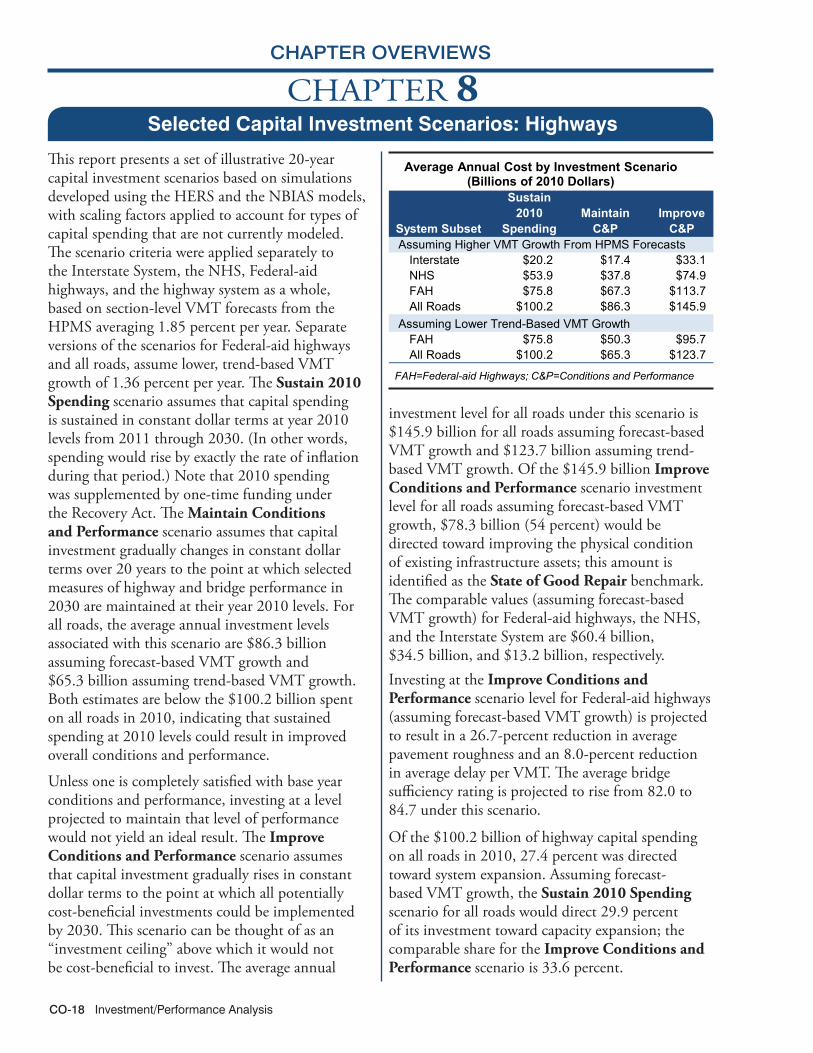
CHAPTER OVERVIEWS

Investment/Performance AnalysisCO-18

Selected Capital Investment Scenarios: Highways

CHAPTER 8

This report presents a set of illustrative 20-year capital investment scenarios based on simulations developed using the HERS and the NBIAS models, with scaling factors applied to account for types of capital spending that are not currently modeled. The scenario criteria were applied separately to the Interstate System, the NHS, Federal-aid highways, and the highway system as a whole, based on section-level VMT forecasts from the HPMS averaging 1.85 percent per year. Separate versions of the scenarios for Federal-aid highways and all roads, assume lower, trend-based VMT growth of 1.36 percent per year. The Sustain 2010 Spending scenario assumes that capital spending is sustained in constant dollar terms at year 2010 levels from 2011 through 2030. (In other words, spending would rise by exactly the rate of inflation during that period.) Note that 2010 spending was supplemented by one-time funding under the Recovery Act. The Maintain Conditions and Performance scenario assumes that capital investment gradually changes in constant dollar terms over 20 years to the point at which selected measures of highway and bridge performance in 2030 are maintained at their year 2010 levels. For all roads, the average annual investment levels associated with this scenario are $86.3 billion assuming forecast-based VMT growth and $65.3 billion assuming trend-based VMT growth. Both estimates are below the $100.2 billion spent on all roads in 2010, indicating that sustained spending at 2010 levels could result in improved overall conditions and performance.

Unless one is completely satisfied with base year conditions and performance, investing at a level projected to maintain that level of performance would not yield an ideal result. The Improve Conditions and Performance scenario assumes that capital investment gradually rises in constant dollar terms to the point at which all potentially cost-beneficial investments could be implemented by 2030. This scenario can be thought of as an “investment ceiling” above which it would not be cost-beneficial to invest. The average annual

investment level for all roads under this scenario is $145.9 billion for all roads assuming forecast-based VMT growth and $123.7 billion assuming trend-based VMT growth. Of the $145.9 billion Improve Conditions and Performance scenario investment level for all roads assuming forecast-based VMT growth, $78.3 billion (54 percent) would be directed toward improving the physical condition of existing infrastructure assets; this amount is identified as the State of Good Repair benchmark. The comparable values (assuming forecast-based VMT growth) for Federal-aid highways, the NHS, and the Interstate System are $60.4 billion, $34.5 billion, and $13.2 billion, respectively. Investing at the Improve Conditions and Performance scenario level for Federal-aid highways (assuming forecast-based VMT growth) is projected to result in a 26.7-percent reduction in average pavement roughness and an 8.0-percent reduction in average delay per VMT. The average bridge sufficiency rating is projected to rise from 82.0 to 84.7 under this scenario.

Of the $100.2 billion of highway capital spending on all roads in 2010, 27.4 percent was directed toward system expansion. Assuming forecast-based VMT growth, the Sustain 2010 Spending scenario for all roads would direct 29.9 percent of its investment toward capacity expansion; the comparable share for the Improve Conditions and Performance scenario is 33.6 percent.

12/15/2013 ESX08H_A R2.xlsx

System Subset

Sustain 2010

SpendingMaintain

C&PImprove

C&P

Interstate $20.2 $17.4 $33.1NHS $53.9 $37.8 $74.9FAH $75.8 $67.3 $113.7All Roads $100.2 $86.3 $145.9

FAH $75.8 $50.3 $95.7All Roads $100.2 $65.3 $123.7

Assuming Higher VMT Growth From HPMS Forecasts

Assuming Lower Trend-Based VMT Growth

Average Annual Cost by Investment Scenario (Billions of 2010 Dollars)

FAH=Federal-aid Highways; C&P=Conditions and Performance

CHAPTER OVERVIEWS

Investment/Performance Analysis CO-19

Selected Capital Investment Scenarios: TransitCHAPTER 8

This report presents a set of illustrative 20- year transit capital investment scenarios. These scenarios build upon analyses developed using the TERM and were applied separately to the Nation’s transit assets as a whole, to urbanized areas (UZAs) with populations of more than one million, and to everyone else.

The Sustain 2010 Spending scenario assumes that capital spending is sustained at 2010 levels, in constant dollar terms, for 20 years. Transit operators spent $16.5 billion on capital projects in 2010. Of this amount, $10.3 billion was devoted to the preservation of existing assets and the remaining $6.2 billion was dedicated to investment in asset expansion to support ongoing ridership growth and to improve service performance. This scenario considers the expected impact on the Nation’s transit infrastructure if these expenditure levels are sustained in constant dollar terms. TERM analysis suggests that sustaining spending at 2010 levels would likely yield an estimated 65-percent increase in the SGR backlog by 2030. The 2010 backlog is estimated at $85.9 billion. Current levels of expansion investment are within the projected range

necessary to limit increases in crowding on transit passenger vehicles.

The Low Growth and High Growth scenarios consider the level of investment to address both asset SGR and service expansion needs subject to two differing potential levels of growth. The Low Growth scenario assumes that transit ridership will grow as projected by the Nation’s metropolitan planning organizations, and the High Growth scenario assumes the average rate of growth (by UZA) as experienced in the industry since 1995. The Low Growth scenario assumes that ridership will grow at an annual rate of 1.4 percent during the 20-year period from 2010 to 2030; conversely, the High Growth scenario assumes that ridership will increase at a rate of 2.2 percent per year during that time frame. TERM estimates this average annual level of investment for the Nation to be between $22.0 billion and $24.5 billion, including between $17.3 billion and $17.4 billion to replace and rebuild assets as they exceed their life expectancy and between $4.6 billion and $7.1 billion for expansion to keep up with growth in demand. The high and low estimates here depend on the expected rate of ridership growth, which is expected to be between these high- and low-growth estimates.

12/15/2013 ESX08T_A R2.xlsx

Mode, Purpose, and Asset Type Sustain 2010 Spending SGR Low Growth High GrowthUrbanized Areas Over 1 Million in Population1

Nonrail2: Preservation $2.9 $4.6 $4.2 $4.2Nonrail2: Expansion $1.2 $0.0 $1.2 $2.1

Subtotal Nonrail3 $4.1 $4.6 $5.4 $6.3Rail: Preservation $6.3 $11.4 $11.0 $11.1Rail: Expansion $4.2 $0.0 $2.9 $4.0

Subtotal Rail3 $10.5 $11.4 $13.9 $15.1Total, Over 1 Million in Population3 $14.6 $16.0 $19.3 $21.4

Nonrail2: Preservation $1.1 $2.2 $1.9 $1.9Nonrail2: Expansion $0.6 $0.0 $0.5 $1.0

Subtotal Nonrail3 $1.7 $2.2 $2.4 $2.9Rail: Preservation $0.0 $0.3 $0.2 $0.2Rail: Expansion $0.2 $0.0 $0.0 $0.0

Subtotal Rail3 $0.2 $0.3 $0.2 $0.2Total, Under 1 Million and Rural3 $1.9 $2.5 $2.7 $3.1

Total3 $16.5 $18.5 $22.0 $24.5

Urbanized Areas Under 1 Million in Population and Rural

Investment Projection (Billions of 2010 Dollars) Annual Average Cost by Investment Scenario (2010–2030)

1Includes 37 different urbanized areas. 2Buses, vans, and other (including ferryboats). 3Note that totals may not sum due to rounding.

CHAPTER OVERVIEWS

Investment/Performance AnalysisCO-20

Supplemental Scenario Analysis: HighwaysCHAPTER 9

While the names and definitions of the highway scenarios presented in the C&P report have varied over time, each edition has generally included one primary scenario oriented toward maintaining the overall state of the system and one oriented toward improving the overall state of the system. Looking at previous editions starting with the 1997 C&P Report, the “gap” between base year spending and the average annual investment level for the primary “Maintain” and “Improve” scenarios has varied, rising as high as 34.2 percent and 121.9 percent, respectively, in the 2008 C&P Report (comparing needs in 2006 dollars with actual spending in 2006). These larger gaps coincided with a 43.3 percent increase in construction costs between 2004 and 2006.

but is largely attributable to a recent decline in construction costs; the National Highway Construction Cost Index declined by 18.0 percent from 2008 to 2010.

For the 20-year period ending in 2028, the 2010 C&P Report estimated the average annual investment levels for the Maintain Conditions and Performance scenario and the Improve Conditions and Performance scenario to be $101.0 billion and $170.1 billion, respectively, both stated in constant 2008 dollars; restating this in 2010 dollars would reduce them to $82.8 billion and $139.4 billion. The comparable forecast-based values presented in the 2013 C&P Report for these scenarios ($86.3 billion and $145.9 billion) are 4.0 percent higher and 4.7 higher, respectively, than these adjusted values.

The investment scenarios presented in this report are “ramped”, applying an annual constant dollar growth rate starting with the $100.2 billion of highway capital spending by all levels of government in 2010. For the forecast-based Improve Conditions and Performance scenario, the amount spent in individual years ranges from $103.6 billion in 2011 (3.46 percent more than 2010 spending) up to $197.8 billion in 2030. These values do not reflect the effects of inflation; assuming a 2 percent annual inflation rate would increase the nominal dollar value for 2030 to $293.8 billion.

11/16/2012 ESX09H_A R2.xlsx

-25%

0%

25%

50%

75%

100%

125%

150%

1997 1999 2002 2004 2006 2008 2010 2013

Diff

eren

ce R

elat

ive

to B

ase

Yea

r

C&P Report Year

Primary "Improve" Scenario Primary "Maintain" Scenario

Gap Between Average Annual Investment Scenarios and Base Year Spending, as Identified

in the 1997 to 2013 C&P Reports

11/16/2012 ESX09H_B R2.xlsx

$100

$125

$150

$175

$200

$225

$250

$275

$300

2010 2015 2020 2025 2030

Ave

rage

Ann

ual I

nves

tmen

t (B

illio

ns o

f Dol

lars

)

Year

Nominal Dollars, If 2% Inflation

Constant 2010 Dollars

Illustration of Potential Impact of Inflation on the Improve Conditions and Performance Scenario

For the forecast-based analyses in the current 2013 C&P Report, the gap associated with the Improve Conditions and Performance scenario has fallen to 45.7 percent, while the gap with the Maintain Conditions and Performance scenario is –13.9 percent because the average annual investment level under the Maintain Conditions and Performance scenario is lower than actual spending in 2010. This negative gap is partially due to increased funding from the Recovery Act

CHAPTER OVERVIEWS

Investment/Performance Analysis CO-21

Supplemental Scenario Analysis: TransitCHAPTER 9

This section is intended to provide the reader with a deeper understanding of the assumptions behind the investment scenarios presented in Chapters 7 and 8. It includes discussion of the following topics:

�� Asset condition projection under the four Chapter 8 scenarios.

�� A comparison of 2010 to 2012 TERM results.

�� A comparison of historic rates of growth in PMT with the growth projections provided by the Nation’s MPOs.

�� An assessment of the impact of an evident gradual transition to alternative fuel and hybrid vehicles on the reinvestment backlog.

�� How many transit vehicles, route miles, and stations would be acquired under the High Growth and Low Growth scenarios.

Asset condition projections for each of the Chapter 8 scenarios are presented both as average condition ratings and as distributions of assets by how much of their useful life will have been consumed. The former includes a discussion of a more realistic (gradual) pay-down of the reinvestment backlog.We then provide an analysis of the reasons that the SGR backlog estimate has changed relative to the projections presented in the 2010 edition of this report.

11/16/2012 ESX09T_A R1.xlsx

Billion $SGR backlog as reported in the 2010 C&P Report $77.7

Impact of 2 additional years of needs +9.0Impact of inflation +3.6Impact from the change in the asset inventory -4.4

SGR backlog as reported in the 2013 C&P Report $85.9

Causes of the Increase in the SGR Backlog between the 2010 C&P Report and the 2013 C&P Report

This is followed by an analysis of average historical rates of transit PMT growth. These rates exceed the MPO-projected rates of growth typically used for long-range transportation planning purposes.

Given the difference between the two growth rates (and the relatively high rate of historic PMT growth as compared with other measures, such as UZA population growth), the 2.1-percent historical growth rate of PMT was identified as a reasonable input value for the High Growth scenario. Similarly, the 1.3-percent MPO-projected growth rate was used as an input value for the Low Growth scenario.

Based on recent trends in vehicle procurement, the share of vehicles powered by alternative fuels is estimated to increase from 23 percent in 2010 to 53 percent in 2030. During the same period, the share of hybrid buses is estimated to increase from 3 percent to 35 percent. The average cost of an alternative-fuel bus is 15.5 percent higher than that of a standard diesel bus of the same size, and hybrid buses cost roughly 65.9 percent more than standard diesel buses of the same size. An analysis of the impact these more expensive vehicles will have on long-term capital needs is presented in this section based on the assumption that these price differentials will remain static.

11/20/2012 ESX09T_B R1

0%

20%

40%

60%

80%

100%

2000 2010 2020 2030

Hybrid and Electric

Compressed Natural Gas and Other Alternative Fuel

Hybrid and Alternative Fuel Vehicles: Share of Total Bus Fleet, 2000–2030

Finally, this section attempts to answer the question: what will our transit system look like in 2030 under these scenarios? In this discussion, fleet size, fixed guideway route miles, and the total number of stations under each scenario over the period of 2010 to 2030 is projected.

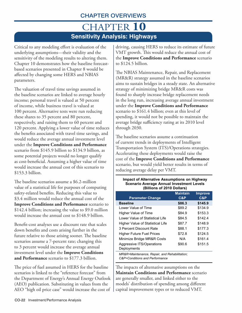
CHAPTER OVERVIEWS

Investment/Performance AnalysisCO-22

Sensitivity Analysis: HighwaysCHAPTER 10

Critical to any modeling effort is evaluation of the underlying assumptions—their validity and the sensitivity of the modeling results to altering them. Chapter 10 demonstrates how the baseline forecast-based scenarios presented in Chapter 8 would be affected by changing some HERS and NBIAS parameters.

The valuation of travel time savings assumed in the baseline scenarios are linked to average hourly income; personal travel is valued at 50 percent of income, while business travel is valued at 100 percent. Alternative tests were run reducing these shares to 35 percent and 80 percent, respectively, and raising them to 60 percent and 120 percent. Applying a lower value of time reduces the benefits associated with travel time savings, and would reduce the average annual investment level under the Improve Conditions and Performance scenario from $145.9 billion to $134.9 billion, as some potential projects would no longer qualify as cost-beneficial. Assuming a higher value of time would increase the annual cost of this scenario to $153.3 billion.

The baseline scenarios assume a $6.2-million value of a statistical life for purposes of computing safety-related benefits. Reducing this value to $3.4 million would reduce the annual cost of the Improve Conditions and Performance scenario to $142.4 billion; increasing the value to $9.0 million would increase the annual cost to $148.9 billion.

Benefit-cost analyses use a discount rate that scales down benefits and costs arising further in the future relative to those arising sooner. The baseline scenarios assume a 7-percent rate; changing this to 3 percent would increase the average annual investment level under the Improve Conditions and Performance scenario to $177.3 billion.

The price of fuel assumed in HERS for the baseline scenarios is linked to the “reference forecast” from the Department of Energy’s Annual Energy Outlook (AEO) publication. Substituting in values from the AEO “high oil price case” would increase the cost of

driving, causing HERS to reduce its estimate of future VMT growth. This would reduce the annual cost of the Improve Conditions and Performance scenario to $124.5 billion.

The NBIAS Maintenance, Repair, and Replacement (MR&R) strategy assumed in the baseline scenarios aims to sustain bridges in a steady state. An alternative strategy of minimizing bridge MR&R costs was found to sharply increase bridge replacement needs in the long run, increasing average annual investment under the Improve Conditions and Performance scenario to $161.4 billion; even at this level of spending, it would not be possible to maintain the average bridge sufficiency rating at its 2010 level through 2030.

The baseline scenarios assume a continuation of current trends in deployments of Intelligent Transportation System (ITS)/Operations strategies. Accelerating these deployments would raise the cost of the Improve Conditions and Performance scenario, but would yield better results in terms of reducing average delay per VMT.

11/26/2012 ESX10H_A R2.xlsx

Parameter ChangeMaintain

C&PImprove

C&PBaseline $86.3 $145.9Lower Value of Time $89.2 $134.9Higher Value of Time $84.9 $153.3Lower Value of Statistical Life $84.5 $142.4Higher Value of Statistical Life $87.7 $148.93 Percent Discount Rate $88.1 $177.3Higher Future Fuel Prices $72.8 $124.5Minimize Bridge MR&R Costs N/A $161.4Aggressive ITS/Operations Deployments

$90.6 $151.5

MR&R=Maintenance, Repair, and Rehabilitation; C&P=Conditions and Performance

Impact of Alternative Assumptions on Highway Scenario Average Annual Investment Levels

(Billions of 2010 Dollars)

The impacts of alternative assumptions on the Maintain Conditions and Performance scenario are generally smaller, and linked either to the models’ distribution of spending among different capital improvement types or to reduced VMT.

CHAPTER OVERVIEWS

Investment/Performance Analysis CO-23

Sensitivity Analysis: TransitCHAPTER 10

The TERM relies on a number of key input values, variations of which can significantly impact the value of TERM’s capital needs projections. Each of the three unconstrained investment scenarios examined in Chapter 8—including the SGR benchmark and the Low Growth and High Growth scenarios—assumes that assets are replaced at a condition rating of 2.50 as determined by TERM’s asset condition decay curves. Analysis suggests that each of these scenarios is sensitive to changes in this replacement condition threshold, with the sensitivity increasing disproportionally with higher replacement condition thresholds. For example, reducing the condition threshold to 2.25 tends to reduce the SGR backlog by just over $1 billion (close to 6 percent). In contrast, increasing the threshold to 2.75 increases preservation needs by more than $3 billion (just under 20 percent), and a further threshold increase to 3.00 increases preservation needs by nearly $7 billion (around 40 percent). This increasing sensitivity reflects the fact that ongoing incremental changes to the replacement condition threshold yield greater proportionate reductions in the length of the asset life cycles as higher replacement condition values are reached.

Needs estimates for scenarios employing TERM’s benefit-cost analysis are also particularly sensitive to changes in capital costs (assuming no comparable increase in benefits) because these increases tend to reduce the value of the benefit-cost ratio, causing some previously acceptable projects to fail this test. For example, a 25-percent increase in capital costs

increases investment costs by more than $4 billion (about 20 percent) for the Low Growth scenario and by around $5 billion (almost 19 percent) for the High Growth scenario. In contrast, needs under the SGR benchmark (which does not utilize TERM’s benefit-cost test) increase by less than $5 billion (25 percent) in response to a 25-percent increase in capital costs.

The most significant source of transit investment benefits as assessed by TERM’s benefit-cost analysis is the net cost savings to users of transit services, a key component of which is the value of travel time savings. Consequently, the per-hour value of travel time for transit riders is a key driver of total investment benefits for scenarios that employ TERM’s benefit-cost test. For example, a doubling of the value of time (from $12.50 per hour to $25 per hour) increases total needs for the Low Growth and High Growth scenarios by approximately $1 billion to $3 billion (7 to 10 percent) due to the increase in total benefits relative to costs. Similarly, a halving of the value of time decreases total investment needs for these scenarios by approximately $1 billion to $2 billion each (5 to 6 percent).

Finally, TERM’s benefit-cost test is responsive to the discount rate used to calculate the present value of the streams of investment costs and benefits. For example, reducing the discount rate from the base rate of 7 percent to 3 percent yields an approximately $1-billion (3 to 6 percent) increase in total annual investment needs under the Low Growth and High Growth scenarios, respectively.

11/13/2012 ESX10T_A R1.xlsx

High Growth Scenario

Replacement Condition Thresholds

Billions of 2010 Dollars

Percent Change

From Baseline

Billions of 2010 Dollars

Percent Change

From Baseline

Billions of 2010 Dollars

Percent Change

From Baseline

Replace assets later (2.25) $17.33 -6.1% $16.00 -5.9% $16.13 -5.8%Baseline (2.50) $18.46 $17.01 $17.12Replace assets earlier (2.75) $22.07 19.6% $20.16 18.5% $20.41 19.2%Very early asset replacement (3.00) $26.03 41.0% $23.28 36.9% $23.49 37.2%

SGR BenchmarkLow Growth

Scenario

Impact of Alternative Replacement Condition Thresholds on Transit Preservation Investment Needs by Scenario (Excludes Expansion Impacts)

CHAPTER OVERVIEWS

Special TopicsCO-24

Transportation Serving Federal and Tribal LandsCHAPTER 11

The Federal government holds title to approximately 650 million acres, or about 30 percent of the total land area of the United States. Additionally, the Federal government holds in trust approximately 55 million acres of land on behalf of Tribal governments. Federal lands are managed by various Federal land management agencies (FLMAs), primarily within the Departments of the Interior, Agriculture, and Defense. Federal lands have many uses, including the facilitation of national defense, recreation, grazing, timber and mineral extraction, energy generation, watershed management, fish and wildlife management, and wilderness maintenance. More than 8 billion vehicle miles are traveled annually on the Tribal Transportation Program road system, with more than 60 percent of the system unpaved.Recreation, national defense, travel, tourism, and resource extraction are all dependent on a quality transportation infrastructure. More than 450,000 miles of Federal roads provide access to Federal lands, which also provides opportunities for recreational travel and tourism, protection and enhancement of resources, and sustained economic development in both rural and urban areas.More than 75 percent of Americans participate in active outdoor recreation each year, contributing $730 billion annually to the U.S. economy. These activities include hunting, fishing, wildlife viewing,

Economic Benefits of Federal Lands

biking, hiking, and water sports. In total, there are nearly 1 billion visits annually to Federal lands.Many FLMAs are no longer able to meet the transportation demands placed upon them due to growing traffic volumes and demands for visitor parking at peak times. As population increases, the demand for access to Federal lands will continue to grow. For FLMAs to continue to fulfill their missions of providing visitor enjoyment and conserving precious resources, innovation and creative solutions will be required.

1/21/2014 ESX31_A R3.xlsx

Recreation Economic Benefits

($ Billion)

Forest Service 205,000 13

National Park Service 258,000 39 Fish and Wildlife Service 27,000 2 Bureau of Land Management 59,000 7

Department of DefenseU.S. Army Corps of Engineers - Civil Works Facilities

270,000 16

Federal AgencyDepartment of Agriculture

Department of the Interior

Recreation Related Jobs

Economic Benefits of Federal Lands*

* Economic benefits include lodging, food, entertainment, recreation, and incidentals expended during travel.

Good Fair Poor TotalStructurally

DeficientForest Service 10,700 25% 50% 25% 259,300 3,840 6% $5.1 billionNational Park Service 5,450 60% 28% 12% 4,100 1,270 3% $5 billionBureau of Land Management 700 60% 20% 20% 2,000 439 3% $350 millionFish & Wildlife Service 400 59% 23% 18% 5,200 281 7% $1 billionBureau of Reclamation 762 N/A N/A N/A 1,253 311 11% N/ABureau of Indian Affairs 8,800 N/A N/A N/A 20,400 929 15% N/ATribal Governments 3,300 N/A N/A N/A 10,200 N/A N/A N/AMilitary Installations 26,000 N/A N/A N/A N/A 1,422 11% N/AU.S. Army Corps of Engineers 5,135 55% 25% 20% N/A 294 11% $100 million

Backlog of Deferred

MaintenanceAgency

Public Paved Road Miles

Public Unpaved

Road Miles

Paved Road Public Bridges

Roads Serving Federal Lands

12/12/2013 ESX31_B R3.xlsx

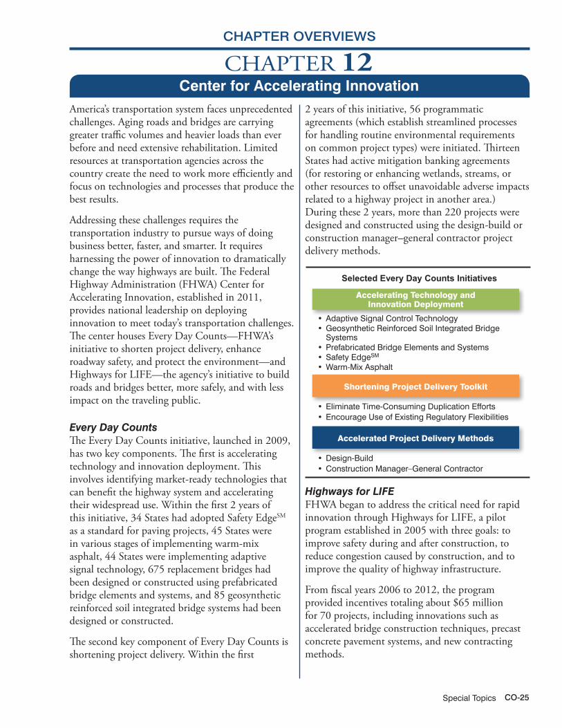
CHAPTER OVERVIEWS

Special Topics CO-25

Center for Accelerating InnovationCHAPTER 12

America’s transportation system faces unprecedented challenges. Aging roads and bridges are carrying greater traffic volumes and heavier loads than ever before and need extensive rehabilitation. Limited resources at transportation agencies across the country create the need to work more efficiently and focus on technologies and processes that produce the best results.

Addressing these challenges requires the transportation industry to pursue ways of doing business better, faster, and smarter. It requires harnessing the power of innovation to dramatically change the way highways are built. The Federal Highway Administration (FHWA) Center for Accelerating Innovation, established in 2011, provides national leadership on deploying innovation to meet today’s transportation challenges. The center houses Every Day Counts—FHWA’s initiative to shorten project delivery, enhance roadway safety, and protect the environment—and Highways for LIFE—the agency’s initiative to build roads and bridges better, more safely, and with less impact on the traveling public.

Every Day CountsThe Every Day Counts initiative, launched in 2009, has two key components. The first is accelerating technology and innovation deployment. This involves identifying market-ready technologies that can benefit the highway system and accelerating their widespread use. Within the first 2 years of this initiative, 34 States had adopted Safety EdgeSM as a standard for paving projects, 45 States were in various stages of implementing warm-mix asphalt, 44 States were implementing adaptive signal technology, 675 replacement bridges had been designed or constructed using prefabricated bridge elements and systems, and 85 geosynthetic reinforced soil integrated bridge systems had been designed or constructed.

The second key component of Every Day Counts is shortening project delivery. Within the first

2 years of this initiative, 56 programmatic agreements (which establish streamlined processes for handling routine environmental requirements on common project types) were initiated. Thirteen States had active mitigation banking agreements (for restoring or enhancing wetlands, streams, or other resources to offset unavoidable adverse impacts related to a highway project in another area.) During these 2 years, more than 220 projects were designed and constructed using the design-build or construction manager–general contractor project delivery methods.

Accelerating Technology and Innovation Deployment

•AdaptiveSignalControlTechnology•GeosyntheticReinforcedSoilIntegratedBridgeSystems

•PrefabricatedBridgeElementsandSystems•SafetyEdgeSM

•Warm-MixAsphalt

•EliminateTime-ConsumingDuplicationEfforts•EncourageUseofExistingRegulatoryFlexibilities

Shortening Project Delivery Toolkit

•Design-Build•ConstructionManager–GeneralContractor

Accelerated Project Delivery Methods

10/29/2012 ESX32_A R1.xlsx

Selected Every Day Counts Initiatives

Highways for LIFEFHWA began to address the critical need for rapid innovation through Highways for LIFE, a pilot program established in 2005 with three goals: to improve safety during and after construction, to reduce congestion caused by construction, and to improve the quality of highway infrastructure.

From fiscal years 2006 to 2012, the program provided incentives totaling about $65 million for 70 projects, including innovations such as accelerated bridge construction techniques, precast concrete pavement systems, and new contracting methods.

CHAPTER OVERVIEWS

Special TopicsCO-26

CHAPTER 13National Fuel Cell Bus Program

This chapter summarizes the accomplishments of fuel cell transit bus research and demonstration projects supported by the FTA through 2011. It describes fuel cell electric bus (FCEB) research projects in the United States and describes their impact on commercialization of fuel cell power systems and electric propulsion for transit buses in general.

FTA sponsors the National Fuel Cell Bus Program (NFCBP), a cooperative research, development, and demonstration program to advance commercialization of FCEBs. The NFCBP is a part of a larger FTA research program to improve transit efficiency and contribute to environmentally sustainable transportation. NFCBP projects target research to improve performance and lower costs of next-generation fuel cell systems for transportation.

FTA’s research to develop FCEBs has been underway since 2006. NFCBP projects require a dollar-for-dollar cost share for Federal funds, bringing the size of the program to more than $150 million through FY 2011.

11/20/2012 ESX33T_A (1st) R2

0

5

10

15

20

25

30

35

2008 2009 2010 2011 2012

Fuel

Cel

l Ele

ctric

Bus

C

ount

Fuel Cell Electric Buses Operating in the United States, 2006-2012

NFCBP accomplishments include: �� Supporting an El Dorado–BAE Systems–Ballard

partnership that developed and demonstrated a new FCEB at SunLine and CTA. The new bus meets Buy America requirements and is assembled in Riverside, CA.

�� Canadian-based fuel cell manufacturer Ballard Power Systems has established manufacturing capabilities for fuel cell power systems in Lowell, MA.

�� The NFCBP funded a project with Connecticut-based fuel cell manufacturer UTC Power to engineer, package, and test a fuel cell power system that can be installed easily into U.S. bus manufacturer models.

11/20/2012 ESX33T_B (2nd) R1.xlsx

Fuel Cell Electric Bus Demonstration Sites

Introduction ................................................................................................I-2U.S. DOT Strategic Plan ................................................................................... I-2Performance Management ............................................................................... I-3

Chapter 1: Household Travel and Freight Movement ...................... 1-1

Chapter 2: System Characteristics ................................................... 2-1

Chapter 3: System Conditions .......................................................... 3-1

Chapter 4: Safety ............................................................................... 4-1

Chapter 5: System Performance ....................................................... 5-1

Chapter 6: Finance ............................................................................ 6-1

PART I

Description of Current System I-1

Description of Current System

Description of Current SystemI-2

IntroductionPart I of the C&P Report, Chapters 1 through 6, present data on the condition and performance of the highway and transit systems, travel behavior, and funding trends. Data are presented for 2010, with comparisons to the 2008 data and the past 10 to 20 years. Data for each year are to be interpreted in the context of the economic and social environment prevalent at the time. Part I, Introduction, presents the background context to the data to be discussed in the following chapters.

Chapter 1, Household Travel and Freight Movement, outlines the trends in travel behavior of households and businesses. The results of the 2009 National Household Travel Survey are discussed in particular, examining the level of travel, time of travel, and mode of travel. Aging of the population and the vehicle fleet are discussed in some detail. Using the data of the travel survey, some of the myths of travel are disputed, for example that the majority of personal travel is for commuting to work. A section on trends in freight travel is added to discuss the trends and issues facing the business community in moving goods across the country to support the diverse and growing economy.

Chapter 2, System Characteristics, describes the highway, bridge, and transit systems, presenting the extent and the types of infrastructure in the United States, as well the ownership and geography.

Chapter 3, System Conditions, presents the data on the condition of the highways, bridges, and transit systems and vehicles in 2010. The 2010 condition is compared to the 2008 condition data and also to earlier periods, by system purpose, jurisdiction, and geography.

Chapter 4, Safety, illustrates the safety data on fatalities and injuries for highways and transit for different modes of travel—motor vehicles, pedestrians, non-motor vehicles and transit systems, and functional class of roads. It discusses the factors contributing to crashes on highways related to roadway design and functionality, as well as human behavior.

Chapter 5, System Performance, discusses the data and performance measures for system performance. System performance is defined broadly to include the implication of transportation usage and construction on the environment, land use, and economic competitiveness. It discusses performance measures for livability, environmental sustainability, and economic competitiveness, outlining some initiatives for livability and sustainability and the trends in national congestion and travel time reliability.

Chapter 6, Finance, provides detailed data on the revenue collected and expended by different levels of government to fund transportation construction and operations throughout the United States. The trends in the data are discussed, providing a context where appropriate.

U.S. DOT Strategic PlanIn 2012, the U.S. DOT developed a 4-year Strategic Plan 2012-16, outlining the objectives and performance goals for the Nation’s transportation system. The U.S. DOT identified five strategic goals that each agency promotes through its programs.

Safety – Improve public health and safety by reducing transportation-related fatalities and injuries.

State of Good Repair – Ensure that the United States proactively maintains its critical transportation infrastructure in a state of good repair.

Economic Competitiveness – Promote transportation policies and investments that bring lasting and equitable economic benefits to the Nation and its citizens.

Livable Communities – Foster livable communities through place-based policies and investments that increase the transportation choices and access to transportation services.

Description of Current System I-3

Environmental Sustainability – Advance environmentally sustainable policies and investments that reduce carbon and other harmful emissions from transportation sources.

Each agency identified specific measures and targets for the goal areas, as appropriate and feasible. For instance, for the goal area of safety, the desired outcome is reduced transportation-related fatalities and injuries, which is measured differently by each mode. One of the measures used for highways is the number of fatalities per million vehicle miles traveled (VMT), referred to as the fatality rate. There is a rich database for this measure, which makes it possible to understand the trends over time and to identify some of the underlying factors that may influence it. This allows the agencies to set future targets and to identify strategies to reach the target.

For some of the goals, the outcome depends on the actions of multiple agencies or even multiple departments. For instance, to reduce the crash rate on roads, it may be necessary to redesign the road, change driving behavior—for example, banning use of phones while driving—or requiring additional training and licensing standards for drivers. An achievement of this goal requires concerted effort from three agencies: FHWA, National Highway Traffic Safety Administration (NHTSA) and Federal Motor Carrier Safety Administration (FMCSA). Achieving the livability outcomes require coordination among FHWA, Federal Transit Administration (FTA), and U.S. Department of Housing and Urban Development (HUD). Often, legislation can influence the products that the private sector develops in response to greater awareness of issues. Motor vehicles have become safer over time as consumers demand greater safety.

Each chapter in this edition of the C&P report pertaining to the goal areas above discusses the performance measures and targets identified in the U.S. DOT’s Performance Plan for Fiscal Year 2013. The discussion includes the challenges of selecting the appropriate measure, the limitations of the data currently available, and research into developing useful measures. Chapter 3, System Conditions, discusses the performance measures for the state of good repair for pavement and bridges; Chapter 4, Safety, discusses the measures for safety; and Chapter 5, System Performance, discusses performance measures relating to economic competitiveness, livability, and environmental sustainability.

Performance ManagementFor many decades, the biennial C&P report has provided data on the condition and performance of the highway and transit systems in the United States, informing Congress and the public of the status of the Nation’s transportation infrastructure. However, the need for Government accountability and transparency has increased over the last decade. To address this need, many government agencies in the United States and abroad have adopted the practice of performance management.

Performance management is by no means a new concept to the transportation sector. Many States and Metropolitan Planning Organizations (MPOs) already use performance management in transportation planning and programming, as do many other countries, see report from the FHWA International Technology Scanning Program, Linking Transportation Performance and Accountability, April 2010 (http:// www.international.fhwa.dot.gov/pubs/pl10011/pl10011.pdf ). According to the PEW Center’s report of May 2011 (Measuring Transportation Investments – Roads to Results), many States have adopted key elements of performance management such as performance goals, measures, and data that provide their policy makers with information to use for making funding decisions. Other States may be in earlier stages of developing performance goals, measures, and data. The U.S. Department of Transportation (DOT) has introduced some elements of performance management into its operations through its FY 2012-2016 Strategic Plan, and in July 2012 the Moving Ahead for Progress into the 21st Century Act (MAP-21) (P.L. 112-141) introduced requirements that have reinforced the importance of performance management for transportation investment decisions.

Description of Current SystemI-4

What is Performance Management of the Federal Transportation Program?Transportation Performance Management (TPM) is a strategic approach that uses system information to make investment and policy decisions to achieve national performance goals. A typical performance management planning and programming process is likely to follow the practice in Exhibit I-1. First, establish a set of goals/objectives to be achieved by the program—these could be general in nature, such as improving safety on the highway system. Second, define measures that support the goal or objective. For safety, this could be the number of crashes or more specifically fatalities. Third, define the measure to be used. Data for the measure and other influencing factors are collected over a period of time to determine the current status, how it has changed over time, and what factors influence its trend. This information can be used to identify actions that are likely to influence the measure trend. Fourth, establish specific future targets for the measure. The specific targets for the measure can be aspirational, based on past trends, or fiscally constrained. Then, specific plans, budgets, and programs are developed to support the desired outcome. Fifth, report the results. After the programs are implemented, the results from the action/investment are assessed against the desired goal. Any discrepancy between the planned outcome and the actual outcome can be addressed by altering strategies and priorities. Performance management is a continual improvement process.

A performance management program for the Federal-aid program will enable States and MPOs to focus on common national goals, targeting investments towards areas of national significance. Tracking performance measures against specific targets helps inform decision makers about how well the current investments are moving the agencies toward achieving national goals. Performance management makes investment decisions more transparent and increase accountability as results are tracked.

Selection of Performance MeasuresPerformance measures can be either output based or outcome based. An output-based performance measure tracks the quantity of activity undertaken. For instance, the number of lane miles constructed in 3 years is an output measure; it does not tell you how the activity affects the condition or performance of the transportation system. An outcome measure would identify the impact of the action or activity on condition or performance of the system. An example would be the percentage of pavement in good condition. An agency may track both types of performance measures. The output measures would be used to inform the agency what actions/activities are undertaken to influence the performance outcome. If the current actions do not achieve the desired outcome, they should be reconsidered or new actions adopted. The focus of performance management is on the outcome.

An effective performance measure needs to directly relate to the investment decisions of the agency. It has to be a measure that the agency can influence and for which the agency can be held accountable. For instance, pavement reconstruction will improve the condition of the system, but increasing U.S. exports is not something a Department of Transportation (DOT) can influence directly because it depends on the investment and decisions of many other parties. Additionally, the measure needs to be easily understood by the public and not be too complex or costly to create or track. In addition, the measure is to be outcome based and change over a relatively short period of time so that the effectiveness of the actions can be tracked.

Description of Current System I-5

Elements Description Examples

Goals and objectives

Goals and objectives that capture an agency's strategic direction

Infrastructure condition, safety, mobility, reliability, and other goals established by an agency.

Performance measure

Agreed on measures for goals and objectives.

Percent of bridges in good condition, travel time index, and other measures linked to agency goals.

Identify targets and trends

Establish aspirational targets or preferred trends based on an understanding of a desirable future for each goal area and measure.

Desired conditions of pavement, bridge, and transit assets. Desired future corridor travel times or reliability levels.Desired future crash, injury, and fatality reductions.

Identify strategies

Strategies, policies, and investments that address transportation system needs within the identified goal areas.

Resurfacing, rehabilitation, replacement, and reconstruction to support infrastructure condition.Signal timing, vehicle maintenance, service patrols, additional capacity (transit or highway), tolling, and other strategies/investments to improve mobility or reliability.Seat belt or drunk driving enforcement, graduated drivers licenses, rumble strips, training, median barriers, and other investments to improve safety.

Strategy evaluation

Evaluate strategies and define program level system performance expectations, may be qualitative.

Examine impact of varying levels of investment on pavement and, bridge preservation and transit assets.Examine impact of packages of operations, capacity and other highway or transit investments on corridor travel time and/or reliability.Examine potential for reduction in crashes, injuries, and fatalities from a package of safety investments.

Investment plan

Identify the amount and mix of funding needed to achieve performance goals within individual program areas.

Investment plan for pavement, bridge, transit asset, operations, expansion, safety, and other projects consistent with strategy evaluation, including specific projects and high-level summary of expected investment levels.

Resource constrained targets and

trends

Established quantitative or qualitative targets or desired trends for each goal/measure.

Expected future conditions of pavement and bridge conditions and transit assets.Expected future corridor travel times or reliability improvements given a package of investments. Expected range of crash, injury, and fatality reduction from a package of safety investments.

Program of projects

Identify specific transportation projects for an agency capital plan, or State/ Transportation Improvement Program (S/TIP) that are consistent with system performance expectations established in strategy evaluation.

S/TIP with specific projects identified in major program areas (pavement, bridge, transit assets, capital, operations, safety, etc.).

Reporting and monitoring

Monitor progress on goals relative to targets and resource allocation efforts.

Report on pavement, bridge, transit assets, reliability, safety, and other metrics presented to stakeholders, public, and decision makers.

Evaluation Identify improvements in analytics, process, etc. to improve the planning process. Evaluating the mix of projects.

Examine actual conditions relative to expected conditions for assets, reliability, safety, and other areas. Identify where tools produced inaccurate estimates or investments and policies were more or less successful than planned.

Strategic Direction (Where do we want to go?)

Programming (What will it take?)

Implementation and Evaluation (How did we do?)

Long-Range Planning (How are we going to get there?)

Exhibit I-1 Performance Management Planning and Programming Elements

Source: Performance Based Planning and Programming, White Paper, FHWA, 2012.

12/12/2013 71X_C (I-1) R5.xlsx

Description of Current SystemI-6

MAP-21 Performance Management RequirementsMAP-21 introduced specific requirements for performance management for Federal highway and transit funding programs, reinforcing the use of performance management for Federal surface transportation investments. MAP- 21 established national goals for transportation, directed U.S. DOT to establish performance measures for each of the goal areas, and requires States to set performance targets for each of the measures and report the outcomes to U.S. DOT to track progress. The national goals are:

• Safety

• Infrastructure Condition

• Congestion Reduction

• System Reliability

• Freight Movement and Economic Activity

• Environmental Sustainability

• Reduced Project Delivery Delay.

Federal Agencies are required to define the measures and standards for achieving the goals identified, unless defined in MAP-21. The States are to determine their own targets to achieve, while minimum standards may be established by Federal agencies where appropriate. The States are required to develop risk-based asset management plans, safety plans, and freight plans. The 20-year, long-range plans are expected to be performance based.

States are to report progress toward the targets established. Failure to meet targets or develop plans has specific penalties for States – reduction in funding or requirements to spend more on the specific goal area. For instance, failure to develop or implement a risk-based asset plan would result in the Federal share payable on account of any project or activity carried out by the State in that year for infrastructure of only 65 percent. If fatality rates on rural roads increase over the recent 2-year period, the State is required to obligate a minimum of 200 percent of the received funds for FY 2009 high-risk rural roads. States are to report progress toward the targets within 4 years of enactment of MAP-21, and biennially thereafter.

Transit agencies that receive FTA grant funds are similarly required to maintain asset management plans, to set goals for achieving a state of good repair, and to report asset inventory condition data to FTA along with metrics demonstrating their progress toward meeting their goals. MAP-21 also established a comprehensive transit safety program at FTA and the States to assist and monitor transit agencies as they strive to eliminate accidents.

Household Travel and Freight Movement

Household Travel ........................................................................................................1-2

Trends in Our Nation’s Travel ....................................................................................1-3Geographic Trends in Trip Rates and Trip Lengths ............................................................ 1-4The Determinants of Travel ................................................................................................. 1-6Travel by Time of Day ......................................................................................................... 1-7

Usual and Actual Commute: A Typical Day Versus a Specific Day ..........................1-7

Baby Boomer Travel Trends.......................................................................................1-8

Travel of Millennials ....................................................................................................1-9

Aging of the Household Vehicle Fleet .......................................................................1-10

Some Myths and Facts About Daily Travel ................................................................1-11Myth 1: The majority of personal travel is for commuting to work ..................................... 1-11Myth 2: Americans love their cars, and that’s why they don’t walk or take transit ............ 1-11Myth 3: Households without vehicles rely completely on transit, walk, and bike ............. 1-12Myth 4: When elderly drivers give up their driver’s license they maintain mobility by using transit or walking instead of using private vehicles ............................................. 1-15Myth 5: We can solve congestion by having people shift noncommuting trips outside of peak periods ...................................................................................................... 1-16

Gas Prices and the Public’s Opinions .......................................................................1-16Number One Issue for the Public: Price of Travel .............................................................. 1-17

Freight Movement .......................................................................................................1-18

Freight Transportation System ..................................................................................1-18

Freight Transportation Demand .................................................................................1-18

Freight Challenges .....................................................................................................1-26

Household Travel and Freight Movement 1-1

CHAPTER 1

Description of Current System1-2

Household Travel

To fully understand daily travel, one must look at it through the lens of the 300 million Americans who are using the transportation system to connect to their jobs, markets, educational facilities, healthcare services, airports, recreational places, and more. The National Household Travel Survey (NHTS) is unique in that it is the only national source of travel data that connects the characteristics of the trip (e.g., mode used, trip purpose, distance) with the characteristics of the household (e.g., income, vehicle ownership, location) and of the individual making the trip (e.g., age, sex, education, worker status). As such, it allows for observation of daily travel behavior and fluctuations in that behavior through the lens of socio-demographic and economic changes in the country. The 2009 NHTS, the most recent survey, was sponsored primarily by the Federal Highway Administration (FHWA), with participation by the Federal Transit Administration (FTA), the American Association of Retired Persons (AARP), and American Automobile Association. The FHWA Office of Highway Policy and Information serves as the project manager for the survey.

It is crucial to understand travel behavior in the context of demographics and location. The average transportation project has a 20-year span from definition of potential need to full completion. The more the relationship between travel behavior and the demographics of the public and the location of homes and workplaces can be documented, the better future needs can be determined and resources effectively used. This chapter describes some elements of how travel is changing as the Nation is changing.

Since 1969, NHTS has collected personal travel information intermittently using a national sample of households in the civilian noninstitutionalized population. The survey captures a snapshot of the American public’s daily travel behavior. It is crucial that the information used to guide policies that impact our transportation system is based on sound statistical data, such as that from the NHTS. The 2009 NHTS data were collected from March 2008 through April 2009, which covered a period when there was a drop in vehicle miles of travel and, in some places, an increase in transit use.

This section contains a discussion of the recent decline in vehicle miles traveled (VMT), the disparity of this decline in urban versus rural areas, and how the decline differed by trip purpose. The section also contains a comparison of the usual mode of travel to work with the actual mode used, the influence of the Baby Boomers on total travel, and the aging of the household vehicle fleet. Five commonly held myths about travel are discussed,

NHTS Methodology and TimingThe NHTS collects travel data from a representative sample of U.S. households to characterize personal travel patterns. The survey obtains demographic characteristics of households and people and information about all vehicles in the household. Details of travel by all modes for all purposes of each household member are collected for a single assigned travel day. In this way, NHTS traces both the interaction of household members and the use of each household vehicle throughout an average day. The data provide national and, with the 2009 survey, State-level estimates of trips and miles by travel mode, trip purpose, time of day, gender and age of traveler, and a wide range of attributes.

Much of the data presented in this section are from the NHTS data series, unless otherwise noted. Since 1990, NHTS data have been collected using a random-digit dial sample of telephone households in the United States. Prior to 1990, NHTS data were collected in face-to-face interviews sampled from respondents to the Census Bureau’s Current Population Survey.

The 2008–2009 NHTS data were collected during a time when the price of gas was hitting a peak of $4 per gallon, unemployment was on the rise, the stock market was falling, and the housing market was declining. The survey results, particularly the decline in household-based vehicle miles traveled (VMT), should be considered against this backdrop. Note that the previous survey in the series, the 2001 NHTS, was also conducted during an economic downturn.

Additional information on NHTS is available at www. fhwa.dot.gov/policyinformation/nhts.cfm or http://nhts.ornl.gov.

Household Travel and Freight Movement 1-3

and the chapter concludes with a discussion of the public’s opinions of travel issues and the related gas price spike in the summer of 2008.

This portion of Chapter 1 presents some of the trends in travel behavior that can be gleaned from the NHTS data. The data allow for analysis of other topics and issue areas as well as tabulations at the national and local levels. As technology continues to impact communications and transportation, the need to track the intersection of demographics and travel behavior increases.

Trends in Our Nation’s TravelThe NHTS results show a consistent increase in VMT during the three-decade period from 1969 through 2001 but a decrease in VMT between 2001 and 2009. As shown in Exhibit 1-2, the total number of trips has increased over time from 1990 through 2009, but household VMT decreased between 2001 and 2009.

Q A&How do the NHTS-derived VMT figures in this Chapter differ from the HPMS-derived VMT figures presented elsewhere in this report?

One key difference is that NHTS does not include freight VMT. Freight movement is discussed later in this Chapter.

The NHTS collects data by interviewing American households and, as such, it differs from the Federal Highway Administration (FHWA) Highway Performance Monitoring System (HPMS), which is a primary source for data in many other chapters of this report. HPMS collects data on extent, condition, performance, use, and operating characteristics of the Nation’s public roads directly from State DOTs. The NHTS data, collected by survey, provide detail on individual and household travel characteristics that is not available from the HPMS data. NHTS also reflects personal travel, not including freight movements and other commercial travel; HPMS is designed to count all travel, both passenger and freight. Exhibit 1-1 depicts the approximate split of VMT between passenger (personal) and freight.

NHTS and HPMS data are deliberately collected to be independent estimates of travel in the United States. Analysis of differences between the two sources is performed for quality control. Note that the one linkage between these two sources is that vehicle occupancy from the NHTS is used in computing person miles of travel for HPMS.

9/20/2012 01XH_A (1-1) R3

Exhibit 1-1 VMT by Type of Travel

Source: Highway Statistics 2008, Table VM-1.

90%

10% Passenger Travel

Freight Travel

9/20/2012 01XH_B (1-2) R2

Exhibit 1-2 Summary Statistics on Total Travel, 1990–2009 NHTS (Millions)

1990 1995 2001 2009Household Vehicle Trips 193,916 229,745 233,030 233,849Household VMT 1,695,290 2,068,368 2,274,769 2,245,111Person Trips 304,471 378,930 384,485 392,023Person Miles of Travel 2,829,936 3,411,122 3,783,979 3,732,791

Notes: 1. The travel of children aged 0-4 is excluded from 2001 NHTS data to make it comparable with other years. 2. 1990 person and vehicle trips were adjusted to account for survey collection method changes. 3. Vehicle miles and person miles are only calculated on trips with distance reported. Source: NHTS data series. See 2009 NHTS Summary of Travel Trends, Table 1.

Description of Current System1-4

Americans drove 30 billion fewer vehicle miles in 2008-2009 than in the 2001-2002 NHTS survey period, as shown in Exhibit 1-3, even though the population grew by almost 10 percent during that period.

The NHTS results also show that transit ridership increased by 16 percent from 2001 to 2009, far outstripping the population growth during that time period. Most of the increase in transit use was for shopping and social/recreational activities other than visiting friends and relatives. This category includes going to movies, plays, restaurants, sporting events, and recreational activities like playing sports and going to the gym.

Geographic Trends in Trip Rates and Trip LengthsTwo basic factors used in land use planning and travel demand forecasting are where people live and where they work. Each time people leave their places of residence, work places, or elsewhere, they generate a “trip,” and the distance traveled and other attributes of the trip are captured in the survey.

As reflected in Exhibit 1-4, daily travel shows a steady increase from 1969 to 2001. Daily person trips peaked in 1995 at 4.30 trips per person per day. Daily miles per person showed a slightly different pattern, peaking in 2001 at 40.25 miles per person per day and declining to 36.13 miles per person per day in 2009. The average person trip length also decreased in 2009 when compared to 2001; average person trip length in 2001 was 10.04 miles and in 2009 it was 9.75 miles, which reduced the average person trip by

9/20/2012 01XH_C (1-3) R3

Exhibit 1-3 Total Annual Household VMT (Billions)

Note: The travel of children aged 0–4 is excluded from 2001 NHTS data to make it compatible with other years. Source: NHTS data series.

1,695

2,068 2,275 2,245

0

500

1,000

1,500

2,000

2,500

1990 1995 2001 2009

Mile

s x

1,00

0,00

0,00

0

9/20/2012 01XH_D (1-4) R2

Exhibit 1-4 Summary of Daily Travel Statistics, 1969–2009 NHTS

1969 1977 1983 1990 1995 2001 2009

Daily Person Trips (count) 2.02 2.92 2.89 3.76 4.3 4.09 3.79Daily PMT (miles) 19.51 25.95 25.05 34.91 38.67 40.25 36.13

Daily Vehicle Trips (count) 2.32 2.34 2.36 3.26 3.57 3.35 3.02Daily VMT (miles) 20.64 19.49 18.68 28.49 32.14 32.73 28.97

Daily Person Trips (count) 6.36 7.69 7.2 8.94 10.49 9.81 9.5Daily PMT (miles) 61.55 68.27 62.47 83.06 94.41 96.56 90.42Daily Vehicle Trips (count) 3.83 3.95 4.07 5.69 6.36 5.95 5.66Daily VMT (miles) 34.01 32.97 32.16 49.76 57.25 58.05 54.38

Average person trip length (miles) 9.67 8.87 8.68 9.47 9.13 10.04 9.75Average vehicle trip length (miles) 8.89 8.34 7.9 8.85 9.06 9.87 9.72

Per Person

Per Driver

Per Household

Per Trip

Notes: 1. Average trip length is calculated using only those records with trip mileage information present. 2. 1990 person and vehicle trips were adjusted to account for survey collection method changes. Source: NHTS data series.

Household Travel and Freight Movement 1-5

approximately one-quarter of a mile. On the surface, one-quarter of a mile may not appear to be considered significant, but when you multiply it by more than 3 billion person trips, the results become notable.

Examining trends by geographic location can provide a better understanding of where these changes are occurring. In 2009, the data showed that there was a significant decrease in passenger trips and passenger miles in both urban and rural areas compared to 2001 (see Exhibit 1-5).

However, residents of urban areas reduced their person trips and person miles of travel more than those living in rural areas. For every decrease of one person trip in rural areas, there was a decrease of two person trips in urban areas. In addition, per capita, there was about a 14.5-percent overall decrease in person miles. In urban areas, the largest person-mile decrease happened at slightly less than 17 percent, whereas there was about a 10 percent decrease in rural areas.

NHTS TerminologyTrip Chain or Linked Trip – Individual trips or trips that are linked together to a destination. Any movement from one address to another, except if only to change mode of transport.

Person Trip – Any trip made by one person regardless of mode (auto, truck, transit, walk, bike, etc.).

Person Miles of Travel – The miles associated with a person trip.

Vehicle Trip – Any movement of a vehicle from one address to another, regardless of the number of vehicle occupants.

Vehicle Miles Traveled (VMT) – The miles associated with a vehicle’s movement, regardless of the number of occupants.

Despite increases in aggregate personal VMT through 2001, a number of indicators point toward saturation in vehicle trips and vehicle miles of travel per person, with the peak of most per-person and per-household statistics occurring in 1995. Several factors could be possible explanations for this apparent saturation, such as the desire to limit the time spent in travel and replacing physical trips with electronic communication or online shopping. Given both the gas price spike in the summer of 2008 and the economic recession starting in autumn of that year, it is difficult to isolate how much of the reduction in travel was the product of these two events and how much was the product of broader changes. The proposed 2015 NHTS will add a crucial data point for continuing to track trends in travel behavior.

12/12/2013 01XH_E (1-5) R4.xlsx

Exhibit 1-5 Annual Person Trips and Person Miles per Capita by Urban/Rural Residence

Note: The travel of children aged 0–4 is excluded from 2001 NHTS data to make it compatible with other years. Source: 2001 and 2009 NHTS.

1,604 1,502

1,581

1,404 1,323 1,385

0

200

400

600

800

1,000

1,200

1,400

1,600

1,800

Urban Rural All

Ann

ual T

rip C

ount

Annual Person Trips per Capita 2001 2009

14,664

18,114

15,424

12,220

16,293

13,188

0

2,000

4,000

6,000

8,000

10,000

12,000

14,000

16,000

18,000

20,000

Urban Rural All

Mile

s

Annual Person Miles per Capita 2001 2009

Description of Current System1-6

The Determinants of TravelThe NHTS is the only national data source that asks the American public why they took a given trip. The purpose of travel is significant because it provides a tool for anticipating travel volumes and demand given predictions of demographic change. Purposes are classified into a number of categories: to work, for work-related business, to shop, to run family or personal errands, to school or church, and to make social or recreational trips.

The 2009 data show that the declines in person miles and person trips were most notable in travel to and from work, personal and family errands, and social and recreational travel, while shopping and trips for other purposes were relatively constant. Travel to work shows a 10-percent decrease in miles and a 7-percent decrease in trips between 2001 and 2009. In 2009, American households were traveling 13.9 percent less for family or personal errands, and trip lengths for these family errands also dropped by 10 percent compared to 2001. In addition, daily person miles for social and recreational purposes declined by 9.5 percent between 2001 and 2009. (See Exhibit 1-6.) Two of the three purpose groupings—errands and social/recreational—are those for which most households have the greatest discretion in amount of travel. Further research of this behavior would be useful for policy considerations because family and personal errands and social and recreational travel have generally been the two most prevalent reasons for travel since 1990. This research would combine NHTS data with other

NHTS Non-Work Trip PurposesSocial/recreational trips include activities such as going out for a meal; visiting friends or relatives; going to a movie or play; and exercising, playing sports, or going to the gym.

Two other significant purposes of travel are (1) shopping and (2) other family and personal errands, which includes purchase of services such as haircuts or dry cleaning, picking up or dropping off someone else, or other family or personal errands and obligations.

9/20/2012 01XH_F (1-6) R3

Exhibit 1-6 Average Annual Person Miles and Person Trips per Household by Trip Purpose

6,701 5,513

6,054

10,579

6,397 6,256

4,620 5,134

9,989

7,005

-

2,000

4,000

6,000

8,000

10,000

12,000

To/From Work Shopping Other Family/ Personal Errands

Social and Recreational

Other

Mile

s

Average Annual Person Miles per Household

2001 2009

565

774 796

952

494 541

725 748

952

500

-

200

400

600

800

1,000

To/From Work Shopping Other Family/ Personal Errands

Social and Recreational

Other

Trip

Cou

nt

Average Annual Person Trips per Household

2001 2009

Note: The travel of children aged 0–4 is excluded from 2001 NHTS data to make it compatible with other years. Source: 2001 and 2009 NHTS.

Household Travel and Freight Movement 1-7

sources to determine the extent to which reduction in these trips between 2001 and 2009 was due to the economic environment at the time or to structural changes in how Americans view daily travel. The latter would have impact on transportation policy and priorities.

Travel by Time of DayNHTS data allow for an examination of vehicle trips by purpose and time of day. Peak travel period information is salient to the study of congestion. Exhibit 1-7 shows the morning and evening peak periods by vehicle trip purpose. Predictably, the traditional peaks of 6 to 9 in the morning and 4 to 7 in the evening reflect commuting to and from work. There is an additional minor peak in total vehicle trips around noon. According to the 2009 NHTS, 34.8 percent of workers have the option of flexible arrival times and about 11 percent of workers have the option of working from home some of the time. This increased flexibility is one of the factors that appears to be reflected in the pattern of travel by time of day. Most of these vehicle trips were for family and personal errands, which are more prevalent between noon and 3 p.m.

Usual and Actual Commute: A Typical Day Versus a Specific Day

The NHTS has questions designed to capture both the “usual” mode of travel to work in a traveler’s previous work week and the “actual” mode of commuting on a specific Travel Day recorded in a travel diary. Comparing the usual mode to the actual travel day trip provides a measure in the day-to-day variability in commute modes, as well as a check on the tendency of respondents to give socially desirable responses. This comparison is particularly important because it gives context to the data on usual mode to work that is collected in the annual American Community Survey (ACS) that replaced the Decennial Census Long Form after 2000. The ACS data on commuting is widely used in State and metropolitan transportation planning, and inclusion of the NHTS comparison on usual versus actual mode helps put the ACS commute data in an appropriate context. This is important because the trip to work is central to the transportation planning process, particularly for the travel demand models used in developing metropolitan and statewide transportation plans.

9/20/2012 01XH_G (1-7) R3

Source: 2009 NHTS. See 2009 NHTS Summary of Travel Trends, Figure 12.

Exhibit 1-7 Number of Vehicle Trips by Start Time and Trip Purpose

0

2,000

4,000

6,000

8,000

10,000

12,000

14,000

16,000

18,000

20,000

1 2 3 4 5 6 7 8 9 10 11 1 2 3 4 5 6 7 8 9 10 11

Veh

icle

Trip

s pe

r Day

(Mill

ions

)

Start Hour of Vehicle Trip

Commute to/from Work Family/Personal (incl. Shopping) School/ Church Social/ Recreational Total

Mid- night

Noon

Description of Current System1-8

Baby Boomer Travel TrendsBy 2050, about one in four members of the U.S. population will be over the age of 65. The cohort of people age 65 and older is projected to grow by another 60 percent during the next 15 years or until 2035. Maintaining the mobility of this group of people 65 or older is a major issue both for the group and for their adult children, who often bear the responsibility for transporting their parents.

In 2009, people age 65 and older made about 45.5 billion trips, which represented an 11-percent increase in this cohort’s total travel from 2001. This total travel encompassed all modes of travel including household private vehicles, transit, motorcycles, walking, and biking. However, travel per capita for this age group declined. For this aging group, the per-person measures of trips and miles decreased by about 6 percent and 12 percent, respectively, from 2001. Exhibit 1-9 shows that, in 2009, women in this age range make 17 percent fewer daily trips and travel about one-third less than men in the same age range. The NHTS recorded 89 percent of older men as drivers, compared with only 73 percent of older women. This trend is expected to change as the percentage of women drivers

The comparisons in Exhibit 1-8 between usual and actual mode of travel show that 93 percent of workers who reported that that they usually drive alone did indeed drive alone on their assigned Travel Day. On the other hand, only about 80 percent of workers who said they usually walk to work actually walked on their assigned Travel Day. Carpoolers showed the greatest change in their comparison of usual to actual travel between 2001 and 2009; in 2001, 75 percent of workers who reported they usually carpooled did carpool on their travel day, but by 2009, only about 55 percent of those who reported that they usually carpooled actually did carpool, and 43 percent of those who reported that they usually carpooled actually drove alone. Finally, for those who said they usually took transit, about 68 percent actually did take transit on Travel Day, and when these individuals did change their mode, about 13 percent of these then switched to driving alone and another 9 percent carpooled.

9/20/2012 01XH_I (1-9) R2

2001 2009 2001 2009 2001 2009

Under 16 3.4 3.2 3.5 3.2 3.4 3.216 to 20 4.1 3.5 4 3.3 4.2 3.721 to 35 4.3 3.9 4.2 3.7 4.5 4.1 36 to 65 4.5 4.2 4.4 4.1 4.5 4.3Over 65 3.4 3.2 3.8 3.5 3.1 2.9

Under 16 24.5 25.3 24.6 27.2 24.4 23.316 to 20 38.1 29.5 34.1 28.2 42.5 3121 to 35 45.6 37.7 49.8 40.5 41.5 3536 to 65 48.8 44 57.7 50.9 40.4 37Over 65 27.5 24 32.9 30.5 23.5 19.3

Person Miles per Person

Age

Total Men Women

Person Trips per Person

Exhibit 1-9 Average Daily Person Trips and Miles per Person

Note: Travel for children aged 0-4 is excluded from 2001 NHTS data to make it comparable to 2009. Source: 2001 and 2009 NHTS.

11/5/2012 01XH_H (1-8) R4.xlsx

Drove Alone Carpool Transit Walk Bike OtherDrove Alone 93.5 5.6 0.1 0.5 0.1 0.4Carpool 42.9 54.8 0.5 1.0 0 0.8Transit 13.2 9.2 68.3 6.6 0.8 1.9Walk 6.1 9.3 3.4 80.2 0.2 0.7Bike 13.8 3.3 6.0 2.6 73 1.4Other 64.1 19.0 4.2 4.3 0.3 8

Usual Commute Mode

Actual Commute Mode on Travel Day

Note: Based on workers who reported both a usual commute mode 'last week' and work trip mode on the assigned travel day. Source: 2009 NHTS. See 2009 NHTS Summary of Travel Trends, Table 26.

Exhibit 1-8 Percentage Agreement Between Usual Mode to Work and Actual Commute Mode on Travel Day

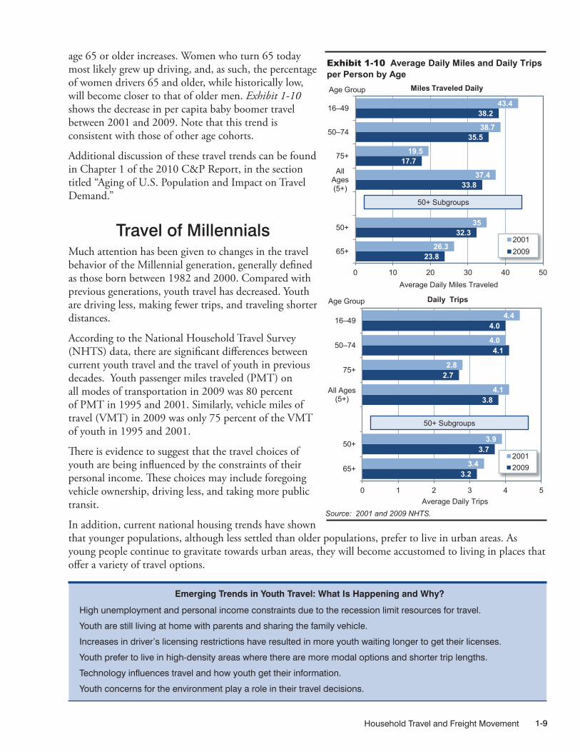
Household Travel and Freight Movement 1-9

age 65 or older increases. Women who turn 65 today most likely grew up driving, and, as such, the percentage of women drivers 65 and older, while historically low, will become closer to that of older men. Exhibit 1-10 shows the decrease in per capita baby boomer travel between 2001 and 2009. Note that this trend is consistent with those of other age cohorts.

Additional discussion of these travel trends can be found in Chapter 1 of the 2010 C&P Report, in the section titled “Aging of U.S. Population and Impact on Travel Demand.”

Travel of Millennials Much attention has been given to changes in the travel behavior of the Millennial generation, generally defined as those born between 1982 and 2000. Compared with previous generations, youth travel has decreased. Youth are driving less, making fewer trips, and traveling shorter distances.

According to the National Household Travel Survey (NHTS) data, there are significant differences between current youth travel and the travel of youth in previous decades. Youth passenger miles traveled (PMT) on all modes of transportation in 2009 was 80 percent of PMT in 1995 and 2001. Similarly, vehicle miles of travel (VMT) in 2009 was only 75 percent of the VMT of youth in 1995 and 2001.

There is evidence to suggest that the travel choices of youth are being influenced by the constraints of their personal income. These choices may include foregoing vehicle ownership, driving less, and taking more public transit.

In addition, current national housing trends have shown that younger populations, although less settled than older populations, prefer to live in urban areas. As young people continue to gravitate towards urban areas, they will become accustomed to living in places that offer a variety of travel options.

9/20/2012 01XH_J (1-10) R3

Exhibit 1-10 Average Daily Miles and Daily Trips per Person by Age

23.8

32.3

33.8

17.7

35.5

38.2

26.3

35

37.4

19.5

38.7

43.4

0 10 20 30 40 50

65+

50+

All Ages (5+)

75+

50–74

16–49

Average Daily Miles Traveled

Age Group Miles Traveled Daily

2001 2009

3.2

3.7

3.8

2.7

4.1

4.0

3.4

3.9

4.1

2.8

4.0

4.4

0 1 2 3 4 5

65+

50+

All Ages (5+)

75+

50–74

16–49

Average Daily Trips

Age Group Daily Trips

2001 2009

Source: 2001 and 2009 NHTS.

50+ Subgroups

50+ Subgroups

Emerging Trends in Youth Travel: What Is Happening and Why?

High unemployment and personal income constraints due to the recession limit resources for travel.

Youth are still living at home with parents and sharing the family vehicle.

Increases in driver’s licensing restrictions have resulted in more youth waiting longer to get their licenses.

Youth prefer to live in high-density areas where there are more modal options and shorter trip lengths.

Technology influences travel and how youth get their information.

Youth concerns for the environment play a role in their travel decisions.

Description of Current System1-10

In 2009, there were about 211 million household vehicles or about 1.86 vehicles per household. Between 2001 and 2009, there was a 0.58-percent annual increase in the average number of household vehicles, in contrast to the long-term annual increase of 2.7 percent over the 40-year period between 1969 and 2009. This indicates that American households continue to depend heavily on automobiles, but appear to be reaching saturation in household vehicle ownership. On the other hand, the number of households with no vehicle available grew slightly by nearly 1 million households, representing a slight increase from 8.1 percent to 8.7 percent of all households. This may be due to changes in economic conditions or household location.

The aging of the household vehicle fleet continues to impact fuel consumption, air quality, and safety. Because over half the household vehicles on the road are more than 9 years old, recent automotive advances in energy efficiency, air quality, and safety are not fully realized in the national vehicle fleet. The 2009 NHTS reflects that the average age of a household vehicle increased from 8.87 years in 2001 to 9.38 years in 2009. In 2009, only 6 percent of household vehicles were 1 year old or newer, 32 percent of vehicles were between 2 and 5 years old, 34 percent were between 6 and 10 years old, and 7 percent were 20 years old or more (see Exhibit 1-12).

Driver’s licensing rates also show a drop between 1995 and 2009. In both 1995 and 2001, 86 percent of all 16-to-28-year-old males were licensed drivers; this drops to 80 percent in 2009. For 16-to-29-year-old females, the licensing rate stays stable at approximately 82 percent across all 3 survey years.

These are some of the emerging factors that are influencing the travel decisions of youth. Together, they warrant further discussion on emerging issues related to travel demand, transportation policy, and the needs and perspectives of those who are soon to be the most predominate users of the transportation system. These and other issues are the topic of research conducted by FHWA (Federal Highway Administration, Office of Transportation Policy Studies, The Next Generation of Travel: Final Report, 2013).

Aging of the Household Vehicle Fleet Like the population as a whole, the household vehicle fleet is also aging. NHTS collects information about household vehicles, including make, model, model year, estimates of annual mileage, and which household member is the primary driver (see Exhibit 1-11). The basic pattern over time is a consistent decrease in household size matched with an increase in vehicles per household.

9/20/2012 01XH_L (1-12) R2

Exhibit 1-12 Age of Household Vehicles

Source: 2009 NHTS.

≤1 Model Year 5.7%

2–5 Model Years 28.6%

6–10 Model Years 32.2%

11–20 Model Years 26.9%

>20 Model Years 6.7%

9/20/2012 01XH_K (1-11) R2

1969 1977 1983 1990 1995 2001 2009Persons per household 3.16 2.83 2.69 2.56 2.63 2.58 2.50Vehicles per household 1.16 1.59 1.68 1.77 1.78 1.87 1.86

Note: The 1969 survey does not include pickups and other light trucks as household vehicles. Source: NHTS data series. See 2009 NHTS Summary of Travel Trends, Table 2.

Exhibit 1-11 Household Size and Vehicles Owned over Time, 1969-2009 NHTS

Household Travel and Freight Movement 1-11

Some Myths and Facts About Daily TravelThis section explores five common misperceptions about travel and what the actual data reveal about these issues.

Myth 1: The majority of personal travel is for commuting to work.Perhaps surprisingly, travel to and from the workplace accounts for only 16 percent of all person trips and 28 percent of all vehicle miles. Only 54 percent of the total population are workers, and 76 percent of the population generally regarded as working age (age 16 to 64) are employed. Even in times of lower unemployment, this percentage does not increase significantly.

Workers drive much more than their nonworker counterparts. Workers age 16 to 64 drive an average of 11,908 miles annually for all purposes, compared to 5,592 for those of the same age who are not employed. Of those 65 and older, those with jobs drive 9,754 miles annually, compared with 4,622 annual miles for those without jobs. The variation in miles driven by employment status is striking considering that workers typically drive more than twice the miles of their nonworking counterparts. Although some of this additional driving is to commute or for work-related travel, workers drive more than nonworkers for each major trip purpose group, as shown below. Exhibit 1-13 displays trip purpose for four groups—workers 16 to 64, workers 65 or older, nonworkers 16 to 64, and nonworkers 65 or older. For workers, 35 percent of driving is for commutes to work, followed by 22 percent for social/recreational trips, and 13 percent each for family/personal errands and for shopping. Together, these four purposes account for 83 percent of driving done by workers.

For the miles driven by the 46 percent of Americans who are not workers, social/recreational travel (34 percent of their VMT) is followed by shopping (24 percent) and family and personal business (23 percent), for a total of 81 percent of their driving.

11/5/2012 01XH_M (1-13) R4.xlsx

Exhibit 1-13 Annual VMT per Person by Trip Purpose, Age, and Worker Status

Source: 2009 NHTS.

1,485 1,567

2,620

4,177

2,059

1,298 1,297

1,778

1,219 1,542 1,539

2,069

2,580

2,024

1,249 974

1,743

656

-

500

1,000

1,500

2,000

2,500

3,000

3,500

4,000

4,500

Shopping Family and Personal Business

Social/Recreational Work Other

Workers (16–64)

Non-Workers (16–64)

Workers (65+)

Non-Workers (65+)

VM

T (M

iles)

Myth 2: Americans love their cars, and that’s why they don’t walk or take transit.Americans’ often cited “love affair” with their cars may have much more to do with the design of our neighborhoods and land use decisions than with transportation. Higher-density areas can provide more opportunities for walking, biking, and transit use than low-density areas. In some low-density neighborhoods, transit services are not cost-effective to provide and there are few destinations, such as schools, jobs, or shopping, within walking distance. People may be left with no other choice but to drive.

Description of Current System1-12

Exhibit 1-14 visually portrays the relationship between population density and the use of transit, walking, and private vehicles.

Households living in higher-density areas have more transportation choices. Of the 50 Metropolitan Statistical Areas (MSAs) with populations greater than 1 million, 14 have at least 10 percent of their populations living in high-density block groups of 10,000 or more persons per square mile. Excluding New York, which accounts for such a huge share of the Nation’s transit trip-making, residents of these 14 areas are at least 8 times more likely to make a trip on transit than those who live in MSAs of 1 million or less, and

9/18/2012 01XH_N (1-14) R4.xlsx

84.1 90.1 96.2 121.9 132.4

157.9

240.4

438.7

0 50

100 150 200 250 300 350 400 450 500

0 to 99

100 to

499

500 to

999

1,000 to

1,999

2,000 to

3,999

4,000 to

9,999

10,000 to

24,999

25,000 and

More

Trip

s P

er P

erso

n pe

r Yea

r

Population per Square Mile (Block Group*)

Annual Walk Trips per Person by Population Density

1.0 1.9 7.7 6.4 13.0 23.2

76.8

244.8

0

50

100

150

200

250

300

0 to 99

100 to

499

500 to

999

1,000 to

1,999

2,000 to

3,999

4,000 to

9,999

10,000 to

24,999

25,000 and

More

Trip

s P

er P

erso

n pe

r Yea

r

Population per Square Mile (Block Group*)

Annual Transit Trips per Person by Population Density

10,889 10,263

8,728 8,406 7,546

6,921

4,851

2,435

0

2,000

4,000

6,000

8,000

10,000

12,000

0 to 99

100 to

499

500 to

999

1,000 to

1,999

2,000 to

3,999

4,000 to

9,999

10,000 to

24,999

25,000 and

More

Ann

ual V

ehic

le M

iles

Population per Square Mile (Block Group*)

Annual Vehicle Miles per Person by Population Density

Exhibit 1-14 Impact of Population Density on Transportation Mode

*Block group – a standard Census Bureau term indicating a subgroup of a Census Tract composed of approximately 1,500 people but may vary from 600-3,000 people. Source: 2009 NHTS. Population density data was appended to the NHTS files from the Nielsen-Claritas annual demographic update. See www.claritas.com/MarketPlace/Default.jsp.

14 MSAs With at Least 10 Percent of People Living in High Density Block Groups of 10,000

Persons or More per Square Mile

New York – 48.0%

Los Angeles – 43.2%

San Francisco – 33.7%

Chicago – 33.0%

Philadelphia – 27.7%

San Diego – 26.8%

Boston – 24.1%

Miami – 23.1%

Las Vegas – 22.2%

Washington DC – 15.7%

Providence – 14.4%

Milwaukee – 12.2%

Pittsburgh – 11.4%

Sacramento – 10.4%

more than 50 times more likely to use transit than those living outside an MSA. Residents of a Big 14 area make walking trips at twice the rate of those in MSAs of 1 million or less, and 2.8 times more than those living outside an MSA (see Exhibit 1-15). (See the discussion of livable communities in Chapter  5 of this edition of the C&P report).

Myth 3: Households without vehicles rely completely on transit, walk, and bike. Although zero-vehicle households rely more heavily on transit, walk, and bike modes than vehicle-owning households do, people in zero-vehicle households accomplish a majority of their travel in private vehicles owned by others. Approximately 9.8 million households, or 8.6 percent of all U.S. households, do not own a vehicle. People in zero-vehicle households average about 100 minutes of travel a day, 76 percent of which are as a driver or passenger in a private vehicle; they accomplish 50.7 percent of their person miles of travel in private vehicles.

Household Travel and Freight Movement 1-13

Because the data in this section are presented as person trips and person miles, private vehicle travel includes travel in a vehicle as a driver and as a passenger. Those in zero-vehicle households could be using a car borrowed from a friend or relative or be a vehicle passenger in another household’s car. (See Exhibit 1-16.) The vehicle occupancy per private vehicle trip by members of zero-vehicle households is, as expected, consistently larger (2.06) than the occupancy rate of vehicle-owning household members (1.67).

11/7/2012 01XH_O (1-15) R4

Source: 2009 NHTS. Population density data was appended to the NHTS files from the Nielsen-Claritas annual demographic update.

Exhibit 1-15 Walk and Transit Rates by Area Type

289.7

185.6

125.6 116.3 99.1

428.3

279.8

161.9 147.4

0

50

100

150

200

250

300

350

400

450

New York Remainder of Big 14 Other MSA, More Than 1 Million

Other MSA, Less Than 1 Million

Not in MSA

Person Trips Per Person Per Year (Walk Rate)

All

High-Density Block Groups

Remainder of Area

131.5

45.1 13.8 9.6 1.6

248.3

102.9

23.4 21.7 0

50

100

150

200

250

300

New York Remainder of Big 14 Other MSA, More Than 1 Million

Other MSA, Less Than 1 Million

Not in MSA

Person Trips Per Person Per Year (Transit Rate)

All High-Density Block Groups Remainder of Area

1/3/2013 01XH_P (1-16) R5.xlsx

Source: 2009 NHTS.

Exhibit 1-16 Distribution of Person Trips and Person Miles by Mode and Household Vehicles

0%

25%

50%

75%

100%

Zero Vehicles At Least 1 Vehicle

Distribution of Person Miles by Mode

Other (e.g., Air)

Walk/Bike

Transit

Privately Owned Vehicle

0%

25%

50%

75%

100%

Zero Vehicles At Least 1 Vehicle

Distribution of Person Trips by Mode

Other (e.g., Air)

Walk/Bike

Transit

Privately Owned Vehicle

1/3/2013 01XH_P (1-16) R5.xlsx

Source: 2009 NHTS.

Exhibit 1-16 Distribution of Person Trips and Person Miles by Mode and Household Vehicles

0%

25%

50%

75%

100%

Zero Vehicles At Least 1 Vehicle

Distribution of Person Miles by Mode

Other (e.g., Air)

Walk/Bike

Transit

Privately Owned Vehicle

0%

25%

50%

75%

100%

Zero Vehicles At Least 1 Vehicle

Distribution of Person Trips by Mode

Other (e.g., Air)

Walk/Bike

Transit

Privately Owned Vehicle

Description of Current System1-14

Who are the zero-vehicle households?

Exhibit 1-17 summarizes the characteristics of zero-vehicle households. Some observations:

• They are disproportionally Black and Hispanic. The share of all U.S. households without a vehicle is 8.7 percent; this percentage goes up to 13.8 percent for Hispanic households and 22.6 percent for Black households.

• They are smaller than average households and have lower incomes. Of all zero-vehicle households, 70 percent have incomes less than $30,000.

• They are typically poorer than average households, but not in all cases. Sixty percent of zero-vehicle households make less than $20,000 annually, as compared to 16 percent of vehicle-owning households.

• Of zero-vehicle U.S. households, 4.3 percent earn more than $80,000 a year, and the majority of this group lives in the New York Metro Region.

• Whether at the low or high end of the income scale, zero-vehicle households tend to be in the largest metro areas with populations of 3 million or more. Zero-vehicle households make up 8.7 percent of all U.S. households, but they make up 12.6 percent of the households in these largest metro areas. In other words, 51 percent of all zero-vehicle households live in areas of 3 million or more, compared to 35 percent for households with one or more vehicles.

Q A&

5/22/2013 01XH_Q (1-17) R3.xlsx

Source: 2009 NHTS.

Exhibit 1-17 Characteristics of Zero-Vehicle Households 0 5 10 15 20 25 30

WhiteBlackAsian

HispanicOther

Less Than $30,000$30,000–$49,999 $50,000–$69,999 $70,000–$99,999

$100,000 or GreaterNot in MSA

Less Than 500,000In MSA of 500,000–999,999

In MSA of 1,000,000–2,999,999 In MSA of 3,000,000 or Greater

Population/Sq Mi Less Than 4,000Pop/Sq Mi 4,000–9,999

Pop/Sq Mi 10,000 or Greater

Rac

e In

com

e D

ensi

ty

MSA

Siz

e

U.S. Average for Zero-Vehicle Households = 8.7%

0 30 25 20 15 10 5 Percent Zero-Vehicle Households

Car Share Services

Some of households that are non-vehicle owning by choice are using the expanding option of car-share services, such as Zip Cars and Car2go. Unlike traditional car rental agencies, car-sharing is set up to allow rentals by the minute or the hour. These services are designed for high-density areas and often have reserved parking spaces, an especially convenient benefit for urban dwellers. The NHTS did not collect data on car-sharing in the 2009 survey, but may do so in 2015.

Whether the household is without a vehicle by necessity or by choice, its daily travel is considerably lower than that of vehicle-owning households. While a zero-vehicle household has half the daily person trip rate of a vehicle-owning household, their daily person miles of travel is one-fifth that of their vehicle-owning counterparts.

Household Travel and Freight Movement 1-15

9/20/2012 01XH_R (1-18) R2

Source: 2009 NHTS.

Exhibit 1-18 Person Miles by Private Vehicle, Transit, and Walk by Age and Travel Disability

0

2,000

4,000

6,000

8,000

10,000

12,000

14,000

16,000

18,000

16–34 35–64 65–74 75–84 85+

Annu

al M

iles

Age of Traveler

Annual Person Miles by Privately Owned Vehicle Per Person by Age, Gender, and Medical Condition

Male (All)

Male (Medical Condition)

Female (All)

Female (Medical Condition)

0

50

100

150

200

250

300

350

400

450

16–34 35–64 65–74 75–84 85+

Annu

al M

iles

Age of Traveler

Annual Person Miles on Transit Per Person by Age, Gender, and Medical Condition

Male (All)

Male (Medical Condition)

Female (All)

Female (Medical Condition)

0

20

40

60

80

100

120

16–34 35–64 65–74 75–84 85+

Annu

al M

iles

Age of Traveler

Annual Person Miles by Walk Per Person by Age, Gender, and Medical Condition

Male (All)

Male (Medical Condition)

Female (All)

Female (Medical Condition)

Myth 4: When elderly drivers give up their driver’s license they maintain mobility by using transit or walking instead of using private vehicles. Like the rest of the U.S. population, the elderly are heavily dependent on private vehicle travel to meet their needs. Although some relocate, a large portion of the elderly age in place in the homes where they raised their families. Issues of diminished eyesight, response time, and physical mobility that might keep an older person from driving may also keep them from being able to walk or take transit, making them more likely to travel as a private vehicle passenger or simply stay at home.The NHTS collects data on whether or not respondents have medical conditions that make it difficult for them to travel outside the home. As shown in Exhibit 1-18, those with a travel disability have a lower rate of

9/20/2012 01XH_R (1-18) R2

Source: 2009 NHTS.

Exhibit 1-18 Person Miles by Private Vehicle, Transit, and Walk by Age and Travel Disability

0

2,000

4,000

6,000

8,000

10,000

12,000

14,000

16,000

18,000

16–34 35–64 65–74 75–84 85+

Ann

ual M

iles

Age of Traveler

Annual Person Miles by Privately Owned Vehicle Per Person by Age, Gender, and Medical Condition

Male (All)

Male (Medical Condition)

Female (All)

Female (Medical Condition)

0

50

100

150

200

250

300

350

400

450

16–34 35–64 65–74 75–84 85+

Ann

ual M

iles

Age of Traveler

Annual Person Miles on Transit Per Person by Age, Gender, and Medical Condition

Male (All)

Male (Medical Condition)

Female (All)

Female (Medical Condition)

0

20

40

60

80

100

120

16–34 35–64 65–74 75–84 85+

Ann

ual M

iles

Age of Traveler

Annual Person Miles by Walk Per Person by Age, Gender, and Medical Condition

Male (All)

Male (Medical Condition)

Female (All)

Female (Medical Condition)

9/20/2012 01XH_R (1-18) R2

Source: 2009 NHTS.

Exhibit 1-18 Person Miles by Private Vehicle, Transit, and Walk by Age and Travel Disability

0

2,000

4,000

6,000

8,000

10,000

12,000

14,000

16,000

18,000

16–34 35–64 65–74 75–84 85+

Ann

ual M

iles

Age of Traveler

Annual Person Miles by Privately Owned Vehicle Per Person by Age, Gender, and Medical Condition

Male (All)

Male (Medical Condition)

Female (All)

Female (Medical Condition)

0

50

100

150

200

250

300

350

400

450

16–34 35–64 65–74 75–84 85+

Ann

ual M

iles

Age of Traveler

Annual Person Miles on Transit Per Person by Age, Gender, and Medical Condition

Male (All)

Male (Medical Condition)

Female (All)

Female (Medical Condition)

0

20

40

60

80

100

120

16–34 35–64 65–74 75–84 85+

Ann

ual M

iles

Age of Traveler

Annual Person Miles by Walk Per Person by Age, Gender, and Medical Condition

Male (All)

Male (Medical Condition)

Female (All)

Female (Medical Condition)

Description of Current System1-16

transit use and walking than others of the same age and there is a slight increase in the relative use of private vehicles, particularly by older women.

Myth 5: We can solve congestion by having people shift noncommuting trips outside of peak periods. Encouraging the traveling public to make noncommuting trips outside of peak periods would appear to be a reasonable proposal for addressing congestion, but there are many scenarios that simply do not allow for such time flexibility. For example, picking up your child from an athletic practice or an after-school event typically needs to be done when the child is ready, not some arbitrary time after peak period. A doctor’s office would usually be open in morning and afternoon peak periods, but it would not likely be open in the evening. Although trips and travel for shopping and errand-running are not as constrained by time of day as some of the other trip purposes, many people choose to make these trips on their way to or from work.

While time-shifting may be possible for some share of trips, it is clear that the public is willing to put up with the inconvenience of congestion during peak periods to accomplish many of their travel needs. Exhibit 1-19 identifies the share of person trips in the peak period for different types of non-commuting trips.

Gas Prices and the Public’s OpinionsThe price of gas rose to a nationwide average of over $3.50 per gallon in May of 2008 and did not drop below that level until October of that year. It peaked at $4.11 per gallon in June and July.

In comparing the two survey years, 2001 and 2009, average daily vehicle miles by month remained around the same through August across the 2 years possibly because the public has come to expect some increases in gas cost during the summer travel season. (See Exhibit 1-20.) In August of 2001, gas prices declined and more daily driving occurred. This follows a typical pattern of personal VMT peaking in August. However, this pattern did not repeat itself in 2008, when gas prices remained high for about 4 months and people adjusted their average daily miles. The average daily VMT per driver decreased by 13 percent in August of 2008, when gas prices remained higher than $3.80 per gallon. This apparent delayed response to high gas prices may have been because the public was waiting to see how long the phenomenon would continue. According to the NHTS data, it appears that most people decided to cut their driving in August of 2008 by an average of 3 to 4 daily miles relative to August 2001.

11/9/2012 01XH_S (1-19) R4.xlsx

* Peak period is defined as 6:30 a.m.–9:30 a.m. and 3:30 p.m.–6:30 p.m. Source: 2009 NHTS.

Exhibit 1-19 Percent of Person Trips by Selected Purpose During Peak and Off-Peak Hours

70.6

38.1 32.1

37.8 37.0

52.0

33.7

29.4 61.9 67.9 62.2 63.0 48.0 66.3

0%

25%

50%

75%

100%

School/ Church

Medical/ Dental

Shopping Social Family Obligations

Serve Passenger

Meals

Off-Peak Travel

Peak Travel*

Household Travel and Freight Movement 1-17

Number One Issue for the Public: Price of Travel Questions to elicit the public’s opinions about transportation were included in the 2009 NHTS because understanding their attitudes and perceptions is valuable when prioritizing policy. Respondents were asked to select what they considered the most important issue from a list of six pre-identified issues:

� Highway congestion � Access to and availability of public transit � Lack of walkways and sidewalks � Price of travel including things like transit fees, tolls and the cost of gasoline � Aggressive and distracted drivers � Safety concerns.

One-third of all respondents selected the price of travel as the most important issue. When drivers were divided by demographic categories such as gender, race, income, and education, the data revealed no significant difference in their selection of travel price as the primary issue. A disproportionate share of respondents say that price of travel was their number one concern. This may have been due to the rising cost of gasoline or because of the economic recession during the data collection period.

Households with incomes of $40,000 to $70,000 ranked price as most important issue about 5 percent more often than households in both higher and lower income categories. During the post-peak period between October 2008 and April 2009, almost all households at all levels started shifting their opinions to the issues of safety and aggressive drivers (approximately 20 percent each) but 27 percent kept price as their major issue. Only households in the highest income bracket (those with incomes of $100,000 or more) selected congestion as their most important concern in this post-peak period (about 26 percent). This suggests that the gas price fluctuation remained important with middle income households throughout the study more so than with other households. 9/20/2012 01XH_T (1-20) R2

Avg. Gas Price

Avg. Gas Price

(in 2008 $) (in 2008 $)

March $1.77 16.6 $3.29 20.4April $1.94 22.3 $3.51 23.1May $2.12 22.7 $3.82 22.2June $2.02 23.4 $4.11 22.0July $1.79 22.9 $4.11 22.6August $1.78 24.0 $3.83 20.8September $1.90 21.8 $3.76 21.2October $1.66 21.9 $3.11 22.8November $1.48 22.3 $2.21 21.6December $1.37 21.3 $1.75 21.1

January $1.40 21.0 $1.84 19.9February $1.41 23.7 $1.98 22.2March $1.57 22.7 $2.01 22.0April $1.76 21.6 $2.10 21.7

2002 2009

Daily VMT per Person

Daily VMT per Person

2001 2008

Source: 2009 NHTS for VMT per Driver. Average Gas Price is from the Energy Information Administration (EIA), Forms EIA-782A, "Refiners'/GasPlant Operators' Monthly Petroleum Product Sales Report," and EIA-782B, "Resellers'/Retailers' Monthly Petroleum Product Sales Report."

Exhibit 1-20 Average Gas Price per Month and Daily VMT per Driver, 2001–2002 and 2008–2009

Description of Current System1-18

Freight Movement

The economy of the United States depends on freight transportation to link businesses with suppliers and markets throughout the Nation and the world. Freight impacts nearly every American business and household in some way. American farms and mines rely on affordable and reliable transportation to compete against their counterparts around the world. Domestic manufacturers rely on remote sources of raw materials to produce goods. Wholesalers and retailers depend on fast and reliable transportation to obtain inexpensive or specialized goods. In the expanding world of e-commerce, households and small businesses increasingly depend on freight transportation to deliver purchases directly to them. Service providers, public utilities, construction companies, and government agencies rely on freight transportation to obtain needed equipment and supplies from distant sources.

The U.S. economy requires effective freight transportation that operates at minimum cost and allows shippers and freight carriers to quickly respond to the demands for goods. As the economy grows over the next several decades, the demand for goods and the volume of freight transportation activity will only increase. Current volumes of freight are straining the capacity of the transportation system to deliver goods quickly, reliably, and cheaply. Anticipated growth of freight could overwhelm the system’s ability to meet the needs of the American economy unless public agencies and private industry work together to improve the system’s performance.

Freight Transportation SystemThe FHWA’s Freight Facts and Figures 2011 publication shows that the U.S. freight transportation system moves nearly 52 million tons of freight worth more than $46 billion each day to meet the logistical needs of the Nation’s 117 million households, 7.4 million business establishments, and 89,500 government units. This system includes nearly 11 million single-unit and combination trucks, nearly 1.4 million locomotives and rail cars, and more than 40,000 marine vessels. The system operates on more than 450,000 miles of arterial highways, nearly 140,000 miles of railroads, 11,000 miles of inland waterways and the Great Lakes-St. Lawrence Seaway system, and 1.7 million miles of petroleum and natural gas pipelines. The U.S. Army Corps of Engineers’ Waterborne Commerce of the United States 2007 publication identifies 146 ports that handle more than 1 million tons of freight per year.

The freight transportation system is more than equipment and facilities. As reported in Freight Facts and Figures 2011, freight transportation establishments with payrolls primarily serving for-hire transportation and warehousing employ nearly 4.2 million workers. Truck transportation businesses make up the largest freight transportation employment sector in the U.S., employing more than 2.6 million workers in 2010. Other freight transportation occupations included rail and water vehicle operators, as well as other occupations such as warehousing and storage, equipment manufacturing, equipment maintenance, and other transportation support service providers.

Freight Transportation DemandFreight movements in the United States take a variety of forms, from the shipment of farm products across town to the shipment of electronic devices across the world. These goods move within, to, and from the U.S. via the Nation’s highways, railroads, waterways, airplanes, and pipelines, sometimes using a combination of modes to complete the trip. Due to the country’s well-developed highway network and the transport

Household Travel and Freight Movement 1-19

connectivity and flexibility that this network provides, the majority of freight moved within, to, or from the United States is transported by truck. Exhibit 1-21 shows a breakdown of freight movements by mode, measured by both tonnage and value of shipment.

Exhibit 1-22 shows a map illustrating the distribution of the tonnage information shown in the table in Exhibit 1-21 for truck, rail, and inland water shipments on the United States freight transportation network.

Exhibit 1-23 shows the same information as Exhibit 1-22, but only includes long-haul truck shipments on the National Highway System.

ModeTons

(Millions) Percent

Value (Billions of

Dollars) PercentTruck 12,778 67.7% 10,780 64.7%Rail 1,900 10.1% 512 3.1%Water 941 5.0% 339 2.0%Air, Air & Truck 13 <0.1% 1,077 6.5%

Multiple Modes & Mail 1,424 7.5% 2,879 17.3%

Pipeline 1,507 8.0% 723 4.3%Other & Unknown 316 1.7% 341 2.0%

Total 18,879 100% 16,651 100%

Exhibit 1-21 Goods Movement by Mode, 2007

Notes: Numbers may not add to totals due to rounding. All truck, rail, water, and pipeline movements that involve more than one mode, including exports and imports that change mode at international gateways, are included in multiple modes and mail to avoid double counting. As a consequence, rail and water totals in this table are less than other published sources. By contrast, all air cargo movements that are shipped via truck at the ends of the trips are included in the "Air, Air & Truck" category. In addition, it should be noted that raw tonnage statistics does not take into account the distance these goods were moved. To use one example, a shipment, such as a shipping container, that is transported 2 miles by truck and 2,000 miles by rail is treated the same when measured by tonnage. Source: Freight Analysis Framework 3.3.

12/12/2013 01XF_A (1-21) R2.xlsx

11/5/2012 01XF_B (1-22) R2.xlsx

Sources: Highways —U.S. Department of Transportation, Federal Highway Administration, Freight Analysis Framework, Version 3.2, 2010. Rail—Based on Surface Transportation Board, Annual Carload Waybill Sample and rail freight flow assignments done by Oak Ridge National Laboratory. Inland Waterways—U.S. Army Corps of Engineers (USACE), Annual Vessel Operating Activity and Lock Performance Monitoring System data, as processed for USACE by the Tennessee Valley Authority, and USACE, Institute for Water Resources, Waterborne Foreign Trade Data. Water flow assignments done by Oak Ridge National Laboratory.

Exhibit 1-22 Tonnage on Highways, Railroads, and Inland Waterways, 2007

ModeTons

(Millions) Percent

Value (Billions of

Dollars) PercentTruck 12,778 67.7% 10,780 64.7%Rail 1,900 10.1% 512 3.1%Water 941 5.0% 339 2.0%Air, Air & Truck 13 <0.1% 1,077 6.5%

Multiple Modes & Mail 1,424 7.5% 2,879 17.3%

Pipeline 1,507 8.0% 723 4.3%Other & Unknown 316 1.7% 341 2.0%

Total 18,879 100% 16,651 100%

Exhibit 1-21 Goods Movement by Mode, 2007

Notes: Numbers may not add to totals due to rounding. All truck, rail, water, and pipeline movements that involve more than one mode, including exports and imports that change mode at international gateways, are included in multiple modes and mail to avoid double counting. As a consequence, rail and water totals in this table are less than other published sources. By contrast, all air cargo movements that are shipped via truck at the ends of the trips are included in the "Air, Air & Truck" category. In addition, it should be noted that raw tonnage statistics does not take into account the distance these goods were moved. To use one example, a shipment, such as a shipping container, that is transported 2 miles by truck and 2,000 miles by rail is treated the same when measured by tonnage. Source: Freight Analysis Framework 3.3.

12/12/2013 01XF_A (1-21) R2.xlsx

Description of Current System1-20

Freight Statistics

Many of the freight statistics in this section are derived from the Freight Analysis Framework (FAF) version 3 (FAF3) and FAF version 2 (FAF2). Both versions of the FAF include all freight flows to, from, and within the United States. FAF estimates are recalibrated every 5 years, primarily with data from the Commodity Flow Survey (CFS), and are updated annually with provisional estimates. The CFS, conducted every 5 years by the Census Bureau and U.S. DOT’s Bureau of Transportation Statistics, measures approximately two-thirds of the tonnage covered by the FAF. FAF3 incorporates data from the 2007 CFS; FAF2 was based on 2002 data.

Statistics on trucking activity are primarily from FHWA’s Highway Performance Monitoring System and the Census Bureau’s Vehicle Inventory and Use Survey (VIUS). The VIUS links truck size and weight, miles traveled, energy consumed, economic activity served, commodities carried, and other characteristics of significant public interest, but was discontinued after 2002. For more information, see www.ops.fhwa.dot.gov/freight/freight_analysis/faf.

Freight movements are expected to increase over the next few decades as both the U.S. and global population grow and national and global consumer spending power increases, helping to increase demand for many types of goods. All freight transportation modes are expected to experience increased volumes, although the amount of expected growth will vary from mode to mode, as shown in Exhibit 1-24.

9/20/2012 01XF_C (1-23) R1

Note: Long-haul trucks typically serve locations at least 50 miles apart, excluding trucks that are used in movements by multiple modes and mail. Source: U.S. Department of Transportation, Federal Highway Administration, Office of Freight Management and Operations, Freight Analysis Framework, Version 3.1, 2010.

Exhibit 1-23 Average Daily Long-Haul Freight Truck Traffic on the National Highway System, 2007

Household Travel and Freight Movement 1-21

Even though the annual volume increases are modest for all modes, the cumulative 30-year growth for each mode is significant, and the increased volume will create additional strain on the entire freight transportation network, most notably the highway network. Exhibit 1-25 shows a map containing the 2040 truck tonnage information shown in Exhibit 1-24 plotted to the National Highway System.

Many key truck routes on the National Highway System are expected to experience significant increases in truck volume between 2007 and 2040. These projected traffic increases would have major implications for highway congestion and freight movement efficiency, especially near large urban areas along or near major truck corridors.

9/20/2012 01XF_D (1-24) R1

Compound Annual

2040 Projected

Growth, 2010–2040

Truck 12,778 12,490 18,503 1.3%Rail 1,900 1,776 2,353 0.9%Water 941 860 1,263 1.3%Air, Air & Truck 13 12 43 4.4%Multiple Modes & Mail* 1,424 1,380 2,991 2.6%

Pipeline 1,507 1,494 1,818 0.7%Other & Unknown 316 302 514 1.8%Total 18,879 18,313 27,484 1.4%

Mode 2007 2010

* In this table, Multiple Modes & Mail includes export and import shipments that move domestically by a different mode than the mode used between the port and foreign location. Note: Data do not include imports and exports that pass through the United States from a foreign origin to a foreign destination by any mode. Numbers may not add to total due to rounding. Source: U.S. Department of Transportation, Federal Highway Administration, Office of Freight Management and Operations, Freight Analysis Framework, version 3.2, 2011.

Exhibit 1-24 Weight of Shipments by Transportation Mode (Millions of Tons)

9/20/2012 01XF_E (1-25) R1

Note: Long-haul trucks typically serve locations at least 50 miles apart, excluding trucks that are used in movements by multiple modes and mail. Source: U.S. Department of Transportation, Federal Highway Administration, Office of Freight Management and Operations, Freight Analysis Framework, Version 3.1, 2010.

Exhibit 1-25 Average Daily Long-Haul Freight Truck Traffic on the National Highway System, 2040

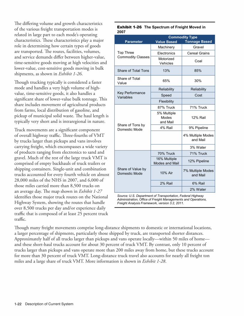
Description of Current System1-22

The differing volume and growth characteristics of the various freight transportation modes is related in large part to each mode’s operating characteristics. These characteristics play a major role in determining how certain types of goods are transported. The routes, facilities, volumes, and service demands differ between higher-value, time-sensitive goods moving at high velocities and lower-value, cost-sensitive goods moving in bulk shipments, as shown in Exhibit 1-26.

Though trucking typically is considered a faster mode and handles a very high volume of high-value, time-sensitive goods, it also handles a significant share of lower-value bulk tonnage. This share includes movement of agricultural products from farms, local distribution of gasoline, and pickup of municipal solid waste. The haul length is typically very short and is intraregional in nature.

Truck movements are a significant component of overall highway traffic. Three-fourths of VMT by trucks larger than pickups and vans involves carrying freight, which encompasses a wide variety of products ranging from electronics to sand and gravel. Much of the rest of the large truck VMT is comprised of empty backhauls of truck trailers or shipping containers. Single-unit and combination trucks accounted for every fourth vehicle on almost 28,000 miles of the NHS in 2007, and 6,000 of those miles carried more than 8,500 trucks on an average day. The map shown in Exhibit 1-27 identifies those major truck routes on the National Highway System, showing the routes that handle over 8,500 trucks per day and/or experience daily traffic that is composed of at least 25 percent truck traffic.

Though many freight movements comprise long-distance shipments to domestic or international locations, a larger percentage of shipments, particularly those shipped by truck, are transported shorter distances. Approximately half of all trucks larger than pickups and vans operate locally—within 50 miles of home—and these short-haul trucks account for about 30 percent of truck VMT. By contrast, only 10 percent of trucks larger than pickups and vans operate more than 200 miles away from home, but these trucks account for more than 30 percent of truck VMT. Long-distance truck travel also accounts for nearly all freight ton miles and a large share of truck VMT. More information is shown in Exhibit 1-28.

10/21/2012 01XF_F (1-26) R2.xlsx

Value Based Tonnage BasedMachinery Gravel

Electronics Cereal GrainsMotorized Vehicles Coal

Share of Total Tons 13% 85%

Share of Total Value 65% 30%

Reliability Reliability

Speed Cost

Flexibility

87% Truck 71% Truck5% Multiple

Modes and Mail

12% Rail

4% Rail 9% Pipeline

4% Multiple Modes and Mail

3% Water

70% Truck 71% Truck16% Multiple

Modes and Mail 12% Pipeline

10% Air 7% Multiple Modes and Mail

2% Rail 6% Rail

2% Water

Share of Value by Domestic Mode

ParameterCommodity Type

Top Three Commodity Classes

Key Performance Variables

Share of Tons by Domestic Mode

Source: U.S. Department of Transportation, Federal Highway Administration, Office of Freight Managements and Operations, Freight Analysis Framework, version 3.2, 2011.

Exhibit 1-26 The Spectrum of Freight Moved in 2007

Household Travel and Freight Movement 1-239/20/2012 01XF_G (1-27) R1

Note: AADTT is the average annual daily truck traffic and includes all freight-hauling and other trucks with six or more tires. AADT is average annual daily traffic and includes all motor vehicles. Source: U.S. Department of Transportation, Federal Highway Administration, Office of Freight Management and Operations, Freight Analysis Framework, version 3.1, 2010.

Exhibit 1-27 Major Truck Routes on the National Highway System, 2007

10/26/2012 01XF_H (1-28) R2

Trucks Truck Miles(percent) (percent)

Off the road 3.3% 1.6%

50 miles or less 53.3% 29.3%

51 to 100 miles 12.4% 13.2%

101 to 200 miles 4.4% 8.1%

201 to 500 miles 4.2% 12.1%

501 miles or more 5.3% 18.4%

Not reported 13.0% 17.3%

Not applicable 4.1% 0.1%

Total 100% 100%

Location

Exhibit 1-28 Trucks and Truck Miles by Range of Operations

Note: Includes trucks registered to companies and individuals in the United States except pickups, minivans, other light vans, and sport utility vehicles. Numbers may not add to total due to rounding. Source: U.S. Department of Commerce, Census Bureau, 2002 Vehicle Inventory and Use Survey: United States, EC02TV-US, Table 3a (Washington, DC: 2004), available at http://www.census.gov/prod/ec02/ec02tv-us.pdf as of July 31, 2012.

Description of Current System1-24

Freight Data Reporting and Ton-Miles

Passenger transportation volumes often use passenger-miles to measure transportation volume. The analogous measure for freight would seem to be ton-miles. Computing freight ton-miles by transportation mode is both difficult and potentially misleading for three reasons: (1) a “ton” of freight varies widely in both the nature and composition of commodities because, unlike passenger miles where a passenger is a fixed unit, for freight a ton of coal is a very different commodity than a ton of frozen ice cream; (2) freight value and tonnage often, though not always, move in opposite directions because lighter-weight goods often have higher value on a per-weight basis and are underrepresented in ton-miles measures while heavier-weight goods often are lower value on a per-weight basis and are overrepresented in ton-miles measures; and (3) ton-miles masks commodity attributes such as value and distance bracket (see Exhibit 1-28), which are important determinants of mode choice.

Although computationally difficult, the Bureau of Transportation Statistics (BTS) has conducted a special tabulation of annual freight ton-miles (1980–2009) for all freight transportation modes (air, truck, railroad, domestic water transportation, and pipeline). Exhibit 1-29 represents an excerpt from the BTS tabulation and shows that railroad moves make up the largest single mode share with over 35 percent of the ton-miles, since the railroads tend to move heavy commodities over long distances. When considered in isolation the downward shift in truck ton-miles from 2005 to 2009 hides the trend of increasing truck VMT during that same time period.

12/18/2013 01XF_I (1-29) R1.xlsx]

2005 2006 2007 2008 2009

TOTAL U.S. ton-miles of freight 4,570,316 4,630,792 4,695,555 4,647,112 4,302,320

Air 15,745 15,361 15,142 13,774 12,027

Truck 1,291,308 1,291,244 1,403,538 1,429,296 1,321,396

Railroad 1,733,329 1,855,902 1,819,633 1,729,737 1,582,093

Domestic water transportation 591,276 561,629 553,143 520,494 477,122

Pipeline 938,659 906,656 904,101 953,812 909,682

Source: Bureau of Transportation Statistics, National Transportation Statistics, Table 1-50. (http://www.rita.dot.gov/bts/sites/rita.dot.gov.bts/files/publications/national_transportation_statistics/html/table_01_50.html).

Exhibit 1-29 U.S. Ton-Miles of Freight (BTS Special Tabulation) (Millions)

12/18/2013 01XF_I (1-29) R1.xlsx]

2005 2006 2007 2008 2009

TOTAL U.S. ton-miles of freight 4,570,316 4,630,792 4,695,555 4,647,112 4,302,320

Air 15,745 15,361 15,142 13,774 12,027

Truck 1,291,308 1,291,244 1,403,538 1,429,296 1,321,396

Railroad 1,733,329 1,855,902 1,819,633 1,729,737 1,582,093

Domestic water transportation 591,276 561,629 553,143 520,494 477,122

Pipeline 938,659 906,656 904,101 953,812 909,682

Source: Bureau of Transportation Statistics, National Transportation Statistics, Table 1-50. (http://www.rita.dot.gov/bts/sites/rita.dot.gov.bts/files/publications/national_transportation_statistics/html/table_01_50.html).

Exhibit 1-29 U.S. Ton-Miles of Freight (BTS Special Tabulation) (Millions)

Household Travel and Freight Movement 1-25

Freight Transportation and the Cost of Goods

Geographic accessibility of the major freight corridors and the performance of these corridors stimulate economic activity and create jobs. While deregulation and other factors lowered the cost of freight transportation for a given level of service over the past four decades, congestion, rising fuel prices, environmental constraints1, and other factors could increase the cost of moving all goods in the years ahead. If these factors are not mitigated, the increased cost of moving freight will be felt throughout the economy, affecting businesses and households alike.

The long and often vulnerable supply chains of high-value, time-sensitive commodities are particularly susceptible to congestion. Congestion results in enormous costs to shippers, carriers, and the economy. For example, Nike spends an additional $4 million per week to carry an extra 7 to 14 days of inventory to compensate for shipping delays.2 One day of delay requires APL’s eastbound trans-Pacific services to use an additional 1,300 containers and chassis, which adds $4 million in costs per year.3 A week-long disruption to container movements through the Ports of Los Angeles and Long Beach could cost the national economy between $65 million and $150 million per day.4 Freight bottlenecks on highways throughout the United States cause more than 243 million hours of delay to truckers annually.5 At a delay cost of $26.70 per hour, the conservative value used by the FHWA’s Highway Economic Requirements System model for estimating national highway costs and benefits, these bottlenecks cost truckers about $6.5 billion per year.

Congestion costs are compounded by continuing increases in operating costs per mile and per hour. The cost of highway diesel fuel more than doubled in constant dollars over the decade ending in 2011 and would have quadrupled if the prices at the peak in 2008 had continued.6 Future labor costs are projected to increase at a faster rate than in the past in response to the growing shortage of truck drivers.7 To attract and retain more drivers, carriers will reduce the number of hours drivers are on the road, which will in turn increase operating costs. Railroads also are facing labor recruitment challenges.8 Beyond fuel and labor, truck operating costs are affected by needed repairs to damaged equipment caused by deteriorating roads; taxes and tolls to pay for repair of infrastructure; and insurance and additional equipment required to meet security, safety, and environmental requirements.

Increased costs to carriers are reflected eventually in increased prices paid for freight transportation. Between 2003 and 2009, prices increased 17 percent for truck transportation, 36 percent for rail transportation, 16 percent for scheduled air freight, 16 percent for water transportation, 41 percent for pipeline transportation of crude petroleum, 29 percent for other pipeline transportation, and 9 percent for freight transportation support activities.9

The importance of freight transportation varies by economic sector. For example, $1 of final demand for agricultural products requires 14.2 cents in transportation services, compared with 9.1 cents for manufactured goods and about 8 cents for mining products.10 An increase in transportation cost affects inexpensive (on a per-ton basis), cost-sensitive bulk commodities more than high-value, time-sensitive commodities that have higher margins. In either case, an increase in transportation costs will ripple through all these industries, affecting not only the cost of goods from all economic sectors but also markets for the goods.1 “Environmental constraints” is primarily meant to include environmental regulations that require the use of cleaner, lower emissions fuels and/or place higher taxes on higher emissions fuels.2 John Isbell, “Maritime and Infrastructure Impact on Nike’s Inbound Delivery Supply Chain,” TRB Freight Roundtable, October 24, 2006 www.trb.org/conferences/FDM/Isbell.pdf.3 John Bowe, “The High Cost of Congestion,” TRB Freight Roundtable, October 24, 2006 www.trb.org/conferences/FDM/Bowe.pdf.4 U.S. Congressional Budget Office, The Economic Costs of Disruptions in Container Shipments, March 26, 2006 www.cbo.gov/ftpdocs/71xx/doc7106/03-29-Container_Shipments.pdf.5 FHWA, An Initial Assessment of Freight Bottlenecks on Highways, October 2005 www.fhwa.dot.gov/policy/otps/bottlenecks.6 FHWA, Freight Facts and Figures 2011, figure 4-2, page 50.7 Inbound Logistics. “Trucking Perspectives, 2013,” September 2013 http://www.inboundlogistics.com/cms/article/trucking-perspectives-2013/8 Federal Railroad Administration, An Examination of Employee Recruitment and Retention in the U.S. Railroad Industry, 2007 www.fra.dot.gov/us/content/1891.9 FHWA, Freight Facts and Figures 2011, table 4-6, page 49.10 DOT, Bureau of Transportation Statistics, “The Economic Importance of Transportation Services: Highlights of the Transportation Satellite Accounts,” BTS/98-TS4R, April 1998, figure 2, page 5.

Description of Current System1-26

Freight ChallengesThe challenges of moving the Nation’s freight cheaply and reliably on an increasingly constrained infrastructure without affecting safety and degrading the environment are substantial, and traditional strategies to support passenger travel may not provide adequate solutions. The freight transportation challenge differs from that of urban commuting and other passenger travel in several ways:

� Freight often moves long distances through localities and responds to distant economic demands, while the majority of passenger travel occurs between local origins and destinations. Freight movement often creates local problems without local benefits.

� Freight movements fluctuate more quickly and in greater relative amounts than passenger travel. Both passenger travel and freight respond to long-term demographic change, but freight responds more quickly than passenger travel to short-term economic fluctuations. Fluctuations can be national or local. The addition or loss of just one major business can dramatically change the level of freight activity in a locality.

� Freight movement is heterogeneous compared with passenger travel. Patterns of passenger travel tend to be very similar across metropolitan areas and among large economic and social strata. The freight transportation demands of farms, steel mills, and clothing boutiques differ radically from one another. Solutions aimed at average conditions are less likely to work because the freight demands of economic sectors vary widely.

� Improvements targeted at freight demand are needed because freight accounts for a larger share of VMT on the transportation system and improvements targeted at general traffic or passenger travel are less likely to aid the flow of freight except as an incidental by-product.

Local public action is difficult to marshal because freight traffic and the benefits of serving that traffic rarely stay within a single political jurisdiction. One-half of the weight and two-thirds of the value of all freight movements cross a State or international boundary. Federal legislation established metropolitan planning organizations (MPOs) in the 1960s to coordinate transportation planning and investment across State and local lines within urban areas, but freight corridors extend well beyond even the largest metropolitan regions and usually involve several States. Various provisions in MAP-21, most notably the requirement to develop a National Freight Strategic Plan outlined in Section 1115, discuss the need to develop a process to address multi-State projects and encouraging jurisdictions to collaborate with one another to address freight transportation needs. MAP-21 Section 1118, which discusses the development of State freight plans, can assist States and other organizations working with the States to identify freight transportation needs both within the State and also at the States’ borders. Creative and ad hoc arrangements are often required through pooled-fund studies and multi-State coalitions to plan and invest in freight corridors that span regions and even the continent, but there are few institutional arrangements that coordinate this activity. One example of a more established multi-State arrangement is the I-95 Corridor Coalition. Additional information about this coalition and similar groups can be found at www.ops.fhwa.dot.gov/freight/corridor_coal.htm.

The growing needs of freight transportation can bring into focus conflicts between interstate and local interests. Many communities do not want the noise and other aspects of trucks and trains that pass through with little benefit to the locality, but those transits can have a huge impact on national freight movement and regional economies.

Household Travel and Freight Movement 1-27

Challenges for Freight Transportation: CongestionCongestion affects economic productivity in several ways, including requiring higher but less-productive labor levels, higher inventory levels, increased equipment use, and a larger number of distribution centers serving smaller geographic areas. Workers’ commuting time also increases when congestion increases. The growth in freight is a major contributor to congestion in urban areas and on intercity routes, and congestion affects the timeliness and reliability of freight transportation. Growing freight demand increases recurring congestion at freight bottlenecks, places where freight and passenger service conflict with one another, and where there is not enough room for local pickup and delivery. Congested freight hubs include international gateways such as ports, airports, and border crossings, and major domestic terminals and transfer points such as Chicago’s rail yards. Bottlenecks between freight hubs are caused by converging traffic at highway intersections and railroad junctions, steep grades on highways and rail lines, lane reductions on highways and single-track portions of railroads, and locks and constrained channels on waterways. A preliminary study for the FHWA identified intersections in large cities, where both personal vehicles and trucks clog the road, as the largest highway freight bottlenecks.1

As passenger cars and trucks compete for space on the highway system, commuter and intercity passenger trains compete with freight trains for space on the railroad network. Rail freight is growing at the same time that rising fuel prices and environmental concerns are encouraging greater use of commuter and intercity rail.

Congestion also is caused by restrictions on freight movement, such as the lack of space for trucks in dense urban areas and limited delivery and pickup times at ports, terminals, and shipper loading docks. One estimate of urban congestion attributes 947,000 hours of vehicle delay to delivery trucks parked at curbside in dense urban areas where office buildings and stores lack off-street loading facilities.2 Limitations on delivery times place significant demands on highway rest areas when large numbers of trucks park outside major metropolitan areas waiting for their destination to open and accept their shipments.3

Bottlenecks cause recurring, predictable congestion in various, high transportation volume locations. Additionally, less predictable, non-recurring congestion can also create challenges for freight movements, especially those that are time-sensitive. Sources of nonrecurring delay include traffic incidents, weather, work zones, and other disruptions. These nonrecurring, often-unpredictable, sources of highway delay have been estimated to exceed delay from recurring congestion.4 Weather, maintenance activities, and incidents have similar effects on aviation, railroads, pipelines, and waterways. Aviation is regularly disrupted by local weather delays; and inland waterways are closed by regional flooding, droughts, and ice.

Chapter 5 includes a broader discussion of system performance, including congestion’s impacts on system performance.1 FHWA, An Initial Assessment of Freight Bottlenecks on Highways, October 2005 www.fhwa.dot.gov/policy/otps/bottlenecks.2 Oak Ridge National Laboratory, Temporary Losses of Highway Capacity and Impacts on Performance: Phase 2, 2004, table 36, page 88 www-cta.ornl.gov/cta/Publications/Reports/ORNL_TM_2004_209.pdf.3 FHWA, Study of Adequacy of Commercial Truck Parking Facilities, 2002 http://www.fhwa.dot.gov/publications/research/safety/01158/index.cfm.4 Oak Ridge National Laboratory, Temporary Losses of Highway Capacity and Impacts on Performance: Phase 2, 2004, table 41, page 101 www-cta.ornl.gov/cta/Publications/Reports/ORNL_TM_2004_209.pdf.

Description of Current System1-28

Challenges for Freight Transportation: Safety, Energy, and the EnvironmentFreight transportation is not just an issue of product throughput and congestion. The growth in freight movement has heightened public concerns about safety, energy consumption, and the environment.

Highways and railroads account for nearly all fatalities and injuries involving freight transportation. Most of these fatalities involve people who are not part of the freight transportation industry, such as trespassers at railroad facilities and occupants of other vehicles killed in crashes involving large trucks. The FHWA’s Freight Facts and Figures 2011 publication shows that, of the 33,808 highway fatalities in 2009, 1.5 percent were occupants of large trucks and 7.5 percent were others killed in crashes involving large trucks (the remaining 91 percent of fatalities were attributed to other types of personal and commercial vehicles). Chapter 5 of Freight Facts and Figures 2011 discusses highway safety in more detail.

According to Freight Facts and Figures 2011, single-unit and combination trucks accounted for 26 percent of all gasoline, diesel, and other fuels consumed by motor vehicles, and 74 percent of the fuel consumed by freight transportation in 2009. Fuel consumption by trucks resulted in 78 percent of the 365.6 million metric tons of carbon dioxide (CO2) equivalent generated by freight transportation, and freight accounted for 26 percent of transportation’s contribution to this major greenhouse gas. Trucks and other heavy vehicles that operate on the U.S. highway system also are a major contributor to air-quality problems related to nitrogen oxide (NOx) (33 percent of all mobile sources) and particulate matter of 10 microns in diameter or smaller (PM-10) (23.3 percent of all mobile sources). Freight modes combined account for 49 percent of all mobile sources of NOx and 36 percent of all mobile sources of PM-10.

Environmental issues involving freight transportation go well beyond emissions. Disposal of dredge spoil, the mud and silt that must be removed to deepen water channels for commercial vessels, is a major challenge for allowing larger ships to berth. Land-use and water-quality concerns are raised against all types of freight facilities, and invasive species can spread through freight movement.

Incidents involving hazardous materials exacerbate public concern and cause real disruption. Freight Facts and Figures 2011 shows that, of the 14,783 accident-related hazardous materials transportation incidents in 2010, highways accounted for 12,635 accidents, air accounted for 1,293 accidents, rail accounted for 750 accidents, and water accounted for 105 accidents. The railcar fire in the Howard Street tunnel under Baltimore City in 2001 illustrates the perceived and real problems of transporting hazardous materials. This incident, which occurred on tracks next to a major league baseball stadium at game time during the evening rush hour, forced the evacuation of thousands of people and closed businesses in much of downtown Baltimore. A vital railroad link between the Northeast and the South, as well as a local rail transit line and all east-west arterial streets through downtown, were closed for an extended period.

Beyond the challenges of intergovernmental coordination, freight transportation raises additional issues involving the relationships between public and private sectors. Virtually all carriers and many freight facilities are privately owned. Freight Facts and Figures 2011 shows that the private sector owns $1.001 trillion in transportation equipment plus $656 billion in transportation structures. In comparison, public agencies own $592 billion in transportation equipment plus $2.94 trillion in highways. Freight railroad facilities and services are owned almost entirely by the private sector, while trucks owned by the private sector operate over public highways. Likewise, air cargo services owned by the private sector operate in public airways and mostly at public airports. Privately owned ships operate over public waterways and at both public and private port facilities. Most pipelines are privately owned but significantly controlled by public regulation. In the public sector, virtually all truck routes are owned by State or local governments, and airports and harbors are typically owned by regional or local authorities. Air and water navigation is typically handled at the Federal level, and safety is regulated by all levels of government. As a consequence of this mixed ownership and management, most solutions to freight problems require joint action by both public and private sectors. Financial, planning, and other institutional mechanisms for developing and implementing joint efforts have been limited, inhibiting effective measures to improve the performance and minimize the public costs of the freight transportation system. In an effort to address these challenges, MAP-21 Section 1117 encourages the

Household Travel and Freight Movement 1-29

creation of State freight advisory committees composed of public and private sector freight stakeholders to help States identify key freight transportation needs within their jurisdictions and across State boundaries. Likewise, MPOs can form their own freight advisory committees to engage public and private sector freight professionals to identify and address freight transportation needs within their metropolitan areas.

Freight challenges are not new, but their ongoing importance and increased complexity warrant creative solutions by all with a stake in the vitality of the American economy.

National Freight PolicyThe recent passage of the Moving Ahead for Progress in the 21st Century (MAP-21) transportation reauthorization created a formal U.S. policy to improve the condition and performance of the national freight network to ensure that it allows the United States to compete in the global economy and achieve various goals that will improve freight movement in the U.S. (Section 1115). This policy greatly increases the visibility and emphasis on freight transportation at the federal level. MAP-21 requires the designation of a primary freight network, the creation of a critical rural freight corridors designation, the creation of a national freight strategic plan, the creation of a freight conditions and performance report, and the creation of new or refinement of existing transportation investment and planning tools to evaluate freight-related and nonfreight-related projects. All of these provisions, as well as other related provisions in MAP-21—such as prioritizing of projects to improve freight movement (Section 1116) —encouraging States to establish freight advisory committees (Section 1117), encouraging States to develop State freight plans (Section 1118), and requiring the creation of freight performance measures and performance targets that the States will use to assess freight movement on the Interstate System (Section 1203)—will increase the focus on addressing and improving freight transportation at the Federal, State, and regional/metropolitan levels. Many States and Metropolitan Planning Organizations (MPOs) were already engaged in formal or informal freight transportation planning efforts prior to the adoption of MAP-21, but the new reauthorization bill will help formalize these efforts.

A U.S. DOT Freight Policy Council composed of multi-modal DOT leadership has been created to coordinate the implementation of MAP-21 freight provisions, develop a national freight policy for improving freight movement, and meet the President’s goal of doubling U.S. exports by 2015. This new council will create a national freight strategic vision to allow the U.S. to better address infrastructure projects focused on the movement of goods and to enhance the Nation’s economic competitiveness in the global economy.

Although the Freight Policy Council is a newly created group, significant efforts had already taken place prior to MAP-21’s passage to better understand freight activities and address freight challenges at all levels of government and in the private sector. The results of these efforts may be able to be leveraged by the Freight Policy Council. The Transportation Research Board convened individuals from transportation providers, shippers, State agencies, port authorities, and the U.S. DOT to form a Freight Transportation Industry Roundtable. Members of the roundtable developed an initial Framework for a National Freight Policy to identify freight activities and focus those activities toward common objectives. The framework continues to evolve within the U.S. DOT as part of its outreach to members of the freight community.

Description of Current System1-30

System Characteristics

Highway System Characteristics.................................................................................2-2

Roads by Ownership..................................................................................................2-2

Roads by Purpose......................................................................................................2-3Review of Functional Classification Concepts.................................................................... 2-3System Characteristics ....................................................................................................... 2-5Highway Travel .................................................................................................................... 2-8

Federal-Aid Highways ................................................................................................2-11

National Highway System ..........................................................................................2-12

Interstate System .......................................................................................................2-14

Highway Freight System ............................................................................................2-14Changes under MAP-21 ...................................................................................................... 2-15

Bridge System Characteristics ....................................................................................2-17

Bridges by Owner ......................................................................................................2-17

Interstate, STRAHNET, and NHS Bridges .................................................................2-18

Bridges by Roadway Functional Classification .........................................................2-19

Bridges by Traffic Volume ..........................................................................................2-21

Transit System Characteristics ....................................................................................2-22

System History ...........................................................................................................2-22

System Infrastructure .................................................................................................2-23Urban Transit Agencies ....................................................................................................... 2-23Transit Fleet ......................................................................................................................... 2-27Track, Stations, and Maintenance Facilities ....................................................................... 2-28

Rural Transit Systems (Section 5311 Providers) ......................................................2-29

Transit System Characteristics for Americans With Disabilities and the Elderly .....2-29

Transit System Characteristics: Alternative Fuel Vehicles ........................................2-31

System Characteristics 2-1

CHAPTER 2

Description of Current System2-2

Highway System Characteristics

The Nation’s extensive network of roadways facilitates the movement of people and goods, promotes the growth of the American economy, provides access to national and international markets, and supports national defense by providing the means for the rapid deployment of military forces and their support systems.

This section explores the characteristics of the Nation’s roadways in terms of ownership, purpose, and usage. Information is presented for the National Highway System (NHS), including its Interstate Highway System component, and for the overall highway system. Separate statistics are also presented for Federal-aid highways, which include roadways that are generally eligible for Federal assistance under current law. Subsequent sections within this chapter explore the characteristics of bridges and transit systems.

Statistics reported in this section draw upon data collected from States through the Highway Performance Monitoring System (HPMS). The terms highways, roadways, and roads are generally used interchangeably in this section and elsewhere in the report. Roadways within a community with a population of 5,000 or more are classified as urban while roadways in areas outside urban boundaries are classified as rural. Some statistics in this section are presented separately for small urban areas that have populations of 5,000 to 49,999 and urbanized areas with populations over 50,000.

Roads by OwnershipAs shown in Exhibit 2-1, local governments owned approximately 77.5 percent of the Nation’s public road mileage in 2010. Local governments generally construct and maintain these roads themselves, but some enter into agreements with the State Departments of Transportation (DOTs) to perform these functions on their behalf. In 2010, State governments owned 19.1 percent of the Nation’s public road mileage. The remaining 3.4 percent of total public road mileage was under the control of the Federal government in 2010 and was located primarily in National Parks and Forests, on Indian reservations, and on military bases. These figures do not reflect privately owned roads or roads not available for use by the general public.

The highway system in the Nation comprised nearly 4.08 million miles in 2010, up from 3.95 million miles in 2000. Total mileage in urban areas grew by an average annual rate of 2.5 percent between 2000 and 2010. However, highway miles in rural areas decreased at an average annual rate of 0.4 percent during the same time period.

In addition to the construction of new roads, two factors have continued to contribute to the increase of urban highway mileage. First, based on the 2000 decennial census, the boundaries of urban areas have expanded resulting in the reclassification of some mileage from rural to urban. States implemented these boundary changes in their HPMS data reporting gradually. As a result, the impact of the census-based changes on these statistics is not confined to a single year. Second, greater focus has been placed on Federal

Q A&Are the 2010 HPMS data cited in this report fully consistent with those reported in the Highway Statistics 2010 publication?

No. The statistics reflected in this report are based on the latest available 2010 HPMS data as of the date the chapters were written, and include revisions that were not reflected in the Highway Statistics 2010 publication.

The HPMS database is subject to further change on an ongoing basis if States identify a need to revise their data. Such changes will be reflected in the next edition of the C&P report.

Additional information on HPMS is available at http://www.fhwa.dot.gov/policy/ohpi/hpms/index.htm.

System Characteristics 2-3

agencies to provide a more complete reporting of Federally owned mileage. As a result, reported Federal mileage in urban areas increased at an average annual rate of 19.4 percent from 2000 to 2010. This is due primarily to more accurate reporting of Department of Defense mileage on military bases within urban areas. In rural areas, Federally owned mileage increased at an annual rate of 0.9 percent over the same period. Chapter 11 provides additional details on roads serving Federal Lands.

Roads by PurposeRoads are often classified by the purpose they serve, which is commonly called functional classification. Exhibit 2-2 shows the hierarchy of the Highway Functional Classification System (HFCS), which is used extensively in this report in the presentation of highway and bridge statistics.

Review of Functional Classification ConceptsRoads serve two important functions: providing access and providing mobility. Much like an equilibrium point, typically the better any individual segment is at serving one of these functions, the worse it is at serving the other. Routes on the Interstate Highway System allow a driver to travel long distances in a relatively short time, but do not allow the driver to enter each property along the way. Contrarily, a subdivision street allows a driver access to any address along its length, but does not allow the driver to travel at high speeds and involves frequent interruption by intersections that often contain traffic control devices.

12/13/2013 02XH_A (2-1) R5.xlsx

2000 2002 2004 2006 2008 2010

Annual Rate of Change 2010/2000

Rural Areas (under 5,000 in population)

Federal 116,707 117,775 117,762 123,393 124,482 128,004 0.9%

State * 663,763 664,814 649,582 636,142 632,679 626,823 -0.6%

Local 2,311,263 2,297,168 2,236,101 2,230,946 2,223,172 2,220,153 -0.4%

Subtotal Rural Areas 3,091,733 3,079,757 3,003,445 2,990,481 2,980,333 2,974,980 -0.4%

Urban Areas (5,000 or more in population)

Federal 1,484 2,820 3,570 4,988 7,077 8,769 19.4%

State * 111,540 111,774 129,661 147,501 151,631 152,666 3.2%

Local 746,344 787,319 860,786 890,038 920,299 938,955 2.3%

Subtotal Urbanized Areas 859,368 901,913 994,017 1,042,527 1,079,007 1,100,390 2.5%

Total Highway Miles

Federal 118,191 120,595 121,332 128,381 131,559 136,773 1.5%

State * 775,303 776,588 779,243 783,643 784,310 779,489 0.1%

Local 3,057,607 3,084,487 3,096,887 3,120,984 3,143,471 3,159,107 0.3%

Total 3,951,101 3,981,670 3,997,462 4,033,008 4,059,340 4,075,370 0.3%

Percentage of Total Highway Miles

Federal 3.0% 3.0% 3.0% 3.2% 3.2% 3.4%

State * 19.6% 19.5% 19.5% 19.4% 19.3% 19.1%

Local 77.4% 77.5% 77.5% 77.4% 77.4% 77.5%

Total 100.0% 100.0% 100.0% 100.0% 100.0% 100.0%

Exhibit 2-1 Highway Miles by Owner and by Size of Area, 2000–2010

* Amounts shown include mileage owned by State highway agencies only; mileage owned by other State entities is combined with local mileage. Source: Highway Performance Monitoring System (as of November 2012).

Description of Current System2-4

The principal arterial system consists of Interstate, Other Freeways & Expressways, and Other Principal Arterial roads. These roads provide the highest level of mobility at the highest speed for long, uninterrupted travel. They typically have higher design standards than other roads because they often include multiple lanes and have some degree of access control. The principal arterial system provides interstate and intercounty service so that all developed areas are within a reasonable distance of an arterial highway. Most urban areas (with populations greater than 25,000) have rural principal arterial highways and rural other freeways and expressways connections with virtually all urbanized areas (with populations greater than 50,000). The principal arterial system serves major metropolitan centers, corridors with the highest traffic volumes, and trips of longer lengths. It carries most trips entering and leaving metropolitan areas and provides continuity for roadways that cross urban boundaries.

Minor arterial routes provide service for trips of moderate length at a lower level of mobility. They provide a connection between collector roadways and the principal arterial highways.

Collectors provide a lower degree of mobility than arterials. They are designed for travel at lower speeds and for shorter distances. Generally, collectors are two-lane roads that collect traffic from local roads and distribute it to the minor arterial system. The collector system is stratified into two subsystems: major and minor. Major collectors serve larger towns not accessed by higher-order roads, and important industrial, commercial, or agricultural areas that generate significant traffic but are not served by arterials. Minor collectors are typically spaced at intervals consistent with population density to collect traffic from local roads and to ensure that a collector road serves smaller population areas.

Unlike arterials, collector roads may penetrate residential communities, distributing traffic from the arterials to the ultimate destination for many motorists. Collectors also channel traffic from local streets onto the arterial system. Local roads represent the largest element in the American public road system in terms of mileage. All public roads below the collector system are considered local. Local roads provide basic access between residential and commercial properties, connecting with higher-order highways.

The distinction between those roads functionally classified as local and locally owned roads is important to note. Some roads functionally classified as local are owned by the Federal or State government, while local governments own some arterials and collectors as well as a large percentage of roads functionally classified as local.

Exhibit 2-3 provides a graphic representation of the percentage of the cumulative distribution of mileage by average annual daily traffic (AADT) volume group for some individual functional classes, ranging from major collectors to Interstates. Higher-ordered systems, such as Interstates, tend to carry more traffic than lower-ordered systems, and urban routes tend to carry more traffic than rural routes with comparable functional class designations.

11/14/2012 02XH_B (2-2) R3.xlsx

ArterialPrincipal Arterial

InterstateOther Freeway & Expressway (OF&E)Other Principal Arterial (OPA)

Minor ArterialCollector

Major CollectorMinor Collector

LocalLocal

Note: Rural and Urban classifications have now been synchronized. Previously, urban collectors were not broken down into separate categories for major and minor, and rural OF&Es were included as part of rural OPAs. Some exhibits presented in this report still use the old classifications. Source: FHWA.

Exhibit 2-2 Revised Highway Functional Classification

System Characteristics 2-5

11/1/2012 02XH_C (2-3) R3.xlsx

0%

20%

40%

60%

80%

100%

Under 500 500 to 1,999

2,000 to 4,999

5,000 to 9,999

10,000 to 19,999

20,000 to 34,999

35,000 to 54,999

55,000 to 84,999

85,000 to 124,999

125,000 to 174,999

175,000 to 249,999

250,000 and more

Per

cent

of S

yste

m M

ileag

e

AADT Volume Groups

Rural Interstate Rural Other Freeway and Expressway Rural Other Principal Arterial Rural Minor Arterial Rural Major Collector

0%

20%

40%

60%

80%

100%

Under 500 500 to 1,999

2,000 to 4,999

5,000 to 9,999

10,000 to 19,999

20,000 to 34,999

35,000 to 54,999

55,000 to 84,999

85,000 to 124,999

125,000 to 174,999

175,000 to 249,999

250,000 and more

Per

cent

of S

yste

m M

ileag

e

AADT Volume Groups

Urban Interstate Urban Other Freeway and Expressway Urban Other Principal Arterial Urban Minor Arterial Urban Major Collector

Exhibit 2-3 Cumulative Percentage Distributions of Mileage by AADT Volume, by Functional System

Source: 2010 HPMS Database.

System Characteristics Exhibit 2-4 summarizes the percentage of highway route miles, lane miles, and vehicle miles traveled (VMT) for 2010 broken down by functional system and by population area. Route miles represent the length of a roadway, while lane miles represent the length of the roadway multiplied by the number of lanes on that roadway. As noted earlier, rural areas have populations of less than 5,000, small urban areas have populations between 5,000 and 49,999, and urbanized areas have populations of 50,000 or more.

The majority of the Nation’s highway miles and lane miles, 72.7 percent and 70.8 percent, respectively, were located in rural areas in 2010. However, only 32.9 percent of the VMT occurred on these roadways. Roads classified as rural local constituted slightly over one-half of all highway mileage, but carried only 4.5 percent of total VMT.

Roads in small urban areas accounted for 5.2 percent of highway mileage, 5.3 percent of lane miles, and 7.4 percent of VMT. Urbanized areas only constituted 22.1 percent of the Nation’s total highway mileage and 23.9 percent of lane miles despite carrying 59.8 percent of the Nation’s VMT in 2010. Urbanized Interstate System highways made up only 0.4 percent of total route mileage, but carried 14.9 percent of total VMT—the greatest amount of all functional classifications.

Description of Current System2-6 11/1/2012 02XH_D (2-4) R3.xlsx

Functional System MilesLane Miles VMT

Rural Areas (less than 5,000 in population)

Interstate 0.7% 1.4% 8.2%

Other Freeway and Expressway 0.1% 0.2% 0.6%

Other Principal Arterial 2.2% 2.7% 6.8%

Minor Arterial 3.3% 3.3% 5.1%

Major Collector 10.2% 9.8% 6.0%

Minor Collector 6.4% 6.1% 1.8%

Local 49.7% 47.3% 4.5%

Subtotal Rural Areas 72.7% 70.8% 32.9%Small Urban Areas (5,000–49,999 in population)

Interstate 0.1% 0.1% 1.1%

Other Freeway and Expressway 0.0% 0.1% 0.3%

Other Principal Arterial 0.4% 0.5% 2.1%

Minor Arterial 0.5% 0.6% 1.7%

Major Collector 0.6% 0.6% 0.9%

Minor Collector 0.0% 0.0% 0.0%

Local 3.6% 3.4% 1.2%

Subtotal Small Urban Areas 5.2% 5.3% 7.4%Urbanized Areas (50,000 or more in population)

Interstate 0.4% 1.0% 14.9%

Other Freeway and Expressway 0.2% 0.5% 6.4%

Other Principal Arterial 1.2% 2.2% 13.4%

Minor Arterial 2.1% 2.7% 11.3%

Major Collector 2.2% 2.2% 5.2%

Minor Collector 0.0% 0.0% 0.0%

Local 16.0% 15.2% 8.5%

Subtotal Urbanized Areas 22.1% 23.9% 59.8%Total 100.0% 100.0% 100.0%

Exhibit 2-4 Percentage of Highway Miles, Lane Miles, and VMT by Functional System

Source: Highway Performance Monitoring System as of December 2011.

Exhibit 2-5 shows trends in public road route mileage from 2000 to 2010. Overall route mileage increased by 132,667 between 2000 and 2010, an annual growth rate of 0.3 percent. From 2000 to 2010, the number of rural route miles declined by 111,253. Urban route miles increased 243,920 route miles during the same period. Among functional classes, rural local roads had the largest decrease in route mileage with a reduction of 78,303. Urban local roads had the largest growth in route mileage with an increase of 178,281.

As noted earlier, the decline in rural route mileage can be partially attributed to changes in urban boundaries resulting from the 2000 Census. These boundary changes have also affected the classification of lane mileage and VMT.

Pedestrian and Bicycle Elements

Improving pedestrian and bicycle data collection and analysis and developing quantitative analysis methods and tools are core elements of FHWA’s programmatic efforts. FHWA has initiated several efforts to develop better pedestrian and bicycle data and to begin to incorporate multimodal data into existing data management systems. For example, the most recent release of the Traffic Monitoring Guide includes recommendations for conducting bicycle and pedestrian counts, and it specifies a standard set of data fields for reporting the counts. In addition, FHWA maintains a system called the Traffic Monitoring Analysis System (TMAS), which receives raw data and computes basic reports from those data. FHWA has funded a project that will modify TMAS to receive and report on bicycle and pedestrian counts based on the Traffic Monitoring Guide format. These enhancements will be included in the next version of TMAS (Version 3.0), which is scheduled to be released in early 2015. FHWA is also exploring the feasibility of building regional bicycle and pedestrian-count databases to simplify access to TMAS and to provide public access to the data.

Third-party efforts such as the Household Travel Survey and the National Bicycle and Pedestrian Documentation Project generate multimodal data and external benchmarking resources. For example, Bicycling and Walking in the U.S.: 2012 Benchmarking Report is an ongoing effort by the Alliance for Biking and Walking to collect and analyze data on bicycling and walking in all 50 states and the 51 largest U.S. cities. The biennial report includes data such as bicycling and walking levels and demographics, bicycle and pedestrian safety, funding for bicycle and pedestrian projects, written policies on bicycling and walking, bicycle infrastructure, bike-transit integration, bicycling and walking education and encouragement activities, public health indicators, and the economic impact of bicycling and walking.

System Characteristics 2-7

11/15/2012 02XH_E (2-5) R3.xlsx

Functional System 2000 2002 2004 2006 2008 2010

Annual Rate of Change 2010/2000

Rural Areas (less than 5,000 in population)

Interstate 33,152 33,107 31,477 30,615 30,227 30,260 -0.9%

Other Freeway & Expressway* 3,299 N/A

Other Principal Arterial* 92,131 N/A

Other Principal Arterial* 99,023 98,945 95,998 95,009 95,002 N/AMinor Arterial 137,863 137,855 135,683 135,589 135,256 135,681 -0.2%

Major Collector 433,926 431,754 420,293 419,289 418,473 418,848 -0.4%

Minor Collector 272,477 271,371 268,088 262,966 262,852 263,271 -0.3%

Local 2,115,293 2,106,725 2,051,902 2,046,796 2,038,517 2,036,990 -0.4%

Subtotal Rural Areas 3,091,733 3,079,757 3,003,441 2,990,264 2,980,327 2,980,480 -0.4%

Urban Areas (5,000 or more in population)

Interstate 13,523 13,640 15,359 16,277 16,789 16,922 2.3%

Other Freeway and Expressway 9,196 9,377 10,305 10,817 11,401 11,371 2.1%

Other Principal Arterial 53,558 53,680 60,088 63,180 64,948 65,505 2.0%

Minor Arterial 90,302 90,922 98,447 103,678 107,182 108,375 1.8%

Collector* 88,798 89,846 103,387 109,639 115,087 N/A

Major Collector* 115,538 N/A

Minor Collector* 3,303 N/A

Local 603,992 644,449 706,436 738,156 763,618 782,273 2.6%

Subtotal Urban Areas 859,368 901,913 994,021 1,041,747 1,079,025 1,103,288 2.5%

Total Highway Route Miles 3,951,101 3,981,670 3,997,462 4,032,011 4,059,352 4,083,768 0.3%

Exhibit 2-5 Highway Route Miles by Functional System, 2000–2010

* 2010 data reflects revised HPMS functional classifications. Rural Other Freeways and Expressways have been split out of the Rural Other Principal Arterial category, and Urban Collect has been split into Urban Major Collector and Urban Minor Collector.

Source: Highway Performance Monitoring System (as of December 2011).

Exhibit 2-6 shows the number of highway lane miles by functional system and by population area. Between 2000 and 2010, lane miles on the Nation’s highways have grown at an average annual rate of 0.4 percent, from approximately 8.3 million to 8.6 million. The number of lane miles in rural areas decreased by 200,443 during this period, while urban area lane mileage increased by 561,133. Among individual functional classes, urban local roads had the largest increase in the number of lane miles, with 356,562 added between 2000 and 2010.

Tunnels In 2003, FHWA conducted a survey regarding tunnel inventories. Of the 45 tunnel owners contacted, 40 responded; the survey results suggest that there are approximately 350 highway tunnel bores in the United States.

It should be noted that there is not a one-to-one correspondence between the number of bores and the number of tunnels. For example, while the Sumner Tunnel in Boston consists of a single bore, some tunnels, such as the Hampton Roads Bridge-Tunnel in Norfolk, include two bores.

A National Tunnel Inspection Standards regulation is under development and is scheduled for publication in the spring of 2014. Data gathered as part of this regulation are expected to provide the basis for improved reporting on tunnels in future editions of the C&P report.

Description of Current System2-8

11/14/2012 02XH_F (2-6) R4.xlsx

Functional System 2000 2002 2004 2006 2008 2010Rural Areas (less than 5,000 in population)

Interstate 135,000 135,032 128,012 124,506 122,956 123,762 -0.9%

Other Freeway and Expressway* 11,907 N/A

Other Principal Arterial* 243,065 N/A

Other Principal Arterial* 253,586 256,458 249,480 248,334 250,153 N/A

Minor Arterial 287,750 288,391 283,173 282,397 281,071 287,761 0.0%

Major Collector 872,672 868,977 845,513 843,262 841,353 857,091 -0.2%

Minor Collector 544,954 542,739 536,177 525,932 525,705 526,540 -0.3%

Local 4,230,588 4,213,448 4,103,804 4,093,592 4,077,032 4,073,980 -0.4%

Subtotal Rural Areas 6,324,550 6,305,044 6,146,159 6,118,023 6,098,270 6,124,107 -0.3%

Urban Areas (5,000 or more in population)

Interstate 74,647 75,864 84,016 89,036 91,924 93,403 2.3%

Other Freeway and Expressway 42,055 43,467 47,770 50,205 53,073 53,231 2.4%

Other Principal Arterial 187,030 188,525 210,506 221,622 228,792 235,127 2.3%

Minor Arterial 229,410 233,194 250,769 269,912 274,225 285,954 2.2%

Collector* 189,839 192,115 220,177 235,240 245,262 N/A

Major Collector* 252,435 N/A

Minor Collector* 7,404 N/A

Local 1,207,984 1,288,898 1,412,872 1,476,314 1,527,230 1,564,546 2.6%

Subtotal Urban Areas 1,930,966 2,022,064 2,226,111 2,342,329 2,420,506 2,492,099 2.6%

Total Highway Lane Miles 8,255,516 8,327,108 8,372,270 8,460,352 8,518,776 8,616,206 0.4%

Annual Rate of Change

2010/2000

Highway Lane Miles

* 2010 data reflects revised HPMS functional classifications. Rural Other Freeways and Expressways have been split out of the Rural Other Principal Arterial category, and Urban Collect has been split into Urban Major Collector and Urban Minor Collector. Source: Highway Performance Monitoring System - December 2011.

Exhibit 2-6 Highway Lane Miles by Functional System and by Size of Area, 2000–2010

Highway TravelTotal highway VMT grew by 0.31 percent in 2010 relative to 2009. As shown in Exhibit 2-7, this small increase followed declines of 1.79 percent in 2008 and 0.66 percent in 2009. These negative growth rates can be partially attributed to the recent period of economic contraction from December 2007 to June 2009 identified by the Business Cycle Dating Committee of the National Bureau of Economic Research (NBER). However, it should be noted that VMT growth had previously been trending downwards; annual VMT growth rate last exceeded 3 percent in 1997 and has not exceeded 1 percent in any year since 2004.

Exhibit 2-8 shows trends in VMT and passenger miles traveled (PMT) by functional class since 2000; VMT measures the number of vehicle miles traveled and PMT weights the travel by the number of occupants of those vehicles. Between 2000 and 2010, VMT grew at an average annual rate of 0.8 percent per year from 2.76 trillion to 2.99 trillion. Estimated total PMT declined over this 10-year period by 0.3 percent per year, decreasing to a total of 4.2 trillion in 2010.

VMT in rural areas totaled 0.99 trillion in 2010. From 2000 to 2010, travel declined on all rural functional classifications except for roads classified as rural local. Rural major collectors experienced the largest percentage reduction in VMT, declining at an average annual rate of 1.8 percent over this period. As noted earlier, the decline in rural VMT can be partially attributed to the expansion of urban boundaries resulting from the 2000 Census.

System Characteristics 2-9

9/14/2012 02XH_G (2-7) R1.xlsx

-3.0%

-2.0%

-1.0%

0.0%

1.0%

2.0%

3.0%

4.0%

1990 1992 1994 1996 1998 2000 2002 2004 2006 2008 2010

Source: Highway Statistics, various years, Tables VM-1 (United States) and VM-2 (Puerto Rico).

Exhibit 2-7 Annual VMT Growth Rates, 1990–2010

11/14/2012 02XH_H (2-8) R4.xlsx

Functional System 2000 2002 2004 2006 2008 2010

Rural Areas (less than 5,000 in population)Interstate 269,533 281,461 267,397 258,324 243,693 246,109 -0.9%

Other Freeway & Expressway2 19,603 N/AOther Principal Arterial2 205,961 N/AOther Principal Arterial2 249,177 258,009 241,282 232,224 222,555 N/AMinor Arterial 172,772 177,139 169,168 162,889 152,246 151,307 -1.3%

Major Collector 210,595 214,463 200,926 193,423 186,275 176,301 -1.8%

Minor Collector 58,183 62,144 60,278 58,229 55,164 53,339 -0.9%

Local 127,560 139,892 132,474 133,378 131,796 132,827 0.4%

Subtotal Rural Areas 1,087,820 1,133,107 1,071,524 1,038,467 991,729 985,447 -1.0%

Urban Areas (5,000 or more in population)Interstate 397,176 412,481 459,767 482,677 481,520 482,726 2.0%

Other Freeway and Expressway 178,185 190,641 209,084 218,411 223,837 221,902 2.2%

Other Principal Arterial 401,356 410,926 453,868 470,423 465,965 460,753 1.4%

Minor Arterial 326,889 341,958 365,807 380,069 380,734 378,048 1.5%

Collector2 137,007 143,621 164,330 175,516 177,665 N/AMajor Collector2 178,909 N/AMinor Collector2 3,837 N/ALocal 236,051 241,721 257,617 268,394 271,329 273,474 1.5%

Subtotal Urban Areas 1,676,664 1,741,348 1,910,473 1,995,489 2,001,050 1,999,648 1.8%

Total VMT 2,764,484 2,874,455 2,981,998 3,033,957 2,992,779 2,985,095 0.8%

Total PMT1 4,390,076 4,667,038 4,832,394 4,933,689 4,871,683 4,244,157 -0.3%

Annual Travel Distance (Millions of Miles)Annual Rate of Change 2010/2000

Exhibit 2-8 Vehicle Miles Traveled (VMT) and Passenger Miles Traveled (PMT), 2000–2010

1 Assumes approximately 1.59 passengers per vehicle per mile in 2000 and approximately 1.63 passengers per vehicle per mile in 2002, 2004, 2006, and 2008 and approximately 1.42 passengers per vehicle mile for 2010. 2 2010 data reflects revised HPMS functional classifications. Rural Other Freeways and Expressways have been split out of the Rural Other Principal Arterial category, and Urban Collect has been split into Urban Major Collector and Urban Minor Collector. Sources: VMT data from Highway Performance Monitoring System; PMT data from Highway Statistics, Table VM-1.

Description of Current System2-10

VMT in urban areas totaled approximately 2.00 trillion in 2010. Urban VMT increased at an average annual rate of 1.8 percent over the 10-year period. In 2010, urban interstates carried a bit less than half a trillion VMT, the highest level among any functional class.

Exhibit 2-9 depicts highway travel by functional classification and vehicle type in 2008 and 2010. Three types of vehicles are identified: passenger vehicles which include motorcycles, buses, and light trucks (two-axle, four-tire models); single-unit trucks having six or more tires; and combination trucks, including trailers and semitrailers. Passenger vehicle travel accounted for 90.3 percent of total VMT in 2010; combination trucks accounted for 5.9 percent of VMT during this period and single-unit trucks accounted for the remaining 3.7 percent. The share of truck travel on the rural interstates is considerably higher; in 2010, single-unit and combination trucks together accounted for 24.6 percent of total VMT on the rural Interstates.

12/13/2013 02XH_I (2-9) R4.xlsx

Functional System 2008 2010

RuralInterstatePV 181,278 185,212 1.1%SU 11,970 11,206 -3.2%Combo 49,973 49,229 -0.7%Other Arterial PV 322,288 324,467 0.3%SU 20,176 18,922 -3.2%Combo 31,771 33,023 2.0%Other Rural PV 335,206 327,748 -1.1%SU 19,286 18,059 -3.2%Combo 16,287 16,281 0.0%Total Rural PV 838,772 837,428 -0.1%SU 51,431 48,188 -3.2%Combo 98,031 98,532 0.3%

UrbanInterstatePV 423,699 427,395 0.4%SU 16,752 14,485 -7.0%Combo 35,663 35,812 0.2%Other Urban PV 1,403,376 1,415,087 0.4%SU 58,672 48,001 -9.5%Combo 50,131 41,567 -8.9%Total Urban PV 1,827,075 1,842,482 0.4%SU 75,423 62,486 -9.0%Combo 85,794 77,379 -5.0%

Total PV 2,665,848 2,679,910 0.3%SU 126,855 110,674 -6.6%Combo 183,826 175,911 -2.2%

Annual Rate of Change 2010/2008

Exhibit 2-9 Highway Travel by Functional System and by Vehicle Type, 2008–2010

The procedures used to develop estimates of travel by vehicle type have been significantly revised; the data available do not support direct comparisons prior to 2007.

Data do not include Puerto Rico.

PV = Passenger Vehicles (including buses, motorcycles and two-axle, four-tire vehicles); SU = Single-Unit Trucks (6 or more tires); Combo = Combination Trucks (trailers and semitrailers).

Source: Highway Statistics, various years, Table VM-1.

Q A&What has happened to highway travel since 2010?

The December 2011 Traffic Volume Trends (TVT) report showed an estimated decrease in VMT of 1.2 percent between 2010 and 2011. VMT on rural Interstates and other rural arterials decreased by 1.5 percent and 1.4 percent, respectively. VMT on other rural roads increased by 1.8 percent, and VMT on urban Interstates decreased by 0.5 percent. VMT on other urban arterials decreased by 1.1 percent, while VMT on other urban roads decreased by 1.2 percent. These numbers are subject to revision when the 2011 HPMS submittals are processed and analyzed.

The May 2012 TVT report shows an increase in travel for the first 5 months of 2012 compared to the same months in 2011. Overall VMT is estimated to have increased by 1.2 percent. VMT on rural Interstate, other arterials, and other rural roads increased by 1.8 percent, 1.2 percent, and 1.8 percent, respectively. VMT on urban Interstates, other urban arterials, and other urban roads increased 1.6 percent, 1.0 percent, and 0.8 percent, respectively.

The TVT report is a monthly report based on hourly traffic count data. These data, collected at approximately 4,000 continuous traffic-counting locations nationwide, are used to calculate the percent change in traffic for the current month compared to the same month in the previous year. Because of limited TVT sample sizes, caution should be used with these estimates.

For additional information on ongoing traffic trends, visit http://www.fhwa.dot.gov/ohim/tvtw/tvtfaq.cfm.

System Characteristics 2-11

9/16/2012 02XH_J (2-10) R1

2000 2002 2004 2006 2008 2010

Annual Rate of Change 2010/2000

Highway Miles 959,339 959,125 971,036 984,093 994,358 1,007,777 0.5%Lane Miles 2,271,990 2,282,024 2,319,417 2,364,514 2,388,809 2,451,140 0.8%VMT (millions) 2,342,690 2,430,698 2,531,629 2,573,956 2,534,490 2,525,455 0.8%

Exhibit 2-10 Federal-Aid Highway Miles, Lane Miles, and VMT, 2000–2010

Source: Highway Performance Monitoring System.

Federal-Aid HighwaysThe term “Federal-aid highways” includes roads that are generally eligible for Federal funding assistance under current law, which includes public roads that are not functionally classified as rural minor collector, rural local, or urban local. As shown in Exhibit 2-10, the extent of Federal-aid highways totaled slightly more than 1.0 million miles in 2010. Federal-aid highways included more than 2.4 million lane miles and carried more than 2.5 trillion VMT in 2010. VMT on Federal-aid highways grew at an average annual rate of 0.8 percent from 2000 to 2010. Lane miles on Federal-Aid Highways also grew at an annual average rate of 0.8 percent during the same period.

Federal-aid highway mileage made up 24.7 percent of the total highway miles on the Nation’s roadways in 2010. The number of lane miles on Federal-aid highways was approximately 28.4 percent of the Nation’s total lane mileage. The VMT carried on Federal-aid highways made up 84.6 percent of the VMT for the Nation.While the system characteristics information presented in this chapter is available for all functional classes, some data pertaining to system conditions and performance presented in other chapters are not available in the HPMS for roads classified as rural minor collector, rural local, or urban local. Thus, some data presented in other chapters may reflect only Federal-aid highways.

Passenger vehicle travel grew at an average annual rate of 0.3 percent from 2008 to 2010. Over the same period, combination truck traffic declined by 2.2 percent per year, and single-unit truck traffic declined by 6.6 percent per year. The decrease in combination truck traffic occurred mostly in urban areas; single-unit truck traffic decreased in both rural and urban areas, but the change was more pronounced in urban areas. Direct comparisons over a longer time period cannot be made due to significant revisions to the vehicle distribution estimation methodology implemented in 2007.

Toll Roads, HOT Lanes, and/or HOV LanesThe best source of information regarding toll roads in the Nation is the Toll Facilities Report (FHWA-PL-11-032, July 2011) published by the Office of Highway Policy Information. The report contains selected information on toll facilities in the United States that has been provided to FHWA by the States and/or various toll authorities regarding toll facilities in operation, financed, or under construction as of July 2011. The report is based on voluntary responses received biennially. Since data submission is voluntary, the report may not contain complete information as to toll roads in the Nation. As of 2011, there were 3,088 miles of Interstate toll roads and 1,992 miles of non-Interstate toll roads reported.

The HPMS database contains very limited data on miles of HOT lanes and HOV lanes. The data available in the HPMS indicate that there were 1,065 miles of HOV lanes. However, since information regarding HOT/HOV lanes may be incomplete, this number may not accurately reflect actual mileage.

Description of Current System2-12

Q A&What changes will the National Highway System experience under MAP-21?

The revised NHS criteria in MAP-21 would add to the NHS most of the principal arterial mileage that is not currently part of the system. If all principal arterial mileage were added, this would expand the length of the NHS by 37.7 percent, to over 224,300 miles from 162,876 miles prior to MAP-21. While this estimate includes some principal arterial mileage that may not ultimately be included in the NHS, it excludes additional intermodal connector mileage that may be added. This estimate of the extent of the future NHS is used in Part II of this report as the basis for 20-year NHS investment/performance projections.

Combining the current NHS with all other principal arterial mileage would cover 5.5 percent of the Nation’s route miles, 8.9 percent of lane miles, and 55.2 percent of VMT.

National Highway SystemWith the Interstate System essentially complete, the Intermodal Surface Transportation Efficiency Act of 1991 (ISTEA) revised the Federal-aid highway program for the post-Interstate System era. The legislation authorized designation of an NHS that would prioritize Federal resources to roads most important for interstate travel, economic expansion, and national defense; that connect with other modes of transportation; and that are essential to the Nation’s role in the international marketplace.

The NHS was designed to be a dynamic system capable of changing in response to future travel and trade demands. The U.S. Department of Transportation may approve modifications to the NHS without congressional approval. States must cooperate with local and regional officials in proposing modifications. In metropolitan areas, local and regional officials must act through metropolitan planning organizations and the State transportation department when proposing modifications. A number of such modifications are proposed and approved each year.

The NHS has five components. The first, the Interstate System, is the core of the NHS and includes the most traveled routes. The second component includes other principal arterials deemed most important for commerce and trade. The third is the Strategic Highway Network (STRAHNET), which consists of highways important to military mobilization. The fourth is the system of STRAHNET connectors that provides access between major military installations and routes that are part of STRAHNET. The final component consists of intermodal connectors, which were not included in the National Highway System Designation Act of 1995 but are eligible for NHS funds. These roads provide access between major intermodal passenger and freight facilities and the other four subsystems that make up the NHS.

The Moving Ahead for Progress in the 21st Century Act of 2012 (MAP-21) modified the scope of the NHS to include some additional principal arterial and related connector mileage not previously designated as part of the NHS. The statistics presented in this chapter pertain to the NHS as it existed in 2010.

Q A&Which governmental entities own the mileage that makes up the National Highway System?

Approximately 96.9 percent of NHS mileage was State-owned in 2010. Only 3.0 percent was locally owned and the Federal government owned the remaining 0.1 percent. The NHS is concentrated on higher functional systems, which tend to have higher shares of State-owned mileage.

System Characteristics 2-13

Total on NHS

Percent of Functional System on

NHSTotal on

NHS

Percent of Functional System on

NHS Total on NHS

Percent of Functional System on

NHSRural NHSInterstate 30,244 100.0% 123,653 100.0% 244,484 100.0%

Other Freeway and Expressway* 4,090 96.0% 15,074 95.8% 18,906 96.4%

Other Principal Arterial* 72,838 79.9% 195,336 82.0% 171,226 83.2%

Minor Arterial 3,124 2.3% 7,311 2.6% 5,338 3.5%

Major Collector 1,159 0.3% 2,619 0.3% 1,603 0.9%

Minor Collector 17 0.0% 33 0.0% 4 0.0%

Local 59 0.0% 197 0.0% 150 0.1%

Subtotal Rural NHS 111,530 3.7% 344,223 5.6% 441,711 44.9%

Urban NHSInterstate 16,657 100.0% 92,266 100.0% 477,591 100.0%

Other Freeway and Expressway* 9,575 84.3% 45,503 85.7% 196,079 88.8%

Other Principal Arterial* 22,774 35.0% 85,493 37.2% 180,778 39.6%

Minor Arterial 1,585 1.5% 4,831 1.7% 7,133 1.9%

Major Collector 466 0.4% 1,163 0.5% 1,329 0.8%

Minor Collector 15 0.5% 31 0.4% 6 0.1%

Local 95 0.0% 233 0.0% 160 0.0%

Subtotal Urban NHS 51,167 4.7% 229,520 9.4% 863,074 43.5%

Total NHS 162,698 4.0% 573,744 6.7% 1,304,786 44.0%

Route Miles Lane Miles VMT (Millions)

4.0% 6.6%

43.9%

96.0% 93.4%

56.1%

0%

20%

40%

60%

80%

100%

Route Miles Lane Miles VMT

NHS Non-NHS

Exhibit 2-11 Highway Route Miles, Lane Miles, and VMT on the NHS Compared With All Roads, by Functional System, 2010

* Under MAP-21, most roads on these functional systems will become part of the NHS. Source: Highway Performance Monitoring System, December 2010.

Exhibit 2-11 summarizes NHS route miles, lane miles, and VMT for the NHS components. The NHS is overwhelmingly concentrated on higher functional systems. All Interstate System highways are part of the NHS, as are 96.0 percent of rural other freeways and expressways, 84.3 percent of urban other freeways and expressways, 79.9 percent of rural other principal arterials, and 39.6 percent of urban other principal arterials. The share of minor arterials, collectors, and local roads on the NHS is relatively small. As of 2010, there were 162,698 route miles on the NHS, excluding any sections not yet open to traffic. While only 4.0 percent of the Nation’s total route mileage and 6.7 percent of the total lane miles were on the NHS, these roads carried 44.0 percent of VMT in 2010.

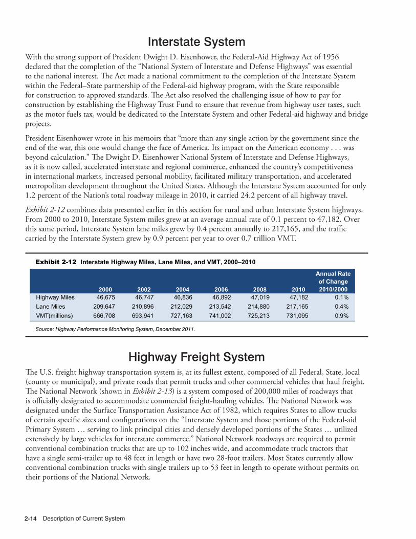
Description of Current System2-14

Interstate SystemWith the strong support of President Dwight D. Eisenhower, the Federal-Aid Highway Act of 1956 declared that the completion of the “National System of Interstate and Defense Highways” was essential to the national interest. The Act made a national commitment to the completion of the Interstate System within the Federal–State partnership of the Federal-aid highway program, with the State responsible for construction to approved standards. The Act also resolved the challenging issue of how to pay for construction by establishing the Highway Trust Fund to ensure that revenue from highway user taxes, such as the motor fuels tax, would be dedicated to the Interstate System and other Federal-aid highway and bridge projects.

President Eisenhower wrote in his memoirs that “more than any single action by the government since the end of the war, this one would change the face of America. Its impact on the American economy . . . was beyond calculation.” The Dwight D. Eisenhower National System of Interstate and Defense Highways, as it is now called, accelerated interstate and regional commerce, enhanced the country’s competitiveness in international markets, increased personal mobility, facilitated military transportation, and accelerated metropolitan development throughout the United States. Although the Interstate System accounted for only 1.2 percent of the Nation’s total roadway mileage in 2010, it carried 24.2 percent of all highway travel.

Exhibit 2-12 combines data presented earlier in this section for rural and urban Interstate System highways. From 2000 to 2010, Interstate System miles grew at an average annual rate of 0.1 percent to 47,182. Over this same period, Interstate System lane miles grew by 0.4 percent annually to 217,165, and the traffic carried by the Interstate System grew by 0.9 percent per year to over 0.7 trillion VMT.

10/24/2012 02XH_L (2-12) R2.xlsx

2000 2002 2004 2006 2008 2010

Annual Rate of Change 2010/2000

Highway Miles 46,675 46,747 46,836 46,892 47,019 47,182 0.1%Lane Miles 209,647 210,896 212,029 213,542 214,880 217,165 0.4%VMT(millions) 666,708 693,941 727,163 741,002 725,213 731,095 0.9%

Exhibit 2-12 Interstate Highway Miles, Lane Miles, and VMT, 2000–2010

Source: Highway Performance Monitoring System, December 2011.

Highway Freight SystemThe U.S. freight highway transportation system is, at its fullest extent, composed of all Federal, State, local (county or municipal), and private roads that permit trucks and other commercial vehicles that haul freight. The National Network (shown in Exhibit 2-13) is a system composed of 200,000 miles of roadways that is officially designated to accommodate commercial freight-hauling vehicles. The National Network was designated under the Surface Transportation Assistance Act of 1982, which requires States to allow trucks of certain specific sizes and configurations on the “Interstate System and those portions of the Federal-aid Primary System … serving to link principal cities and densely developed portions of the States … utilized extensively by large vehicles for interstate commerce.” National Network roadways are required to permit conventional combination trucks that are up to 102 inches wide, and accommodate truck tractors that have a single semi-trailer up to 48 feet in length or have two 28-foot trailers. Most States currently allow conventional combination trucks with single trailers up to 53 feet in length to operate without permits on their portions of the National Network.

System Characteristics 2-159/14/2012 02XH_M (2-13) R1.xlsx

Notes: This map should not be interpreted as the official National Network and should not be used for truck size and weight enforcement purposes. The National Network and NHS are approximately 200,000 miles in length, but the National Network includes 65,000 miles of highway beyond the NHS, and the NHS encompasses about 50,000 miles of highways that are not part of the National Network. "Other NHS" refers to NHS mileage that is not included on the National Network. Conventional combination trucks are tractors with one semitrailer up to 48 feet in length or with one 28-foot semitrailer and one 28-foot trailer. Conventional combination trucks can be up to 102 inches wide. Source: U.S. Department of Transportation, Federal Highway Administration, Office of Freight Management and Operations, Freight Analysis Framework, version 2.2, 2009. ops.fhwa.dot.gov/freight/freight_analysis/nat_freight_stats/docs/09factsfigures/figure3_3.htm.

Exhibit 2-13 National Network for Conventional Combination Trucks, 2009

Although there is significant overlap between the National Network and the NHS, they represent two distinct systems. The National Network has not changed significantly since its designation in 1982. Maintaining truck access to ports, industrial activities in central cities, supporting interstate commerce, and regulating the size of trucks are main priorities of the National Network.

Changes under MAP-21The MAP-21 surface transportation reauthorization bill requires the creation and definition of a National Freight Network, which is intended to include the most important urban, rural, and intercity routes for commercial truck movements. This newly designated network, which does not have a specified roadway mileage, will likely be smaller than National Network or the NHS, and will overlap portions of both previously defined systems, though it will also include mileage that is not part of either the National Network or the NHS. The National Freight Network will consist of (1) a Primary Freight Network designated by the U.S. DOT, (2) the portions of the Interstate Highway System that are not selected to be part of the Primary Freight Network, and (3) Critical Rural Freight Corridors that are designated by the States. The Primary Freight Network will initially include no more than 27,000 centerline miles of existing

Description of Current System2-16

roadways, and will be determined based on eight freight-related factors identified in 23 USC 167(d)(1)(B): “(i) the origins and destinations of freight movement in the United States; (ii) the total freight tonnage and the value of freight movement by highways; (iii) the percentage of average annual daily truck traffic in the annual average daily traffic on principal arterials; (iv) the annual average daily truck traffic on principal arterials; (v) land and maritime ports of entry; (vi) access to energy exploration, development, installation, or production areas; (vii) population centers; and (viii) network connectivity.” The Critical Rural Freight Corridors will need to meet at least one of the following three criteria: (1) is a rural, principal arterial that has trucks comprising a minimum of 25 percent of total AADT; (2) provides access to energy exploration, development, installation, or production; or (3) connects the primary freight network, a roadway meeting either (1) or (2) above, or an Interstate Highway System corridor to facilities that annually handle more than 50,000 twenty-foot equivalent (TEU) units or 500,000 tons of bulk commodities.

System Resiliency An important aspect of system reliability (see Chapter 5) is the resiliency of the system. Resiliency measures the ability of the transportation system to minimize service disruptions despite variable and unexpected condition changes, such as extreme weather or a failure of infrastructure. Resiliency impacts both the physical infrastructure and operational solutions to overcome the sudden change. Events which test resiliency are of a low probability but are potentially highly disruptive to operations such as a hurricane, port/terminal closure, or bridge collapse, such as the Washington I-5 bridge collapse in May 2013. Resiliency is a factor of both the physical infrastructure (for example, how well a bridge responds to being hit) and the operations of the infrastructure (for example, how quickly responders are able to precipitate a safe detour and reconstruct the bridge). While the I-5 bridge did not demonstrate structural resilience to the strike of the truck that caused the collapse, Washington DOT used operational strategies to quickly operationalize a detour route, construct a temporary bridge in less than 1 month, and construct a replacement bridge in less than 5 months. System resiliency requires investments in both resilient infrastructure and emergency response plans by State DOTs.

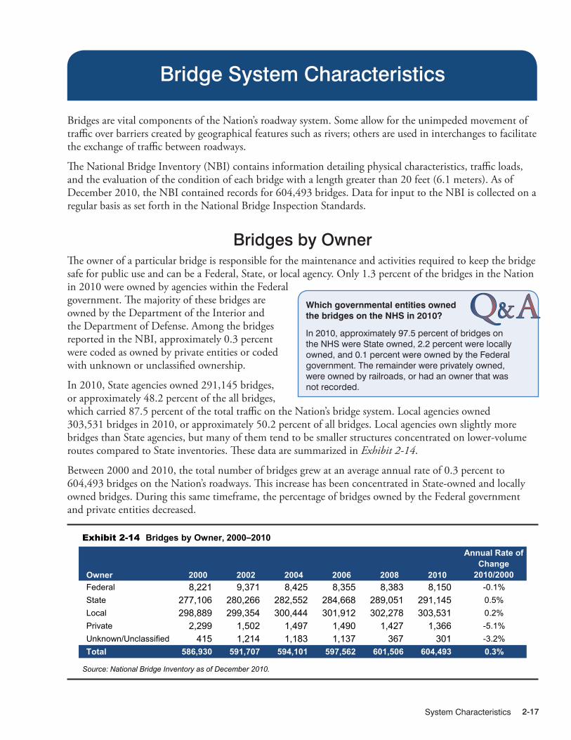
System Characteristics 2-17

Bridges are vital components of the Nation’s roadway system. Some allow for the unimpeded movement of traffic over barriers created by geographical features such as rivers; others are used in interchanges to facilitate the exchange of traffic between roadways.

The National Bridge Inventory (NBI) contains information detailing physical characteristics, traffic loads, and the evaluation of the condition of each bridge with a length greater than 20 feet (6.1 meters). As of December 2010, the NBI contained records for 604,493 bridges. Data for input to the NBI is collected on a regular basis as set forth in the National Bridge Inspection Standards.

Bridges by OwnerThe owner of a particular bridge is responsible for the maintenance and activities required to keep the bridge safe for public use and can be a Federal, State, or local agency. Only 1.3 percent of the bridges in the Nation in 2010 were owned by agencies within the Federal government. The majority of these bridges are owned by the Department of the Interior and the Department of Defense. Among the bridges reported in the NBI, approximately 0.3 percent were coded as owned by private entities or coded with unknown or unclassified ownership.

In 2010, State agencies owned 291,145 bridges, or approximately 48.2 percent of the all bridges, which carried 87.5 percent of the total traffic on the Nation’s bridge system. Local agencies owned 303,531 bridges in 2010, or approximately 50.2 percent of all bridges. Local agencies own slightly more bridges than State agencies, but many of them tend to be smaller structures concentrated on lower-volume routes compared to State inventories. These data are summarized in Exhibit 2-14.

Between 2000 and 2010, the total number of bridges grew at an average annual rate of 0.3 percent to 604,493 bridges on the Nation’s roadways. This increase has been concentrated in State-owned and locally owned bridges. During this same timeframe, the percentage of bridges owned by the Federal government and private entities decreased.

Bridge System Characteristics

Q A&Which governmental entities owned the bridges on the NHS in 2010?

In 2010, approximately 97.5 percent of bridges on the NHS were State owned, 2.2 percent were locally owned, and 0.1 percent were owned by the Federal government. The remainder were privately owned, were owned by railroads, or had an owner that was not recorded.

11/1/2012 02XB_A (2-14) R2.xlsx

Owner 2000 2002 2004 2006 2008 2010

Annual Rate of Change

2010/2000Federal 8,221 9,371 8,425 8,355 8,383 8,150 -0.1%State 277,106 280,266 282,552 284,668 289,051 291,145 0.5%Local 298,889 299,354 300,444 301,912 302,278 303,531 0.2%Private 2,299 1,502 1,497 1,490 1,427 1,366 -5.1%Unknown/Unclassified 415 1,214 1,183 1,137 367 301 -3.2%Total 586,930 591,707 594,101 597,562 601,506 604,493 0.3%

Exhibit 2-14 Bridges by Owner, 2000–2010

Source: National Bridge Inventory as of December 2010.

Description of Current System2-18

As shown in Exhibit 2-15, despite States owning 48.2 percent of total bridges in 2010, these bridges constituted 76.5 percent of total bridge deck area and carried 87.5 percent of total bridge traffic. In 2010, State agencies owned more than 3 times the bridge deck area of local agencies and carried more than 7 times the traffic of bridges owned by local agencies.

Interstate, STRAHNET, and NHS Bridges

Exhibit 2-16 shows that the Interstate system had 55,339 bridges, or 9.2 percent of the total bridges on the road system of the Nation, in 2010. Bridges on the Interstate make up 26.4 percent of the total deck area of bridges on the Nation’s roadway system. Interstate bridges carry approximately 44.9 percent of average daily traffic and 58.3 percent of the Nation’s Average Daily Truck Travel (ADTT).

The Strategic Highway Network (STRAHNET) system, including Interstate highways and other routes critical to national defense, included 68,529 bridges in 2010. All STRAHNET routes, including STRAHNET connectors, are included as part of the National Highway System (NHS).

As of 2010, the 116,669 bridges on the NHS constituted 19.3 percent of total bridges in the Nation. However, NHS bridges constituted 49.0 percent of total bridge deck area, carried 70.7 percent of total bridge traffic, and carried 81.0 percent of bridge truck traffic. As referenced earlier in this chapter, the NHS includes the entire Interstate System as well as additional critical routes.

11/1/2012 02XB_B (2-15) R2.xlsx

Federal 1.3%

Local 50.2% Other

0.3%

State 48.2%

Bridge Ownership (by Percentage of Bridge Inventory)

Federal 0.2%

Local 12.1% Other

0.2% State 87.5%

Percentage of Traffic Carried (by Owner)

Federal 0.7%

Local 22.4%

Other 0.3%

State 76.5%

Percentage of Total Deck Area (by Owner)

Exhibit 2-15 Bridge Inventory Characteristics for Ownership, Traffic, and Deck Area, 2010

Source: National Bridge Inventory as of December 2010.

10/24/2012 02XB_C (2-16) R2.xlsx

Interstate System 55,339 9.2% 92,668 26.4% 1,992,392 44.9% 240,911 58.3%STRAHNET 68,529 11.3% 108,690 30.9% 2,223,702 50.1% 262,512 63.6%NHS 116,669 19.3% 172,167 49.0% 3,138,800 70.7% 334,973 81.1%Federal-Aid Hwy 319,108 52.8% 293,485 83.5% 4,235,908 95.4% 402,992 97.6%All Systems 604,493 100% 351,470 100% 4,438,757 100% 413,073 100%

Truck ADT

(1000)

Percent of Total

Truck ADTFederal System*Number of

Bridges

Percent by Number of

Bridges

Percent of Total Deck

Area

Percent of Total

ADT

Deck Area Sq Meters

(1000)ADT

(1000)

Exhibit 2-16 Interstate, STRAHNET, and NHS Bridges Weighted by Numbers, ADT, and Deck Area, 2010

* The NHS includes all of STRAHNET; STRAHNET includes the entire Interstate System. Source: National Bridge Inventory as of December 2010.

System Characteristics 2-19

Bridges by Roadway Functional ClassificationThe NBI maintains the highway functional classification of the road on which a bridge is located. The NBI follows the hierarchy used for highway systems as previously described in this chapter. The number of bridges by roadway functional classification is summarized and compared with previous years in Exhibit 2-17.

As noted earlier in this chapter, changes in urban area boundaries resulting from the 2000 Census led to reductions in the number of rural bridges and an increase in urban bridges. As shown in Exhibit 2-17, the largest change in the number of bridges on a single functional class highway between 2000 and 2010 occurred on urban collectors with an annual increase of 3.1 percent.

Exhibit 2-18 shows the relationship between bridges among various rural and urban functional classes. In 2010, there were approximately 2.8 bridges on rural roadways for every bridge on the urban system. However, urban bridges carried more than 3.2 times the ADT of rural bridges and constituted slightly less than 1.3 times the deck area of rural bridges.

The greatest number of bridges on any functional system, rural or urban, is on rural local. In 2010 there were a total of 205,609 rural local functional class bridges constituting 34.0 percent of all bridges. Rural functional class bridges alone outnumber bridges in urban areas on all functional classifications. However, rural local bridges only account for 9.5 percent of the total bridge deck area in the Nation and carry only 1.4 percent of total bridge ADT.

The 30,116 urban Interstate bridges constitute only 5.0 percent of the Nation’s bridges. However, urban Interstate bridges have the greatest share of deck area among the functional classes at 19.4 percent and carry the greatest share of ADT at 35.8 percent. Many urban Interstate bridges are part of interchanges and carry significant volumes of traffic.

Q A&What is meant by “deck area” and how is the information about deck area used?

The deck area of a bridge is the width of the roadway surface of a bridge multiplied by the length of the bridge. Pedestrian walkways and bike paths may be included in the roadway width.

Prior to MAP-21, the deck area of bridge was an essential calculation for use in the apportionment process of Highway Bridge Program funds.

The deck area of a bridge is an indicator as to the size of a bridge. Bridges with large deck areas are usually associated with having multiple lanes and large traffic volumes, and/or are over major geographical features requiring a great distance to span. The deck area of a bridge may be used to aid in determining the level of investment as part of a risk based prioritization process.

Example:

Bridge “A” carries two lanes of traffic on a local road that crosses a small stream. The bridge length is 30 feet and the roadway width is 26 feet for a total deck area of 780 square feet. The bridge has been rated as deficient.

Bridge “B” carries four lanes of traffic on the Interstate and crosses over a major river. The length of the bridge is 600 feet and the roadway width is 60 feet for a total deck area of 36,000 square feet. It has also been rated as deficient.

In a simple count reflecting deficient bridges both are equal in value, however, when deck area is considered, the difference between a 36,000 square foot bridge and a 780 square foot bridge indicates there is a potentially vast difference in the funding required to rehabilitate the Interstate bridge versus the bridge on the local road.

Description of Current System2-20

11/2/2012 02XB_D (2-17) R2.xlsx

Functional System 2000 2002 2004 2006 2008 2010

Annual Rate of Change

2010/2000RuralInterstate 27,797 27,310 27,648 26,633 25,997 25,223 -1.0%Other Principal Arterials 35,417 35,215 36,258 35,766 35,594 36,084 0.2%Minor Arterial 39,377 39,571 40,197 39,521 39,079 39,048 -0.1%Major Collector 95,559 94,766 94,079 93,609 93,118 93,059 -0.3%Minor Collector 47,797 49,309 49,391 48,639 48,242 47,866 0.0%Local 209,410 209,358 208,641 207,130 205,959 205,609 -0.2%Subtotal Rural 455,357 455,529 456,214 451,298 447,989 446,889 -0.2%UrbanInterstate 27,882 27,924 27,667 28,637 29,629 30,116 0.8%Other Expressways 16,011 16,843 17,112 17,988 19,168 19,791 2.1%Other Principal Arterials 24,146 24,301 24,529 26,051 26,934 27,373 1.3%Minor Arterial 23,020 24,510 24,802 26,239 27,561 28,103 2.0%Collectors 15,036 15,169 15,548 17,618 18,932 20,311 3.1%Local 25,683 26,592 27,940 29,508 31,183 31,877 2.2%Subtotal Urban 131,778 135,339 137,598 146,041 153,407 157,571 1.8%Unclassified 600 375 288 222 110 33Total 587,735 591,243 594,100 597,561 601,506 604,493 0.3%

Exhibit 2-17 Number of Bridges by Functional System, 2000–2010

Source: National Bridge Inventory as of December 2010.

11/2/2012 02XB_E (2-18) R2.xlsx

RuralInterstate 25,223 4.2% 24,656 7.0% 404,151 9.1%Other Principal Arterial 36,084 6.0% 31,015 8.8% 259,639 5.8%Minor Arterial 39,048 6.5% 21,576 6.1% 144,499 3.3%Major Collector 93,059 15.4% 32,591 9.3% 142,267 3.2%Minor Collector 47,866 7.9% 11,302 3.2% 34,828 0.8%Local 205,609 34.0% 33,529 9.5% 63,373 1.4%Subtotal Rural 446,889 73.9% 154,668 44.0% 1,048,757 23.6%Urban Interstate 30,116 5.0% 68,012 19.4% 1,588,241 35.8%Other Freeways & Expressways 19,791 3.3% 37,296 10.6% 720,988 16.2%Other Principal Arterial 27,373 4.5% 39,333 11.2% 525,255 11.8%Minor Arterial 28,103 4.6% 26,354 7.5% 327,646 7.4%Collector 20,311 3.4% 12,652 3.6% 123,222 2.8%Local 31,877 5.3% 13,124 3.7% 104,495 2.4%Subtotal Urban 157,571 26.1% 196,772 56.0% 3,389,846 76.4%Unclassified 33 0.0% 30 0.0% 154 0.0%Total 604,493 100.0% 351,470 100.0% 4,438,757 100.0%

Functional SystemNumber of

Bridges

Percent by Total

Number

Percent of Total Deck

AreaPercent of Total ADT

Deck Area Sq Meters

(1000)ADT

(1,000)

Source: National Bridge Inventory as of December 2010.

Exhibit 2-18 Bridges by Functional System Weighted by Numbers, ADT, and Deck Area, 2010

System Characteristics 2-21

11/2/2012 02XB_F (2-19) R2.xlsx

Functional System

< 1,000 ADT1,001 to 10,000

ADT10,001 to 50,000

ADT > 50,000 ADTRuralInterstate 394 10,078 13,979 772Other Principal Arterial 1,342 27,742 6,879 121Minor Arterial 7,616 29,131 2,287 14Major Collector 54,334 37,589 1,133 3Minor Collector 38,980 8,708 173 5Local 195,682 9,429 481 17Subtotal Rural 298,348 122,677 24,932 932UrbanInterstate 364 4,044 14,333 11,375Other Freeways & Expressways 243 4,113 11,328 4,107Other Principal Arterial 356 7,700 18,272 1,045Minor Arterial 1,140 14,213 12,571 179Collector 3,050 13,850 3,353 58Local 15,670 13,771 2,339 97Subtotal Urban 20,823 57,691 62,196 16,861Unclassified 25 3 5 0Total 319,196 180,371 87,133 17,793

Average Daily Traffic Category

Exhibit 2-19 Number of Bridges by Functional Class and ADT Group, 2010

Source: National Bridge Inventory as of December 2010.

In 2010, there were 2.8 Interstate bridges on rural roadways for every Interstate bridge in urban areas. While there were fewer bridges in urban areas compared to rural areas, the volume of traffic carried by urban Interstate bridges was more than 3.9 times the ADT carried by rural Interstate bridges in 2010. As reported in the 2010 Conditions & Performance Report, the ADT carried on urban Interstate bridges in 2010 was more than 1.5 times the ADT carried on all rural bridges combined.

Bridges by Traffic VolumeAs shown in Exhibit 2-19, many bridges carried relatively low volumes of traffic on a typical day in 2010. Approximately 319,196 bridges, or 52.8 percent of the total bridges in the Nation, had an ADT of 1,000 or less. An additional 180,371 bridges, or 29.8 percent of all bridges, had an ADT between 1,001 and 10,000. Only 17,793 of the Nation’s bridges, or 2.9 percent, had an ADT higher than 50,000. The remaining 87,133 bridges, or 14.4 percent, had an ADT between 10,001 and 50,000.

Of the bridges which have an ADT higher than 50,000, approximately 2.0 percent, or 12,147 bridges, are on the Interstate system. Interstate bridges in urban areas account for slightly more than 93.6 percent of these bridges. When all bridges that carry the highest category of ADT are considered, the number of bridges in urban areas outnumber rural bridges by more than 100 to 1.

Description of Current System2-22

Transit System Characteristics

Some Transit VocabularyModal network refers to a system of routes and stops served by one type of transit technology; this could be a bus network, a light rail network, a ferry network, or a demand response system. Transit operators often maintain several different modal networks, most often motor bus systems augmented with demand response service.

Articulated bus is an extra-long (54- to 60-foot) bus with two connected passenger compartments. The rear body section is connected to the main body by a joint mechanism that allows the vehicles to bend when in operation for sharp turns and curves and yet have a continuous interior.

Automated Guideway Systems are driverless, rubber-tire vehicles usually running alone or in pairs on a single broad concrete rail, typical of most airport trains, although airport trains are not considered transit service by FTA.

Demand response service usually consists of passenger cars, vans, or small buses operating in response to calls from passengers or their agents to the transit operator, who then dispatches a vehicle to pick up the passengers and transport them to their destinations. The vehicles do not operate over a fixed route or on a fixed schedule, except on a temporary basis to satisfy a special need. A vehicle may be dispatched to pick up several passengers at different pickup points before taking them to their respective destinations.

Públicos or “public cars” are typically 17-passenger vans that serve towns throughout Puerto Rico, stopping in each community’s main plaza or at a destination requested by a passenger. They generally operate without a set schedule, primarily during the day; the public service commission fixes routes and fares. San Juan-based Público companies include Blue Line for trips to Aguadilla and the northwest coast, Choferes Unidos de Ponce for Ponce, Línea Caborrojeña for Cabo Rojo and the southwest coast, Línea Boricua for the interior and the southwest, Línea Sultana for Mayagüez and the west coast, and Terminal de Transportación Pública for Fajardo and the east.

Jitneys are generally small-capacity vehicles that follow a rough service route but can go slightly out of their way to pick up and drop off passengers. In many U.S. cities (e.g., Pittsburgh and Detroit), the term “jitney” refers to an unlicensed taxicab. In some U.S. jurisdictions, the limit to a jitney is seven passengers.

Cutaways are vehicles comprising a bus body mounted on the chassis of a van or light-duty truck. The original van or light-duty truck chassis may be reinforced or extended. Cutaways typically seat 15 or more passengers and may accommodate some standing passengers.

Revenue service is the time when a vehicle is actively providing service to the general public and either is carrying passengers or is available to them. Revenue from fares is not necessary because vehicles are considered to be in revenue service even when the ride is free.

System HistoryThe first transit systems in the United States date to the late 19th century. These were privately owned, for-profit businesses that were instrumental in defining the urban communities of that time. By the postwar period, competition from the private automobile was making it impossible for transit businesses to operate at a profit. As they started to fail, local, State, and national government leaders began to realize the importance of sustaining transit services. In 1964, Congress passed the Urban Mass Transportation Act, which established the agency now known as the Federal Transit Administration (FTA) to administer Federal funding for transit systems. The Act also changed the character of the industry by specifying that Federal funds for transit were to be given to public agencies rather than private firms; this accelerated the transition from private to public ownership and operation of transit systems. The Act also required local governments to contribute matching funds in order to receive Federal aid for transit services, setting the stage for the multilevel governmental partnerships that continue to characterize the transit industry today.

State government involvement in the provision of transit services is usually through financial support and performance oversight. However, some States have undertaken outright ownership and operation of transit services. Connecticut, Georgia, Louisiana, Maryland, Ohio, and Washington all own and operate transit systems directly, as does Puerto Rico. Michigan and Pennsylvania contract for transit services.

System Characteristics 2-23

In 1962, the U.S. Congress passed legislation that required the formation of metropolitan planning organizations (MPOs) for urbanized areas with populations greater than 50,000. MPOs are composed of State and local officials who work to address the transportation planning needs of an urbanized area at a regional level. Twenty-nine years later, the Intermodal Surface Transportation Efficiency Act of 1991 made MPO coordination an essential prerequisite for Federal funding of many transit projects.

State and local transit agencies have evolved into a number of different institutional models. A transit provider may be a unit of a regional transportation agency; may be operated directly by the State, county, or city government; or may be an independent agency with an elected or appointed Board of Governors. Transit operators can provide service directly with their own equipment or they may purchase transit services through an agreement with a contractor. All public transit services must be open to the general public without discrimination and meet the accessibility requirements of the Americans with Disabilities Act of 1990 (ADA).

System Infrastructure

Urban Transit AgenciesIn 2010, there were 728 agencies in urbanized areas that were required to submit data to the National Transit Database (NTD), of which 709 were public agencies, including eight State Departments of Transportation (DOTs). The remaining 19 agencies were either private operators or independent agencies (e.g., nonprofit organizations). One hundred thirty-one agencies received either a reporting exemption for operating nine or fewer vehicles or a temporary reporting waiver; 611 agencies reported providing service on 1,240 separate modal networks; all but 148 agencies operated more than one mode. In 2010, there were an additional 1,599 transit operators serving rural areas. Not all transit providers are included in these counts because those that do not receive grant funds from FTA are not required to report to NTD. Some, but not all, agencies report anyway, as this can help their region receive Federal transit funding.

The Nation’s motor bus and demand response systems are much more extensive than the Nation’s rail transit system. In 2010, there were 612 motor bus systems and 587 demand-response systems (not including demand-response taxi) in urban areas, compared with 18 heavy rail systems, 30 commuter rail systems, and 33 light rail systems (some of which are not yet in service). While motor bus and demand response systems were found in every major urbanized area in the United States, 44 urbanized areas were served by at least one of the three primary rail modes, including 20 by commuter rail, 30 by light rail, and 14 by heavy rail (rail systems are listed in Exhibit 2-20). In addition to these modes, there were 70 publicly operated transit vanpool systems, 20 ferryboat systems, five trolleybus systems, three automated guideway systems, three inclined plane systems, and one cable car system operating in urbanized areas of the United States and its territories.

The transit statistics presented in this report also include the San Francisco Cable Car, the Seattle Monorail, the Roosevelt Island Aerial Tramway in New York, and the Alaska Railroad (which is a long-distance passenger rail system included as public transportation by statutory exemption).

Description of Current System2-24

Urbanized Areas with Population over 1 Million in 2010 Census

02CT_C R1.docx Callout Box 12/19/2013

Callout Box

Urbanized Areas with Population over 1 Million in 2010 Census UZA Rank UZA Name 2010

Population 2011

Unlinked Transit Trips 1 New York-Newark, NY-NJ-CT 18,351,295 4,017,665,768 2 Los Angeles-Long Beach-Anaheim, CA 12,150,996 661,822,454 3 Chicago, IL-IN 8,608,208 644,479,067 4 Miami, FL 5,502,379 158,711,484 5 Philadelphia, PA-NJ-DE-MD 5,441,567 403,855,701 6 Dallas-Fort Worth-Arlington, TX 5,121,892 71,341,858 7 Houston, TX 4,944,332 81,090,736 8 Washington, DC-VA-MD 4,586,770 487,325,732 9 Atlanta, GA 4,515,419 149,556,097

10 Boston, MA-NH-RI 4,181,019 389,568,759 11 Detroit, MI 3,734,090 49,824,000 12 Phoenix-Mesa, AZ 3,629,114 68,018,113 13 San Francisco-Oakland, CA 3,281,212 388,347,627 14 Seattle, WA 3,059,393 187,098,251 15 San Diego, CA 2,956,746 98,128,677 16 Minneapolis-St. Paul, MN-WI 2,650,890 93,892,746 17 Tampa-St. Petersburg, FL 2,441,770 29,116,395 18 Denver-Aurora, CO 2,374,203 89,614,960 19 Baltimore, MD 2,203,663 98,303,955 20 St. Louis, MO-IL 2,150,706 45,258,440 21 San Juan, PR 2,148,346 46,721,752 22 Riverside-San Bernardino, CA 1,932,666 18,495,303 23 Las Vegas-Henderson, NV 1,886,011 56,686,089 24 Portland, OR-WA 1,849,898 111,985,241 25 Cleveland, OH 1,780,673 47,764,261 26 San Antonio, TX 1,758,210 45,493,533 27 Pittsburgh, PA 1,733,853 65,501,247 28 Sacramento, CA 1,723,634 28,712,623 29 San Jose, CA 1,664,496 47,349,903 30 Cincinnati, OH-KY-IN 1,624,827 22,819,990 31 Kansas City, MO-KS 1,519,417 16,766,058 32 Orlando, FL 1,510,516 21,995,359 33 Indianapolis, IN 1,487,483 9,512,303 34 Virginia Beach, VA 1,439,666 16,654,615 35 Milwaukee, WI 1,376,476 46,489,545 36 Columbus, OH 1,368,035 19,049,187 37 Austin, TX 1,362,416 34,740,271 38 Charlotte, NC-SC 1,249,442 27,028,511 39 Providence, RI-MA 1,190,956 21,205,831 40 Jacksonville, FL 1,065,219 12,599,527 41 Memphis, TN-MS-AR 1,060,061 10,616,855 42 Salt Lake City-West Valley City, UT 1,021,243 30,566,260

System Characteristics 2-25

12/28/2012 02XT_Q (2-20) R5.xlsx

Mode: Heavy RailRail System Name UZA Name VehiclesMTA New York City Transit (NYCT) New York-Newark, NY-NJ-CT 5,354 Chicago Transit Authority (CTA) Chicago, IL-IN 980 Washington Metropolitan Area Transit Authority (WMATA) Washington, DC-VA-MD 850 San Francisco Bay Area Rapid Transit District (BART) San Francisco-Oakland, CA 534 Massachusetts Bay Transportation Authority (MBTA) Boston, MA-NH-RI 342 Southeastern Pennsylvania Transportation Authority (SEPTA) Philadelphia, PA-NJ-DE-MD 284 Port Authority Trans-Hudson Corporation (PATH) New York-Newark, NY-NJ-CT 266 Metropolitan Atlanta Rapid Transit Authority (MARTA) Atlanta, GA 188 Miami-Dade Transit (MDT) Miami, FL 84 Port Authority Transit Corporation (PATCO) Philadelphia, PA-NJ-DE-MD 84 Los Angeles County Metropolitan Transportation Authority (LACMTA) Los Angeles-Long Beach-Santa Ana, CA 70 Maryland Transit Administration (MTA) Baltimore, MD 54 Staten Island Rapid Transit Operating Authority (SIRTOA) New York-Newark, NY-NJ-CT 46 Puerto Rico Highway and Transportation Authority (PRHTA) San Juan, PR 40 The Greater Cleveland Regional Transit Authority (GCRTA) Cleveland, OH 22 Santa Clara Valley Transportation Authority (VTA) San Jose, CA City and County of Honolulu Department of Transportation Services (DTS) Honolulu, HI Mode: Commuter RailRail System Name UZA Name VehiclesNew Jersey Transit Corporation (NJ TRANSIT) New York-Newark, NY-NJ-CT 1,291 Metro-North Commuter Railroad Company (MTA-MNCR) New York-Newark, NY-NJ-CT 1,075 Northeast Illinois Regional Commuter Railroad Corporation (Metra) Chicago, IL-IN 1,057 MTA Long Island Rail Road (MTA LIRR) New York-Newark, NY-NJ-CT 1,014 Massachusetts Bay Transportation Authority (MBTA) Boston, MA-NH-RI 418 Southeastern Pennsylvania Transportation Authority (SEPTA) Philadelphia, PA-NJ-DE-MD 325 Southern California Regional Rail Authority (Metrolink) Los Angeles-Long Beach-Santa Ana, CA 169 Maryland Transit Administration (MTA) Baltimore, MD 132 Peninsula Corridor Joint Powers Board (PCJPB) San Francisco-Oakland, CA 95 Virginia Railway Express (VRE) Washington, DC-VA-MD 78 Northern Indiana Commuter Transportation District (NICTD) Chicago, IL-IN 66 Central Puget Sound Regional Transit Authority (ST) Seattle, WA 56 Trinity Railway Express Dallas-Fort Worth-Arlington, TX 36 South Florida Regional Transportation Authority (TRI-Rail) Miami, FL 34 Utah Transit Authority (UTA) Salt Lake City, UT 34 Connecticut Department of Transportation (CDOT) Hartford, CT 28 North County Transit District (NCTD) San Diego, CA 26 Rio Metro Regional Transit District (RMRTD) Albuquerque, NM 25 Metro Transit Minneapolis-St. Paul, MN 23 Altamont Commuter Express (ACE) Stockton, CA 21 Pennsylvania Department of Transportation (PENNDOT) Philadelphia, PA-NJ-DE-MD 20 Northern New England Passenger Rail Authority (NNEPRA) Boston, MA-NH-RI 14 Regional Transportation Authority (RTA) Nashville-Davidson, TN 7 Tri-County Metropolitan Transportation District of Oregon (TriMet) Portland, OR-WA 4 Capital Metropolitan Transportation Authority (CMTA) Austin, TX 4

Exhibit 2-20 Rail Modes Serving Urbanized Areas

Description of Current System2-26

12/28/2012 02XT_Q (2-20) R5.xlsx

Mode: Light RailRail System Name UZA Name Vehicles

Massachusetts Bay Transportation Authority (MBTA) Boston, MA-NH-RI 156 San Francisco Municipal Railway (MUNI) San Francisco-Oakland, CA 139 Southeastern Pennsylvania Transportation Authority (SEPTA) Philadelphia, PA-NJ-DE-MD 124 Los Angeles County Metropolitan Transportation Authority (LACMTA) Los Angeles-Long Beach-Santa Ana, CA 118 Tri-County Metropolitan Transportation District of Oregon (TriMet) Portland, OR-WA 110 Denver Regional Transportation District (RTD) Denver-Aurora, CO 104 San Diego Metropolitan Transit System (MTS) San Diego, CA 93 Dallas Area Rapid Transit (DART) Dallas-Fort Worth-Arlington, TX 76 New Jersey Transit Corporation (NJ TRANSIT) New York-Newark, NY-NJ-CT 73 Sacramento Regional Transit District (Sacramento RT) Sacramento, CA 56 Port Authority of Allegheny County (Port Authority) Pittsburgh, PA 51 Bi-State Development Agency (METRO) St. Louis, MO-IL 50 Santa Clara Valley Transportation Authority (VTA) San Jose, CA 47 Utah Transit Authority (UTA) Salt Lake City, UT 43 Maryland Transit Administration (MTA) Baltimore, MD 38 Valley Metro Rail, Inc. (VMR) Phoenix-Mesa, AZ 32 Metro Transit Minneapolis-St. Paul, MN 27 Central Puget Sound Regional Transit Authority (ST) Seattle, WA 26 Niagara Frontier Transportation Authority (NFT Metro) Buffalo, NY 23 New Orleans Regional Transit Authority (NORTA) New Orleans, LA 21 The Greater Cleveland Regional Transit Authority (GCRTA) Cleveland, OH 17 Metropolitan Transit Authority of Harris County, Texas (Metro) Houston, TX 17 Charlotte Area Transit System (CATS) Charlotte, NC-SC 16 Memphis Area Transit Authority (MATA) Memphis, TN-MS-AR 12 North County Transit District (NCTD) San Diego, CA 6 Hillsborough Area Regional Transit Authority (HART) Tampa-St. Petersburg, FL 4 Island Transit (IT)* Galveston, TX 4 Central Arkansas Transit Authority (CATA) Little Rock, AR 3 Kenosha Transit (KT) Kenosha, WI 3 Central Puget Sound Regional Transit Authority (ST) Seattle, WA 2 King County Department of Transportation (King County Metro) Seattle, WA 2

Exhibit 2-20 Rail Modes Serving Urbanized Areas

*Island Transit (IT) was not operating in 2010. Source: National Transit Database.

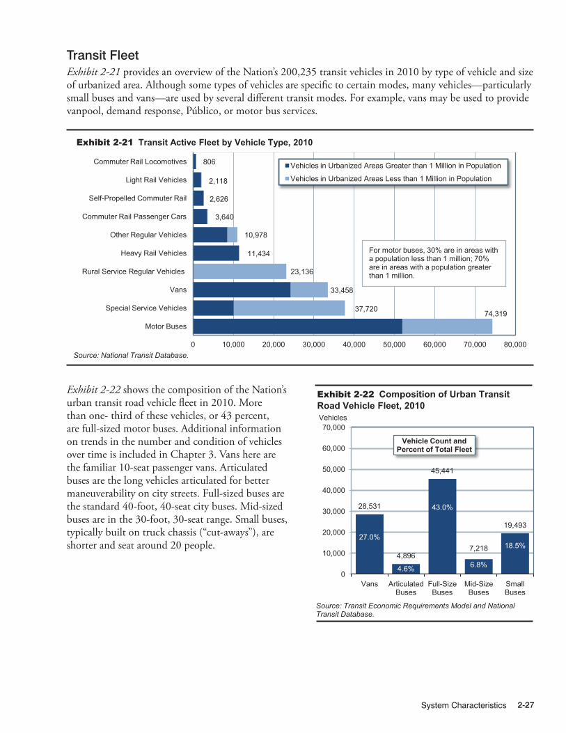
System Characteristics 2-27

12/28/2012 02XT_A (2-21) R4.xlsx

0 10,000 20,000 30,000 40,000 50,000 60,000 70,000 80,000

Motor Buses

Special Service Vehicles

Vans

Rural Service Regular Vehicles

Heavy Rail Vehicles

Other Regular Vehicles

Commuter Rail Passenger Cars

Self-Propelled Commuter Rail

Light Rail Vehicles

Commuter Rail Locomotives Vehicles in Urbanized Areas Greater than 1 Million in Population

Vehicles in Urbanized Areas Less than 1 Million in Population

806

2,118

2,626

3,640

10,978

11,434

23,136

33,458

37,720

Exhibit 2-21 Transit Active Fleet by Vehicle Type, 2010

Source: National Transit Database.

For motor buses, 30% are in areas with a population less than 1 million; 70% are in areas with a population greater than 1 million.

74,319

Transit FleetExhibit 2-21 provides an overview of the Nation’s 200,235 transit vehicles in 2010 by type of vehicle and size of urbanized area. Although some types of vehicles are specific to certain modes, many vehicles—particularly small buses and vans—are used by several different transit modes. For example, vans may be used to provide vanpool, demand response, Público, or motor bus services.

10/23/2012 02XT_B (2-22) R2x.xlsx

28,531

4,896

45,441

7,218

19,493 27.0%

4.6%

43.0%

6.8%

18.5%

0

10,000

20,000

30,000

40,000

50,000

60,000

70,000

Vans Articulated Buses

Full-Size Buses

Mid-Size Buses

Small Buses

Vehicles

Vehicle Count and Percent of Total Fleet

Exhibit 2-22 Composition of Urban Transit Road Vehicle Fleet, 2010

Source: Transit Economic Requirements Model and National Transit Database.

Exhibit 2-22 shows the composition of the Nation’s urban transit road vehicle fleet in 2010. More than one- third of these vehicles, or 43 percent, are full-sized motor buses. Additional information on trends in the number and condition of vehicles over time is included in Chapter 3. Vans here are the familiar 10-seat passenger vans. Articulated buses are the long vehicles articulated for better maneuverability on city streets. Full-sized buses are the standard 40-foot, 40-seat city buses. Mid-sized buses are in the 30-foot, 30-seat range. Small buses, typically built on truck chassis (“cut-aways”), are shorter and seat around 20 people.

Description of Current System2-28

Track, Stations, and Maintenance FacilitiesMaintenance facility counts are broken down by mode and by size of urbanized area in Exhibit 2-23. Additional data on the age and condition of these facilities is included in Chapter 3.

As shown in Exhibit 2-24, in 2010, transit providers operated 12,438 miles of track and served 3,175 stations, compared with 11,864 miles of track and 3,078 stations in 2008. Expansion in light rail track mileage (8.1 percent) and stations (7.8 percent) accounted for most of the increase, a trend that continues from the recent past. The Nation’s rail system mileage is dominated by the longer distances generally covered by commuter rail. Light and heavy rail typically operate in more densely developed areas and have more stations per track mile.

Maintenance Facility Type1Over

1 MillionUnder

1 Million TotalHeavy Rail 59 0 59Commuter Rail 51 1 52Light Rail 37 6 43

Other Rail2 3 4 7Motorbus 316 245 561Demand Response 37 84 122Ferryboat 8 1 9

Other Nonrail3 6 3 8Total Urban Maintenance Facilities 516 344 860

Rural Transit 4 682 682Total Maintenance Facilities 516 1,026 1,542

Population Category

Exhibit 2-23 Maintenance Facilities for Directly Operated Services, 2010

1 Includes owned and leased facilities. 2 Alaska railroad, automated guideway, cable car, inclined plane, and monorail. 3 Aerial tramway, jitney, Público, and vanpool. 4 Vehicles owned by operators receiving funding from FTA as directed by 49 USC Section 5311. These funds are for transit services in areas with populations of less than 50,000. (Section 5311 Status of Rural Public Transportation 2000, Community Transportation Association of America, April 2001.) Source: National Transit Database.

Urbanized Area Track MileageHeavy Rail 2,272Commuter Rail 7,786Light Rail 1,664Other Rail and Tramway* 715Total Urbanized Area Track Mileage 12,438Urbanized Area Transit Rail Stations CountHeavy Rail 1,041Commuter Rail 1,225Light Rail 848Other Rail and Tramway 61Total Urbanized Area Transit Rail Stations 3,175

* Alaska railroad, automated guideway, cable car, inclined plane, monorail, and aerial tramway. Source: National Transit Database.

Exhibit 2-24 Transit Rail Mileage and Stations, 2010

Transit System ResiliencyTransit systems practice resiliency by operating through all but the worst weather on a daily basis. Most play a key role in community emergency response plans. Dispatchers and vehicle operators receive special training for these circumstances. Bus systems all have reserve fleets that can replace damaged vehicles on short notice. Rail systems have contingency plans for loss of key assets and most can muster local resources to operate bus bridges in emergency situations. Operationally speaking, transit providers are some of the most resilient community institutions. However, much transit infrastructure has not yet been upgraded to address changing climactic patterns. FTA does not collect systematic data on this, but a significant amount of grant money has been made available for transit systems to upgrade their structures and guideways to be more resistant to extreme precipitation events, sea level rise, storm surge, heat waves, and other environmental stress. This is particularly evident in the aftermath of “superstorm” Sandy. Addressing these issues is a common use of FTA grant funds.

System Characteristics 2-29

Rural Transit Systems (Section 5311 Providers)The FTA first instituted rural data reporting to the NTD in 2006. In 2010, 1,582 transit operators reported providing rural service. They reported 123.2 million unlinked passenger trips and 570 million vehicle revenue miles. This included 61 Indian tribes that provided 1,008,701 unlinked passenger trips. There are 327 urbanized areas that report providing rural service; they added another 24 million unlinked passenger trips and 37 million vehicle revenue miles.

The data indicates that rural transit service has been growing rapidly; however, because the NTD is still adding rural reporters, this cannot yet be validated. The data also indicate every State and four territories provide some form of rural transit service.

Rural systems provide both traditional fixed-route and demand response services, with 1,180 demand response services, 530 motor bus services, and 16 vanpool services. They reported 23,136 vehicles in 2010. Exhibit 2-25 shows the number of rural transit vehicles in service.

Transit System Characteristics for Americans with Disabilities and the Elderly

The Americans with Disabilities Act (ADA) is intended to ensure that persons with disabilities have access to the same facilities and services as other Americans, including transit vehicles and facilities. This equality of access is brought about through the upgrading of transit vehicles and facilities on regular routes, through the provision of demand response transit service for those individuals who are still unable to use regular transit service, and through special service vehicles operated by private entities and some public organizations, often with the assistance of FTA funding.

Since the passage of the ADA in 1990, transit operators have been working to upgrade their regular vehicle fleets and improve their demand response services in order to meet the ADA’s requirement to provide persons with disabilities with a level of service comparable to that of fixed-route systems. U.S. DOT regulations provide minimum guidelines and accessibility standards for buses; vans; and heavy, light, and commuter rail vehicles. For example, commuter rail transportation systems are required to have at least one accessible car per train and all new cars must be accessible. The ADA deems it discriminatory for a public entity providing a fixed-route transit service to provide disabled individuals with services that are inferior to those provided to nondisabled individuals.

The overall percentage of transit vehicles that are ADA compliant has not significantly changed in recent years. In 2010, 79.3 percent of all transit vehicles reported in the NTD were ADA compliant. This percentage has increased slightly from 79.0 percent in 2008 and, more substantially, from 73.3 percent reported for 2000. The percentage of vehicles compliant with the ADA for each mode is shown in Exhibit 2-26.

In addition to the services provided by urban transit operators, a recent survey by the University of Montana found that, in 2002, there were 4,836 private and nonprofit agencies that received funding from FTA for Transportation for Elderly Persons and Persons with Disabilities. This funding supports “special” transit

11/1/2012 02XT_M (2-25) R2.xlsx

10,621

4,459

3,907

3,422

420

307

0 4,000 8,000 12,000

Small Bus

Van

Bus

Minivan

Auto

Other

Exhibit 2-25 Rural Transit Vehicles, 2010

Note: Other includes over-the-road bus, school bus, sport utility vehicle, and other similar vehicles. Source: National Transit Database.

Description of Current System2-30

10/23/2012 02XT_N (2-26) R2.xlsx

Transit ModeActive

Vehicles

ADA-Compliant Vehicles

Percent of Active

Vehicles ADA

CompliantRailHeavy Rail 11,434 11,035 96.5%Commuter Rail 6,976 3,776 54.1%Light Rail 2,155 1,803 83.7%Alaska Railroad 96 30 31.3%Automated Guideway

51 51 100.0%

Cable Car 39 0 0.0%Inclined Plane 8 6 75.0%Monorail 8 8 100.0%Total Rail 20,767 16,709 80.5%NonrailMotor Bus 64,552 63,780 98.8%Demand Response 30,512 24,821 81.3%Vanpool 11,711 136 1.2%Ferryboat 131 104 79.4%Trolleybus 571 571 100.0%Público 5,620 0 0.0%Total Nonrail 113,097 89,412 79.1%Total All Modes 133,864 106,121 79.3%

Exhibit 2-26 Urban Transit Operators' ADA Vehicle Fleets by Mode, 2010

Source: National Transit Database.

services (i.e., demand response) to persons with disabilities and the elderly. These providers include religious organizations, senior citizen centers, rehabilitation centers, nursing homes, community action centers, sheltered workshops, and coordinated human services transportation providers.

In 2002, the most recent year for which data are available, these providers were estimated to be using 37,720 special service vehicles. Approximately 62 percent of these special service providers were in rural areas and 38 percent were in urbanized areas. Data collected by FTA show that approximately 76 percent of the vehicles purchased in fiscal year (FY) 2002 were wheelchair accessible, about the same as in the previous few years.

The ADA requires that new transit facilities and alterations to existing facilities be accessible to the disabled. In 2010, 75.9 percent of total transit stations were ADA compliant. This is an increase from the 2008 count, in which 73.7 percent were compliant. Earlier data on this issue may not be comparable to data provided in this report due to improvements in reporting quality Exhibit 2-27 gives data on the number of urban transit ADA stations by mode.

Under the ADA, FTA was given responsibility for identifying key rail stations and facilitating the accessibility of these stations to disabled persons by July 26, 1993. Key rail stations are identified on the basis of the following criteria:

� The number of passengers boarding at the key station exceeds the average number of passengers boarding on the rail system as a whole by at least 15 percent.

� The station is a major point where passengers shift to other transit modes.

� The station is at the end of a rail line, unless it is close to another accessible station.

� The station serves a “major” center of activities, including employment or government centers, institutions of higher education, and major health facilities.

Although ADA legislation required all key stations to be accessible by July 26, 1993, the U.S. DOT ADA regulation—Title 49 Code of Federal

10/23/2012 02XT_O (2-27) R2.xlsx

Transit ModeTotal

Stations

ADA-Compliant Stations

Percent of Stations ADA

CompliantRailHeavy Rail 1,041 522 50.1%Commuter Rail 1,225 798 65.1%Light Rail 848 734 86.6%Alaska Railroad 10 10 100.0%Automated Guideway

41 40 97.6%

Inclined Plane 8 7 87.5%Monorail 2 2 100.0%Total Rail 3,175 2,113 66.6%NonrailMotor Bus 1,462 1,395 95.4%Ferryboat 82 77 93.9%Trolleybus 5 5 100.0%Total Nonrail 1,549 1,477 95.4%Total All Modes 4,724 3,590 76.0%

Exhibit 2-27 Urban Transit Operators' ADA-Compliant Stations by Mode, 2010

Source: National Transit Database.

System Characteristics 2-31

Regulations (CFR) Part 37.47(c)(2)—permitted the FTA Administrator to grant extensions up to July 26, 2020, for stations that required extraordinarily expensive structural modifications to achieve compliance. In 2008, there were 687 key rail stations, of which 27 stations (3.9 percent) were under FTA-approved time extensions. The total number of key rail stations has changed slightly over the years as certain stations have closed. As of February 8, 2012, there were 680 key rail stations, 664 stations were accessible and compliant or accessible but not fully compliant (97.6 percent). “Accessible but not fully compliant” means that these stations are functionally accessible (i.e., persons with disabilities, including wheelchair users, can make use of the station), but there are still minor outstanding issues that must be addressed in order to be fully compliant; these usually involve things like missing or mislocated signage and parking-lot striping errors. There are 16 key rail stations that are not yet compliant and are in the planning, design, or construction stage at this time. Of these, eight stations are under FTA-approved time extensions up to 2020 (as provided under 49 CFR §37.47[c][2]), one of which will expire on June 26, 2012. The FTA continues to focus its attention on the eight stations that are not fully accessible and are not under a time extension, as well as on the eight stations with time extensions that will be expiring in the coming years.

Transit System Characteristics: Alternative Fuel VehiclesExhibit 2-28 indicates that the share of alternative fuel buses increased from 7.8 percent in 2000 to 23.0 percent in 2010. In 2010, 12.9 percent of buses used compressed natural gas, 7.9 percent used

12/28/2012 02XT_P (2-28) R3

7.8% 8.9%

10.5% 11.8%

13.3% 14.3%

16.3% 17.3%

20.0% 21.5%

23.0%

5%

10%

15%

20%

25%

2000 2001 2002 2003 2004 2005 2006 2007 2008 2009 2010

Exhibit 2-28 Percentage of Urban Bus Fleet Using Alternative Fuels, 2000–2010

Source: National Transit Database.

10/23/2012 02XT_S (2-29) R2.xlsx

0.0% 0.2%

0.4%

0.9%

1.6%

2.7%

0.0%

0.5%

1.0%

1.5%

2.0%

2.5%

3.0%

2005 2006 2007 2008 2009 2010

Exhibit 2-29 Hybrid Buses as a Percentage of Urban Bus Fleet, 2005–2010

Source: National Transit Database.

biodiesel, and 2.0 percent used liquefied natural or petroleum gas. Conventional fuel buses, which make up the majority of the U.S. bus fleet, utilized diesel fuel and gasoline. In 2010, hybrid buses made up 2.7 percent of urban bus fleets as shown in Exhibit 2-29. These hybrid vehicles are more efficient than conventional fuel buses, but they are not technically counted as alternative-fuel vehicles.

Description of Current System2-32

System Conditions

Highway System Conditions ........................................................................................3-2

Pavement Terminology and Measurements ..............................................................3-2

Factors Impacting Pavement Performance ...............................................................3-3

Implications of Pavement Condition for Highway Users ..........................................3-3

Pavement Ride Quality on the National Highway System ........................................3-5

Pavement Ride Quality on Federal-Aid Highways ....................................................3-5Pavement Ride Quality by Functional Classification .......................................................... 3-7

Lane Width .................................................................................................................3-9

Roadway Alignment ...................................................................................................3-9

Bridge System Conditions ...........................................................................................3-11

Bridge Ratings ............................................................................................................3-11Condition Ratings ............................................................................................................... 3-12Appraisal Ratings ................................................................................................................ 3-14

Bridge Conditions ......................................................................................................3-16Bridge Conditions on the NHS ........................................................................................... 3-16Bridge Conditions by Functional Classification .................................................................. 3-18Bridge Conditions by Owner .............................................................................................. 3-18

Bridges by Age ...........................................................................................................3-20

Transit System Conditions ...........................................................................................3-23

The Replacement Value of U.S. Transit Assets .........................................................3-24

Bus Vehicles (Urban Areas) .......................................................................................3-25

Other Bus Assets (Urban Areas) ...............................................................................3-27

Rail Vehicles ...............................................................................................................3-27

Other Rail Assets........................................................................................................3-29

Rural Transit Vehicles and Facilities ..........................................................................3-31

System Conditions 3-1

CHAPTER 3

Description of Current System3-2

Highway System Conditions

Roadway pavement condition can impact the costs of passenger travel and freight transportation. Poor road surfaces cause additional wear and tear on vehicle suspensions, wheels, and tires. Significant congestion and delays can be attributed to vehicles slowing down in heavy traffic to avoid potholes or rough pavement. An increasing frequency of crashes also can be caused by unexpected changes in surface conditions because of reduction of road friction which affects the stopping ability and maneuverability of vehicles.

This section examines the physical conditions of the Nation’s roadways, addressing both roadway surface conditions and other condition measures. This information is presented for Federal-aid highways only. Pavement data are not collected in the Highway Performance Monitoring System (HPMS) for roads functionally classified as rural minor collectors, rural local, or urban local. Separate statistics are presented for the National Highway System (NHS). Subsequent sections within this chapter explore the physical conditions of bridges and transit systems. Safety trends and system performance trends are discussed separately in Chapter 4 and Chapter 5.

Pavement Terminology and MeasurementsPavement condition ratings presented in this section are derived from either the International Roughness Index (IRI) or the Present Serviceability Rating (PSR). The IRI objectively measures the cumulative deviation from a smooth surface in inches per mile. The PSR is a subjective rating system based on a scale of 0 to 5. HPMS coding instructions recommend the reporting of IRI data for all facility types. However, States are permitted to instead provide PSR data for roadway sections classified as rural major collectors, urban minor arterials, or urban collectors. The Federal Highway Administration (FHWA) adopted the IRI for the higher functional classifications because it is generally accepted worldwide as a pavement roughness measurement. The IRI system results in more consistent data for trend analyses and cross jurisdiction comparisons.

A conversion table was utilized to translate PSR values into equivalent IRI values to classify mileage for this report. Exhibit 3-1 contains a description of qualitative pavement condition terms used in this report and corresponding quantitative PSR and IRI values. The translation between PSR and IRI is not exact. IRI values are based on objective measurements of pavement roughness, while PSR is a subjective evaluation of a broader range of pavement characteristics. The term “good ride quality” applies to pavements with an IRI value of less than 95 inches per mile. The term “acceptable ride quality” applies to pavements with an IRI value of less than or equal to 170 inches per mile, which also includes those pavements classified as having good ride quality. It is important to note that the specific IRI values associated with good ride quality and acceptable ride quality were adopted by the FHWA as pavement condition indicators for the NHS. These values are applied to all Federal-aid highways in this report, but States and local governments may have different standards of what constitutes acceptable pavement conditions, particularly for low-volume roadways that are not part of the NHS.

9/14/2012 03XH_A (3-1) R1.xlsx

IRI Rating PSR RatingGood < 95 > 3.5Acceptable < 170 > 2.5

All Functional ClassificationsRide Quality Terms*

Exhibit 3-1 Pavement Condition Criteria

* The rating thresholds for good and acceptable ride quality used in this report were initially determined for use in assessing pavements on the NHS. Some transportation agencies may use less stringent standards for lower functional classification roadways. Source: Highway Performance Monitoring System (HPMS).

System Conditions 3-3

Factors Impacting Pavement PerformanceBecause pavements are continuously exposed to the environment, environmental conditions play a significant part in the ongoing deterioration of pavements. High volumes of traffic and increases in the volume of heavy traffic vehicles also contribute to the deterioration of pavements.

Reconstruction, rehabilitation, or preventive maintenance actions can be taken to mitigate the deterioration caused by these factors. Since the impacts of traffic and the environment are cumulative, deterioration can happen rapidly and, if no action is taken, deterioration of the pavement can continue until the pavement can no longer support traffic loads.

Construction of a new pavement and the major rehabilitation of a pavement are relatively expensive. Consequently, such actions may not be economically justified until the pavement section has deteriorated to a relatively bad condition. Such considerations are reflected in the investment scenarios presented in Part II of this report, which show that even if all cost-beneficial investments were made, at any given time a certain percentage of pavements would not meet the criteria for “acceptable ride quality”.

Preventive maintenance actions are less expensive and can be used to maintain and temporarily improve the quality of a pavement section. However, preventive maintenance actions have shorter useful lives than reconstruction or rehabilitation actions; this shorter life results in a more rapid deterioration rate after they are implemented. Preventative maintenance actions are important to preserve the quality of a pavement section but cannot completely address pavement deterioration over the long term. More aggressive actions would eventually need to be taken to preserve pavement quality.

Implications of Pavement Condition for Highway UsersAmong the three major components of highway user costs measured in this report (travel time costs, vehicle operating costs, and crash costs), pavement condition has the most direct impact on vehicle operating costs in the form of increased wear and tear on vehicles and repair costs. Poor pavement can also impact travel time costs to the extent that road conditions force drivers to reduce speed. Additionally, poor pavement can increase the frequency of crash rates. Highway user costs are discussed in more detail in Chapter 7.

Good ride quality and acceptable ride quality are defined based on a range of IRI values, and the impact of ride quality on highway user costs varies depending on where pavements fall within these categories. In general, pavements falling below the acceptable ride quality threshold would tend to have greater impacts on user costs than those classified as having acceptable or good ride quality. However, the relative impacts on user costs of a pavement with an IRI of 169 (acceptable) compared with a pavement with an IRI of 171 (not acceptable) would not be significant. The same would be true for pavements just above or below the standard for good ride quality (an IRI of less than or equal to 95).

Q A&What are some measures of pavement condition other than IRI?

Other principal measures of pavement condition or distress such as rutting, cracking, and faulting existed but were not included in HPMS until 2010, when the HPMS reporting requirements were modified to collect information on these distresses and other pavement-related data. At the time of this report, data available through the HPMS are incomplete. It is expected that national level summaries will be presented in the 2015 C&P Report.

In addition to allowing more robust assessments of the current state of the Nation’s pavements, these new data will support the use of enhanced pavement deterioration equations in the HERS model, which will provide refined projections of future pavement conditions.

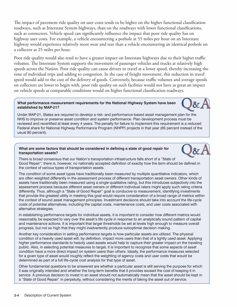
Description of Current System3-4

The impact of pavement ride quality on user costs tends to be higher on the higher functional classification roadways, such as Interstate System highways, than on the roadways with lower functional classifications, such as connectors. Vehicle speed can significantly influence the impact that poor ride quality has on highway user costs. For example, a vehicle encountering a pothole at 55 miles per hour on an Interstate highway would experience relatively more wear and tear than a vehicle encountering an identical pothole on a collector at 25 miles per hour.

Poor ride quality would also tend to have a greater impact on Interstate highways due to their higher traffic volumes. The Interstate System supports the movement of passenger vehicles and trucks at relatively high speeds across the Nation. Poor ride quality can cause drivers to travel at a lower speed, thereby increasing the time of individual trips and adding to congestion. In the case of freight movement, this reduction in travel speed would add to the cost of the delivery of goods. Conversely, because traffic volumes and average speeds on collectors are lower to begin with, poor ride quality on such facilities would not have as great an impact on vehicle speeds as comparable conditions would on higher functional classification roadways.

Q A&What are some factors that should be considered in defining a state of good repair for transportation assets?

There is broad consensus that our Nation’s transportation infrastructure falls short of a “State of Good Repair”; there is, however, no nationally accepted definition of exactly how the term should be defined in the context of various types of transportation assets.

The condition of some asset types have traditionally been measured by multiple quantitative indicators, which are often weighted differently in the assessment process of different transportation asset owners. Other kinds of assets have traditionally been measured using a single qualitative rating, but this introduces subjectivity into the assessment process because different asset owners or different individual raters might apply such rating criteria differently. Thus, although a “State of Good Repair” goal is conducive to measurement, identifying investments that provide the greatest utility in meeting this goal would require consideration of a broad range of metrics within the context of sound asset management principles. Investment decisions should take into account the life-cycle costs of potential alternatives, including the capital costs, maintenance costs, and user costs associated with alternative strategies.

In establishing performance targets for individual assets, it is important to consider how different metrics would reasonably be expected to vary over the asset’s life cycle in response to an analytically sound pattern of capital and maintenance actions. It is important that target thresholds be set at levels high enough to measure overall progress, but not so high that they might inadvertently produce suboptimal decision making.

Another key consideration in setting performance targets is how particular assets are utilized. The physical condition of a heavily used asset will, by definition, impact more users than that of a lightly used asset. Applying higher performance standards to heavily used assets would help to capture their greater impact on the traveling public. Also, in selecting potential measures to target, it is important to recognize that some aspects of asset condition have a more direct impact on system users than others. Ideally, the performance measures selected for a given type of asset would roughly reflect the weighting of agency costs and user costs that would be determined as part of a full life-cycle cost analysis for that type of asset.

Other fundamental questions to be answered are whether a particular asset is still serving the purpose for which it was originally intended and whether the long-term benefits that it provides exceed the cost of keeping it in service. A previous decision to invest in an asset should not automatically mean that the asset should be kept in a “State of Good Repair” in perpetuity, without considering the merits of taking the asset out of service.

Q A&What performance measurement requirements for the National Highway System have been established by MAP-21?

Under MAP-21, States are required to develop a risk- and performance-based asset management plan for the NHS to improve or preserve asset condition and system performance. Plan development process must be reviewed and recertified at least every 4 years. The penalty for failure to implement this requirement is a reduced Federal share for National Highway Performance Program (NHPP) projects in that year (65 percent instead of the usual 80 percent).

System Conditions 3-5

11/28/2012 03XH_B (3-2) R2.xlsx

Calendar Year 2000 2002 2004 2006 2008 2010Fiscal Year * 2001 2003 2005 2007 2009 2011

Good (IRI < 95) 48% 50% 52% 57% 57% 60%

Acceptable (IRI ≤ 170) 91% 91% 91% 93% 92% 93%*The pavement data in this section reflect conditions as of December 31 of each year, as reported in the HPMS. In this report, these values are presented on a calendar-year basis, consistent with the annual Highway Statistics publication. Some other Department of Transportation documents, such as the FY 2011 Performance and Accountability Report, are based on a Federal fiscal year basis; values as of December 31 in one calendar year fall into the next fiscal year. For example, the 60 percent figure identified as good for calendar year 2010 in this exhibit, is reported as a fiscal year 2011 value in the FY 2011 Performance and Accountability Report. Source: Highway Performance Monitoring System as of July 2012.

Exhibit 3-2 Percent of NHS VMT on Pavements With Good and Acceptable Ride Quality, 2000–2010

Pavement Ride Quality on the National Highway SystemAs shown in Exhibit 3-2, the share of vehicle miles traveled (VMT) on NHS pavements with acceptable ride quality has changed very little, from approximately 91 percent in 2000 to approximately 93 percent in 2010. However, the share of VMT on NHS pavements meeting the more rigorous standard of good ride quality has risen sharply over time, from approximately 48 percent in 2000 to approximately 60 percent in 2010. As noted above, the percentage of pavements with good ride quality is a subset of the percentage of pavements with acceptable ride quality.

Q A&What goal was established by the Department of Transportation for pavement ride quality?

The Department of Transportation’s FY 2011 Performance and Accountability Report presented a fiscal year (FY) 2011 target of 58 percent for the share of travel on the NHS on pavements with good ride quality; this corresponds to the calendar year 2010 data of 60 percent presented in this report, indicating that this goal was surpassed.

Q A&What would be the percent VMT on “good” and “acceptable” pavements based on the NHS as newly defined under MAP-21?

Combining data for NHS routes with other principal arterials not on the NHS prior to MAP-21, the share of VMT on the expanded NHS on good pavements is estimated to be 54.7 percent, while the share of VMT on acceptable pavements is estimated to be 88.8 percent. These values are lower than those reported for the old NHS, because principal arterials not included on the MAP-21 NHS tend to have lower ride quality than other NHS routes on average. The values are considered preliminary and may be revised once the expanded NHS has been coded into the HPMS.

The USDOT FY 2013 Performance Plan sets a target for 2013 of having 57 percent of VMT on the expanded NHS to be on pavements with “good” ride quality; the target for 2012 is 56 percent.

Pavement Ride Quality on Federal-Aid HighwaysThe HPMS collects ride-quality data only for Federal-aid highways, which include all functional classes except for rural minor collectors, rural local, and urban local. As described in Chapter 2, these three functional classifications account for approximately three-fourths of the total mileage on the Nation’s system, but carry less than one-sixth of the total daily VMT on the Nation’s roadway system. Because the focus of this report is on VMT-based measures of ride quality rather than mileage-based measures, the omission of these functional classes from the statistics in this section is less significant.

As shown in Exhibit 3-3, for those functional classes for which data are collected, the VMT on pavements with good ride quality increased from 42.8 percent in 2000 to 50.6 percent in 2010. Between 2008 and 2010, the increase in VMT on pavements with good ride quality increased 4.2 percent. This improvement could be related to the impact of the American Recovery and Reinvestment Act, but further research and data collection is needed to confirm this relationship. The VMT on pavements meeting the standard of acceptable (which includes the category of good) ride quality decreased slightly from 85.4 percent in 2000 to 82.0 percent in 2010.

Description of Current System3-6

12/5/2013 03XH_C (3-3) R3.xlsx

2000 2002 2004 2006 2008 20101

Rural Interstate 69.6% 72.2% 73.7% 78.6% 79.0% 79.1%Rural Other Freeway & Expressway2 74.3%Rural Other Principal Arterial2 72.9%Rural Other Principal Arterial2 56.8% 60.2% 61.0% 66.8% 68.4%Rural Minor Arterial 48.9% 51.0% 51.5% 56.3% 56.2% 60.9%Rural Major Collector 39.9% 42.4% 40.3% 39.8% 39.0% 41.4%

Subtotal Rural 55.2% 58.0% 58.3% 62.2% 62.5% 64.6%Urban Interstate 43.6% 45.0% 49.4% 54.0% 55.7% 64.6%Urban Other Freeway and Expressway 32.4% 33.6% 38.8% 45.3% 44.4% 53.3%Urban Other Principal Arterial 26.9% 25.7% 26.5% 28.8% 26.9% 39.7%Urban Minor Arterial 34.4% 34.1% 32.3% 33.6% 32.5% 28.8%Urban Collector2 37.9% 35.5% 35.7% 34.1% 31.5%Urban Major Collector2 25.7%

8.6%Subtotal Urban 35.0% 34.9% 36.6% 39.5% 38.9% 44.0%

Total Good3 42.8% 43.8% 44.2% 47.0% 46.4% 50.6%

Rural Interstate 97.4% 97.3% 97.8% 98.2% 97.3% 91.1%Rural Other Freeway & Expressway2 93.7%Rural Other Principal Arterial2 93.0%Rural Other Principal Arterial2 96.0% 96.2% 96.1% 97.0% 97.6%Rural Minor Arterial 93.1% 93.8% 94.3% 95.1% 94.5% 87.3%Rural Major Collector 86.9% 87.6% 88.5% 87.8% 88.3% 81.2%

Subtotal Rural 93.8% 94.1% 94.5% 94.9% 94.8% 87.8%Urban Interstate 91.2% 89.6% 90.3% 92.7% 91.9% 89.8%Urban Other Freeway and Expressway 87.2% 87.8% 87.7% 92.1% 91.4% 89.2%Urban Other Principal Arterial 71.0% 71.0% 72.6% 73.8% 72.4% 76.4%Urban Minor Arterial 76.5% 76.3% 73.8% 75.6% 75.5% 70.6%Urban Collector2 76.1% 74.6% 72.6% 72.6% 72.0%Urban Major Collector2 67.0%

26.2%Subtotal Urban 80.3% 79.8% 79.7% 81.7% 81.0% 79.4%

Total Acceptable3 85.5% 85.3% 84.9% 86.0% 85.4% 82.0%

Urban Minor Collector2

Functional System

Functional System

Percent Good

Percent Acceptable

Urban Minor Collector2

Exhibit 3-3 Percent of VMT on Pavements with Good and Acceptable Ride Quality, by Functional System, 2000–2010

1 HPMS pavement reporting requirements were modified in 2009 to include bridges; features such as open grated bridge decks or expansion joints can greatly increase the IRI for a given section. 2 2010 data reflects revised HPMS functional classifications. Rural Other Freeways and Expressways have been split out of the Rural Other Principal Arterial category, and Urban Collect has been split into Urban Major Collector and Urban Minor Collector. 3 Totals shown reflect Federal-aid highways only and exclude roads classified as rural minor collector, rural local, or urban local, for which pavement data are not reported in HPMS. Source: Highway Performance Monitoring System as of July 2012.

System Conditions 3-7

As noted in Chapter 2, rural areas contain about three-fourths of national road miles, but support only about one-third of annual national VMT. Consequently, pavement conditions in urban areas have a greater impact on the VMT-weighted measure shown in Exhibit 3-3 than do pavement conditions in rural areas. Pavement conditions are generally better in rural areas. For those functional systems for which data are available, the share of rural VMT on pavements with good ride quality rose from 55.2 percent in 2000 to 64.6 percent in 2010, while the portion of urban VMT on pavements with good ride quality increased from 35.0 percent in 2000 to 44.0 percent in 2010. The share of VMT on pavements with acceptable ride quality rose slightly between 2000 to 2010 in rural areas and declined slightly in urban areas.

Q A&What potential impact on pavement performance might be expected due to the American Recovery and Reinvestment Act?

As discussed in Chapter 6, a significant share of Recovery Act funding was directed toward pavement resurfacing. This funding is likely contributing to the increase in the percentage of VMT on pavements with good ride quality shown in Exhibit 3-3. However, IRI reporting in HPMS is conducted on a 2-year cycle, so some impacts of Recovery Act investment will not immediately be reflected in the data. Also, to the extent to which IRI was measured on sections while resurfacing projects were underway, the data may reflect much higher pavement roughness temporarily experienced by drivers during construction (when driving on grooved pavement, for example).

Pavement Ride Quality by Functional ClassificationPercentage of VMT on pavements rated as having good ride quality increased in both the rural and urban areas during the period from 2000 to 2010. In rural areas the increase was from 55.2 percent to 64.6 percent, while in the urban areas the increase was from 35.0 percent to 44.0 percent. The total increase in VMT on good ride quality pavements was from 42.8 percent in 2000 to 50.6 percent in 2010. The percentage of VMT on pavements with acceptable ride quality fell slightly from 85.4 percent in 2000 to 82.0 percent in 2010. A total of 91.1 percent of all VMT on the rural portion of the Interstate System occurred on pavements with acceptable ride quality; the comparable share on the urban portion of the Interstate System was 89.8 percent.

Among all of the functional systems identified in Exhibit 3-3, the rural portion of the Interstate System had the highest percentage of VMT on pavements with good ride quality in 2010, at 79.1 percent, up from 69.6 percent in 2000. The share of urban Interstate System VMT on pavements with good ride quality from 2000 to 2010 rose from 43.6 percent to 64.6 percent, which represents the largest increase among the functional systems for which data are available.

Q A&What is the significance of the differing results shown for VMT-weighted pavement condition shown in Exhibit 3-3 versus pavement condition on a mileage basis shown in Exhibit 3-4?

While the percentage of pavements with good ride quality based on mileage has declined from 2002 through 2010, the percent of VMT on pavements with good ride quality improved during this period. This result appears consistent with a change in philosophy among many transportation agencies leading them to move away from a simple strategy of addressing assets on a “worst first” basis towards more comprehensive strategies aimed at targeting investment where it will benefit the most users. For example, while the Federal Highway Administration 1998 National Strategic Plan included a target for pavement ride quality for NHS mileage, by the time of the FHWA Fiscal Year 2003 Performance Plan, the target had been modified to a VMT-weighted measure.

Description of Current System3-8

Pavement Ride Quality by MileageExhibit 3-4 shows the pavement ride quality by functional classification from 2000 to 2010 based on mileage rather than VMT. On a mileage basis, the percentage of pavements with both good and acceptable ride quality declined between 2000 and 2010. Consistent with the VMT-weighted figures presented earlier, the share of pavements with good ride quality decreased for all functional classes except urban Interstate. The share of pavements with acceptable ride quality increased for rural principal arterials, rural minor arterials, urban Interstate, urban other freeway & expressway, and urban other principal arterials.

11/6/2012 03XH_D (3-4) R2.xlsx

2000 2002 2004 2006 2008 20101

Rural Interstate 68.5% 71.9% 72.9% 77.2% 78.2% 73.8%Rural Other Freeway & Expressway2 75.3%Rural Other Principal Arterial2 63.2%Rural Other Principal Arterial2 57.4% 60.9% 60.1% 65.3% 66.5%Rural Minor Arterial 47.7% 50.2% 47.6% 53.3% 53.3% 49.7%Rural Major Collector 36.2% 43.1% 36.3% 35.1% 34.0% 28.7%

Subtotal Rural 46.5% 50.9% 47.0% 45.4% 44.9% 40.0%Urban Interstate 50.0% 50.9% 55.0% 59.3% 61.4% 63.2%Urban Other Freeway and Expressway 38.7% 40.9% 44.6% 50.2% 50.6% 48.0%Urban Other Principal Arterial 26.9% 25.7% 26.2% 29.7% 27.4% 26.7%Urban Minor Arterial 37.7% 38.8% 35.7% 33.0% 32.1% 22.2%Urban Collector2 31.0% 33.4% 31.2% 30.1% 28.3%Urban Major Collector2 16.6%

32.6%Subtotal Urban 33.6% 34.3% 33.6% 33.3% 32.0% 24.3%

Total Good3 43.2% 46.6% 43.1% 41.5% 40.7% 35.1%

Rural Interstate 97.8% 97.8% 98.0% 98.0% 98.0% 94.5%Rural Other Freeway & Expressway2 98.0%Rural Other Principal Arterial2 97.8%Rural Other Principal Arterial2 96.0% 96.6% 95.8% 96.7% 97.1%Rural Minor Arterial 92.0% 93.8% 93.9% 94.0% 94.1% 95.7%Rural Major Collector 82.1% 85.9% 85.8% 84.5% 85.1% 77.3%

Subtotal Rural 89.0% 91.0% 90.9% 89.0% 89.4% 84.7%Urban Interstate 93.4% 92.2% 92.6% 94.5% 94.4% 96.6%Urban Other Freeway and Expressway 89.0% 89.5% 90.2% 93.2% 93.3% 95.7%Urban Other Principal Arterial 71.3% 71.1% 72.7% 74.4% 73.1% 83.0%Urban Minor Arterial 78.7% 77.3% 76.0% 75.0% 74.7% 67.2%Urban Collector2 75.3% 75.9% 73.5% 67.9% 68.0%Urban Major Collector2 57.5%

49.3%Subtotal Urban 77.3% 76.9% 76.5% 74.0% 73.6% 69.4%

Total Acceptable3 86.0% 87.4% 86.6% 84.2% 84.2% 80.0%

Functional System

Functional System

Percent Good

Percent Acceptable

Urban Minor Collector2

Urban Minor Collector2

Exhibit 3-4 Percent of Mileage with Acceptable and Good Ride Quality, by Functional System, 2000–2010

1 HPMS pavement reporting requirements were modified in 2009 to include bridges; features such as open grated bridge decks or expansion joints can greatly increase the IRI for a given section. 2 2010 data reflects revised HPMS functional classifications. Rural Other Freeways and Expressways have been split out of the Rural Other Principal Arterial category, and Urban Collect has been split into Urban Major Collector and Urban Minor Collector. 3 Totals shown reflect Federal-aid highways only and exclude roads classified as rural minor collector, rural local, or urban local, for which pavement data are not reported in HPMS. Source: Highway Performance Monitoring System as of July 2012.

System Conditions 3-9

Lane WidthLane width affects capacity and safety. Narrow lanes have a lower capacity and can affect the frequency of crashes. As with roadway alignment, lane width is more crucial on functional classifications with higher travel volumes.

Currently, higher functional systems such as the Interstate System are expected to have 12-foot lanes. As shown in Exhibit 3-5, approximately 99.0 percent of rural Interstate System miles and 98.6 percent of urban Interstate System miles had minimum 12-foot lane widths in 2008.

In 2008, approximately 49.8 percent of urban collectors have lane widths of 12 feet or greater, but approximately 19.3 percent have 11-foot lanes and 22.9 percent have 10-foot lanes; the remaining 8.1 percent have lane widths of 9 feet or less. Among rural major collectors, 40.5 percent have lane widths of 12 feet or greater, but approximately 25.0 percent have 11-foot lanes and 26.3 percent have 10-foot lanes. Roughly 8.1 percent of rural major collector mileage has lane widths of 9 feet or less.

11/2/2012 03XH_E (3-5) R2.xlsx

> 12 foot 11 foot 10 foot 9 foot < 9 footRuralInterstate 99.0% 1.0% 0.0% 0.0% 0.0%Other Principal Arterial 90.6% 7.3% 1.4% 0.4% 0.2%Minor Arterial 72.3% 18.3% 8.5% 0.8% 0.2%Major Collector 40.5% 25.0% 26.3% 6.0% 2.1%UrbanInterstate 98.6% 1.0% 0.1% 0.1% 0.2%Other Freeway and Expressway 94.8% 3.9% 0.4% 0.1% 0.8%Other Principal Arterial 79.9% 13.0% 5.5% 0.5% 1.0%Minor Arterial 64.1% 19.2% 13.6% 1.7% 1.5%Collector 49.8% 19.3% 22.9% 5.7% 2.4%

Exhibit 3-5 Lane Width by Functional Class, 2008

Note: The most recent lane width data available through HPMS is for 2008; due to changes in the HPMS data structure, more recent data cannot yet be extracted. Source: Highway Performance Monitoring System as of December 2009.

Roadway AlignmentThe term “roadway alignment” refers to the curvature and grade of a roadway; i.e., the extent to which it swings from side to side and points up or down. The term “horizontal alignment” relates to curvature (how sharp the curves are), while the term “vertical alignment” relates to gradient (how steep a slope is). Alignment adequacy affects the level of service and safety of the highway system. Inadequate alignment may result in speed reductions and impaired sight distance. Trucks are particularly affected by inadequate vertical alignment with regard to speed. Alignment adequacy is evaluated on a scale from Code 1 (best) to Code 4 (worst).

Alignment adequacy is more important on roads with higher travel speeds and/or higher volumes (e.g., the Interstate System). Because alignment is generally not a major issue in urban areas, only rural alignment statistics are presented in this section. The amount of change in roadway alignment over time is gradual and occurs only during major reconstruction of existing roadways. New roadways are constructed to meet current vertical and horizontal alignment criteria and, therefore, do not generally have alignment problems except under very extreme conditions.

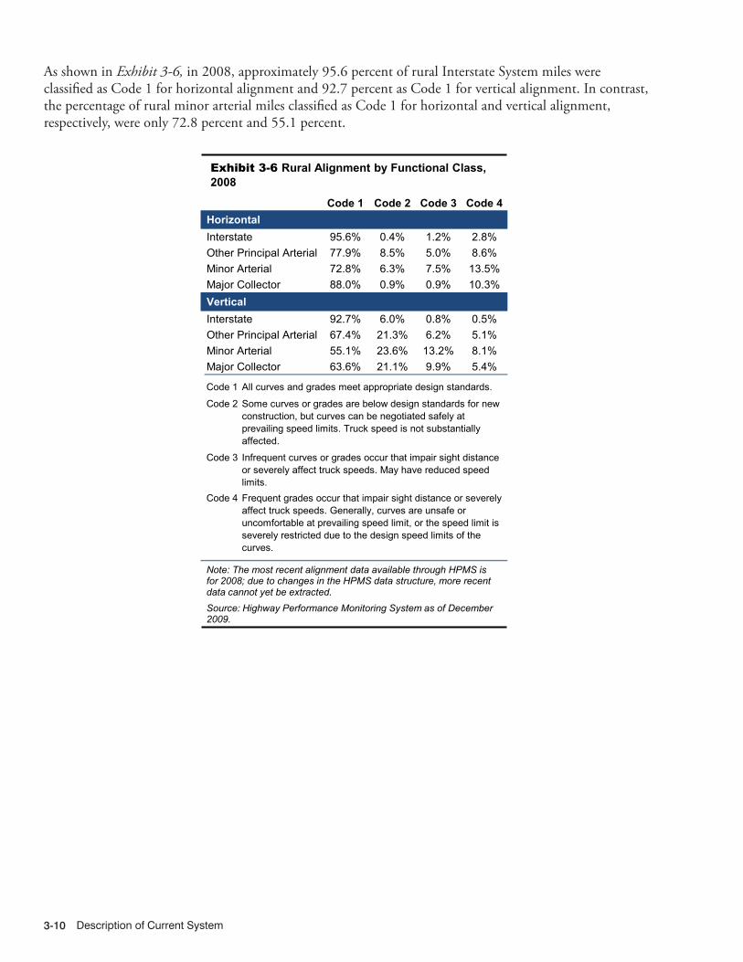
Description of Current System3-10

11/2/2012 03XH_F (3-6) R2.xlsx

Code 1 Code 2 Code 3 Code 4HorizontalInterstate 95.6% 0.4% 1.2% 2.8%Other Principal Arterial 77.9% 8.5% 5.0% 8.6%Minor Arterial 72.8% 6.3% 7.5% 13.5%Major Collector 88.0% 0.9% 0.9% 10.3%VerticalInterstate 92.7% 6.0% 0.8% 0.5%Other Principal Arterial 67.4% 21.3% 6.2% 5.1%Minor Arterial 55.1% 23.6% 13.2% 8.1%Major Collector 63.6% 21.1% 9.9% 5.4%

Code 1 All curves and grades meet appropriate design standards.

Code 2

Code 3

Code 4 Frequent grades occur that impair sight distance or severely affect truck speeds. Generally, curves are unsafe or uncomfortable at prevailing speed limit, or the speed limit is severely restricted due to the design speed limits of the curves.

Infrequent curves or grades occur that impair sight distance or severely affect truck speeds. May have reduced speed limits.

Some curves or grades are below design standards for new construction, but curves can be negotiated safely at prevailing speed limits. Truck speed is not substantially affected.

Exhibit 3-6 Rural Alignment by Functional Class, 2008

Note: The most recent alignment data available through HPMS is for 2008; due to changes in the HPMS data structure, more recent data cannot yet be extracted. Source: Highway Performance Monitoring System as of December 2009.

As shown in Exhibit 3-6, in 2008, approximately 95.6 percent of rural Interstate System miles were classified as Code 1 for horizontal alignment and 92.7 percent as Code 1 for vertical alignment. In contrast, the percentage of rural minor arterial miles classified as Code 1 for horizontal and vertical alignment, respectively, were only 72.8 percent and 55.1 percent.

System Conditions 3-11

Bridge System Conditions

The data used to evaluate the condition of the Nation’s bridges is drawn from the National Bridge Inventory (NBI) and reflects information gathered by States during their periodic safety inspections of bridges. Bridge inspectors are trained to inspect bridges based on the criteria in the National Bridge Inspection Standards (NBIS), at a minimum. Regular inspections are required for all 604,485 bridges with spans of more than 20 feet (6.1 meters) located on public roads. All data presented in this section are from the NBI database as of December 2010. Some of the statistics presented in this section are based on actual bridge counts, and others are weighted by bridge deck area (taking bridge size into account) or by average daily traffic (ADT). ADT represents the number of vehicles crossing a structure on a typical day, but does not reflect the length of the structure crossed. In contrast, the VMT-weighted figures for pavements presented in the previous section take into account both the number of vehicles and the distance they travel.

Bridge RatingsFrom the information collected through the inspection process, assessments are performed to determine the adequacy of a structure to service the current structural and functional demands; factors considered include load-carrying capacity, deck geometry, clearances, waterway adequacy, and approach roadway alignment. Structural assessments together with ratings of the physical condition of key bridge components determine whether a bridge should be classified as “structurally deficient.” Functional adequacy is assessed by comparing the existing geometric configurations and design load-carrying capacities to current standards and demands. Disparities between the actual and preferred configurations are used to determine whether a bridge should be classified as “functionally obsolete.”

Q A&How often are the bridges inspected?

Most bridges in the NBI are inspected once every 24 months. Structures with advanced deterioration or other conditions warranting close monitoring may be inspected more frequently. Certain types of structures in satisfactory or better condition—also considering other factors, including but not limited to structure type and description, structure age, and structure load rating—may receive an exemption from the 24-month inspection cycle. With FHWA approval, these structures may be inspected at intervals that do not exceed 48 months. A discussion of the criteria can be found in Technical Advisory 5140.21, subparagraph 7 of Varying the Frequency of Routine Inspection (http://staffnet/pgc/results.cfm?id=2341).

Approximately 83 percent of bridges are inspected once every 24 months, 12 percent are inspected on a 12-month cycle, and 5 percent are inspected on a maximum 48-month cycle.

Q A&What makes a bridge structurally deficient, and are structurally deficient bridges unsafe?

Structurally deficient bridges are not inherently unsafe.

Bridges are considered structurally deficient if significant load-carrying elements are found to be in poor or worse condition due to deterioration and/or damage, or if the adequacy of the waterway opening provided by the bridge is determined to be extremely insufficient to the point of causing intolerable roadway traffic interruptions.

The classification of a bridge as structurally deficient does not imply that it is likely to collapse or that it is unsafe. By conducting properly scheduled inspections, unsafe conditions may be identified; if the bridge is determined to be unsafe, the structure must be closed. A deficient bridge, when left open to traffic, typically requires significant maintenance and repair to remain in service and eventual rehabilitation or replacement to address deficiencies. To remain in service, structurally deficient bridges often have weight limits that restrict the gross weight of vehicles using the bridges to less than the maximum weight typically allowed by statute.

Description of Current System3-12

Condition RatingsThe primary considerations in classifying structural deficiencies are the bridge component condition ratings. The NBI database contains condition ratings on the three primary components of a bridge: deck, superstructure, and substructure. The bridge deck is the surface on which vehicles travel and is supported by the superstructure. The superstructure transfers the load of the deck and bridge traffic to the substructure, which provides support for the entire bridge.

Condition ratings have been established to measure the state of bridge components over time in a consistent and uniform manner. Bridge inspectors assign condition ratings by evaluating the severity of any deterioration of bridge components relative to their as-built condition, and the extent to which this deterioration affects the performance of the component being rated. These ratings provide an overall characterization of the general condition of the entire component being rated; the condition of specific individual bridge elements may be higher or lower. Exhibit 3-7 describes the bridge condition ratings in more detail.

The condition ratings for bridges in the Nation are shown in Exhibit 3-8. When a primary component of a structure has a rating of 4 or lower, it is considered to be structurally deficient. A structural deficiency does not indicate that a bridge is unsafe but instead indicates the extent to which a bridge has depreciated from its original condition when first built. Once bridge components become structurally deficient, the bridge may experience reduced performance in the form of lane closures or load limits. Bridges are closed to traffic if they have components in such disrepair that there is a safety risk.

Q A&How does a bridge become functionally obsolete?

Functional obsolescence is a function of the geometrics of the bridge in relation to the geometrics required by current design standards. In contrast to structural deficiencies, which are generally the result of deterioration of the conditions of the bridge components, functional obsolescence generally results from changing traffic demands on the structure.

Facilities, including bridges, are designed to conform to the design standards in place at the time they are designed. Over time, improvements are made to the design requirements. As an example, a bridge designed in the 1930s would have shoulder widths in conformance with the design standards of the 1930s, but current design standards are based on different criteria and require wider bridge shoulders to meet current safety standards. The difference between the required, current-day shoulder width and the 1930s’ designed shoulder width represents a deficiency. The magnitude of these types of deficiencies determines whether a bridge is classified as functionally obsolete.

Q A&If a bridge has issues that would warrant classification as both structurally deficient and functionally obsolete, which classification takes precedence?

In such cases, the standard NBI data reporting convention is to identify the bridge as structurally deficient because structural deficiencies are considered more critical. Thus, while a significant percentage of bridges classified as structurally deficient will also have functional issues in need of correction, bridges classified as functionally obsolete do not have significant structural deficiencies.

Q A&How many of bridges reported in the NBI are currently closed?

Of the structures reported in the NBI, 3,585 (0.6 percent) are currently closed to traffic. Closed bridges are generally removed from the inventory 5 years after closure, unless there are special circumstances, such as active work underway that will permit the structure to be reopened in the future.

System Conditions 3-13

9/14/2012 03XB_A (3-7) R1.xlsx

RatingCondition Category Description*

9 Excellent8 Very Good No problems noted.7 Good Some minor problems.6 Satisfactory Structural elements show some minor deterioration.

5 Fair All primary structural elements are sound but may have minor section loss, cracking, spalling, or scour.

4 Poor Advanced section loss, deterioration, spalling, or scour.

3 SeriousLoss of section, deterioration, spalling, or scour have seriously affected primary structural components. Local failures are possible. Fatigue cracks in steel or shear cracks in concrete may be present.

2 Critical

Advanced deterioration of primary structural elements. Fatigue cracks in steel or shear cracks in concrete may be present or scour may have removed substructure support. Unless closely monitored, it may be necessary to close the bridge until corrective action is taken.

1 Imminent Failure

Major deterioration or section loss present in critical structural components, or obvious loss present in critical structural components, or obvious vertical or horizontal movement affecting structural stability. Bridge is closed to traffic, but corrective action may be sufficient to put the bridge back in light service.

0 Failed Bridge is out of service and is beyond corrective action.

Exhibit 3-7 Bridge Condition Rating Categories

*The term "section loss" is defined in The Bridge Inspector’s Reference Manual (BIRM) Publication No. FHWA NHI 03-001 as the loss of a (bridge) member’s cross-sectional area usually by corrosion or decay. A "spall" is a depression in a concrete member resulting from the separation and removal of a volume of the surface concrete. Spalls can be caused by corroding reinforcement, friction from thermal movement, and overstress. The term "scour" refers to the erosion of streambed or bank material around bridge supports due to flowing water. Source: Recording and Coding Guide for the Structure Inventory and Appraisal of the Nation's Bridges, Report No. FHWA-PD-96-001.

Approximately 58.9 percent of the bridges rated had bridge decks with ratings of 7 or better. Weighting bridges by deck area changes this value to 59.4 percent, suggesting that larger bridges are in slightly better shape on average; the corresponding value weighted by ADT is 55.6 percent, suggesting that bridge decks on heavily traveled bridges are in slightly worse shape on average. The share of bridge decks with ratings of 4 or worse was 5.5 percent based on raw bridge counts or weighted by ADT; the corresponding figure weighted by deck area was 5.0 percent.

Weighted by deck area, the share of bridge superstructures with ratings of 7 or better was 65.4 percent, while the comparable value for bridge substructures was 64.8 percent. The share of bridge superstructures weighted by deck area having a rating of 4 or worse was 3.8 percent, compared to 3.5 percent for bridge substructures. The percentages shown in Exhibit 3-8 do not reflect culverts, which do not have a deck, superstructure, or substructure, but instead are self-contained units typically located under roadway fill.

Description of Current System3-14

10/26/2012 03XB_M (3-8) R1.xlsx

Rating *By Bridge

CountWeighted by Deck Area

Weighted by ADT

9 4.0% 2.9% 2.0%8 17.4% 15.2% 11.3%7 37.5% 41.3% 42.2%6 23.2% 24.9% 26.5%5 12.4% 10.7% 12.4%4 4.0% 3.7% 4.1%3 1.0% 1.0% 1.2%2 0.3% 0.1% 0.1%1 0.1% 0.1% 0.1%0 0.2% 0.1% 0.0%

Rating*By Bridge

CountWeighted by Deck Area

Weighted by ADT

9 4.6% 3.8% 2.7%8 22.8% 24.8% 22.4%7 34.0% 36.8% 41.9%6 21.4% 21.1% 21.9%5 11.6% 9.8% 8.6%4 3.9% 2.9% 2.1%3 1.1% 0.6% 0.4%2 0.3% 0.2% 0.1%1 0.1% 0.0% 0.0%0 0.2% 0.1% 0.0%

Rating*By Bridge

CountWeighted by Deck Area

Weighted by ADT

9 4.3% 3.4% 2.2%8 17.5% 17.0% 12.6%7 36.0% 44.4% 51.2%6 22.7% 22.1% 23.2%5 12.5% 9.6% 8.5%4 4.9% 2.8% 1.9%3 1.3% 0.5% 0.2%2 0.5% 0.1% 0.0%1 0.1% 0.0% 0.0%0 0.2% 0.1% 0.0%

Deck Rating Distribution

Superstructure Rating Distribution

Substructure Rating Distribution

Exhibit 3-8 Bridge Condition Ratings, 2010

* Percentages are based on deck ratings for 468,466 bridges, superstructure ratings for 473,116 bridges, and substructure ratings for 473,305 bridges. These percentages exclude 124,823 culverts (self-contained units located under roadway fill that do not have a deck, superstructure, or substructure), other structures for which these ratings are nonapplicable, and other structures for which no value was coded.

Source: National Bridge Inventory, December 2010.

Appraisal RatingsAppraisal ratings compare existing bridge characteristics to the most current standards used for highway and bridge design. Appraisal ratings are a factor used in the classification of bridges as structurally deficient or functionally obsolete. Exhibit 3-9 describes appraisal rating codes in more detail.

9/14/2012 03XB_C (3-9) R1.xlsx

Rating DescriptionN Not applicable.9 Superior to present desirable criteria.8 Equal to present desirable criteria.7 Better than present minimum criteria.6 Equal to present minimum criteria.

5 Somewhat better than minimum adequacy to tolerate being left in place as-is.

4 Meets minimum tolerable limits to be left in place as-is.

3 Basically intolerable requiring a high priority of corrective action.

2 Basically intolerable requiring a high priority of replacement.

1 This value of rating code is not used. 0 Bridge closed.

Exhibit 3-9 Bridge Appraisal Rating

Source: Recording and Coding Guide for the Structure Inventory and Appraisal of the Nation's Bridges, Report No. FHWA-PD-96-001.

Deck Geometry, Underclearance, and Approach Alignment RatingsThe primary considerations in determining functional obsolescence are the deck geometry rating, the underclearance rating, and the rating of the alignment of the roadway approaching the bridge.

A deck geometry rating reflects the width of the bridge, the minimum vertical clearance over the bridge, the ADT, the number of lanes on the structure, whether the structure carries two-way or one-way traffic, and the functional classification of the structure. As noted above, appraisal ratings are used to compare existing characteristics of a bridge to

System Conditions 3-15

the current standards used for highway and bridge design; thus, when a more stringent standard is adopted, this leads to downward adjustments to the ratings of existing bridges that do not meet the new standard. For example, a bridge built to the design standards for deck width in the 1960s may not meet the current design standards for deck width, and thus would receive a lower deck geometry rating.

Underclearance appraisals consider both the vertical and horizontal distances measured from a roadway or railway passing beneath a bridge to the nearest bridge component. The functional classification of the route passing under the bridge is also considered, along with its Federal-aid designation and defense categorization (i.e., whether the bridge crosses over a Strategic Highway Network [STRAHNET] route).

Approach alignment ratings differ from the appraisal ratings previously discussed in that, rather than comparing approach roadway alignment with a specific set of standards, they are determined by comparing the existing approach roadway alignment to the general alignment for the section of highway on which the bridge is located. Disparities in alignment between a bridge and its approach roadway can pose a hazard to drivers.

Exhibit 3-10 shows the distribution of appraisal ratings for deck geometry, underclearance, and approach alignment. Approximately 34.3 percent of bridges received a deck geometry performance rating of 4 or less, indicating problems that generally would not be correctable unless the structure were

Additional Factors Affecting Bridge PerformanceLoad-carrying capacity does not influence the assignment of the condition ratings, but it does factor into the structural evaluation appraisal rating. This is calculated according to the capacity ratings for various categories of traffic in terms of ADT. Depending on how low its rating, a bridge can be classified as functionally obsolete. A very low structural evaluation rating indicates that the load-carrying capacity is too low and the structure should be replaced; in this case, the bridge is classified as structurally deficient. Neither rating is indicative of a bridge that is unsafe, but rather is a measure of the bridge’s original design and the extent of the bridge’s depreciation relative to current design standards.

The waterway adequacy appraisal rating describes the size of the opening of the structure with respect to the passage of water flow under the bridge. This rating, which considers the potential for a structure to be submerged during a flood event and the potential inconvenience to the traveling public, is based on criteria assigned by functional classification. A sufficiently low waterway adequacy rating for a bridge can result in the bridge being classified as structurally deficient.

10/26/2012 03XB_N (3-10) R1.xlsx

Rating*By Bridge

CountWeighted by Deck Area

Weighted by ADT

9 8.9% 21.2% 31.0%8 2.2% 2.4% 2.0%7 11.3% 14.4% 12.4%6 20.7% 16.4% 13.5%5 22.6% 15.8% 11.7%4 18.4% 16.5% 14.7%3 7.2% 4.8% 4.0%2 8.5% 8.5% 10.8%1 0.0% 0.0% 0.0%0 0.1% 0.1% 0.0%

Rating*By Bridge

CountWeighted by Deck Area

Weighted by ADT

9 2.7% 3.5% 5.4%8 62.4% 73.2% 79.2%7 12.3% 10.0% 7.9%6 14.4% 8.9% 5.5%5 3.8% 2.1% 1.1%4 2.8% 1.5% 0.8%3 1.4% 0.6% 0.2%2 0.2% 0.1% 0.0%1 0.0% 0.0% 0.0%0 0.1% 0.0% 0.0%

Rating*By Bridge

CountWeighted by Deck Area

Weighted by ADT

9 10.4% 12.3% 9.1%8 2.0% 2.0% 1.6%7 9.1% 8.3% 7.8%6 17.3% 16.7% 17.1%5 16.2% 14.2% 15.0%4 20.3% 19.3% 23.5%3 21.6% 24.2% 23.4%2 3.0% 2.9% 2.4%1 0.0% 0.0% 0.0%0 0.1% 0.1% 0.0%

Deck Geometry Rating Distribution

Approach Alignment Rating Distribution

Underclearance Rating Distribution

Exhibit 3-10 Bridge Appraisal Ratings Based on Geometry and Function, 2010

* Percentages are based on deck geometry ratings for 519,386 structures, approach alignment ratings for 602,100 structures, and underclearance ratings for 101,860 structures. Underclearance adequacy is rated only for those bridges crossing over a highway or railroad. Source: National Bridge Inventory, December 2010.

Description of Current System3-16

replaced. The comparable figure weighted by ADT is 29.5 percent because deck geometry adequacy is more of a problem on higher-traveled routes, on average. Approximately 1.0 percent of approach alignments were rated as having ratings of 4 or worse when weighted by ADT; for those bridges for which underclearance adequacy was evaluated, 49.4 percent had ratings of 4 or lower.

Bridge ConditionsExhibit 3-11 identifies the percentage of all bridges classified as structurally deficient or functionally obsolete based on the number of bridges, bridges weighted by deck area, and bridges weighted by ADT. The total number of bridges has grown over time; totals for individual years are identified in Chapter 2.

12/9/2013 03XB_E (3-11) R2.xlsx

Analysis Approach 2000 2002 2004 2006 2008 2010By Bridge Count

Structurally Deficient 15.2% 14.2% 13.5% 12.6% 12.1% 11.7%Functionally Obsolete 15.5% 15.4% 15.2% 15.0% 14.8% 14.2%

Total Deficient 30.7% 29.6% 28.7% 27.6% 26.9% 25.9%Weighted by Deck Area

Structurally Deficient 10.8% 10.4% 10.1% 9.6% 9.3% 9.1%Functionally Obsolete 20.8% 20.4% 20.5% 20.3% 20.5% 19.8%

Total Deficient 31.6% 30.8% 30.6% 29.9% 29.8% 28.9%Weighted by ADT

Structurally Deficient 8.5% 8.0% 7.6% 7.4% 7.2% 6.7%Functionally Obsolete 23.0% 22.0% 21.9% 21.9% 22.2% 21.5%

Total Deficient 31.5% 30.0% 29.5% 29.3% 29.4% 28.2%

Percentage of Deficient Bridges by Year

Exhibit 3-11 Systemwide Bridge Deficiencies, 2000–2010

Source: National Bridge Inventory, December 2010.

Based on raw bridge counts, approximately 11.7 percent of bridges were classified as structurally deficient in 2010, and 14.2 percent were classified as functionally obsolete. Weighted by deck area, the comparable shares were 9.1 percent structurally deficient and 19.8 percent functionally obsolete. The differences are even more pronounced when bridges are weighted by ADT, as this adjustment results in a structurally deficient share of 6.7 percent and a functionally obsolete share of 21.5 percent.

Since 2000, the total share of deficient bridges weighted by deck area has decreased from 31.6 percent to 28.9 percent, representing an overall improvement in the condition of the Nation’s bridges. Whether considering raw bridge counts, deck-area-weighted values, or ADT-weighted values, more progress was made during this period in reducing the percentage of structurally deficient bridges than in reducing the share of functionally obsolete bridges.

Bridge Conditions on the NHSExhibit 3-12 identifies the percent of bridges on the NHS classified as structurally deficient or functionally obsolete based on the number of bridges, bridges weighted by deck area, and bridges weighted by ADT. The total number of NHS bridges for individual years are identified in Chapter 2.

Q A&What goal was established by the Department of Transportation for NHS bridges?

The Department of Transportation’s FY 2010 Performance Report presented a FY 2010 target of a maximum 28.9 percent for the share of deck area on NHS bridges that were rated as deficient. The target was met and exceeded. The final percentage was 25.2 percent.

System Conditions 3-17

In 2010, approximately 5.1 percent of NHS bridges were classified as structurally deficient and 16.3 percent were classified as functionally obsolete, resulting in a total of 21.4 percent of the 116,669 NHS bridges classified as deficient; the comparable values weighted by deck area and ADT were 28.7 percent and 25.7 percent, respectively. This suggests that there is a greater-than-average concentration of deficiencies on heavily traveled and larger bridges, respectively.

The FHWA has adopted deck-area weighting for use in agency performance planning in recognition of the significant logistical and financial challenges that may be involved in addressing deficiencies on larger bridges. The share of NHS bridges weighted by deck area that are classified as structurally deficient remained essentially the same from 2000 (8.7 percent) to 2010 (8.3 percent), while the deck-area weighted share classified as functionally obsolete decreased from 22.0 percent to 20.3 percent during the same period. NHS routes tend to carry significantly more traffic than average roads, and functional obsolescence remains a significant challenge on NHS bridges.

12/9/2013 03XB_F (3-12) R2.xlsx

Analysis Approach 2000 2002 2004 2006 2008 2010Weighted by Deck Area

Structurally Deficient 8.7% 8.6% 8.9% 8.4% 8.2% 8.3%Functionally Obsolete 22.0% 21.1% 20.9% 20.8% 21.4% 20.3%

Total Deficient 30.7% 29.7% 29.8% 29.2% 29.6% 28.7%Weighted by ADT

Structurally Deficient 7.5% 7.1% 6.8% 6.6% 6.4% 6.0%Functionally Obsolete 21.4% 20.0% 19.8% 20.1% 20.5% 19.7%

Total Deficient 28.9% 27.1% 26.6% 26.7% 26.9% 25.7%By Bridge Count

Structurally Deficient 6.0% 5.9% 5.7% 5.5% 5.4% 5.1%Functionally Obsolete 17.7% 17.2% 16.9% 16.8% 16.9% 16.3%

Total Deficient 23.7% 23.1% 22.6% 22.3% 22.3% 21.4%

Percentage of Deficient Bridges by YearExhibit 3-12 NHS Bridge Deficiencies, 2000–2010

Source: National Bridge Inventory, December 2010.

Q A&What provisions are in MAP-21 to support and improve the performance level of bridges on the NHS and on the Interstate System?

The provisions of MAP-21 include the National Highway Performance Program (NHPP) and Surface Transportation Program (STP), each of which provides support for the condition and performance of the Nation’s highway bridges. The NHPP specifically provides support for highway bridges on the NHS and the STP provides flexibility for States and localities to preserve and improve the conditions and performance of highway bridges on any public road. The NHPP also establishes a minimum standard for the condition of bridges located on the NHS and a penalty if the standard is not achieved:

If more than 10% of the total deck area of NHS bridges in a State is on structurally deficient bridges for three consecutive years, the State must devote NHPP funds in an amount equal to 50% of the State’s FY 2009 Highway Bridge Program apportionment to improve NHS bridge conditions during the following fiscal year (and each year thereafter if the condition remains below the minimum standard).

Additionally, the provisions for the National Bridge and Tunnel Inventory and Inspection Standards recognize the importance of the safety of the traveling public as well as support the efforts to improve the condition of the Nation’s bridges. The purposes of this provision include providing a basis for a data-driven and risk-based approach and a cost-effective strategy to bridge investment, and establishing and maintaining existing minimum Federal standards related to the inventory and safety inspection of bridges on all public roads.

Description of Current System3-18

Bridge Conditions on the STRAHNETThe STRAHNET system is a key subset of the NHS. The physical composition of this system was described in Chapter 2 and the condition of the pavement portion was presented earlier in this chapter. The share of structurally deficient bridges decreased from 6.2 percent in 2000 to 4.9 percent in 2010. The share of functionally obsolete bridges decreased from 17.2 percent in 2000 to 16.9 percent in 2010. The share of bridges either structurally deficient or functionally obsolete decreased from 23.4 percent in 2000 to 21.8 percent in 2010. These data are shown in Exhibit 3-13.

Year BridgesNumber Number Percentage Number Percentage Number Percentage

2000 102,856 6,357 6.2% 17,742 17.2% 24,099 23.4%

2002 79,852 4,320 5.4% 13,724 17.2% 18,044 22.6%

2004 72,046 3,640 5.1% 12,444 17.3% 16,084 22.4%

2006 73,003 3,645 5.0% 12,664 17.3% 16,309 22.3%

2008 73,771 3,659 5.0% 12,942 17.5% 16,601 22.5%

2010 68,529 3,355 4.9% 11,613 16.9% 14,968 21.8%

Structurally Deficient Functionally Obsolete Total Deficient

Exhibit 3-13 STRAHNET-Deficient Bridges

Source: National Bridge Inventory, December 2010.

Bridge Conditions by Functional ClassificationBased on the number of bridges, the total percentage of structurally deficient and functionally obsolete bridges on the Nation’s roadways decreased from 30.8 percent in 2000 to 25.9 percent in 2010. The percentage of structurally deficient bridges for most functional classes decreased between 2000 and 2010, with the exception of rural Interstate System bridges. As shown in Exhibit 3-14, the share of rural Interstate System bridges classified as structurally deficient increased from 4.0 percent to 4.5 percent during this period. The share of bridges classified as functionally obsolete decreased from 15.5 percent in 2000 to 14.2 percent in 2010.

Among the individual functional classes, the highest percentage observed in 2010 for structurally deficient bridges was 17.9 percent for rural local; the rural portion of the Interstate System and rural other principal arterial roadways tied for the lowest percentage of structurally deficient bridges at 4.5 percent. Urban minor arterials had the highest share of functionally obsolete bridges in 2000, at approximately 28.6 percent. The functional class with the lowest share of functionally obsolete bridges in 2010 was rural other principal arterials with 8.5 percent; rural other principal arterials have continuously had the lowest share of functionally obsolete bridges since 2000.

Bridge Conditions by OwnerAs discussed in Chapter 2, the entity responsible for the maintenance and operation of a bridge is characterized as its owner. A secondary agency (such as the State) may perform maintenance and operation work under an interagency agreement with the owner (such as a local community). However, such agreements do not transfer ownership and, therefore, do not negate the responsibilities of the bridge owners to ensure that the maintenance and operation of all bridges that they own are in compliance with Federal and State requirements. Each State has the responsibility for inspection of all bridges in that State except for tribally or Federally owned bridges.

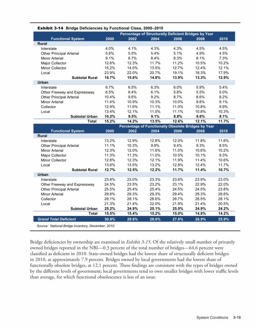
System Conditions 3-19

12/13/2013 03XB_H (3-14) R2.xlsx

Functional System 2000 2002 2004 2006 2008 2010Rural

Interstate 4.0% 4.1% 4.3% 4.3% 4.5% 4.5%Other Principal Arterial 5.6% 5.5% 5.4% 5.1% 4.9% 4.5%Minor Arterial 9.1% 8.7% 8.4% 8.3% 8.1% 7.3%Major Collector 12.6% 12.3% 11.7% 11.2% 10.5% 10.2%Minor Collector 15.2% 14.0% 13.5% 12.7% 12.4% 12.1%Local 23.9% 22.0% 20.7% 19.1% 18.3% 17.9%

Subtotal Rural 16.7% 15.6% 14.8% 13.9% 13.3% 12.9%Urban

Interstate 6.7% 6.5% 6.3% 6.0% 5.9% 5.4%Other Freeway and Expressway 6.5% 6.4% 6.1% 5.8% 5.5% 5.0%Other Principal Arterial 10.4% 9.6% 9.2% 8.7% 8.6% 8.2%Minor Arterial 11.4% 10.9% 10.3% 10.0% 9.8% 9.1%Collector 12.9% 11.6% 11.1% 11.0% 10.8% 9.9%Local 13.4% 12.1% 11.5% 11.1% 10.8% 10.3%

Subtotal Urban 10.2% 9.5% 9.1% 8.8% 8.6% 8.1%Total 15.2% 14.2% 13.5% 12.6% 12.1% 11.7%

Functional System 2000 2002 2004 2006 2008 2010Rural

Interstate 13.2% 12.9% 12.8% 12.0% 11.8% 11.6%Other Principal Arterial 11.1% 10.3% 9.9% 9.4% 9.3% 8.5%Minor Arterial 12.3% 12.0% 11.6% 11.0% 10.6% 10.2%Major Collector 11.3% 11.3% 11.0% 10.5% 10.1% 9.3%Minor Collector 12.8% 12.3% 12.1% 11.9% 11.4% 10.6%Local 13.6% 13.5% 13.2% 12.8% 12.4% 11.7%

Subtotal Rural 12.7% 12.5% 12.2% 11.7% 11.4% 10.7%Urban

Interstate 23.8% 23.0% 23.3% 23.6% 23.9% 23.0%Other Freeway and Expressway 24.5% 23.5% 23.2% 23.1% 22.9% 22.0%Other Principal Arterial 25.5% 25.4% 25.4% 24.5% 24.5% 23.8%Minor Arterial 29.6% 29.3% 29.3% 29.4% 29.3% 28.6%Collector 28.1% 28.1% 28.6% 28.7% 28.5% 28.1%Local 21.3% 21.4% 22.0% 21.9% 21.4% 20.5%

Subtotal Urban 25.2% 24.9% 25.1% 25.0% 24.9% 24.2%Total 15.5% 15.4% 15.2% 15.0% 14.8% 14.2%

Grand Total Deficient 30.8% 29.6% 28.6% 27.6% 26.9% 25.9%

Percentage of Structurally Deficient Bridges by Year

Percentage of Functionally Obsolete Bridges by Year

Exhibit 3-14 Bridge Deficiencies by Functional Class, 2000–2010

Source: National Bridge Inventory, December, 2010.

Bridge deficiencies by ownership are examined in Exhibit 3-15. Of the relatively small number of privately owned bridges reported in the NBI—0.3 percent of the total number of bridges—64.6 percent were classified as deficient in 2010. State-owned bridges had the lowest share of structurally deficient bridges in 2010, at approximately 7.9 percent. Bridges owned by local governments had the lowest share of functionally obsolete bridges, at 12.1 percent. These findings are consistent with the types of bridges owned by the different levels of government; local governments tend to own smaller bridges with lower traffic levels than average, for which functional obsolescence is less of an issue.

Description of Current System3-20

12/9/2013 03XB_I (3-15) R3.xlsx

Federal State LocalPrivate/Other* Total

CountTotal Bridges 8,145 291,145 303,531 1,667 604,488Total Deficient 2,016 70,209 82,984 1,077 156,286

Structurally Deficient 672 23,049 46,178 532 70,431Functionally Obsolete 1,344 47,160 36,806 545 85,855

PercentagesPercent of Total Inventory Owned 1.3% 48.2% 50.2% 0.3% 100.0%Percent Deficient 24.8% 24.1% 27.3% 64.6% 25.9%

Percent Structurally Deficient 8.3% 7.9% 15.2% 31.9% 11.7%Percent Functionally Obsolete 16.5% 16.2% 12.1% 32.7% 14.2%

Exhibit 3-15 Bridge Deficiencies by Owner, 2010

* Note that these data only reflect bridges for which inspection reports were submitted to the NBI. An unknown number of privately owned bridges are omitted. Source: National Bridge Inventory, December 2010.

Bridges by AgeExhibit 3-16 identifies the age composition of Interstate System bridges, NHS bridges, and all total highway bridges in the Nation. As of 2010, approximately 37.7 percent of the Nation’s bridges were between 26 and 50 years old; this share was higher for NHS bridges, at 52.7 percent, while 68.4 percent of the Interstate bridges fell into this age range.

11/28/2012 03XB_J (3-16) R2.xlsx

Age Range Count Percent Count Percent Count Percent0–10 Years 66,877 11.1% 11,824 10.1% 3,637 6.6%11–25 Years 123,231 20.4% 18,957 16.2% 5,831 10.5%26–50 Years 228,103 37.7% 61,515 52.7% 37,830 68.4%51–75 Years 125,274 20.7% 19,610 16.8% 7,810 14.1%76–100 Years 50,525 8.4% 4,506 3.9% 186 0.3%>100 Years 10,181 1.7% 212 0.2% 6 0.0%Not reported 294 0.0% 45 0.0% 35 0.1%

Total 604,485 100.0% 116,669 100.0% 55,335 100.0%

All Bridges NHS Bridges Interstate Bridges

Exhibit 3-16 Bridges by Age Range, as of 2010

Source: National Bridge Inventory, December 2010.

Approximately 68.5 percent of all bridges are 26 years old or older. The percentage of NHS and Interstate bridges in this group are 73.6 percent and 82.8 percent, respectively. The largest number of bridges for each system is in the 26- to 50-years-of-age group: 37.7 percent of all bridges, 52.7 percent of NHS bridges, and 68.4 percent of Interstate bridges. The large number of bridges with ages of 26 years to 50 years has potential implications in terms of long-term bridge rehabilitation and replacement strategies because the need for such actions may be concentrated within certain time periods rather than being spread out evenly, which might be the case if the original construction of bridges had been spread out more evenly over time. However, a number of other variables such as maintenance practices and environmental conditions also affect when future capital investments might be needed.

System Conditions 3-21

Exhibit 3-17 identifies the distribution of bridge deficiencies within the age ranges presented in Exhibit 3-16. The percent of bridges classified as either structurally deficient or functionally obsolete generally tends to rise as bridges age. Among Interstate System bridges, 22.0 percent of the bridges constructed between 26 and 50 years ago were classified as deficient; this share rose to 34.5 percent for Interstate System bridges constructed between 51 and 75 years ago. Note that some existing bridges were absorbed into the Interstate System at the time it was designated; some of these structures remain in service today.

12/13/2013 03XB_K (3-17) R2.xlsx

Count Percent Count Percent Count Percent0–10 Years 66,877 450 0.7% 6,096 9.1% 6,546 9.8%11–25 Years 123,231 3,055 2.5% 11,059 9.0% 14,114 11.5%26–50 Years 228,103 21,508 9.4% 30,671 13.4% 52,179 22.9%51–75 Years 125,274 25,883 20.7% 24,289 19.4% 50,172 40.0%76–100 Years 50,525 15,430 30.5% 11,078 21.9% 26,508 52.5%>100 Years 10,181 4,079 40.1% 2,574 25.3% 6,653 65.3%Null 294 26 8.8% 90 30.6% 116 39.5%

Total 604,485 70,431 11.7% 85,857 14.2% 156,288 25.9%

Count Percent Count Percent Count Percent0–10 Years 11,824 57 0.5% 1,366 11.6% 1,423 12.0%11–25 Years 18,957 148 0.8% 1,853 9.8% 2,001 10.6%26–50 Years 61,515 3,221 5.2% 10,019 16.3% 13,240 21.5%51–75 Years 19,610 1,839 9.4% 4,824 24.6% 6,663 34.0%76–100 Years 4,506 581 12.9% 910 20.2% 1,491 33.1%>100 Years 212 54 25.5% 63 29.7% 117 55.2%Null 45 2 4.4% 26 57.8% 28 62.2%

Total 116,669 5,902 5.1% 19,061 16.3% 24,963 21.4%

Count Percent Count Percent Count Percent0–10 Years 3,637 35 1.0% 654 18.0% 689 18.9%11–25 Years 5,831 61 1.0% 805 13.8% 866 14.9%26–50 Years 37,830 2,019 5.3% 6,312 16.7% 8,331 22.0%51–75 Years 7,810 640 8.2% 2,052 26.3% 2,692 34.5%76–100 Years 186 19 10.2% 21 11.3% 40 21.5%>100 Years 6 1 16.7% 1 16.7% 2 33.3%Null 35 0 0.0% 22 62.9% 22 62.9%

Total 55,335 2,775 5.0% 9,867 17.8% 12,642 22.8%

Structurally Deficient Functionally Obsolete All Deficient

Age Range of All Bridges

Bridge Count

Bridge Count

Age Range of NHS Bridges

Age Range of Interstate Bridges

Bridge Count

Structurally Deficient Functionally Obsolete All Deficient

Structurally Deficient Functionally Obsolete All Deficient

Exhibit 3-17 Bridge Deficiencies by Period Built, as of 2010

Source: National Bridge Inventory, December 2010.

Q A&What is the average age of the Nation’s bridges and has it changed since 2000?

The average year of construction in 2000 was 1963 which meant the average age was 37 years. In 2010, the average year of construction was 1971 which results in an average age of 39 years. Therefore, the overall age of the Nation’s bridges increased 2 years over a period of 10 years.

In 2000, there were 588,844 bridges listed in the National Bridge Inventory (NBI). Approximately 67.2 percent of these bridges were more than 25 years old and 26.2 percent were over 50 years in age.

By 2010, the number of bridges in the NBI increased to 604,485 bridges. Of these, 68.5 percent were older than 25 years and 30.8 percent were over 50 years old.

Description of Current System3-22

The age of a bridge structure is one indicator of its serviceability. However, a combination of several factors impacts the serviceability of a structure, including the original type of design; the frequency, timeliness, effectiveness, and appropriateness of the maintenance activities implemented over the life of the structure; the loading the structure has been subject to during its life; the climate of the area where the structure is located; and any additional stresses from events such as flooding to which the structure has been subjected. As an example, two structures built at the same time, using the same design standards, and in the same climate area can have very different serviceability levels. The first structure may have had increasing loads due to increased heavy truck traffic, lack of maintenance of the deck or the substructure, or lack of rehabilitation work. The second structure may have had the same increases in heavy truck traffic but received correctly timed preventive maintenance activities on all parts of the structure and proper rehabilitation activities. In this case, the first structure would have a very low serviceability level while the second structure would have a high serviceability level.

Historic Bridges on the Nation’s RoadwaysOf the 604,485 bridges in the NBI, approximately 0.29 percent are registered as historic and an additional 0.64 percent are eligible to be registered. Some historic bridges carry significant traffic volumes; over 17 percent of the bridges on the historic register are on principal arterials.

Bridges do not have to be extremely old to be classified as historic. Approximately 9.5 percent of the registered historic bridges are 50 years old or younger, well within the typical useful lifespan of a bridge; approximately 4.1 percent are 10 years old or less.

Of the registered historic bridges, 33.3 percent are classified as structurally deficient and 40.2 percent are classified as functionally obsolete. At some time, it will be necessary to take mitigation actions on those bridges classified as structurally deficient; however, mitigation actions on the bridges classified as functionally obsolete may not be possible due to their historic classification. These bridges are still open to vehicular traffic even though, in some cases, heavy trucks and similar vehicles may not be allowed to use a particular historic bridge.

System Conditions 3-23

Transit System Conditions

The condition and performance of the U.S. transit infrastructure should ideally be evaluated by how well it supports the objectives of the transit agencies that operate it. Presumably these objectives include providing fast, safe, cost-effective, and comfortable service that takes people where they want to go. However, the degree to which transit service meets these objectives is difficult to quantify and involves trade-offs that are outside the scope of Federal responsibility. This section reports on the quantity, age, and physical condition of transit assets because these factors determine how well the infrastructure can support any agency’s objectives and set a foundation for uniform, consistent measurement. The assets in question include vehicles, stations, guideway, rail yards, administrative facilities, maintenance facilities, maintenance equipment, power systems, signaling systems, communication systems, and structures that carry both elevated and subterranean guideway. Chapter 5 addresses issues relating to the operational performance of transit systems. The FTA uses a numerical condition rating scale ranging from 1 to 5, detailed in Exhibit 3-18, to describe the relative condition of transit assets. A rating of 4.8 to 5.0, or “excellent,” indicates that the asset is in nearly new condition or lacks visible defects. At the other end of the scale, a rating of 1.0 to 1.9, or “poor,” indicates that the asset needs immediate repair and is not capable of supporting satisfactory transit service.The FTA uses the Transit Economic Requirements Model (TERM) to estimate the conditions of transit assets for this report. This model consists of a database of transit assets and deterioration schedules that express asset conditions principally as a function of an asset’s age. Vehicle condition is based on an estimate of vehicle maintenance history and major rehabilitation expenditures in addition to vehicle age; the conditions of wayside control systems and track are based on an estimate of use (revenue miles per mile of track) in addition to age. For the purposes of this report, the state of good repair was defined using TERM’s numerical condition rating scale. Specifically, this report considers an asset to be in a state of good repair when the physical condition of that asset is at or above a condition rating value of 2.5 (the mid-point of the marginal range). An entire transit system would be in a state of good repair if all of its assets have an estimated condition value of 2.5 or higher. The State of Good Repair benchmark presented in Chapter 8 represents the level of investment required to attain and maintain this definition of a state of good repair by rehabilitating or replacing all assets with estimated condition ratings that are less than this minimum condition value. FTA is currently developing a broader definition of a state of good repair to use as a basis for administering MAP-21 grant programs and requirements that are intended to foster better infrastructure re-investment practices across the industry. This definition may not be the same as the one used in this report.Typical deterioration schedules for vehicles, maintenance facilities, stations, train control systems, electric power systems, and communication systems have been estimated by FTA through special on-site engineering surveys. Transit vehicle conditions also reflect the most recent information on vehicle age, use, and level of maintenance from the National Transit Database (NTD); the information used in this edition of the C&P report is from 2010. Age information is available on a vehicle-by-vehicle basis from the NTD and collected for all other assets through special surveys. Average maintenance expenditures and major

10/24/2012 03XT_A (3-18) R3.xlsx

Rating Condition DescriptionExcellent 4.8–5.0 No visible defects, near-new

condition.Good 4.0–4.7 Some slightly defective or

deteriorated components.Adequate 3.0–3.9 Moderately defective or

deteriorated components.Marginal 2.0–2.9 Defective or deteriorated

components in need of replacement.

Poor 1.0–1.9 Seriously damaged components in need of immediate repair.

Exhibit 3-18 Definitions of Transit Asset Conditions

Source: Transit Economic Requirements Model.

Description of Current System3-24

rehabilitation expenditures by vehicle are also available on agency and modal bases. For the purpose of calculating conditions, agency maintenance and rehabilitation expenditures for a particular mode are assumed to be the same average value for all vehicles operated by that agency in that mode. Because agency maintenance expenditures may fluctuate from year to year, TERM uses a 5-year average. The deterioration schedules applied for track and guideway structures are based on special studies. The methods used to calculate deterioration schedules and the sources of the data on which deterioration schedules are based are discussed in Appendix C.

Condition estimates in each edition of the C&P report are based on contemporary updated asset inventory information and reflect updates in TERM’s asset inventory data. Annual data from the NTD were used to update asset records for the Nation’s transit vehicle fleets. In addition, updated asset inventory data were collected from 30 of the Nation’s largest rail and bus transit agencies to support analysis of non-vehicle needs. Because these data are not collected annually, it is not possible to provide accurate time series analysis of non-vehicle assets. FTA is working to develop improved data in this area. Appendix C provides a more detailed discussion of TERM’s data sources. Exhibit 3-19 shows the distribution of asset conditions, by replacement value, across major asset categories for the entire U.S. transit industry.

Condition estimates for assets in this report are weighted by the replacement value of each asset. This takes into account the fact that assets vary substantially in replacement value. So, a $1-million railcar in poor condition is a much bigger problem than a $1-thousand turnstile in similar condition. As an example of the calculation involved, consider: the cost-weighted average of a $100 asset in condition 2 and a $50 asset in condition 4 would be (100x2+50x4)/(100+50) = 2.67. The un-weighted average would be (2+4)/2 = 3.

The Replacement Value of U.S. Transit AssetsThe total replacement value of the transit infrastructure in the United States was estimated at $678.9 billion in 2010. These estimates, presented in Exhibit 3-20, are based on asset inventory information contained in TERM. The estimates are reported in 2010 dollars. They exclude the value of assets that belong to special service operators that do not report to the NTD. Rail assets totaled $547.6 billion, or roughly 80 percent of all transit assets. Non-rail assets were estimated at $120.5 billion. Joint assets totaled $10.8 billion; they consist of assets that serve more than one mode within a single agency and can include administrative facilities, intermodal transfer centers, agency communications systems (e.g., telephone, radios, and computer networks), and vehicles used by agency management (e.g., vans and automobiles).

10/24/2012 03XT_B (3-19) R3.xlsx

$0

$50

$100

$150

$200

$250

Guideway Elements

Facilities Systems Stations Vehicles

Rep

lace

men

t Val

ue in

Bill

ions

of D

olla

rs  4.8–5.0 Excellent

 4.0–4.7 Good  3.0–3.9 Adequate  2.0–2.9 Marginal  1.0–1.9 Poor

Exhibit 3-19 Distribution of Asset Physical Conditions by Asset Type for All Modes

Source: Transit Economic Requirements Model.

10/24/2012 03XT_C (3-20) R3.xlsx

Transit Asset Nonrail RailJoint

Assets TotalMaintenance Facilities $59.8 $30.6 $5.4 $95.8Guideway Elements $12.1 $240.4 $1.0 $253.5Stations $3.7 $88.1 $0.6 $92.4Systems $3.0 $112.9 $3.3 $119.2Vehicles $41.9 $75.7 $0.5 $118.0

Total $120.5 $547.6 $10.8 $678.9

Replacement Value(Billions of 2010 Dollars)

Source: Transit Economic Requirements Model.

Exhibit 3-20 Estimated Replacement Value of the Nation's Transit Assets, 2010

System Conditions 3-25

Bus Vehicles (Urban Areas)Bus vehicle age and condition information is reported according to vehicle type for 2000 to 2010 in Exhibit 3-21. When measured across all vehicle types, the average age of the Nation’s bus fleet has remained essentially unchanged since 2004. Similarly, the average condition rating for all bus types (calculated as the weighted average of bus asset conditions, weighted by asset replacement value) is also relatively unchanged, remaining near the bottom of the adequate range for the last decade. The percentage of vehicles below the state of good repair replacement threshold (condition 2.5) has remained in the range of 10 to 12 percent for this same time period. Note that while this observation holds across all vehicle types, the proportion of full-size buses (the vehicle type that supports most fixed-route bus services) declined from 15.2 percent in 2008 to 12.5 percent in 2010. This reduction likely reflects the preliminary impacts of transit-related American Recovery and Reinvestment Act (Recovery Act) spending, a significant proportion of which was expended on full-sized buses. It is expected that this proportion will be shown to have declined further as newer vehicle age data become available that reflect Recovery Act related bus vehicle procurements on or after 2010.

10/24/2012 03XT_D (3-21) R3.xlsx

2000 2002 2004 2006 2008 2010Articulated BusesFleet Count 2,002 2,799 3,074 3,445 4,302 4,896Average Age (Years) 6.6 7.2 5.0 5.3 6.3 6.5Average Condition Rating 3.5 3.3 3.5 3.5 3.3 3.2Below Condition 2.50 (Percent) 24.9% 16.6% 5.0% 2.1% 2.6% 3.7%Full-Size BusesFleet Count 46,380 46,573 46,139 46,714 45,985 45,441Average Age (Years) 8.1 7.5 7.2 7.4 7.9 7.8Average Condition Rating 3.2 3.2 3.2 3.2 3.1 3.1Below Condition 2.50 (Percent) 14.5% 13.1% 12.3% 11.3% 15.2% 12.5%Mid-Size BusesFleet Count 7,203 7,269 7,114 6,844 7,009 7,218Average Age (Years) 5.5 8.4 8.1 8.2 8.3 8.1Average Condition Rating 3.4 3.1 3.1 3.1 3.1 3.1Below Condition 2.50 (Percent) 8.3% 14.1% 13.2% 14.2% 12.4% 12.5%Small BusesFleet Count 8,646 14,857 15,972 16,156 19,366 19,493Average Age (Years) 4.2 4.5 4.6 5.1 5.1 5.2Average Condition Rating 3.6 3.4 3.5 3.4 3.4 3.4Below Condition 2.50 (Percent) 2.2% 8.8% 10.1% 10.3% 11.6% 10.2%VansFleet Count 14,583 17,147 18,713 19,515 26,823 28,531Average Age (Years) 3.2 3.2 3.3 3.0 3.2 3.4Average Condition Rating 3.8 3.7 3.8 3.8 3.8 3.7Below Condition 2.50 (Percent) 0.2% 7.2% 6.7% 8.4% 8.0% 8.2%Total BusTotal Fleet Count 78,814 88,645 91,012 92,674 103,485 105,579Weighted Average Age (Years) 6.5 6.2 6.0 6.0 6.1 6.1Weighted Average Condition Rating 3.3 3.2 3.3 3.3 3.1 3.0Below Condition 2.50 (Percent) 10.2% 11.8% 10.6% 10.4% 12.0% 10.5%

Sources: Transit Economic Requirements Model and National Transit Database.

Exhibit 3-21 Urban Transit Bus Fleet Count, Age, and Condition, 2000–2010

Description of Current System3-26

The Nation’s bus fleet has grown at an average annual rate of roughly 3 percent over the last decade, with most of this growth concentrated in three vehicle types including: large, 60-foot articulated buses; small buses of under 25 feet (frequently dedicated to flexible route bus services); and vans. The large increase in the number of vans reflects both the needs of an aging population (paratransit services) and an increase in the popularity of vanpool services. In contrast, the number of full- and medium-sized buses has remained relatively flat since 2000.

Similarly, Exhibit 3-22 presents the age distribution of the Nation’s transit buses and vans. Note here that full-size buses and vans account for the highest proportion (roughly 70 percent) of the Nation’s rubber tire transit vehicles. Moreover, while most vans are retired by age 6 and most buses by age 15, roughly 5 to 10 percent of these fleets remain in service well after their typical retirement ages.

Furthermore, it appears the economic recession had an impact on the purchase of new vehicles and, thus, the age profile of buses and vans at transit agencies in the Nation. The peak of the age distribution reflects vehicles 2 years old, i.e., those purchased between July 1, 2007, and June 30, 2008. Purchases declined in the 2 years following that period.

10/24/2012 03XT_I (3-22) R4.xlsx

0 2,000 4,000 6,000 8,000 10,000 12,000

0 1 2 3 4 5 6 7 8 9

10 11 12 13 14 15 16 17 18 19 20

> 20

Bus and Van Count

Veh

icle

Age

, Yea

rs

Articulated

Full-Size Bus

Medium-Size Bus

Small-Size Bus

Van

Exhibit 3-22 Age Distribution of Buses and Vans, 2010

Source: Transit Economic Requirements Model and National Transit Database.

System Conditions 3-27

Other Bus Assets (Urban Areas)The more comprehensive capital asset data described above allow us to report a more complete picture of the overall condition of bus-related assets. Exhibit 3-23 shows TERM estimates of current conditions for the major categories of fixed-route bus assets. Vehicles constitute roughly half of all fixed-route bus assets and maintenance facilities make up another third. Roughly one-third of bus maintenance facilities are rated below condition 3.0, compared to roughly one-half for bus, paratransit, and vanpool vehicles.

Rail VehiclesThe NTD collects annual data on all rail vehicles; this data is shown in Exhibit 3-24 broken down by the major categories of rail vehicle. Measured across all rail vehicle types, the average age of the Nation’s rail fleet has remained essentially unchanged, averaging between 19 to 20 years since 2004. The average condition of all rail vehicle types (calculated as the weighted average of vehicle conditions, weighted by vehicle replacement cost) is also relatively unchanged, remaining near 3.5 since 2000. The percentage of vehicles below the state of good repair replacement threshold (condition 2.5) has remained in the range of 3.6 to 4.6 percent since 2002. Note that, although this observation holds across all vehicle types, the analysis suggests that the majority of lower condition vehicles are found in the light and heavy rail fleets. It should be noted, however, that the majority of light rail vehicles with an estimated condition of less than 2.5 are historic street cars and trolley cars with an average age of 75 years. Given their historic vehicle status, the estimated condition of these vehicles (driven primarily by age) should be viewed as a fairly rough approximation.

During the period from 2000 to 2010, the Nation’s rail transit fleet grew at an annual average rate of roughly 2.0 percent, with this rate of growth largely determined by the rate of increase in the heavy rail fleet (which represents just over half of the total fleet and which grew at an average annual rate of 1.5 percent over this time period). In contrast, the annual rate of increase in commuter rail and light rail fleets has been appreciably higher, averaging roughly 3.1 percent and 5.2 percent, respectively. This reflects recent rail transit investments in small- and medium-sized urban areas whose size and density do not justify the greater investment needed for heavy rail construction.

10/24/2012 03XT_E (3-23) R3.xlsx

$0

$5

$10

$15

$20

$25

$30

$35

$40

$45

Guideway Elements

Facilities Systems Stations Vehicles

Bill

ions

of D

olla

rs

4.8–5.0 Excellent 4.0–4.7 Good 3.0–3.9 Adequate 2.0–2.9 Marginal 1.0–1.9 Poor

Exhibit 3-23 Distribution of Estimated Asset Conditions by Asset Type for Bus

Source: Transit Economic Requirements Model.

Description of Current System3-28

10/24/2012 03XT_F (3-24) R3.xlsx

2000 2002 2004 2006 2008 2010Commuter Rail LocomotivesFleet Count 576 709 710 740 790 822Average Age (Years) 15.2 17.2 17.8 16.7 19.6 19.4Average Condition Rating 4.5 3.7 3.7 4.0 3.6 3.6Below Condition 2.50 (Percent) 5.7% 0.0% 0.0% 0.0% 0.0% 0.0%Commuter Rail Passenger CoachesFleet Count 2,743 2,985 3,513 3,671 3,539 3,711Average Age (Years) 17.5 19.2 17.7 16.8 19.9 19.1Average Condition Rating 4.3 3.7 3.8 4.1 3.6 3.7Below Condition 2.50 (Percent) 10.8% 0.0% 0.0% 0.0% 0.0% 0.0%Commuter Rail Self-Propelled Passenger CoachesFleet Count 2,466 2,389 2,470 2,933 2,665 2,659Average Age (Years) 25.2 27.1 23.6 14.7 18.9 19.7Average Condition Rating 4.1 3.5 3.7 3.8 3.7 3.7Below Condition 2.50 (Percent) 4.1% 0.0% 0.0% 0.0% 0.0% 0.0%Heavy RailFleet Count 10,028 11,093 11,046 11,075 11,570 11,648Average Age (Years) 23.1 19.8 19.8 22.3 21.0 18.8Average Condition Rating 3.2 3.4 3.4 3.3 3.3 3.4Below Condition 2.50 (Percent) 4.8% 6.1% 5.6% 5.5% 6.1% 5.2%Light RailFleet Count 1,335 1,637 1,884 1,832 2,151 2,222Average Age (Years) 15.8 17.9 16.5 14.6 17.1 18.1Average Condition Rating 3.6 3.5 3.6 3.7 3.6 3.5Below Condition 2.50 (Percent) 8.4% 11.8% 9.3% 6.4% 7.1% 6.9%Total RailTotal Fleet Count 17,148 18,813 19,623 20,251 20,715 21,062Weighted Average Age (Years) 21.7 20.4 19.5 19.3 20.1 18.9Weighted Average Condition Rating 3.5 3.5 3.5 3.6 3.5 3.5Below Condition 2.50 (Percent) 6.0% 4.6% 4.1% 3.6% 4.2% 3.6%

Exhibit 3-24 Urban Transit Rail Fleet Count, Age, and Condition, 2000–2010

Sources: Transit Economic Requirements Model and National Transit Database.

Similarly, Exhibit 3-25 presents the age distribution of the Nation’s rail transit vehicles, emphasizing that heavy rail vehicles account for more than one-half of the Nation’s rail fleet whereas light rail, a mode typically found in smaller rail markets, only accounts of 10 percent of rail vehicles. At the same time, roughly one-third of rail and commuter vehicles are more than 25 years old—with close to 2,000 heavy and commuter rail vehicles exceeding 35 years in age. It is instructive to compare the results in Exhibit 3-25 with the age distribution of transit buses and vans in Exhibit 3-22; while the latter show a comparatively clear pattern of preferred retirement age by bus and van vehicle type, this pattern is absent from the rail vehicle results.

System Conditions 3-29

Other Rail AssetsNon-vehicle transit rail assets can be divided into four general categories: guideway elements, facilities, systems, and stations. TERM estimates of the condition distribution for each of these categories are shown in Exhibit 3-26.

The largest category by replacement value is guideway elements. These consist of tracks, ties, switches, ballasts, tunnels, and elevated structures. The replacement value of this category is $213.0 billion, of which $35.8 billion is rated below condition 2.0 (17 percent) and $22.6 billion is rated between condition 2.0 and 3.0. The relatively large proportion of guideway and systems assets that are rated below condition 2.0 and the magnitude of the $49.5-billion investment required to replace them represent major challenges to the rail transit industry. Although maintaining these assets is one of the largest expenses associated with operating rail transit, FTA does not collect detailed data on these elements, in part because they are hard to break down into discrete sections that have common life expectancies. Service life for track, for example, is highly dependent on the amount of use and on location factors.

10/24/2012 03XT_J (3-25) R4.xlsx

0 500 1,000 1,500 2,000 2,500

0 1 2 3 4 5 6 7 8 9

10 11 12 13 14 15 16 17 18 19 20 21 22 23 24 25 26 27 28 29 30 31 32 33 34 35

>35

Transit Vehicle Count

Veh

icle

Age

, Yea

rs

Heavy Rail

Light Rail

Commuter Rail

Source: Transit Economic Requirements Model and National Transit Database.

Exhibit 3-25 Age Distribution of Rail Transit Vehicles, 2010

Description of Current System3-30

Systems, which consist of power, communication, and train control equipment, represent the next largest category. These assets have a replacement value of $93.6 billion, of which $13.7 billion is rated below condition 2.0 (19 percent) and $15.3 billion is rated between condition 2.0 and 3.0. This is another category where many assets are difficult to characterize according to standard types and life expectancies. As a result, FTA has only limited data from which to make needs projections.

Stations have a replacement value of $83.8 billion with only $2.3 billion rated below condition 2.0 and $23.8 billion rated between condition 2.0 and 3.0. Facilities, mostly consisting of maintenance and administration buildings, have a replacement value of $28.1 billion with $1.8 billion rated below condition 2.0 and $7.0 billion rated between condition 2.0 and 3.0.

Rail transit consists of heavy rail (urban dedicated guideway), light rail (in mixed traffic), and commuter rail (suburban passenger rail) modes. Almost half of rail transit vehicles are in heavy rail systems. Heavy rail represents $318 billion (64 percent) of the total transit rail replacement cost of $547.6 billion. Some of the Nation’s oldest and largest transit systems are served by heavy rail (Boston, New York, Washington, San Francisco, Philadelphia, and Chicago). The condition distribution of heavy rail assets, which represent the largest share of U.S. rail transit assets, is shown in Exhibit 3-27.

10/24/2012 03XT_G (3-26) R3.xlsx

$0

$50

$100

$150

$200

$250

Guideway Elements

Facilities Systems Stations Vehicles

Rep

lace

men

t Val

ue in

Bill

ions

of D

olla

rs

4.8–5.0 Excellent 4.0–4.7 Good 3.0–3.9 Adequate 2.0–2.9 Marginal 1.0–1.9 Poor

Exhibit 3-26 Distribution of Asset Physical Conditions by Asset Type for All Rail

Source: Transit Economic Requirements Model.

10/24/2012 03XT_H (3-27) R3.xlsx

$0

$20

$40

$60

$80

$100

$120

$140

$160

Guideway Elements

Facilities Systems Stations Vehicles

Bill

ions

of D

olla

rs

4.8–5.0 Excellent

4.0–4.7 Good

3.0–3.9 Adequate

2.0–2.9 Marginal

1.0–1.9 Poor

Source: Transit Economic Requirements Model.

Exhibit 3-27 Distribution of Asset Physical Conditions by Asset Type for Heavy Rail

System Conditions 3-31

Rural Transit Vehicles and FacilitiesAll transit vehicles owned by rural systems are buses, vans, or other small passenger vehicles (see Chapter 2). Data on the number and age of rural vehicles and the number of maintenance facilities is now collected in the NTD, allowing FTA to report more accurately on rural transit conditions and on the 682 rural maintenance facilities that were reported. The age distribution of rural transit vehicles is summarized in Exhibit 3-28.

For 2010, data reported to the NTD indicated that 8.1 percent of rural buses, 18.4 percent of cutaways, and 38.6 percent of rural vans were past their FTA minimum life expectancy (12 years for buses, 7 to 10 for cutaways, and 4 for vans). The rural transit fleet had an average age of 4.5 years in 2010; buses, with an average age of 5.9 years, were older than vans and cutaways, which had an average age of 4.1 years and 4.4 years, respectively. Overall, 33.3 percent of the U.S. fleet was more than 5 years old.

12/28/2012 03XT_K (3-28) R5.xlsx

0

200

400

600

800

1,000

1,200

1,400

1,600

1,800

2,000

0 1 2 3 4 5 6 7 8 9 10 11 12 13 14 15 16 17 18 19 20 >20

Rur

al T

rans

it V

ehic

le C

ount

Vehicle Age, Years

Bus

Cutaway

Vans, Minivans, and Autos

Source: Transit Economic Requirements Model and National Transit Database.

Exhibit 3-28 Age Distribution of Rural Transit Vehicles, 2010

Description of Current System3-32

Safety

Highway Safety .............................................................................................................4-2

Overall Fatalities and Injuries ....................................................................................4-3

Highway Fatalities: Roadway Contributing Factors ..................................................4-5Focus Area Safety Programs .............................................................................................. 4-5Roadway Departures .......................................................................................................... 4-6Intersections ........................................................................................................................ 4-7Pedestrians and Other Nonmotorists ................................................................................. 4-8Fatalities by Roadway Functional Class ............................................................................. 4-9Behavioral ........................................................................................................................... 4-11

Transit Safety ................................................................................................................4-13Incidents, Fatalities, and Injuries ...............................................................................4-13

Safety 4-1

CHAPTER 4

Description of Current System4-2

Every agency within the U.S. Department of Transportation (DOT) is concerned with safety; however, three operating administrations have specific responsibilities for addressing highway safety. The Federal Highway Administration (FHWA) focuses on infrastructure safety design and operations. The National Highway Traffic Safety Administration (NHTSA) has responsibility for overseeing vehicle safety standards and administering driver behavior programs. The Federal Motor Carrier Safety Administration (FMCSA) has the mission to reduce crashes, injuries, and fatalities involving large trucks and buses. This section describes the safety of the Nation’s highway system, with a focus on roadway factors and programs administered by FHWA.

Statistics in this section are primarily drawn from the Fatality Analysis Reporting System (FARS). FARS is maintained by NHTSA, which has a cooperative agreement with States to provide information on fatal crashes. FARS is a nationwide census providing DOT, Congress, and the American public data regarding fatal motor vehicle traffic crashes. Safety statistics in this section were compiled in early 2012 and represent a “snapshot in time” during the preparation of this report, which is why they may not precisely correspond to other reports completed during the past year.

In addition to examining the progress of safety efforts to date, FHWA continues to pursue opportunities to improve safety programming. One example of this is FHWA’s work within DOT and with appropriate stakeholders to prepare for the transition to a performance-based management framework for the Federal Highway Program. Transportation Performance Management will support the decision making process, increase accountability and oversight of the Federal-Aid Program, and inform the public on the condition and performance of the Nation’s highway transportation system. The safety performance area is well positioned for performance management because FARS is a highly credible, broadly accepted national data source. The National Center for Statistics and Analysis at NHTSA also estimates serious injuries nationally through the National Automotive Sampling System General Estimates System. These national data sets offer a statistically produced annual estimate of the total number of serious injury crashes.

FHWA also recognizes that data are critical to the success of any highway safety program because data support problem identification, program development and implementation, evaluation, and performance

Highway Safety

2010 FARS UpdateRecently, the Fatality Analysis Reporting System (FARS) and the National Automotive Sampling System General Estimates System (NASS GES) underwent a standardization effort. The effort began in 2006 and the second phase was implemented in the 2010 data-collection year. The definition and element attribute changes introduced in 2010 are the most substantive and most numerous 1-year changes in these systems.

Probably the most notable changes were the introduction of precrash information in FARS (already collected in NASS GES) and a change to how the groups of related data elements are organized. The precrash information represents not only a new coding form, but also, more important, a largely new concept for FARS: attempting to collect data about the conditions, events, and driver actions that preceded and may have contributed to the crash. Precrash data are intended to improve crash avoidance research and have been included in NASS GES since 1992. The new FARS Precrash form information consists of 23 data elements, nine of which were previously coded at the Crash level, three each at the Vehicle and Driver levels, and eight new elements. These elements provide details about the characteristics of the roadway selected for each vehicle.

The final phase of the FARS/NASS GES standardization will occur during the 2011 data collection year, at which point FARS and NASS GES, while remaining separate data systems, will share a single data-entry system and uniform set of data elements.

Safety 4-3

management. The Roadway Safety Data Program (RSDP) is a collaborative effort between FHWA and States to ensure that they are best able to develop robust data-driven safety capabilities. The RSDP focuses on four areas: collection, analysis, management, and expandability/linkability.

In 2011 and 2012, the RSDP State Roadway Safety Data Capability Assessment project assessed the capability level of each State’s roadway safety data program. With participation from all 50 States and the District of Columbia, this project is a cornerstone for data improvement efforts at both the State and national levels. In addition to the results from the assessment, each State also receives an action plan outline to help them work toward improving their roadway safety data capabilities. Additionally, a national gap analysis and action plan will be developed based on common themes and identified needs across the States.

Overall Fatalities and InjuriesThere were more than 5.2 million police-reported motor vehicle crashes in the United States in 2010. Fewer than 1 percent (0.6 percent or 30,196) of these crashes were severe enough to result in a fatality, while 27.9 percent (approximately 1.45 million) resulted in injuries and 71.5 percent (approximately 3.72 million) resulted in property damage without injury, as shown in Exhibit 4-1. The total economic cost of crashes in the United States was estimated at $230.6 billion in 2000. Motor vehicle crashes cost U.S. society an estimated $7,300 per second. These costs include medical-related costs, market and household productivity, insurance administration, workplace costs, legal costs, travel delay, and property damage. More information on the cost of crashes can be found in NHTSA’s report Economic Impact of Motor Vehicle Crashes 2000.

Exhibit 4-2 describes the considerable improvement in highway safety since Federal legislation first addressed the issue in 1966. In 1966, there were 50,894 traffic deaths. Fatalities reached their highest point in 1972 with 54,589 fatalities, then declined sharply to 39,250 fatalities in 1992; the implementation of a national speed limit is believed to have contributed to this decline. Between 1992 and 2006, there was more limited progress in reducing the number of fatalities. The number of fatalities generally increased year to year from 1992 (39,250 fatalities) to 2006 (42,708 fatalities). However, in 2010, a record low number of fatalities occurred (32,885), the lowest number in the post-1966 era.

Fatality rate per vehicle miles traveled (VMT) provides a metric that allows transportation professionals to consider fatalities in terms of the additional exposure associated with driving more miles. In 1966, the

9/13/2012 04XH_A (4-1) R1.xlsx

Exhibit 4-1 Crashes by Severity, 2000–2010

Year Number Percent Number Percent Number Percent Number Percent2000 37,526 0.6 2,024,840 34.1 3,876,303 65.3 5,938,669 100.02001 37,862 0.6 1,949,680 32.0 4,100,041 67.4 6,087,583 100.02002 38,491 0.6 1,872,498 30.8 4,172,434 68.6 6,083,423 100.02003 38,477 0.6 1,869,084 30.7 4,174,298 68.6 6,081,859 100.02004 38,444 0.6 1,789,046 30.0 4,126,283 69.3 5,953,773 100.02005 39,252 0.7 1,753,835 29.6 4,132,826 69.7 5,925,913 100.02006 38,648 0.7 1,677,165 29.3 4,007,220 70.0 5,723,033 100.02007 37,435 0.6 1,651,565 28.6 4,076,939 70.7 5,765,939 100.02008 34,172 0.6 1,573,910 28.3 3,953,040 71.1 5,561,122 100.02009 30,862 0.6 1,460,500 27.7 3,782,288 71.7 5,273,650 100.02010 30,196 0.6 1,452,378 27.9 3,724,801 71.5 5,207,375 100.0

Source: Fatality Analysis Reporting System/National Center for Statistics and Analysis, NHTSA.

Fatal InjuryProperty

Damage Only Total Crashes

Crash Severity

Description of Current System4-4

fatality rate was 5.50 fatalities per 100 million VMT. By 2010, the fatality rate had declined to 1.11 per 100 million VMT. Exhibit 4-3 and Exhibit 4-4 compare the number of fatalities with fatality rates per VMT between 1980 and 2010. It is also worth noting that the number of fatalities decreased by 23 percent

10/23/2012 04XH_B (4-2) R3.xlsx

Year Fatalities

Resident Population

(Thousands)

Fatalities per 100,000

Population

Licensed Drivers

(Thousands)

Fatalities per 100

Million VMT Injured

Injuries per 100,000

Population

Injuries per 100 Million

VMT1966 50,894 196,560 25.89 100,998 5.501968 52,725 200,706 26.27 105,410 5.201970 52,627 205,052 25.67 111,543 4.741972 54,589 209,896 26.01 118,414 4.301974 45,196 213,854 21.13 125,427 3.501976 45,523 218,035 20.88 134,036 3.251978 50,331 222,585 22.61 140,844 3.261980 51,091 227,225 22.48 145,295 3.351982 43,945 231,664 18.97 150,234 1.761984 44,257 235,825 18.77 155,424 2.571986 46,087 240,133 19.19 159,486 2.511988 47,087 244,499 19.26 162,854 2.32 3,416,000 1,397 1691990 44,599 249,439 17.88 167,015 2.08 3,231,000 1,295 1511992 39,250 254,995 15.39 173,125 1.75 3,070,000 1,204 1371994 40,716 260,327 15.64 175,403 1.73 3,266,000 1,255 1391996 42,065 265,229 15.86 179,539 1.69 3,483,000 1,313 1401998 41,501 270,248 15.36 184,861 1.58 3,192,000 1,181 1212000 41,945 281,422 14.90 190,625 1.53 3,077,580 1,094 1122002 43,005 288,369 14.91 194,296 1.51 2,813,502 976 992004 42,836 293,655 14.59 198,889 1.45 2,652,710 903 902006 42,708 299,398 14.26 202,810 1.42 2,453,369 819 812008 37,423 304,060 12.31 208,321 1.26 2,250,357 740 762009 33,883 307,007 11.04 209,618 1.15 2,117,613 690 722010 32,885 309,350 10.63 210,115 1.11 2,105,030 680 71

Source: Fatality Analysis Reporting System/National Center for Statistics and Analysis, NHTSA.

Exhibit 4-2 Summary of Fatality and Injury Rates, 1966–2010

11/9/2012 04XH_C (4-3) R4.xlsx

0

10,000

20,000

30,000

40,000

50,000

60,000

1980 1982 1984 1986 1988 1990 1992 1994 1996 1998 2000 2002 2004 2006 2008 2010

Source: Fatality Analysis Reporting System/National Center for Statistics and Analysis, NHTSA.

Exhibit 4-3 Fatalities Related to Motor Vehicle Operation, 1980–2010

Safety 4-5

between 2006 and 2010, coinciding with the timing of the implementation of FHWA’s Highway Safety Improvement Program.

Between 1990 and 2010, the overall number of fatalities dropped by more than 26 percent and the overall number of traffic-related injuries decreased by almost 35 percent (from 3.2 million to 2.1 million). Injuries increased between 1992 and 1996, but have steadily declined since then. In 1990, the injury rate was 151 per 100 million VMT; by 2010, the number had dropped (by almost 53 percent) to 71 per 100 million VMT.

Highway Fatalities: Roadway Contributing FactorsWhen a crash occurs, it is generally the result of numerous contributing factors. Roadway, driver, weather, and vehicle factors all have an impact on the safety of the Nation’s highway system. Though FHWA focuses on roadway factors, it also recognizes the importance of collaborating with other agencies to better understand the relationship between all three areas of contributing factors and to address cross-cutting ones.

FHWA has three focus areas related to the roadway reduction of crashes: roadway departures, intersection, and pedestrian crashes. These three focus areas have been selected because they account for a noteworthy portion of overall fatalities and represent an opportunity to significantly impact the overall number of fatalities and serious injuries. In 2010, roadway departure, intersection, and pedestrian fatalities accounted for 52.9 percent, 20.3 percent, and 13.0 percent of all crash fatalities, respectively. Exhibit 4-5 shows data for these crash types between 2000 and 2010.

Focus Area Safety ProgramsThese categories are not mutually exclusive; the fatalities shown in Exhibit 4-5 can involve a combination of factors—intersection- and pedestrian-related, for example—so that some fatalities appear in more than one category. Because of this interdependence, FHWA has developed two programs that are targeted at collaborative and comprehensive efforts to address these areas.

First, the Focused Approach to Safety Program works to better address the most critical safety challenges by devoting additional efforts to high-priority States and targeting technical assistance and resources. After an evaluation in 2010, eligibility criteria were revised and lessons learned were incorporated to improve the program.

9/13/2012 04XH_D (4-4) R2.xlsx

0.0

0.5

1.0

1.5

2.0

2.5

3.0

3.5

1980 1982 1984 1986 1988 1990 1992 1994 1996 1998 2000 2002 2004 2006 2008 2010

Fata

litie

s pe

r 100

Mill

ion

VM

T

Source: Fatality Analysis Reporting System/National Center for Statistics and Analysis, NHTSA.

Exhibit 4-4 Fatality Rates, 1980–2010

Description of Current System4-6

Second, in January 2012, FHWA issued a “Guidance Memorandum on Promoting the Implementation of Proven Safety Countermeasures.” This guidance takes into consideration the latest safety research to advance a group of countermeasures that have shown great effectiveness in improving safety. The nine countermeasures are targeted to address three focus areas: Roadway Departure Safety, Intersection Safety, and Pedestrian Safety. This combined approach is designed to provide consistency in safety programming, and to target limited resources to problem areas and safety countermeasures that are likely to yield the greatest results in reducing the number of crash-related fatalities and injuries.

Roadway DeparturesIn 2010, there were 17,389 roadway departure fatalities; this accounts for 52.9 percent of all fatalities. A roadway departure crash is defined as a non-intersection crash which occurs after a vehicle crosses an edge line or a center line, or otherwise leaves the traveled way. In some cases, a vehicle crossed the centerline

Roadway Departure Focus States and CountermeasuresFHWA currently offers roadway departure technical assistance to State highway agencies that have a particularly high number of roadway departure fatalities in the form of crash data analysis and implementation plan development. Roadway Departure Implementation Plans have been developed for Kentucky, North Carolina, Oregon, South Carolina, and Tennessee, with additional State plans for Louisiana, California, and Arizona at various stages of development. Each plan is designed to address State-specific roadway departure safety issues on both State and local roadways to the extent that relevant data can be obtained and as is appropriate based on consultation with State and local agencies and the FHWA Division Office.

FHWA works with participating roadway departure focus States to develop individual data analysis packages focused on crash history and roadway attributes, and identify a set of strategies that can be used to reduce roadway departure crashes. Using a systemic approach, the plans identify a set of cost-effective countermeasures, deployment levels, and funding needs to reduce the number and severity of roadway departure crashes in the State by a target amount consistent with Strategic Highway Safety Plan goals. The final plan quantifies the costs and benefits of a roadway departure-focused initiative and provides a step-by-step process for implementation.

Three proven safety countermeasures for reducing roadway departure crashes are:

• Longitudinal rumble strips and stripes on two-lane rural roads – Milled or raised elements on the pavement intended to alert inattentive drivers through vibration and sound that their vehicles have left the travel lane

• Enhanced delineation and friction for horizontal curves – Signs and pavement designed to warn the driver in advance of the curve, with pavement friction critical for changing a vehicle’s direction and ensuring that it remains in its lane

• Safety Edge – Technology that shapes the edge of a paved roadway in a way that eliminates tire scrubbing, a phenomenon that contributes to losing control of a vehicle (see Chapter 12 for additional discussion of this technology).

9/13/2012 04XH_E (4-5) R1.xlsx

Exhibit 4-5 Highway Fatalities by Crash Type, 2000–2010Percent Change

2000 2002 2004 2006 2008 2010 2010 to 2000Roadway Departures1, 2 23,046 25,415 22,340 22,665 19,878 17,389 -24.5%Intersection-Related1,3 8,689 9,273 9,176 8,850 7,809 6,758 -22.2%Pedestrian-Related1 4,763 4,851 4,675 4,795 4,414 4,280 -10.1%

1 Some fatalities may overlap; for example, some intersection-related fatalities may involve pedestrians. 2 Definition for roadway departure crashes was modified beginning in 2004. 3 Definition for Intersection crashes was modified beginning in 2010. Source: Fatality Analysis Reporting System/National Center for Statistics and Analysis, NHTSA.

Safety 4-7

and struck another vehicle, hitting it head-on or sideswiping it. In other cases, the vehicle left the roadway and struck one or more man-made or natural objects, such as utility poles, embankments, guardrails, trees, or parked vehicles.

IntersectionsOf the 32,885 fatalities that occurred in 2010, about 20.3 percent (6,673) occurred at intersections, of which 38.3 percent were rural and 61.7 percent were urban, as shown in Exhibit 4-6.

There are more than 3 million intersections in the United States, both signalized (e.g., those controlled by traffic signals) and nonsignalized (e.g., those controlled by stop or yield signs); and many factors may contribute to unsafe conditions at these areas. Road designs or traffic signals may need to be upgraded to account for current traffic levels. Approximately one-third of signalized intersection fatalities (2,224 fatalities) involve red-light running, which indicates a need to raise enforcement in this area.

9/13/2012 04XH_F (4-6) R1.xlsx

CountPercent of Total

Rural Areas (under 5,000 in population)Principal Arterials 706 10.6%Minor Arterials 554 8.3%Collectors (Major and Minor) 765 11.5%Locals 530 7.9%

Subtotal Rural Areas 2,555 38.3%Urban Areas(5,000 or more in population)Principal Arterials 1,840 27.6%Minor Arterials 1,086 16.3%Collectors (Major and Minor) 290 4.3%Locals 902 13.5%

Subtotal Urban Areas 4,118 61.7%Total Highway Fatalities* 6,673 100.0%

Exhibit 4-6 Intersection-Related Fatalities byFunctional System, 2010

Fatalities

* Total excludes 85 intersection-related fatalities not identified by functional class. Source: Fatality Analysis Reporting System/ National Center for Statistics and Analysis, NHTSA.

Intersection Focus States and CountermeasuresIntersection Focus States are eligible based on their average number of intersection fatalities over a 3-year period. In addition, FHWA considers the urban and rural roadway percentages within these States and the ratio of their actual intersection fatality rate versus the expected intersection fatality rate per VMT based on national urban and rural rates.

FHWA recognizes that, although a number of States have identified intersection safety as an emphasis area in their Strategic Highway Safety Plans (SHSPs), they may not have implementation plans to guide their intersection safety implementation activities on State and local roads. As part of the Focused Approach to Safety, FHWA works with States to develop Intersection Safety Implementation Plans (ISIPs). Using a systemic approach, these ISIPs include the specific activities, countermeasures, strategies, deployment levels, implementation steps, and estimates of funds necessary to achieve the intersection component of a State’s SHSP goals. FHWA is also providing assistance to those States through webinars, technical assistance, and training courses.

FHWA is promoting three proven countermeasures associated specifically with intersection safety:

• Roundabouts – Modern type of circular intersection defined by a set of specific operational principles designed to create a low-speed environment, high operational performance, and a reduction of conflict points

• Corridor access management – Set of techniques that can be used to control access to highways, major arterials, and other roadways and that result in improved movement of traffic, reduced crashes, and fewer vehicle conflicts

• Backplates with retroreflective border – Added to traffic signals to improve the visibility of the illuminated face of the signal.

In addition, two of the countermeasures being promoted for pedestrian safety can also improve intersection safety: pedestrian hybrid beacons and road diets. Additional information on the benefits of countermeasures can be found at http://safety.fhwa.dot.gov/provencountermeasures/.

Description of Current System4-8

Pedestrians and Other Nonmotorists

Pedestrian Safety Focus States and CountermeasuresFor the pedestrian focus area, FHWA designates focus cities and focus States. Cities are eligible to participate as pedestrian focus cities based on the number of pedestrian fatalities or the pedestrian fatality rate per population over a three year period.

FHWA’s Office of Safety is aggressively working to reduce pedestrian fatalities by providing resources to focus States and cities. The Focused Approach effort has helped raise awareness of pedestrian safety problems and draw attention and resources to generate momentum for addressing pedestrian issues. The Focused Approach has provided support in the form of course offerings, conference calls, Web conferences, data analysis, and technical assistance for development of Pedestrian Safety Action Plans, which help State and local officials determine where to begin addressing pedestrian safety issues.

The Focused Approach offers free technical assistance and training courses to each of the focus States and cities and free bi-monthly webinars on a comprehensive, systemic approach to preventing pedestrian crashes. Training is available at a cost to non-focus States and cities through the Pedestrian and Bicycle Information Center and is made available through the National Highway Institute.

FHWA is promoting three proven countermeasures associated specifically with pedestrian safety:

• Median and pedestrian crossing islands in urban and suburban areas – Improve safety benefits to both pedestrians and vehicles by providing an area of refuge at the mid-point of the roadway, enhancing pedestrian crossing visibility, and reducing the speed of vehicles approaching the crossing

• Pedestrian hybrid beacons – Pedestrian-activated warning device located on the roadside or on mast arms over midblock pedestrian crossings.

• Road diets: A classic roadway reconfiguration that involves converting an undivided four-lane roadway into three lanes made up of two through-lanes and a center two-way left turn lane.

9/13/2012 04XH_G (4-7) R3.xlsx

4,763 4,904 4,853 4,778 4,679 4,898 4,796 4,700

4,414 4,108

4,282

693 732 665 628 726 786 773 701 718 628 618

141 120 112 137 127 180 183 157 188 152 180

5,597 5,756 5,630 5,543 5,532

5,864 5,752 5,558

5,320

4,888 5,080

0

1,000

2,000

3,000

4,000

5,000

6,000

7,000

2000 2001 2002 2003 2004 2005 2006 2007 2008 2009 2010

Pedestrians Pedalcyclists Other Total

Source: Fatality Analysis Reporting System/National Center for Statistics and Analysis, NHTSA.

Exhibit 4-7 Pedestrian and Other Nonmotorist Traffic Fatalities, 2000–2010

Fata

litie

s

Exhibit 4-7 displays nonmotorist traffic fatalities that occurred between 2000 and 2010. For the purposes of this report, the term nonmotorist includes pedestrians, pedalcyclists (such as bicyclists), skateboarders, roller skaters, and others using forms of transportation that are not motorized.

Safety 4-9

The number of nonmotorist fatalities decreased 9.2 percent, from 5,597 in 2000 to 5,080 in 2010. This represents the overall reduction from 2000 to 2010, but the 5,080 nonmotorists killed in 2010 is an increase over the 11-year low of 4,888 reached in 2009.

Since 2000, the number of pedestrians killed by motor vehicle crashes has decreased by 10.1 percent, from 4,763 to 4,282, and the number of pedalcyclists has decreased almost 10.8 percent, from 693 to 618. However, there is some fluctuation in pedalcyclist fatalities, with the highest number of pedalcyclist fatalities (726) between 2000 and 2010 being reported in 2005.

There are several fatal crash scenarios involving pedestrians and bicyclists that are more common than others. In 2010, over three-fourths (79 percent) of all pedestrian fatalities occurred at non-intersection locations. Pedestrian fatalities are also more common in urban areas (73 percent) than rural areas (27 percent), and males made up 69 percent of the total pedestrian fatalities. Bicyclist fatalities demonstrate similar trends. In 2010, bicyclist fatalities usually occurred at non-intersections (67 percent) and in urban areas (72 percent), and mostly involved males (86 percent). FHWA has developed resources to conduct both pedestrian- and bicyclist-focused road safety audits, which can be used to identify nonmotorist safety problems and recommend potential solutions, such as roadway lighting, median refuges, bike lanes, HAWK (or High-Intensity Activated Crosswalk beacon) signals, road diets, and other traffic calming strategies. A number of States and cities have adopted “complete streets” policies, which aim to safely accommodate all road users. Such policies help ensure that safe and convenient walking and bicycling networks are developed.

Fatalities by Roadway Functional ClassExhibit 4-8 and Exhibit 4-9 show the number of fatalities and fatality rates by rural and urban functional class between 2000 and 2010. (See Chapter 2 for functional class definitions.)

As shown in Exhibit 4-8, the absolute number of fatalities grew slightly between 2000 and 2004 and then declined to 32,885 deaths in 2010. During the period from 2000 to 2010, the number of fatalities on urban

9/13/2012 04XH_H (4-8) R1.xlsx

Exhibit 4-8 Fatalities by Functional System, 2000–2010

Functional System 2000 2002 2004 2006 2008 2010

Interstate 3,254 3,298 3,227 2,887 2,422 2,119 -34.9%Other Principal Arterial 4,917 4,894 5,167 4,554 4,395 3,962 -19.4%Minor Arterial 4,090 4,467 5,043 4,346 3,507 3,009 -26.4%Major Collector 5,501 6,014 5,568 5,675 5,084 4,162 -24.3%Minor Collector 1,808 2,003 1,787 1,650 1,421 1,137 -37.1%Local 4,414 5,059 4,162 4,294 4,060 3,526 -20.1%Unknown Rural 854 161 225 240 98 111 -87.0%Subtotal Rural 24,838 25,896 25,179 23,646 20,987 18,026 -27.4%

Interstate 2,419 2,482 2,602 2,663 2,300 2,110 -12.8%Other Freeway and Expressway 1,364 1,506 1,673 1,690 1,538 1,233 -9.6%Other Principal Arterial 4,948 5,124 4,847 5,447 4,504 4,247 -14.2%Minor Arterial 3,211 3,218 3,573 3,807 3,128 2,928 -8.8%Collector 1,001 1,151 1,385 1,513 1,256 1,061 6.0%Local 2,912 3,497 3,290 3,622 3,461 2,951 1.3%Unknown Urban 258 35 211 49 31 16 -93.8%Subtotal Urban 16,113 17,013 17,581 18,791 16,218 14,546 -9.7%Unknown Rural or Urban 994 96 76 271 218 313 -68.5%Total Highway Fatalities 41,945 43,005 42,836 42,708 37,423 32,885 -21.6%

Rural Areas (under 5,000 in population)

Urban Areas (5,000 or more in population)

Percent Change2010/2000

Source: Fatality Analysis Reporting System/National Center for Statistics and Analysis, NHTSA.

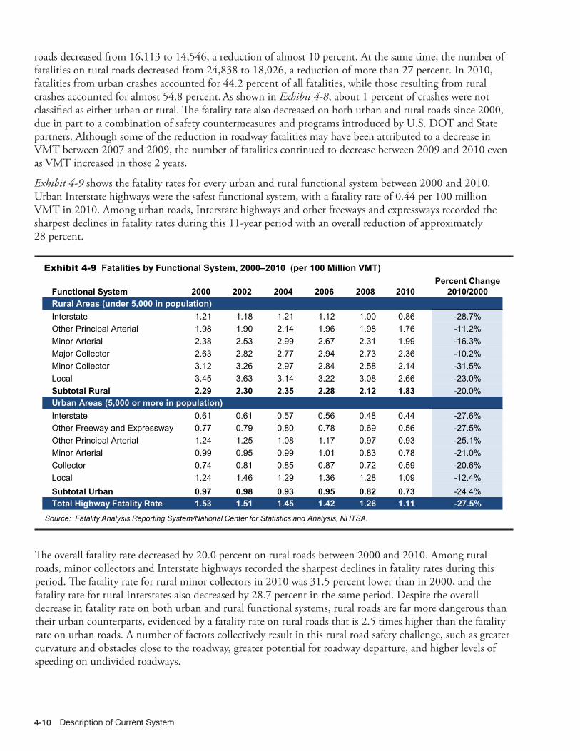
Description of Current System4-10

roads decreased from 16,113 to 14,546, a reduction of almost 10 percent. At the same time, the number of fatalities on rural roads decreased from 24,838 to 18,026, a reduction of more than 27 percent. In 2010, fatalities from urban crashes accounted for 44.2 percent of all fatalities, while those resulting from rural crashes accounted for almost 54.8 percent. As shown in Exhibit 4-8, about 1 percent of crashes were not classified as either urban or rural. The fatality rate also decreased on both urban and rural roads since 2000, due in part to a combination of safety countermeasures and programs introduced by U.S. DOT and State partners. Although some of the reduction in roadway fatalities may have been attributed to a decrease in VMT between 2007 and 2009, the number of fatalities continued to decrease between 2009 and 2010 even as VMT increased in those 2 years.

Exhibit 4-9 shows the fatality rates for every urban and rural functional system between 2000 and 2010. Urban Interstate highways were the safest functional system, with a fatality rate of 0.44 per 100 million VMT in 2010. Among urban roads, Interstate highways and other freeways and expressways recorded the sharpest declines in fatality rates during this 11-year period with an overall reduction of approximately 28 percent.

The overall fatality rate decreased by 20.0 percent on rural roads between 2000 and 2010. Among rural roads, minor collectors and Interstate highways recorded the sharpest declines in fatality rates during this period. The fatality rate for rural minor collectors in 2010 was 31.5 percent lower than in 2000, and the fatality rate for rural Interstates also decreased by 28.7 percent in the same period. Despite the overall decrease in fatality rate on both urban and rural functional systems, rural roads are far more dangerous than their urban counterparts, evidenced by a fatality rate on rural roads that is 2.5 times higher than the fatality rate on urban roads. A number of factors collectively result in this rural road safety challenge, such as greater curvature and obstacles close to the roadway, greater potential for roadway departure, and higher levels of speeding on undivided roadways.

9/13/2012 04XH_I (4-9) R1.xlsx

Functional System 2000 2002 2004 2006 2008 2010Rural Areas (under 5,000 in population)Interstate 1.21 1.18 1.21 1.12 1.00 0.86 -28.7%Other Principal Arterial 1.98 1.90 2.14 1.96 1.98 1.76 -11.2%Minor Arterial 2.38 2.53 2.99 2.67 2.31 1.99 -16.3%Major Collector 2.63 2.82 2.77 2.94 2.73 2.36 -10.2%Minor Collector 3.12 3.26 2.97 2.84 2.58 2.14 -31.5%Local 3.45 3.63 3.14 3.22 3.08 2.66 -23.0%Subtotal Rural 2.29 2.30 2.35 2.28 2.12 1.83 -20.0%Urban Areas (5,000 or more in population)Interstate 0.61 0.61 0.57 0.56 0.48 0.44 -27.6%Other Freeway and Expressway 0.77 0.79 0.80 0.78 0.69 0.56 -27.5%Other Principal Arterial 1.24 1.25 1.08 1.17 0.97 0.93 -25.1%Minor Arterial 0.99 0.95 0.99 1.01 0.83 0.78 -21.0%Collector 0.74 0.81 0.85 0.87 0.72 0.59 -20.6%Local 1.24 1.46 1.29 1.36 1.28 1.09 -12.4%Subtotal Urban 0.97 0.98 0.93 0.95 0.82 0.73 -24.4%Total Highway Fatality Rate 1.53 1.51 1.45 1.42 1.26 1.11 -27.5%

Percent Change2010/2000

Exhibit 4-9 Fatalities by Functional System, 2000–2010 (per 100 Million VMT)

Source: Fatality Analysis Reporting System/National Center for Statistics and Analysis, NHTSA.

Safety 4-11

There have been notable decreases in the fatality rates for both rural and urban local roads since 2000, at 23.0 and 12.4 percent, respectively. However, the fatality rate for rural local roads in 2010 was more than three times higher than that for the safest rural functional system (Interstate). Similarly, the fatality rate for urban local roads was more than two times higher the fatality rate for the safest urban functional classification (Interstate). Addressing the challenges associated with non-Interstate roads can be made more difficult by the diversity of ownership; Interstate roads are maintained by the State while other roads may be maintained by the State or a variety of local organizations, including cities and counties.

BehavioralSpeeding is one of the most prevalent factors contributing to traffic crashes, and represents one area of great collaboration between transportation safety professionals from both the roadway and driver behavior areas of expertise. Speeding is also a contributing factor that affects all of the FHWA focus areas. The economic cost to society of speeding-related crashes is estimated by NHTSA to be $40.4 billion per year.

Nearly one-half of all vehicles involved in fatal crashes in 2010 were on roads with posted speed limits of 55 miles per hour or more, as compared with 19 percent of vehicles involved in injury crashes and 18 percent of vehicles involved in property-damage-only crashes. Although much of the public concern about speed-related crashes focuses on high-speed roadways, speeding is a safety concern on all roads. In 2010, about 21 percent of drivers involved in fatal crashes (10,532) were given tickets for driving too fast for conditions or in excess of posted speed limits—the highest driver factor cited for all fatal crashes. While speeding has often been seen as a prevalent occurrence on major highways, 86 percent of speeding-related fatalities occurred on roads that were not Interstate highways in 2010.

In addition to addressing opportunities for safety improvements associated with roadway design and operations, it is important to consider safety improvements associated with the drivers responsible for navigating the roadway environments.

Among drivers involved in fatal crashes, young males are the most likely to be speeding. The relative proportion of speeding-related crashes to all crashes decreases with increasing driver age. In 2010, 39 percent of male drivers in the 15- to 24-year-old age groups who were involved in fatal crashes were reported to be speeding at the time of the crash.

As shown by cases for which blood alcohol data are available, alcohol involvement is prevalent for drivers involved in speeding-related crashes. In 2010, 41 percent of drivers with a blood alcohol content (BAC) of 0.08 grams per deciliter (g/dL) or higher involved in fatal crashes were speeding, compared with only 15 percent of drivers with a BAC of 0.00 g/dL who were involved in fatal crashes. In 2010, 27 percent of the speeding drivers under age 21 who were involved in fatal crashes also had a BAC of 0.08 g/dL or higher; in contrast, only 13 percent of the nonspeeding drivers under age 21 involved in fatal crashes in 2010 had a BAC of 0.08 g/dL or higher.

Distracted driving is a behavior dangerous to drivers, passengers, and nonoccupants alike. Distraction is a specific type of inattention that occurs when drivers divert their attention from the driving task to focus on some other activity. A distraction-affected crash is any crash in which a driver was identified as distracted at the time of the crash.

Locally Owned Road SafetyThere are more than 30,000 local agencies that own and operate more than 75 percent of the Nation’s roadways. Agency practitioners have varying levels of transportation safety expertise and often perform several duties in addition to transportation safety. The FHWA developed the workshop “Road Safety 365: A Workshop for Local Governments” to help local practitioners routinely identify safety issues along their roadways and provide ideas on how to address them.

Description of Current System4-12

In 2011, 10 percent of fatal crashes and 17 percent of injury crashes were reported as distraction-affected crashes. Of those people killed in distraction-affected crashes, 12 percent (385) died in crashes in which at least one of the drivers was using a cell phone at the time of the crash. Use of a cell phone includes talking/listening to a cell phone, dialing/texting a cell phone, and other cell-phone-related activities. Eleven percent of all drivers 15 to 19 years old involved in fatal crashes were reported as distracted at the time of the crashes. This age group has the largest proportion of drivers who were distracted. Twenty-one percent in this group were distracted by the use of cell phones. To put this in context, for all fatal crashes, only 7 percent of the drivers in the fatal crashes were 15 to 19 years old. However, for distraction, 11 percent of the drivers in fatal distraction-affected crashes were 15 to 19 years old. Likewise, drivers in their 20s were overrepresented in distraction-affected crashes relative to their proportion in total drivers—23 percent of all drivers in fatal crashes were in their 20s, but 26 percent of distracted drivers were in their 20s.

Another area of particular concern is motorcycle fatalities. While motorcycles made up 3 percent of all registered vehicles in the United States in 2011 and accounted for only 0.6 percent of all vehicle miles traveled, motorcycle fatalities accounted for 14 percent of all traffic fatalities for the year. Per vehicle mile traveled in 2011, motorcyclists were more than 30 times more likely than passenger car occupants to die in motor vehicle traffic crashes and 5 times more likely to be injured. Per registered vehicle, the fatality rate for motorcyclists in 2011 was 6 times the fatality rate for passenger car occupants. The injury rate for motorcyclists was about the same as the injury rate for passenger car occupants.

In 2011, 40 percent of fatally injured motorcycle riders and 51 percent of fatally injured motorcycle passengers were not wearing helmets at the time of the crash.

More than one-fifth of motorcycle riders (22 percent) involved in fatal crashes in 2011 were driving the vehicles with invalid licenses at the time of the collision. The percentage of motorcycle riders involved in fatal crashes in 2011 who had BAC levels of .08 g/dL or higher—29 percent—was higher than for any other type of motor vehicle driver. NHTSA estimates that helmets saved the lives of 1,617 motorcyclists in 2011. If all motorcyclists had worn helmets, an additional 703 lives could have been saved.

Safety 4-13

Transit Safety

This section describes the safety of the Nation’s public transportation system. Statistics are primarily drawn from the National Transit Database (NTD). The NTD serves as a nationwide repository of transit operating, financial, service, asset, and safety data. It captures information from 47 rail transit systems, more than 650 bus transit service providers, and 1,500 demand response agencies. Combined, these modes of public transportation provided over 10 billion passenger trips and 41 billion passenger miles of service in 2010. The NTD does not collect safety data for commuter rail systems; we report FRA data for them here.

Based on the number of fatalities and injuries reported on an annual basis, public transportation generally experiences lower rates of incident, fatality, and injury than other modes of transportation in the same year. However, serious incidents do occur, and the potential for catastrophic events remains. Several transit agencies in recent years have had major accidents that resulted in fatalities, injuries, and significant property damage. The National Transportation Safety Board (NTSB) has investigated a number of these accidents and has issued reports identifying the probable causes of and factors that contributed to them. Since 2004, the NTSB has reported on nine transit accidents that, collectively, resulted in 15 fatalities, 297 injuries, and over $30 million in property damages. The NTSB identified serious deficiencies in the training and supervision of employees; the maintenance of equipment and infrastructure; and deficiencies in safety management and oversight, such as weaknesses in transit agencies’ safety rules and procedures, lack of a safety culture within the transit agency, and lack of adequate oversight by the state and Federal agencies. Of the 42 safety recommendations NTSB has made to FTA since 1991, 26 of them have been addressed and closed. FTA is working diligently to address the remaining safety recommendations.

The Moving Ahead for Progress in the 21st Century (MAP-21) Act, signed into law on July 6, 2012, provides new authorities for FTA to strengthen public transportation safety throughout the United States. The law requires new safety provisions for rail and bus operators and provides grant funds to States to support enhanced oversight. FTA will implement the new law in consultation with the transit community, the State oversight agencies, and the U.S. Department of Transportation Transit Rail Advisory Committee for Safety (TRACS).

Incidents, Fatalities, and Injuries

An incident is recorded by a transit agency for a variety of events occurring on transit property or vehicles, involving transit vehicles, or affecting persons using the transit system. The Q&A box on this page provides exact reporting thresholds.

Q A&What sort of events result in a recorded transit incident?

A transit agency records an incident for any event occurring on transit property, onboard or involving transit vehicles, or to persons using the transit system that results in one of the following:

• One or more confirmed fatalities within 30 days of the incident

• One or more injuries requiring immediate transportation away from the scene for medical attention

• Total property damage to transit property or private property in excess of $25,000

• An evacuation for life safety reasons• A mainline derailment (i.e., occurring on a revenue

service line, regardless of whether the vehicle was in service or out of service)

• A fire.Additionally, an incident is recorded by a transit agency whenever certain security situations occur on transit property, such as:

• A robbery, burglary, or theft• A rape• An arrest or citation, such as for trespassing,

vandalism, fare evasion, or assault• A cyber security incident• A hijacking• A nonviolent civil disturbance that results in the

disruption of transit service.

Description of Current System4-14

Included among these is any event that results in significant property damage, one or more reported injuries, one or more reported fatalities, or some combination thereof. From 2002 to 2007, the definition of significant property damage was total property damage in excess of $7,500 (in current-year dollars, not indexed to inflation); this threshold increased to $25,000 in 2008.

An injury is reported when a person has been immediately transported away from the scene of a transit incident for medical care. Any event producing a reported injury is also reported as an incident.

A transit-related fatality is reported for any death occurring within 30 days of a transit incident that is confirmed to be a result of that incident.

Since 2008, nationwide, collisions have resulted in about 140 fatalities per year, mostly occurring when pedestrians, bicyclists, motorists, and individuals waiting in stations, at stops, at rail grade crossings, or at intersections are struck by the transit vehicle.

Exhibit 4-10 provides data on fatalities, excluding suicides, both in total fatalities and per 100 million PMT for heavy rail, light rail, demand response, and motor bus. From 2002 to 2010, the number of fatalities has remained relatively flat while the rate per 100 million passenger miles has declined slightly due to increasing ridership. Unlike other modes, such as highway travel, public transportation has not achieved a consistent decrease in fatalities.

3/20/2013 04XT_B (4-10) R4.xlsx

158 165 150

136 147

160 143

170 164

0.45 0.47

0.42 0.37 0.39 0.41

0.35

0.41 0.41

0.00

0.05

0.10

0.15

0.20

0.25

0.30

0.35

0.40

0.45

0.50

0

50

100

150

200

250

2002 2003 2004 2005 2006 2007 2008 2009 2010

Tota

l Fat

aliti

es p

er 1

00 M

illio

n P

MT

Fata

lity

Cou

nt

Passenger Patron Public Worker Non-suicide Fatalities per 100 Million PMT

Exhibit 4-10 Annual Transit Fatalities Excluding Suicides, 2002–2010

Note: Exhibit includes data for DR, HR, LR, and MB. Also, fatality totals include both directly operated (DO) and purchased transportation (PT) service types. Source: National Transit Database—Transit Safety and Security Statistics and Analysis Reporting.

Q A&What types of injuries and fatalities are reported?

Person types are defined as:

• Passengers: Individuals on-board a transit vehicle or boarding or alighting a transit vehicle

• Patrons: Individuals waiting for or leaving transit at stations, in mezzanines, on stairs, escalators, or elevators, in parking lots and other transit-controlled property

• Public: All others who come into contact with the transit system, including pedestrians, automobile drivers, and trespassers

• Workers: Transit agency employees or contractors engaged in operations or maintenance, not construction of new transit infrastructure

• Suicides: Individuals who come into contact with the transit system intending to harm themselves

Safety 4-15

Transit interaction with pedestrians, cyclists, and motorists at rail grade crossings, pedestrian crosswalks, and intersections largely drives overall transit safety performance. The majority of fatalities and injuries in public transportation result from interaction with the public on busy city streets, from suicides, and from trespassing on transit right-of-way and facilities. Pedestrian fatalities accounted for 29 percent of all transit fatalities in 2010.

Exhibit 4-11 shows the transit fatality rate by person type between 2002 and 2010.

Exhibit 4-11 shows that workers typically account for the lowest fatality rate by person type, but that this percentage remains well above its historic level throughout the 1990s, when worker fatalities accounted for 2 percent of all transit fatalities. The NTSB also has issued a series of recommendations to support needed improvements in this area, and FTA has targeted this number with a series of new worker protection initiatives in an effort to ensure greater safety for transit workers.

3/1/2013 04XT_L (4-11) R1.xlsx

Year Passenger Patron Public Worker Suicide2002 0.03 0.10 0.30 0.01 0.042003 0.10 0.04 0.33 0.02 0.042004 0.06 0.03 0.33 0.02 0.042005 0.08 0.04 0.22 0.02 0.022006 0.05 0.01 0.31 0.02 0.032007 0.04 0.02 0.32 0.02 0.062008 0.03 0.04 0.25 0.02 0.062009 0.04 0.07 0.28 0.03 0.122010 0.02 0.09 0.27 0.01 0.13

Exhibit 4-11 Transit Fatality Rates by Person Type, 2002–2010, per 100 Million PMT

Note: Exhibit includes data for all transit modes, excluding commuter rail. Source: National Transit Database.

Exhibit 4-11 also highlights that, although public fatalities have been decreasing in recent years, suicides have steadily increased. This change could be attributed to improvements arising from clarifications to the procedures for reporting and distinguishing between trespasser fatalities and suicides, or it could indicate a rising trend of suicides in public transportation environments. On average, fatalities involving suicides and persons who are not transit passengers or patrons (usually pedestrians and drivers) account for about 75 percent of all public transportation fatalities. This creates distinct challenges for public transportation agencies and FTA because they involve causalities which are largely outside the control of transit operators.

Many agencies and FTA are partnering with groups such as Operation Lifesaver International, universities, and local mental health agencies to devise programs to reach trespassers and suicidal individuals to attempt to change their behavior before their actions result in fatal incidents. Transit providers are working with highway agencies to address traffic problems associated with light rail and bus operations on public streets. Accident rates are expected to decline as drivers adjust to new light rail facilities and as municipalities correct roadway design features that experience multiple accidents.

Exhibit 4-12 presents fatality data for the transit industry that includes suicides. Since 2005, the number and rate of suicides has increased each year. Many transit agencies also are concerned at the recent increase in patron fatalities, largely in stations, which accounts for 18 percent of fatalities in 2010, up from a low of 4 percent in 2007.

Description of Current System4-16

Exhibit 4-13, which shows transit injury rates by person type, also highlights a sharp increase in patron injury rates in recent years. Although transit incident occurrences and impacts fluctuate from year to year, it appears that transit patrons are experiencing an increased risk of fatality and injury in transit stations, stops, and mezzanines. One potential cause of this increased risk could be greater passenger crowding, particularly on rail transit modes, where this increasing patron injury trend has been reported.

Exhibit 4-14 shows fatality rates per 100 million PMT for motor bus and demand response (including suicides). The data show more volatility in the demand response rate, as would be expected because relatively fewer people use demand response. One or two more fatalities in a year can make the rate jump significantly. Considering this, fatality rates have not changed significantly for either mode. Absolute fatalities are not comparable across modes because of the wide range of passenger miles traveled on each mode; they are, therefore, not provided. Note that demand response fatality rates are similar to those of privately operated automobiles, which they resemble in both form and operating characteristics.

3/15/2013 04XT_A (4-12) R4.xlsx

0.04 0.04 0.05

0.01

0.03

0.05 0.07

0.12 0.13

0.00

0.02

0.04

0.06

0.08

0.10

0.12

0.14

0

50

100

150

200

250

300

2002 2003 2004 2005 2006 2007 2008 2009 2010

Tran

sit-R

elat

ed S

uici

des

per 1

00 M

illio

n P

MT

Fata

lity

Cou

nt

Fatalities Excluding Suicides Suicides Total Suicides per 100 Million PMT

160

219 214

180

159 141

166 180 171

Note: Exhibit includes data for DR, HR, LR, and MB. Also, fatality totals include both directly operated (DO) and purchased transportation (PT) service types. Source: National Transit Database—Transit Safety and Security Statistics and Analysis Reporting.

Exhibit 4-12 Annual Transit Fatalities Including Suicides, 2002–2010

3/15/2013 04XT_M (4-13) R2.xlsx

Year Passenger Patron Public Worker Suicide2002 34.23 7.06 7.69 2.99 0.052003 29.93 8.85 9.90 3.29 0.032004 29.65 10.44 10.20 2.95 0.002005 28.22 9.06 8.32 2.59 0.002006 31.11 9.20 8.00 3.08 0.072007 33.32 7.35 8.74 4.72 0.042008* 30.34 16.89 6.86 4.03 0.042009 32.35 17.61 7.80 4.08 0.052010 35.33 13.60 8.01 3.77 0.09

Exhibit 4-13 Transit Injury Rates by Person Type, 2002–2010, per 100 Million PMT

Note: Exhibit includes data for all transit modes, excluding commuter rail. *Beginning for calendar year 2008, the reporting threshold for a reportable injury changed from two people to one person. Source: National Transit Database.

Safety 4-17

2/27/2013 04XT_E (4-14) R2.xlsx

0.0

0.5

1.0

1.5

2.0

2002 2003 2004 2005 2006 2007 2008 2009 2010

Fata

litie

s pe

r 100

Mill

ion

PM

T Motor Bus Demand Response

Note: Fatality totals include both DO and PT service types. Source: National Transit Database.

Exhibit 4-14 Annual Transit Fatality Rates by Highway Mode, 2002–2010

Exhibit 4-15 shows fatality rates per 100 million PMT for heavy rail and light rail (including suicides). Heavy rail fatality rates were more than twice as high in 2010 as they were in 2006, although lower than they were in 2009. Of the 96 fatalities reported by heavy rail systems in 2010, 41 were classified as suicides. Light rail experiences more accidents than heavy rail because it does not usually operate on dedicated guideway and it generally picks up passengers from stops on the roadside rather than from station platforms.

2/27/2013 04XT_F (4-15) R2.xlsx

0.00

0.25

0.50

0.75

1.00

1.25

1.50

1.75

2.00

2.25

2002 2003 2004 2005 2006 2007 2008 2009 2010

Fata

litie

s pe

r 100

Mill

ion

PM

T Heavy Rail Light Rail

Exhibit 4-15 Annual Transit Fatality Rates by Rail Mode, 2002–2010

Note: Fatality totals include both DO and PT service types. Source: National Transit Database.

Exhibit 4-16 provides data on incidents and injuries per 100 million PMT for transportation services on the four largest modes reporting to the NTD from 2004 to 2010. Commuter rail data are presented separately because that data was collected according to different definitions in the FRA’s Rail Accident/Incident Reporting System (RAIRS). The data in Exhibit 4-17 suggest that the highway modes (motor bus and demand response) saw a decrease in incidents between 2004 and 2010 while they simultaneously saw an increase in injuries. This is unexplained and may be due to a change in reporting practices. Data for the rail modes is volatile, but does not suggest any significant positive or negative trends.

Description of Current System4-18

Exhibit 4-17 shows both the absolute number and fatality rate per 100 million PMT for commuter rail. This data was obtained from the FRA’s RAIRS. The RAIRS database records fatalities that occurred as a result of a commuter rail collision, derailment, or fire. The database also includes a category called “not otherwise classified,” which includes fatalities that occurred as a result of a slip, trip, or fall. In 2011, FRA added a separate category for suicides; this data may be reported in future editions of the C&P report (suicides are not included in the data shown here). In 2010, 214 fatalities were recorded in the NTD for demand response, heavy rail, light rail, and motor bus modes, and the fatality rate per 100 million PMT (excluding suicides) was 0.41. For commuter rail, however, the absolute number of fatalities in 2010 was 71 and the fatality rate per 100 million PMT was 0.66.

2/27/2013 04XT_G (4-16) R2.xlsx

Analysis Parameter 2004 2005 2006 2007 2008 2009 2010Incidents per 100 Million PMTMotor Bus 65.82 65.16 69.38 66.02 54.14 58.28 55.79Heavy Rail 43.68 39.80 42.57 43.15 52.83 51.75 53.17Light Rail 59.57 66.43 60.57 61.18 48.48 44.90 37.55Demand Response 289.41 325.44 373.82 247.39 204.28 194.81 171.68Injuries per 100 Million PMTMotor Bus 67.52 63.15 62.30 68.57 66.89 72.27 72.49Heavy Rail 33.15 26.45 32.74 31.08 43.11 44.84 45.84Light Rail 41.49 36.13 35.16 43.67 48.34 47.99 42.51Demand Response 146.48 159.87 213.33 227.33 234.50 215.24 196.06

Source: National Transit Database.

Exhibit 4-16 Transit Incidents and Injuries by Mode, 2004–2010

2/27/2013 04XT_I (4-17) R2.xlsx

88

62 70 73 68 75

93

71 71

0.93

0.65 0.72 0.77

0.66 0.67

0.84

0.64 0.66

0.00

0.10

0.20

0.30

0.40

0.50

0.60

0.70

0.80

0.90

1.00

0

10

20

30

40

50

60

70

80

90

100

2002 2003 2004 2005 2006 2007 2008 2009 2010

Fata

litie

s pe

r 100

Mill

ion

VM

T

Com

mut

er R

ail F

atal

ity C

ount

Fatalities Fatalities per 100 Million PMT

Source: Federal Railroad Administration Rail Accident/Incident Reporting System.

Exhibit 4-17 Commuter Rail Fatalities, 2002–2010

Safety 4-19

Exhibits 4-18 and 4-19 show the absolute number of commuter rail incidents and injuries per 100 million PMT, respectively. Although commuter rail has a very low number of incidents per PMT, commuter rail incidents are far more likely to result in a fatality than incidents occurring on any other mode. Most likely, this is because the average speed of commuter rail vehicles is considerably higher than the other modes (except vanpools). The number of both incidents and injuries declined from 2007 to 2008. However, between 2008 and 2010 there was a steady increase in the number of both incidents and injuries.

2/27/2013 04XT_H (4-18) R2.xlsx

1,748 1,790 1,630 1,660 1,605

1,970 1,781

1,996 2,202

18 19

17 18

15

18 16

18

20

0

5

10

15

20

25

0

500

1000

1500

2000

2500

2002 2003 2004 2005 2006 2007 2008 2009 2010

Inci

dent

s pe

r 100

Mill

ion

VM

T

Com

mut

er R

ail I

ncid

ent C

ount

Incidents Incidents per 100 Million PMT

Source: Federal Railroad Administration Rail Accident/Incident Reporting System.

Exhibit 4-18 Commuter Rail Incidents, 2002–2010

2/27/2013 04XT_J (4-19) R2.xlsx

1,562 1,661 1,422

1,710 1,473

1,925 1,784 1,867 2,004

16 17

15

18

14 13

16 17

19

0

2

4

6

8

10

12

14

16

18

20

0

500

1000

1500

2000

2500

2002 2003 2004 2005 2006 2007 2008 2009 2010

Inju

ries

per 1

00 M

illio

n V

MT

Com

mut

er R

ail I

njur

y C

ount

Injuries Injuries per 100 Million PMT

Source: Federal Railroad Administration Rail Accident/Incident Reporting System.

Exhibit 4-19 Commuter Rail Injuries, 2002–2010

Description of Current System4-20

System Performance

Highway System Performance ....................................................................................5-2

Transportation Systems and Livable Communities ..................................................5-2Fostering Livable Communities .......................................................................................... 5-3Advancing Environmental Sustainability ............................................................................ 5-6

Economic Competitiveness .......................................................................................5-8System Reliability ................................................................................................................ 5-9System Congestion ............................................................................................................ 5-10Effect of Congestion and Reliability on Freight Travel ....................................................... 5-11Congestion Mitigation and Reliability Improvement .......................................................... 5-13

Transit System Performance ........................................................................................5-16

Average Operating (Passenger-Carrying) Speeds ...................................................5-16

Vehicle Use .................................................................................................................5-17Vehicle Occupancy ............................................................................................................. 5-17Revenue Miles per Active Vehicle (Service Use) ................................................................ 5-18

Frequency and Reliability of Service .........................................................................5-19

System Coverage: Urban Directional Route Miles ...................................................5-21

System Capacity ........................................................................................................5-21

Ridership ....................................................................................................................5-23

System Performance 5-1

CHAPTER 5

Description of Current System5-2

Highway System Performance

The transportation system provides for the movement of people and goods and influences land use and the environment around it. Transportation agencies make decisions on where to expand an existing system and where to build a new one. Increasingly, when making these decisions, the various impacts are assessed to ensure that negative ramifications on the environment are minimized, while providing a service that serves the diverse needs of its users. Many of these issues are addressed during the project development phase as directed by Federal and/or State policy.

The transportation system is best able to operate at the peak of its performance when it can support economic competitiveness at the local, regional, and national levels by providing adequate capacity and reliability, while upholding sustainability goals. Therefore, transportation agencies are being held accountable for how well they address these issues in addition to providing a system that is safe and in a state of good repair, as discussed in Chapters 3 and 4. This chapter discusses the performance of the highway system, and how sustainable transportation systems, livability, and economic competitiveness contribute to this performance. It also includes a discussion of the effect of congestion on freight travel. The U.S. Department of Transportation (DOT) Strategic Plan FY 2012–FY 2016 included the goals of reliability, economic competitiveness, livable communities, and environmental sustainability. MAP-21 also recognized the importance of developing measures for congestion reduction, system reliability, freight movement, and economic activity.

Adopting these goals and tracking performance using the new metrics could influence the type of investments made. Different highways may be selected to serve different trip purposes, e.g., freight versus a commuter trip or a local trip versus an intrastate or interstate trip. Better understanding the types of trips served by a particular roadway or mode would help in determining where to invest resources. A congested metropolitan area may provide improved transit, pedestrian, or biking facilities to take some trips off a highway in order to better serve freight trips or reduce emissions. A trade-off between the goal areas will be necessary.

Transportation Systems and Livable CommunitiesThe U.S. DOT Strategic Plan FY 2012–FY 2016 includes a goal to “Foster livable communities through place-based policies and investments that increase transportation choices and access to transportation services.” Livable communities are places where transportation, housing, and commercial development investments have been coordinated so that people have access to adequate, affordable, and environmentally sustainable travel options. Incorporating livability approaches into transportation, land use, and housing policies can help improve public health and safety, lower infrastructure costs, reduce combined household transportation and housing costs, reduce growth in vehicle miles traveled, and improve air and water quality, among many other benefits.

U.S. DOT Strategic Goals Covered in Chapter 5Economic Competitiveness – Promote transportation policies and investments that bring lasting and equitable economic benefits to the Nation and its citizens.

Livable Communities – Foster livable communities through place-based policies and investments that increase the transportation choices and access to transportation services.

Environmental Sustainability – Advance environmentally sustainable policies and investments that reduce carbon and other harmful emissions from transportation sources.

System Performance 5-3

The U.S. DOT Strategic Plan FY 2012–FY 2016 includes a separate goal to “Advance environmentally sustainable policies and investments that reduce carbon and other harmful emissions from transportation sources.” Transportation is crucial to our economy and our quality of life, but building, operating, and maintaining transportation systems clearly have environmental consequences. In order to meet today’s set of challenges—reducing carbon and other harmful emissions, promoting energy independence, and addressing global climate change—it is critical to foster more sustainable approaches to transportation in order to allow future generations to enjoy even higher standards of living and mobility.

Fostering Livable CommunitiesDesigning transportation systems to balance access and mobility needs of all users is an important aspect of promoting livable communities. This includes drivers, bicyclists, pedestrians, and transit riders, among others. This approach to improving transportation systems also recognizes that each community is different and should determine what its needs are.

Transportation systems provide the foundation for how communities are formed. Deciding to build houses, schools, grocery stores, employment centers, and transit stations close to one another—while providing a well-connected street network and facilities for walking or biking—provides more transportation choices and convenient access to daily activities. It also ensures that community resources and services are used efficiently. Transportation agencies are being called upon by their stakeholders to plan, build, and operate transportation systems that support a variety of environmental, economic, and social objectives such as protecting natural resources, improving public health and safety, expanding the economy, and providing mobility. These objectives lead to a desire for a more integrated and holistic approach to planning, building, and expanding the transportation system.

Communities benefit when decisions about transportation and land use are made simultaneously. Containing development to a more compact area, allowing for mixed-use zoning, and reutilizing existing spaces or redeveloping parcels of land can reduce infrastructure costs, lower household transportation costs, preserve rural lands, reduce air and water pollution, and protect natural resources. Coordinating land use and development decisions with transportation investments can produce clear results, such as increasing viable options for people to access opportunities, goods, services, and other resources to improve quality of life.

Millwork District ProjectAn example of a community that has benefited from coordinated transportation and land use is the Millwork District in Dubuque, Iowa. Dubuque was challenged to reinvigorate the Millwork District, which includes the waterfront area and the Washington neighborhood, while respecting and recognizing the area’s historic character. The new concept was for the District to connect the Port of Dubuque to the downtown area in order to create a thriving livable community. The Historic Millwork District was redeveloped from old factories and mills into a new mixed-use development incorporating housing, workplaces, and entertainment. Multimodal transportation improvements were made as a keystone in the strategy to bolster the community. Expanding the District’s transportation options attracted both businesses and residents of the area.

The project made use of cost-effective and sustainable practices, such as reusing brick pavers and installing energy-efficient street lights. It also created jobs and capitalized on local resources by using locally manufactured benches, bike racks, and trash receptacles. As a result of the Millwork District project, new streets are now accessible to all road users regardless of age or ability. The once-empty warehouses and idle mills have become popular shops, employment centers, and homes. The Millwork District is now a vibrant community, building on the past that has transformed into a more livable community. The U.S. DOT awarded a $5.6-million Transportation Investment Generating Economic Recovery (TIGER) Discretionary grant to Dubuque, Iowa, for revitalization of the Millwork District. Federal dollars are helping the city leverage millions more in additional investments for a total of $7.7 million.

Description of Current System5-4

Addressing livability issues in transportation ensures that transportation investments support both mobility and broader community goals. A well-designed transportation system can be the catalyst for achieving a range of community and regional goals including economic growth, job creation, goods movement, and access to education and health care. Transportation also contributes to increased quality of life for residents and helps maintain the Nation’s role in a global economy. As will be discussed later in this chapter, freight movement is an essential part to moving goods and building stronger economies and, when carefully planned, it helps reduce congestion and fosters livable communities. Communities can be aesthetically pleasing, safe, and walkable, while still providing efficient access for large trucks, rail lines, and other modes of transportation.

There is a growing demand to design facilities for all users, while balancing the different access and mobility needs of motorists, truckers, bicyclists, pedestrians, and transit riders. The ability of transportation networks to connect and function, support regional economies, and protect environmental and public health is becoming increasingly relevant to long-term economic prosperity and community quality of life. Additional information on the characteristics of livability and the benefits of livable communities can be found in Chapter 13 of the 2010 C&P Report and at the U.S. DOT Livability website at www.dot.gov/livability.

Measuring LivabilityMeasuring the impact of transportation investments on livability is an ongoing effort. The U.S. DOT Strategic Plan FY 2012–FY 2016 emphasizes the importance of adopting a comprehensive, coordinated, and performance-based approach to enhancing livability and evaluating transportation investments. As previously mentioned, in support of this coordinated outcome-driven approach, the U.S. DOT Strategic Plan establishes as one of five strategic goals “fostering livable communities through place-based policies and investment that increase transportation choices and access to transportation services.” This Livable Communities strategic goal is supported by three outcome-based objectives, shared among the Federal Highway Administration (FHWA), the Federal Transit Administration (FTA), and the Federal Railroad Administration (FRA):

1. Increased access to convenient and affordable transportation choices

2. Improved networks that accommodate pedestrians and bicycles

3. Improved access to transportation for people with disabilities and older adults.

Philadelphia Area Pedestrian Bicycle Network In Philadelphia, PA, the area pedestrian and bicycle network spans 128 miles connecting six counties around Philadelphia and Southern NJ. U.S. DOT TIGER funds are being used to repair and improve 16 miles of the network on well-used commuter routes to downtown and in economically distressed neighborhoods in Philadelphia and Camden, NJ.

Livable Communities Outcomes and Performance MeasuresFHWA focuses on two of the three outcomes, and is tracking them by State using performance measures:

• Outcome: Improved networks that accommodate pedestrians and bicycles. Performance Measure: Increase the number of States that have policies that improve transportation choices for walking, wheeling, and bicycling. In FY2011, the target was 22 States and the actual was 24; in FY2012, the target was 26, increasing to 27 by FY2013.

• Outcome: Improved access to transportation for people with disabilities and older adults. Performance Measure: Increase the number of States that have developed an Americans with Disabilities Act (ADA) transition plan that is current and includes public rights-of-way. In FY2011, the target was nine States and the actual was 13; in FY2012, the target was 13, increasing to 15 by FY2013.

System Performance 5-5

The Interagency Partnership for Sustainable Communities, a joint initiative of the U.S. Department of Housing and Urban Development, U.S. DOT, and U.S. Environmental Protection Agency (EPA), is working to share information about how communities can track performance. In addition, FHWA is examining ways that communities can gauge whether their programs, policies, and projects are making a positive impact on quality of life. Exhibit 5-1 lists examples of measures that communities could consider.

Sustainable Transportation Performance Measures• Transit Accessibility

• Bicycle and Pedestrian Mode Share

• Vehicle Miles Travelled per Capita

• Carbon Intensity

• Mixed Land Use

• Transportation Affordability

• Benefits by Income Group

• Land Consumption

• Bicycle and Pedestrian Activity and Safety

• Bicycle and Pedestrian Level of Service

• Average Vehicle Occupancy

• Transit Productivity

The U.S. EPA has also identified 12 sustainable transportation performance measures in its Guide to Sustainable Transportation Performance Measures (http://www.epa.gov/dced/transpo_performance.htm). The guidebook describes the 12 measures that can readily be applied in transportation decision-making. It also presents possible metrics, summarizes the relevant analytical methods and data sources, and illustrates the use of each measure.

10/22/2012 05XH_J (5-1) R2.xlsx

Accessibility Economic Housing Land Use Public Health SafetyAnnual public transportation passenger miles per capita

Annual public transportation trips per capita

Availability of bicycle parking

Average commute distances

Access to jobs and markets for disadvantaged populations compared to entire population

Access to personal vehicle, by age, race, income, and location

Average number of employment opportunities within a given number of miles of a transit stop

Acres of land consumed per residential unit

Average commute distances

Average energy efficiency rating of homes

Average number of full-service super-markets within a given number of miles or minutes

Acreage of agricultural lands disturbed

Acreage of habitat consumed/habitat fragmentation index

Acreage of high-quality wetlands

Acreage of land consumed per lane mile

Acreage of sensitive lands/important habitats impacted/ consumed

Air quality conformity status

Ambient air quality

Amount and percent change in greenery and open space

Average commute distances

Barriers to pedestrians and cyclists

Average speed of emergency vehicles on emergency calls

Pedestrian crash fatality rate

Number/percent of people living in substandard residential units

Exhibit 5-1 Potential Livability Performance Measures

Description of Current System5-6

Advancing Environmental SustainabilityThe 1987 United Nations (UN) World Commission on Environment and Development defined sustainability as “development that meets the needs of the present without compromising the ability of future generations to meet their own needs.” While a number of other definitions for sustainability have emerged, a concept often used is the “triple bottom line,” referring to environmental, social, and economic principles. In transportation, the triple bottom line relates to sustainable solutions for the natural environment, the economic efficiency of the system, and societal needs for those using the system (e.g., mobility, accessibility, and safety). Transportation agencies can address sustainability through a wide range of initiatives, such as Intelligent Transportation Systems, livability, smart growth, planning and environment linkages, and addressing requirements of the National Environmental Policy Act (NEPA).

From an environmental sustainability perspective, the heavy reliance of the transportation system on fossil fuels is a significant concern. Fossil fuels are non-renewable; generate air pollution; and contribute to the buildup of carbon dioxide (CO2) and other greenhouse gases (GHGs), which trap heat in the Earth’s atmosphere. Although some progress has been made in reducing emissions of air pollutants both nationally and from the transportation sector in particular, many Americans continue to live in regions that do not meet health-based air-quality standards. Through oversight of the Clean Air Act “conformity” requirements, FHWA helps to ensure that these regions continue to make progress toward their air-quality standards.

Multimodal Transportation and LivabilityOne of the key efforts of the U.S. DOT livability initiative is to promote safe, affordable, and convenient transportation choices. Across the country, States and communities are focusing renewed attention on improving transportation facilities for walking and bicycling. This is evident in the use of Federal-aid funds for walking and bicycling projects. The highest level of Federal-aid investment on record for nonmotorized facilities was achieved in FYs 2009, 2010, and 2011 ($1.19 billion, $1.04 billion, and $790 million, respectively). SAFETEA-LU created two new programs that specifically focused on walking and bicycling: the Nonmotorized Transportation Pilot Program (NTPP) and the Safe Routes to School (SRTS) Program. The programs have explored how communities can improve safety and transportation choices with increased investment in walking and bicycling.

The NTPP provides a glimpse at what happens when communities increase their investment in walking and bicycling transportation facilities. SAFETEA-LU specified that four communities—Marin County, CA; Columbia, MO; Sheboygan County, WI; and Minneapolis, MN—would each receive $25 million to improve their walking and bicycling transportation networks. The FHWA was tasked with reporting on the outcomes of this investment in a Report to Congress (see http://www.fhwa.dot.gov/environment/bicycle_pedestrian/ntpp/2012_report/). This report documents the changes in transportation use and estimated changes in several key factors including safety and emissions as well. Among the key findings are that counts of walkers and bicyclists increased an average of 49 percent and 22 percent, respectively. An estimated 16 million miles were walked and bicycled in the communities in 2010 and it is estimated that the pilot communities saved 22 pounds of CO2 in 2010 per person, or a total of 7,710 tons, due to replacing personal vehicle trips with walking and bicycling. Despite notable increases in walking and bicycling, fatal bicycle and pedestrian crashes remained steady, indicating that safety has not been adversely affected.

On the other hand, the SRTS Program has provided funds to each State by a formula based on each State’s population of children in kindergarten through eighth grade. The SRTS Program, a $612-million program over 5 years, has supported infrastructure and noninfrastructure (e.g., safety education) activities and required that each State have an SRTS Coordinator. As of August 2011, over 10,400 schools in all 50 states and the District of Columbia, have been involved in the program (see http://www.saferoutesinfo.org/sites/default/files/resources/progress%20report_FINAL_web.pdf). So far the most common use of funds has been sidewalk improvements (19 percent), followed by traffic calming (14 percent) and education (14 percent). In sum, estimates are that over 4.8 million students may benefit from the transportation improvements near their schools.

Although the two SAFETEA-LU programs have taken different approaches (e.g., providing funding to specific communities versus distributing funds to all States), they both demonstrate the national interest in walking and bicycling transportation. Based on recent demographic changes, which indicate that adults under age 30 are driving less, it will be even more important to provide safe, convenient, and affordable transportation options for people of all ages and abilities (see http://www.fhwa.dot.gov/policy/otps/nextgen_htps_scan.htm).

System Performance 5-7

Projects funded through the Congestion Mitigation and Air Quality Improvement program (CMAQ) contribute to emissions reductions in these regions. FHWA also promotes potential strategies to reduce GHG emissions, through improving system efficiency, reducing VMT, and transitioning to fuel-efficient vehicles and alternative fuels. FHWA supports research related to these strategies, provides technical assistance to stakeholders, and coordinates its activities within U.S. DOT and with other Federal agencies.

Beyond strategies to reduce emissions, the transportation community is beginning to focus its efforts on anticipating future extreme weather events and changes in climate (e.g., higher sea levels, increased temperatures, altered precipitation patterns, greater storm intensity) and the potential impact of these changes on the transportation system (e.g., damaged or flooded facilities). For a transportation system to be sustainable, it must be able to adapt to future as well as present conditions. Research efforts regarding the potential impacts of climate change on transportation infrastructure are ongoing at the Federal, State, and local levels. The U.S. DOT released a report on projected changes in climate over the next century, used geographical information systems to map areas with transportation infrastructure along the Atlantic coast that will be potentially vulnerable to sea level rise, and is conducting a second adaptation study focused on the Gulf Coast region. These studies identify potential climate change impacts that are widespread and modally diverse and that would stress transportation systems in ways beyond which they were designed. FHWA has developed a flexible framework to assist transportation agencies in adapting to the impacts of climate change that starts with inventorying critical infrastructure, understanding potential future climate change impacts, and assessing vulnerabilities and risks.

Adaptation PilotsIn autumn of 2010, FHWA funded five State areas’ DOTs and Metropolitan Planning Organizations to pilot a draft framework for conducting vulnerability and risk assessments of transportation infrastructure given the projected impacts of climate change. Each area’s approach was different and contributed significantly to its understanding of potential climate change impacts on its transportation assets, and to the body of knowledge of the transportation community as a whole. FHWA is currently using the experiences of these five pilots and other studies to update the draft framework and expand it with “in-practice” examples.

The Washington DOT (WSDOT) assessed the infrastructure it owns, including roads, rail, ferry facilities, and airports. In internal workshops around the State, they developed criticality and impact ratings for each asset, which they used to create vulnerability maps for each region.

An interagency group in New Jersey, led by the North Jersey Transportation Planning Authority, closely followed the three steps of FHWA’s framework in its analysis of the New Jersey Turnpike/I-95 corridor and the New Jersey Coast. It worked closely with the State climatologist to downscale climate model projections to New Jersey, estimating future changes to the 100-year floodplain due to heavier rainfall resulting from climate change. In addition, the interagency group worked with the New Jersey Department of Environmental Protection to create estimates of relative sea level rise. To identify facilities vulnerable to the effects of sea level rise, storm surge, and inland flooding, it used geographic information systems to determine intersections between inundated areas and transportation assets.

The Oahu Metropolitan Planning Organization used an interagency, multidisciplinary, 2-day workshop to facilitate a climate change dialogue and identify five key groups of vulnerable transportation assets for further study. The five groups of assets, based on geographic areas, were then analyzed in more detail by transportation experts in three full-day work sessions, resulting in a detailed qualitative risk assessment for each asset.

The University of Virginia’s Center for Transportation developed a priority-setting tool to assess how consideration of climate change and other factors may affect project prioritization in a transportation plan. It used the Hampton Roads region as a case study and made the model available for use by other regions.

The Metropolitan Transportation Commission, in partnership with the San Francisco Bay Conservation and Development Commission and others, led a study of a portion of the San Francisco Bay stretching from the Oakland Bay Bridge to the San Mateo Bridge (Alameda County). This study was focused on sea level rise. The project team developed profiles of risk from the effects of sea level rise, including exposure, sensitivity, and adaptive capacity for a representative list of roads, transit, facility, and pedestrian and bicycle transportation assets within the study area.

Description of Current System5-8

Additional information on sustainability and climate change can be found in Chapters 11 and 12 of the 2010 C&P Report, and at FHWA’s sustainable transport and climate change websites at http://www.fhwa.dot.gov/environment/climate_change and at http://www.sustainablehighways.dot.gov.

Measuring SustainabilityUsing sustainability as a metric generally means an expansion of traditional measurement frameworks to take into account the triple bottom line of social, environmental, and economic performance. Many organizations are developing organization-specific or industry-specific measurement tools and best practices to help them achieve the appropriate balance among social, environmental, and economic principles.

At the Federal level, environmental sustainability has been adopted as a strategic goal in the U.S. DOT Strategic Plan FY 2012–FY 2016. At the State level, transportation agencies are developing metrics that address various aspects of sustainability and are monitoring progress toward specific goals—often in their long-range and project-level planning process. Some potential measures that have been identified for assessing progress in improving sustainability relate to reducing GHG emissions, improving system efficiency, reducing the growth of VMT, transitioning to fuel-efficient vehicles and alternative fuels, and increasing the use of recycled materials in transportation.

FHWA’s INVEST Sustainability Self-Evaluation ToolThe FHWA has launched an initiative to support transportation agencies in making highway projects and programs more sustainable. This new initiative features a voluntary web-based self-evaluation tool, the Infrastructure Voluntary Evaluation Sustainability Tool (INVEST). In addition to measuring the sustainability of a project or program, INVEST can enable transportation agencies to:

• Evaluate Sustainability Trade-Offs. INVEST can help users better evaluate sustainability tradeoffs. Every highway project involves tradeoffs, and decisions often become more difficult when two or more options are not directly comparable. INVEST can help with these decisions by assigning points to various criteria based on their sustainability impacts.

• Find and Address Programmatic Barriers. Measuring sustainability on a program, project, or group of projects can enhance an agency’s ability to identify programmatic barriers that they encounter so they can be addressed and removed. These barriers might be the result of policies, design standards and specifications, or stakeholder agency policies.

• Communicate Benefits and Goals. Measuring sustainability and reporting results allows transportation organizations to communicate sustainability goals and benefits to stakeholders.

More information on INVEST can be found at www.sustainablehighways.org.

Economic CompetitivenessThe U.S. DOT Strategic Plan FY 2012–FY 2016 includes a goal to “Promote transportation policies and investments that bring lasting and equitable economic benefits to the Nation and its citizens.”

Maintaining economic competitiveness means increasing and maximizing the contribution of the transportation system to economic growth. At the same time, such investments help accomplish other strategic goals, because maximizing economic benefits requires consideration of the safety, asset management, livability, personal and freight mobility, and environmental sustainability of the entire transportation network. Economic competitiveness will also require implementation of new technologies that enable people and goods to move more efficiently and fully utilize existing capacity across all modes. This section presents information on various aspects of a highway transportation system that affect economic competitiveness.

System Performance 5-9

System ReliabilityReliability is an important characteristic of any transportation system, one that industry in particular requires for efficient production. American manufacturers are increasingly shifting production to high-value, high-tech products whose manufacture integrates transportation into a just-in-time supply chain based on efficient performance and consistent reliability. Additional emphasis will be placed on the American freight network as more manufactured products will need to move across the country. Imported goods shipped to ports will also increase as the American economy continues to grow. Freight shippers, a substantial portion of the nation’s economy, depend on a predictable and reliable system to move goods across regions. Although industry may budget for extra time for congestion, unexpected travel delays cannot be accounted for. If industry is unable to utilize a reliable system, they may be required to carry greater inventory than would otherwise be necessary, thereby incurring higher costs.

Travel time reliability is a measure of congestion easily understood by a wide variety of audiences, and is one of the more direct measures of the effects of congestion on the highway user. Before travel time reliability, simple averages were mostly used to explain traffic congestion. However, most travelers experience and remember something much different than a simple average throughout a year of commutes. Their travel times vary greatly from day to day, and they remember those few bad days they suffered through unexpected delays. If unexpected delays are minimized in a given period, all users are able to adequately plan for the best use of their time while moving through the transportation network.

Many transportation reliability measures exist, with varying levels of utility. Such measures typically compare high-delay days with average-delay days. The simplest method identifies days that exceed the 90th or 95th percentile in terms of travel times and estimates the severity of delay on specific routes during the worst one or two travel days each month. Another method, the Buffer Index, measures the percentage of extra time travelers must add to their average peak-hour travel time to allow for congestion delays and arrive at a location on time about 95 percent of the time. Generally, the Buffer Index goes up during peak periods—when congestion occurs—indicating a reliability problem.

FHWA Urban Congestion ReportThe Urban Congestion Report (UCR) is produced quarterly and characterizes traffic congestion and reliability at the national and city levels. The reports utilize archived traffic operations data gathered from State DOTs and through a public-private partnership with a traffic information company and reflect data from 19 urban areas in the Nation. The production of these reports is a cooperative effort between the Texas Transportation Institute and FHWA. The UCR data are also being used to report Travel Time Reliability in metropolitan areas for the FHWA Strategic Plan, which is available at http://www.fhwa.dot.gov/policy/fhplan.html#measurement.

The congestion information presented in these reports may not be representative of the entire roadway system in any particular city because the UCR includes only those roadways that are instrumented with traffic sensors for the purposes of real-time traffic management and/or traveler information. Construction may affect the roadways that are included in this report. The congestion and reliability trends are calculated by comparing the most recent 3 months of the current year to the same 3 months of the prior year.

Data from April through June 2012 concluded that the average duration of weekday congestion is 1 minute longer than in 2011 at 4 hours and 23 minutes per day (during the hours of 6 a.m. to 10 p.m.). Further information can be found at http://ops.fhwa.dot.gov/perf_measurement/ucr/.

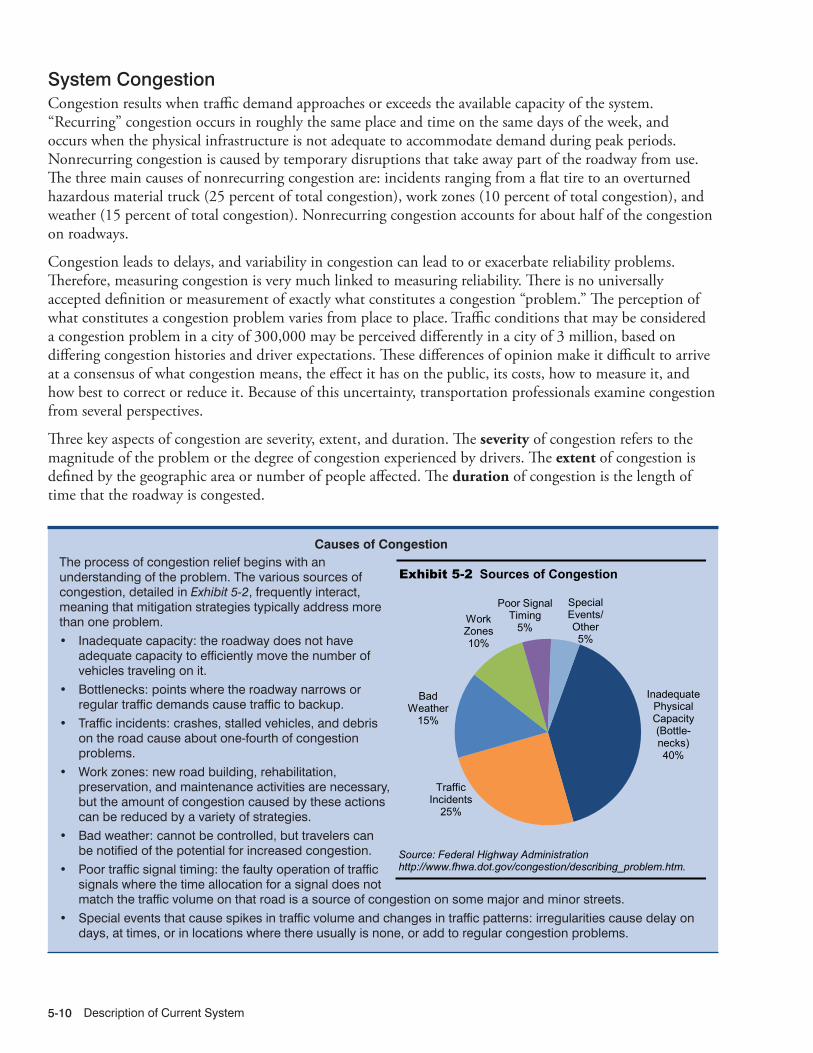
Description of Current System5-10

System CongestionCongestion results when traffic demand approaches or exceeds the available capacity of the system. “Recurring” congestion occurs in roughly the same place and time on the same days of the week, and occurs when the physical infrastructure is not adequate to accommodate demand during peak periods. Nonrecurring congestion is caused by temporary disruptions that take away part of the roadway from use. The three main causes of nonrecurring congestion are: incidents ranging from a flat tire to an overturned hazardous material truck (25 percent of total congestion), work zones (10 percent of total congestion), and weather (15 percent of total congestion). Nonrecurring congestion accounts for about half of the congestion on roadways.

Congestion leads to delays, and variability in congestion can lead to or exacerbate reliability problems. Therefore, measuring congestion is very much linked to measuring reliability. There is no universally accepted definition or measurement of exactly what constitutes a congestion “problem.” The perception of what constitutes a congestion problem varies from place to place. Traffic conditions that may be considered a congestion problem in a city of 300,000 may be perceived differently in a city of 3 million, based on differing congestion histories and driver expectations. These differences of opinion make it difficult to arrive at a consensus of what congestion means, the effect it has on the public, its costs, how to measure it, and how best to correct or reduce it. Because of this uncertainty, transportation professionals examine congestion from several perspectives.

Three key aspects of congestion are severity, extent, and duration. The severity of congestion refers to the magnitude of the problem or the degree of congestion experienced by drivers. The extent of congestion is defined by the geographic area or number of people affected. The duration of congestion is the length of time that the roadway is congested.

Causes of CongestionThe process of congestion relief begins with an understanding of the problem. The various sources of congestion, detailed in Exhibit 5-2, frequently interact, meaning that mitigation strategies typically address more than one problem. • Inadequate capacity: the roadway does not have

adequate capacity to efficiently move the number of vehicles traveling on it.

• Bottlenecks: points where the roadway narrows or regular traffic demands cause traffic to backup.

• Traffic incidents: crashes, stalled vehicles, and debris on the road cause about one-fourth of congestion problems.

• Work zones: new road building, rehabilitation, preservation, and maintenance activities are necessary, but the amount of congestion caused by these actions can be reduced by a variety of strategies.

• Bad weather: cannot be controlled, but travelers can be notified of the potential for increased congestion.

• Poor traffic signal timing: the faulty operation of traffic signals where the time allocation for a signal does not match the traffic volume on that road is a source of congestion on some major and minor streets.

• Special events that cause spikes in traffic volume and changes in traffic patterns: irregularities cause delay on days, at times, or in locations where there usually is none, or add to regular congestion problems.

9/19/2012 05XH_A (5-2) R2.xlsx

Inadequate Physical Capacity (Bottle- necks) 40%

Traffic Incidents

25%

Bad Weather

15%

Work Zones 10%

Poor Signal Timing

5%

Special Events/ Other 5%

Exhibit 5-2 Sources of Congestion

Source: Federal Highway Administration http://www.fhwa.dot.gov/congestion/describing_problem.htm.

System Performance 5-11

Effect of Congestion and Reliability on Freight TravelFHWA has created and examined various freight performance measures (FPMs) to analyze the impacts of congestion and determine the operational capacity and efficiency of various Interstate highways and other important freight routes in the United States. Much of the current congestion negatively impacting truck carrier operations occurs on a recurring basis during peak periods of 6 a.m. to 9 a.m. and 4 p.m. to 7 p.m. local time, particularly in and near major metropolitan areas. Exhibit 5-3 shows a map indicating where this peak period congestion on high-volume truck portions of the National Highway System (NHS) took place

Freight Performance MeasurementThe FHWA has been collecting and analyzing data for freight-significant Interstate corridors since 2004. FHWA plans to continue to collect travel time information on 25 interstate corridors and 15 U.S./Canada land-border crossings at least through 2012. Key objectives of the current FPM research program are to expand on the existing data sources; further develop and refine methods for analyzing data; derive national measures of congestion and reliability; analyze freight bottlenecks and intermodal connectors; and develop data products and tools that will assist U.S. DOT, FHWA, and State and local transportation agencies in addressing surface transportation congestion. A web tool for disseminating FPM data on the 25 study corridors, www.freightperformance.org, provides an example of the types of tools that FHWA will develop. The goal is to evolve the research into a credible freight data source that can be used to continuously measure freight performance and inform the development of strategies and tactics for managing and relieving freight congestion.

Exhibit 5-3 Peak-Period Congestion on High-Volume Truck Portions of the National Highway System, 2007

Note: High-volume truck portions of the National Highway System carry more than 8,500 trucks per day, including freight-hauling long-distance trucks, freight-hauling local trucks, and other trucks with six or more tires. Highly congested segments are stop-and-go conditions with volume/service flow ratios greater than 0.95. Congested segments have reduced traffic speeds with volume/service flow ratios between 0.75 and 0.95. Sources: U.S. Department of Transportation, Federal Highway Administration, Office of Highway Policy Information, Highway Performance Monitoring System, and Office of Freight Management and Operations, Freight Analysis Framework, version 3.2, 2010.

12/9/2013 05XH_B (5-3) R4.xlsx

Description of Current System5-12

5 53.0 52.1 53.2 70 57.1 56.8 57.210 57.8 57.6 58.1 75 57.3 56.7 57.915 56.7 56.5 56.8 76 55.4 55.3 55.420 59.2 59.0 59.1 77 55.3 54.9 55.324 57.5 56.7 57.5 80 58.0 57.8 58.125 59.3 59.3 59.2 81 56.8 56.8 56.826 54.2 53.8 54.3 84 54.1 52.7 54.535 56.9 56.1 57.2 85 57.6 56.7 57.740 59.0 58.8 59.1 87 54.5 54.1 54.745 55.4 54.3 55.8 90 57.2 57.0 57.355 57.8 57.6 57.8 91 53.6 52.8 54.165 58.0 57.5 58.1 94 58.4 58.1 58.5

95 56.5 55.4 57.0

Average Nonpeak

Period Speed

Interstate Route

Average Operating

Speed

Average Speed

Nonpeak Period

Interstate Route

Average Operating

Speed

Average Peak Period

Speed*

Average Peak Period

Speed*

Exhibit 5-4 Average Truck Speeds on Selected Interstate Highways, 2010

* Both urban and rural areas were combined to determine the speeds shown. This procedure reduces the impact of urban congestion on average speeds. Average speeds are available separated by urban and rural areas on request from the U.S. Department of Transportation, Federal Highway Administration, Office of Freight Management and Operations. Sources: U.S. Department of Transportation, Federal Highway Administration, Office of Freight Management and Operations, Performance Measurement Program, 2011 (map), 2012 (table data).

12/9/2013 05XH_C (5-4) R4.xlsx

in 2007. Overall, peak period congestion created stop-and-go conditions on 3,700 miles of the NHS and caused traffic to travel below posted speed limits on an additional 4,700 miles of the NHS.

In some locations, freight-hauling trucks are impacted not only during peak periods, but also at other times during the day. In cooperation with private industry, FHWA measures the speed and travel time reliability of more than 500,000 trucks along 25 Interstate corridors on an annual basis. Exhibit 5-4 shows some of the results of this cooperative initiative, indicating the average truck travel speeds on selected Interstate

System Performance 5-13

highways. Reduced truck travel speeds most commonly occur in large metropolitan areas, but can also occur at international border crossings and gateways, in mountainous areas that require trucks to climb steep inclines, and in areas frequently prone to poor visibility driving conditions.

Projections of Future CongestionThough in many cases congestion on many high-volume NHS truck routes in various large metropolitan areas is already severe, particularly during peak periods, the congestion could become much more severe in terms of its geographic scope and impact on major intercity corridors and metropolitan areas if network capacity remains unchanged. Exhibit 5-5 shows a map indicating where this peak-period congestion on high-volume truck portions of the NHS could take place in 2040 . Peak-period congestion is projected to create stop-and-go conditions on 23,500 miles of the NHS (over six times as many miles as in 2007) and traffic slower than posted speed limits on an additional 7,200 miles of the NHS (nearly twice as many miles as in 2007).

Exhibit 5-5 Peak-Period Congestion on High-Volume Truck Portions of the National Highway System, 2040

Note: High-volume truck portions of the National Highway System carry more than 8,500 trucks per day, including freight-hauling long-distance trucks, freight-hauling local trucks, and other trucks with six or more tires. Highly congested segments are stop-and-go conditions with volume/service flow ratios greater than 0.95. Congested segments have reduced traffic speeds with volume/service flow ratios between 0.75 and 0.95. The volume/service flow ratio is estimated using the procedures outlined in the HPMS Field Manual, Appendix N. Sources: U.S. Department of Transportation, Federal Highway Administration, Office of Highway Policy Information, Highway Performance Monitoring System, and Office of Freight Management and Operations, Freight Analysis Framework, version 3.2, 2010.

12/9/2013 05XH_D (5-5) R5.xlsx

Congestion Mitigation and Reliability ImprovementEfforts to mitigate congestion and improve reliability can take place by improving service on existing roads, introducing pricing schemes, or enhancing information provided to drivers. Frequently, several of the strategies presented below are applied in tandem, mitigating a number of congestion sources in a holistic manner. More detail can be found at http://www.fhwa.dot.gov/congestion/toolbox/index.htm.

Description of Current System5-14

Improve Service on Existing Roads � Traffic Incident Management is a planned and coordinated process shared by public and private sector

partners to detect, respond to, and remove traffic incidents and restore traffic capacity as safely and quickly as possible.

� Arterial Management improves travel throughout entire communities by coordinating traffic signals through timing and access management. Arterial roadways are high-capacity roads to deliver traffic from collector roads to freeways, and between urban centers. ‒ Traffic Signal Timing can produce benefit-cost ratios as high as 40 to 1. The costs for retiming traffic

signals are generally very small, but provide substantial benefit.

‒ Access Management is the proactive management of vehicular access points to land parcels adjacent to roadways. State and local governments can control access to facilities by increasing the distance between traffic signals; constructing fewer driveways spaced farther apart to allow for more orderly merging; constructing dedicated left- and right-turn lanes, indirect left-turn and U-turn lanes, and roundabouts to keep through-traffic flowing; constructing two-way left-turn lanes and non-traversable, raised medians; and managing right-of-way for future widening, good sight distance, access location, and other access-related issues.

� Freeway Management and Traffic Operations involves applying the appropriate policies, strategies, and actions to mitigate any potential impacts resulting from the intensity, timing, and location of travel and to reduce congestion. The Traffic Management Center (TMC) is often the hub of most freeway management systems.

� Active Transportation and Demand Management (ATDM) is the dynamic management, control, and influence of travel demand, traffic demand, and traffic flow of transportation facilities. Through the use of archived data and/or predictive methods, traffic flow is managed and traveler behavior is influenced in real time to achieve operational objectives, such as preventing or delaying breakdown conditions, improving safety, promoting sustainable travel modes, reducing emissions, or maximizing system efficiency.

� Road Weather Management allows weather events and their impacts on roads to be viewed as predictable, nonrecurring incidents that affect safety, congestion, and productivity. Advisory strategies provide information on prevailing and predicted conditions to both transportation managers and motorists, such as posting fog warnings on dynamic message signs or listing flooded routes on websites. Control strategies alter roadway devices (messages, timing of signals, etc.) to permit or restrict traffic flow and regulate roadway capacity, such as reducing speed limits with variable speed limit signs and modifying traffic signal timing. Treatment strategies supply resources to roads to minimize or eliminate weather impacts, the most common of which are application of sand, salt, and anti-icing chemicals to pavements to improve traction and prevent ice bonding.

� Planned Special Events Traffic Management allows agencies to develop and deploy the operational strategies, traffic control plans, protocols, procedures, and technologies needed to control traffic and share real-time information with other stakeholders on the day of an event. Planned special events cause congestion and unexpected delays to travelers by increasing traffic demand or reducing roadway capacity (e.g., street closures for parades).

Pricing � Congestion Pricing, sometimes referred to as value pricing or peak-period pricing, involves charging

relatively higher prices for travel during peak periods. It is identical to the technique used in many other sectors of the economy to respond to peak-use demands. Congestion pricing entails fees or tolls for road use that vary with the level of congestion. Introducing congestion pricing to highway facilities brings

System Performance 5-15

transportation supply and demand into balance and keeps the lanes congestion free. Fees are typically assessed electronically to eliminate delays associated with manual toll collection facilities.

Add Capacity � Easing Bottlenecks is necessary when a road is at capacity and the flow of traffic is disrupted. The

capacity of a road is determined by a number of factors, including the number and width of lanes and shoulders, merge areas at interchanges, and roadway alignment (grades and curves). Minimizing the impacts of or eliminating bottlenecks is one of the most effective ways to reduce congestion.

Better Work Zones � Work Zone Management can have a positive impact on preventing or relieving congestion by

aggressively anticipating and mitigating congestion caused by highway work zones. Solutions can come from fundamental changes in the way projects are planned, estimated, designed, bid, and constructed.

Travel Options � Travel Demand Management involves strategies to provide travelers with effective travel choices such as

work location, route, time, and mode. Managing both the growth of and periodic shifts in traffic demand are necessary elements of managing traffic congestion.

� Transportation Choices such as accessibility to transit, car-sharing or bicycle/pedestrian facilities helps alleviate congestion on the Nation’s road network. By promoting the use of transit or bicycle/pedestrian facilities, the use of fewer cars during peak travel times also improves air quality in communities with close proximity to major highways.

Traveler Information � The 511 telephone number was designated for traveler information services by the Federal

Communications Commission in 2001 and assigned to public transportation agencies for implementing services throughout the United States. FHWA is working cooperatively with FTA, the American Association of State Highway and Transportation Officials, the American Public Transportation Association, the Intelligent Transportation Society of America, and the members of the 511 Coalition to establish more 511 travel information services throughout the United States.

� Travel Time Message Signs are dynamic signs located near roadways that give motorists the estimated time it will take them to get to the next one or two significant destinations.

� National Traffic and Road Closure Information is provided to travelers and freight shippers to broadcast current weather, road, and traffic conditions.

� Real-Time System Management Information is a real-time information system that provides the capability to monitor traffic and travel conditions on major highways. This information enables drivers to make informed decisions. FHWA is supporting the deployment of the Real-Time System Management Information Program so that all States are able to broadcast information to travelers.

� The Cross-Town Improvement Project (C-TIP) combines real-time travel time information and freight shipper congestion information to optimize the flow of freight within a metropolitan area. Cross-town truck traffic is coordinated using both public and private traffic and freight data to reduce empty truck bobtail (tractor without trailer) moves between railroad terminals and freight distribution facilities. The system uses four components that include an information exchange, wireless update capability, real-time traffic monitoring, and dynamic routing applications to deliver up-to-the-minute information regarding roadway conditions, travel speeds, and predicted travel times. This information is passed to the freight traveler to deliver enhanced traveler information and predictive travel times for freight pick-up and delivery routes in urban areas.

Description of Current System5-16

Transit System Performance

Basic goals shared by all transit operations include minimizing travel times, making efficient use of vehicle capacity, and providing reliable performance. The Federal Transit Administration (FTA) collects data on average speed, how full the vehicles are (utilization), and how often they break down (mean distance between failures) to characterize how well transit service meets these goals. These data are reported here; safety data are reported in Chapter 4.

More subjective customer satisfaction issues, such as how easy it is to access transit service (accessibility) and how well that service meets a community’s needs, are harder to measure. Data from the FHWA 2009 National Household Travel Survey, reported here, provide some insights but are not available on an annual basis and so do not support time series analysis.

New technology has allowed progressive transit agencies to report service metrics on their Web sites. Because this is a relatively new practice, measures that are standardized across the industry have not yet been developed. Industry associations are beginning to address this issue, but for now there is no generally recognized set of standards.

The following analysis presents data on average operating speeds, average number of passengers per vehicle, average percentage of seats occupied per vehicle, average distance traveled per vehicle, and mean distance between failures for vehicles. Average speed, seats occupied, and distance between failures address efficiency and customer service issues; passengers per vehicle and miles per vehicle are primarily efficiency measures. Financial efficiency metrics, including operating expenditures per revenue mile or passenger mile, are discussed in Chapter 6.

Average Operating (Passenger-Carrying) SpeedsAverage vehicle operating speed is an approximate measure of the speed experienced by transit riders; it is not a measure of the operating speed of transit vehicles between stops. More specifically, average operating speed is a measure of the speed passengers experience from the time they enter a transit vehicle to the time they exit it, including dwell times at stops. It does not include the time passengers spend waiting or transferring. Average vehicle operating speed is calculated for each mode by dividing annual vehicle revenue miles by annual vehicle revenue hours for each agency in each mode, weighted by the passenger miles traveled (PMT) for each mode, as reported to the National Transit Database (NTD). In cases where an agency contracts with

FTA Livable Communities Outcomes and Performance Measures

Modal Network Demand Response

1. Increased access to convenient and affordable transportation choices

• Increase the number of transit boardings reported by urbanized area transit providers from 10.0 billion in 2011 to 10.5 billion in 2016.

• Increase the number of transit boardings reported by rural area transit providers from 141 million in 2011 to 160 million in 2016.

• Increase transit’s market share among commuters to work in at least 10 of the top 50 urbanized areas by population, as compared to 2010 market share levels.

2. Improved access to transportation for people with disabilities and older adults

• Increase the number of key transit rail stations verified as accessible and fully compliant from 522 in 2010 to 560 in 2016.

System Performance 5-17

12/17/2013 05XT_A (5-6) R3.xlsx

41.1

32.9

20.2

15.0

14.4

12.5

11.5

7.0

0 15 30 45

Vanpool

CommuterRail

HeavyRail

LightRail

DemandResponse

MotorBus

OtherNonrail

OtherRail

Miles per Hour

Tran

sit

Mod

e Notes: Other Nonrail includes Público, trolleybus, and demand taxi; Other Rail includes Alaska railroad, automated guideway, cable car, inclined plane, and monorail. Source: National Transit Database.

Exhibit 5-6 Average Speeds for Passenger- Carrying Transit Modes, 2010

a service provider and provides the service directly, the speeds for each of the services within a mode are calculated and weighted separately. The results of these average speed calculations are presented in Exhibit 5-6.

The average speed of a transit mode is strongly affected by the number of stops it makes. Motor bus service, which typically makes frequent stops, has a relatively low average speed. In contrast, commuter rail has high sustained speeds between infrequent stops, and thus a relatively high average speed. Vanpools also travel at high speeds, usually with only a few stops at each end of the route. Modes using exclusive guideway can offer more rapid travel time than similar modes that do not. Heavy rail, which travels exclusively on dedicated guideway, has a higher average speed than light rail, which often shares its guideway with mixed traffic. These average speeds have not changed significantly over the last decade.

Vehicle Use

Vehicle OccupancyExhibit 5-7 shows vehicle occupancy by mode for selected years from 2000 to 2010. Vehicle occupancy is calculated by dividing PMT by vehicle revenue miles (VRMs), resulting in the average number of people carried in a transit vehicle. There has been little change in vehicle occupancy between 2000 and 2010 indicating sustained ridership levels across all types of transit.

Taking into account that vehicle capacities differ by mode, Exhibit 5-8 shows the 2010 vehicle occupancy as a percentage of the seating capacity for an average vehicle in each mode (based on the average number of seats reported per vehicle in 2010: vanpool, 11; heavy rail, 59; light rail, 57; trolleybus, 45; ferryboat, 385; commuter rail, 96; motor bus, 33; demand response, 12). For example, the average full-size bus seats 33 people and, as shown in Exhibit 5-7, the average occupancy for a bus in 2010 was 10.7 riders. This occupancy, as a percentage of seating capacity, is 32.5 percent. Some modes also have substantial standing capacity that is not considered here, but which can allow the measure of the percentage of seats occupied to exceed 100 percent for a full vehicle.

Although, on average, it appears that there is excess capacity in all these modes, commuting patterns make it difficult to fill vehicles returning to the suburbs from downtown employment centers during the morning rush hours and, likewise, to fill vehicles going downtown in the evening rush. Vehicles also tend to be relatively empty at the beginning and ends of their routes. For many commuter routes, a vehicle that is crush-loaded (i.e., filled to maximum capacity) on part of the trip may still only achieve an average occupancy of around 35 percent (as shown by analysis of the Washington Metropolitan Area Transit Authority peak-period data).

Description of Current System5-18

12/17/2013 05XT_B (5-7) R3.xlsx

Mode 2000 2002 2004 2006 2008 2010RailHeavy Rail 23.9 22.6 23.0 23.2 25.7 25.3Commuter Rail 37.9 36.7 36.1 36.1 35.7 34.2Light Rail 26.1 23.9 23.7 25.5 24.1 23.7Other Rail1 8.4 8.4 10.4 8.4 9.3 10.7NonrailMotor Bus 10.7 10.5 10.0 10.8 10.8 10.7Demand Response 1.3 1.2 1.3 1.3 1.2 1.2Ferryboat 120.1 112.1 119.5 130.7 118.1 119.3Trolleybus 13.8 14.1 13.3 13.9 14.3 13.6Vanpool 6.6 6.4 5.9 6.3 6.3 6.0Other Nonrail2 7.3 7.9 5.8 7.8 8.2 7.4

Exhibit 5-7 Unadjusted Vehicle Occupancy: Passengers per Transit Vehicle, 2000–2010

1 Alaska railroad, automated guideway, cable car, inclined plane, and monorail. 2 Aerial tramway and Público. Source: National Transit Database.

12/17/2013 05XT_C (5-8) R3.xlsx

Note: Some modes also have substantial standing capacity that is not considered here, but which can allow the measure of the percentage of seats occupied to exceed 100 percent for a full vehicle. Source: National Transit Database.

Exhibit 5-8 Average Seat Occupancy Calculations for Passenger-Carrying Transit Modes, 2010

55.6%

43.0%

41.3%

35.8%

32.5%

31.0%

30.1%

9.9%

0% 20% 40% 60%

Vanpool

HeavyRail

LightRail

CommuterRail

Bus

Ferryboat

Trolleybus

DemandResponse

Tran

sit M

ode

Another issue that makes it hard to fully use vehicle capacity is called “bunching.” If a stop has a particularly large number of passengers, the servicing vehicle takes longer to load increasing the spacing between it and the previous vehicle. This not only means the vehicle’s next stop will have more riders due to the longer interval, but that there will be a shorter interval between it and the vehicle behind it. This compounds the problem by slowing the vehicle more and speeding up the vehicle behind it. Soon the vehicles become bunched up, causing longer wait times for some passengers and inconsistent in-vehicle volumes with some being overcrowded and others underutilized. This situation is common and difficult to mitigate.

Revenue Miles per Active Vehicle (Service Use)Vehicle service use, the average distance traveled per vehicle in service, can be measured by VRMs. Exhibit 5-9 provides vehicle service use by mode for selected years from 2000 to 2010. Heavy rail, generally offering long hours of frequent service, had the highest vehicle use during this period. Vehicle service use for light rail, and to a lesser extent for vanpool and demand response, shows an increasing trend. Vehicle service use for other nonrail modes appears to be relatively stable over the past few years with no apparent trends in either direction.

System Performance 5-19

Frequency and Reliability of ServiceThe frequency of transit service varies considerably according to location and time of day. Transit service is more frequent in urban areas and during rush hours—namely, where and when the demand for transit is highest. Studies have found that transit passengers consider the time spent waiting for a transit vehicle to be less well spent than the time spent traveling in a transit vehicle. The higher the degree of uncertainty in waiting times, the less attractive transit becomes as a means of transportation and it will attract fewer users. Further, when scheduled service is offered less frequently, reliability becomes more important to users.

Exhibit 5-10 shows findings on wait-times from the 2009 FHWA National Household Travel Survey (NHTS), the most recent nationwide survey of this information. The NHTS found that 44.5 percent of all passengers who ride transit wait 5 minutes or less and 73.2 percent wait 10 minutes or less. The NHTS also found that 8.0 percent of all passengers wait 21 minutes or more. A number of factors influence passenger wait-times, including the frequency of service, the reliability of service, and passengers’ awareness of timetables. These factors are also interrelated. For example, passengers may intentionally arrive earlier for service that is infrequent, compared with equally reliable services that are more frequent. Overall, waiting times of 5 minutes or less are clearly associated with good service that is either frequent, reliably provided according to a schedule, or both. Waiting times of 5 to 10 minutes are most likely consistent with adequate levels of service that are both reasonably frequent and generally reliable. Waiting times of 21 minutes or more indicate that service is likely less frequent or less reliable.

Access to transit service varies by location. Exhibit 5-11 shows the share of working-age residents that have access to transit in 100 selected metro areas. The study evaluated census block groups and counted block groups with at least one transit stop within three-fourths of a mile of their population-weighted centroid as having access. Cities in the Western U.S. tend to enjoy higher rates of coverage while those in the southeast tend to have a lower percentage of residents with access to transit.

12/17/2013 05XT_E (5-10) R3.xlsx

8.0%

5.5%

13.2%

28.7%

44.5%

0% 10% 20% 30% 40% 50%

21 Minutes or More

16 to 20Minutes

11 to 15Minutes

6 to 10Minutes

5 Minutes or Less

Wai

t-Tim

e

Exhibit 5-10 Distribution of Passengers by Wait-Time

Source: National Household Travel Survey, FHWA, 2009.

12/17/2013 05XT_D (5-9) R3.xlsx

Average Annual Rate of Change

Mode 2000 2002 2004 2006 2008 2010 2010/2000RailHeavy Rail 55.6 55.1 57.0 57.2 57.7 56.6 0.2%Commuter Rail 42.1 43.9 41.1 43.0 45.5 45.1 0.7%Light Rail 32.5 41.1 39.9 39.9 44.1 42.5 2.7%NonrailMotor Bus 28.0 29.9 30.2 30.2 30.3 29.7 0.6%Demand Response 17.9 21.1 20.1 21.7 21.3 20.0 1.1%Ferryboat 24.1 24.4 24.9 24.8 21.9 24.9 0.3%Vanpool 12.9 13.6 14.1 13.7 14.3 15.5 1.8%Trolleybus 18.9 20.3 21.1 19.1 18.7 20.4 0.8%

Thousands of Revenue Vehicle Miles

Exhibit 5-9 Vehicle Service Utilization: Vehicle Revenue Miles per Active Vehicle by Mode

Source: National Transit Database.

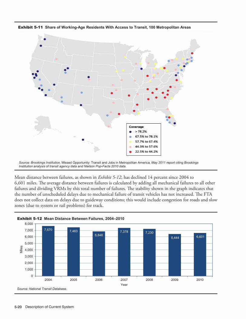
Description of Current System5-20

12/17/2013 05XT_F (5-11) R3.xlsx

Source: Brookings Institution, Missed Opportunity: Transit and Jobs in Metropolitan America, May 2011 report citing Brookings Institution analysis of transit agency data and Nielson Pop-Facts 2010 data.

Exhibit 5-11 Share of Working-Age Residents With Access to Transit, 100 Metropolitan Areas

12/17/2013 05XT_G (5-12) R3.xlsx

7,670 7,463 6,848

7,378 7,230 6,444 6,601

0

1,000

2,000

3,000

4,000

5,000

6,000

7,000

8,000

2004 2005 2006 2007 2008 2009 2010

Mile

s

Year Source: National Transit Database.

Exhibit 5-12 Mean Distance Between Failures, 2004–2010

Mean distance between failures, as shown in Exhibit 5-12, has declined 14 percent since 2004 to 6,601 miles. The average distance between failures is calculated by adding all mechanical failures to all other failures and dividing VRMs by this total number of failures. The stability shown in the graph indicates that the number of unscheduled delays due to mechanical failure of transit vehicles has not increased. The FTA does not collect data on delays due to guideway conditions; this would include congestion for roads and slow zones (due to system or rail problems) for track.

12/17/2013 05XT_F (5-11) R3.xlsx

Source: Brookings Institution, Missed Opportunity: Transit and Jobs in Metropolitan America, May 2011 report citing Brookings Institution analysis of transit agency data and Nielson Pop-Facts 2010 data.

Exhibit 5-11 Share of Working-Age Residents With Access to Transit, 100 Metropolitan Areas

12/17/2013 05XT_F (5-11) R3.xlsx

Source: Brookings Institution, Missed Opportunity: Transit and Jobs in Metropolitan America, May 2011 report citing Brookings Institution analysis of transit agency data and Nielson Pop-Facts 2010 data.

Exhibit 5-11 Share of Working-Age Residents With Access to Transit, 100 Metropolitan Areas

System Performance 5-21

System Coverage: Urban Directional Route MilesThe extent of the Nation’s transit system is measured in directional route miles, or simply “route miles.” Route miles measure the distance covered by a transit route; even though opposite-direction transit routes may use the same road or track, they are counted separately. Data associated with route miles are not collected for demand response and vanpool modes because these transit modes do not travel along specific predetermined routes. Route miles data are also not collected for jitney services because these transit modes often have highly variable route structures.

Exhibit 5-13 shows directional route miles by mode over the past 10 years. Growth in both rail (27.3 percent) and nonrail (20.7 percent) route miles is evident over this period. The average 6.0 percent rate of annual growth for light rail clearly outpaces the rate of growth for all other modes.

12/17/2013 05XT_H (5-13) R3.xlsx

Average Annual Rate of Change

Transit Mode 2000 2002 2004 2006 2008 2010 2010/2000Rail 9,222 9,484 9,782 10,865 11,270 11,735 +2.4%Commuter Rail 1 6,802 6,923 6,968 7,930 8,219 8,590 +2.4%Heavy Rail 1,558 1,572 1,597 1,623 1,623 1,617 +0.4%Light Rail 834 960 1,187 1,280 1,397 1,497 +6.0%Other Rail 2 29 30 30 31 30 30 +0.5%Nonrail3 196,858 225,820 216,619 223,489 212,801 237,580 +1.9%Bus 195,884 224,838 215,571 222,445 211,664 236,434 +1.9%Ferryboat 505 513 623 620 682 690 +3.2%Trolleybus 469 468 425 424 456 456 -0.3%Total 206,080 235,304 226,401 234,354 224,071 249,314 +1.9%Percent Nonrail 95.5% 96.0% 95.7% 95.4% 95.0% 95.3%

Route Miles

Exhibit 5-13 Transit Urban Directional Route Miles, 2000–2010

1 Includes Alaska rail. 2 Automated guideway, inclined plane, cable car, and monorail. 3 Excludes jitney, Público, and vanpool. Source: National Transit Database.

System CapacityExhibit 5-14 provides reported VRMs for both rail and nonrail modes. These numbers are of interest because they show the actual number of miles traveled by each mode in revenue service. VRMs provided by both bus services and rail services show consistent growth, with light rail and vanpool miles growing somewhat faster than the other modes. Overall, the number of VRMs has increased by 22.5 percent since 2000.

Transit system capacity, particularly in cross-modal comparisons, is typically measured by capacity-equivalent VRMs. These measure the distance traveled by transit vehicles in revenue service and adjust them by the passenger-carrying capacity of each transit vehicle type, with the average carrying capacity of motor bus vehicles representing the baseline. To calculate capacity-equivalent VRMs, the number of revenue miles for a vehicle is multiplied by the bus-equivalent capacity of that vehicle. Thus, a heavy rail car that seats 2.5 times more people than a full-size bus provides 2.5 capacity-equivalent miles for each revenue mile it travels.

Description of Current System5-22

Average Annual Rate of Change

Transit Mode 2000 2002 2004 2006 2008 2010 2010/2000Rail 879 925 963 997 1,054 1,056 1.9%

Heavy Rail 578 603 625 634 655 647 1.1%Commuter Rail 248 259 269 287 309 315 2.4%Light Rail 51 60 67 73 86 92 6.0%Other Rail 2 3 2 3 3 2 1.7%

Nonrail 2,322 2,502 2,586 2,674 2,841 2,863 2.1%Motor Bus 1,764 1,864 1,885 1,910 1,956 1,917 0.8%Demand Response 452 525 561 607 688 718 4.7%Vanpool 62 71 78 110 157 181 11.3%Ferryboat 2 3 3 3 3 3 5.0%Trolleybus 14 13 13 12 11 12 -1.8%Other Nonrail 28 26 46 32 25 32 1.5%

Total 3,201 3,427 3,549 3,671 3,895 3,920 2.0%

Miles (Millions)

Exhibit 5-14 Rail and Nonrail Vehicle Revenue Miles, 2000–2010

Source: National Transit Database.

The 2010 capacity-equivalent factors for each mode are shown in Exhibit 5-15. Unadjusted VRMs for each mode are multiplied by a capacity-equivalent factor in order to calculate capacity-equivalent VRMs. These factors are equal to the average full-seating and full-standing capacities of vehicles in active service for each transit mode divided by the average full-seating and full-standing capacities of all motor bus vehicles in active service. The average capacity of the national motor bus fleet changes slightly from year to year as the proportion of large, articulated, and small buses varies. The average capacity of the bus fleet in 2010 was 39 seated and 23 standing for a total of 62 riders.

12/17/2013 05XT_J (5-15) R3.xlsx

10.6

2.7

2.7

2.5

1.8

1.4

1.4

1.0

0.8

0.8

0.4

0.3

0.2

0.2

0.1

Ferryboats

Light Rail

Commuter Rail

Heavy Rail

Monorail

Trollybus

Automated Guideway

Motor Bus

Cable Car

Inclined Plane

Alaska Railroad

Público

Demand Response

Vanpool

Demand Taxi

Capacity-Equivalent Factor

Mod

e

Base = Average Motor Bus Vehicle Capacity

Source: National Transit Database.

Exhibit 5-15 Capacity-Equivalent Factors by Mode

0.0 2.0 4.0 6.0 8.0 10.0 12.0

System Performance 5-23

Total capacity-equivalent VRMs are shown in Exhibit 5-16. Showing the most rapid expansion in capacity-equivalent VRMs in the period from 2000 to 2010 was vanpools, followed by light rail, demand response, and then commuter rail. Total capacity-equivalent revenue miles increased from 3,954 million in 2000 to 4,845 million in 2010, an increase of 22.5 percent.

05XT_K 12/17/2013 05XT_K (5-16) R3.xlsx

Average Annual Rate of Change

Transit Mode 2000 2002 2004 2006 2008 2010 2010/2000Rail 2,046 2,274 2,413 2,681 2,799 2,714 2.9%Heavy Rail 1,321 1,469 1,546 1,648 1,621 1,599 1.9%Commuter Rail 595 652 685 832 940 860 3.8%Light Rail 127 150 179 197 235 252 7.1%Other Rail 3 3 3 4 3 3 -1.1%Nonrail 1,908 2,037 2,064 2,118 2,152 2,131 1.1%Motor Bus 1,764 1,864 1,885 1,910 1,956 1,917 0.8%Demand Response 76 100 101 121 115 124 5.1%Vanpool 11 15 15 22 27 30 10.0%Ferryboat 30 32 32 37 32 35 1.4%Trolleybus 20 20 20 19 16 17 -1.6%Other Nonrail 7 7 12 10 6 8 1.3%Total 3,954 4,311 4,478 4,800 4,951 4,845 2.1%

Vehicle Miles (Millions)

Exhibit 5-16 Capacity-Equivalent Vehicle Revenue Miles, 2000–2010

Source: National Transit Database.

RidershipThere are two primary measures of transit ridership: unlinked passenger trips and PMT. An unlinked passenger trip, sometimes called a boarding, is defined as a journey on one transit vehicle. PMT is calculated on the basis of unlinked passenger trips and estimates of average trip length. Either measure provides an appropriate time series because average trip lengths, by mode, have not changed substantially over time. Comparisons across modes, however, may differ substantially depending on which measure is used due to large differences in the average trip length for the different modes.

Exhibit 5-17 and Exhibit 5-18 show the distribution of unlinked passenger trips and PMT by mode. In 2010, urban transit systems provided 9.9 billion unlinked trips and 52.6 billion PMT across all modes. Heavy rail and motorbus modes continue to be the largest segments of both measures. Commuter rail supports relatively more PMT due to its greater average trip length (23.4 miles compared to 4.0 for bus, 4.6 for heavy rail, and 4.8 for light rail).

Exhibit 5-19 provides total PMT for selected years between 2000 and 2010, showing steady growth in all the major modes. Demand response, light rail, and vanpool modes grew at the fastest rates. Growth in demand response (up 4.0 percent per year) may be a response to demand from the growing number of

12/17/2013 05XT_L (5-17) R3.xlsx

0.03 0.32 0.46 0.46

3.55

5.14

0.3% 3.2% 4.6% 4.6%

35.6%

51.6%

0.0

1.0

2.0

3.0

4.0

5.0

6.0

Unl

inke

d P

asse

nger

Trip

s (B

illio

ns)

Exhibit 5-17 Unlinked Passenger Trips (Total in Billions and Percent of Total) by Mode, 2010

Note: Other includes Alaska railroad, automated guideway, cable car, demand response, ferryboat, inclined plane, monorail, Público, trolleybus, and demand taxi. Source: National Transit Database.

Description of Current System5-2412/17/2013 05XT_M (5-18) R3.xlsx

1.1 1.6 2.2

10.8

16.4

20.6

31%

20%

4%

39%

3% 2%

0.0

5.0

10.0

15.0

20.0

25.0

Pas

seng

er M

iles

Trav

eled

(Bill

ions

)

Exhibit 5-18 Passenger Miles Traveled (Total in Billions and Percent of Total) by Mode, 2010

Note: "Other" includes Alaska railroad, automated guideway, cable car, demand response, ferryboat, inclined plane, monorail, Público, trolleybus, and demand taxi. Source: National Transit Database.

elderly citizens. Light rail (up 5.0 percent per year) enjoyed increased capacity during this period due to expansions and addition of new systems. Vanpool’s rapidly increasing popularity (up 10.3 percent per year), particularly the surge between 2006 and 2008 (up 20 percent per year), can be partially attributed to rising gas prices—regular gasoline sold for more than $4 per gallon in July of 2008. FTA has also encouraged vanpool reporting during this period, successfully enrolling a large number of new vanpool systems to report to NTD.Exhibit 5-20 shows the complex relationship among an index of rolling 12 months’ transit ridership, gasoline prices, and employment rates.On the most basic level, the effectiveness of transit operations can be gauged by the demand for transit services. People choose to use transit if they perceive that it meets their needs as well as, or better than, the alternatives. These choices occur in an economic context in which the need for transportation and the cost of that transportation are constantly changing due to factors that have very little to do with the characteristics of transit.

05XT_N 12/17/2013 05XT_N (5-19) R3.xlsx

Average Annual Rate of Change

Transit Mode 2000 2002 2004 2006 2008 2010 2010/2000Rail 24,604 24,617 25,667 26,972 29,989 29,380 1.8%Heavy Rail 13,844 13,663 14,354 14,721 16,850 16,407 1.7%Commuter Rail 9,400 9,500 9,715 10,359 11,032 10,774 1.4%Light Rail 1,340 1,432 1,576 1,866 2,081 2,173 5.0%Other Rail1 20 22 22 25 26 26 2.8%Nonrail 20,497 21,328 20,879 22,533 23,723 23,247 1.3%Motor Bus 18,807 19,527 18,921 20,390 21,198 20,570 0.9%Demand Response 588 651 704 753 844 874 4.0%Vanpool 407 455 459 689 992 1,087 10.3%Ferryboat 298 301 357 360 390 389 2.7%Trolleybus 192 188 173 164 161 159 -1.9%Other Nonrail2 205 206 265 176 138 169 -1.9%Total 45,101 45,945 46,546 49,504 53,712 52,627 1.6%Percent Rail 54.6% 53.6% 55.1% 54.5% 55.8% 55.8%

Passenger Miles (Millions)

Exhibit 5-19 Transit Urban Passenger Miles, 2000–2010

1 Alaska railroad, automated guideway, cable car, inclined plane, and monorail. 2 Aerial tramway and Público. Source: National Transit Database.

The relationship between employment and transit is well established. According to the May 2007 APTA report A Profile of Public Transportation Passenger Demographics and Travel Characteristics Reported in On-Board Surveys: “Commuting to work is the most common reason a person rides public transportation, accounting for 59.2 percent of all transit trips reported in on-board surveys.” It would follow from this that

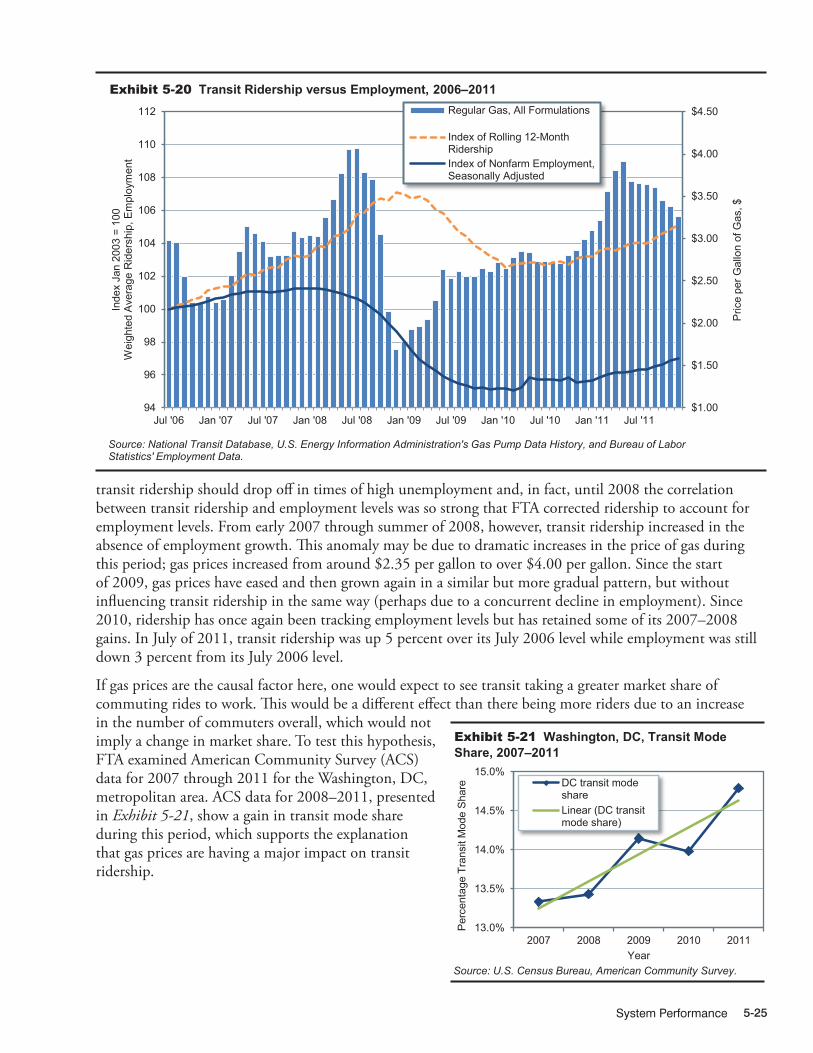
System Performance 5-25

$1.00

$1.50

$2.00

$2.50

$3.00

$3.50

$4.00

$4.50

94

96

98

100

102

104

106

108

110

112

Jul '06 Jan '07 Jul '07 Jan '08 Jul '08 Jan '09 Jul '09 Jan '10 Jul '10 Jan '11 Jul '11

Pric

e pe

r Gal

lon

of G

as, $

Inde

x Ja

n 20

03 =

100

W

eigh

ted

Ave

rage

Rid

ersh

ip, E

mpl

oym

ent

Regular Gas, All Formulations

Index of Rolling 12-MonthRidershipIndex of Nonfarm Employment,Seasonally Adjusted

Source: National Transit Database, U.S. Energy Information Administration's Gas Pump Data History, and Bureau of Labor Statistics' Employment Data.

Exhibit 5-20 Transit Ridership versus Employment, 2006–2011

12/17/2013 05XT_O (5-20) R4.xlsx

transit ridership should drop off in times of high unemployment and, in fact, until 2008 the correlation between transit ridership and employment levels was so strong that FTA corrected ridership to account for employment levels. From early 2007 through summer of 2008, however, transit ridership increased in the absence of employment growth. This anomaly may be due to dramatic increases in the price of gas during this period; gas prices increased from around $2.35 per gallon to over $4.00 per gallon. Since the start of 2009, gas prices have eased and then grown again in a similar but more gradual pattern, but without influencing transit ridership in the same way (perhaps due to a concurrent decline in employment). Since 2010, ridership has once again been tracking employment levels but has retained some of its 2007–2008 gains. In July of 2011, transit ridership was up 5 percent over its July 2006 level while employment was still down 3 percent from its July 2006 level.

If gas prices are the causal factor here, one would expect to see transit taking a greater market share of commuting rides to work. This would be a different effect than there being more riders due to an increase in the number of commuters overall, which would not imply a change in market share. To test this hypothesis, FTA examined American Community Survey (ACS) data for 2007 through 2011 for the Washington, DC, metropolitan area. ACS data for 2008–2011, presented in Exhibit 5-21, show a gain in transit mode share during this period, which supports the explanation that gas prices are having a major impact on transit ridership.

12/17/2013 05XT_P (5-21) R2.xlsx

13.0%

13.5%

14.0%

14.5%

15.0%

2007 2008 2009 2010 2011

Per

cent

age

Tran

sit M

ode

Sha

re

Year

DC transit modeshareLinear (DC transitmode share)

Exhibit 5-21 Washington, DC, Transit Mode Share, 2007–2011

Source: U.S. Census Bureau, American Community Survey.

Description of Current System5-26

Finance

Highway Finance ..........................................................................................................6-2

Revenue Sources for Highways ................................................................................6-2Revenue Trends .................................................................................................................. 6-5

Highway Expenditures ...............................................................................................6-7Types of Highway Expenditures ......................................................................................... 6-7Historical Expenditure and Funding Trends ....................................................................... 6-8

Highway Capital Outlay .............................................................................................6-12Capital Outlays on Federal-Aid Highways .......................................................................... 6-16Capital Outlays on the National Highway System .............................................................. 6-17Capital Outlays on the Interstate System ........................................................................... 6-18

Innovative Finance .....................................................................................................6-18Public-Private Partnerships ................................................................................................. 6-19Federal Credit Assistance ................................................................................................... 6-19Debt Financing Tools .......................................................................................................... 6-20

Transit Finance .............................................................................................................6-21

Level and Composition of Transit Funding ...............................................................6-21Federal Funding .................................................................................................................. 6-22State and Local Funding ..................................................................................................... 6-24System-Generated Funds ................................................................................................... 6-24

Trends in Funding ......................................................................................................6-25Funding in Current and Constant Dollars ........................................................................... 6-25

Capital Funding and Expenditures ............................................................................6-26

Operating Expenditures .............................................................................................6-29Operating Expenditures by Transit Mode ........................................................................... 6-30Operating Expenditures by Type of Cost ........................................................................... 6-31Operating Expenditures per Vehicle Revenue Mile ............................................................ 6-31Operating Expenditures per Passenger Mile ..................................................................... 6-33Farebox Recovery Ratios .................................................................................................... 6-33

Rural Transit ...............................................................................................................6-34

Finance 6-1

CHAPTER 6

Description of Current System6-2

Highway Finance

This chapter provides data and analysis of finance trends for highways and transit across all levels of government. The revenue sources that support investments in highways and bridges are outlined first, followed by a presentation of total highway expenditures and then highway capital outlays only. A separate section of the chapter presents finance trends for transit systems.

In February 2009, the American Recovery and Reinvestment Act (Recovery Act) provided additional funds for transportation and other programs. Transportation received over $48 billion for expenditures in highways, transit, rail, aviation, and other transportation modes. The Department’s broad recovery goals reflect those of the Recovery Act, primarily (1) creating and preserving jobs and promoting economic recovery and (2) investing in infrastructure that has long-term economic benefits. The effects of the additional funds will be evident in the revenue and expenditure levels and trends presented; these effects are referenced and explained where relevant.

Revenue Sources for HighwaysThe revenue generated from all levels for government for highways in 2010 was $221.0 billion, as shown in Exhibit 6-1. Of the total revenue, the Federal government contributed $59.0 billion, State governments contributed $109.0 billion and Local governments contributed $53.1 billion.

12/13/2013 06XH_A (6-1) R2.xlsx

Source Federal State Local Total Percent

$26.1 $30.3 $1.0 $57.4 26.0%$2.6 $22.8 $1.5 $26.9 12.2%$0.0 $7.9 $1.7 $9.6 4.3%

$28.7 $61.0 $4.1 $93.8 42.5%

$0.0 $0.0 $9.4 $9.4 4.3%$29.6 $7.2 $21.8 $58.6 26.5%

$0.6 $6.6 $4.9 $12.2 5.5%$0.0 $8.2 $5.6 $13.9 6.3%$0.0 $25.9 $7.1 $33.0 14.9%

$30.2 $48.0 $48.9 $127.1 57.5%$59.0 $109.0 $53.1 $221.0 100.0%

($11.9) ($3.7) ($0.1) ($15.7) -7.1%$47.1 $105.3 $52.9 $205.3 92.9%

Funds Drawn From (or Placed in) Reserves3

Total Expenditures Funded During 2010

Subtotal

Highway Revenue, Billions of Dollars

Subtotal

Total Revenues

General Fund Appropriations2

Other Taxes and Fees Investment Income and Other Receipts Bond Issue Proceeds

User Charges1

Motor-Fuel Taxes Motor-Vehicle Taxes and Fees Tolls

Other Property Taxes and Assessments

Exhibit 6-1 Government Revenue Sources for Highways, 2010

1 Amounts shown represent only the portion of user charges that are used to fund highway spending; a portion of the revenue generated by motor-fuel taxes, motor-vehicle taxes and fees, and tolls is used for mass transit and other nonhighway purposes. Gross receipts generated by user charges totaled $120.4 billion in 2010. 2 The $29.6 billion shown for Federal reflects $14.7 billion transferred from the General Fund to the Highway Trust Fund in 2010, as well as the expenditure in 2010 of $11.9 billion of the funding authorized for use on highways by the Recovery Act. The remainder supported expenditures by the FHWA and other Federal agencies that were not paid for from the Highway Trust Fund. 3 The $11.9 billion figure shown for Federal reflects the increase in the balance of the Highway Account of the Highway Trust Fund from approximately $8.9 billion at the beginning of the year to approximately $20.7 billion at the end of the year. Without the $14.7 billion transfer of general funds to the Highway Account, this balance would have declined. It should be noted that while the increase in the Highway Account balance in 2010 and the amount of Recovery Act funds expended for highways during 2010 both round to $11.9 billion, this is entirely coincidental. Recovery Act funding was authorized from the General Fund, and has no direct impact on the Highway Trust Fund. Sources: Highway Statistics 2010, Table HF-10, and unpublished FHWA data.

Finance 6-3

Q A&Do the user charges reflected in Exhibit 6-1 include all revenues generated by motor-fuel taxes, motor-vehicle taxes and fees, and tolls in 2010?

No. The $93.8 billion identified as highway-user charges in Exhibit 6-1 represents only 77.8 percent of total highway-user revenue, defined as all revenue generated by motor-fuel taxes, motor-vehicle taxes, and tolls. Exhibit 6-2 shows that combined highway-user revenue collected in 2010 by all levels of government totaled $120.4 billion.

In 2010, $14.7 billion of highway-user revenue was used for transit, and $11.9 billion was used for other purposes, such as ports, schools, collection costs, and general government activities. The $0.4 billion shown as Federal highway-user revenue used for other purposes reflects the difference between total collections in 2010 and the amounts deposited into the HTF during FY 2010. Much of this difference is attributable to the proceeds of 0.1 cent of the motor-fuel tax being deposited into the Leaking Underground Storage Tank trust fund.

The $5.9 billion shown as Federal highway-user revenue used for transit includes deposits into the Transit Account of the HTF, as well as deposits into the Highway Account of the HTF that States elected to use for transit purposes.

12/13/2013 06XH_C (6-2) R2.xlsx

Federal State Local Total$28.7 $61.0 $4.1 $93.8

$5.9 $7.7 $1.0 $14.7$0.4 $11.3 $0.2 $11.9

$35.1 $80.0 $5.3 $120.4

Revenue, Billions of Dollars

Total Collected

HighwaysTransitOther

Exhibit 6-2 Disposition of Highway-User Revenue by Level of Government, 2010

Sources: Highway Statistics 2010, Table HF-10, and unpublished FHWA data.

These revenues were raised from user charges and a number of other sources (other taxes, investment income and debt financing). Federal, State and local governments provide a different mix of revenue sources. A significant share of Federal and State revenues are from user charges. Most of the local revenues are from other sources, particularly General Fund Appropriations.

As shown in Exhibit 6-1, all levels of government combined spent $205.3 billion for highways in 2010. The net difference of $15.7 billion between the total revenues generated during the year and the expenditures during the year increased the reserves available for use in future years. For example, the $11.9 billion difference between total Federal revenues and expenditures represents the increase in the cash balance of the Highway Account of the Highway Trust Fund (HTF) in 2010. While cash balances for some States and localities rose during the year, others fell. Collectively, cash balances in dedicated highway accounts at the State level rose by $3.7 billion, while highway accounts at the local level grew by $0.1 billion.

The total proceeds to the Highway Account of the HTF from dedicated excise taxes and other receipts have fallen below annual expenditures for several years. Transfers of Federal General Fund to the Highway Account were made in 2008, 2009 and 2010 to keep the account solvent. Public Law 111-147 transferred $14.7 billion from the General Fund to the Highway Account of the HTF in 2010. In the absence of this transfer, the balance of the Highway Account would have declined rather than increased.

The $29.6 billion identified as Federal General Fund Appropriations in Exhibit 6-1 includes these $14.7 billion of transferred funds as well as the 2010 expenditure of $11.9 billion authorized under the Recovery Act. The remaining $3.0 billion represents highway-related expenditures of a variety of Federal agencies for activities that are not supported by the Federal Highway Trust Fund, including certain programs of the FHWA (such as a portion of the Emergency Relief Program) and the National Highway Traffic Safety Administration, some direct expenditures by other Federal agencies for roads that they own (see Chapter 12 for a discussion of transportation on Federal lands), and payments to States and local governments under some programs managed by other agencies for which road improvements are an eligible activity. As a result of the unusually high reliance on general funds to support highways at the Federal level in 2010, user charges accounted for less than half of the Federal revenue for highways. User charges accounted for a higher share of State revenues (55.8 percent), consisting of motor fuel taxes ($30.3 billion), motor vehicle taxes and fees ($22.8 billion) and tolls ($7.9 billion). Of the other sources, bond proceeds provided the largest revenue for the States ($25.9 billion).

Description of Current System6-4

Many States do not permit local governments to impose motor-fuel or motor-vehicle taxes; if allowed they cap them at relatively low levels. Therefore, at the local government level, only $4.1 billion (7.8 percent) of highway funding was provided by user charges in 2010. General fund appropriations contributed $21.8 billion (41.1 percent) toward total local highway revenues, while property taxes generated $9.4 billion (17.7 percent).

The “Investment Income and Other Receipts” category in Exhibit 6-1 includes development fees and special district assessments. Other private sector investment in highways would also be reflected in this category, to the extent that such investment is captured in State and local accounting systems.

American Recovery and Reinvestment ActIn February 2009, the American Recovery and Reinvestment Act authorized $48.1 billion for programs administered by the Department of Transportation. The goal was to stimulate the economy by supporting jobs in the construction sector and to invest in critical transportation infrastructure. Of this total, $27.5 billion was appropriated for FHWA. In addition, highway and bridge projects were eligible to compete for Office of the Secretary of Transportation’s Supplemental Discretionary Grant for a National Surface Transportation System program, later referred to as the TIGER I program.

Most of the obligation authority for the highway infrastructure investment funds was distributed to the States by the Federal-aid allocation formula. States were required to obligate these funds to specific projects by the end of September 2010 to avoid losing them. The expenditure of these funds is occurring gradually as States are reimbursed by the FHWA for their expenditures over the life of these projects as the work is completed, which is consistent with how the regular Federal-aid highway program operates. The statistics presented in this Chapter reflect expenditures on a cash basis rather than obligations, so the Recovery Act may continue to have an impact on the reported highway revenues and expenditures for several years.

The period over which cash expenditures are incurred for an individual project depends on the length of time it takes to complete the work, which can vary by project type. During 2010, $11.9 billion of Recovery Act funds were expended for highway-related activities.

Private Sector FinancingFinancing for highways comes from both the public and private sectors. The private sector has increasingly played a role in the delivery of highway infrastructure, but the vast majority of funding is still provided by the public sector. The financial statistics presented in this chapter are predominantly drawn from State reports based on State and local accounting systems. Figures in these systems can include some private sector investment; where it does, these amounts are generally classified as “other receipts.” For additional information on private sector investment in highways, see http:/ www.fhwa.dot.gov/ipd/p3/index.htm.

Q A&Could the Recovery Act project selection process be affecting the spending rates for the regular Federal-aid Highway Program?

States were under tight deadlines to obligate Recovery Act funds by September 30, 2010, and their progress in obligating these funds was closely monitored by FHWA; less emphasis was placed on the obligation of regular Federal-aid program funds, provided that regular deadlines were met. In addition, States were not required to contribute matching funds for projects funded from the Recovery Act, providing an additional incentive to use these funds before the regular Federal-aid highway program funds. The financial data presented in this report are presented on a cash basis; to the extent that delays in obligating funds for a given project within a given fiscal year affected the start date for that project, this could influence the timing of the cash expenditures associated with that project.

Much of the Recovery Act funding was directed to projects that could be implemented relatively quickly in order to maximize their short-term impacts on employment. This reduced the pool of such potential projects under consideration by States for funding from their regular Federal-aid highway program, which could have affected the relative mix of projects selected. To the extent that some States obligated their Federal-aid highway program funds to projects of longer duration than usual, this would have tended to slow down the average Federal cash spending rate, since cash reimbursements are made to States only after work has been completed. To the extent that such a phenomenon has occurred it could have dampened the initial impacts of Recovery Act funding, but increased the duration of these impacts.

Finance 6-5

Q A&How long has it been since excise tax revenue deposited into the Highway Account exceeded expenditures?

The last time that annual net receipts credited to the Highway Account of the HTF exceeded annual expenditures from the Highway Account was in 2000. As shown in Exhibit 6-3, for each year since 2000, total annual receipts to the Highway Account from excise taxes and other income (such as interest income and motor carrier safety fines and penalties) have been lower than the annual expenditures from the Highway Account (including amounts transferred to the Transit Account).

To help maintain a positive cash balance in the HTF, three transfers from the General Fund to the HTF were legislatively mandated in FY 2008, FY 2009, and FY 2010. From FY 2007 to FY 2010 gross excise tax receipts from gasoline, diesel and special motor fuels, tires, trucks and trailers, and the heavy vehicle use tax all declined. In 2011, the receipts increased for the first time since 2007. The outlays also increased, retaining the gap between tax revenue deposited in the HTF and the expenditures.

0

5

10

15

20

25

30

35

40

45

2000 2002 2004 2006 2008 2010

Bill

ions

of D

olla

rs

Highway Account Outlays (Plus Transfers to Transit Account)

Highway Account Excise Tax and Other Receipts (Excluding General Fund Transfers)

Sources: Highway Statistics, various years, Tables FE-210 and FE-10.

Exhibit 6-3 Highway Trust Fund Highway Account Receipts and Outlays, Fiscal Years 2000–2011

12/17/2013 06XH_D (6-3) R2.xlsx

Revenue TrendsSince the passage of the Federal-Aid Highway Act of 1956 and the establishment of the HTF, user charges such as motor-fuel and motor-vehicle tax receipts have consistently provided the majority of the combined revenues raised for highway and bridge programs by all levels of government.

Exhibit 6-4 shows the trends in revenue for all governments for the period 2000 to 2010. Total revenues have increased on average by 5.4 percent per year between 2000 and 2010. The annual growth in revenue from motor fuel and vehicle taxes was only 1.1 percent per year. General Fund appropriation and Bond issue proceeds each increased by over eleven percent per year. The increase in the General Fund appropriations was particularly strong in 2008 and 2010, when transfers were made from the General Fund to keep the HTF solvent, following many years of cash outlays exceeding cash receipts and running down the reserve balance.

The graph in Exhibit 6-4 illustrates the percentage of revenue from different sources to the total revenue each year for the period 2000 to 2010. The percentage of revenue from user charges, particularly motor fuel and vehicle taxes, has declined over time, whereas the General Fund appropriations and bond proceeds have increased.

Motor fuel tax revenues are sensitive to changes in VMT and fuel efficiency. The growth in VMT over the decade from 2000 to 2010 has averaged 0.8 percent per year in contrast to the previous 10 years, when

Description of Current System6-6

VMT increased by 2.9 percent per year. In 2008 and 2009, VMT declined each year; 2010 VMT is lower than the 2007 level. Motor fuel efficiency has also increased over the period from 2000 to 2010; from an average of 16.9 miles traveled per gallon of fuel consumed to 17.4 miles traveled per gallon of fuel consumed (Highway Statistics, Table VM-1). Some States compensated for declines in user revenues by increasing fuel tax rates and other motor vehicle taxes. The weighted average State gasoline motor fuel tax increased from 19.96 cents per gallon in 2000 to 21.82 cents per gallon in 2010. Similarly, the diesel motor fuel tax rate increased from 19.96 cents per gallon to 22.36 cents per gallon (Highway Statistics, Table MF-205). The increases in tax rates were more evident after 2005. The decline in user revenues was offset by increasing revenues from other sources. Transfers from the General Fund helped to sustain the HTF at the level necessary to support the federal spending levels specified in the SAFETEA-LU. Bond issue proceeds increased from $20.9 billion in 2008 to $33.0 billion in 2010, a 58 percent increase in two years.

Annual Rate ofChange

Source 2000 2002 2004 2006 2008 2010 2010/2000Motor-Fuel and Motor-Vehicle Taxes $75.6 $73.1 $76.4 $85.4 $84.7 $84.3 1.1%Tolls $5.7 $6.6 $6.6 $8.3 $9.1 $9.6 5.3%Property Taxes and Assessments $6.1 $6.5 $7.5 $9.0 $9.0 $9.4 4.4%General Fund Appropriations $19.3 $20.3 $23.6 $28.3 $40.0 $58.6 11.8%Other Taxes and Fees $5.7 $7.5 $7.9 $10.1 $12.2 $12.2 7.8%Investment Income & Other Receipts $7.3 $8.1 $7.6 $9.7 $16.6 $13.9 6.6%Bond Issue Proceeds $11.3 $12.7 $15.8 $18.3 $20.9 $33.0 11.3%Total Revenues $131.1 $134.8 $145.3 $169.0 $192.6 $221.0 5.4%

1

Highway Revenue, Billions of Dollars

0.0%

10.0%

20.0%

30.0%

40.0%

50.0%

60.0%

70.0%

Motor-Fuel andMotor-Vehicle

Taxes

Tolls Property Taxesand Assessments

General FundAppropriations

Other Taxes andFees

InvestmentIncome & Other

Receipts

Bond IssueProceeds

2000 2002 2004 2006 2008 2010

Sources: Highway Statistics, various years, Tables HF-10A and HF-10.

Exhibit 6-4 Government Revenue Sources for Highways, 2000–2010

12/17/2013 06XH_E (6-4) R2.xlsx

Exhibit 6-5 shows the change in the share of highway revenue derived from user charges by the level of government. The share has declined for all levels of government combined from 2000 to 2010, but the decline has been more significant for the Federal user charges, from 95.5 percent to 48.8 percent. As noted earlier, the declines since 2007 can be attributed in part from General Fund transfers to the HTF, as well as general funds provided through the Recovery Act. State user revenue share has declined to 42.5 percent from 62.0 percent. User charges have also declined as a share of local government revenue.

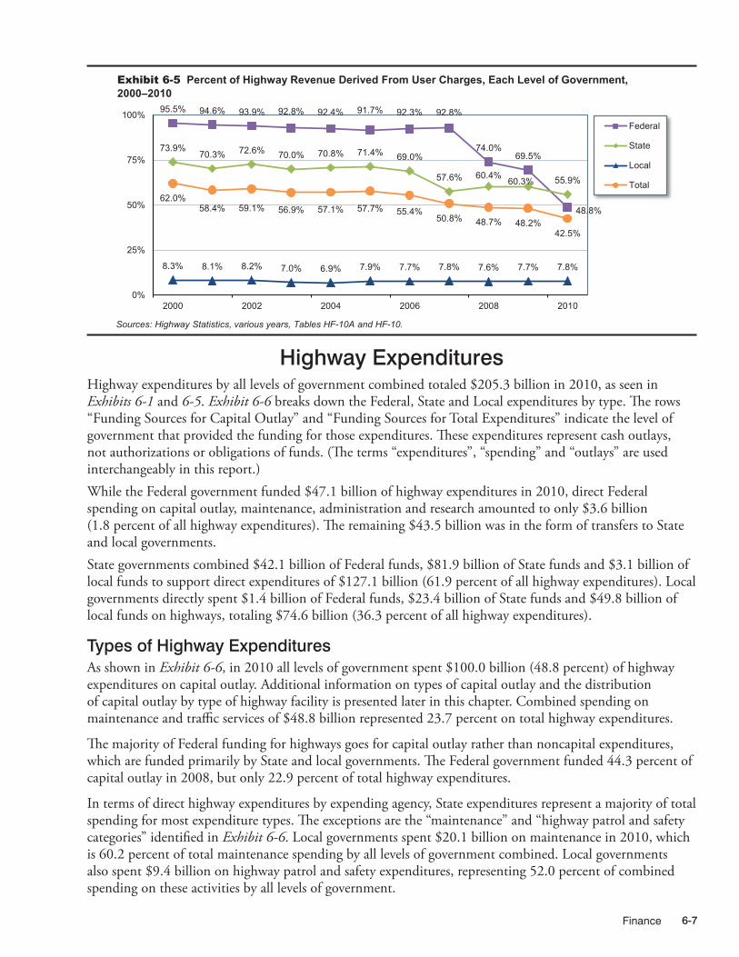
Finance 6-7

Highway ExpendituresHighway expenditures by all levels of government combined totaled $205.3 billion in 2010, as seen in Exhibits 6-1 and 6-5. Exhibit 6-6 breaks down the Federal, State and Local expenditures by type. The rows “Funding Sources for Capital Outlay” and “Funding Sources for Total Expenditures” indicate the level of government that provided the funding for those expenditures. These expenditures represent cash outlays, not authorizations or obligations of funds. (The terms “expenditures”, “spending” and “outlays” are used interchangeably in this report.) While the Federal government funded $47.1 billion of highway expenditures in 2010, direct Federal spending on capital outlay, maintenance, administration and research amounted to only $3.6 billion (1.8 percent of all highway expenditures). The remaining $43.5 billion was in the form of transfers to State and local governments. State governments combined $42.1 billion of Federal funds, $81.9 billion of State funds and $3.1 billion of local funds to support direct expenditures of $127.1 billion (61.9 percent of all highway expenditures). Local governments directly spent $1.4 billion of Federal funds, $23.4 billion of State funds and $49.8 billion of local funds on highways, totaling $74.6 billion (36.3 percent of all highway expenditures).

Types of Highway ExpendituresAs shown in Exhibit 6-6, in 2010 all levels of government spent $100.0 billion (48.8 percent) of highway expenditures on capital outlay. Additional information on types of capital outlay and the distribution of capital outlay by type of highway facility is presented later in this chapter. Combined spending on maintenance and traffic services of $48.8 billion represented 23.7 percent on total highway expenditures.

The majority of Federal funding for highways goes for capital outlay rather than noncapital expenditures, which are funded primarily by State and local governments. The Federal government funded 44.3 percent of capital outlay in 2008, but only 22.9 percent of total highway expenditures.

In terms of direct highway expenditures by expending agency, State expenditures represent a majority of total spending for most expenditure types. The exceptions are the “maintenance” and “highway patrol and safety categories” identified in Exhibit 6-6. Local governments spent $20.1 billion on maintenance in 2010, which is 60.2 percent of total maintenance spending by all levels of government combined. Local governments also spent $9.4 billion on highway patrol and safety expenditures, representing 52.0 percent of combined spending on these activities by all levels of government.

95.5% 94.6% 93.9% 92.8% 92.4% 91.7% 92.3% 92.8%

74.0% 69.5%

48.8%

73.9% 70.3% 72.6% 70.0% 70.8% 71.4% 69.0%

57.6% 60.4% 60.3% 55.9%

8.3% 8.1% 8.2% 7.0% 6.9% 7.9% 7.7% 7.8% 7.6% 7.7% 7.8%

62.0% 58.4% 59.1% 56.9% 57.1% 57.7% 55.4%

50.8% 48.7% 48.2% 42.5%

0%

25%

50%

75%

100%

2000 2002 2004 2006 2008 2010

Federal

State

Local

Total

Sources: Highway Statistics, various years, Tables HF-10A and HF-10.

Exhibit 6-5 Percent of Highway Revenue Derived From User Charges, Each Level of Government, 2000–2010

12/17/2013 06XH_F (6-5) R2.xlsx

Description of Current System6-8

Historical Expenditure and Funding TrendsExhibit 6-7 breaks out expenditures by type since 2000. The largest percentage increases related to debt service, as bond retirement expenditures grew at an average annual rate of 9.2 percent from 2000 to 2010, while interest on debt grew an average annual rate of 7.9 percent. Total highway expenditures grew by 5.3 percent per year over this period in nominal dollar terms, while capital outlay rose at an average annual rate of 5.0 percent, capital expenditures becoming a smaller share of total expenditures.

12/13/2013 06XH_G (6-6) R3.xlsx

Federal State Local Total PercentExpenditures by TypeCapital Outlay $0.8 $72.6 $26.8 $100.2 48.8%Noncapital Expenditures

Maintenance $0.3 $13.0 $20.1 $33.4 16.2%Highway and Traffic Services $0.0 $9.0 $6.5 $15.4 7.5%Administration $2.4 $8.8 $4.9 $16.2 7.9%Highway Patrol and Safety $0.0 $8.7 $9.4 $18.1 8.8%Interest on Debt $0.0 $7.0 $2.9 $9.8 4.8%Subtotal $2.7 $46.4 $43.7 $92.9 45.2%

Total, Current Expenditures $3.6 $119.0 $70.5 $193.0 94.0%Bond Retirement $0.0 $8.1 $4.1 $12.3 6.0%Total, All Expenditures $3.6 $127.1 $74.6 $205.3 100.0%Funding Sources for Capital Outlay

Funded by Federal Government* $0.8 $42.1 $1.4 $44.4 44.3%Funded by State or Local Govts* $0.0 $30.4 $25.4 $55.8 55.7%Total $0.8 $72.5 $26.8 $100.2 100.0%

Funding Sources for Total ExpendituresFunded by Federal Government* $3.6 $42.1 $1.4 $47.1 22.9%Funded by State Governments* $0.0 $81.9 $23.4 $105.3 51.3%Funded by Local Governments* $0.0 $3.1 $49.8 $52.9 25.8%

Total $3.6 $127.1 $74.6 $205.3 100.0%

Highway Expenditures (Billions of Dollars)

Exhibit 6-6 Direct Expenditures for Highways, by Expending Agencies and by Type, 2010

* Amounts shown in italics are provided to link this table back to revenue sources shown in Exhibit 6-1. These are nonadditive to the rest of the table, which classifies spending by expending agency. Sources: Highway Statistics 2010, Table HF-10, and unpublished FHWA data.

12/13/2013 06XH_H (6-7) R2.xlsx

Annual Rateof Change

2000 2002 2004 2006 2008 2010 2010/2000Expenditure TypeCapital Outlay $61.3 $68.2 $70.3 $80.2 $90.4 $100.2 5.0%Maintenance and Traffic Services $30.6 $33.2 $36.3 $40.8 $45.9 $48.8 4.8%Administration $10.0 $10.7 $12.7 $13.1 $17.8 $16.2 4.9%Highway Patrol and Safety $11.0 $11.7 $14.3 $14.7 $17.3 $18.1 5.1%Interest on Debt $4.6 $5.4 $5.8 $6.6 $8.5 $9.8 7.9%Total, Current Expenditures $117.6 $129.1 $139.5 $155.5 $180.0 $193.0 5.1%Bond Retirement $5.1 $6.8 $8.0 $8.1 $8.6 $12.3 9.2%Total, All Expenditures $122.7 $135.9 $147.5 $163.5 $188.5 $205.3 5.3%

Highway Expenditures, Billions of Dollars

Exhibit 6-7 Expenditures for Highways by Type, All Units of Government, 2000–2010

Sources: Highway Statistics, various years, Tables HF-10A and HF-10.

Finance 6-9

Highway Expenditure TerminologyThe classification of the revenue and expenditure items in this report is based on definitions contained in A Guide to Reporting Highway Statistics, the instructional manual for States providing financial data for the Highway Statistics publication.

• “Capital outlay” consists of those expenditures associated with highway improvements. Improvements include land acquisition and other right-of-way costs; preliminary and construction engineering; new construction, reconstruction, resurfacing, rehabilitation, and restoration; and installation of guardrails, fencing, signs, and signals.

• “Maintenance” includes routine and regular expenditures required to keep the highway surface, shoulders, roadsides, structures, and traffic control devices in usable condition. This includes completing spot patching and crack sealing of roadways and bridge decks and maintaining and repairing highway utilities and safety devices such as route markers, signs, guardrails, fence, signals, and highway lighting. (Other definitions of maintenance are used by different organizations. Some resurfacing, restoration, and rehabilitation projects that meet this report’s definition of capital outlay might be classified as maintenance activities in internal State or local accounting systems.)

• “Highway and traffic services” include activities designed to improve the operation and appearance of the roadway. This includes items such as the operation of traffic control systems, snow and ice removal, highway beautification, litter pickup, mowing, toll collection, and air quality monitoring.

• “Current expenditures” includes all highway expenditures except for bond retirement. When looking at cash outlays for a particular year, total expenditures is more relevant, as it measures the full scope of highway-related activity. However, when summing expenditures across years, it is sometimes more appropriate to use current expenditures. For example, if bonds were issued to pay for a capital project, and retired 20 years later, then summing total expenditures over 20 years would effectively capture this transaction twice, as both the initial capital expenditure and the retirement of the bonds would be included.

• “Non-capital expenditures” consists of all current expenditures except for capital outlay. It includes maintenance, highway and traffic services, administration, highway law enforcement, safety programs, and interest on debt.

Exhibit 6-8 shows that Federal funding for highways grew more quickly from 2000 to 2010 than did State or local funding. The portion of total highway expenditures rose from 22.4 percent to 22.9 percent over this period, while the Federally funded share of highway capital outlay rose from 42.6 percent to 44.3 percent. As noted earlier in this chapter, the Federal expenditure figures for 2010 include $11.9 billion funded by the Recovery Act. As Federally funded highway expenditures grew by only $7.3 billion from 2008 to 2010 (from $39.8 billion to $47.1 billion), this indicates that cash-basis expenditures funded from other Federal sources declined over this 2-year period.

Despite budgetary pressures relating to the recent recession, State funding for highways increased from $96.6 billion in 2008 to $105.3 billion in 2010. Local government funding also increased slightly during this period, from $52.2 billion in 2008 to $52.9 billion in 2010.

12/13/2013 06XH_I (6-8) R2.xlsx

Annual Rateof Change

2000 2002 2004 2006 2008 2010 2010/2000 Capital Outlay

Funded by Federal Government $26.1 $31.5 $30.8 $34.6 $37.6 $44.4 5.4%Funded by State or Local Govt's $35.2 $36.7 $39.5 $45.6 $52.8 $55.8 4.7%Total $61.3 $68.2 $70.3 $80.2 $90.4 $100.2 5.0%Federal Share 42.6% 46.1% 43.8% 43.1% 41.6% 44.3%

Total ExpendituresFunded by Federal Government $27.5 $32.8 $33.1 $36.3 $39.8 $47.1 5.5%Funded by State Governments $62.7 $69.0 $72.8 $77.4 $96.6 $105.3 5.3%Funded by Local Governments $32.6 $34.1 $41.6 $49.8 $52.2 $52.9 5.0%Total $122.7 $135.9 $147.5 $163.5 $188.5 $205.3 5.3%Federal Share 22.4% 24.1% 22.4% 22.2% 21.1% 22.9%

Highway Funding, Billions of Dollars

Exhibit 6-8 Funding for Highways by Level of Government, 2000–2010

Sources: Highway Statistics, various years, Tables HF-10A and HF-10.

Description of Current System6-10

Constant Dollar ExpendituresExhibits 6-9 and 6-10 display time series data on highway expenditures in both current (nominal) and constant (real) 2010 dollars. While there have been periods of decrease in constant dollars for both highway capital expenditures and total highway expenditures, both reached an all-time high in 2010.

0

20

40

60

80

100

120

1990 1992 1994 1996 1998 2000 2002 2004 2006 2008 2010

Highway Capital Expenditures

Current Dollars Constant 2010 Dollars*

Billions of Dollars

0

20

40

60

80

100

120

1990 1992 1994 1996 1998 2000 2002 2004 2006 2008 2010

Other Highway Expenditures

Current Dollars Constant 2010 Dollars*

Billions of Dollars

0

40

80

120

160

200

240

1990 1992 1994 1996 1998 2000 2002 2004 2006 2008 2010

Total Highway Expenditures

Current Dollars Constant 2010 Dollars*

Billions of Dollars

* Constant dollar conversions for highway capital expenditures were made using the FHWA BPI through the year 2006, and the FHWA NHCCI in subsequent years. Constant dollar conversions for other types of highway spending were made using the Bureau of Labor Statistics' CPI.

Sources: Highway Statistics, various years, Tables HF-10A, HF-10, PT-1; http://www.bls.gov/cpi/.

Exhibit 6-9 Highway Capital, Noncapital, and Total Expenditures in Current and Constant 2010 Dollars, All Units of Government, 1990–2010

12/17/2013 06XH_J (6-9) R2.xlsx

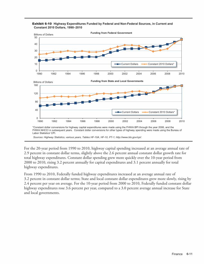
Finance 6-11

For the 20-year period from 1990 to 2010, highway capital spending increased at an average annual rate of 2.9 percent in constant dollar terms, slightly above the 2.6 percent annual constant dollar growth rate for total highway expenditures. Constant dollar spending grew more quickly over the 10-year period from 2000 to 2010, rising 3.2 percent annually for capital expenditures and 3.1 percent annually for total highway expenditures.

From 1990 to 2010, Federally funded highway expenditures increased at an average annual rate of 3.2 percent in constant dollar terms; State and local constant dollar expenditures grew more slowly, rising by 2.4 percent per year on average. For the 10-year period from 2000 to 2010, Federally funded constant dollar highway expenditures rose 3.6 percent per year, compared to a 3.0 percent average annual increase for State and local governments.

0

10

20

30

40

50

1990 1992 1994 1996 1998 2000 2002 2004 2006 2008 2010

Funding from Federal Government

Current Dollars Constant 2010 Dollars*

Billions of Dollars

0

40

80

120

160

1990 1992 1994 1996 1998 2000 2002 2004 2006 2008 2010

Billions of Dollars Funding from State and Local Governments

Current Dollars Constant 2010 Dollars*

Exhibit 6-10 Highway Expenditures Funded by Federal and Non-Federal Sources, in Current and Constant 2010 Dollars, 1990–2010

*Constant dollar conversions for highway capital expenditures were made using the FHWA BPI through the year 2006, and the FHWA NHCCI in subsequent years. Constant dollar conversions for other types of highway spending were made using the Bureau of Labor Statistics' CPI. Sources: Highway Statistics, various years, Tables HF-10A, HF-10, PT-1; http://www.bls.gov/cpi/.

12/17/2013 06XH_K (6-10) R2.xlsx

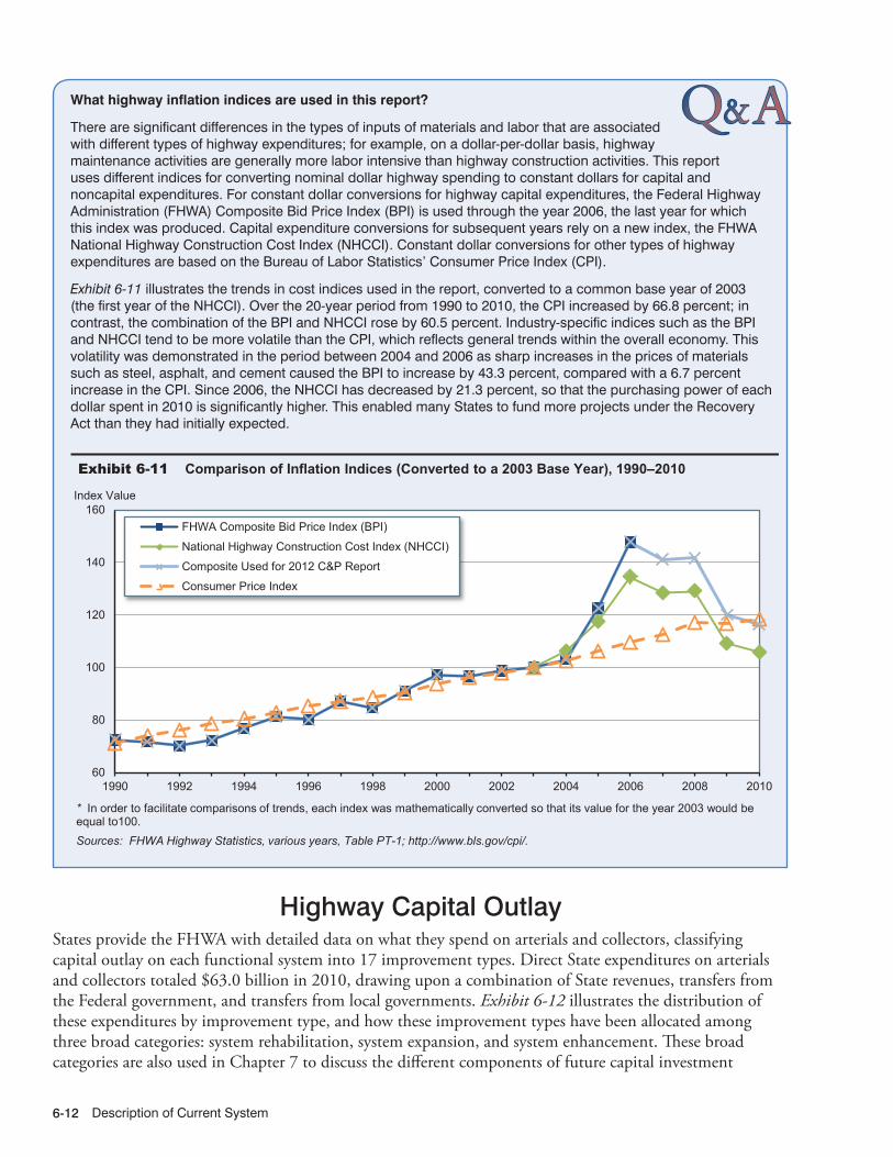
Description of Current System6-12

Q A&What highway inflation indices are used in this report?

There are significant differences in the types of inputs of materials and labor that are associated with different types of highway expenditures; for example, on a dollar-per-dollar basis, highway maintenance activities are generally more labor intensive than highway construction activities. This report uses different indices for converting nominal dollar highway spending to constant dollars for capital and noncapital expenditures. For constant dollar conversions for highway capital expenditures, the Federal Highway Administration (FHWA) Composite Bid Price Index (BPI) is used through the year 2006, the last year for which this index was produced. Capital expenditure conversions for subsequent years rely on a new index, the FHWA National Highway Construction Cost Index (NHCCI). Constant dollar conversions for other types of highway expenditures are based on the Bureau of Labor Statistics’ Consumer Price Index (CPI).

Exhibit 6-11 illustrates the trends in cost indices used in the report, converted to a common base year of 2003 (the first year of the NHCCI). Over the 20-year period from 1990 to 2010, the CPI increased by 66.8 percent; in contrast, the combination of the BPI and NHCCI rose by 60.5 percent. Industry-specific indices such as the BPI and NHCCI tend to be more volatile than the CPI, which reflects general trends within the overall economy. This volatility was demonstrated in the period between 2004 and 2006 as sharp increases in the prices of materials such as steel, asphalt, and cement caused the BPI to increase by 43.3 percent, compared with a 6.7 percent increase in the CPI. Since 2006, the NHCCI has decreased by 21.3 percent, so that the purchasing power of each dollar spent in 2010 is significantly higher. This enabled many States to fund more projects under the Recovery Act than they had initially expected.

Highway Capital OutlayStates provide the FHWA with detailed data on what they spend on arterials and collectors, classifying capital outlay on each functional system into 17 improvement types. Direct State expenditures on arterials and collectors totaled $63.0 billion in 2010, drawing upon a combination of State revenues, transfers from the Federal government, and transfers from local governments. Exhibit 6-12 illustrates the distribution of these expenditures by improvement type, and how these improvement types have been allocated among three broad categories: system rehabilitation, system expansion, and system enhancement. These broad categories are also used in Chapter 7 to discuss the different components of future capital investment

60

80

100

120

140

160

1990 1992 1994 1996 1998 2000 2002 2004 2006 2008 2010

FHWA Composite Bid Price Index (BPI)

National Highway Construction Cost Index (NHCCI)

Composite Used for 2012 C&P Report

Consumer Price Index

Index Value

* In order to facilitate comparisons of trends, each index was mathematically converted so that its value for the year 2003 would be equal to100. Sources: FHWA Highway Statistics, various years, Table PT-1; http://www.bls.gov/cpi/.

Exhibit 6-11 Comparison of Inflation Indices (Converted to a 2003 Base Year), 1990–2010

12/17/2013 06XH_S (6-11) R1.xlsx

Finance 6-13

Q A&How are “system rehabilitation,” “system expansion,” and “system enhancement” defined in this report?

System rehabilitation consists of capital improvements on existing roads and bridges that are intended to preserve the existing pavement and bridge infrastructure. These activities include reconstruction, resurfacing, pavement restoration or rehabilitation, widening of narrow lanes or shoulders, bridge replacement, and bridge rehabilitation. Also included is the portion of widening (lane addition) projects estimated to be related to reconstructing or improving existing lanes. System rehabilitation does not include routine maintenance costs.

System expansion includes construction of new roads and new bridges and addition of new lanes to existing roads. This includes all “New Construction,” “New Bridge,” “Major Widening,” and most of the costs associated with “Reconstruction-Added Capacity,” except for the portion of these expenditures estimated to be related to improving the existing lanes of a facility.

System enhancement includes safety enhancements, traffic operations improvements such as the installation of intelligent transportation systems, and environmental enhancements.

9/18/2012 06XH_L (6-12) R1.xlsx

$1.5 $2.2 $3.7$4.7 $0.7 $1.1 $0.7 $7.2

$4.8 $4.8$1.0 $1.0

$1.7 $4.0 $5.7$3.3 $3.3

$3.1 $3.1$1.3 $1.3

$17.1 $17.1$0.0 $0.0

$0.5 $0.5$5.5 $5.5$3.0 $3.0$2.1 $2.1

$2.1 $2.1$0.9 $0.9$1.8 $1.8

$38.7 $7.5 $11.4 $5.4 $63.0

$33.8 $8.8 $13.9 $7.0 $63.6$13.1 $0.7 $13.8$46.9 $9.5 $13.9 $7.0 $77.4

$42.9 $11.5 $15.0 $12.8 $82.2$17.1 $0.9 $18.0$60.0 $12.4 $15.0 $12.8 $100.2

59.9% 12.4% 15.0% 12.8% 100.0%

Distribution of Capital Outlay, Billions of DollarsSystem Expansion

System Rehabilitation

New Roads and Bridges

Existing Roads

System Enhancements

EngineeringNew ConstructionRelocation

Type of Expenditure

Right-of-Way

Direct State Expenditures on Arterials and CollectorsTotal Outlay

Reconstruction—Added CapacityReconstruction—No Added CapacityMajor WideningMinor WideningRestoration and RehabilitationResurfacingNew BridgeBridge ReplacementMajor Bridge RehabilitationMinor Bridge WorkSafetyTraffic Management/EngineeringEnvironmental and OtherTotal, State Arterials and CollectorsTotal, Arterials and Collectors, All Jurisdictions (estimated)*Highways and Other

BridgesTotal, Arterials and Collectors

Highways and OtherBridgesTotal, All SystemsPercent of Total

Total Capital Outlay on All Systems (estimated)*

Exhibit 6-12 Highway Capital Outlay by Improvement Type, 2010

*Improvement type distribution was estimated based on State arterial and collector data. Sources: Highway Statistics 2010, Table SF-12A, and unpublished FHWA data.

Description of Current System6-14

9/18/2012 06XH_M (6-13) R1

74.4%

51.4%

66.8%

72.0%

80.0%

65.1%

62.7%

48.7%

52.9%

60.2%

63.0%

57.7%

57.3%

59.9%

6.3%

6.5%

8.8%

8.0%

12.2%

7.5%

7.3%

12.8%

10.8%

11.6%

10.7%

10.1%

25.3%

12.8%

19.3%

42.1%

24.4%

20.0%

7.8%

27.4%

30.1%

38.5%

36.4%

28.2%

26.3%

32.2%

17.4%

27.4%

0% 10% 20% 30% 40% 50% 60% 70% 80% 90% 100%

Rural Interstate ($7.0 Billion)

Rural Other Principal Arterial ($10.3 Billion)

Rural Minor Arterial ($6.9 Billion)

Rural Major Collector ($5.6 Billion)

Rural Minor Collector ($1.6 Billion)

Subtotal, Rural Arterials and Collectors ($31.4 Billion)

Urban Interstate ($13.2 Billion)

Urban Other Freeways and Expressways ($5.3 Billion)

Urban Other Principal Arterial ($14.1 Billion)

Urban Minor Arterial ($8.2 Billion)

Urban Collector ($5.2 Billion)

Subtotal, Urban Arterials and Collectors ($46.0 Billion)

Rural and Urban Local (Estimated) ($22.8 Billion)

Total, All Systems (Estimated) ($100.2 Billion)

System Rehabilitation System Enhancements System Expansion

Exhibit 6-13 Distribution of Capital Outlay by Improvement Type and Functional System, 2010

Sources: Highway Statistics 2008, Table SF-12A, and unpublished FHWA data.

scenarios. Exhibit 6-12 presents an estimated distribution of total highway capital outlay by all levels of government on all roads. Of the $100.2 billion in total highway capital outlay, an estimated $60.0 billion was used for system rehabilitation, $27.4 billion went for system expansion, and $12.8 billion was used for system enhancement. These estimates are derived based primarily on State expenditure patterns on arterials and collectors, along with limited data from other sources.

Exhibit 6-13 shows the distribution of capital expenditures by type and functional system. $31.4 billion was invested on rural arterials and collectors in 2010, with 65.1 percent directed towards system rehabilitation and 27.4 percent towards expansion; the remainder was directed toward system enhancement. Capital outlays on urban arterials and collectors were $46.0 billion, of which 57.7 percent went for system rehabilitation and 32.2 percent went for system expansion.

Exhibit 6-14, shows trends in capital outlays by improvement type from 2000 to 2010. Each year, a majority of capital outlays were directed towards system rehabilitation reflecting the need to preserve the aging system. However, system preservation’s share of total capital spending rose dramatically between 2008 and 2010, rising from 51.1 percent to 59.9 percent. System rehabilitation expenditures increased from $46.2 billion to $60.0 billion, an increase of almost 30 percent over the 2 years. This dramatic increase was partly driven by the Recovery Act. One of the goals of the Recovery Act was to support jobs through

Finance 6-15

9/18/2012 06XH_N (6-14) R1.xlsx

Improvement Type 2000 2002 2004 2006 2008 2010System RehabilitationHighway $25.0 $25.5 $26.7 $31.0 $33.5 $42.9 5.5%Bridge $7.3 $10.7 $9.6 $10.3 $12.7 $17.1 8.9%Subtotal $32.3 $36.2 $36.3 $41.3 $46.2 $60.0 6.4%System ExpansionAdditions to Existing Roadways $11.4 $11.9 $12.1 $14.0 $15.7 $15.0 2.8%New Routes $10.5 $11.4 $12.6 $15.2 $16.1 $11.5 0.9%New Bridges $1.1 $1.1 $1.4 $1.2 $1.5 $0.9 -2.0%Subtotal $23.0 $24.4 $26.1 $30.4 $33.3 $27.4 1.8%System Enhancements $6.1 $7.6 $7.8 $8.5 $10.9 $12.8 7.7%

Total $61.3 $68.2 $70.3 $80.2 $90.4 $100.2 5.0%

Percent of Total Capital OutlaySystem Rehabilitation 52.7% 53.1% 51.7% 51.5% 51.1% 59.9%System Expansion 37.4% 35.8% 37.1% 37.9% 36.9% 27.4%System Enhancements 9.9% 11.1% 11.2% 10.6% 12.0% 12.8%

Annual Rate of Change

2010/2000Capital Outlay, Billions of Dollars

Exhibit 6-14 Capital Outlay on All Roads by Improvement Type, 2000–2010

Sources: Highway Statistics 2010, Table SF-12A, and unpublished FHWA data.

Over the 10-year period from 2000 to 2010, system rehabilitation expenditures grew at an average annual rate of 6.4 percent. System expansion expenditures have increased at a slower average annual rate of 1.8 percent, resulting in a decline in share of total capital outlays from 37.4 percent in 2000 to 27.4 percent in 2010. System enhancement expenditures have grown more quickly, rising from 9.9 percent of total capital outlays in 2000 to 12.8 percent in 2010.

Q A&How have constant dollar expenditures for different capital improvement types grown in recent years?

As noted earlier in this section, total capital outlay by all levels of government grew at an average annual rate of 3.2 percent from 2000 to 2010 in constant dollar terms. Constant dollar system rehabilitation expenditures rose by 4.5 percent per year over this period, while system expansion expenditures showed little annual change. Expenditures for system enhancements grew by 5.8 percent per year in constant dollar terms from 2000 to 2010.

construction expenditures, providing an incentive for the selection of projects that could be initiated and completed relatively quickly. This led many States to direct a larger portion of their Recovery Act funding toward pavement improvement projects than they usually do from regular Federal-aid funds in a typical year. (For example, in 2008, States obligated 42.3 percent to the types of projects that would be classified as “System Rehabilitation-Highway” in this report. However, the share of Recovery Act funding obligated for such projects in 2009 and 2010 was 58.3 percent. This was however, partially offset by a lower share of Recovery Act funding being obligated to the “System Rehabilitation-Bridges” category.)

Description of Current System6-16

Capital Outlays on Federal-Aid HighwaysAs discussed in Chapter 2, the term “Federal-aid Highways” refers to roads that are generally eligible for Federal funding, and excludes roads that are functionally classified as rural minor, rural local or urban local. Exhibit 6-16 shows that total capital outlays on Federal-aid highways increased at an average annual rate of 4.6 percent from 2000 to 2010, rising to $75.8 billion in 2010.

Capital outlays on system rehabilitation increased from $35.5 billion in 2008 to $45.6 billion in 2010, an increase greater than the increase in total capital outlays on the Federal-aid system. The share of system rehabilitation increased from 50.7 percent in 2008 to 60.2 percent in 2010.

Q A&Was the share of recovery funds spent on system rehabilitation higher than the share of 2008 system rehabilitation expenditures?

The spending pattern of the Recovery Act funds has been different from the year 2008 spending. Exhibit 6-15 presents the 2008 FHWA obligations and Recovery Act obligations and expenditures through December 2010. Rehabilitation expenditures account for more than 50 percent of the obligations for both periods, but under the Recovery Act, the share has increased to above 60 percent in obligations and well over 70 percent in the funds expended through December 2010.

The Recovery Act had specific requirements regarding the time by which the funds had to be obligated. The objectives of the Act were to ensure that funds were quickly invested to support construction jobs lost due to the economic recession. To encourage the States and other funding recipients to select projects quickly, they were required to obligate 50 percent of the Recovery Act funds (excluding sub-allocations to local entities) within 120 days of apportionment or lose funding to other States that were successful in meeting this deadline. All recipients were required to obligate 100 percent of their funds by the end of September 2010 or lose what was remaining. States were requested to select projects that were ready. This resulted in choosing projects that required minimum level of planning and approval. This favored the selection of rehabilitation and replacement projects.

The share of Recovery Act expenditures for system rehabilitation is higher than the share of Recovery Act funds obligated for that purpose (74.7 per cent compared to 67.6 per cent) because rehabilitation and resurfacing projects are likely to incur expenditures sooner than other types of projects. Resurfacing and pavement rehabilitation typically require less advance planning and can be completed in a shorter timeframe. Alternatively, expansion projects require more planning and coordination and may include purchase of right of way, and project construction may range from a few months to multiple years.

0.0%

10.0%

20.0%

30.0%

40.0%

50.0%

60.0%

70.0%

80.0%

System Rehabilitation System Expansion System Enhancement

FY 2008 Federal-Aid ObligatedProjects

Recovery Act Obligated Projects asof December 31, 2010

Recovery Act Funds Expended asof December 31, 2010

Exhibit 6-15 Comparison of FHWA Expenditures by Type, Prior to and During the Recovery Act

Source: FHWA Recovery Act Data.

12/17/2013 06XH_O (6-15) R2.xlsx

Finance 6-17

9/18/2012 06XH_P (6-16) R1.xlsx

Improvement Type 2000 2002 2004 2006 2008 2010System RehabilitationHighway $19.3 $19.6 $19.4 $22.9 $26.1 $33.1 5.5%Bridge $5.5 $8.3 $7.2 $7.7 $9.3 $12.5 8.6%Subtotal $24.8 $27.9 $26.6 $30.6 $35.5 $45.6 6.3%System ExpansionAdditions to Existing Roadways $10.4 $11.0 $11.6 $12.9 $14.3 $13.8 2.9%New Routes $8.4 $9.1 $9.8 $12.0 $12.8 $8.8 0.4%New Bridges $0.9 $0.9 $1.2 $0.9 $1.0 $0.7 -2.5%Subtotal $19.7 $21.0 $22.6 $25.9 $28.1 $23.3 1.7%System Enhancements $3.8 $4.8 $5.0 $5.5 $6.4 $6.8 6.1%Total $48.3 $53.7 $54.2 $61.9 $70.0 $75.8 4.6%Percent of Total Capital OutlaySystem Rehabilitation 51.4% 52.0% 49.1% 49.3% 50.7% 60.2%System Expansion 40.8% 39.1% 41.6% 41.9% 40.1% 30.8%System Enhancements 7.8% 8.9% 9.3% 8.8% 9.2% 9.0%

Annual Rate of Change 2010/2000

Capital Outlay, Billions of Dollars

Exhibit 6-16 Capital Outlay on Federal-Aid Highways, by Improvement Type, 2000–2010

Sources: Highway Statistics 2008, Table SF-12A, and unpublished FHWA data.

Capital Outlays on the National Highway SystemThe National Highway System (NHS) includes roads important to the Nation’s economy, defense and mobility, as described in chapter 2. Exhibit 6-17 shows that $44.4 billion of capital investments were made on the NHS in 2010, having grown at an average annual rate of 4.0 percent since 2000. On the NHS, the shift within capital expenditures towards system rehabilitation is even more significant than for all highways and the Federal-aid system. NHS system rehabilitation expenditures increased from $20.4 billion to $27.3 billion, increasing its share of total capital spending from 48.5 percent in 2008 to 61.5 percent in 2010.

9/18/2012 06XH_Q (6-17) R1.xlsx

Improvement Type 2000 2002 2004 2006 2008 2010System RehabilitationHighway $11.1 $10.6 $9.5 $12.3 $14.9 $19.9 6.0%Bridge $3.1 $4.5 $4.0 $4.3 $5.4 $7.4 9.3%Subtotal $14.2 $15.1 $13.5 $16.6 $20.4 $27.3 6.8%System ExpansionAdditions to Existing Roadways $6.4 $7.1 $7.1 $8.1 $9.2 $8.6 3.1%New Routes $6.6 $6.7 $6.8 $8.9 $8.6 $4.7 -3.3%New Bridges $0.8 $0.6 $0.9 $0.7 $0.6 $0.3 -7.9%Subtotal $13.7 $14.5 $14.8 $17.7 $18.3 $13.7 0.0%System Enhancements $2.0 $2.8 $2.8 $2.8 $3.3 $3.4 5.6%Total $29.9 $32.4 $31.1 $37.2 $42.0 $44.4 4.0%Percent of Total Capital OutlaySystem Rehabilitation 47.5% 46.7% 43.5% 44.7% 48.5% 61.5%System Expansion 46.0% 44.7% 47.6% 47.7% 43.7% 30.9%System Enhancements 6.6% 8.7% 8.9% 7.6% 7.8% 7.6%

Annual Rate of Change 2010/2000

Capital Outlay, Billions of Dollars

Exhibit 6-17 Capital Outlay on the NHS, by Improvement Type, 2000–2010

Sources: Highway Statistics 2008, Table SF-12B, and unpublished FHWA data.

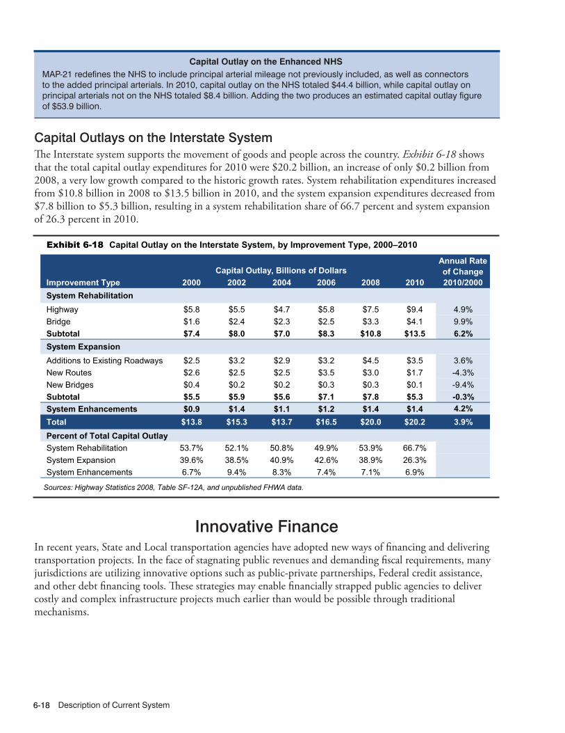
Description of Current System6-18

Capital Outlays on the Interstate SystemThe Interstate system supports the movement of goods and people across the country. Exhibit 6-18 shows that the total capital outlay expenditures for 2010 were $20.2 billion, an increase of only $0.2 billion from 2008, a very low growth compared to the historic growth rates. System rehabilitation expenditures increased from $10.8 billion in 2008 to $13.5 billion in 2010, and the system expansion expenditures decreased from $7.8 billion to $5.3 billion, resulting in a system rehabilitation share of 66.7 percent and system expansion of 26.3 percent in 2010.

9/18/2012 06XH_R (6-18) R1.xlsx

Improvement Type 2000 2002 2004 2006 2008 2010System RehabilitationHighway $5.8 $5.5 $4.7 $5.8 $7.5 $9.4 4.9%Bridge $1.6 $2.4 $2.3 $2.5 $3.3 $4.1 9.9%Subtotal $7.4 $8.0 $7.0 $8.3 $10.8 $13.5 6.2%System ExpansionAdditions to Existing Roadways $2.5 $3.2 $2.9 $3.2 $4.5 $3.5 3.6%New Routes $2.6 $2.5 $2.5 $3.5 $3.0 $1.7 -4.3%New Bridges $0.4 $0.2 $0.2 $0.3 $0.3 $0.1 -9.4%Subtotal $5.5 $5.9 $5.6 $7.1 $7.8 $5.3 -0.3%System Enhancements $0.9 $1.4 $1.1 $1.2 $1.4 $1.4 4.2%Total $13.8 $15.3 $13.7 $16.5 $20.0 $20.2 3.9%Percent of Total Capital OutlaySystem Rehabilitation 53.7% 52.1% 50.8% 49.9% 53.9% 66.7%System Expansion 39.6% 38.5% 40.9% 42.6% 38.9% 26.3%System Enhancements 6.7% 9.4% 8.3% 7.4% 7.1% 6.9%

Capital Outlay, Billions of DollarsAnnual Rate of Change 2010/2000

Exhibit 6-18 Capital Outlay on the Interstate System, by Improvement Type, 2000–2010

Sources: Highway Statistics 2008, Table SF-12A, and unpublished FHWA data.

Capital Outlay on the Enhanced NHSMAP-21 redefines the NHS to include principal arterial mileage not previously included, as well as connectors to the added principal arterials. In 2010, capital outlay on the NHS totaled $44.4 billion, while capital outlay on principal arterials not on the NHS totaled $8.4 billion. Adding the two produces an estimated capital outlay figure of $53.9 billion.

Innovative FinanceIn recent years, State and Local transportation agencies have adopted new ways of financing and delivering transportation projects. In the face of stagnating public revenues and demanding fiscal requirements, many jurisdictions are utilizing innovative options such as public-private partnerships, Federal credit assistance, and other debt financing tools. These strategies may enable financially strapped public agencies to deliver costly and complex infrastructure projects much earlier than would be possible through traditional mechanisms.

Finance 6-19

Public-Private PartnershipsPublic-Private Partnerships (P3s) are contractual agreements formed between a public agency and a private entity that allow for greater private sector participation in the delivery and financing of transportation projects. Typically, this participation involves the private sector taking on additional project risks, such as design, finance, long-term operation, maintenance, or traffic revenue. P3s are undertaken for a variety of purposes, including monetizing the value of existing assets, developing new transportation facilities, or rehabilitating or expanding existing facilities. While P3s may offer certain advantages, such as increased financing capacity and reducing up-front costs, the public sector still must identify a source of revenue for the project to provide a return to the private partner’s investment, and must ensure that the goals and interests of the public are adequately secured.

Additional information on P3s is available at http://www.fhwa.dot.gov/ipd/p3/index.htm.

Public-Private Partnership Project: IH-635 Managed Lanes (LBJ Express)The LBJ Express Project will relieve congestion north of Dallas on 13 miles of IH-635 (LBJ Freeway) from just west of IH-35E to just east of US-75, and south on IH-35E from I-635 to Loop 12. The project will involve:

• Reconstruction of the main lanes and frontage roads along IH-635

• Addition of six managed lanes (mostly subsurface) along IH-635 from IH-35E to US-75 and four managed lanes west and east of that stretch

• Addition of six elevated managed lanes along IH-35E from Loop 12 to the IH-35E/IH-635 interchange.

The project is being built under a public-private partnership (Comprehensive Development Agreement) executed in September 2009 between the Texas Department of Transportation and LBJ Infrastructure Group, which will operate and maintain the facility for 52 years. Construction began in early 2011 and is expected to be complete by December 2015. The total cost of the project is $2.6 billion.

Federal Credit AssistanceFederal credit assistance for highway improvements can take one of two forms: loans, where project sponsors borrow Federal highway funds directly from a State DOT or the Federal government; and credit enhancements, where a State DOT or the Federal government makes Federal funds available on a contingent (or standby) basis. Credit enhancement helps reduce risk to investors and thus allows project sponsors to borrow at lower interest rates. Loans can provide the capital necessary to proceed with a project, and reduce the amount of capital borrowed from other sources, and may also serve a credit enhancement function by reducing the risk borne by other investors. Federal tools currently available to project sponsors include the Transportation Infrastructure and Finance Innovation Act (TIFIA) program, State Infrastructure Bank (SIB) programs, and Section 129 loans.

The TIFIA Credit Program provides Federal credit assistance in the form of direct loans, loan guarantees, and standby lines of credit to finance surface transportation projects of national and regional significance. A TIFIA project must pledge repayment in whole or in part with dedicated revenue sources such as tolls, user fees, special assessments (taxes), or other non-Federal sources. SIBs are State-run revolving funds that provide loans, credit enhancements, and other forms of non-grant assistance to surface transportation projects. SIBs can be capitalized with regularly apportioned Federal-aid funds. Section 129 loans allow States to lend apportioned Federal-aid highway funds to toll and non-toll projects generating dedicated revenue streams.

Additional information on credit assistance tools is available at http://www.fhwa.dot.gov/ipd/finance/tools_programs/federal_credit_assistance/index.htm

Description of Current System6-20

Debt Financing Tool Project: Maine’s Veterans Memorial BridgeMaine’s third Grant Anticipation Revenue Vehicles (GARVEE) sale took place in November 2010 in the amount of $50 million in Taxable Build America Bonds issued by the Maine Municipal Bond Bank. A portion of the proceeds is being used to partially fund the construction of the replacement of the Veterans Memorial Bridge over the Fore River between the Cities of Portland and South Portland. The bridge is nearing 60 years of age and is designed to be a gateway to Maine’s largest city.

Debt Financing ToolsSome transportation projects are so large that their cost exceeds available current grant funding and tax receipts or would consume so much of these current funding sources as to delay many other planned projects. For this reason, State and local governments often look to finance large projects through borrowing, which provides an immediate influx of cash to fund project construction costs. The borrower then retires the debt by making principal and interest payments over time. Tax-exempt municipal bonds, backed by future government revenues, are the most common method of borrowing by government agencies for transportation projects.

Three innovative debt instrument tools—Grant Anticipation Revenue Vehicles (GARVEEs), Private Activity Bonds (PABs), and Build America Bonds (BABs)—provide further borrowing opportunities. A GARVEE is a debt financing instrument—such as a bond, note, certificate, mortgage, lease, or other debt financing technique—that has a pledge of future Federal-aid funding. PABs are debt instruments issued by State or local governments on behalf of a private entity for highway and freight transfer projects, allowing a private project sponsor to benefit from the lower financing costs of tax-exempt municipal bonds. BABs, which were authorized by the American Recovery and Reinvestment Act (Recovery Act), are taxable bonds that are eligible for an interest rate subsidy paid directly from the U.S. Treasury. The Recovery Act allowed States and local governments to issue BABs through December 2010.

Additional information on Federal debt financing tools is available at http://www.fhwa.dot.gov/ipd/finance/tools_programs/federal_debt_financing/index.htm.

Federal Credit Assistance Project – Port of Miami TunnelThe Port of Miami Tunnel will improve access to and from the Port of Miami, serving as a dedicated roadway connector linking the port (located on an island in Biscayne Bay) with the MacArthur Causeway and I-395 on the mainland. Currently, the Port is linked to the mainland only by the Port Bridge. The project includes a tunnel under the Main Channel (the shipping channel between Dodge and Watson Islands), roadway work on Dodge Island and Watson Island/MacArthur Causeway, and widening the MacArthur Causeway Bridge. Twin tubes, each 3,900 feet long and 41 feet in diameter, will reach a depth of 120 feet below the water.

The project is being developed and operated as a public-private partnership with Miami Access Tunnel, LLC (MAT). Under the concession agreement, the Florida DOT will provide MAT with milestone payments during the construction period (2010–2014) and a final acceptance payment upon construction completion in 2014. This will be followed by 30 years of availability payments during the operating period. Deductions will be made from this amount if MAT’s operation of the facility does not meet prescribed performance standards. The State has agreed to pay for approximately 50 percent of the capital costs (design and construction) and all operations and maintenance, while the remaining 50 percent of the capital costs will be provided by Miami-Dade County and the City of Miami.

Financing for this $1.1 billion project includes a $341 million TIFIA loan secured by a pledge of the availability payments due to the concessionaire. The TIFIA loan was executed in October 2009.

Finance 6-21

Transit Finance

Transit funding comes from two major sources: public funds allocated by Federal, State, and local governments, and system-generated revenues earned from the provision of transit services. As shown in Exhibit 6-19, the total amount available for transit financing in 2010 was $54.3 billion. Federal funding for transit includes fuel taxes dedicated to transit from the Mass Transit Account (MTA) of the Highway Trust Fund (HTF), as well as undedicated taxes allocated from Federal general fund appropriations. State and local governments also provide funding for transit from their General Fund appropriations, as well as from fuel, income, sales, property, and other unspecified taxes, specific percentages of which may be dedicated to transit. These percentages vary considerably among taxing jurisdictions and by type of tax. Other public funds from sources such as toll revenues and general transportation funds may also be used to fund transit. System-generated revenues are composed principally of passenger fares, although additional revenues are also earned by transit systems from advertising and concessions, park-and-ride lots, investment income, and rental of excess property and equipment.

10/1/2012 06XT_A (6-19) R1.xlsx

Federal State Local Total PercentPublic Funds 10,364.1 11,788.4 18,021.1 40,173.6 73.9%General Fund 2,072.8 3,041.0 3,955.3 9,069.1 16.7%Fuel Tax 8,291.3 587.0 183.4 9,061.7 16.7%Income Tax 478.7 78.6 557.3 1.0%Sales Tax 3,140.6 4,556.9 7,697.5 14.2%Property Tax 27.4 418.1 445.4 0.8%Other Dedicated Taxes 2,328.0 294.1 2,622.1 4.8%Other Public Funds 2,185.7 8,534.8 10,720.5 19.7%System-Generated Revenue 14,156.2 26.1%Passenger Fares 12,126.3 22.3%Other Revenue 2,029.9 3.7%Total All Sources 54,329.8 100.0%

(Millions of Dollars)

Source: National Transit Database.

Exhibit 6-19 2010 Revenue Sources for Transit Funding

Level and Composition of Transit FundingExhibit 6-20 breaks down the sources of total transit funding. In 2010, public funds of $40.2 billion were available for transit and accounted for 73.9 percent of total transit funding. Of this amount, Federal funding was $10.4 billion, accounting for 25.8 percent of total public funding and for 19.1 percent of all funding from both public and nonpublic sources. State funding was $11.8 billion, accounting for 29.3 percent of total public funds and 21.7 percent of all funding. Local jurisdictions provided the bulk of transit funds, $18 billion in 2010, or 44.9 percent of total public funds and 33.2 percent of all funding. System-generated revenues were $14.2 billion, 26.1 percent of all funding. During the Recovery Act years of 2009, 2010, and 2011, transit agencies reported annual

9/25/2012 06XT_B (6-20) R1.xlsx

Federal $10.4 19%

State $11.8 22% Local

$18.1 33%

System-Generated Revenue

$14.2 26%

Exhibit 6-20 2010 Public Transit Revenue Sources (Billions of Dollars)

Source: National Transit Database.

Description of Current System6-22

Q A&What type of dedicated funding does public transit receive from Federal highway-user fees?

In 1983, the MTA was established within the HTF. It is funded by 2.86 cents of Federal highway-user fees on gasohol, diesel and kerosene fuel, and other special fuels (benzol, benzene, and naphtha). Since 1997, the Federal fuel tax on a gallon of gasoline has been 18.4 cents and the tax on a gallon of diesel has been 24.4 cents.

The MTA also receives 2.13 cents of the user fee on liquefied petroleum gas (LPG) and 1.86 cents of the user fee on liquefied natural gas (LNG). The MTA does not receive any of the nonfuel revenues (such as heavy vehicle use taxes) that accrue to the HTF.

Since the passage of the Safe, Accountable, Flexible, Efficient Transportation Equity Act: A Legacy for Users (SAFETEA-LU), only the Formula and Bus Grants Program is funded from the MTA. Prior to SAFETEA-LU, MTA funded other FTA programs.

expenditures averaging $17.0 billion. The infusion of $5.3 billion in Recovery Act funds during that period allowed the industry to maintain investment levels near the record 2008 funding level of $17.1 billion.

Federal FundingFederal funding for transit comes from two sources: the general revenues of the U.S. government and revenues generated from fuel taxes credited to the HTF’s MTA. General revenue sources include income taxes, corporate taxes, tariffs, fees, and other government income not required by statute to be accounted for in a separate fund. The MTA, a trust fund for capital projects in transit, is generally the largest source of Federal funding for transit, though it was overtaken by American Recovery and Reinvestment Act (Recovery Act) funds from the general account in 2009. Exhibit 6-22 shows how Recovery Act funds were awarded in 2009, 2010, and 2011 in comparison to other Federal funding that comes from both the MTA

Q A&How long has it been since excise tax revenue deposited into the MTA exceeded expenditures?

The last time that annual net receipts credited to the MTA of the HTF exceeded annual expenditures from the Highway Account was in 2007. As shown in Exhibit 6-21, for 10 of the 12 years since 2000, total annual receipts to the MTA from excise taxes and other income (including amounts transferred from the Highway Account) have been lower than the annual expenditures from the MTA.

0.0

1.0

2.0

3.0

4.0

5.0

6.0

7.0

8.0

2000 2002 2004 2006 2008 2010

Bill

ions

of D

olla

rs

Mass Transit Account Outlays

Mass Transit Account Receipts (ExcludingGeneral Fund Transfers)

Sources: Highway Statistics, various years, Tables FE-210 and FE-10.

Exhibit 6-21 Mass Transit Account Receipts and Outlays, Fiscal Years 2000–2011

12/17/2013 06XT_V (6-21) R1.xlsx

Finance 6-23

and the General Fund. Of the funds authorized for transit grants in FTA’s 2010 budget, 79.0 percent were derived from the MTA. Funding from the MTA in nominal dollars increased from $0.5 billion in 1983 to $8.3 billion in 2010.

The Department of Homeland Security (DHS) provides funding for projects aimed at improving transit security. In 2010, DHS provided a total of $253 million to transit service providers.

Since 1973, Federal surface transportation authorization statutes have contained flexible funding provisions that enable transfers from certain highway funds to transit programs and vice versa. Transfers are subject to State and regional/local discretion, and priorities are established through statewide transportation planning processes. All States within the United States participate in the flexible funding program except Arkansas, Delaware, Hawaii, Nebraska, North Dakota, South Dakota, and Wyoming. U.S. territories, including American Samoa, Guam, North Mariana Islands, Puerto Rico, and the Virgin Islands do not participate. Flexible funding transferred from highways to transit fluctuates from year to year and is drawn from several different sources.

The Surface Transportation Program is also the source of Federal Highway Administration (FHWA) funds that are “flexed” to FTA to pay for transit projects. Funding is at 80 percent of Federal share and may be used for all capital and maintenance projects eligible for funds under current Federal Transit Administration

Q A&What are Flex Funds?

In FY 2008, $1.4 billion in flexible funds/transfers from Federal highway programs were available to FTA for obligation. Of that total, $957.3 million (67.0 percent) was transferred in FY 2008; the remaining available $472.5 million (33.0 percent) was the un-obligated carryover or recovery of prior year transfers. Thirty-nine states transferred flexible funds during FY 2008 and obligations totaled $1.1 billion. Once transferred, these funds take on the characteristics of the program in which they are received and are included in the figures reported across various programs. Obligations in FY 2008 were:

• Urbanized Area Formula: $938.6 million (87.4 percent);

• Capital: $45.6 million (4.2 percent);

• Elderly and Persons with Disabilities: $67.8 million (6.3 percent); and

• Non-urbanized Area Formula: $21.9 million (2.0 percent).

Since the program’s initiation in FY 1992, a total of $15.0 billion has been transferred from FHWA for transit projects. FHWA funds can be used for transit projects without being “flexed” to FTA, so this number may understate the total use of highway funds for transit projects.

$0

$2

$4

$6

$8

$10

$12

$14

FY06 FY07 FY08 FY09 FY10 FY11 FY12

FTA

Fun

ding

(Bill

ions

of D

olla

rs) Amount Awarded (Non-Recovery Act) Amount Awarded (Recovery Act)

Source: Federal Transit Administration, Grants Data.

Exhibit 6-22 Recovery Act Funding Awards Compared to Other FTA Fund Awards

12/17/2013 06XT_U (6-22) R2.xlsx

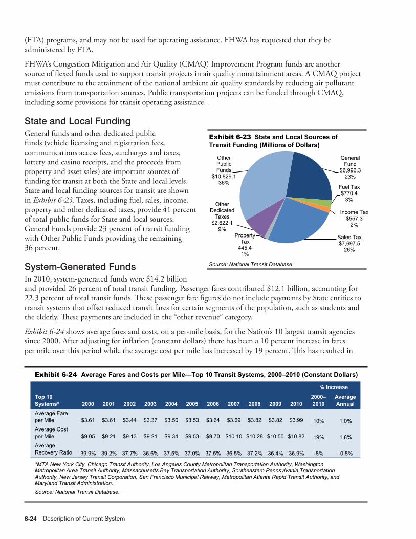
Description of Current System6-24

General Fund

$6,996.3 23%

Fuel Tax $770.4

3%

Income Tax $557.3

2%

Sales Tax $7,697.5

26%

Property Tax

445.4 1%

Other Dedicated

Taxes $2,622.1

9%

Other Public Funds

$10,829.1 36%

Exhibit 6-23 State and Local Sources of Transit Funding (Millions of Dollars)

Source: National Transit Database.

12/17/2013 06XT_C (6-23) R3.xlsx

(FTA) programs, and may not be used for operating assistance. FHWA has requested that they be administered by FTA.

FHWA’s Congestion Mitigation and Air Quality (CMAQ) Improvement Program funds are another source of flexed funds used to support transit projects in air quality nonattainment areas. A CMAQ project must contribute to the attainment of the national ambient air quality standards by reducing air pollutant emissions from transportation sources. Public transportation projects can be funded through CMAQ, including some provisions for transit operating assistance.

State and Local FundingGeneral funds and other dedicated public funds (vehicle licensing and registration fees, communications access fees, surcharges and taxes, lottery and casino receipts, and the proceeds from property and asset sales) are important sources of funding for transit at both the State and local levels. State and local funding sources for transit are shown in Exhibit 6-23. Taxes, including fuel, sales, income, property and other dedicated taxes, provide 41 percent of total public funds for State and local sources. General Funds provide 23 percent of transit funding with Other Public Funds providing the remaining 36 percent.

System-Generated FundsIn 2010, system-generated funds were $14.2 billion and provided 26 percent of total transit funding. Passenger fares contributed $12.1 billion, accounting for 22.3 percent of total transit funds. These passenger fare figures do not include payments by State entities to transit systems that offset reduced transit fares for certain segments of the population, such as students and the elderly. These payments are included in the “other revenue” category.

Exhibit 6-24 shows average fares and costs, on a per-mile basis, for the Nation’s 10 largest transit agencies since 2000. After adjusting for inflation (constant dollars) there has been a 10 percent increase in fares per mile over this period while the average cost per mile has increased by 19 percent. This has resulted in

12/17/2013 06XT_D (6-24) R3.xlsx

Top 10 Systems* 2000 2001 2002 2003 2004 2005 2006 2007 2008 2009 2010

2000–2010

Average Annual

Average Fare per Mile $3.61 $3.61 $3.44 $3.37 $3.50 $3.53 $3.64 $3.69 $3.82 $3.82 $3.99 10% 1.0%Average Cost per Mile $9.05 $9.21 $9.13 $9.21 $9.34 $9.53 $9.70 $10.10 $10.28 $10.50 $10.82 19% 1.8%Average Recovery Ratio 39.9% 39.2% 37.7% 36.6% 37.5% 37.0% 37.5% 36.5% 37.2% 36.4% 36.9% -8% -0.8%

% Increase

*MTA New York City, Chicago Transit Authority, Los Angeles County Metropolitan Transportation Authority, Washington Metropolitan Area Transit Authority, Massachusetts Bay Transportation Authority, Southeastern Pennsylvania Transportation Authority, New Jersey Transit Corporation, San Francisco Municipal Railway, Metropolitan Atlanta Rapid Transit Authority, and Maryland Transit Administration. Source: National Transit Database.

Exhibit 6-24 Average Fares and Costs per Mile—Top 10 Transit Systems, 2000–2010 (Constant Dollars)

Finance 6-25

an 8.0 percent decrease in the “fare recovery ratio,” which is the percentage of operating costs covered by passenger fares. The 2010 fare recovery ratio for these ten agencies was 36.9 percent. Because these are all rail agencies, and rail systems tend to have lower operating costs per passenger mile, this is a higher fare recovery ratio than would be found for most bus or demand response operations. In many cases, municipalities operating these systems have determined that it is more cost effective for them to provide free service as fare collection is expensive and fares for these operations are generally kept low.

Trends in FundingBetween 2000 and 2010, public funding for transit increased at an average annual rate of 4.3 percent, Federal funding increased at an average annual rate of 4.4 percent, and State and local funding grew at an average annual rate of 4.3 percent after adjusting for inflation (constant dollars). These data are presented in Exhibit 6-25.

Federal funding for transit, as a percentage of total funding for transit from Federal, State, and local sources combined, reached a peak of 42.9 percent in the late 1970s, and declined to near its present value by the early 1990s as State and local funding increased. Exhibit 6-25 shows that, since 2000, the Federal government has provided between 16.9 and 19.5 percent of total funding for transit (including system-generated funds); in 2010, it provided 19.1 percent of these funds.

Funding in Current and Constant DollarsPublic funding for transit in current and constant dollar terms since 1990 is presented in Exhibit 6-26. Total public funding for transit was $40.2 billion in 2010. After adjusting for inflation (constant dollars), this was 2.2 percent higher than in 2008. Between 2008 and 2010 Federal funding increased from nearly $9.0 billion to $10.4 billion (15.3 percent) in current dollars. In constant dollars this represents a 13.9 percent increase. From 2008 to 2010, in current dollars, State and local funding stayed the same at $29.8 billion. In constant dollars this represents a 1.4 percent decrease in funding.

$10.36

$29.68

$14.29

Federal Share, 19.1%

0.0%

2.0%

4.0%

6.0%

8.0%

10.0%

12.0%

14.0%

16.0%

18.0%

20.0%

$0

$10

$20

$30

$40

$50

$60

$70

$80

2000 2001 2002 2003 2004 2005 2006 2007 2008 2009 2010

Fede

ral S

hare

of F

undi

ng

Bill

ions

of C

onst

ant 2

010

Dol

lars

Federal State and Local System-Generated Federal Share

Exhibit 6-25 Funding for Transit by Government Jurisdiction, 2000–2010

Source: National Transit Database.

12/17/2013 06XT_E (6-25) R3.xlsx

Description of Current System6-26

10

15

20

25

30

35

40

45

1990 1992 1994 1996 1998 2000 2002 2004 2006 2008 2010

Bill

ions

of D

olla

rs

Total Current Dollars Total Constant 2010 Dollars

Source: National Transit Database.

Exhibit 6-26 Current and Constant Dollar Funding for Public Transportation (All Sources)

06XT_F (6-26) R3.xlsx 12/17/2013

While Federal funds directed to capital expenditures have increased 4.8 percent from 2000 to 2010, funds applied to operating expenditures have increased 13.7 percent during the same period (current dollars). As indicated in Exhibit 6-27, $3.6 billion was applied to operating expenditures and $6.8 billion was applied to capital expenditures in 2010. More than half of the operating expenditures were for preventive maintenance, which is reimbursed as a capital expense under FTA’s 5307 grant program.

$4.3 $5.5 $5.0 $5.1 $4.9 $4.6

$5.6 $5.6 $6.4 $7.1 $6.8

$1.0 $1.4

$1.6 $1.8 $1.3 $1.6 $2.0

$1.0

$1.1 $1.3 $1.6 $1.0 $0.8

$0.9 $0.8 $1.3

$1.5 $1.6

$0

$2

$4

$6

$8

$10

$12

2000 2001 2002 2003 2004 2005 2006 2007 2008 2009 2010

Bill

ions

of C

urre

nt D

olla

rs

Year

Capital Expenditures Operating Expenditures – 5307 Preventive Maintenance Operating Expenditures – All Others

Average Annual Growth Rate,

2000–2010

Capital Funds 4.8%

Total Operating Funds

13.7%

Source: National Transit Database.

Exhibit 6-27 Applications of Federal Funds for Transit Operating and Capital Expenditures, 2000–2010

12/17/2013 06XT_G (6-27) R5.xlsx

Capital Funding and ExpendituresFunding for capital investments by transit operators in the United States comes primarily from public sources. A relatively small amount of private sector funds for capital investment in transit projects are generated through innovative finance programs.

Capital investments include the design and construction of new transit systems, extensions of existing systems (“New Starts”), and the modernization or replacement of existing assets. Capital investment expenditures can be for the acquisition, renovation, and repair of rolling stock (i.e., buses, railcars, locomotives, and service vehicles) or fixed assets (which include fixed guideway systems, terminals, and stations, as well as maintenance and administrative facilities).

Finance 6-27

As shown in Exhibit 6-28, in 2010, total public transit agency expenditures for capital investment were $16.6 billion. This accounted for 41.3 percent of total available funds. Federal funds were $4.4 billion in 2010, 26.6 percent of total transit agency capital expenditures. State funds provided 14.2 percent and local funds provided 44.6 percent of total transit funding. Recovery Act funds provided the remaining 14.5 percent of revenues for agency capital expenditures.

Substantial amounts of Recovery Act funding were made available in 2009 and 2010, years in which use of non-Recovery Act Federal funds for capital investment went down. Total Federal expenditures were only slightly higher than in previous years, so it appears that Recovery Act funds displaced regular FTA grant funds in 2009 and 2010. This is not surprising given the strict 2-year obligation limit specified for Recovery Act funds. They would have to be used first due to their shorter availability period. As transit agencies have limited staff to process grants, and limited “shovel-ready” projects available for funding, expenditure of non-Recovery Act FTA grant funds was delayed so Recovery Act funds could be processed quickly.

$4.3 $5.5 $5.0 $5.1 $4.9 $4.6 $5.6 $5.6 $6.4 $6.0

$4.4

$1.1 $2.4

$1.0 $1.0 $1.4 $1.6 $1.8 $1.5

$1.7 $1.5 $2.0

$2.4 $2.4 $3.8

$4.3 $5.9 $6.1 $5.9

$5.7 $5.5 $6.5

$7.7 $7.3 $7.4

$0

$2

$4

$6

$8

$10

$12

$14

$16

$18

$20

2000 2001 2002 2003 2004 2005 2006 2007 2008 2009 2010

Bill

ions

of D

olla

rs

LocalStateRecovery ActFederal

Federal Funds

9.2%

0.3%

State Funds

6.8% Local Funds

6.2% Total

Average Annual Growth Rate,

2000–2010 Constant 2010 Dollars

Source: National Transit Database.

Exhibit 6-28 Sources of Funds (Billions of Dollars) for Transit Capital Expenditures, 2000–2010

12/17/2013 06XT_H (6-28) R3.xlsx

As shown in Exhibit 6-29, rail modes require a higher percentage of total transit capital investment than bus modes because of the higher cost of building fixed guideways and rail stations, and because bus systems typically do not pay to build or maintain the roads on which they run. In 2010, $11.9 billion, or 72 percent of total transit capital expenditures, were invested in rail modes of transportation, compared with $4.6 billion, or 28 percent of the total, which was invested in nonrail modes. This investment distribution has been consistent over the last decade.

Fluctuations in the levels of capital investment in different types of transit assets reflect normal rehabilitation and replacement cycles, as well as new investment. Capital investment expenditures have only been reported to the National Transit Database (NTD) at the level of detail in Exhibit 6-29 since 2002.

Total guideway investment was $6.2 billion in 2010, and total investment in systems was $1.1 billion. Guideway includes at-grade rail, elevated and subway structures, tunnels, bridges, track and power systems for all rail modes, and paved highway lanes dedicated to buses. Investment in systems by transit operators includes groups of devices or objects forming a network, most notably for train control, signaling, and communications.

Description of Current System6-28

Total investment in rolling stock in 2010 was $4.3 billion, total investment in stations was $2.8 billion, and total investment in maintenance facilities was $0.9 billion. Rolling stock includes the bodies and chassis of transit vehicles and their attached fixtures and appliances, but does not include fare collection equipment and revenue vehicle movement control equipment such as radios. Stations include station buildings, platforms, shelters, parking and other forms of access, and crime prevention and security equipment at stations. Facilities include the purchase, construction, and rehabilitation of administrative and maintenance

12/17/2013 06XT_I (6-29) R3.xlsx

TypeCommuter

RailHeavy Rail

Light Rail

Other Rail1

Guideway $1,812 $2,005 $2,273 $5.5 $6,096Rolling Stock $403 $877 $327 $3.4 $1,611Systems $118 $591 $139 $7.7 $855Maintenance Facilities $159 $84 $92 $1.2 $337Stations $427 $1,572 $341 $1.7 $2,342Fare Revenue Collection Equipment $14 $41 $27 $0 $82Administrative Buildings $5 $30 $7.9 $0.3 $43Other Vehicles $14 $28 $6.1 $0.1 $49Other Capital Expenditures2 $74 $419 $21 $0.6 $514Total $3,026 $5,646 $3,234 $20 $11,927Percent of Total 18.3% 34.1% 19.5% 0.1% 72.0%

TypeFixed Route

BusDemand

Response Ferryboat VanpoolGuideway $136 $0 $0 $0 $136Rolling Stock $2,374 $222 $128 $12 $2,736Systems $239 $22 $0.20 $0.07 $261Maintenance Facilities $534 $26 $9.8 $0.01 $569Stations $379 $0.9 $45.2 $0.01 $425Fare Revenue Collection Equipment $88 $3.9 $0.24 $0 $92Administrative Buildings $184 $14 $7.2 $0.16 $206Other Vehicles $35 $1.2 $0 $0.02 $36Other Capital Expenditures2 $156 $7.0 $11.9 $0.32 $176Total $4,125 $297 $203 $12 $4,637Percent of Total 24.9% 1.8% 1.2% 0.1% 28.0%

TypeGuideway 37.6%Rolling Stock 26.2%Systems 6.7%Maintenance Facilities 5.5%Stations 16.7%Fare Revenue Collection Equipment 1.1%Administrative Buildings 1.5%Other Vehicles 0.5%Other Capital Expenditures2 4.2%Total 100.0%

Total Nonrail

Total Rail

Rail Capital Expenditures, Millions of Dollars

Nonrail Capital Expenditures, Millions of Dollars

$174

Percent of Total

$249$85

$689$16,564

Total Expenditures, Millions of Dollars for Rail and

Nonrail Modes$6,232$4,347$1,117

$906$2,766

Exhibit 6-29 2010 Transit Capital Expenditures by Mode and Type

1 Alaska railroad, automated guideway, cable car, inclined plane, and monorail. 2 Capital expenditures not elsewhere included. These expenditures include furniture and equipment that are not an integral part of buildings and structures; they also include shelters, signs, and passenger amenities (e.g., benches) not in passenger stations. Note: Fixed Route Bus includes Motor Bus and Trolleybus. Source: National Transit Database.

Finance 6-29

$1.0 $1.1 $1.3 $1.6 $2.0 $2.2 $2.5 $2.5 $2.6 $3.1 $3.6

$4.4 $5.1

$6.1 $6.0 $6.0 $6.7 $6.9

$7.9 $9.4 $9.5 $9.4

$6.5 $7.1

$6.9 $7.4 $7.9

$8.4 $8.9

$10.5 $10.8 $10.9 $10.6

$9.8 $10.1 $9.9

$10.4 $10.9

$11.5 $12.3

$12.7

$13.7 $14.0 $14.2

0%

5%

10%

15%

20%

25%

30%

35%

40%

45%

50%

$0

$5

$10

$15

$20

$25

$30

$35

$40

2000 2001 2002 2003 2004 2005 2006 2007 2008 2009 2010

Bill

ions

of C

urre

nt D

olla

rs

Year

Local Funds

State Funds

Federal Funds

System- Generated

Funds

Average Annual Growth Rate,

2000–2010

5.7%

5.0%

8.0%

13.7%

3.7%

Total

Recovery Ratio= System-Generated Funds / Total (right axis)

Exhibit 6-30 Sources of Funds for Transit Operating Expenditures, 2000–2010

Source: National Transit Database.

12/17/2013 06XT_J (6-30) R3.xlsx

Q A&What are “New Starts?”

FTA provides dedicated funding for the construction of new fixed guideway systems through a competitive program known as “New Starts”. Title 49 USC Section 5309 provides for the allocation of funds for the design and construction of new transit systems and extensions to current systems (“New Starts”), among other purposes. To receive FTA capital investment funds for a New Starts project, the proposed project must emerge from the metropolitan and/or statewide planning process. A rigorous series of planning and project development requirements must be completed in order for a project to qualify for this funding. FTA evaluates proposed projects on the basis of financial criteria and project justification criteria as prescribed by statute. Initial planning efforts are not funded through the Section 5309 program, but may be funded through Section 5303, Metropolitan Planning; Section 5339, Alternatives Analysis; or Section 5307, Urbanized Area Formula Grants programs.

Under current law, Federal funding may account for up to 80 percent of a New Starts funding requirement. Generally, the Federal share of such projects now averages about 50 percent of the total project cost. However, not all new fixed guideway projects are constructed through the New Starts Program.

facilities. Facilities also include investment in building structures, climate control, parking, yard track, vehicle and facilities maintenance equipment, furniture, office equipment, and computer systems.

Other capital includes capital costs associated with general administration facilities, furniture, equipment that is not an integral part of buildings and structures, data processing equipment (including computers and peripheral devices whose sole use is in data processing operations), and shelters located at on-street bus stops.

Operating ExpendituresTransit operating expenditures include wages, salaries, fuel, spare parts, preventive maintenance, support services, and certain leases used in providing transit service. As indicated in Exhibit 6-30, $37.8 billion

Description of Current System6-30

was available for operating expenses in 2010, the Federal share of which has increased from the 2008 level of 7.1 percent to 9.4 percent. The share generated from system revenues remained relatively stable from 37.6 percent in 2008 to 37.5 percent in 2010. The State share decreased slightly from 25.8 percent in 2008 to 24.9 percent in 2010. The local share of operating expenditures decreased slightly from 29.5 percent in 2008 to 28.2 percent in 2010.

12/17/2013 06XT_K (6-31) R3.xlsx

Heavy Commuter Light DemandYear Motor Bus Rail Rail Rail Response Other Total2000 $11,026 $3,931 $2,679 $592 $1,225 $549 $20,0032001 $11,814 $4,180 $2,854 $676 $1,410 $595 $21,5292002 $12,586 $4,267 $2,995 $778 $1,636 $643 $22,9052003 $13,316 $4,446 $3,173 $754 $1,779 $718 $24,1852004 $13,790 $4,734 $3,436 $826 $1,902 $739 $25,4272005 $14,666 $5,145 $3,657 $978 $2,071 $721 $27,2382006 $15,796 $5,287 $3,765 $1,070 $2,286 $820 $29,0252007 $16,812 $5,888 $4,001 $1,163 $2,539 $901 $31,3042008 $17,963 $6,129 $4,294 $1,259 $2,861 $975 $33,4792009 $18,313 $6,311 $4,538 $1,393 $3,053 $1,030 $34,6382010 $18,399 $6,370 $4,595 $1,499 $3,171 $1,037 $35,071

2000 55.1% 19.7% 13.4% 3.0% 6.1% 2.7% 100.0%2010 52.5% 18.2% 13.1% 4.3% 9.0% 3.0% 100.0%

Percent of Total

Expenditures, Millions of Current Dollars

Exhibit 6-31 Transit Operating Expenditures by Mode, 2000–2010

Source: National Transit Database.

Q A&What happens after the census?

TEA-21 mandated that Federal funding to transit systems in urbanized areas with populations over 200,000 be used only for capital expenses and preventive maintenance, and not for operating expenses. Formula grant funds to urbanized areas with populations of less than 200,000 were still allowed to be used for operating expenses. As a result of the 2000 census, 56 areas were reclassified as urbanized areas with populations of more than 200,000. (These reclassifications were announced by the Census Department in May 2002.) Transit agencies operating in these areas were slated to lose their eligibility to use Federal formula funding to finance transit operations starting in FY 2003. The Transit Operating Flexibility Act of 2002 amended Section 5307 of 49 USC to allow transit systems that were in these areas to continue to use their formula funds for operating expenses as well as for capital expenses in FY 2003, despite their change in status. This change was extended by the Surface Transportation Extension Act of 2003. Under SAFETEA-LU these transit agencies may continue to use formula funds for operating expenses in FY 2005 at 100 percent of their FY 2002 apportionment, in FY 2006 at 50 percent of their FY 2002 apportionment, and in FY 2007 at 25 percent of their FY 2002 apportionment. The impact of the 2010 census did not take place until the 2013 apportionment. Legislative responses to these reclassifications have not yet been considered.

Operating Expenditures by Transit ModeAs shown in Exhibit 6-31, total transit operating expenditures were $35.1 billion in 2010. These expenditures increased at an average annual rate of 5.8 percent between 2000 and 2010 (in current-year dollars). Light rail and demand response modes have experienced the largest percentage increase in operating expenditures during this period. This is due to relatively greater investment in new light rail and demand response capacity over the past 10 years.

Finance 6-31

Operating Expenditures by Type of CostIn 2010, $18.6 billion—or 53.1 percent of total transit operating expenditures—went toward vehicle operations. Smaller amounts were expended on maintenance and administration; these expenses, which have virtually been the same for the last several years, are broken down across cost categories in Exhibit 6-32.

12/17/2013 06XT_L (6-32) R3.xlsx

ModeMotor Bus $10,788 $3,717 $773 $3,121 $18,399Heavy Rail $2,789 $1,113 $1,577 $890 $6,370Commuter Rail $1,860 $1,161 $822 $752 $4,595Light Rail $612 $308 $262 $317 $1,499Demand Response $2,016 $409 $85 $661 $3,171Other $561 $170 $80 $226 $1,037Total $18,625 $6,878 $3,600 $5,968 $35,071Percent of All Modes 53.1% 19.6% 10.3% 17.0% 100.0%

Total

Distribution of Expenditures, Millions of DollarsVehicle

OperationsVehicle

MaintenanceNonvehicle

MaintenanceGeneral

Administration

Exhibit 6-32 Operating Expenditures by Mode and Type of Cost, 2010

Source: National Transit Database.

Exhibits 6-33 and 6-34 illustrate how road and rail operations have inherently different cost structures because, in most cases, roads are not paid for by the transit provider, but tracks are. A significantly higher percentage of expenditures for rail modes of transportation are classified as nonvehicle maintenance, corresponding to the repair and maintenance costs of fixed guideway systems.

Vehicle Operations $5,261.1

42%

Vehicle Mainten-

ance $2,581.7

21%

Nonvehicle Mainten-

ance $2,661.6

21%

General Administra-

tion $1,959.3

16%

Source: National Transit Database.

Exhibit 6-33 Rail Operating Expenditures by Type of Cost, Millions of Dollars

12/17/2013 06XT_M (6-33) R3.xlsx

Vehicle Operations $13,364.1

59%

Vehicle Maintenance

$4,296.3 19%

Nonvehicle Maintenance

$938.4 4%

General Administra-

tion $4,008.9

18%

Exhibit 6-34 2010 Nonrail Operating Expenditures by Type of Cost, Millions of Dollars

Source: National Transit Database.

12/17/2013 06XT_N (6-34) R3.xlsx

Operating Expenditures per Vehicle Revenue Mile Operating expenditures per vehicle revenue mile (VRM) is one measure of financial or cost efficiency. It shows the expense of operating a transit vehicle in revenue service. As shown in Exhibit 6-35, operating expenditures per VRM for all transit modes combined was $8.95 in 2010; the average annual increase in operating expenditures per VRM for all modes combined between 2000 and 2010 was 1.3 percent in constant dollars.

As shown in Exhibit 6-36, analysis of NTD reports for urbanized areas with greater than 1 million in population shows that the growth in operating expenses is led by the cost of fringe benefits, which have

Description of Current System6-32

12/17/2013 06XT_O (6-35) R3.xlsx

Motor Heavy Commuter Light DemandYear Bus1 Rail Rail Rail Response Other2 Total2000 $7.84 $8.52 $13.55 $14.43 $3.40 $6.33 $7.832001 $7.94 $8.66 $13.81 $15.58 $3.52 $6.62 $7.942002 $8.13 $8.52 $13.92 $15.64 $3.75 $6.73 $8.052003 $8.36 $8.58 $14.30 $14.46 $3.86 $7.52 $8.212004 $8.43 $8.73 $14.72 $14.27 $3.90 $5.99 $8.252005 $8.68 $9.14 $14.72 $16.06 $3.90 $5.20 $8.432006 $8.92 $8.99 $14.15 $15.81 $4.07 $5.53 $7.882007 $9.12 $9.66 $14.12 $14.79 $4.12 $5.41 $8.702008 $9.40 $9.57 $14.22 $14.92 $4.26 $5.01 $8.802009 $9.39 $9.55 $14.67 $15.82 $4.26 $4.58 $8.772010 $9.60 $9.84 $14.60 $16.36 $4.42 $4.49 $8.95

2010/2000 2.0% 1.4% 0.8% 1.3% 2.7% -3.4% 1.3%Average Annual Rate of Change

1 Note that annual changes in operating expense per capacity-equivalent VRM and unadjusted motor bus operating expenditures are consistent with those shown in Exhibit 6-31. 2 Automated guideway, Alaska railroad, cable car, ferryboat, inclined plane, monorail, Público, trolleybus, and vanpool. Source: National Transit Database.

Exhibit 6-35 Operating Expenditures per Vehicle Revenue Mile, 2000–2010 (Constant Dollars)

been going up at a rate of 3.8 percent per year above inflation (constant dollars) since 2000. By comparison, average salaries at these 10 agencies grew at an inflation-adjusted rate of only 0.4 percent per year in that period. FTA does not collect data on the different components of fringe benefits, but increases in the cost of medical insurance drive growth rates in fringe benefits across the economy and likely drive the growth in this category.

12/17/2013 06XT_P (6-36) R3.xlsx

Cost Component 2000 2001 2002 2003 2004 2005 2006 2007 2008 2009 2010

2000–2010

Average Annual

Salaries $3.49 $3.48 $3.58 $3.62 $3.56 $3.51 $3.56 $3.58 $3.61 $3.62 $3.63 4% 0.4%Fringe Benefits $2.12 $2.17 $2.31 $2.49 $2.62 $2.69 $2.69 $2.85 $2.81 $2.93 $3.07 45% 3.8%Labor Cost $5.61 $5.65 $5.89 $6.11 $6.18 $6.20 $6.25 $6.44 $6.42 $6.55 $6.69 19% 1.8%

Total $11.21 $11.29 $11.78 $12.21 $12.36 $12.41 $12.50 $12.88 $12.84 $13.10 $13.39 19% 1.8%

Average Cost per Mile, Constant Dollars % Increase

*MTA New York City, Chicago Transit Authority, Los Angeles County Metropolitan Transportation Authority, Washington Metropolitan Area Transit Authority, Massachusetts Bay Transportation Authority, Southeastern Pennsylvania Transportation Authority, New Jersey Transit Corporation, San Francisco Municipal Railway, Metropolitan Atlanta Rapid Transit Authority, and Maryland Transit Administration. Source: National Transit Database.

Exhibit 6-36 Growth in Operating Costs—UZAs over 1 million*, 2000–2010

Operating expenditures per capacity-equivalent VRM is a better measure of comparing cost efficiency among modes than operating expenditures per VRM because it adjusts for passenger-carrying capacities. As demonstrated by the data in Exhibit 6-37, rail systems are more cost efficient in providing service than nonrail systems, once investment in rail infrastructure has been completed. Based on operating costs alone, heavy rail is the most efficient at providing transit service, and demand response systems are the least efficient. Annual changes in operating expense per capacity-equivalent VRM are not comparable across modes because average capacities for all vehicle types are adjusted separately each year based on reported fleet averages.

Finance 6-33

12/17/2013 06XT_Q (6-37) R3.xlsx

Year2000 $7.84 $3.61 $5.81 $5.73 $18.86 $9.66 $6.462001 $7.94 $3.67 $5.93 $6.18 $19.56 $10.45 $6.422002 $8.13 $3.61 $5.98 $6.21 $20.85 $10.16 $6.402003 $8.36 $3.46 $5.61 $5.38 $21.43 $11.30 $6.482004 $8.43 $3.52 $5.78 $5.31 $22.95 $10.48 $6.542005 $8.68 $3.68 $4.80 $5.83 $23.51 $9.66 $6.702006 $8.92 $3.62 $4.62 $5.74 $24.49 $10.69 $6.792007 $9.12 $3.91 $4.64 $5.44 $24.59 $10.49 $6.762008 $9.40 $3.87 $4.67 $5.49 $25.39 $13.22 $6.932009 $9.39 $4.54 $5.33 $6.32 $25.80 $11.47 $7.502010 $9.60 $3.98 $5.34 $5.95 $25.48 $11.16 $7.24

2010/2000 2.0% 1.0% -0.8% 0.4% 3.1% 1.5% 1.1%

Other Total

Compound Annual Growth Rate

Motor Bus

Heavy Rail

Commuter Rail

Light Rail

Demand Response

Source: National Transit Database.

Exhibit 6-37 Operating Expenditures per Capacity-Equivalent Vehicle Revenue Mile by Mode, 2000–2010 (Constant Dollars)

Operating Expenditures per Passenger MileOperating expense per passenger mile is an indicator of the cost effectiveness of providing a transit service. It shows the relationship between service inputs as expressed by operating expenses and service consumption as expressed by passenger miles traveled. Operating expenditures per passenger mile for all transit modes combined increased at an average annual rate of 1.8 percent between 2000 and 2010 (from $0.56 to $0.67). These data are shown in Exhibit 6-38.

12/17/2013 06XT_R (6-38) R3.xlsx

2000 $0.73 $0.36 $0.36 $0.55 $2.61 $0.61 $0.562001 $0.74 $0.36 $0.37 $0.58 $2.76 $0.63 $0.572002 $0.78 $0.38 $0.38 $0.65 $3.03 $0.66 $0.602003 $0.81 $0.39 $0.39 $0.65 $3.05 $0.66 $0.632004 $0.84 $0.38 $0.40 $0.64 $3.11 $0.61 $0.632005 $0.84 $0.40 $0.43 $0.64 $3.13 $0.59 $0.642006 $0.84 $0.39 $0.39 $0.62 $3.27 $0.62 $0.632007 $0.86 $0.38 $0.38 $0.63 $3.42 $0.63 $0.632008 $0.87 $0.37 $0.40 $0.62 $3.47 $0.58 $0.642009 $0.88 $0.38 $0.41 $0.64 $3.50 $0.58 $0.652010 $0.89 $0.39 $0.43 $0.69 $3.63 $0.57 $0.67

2.0% 0.9% 1.8% 2.2% 3.3% -0.8% 1.8%

Year

Compounded Annual Growth Rate2010/2000

Motor Bus

Demand Response

Light Rail

Commuter Rail

Heavy Rail Other* Total

Exhibit 6-38 Operating Expenditures per Passenger Mile, 2000–2010 (Constant Dollars)

* Automated guideway, cable car, ferryboat, inclined plane, jitney, monorail, Público, trolleybus, aerial tramway, and vanpool. Source: National Transit Database.

Farebox Recovery RatiosThe farebox recovery ratio represents farebox revenues as a percentage of total transit operating costs. It measures users’ contributions to the variable cost of providing transit services and is influenced by the number of riders, fare structure, and rider profile. Low regular fares, the high availability and use of

Description of Current System6-34

discounted fares, and high transfer rates tend to result in lower farebox recovery ratios. Farebox recovery ratios for 2004 to 2010 are provided in Exhibit 6-39. The average farebox recovery ratio over this period for all transit modes combined was 34.6 percent; heavy rail had the highest average farebox recovery ratio at 59.9 percent. Farebox recovery ratios for total costs are not provided because capital investment costs are not spread evenly across years. Rail modes have farebox recovery ratios for total costs that are significantly lower than for operating costs alone because of these modes’ high level of capital costs.

12/17/2013 06XT_S (6-39) R3.xlsx

27.9% 61.3% 47.0% 26.2% 9.6% 36.2% 35.5%27.6% 58.4% 47.2% 25.4% 9.5% 12.6% 34.8%26.6% 60.9% 49.4% 27.4% 9.3% 34.3% 34.8%26.6% 56.8% 49.5% 26.6% 8.2% 35.3% 34.0%26.3% 59.4% 50.3% 29.3% 7.5% 32.7% 34.1%26.7% 60.2% 47.9% 28.0% 7.8% 34.9% 34.2%26.7% 62.3% 48.5% 27.5% 7.9% 37.0% 34.7%

Average 26.9% 59.9% 48.5% 27.2% 8.5% 31.9% 34.6%

2007200820092010

2004 1

2005 1

2006 1

Motor Bus Other2 Total

Demand Response

Light Rail

Commuter Rail

Heavy RailYear

Exhibit 6-39 Farebox Recovery Ratio by Mode, 2004–2010

1 Note that the ratios presented in this exhibit were calculated differently than the ratios presented in the 2008 C&P Report; therefore, they are not totally comparable. The ratios presented here were calculated using data from NTD data table 26, "Fares per Passenger and Recovery Ratio", which is available at www.ntdprogram.gov/ntdprogram/data.htm. 2 Automated guideway, Alaska railroad, cable car, ferryboat, inclined plane, jitney, monorail, Público, trolleybus, aerial tramway, and vanpool. Source: National Transit Database.

Rural TransitSince 1978, the Federal government has contributed to the funding of transit in rural areas (i.e., areas with populations of less than 50,000). These rural areas are estimated to account for approximately 36 percent of the U.S. population and 38 percent of the transit-dependent population.

Funding for rural transit is currently provided through 49 U.S.C. Section 5311, the Rural Formula Grant Program. Rural transit funding was increased substantially with passage of TEA-21 and continued to increase under SAFETEA-LU. Federal funding for rural transit was $240 million in the last year of TEA-21, FY 2004, and reached $465 million in FY 2009 under SAFETEA-LU. States may transfer additional funds to rural transit from highway projects or formula transit funds for small urbanized areas.

As shown in Exhibit 6-40, 28 percent of rural transit authorities’ operating budgets come from Federal funds. State and local governments cover 45 percent of their rural transit operating budgets through a combination of dedicated State and local taxes, appropriations from State general revenues, and allocations from other city and county funds. Contract revenue, defined as reimbursement from a private entity (profit or nonprofit) for the provision of transit service, accounts for 19 percent of rural transit operating budgets. Fares accounted for only 8 percent, close to the average farebox recovery rate for demand response service (which constitutes most of rural transit). In 2010, the total value of rural transit operating budgets reported to the NTD was $1.25 billion.

System Generated

8%

Contract Revenue

19% Federal

28%

State and Local 45%

Exhibit 6-40 Rural Transit Funding Sources for Operating Expenditures, 2010

Source: National Transit Database.

12/17/2013 06XT_T (6-40) R3.xlsx

PART II

Investment/Performance Analysis II-1

Investment/Performance AnalysisIntroduction ................................................................................................II-2

Capital Investment Scenarios ....................................................................II-3Highway and Bridge Investment Scenarios ..................................................... II-3Transit Investment Scenarios ............................................................................ II-4Comparisons Between Report Editions ........................................................... II-5

The Economic Approach to Transportation Investment Analysis ............II-6The Economic Approach in Theory and Practice ............................................ II-6Measurement of Costs and Benefits in “Constant Dollars” ............................. II-8Multimodal Analysis .......................................................................................... II-9Uncertainty in Transportation Investment Modeling ......................................... II-9

Chapter 7: Potential Capital Investment Impacts ........................... 7-1

Chapter 8: Selected Capital Investment Scenarios ........................ 8-1

Chapter 9: Supplemental Scenario Analysis .................................. 9-1

Chapter 10: Sensitivity Analysis ...................................................... 10-1

Investment/Performance AnalysisII-2

IntroductionChapters 7 through 10 present and analyze future capital investment scenario estimates for highways, bridges, and transit. These chapters provide general investment benchmarks as a basis for the development and evaluation of transportation policy and program options. The 20-year investment scenario estimates shown in these chapters reflect the total capital investment from all sources that is projected to be required to achieve certain levels of performance. They do not directly address specific public or private revenue sources that might be used to finance the investment under each scenario, nor do they identify how much might be contributed by each level of government.

These four investment-related chapters include the following analyses:

Chapter 7, Potential Capital Investment Impacts, analyzes the projected impacts of alternative levels of future investment on measures of physical condition, operational performance, and benefits to system users. Each alternative pertains to investment from 2011 through 2030, and is presented as an annual average level of investment (highway and transit) and as the annual rates of increase or decrease in investment that would produce that annual average (highway only). Both the level and rate of growth in investment are measured using constant 2010 dollars.

Chapter 8, Selected Capital Investment Scenarios, examines several scenarios distilled from the investment alternatives considered in Chapter 7. Some of the scenarios are oriented around maintaining different aspects of system condition and performance or achieving a specified minimum level of performance, while others link to broader measures of system user benefits. The scenarios included in this chapter are intended to be illustrative and do not represent comprehensive alternative transportation policies; U.S. Department of Transportation (DOT) does not endorse any of these scenarios as a target level of investment.

Chapter 9, Supplemental Scenario Analysis, explores some of the implications of the scenarios presented in Chapter 8 and contains some additional policy-oriented analyses addressing issues not covered in Chapters 7 and 8. As part of this analysis, highway projections from previous editions of the C&P report are compared with actual outcomes to throw light on the value and limitations of the projections presented in this edition.

Chapter 10, Sensitivity Analysis, explores the impacts on scenario projections of varying some of the key assumptions. The investment scenario projections in this report are developed using models that evaluate current system condition and operational performance and make 20-year projections based on assumptions about future travel growth and a variety of engineering and economic variables. The accuracy of these projections depends, in large part, on the realism of these assumptions. To address the uncertainty concerning which assumptions would be most realistic, Chapter 10 presents sensitivity analyses that vary the discount rate, the value of travel time savings, and other assumed parameter values. Other sources of uncertainty in the modeling procedures are discussed further below.

Unlike Chapters 1 through 6, which largely present highway and transit statistics drawn from other sources, the investment scenario projections presented in these chapters (and the models used to create the projections) were developed exclusively for the C&P report. The procedures for developing the investment scenario estimates have evolved over time to incorporate recent research, new data sources, and improved estimation techniques. The methodologies used to analyze investment for highways, bridges, and transit are discussed in greater detail in Appendices A, B, and C.

The combination of engineering and economic analysis in this part of the report is consistent with the movement of transportation agencies toward asset management, value engineering, and greater consideration of cost effectiveness in decision making. The economic approach to transportation investment is discussed in greater detail at the end of this section.

Investment/Performance Analysis II-3

Capital Investment ScenariosThe 20-year capital investment scenario projections shown in this report reflect complex technical analyses that attempt to predict the impact that capital investment may have on the future conditions and performance of the transportation system. These scenarios are intended to be illustrative, and the U.S. DOT does not endorse any of them as a target level of investment. Where practical, supplemental information has been included to describe the impacts of other possible investment levels.

This report does not attempt to address issues of cost responsibility. The investment scenarios predict the impact that particular levels of combined Federal, State, local, and private investment might have on the overall conditions and performance of highways, bridges, and transit. While Chapter 6 provides information on what portion of highway investment has come from different revenue sources in the past, the report does not make specific recommendations about how much could or should be contributed by each level of government or the private sector in the future.

In considering the system condition and performance projections in this report’s capital investment scenarios, it is important to note that they represent what could be achievable assuming a particular level of investment, rather than what would be achieved. The models used to develop the projections generally assume that, when funding is constrained, the benefit-cost ratio (BCR) establishes the order of precedence among potential capital projects, with projects having higher BCRs being selected first. In actual practice, the BCR generally omits some types of benefits and costs because of difficulties in valuing them monetarily, and these other benefits and costs can and do affect project selection.

Also, some potential capital investments selected by the models, regardless of their economic merits or impact on conditions and performance, may be infeasible for political or other reasons. As a result, the supply of feasible cost-beneficial projects could be lower than the levels estimated by the modeling assumptions of some scenarios.

Highway and Bridge Investment ScenariosProjections for future conditions and performance under alternative potential levels of investment are developed independently for highways and bridges in Chapter 7 using separate models and techniques, and then combined for selected investment scenarios in Chapter 8. Investments in bridge repair, rehabilitation, and replacement are modeled by the National Bridge Investment Analysis System (NBIAS); those in capacity expansion and the highway resurfacing and reconstruction component of system rehabilitation are modeled by the Highway Economic Requirements System (HERS). Although HERS was primarily designed to analyze highway segments, it also factors in the costs of expanding bridges and other structures when deciding whether to add lanes to a highway segment. Some elements of highway investment spending are modeled by neither HERS nor NBIAS. Chapter 8 factors these elements into the investment levels associated with each scenario using scaling procedures external to the models. The scenario investment levels are estimates of the amount of future capital spending required to meet the performance goals specified in the scenarios.

Chapter 8 uses consistent performance criteria to create separate but parallel investment scenarios for all Federal-aid highways, the National Highway System, and the Interstate System. Corresponding scenarios are also presented for all roads system-wide, but projections for these scenarios are less reliable because data coverage is more limited off the Federal-aid highways. Although the NBIAS database includes information on all bridges, the Highway Performance Monitoring System (HPMS) database, on which the HERS model relies, includes detailed information only on Federal-aid highways; for the scenarios based on all roads, non-model-based estimates must be generated for roads functionally classified as rural minor collectors, rural local, or urban local. For system-wide and Federal-aid highway investment, Chapter 8 includes an alternative set of scenarios that assume future lower reduce the vehicle miles traveled (VMT) growth forecasts derived from HPMS to match the actual trend in VMT growth from 1995 to 2010.

Investment/Performance AnalysisII-4

The Sustain 2010 Spending scenario projects the potential impacts of sustaining capital spending at 2010 base-year levels in constant dollar terms over the 20-year period 2011 through 2030. The Maintain Conditions and Performance scenario assumes that combined highway capital investment by all levels of government gradually changes in constant dollar terms over 20 years to the point at which selected performance indicators in 2030 are maintained at their 2010 base year levels. For this edition, the HERS component of the scenario is defined as the average of the investment level required to maintain average pavement roughness and the investment level required to maintain the average amount of congestion delay per VMT (the scenario is defined around the average of the investment level required to maintain each); the NBIAS component is defined as the investment level required to maintain the average sufficiency rating for bridges. The investment levels for the Improve Conditions and Performance scenario are determined by identifying the highest rate of annual spending growth for which potentially cost-beneficial highway and bridge improvements can be identified. This scenario represents an “investment ceiling” above which it would not be cost-beneficial to invest, even if available funding were unlimited. The portion of this scenario directed toward addressing engineering deficiencies on pavements and bridges is described as the State of Good Repair benchmark.

The Intermediate Improvement scenario is included in Chapter 8 in recognition that any investment above the level of the Maintain Conditions and Performance scenario described above should theoretically improve conditions and performance. The HERS portion of this scenario reflects a level of investment at which all potential improvements with a BCR of 1.5 or higher could be funded (in contrast to the Improve Conditions and Performance scenario, which utilizes a minimum BCR of 1.0). The NBIAS portion of this scenario assumes an increase in spending sufficient to achieve, for illustration, half the improvement in the average sufficiency index projected under the Improve Conditions and Performance scenario.

Transit Investment ScenariosThe transit section of Chapter 7 evaluates the impact of varying levels of capital investment on various measures of condition and performance, while the transit section of Chapter 8 provides a more in-depth analysis of specific investment scenarios.

The Sustain 2010 Spending scenario projects the potential impacts of sustaining preservation and expansion spending at 2010 base-year levels in constant dollar terms over the 20-year period of 2011 through 2030. The scenario applies benefit-cost analysis to prioritize investments within this constrained budget target.

The State of Good Repair benchmark projects the level of investment needed to bring all assets to a state of good repair over the next 20 years, defined as asset condition ratings of 2.5 or higher on a 5-point scale (Chapter 3 discusses these ratings). This scenario is focused solely on the preservation of existing assets and does not apply a benefit-cost screen.

The Low Growth scenario adds a system expansion component on top of the system preservation needs associated with the State of Good Repair benchmark. The goal of this scenario is to preserve existing assets and expand the transit asset base to support projected ridership growth over 20 years as forecast by metropolitan planning organizations. The High Growth scenario incorporates a more extensive expansion of the existing transit asset base to support a higher annual rate of growth consistent with that experienced between 1995 and 2010. Both of these scenarios incorporate a benefit-cost test for evaluating potential investments.

Investment/Performance Analysis II-5

Comparisons Between Report EditionsWhen comparing capital investment scenarios presented in different editions of the C&P report, several considerations should be taken into account:

Scenario definitions have been modified over time. Between the present edition and the 2010 C&P report, the target performance indicators in the Maintain Conditions and Performance scenarios have changed. In the 2010 edition, those indicators were average speed for investments modeled by HERS and the backlog of potential cost-beneficial bridge investments modeled by NBIAS. In the present edition, the corresponding indicators are pavement roughness/congestion delay and the average sufficiency rating for bridges. In addition, the expansion of the National Highway System under the Moving Ahead for Progress in the 21st Century Act (MAP-21) means that the scenarios for that system considered in this edition of the C&P report are not comparable to those considered in the 2010 edition.

The scenarios for highway and bridge investment now present alternate sets of projections applying the 15-year historic trend in VMT growth to the assumed rate of future growth, whereas all recent editions of the report have exclusively used the traffic growth forecasts from HPMS. This change makes the highway and bridge investment scenarios more comparable to the transit investment scenarios, which introduced an alternative trend-based ridership growth forecast in the 2010 edition.

The analytical tools and data used in generating the scenarios have been refined and improved over time.

The base year of the analysis advances two years between successive editions of this biennial report. During this period, changes in many real-world factors can affect the investment scenario estimates. Among these factors are construction costs and other prices, conditions and performance of the highway and transit systems, expansion of the system asset base, and changes in technology (such as improvements in motor vehicle fuel economy). While this issue is relevant to all scenarios, it is particularly significant for scenarios aimed at maintaining base-year conditions.

Selected comparisons of this report’s capital investment scenarios for highways with those from previous editions are presented in Chapter 9. Chapter 9 also includes analyses that look back at the highway and bridge scenarios presented in the 1991 C&P Report to see how its projections of future conditions and performance have lined up with what has actually occurred over time, taking into account factors such as changes in capital spending and travel growth.

Q A&Why do the scenarios presented in Part II of this report focus on the NHS as expanded by MAP-21, rather than the NHS as it existed in 2010?

While the data presented in Part I of this report naturally focus on the NHS as it existed in 2010, presenting investment scenarios through the year 2030 for that version of the NHS would provide little value going forward given that MAP-21 significantly expanded the size of the system.

While basing the Part II 20-year investment scenarios on the NHS as expanded by MAP-21 requires readers to be mindful that the 2010 data presented in Part I relate to the pre-expanded system, this approach was deemed preferable to the alternative of simply excluding NHS-based scenarios from this edition entirely.

Investment/Performance AnalysisII-6

The Economic Approach to Transportation Investment Analysis

The methods and assumptions used to analyze future highway, bridge, and transit investment scenarios are continuously evolving. Since the beginning of the highway report series in 1968, improvements in the data and techniques relating to the highway investment scenarios have resulted from innovations in analytical methods, new data and evidence, and changes in transportation planning objectives. Estimates of future highway investment requirements, as reported in the 1968 National Highway Needs Report to Congress, began as a combined “wish list” of State highway “needs.” As the focus of national highway investment changed from system expansion to management of the existing system during the 1970s, national engineering standards were defined and applied to identify system deficiencies, and the investments necessary to remedy these deficiencies were estimated. By the end of the decade, a comprehensive database, the HPMS, had been developed to allow monitoring of highway system conditions and performance nationwide.

By the early 1980s, a sophisticated simulation model, the HPMS Analytical Process (HPMS-AP), was available to evaluate the impact of alternative investment strategies on system conditions and performance. The procedures used in the HPMS-AP were based on engineering principles. Engineering standards were applied to determine which system attributes were considered deficient, and improvement option packages were developed using standard engineering practices to potentially correct given deficiencies, but without consideration of comparative economic benefits and costs.

In 1988, the Federal Highway Administration embarked on a long-term research and development effort to produce an alternative simulation procedure combining engineering principles with economic analysis, culminating in the development of the HERS. The HERS model was first utilized to develop one of the two highway investment scenarios presented in the 1995 C&P Report. In subsequent reports, HERS has been used to develop all of the highway investment scenarios.

Executive Order 12893, “Principles for Federal Infrastructure Investments,” issued on January 26, 1994, directs that Federal infrastructure investments be selected on the basis of a systematic analysis of expected benefits and costs. This order provided additional momentum for the shift toward developing analytical tools that incorporate economic analysis into the evaluation of investment requirements.

In the 1997 C&P Report, the Federal Transit Administration introduced the Transit Economics Requirements Model (TERM), which was used to develop both of the transit investment scenarios. TERM incorporates benefit-cost analysis into its determination of transit investment levels.

The 2002 C&P Report introduced the NBIAS, incorporating economic analysis into bridge investment modeling for the first time.

The Economic Approach in Theory and PracticeThe economic approach to transportation investment entails analysis and comparison of benefits and costs. Investments that yield benefits whose values exceed their costs have the potential to increase societal welfare and are thus considered “economically efficient.” For such analysis to be reliable, it must give adequate consideration to the range of possible benefits and costs and the range of possible investment alternatives.

Which Benefits and Costs Should Be Considered? A comprehensive benefit-cost analysis of a transportation investment would consider all impacts of potential significance for society and value them in monetary terms to the extent feasible. For some types of impacts, monetary valuation is facilitated by the existence of observable market prices. Such prices are generally available for inputs to the provision of transportation infrastructure, such as concrete for building highways

Investment/Performance Analysis II-7

or buses purchased for a transit system. The same is true for some types of benefits from transportation investments, such as savings in business travel time, which are conventionally valued at a measure of average hourly labor cost of the travelers.

For some other types of impacts, market prices are not available but monetary values can be reasonably inferred from behavior or expressed preferences. In this category are savings in non-business travel time and reductions in risk of crash-related fatality or other injury. As discussed in Chapter 10 (under “Value of a Statistical Life”), what is inferred is the amount that people would typically be willing to pay per unit of improvement, e.g., per hour of non-business travel time saved. These values are combined with estimates of the magnitude of the improvement (or, as may happen, deterioration).

For other impacts, monetary valuation may not be possible because of problems with reliably estimating the magnitude of the improvement, putting a monetary value on the improvement, or both. Even when possible, reliable monetary valuation may require time and effort that would be out of proportion to the likely importance of the impact concerned. Benefit-cost analyses of transportation investments will thus typically omit to value certain impacts that could nevertheless be of interest.

The benefit-cost analyses performed by the models used in this report to evaluate levels of transportation investment—HERS, NBIAS, and TERM—each omit various types of investment impacts. To some extent, this reflects the national coverage of their primary databases; while consistent with this report’s focus on the Nation’s highways and transit systems, such broad geographic coverage requires some sacrifice of detail to stay within feasible budgets for data collection. In the future, technological progress in data collection as well as growing demand for data for performance management systems for transportation infrastructure will likely yield richer national databases.

In addition, U.S. DOT will continue to explore other avenues for addressing impacts not captured by the suite of models used for the C&P report. One approach is to have the models represent impacts in ways that are sufficiently simplified to demand no more data than are available. This approach was taken to represent within HERS the impacts of traffic disruptions resulting from road construction. Another approach that U.S. DOT will continue to explore for the C&P report is to supplement the findings from HERS, NBIAS and TERM with evidence from other sources. This could shed additional light on various environmental, health, and community impacts of highway and transit investments. Examples include environmental impacts of increased water runoff from highway pavements, barrier effects of highways for human and animal populations, the health benefits from the additional walking activity when travelers go by transit rather than by car, and other impacts related to livability. Another effect not considered by the DOT models, but which may be significant for some transportation investments, is the boost to economic competitiveness that results when travel times among competing producers are lessened. Faced with stiffer competition from rivals in other locations, producers may become more efficient and lower prices.

What Alternatives Should Be Analyzed?In defining the investment alternatives in a benefit-cost analysis of transportation investments, it is important to make the range of alternatives sufficiently broad. For some transit and highway projects, this would require consideration of cross-modal alternatives. Transit and highway projects can be complements, as when the addition of high-occupancy toll lanes to a freeway creates a demand for bus express services; they can also be substitutes, as when construction of a light rail line lessens the demand for travel on a parallel freeway. In contrast, HERS and TERM each focus on investment in just one mode, and to properly incorporate a cross-modal perspective would require a major increase in the level of detail in their supporting databases that, as was noted above, necessarily sacrifice detail to provide national-level coverage. For the foreseeable future, the best way to address this deficiency in future editions of the C&P report would be through review of evidence obtained from more regionally focused analyses using other modeling frameworks.

Investment/Performance AnalysisII-8

Beyond related cross-modal investment possibilities, economic evaluations of investments in highways or transit should also attempt to consider related public choices, such as policies for travel demand management and local zoning, or investment in other infrastructure.

Several previous editions of the C&P report presented the HERS modeling of highway investment combined with system-wide highway congestion pricing. Although this modeling indicated that pricing has potential to substantially reduce the amount of highway investment that would be cost-beneficial, a subsequent review of the methodology found significant limitations, which reflected in large part the lack of transportation network detail in the HPMS database. For this reason, and because the estimated effects of congestion pricing would likely have differed little from that reported in previous editions of the C&P report, the present edition does not repeat this analysis. Also omitted from this edition are HERS analyses of scenarios that adjusted future motor fuel taxes, or other taxes related to highway use, to produce changes in revenue offsetting any increases in highway investment relative to the base year level. The inclusion of this mechanism had minimal effects on the HERS results.

Future editions of the C&P report could further explore the implications for highway and transit investments of congestion pricing and other regionally or locally focused measures with which these investments could be packaged. However, because the databases supporting HERS and TERM lack regional economic and transportation network data, these models are probably not the best vehicles for such analysis. More could probably be learned from regional case studies that use alternative modeling frameworks and databases.

Measurement of Costs and Benefits in “Constant Dollars”Benefit-cost analyses normally measure all benefits and costs in “constant dollars”, i.e., at the prices prevailing in some base year that is normally near the year when the analysis is released. Future price changes may be difficult to forecast, and benefits and costs measured in base-year prices are more comprehensible.

In the simplest form of constant dollar measurement, conversion of any quantity to a dollar value is done at that quantity’s base-year price. Future savings in gallons of gasoline, for example, are monetized at the average price per gallon of gasoline in the base year (with the price possibly measured net of excise tax, as in HERS). This approach is still quite common in benefit-cost analysis and was the general practice in pre-2008 editions of the C&P report. It is important to note that this approach does not assume a future without inflation, but simply that ratios among prices will remain at their base-year levels. With relative prices constant, whether a benefit-cost analysis uses actual base-year prices or those prices uniformly inflated at a projected rate of inflation is a purely a presentational issue.

An alternative approach is called for when significant changes in the relative price of a quantity important to the analysis can be predicted with sufficient confidence. What constitutes sufficient confidence is a judgment call, but some predictions carry official weight. The Energy Information Administration’s Annual Energy Outlook forecasts changes in motor fuel prices relative to the consumer price index (CPI) 25 years out. The 2008 edition of the C&P report incorporated these CPI-deflated forecasts in the highway investment scenarios, a practice that resumes in this edition. The 2010 edition incorporated CPI-deflated forecasts of the marginal damage cost of CO2 emissions, taken from a 2010 report by a Federal inter-agency working group, into its baseline HERS simulations; the 2013 edition continues this approach (Interagency Working Group on Social Cost of Carbon. February 2010. Social Cost of Carbon for Regulatory Impact Analysis under Executive Order 12866, http://www.whitehouse.gov/sites/default/files/omb/inforeg/for-agencies/Social-Cost-of-Carbon-for-RIA.pdf ).

The modeling presented in Part II of the present edition of the C&P report moves allows for still other changes in relative prices. Chapter 10 includes sensitivity tests to examine the effects on some of the modeling results of assuming growth in the real (i.e., CPI-deflated) values of travel time savings and crash

Investment/Performance Analysis II-9

reductions, as now recommended under guidance for U.S. DOT analyses issued in 2011 by the Office of Economic and Strategic Analysis under the Assistant Secretary for Transportation Policy. This guidance recommends assuming that these values will grow over time at specified rates that are based on expected growth in real income.

Notwithstanding these allowances for likely changes in prices relative to the CPI, the analysis in this report may be considered to measure benefits and costs in constant 2010 dollars. Office of Management and Budget guidance on benefit-cost analysis defines “real or constant dollar values” as follows:

Economic units measured in terms of constant purchasing power. A real value is not affected by general price inflation. Real values can be estimated by deflating nominal values with a general price index, such as the implicit deflator for Gross Domestic Product or the Consumer Price Index (OMB Circular No. A-94 Revised, http://www.whitehouse.gov/omb/circulars_a094).

Multimodal AnalysisThe HERS, TERM, and NBIAS all use consistent valuations of travel time savings and of reductions in transportation injuries and fatalities, which are key variables in any economic analysis of transportation investment. Although HERS, TERM, and NBIAS all use benefit-cost analysis, their methods for implementing this analysis differ significantly. The highway, transit, and bridge models each rely on separate databases, making use of the specific data available for each mode of the transportation system and addressing issues unique to that mode.

These three models have not yet evolved to the point where direct multimodal analysis would be possible. For example, HERS assumes that, when lanes are added to a highway, highway user costs will initially fall, resulting in additional highway travel. Some of the increased use of the expanded facility would result from newly generated travel, while some would be the result of travel shifting from transit to highways. However, HERS is unable to distinguish between these different sources of additional highway travel. At present, the models provide no direct way to analyze the impact that a given level of highway investment in a particular location would have on the transit investment in that vicinity (or vice versa). Opportunities for future development of HERS, TERM, and NBIAS, including efforts to allow feedback between the models, are discussed in Appendix D.

Uncertainty in Transportation Investment ModelingThe three investment analysis models used in this report are deterministic rather than probabilistic, meaning that they provide a single projected value of total investment for a given scenario rather than a range of likely values. As a result, it is possible to make only general statements about the element of uncertainty in these projections, based on the characteristics of the process used to develop them, rather than giving specific information about confidence intervals. As was indicated above, the analysis in Chapter 10 of this edition of the C&P report enables statements about the sensitivity of the scenario projections to variation in the underlying parameters (e.g., discount rates, value of time saved, statistical value of lives saved, etc.). As far as possible, the range of variation considered in these tests corresponds to the range considered plausible in the corresponding research literature or to ranges recommended in authoritative guidance. The sensitivity tests address only some of the elements of uncertainty in the scenario projections. In some cases, the uncertainty goes beyond the value of a model parameter to the entire specification of the equations in which the parameters are embedded.

The modeling undertaken for the C&P report is simplified by omitting certain effects. These are effects for which reliable quantification is either unfeasible or would require a modeling or data collection effort out of proportion with their likely significance. In particular, while the modeling uses benefit-cost analysis to evaluate potential investments in transportation infrastructure, some external costs and benefits are omitted.

Investment/Performance AnalysisII-10

The omissions include, for example, costs or benefits from impacts on noise pollution and benefits from increased competition when transportation investments improve access to markets. Across a broad program of investment projects, such external effects may fully or partially cancel each other out; to the extent that they do not, the “true” level of investment required to achieve a particular goal may be either higher or lower than those predicted by the model. Some projects that HERS, TERM, or NBIAS view as economically justifiable may not be after more careful scrutiny, while other projects that the models would reject might actually be justifiable if these other factors were considered.

There are differences in the relative level of uncertainty among different projections made in this report. As already noted, the projections for all roads system-wide are less reliable than those for Federal-aid highways. In addition, the projections for absolute levels of conditions and performance indicators entail more uncertainty than the differences among these levels according to an assumed level of investment. For example, if speed limits were increased nationwide in the future, contrary to the HERS modeling assumption of no change from the base-year speed limits, this might significantly reduce the accuracy of the model’s projections for average speed. At the same time, the indications based on these projections of how the amount of future investments in highways affects average speed could be relatively accurate. Although investments in highway capacity expansion increase average speed, the increase will occur mainly under conditions of congestion when average speeds can be well below even the current speed limit. Under such conditions, an increase in the speed limit may have a negligible effect on the congestion reduction benefits from adding lanes.

Potential Capital Investment Impacts

Potential Highway Capital Investment Impacts ..........................................................7-2Types of Capital Spending Projected by HERS and NBIAS .....................................7-2Alternative Levels of Future Capital Investment Analyzed .......................................7-4Highway Economic Requirements System ...............................................................7-5

HPMS Database .................................................................................................................. 7-6Operations Strategies ......................................................................................................... 7-7HERS Treatment of Traffic Growth ...................................................................................... 7-8Travel Demand Elasticity ..................................................................................................... 7-10

Impacts of Federal-Aid Highway Investments Modeled by HERS ...........................7-10Selection of Investment Levels for Analysis ....................................................................... 7-10Investment Levels and BCRs by Funding Period ............................................................... 7-12Impact of Future Investment on Highway Pavement Ride Quality ..................................... 7-13Impact of Future Investment on Highway Operational Performance ................................. 7-16Impact of Future Investment on Highway User Costs ........................................................ 7-19

Impacts of NHS Investments Modeled by HERS ......................................................7-22Impact of Future Investment on NHS Pavement Ride Quality ........................................... 7-23Impact of Future Investment on NHS Travel Times and User Costs .................................. 7-24

Impacts of Interstate System Investments Modeled by HERS .................................7-26Impact of Future Investment on Interstate Pavement Ride Quality .................................... 7-26Impact of Future Investment on Interstate System Travel Times and User Costs ............. 7-27

National Bridge Investment Analysis System ...........................................................7-28Performance Measures ....................................................................................................... 7-29

Impacts of Systemwide Investments Modeled by NBIAS ........................................7-30Impacts of Federal-Aid Highway Investments Modeled by NBIAS ..........................7-31Impacts of NHS Investments Modeled by NBIAS .....................................................7-32Impacts of Interstate Investments Modeled by NBIAS .............................................7-34

Potential Transit Capital Investment Impacts .............................................................7-35Types of Capital Spending Projected by TERM ........................................................7-35

Preservation Investments.................................................................................................... 7-35Expansion Investments ....................................................................................................... 7-36Recent Investment in Transit Preservation and Expansion ................................................ 7-37

Impacts of Systemwide Investments Modeled by TERM .........................................7-37Impact of Preservation Investments on Transit Backlog and Conditions .......................... 7-37Impact of Expansion Investments on Transit Ridership ..................................................... 7-40

Impacts of Urbanized Area Investments Modeled by TERM ....................................7-41Urbanized Areas Over 1 Million in Population .................................................................... 7-42Other Urbanized and Rural Areas....................................................................................... 7-44

Potential Capital Investment Impacts 7-1

CHAPTER 7

Investment/Performance Analysis7-2

Potential Highway Capital Investment Impacts

The analyses presented in this section use a common set of assumptions to derive relationships between alternative levels of future highway capital investment and various measures of future highway and bridge conditions and performance. A subsequent section within this chapter provides comparable information for different types of potential future transit investments.

The analyses in this section focus on the types of investment within the scopes of the Highway Economic Requirements System (HERS) and the National Bridge Investment Analysis System (NBIAS), and form the building blocks for the capital investment scenarios presented in Chapter 8. The accuracy of the projections in this chapter depends on the validity of the technical assumptions underlying the analysis, some of which are varied in the sensitivity analysis in Chapter 10. The analyses presented in this section do not make any explicit assumptions regarding how future investment in highways might be funded.

Types of Capital Spending Projected by HERS and NBIASThe types of investments evaluated by HERS and NBIAS can be related to the system of highway functional classification introduced in Chapter 2 and to the broad categories of capital improvements introduced in Chapter 6 (system rehabilitation, system expansion, and system enhancement). NBIAS relies on the NBI database, which covers bridges on all highway functional classes, and evaluates improvements that generally fall within the system rehabilitation category.

HERS evaluates pavement improvements—resurfacing or reconstruction—and highway widening; the types of improvements included in these categories roughly correspond to system rehabilitation and system expansion as described in Chapter 6. In estimating the per-mile costs of widening improvements, HERS recognizes a typical number of bridges and other structures that would need modification. Thus, the estimates from HERS are considered to represent system expansion costs for both highways and bridges. Coverage of the HERS analysis is limited, however, to Federal-aid highways, as the Highway Performance Monitoring System (HPMS) sample does not include data for rural minor collectors, rural local roads, or urban local roads.

The term “non-modeled spending” refers in this report to spending on highway and bridge capital improvements not evaluated in HERS or NBIAS; while these types of spending are absent from the analyses presented in this chapter, the capital investment scenarios presented in Chapter 8 are adjusted to account for them. Non-modeled spending includes capital improvements on highway classes omitted from the HPMS sample and hence the HERS model. Development of future investment scenarios for the highway system as a whole thus requires separate estimation outside the HERS modeling process.

Non-modeled spending also includes types of capital expenditures classified in Chapter 6 as system enhancements, which neither HERS nor NBIAS currently evaluate. Although HERS incorporates assumptions about future operations investments, whose capital components would be classified as system enhancements, the model does not directly evaluate the need for these deployments. In addition, HERS does not identify specific safety-oriented investment opportunities, but instead considers the ancillary safety impacts of capital investments that are directed primarily toward system rehabilitation or capacity expansion. This limitation of the model owes to the HPMS database containing no information on the location of crashes or of safety devices such as guardrails or rumble strips.

Potential Capital Investment Impacts 7-3

How closely do the types of capital improvements modeled in HERS and NBIAS correspond to the specific capital improvement type categories presented in Chapter 6?

Exhibit 6-12 in Chapter 6 provides a crosswalk between a series of specific capital improvement types for which data are routinely collected from the States, and three major summary categories: system rehabilitation, system expansion, and system enhancement. The types of improvements covered by the HERS and NBIAS model are assumed to correspond with the system rehabilitation and system expansion categories. As in Exhibit 6-12, HERS splits spending on “reconstruction with added capacity” between these categories.

The assumed correspondence is close overall, but for some of the detailed categories in Exhibit 6-12 not exact. In particular, the extent to which HERS covers construction of new roads and bridges is ambiguous. While not directly modeled in HERS, such investments are often motivated by a desire to alleviate congestion on existing facilities in a corridor, and thus would be captured indirectly by the HERS analysis in the form of additional normal-cost or high-cost lanes. As described in Appendix A, the costs per mile assumed in HERS for high-cost lanes are based on typical costs of tunneling, double-decking, or building parallel routes, depending on the functional class and area population size for the section being analyzed. To the extent that investments in the “new construction” and “new bridge” improvement types identified in Chapter 6 are motivated by desires to encourage economic development or accomplish other goals aside from the reduction of congestion on the existing highway network, such investments would not be captured in the HERS analysis.

Some other comparability issues include:

• HERS captures relocation improvements that are components of system expansion projects to relieve congestion, but may not capture relocation improvements that are motivated more by safety concerns.

• The bridge expenditures that Exhibit 6-12 counts as system rehabilitation may include work on bridge approaches and ancillary improvements that are not modeled by NBIAS.

• HERS and NBIAS are assumed not to capture improvements that count as system enhancement spending, including the spending on the “safety” category in Exhibit 6-12. However, some safety deficiencies may be addressed as part of broader pavement and capacity improvements modeled in HERS.

• The HERS Operations preprocessor described in Appendix A includes capital investments in operations equipment and technology that would fall under the definition of the “traffic management/engineering” improvement type in Chapter 6. These investments are counted among the non-modeled system enhancements because they are not evaluated within the benefit-cost framework that HERS applies to system preservation and expansion investments.

Q A&

Exhibit 7-1 shows that systemwide in 2010, highway capital spending amounted to $100.2 billion, of which $56.4 billion went for types of improvements modeled in HERS and $17.1 billion for types of improvement modeled in NBIAS. The other $26.7 billion that went for non-modeled highway capital spending was divided fairly evenly between system enhancement expenditures and capital improvements to classes of highways not reported in HPMS.

Because the HPMS sample data are available only for Federal-aid highways, the percentage of capital improvements classified as non-modeled spending is lower for Federal-aid highways than is the case systemwide. Of the $75.8 billion spent by all levels of government on capital improvements to Federal-aid highways in 2010, 74.5 percent fell within the scope of HERS, 16.5 percent fell within the scope of NBIAS, and 9.0 percent was for spending captured by neither model. The percent distribution is similar for the Interstate Highway System.

It should be noted that the statistics presented in this chapter and Chapter 8 relating to future National Highway System (NHS) investment are based on an estimate of what the NHS will look like after it is expanded pursuant to MAP-21, rather than the system as it existed in 2010. As indicated in Chapter 6, combined highway capital spending by all levels of government on the NHS in 2010 totaled $44.4 billion.

Investment/Performance Analysis7-4

10/25/2012 07XH_A (7-1) R1

$56.4 56.3%

$17.1 17.0%

$12.8 12.8%

$13.9 13.9%

Systemwide (All Roads)

$100.2 Billion

Improvement types modeled in HERS Improvement types modeled in NBIAS Improvement types not modeled in HERS or NBIAS Highway functional systems not reported in HPMS

$56.4 74.5%

$12.5 16.5%

$6.8 9.0%

$0.0 0%

Federal-Aid Highways

$75.8 Billion

$14.7 72.7%

$4.1 20.4%

$1.4 6.9%

Interstate System $20.2 Billion

$40.6 75.3%

$8.7 16.2%

$4.6 8.5%

$0.0 0.0%

National Highway System*

$53.9 Billion

Exhibit 7-1 Distribution of 2010 Capital Expenditures by Investment Type (Billions of Dollars)

*The NHS statistics presented in this chapter are intended to approximate the NHS as it will exist after its expansion directed by MAP-21, not the NHS as it existed in 2010. Source: Highway Statistics 2010, Table SF-12A, and unpublished FHWA data.

The $53.9 billion NHS spending figure referenced in Exhibit 7-1 includes amounts spent on other principal arterials, as much of this mileage will be added to the NHS.

Treatment of the NHS in 20-Year ProjectionsPursuant to MAP-21, the NHS will be expanded to include additional principal arterial and connector mileage that was not part of the original system. In light of this change, projecting future NHS investment needs over 20 years based on the system as it existed in 2010 would not produce particularly useful results.

Rather than dropping the NHS projections from the C&P report series until such time as the system as the formal NHS re-designation is completed, this report includes projections based on an estimate of what the system would ultimately look like, by adding in principal arterials that are not currently part of the NHS.

Once the revised NHS designations have been coded into the HPMS and NBI, future editions of this report will use them for all NHS-based analyses.

Alternative Levels of Future Capital Investment Analyzed

The HERS and NBIAS analyses presented in this chapter each assumes that capital investment within the scope of the model will grow over the 20 years at a constant annual percentage rate, which could be positive, negative, or zero. The starting point for each analysis is the level of investment in 2010, which includes one-time funding under the American Recovery and Reinvestment Act of 2009 (Recovery Act). Because future levels are measured in constant 2010 dollars, the percent rates of growth are real (inflation-adjusted). This “ramped” approach to analyzing alternative investment levels was introduced in the 2008 C&P Report. Previous editions had either assumed a fixed amount would be spent in each year or set funding levels based on benefit-cost ratios, which tended to front-load the investment within the 20-year analysis period. Chapter 9 includes an analysis of the impacts on conditions and performance of these alternative investment timing patterns, as well as an example of how the ramping approach impacts year-by-year funding levels for some of the highway investment scenarios presented in Chapter 8.

Potential Capital Investment Impacts 7-5

This chapter provides a quantitative picture of potential highway and bridge system outcomes under alternative assumptions about the rate of ramped investment growth. The particular investment levels identified were selected from among the results of a much larger number of model simulations. Each investment level shown corresponds to a particular target outcome, such as funding all potential capital improvements with a benefit-cost ratio above a certain threshold or attaining a certain performance standard for highways or bridges. While each of the particular rates of change selected has some specific analytical significance, the analyses presented in this chapter do not constitute complete investment scenarios, but rather form the building blocks for such scenarios, which are presented in Chapter 8.

Highway Economic Requirements SystemSimulations conducted with the HERS model provide the basis for this report’s analysis of investment in highway resurfacing and reconstruction as well as for highway and bridge capacity expansion. HERS employs incremental benefit-cost analysis to evaluate highway improvements based on data from the HPMS. The HPMS includes State-supplied information on current roadway characteristics, conditions, and performance and anticipated future travel growth for a nationwide sample of more than 120,000 highway sections. HERS analyzes individual sample sections only as a step toward providing results at the national level; the model does not provide definitive improvement recommendations for individual sections.

Simulations with the HERS model start by evaluating the current state of the highway system using data from the HPMS sample. These data provide information on pavements, roadway geometry, traffic volume and composition (percent trucks), and other characteristics of the sampled highway sections. For sections with one or more deficiencies identified, the model then considers potential improvements, including resurfacing, reconstruction, alignment improvements, and widening or adding travel lanes. HERS selects the improvement (or combination of improvements) with the greatest net benefits, where benefits are defined as reductions in direct highway user costs, agency costs for road maintenance, and societal costs from vehicle emissions of greenhouse gases and other pollutants. (The model uses estimates of emission costs that include damage to property and human health and, in the case of greenhouse gases, certain other potential impacts such as loss of outdoor recreation amenities.) The model allocates investment funding only to the sections where at least one of the potential improvements are projected to produce benefits exceeding construction costs.

Q A&How closely does the HERS model simulate the actual project selection processes of State and local highway agencies?

While the HERS model is a powerful tool for projecting future investment/performance relationships, the process of project selection in the model differs from reality in several respects. HERS assumes that the allocation of total national spending on highway investment will be “economically efficient,” meaning that the projects selected will be the set that maximizes total benefits to society. The model takes no account of the division of funding authority among States and localities. For example, it could program a large increase in highway investment in a State that lacks the needed budgetary resources. The model does not attempt to simulate the influence on project selection decisions of evaluation criteria other than economic efficiency, such as perceptions of fairness and political considerations. To the extent that these other factors shape the project selection decisions, HERS may underestimate the level of investment needed to achieve a given performance or conditions target, such as maintaining average pavement ride quality.

In addition, HERS lacks access to the full array of information that governments would need to determine what is economically efficient. It relies on the HPMS database, which provides only a limited amount of information on each sampled highway section. For example, while the HPMS includes information regarding the potential for adding lanes to each highway section, and obstacles to further widening, it does not currently include information on the feasibility of alternative approaches to added capacity in a given location (construction of parallel routes, double-decking, tunneling, investments in other transportation modes, etc.). This issue is discussed further in Appendix A.

Investment/Performance Analysis7-6

HERS normally considers highway conditions and performance over a period of 20 years from the base (“current”) year, which is the most recent year for which HPMS data are available. This analysis period is split into four funding periods of equal length. After HERS performs its analysis for the first funding period, it updates the database to reflect the influences of what is predicted to happen during the first period, including the effects of the selected highway improvements. The updated database is the foundation for the analysis of conditions and performance in the second period, and so on through the fourth and last period. Appendix A contains a more detailed description of the project selection and implementation process used by HERS.

HPMS DatabaseThe analyses presented in the 2010 C&P report relied on the 2008 HPMS database. The HPMS has subsequently been significantly modified, incorporating major changes in database structure and data items. These changes emerged from a comprehensive reassessment of how well the database was meeting user and customer needs; for details, see the HPMS Reassessment 2010+ Final Report issued in September 2008.

Changes to the HPMSThe new HPMS structure organizes data into program areas and links them together through a Geographic Information System (GIS) using spatial relationships. The revised procedures include those for creating the statistical population of highway sections from which the HPMS sample is drawn (to better ensure homogeneity over each section’s length with respect to traffic volume, number of through lanes, and other key variables) and those for averaging or summarizing measures from which different values have been estimated over a section’s length (e.g., for pavement roughness). A number of new data items have been added to the HPMS, particularly in regards to pavement characteristics and different types of pavement distresses, which are intended to support more robust analysis of pavement performance in HERS. Another key change from the HERS perspective was the replacement of an old data item regarding widening feasibility with two new items intended to provide more specific information on widening potential in terms of the specific number of lanes that could be added to a given location and obstacles to further widening; these data items are intended to support more robust analysis of widening alternatives. Appendix D discusses possible enhancements to HERS to make use of new data items on highway ramps and on measures of pavement distress other than pavement roughness.

Assessment of 2010 HPMS Sample Database’s Suitability for HERSWith the data requirements for the C&P report in mind, the initial timetable for the HPMS reassessment implementation called for States to start submitting data in the new format for the 2009 data year, in the hopes that any problems with the changeover could be addressed and resolved in time for the 2010 data submittal. However, the timetable was delayed, and only 15 States reported using the new HPMS format in 2009; for most States, 2010 was the first year in which they submitted data items under the new format.

The initial Federal Highway Administration (FHWA) data reviews conducted on the 2010 HPMS data focused on addressing issues pertaining to the types of statistics on current system characteristics and system conditions that are presented in Chapters 2 and 3. While these national-level data are considered reasonably reliable, subsequent examination of the more detailed HPMS sample data identified a large number of omissions and seemingly implausible coding for some individual items and for some combinations of data reported in different fields. Of particular concern were the large numbers of:

� Blank entries for both the International Roughness Index (IRI) and Present Serviceability Rating (PSR) � Blank entries for pavement surface type or inconsistent entries relative to what is coded in other fields � Miscoded responses for widening potential (at most, 20 States coded the field correctly) � Seemingly implausible entries for the numbers of peak, counterpeak, and total lanes relative to each other � Missing entries for single unit and combination truck traffic.

Potential Capital Investment Impacts 7-7

The data omissions in particular present a problem for the HERS model, which relies on having a completely populated sample data set for each individual sample record that it analyzes. In order to make use of the 2010 HPMS data, a significant effort was undertaken to impute logical values for some of the omitted data, and to develop additional screens to adjust apparent data outliers. Based on these procedures, a modified data set was then tested in HERS. This testing found anomalies in the pavement performance analysis; this was not wholly unexpected, as this was the first full national-level test of both new pavement data items and new pavement performance models that had been introduced into HERS to take advantage of these data. More puzzling were anomalies in the operational performance analysis, as these aspects of HERS had not been significantly modified, so that the changes in results could be attributed solely to the HPMS data.

In light of these issues, the FHWA has determined that for the purposes of this report, the 2008 HPMS sample data would serve as a better proxy for the “current” conditions and performance of the highway system than would the 2010 HPMS sample data set in its present form. Based on this decision, the analyses presented in this report have been developed using an older version of HERS very similar to that used for the 2010 C&P report, rather than utilizing the newer version of HERS that is customized for use with the new HPMS data format.

The FHWA will be working with the States to address issues with the HPMS sample data reporting to improve its utility for supporting future editions of the C&P report. As States become more familiar with the new HPMS data structure and data fields over time, the completeness and quality of the data should improve. To the extent that the modified HPMS structure facilitates the reporting of better data, some degree of inconsistency with the data reported in previous years can be expected.

Implications of Database Selection Although this edition uses the same 2008 HPMS database as was used in the 2010 C&P report, other input variables were updated from 2008 to 2010, resulting in significantly different projections than those presented in the 2010 C&P report. Base-year values were updated to 2010 for prices and unit costs, average vehicle fuel efficiency, vehicle emission rates, and the level on highway investment (for runs that assume highway investment to remain at the base-year level in constant dollars). Inputs in the form of projections for fuel efficiency and vehicle emissions rates were updated to the analysis period used throughout Part II of this report, 2011-2030.

On the basis of these updates, this report considers the base year for the HERS analyses to be 2010 and the projection period to be the subsequent two decades through 2030. However, the reliance on the 2008 HPMS database should be borne in mind when interpreting the exhibits in this and following chapters. Except as noted, the base year values reported for conditions and performance indicators are actually HERS-computed values for 2008 serving as proxies for 2010 values.

Operations StrategiesStarting with the 2004 C&P report, the HERS model has considered the impacts of certain types of highway operational improvements, in which intelligent transportation systems (ITS) feature prominently. The types of strategies currently evaluated by HERS include:

� Freeway management (ramp metering, electronic roadway monitoring, variable message signs, integrated corridor management, variable speed limits, queue warning systems, lane controls)

� Incident management (incident detection, verification, and response) � Arterial management (upgraded signal control, electronic monitoring, variable message signs) � Traveler information (511 systems and advanced in-vehicle navigation systems with real-time traveler

information).

Investment/Performance Analysis7-8

Appendix A describes these strategies in more detail and their treatment in the HERS model. It is important to note that HERS does not subject these types of investments to benefit-cost analysis and does not directly analyze tradeoffs between them and the pavement improvements and widening options also considered by the model. Instead, operations strategies are modeled via a separate preprocessor that estimates their impact on the performance of highway sections where they are deployed. The analyses presented in this chapter assume a package of investments representing the continuation of existing deployment trends, while a sensitivity analysis presented in Chapter 10 considers the impacts of a more aggressive deployment pattern. HERS does not currently model various applications of vehicle-to-vehicle and vehicle-to-infrastructure communications that are under development because it is too early to reliably predict their impacts and patterns of deployment.

Q A&How will Vehicle-to-Vehicle (V2V) and Vehicle-to-Infrastructure (V2I) communications potentially impact future investment needs?

Cellular, Wi-Fi, and other dedicated short-range communication technologies are expanding the possibilities for a Connected Vehicle Environment. Communications among vehicles on the road (V2V), and between these vehicles and infrastructure (V2I) hold promise for substantial reductions in crashes and vehicle emissions, and enhanced mobility through more efficient transportation systems management and operations. Adding to this potential are rapid advances in vehicle automation. For example, under advanced speed harmonization, vehicle speed would adjust automatically to speed limits that vary based on road, traffic, and weather conditions (an existing V2I application).

Additional examples of connectivity applications include blind spot monitoring/lane change warning, smart parking, forward collision warning, do-not-pass warning, curve speed warning, red light violation warning, transit pedestrian warning, cooperative adaptive cruise control, breaking assist, and dynamic lane closure management.

To reach the full potential of connected vehicles will require investment, coordination, and partnership with public and private entities. As development and implementation of connected vehicle applications proceeds, additional information should make possible their representation in HERS. Research efforts by FHWA, FTA, NHTSA, AASHTO and others that will measure benefits and costs of these applications include: (1) Applications for the Environment: Real-Time Information Synthesis (AERIS) Program; (2) AASHTO Connected Vehicle Field Infrastructure Footprint Analysis; (3) Connected and Automated Vehicle Benefit Cost Analysis; and (4) Measuring Local, Regional and Statewide Economic Development Associated with the Connected Vehicle program.

HERS Treatment of Traffic GrowthFor each HPMS sample highway section, States provide the actual traffic volume in the base year and a forecast of traffic volume for a future year, based on available information concerning the particular section and the corridor of which it is a part. These forecasts are interpreted by HERS as having been made under the assumption that the average user cost per mile of travel, including costs of travel time, vehicle operation, and crash risk, would remain unchanged over the 20-year analysis period.

Because the present HERS analysis uses the HPMS sample data for 2008, the traffic volumes for the base and forecast years pertain to 2008 and 2028. In the 2008 database, the composite weighted average annual VMT growth rate between the 2008 base year and the forecast year is 1.85 percent. Projected VMT growth in rural areas averages 2.15 percent per year, somewhat higher than the average of 1.70 percent in urban areas.

To allow for the possibility that future traffic growth will be lower than forecast in the HPMS, the HERS analysis presented in this report considers an alternative in which VMT grows at the trend rate of 1.36 percent per annum that prevailed from 1985 to 2010. In this case, the section-level forecasts of VMT from the HPMS are reduced in uniform proportion to bring the growth rate of VMT down to this level from the 1.85 percent assumed in the baseline. Exhibit 7-2 applies the alternative forecast growth rates,

Potential Capital Investment Impacts 7-9

Q A&What are some of the technical limitations associated with the analysis of alternative trend-based travel growth rates included in this section?

One of the strengths of the State-provided VMT forecasts used in the baseline analysis is their geographic specificity. Separate forecasts are provided for the more than 100,000 HPMS sample sections. The 1.85 percent average annual VMT growth rate referenced as the “forecast VMT growth” in this section reflects a compilation of these forecasts for individual sample sections.

In forming their section-specific forecasts, States can take account of specific local influences on travel growth and their own long-range planning assumptions about future travel patterns on particular routes or corridors. The inclusion of these section-level forecasts, as opposed to regional or statewide travel estimates, allows for more refined analyses of projected future investment/performance relationships.

The analyses based on the alternative “trend VMT growth”, adjust the HPMS-derived forecasts for the next 20 years to match the 15-year trend from 1995 to 2010 when average VMT increased at an average annual rate of 1.36 percent. These analyses use a top-down, rather than a bottom-up approach; while they use the HPMS forecasts for individual highway sections as a starting point, these forecasts are adjusted downward in uniform proportion on a national basis. In reality, if VMT were to grow more slowly than the State projections, these differences would not be uniform, and could be heavily concentrated in particular corridors, regions, or States. Moreover, these differences could significantly impact the level of investment that might be required to achieve particular systemwide performance targets. The assumption of uniformity thus limits the reliability of this section’s analysis of the trend-based alternative VMT growth rates.

10/26/2012 07XH_B (7-2) R1

2.99 3.12

3.25 3.38

3.51 3.65

3.78 3.91

4.04 4.17

4.31

3.91

3.64

2.53 2.60

2.68 2.76

2.84 2.92

2.99 3.07

3.15 3.23

3.31

2.0

2.5

3.0

3.5

4.0

4.5

5.0

2010 2012 2014 2016 2018 2020 2022 2024 2026 2028 2030

VM

T, T

rillio

ns

HPMS-Derived Forecast: Applied to All Roads 15-Year Average Growth Trend: Applied to All Roads HPMS-Derived Forecast: Federal-Aid Highways 15-Year Average Growth Trend: Applied to Federal-Aid Highways

Exhibit 7-2 Annual Projected Highway VMT Based on HPMS Forecasts or Actual 15-Year Average Growth Trend

Note: The HPMS forecasts were for the period 2008 to 2028, but their average annual growth rates have been applied to actual 2010 VMT and extended to 2030 for purposes of this analysis. The alternative forecast substitutes in the actual average annual VMT growth trend from 1995 to 2010 and extends it through 2030. Source: Highway Performance Monitoring System.

1.36 percent and 1.85 percent, to actual Federal-aid highway and systemwide VMT for 2010 to derive year-by-year estimates through 2030. An underlying assumption is that VMT will grow in a linear fashion (so that 1/20th of the additional VMT is added each year), rather than geometrically (growing at a constant annual rate). With linear growth, the annual percent rate of growth gradually declines over the forecast period.

Investment/Performance Analysis7-10

Travel Demand ElasticityOne of the key features of the economic analysis in HERS is the influence of the cost of travel on the demand for travel. HERS represents this relationship as a travel demand elasticity that relates demand, measured by VMT, to average user cost per VMT. The model applies this elasticity to the forecasts of future travel (VMT) found in the HPMS sample data, which are interpreted as constant user cost forecasts. Any change that HERS projects in user cost relative to the base-year level will, through the mechanism of the travel demand elasticity, affect the model’s projection for future travel growth. For any highway investment scenario that predicts average user cost to decrease, the projected growth rate will be higher than the baseline rate derived from HPMS. The demand for travel induced by the reduction in cost could arise from various traveler responses in various ways—for example, changing route or mode of travel, or even the total amount of travel undertaken. Conversely, for scenarios in which highway user cost increases, the projected VMT growth rate will tend to be lower than the baseline rate.

HERS also allows the induced demand predicted through the elasticity mechanism to influence the cost of travel to highway users. On congested sections of highway, the initial congestion relief afforded by an increase in capacity will reduce the average user cost per VMT, which in turn will stimulate demand for travel and this increased demand will reverse a portion of the initial congestion relief. The elasticity feature operates likewise with respect to improvements in pavement quality by allowing for induced traffic that adds to pavement wear. (Conversely, an initial increase in user costs can start a causal chain with effects in the opposite direction). By capturing these offsets to initial impacts on highway user costs, HERS is able to estimate the net impacts.

Impacts of Federal-Aid Highway Investments Modeled by HERS

The present HERS analysis starts with an evaluation of the state of Federal-aid highways in the 2010 base year. Exhibit 7-1 showed that capital spending on these highways for the types of improvements modeled in HERS then amounted to $56.4 billion (out of total highway capital spending of $100.2 billion). The analysis next goes on to consider the potential impacts on system performance of raising or lowering the amount of investment within the scope of HERS at various annual rates over 20 years. Spending in any year is measured in constant 2010 dollars, so that spending and its rate of growth are both measured in real rather than nominal terms. Chapter 9 includes an illustration of how future spending levels could be converted from real to nominal dollars levels under alternative assumptions about the future inflation rate.

Selection of Investment Levels for Analysis Exhibit 7-3 describes the significance of the 10 funding levels selected for presentation in this chapter. Some of these funding levels over the 20-year analysis period are geared toward the attainment of a specific minimum value over that period for the benefit-cost ratio (BCR). As explained in the introduction to Part II of this report, HERS ranks potential projects in order of BCR and implements them until the funding constraint is reached. The lowest BCR among the projects selected, the “marginal BCR” will vary across the four funding periods, and HERS refers to the lowest of these values across the funding periods as the “minimum BCR”. For each minimum BCR target, 1.0 or 1.5, the requisite amount of investment is determined under the alternative baseline assumptions about the future growth rate of VMT: the HPMS forecast rate (1.85 percent per annum) or the historical trend rate (1.36 percent per annum). The highest level of spending shown in Exhibit 7-3 corresponds to the annual growth rate in real spending, 3.95 percent, associated with a minimum BCR of 1.0 in the forecast VMT growth case. The attainment of this minimum BCR can be interpreted as having implemented all potentially cost-beneficial projects (BCR≥1.0). The next highest level of spending shown in Exhibit 7-3 is the estimate of what would achieve this target assuming

Potential Capital Investment Impacts 7-11

trend-based VMT growth and averages $70.5 billion per year, which is about 18 percent less than in the forecast-based VMT growth case ($86.9 billion per year).

Other funding levels shown in Exhibit 7-3 are geared toward achieving a specific level of performance for a particular indicator for 2030—average congestion delay per VMT, average speed, or the average IRI. For each such indicator, the requisite amount of investment to maintain the base-year level is shown for the forecast-based VMT growth case. Shown for the cases of both forecast-based and trend-based VMT, growth is the “Cost to Maintain,” which is the average of the investment levels associated with maintaining the congestion delay and pavement roughness indicators. (Separate values are not shown for the investment levels associated with maintaining average delay per VMT and maintaining average IRI in the trend-based VMT growth case, as coincidentally they are virtually identical). In the trend-based VMT growth case, this level of investment averages $35.7 billion per year, the lowest amount shown in Exhibit 7-3, and associated rate with negative 4.3-percent annual growth in investment. (The connections between funding growth rates and performance indicators are identifiable from the exhibits presented later in this section).

The other rate of investment growth in Exhibit 7-3 is zero, for the case where average annual spending over 2010–2030 remains at the actual level of spending in 2010 in constant dollar terms.

1/16/2014 07XH_C (7-3) R3.xlsx

Annual AveragePercent Annual Assuming AssumingChange Spending 1 Forecast Trend Funding Level Description Assuming Future VMT Growth

in (Billions of VMT VMT Consistent With HPMS Forecast ("Forecast") Spending 2010 Dollars) Growth 3 Growth 4 or Consistent with VMT Growth Trend "(Trend)"

3.95% $86.9 1.00 – Minimum BCR=1.0 (Forecast)2.08% $70.5 1.42 1.00 Minimum BCR=1.0 (Trend)1.71% $67.8 1.50 1.06 Minimum BCR=1.5 (Forecast)0.72% $60.9 1.73 1.27 Average Delay per VMT in 2030 Matches 2010 Level (Forecast)0.00% $56.4 1.92 1.42 Constant Dollar Investment Sustained at 2010 Level-0.32% $54.6 2.01 1.50 Minimum BCR=1.5 (Trend)-0.66% $52.7 2.09 1.58 Average Speed in 2030 Matches 2010 Level (Forecast)-0.95% $51.1 2.17 1.64 "Cost to Maintain" (Forecast) 5

-2.62% $43.2 2.64 2.08 Average IRI in 2030 Matches 2010 Level (Forecast)-4.60% $35.7 2.83 2.53 "Cost to Maintain" (Trend) 5 6

HERS-Modeled Capital Investment Minimum BCR 2

Exhibit 7-3 Description of Ten Alternative HERS-Modeled Investment Levels Selected for Further Analysis

1 The amounts shown represent the average annual investment over 20 years that would occur if annual investment grows in constant dollar terms by the percentage shown in each row of the first column. 2 The minimum BCR represents the lowest benefit-cost ratio for any project implemented by HERS during the 20-year analysis period at the level of funding shown. 3 The "Forecast" VMT growth is computed by comparing the current average annual daily traffic (AADT) with the future AADT that are reported by the States for individual HPMS sample sections; nationally this comes out to an average annual growth rate of 1.85% . HERS assumes this represents the VMT that would occur at a constant price (i.e., highway user costs do not increase or decrease), but adjusts the growth for individual sections during its analysis in response to changes in user costs. 4 The average annual growth rate assumed in the "Trend" VMT growth analyses is 1.36%, matching the average growth rate for the 15-year period from 1995 to 2010. To implement this assumption, the future AADT values reported for each HPMS sample section in HPMS were proportionally reduced; the resulting values were assumed to be the VMT that would occur at a constant price. 5 The "Cost to Maintain" represents the average of the investment levels associated with maintaining average delay per VMT and maintaining IRI, and is used in the "Maintain Conditions and Performance" investment scenarios in Chapter 8. 6 Assuming VMT growth follows its 15-Year Trend, the annual percent change in spending at which average delay per VMT in 2030 matches the 2010 level is negative 4.61 percent, while the annual rate of spending change at which average IRI in 2030 matches the 2010 level is negative 4.60 percent. Since these values are so close, their investment levels are not identified separately, and the "Cost to Maintain" is defined around an annual change of negative 4.60 percent. Source: Highway Economic Requirements System.

Investment/Performance Analysis7-12

10/22/2012 07XH_D (7-4) R1.xlsx

Annual MinimumPercent Average BCRChange 5-Year 5-Year 5-Year 5-Year 20-Year Annual 5-Year 5-Year 5-Year 5-Year 20-Yearin HERS 2011 2016 2021 2026 2011 Spending 2011 2016 2021 2026 2011Capital to to to to to Over 20 to to to to to

Spending 2015 2020 2025 2030 2030 Years 1 2015 2020 2025 2030 2030Assuming Forecast VMT Growth

3.95% $317 $385 $468 $568 $1,738 $86.9 2.30 1.73 1.30 1.00 1.002.08% $300 $333 $369 $409 $1,411 $70.5 2.40 1.97 1.63 1.42 1.421.71% $297 $323 $352 $383 $1,355 $67.8 2.42 2.03 1.70 1.50 1.500.72% $288 $299 $310 $321 $1,218 $60.9 2.47 2.17 1.89 1.73 1.730.00% $282 $282 $282 $282 $1,129 $56.4 2.51 2.28 2.04 1.92 1.92-0.32% $279 $275 $271 $266 $1,092 $54.6 2.54 2.33 2.10 2.01 2.01-0.66% $277 $268 $259 $250 $1,054 $52.7 2.56 2.39 2.17 2.09 2.09-0.95% $274 $261 $249 $238 $1,023 $51.1 2.58 2.43 2.24 2.17 2.17-2.62% $261 $228 $200 $175 $864 $43.2 2.68 2.72 2.64 2.72 2.64-4.60% $246 $194 $153 $121 $714 $35.7 2.83 3.12 3.18 3.38 2.83

Assuming Trend VMT Growth2.08% $300 $333 $369 $409 $1,411 $70.5 2.18 1.66 1.22 1.00 1.001.71% $297 $323 $352 $383 $1,355 $67.8 2.20 1.71 1.28 1.06 1.060.72% $288 $299 $310 $321 $1,218 $60.9 2.27 1.84 1.44 1.27 1.270.00% $282 $282 $282 $282 $1,129 $56.4 2.32 1.93 1.57 1.42 1.42-0.32% $279 $275 $271 $266 $1,092 $54.6 2.34 1.98 1.64 1.50 1.50-0.66% $277 $268 $259 $250 $1,054 $52.7 2.36 2.03 1.70 1.58 1.58-0.95% $274 $261 $249 $238 $1,023 $51.1 2.38 2.07 1.75 1.64 1.64-2.62% $261 $228 $200 $175 $864 $43.2 2.49 2.33 2.10 2.08 2.08-4.60% $246 $194 $153 $121 $714 $35.7 2.62 2.67 2.53 2.63 2.53

CumulativeSpending Modeled in HERS (Billions of 2010 Dollars)

Marginal BCR 2

Exhibit 7-4 Benefit-Cost Ratio Cutoff Points Associated With Different Possible Funding Levels for Federal-Aid Highways

1 The amounts shown represent the average annual investment over 20 years that would occur if annual investment grows in constant dollar terms by the percentage shown in each row of the first column. 2 The marginal BCR represents the lowest benefit-cost ratio for any project implemented during the period identified at the level of funding shown. The minimum BCRs, indicated by bold font and also shown in the last column, are the smallest of the marginal BCRs across the funding periods. Source: Highway Economic Requirements System.

Q A&Why are many of the spending growth rates associated with meeting performance targets negative in this report, when they were positive in the 2010 C&P report?

Actual highway capital investment for capital improvements modeled in HERS rose from $54.7 billion in 2008 (base year for the 2010 C&P report) to $56.4 billion in 2010, a 3 percent increase in nominal dollar terms. However, this coincided with a steep drop in highway construction costs, estimated in this report to have been about 18 percent. Factoring in this price change, real spending within the scope of HERS is estimated to have increased between 2008 and 2010 by almost 26 percent. This does much to explain why the present analysis indicates that maintaining target performance indicators at their base-year levels would be consistent with spending less than in the base year, whereas the analysis presented in the 2010 C&P report indicated that spending more than in the base year would be required.

It should also be noted that 2010 highway capital investment was supplemented by one-time funding under the Recovery Act, which would make it more challenging to sustain this level of investment in the future.

Investment Levels and BCRs by Funding Period Exhibit 7-4 illustrates how the 10 alternative funding growth rates for Federal-aid highways that were selected for further analysis in this chapter would translate into cumulative spending in 5-year intervals

Potential Capital Investment Impacts 7-13

(corresponding to 5-year analysis periods used in HERS), along with the marginal benefit-cost ratios associated with that investment. The marginal BCR is generally higher for earlier than for later subperiods, resulting in the minimum BCR over the entire analysis period, shown in the last column, equaling the marginal BCR in the last subperiod. This pattern reflects the tendency in HERS for implementing the most worthwhile improvements first. The exception to this pattern occurs when funding is assumed to decline at an annual real rate of negative 2.62 percent or more; in this case, the relative scarcity of funding toward the end of the analysis period limits what can be implemented to relatively high-return projects.

As shown in Exhibit 7-4, achieving a minimum BCR of 1.0 is estimated to require $1.738 trillion over the analysis period when forecast VMT growth is assumed and about $1.411 trillion when trend VMT growth is assumed. Applying the more restrictive minimum BCR target of 1.50 would require, respectively, 15 percent and 20 percent less than these amounts ($1.355 trillion and $1.092 trillion over the analysis period).

Further evident in Exhibits 7-3 and 7-4 is the inverse relationship described in the introduction to Part II between the minimum BCR and the level of investment. Exhibit 7-5 graphs this inverse relationship, as well as that between the average BCR and the level of investment. At any given level of average annual investment, the average BCR always exceeds the marginal BCR. For example, at the lowest level of investment considered, $714 billion over 20 years, the average BCR of 5.82 exceeds the minimum BCR of 2.83, assume forecast VMT growth.

12/17/2012 07XH_E (7-5) R2.xlsx

1.00 1.42

1.92 2.17 2.83

3.08 3.65

4.29 4.60

5.82

0.00

1.00

2.00

3.00

4.00

5.00

6.00

7.00

$30.0 $40.0 $50.0 $60.0 $70.0 $80.0 $90.0

Ben

efit-

Cos

t Rat

io

Average Annual Investment Modeled in HERS (Billions of Dollars)

Minimum BCR Average BCR

Exhibit 7-5 Minimum and Average Benefit-Cost Ratios (BCRs) for Different Possible Funding Levels for Federal-Aid Highways

Note: The five minimum BCR points that are labeled correspond to five of the 10 investment levels presented in Exhibit 7-3. As HERS ranks potential improvements by their estimated BCRs and assumes that the improvements with the highest BCRs will be implemented first (up until the point where the available budget specified is exhausted), the minimum and average BCRs will naturally tend to decline as the level of investment analyzed rises. The BCRs shown assuming VMT growth consistent with the HPMS-derived forecast. Source: Highway Economic Requirements System.

Impact of Future Investment on Highway Pavement Ride QualityThe primary measure in HPMS of highway physical condition is pavement ride quality as measured by the IRI index of pavement roughness (defined in Chapter 3). The HERS analysis presented in this report focuses on VMT-weighted IRI values; the average IRI values shown thus reflect the pavement ride quality experienced on a typical mile of travel. Exhibit 7-6 shows how the projection for the average IRI on Federal-aid highways in 2030 varies with the total amount of HERS-modeled investment and between the assumptions regarding VMT growth. Also shown is the portion of investment that HERS allocates to system rehabilitation, which is more significant than investment in system expansion in influencing average pavement ride quality.

Investment/Performance Analysis7-14

For each of the funding levels analyzed, HERS would direct a greater share of total spending toward system rehabilitation assuming the trend rate of VMT growth (1.36 percent per annum) rather than the forecast rate of VMT growth (1.85 percent per annum). The lower VMT under the trend growth case also results in less pavement damage from traffic. Consequently, for any given level of investment in Federal-aid highways, Exhibit 7-6 indicates the average IRI projected for 2030 to be lower in the trend than in the forecast case. For example, assuming that real investment in highways remains at the 2010 base year level of $56.4 billion, the projection is for the average IRI to decline by 17.7 percent to 94.1 in the trend VMT growth case, while it would only decline by 11.5 percent to 101.3 for the forecast VMT growth case.

For almost all combinations of investment level and traffic growth that Exhibit 7-6 presents, pavements on Federal-aid highways are projected to be smoother on average in 2030 than in 2010. The exception combines spending declining at an average annual rate of 4.6 percent with traffic growing at the forecast

11/19/2012 07XH_F (7-6) R2.xlsx

AnnualPercentChange

in Total 1 If Forecast If Trend If Forecast If Trend If Forecast If TrendSpending VMT Growth VMT Growth VMT Growth VMT Growth VMT Growth VMT Growth

3.95% $86.9 $43.9 – 83.9 – -26.7% –2.08% $70.5 $36.7 $40.6 92.3 85.7 -19.3% -25.1%1.71% $67.8 $35.6 $39.3 93.8 87.0 -18.0% -24.0%0.72% $60.9 $32.6 $35.8 98.0 91.3 -14.3% -20.2%0.00% $56.4 $30.6 $33.6 101.3 94.1 -11.5% -17.7%-0.32% $54.6 $29.7 $32.6 102.7 95.5 -10.2% -16.5%-0.66% $52.7 $28.9 $31.6 104.2 96.9 -8.9% -15.3%-0.95% $51.1 $28.1 $30.8 105.7 98.1 -7.6% -14.2%-2.62% $43.2 $24.2 $26.6 114.4 105.4 0.0% -7.9%-4.60% $35.7 $20.6 $22.6 123.8 114.4 8.2% 0.0%

Base Year Value: 114.4

Projected Impacts on Federal-Aid Highways 3

Average IRI (VMT-Weighted)Average Annual Spending

System Rehabilitation 2Percent Change

Relative to Base YearProjected 2030 Level

HERS-Modeled Capital Investment

(Billions of 2010 Dollars)

-30% -25% -20% -15% -10%

-5% 0% 5%

10% 15%

$30.0 $40.0 $50.0 $60.0 $70.0 $80.0 $90.0 Average Annual Investment Modeled in HERS (Billions of Dollars)

Assuming Forecast VMT Growth Assuming Trend VMT Growth

Per

cent

Cha

nge

in A

vera

ge

Pav

emen

t Rou

ghne

ss F

rom

Bas

e

Exhibit 7-6 Projected 2030 Average Pavement Roughness on Federal-Aid Highways Compared with Base Year, for Different Possible Funding Levels

1 The amounts shown represent the average annual investment over 20 years by all levels of government combined that would occur if such spending grows annually in constant dollar terms by the percentage shown in each row of the first column. 2 The amounts shown represent the portion of HERS-modeled spending directed toward system rehabilitation, rather than system expansion, which is influenced by the assumption made about future VMT growth rates. 3 The HERS model relies on information from the HPMS sample section database, which is limited to those portions of the road network that are generally eligible for Federal funding (i.e., "Federal-aid highways") and excludes roads classified as rural minor collectors, rural local, and urban local. Source: Highway Economic Requirements System.

Potential Capital Investment Impacts 7-15

rate (1.85 percent per annum). For those circumstances, HERS projects an 8.2-percent increase in average pavement roughness. The same rate of decline in spending combined with the trend rate of traffic growth (1.36 percent per annum) is projected to maintain the average IRI at the base year level. The rate of spending growth that would maintain average IRI at the 2010 level case is higher when traffic is assumed to grow at the forecast rate, but still negative (-2.62 percent per annum).

Exhibit 7-7 shows the HERS projections for the percentage of travel occurring on pavements with ride quality that would be rated good or acceptable based on the IRI thresholds set in Chapter 3. Under all circumstances represented in the exhibit, the 2030 projection for the percent of travel occurring on pavements with good ride quality exceeds the 50.6 percent that occurred in 2010. With traffic assumed to grow at the forecast rate, the projection for 2030 ranges from 75.8 percent at the highest level of investment modeled, which implements all projects with BCR≥1.0, to 51.0 percent at the lowest level, which would reduce investment at an average annual rate of 4.6 percent. When zero change from the 2010 level of investment is modeled, the projections for 2030 in the forecast growth case are for pavements with good ride quality to carry 64.7 percent of travel. In the trend traffic case, the corresponding projections are 4 to 5 percentage points higher, reflecting the greater share of investment directed toward system rehabilitation.

11/19/2012 07XH_G (7-7) R2.xlsx

AnnualPercentChange

in If Forecast If Trend If Forecast If Trend If Forecast If TrendSpending Total VMT Growth VMT Growth VMT Growth VMT Growth VMT Growth VMT Growth

3.95% $86.9 $43.9 – 75.8% – 93.4% –2.08% $70.5 $36.7 $40.6 70.5% 74.8% 90.8% 93.1%1.71% $67.8 $35.6 $39.3 69.5% 74.0% 90.4% 92.6%0.72% $60.9 $32.6 $35.8 66.8% 71.2% 89.1% 91.3%0.00% $56.4 $30.6 $33.6 64.7% 69.2% 88.1% 90.3%-0.32% $54.6 $29.7 $32.6 63.9% 68.3% 87.6% 89.9%-0.66% $52.7 $28.9 $31.6 62.9% 67.3% 87.2% 89.5%-0.95% $51.1 $28.1 $30.8 62.1% 66.5% 86.7% 89.1%-2.62% $43.2 $24.2 $26.6 56.6% 61.6% 84.0% 86.8%-4.60% $35.7 $20.6 $22.6 51.0% 55.8% 81.5% 84.0%

Base Year Values 2: 50.6% 82.0%

HERS-Modeled Capital InvestmentAverage Annual Spending(Billions of 2010 Dollars)

System Rehabilitation

Projected Impacts on Federal-Aid HighwaysPercent of 2030 VMT on

Roads With IRI<95 (Good Ride Quality)1

Percent of 2030 VMT on Roads With IRI<170

(Acceptable Ride Quality)1

50%

55%

60%

65%

70%

75%

80%

$30.0 $40.0 $50.0 $60.0 $70.0 $80.0 $90.0

VM

T on

Roa

ds w

ith G

ood

R

ide

Qua

lity,

Per

cent

Average Annual Investment Modeled in HERS (Billions of Dollars)

Assuming Trend VMT Growth Assuming Forecast VMT Growth

Exhibit 7-7 Projected 2030 Pavement Ride Quality Indicators on Federal-Aid Highways Compared with 2010, for Different Possible Funding Levels

1 As discussed in Chapter 3, IRI values of 95 and 170 inches per mile, respectively, are the thresholds associated with "good" and "acceptable" pavement ride quality on the NHS. 2 Base Year values shown are 2010 values reported in Chapter 3, rather than those reflected in the 2008 HPMS sample dataset. Source: Highway Economic Requirements System.

Investment/Performance Analysis7-16

In almost all the circumstances considered, Exhibit 7-7 also shows increases relative to the base year level of 82.0 percent in the proportion of travel occurring on pavements with ride quality rated as acceptable. With traffic assumed to grow at the forecast rate, the projection for 2030 ranges from 93.4 percent at the highest level of investment modeled to 81.5 percent at the lowest. When no change from the 2010 level of investment is modeled, 88.1 percent of travel in 2030 in the forecast traffic growth case is projected to occur on pavements with acceptable ride quality. In the trend traffic growth case, the corresponding projections are 2 to 3 percentage points higher. As noted in Chapter 3, the IRI threshold of 170 used to identify acceptable ride quality was originally set to measure performance on the NHS and may not be fully applicable to non-NHS routes, which tend to have lower travel volumes and speeds.

Impact of Future Investment on Highway Operational PerformanceExhibit 7-8 shows the HERS projections for travel time-related indicators of highway performance for the case where traffic grows as forecast in the HPMS. As noted above, HERS assumes the continuation of existing trends in the deployment of certain system management and operations strategies. Among these strategies are several, such as freeway incident management programs, that can be expected to mitigate delay associated with isolated incidents more than the delay associated with recurring congestion (“congestion delay”). In line with this, Exhibit 7-8 shows the amount of incident delay decreasing relative to congestion delay over the period 2010-2030. Assuming that investment within the scope of HERS remains in real terms at its 2010 level, the model projects incident delay per VMT on Federal-aid highways to decrease 10.3 percent between 2010 and 2030, and congestion delay to increase 12.9 percent.

The results in Exhibit 7-8 also reveal investment within the scope of HERS to be a potent instrument for reducing congestion delay. Exhibit 7-8 splits out the portion of that investment that HERS programs for system expansion (such as the widening of existing highways or building new routes in existing corridors), which will tend to reduce congestion delay more than spending on system rehabilitation.

When average annual total investment is assumed to be sustained at the 2010 level of $56.4 billion, total delay per VMT in 2030 is projected to be 1.9 percent higher than in 2010. If instead annual total investment is assumed to average the $86.9 billion that HERS estimates would be needed to fund all

Q A&How large is the investment backlog estimated by HERS?

The investment backlog represents all improvements that could be economically justified for immediate implementation, based solely on the current conditions and operational performance of the highway system (without regard to potential future increases in VMT or potential future physical deterioration of pavements).

The HERS model does not routinely produce rolling backlog figures over time as an output, but is equipped to do special analyses to identify the base year backlog. To determine which action items to include in the backlog, HERS evaluates the current state of each highway section before projecting the effects of future travel growth on congestion and pavement deterioration. Any potential improvement that would correct an existing pavement or capacity deficiency and that has a BCR greater than or equal to 1.0 is considered part of the current highway investment backlog.

HERS estimates the size of the backlog as $486.6 billion for Federal-aid highways, stated in constant 2010 dollars. The estimated backlog for the Interstate System is $145.9 billion; adding in other principal arterials produces an estimated backlog of $344.8 billion for the expanded NHS. The investment levels associated with a minimum BCR of 1.0 presented in this chapter would fully eliminate this backlog, as well as addressing other deficiencies that arise over the next 20 years, when it is cost beneficial to do so.

It should be noted that these figures reflect only a subset of the total highway investment backlog; they do not include the types of capital improvements modeled in NBIAS (presented later in this chapter) or the types of capital improvements not currently modeled in HERS or NBIAS. Chapter 8 presents an estimate of the combined backlog for all types of improvements.

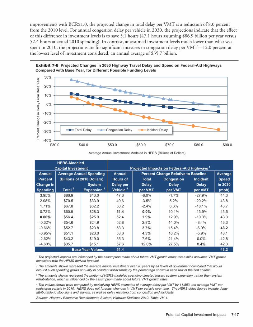
Potential Capital Investment Impacts 7-17

improvements with BCR≥1.0, the projected change in total delay per VMT is a reduction of 8.0 percent from the 2010 level. For annual congestion delay per vehicle in 2030, the projections indicate that the effect of this difference in investment levels is to save 5.1 hours (47.1 hours assuming $86.9 billion per year versus 52.4 hours at actual 2010 spending). In contrast, at assumed investment levels much lower than what was spent in 2010, the projections are for significant increases in congestion delay per VMT—12.0 percent at the lowest level of investment considered, an annual average of $35.7 billion.

10/25/2012 07XH_H (7-8) R1

Annual Annual Percent Change Relative to Baseline AveragePercent Hours of Total Congestion Incident Speed

Change in System Delay per Delay Delay Delay in 2030Spending Total 2 Expansion 3 Vehicle 4 per VMT per VMT per VMT (mph)

3.95% $86.9 $43.0 47.3 -8.0% -1.7% -27.9% 44.32.08% $70.5 $33.9 49.6 -3.5% 5.2% -20.2% 43.81.71% $67.8 $32.2 50.2 -2.4% 6.6% -18.1% 43.70.72% $60.9 $28.3 51.4 0.0% 10.1% -13.9% 43.50.00% $56.4 $25.9 52.4 1.9% 12.9% -10.3% 43.3-0.32% $54.6 $24.9 52.8 2.8% 14.0% -8.4% 43.3-0.66% $52.7 $23.8 53.3 3.7% 15.4% -6.9% 43.2-0.95% $51.1 $23.0 53.6 4.3% 16.2% -5.9% 43.1-2.62% $43.2 $19.0 55.3 7.6% 21.4% 0.0% 42.8-4.60% $35.7 $15.1 57.6 12.0% 27.5% 8.4% 42.3

Base Year Values: 51.4 43.2

HERS-Modeled Capital Investment

Average Annual Spending(Billions of 2010 Dollars)

Projected Impacts on Federal-Aid Highways 1

-40%

-30%

-20%

-10%

0%

10%

20%

30%

$30.0 $40.0 $50.0 $60.0 $70.0 $80.0 $90.0

Average Annual Investment Modeled in HERS (Billions of Dollars)

Total Delay Congestion Delay Incident Delay

Per

cent

Cha

nge

in D

elay

Fro

m B

ase

Yea

r

Exhibit 7-8 Projected Changes in 2030 Highway Travel Delay and Speed on Federal-Aid Highways Compared with Base Year, for Different Possible Funding Levels

1 The projected impacts are influenced by the assumption made about future VMT growth rates; this exhibit assumes VMT growth consistent with the HPMS-derived forecast. 2 The amounts shown represent the average annual investment over 20 years by all levels of government combined that would occur if such spending grows annually in constant dollar terms by the percentage shown in each row of the first column. 3 The amounts shown represent the portion of HERS-modeled spending directed toward system expansion, rather than system rehabilitation, which is influenced by the assumption made about future VMT growth rates. 4 The values shown were computed by multiplying HERS estimates of average delay per VMT by 11,853, the average VMT per registered vehicle in 2010. HERS does not forecast changes in VMT per vehicle over time. The HERS delay figures include delay attributable to stop signs and signals, as well as delay resulting from congestion and incidents. Source: Highway Economic Requirements System; Highway Statistics 2010, Table VM-1.

Investment/Performance Analysis7-18

Exhibit 7-9 presents results from HERS simulations in which the baseline VMT growth conforms to 15- year historical trend rather than the HPMS forecasts. Because this reduces the rate of VMT growth, the projections of delay for 2030 are lower than in Exhibit 7-8. For the case where spending continues at the 2010 level, annual delay per vehicle is projected at 47.4 hours versus the 52.4 hours that was projected in Exhibit 7-8 when forecast traffic growth was assumed. The impacts on delay of varying the level of investment are somewhat smaller, as well. For example, increasing average annual investment from the 2010 level to $68.4 billion reduces the 2030 projection of annual delay per vehicle by 1.8 hours (from 47.4 to 45.6), whereas the corresponding reduction in Exhibit 7-8 was 2.2 hours.

11/19/2012 07XH_I (7-9) R2.xlsx

Annual Annual Percent Change Relative to Baseline AveragePercent Hours of Total Congestion Incident Speed

Change in System Delay per Delay Delay Delay in 2030Spending Total 2 Expansion 3 Vehicle 4 per VMT per VMT per VMT (mph)

2.08% $70.5 $30.0 45.2 -12.1% -9.1% -33.0% 44.61.71% $67.8 $28.5 45.6 -11.2% -7.8% -31.6% 44.50.72% $60.9 $25.1 46.6 -9.3% -5.0% -28.0% 44.30.00% $56.4 $22.8 47.4 -7.8% -2.9% -25.2% 44.2-0.32% $54.6 $22.0 47.6 -7.3% -2.2% -23.9% 44.2-0.66% $52.7 $21.1 48.0 -6.7% -1.3% -22.6% 44.1-0.95% $51.1 $20.3 48.2 -6.2% -0.7% -21.6% 44.0-2.62% $43.2 $16.6 49.7 -3.2% 3.6% -15.9% 43.8-4.60% $35.7 $13.1 51.4 0.0% 8.0% -9.5% 43.4

Base Year Values: 51.4 43.2

HERS-Modeled Capital Investment

Average Annual Spending(Billions of 2010 Dollars)

Projected Impacts on Federal-Aid Highways 1

-40%

-30%

-20%

-10%

0%

10%

20%

30%

$30.0 $40.0 $50.0 $60.0 $70.0 $80.0

Average Annual Investment Modeled in HERS (Billions of Dollars)

Total Delay Congestion Delay Incident Delay

Per

cent

Cha

nge

in D

elay

Fro

m B

ase

Yea

r

1 The projected impacts are influenced by the assumption made about future VMT growth rates; this exhibit assumes VMT growth consistent with the trend over the 15-year period from 1995 to 2010. 2 The amounts shown represent the average annual investment over 20 years by all levels of government combined that would occur if such spending grows annually in constant dollar terms by the percentage shown in each row of the first column. 3 The amounts shown represent the portion of HERS-modeled spending directed toward system expansion, rather than system rehabilitation, which is influenced by the assumption made about future VMT growth rates. 4 The values shown were computed by multiplying HERS estimates of average delay per VMT by 11,853, the average VMT per registered vehicle in 2010. HERS does not forecast changes in VMT per vehicle over time. The HERS delay figures include delay attributable to stop signs and signals, as well as delay resulting from congestion and incidents. Sources: Highway Economic Requirements System; Highway Statistics 2010, Table VM-1.

Exhibit 7-9 Projected Changes in 2030 Highway Travel Delay and Speed on Federal-Aid Highways Compared with Base Year, for Different Possible Funding Levels, Assuming Trend-Based VMT Growth

11/19/2012 07XH_I (7-9) R2.xlsx

Annual Annual Percent Change Relative to Baseline AveragePercent Hours of Total Congestion Incident Speed

Change in System Delay per Delay Delay Delay in 2030Spending Total 2 Expansion 3 Vehicle 4 per VMT per VMT per VMT (mph)

2.08% $70.5 $30.0 45.2 -12.1% -9.1% -33.0% 44.61.71% $67.8 $28.5 45.6 -11.2% -7.8% -31.6% 44.50.72% $60.9 $25.1 46.6 -9.3% -5.0% -28.0% 44.30.00% $56.4 $22.8 47.4 -7.8% -2.9% -25.2% 44.2-0.32% $54.6 $22.0 47.6 -7.3% -2.2% -23.9% 44.2-0.66% $52.7 $21.1 48.0 -6.7% -1.3% -22.6% 44.1-0.95% $51.1 $20.3 48.2 -6.2% -0.7% -21.6% 44.0-2.62% $43.2 $16.6 49.7 -3.2% 3.6% -15.9% 43.8-4.60% $35.7 $13.1 51.4 0.0% 8.0% -9.5% 43.4

Base Year Values: 51.4 43.2

HERS-Modeled Capital Investment

Average Annual Spending(Billions of 2010 Dollars)

Projected Impacts on Federal-Aid Highways 1

-40%

-30%

-20%

-10%

0%

10%

20%

30%

$30.0 $40.0 $50.0 $60.0 $70.0 $80.0

Average Annual Investment Modeled in HERS (Billions of Dollars)

Total Delay Congestion Delay Incident Delay

Per

cent

Cha

nge

in D

elay

Fro

m B

ase

Yea

r

1 The projected impacts are influenced by the assumption made about future VMT growth rates; this exhibit assumes VMT growth consistent with the trend over the 15-year period from 1995 to 2010. 2 The amounts shown represent the average annual investment over 20 years by all levels of government combined that would occur if such spending grows annually in constant dollar terms by the percentage shown in each row of the first column. 3 The amounts shown represent the portion of HERS-modeled spending directed toward system expansion, rather than system rehabilitation, which is influenced by the assumption made about future VMT growth rates. 4 The values shown were computed by multiplying HERS estimates of average delay per VMT by 11,853, the average VMT per registered vehicle in 2010. HERS does not forecast changes in VMT per vehicle over time. The HERS delay figures include delay attributable to stop signs and signals, as well as delay resulting from congestion and incidents. Sources: Highway Economic Requirements System; Highway Statistics 2010, Table VM-1.

Exhibit 7-9 Projected Changes in 2030 Highway Travel Delay and Speed on Federal-Aid Highways Compared with Base Year, for Different Possible Funding Levels, Assuming Trend-Based VMT Growth

Potential Capital Investment Impacts 7-19

Whichever the traffic growth assumption, forecast or trend, it is important to bear in mind some traffic basics when interpreting these results. In addition to congestion and incident delay, some delay inevitably results from traffic control devices. For this reason, and because traffic congestion occurs only at certain places and times, Exhibits 7-8 and 7-9 show the variation in the level of investment as having less of an impact on projections for total delay and average speed than on the projections for congestion and incident delay. In addition, while the impacts of additional investment on average speed are proportionally small—when trend traffic growth is assumed, investing enough to implement all cost beneficial projects rather than at the 2010 level increases average speed projected for 2030 from 44.2 mph to 44.6 mph—these impacts apply to a vast amount of travel, so that the associated savings in user cost are not necessarily small relative to the cost of the investment.

Impact of Future Investment on Highway User Costs In the HERS model, the benefits from highway improvements are the reductions in highway user costs, agency costs, and societal costs of vehicle emissions. In measuring the highway user costs, the model includes the costs of travel time, vehicle operation, and crashes, but excludes from vehicle operating costs taxes imposed on highway users (such as motor fuel taxes and vehicle registration fees). As discussed in the Introduction to Part II, the exclusion of these taxes conforms with the principle in benefit-cost analysis of measuring the costs of transportation inputs as their opportunity cost to society. The exclusion also makes the measure of user costs more of an indicator of highway conditions and performance, of which the amount paid in highway-user taxes provides no indication.

Impact on Overall User Cost For Federal-aid highways, HERS estimates that user costs—the costs of travel time, vehicle operation, and crashes—averaged $1.030 per mile of travel in the base year (Exhibit 7-10). When baseline traffic is assumed to grow as forecast, the average user cost is generally higher in the 2030 projection than in the base year estimate. Average user cost is projected to increase between 2010 and 2030 by 0.8 percent and by 2.1 percent under the assumptions that real annual spending remains at the base year level or, alternatively, decreases annually at the rate geared toward maintaining average pavement roughness (2.62 percent). Decreases in average user cost are projected for the two highest levels of spending considered. At the level HERS indicates would be needed to fund all cost-beneficial projects (averaging $86.9 billion annually), average user cost per mile of travel in 2030 is projected to be $1.018, or 1.1 percent less than in the base year. Exhibit 7-10 also reveals that assuming baseline traffic growth to follow trend rather than the HPMS forecasts reduces the projections of average user cost at a given level of investment by 1 to 2 percent.

Q A&How much does HERS modify the baseline projections of VMT?

The modification is largest at the lowest investment level presented in Exhibit 7-10, which averages $35.7 billion per year and corresponds to negative 4.6 percent annual growth in spending. At this investment level, average user costs are projected to increase between 2010 and 2030 by 3.1 percent when the baseline traffic growth is assumed to be as forecast in HPMS. The projected increase in average user cost operates through the HERS elasticity mechanism to reduce the VMT projection for 2030. The increase from 2.520 trillion VMT in the base year to 3.550 trillion VMT in 2030 translates into an average annual VMT growth rate of 1.73 percent, which falls below the 1.85 percent growth rate forecast in HPMS.

Similarly, when traffic growth is assumed to follow the 15-year trend, average user costs per VMT are projected to increase by 1.3 percent; the increase from 2.520 trillion VMT to 3.253 trillion VMT translates into an average annual VMT growth rate of 1.28 percent, rather than the 1.36 percent annual growth rate assumed if user costs remained constant.

In the present analysis, the percent changes in average user cost are relatively small. For this reason, and because HERS incorporates the indications from available evidence that travel demand is not highly sensitive to price, HERS only slightly modifies the baseline projection of VMT.

Investment/Performance Analysis7-20

The projections in Exhibit 7-10 for VMT on Federal-aid highways incorporate the effects on travel demand of changes in average user cost. These outputs from the HERS analysis differ from the “trend” and “forecast” projections of VMT on Federal-aid highways that are inputs to the analysis. The input projections, which were shown in Exhibit 7-2, are interpreted as representing the baseline levels of traffic in the absence of any change in average user cost from the 2010 level. The 2030 traffic levels presented in Exhibit 7-10 are thus higher or lower than these baseline levels according to whether average user cost is projected to decrease or increase.

12/27/2012 07XH_J (7-10) R3.xlsx

Annual AveragePercent AnnualChange Spending

in (Billions of If Forecast If Trend If Forecast If Trend If Forecast If TrendSpending 2010 Dollars) VMT Growth VMT Growth VMT Growth VMT Growth VMT Growth VMT Growth

3.95% $86.9 $1.018 – -1.1% – 3.629 –2.08% $70.5 $1.027 $1.015 -0.2% -1.4% 3.612 3.3031.71% $67.8 $1.029 $1.017 0.0% -1.3% 3.608 3.3000.72% $60.9 $1.034 $1.021 0.4% -0.9% 3.599 3.2930.00% $56.4 $1.038 $1.024 0.8% -0.6% 3.592 3.287-0.32% $54.6 $1.040 $1.025 1.0% -0.5% 3.589 3.285-0.66% $52.7 $1.041 $1.026 1.1% -0.3% 3.586 3.282-0.95% $51.1 $1.043 $1.028 1.3% -0.2% 3.584 3.280-2.62% $43.2 $1.051 $1.035 2.1% 0.5% 3.568 3.268-4.60% $35.7 $1.062 $1.043 3.1% 1.3% 3.550 3.253

Base Year Values: $1.030 2.520* The HERS model relies on information from the HPMS sample section database, which is limited to those portions of the road network that are generally eligible for Federal funding (i.e., "Federal-aid highways") and excludes roads classified as rural minor collectors, rural local, and urban local.

HERS-Modeled Capital Investment

Percent Change in User Costs per VMT, Relative to

Base Year

Average Total User Costs ($/VMT)

Projected 2030 VMT on Federal-aid Highways

(Trillions of VMT)*

Projected Impacts on Federal-Aid Highways*

-2%

-1%

0%

1%

2%

3%

4%

$30.0 $40.0 $50.0 $60.0 $70.0 $80.0 $90.0

Average Annual Investment Modeled in HERS (Billions of Dollars)

Assuming Forecast VMT Growth Assuming Trend VMT Growth

Per

cent

Cha

nge

in A

vera

ge

Tota

l Use

r Cos

ts fr

om B

ase

Yea

r

Exhibit 7-10 Projected 2030 Average Total User Costs and VMT on Federal-Aid Highways Compared with Base Year, for Different Possible Funding Levels

Source: Highway Economic Requirements System.

Impact on User Cost ComponentsExhibit 7-11 shows the projected changes from 2010 to 2030 in average user cost of travel on Federal-aid highways by cost component. The cost of crashes is the component least sensitive to the assumed level of highway investment, which as an annual average varies between $35.7 billion and $86.9 billion or $70.5 billion depending on whether baseline VMT growth is assumed to follow the HPMS forecast or the 15-year trend. Compared with the lowest level, the highest level of spending reduces the crash cost

Potential Capital Investment Impacts 7-21

11/19/2012 07XH_K (7-11) R2.xlsx

Annual AveragePercent AnnualChange Spending

in (Billions of If Forecast If Trend If Forecast If Trend If Forecast If TrendSpending 2010 Dollars) VMT Growth VMT Growth VMT Growth VMT Growth VMT Growth VMT Growth

3.95% $86.9 -3.0% – 0.2% – 1.1% –2.08% $70.5 -1.8% -3.9% 1.0% 0.8% 1.3% 0.1%1.71% $67.8 -1.6% -3.7% 1.1% 0.9% 1.3% 0.1%0.72% $60.9 -0.9% -3.2% 1.6% 1.3% 1.4% 0.2%0.00% $56.4 -0.4% -2.8% 1.8% 1.5% 1.5% 0.3%-0.32% $54.6 -0.2% -2.7% 2.0% 1.7% 1.5% 0.3%-0.66% $52.7 0.1% -2.5% 2.1% 1.8% 1.5% 0.4%-0.95% $51.1 0.2% -2.4% 2.3% 1.9% 1.6% 0.4%-2.62% $43.2 1.2% -1.5% 3.2% 2.7% 1.6% 0.4%-4.60% $35.7 2.5% -0.6% 4.1% 3.7% 1.8% 0.6%

HERS-Modeled Capital Investment Projected Impacts on Federal-Aid Highways

2 The HPMS does not contain the type of detail that would be needed to conduct an analysis of targeted safety enhancements. The crash costs estimated by the HERS model represent ancillary impacts associated with pavement and capacity improvements and are heavily influenced by traffic volume and speed.

Source: Highway Economic Requirements System.

1 The projected vehicle operating costs are heavily influenced by an assumption drawn from the EIA Annual Energy Outlook 2012 publication that motor fuel prices would grow by 45 percent over the 20 year analysis period. The average retail price of a gallon of gasoline was $2.44 per gallon in 2010, but had already risen to $3.58 by 2011.

Travel Time Costs Vehicle Operating Costs 1 Crash Costs 2

Percent Change in Average User Costs per VMT in 2030, Relative to Base Year

Exhibit 7-11 Projected Changes in 2030 Average Highway User Costs on Federal-Aid Highways Compared With Base Year, for Different User Cost Components and Different Possible Funding Levels

per VMT by 0.7 percent (forecast case) or 0.1 percent (trend case). These levels of spending are limited to the types of improvements that HERS evaluates, which are basically system rehabilitation and expansion. Because the HPMS lacks detailed information on the current location and characteristics of safety-related features (e.g., guardrail, rumble strips, roundabouts, yellow change intervals at signals), safety-focused investments are not evaluated. Thus, the findings presented in Exhibit 7-11 establish nothing about how such investments affect highway safety.

Crash costs also form the smallest of the three components of highway user costs. For 2010 travel on Federal-aid highways, HERS estimates the breakdown by cost component to be crash cost, 13.6 percent; travel time cost, 44.9 percent, and vehicle operating cost, 41.5 percent. Research under way to update the vehicle operating cost equations in HERS (see Appendix D) may somewhat alter the split among these costs, but crash costs will remain a small component. Although highway trips always consume traveler time and resources for vehicle operation, only a small fraction involve crashes. In addition, most crashes are non-catastrophic: particularly on urban highways, many involve only damage to property without anyone being injured.

The projections for the travel time costs are somewhat more sensitive to the assumed level of investment than are the projections for vehicle operating costs. When baseline VMT growth is based on HPMS forecasts, the projected 2010-2030 change in travel cost per VMT ranges from a decrease of 3.5 percent at the highest level of assumed investment to an increase of 2.5 percent at the lowest. This implies that investing at the highest rather than the lowest level would reduce the per VMT cost of travel in 2030 by 5.4 percent (= (035+.025)/(1-.025)). For vehicle operating cost, the corresponding estimate is a reduction of 3.3 percent. When VMT growth is based on trend rather than forecasts, the projections of travel time and vehicle operating cost are lower and less sensitive to variation in the assumed investment level. Investing at the

Investment/Performance Analysis7-22

highest level shown for the trend forecast case rather than at the lowest level reduces the projected time cost of travel in 2030 by 3.7 percent and the projected vehicle operating cost by 2.8 percent.

For vehicle operating costs per VMT, all the projections in Exhibit 7-11 show levels in 2030 to exceed those for 2010. This uniformity contrasts with the mixed pattern in the projections for travel time cost and reflects the assumption of future increases in motor fuel prices. For these prices and for vehicle fuel economy, the assumptions are based on projections from the Energy Information Administration (EIA) Annual Energy Outlook 2012. The weighted average price of gasoline and diesel fuel is assumed to increase between 2010 and 2030 by 45 percent more than the consumer price index. This increase outweighs the fuel cost savings that would result from the improvements in vehicle energy efficiency that the EIA projects for this same period; these equate to increases in average MPG of 32.8 percent for light-duty vehicles, 30.0 percent for two-axle trucks, and 19.4 percent for 3+ axle trucks. These projections incorporate the effect of increases in Corporate Average Fuel Economy (CAFE) standards and U.S. Environmental Protection Agency (EPA) standards for emissions of greenhouse gases by automobiles and light trucks through model year 2016, as well as new standards for fuel efficiency and greenhouse gas emissions for medium- and heavy-duty trucks through model year 2018 adopted by U.S. Department of Transportation (DOT) and EPA.

Q A&What changes in CAFE standards have recently been adopted, and what impacts are these changes expected to have?

On May 7, 2010, NHTSA and EPA jointly adopted Corporate Average Fuel Economy (CAFE) and carbon dioxide (CO2) emission standards for cars and light trucks produced during model years 2012 through 2016. In combination with NHTSA’s previous actions, this rule raised required fuel economy levels for cars from 27.5 miles per gallon (mpg) in model year 2010 to 37.8 mpg for model year 2016, and those for light trucks from 23.5 mpg in 2010 to 28.8 mpg for 2016. On August 28, 2012, the two agencies adopted new rules that further increased CAFE standards for model year 2021 to 46.1 to 46.8 mpg for automobiles and to 32.6 to 33.3 mpg for light trucks; this most recent action also established tentative CAFE standards for model year 2025 of 55.3 to 56.2 mpg for cars and 39.3 to 40.3 mpg for light trucks.

The impacts of these standards on the fuel economy of the overall vehicle fleet will continue to grow for many years beyond 2025, as new vehicles meeting the higher fuel economy requirements gradually replace older, less-fuel-efficient vehicles. In announcing the most recent increases in CAFE standards, NHTSA estimated that the cumulative effects of its actions would be to save more than 500 billion gallons of fuel and reduce carbon dioxide emissions by 6 billion metric tons over the lifetimes of cars and light trucks produced in 2011 through 2025. The agency also estimated that its standards would save the Nation’s drivers more than $1.7 trillion in fuel costs over these vehicles’ lifetimes.

In 2011, NHTSA and EPA also established new fuel efficiency and CO2 emission standards for medium- and heavy-duty trucks produced from 2014 through 2018. These standards are expected to reduce fuel consumption by an additional 22 billion gallons, while further reducing CO2 emissions by nearly 270 million metric tons.

Impacts of NHS Investments Modeled by HERSAs described in Chapter 2, the NHS includes the Interstate System as well as other routes most critical to national defense, mobility, and commerce. As noted earlier, the NHS analyses presented in this chapter are based on an estimate of what the NHS will look like after it is expanded pursuant to MAP-21, rather than the actual system as it existed in 2010.

This section examines the total spending modeled in HERS, identifying the portion of this investment that is directed by the model to the NHS, and the impacts that such investment could have on future NHS conditions and performance. For Federal-aid highways, the preceding analysis in this chapter examined the effect on the HERS projections of replacing the HPMS traffic forecasts with trend traffic growth. In analyzing investments in the NHS portion of Federal-aid highways, this section assumes traffic growth as forecast in the HPMS.

Potential Capital Investment Impacts 7-23

HERS allocates a portion of future investment in Federal-aid highways to the NHS based on the model’s engineering and economic criteria, which give funding priority to high-BCR projects. The levels of future investment in Federal-aid highways considered in this section’s analysis are either identical to or counterparts of levels considered in this chapter’s preceding sections. Carried over from the preceding analysis are the investment levels tied to a specific minimum BCR among all improvements to the Federal-aid highways that HERS programs over the analysis period. Also included are levels of investment in Federal-aid highways tied to one of the goals considered in the preceding analysis, such as maintaining average pavement roughness at the base year level, except that the goals are now limited to the NHS. In the simulations with these investment levels, HERS allocates to the NHS the amount needed to achieve the goal for the NHS without regard to whether or not the same goal is met for other Federal-aid highways.

Q A&How were the seven NHS investment levels presented in Exhibits 7-12 and 7-13 selected?

As MAP-21 directs that the NHS be expanded, the 20-year NHS projections presented in this report were based on all sections coded in HPMS as being on the NHS, plus those other principal arterials that are not currently part of the NHS. While this will not exactly match the scope of the NHS in the future (some sections currently coded as principal arterials may not be ultimately be included in the NHS, and some additional connector mileage may be included), it represents a reasonably close approximation for purposes of the types of analyses presented.

The investment levels associated with minimum BCR cutoffs of 1.00 and 1.50 were derived from the same HERS runs identified in Exhibit 7-3 as associated with these cutoffs assuming VMT growth consistent with the HPMS-derived forecast. The investment levels shown reflect the portion of spending in those runs that was directed to the NHS.

The remaining five levels were selected using comparable criteria to those identified in Exhibit 7-3, but in terms of the NHS in particular, rather than Federal-aid highways in general. The 20-year investment level associated with a minimum BCR cutoff of 1.78 results in an average annual investment level of $40.6 billion, consistent with spending on the NHS in 2010 on types of capital improvements modeled in HERS.

The investment level associated with a minimum BCR cutoff of 2.49 was selected to be included because it results in projected average speed in 2030 matching the base year level. Investing at the level associated with a minimum BCR cutoff of 2.19 is projected to result in average delay being maintained, while applying a minimum BCR cutoff of 2.88 would maintain average IRI. The minimum BCR cutoff of 2.74 was selected as it results in a level of NHS spending that equals the average of the levels associated with maintaining average delay and maintaining average IRI.

Impact of Future Investment on NHS Pavement Ride QualityExhibit 7-12 shows the portions of the levels of Federal-aid highway investment considered that HERS allocates to the NHS. To throw light on the projections for NHS pavement quality that are presented, the exhibit also shows the sub-portions of modeled NHS spending that HERS allocates to rehabilitation projects (which influence average pavement quality more than expansion projects). At the assumed level of Federal-aid investment that would cause HERS to allocate to the NHS an annual average of $40.6 billion, matching the level invested in 2010, the model projects average pavement roughness on the NHS will be 23.7 percent lower in 2030 than in 2010. For HERS to project average pavement roughness to remain unchanged between these years would require assuming an annual average NHS spending level of $22.5 billion, an amount that could be achieved if NHS spending declined by 6.01 percent per year beginning in 2010.

At the other end of the investment spectrum in Exhibit 7-12, implementing all cost-beneficial improvements would require annual average spending on the NHS estimated at $58.1 billion, which is projected to reduce the average IRI over the analysis period by 35.3 percent. At this level of investment in the system, the model also projects that pavements with an IRI below 95, which was the criterion in Chapter 3 for rating ride quality as “good”, will carry 89.6 percent of the VMT on the NHS, up from the 54.7 percent estimated for 2010. Based on these modeling results, additional investment to bring this percentage closer to 100 percent would be economically inefficient, as the costs would exceed the benefits.

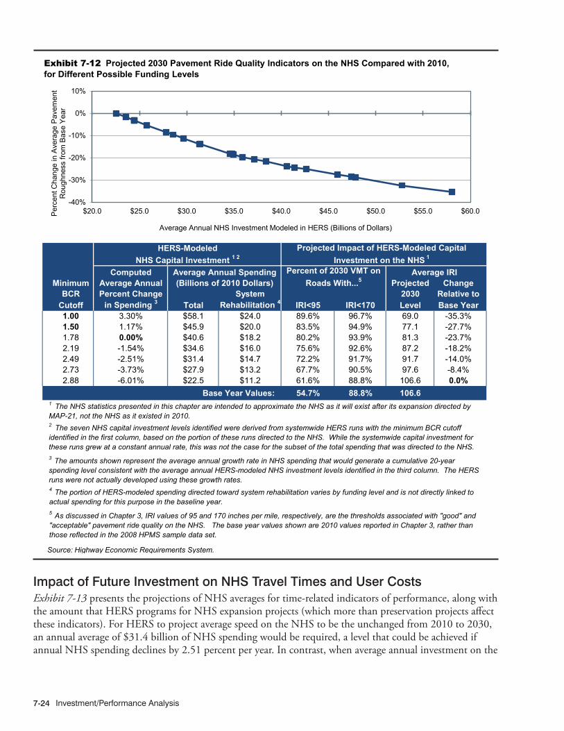
Investment/Performance Analysis7-24

Impact of Future Investment on NHS Travel Times and User CostsExhibit 7-13 presents the projections of NHS averages for time-related indicators of performance, along with the amount that HERS programs for NHS expansion projects (which more than preservation projects affect these indicators). For HERS to project average speed on the NHS to be the unchanged from 2010 to 2030, an annual average of $31.4 billion of NHS spending would be required, a level that could be achieved if annual NHS spending declines by 2.51 percent per year. In contrast, when average annual investment on the

12/27/2012 07XH_L (7-12) R2.xlsx

ComputedMinimum Average Annual Projected Change

BCR Percent Change System 2030 Relative toCutoff in Spending 3 Total Rehabilitation 4 IRI<95 IRI<170 Level Base Year1.00 3.30% $58.1 $24.0 89.6% 96.7% 69.0 -35.3%1.50 1.17% $45.9 $20.0 83.5% 94.9% 77.1 -27.7%1.78 0.00% $40.6 $18.2 80.2% 93.9% 81.3 -23.7%2.19 -1.54% $34.6 $16.0 75.6% 92.6% 87.2 -18.2%2.49 -2.51% $31.4 $14.7 72.2% 91.7% 91.7 -14.0%2.73 -3.73% $27.9 $13.2 67.7% 90.5% 97.6 -8.4%2.88 -6.01% $22.5 $11.2 61.6% 88.8% 106.6 0.0%

Base Year Values: 54.7% 88.8% 106.6

4 The portion of HERS-modeled spending directed toward system rehabilitation varies by funding level and is not directly linked to actual spending for this purpose in the baseline year. 5 As discussed in Chapter 3, IRI values of 95 and 170 inches per mile, respectively, are the thresholds associated with "good" and "acceptable" pavement ride quality on the NHS. The base year values shown are 2010 values reported in Chapter 3, rather than those reflected in the 2008 HPMS sample data set.

Projected Impact of HERS-Modeled Capital Investment on the NHS 1

Average Annual Spending Percent of 2030 VMT on Roads With...5

Average IRI(Billions of 2010 Dollars)

HERS-ModeledNHS Capital Investment 1 2

2 The seven NHS capital investment levels identified were derived from systemwide HERS runs with the minimum BCR cutoff identified in the first column, based on the portion of these runs directed to the NHS. While the systemwide capital investment for these runs grew at a constant annual rate, this was not the case for the subset of the total spending that was directed to the NHS. 3 The amounts shown represent the average annual growth rate in NHS spending that would generate a cumulative 20-year spending level consistent with the average annual HERS-modeled NHS investment levels identified in the third column. The HERS runs were not actually developed using these growth rates.

1 The NHS statistics presented in this chapter are intended to approximate the NHS as it will exist after its expansion directed by MAP-21, not the NHS as it existed in 2010.

-40%

-30%

-20%

-10%

0%

10%

$20.0 $25.0 $30.0 $35.0 $40.0 $45.0 $50.0 $55.0 $60.0

Average Annual NHS Investment Modeled in HERS (Billions of Dollars)

Per

cent

Cha

nge

in A

vera

ge P

avem

ent

Rou

ghne

ss fr

om B

ase

Yea

r Exhibit 7-12 Projected 2030 Pavement Ride Quality Indicators on the NHS Compared with 2010, for Different Possible Funding Levels

Source: Highway Economic Requirements System.

Potential Capital Investment Impacts 7-25

1/16/2014 07XH_M (7-13) R2.xlsx

ComputedMinimum Average Annual Projected Change

BCR Percent Change System Average Average 2030 Relative toCutoff in Spending Total Expansion2 User Costs Delay Level (mph) Base Year1.00 3.30% $58.1 $34.1 -2.4% -18.3% 50.8 4.4%1.50 1.17% $45.9 $25.9 -1.2% -10.2% 50.0 2.7%1.78 0.00% $40.6 $22.4 -0.6% -5.9% 49.6 1.9%2.19 -1.54% $34.6 $18.6 0.2% 0.0% 49.0 0.6%2.49 -2.51% $31.4 $16.7 0.7% 2.8% 48.7 0.0%2.73 -3.73% $27.9 $14.6 1.5% 6.7% 48.3 -0.9%2.88 -6.01% $22.5 $11.4 2.7% 13.8% 47.5 -2.5%

Base Year Value: 48.7

Projected Impact of HERS-Modeled Capital Investment on the NHS 1

Average SpeedAverage Annual Spending (Billions of 2010 Dollars)

Percent Change Relative to Baseline per VMT

HERS-Modeled NHS Capital Investment 1

-20.0%

-15.0%

-10.0%

-5.0%

0.0%

5.0%

10.0%

15.0%

20.0%

$20.0 $25.0 $30.0 $35.0 $40.0 $45.0 $50.0 $55.0 $60.0

Per

cent

Cha

nge

in A

vera

ge D

elay

fro

m B

ase

Yea

r

Average Annual NHS Investment Modeled in HERS (Billions of Dollars)

Exhibit 7-13 Projected Changes in 2030 Delay, Speed, and Highway User Costs on the NHS Compared with 2030 for Different Possible Funding Levels

1 The NHS statistics presented in this chapter are intended to approximate the NHS as it will exist after its expansion directed by MAP-21, not the NHS as it existed in 2010. 2The portion of HERS-modeled spending directed toward system expansion varies by funding level and is not directly linked to actual spending for this purpose in the baseline year. System expansion expenditures have a more direct impact on delay and speed, while both system expansion and system rehabilitation expenditures impact highway user costs. Source: Highway Economic Requirements System.

NHS is what would be needed to implement all cost-beneficial improvements, an estimated $58.1 billion, HERS projects average NHS speed to be 4.4 percent higher in 2030 than in 2010 (50.8 mph versus 48.7 mph). At this investment level, HERS also projects for the NHS that average delay will decline by 18.4 percent, and average user cost by 2.4 percent, over the analysis period. For the case where investment in the NHS would remain at the 2010 level, average delay decreases by 5.9 percent, while average user costs are projected to decrease by 0.6 percent.

Investment/Performance Analysis7-26

Impacts of Interstate System Investments Modeled by HERSThe Interstate System, unlike the broader NHS of which it is a part, has standard design and signing requirements, which makes it the most recognizable subset of the highway network. This section examines the amount of investment that HERS directs to the Interstate System, and the potential impacts of this investment on future Interstate System conditions and performance. For this analysis, the funding levels presented were selected in the same way as those for the preceding section’s analysis of investment in the NHS.

Q A&How were the seven Interstate System investment levels presented in Exhibits 7-14 and 7-15 selected?

The investment levels associated with minimum benefit-cost ratio cutoffs of 1.00 and 1.50 were derived from the same HERS runs identified in Exhibit 7-3 as associated with these cutoffs assuming VMT growth consistent with the HPMS-derived forecast. The investment levels shown reflect the portion of spending in those runs that was directed to the Interstate System.

The remaining five levels were selected using comparable criteria to those identified in Exhibit 7-3, but in terms of the Interstate System in particular, rather than Federal-aid highways in general. The 20-year investment level associated with a minimum benefit-cost ratio cutoff of 2.72 results in an average annual investment level of $14.7 billion, consistent with spending on the Interstate System in 2010 on types of capital improvements modeled in HERS.

The investment level associated with a minimum benefit-cost ratio cutoff of 2.66 was selected to be included because it results in projected average speed in 2030 matching the base year level. Investing at the level associated with a minimum benefit-cost ratio cutoff of 2.70 is projected to result in average delay being maintained, while applying a minimum benefit-cost ratio cutoff of 2.97 would maintain average IRI. The minimum benefit-cost ratio cutoff of 2.84 was selected as it results in a level of Interstate System spending that equals the average of the levels associated with maintaining average delay and maintaining average IRI.

Impact of Future Investment on Interstate Pavement Ride QualityExhibit 7-14 shows the levels of Federal-aid highway investment that HERS allocates to the Interstate System. To throw light on the projections for Interstate System pavement, the exhibit also shows the portion of modeled Interstate System spending that HERS allocates to system rehabilitation projects. At the assumed level of Federal-aid investment that would cause HERS to allocate to the Interstate System an annual average of $14.7 billion, matching the level invested in 2010, the model projects average pavement roughness on the Interstate System to be 12.7 lower in 2030 than in 2010. For HERS to project average pavement roughness to remain unchanged between these years would require assuming a level of Federal-aid highway investment out of which the model would allocate to the Interstate System an annual average of $11.1 billion, which could be achieved with an average annual reduction in spending of 2.71 percent per year starting in 2010.

At the other end of the investment spectrum in Exhibit 7-14, implementing all cost-beneficial improvements would require annual average spending on the Interstate System estimated at $26.2 billion; this level of investment is projected to reduce the average IRI over the analysis period by 32.9 percent. At this economically efficient level of investment in the Interstate System, the model also projects that pavements with an IRI below 95, which was the criterion in Chapter 3 for rating ride quality as “good”, will carry 94.2 percent of the VMT on the Interstate System, up from the 69.5 percent estimated for 2010.

Potential Capital Investment Impacts 7-27

Impact of Future Investment on Interstate System Travel Times and User CostsExhibit 7-15 presents the projections of Interstate System averages for time-related indicators of performance, along with the amount that HERS programs for Interstate System expansion projects. For HERS to project average speed on the Interstate System to be unchanged from 2010 to 2030, an annual average of $15.2 billion of Interstate System spending would be required, which could be achieved if spending increases by 0.35 percent per year beginning in 2010. In contrast, when average annual investment in the Interstate System is what would be needed to implement all cost-beneficial improvements, an

10/25/2012 07XH_N (7-14) R1

ComputedMinimum Average Annual Projected Change

BCR Percent Change System 2030 Relative toCutoff in Spending 2 Total Rehabilitation 3 IRI<95 IRI<170 Level Base Year1.00 5.22% $26.2 $8.5 94.2% 99.6% 62.3 -32.9%1.50 3.77% $22.2 $7.7 90.8% 98.9% 66.6 -28.2%2.66 0.35% $15.2 $5.9 81.6% 96.5% 79.3 -14.5%2.70 0.17% $15.0 $5.9 81.0% 96.3% 79.9 -13.9%2.72 0.00% $14.7 $5.8 80.3% 96.2% 81.0 -12.7%2.84 -1.28% $12.9 $5.3 76.8% 95.4% 86.8 -6.5%2.97 -2.71% $11.1 $4.6 72.1% 94.4% 92.8 0.0%

Base Year Values: 69.5% 90.3% 92.8

Projected Impact of HERS-Modeled Capital Investment on the Interstate System

Average Annual Spending Percent of 2030 VMT on Roads With...4

Average IRI(Billions of 2010 Dollars)

HERS-ModeledInterstate Capital Investment 1

-40%

-30%

-20%

-10%

0%

10%

$10.0 $12.0 $14.0 $16.0 $18.0 $20.0 $22.0 $24.0 $26.0 $28.0

Average Annual Interstate Investment Modeled in HERS (Billions of Dollars)

Per

cent

Cha

nge

in A

vera

ge

Pav

emen

t Rou

ghne

ss fr

om B

ase

Exhibit 7-14 Projected 2030 Pavement Ride Quality Indicators on the Interstate System Compared with 2010, for Different Funding Levels

1 The seven Interstate System capital investment levels identified were derived from systemwide HERS runs with the minimum BCR cutoff identified in the first column, based on the portion of these runs directed to the Interstate System. While the systemwide capital investment for these runs grew at a constant annual rate, this was not the case for the subset of the total spending that was directed to the Interstate System. 2 The amounts shown represent the average annual growth rate in Interstate System spending that would generate a cumulative 20-year spending level consistent with the average annual HERS-modeled Interstate System investment levels identified in the third column. The HERS runs were not actually developed using these growth rates. 3 The portion of HERS-modeled spending directed toward system rehabilitation varies by funding level and is not directly linked to actual spending for this purpose in the baseline year. 4 As discussed in Chapter 3, IRI values of 95 and 170 inches per mile, respectively, are the thresholds associated with "good" and "acceptable" pavement ride quality on the NHS. The base year values shown are based on 2010 values reported in Chapter 3, rather than those reflected in the 2008 HPMS sample data set. Source: Highway Economic Requirements System.

Investment/Performance Analysis7-28

estimated $26.2 billion, HERS projects average Interstate System speed to be 7.5 percent higher in 2030 than in 2010 (64.6 mph versus 60.1 mph). At this investment level, HERS also projects for the Interstate System that average congestion delay will decline by 39.5 percent, and average user cost by 2.9 percent, over the analysis period. For the case where investment in the Interstate System would remain at the 2010 level, average congestion delay and average user cost are each projected to decrease by about one percent.

10/25/2012 07XH_O (7-15) R1

ComputedMinimum Average Annual Projected Change

BCR Percent Change System Average Average 2030 RelativeCutoff in Spending Total Expansion 1 User Costs Delay Level (mph) to Baseline1.00 5.22% $26.2 $17.6 -2.9% -39.5% 64.6 7.5%1.50 3.77% $22.2 $14.5 -1.9% -27.3% 63.1 5.0%2.66 0.35% $15.2 $9.3 0.6% -1.7% 60.1 0.0%2.70 0.17% $15.0 $9.1 0.8% 0.0% 60.0 -0.3%2.72 0.00% $14.7 $8.9 0.9% 1.0% 59.8 -0.5%2.84 -1.28% $12.9 $7.6 2.0% 10.1% 58.6 -2.5%2.97 -2.71% $11.1 $6.5 3.1% 19.8% 57.6 -4.2%

Base Year Values: 60.1

Projected Impact of HERS-Modeled Capital Investment on the Interstate System

Average Annual Spending Percent Change Relative to Baseline per VMT

Average Speed(Billions of 2008 Dollars)

HERS-ModeledInterstate Capital Investment

-50%

-40%

-30%

-20%

-10%

0%

10%

20%

30%

$10.0 $12.0 $14.0 $16.0 $18.0 $20.0 $22.0 $24.0 $26.0 $28.0

Per

cent

Cha

nge

in A

vera

ge D

elay

fro

m B

ase

Yea

r

Average Annual Interstate Investment Modeled in HERS (Billions of Dollars)

Exhibit 7-15 Projected Changes in 2030 Speed, Delay, and Highway User Costs on the Interstate System Compared with 2010, for Different Possible Funding Levels

1 The portion of HERS-modeled spending directed toward system expansion varies by funding level and is not directly linked to actual spending for this purpose in the baseline year. System expansion expenditures have a more direct impact on delay and speed, while both system expansion and system rehabilitation expenditures impact highway user costs. Source: Highway Economic Requirements System.

National Bridge Investment Analysis SystemThe scenario estimates relating to bridge repair and replacement shown in this report are derived primarily from NBIAS, which accepts detailed structural data on individual bridge elements. Because such detailed information is not currently available at the national level, NBIAS also has the capability to synthesize element level data from the general condition ratings reported for individual bridges in the National Bridge Inventory (NBI). The analyses presented in this report are based on synthesized element level data. Examples of bridge elements include the bridge deck, a steel girder used for supporting the deck, a concrete pier cap on which girders are placed, a concrete column used for supporting the pier cap, or a bridge railing.

Potential Capital Investment Impacts 7-29

The NBIAS model uses a probabilistic approach to model bridge deterioration for each synthesized bridge element. It relies on a set of transition probabilities to project the likelihood that an element will deteriorate from one condition state to another over a given period of time. Another key input to the model is the overall objective assumed for maintenance, repair, and rehabilitation (MR&R) policies. Previous C&P reports assumed that the bridge owners would follow MR&R policies aimed at minimizing costs, but NBIAS has recently been enhanced to allow alternative assumptions. In this report, the standard assumption is that bridge owners will pursue MR&R policies aimed at achieving a steady state of bridge performance; other assumptions are considered for sensitivity analysis in Chapter 10. Given the assumed policy objective, NBIAS determines an optimal set of MR&R actions to take for each bridge element based on the condition of the element.

To estimate functional improvement needs, NBIAS applies a set of improvement standards and costs to each bridge in the NBI. The model then identifies potential improvements—such as widening existing bridge lanes, raising bridges to increase vertical clearances, and strengthening bridges to increase load-carrying capacity—and evaluates their potential benefits and costs. NBIAS evaluates potential bridge replacements by comparing their benefits and costs with what could be achieved through MR&R work alone. Appendix B discusses the NBIAS model in more detail.

In using the NBIAS model to project conditions and performance of the Nation’s bridges over 20 years, this section considers the alternatives of continuing to invest in bridge rehabilitation at the 2010 level (in constant dollars) and at higher or lower levels. The expenditures modeled pertain only to bridge system rehabilitation; expenditures associated with bridge system expansion are modeled separately as part of the capacity expansion analysis in the HERS model. (The NBIAS-modeled investments presented here should be considered as additive to the HERS-modeled investments presented above; each of the capital investment scenarios presented in Chapter 8 combines one of the HERS analyses with one of the NBIAS analyses, and makes adjustments to account for non-modeled spending.)

Performance MeasuresThe NBIAS model considers bridge deficiencies at the level of individual bridge elements based on engineering criteria and computes an initial value for the cost of a set of corrective actions that would address all such deficiencies. The economic bridge investment backlog represents the combined cost of these corrective actions in those cases where NBIAS estimates it would be cost-beneficial to implement them. Changes in this economic bridge investment backlog over time can be viewed as a proxy for changes in overall bridge conditions.

Previous editions of the C&P report used the economic bridge investment backlog as the sole indicator of bridge system performance. For a more comprehensive view of the impacts of various levels of investment, two new additional metrics have been added for this edition, the average Sufficiency Rating and the average Health Index.

Q A&How does the NBIAS definition of bridge deficiencies compare with the information on structurally deficient bridges reported in Chapter 3?

NBIAS considers bridge deficiencies and corrective improvements at the level of individual bridge elements. The economic backlog of bridge deficiencies estimated by NBIAS thus consists of the cost of all improvements to bridge elements that would be justified on both engineering and economic grounds. It includes many improvements on bridges with certain components that may warrant repair, rehabilitation, or replacement, but whose overall condition is not sufficiently deteriorated for them to be classified as structurally deficient.

The corrective actions recommended by NBIAS would include those aimed at addressing structural deficiencies, as well as some functional deficiencies. System expansion needs for both highways and bridges are addressed separately as part of the HERS model analysis.

Investment/Performance Analysis7-30

Prior to MAP-21, under the Highway Bridge Program (HBP), the Sufficiency Rating of a bridge served as a factor for determining funding eligibility and as an initial prioritization. This initial prioritization, which was provided annually to the States and known as the “Selection List,” was a listing of bridges that were eligible for programming for replacement and rehabilitation (other activities under the HBP with separate and different eligibility criteria such as systematic preventive maintenance were also eligible for programming). The Sufficiency Rating is a numeric value that ranges from 100 to 0, in which 100 represents an entirely sufficient bridge and 0 represents an entirely insufficient or deficient bridge. Its calculation is based on a complex formula involving a number of NBI data fields relating to: structural adequacy and safety (in terms of bridge component condition ratings and a load capacity rating), serviceability and functional obsolescence (in terms of bridge geometric features and appraisal ratings, volume of traffic carried, approach roadway features, deck condition rating, structural evaluation, and whether the bridge is on the Strategic Highway Network [STRAHNET]), and essentiality for public use (in terms of volume of traffic carried, detour length, and whether the bridge is on the STRAHNET). For this report, the investment scenarios presented in Chapter 8 focus on the Sufficiency Rating rather than the economic bridge investment backlog.

The Bridge Health Index is a 0-100 ranking system typically used in the context of decision making for bridge preventative maintenance. Although element condition states are categorical; it is useful to think of the condition of an element at a given time as a point along a continuous timeline from 100 percent in the best state to 100 percent in the worst state. The Health Index merely indicates where the element is along this continuum. To aggregate the element-level result to the bridge level, weights are assigned to the elements according to the economic consequences of element failure. Thus, elements whose failure has relatively little economic effect, such as railings, receive less weight than elements whose failure could close the bridge, such as girders. In general, the lower the Health Index number, the higher the priority for rehabilitation or maintenance of the structure, though other factors also come into play when determining priority of work on bridges.

Impacts of Systemwide Investments Modeled by NBIASAs referenced in Chapter 6, of the $100.2 billion invested in highways in 2010, $17.1 billion was used for bridge system rehabilitation, an increase of more than one-third compared to 2008. This sharp increase is attributable in part to the use of Recovery Act funds to repair and replace bridges.

For investments of the types modeled by NBIAS, Exhibit 7-16 shows how the total amount invested over the 20-year analysis period influences the bridge performance levels projected for the final year, 2030. If spending were sustained at its 2010 level in constant dollar terms, projected performance for 2030 would improve relative to 2010 for each of the three measures considered. The average Sufficiency Rating would increase from 81.7 in 2010 to 84.1 in 2030, the average Health Index would rise from 92.1 to 92.7; and the economic investment backlog would decrease by 92.6 percent relative to its 2010 level of $106.4 billion. The highest level of spending shown in Exhibit 7-16 averages $20.2 billion per year, which is the estimate of what would be needed to eliminate the economic backlog by 2030.

Exhibit 7-16 also indicates that bridge investment spending could be reduced from the 2010 level while maintaining bridge performance. If average annual spending declined by 2.30 percent to an average annual investment level of $13.5 billion, this would still be sufficient to maintain the average Health Index at its 2010 level through 2030. An annual decrease in investment of 3.33 percent to an average investment level of $12.2 billion would be adequate to maintain the average Sufficiency Rating at its 2010 level. The economic bridge investment backlog could be maintained at its 2010 level even if annual bridge investment declined by 6.72 percent per year to an average annual level of $8.9 billion.

Potential Capital Investment Impacts 7-31

Q A&Why does the economic backlog estimated by NBIAS differ from bridge backlog figures estimated by some other organizations?

One major reason for such differences is that the backlog estimated by NBIAS is not intended to constitute a complete bridge investment estimate backlog. The NBIAS figures relate only to investment needs associated with the condition of existing structures, and not capacity expansion needs. The backlog estimated by HERS includes estimates of capacity-related needs for highways and bridges combined.

Some estimates of bridge backlog produced by other organizations do attempt to combine estimates of needs relating to bridge capacity with those relating to existing structures.

10/26/2012 07XH_P (7-16) R1

Annual Average Annual 2030 2030Percent Spending1 Average Average 2030 Change

Change in (Billions of Sufficiency Health (Billions of Relative toSpending 2010 Dollars) Rating Index 2010 Dollars) Baseline

1.57% $20.2 84.6 92.8 $0.0 -100.0%0.00% $17.1 84.1 92.7 $7.9 -92.6%-1.70% $14.3 83.2 92.3 $20.6 -80.6%-2.30% $13.5 82.7 92.1 $26.4 -75.2%-3.33% $12.2 81.7 91.3 $39.5 -62.9%-6.72% $8.9 75.6 87.1 $106.4 0.0%

2010 Baseline Values: 81.7 92.1 $106.4

Projected Impact of NBIAS-Modeled Capital InvestmentNBIAS-Modeled

Capital InvestmentEconomic Investment Backlog 2

75

80

85

90

95

100

$8.5 $10.5 $12.5 $14.5 $16.5 $18.5 $20.5

Pro

ject

ed A

vera

ge S

uffic

ienc

y R

atin

g an

d H

ealth

Inde

x R

atin

g

Average Annual Investment Modeled in NBIAS (Billions of Dollars)

Average Health Index Rating Average Sufficiency Rating

1 The amounts shown represent the average annual investment over 20 years by all levels of government combined that would occur if annual investment grows in constant dollar terms by the percentage shown in each row of the first column. 2 The amounts shown do not reflect system expansion needs; the bridge components of such needs are addressed as part of the HERS model analysis. Source: National Bridge Investment Analysis System.

Exhibit 7-16 Projected 2030 Bridge Condition Indicators for All Bridges, for Different Funding Scenarios

Impacts of Federal-Aid Highway Investments Modeled by NBIAS

For bridges on Federal-aid highways, Exhibit 7-17 compares performance projections for 2030 at various levels of investment with measured performance in 2010. If spending on types of improvements modeled in NBIAS were sustained at the 2010 level of $12.5 billion (in constant dollars), the projections show performance improving. The average Sufficiency Rating would increase from 82.0 in 2010 to 83.6 in 2030 and the average Health Index would rise from 92.0 to 92.5; the economic investment backlog would

Investment/Performance Analysis7-32

decrease by 84.8 percent from its 2010 level of $86.8 billion. If spending increases by 2.61 percent per year to an average annual level of $16.6 billion, the economic investment backlog would fall to zero by 2030, while the average Sufficiency Rating would increase to 84.7 and the average Health Index would increase to 92.9.

If spending declined by 1.31 percent per year to an average annual investment level of $10.9 billion, this would still be sufficient to maintain the average Health Index at its 2010 level through 2030. An annual decrease in investment of 2.09 percent to an average investment level of $10.1 billion would be adequate to maintain the average Sufficiency Rating at its 2010 level. The economic bridge investment backlog could be maintained at its 2010 level even if annual bridge investment declined by 5.67 percent per year to an average annual level of $7.2 billion.

Impacts of NHS Investments Modeled by NBIASExhibit 7-18 shows the impact of varying funding levels on the performance of bridges on the NHS. As noted earlier, the NHS analyses presented in this chapter are based on an estimate of what the NHS will look like after it is expanded pursuant to MAP-21, rather than the actual system as it existed in 2010.

10/26/2012 07XH_Q (7-17) R1

Annual Average Annual 2030 2030Percent Spending1 Average Average 2030 Change

Change in (Billions of Sufficiency Health (Billions of Relative toSpending 2010 Dollars) Rating Index 2010 Dollars) Baseline

2.61% $16.6 84.7 92.9 $0.0 -100.0%0.00% $12.5 83.6 92.5 $13.2 -84.8%-0.44% $12.0 83.3 92.4 $16.2 -81.3%-1.31% $10.9 82.7 92.0 $22.8 -73.7%-2.09% $10.1 82.0 91.6 $30.8 -64.5%-5.67% $7.2 75.7 87.3 $86.8 0.0%

2010 Baseline Values: 82.0 92.0 $86.8

NBIAS-Modeled Capital Investmenton Federal-Aid Highway Bridges

Economic Investment Backlog 2

Projected Impact of NBIAS-Modeled Capital Investment on Federal-Aid Highway Bridges

75

80

85

90

95

100

$7.0 $8.0 $9.0 $10.0 $11.0 $12.0 $13.0 $14.0 $15.0 $16.0 $17.0 Average Annual Investment Modeled in NBIAS (Billions of Dollars)

Average Health Index Rating Average Sufficiency Rating

Pro

ject

ed A

vera

ge S

uffic

ienc

y R

atin

g an

d H

ealth

Inde

x R

atin

g Exhibit 7-17 Projected 2030 Bridge Condition Indicators for Bridges on Federal-Aid Highways, for Different Possible Funding Levels

1 The amounts shown represent the average annual investment over 20 years by all levels of government combined that would occur if annual investment grows in constant dollar terms by the percentage shown in each row of the first column. Bridges on roadways functionally classified as rural minor collector, rural local, and urban local are not included in these figures. 2 The amounts shown do not reflect system expansion needs; the bridge components of such needs are addressed as part of the HERS model analysis. Source: National Bridge Investment Analysis System.

Potential Capital Investment Impacts 7-33

If spending on types of improvements modeled in NBIAS on NHS bridges were sustained at the 2010 level of $8.7 billion in constant dollar terms, projected performance for 2030 would improve relative to 2010. The average Sufficiency Rating would increase from 82.5 in 2010 to 84.1 in 2030, the average Health Index would rise from 92.0 to 92.9, and the economic investment backlog would decrease by 91.7 percent relative to its 2010 level of $59.2 billion. If spending were to increase by 1.72 percent per year to an average annual level of $10.5 billion, this is estimated to be sufficient to reduce the economic investment backlog to zero by 2030, while increasing the average Sufficiency Rating to 84.7 and increasing the average Health Index to 93.0.

If spending declined by 2.38 percent per year to an average annual investment level of $6.8 billion, this would still be sufficient to maintain the average Health Index at its 2010 level through 2030. An annual decrease in investment of 2.53 percent to an average investment level of $6.7 billion would be adequate to maintain the average Sufficiency Rating at its 2010 level. The economic bridge investment backlog could be maintained at its 2010 level even if annual bridge investment declined by 6.55 percent per year to an average annual level of $4.6 billion.

1/16/2014 07XH_R (7-18) R2.xlsx

Annual Average Annual 2030 2030Percent Spending2 Average Average 2030 Change

Change in (Billions of Sufficiency Health (Billions of Relative toSpending 2010 Dollars) Rating Index 2010 Dollars) Baseline

1.72% $10.5 84.7 93.0 $0.0 -100.0%0.00% $8.7 84.1 92.9 $4.9 -91.7%-0.97% $7.9 83.6 92.6 $10.3 -82.6%-2.38% $6.8 82.6 92.0 $18.9 -68.2%-2.53% $6.7 82.5 91.9 $19.9 -66.4%-6.55% $4.6 76.3 87.3 $59.2 0.0%

2010 Baseline Values: 82.5 92.0 $59.2

NBIAS-Modeled Capital Investmenton NHS Bridges1

Economic Investment Backlog 3

Projected Impact of NBIAS-Modeled Capital Investment on NHS Bridges1

75

80

85

90

95

100

$4.0 $5.0 $6.0 $7.0 $8.0 $9.0 $10.0 $11.0

Pro

ject

ed A

vera

ge S

uffic

ienc

y R

atin

g an

d H

ealth

Inde

x R

atin

g

Average Annual Investment Modeled in NBIAS (Billions of Dollars)

Average Health Index Average Sufficiency Rating

Exhibit 7-18 Projected 2030 Bridge Condition Indicators for Bridges on the NHS, for Different Possible Funding Levels

1 The NHS statistics presented in this chapter are intended to approximate the NHS as it will exist after its expansion directed by MAP-21, not the NHS as it existed in 2010. 2 The amounts shown represent the average annual investment over 20 years by all levels of government combined that would occur if annual investment grows in constant dollar terms by the percentage shown in each row of the first column. Bridges on roadways functionally classified as rural minor collector, rural local, and urban local are not included in these figures. 3 The amounts shown do not reflect system expansion needs; the bridge components of such needs are addressed as part of the HERS model analysis. Source: National Bridge Investment Analysis System.

Investment/Performance Analysis7-34

Impacts of Interstate Investments Modeled by NBIASExhibit 7-19 shows the impact of varying funding levels on the performance of those bridges on the Interstate System. If spending on types of improvements modeled in NBIAS on Interstate bridges were sustained at the 2010 level of $4.1 billion in constant dollar terms, projected performance for 2030 would improve relative to 2010. The average Sufficiency Rating would increase from 82.3 in 2010 to 84.0 in 2030, the average Health Index would rise from 91.7 to 92.9, and the economic investment backlog would decrease by 91.4 percent relative to its 2010 level of $30.4 billion. If spending were to increase by 1.23 percent per year to an average annual level of $4.7 billion, this is estimated to be sufficient to reduce the economic investment backlog to zero by 2030, while increasing the average Sufficiency Rating to 84.5 and increasing the average Health Index to 93.1.

If annual spending declined by 2.20 percent per year to an average annual investment level of $3.3 billion, this would still be adequate to maintain the average Sufficiency Rating at its 2010 level through 2030. An annual decrease in investment of 2.60 percent to an average investment level of $3.2 billion would be sufficient to maintain the average Health Index at its 2010 level. The economic bridge investment backlog could be maintained at its 2010 level even if annual bridge investment declined by 5.94 percent per year to an average annual level of $2.3 billion.

10/26/2012 07XH_S (7-19) R1

Annual Average Annual 2030 2030Percent Spending1 Average Average 2030 Change

Change in (Billions of Sufficiency Health (Billions of Relative toSpending 2010 Dollars) Rating Index 2010 Dollars) Baseline

1.23% $4.7 84.5 93.1 $0.0 -100.0%0.00% $4.1 84.0 92.9 $2.6 -91.4%-0.93% $3.7 83.4 92.6 $5.7 -81.1%-2.20% $3.3 82.3 91.9 $11.3 -62.7%-2.60% $3.2 82.0 91.7 $12.8 -57.7%-5.94% $2.3 76.8 87.7 $30.4 0.0%

2010 Baseline Values: 82.3 91.7 $30.4

NBIAS-Modeled Capital Investmenton Interstate Bridges

Economic Investment Backlog 2

Projected Impact of NBIAS-Modeled Capital Investment on Interstate Bridges

75

80

85

90

95

100

$2.0 $2.5 $3.0 $3.5 $4.0 $4.5 $5.0

Pro

ject

ed A

vera

ge S

uffic

ienc

y R

atin

g an

d H

ealth

Inde

x R

atin

g

Average Annual Investment Modeled in NBIAS (Billions of Dollars)

Average Health Index Average Sufficiency Rating

Exhibit 7-19 Projected 2030 Bridge Condition Indicators for Bridges on the Interstate System, for Different Funding Levels

1 The amounts shown represent the average annual investment over 20 years by all levels of government combined that would occur if annual investment grows in constant dollar terms by the percentage shown in each row of the first column. Bridges on roadways functionally classified as rural minor collector, rural local, and urban local are not included in these figures. 2 The amounts shown do not reflect system expansion needs; the bridge components of such needs are addressed as part of the HERS model analysis. Source: National Bridge Investment Analysis System.

Potential Capital Investment Impacts 7-35

Potential Transit Capital Investment Impacts

This section examines how different types and levels of annual capital investments would likely affect transit system condition and performance by the year 2030. It begins with an overview of the types of capital spending projected by the Federal Transit Administration’s (FTA’s) Transit Economic Requirements Model (TERM), which is the primary analysis tool used to assess transit investment needs and impacts in Part II of this report. The section then examines how variations in the level of annual capital spending are likely to impact future transit conditions and performance—both at the national level and for urbanized areas (UZAs) with populations greater than 1 million.

Types of Capital Spending Projected by TERMTERM is an analysis tool that uses engineering and economic concepts to forecast total capital investment needs for the U.S. transit industry through a 20-year time horizon. Specifically, TERM is designed to forecast the following types of investment needs:

� Preservation: The level of investment in the rehabilitation and replacement of existing transit capital assets required to attain specific investment goals (e.g., to attain a state of good repair [SGR]) subject to potentially limited capital funding.

� Expansion: The level of investment in the expansion of transit fleets, facilities, and rail networks required to support projected growth in transit demand (i.e., maintain performance at current levels as demand for service increases).

TERM includes a benefit-cost test that is applied to expansion scenarios to determine which investments are cost effective and which are not; TERM reports investment costs only for investments that pass the test. The SGR benchmark, described in Chapter 8, uses a zero-growth assumption and turns off the cost-benefit test. It estimates the cost of maintaining what is currently in service as an analytical exercise and is not considered to be a realistic scenario.

The data used to support TERM’s needs estimates are derived from a variety of sources—including asset inventory data provided by local transit agencies (at FTA’s request), fleet investment and transit performance data obtained from the National Transit Database (NTD), and transit travel demand forecast data provided by metropolitan planning organizations (MPOs). Appendix C contains a detailed description of the analysis methodology used by TERM.

Preservation InvestmentsTERM estimates current and future preservation investment needs by first assessing the age and current condition of the Nation’s existing stock of transit assets (the results of this analysis were presented in Chapter 3 of this report). TERM then uses this information to assess both current reinvestment needs (i.e., the reinvestment backlog) as well as the expected level of ongoing investment required to meet the life-cycle needs of the Nation’s transit assets over the next 20 years, including all required rehabilitation and replacement activities.

Condition-Based Reinvestment. Rather than relying on age alone in assessing the timing and cost of current and future reinvestment activities, TERM uses a set of empirical asset deterioration curves that estimate asset condition (both current and future) as a function of asset type, age, past rehabilitation activities, and possibly past maintenance and utilization levels (depending on asset type). The timing of specific rehabilitation and replacement activities is determined by an asset’s estimated condition at the start

Investment/Performance Analysis7-36

of each year over the 20-year forecast horizon, with asset condition declining as the asset ages, triggering reinvestment events at different levels of deterioration and leading ultimately to outright replacement.Financial Constraints, the Investment Backlog, and Future Conditions. TERM is designed to estimate investment needs with or without annual capital funding constraints. When run without funding constraints, TERM estimates the total level of investment required to complete all of the rehabilitation and replacement needs identified by the model at the time when those investment needs come due (hence, there is no appreciable investment backlog with unconstrained analyses after any initial deferred investment is addressed). In contrast, when TERM is run in a financially constrained mode, there may not be sufficient funding to cover the reinvestment needs of all assets, in which case some reinvestment activities are deferred until a future period when sufficient funds become available. The lack of sufficient funds to address all reinvestment needs for some or all years of the 20-year model results in varying levels of investment backlog during this time period. Most analyses presented in this chapter were completed using funding constraints. Similarly, TERM’s ability to estimate asset conditions—both current and future—allows for assessment of how future asset conditions are likely to improve or decline given varying levels of capital reinvestment. Finally, note that TERM’s benefit-cost analysis is utilized to determine the order in which reinvestment activities are completed when funding capacity is limited, with investments with the highest benefit-cost ratios addressed first.

Expansion InvestmentsIn addition to ongoing reinvestment in existing assets, most transit agencies also invest in the expansion of their vehicle fleets, maintenance facilities, fixed guideway, and other assets. Investments in expansion assets can be thought of as serving two distinct purposes. First, the demand for transit services typically increases over time in line with population growth, employment, and other factors. To maintain current levels of performance in the face of expanding demand, transit operators must similarly expand the capacity of their services (e.g., by increasing the number of vehicles in their fleets). Failure to accommodate this demand would result in increased vehicle crowding, increased dwell times at passenger stops, and decreased operating speeds for existing services. Second, transit operators also invest in expansion projects with the aim of improving current service performance. Such improvements include capital expansion projects (e.g., a new light rail segment) to reduce vehicle crowding or increase average operating speeds. TERM is designed to assess investment needs and impacts for both types of expansion investments.

Expansion Investments: Maintain PerformanceTo assess the level of investment required to maintain existing service quality, TERM estimates the rate of growth in transit vehicle fleets required to maintain current vehicle occupancy levels given the projected growth rate in transit passenger miles. In addition to assessing the level of investment in new fleet vehicles required to support this growth, TERM also forecasts investments in the expansion of other assets needed to support projected fleet growth, including bus maintenance facilities and, in the case of rail systems, additional investment in guideway, track work, stations, maintenance facilities, train control, and traction power systems. Asset expansion investment needs are assessed for all agencies reporting to the NTD on a mode-by-mode basis. However, cost-benefit constraints prevent TERM from investing in asset expansion for those agency-modes with low ridership (per vehicle) as compared with the national average.

Expansion Investments: Improve PerformanceIn prior editions of the C&P report, TERM was used to estimate the level of investment required to improve current transit performance by (1) reducing crowding in higher-utilization transit systems and (2) expanding existing investment in rail as a means of improving average operating speeds in urbanized areas with average operating speeds (across all transit modes) well below the national average. For this edition, the impact of increased investment on system performance is assessed by developing TERM scenarios where the rate of investment in transit asset expansion exceeds the projected rate of growth in transit passenger miles. This difference between the rate of asset expansion and actual growth in travel demand represents projected long-term reductions in in-vehicle crowding and potential increases in average operating speed.

Potential Capital Investment Impacts 7-37

Recent Investment in Transit Preservation and ExpansionExhibit 7-20 shows the broad composition of the 2010 spending by U.S. transit agencies on capital projects that correspond to the investment types modeled in TERM. Of the total spending amounting to $16.5 billion, $10.3 billion or 62.5 percent was devoted to preserving existing assets, and the rest was spent on expansion investments.

As expected, preservation and expansion spending were concentrated in the large urban systems. In combination, urbanized areas with populations greater than 1 million in 2010 accounted for 87.1 percent of preservation spending and 86.1 percent of expansion spending. Smaller urbanized areas and rural areas accounted for the rest.

Impacts of Systemwide Investments Modeled by TERMThis section uses TERM analyses to assess how different levels of investment in the preservation and expansion of the Nation’s transit asset base can be expected to impact transit conditions and performance over the next 20 years. A key objective here is to place a broad range of potential future investment levels—and the consequences of those levels of investment—within the context of both the current expenditures on transit preservation and expansion and of some potential investment goals (e.g., attainment of an SGR within 20 years). More specifically, these analyses consider the impact of different levels of transit capital expenditures on the following:

� Preservation Investments—Average condition rating of U.S. transit assets and state of good repair backlog

� Expansion Investments—Additional ridership (boardings) capacity.Each of these analyses is completed first at the national level (the remainder of this section) and then repeated (in the following section) for two different segments of urbanized areas, including the following:

� Urbanized areas with populations greater than 1 million � All other urbanized areas and rural areas with existing transit services.

Impact of Preservation Investments on Transit Backlog and Conditions This subsection considers the expected impact of varying levels of aggregate capital reinvestment by all levels of government on the future investment backlog and physical condition (as of 2030) for the Nation’s existing stock of transit assets.

Transit Backlog. The 2010 Conditions and Performance Report introduced the concept of reinvestment backlog as an indication of the amount of near-term investment needed to replace assets that are past their expected useful lifetime. It focuses attention on assets that are in the worst condition rather than on the average condition of all assets, which is reported below and has been the primary measure in previous editions. This additional perspective is needed since average condition has become less meaningful in the current environment with high levels of investment in new assets for transit system expansion. Investment backlog is a measure of the need for investment in infrastructure preservation. TERM estimates that investment backlog is $85.9 billion (see Chapter 8).

10/10/2012 07XT_A (7-20) R2.xlsx

9.0

5.4

1.3

0.9

Total: $10.3

Total: $6.2

$0

$2

$4

$6

$8

$10

$12

Preservation Investments

Expansion Investments

Bill

ions

of D

olla

rs

UZAs Under 1 Million in Population UZAs Over 1 Million in Population

Exhibit 7-20 2010 Transit Capital Expenditures (Billions of Dollars)

Numbers may not total due to rounding. Source: National Transit Database.

Investment/Performance Analysis7-38

Exhibit 7-21 focuses on the impact of future spending levels on this investment backlog. Specifically, Exhibit 7-21 presents the estimated impact of differing levels of annual capital reinvestment on the expected size of the investment backlog in 2030. The investment backlog is defined here as the level of investment required to bring all of the Nation’s assets to a state of good repair. This includes replacement of those assets that currently exceed their useful lives (the $85.9 billion) and the performance of all major rehabilitation activities and replacement of assets that will exceed their useful lives during the analysis period. If future reinvestment rates are insufficient to address these ongoing reinvestment needs as they arise, then the size of the backlog will increase over time. Reinvestment at a rate above that required to address new needs as they arise will ultimately result in elimination of the existing backlog.

As shown in Exhibit 7-21, TERM analysis suggests that the current rate of capital reinvestment of $10.3 billion is insufficient to keep pace with ongoing rehabilitation and replacement needs and, if maintained over the next 20 years, would result in a reinvestment backlog of roughly $141.7 billion by 2030. In contrast, increasing the annual rate of reinvestment to an average of $18.5 billion will completely eliminate the backlog by 2030. The annual level of reinvestment would need to be increased to roughly $12.7 billion just to maintain the backlog at roughly its current size.

Funding Level Description$18.5 5.5% 3.54 $0.0 -100% SGR (Unconstrained, Replace at 2.50)

$12.7 2.0% 3.48 $85.9 0% Maintain Current Backlog$10.3 0.0% 3.39 $141.7 65% 2010 Capital Expenditures (Sustain

2010 Spending)$8.6 -1.9% 3.34 $168.7 96% Reduce 2.5 Percent$6.8 -5.1% 3.28 $199.0 132% Reduce 5 Percent$4.4 -9.9% 3.20 $239.5 179% Reduce 10 Percent$2.2 -22.2% 3.13 $275.6 221% Reduce 20 Percent

Average Annual Percent Change

vs. 2010

Average Annual Investment

(Billions of 2010 Dollars)

Average Condition

Rating in 2030

Backlog in 2030 (Billions of

2010 Dollars)

Percent Change From Current

Backlog

$0

$20

$40

$60

$80

$100

$120

$140

$160

$180

$200

$8.0 $10.0 $12.0 $14.0 $16.0 $18.0 $20.0

2030

Sta

te o

f Goo

d R

epai

r Bac

klog

(B

illio

ns o

f 201

0 D

olla

rs)

Annual Expenditures for Preservation (Billions of 2010 Dollars)

Current Backlog ($85.9 B)

Current Annual Capital Investment ($10.3 B)

Note that for this report, assets are considered past their useful lives once their estimated condition in TERM falls below condition 2.50. Source: Transit Economic Requirements Model.

Exhibit 7-21 Impact of Preservation Investment on 2030 Transit State of Good Repair Backlog in All Urbanized and Rural Areas

12/18/2013 07XT_C (7-21) R5.xlsx

Funding Level Description$18.5 5.5% 3.54 $0.0 -100% SGR (Unconstrained, Replace at 2.50)

$12.7 2.0% 3.48 $85.9 0% Maintain Current Backlog$10.3 0.0% 3.39 $141.7 65% 2010 Capital Expenditures (Sustain

2010 Spending)$8.6 -1.9% 3.34 $168.7 96% Reduce 2.5 Percent$6.8 -5.1% 3.28 $199.0 132% Reduce 5 Percent$4.4 -9.9% 3.20 $239.5 179% Reduce 10 Percent$2.2 -22.2% 3.13 $275.6 221% Reduce 20 Percent

Average Annual Percent Change

vs. 2010

Average Annual Investment

(Billions of 2010 Dollars)

Average Condition

Rating in 2030

Backlog in 2030 (Billions of

2010 Dollars)

Percent Change From Current

Backlog

$0

$20

$40

$60

$80

$100

$120

$140

$160

$180

$200

$8.0 $10.0 $12.0 $14.0 $16.0 $18.0 $20.0

2030

Sta

te o

f Goo

d R

epai

r Bac

klog

(B

illio

ns o

f 201

0 D

olla

rs)

Annual Expenditures for Preservation (Billions of 2010 Dollars)

Current Backlog ($85.9 B)

Current Annual Capital Investment ($10.3 B)

Note that for this report, assets are considered past their useful lives once their estimated condition in TERM falls below condition 2.50. Source: Transit Economic Requirements Model.

Exhibit 7-21 Impact of Preservation Investment on 2030 Transit State of Good Repair Backlog in All Urbanized and Rural Areas

12/18/2013 07XT_C (7-21) R5.xlsx

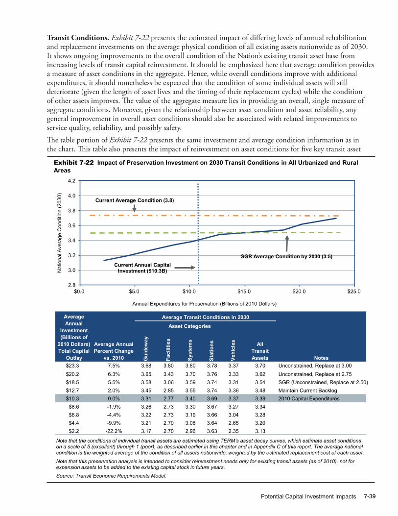
Potential Capital Investment Impacts 7-39

Transit Conditions. Exhibit 7-22 presents the estimated impact of differing levels of annual rehabilitation and replacement investments on the average physical condition of all existing assets nationwide as of 2030. It shows ongoing improvements to the overall condition of the Nation’s existing transit asset base from increasing levels of transit capital reinvestment. It should be emphasized here that average condition provides a measure of asset conditions in the aggregate. Hence, while overall conditions improve with additional expenditures, it should nonetheless be expected that the condition of some individual assets will still deteriorate (given the length of asset lives and the timing of their replacement cycles) while the condition of other assets improves. The value of the aggregate measure lies in providing an overall, single measure of aggregate conditions. Moreover, given the relationship between asset condition and asset reliability, any general improvement in overall asset conditions should also be associated with related improvements to service quality, reliability, and possibly safety.The table portion of Exhibit 7-22 presents the same investment and average condition information as in the chart. This table also presents the impact of reinvestment on asset conditions for five key transit asset

07XT_B (7-22) R4.xlsx 12/28/2012

Gui

dew

ay

Faci

litie

s

Syst

ems

Stat

ions

Vehi

cles

Notes$23.3 7.5% 3.68 3.80 3.80 3.78 3.37 3.70 Unconstrained, Replace at 3.00$20.2 6.3% 3.65 3.43 3.70 3.76 3.33 3.62 Unconstrained, Replace at 2.75$18.5 5.5% 3.58 3.06 3.59 3.74 3.31 3.54 SGR (Unconstrained, Replace at 2.50)$12.7 2.0% 3.45 2.85 3.55 3.74 3.36 3.48 Maintain Current Backlog$10.3 0.0% 3.31 2.77 3.40 3.69 3.37 3.39 2010 Capital Expenditures$8.6 -1.9% 3.26 2.73 3.30 3.67 3.27 3.34$6.8 -4.4% 3.22 2.73 3.19 3.66 3.04 3.28$4.4 -9.9% 3.21 2.70 3.08 3.64 2.65 3.20$2.2 -22.2% 3.17 2.70 2.96 3.63 2.35 3.13

Average Annual Percent Change

vs. 2010

Average Annual

Investment (Billions of

2010 Dollars)Total Capital

Outlay

Average Transit Conditions in 2030Asset Categories

All Transit Assets

2.8

3.0

3.2

3.4

3.6

3.8

4.0

4.2

$0.0 $5.0 $10.0 $15.0 $20.0 $25.0

Nat

iona

l Ave

rage

Con

ditio

n (2

030)

Annual Expenditures for Preservation (Billions of 2010 Dollars)

Current Annual Capital Investment ($10.3B)

Current Average Condition (3.8)

SGR Average Condition by 2030 (3.5)

Note that the conditions of individual transit assets are estimated using TERM’s asset decay curves, which estimate asset conditions on a scale of 5 (excellent) through 1 (poor), as described earlier in this chapter and in Appendix C of this report. The average national condition is the weighted average of the condition of all assets nationwide, weighted by the estimated replacement cost of each asset. Note that this preservation analysis is intended to consider reinvestment needs only for existing transit assets (as of 2010), not for expansion assets to be added to the existing capital stock in future years. Source: Transit Economic Requirements Model.

Exhibit 7-22 Impact of Preservation Investment on 2030 Transit Conditions in All Urbanized and Rural Areas

Investment/Performance Analysis7-40

categories (i.e., guideway and track, facilities, systems, stations, and vehicles) as well as the average annual percent change in constant dollar funding from 2010 levels to achieve each projected condition level.

Further review of Exhibit 7-22 reveals several observations. First, note that none of the selected reinvestment rates presented (including the current level of reinvestment, which was $10.3 billion in 2010) is sufficient to maintain aggregate conditions at or near the current national average condition rating of 3.8. Even the highest reinvestment rate presented here of $23.3 billion annually (replacement at condition rating 3.0), which represents a fairly aggressive reinvestment rate, is not quite sufficient to maintain aggregate conditions at current levels. A primary factor driving this result is the ongoing expansion investment in new rail systems over the past several decades, which has tended to maintain or even increase the average condition rating of assets nationwide (despite the ongoing deterioration of older assets), but has also resulted in an average condition rating that is not sustainable in the long term (i.e., without including the influence of further expansion investments or replacing assets at an unreasonably early age). Second, note that reinvestment at roughly $18.5 billion annually is required to attain a condition of SGR by 2030 and that this level of reinvestment is estimated to yield an average condition value of roughly 3.5 by 2030. Given the definition of the SGR benchmark (described in more detail in Chapter 8), which seeks to eliminate the existing investment backlog and then address all subsequent rehabilitation and replacement activities “on time” thereafter, the 3.5 value could be considered representative of the expected long-term average condition of a well-maintained and financially unconstrained national transit system. Hence, an average condition rating of roughly 3.5 represents a more reasonable long-term condition target for existing transit infrastructure than the current aggregate rating of 3.8.

A final observation is that a significant level of reinvestment is required to alter the estimated 2030 average condition measure by a point or more. This result is also driven in part by a large proportion of transit assets with expected useful lives of up to 80 years or more that will not require significant reinvestment over the 20-year period of this analysis (regardless of the level of reinvestment). These assets tend to contribute a high weighting in the average condition measure, making the measure somewhat insensitive to the rate of reinvestment (note that a high proportion of reinvestment activity is focused on the replacement of those assets with relatively shorter useful lives, such as vehicles).

Impact of Expansion Investments on Transit RidershipWhile capital spending on preservation primarily benefits the physical condition of existing transit assets, expansion investments are typically undertaken to expand the asset base to accommodate projected growth in ridership and potentially to improve service performance for existing transit system users.

Exhibit 7-23 shows the relationship between aggregated annual capital spending by all levels of government on expansion investments and the additional number of annual passenger boardings that transit systems would be able to support by 2030. More precisely, this chart presents the level of expansion investment required to ensure that transit vehicle occupancy rates are maintained at current levels over the next two decades for a broad range of the potential rates of growth in transit passenger miles traveled (PMT). As the upward sloping curve of the chart indicates, higher levels of investment are required to support greater numbers of additional riders at a constant level of service. If investment levels are insufficient to fully support the projected growth in ridership, then vehicle occupancy rates will tend to increase, leading to increased crowding on high-utilization systems and potentially leading to increased dwell times at stops, reduced average operating speeds, and increased rates of vehicle wear. Conversely, if the rate of transit capacity expansion exceeds the actual rate of ridership growth, then occupancy rates will tend to decline and service performance would likely also improve.

The findings presented in Exhibit 7-23 suggest the following trends. First, the recent rate of investment in asset expansion ($6.2 billion in 2010) could support roughly 4.6 billion additional boardings by 2030 (approximately a 1.8 percent annual growth in ridership). This amount is greater than that required to support the level of growth projected by the Nation’s MPOs (roughly 1.3 percent when adjusted to

Potential Capital Investment Impacts 7-41

exclude expansion investments that do not pass TERM’s benefit-cost test). As discussed in further detail in Chapter 9, MPO projections of transit growth (which are financially constrained) have typically fallen well short of actual growth in recent years. Assuming that the actual rate of ridership growth is close to the trend rate of growth for the last 15 years, then an average of $7.1 billion in annual transit capital expansion investment would be required over the next 20 years to support an additional 5.4 billion annual boardings (again after excluding expansion investments that do not pass TERM’s benefit-cost test). Hence, while the existing levels of transit capital expansion investment may be sufficient to maintain current service performance (i.e., vehicle occupancy rates) if ridership growth is relatively low, this level of investment is roughly two-thirds that required to support a level of ridership growth consistent with that experienced over the most recent 15-year period.

12/28/2012 07XT_D (7-23) R3.xlsx

Funding Level Description$14.4 7.7% 13.8 4.3%$10.2 4.6% 8.5 3.0%$7.1 1.3% 5.4 2.1% Trend Growth in PMT (1995 to 2010)$6.2 0.0% 4.6 1.8% 2010 Capital Expenditures (Maintain Current Spending)$4.6 -3.5% 3.0 1.3% MPO Projected Increase in PMT$3.5 -6.3% 2.0 0.9%$0.8 -36.0% 0.4 0.2%

Average Annual Percent

Change vs. 2010

Average Annual

Investment (Billions of

2010 Dollars)

Total New Boardings by 2030New Riders

Supported (Billions of Annual

Boardings)

Average Annual Growth in

Boardings*

0

2

4

6

8

10

12

14

16

$0.0 $2.0 $4.0 $6.0 $8.0 $10.0 $12.0 $14.0 $16.0

New

Boa

rdin

gs S

uppo

rted

by 2

030

(Bill

ions

)

Annual Expenditures in Expansion (Billions of 2010 Dollars)

MPO Projected Increase in Boardings by 2030 (3.0B)

Average Investment in Expansion 2010 ($6.2B)

Trend Increase in Boardings by 2030 (5.4B)

* As compared with total urban ridership in 2010; only includes increases covered by investments passing TERM's benefit-cost test. Note that TERM assesses expansion needs at the agency-mode level subject to (1) current vehicle occupancy rates at the agency-mode level and (2) expected transit PMT growth at the UZA level (hence, all agency modes within a given UZA are subject to the same transit PMT growth rate). Note, however, that TERM does not generate expansion needs estimates for agency modes that have occupancy rates that are well below the national average for that mode. Source: Transit Economic Requirements Model.

Exhibit 7-23 New Ridership Supported in 2030 by Expansion Investments in All Urbanized and Rural Areas

12/28/2012 07XT_D (7-23) R3.xlsx

Funding Level Description$14.4 7.7% 13.8 4.3%$10.2 4.6% 8.5 3.0%$7.1 1.3% 5.4 2.1% Trend Growth in PMT (1995 to 2010)$6.2 0.0% 4.6 1.8% 2010 Capital Expenditures (Maintain Current Spending)$4.6 -3.5% 3.0 1.3% MPO Projected Increase in PMT$3.5 -6.3% 2.0 0.9%$0.8 -36.0% 0.4 0.2%

Average Annual Percent

Change vs. 2010

Average Annual

Investment (Billions of

2010 Dollars)

Total New Boardings by 2030New Riders

Supported (Billions of Annual

Boardings)

Average Annual Growth in

Boardings*

0

2

4

6

8

10

12

14

16

$0.0 $2.0 $4.0 $6.0 $8.0 $10.0 $12.0 $14.0 $16.0

New

Boa

rdin

gs S

uppo

rted

by 2

030

(Bill

ions

)

Annual Expenditures in Expansion (Billions of 2010 Dollars)

MPO Projected Increase in Boardings by 2030 (3.0B)

Average Investment in Expansion 2010 ($6.2B)

Trend Increase in Boardings by 2030 (5.4B)

* As compared with total urban ridership in 2010; only includes increases covered by investments passing TERM's benefit-cost test. Note that TERM assesses expansion needs at the agency-mode level subject to (1) current vehicle occupancy rates at the agency-mode level and (2) expected transit PMT growth at the UZA level (hence, all agency modes within a given UZA are subject to the same transit PMT growth rate). Note, however, that TERM does not generate expansion needs estimates for agency modes that have occupancy rates that are well below the national average for that mode. Source: Transit Economic Requirements Model.

Exhibit 7-23 New Ridership Supported in 2030 by Expansion Investments in All Urbanized and Rural Areas

Impacts of Urbanized Area Investments Modeled by TERMThe remainder of this chapter focuses on how different levels of annual capital investment in the U.S. transit infrastructure affect urbanized areas with dissimilar transit investment needs. Specifically, this section explores the impact of capital expenditures by transit agencies sorted into two distinct UZA groupings: (1) the urbanized areas with populations greater than 1 million and (2) all other urbanized and rural areas with existing transit services.

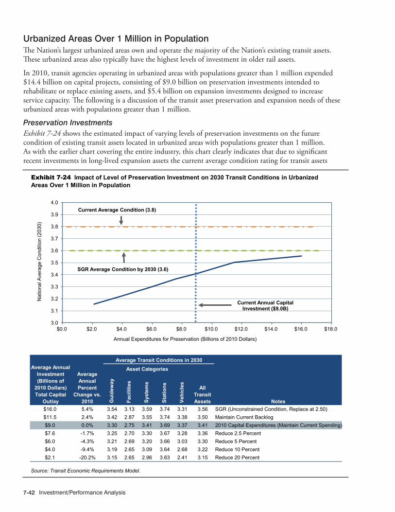
Investment/Performance Analysis7-42

Urbanized Areas Over 1 Million in PopulationThe Nation’s largest urbanized areas own and operate the majority of the Nation’s existing transit assets. These urbanized areas also typically have the highest levels of investment in older rail assets.

In 2010, transit agencies operating in urbanized areas with populations greater than 1 million expended $14.4 billion on capital projects, consisting of $9.0 billion on preservation investments intended to rehabilitate or replace existing assets, and $5.4 billion on expansion investments designed to increase service capacity. The following is a discussion of the transit asset preservation and expansion needs of these urbanized areas with populations greater than 1 million.

Preservation InvestmentsExhibit 7-24 shows the estimated impact of varying levels of preservation investments on the future condition of existing transit assets located in urbanized areas with populations greater than 1 million. As with the earlier chart covering the entire industry, this chart clearly indicates that due to significant recent investments in long-lived expansion assets the current average condition rating for transit assets

12/28/2012 07XT_E (7-24) R4.xlsx

Gui

dew

ay

Fac

ilitie

s

Sys

tem

s

Sta

tions

Veh

icle

s

Notes$16.0 5.4% 3.54 3.13 3.59 3.74 3.31 3.56 SGR (Unconstrained Condition, Replace at 2.50)$11.5 2.4% 3.42 2.87 3.55 3.74 3.38 3.50 Maintain Current Backlog$9.0 0.0% 3.30 2.75 3.41 3.69 3.37 3.41 2010 Capital Expenditures (Maintain Current Spending)$7.6 -1.7% 3.25 2.70 3.30 3.67 3.28 3.36 Reduce 2.5 Percent$6.0 -4.3% 3.21 2.69 3.20 3.66 3.03 3.30 Reduce 5 Percent$4.0 -9.4% 3.19 2.65 3.09 3.64 2.68 3.22 Reduce 10 Percent$2.1 -20.2% 3.15 2.65 2.96 3.63 2.41 3.15 Reduce 20 Percent

Average Annual Percent

Change vs. 2010

Average Annual Investment (Billions of

2010 Dollars)Total Capital

Outlay

Average Transit Conditions in 2030Asset Categories

All Transit Assets

3.0

3.1

3.2

3.3

3.4

3.5

3.6

3.7

3.8

3.9

4.0

$0.0 $2.0 $4.0 $6.0 $8.0 $10.0 $12.0 $14.0 $16.0 $18.0

Nat

iona

l Ave

rage

Con

ditio

n (2

030)

Annual Expenditures for Preservation (Billions of 2010 Dollars)

Current Annual Capital Investment ($9.0B)

Current Average Condition (3.8)

SGR Average Condition by 2030 (3.6)

Source: Transit Economic Requirements Model.

Exhibit 7-24 Impact of Level of Preservation Investment on 2030 Transit Conditions in Urbanized Areas Over 1 Million in Population

Potential Capital Investment Impacts 7-43

located in the largest urbanized areas is not sustainable in the long term without replacing assets on a fairly aggressive schedule (i.e., replacement at or before condition rating 3.0). At the same time, the 2010 level of reinvestment ($9.0 billion) is less than that required to attain a state of good repair ($16.0 billion), with the latter supporting a more sustainable long-term average condition rating of roughly 3.6.

As shown in Exhibit 7-25, the 2010 level of capital reinvestment of $9.0 billion for the largest urbanized areas is insufficient to keep pace with ongoing rehabilitation and replacement needs and, if maintained over the next 20 years, would result in a larger SGR backlog of roughly $120.4 billion by 2030 compared with the current $73.8 billion backlog. In contrast, increasing the rate of reinvestment to an annual average of roughly $16.0 billion will completely eliminate the entire backlog by 2030. The annual level of reinvestment would need to be increased to roughly $11.5 billion to maintain the backlog at roughly its current size.

07XT_F (7-25) R4.xlsx 12/28/2012

Funding Level Description$16.0 5.4% 2.50 3.56 $0.0 SGR (Unconstrained, Replace at 2.50)$11.5 2.4% 2.50 3.50 $73.8 Current Backlog$9.0 0.0% 2.50 3.41 $120.4 2010 Capital Expenditures$7.6 -1.7% 2.50 3.36 $145.7$6.0 -4.3% 2.50 3.30 $173.9$4.0 -9.4% 2.50 3.22 $209.2

Average Annual Percent Change

vs. 2010

Average Annual Investment

(Billions of 2010 Dollars)

Replacement Condition

Average Condition

Rating in 2030

Backlog in 2030 (Billions of 2010

Dollars)

$0

$50

$100

$150

$200

$250

$4.0 $6.0 $8.0 $10.0 $12.0 $14.0 $16.0

2030

Sta

te o

f Goo

d R

epai

r Bac

klog

(B

illio

ns o

f 201

0 D

olla

rs)

Annual Expenditures for Preservation (Billions of 2010 Dollars)

Current Backlog ($73.8B)

Current Annual Capital Investment ($9.0B)

Source: Transit Economic Requirements Model.

Exhibit 7-25 Impact of Preservation Investment on 2030 Transit State of Good Repair Backlog in Urbanized Areas Over 1 Million in Population

Expansion InvestmentsAlthough urbanized areas with populations greater than 1 million tend to be cities with slower rates of increase in population and transit ridership (e.g., Boston, Philadelphia, and Chicago), this group also includes urbanized areas expected to experience relatively high rates of growth in transit boardings and PMT over the next two decades, including Los Angeles, Atlanta, and Seattle. Given the high numbers of existing riders and transit capacity in these higher-growth large urbanized areas, they will require significant increases in expansion investments to maintain current service performance during this time period.

Investment/Performance Analysis7-44

Exhibit 7-26 presents estimates of the level of expansion investment required to support varying levels of growth in transit demand while maintaining current performance levels (as measured by vehicle capacity utilization) for these large urbanized areas. Note that the 2010 level of investment for these urbanized areas ($5.4 billion) was more than that required to support the rate of increase in transit demand as projected by the Nation’s MPOs (low growth) but well short of that required to support a rate of growth comparable to the trend rate of increase as experienced in recent years.

12/28/2012 07XT_G (7-26) R3.xlsx

Funding Level Description$11.8 7.3% 11.0 4.0%$8.6 4.5% 6.9 2.8%$6.1 1.3% 4.4 2.0% Trend Growth in PMT (1995 to 2010)$5.4 0.0% 3.7 1.7% Maintain Spending (2010)$4.1 -2.8% 2.5 1.2% MPO Projected Growth$3.2 -5.6% 1.7 0.8%$0.8 -31.8% 0.4 0.2%

Average Annual Percent Change

vs. 2010

Average Annual

Investment (Billions of

2010 Dollars)

Total New Boardings by 2030New Riders

Supported (Billions of Annual

Boardings)

Average Annual Growth in

Boardings*

0

2

4

6

8

10

12

$0.0 $2.0 $4.0 $6.0 $8.0 $10.0 $12.0 $14.0

New

Boa

rdin

gs S

uppo

rted

by 2

030

(Bill

ions

)

Annual Expenditures in Expansion (Billions of 2010 Dollars)

MPO Projected Increase in Boardings by 2030 (2.5B)

Average Investment in Expansion 2010 ($5.4B)

Trend Increase in Boardings by 2030 (4.4B)

* As compared with total urban ridership in 2010; only includes increases covered by investments passing TERM's benefit-cost test. Source: Transit Economic Requirements Model.

Exhibit 7-26 New Ridership Supported in 2030 by Expansion Investments in Urbanized Areas Over 1 Million in Population

Other Urbanized and Rural AreasThe following analysis considers the combined preservation and expansion needs of urbanized areas under 1 million in population and those of all rural areas with existing transit service. This diverse group therefore includes a large number of mid- and small-sized urbanized and rural transit operators offering only bus and/or paratransit services.

In 2010, transit agencies operating outside of the largest urbanized areas expended $2.2 billion on capital projects, consisting of $1.3 billion on preservation investments intended to rehabilitate or replace existing assets, and $0.9 billion on expansion investments designed to increase service capacity. The following is a discussion of the transit asset preservation and expansion needs of transit agencies in these areas.

Potential Capital Investment Impacts 7-45

Preservation InvestmentsExhibit 7-27 shows the estimated impact of varying levels of preservation investments on the future condition of existing transit assets located in urbanized areas with populations less than 1 million and in rural areas. As with the earlier analyses for the largest urbanized areas, this chart also indicates that the current average condition rating for transit assets in these smaller urbanized and rural areas is not sustainable in the long term without replacing assets on a fairly aggressive schedule (i.e., replacement at or before condition rating 3.0). At the same time, the 2010 level of reinvestment ($1.3 billion) is significantly less than that required to attain an SGR ($2.5 billion), with the latter supporting a more sustainable long-term average condition rating of roughly 3.4.

12/28/2012 07XT_H (7-27) R4.xlsx

Gui

dew

ay

Faci

litie

s

Syst

ems

Stat

ions

Vehi

cles

Notes$2.5 7.5% 4.45 2.93 3.73 3.87 3.30 3.36 SGR (Unconstrained, Replace at 2.5)$1.3 0.0% 3.57 2.79 3.11 3.75 3.32 3.09 2010 Capital Expenditures (Maintain Current Spending)

$0.90 -2.1% 3.57 2.78 3.05 3.51 3.23 3.06 Reduce 2.5 Percent$0.8 -3.3% 3.57 2.78 3.03 3.41 3.09 3.02 Reduce 5 Percent$0.4 -12.2% 3.57 2.78 2.99 3.38 2.37 2.86 Reduce 10 Percent$0.1 -52.1% 3.57 2.78 2.98 3.35 1.88 2.76 Reduce 20 Percent

Average Annual Percent Change vs. 2010

Average Annual

Investment (Billions of

2010 Dollars)Total Capital

Outlay

Average Transit Conditions in 2030Asset Categories

All Transit Assets

2.4

2.6

2.8

3.0

3.2

3.4

3.6

3.8

4.0

$0.0 $0.5 $1.0 $1.5 $2.0 $2.5

Nat

iona

l Ave

rage

Con

ditio

n (2

030)

Annual Expenditures for Preservation (Billions of 2010 Dollars)

Current Annual Capital Investment ($1.3 B)

Current Average Condition (3.6)

SGR Average Condition by 2030 (3.4)

Source: Transit Economic Requirements Model.

Exhibit 7-27 Impact of Preservation Investment on 2030 Transit Conditions in Urbanized Areas Under 1 Million in Population

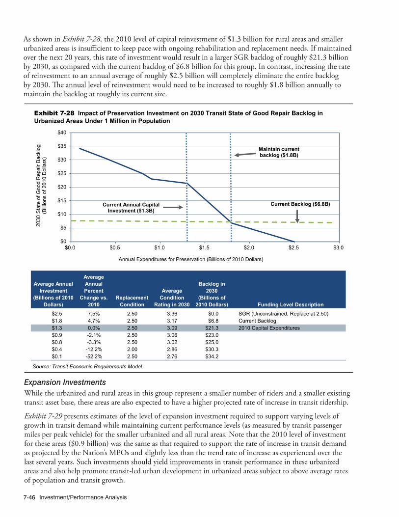
Investment/Performance Analysis7-46

As shown in Exhibit 7-28, the 2010 level of capital reinvestment of $1.3 billion for rural areas and smaller urbanized areas is insufficient to keep pace with ongoing rehabilitation and replacement needs. If maintained over the next 20 years, this rate of investment would result in a larger SGR backlog of roughly $21.3 billion by 2030, as compared with the current backlog of $6.8 billion for this group. In contrast, increasing the rate of reinvestment to an annual average of roughly $2.5 billion will completely eliminate the entire backlog by 2030. The annual level of reinvestment would need to be increased to roughly $1.8 billion annually to maintain the backlog at roughly its current size.

Funding Level Description$2.5 7.5% 2.50 3.36 $0.0 SGR (Unconstrained, Replace at 2.50)$1.8 4.7% 2.50 3.17 $6.8 Current Backlog$1.3 0.0% 2.50 3.09 $21.3 2010 Capital Expenditures$0.9 -2.1% 2.50 3.06 $23.0$0.8 -3.3% 2.50 3.02 $25.0$0.4 -12.2% 2.00 2.86 $30.3$0.1 -52.2% 2.50 2.76 $34.2

Average Annual Percent

Change vs. 2010

Average Annual Investment

(Billions of 2010 Dollars)

Replacement Condition

Average Condition

Rating in 2030

Backlog in 2030

(Billions of 2010 Dollars)

$0

$5

$10

$15

$20

$25

$30

$35

$40

$0.0 $0.5 $1.0 $1.5 $2.0 $2.5 $3.0

2030

Sta

te o

f Goo

d R

epai

r Bac

klog

(B

illio

ns o

f 201

0 D

olla

rs)

Annual Expenditures for Preservation (Billions of 2010 Dollars)

Current Backlog ($6.8B) Current Annual Capital Investment ($1.3B)

Maintain current backlog ($1.8B)

Source: Transit Economic Requirements Model.

Exhibit 7-28 Impact of Preservation Investment on 2030 Transit State of Good Repair Backlog in Urbanized Areas Under 1 Million in Population

07XT_I (7-28) R5.xlsx 12/18/2013

Expansion InvestmentsWhile the urbanized and rural areas in this group represent a smaller number of riders and a smaller existing transit asset base, these areas are also expected to have a higher projected rate of increase in transit ridership.

Exhibit 7-29 presents estimates of the level of expansion investment required to support varying levels of growth in transit demand while maintaining current performance levels (as measured by transit passenger miles per peak vehicle) for the smaller urbanized and all rural areas. Note that the 2010 level of investment for these areas ($0.9 billion) was the same as that required to support the rate of increase in transit demand as projected by the Nation’s MPOs and slightly less than the trend rate of increase as experienced over the last several years. Such investments should yield improvements in transit performance in these urbanized areas and also help promote transit-led urban development in urbanized areas subject to above average rates of population and transit growth.

Potential Capital Investment Impacts 7-47

12/28/2012 07XT_J (7-29) R3.xlsx

Funding Level Description$2.6 9.9% 2.8 6.4%$1.5 5.1% 1.6 4.5%$1.0 1.4% 1.0 3.2% Trend Growth in PMT (1995 to 2010)$0.9 0.0% 0.9 2.8% Maintain Spending (2010)$0.5 -7.3% 0.5 1.6% MPO Projected Growth$0.3 -11.6% 0.3 1.3%$0.1 -68.0% 0.1 0.3%

Average Annual Percent Change

vs. 2010

Average Annual Investment

(Billions of 2010 Dollars)

Total New Boardings by 2030New Riders

Supported (Billions of Annual

Boardings)

Average Annual Growth in

Boardings*

0.0

0.5

1.0

1.5

2.0

2.5

3.0

$0.0 $0.5 $1.0 $1.5 $2.0 $2.5 $3.0

New

Boa

rdin

gs S

uppo

rted

by 2

030

(Bill

ions

)

Annual Expenditures in Expansion (Billions of 2010 Dollars)

MPO Projected Increase in Boardings by 2030 (0.5B)

Average Investment in Expansion 2010 ($0.9B)

Trend Increase in Boardings by 2030 (1.0B)

* As compared with total urban ridership in 2008; only includes increases covered by investments passing TERM's benefit-cost test. Source: Transit Economic Requirements Model.

Exhibit 7-29 New Ridership Supported in 2030 by Expansion Investments in Urbanized Areas Under 1 Million in Population

Investment/Performance Analysis7-48

Selected Capital Investment Scenarios

Selected Highway Capital Investment Scenarios .......................................................8-2

Scenario Selected for Analysis ..................................................................................8-2

Scenario Spending Levels .........................................................................................8-4Spending Levels Assuming Forecast Growth in VMT ........................................................ 8-4Spending Levels Assuming Trend Growth in VMT ............................................................. 8-7

Scenario Spending Patterns and Conditions and Performance Projections ...........8-7Systemwide Scenarios ....................................................................................................... 8-7Federal-Aid Highway Scenarios ......................................................................................... 8-11Scenarios for the National Highway System and the Interstate Highway System ............ 8-18

Highway and Bridge Investment Backlog .................................................................8-21

Selected Transit Capital Investment Scenarios ..........................................................8-23

Sustain 2010 Spending Scenario ..............................................................................8-25Preservation Investments.................................................................................................... 8-26Expansion Investments ....................................................................................................... 8-27

State of Good Repair Benchmark..............................................................................8-29SGR Investment Needs ...................................................................................................... 8-29Impact on the Investment Backlog ..................................................................................... 8-30Impact on Conditions ......................................................................................................... 8-30Impact on Vehicle Fleet Performance ................................................................................. 8-31

Low and High Growth Scenarios ...............................................................................8-31Low Growth Assumption .................................................................................................... 8-32High Growth Assumption.................................................................................................... 8-32Low and High Growth Scenario Needs .............................................................................. 8-32Impact on Conditions and Performance ............................................................................ 8-33

Scenario Benefits Comparison ..................................................................................8-34Scorecard Comparisons ..................................................................................................... 8-36

Selected Capital Investment Scenarios 8-1

CHAPTER 8

Investment/Performance Analysis8-2

Selected Highway Capital Investment Scenarios

This section presents future investment scenarios that build on the Chapter 7 analyses of alternative levels of future investment in highways and bridges. Each scenario includes projections for system conditions and performance based on simulations with the Highway Economic Requirements System (HERS) and National Bridge Investment Analysis System (NBIAS). To put the modeling results in perspective, each scenario scales up the total amount of simulated investment using ratio factors to add in the types of highway and bridge investment that are beyond these models’ scopes. A subsequent section of this chapter explores transit investment scenarios that, like those of this section, start with a 2010 base year and cover the 20-year period through 2030. All the scenarios are intended to be illustrative; none of them is endorsed as a target level of funding.

Chapter 9 includes supplemental analyses relating to these scenarios, including comparisons with the investment levels presented for comparable scenarios in previous C&P reports. Chapter 10 includes a series of sensitivity analyses that explore the implications of alternative technical assumptions for the scenario investment levels. The Introduction to Part II provides critical background information relating to the technical limitations of the analysis, which are discussed further in the appendices.

Pursuant to Moving Ahead for Progress in the 21st Century (MAP-21), the National Highway System (NHS) will be expanded to include additional principal arterial and connector mileage that was not part of the original system. In light of this change, projecting future NHS investment needs over 20 years based on the system as it existed in 2010 would have limited value. Rather than dropping the NHS scenarios from the C&P report series until a formal NHS re-designation is completed, this report includes projections based on an estimate of what the system would ultimately look like by adding in principal arterials that are not currently part of the NHS. After the revised NHS designations have been coded into the HPMS and National Bridge Inventory (NBI), future editions of this report will use them for the NHS-based scenarios.

Scenarios Selected for AnalysisFor the entire road network and then separately for Federal-aid highways, the NHS, and the Interstate Highway System, this section examines the four scenarios described in Exhibit 8-1. Each of these scenarios is based on capital investment by all levels of government combined. The question of what portion should be funded by the Federal government, State governments, local governments, or the private sector is beyond the scope of this report. Each scenario pairs an assumed level of total investment in the types of improvements modeled by HERS with an assumed level of investment in the types of improvements modeled by NBIAS; these levels are drawn from those considered in Chapter 7. Together, the scopes of these models cover spending on highway expansion and pavement improvements on Federal-aid highways (HERS) and on bridge rehabilitation on all highways (NBIAS). In the absence of data required for the non-modeled types of highway and bridge investment, each scenario simply assumes that their share of highway and bridge investment will remain at the 2010 percentage. Percent shares in 2010 also served to distribute the amount of non-modeled investment among the component categories: pavement spending on non-Federal-aid highways, system expansion spending on non-Federal-aid highways, and system enhancement spending (which include safety enhancements, operational improvements, and environmental projects).

Selected Capital Investment Scenarios 8-3

12/12/2013 08XH_A (8-1) R2.xlsx

Intermediate Improvement

Improve Conditions and Performance

HERS-Derived

Sustain spending on types of capital improvements modeled in HERS at 2010 levels in constant dollar terms over next 20 years

Set spending at the average of (1) the level at which projected average IRI in 2030 matches that in 2010, and (2) the level at which projected average delay per VMT in 2030 matches that in 2010

Set spending at the level sufficient to fund all potential projects with a BCR greater than or equal to 1.5

Set spending at the level sufficient to fund all cost-beneficial potential projects (i.e., those with a BCR greater than or equal to 1.0)

NBIAS-Derived

Sustain spending on types of capital improvements modeled in NBIAS at 2010 levels in constant dollar terms over the next 20 years

Set spending at the level at which the projected average bridge sufficiency rating in 2030 matches that in 2010

Set spending at the level which achieves one-half of the projected increase to the average bridge sufficiency rating under the Improve Conditions and Performance scenario

Set spending at the level sufficient to fund all cost-beneficial potential projects

Other (Non-Modeled)

Sustain spending on types of capital improvements not modeled in HERS or NBIAS at 2010 levels in constant dollar terms over the next 20 years

Set spending at the level necessary so thatthe nonmodeled share of total highway and bridge investment will remain the same as in 2010

Set spending at the level necessary so that the nonmodeled share of total highway and bridge investment will remain the same as in 2010

Set spending at the level necessary so that the nonmodeled share of total highway and bridge investment will remain the same as in 2010

Scenario Component

Sustain 2010 Spending*

Maintain Conditions and Performance

Exhibit 8-1 Capital Investment Scenarios for Highways and Bridges, Derivation of Components

* Highway capital spending in 2010 was supplemented by one-time funding under the Recovery Act.

How do the definitions of the selected scenarios presented in this report compare to those presented in the 2010 C&P Report?

The Sustain 2010 Spending scenario is defined in a manner consistent with the Sustain Current Spending scenario presented in previous editions of the C&P report; however, the scenario name was changed to emphasize that 2010 was an atypical year, since spending was boosted by one-time funding under the Recovery Act. The names and definitions of the Improve Conditions and Performance scenario and the State of Good Repair benchmark are unchanged.

The definition of the HERS-derived component of the Intermediate Improvement scenario remains unchanged. For the 2010 C&P Report, the NBIAS-derived component was defined around the average annual spending growth rate taken from the HERS-derived component; for this edition, the NBIAS-derived component has been redefined to be independent of HERS, and instead represents a level of investment that achieves half of the improvement in the average bridge sufficiency rating computed for the Improve Conditions and Performance scenario.

The Maintain Conditions and Performance scenario is similar in concept to the comparable scenario in the 2010 C&P Report, in that it attempts to maintain selected performance measures at their base-year levels through the end of the 20-year analysis period; however, the target measures have been modified. The NBIAS-derived component of the scenario targets the average bridge sufficiency rating rather than the bridge investment backlog, a measure that was utilized for the last several editions of the C&P report.

The HERS-derived component of the Maintain Conditions and Performance scenario had been defined around maintaining average highway user cost for several editions through the 2008 C&P Report. For technical reasons, it had become increasingly cumbersome to apply and explain this target measure, so in the 2010 C&P Report, average speed was adopted instead, in large part because it yielded similar results at the systemwide level (though this was not consistently true for subsets of the system). The HERS-derived component of this scenario used for the current edition is defined as the average of the investment level estimated to be sufficient to maintain average IRI, and the investment level estimated to be sufficient to maintain average delay. In practice, this approach results in one of these target measures improving somewhat over 20 years, while the other gets somewhat worse—an outcome consistent with the results obtained when the target measure was average highway user cost. At the systemwide level, and assuming that VMT growth conforms to HPMS forecasts, using average speed as the target measure as in the 2010 C&P Report would have produced annual average investment levels of $88.4 billion, or 2.5 percent more than what is shown in Exhibit 8-2.

Q A&

Investment/Performance Analysis8-4

The projections for conditions and performance in each scenario represent estimates of what could be achieved with a given level of investment assuming an economically driven approach to project selection. They do not represent what would be achieved given current decision making practices. Consequently, comparing the relative conditions and performance outcomes across the different scenarios may be more illuminating than focusing on the specific projections for each individual scenario.

Scenario Spending LevelsFuture spending levels by scenario, summarized in Exhibit 8-2, are stated in constant 2010 dollars. (Chapter 9 illustrates how to convert these real-dollar values into nominal [future dollar] values that factor in inflation beyond 2010.) The modeling on which the scenarios are based (which was presented in Chapter 7) assumes that spending grows at an annual percent rate that does not vary over the 20-year analysis period, but which differs between the types of investments modeled by HERS and those modeled by NBIAS, and also in some scenarios according to the assumed rate of future traffic growth. (The average annual investment levels are determined by summing the amounts expended for each year from 2011 through 2030 under the scenario, and dividing by 20.)

The application of the four illustrative scenarios to different highway systems produces the subscenarios in Exhibit 8-2. For example, the subscenario for Federal-aid highways in the Sustain 2010 Spending scenario fixes average annual spending on those highways at what was actually spent in 2010, $75.8 billion, without likewise forcing the portions of that spending directed to the NHS or the Interstate System to match their 2010 levels. Differences between these portions and the corresponding base-year amounts arise because HERS and NBIAS rely on benefit-cost principles to flexibly allocate spending among potential improvements within their scope.

For each of the other scenarios in Exhibit 8-2, the spending levels vary according to the future growth rate assumed for vehicle miles traveled (VMT). As discussed in Chapter 7, the VMT forecasts from the HPMS imply an average annual growth rate of 1.85 percent, whereas the 15-year trend growth (between 1995 and 2010) was only 1.36 percent. Assuming that future growth follows the trend rather than the forecast rate reduces the spending level associated with achieving scenario goals related to pavement improvements and system expansion, which are modeled with HERS. The needs for bridge rehabilitation spending are less sensitive to changes in VMT growth, so the implied traffic growth from the NBI forecasts was used to generate all of the NBIAS inputs to these scenarios.

The Maintain Conditions and Performance scenario is geared toward maintaining overall conditions and performance on the particular portion of the road network to which the scenario is being applied. For example, when the scenario relates to maintaining average conditions and performance on Federal-aid highways, it may entail improvement or deterioration in average conditions and performance on subsets of these highways, such as the Interstate Highway System. The models used to simulate the scenarios, HERS and NBIAS, are each designed to determine the investment program that will minimize the cost of achieving the scenario goal.

Spending Levels Assuming Forecast Growth in VMTThe Maintain Conditions and Performance scenario uses average pavement roughness, average delay per VMT, and average bridge sufficiency rating as the measures of overall system conditions and performance that it seeks to maintain. Although the system to which these goals pertain varies across the subscenarios, the average annual amount of investment is uniformly less than actual 2010 spending. A major reason for this pattern is that the 2010 level of investment was quite high by historical standards (due largely to the

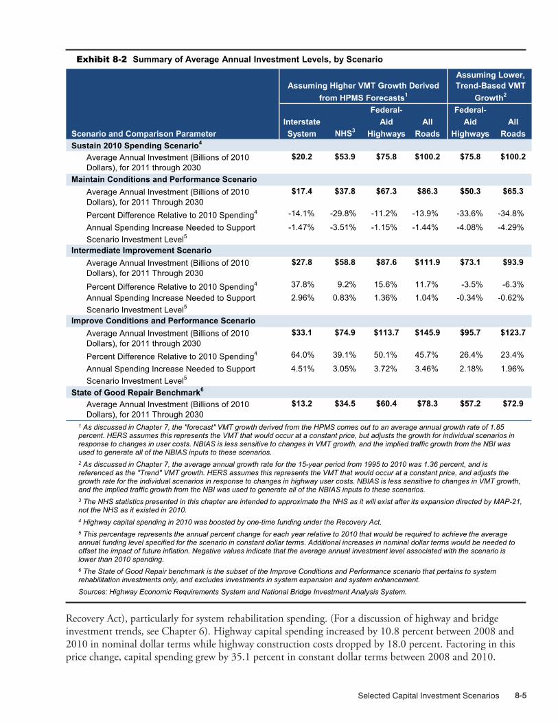
Selected Capital Investment Scenarios 8-5

12/12/2013 08XH_B (8-2) R2.xlsx

Federal- Federal-Interstate Aid All Aid All

Scenario and Comparison Parameter System NHS3 Highways Roads Highways Roads

Average Annual Investment (Billions of 2010 Dollars), for 2011 through 2030

$20.2 $53.9 $75.8 $100.2 $75.8 $100.2

Average Annual Investment (Billions of 2010 Dollars), for 2011 Through 2030

$17.4 $37.8 $67.3 $86.3 $50.3 $65.3

Percent Difference Relative to 2010 Spending4 -14.1% -29.8% -11.2% -13.9% -33.6% -34.8%

Annual Spending Increase Needed to Support Scenario Investment Level5

-1.47% -3.51% -1.15% -1.44% -4.08% -4.29%

Average Annual Investment (Billions of 2010 Dollars), for 2011 Through 2030

$27.8 $58.8 $87.6 $111.9 $73.1 $93.9

Percent Difference Relative to 2010 Spending4 37.8% 9.2% 15.6% 11.7% -3.5% -6.3%Annual Spending Increase Needed to Support Scenario Investment Level5

2.96% 0.83% 1.36% 1.04% -0.34% -0.62%

Average Annual Investment (Billions of 2010 Dollars), for 2011 through 2030

$33.1 $74.9 $113.7 $145.9 $95.7 $123.7

Percent Difference Relative to 2010 Spending4 64.0% 39.1% 50.1% 45.7% 26.4% 23.4%

Annual Spending Increase Needed to Support Scenario Investment Level5

4.51% 3.05% 3.72% 3.46% 2.18% 1.96%

Average Annual Investment (Billions of 2010 Dollars), for 2011 Through 2030

$13.2 $34.5 $60.4 $78.3 $57.2 $72.9

Assuming Higher VMT Growth Derived from HPMS Forecasts1

Assuming Lower, Trend-Based VMT

Growth2

State of Good Repair Benchmark6

Sustain 2010 Spending Scenario4

Maintain Conditions and Performance Scenario

Intermediate Improvement Scenario

Improve Conditions and Performance Scenario

Exhibit 8-2 Summary of Average Annual Investment Levels, by Scenario

1 As discussed in Chapter 7, the "forecast" VMT growth derived from the HPMS comes out to an average annual growth rate of 1.85 percent. HERS assumes this represents the VMT that would occur at a constant price, but adjusts the growth for individual scenarios in response to changes in user costs. NBIAS is less sensitive to changes in VMT growth, and the implied traffic growth from the NBI was used to generate all of the NBIAS inputs to these scenarios. 2 As discussed in Chapter 7, the average annual growth rate for the 15-year period from 1995 to 2010 was 1.36 percent, and is referenced as the "Trend" VMT growth. HERS assumes this represents the VMT that would occur at a constant price, and adjusts the growth rate for the individual scenarios in response to changes in highway user costs. NBIAS is less sensitive to changes in VMT growth, and the implied traffic growth from the NBI was used to generate all of the NBIAS inputs to these scenarios. 3 The NHS statistics presented in this chapter are intended to approximate the NHS as it will exist after its expansion directed by MAP-21, not the NHS as it existed in 2010. 4 Highway capital spending in 2010 was boosted by one-time funding under the Recovery Act. 5 This percentage represents the annual percent change for each year relative to 2010 that would be required to achieve the average annual funding level specified for the scenario in constant dollar terms. Additional increases in nominal dollar terms would be needed to offset the impact of future inflation. Negative values indicate that the average annual investment level associated with the scenario is lower than 2010 spending. 6 The State of Good Repair benchmark is the subset of the Improve Conditions and Performance scenario that pertains to system rehabilitation investments only, and excludes investments in system expansion and system enhancement. Sources: Highway Economic Requirements System and National Bridge Investment Analysis System.

Recovery Act), particularly for system rehabilitation spending. (For a discussion of highway and bridge investment trends, see Chapter 6). Highway capital spending increased by 10.8 percent between 2008 and 2010 in nominal dollar terms while highway construction costs dropped by 18.0 percent. Factoring in this price change, capital spending grew by 35.1 percent in constant dollar terms between 2008 and 2010.

Investment/Performance Analysis8-6

For the version of the Maintain Conditions and Performance scenario focused on all roads (and assuming HPMS forecast VMT growth), the average annual investment level of $86.3 billion is 13.9 percent lower than actual 2010 capital spending of $100.2 billion on all roads; the goals of this subscenario could be achieved even if capital spending declined by 1.44 percent per year over 20 years in constant dollar terms. Similar percentage differences are evident in the subscenarios for Federal-aid highways (11.2 percent) and Interstate highways (14.1 percent). The outlier is the sub-scenario for the NHS, where the level of investment to maintain conditions and performance is estimated to be 29.8 percent lower than the amount of investment directed to that system in 2010. Because the Interstate highways form a significant portion of the NHS, this implies relatively sharp reductions in spending for the remaining portion off of the Interstate System. Annual percentage growth rates in spending are between -1.0 percent and -1.5 percent across subscenarios, except for the -3.5 percent annual decline in spending indicated to be consistent with maintaining overall conditions and performance on the NHS. It is important to note that because 2010 highway capital spending included one-time funding under the Recovery Act, sustaining this level of investment in the future would present a greater challenge than would be the case for a more typical base year.

Unless one is completely satisfied with base year conditions and performance, investing at a level projected to maintain that level of performance would not yield an ideal result. The analyses reflected in the Improve Conditions and Performance scenario suggest that an economically driven approach to investment that funds all cost-beneficial improvements would substantially increase real spending on highways and bridges above base-year levels. Assuming forecast VMT growth for the 2011–2030 analysis period, the annual percent increase in investment associated with implementation of all cost-beneficial capital improvements is 4.51 percent for the Interstate highways, 3.05 percent for the NHS, 3.72 percent for Federal-aid highways, and 3.46 percent for all roads. The associated levels of average annual spending represent an investment ceiling above which it would not be cost-beneficial to invest even if available funding were unlimited, and exceed the 2010 levels by 64.0 percent for Interstate highways, 39.1 percent for the NHS, 50.1 percent for Federal-aid highways, and 45.7 percent for all roads. For all roads, the average annual spending amounts to fully implement all cost-beneficial investments is estimated to be $145.9 billion, or $2.9 trillion over the 20-year period, stated in constant 2010 dollars.

The State of Good Repair benchmark represents the portion of average annual spending that the Improve Conditions and Performance scenario allocates to system rehabilitation investments. Put at $78.3 billion in Exhibit 8-2 for all roads, this benchmark represents the amount of cost-beneficial investment identified

Does the State of Good Repair benchmark apply the same criteria for all types of roadways modeled in HERS?

No. For principal arterials, the deficiency levels in HERS have been set so that the model will consider taking action on a pavement only when its International Roughness Index (IRI) value has risen above 95 (inches per mile), meaning that it would no longer be considered to have “good” ride quality based on the criteria described in Chapter 3.

For roads functionally classified as collectors, the HERS deficiency levels have been set so that pavement actions will only be considered when IRI values have risen above 170, and the roads, thus, no longer meet the criteria for “acceptable” ride quality. The IRI threshold for minor arterials is set at 120.

Although the engineering thresholds identified above define when the model may consider a pavement improvement, any such improvement must pass a benefit-cost test in order to be implemented. Even when HERS is given an unlimited budget to work with, it does not recommend improving all principal arterials to the “good” ride quality level, or all collectors to the “acceptable” ride quality level. The specific IRI value at which a pavement improvement will pass a benefit-cost test depends on a number of factors, including the traffic volume and average speeds on that facility. As discussed in Chapter 3, pavement ride quality has a greater impact on highway user costs on higher-speed roads.

Q A&

Selected Capital Investment Scenarios 8-7

for rehabilitation of existing pavements and bridges. In determining the size of this benchmark, HERS and NBIAS screen out through benefit-cost analysis any assets that may have outlived their original purpose, rather than automatically re-investing in all assets in perpetuity. With national consensus lacking on exactly what constitutes a “state of good repair” for the various transportation assets, alternative benchmarks with different objectives could be equally valid from a technical perspective.

The goal of the Intermediate Improvement scenario is to partially achieve the performance improvements associated with the economically driven approach to investment taken in the Improve Conditions and Performance scenario. For bridge rehabilitation spending, the Intermediate Improvement scenario seeks to achieve half of the improvement in the average bridge sufficiency rating; for spending on pavement rehabilitation and highway expansion, the scenario implements all projects with a benefit-cost ratio (BCR) of 1.5 or greater, as opposed to 1.0 or greater in the Improve Conditions and Performance scenario. (Applying a minimum BCR cutoff higher than 1.0 reduces the risk of investing in projects that initially appear cost beneficial but do not prove so due to unexpected changes in future costs or travel demand.) Assuming forecast VMT growth for 2011–2030, the average annual spending in the Intermediate Improvement scenario for all roads, $111.9 billion, exceeds the actual 2010 level by $11.7 billion, which is about one-fourth of the $45.7 billion increase indicated in the Improve Conditions and Performance scenario. For the Federal-aid highways and the NHS, the corresponding proportion is similar to that for all roads, but, for the Interstate System, the increase in spending relative to 2010 under the Intermediate Improvement scenario amounts to nearly three-fifths of the increase under the Improve Conditions and Performance scenario.

Spending Levels Assuming Trend Growth in VMTReplacing the overall rate of traffic growth implied by the HPMS forecasts with the 15-year historic trend rate of growth reduces the scenario levels of spending substantially. Annual spending in the Maintain Conditions and Performance scenario averages $65.3 billion for all roads and $50.3 billion for Federal-aid highways, which are each about 25 percent lower than when the overall rate of VMT growth from the HMPS forecasts was used. For the Intermediate Improvement and Improve Conditions and Performance scenarios, the spending reductions from the forecast growth case are smaller, at about 16 percent. The results for annual percent growth in spending show spending decreasing at just over 4 percent per year in the Maintain Conditions and Performance scenario, and at less than one percent in the Intermediate Improvement scenario. Only in the Improve Conditions and Performance scenario does spending increase, at about 2 percent per year, when trend growth in traffic is assumed.

Scenario Spending Patterns and Conditions and Performance Projections

The following discussion details the derivation of scenario spending levels, the patterns in spending by type of improvement and highway functional class, and the projections for conditions and performance.

Systemwide ScenariosFor the scenarios that consider all roads, the derivation of the average annual investment levels is presented in Exhibit 8-3 (forecast-based VMT growth) and Exhibit 8-4 (trend-based VMT growth). The HERS-derived component, which accounts in each scenario for most of the total investment, represents spending on pavement rehabilitation and capacity expansion on Federal-aid highways. The NBIAS-derived component represents rehabilitation spending on all bridges, including those not on the Federal-aid highways. In the Sustain 2010 Spending scenario, the values for these components sum to $72.5 billion, of which $56.4 billion is the HERS-derived component. Nonmodeled spending accounted in 2010 for 26.6 percent

Investment/Performance Analysis8-8

of total investment ($26.7 billion out of $100.2 billion) and is assumed to form the same share in all scenarios. The non-modeled spending is allocated among types of capital improvements according to its 2010 percent distribution: 36.7 percent, system rehabilitation (non-Federal-aid highways); 15.4 percent, system expansion (non-Federal-aid highways), and 47.9 percent, system enhancements. Because they include non-modeled spending, the amounts shown in any scenario for the “system rehabilitation-highway” and “system expansion” categories sum to more than the HERS-derived component of spending.

The minimum BCR associated with the HERS components of the Improve Conditions and Performance scenario (1.0) and the Intermediate Improvement scenario (1.5) are the same whether forecast VMT growth or trend-based VMT growth is assumed, as these scenarios are defined around these particular BCR levels. For the Sustain 2010 Spending scenario, the minimum BCR of 1.92 assuming forecast VMT growth (Exhibit 8-3) is higher than the minimum BCR of 1.42 assuming trend-based VMT growth (Exhibit 8-4) because higher future travel volumes would tend to increase the benefits associated with both pavement and 12/11/2013 08XH_C (8-3) R2.xlsx

Sustain Maintain Improve2010 Conditions & Intermediate Conditions &

Spending Performance Improvement PerformanceScenario Scenario Scenario Scenario

Scenario Derivation, by Input Components*Average Annual Investment (Billions of 2010 Dollars) $100.2 $86.3 $111.9 $145.9HERS-Derived Component (Billions of 2010 Dollars) $56.4 $51.1 $67.8 $86.9Percent of Scenario Derived from HERS 56.3% 59.2% 60.6% 59.5%Annual Percent Change in HERS Spending 0.0% -1.0% 1.7% 4.0%Minimum BCR for HERS-Derived Component 1.92 2.17 1.50 1.00NBIAS-Derived Component (Billions of 2010 Dollars) $17.1 $12.2 $14.3 $20.2Percent of Scenario Derived from NBIAS 17.0% 14.1% 12.8% 13.8%Annual Percent in NBIAS Spending 0.0% -3.3% -1.7% 1.6%Other Component (Billions of 2010 Dollars) $26.7 $23.0 $29.8 $38.8Percent of Scenario Derived from Other 26.6% 26.6% 26.6% 26.6%Distribution by Capital Improvement Type, Average Annual (Billions of 2010 Dollars)System Rehabilitation-Highway $40.4 $36.5 $46.5 $58.1System Rehabilitation-Bridge $17.1 $12.2 $14.3 $20.2System Rehabilitation-Total $57.4 $48.7 $60.8 $78.3System Expansion $30.0 $26.6 $36.8 $49.0System Enhancement $12.8 $11.0 $14.3 $18.6Total, All Improvement Types $100.2 $86.3 $111.9 $145.9Percent Distribution by Capital Improvement TypeSystem Rehabilitation 57.3% 56.5% 54.4% 53.7%System Expansion 29.9% 30.8% 32.9% 33.6%System Enhancement 12.8% 12.8% 12.8% 12.8%

Exhibit 8-3 Systemwide Highway Capital Investment Scenarios for 2011 through 2030: Derivation and Distribution

* Each scenario consists of three separately estimated components. The HERS-derived scenario components are linked directly to the analyses presented in Exhibits 7-3 through 7-11 in Chapter 7 that assumed future VMT consistent with HPMS forecasts; the NBIAS-derived components are linked directly to the analysis presented in Exhibit 7-16. These components can be cross-referenced to those exhibits using the annual percent change in HERS spending or NBIAS spending reflected in this table. The third scenario component, identified as "Other," represents types of capital spending beyond those modeled in HERS or NBIAS; each scenario assumes that the percentage of total spending on these items in the future will remain the same as in 2010. Sources: Highway Economic Requirements System and National Bridge Investment Analysis System.

Selected Capital Investment Scenarios 8-9

12/11/2013 08XH_D (8-4) R2.xlsx

Sustain Maintain Improve2010 Conditions & Intermediate Conditions &

Spending Performance Improvement PerformanceScenario Scenario Scenario Scenario

Scenario Derivation, by Input Components*

Average Annual Investment (Billions of 2010 Dollars) $100.2 $65.3 $93.9 $123.7

HERS-Derived Component (Billions of 2010 Dollars) $56.4 $35.7 $54.6 $70.5

Percent of Scenario Derived from HERS 56.3% 54.7% 58.1% 57.1%

Annual Percent Change in HERS Spending 0.0% -4.6% -0.3% 2.1%

Minimum BCR for HERS-Derived Component 1.42 2.53 1.50 1.00

NBIAS-Derived Component (Billions of 2010 Dollars) $17.1 $12.2 $14.3 $20.2

Percent of Scenario Derived from NBIAS 17.0% 18.7% 15.3% 16.3%

Annual Percent in NBIAS Spending 0.0% -3.3% -1.7% 1.6%

Other Component (Billions of 2010 Dollars) $26.7 $17.4 $25.0 $32.9

Percent of Scenario Derived from Other 26.6% 26.6% 26.6% 26.6%Distribution by Capital Improvement Type, Average Annual (Billions of 2010 Dollars)System Rehabilitation-Highway $43.4 $29.0 $41.8 $52.7System Rehabilitation-Bridge $17.1 $12.2 $14.3 $20.2System Rehabilitation-Total $60.4 $41.2 $56.1 $72.9System Expansion $26.9 $15.8 $25.8 $35.0System Enhancement $12.8 $8.3 $12.0 $15.8Total, All Improvement Types $100.2 $65.3 $93.9 $123.7Percent Distribution by Capital Improvement TypeSystem Rehabilitation 60.3% 63.1% 59.8% 58.9%System Expansion 26.9% 24.1% 27.5% 28.3%System Enhancement 12.8% 12.8% 12.8% 12.8%

Exhibit 8-4 Systemwide Highway Capital Investment Scenarios for 2011 through 2030: Derivation and Distribution, Assuming Lower Trend-Based VMT Growth

* Each scenario consists of three separately estimated components. The HERS-derived scenario components are linked directly to the analyses presented in Exhibits 7-3 through 7-11 in Chapter 7 that assumed future VMT consistent with the 15-year trend from 1995 to 2010; the NBIAS-derived components are linked directly to the analysis presented in Exhibit 7-16. These components can be cross-referenced to those exhibits using the annual percent change in HERS spending or NBIAS spending reflected in this table. The third scenario component, identified as "Other," represents types of capital spending beyond those modeled in HERS or NBIAS; each scenario assumes that the percentage of total spending on these items in the future will remain the same as in 2010. Sources: Highway Economic Requirements System and National Bridge Investment Analysis System.

capacity improvements. For the Maintain Conditions and Performance scenario, the minimum BCR of 2.17 assuming forecast VMT growth is higher than the minimum BCR of 1.42 assuming trend-based VMT growth primarily because the average annual investment level associated with achieving the goals of this scenario is considerably higher assuming forecast VMT growth, so HERS would need to move further down its BCR-prioritized list of potential improvements.

Spending by Improvement TypeIn the Improve Conditions and Performance scenario, annual spending on highway and bridge rehabilitation averages $78.3 billion assuming forecast VMT growth and $72.9 billion assuming trend VMT growth, in either case considerably more than the $60.0 billion of such spending in 2010 identified in Chapter 6. This suggests that achieving a state of good repair on the Nation’s highways would require either a significant increase in overall highway and bridge investment or a significant redirection of investment from other types of improvements toward system rehabilitation.

Investment/Performance Analysis8-10

Exhibit 8-5 compares the distributions from the preceding two exhibits for investment spending by improvement type with the actual distribution of capital spending in 2010. When higher VMT growth is assumed (based on HPMS forecast), system expansion comprises between 29.9 percent and 33.6 percent of each scenario’s total investment in highways and bridges, somewhat higher than its actual 27.4 percent share of such spending in 2010. The share of spending directed to rehabilitation is correspondingly lower

42.8%

40.3%

42.3%

41.6%

39.8%

43.3%

44.4%

44.5%

42.6%

17.0%

17.0%

14.1%

12.8%

13.8%

17.0%

18.7%

15.3%

16.3%

27.4%

29.9%

30.8%

32.9%

33.6%

26.9%

24.1%

27.5%

28.3%

12.8%

12.8%

12.8%

12.8%

12.8%

12.8%

12.8%

12.8%

12.8%

0% 20% 40% 60% 80% 100%

Base Year 2010 Spending

Scenarios Assuming Higher VMT Growth

Sustain 2010 Spending Scenario

Maintain Conditions and Performance Scenario

Intermediate Improvement Scenario

Improve Conditions and Performance Scenario

Scenarios Assuming Lower VMT Growth

Sustain 2010 Spending Scenario

Maintain Conditions and Performance Scenario

Intermediate Improvement Scenario

Improve Conditions and Performance Scenario

System Rehabilitation - Highway System Rehabilitation - Bridge System Expansion System Enhancement

Sources: Highway Economic Requirements System and National Bridge Investment Analysis System.

Exhibit 8-5 Systemwide Highway Capital Investment Scenarios for 2011 Through 2030: Distribution by Capital Improvement Type Compared to 2010 Spending

12/16/2013 08XH_E (8-5) R4.xlsx

in each scenario than it was in 2010; the sharpest decline is indicated for bridge rehabilitation spending, which attracts only 13.1 percent of spending in the Improve Conditions and Performance scenario versus 17.0 percent in 2010.

When lower VMT growth is assumed (based on the 15-year historic trend), compared with its actual 27.4 percent share in 2010, the system expansion share of spending is virtually the same in the Intermediate Improvement scenario, 3.3 percentage points lower in the Sustain 2010 Spending scenario, and marginally higher or lower in the other scenarios. In each scenario, the system expansion share of spending assuming trend-based VMT growth is lower than where a higher VMT growth rate is assumed—in the Improve Conditions and Performance scenario, for example, 28.3 percent versus 33.6 percent. This reflects that benefits from system expansion projects tend to be more sensitive to future traffic volumes than benefits from system rehabilitation projects.

Projections for 2030 Conditions and PerformanceSince the HERS model considers only Federal-aid highways, whereas NBIAS considers bridges on all roads, the only conditions and performance indicators available for the systemwide scenarios are those for bridges. Exhibit 8-6 presents projections for the average bridge sufficiency index . Apart from the Maintain Conditions and Performance scenario, the values of this index projected for 2030 indicate improvement on the 2010 base year values. The largest improvement is in the Improve Conditions and Performance

Selected Capital Investment Scenarios 8-11

81.7

84.1

81.7

83.2

84.6

50.0 60.0 70.0 80.0 90.0 100.0

2010 Base Year

Sustain 2010 Spending Scenario

Maintain Conditions and Performance Scenario

Intermediate Improvement Scenario

Improve Conditions and Performance Scenario

Source: National Bridge Investment Analysis System.

Exhibit 8-6 Projected Impact of Systemwide Capital Investment Scenarios on Average Bridge Sufficiency Rating in 2030

12/16/2013 08XH_F (8-6) R4.xlsx

scenario, where spending on bridge rehabilitation is at the highest level considered and the average sufficiency index is projected to be 84.6 in 2030 compared with 81.7 in 2010.

Federal-Aid Highway Scenarios For the scenarios that focus on Federal-aid highways, the average annual investment totals are derived in Exhibit 8-7 (forecast-based VMT growth) and Exhibit 8-8 (trend-based VMT growth). The NBIAS-derived components are smaller than in the corresponding systemwide scenarios (compare with Exhibit 8-3 and Exhibit 8-4) because they exclude spending on types of roads generally ineligible for Federal aid— local roads and rural minor collectors. Bridge rehabilitation spending on such roads is excluded in these scenarios, even though the bridges themselves are eligible for Federal aid. On the other hand, the HERS-derived components of the Federal-aid highway scenarios are the same as in the systemwide scenarios because the scope of HERS is limited to Federal-aid highways. The systemwide scenarios added an allowance for nonmodeled spending on pavement rehabilitation and system expansion on highways ineligible for Federal aid, but restricting the scenario focus to Federal-aid highways eliminates the need for such adjustment. The only nonmodeled spending in the Federal-aid highway scenarios is on system enhancements, which accounted for 9.0 percent of investment in Federal-aid highways in 2010.

Under the Sustain 2010 Spending scenario, highway rehabilitation and system expansion (the HERS-derived component) accounted for 74.5 percent of the total, matching their combined share of 2010 spending. Bridge rehabilitation (the NBIAS-derived component) accounted for 16.5 percent of the investment under this scenario, also matching its share of 2010 spending. As shown in Exhibit 8-7, assuming forecast-based VMT growth, average International Roughness Index (IRI) is projected to be reduced (i.e., to improve) by 11.5 percent, while average delay per VMT increases (worsens) by 1.9 percent. As shown in Exhibit 8-8, assuming trend-based VMT growth, both average IRI and average delay are projected to be reduced, by 17.7 percent and 7.8 percent, respectively.

Although the Maintain Conditions and Performance scenario is geared toward conditions and performance in 2030 being the same as in 2010 overall, it does not force each individual indicator of conditions and performance to remain at its 2010 level. Assuming forecast-based VMT growth, average pavement roughness is projected to be 7.6 percent lower in 2030 than in 2010 under this scenario and for average delay per VMT to be 4.3 percent higher (Exhibit 8-7). Only in the two scenarios geared toward improving conditions and performance are both average pavement roughness and average delay projected to be lower in 2030 than in 2010. Under the Improve Conditions and Performance scenario, the projected declines are 26.7 percent and 8.0 percent, respectively. The patterns in the bridge performance indicators are very similar to those found in the systemwide projections discussed above.

Investment/Performance Analysis8-12

12/11/2013 08XH_G (8-7) R2.xlsx

Sustain Maintain Improve2010 Conditions & Intermediate Conditions &

Spending Performance Improvement PerformanceScenario Scenario Scenario Scenario

Scenario Derivation, by Input Components1

Average Annual Investment (Billions of 2010 Dollars) $75.8 $67.3 $87.6 $113.7HERS-Derived Component (Billions of 2010 Dollars) $56.4 $51.1 $67.8 $86.9Percent of Scenario Derived from HERS 74.5% 76.0% 77.4% 76.4%Annual Percent Change in HERS Spending 0.0% -1.0% 1.7% 4.0%Minimum BCR for HERS-Derived Component 1.92 2.17 1.50 1.00NBIAS-Derived Component (Billions of 2010 Dollars) $12.5 $10.1 $12.0 $16.6Percent of Scenario Derived from NBIAS 16.5% 15.0% 13.6% 14.6%Annual Percent in NBIAS Spending 0.0% -2.1% -0.4% 2.6%Other Component (Billions of 2010 Dollars) $6.8 $6.1 $7.9 $10.2Percent of Scenario Derived from Other 9.0% 9.0% 9.0% 9.0%Distribution by Capital Improvement Type, Average Annual (Billions of 2010 Dollars)System Rehabilitation-Highway $30.6 $28.1 $35.6 $43.9System Rehabilitation-Bridge $12.5 $10.1 $12.0 $16.6System Rehabilitation-Total $43.1 $38.2 $47.5 $60.4System Expansion $25.9 $23.0 $32.2 $43.0System Enhancement $6.8 $6.1 $7.9 $10.2Total, All Improvement Types $75.8 $67.3 $87.6 $113.7Percent Distribution by Capital Improvement TypeSystem Rehabilitation 56.9% 56.8% 54.3% 53.2%System Expansion 34.1% 34.2% 36.7% 37.8%System Enhancement 9.0% 9.0% 9.0% 9.0%

Projected 2030 Values for Selected IndicatorsAverage Bridge Sufficiency Rating 83.6 82.0 83.3 84.7Percent of VMT on Roads with Good Ride Quality 64.7% 62.1% 69.5% 75.8%Percent of VMT on Roads with Acceptable Ride Quality 88.1% 86.7% 90.4% 93.4%Projected Changes by 2030 Relative to 2010 for Selected IndicatorsPercent Change in Average IRI2 -11.5% -7.6% -18.0% -26.7%Percent Change in Average Delay 1.9% 4.3% -2.4% -8.0%

Exhibit 8-7 Federal-Aid Highway Capital Investment Scenarios for 2011 through 2030: Derivation, Distribution, and Projected Impacts

1 Each scenario consists of three separately estimated components. The HERS-derived scenario components are linked directly to the analyses presented in Exhibits 7-3 through 7-11 in Chapter 7 that assumed future VMT consistent with HPMS forecasts; the NBIAS-derived components are linked directly to the analysis presented in Exhibit 7-17. These components can be cross-referenced to those exhibits using the annual percent change in HERS spending or NBIAS spending reflected in this table. The third scenario component, identified as "Other," represents types of capital spending beyond those modeled in HERS or NBIAS; each scenario assumes that the percentage of total spending on these items in the future will remain the same as in 2010. 2 Reductions in average pavement roughness (IRI) translate into improved ride quality. Sources: Highway Economic Requirements System and National Bridge Investment Analysis System.

As shown in Exhibit 8-8, assuming trend-based VMT growth under the Maintain Conditions and Performance scenario for Federal-aid highways, average IRI and average delay would both remain unchanged in 2030 relative to 2010. This is a coincidence rather than an outcome forced by the scenario definition; it is simply the case that the mix of investments identified by HERS as having a BCR of 2.53 or higher just so happens to result in average IRI and average delay both being maintained. Ordinarily, based on the scenario definition, one would expect that one of these indicators would improve a little, while the

Selected Capital Investment Scenarios 8-13

12/11/2013 08XH_H (8-8) R2.xlsx

Sustain Maintain Improve2010 Conditions & Intermediate Conditions &

Spending Performance Improvement PerformanceScenario Scenario Scenario Scenario

Scenario Derivation, by Input Components1

Average Annual Investment (Billions of 2010 Dollars) $75.8 $50.3 $73.1 $95.7HERS-Derived Component (Billions of 2010 Dollars) $56.4 $35.7 $54.6 $70.5Percent of Scenario Derived from HERS 74.5% 70.9% 74.7% 73.7%Annual Percent Change in HERS Spending 0.0% -4.6% -0.3% 2.1%Minimum BCR for HERS-Derived Component 1.42 2.53 1.50 1.00NBIAS-Derived Component (Billions of 2010 Dollars) $12.5 $10.1 $12.0 $16.6Percent of Scenario Derived from NBIAS 16.5% 20.1% 16.3% 17.3%Annual Percent in NBIAS Spending 0.0% -2.1% -0.4% 2.6%Other Component (Billions of 2010 Dollars) $6.8 $4.5 $6.6 $8.6Percent of Scenario Derived from Other 9.0% 9.0% 9.0% 9.0%Distribution by Capital Improvement Type, Average Annual (Billions of 2010 Dollars)System Rehabilitation-Highway $33.6 $22.6 $32.6 $40.6System Rehabilitation-Bridge $12.5 $10.1 $12.0 $16.6System Rehabilitation-Total $46.1 $32.7 $44.6 $57.2System Expansion $22.8 $13.1 $22.0 $30.0System Enhancement $6.8 $4.5 $6.6 $8.6Total, All Improvement Types $75.8 $50.3 $73.1 $95.7Percent Distribution by Capital Improvement TypeSystem Rehabilitation 60.9% 65.0% 61.0% 59.7%System Expansion 30.2% 26.0% 30.0% 31.3%System Enhancement 9.0% 9.0% 9.0% 9.0%Projected 2030 Values for Selected IndicatorsAverage Bridge Sufficiency Rating 83.6 82.0 83.3 84.7Percent of VMT on Roads with Good Ride Quality 69.2% 55.8% 68.3% 74.8%Percent of VMT on Roads with Acceptable Ride Quality 90.3% 84.0% 89.9% 93.1%Projected Changes by 2030 Relative to 2010 for Selected IndicatorsPercent Change in Average IRI2 -17.7% 0.0% -16.5% -25.1%Percent Change in Average Delay -7.8% 0.0% -7.3% -12.1%

Exhibit 8-8 Federal-Aid Highway Capital Investment Scenarios for 2011 through 2030: Derivation, Distribution, and Projected Impacts, Assuming Lower Trend-Based VMT Growth

1 Each scenario consists of three separately estimated components. The HERS-derived scenario components are linked directly to the analyses presented in Exhibits 7-3 through 7-11 in Chapter 7 that assumed future VMT consistent with the 15-year trend from 1995 to 2010; the NBIAS-derived components are linked directly to the analysis presented in Exhibit 7-16. These components can be cross-referenced to those exhibits using the annual percent change in HERS spending or NBIAS spending reflected in this table. The third scenario component, identified as "Other," represents types of capital spending beyond those modeled in HERS or NBIAS; each scenario assumes that the percentage of total spending on these items in the future will remain the same as in 2010. 2 Reductions in average pavement roughness (IRI) translate into improved ride quality. Sources: Highway Economic Requirements System and National Bridge Investment Analysis System.

other would worsen a little. Under the Improve Conditions and Performance scenario assuming trend-based VMT growth, the projected reductions in average IRI and average delay per VMT are 25.1 percent and 12.1 percent, respectively.

Spending by Improvement Type and Highway Functional ClassAs in the systemwide scenarios, basing the average rate of VMT growth on trend rather than the HPMS forecasts increases the rehabilitation share of spending in each Federal-aid highway scenario. The share ranges

Investment/Performance Analysis8-14

from 53.2 percent in the Improve Conditions and Performance scenario when forecast growth is assumed (Exhibit 8-7) to 65.0 percent in the Maintain Conditions and Performance scenario when trend growth is assumed (Exhibit 8-8).

For the forecast VMT growth case, the next four exhibits add highway functional class to the breakdown of Federal-aid highway spending; Exhibit 8-9, Exhibit 8-10, Exhibit 8-11, and Exhibit 8-12 present the distribution by improvement type and highway functional class for the Sustain 2010 Spending scenario,

12/11/2013 08XH_I (8-9) R3.xlsx

System Rehabilitation System SystemFunctional Class Highway Bridge Total Expansion Enhancement Total

Interstate $1.6 $0.9 $2.5 $1.2 $0.4 $4.1Other Principal Arterial $1.8 $0.8 $2.6 $0.6 $0.7 $3.9Minor Arterial $1.9 $0.7 $2.7 $0.3 $0.6 $3.6Major Collector $2.7 $1.1 $3.9 $0.3 $0.4 $4.6Subtotal $8.1 $3.5 $11.6 $2.4 $2.2 $16.1

Interstate $5.4 $3.0 $8.4 $10.9 $1.0 $20.3Other Freeway and Expressway $2.7 $1.2 $3.9 $4.8 $0.7 $9.3Other Principal Arterial $5.7 $2.2 $7.9 $3.5 $1.5 $12.9Minor Arterial $6.0 $1.9 $7.9 $2.9 $0.9 $11.8Collector $2.7 $0.7 $3.4 $1.4 $0.6 $5.4Subtotal $22.5 $9.0 $31.5 $23.5 $4.7 $59.6

Total, Federal-Aid Highways* $30.6 $12.5 $43.1 $25.9 $6.8 $75.8

System Rehabilitation System SystemFunctional Class Highway Bridge Total Expansion Enhancement Total

Interstate -65.1% 29.7% -52.7% -12.2% 0.0% -41.5%Other Principal Arterial -58.0% -13.9% -50.5% -85.9% 0.0% -62.1%Minor Arterial -49.3% -6.3% -42.1% -82.4% 0.0% -48.3%Major Collector -11.1% 14.8% -4.9% -73.3% 0.0% -18.2%Subtotal -48.8% 5.2% -39.4% -71.8% 0.0% -45.8%

Interstate 11.5% -13.2% 1.3% 174.1% 0.0% 53.2%Other Freeway and Expressway 36.8% 98.3% 51.3% 132.8% 0.0% 76.2%Other Principal Arterial 20.0% -20.6% 5.1% -31.4% 0.0% -8.7%Minor Arterial 68.1% 41.6% 60.8% 26.9% 0.0% 44.2%Collector 22.7% -30.8% 5.8% 0.3% 0.0% 3.7%Subtotal 29.7% -1.9% 18.8% 58.3% 0.0% 29.6%

Total, Federal-Aid Highways* -7.7% 0.0% -5.6% 11.0% 0.0% 0.0%

Urban Arterials and Collectors

Average Annual National Investment on Federal-Aid Highways (Billions of 2010 Dollars)

Percent Above Actual 2010 Capital Spending on Federal-Aid Highways by All Levels of Government Combined

Rural Arterials and Major Collectors

Urban Arterials and Collectors

Rural Arterials and Major Collectors

Exhibit 8-9 Sustain 2010 Spending Scenario for Federal-Aid Highways: Distribution of Average Annual Investment for 2011 Through 2030 Compared With Actual 2010 Spending, by Functional Class and Improvement Type

* The term "Federal-Aid Highways" refers to those portions of the road network that are generally eligible for Federal funding. Roads functionally classified as rural minor collectors, rural local, and urban local are excluded, although some types of Federal program funds can be used on such facilities. Sources: Highway Economic Requirements System and National Bridge Investment Analysis System.

Selected Capital Investment Scenarios 8-15

11/28/2012 08XH_J (8-10) R2.xlsx

System Rehabilitation System SystemFunctional Class Highway Bridge Total Expansion Enhancement Total

Interstate $1.5 $0.7 $2.2 $1.1 $0.4 $3.8Other Principal Arterial $1.7 $0.7 $2.4 $0.6 $0.6 $3.5Minor Arterial $1.7 $0.6 $2.4 $0.3 $0.5 $3.2Major Collector $2.4 $1.0 $3.3 $0.2 $0.4 $4.0Subtotal $7.3 $3.0 $10.3 $2.2 $1.9 $14.4

Interstate $5.1 $2.4 $7.6 $9.8 $0.9 $18.2Other Freeway and Expressway $2.5 $1.1 $3.6 $4.3 $0.6 $8.5Other Principal Arterial $5.1 $1.7 $6.8 $3.1 $1.4 $11.2Minor Arterial $5.6 $1.4 $7.0 $2.5 $0.8 $10.3Collector $2.4 $0.5 $3.0 $1.2 $0.5 $4.7Subtotal $20.8 $7.1 $27.9 $20.8 $4.1 $52.8

Total, Federal-Aid Highways* $28.1 $10.1 $38.2 $23.0 $6.1 $67.3

System Rehabilitation System SystemFunctional Class Highway Bridge Total Expansion Enhancement Total

Interstate -66.5% 4.9% -57.1% -14.8% -11.2% -46.0%Other Principal Arterial -62.2% -20.2% -55.1% -86.9% -11.2% -65.6%Minor Arterial -54.6% -17.9% -48.5% -84.8% -11.2% -54.1%Major Collector -23.2% 1.3% -17.3% -80.2% -11.2% -29.4%Subtotal -54.0% -8.2% -46.0% -74.1% -11.2% -51.5%

Interstate 5.5% -29.1% -8.9% 145.7% -11.2% 37.4%Other Freeway and Expressway 27.8% 73.0% 38.5% 110.2% -11.2% 59.8%Other Principal Arterial 8.7% -39.9% -9.2% -40.7% -11.2% -20.8%Minor Arterial 58.0% 1.5% 42.3% 9.4% -11.2% 26.8%Collector 9.2% -49.0% -9.2% -10.9% -11.2% -9.9%Subtotal 20.1% -23.3% 5.1% 40.6% -11.2% 14.9%

Total, Federal-Aid Highways* -15.2% -19.3% -16.3% -1.1% -11.2% -11.2%

Urban Arterials and Collectors

Average Annual National Investment on Federal-Aid Highways (Billions of 2010 Dollars)

Rural Arterials and Major Collectors

Urban Arterials and Collectors

Percent Above Actual 2010 Capital Spending on Federal-Aid Highways by All Levels of Government Combined

Rural Arterials and Major Collectors

Exhibit 8-10 Maintain Conditions and Performance Scenario for Federal-Aid Highways: Distribution of Average Annual Investment for 2011 Through 2030 Compared With Actual 2010 Spending, by Functional Class and Improvement Type

* The term "Federal-Aid Highways" refers to those portions of the road network that are generally eligible for Federal funding. Roads functionally classified as rural minor collectors, rural local, and urban local are excluded, although some types of Federal program funds can be used on such facilities. Sources: Highway Economic Requirements System and National Bridge Investment Analysis System.

the Maintain Conditions and Performance scenario, the Intermediate Improvement scenario, and the Improve Conditions and Performance scenario, respectively.

Moving to a finer level of detail tends to reduce the reliability of simulation results from HERS and NBIAS, so the results presented in these exhibits should be viewed with caution. It should also be noted that comparing scenario results with actual spending for the single year 2010 may result in some apparent anomalies that are primarily attributable to atypical spending patterns for that year influenced in part by the Recovery Act, rather than to the model results. Nevertheless, the patterns are strongly suggestive of

Investment/Performance Analysis8-16

certain directions in which spending patterns would need to change for scenario goals to be realized. The scenarios can feature shifts in spending across highway functional classes and in highway spending between rehabilitation and expansion because the modeling frameworks determine allocations through benefit-cost optimization. Salient patterns common to all the scenarios and illustrations from particular scenarios include:

� Rural spending decreases relative to 2010. In the Sustain 2010 Spending scenario, total spending remains at the 2010 level, but spending on rural highways averages 45.8 percent less than the 2010

11/28/2012 08XH_K (8-11) R2.xlsx

System SystemFunctional Class Highway Bridge Total Expansion Enhancement Total

Interstate $1.7 $0.8 $2.5 $1.2 $0.5 $4.3Other Principal Arterial $2.3 $0.8 $3.1 $0.7 $0.8 $4.6Minor Arterial $2.3 $0.7 $3.0 $0.4 $0.7 $4.1Major Collector $3.6 $1.1 $4.7 $0.4 $0.5 $5.6Subtotal $9.9 $3.4 $13.3 $2.7 $2.5 $18.6

Urban Arterials and CollectorsInterstate $6.0 $2.9 $8.9 $13.2 $1.1 $23.2Other Freeway and Expressway $3.1 $1.2 $4.2 $6.1 $0.8 $11.1Other Principal Arterial $6.8 $2.1 $8.9 $4.6 $1.8 $15.2Minor Arterial $6.5 $1.8 $8.3 $3.7 $1.1 $13.1Collector $3.2 $0.7 $3.9 $1.8 $0.6 $6.4Subtotal $25.7 $8.6 $34.2 $29.4 $5.4 $69.0

Total, Federal-Aid Highways* $35.6 $12.0 $47.5 $32.2 $7.9 $87.6

System Rehabilitation System SystemFunctional Class Highway Bridge Total Expansion Enhancement Total

Interstate -62.7% 22.1% -51.5% -8.1% 15.6% -38.9%Other Principal Arterial -47.3% -14.9% -41.8% -82.8% 15.6% -55.3%Minor Arterial -39.7% -8.2% -34.5% -78.2% 15.6% -40.8%Major Collector 17.7% 12.3% 16.4% -65.5% 15.6% 0.0%Subtotal -37.2% 2.2% -30.4% -67.7% 15.6% -37.7%

Interstate 23.4% -16.0% 7.1% 233.2% 15.6% 75.7%Other Freeway and Expressway 56.0% 90.4% 64.2% 196.8% 15.6% 109.1%Other Principal Arterial 43.6% -25.0% 18.3% -11.0% 15.6% 7.4%Minor Arterial 84.5% 30.9% 69.6% 61.8% 15.6% 61.1%Collector 45.8% -35.7% 19.9% 34.5% 15.6% 23.3%Subtotal 48.0% -6.9% 29.0% 98.6% 15.6% 50.1%

Total, Federal-Aid Highways* 7.4% -4.5% 4.1% 38.1% 15.6% 15.6%

Urban Arterials and Collectors

Average Annual National Investment on Federal-Aid Highways (Billions of 2010 Dollars)

Rural Arterials and Major Collectors

System Rehabilitation

Percent Above Actual 2010 Capital Spending on Federal-Aid Highways by All Levels of Government Combined

Rural Arterials and Major Collectors

Exhibit 8-11 Intermediate Improvement Scenario for Federal-Aid Highways: Distribution of Average Annual Investment for 2011 Through 2030, Compared With Actual 2010 Spending, by Functional Class and Improvement Type

* The term "Federal-Aid Highways" refers to those portions of the road network that are generally eligible for Federal funding. Roads functionally classified as rural minor collectors, rural local, and urban local are excluded, although some types of Federal program funds can be used on such facilities. Sources: Highway Economic Requirements System and National Bridge Investment Analysis System.

Selected Capital Investment Scenarios 8-17

level, whereas spending on urban highways averages 29.6 percent more (Exhibit 8-9). The rural share of spending in this scenario would be 21.3 percent ($16.1 billion out of $75.8 billion), compared to 39.3 percent in 2010. Even in the Improve Conditions and Performance scenario, which funds all projects that appear to be cost-beneficial without consideration of funding constraints, spending on rural highways averages 21.0 percent less than in 2010 (Exhibit 8-12).

12/11/2013 08XH_L (8-12) R3.xlsx

System Rehabilitation System SystemFunctional Class Highway Bridge Total Expansion Enhancement Total

Interstate $1.9 $1.1 $2.9 $1.4 $0.7 $5.0Other Principal Arterial $2.9 $0.8 $3.7 $1.0 $1.0 $5.7Minor Arterial $3.2 $0.8 $4.0 $0.4 $0.9 $5.3Major Collector $5.1 $1.2 $6.3 $0.5 $0.7 $7.5Subtotal $13.1 $3.9 $17.0 $3.3 $3.2 $23.5

Interstate $6.6 $3.7 $10.3 $16.3 $1.4 $28.0Other Freeway and Expressway $3.7 $1.5 $5.2 $8.0 $1.0 $14.2Other Principal Arterial $8.7 $3.2 $11.9 $7.4 $2.3 $21.6Minor Arterial $7.6 $3.1 $10.8 $5.4 $1.4 $17.6Collector $4.1 $1.2 $5.3 $2.7 $0.8 $8.8Subtotal $30.8 $12.7 $43.5 $39.7 $7.0 $90.2

Total, Federal-Aid Highways* $43.9 $16.6 $60.4 $43.0 $10.2 $113.7

System Rehabilitation System SystemFunctional Class Highway Bridge Total Expansion Enhancement Total

Interstate -58.3% 55.4% -43.4% 3.1% 50.1% -28.5%Other Principal Arterial -33.1% -11.4% -29.4% -77.4% 50.1% -44.5%Minor Arterial -17.6% 2.8% -14.2% -73.9% 50.1% -23.2%Major Collector 66.6% 24.8% 56.5% -54.2% 50.1% 33.9%Subtotal -17.1% 16.2% -11.3% -60.9% 50.1% -21.0%

Interstate 36.3% 6.8% 24.1% 309.0% 50.1% 111.6%Other Freeway and Expressway 85.2% 148.9% 100.2% 289.9% 50.1% 166.9%Other Principal Arterial 84.1% 17.6% 59.6% 44.0% 50.1% 52.9%Minor Arterial 115.6% 129.7% 119.5% 135.9% 50.1% 116.1%Collector 86.1% 13.6% 63.1% 95.0% 50.1% 70.1%Subtotal 77.5% 38.4% 64.0% 167.9% 50.1% 96.1%

Total, Federal-Aid Highways* 32.4% 32.5% 32.4% 84.7% 50.1% 50.1%

Urban Arterials and Collectors

Average Annual National Investment on Federal-Aid Highways (Billions of 2008 Dollars)

Percent Above Actual 2010 Capital Spending on Federal-Aid Highways by All Levels of Government Combined

Rural Arterials and Major Collectors

Urban Arterials and Collectors

Rural Arterials and Major Collectors

Exhibit 8-12 Improve Conditions and Performance Scenario for Federal-Aid Highways: Distribution of Average Annual Investment for 2011 Through 2030 Compared With Actual 2010 Spending, by Functional Class and Improvement Type

* The term "Federal-Aid Highways" refers to those portions of the road network that are generally eligible for Federal funding. Roads functionally classified as rural minor collectors, rural local, and urban local are excluded, although some types of Federal program funds can be used on such facilities. Sources: Highway Economic Requirements System and National Bridge Investment Analysis System.

Investment/Performance Analysis8-18

� Urban spending increases relative to 2010. Even in the Maintain Conditions and Performance scenario, where average annual spending is 11.2 percent lower than base-year 2010 spending overall, total spending on urban highways is 14.9 percent higher (Exhibit 8-10).

� For rural highways, the system rehabilitation share of spending increases relative to 2010. In the Intermediate Improvement scenario, relative to base-year levels, spending on rural rehabilitation decreases 30.4 percent, but spending on rural expansion decreases proportionally more than twice as much, by 67.7 percent (Exhibit 8-11). As a result, the rehabilitation share of rural spending increases from 64.3 percent in the base year to 71.8 percent in the scenario.

� For urban highways, the system expansion share of spending increases on urban highways relative to 2010. In the Improve Conditions and Performance scenario, spending on urban system expansion increases 64.0 percent relative to base-year levels, but urban expansion spending increases more than twice as much, by 167.9 percent (Exhibit 8-12). As a result, system expansion’s share of urban spending increases from 32.2 percent in 2010 to 44.0 percent under this scenario.

The exhibits also display some striking patterns for individual highway functional classes. For example, the scenarios significantly increase the share of rural highway rehabilitation spending that is allocated to rural major collectors. In the Improve Conditions and Performance scenario, for instance, relative to levels in 2010, spending on rural highway rehabilitation averages 17.1 percent lower, while the portion of this spending allocated to rural major collectors averages 66.1 percent higher (Exhibit 8-12). This and other eye-catching results for individual functional classes reflect features of the models and databases used to simulate the scenarios, as well as investment patterns in 2010 that may or may not continue in the future. In the case of rural major collectors, the increase in this class’ share of rehabilitation spending on rural highways stems partly from pavements being rougher on this class than on other rural highway classes, as discussed in Chapter 3.

Suggestive though these patterns are from a policy perspective, some caveats apply. Importantly, differences between spending shares in the scenario for 2011 through 2030 and corresponding spending shares in 2010 do not necessarily indicate misallocations of actual capital spending. Apart from the errors that may result from limitations of the HERS and NBIAS models and the associated databases, two other considerations argue for caution. First, the actual distribution of expenditures among improvement types and functional classes varies from year to year, and 2010 may be atypical in some respects. Second, even if annual highway and bridge investment were to continue on average at the 2010 level, changing circumstances would alter the economically optimal distribution of this spending. The actual distribution in 2010 could, therefore, make perfect economic sense and still differ significantly from the economically optimal distribution over the following 20 years.

Moreover, these results pertain only to Federal-aid highways. The rural shares of spending are relatively modest partly because rural minor collectors (along with rural local and urban local roads) are not classified as such. As discussed in Chapter 2, while Federal-aid highways carry over five-sixths of total VMT, they account for less than one-quarter of total mileage. The system rehabilitation needs on the remaining three-quarters of total mileage are significant.

Scenarios for the National Highway System and the Interstate Highway SystemSince the effects of differences in VMT growth have already been revealed in the scenarios for Federal-aid highways, only the forecast rate of growth is considered in the scenarios for the NHS (Exhibit 8-13) and the Interstate Highway System (Exhibit 8-14). All these scenarios are derived in the same way, and the only non-modeled spending component is system enhancements, which, in 2010, accounted for slightly smaller shares of spending on the NHS and Interstate Highway Systems than on all Federal-aid highways.

Selected Capital Investment Scenarios 8-19

12/11/2013 08XH_M (8-13) R2.xlsx

Sustain Maintain Improve2010 Conditions & Intermediate Conditions &

Spending Performance Improvement PerformanceScenario Scenario Scenario Scenario

Scenario Derivation, by Input Components1, 2

Average Annual Investment (Billions of 2010 Dollars) $53.9 $37.8 $58.8 $74.9HERS-Derived Component (Billions of 2010 Dollars) $40.6 $27.9 $45.9 $58.1

Percent of Scenario Derived from HERS 75.3% 73.7% 78.1% 77.5%

Annual Percent Change in HERS Spending 0.0% -3.7% 1.2% 3.3%

Minimum BCR for HERS-Derived Component 1.78 2.73 1.50 1.00

NBIAS-Derived Component (Billions of 2010 Dollars) $8.7 $6.7 $7.9 $10.5

Percent of Scenario Derived from NBIAS 16.2% 17.8% 13.4% 14.0%

Annual Percent in NBIAS Spending 0.0% -2.5% -1.0% 1.7%

Other Component (Billions of 2010 Dollars) $4.6 $3.2 $5.0 $6.4

Percent of Scenario Derived from Other 8.5% 8.5% 8.5% 8.5%Distribution by Capital Improvement Type, Average Annual (Billions of 2010 Dollars)2

System Rehabilitation-Highway $18.1 $13.2 $20.0 $24.0System Rehabilitation-Bridge $8.7 $6.7 $7.9 $10.5System Rehabilitation-Total $26.9 $20.0 $27.9 $34.5System Expansion $22.4 $14.6 $25.9 $34.1System Enhancement $4.6 $3.2 $5.0 $6.4Total, All Improvement Types $53.9 $37.8 $58.8 $74.9Percent Distribution by Capital Improvement Type2

System Rehabilitation 49.9% 52.8% 47.4% 46.0%System Expansion 41.6% 38.7% 44.1% 45.5%System Enhancement 8.5% 8.5% 8.5% 8.5%

Projected 2030 Values for Selected Indicators2

Average Bridge Sufficiency Rating 84.1 82.5 83.6 84.7Percent of VMT on Roads with Good Ride Quality 80.2% 67.7% 83.5% 89.6%Percent of VMT on Roads with Acceptable Ride Quality 93.9% 90.5% 94.9% 96.7%Projected Changes by 2030 Relative to 2010 for Selected Indicators2

Percent Change in Average IRI3 -23.7% -8.4% -27.7% -35.3%Percent Change in Average Delay -5.9% 6.7% -10.2% -18.3%

Exhibit 8-13 NHS Capital Investment Scenarios for 2011 through 2030: Derivation, Distribution, and Projected Impacts

1 Each scenario consists of three separately estimated components. The HERS-derived scenario components are linked directly to the analyses presented in Exhibits 7-12 through 7-13 in Chapter 7 that assumed future VMT consistent with HPMS forecasts; the NBIAS-derived components are linked directly to the analysis presented in Exhibit 7-18. These components can be cross-referenced to those exhibits using the annual percent change in HERS spending or NBIAS spending reflected in this table. The third scenario component, identified as "Other," represents types of capital spending beyond those modeled in HERS or NBIAS; each scenario assumes that the percentage of total spending on these items in the future will remain the same as in 2010. 2 The NHS statistics presented in this chapter are intended to approximate the NHS as it will exist after its expansion directed by MAP-21, not the NHS as it existed in 2010. 3 Reductions in average pavement roughness (IRI) translate into improved ride quality. Sources: Highway Economic Requirements System and National Bridge Investment Analysis System.

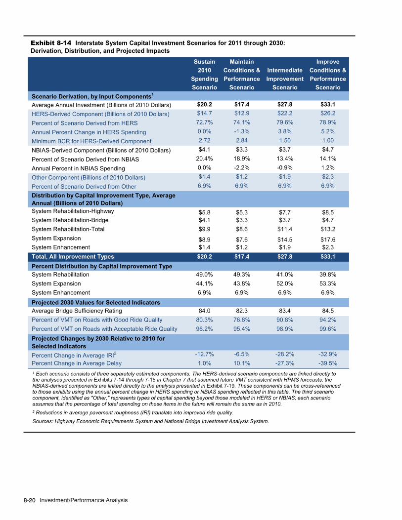
Investment/Performance Analysis8-20

12/11/2013 08XH_N (8-14) R2.xlsx

Sustain Maintain Improve2010 Conditions & Intermediate Conditions &

Spending Performance Improvement PerformanceScenario Scenario Scenario Scenario

Scenario Derivation, by Input Components1

Average Annual Investment (Billions of 2010 Dollars) $20.2 $17.4 $27.8 $33.1HERS-Derived Component (Billions of 2010 Dollars) $14.7 $12.9 $22.2 $26.2

Percent of Scenario Derived from HERS 72.7% 74.1% 79.6% 78.9%

Annual Percent Change in HERS Spending 0.0% -1.3% 3.8% 5.2%

Minimum BCR for HERS-Derived Component 2.72 2.84 1.50 1.00

NBIAS-Derived Component (Billions of 2010 Dollars) $4.1 $3.3 $3.7 $4.7

Percent of Scenario Derived from NBIAS 20.4% 18.9% 13.4% 14.1%

Annual Percent in NBIAS Spending 0.0% -2.2% -0.9% 1.2%

Other Component (Billions of 2010 Dollars) $1.4 $1.2 $1.9 $2.3

Percent of Scenario Derived from Other 6.9% 6.9% 6.9% 6.9%Distribution by Capital Improvement Type, Average Annual (Billions of 2010 Dollars)System Rehabilitation-Highway $5.8 $5.3 $7.7 $8.5System Rehabilitation-Bridge $4.1 $3.3 $3.7 $4.7System Rehabilitation-Total $9.9 $8.6 $11.4 $13.2System Expansion $8.9 $7.6 $14.5 $17.6System Enhancement $1.4 $1.2 $1.9 $2.3Total, All Improvement Types $20.2 $17.4 $27.8 $33.1Percent Distribution by Capital Improvement TypeSystem Rehabilitation 49.0% 49.3% 41.0% 39.8%System Expansion 44.1% 43.8% 52.0% 53.3%System Enhancement 6.9% 6.9% 6.9% 6.9%

Projected 2030 Values for Selected IndicatorsAverage Bridge Sufficiency Rating 84.0 82.3 83.4 84.5Percent of VMT on Roads with Good Ride Quality 80.3% 76.8% 90.8% 94.2%Percent of VMT on Roads with Acceptable Ride Quality 96.2% 95.4% 98.9% 99.6%Projected Changes by 2030 Relative to 2010 for Selected IndicatorsPercent Change in Average IRI2 -12.7% -6.5% -28.2% -32.9%Percent Change in Average Delay 1.0% 10.1% -27.3% -39.5%

Exhibit 8-14 Interstate System Capital Investment Scenarios for 2011 through 2030: Derivation, Distribution, and Projected Impacts

1 Each scenario consists of three separately estimated components. The HERS-derived scenario components are linked directly to the analyses presented in Exhibits 7-14 through 7-15 in Chapter 7 that assumed future VMT consistent with HPMS forecasts; the NBIAS-derived components are linked directly to the analysis presented in Exhibit 7-19. These components can be cross-referenced to those exhibits using the annual percent change in HERS spending or NBIAS spending reflected in this table. The third scenario component, identified as "Other," represents types of capital spending beyond those modeled in HERS or NBIAS; each scenario assumes that the percentage of total spending on these items in the future will remain the same as in 2010. 2 Reductions in average pavement roughness (IRI) translate into improved ride quality. Sources: Highway Economic Requirements System and National Bridge Investment Analysis System.

Selected Capital Investment Scenarios 8-21

Comparison of these scenarios with the Federal-aid highway scenarios reveals several patterns of interest:

� The shares of spending directed to system rehabilitation are smaller, particularly in the Interstate Highway System scenarios, than in the Federal-aid highway scenarios. In the Improve Conditions and Performance scenario, the rehabilitation share is 53.2 percent when the scenario relates to Federal-aid highways (Exhibit 8-7) and 39.8 percent when it relates to Interstate highways (Exhibit 8-14).

� In the Maintain Conditions and Performance scenario, future annual spending on Interstate highways averages $17.4 billion when the scenario concerns only those highways versus $22.0 billion ($3.8 billion plus $18.2 billion from Exhibit 8-10) when it considers all Federal-aid highways. In combination, HERS and NBIAS found that the most cost-effective way to maintain overall system conditions and performance would be, on average, to improve them somewhat on the Interstate System, and to let them deteriorate somewhat on non-Interstate routes. Similarly, in the Sustain 2010 Spending scenario, future annual spending on Interstate highways averages $20.2 billion versus $24.4 billion ($4.1 billion plus $20.3 billion from Exhibit 8-9) when it considers all Federal-aid highways. This again suggests that an economically driven approach to investment in highways and bridges would favor the Interstate highways.

� Projected changes between 2010 and 2030 in average pavement roughness and average delay are more favorable in these scenarios than in those for Federal-aid highways. In the Improve Conditions and Performance scenario, when the scenario concerns only Interstate highways, the average IRI is projected to decrease by 32.9 percent and average delay by 39.5 percent; when the focus extends to all Federal-aid highways, the reductions are 26.7 percent and 8.0 percent (Exhibit 8-7). By design, no matter which set of roads is the focus, the Maintain Conditions and Performance scenario projections indicate no unambiguous improvement or deterioration in conditions and performance. The projected outcomes for the bridge condition indices also appear relatively invariant to changes in focus among Federal-aid highways, the NHS, and Interstate highways.

Highway and Bridge Investment BacklogThe investment backlog represents all highway and bridge improvements that could be economically justified for immediate implementation, based solely on the current conditions and operational performance of the highway system (without regard to potential future increases in VMT or potential future physical deterioration of infrastructure assets). Conceptually, the backlog represents a subset of the investment levels reflected in the Improve Conditions and Performance scenario, which addresses the existing backlog as well as additional projected pavement, bridge, and capacity needs that may arise over the next 20 years.

Exhibit 8-15 presents an estimate of the backlog in 2010 for the types of capital improvements that are modeled in HERS and NBIAS, plus an adjustment factor for nonmodeled capital improvement types. The portion of the backlog derived from NBIAS amounts to $106.4 billion in spending on bridge rehabilitation. The portion derived from HERS, $598.6 billion, is much larger and represents the pool of cost-beneficial investments in system expansion and pavement improvements based solely on conditions and performance in 2010.

Of the estimated $808.2 total backlog, approximately $189.4 billion (23.4 percent) is on the Interstate Highway System and $441.4 billion (54.6 percent) is on the NHS (which includes the Interstate Highway System). Approximately 59.3 percent ($479.1 billion) of the total backlog is attributable to system rehabilitation needs, while the remainder is mainly associated with system expansion improvements to address existing capacity deficiencies. The share of the total backlog attributable to system rehabilitation is progressively lower for Federal-aid highways (60.6 percent), the NHS (56.8 percent), and the Interstate Highway System (47.4 percent).

Investment/Performance Analysis8-22

The $808.2 billion estimated backlog is heavily weighted toward urban areas; approximately 63.9 percent of this total is attributable to Federal-aid highways in urban areas. As noted in Chapter 3, average pavement ride quality on Federal-aid highways in 2008 was worse in urban areas than rural areas; urban areas also face relatively greater problems with congestion and functionally obsolete bridges than do rural areas.

It should be noted that the $808.2-billion backlog is considerably higher than that presented in previous C&P reports because it includes $215.1 billion for the types of capital improvements that are not modeled in HERS or NBIAS; nonmodeled investment types were previously excluded.

11/2/2012 08XH_O (8-15) R1.xlsx

System PercentSystem Enhance- of

System Component Highway Bridge Total Expansion ment* Total TotalFederal-Aid Highways—Rural $57.3 $28.4 $85.7 $8.8 $17.4 $111.9 13.9%Federal-Aid Highways—Urban $236.5 $58.5 $294.9 $184.0 $37.6 $516.5 63.9%Federal-Aid Highways—Total $293.8 $86.8 $380.6 $192.9 $55.0 $628.5 77.8%Non-Federal-Aid Highways* $78.9 $19.6 $98.5 $33.1 $48.2 $179.8 22.2%All Roads* $372.7 $106.4 $479.1 $225.9 $103.1 $808.2 100.0%Interstate Highway System $59.4 $30.4 $89.8 $86.4 $13.1 $189.4 23.4%National Highway System $191.3 $59.2 $250.6 $153.4 $37.4 $441.4 54.6%

(Billions of 2010 Dollars)

System Rehabilitation

Exhibit 8-15 Estimated Highway and Bridge Investment Backlog as of 2010

* Italicized values are estimates for those system components and capital improvement types not modeled in HERS or NBIAS, such as system enhancements, as well as pavement and expansion improvements to roads functionally classified as rural minor collector, rural local, or urban local, for which HPMS data are not available to support an HERS analysis. Sources: Highway Economic Requirements System and National Bridge Investment Analysis System.

Selected Capital Investment Scenarios 8-23

Selected Transit Capital Investment Scenarios

While Chapter 7 considered the impacts of varying levels of capital investment on transit conditions and performance, this chapter provides in-depth analysis of four specific investment scenarios, as outlined below in Exhibit 8-16. The Sustain 2010 Spending scenario assesses the impact of sustaining current expenditure levels on asset conditions and system performance over the next 20-year period. Given that current expenditure rates are generally less than are required to maintain current condition and performance levels, this scenario reflects the magnitude of the expected declines in conditions and performance given maintenance of current capital investment rates. The state of good repair (SGR) benchmark considers the level of investment required to eliminate the existing capital investment backlog as well as the condition and performance impacts of doing so. In contrast to the other scenarios considered here, the SGR benchmark only considers the preservation needs of existing transit assets (with no consideration of expansion requirements). Moreover, this is the only scenario that does not require that investments pass the Transit Economic Requirements Model’s (TERM’s) benefit-cost test (hence, this scenario brings all assets to an SGR regardless of TERM’s assessment of whether reinvestment is warranted). Finally, the Low Growth and High Growth scenarios both assess the required levels of reinvestment to (1) preserve existing transit assets at a condition rating of 2.5 or higher and (2) expand transit service capacity to support differing levels of ridership growth while passing TERM’s benefit-cost test.

12/13/2013 08XT_A (8-16) R3.xlsx

Low Growth(MPO Projected

Growth)High Growth

(Historical Growth)Description Sustain preservation

and expansion spending at current levels over next 20 years

Level of investment to attain and maintain SGR over next 20 years (no assessment of expansion needs)

Preserve existing assets and expand asset base to support MPO projected ridership growth (about 1.4%)

Preserve existing assets and expand asset base to support historical rate of ridership growth (2.2% between 1995 and 2010)

Objective Assess impact of constrained funding on condition, SGR backlog, and ridership capacity

Requirements to attain SGR (as defined by assets in condition 2.5 or better)

Assess unconstrained preservation and capacity expansion needs assuming low ridership growth

Assess unconstrained preservation and capacity expansion needs assuming high ridership growth

Apply Benefit-Cost Test?

Yes1 No Yes Yes

Preservation? Yes2 Yes2 Yes2 Yes2

Expansion? Yes No Yes Yes

Scenario Aspect Sustain 2010 Spending SGR

Exhibit 8-16 2010 C&P Analysis Scenarios for Transit

1 To prioritize investments under constrained funding. 2 Replace at condition 2.5.

Exhibit 8-17 summarizes the analysis results for each of these scenarios. It should be noted that each of the scenarios presented in Exhibit 8-17 imposes the same asset condition replacement threshold (i.e., assets are replaced at condition rating 2.5 when there is sufficient budget to do so) when assessing transit reinvestment needs. Hence, the differences in the total preservation expenditure amounts across each of these scenarios primarily reflect the impact of either (1) an imposed budget constraint (Sustain 2010 Spending scenario)

Investment/Performance Analysis8-24

or (2) application of TERM’s benefit-cost test (the SGR benchmark does not apply the benefit-cost test). A brief review of Exhibit 8-17 reveals the following:

� Sustain 2010 Spending Scenario: Total spending under this scenario is well below that of each of the other needs-based scenarios, indicating that sustaining recent spending levels is insufficient to attain the investment objectives of the SGR, Low Growth, or High Growth scenarios (suggesting future increases in the size of the SGR backlog and a likely increase in the number of transit riders per peak vehicle—including an increased incidence of crowding—in the absence of increased expenditures).

� SGR Benchmark: The level of expenditures required to attain and maintain an SGR over the upcoming 20-year period—which covers preservation needs but excludes any expenditures on expansion investments—is 12 percent higher than that currently expended on asset preservation and expansion combined.

� Low and High Growth Scenarios: The level of investment to address expected preservation and expansion needs is estimated to be roughly 33 percent to 49 percent higher than currently expended by the Nation’s transit operators. Preservation and expansion needs are highest for urbanized areas (UZAs) exceeding 1 million in population.

The following subsections present more detailed assessments of each scenario.

12/13/2013 08XT_B (8-17) R3.xlsx

Mode, Purpose, and Asset Type

Sustain 2010 Spending SGR

LowGrowth

HighGrowth

Urbanized Areas Over 1 Million in Population1

Nonrail2

Preservation $2.9 $4.6 $4.2 $4.2Expansion $1.2 $0.0 $1.2 $2.1

Subtotal Nonrail3 $4.1 $4.6 $5.4 $6.3Rail

Preservation $6.3 $11.4 $11.0 $11.1Expansion $4.2 $0.0 $2.9 $4.0

Subtotal Rail3 $10.5 $11.4 $13.9 $15.1Total, Over 1 Million in Population3 $14.6 $16.0 $19.3 $21.4

Nonrail2

Preservation $1.1 $2.2 $1.9 $1.9Expansion $0.6 $0.0 $0.5 $1.0

Subtotal Nonrail3 $1.7 $2.2 $2.4 $2.9Rail

Preservation $0.0 $0.3 $0.2 $0.2Expansion $0.2 $0.0 $0.0 $0.0

Subtotal Rail3 $0.2 $0.3 $0.2 $0.2Total, Under 1 Million and Rural3 $1.9 $2.5 $2.7 $3.1

Total3 $16.5 $18.5 $22.0 $24.5

Urbanized Areas Under 1 Million in Population and Rural

Investment Projection (Billions of 2010 Dollars) Exhibit 8-17 Annual Average Cost by Investment Scenario (2010–2030)

1 Includes 37 different urbanized areas. 2 Buses, vans, and other (including ferryboats). 3 Note that totals may not sum due to rounding. Source: Transit Economic Requirements Model.

Selected Capital Investment Scenarios 8-25

Sustain 2010 Spending ScenarioIn 2010, as reported by transit agencies to the National Transit Database (NTD), transit operators spent a total of $16.5 billion on capital projects (see Exhibit 7-20 and the corresponding discussion in Chapter 7). Of this amount, $10.3 billion was dedicated to the preservation of existing assets while the remaining $6.2 billion was dedicated to investment in asset expansion, both to support ongoing ridership growth and to improve service performance. This Sustain 2010 Spending scenario considers the expected impact on the long-term physical conditions and service performance of the Nation’s transit infrastructure if these 2010 expenditure levels are sustained in constant dollar terms through 2030. Similar to the discussion in Chapter 7, the analysis considers the impacts of asset preservation investments separately from those of asset expansion.

Capital Expenditures for 2010. As reported to the NTD, the level of transit capital expenditures peaked in 2009 at $16.6 billion and experienced a slight decrease in 2010 to $16.5 billion. (See Exhibit 8-18.) Although the annual transit capital expenditures averaged $14.3 billion from 2004 to 2010, expenditures averaged $16.4 billion in the last three years of NTD reporting. Furthermore, even though capital expenditures for preservation purposes in 2010 decreased $1.0 billion relative to prior year levels, capital expenditures for expansion purposes increased $0.9 billion in 2010.

TERM’s Funding Allocation. The following analysis of the Sustain 2010 Spending scenario relies on TERM’s allocation of 2010-level preservation and expansion expenditures to the Nation’s existing transit operators, their modes, and their assets over the upcoming 20-year period as depicted in Exhibit 8-19. As with other TERM analyses involving the allocation of constrained transit funds, TERM allocates limited funds based on the results of the model’s benefit-cost analysis, which ranks potential investments based on their assessed benefit-cost ratios (with the highest-ranked investments being funded first). Note that this TERM benefit-cost–based allocation of funding between assets and modes may differ from the allocation that local agencies might actually pursue assuming that total spending is sustained at current levels over 20 years.

10/9/2012 08XT_C (8-18) R2.xlsx

Year Preservation Expansion Total

2004 $9.4 $3.2 $12.6 2005 $9.0 $2.9 $11.8 2006 $9.3 $3.5 $12.8 2007 $9.6 $4.0 $13.6 2008 $11.0 $5.1 $16.1 2009 $11.3 $5.3 $16.6 2010 $10.3 $6.2 $16.5

Average $10.0 $4.3 $14.3

Average $10.5 $4.5 $15.0

Expenditures 2004 to 2010 in 2010 Dollars

Exhibit 8-18 Annual Transit Capital Expenditures, 2004 to 2010 (Billions of Current-Year Dollars)

Source: National Transit Database.

12/13/2013 08XT_D (8-19) R3.xlsx

Asset Type Preservation Expansion TotalRailGuideway Elements $1.2 $1.2 $2.4Facilities $0.0 $0.1 $0.1Systems $2.3 $0.2 $2.5Stations $0.4 $0.6 $1.1Vehicles $2.4 $1.1 $3.5Other Project Costs $0.0 $1.1 $1.1

Subtotal Rail* $6.3 $4.4 $10.7Nonrail Guideway Elements $0.0 $0.1 $0.1Facilities $0.1 $0.3 $0.4Systems $0.1 $0.1 $0.2Stations $0.0 $0.0 $0.1Vehicles $3.8 $1.2 $5.0Other Project Costs $0.0 $0.0 $0.0

Subtotal Nonrail* $4.0 $1.8 $5.8Total* $10.3 $6.2 $16.5

Investment Category

Exhibit 8-19 Sustain 2010 Spending Scenario: Average Annual Investment by Asset Type, 2010–2030 (Billions of 2010 Dollars)

* Note that totals may not sum due to rounding. Source: Transit Economic Requirements Model and FTA staff estimates.

Investment/Performance Analysis8-26

Preservation InvestmentsAs noted above, transit operators spent an estimated $10.3 billion in 2010 on the rehabilitation and replacement of existing transit infrastructure. Based on current TERM analyses, this level of reinvestment is less than that required to address the anticipated reinvestment needs of the Nation’s existing transit assets, and, if sustained over the forecasted 20-year period, would result in an overall decline in the condition of existing transit assets as well as an increase in the size of the investment backlog.

For example, Exhibit 8-20 presents the projected increase in the proportion of existing assets that exceed their useful life by asset category during the period from 2010 to 2030. Given the benefit-cost-based prioritization imposed by TERM for this scenario, the proportion of existing assets that exceed their useful life is projected to undergo a near-continuous increase across each of these asset categories. (This condition projection uses TERM’s benefit-cost test to prioritize rehabilitation and replacement investments in this scenario. Specifically, for each investment period in the forecast, TERM ranks all proposed investment activities based on their assessed benefit-cost ratios [highest to lowest.) TERM then invests in the highest-ranked projects for each period until the available funding for the period is exhausted. It is apparent here that TERM investment priorities favor vehicle investments (as do those of most transit agencies). Between 2015 and 2025 TERM invests in vehicles, which rate highly on several investment criteria, decreasing the vehicle over-age forecast over this time period. (Investments not addressed in the current period as a result of the funding constraint are then deferred until the following period.) Also, given that the proportion of over-age assets is projected to increase for all asset categories under this prioritization, it is clear that any reprioritization to favor reinvestment in one asset category over another would accelerate the rate of increase of the remaining categories. Note that these over-age assets tend to deliver the lowest-quality transit service to system users (e.g., have the highest likelihood of in-service failures).

0%

10%

20%

30%

40%

50%

60%

2010 2012 2014 2016 2018 2020 2022 2024 2026 2028 2030

Per

cent

of A

sset

s E

xcee

ding

The

ir U

sefu

l Life

(b

y V

alue

)

Forecast Year

Guideway ElementsFacilitiesSystemsStationsVehicles

(Existing Transit Assets; Federal Transit Administration Minimum Useful Life for Vehicles)

Note: The proportion of assets exceeding their useful life is measured based on asset replacement value, not asset quantities. Source: Transit Economic Requirements Model.

Exhibit 8-20 Sustain 2010 Spending Scenario: Over-Age Forecast by Asset Category, 2010–2030

12/16/2013 08XT_E (8-20) R3.xlsx

Finally, Exhibit 8-21 presents the projected change in the size of the investment backlog if reinvestment levels are sustained at the 2010 level of $10.3 billion, in constant dollar terms. As described in Chapter 7, the investment backlog represents the level of investment required to replace all assets that exceed their useful life and also to address all rehabilitation activities that are currently past due. Given that the current rate of

Selected Capital Investment Scenarios 8-27

capital reinvestment is insufficient to address the replacement needs of the existing stock of transit assets, the size of that backlog is projected to increase from the currently estimated level of $85.9 billion to roughly $142.0 billion by 2030. This chart also divides the backlog amount according to transit service area size, with the lower portion showing the backlog for UZAs with populations greater than 1 million and the upper portion showing the backlog for all other UZAs and rural areas combined. This segmentation highlights the significantly higher existing backlog for those UZAs serving the largest number of transit riders. The initial reduction in the backlog for these largest-transit UZAs, as shown in Exhibit 8-21, results from TERM’s higher prioritization of replacement needs for this urban area type and does not necessarily reflect the actual or expected allocation of expenditures between urban area types given maintenance of current spending levels in the future. Regardless of the actual allocation, it is clear that the 2010 expenditure level of $10.3 billion, if sustained, is not sufficient to prevent a further increase in the backlog needs of one or more of these UZA types.

$0

$20

$40

$60

$80

$100

$120

$140

$160

2010 2012 2014 2016 2018 2020 2022 2024 2026 2028 2030

Bill

ions

of 2

010

Dol

lars

Forecast Year

Under 1 Million PopulationOver 1 Million Population

Source: Transit Economic Requirements Model.

Exhibit 8-21 Investment Backlog: Sustain 2010 Spending ($10.3 Billion Annually)

12/16/2013 08XT_F (8-21) R3.xlsx

Expansion InvestmentsIn addition to the $10.3 billion spent on transit asset preservation in 2010, transit agencies spent $6.2 billion on expansion investments to support ridership growth and to improve transit performance. This section considers the impact of sustaining the 2010 level of expansion investment on future ridership capacity and vehicle utilization rates under both lower and higher ridership growth rate assumptions. As noted above, it is important to consider here that the $6.2 billion spent on expansion investments in 2010 was significantly higher than that reported in prior years.

As already considered in Chapter 7 (see Exhibit 7-23), the 2010 rate of investment in transit expansion is not sufficient to expand transit capacity at a rate equal to the rate of growth in travel demand, as projected by the historical trend rate of increase. Under these circumstances, it should be expected that transit capacity utilization (e.g., passengers per vehicle) will increase, with the level of increase determined by actual growth in demand. Although the impact of this change may be minimal for systems that currently have lower capacity utilization, service performance on some higher utilization systems would likely decline as riders experience increased vehicle crowding and potential for service delays. This impact is illustrated in Exhibit 8-22, which presents the projected change in vehicle occupancy rates by mode during the period from 2010 through 2030 (reflecting the impacts of spending from 2009 through 2030) under both lower (metropolitan planning organization [MPO]) and higher (trend) rates of growth scenarios in transit ridership, assuming that transit agencies continue to invest an average of $6.2 billion per year on transit expansion. Under the MPO-projected rate of increase, capacity utilization is stable, indicating that investment is sufficient. However, for the higher historical trend rates of increase, there is a steady rise in the

Investment/Performance Analysis8-28

5

10

15

20

25

30

35

40

45

2010 2015 2020 2025 2030

Ave

rage

Veh

icle

Occ

upan

cy

Forecast Year

Commuter Rail (Trend)

Commuter Rail (MPO)

Heavy Rail (Trend)

Heavy Rail (MPO)

Light Rail (Trend)

Light Rail (MPO)

Motor Bus (Trend)

Motor Bus (MPO)

Source: Transit Economic Requirements Model.

Exhibit 8-22 Sustain 2010 Spending Scenario: Capacity Utilization by Mode Forecast, 2010–2030

12/16/2013 08XT_G (8-22) R3.xlsx

average number of riders per transit vehicle across each of the four modes depicted here. For perspective, note that MPO growth rate projections tend to be conservative because they are developed based on financially constrained transportation plans. Moreover, the actual growth in travel demand has typically exceeded the MPO growth projections for much of the past decade.

Exhibit 8-23 presents the projected growth in transit riders that can be supported by the 2010 level of investment (keeping vehicle occupancy rates constant) as compared with the potential growth in total ridership under both the lower and higher growth rate scenarios. Similar to prior analyses, the $6.2-billion level of investment for expansion can support ridership growth that is similar to the MPO-projected ridership increases, but is short of that required to support continued ridership growth at recent historical rates (i.e., without impacting service performance).

10/10/2012 08XT_H (8-23) R2.xlsx

10.0

11.0

12.0

13.0

14.0

15.0

16.0

17.0

18.0

2010 2015 2020 2025 2030

Bill

ions

of A

nnua

l Boa

rdin

gs

Forecast Year

Projected Increase in Ridership (Trend) Rider Growth Supported by 2010 Spending Projected Increase in Ridership (MPO)

Source: Transit Economic Requirements Model.

Exhibit 8-23 Projected Versus Currently Supported Ridership Growth

Selected Capital Investment Scenarios 8-29

State of Good Repair BenchmarkThe preceding scenario considered the impacts of sustaining transit spending at current levels, which appear to be insufficient to address either deferred investment needs (which are projected to increase) or the projected trends in transit ridership (without a reduction in service performance). In contrast, this section focuses on the level of investment required to eliminate the investment backlog over the next 20 years and to provide for sustainable rehabilitation and replacement needs once the backlog has been addressed. Specifically, the SGR benchmark estimates the level of annual investment required to replace assets that currently exceed their useful life, to address all deferred rehabilitation activities (yielding an SGR where the asset has a condition rating of 2.5 or higher), and then to address all future rehabilitation and replacement activities as they come due. The SGR benchmark considered here uses the same methodology as that described in the Federal Transit Administration’s National State of Good Repair Assessment, released June 2010.

Differences with Other Scenarios: In contrast to the other scenarios in this chapter, the SGR benchmark (1) makes no assessment of expansion needs and (2) does not apply TERM’s benefit-cost test to investments proposed by TERM. These benchmark characteristics are inconsistent with the SGR concept. First, analyses of expansion investments are ultimately focused on capacity improvements and not on the needs of deteriorated assets. Second, application of TERM’s benefit-cost test would leave some reinvestment needs unaddressed. The intention of this benchmark is to assess the total magnitude of unaddressed reinvestment needs for all transit assets currently in service, regardless of whether it appears to be cost-beneficial for these assets to remain in service.

SGR Investment NeedsAnnual reinvestment needs under the SGR benchmark are presented in Exhibit 8-24. Under this benchmark, an estimated $ 18.5 billion in annual expenditures will be required over the next 20 years to bring the condition of all existing transit assets to an SGR. Of this amount, roughly $11.7 billion (63 percent) is required to address the SGR needs of rail assets. Note that a large proportion of rail reinvestment needs are associated with guideway elements (primarily aging elevated and tunnel structures) and rail systems (including train control, traction power, and communications systems) that are past their useful life as well as potentially technologically obsolete. Bus-related reinvestment needs are primarily associated with aging vehicle fleets.

Exhibit 8-24 also provides a breakout of capital reinvestment needs by type of UZA. This breakout emphasizes the fact that capital reinvestment needs are most heavily concentrated in the Nation’s larger UZAs. Together, these urban areas account

What is the definition of a state of good repair (SGR)?

The definition of “state of good repair” used for this scenario relies on TERM’s assessment of transit asset conditions. Specifically, for this scenario, TERM considers assets to be in a state of good repair if they are rated at a condition rating of 2.50 or higher and if all required rehabilitation activities have been addressed.

Q A&

10/9/2012 08XT_I (8-24) R2.xlsx

Asset Type

Over 1 Million

Population

Under 1 Million

Population TotalRailGuideway Elements $2.8 $0.1 $2.9Facilities $0.8 $0.1 $0.9Systems $3.4 $0.0 $3.4Stations $2.0 $0.0 $2.0Vehicles $2.5 $0.0 $2.5

Subtotal Rail* $11.4 $0.3 $11.7Nonrail Guideway Elements $0.4 $0.1 $0.5Facilities $0.9 $0.7 $1.6Systems $0.2 $0.0 $0.2Stations $0.1 $0.0 $0.1Vehicles $3.0 $1.3 $4.3

Subtotal Nonrail* $4.6 $2.2 $6.7Total* $16.0 $2.5 $18.5

Urban Area Type

Exhibit 8-24 SGR Benchmark: Average Annual Investment by Asset Type, 2010–2030 (Billions of 2010 Dollars)

* Note that totals may not sum due to rounding. Source: Transit Economic Requirements Model.

Investment/Performance Analysis8-30

for approximately 86 percent of total reinvestment needs (across all mode and asset types), with the rail reinvestment needs of these urban areas accounting for more than one-half of the total reinvestment required to bring all assets to an SGR. This high proportion of total needs reflects the high level of investment in older assets found in these urban areas.

Impact on the Investment BacklogA key objective of the SGR benchmark is to determine the level of investment required to attain and then maintain an SGR across all transit assets over the next 20 years, including elimination of the existing investment backlog. Exhibit 8-25 shows the estimated impact of the $18.5 billion in annual expenditures under the SGR benchmark on the existing investment backlog over the 20-year forecast period (compare these data with Exhibit 8-21). Given this level of expenditures, the backlog is projected to be eliminated by 2030, with the majority of this drawdown addressing the reinvestment needs of the UZAs with populations greater than 1 million.

10/10/2012 08XT_J (8-25) R2.xlsx

$0

$10

$20

$30

$40

$50

$60

$70

$80

$90

$100

2010 2012 2014 2016 2018 2020 2022 2024 2026 2028 2030

Bill

ions

of 2

010

Dol

lars

Forecast Year

Under 1 Million Population Over 1 Million Population

Source: Transit Economic Requirements Model.

Exhibit 8-25 Investment Backlog: State of Good Repair Benchmark ($18.5 Billion Annually)

Impact on ConditionsIn drawing down the investment backlog, the annual capital expenditures of $18.5 billion under the SGR benchmark would also lead to the replacement of assets with an estimated condition rating of 2.5 or lower. Within TERM’s condition rating system, this includes assets in marginal condition that have ratings of below 2.5 and all assets in poor condition. Exhibit 8-26 shows the current distribution of asset conditions for assets estimated to be in a rating condition of 2.5 or lower (with assets in poor condition segmented into two sub-groups). Note that this graphic excludes both tunnel structures and subway stations in tunnel structures because these are considered assets that require ongoing capital rehabilitation expenditures but that are never actually replaced. As with the investment backlog, the proportion of assets at condition rating 2.5 or lower is projected to decrease under the SGR benchmark from roughly 10 percent of assets in 2010 to well below 1 percent by 2030. Once again, this replacement activity would remove from service those assets with higher occurrences of service failures, technological obsolescence, and lower overall service quality.

Selected Capital Investment Scenarios 8-31

Impact on Vehicle Fleet PerformanceWhile the preceding analysis considered the impact of higher investment on reducing the investment backlog and potential replacement of assets past their useful life, this analysis may not provide a sense of the potential positive implications of these changes for daily transit service. To help better understand these effects, Exhibit 8-27 shows the estimated percent reduction in fleet-wide revenue service disruptions (relative to 2010) for heavy rail and motor bus vehicles resulting from the retirement of over-age transit passenger vehicles under the SGR benchmark. Note that the large variation in the percent reduction for bus is a result of the timing of large bus fleet replacements. Also, while the reduction in service disruptions is significant for bus and heavy rail vehicles, some vehicle types (e.g., light and commuter rail) actually show a net increase in service disruptions under the SGR benchmark; this is because the current age distribution for these fleets is skewed toward younger vehicle ages and is not sustainable in the longer term. This effect is the result of the recent development of new light rail and commuter rail systems.

Low and High Growth ScenariosThe preceding scenario considered the level of investment to bring existing transit assets to a SGR but in doing so did not consider either (1) the cost effectiveness of these investments (investments were not required to pass TERM’s benefit-cost test) or (2) the level of expansion investment required to support projected ridership growth. The Low Growth scenario and High Growth scenario address both of these issues. Specifically, these scenarios use the same rules to assess when assets should be rehabilitated or replaced as were applied in the preceding SGR benchmark (e.g., with assets being replaced at condition 2.5), but also require that these preservation and expansion investments pass TERM’s benefit-cost test. In general, some reinvestment activities do not pass this test (i.e., have a benefit-cost ratio of less than one), which can

10/10/2012 08XT_K (8-26) R2.xlsx

0%

2%

4%

6%

8%

10%

12%

14%

2010 2012 2014 2016 2018 2020 2022 2024 2026 2028 2030

Per

cent

of A

ll Tr

ansi

t Ass

ets

(b

y V

alue

)

Forecast Year

Condition 2.0 to 2.5

Condition 1.5 to 2.0

Below 1.5

Source: Transit Economic Requirements Model.

Exhibit 8-26 Proportion of Transit Assets Not in State of Good Repair (Excluding Tunnel Structures)

10/10/2012 08XT_L (8-27) R2.xlsx

-30%

-25%

-20%

-15%

-10%

-5%

0%

2010 2015 2020 2025 2030

Red

uctio

n in

Dis

rupt

ions

Year

Heavy Rail

Motor Bus

Exhibit 8-27 Percent Reduction in Revenue Service Disruptions Relative to 2010 for State of Good Repair Benchmark

Source: Transit Economic Requirements Model.

Investment/Performance Analysis8-32

result from low ridership benefits, higher capital or operating costs, or a mix of these factors. Excluding investments that do not pass the benefit-cost test has the effect of reducing total estimated needs.

In addition, the Low and High Growth scenarios also assess transit expansion needs given ridership growth as projected by the Nation’s MPOs (low growth) and based on the average annual compound rate as experienced over the last 15-year period (high growth). For the expansion component of this scenario, TERM assesses the level of investment required to maintain current vehicle occupancy rates (at the agency-mode level) subject to the rate of projected growth in transit demand in that UZA and also subject to the proposed expansion investment passing TERM’s benefit-cost test.

Low Growth AssumptionThe Low Growth scenario is intended to provide a lower bound on the level of investment required to maintain current service performance (as measured by transit vehicle capacity utilization) as determined by a relatively low rate of growth in travel demand. In particular, this Low Growth scenario relies on growth in travel demand as projected by a sample of the MPOs (representing the Nation’s 30 largest UZAs and a sample of smaller UZAs). When aggregated across the Nation’s UZAs (and corrected for differences in transit demand by UZA), this source yields a national average annual growth rate of 1.4 percent over the 20-year period from 2010 to 2030. (This represents the weighted average growth rate at the national level. In practice, the ridership growth rates applied by TERM vary by UZA based on the growth projections obtained from that UZA’s MPO.) This projected rate of growth is less than the 2.2-percent trend rate experienced over the 15 year period from 1995 to 2010 (as utilized by the High Growth scenario presented below), but is higher than the 1.2 percent trend rate of growth in urban population over the decade from 2000 to 2010 (a primary driver of transit ridership).

The MPO projections are considered low (or at least conservative) for the following reasons. First, MPO transit demand projections are financially constrained (i.e., projected ridership growth is limited by the expected capacity to fund expansion projects) and, hence, these projections are lower than the potential for increased ridership demand if funding were unconstrained. Second, as discussed further in Chapter 9, the historical rate of increase in transit ridership and transit passenger miles have generally exceeded MPO growth projections for these same time periods, again tending to characterize the MPO growth projections as relatively low or conservative.

High Growth AssumptionThe High Growth scenario provides a higher bound on the level of investment required to maintain current service performance as determined by a relatively high rate of growth in travel demand. In particular, the High Growth scenario relies on the trend rate of growth in transit passenger miles over the period 1995 through 2010 as reported to the NTD. When calculated across all transit operators, this historical trend rate of growth converts to a national average compound annual growth rate of 2.2 percent during this time period. Similar to the MPO growth rates in the Low Growth scenario, the 15-year trend growth rates applied by TERM for the High Growth scenario also vary by UZA either based on the actual trend rates of growth experienced by each UZA (for UZAs close to or higher than 1 million in population) or based on the average for UZAs of comparable size in the same geographic region. This rate is considered relatively high primarily due to the unusually high rate of growth in ridership experienced over the period from roughly 2006 to 2010, partly in response to high fuel prices.

Low and High Growth Scenario NeedsTERM’s projected annual average capital investment needs under the Low and High Growth scenarios—including those for both asset preservation and asset expansion—is presented in Exhibit 8-28.

Selected Capital Investment Scenarios 8-33

Lower Growth NeedsAssuming the relatively low ridership growth in the Low Growth scenario, total investment needs for both system preservation and expansion are estimated to average roughly $22.0 billion each year for the next two decades. Of this amount, roughly 79 percent are for preservation of existing assets and approximately $11 billion is associated with preservation of existing rail infrastructure alone. Note that the $1.2 billion difference between the $18.5 billion in annual preservation needs under the SGR benchmark and the $17.3 billion in preservation needs under the Low Growth scenario is entirely due to the application of TERM’s benefit-cost test under the Low Growth scenario. Finally, expansion needs in this scenario total $4.6 billion annually, with 63 percent of that amount associated with rail expansion costs.

Higher Growth NeedsIn contrast, total investment needs under the High Growth scenario are estimated to be $24.5 billion annually, a 12 percent increase over the total investment needs under the Low Growth scenario. The High Growth scenario total includes $17.4 billion for system preservation and an additional $7.1 billion for system expansion. Note that system preservation costs are higher under the High Growth scenario because the higher growth rate leads to a larger expansion of the asset base as compared to the Low Growth scenario. Under this scenario, investment in expansion of rail assets is still larger than that for nonrail expansion (56 percent for rail and 44 percent for non-rail). However, under the High Growth scenario rail takes only 56 percent of total expansion investment versus 63 percent of expansion needs under the Low Growth scenario. Overall, total expansion investment needs are roughly 53 percent higher for the High Growth scenario than for the Low Growth scenario (which is somewhat consistent with the high growth rate at 2.2 percent being approximately 60 percent higher than the low growth rate of 1.4 percent).

Impact on Conditions and PerformanceThe impact of the Low and High Growth Rate preservation investments on transit conditions is essentially the same as that already presented for the SGR benchmark in Exhibit 8-25 and Exhibit 8-26. As noted 10/9/2012 08XT_M (8-28) R2.xlsx

Asset Type Preservation Expansion Total Preservation Expansion TotalRailGuideway Elements $2.7 $0.7 $3.5 $2.8 $0.9 $3.6Facilities $0.9 $0.1 $0.9 $0.9 $0.1 $1.0Systems $3.4 $0.2 $3.5 $3.4 $0.2 $3.6Stations $1.8 $0.5 $2.2 $1.8 $0.6 $2.4Vehicles $2.5 $0.8 $3.3 $2.5 $1.3 $3.8Other Project Costs $0.0 $0.7 $0.7 $0.0 $0.9 $0.9

Subtotal Rail* $11.2 $2.9 $14.2 $11.3 $4.0 $15.3Nonrail Guideway Elements $0.4 $0.1 $0.5 $0.4 $0.1 $0.5Facilities $1.4 $0.3 $1.7 $1.4 $0.6 $2.0Systems $0.2 $0.0 $0.3 $0.2 $0.1 $0.3Stations $0.1 $0.0 $0.1 $0.1 $0.0 $0.1Vehicles $4.0 $1.2 $5.3 $4.1 $2.3 $6.3Other Project Costs $0.0 $0.0 $0.0 $0.0 $0.0 $0.0

Subtotal Nonrail* $6.1 $1.7 $7.8 $6.1 $3.1 $9.2Total Investment* $17.3 $4.6 $22.0 $17.4 $7.1 $24.5

Lower Growth Higher Growth

Exhibit 8-28 Low and High Growth Scenarios: Average Annual Investment by Asset Type, 2010–2030 (Billions of 2010 Dollars)

* Note that totals may not sum due to rounding. Source: Transit Economic Requirements Model.

Investment/Performance Analysis8-34

above, these scenarios use the same rules to assess when assets should be rehabilitated or replaced as were applied in the SGR benchmark (e.g., with assets being replaced at condition rating 2.5). In terms of asset conditions, the primary difference between the SGR benchmark and the Low and High Growth scenarios relates to: (1) TERM’s benefit-cost test not applying to the SGR benchmark (leading to higher SGR preservation needs overall) and (2) the Low and High Growth scenarios having some additional needs for the replacement of expansion assets with short service lives. Together, these impacts tend to work in opposite directions with the result that the rate of drawdown in the investment backlog and the elimination of assets exceeding their useful life are roughly comparable for each of these three scenarios.

Similarly, the impact of the Low and High Growth rate expansion investments on transit performance was considered in Exhibit 8-23. That analysis demonstrated the significant difference in the level of ridership growth supported by the High Growth scenario as compared with either the current level of expenditures ($5.4 billion in 2010 for UZAs over 1 million) or the rate of growth supported under the Low Growth scenario.

Scenario Benefits ComparisonFinally, this subsection summarizes and compares many of the investment benefits associated with each of the four analysis scenarios considered above. While much of this comparison is based on measures already introduced above, this discussion also considers a few additional investment impact measures. These comparisons are presented in Exhibit 8-29. Note that the first column of data in Exhibit 8-29 presents the current values for each of these measures (as of 2010). The subsequent columns present the estimated future values in 2030 assuming the levels, allocations, and timing of expenditures associated with each of the four investment scenarios.

Exhibit 8-29 includes the following measures:

� Average Annual Expenditures (billions of dollars): This amount is broken down into preservation and expansion expenditures.

� Condition of Existing Assets: This analysis only considers the impact of investment funds on the condition of those assets currently in service.Average Physical Condition Rating: The weighted average condition of all existing assets on TERM’s condition scale of 5 (excellent) through 1 (poor).

Investment Backlog: The value of all deferred capital investment, including assets exceeding their useful lives and rehabilitation activities that are past due (this value can approach but never reach zero due to assets continually aging with some exceeding their useful life). The backlog is presented here both as a total dollar amount and also as a percent of the total replacement value of all U.S. transit assets.

Backlog Ratio: The ratio of the current investment backlog to the annual level of investment required to maintain normal annual capital needs once the backlog is eliminated.

� Performance Measures: The impact of investments on U.S. transit ridership capacity and system reliability.New Boardings Supported by Expansion Investments: The number of additional riders that transit systems can carry without a loss in performance (given the projected ridership assumptions for each scenario).

Carbon Dioxide (CO2) Emissions Avoided (millions of metric tons): Potential reduction in CO2 emissions from providing the additional transit rider carrying capacity (assumes that riders would otherwise use other modes of travel, including automobiles).

Selected Capital Investment Scenarios 8-35

Revenue Service Disruptions per Passenger Mile Traveled: Number of disruptions to revenue service per million passenger miles.

Fleet Maintenance Cost per Vehicle Revenue Mile: Fleet maintenance costs tend to increase with fleet age (or reduced asset condition). This measure estimates the change in fleet maintenance costs expressed in a per-revenue-vehicle-mile basis.

� Other Benefits: Impacts other than those to transit conditions and performance. The jobs and Gross Domestic Product (GDP) impacts considered here were determined using an input-output analysis.Jobs Impacts: The number of job years associated with both transit mode operations and ongoing capital investment (both preservation and expansion), including direct, indirect, and induced job years.

12/13/2013 08XT_N (8-29) R3.xlsx

Measure

Sustain 2010

Spending SGRLow

Growth High

Growth

Preservation $10.3 $10.3 $18.5 $17.3 $17.4Expansion $6.2 $6.2 NA $4.6 $7.1

Total $16.5 $16.5 $18.5 $22.0 $24.5

Average Physical Condition Rating 3.75 3.39 3.54 3.54 3.54Investment Backlog (Billions of Dollars) $85.9 $141.7 $0.0 $0.0 $0.0Investment Backlog (% of Replacement Costs) 12.6% 20.9% 0.0% 0.0% 0.0%

Backlog Ratio1 6.1 10.0 0.0 0.0 0.0

New Boardings Supported by Expansion (Billions)

NA 4.6 NA 3.0 5.4

CO2 Emissions Avoided (Millions of Metric Tons) NA 3.0 NA 1.9 3.5Fleet Performance

Revenue Service Disruptions per Thousand PMT 9.5 10.5 9.3 9.2 9.3Fleet Maintenance Cost per Revenue Vehicle Mile

$1.75 $1.86 $1.74 $1.73 $1.73

Job Years Impact (Thousands)2

Operating and Maintenance 1,201.7 1,620.6 1,201.7 1,549.3 1,828.4Capital 264.3 264.3 295.4 351.3 392.6Total Annual Job Years Supported 1,466.0 1,884.9 1,497.0 1,900.6 2,221.0

GDP Impact (Billions of Dollars)Operating and Maintenance $71.1 $95.9 $71.1 $91.7 $108.2Capital $22.0 $22.0 $24.6 $29.3 $32.7Total Annual Incremental Impact $93.1 $117.9 $95.7 $120.9 $140.9

Other Benefits

Baseline 2010 Actual

Spending, Conditions and

Performance

Scenarios for 2030

Average Annual Expenditures (Billions of 2010 Dollars)

Conditions (Existing Assets)

PerformanceRidership Impacts of Expansion Investments (2010)

Exhibit 8-29 Scenario Investment Benefits Scorecard

1 The backlog ratio is the ratio of the current investment backlog to the annual level of investment to maintain SGR once the backlog is eliminated. 2 Includes direct, indirect, and induced impacts. Source: Transit Economic Requirements Model.

Investment/Performance Analysis8-36

Each $1 million invested in transit operation activities is estimated to support 33 job years while each $1 million invested in transit capital investments supports 16 job years.

GDP Impacts: The impact on GDP associated with both transit mode operations and ongoing capital investment (both preservation and expansion), including direct, indirect, and induced impacts. Each $1 invested in transit operation activities is estimated to generate $0.95 in additional GDP while each $1 invested in transit capital investments generates $0.33 in additional GDP.

Scorecard ComparisonsA review of the scorecard results for each of the four investment scenarios reveals the impacts discussed below.

Preservation ImpactsContinued reinvestment at the 2010 level is likely to yield a decline in overall asset conditions, an increase in the size of the investment backlog, and an increase in both service disruptions per million passenger miles and in maintenance costs per vehicle revenue mile. In contrast, with the exception of overall asset conditions, each of these measures is projected to improve under the SGR, Low Growth, and High Growth scenarios, each of which project roughly comparable levels of required capital reinvestment expenditures. Note that the overall condition rating measure of 3.54 under these last three investment scenarios represents a sustainable, long-term condition level for the Nation’s existing transit assets over the long term (in contrast to the current measure of roughly 3.8, which would be difficult to maintain in the long term without replacing many asset types prior to the conclusion of their expected useful lives).

Expansion ImpactsWhile continued expansion investment at the 2010 level appears sufficient to support a relatively low rate of increase in transit ridership, recent historical rates of growth suggest that a significantly higher rate of expansion investment is required to avoid a decline in overall transit performance (e.g., in the form of increased crowding on high utilization systems). Higher rates of transit expansion investment, as required to support higher transit ridership growth or through a shift from auto travel to transit, can also help yield reductions in CO2 emissions. Finally, higher rates of expansion investment also tend to support higher direct, indirect and induced impacts on jobs and other economic activity related to transit operations, construction, and rehabilitation activities.

Supplemental Scenario Analysis

Highway Supplemental Scenario Analysis .................................................................9-2

Comparison of Scenarios With Previous Reports ....................................................9-2Comparison With 2010 C&P Report ................................................................................... 9-2Comparisons of Implied Funding Gaps ............................................................................. 9-3

Comparison of Scenario Projections in 1991 C&P Report to Actual Expenditures, Conditions, and Performance ............................................................9-4

1991 C&P Report Scenario Definitions ............................................................................... 9-4Comparison of Scenario Projections in 1991 C&P Report to Actual Spending ................ 9-5Comparison of Scenario Projections in 1991 C&P Report to Actual Outcomes ............... 9-6

Accounting for Inflation ..............................................................................................9-7

Timing of Investment..................................................................................................9-10Alternative Timing of Investment in HERS .......................................................................... 9-10Alternative Timing of Investment in NBIAS ........................................................................ 9-13

Transit Supplemental Scenario Analysis ....................................................................9-15Asset Conditions Forecasts and Expected Useful Service Life Consumed for All Transit Assets Under Four Scenarios .............................................................9-15

Alternative Methodology ..................................................................................................... 9-18

Comparison of 2010 to 2013 TERM Results .............................................................9-19

Comparison of Passenger Miles Traveled (PMT) Growth Rates ..............................9-20MPO Growth Compared to Historical Growth for All Urbanized and Rural Areas ............. 9-20UZAs Over 1 Million in Population ...................................................................................... 9-21UZAs Under 1 Million in Population and Rural Areas ......................................................... 9-21

Impact of New Technologies on Transit Investment Needs .....................................9-22Impact of Compressed Natural Gas and Hybrid Buses on Future Needs ........................ 9-23Impact on Costs .................................................................................................................. 9-23Impact on Needs................................................................................................................. 9-23Impact on Backlog .............................................................................................................. 9-24

Forecasted Expansion Investment ............................................................................9-25

Supplemental Scenario Analysis 9-1

CHAPTER 9

Investment/Performance Analysis9-2

This section explores the implications of the highway investment scenarios considered in Chapter 8, starting with a comparison of the scenario investment levels relative to those presented in previous C&P reports. For a longer-term perspective, this section also looks back to the 20-year projections presented in the 1989 C&P Report relative to actual outcomes in terms of system conditions and performance.

This section also includes an illustration of the impact of alternative rates of future inflation on the constant dollar scenario investment levels presented in Chapter 8, and explores alternative assumptions concerning the timing of investment over the 20-year analysis period. A subsequent section within this chapter provides supplementary analysis regarding the transit investment scenarios.

Comparison of Scenarios With Previous ReportsEach edition of this report presents various projections of travel growth, pavement conditions, and bridge conditions under different scenarios. The projections cover 20 year periods, beginning the first year after the data presented on current conditions and performance. While the scenario names and criteria have varied over time, the C&P Report has traditionally included highway investment scenarios corresponding in concept to Maintain Conditions and Performance scenario and Improve Conditions and Performance scenario presented in Chapter 8.

Comparison With 2010 C&P ReportAs discussed in Chapter 8, the measures targeted by the Maintain Conditions and Performance scenario have been changed; the 2010 C&P Report version of this scenario attempted to maintain average speed and the bridge investment backlog, but the current version targets average pavement roughness, average delay and the average bridge sufficiency rating. However, the fundamental purpose of the scenario is to identify a level of investment associated with keeping overall conditions and performance in 20 years at roughly base-year levels. The criteria used to define the Improve Conditions and Performance scenario remains unchanged from the 2010 C&P Report; the only difference is that the 2010 C&P Report projected the impact of investment for 2009 through 2028, rather than the 2011 through 2030 period covered in the current edition.

As discussed in Chapter 6, highway construction costs as measured by the Federal Highway Administration’s (FHWA’s) National Highway Construction Cost Index decreased by 18.0 percent between 2008 and 2010. Consequently, adjusting the 2010 C&P Report’s scenario figures from 2008 dollars to 2010 dollars causes them to appear smaller. As shown in Exhibit 9-1, the 2010 C&P Report estimated the average annual investment level in the scenario comparable to the current Maintain Conditions and Performance scenario at $101.0 billion; adjusting for inflation (or, in this discussion, deflation) decreases this amount to $82.8 billion in 2010 dollars. The comparable amount for the Maintain Conditions and Performance scenario presented in Chapter 8 of this edition is $86.3 billion, approximately 4.2 percent higher.

The average annual investment level in the 2010 C&P Report scenario comparable to the current Improve Conditions and Performance scenario was $170.1 billion; adjusting for inflation decreases this amount to $139.4 billion in 2010 dollars. The comparable amount for the current Improve Conditions and Performance scenario presented in Chapter 8 of this edition is $145.9 billion, approximately 4.7 percent higher.

Highway Supplemental Scenario Analysis

Supplemental Scenario Analysis 9-3

The changes in the scenario findings in this report relative to the 2010 C&P Report are also partially attributable to changes in the underlying characteristics, conditions, and performance of the bridge system reported in Chapters 2 and 3, as well as to changes in the analytical methodology in the National Bridge Investment Analysis System (NBIAS) model. As noted in Chapter 7, the version of the Highway Economic Requirements System (HERS) used for this report was not significantly different from that used in the 2010 C&P Report, and the same underlying Highway Performance Monitoring System (HPMS) dataset was used. The main differences within the HERS analysis related to updated model parameter values.

Comparisons of Implied Funding GapsExhibit 9-2 compares the funding gaps implied by the analysis in the present report with those implied by previous C&P report analyses. Each such gap is measured as the percentage by which the average annual investment estimated for a specific scenario exceeds the base-year level of investment. The scenarios examined are this report’s Maintain Conditions and Performance and Improve Conditions and Performance scenarios, and their counterparts in previous C&P reports.

For each of the reports identified, actual spending in the base year for that report has been below the estimate of the average annual investment level required to maintain conditions and performance at base-year levels over 20 years. In the current report, the gap between these amounts, negative 13.9 percent, is dramatically different than in the 2010 C&P Report when it was positive 10.8 percent. This indicates that 2010 spending was greater than the level of spending identified for the Maintain Conditions and Performance scenario. This is partly due to the increase in funding under the American Recovery and Reinvestment Act, but largely due to the fact that construction costs have declined, making it cheaper to meet the scenario’s objectives.

Changes in the actual capital spending by all levels of government combined can substantially alter these spending gaps, as can sudden, large swings in construction costs. The large increase in the gap between base-year spending and the primary “Maintain” scenario presented in the 2008 C&P Report coincided with a large increase of construction costs experienced between 2004 and the 2006 base year for that report. The decreases in the gaps presented in the 2010 and 2012 editions coincided with declines in construction costs since their 2006 peak.

The differences among C&P report editions in the implied gaps reported in Exhibit 9-2 do not constitute a consistent indicator of change over time in how effectively highway investment needs are addressed. The FHWA continues to enhance the methodology used to determine scenario estimates for each edition of

11/13/2012 09XH_A (9-1) R3.xlsx

Highway and Bridge Scenarios—All Roads

2010 C&P Report

Adjusted for Inflation1

(Billions of 2008 Dollars)

(Billions of 2010 Dollars)

(Billions of 2010 Dollars)

Maintain Conditions and Performance scenario2 $101.0 $82.8 $86.3Improve Conditions and Performance scenario $170.1 $139.4 $145.9

2009–2028 Projection (Based on 2008 Data)

2011–2030 Projection

Exhibit 9-1 Selected Highway Investment Scenario Projections Compared With Comparable Data From the 2010 C&P Report (Billions of Dollars)

1 The investment levels for the highway and bridge scenarios were adjusted for inflation using the FHWA National Highway Construction Cost Index (NHCCI). 2 In the 2010 C&P report, the HERS component of this scenario focused on maintaining average speed, rather than representing the average of the cost associated with maintaining average delay and the cost associated with maintaining average pavement condition; the NBIAS component of the scenario focused on maintaining the bridge investment backlog, rather than maintaining the average sufficiency rating for bridges. Sources: Highway Economic Requirements System and National Bridge Investment Analysis System.

Investment/Performance Analysis9-4

the C&P report in order to provide a more comprehensive and accurate assessment. In some cases, these refinements have increased the level of investment in one or both of the scenarios (the “Maintain” or “Improve” scenarios, or their equivalents); other refinements have reduced this level.

12/10/2013 09XH_B (9-2) R4.xlsx

Report Primary Primary Year "Maintain" Scenario* "Improve" Scenario*1997 21.0% 108.9%

1999 16.3% 92.9%

2002 17.5% 65.3%

2004 8.3% 74.3%

2006 12.2% 87.4%

2008 34.2% 121.9%

2010 10.8% 86.6%

2013 -13.9% 45.7%

Average annual investment scenario estimates for 2003 through 2022 compared with 2002 spending

Average annual investment scenario estimates for 2007 through 2026 compared with 2006 spending

Average annual investment scenario estimates for 1996 through 2015 compared with 1995 spending

Percent Above Base-Year Spending

Average annual investment scenario estimates for 2011 through 2030 compared with 2010 spending

Average annual investment scenario estimates for 1998 through 2017 compared with 1997 spendingAverage annual investment scenario estimates for 2001 through 2020 compared with 2000 spending

Average annual investment scenario estimates for 2005 through 2024 compared with 2004 spending

Average annual investment scenario estimates for 2009 through 2028 compared with 2008 spending

Relevant Comparison

Exhibit 9-2 Comparison of Average Annual Highway and Bridge Investment Scenario Estimates With Base Year Spending, 1997 to 2013 C&P Reports

* Amounts shown correspond to the primary investment scenario associated with maintaining or improving the overall highway system in each C&P report; the definitions of these scenarios are not fully consistent between reports. The values shown for this report reflect the Maintain Conditions and Performance and the Improve Conditions and Performance scenarios. Negative numbers signify that the investment scenario estimate was lower than base year spending. Sources: Highway Economic Requirements System and National Bridge Investment Analysis System.

Comparison of Scenario Projections in 1991 C&P Report to Actual Expenditures, Conditions, and Performance

The highway component of the C&P report is part of a series dating back to the 1968 National Highway Needs report to Congress.

The 1991 Status of the Nation’s Highways and Bridges: Condition and Performance report to Congress (1991 C&P Report) is the most recent edition for which the 20-year forecast period has ended. This section explores the predictions made in the 1991 report for the year 2009 relative to what actually occurred in terms of pavement conditions, bridge conditions, and operational performance, taking into account actual investment and travel growth that has occurred.

Comparing such past predictions with actual results can be very informative in placing the projections from the current edition in their proper context. However, direct comparisons of results across different C&P editions pose challenges for multiple reasons, including differences in base-year conditions and analysis periods, changes in analytical models, and changes in scenario definitions.

1991 C&P Report Scenario DefinitionsSimilar to the current edition, the 1991 C&P Report estimated two scenarios for future investment requirements: Improve 1989 Conditions and Performance and Maintain 1989 Conditions and Performance. The investment levels presented were stated in constant 1989 dollars.

Supplemental Scenario Analysis 9-5

The 1991 C&P Report develops scenarios based on engineering standards that were applied uniformly nationwide without the consideration of the relative importance of specific facilities, regional variation, or other policy considerations. The scenario predictions were designed to provide general financial and performance benchmarks and were a basis for development and evaluation of policy and program options.

Improve 1989 Conditions and PerformanceThe Improve 1989 Conditions and Performance scenario estimated the costs associated with addressing deficiencies relative to a set of engineering-based minimum standards for physical conditions and performance. The goal of this scenario was to improve conditions and performance across all functional systems on a uniform basis nationwide, for both urban and rural, even as travel demand increased at a rate of 2.5 percent annually for 20 years. However, the 1991 C&P Report indicates that a cap on the width of individual highway sections was imposed, which resulted in a set of unmet capacity needs to the extent to which operational performance in larger urbanized areas could not be maintained. The scenario reflected estimated annual capital savings from an aggressive traffic management program.

Unlike the present edition, which prioritizes investment based on benefit-cost analysis, the 1991 C&P Report acknowledges that the scenarios did not involve priorities regarding cost-effectiveness and was not intended to represent an optimum recommended investment strategy. Instead, the scenario was intended to provide a framework for policy development by establishing a measure of the total capital costs of providing a desirable level of highway and bridge infrastructure on all facilities, assuming a future travel demand growth of 2.5 percent annually.

Maintain 1989 Conditions and PerformanceThe Maintain 1989 Conditions and Performance scenario estimated the cost of maintaining both current overall physical conditions and current levels of performance as traffic increased over a 20-year period. The 1991 C&P Report notes that overall system performance would not be maintained in the largest urbanized areas assuming a 2.5 percent annual growth in vehicle miles traveled (VMT).

Comparison of Scenario Projections in 1991 C&P Report to Actual SpendingExhibit 9-3 shows the estimated average annual and cumulative 20-year highway and bridge needs associated with the two scenarios presented in the 1991 C&P Report. The cumulative values are also adjusted for

10/29/2012 09XH_C (9-3) R1.xlsx

Adjusted for Inflation

Average Cumulative CumulativeAnnual 20 Years 20 Years

(Billions of 1989 Dollars)

(Billions of 1989 Dollars)

(Billions of 2010 Dollars)

$74.9 $1,498.0 $2,422.2$45.7 $914.0 $1,477.9

$1,418.9

Actual 20-Year Highway Capital Investment (VMT Grew 1.74 Percent per Year from 1989 to 2009)

Cumulative Capital Outlay, 1990 through 2009*

Maintain Conditions and Performance Scenario

1990–2009 Projection From 1991 C&P Report

20-Year Highway Capital Investment Scenarios (Assuming 2.5-Percent Annual VMT Growth from 1989 to 2009)

Improve Conditions and Performance Scenario

Exhibit 9-3 1991 C&P Report Highway and Bridge Investment Scenario Estimates and Cumulative Spending, 1990 Through 2009

* Highway capital outlay by all levels of Government combined totaled $1.2111 trillion in nominal dollar terms over the 20-year period from 1990 through 2009. This equates to $1.4189 trillion in constant 2010 dollars. Sources: 1991 Status of the Nation's Highways and Bridges: Conditions and Performance Report to Congress; Highway Statistics, various years, Tables HF-10A, HF-10, PT-1, and SF-12A; and unpublished FHWA data.

Investment/Performance Analysis9-6

inflation to 2010 dollars using the FHWA Composite Bid Price Index (BPI) through the year 2006 and the new FHWA National Highway Construction Cost Index (NHCCI) for subsequent years.

The 1991 C&P Report estimated the average annual cost of the Improve 1989 Condition and Performance scenario at $74.9 billion for 1990 through 2009, assuming a 2.5 percent VMT growth rate.

The average annual cost to Maintain 1989 Condition and Performance on existing roads and bridges through 2009 was estimated at $45.7 billion, again assuming a 2.5 percent VMT growth rate.

The cumulative 20-year value inflated to 2010 dollars for the Improve 1989 Condition and Performance scenario equates to $2.422 trillion. The cumulative value of the Maintain Conditions and Performance scenario in 2010 dollars equates to $1.478 trillion, which is within 4 percent of the actual cumulative capital outlay of $1.419 trillion, stated in constant 2010 dollars.

Assumptions about future VMT growth are a critical input to the investment scenario. The actual rate of VMT growth over the 20-year period from 1989 to 2009 was 1.74 percent per year, well below the 2.5 percent annual VMT growth forecast used in the 1991 C&P Report scenarios.

The 1991 C&P Report included sensitivity analysis that assumed a higher average annual VMT growth rate of 3.0 percent for some of the major components of the two investment scenarios, which increased their cost by 13 percent (Improve) to 17 percent (Maintain). However, the 1991 C&P Report did not conduct any tests of VMT growth rates lower than 2.5 percent. As a result, although these analyses demonstrate that the scenarios were significantly affected by the VMT growth rate assumption, it would not be safe to assume that the reductions in scenario costs associated with lower VMT growth rates would be proportional to these increases in scenario costs associated with higher VMT growth forecasts. If the forecasts had been developed assuming a 1.74-percent average annual growth rate, the cost associated with both scenarios would have been lower.

Comparison of Scenario Projections in 1991 C&P Report to Actual OutcomesThe 1991 C&P Report included projections for measures of pavement condition, bridge condition, and operational performance. As was demonstrated in Exhibit 9-3, actual capital spending from 1990 through 2009 was slightly lower than the investment levels associated with the Maintain Conditions and Performance scenario, which suggests that overall highway and bridge system conditions would have deteriorated slightly relative to 1989. However, because the VMT growth rate assumed in that scenario was significantly higher than what actually occurred from 1989 to 2009, the investment levels associated with that scenario were overstated to some degree. Consequently, improvements to some measures of conditions and performance relative to 1989 could reasonably be expected.

Exhibit 9-4 compares the percentage of pavement in good condition by facility type; bridge deficiencies; and travel under congested condition for 1989, 2008, and 2010. The pavement condition ratings presented in the 1991 C&P Report were based on a subjective evaluation of overall pavement quality which has subsequently been replaced by a more objective measure of pavement ride quality. However, the percentage of pavements in good condition is roughly comparable between the two reports. Since 1989, the percent of good pavement mileage has increased for the rural functional classes shown, except for rural major collectors. In contrast, for urban highways, the percent of good pavement mileage has decreased for all functional classes shown except urban Interstate.

The percentage of bridges classified as structurally deficient or functionally obsolete is still defined in a manner comparable to that in the 1991 C&P Report. There has been improvement since 1989, as the percentage of structurally deficient bridges has been cut sharply and reductions in the percentage of functionally obsolete bridges have been achieved.

Supplemental Scenario Analysis 9-7

10/31/2012 09XH_D (9-4) R1.xlsx

Scenario and Comparison Parameter 1989 2008 2010

Rural Interstate 58.2% 78.2% 73.8%Rural Other Principal Arterial 51.9% 66.5% N/ARural Minor Arterial 45.5% 53.3% 49.7%Rural Major Collector 34.2% 34.0% 28.7%Urban Interstate 57.4% 61.4% 63.2%Urban Other Freeway & Expressway 52.7% 50.6% 48.0%Urban Other Principal Arterial 42.7% 27.4% 26.7%Urban Minor Arterial 40.7% 32.1% 22.2%Urban Collector 31.3% 28.3% N/A

Percent Structurally Deficient 23.2% 11.9% 11.5%Percent Functionally Obsolete 15.9% 13.3% 12.8%Total Percent Deficient 39.2% 25.2% 24.3%

Percent of Travel Under Congested Conditions 20.6% 26.3% 26.2%

Percent of "Good" Pavement Mileage1

Bridge Deficiencies2

Operational Performance3

Exhibit 9-4 Selected Pavement, Bridge, and Congestion Metrics, 1989, 2008, and 2010

1 The 1991 C&P Report classified pavements as "Good" if they had a Pavement Serviceability Rating (PSR) of 3.5 or higher on a scale of 5.0. The current terminology reflected in Chapter 3 describes pavements as having "Good Ride Quality" if they have a reported IRI of 95 inches per mile or lower (or a PSR of 3.5 or higher if IRI is not available). Subtotals and Totals are not provided because the 1991 C&P Report did not include them. N/A is shown for functional classes that were split starting in 2010. 2 See Chapter 3 for more information on these measures. 3 See Chapter 5 for more information on this measure. Sources: Sources: 1991 C&P Report, Highway Performance Monitoring System, National Bridge Inventory, and Texas Transportation Institute.

The operational performance measures presented in the 1991 C&P Report are not consistent with those in the current edition. However, the Texas Transportation Institute has computed a fully comparable historic time series for a metric presented in Chapter 5: the percent of travel occurring under congested conditions. Based on this measure, congestion has worsened since 1989.

Although these types of rough comparisons of individual conditions and performance measures are not sufficiently robust to make definitive statements of the validity of the analyses presented in the 1991 C&P Report, actual trends over the forecast period do not appear to be wildly inconsistent with the report’s findings, taking into account the lower than projected growth in VMT. Because actual capital investment over the 20-year period was relatively close to the Maintain 1989 Conditions and Performance scenario, it is not surprising that actual performance outcomes were mixed, with pavement condition improving on some functional classes while worsening on others, with bridge conditions improving, and with operational performance deteriorating relative to 1989.

Accounting for InflationThe analysis of potential future investment/performance relationships in the C&P report has traditionally stated future investment levels in constant dollars, with the base-year set according to the year of the conditions and performance data supporting the analysis. Throughout Chapters 7 and 8, this edition of the C&P report has stated all investment levels in constant 2010 dollars. For some purposes, however, such as comparing investment spending in a particular scenario with nominal dollar revenue projections, one would want to adjust for inflation. Given an assumption about future inflation, one could either convert the C&P report’s constant-dollar numbers to nominal dollars or convert the nominal projected revenues to constant 2010 dollars.

Investment/Performance Analysis9-8

Q A&The investment/performance models discussed in this report estimate the future benefits and costs of transportation investments in constant-dollar terms. This is standard practice for this type of economic analysis. To convert the model outputs from constant dollars to nominal dollars, it would be necessary to externally adjust them to account for projected future inflation.

Traditionally, this type of adjustment has not been made in the C&P report. Because inflation prediction is an inexact science, adjusting the constant-dollar figures to nominal dollars tends to add to the uncertainty of the overall results and make the report more difficult to use if the inflation assumptions are inaccurate. Allowing readers to make their own inflation adjustments based on actual trends observed subsequent to the publication of the C&P report and/or the most recent projections from other sources is expected to yield a better overall result, particularly in light of the sharp swings in highway construction materials costs in recent years.

The use of constant-dollar figures is also intended to provide readers with a reasonable frame of reference in terms of an overall cost level that they have recently experienced. When inflation rates are compounded for 20 years, even relatively small growth rates can produce nominal dollar values that appear very large when viewed from the perspective of today’s typical costs.

Why are the investment analyses presented in this report expressed in constant base-year dollars?

The average annual increase in highway construction costs over the last 20 years (1990 to 2010) was 2.4 percent. Since the creation of the Federal Highway Trust Fund in 1956, the 20-year period with the smallest increase in construction costs was 1980 to 2000, when costs grew by 2.0 percent per year; the largest increase occurred from 1960 to 1980, when costs grew by 7.4 percent per year. From 1986 to 2006, highway construction costs grew by 4.0 percent annually. (Historic inflation rates were determined using the FHWA Composite Bid Price Index through 2006, and the new FHWA National Highway Construction Cost Index from 2006 to 2010; these indices are discussed in Chapter 6.) Exhibit 9-5 illustrates how the constant dollar figures associated with three of the four systemwide scenarios for highways and bridges

Q A&Chapter 7 provided the definition of constant dollar measurement that the Office of Management and Budget includes in its guidance on benefit-cost analysis. Under this definition, any price predicted for a future year must be adjusted for the general inflation expected to occur between the base year and the future year, For example, if a future-year price is expected to be $1.10, whereas prices in general are expected to increase 3 percent between the base year and the future year, the price in constant dollars would be calculated as $1.10 divided by 1.03, which is approximately $1.068.

With a few exceptions, this report’s analyses of future investments in highways assume that prices entering the HERS model will change by the same percentage as general inflation, as measured by the Consumer Price Index (CPI). Under this assumption, the future price in constant dollars simply equates to the base-year price. As discussed in Chapter 7, the exceptions include the price of motor fuel and the marginal damage cost of CO emissions; as discussed in Chapter 10, the values of travel time savings and of crash reductions are also exceptions.

The costs of highway improvements were not among the exceptions. Typical prices by type of improvement were assumed to increase at the same rate as the CPI, so that base-year prices were applied to future years. One reason for making this simplifying assumption is that, as discussed in Chapter 6, highway construction prices have been volatile in recent years; this suggests that forecasting their future movements relative to the CPI would be challenging. (Motor fuel price have also been volatile, but long-range forecasts are available from the Energy Information Administration.)

Additional challenges to attempting such forecasting include limitations of the historical data on construction prices, as discussed in Appendix D of the 2010 C&P Report. It should be noted that the assumption that construction prices will change at the rate of general inflation may be fairly reasonable on average. As noted in Chapter 6, this report’s reading of the historical evidence is that, over the 20-year period from 1990 to 2010, highway construction costs increased 60.5 percent, which is not much different from the 66.8 percent increase in the CPI.

Why does this report assume that construction costs measured in constant dollars remain unchanged over the analysis period?

Supplemental Scenario Analysis 9-9

12/10/2013 09XH_E (9-5) R3.xlsx

Year2010 $100.2 $100.2 $100.2 $100.2 $100.2 $100.2 $100.2 $100.2 $100.22011 $100.2 $98.7 $103.6 $102.2 $100.7 $105.7 $104.2 $102.7 $107.82012 $100.2 $97.3 $107.2 $104.2 $101.2 $111.6 $108.3 $105.2 $116.02013 $100.2 $95.9 $110.9 $106.3 $101.8 $117.7 $112.7 $107.9 $124.82014 $100.2 $94.5 $114.8 $108.4 $102.3 $124.2 $117.2 $110.6 $134.32015 $100.2 $93.2 $118.7 $110.6 $102.8 $131.1 $121.9 $113.3 $144.52016 $100.2 $91.8 $122.8 $112.8 $103.4 $138.3 $126.8 $116.2 $155.42017 $100.2 $90.5 $127.1 $115.1 $103.9 $146.0 $131.8 $119.1 $167.32018 $100.2 $89.2 $131.5 $117.4 $104.5 $154.1 $137.1 $122.0 $180.02019 $100.2 $87.9 $136.0 $119.7 $105.0 $162.6 $142.6 $125.1 $193.62020 $100.2 $86.6 $140.7 $122.1 $105.6 $171.6 $148.3 $128.2 $208.32021 $100.2 $85.4 $145.6 $124.6 $106.1 $181.1 $154.2 $131.4 $224.22022 $100.2 $84.1 $150.7 $127.0 $106.7 $191.1 $160.4 $134.7 $241.22023 $100.2 $82.9 $155.9 $129.6 $107.3 $201.6 $166.8 $138.1 $259.52024 $100.2 $81.7 $161.3 $132.2 $107.8 $212.8 $173.5 $141.5 $279.22025 $100.2 $80.5 $166.8 $134.8 $108.4 $224.5 $180.4 $145.1 $300.52026 $100.2 $79.4 $172.6 $137.5 $109.0 $236.9 $187.6 $148.7 $323.32027 $100.2 $78.2 $178.6 $140.3 $109.6 $250.0 $195.1 $152.4 $347.82028 $100.2 $77.1 $184.7 $143.1 $110.1 $263.9 $202.9 $156.2 $374.32029 $100.2 $76.0 $191.1 $145.9 $110.7 $278.5 $211.1 $160.1 $402.72030 $100.2 $74.9 $197.8 $148.9 $111.3 $293.8 $219.5 $164.1 $433.3Total $2,003.5 $1,725.9 $2,918.6 $2,482.7 $2,118.3 $3,697.1 $3,102.3 $2,622.6 $4,717.9

0.00% -1.44% 3.46% Constant Dollar Growth Rate$100.2 $86.3 $145.9 Average Annual Investment Level in Constant 2010 Dollars

Improve Conditions & Perfor-mance

Scenario

Improve Conditions & Perfor-mance

Scenario

Maintain Conditions & Perfor-mance

Scenario

Sustain 2010

Spend-ing

Scenario

Sustain 2010

Spend-ing

Scenario

Maintain Conditions & Perfor-mance

Scenario

Improve Conditions & Perfor-mance

Scenario

Sustain 2010

Spend-ing

Scenario

Maintain Conditions & Perfor-mance

Scenario

Nominal Dollars (Assuming 4.0 Percent Annual Inflation)

Highway Capital Investment (Billions of Dollars)Nominal Dollars (Assuming 2.0

Percent Annual Inflation)Constant 2010 Dollars*

* Based on average annual investment levels and annual constant dollar growth rates identified in Exhibit 8-2. Source: FHWA staff analysis.

Exhibit 9-5 Illustration of Potential Impact of Alternative Inflation Rates on Selected Systemwide Investment Scenarios

presented in Chapter 8 could be converted to nominal dollars based on two alternative inflation rates of 2.0 percent and 4.0 percent.

The systemwide Sustain 2010 Spending scenario presented in Chapter 8 assumes that combined capital spending for highway and bridge improvements would be sustained at its 2010 level in constant-dollar terms for 20 years. Hence, Exhibit 9-5 shows $100.2 billion of spending in constant 2010 dollars for each year from 2011 through 2030, for a 20-year total of $2.0 trillion. Applying annual inflation in construction costs of 2.0 percent or 4.0 percent would imply a 20-year total in nominal dollars of $2.5 trillion or $3.1 trillion, respectively, for this scenario.

Chapter 8 indicates that achieving the objectives of the systemwide Maintain Conditions and Performance scenario would require investment averaging $86.3 billion per year in constant 2010 dollars, equivalent to the level of investment achieved with a reduction of 1.44 percent per year in constant-dollar spending. Exhibit 9-5 illustrates the application of this real reduction rate, demonstrating how annual capital investment would decrease from $100.1 billion in 2010 to $74.9 billion in 2030, resulting in a 20-year

Investment/Performance Analysis9-10

(2011 to 2030) total of $1.7 trillion in constant 2010 dollars. A 2.0-percent inflation rate applied to these constant-dollar estimates would produce a 20-year cost of $2.1trillion in nominal dollar terms, while a 4.0-percent inflation rate results in a 20-year nominal dollar cost of $2.6 trillion.

The compounding impacts of inflation are even more evident in the figures for the systemwide Improve Conditions and Performance scenario presented in Exhibit 9-5. As described in Chapter 8, this scenario assumes 3.46 percent growth in constant-dollar highway capital spending per year in order to address all potentially cost-beneficial highway and bridge improvements by 2030. The $145.9-billion average annual investment level associated with this scenario equates to a 20-year investment level of $2.9 trillion in constant 2010 dollars. Adjusting this figure to account for inflation of 2.0 percent or 4.0 percent would translate into 20-year nominal dollar costs of $3.7 trillion or $4.7 trillion, respectively.

Over any 20 year period, construction costs will increase despite the occasional year-to-year drops sometimes experienced. Using a low inflation rate of 2.0 percent adds between 23 and 27 percent to the constant dollar estimates for the 20-year period for the three scenarios. Using a higher inflation rate of 4.0 percent requires between 52 and 62 percent of additional funding to meet the needs identified under the three scenarios.

Timing of InvestmentThe investment/performance analyses presented in this report focus mainly on how alternative average annual investment levels over 20 years might impact system performance at the end of this period. Within this period, system performance can be significantly influenced by the timing of investment. Consistent with the approach in the 2008 C&P Report, and as discussed in Chapter 7, the analyses in the present edition assume that any change from the 2008 level of combined investment per year by all levels of government would occur gradually and at a constant percent rate. However, some previous editions used different approaches. The HERS 2006 C&P Report assumed that combined investment would immediately jump to the average annual level being analyzed, then remain fixed at that level for 20 years. The HERS analyses presented in the 2004 C&P Report were tied directly to alternative benefit-cost ratio (BCR) cutoffs rather than to particular levels of investment in any given year. At higher spending levels, this approach resulted in a significant front-loading of capital investment in the early years of the analysis as the existing backlog of potential cost-beneficial investments (discussed above) was addressed, followed by a sharp decline in later years. The analysis did not assume any increase in material and labor costs in response to the sharp increase in the number of highway construction projects.

The discussion below explores the impact of each of these three assumptions about the timing of future investment—ramped spending, flat spending, or BCR-driven spending—on system performance within the 20-year period analyzed. Each of the average annual investment levels analyzed correspond to the baseline HERS analyses for Federal-aid Highways, and the baseline NBIAS analyses for all bridges presented in Chapter 7.

Alternative Timing of Investment in HERSThis section presents information regarding how the timing of investment would impact the distribution of spending among the four 5-year funding periods considered in HERS, and how these spending patterns could potentially impact average pavement conditions (measured using International Roughness Index [IRI]) and delay per VMT. Because the timing of investment is varied for any given capital investment level, the pavement condition and delay per VMT will change.

Alternative Investment PatternsExhibit 9-6 indicates how alternative assumptions regarding the timing of investment would impact the distribution of spending among the four 5-year funding periods considered in HERS, and how these

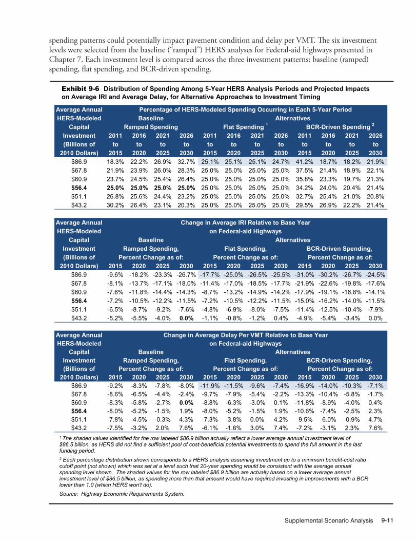
Supplemental Scenario Analysis 9-11

10/31/2012 09XH_F (9-6) R1.xlsx

Average AnnualHERS-Modeled

CapitalInvestment 2011 2016 2021 2026 2011 2016 2021 2026 2011 2016 2021 2026(Billions of to to to to to to to to to to to to

2010 Dollars) 2015 2020 2025 2030 2015 2020 2025 2030 2015 2020 2025 2030$86.9 18.3% 22.2% 26.9% 32.7% 25.1% 25.1% 25.1% 24.7% 41.2% 18.7% 18.2% 21.9%$67.8 21.9% 23.9% 26.0% 28.3% 25.0% 25.0% 25.0% 25.0% 37.5% 21.4% 18.9% 22.1%$60.9 23.7% 24.5% 25.4% 26.4% 25.0% 25.0% 25.0% 25.0% 35.8% 23.3% 19.7% 21.3%$56.4 25.0% 25.0% 25.0% 25.0% 25.0% 25.0% 25.0% 25.0% 34.2% 24.0% 20.4% 21.4%$51.1 26.8% 25.6% 24.4% 23.2% 25.0% 25.0% 25.0% 25.0% 32.7% 25.4% 21.0% 20.8%$43.2 30.2% 26.4% 23.1% 20.3% 25.0% 25.0% 25.0% 25.0% 29.5% 26.9% 22.2% 21.4%

Average AnnualHERS-Modeled

CapitalInvestment(Billions of

2010 Dollars) 2015 2020 2025 2030 2015 2020 2025 2030 2015 2020 2025 2030$86.9 -9.6% -18.2% -23.3% -26.7% -17.7% -25.0% -26.5% -25.5% -31.0% -30.2% -26.7% -24.5%$67.8 -8.1% -13.7% -17.1% -18.0% -11.4% -17.0% -18.5% -17.7% -21.9% -22.6% -19.8% -17.6%$60.9 -7.6% -11.8% -14.4% -14.3% -8.7% -13.2% -14.9% -14.2% -17.9% -19.1% -16.8% -14.1%$56.4 -7.2% -10.5% -12.2% -11.5% -7.2% -10.5% -12.2% -11.5% -15.0% -16.2% -14.0% -11.5%$51.1 -6.5% -8.7% -9.2% -7.6% -4.8% -6.9% -8.0% -7.5% -11.4% -12.5% -10.4% -7.9%$43.2 -5.2% -5.5% -4.0% 0.0% -1.1% -0.8% -1.2% 0.4% -4.9% -5.4% -3.4% 0.0%

Average AnnualHERS-Modeled

CapitalInvestment(Billions of

2010 Dollars) 2015 2020 2025 2030 2015 2020 2025 2030 2015 2020 2025 2030$86.9 -9.2% -8.3% -7.8% -8.0% -11.9% -11.5% -9.6% -7.4% -16.9% -14.0% -10.3% -7.1%$67.8 -8.6% -6.5% -4.4% -2.4% -9.7% -7.9% -5.4% -2.2% -13.3% -10.4% -5.8% -1.7%$60.9 -8.3% -5.8% -2.7% 0.0% -8.8% -6.3% -3.0% 0.1% -11.8% -8.9% -4.0% 0.4%$56.4 -8.0% -5.2% -1.5% 1.9% -8.0% -5.2% -1.5% 1.9% -10.6% -7.4% -2.5% 2.3%$51.1 -7.8% -4.5% -0.3% 4.3% -7.3% -3.8% 0.0% 4.2% -9.5% -6.0% -0.9% 4.7%$43.2 -7.5% -3.2% 2.0% 7.6% -6.1% -1.6% 3.0% 7.4% -7.2% -3.1% 2.3% 7.6%

Change in Average IRI Relative to Base Yearon Federal-aid Highways

Baseline AlternativesRamped Spending, Flat Spending, BCR-Driven Spending,

Percent Change as of: Percent Change as of: Percent Change as of:

Percent Change as of:

Change in Average Delay Per VMT Relative to Base Yearon Federal-aid Highways

Baseline

BaselineRamped Spending

AlternativesPercentage of HERS-Modeled Spending Occurring in Each 5-Year Period

BCR-Driven Spending 2Flat Spending 1

AlternativesRamped Spending, Flat Spending, BCR-Driven Spending,

Percent Change as of: Percent Change as of:

Exhibit 9-6 Distribution of Spending Among 5-Year HERS Analysis Periods and Projected Impacts on Average IRI and Average Delay, for Alternative Approaches to Investment Timing

1 The shaded values identified for the row labeled $86.9 billion actually reflect a lower average annual investment level of $86.5 billion, as HERS did not find a sufficient pool of cost-beneficial potential investments to spend the full amount in the last funding period. 2 Each percentage distribution shown corresponds to a HERS analysis assuming investment up to a minimum benefit-cost ratio cutoff point (not shown) which was set at a level such that 20-year spending would be consistent with the average annual spending level shown. The shaded values for the row labeled $86.9 billion are actually based on a lower average annual investment level of $86.5 billion, as spending more than that amount would have required investing in improvements with a BCR lower than 1.0 (which HERS won't do). Source: Highway Economic Requirements System.

spending patterns could potentially impact pavement condition and delay per VMT. The six investment levels were selected from the baseline (“ramped”) HERS analyses for Federal-aid highways presented in Chapter 7. Each investment level is compared across the three investment patterns: baseline (ramped) spending, flat spending, and BCR-driven spending.

Investment/Performance Analysis9-12

For the baseline (ramped) analyses, the distribution of spending among funding periods is driven by the annual constant dollar spending growth rate assumed; for higher growth rates, a smaller percentage of a total 20-year investment would occur in the first 5 years.

The flat spending alternative is linked directly to the average annual investment levels associated with each of the baseline analyses; as shown in the top section of Exhibit 9-6, because spending would remain the same in each of the 20 years, the distribution of spending within each 5-year period makes up exactly one-quarter of the total. For example, when HERS-modeled capital investment spending is sustained at the base-year level of $56.4 billion, the results of the ramped spending and flat spending alternatives are identical. (Spending is flat when its growth rate is zero.) As noted in Exhibit 9-6, although HERS finds an average annual investment level of $86.9 billion to be cost-beneficial assuming ramped spending, the model identifies only $86.5 billion of cost-beneficial investment assuming flat spending.

The BCR-driven spending percentages identified in Exhibit 9-6 represent the distribution of spending that would occur if a uniform minimum BCR were applied in HERS across all four 5-year funding periods. The benefit-cost cutoff points were selected to coordinate with the total 20-year spending for each of the baseline analyses. At higher spending levels, the existence of the backlog of cost-beneficial investments would cause a higher percentage of spending to occur in the first 5-year period through 2015. This effect is less pronounced at lower levels of investment because some potential projects included in the estimated backlog would have a BCR below the cutoff point associated with that level of spending, and would thus be deferred for consideration in later funding periods. The percentage of total HERS-modeled, BCR-driven spending occurring in the first 5 years ranged from 29.5 percent for the lowest spending level analyzed to 41.2 percent for the highest level analyzed.

Impacts of Alternative Investment PatternsAn obvious difference among the three alternative investment patterns is that the higher the level of investment within the first 5-year analysis period, the better the level of performance achieved by 2015. At levels of HERS-modeled investment above $56.4 billion per year, the flat spending approach invests more in the first 5 years, resulting in lower IRI and average delay in 2015 than under the ramped spending approach; the reverse is true at funding levels less than $56.4 billion. The BCR-driven approach invests more in the first 5 years for all but the lowest average annual investment level presented of $43.2 billion per year; thus, at the higher investment levels, the BCR-driven approach achieves more IRI and delay reduction by 2015.

The more significant results pertain to system performance in 2030. In terms of average IRI, the flat spending approach and the BCR-driven approach yield results that are equal to or slightly inferior to those assuming ramped spending. For example, at an average annual investment level of $43.2 billion, average IRI would remain unchanged under the ramped spending approach or the BCR-driven approach in 2030 relative to 2010, but would increase by 0.4 percent under the flat spending approach.

The flat spending alternative achieves the largest reduction in average delay per VMT in 2030 relative to the baseline ramped spending approach only for HERS investment levels below the base-year level of $56.4 billion; the BCR-driven alternative produces average delay results equal or slightly inferior to the other two approaches at all levels of investment. For example, at an average annual investment level of $60.9 billion, average delay would remain unchanged under the ramped spending approach, but would increase by 0.1 percent under the flat funding alternative and by 0.4 percent under the BCR-driven funding alternative.

The significance of these 2030 results is that, although the ramped funding approach is often marginally superior to the two alternatives presented, it is ultimately the amount of funding invested over 20 years that has the most impact on system performance rather than the timing of that investment. Based on this analysis, the main advantage to front-loading highway investment is not in reducing 20-year investment

Supplemental Scenario Analysis 9-13

10/31/2012 09XH_G (9-7) R1.xlsx

Average AnnualNBIAS-Modeled

CapitalInvestment 2011 2016 2021 2026 2011 2016 2021 2026 2011 2016 2021 2026(Billions of to to to to to to to to to to to to

2010 Dollars) 2015 2020 2025 2030 2015 2020 2025 2030 2015 2020 2025 2030$20.2 22.2% 24.0% 25.9% 28.0% 25.0% 25.0% 25.0% 25.0% 38.9% 21.4% 20.7% 19.0%$17.1 25.0% 25.0% 25.0% 25.0% 25.0% 25.0% 25.0% 25.0% 37.3% 22.8% 20.9% 19.1%$14.3 28.3% 26.0% 23.8% 21.9% 25.0% 25.0% 25.0% 25.0% 34.5% 24.4% 21.3% 19.7%$12.2 31.7% 26.7% 22.6% 19.0% 25.0% 25.0% 25.0% 25.0% 31.6% 23.5% 24.6% 20.3%

Average AnnualNBIAS-Modeled

CapitalInvestment(Billions of

2010 Dollars) 2015 2020 2025 2030 2015 2020 2025 2030 2015 2020 2025 2030$20.2 82.8 83.9 84.6 84.6 83.4 84.4 84.5 84.3 85.3 84.6 84.1 83.9$17.1 82.5 83.2 83.9 84.1 82.5 83.2 83.9 84.1 84.3 83.9 83.6 83.4$14.3 82.3 82.5 82.9 83.2 81.5 81.8 82.7 83.5 83.2 82.9 82.8 82.9$12.2 82.0 81.8 81.7 81.7 80.6 80.3 80.9 82.2 82.1 81.5 81.8 82.1

Projected Average Bridge Sufficiency RatingBaseline Alternatives

Ramped Spending, Flat Spending, BCR-Driven Spending*Percent Change as of: Percent Change as of: Percent Change as of:

BaselineRamped Spending

AlternativesPercentage of NBIAS-Modeled Spending Occurring in Each 5-Year Period

BCR-Driven Spending*Flat Spending

Exhibit 9-7 Distribution of Spending Among 5-Year Periods in NBIAS and Projected Impacts on the Average Bridge Sufficiency Rating, for Alternative Approaches to Investment Timing

* Each percentage distribution shown corresponds to a NBIAS analysis assuming investment up to a minimum benefit-cost ratio cutoff point (not shown) which was set at a level such that 20-year spending would be consistent with the average annual spending level shown. Source: National Bridge Investment Analysis System.

needs; instead, the advantage is the years of additional benefits that highway users would accrue over time if system conditions and performance were improved earlier in the 20-year period.

Alternative Timing of Investment in NBIASExhibit 9-7 identifies the impacts of alternative investment timing on the average bridge sufficiency rating using four investment levels selected from those presented in Chapter 7. (See Chapter 7 for additional discussion of the sufficiency rating.) One of these investment levels matches the 2010 spending level of $17.1 billion on types of investments modeled in NBIAS, one corresponds to a higher level of investment of $20.2 billion annually (representing the NBIAS-derived component of the Improve Conditions and Performance scenario presented in Chapter 8), and two lower investment average annual levels of $14.3 billion and $12.2 billion (representing the NBIAS-derived component of the Maintain Conditions and Performance scenario presented in Chapter 8).

Similar to the HERS results presented earlier, the projected average bridge sufficiency rating in 2015 is driven by the amount of NBIAS investment during the first 5-year period. Unlike the HERS results presented earlier, NBIAS does not find the maximum level of cost-beneficial investment to be lower under the two alternatives than under the baseline ramped spending approach; in all three cases, NBIAS identified 20 years of cost-beneficial investment corresponding to an average annual investment level of $20.2 billion.

At an average annual investment level of $20.2 billion, NBIAS projects that the highest average bridge sufficiency rating in 2030 would be achieved under the baseline ramped spending approach at 84.6 (on a scale of 0 to 100), compared to 84.3 assuming ramped spending and 83.9 for the BCR-driven spending

Investment/Performance Analysis9-14

alternative. However, at an average annual investment level of $12.2 billion, NBIAS projects that the average bridge sufficiency rating in 2030 would match the 2010 level of 81.7 assuming the baseline ramped funding approach, which is lower than the 82.2 and 82.1 average sufficiency ratings projected for the flat spending and BCR-driven spending alternatives, respectively.

The BCR-driven spending approach is intended to better align annual capital spending to annual needs. This approach has a benefit in terms of reducing ongoing maintenance costs; however, front-loading capital investment in this manner tends to exacerbate the concentration of future bridge needs by putting a larger number of bridges on the same repair and rehabilitation cycle. The imposition of an annual spending constraint in the baseline ramped spending analyses tends to stretch out bridge work across a longer period, so that subsequent repair and rehabilitation cycles would be more spread out.

Supplemental Scenario Analysis 9-15

Transit Supplemental Scenario Analysis

This section is intended to provide the reader with a deeper understanding of the assumptions behind the scenarios presented in Chapters 7 and 8 and also of the real-world issues that impact transit operators’ ability to address their outstanding capital needs. Specifically, this section includes discussion of the following topics:

� Asset condition forecasts under four scenarios: (1) Sustain 2010 Spending, (2) State of Good Repair (SGR) benchmark, (3) Low Growth, and (4) High Growth

� A comparison of 2010 to 2013 TERM results � A comparison of recent historic passenger miles traveled (PMT) growth rates with the growth projections

of the Nation’s Metropolitan Planning Organizations (MPOs) � An assessment of the impact of purchasing hybrid vehicles to the backlog estimate � The forecast of purchased transit vehicles, route miles, and stations under the High Growth and

Low Growth scenarios.

Asset Conditions Forecasts and Expected Useful Service Life Consumed for All Transit Assets Under Four Scenarios

As in the 2010 edition, this edition of the C&P report uses four condition projection scenarios (i.e., SGR benchmark, Sustain 2010 Spending, Low Growth, and High Growth scenarios) to better understand which conditions outcome is desirable or even sensible. For example, are current asset conditions at an acceptable level or are they too low (or too high) for individual asset types?

To help answer this question, consider Exhibit 9-8, which presents the condition projections for each of the four scenarios. Note that these projections predict the condition of all transit assets in service each year of the 20-year analysis period, including transit assets that exist today and any investments in expansion assets by these scenarios. The Sustain 2010 Spending, Low Growth, and High Growth scenarios each make investments in expansion assets while the SGR benchmark scenario only reinvests in existing assets. Note that the estimated current average condition of the Nation’s transit assets is 3.75. As discussed in Chapter 8, expenditures under the financially constrained Sustain 2010 Spending scenario are not sufficient to address replacement needs as they arise, leading to a predicted increase in the investment backlog. This increasing backlog is a key driver in the decline in average transit asset conditions as shown for this scenario in Exhibit 9-8.

In contrast to the Sustain 2010 Spending scenario, the SGR benchmark scenario is financially unconstrained and considers the level of investment required to both eliminate the current investment backlog and to address all ongoing reinvestment needs as they arise such that all assets remain in an SGR (i.e., a condition of 2.5 or higher). Despite adopting the objective of maintaining all assets in an SGR throughout the forecast period, average conditions under the SGR benchmark scenario ultimately decline to levels well below the current average condition value of 3.75.

This result, although counterintuitive, is explained by a high proportion of long-lived assets (e.g., guideway structures, facilities, and stations) that currently have fairly high average condition ratings and a significant amount of useful life remaining, as shown in Exhibit 9-9. The exhibit shows the share of all transit assets (equal to approximately $658 billion in 2010) as a function of their useful life consumed. The spike in

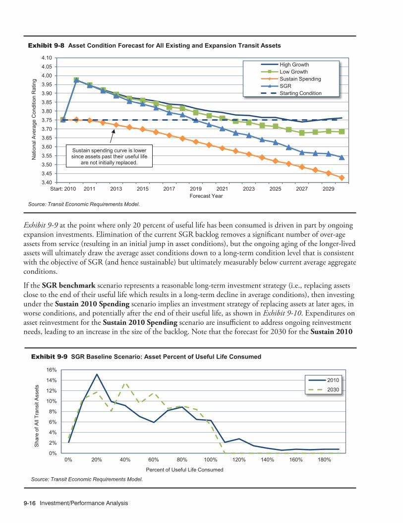
Investment/Performance Analysis9-16

12/28/2012 09XT_A (9-8) R4.xlsx

3.40

3.45

3.50

3.55

3.60

3.65

3.70

3.75

3.80

3.85

3.90

3.95

4.00

4.05

4.10

Start: 2010 2011 2013 2015 2017 2019 2021 2023 2025 2027 2029

Nat

iona

l Ave

rage

Con

ditio

n R

atin

g

Forecast Year

High Growth Low Growth Sustain Spending SGR Starting Condition

Sustain spending curve is lower since assets past their useful life

are not initially replaced.

Source: Transit Economic Requirements Model.

Exhibit 9-8 Asset Condition Forecast for All Existing and Expansion Transit Assets

Exhibit 9-9 at the point where only 20 percent of useful life has been consumed is driven in part by ongoing expansion investments. Elimination of the current SGR backlog removes a significant number of over-age assets from service (resulting in an initial jump in asset conditions), but the ongoing aging of the longer-lived assets will ultimately draw the average asset conditions down to a long-term condition level that is consistent with the objective of SGR (and hence sustainable) but ultimately measurably below current average aggregate conditions.

If the SGR benchmark scenario represents a reasonable long-term investment strategy (i.e., replacing assets close to the end of their useful life which results in a long-term decline in average conditions), then investing under the Sustain 2010 Spending scenario implies an investment strategy of replacing assets at later ages, in worse conditions, and potentially after the end of their useful life, as shown in Exhibit 9-10. Expenditures on asset reinvestment for the Sustain 2010 Spending scenario are insufficient to address ongoing reinvestment needs, leading to an increase in the size of the backlog. Note that the forecast for 2030 for the Sustain 2010

11/13/2012 09XT_B (9-9) R2.xlsx

0%

2%

4%

6%

8%

10%

12%

14%

16%

0% 20% 40% 60% 80% 100% 120% 140% 160% 180%

Sha

re o

f All

Tran

sit A

sset

s

Percent of Useful Life Consumed

2010

2030

Source: Transit Economic Requirements Model.

Exhibit 9-9 SGR Baseline Scenario: Asset Percent of Useful Life Consumed

Supplemental Scenario Analysis 9-17

Spending scenario in Exhibit 9-10 indicates that assets under this scenario will be closer to or beyond the end of their useful life when compared with the other scenarios; this difference reflects a larger portion of the national transit assets still in use after the end of their useful lives.

0%

2%

4%

6%

8%

10%

12%

14%

16%

0% 20% 40% 60% 80% 100% 120% 140% 160% 180% 200%

Sha

re o

f All

Tran

sit A

sset

s

Percent of Useful Life Consumed

2010

2030

Source: Transit Economic Requirements Model.

Exhibit 9-10 Sustain 2010 Spending Scenario: Asset Percent of Useful Life Consumed

12/11/2013 09XT_C (9-10) R3.xlsx

To underscore these findings, note that the Low Growth scenario and the High Growth scenario include unconstrained investments in both asset replacements and asset expansions. Hence, not only are older assets replaced as needed with an aggressive reinvestment rate, but new expansion assets are also continually added to support ongoing growth in travel demand. While initially insufficient to fully arrest the decline in average conditions, the impact of these expansion investments would ultimately reverse the downward decline in average asset conditions in the final years of the 20-year projections. This would also result in a higher proportion of long-lived assets with a larger amount of useful life remaining in 2030 than in 2010 as illustrated in Exhibit 9-11 and Exhibit 9-12, respectively. Furthermore, the High Growth scenario (Exhibit 9-12) adds newer expansion assets at a higher rate than does the Low Growth scenario (Exhibit 9-11), ultimately yielding higher average condition values for that scenario (and average condition values that exceed the current average of 3.75 throughout the entire forecast period).

11/13/2012 09XT_D (9-11) R2.xlsx

0%

2%

4%

6%

8%

10%

12%

14%

16%

0% 20% 40% 60% 80% 100% 120% 140% 160% 180% 200%

Sha

re o

f All

Tran

sit A

sset

s

Percent of Useful Life Consumed

2010

2030

Source: Transit Economic Requirements Model.

Exhibit 9-11 Low Growth Scenario: Asset Percent of Useful Life Consumed

Investment/Performance Analysis9-18

Alternative MethodologyWhen we consider current transit investment practices, the level of investment needed to eliminate the SGR backlog in 1 year is unfeasible. So the SGR benchmark, Low Growth, and High Growth scenarios’ financially unconstrained assumptions (e.g., spending of unlimited transit investment funds each year) is unrealistic. As indicated in Exhibit 9-8, the elimination of the backlog in the first year and the resulting jump in asset conditions in year 1 can be attributed to this unconstrained assumption.

An alternative, more feasible methodology is to have the SGR benchmark, Low Growth, and High Growth scenarios use a financially constrained reinvestment rate to eliminate the SGR backlog by year 20 while maintaining the collective national transit assets at a condition rating of 2.5 or higher. Analysis has determined that investing $17.5 billion annually would achieve this objective of eliminating the backlog in 20 years.

Exhibit 9-13 presents the condition projections for each of the four scenarios using this alternative methodology. However, the SGR benchmark, Low Growth, and High Growth scenarios are financially constrained so the investment strategies result in replacing assets at later ages, in worse conditions, and potentially after the end of their useful lives.

11/13/2012 09XT_F (9-13) R2.xlsx

3.40

3.45

3.50

3.55

3.60

3.65

3.70

3.75

3.80

3.85

Start: 2010 2011 2013 2015 2017 2019 2021 2023 2025 2027 2029

Nat

iona

l Ave

rage

Con

ditio

n R

atin

g

Forecast Year

Sustain Spending SGR Low Growth High Growth Starting Condition

Source: Transit Economic Requirements Model.

Exhibit 9-13 Asset Condition Forecast for All Existing and Expansion Transit Assets Under Alternative Methodology

11/13/2012 09XT_E (9-12) R2.xlsx

0%

2%

4%

6%

8%

10%

12%

14%

16%

18%

0% 20% 40% 60% 80% 100% 120% 140% 160% 180% 200%

Sha

re o

f All

Tran

sit A

sset

s

Percent of Useful Life Consumed

2010

2030

Source: Transit Economic Requirements Model.

Exhibit 9-12 High Growth Scenario: Asset Percent of Useful Life Consumed

Supplemental Scenario Analysis 9-19

Comparison of 2010 to 2013 TERM ResultsThe backlog and investment needs estimated by TERM differ between the 2010 and 2013 C&P Reports. This section compares the TERM results between these two reports and explains why they differ.

The estimated backlog in the 2013 C&P Report increased from $77.7 billion (as reported in the 2010 C&P Report) to $85.9 billion, representing an increase of more than 10 percent. There are three primary reasons for the increase in the backlog:

� Additional needs: The value of the backlog is strongly correlated to the age of the inventory of assets. Certain assets that were nearing the condition threshold of 2.5 in 2008 continued to age and degrade until 2010. As the predicted condition of these assets moved from better than 2.5 to worse than 2.5 during this period, the cost of replacing them was added to the backlog calculation. The backlog increased by $9 billion for this reason between the 2010 and the 2013 C&P Report.

� Inflation: Using published construction inflation factors, the backlog was escalated from 2008 to 2010 dollars. The impact of inflation on the backlog between the 2010 and 2013 C&P Reports is $3.6 billion.

� Changed Asset Inventory: The asset inventory used in the TERM simulation consists of nearly 84,000 asset records for almost 2,400 transit agencies. For each edition of the C&P report, the Federal Transit Administration (FTA) collects new asset data from select agencies. In general, agencies continue to improve the defensibility and accuracy of their inventory data. As a result, FTA expects some change to reflect the improved data. For the 2013 C&P Report, the impact of improved data resulted in a net decrease of approximately $4.4 billion.

Exhibit 9-14 provides a summary of these three adjustments. Note that the SGR backlog of $77.7 billion dollars comes from Exhibit 8-30 in the 2008 C&P Report.

Nonrail investment projections decreased in this 2013 C&P Report relative to the 2010 C&P Report for all scenarios, as presented in Exhibit 9-15, while rail investments decreased in this report relative to the previous report only for the High Growth scenario. This is because the high growth rate in this 2013 C&P Report is lower than the high growth rate in the 2010 C&P Report.

The high growth rate is projected using 10- or 15-year historical ridership growth trends. The 2010 C&P Report used a 10-year trend (1999 to 2008), which gave a high growth rate of 2.8 percent. The 10-year trend for the 2013 C&P Report (2001 to 2010) included the effects of the recession and, thus, was not

11/13/2012 09XT_G (9-14) R2.xlsx

Billion $SGR Backlog as reported in the 2010 C&P report $77.7

Impact of two additional years of needs +9.0Impact of inflation +3.6Impact from the change in the asset inventory -4.4

SGR Backlog as reported in the 2013 C&P report $85.9

Exhibit 9-14 Causes of the Increase in the Backlog between the 2010 C&P Report and the 2013 C&P Report

Source: Transit Economic Requirements Model.

Scenario2010 C&P

Report2013 C&P

Report2010 C&P

Report2013 C&P

Report2010 C&P

Report2013 C&P

ReportSustain 2010 Spending $6.4 $5.8 $10.7 $10.7 $17.1 $16.5SGR Benchmark $7.5 $6.7 $11.6 $11.7 $19.1 $18.5Low Growth $8.4 $7.8 $13.6 $14.2 $22.1 $22.0High Growth $10.0 $9.2 $16.0 $15.3 $26.0 $24.5

Investment Projection (Billions of 2010 Dollars) Nonrail Rail Total

Source: Transit Economic Requirements Model.

Exhibit 9-15 Comparison of Projected Investment Needs for 2010 and 2013 C&P Report Investment Scenarios

12/12/2013 09XT_H (9-15) R5.xlsx

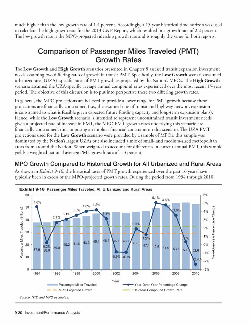
Investment/Performance Analysis9-20

much higher than the low growth rate of 1.4 percent. Accordingly, a 15-year historical time horizon was used to calculate the high growth rate for the 2013 C&P Report, which resulted in a growth rate of 2.2 percent. The low growth rate is the MPO-projected ridership growth rate and is roughly the same for both reports.

Comparison of Passenger Miles Traveled (PMT) Growth Rates

The Low Growth and High Growth scenarios presented in Chapter 8 assessed transit expansion investment needs assuming two differing rates of growth in transit PMT. Specifically, the Low Growth scenario assumed urbanized-area (UZA)–specific rates of PMT growth as projected by the Nation’s MPOs. The High Growth scenario assumed the UZA-specific average annual compound rates experienced over the most recent 15-year period. The objective of this discussion is to put into perspective these two differing growth rates.

In general, the MPO projections are believed to provide a lower range for PMT growth because these projections are financially constrained (i.e., the assumed rate of transit and highway network expansion is constrained to what is feasible given expected future funding capacity and long-term expansion plans). Hence, while the Low Growth scenario is intended to represent unconstrained transit investment needs given a projected rate of increase in PMT, the MPO PMT growth rates underlying this scenario are financially constrained, thus imposing an implicit financial constraint on this scenario. The UZA PMT projections used for the Low Growth scenario were provided by a sample of MPOs; this sample was dominated by the Nation’s largest UZAs but also included a mix of small- and medium-sized metropolitan areas from around the Nation. When weighted to account for differences in current annual PMT, this sample yields a weighted national average PMT growth rate of 1.3 percent.

MPO Growth Compared to Historical Growth for All Urbanized and Rural AreasAs shown in Exhibit 9-16, the historical rates of PMT growth experienced over the past 16 years have typically been in excess of the MPO-projected growth rates. During the period from 1994 through 2010

11/13/2012 09XT_I (9-16) R2.xlsx

37.9 38.0 39.0

40.2 41.6 43.3 45.1 46.5 46.1 45.7 46.5 47.1 49.5 51.9 53.7 53.9 52.6

4.6%

0.2%

2.7% 3.1%

3.5% 4.0% 4.2%

3.1%

-0.9% -0.9%

1.9%

1.2%

5.1% 4.8%

3.5%

0.3%

-2.4%

-3%

-2%

-1%

0%

1%

2%

3%

4%

5%

6%

0

10

20

30

40

50

60

1994 1996 1998 2000 2002 2004 2006 2008 2010

Yea

r-Ove

r-Yea

r Per

cent

age

Cha

nge

Pas

seng

er M

iles

Trav

eled

(Bill

ions

)

Year Passenger Miles Traveled Year-Over-Year Percentage Change MPO Projected Growth 15-Year Compound Growth Rate

Source: NTD and MPO estimates.

Exhibit 9-16 Passenger Miles Traveled, All Urbanized and Rural Areas

Supplemental Scenario Analysis 9-21

presented in Exhibit 9-16, the compound annual growth rate averaged roughly 2.1 percent rather than the 1.3-percent growth rate projected by MPOs for the upcoming 20- to 30-year period. The average compound annual growth rate of 2.1 percent closely resembles the 2.0 percent high growth rate. Given the significant difference in these two rates (and the relatively high rate of historic PMT growth as compared to other additional measures, such as urban area population growth), the historical rate of PMT was identified as a reasonable input value for the High Growth (or higher-growth) scenario. There is a significant drop in year-over-year percentage change in 2009 and 2010 PMT that is mostly due to the decrease in PMT for UZAs over 1 million in population.

UZAs Over 1 Million in PopulationAs shown in Exhibit 9-17, the difference between the MPO-projected growth rate and the recent historical PMT growth rate remains unchanged when limited to UZAs with populations greater than 1 million. For these larger UZAs, the compound average annual growth rate again averaged roughly 2.2 percent during the period from 1994 through 2010 as compared with the 1.2-percent growth rate projected by MPOs for the up-coming 20- to 30-year period.

11/13/2012 09XT_J (9-17) R2.xlsx

34.5

34.7 35.9 36.7 38.1 39.6 41.3

42.7 42.2 41.9 43.0 43.3 45.3

47.5 48.9 49.0 47.8

4.9%

0.6%

3.3%

2.4%

3.8% 3.8% 4.5% 3.3%

-1.1% -0.6%

2.4%

0.6%

4.8%

4.8% 3.1%

0.1%

-2.4%

-4%

-2%

0%

2%

4%

6%

8%

0

5

10

15

20

25

30

35

40

45

50

1994 1996 1998 2000 2002 2004 2006 2008 2010

Yea

r-Ove

r-Yea

r Per

cent

age

Cha

nge

Pas

seng

er M

iles

Trav

eled

(Bill

ions

)

Year

Passenger Miles Traveled Year-Over-Year Percentage Change MPO Projected Growth 15-Year Compound Growth Rate

Source: NTD and MPO estimates.

Exhibit 9-17 Passenger Miles Traveled, UZAs over 1 Million in Population

UZAs Under 1 Million in Population and Rural AreasFinally, as shown in Exhibit 9-18, there is significantly less difference between the MPO-projected and recent annual average historical PMT growth rates when the analysis is limited to urbanized areas with populations less than 1 million and rural areas. For UZAs under 1 million in population, the compound average annual growth rate averaged roughly 2.3 percent during the period from 1994 through 2010, which is close to the 2.2-percent growth rate projected by MPOs for this group. There are two significant differences to note here with the findings for the larger UZAs. First, the MPO-projected rate of increase for UZAs under 1 million in population is roughly 64 percent higher than for UZAs over 1 million in population. This difference is partly accounted for by (1) the higher rates of population growth in many of these smaller UZAs (particularly in the south and in the west) and (2) proposed light and commuter rail investments in some UZAs in this group. Second, the year-to-year variance in the actual growth rates is roughly double that

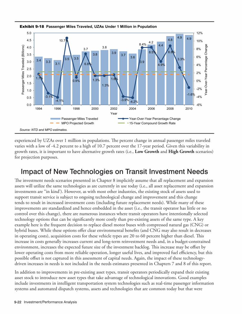
Investment/Performance Analysis9-22

11/13/2012 09XT_K (9-18) R2.xlsx

3.4 3.3 3.1 3.5 3.5

3.7

3.8

3.8

3.9 3.7

3.6 3.9

4.2 4.4

4.8 4.9 4.9

1.7%

-3.1% -4.1%

10.7%

0.9%

6.8%

1.3% 1.3%

1.6%

-3.9% -4.2%

8.4%

8.5%

4.9%

8.8%

3.3%

-1.6%

-6%

-4%

-2%

0%

2%

4%

6%

8%

10%

12%

0.0

0.5

1.0

1.5

2.0

2.5

3.0

3.5

4.0

4.5

5.0

1994 1996 1998 2000 2002 2004 2006 2008 2010

Yea

r-Ove

r-Yea

r Per

cent

age

Cha

nge

Pas

seng

er M

iles

Trav

eled

(Bill

ions

)

Year Passenger Miles Traveled Year-Over-Year Percentage Change MPO Projected Growth 15-Year Compound Growth Rate

Source: NTD and MPO estimates.

Exhibit 9-18 Passenger Miles Traveled, UZAs Under 1 Million in Population

experienced by UZAs over 1 million in populations. The percent change in annual passenger miles traveled varies with a low of -4.2 percent to a high of 10.7 percent over the 17-year period. Given this variability in growth rates, it is important to have alternative growth rates (i.e., Low Growth and High Growth scenarios) for projection purposes.

Impact of New Technologies on Transit Investment NeedsThe investment needs scenarios presented in Chapter 8 implicitly assume that all replacement and expansion assets will utilize the same technologies as are currently in use today (i.e., all asset replacement and expansion investments are “in kind’). However, as with most other industries, the existing stock of assets used to support transit service is subject to ongoing technological change and improvement and this change tends to result in increased investment costs (including future replacement needs). While many of these improvements are standardized and hence embedded in the asset (i.e., the transit operator has little or no control over this change), there are numerous instances where transit operators have intentionally selected technology options that can be significantly more costly than pre-existing assets of the same type. A key example here is the frequent decision to replace diesel motor buses with compressed natural gas (CNG) or hybrid buses. While these options offer clear environmental benefits (and CNG may also result in decreases in operating costs), acquisition costs for these vehicle types are 20 to 60 percent higher than diesel. This increase in costs generally increases current and long-term reinvestment needs and, in a budget-constrained environment, increases the expected future size of the investment backlog. This increase may be offset by lower operating costs from more reliable operation, longer useful lives, and improved fuel efficiency, but this possible offset is not captured in this assessment of capital needs. Again, the impact of these technology-driven increases in needs is not included in the needs estimates presented in Chapters 7 and 8 of this report.

In addition to improvements in pre-existing asset types, transit operators periodically expand their existing asset stock to introduce new asset types that take advantage of technological innovations. Good examples include investments in intelligent transportation system technologies such as real-time passenger information systems and automated dispatch systems, assets and technologies that are common today but that were

Supplemental Scenario Analysis 9-23

not available 15 to 20 years ago. These improvements typically yield improvements in service quality and efficiency, but they also tend to yield increases in asset acquisition, maintenance, and replacement costs, resulting in an overall increase in reinvestment costs as well as the expected future size of the SGR backlog.

Impact of Compressed Natural Gas and Hybrid Buses on Future NeedsTo provide a better sense of the impact of new technology adoption on long-term needs, the analysis below presents estimates of the long-term cost of the shift from diesel to compressed natural gas (CNG) and hybrid buses. It is important to emphasize that this analysis is only intended to provide a sense of the significance of this impact on long-term capital needs (including the possible consequences of not capturing this impact in TERM’s needs estimates). This is not an assessment of the full range of operational, environmental, or other potential costs and benefits arising from this shift and, hence, is not an evaluation of the decision to invest in any specific technology.

Exhibit 9-19 below presents historical (2000 to 2010) and forecast (2011 to 2030) estimates of the share of transit buses that rely on CNG and other alternative fuels vehicles and on hybrid power sources. The forecast estimates assume the current trend rate of increase in alternative and hybrid vehicle shares as observed over the period 2005 to 2010. Based on this projection, the share of vehicles powered by alternative fuels is estimated to increase from 23 percent in 2010 to 53 percent in 2030. During the same period, the share of hybrid buses is estimated to increase from 3 percent to 35 percent. This results in diesel shares declining from roughly 74 percent today to roughly 12 percent by 2030.

11/15/2012 09XT_L (9-19) R2

0%

20%

40%

60%

80%

100%

2000 2005 2010 2015 2020 2025 2030

Hybrid and Electric

CNG and Other Alternative Fuel

Exhibit 9-19 Hybrid and Alternative Fuel Vehicles: Share of Total Bus Fleet, 2000–2030

Source: Transit Economic Requirements Model.

Impact on CostsBased on FTA analysis, the average unit cost of an alternative fuels bus is 15.5 percent higher than that of a standard diesel bus of the same size. Similarly, hybrid buses cost roughly 65.9 percent more than standard diesel buses of the same size. When combined with the current and projected mix of bus vehicle types presented above in Exhibit 9-19, these cost assumptions yield an estimated increase in average bus vehicle capital costs of 25.7 percent over the period 2010 to 2030 (using the mix of bus types from 2010 as the base of comparison). (It is important to note here that this cost increase represents a shift in the mix of bus types purchased and not the impact of underlying inflation, which will impact all vehicle types, including diesel, alternative fuels, and hybrid.) Reductions in operating costs due to the new technology are not shown in this analysis of capital needs but are presumably part of the motivation for agencies that purchase these vehicles.

Impact on NeedsWhat, then, is the impact of this cost increase on long-term transit capital needs? Exhibit 9-20 presents the impact of this potential cost increase on annual transit needs as estimated for the Low Growth scenario

Investment/Performance Analysis9-24

11/15/2012 09XT_M (9-20) R2

$0

$5

$10

$15

$20

$25

$30

$35

$40

2011 2012 2013 2014 2015 2016 2017 2018 2019 2020 2021 2022 2023 2024 2025 2026 2027 2028 2029 2030

Inve

stm

ent D

olla

rs, B

illio

ns

Hybrid and Alternative Fuels Impact

Scenario Needs Estimates

Source: Transit Economic Requirements Model.

Exhibit 9-20 Impact of Shift to Vehicles Using Hybrid and Alternative Fuels on Investment Needs: Low Growth Scenario

presented in Chapter 8. For this scenario, the cost impact is negligible in the early years of the projection period but grows over time as the proportion of buses using alternative fuel and hybrid power increases (note that the investment backlog is not included in this depiction). The impact on total investment needs for all Chapter 9 investment scenarios (SGR baseline, Low Growth, and High Growth) is presented in dollar and percentage terms in Exhibit 9-21. Note that the shift to alternative fuels and hybrid buses is estimated to increase average annual replacement needs by $0.5 to $0.8 billion, yielding a 2.5- to 3.5-percent increase in investment needs. To help place these estimated amounts in perspective, it is helpful to note that (1) the shift from diesel to alternative fuels and hybrid buses is only one of a number of technology changes that may impact long-term transit reinvestment needs, but (2) reinvestment in transit buses likely represents the largest share of transit needs subject to this type of significant technological change. Hence, the impact of all new technology adoptions (not accounted for in the Chapter 8 scenarios and including but not limited to new bus propulsion systems) may add on the order of 5 to 10 percent to long-term transit capital needs.

Impact on BacklogFinally, in addition to impacting unconstrained capital needs, the shift from diesel to hybrid and alternative-fuel vehicles can also have an impact on the size of the future backlog. For example, Exhibit 9-22 shows the estimated impact of this shift on the SGR backlog as was estimated for the Sustain 2010 Spending scenario from Chapter 8. Under this scenario, long-term spending is capped at current levels such that any increase in costs over the analysis period must necessarily be added to the backlog. Moreover, given that buses’ useful lives as estimated by TERM range from roughly 7 to 14 years, all existing and many expansion vehicles will need to be replaced over the 20-year analysis period, meaning that any increase in costs for this asset type will be added to the backlog over this period of analysis.

As with the analysis above, Exhibit 9-22 suggests that the initial impact of the shift to hybrid and alternative-fuel vehicles is small but increases over time as these vehicle types make up an increasing share of the Nation’s bus fleet. By 2030, this shift is estimated to increase the size of the backlog from $141.7 billion to $151.4 billion, an increase of $9.8 billion or 6.9 percent.

11/13/2012 09XT_N (9-21) R2.xlsx

MeasureSGR

BaselineLow

GrowthHigh

GrowthAverage Annual Needs $0.47B $0.67B $0.83BPercent Increase 2.50% 3.00% 3.50%

Source: Transit Economic Requirements Model.

Exhibit 9-21 Impact of Shift from Diesel to Alternative Fuels and Hybrid Vehicles on Annual Investment Needs

Supplemental Scenario Analysis 9-25

$0

$20

$40

$60

$80

$100

$120

$140

$160

2010 2012 2014 2016 2018 2020 2022 2024 2026 2028 2030

Inve

stm

ent D

olla

rs, B

illio

ns

Hybrid and Alternative Fuels Impact

Scenario SGR Backlog Estimate

Source: Transit Economic Requirements Model.

Exhibit 9-22 Impact of Shift to Vehicles Using Hybrid and Alternative Fuels on Backlog Estimate: Sustain 2010 Spending Scenario

12/11/2013 09XT_O (9-22) R4.xlsx

Forecasted Expansion InvestmentThis section compares key characteristics of the national transit system in 2010 to their forecasted TERM results over the next 20 years for different scenarios. It also includes expansion projections of fleet size, guideway route miles, and stations broken down by scenario to better understand the expansion investments that TERM is making.

TERM’s projections of fleet size are presented in Exhibit 9-23. The projections for the Low Growth and High Growth scenarios are higher than the projected Sustain 2010 Spending scenario in order to preserve existing transit assets at a condition rating of 2.5 or higher and expand transit service capacity to support differing levels of ridership growth while passing TERM’s benefit-cost test. An exponential trend line based on historical data from 2002 to 2010 is extrapolated 20 years into the future also is shown in Exhibit 9-23. This extrapolated historical trend line falls between the low and high growth projections indicating that the Low Growth and High Growth scenario investments potentially could maintain current conditions.

12/18/2013 09XT_P (9-23) R4.xlsx

55,000

105,000

155,000

205,000

255,000

2002 2006 2010 2014 2018 2022 2026 2030

Flee

t Veh

icle

Cou

nt High (est)

Low (est)

Sustain 2010 Spending

Actual

Historical Trend

Note: Data through 2010 are actual; data after 2010 are estimated based on trends. Source: Transit Economic Requirements Model.

Exhibit 9-23 Projection of Fleet Size by Scenario

Investment/Performance Analysis9-26

In contrast, the projected guideway route miles for the Sustain 2010 Spending, Low Growth, and High Growth scenarios are less than the projected historical trend scenario as shown in Exhibit 9-24. (Note that TERM’s projections of guideway route miles for the Sustain 2010 Spending and Low Growth scenarios are nearly identical.) Commuter rail has substantially more guideway route miles than heavy and light rail, making it very hard to accurately project total guideway route miles for all rail modes; therefore, the historical trend line is not provided.

12/18/2013 09XT_Q (9-24) R4.xlsx

9,000

9,500

10,000

10,500

11,000

11,500

12,000

12,500

13,000

13,500

2002 2006 2010 2014 2018 2022 2026 2030

High (est)

Low (est)

Sustain 2010SpendingActual

Exhibit 9-24 Projection of Guideway Route Miles by Scenario

Note: Data through 2010 are actual; data after 2010 are estimated based on trends. Source: Transit Economic Requirements Model.

TERM’s expansion projections of stations by scenario needed to preserve existing transit assets at a condition rating of 2.5 or higher and expand transit service capacity to support differing levels of ridership growth (while passing TERM’s benefit-cost test) are presented Exhibit 9-25, along with the historical trend. TERM’s Low Growth estimates generally are in line with the historical trend, indicating that expansion projects of stations under the Low Growth scenario could maintain current transit conditions.

12/18/2013 09XT_R (9-25) R4.xlsx

2,500

3,000

3,500

4,000

4,500

5,000

2002 2006 2010 2014 2018 2022 2026 2030

Sta

tion

Cou

nt High (est)

Low (est)

Sustain 2010SpendingActual

Historical Trend

Exhibit 9-25 Projection of Stations by Scenario

Note: Data through 2010 are actual; data after 2010 are estimated based on trends. Source: Transit Economic Requirements Model.

Supplemental Scenario Analysis 9-27

For each of the various scenarios, TERM estimates future investment in fleet size, guideway route miles, and stations for each of the next 20 years. Exhibit 9-26 presents TERM’s projection for total fixed guideway route miles under a Low Growth scenario by rail mode. TERM projects different investment needs for each year that is added to the year 2010 actual total stock. Heavy rail’s share of the projected annual fixed guideway route miles remains relatively constant over the 20-year period, while the amount of fixed guideway route miles increases slightly for light and commuter rail.

11/15/2012 09XT_S (9-26) R2

0

2,000

4,000

6,000

8,000

10,000

12,000

14,000

16,000

2010 (actual)

2012 2014 2016 2018 2020 2022 2024 2026 2028 2030

Fixe

d G

uide

way

Len

gth,

Mile

s

Light Rail

Heavy Rail

Commuter Rail

Source: Transit Economic Requirements Model.

Exhibit 9-26 Stock of Fixed Guideway Miles by Year Under Low Growth Scenario, 2010–2030

Investment/Performance Analysis9-28

Sensitivity Analysis

Highway Sensitivity Analysis .......................................................................................10-2

Alternative Economic Analysis Assumptions ............................................................10-2Value of Travel Time ............................................................................................................ 10-2Growth in the Value of Time ................................................................................................ 10-5Value of a Statistical Life ..................................................................................................... 10-7Discount Rate ...................................................................................................................... 10-8Alternative Future Fuel Price Assumptions ......................................................................... 10-10

Alternative Strategies .................................................................................................10-11Alternative Bridge Maintenance, Repair, and Rehabilitation Strategies ............................. 10-11Accelerating Operations/ITS Deployments ........................................................................ 10-12

Transit Sensitivity Analysis ..........................................................................................10-15

Changes in Asset Replacement Timing (Condition Threshold) ...............................10-15

Changes in Capital Costs ..........................................................................................10-16

Changes in the Value of Time ....................................................................................10-16

Changes to the Discount Rate ...................................................................................10-17

Sensitivity Analysis 10-1

CHAPTER 10

Investment/Performance Analysis10-2

In any modeling effort, it is critical to evaluate the validity of the underlying assumptions and determine the degree to which projected outcomes could be affected by changes to these assumptions. This section demonstrates how the average annual highway investment requirements associated with the Maintain Conditions and Performance scenario and the Improve Conditions and Performance scenario presented in Chapter 8 would be affected by changes in some of the underlying assumptions in the Highway Economic Requirements System (HERS) and the National Bridge Investment Analysis System (NBIAS). To simplify the presentation of results, these sensitivity tests were applied only to the systemwide versions of these scenarios based on HPMS-derived future growth in vehicle miles traveled (VMT), rather than to the full range of subscenarios presented in Chapter 8.

This section begins with sensitivity tests on economic inputs to the models, varying the assumptions about the value that travelers attach to travel time and crash risk, and the discount rate used to convert future costs and benefits into present equivalents. The effects of assuming growth in the value of travel time and price of fuel are also discussed. This is followed by tests relating to investment strategies, including the impact of applying some alternative Maintenance, Repair, and Rehabilitation (MR&R) strategies built into NBIAS, and the impact of alternative assumptions about future Operations/Intelligent Transportation System (ITS) deployment strategies in HERS. A subsequent section within this chapter explores information regarding the assumptions underlying the analyses developed using the Transit Economic Requirements Model (TERM).

Alternative Economic Analysis AssumptionsThe U.S. Department of Transportation (DOT) periodically issues guidance on the valuation of travel time and the economic value of a statistical life, while the Office of Management and Budget (OMB) provides guidance to Federal agencies on the discount rate to be applied in benefit-cost analysis. Recognizing the uncertainty regarding these values, the guidance documents include both specific recommended values and ranges of values to be tested. The analyses presented in Chapter 7 and 8 of this report are based on the primary recommendations from the OMB and U.S. DOT guidance for these economic inputs, whereas the analyses presented in this chapter rely on recommended alternative values to be used for sensitivity testing.

The HERS analyses presented in Chapter 7 and 8 assume future changes in fuel prices consistent with forecasts from the U.S. Department of Energy’s Annual Energy Outlook (AEO) publication. This publication presents a range of potential alternative forecasts. One such alternative assuming higher fuel prices is explored in this section.

Value of Travel TimeThe value of travel time is a critical component of benefit-cost analysis of transportation investments. It is often the largest component of the benefits estimated. Time used for travel represents a cost to society and the economy because that time could be used for other more enjoyable or productive purposes. There is much debate on the appropriate value of travel time. Studies show that the value of time can vary by income, time of day and type of trip. The U.S. DOT’s Revised Departmental Guidance on the Value of Travel Time in Economic Analysis, 2011 recommends values of time to use for economic analysis developed from the findings of current research and the values used in other countries (see http://www.dot.gov/sites/dot.dev/files/docs/vot_guidance_092811c_0.pdf ). The value of time is tied to specified percentages of the median annual household income for personal travel and the median gross wage for business travel, which vary

Highway Sensitivity Analysis

Sensitivity Analysis 10-3

Why conduct a sensitivity analysis for the assumed value of travel time savings?

Sensitivity analysis is done to test the results of models using information that is uncertain, such as the value of travel time saved.

The U.S. DOT based its guidance for valuing travel time on a review of the research literature, which reflects estimates that vary widely even after attempts to standardize them. Particularly for personal travel (including commuting), the evidence is hard to synthesize. Internationally, common practice among transportation government agencies is to assume that the average value of personal travel time bears a fixed ratio to a measure of economy-wide average wages (or some similar measure).

For local personal travel, the value of travel time savings is estimated to be 50 percent of hourly median household income, derived by dividing the nationwide median annual household income by 2,080 hours to yield an hourly income. For business travel, the value of travel time savings is assumed to be equal to a nationwide median gross wage, defined as the sum of the median hourly wage and estimated hourly benefits.

The U.S. DOT recognizes the uncertainty in the recommended values and therefore recommends that alternative calculations be done using the range of high and low dollar values. For personal auto travel, the low value is 35 percent of the estimated hourly median household income and the high value is about 60 percent. For business travel, 80 percent of the median wage is used for the low dollar value and 120 percent is used for the high value.

Q A&

depending on the mode of travel. Within the HERS and NBIAS models, the per-person-hour estimates of travel time savings based on this guidance are converted to average values of time per vehicle-hour for different types of vehicle classes, drawing upon estimates of average vehicle occupancy; time-related vehicle depreciation cost; and, for trucks, the inventory cost of freight in transit. For 2010, the average values per vehicle-hour ranged from $16.89 for small autos to $31.44 for five-axle combination trucks. (For the passenger vehicle classes, the averages are weighted means of a value for personal travel and a higher value for business travel.) The U.S. DOT guidance recommends sensitivity analyses using a lower and a higher value of travel time savings given the uncertainty of the values recommended; these alternative values are based on different valuations of travel time savings per person hour as a percentage of hourly earnings. Exhibit 10-1 shows the results of applying these alternative travel time values to the average annual investment levels

11/19/2012 10XH_A (10-1) R3.xlsx

Billions Percent Billions Percentof 2010 Change From of 2010 Change FromDollars Baseline Dollars Baseline

Baseline* (Personal–50%; Business–100%) $86.3 $145.9 HERS-Derived Component $51.1 $86.9 NBIAS-Derived Component $12.2 $20.2 Other (Non-modeled) Component $23.0 $38.8Lower (Personal–35%; Business–80%) $89.2 3.3% $134.9 -7.6% HERS-Derived Component $53.2 4.0% $78.9 -9.2% NBIAS-Derived Component $12.2 0.4% $20.1 -0.5% Other (Nonmodeled) Component $23.7 3.3% $35.9 -7.6%Higher (Personal–60%; Business–120%) $84.9 -1.6% $153.3 5.1% HERS-Derived Component $50.1 -2.0% $92.3 6.2% NBIAS-Derived Component $12.2 0.1% $20.2 0.1% Other (Nonmodeled) Component $22.6 -1.6% $40.8 5.1%

Maintain Conditions and Performance Scenario

Improve Conditions and Performance ScenarioAlternative Assumptions About the

Valuation of Travel Time Savings per Hour as a Percentage of Hourly Earnings,

for Personal and Business Travel

Exhibit 10-1 Impact of Alternative Value of Time Assumptions on Highway Investment Scenario Average Annual Investment Levels

* The Baseline levels shown correspond to the systemwide scenarios presented in Chapter 8 that applied higher, HPMS-derived VMT growth forecasts. The investment levels shown are average annual values for the period from 2011 through 2030. Sources: Highway Economic Requirements System and National Bridge Investment Analysis System.

Investment/Performance Analysis10-4

associated with the Maintain Conditions and Performance scenario and the Improve Conditions and Performance scenario. Results are shown separately for the portions of these scenarios derived from HERS and NBIAS because their sensitivity to these inputs is very different. As discussed in Chapter 8, each scenario includes non-modeled investment components reflecting types of investments not modeled in HERS or NBIAS, which varies proportionally based on the model results.

Non-modeled Highway InvestmentsThe HERS-derived component of each scenario represents spending on pavement rehabilitation and capacity expansion on Federal-aid highways. The NBIAS-derived component represents rehabilitation spending on all bridges, including those off the Federal-aid highways. The non-modeled component corresponds to system enhancement spending, plus pavement rehabilitation and capacity expansion on roads not classified as Federal-aid highways.

In the Sustain 2010 Spending scenario presented in Chapter 8, the values for these HERS and NBIAS components sum to $72.5 billion. In 2010, non-modeled spending accounted for 26.6 percent of total investment ($26.7 billion out of $100.2 billion) and is assumed to form the same share in all scenarios presented in Chapter 8.

Similarly for the sensitivity analysis for the Maintain Condition and Performance scenario and the Improve Condition and Performance scenario presented in this section, the non-modeled component is set at 26.6 percent of the total investment level. As the combined levels of the HERS-derived and NBIAS-derived scenario components rise or fall, the non-modeled component changes proportionally. Consequently, the percent change in the non-modeled component of each alternative scenario relative to the baseline always matches the percent change in the total investment level for that scenario.

Impact on Improve Conditions and Performance ScenarioAs shown in Exhibit 10-1, applying a lower value of travel time reduces the average annual investment level for the Improve Conditions and Performance scenario from $145.9 billion to $134.9 billion (-7.6 percent). The HERS-derived component of the scenario declines by 9.0 percent from $86.9 billion to $78.9 billion, whereas the NBIAS-derived component declines by only 0.5 percent. Applying a higher value of time would increase the average annual investment level associated with this scenario by 5.5 percent in total, again with HERS investments being more sensitive, increasing by 6.2 percent.

The HERS investments are more sensitive to the value of travel time savings because the HERS model evaluates a mix of system rehabilitation and system expansion investments, and system expansion investments tend to be more sensitive to changes in travel time savings. NBIAS only considers system rehabilitation investments, which tend to have a much smaller impact on travel time, except to the extent that they address situations where weight restrictions had been imposed on a bridge requiring long detours for trucks.

As described in Chapter 8, the Improve Conditions and Performance scenario is defined to include all investments that would be cost-beneficial (i.e., with a benefit-cost ratio [BCR] greater than or equal to 1.00). The change in the value of travel time saved affects the benefits estimated. A reduction in the value of travel time saved is likely to reduce the magnitude of the benefits estimated from the time savings, thus reducing the BCR for individual projects under consideration. To the extent that the estimated BCR for some of these projects falls below 1.00, they would no longer qualify for inclusion under this scenario. Conversely, applying a higher value of time increases the estimated benefits and, hence, the BCR, causing more projects to appear to be cost-beneficial.

Sensitivity Analysis 10-5

Impact on Maintain Conditions and Performance ScenarioAs described in Chapter 8, the Maintain Conditions and Performance scenario is intended to keep overall system conditions and performance in 2030 at roughly the same level as in 2010. The NBIAS-derived portion of this scenario is based on maintaining the average bridge sufficiency rating (see Chapter 7 for a discussion of this measure). The HERS-derived portion represents the average of two investment levels: (1) the amount of total HERS investment in system rehabilitation and system expansion that results in average pavement roughness (as measured by the International Roughness Index [IRI]) being maintained; and (2) an investment level which results in average delay per VMT being maintained. Generally, this approach results in one of these two indicators (IRI in the baseline analysis) improving a little over the 20- year period, while the other (delay in the baseline analysis) gets a little worse.

For the Maintain Condition and Performance scenario, applying a lower value of travel time savings increases the average annual investment level for HERS-derived component by 4.0 percent, from $51.1 billion to $53.2 billion. This change is primarily driven by changes in the mix of investments selected by HERS; reducing the value of time makes capacity projects less attractive, so that HERS will direct a greater share of investment towards pavement rehabilitation. This has the effect of reducing the level of total HERS investment required to maintain average pavement roughness, while increasing the level of total HERS investment required to maintain average delay. In this case, these changes were not proportional, causing the average of these two HERS investment levels to rise. The opposite is true applying a higher value of travel time savings, which brings the investment level associated with maintaining average pavement roughness closer to the investment level associated with maintaining average delay, and reduces their average by 2.0 percent relative to the baseline.

The NBIAS-derived component of the Maintain Condition and Performance scenario rounds to $12.2 billion regardless of which set of travel time assumptions is applied. The overall investment level associated with this scenario would increase by 3.3 percent, from $86.3 billion to $89.2 billion, assuming a lower value of time, and decline by 1.6 percent to $84.9 billion assuming a higher value of time.

Growth in the Value of TimeBenefit cost analysis is generally done in constant base year dollars, assuming no change in the value of the parameters used in the analysis. The implicit assumption of this approach is that all values will experience the same rate of growth in the future, therefore not changing the relative values. U.S. DOT guidance recommended value for travel time savings is based on the median national gross hourly wage for business travel and the median hourly household income for personal travel. The guidance also recognizes the need to increase the value of travel time savings in line with the growth in income adjusted for inflation. It assumes income elasticity equal to one for scaling the value of travel time savings, based on time series estimates of income elasticity. The recommendation is that the value of travel time savings increases annually by 1.6 percent based on Congressional Budget Office assumption of future annual growth in real median household income.

This poses a few challenges on how to appropriately include the increase in the real value of time. The value of time will affect both the demand for travel and the value of the benefits estimated. Since the real value of time increases due to an increase in income, this would increase the demand for travel given income elasticity of demand for travel, possibly in addition to the other changes. However, as HERS is currently configured, the base year value of time is factored into the implicit baseline price that the model assumes is consistent with the HPMS-derived VMT growth forecast. If the value of time is increased over time, the HERS model will interpret the resulting increase in travel time costs relative to the base year the same way it would if this increase in costs were related to increased congestion. Consequently, the travel demand elasticity feature in HERS will cause some of the HPMS-derived future VMT growth to be suppressed.

Investment/Performance Analysis10-6

Exhibit 10-2 illustrates the effect of including an increase in the real value of time in HERS as it is currently configured. Under the Improve Conditions and Performance scenario, the growth in the value of time increases the HERS-modeled component of the average annual investment level from $86.9 billion to $87.7 billion, a 0.9 percent change. Projected 2030 Federal-aid highway VMT would be 3.544 trillion under this alternative, rather than the 3.629 trillion predicted for 2030 in the baseline analysis. The reduction in travel demand reduces the net time savings and pavement improvements resulting from the investments, while the value of time estimate increases. The two countervailing impacts have a very small effect on the estimated benefits, and hence the resulting investment needs.

What are some examples of the types of behavior that the travel demand elasticity features in HERS represent?

If highway congestion worsens in an area, this increases travel time costs on the road network. In response, some highway users might shift their trips to mass transit or perhaps forgo some personal trips that they might ordinarily make. For example, they might be more likely to combine multiple errands into a single trip because the time spent in traffic discourages them from making a trip unless it is absolutely necessary. Increases in fuel prices also increase the cost of driving and would have a similar impact.

In the longer term, people might make additional adjustments to their lifestyles in response to changes in user costs that would impact their travel demand. For example, if travel time in an area is reduced substantially for an extended period of time, some people may make different choices about where to purchase a home. If congestion is reduced, purchasing a home far out in the suburbs might become more attractive because commuters would be able to travel farther in a shorter period of time.

Q A&

11/14/2012 10XH_B (10-2) R2.xlsx

Billions Percent Billions Percentof 2010 Change From of 2010 Change FromDollars Baseline Dollars Baseline

Baseline* (No change) $86.3 $145.9 HERS-Derived Component $51.1 $86.9Alternative (1.6 % increase per year) $77.8 -9.8% $147.0 0.8% HERS-Derived Component $44.9 -12.2% $87.7 0.9%

Maintain Conditions and Performance Scenario

Improve Conditions and Performance ScenarioAlternative Assumptions About Growth

in Value of Time in Response to Projected Increases in Real Median Household Income

Exhibit 10-2 Impact of Alternative Assumptions About Growth in the Real Value of Time on Highway Investment Scenario Average Annual Investment Levels

* The Baseline levels shown correspond to the systemwide scenarios presented in Chapter 8 that applied higher, HPMS-derived VMT growth forecasts. The investment levels shown are average annual values for the period from 2011 through 2030. Sources: Highway Economic Requirements System and National Bridge Investment Analysis System.

For the Maintain Conditions and Performance scenario, the average annual investment level associated with the HERS-derived component would fall from $51.1 billion to $44.9 billion under this alternative, a 12.2 percent decline. The investment associated both with maintaining average pavement roughness and average delay per VMT would be lower under this alternative—projected 2030 Federal-aid highway VMT would be 3.489 trillion, down from 3.584 trillion in the baseline analysis. The increased value of time tends to increase the BCR associated with some projects, which has an impact on the prioritized ranking of potential projects, but this effect is swamped by the HERS perception that any increase in travel time costs equates to a higher implicit price and, consequently, less travel.

The initial plans for this report had been to factor in an increasing value of time into the baseline analysis, as directed by U.S. DOT guidance. However, as a result of HERS testing similar to that presented above, this increased value was not included in the analysis for this report, and instead to work on alternative approaches that would better capture the impacts of higher incomes without unintentionally suppressing travel growth. The NBIAS model does not currently have the capability to process changes to the value of time during its analysis period.

Sensitivity Analysis 10-7

Value of a Statistical LifeOne of the most challenging issues in benefit-cost analysis is how to best determine the monetary cost to place on injuries of various severities. Few people would consider any amount of money to be adequate compensation for a person being seriously injured, much less killed. On the other hand, people can attach a value to changes in their risk of suffering an injury, and indeed such valuations are implicit in their everyday choices. For example, a traveler may face a choice between two travel options that are equivalent except that one carries a lower risk of fatal injury but costs more. If the additional cost is $1, then a traveler who selects the safer option is manifestly willing to pay at least $1 for the added safety—what economists call “revealed preference.” Moreover, if the difference in risk is, say, one in a million, then a million travelers who select the safer option are collectively willing to pay at least $1 million for a risk reduction that statistically can be expected to save one of their lives. In this sense, the “value of a statistical life” among this population is at least $1 million.

Based on the results of various studies of individual choices involving money versus safety trade-offs, some government agencies estimate an average value of a statistical life (VSL) for use in their regulatory and investment analyses. The U.S. DOT issued guidance in 2008 (Revised Departmental Guidance: Treatment of the Value of Preventing Fatalities and Injuries in Preparing Economic Analyses) recommending a value of $5.8 million per statistical life, to be updated annually by the changes in prices and income. The 2010 inflated VSL is $6.2 million. (Subsequent to the analysis undertaken for this report, guidance issued by the DOT in 2013 increased the VSL to $9.1 million for analyses with a base year of 2012 [Guidance on Treatment of the Economic Value of a Statistical Life in U.S. Department of Transportation Analyses, http:// www.dot.gov/office-policy/transportation-policy/guidance-treatment-economic-value-statistical-life].) For nonfatal injuries, the DOT retained from its 1993 guidance the practice of setting values per statistical injury as percentages of the value of a statistical life; these vary according to the level of severity, from 0.2 percent for a “minor” injury to 76.3 percent for a “critical” injury. (The injury levels are from the Maximum Abbreviated Injury Scale.) In view of the uncertainty surrounding the average value of a statistical life, the Department also required that regulatory and investments analyses include sensitivity tests using alternative values; alternative values of $3.4 million as the lower bound and $9.0 million as the upper bound are presented.

Impact of Alternatives on HERS ResultsThe HERS model contains for each highway functional class equations to predict crash rates per VMT and parameters to determine the number of fatalities and nonfatal injuries per crash. The model assigns to crashes involving fatalities and other injuries an average cost consistent with the guidance in the U.S. DOT memorandum. Exhibit 10-3 demonstrates that the results from the HERS simulations are nevertheless relatively insensitive to the use of alternative values of a statistical life. This is consistent with the observations from Chapter 7 that crash costs: (1) form a small share of highway user cost (13.6 percent in 2010); and (2) are much less sensitive than travel time and vehicle operating costs to changes in the level of total investment within the scope of HERS, which excludes targeted safety-oriented investments due to data limitations. Replacing the baseline value of a statistical life with a figure of $9.0 million slightly raises the BCR for potential improvements and increases the estimate of the amount of potentially cost-beneficial investment (the HERS component of the Improve Conditions and Performance scenario) by 0.9 percent, from $86.9 billion to $87.7 billion. Conversely, assuming a value of statistical life of $3.4 million would reduce the average annual investment level associated with the HERS-derived component of the scenario by 0.7 percent.

For the Maintain Conditions and Performance scenario, increasing (to $9.0 million) or lowering (to $3.4 million) the average value of a statistical life would change the average annual investment level by negative 0.8 percent or positive 0.5 percent respectively.

Investment/Performance Analysis10-8

11/15/2012 10XH_C (10-3) R2.xlsx

Billions Percent Billions Percentof 2010 Change From of 2010 Change FromDollars Baseline Dollars Baseline

Baseline* ($6.2 Million) $86.3 $145.9 HERS-Derived Component $51.1 $86.9 NBIAS-Derived Component $12.2 $20.2 Other (Non-modeled) Component $23.0 $38.8Lower ($3.4 Million) $84.5 -2.1% $142.4 -2.4% HERS-Derived Component $50.7 -0.8% $86.3 -0.7% NBIAS-Derived Component $11.3 -7.6% $18.2 -9.8% Other (Non-modeled) Component $22.5 -2.1% $37.9 -2.4%Higher ($9.0 Million) $87.7 1.7% $148.9 2.0% HERS-Derived Component $51.4 0.5% $87.7 0.9% NBIAS-Derived Component $13.0 6.5% $21.5 6.7% Other (Non-modeled) Component $23.4 1.7% $39.6 2.0%

Maintain Conditions and Performance Scenario

Improve Conditions and Performance ScenarioAlternative Value of a

Statistical Life Assumption, in 2010 Dollars

Exhibit 10-3 Impact of Alternative Value of Life Assumptions on Highway Investment Scenario Average Annual Investment Levels

* The Baseline levels shown correspond to the systemwide scenarios presented in Chapter 8 that applied higher, HPMS-derived VMT growth forecasts. The investment levels shown are average annual values for the period from 2011 through 2030. Sources: Highway Economic Requirements System and National Bridge Investment Analysis System.

Impact of Alternatives on NBIAS ResultsExhibit 10-3 also shows that increasing the assumed value of a statistical life to $9.0 million raises the NBIAS estimate of the average annual investment in bridges that would be needed over the following 20 years to fund all cost-beneficial projects by 2030 (the NBIAS component of the Improve Conditions and Performance scenario) by 6.7 percent, from $20.2 billion to $21.5 billion. Assuming a higher value of life increases the benefits associated with projects that reduce crash rates, causing additional projects to have a BCR above 1.0. Conversely, reducing the statistical value of life to $3.4 million reduces the NBIAS-derived component of the Improve Conditions and Performance scenario by 9.8 percent, indicating that there are a number of projects with BCRs not far above 1.0 in the baseline analysis that derived benefits from reducing crash rates.

At any given level of investment, increasing the value of statistical life shifts investment toward producing significant safety benefits to bridge users (by reducing crash rates) and away from projects that may be more focused on addressing issues with the physical conditions of bridges. Consequently, the overall level of NBIAS investment associated with maintaining the average bridge sufficiency rating is 6.5 percent higher ($13.0 billion versus $12.2 billion per year) assuming a $9.0 million value of a statistical life than in the baseline analysis. Assuming a $3.4 million value of a statistical life reduces the average annual NBIAS-derived component of the Maintain Conditions and Performance scenario by 7.6 percent, because a greater share of this spending is directed towards projects that would more directly impact the sufficiency rating.

Discount RateBenefit-cost analyses use a discount rate that scales down benefits and costs arising in the future relative to those arising in the base year. To this point, the real discount rate has been 7 percent in this report’s applications of HERS, NBIAS, and TERM; this means that deferring a benefit or cost for a year reduces its real value by approximately 6.5 percent (1/1.07). This choice of real discount rate conforms to the “default position” in the 1992 OMB guidance on discount rates, in Circular A-94, for benefit-cost analyses of public investment and regulatory programs. Subsequently, in 2003, OMB’s Circular A-4 recommended that

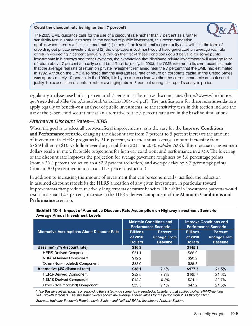
Sensitivity Analysis 10-9

regulatory analyses use both 3 percent and 7 percent as alternative discount rates (http://www.whitehouse.gov/sites/default/files/omb/assets/omb/circulars/a004/a-4.pdf ). The justifications for these recommendations apply equally to benefit-cost analyses of public investments, so the sensitivity tests in this section include the use of the 3-percent discount rate as an alternative to the 7-percent rate used in the baseline simulations.

Alternative Discount Rates—HERSWhen the goal is to select all cost-beneficial improvements, as is the case for the Improve Conditions and Performance scenario, changing the discount rate from 7 percent to 3 percent increases the amount of investment in HERS programs by 21.6 percent, with the annual average amount increasing from $86.9 billion to $105.7 billion over the period from 2011 to 2030 Exhibit 10-4). This increase in investment dollars results in more favorable projections for highway conditions and performance in 2030. The lowering of the discount rate improves the projection for average pavement roughness by 5.8 percentage points (from a 26.4 percent reduction to a 32.2 percent reduction) and average delay by 3.7 percentage points (from an 8.0 percent reduction to an 11.7 percent reduction).

In addition to increasing the amount of investment that can be economically justified, the reduction in assumed discount rate shifts the HERS allocation of any given investment, in particular toward improvements that produce relatively long streams of future benefits. This shift in investment patterns would result in a small (2.7 percent) increase in the HERS-derived component of the Maintain Conditions and Performance scenario.

11/15/2012 10XH_D (10-4) R2.xlsx

Billions Percent Billions Percentof 2010 Change From of 2010 Change FromDollars Baseline Dollars Baseline

Baseline* (7% discount rate) $86.3 $145.9 HERS-Derived Component $51.1 $86.9 NBIAS-Derived Component $12.2 $20.2 Other (Non-modeled) Component $23.0 $38.8Alternative (3% discount rate) $88.1 2.1% $177.3 21.5% HERS-Derived Component $52.5 2.7% $105.7 21.6% NBIAS-Derived Component $12.2 -0.3% $24.4 20.7% Other (Non-modeled) Component $23.5 2.1% $47.2 21.5%

Maintain Conditions and Performance Scenario

Improve Conditions and Performance Scenario

Alternative Assumptions About Discount Rate

Exhibit 10-4 Impact of Alternative Discount Rate Assumption on Highway Investment Scenario Average Annual Investment Levels

* The Baseline levels shown correspond to the systemwide scenarios presented in Chapter 8 that applied higher, HPMS-derived VMT growth forecasts. The investment levels shown are average annual values for the period from 2011 through 2030. Sources: Highway Economic Requirements System and National Bridge Investment Analysis System.

Could the discount rate be higher than 7 percent?

The 2003 OMB guidance calls for the use of a discount rate higher than 7 percent as a further sensitivity test in some instances. In the context of public investment, this recommendation applies when there is a fair likelihood that: (1) much of the investment’s opportunity cost will take the form of crowding out private investment, and (2) the displaced investment would have generated an average real rate of return exceeding 7 percent annually. Although the first of these conditions could be valid for some public investments in highways and transit systems, the expectation that displaced private investments will average rates of return above 7 percent annually could be difficult to justify. In 2003, the OMB referred to its own recent estimate that the average real rate of return on private investment remained near the 7 percent that the OMB had estimated in 1992. Although the OMB also noted that the average real rate of return on corporate capital in the United States was approximately 10 percent in the 1990s, it is by no means clear whether the current economic outlook could justify the expectation of a rate of return averaging above 7 percent during this report’s analysis period.

Q A&

Investment/Performance Analysis10-10

Alternative Discount Rates—NBIASSince many of the bridge improvements evaluated in NBIAS are relatively long-lived, the choice of discount rate can significantly affect the model’s estimate of investments necessary to maintain or improve the condition and performance of the system. Reducing the discount rate increases the number of potential investments that pass the benefit cost test. Exhibit 10-4 shows that reducing the real discount rate in NBIAS from the baseline 7 percent to 3 percent would increase the NBIAS-derived component of the Improve Conditions and Performance scenario by 20.7 percent, from $20.2 billion to $24.4 billion, annually.

For the maintain scenario, the BCR is not the limiting factor or the goal. Many projects that pass the benefit test will not be included under the maintain scenario, so increasing the number of eligible projects does not significantly affect the needs estimated. The change in discount rate would change the composition of investments implemented in NBIAS, which would result in a 0.3 percent reduction in the NBIAS-derived component for the Maintain Conditions and Performance scenario.

Alternative Future Fuel Price Assumptions In this edition of the C&P report, the price of oil used in the baseline analyses presented in Chapters 7 and 8 is the AEO reference forecast. This is a change from the 2010 C&P report where price of oil was held constant at the base year level. From 2008 to 2010 the price of fuel (both gasoline and diesel) declined by 38.5 percent. AEO projects oil prices to increase above the rate of inflation and anticipates that, after recovering in 2011, fuel prices will ease up for a few years and then start to increase above the rate of inflation, resulting in an increase of 28.2 percent over the first 5 years of the C&P analysis period, and a 45.0 percent increase over the 20-year period.

The sensitivity analysis presented in Exhibit 10-5 compares the changes in investment needs using AEO’s projections assuming a more aggressive rate of growth in prices. Under this projection, the oil prices continue to increase, resulting in 93.1 percent growth in the first 5 years, with a total increase of 162.6 percent over the 20-year period. Exhibit 10-5 shows the results of using a more aggressive rate of growth in oil prices. For the Improve Conditions and Performance scenario, the average annual investment level would decline by 14.7 percent, driven by a decline in the HERS-modeled component of 18.1 percent. For the Maintain Conditions and Performance scenario, the average annual investment level would decline from $86.3 billion to $72.8 billion, a reduction of 15.7 percent, driven by a decline in the HERS-modeled component of 19.4 percent. Under both scenarios, the reduction in investments results primarily from reduced spending on system expansion. This sensitivity test was not applied to NBIAS, as it does not include fuel prices as a separate discrete model input.

11/15/2012 10XH_E (10-5) R2.xlsx

Billions Percent Billions Percentof 2010 Change From of 2010 Change FromDollars Baseline Dollars Baseline

Baseline* (AEO Reference Case) $86.3 $145.9 HERS-Derived Component $51.1 $86.9Alternative (AEO High Oil Price Case) $72.8 -15.7% $124.5 -14.7% HERS-Derived Component $41.2 -19.4% $71.2 -18.1%

Maintain Conditions and Performance Scenario

Improve Conditions and Performance Scenario

Alternative Assumptions About Future Fuel Prices

Exhibit 10-5 Impact of Alternative Future Fuel Price Assumption on Highway Investment Scenario Average Annual Investment Levels

* The Baseline levels shown correspond to the systemwide scenarios presented in Chapter 8 that applied higher, HPMS-derived VMT growth forecasts. The investment levels shown are average annual values for the period from 2011 through 2030. Sources: Highway Economic Requirements System and National Bridge Investment Analysis System.

Sensitivity Analysis 10-11

Assuming a higher rate of growth in oil prices increases the user costs by increasing the cost of driving. As discussed in Chapter 7, an increase in user costs lead to reduced miles of travel. Under the Maintain Conditions and Performance scenario, projected 2030 VMT on Federal-aid highways would be 8.1 percent lower (3.293 trillion vs. 3.584 trillion) relative to the baseline assumption. Under the Improve Conditions and Performance scenario, VMT would be 8.2 percent lower assuming higher fuel prices than in the baseline.

Alternative StrategiesIn addition to analyses based on alternative technical assumptions, the HERS and NBIAS models are capable of analyzing selected policy alternatives as well. Two such alternatives pertain to strategies for bridge MR&R (modeled in NBIAS), and accelerating the future rate of deployment of Operations/ITS strategies.

Alternative Bridge Maintenance, Repair, and Rehabilitation StrategiesAs discussed in Appendix B, the NBIAS model has been adapted to consider four alternative strategies for the MR&R actions simulated in NBIAS. The State of Good Repair MR&R strategy is the most aggressive, and seeks to bring all bridges to a relatively high condition level that can be sustained via ongoing investment, and involves heavy frontloading of MR&R spending. The Sustain Steady State MR&R strategy is somewhat less aggressive, and is aimed toward identifying and implementing a pattern of MR&R improvements that would reach and achieve an improved steady state in terms of overall bridge system conditions without frontloading MR&R investment. The Maximize Average Returns strategy is even less aggressive, seeking to maximize the degree of bridge system performance improved per dollar of MR&R expenditure. The least aggressive alternative is the Minimize MR&R Costs strategy, which seeks to minimize MR&R costs only, without regard to the implications for other types of NBIAS-modeled spending. The baseline analyses presented in Chapters 7 and 8 applied the Sustain Steady State MR&R strategy; previous C&P reports relied on the Minimize MR&R Costs strategy.

As discussed in Chapter 7, the NBIAS model considers bridge deficiencies at the level of individual bridge elements based on engineering criteria and computes an initial value for the cost of a set of corrective actions that would address all such deficiencies. The economic bridge investment backlog represents the combined cost of these corrective actions in those cases where NBIAS estimates that it would be cost-beneficial to implement them. Assuming the Sustain Steady State MR&R strategy, the economic backlog for year 2010, as reported in Chapter 7, was estimated to be $106.4 billion. Exhibit 10-6 shows that, if less-aggressive MR&R strategies are assumed, the size of the initial backlog would be smaller. Reducing the set of MR&R actions considered results in an estimated 2010 backlog of $93.4 billion assuming the Minimize MR&R Costs strategy and $100.8 assuming the Maximize Average Return strategy. Assuming the more aggressive State of Good Repair MR&R strategy would increase the 2010 backlog computed by NBIAS to $114.3  billion.

Although the Minimize MR&R Costs strategy has the lowest initial backlog from among the four alternatives, the average annual investment level associated with implementing all cost-beneficial NBIAS modeled investment within the Improve Conditions and Performance scenario is $31.6 billion, 56.3 percent higher than the $20.2 billion level estimated in the baseline. Even this level of investment is insufficient to maintain the average sufficiency rating at its 2010 level of 81.7 on a scale of zero to 100; the projected average sufficiency rating for 2030 would be only 75.4. Thus, it is not possible to achieve the objective of the Maintain Conditions and Performance scenario assuming a Minimize MR&R Cost strategy. The implications of these findings are that skimping on MR&R spending in the short term may make it necessary to conduct major bridge rehabilitation actions or bridge replacements sooner than would have been the case had MR&R spending been more robust.

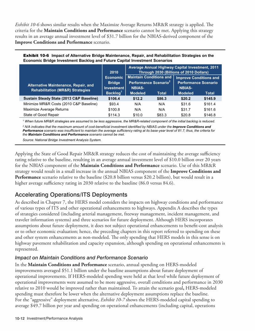
Investment/Performance Analysis10-12

Exhibit 10-6 shows similar results when the Maximize Average Returns MR&R strategy is applied. The criteria for the Maintain Conditions and Performance scenario cannot be met. Applying this strategy results in an average annual investment level of $31.7 billion for the NBIAS-derived component of the Improve Conditions and Performance scenario.

11/15/2012 10XH_F (10-6) R2.xlsx

2010Economic

BridgeInvestment NBIAS- NBIAS-Backlog1 Modeled Total Modeled Total

Sustain Steady State (2013 C&P Baseline) $106.4 $12.2 $86.3 $20.2 $145.9Minimize MR&R Costs (2010 C&P Baseline) $93.4 N/A N/A $31.6 $161.4Maximize Average Returns $100.8 N/A N/A $31.7 $161.6State of Good Repair $114.3 $10.0 $83.3 $20.8 $146.8

Average Annual Highway Capital Investment, 2011 Through 2030 (Billions of 2010 Dollars)

Maintain Conditions and Performance Scenario2

Improve Conditions and Performance ScenarioAlternative Maintenance, Repair, and

Rehabilitation (MR&R) Strategies

Exhibit 10-6 Impact of Alternative Bridge Maintenance, Repair, and Rehabilitation Strategies on the Economic Bridge Investment Backlog and Future Capital Investment Scenarios

1 When future MR&R strategies are assumed to be less aggressive, the MR&R-related component of the initial backlog is reduced. 2 N/A indicates that the maximum amount of cost-beneficial investment identified by NBIAS under the Improve Conditions and Performance scenario was insufficient to maintain the average sufficiency rating at its base-year level of 81.7; thus, the criteria for the Maintain Conditions and Performance scenario cannot be met. Source: National Bridge Investment Analysis System.

Applying the State of Good Repair MR&R strategy reduces the cost of maintaining the average sufficiency rating relative to the baseline, resulting in an average annual investment level of $10.0 billion over 20 years for the NBIAS component of the Maintain Conditions and Performance scenario. Use of this MR&R strategy would result in a small increase in the annual NBIAS component of the Improve Conditions and Performance scenario relative to the baseline ($20.8 billion versus $20.2 billion), but would result in a higher average sufficiency rating in 2030 relative to the baseline (86.0 versus 84.6).

Accelerating Operations/ITS DeploymentsAs described in Chapter 7, the HERS model considers the impacts on highway conditions and performance of various types of ITS and other operational enhancements to highways. Appendix A describes the types of strategies considered (including arterial management, freeway management, incident management, and traveler information systems) and three scenarios for future deployment. Although HERS incorporates assumptions about future deployment, it does not subject operational enhancements to benefit-cost analysis or to other economic evaluation; hence, the preceding chapters in this report referred to spending on these and other system enhancements as non-modeled. The only spending that HERS models in this sense is on highway pavement rehabilitation and capacity expansion, although spending on operational enhancements is represented.

Impact on Maintain Conditions and Performance Scenario In the Maintain Conditions and Performance scenario, annual spending on HERS-modeled improvements averaged $51.1 billion under the baseline assumptions about future deployment of operational improvements. If HERS-modeled spending were held at that level while future deployment of operational improvements were assumed to be more aggressive, overall conditions and performance in 2030 relative to 2010 would be improved rather than maintained. To attain the scenario goal, HERS-modeled spending must therefore be lower when the alternative deployment assumptions replace the baseline. For the “aggressive” deployment alternative, Exhibit 10-7 shows the HERS-modeled capital spending to average $49.7 billion per year and spending on operational enhancements (including capital, operations

Sensitivity Analysis 10-13

and maintenance costs) to be $4.6 billion per year more than in the baseline. The sum of these figures, $54.3 billion, indicates a $3.2 billion increase in total spending relative to the baseline value of $51.1 billion to achieve the objectives of the Maintain Conditions and Performance scenario. For the “full immediate deployment alternative,” total spending is $55.1 billion, or $4.0 billion higher than the baseline value.

11/15/2012 10XH_G (10-7) R2.xlsx

Average AverageOperations/ITS Deployments HERS Additional Pavement Delay

Assumption1 Modeled Deployment Total Roughness perSpending Spending2 HERS Total (IRI) VMT

Baseline3 (continue existing trends) $51.1 N/A $51.1 $86.3 -7.6% 4.3%Aggressive deployments alternative $49.7 $4.6 $54.3 $90.6 -6.6% 3.3%Full immediate deployments alternative $45.0 $10.1 $55.1 $91.7 -1.9% 3.5%

Baseline3 (continue existing trends) $86.9 N/A $86.9 $145.9 -26.7% -8.0%Aggressive deployments alternative $86.4 $4.6 $91.0 $151.5 -26.7% -9.3%Full immediate deployments alternative $86.4 $10.1 $96.5 $159.0 -27.0% -11.0%Average Annual Spending $145.9 BillionBaseline3 (continue existing trends) $86.9 N/A $86.9 $145.9 -26.7% -8.0%Aggressive deployments alternative $82.3 $4.6 $86.9 $145.9 -25.3% -8.1%Full immediate deployments alternative $76.8 $10.1 $86.9 $145.9 -22.8% -8.7%

Percent Change, 2030Compared With 2010

Average Annual Highway Investment, 2011 Through 2030 (Billions of 2010 Dollars)

HERS-Derived Component

Maintain Conditions and Performance Scenario

Improve Conditions and Performance Scenario

Exhibit 10-7 Impact of Alternative Operations Strategies Deployment Rate Assumptions on Selected Performance Indicators and Highway Investment Scenarios

1 The analyses presented in this table assume one of the following: (1) existing trends in ITS deployments will continue for 20 years; (2) an aggressive pattern of deployment will occur over the next 20 years; or (3) all of the aggressive deployments will occur immediately, rather than being spread out over 20 years. The costs associated with the more aggressive deployments were deducted from the budget available in HERS for pavement and widening investments. 2 Amounts reflect additional capital and operation and maintenance costs associated with the alternative Operations/ITS deployment strategies relative to the Baseline. 3 The Baseline levels shown correspond to the systemwide scenarios presented in Chapter 8 that applied higher, HPMS-derived VMT growth forecasts. Source: Highway Economic Requirements System.

By design, under any of the deployment assumptions, the Maintain Conditions and Performance scenario shows no unambiguous change in overall conditions and performance relative to the baseline. An improvement in one of the scenario’s measures of conditions and performance must be accompanied by deterioration in the other measure. Under each deployment assumption, the measure which shows improvement happens to be average pavement roughness; at the same time, average delay per VMT worsens. Assuming aggressive rather than baseline deployment makes the projected change less favorable for average pavement roughness (-6.6 percent versus -7.6 percent) but more favorable for average delay (3.3 percent versus 4.3 percent). The projections for average delay are more favorable because the types of operational improvements represented are assumed to have direct impacts only on travel time and accident rates; direct impacts on pavement conditions are assumed to be negligible.

These findings suggest that at the particular investment level reflected in the Maintain Conditions and Performance scenario (which is 13.9 percent below the actual level of spending by all levels of government in 2010), diverting resources from pavement and capacity improvements towards more aggressive deployment of operational improvements would not produce better conditions and performance outcomes. It should be noted however, that some of the operational improvements being considered, such as incident management systems, have benefits in crash reductions that would not be reflected in the IRI and delay measures used as targets in the Maintain Conditions and Performance scenario.

Investment/Performance Analysis10-14

Impact on Improve Conditions and Performance ScenarioIn the Improve Conditions and Performance scenario, more aggressive deployment of operational enhancements marginally reduces the amount of highway rehabilitation and capacity investment that HERS finds to be cost-beneficial. HERS-modeled rehabilitation and capacity investment decreases from $86.9 billion per year assuming baseline deployment to $86.4 billion per year assuming either of the more aggressive deployment alternatives. Total spending represented in HERS increases, however, because of the extra spending on the operations deployments, from $86.9 billion per year in the baseline to $96.5 billion per year assuming full immediate deployments. After adding an allowance for capital spending on non-modeled improvements, Exhibit 10-7 indicates the corresponding variation in total spending to be between $145.9 billion per year in the baseline and $159.0 billion per year assuming full immediate deployments.

Because of the increased spending on operational enhancements, projections for average delay are more favorable when deployment is more aggressive than when the baseline is assumed. Although the types of operational enhancements considered in these cases are assumed to have no direct impacts on pavement quality, the projections for average pavement roughness are also slightly better than in the baseline. One reason for this is that spending on pavement rehabilitation is slightly higher under more aggressive deployment even though total HERS-modeled spending is lower. Pavement rehabilitation receives $44.3 billion out of the total $86.4 billion in HERS-modeled spending under the full immediate deployment alternative, versus $43.9 billion out $86.9 billion in the baseline.

Although these findings suggest that adopting more aggressive Operations/ITS deployment strategies would be advantageous if overall highway spending levels were significantly increased, the different levels of investment associated with each of these alternatives under the Improve Conditions and Performance scenario make direct tradeoffs more difficult to assess. To address this issue, the bottom three rows in Exhibit 10-7 present alternative allocations of fixed total spending between the HERS-modeled types of improvements and operational enhancements given a single fixed level of HERS investment, based on the $86.9 billion HERS-derived component of the Improve Conditions and Performance scenario. The additional spending on operational improvements in the more aggressive deployment alternatives is assumed to come out of this total, reducing dollar-for-dollar the HERS-modeled component of spending. The balance of this spending offset between pavement rehabilitation and highway capacity expansion is determined by the model’s cost-benefit optimization.

Exhibit 10-7 indicates that such reallocation of spending would produce worse outcomes in 2030 for pavement roughness, but better outcomes for travel delay. For pavement roughness, this reflects reduced spending on pavement rehabilitation together with operational enhancements being assumed to have no direct effect. For average delay, the reduction from the additional spending on operational enhancements outweighs the effect of the offset to spending on highway capacity. With the full immediate deployment assumed, pavements are projected to become 22.8 percent smoother between 2010 and 2030, compared with 26.7 percent smoother with baseline deployment assumed. For average delay per VMT, the corresponding projections are for reductions of 8.7 percent versus 8.0 percent.

Sensitivity Analysis 10-15

Transit Sensitivity Analysis

This section examines the sensitivity of the Transit Economic Requirements Model’s (TERM’s) transit investment needs estimates to variations in the values of these key inputs:

� Asset Replacement Timing (Condition Threshold) � Capital Costs � Value of Time � Discount Rate.

Specifically, these alternative projections assess how the estimates of baseline investment needs for the State of Good Repair (SGR) Benchmark and the Low Growth and High Growth Scenarios discussed in Chapter 8 vary in response to changes in the assumed values of these input variables. Note here that, by definition, funding under the Sustain 2010 Spending Scenario is invariant to changes in any input variable and, for this reason, that scenario is not considered in this sensitivity analysis.

Changes in Asset Replacement Timing (Condition Threshold)

Each of the four investment scenarios examined in Chapter 8 assume that assets are replaced at condition rating 2.50 as determined by TERM’s asset condition decay curves (in this context, 2.50 is referred to as the “replacement condition threshold”). Recall here that TERM’s condition rating scale runs from 5.0 for assets in “excellent” condition through 1.0 for assets in “poor” condition. In practice, this assumption implies replacement of assets within a short-term period (e.g., roughly 1 to 5 years depending on asset type) after they have attained their expected useful life. Replacement at condition 2.50 can therefore be thought of as providing a replacement schedule that is both realistic (in practice, few assets are replaced exactly at their expected useful life value due to a range of factors including the time to plan, fund, and procure an asset replacement) and potentially conservative (i.e., the needs estimates would be higher if all assets were assumed to be replaced at precisely the end of their expected useful life).

Based on this background, Exhibit 10-8 shows the impact of varying the replacement condition threshold by increments of 0.25 on TERM’s projected asset preservation needs for the SGR Benchmark and the Low

12/10/2013 10XT_A (10-8) R3.xlsx

High Growth Scenario

Replacement Condition Thresholds

Billions of 2010 Dollars

Percent Change

From Baseline

Billions of 2010 Dollars

Percent Change

From Baseline

Billions of 2010 Dollars

Percent Change

From Baseline

Very late asset replacement (2.00) $15.57 -15.7% $14.68 -13.7% $14.77 -13.7%Replace assets later (2.25) $17.33 -6.1% $16.00 -5.9% $16.13 -5.8%Baseline (2.50) $18.46 $17.01 $17.12Replace assets earlier (2.75) $22.07 19.6% $20.16 18.5% $20.41 19.2%Very early asset replacement (3.00) $26.03 41.0% $23.28 36.9% $23.49 37.2%

SGR BenchmarkLow Growth

Scenario

Exhibit 10-8 Impact of Alternative Replacement Condition Thresholds on Transit Preservation Investment Needs by Scenario (Excludes Expansion Impacts)

Source: Transit Economic Requirements Model.

Investment/Performance Analysis10-16

Growth and High Growth Scenarios. It should be noted that selection of a higher replacement condition threshold results in assets being replaced at a higher condition (i.e., at an earlier age), which in turn reduces the length of each asset’s service life, thus increasing the number of replacements over any given period of analysis and driving up scenario costs. Reducing the replacement condition threshold will, of course, have the opposite effect. As shown in Exhibit 10-8, each of these three scenarios shows significant changes to total estimated preservation needs from quarter point changes in the replacement condition threshold. Relatively small changes in the replacement condition threshold frequently translate into significant changes in the expected useful life of some asset types; hence, small changes can also drive significant changes in replacement timing and replacement costs.

Changes in Capital CostsThe asset costs used in TERM are based on actual prices paid by agencies for capital purchases as reported to Federal Transit Administration (FTA) in the Transit Electronic Award Management (TEAM) System and in special surveys. Asset prices in the current version of TERM have been converted from the dollar year replacement costs in which assets were reported to FTA by local agencies (which vary by agency and asset) to 2010 dollars using RSMeans© construction cost index. Given the uncertain nature of capital costs, a sensitivity analysis has been performed to examine the effect that higher capital costs would have on the dollar value of TERM’s baseline projected transit investment.

As shown in Exhibit 10-9, TERM projects that a 25 percent increase in capital costs (i.e., beyond the 2010 level used for this report) would be fully reflected in the SGR Benchmark, but only partially realized under either the Low Growth or High Growth Scenarios. This difference in sensitivity results is driven by the fact that investments are not subject to TERM’s benefit-cost ratio in computing the SGR Benchmark (i.e., there are no consequences to increasing costs), whereas the two cost-constrained scenarios do employ this test. Hence, for the Low Growth or High Growth Scenarios, any increase in capital costs (without a similar increase in the value of transit benefits) results in lower benefit-cost ratios and the failure of some investments to pass this test. Therefore, for these latter two scenarios, a 25 percent increase in capital costs would yield a range of roughly 19 to 20 percent increase in needs that pass TERM’s benefit-cost test.

11/13/2012 10XT_B (10-9) R2.xlsx

High Growth Scenario

Capital Cost Increases

Billions of

2010 Dollars

Percent Change

From Baseline

Billions of

2010 Dollars

Percent Change

From Baseline

Billions of

2010 Dollars

Percent Change

From Baseline

Baseline (no change) $18.46 $21.96 $24.54Increase Costs 25% $23.08 25.0% $26.38 20.1% $29.19 18.9%

SGR BenchmarkLow Growth

Scenario

Exhibit 10-9 Impact of an Increase in Capital Costs on Transit Investment Estimates by Scenario

Source: Transit Economic Requirements Model.

Changes in the Value of TimeThe most significant source of transit investment benefits, as assessed by TERM’s benefit-cost analysis, is the net cost savings to users of transit services, a key component of which is the value of travel time savings. Therefore, the per-hour value of travel time for transit riders is a key model input and a key driver of total investment benefits for those scenarios that employ TERM’s benefit-cost test. Readers interested in learning more about the measurement and use of the value of time for the benefit-cost analyses performed by TERM, Highways Economic Requirements System (HERS), and National Bridge Investment Analysis System (NBIAS) should refer to the related discussion presented earlier in the highway section of this chapter.

Sensitivity Analysis 10-17

For this C&P report, the Low Growth and High Growth Scenarios are the only scenarios with investment needs estimates that are sensitive to changes in the benefit-cost ratio. (Note: The Sustain 2010 Spending Scenario uses TERM’s estimated benefit-cost ratios to allocate fixed levels of funding to preferred investments, while the computation of the SGR Benchmark does not employ TERM’s benefit-cost test in any way.)

Exhibit 10-10 shows the effect of varying the value of time on the needs estimates of the Low Growth and High Growth Scenarios. The baseline value of time for transit users is currently $12.50 per hour, based on Department of Transportation (DOT) guidance. TERM applies this amount to all in-vehicle travel, but then doubles this amount to $25.00 per hour when accounting for out-of vehicle travel time, including time spent waiting at transit stops and stations.

Given that value of time is a key driver of total investment benefits, changes in this variable lead to changes in investment ranging from an increase of more than 10 percent to a decrease of more than 6 percent. The resulting different magnitudes of percent changes is because the absolute value of the changes from the baseline are different ($6.25 is a 50 percent change from baseline and $25 is a 100 percent change from baseline). In addition to this issue, we observe that the High Growth Scenario appears to be more sensitive to the value of time than the Low Growth Scenario. This is due to the fact that higher investment levels are associated with the High Growth Scenario than with the Low Growth Scenario; therefore, any changes in the value of time will be magnified accordingly.

11/13/2012 10XT_C (10-10) R2.xlsx

Changes in Value of TimeBillions of

2010 DollarsPercent Change From Baseline

Billions of 2010 Dollars

Percent Change From Baseline

Reduce 50% ($6.25) $20.85 -5.1% $22.98 -6.4%Baseline ($12.50) $21.96 $24.54Increase 100% ($25.00) $23.40 6.6% $27.04 10.2%

Low Growth Scenario High Growth ScenarioExhibit 10-10 Impact of Alternative Value of Time Rates on Transit Investment Estimates by Scenario

Source: Transit Economic Requirements Model.

Changes to the Discount RateFinally, TERM’s benefit-cost module utilizes a discount rate of 7.1 percent in accordance with White House Office of Management and Budget (OMB) guidance. Readers interested in learning more about the selection and use of discount rates for the benefit-cost analyses performed by TERM, HERS, and NBIAS should refer to the related discussion presented earlier in the highway section of this chapter. For this sensitivity analysis and for consistency with the HERS and NBIAS discount rate sensitivity discussion above, TERM’s needs estimates for the Low Growth and High Growth Scenarios were re-estimated using a 3 percent discount rate. The results of this analysis are presented in Exhibit 10-11. These results show that this approximately 58 percent reduction in the discount rate yields an increase in total investment needs (or an increase in the proportion of needs passing TERM’s benefit-cost test) of 3.2 to 6.1 percent.

11/13/2012 10XT_D (10-11) R2.xlsx

High Growth Scenario

Discount RatesBillions of

2010 DollarsPercent Change From Baseline

Billions of 2010 Dollars

Percent Change From Baseline

7.10% (Baseline) $21.96 $24.543.00% $22.67 3.2% $26.03 6.1%

Low Growth ScenarioExhibit 10-11 Impact of Alternative Discount Rates on Transit Investment Estimates by Scenario

Source: Transit Economic Requirements Model.

Investment/Performance Analysis10-18

Chapter 11: Transportation Serving Federal and Tribal Lands .......11-1

Chapter 12: Center for Accelerating Innovation ..............................12-1

Chapter 13: National Fuel Cell Bus Program ..................................13-1

PART III

Special Topics III-1

Special Topics

Special TopicsIII-2

IntroductionChapters 11 through 13 are intended to provide additional insights into topics touched on elsewhere in this report, and to highlight related issues. Chapter 11 provides information on transportation serving Federal and tribal lands, a subset of the transportation system that is not explored in depth in the analyses presented in Chapters 1 through 10. While the investment analyses presented in Part II of this report focus mainly on the potential impacts of alternative levels of investment on future conditions and performance, it is important to recognize the role that innovation and technology can play in ensuring the efficacy of these investments; for this reason, in Part III, Chapters 12 and 13 explore some activities currently under way within the U.S. Department of Transportation (U.S. DOT) to accelerate innovation and explore new technologies.

Chapter 11, Transportation Serving Federal and Tribal Lands, examines the transportation systems serving Federal lands, including resources and types of lands served, and the role of these systems. It also discusses the condition, sources of funding, and expenditures. Lastly, it discusses the future of the transportation systems in Federal lands.

Chapter 12, Center for Accelerating Innovation, examines aspects of utilizing innovation to improve the way transportation infrastructure is created and maintained. It includes initiatives under this program and also discusses the benefits generated for the highway system because of the innovative initiatives.

Chapter 13, National Fuel Cell Bus Program, discusses the background, accomplishments, and current status of fuel cell transit bus research. It describes fuel cell electric bus research projects in the United States and the impact of these projects on commercialization of fuel cell power systems and electric propulsion for transit buses in general.

Transportation Serving Federal and Tribal LandsTransportation Serving Federal and Tribal Lands .....................................................11-2

Types of Federal and Tribal Lands .............................................................................11-2

Accessing Tribal Communities ..................................................................................11-3

Resources Served within Federal Lands ...................................................................11-3

Role of Transportation in the Use of Federal and Tribal Lands ................................11-4

Role of Federal Lands in U.S. Economy ...................................................................11-5

Condition and Performance of Roads Serving Federal and Tribal Lands ................11-6Forest Service ..................................................................................................................... 11-7National Park Service .......................................................................................................... 11-7Fish and Wildlife Service ..................................................................................................... 11-9Bureau of Land Management ............................................................................................. 11-10Bureau of Reclamation ....................................................................................................... 11-11Bureau of Indian Affairs....................................................................................................... 11-11Department of Defense ....................................................................................................... 11-11United States Army Corps of Engineers ............................................................................. 11-12

Transportation Funding for Federal and Tribal Lands ...............................................11-13

Increasing Walking, Biking, and Transit Use on Federal and Tribal Lands ..............11-14

The Future of Transportation on Federal and Tribal Lands ......................................11-15

Transportation Serving Federal Lands 11-1

CHAPTER 11

Special Topics11-2

Transportation Serving Federal and Tribal Lands

This chapter documents transportation serving Federal and Tribal lands, a subset of the transportation system that is not explored in depth in the analyses presented in Chapters 1 through 10. Included are discussions of the types of lands, the resources served, the role of Federal and Tribal lands in the U.S. economy, the role of transportation in the use of Federal and Tribal lands, the condition of the transportation system, sources of funding, expenditures of funds for construction and maintenance of transportation infrastructure, and the future of Federal and Tribal transportation.

Types of Federal and Tribal LandsThe Federal government has title to about 650 million acres1, or about 30 percent of the United States’ total area of 2.3 billion acres2. Additionally, the Federal government holds in trust approximately 55 million acres of land on behalf of Tribal governments. These lands are primarily located in the western part of the country. Federal lands are managed by various Federal land management agencies (FLMAs), primarily within the Departments of the Interior (DOI), Agriculture (USDA), and Defense (DOD). Tribal lands are primarily held in trust by the DOI’s Bureau of Indian Affairs, though many Tribes own additional land beyond these trust lands. Exhibit 11-1 illustrates the major Federal and Tribal lands (note that this only shows the large

9/19/2012 31X_A (11-1) R1.xlsx

Source: The National Atlas of the United States of America.

Exhibit 11-1 Major Federal Lands

Transportation Serving Federal Lands 11-3

units; many smaller units are not shown due to the scale of the image). Exhibit 11-2 highlights resources managed by eight FLMAs.

Federal Agency Federal Lands Served

Forest Service (FS) 155 National Forests and 20 National Grass Lands

National Park Service (NPS) 401 National Parks and MonumentsFish and Wildlife Service 556 Wildlife Refuges, 38 Wetland Management Districts, 70 Fish

Hatcheries and 43 Administrative sitesBureau of Land Management 247.5 million acres of public lands; 700 million acres of subsurface

mineral estate; 601 recreation sitesBureau of Indian Affairs 566 federally-recognized Indian TribesBureau of Reclamation 476 dams, 348 reservoirs, 187 recreation areas, and 58 power plants

Military Installations 400 Major Military Installations

Department of Agriculture

Department of the Interior

Department of Defense

423 lakesU.S. Army Corps of Engineers - Civil Works Facilities

Exhibit 11-2 Types of Lands Managed by Federal Land Management Agencies

Source: FLMAs.

12/12/2013 31X_B (11-2) R3.xlsx

Accessing Tribal CommunitiesAn Indian reservation is land reserved for a Tribe when it relinquished its other land areas to the United States through treaties. More recently, Congressional acts, Executive Orders, and administrative acts have also officially recognized Tribes and their lands. Tribal communities exist in all corners of the country. Some Tribes are located in the cities or suburbs, but most are located in rural America. The 229 Alaska Native Villages continue to be found at their historic locations throughout the State of Alaska. Access to basic community services for the 566 federally recognized sovereign Tribal governments is primarily served by roads, but also can include ice roads, snow machine and ATV trails, airfields, and waterways in remote Alaskan villages. Some Tribes operate transit service within their communities. This transportation infrastructure (roads, bridges, trails, or transit systems) can be owned by the Bureau of Indian Affairs, Tribes, States, counties, or other local governments.

Many roads accessing tribal lands can be characterized as substandard native surface roadways, which can only be used during periods of good weather. Access to many critical community services, jobs, stores, schools, hospitals, emergency services, or intercommunity commerce can be compromised by a common rain event or a thaw of an Alaskan river or permafrost. More than 8 billion vehicle miles are traveled annually on the Tribal Transportation Program road system, even though it is among the most rudimentary of any transportation network in the United States, with more than 60 percent of the system unpaved.

Resources Served within Federal LandsThe natural and cultural resources of Federal and Tribal lands are among the Nation’s greatest assets. Each individual site managed by the FLMAs has a unique mission for managing its resources while providing access in varying degrees to those resources for the enjoyment of the public and the citizens living on those lands. Most FLMAs are charged with managing the wise use of resources for the benefit of present and future generations. Resource management includes preserving and protecting natural, cultural, and historical areas as well as wildlife use areas. Many of the sites have multiple uses, while others have a very limited, specific use. It is estimated that approximately one-half of the Federal lands are managed under multiple use and sustained yield policies that rely on transportation. The remaining lands have protected use management

Special Topics11-4

policies, but even so, transportation systems are essential to their resource management, development, recreational use, and protection.

Federal lands have many uses. These include facilitating national defense, recreation, range and grazing, timber and minerals extraction, energy generation, watershed management, fish and wildlife management, and wilderness. These lands are also managed to protect natural, scenic, scientific, and cultural values. In recent years, resource extraction and cutting of timber have been significantly reduced. At the same time, recreation use has significantly increased. Exhibit 11-3 summarizes annual recreation use and visits on Federal lands. Recreation on Federal lands is measured in recreation visitor days (RVD), which is equivalent to a 12-hour visit.

Forest Service 173 288 175

National Park Service 279 101 397 Fish and Wildlife Service 46 46 626 Bureau of Land Management 58 58 601 Bureau of Indian Affairs N/A N/A N/ABureau of Reclamation 28 28 187 areas

Military Installations 10 53 400+U.S. Army Corps of Engineers - Civil Works Facilities 365 210 463

Total 959 884 2,849+

Department of Defense

Agency Recreation Visits

(Millions) # of SitesDepartment of Agriculture

Department of the Interior

Recreation Visitor Days (Millions)

Exhibit 11-3 Summary of Annual Recreation Use and Visits

Source: FLMAs.

12/12/2013 31X_C (11-3) R3.xlsx

Role of Transportation in the Use of Federal and Tribal LandsTribal communities, national defense, recreation, travel and tourism, and resource extraction are all dependent on quality transportation infrastructure. Transportation plays a key role in the way that people access and enjoy Federal and Tribal lands, and in providing access to jobs and resources. It is impossible to conceive of visiting our Federal lands without the hundreds of thousands of miles of Federal and Tribal roads, trails, and transit systems providing access to and within these lands. This transportation infrastructure provides opportunities for employment, recreational travel and tourism, protection and enhancement of resources, sustained economic development in rural/urban areas, access to educational and health services, and national and international access to our Nation’s most pristine natural, cultural, and historic resources.

Federal agencies, along with States, have designated numerous highways as Scenic Byways, many of which are Federal roads. The Forest Service began designating National Forest Scenic Byways in 1988; as of 2012, more than 130 routes have been designated, totaling 9,000 miles in 36 States. There are more than 3,000 miles of U.S. National Park Service (NPS) roads and parkways that also meet the criteria for Scenic Byways. In 1989, the Bureau of Land Management (BLM) began designating the Back Country Byways; more than 60 routes have been designated to date, totaling 3,100 miles in 11 States.

Public roads make up significant portions of the transportation systems serving these Federal and Tribal lands. In many areas—both urban and rural—transit, bicycling, and pedestrian use supplement this road network, though most agencies do not track this usage. In many remote areas, motorized and non-motorized trails, waterways, and air transports serve as the primary mode of transportation. The broad range of needs dependent on transportation access to Federal lands is summarized in Exhibit 11-4.

Transportation Serving Federal Lands 11-5

Role of Federal Lands in U.S. EconomyThe American outdoor recreation economy produces 6.1 million jobs, spurs $646 billion in spending, and creates $39.9 billion in Federal tax revenue and $39.7 billion in state and local tax revenue.3 In total, there are nearly 1 billion visits per year to Federal lands. In 2011, the recreational visits to lands owned by the Department of the Interior supported over 403,000 jobs and contributed around $48.7 billion in economic activity4. This economic output in 2011 represents about 6.5 percent of the direct output of tourism related personal consumption expenditures for the United States and about 7.6 percent of the direct tourism-related employment. The travel, tourism, and recreation industry claim a share of many other industry sectors, including transportation, lodging, communications, power, wholesale and retail trade, manufacturing, and construction.

Not only is travel and tourism a significant part of our Nation’s economy, it is also an integral part of many local economies in communities adjacent to Federal lands. Overall, recreating visitors spend a little more than $11 billion per year in areas around National Forest System lands. In total, spending by visitors to National Forests and Grasslands contributes almost $13.4 billion to the U.S. economy and sustains more than 205,000 full-and part-time jobs5. Direct and indirect economic benefits on BLM lands from recreation are $7 billion and contribute a total of nearly 59,000 jobs6 . The U.S. Fish and Wildlife Service (FWS) reported that visits to units of the National Wildlife Refuge System (NWRS) generated more than $1.7 billion for the economy per year and employ nearly 27,000 people7. Nationally, U.S. Army Corps of Engineers lakes attract 365 million recreation visitors every year, and the economic impact on these areas is enormous. The total economic benefits on local communities (within 30 miles of a lake) include more than 112,000 jobs, almost $3 billion in annual salaries and wages, and more than $9.7 billion in total spending. An additional $1.5 billion in spending are generated outside the 30-mile radius resulting in total spending of over $11 billion and supporting 189,000 jobs nationwide. In addition, visitors to Corps lakes also spend $5 billion a year on recreation equipment which supports 81,000 jobs. That is $16 billion a year in spending by Corps lake visitors and 270,000 jobs to the Nation’s economy8.

Forest Service X X X X X X X X X X

National Park Service X X X XFish and Wildlife Service X X X X X X X XBureau of Land Management X X X X X X X XBureau of Indian Affairs X X X X X X X X XBureau of Reclamation X X X X X X

Military Installations X X X X X XU.S. Army Corps of Engineers - Civil Works Facilities X X X X X X X

Department of the Interior

Department of Defense

Tim

ber

Indu

stry

Ener

gy

Hou

sing

Nat

iona

l Def

ense

Department of AgricultureFederal Agency R

ecre

atio

n

Wild

life

Min

eral

s, O

il, &

Gas

Gra

zing

& F

arm

ing

Wat

er R

esou

rces

Source: FLMAs.

Exhibit 11-4 Federal Land Use

12/12/2013 31X_D (11-4) R3.xlsx

Special Topics11-6

There are significant amounts of national and international visitation to national parks that add considerably to the gross national product of the United States. The national park units receive approximately 279 million visitors annually. Recreational use in the national parks is expected to double by the year 2020. Park visitors spent $12.13 billion9 in the local region surrounding the parks. The contribution of this spending to the national economy is 258,400 jobs, $9.8 billion in labor income, and $16.6 billion in value added. Exhibit 11-5 summarizes recreation-related economic benefits and employment.

In addition to recreation, travel, and tourism, Federal lands provide substantial economic benefit from resource outputs including defense-related industries, grazing, timber harvesting, oil extraction, mining, electrical generation, and related activities. In many instances, a portion of the receipts are returned directly to local governments.

Condition and Performance of Roads Serving Federal and Tribal Lands

While the primary focus of the C&P report is on the Nation’s highways, bridges, and transit systems as a whole, the Federal government has a special interest and responsibility for public roads and transportation that provide access to and within federally and tribally owned lands. The transportation systems serving various Federal and Tribal lands are discussed below. Roads serving these lands are summarized in Exhibit 11- 6.

12/16/2013 31X_R (11-6) R2.xlsx

StructurallyGood Fair Poor Total Deficient

Forest Service 10,700 25% 50% 25% 259,300 3,840 6% $5.1 billionNational Park Service 5,450 60% 28% 12% 4,100 1,270 3% $5 billionBureau of Land Management 700 60% 20% 20% 2,000 439 3% $350 millionFish & Wildlife Service 400 59% 23% 18% 5,200 281 7% $1 billionBureau of Reclamation 762 N/A N/A N/A 1,253 311 11% N/ABureau of Indian Affairs 8,800 N/A N/A N/A 20,400 929 15% N/ATribal Governments 3,300 N/A N/A N/A 10,200 N/A N/A N/AMilitary Installations 26,000 N/A N/A N/A N/A 1,422 11% N/AU.S. Army Corps of Engineers 5,135 55% 25% 20% N/A 294 11% $100 million

AgencyPaved Road Condition

Public Bridges Backlog of Deferred

Maintenance

Public Paved Road Miles

Public Unpaved

Road Miles

Exhibit 11-6 Roads Serving Federal Lands

Source: FLMAs.

11/2/2012 31X_E (11-5) R2.xlsx

Recreation Related Jobs

Recreation Economic Benefits

($ Billion)

Forest Service 205,000 13

National Park Service 258,000 39 Fish and Wildlife Service 27,000 2 Bureau of Land Management 59,000 7

Bureau of Reclamation N/A N/ADepartment of DefenseMilitary Installations N/A N/AU.S. Army Corps of Engineers - Civil Works Facilities

270,000 16

Federal Agency

Department of the Interior

Department of Agriculture

Exhibit 11-5 Economic Benefits of Federal Lands*

* Economic benefits include lodging, food, entertainment, recreation, and incidentals expended during travel. Source: FLMAs.

Transportation Serving Federal Lands 11-7

Forest ServiceThe USDA Forest Service has jurisdiction over the National Forest System (NFS) that contains a total of 155 national forests and 20 grasslands spanning approximately 193 million acres in 40 States plus Puerto Rico and the Virgin Islands. The NFS is about 25 percent of federally owned lands.

There are approximately 372,000 miles of National Forest System Roads (NFSR) under the jurisdiction of the Forest Service serving the NFS. About 308,000 miles of NFSR are managed for high-clearance vehicles. Of the 270,000 miles of NFSR, 65,000 miles open to public travel are designated for passenger car use. Of these 137 (9,126 miles) are byways in the National Forest Scenic Byways Program.

The timber harvest volumes have been reduced by 80 percent since the 1980s. The loss of road maintenance support from the timber sale program, reduced resource project related work, and the increase in recreation use has resulted in significant deterioration of the entire road system. The agency currently has a $5.1 billion backlog of deferred maintenance. Approximately 10,700 miles of these roads are paved, and the remainder are surfaced with gravel. As shown in Exhibit 11-7, of the paved roads, 25 percent are in good condition, 50 percent are in fair condition, and 25 percent are in poor condition. There are approximately 3,840 bridges on public NFSRs, 6 percent of which are structurally deficient. (See Chapter 3 for a more extensive discussion of structural deficiencies.)

The 102,000 miles of non-public NFSRs provide access for management and protection of the NFS. These roads are generally maintained for high-clearance vehicles. The backlog of deferred maintenance for these roads is estimated at $4.3 billion. Approximately 100,000 miles of the roads are gravel surface, and the remainder are earth surface. There are approximately 1,000 bridges on non-public NFSRs. Approximately 20 percent of these bridges are structurally deficient.

National Park ServiceThe NPS system includes more than 84 million acres over 401 national park units, which include National Parks, National Parkways, National Monuments, National Historic Sites, National Military Parks, National Battlefields, National Memorials, National Recreational Areas, National Scenic Waterways, and National Seashores.

Roads continue to be the primary method of access to and within the NPS system. With few exceptions, travel by private vehicle or tour buses are the only means of getting to and moving within the system. As a result, some of the most conspicuous problems in units of the NPS system with high visitation levels stem from an inability to accommodate increasing volumes of traffic, larger vehicles and the spiraling demand for visitor parking.

There are about 10,000 miles of park roads and parkways (PRP). Approximately 5,500 miles are paved. As shown in Exhibit 11-8, the condition rankings of paved roads are 60 percent good, 28 percent fair, and 12 percent poor. There are approximately 1,270 bridges and 69 tunnels. Approximately 3 percent of the bridges are structurally deficient—deficient due to deterioration. An additional 23 percent of the bridges are functionally obsolete and are labeled such due to a function of the geometrics of these bridges in relation to the geometrics required by current design standards. The NPS owns a number of historic bridges, which are often functionally obsolete. The annual vehicle miles traveled (VMT) is in excess of 2.4 billion based upon

11/2/2012 31X_F (11-7) R2.xlsx

Exhibit 11-7 Forest Roads Pavement Condition (Paved Roads Only)

Source: USFS.

Poor 25%

Fair 50%

Good, 25%

Special Topics11-8

a subset of 33 parks representing 63 percent of paved road miles for which VMT information is available. The number of fatal crashes in the NPS varies between 40 and 60 fatalities per year, with an annual average of 47 fatalities. The average fatal crash rate is less than 2 fatalities per 100 million VMT.

The backlog of improvement needs for paved roads and bridges is more than $5 billion. In addition to this backlog, more than $270 million of new park road construction remains to complete the Natchez Trace Parkway and the Foothills Parkway. Also, there are national parks where congestion has become a major problem and constructing wider or new roadways is not a preferred solution. Investments made in alternative modes of transportation and the integration of several transport alternatives will be key to solving these capacity problems. To address this challenge, the NPS pursues a performance-based strategy, using both analytical tools to maximize investment decisions in terms of pavement, bridge, congestion, and safety metrics, as well as mechanisms that ensure preventive maintenance for those assets.

There are approximately 450 miles of roads intended for non-public use (i.e., roads restricted to official use) which are not funded from the Federal Lands Highway Program (FLHP), but are funded from DOI appropriations. NPS also uses NPS Fee Program dollars and various other funding avenues both public and private to cover the cost to build, operate, and maintain all the different aspects of the NPS transportation system.

The NPS manages 147 discrete transit systems in 72 of the 401 NPS units10. These transit systems annually accommodate 36.3 million passenger boardings. Shuttle, bus, van, and tram systems make up the largest share of all system types (44 percent), followed by boat and ferry systems (34 percent), planes (9 percent), snow coaches (10 percent), and trains and trolleys (3 percent). Twenty of these systems are owned and operated by NPS directly and 13 operate under service contracts; together, they account for 13.4 percent of all passenger boardings. A further 97 systems operate under concession contracts and represent the majority (54.4 percent) of all passenger boardings. The final 17 systems operate under a cooperative agreement and represent 18.7 percent of passenger boardings. Fifty-two of these systems provide the sole access to an NPS unit because of resource or management needs and geographic constraints. Twelve systems are operated by a local transit agency under a specific agreement with the NPS. In total, these transit systems include 890 vehicles, including 264 vehicles owned or leased by the NPS, and 56 vehicles which operate in systems with intermixed NPS and non-NPS owners. Two thirds (175 of 264) of the NPS-owned or leased vehicles operate on alternative fuel, while 14 percent (79 of 562) of non-NPS-owned vehicles operate on alternative fuel.

Bicycling and pedestrian usage in the National Parks plays an integral role in the visitor’s experience and serves a critical non-motorized transportation function providing access to areas unreachable by motorized travel. Bicycling, hiking, and walking are effective and pleasurable alternatives to motor vehicle travel. NPS is exploring the use of these and other transportation alternatives to disperse visitor use and accommodate more park visitors while alleviating congestion, protecting park resources, and improving the visitor experience. All park trails are open to pedestrians, while 28 percent are paved and used by bicyclists. Bicycle and pedestrian access provides an interface between different transportation modes (i.e., park shuttle and public transportation systems) and many times serves as the primary transportation facility linking visitors (including disabled visitors) with the resources they want to see and experience. The NPS trails inventory includes 17,872 miles of trails, of which 5,012 miles (28 percent) consist solely of front country paved

10/22/2012 31X_H (11-8) R2x.xlsx

Good 60%

Fair 28%

Poor 12%

Exhibit 11-8 Park Roads and Parkways Pavement Condition (Paved Roads Only)

Source: NPS.

Transportation Serving Federal Lands 11-9

trails. The total replacement value of these trails is approximately $2.5 billion. The approximate deferred maintenance value is over $315 million. Approximately 21 percent of front country paved trails (1,070 miles) are in fair, poor, or serious condition.

The NPS does not generally track usage of bicycle or pedestrian trails. However, some NPS units track bicycle or pedestrian usage in multi-modal contexts. For example, the Cuyahoga valley Scenic Railroad has served an average of 21,000 “Bike Aboard!” passengers each year since its inception in 2008. Cuyahoga Valley National Park in Ohio partnered with the Cuyahoga Valley Scenic Railroad to offer “Bike Aboard!” so that bicyclists can ride the Towpath Trail and pick up the railroad to return to their starting location. This program offers visitors the flexibility to pedal as far as they want with an option to return by train. It also provides a wonderful opportunity to view the park from two different perspectives. Another example is the 45-mile historic Carriage Path network in Acadia National Park in Maine, a crushed stone aggregate system of paths providing access to pedestrians and non-motorized equipment users (e.g., bicycles, skis) to park resources directly from surrounding towns without the need of a vehicle. In conjunction with the Carriage Path network, the Acadia Island Explorer public transportation system carried nearly 424,000 visitors in 2013. Each bus has the capacity to transport bicycles to points throughout the park to access the Carriage Path network, and a dedicated Bicycle Express route carried over 17,000 riders in 2013 alone. Ridership of this transportation system has increased 77 percent since it started in 2001.

Fish and Wildlife ServiceThe U.S. Fish and Wildlife Service (FWS) manages the National Wildlife Refuge System (NWRS). This system consists of 594 wildlife refuges and wetland management districts encompassing 150 million acres of land. It receives about 46 million recreation visits per year and has a variety of roads, trails, boat ramps, access points, bicycle trails, viewing areas, etc. The FWS also operates 70 National Fish Hatcheries that are open to the public for visits and tours. The FWS owns more than 11,000 miles of wildlife refuge roads, including 5,600 miles of public roads.

Approximately 400 public miles are paved; the remaining 5,200 miles consist of gravel and native surfaced roads open to the public. The condition of the public-use roads during the 2008–2012 condition assessments were 59 percent excellent to good, 23 percent fair, and 18 percent poor to failed, as shown in Exhibit 11-9. There are about 281 bridges and 5,150 parking lots associated with the public road system. Approximately 7 percent of the bridges are structurally deficient.

The 2008–2012 inventory and condition assessment identified a maintenance backlog that approaches $1 billion for all public roads and bridges. Using estimated life cycles of 10 years for gravel roads and 20 years for paved roads, prorated annual infrastructure replacement costs amount to approximately $100 million a year to maintain the existing system.

The FWS owns and operates 16 permanent transit systems, with temporary service expanded to other units during special events, such as the 3-day Festival of the Cranes at Bosque Del Apache National Wildlife Refuge in New Mexico. A more comprehensive inventory of FWS transit needs will be conducted in FY 2014. Further, at least seven urban transit systems currently serve FWS units. Additionally, the 2013 FWS Urban Refuge Initiative implementation strategy has included as a “standard of excellence” the increase of equitable access to urban refuges by transit and trails for refuges within 25 miles of urban areas with populations greater than 250,000.

10/22/2012 31X_J (11-9) R2.xlsx

Exhibit 11-9 Wildlife Refuge Roads Condition

Source: FWS.

Good 59%

Fair 23%

Poor 18%

Special Topics11-10

Also, pedestrian and bicycle use continue to be important ways for visitors to experience FWS lands. There are nearly a million visits on bicycles on FWS lands and more than 15 million uses of FWS footpaths annually. The FWS maintains 2,187 miles of trails, 95 percent of which are in excellent to good condition. Approximately 32 percent of these miles are paved or boardwalk, and the remainder are gravel, native surface, wood chipped, or mowed. These trails have a current replacement value of $186 million, with a deferred maintenance backlog of $1.3 million, which yields a trails facility condition index of 0.007.

Bureau of Land ManagementThe BLM manages 16 percent of the surface area of the United States and is the largest manager (40 percent) of Federal lands. The BLM lands, totaling 247.5 million acres, are concentrated primarily in the 11 Western States and Alaska. These lands often make up between 20 to 80 percent of the individual States and/or their political subdivisions. These lands play a significant role in the environmental and socioeconomic fabric of the Nation, its Western States, Alaska, and local governmental units. The BLM also manages 700 million acres of subsurface mineral estate throughout the United States.

As the National Parks and National Forest have become more overcrowded, an increasing number of people are using facilities on BLM-managed lands. Between 1991 and 2007, visitor use of BLM lands and facilities increased 62 percent.

Comprehensive transportation planning has become a major priority to the BLM. Extensive cross-country travel, which can impact vegetation, soils, air and water quality, and cultural resources, and can fragment habitat on “open” or unrestricted lands, has led the BLM into an era that calls for thoughtful and comprehensive transportation planning. Completing travel plans by inventorying, evaluating, and deciding how roads or areas will be designated is an enormous task. Travel plans on more than 100,000,000 acres still remain to be completed.

The BLM owns approximately 74,000 miles of public lands development roads and trails (PLDR&T), which is the primary road system on BLM lands. The PLDR&T are not considered public roads. However, there are about 2,700 miles of BLM roads being proposed for inclusion in the Federal Land Highway system under Moving Ahead for Progress in the 21st Century (MAP-21) as public roads. Many of the roads serve public uses and special purposes, such as those that serve recreational development areas. The PLDR&T system evolved from a user-established system dating back to the period in which settlement of the West first began. The BLM will soon complete a 10-year effort to inventory and assess the condition of its road system. This effort has identified deferred maintenance and capital replacement costs as well as gathered basic inventory and geospatial data over what is currently considered to be the agency’s road system (approximately 49,000 miles). Additionally, the BLM has another set of assets as part of its formal transportation system, known as Primitive Roads. Primitive roads, or high-clearance roads, do not normally meet any BLM road design standards. The BLM has an inventory of approximately 25,000 miles of primitive roads.

The PLDR&T system has approximately 700 miles of paved public roadways. The system has about 439 public bridges and major culverts. As shown in Exhibit 11-10, the condition of paved roads is 60 percent good, 20 percent fair, and 20 percent poor. Approximately 3 percent of the public bridges are structurally deficient. The backlog of improvement needs is $350 million.

11/2/2012 31X_L (11-10) R2.xlsx

Good 60%

Fair 20%

Poor 20%

Exhibit 11-10 BLM Roads Pavement Condition (Paved Roads Only)

Source: BLM.

Transportation Serving Federal Lands 11-11

Bureau of ReclamationThe Bureau of Reclamation (Reclamation) administers 476 dams and 348 reservoirs in the 17 Western States and manages in partnership 187 recreation areas. One of the most notable reservoirs is Lake Mead, created by the Hoover Dam. Reclamation is the ninth largest electric utility and second largest producer of hydropower in the United States, with 58 power plants producing on the average 40 billion kilowatt-hours annually. Reclamation is also the Nation’s largest wholesale water supplier, delivering 10 trillion gallons of water to more than 31 million people each year and providing one out of five western farmers with irrigation water.

Reclamation owns approximately 2,015 miles of roads that are open for use by the general public, of which 762 miles are paved. Additionally, Reclamation owns 311 public bridges, and approximately 11 percent of the public bridges are structurally deficient. Reclamation also owns administrative roads and operations and maintenance (O&M) roads which are estimated to be approximately 8,000 miles, and are not open to the public.

Bureau of Indian AffairsThe United States has a unique legal and political relationship with Indian tribes and Alaska Native entities as provided by the Constitution of the United States, treaties, court decisions, and Federal statutes. Within the government-to-government relationship, the Bureau of Indian Affairs (BIA) provides services directly or through contracts, grants, or compacts to 566 federally recognized tribes with a service population of about 1.9 million American Indian and Alaska Natives. The BIA offers an extensive scope of programs that covers the entire range of Federal, State, and local government services. Programs administered through the BIA include social services, natural resources management on trust lands representing 55 million surface acres and 57 million acres of subsurface minerals estates, economic development programs in some of the most isolated and economically depressed areas of the United States, law enforcement and detention services, administration of tribal courts, implementation of land and water claim settlements, housing improvement, disaster relief, replacement and repair of schools, repair and maintenance of roads and bridges, and the repair of structural deficiencies on high-hazard dams. The BIA operates a series of irrigation systems and provides electricity to rural parts of Arizona.

The BIA has responsibility over approximately 29,200 miles of existing roads that are open for use by the general public, of which 8,800 miles are paved. Tribal governments further own an additional 13,500 miles of existing public use roads, including 3,300 miles of paved roads. Neither number includes any mileage for future or proposed roads that are in the inventory. Approximately 17 percent of total BIA and tribally owned roads are in acceptable condition. Additionally, the BIA owns 929 public bridges, and approximately 15 percent of the public bridges are structurally deficient. Approximately 68 percent of these bridges are in acceptable condition. The number and condition of tribally owned bridges is currently unknown, since these were first required to be inspected in 2013 with the passage of the Moving Ahead for Progress in the 21st Century Act (MAP-21).

Department of Defense The mission of the Department of Defense (DOD) is to provide the military forces needed to deter war and to protect the security of our country. The DOD owns millions of acres of land within the continental United States. There are more than 400 major military installations in the United States, encompassing about 20 million acres of land, which are integral to the defense of the country. The economic benefit provided by the DOD to the country as a whole has not been precisely calculated, but is in the hundreds of billions of dollars.

Special Topics11-12

When one thinks of DOD installations, one assumes that they are generally not open to the public due to the overriding military mission of those specific areas. However, many installation roads are open to use by dependents, visitors, and other members of the public, even though there may be a requirement to stop at a gate area. Roads on military installations serve housing offices, commissaries, base exchanges, recreation facilities, unrestricted training facilities, hospitals, and traffic crossing the installation. This public street system is similar to the street system in urban areas. In many cases, the military streets are an integral part of the street system of the local community.

The 2008 calculations indicated that the DOD has in excess of 26,000 miles of paved roads under its jurisdiction deemed open for public travel. Travel on installation roads consists of military personnel and their dependents, civilian work force on military installations, contractors performing work for the military, civilian personnel operating businesses, and visitors (to include non-military associated sportsmen). The DOD has 1,422 public bridges, of which 11 percent are structurally deficient.

The DOD maintenance and construction of roadways are prioritized at the local installation level. As the mission of each installation may be extremely different from one installation to another, the infrastructure needs from one installation to another will vary greatly. Therefore, the DOD does not track roadway condition for all installations in any one central repository. That tracking is done at the local level and will continue to remain there. Currently, the DOD does record and document to the FHWA the condition and performance of all bridge structures. This philosophy is consistent in all aspects from geometrics to sign standards. It is DOD policy to adhere, whenever possible, to the same standards non-DOD public roadways are held. For instance, DOD policy is that all DOD roadways are subject to the Manual of Uniform Traffic Control Devices (MUTCD) and should be operated in conformance to MUTCD standards. It is the local installation’s responsibility to maintain sign inventories and monitor their programs. This philosophy is in part tied to how installation roadways receive funding for roads. Roadway projects are prioritized and funded with all other military construction work, i.e. barracks, offices, training sites. The DOD does collect State and Federal gas taxes on all military installation service stations but does not retain those funds. In 2011, those sales included more than 468 million gallons of gasoline and more than 5 million gallons of diesel fuel. These sales were to DOD civilians and military personnel who in general live and shop outside military installations.

Additionally, in the past 20 years, residences of military personnel have shifted from on-base facilities to off-base housing. This trend has placed a greater emphasis on the need for alternative transportation. Many installations across the country have partnered with adjacent communities to incorporate local transit services onto the installation. For example, Scott Air Force Base is directly served by the St Louis area metro rail and is serviced on base by a bus service operated by the regional transit service. Other installations have implemented similar programs and are implementing transit options where feasible. In addition, the DOD discourages single occupancy vehicle usage by restricting parking and offering special parking for carpooling.

United States Army Corps of EngineersThe United States Army Corps of Engineers (USACE) has the responsibility to maintain and improve navigable waterways throughout the United States, and to mitigate flooding risks affecting the country. One supplementary benefit to the public of the USACE’s navigation and flood protection projects is that the USACE has become the largest provider of water-based recreation in the country. The USACE currently administers approximately 12.8 million acres of land and water at 423 lakes and waterways reporting public recreation use throughout the United States.

Transportation Serving Federal Lands 11-13

There are more than 8,800 miles of public roads serving USACE lakes and waterways. About 6,234 miles are owned by the USACE. More than 5,135 miles are paved. The USACE also own 294 public bridges, of which 11 percent are structurally deficient. As shown in Exhibit 11-11, the condition of USACE roads are 55 percent Good, 25 percent Fair, and 20 percent Poor. The backlog of improvement needs of public roads and bridges is estimated at $100 million.

Transportation Funding for Federal and Tribal LandsProviding access within Federal and Tribal lands is generally not a State or local responsibility, but Federal government responsibility. Before the 1980s, all road improvements were dependent upon the unpredictability of the various annual Federal Agency appropriations competing with non-transportation needs. This caused many road systems on Federal and Tribal lands to fall into disrepair. The Surface Transportation Assistance Act of 1982 (STAA) established the Federal Lands Highway Program (FLHP). It brought together for the first time a consolidated and coordinated long-range program funded under the Highway Trust Fund.

The funding for FLHP continued and, under SAFETEA-LU, the FLHP provided funding for the NPS’s Park Roads and Parkways (PRP), the Bureau of Indian Affair’s Indian Reservation Roads (IRR), the FWS’s Refuge Roads (RR), and two components of the Public Lands Highway Program: Forest Highways (FH) and a discretionary component called the Public Lands Highway Discretionary Program (PLHD). The funding categories and annual authorizations are shown for FY 1983 through FY 2012 in Exhibit 11-12.

On July 6, 2012, the President signed MAP-21 into law. This transformative law realigned and expanded the component programs of the FLHP into three more comprehensive Federal Lands and Tribal Transportation Programs (FLTTP), funded at a total of $1 billion annually for FY 2013 and 2014. The Tribal Transportation Program (TTP), funded at $450 million annually for FY 2013 and 2014, replaces the IRR program. The Federal Lands Transportation Program (FLTP), funded at $300 million annually for FY 2013 and 2014, merges the PRP and RR programs and expands to include transportation facilities owned by the Bureau of Land Management, the U.S. Army Corps of Engineers, and the USDA Forest Service to address improvements to transportation facilities owned by the biggest Federal recreation providers. The Federal Lands Access Program (FLAP) is funded at $250 million annually for FY 2013 and 2014, takes attributes from the FH and PLHD programs to comprehensively address transportation needs on non-Federal roads which provide access to all types of Federal lands.

The FLHP and FLTTP funds may be used for transportation planning, research engineering, and construction of roadways. They may also be used to fund transit facilities that provide access to or within Federal and Tribal lands. Maintenance, rehabilitation, and reconstruction of transportation facilities may also be funded through various other FLMA appropriations.

10/22/2012 31X_O (11-11) R2.xlsx

Poor 20%

Good 55%

Fair 25%

Exhibit 11-11 U.S. Army Corps of Engineers Road Condition

Source: USACE.

Special Topics11-14

Increasing Walking, Biking, and Transit Use on Federal and Tribal Lands

Growth in public use of Federal and Tribal lands has created a need for additional investment in transportation facilities for transit, bicycle, and pedestrian uses on Federal and Tribal lands. High visitation levels, in both large and small sites, are causing problems due to the growing volumes of traffic and demands for visitor parking. In many areas, it is not that there are too many people but too many motor vehicles and too many visits concentrated in certain time periods. Specific examples of parks that have made successful investments in transit are shuttle bus systems in Denali National Park and Preserve, Acadia National Park, Cape Cod National Seashore, Zion National Park, and Grand Canyon National Park; the train system serving Cuyahoga National Park; and the ferry system serving Fire Island National Seashore.11/2/2012 31X_Q (11-12) R2.xlsx

FH PLHD IRR PRP RR1983 50 50 75 75 0 250 1984 50 50 100 100 0 300 1985 50 50 100 100 0 300 1986 50 50 100 100 0 300 1987 55 40 80 60 0 235 1988 55 40 80 60 0 235 1989 55 40 80 60 0 235 1990 55 40 80 60 0 235 1991 55 40 80 60 0 235 1992 94 49 159 69 0 371 1993 113 58 191 83 0 445 1994 113 58 191 83 0 445 1995 113 58 191 83 0 445 1996 114 58 191 84 0 447 1997 114 58 191 84 0 447 1998 129 67 225 115 0 536 1999 162 84 275 165 20 706 2000 162 84 275 165 20 706 2001 162 84 275 165 20 706 2002 162 84 275 165 20 706 2003 162 84 275 165 20 706

TEA-21 Extension 2004 162 84 275 165 20 706 2005 172 88 314 180 29 783 2006 185 95 344 195 29 848 2007 185 95 384 210 29 903 2008 191 99 424 225 29 968 2009 198 102 464 240 29 1,033 2010 198 102 464 240 29 1,033 2011 198 102 464 240 29 1,033 2012 198 102 464 240 29 1,033 Total 3,762 2,095 7,086 4,036 352 17,331

ISTEA

TEA-21

SAFETEA-LU

SAFETEA-LU Extension

Authorization FYProgram

TotalSTAA

STURAA

Exhibit 11-12 FLHP Annual Authorizations ($M)

Source: FLHP.

Transportation Serving Federal Lands 11-15

A 2004 U.S. DOT study estimated transit needs on USDA Forest Service lands. This study identified 30 sites that would benefit from new or supplemental transit investments and estimated that approximately $698 million in 2003 dollars ($714 million in 2004 dollars or $60 million per year) would be needed in these areas between 2003 and 2022. An earlier joint FTA/FHWA study, undertaken in 2001, estimated transit investment needs on NPS, BLM, and FWS lands, which are all part of the DOI. Total DOI needs for the period 2002 to 2020 were estimated to be $1.71 billion in 1999 dollars ($2.16 billion in 2004 dollars or $180 million per year). Ninety-one percent of these needs were estimated to be required by the NPS, 7 percent by the FWS, and 2 percent by the BLM.

In 2005, the Paul S. Sarbanes Transit in the Parks (TRIP) Program was established under the SAFETEA-LU, and provided approximately $26 million of federal funding annually. The TRIP Program was established to help develop new alternatives for enjoying our parks and public lands while protecting resources. The program funded transportation in the parks and public lands; helped conserve natural, historical, and cultural resources; reduced congestion and pollution; improved visitor mobility and accessibility; enhanced the visitors’ experience; and helped to ensure access to all, including persons with disabilities. The TRIP Program was not continued under the most recent surface transportation authorization, MAP-21.

Also in 2005, the SAFETEA-LU created the Tribal Transit Program. The SAFETEA-LU authorized funding for this program beginning in FY 2006 at $8 million, increasing to $10 million in FY 2007, to $12 million in FY 2008, and to $15 million in FY 2009 through FY 2012. The MAP-21 increased the funding to $30 million in FY 2013 and 2014. Federally recognized Tribes may use the funding for capital, operating, planning, and administrative expenses for public transit projects that meet the growing needs of rural Tribal communities. Examples of eligible activities include: capital projects; operating costs of equipment and facilities for use in public transportation; and the acquisition of public transportation services, including service agreements with private providers of public transportation services.

The Future of Transportation on Federal and Tribal LandsIn looking at the future transportation needs on Federal and Tribal lands, FLMAs need to address challenges in identifying and involving all of the stakeholders and gaining a better understanding of the complex relationship among these entities. Along with this, the following significant issues continually need to be addressed:

1. As population increases, the demand for access to Federal and Tribal lands will continue to grow. This will require the need to fully consider and implement innovative transportation solutions, including efficient intermodal transfers among the available modes of transportation (pedestrians, bicycles, cars, buses, RVs, transit, ferries, or aircraft). Intelligent transportation systems will continue to play more and more important roles as a way to communicate congestion and provide information on alternative routes and times to visit Federal and Tribal lands.

2. In many instances, urban growth is expanding closer and closer to Federal and Tribal lands. As these lands become part of urban areas, FLMAs and Tribes are challenged with all the issues affecting urban transportation officials. These agencies need to undertake and implement effective urban transportation planning in close cooperation with metropolitan transportation officials, local officials, and various transportation officials. Tribes and FLMAs are focusing on intermodal solutions to challenges of increasing demands for access and balancing those desires with impacts on natural, cultural, and historic resources; and the environment, including air and water quality.

3. As transportation funding continues to lag behind transportation needs, there is a need to ensure more effective coordination between Federal agencies, Tribal governments, and State/local transportation agencies. It also necessitates effective development and implementation of transportation investment that

Special Topics11-16

fully uses products of transportation planning and bridge, safety, pavement, and congestion management systems.

4. The average age of drivers on Federal and Tribal lands will continue to increase. This requires continued improvements in signs, information systems, and accommodation for visitors with disabilities. This will be especially important in urban areas where the need for effective destination guidance is a challenge to implement.

Endnotes1 http://www.nationalatlas.gov/printable/fedlands.html2 “Public Land Statistics 2011”, Bureau of Land Management, Department of Interior, May 2012. http://www.blm.gov/public_land_statistics/pls11/pls2011.pdf3 “The Outdoor Recreation Economy”, Outdoor Industry Association, 2012. http://www.outdoorindustry.org/images/researchfiles/OIA_OutdoorRecEconomyReport2012.pdf?1674 The Department of the Interior’s Economic Contributions Report, FY 2011: http://www.doi.gov/americasgreatoutdoors/loader.cfm?csModule=security/getfile&pageid=3089315 “National Visitor Use Monitoring Results National Summary Report”, USDA Forest Service (Last updated 22 May 2012). http://www.fs.fed.us/recreation/programs/nvum/nvum_national_summary_fy2011.pdf6 “The BLM: A Sound Investment for America, 2012” Bureau of Land Management, May 2012 http://www.blm.gov/pgdata/etc/medialib/blm/wo/Communications_Directorate/public_affairs/socioeconomic.Par.81563.File.dat/socioeconomic_2012.pdf7 “Welcome to the National Wildlife Refuge System”, U.S. Fish & Wildlife Service, October 2011. http://www.fws.gov/refuges/about/welcome.html.8 “Recreation Economic Impacts”, U.S. Army Corps of Engineers, September 2012, http://www.corpsresults.us/recreation/receconomic.cfm.9 Stynes, D. J. 2011. Economic benefits to local communities from national park visitation and payroll, 2010. Natural Resource Report NPS/NRSS/EQD/NRR—2011/481. National Park Service, Fort Collins, Colorado. http://atfiles.org/files/pdf/NPS-LocalPayroll2010.pdf10 “NPS National Transit Inventory, 2012”, http://www.volpe.dot.gov/transportation-planning/public-lands/national-park-service-national-transit-inventory-2012

Center for Accelerating Innovation

Center for Accelerating Innovation ............................................................................12-2

Highways for LIFE: Improving the American Driving Experience ............................12-2

Every Day Counts: Creating a Sense of Urgency .....................................................12-3Accelerating Technology and Innovation Deployment ...................................................... 12-5Accelerating Project Delivery Methods ............................................................................... 12-7Shortening Project Delivery Toolkit ..................................................................................... 12-9Every Day Counts Round Two ............................................................................................ 12-10

A New Way of Doing Business ..................................................................................12-12

Center for Accelerating Innovation 12-1

CHAPTER 12

Special Topics12-2

Center for Accelerating Innovation

America’s transportation system faces unprecedented challenges. Aging roads and bridges that carry greater traffic volumes and heavier loads than ever need extensive rehabilitation. Limited resources—both staff and budgets—at transportation agencies across the country create the need to work more efficiently and focus on technologies and processes that produce the best results.

At the same time, Americans continue to expect a multimodal transportation system that is safe, accessible, reliable, and convenient. They want to experience a minimum of traffic congestion, whether they are going about their daily lives in their communities or traveling across the country. They also want accountability for the tax dollars that support the building, maintenance, and repair of roads and bridges.

Addressing these challenges requires the transportation industry to pursue ways of doing business that are better, faster, and smarter. It requires harnessing the power of innovation to dramatically change the way highways are built. The FHWA Center for Accelerating Innovation, established in 2011, provides national leadership on deploying innovation to meet today’s transportation challenges. The center houses Every Day Counts—an initiative launched in 2009 by FHWA to shorten project delivery, enhance roadway safety, and protect the environment—and Highways for LIFE—the agency’s initiative to build roads and bridges faster, better, more safely, and with less impact on the traveling public.

This chapter discusses the goals of the Center for Accelerating Innovation initiatives and the benefits they generate for America’s highway system. It also highlights the progress of the initiatives between 2005 and 2012 in helping the highway community use innovation to improve the way the transportation infrastructure is built.

Highways for LIFE: Improving the American Driving Experience

Highways for LIFE, a pilot program established in 2005 by the Safe, Accountable, Flexible, Efficient Transportation Equity Act: A Legacy for Users, has three goals: improve safety during and after construction, reduce congestion caused by construction, and improve the quality of highway infrastructure. To achieve these goals the program focuses on using sophisticated marketing approaches and dedicated teams to deploy innovations faster and more effectively; it gives highway agencies incentives to use innovations and customer-focused performance goals to build highways better; and it helps industry move promising innovations from the prototype to the market-ready stage, where they can benefit the traveling public.

Accelerating Project Delivery in MAP-21The Moving Ahead for Progress in the 21st Century Act builds on the Every Day Counts initiative with provisions designed to speed up the project delivery process several ways:

• It encourages the use of innovative technologies and practices and enhances contracting efficiencies.

• It targets the environmental review process, providing for earlier coordination, promoting greater linkage between the planning and environmental review process, using a programmatic approach where possible, and consolidating environmental documents. Projects stalled in the environmental review process can get technical assistance to speed their completion.

• It strives to improve project delivery efficiency by broadening States’ ability to acquire or preserve right-of-way for a transportation facility before completion of the review process required under the National Environmental Policy Act.

Center for Accelerating Innovation 12-3

Through the Highways for LIFE Vanguard Technologies effort, FHWA developed a model technology deployment process that combines multidisciplinary teams, marketing techniques, and focused effort to move innovations all the way to full implementation. The process is designed to deploy technology quickly and efficiently so that years don’t elapse between the time that research is done and the time that highway users benefit from an innovation. FHWA also created a training program (Leap Not Creep: Accelerating Innovation Implementation) and a guide to developing marketing plans (FHWA’s Guide to Creating an Effective Marketing Plan) that organizations are using to launch their own innovation deployment efforts.

Highways for LIFE helps highway agencies try new approaches by offering financial incentives for construction projects that employ proven but little-used innovations. From fiscal years 2006 to 2012, the program provided incentives totaling about $65 million for 70 projects in 35 States, the District of Columbia, and Puerto Rico. These projects featured innovations such as accelerated bridge construction techniques, precast concrete pavement systems, and new contracting methods. Many projects include showcases to draw transportation professionals from around the country to view innovations in person and learn from their peers what it takes to deploy them.

To qualify for incentive funding, highway agencies had to set project performance goals by defining desired results for safety, speed of construction, mobility, quality, and user satisfaction, and committing to measuring their success in meeting those goals. A change from the traditional practice of specifying how a project should be built, performance goals spur agencies and contractors to use creativity and flexibility in developing solutions to meet project goals and challenges. By documenting and comparing project results to the performance goals set, agencies get data on which to base future decisions.

Recognizing that the private sector is a reservoir of innovation that can benefit the highway system, FHWA developed the Technology Partnerships Program to move useful innovations into routine practice. The program offers grants to help industry turn promising prototypes into market-ready products and fosters partnerships with highway agencies to demonstrate the technologies under real-world conditions. FHWA has funded eight Technology Partnerships projects with grants ranging from $200,000 to $500,000 for a total of nearly $2.8 million. It also launched a program to provide independent evaluation of worthwhile safety technologies with limited U.S. use.

Through Highways for LIFE, the highway community has begun to harness the power of innovation by deploying available technologies with immediate, tangible benefits. As a result, highway community stakeholders are adopting a customer-focused performance model and making innovations that enhance the highway system standard practice. They are changing the way the Nation builds highways to improve the American driving experience.

Every Day Counts: Creating a Sense of UrgencyThe Every Day Counts Initiative was launched by FHWA in 2009 to identify and deploy market-ready innovations aimed at speeding up project delivery, making roads safer, and protecting the environment. The idea behind the initiative is to create a new sense of urgency in pursuing better, faster, and smarter ways to build highway infrastructure.

Working on the premise that technology deployment needs to occur much more rapidly to meet today’s transportation needs, FHWA created a State-based model in which FHWA teams work with State departments of transportation (DOTs) and other highway community stakeholders to make innovations standard practice. Every Day Counts focuses on high-priority initiatives to accelerate technology and innovation deployment and open highway projects to the public faster. From that menu of technologies, tactics, and techniques, each State chooses the options that work best for its highway program. FHWA

Special Topics12-4

teams work closely with the States to mainstream their selected initiatives over a 2-year period and develop performance measures to gauge their success.

Every Day Counts focuses on two key components:

� Accelerating technology and innovation deployment. This category involves identifying market-ready technologies that can benefit the highway system and accelerating their widespread use. This effort is aimed at advancing solutions that enhance safety, reduce congestion, and keep America moving and competitive.

� Shortening project delivery. To help the highway community deliver projects faster, FHWA developed a toolkit of strategies for using flexibilities available under current law and eliminating duplicate efforts in the planning and environmental review process. The agency is also recommending innovative contracting practices that accelerate project delivery as standard business practices.

In choosing candidates for the first round of Every Day Counts initiatives that began in October 2010, FHWA sought input from stakeholders throughout the highway community, including industry experts, the American Association of State Highway and Transportation Officials (AASHTO), the American Road and Transportation Builders Association, and the Associated General Contractors of America. Through this collaborative process, FHWA designated five initiatives to focus on in the accelerating technology and innovation category and 10 in the shortening project delivery category (Exhibit 12-1). FHWA identified agency experts to champion each initiative and assembled deployment teams.

Working with AASHTO, FHWA advanced the Every Day Counts program nationwide through a series of regional summits in the autumn of 2010. FHWA invited Federal, State, and local agency representatives, industry leaders, and technical experts with direct involvement in delivering Federal-Aid Highway Program projects to participate.

After the summits, each State formed a State Transportation Innovation Council to provide leadership for its Every Day Counts effort. States selected a minimum of five initiatives to pursue over a 2-year period and developed action plans. Many chose to incorporate all of the initiatives into their Every Day Counts effort. This State-based approach recognizes that DOTs serve as the innovation leaders for their States and, by partnering with local and county agencies and industry stakeholders, they can play a key role in innovation deployment.

On an ongoing basis, FHWA staff support the State DOTs by offering recommendations on maximizing the effectiveness of Every Day Counts activities. FHWA also provides training and guidance to help State DOTs achieve the goals they set in their action plans (Exhibit 12-2). For example, the team focusing on accelerating project delivery conducted regional peer exchanges on the construction manager–general contractor (CM-GC) and design-build initiatives. At each, participants from several States heard perspectives and best practices from DOTs with experience using the contracting approaches, examined case studies, and participated in group exercises. FHWA also uses Web conferences to expedite dissemination of information on technology initiatives. Target audiences include staff from State, regional, and local transportation agencies and the contracting industry.

Accelerating Technology and Innovation Deployment

•Adaptive Signal Control Technology•Geosynthetic Reinforced Soil Integrated Bridge

Systems•Prefabricated Bridge Elements and Systems•Safety EdgeSM

•Warm-Mix Asphalt

•Eliminate Time-Consuming Duplication Efforts•Encourage Use of Existing Regulatory Flexibilities

Shortening Project Delivery Toolkit

•Design-Build•Construction Manager–General Contractor

Accelerated Project Delivery Methods

9/19/2012 32X_A (12-1) R1.xlsx

Exhibit 12-1 Selected Every Day Counts Initiatives

Center for Accelerating Innovation 12-5

As well as being rapidly deployable, the initiatives are performance based and measurable. Accountability is inherent to the process of pursuing better, faster, and smarter ways of doing business. As steward of the Nation’s transportation system, FHWA is responsible for delivering products and services that engender public trust. The performance goals FHWA set for each initiative help the agency track its progress. All of the initiatives are moving forward as teams implement them across the country. The following sections take a closer look at how several are succeeding in making innovative technologies and construction methods standard practice and shortening project delivery.

Every Day Counts HighlightsIn its first 2 years, the Every Day Counts initiative helped States deploy innovations that benefit road users nationwide:

• Forty-three States used the Safety EdgeSM on a paving project. • Forty-five States are in various stages of implementing warm-mix asphalt.• Adaptive signal control technology is being installed at 64 project locations.• A total of 675 replacement bridges were designed or constructed using prefabricated bridge elements and

systems (PBES).• Eighty-five geosynthetic reinforced soil integrated bridge system (GRS-IBS) bridges were designed or

constructed.• Thirteen States have active mitigation banking agreements. • Fifty-six programmatic agreements were initiated and 101 were updated.• More than 220 projects were designed and constructed using the design-build (DB) and construction manager-

general contractor (CM-GC) project delivery methods.

9/19/2012 32X_B (12-2) R2.xlsx

Exhibit 12-2 Every Day Counts State-Based Structure

Accelerating Technology and Innovation DeploymentAccelerating technology and innovation deployment is about taking effective, proven, and market-ready technologies and putting them into widespread use. FHWA is working with State, local, and industry partners to implement the following technologies to improve safety, reduce congestion, and keep people and goods moving.

Safety EdgeSM. Pavement edge drop-off on highways has been linked to many serious crashes and fatalities. Rather than leave a vertical drop-off at the pavement shoulder, the Safety Edge shapes the edge of the pavement to a 30-degree angle, making it easier for drivers to steer back onto the roadway for drivers who stray off the travel lane (see Safety Edge discussion in Chapter 4).

The Safety Edge is installed during paving, using a commercially available shoe that attaches to existing paving equipment in just a few minutes. The Safety Edge also decreases pavement edge raveling and contributes to longer pavement life. The benefits of Safety Edge have encouraged 34 State DOTs and all three Federal Lands Highway Divisions to adopt the Safety Edge as a standard for paving projects.

Safety EdgeThe Iowa Department of Transportation (DOT) has made the Safety Edge a standard practice, and requires it on all projects with a paved shoulder less than 4 feet wide. In addition to using it on asphalt paving projects, the Iowa DOT was the first in the country to try it on a Portland cement concrete paving project.

Special Topics12-6

Warm-mix asphalt (WMA). Composed in various fashions, WMA enables construction crews to produce and place asphalt on a road at lower temperatures than possible using conventional hot-mix methods. In most cases, the lower temperatures result in significant cost savings because fuel consumption during WMA production is typically 20 percent lower. WMA production also generates fewer emissions, making conditions for workers healthier, and has the potential to extend the construction season, enabling agencies to deliver projects faster.

By July 2012, 45 State DOTs and all three Federal Lands Highway Divisions had adopted a standard specification for WMA use. Twenty-four State DOTs and Federal Lands Highway Divisions had set usage goals ranging from 46,000 to 600,000 tons of WMA per year, or 20 percent to 50 percent of all applicable projects. In 2010, more than 47 million tons of WMA were produced nationwide, a nearly 150-percent increase over 2009. That saved more than 30 million gallons of fuel worth more than $80 million and removed 800,000 tons of CO2 from the air, which equates to taking more than 150,000 cars off the road.

According to the National Asphalt Paving Association, current data indicate that WMA will capture more than 25 percent of the market in the next year and will be the industry standard for asphalt mixtures in 3 to 5 years.

Geosynthetic reinforced soil integrated bridge system (GRS-IBS). While utilizing traditional equipment and materials, GRS-IBS uses alternating layers of compacted granular fill material and fabric sheets of geotextile reinforcement to provide support. The technology is particularly advantageous in the construction of small bridges (less than 140 feet long), reducing construction time and generating cost savings of 25 to 60 percent compared to conventional construction methods. It facilitates design flexibility conducive to construction under variable site conditions, including soil type, weather, utilities and other obstructions, and proximity to existing structures.

From October 2010 to July 2012, 85 bridges across the country were designed or built using GRS-IBS. Thirty-seven State DOTs and Federal Lands Highway Divisions are implementing GRS-IBS.

Warm-Mix AsphaltThe New Hampshire DOT placed about 243,000 tons of WMA in 2011, 41 percent of all pavement the State placed during the year. The Delaware DOT used WMA on about 40 percent of its paving projects in 2011 and plans to use it on all projects by 2015. In Puerto Rico, more than 60,000 tons of WMA were placed on three 2012 projects, resulting in a 30-percent reduction in fuel costs. (Source: Federal Highway Administration, The Best of EDC, May 2012, www.fhwa.dot.gov/everydaycounts/pdfs/bestofedc.pdf.)

GRS-IBSDefiance County, OH, used GRS-IBS to build a bridge in just 6 weeks, compared to the months required for traditional construction methods.1 The county saved nearly 25 percent on the project, not only because of the reduced labor costs resulting from shorter construction time and simpler construction, but also because fewer materials were required for the GRS bridge abutments. GRS-IBS technology helped Clearfield County, PA, build a bridge on a school bus route in just 35 days, saving months of time and 50 percent on costs.2 Another bridge built using GRS-IBS technology in St. Lawrence County, NY, realized a 60-percent cost savings.3

1 Federal Highway Administration, Every Day Counts, GRS-IBS Case Studies, www.fhwa.dot.gov/everydaycounts/technology/grs_ibs/casestudies.cfm.

2 Randy Albert, Pennsylvania Department of Transportation, “Every Day Counts,” EDC Forum, www.fhwa.dot.gov/everydaycounts/forum/post.cfm?id=27

3 Federal Highway Administration, Every Day Counts, GRS-IBS Case Studies, www.fhwa.dot.gov/everydaycounts/technology/grs_ibs/casestudies.cfm.

Center for Accelerating Innovation 12-7

Adaptive signal control technology. These technologies coordinate the control of traffic signals across a network by adjusting the lengths of signal phases based on prevailing traffic conditions. This improves travel time reliability, reduces congestion, and creates smoother traffic flow.

According to the Information Technology and Innovation Foundation’s 2010 report titled Explaining International IT Application Leadership: Intelligent Transportation Systems, applying real-time traffic data to traffic signals can cut red-light delays by as much as 40 percent, CO2 emissions by 22 percent, and gas consumption by 10 percent. Although adaptive signal control technology has been used in the United States for about 20 years, it had been deployed on less than 1 percent of the Nation’s 260,000 traffic signals before its adoption as an Every Day Counts technology in October 2010. By July 2012, 44 State DOTs were implementing the technology.

Adaptive Signal Control TechnologyTopeka, KS, installed new traffic signals equipped with cameras and processors on the 21st Street corridor. The system saves drivers on the corridor an estimated 123,000 gallons of gasoline and 191,000 pounds of CO2 a year. Crashes dropped by 30 percent during the system’s first year of operation.1 The city of Temecula, CA, deployed the technology at 83 intersections spanning 18 miles of roadway. As a result, drivers have enjoyed a 14 percent reduction in travel time, a 17 percent increase in corridor speed, and a 29 percent reduction in stops. That translates to annual savings of about $2.6 million in travel time and $437,000 in fuel costs.2

1 Federal Highway Administration, The Best of EDC, May 2012, www.fhwa.dot.gov/everydaycounts/pdfs/bestofedc.pdf.

2 Federal Highway Administration, Every Day Counts, Adaptive Signal Control Case Studies, www.fhwa.dot.gov/everydaycounts/technology/adsc/casestudies.cfm.

Prefabricated bridge elements and systems (PBES). With PBES, prefabricated components are constructed off-site and moved to the work zone for rapid installation, reducing the level of traffic disruption typically associated with bridge replacement. In some cases, PBES makes it possible to remove the old bridge overnight while putting the new bridge in place the next day. Because PBES components are usually fabricated under controlled conditions, weather has less impact on the quality and duration of the project.

Forty-seven State DOTs and Federal Lands Highway Divisions are implementing PBES as part of Every Day Counts. Between October 2010 and July 2012, 675 replacement bridges were designed or constructed using PBES. About 18 percent of all replacement bridges using Federal-aid funds have at least one major prefabricated bridge element.

Accelerating Project Delivery MethodsThe sooner highway agencies can complete major projects, the sooner the public can begin enjoying their benefits. With the traditional design-bid-build (DBB) construction method, highway projects can take years to deliver. The accelerated project delivery method initiative is aimed at reducing the time it takes to complete highway projects by as much as 50 percent. Every Day Counts is focusing on two innovative contracting methods that can trim years from project schedules and is encouraging State DOTs to adopt them as standard business practices.

Prefabricated Bridge Elements and SystemsThe Massachusetts DOT used prefabricated bridge elements on a project to replace 14 bridge superstructures on I-93 in Medford, shrinking a 4-year bridge replacement project to just one summer. The agency built the bridge superstructures in sections off-site and installed them on weekends during 55-hour windows to minimize impact on travelers.

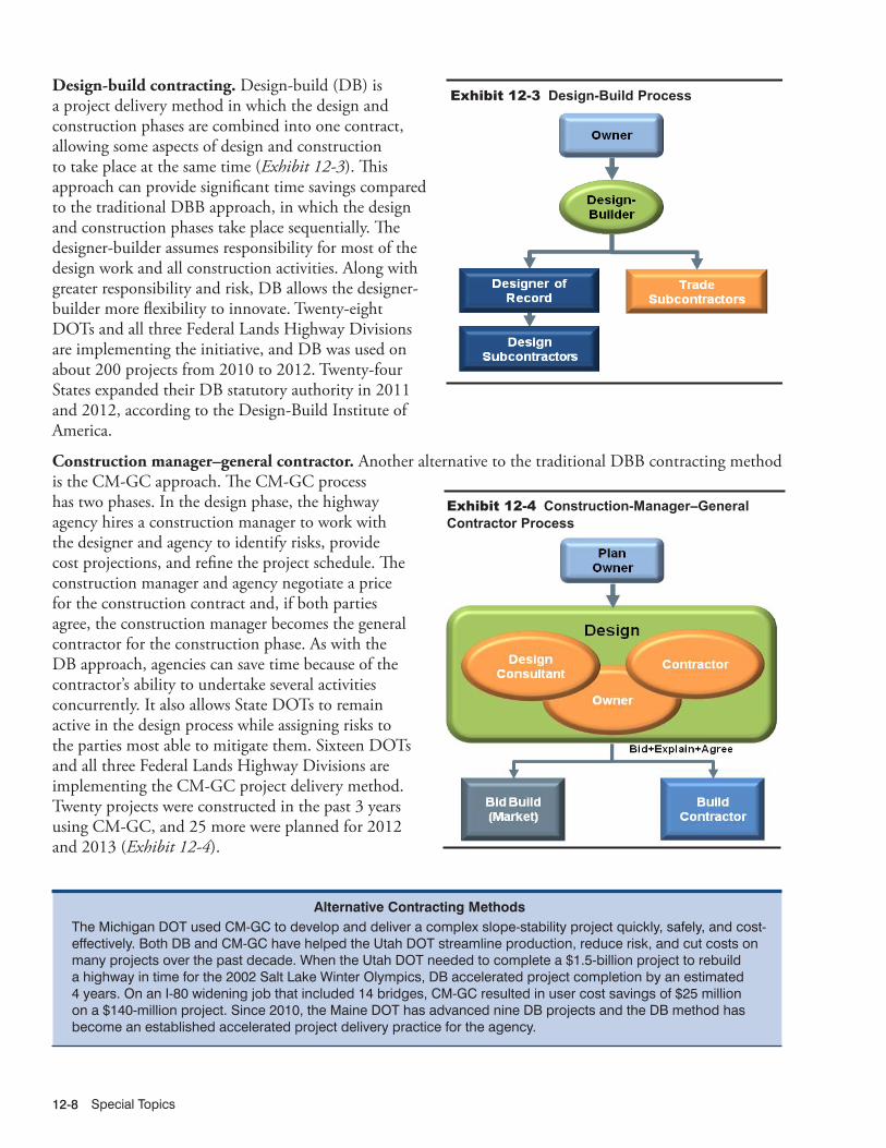
Special Topics12-8

Design-build contracting. Design-build (DB) is a project delivery method in which the design and construction phases are combined into one contract, allowing some aspects of design and construction to take place at the same time (Exhibit 12-3). This approach can provide significant time savings compared to the traditional DBB approach, in which the design and construction phases take place sequentially. The designer-builder assumes responsibility for most of the design work and all construction activities. Along with greater responsibility and risk, DB allows the designer-builder more flexibility to innovate. Twenty-eight DOTs and all three Federal Lands Highway Divisions are implementing the initiative, and DB was used on about 200 projects from 2010 to 2012. Twenty-four States expanded their DB statutory authority in 2011 and 2012, according to the Design-Build Institute of America.

Construction manager–general contractor. Another alternative to the traditional DBB contracting method is the CM-GC approach. The CM-GC process has two phases. In the design phase, the highway agency hires a construction manager to work with the designer and agency to identify risks, provide cost projections, and refine the project schedule. The construction manager and agency negotiate a price for the construction contract and, if both parties agree, the construction manager becomes the general contractor for the construction phase. As with the DB approach, agencies can save time because of the contractor’s ability to undertake several activities concurrently. It also allows State DOTs to remain active in the design process while assigning risks to the parties most able to mitigate them. Sixteen DOTs and all three Federal Lands Highway Divisions are implementing the CM-GC project delivery method. Twenty projects were constructed in the past 3 years using CM-GC, and 25 more were planned for 2012 and 2013 (Exhibit 12-4).

Alternative Contracting MethodsThe Michigan DOT used CM-GC to develop and deliver a complex slope-stability project quickly, safely, and cost-effectively. Both DB and CM-GC have helped the Utah DOT streamline production, reduce risk, and cut costs on many projects over the past decade. When the Utah DOT needed to complete a $1.5-billion project to rebuild a highway in time for the 2002 Salt Lake Winter Olympics, DB accelerated project completion by an estimated 4 years. On an I-80 widening job that included 14 bridges, CM-GC resulted in user cost savings of $25 million on a $140-million project. Since 2010, the Maine DOT has advanced nine DB projects and the DB method has become an established accelerated project delivery practice for the agency.

9/18/2012 32X_C (12-3) R2.xlsx

Exhibit 12-3 Design-Build Process

10/22/2012 32X_D (12-4) R3.xlsx

Exhibit 12-4 Construction-Manager–General Contractor Process

Center for Accelerating Innovation 12-9

Shortening Project Delivery ToolkitHighway projects that require environmental impact statements under the National Environmental Policy Act (NEPA) typically take 12 to 13 years to complete. In order to deliver needed projects faster, FHWA created the Shortening Project Delivery Toolkit to encourage greater use of regulatory flexibilities available under current laws. The following highlights how State DOTs are using the initiatives to streamline projects.

Expanded use of programmatic agreements. Programmatic agreements establish streamlined processes for handling routine environmental requirements on common project types. A programmatic agreement spells out the terms of a formal agreement between a State DOT and other State or Federal agencies and sets up a process for consultation, review, and compliance with applicable Federal laws. Such agreements save time in the project delivery process by specifying clear roles and responsibilities, standardizing coordination and compliance procedures, and improving relationships among DOT and regulatory agency staff.

Thirty-seven States have at least two active programmatic agreements. Since October 2010, 56 programmatic agreements have been initiated.

Enhanced technical assistance. FHWA is providing additional technical assistance to help States identify NEPA-related challenges and implement solutions to resolve project delays where feasible. Interagency coordination at all levels of government is helping move projects forward in a streamlined manner.

FHWA is focusing on new projects that are expected to experience delays and ongoing projects for which no record of decision has been issued 60 months or more after the project’s notice of intent was published. Of the 10 projects on which assistance is being provided, four—in Alaska, Nebraska, North Carolina, and Utah—had a record of decision or withdrawal of the notice of intent by July 2012.

Use of in-lieu fees and mitigation banking. In-lieu fees are those charged to perform environmental enhancement activities throughout an entire watershed rather than at a particular site. Mitigation banking refers to restoring or enhancing wetlands, streams, or other resources to offset unavoidable adverse impacts related to a highway project in another area. FHWA is encouraging highway agencies to use both approaches where allowed. Thirteen of the 23 States participating in the initiative have active agreements for mitigation banking programs, and seven of those agreements extend to local agencies. Six States have agreements in place for in-lieu fees.

Planning and environmental linkages. This initiative set up a framework for considering and incorporating planning documents and decisions from the earliest stages of project planning into the environmental review process. Linking planning and environmental considerations can lead to a seamless decision-making process that minimizes duplication of effort, promotes environmental

Programmatic AgreementsThe Nebraska Department of Roads developed a programmatic agreement for a biological evaluation process. When the programmatic conditions are met at the project level, the agency no longer needs to coordinate with or obtain concurrence from FHWA, the U.S. Fish and Wildlife Service, or the Nebraska Game and Parks Commission. This agreement results in a minimum savings of 5 weeks in the project schedule for an estimated 80 percent of the projects in the State’s transportation program. In another case, the Oklahoma DOT’s American Burying Beetle Programmatic Biological Opinion has expedited projects by as much as a year, and it minimizes schedule uncertainty on projects where American Burying Beetles, a critical endangered species, might be present.

In-Lieu Fees and Mitigation BankingThe Alaska Department of Transportation and Public Facilities has used the in-lieu fee program to meet wetland mitigation commitments on more than 70 projects since the Every Day Counts program began. Additionally, the Mississippi DOT has streamlined the compensatory mitigation permitting process for wetland and stream impacts on all applicable transportation projects. The Mississippi DOT now owns wetland and stream credits in 18 mitigation properties, perpetually conserving some 20,000 acres of land.

Special Topics12-10

stewardship, and reduces project delays. To ensure that planning information and decisions are properly coordinated for use in the NEPA review process, FHWA is recommending use of the Planning and Environmental Linkages (PEL) Questionnaire, which was adapted from a questionnaire developed for use in Colorado. By July 2012, 18 of the 32 States and Federal Lands Highway Divisions participating in the initiative had made use of the PEL Questionnaire or an equivalent process.

Planning and Environmental LinkagesThe Louisiana Department of Transportation and Development created a National Best Practice Planning and Environmental Linkages Checklist and is using it on all new projects to save time and money. The Montana DOT has standardized its corridor planning process through its Corridor Planning Study Checklist.

Every Day Counts Round TwoIn July 2012, FHWA announced a new round of innovative technologies and processes under its Every Day Counts initiative that can shorten the time needed to open highway projects to the public and enhance safety and environmental outcomes. Over the next 2 years, expert teams will work with State transportation agencies and the design and construction industries to deploy 13 innovations.

Programmatic agreements. Also part of the first round of Every Day Counts, programmatic agreements establish streamlined approaches for handling routine environmental requirements. In this round, some of the newly developed agreements will be applied in additional States or expanded to include regions.

Locally administered Federal-aid projects. FHWA has developed a three-pronged strategy to help local agencies navigate the complexities of the Federal-Aid Highway Program. The strategies include certification and qualification-type programs, indefinite delivery–indefinite quantity consultant contracts, and stakeholder committees.

Three-dimensional modeling technology. With 3D modeling software, design and construction teams can connect virtually to collaborate on project designs throughout the design and construction phases. This technology allows for faster, more accurate, and more efficient planning and construction, in many cases increasing productivity by up to 50 percent.

Intelligent compaction. When pavement cracks prematurely, a potential cause is that it was not compacted properly during construction. Intelligent compaction—using global positioning system (GPS)-based mapping and real-time monitoring to enable adjustment of the compaction process—improves the quality, uniformity, and lifespan of pavements.

Accelerated bridge construction. FHWA is advancing three technologies to replace bridges faster, more safely, and sometimes at less cost. They are PBES, in which components are built off-site and moved into place quickly; slide-in bridge construction, in which a bridge is built next to an existing structure and slid into place; and GRS-IBS, which uses geosynthetic reinforcement and granular soils as a composite material to build abutments and approach embankments.

Design-build and construction manager–general contractor project delivery methods. FHWA is continuing its deployment of DB and CM-GC methods, accelerated project delivery methods that can shorten construction project schedules by years. Accelerated project delivery also provides opportunities for significant cost savings and safety improvements.

Alternative technical concepts. Through this flexible contracting process, contractors can recommend innovative, cost-effective solutions that are equal to or better than a State’s design and construction criteria. The approach promotes competition and gives highway agencies the opportunity to choose design and construction solutions that offer the best value.

Center for Accelerating Innovation 12-11

High-friction surface treatment. This pavement technology reduces crashes, injuries, and fatalities. It involves applying high-quality aggregate with friction values far exceeding conventional pavement friction to existing or potential high-crash areas to help drivers maintain better control in dry and wet conditions.

Intersection and interchange geometrics. Innovative designs can reduce or move crossover or conflict points in intersections and interchanges, increasing safety for motorists, pedestrians, and bicyclists. Roundabouts, diverging diamond interchanges, and intersections with displaced left-turns or variations on U-turns are among the effective alternatives to traditional designs.

Geospatial data collaboration. This initiative uses cloud-based geographic information system services, which are used to build maps, to improve data sharing within agencies and among project delivery stakeholders. Collaborative analyses and rapid updating of shared maps will lead to faster consensus building, improved decisions, and better scheduling on highway projects.

Quality environmental documentation. FHWA is promoting recommendations to improve the quality and reduce the size of NEPA documents developed for construction projects. The initiative will help make NEPA documents more effective in disclosing to the public and participating agencies the information that is used to make project decisions. That, in turn, will help project proponents accelerate project delivery and achieve better environmental outcomes.

First responder training. Crashes, disabled vehicles, and road debris create unsafe driving conditions and cause about 25 percent of all traffic delays. This initiative offers the first national, multidisciplinary traffic incident management process and training program. It promotes understanding among first responders of the requirements for safe and quick clearance of traffic incidents, prompt and open communications, and motorist and responder safeguards.

Improving Safety Through Intersection GeometricsIntersections and interchanges are planned points of conflict where motorists, pedestrians, and bicyclists cross paths or change direction. This creates conditions that could result in a crash. More than 20 percent of roadway fatalities in 2009 were intersection-related, a percentage that has not changed significantly for 25 years.

FHWA encourages highway agencies to consider alternative geometric intersection and interchange designs that reduce or alter conflict points and allow for safer travel. Past and ongoing FHWA studies of alternative intersection and interchange designs document the magnitude of both safety and operational improvements. Among the effective alternatives to traditional designs are roundabouts, diverging diamond interchanges (DDIs), and intersections with displaced left turns or variations on U-turns.

A roundabout is a circular intersection in which traffic travels counterclockwise around a central island and entering traffic must yield to circulating traffic. Roundabouts change the nature of intersection conflicts by eliminating perpendicular crossings and opposing direction turns in favor of low-speed merging and diverging maneuvers.

DDIs simplify the operation of intersections at a diamond-style interchange by removing from the signalized intersection the turns on to and off of the ramps. This is accomplished by moving traffic to the left side of the road between the ramp terminals. DDI design reduces the number of perpendicular conflict points in an equivalent conventional diamond layout.

With displaced left turns, motorists cross opposing lanes at an intersection several hundred feet from the main intersection. Motorists then travel on a road parallel to the main road until they turn left with the through-traffic at the main intersection. Similarly, U-turn designs require motorists to make a U-turn maneuver at a one-way median away from the main intersection instead of a direct left turn at the main intersection.

10/25/2012 32X_E (12-5) R2.xlsx

Exhibit 12-5 Diverging Diamond Interchange

Photo courtesy of FHWA.

10/25/2012 32X_E (12-5) R2.xlsx

Exhibit 12-5 Diverging Diamond Interchange

Photo courtesy of FHWA.

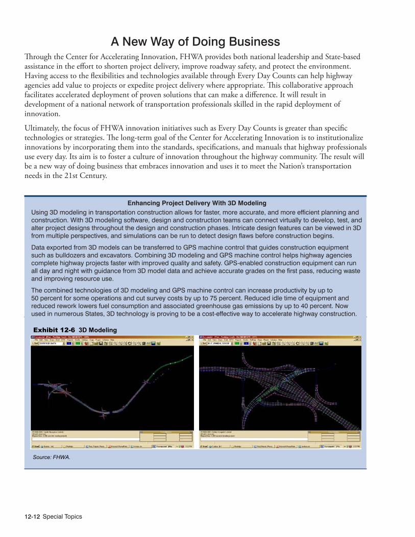
Special Topics12-12

A New Way of Doing BusinessThrough the Center for Accelerating Innovation, FHWA provides both national leadership and State-based assistance in the effort to shorten project delivery, improve roadway safety, and protect the environment. Having access to the flexibilities and technologies available through Every Day Counts can help highway agencies add value to projects or expedite project delivery where appropriate. This collaborative approach facilitates accelerated deployment of proven solutions that can make a difference. It will result in development of a national network of transportation professionals skilled in the rapid deployment of innovation.

Ultimately, the focus of FHWA innovation initiatives such as Every Day Counts is greater than specific technologies or strategies. The long-term goal of the Center for Accelerating Innovation is to institutionalize innovations by incorporating them into the standards, specifications, and manuals that highway professionals use every day. Its aim is to foster a culture of innovation throughout the highway community. The result will be a new way of doing business that embraces innovation and uses it to meet the Nation’s transportation needs in the 21st Century.

Enhancing Project Delivery With 3D ModelingUsing 3D modeling in transportation construction allows for faster, more accurate, and more efficient planning and construction. With 3D modeling software, design and construction teams can connect virtually to develop, test, and alter project designs throughout the design and construction phases. Intricate design features can be viewed in 3D from multiple perspectives, and simulations can be run to detect design flaws before construction begins.

Data exported from 3D models can be transferred to GPS machine control that guides construction equipment such as bulldozers and excavators. Combining 3D modeling and GPS machine control helps highway agencies complete highway projects faster with improved quality and safety. GPS-enabled construction equipment can run all day and night with guidance from 3D model data and achieve accurate grades on the first pass, reducing waste and improving resource use.

The combined technologies of 3D modeling and GPS machine control can increase productivity by up to 50 percent for some operations and cut survey costs by up to 75 percent. Reduced idle time of equipment and reduced rework lowers fuel consumption and associated greenhouse gas emissions by up to 40 percent. Now used in numerous States, 3D technology is proving to be a cost-effective way to accelerate highway construction.

10/22/2012 32X_F (12-6) R2.xlsx

Exhibit 12-6 3D Modeling

Source: FHWA.

Center for Accelerating Innovation 12-13

Using Intelligent Compaction to Improve Pavement QualityCompaction is one of the most important processes in roadway construction. When pavement crumbles before it reaches its expected lifespan, a potential cause is that it was not compacted properly or the thickness is not uniform. Intelligent compaction (IC) technology improves the quality, uniformity, and long-lasting performance of pavements.

Using vibration and a system to collect, process, and analyze measurements in real time, IC rollers can compact more pavement with fewer passes than traditional rollers. IC efficiencies result in time, cost, and fuel savings. With more efficient paving processes, production can increase and highway agencies can pave larger roadway sections daily.

Using GPS-based mapping and an onboard computer reporting system, IC roller operators can monitor and provide immediate corrections to the compaction process. A continuous record of color-coded plots records the number of roller passes, compaction measurement values, and precise location of the roller. The system analyzes the data and compares the results of previous passes to determine whether adjustments are needed.

Expanding IC use nationwide is a cost-effective way to accelerate highway pavement construction. Cost-benefit analyses show that investment in IC will break even in 1 to 2 years. Use of IC technology will produce better-quality roadways that help keep motorists safe and allow highway agencies to operate more efficiently.

10/25/2012 32X_G (12-7) R2.xlsx

Exhibit 12-7 Intelligent Compaction

Photo courtesy of FHWA.

Special Topics12-14

National Fuel Cell Bus Program

National Fuel Cell Bus Program ..................................................................................13-2

Value and Challenges of Fuel Cell Electric Propulsion for Transit Buses ................13-2

History and Status of FCEB Research ......................................................................13-4

Research Accomplishments ......................................................................................13-5

National Fuel Cell Bus Program 13-1

CHAPTER 13

Special Topics13-2

National Fuel Cell Bus Program

This chapter summarizes accomplishments of fuel cell transit bus research and demonstration projects supported by the Federal Transit Administration (FTA) through 2011. It describes fuel cell electric bus (FCEB) research projects in the United States and describes their impact on commercialization of fuel cell power systems and electric propulsion for transit buses in general.

FTA conducts most of its FCEB research under the National Fuel Cell Bus Program (NFCBP), a cooperative research, development, and demonstration program to advance commercialization of FCEBs. The NFCBP is a part of a larger FTA research program to improve transit efficiency and contribute to environmentally sustainable transportation. The FTA conducts the NFCBP in partnership with industry. Projects target research to improve performance and lower costs of next-generation fuel cell systems for transportation.

Congress established the NFCBP in the Safe, Accountable, Flexible, Efficient Transportation Equity Act: A Legacy for Users (SAFETEA-LU). FTA’s research to develop FCEBs has been under way since 2006. The NFCBP requires an equal cost share by project teams for each Federal dollar invested, bringing the size of the program to more than $150 million through FY 2011.

NFCBP objectives, which apply to all FTA-funded FCEB research, are:

� Significantly advance development of FCEBs and related infrastructure through innovation of FCEB design, component development, improved systems integration, and real-world implementation and demonstration

� Document the state of FCEB technologies development, and examine requirements and next steps for market introduction

� Enhance awareness and education related to FCEBs and related infrastructure.

Value and Challenges of Fuel Cell Electric Propulsion for Transit Buses

U.S. interest in hydrogen FCEBs has grown over the past 20 years, driven primarily by the desire to reduce both petroleum-based fuel consumption and emissions, particularly greenhouse gas emissions. In October 2010, the U.S. Environmental Protection Agency (EPA) and the National Highway Traffic Safety Administration (NHTSA) introduced a program to reduce greenhouse gas emissions and improve fuel efficiency of medium- and heavy-duty trucks and buses. These federal programs will significantly impact transit bus propulsion products in the future.

Transit buses are well suited to demonstrating fuel-cell applications in transportation because:

• They are centrally located and fueled

• They are government subsidized

• They are professionally operated and maintained

• They operate on fixed routes and fixed schedules

• They tolerate the weight and volume requirements of advanced systems

• They have rigorous start-up and pull-out requirements

• They provide public exposure to the benefits of advanced technologies, which leads to greater public acceptance.

National Fuel Cell Bus Program 13-3

Exhibit 13-1 illustrates fuel cell operation. Fuel cell electric technology for transit buses can produce benefits such as:

� Zero tailpipe emissions � Improved fuel economy � Reduced dependence on foreign oil � Quiet, smooth ride � Creation of green technology jobs � Technologies for better-performing, more-efficient hybrid and electric buses � Demonstration of the value of fuel cell technology to a larger, heavy-duty vehicle market.

12/28/2012 33XT_E (13-1) R1.xlsx

Heat and Water

Clean Exhaust

Electricity

Air(Oxygen)

FuelProcessor

Fuel HydrogenRich Gas

FuelCell

Stacks

PowerConditioner

DC AC

Source: Department of Energy, Fuel Cell Report to Congress (ESECS EE-1973), February 2003.

Exhibit 13-1 Diagram of Fuel Cell Operation

The major barriers to reaching full commercialization of FCEBs are:

� Durability – The useful life of fuel cell power systems is increasing, but more work is needed to meet transit requirements.

� Initial purchase costs – The cost of buses and infrastructure is decreasing, but to become competitive the market will need to realize economies of scale through greatly expanded production.

� Delivery of “green” hydrogen – The availability and cost of hydrogen for FCEB operations remain significant barriers. Hydrogen is produced by electrolysis or through natural gas reforming, or it is trucked as a liquid into operating locations. These production and delivery methods all pose cost and greenhouse gas emission issues that must be resolved before FCEBs are fully commercialized.

Special Topics13-4

History and Status of FCEB ResearchFTA FCEB propulsion and infrastructure demonstrations began in the early 1990s with buses developed at Georgetown University. These 30- and 40-foot buses were fueled by methanol that was reformed into hydrogen onboard and used in the buses’ electric fuel cell propulsion systems. Between 1998 and 2000, the FTA supported a second major demonstration of three, 40-foot hydrogen fuel cell buses, with Ballard fuel cells, operated at Chicago Transit Authority (CTA). During this same time period, three fuel cell buses of the same generation also operated in Vancouver, Canada.

FTA’s early demonstrations proved the feasibility of fuel cell propulsion for transit buses and identified research needed to:

� Reduce the size of fuel cell stacks and balance-of-plant onboard buses � Increase power density of the fuel cell power system � Reduce the weight of fuel cell and electric propulsion systems � Develop a hydrogen fueling infrastructure suitable for transit bus operations.

The first “next-generation” FCEB, a 40-foot bus with a Ballard fuel cell power system, operated at SunLine Transit Agency (SunLine) during 2000 and 2001. A second “next-generation” FCEB, a 30-foot bus with a UTC Power fuel cell power system, operated first at SunLine and then at Alameda-Contra Costa Transit District (AC Transit) during 2002 and 2003.

In August 2005, Congress established the National Fuel Cell Bus Technology Development Program to facilitate development of commercially viable FCEB propulsion technologies. The FTA released the initial competitive solicitation for the NFCBP on April 10, 2006. A multi-department technical team recommended 14 projects for funding under the program. Projects included partners from

Accomplishments from FTA research on Fuel Cell Bus Technology:

• Design – Seven fully integrated FCEB designs are now available, in either a fuel cell dominant or battery dominant configurations.

• Manufacture – The NFCBP funded Proterra’s first bus, a battery dominant FCEB that operated in Columbia, South Carolina, and will soon operate in Austin, Texas.

• Demonstration – The newest-generation Van Hool/UTC Power FCEB design was delivered, with 12 buses going to the San Francisco Bay Area and 4 buses going to Hartford, Connecticut. These 16 FCEBs are the largest demonstration of one FCEB design in the United States.

• Reliability – As of the end of 2011, one of the Bay Area buses has a fuel cell power system with 11,000 hours of operation without significant maintenance (i.e., no change out of the fuel cell system or individual cells) and other buses in the fleet have fuel cell power systems with 6,000 and 8,000 hours of operation without significant maintenance.

• Buy America – FTA has made progress in integrating FCEBs that are “Buy America” compliant. Ballard, a major supplier, is producing systems in Lowell, Massachusetts; and UTC Power, another major supplier, is working toward packaging its system for easier integration into buses from U.S. manufacturers.

• Fueling Infrastructure – Ongoing demonstrations are facilitating a better understanding of needed infrastructure and safe operations for existing transit operations.

• Hybrid Propulsion – FTA-funded research is leading to better components and the integration of electric systems for electric propulsion.

• Public Awareness – FTA research projects support awareness and education for transit agencies and the public. FTA has funded outreach through National and International Fuel Cell Bus Workshops, and develops research reports for industry.

National Fuel Cell Bus Program 13-5

industry, government, and transit and provided a balanced portfolio for the NFCBP to advance FCEB commercialization. The NFCBP continued beyond its initial four years, funded through extensions of SAFETEA-LU for FY 2010 and FY 2011. Each annual extension added approximately $13.5 million, for a total of nearly $76 million in federal funding through FY 2011. The 50 percent cost share requirement was also continued for all projects, bringing funding for the program to more than $150 million.

NFCBP projects are managed through one of three non-profit consortia:

� CALSTART – a nonprofit consortium headquartered in Pasadena, California. CALSTART represents more than 140 firms. It provides services and consulting to develop clean, advanced transportation technologies for all types of vehicles, including trucks, buses, and military vehicles.

� Center for Transportation and the Environment (CTE) – a nonprofit consortium headquartered in Atlanta, Georgia. CTE provides research, training, and information exchange for improving transportation infrastructure while preserving the integrity of the environment.

� Northeast Advanced Vehicle Consortium (NAVC) – a nonprofit, public-private partnership headquartered in Boston, Massachusetts. NAVC conducts research and technology analysis and fosters information sharing and collaboration on advanced vehicle technology projects.

Current FTA FCEB research focuses on developing transit buses that demonstrate full transit operation and service. Current bus configurations have either large fuel cell power systems in hybrid electric propulsion systems or smaller fuel cell power systems in plug-in/battery dominant hybrid electric propulsion systems. Ongoing research also includes electrifying accessories (e.g., air conditioning) and, in some cases, adding small fuel cell auxiliary power units (APUs) to power the electric accessories.

The U.S. Department of Energy (DOE) also funds FCEB research. Most of DOE’s fuel cell and hydrogen research is done through the Fuel Cell Technologies Program within the Office of Energy Efficiency and Renewable Energy (EERE). DOE’s research in fuel cells and hydrogen complements FTA’s transit bus research and demonstration, usually through DOE’s investment in developing technologies used in the demonstrations. For example, the DOE supported hydrogen fueling stations at several demonstration locations in California. In addition, DOE’s Clean Cities program provides grants for clean energy projects that include a hydrogen fueling station planned for CTTRANSIT in Hartford, Connecticut.

In March 2012, the FTA released a report, FTA Fuel Cell Bus Program: Research Accomplishments through 2011, (http://www.fta.dot.gov/documents/FTA_Report_No._0014.pdf ) that summarizes 42 research projects, including NFCBP projects, other FTA research, and supporting research funded by the DOE. To date, 17 of these projects have been completed and 25 are ongoing FTA and DOE projects.

Research AccomplishmentsResearch under the NFCBP shows progress toward commercialization and readiness for implementation of FCEBs in transit operations. The NFCBP has seven performance objectives for the research projects it funds. Exhibit 13-2 lists these objectives and summarizes progress toward meeting them. Although progress is significant, more investment is needed to meet the objectives.

Exhibit 13-3 shows the number of FCEBs operating in the United States. Between 2005 and 2009, potential regulation by the California Air Resources Board was the impetus for FCEB research, and the first seven FCEBs operated in California at SunLine, Santa Clara VTA, and AC Transit. Beginning in 2007, one FCEB began operating at CTTRANSIT in Hartford, Connecticut.

Special Topics13-6

Funding though the NFCBP was available starting in 2006. However, its influence becomes apparent only in 2010, due to the lag time between designing and building FCEBs and getting them into operation. The projected number (32) of FCEBs that will be in operation by the end of 2012 is conservative.

Exhibit 13-4 is a map of current or planned FCEB operating locations. FCEB demonstrations have expanded and are now located across the United States, not just in California.

The 42 projects discussed in the FTA report represent multiple design configurations for FCEBs. Exhibit 13-5 shows the current fully integrated FCEB configurations and their manufacturers. Three are fuel cell dominant configurations, and four are battery dominant fuel cell configurations. The design configurations represent seven bus manufacturers and three fuel cell power system manufacturers. Another FCEB is planned with a fourth fuel cell power system manufacturer, Nuvera. In addition to those listed in the table, one existing hybrid electric bus design, Orion VII, BAE Systems, was modified using all-electric accessories powered by a small fuel cell power system by Hydrogenics. This modified design also provides some power for all-electric operation of the power plant dominant hybrid.

12/27/2012 33XT_A (13-2) R3.xlsx

NFCBP Performance Objective Progress Through FY 2011

1. Less than five times the cost of a conventional (commercial diesel) transit bus

Cost reductions from more than $3.0 million per bus in 2006 to $2.3 million for last bus ordered. Battery dominant bus with smaller fuel cell power system significantly less than $2.3 million.

2. Four to six years or 20,000 to 30,000 hours of durability for the fuel cell power system

10,000+ hours achieved on fuel cell power system, with durability warranties at 10,000 to 12,000 hours.

3. Double the fuel economy compared to commercial (diesel transit) bus

Exceed two times conventional (diesel transit) bus fuel economy, but depends on route.

4. Bus performance equal to or greater than equivalent commercial (diesel transit) bus

Operated up to 19 hours/day, with good availability, and miles between road calls at 4,000 miles. Better acceleration. Quiet operation. Weight is still high.

5. Exceed current emissions standards Zero emissions.6. Foster economic competitiveness in FCEB technologies Multiple manufacturers and platforms demonstrating buses.7. Increase public acceptance for FCEB technologies Continued progress.

Exhibit 13-2 Progress Toward Achieving Technical Performance Objectives

Source: FTA, FTA Fuel Cell Bus Program: Research Accomplishments through 2011, FTA Report No.14, March 2012.

12/28/2012 33XT_B (13-3) R3.xlsx

0

5

10

15

20

25

30

35

2005 2006 2007 2008 2009 2010 2011 2012

Fuel

Cel

l Ele

ctric

Bus

Cou

nt

Source: FTA, FTA Fuel Cell Bus Program: Research Accomplishments through 2011, FTA Report No.14, March 2012.

Exhibit 13-3 Fuel Cell Electric Buses Operating in the United States, 2006–2012

National Fuel Cell Bus Program 13-7

12/28/2012 33XT_C (13-4) R3.xlsx

Exhibit 13-4 Fuel Cell Electric Bus Demonstration Sites

Source: FTA, FTA Fuel Cell Bus Program: Research Accomplishments through 2011, FTA Report No.14, March 2012.

12/27/2012 33XT_D (13-5) R3.xlsx

Bus Manufacturer Fuel Cell System Hybrid SystemHybrid

Configuration Energy Storage Status

Van Hool 40-ft UTC Power Siemens ELFA Fuel cell dominantLithium-based

batteries Operational

ElDorado 40-ft Ballard BAE Systems Fuel cell dominantLithium-based

batteries Operational

New Flyer 40-ft Ballard Siemens ELFA Fuel cell dominantLithium-based

batteries Operational

Proterra 35-ftHydrogenics or

BallardProterra

integration Battery dominantLithium-based

batteries Operational

DesignLine 35-ft BallardDesignLine integration Battery dominant

Lithium-based batteries

Under development

Ebus 22-ft Ballard Ebus integration Battery dominantNickel cadmium

batteries Operational

EVAmerica 30-ft BallardEVAmerica integration Battery dominant

Lithium-based batteries

Under development

Source: FTA, FTA Fuel Cell Bus Program: Research Accomplishments through 2011, FTA Report No.14, March 2012.

Exhibit 13-5 Fuel Cell Bus Configurations

In 2007, Proterra, a new “green” bus manufacturer, started design of and delivered its first bus, a battery dominant hybrid fuel cell bus, for demonstration in Columbia, South Carolina (completed in 2010), and Austin, Texas (planned to start in 2012). The NFCBP helped Proterra acquire the start-up capital to begin manufacturing this bus. Since then, Proterra has built and delivered two more FCEBs that are essentially the same as the first one. Proterra based its propulsion system on an all-electric design with the capability to add a fuel cell power system as a range extender. Its buses are also designed for opportunity charging while on route. Foothill Transit (West Covina, California) purchased three electric buses with one of Proterra’s fast charging stations. Proterra is assembling another 10 or more buses for transit operations in other locations.

Special Topics13-8

Several transit agencies in California began testing FCEBs because of potential state regulation and purchase requirements for zero-emission buses. Beginning in 2005, this testing included an FCEB design from Van Hool, UTC Power, and ISE (now Bluways), with energy storage in ZEBRA batteries. SunLine operated one of these buses and AC Transit operated three more. Two additional buses of this design operated in Belgium and at CTTRANSIT in Hartford, Connecticut.

The NFCBP funded UTC Power and AC Transit to maximize operation of AC Transit’s three FCEBs (i.e., accelerated testing) to study reliability, durability, and failure modes of the fuel cell power system. This accelerated testing began in late 2007. The lessons learned and improvements to the design of the UTC Power fuel cell power system increased durability so that one of the systems reached 11,000 operating hours without significant maintenance, and two others have accumulated 6,000 and 8,000 operating hours without significant maintenance. Previous fuel cell power systems reached only about 4,000 operating hours before a low power output level indicated the end of useful life for the systems.

Following these initial testing activities, AC Transit, Van Hool, and UTC Power designed and developed an improved “next-design” FCEB for the Zero Emission Bay Area (ZEBA) advanced demonstration in California. AC Transit is leading a group of San Francisco Bay Area (Bay Area) transit agencies in this demonstration. The demonstration includes 12 new FCEBs and two new hydrogen fueling stations at two AC Transit operating depots. UTC Power and CTTRANSIT are demonstrating four more “next-design” FCEBs in Hartford, Connecticut. Demonstration of the “next-design” version of Van Hool/UTC Power FCEBs now includes 16 buses in two locations, making it the largest FCEB demonstration in the United States.

Buy America requirements (Title 49 CFR Part 661), set standards for federally assisted procurements, specifically: “…no funds may be obligated by FTA for a grantee project unless all iron, steel, and manufactured products used in the project are produced in the United States.” In 2008, FTA granted a public interest waiver to the FTA Buy America requirements for NFCBP projects, so that project teams could access all available technologies and components, regardless of origin, in order to hasten the development of fuel cell technology for transit. This allowed teams to access a full slate of technologies, many of which were not readily available domestically, for validating fuel cell bus technology, with the overall goal to stimulate and further expand the U.S. fuel cell bus industry. Over the past few years, FTA and the consortia have made progress toward meeting “Buy America” requirements:

� The FTA-funded ElDorado/BAE Systems/Ballard as new manufacturer partners to develop and demonstrate a new FCEB at SunLine and CTA. The new bus meets Buy America requirements, and is assembled in Riverside, CA.

� Increasing orders for FCEBs in the United States led Canadian-based fuel cell manufacturer, Ballard Power Systems, to establish manufacturing capabilities for fuel cell power systems in Lowell, Massachusetts. Fuel cell power systems are the largest cost component of FCEBs. Their availability in the United States helps bus manufacturers meet Buy America requirements.

� The UTC Power fuel cell power system is currently only available in Van Hool buses from Belgium. The NFCBP funded a project with Connecticut-based fuel cell manufacturer, UTC Power, to engineer, package, and test a further optimized fuel cell power system that can be installed easily into U.S. bus manufacturer models.

Hybrid electric propulsion for transit buses increases energy efficiency for the buses, but it also increases complexity. Hybrid electric propulsion has the potential to reduce maintenance costs through fewer moving parts, battery energy storage, and regenerative braking, which reduces both brake wear and brake maintenance. The challenges for hybrid electric propulsion for buses are reliability and durability of the major components and optimized integration, especially software integration.

National Fuel Cell Bus Program 13-9

FTA funding for FCEB research enabled several bus manufacturers and integrators to gain experience in building and optimizing electric propulsion systems. It also enabled BAE Systems, a commercial electric propulsion manufacturer/supplier, to enter the FCEB market. With NFCBP funding, BAE Systems electrified accessories in its Compound Bus 2010 project, which led to an electric accessory package that will be integrated into its commercial hybrid products in the future. In addition, the NFCBP funded development of critical power electronics components for hybrid electric propulsion systems, such as DC-DC convertors. All of this research expands the availability of products to the transit industry.

Hydrogen fuel for FCEB demonstration projects is typically supplied through electrolysis or natural gas reforming, or it is trucked into a fueling site as liquid or high-pressure gas. The FTA has invested in all of these methods to support not only the development of hydrogen fueling infrastructure, but also safe operations in and around transit maintenance, storage, and wash facilities. In addition, the FTA funded the Volpe Center to review safety plans for transit FCEB operations and infrastructure as well as to provide technical assistance to each transit agency operator of FCEBs.

An objective of all FTA research is to share results and lessons learned. Information sharing is a specific objective of the NFCBP, including lessons learned from FCEB and infrastructure research to facilitate technical progress and future research. FCEB development and demonstration reports document implementation to facilitate understanding of the requirements for market introduction.

All NFCBP demonstration projects include an awareness and education component. Transit agencies that operate FCEBs are able to educate their passengers and the communities through outreach and public events. Through FY 2011, the NFCBP has funded and/or produced 10 brochures and 29 reports about FCEB research.

The NFCBP also established both a national and an international working group for information sharing and cooperation. The FTA initiated the International Fuel Cell Bus Working Group and workshops in 2002 to facilitate information sharing on worldwide FCEB demonstrations and to harmonize data collection to better understand the status of the technologies. Since the first workshop in 2002, the FTA has facilitated six more workshops.

The FTA formed the National Fuel Cell Bus Working Group for information sharing about FCEB demonstrations in the United States. To facilitate participation from transit agencies around the country, the working group usually meets in conjunction with American Public Transportation Association (APTA) conferences. The working group was initiated at the 2002 APTA EXPO in Las Vegas, Nevada, and since that time has held three additional meetings to discuss national demonstrations and progress toward commercialization.

The FTA intends to continue efforts to collaborate and coordinate with industry on FCEBs through outreach efforts with CTE to conduct a series of webinars on FCEB for the transit industry, and a new website on worldwide activities and developments on fuel cell buses, that will help facilitate national and international data sharing.

Special Topics13-10

PART IV

Recommendations for HPMS Changes IV-1

Recommendations for HPMS Changes

Recommendations for HPMS Changes ........................................... IV-2Background ................................................................................................ IV-2

Changes to HPMS ...................................................................................... IV-3

Recommendations for HPMS ChangesIV-2

Section 52003 of the Moving Ahead for Progress in the 21st Century Act (MAP-21) added a requirement for this report to include recommendations on changes to the Highway Performance Monitoring System (HPMS) that address: “(i) improvements to the quality and standardization of data collection on all functional classifications of Federal-aid highways for accurate system length, lane length, and vehicle-mile of travel; and (ii) changes to the reporting requirements authorized under section 315 to reflect recommendations under this paragraph for collection, storage, analysis, reporting, and display of data for Federal-aid highways and, to the maximum extent practical, all public roads.” Part IV of this report is intended to begin to address this requirement; future editions of the C&P report will contain updates as progress is made in implementing improvements to the HPMS and as other potential changes are identified.

The HPMS is a major data source for the analyses presented in Chapters 2, 3, 7, 8, 9, and 10 of this report; the HPMS is also discussed in Appendices A and D.

BackgroundThe Highway Performance Monitoring System (HPMS) is an annual collection of information on the extent, condition, performance, use, and operating characteristics of the Nation’s highways. It was first developed in 1978 to replace numerous uncoordinated annual State data reports and special studies. HPMS includes key data on all public roads, more detailed data for a sample of the arterial and collector functional systems, complete (full extent) coverage of the Interstate and other principle arterials, and other statewide summary data.

HPMS provides essential information for apportioning Federal-aid funds to the States and for assessing highway system performance under the Federal Highway Administration’s (FHWA’s) strategic planning process. Pavement condition data, congestion-related data, and traffic data are used extensively to measure progress in meeting the objectives embodied in the FHWA’s Performance Plan and other strategic goals. It also supports the biennial C&P Reports to Congress.

In addition, the HPMS serves needs of the States, metropolitan planning organizations, and local governments in assessing highway condition, performance, air quality trends, and future investment requirements. Data from HPMS are the source of a large portion of the information included in FHWA’s annual Highway Statistics report and other publications.

HPMS is a collaborative effort between FHWA and the States. The States are responsible for collecting and reporting the data, and FHWA reviews the data for quality and consistency, provides guidance on data collection, and offers technical support on improving data quality. As much as possible, States employ common practices, such as American Association of State Highway and Transportation Officials and American Society for Testing and Materials standards, to enable consistency among the States. There is a National Cooperative Highway Research Program study currently underway (20-24[82]), “Increasing Consistency in the Highway Performance Monitoring System for Pavement Reporting,” that will identify and prioritize measures that might be taken to further reduce any inconsistencies on pavement performance information.

Periodically, there is a reassessment of the HPMS to ensure that it is still fulfilling its role as the repository for national highway performance data and to recommend changes to improve it. The most recent reassessment began in 2006 and led to the elimination of data items no longer needed and the inclusion of additional

Recommendations for HPMS Changes

Recommendations for HPMS Changes IV-3

data items required by its users. It also introduced a new geospatial data model to allow more efficient data processing and geospatial analysis. After a series of intensive outreach workshops and webinars, the HPMS Reassessment 2010+ Final Report was issued in September 2008.

The new HPMS requirements have been in effect starting with the submittal of data collected in 2009. This led to the development of a new geospatial database management system that incorporates State linear referencing systems to locate highway sections. In other words, the HPMS data are attached to the State’s highway map, which allows the HPMS data to be mapped and spatially analyzed.

The forthcoming 2012 edition of the Traffic Monitoring Guide (TMG) will be the basis for travel data collected by the States and reported to FHWA. This new edition will provide improved guidance on the methods for properly collecting, analyzing, and reporting travel data. One of the new data areas in HPMS that will benefit from the forthcoming TMG will be traffic counts on ramps. The new HPMS requires States to submit basic information for all ramps including: ramp length, functional class, number of lanes, and annual average daily traffic.

Changes to HPMSMAP-21 indirectly made two changes to HPMS by expanding the National Highway System (NHS) to include all principal arterials. This leads to increased data collection for truck travel data in HPMS, which must cover the NHS while being sampled elsewhere, and International Roughness Index (IRI) data, which must be collected annually on the NHS in contrast to biennially elsewhere.

HPMS will serve as the foundation for linking FHWA data systems, which will enable more comprehensive analyses thanks to the combining of the financial and bridge data with the highway information in HPMS. On August 7, 2012, FHWA notified the States that, starting with data submitted in 2014, it is asking States to provide geospatial information for their road network on all public roads. This information will allow FHWA to build a national basemap for an integrated system of highway attributes for analysis of safety, bridge, freight, and planning data. Also included is a requirement for States to provide dual networks for all divided highways. This will enable the States to provide FHWA their highway attribute data by roadway direction, which is more convenient for many States.

FHWA is considering a possible change to the reporting requirements of the IRI data that are used for performance measurement of pavement condition. This change would standardize the section length required for reporting IRI so that comparisons are consistent. Currently, States use different IRI section lengths, although the most common is one-tenth of a mile.

Q A&What does the term “dual network” mean?

The geospatial networks, or maps, that States currently submit in HPMS are considered a single centerline network, which means that the networks use only single lines to represent all roads regardless of whether the roads are two-lane collectors or divided Interstate. To contrast, the dual network is two lines for all divided highways, one for each of the directional roadways. This allows for a more accurate spatial representation of divided highways, improves data quality for these roads, and enhances analysis capabilities.

Recommendations for HPMS ChangesIV-4

Appendix A: Highway Investment Analysis Methodology ..............A-1

Appendix B: Bridge Investment Analysis Methodology ..................B-1

Appendix C: Transit Investment Analysis Methodology ..................C-1

Appendix D: Crosscutting Investment Analysis Issues ...................D-1

PART V

Appendices V-1

Appendices

AppendicesV-2

IntroductionAppendices A, B, and C describe the modeling techniques used to generate the investment/performance analyses and selected capital investment scenario estimates highlighted in Chapters 7 through 10. Appendix D discusses crosscutting analytical issues.

Appendix A describes selected technical aspects of the Highway Economic Requirements System (HERS), which is used to analyze potential future investments for highway resurfacing and reconstruction and highway and bridge capacity expansion.

Appendix B describes the National Bridge Investment Analysis System (NBIAS), which is used for analyzing potential future bridge rehabilitation and replacement investments.

Appendix C presents technical information on the Transit Economic Requirements Model (TERM), which is used to analyze potential future transit investments in urbanized areas. TERM includes modules which estimate the funding that will be required to replace and rehabilitate transit vehicles and other assets and to invest in new assets to accommodate future transit ridership growth.

Appendix D describes ongoing research activities and identifies potential areas for improvement in the data and analytical tools used to produce the highway, bridge, and transit analyses contained in this report.

Highway Investment Analysis Methodology

Highway Investment Analysis Methodology ...............................................................A-2

Highway Economic Requirements System ...............................................................A-2

Highway Operational Strategies ................................................................................A-3Current Operations Deployments ....................................................................................... A-4Future Operations Deployments ........................................................................................ A-4Operations Investment Costs ............................................................................................ A-4

Impacts of Operations Deployments .........................................................................A-5

HERS Improvement Costs .........................................................................................A-7Allocating HERS Results Among Improvement Types ....................................................... A-7

Costs of Air Pollutant Emissions ...............................................................................A-8Greenhouse Gas Emissions .............................................................................................. A-8Emissions of Criteria Air Pollutants .................................................................................... A-9Effects on HERS Results .................................................................................................... A-10

Valuation of Travel Time Savings ..............................................................................A-10

Highway Investment Analysis Methodology A-1

APPENDIX A

AppendicesA-2

Highway Investment Analysis Methodology

Investments in highway resurfacing and reconstruction and in highway and bridge capacity expansion are modeled by the Highway Economic Requirements System (HERS), which has been used since the 1995 C&P Report. This appendix describes the basic HERS methodology and approach in slightly more detail than is presented in Part II including the model features that have changed significantly since the 2010 C&P Report: the valuation of travel time and the equations for emissions costs

Highway Economic Requirements SystemThe HERS model begins the investment analysis process by evaluating the current state of the highway system using information on pavements, geometry, traffic volumes, vehicle mix, and other characteristics from the Highway Performance Monitoring System (HPMS) sample dataset. Using section-specific traffic growth projections, HERS forecasts future conditions and performance across several funding periods. As used in this report, the future analysis covers four consecutive 5-year periods. At the end of each period, the model checks for deficiencies in eight highway section characteristics: pavement condition, surface type, volume/service flow (V/SF) ratio (a measure of congestion), lane width, right shoulder width, shoulder type, horizontal alignment (curves), and vertical alignment (grades).

After HERS determines that a section’s pavement or capacity is deficient, it identifies potential improvements to correct some or all of the section’s deficient characteristics. The HERS model evaluates seven kinds of improvements: resurfacing, resurfacing with shoulder improvements, resurfacing with widened lanes (i.e., minor widening), resurfacing with added lanes (i.e., major widening), reconstruction, reconstruction with widened lanes, and reconstruction with added lanes. For reconstruction projects, the model allows for upgrades of low-grade surface types when warranted by sufficient traffic volumes. For improvements that add travel lanes, HERS further distinguishes between those that can be made at “normal cost” and those on sections with limited widening feasibility that could only be made at “high cost.” HERS may also evaluate alignment improvements to improve curves, grades, or both.

When evaluating which potential improvement, if any, should be implemented on a particular highway section, HERS employs incremental benefit-cost analysis. Such an analysis compares the benefits and costs of a candidate improvement relative to a less-aggressive alternative—for example, reconstructing and adding lanes to a section may be compared with reconstruction alone. The HERS model defines benefits as reductions in direct highway user costs, agency costs, and societal costs. Highway user benefits include reductions in travel time costs, crash costs, and vehicle operation costs (e.g., fuel, oil, and maintenance costs); agency benefits include reduced routine maintenance costs (plus the residual value of projects with longer expected service lives than the alternative); and societal benefits include reduced vehicle emissions.

Q A&Where can I find more detailed technical information concerning the HERS model?

The most recent comprehensive documentation of the HERS model is a Technical Report from December 2000 that is based on the version of HERS used in the development of the 1999 C&P Report. An updated Technical Report based on the version of HERS used for the 2012 C&P Report will be released in 2013.

More current documentation is available for a modified version of HERS that the Federal Highway Administration developed for use by States. This model, HERS-ST, builds on the primary HERS analytical engine with a number of customized features to facilitate analysis on a section-by-section basis. The 2005 Technical Report on HERS-ST describes a version largely based on the version of HERS that was used to develop the 2004 C&P Report. See http://www.fhwa.dot.gov/asset/hersst/pubs/tech/tech00.cfm for more information.

Highway Investment Analysis Methodology A-3

Increases in any of these costs resulting from a highway improvement (such as higher emissions rates at high speeds or the increased delay associated with a work zone) would be factored into the analysis as a negative benefit (“disbenefit”).

Dividing these improvement benefits by the capital costs associated with implementing the improvement results in a benefit-cost ratio (BCR) that is used to rank potential projects on different highway sections. The HERS model implements improvements with the highest BCR first. Thus, as each additional project is implemented, the marginal BCR declines, resulting in a decline in the average BCR for all implemented projects. However, until the point where the marginal BCR falls below 1.0 (i.e., costs exceed benefits), total net benefits continue to increase as additional projects are implemented. Investment beyond this point is not economically justified because it would result in a decline in total net benefits.

Because the HERS model analyzes each highway section independently rather than the entire transportation system, it cannot fully evaluate the network effects of individual highway improvements. Although efforts have been made to indirectly account for some network effects, HERS is fundamentally rooted to its primary data source, the national sample of independent highway sections contained in the HPMS. To fully recognize all network effects, it would be necessary to develop significant new data sources and analytical techniques.

Highway Operational StrategiesOne of the key modifications to HERS featured in previous reports was the ability to consider the impact of highway management and operational strategies, including Intelligent Transportation Systems (ITSs), on highway system performance. This feature is continued in this report with only minor modifications. Current and future investments in operations are modeled outside of HERS, but the impacts of these deployments affect the model’s internal calculations and, thus, also affect the capital improvements considered and implemented in HERS.

Among the many operational strategies available to highway agencies, HERS considers only certain types based on the availability of suitable data and empirical impact relationships. Grouped by category, these are:

� Arterial Management ‒ Signal Control

‒ Electronic Roadway Monitoring (considered a supporting deployment necessary to other operations strategies)

‒ Variable Message Signs (VMS)

� Freeway Management ‒ Ramp Metering (preset and traffic-actuated)

‒ Electronic Roadway Monitoring (considered to be a supporting deployment necessary to other operations strategies)

‒ VMS

‒ Integrated Corridor Management, with and without comprehensive deployment of Vehicle Infrastructure Integration (VII) technologies1. Integrated Corridor Management coordinates the operation of the infrastructure elements within a corridor—for example, the timing of traffic signals near freeway interchanges with freeway incident management and ramp metering

‒ Active Traffic Management, which includes lane controls, queue warning systems, and Variable Speed Limits (VSL), also known as “speed harmonization”

AppendicesA-4

� Incident Management (freeways only) ‒ Incident Detection (free cell phone call number and detection algorithms)

‒ Incident Verification (surveillance cameras)

‒ Incident Response (on-call service patrols)

� Traveler Information ‒ 511 systems

‒ Advanced in-vehicle navigation systems with real-time traveler information (enabled by VII deployment)

‒ Incident response (on-call service patrols).

Creating the operations improvements input files for use in HERS involved four steps: determining current operations deployment, determining future operations deployments, determining the cost of future operations investments, and determining the impacts of operations deployments. Different levels and types of deployments can be selected for an individual scenario.

Current Operations DeploymentsTo determine current operations deployments on the HPMS sample sections, data from the ITS Deployment Tracking Survey were used (http://www.itsdeployment.its.dot.gov/). These data were assigned to HPMS sample sections for each urbanized area using existing congestion and traffic levels on those sections as criteria.

Future Operations DeploymentsFor future ITS and operational deployments, projections were developed based on three alternatives. For the “Continuation of Existing Deployment Trends” alternative, existing deployments in urban areas were correlated with the congestion level and area population in order to predict on the basis of these factors where future deployments will occur. This alternative is reflected in the analyses presented in Chapters 7 and 8.

The other two alternatives are reflected in sensitivity analysis presented in Chapter 10. The “Aggressive Deployment” alternative assumes that deployment accelerates above existing trends and expands to more advanced strategies. Under this alternative, advanced in-vehicle navigation systems that provide real-time traveler information would supersede the current 511 systems. The “Full Immediate Deployment” alternative takes all of the deployments made in the first 20 years of the “Aggressive Deployment” alternative and assigns them to the first year. The “Full Immediate Deployment” alternative is intended to illustrate the maximum potential impact of the strategies and technologies modeled in HERS on highway operational performance. Exhibit A-1 identifies the strategies employed in each alternative.

Operations Investment CostsThe unit costs for each deployment item were taken from the U.S. Department of Transportation’s (DOT’s) ITS Benefits Database and Unit Costs Database and supplemented with costs based on the ITS Deployment Analysis System (IDAS) model. Costs were broken down into initial capital costs and annual operating and maintenance costs. Additionally, costs were determined for building the basic infrastructure to support the equipment, as well as for the incremental costs per piece of equipment that is deployed.

Highway Investment Analysis Methodology A-5

Impacts of Operations DeploymentsExhibit A-2 shows the estimated impacts of the different operations strategies considered in HERS. These effects include: � Incident Management: Incident duration and the number of crash fatalities are reduced. Incident

duration is used as a predictor variable in estimating incident delay in the HERS model. � Signal Control: The effects of the different levels of signal control are directly considered in the HERS

delay equations. � Ramp Meters, VMS, VSL, Integrated Corridor Management, and Traveler Information: Delay

adjustments are applied to the basic delay equations in HERS. VSL is assumed to have a small impact on fatalities as well.

Based on the current and future deployments and the impact relationships, an operations improvements input file was created for each of the two deployment scenarios. The file contains section identifiers, plus current and future values (for each of the four funding periods in the HERS analysis) for the following five fields: � Incident Duration Factor � Delay Reduction Factor � Fatality Reduction Factor � Signal Type Override � Ramp Metering.

11/15/2012 51X_A (A-1) R2.xlsx

Continue Existing Trends

Aggressive and Full Immediate

Deployment

• •• •

freeways only freeways & arterials

•

• •• ••

•••

• •• •• •

DetectionVerificationResponse

Ramp MeteringFreeway Management

Incident Management (Freeways Only)

Variable Message Signs511 Traveler Information

Scenario

Advanced Traveler Information

Integrated Corridor Mgmt.Active Traffic Mgmt.

Operations Strategy

Signal Control

Advanced Traveler Information

Emergency Vehicle Signal Preemption

Arterial Management

Variable Message Signs

Exhibit A-1 Types of Operations Strategies Included in Each Scenario

Source: Highway Economic Requirements System.

AppendicesA-6 10/19/2012 51X_B (A-2) R2.xlsx

Operations Strategy Impact Category Impact

Congestion/Delay Signal Density Factor = n(nx+2)/(n+2), wheren = no. of signals per milex = 1 for fixed time control

2/3 for traffic actuated control1/3 for closed loop control0 for real-time adaptive control/SCOOT/SCATS

Signal Density Factor is used to compute zero-volume delay due to traffic signals

Congestion/Delay Supporting deployment for corridor signal control (two highest levels) and traveler information

Variable Message Signs Congestion/Delay -0.5% incident delay

Congestion/Delay New delay = ((1 - 0.13)(original delay)) + 0.16 hrs per 1000 VMT

Congestion/Delay New delay = ((1 - 0.13)(original delay)) + 0.16 hrs per 1000 VMT

Safety -3% number of injuries and property damage only accidents

Congestion/Delay Supporting deployment for ramp metering and traveler information

Variable Message Signs Congestion/Delay -0.5% incident delay Congestion/Delay -7.5% total delay without VII,

12.5% total delay with VII Congestion/Delay -7.5% total delay Safety -5% fatalities

Incident Characteristics -4.5% incident duration Safety -5% fatalities Incident Characteristics -4.5% incident duration Safety -5% fatalities

On-Call Service Patrols Incident Characteristics -25% incident duration Safety -10% fatalities Incident Characteristics -35% incident duration Safety -10% fatalities Incident Characteristics Multiplicative reduction Safety -10% fatalities

511 Only Congestion/Delay -1.5% total delay, rural only Congestion/Delay -3% total delay, all highways

Electronic Roadway Monitoring

Detection Algorithm/ Free Cell

Surveillance Cameras

Aggressive

Incident Management (Freeways Only)

Traveler Information

Advanced Traveler Information (VII-enabled)

Integrated Corridor ManagementActive Traffic Management

Typical

All Combined

Arterial Management

Ramp MeteringFreeway Management

Signal Control

Electronic Roadway Monitoring

Emergency Vehicle Signal Preemption

Preset

Traffic Actuated

Exhibit A-2 Impacts of Operations Strategies in HERS

Source: Highway Economic Requirements System.

Highway Investment Analysis Methodology A-7

HERS Improvement CostsFor the 2004 C&P Report, significant changes were made to the structure of the HERS improvement cost matrix, the assumed unit costs in that matrix, and the manner in which those values were applied. The improvement cost updates reflected in the 2004 C&P Report were based on highway project data from six States (see Appendix A of that report for more information) that, although adequate in most respects, were relatively thin in certain key areas. The 2004 update disaggregated the improvement cost values in urban areas by functional class and by urbanized area size. Three population groupings were used: small urban (populations of 5,000 to 49,999), small urbanized (populations of 50,000 to 200,000), and large urbanized (populations of more than 200,000). However, the data used to create values for the large urbanized areas did not include a significant number of projects in very large urbanized areas, and concerns were raised about the degree of construction cost comparability within this category.

For the 2006 C&P Report, additional project cost data were collected for large urbanized areas, rural mountainous regions, and high-cost capacity improvements. These data were used to update the HERS improvement cost matrix, which was also modified to include a new category for major urbanized areas with populations of more than 1 million. The HERS improvement cost matrix was adjusted further for the 2008 C&P Report based on some additional analysis of the data previously collected. For this report, no changes were made to the cost matrix except to adjust it for the change in the National Highway Construction Cost Index between 2006 and 2010.

Exhibit A-3 identifies the costs per lane mile assumed by HERS for different types of capital improvements. For rural areas, separate cost values are applied by terrain type and functional class, while costs are broken down for urban areas by population area size and type of highway. These costs are intended to reflect the typical values for these types of projects in 2010, and thus do not reflect the large variation in cost among projects of the same type, even in a given year. Such variation is evident in the project-level data on which these typical values are based, and are attributable to a number of location-specific factors. For example, the costs assumed for highway widening projects will be predicated on each section having a number of bridges typical for its length, but in reality some sections will have more bridges than other sections of equal length, which adds to costs. Among other factors that could make costs unusually high are complicated interchanges, major environmental issues, and/or other extreme engineering issues.

The values shown for adding a lane at “Normal Cost” reflect costs for projects where sufficient right-of-way is available or could be readily obtained to accommodate additional lanes. The values for adding lane equivalents at “High Cost” are intended to reflect situations in which conventional widening is not feasible and alternative approaches are required in order to add capacity to a given corridor. Such alternatives include the construction of parallel facilities, double-decking, tunneling, or the purchase of extremely expensive right-of-way. HERS models these lane equivalents as though they are part of existing highways, but some of this capacity could come in the form of new highways or investment in other modes of transportation.

Allocating HERS Results Among Improvement TypesHighway capital expenditures can be divided among three types of improvements: system rehabilitation, system expansion, and system enhancements (see Chapters 6 and 7 for definitions and discussion). All improvements selected by HERS that do not add lanes to a facility are classified as part of system rehabilitation, and highway projects that add lanes to a facility normally include resurfacing or reconstructing the existing lanes. HERS therefore splits the costs of such projects between system rehabilitation and system expansion.

AppendicesA-8

Costs of Air Pollutant Emissions

Greenhouse Gas EmissionsRoad traffic generates an appreciable share of anthropogenic emissions of greenhouse gases (GHG). In the United States, passenger vehicles alone account for roughly 20 percent of emissions of carbon dioxide, and CO2 emissions account for about 95 percent of the total global warming potential from all U.S. emissions of GHGs. In line with carbon dioxide emissions being the dominant concern relating to global warming, the HERS model has included a capability for quantifying and costing these emissions starting with the version of the model used for the 2010 C&P Report.

10/8/2012 51X_C (A-3) R1.xlsx

Reconstruct and Widen

Lane

Reconstruct Existing

Lane

Resurface and Widen

Lane

Resurface Existing

LaneImprove Shoulder

Add Lane, Normal

Cost

Add Lane, Equivalent High Cost

New Alignment,

Normal

New Alignment,

High

RuralInterstateFlat $1,409 $920 $797 $327 $61 $1,811 $2,510 $2,510 $2,510Rolling $1,579 $944 $918 $348 $100 $1,963 $3,177 $3,177 $3,177Mountainous $2,994 $2,067 $1,521 $515 $210 $6,113 $7,156 $7,156 $7,156Other Principal ArterialFlat $1,100 $737 $665 $262 $41 $1,451 $2,076 $2,076 $2,076Rolling $1,242 $757 $756 $292 $68 $1,553 $2,507 $2,507 $2,507Mountainous $2,413 $1,705 $1,465 $412 $89 $5,483 $6,314 $6,314 $6,314Minor ArterialFlat $1,006 $647 $620 $232 $38 $1,318 $1,851 $1,851 $1,851Rolling $1,215 $716 $771 $250 $70 $1,511 $2,384 $2,384 $2,384Mountainous $2,018 $1,323 $1,465 $343 $159 $4,629 $5,555 $5,555 $5,555Major CollectorFlat $1,060 $685 $640 $237 $49 $1,370 $1,850 $1,850 $1,850Rolling $1,160 $696 $720 $252 $66 $1,399 $2,277 $2,277 $2,277Mountainous $1,758 $1,089 $1,048 $343 $101 $2,963 $3,870 $3,870 $3,870UrbanFreeway/Expressway/InterstateSmall Urban $2,297 $1,591 $1,810 $386 $71 $2,882 $9,434 $3,884 $13,259Small Urbanized $2,469 $1,605 $1,873 $457 $94 $3,170 $10,346 $5,236 $17,873Large Urbanized $3,938 $2,626 $2,900 $613 $354 $5,270 $17,676 $7,679 $26,216Major Urbanized $7,877 $5,253 $5,629 $1,015 $707 $10,540 $43,953 $15,359 $58,755Other Principal ArterialSmall Urban $2,002 $1,351 $1,657 $324 $72 $2,450 $8,002 $3,062 $10,451Small Urbanized $2,142 $1,368 $1,732 $383 $96 $2,654 $8,702 $3,778 $12,895Large Urbanized $3,060 $2,005 $2,534 $481 $309 $3,884 $12,977 $5,186 $17,702Major Urbanized $6,120 $4,009 $5,068 $777 $617 $7,768 $30,113 $10,372 $44,897Minor Arterial/CollectorSmall Urban $1,475 $1,021 $1,253 $237 $52 $1,809 $5,860 $2,209 $7,542Small Urbanized $1,546 $1,032 $1,265 $269 $64 $1,906 $6,194 $2,711 $9,254Large Urbanized $2,081 $1,380 $1,729 $331 $173 $2,643 $8,774 $3,528 $12,042Major Urbanized $4,162 $2,761 $2,616 $550 $347 $5,285 $30,113 $7,056 $37,264

Category

(Thousands of 2010 Dollars per Lane Mile)

Exhibit A-3 Typical Costs per Lane Mile Assumed in HERS, by Type of Improvement

Source: Highway Economic Requirements System.

Highway Investment Analysis Methodology A-9

The quantification of CO2 emissions from motor vehicle traffic is based on the amounts of gasoline and diesel fuel consumed (alternative fuels have yet to be incorporated into the model). Emissions directly from vehicles amount to 8,852 grams of CO2 per gallon of gasoline consumed, and 10,239 grams per gallon of diesel fuel.2 These are often referred to as tailpipe emissions, because they result from the fuel combustion process in motor vehicles’ engines. In addition to these direct emissions, the fuel production and distribution processes produce CO2 emissions as well, which are often referred to as upstream emissions. HERS allows users of the model the option of adding these upstream emissions, about which there is greater quantitative uncertainty, to its estimates of direct or tailpipe CO2 emissions. HERS’ estimates of upstream emissions are 2,072 grams of CO2 per gallon of gasoline consumed, and 2,105 grams CO2 per gallon of diesel.

HERS uses these estimates of CO2 emissions per gallon of fuel consumed to convert vehicles’ fuel consumption rates to CO2 emissions per vehicle mile. The resulting estimates of CO2 emissions per vehicle mile are then converted to dollar costs using estimates of climate-related economic damages caused by CO2 emissions. A recent study by a Federal interagency working group (Interagency Working Group on Social Cost of Carbon 2010) estimated the costs to society from future climate-related economic damages caused by incremental CO2 emissions. The group’s estimates of this social cost of carbon were intended to include, at a minimum, the monetized impacts of emissions-induced climate change on net agricultural productivity, on human health, on property damages from increased flood risk, and on the value of ecosystem services. Low, medium, and high estimates of the social cost per metric ton of carbon were formed for each year from 2010 through 2050 using alternative discount rates. All estimates were originally reported in 2007 dollars.

The analyses presented in this report have used the medium estimates, and updated them to 2010 dollars using the gross domestic product price deflator (as was done in a recent analysis of corporate average fuel economy standards conducted by the National Highway Traffic Safety Administration). The adjusted values of CO2 damage costs increase annually from $22.22 per metric ton in 2010 and reach $34.06 by 2030, the final year for which this report projects highway conditions and performance. For use as HERS inputs, the values were averaged to produce estimates of CO2 damage costs for each 5-year HERS funding period. At the same time, however, vehicles’ fuel consumption rates—and, thus, the rates at which they emit CO2—are projected to decline in the future as the more fuel-efficient models required by Federal regulations replace older vehicles being retired from the fleet. On balance, CO2 damage costs per vehicle mile under given driving conditions are projected to increase from 2010 to 2030, by about 15 percent for two-axle vehicles and about 28 percent for trucks with three or more axles.

Emissions of Criteria Air PollutantsFor the 2013 C&P Report, FHWA conducted new research to enhance and update HERS’ procedures for estimating economic damage costs from motor vehicle emissions of criteria air pollutants or their chemical precursors: carbon monoxide, volatile organic compounds, nitrogen oxides, sulfur dioxide, and fine particulate matter.3 These enhanced procedures and updated values of emission damage costs replace those previously used in HERS, which were originally documented in the 2005 HERS-ST Technical Report and previously updated as described in earlier editions of the C&P report.

HERS estimates of economic damages from vehicle emissions of air pollutants were updated by first estimating new emission rates—measured in mass per vehicle-mile of travel—for criteria pollutants and their precursors. These updated estimates were developed using the U.S. Environmental Protection Agency’s (EPA’s) recently issued Motor Vehicle Emission Simulator (MOVES) model. Average emissions per vehicle-mile of each pollutant vary among the roadway functional classes used in HERS because the typical mix of vehicles operating on each functional class varies and different types of vehicles emit these pollutants at different rates per vehicle mile. MOVES’s emission rates also vary with travel speed and other driving conditions that affect vehicles’ power output.

AppendicesA-10

Repeated runs of the MOVES model were conducted to develop a schedule of average emissions per vehicle mile of each pollutant by travel speed for each roadway functional class during the midpoint year of each 5-year funding period used by HERS. Because MOVES utilizes different roadway classes than HERS, the most appropriate MOVES roadway class was used to represent each HERS functional class.

HERS combines these schedules of average emissions per vehicle mile for different pollutants with estimates of the average dollar cost of health damages caused per unit mass of each pollutant to calculate damage costs per vehicle mile for each pollutant. The dollar costs per unit of each pollutant used in HERS were updated using estimates for the years 2015, 2020, 2030, and 2040 supplied by EPA; these were interpolated to produce estimates for the midpoint of each 5-year funding period.4 HERS then adds the estimates of damage costs for individual pollutants together to calculate total air-pollution-related costs per vehicle mile at different speeds. This process resulted in updated schedules of the average dollar cost of air-pollution-related damages per vehicle mile by speed for each HERS functional class and funding period.

Motor vehicles emission rates for each criteria pollutant are projected to decline significantly in the future as new vehicles that meet more stringent emissions standards gradually replace older models in the vehicle fleet. At the same time, however, EPA projects that economic damage costs per unit of each criteria air pollutant (except carbon monoxide) will increase rapidly over time. On balance, damage costs from vehicle emissions of criteria air pollutants are projected to decline by approximately 50 percent from the present through 2030 for four-tire vehicles operating on each HERS functional class, and by 80 to 90 percent for single-unit and combination trucks.

Effects on HERS ResultsPotential improvement projects evaluated by HERS can affect air pollution and CO2 damage costs by increasing the volume of travel on a section during future funding periods, as well as by increasing the average speed of travel on that section. Higher travel volumes invariably increase emissions and damage costs, but emission and fuel consumption rates are more complex functions of travel speeds, so increasing travel speed on a sample section can cause air pollution and CO2 damage costs to either increase or decline. Since the speed-mediated effect is often to reduce emissions, the overall effect of an improvement project on air pollution or CO2 damage costs can go either way. Net reductions in air pollution costs represent one component of the benefits from a potential improvement to a HERS sample section, while net increases represent one component of the costs (disbenefits).

Valuation of Travel Time SavingsNew research was conducted to update estimates of the value of time in HERS for use in this edition of the C&P report. Estimates of the value of time in HERS are disaggregated by type of travel (i.e., personal and business) and type of vehicle (i.e., small auto, medium auto, four-tire truck, six-tire truck, three- and four-axle trucks, four-axle combination trucks, and combination trucks with five or more axles). Values of time for both personal and business travel are specified as functions of the value of time per person hour and average vehicle occupancy (i.e., representing the sum of personal travel costs across vehicle occupants); the value of time for business travel is also a function of vehicle capital costs and the value of cargo (for combination trucks capable of carrying significant payloads). For each vehicle type, the estimate of the value of time is the weighted average across personal and business travel value of time estimates (with no personal travel represented within six-tire trucks and combination trucks).

Exhibit A-4 shows the values for each of the components of the value of travel time savings, including the aggregate cost of travel for 2010 and 2008. The updating of the values to 2010 was more comprehensive than that for 2008, and the resulting estimates were more reliable. Values for 2010 were estimated using recent data, whereas values for 2008 were based on estimates for an earlier reference year that varied across

Highway Investment Analysis Methodology A-11

the elements in the calculations. For average vehicle occupancy and the business-purpose share of travel in four-tire vehicles, pre-2002 estimates were used. For monetary elements, reference-year estimates were updated using a relevant price deflator. For example, the entry for vehicle capital cost was updated from a 1995 reference year to 2008 using a measure of the change in average price of new motor vehicles during that period.

The value of travel time is estimated to be lower in 2010 than in 2008 for all vehicle types except six-tire trucks and the three- or four-axle vehicles. The value of travel time for six-tire trucks increased slightly because the new methodology increased the vehicle capital cost component. The value of travel time for three- to four-axle trucks increased substantially because the new methodology recognizes that some of these vehicles are actually buses, which have more occupants than trucks. Values for the other vehicle types have declined in 2010 compared to 2008 because of changes in methodology and data sources.

The value of time per person hour used in this edition follows the U.S. DOT’s Revised Guidance on the Value of Travel Time in Economic Analysis, 2011. For personal travel that is local, the guidance recommends taking 50 percent of median household income divided by 2,080, which is the annual total hours worked by someone employed full-time (40 hours per week) and full-year (52 weeks). Although the guidance recommends upping this percentage to 70 percent for personal travel that is intercity, data with which to apportion personal travel between local and intercity trips is lacking. As a result, the HERS practice has been to value all personal travel following U.S. DOT recommendation for valuing personal travel that is local. For business travel, each hour is valued at the median nationwide gross wage plus fringe benefits, except for travel in trucks with three or more axles, for which the average truck driver wage is used.

10/8/2012 51X_D (A-4) R1.xlsx

2010 Travel Time Cost Elements

Travel Type

Small Auto

Medium Auto

4-Tire Truck

6-Tire Truck

3- and 4-Axle

Truck4-Axle

Combination

5- or-More-Axle

Combination

Value of Time per Person Hour $23.98 $23.98 $23.98 $23.98 $22.98 $22.98 $22.98

Average Vehicle Occupancy 1.04 1.04 1.04 1.01 1.01 1.02 1.02

Vehicle Capital Cost per Vehicle $2.79 $3.42 $4.41 $6.22 $8.97 $8.05 $7.33

Inventory Value of Cargo -- -- -- -- -- $0.77 $0.77

Value of Time per Vehicle Hour Subtotal $27.73 $28.35 $29.46 $30.47 $32.23 $32.17 $31.44

Value of Time per Person Hour $11.89 $11.89 $11.89 $11.89 $11.89 -- --Average Vehicle Occupancy 1.38 1.38 1.61 1.61 20.20 -- --

Value of Time per Vehicle Hour Subtotal $16.35 $16.35 $19.16 $19.16 $272.03 -- --Share of Personal Travel (% Vehicle Miles) 95.2% 95.2% 94.3% 0.0% 11.1% 0.0% 0.0%

2010 Total $16.89 $16.92 $19.75 $30.47 $58.80 $32.17 $31.442008 Total $20.96 $21.00 $24.51 $29.88 $34.35 $38.32 $38.00

Personal

Business

Exhibit A-4 Estimated 2010 Values of Travel Time by Vehicle Type

Source: U.S. DOT Revised Guidance on the Value of Travel Time in Economic Analysis (September 28, 2011) and internal DOT estimates.

AppendicesA-12

Vehicle occupancy data was updated using the 2009 National Household Travel Survey (NHTS) for personal vehicles and the road freight inspection data from the Freight Motor carriers Safety Administration for freight. The estimates of average vehicle occupancy are overall lower for 2010 than for 2008. The decrease is from 1.15 to 1.04 for autos and from 1.12 to 1.02 for combination trucks. The recognition that some of the vehicles in the three- to four-axle truck category are actually buses increased average vehicle occupancy for that category significantly; although buses account for about 11 percent of the VMT of the vehicles classified as three- to four-axle trucks, they carry an average of 21.2 occupants including the driver.

The estimates of vehicle capital cost include the costs of interest and time-related deprecation, based on a 7-percent real discount rate. Time-related depreciation is based on the decline in vehicle value after the first five years of vehicle life (from the Consumer Reports Depreciation Calculator) net of the portion of this decline attributable to mileage (from HERS model calculations). The residual is the portion of depreciation that is time-related, due to vehicle aging. Data sources for the estimation of vehicle capital costs included the Energy Information Administration’s Annual Energy Outlook, the 2009 NHTS, and 2002 Vehicle Inventory and Use Survey. The estimates of vehicle capital cost have increased in 2010 relative to 2008 for autos and small trucks and declined for trucks with three or more axles. The estimated value of cargo declined from $0.82 per hour in 2008 to $0.77 per hour in 2010. The inventory value of cargo represents the hourly financial carrying cost of holding inventory in transit. The estimate of the inventory value of cargo was found by assuming an interest rate of 7 percent and vehicle use of 2,000 hours per year, and applying these values to estimates of average weight of truck cargo (44,800 pounds, as calculated using the 2007 Commodity Flow Survey from the Bureau of Transportation Statistics) and average shipment value per pound (as calculated from the total value of shipments and total ton-miles carried by truck, also from the 2007 Commodity Flow Survey), with prices adjusted to 2010 dollars.

Endnotes1 The VII program at U.S. DOT has evolved into the Connected Vehicle Program: http://www.its.dot.gov/connected_vehicle/connected_vehicle.htm. As of this writing, for HERS the strategy enabled by VII technologies is advanced traveler information. Additional strategies covered under the Connected Vehicle program have not been incorporated.2 The chemical properties of fuels were obtained from Wang, M.Q., GREET 1.5 — Transportation Fuel-Cycle Model: Volume 1, Methodology, Use, and Results, ANL/ESD-39, Vol.1, Center for Transportation Research, Argonne National Laboratory, Argonne, Ill., August 1999, Table 3.3, p. 25 (available at http://greet.es.anl.gov/index.php?content=publications&by=date&order=up#Technical_Publications).3 Fine particulate matter now includes only particles up to 2.5 microns in diameter and is often referred to as PM2.5 for that reason. This revised definition excludes most or all components of road dust and particles produced by brake and tire wear. The main components of PM2.5 are sulfate, nitrate, and other particles formed by chemical reactions in the atmosphere from gaseous tailpipe emissions.4 For a description of these estimated damage costs, see: U.S. EPA and National Highway Traffic Safety Administration, Joint Technical Support Document, Final Rulemaking for 2017-2025 Light-Duty Vehicle Greenhouse Gas Emission Standards and Corporate Average Fuel Economy Standards, August 2012, pp. 4-42 to 4-48 (available at http://www.nhtsa.gov/fuel-economy).

Bridge Investment Analysis Methodology

Bridge Investment Analysis Methodology ..................................................................B-2

General Methodology ................................................................................................B-2

Determining Functional Improvement Needs ...........................................................B-3

Determining Repair and Rehabilitation Needs .........................................................B-3Predicting Bridge Element Composition ............................................................................ B-3Calculating Deterioration Rates .......................................................................................... B-4Forming of the Optimal Preservation Policy ....................................................................... B-4Applying the Preservation Policy ........................................................................................ B-5

Bridge Investment Analysis Methodology B-1

APPENDIX B

AppendicesB-2

Bridge Investment Analysis Methodology

The National Bridge Investment Analysis System (NBIAS) was developed for assessing national bridge investment needs and the trade-off between funding and performance. NBIAS, first introduced in the 1999 C&P Report, is used to model investments in bridge repair, rehabilitation, and functional improvements. Over time, the system has been used increasingly as an essential decision support tool for analyzing policy and providing information to the U.S. Congress.

The NBIAS is based on an analytical framework similar to that used in the Pontis bridge program first developed by the Federal Highway Administration (FHWA) in 1992 and subsequently taken over by the American Association of State Highway and Transportation Officials (AASHTO). It incorporates economic forecasting analysis tools to project the multiyear funding needs required to meet user-selected performance metrics over the length of a user-specified performance period. The NBIAS is modified to work with bridge condition as reported by the States for the National Bridge Inspection System as well as the element/condition State inspection regime used in Pontis. The NBIAS combines statistical models with engineering judgment and heuristic rules to synthesize representative condition units so that they can be defined and manipulated using the same structure of condition states, actions, deterioration, costs, and effectiveness probabilities used in Pontis, making them compatible with Pontis’ predictive models and analytical routines. NBIAS extends the Pontis element model by introducing the climate zone dimension into the stratification scheme and adding user cost components into the cost model. Effective in version 4.0 (2011), NBIAS also features an enhanced element optimization model that integrates selected maintenance policies.

General MethodologyUsing linear programming optimization, NBIAS generates a set of prototype maintenance policies for defined subsets of the Nation’s bridge inventory. Models of element deterioration, feasible actions, and the cost and effectiveness of those actions are incorporated as major inputs for each subset of the inventory. For functional deficiencies and improvements, NBIAS uses a model similar to the bridge level of service standards and user cost models of Pontis augmented by a bridge improvement model developed by the Florida Department of Transportation (DOT).

With a set of synthesized projects developed from the maintenance and functional improvement models, NBIAS calculates a trade-off structure showing the effect of hypothetical funding levels on each of more than 200 performance measures. For this analysis, it utilizes an adaptation of an incremental benefit-cost model with a graphical output showing the trade-off between funding and performance. To estimate functional improvement needs, NBIAS applies a set of improvement standards and costs, which can be modified by the user, to each bridge in the National Bridge Inventory (NBI). The system uses the available NBI data to predict detailed structural element data for each bridge. The system measures repair and rehabilitation needs at the bridge element level using the Markov decision model and then applies the obtained maintenance strategy, along with the improvement model, to each individual bridge.

The replacement costs for structures are determined based on State-reported values provided by the FHWA. Improvement costs are based on default costs from Pontis adjusted to account for inflation. In evaluating functional improvement needs and repair and rehabilitation needs, the system uses a set of unit costs of different improvement and preservation actions. State-specific cost adjustment factors are applied to the unit costs.

Bridge Investment Analysis Methodology B-3

Determining Functional Improvement NeedsThe standards for functional improvement include standards for lane widths, shoulder width, load ratings, and clearances (vertical and horizontal). The NBIAS includes a set of standards by functional class and additional standards derived from Sufficiency Rating calculations, as well as those prescribed by the models developed by Florida DOT.

The standards used in NBIAS initially were set to be the same as those specified by default in Pontis, which were established as an early effort to define level of service standards for AASHTO. The standards used in the previous editions of the C&P report were reviewed and compared with design standards in the AASHTO Green Book, and adjustments were made where warranted. A revised set of standards has subsequently been added that triggers consideration of a functional improvement whenever there is a deduction in Sufficiency Rating as a result of a road width, load rating, or clearances. The adoption of the Florida improvement model allowed for further fine tuning of the analysis logic of functional needs.

The NBIAS determines needs for the following types of bridge functional improvements: widening existing bridge lanes, raising bridges to increase vertical clearances, and strengthening bridges to increase load-carrying capacity. Functional improvement needs are determined by applying user-specified standards to the existing bridge inventory, subject to benefit-cost considerations. For instance, a need to raise a bridge will be identified if the vertical clearance under the bridge fails to meet the specified standard and if the stream of discounted increased cost of diverting commercial vehicles around the bridge exceeds the cost of improving the bridge.

If functional improvement is infeasible due to the bridge design or impractical because of its inferior structural condition, then the replacement need for the bridge is determined. Replacement need may also be identified if a user-specified replacement rule is triggered. For example, it is possible to introduce in NBIAS one or more replacement rules based on the threshold values of age, Sufficiency Rating, and Health Index.

Because the benefit predicted for a functional improvement increases proportionately with the amount of traffic, the determination of whether a functional improvement is justified and the amount of benefit from the improvement is heavily dependent upon predicted traffic. In the current version of NBIAS, traffic predictions are made for each year in an analysis period based on NBI data. The NBIAS allows the user to apply either linear or exponential traffic growth projections. Linear growth was selected for this edition of the C&P report, consistent with the assumption used in the Highway Economic Requirements System (HERS). When NBIAS selects a structure for replacement, the cost of the replacement is based on the number of lanes on the existing bridge. The cost of adding lanes to satisfy increased capacity demands is not included in the cost to construct the replacement structure. Additional costs for expanding bridges to meet increased capacity demands are included in the cost to construct a lane-mile of highway used in the HERS model.

Determining Repair and Rehabilitation NeedsTo determine repair and rehabilitation needs, NBIAS predicts the elements that exist on each bridge in the U.S. bridge inventory and applies a set of deterioration and cost models to the existing bridge inventory. This allows NBIAS to determine the optimal preservation actions for maintaining the bridge inventory in a state of good repair while minimizing user and agency costs.

Predicting Bridge Element CompositionThe NBIAS analytical approach relies on structural element data not available in the NBI. To develop this data, NBIAS uses a set of Synthesis, Quantity, and Condition (SQC) models to predict the elements that exist on each bridge in the NBI and the condition of those elements.

AppendicesB-4

The synthesis part of the SQC model is implemented as the decision tree, in which the choice of the elements for a bridge is dictated by its design, material, and several other characteristics available in the NBI. Element quantities are evaluated based on the geometric dimensions of the bridge, its design, and material. The condition of the synthesized elements is modeled in the form of percentage-based distribution of element quantities across condition states. Such distributions are evaluated based on the structural ratings (superstructure, substructure, and deck) of the bridge to which the statistically tabulated lookup data and Monte Carlo simulation are applied.

The current version of NBIAS has the capability to accept the direct import of structural element data where these data are available, but this capability was not used for the development of this report. While most of the States now routinely collect such data on State-owned bridges as part of the bridge inspection process, these data are not currently part of the NBI data set.

MAP-21 requires the use of element-level data to analyze the performance of the bridges on the National Highway System (NHS). All other bridges will have the minimum data recorded and will require element-level data to be generated. Therefore, bridges on the NHS with detailed data will be combined with bridges with generated element data. This will require NBIAS to conduct analysis using a database containing bridges with detailed element information and bridges with generated detained information.

Calculating Deterioration RatesThe NBIAS takes a probabilistic approach to modeling bridge deterioration based on techniques first developed for Pontis. In the system, deterioration rates are specified for each bridge element through a set of transition probabilities that specify the likelihood of progression from one condition state to another over time. For each element, deterioration probability rates vary across nine climate zones.

Forming of the Optimal Preservation PolicyThe policy of maintenance, repair, and rehabilitation (MR&R) of NBIAS is generated with the help of two optimization models: long-term and short-term. The long-term model is formulated as a linear problem with the objective of keeping the element population in a steady-state condition that requires the minimum cost to maintain. The short-term model, not being concerned with the steady state, seeks to find such prescription of remedial actions for condition states that minimize the subsequent costs of the actions including the discounted future costs. The short-term model of MR&R is implemented as the Markov Decision Model solved as a linear programming problem.

In the previous versions of NBIAS, only one MR&R strategy was available. In the course of the development of the NBIAS version 4.0, a study was conducted to develop alternative MR&R models. The result was the development of three additional MR&R strategies reflecting more diverse approaches to the maintenance of a bridge network.

Minimize MR&R CostsThis strategy involves identifying and implementing a pattern of MR&R improvements that minimizes MR&R spending. This model was adopted from Pontis, and used for the NBIAS analyses presented in all previous editions of the C&P report. This strategy is intended to prevent a catastrophic decrease in bridge network performance rather than to maintain or improve the overall condition of the bridge network. Some Pontis users and participants on expert peer review panels for NBIAS had raised concerns that this strategy was not consistent with typical bridge management strategies, and that following such a strategy may advance the point in time when a bridge would require replacement than might be the case if a more aggressive MR&R approach were utilized.

Bridge Investment Analysis Methodology B-5

One of the side effects of having initially built this strategy as the only MR&R option in NBIAS was that most measures of bridge performance (such as the health index or sufficiency rating) would always get worse over the 20-year analysis period, even if all the potential bridge improvements identified as NBIAS as cost-beneficial were implemented. The exception was the estimated backlog of bridge needs, which is why this report has focused on that metric in the past. The estimated backlog is affected by the MR&R strategy; assuming a less aggressive MR&R strategy reduces the estimate of the MR&R backlog but increases the estimate of the bridge replacement backlog, generally resulting in a higher combined backlog estimate.

Maximize Average ReturnsThis strategy seeks to maximize the degree of bridge system performance improved per dollar of MR&R expenditure. Following this strategy results in more MR&R spending than under the Minimize MR&R strategy, but still generally results in deterioration in bridge performance over time.

State of Good RepairThis strategy seeks to bring all bridges to a relatively high condition level that can be sustained via ongoing investment. MR&R investment is front-loaded under this strategy, as large MR&R investments would be required in the early years of the forecast period to improve bridge conditions, while smaller MR&R investments would be needed in the later years to sustain bridge conditions.

This strategy would be optimal from a theoretical perspective if sufficient funding were available to implement it, but the high level of investment funds required in the initial years would make it challenging to follow this strategy given real-world financial constraints.

Sustain Steady StateThis strategy involves identifying and implementing a pattern of MR&R improvements that would reach and achieve an improved steady state in terms of overall bridge system conditions, without frontloading MR&R investment. Following this strategy results in more MR&R spending than under the Maximize Average Returns strategy, but less than under the State of Good Repair strategy.

This Sustain Steady State strategy appears to be more consistent with current bridge agency practices than the other three strategies considered by NBIAS, and has been adopted for use in the baseline analyses presented in Chapters 7 and 8 of this report.

Applying the Preservation PolicyUsing transition probability data, together with information on preservation action costs and user costs for operating on deteriorated bridge decks, NBIAS applies the Markov decision model to determine the optimal set of repair and rehabilitation actions to take for each bridge element based on the element’s condition. During the simulation process, the preservation policy is applied to each bridge in the NBI to determine bridge preservation work needed to minimize user and agency costs over time.

In analyzing potential improvement options, the NBIAS compares the cost of performing preservation work with the cost of completely replacing a bridge, to identify situations where replacement is more cost effective. If the physical condition of the bridge has deteriorated to the point where it is considered unsafe (where the threshold for such a determination is specified by the system user), the system may consider bridge replacement to be the only feasible alternative for the bridge.

AppendicesB-6

Transit Investment Analysis Methodology

Transit Investment Analysis Methodology ..................................................................C-2

Transit Economic Requirements Model ....................................................................C-2TERM Database .................................................................................................................. C-2Investment Categories ........................................................................................................ C-4Asset Decay Curves ............................................................................................................ C-6Benefit-Cost Calculations ................................................................................................... C-8

Transit Investment Analysis Methodology C-1

APPENDIX C

AppendicesC-2

Transit Investment Analysis Methodology

The Transit Economic Requirements Model (TERM), an analytical tool developed by the Federal Transit Administration (FTA), forecasts transit capital investment needs over a 20-year period. Using a broad array of transit-related data and research including data on transit capital assets, current service levels and performance, projections of future travel demand, and a set of transit asset-specific condition decay relationships, the model generates the forecasts that appear in the biennial C&P report.

This appendix provides a brief technical overview of TERM and describes the various methodologies used to generate the estimates for the 2010 C&P Report.

Transit Economic Requirements ModelTERM forecasts the level of annual capital expenditures required to attain specific physical condition and performance targets within a 20-year period. These annual expenditure estimates cover the following types of investment needs: (1) asset preservation (rehabilitations and replacements); and (2) asset expansion to support projected ridership growth.

TERM DatabaseThe capital needs forecasted by TERM rely on a broad range of input data and user-defined parameters. Gathered from local transit agencies and the National Transit Database (NTD), the input data are the foundation of the model’s investment needs analysis, and include information on the quantity and value of the Nation’s transit capital stock. The input data in TERM are used to draw an overall picture of the Nation’s transit landscape; the most salient data tables that form the backbone of the TERM database are described below.

Asset Inventory Data TableThe asset inventory data table documents the asset holdings of the Nation’s transit operators. Specifically, these records contain information on each asset’s type, transit mode, age, and expected replacement cost. As the FTA does not directly measure the condition of transit assets, asset condition data are not maintained in this table. Instead, TERM uses asset decay relationships to estimate the current and future physical condition as required for each model run. These condition forecasts are then used to determine when each type of asset identified in the asset inventory table is due for either rehabilitation or replacement. The decay relationships are statistical equations that relate asset condition to asset age, maintenance, and utilization. The decay relations and how TERM estimates asset conditions are further explained later in this appendix.

The asset inventory data are derived from a variety of sources including the NTD, responses by local transit agencies to the FTA data requests, and special FTA studies. The asset inventory data table is the primary data source for the information used in TERM’s forecast of preservation needs. Note that the FTA does not currently require agencies to report on all asset types (with the exception of data for revenue vehicles, these data are provided only when requested). Furthermore, the transit industry has no standards for collecting or recording such data. Because of this, TERM analyses must rely on asset inventory data in the format and level of detail as provided by those agencies that respond to the FTA’s asset data requests. Hence, the accuracy and consistency of TERM’s estimates of asset needs would benefit from the availability of consistent and ongoing reporting of local agency asset holdings, including those asset’s types, ages, modes and replacement values.

Transit Investment Analysis Methodology C-3

Urban Area Demographics Data TableThis data table stores demographic information on close to 500 large-, medium-, and small-sized urbanized areas as well as for 10 regional groupings of rural operators. Fundamental demographic data, such as current and anticipated population, in addition to more transit-oriented information, such as current levels of vehicle miles traveled (VMT) and transit passenger miles, are used by TERM to predict future transit asset expansion needs.

Agency-Mode Statistics Data TableThe agency-mode statistics table contains operations and maintenance (O&M) data on each of the individual modes operated by approximately 700 urbanized transit agencies and more than 1,000 rural operators. Specifically, the agency-mode data on annual ridership, passenger miles, operating and maintenance costs, mode speed, and average fare data are used by TERM to help assess current transit performance, future expansion needs, and the expected benefits from future capital investments in each agency-mode (both for preservation and expansion). All the data in this portion of the TERM database come from the most recently published NTD reporting year. Where reported separately, directly operated and contracted services are both merged into a single agency-mode within this table.

Asset Type Data TableThe asset type data table identifies approximately 500 different asset types utilized by the Nation’s public transit systems in support of transit service delivery (either directly or indirectly). Each record in this table documents each asset’s type, unit replacement costs, and the expected timing and cost of all life-cycle rehabilitation events. Some of the asset decay relationships used to estimate asset conditions are also included in this data table. The decay relationships—statistically estimated equations relating asset condition to asset age, maintenance, and utilization—are discussed more in the next section of this appendix.

Benefit-Cost Parameters Data TableThe benefit-cost parameters data table contains values used to evaluate the merit of different types of transit investments forecasted by TERM. Measures in the data table include transit rider values (e.g., value of time and links per trip), auto costs per VMT (e.g., congestion delay, emissions costs, and roadway wear), and auto user costs (e.g., automobile depreciation, insurance, fuel, maintenance, and daily parking costs).

Mode Types Data TableThe mode types data table provides generic data on all of the mode types used to support U.S. transit operations—including their average speed, average headway, and average fare—and estimates of transit riders’ responsiveness to changes in fare levels. Similar data are included for non-transit modes, such as private automobile and taxi costs. The data in this table are used to support TERM’s benefit-cost analysis.

The input tables described above form the foundation of TERM, but are not the sole source of information used when modeling investment forecasts. In combination with the input data, which are static—meaning that the model user does not manipulate them from one model run to the next—TERM contains user-defined parameters to facilitate its capital expenditure forecasts.

Investment Policy ParametersAs part of its investment needs analysis, TERM predicts the current and expected future physical condition of U.S. transit assets over a 20-year period. These condition forecasts are then used to determine when each of the individual assets identified in the asset inventory table are due for either rehabilitation or replacement. The investment policy parameters data table allows the model user to set the physical condition ratings at which rehabilitation or replacement investments are scheduled to take place (though the actual timing of rehabilitation and replacement events may be deferred if the analysis is budget constrained). Unique replacement condition thresholds may be chosen for the following asset categories: guideway elements,

AppendicesC-4

facilities, systems, stations, and vehicles. For the 2010 C&P Report, all of TERM’s replacement condition thresholds have been set to trigger asset replacement at condition 2.50 (under the Sustain 2010 Spending scenario, many of these replacements would be deferred due to insufficient funding capacity).

In addition to varying the replacement condition, users can also vary other key input assumptions intended to better reflect the circumstances under which existing assets are replaced and the varying cost impacts of those circumstances. For example, users can assume that existing assets are replaced under full service, partial service, or a service shut down. Users can also assume assets are replaced either by agency (force-account) or by contracted labor. Each of these affects the cost of asset replacement for rail assets.

Financial ParametersTERM also includes two key financial parameters. First, the model allows the user to establish the rate of inflation used to escalate the cost of asset replacements for TERM’s needs forecasts. Note that this feature is not used for the C&P report, which reports all needs in current dollars. Second, users can adjust the discount rate used for TERM’s benefit-cost analysis.

Investment CategoriesThe data tables described above allow TERM to estimate different types of capital investments, including rehabilitation and replacement expenditures, expansion investments, and capital projects aimed at performance improvements. These three different investment categories are described below.

Asset Rehabilitation and Replacement InvestmentsTERM’s asset rehabilitation and replacement forecasts are designed to estimate annual funding needs for the ongoing rehabilitation and replacement of the Nation’s existing transit assets. Specifically, these needs include the normal replacement of assets reaching the end of their useful life, mid-life rehabilitations, and annual “capital expenditures” to cover the cost of smaller capital reinvestment amounts not included as part of asset replacement or rehabilitation activities.

To estimate continuing replacement and rehabilitation investments, TERM estimates the current and expected future physical condition of each transit asset identified in TERM’s asset inventory for each year of the 20-year forecast. These projected condition values are then used to determine when individual assets will require rehabilitation or replacement. TERM also maintains an output record of this condition forecast to assess the impacts of alternate levels of capital reinvestment on asset conditions (both for individual assets and in aggregate). In TERM, the physical conditions of all assets are measured using a numeric scale of 5 through 1; see Exhibit C-1 for a description of the scale.

TERM currently allows an asset to be rehabilitated up to five times throughout its life cycle before being replaced. During a life-cycle simulation, TERM records the cost and timing of each reinvestment event as a model output and adds it to the tally of national investment needs (provided they pass a benefit-cost test, if applied).

9/21/2012 53XT_A (C-1) R1.xlsx

Rating Condition DescriptionExcellent 4.8–5.0 No visible defects, near new condition.Good 4.0–4.7 Some slightly defective or deteriorated

components.Adequate 3.0–3.9 Moderately defective or deteriorated

components.Marginal 2.0–2.9 Defective or deteriorated components in

need of replacement.Poor 1.0–1.9 Seriously damaged components in need

of immediate repair.

Exhibit C-1 Definitions of Transit Asset Conditions

Source: Transit Economic Requirements Model.

Transit Investment Analysis Methodology C-5

TERM’s process of estimating rehabilitation and replacement needs is represented conceptually for a generic asset in Exhibit C-2. In this theoretical example, asset age is shown on the horizontal axis, the cost of life-cycle capital investments is shown on the left-vertical axis (as a percent of acquisition cost), and asset conditions are shown on the right-vertical axis. At the acquisition date, each asset is assigned an initial condition rating of 5, or “excellent,” and the asset’s initial purchase cost is represented by the tall vertical bar at the left of the chart. Over time, the asset’s condition begins to decline in response to age and use, represented by the dotted line, requiring periodic lifecycle improvements including annual capital maintenance and periodic rehabilitation projects. Finally, the asset reaches the end of its useful life, defined in this example as a physical condition rating of 2.5, at which point the asset is retired and replaced.

10/4/2012 53XT_B (C-2) R2.xlsx

1

2

3

4

5

0%

20%

40%

60%

80%

100%

0 5 10 15 20

Ass

et C

ondi

tion

% o

f Acq

uisi

tion

Cos

t

Asset Age [Condition]

Replacement Condition Threshold 1/2 Life Rehab

3/4 Life Rehab 1/4 Life Rehab

[5.0] [4.9] [4.6] [3.8] [2.5]

Acquisition Replacement

Asset Condition (right scale)

Exhibit C-2 Scale for Determining Asset Condition Over Time, From Acquisition to Replacement

Asset Expansion InvestmentsIn addition to devoting capital to the preservation of existing assets, most transit agencies invest in expansion assets to support ongoing growth in transit ridership. To simulate these expansion needs, TERM continually invests in new transit fleet capacity as required to maintain at current levels the ratio of peak vehicles to transit passenger miles. The rate of expansion is projected individually for each of the Nation’s roughly 500 urbanized areas (e.g., based on the urbanized area’s specific growth rate projections or historic rates of transit passenger mile growth) while the expansion needs are determined at the individual agency-mode level. TERM will not invest in expansion assets for agency-modes with current ridership per peak vehicle levels that are well below the national average (these agency modes can become eligible for expansion during a 20-year model run if there is sufficient projected growth in ridership for them to rise above the expansion investment threshold).

In addition to forecasting fleet expansion requirements to support the projected ridership increases, the model also forecasts expansion investments in other assets needed to support that fleet expansion. This includes investment in maintenance facilities and, in the case of rail systems, additional guideway miles including guideway structure, trackwork, stations, train control, and traction power systems. Like other investments forecast by the model, TERM can subject all asset expansion investments to a benefit-cost analysis. Finally, as TERM adds the cost of newly acquired vehicles and supporting infrastructure to its tally of investment needs, it also ensures that the cost of rehabilitating and replacing the new assets is accounted for during the 20-year period of analysis.

AppendicesC-6

The rate of growth in transit passenger miles underlying these asset expansion investments have typically been based on growth rate projections obtained from a sample from the Nation’s 20 to 30 largest Metropolitan Planning Organizations. For this edition of the C&P report, urbanized-area-specific historic growth rates have also been used. Note that if the actual growth rate that materializes in the future is less than the current projected rate of increase, then the level of expansion will be higher than that required to maintain current service and service quality will improve.

Asset Decay CurvesTERM asset decay curves were developed expressly for use within TERM and are comparable to asset decay curves used in other modes of transportation and bridge and pavement deterioration models. While the collection of asset condition data is not uncommon within the transit industry, TERM asset decay curves are believed to be the only such curves developed at a national level for transit assets. Most of the TERM key decay curves were developed using data collected by FTA at multiple U.S. transit properties specifically for this purpose.

TERM decay curves serve two primary functions: (1) to estimate the physical conditions of groups of transit assets and (2) to determine the timing of rehabilitation and replacement reinvestment.

Estimating Physical ConditionsOne use of the decay curves is to estimate the current and future physical conditions of groups of transit assets. The groups can reflect all of the national transit assets or specific sub-sets, such as all assets for a specific mode. For example, the Exhibit C-3 below presents a TERM analysis of the distribution of transit asset conditions at the national level as of 2010.

This exhibit shows the proportion and replacement value of assets in each condition category (excellent, good, etc.) segmented by asset category. TERM produced this analysis by first using the decay curves to estimate the condition of individual assets identified in the inventory of the national transit assets and grouping these individual asset condition results by asset type.

TERM also uses the decay curves to predict expected future asset conditions under differing capital reinvestment funding scenarios. An example of this type of analysis is presented below in Exhibits C4 and C-5, which present TERM forecasts of the future condition of the national transit assets assuming the national level of reinvestment remains unchanged. Exhibit C-4 shows the future condition values estimated for each of the individual assets identified in the asset inventory (weighted by replacement value) to generate annual point estimates of average future conditions at the national level by asset category. Exhibit C-5 presents a forecast of the proportion of assets in either marginal or poor condition, assuming limited reinvestment funding for a subset of the national transit assets.

9/24/2012 53XT_C (C-3) R1.xlsx

$0

$50

$100

$150

$200

$250

Guideway Elements

Facilities Systems Stations Vehicles

Rep

lace

men

t Val

ue, B

illio

ns o

f D

olla

rs

4.8–5.0 Excellent 4.0–4.7 Good 3.0–3.9 Adequate 2.0–2.9 Marginal 1.0–1.9 Poor

Exhibit C-3 Distribution of Asset Physical Condition by Asset Type for All Modes

Source: Transit Economics Requirements Model.

Transit Investment Analysis Methodology C-7

2.50

3.00

3.50

4.00

4.50

5.00

2010

2011

2012

2013

2014

2015

2016

2017

2018

2019

2020

2021

2022

2023

2024

2025

2026

2027

2028

2029

Con

ditio

n R

atin

g

Year

Guideway ElementsFacilitiesSystemsStationsVehicles

Source: TERM, Sustain 2010 Spending.

Exhibit C-4 Weighted Average by Asset Category, 2010–2029

12/10/2013 53XT_D (C-4) R2.xlsx

0%

10%

20%

30%

40%

50%

60%

70%

80%

90%

2010

2011

2012

2013

2014

2015

2016

2017

2018

2019

2020

2021

2022

2023

2024

2025

2026

2027

2028

2029

% o

f Tot

al R

epla

cem

ent V

alue

Year

Poor

Marginal

Source: TERM, Sustain 2010 Spending (Excludes Unreplaceable Assets).

Exhibit C-5 Assets in Marginal or Poor Condition, 2010–2029

12/10/2013 53XT_E (C-5) R2.xlsx

Determine the Timing of ReinvestmentAnother key use of the TERM asset decay curves is to determine when the individual assets identified in the asset inventory will require either rehabilitation or replacement, with the ultimate objective of estimating replacement needs and the size of the state of good repair (SGR) backlog. Over the 20-year period of analysis covered by a typical TERM simulation, the model uses the decay curves to continually monitor the declining condition of individual transit assets as they age. As an asset’s estimated condition value falls below pre-defined threshold levels (known as “rehabilitation condition threshold” and “replacement condition threshold”), TERM will seek to rehabilitate or replace that asset accordingly. If sufficient funding is available to address the need, TERM will record this investment action as a need for the specific period in which it occurs. If insufficient funding remains to address a need, that need will be added to the SGR backlog. These rehabilitation and replacement condition thresholds are controlled by asset type and can be changed by the user. Some asset types, such as maintenance facilities, undergo periodic rehabilitation while others, such as radios, do not.

AppendicesC-8

Development of Asset Decay CurvesAsset decay curves are statistically estimated mathematical formulas that rate the physical condition of transit assets on a numeric scale of 5 (excellent) to 1 (poor).

The majority of TERM decay curves are based on empirical condition data obtained from a broad sample of U.S. transit operators; hence, they are considered to be representative of transit asset decay processes at the national level. An example decay curve showing bus asset condition as a function of age and preventive maintenance based on observations of roughly 900 buses at 43 different transit operators is presented in Exhibit C-6 below.

9/25/2012 53XT_F (C-6) R1.xlsx

Source: FTA; empirical condition data obtained from a broad sample of U.S. transit operators.

Exhibit C-6 TERM Asset Decay Curve for 40-Foot Buses

Benefit-Cost CalculationsTERM uses a benefit-cost (B/C) module to assess which of a scenario’s capital investments are cost effective and which are not. The purpose of this module is to identify and filter investments that are not cost effective from the tally of national transit capital needs. Specifically, TERM can filter all investments where the present value of investment costs exceeds investment benefits (B/C<1).

The TERM B/C module is a business case assessment of each agency-mode (e.g., “Metroville Bus” or “Urban City Rail”) identified in the NTD. Rather than assessing the B/C for each individual investment need for each agency-mode (e.g., replacing a worn segment of track for Urban City Rail), the module compares the stream of future benefits arising from continued future operation for an entire agency-mode against all capital (rehab-replace and expansion) and operating costs required to keep that agency-mode in service. If the discounted stream of benefits exceeds the costs, then TERM includes that agency-mode’s capital needs in the tally of national investment needs. If the net present value of that agency-mode investment is less than 1 (B/C<1), then TERM scales back these agency-mode needs until the benefits are equal to costs as discussed below.

In effect, the TERM B/C module conducts a system-wide business case analysis to determine if the value generated by an existing agency-mode is sufficient to warrant the projected cost to operate, maintain, and potentially expand that agency-mode. If an agency-mode does not pass this system-wide business case

Transit Investment Analysis Methodology C-9

assessment, then TERM will not include some or all of that agency-mode’s identified reinvestment needs in the tally of national investment needs. The benefits assessed in this analysis include user, agency, and social benefits of continued agency operations.

The specific calculations used by the TERM B/C module – comparing the stream of investment benefits for agency-mode “j” against the stream of ongoing costs, calculated over the TERM 20-year analysis horizon – is presented below in equation (1).

=− jmodeagencyRatioCostBenefit / (1)

( ) ( )( ) ( ){ }

( )( )( ) ( ){ }

++++

++

∑

∑

=

==

20

1,,,

20

10,

11*&

11*&,

t

ttjtjtjtj

t

ttjtj

iGrowthTPMCostsMOCostExpansionCostReplace

iGrowthTMPBenefitsSocialAgencyUser

Why Use a System-wide Business Case Approach?TERM considers the cost-benefit of the entire agency rail investment versus simply considering the replacement of a single rail car. Costs and benefits are grouped into an aggregated investment evaluation and not evaluated at the level of individual asset investment actions (e.g., replacement of a segment of track) for two primary reasons: (1) lack of empirical benefits data, and (2) transit asset interrelationships.

Lack of Empirical Benefits Data: The marginal benefits of transit asset reinvestment are very poorly understood for some asset types (e.g., vehicles) to non-existent for others. Consider this example: replacement of an aging motor bus will generate benefits in the form of reduced maintenance costs, improved reliability (fewer in-service failures and delays) and improved rider comfort, and potentially increased ridership in response to these benefits. The magnitude of each of these benefits will be dependent on the age of the vehicle retired (with benefits increasing with increasing age of the vehicle being replaced). But what is the dollar value of these benefits? Despite the fact that transit buses are the most numerous of all transit assets and a primary component of most transit operations, the relationship between bus vehicle age and O&M cost, reliability, and the value of rider comfort is poorly understood (there are no industry standard metrics tying bus age to reliability and related agency costs). The availability of reinvestment benefits for other transit asset types is even more limited (perhaps with the exception of rail cars, where the understanding is comparable to that of bus vehicles).

Transit Asset Interrelationships: The absence of empirical data on the benefits of transit asset replacement is further compounded by both the large number of transit assets that must work together to support transit service and the high level of interrelatedness between many of these assets. Consider the example of a (1) rail car operating on (2) trackwork equipped with (3) train control circuits and (4) power supply (running through the track), all supported by (4) a central train control system and located on (5) a foundation such as, elevated structure, subway, retained embankment, etc.. This situation represents a system that is dependent on the ongoing operation of multiple interdependent assets, each with differing costs, life cycles and reinvestment needs – and yet totally interdependent of one another. Now consider the benefits of replacing a segment of track that has failed. The cost of replacement (thousands of dollars) is insignificant compared to the benefits derived from all the riders that depend on that rail line for transit service of maintaining system operations. The fallacy in making this comparison is that the rail line benefits are dependent on ongoing reinvestment in all components of that rail line (track, structures, control systems, electrification, vehicles, and stations) and not just from reinvestment in specific components.

AppendicesC-10

Incremental Benefit-Cost AssessmentTERM’s B/C module is designed to assess the benefits of incremental levels of reinvestment in each agency-mode in a three-step approach:

Step 1: TERM begins its benefit-cost assessment by considering the benefits derived from all of TERM’s proposed capital investment actions for a given agency-mode – including all identified rehabilitation, replacement, and expansion investments. If the total stream of benefits from these investments exceeds the costs, then all assets for this agency-mode are assigned the same (passing) benefit-cost ratio. If not, then the B/C module proceeds to Step 2.

Step 2: Having “failed” the Step 1 B/C test, TERM repeats this B/C evaluation, but this time excludes all expansion investments. In effect, this test suggests that this agency-mode does not generate sufficient benefits to warrant expansion but may generate enough benefits to warrant full reinvestment. If the agency-mode passes this test, then all reinvestment actions are assigned the same, passing B/C ratio. Similarly, all expansion investments are assigned the same failing B/C ratio (as calculated in Step 1). If the agency-mode fails the Step 2 B/C test, the B/C module proceeds to Step 3.

Step 3: The Step 3 B/C test provides a more realistic assessment of agency-mode benefits. Under this test, it is assumed that agency-mode benefits exceed costs for at least some portion of that agency-mode’s operations; hence, this portion of services is worth maintaining.

Investment BenefitsTERM’s B/C module segments investment benefits into three groups of beneficiaries:

� Transit riders (user benefits) � Transit operators � Society.

Rider Benefits: By far the largest individual source of investment benefits (roughly 86% of total benefits) accrue to transit riders. Moreover, as assessed by TERM, these benefits are measured as the difference in total trip cost between a trip made via the agency-mode under analysis versus the agency-mode user’s next best alternative. The total trip cost includes both out-of-pocket costs (e.g., transit fare, station parking fee) and value of time costs (including access time, wait time, and in-vehicle travel time).

Transit Agency Benefits: In general, the primary benefit to transit agencies of reinvestment in existing assets comes from the reduction in asset O&M costs. In addition to fewer asset repair requirements, this benefit also includes reductions of in-service failures (technically also a benefit to riders) and the associated in-service failures response costs (e.g., bus vehicle towing and substitution, bus for rail vehicle failures).

At present, none of these agency benefits is considered by TERM’s B/C model. As noted above, there is little to no data to measure these cost savings. That said, there are some data on which to evaluate these benefits (mostly as related to fleet reinvestment and not available at the time the B/C module was developed). FTA could move to incorporate some of these benefits in future versions of TERM.

Societal Benefits: TERM assumes that investment in transit provides benefits to society by maintaining or expanding an alternative to travel by car. More specifically, reductions in vehicle miles traveled (VMT) made possible by the existence or expansion of transit assets is assumed to generate benefits to society. Some of these benefits may include reductions in highway congestion, air and noise pollution, greenhouse gases, energy consumption, and automobile accidents. TERM’s B/C module does not consider any societal benefits beyond those related to reducing VMT (hence, benefits such as improved access to work, are not considered).

Crosscutting Investment Analysis Issues

Crosscutting Investment Analysis Issues ...................................................................D-2

Conditions and Performance .....................................................................................D-2Pavement Condition ........................................................................................................... D-2Transit Asset Reporting ....................................................................................................... D-3Vehicle Operating Costs ..................................................................................................... D-4Bridge Performance Issues ................................................................................................ D-6Transit Conditions, Reliability, and Safety .......................................................................... D-7Transit Vehicle Crowding by Agency-Mode ....................................................................... D-7

Transportation Supply and Demand..........................................................................D-7Cost of Travel Time ............................................................................................................. D-7Construction Costs ............................................................................................................. D-13Travel Demand .................................................................................................................... D-14

Productivity and Economic Development .................................................................D-15

Crosscutting Investment Analysis Issues D-1

APPENDIX D

AppendicesD-2

Crosscutting Investment Analysis Issues

Appendix D of the 2010 C&P Report discussed limitations of the modeling and databases used for the report’s analysis as well as possible remedies. Appendix D in this report updates that discussion with recent progress and plans. It further explores select issues that recent developments have made more relevant. The economic slow-down from which the Nation is now emerging has stimulated interest in the impacts of transportation investments on aggregate employment and on U.S. economic competitiveness—impacts which have always been difficult to measure. The increased policy emphasis at the U.S. Department of Transportation (DOT) on livability, sustainability, and maintenance of transportation assets in a state of good repair has likewise moved certain modeling challenges to the fore. The structure of the discussion in this appendix largely follows that of Appendix D in the 2010 C&P Report; readers can refer back to that report’s appendix for discussion of the many issues that have not been revisited.

Conditions and Performance

Pavement ConditionIn recent years, the Federal Highway Administration (FHWA) has used the International Roughness Index (IRI) to describe the condition of the Nation’s pavements. The IRI is an objective measure and pavement roughness directly affects road users by influencing ride quality. The current pavement performance models in the Highway Economic Requirements System (HERS) use an alternative measure, the Present Serviceability Rating, which is strongly correlated with IRI. However, the models are somewhat out of date with respect to pavement design and to structural pavement problems that do not manifest themselves through roughness alone.

Enhanced Pavement Deterioration ModelsIn the last several years, research in the fields of pavement management, pavement design, and the collection of pavement distress data has resulted in the development of new pavement design formulas, improvements in data collection, and better approaches to monitoring highway pavement conditions. The development of a Mechanistic Empirical Pavement Design Guide (ME-PDG) formula was sponsored by the American Association of State Highway and Transportation Officials and the FHWA through the National Cooperative Highway Research Program.

Applying the ME-PDG pavement design formulas in the context of the HERS model presents several challenges. The ME-PDG formulas require an extensive amount of data for use in designing pavements for individual highway projects; collecting such information on a national basis for all Highway Performance Monitoring System (HPMS) sample sections (whether they are currently under consideration for improvement or not) would have placed an excessive reporting burden on the States that would not be warranted for conducting an aggregate national-level analysis of systemwide needs. Even if the necessary input data were readily available, applying the ME-PDG equations in their original form within the HERS model would have significantly impacted the run time for the model, making it impractical from a C&P report development perspective.

An evaluation of the components of the ME-PDG formulas was conducted to determine the minimum number of data items required to predict general pavement performance at an aggregate level that would be more appropriate for pavement performance analysis at the national level. Based on this evaluation, it was determined the number of additional data items required to be reported by State DOTs could be

Crosscutting Investment Analysis Issues D-3

limited from the more than 100 original ME-PDG inputs to less than 10. Some of the items needed related to date of construction, last rehabilitation/maintenance date, and pavement type; such items should be readily obtainable from project records. Other items vary with time and would need to be obtained through automated data collection and/or observation in the field, including pavement roughness (IRI), depth of rutting or faulting, amount of cracking present per mile (percent), and the total area of failure per mile (percent). In some cases, default values at the State level representing typical conditions or construction practices were deemed sufficient; this includes items such as dowel bar spacing and soil type. Based on feedback from a working group of State DOT representatives, it was determined that collecting this limited set of additional data items from States is feasible, particularly because many States routinely collect information of this nature as part of their own pavement management programs.

The evaluation of the ME-PDG’s suitability for adaptation into the HERS model fed into the most recent formal reassessment of the HPMS. As a result, the HPMS was modified to begin collecting additional pavement information to support a set of simplified ME-PDG-based models in HERS. The simplified pavement deterioration equations have been added to the HERS model and initial testing has been conducted. However, the reporting of the new and revised pavement data items for 2010 HPMS highway sample sections by the States was not sufficiently complete to support full testing of the new pavement equations. Additional testing will be conducted on future HPMS submittals as States have time to better adapt to the revised HPMS reporting requirements. In addition, the underlying ME-PDG pavement design formulas have been revised subsequent to the versions originally adapted for use in HERS. The FHWA will be evaluating these ME-PDG revisions to determine the extent to which they would impact the simplified ME-PDG equations developed for HERS, and will adapt the simplified equations as necessary.

Preventive Maintenance ModelsAs discussed in Chapter 7, the investment scenarios estimated in this report are for capital expenditures only and do not include costs associated with preventive maintenance. However, the FHWA and State DOTs are paying increased attention to preventive maintenance strategies as a means of extending the useful life of pavement improvements. To the extent that such strategies are successful, they can reduce the need for capital improvements to address pavement condition deficiencies, an effect that the investment models should account for where possible. Future improvements to the HERS model based on these new data and equations should facilitate the evaluation of tradeoffs between more aggressive preventive maintenance strategies and capital improvements.

The FHWA has research underway to classify different types of State preventative maintenance strategies into broad groups with similar costs and impacts to make it feasible to simulate them within the HERS model framework. This research also involves the development of procedures for determining the optimal types and timing of preventive maintenance actions to be considered, for assessing the impacts of different types of actions on the remaining pavement service life and on future pavement performance, and for estimating the impacts of preventative maintenance actions on routine maintenance costs incurred by highway agencies and on the costs experienced by system users.

Transit Asset ReportingThe Transit Economic Requirements Model’s (TERM’s) assessment of transit capital needs for both asset preservation and service expansion rely heavily on data that document the asset holdings of the Nation’s urban and rural transit operators. However, with the exception of agency passenger vehicle fleets, local transit operators receiving Federal transit funding have not been required to report asset inventory data documenting the types, quantities, ages, conditions, or replacement values of assets they use in support of transit service. Therefore, to obtain asset inventory data for use in TERM, the Federal Transit Administration (FTA) must periodically submit asset inventory data requests to the Nation’s largest bus and rail operators and a sample of smaller operators. Given the absence of any standards for asset inventory recording or

AppendicesD-4

reporting, the response to these requests provides inventory data in a variety of formats and at varying levels of detail and quality. Moreover, the asset holdings of those agencies that either do not receive or do not effectively respond to these requests must be estimated (based on the asset composition and age distribution of agencies of comparable size).

This situation will be changing due to requirements in the 2012 surface transportation bill (Moving Ahead for Progress in the 21st Century [MAP-21]) for FTA grant recipients to report asset inventory and condition data to the National Transit Database (NTD). Work to roll out this new data collection is underway and FTA hopes to collect an initial round of asset inventory data when agencies report their 2013 data. These data will provide for significantly better estimates of long-term transit reinvestment needs and will ensure greater comparability of results across future editions of the C&P report and allow for establishment of meaningful performance goals and measures. Although this data collection effort is anticipated to start with the 2013 NTD reporting year, actual implementation will depend on transit agencies’ response to the Federal Register Notice of Proposed Rulemaking and on the Office of Management and Budget’s response to the Paperwork Reduction Act request.

Vehicle Operating CostsGrowing concerns about energy independence and the environmental costs of vehicle emissions have stimulated interest in the impacts of highway investments and policies on fuel consumption. Unfortunately, the modeling of the impacts on road fuel economy and, more generally, on vehicle operating costs is an area in which highway performance evaluation models have lagged. HERS, along with various other models (e.g., the FHWA’s project evaluation tool, BCA.net), has relied primarily on decades-old evidence, including foreign evidence that is not easily generalized to U.S. scenarios. The HERS equations for vehicle operating cost are based on the model of vehicle operating costs developed in a 1982 study by the Texas Research and Development Foundation (TRDF) (Vehicle Operating Costs, Fuel Consumption, and Pavement Type and Condition Factors by J.P. Zaniewski et al., TRDF, June 1982, prepared for FHWA). For the impacts of pavement condition on vehicle operating costs, the study drew on the results of tests conducted in Brazil in the 1970s on pavements typically rougher than those on U.S. roads. For the impacts of vehicle speed on vehicle operating costs, the study relied on tests conducted on U.S. roads in the 1970s. Reflecting the limitations of the TRDF study, HERS does not fully allow for the effects of congestion delay on fuel consumption. These effects are sometimes conceptualized as stemming partly from a reduction in average speed and partly from an increase in speed variability due to stop-and-go driving conditions. The HERS model allows for the speed variability effect only on signalized roadways. A more complete account of this effect would also extend to stop-and-go conditions on unsignalized facilities and in work zones.

For each edition of the C&P report, the prices in HERS for vehicle operating inputs are updated to the base-year levels using the most suitable price indices available. Price indices specific to fuel and tires are available, but more general price indices are used for some of the other input categories (such as repair and maintenance), which causes some divergence between actual price levels and what HERS assumes. For fuel consumption, the HERS equations include efficiency factors that incorporate the percent changes over time in average vehicle fuel efficiency on U.S. highways. Because this adjustment only scales the equations without otherwise changing the parameters, it cannot capture fundamental changes over time in how vehicle speed and other factors affect fuel economy—for example, changes in the speed range at which fuel economy is highest.

To chart a course for improving the HERS treatment of vehicle operating costs, the FHWA has initiated a scoping study that generated a set of preliminary recommendations for improved modeling of fuel consumption. The recommended short-term option would make use of a vehicle fuel consumption simulation model, quite possibly VEHSIM, to develop relationships in HERS that would predict fuel economy on highway sections as a function of congestion levels, pavement roughness, and other section

Crosscutting Investment Analysis Issues D-5

characteristics. The longer-term and more expensive option would improve modeling accuracy, particularly for trucks, by: (1) expanding the set of vehicle drive cycles, which characterize at different levels of congestion a typical second-by-second speed trajectory over a short time cycle; and (2) providing a more comprehensive profile of the vehicle fleet for modeling fuel economy at the fleet level. The vehicle simulation models have been developed to facilitate the design and optimization of individual vehicle models. They require information on many vehicle parameters such as engine size, transmission type, transmission shift logic, gearing, and vehicle weight, which increases accuracy but also the time and effort in profiling the entire vehicle fleet.

For the longer-term option, special consideration was given to using the EPA Motor Vehicle Emission Simulator (MOVES) model because it is currently the basis for the emissions equations in HERS and because of its widespread use and reputation. Indeed, for the 2011 Urban Mobility Report, the Texas Transportation Institute switched to estimating wasted fuel due to congestion based on regression analysis of results from the MOVES model simulations. (In previous years’ editions of that report, the estimation was based on the results of field tests conducted in the 1970s in which fuel consumption was measured for vehicles driving on urban arterials.) On the other hand, the vehicle operating cost scoping study identified a number of limitations of the MOVES modeling of fuel consumption that would need to be addressed. In particular, the model’s “operating bins” that describe vehicle operating conditions—i.e., the combination of drive cycles and amount of energy demanded (Vehicle Specific Power)—were found to be too coarse for HERS requirements. A consequence of this lack of detail is that the model tends to over-predict fuel consumption at high speeds.

Another phase of this vehicle operating cost scoping study is still underway, which involves the development of recommended options for enhancing the HERS treatment of vehicle operating costs other than fuel. A key reference in the related research literature under review is the National Cooperative Highway Research Program (NCHRP) Report 720, Estimating the Effects of Pavement Condition on Vehicle Operating Costs. Because this report considers impacts on fuel consumption among the other impacts of pavement condition, the focus partly overlaps with that of the completed first phase of the current FHWA study.

For fuel consumption and tire costs, NCHRP Report 720 presents research that calibrated the World Bank HDM 4 model to U.S. conditions using data from Michigan road tests. In common with the models being considered as platforms for revamping the HERS fuel consumption equations (e.g., MOVES, VEHSIM), the models of fuel consumption and tire costs within HDM 4 are “mechanistic,” meaning that they draw on the theoretical laws of physics. In contrast, “empirical” models are developed purely from field tests and generalizing their results much beyond the context in which the tests were conducted (the year, country, etc.) is not viable. Mechanistic models can be adapted to different contexts through empirical calibration that is a generally less data-intensive than re-estimating a purely empirical model. As indicated above, the TRDF study model from which the HERS vehicle operating cost equations derive is largely empirical. For vehicle repairs and maintenance, for which models have generally been empirical, the NCHRP study took an approach that combined (1) development of a hybrid mechanistic-empirical model and (2) updating the TRDF study model using recent data on the vehicle fleets of the Texas and Michigan DOTs.

For fuel consumption, the results of the NCHRP study indicate that pavement condition as measured by average roughness has a significant effect. In the illustrations provided for medium-size cars, increasing the measure of roughness (IRI) from 1 to 3 meters per kilometer (equivalent to raising it from 63 to 189 inches per mile) increases fuel consumption by 4.8 percent. (This is the estimate after the calibration of the HDM 4 model to U.S. conditions; without calibration, the estimate is 2.6 percent.) To put these IRI values into context, the threshold for good ride quality identified in Chapter 3 is an IRI value of less than 95 inches per mile, and the threshold for acceptable ride quality is an IRI value of less than or equal to 170 inches per mile. Thus, an IRI value of 63 would be considered good, while an IRI value of 189 would not meet the definition of acceptable. In 2010, approximately one-half of vehicle miles traveled (VMT) on Federal-aid

AppendicesD-6

highways was on pavements with good ride quality, while 18 percent of VMT was on pavements with poor ride quality (i.e., ride quality that was less than acceptable).

Bridge Performance IssuesThe National Bridge Investment Analysis System (NBIAS) model has undergone several enhancements since its first use to refine and improve its predictions of future funding needs for the Nation’s bridges. A number of additional enhancements are under consideration.

Element Level Data Versus Summary Rating DataThe NBIAS model is capable of using detailed bridge element level data to conduct analysis of bridge conditions. If this level of detailed information is not available, NBIAS can generate element level data based on the types of summary ratings included in the National Bridge Inventory (NBI) by combining statistical models, engineering judgment, and heuristic rules to synthesize representative condition levels of bridge elements. The NBIAS model has been used to conduct analysis using databases compiled using one or the other of the two above methods but not using a database with both types of bridge data.

MAP-21 requires that States begin reporting element level data for all bridges on the National Highway System to NBI within two years of its enactment. (MAP-21 also requires that a study be conducted on the benefits, cost effectiveness, and feasibility of requiring element-level data collection for bridges not on the National Highway System [NHS].) This presents a challenge from an NBIAS perspective because the model cannot currently process a single database that contains element level data for some bridges and summary ratings for other bridges.

It would be possible to analyze two different databases (one with element-level data and one with summary ratings) separately and combine the results, but this would prevent direct investment tradeoffs between NHS bridges and non-NHS bridges to be considered. A better solution would be to adapt NBIAS to accept both types of data as inputs simultaneously; FHWA plans to pursue this option, and will adapt the software accordingly, if this approach appears to be viable from a programming perspective.

Linkages With HERSFuture enhancements to NBIAS may provide the capability to take advantage of the Geographic Information System information in HPMS to permit integrated applications of the model and HERS. Linking the two models could enable improved identification of functional deficiencies on bridges, for example due to curvature characteristics on adjacent sections of highway, on which the HPMS includes data.

Currently, NBIAS does not increase the number of lanes on a bridge even when traffic volumes would warrant additional lanes. The issue of requiring additional lanes for bridges has been addressed indirectly by including costs associated with structures within the average cost per lane mile assumed in the HERS model for capacity expansion. Research is planned to add the capability for NBIAS to replace bridges with wider bridges when warranted due to traffic volumes; the widening costs assumed in HERS would be simultaneously reduced. It is anticipated that adding this capability to NBIAS will allow for a more accurate assessment of the benefits and costs associated with widening projects involving structures.

There are a large number of culverts under the Nation’s roadways. Culverts are typically used to convey water under a roadway, but some provide for the movement of people or animals from one side of a roadway to the other. By definition, culverts with a length of more than 20 feet meet the criteria of a bridge and data for them is entered in the NBI. They require regular maintenance and, at some point in time, replacement. The costs associated with culverts are factored into the typical per-mile costs assumed in HERS. However, adapting NBIAS to directly analyze costs associated with culverts would generate more refined estimates of their deterioration, maintenance, and replacement needs. The FHWA is planning to initiate research that would lead to the addition of this analytical capability to NBIAS.

Crosscutting Investment Analysis Issues D-7

User ImpactsFHWA’s long-term research plans for NBIAS include improving the model’s ability to measure the impact of the loss of a bridge or the restriction of its load carrying capacity. One approach would be to develop a “Risk Factor” that would be merged with the other ranking factors in NBIAS to better prioritize bridges for maintenance or construction activities. Bridges in areas where the loss of service due to failure or access restriction would create a greater hardship for the traveling public would be assigned higher risk factors and could, possibly, be scheduled for work before other bridge projects.

Additional modifications being planned would determine the time cost to bridge users that results from a broader set of deficiencies, structural (e.g., deck, superstructure, and substructure) as well as functional. The time cost, formally measured by a mean time to service interruption (MTSI) will, in concept, allow for disruptions resulting from a deficiency before being remedied (e.g., heavy trucks having to divert around a load-posted bridge) as well as from the remedial bridge work. The MTSI for each bridge can be adjusted to reflect traffic (level and composition), environmental, and other factors such as detour length and crash rates. For structural deficiencies, NBIAS currently differentiates user costs only as a function of bridge size, without considering traffic volumes or other factors.

Transit Conditions, Reliability, and SafetyTERM’s condition decay curves have provided an effective means of assessing current asset conditions and expected future conditions under alternative investment scenarios, but the FTA and the transit industry in general would benefit from an improved understanding of the relationship between asset conditions and key outcome measures such as service reliability, safety, and transit ridership. It is helpful to note in this context that the intended outcome of the FTA’s heightened focus on a state of good repair is not to have assets in good condition per se; it is rather to ensure quality, safe, reliable, and cost-effective transit service. Research on and understanding of the relationships between condition and other outcome measures would also improve the understanding of the merits of investment scenarios considered in future editions of this report.

Transit Vehicle Crowding by Agency-ModeGiven the nature and granularity of transit operating data as currently reported to NTD, most TERM analysis on transit operating performance is limited to the agency-mode level of detail (for example, Houston metro bus is considered as a single agency-mode). Given this limitation, TERM is not capable of determining whether some or any portions of an agency-mode’s existing service (e.g., specific rail lines or bus corridors) are in need of transit capacity improvements. Rather, TERM must assess expansion and performance improvement needs for the agency-mode as a whole, without consideration of the performance of individual service corridors (this is in contrast to the highway segment HPMS data used by HERS). In this regard, TERM would benefit from the availability of corridor-level operational data (e.g., level of service supplied and service consumed), if only for a sample of the Nation’s transit operators, with which to better assess transit operator expansion needs at the subagency-mode level of detail).

Transportation Supply and Demand

Cost of Travel TimeThe valuation of travel time savings—equivalently, the costing of travel time—figures significantly in the benefit-cost frameworks of the models used in this report. For valuing person hours of travel time, the models basically conform to DOT guidance on this subject referenced in Chapter 10. In recommending certain average values of travel time by trip purpose, the guidance acknowledges the considerable uncertainty as to which values would be most representative, particularly in the case of travel for personal (non-business)

AppendicesD-8

purposes. The guidance also notes travel time reliability—being able to predict in advance how long a trip will take—to be a distinct and complex issue in the costing of travel time, but provides no specific direction regarding its measurement. This issue is closely related to the costing of delay due to highway incidents, which is a major source of unreliability of highway travel time.

The following discussion examines the state of research in relation to the potential refinement of the HERS valuation of travel time, focusing on valuation elements for which the U.S. DOT has not established official guidance. In addition to incident delay/reliability, it also considers the vexing question of how to value travel time savings for freight, for which HERS makes an allowance that some see as conservative.

Cost of Incident DelayCrashes and other traffic incidents (including disabled vehicles) can produce delays that are very hard for travelers to predict or plan for, particularly when these incidents result in lane closures. The HERS model differentiates this source of delay from routine traffic congestion and from traffic control devices (on road sections lacking full access control). Via a preprocessor, the model incorporates growth over the 20-year analysis period in the deployment of selected types of highway operational/Intelligent Transportation Systems (ITS) enhancements, such as ramp meters, real-time traveler information systems, and incident management systems. The benefits of these enhancements are represented in HERS as reductions in incident and other travel delay and in accidents. On the other hand, HERS does not vet these enhancements with benefit-cost analysis. The need to assign a cost to incident delay time arises primarily from the model’s use of benefit-cost analysis to screen potential expansions to highway capacity. In the model and reality, adding capacity to congested sections of roadway reduces the amount of incident delay per VMT. One of the reasons for this is that closure of a single lane due to an incident represents a smaller percent reduction in capacity when additional alternative lanes are available.

The practice in HERS, and in some other models, has been to value savings in incident delay at a premium above the value assigned to savings in ordinary delay. For HERS, the rationale is that the occurrence of incidents makes travel time less reliable, which increases the risk of early or late arrival and the associated inconveniences. Travelers can reduce this risk by adding buffer time to their travel plans, but this entails inconveniences of its own. The intention in HERS is to make a rough overall allowance for these inconveniences by including a premium in the cost attached to incident delay. This premium has been set at 2.0, meaning that HERS values incident delay time as twice the value for ordinary delay time. The premium for incident delay time also features in the ITS Deployment Analysis System (IDAS) model, which FHWA developed as a tool for cost-benefit analysis of ITS deployments; when incident delay was first added to the HERS model, IDAS was utilizing a premium of 3.0. Although this value was taken into account, it did not appear to have a strong empirical basis. When a value was set for HERS, it was decided that a more conservative value of 2.0 should be utilized.

The choice of the value of 2.0 for HERS was also guided by the findings of NCHRP Report 431, Valuation of Travel Time savings and Predictability in Congested Conditions for Highway User-Cost Estimation. The findings were largely based on stated preference experiments that asked travelers for their preferences among hypothetical travel alternatives. The alternatives differed in expected travel time and in either the reliability of travel time or the amount of travel time spent under congested conditions. Similar experiments were conducted with freight carrier participants, but these were based on a very small sample and yielded weaker results. In the models estimated using the stated preference data, the values of travel time and reliability vary with traveler characteristics and, depending on the model, other variables such as level of congestion and trip purpose. As the report noted, the application of these models in benefit-cost analyses of particular road projects requires data inputs that may not be readily available. As a fallback option that it considered broadly consistent with its findings, the NCHRP study proposed that benefit-cost analyses value travel time under severe congestion at 2.5 times the rate for other travel time.

Crosscutting Investment Analysis Issues D-9

These underpinnings of the valuation of incident delay in HERS leave considerable room for improvement. The rule of thumb from the NCHRP study relates to travel under severely congested conditions rather than to incident delay as such. Its cost premium is meant to allow for both the discomfort of travel under these conditions and the associated loss of reliability, whereas the HERS cost premium for incident delay is meant only to allow for the loss of reliability. Although incident delay results in congestion, HERS does not factor into its valuations of travel time the discomfort cost of traveling under highly congested conditions. To do so only for the congestion associated with incident delay would make the model internally inconsistent. To do so for severe congestion delay in general, including that resulting from recurrent congestion (traffic values being high relative to normal capacity) and from other sources, could be an option for future enhancement of HERS. However, available evidence is insufficient to reliably implement this refinement at present, and current U.S. DOT guidance does not provide latitude to differentiate values of travel time by level of congestion.

It must also be borne in mind that the data for the NCHRP study was collected on a particular corridor (SR 91) in Southern California in the 1990s. Additional research into the valuation of travel time and reliability has been conducted since, and some recent evidence indicates that the effect of congestion on the value of travel time may differ significantly between regions.

SHRP2 Research on Value of Travel Time and ReliabilityMuch of the recent U.S. research on this topic has been funded under the Transportation Research Board Strategic Highway Research Program 2 (SHRP2). One of the program’s four primary research areas focuses on travel time reliability—specifically, on “developing basic analytical techniques, design procedures, and institutional approaches to address the events—such as crashes, work zones, special events, and inclement weather—that result in the unpredictable congestion that makes travel times unreliable.” Recently completed Project C04, Improving Our Understanding of How Highway Congestion and Pricing Affect Travel Demand, produced a number of findings relevant to an evaluation of possible future directions for valuing travel time and reliability in HERS.

The SHRP2 study relied primarily on three types of data sources on travel patterns in the New York and Seattle metropolitan regions:

� Household travel surveys. For each region, the study conducted revealed preference modeling using data from household surveys that ask respondents to maintain a diary of travel undertaken by household members for one or two days. These data do not include information on non-chosen travel alternatives that were available to the survey respondents, nor on the travel times and costs related to the chosen and non-chosen alternatives. The study therefore inferred and imputed this information using representations of the highway and transit networks.

� Stated preference survey (Seattle region). Because this approach presents survey respondents with hypothetical choices in which the travel alternatives and their characteristics are specified, it obviates the need for imputing and inferring such information. Another advantage over revealed preference analysis is the quasi-experimental design. In revealed preference analysis, the modeled determinants of travel choices may be highly correlated, which hinders estimation of their separate influences. For example, tolled express lanes offer both lower average travel time and increased reliability; the influences of these factors on traveler choices between these and general purpose lanes may be hard to empirically disentangle. These advantages must be weighed against the drawbacks of the stated preference approach. Respondents may not interpret the hypothetical alternatives as intended, may have trouble relating to them, and may make choices in the real-world quite different from those made in the research experiment.

� Experimental data. The study also made extensive use of data from the Traffic Choices Study, which recruited Seattle region households for a unique experiment. Participants were given a real monetary budget, but then money was deducted from the account every time they used certain roads at certain

AppendicesD-10

times of day and week. Respondents were given a pricing schedule and map, as well as an in-vehicle meter that showed the price whenever they were being charged. (More information can be found at http://www.psrc.org/transportation/traffic.) The resulting data set combines, to a large degree, the best of the other types of data sets: experimental design (in common with stated preference data) and observations on actual travel choices (in common with the household travel surveys).

Several of the study’s findings are of particular interest from a HERS model development perspective. First, travelers place a significant value on travel time reliability as measured by the standard deviation of travel time, which the study found to be the measure that performed best in its models. The reliability ratio—the value of reducing the standard deviation of travel time by one minute divided by the value of reducing the average travel time by one minute—was estimated in the range 0.7 to 1.5.

Second, in contrast with NCHRP Report 431, the study did not yield consistent evidence of a congestion stress factor in values of travel time. This factor was evident in the modeling results obtained for the New York region, particularly for mode choice, but not in the results for the Seattle region. The report speculates that this difference stems from the overall level of congestion being higher in the New York region. As in the NCHRP study, the estimated models included the share of travel time under relatively congested conditions or a measure of travel time reliability, but not both. In the models that included the share of travel time under relatively congested conditions, the estimated impact of this factor would also have reflected to some extent the effects of travel time reliability because these two factors are correlated. In light of this, even the results for the New York region do not clearly confirm a significant congestion discomfort component in the cost of travel time.

Third, the study found that savings on average commuting time are generally valued more highly for longer than for shorter trips, as the U.S. DOT guidance had found to be the case in previous research. However, the SHRP2 study found that the pattern reverses when trip lengths become unusually long (over 40 miles), resulting in an inverse U-shaped relationship. In addition, for the value of travel time reliability, the findings indicated a relative dampening effect for longer trips.

These findings are suggestive, but future research using more advanced data sets and methods could yield significantly different results. Among the needed improvement that the SHRP2 study identified is more comprehensive and accurate measurement of travel time reliability. The main challenge is conducting the measurement on a trip origin-destination basis rather than for individual highway links. The study noted that measurement on this origin-destination basis is still in its infancy and its own method to be only a “crude surrogate” for real-world travel time variation. In particular, its method cannot fully address nonrecurrent sources of congestion (like traffic incidents). There is also a need for research that can empirically distinguish the effect of congestion on the value of time (the stress factor) from the value of travel time reliability.

A current SHRP2 Project L04, Incorporating Reliability Performance Measures in Operations and Planning Modeling Tools, should help resolve a number of the outstanding issues, including how to measure reliability. Although the study for SHRP2 Project C04 found that the standard deviation of travel time worked best in its models, other research has argued both on conceptual and model-performance grounds for alternative measures such as buffer time (the difference between the median and an upper percentile travel time, commonly the 95th percentile).

Valuation of Travel Time for FreightIn a recent critique of the benefit-cost analysis used for a range of potential transportation improvement projects in the San Francisco Bay region, the Reason Foundation faulted as unrealistically low the values assumed for truck travel time savings. These analyses, which were conducted by the region’s Metropolitan Planning Commission, used the values of travel time in the HERS model. Estimation of these values in

Crosscutting Investment Analysis Issues D-11

HERS is based on the resource cost approach described in Appendix A. The resource cost per hour of truck travel estimated for each cost component:

� Truck labor (the crew, usually just a driver) � Vehicle capital cost (interest and time-related depreciation) � Inventory cost of the truck cargo in transit.

Estimation of the labor cost component, based on average hourly cost and the average crew size, is relatively straightforward. In the vehicle capital cost, the estimate of time-related depreciation component may contain a fair amount of error, though it is unclear in which direction. The estimation procedure derives time-related depreciation as a residual after netting out the portion of depreciation that is mileage-related. Current and planned research to improve the HERS equations for vehicle operating cost should lead to significantly improved estimates of mileage-related depreciation and hence of time-related depreciation as well. The inventory cost of the freight in transit, calculated from the average value of the cargo and the interest rate, is likely a conservative allowance for the freight time cost. It does not include the costs of damage in transit from spoilage and could significantly understate the time cost for goods that cannot be stockpiled at the destination (e.g., custom orders).

In gauging the potential for error in the HERS values of truck travel time, one must consider the relative magnitudes of each component. Labor cost is the component that can be estimated with the most confidence and is also for the largest: for five-axle combination trucks, for example, it amounts to $23.34 per hour, or about three-fourths of the overall value of $31.44 per hour. Although the other components contain more scope for error, the errors would have to be substantial to translate into large errors overall.

So how large could the errors in the nonlabor components be? This question is somewhat difficult to answer from available evidence. For the time cost of freight, an alternative to the inventory interest cost calculation is to derive an estimate from stated preference studies that ask shippers about their preferences among hypothetical shipping alternatives. The association of Australian and New Zealand road transport and traffic authorities, AUSTROADS, incorporated such estimates into its 2010 guidance on values of truck travel time for use in benefit-cost analysis. The time cost of freight is a far larger component of these values than of those used in HERS. For five-axle tractor-trailer combinations, for example, AUSTROADS set the cost of freight per vehicle-hour at what was worth, in U.S. dollars, $16.13 for nonurban shipments and $31.79 for urban shipments, compared with $22.69 for the cost per driver-hour. (In 2010, the Australian dollar averaged $0.92 in U.S. dollars.) In comparison, for the same class of truck, HERS sets the time cost of freight at only $0.77 per hour versus a cost per driver-hour of $22.98.

Although this comparison might seem to suggest that HERS greatly understates the time cost of freight, the above-discussed limitations of stated preference analysis significantly limit the confidence that can be placed in the AUSTROADS estimates. Moreover, the authors of the stated preference analysis on which AUSTROADS drew describe their effort as a “first basis” for further research, and noted the need for larger samples for more statistical precision.

Other possible approaches to valuing truck travel time savings are stated or revealed preference analysis of truck carrier choices or application of logistic optimization models. The analysis of carrier choices usually takes the form of stated preference analysis. The sample of carriers providing the data for these analyses tends to be small relative to requirements for valid statistical inferences and may not be representative. Resulting estimates of the value of truck travel time savings can be strikingly large—for example, the NCHRP Report 431 estimated that carriers on average value an hour of transit saved between $144.22 and $192.83, and an hour lateness avoided at $371.33. However, the report itself described the findings as statistically weak. The Reason Foundation critique of the Metropolitan Planning Commission’s analysis cited evidence from a recent academic study (Assessing the Value of Delay to Truckers and Carriers, Q. Miao, B.X.Wang, and T.M.

AppendicesD-12

Adams, University Transportation Center for Mobility, July 2011, prepared for U.S. DOT Research and Innovative Technology Administration) that used both stated preference analysis and logistic optimization modeling to estimate values of truck time savings. The FHWA will be reviewing the results and methodology of this study more closely as part of a broader literature review. From an initial review, it does not appear that the stated preference analysis yields values much out of line with those in HERS. The optimization modeling yields higher values, but is based on illustrative data (commercial sensitivity makes actual data hard to obtain) for one particular metropolitan area (Houston).

Overall, the values of truck travel time in HERS would seem to be most reasonable that can be derived from available evidence. Given the limitations of the alternative approaches, the resource cost approach taken in HERS is preferable, particularly considering that the labor component of the value of truck travel time is likely the largest and can be estimated with reasonable confidence. The FHWA will monitor and assess new evidence that becomes available, although enhancements to the truck value of time will not necessarily rank among the highest priorities for HERS model development. Because traffic on Federal-aid highways consists preponderantly of light-duty vehicles, even allowing for trucks having a higher value of time, the results of HERS analyses may not be particularly sensitive to adjustments to the value of truck travel time.

Potential Improvements to HERS Valuation of Travel TimeIn its program for HERS model development, the FHWA will carefully monitor the progress in research on travel time and reliability. Advances in computer and data collection technologies can be expected to contribute significantly to this progress. In particular, the developing global positioning system/probe vehicles and other distributed wireless technologies will facilitate collection of data on actual travel times and speeds on routes between origins and destinations. These data will allow measurement of travel reliability over entire trips, which matters far more to travelers than reliability on particular links traversed during their trips. (A particular link could have travel times that are unpredictable day-to-day, but deviations from what is normal could average out over the many links traversed in a trip, making the entire trip time relatively predictable.) For this reason, the SHRP2 study focused on trip reliability, as will most future research on the value of travel time and reliability.

The focus on trip reliability will create challenges in drawing on the results of such research to enhance the HERS model. HERS estimates travel time for the individual highway sections in the HPMS sample, and with some refinement could also estimate travel time reliability. On the other hand, since HERS is not a network model, it cannot perform such estimation for trips by origin and destination. Rough adjustments around this limitation may be possible, however, as is already done in the model’s s treatment of induced demand (which makes rough allowance for route diversion).

The non-network nature of HERS is also an obstacle to differentiating values of travel time by trip distance. (For this reason, the model does not incorporate U.S. DOT guidance’s recommendation to value personal travel time more highly when it is intercity rather than local.) However, additional evidence on the effect of trip distance could aid the interpretation of the model’s results, particularly by highway functional class. (For example, long-distance trips likely form a particularly high share of traffic on rural Interstates.)

Future editions of the C&P report may include new or modified sensitivity tests regarding the value of travel time savings. One option would be to differentiate values of travel time by geography. The results from SHRP2 Project L04 confirm the strong effect of income on the value of travel time that many other studies have found. It is also known that incomes vary geographically and are typically higher in urban than in rural areas. HERS recognizes that highway improvement costs are higher in urban than rural areas, and to do likewise for the value of travel time would make for greater consistency. For growth in the value of travel time, modified sensitivity tests will eventually be needed to address future changes in technology. Driverless cars, for example, could reduce substantially the value of travel time savings by allowing travelers to undertake other tasks, including work, while in their vehicles.

Crosscutting Investment Analysis Issues D-13

Construction CostsAllowing construction costs to change relative to consumer prices is another potential refinement for future C&P report modeling. In the Chapter 9 supplemental analysis where the timing of investment is driven by benefit-cost ratios, spending can ramp up dramatically toward the start of the analysis period. At the highest overall level of investment considered, an average of $86.9 billion per year over 20 years, 41.2 percent of the 20-year investment total would occur within the first funding period, 2011 through 2015. That means that annual spending during those first five years would average $143.2 billion, about 2.5 times as much as the $56.4 billion actually spent in the 2010 base year.

In reality, a spending increase of this scale and speed would likely drive up prices for highway construction work relative to consumer prices. Even when unemployment rates are high, as at present, such increases in demand for highway construction could run up against short-run constraints on the supply of skilled labor and other specialized resources. At present, the looming wave of baby boomer retirements and the demand for American engineering expertise being generated by the infrastructure boom in developing countries are among the factors that could create shortages in the supply of skilled labor for U.S. highway construction projects, if demand for such labor increases substantially. To the extent that some of the spending levels considered in this report’s modeling would run up against supply-side constraints, they would lead to higher costs for highway construction projects, contrary to the modeling assumption that these costs remain constant. In this respect, the projections for highway conditions and performance at relatively high levels of spending are overly optimistic.

Even without major demand-side pressures, future rates of inflation could differ significantly between industries engaged in transportation infrastructure construction industries and the economy generally. A forecasting exercise would need to consider the input cost structure of these industries, the expected rates of input cost inflation, and the likely rate of industry productivity growth. The industry has also been characterized as relatively energy-intensive; together with the U.S. Energy Information Administration projections for sharp increases in energy prices—relative to the consumer price index, a 45 percent increase between 2010 and 2030—this could suggest future upward pressures on the industry’s output inflation rate relative to general inflation.

The industry’s future productivity growth relative to the rest of the economy is also an important determinant of its relative inflation rate. An example of such growth is the significant advances in recent years in the development of long-life asphalt and concrete pavements. Common practice in forecasting industry growth combines reliance on expert assessments of future technology prospects with extrapolations from estimates of past rates of productivity growth. For the construction sector, however, the measurement of productivity growth is often made challenging by the lack of adequate price indices for the sector’s output. For highway construction prices, the changeover from using the FHWA Bid Price Index to using its successor, the National Highway Construction Cost Index, has created some uncertainty about the rate at which prices increased in the recent past, as was discussed in Chapter 10 of the 2010 C&P Report. Moreover, neither of these indices adequately reflects the decreases in quality-adjusted prices that result from technological advances such as the above-mentioned development of new construction techniques that make pavements longer-lived. For transit investment, matters are still worse: the transit industry does not even have a price index suitable for inflating historical costs to current or future levels. TERM’s needs estimates and those of the transit industry in general would clearly benefit from the availability of a transit-specific capital cost index.

Such problems with the price indices hinder the measurement of past real growth in industry output, and hence of past productivity trends. Nevertheless, the prospects for future productivity growth in transportation infrastructure construction warrants consideration in the preparation of future C&P reports as part of an analysis of how construction prices are likely to change relative to consumer prices.

AppendicesD-14

The FHWA has initiated a scoping study to investigate possible approaches for performing such analysis. Among these approaches are econometric modeling (practiced in some States) and simulation with national economic models. The Global Insight model, for example, yielded forecasts of highway construction costs that indicated percentage increases between 2010 and 2016 above most forecasts of Consumer Price Index inflation. Another model that might be used is the United States Applied General Equilibrium (USAGE) model, which FHWA will be using to estimate economic impacts of changes in overall highway investment (as discussed later in this Appendix).

Travel DemandFor highways as well as transit systems, the model-based projections presented in Part II of this report are sensitive to variations in assumptions about future travel demand. The assumptions in the current versions of the models have been described in Chapter 7 for HERS and Chapter 8 for TERM. NBIAS is less sensitive to travel demand than the other two models.

Highway VMT ForecastsThe HERS model uses as a baseline the section-level forecast of VMT in the HPMS sample. FHWA has recently initiated a study to investigate the forecasting procedures being used by the States, on which HPMS Field Manual provides only general guidance. The manual requires a forecast for each sampled section, “which may cover a period of 18 to 25 year periods from the data year of the submittal.” On choice of methodology, the manual allows wide latitude ranging from projections of existing trends to forecasts from travel demand models. Based on the findings about current practice, the study underway will assess options for changing the guidance and the HERS model assumptions. The goals of recommended changes will be increases in forecasting accuracy and consistency among forecasts or between them and the HERS model assumptions.

The procedure in HERS for adjusting the baseline forecasts assumes values for two types of demand elasticities: general and route diversion. Conceptually, a general elasticity describes a relationship at a system level and measures both VMT and average cost per VMT for an entire highway network. The modeling in this report assumed the general elasticity to have a long-run value of -0.8, meaning that a 1.0-percent reduction in travel cost systemwide would generate approximately 0.8 percent of additional VMT systemwide in the long run. For short-run responses, the model assumes a general elasticity of -0.4. These values are somewhat lower than those originally assumed based on review of related research conducted over a decade ago. The values were reduced starting with the 2006 C&P Report because some of the more recent research at the time seemed to point toward lower values.

As the first phase of a study to enhance the HERS treatment of induced demand, FHWA undertook an effort to re-estimate general elasticity based on a full review of relevant evidence. The review was completed in 2012 but too late to adjust the demand in light of its findings, which pointed toward elasticities close to those originally assumed: -0.6 for the short run and -1.2 for the long run. Some of the evidence reviewed came from models in which demand for travel depended on household income as well as the cost of travel. The effect of household income was found to be positive; as noted in Chapter 10, HERS would need to be modified to reflect this effect because it currently treats growth in travel time costs related to growth in household income in the same manner as it would an increase in travel time cost resulting from increased congestion, operating through the elasticity mechanism in HERS to reduce travel demand. The second phase of the study on induced demand will consider ways to deal with this inconsistency was well as the problems in modeling induced demand within a non-network model. Appendix D of the 2010 C&P Report described in detail the current representation of induced demand in HERS.

Crosscutting Investment Analysis Issues D-15

Transit Ridership Growth ForecastsFor all but the 2010 editions of this report, TERM’s estimates of the investment expansion needs for transit were founded solely on the rate of growth in transit demand (passenger miles traveled [PMT]) as projected by the Nation’s Metropolitan Planning Organizations (MPOs). Observers have always expressed concern regarding this use of the MPO forecasts to generate unconstrained expansion needs estimates because these PMT growth projections are themselves based on financially constrained travel demand models (i.e., MPO PMT growth projections make assumptions regarding the level of potential future funding for transit capital improvements, including how those funds will be distributed between various modes and projects, with subsequent impacts on the rate of growth in transit ridership within each urbanized area). Hence, when used by TERM, the MPO growth forecasts effectively represent constrained PMT growth projections that are used to project unconstrained transit capital expansion needs.

As in the 2010 edition, this edition of the C&P report has addressed this issue by labeling expansion needs based on MPO projections as a “Low Growth” scenario and by also introducing a “High Growth” scenario based for each urbanized area on its historical average rate of growth in PMT, which is roughly 60 percent higher than the low, MPO-projected rates. Future editions of the C&P report might consider other approaches to projecting PMT growth for assessing future transit capital expansion needs. Additional understanding of the factors that determine demand for transit services is needed.

Productivity and Economic DevelopmentA better understanding of how transportation investments affect the economy continues to be a priority for FHWA research. MAP-21 emphasizes the importance of transportation to improve economic efficiency. It requires the U.S. DOT to establish a national freight network and develop a national freight policy that will improve the condition and performance of the national freight network to provide the foundation for the United States to compete in the global economy, with goals to improve economic efficiency. This would require FHWA to develop performance measures that track freight movement and economic activity.

In the 2010 C&P Report, Appendix D discussed a developing shift in FHWA’s approach to modeling the national economic impacts of highway investment. Earlier econometric studies of productivity gains from highway investment yielded estimates that were unstable with respect to reasonable changes in model specification or sample period. One possible explanation of this problem is that the marginal returns from additional investment have declined over the years as the highway network has expanded, to the point where they have become difficult to econometrically decipher and pin down.

An alternative approach that is now being explored is simulation with national economic models drawing on evidence from benefit-cost analyses. After analyzing the capabilities of various macroeconomic models (econometric, input-output, and computable general equilibrium), the USAGE model has been selected for further testing and development. USAGE is a 500-industry dynamic computable general equilibrium model of the U.S. economy developed at Monash University in collaboration with the U.S. International Trade Commission. It was the only model that satisfied all of the following criteria important for estimating the economic effects of transportation investments:

� The freight-carrying modes are represented as separate industries, and substitution between modes can be represented.

� The model can represent a change in the productivity of each freight mode through a change in the highway (or other modal) capital stock input it utilizes, or in the technical parameters defining the productivity of the industry. Further, changes in prices of the freight services influence demand for those services, consistent with economic theory.

AppendicesD-16

� The model allows for prices and demand to adjust in response to changes in taxation policy (primarily fuel and income taxes).

� The model can account for short-term Keynesian effects of government spending under the presence of slack resources (i.e., stimulus effects).

The USAGE model will be run using the outputs of the HERS model as its inputs to estimate the economy-wide impacts of increased investment in transportation infrastructure, as well as other transportation policy scenarios. In contrast with this focus on national-level impacts, other research has been investigating the impacts of highway improvements on State, regional, or local economies—for example, the SHRP2 Projects C03 (Interactions between Transportation Capacity, Economic Systems, and Land Use merged with Integrating Economic Considerations Project Development) and the follow-on SHRP2 project C11. Although the focus of such research is not directly related to the HERS model, the results would be useful for other modeling, possibly including application of the State-level version of HERS, HERS-ST, which is maintained by FHWA.

Another research study looked at the relationship between transportation investments and the economy. Historically, the growth in VMT has mirrored the growth in the economy, suggesting a strong correlation between the two. A literature search was conducted to find the current state of knowledge on the relationship between growth in Gross Domestic Product (GDP) and VMT. Current literature on this subject is limited and the evidence is inconclusive on the direction or the nature of this relationship. Understanding how changes in VMT affect GDP is important because some MPOs look to reduce VMT as a way to reduce the externalities of vehicle use including greenhouse gas (GHG) emissions, pollution, and roadway congestion. Alternatively, policies to attain lower GHG emissions could be achieved through the use of alternative fuel or technologies to improve fuel efficiency, and congestion reduction goals could be achieved by means other than reducing total VMT. Knowing how changes in VMT affect GDP could influence transportation policy decisions about congestion and GHG emissions.