Analysis & PDE vol. 8 (2015), no. 2 - Mathematical Sciences ...
260
A NALYSIS & PDE Volume 8 No. 2 2015 msp
-
Upload
khangminh22 -
Category
Documents
-
view
0 -
download
0
Transcript of Analysis & PDE vol. 8 (2015), no. 2 - Mathematical Sciences ...

ANALYSIS & PDEVolume 8 No. 2 2015
msp

Analysis & PDEmsp.org/apde
EDITORS
EDITOR-IN-CHIEF
Maciej [email protected]
University of CaliforniaBerkeley, USA
BOARD OF EDITORS
Nicolas Burq Université Paris-Sud 11, [email protected]
Sun-Yung Alice Chang Princeton University, [email protected]
Michael Christ University of California, Berkeley, [email protected]
Charles Fefferman Princeton University, [email protected]
Ursula Hamenstaedt Universität Bonn, [email protected]
Vaughan Jones U.C. Berkeley & Vanderbilt [email protected]
Herbert Koch Universität Bonn, [email protected]
Izabella Laba University of British Columbia, [email protected]
Gilles Lebeau Université de Nice Sophia Antipolis, [email protected]
László Lempert Purdue University, [email protected]
Richard B. Melrose Massachussets Institute of Technology, [email protected]
Frank Merle Université de Cergy-Pontoise, [email protected]
William Minicozzi II Johns Hopkins University, [email protected]
Werner Müller Universität Bonn, [email protected]
Yuval Peres University of California, Berkeley, [email protected]
Gilles Pisier Texas A&M University, and Paris [email protected]
Tristan Rivière ETH, [email protected]
Igor Rodnianski Princeton University, [email protected]
Wilhelm Schlag University of Chicago, [email protected]
Sylvia Serfaty New York University, [email protected]
Yum-Tong Siu Harvard University, [email protected]
Terence Tao University of California, Los Angeles, [email protected]
Michael E. Taylor Univ. of North Carolina, Chapel Hill, [email protected]
Gunther Uhlmann University of Washington, [email protected]
András Vasy Stanford University, [email protected]
Dan Virgil Voiculescu University of California, Berkeley, [email protected]
Steven Zelditch Northwestern University, [email protected]
Silvio Levy, Scientific Editor
See inside back cover or msp.org/apde for submission instructions.
The subscription price for 2015 is US $205/year for the electronic version, and $390/year (+$55, if shipping outside the US) for print andelectronic. Subscriptions, requests for back issues from the last three years and changes of subscribers address should be sent to MSP.
Analysis & PDE (ISSN 1948-206X electronic, 2157-5045 printed) at Mathematical Sciences Publishers, 798 Evans Hall #3840, c/o Uni-versity of California, Berkeley, CA 94720-3840, is published continuously online. Periodical rate postage paid at Berkeley, CA 94704, andadditional mailing offices.
APDE peer review and production are managed by EditFLOW® from MSP.
PUBLISHED BY
mathematical sciences publishersnonprofit scientific publishing
http://msp.org/© 2015 Mathematical Sciences Publishers

ANALYSIS AND PDEVol. 8, No. 2, 2015
dx.doi.org/10.2140/apde.2015.8.257 msp
SMOOTH PARAMETRIC DEPENDENCE OF ASYMPTOTICSOF THE SEMICLASSICAL FOCUSING NLS
SERGEY BELOV AND STEPHANOS VENAKIDES
We consider the one-dimensional focusing (cubic) nonlinear Schrödinger equation (NLS) in the semiclas-sical limit with exponentially decaying complex-valued initial data, whose phase is multiplied by a realparameter. We prove smooth dependence of the asymptotic solution on the parameter. Numerical resultssupporting our estimates of important quantities are presented.
1. Introduction
We consider the semiclassical focusing nonlinear Schrödinger (NLS) equation
i" @tqC "2 @2
xqC 2jqj2q D 0 (1)
with the initial dataq.x; 0/DA.x/e
i�"
S.x/; A.x/;S.x/ 2 R; �� 0; (2)
in the asymptotic limit "! 0. Equation (1) is a well-known integrable system [Zakharov and Shabat1972], and a lot of work has been done on this initial value problem (see below). The focus of the presentstudy is on the parameter � in the exponent of the initial data. For the specific data
A.x/D�sech x; S 0.x/D�tanh x; �� 0; (3)
studied in [Kamvissis et al. 2003; Tovbis et al. 2004], the solution undergoes a transition at �D 2. When� < 2, the Lax spectrum contains discrete eigenvalues numbering O
�1"
�, each eigenvalue giving rise
to a soliton in the solution, which thus consists of both a radiative and a solitonic part. When � � 2,the spectrum is purely continuous and the solution is purely radiative (absence of solitons). We provethat the local wave parameters (branch points of the Riemann surface that represents the asymptoticsolution locally in space-time) vary smoothly with �, even at the critical value �D 2. Indeed, numericalexperiments have shown absence of any noticeable transition in the behavior of the branch points at thecritical value [Miller and Kamvissis 1998]. Theorem 4.5 establishes this fact rigorously.
The reason � deserves special attention as a perturbation parameter is twofold. First, at the valueof �D 2 there is a phase transition in the nature of the solution (there is a solitonic part when � < 2;see below). Perturbing � across this value allows continuation of the validity of rigorously derivedasymptotics [Tovbis et al. 2006] from the region �� 2 to the region � < 2. Ab initio derivation of such
Venakides thanks the NSF for supporting this work under grants NSF DMS-0707488 and NSF DMS-1211638.MSC2010: primary 37K15, 37K40; secondary 35P25.Keywords: NLS, semiclassical limit, Riemann–Hilbert problems.
257

258 SERGEY BELOV AND STEPHANOS VENAKIDES
asymptotics in the region � < 2 would be technically more demanding. Also, � is a singularity of theRH contour in a way that cannot be remedied by contour deformations. Such a difficulty is absent whenthe perturbation parameters are space and time variables x and t . Indeed, the methods of [Tovbis andVenakides 2009; 2010] are applied in this work, and amongst the surprises which allow the methods toapply is a collection of explicit formulae for dependence on � summarized in Lemmas 4.1–4.3.
Essential mathematical difficulties are encountered in the solution of the initial value problem (1) and(2) in general, and (1) and (3) in particular.
(1) The calculation of the scattering data at t D 0 is extremely delicate, as seen from the work of Klausand Shaw [2002].
(2) The linearizing Zakharov–Shabat eigenvalue problem [1972] is not self-adjoint. This is in contrast tothe self-adjointness of the initial value problem for the small-dispersion Korteweg–de Vries (KdV)equation, in which a systematic steepest descent procedure was developed by Deift, Venakides andZhou [Deift et al. 1997] for calculating the asymptotic solution (see also [Deift et al. 1994]). Theapproach in [Deift et al. 1997] extended the original steepest descent analysis of Deift and Zhou [1993]for oscillatory Riemann–Hilbert problems by adding to it the g-function mechanism. A systematicprocedure then obtained the KdV solution, which consists of waves that are fully nonlinear. Thesewaves are typically modulated. In other words, the oscillations are rapid, exhibiting wavenumbersand frequencies in the small spatiotemporal scale that vary in the large scale in accordance withmodulation equations.
(3) The system of modulation equations in the form of a set of PDEs for the NLS equation exhibitscomplex characteristics [Forest and Lee 1986]. Posed naturally as an initial value problem, thesystem is thus ill-posed and modulated NLS waves are unstable. The instability to the large-scalespatio-temporal variation of the wave parameters (modulational instability) is the primary source ofproblems in nonlinear fiber optical transmission, which is governed by the NLS equation.
In spite of the modulational instability, there exist initial data with a particular combination of A and S
that evolve into a profile of modulated waves. The ordered structure of modulated nonlinear waves wasfirst observed numerically by Miller and Kamvissis [1998], for the initial data of (3) with �D 0 and valuesof " that allowed them to implement the multisoliton NLS formulae. Miller and Kamvissis observedthe phenomenon of wave breaking (see below) and the formation of more complex wave structures pastthe break in this work. Later numerical findings by Ceniseros and Tian [2002], as well as by Cai, D. W.McLaughlin, and K. D. T.-R. McLaughlin [Cai et al. 2002], also detected the ordered structures.
These studies were followed by analytic work of Kamvissis, K. D. T.-R. McLaughlin and Miller[Kamvissis et al. 2003] for the same initial data (�D 0), the corresponding initial scattering data havingbeen earlier calculated explicitly by Satsuma and Yajima [1974]. This work set forth a procedure aimingat the analytic determination of the observed phenomena that would practically extend the steepest descentprocedure cited above to the non-self-adjoint case. Following a similar approach, Tovbis, Venakidesand Zhou derived these phenomena rigorously from the initial data (3) with � > 0 [Tovbis et al. 2004];the initial scattering data were previously obtained by Tovbis and Venakides [2000]. The asymptotic

SMOOTH PARAMETRIC DEPENDENCE OF ASYMPTOTICS OF THE SEMICLASSICAL FOCUSING NLS 259
calculation of the wave solution was with error of order " for points in space-time that are off the breakpoint and off the caustic curves (see below). In further work [Tovbis et al. 2006; 2007], the same authorsalso derived the long-time behavior of the asymptotic solution for �� 2 and generalized the prebreakanalysis to a wide class of initial data. The detailed asymptotic behavior in a neighborhood of the firstbreak point was derived recently by Bertola and Tovbis [2013].
The rigorous derivation of the mechanism of the second break remains an open problem. Using acombination of theoretical and numerical arguments, Lyng and Miller [2007] obtained significant insightsfor initial data (3) with �D 0 when the solution is an N -soliton, where N DO
�1"
�. In particular, they
identified a mathematical mechanism for the second break, which depends essentially on the discretenature of the spectrum of the N -soliton and turns out to differ from the mechanism of the first break.
The asymptotic solution for shock initial data,
AD constant; S 0.x/D sign x; � > 0; (4)
was derived globally in time by Buckingham and Venakides [2007].The work of the present paper relies on the determinant form of the modulation equations of the NLS
obtained by Tovbis and Venakides [2009]. The modulation equations are transcendental equations, notdifferential equations, and thus the modulational instability does not hinder the analysis. Tovbis andVenakides utilized the determinant form to study the variation of the asymptotic procedure as parametersof the Riemann–Hilbert problem, in particular the spatial and the time variables that are parameters inthe Riemann–Hilbert problem analysis, change. They proved [2010] that, in the case of a regular break,the nonlinear steepest descent asymptotics can be “automatically” continued through the breaking curve(however, the expressions for the asymptotic solution will be different on different sides of the curve).Although the results are stated and proven for the focusing NLS equation, they can be reformulated forAKNS systems, as well as for the nonlinear steepest descent method in a more general setting. Thepresent paper examines the variation of the procedure with respect to the parameter � and proves that thevariation is smooth even as � crosses the critical value �D 2.
1A. Background: n-phase waves, inverse scattering, and the Riemann–Hilbert Problem. In order tomake the study accessible beyond the group of experts in the subject, we give an overview of ourunderstanding of the phenomenology of the time evolution of the semiclassical NLS equation and themathematics that represents this phenomenology.
In the ideal (and necessarily unstable) scenario, in which modulated wave profiles persist in space-time,so does the separation in two space-time scales. In the large scale, a set of boundaries (breaking or causticcurves) divides the space-time half-plane .x; t/, t > 0, into regions. Inside each region, and in the leadingorder as "! 0, the solution is an n-phase wave (nD 0; 1; 2; 3; : : : ), with wave periods and wavelengthsin the small scale. The wave parameters vary in the large scale. The increase in n occurs typically as anew phase is generated at a point in space-time, due, for example, to wave-breaking (more precisely, toavert wave-breaking) or to two existing phases coming together. The newly generated oscillatory phasespreads in space with finite speed and the trace of its fronts in space-time constitutes the set of breakingcurves.

260 SERGEY BELOV AND STEPHANOS VENAKIDES
An n-phase NLS wave is a solution of (1) which exhibits a “carrier” plane wave and n nonlinearlyinteracting wave-phases that control its oscillating amplitude. The wave is characterized by a set of2nC2 real wave parameters: nC1 frequencies and nC1 wavenumbers. In the scenario discussed above,waves with periods and wavelengths of order O."/ constitute the small space-time scale. The boundariesseparating phases in space-time exist in the large scale, which is of order O.1/. These boundaries play therole of nonlinear caustic curves. The analytic wave profile of an n-phase wave is given explicitly in termsof an elliptic (nD 1) or hyperelliptic (n> 1) Riemann theta function, derived from a compact Riemannsurface of genus n. This is true not only for the NLS but for most of the integrable wave equations studied.The 2nC 2 branch points of the Riemann surface are the wave parameters of choice that determine thenC1 frequencies and nC1 wavenumbers. In the case of the NLS, the 0-phase wave is simply a plane wave.
The initial data (2) have the structure of a modulated 0-phase wave. As t , increasing from zero, reachesa value t D tbreak, the nD 0 initial phase breaks at a caustic point in space-time. As described above, awave-phase of higher n emerges then and spreads in space. As time increases, the endpoints of the spatialinterval of existence of the new phase define the two caustic curves in space-time that emanate from thebreak point. The eventual breaking of this new phase is called the second break. The mechanism of thesecond break is fundamentally different from that of the first.
The analytic description of n-phase waves [Belokolos et al. 1994] is in terms of an n-phase Riemanntheta function. This is an n-fold Fourier series obtained by summing expf2� iz �mC� i.Bm;m/g overthe multi-integer m. B is an n � n matrix with positive definite imaginary part that gives the seriesexponential quadratic convergence. In the case of NLS waves, the matrix B arises from periods of theRiemann surface of the radical
R.z/D
�2nC1YiD0
.z�˛i/
�12
; where ˛2jC1 D ˛2j I (5)
the elements of B are linear combinations of the hyperelliptic integralsIzk
R.z/; k D 0; 1; : : : ; n� 1;
along appropriate closed contours on the Riemann surface of R [Belokolos et al. 1994]. The series has anatural quasiperiodic structure in the n complex arguments zD .z1; : : : ; zn/. Each zj is linear in x and t
and represents a nonlinear phase of the wave; the wavenumbers and frequencies are expressed in termsof hyperelliptic integrals of the radical R and are thus functions of the ˛2j , whose status as preferredparameters is obvious from (5).
The semiclassical limit procedure gives the emergent wave structure described above without any apriori ansatz of such structure. The radical R.z/ and the wave parameters arise naturally in the procedure.As mentioned above, these wave structures are modulated in space-time. In the large space-time scale, thebranch points ˛i vary and their number experiences a jump across the breaking curves. The branch pointsare calculated from the modulation equations in determinant form (they are transcendental equations, notpartial differential equations, and thus there is no ill-posedness at hand). The number of branch points isobtained with the additional help of sign conditions that are obtained in the procedure.

SMOOTH PARAMETRIC DEPENDENCE OF ASYMPTOTICS OF THE SEMICLASSICAL FOCUSING NLS 261
Overview of scattering, inverse scattering, and the Riemann–Hilbert problem (RHP). The NLS wassolved by Zakharov and Shabat [1972], who discovered a Lax pair that linearizes it. The Lax pair consistsof two ordinary differential operators, one in the spatial variable x and the second in the time variable t .
The first operator of the Lax pair is a Dirac-type operator that is not self-adjoint. The correspondingeigenvalue problem (Zakharov–Shabat) is a 2�2 first-order linear ODE, with independent variable x. TheNLS solution q.x; t; "/ plays the role of a scatterer, entering in the off-diagonal entries of the ODE matrix.Scattering data are defined for those values of the spectral parameter z that produce bounded (Zakharov–Shabat) solutions. This happens when z is real (these solutions are called scattering states) and at thediscrete set of proper eigenvalues zj (the eigenvalues come in complex-conjugate pairs; the normalizedL2 solutions are called bound states). The reflection coefficient r.z/, z 2R provides a connection betweenthe asymptotic behaviors of the scattering states as x!˙1. The norming constants cj , correspondingto the proper eigenvalues zj , provide the asymptotic behavior of the bound states as x!C1.
The second operator of the Lax pair evolves the scattering states and the bound states in time andis again a 2� 2 linear ODE system. The holding of the NLS equation guarantees that this evolutioninvolves the action of a time-dependent unitary operator. As a result, the spectrum of the first Lax operatorremains constant in time and the scattering data evolve in time through multiplication by simple explicitexponential propagators. The continuous spectrum contributes radiation to the solution of the NLS. Thebound states contribute solitons.
Zakharov and Shabat [1972] developed the inverse scattering procedure for deriving q.x; t/ at any.x; t/ given the scattering data at t D 0. In the modern approach initiated by Shabat [1976], the procedureis recast into a matrix Riemann–Hilbert problem for a 2� 2 matrix on the complex plane of the spectralvariable z. One needs to determine the matrix m.z/ that is analytic on the closed complex plane, offan oriented contour †, that consists of the real axis and of small circles surrounding the eigenvalues.Modulo multiplication of its columns by normalizing factors e˙ixz=", the matrix m.z/ (the unknown ofthe problem at t > 0) is a judiciously specified fundamental matrix solution of the eigenvalue problem ofthe first operator of the Lax pair (Zakharov–Shabat eigenvalue problem). In order to determine the matrixm.z/, one is given a jump condition on the contour †, and a normalization condition at z!1,
m.z/D
�m11 m12
m21 m22
�! identity, as z!1I mC.z/Dm�.z/V; when z 2†: (6)
The subscripts˙ indicate limits taken from the left/right of the contour. The 2�2 matrix V DV .z;x; t; "/,defined on the jump contour and referred to as the jump matrix, is nonsingular and encodes the scatteringdata (see below). The space-time variables x; t (and the semiclassical parameter ") are parameters in theproblem.
The solution to (1) is given by the simple formula
q.x; t; "/D limz!1
zm12.z;x; t; "/: (7)
The results and the calculations of this study are in the asymptotic limit of the semiclassical parameter"! 0.

262 SERGEY BELOV AND STEPHANOS VENAKIDES
1B. Background: the semiclassical limit "! 0. The Riemann–Hilbert approach is a major tool in theasymptotic analysis of integrable systems, as established with the discovery of the steepest descent method[Deift and Zhou 1993; 1995] and its extension through the g-function mechanism [Deift et al. 1997;Tovbis et al. 2004]. The asymptotic methods via the RHP approach also apply to orthogonal polynomialasymptotics [Deift 1999; Deift et al. 1999a] and to random matrices [Baik et al. 1999; Deift et al. 1999b;Duits and Kuijlaars 2009; Ercolani and McLaughlin 2003].
The semiclassical asymptotic analysis of the highly oscillatory RHP is similar in spirit to the steepestdescent method for integrals in the complex plane. Throughout the analysis, the quantities x, t , and �enter as parameters. The semiclassical analysis, performed with the aid of the g-function mechanism[Deift et al. 1997; Tovbis et al. 2004], is constructive. An undetermined function g.z/ is introduced inthe RHP through a simple transformation of the independent matrix variable of the RHP. The contourof the RHP, itself an unknown, is partitioned (in a way to be determined) into two types of interlacingsubarcs. The jump matrix is manipulated differently in the two subarc types. In one of them (mainarcs), the jump matrix is factored in a certain way. In the other type (complementary arcs), it is factoreddifferently or is left as is. The g-function mechanism then imposes on appropriate entries of the jumpmatrix factors the condition of constancy in the complex spectral variable combined with boundednessas "! 0, while imposing decay as "! 0 on other entries. The constancy conditions are equalities andthe decay conditions are sign conditions that act on exponents, forcing the decay of the correspondingexponential entries. Put together, these conditions constitute a scalar RHP for the function g.z/ (or, asbelow, on its sister function h.z/). The contour of the RHP, its partitioning, and finally the functions g.z/
and h.z/ follow from the analysis of this scalar RHP. This procedure allows the peeling-off of the leadingorder solution of the original matrix RHP and leaves behind a matrix RHP for the error. This RHP issolvable with the aid of a Neumann series.
The formulae for the conditions obtained through the g-function mechanism have an intuitive interpre-tation that arises from (2D) potential theory in the complex plane of the spectral parameter z. The mainquestion is to determine the equilibrium measure for an energy functional [Deift 1999; Kamvissis andRakhmanov 2005; Simon 2011] that depends parametrically on the variables x and t . The support ofthe measure depends on x and t . For problems with self-adjoint Lax operators (e.g., the Korteweg–deVries equation in the small dispersion limit), the support is on the real line (typically a set of intervals asin [Lax and Levermore 1983a; 1983b; 1983c; Venakides 1985]). In a general non-self-adjoint case thesupports are in the complex plane. This is the case with the (focusing) NLS under study, whose spatialLax operator, the Zakharov–Shabat system, is of Dirac type and is non-self-adjoint.
The conditions obtained through the g-function mechanism are exactly the variational conditions forthe equilibrium measure. Deriving these conditions rigorously as such is highly taxing, especially in thenon-self-adjoint case. This is not needed though. The conditions are used essentially as an ansatz in theRHP. As long as the calculation confirms the ansatz, the whole procedure is rigorous.
In the cases of the (focusing) NLS in the semiclassical limit that have been worked out so far [Boutet deMonvel et al. 2011; Buckingham and Venakides 2007; Lyng and Miller 2007; Tovbis et al. 2004; 2007], thesupport of the equilibrium measure is a finite union of arcs in the complex plane with complex-conjugate

SMOOTH PARAMETRIC DEPENDENCE OF ASYMPTOTICS OF THE SEMICLASSICAL FOCUSING NLS 263
symmetry. Denote the endpoints of the “main arcs” (see below) by f j gN 0
jD0, with some finite N 0 2 N.
The analysis leads naturally to the representation of these points as the roots of a monic polynomial, thesquare root of which is exactly the radical in (5). This radical, a finite-genus Riemann surface, constitutesthe passage to the periodic structure of the local waveform. We refer to these endpoints henceforth as“branch points”. It is necessary to establish the existence and the number of the branch points for eachpair .x; t/ as well as the existence of the arcs, which provide the leading contribution to the expression ofthe local waveform.
The approach to obtaining the asymptotic solution from the initial data is to analyze the RHP for fixedx and t , thus treating the space and time variables as parameters. The smooth dependence of the branchpoints j on the parameters x and t for the semiclassical NLS with q.x; 0/D sech.x/, �D 0 was studiedin [Kamvissis et al. 2003, pp. 148–162] by considering moment conditions. A different approach, to startwith local behavior near the j , was applied in [Tovbis and Venakides 2009], leading to formulae of theform
@ j
@x.x; t/D�
2� i@K
@x. j ; E;x; t/
D. E/
IO
f 0.�;x; t/
.�� j .x; t//R.�; E/d�
; (8)
@ j
@t.x; t/D�
2� i@K
@t. j ; E;x; t/
D. E/
IO
f 0.�;x; t/
.�� j .x; t//R.�; E/d�
; (9)
where E D E.x; t/.In addition to [Tovbis and Venakides 2009; 2010], this work is similar in spirit to [Kuijlaars and
McLaughlin 2000], which pertains to random matrix theory. Those authors put a strong topology onthe set of allowable potentials (a potential is analogous to the function f in the present work) anddemonstrate that the so-called “regular case” is generic — i.e., if you find a potential with fixed genus andall other side-conditions are satisfied in a strict sense, then the same genus holds for all potentials in aneighborhood.
In this study, we obtain the following main results.
(1) We extend formulae (8) and (9) to include the dependence of the branch points and of the contourO D O .�/ on the external parameter �,
@ j
@�.x; t; �/D�
2� i@K
@�. j ; E;x; t; �/
D. E/IO .�/
f 0.�;x; t; �/
.�� j .x; t; �//R.�; E/d�; (10)
where E D E.x; t; �/. We show that the dependence is smooth, meaning that the contour, the jumpmatrix, and the solution of the scalar RHP evolve smoothly (they are continuously differentiable)in �.
(2) We simplify the expression for @K@�
in (43).

264 SERGEY BELOV AND STEPHANOS VENAKIDES
α8
γm, 2 γm,0γc,1
α9
α2
α3
α0
α1
α6 α4
α7 α5
µ2z =0 −
Figure 1. The RHP jump contour in the case of genus 4 with complex-conjugate sym-metry in the notation of [Tovbis et al. 2004].
(3) We show good agreement of formula (10) with the dependence of the branch points on the parameter�,obtained by the direct numerical solution of the system (19) (see Figure 3).
(4) We prove the preservation of genus of the asymptotic solution in an open interval of parameter �. Inparticular, the genus is preserved (0 or 2) for all x and t > 0 for some open interval (which dependson x and t ) for � < 2.
This paper is organized as follows. Section 2 contains definitions and prior results. Section 3 discussesthe analyticity of f in � and the differentiability of the branch points j D j .�/. Section 4 studies the�-dependence of the quantities that appear in Theorem 4.5. Section 5 is devoted to sign conditions andthe preservation of genus (Theorem 5.8). Section 6 provides numerical support for the main result of thepaper. The Appendix supplies explicit formulations of all relevant expressions and the main result in thegenus 0 and genus 2 cases.
2. Preliminaries
We consider a model scalar Riemann–Hilbert problem which arises in the process of the asymptoticsolution of the semiclassical focusing NLS (1) with the initial condition (3). The input to the problem is agiven function f .z/ that derives originally from the asymptotic limit of the scattering data for this initialvalue problem. The function f .z/ (see (21)) depends parametrically on the space and time variables, x
and t . It also depends on the real parameter � in the initial data of the NLS (3). The following propertiesof the function f .z/ are crucial for our calculations.
(1) f .z/ is analytic at all points of C nR except for branch cuts.
(2) f .z/ has a z ln z singularity at the point z D �=2.
(3) f .z/ is Schwarz-symmetric.
Other functions that satisfy these conditions are a priori admissible as inputs to our model problem;whether they too lead to solutions is a matter of calculation.

SMOOTH PARAMETRIC DEPENDENCE OF ASYMPTOTICS OF THE SEMICLASSICAL FOCUSING NLS 265
α8
α9
α2
α3
α0
α1
α6 α4
α7 α5
µ2z =0 −
γ
α8
γm, 2 γc,1
α9
α2
α3
α0
α1
α6 α4
α7 α5
µ2z =0 −
Contour O Contours O m;j
Figure 2. Contours of integration for the function h.z/ of (14). The point z0 D �=2 is apoint of nonanalyticity of f .z/ on .
The unknown of the problem is a function h.z/ that has the following properties.
(1) The function h.z/ is Schwarz-reflexive.
(2) The function h.z/ compensates for the points of nonanalyticity of f .z/ in the sense that hCf isanalytic at these points with only one exception, the point z D �=2.
(3) The function hC f is analytic in C n , where is a contour to be determined that passes throughpoint z D �=2 and is symmetric with respect to the real axis.
(4) The function h.z/ exhibits constant (independent of z) jumps across subarcs of the contour . Thisis made more specific below.
Remark. A cleaner formulation of the RHP could be achieved with the unknown f C h instead of h.Indeed, the function
g.z/D 12.h.z/Cf .z//
jumps only across the contour , providing a cleaner RHP formulation. Yet the results are in terms of thefunction h.z/; hence our choice in its favor.
Remark. Based on the previous remark, we still refer to the contour as the contour of the RHP. Sincethe contour itself is one of the unknowns, we refer to the problem as a “free contour RHP”, in analogy tothe well-known “free boundary value problems”.
We now set the precise conditions for the contour and the jumps across it.
(1) The contour is a finite-length, non-self-intersecting arc that is symmetric with respect to the realaxis. It intersects the real axis at a point z D �=2 (we refer to this point as z0) to be discussed below.
(2) The contour is oriented from its endpoint in the lower complex half-plane to its endpoint in theupper half-plane.

266 SERGEY BELOV AND STEPHANOS VENAKIDES
(3) For some integer N , we consider 2N C 1 distinct points of the contour in the upper half-plane,including the contour endpoint; we also consider their complex conjugates in the lower half-plane.We label the points in the upper half-plane with even indices f˛
2ig2NiD0
that increase in the directionof orientation of the contour and we label the points in the lower half-plane with odd indicesf˛
2iC1g2NiD0
that decrease in the direction of orientation. Clearly, the sequence of points in thedirection of orientation are
˛4NC1; ˛4N�1; ˛4N�3; : : : ; ˛3; ˛1„ ƒ‚ …lower half-plane
; ˛0; ˛2; : : : ; ˛4N�4; ˛4N�2; ˛4N„ ƒ‚ …upper half-plane
;
˛4NC1
and ˛4N
are the endpoints of the contour , and
˛2iC1 D ˛2i; i D 0; 1; 2; : : : ; 2N: (11)
The jumps of the RHP are defined on the arcs into which the contour is partitioned by these points.Two alternative types of RHP jumps are imposed; each arc is labeled as a main arc or a complementaryarc, respectively. The two arc types interlace along the contour and the contour has main arcs at bothends. All arcs inherit their orientation from the contour .
It is trivial to check that arcs which are complex-conjugate to each other are either both main or bothcomplementary. It is convenient to lump such an arc pair into one entity; in the following definitions, weretain the terms main arc and complementary arc for such arc pairs, by abuse of vocabulary.
(1) We define as main arcs m;j , where j D 0; 1; : : : ;N :
m;0 D Œ˛1; ˛0�; m;j D Œ˛4j�2; ˛4j �[ Œ˛4jC1; ˛4j�1�; j D 1; : : : ;N:
Thus, a main arc consists of a single arc when j D 0 and a union of two arcs when j > 0.
(2) We define as complementary arcs c;j , where j D 1; : : : ;N :
c;j D Œ˛4j�4; ˛4j�2�[ Œ˛4j�1; ˛4j�3�; j D 1; : : : ;N:
The jump conditions of the RHP are given by8<:
hC.z/C h�.z/D 2Wj on m;j ; j D 0; 1; : : : ;N;
hC.z/� h�.z/D 2�j on c;j ; j D 1; : : : ;N;
h.z/Cf .z/ is analytic in C n ;
(12)
where Wj and �j are real constants with a normalization W0 D 0.We end our formulation of the free contour RHP for the function h.z/ by reiterating what the knowns
and what the unknowns of the problem are. The contour is unknown, except for the requirement ofpassing through the singular point z0D�=2. The positions of the 4N C2 partitioning points are unknown.As we have formulated the problem so far, the value of the integer N is free. This freedom is lifted ifimportant additional conditions (“sign conditions”) are imposed on the RHP, as occurs in the case ofNLS [Tovbis et al. 2004]. The sign conditions guarantee the decay of certain jump matrix entries. In the

SMOOTH PARAMETRIC DEPENDENCE OF ASYMPTOTICS OF THE SEMICLASSICAL FOCUSING NLS 267
presence of these conditions, the number of points turns into an important unknown; the n-phase waverepresented has nD 2N . Finally, the real constants in the jump conditions are unknown. To summarize,the only known data is the function f .zI�; ˇ/.
Our main concern is the dependence of the solution of the problem on the parameter �. Any otherparameters (space and time if the RHP arises from the focusing NLS) are collectively labeled ˇ. Amultiparameter family of such functions f will be discussed below. The specific function f thatcorresponds to the focusing NLS equation with initial data (3) is given in the beginning of Section 3.
Definition 2.1. Let
E D f˛0; ˛1; ˛2; : : : ; ˛4NC1g: (13)
We say
2 �. E ; �/
if a contour satisfies all the conditions set above and shown in Figure 1.
Note that for fixed E and �, the contour , aside from passing through z D j and z D �=2, is free todeform continuously within a domain of analyticity of f . Thus for a fixed f , the notation D . E; �/may indicate the general element of the set �. E; �/. The following lemma is an immediate consequenceof our definitions.
Lemma 2.2. Consider 0 D 0. E0; �0/ 2 �. E0; �0/.There exist open neighborhoods of E0 and �0 such that for all E in the neighborhood of E0, for all � in
the neighborhood of �0 there is a contour . E; �/ 2 �. E; �/.
Definition 2.3. We say that
O 2 O�. ; E; �/
if O is a non-self-intersecting closed contour around 2 �. E; �/ within the domain of analyticity of fexcept at z0 D �=2, with complex-conjugate symmetry O D O .
We define O m;j and O c;j similarly.
Remark 2.4. By considering the loop contours O , O m;j , O c;j , the explicit dependence of the contourson the end points E is removed (for example in (32)–(35)). So even though D . E; �/, in all ourevaluations below O D O .�/.
Remark 2.5. Lemma 2.2 implies that if O 0 2O�. 0; E0; �0/, then there is a contour 2 �. E; �/ such
that O 2 O�. ; E; �/ for all E and � in some open neighborhoods of E0 and �0.
Definition 2.6. We denote the RHP (12) as
RHP. ; E; �; f /;
where 2 �. E; �/.

268 SERGEY BELOV AND STEPHANOS VENAKIDES
The solution of the RHP (12), h.z/, can be found explicitly [Tovbis et al. 2004]:
h.z/DR.z/
2� i
�IO
f .�/
.� � z/R.�/d�C
NXjD1
IO m;j
Wj
.� � z/R.�/d�C
NXjD1
IO c;j
�j
.� � z/R.�/d�
�; (14)
or, in determinant form [Tovbis and Venakides 2009],
h.z/DR.z/
DK.z/; (15)
where z lies inside of O and outside all O c;j and O m;j , and where
K.z/D1
2� i
ˇˇˇˇˇˇˇ
IO m;1
d�
R.�/: : :
IO m;1
�N�1d�
R.�/
IO m;1
d�
.��z/R.�/:::
: : ::::
:::IO m;N
d�
R.�/: : :
IO m;N
�N�1d�
R.�/
IO m;N
d�
.��z/R.�/IO c;1
d�
R.�/: : :
IO c;1
�N�1d�
R.�/
IO c;1
d�
.��z/R.�/:::
: : ::::
:::IO c;N
d�
R.�/: : :
IO c;N
�N�1d�
R.�/
IO c;N
d�
.��z/R.�/IO
f .�/ d�
R.�/: : :
IO
�N�1f .�/ d�
R.�/
IO
f .�/ d�
.��z/R.�/
ˇˇˇˇˇˇˇ
(16)
andD D det.A/; (17)
with
AD
0BBBBBBBBBBBBBBBB@
IO m;1
d�
R.�/: : :
IO m;1
�N�1d�
R.�/:::
: : ::::I
O m;N
d�
R.�/: : :
IO m;N
�N�1d�
R.�/IO c;1
d�
R.�/: : :
IO c;1
�N�1d�
R.�/:::
: : ::::I
O c;N
d�
R.�/: : :
IO c;N
�N�1d�
R.�/
1CCCCCCCCCCCCCCCCA: (18)
The arc end points f j g satisfy the system
K. j /D 0; j D 0; 1; : : : ; 4N C 1: (19)
The dependence on x and t was considered in [Tovbis and Venakides 2009]. This is a simpler situationwhen the jump contour in the RHP (12) is independent of the parameters.

SMOOTH PARAMETRIC DEPENDENCE OF ASYMPTOTICS OF THE SEMICLASSICAL FOCUSING NLS 269
The main related results in [Tovbis and Venakides 2009] are the determinant form (15) and:
Theorem 2.7. Let f .z; E/, where E 2 B � Rm. For all E 2 B assume f .z; E/ is analytic on S 2 C.Moreover, nS consists of no more than finitely many points and f is continuous on . The modulationequations (19) imply the system of 4N C 2 differential equations
. j /ˇkD�
2� i@
@ˇk
K. j /
DIO
f 0.�/
.�� j /R.�/d�: (20)
In particular, one gets (8) and (9) for parameters x and t . Note that the contour is assumed independentof parameters x and t explicitly. The dependence on these parameters comes in through the branch pointsE D E.x; t/.
The main related result in [Tovbis and Venakides 2010] is:
Theorem 2.8. Let the nonlinear steepest descent asymptotics for solution q.x; t; "/ of the NLS (1) be validat some point .x0; t0/. If .x�; t�/ is an arbitrary point, connected with .x0; t0/ by a piecewise-smoothpath †, if the contour .x; t/ of the RHP (12) does not interact with singularities of f .z/ as .x; t/ variesfrom .x0; t0/ to .x�; t�/ along †, and if all the branch points are bounded and stay away from the realaxis, then the nonlinear steepest descent asymptotics (with the proper choice of genus) are also valid at.x�; t�/.
We extend Theorem 2.7 and make partial progress in the direction of Theorem 2.8 in the case when thejump contour explicitly depends on the parameter �. We require that the point of logarithmic singularityof f D f .z; �/, z0 D �=2 be always on . Additionally, we prove preservation of genus for all x > 0,t > 0, � > 0, under certain conditions which guarantee that the parameters are away from asymptoticsolution breaks (see Theorem 5.8). In particular, the genus is preserved in a neighborhood of the specialvalue of the parameter �D 2. Thus we obtain that for all x > 0, t > 0 (except on the first breaking curve),there is a small neighborhood such that for all � < 2 in the neighborhood, the genus is the same as for�D 2, where it is known to be 0 or 2.
3. �-dependence in the semiclassical focusing NLS
To apply the methods from [Tovbis and Venakides 2009] we need analyticity of f .z; �/ in the parameter �.The function f .z/, obtained in [Tovbis et al. 2004] from a semiclassical approximation of the exactly
derived scattering data for the NLS with initial condition (3) [Tovbis and Venakides 2000], is given by
f .z; �;x; t/D
��
2� z
��� i
2C ln
��
2� z
��C
zCT
2ln.zCT /C
z�T
2ln.z�T /
�T tanh�1 T
�=2�xz� 2tz2
C�
2ln 2 when =z � 0; (21)
andf .z/D f .z/ when =z < 0; (22)

270 SERGEY BELOV AND STEPHANOS VENAKIDES
where the branch cuts are chosen as follows: for 0<�< 2, the logarithmic branch cuts are from zD�=2
along the real axis to C1, from z D T to 0 and along the real axis to C1, and from z D�T to 0 andalong the real axis to �1; for �� 2, the branch cuts are from z D T to C1 and from z D�T to �1along the real axis, where
T D T .�/D
r�2
4� 1; =T � 0: (23)
For �� 2, T � 0 is real and for 0< � < 2, T is purely imaginary with =T > 0.
Lemma 3.1. f .z; �/ and f 0.z; �/ are analytic in � for �> 0, x> 0, t > 0, for all z, =z¤ 0, z 62 Œ�T;T �.
Proof. Consider
f 0.z; �/D�� i
2� ln
��
2� z
�C
1
2ln�
z2��2
4C 1
��x� 4tz; (24)
which is analytic in � > 0, for =z ¤ 0, z 62 Œ�T;T �.For � > 0, �¤ 2, f .z; �/ is clearly analytic in � for =z ¤ 0. At �D 2 (T D 0) we find the power
series of f .z; �/ in T and show that it contains only even powers. Since
T 2kD
��2
4� 1
�k
D.�C 2/k
4k.�� 2/k ; (25)
it will show analyticity of f .z; �/ in �.Start with expanding basic terms in series at T D 0:
1
�=2D
p1CT 2
�1D
1XkD0
ckT 2k ; ln.z˙T /D z ln z
1XnD1
.�1/nC1
n
�˙
T
z
�n
: (26)
Then the logarithmic terms in (21) become
zCT
2ln.zCT /C
z�T
2ln.z�T /D z ln z� z
Xn is even
1
n
�T
z
�n
CTX
n is odd
1
n
�T
z
�n
D z ln zC
1XkD1
1
2k.2k � 1/z2k�1T 2k ; (27)
which has only even powers of T and is analytic in � for =z¤ 0. Next we consider the inverse hyperbolictangent term in (21), and taking into account that tanh�1 z is an odd function,
T tanh�1 T
�=2D T tanh�1 Tp
1CT 2D T tanh�1
1XkD0
ckT 2kC1
D T
1XkD0
QckT 2kC1D
1XkD0
QckT 2kC2; (28)
which also has only even powers of T .So f .z;x; t; �/ is analytic in � for � > 0, x > 0, t > 0, =z ¤ 0, z 62 Œ�T .�/;T .�/�. �

SMOOTH PARAMETRIC DEPENDENCE OF ASYMPTOTICS OF THE SEMICLASSICAL FOCUSING NLS 271
Then, for =z > 0,
@f
@�.z; �/D
� i
4C
1
2ln��
2� z
�C ln 2C
�
8T
�ln.zCT /� ln.z�T /� 2 tanh�1 2T
�
�; (29)
where tanh�1 x D xCO.x3/, as x! 0; then
@f
@�.z; �/D
� i
4C
1
2ln��
2� z
�C ln 2C
�
4z�
1
2CO.T /; T ! 0: (30)
So �D 2 is a removable singularity for f�.z; �/ and
lim�!2T!0
@f
@�.z; �/D
� i
4C
1
2ln.1� z/C ln 2C
1
2z�
1
2; (31)
which is analytic in z for =z ¤ 0.
Remark 3.2. The jump of f .z/ is caused by the Schwarz reflection (22) on the real axis and is linear inz since =f is a linear function on the real axis (as a limit) near �=2 with =f .�=2/D 0 [Tovbis et al.2004].
4. Parametric dependence of the scalar RHP
The main difficulty is the dependence of f .z/ (thus the RHP (12)) and the modulation equations (19) onparameter �, which also controls the logarithmic branch point z D �=2 on the contour O . We show thatthe dependence on � is smooth.
To solve EK. E; �/D E0, we need nondegeneracy of the system and apply the implicit function theorem.The following technical lemma simplifies expressions for partial derivatives in � of (14) and (16).
Lemma 4.1. Let the function f be given by (21), and consider a contour 0 D . E; �0/ 2 �. E; �0/
having fixed arc end points E. There is an open neighborhood of �0 such that for all � in the neighborhoodof �0, there is O .�/ 2 O�. ; E; �/, and for all j D 0; 1; : : : ; 4N C 1, n 2 N,
@
@�
IO .�/
�nf .�; �/ d�
R.�; E/D
IO .�/
�n @f .�; �/
@�d�
R.�; E/; (32)
@
@�
IO .�/
f .�; �/ d�
.� � j /R.�; E/D
IO .�/
@f .�; �/
@�d�
.� � j /R.�; E/; (33)
@
@�
IO m;k
�nd�
R.�; E/D 0;
@
@�
IO m;k
d�
.� � j /R.�; E/D 0; k D 1; 2; : : : ;N; (34)
@
@�
IO c;k
�nd�
R.�; E/D 0;
@
@�
IO c;k
d�
.� � j /R.�; E/D 0; k D 1; 2; : : : ;N: (35)
272 SERGEY BELOV AND STEPHANOS VENAKIDES
Proof. The idea of the proof is to consider finite differences and take the limit as �� ! 0. Thecomplication is that both the integrands and the contours of integration depend on �.
Denote the integral on the left in (32) by I1:
I1.�/D
IO .�/
�nf .�; �/
R.�; E/d�; (36)
where O .�/ 2 O�. ; E; �/. Consider
I1.�C��/� I1.�/
��; (37)
with small real��¤ 0. There are two logarithmic branch cuts near the contours of integration, in f .z; �/and in f .z; �C��/, with both branch cuts chosen from z0.�/D �=2 and z0.�C��/ horizontally tothe right along the real axis. Additionally, these functions have a jump on the real axis for z < �=2 fromSchwarz symmetry.
We choose some fixed points ı1 and ı2 to be real, satisfying
ı1 <�
2�j��j
2<�
2Cj��j
2< ı2: (38)
Both contours of integration O .�/, O .�C��/ are pushed to the real axis near z0 and split into
Œı1; ı2� WD Œı1C i0; ı2C i0�[ Œı2� i0; ı1� i0� (39)
and its complement. On the complement, we can also deform both contours to coincide. So O .�C��/DO .�/.
Across Œı1; ı2�, f .z; �/ has a jump � i jz0.�/� zj and f .z; �C��/ has a jump � i jz0.�C��/� zj.So contributions near z0 in both cases are small.
Then
I1.�C��/� I1.�/
��D
1
��
�IO .�C��/
�nf .�; �C��/
R.�; E/d� �
IO .�/
�nf .�; �/
R.�; E/d�
�I (40)
we add and subtractIO .�/
�nf .�; �C��/
R.�; E/d�, giving
(40)D1
��
�IO .�C��/� O .�/
�nf .�; �C��/
R.�; E/d�C
IO .�/
�n.f .�; �C��/�f .�; �//
R.�; E/d�
�: (41)
The first integral is 0, because O .�C��/D O .�/.Thus
I1.�C��/� I1.�/
��D
IO .�/
�n f .�; �C��/�f .�; �/
��
R.�; E/d�: (42)
The last step is to take the limit as ��! 0 and to interchange it with the integral. The contour ofintegration is split into two: a small neighborhood near z0 and its complement. For the integral near z0,by a direct computation it can be shown that the limit can be passed under the integral. The integral over

SMOOTH PARAMETRIC DEPENDENCE OF ASYMPTOTICS OF THE SEMICLASSICAL FOCUSING NLS 273
the second part of the contour has the integrand uniformly bounded in �, since log.� ��=2/ in @f=@� isuniformly bounded away from �=2, so the limit and the integral can be interchanged. This completes theproof for the first integral (32).
The second integral (33) is done similarly. The rest of the integrals (34), (35) are independent of �since the only dependence on � sits in z0.�/ 2 m;0. �
Using Lemma 4.1,
@K
@�. j ; E; �/D
1
2� i
ˇˇˇˇˇˇˇ
IO m;1
d�
R.�/: : :
IO m;1
�N�1d�
R.�/
IO m;1
d�
.�� j /R.�/:::
: : ::::
:::IO m;N
d�
R.�/: : :
IO m;N
�N�1d�
R.�/
IO m;N
d�
.�� j /R.�/IO c;1
d�
R.�/: : :
IO c;1
�N�1d�
R.�/
IO c;1
d�
.�� j /R.�/:::
: : ::::
:::IO c;N
d�
R.�/: : :
IO c;N
�N�1d�
R.�/
IO c;N
d�
.�� j /R.�/IO
f�.�/ d�
R.�/: : :
IO
�N�1f�.�/ d�
R.�/
IO
f�.�/ d�
.�� j /R.�/
ˇˇˇˇˇˇˇ
; (43)
where f� is given by (29).
Lemma 4.2. Let f be given by (21) and consider a contour 0 D . E0; �0/ 2 �. E0; �0/ having arc endpoints E0. Then there are open neighborhoods of E0 and �0 such that for all E and � in the neighborhoodsof E0 and �0, respectively, there is a contour D . E; �/ 2 �. E; �/ and
Kj . E; �/ WDK. j ; E; �/; j D 0; 1; : : : ; 4N C 1; (44)
is continuously differentiable in E and in �.
Proof. Since 0 2 �. E0; �0/ by Lemma 2.2, there are neighborhoods of E0 and �0 such that for all Eand � in the neighborhoods of E0 and �0, respectively, there is a contour D . E; �/ 2 �. E; �/.
Kj . E; �/ is analytic in E by the determinant structure and the integral entries (16), where explicitdependence on E is only in the R.z; E/ term, which is analytic away from z D j , j D 0; : : : ; 4N C 1.
The integrals in the last row of the matrix in (43) involve the function f� given by (29), which isintegrable near z D �=2, and hence the whole determinant is continuous in �. Thus Kj . j ; E; �/ iscontinuously differentiable in E and in �. �
By Lemma 4.2, the modulation equations (19)
Kj . E; �/DK. j ; E; �/D 0 (45)
are smooth in E and in the parameter �. Next we want to solve this system for E D E.�/ and derivesmoothness in � by the implicit function theorem.

274 SERGEY BELOV AND STEPHANOS VENAKIDES
For the next lemma we need K0.z; E; �/DdK
dz.z; E; �/:
K0.z; E; �/D1
2� i
ˇˇˇˇˇˇˇ
IO m;1
d�
R.�/: : :
IO m;1
�N�1d�
R.�/
IO m;1
d�
.��z/2R.�/:::
: : ::::
:::IO m;N
d�
R.�/: : :
IO m;N
�N�1d�
R.�/
IO m;N
d�
.��z/2R.�/IO c;1
d�
R.�/: : :
IO c;1
�N�1d�
R.�/
IO c;1
d�
.��z/2R.�/:::
: : ::::
:::IO c;N
d�
R.�/: : :
IO c;N
�N�1d�
R.�/
IO c;N
d�
.��z/2R.�/IO
f .�/ d�
R.�/: : :
IO
�N�1f .�/ d�
R.�/
IO
f .�/ d�
.��z/2R.�/
ˇˇˇˇˇˇˇ
; (46)
where z is inside of O .�/ and inside of O m;j and O c;j or O c;jC1.
Lemma 4.3. Let f be given by (21) and consider a contour 0 2 �. E0; �0/, where E0 and �0 satisfy
EK. E0; �0/D E0:
Assume that for E0 D f˛0j g
4NC1jD0
,
limz!˛0
j
K0.z; E0; �0/¤ 0; j D 0; 1; : : : ; 4N C 1:
Then the modulation equationsEK. E; �/D E0
can be uniquely solved for E D E.�/, which is continuously differentiable for all � in some openneighborhood of �0 and E.�0/D E0.
Proof. EK is continuously differentiable in E and in � by Lemma 4.2.As shown in [Tovbis and Venakides 2009], the matrix�
@ EK
@ E
�j ;l
D
�@K. j /
@˛l
�j ;l
is diagonal and@K. j /
@ jD
3
2D lim
z!˛0j
�h.z/
R.z/
�0D
3
2lim
z!˛0j
K0.z; E; �/¤ 0: (47)
So
detˇ@ EK
@ E. E0/
ˇD
Yj
@K. j /
@ j¤ 0; (48)
under the assumptions. By the implicit function theorem, E.�/ are uniquely defined in some neighborhoodof �0 and smooth in �. Note that E.�0/D E0 by assumption. �

SMOOTH PARAMETRIC DEPENDENCE OF ASYMPTOTICS OF THE SEMICLASSICAL FOCUSING NLS 275
Remark 4.4. The condition limz!˛0
j
K0.z; E0; �0/¤ 0, j D 0; 1; : : : ; 4N C1, in Lemma 4.3 is equivalent to
limz!˛0
j
h0.z; E0; �0/
R.z; E0/¤ 0; j D 0; 1; : : : ; 4N C 1:
All quantities below depend on parameters x and t . We assume that for the rest of the paper x and t
are fixed.
Theorem 4.5 (�-perturbation in genus N ). Consider a finite-length non-self-intersecting contour 0 inthe complex plane consisting of a finite union of oriented arcs
0 D�S
m;j
�[�S
c;j
�2 �. E0; �0/
with the distinct arc end points E0 and depending on parameter � (see Figure 1). Assume E0 and �0
satisfy a system of equationsEK. E0; �0/D E0;
and f is given by (21). Let D . E; �/ be a contour of an RHP which seeks a function h.z/ whichsatisfies the conditions 8<
:hC.z/C h�.z/D 2Wj on m;j ; j D 0; 1; : : : ;N;
hC.z/� h�.z/D 2�j on c;j ; j D 1; : : : ;N;
h.z/Cf .z/ is analytic in C n ,
(49)
where �j D �j . E; �/ and Wj D Wj . E; �/ are real constants (with normalization W0 D 0) whosenumerical values will be determined from the RH conditions. Assume that there is a function h.z; E0; �0/
which satisfies (49) and suppose h0.z; E0; �0/=R.z; E0/¤ 0 for all z on 0.Then there is a contour . E; �/ 2 �. E; �/ such that the solution E D E.�/ of the system
EK. E; �/D E0 (50)
and h.z; E.�/; �/ which solves (49) are uniquely defined and continuously differentiable in � in someopen neighborhood of �0.
Moreover,
@ j
@�.�/D�
2� i@K
@�. j .�/; E.�/; �/
D. E.�/; �/
IO .�/
f 0.�; �/
.�� j .�//R.�; E.�//d�
; (51)
@h
@�.z; �/D
R.z; E.�//
2� i
IO .�/
@f
@�.�; �/
.� � z/R.�; E.�//d�; (52)
where z is inside of O .

276 SERGEY BELOV AND STEPHANOS VENAKIDES
Furthermore, �j .�/D�j . E.�/; �/ and Wj .�/DWj . E.�/; �/ are defined and continuously differ-entiable in � in some open neighborhood of �0, and
@�j
@�.�/D�
1
D
ˇˇˇˇˇˇˇˇˇˇˇ
IO m;1
d�
R.�/: : :
IO m;1
�N�1d�
R.�/:::
: : ::::I
O m;N
d�
R.�/: : :
IO m;N
�N�1d�
R.�/IO c;1
d�
R.�/: : :
IO c;1
�N�1d�
R.�/:::
: : ::::I
O c;j�1
d�
R.�/: : :
IO c;j�1
�N�1d�
R.�/IO
f�.�/
R.�; E/d� : : :
IO
�N�1f�.�/
R.�; E/d�I
O c;jC1
d�
R.�/: : :
IO c;jC1
�N�1d�
R.�/:::
: : ::::I
O c;N
d�
R.�/: : :
IO c;N
�N�1d�
R.�/
ˇˇˇˇˇˇˇˇˇˇˇ
;
@Wj
@�.�/D�
1
D
ˇˇˇˇˇˇˇˇˇˇˇ
IO m;1
d�
R.�/: : :
IO m;1
�N�1d�
R.�/:::
: : ::::I
O m;j�1
d�
R.�/: : :
IO m;j�1
�N�1d�
R.�/IO
f�.�/
R.�; E/d� : : :
IO
�N�1f�.�/
R.�; E/d�I
O m;jC1
d�
R.�/: : :
IO m;jC1
�N�1d�
R.�/:::
: : ::::I
O m;N
d�
R.�/: : :
IO m;N
�N�1d�
R.�/IO c;1
d�
R.�/: : :
IO c;1
�N�1d�
R.�/:::
: : ::::I
O c;N
d�
R.�/: : :
IO c;N
�N�1d�
R.�/
ˇˇˇˇˇˇˇˇˇˇˇ
;
(53)
where R.�/DR.�; E/, f .�/D f .�; �/, f�.�/D@f
@�.�; �/, and D DD. E.�//.
SMOOTH PARAMETRIC DEPENDENCE OF ASYMPTOTICS OF THE SEMICLASSICAL FOCUSING NLS 277
Proof. By Lemma 4.3, there is a contour . E; �/ 2 �. E; �/ for all � in some neighborhood of �0 andthe j .�/ are continuously differentiable in �. The formula for @ j=@� is derived similarly as in [Tovbisand Venakides 2009]. We differentiate the modulation equations K. j /DK. j ; E; �/D 0 which defineE D E.�/ with respect to �,
4NC1XlD0
@K. j /
@˛l
@˛l
@�C@K
@�. j /D 0; (54)
where the matrix�@K. j /
@˛l
�j ;l
is diagonal [Tovbis and Venakides 2009], so
@K. j /
@ j
@ j
@�D�
@K. j /
@�: (55)
Since@K. j /
@ jD
D. E; �/
2� i
IO .�/
f 0.�; �/
.� � j /R.�; E/d�; (56)
we arrive at the evolution equations for the j :
@ j
@�D�
2� i@K
@�. j /
D. E; �/IO .�/
f 0.�; �/
.�� j /R.�; E/d�; j D 0; : : : ; 4N C 1: (57)
Next we compute@h
@�, which satisfies the scalar RHP
�h�;C.z/C h�;�.z/D 0; z 2 m;j ; j D 0; 1; : : : ;N;
h�.z/Cf�.z/ is analytic in C n :(58)
Then
@h
@�.z; �/D
R.z; E.�//
2� i
IO .�/
@f
@�.�; �/
.� � z/R.�; E.�//d�; (59)
where z is inside of O . The integrand @f@�.�; �/ behaves like log.� � z0/ near � D z0, and therefore is
integrable.Constants Wj and �j are found from the linear system [Tovbis et al. 2004]IO .�/
�nf .�; �/
R.�; E/d�C
NXjD1
IO c;j
�n�j
R.�; E/d�C
NXjD1
IO m;j
�nWj
R.�; E/d� D 0; nD 0; : : : ;N � 1: (60)
Differentiating in � and using Lemma 4.1 leads toIO .�/
�nf�.�; �/
R.�; E/d�C
NXjD1
IO c;j
�n.�j /�
R.�; E/d�C
NXjD1
IO m;j
�n.Wj /�
R.�; E/d� D 0; nD 0; : : : ;N �1; (61)

278 SERGEY BELOV AND STEPHANOS VENAKIDES
or in matrix form,0BBBBBBBBBBBBBBBB@
IO m;1
d�
R.�/: : :
IO m;1
�N�1d�
R.�/:::
: : ::::I
O m;N
d�
R.�/: : :
IO m;N
�N�1d�
R.�/IO c;1
d�
R.�/: : :
IO c;1
�N�1d�
R.�/:::
: : ::::I
O c;N
d�
R.�/: : :
IO c;N
�N�1d�
R.�/
1CCCCCCCCCCCCCCCCA
T
0BB@@ EW
@�
@ E�
@�
1CCAD�0BBBB@
IO .�/
f�.�; �/
R.�; E/d�
:::IO .�/
�N�1f�.�; �/
R.�; E/d�
1CCCCA : (62)
So@�j
@�and
@Wj
@�satisfy (53). Note that D ¤ 0 for distinct j ’s [Tovbis and Venakides 2009]. �
Remark 4.6. In [Tovbis and Venakides 2009], the case was considered where the contour is independentof external parameters x and t and the dependence of f on these parameters is linear. Here we apply themethods of that paper to the case of a dependence on the parameter � when the jump contour explicitlypasses through z D �=2, a point of singularity of f . Despite this more complicated dependence on �,the resulting formulae are the same. The main reason is Lemma 4.1, which allows us to find partialderivatives with respect to � of contour integrals involving dependence on � in both integrands andcontours of integration.
Remark 4.7. Theorem 4.5 guarantees that the solution of the RHP (49) is uniquely continued with respectto external parameters. Additional sign conditions on =h need to be satisfied for h to correspond to anasymptotic solution of the NLS as in [Tovbis et al. 2004]. The sign conditions have to be satisfied near and additionally on semi-infinite complementary arcs connecting the arc end points of to1.
5. Sign conditions and preservation of genus
If the scalar RHP (12) is implemented in the asymptotic solution of the semiclassical NLS, certain signconditions must be satisfied. Specifically, =h.z/ D 0 on m;j , =h.z/ < 0 on both sides of m;j , and=h.z/� 0 on c;j (see Definition 5.3 below). In this section we investigate the preservation of the signstructure of =h under perturbations of �.
Definition 5.1. Define 1 D 1. E; �/ as an extension of a contour . E; �/ 2 �. E; �/ as 1. E; �/D.1; ˛4NC1�[ . E; �/[Œ˛4N ;1/. Both additional arcs are considered as a complementary arc c;NC1D
.1; ˛4NC1�[ Œ˛4N ;1/, and assume c;NC1 D c;NC1, so 1 D 1. With a slight abuse of notationwe write 1. E; �/ 2 �. E; �/.
Lemma 5.2. If the conditions of Theorem 4.5 hold on 1. E0; �0/ 2 �. E0; �0/ for EK. E0; �0/D E0, thestatement of the theorem holds on 1. E; �/, where EK. E; �/D E0.

SMOOTH PARAMETRIC DEPENDENCE OF ASYMPTOTICS OF THE SEMICLASSICAL FOCUSING NLS 279
Proof. The proof is unchanged since f is analytic near the additional semi-infinite arcs in c;NC1 andthe jump condition on the additional complementary arc c;NC1 is taken to be zero (�NC1 D 0) [Tovbiset al. 2004]. �
Note that the conditions in Lemma 5.2 are more restrictive since � 1.
Definition 5.3. A function h satisfies sign conditions on 1 if =h.z/D 0 if z 2 m;j , =h.z/ < 0 on bothsides of m;j for all j D 0; : : : ;N , and =h.z/ � 0 if z 2 c;j for all j D 1; : : : ;N C 1. We then writeh 2 SC. 1/.
Note that the zero sign conditions (=h.z/D 0) on m;j are satisfied automatically through the construc-tion of h.z/ by (14) in the case of h solving an RHP (49). We only need to check preservation of negativesigns of =h on both sides of the main arcs m;j and the nonnegativity of =h on the complementary arcs c;j , especially on the semi-infinite arcs .1; ˛4NC1� and Œ˛4N ;1/.
Remark 5.4. Introducing the sign conditions in Definition 5.3 requires us to revisit Lemma 2.2, since themain arcs m;j are now rigid (nondeformable like the complementary arcs) due to the requirement for =h
to be negative on both sides of . E.�/; �/. It has been established [Kamvissis et al. 2003, Lemma 5.2.1;Tovbis et al. 2007, Theorem 3.2] that all the contours persist under deformations of parameters x and t
provided all sign inequalities are satisfied. This can be adapted to the deformations of �. The danger of amain arc splitting into several disconnected branches as we perturb � is averted by the fact that in thelimit as �! �0, nonlinear local behavior would be produced near the main arcs, while the conditionh0=R¤ 0 on implies linear local behavior. Thus Lemma 2.2 is valid even with the added new signconditions. Thus we only need to show that the sign conditions are satisfied.
Theorem 5.5. Let f be defined by (21). Let EK. E0; �0/ D E0, 102 �. E0; �0/ and assume h solves
RHP. 10; E0; �0; f / with h0.z; �0/=R.z; �0/¤ 0 for all z 2 1
0, and h 2 SC. 1
0/.
Then there is an open neighborhood of�0 where for all�, there is an h which solves RHP. 1; E; �; f /with 1 D 1. E; �/, EK. E; �/D E0, h0.z; �/=R.z; �/¤ 0 for all z 2 1, and h 2 SC. 1/.
Proof. Take any � in a small enough open neighborhood of �0. There are two things we need to prove inaddition to Lemma 5.2: h0.z; �/=R.z; E.�//¤ 0 on 1 and the sign conditions of =h on 1.
Assume h0.z; �0/=R.z; E.�0//¤ 0 on 10
. Then there is a constant C > 0 such thatˇh0.z; �0/
R.z; E.�0//
ˇ> C
for all z 2 0. Consider the solution h.z; �/ of RHP. 1; E; �/, where EK. E; �/D E0. By Theorem 4.5and Lemma 5.2, such a function exists and is continuously differentiable in �. Moreover, h0.z; �/ iscontinuous in �. Since is a compact set in C and h0.z; �/=R.z; E.�// is continuous in z and �, wehave h0.z; �/=R.z; E.�//¤ 0 for all z 2 .
To show that h0.z; �/=R.z; E.�//¤ 0 holds on 1, we will now make use of the following propertiesof f .z/. On the real axis (in the nontangential limit from the upper half-plane),
=f .zC i0/D limı!0C
f .zC iı/; z 2 R;

280 SERGEY BELOV AND STEPHANOS VENAKIDES
is a piecewise linear function [Tovbis et al. 2004]
=f .zC i0/D
8<:�
2
��
2� jzj
�if z <
�
2;
�
2
�z�
�
2
�if z �
�
2;
(63)
and since g.z/ is real on the real axis, =h.zC i0/D�=f .zC i0/. It is important for us that j=h.z/j canbe bounded away from zero as z!1.
Similarly,
=f 0.zC i0/D
8<ˆ:
�
2if z � 0;
��
2if 0< z �
�
2;
�
2if z >
�
2;
and since g0.z/ is real on the real axis, =h0.zC i0/D�=f 0.zC i0/.Recall that 1 D .1; ˛4NC1�[ [ Œ˛4N ;1/. The semi-infinite arcs .1; ˛4NC1� and Œ˛4N ;1/
can be pushed to the real axis as .�1� i0;��=2� i0/[ Œ��=2� i0; ˛4NC1� and Œ˛4N ;��=2C i0�[
.��=2C i0;�1C i0/, respectively.On Œ��=2� i0; ˛4NC1� and Œ˛4N ;��=2C i0�, we have h0.z; �/=R.z; E.�// ¤ 0 by continuity on
a compact set. Finally, =h0.z; �/ D ��=2 and R.z; E/ 2 R for all z 2 .��=2C i0;�1C i0/. Soh0.z; �/=R.z; E.�//¤ 0 for all z 2 .��=2C i0;�1C i0/. The interval .�1� i0;��=2� i0/ is donesimilarly. So h0.z; �/=R.z; E.�//¤ 0 for all z 2 1, for any � in the neighborhood of �0.
Let h2SC. 10/. Then h2SC. .�// by continuity of h in z and �, compactness of , and harmonicity
of =h combined with h0.z; �/=R.z; E.�// ¤ 0 for all z 2 1, which guarantees that the (negative)signs near the main arcs O m;j are preserved. On the semi-infinite arcs .�1 � i0;��=2 � i0/ and.��=2C i0;�1C i0/, =h.z/D .�=2/.jzj��=2/ is positive and Œ˛4N ;��=2� and Œ��=2; ˛4NC1� arecompact. So =h� 0 on 1.�/, that is, h 2 SC. 1.�//. �
Definition 5.6. We define the (finite) genus G D G.�/ of the asymptotic solution of the semiclassicalone-dimensional focusing NLS with initial condition defined through f .z; �/ as (finite) N 2 N ifthere exists an asymptotic solution of the NLS through the solution h.z; �/ of RHP. 1; E; �; f / withE D .˛0; ˛1; : : : ; ˛4NC1/, such that h0.z; �/=R.z/¤ 0 for all z 2 1 and the sign conditions of h on 1 are satisfied: h 2 SC. 1/.
Remark 5.7. This definition of the genus of the asymptotic solution coincides with the genus of the(limiting) hyperelliptic Riemann surface of R.z/.
Theorem 5.8 (preservation of genus). Suppose that for �0, the genus of the asymptotic solution of theNLS with initial condition defined through f .z; �0/ in (21) is G.�0/.
Then there is an open neighborhood of�0 such that, for all� in the neighborhood of�0, the genus of theasymptotic solution of the NLS with initial condition defined through f .z; �/ is preserved: G.�/DG.�0/.

SMOOTH PARAMETRIC DEPENDENCE OF ASYMPTOTICS OF THE SEMICLASSICAL FOCUSING NLS 281
x = 0.4 , t = 0.5 , mµ ∈ [1, 3]1.4
1.2
1.0
0.8
0.6
0.4
0.2
0−2.0 −1.5 −1.0 −0.5 0 0.5 1.0 1.5 2.0
Re (α )j
α (µ)4
α (µ)0
α (µ)2
Im (α
) j
Figure 3. Comparison of � evolution of E D .˛0; ˛2; ˛4/ using (82) (solid lines) and (83) (circles).
Proof. Follows from Theorem 5.5 and Definition 5.6. �
Corollary 5.9. Fix x and t > t0, where t0.x/ is the time of the first break in the asymptotic solution. Thenin some open neighborhood of �D 2, the genus of the solution is 2.
Proof. For �D 2 and t > t0.x/ the genus is 2 for all x [Tovbis et al. 2004]. By Theorem 5.8, the genus ispreserved in some open neighborhood of �D 2, including some open interval for � < 2. �
6. Numerics
Figure 3 compares solutions of (50) and (51) in genus 2 (see also (82) and (83) in the Appendix for moreexplicit expressions). The solutions are practically indistinguishable in the figure, with absolute differenceless than 10�3 for �2 Œ1; 3�. This interval includes the critical value �D 2, which is the transition betweenthe (solitonless) pure radiation case (�� 2) and the region with solitons (0< � < 2). Computations arebased on the code we developed for long-time studies of an obstruction in the g-function mechanism[Belov and Venakides 2015].
Appendix
A1. Genus 0 region. It was shown in [Tovbis et al. 2004] that for all � > 0 and for all x, there is abreaking curve t D t0.x/ in the .x; t/ plane. The region 0� t < t0.x/ has genus 0 in the sense of genusof the underlying Riemann surface for the square root
R.z; ˛0/Dp.z�˛0/.z�˛1/; ˛1 D ˛0;

282 SERGEY BELOV AND STEPHANOS VENAKIDES
γm,0
α0
α1
µ2z =0 −
γm,0
α0
α1
α4 α2
α5 α3
µ2z =0 −
Figure 4. The jump contour in the case of genus 0 (left diagram) and genus 2 (right)with complex-conjugate symmetry in the notation of [Tovbis et al. 2004].
where the branch cut is chosen along the main arc connecting ˛0 and ˛1 D ˛0 through z D �=2, and thebranch is fixed by R.z/!�z as z!C1. The asymptotic solution of the NLS is expressed in terms of˛0 D ˛0.x; t; �/.
All expressions in the genus 0 region (N D 0) have a simpler form. In particular,
h.z; ˛0; �/DR.z; ˛0/
2� i
IO .�/
f .�; �/ d�
.� � z/R.�; ˛0/; (64)
K.z; ˛0; �/D1
2� i
IO .�/
f .�; �/ d�
.� � z/R.�; ˛0/; (65)
and with a slight abuse of notation,
K.˛0; �/ WDK.˛0; ˛0; �/D1
2� i
IO .�/
f .�; �/d�
.� �˛0/R.�; ˛0/; (66)
@K
@�.˛0; �/ WD
@K
@�.˛0; ˛0; �/D
1
2� i
IO .�/
f�.�; �/d�
.� �˛0/R.�; ˛0/: (67)
Theorem A.1 (�-perturbation in genus 0). Consider a finite-length non-self-intersecting oriented arc 0 D Œ˛0.�0/; ˛0.�0/� 2 �. E; �0/ in the complex plane with the distinct end points (˛0 ¤ ˛0) anddepending on a parameter � (see Figure 4). Assume ˛0 and �0 satisfy the equation
K.˛0; �0/D 0;
and f is given by (21). Let D . E; �/ be the contour of an RHP which seeks a function h.z/ whichsatisfies the conditions �
hC.z/C h�.z/D 0 on ;h.z/Cf .z/ is analytic in C n :
(68)
Assume that there is a function h.z; ˛0; �0/ which satisfies (68) and supposeh0.z; ˛0; �0/
R.z; ˛0/¤ 0 for all z
on 0.

SMOOTH PARAMETRIC DEPENDENCE OF ASYMPTOTICS OF THE SEMICLASSICAL FOCUSING NLS 283
Then there is a contour . E; �/ 2 �. E; �/ such that the solution ˛0.�/ of the equation
K .˛0; �/D 0 (69)
and h.z; ˛.�/; �/ which solves (68) are uniquely defined and continuously differentiable in � in someopen neighborhood of �0.
Moreover,
@˛0
@�.�/D�
2� i@K
@�.˛0.�/; �/I
O .�/
f 0.�; �/
.��˛0.�//R.�; ˛0.�//d�
(70)
and
@h
@�.z; �/D
R.z; ˛0.�//
2� i
IO .�/
@f
@�.�; �/
.� � z/R.�; ˛0.�//d�; (71)
where z is inside of O .
A2. Genus 2 region. We now consider the genus 2 region (N D 2), with underlying Riemann surfacefor the square root
R.z/Dp.z�˛0/.z�˛1/.z�˛2/.z�˛3/.z�˛4/.z�˛5/;
where the branch cut is chosen along the main arcs connecting ˛0 and ˛1, ˛2 and ˛4, ˛5 and ˛3; and thebranch is fixed by R.z/!�z3 as z!C1.
Taking into account the complex-conjugate symmetry
˛1 D ˛0; ˛3 D ˛2; ˛5 D ˛4; (72)
we have
h.z/DR.z/
2� i
�IO
f .�/
.� � z/R.�/d�C
IO m
W
.� � z/R.�/d�C
IO c
�
.� � z/R.�/d�
�; (73)
where z is inside of O , O m is a loop around the main arc m D Œ˛2; ˛4�[ Œ˛5; ˛3�, and O c is a loop aroundthe complementary arc c D Œ˛0; ˛2�[ Œ˛3; ˛1� (see Figure 4). The real constants W and � solve thesystem 8<
ˆ:IO
f .�/
R.�/d�C�
IO c
d�
R.�/CW
IO m
d�
R.�/D 0;
IO
�f .�/
R.�/d�C�
IO c
�
R.�/d�CW
IO m
�
R.�/d� D 0:
(74)

284 SERGEY BELOV AND STEPHANOS VENAKIDES
Other useful expressions written explicitly in the genus 2 region are
K.z/D1
2� i
ˇˇˇˇ
IO m
d�
R.�/
IO m
�d�
R.�/
IO m
d�
.��z/R.�/IO c
d�
R.�/
IO c
�d�
R.�/
IO c
d�
.��z/R.�/IO
f .�/ d�
R.�/
IO
�f .�/ d�
R.�/
IO
f .�/ d�
.��z/R.�/
ˇˇˇˇ
(75)
and
K.z/D1
2� i
�IO
f .�/
.� � z/R.�/d�C
IO m
W
.� � z/R.�/d�C
IO c
�
.� � z/R.�/d�
�; (76)
where z is inside of O ; and
@K
@�. j ; E; �/D
1
2� i
ˇˇˇˇ
IO m
d�
R.�/
IO m
� d�
R.�/
IO m
d�
.�� j /R.�/IO c
d�
R.�/
IO c
� d�
R.�/
IO c
d�
.�� j /R.�/IO
f�.�/ d�
R.�/
IO
�f�.�/ d�
R.�/
IO
f�.�/ d�
.�� j /R.�/
ˇˇˇˇ
(77)
or
@K
@�. j ; E; �/D
1
2� i
�IO
f�.�/
.� � j /R.�/d�C
IO m
W�
.� � j /R.�/d�C
IO c
��
.� � j /R.�/d�
�; (78)
where f� is given by (29). The real constants W� and �� solve the system8<ˆ:IO
f�.�/
R.�/d�C��
IO c
d�
R.�/CW�
IO m
d�
R.�/D 0;I
O
�f�.�/
R.�/d�C��
IO c
�
R.�/d�CW�
IO m
�
R.�/d� D 0:
(79)
Also,
D D
ˇˇIO m
d�
R.�/
IO m
� d�
R.�/IO c
d�
R.�/
IO c
� d�
R.�/
ˇˇ : (80)
Theorem A.2 (�-perturbation in genus 2). Consider a finite-length non-self-intersecting contour 0 inthe complex plane consisting of a union of oriented arcs 0 D m[ c [ Œ˛0; ˛0� with the distinct arc endpoints E0 D .˛0; ˛2; ˛4/ in the upper half-plane and depending on a parameter � (see Figure 4). AssumeE0 and �0 satisfy a system of equations

SMOOTH PARAMETRIC DEPENDENCE OF ASYMPTOTICS OF THE SEMICLASSICAL FOCUSING NLS 2858<:
K.˛0; E0; �0/D 0;
K.˛2; E0; �0/D 0;
K.˛4; E0; �0/D 0;
and f is given by (21). Let D . E; �/ be the contour of an RHP which seeks a function h.z/ whichsatisfies the conditions 8
<ˆ:
hC.z/C h�.z/D 0 on m;0 D Œ˛0; ˛0�,
hC.z/C h�.z/D 2W on m,
hC.z/� h�.z/D 2� on c ,
h.z/Cf .z/ is analytic in C n ,
(81)
where �D�. E; �/ and W DW . E; �/ are real constants whose numerical values will be determinedfrom the RH conditions. Assume that there is a function h.z; E0; �0/ which satisfies (81) and supposeh0.z; E0; �0/=R.z; E0/¤ 0 for all z on 0.
Then there is a contour . E; �/ 2 �. E; �/ such that the solution E D E.�/ of the system8<:
K.˛0; E; �/D 0;
K.˛2; E; �/D 0;
K.˛4; E; �/D 0
(82)
and h.z; E.�/; �/ which solves (81) are uniquely defined and continuously differentiable in � in someneighborhood of �0.
Moreover,
@˛0
@�.x; t; �/D�
2� i@K
@�.˛0; E; �/
D
IO .�/
f 0.�/
.��˛0/R.�/d�
;
@˛2
@�.x; t; �/D�
2� i@K
@�.˛2; E; �/
D
IO .�/
f 0.�/
.��˛2/R.�/d�
; (83)
@˛4
@�.x; t; �/D�
2� i@K
@�.˛4; E; �/
D
IO .�/
f 0.�/
.��˛4/R.�/d�
;
@h
@�.z;x; t; �/D
R.z/
2� i
IO .�/
@f
@�.�/
.� � z/R.�/d�; (84)
where z is inside of O .

286 SERGEY BELOV AND STEPHANOS VENAKIDES
Furthermore,�.�/D�. E.�/; �/ and W .�/DW . E.�/; �/ are defined and continuously differentiablein � in some open neighborhood of �0, and
@�
@�.x; t; �/D�
1
D
ˇˇIO m
d�
R.�/
IO m
� d�
R.�/IO
f�.�/
R.�/d�
IO
�f�.�/
R.�/d�
ˇˇ ; (85)
@W
@�.x; t; �/D�
1
D
ˇˇIO
f�.�/
R.�/d�
IO
�f�.�/
R.�/d�I
O c
d�
R.�/
IO c
� d�
R.�/
ˇˇ ; (86)
where j D j .x; t; �/, R.�/ D R.�; E.x; t; �//, f .�/ D f .�;x; t; �/, f�.�/ D@f
@�.�;x; t; �/, and
D DD. E.x; t; �//.
References
[Baik et al. 1999] J. Baik, P. Deift, and K. Johansson, “On the distribution of the length of the longest increasing subsequence ofrandom permutations”, J. Amer. Math. Soc. 12:4 (1999), 1119–1178. MR 2000e:05006 Zbl 0932.05001
[Belokolos et al. 1994] E. Belokolos, A. Bobenko, V. Enol’skij, A. Its, and V. Matveev, Algebro-geometric approach to nonlinearintegrable equations, Springer, Berlin, 1994. Zbl 0809.35001
[Belov and Venakides 2015] S. Belov and S. Venakides, “Long-time limit studies of an obstruction in the g-function mechanismfor semiclassical focusing NLS”, preprint, 2015. arXiv 1504.02359
[Bertola and Tovbis 2013] M. Bertola and A. Tovbis, “Universality for the focusing nonlinear Schrödinger equation at thegradient catastrophe point: rational breathers and poles of the tritronquée solution to Painlevé I”, Comm. Pure Appl. Math. 66:5(2013), 678–752. MR 3028484 Zbl 06155918
[Boutet de Monvel et al. 2011] A. Boutet de Monvel, V. P. Kotlyarov, and D. Shepelsky, “Focusing NLS equation: long-timedynamics of step-like initial data”, Int. Math. Res. Not. 2011:7 (2011), 1613–1653. MR 2012f:35498 Zbl 1220.35166
[Buckingham and Venakides 2007] R. Buckingham and S. Venakides, “Long-time asymptotics of the nonlinear Schrödingerequation shock problem”, Comm. Pure Appl. Math. 60:9 (2007), 1349–1414. MR 2008j:35167 Zbl 1125.35089
[Cai et al. 2002] D. Cai, D. W. McLaughlin, and K. D. T.-R. McLaughlin, “The nonlinear Schrödinger equation as both aPDE and a dynamical system”, pp. 599–675 in Handbook of dynamical systems, vol. 2, edited by B. Fiedler, North-Holland,Amsterdam, 2002. MR 2004e:37002 Zbl 1004.35111
[Ceniceros and Tian 2002] H. D. Ceniceros and F.-R. Tian, “A numerical study of the semi-classical limit of the focusingnonlinear Schrödinger equation”, Phys. Lett. A 306:1 (2002), 25–34. MR 2004a:78001 Zbl 1005.81029
[Deift 1999] P. Deift, Orthogonal polynomials and random matrices: a Riemann–Hilbert approach, Courant Lecture Notes inMathematics 3, Courant Institute of Mathematical Sciences, New York, 1999. MR 2000g:47048 Zbl 0997.47033
[Deift and Zhou 1993] P. Deift and X. Zhou, “A steepest descent method for oscillatory Riemann–Hilbert problems: Asymptoticsfor the MKdV equation”, Ann. of Math. .2/ 137:2 (1993), 295–368. MR 94d:35143 Zbl 0771.35042
[Deift and Zhou 1995] P. Deift and X. Zhou, “Asymptotics for the Painlevé II equation”, Comm. Pure Appl. Math. 48:3 (1995),277–337. MR 96d:34004 Zbl 0869.34047
[Deift et al. 1994] P. Deift, S. Venakides, and X. Zhou, “The collisionless shock region for the long-time behavior of solutions ofthe KdV equation”, Comm. Pure Appl. Math. 47:2 (1994), 199–206. MR 95f:35220 Zbl 0797.35143
[Deift et al. 1997] P. Deift, S. Venakides, and X. Zhou, “New results in small dispersion KdV by an extension of the steepest de-scent method for Riemann–Hilbert problems”, Internat. Math. Res. Notices 6 (1997), 286–299. MR 98b:35155 Zbl 0873.65111

SMOOTH PARAMETRIC DEPENDENCE OF ASYMPTOTICS OF THE SEMICLASSICAL FOCUSING NLS 287
[Deift et al. 1999a] P. Deift, T. Kriecherbauer, K. D. T.-R. McLaughlin, S. Venakides, and X. Zhou, “Strong asymptotics of orthog-onal polynomials with respect to exponential weights”, Comm. Pure Appl. Math. 52:12 (1999), 1491–1552. MR 2001f:42037Zbl 1026.42024
[Deift et al. 1999b] P. Deift, T. Kriecherbauer, K. D. T.-R. McLaughlin, S. Venakides, and X. Zhou, “Uniform asymptotics forpolynomials orthogonal with respect to varying exponential weights and applications to universality questions in random matrixtheory”, Comm. Pure Appl. Math. 52:11 (1999), 1335–1425. MR 2001g:42050 Zbl 0944.42013
[Duits and Kuijlaars 2009] M. Duits and A. B. J. Kuijlaars, “Universality in the two-matrix model: a Riemann–Hilbertsteepest-descent analysis”, Comm. Pure Appl. Math. 62:8 (2009), 1076–1153. MR 2010f:82046 Zbl 1221.15052
[Ercolani and McLaughlin 2003] N. M. Ercolani and K. D. T.-R. McLaughlin, “Asymptotics of the partition function for randommatrices via Riemann–Hilbert techniques and applications to graphical enumeration”, Int. Math. Res. Not. 2003:14 (2003),755–820. MR 2005f:82048 Zbl 1140.82307
[Forest and Lee 1986] M. G. Forest and J. E. Lee, “Geometry and modulation theory for the periodic nonlinear Schrödingerequation”, pp. 35–69 in Oscillation theory, computation, and methods of compensated compactness (Minneapolis, 1985), editedby C. Dafermos et al., IMA Vol. Math. Appl. 2, Springer, New York, 1986. MR 869821 Zbl 0615.35003
[Kamvissis and Rakhmanov 2005] S. Kamvissis and E. A. Rakhmanov, “Existence and regularity for an energy maximizationproblem in two dimensions”, J. Math. Phys. 46:8 (2005), 083505, 24. MR 2006f:81069 Zbl 1110.81083
[Kamvissis et al. 2003] S. Kamvissis, K. D. T.-R. McLaughlin, and P. D. Miller, Semiclassical soliton ensembles for thefocusing nonlinear Schrödinger equation, Annals of Mathematics Studies 154, Princeton Univ. Press, 2003. MR 2004h:37115Zbl 1057.35063
[Klaus and Shaw 2002] M. Klaus and J. K. Shaw, “Purely imaginary eigenvalues of Zakharov–Shabat systems”, Phys. Rev. E.3/ 65:3 (2002), 036607. MR 2003c:34144
[Kuijlaars and McLaughlin 2000] A. B. J. Kuijlaars and K. D. T.-R. McLaughlin, “Generic behavior of the density of states inrandom matrix theory and equilibrium problems in the presence of real analytic external fields”, Comm. Pure Appl. Math. 53:6(2000), 736–785. MR 2001f:31003 Zbl 1022.31001
[Lax and Levermore 1983a] P. D. Lax and C. D. Levermore, “The small dispersion limit of the Korteweg–de Vries equation, I”,Comm. Pure Appl. Math. 36:3 (1983), 253–290. MR 85g:35105a Zbl 0532.35067
[Lax and Levermore 1983b] P. D. Lax and C. D. Levermore, “The small dispersion limit of the Korteweg–de Vries equation, II”,Comm. Pure Appl. Math. 36:5 (1983), 571–593. MR 85g:35105b Zbl 0527.35073
[Lax and Levermore 1983c] P. D. Lax and C. D. Levermore, “The small dispersion limit of the Korteweg–de Vries equation,III”, Comm. Pure Appl. Math. 36:6 (1983), 809–829. MR 85g:35105c Zbl 0527.35074
[Lyng and Miller 2007] G. D. Lyng and P. D. Miller, “The N -soliton of the focusing nonlinear Schrödinger equation for N
large”, Comm. Pure Appl. Math. 60:7 (2007), 951–1026. MR 2008k:35454 Zbl 1185.35259
[Miller and Kamvissis 1998] P. D. Miller and S. Kamvissis, “On the semiclassical limit of the focusing nonlinear Schrödingerequation”, Phys. Lett. A 247:1-2 (1998), 75–86. MR 99e:81058 Zbl 0941.81029
[Satsuma and Yajima 1974] J. Satsuma and N. Yajima, “Initial value problems of one-dimensional self-modulation of nonlinearwaves in dispersive media”, Progr. Theoret. Phys. Suppl. No. 55 (1974), 284–306. MR 57 #3675
[Shabat 1976] A. B. Shabat, “One-dimensional perturbations of a differential operator, and the inverse scattering problem”,pp. 279–296 in Zadaqi mehaniki i matematiqeskoi fiziki, posv. pam�ti I. G. Petrovskogo, edited by S. L.Sobolev and A. I. Suslov, Nauka, Moscow, 1976. In Russian; translated in Sel. Math. Sov. 4 (1975), 19–35. MR 56 #16043Zbl 0569.34026
[Simon 2011] B. Simon, Szego’s theorem and its descendants, Princeton Univ. Press, 2011. MR 2012b:47080 Zbl 1230.33001
[Tovbis and Venakides 2000] A. Tovbis and S. Venakides, “The eigenvalue problem for the focusing nonlinear Schrödingerequation: new solvable cases”, Phys. D 146:1-4 (2000), 150–164. MR 2001i:35266 Zbl 0984.34072
[Tovbis and Venakides 2009] A. Tovbis and S. Venakides, “Determinant form of the complex phase function of the steepestdescent analysis of Riemann–Hilbert problems and its application to the focusing nonlinear Schrödinger equation”, Int. Math.Res. Not. 2009:11 (2009), 2056–2080. MR 2010e:35271 Zbl 1175.30039

288 SERGEY BELOV AND STEPHANOS VENAKIDES
[Tovbis and Venakides 2010] A. Tovbis and S. Venakides, “Nonlinear steepest descent asymptotics for semiclassical limit ofintegrable systems: continuation in the parameter space”, Comm. Math. Phys. 295:1 (2010), 139–160. MR 2011b:35494Zbl 1194.35429
[Tovbis et al. 2004] A. Tovbis, S. Venakides, and X. Zhou, “On semiclassical (zero dispersion limit) solutions of the focusingnonlinear Schrödinger equation”, Comm. Pure Appl. Math. 57:7 (2004), 877–985. MR 2005c:35269 Zbl 1060.35137
[Tovbis et al. 2006] A. Tovbis, S. Venakides, and X. Zhou, “On the long-time limit of semiclassical (zero dispersion limit)solutions of the focusing nonlinear Schrödinger equation: pure radiation case”, Comm. Pure Appl. Math. 59:10 (2006),1379–1432. MR 2007e:37041 Zbl 1115.35127
[Tovbis et al. 2007] A. Tovbis, S. Venakides, and X. Zhou, “Semiclassical focusing nonlinear Schrödinger equation, I: in-verse scattering map and its evolution for radiative initial data”, Int. Math. Res. Not. 2007:22 (2007), Art. ID rnm094, 54.MR 2009a:37146 Zbl 1142.35089
[Venakides 1985] S. Venakides, “The zero dispersion limit of the Korteweg–de Vries equation for initial potentials with nontrivialreflection coefficient”, Comm. Pure Appl. Math. 38:2 (1985), 125–155. MR 87d:35129 Zbl 0571.35095
[Zakharov and Shabat 1972] V. E. Zakharov and A. B. Shabat, “Exact theory of two-dimensional self-focusing and one-dimensional self-modulation of waves in nonlinear media”, J. Exper. Teoret. Phys. 34:1 (1972), 62–69. MR 53 #9966
Received 29 Nov 2012. Revised 13 Jun 2014. Accepted 9 Jan 2015.
SERGEY BELOV: [email protected] of Mathematics, University of Houston, 4800 Calhoun Rd., Houston, TX 77204-2008, United States
STEPHANOS VENAKIDES: [email protected] of Mathematics, Duke University, Box 90320, Durham, NC 27708, United States
mathematical sciences publishers msp

ANALYSIS AND PDEVol. 8, No. 2, 2015
dx.doi.org/10.2140/apde.2015.8.289 msp
TUNNEL EFFECT FOR SEMICLASSICAL RANDOM WALKS
JEAN-FRANÇOIS BONY, FRÉDÉRIC HÉRAU AND LAURENT MICHEL
We study a semiclassical random walk with respect to a probability measure with a finite number n0 ofwells. We show that the associated operator has exactly n0 eigenvalues exponentially close to 1 (in thesemiclassical sense), and that the others are O.h/ away from 1. We also give an asymptotic of these smalleigenvalues. The key ingredient in our approach is a general factorization result of pseudodifferentialoperators, which allows us to use recent results on the Witten Laplacian.
1. Introduction
Let � W Rd ! R be a smooth function and let h 2 �0; 1� denote a small parameter throughout. Undersuitable assumptions specified later, the density e��.x/=h is integrable and there exists Zh > 0 such thatd�h.x/ D Zhe��.x/=hdx defines a probability measure on Rd . We can associate to �h the Markovkernel th.x; dy/ given by
th.x; dy/D1
�h.B.x; h//1jx�yj<h d�h.y/: (1-1)
From the point of view of random walks, this kernel can be understood as follows: Assume that atstep n the walk is in xn; then the point xnC1 is chosen in the small ball B.xn; h/ uniformly at randomwith respect to d�h. The probability distribution at time n 2 N of a walk starting from x is given by thekernel tn
h.x; dy/. The long-time behavior (n!1) of the kernel tn
h.x; dy/ carries information on the
ergodicity of the random walk, and has many practical applications (we refer to [Lelièvre et al. 2010] foran overview of computational aspects). Observe that, if � is a Morse function, then the density e��=h
concentrates at scalep
h around minima of �, whereas the moves of the random walk are at scale h.Another point of view comes from statistical physics and can be described as follows: One can associate
to the kernel th.x; dy/ an operator Th acting on the space C0 of continuous functions going to zero atinfinity by the formula
Thf .x/D
ZRd
f .y/th.x; dy/D1
�h.B.x; h//
Zjx�yj<h
f .y/ d�h.y/:
This defines a bounded operator on C0, enjoying the Markov property .Th.1/D 1/.
Bony and Hérau are supported by the ANR project NOSEVOL, ANR 2011 BS01019 01. Michel is a member of the ERC projectSemiclassical Analysis of Partial Differential Equations, ERC-2012-ADG, project number 320845.MSC2010: 35S05, 35P15, 47A10, 60J05.Keywords: analysis of PDEs, probability, spectral theory.
289

290 JEAN-FRANÇOIS BONY, FRÉDÉRIC HÉRAU AND LAURENT MICHEL
The transpose T ?h
of Th is defined by duality on the set of bounded positive measures MC
b(resp.
bounded measures Mb). If d� is a bounded measure, we have
T ?h .d�/D
�ZRd
1jx�yj<h�h.B.y; h//�1 d�.y/
�d�h: (1-2)
Assume that a particle in Rd is distributed according to a probability measure d�; then T ?h.d�/ represents
its distribution after a move according to th.x; dy/, and the distribution after n steps is then givenby .T ?
h/n.d�/. The existence of a limit distribution is strongly related to the existence of an invariant
measure. In the present context, one can easily see that T ?h
admits the invariant measure
d�h;1.x/D zZh�h.B.x; h// d�h.x/;
where zZh is chosen so that d�h;1 is a probability. The aim of the present paper will be to prove theconvergence of .T ?
h/n.d�/ towards d�h;1 when n goes to infinity for any probability measure d�, and
to get precise information on the speed of convergence. Taking d�.y/ D ıx.y/, it turns out that it isequivalent to study the convergence of tn
h.x; dy/ towards d�h;1. Note that, in the present setting, proving
pointwise convergence (h being fixed) of tnh.x; dy/ towards the invariant measure is an easy consequence
of a general theorem (see [Feller 1971, Theorem 2, p. 272]). The purpose of our approach is to getconvergence in a stronger topology and to obtain precise information on the behavior with respect to thesemiclassical parameter h.
Before going further, let us recall some elementary properties of Th that will be useful in the sequel.First, we can see easily from its definition that the operator Th can be extended as a bounded operatorboth on L1.d�h;1/ and L1.d�h;1/. From the Markov property and the fact that d�h;1 is stationary, itis clear that
kThkL1.d�h;1/!L1.d�h;1/ D kThkL1.d�h;1/!L1.d�h;1/D 1:
Hence, by interpolation, Th defines also a bounded operator of norm 1 on L2.Rd ; d�h;1/. Finally,observe that Th is selfadjoint on L2.d�h;1/ (thanks again to the Markov property).
Let us go back to the study of the sequence .T ?h/n and explain the topology we use to study the
convergence of this sequence. Instead of looking at this evolution on the full set of bounded measures,we restrict the analysis by introducing the stable Hilbert space
Hh DL2.d�h;1/D˚f measurable on Rd such that
Rjf .x/j2 d�h;1 <1
; (1-3)
for which we have a natural injection with norm 1, J W Hh ,!Mb; when identifying an absolutelycontinuous measure d�h D f .x/d�h;1 with its density f . Using (1-2), we can see easily that T ?
hıJD
J ıTh. From this identification, T ?h
(acting on Hh) inherits the properties of Th:
T ?h WHh!Hh is selfadjoint and continuous with operator norm 1: (1-4)
Hence, its spectrum is contained in the interval Œ�1; 1�. Moreover, we will see later that �1 is sufficientlyfar from the spectrum. Since we are interested in the convergence of .T ?
h/n in the L2 topology, it is then
sufficient for our purpose to give a precise description of the spectrum of Th near 1.

TUNNEL EFFECT FOR SEMICLASSICAL RANDOM WALKS 291
Convergence of Markov chains to stationary distributions is a wide area of research with manyapplications. Knowing that a computable Markov kernel converges to a given distribution may be veryuseful in practice. In particular, it is often used to sample a given probability in order to implement MonteCarlo methods (see [Lelièvre et al. 2010] for numerous algorithms and computational aspects). However,most results giving a priori bounds on the speed of convergence for such algorithms hold for discretestate space (we refer to [Diaconis 2009] for a state of the art on Monte Carlo Markov chain methods).
This point of view is also used to track extremal points of any function by simulated annealing procedure.For example, this was used in [Holley and Stroock 1988] on finite state space and in [Holley et al. 1989;Miclo 1992] on continuous state space.
Relatedly, let us recall that the study of time-continuous processes is of current interest in statisticalphysics (see for instance the work of Bovier, Eckhoff, Gayrard and Klein [Bovier et al. 2004; 2005] onmetastable states).
More recently, Diaconis and Lebeau [2009] obtained first results on discrete time processes oncontinuous state space. This approach was then further developed in [Diaconis et al. 2011] to getconvergence results on the Metropolis algorithm on bounded domains of Euclidean space. Similar resultswere also obtained in [Lebeau and Michel 2010; Guillarmou and Michel 2011] in various geometricsituations. In all these papers, the probability d�h is independent of h, which leads ultimately to a spectralgap of order h2. Here, the situation is quite different and somehow “more semiclassical”. This permits usto exhibit situations with very small spectral gap of order e�c=h. The precise asymptotic of this gap (andmore generally of the eigenvalues close to 1) is driven by the tunnel effect between wells (see [Helfferand Sjöstrand 1984] for results in the case of Schrödinger operators). In this paper, we shall computeaccurately this quantity under the following assumptions on �:
Hypothesis 1. We suppose that � is a Morse function with nondegenerate critical points and that thereexist c, R> 0 and some constants C˛ > 0, ˛ 2 Nd such that, for all jxj �R, we have
j@˛x�.x/j � C˛; jr�.x/j � c and �.x/� cjxj for all ˛ 2 Ndn f0g:
In particular, there is a finite number of critical points.
Observe that functions � satisfying this assumption are at most linear at infinity. It may be possible torelax this assumption to quadratic growth at infinity, and we guess our results hold true also in this context.However, it doesn’t seem possible to get a complete proof with the class of symbols used in this paper.
Under the above assumption, it is clear that d�h.x/DZhe��.x/=h dx is a probability measure. Forthe following, we call U the set of critical points u. We denote by U.0/ the set of minima of � and byU.1/ the set of saddle points, i.e., the critical points with index 1 (note that this set may be empty). Wealso introduce nj D ]U.j/, j D 0, 1, the number of elements of U.j/.
We shall first prove the following result:
Theorem 1.1. There exist ı, h0 > 0 such that the following assertions hold true for h 2 �0; h0�: First,�.T ?
h/� Œ�1Cı; 1� and �ess.T
?h/� Œ�1Cı; 1�ı�. Moreover, T ?
hhas exactly n0 eigenvalues in Œ1�ıh; 1�,
which are in fact in Œ1� e�ı=h; 1�. Lastly, 1 is a simple eigenvalue for the eigenstate �h;1 2Hh.

292 JEAN-FRANÇOIS BONY, FRÉDÉRIC HÉRAU AND LAURENT MICHEL
This theorem will be proved in the next section. The goal of this paper is to describe accurately theeigenvalues close to 1. We will see later that describing the eigenvalues of T ?
hclose to 1 has many
common points with the spectral study of the so-called semiclassical Witten Laplacian (see Section 4).We introduce the following generic assumptions on the critical points of �:
Hypothesis 2. We suppose that the values �.s/��.m/ are distinct for any s 2U.1/ and m 2U.0/.
Note that this generic assumption could easily be relaxed at the cost of messy notation and lessprecise statements, following, e.g., [Hérau et al. 2011], and that we chose to focus in this article on otherparticularities of the problem.
Let us recall that, under the above assumptions, there exists a labeling of minima and saddle points,U.0/ D fmk W k D 1; : : : ; n0g and U.1/ D fsj W j D 2; : : : ; n1 C 1g, which permits us to describe thelow-lying eigenvalues of the Witten Laplacian (see [Helffer et al. 2004; Hérau et al. 2011], for instance).Observe that the enumeration of U.1/ starts with j D 2, since we will need a fictional saddle points1 DC1. We shall recall this labeling procedure in the Appendix.
Let us denote by 1D �?1.h/ > �?
2.h/� � � � � �?n0
.h/ the n0 largest eigenvalues of T ?h
. The main resultof this paper is the following:
Theorem 1.2. Under Hypotheses 1 and 2, there exists a labeling of minima and saddle points andconstants ˛, h0 > 0 such that, for all k D 2; : : : ; n0 and for any h 2 �0; h0�,
1��?k.h/Dh
.2d C 4/��k
sˇdet�00.mk/
det�00.sk/
ˇe�2Sk=h.1CO.h//;
where Sk WD �.sk/��.mk/ (the Arrhenius number) and ��k denotes the unique negative eigenvalueof �00 at sk .
Remark 1.3. The leading term in the asymptotic of 1��?k.h/ above is exactly (up to the factor .2dC4/)
the one of the k-th eigenvalue of the Witten Laplacian on the 0-forms obtained in [Helffer et al. 2004].This relationship will be transparent from the proof below.
As an immediate consequence of these results and of the spectral theorem, we get that the convergenceto equilibrium holds slowly and that the system has a metastable regime. More precisely, we have thefollowing result, whose proof can be found at the end of Section 5.
Corollary 1.4. Let d�h be a probability measure in Hh and assume first that � has a unique minimum.Then, using that �.T ?
h/� Œ�1C ı; 1� ıh�, it yields
k.T ?h /
n.d�h/� d�h;1kHhD O.h/kd�hkHh
(1-5)
for all n& jln hjh�1, which corresponds to the Ehrenfest time. But, if � has several minima, we can write
.T ?h /
n.d�h/D…d�hCO.h/kd�hkHh(1-6)
for all h�1jln hj . n . e2Sn0=h. Here, … can be taken as the orthogonal projector on the n0 functions
�k.x/e�.�.x/��.mk//=h, where �k is any cutoff function near mk .

TUNNEL EFFECT FOR SEMICLASSICAL RANDOM WALKS 293
On the other hand, we have, for any n 2 N,
k.T ?h /
n.d�h/� d�h;1kHh� .�?2.h//
nkd�hkHh
; (1-7)
where �?2.h/ is described in Theorem 1.2. Note that this inequality is optimal. In particular, for
n& jln hjh�1e2S2=h, the right-hand side of (1-7) is of order O.h/kd�hkHh.
Thus, for a reasonable number of iterations (which guarantees (1-5)), 1 seems to be an eigenvalue ofmultiplicity n0; whereas, for a very large number of iterations, the system returns to equilibrium. Then,(1-6) is a metastable regime.
Since th.x; dy/ is absolutely continuous with respect to d�h;1, then .T ?h/n.ıyDx/D tn
h.x; dy/ belongs
to Hh for any n� 1. Hence, the above estimate and the fact that d�h;1 is invariant show that
ktnh .x; dy/� d�h;1kHh
� .�?2.h//n�1kth.x; dy/kHh
:
Moreover, the prefactor kth.x; dy/kHhcould be easily computed but depends on x and h.
Throughout this paper, we use semiclassical analysis (see [Dimassi and Sjöstrand 1999; Martinez 2002;Zworski 2012] for expository books on this theory). Let us recall that a function m WRd!RC is an orderfunction if there exists N0 2N and a constant C > 0 such that, for all x, y 2Rd ; m.x/�C hx�yiN0m.y/.Here and throughout we use the notation hxi D .1Cjxj2/
12 . This definition can be extended to functions
m W Rd �Cd 0! RC by identifying Rd �Cd 0 with RdC2d 0 . Given an order function m on T �Rd ' R2d ,we will denote by S0.m/ the space of semiclassical functions on T �Rd whose derivatives are all boundedby m, and by ‰0.m/ the set of corresponding pseudodifferential operators. For any � 2 �0;1� and anyorder function m on Rd �Cd , we will denote by S0
� .m/ the set of symbols which are analytic with respectto � in the strip jIm �j < � and bounded by some constant times m.x; �/ in this strip. We will denoteby S0
1.m/ the union over � >0 of S0� .m/. We denote by‰0
� .m/ the set of corresponding operators. Lastly,we say that a symbol p is classical if it admits an asymptotic expansion p.x; �I h/�
Pj�0 hj pj .x; �/.
We will denote by S0�;cl.m/ and S0
cl.m/ the corresponding classes of symbols.We will also need some matrix-valued pseudodifferential operators. Let Mp;q denote the set of real-
valued matrices with p rows and q columns, and Mp D Mp;p. Let A W T �Rd ! Mp;q be a smoothfunction. We will say that A is a .p; q/-matrix weight if A.x; �/D .ai;j .x; �//i;j and ai;j is an orderfunction for every i D 1; : : : ;p and j D 1; : : : ; q. If p D q, we will simply say that A is a q-matrixweight.
Given a .p; q/-matrix weight A, we will denote by S0.A/ the set of symbols p.x; �/D .pi;j .x; �//i;j
defined on T �Rd with values in Mp;q such that, for all i , j , pi;j 2 S0.ai;j /, and by ‰0.Mp;q/ the set ofcorresponding pseudodifferential operators. Obvious extensions of these definitions leads to the definitionof matrix-valued symbols analytic w.r.t. to � and the corresponding operators, S0
� .A/ and ‰0� .A/. In the
following, we shall mainly use the Weyl semiclassical quantization of symbols, defined by
Op.p/u.x/D .2�h/�d
ZT �Rd
eih�1.x�y/�p�
12.xCy/; �
�u.y/ dy d� (1-8)

294 JEAN-FRANÇOIS BONY, FRÉDÉRIC HÉRAU AND LAURENT MICHEL
for p 2 S0.A/. We shall also use the following notations. Given two pseudodifferential operators A andB, we shall write AD BC‰k.m/ if the difference A�B belongs to ‰k.m/. At the level of symbols,we shall write aD bCSk.m/ instead of a� b 2 Sk.m/.
The preceding theorem is close — in the spirit and in the proof — to the ones given for the WittenLaplacian in [Helffer et al. 2004] and for the Kramers–Fokker–Planck operators in [Hérau et al. 2011]. Inthose works, the results are deeply linked with some properties inherited from a so-called supersymmetricstructure, which allow the operators to be written as twisted Hodge Laplacians of the form
P D d��;hAd�;h;
where d is the usual differential, d�;hDhdCd�.x/^De��=hhde�=h is the differential twisted by �, andA is a constant matrix in Md . Here we are able to recover a supersymmetric-type structure, and the mainingredients for the study of the exponentially small eigenvalues are therefore available. This is containedin the following theorem, that we give in rather general context since it may be useful in other situations.
Let us introduce the d-matrix weights „, A W T �Rd ! Md given by Ai;j .x; �/ D .h�iih�j i/�1,
„i;j D ıi;j h�ii, and observe that .„A/i;j D h�j i�1. In the following theorem, we state an exact
factorization result, which will be the key point in our approach.
Theorem 1.5. Let p.x; �I h/2S01.1/ and let PhDOp.p/. Suppose that p.x; �I h/Dp0.x; �/CS0
1.h/
and that, for all .x; �/ 2 R2d , p.x; �I h/ is real. Let � satisfy Hypotheses 1 and 2 and assume that thefollowing assumptions hold true:
(i) Ph.e��=h/D 0;
(ii) for all x 2 Rd , the function � 2 Rd 7! p.x; �I h/ is even;
(iii) for all ı > 0, there exists ˛ > 0 such that, for all .x; �/ 2 T �Rd , d.x;U/2 C j�j2 � ı impliesp0.x; �/� ˛;
(iv) for any critical point u 2U, we have
p0.x; �/D j�j2Cjr�.x/j2C r.x; �/
with r.x; �/D O.j.x�u; �/j3/ near .u; 0/.
Then, for h> 0 small enough, there exists a symbol q 2 S0.„A/ satisfying the following properties:First, Ph D d�
�;hQ�Qd�;h with QD Op.q/.
Next, q.x; �I h/D q0.x; �/CS0.h„A/ and, for any critical point u 2U, we have
q0.x; �/D IdCO.j.x�u; �/j/:
If we assume additionally that r.x; �/D O.j.x�u; �/j4/, then q0.x; �/D IdCO.j.x�u; �/j2/ near .u; 0/for any critical point u 2U.
Lastly, if p 2 S0cl.1/ then q 2 S0
cl.„A/.
TUNNEL EFFECT FOR SEMICLASSICAL RANDOM WALKS 295
As already mentioned, we decided in this paper not to give results in the most general case so thattechnical aspects do not hide the main ideas. Nevertheless, we would like to mention here some possiblegeneralizations of the preceding result.
First, it should certainly be possible to use more general order functions and to prove factorizationresults for symbols in other classes (for instance S0.h.x; �/i2/). This should allow us to see the super-symmetric structure of the Witten Laplacian as a special case of our result. In other words, the symbolp.x; �I h/D j�j2Cjr�.x/j2� h��.x/ would satisfy assumptions (i) to (iv) above.
The analyticity of the symbol p with respect to the variable � is certainly not necessary in order to geta factorization result (it suffices to take a nonanalytic q in the conclusion to see it). Nevertheless, sinceour approach consists in conjugating the operator by e��=h, it seems difficult to deal with nonanalyticsymbols. Moreover, using a regularization procedure in the proof the above theorem, it is certainlypossible to prove that the symbol q above can be chosen in a class S0
� .„A/ for some � > 0. Usingthis additional property, it may be possible to prove some Agmon estimates, construct more accuratequasimodes (on the 1-forms), and then to prove a full asymptotic expansion in Theorem 1.2.
A more delicate question should be to get rid of the parity assumption (ii). It is clear that this assumptionis not necessary (take q.x; �/ D h�i�2
�IdC diag.�i=h�i/
�in the conclusion), but it seems difficult to
prove a factorization result without it. For instance, if we consider the case � D 0 in dimension 1 (whichdoesn’t fit exactly in our framework but enlightens the situation) then Ph D hDx cannot be smoothlyfactorized simultaneously on the left and on the right.
As will be seen in the proof below, the operator Q (as well as Q�Q) above is not unique. Trying tocharacterize the set of all possible Q should be also a question of interest.
The optimality of assumption (iv) should be questioned. Expanding q0 near .u; 0/, we can see that wenecessarily have
p0.x; �/D jq0.u; 0/.� � ir�/j2CO.j.x�u; �/j3/
near any critical point. In assumption (iv) we consider the case q0.u; 0/ D Id, but it could easily berelaxed to any invertible matrix q0.u; 0/.
Lastly, we shall mention that, for semiclassical differential operators of order 2, a supersymmetricstructure (in the class of differential operators) was established by Hérau, Hitrik and Sjöstrand [Hérauet al. 2013]. This result requires fewer assumptions, but doesn’t hold true in any good class of symbols.
The plan of the article is the following. In the next section we analyze the structure of the operator T ?h
and prove the first results on the spectrum stated in (1-1). In Section 3 we prove Theorem 1.5 and applyit to the case of the random walk operator. In Section 4, we prove some preliminary spectral results, andin Section 5 we prove Theorem 1.2.
2. Structure of the operator and first spectral results
In this section, we analyze the structure of the spectrum of the operator T ?h
on the space HhDL2.d�h;1/
(see (1-3)). But it is more convenient to work with the standard Lebesgue measure than with the

296 JEAN-FRANÇOIS BONY, FRÉDÉRIC HÉRAU AND LAURENT MICHEL
measure d�h;1. We then introduce the Maxwellian Mh, defined by
d�h;1 DMh.x/ dx; so that Mh DzZh�h.Bh.x//Zhe��.x/=h; (2-1)
and we make the change of function
Uhu.x/ WDM�1=2
h.x/u.x/;
where Uh is unitary from L2.Rd /DL2.Rd ; dx/ to Hh. Letting
Th WDU�hT ?h Uh; (2-2)
the conjugated operator acting in L2.Rd /, we have
Thu.x/DZhM�1=2
h.x/e��.x/=h
ZRd
1jx�yj<hM1=2
h.y/�h.B.y; h//
�1u.y/ dy
D
�Zhe��.x/=h
�h.B.x; h//
�12Zjx�yj<h
u.y/
�Zhe��.y/=h
�h.B.y; h//
�12
dy:
We let
ah.x/D .˛dhd /1=2�
Zhe��.x/=h
�h.B.x; h//
�12
;
and define the operator G by
Gu.x/D1
˛dhd
Zjx�yj<h
u.y/ dy (2-3)
where ˛d D vol.B.0; 1// denotes the Euclidean volume of the unit ball, so that, with these notations, theoperator Th is
Th D ahGah; (2-4)
i.e.,
Thu.x/D ah.x/G.ahu/.x/:
We note that
a�2h .x/D
�h.B.x; h//e�.x/=h
˛dhdZh
D1
˛dhd
Zjx�yj<h
e.�.x/��.y//=h dy D e�.x/=hG.e��=h/.x/: (2-5)
We now collect some properties of G and ah.One simple but fundamental observation is that G is a semiclassical Fourier multiplier, GDG.hD/D
Op.G/, where
G.�/D1
˛d
Zjzj<1
eiz�� dz for all � 2 Rd : (2-6)
Lemma 2.1. The function G is analytic on Cd and enjoys the following properties:
(i) G W Rd ! R.

TUNNEL EFFECT FOR SEMICLASSICAL RANDOM WALKS 297
(ii) There exists ı > 0 such that G.Rd /� Œ�1C ı; 1�. Near � D 0, we have
G.�/D 1�ˇd j�j2CO.j�j4/;
where ˇd D .2d C 4/�1. For any r > 0, supj�j�r jG.�/j< 1 and limj�j!1G.�/D 0.
(iii) For all � 2 Rd , we have G.i�/ 2 R, G.i�/� 1 and, for any r > 0, infj� j�r G.i�/ > 1.
(iv) For all �, � 2 Rd we have jG.�C i�/j �G.i�/.
Proof. The function G is analytic on Cd since it is the Fourier transform of a compactly supporteddistribution. The fact that G.Rd /�R is clear using the change of variable z 7! �z. The second item wasshown in [Lebeau and Michel 2010].
We now prove (iii). The fact that G.i�/ is real for any � 2Rd is clear. Moreover, one can see easily that� 7!G.i�/ is radial, so that there exists a function � W R! R such that, for all � 2 Rd , G.i�/D �.j� j/.Simple computations show that � enjoys the following properties:
� � is even;
� � is strictly increasing on RC;
� �.0/D 1.
This leads directly to the claimed properties for G.i�/.Finally, the fact that jG.� C i�/j � G.i�/ for all �, � 2 Rd is trivial, since jeiz�.�Ci�/j D e�z�� for
all z 2 Rd . �
Lemma 2.2. There exist c1, c2 > 0 such that c1 < ah.x/ < c2 for all x 2 Rd and h 2 �0; 1�. Moreover,the functions ah and a�2
hbelong to S0.1/ and have classical expansions ah D a0 C ha1 C � � � and
a�2hD a�2
0C � � � . In addition,
a0.x/DG.ir�.x//�1=2;
a1.x/DG.ir�.x//�3=2 1
4˛d
Zjzj<1
e�r�.x/�zh�00.x/z; zi dz:
Lastly, there exist c0, R> 0 such that, for all jxj �R, a�2h.x/� 1C c0 for h> 0 small enough.
Proof. By a simple change of variable, we have
a�2h .x/D
1
˛d
Zjzj<1
e.�.x/��.xChz//=h dz:
Since there exists C > 0 such that jr�.x/j �C for all x 2Rd , we can find some constants c1, c2> 0 suchthat c1 < ah.x/
�2 < c2 for all x 2 Rd and h 2 �0; 1�. Moreover, thanks to the bounds on the derivativesof �, we get easily that derivatives of a�2
hare also bounded. This shows that a�2
hbelongs to S0.1/ and,
since it is bounded from below by c1 > 0, we get immediately that ah 2 S0.1/.On the other hand, by simple Taylor expansion, we get that ah and a�2
hhave classical expansions
and the required expressions for a0 and a1. Since jr�.x/j � c > 0 for x large enough, it follows from
298 JEAN-FRANÇOIS BONY, FRÉDÉRIC HÉRAU AND LAURENT MICHEL
Lemma 2.1(iii) that there exist c0, R > 0 such that, for all jxj �R, G.ir�.x// � 1C 2c0, and hencea�2
h.x/� 1C c0 for h> 0 sufficiently small. �
Since we want to study the spectrum near 1, it will be convenient to introduce
Ph WD 1�Th: (2-7)
Using (2-4) and (2-5), we getPh D ah.Vh.x/�G.hDx//ah (2-8)
with Vh.x/D a�2h.x/D e�=hG.hDx/.e
��=h/. As a consequence of the previous lemmas, we get thefollowing proposition for Ph:
Proposition 2.3. The operator Ph is a semiclassical pseudodifferential operator whose symbol p.x; �I h/
in S01.1/ admits a classical expansion that reads p D p0C hp1C � � � with
p0.x; �/D 1�G.ir�.x//�1G.�/� 0 and p1.x; �/DG1.x/G.�/;
where
G1.x/D�G.ir�.x//�2 1
2˛d
Zjzj<1
e�r�.x/�zh�00.x/z; zi dz D�ˇd��.u/CO.jx�uj/;
near any u 2U.
Proof. The fact that p belongs to S01.1/ and admits a classical expansion is clear thanks to Lemma 2.1
and Lemma 2.2. From the standard pseudodifferential calculus in Weyl quantization, the symbol p
satisfies
p.x; �I h/D 1� a20G � 2a0a1Gh�
h
2ia0fG; a0g�
h
2ifa0; a0GgCS0.h2/
D 1� a20G � 2a0a1GhCS0.h2/:
Combined with Lemma 2.2, this leads to the required expressions for p0 and p1.Finally, the nonnegativity of p0 comes from the formula
p0 DG.ir�.x//�1�.1�G.�//C
�G.ir�.x//� 1
��;
and Lemma 2.1, which implies that 1�G.�/� 0 and G.ir�.x//� 1� 0. �
We finish this section with the following proposition, which is a part of Theorem 1.1.
Proposition 2.4. There exist ı, h0 > 0 such that the following assertions hold true for h 2 �0; h0�:First, �.Th/ � Œ�1C ı; 1� and �ess.Th/ � Œ�1C ı; 1 � ı�. Second, 1 is a simple eigenvalue for theeigenfunction M
1=2
h.
Proof. We start by proving �.Th/ � Œ�1C ı; 1�. From (1-4), we already know that �.Th/ � Œ�1; 1�.Moreover, Lemma 2.1(ii)–(iii) implies 0� a0.x/� 1 and G.Rd /� Œ�1C�; 1� for some � > 0. Thus, wededuce that the symbol �h.x; �/ of the pseudodifferential operator Th 2‰
0.1/ satisfies
�h.x; �/� �1C �CO.h/:

TUNNEL EFFECT FOR SEMICLASSICAL RANDOM WALKS 299
Then, Gårding’s inequality yieldsTh � �1C 1
2�
for h small enough. Summing up, we obtain �.Th/� Œ�1C ı; 1�.Let us prove the assertion about the essential spectrum. Let �2C1
0.Rd I Œ0; 1�/ be equal to 1 on B.0;R/,
where R> 0 is as in Lemma 2.2. Since GDG.hD/ 2‰0.1/ and limj�j!1G.�/D 0, the operator
Th� .1��/Th.1��/D �ThCTh���Th�
is compact. Hence, �ess.Th/D �ess..1��/Th.1��//. Now, for all u 2L2.Rd /, we have
h.1��/Th.1��/u;ui D hGah.1��/u; ah.1��/ui
� kah.1��/uk2� .1C c0/
�1kuk2;
since kGkL2!L2 � 1 and jah.1��/j � .1C c0/�1=2, thanks to Lemma 2.1(iii) and Lemma 2.2. As a
consequence, there exists ı > 0 such that �ess.Th/� Œ�1C ı; 1� ı�.To finish the proof, it remains to show that 1 is a simple eigenvalue. Let kh.x;y/ denotes the distribution
kernel of Th. From (2-3), (2-4) and Lemma 2.2, there exists " > 0 such that, for all x, y 2 Rd ,
kh.x;y/� "h�d1jx�yj<h: (2-9)
We now consider zTh D ThC 1. Since kThk D 1, the operator zTh is bounded and nonnegative. Moreover,M
1=2
his clearly an eigenvector associated to the eigenvalue k zThkD 2. On the other hand, (2-9) implies that
zTh is positivity-preserving (this means that u.x/� 0 almost everywhere and u¤ 0 implies zThu.x/� 0
almost everywhere and zThu¤ 0). Furthermore, zTh is ergodic (in the sense that, for any u, v 2L2.Rd /
nonnegative almost everywhere and not the zero function, there exists n � 1 such that hu; zT nhvi > 0).
Indeed, let u, v be two such functions. We have hu; zT nhvi � hu;T n
hvi, where, by (2-9), the distribution
kernel of T nh
satisfies
k.n/
h.x;y/� "nh�d1jx�yj<.n�1/h
with "n> 0. Thus, if n� 1 is chosen such that dist.ess-supp.u/; ess-supp.v//< nh, we have hu; zT nhvi> 0.
Lastly, the above properties of zTh and the Perron–Frobenius theorem (see Theorem XIII.43 of [Reed andSimon 1978]) imply that 1 is a simple eigenvalue of Th. �
3. Supersymmetric structure
In this section, we prove that the operator Id�T ?h
admits a supersymmetric structure and prove Theorem 1.5.We showed in the preceding section that
Id�T ?h DUPhU�
and, before proving Theorem 1.5, we state and prove as a corollary the main result on the operator Ph.Recall here that ˇd D .2d C 4/�1 and „A is the matrix symbol defined by „Ai;j D h�j i
�1 for alli , j D 1; : : : ; d .

300 JEAN-FRANÇOIS BONY, FRÉDÉRIC HÉRAU AND LAURENT MICHEL
Corollary 3.1. There exists a classical symbol q 2 S0cl.„A/ such that the following holds true: First,
Ph D L��L� with L� D Qd�;hah and Q D Op.q/. Second, q D q0 C ‰
0.h„A/ with q0.x; �/ D
ˇ1=2
dIdCO.j.x�u; �/j2/ for any critical point u 2U.
Proof. Since we know that Ph D ah.Vh.x/ �G/ah, we only have to prove that ˇ�1dzPh satisfies the
assumptions of Theorem 1.5, where
zPh D Vh.x/�G.hD/: (3-1)
Assumption (i) is satisfied by construction.Observe that, thanks to Proposition 2.3, zPh is a pseudodifferential operator and, since the variables
x and � are separated, its symbol in any quantization is given by Qph.x; �/D Vh.x/�G.�/. Moreover,Lemma 2.2 and Proposition 2.3 show that Qph admits a classical expansion QpD
P1jD0 hj Qpj with Qpj , j � 1,
depending only on x, and Qp0.x; �/DG.ir�.x//�G.�/. Hence, it follows from Lemma 2.1 that Qp satisfiesassumptions (ii) and (iii).
Finally, it follows from Lemma 2.1(ii) that, near .u; 0/ (for any u 2U), we have
Qp.x; �/D ˇd .j�j2Cjr�.x/j2/CO.j.x�u; �/j4/CS0.h/;
so that we can apply Theorem 1.5 in the case where r D O.j.x � u; �/j4/. Taking into account themultiplication by ah completes the proof for Ph. �
Proof of Theorem 1.5. Given a symbol p 2S0.1/ we recall first the well-known left and right quantizations
Opl.p/u.x/D .2�h/�d
ZT �Rd
eih�1.x�y/�p.x; �/u.y/ dy d� (3-2)
and
Opr .p/u.x/D .2�h/�d
ZT �Rd
eih�1.x�y/�p.y; �/u.y/ dy d�: (3-3)
If p.x;y; �/ belongs to S0.1/, we define zOp.p/, by
zOp.p/.u/.x/D .2�h/�d
ZT �Rd
eih�1.x�y/�p.x;y; �/u.y/ dy d�; (3-4)
We recall the formula allowing us to pass from one of these quantizations to the other. If p.x;y; �/
belongs to S0.1/, then zOp.p/D Opl.pl/D Opr .pr / with
pl.x; �/D .2�h/�d
ZT �Rd
eih�1z.�0��/p.x;x� z; � 0/ d� 0 dz; (3-5)
and
pr .y; �/D .2�h/�d
ZT �Rd
eih�1z.�0��/p.yC z;y; � 0/ d� 0 dz: (3-6)
Recall that we introduced the d-matrix weight A W T �Rd ! Md given by Ai;j .x; �/ D .h�iih�j i/�1.
Suppose that p satisfies the hypotheses of Theorem 1.5: P D Op.p/ with p 2 S01.1/, p.x; �I h/ D
p0.x; �/CS0.h/ such that:

TUNNEL EFFECT FOR SEMICLASSICAL RANDOM WALKS 301
(i) P .e��=h/D 0;
(ii) for all x 2 Rd , the function � 2 Rd 7! p.x; �I h/ is even;
(iii) for all ı > 0, there exists ˛ > 0 such that, for all .x; �/ 2 T �Rd , d.x;U/2 C j�j2 � ı impliesp0.x; �/� ˛;
(iv) near any critical points u 2U we have
p0.x; �/D j�j2Cjr�.x/j2C r.x; �/
with either r D O.j.x�u; �/j3/ (assumption (A2)), or r D O.j.x�u; �/j4/ (assumption (A20)).
The symbol p may depend on h, but we omit this dependence in order to lighten the notations.The proof goes in several steps. First we prove that there exists a symbol Oq 2 S0
1.A/ such that
Ph D d��;hyQd�;h; where yQD Op. Oq/:
In a moment we shall prove that the operator yQ can be chosen so that yQDQ�Q for some pseudodifferentialoperator Q satisfying some good properties.
Let us start with the first step. For this purpose we need the following lemma:
Lemma 3.2. Let p 2 S01.1/ and Ph D Op.p/. Assume that, for all x 2 R, the function � 7! p.x; �I h/ is
even. Suppose also that Ph.e��=h/D 0. Then, there exists Oq 2 S0
1.A/ such that Ph D d��;hyQd�;h with
yQD Op. Oq/. Moreover, if p has a principal symbol then so does Oq, and if p 2 S01;cl then Oq 2 S0
1;cl.
Remark 3.3. Since Ph.e��=h/D 0, it is quite clear that Ph can be factorized by d�;h on the right. On the
other hand, the fact that Ph can be factorized by d��;h
on the left necessarily implies that P�h.e��=h/D 0.
At first glance, there is no reason for this identity to hold true, since we don’t suppose in the above lemmathat Ph is selfadjoint. This is actually verified for the following reason. Start from Op.p/.e��=h/D 0;then, taking the conjugate and using the fact that � is real, we get
Op.p.x;��//.e��=h/D 0:
Hence, the parity assumption on p implies that Op.p/�.e��=h/D 0:
Proof of Lemma 3.2. The fundamental, simple remark is that, if a is a symbol such that a.x; �/Db.x; �/�� ,then the operator Opl.a/ can be factorized by hDx on the right: Opl.a/D Opl.b/ � hDx , whereas theright quantization of a can be factorized on the left: Opr .a/D hDx �Opr .b/. We have to implement thissimple idea, dealing with the fact that our operator is twisted by e�=h.
Introduce the operator P�;h D e�=hPhe��=h. Then, for any u 2 S.Rd /,
P�;hu.x/D .2�h/�d
Zeih�1.x�y/�eh�1.�.x/��.y//p
�12.xCy/; �
�u.y/ dy d�:
We now use the Kuranishi trick. Let �.x;y/DR 1
0 r�.txC .1� t/y/ dt . Then �.x/��.y/D .x�y/ �
�.x;y/ and
P�;hu.x/D .2�h/�d
Zeih�1.x�y/.��i�.x;y//p
�12.xCy/; �
�u.y/ dy d�:

302 JEAN-FRANÇOIS BONY, FRÉDÉRIC HÉRAU AND LAURENT MICHEL
Since p 2 S01, a simple change of integration path shows that P�;h is a bounded pseudodifferential
operator P�;h D zOp. Qp�/ with
Qp�.x;y; �/D p�
12.xCy/; �C i�.x;y/
�:
To get the expression of P�;h in left quantization, it suffices then to apply (3-5) to get P�;h D Opl.p�/
with
p�.x; �/D .2�h/�d
ZR2d
eih�1.�0��/.x�z/p�
12.xC z/; � 0C i�.x; z/
�d� 0 dz
D .2�h/�d
ZR2d
eih�1�0.x�z/p�
12.xC z/; � 0C �C i�.x; z/
�d� 0 dz:
Observe that for any smooth function g W Rd ! R we have
g.�/�g.0/D
dXjD1
Z 1
0
�j@�j g. ˙j .s; �// ds (3-7)
with Cj .s; �/D .�1; : : : ; �j�1; s�j ; 0; : : : ; 0/ and �j .s; �/D .0; : : : ; 0; s�j ; �jC1; : : : ; �d /. A very simpleobservation is that, for any .x; �/ 2 T �Rd and any s 2 Œ0; 1�, we have x � ˙j .s; �/D
˙j .s;x/ � �. This
will be used often in the sequel.Let us go back to the study of p� . Since Ph.e
��=h/D 0, we have p�.x; 0/D 0 and, by (3-7), we get
p�.x; �/D
dXjD1
�j Lq˙�;j .x; �/D
dXjD1
�j Lq�;j .x; �/
with Lq�;j D 12. LqC�;jC Lq�
�;j/ and
Lq˙�;j .x; �/D .2�h/�d
ZR2d
eih�1�0.x�z/
Z 1
0
@�j p�
12.xC z/; � 0C ˙j .s; �/C i�.x; z/
�ds dz d� 0;
where the above integral has to be understood as an oscillatory integral. Since @˛�p is bounded for any ˛,
integration by parts with respect to � 0 and z shows that Lq˙�;j2 S01.1/. Moreover, by definition of ˙j we
have
�j Lq˙�;j D .2�h/�d
ZR2d
eih�1�0.x�z/c˙j .x; z; �/ dz d�
with c˙j .x; z; �/D p�
12.xC z/; � 0C ˙j .1; �/C i�.x; z/
��p
�12.xC z/; � 0C ˙j .0; �/C i�.x; z/
�. This
symbol is clearly in S01.1/, so that integration by parts as before shows that �j Lq˙�;j 2 S0
1.1/. Since �jand Lq˙
�;jare both scalar, this proves that Lq˙
�;j2 S01.h�j i
�1/.Observe now that
Ph D e��=hP�;he�=hD e��=h Opl
�12. LqC�C Lq�� /
��
�h
irx
�e�=h
D e��=h zQe�=h� d�;h

TUNNEL EFFECT FOR SEMICLASSICAL RANDOM WALKS 303
with zQD 12. zQCC zQ�/ and zQ˙ D Opl. Lq˙
�/. Let zQ˙
�D e�2�=h Opl. Lq˙
�/e2�=h; then zQ˙
�D zOp. Qq˙
�/
with Qq˙�D . Qq˙
�;1; : : : ; Qq˙
�;d/ and
Qq˙�;j .x;y; �/D Lq˙�;j .x; � � 2i�.x;y//
D .2�h/�d
ZR2d
eih�1�0.x�z/
Z 1
0
@�j p�
12.xCz/; � 0C ˙j .s; �/�2i ˙j .s; �.x;y//Ci�.x; z/
�ds dz d� 0;
and it follows from (3-6) that zQ� D Opr . Mq�/ with Mq� D MqC
�C Mq�
�, Mq˙�D . Mq˙
�;1; : : : ; Mq˙
�;d/ and
Mq˙�;j .x; �/
D .2�h/�d
ZR2d
eih�1.�0��/uQq˙�;j .xCu;x; � 0/ du d� 0
D .2�h/�2d
ZR4d
Z 1
0
eih�1Œ.�0��/uC.xCu�z/��
� @�j p�
12.xCuC z/; �C ˙j .s; �
0/� 2i ˙j .s; �.xCu;x//C i�.xCu; z/�
ds dz du d� 0 d�:
Make the change of variables z D xC v and � D ˙j .s; �0/C �; the above equation yields
Mq˙�;j .x; �/D .2�h/�2d
ZR4d
Z 1
0
eih�1Œ.�0��/uC.u�v/.�� ˙j.s;�0//�
� @�j p�xC 1
2.uC v/; �C ˙j .s;x;u; v/
�ds du dv d� d� 0
with ˙j .s;x;u; v/D i�.xCu;xC v/� 2i ˙j .s; �.xCu;x//.Define Op2.x; z/D
Re�iz�p.x; �/ d�, the Fourier transform of p with respect to the second variable,
and observe that, since � 7! p.x; �/ is even, so is z 7! Op2.x; z/. Using the above notations, we have
@�jp.x; �/D
i
.2�/d
ZRd
eiz�zj Op2.x; z/ dz;
and we get
Mq˙�;j .x; �/Di
.2�/d .2�h/2d
ZR4d�Œ0;1��Rd
zj eih�1Œ.u�vChz/�C.�0��/u�.u�v/ ˙j.s;�0/�
� Op2�xC 1
2.uC v/; z
�eiz ˙
j.s;x;u;v/ du dv d� 0 d� ds dz:
Let Fh;� 7!v denote the semiclassical Fourier transform with respect to �, and Fh;u 7!� its inverse.Writing
fs;x;v;z.u/D zj Op2�xC 1
2.uC v/; z
�eih�1Œ.�0��/u�.u�v/ ˙
j.s;�0/�eiz ˙
j.s;x;u;v/;

304 JEAN-FRANÇOIS BONY, FRÉDÉRIC HÉRAU AND LAURENT MICHEL
we get
Mq˙�;j .x; �/Di
.2�/d .2�h/d
ZR2d�Œ0;1��Rd
Fh;� 7!vFh;u7!�.fs;x;v;z/.v� hz/ dv d� 0 ds dz
Di
.2�/d .2�h/d
ZR2d�Œ0;1��Rd
zj eih�1Œ.�0��/.v�hz/Ch ˙j.s;z/�0�
� Op2�xC v� 1
2hz; z
�ei ˙
j.s;x;v�hz;v/z dv d� 0 ds dz;
where we have used the fact that ˙j .s; �0/z D ˙j .s; z/�
0. Similarly, integrating with respect to � 0 and v,we obtain
Mq˙�;j .x; �/Di
.2�/d
ZŒ0;1��Rd
zj ei ˙j.s;z/�
Op2�xC h
�12z� ˙j .s; z/
�; z�e'˙j.s;z/ ds dz
with '˙j .s; z/D iz ˙j�s;x;�h ˙j .s; z/; h.z�
˙j .s; z//
�. From the definition of ˙j , we get
'˙j .s; z/D 2z ˙j�s; �.x� h ˙j .s; z/;x/
�� z�
�x� h ˙j .s; z/;xC h.z� ˙j .s; z//
�D 2 ˙j .s; z/�.x� h ˙j .s; z/;x/� z�
�x� h ˙j .s; z/;xC h.z� ˙j .s; z//
�;
and, since � is defined by �.x/��.y/D .x�y/�.x;y/, it follows easily that
'˙j .s; z/D1
h
�2�.x/��.x� h ˙j .s; z//��
�xC h.z� ˙j .s; z//
��:
Let us write �˙j .x; s; z/D Op2�xC h
�12z� ˙j .s; z/
�; z�; then
Mq˙�;j .x; 0/Di
.2�/d
ZŒ0;1��Rd
zj�˙j .x; s; z/e
'˙j.s;z/ ds dz: (3-8)
Observe now that we have the identities
˙j .1� s;�z/D�.z� �
j .s; z//;
12z� ˙j .s; z/D�
12z�
�
j .1� s;�z/(3-9)
for all s 2 Œ0; 1�, z 2 Rd . In particular, since Op2 is even with respect to the second variable, we get
�˙j .x; 1� s;�z/e'˙j.1�s;�z/
D ��
j .x; s; z/e'�
j.s;z/:
As a consequence, by the change of variables .s; z/ 7! .1�s;�z/ in (3-8), we get MqC�;j.x; 0/D�Mq�
�;j.x; 0/,
and hence Mq�.x; 0/D0. Since Mq�;j belongs to S01.h�j i
�1/ for all j , we get by the same trick as for the rightfactorization that there exists some symbol qD .qj;k/2S0
1.A/ such that Mq�;j .x; �/DPd
kD1 �kqj;k.x; �/.Since we use right quantization, it follows that, for all u 2 S.Rd ;Cd /,
Opr . Mq�/uDh
idiv Opr .q/uD hD�x Opr .q/u;
where we have used the matrix-valued symbol q D .qj;k/. Consequently, for all u 2 S.Rd /,
PhuD e�=h Opr . Mq�/e��=hd�;huD d��;he�=h Opr .q/e��=hd�;hu:

TUNNEL EFFECT FOR SEMICLASSICAL RANDOM WALKS 305
Using again the analyticity of q, there exists Oq 2 S01.A/ such that
yQ WD e�=h Opr .q/e��=hD Op. Oq/;
and the factorization is proved. The fact that Oq admits an expansion in powers of h follows easily fromthe above computations, since it is the case for p. �
Let us apply Lemma 3.2 to Ph D Op.p/. Then, there exists a symbol Oq 2 S01.A/ such that
Ph D d��;hyQd�;h;
with yQD Op. Oq/ and Oq D Oq0CS0.h/. Now the strategy is the following: we will modify the operator yQso that the new yQ is selfadjoint, nonnegative and yQ can be written as the square of a pseudodifferentialoperator, yQDQ�Q.
First observe that, since Ph is selfadjoint,
Ph D12.PhCP�h /D d��;h
12. yQC yQ�/d�;h;
so that we can assume in the following that yQ is selfadjoint. This means that the partial operatorsyQj;k DOp. Oqj ;k/ satisfy yQ�
j;kD yQk;j (or, at the level of symbols, Oqk;j D Oqj;k/. For k D 1; : : : ; d , let us
write dk�;hD h@k C @k�.x/. Then
Ph D
dXj;kD1
.dj
�;h/� yQj;kdk
�;h: (3-10)
We would like to take the square root of yQ and show that it is still a pseudodifferential operator. Theproblem is that we don’t even know if yQ is nonnegative. Nevertheless, we can use the nonuniquenessof operators yQ such that (3-10) holds to go to a situation where yQ is close to a diagonal operator withnonnegative partial operators on the diagonal. The starting point of this strategy is the commutationrelation
Œdj
�;h; dk�;h�D 0 for all j ; k 2 f1; : : : ; dg; (3-11)
which holds thanks to dj
�;hD e��=hh@j e�=h and Schwarz’ theorem. Hence, for any bounded operator B,
we have
Ph D d��;hyQmod;�d�;h D
dXj;kD1
.dj
�;h/� yQ
mod;�j;k
dk�;h; (3-12)
with yQmod;� D yQCB�, � 2 f0;1g for some B� having one of the two following forms:
� (exchange between three coefficients) For any j0, k0, n2f1; : : : ; dg, the operator B1.j0; k0; nIB/D
.B1j;k/j;kD1;:::;d is defined by
B1j;k D 0 if .j; k/ … f.n; n/; .j0; k0/; .k0; j0/g;
B1j0;k0D�.dn
�;h/�Bdn
�;h and B1k0;j0D .B1j0;k0
/�;
B1n;n D .dj0
�;h/�Bd
k0
�;hC .d
k0
�;h/�B�d
j0
�;h:
(3-13)

306 JEAN-FRANÇOIS BONY, FRÉDÉRIC HÉRAU AND LAURENT MICHEL
When j0 D k0, we use the convention that B1j0;j0D �.dn
�;h/�.BCB�/dn
�;h. Such modifications
will be used away from the critical points.
� (exchange between four coefficients) For any j0, k0, k12f1; : : : ; dg, the operator B0.j0; k0; k1IB/D
.B0j;k/j;kD1;:::;d is defined by
B0j;k D 0 if .j; k/ … f.j0; k0/; .k0; j0/; .j0; k1/; .k1; j0/g;
B0j0;k0
D�Bdk1
�;hand B0
k0;j0D .B0
j0;k0/�;
B0j0;k1
D Bdk0
�;hand B0
k1;j0D .B0
j0;k1/�:
(3-14)
Such modifications will be used near the critical points.
Recall that the d-matrix weights A and „A are given by Aj;k D h�j i�1h�ki
�1 and .„A/j;k D h�ki�1.
Using the preceding remark, we can prove the following:
Lemma 3.4. Let yQDOp. Oq/, where Oq2S0.A/ is a Hermitian symbol with Oq.x; �I h/D Oq0.x; �/CS0.hA/.We let P D d�
�;hyQd�;h and let p.x; �I h/ D p0.x; �/C S0.h/ 2 S0.1/ be its symbol. Assume that the
following assumptions hold:
(A1) For all ı > 0, there exists ˛ > 0 such that, for all .x; �/ 2 T �Rd , j�j2 C d.x;U/2 � ı impliesp0.x; �/� ˛.
(A2) Near .u; 0/, for any critical point u 2U, we have
p0.x; �/D j�j2Cjr�.x/j2C r.x; �/ (3-15)
with r.x; �/D O.j.x�u; �/j3/.
Then, for h small enough, there exists a symbol q 2 S0.„A/ such that
Ph D d��;hQ�Qd�;h;
with QD Op.q/ and
q.x; �I h/D IdCO.j.x�u; �/j/CS0.h/ (3-16)
near .u; 0/ for any u 2 U. Moreover, Q D F Op.„�1/ for some F 2 ‰0.1/ that is invertible andselfadjoint with F�1 2‰0.1/.
If , additionally to the previous assumptions, we suppose:
(A20) the remainder term in (3-15) satisfies r.x; �/D O.j.x�u; �/j4/;
then
q.x; �I h/D IdCO.j.x�u; �/j2/CS0.h/ (3-17)
near .u; 0/.Finally, if Oq 2 S0
cl.A/ then q 2 S0cl.„A/.
TUNNEL EFFECT FOR SEMICLASSICAL RANDOM WALKS 307
Proof. In the following, we assume that � has a unique critical point u and that u D 0. Using somecutoff in space, we can always make this assumption without loss of generality. Given " > 0, letw0, w1; : : : ; wd 2 S0.1/ be nonnegative functions such that
w0Cw1C � � �Cwd D 1 (3-18)
whose support satisfies
supp.w0/� fj�j2Cjr�.x/j2 � 2"g;
and, for all `� 1,
supp.w`/�nj�j2Cjr�.x/j2 � " and j�`j
2Cj@`�.x/j
2�
1
2d.j�j2Cjr�.x/j2/
o:
Let us decompose yQ according to these truncations:
yQD
dX`D0
yQ` (3-19)
with yQ` WD Op.w` Oq/ for all ` � 0. We will modify each of the operators yQ` separately, using thefollowing modifiers. For j0, k0, n 2 f1; : : : ; dg and ˇ 2 S0.h�j0
i�1h�k0i�1h�ni
�2/ we write for short
B1.j0; k0; nIˇ/ WDB1.j0; k0; nIOp.ˇ//;
where the right-hand side is defined by (3-13). In the same way, given j0; k0; k1 2 f1; : : : ; dg andˇ 2 S0.h�j0
i�1h�k0i�1h�k1
i�1/ we write for short
B0.j0; k0; k1Iˇ/ WDB0.j0; k0; k1IOp.ˇ//;
where the right-hand side is defined by (3-14). Observe that any operator of one of these two formsbelongs to ‰0.A/. Let M.A/�‰0.A/ be the vector space of bounded operators on L2.Rd /d generatedby these operators. Then, (3-12) says exactly that
Ph D d��;h.yQCM/d�;h for any M 2M.A/: (3-20)
Step 1. We first remove the terms of order 1 near the origin. More precisely, we show that there existsM0 2M.A/ such that
MQ0WD yQ0
CM0D Op. Mq0/C‰0.hA/; (3-21)
where Mq0 2 S0.A/ satisfies, near .0; 0/ 2 T �Rd ,
Mq0.x; �/D w0.x; �/.IdC�.x; �// (3-22)
with � 2 S.A/ such that:
� �.x; �/D O.j.x; �/j/ under the assumption (A2);
� �.x; �/D O.j.x; �/j2/ under the assumption (A20).

308 JEAN-FRANÇOIS BONY, FRÉDÉRIC HÉRAU AND LAURENT MICHEL
From (3-10), we have
p0.x; �/D
dXj;kD1
Oq0Ij;k.x; �/.�j C i@j�.x//.�k � i@k�.x//;
where Oq0 D . Oq0Ij;k/j;k denotes the principal symbol of Oq. Expanding Oq0 near the origin, we get
Oq0.x; �/D Oq0.0; 0/C �.x; �/
with �.x; �/D O.j.x; �/j/. Then, we deduce
p0.x; �/D
dXj;kD1
. Oq0Ij;k.0; 0/C �j;k.x; �//.�j C i@j�.x//.�k � i@k�.x//: (3-23)
Identifying (3-15) and (3-23), we obtain Oq0Ij;k.0; 0/D ıj;k , which establishes (3-21)–(3-22) under theassumption (A2).
Suppose now that (A20) is satisfied. Identifying (3-15) and (3-23) as before, we obtain
dXj;kD1
�j;k.x; �/.�j C i@j�.x//.�k � i@k�.x//D O.j.x; �/j4/: (3-24)
Defining A WD Hess.�/.0/, we have @j�.x/D .Ax/j CO.x2/. Then, (3-24) becomes
dXj;kD1
�j;k.x; �/.�j C i.Ax/j /.�k � i.Ax/k/D O.j.x; �/j4/: (3-25)
Let us introduce the new variables �D �C iAx and �D � � iAx. Then, (3-25) reads
dXj;kD1
�j;k.x; �/�j�k D O.j.x; �/j4/D O.j.�; �/j4/: (3-26)
On the other hand, since A is invertible, there exist some complex numbers ˛nj;k
, Qnj;k
for j , k, nD1; : : : ; d
such that
�j;k.x; �/D
dXnD1
.˛nj;k�nC Q
nj;k�n/CO.j.�; �/j2/: (3-27)
Combined with (3-26), this yieldsPd
j;k;nD1.˛nj;k�nC Q
nj;k�n/�j�k DO.j.�; �/j4/ and, since the left-hand
side is a polynomial of degree 3 in .�; �/, it follows that
dXj;k;nD1
.˛nj;k�nC Q
nj;k�n/�j�k D 0 (3-28)
for any � 2 Cd . Hence, uniqueness of coefficients of polynomials of .�; �/ implies
˛nj;k C˛
kj;n D 0 for all j ; k; n 2 f1; : : : ; dg: (3-29)

TUNNEL EFFECT FOR SEMICLASSICAL RANDOM WALKS 309
In particular, ˛kj;kD 0. On the other hand, Qn
j;kD ˛n
k;jfor all j , k, n since yQ is selfadjoint.
Now, we define
MQ0WD yQ0
CM0 with M0WD
dXj0;k0D1
dXnDk0C1
˛nj0;k0
B0.j0; k0; nIw0/:
It follows from symbolic calculus that MQ0 D Op. Mq0/, with Mq0 2 S0.A/ given by
Mq0j;k D w0
�Oq0Ij;k �
Xn>k
˛nj;k.�n� i@n�.x//C
Xn<k
˛kj;n.�n� i@n�.x//
�
Xn>j
˛nk;j.�nC i@n�.x//C
Xn<j
˛j
k;n.�nC i@n�.x//
�CS0.hA/
for any j , k. Moreover, from (3-29) and �nC i@n�.x/D �nCO.jxj2/ near .0; 0/, we get
Mq0j;k D w0
�Oq0Ij;k �
dXnD1
˛nj;k�n�
dXnD1
˛nk;j�nC Q�j;k
�CS0.hA/
with Q� 2S0.A/ such that Q�D O.j.x; �/j2/ near the origin. Using the identity Oq0Ij;k D ıj;kC�j;k togetherwith (3-27), we get
Mq0j;k D w0.ıj;k C �j;k/CS0.hA/
with � 2 S0.A/ such that � D O.j.x; �/j2/ near the origin. This implies (3-21)–(3-22) under theassumption (A20), and achieves the proof of Step 1.
Step 2. We now remove the antidiagonal terms away from the origin. More precisely, we show that thereexist some M` 2M.A/ and some diagonal symbols Qq` 2 S0.A/ such that
zQ`WD yQ`
CM`D Op.w` Qq
`/C‰0.hA/ (3-30)
for any ` 2 f1; : : : ; dg.For j0, k0, ` 2 f1; : : : ; dg with j0 ¤ k0, let j0;k0;` be defined by
j0;k0;`.x; �/ WDw`.x; �/ Oqj0;k0
.x; �/
j�`j2Cj@`�.x/j
2:
By the support properties ofw`, we have j0;k0;` 2S0.h�j0i�1h�k0
i�1h�`i�2/, so B1.j0; k0; `I j0;k0;`/
belongs to M.A/. DefiningM`WD
Xj0¤k0
B1.j0; k0; `I j0;k0;`/;
the pseudodifferential calculus gives
.d`�;h/�Op. j0;k0;`/d
`�;h D Op.w` Oqj0;k0
/C‰0.hh�j0i�1h�k0i�1/;
which impliesyQ`CM`
D Op.w` Oq/CM`D Op.w` Qq
`/C‰0.hA/

310 JEAN-FRANÇOIS BONY, FRÉDÉRIC HÉRAU AND LAURENT MICHEL
with Qq` 2 S0.A/ diagonal. This proves (3-30).
Step 3. Let us now prove that we can modify each zQ` so that its diagonal coefficients are suitably
bounded from below. More precisely, we claim that there exist c > 0 and zM`2M.A/ such that
MQ`WD zQ`
C zM`D Op. Mq`/C‰0.hA/ (3-31)
with Mq` diagonal and Mq`i0;i0.x; �/� cw`.x; �/h�i0
i�2 for all i0 2 f1; : : : ; dg.For `, i0 2 f1; : : : ; dg, let ˇi0;` be defined by
ˇi0;`.x; �/ WDw`.x; �/
2.j�`j2Cj@`�.x/j
2/
�Qq`i0;i0
.x; �/�
1Cj�i0j2Cj@i0
�.x/j2
�;
where >0 will be specified later. The symbol ˇi0;` belongs to S0.h�i0i�2h�`i
�2/, so B1.i0; i0; `Iˇi0;`/
is in M.A/. DefiningzM`WD
Xi0¤`
B1.i0; i0; `Iˇi0;`/;
the symbolic calculus shows that zQ`C zM`D Op. Mq`/C‰0.hA/ with Mq` diagonal and
Mq`i0;i0.x; �/D
w`.x; �/
1Cj�i0j2Cj@i0
�.x/j2for all i0 ¤ `: (3-32)
It remains to prove that we can choose > 0 above, so that Mq``;`.x; �/� cw`.x; �/h�`i
�2. Thanks toassumption (A1), there exists ˛ > 0 such that
p0.x; �/� ˛ for all .x; �/ 2 supp.w`/: (3-33)
On the other hand, a simple commutator computation shows that Op.w`/Ph D d��;hyQ`d�;hC‰
0.h/.
Combined with (3-20), (3-30) and the definition of Mq`, this yields
Op.w`/Ph D d��;hzQ`d�;hC‰
0.h/D d��;h Op. Mq`/d�;hC‰0.h/;
and then
.w`p0/.x; �/D
dXi0D1
Mq`i0;i0.x; �/.j�i0
j2Cj@i0
�.x/j2/CS0.h/:
Now, using (3-32), we get
.w`p0/.x; �/D Mq``;`.x; �/.j�`j
2Cj@`�.x/j
2/C .d � 1/w`.x; �/CS0.h/:
Combining this relation with (3-33) and choosing D ˛=.2d/, we obtain
Mq``;`.x; �/�˛w`.x; �/
2.j�`j2Cj@`�.x/j
2/CS0.hh�`i
�2/: (3-34)
Thus, Mq``;`
satisfies the required lower bound and (3-31) follows.

TUNNEL EFFECT FOR SEMICLASSICAL RANDOM WALKS 311
Step 4. Lastly, we take the square root of the modified operator. Let us define
MQ WD
dX`D0
MQ`2‰0.A/; (3-35)
with MQ` defined above. Thanks to (3-20), we have Ph D .d�;h/� yQd�;h D .d�;h/
� MQd�;h and it followsfrom the preceding constructions that the principal symbol Mq of MQ satisfies
Mq.x; �/� w0.x; �/.IdCO.j.x; �/j//C cX`�1
w`.x; �/ diag.h�j i�2/:
Shrinking c > 0 and the support of w0 if necessary, it follows that
Mq.x; �/� c diag.h�j i�2/:
Letting E D Op.„/ MQ Op.„/, and e 2 S0.1/ be the symbol of E, the pseudodifferential calculus givese.x; �I h/D e0.x; �/CS0.h/ with
e0.x; �/� c diag.h�j ih�j i�2h�j i/D c Id; (3-36)
so that, for h > 0 small enough, e.x; �/ � 12c Id. Hence, we can adapt the proof of Theorem 4.8 of
[Helffer and Nier 2005] to our semiclassical setting to get that F WD E1=2 belongs to ‰0.1/ and thatF�1 2‰0.1/. Then, MQDQ�Q with Q WD F Op.„�1/ and, by construction, Q 2‰0.„A/.
In addition, as in Theorem 4.8 of [Helffer and Nier 2005], we can show that F D Op.e1=20/C‰0.h/,
so that QD Op.q0/C‰0.h„A/ with q0 D e
1=20„�1. If, moreover, Oq admits a classical expansion, then
Mq 2 S0cl.A/, and the same argument shows that both e and q admit classical expansions.
Let us now study q0 near .u; 0/. For .x; �/ close to .u; 0/ we have „ D IdCO.j�j2/ and Mq0 D
IdC�.x; �/, so
e0.x; �/D„ Mq0„D IdC�.x; �/CO.j�j2/;
and we get easily q0 D e1=20„�1 D IdCO.j�j2C �.x; �//, which proves (3-16) and (3-17). �
This completes the proof of Theorem 1.5. �
4. Quasimodes on k-forms and first exponential-type eigenvalue estimates
Pseudodifferential Hodge–Witten Laplacian on the 0-forms. This part is devoted to the rough asymp-totic of the small eigenvalues of Ph and to the construction of associated quasimodes. From Theorem 1.5,this operator has the expression
Ph D ahd��;hGd�;hah; (4-1)
where G is the matrix of pseudodifferential operators
G D .Op.gj;k//j;k WDQ�QD Op.„/�1F�F Op.„/�1:

312 JEAN-FRANÇOIS BONY, FRÉDÉRIC HÉRAU AND LAURENT MICHEL
Using Corollary 3.1 and that G is selfadjoint, we remark that gj;k 2 S0.h�j i�1h�ki
�1/ and gj;k D gk;j .Thus, Ph can be viewed as a Hodge–Witten Laplacian on 0-forms (or a Laplace–Beltrami operator) withthe pseudodifferential metric G�1. In the following, we will then use the notation P .0/ WD Ph.
Since ah.u/D 1C O.h/ and g.u; 0/D ˇd IdCO.h/ for all the critical points u 2 U, it is natural toconsider the operator with the coefficients ah and G frozen at 1 and ˇd Id, respectively. For that, let�p.Rd /, p D 1; : : : ; d , be the space of C1 p-forms on Rd . We then define
PWD d��;hd�;hC d�;hd��;h; (4-2)
the semiclassical Witten Laplacian on the de Rham complex, and PW ;.p/, its restriction to the p-forms.This operator has been intensively studied (see, e.g., [Helffer and Sjöstrand 1985; Cycon et al. 2008;Bovier et al. 2004; 2005; Helffer et al. 2004]), and a lot is known concerning its spectral properties. Inparticular, from Lemma 1.6 and Proposition 1.7 of [Helffer and Sjöstrand 1985], we know that there aren0 exponentially small (real nonnegative) eigenvalues, and that the others are above h=C .
From [Helffer et al. 2004; Hérau et al. 2011], we have good normalized quasimodes for PW ;.0/
associated to all minima of �. For k 2 f1; : : : ; n0g, they are given by
fW ;.0/
k.x/D �k;".x/b
.0/
k.h/e�.�.x/��.mk//=h;
where b.0/
k.h/ D .�h/�d=4 det.Hess�.mk//
1=4.1 C O.h//, and where the �k;" are cutoff functionslocalized in sufficiently large areas containing mk 2U.0/. In fact, we need large support (associated tolevel sets of �) and properties for the cutoff functions �k;", so that the refined analysis of the next sectioncan be done. We postpone to the Appendix the construction of the cutoff functions, the definition of " > 0,refined estimates on this family .f W ;.0/
k/k , and in particular the fact that it is a quasiorthonormal free
family of functions, following closely [Helffer et al. 2004; Hérau et al. 2011].We now define the quasimodes associated to P .0/ in the following way:
f.0/
k.x/ WD ah.x/
�1fW ;.0/
k.x/D ah.x/
�1b.0/
k.h/�k;".x/e
�.�.x/��.mk//=h (4-3)
for 1� k � n0. We then have:
Lemma 4.1. The system .f.0/
k/k is free, and there exists ˛ > 0 independent of " such that
hf.0/
k; f
.0/
k0i D ık;k0 CO.h/ and P .0/f
.0/
kD O.e�˛=h/:
Remark 4.2. For this result to be true, it would have been sufficient to take truncation functions withsmaller support (say in a small neighborhood of each minimum mk). We emphasize again that the morecomplicated construction for the quasimodes is justified by their later use.
Proof. First, observe that
hf.0/
k; f
.0/
k0i D ha�2
h fW ;.0/
k; f
W ;.0/
k0i D ıkk0 Ch.a
�2h � 1/f
W ;.0/
k; f
W ;.0/
k0i:
Moreover, near any minimum mk , a�2h� 1D O.hCjx�mk j
2/ and �.x/��.mk/ is quadratic, so
k.a�2h � 1/f
W ;.0/
kk D O.h/; (4-4)

TUNNEL EFFECT FOR SEMICLASSICAL RANDOM WALKS 313
which proves the first statement. For the last statement, it is enough to notice that
P .0/f.0/
kD a�hd��;hQ�Qd�;hf
W ;.0/
k
and apply Lemma A.3. �
We now prove a first rough spectral result on P .0/, using the preceding lemma.
Proposition 4.3. The operator P .0/ has exactly n0 exponentially small (real nonnegative) eigenvalues,and the remaining part of its spectrum is in Œ"0h;C1Œ for some "0 > 0.
Usually, this type of result is a consequence of an IMS formula. It is possible to do that here (witheffort) but we prefer to give a simpler proof using what we know about PW ;.0/. The following proof isbased on the spectral theorem and the maxi-min principle.
Proof. Thanks to Proposition 2.4, the spectrum of P .0/ is discrete in Œ0; ı� and its j -th eigenvalue is givenby
supdim EDj�1
infu2E?; kukD1
hP .0/u;ui: (4-5)
Lemma 4.1 directly implies
hP .0/f.0/
k; f
.0/
k0i � kP .0/f
.0/
kkkf
.0/
k0k D O.e�˛=h/
for some ˛ > 0. Using the almost orthogonality of the f .0/k
, (4-5) and P .0/ � 0, we deduce that P .0/ hasat least n0 eigenvalues that are exponentially small.
We now want to prove that the remaining part of the spectrum of P .0/ is above "0h for some "0 > 0
small enough. For this, we set
E WD Vectff W ;.0/
kW k D 1; : : : ; n0g;
and we consider u 2 a�1h
E? with kuk D 1. We have, again,
hP .0/u;ui D kF Op.„�1/d�;hahuk2 � "0kOp.„�1/d�;hahuk2 (4-6)
for some "0 > 0 independent of h, which may change from line to line. For the last inequality, we haveused that kF�1k is uniformly bounded since F�1 2 ‰0.1/. On the other hand, using 0 � PW ;.1/ D
�h2�˝ IdCO.1/, we notice that
Op.„�1/2 � .�h2�C 1/�1˝ Id� "0.P
W ;.1/C 1/�1
for some (other) "0 > 0. Therefore, using the classical intertwining relations
.PW ;.1/C 1/�1=2d�;h D d�;h.P
W ;.0/C 1/�1=2;
and the fact that PW ;.0/ D d��;h
d�;h on 0-forms, we get
hP .0/u;ui � "0k.PW ;.1/
C 1/�1=2d�;hahuk2 D "0kd�;h.PW ;.0/
C 1/�1=2ahuk2
D "0hPW ;.0/.PW ;.0/
C 1/�1ahu; ahui: (4-7)

314 JEAN-FRANÇOIS BONY, FRÉDÉRIC HÉRAU AND LAURENT MICHEL
Now, let F be the eigenspace of PW ;.0/ associated to the n0 exponentially small eigenvalues, and let …E
(resp. …F) be the orthogonal projectors onto E (resp. F). Then, from Proposition 1.7 of [Helffer andSjöstrand 1985] (see also Theorem 2.4 of [Helffer and Sjöstrand 1984]), we have k…E�…FkDO.e�˛=h/.Moreover, since the .n0C1/-st eigenvalue of PW ;.0/ is of order h, the spectral theorem gives
PW ;.0/.PW ;.0/C 1/�1
� "0h.1�…F/CO.e�˛=h/� "0h.1�…E/CO.e�˛=h/:
Then, using ahu 2 E?, kuk D 1 and Lemma 2.2, (4-7) becomes
hP .0/u;ui � "0hkahuk2CO.e�˛=h/� 12c1"0h:
Finally, this estimate and (4-5) imply that P .0/ has at most n0 eigenvalues below 12c1"0h. Taking 1
2c1"0
as the new value of "0 gives the result. �
Pseudodifferential Hodge–Witten Laplacian on the 1-forms. Since we want to follow a supersymmetricapproach to prove the main theorem of this paper, we have to build an extension P .1/ of P .0/ defined on1-forms which satisfies properties similar to those of PW ;.1/. To do this, we use the following coordinatesfor ! 2�1.Rd / and � 2�2.Rd /:
! D
dXjD1
!j .x/dxj ; � DXj<k
�j;k.x/dxj ^ dxk ;
and we extend the matrix �j;k as a function with values in the space of antisymmetric matrices. Recallthat the exterior derivative satisfies
.d .1/!/j;k D @xj!k � @xk
!j and .d�.1/�/j D�X
k
@xk�k;j : (4-8)
In the previous section, we saw that P .0/ can be viewed as the Hodge–Witten Laplacian on 0-formswith a pseudodifferential metric G�1. It is then natural to consider the corresponding Hodge–WittenLaplacian on 1-forms. Thus, mimicking the construction in the standard case, we define
P .1/WDQd�;ha2
hd��;hQ�C .Q�1/�d��;hMd�;hQ�1; (4-9)
where M is the linear operator acting on �2.Rd / with coefficients
M.j;k/;.a;b/ WD12
Op.a2h.gj;agk;b �gk;agj;b//: (4-10)
Note that M is well-defined on �2.Rd / (i.e., M� is antisymmetric if � is antisymmetric) sinceM.k;j/;.a;b/ DM.j;k/;.b;a/ D�M.j;k/;.a;b/. Furthermore, we deduce from the properties of gj;k that
M.j;k/;.a;b/ 2‰0.h�j i
�1h�ki
�1h�ai�1h�bi
�1/: (4-11)
Remark 4.4. When G�1 is a true metric (and not a matrix of pseudodifferential operators), the operatorP .1/ defined in (4-9) is the usual Hodge–Witten Laplacian on 1-forms. Our construction is then anextension to the pseudodifferential case. Generalizing these structures to p-forms, it should be possible

TUNNEL EFFECT FOR SEMICLASSICAL RANDOM WALKS 315
to define a Hodge–Witten Laplacian on the total de Rham complex. It could also be possible to definesuch an operator using only abstract geometric quantities (and not explicit formulas like (4-10)).
On the other hand, a precise choice for the operator M is not relevant in the present paper. Indeed,for the study of the small eigenvalues of P .0/, only the first part (in (4-9)) of P .1/ is important (seeLemma 4.7 below). The second part is only used to make the operator P .1/ elliptic. Thus, any M
satisfying (4-11) and M.j;k/;.a;b/ � "Op.h�j i�2h�ki�2/˝ Id should probably work.
We first show that P .1/ acts diagonally (at the first order), as is the case for PW ;.1/.
Lemma 4.5. The operator P .1/ 2‰0.1/ is selfadjoint on �1.Rd /. Moreover,
P .1/D P .0/
˝ IdC‰0.h/: (4-12)
Proof. We begin by estimating the first part of P .1/,
P.1/1WDQd�;ha2
hd��;hQ�:
Let qj;k 2 S0.h�ki�1/ denote the symbol of the coefficients of Q and let d
j
�;hD h@j C .@j�/. Using the
composition rules of matrices, a direct computation gives
.P.1/1/j;k D
Xa
Op.qj;a/da�;ha2
h.d��;hQ�/k D
Xa;b
Op.qj;a/da�;ha2
h.db�;h/�Op.qk;b/: (4-13)
We then deduce that P.1/1
is a selfadjoint operator on �1.Rd / with coefficients of class ‰0.1/. Moreover,this formula implies
.P.1/1/j;k D
Xa;b
Op.a2hqj;aqk;b/d
a�;h.d
b�;h/�C‰0.h/: (4-14)
It remains to study
P.1/2WD .Q�1/�d��;hMd�;hQ�1:
Let q�1j;k2 S0.h�j i/ denote the symbol of the coefficients of Q�1. The formulas of (4-8), the definition
(4-10) and the composition rules of matrices imply
.P.1/2/j;k D
X˛
Op.q�1˛;j /.d
��;hMd�;hQ�1/˛;k
D�
Xa;˛
Op.q�1˛;j /.d
a�;h/�.Md�;hQ�1/.a;˛/;k
D�
Xa;b;˛;ˇ
Op.q�1˛;j /.d
a�;h/�M.a;˛/;.b;ˇ/.d�;hQ�1/.b;ˇ/;k
D�
Xa;b;˛;ˇ
Op.q�1˛;j /.d
a�;h/�M.a;˛/;.b;ˇ/.d
b�;h Op.q�1
ˇ;k/� dˇ
�;hOp.q�1
b;k//
D�2X
a;b;˛;ˇ
Op.q�1˛;j /.d
a�;h/�M.a;˛/;.b;ˇ/d
b�;h Op.q�1
ˇ;k/; (4-15)

316 JEAN-FRANÇOIS BONY, FRÉDÉRIC HÉRAU AND LAURENT MICHEL
where we have used that M.a;˛/;.b;ˇ/ D�M.a;˛/;.ˇ;b/. By (4-11), a typical term of these sums satisfies
Op.q�1˛;j /.d
a�;h/�M.a;˛/;.b;ˇ/d
b�;h Op.q�1
ˇ;k/ 2‰0.h�˛ih�aih�ai
�1h�˛i
�1h�bi
�1h�ˇi
�1h�bih�ˇi/;
and then P.1/22‰0.1/. On the other hand, using gj;k D gk;j and (4-10), we get
.P.1/2/�j;k D�
Xa;b;˛;ˇ
Op.q�1ˇ;k/.db
�;h/�Op.a2
h.ga;bg˛;ˇ �g˛;bga;ˇ//d
a�;h Op.q�1
˛;j /
D�
Xa;b;˛;ˇ
Op.q�1ˇ;k/.db
�;h/�Op.a2
h.gb;agˇ;˛ �gb;˛gˇ;a//da�;h Op.q�1
˛;j /
D�
Xa;b;˛;ˇ
Op.q�1˛;k/.da
�;h/�Op.a2
h.ga;bg˛;ˇ �ga;ˇg˛;b//db�;h Op.q�1
ˇ;j /D .P.1/2/k;j ;
so that P.1/2
is selfadjoint on �1.Rd /. Finally, (4-11) and (4-15) yield
.P.1/2/j;k D
Xa;b
Op�
a2h
X˛;ˇ
q�1˛;j q�1
ˇ;k.ga;bg˛;ˇ �ga;ˇg˛;b/
�.da�;h/�db�;hC‰
0.h/
D
Xa;b
Op.a2hga;bıj;k � a2
hqj;bqk;a/.da�;h/�db�;hC‰
0.h/; (4-16)
since Xj
ga;j q�1j;b D qb;aCS0.hh�ai
�1/ andX
j
qa;j q�1j;b D ıa;bCS0.h/;
which follow from GQ�1 DQ� and QQ�1 D Id.Summing up the previous properties of P .1/
�, the operator P .1/ D P
.1/1CP
.1/22‰0.1/ is selfadjoint
on �1.Rd /. Lastly, combining (4-14) and (4-16), we obtain
P .1/D
Xa;b
.da�;h/�Op.a2
hga;b/db�;h˝ IdC‰0.h/D ahd��;hGd�;hah˝ IdC‰0.h/
D P .0/˝ IdC‰0.h/; (4-17)
and the lemma follows. �
The next result compares P .1/ and PW ;.1/.
Lemma 4.6. There exist some pseudodifferential operators .Rk/kD0;1;2 such that
P .1/D ˇdPW ;.1/
CR0CR1CR2;
where the remainder terms enjoy the following properties:
(i) R0 is a d � d matrix whose coefficients are finite sums of terms of the form
.da�;h/�.Op.r0/C‰
0.h//db�;h
with a, b 2 f1; : : : ; dg and r0 2 S0.1/ satisfying r0.x; �/D O.j.x�u; �/j2/ near .u; 0/, u 2U;

TUNNEL EFFECT FOR SEMICLASSICAL RANDOM WALKS 317
(ii) R1 is a matrix whose coefficients are finite sums of terms of the form h Op.r1/da�;h
or h.da�;h/�Op.r1/
with a 2 f1; : : : ; dg and r1 2 S0.1/ satisfying r1.x; �/D O.j.x�u; �/j/ near .u; 0/, u 2U;
(iii) R2 2‰0.h2/.
Proof. As in the proof of Lemma 4.5, we use the decomposition P .1/ D P.1/1CP
.1/2
. From Corollary 3.1and Lemma 2.2, the coefficients appearing in these operators satisfy
ah D QaCS0.h/ 2 S0.1/;
qa;b D Qqa;bCS0.hh�bi�1/ 2 S0.h�bi
�1/;
q�1a;b D Qq
�1a;bCS0.hh�ai/ 2 S0.h�ai/;
M.j;k/;.a;b/ D Op. Qm.j;k/;.a;b//C‰0.hh�j i
�1h�ki
�1h�ai�1h�bi
�1/
with Qm.j;k/;.a;b/ 2 S0.h�j i�1h�ki
�1h�ai�1h�bi
�1/ and
QaD 1CO.j.x�u; �/j2/; Qm.j;k/;.a;b/ D12ˇ2
d .ıj;aık;b � ık;aıj;b/CO.j.x�u; �/j2/;
Qqa;b D ˇ1=2
dıa;bCO.j.x�u; �/j2/; Qq�1
a;b D ˇ�1=2
dıa;bCO.j.x�u; �/j2/
near .u; 0/, u 2U. Then, making commutations in (4-13) and (4-15), we obtain the desired result. �
We now make the link between the eigenvalues of P .0/ and P .1/. For that, we will use the so-calledintertwining relations, which are a fundamental tool in the supersymmetric approach. Recall that, thanksto Theorem 1.5, P .0/ can be written as
P .0/DL��L� with L� DQd�;hah: (4-18)
We obtain the following result:
Lemma 4.7. On 0-forms, we have
L�P .0/D P .1/L� DL�L��L� : (4-19)
Moreover, for all � 2 R n f0g, the operator L� W ker.P .0/ � �/! ker.P .1/ � �/ is injective. Finally,L�.ker.P .0///D f0g.
Proof. Let us first prove (4-19). Using (4-9), (4-18) and the usual cohomology rule (i.e., d2�;hD 0), we
haveP .1/L� DL�L��L� C .Q
�1/�d��;hMd�;hQ�1Qd�;hah
DL�L��L� C .Q�1/�d��;hMd�;hd�;hah
DL�L��L� DL�P .0/: (4-20)
Now, let u ¤ 0 be an eigenfunction of P .0/ associated to � 2 R. In particular, kL�uk2 D �kuk2
vanishes if and only if �D 0. Moreover, (4-19) yields
P .1/L�uDL�P .0/uD �L�u:
This implies the second part of the lemma. �

318 JEAN-FRANÇOIS BONY, FRÉDÉRIC HÉRAU AND LAURENT MICHEL
We shall now study more precisely the small eigenvalues of P .1/. Recall that sj , j D 2; : : : ; n1C 1,denote the saddle points (of index 1) of �. Again, we will stick to the analysis already made for theWitten Laplacian on 1-forms PW ;.1/, for which we recall the following properties. From Lemma 1.6and Proposition 1.7 of [Helffer and Sjöstrand 1985], the operator PW ;.1/ is selfadjoint, positive and hasexactly n1 exponentially small (nonzero) eigenvalues (counted with multiplicities). We next recall theconstruction of associated quasimodes made in Definition 4.3 of [Helffer et al. 2004]. Let uj denote anormalized fundamental state of PW ;.1/ restricted to an appropriate neighborhood of sj with Dirichletboundary conditions. The quasimodes f W ;.1/
j are then defined by
fW ;.1/
j WD k�j ujk�1�j .x/uj .x/; (4-21)
where � is a well-chosen C10
localization function around sj . Since the f W ;.1/j have disjoint support,
we immediately deduce
hfW ;.1/
j ; fW ;.1/
j 0 i D ıj;j 0 : (4-22)
In particular, the family ff W ;.1/j Wj D2; : : : ; n1C1g is a free family of 1-forms. Furthermore, Theorem 1.4
of [Helffer and Sjöstrand 1985] implies that these quasimodes have a WKB expression,
fW ;.1/
j .x/D �j .x/b.1/j .x; h/e��C;j .x/=h; (4-23)
where b.1/j .x; h/ is a normalization 1-form having a semiclassical asymptotic, and �C;j is the phase
associated to the outgoing manifold of �2C jrx�.x/j2 at .sj ; 0/. Moreover, the phase function �C;j
satisfies the eikonal equation jrx�C;j j2 D jrx�j
2 and �C;j .x/� jx� sj j2 near sj . For other properties
of �C;j , we refer to [Helffer and Sjöstrand 1985]. On the other hand, Lemma 1.6 and Proposition 1.7 of[Helffer and Sjöstrand 1985] imply that there exists ˛ > 0 independent of " such that
PW ;.1/fW ;.1/
j D O.e�˛=h/: (4-24)
Lastly, we deduce from Proposition 1.7 of [Helffer and Sjöstrand 1985] that there exists � > 0 such that
hPW ;.1/u;ui � �hkuk2 (4-25)
for all u? Vectff W ;.1/j W j D 2; : : : ; n1C 1g.
Now, let us define the quasimodes associated to P .1/ by
f.1/
j .x/ WD ˇ1=2
d.Q�/�1f
W ;.1/j (4-26)
for 2 � j � n1C 1. Note that this is possible since .Q�/�1 2 ‰0.h�i/. Using that .Q�/�1 is close toˇ�1=2
dId microlocally near .sj ; 0/, we will prove that they form a good, approximately normalized and
orthogonal family of quasimodes for P .1/.
Lemma 4.8. The system .f.1/
j /j is free and, for all j , j 0 D 2; : : : ; n1C 1, we have
kf.1/
j �fW ;.1/
j k D O.h/; hf.1/
j ; f.1/
j 0 i D ıj;j 0 CO.h/ and P .1/f.1/
j D O.h2/:

TUNNEL EFFECT FOR SEMICLASSICAL RANDOM WALKS 319
Proof. From (4-26) and Corollary 3.1, we have
f.1/
j �fW ;.1/
j D .ˇ1=2
d.Q�/�1
� Id/f W ;.1/j D Op.r/f W ;.1/
j
with r 2 S0.h�i2/ such that, modulo S0.hh�i2/, r.x; �/D O.j.x�u; �/j2/ near .u; 0/, u 2U. Moreover,using Taylor expansion and symbolic calculus, we can write
r.x; �/DX
j˛Cˇj2f0;2g
h1�j˛Cˇj=2r˛;ˇ.x; �/.x� sj /˛�ˇ
with r˛;ˇ 2 S0.h�i2/. Combined with the WKB form of the f W ;.1/j given in (4-23) (and, in particular,
with �C;j .x/� jx� sj j2 near sj ), it shows that
Op.r/f W ;.1/j D O.h/; (4-27)
which proves the first statement.The second statement is a direct consequence of the above estimate and (4-22).For the last estimate, we follow the same strategy. Thanks to Lemma 4.6, we have
P .1/f.1/
j D ˇdPW ;.1/fW ;.1/
j CˇdPW ;.1/.f.1/
j �fW ;.1/
j /CR0f.1/
j CR1f.1/
j CR2f.1/
j : (4-28)
Proceeding as above, we write
PW ;.1/.f.1/
j �fW ;.1/
j /D PW ;.1/.ˇ1=2
d.Q�/�1
� Id/f W ;.1/j ;
where, using (4-2), Corollary 3.1 and the pseudodifferential calculus, the corresponding operator can bedecomposed as
PW ;.1/.ˇ1=2
d.Q�/�1
� Id/D Op� Xj˛Cˇj2f0;2;4g
h2�j˛Cˇj=2Qr˛;ˇ.x; �I h/.x� sj /
˛�ˇ�
for some Qr˛;ˇ 2 S0.h�i3/. Thus, as in (4-27), we deduce
ˇdPW ;.1/.f.1/
j �fW ;.1/
j /D O.h2/: (4-29)
In the same way, we deduce from Lemma 4.6 that, for any p D 0, 1, 2,
Rpˇ1=2
d.Q�/�1
D Op� Xj˛Cˇj2f0;2;4g
h2�j˛Cˇj=2rp
˛;ˇ.x; �I h/.x� sj /
˛�ˇ�
with rp
˛;ˇ2 S0.h�i3/. Thus,
Rpf.1/
j DRpˇ1=2
d.Q�/�1f
W ;.1/j D O.h2/: (4-30)
Combining (4-28) with the estimates (4-24), (4-29) and (4-30), we obtain P .1/f.1/
j D O.h2/ and thisconcludes the proof of the lemma. �
The following proposition is the analogue of Proposition 4.3.

320 JEAN-FRANÇOIS BONY, FRÉDÉRIC HÉRAU AND LAURENT MICHEL
Proposition 4.9. The operator P .1/ has exactly n1 O.h2/ (real) eigenvalues, and the remaining part ofthe spectrum is in Œ"1h;C1Œ for some "1 > 0.
The idea of the proof is to consider separately the regions of the phase space close to the criticalpoints U and away from this set. In the first one, we approximate P .1/ by PW ;.1/ using that Q' ˇ
1=2
dId
microlocally near .u; 0/, u 2U. In the second one, we use that (the symbol of) P .1/ is elliptic by (4-12).We start this strategy with a pseudodifferential IMS formula. For �>0 fixed, let �02C1
0.R2d I Œ0; 1�/ be
supported in a neighborhood of size � of U and such that �0D1 near U and �1 WD .1��20/1=22C1.R2d /.
In particular,�2
0.x; �/C�21.x; �/D 1 for all .x; �/ 2 R2d : (4-31)
In the sequel, the remainder terms may depend on �, but C will denote a positive constant independentof �, which may change from line to line. Using Lemma 4.5 and the shorthand Op.a/D Op.a/˝ Id, thepseudodifferential calculus gives
P .1/D
12.Op.�2
0C�21/P
.1/CP .1/ Op.�2
0C�21//
D12.Op.�0/
2P .1/CP .1/ Op.�0/
2/C 12.Op.�1/2P .1/
CP .1/ Op.�1/2/C‰0.h2/
D Op.�0/P.1/ Op.�0/COp.�1/P .1/ Op.�1/
C12ŒOp.�0/; ŒOp.�0/;P
.1/��C 12ŒOp.�1/; ŒOp.�1/;P .1/��CO.h2/
D Op.�0/P.1/ Op.�0/COp.�1/P .1/ Op.�1/CO.h2/: (4-32)
In the previous estimate, we have crucially used that Op.��/˝ Id are matrices of pseudodifferentialoperators collinear to the identity.
Lemma 4.10. There exists ı� > 0, which may depend on �, such that
Op.�1/P .1/ Op.�1/� ı� Op.�1/2CO.h1/: (4-33)
Moreover, there exists C > 0 such that, for all � > 0,
Op.�0/P.1/ Op.�0/� .ˇd �C�/Op.�0/P
W ;.1/ Op.�0/� .C�hCO.h2//: (4-34)
Proof. We first estimate P .1/ outside of the critical points U. Since �1 vanishes near U, Proposition 2.3yields that there exist ı� > 0 and Qp� 2 S0.1/ (which may depend on �) such that p D Qp� in a vicinity ofthe support of �1 and Qp�.x; �/� 2ı� for all .x; �/ 2 R2d . Then, Lemma 4.5 and the pseudodifferentialcalculus (in particular, the Gårding inequality) imply
Op.�1/P .1/ Op.�1/D Op.�1/P .0/ Op.�1/COp.�1/O.h/Op.�1/
D Op.�1/Op. Qp�/Op.�1/COp.�1/O.h/Op.�1/CO.h1/
� Op.�1/.2ı�CO.h//Op.�1/CO.h1/;
which implies (4-33) for h small enough. Here, we have identified as before A with A˝ Id for scalaroperators A.

TUNNEL EFFECT FOR SEMICLASSICAL RANDOM WALKS 321
We now consider Op.�0/P.1/ Op.�0/. Thanks to Lemma 4.6, we can write
Op.�0/P.1/ Op.�0/D ˇd Op.�0/P
W ;.1/ Op.�0/C
2XkD0
Op.�0/Rk Op.�0/:
Let Q�0 2C10.R2d I Œ0; 1�/ be supported in a neighborhood of size � of .u; 0/, u 2U, and such that Q�0D 1
near the support of �0. Then, for ! 2�1.Rd /, hR0 Op.�0/!;Op.�0/!i is a finite sum of terms of theform
Qr0 D h.da�;h/�.Op.r0/C‰
0.h//db�;h Op.�0/!j ;Op.�0/!ki: (4-35)
Using functional analysis and pseudodifferential calculus, we get
j Qr0j D jh.Op.r0 Q�0/C‰0.h//db
�;h Op.�0/!j ; da�;h Op.�0/!kijCO.h1/k!k2
� .kOp.r0 Q�0/kCO.h//kdb�;h Op.�0/!jkkd
a�;h Op.�0/!kkCO.h1/k!k2
� .kOp.r0 Q�0/kCO.h//hPW ;.0/ Op.�0/!;Op.�0/!iCO.h1/k!k2: (4-36)
Recall now that, for a 2 S0.1/,
kOp.a/kL2.Rd /!L2.Rd / D kakL1.R2d /CO.h/
(see, e.g., [Zworski 2012, Theorem 13.13]). Thus, using that Q�0 is supported in a neighborhood of size �of .u; 0/ at which r0 vanishes yields kOp.r0 Q�0/k � C�, and (4-36) implies
jhR0 Op.�0/!;Op.�0/!ij � C�hPW ;.0/ Op.�0/!;Op.�0/!iCO.h1/k!k2: (4-37)
As before, hR1 Op.�0/!;Op.�0/!i is a finite sum of terms of the form
Qr1 D h‰0.h/da
�;h Op.�0/!j ;Op.�0/!ki (4-38)
or its complex conjugate. These terms can be estimated as
j Qr1j � C hkda�;h Op.�0/!jkk!k
� �kda�;h Op.�0/!jk
2CO.h2/k!k2
� �hPW ;.0/ Op.�0/!;Op.�0/!iCO.h2/k!k2;
and then
jhR1 Op.�0/!;Op.�0/!ij � C�hPW ;.0/ Op.�0/!;Op.�0/!iCO.h2/k!k2: (4-39)
Combining Lemma 4.6 with the estimates (4-37), (4-39) and R2 2‰0.h2/, we obtain
Op.�0/P.1/ Op.�0/� ˇd Op.�0/P
W ;.1/ Op.�0/�C�Op.�0/PW ;.0/ Op.�0/�O.h2/:
Since PW ;.1/ D PW ;.0/˝ IdC‰0.h/ (see Equation (1.9) of [Helffer and Sjöstrand 1985], for example),this inequality gives (4-34). �
Let… denote the orthogonal projection onto Vectff .1/j W j D 2; : : : ; n1C1g. Using the previous lemmaand its proof, we can describe the action of P .1/ on …:

322 JEAN-FRANÇOIS BONY, FRÉDÉRIC HÉRAU AND LAURENT MICHEL
Lemma 4.11. The rank of … is n1 for h small enough. Moreover,
P .1/…D O.h2/ and …P .1/D O.h2/: (4-40)
Finally, there exists "1 > 0 such that
.1�…/P .1/.1�…/� "1h.1�…/ (4-41)
for h small enough.
Proof. Since the functions f .1/j are almost orthogonal (i.e., hf .1/j ; f.1/
j 0 i D ıj;j 0 CO.h/), the rank of …is n1. Moreover, (4-40) is a direct consequence of Lemma 4.8.
We now give the lower bound for P .1/ on the range of 1�…. Let E.1/ denote the space spanned bythe f W ;.1/
k, k D 2; : : : ; n1C 1 and F.1/ the eigenspace associated to the n1 first eigenvalues of PW ;.1/.
Let …E.1/ , …F.1/ denote the corresponding orthogonal projectors. It follows from [Helffer and Sjöstrand1985] that k…E.1/ �…F.1/k D O.e�c=h/ for some c > 0. On the other hand, it follows from the firstestimate of Lemma 4.8 that k…�…E.1/k D O.h/. Combining these two estimates, we get
k…�…F.1/k D O.h/:
Using this bound and the spectral properties of PW ;.1/, we get
PW ;.1/� �h� �h…F.1/ � �h� �h…CO.h2/ (4-42)
for some � > 0. From (4-23) and integration by parts, we also have Op.�0/…D…CO.h1/. Estimate(4-42) together with (4-31), (4-32), (4-33) and (4-34) give
P .1/D Op.�0/P
.1/ Op.�0/COp.�1/P .1/ Op.�1/CO.h2/
� .ˇd �C�/Op.�0/PW ;.1/ Op.�0/C ı� Op.�1/2� .C�hCO.h2//
� �h.ˇd �C�/Op.�0/2� �h.ˇd �C�/…C ı� Op.�1/2� .C�hCO.h2//
� �h.ˇd �C�/� �h.ˇd �C�/…� .C�hCO.h2//: (4-43)
Thus, taking � > 0 small enough and applying 1�…, we finally obtain (4-41) for some "1 > 0. �
Proof of Proposition 4.9. From Proposition 2.4 and Lemma 4.5, the operator P .1/ is bounded and itsessential spectrum is above some positive constant independent of h. Next, the maxi-min principletogether with (4-40) implies that P .1/ has at least rank.…/D n1 eigenvalues below C h2. In the sameway, (4-41) yields that P .1/ has at most n1 eigenvalues below "1h. Finally,
P .1/D .1�…/P .1/.1�…/C…P .1/.1�…/C .1�…/P .1/…C…P .1/…� �C h2
proves that all the spectrum of P .1/ is above �C h2. �

TUNNEL EFFECT FOR SEMICLASSICAL RANDOM WALKS 323
5. Eigenspace analysis and proof of the main theorem
Now we want to project the preceding quasimodes onto the generalized eigenspaces associated toexponentially small eigenvalues, and prove the main theorem. Recall that we have built in the precedingsection quasimodes f .0/
k, k D 1; : : : ; n0, for P .0/ with good support properties. To each quasimode we
will associate a function in E.0/, the eigenspace associated to the O.h2/ eigenvalues. For this, we firstdefine the spectral projector
….0/ D1
2� i
Z
.z�P .0//�1 dz; (5-1)
where D @B�0; 1
2"0h
�and "0 > 0 is defined in Proposition 4.3. From the fact that P .0/ is selfadjoint,
we get that….0/ D O.1/:
For the following, we denote the corresponding projection by
e.0/
kD….0/.f
.0/
k/:
Lemma 5.1. The system .e.0/
k/k is free and spans E.0/. Further, there exists ˛ > 0 independent of " such
thate.0/
kD f
.0/
kCO.e�˛=h/ and he
.0/
k; e.0/
k0i D ık;k0 CO.h/:
Proof. The proof follows [Helffer and Sjöstrand 1985] (see also [Dimassi and Sjöstrand 1999]). Wesketch it for the sake of completeness and to give the necessary modifications. Using (5-1) and the Cauchyformula, we get
e.0/
k�f
.0/
kD….0/f
.0/
k�f
.0/
kD
1
2� i
Z
.z�P .0//�1f.0/
kdz�
1
2� i
Z
z�1f.0/
kdz
D1
2� i
Z
.z�P .0//�1z�1P .0/f.0/
kdz:
Since P .0/ is selfadjoint and according to Proposition 4.3, we have
k.z�P .0//�1k D O.h�1/
uniformly for z 2 . Using also the second estimate in Lemma 4.1, this yields
k.z�P .0//�1z�1P .0/f.0/
kk D O.h�2e�˛=h/;
and, after integration,ke.0/
k�f
.0/
kk D O.h�1e�˛=h/:
Decreasing ˛, we obtain the first estimate of the lemma. In particular, this implies that the family .e.0/k/k
is free. Using that E.0/ is of dimension n0, the family .e.0/k/k spans E.0/.
For the last equality of the lemma, we just have to notice that
he.0/
k; e.0/
k0i D hf
.0/
k; f
.0/
k0iCO.e�˛=h/D ık;k0 CO.h/CO.e�˛=h/D ık;k0 CO.h/;

324 JEAN-FRANÇOIS BONY, FRÉDÉRIC HÉRAU AND LAURENT MICHEL
according to Lemma 4.1. The proof is complete. �
We can do a similar study for the analysis of P .1/, for which we know that exactly n1 (real) eigenvaluesare O.h2/, and among them at least n0� 1 are exponentially small. Note that there is no particular reasonfor the remaining ones to also be exponentially small.
To the family of quasimodes .f .1/j /j , we now associate a family of functions in E.1/, the eigenspaceassociated to the O.h2/ eigenvalues for P .1/. By the spectral properties of the selfadjoint operator P .1/,its spectral projector onto E.1/ is given by
….1/ D1
2� i
Z
.z�P .1//�1 dz; (5-2)
where D @B�0; 1
2"1h
�, with "1 defined in Proposition 4.9. In the sequel, we write
e.1/j D….1/.f
.1/j /:
Mimicking the proof of Lemma 5.1, one can show that the family .e.1/j /j satisfies the following estimates:
Lemma 5.2. The system .e.1/j /j is free and spans E.1/. Further, we have
e.1/j D f
.1/j CO.h/ and he
.1/j ; e
.1/j 0 i D ıj;j 0 CO.h/:
Thanks to the preceding lemmas, the families .e.0/k/k and .e.1/j /j are orthonormal, apart from an O.h/
factor. To accurately compute the eigenvalues of P .0/ and prove the main theorem, we need more preciseestimates of exponential type. For this, we will use the intertwining relation L�P .0/ D P .1/L� .
More precisely, we denote by L the n1 � n0 matrix of this restriction of L� with respect to the bases.e.1/j /j and .e.0/
k/k :
Lj;k WD he.1/j ;L�e
.0/
ki: (5-3)
The classical way (e.g., [Helffer et al. 2004; Helffer and Sjöstrand 1985]) to compute the exponentiallysmall eigenvalues of P .0/ is to then accurately compute the singular values of L. For this, we first state arefined lemma about exponential estimates.
Lemma 5.3. There exists ˛ > 0 independent of " such that
L�L��f.1/
j D O.e�˛=h/; (5-4)
and also a smooth 1-form r.1/j such that
L��.e.1/j �f
.1/j /DL��r
.1/j and r
.1/j D O.e�˛=h/:
Proof. We first note that
L�L��f.1/
j D ˇ1=2
dL�ahd��;hQ�.Q�/�1f
W ;.1/j
D ˇ1=2
dL�ah.d
��;hf
W ;.1/j /: (5-5)
TUNNEL EFFECT FOR SEMICLASSICAL RANDOM WALKS 325
On the other hand, (4-2) and (4-24) give
kd��;hfW ;.1/
j k2� kd��;hf
W ;.1/j k
2Ckd�;hf
W ;.1/j k
2D hPW ;.1/f
W ;.1/j ; f
W ;.1/j i D O.e�˛=h/
for some ˛ > 0 independent of ". Since ah and L� are uniformly bounded operators, (5-5) provides therequired estimate.
Now we show the second and third equalities, following closely the proof of Lemma 5.1. Using (5-1),the intertwining relation (see Lemma 4.7) and the Cauchy formula, we have
L��.e.1/j �f
.1/j /DL��…
.1/f.1/
j �L��f.1/
j
D….0/L��f.1/
j �L��f.1/
j
D1
2� i
Z
.z�P .0//�1L��f.1/
j dz�1
2� i
Z
z�1L��f.1/
j dz
D1
2� i
Z
.z�P .0//�1z�1P .0/L��f.1/
j dz; (5-6)
where D @B�0; 1
2min."0; "1/h
�. Using again Lemma 4.7, this becomes
L��.e.1/j �f
.1/j /D
1
2� i
Z
.z�P .0//�1z�1L��L�L��f.1/
j dz
DL��1
2� i
Z
.z�P .1//�1z�1L�L��f.1/
j dz:
We then let
r.1/j D
�1
2� i
Z
.z�P .1//�1z�1 dz
�L�L��f
.1/j ; (5-7)
and the preceding equality reads
L��.e.1/j �f
.1/j /DL��r
.1/j : (5-8)
Moreover, as in proof of Lemma 5.1, we have
1
2� i
Z
.z�P .1//�1z�1 dz D O.h�1/:
Combining with (5-4), this shows that r.1/j D O.e�˛=h/ for some (new) ˛ > 0. �
We begin the study of the matrix L with the following lemma:
Lemma 5.4. There exists ˛0 > 0 such that, if " > 0 is sufficiently small and fixed, we have, for all2� j � n1C 1 and 2� k � n0,
Lj;k D hf.1/
j ;L�f.0/
kiCO.e�.SkC˛
0/=h/:
Moreover, Lj;1 D 0 for all 2� j � n1C 1.

326 JEAN-FRANÇOIS BONY, FRÉDÉRIC HÉRAU AND LAURENT MICHEL
Proof. We first treat the case k D 1. Since f .0/1
is collinear to a�1h
e��=h, it belongs to ker.P .0//.Then, e
.0/1D ….0/f
.0/1D f
.0/1
satisfies L�e.0/1D 0 from Lemma 4.7. In particular, Lj;1 D 0 for all
2� j � n1C 1.We now assume 2� k � n0. Using Lemma 4.7 and the definition of e.?/
�, we can write
Lj;k D he.1/j ;L�e
.0/
ki D he
.1/j ;L�…
.0/f.0/
ki D he
.1/j ;….1/L�f
.0/
ki
D h….1/e.1/j ;L�f
.0/
ki D he
.1/j ;L�f
.0/
ki D hf
.1/j ;L�f
.0/
kiC he
.1/j �f
.1/j ;L�f
.0/
ki
D hf.1/
j ;L�f.0/
kiC hL��.e
.1/j �f
.1/j /; f
.0/
ki:
From Lemma 5.3, this becomes
Lj;k D hf.1/
j ;L�f.0/
kiC hL��r
.1/j ; f
.0/
ki
D hf.1/
j ;L�f.0/
kiC hr
.1/j ;L�f
.0/
ki: (5-9)
Now, since Q is bounded and according to Lemma A.3, we have
L�f.0/
kDQd�;hf
W ;.0/D O.e�.Sk�C"/=h/:
Using Lemma 5.3 again, this yields
hr.1/j ;L�f
.0/
ki D O.e�.SkC˛�C"/=h/ (5-10)
with ˛ > 0 independent of ". Taking " > 0 small enough, the lemma follows from (5-9) and (5-10). �
Now we recall the explicit computation of the matrix L. This is just a consequence of the study of thecorresponding Witten Laplacian.
Lemma 5.5. For all 2� j � n1C 1 and 2� k � n0, we have
Lk;k D
�h
.2d C 4/�
�1=2
�1=2
k
ˇdet�00.mk/
det�00.sk/
ˇ1=4e�Sk=h.1CO.h//DW h1=2`k.h/e
�Sk=h
andLj;k D O.e�.SkC˛
0/=h/ for all j ¤ k;
where Sk WD �.sk/��.mk/ and ��k denotes the unique negative eigenvalue of �00 at sk .
Proof. First, we note that
hf.1/
j ;L�f.0/
ki D ˇ
1=2
dhf
W ;.1/j ; d�;hf
W ;.0/
ki;
by (4-3), (4-26) and L� DQd�;hah. Thus, Lemma 5.4 implies
Lj;k D ˇ1=2
dhf
W ;.1/j ; d�;hf
W ;.0/
kiCO.e�.SkC˛
0/=h/:
The first term is exactly the approximate singular value of d�;h computed in [Helffer et al. 2004]. Theresult is then a direct consequence of Proposition 6.4 of [Helffer et al. 2004]. �
Now we are able to compute the singular values of L (i.e., the eigenvalues of .L�L/1=2).

TUNNEL EFFECT FOR SEMICLASSICAL RANDOM WALKS 327
Lemma 5.6. There exists ˛0 > 0 such that the singular values �k.L/ of L, enumerated in a suitable order,satisfy
�k.L/D jLk;k j.1CO.e�˛0=h// for all 1� k � n0:
Proof. Since the first column of L consists of zeros, we get �1 D 0. Moreover, the other singularvalues of L are those of the reduced matrix L0 with entries L0
j;kD LjC1;kC1 for 1 � j � n1 and
1 � k � n0 � 1. We shall now use that the dominant term in each column of L0 lies on the diagonal.Define the .n0� 1/� .n0� 1/ diagonal matrix D by
D WD diag.LkC1;kC1 W k D 1; : : : ; n0� 1/:
Notice that D is invertible, thanks to the ellipticity of `kC1.h/, and that �k.D/D jLkC1;kC1j. We alsodefine the n1 � .n0� 1/ characteristic matrix of L0
U D .ıj;k/j;k :
From Lemma 5.5, there is a constant ˛0 > 0 such that
L0 D .U CO.e�˛0=h//D: (5-11)
The Fan inequalities (see, for example, Theorem 1.6 of [Simon 1979]) therefore give
�k.L0/� .1CO.e�˛
0=h//�k.D/: (5-12)
To get the opposite estimate, we remark that U �U D Idn0�1. Then, (5-11) implies
D D .1CO.e�˛0=h//U �L0;
and, as before,�k.D/� .1CO.e�˛
0=h//�k.L0/: (5-13)
The lemma follows from �kC1.L/D �k.L0/, (5-12), (5-13) and �k.D/D jLkC1;kC1j. �
Now, Theorem 1.2 is a direct consequence of the explicit computations of Lemma 5.5 and of thefollowing equivalent formulation:
Lemma 5.7. The nonzero exponentially small eigenvalues of Ph are of the form
h.`2k.h/CO.h//e�2Sk=h for 2� k � n0:
Proof. According to Lemma 5.1 and Lemma 5.2, the bases .e.0/k/k and .e.1/j /j of E.0/ and E.1/
respectively are orthonormal up to O.h/ small errors. Let . Qe.0/k/k and . Qe.1/j /j be the corresponding
orthonormalizations (obtained by taking square roots of the Gramians), which differ from the originalbases by O.h/ small recombinations. Then, with respect to the new bases, the matrix of L� takes theform zLD .1CO.h//L.1CO.h//. Using the Fan inequalities, we see that the conclusion of Lemma 5.6is also valid for zL (note that there is no need to have exponentially small errors here). Since the matrix ofthe restriction of P .0/ to E.0/ with respect to the basis . Qe.0/
k/k is given by zL� zL, the lemma follows. �

328 JEAN-FRANÇOIS BONY, FRÉDÉRIC HÉRAU AND LAURENT MICHEL
We end this section by showing that the main theorems stated in Section 1 imply the metastability ofthe system.
Proof of Corollary 1.4. We first prove (1-5) and (1-7). If � has a unique minimum, Theorem 1.1 gives
k.T ?h /
n.d�h/� d�h;1kHh� .1� ıh/nkd�hkHh
D en ln.1�ıh/Cjln hjhkd�hkHh:
Using that n ln.1� ıh/��ıhn, this estimate yields
k.T ?h /
n.d�h/� d�h;1kHh� hkd�hkHh
for n& jln hjh�1. In the same way, if � has several minima, Theorem 1.2 implies
k.T ?h /
n.d�h/� d�h;1kHh� .�?2.h//
nkd�hkHh
D en ln.�?2.h//Cjln hjhkd�hkHh
:
Using now that n ln.�?2.h//� n.�?
2.h/� 1/��C nhe�S2=h for some C > 0, this estimate yields
k.T ?h /
n.d�h/� d�h;1kHh� hkd�hkHh
for n& jln hjh�1eS2=h.It remains to show (1-6). From Theorem 1.1, Theorem 1.2 and the proof of (1-5), we can write
.T ?h /
n.d�h/D
n0XkD1
.�?k.h//n…kd�hCO.h/kd�hkHh
;
for n & jln hjh�1. Here, …k is the spectral projector of T ?h
associated to the eigenvalue �?k.h/. If we
assume in addition that n. e2Sn0=h, then .�?
k.h//nD 1CO.h/ for any k D 1; : : : ; n0. Thus, the previous
equation becomes.T ?
h /n.d�h/D…
.0/d�hCO.h/kd�hkHh; (5-14)
since ….0/ D…1C � � �C…n0. Let
gk.x/ WD�k.x/e
�.�.x/��.mk//=h
k�ke�.���.mk//=hk:
From (A-1), we immediately get gk D fW ;.0/
kCO.h/. Moreover, as in (4-4), we have
kf.0/
k�f
W ;.0/
kk D k.a�1
h � 1/fW ;.0/
kk D O.h/:
Combining with Lemma 5.1, we deduce
gk D e.0/
kCO.h/: (5-15)
Using Lemma 5.1 one more time, the bases .e.0/k/k and .gk/k of Im….0/ and Im…, respectively, are
almost orthogonal, in the sense that
he.0/
k; e.0/
k0i D ık;k0 CO.h/ and hgk ;gk0i D ık;k0 CO.h/:
This then yields…D….0/CO.h/; (5-16)

TUNNEL EFFECT FOR SEMICLASSICAL RANDOM WALKS 329
and (1-6) follows from (5-14). �
Appendix: Quasimodes, truncation procedure and labeling
In this appendix, we gather from [Helffer et al. 2004; Hérau et al. 2011] the refined construction ofquasimodes on 0-forms for the Witten Laplacian, and the labeling procedure linking each minima with asaddle point of index 1. We recall briefly the construction proposed in [Hérau et al. 2011] (which was inthe Fokker–Planck case there) but in a generic situation where all �.s/��.m/ are distinct for m in theset of minima and s in the set of saddle points of �.
In the following, we will denote by L.�/ D fx 2 Rn W �.x/ < �g the sublevel set associated to thevalue � 2 R. Let s be a saddle point of � and B.s; r/D fx 2 Rn W jx � sj < rg. Then, for r > 0 smallenough, the set
B.s; r/\L.�.s//D fx 2 B.s; r/ W �.x/ < �.s/g
has precisely 2 connected components, Cj .s; r/ with j D 1, 2.
Definition A.1. We say that s 2 Rn is a separating saddle point (ssp) if it is either 1 or it is a usualsaddle point such that C1.s; r/ and C2.s; r/ are contained in different connected components of the setfx 2 Rn W �.x/ < �.s/g. We denote by SSP the set of ssps.
We also introduce the set of separating saddle values (ssv), SSVDf�.s/ W s 2 SSPg with the conventionthat �.1/DC1.
A connected component E of the sublevel set L.�/ will be called a critical component if either@E \SSP¤∅ or E D Rn.
Let us now explain the way we label the critical points. We first order the saddle points in the followingway. We recall from [Helffer et al. 2004] that ]SSVD n0 and then enumerate the ssvs in a decreasingway: 1D �1 > �2 > � � �> �n0
. To each ssv �j we can associate a unique ssp: we define s1 D1 and,for any j D 2; : : : ; n0, we let sj be the unique ssp such that �.sj /D �j (note that this sj is unique thanksto Hypothesis 2).
Then we can proceed to the labeling of minima. We denote by m1 the global minimum of �, E1DRd
and by S1 D �.s1/��.m1/DC1 the critical Arrhenius value.Next we observe that the sublevel set L.�2/ D fx 2 Rn W �.x/ < �2g is the union of two critical
components, with one containing m1. The remaining connected component of the sublevel set L.�2/
will be denoted by E2 and its minimum by m2. To the pair .m2; s2/ of critical points we associate theArrhenius value S2 D �.s2/��.m2/.
Continuing the labeling procedure, we decompose the sublevel set L.�3/ into its connected componentsand perform the labeling as follows: we omit all those components that contain the already labeled minimam1 and m2. Some of these components may be noncritical. There is only one critical one remaining, andwe denote it by E3. We then let m3 be the point of global minimum of the restriction of � to E3 andS3 D �.s3/��.m3/.
We go on with this procedure, proceeding in the order dictated by the elements of the set SSV,arranged in the decreasing order, until all n0 local minima m have been enumerated. In this way we have

330 JEAN-FRANÇOIS BONY, FRÉDÉRIC HÉRAU AND LAURENT MICHEL
associated each local minima to one ssp: to each local minimum mk , there is one critical component Ek
containing mk , and one ssp sk . We emphasize that in this procedure some of the saddle points (thenoncritical ones) may not have been enumerated. For convenience, we enumerate these remaining saddlepoints from n0C 1 to n1C 1. Note that, with this labeling, U.1/ D fs2; : : : ; sn1C1g. We then have
minimaD fm1; : : : ;mn0g; SSPD fs1 D1; s2; : : : ; sn0
g:
We summarize the preceding discussion in the following proposition:
Proposition A.2. The families of minima U.0/ D fmk W k D 1; : : : ; n0g, separating saddle points fsk W
k D 1; : : : ; n0g and connected sets fEk W k D 1; : : : ; n0g satisfy:
(i) s1 D1, E1 D Rn and m1 is the global minimum of �.
(ii) For every k � 2, Ek is compact, Ek is the connected component containing mk in
fx 2 RnW �.x/ < �.sk/g
and �.mk/DminEk�.
(iii) If sk0 2Ek for some k, k 0 2 f1; : : : ; n0g, then k 0 > k.
To ensure that the eigenvalues �?k
are decreasing, if necessary we relabel the pairs of minima andcritical saddle points so that the sequence Sk is decreasing.
Using [Helffer et al. 2004; Hérau et al. 2011], we shall now introduce suitable refined quasimodes,adapted to the local minima of � and the simplified labeling, described in Proposition A.2. Let "0 > 0
be such that the distance between critical points is larger than 10"0 and such that, for every criticalpoint u and k 2 f1; : : : ; n0g, we have either u 2Ek or dist.u;Ek/� 10"0. Also let C0 > 1, to be definedlater, and note that "0 may also be taken smaller later. For 0 < " < "0 we build a family of functions�k;", k 2 f1; : : : ; n0g as follows: for k D 1, we let �1;" D 1 and, for k � 2, we consider the open setEk;" DEk nB.sk ; "/, and let �k;" be a C1
0-cutoff function supported in Ek;"CB.0; "=C0/ and equal
to 1 in Ek;"CB.0; "=.2C0//. Then, we define the quasimodes for 1� k � n0 by
fW ;.0/
kD bk.h/�k;".x/e
�.�.x/��.mk//=h; (A-1)
where bk is a normalization constant, given thanks to the stationary phase theorem by
bk.h/D .�h/�d=4 det.Hess�.mk//1=4.bk;0C hbk;1C � � � /; bk;0 D 1:
Then, for "0 small enough and C0 large enough, there exists C > 0 such that, for all 0< " < "0, we havethe following lemma:
Lemma A.3. The system .fW ;.0/
k/ is free and there exists ˛ > 0 uniform in " < "0 such that
hfW ;.0/
k; f
W ;.0/
k0i D ık;k0 CO.e�˛=h/; d�;hf
W ;.0/
kD O.e�.Sk�C"/=h/;
and, in particular,PW ;.0/f
W ;.0/
kD O.e�˛=h/:
Proof. This is a direct consequence of the statement and proof of Proposition 5.3 in [Hérau et al. 2011]. �

TUNNEL EFFECT FOR SEMICLASSICAL RANDOM WALKS 331
References
[Bovier et al. 2004] A. Bovier, M. Eckhoff, V. Gayrard, and M. Klein, “Metastability in reversible diffusion processes, I: Sharpasymptotics for capacities and exit times”, J. Eur. Math. Soc. .JEMS/ 6:4 (2004), 399–424. MR 2006b:82112 Zbl 1105.82025
[Bovier et al. 2005] A. Bovier, V. Gayrard, and M. Klein, “Metastability in reversible diffusion processes, II: Precise asymptoticsfor small eigenvalues”, J. Eur. Math. Soc. .JEMS/ 7:1 (2005), 69–99. MR 2006b:82113
[Cycon et al. 2008] H. L. Cycon, R. G. Froese, W. Kirsch, and B. Simon, Schrödinger operators with application to quantummechanics and global geometry, Springer, Berlin, 2008. Corrected and extended 2nd printing. MR 88g:35003 Zbl 0619.47005
[Diaconis 2009] P. Diaconis, “The Markov chain Monte Carlo revolution”, Bull. Amer. Math. Soc. .N.S./ 46:2 (2009), 179–205.MR 2010b:60204 Zbl 1168.60032
[Diaconis and Lebeau 2009] P. Diaconis and G. Lebeau, “Micro-local analysis for the Metropolis algorithm”, Math. Z. 262:2(2009), 411–447. MR 2010k:60255 Zbl 1178.60053
[Diaconis et al. 2011] P. Diaconis, G. Lebeau, and L. Michel, “Geometric analysis for the metropolis algorithm on Lipschitzdomains”, Invent. Math. 185:2 (2011), 239–281. MR 2012f:47030 Zbl 1227.60093
[Dimassi and Sjöstrand 1999] M. Dimassi and J. Sjöstrand, Spectral asymptotics in the semi-classical limit, London MathematicalSociety Lecture Note Series 268, Cambridge University Press, 1999. MR 2001b:35237 Zbl 0926.35002
[Feller 1971] W. Feller, An introduction to probability theory and its applications, II, 2nd ed., John Wiley & Sons, New York,1971. MR 42 #5292 Zbl 0219.60003
[Guillarmou and Michel 2011] C. Guillarmou and L. Michel, “Spectral analysis of random walk operators on Euclidean space”,Math. Res. Lett. 18:3 (2011), 405–424. MR 2012f:60159 Zbl 1256.47061
[Helffer and Nier 2005] B. Helffer and F. Nier, Hypoelliptic estimates and spectral theory for Fokker–Planck operators andWitten Laplacians, Lecture Notes in Mathematics 1862, Springer, Berlin, 2005. MR 2006a:58039 Zbl 1072.35006
[Helffer and Sjöstrand 1984] B. Helffer and J. Sjöstrand, “Multiple wells in the semiclassical limit, I”, Comm. Partial DifferentialEquations 9:4 (1984), 337–408. MR 86c:35113 Zbl 0546.35053
[Helffer and Sjöstrand 1985] B. Helffer and J. Sjöstrand, “Puits multiples en mécanique semi-classique, IV: Étude du complexede Witten”, Comm. Partial Differential Equations 10:3 (1985), 245–340. MR 87i:35162 Zbl 0597.35024
[Helffer et al. 2004] B. Helffer, M. Klein, and F. Nier, “Quantitative analysis of metastability in reversible diffusion processesvia a Witten complex approach”, Mat. Contemp. 26 (2004), 41–85. MR 2005i:58025 Zbl 1079.58025
[Hérau et al. 2011] F. Hérau, M. Hitrik, and J. Sjöstrand, “Tunnel effect and symmetries for Kramers–Fokker–Planck-typeoperators”, J. Inst. Math. Jussieu 10:3 (2011), 567–634. MR 2012h:35249 Zbl 1223.35246
[Hérau et al. 2013] F. Hérau, M. Hitrik, and J. Sjöstrand, “Supersymmetric structures for second order differential operators”,Algebra i Analiz 25:2 (2013), 125–154. In Russian; translated in St. Petersbg. Math. J. 25:2 (2014), 241-263. MR 3114853Zbl 1303.81086
[Holley and Stroock 1988] R. A. Holley and D. W. Stroock, “Simulated annealing via Sobolev inequalities”, Comm. Math. Phys.115:4 (1988), 553–569. MR 90g:60091 Zbl 0643.60092
[Holley et al. 1989] R. A. Holley, S. Kusuoka, and D. W. Stroock, “Asymptotics of the spectral gap with applications to thetheory of simulated annealing”, J. Funct. Anal. 83:2 (1989), 333–347. MR 92d:60081 Zbl 0706.58075
[Lebeau and Michel 2010] G. Lebeau and L. Michel, “Semi-classical analysis of a random walk on a manifold”, Ann. Probab.38:1 (2010), 277–315. MR 2011f:58063 Zbl 1187.58033
[Lelièvre et al. 2010] T. Lelièvre, M. Rousset, and G. Stoltz, Free energy computations: a mathematical perspective, ImperialCollege Press, London, 2010. MR 2012c:82068 Zbl 1227.82002
[Martinez 2002] A. Martinez, An introduction to semiclassical and microlocal analysis, Springer, New York, 2002. MR 2003b:35010 Zbl 0994.35003
[Miclo 1992] L. Miclo, “Recuit simulé sur Rn: étude de l’évolution de l’énergie libre”, Ann. Inst. H. Poincaré Probab. Statist.28:2 (1992), 235–266. MR 93f:60118 Zbl 0747.60071
[Reed and Simon 1978] M. Reed and B. Simon, Methods of modern mathematical physics, IV: Analysis of operators, AcademicPress, New York, 1978. MR 58 #12429c Zbl 0401.47001

332 JEAN-FRANÇOIS BONY, FRÉDÉRIC HÉRAU AND LAURENT MICHEL
[Simon 1979] B. Simon, Trace ideals and their applications, London Mathematical Society Lecture Note Series 35, CambridgeUniversity Press, 1979. MR 80k:47048 Zbl 0423.47001
[Zworski 2012] M. Zworski, Semiclassical analysis, Graduate Studies in Mathematics 138, American Mathematical Society,Providence, RI, 2012. MR 2952218 Zbl 1252.58001
Received 22 Jan 2014. Revised 9 Jan 2015. Accepted 9 Feb 2015.
JEAN-FRANÇOIS BONY: [email protected] Mathématiques de Bordeaux, Université de Bordeaux, 351, cours de la Libération, 33405 Talence, France
FRÉDÉRIC HÉRAU: [email protected] de Mathématiques Jean Leray, Université de Nantes, 2, rue de la Houssinière, 44322 Nantes, France
LAURENT MICHEL: [email protected] J. A. Dieudonné, Université de Nice, Parc Valrose, 06000 Nice, France
mathematical sciences publishers msp

ANALYSIS AND PDEVol. 8, No. 2, 2015
dx.doi.org/10.2140/apde.2015.8.333 msp
TRAVELING WAVE SOLUTIONS IN A HALF-SPACEFOR BOUNDARY REACTIONS
XAVIER CABRÉ, NEUS CÓNSUL AND JOSÉ V. MANDÉ
We prove the existence and uniqueness of a traveling front and of its speed for the homogeneous heatequation in the half-plane with a Neumann boundary reaction term of unbalanced bistable type or ofcombustion type. We also establish the monotonicity of the front and, in the bistable case, its behaviorat infinity. In contrast with the classical bistable interior reaction model, its behavior at the side of theinvading state is of power type, while at the side of the invaded state its decay is exponential. These decayresults rely on the construction of a family of explicit bistable traveling fronts. Our existence results areobtained via a variational method, while the uniqueness of the speed and of the front rely on a comparisonprinciple and the sliding method.
1. Introduction
This paper concerns the problem {vt −1v = 0 in R2
+× (0,∞),
∂v
∂ν= f (v) on ∂R2
+× (0,∞)
(1-1)
for the homogeneous heat equation in a half-plane with a nonlinear Neumann boundary condition. Tostudy the propagation of fronts given an initial condition, it is important to understand first the existenceand properties of traveling fronts — or traveling waves — for (1-1). Taking R2
+= {(x, y) ∈ R2
: x > 0},these are solutions of the form v(x, y, t) := u(x, y− ct) for some speed c ∈R. Thus, the pair (c, u) mustsolve the elliptic problem {
1u+ cu y = 0 in R2+= {(x, y) ∈ R2
: x > 0},∂u∂ν= f (u) on ∂R2
+,
(1-2)
where ∂u/∂ν =−ux is the exterior normal derivative of u on ∂R2+= {x = 0}, u is real valued, and c ∈ R.
We look for solutions u with 0< u < 1 and having the limits
limy→−∞
u(0, y)= 1 and limy→+∞
u(0, y)= 0. (1-3)
Our results apply to nonlinearities f of unbalanced bistable type or of combustion type, as defined next.
The authors were supported by grants MINECO MTM2011-27739-C04-01 and GENCAT 2009SGR-345.MSC2010: 35J65, 35K57.Keywords: traveling front, traveling wave, boundary reaction, homogeneous heat equation, bistable nonlinearity, combustion
nonlinearity.
333
334 XAVIER CABRÉ, NEUS CÓNSUL AND JOSÉ V. MANDÉ
Definition 1.1. Let f in C1,γ ([0, 1]) for some γ ∈ (0, 1) satisfy
f (0)= f (1)= 0 (1-4)
and, for some δ ∈(0, 1
2
),
f ′ ≤ 0 in (0, δ)∪ (1− δ, 1). (1-5)
(a) We say that f is of positively balanced bistable type if it satisfies (1-4) and (1-5), it has a uniquezero — named α— in (0, 1), and that it is “positively balanced” in the sense that∫ 1
0f (s) ds > 0. (1-6)
(b) We say that f is of combustion type if it satisfies (1-4) and (1-5), and that there exists 0< β < 1(called the ignition temperature) such that f ≡ 0 in (0, β) and
f > 0 in (β, 1). (1-7)
In (1-2) one must find not only the solution u but also the speed c, which is a priori unknown. We willestablish that there is a unique speed c ∈ R for which (1-2) admits a solution u satisfying the limits (1-3).For this speed c, using variational techniques we show the existence of a solution u which is decreasingin y, with limits 1 and 0 at infinity on every vertical line. Moreover, we prove the uniqueness (up totranslations in the y variable) of a solution u with limits 1 and 0 as y→∓∞.
The speed c of the front will be shown to be positive. Hence, since c > 0, we have that
v(x, y, t)= u(x, y− ct)→ 1 as t→+∞.
That is, the state u ≡ 1 invades the state u ≡ 0.For unbalanced bistable nonlinearities which satisfy in addition f ′(0) < 0 and f ′(1) < 0, we find
the behaviors of the front at y =±∞. In contrast with the classical bistable interior reaction model, itsbehavior at the side of the invading state u = 1, i.e., as y→−∞, is of power type, while its decay isexponential as y→+∞.
Our results are collected in the following theorem. Since f is in C1,γ , weak solutions to (1-2) can beshown to be classical, indeed C2,γ up to ∂R2
+. This is explained in the beginning of Section 4.
Theorem 1.2. Let f be of positively balanced bistable type or of combustion type as in Definition 1.1.We have:
(i) There exists a solution pair (c, u) to (1-2), where c > 0, 0< u < 1, and u has the limits (1-3). Thesolution u lies in the weighted Sobolev space
H 1c (R
2+) :=
{w ∈ H 1
loc(R2+) : ‖w‖c :=
∫R2+
ecy{w2+ |∇w|2} dx dy <∞
}.
(ii) Up to translations in the y variable, (c, u) is the unique solution pair to (1-2) among all constantsc ∈ R and solutions u satisfying 0≤ u ≤ 1 and the limits (1-3).

TRAVELING WAVE SOLUTIONS IN A HALF-SPACE FOR BOUNDARY REACTIONS 335
(iii) For all x ≥ 0, u is decreasing in the y variable and has limits u(x,−∞) = 1 and u(x,+∞) = 0.Furthermore, limx→+∞ u(x, y)= 0 for all y ∈R. If f is of combustion type then we have, in addition,ux ≤ 0 in R2
+.
(iv) If f1 is of positively balanced bistable type or of combustion type, if another nonlinearity f2 is of thesame type, with f1 ≥ f2 and f1 6≡ f2, then their corresponding speeds satisfy c1 > c2.
(v) Assume that f is of positively balanced bistable type and that
f ′(0) < 0 and f ′(1) < 0. (1-8)
Then, there exists a constant b > 1 such that:
1b
e−cy
y3/2 ≤−u y(0, y)≤ be−cy
y3/2 for y > 1, (1-9)
1b
1(−y)3/2
≤−u y(0, y)≤ b1
(−y)3/2for y <−1, (1-10)
1b
e−cy
y3/2 ≤ u(0, y)≤ be−cy
y3/2 for y > 1, and (1-11)
1b
1(−y)1/2
≤ 1− u(0, y)≤ b1
(−y)1/2for y <−1. (1-12)
The lower bounds for −u y , u, and 1− u in (1-9)–(1-12) hold for any f of positively balancedbistable type or of combustion type as in Definition 1.1.
Our result on the existence of the traveling front will be proved using a variational method introducedby Steffen Heinze [2001]. It is explained later in this section. Heinze studied (1-2) in infinite cylindersof Rn instead of half-spaces. For these domains and for both bistable and combustion nonlinearities, heshowed the existence of a traveling front. Using a rearrangement technique after making the change ofvariables z = eay/a, he also proved the monotonicity of the front. In addition, [Heinze 2001] found aninteresting formula, (1-24), for the front speed in terms of the minimum value of the variational problem.The formula has interesting consequences, such as part (iv) of our theorem, the relation between thespeeds for two comparable nonlinearities.
For our existence result, we will proceed as in [Heinze 2001]. The weak lower semicontinuity ofthe problem will be more delicate in our case due to the unbounded character of the problem in thex variable — a feature not present in cylinders. The rearrangement technique will produce a monotonefront. Its monotonicity will be crucial in order to establish that it has limits 1 and 0 as y→∓∞. Onthe other hand, the front being in the weighted Sobolev space H 1
c (R2+) will lead easily to the fact that
u→ 0 as x→+∞. While ux ≤ 0 in the case of combustion nonlinearities — as stated in part (iii) of thetheorem — this property is not true for bistable nonlinearities since the normal derivative −ux = f (u)changes sign on {x = 0}.
The variational approach has another interesting feature. Obviously, the solutions that we producein the half-plane are also traveling fronts for the same problem in a half-space Rn
+for n ≥ 3: they only
depend on two Euclidean variables. However, if the minimization problem is carried out directly in Rn+

336 XAVIER CABRÉ, NEUS CÓNSUL AND JOSÉ V. MANDÉ
for n ≥ 3, then it produces a different type of solution that decays to 0 in all variables but one; seeRemark 1.5 for more details.
In the case of combustion nonlinearities, (1-2) in a half-plane has been studied by Caffarelli, Mellet, andSire [Caffarelli et al. 2012], a paper developed at the same time as most of our work. They establish theexistence of a speed admitting a monotone front. As mentioned in [Caffarelli et al. 2012], our approachestowards the existence result are different. Their work does not use minimization methods, but insteadapproximation by truncated problems in bounded domains — as in [Berestycki and Nirenberg 1992].They also rely in an interesting explicit formula for traveling fronts of a free boundary problem obtainedas a singular limit of (1-2). In addition, [Caffarelli et al. 2012] establishes the following precise behaviorof the combustion front at the side of the invaded state u = 0. For some constant µ0 > 0,
u(0, y)= µ0e−cy
y1/2 +O(
e−cy
y3/2
)as y→+∞ (1-13)
(here we follow our notation; [Caffarelli et al. 2012] reverses the states u = 0 and u = 1). The decayfor combustion fronts is different than ours: y1/2 in (1-13) is replaced by y3/2 in the bistable case. Notehowever that the main order in the decays is e−cy and that the exponent c depends in a highly nontrivialway on each nonlinearity f .
Uniqueness issues for the speed or for the front in (1-2) are treated for first time in the presentpaper. Our result on uniqueness of the speed and of the front relies heavily on the powerful slidingmethod of Berestycki and Nirenberg [1991]. We also use a comparison principle analogue to one inthe paper by Cabré and Solà-Morales [2005], which studied (1-2) with c = 0. Among other things,[Cabré and Solà-Morales 2005] established the existence, uniqueness, and monotonicity of a frontfor (1-2) when c = 0 and f is a balanced bistable nonlinearity. It was also shown there that, in thebalanced bistable case, the front reaches its limits 1 and 0 at the power rate 1/|y|. We point out thatthe variational method in the present paper requires f to be unbalanced. It cannot be carried out in thebalanced case.
Suppose now that f satisfies the assumptions made above for bistable nonlinearities except forcondition (1-6), and assume instead that ∫ 1
0f (s) ds ≤ 0.
First, if the above integral is zero (i.e., f is balanced), [Cabré and Solà-Morales 2005] established theexistence of a monotone front for f with speed c = 0. Suppose now that the above integral is negative.Then, the nonlinearity f (s) := − f (1− s) has positive integral and is of bistable type. Thus, it produces asolution pair (c, u) for (1-2) with positive speed c. Then, if u(x, y) := 1− u(x,−y), (−c, u) is a solutionpair to (1-2) for the original f . The traveling speed −c is now negative.
To prove our decay estimates as y→±∞, we use ideas from [Caffarelli et al. 2012; Cabré and Sire2015]. The estimates rely on the construction of a family of explicit fronts for some bistable nonlinearities.Their formula and properties are stated in Theorem 1.3 below. To see how we construct these fronts, note

TRAVELING WAVE SOLUTIONS IN A HALF-SPACE FOR BOUNDARY REACTIONS 337
that u is a solution of (1-2) if and only if its trace v(y) := u(0, y) solves the fractional diffusion equation
(−∂yy − c∂y)1/2v = f (v) in R for v(y) := u(0, y). (1-14)
This follows from two facts. First, if u solves the first equation in (1-2), then so does −ux . Second,we have (−∂x)
2= ∂xx =−∂yy − c∂y . Our main result states that there is a unique c ∈ R for which the
fractional equation (1-14) admits a solution connecting 1 and 0.As in the paper by Cabré and Sire [2015], which studied problem (−∂yy)
sv = f (v) in R for balancedbistable nonlinearities, the construction of explicit fronts will be based on the fundamental solution forthe homogeneous heat equation associated to the fractional operator in (1-14), that is, equation
∂tv+ (−∂yy − c∂y)1/2v = 0.
The process to find such heat kernel uses an idea from [Caffarelli et al. 2012], and it is explained inSection 6 below.
Regarding the resulting decays (1-11) and (1-12) for bistable fronts, note that the exponential decay atthe side of the invaded state u = 0 is much faster than the power decay (1-12) at the side of the invadingstate u = 1. This large difference of rates is clearly seen in the explicit fronts that we built. See Figure 1for the plots of one such front, where the much steeper decay on the right is clearly seen.
These decays are also in contrast with the classical ones for the bistable equation u yy+cu y+ f (u)= 0in R, which are both pure exponentials — with exponents that may be different at +∞ and −∞. Notehowever that the exponent c in the exponential term at +∞ for our problem will be different, in general,than the corresponding exponent in the classical case — taking the same nonlinearity f for both problems.
The next theorem concerns the explicit bistable fronts that we construct. They will lead to the decaybounds of Theorem 1.2 for general bistable fronts. They involve the modified Bessel function of thesecond kind K1 with index ν = 1. We recall that K1(s) is a positive and decreasing function of s > 0 (see[Abramowitz and Stegun 1964]).
Theorem 1.3. For every c > 0 and t > 0, let
ut,c(x, y) := ut(
c2
x, c2
y),
where
ut(x, y) :=∫+∞
ye−z x + t
π√(x + t)2+ z2
K1(√(x + t)2+ z2) dz
and K1 is the modified Bessel function of the second kind with index ν = 1.Then, there exists a nonlinearity f t,c of positively balanced bistable type for which (c, ut,c) is the
unique solution pair to (1-2) with 0≤ ut,c≤ 1 satisfying the limits (1-3). In addition, we have
( f t,c)′(0)= ( f t,c)′(1)=− c2t.
and that f t,c= (c/2) f t for a nonlinearity f t independent of c.

338 XAVIER CABRÉ, NEUS CÓNSUL AND JOSÉ V. MANDÉ
− − − −
.
.
.
x = 0 0≤ x ≤ 2
Figure 1. The explicit bistable front u1, for y ∈ [−22, 2]. Left: x = 0. Right: x ∈ [0, 2].
Furthermore, on ∂R2+
the derivative of ut,c satisfies
−ut,cy (0, y)=
t(πc)1/2
e−cy
y3/2 + o(
e−cy
y3/2
)as y→+∞, and
−ut,cy (0, y)=
t(πc)1/2
1(−y)3/2
+ o(
1(−y)3/2
)as y→−∞.
Figure 1 shows plots of the explicit bistable front u1= u1,2, a front with speed c = 2. In both of them
we have −22≤ y ≤ 2. The much faster decay for positive values of y than for negative values is clearlyappreciated. In the three-dimensional plot, the steepest profile corresponds to x = 0 while the profile inthe back of the picture is for x = 2.
Kyed [2008] also studies problem (1-2) in infinity cylinders of R3. It deals with nonlinearities f thatvanish only at 0 and that appear in models of boiling processes. Kyed also uses the variational principle ofHeinze. In addition, [Kyed 2008] contains some exponential decay bounds. Landes [2009; 2012] studiesproblem (1-1) in finite cylinders, with special interest in bistable nonlinearities. These articles establishthe presence of wavefront-type solutions for some initial conditions and give in addition bounds for theirpropagation speed. For this, appropriate sub- and supersolutions are constructed.
The variational method in [Heinze 2001] has also been used by Lucia, Muratov, and Novaga [Luciaet al. 2004] to study the classical interior reaction equation u yy + cu y + f (u)= 0 for monostable-typenonlinearities f . Their paper gives a very interesting characterization of the phenomenon of linear versusnonlinear selection for the front speed.
In relation to fractional diffusions — such as (1-14) — the existence of traveling fronts for
∂tv+ (−∂yy)sv = f (v) in R (1-15)
has been established in [Mellet et al. 2010] when s ∈( 1
2 , 1)
and f is a combustion nonlinearity. Thisarticle also shows that v tends to 0 at +∞ at the power rate 1/|y|2s−1. Note that the equation for travelingfronts of (1-15) is
{(−∂yy)s− c∂y}v = f (v) in R,

TRAVELING WAVE SOLUTIONS IN A HALF-SPACE FOR BOUNDARY REACTIONS 339
which should be compared with (1-14). In the case of bistable nonlinearities, [Gui and Zhao 2014]establishes that (1-15) admits a unique traveling front and a unique speed for any s ∈ (0, 1). In contrastwith the decay in [Mellet et al. 2010] for combustion nonlinearities, in the bistable case [Gui andZhao 2014] shows that the front reaches its two limiting values at the rate 1/|y|2s — as in [Cabré andSolà-Morales 2005; Cabré and Sire 2015] for balanced bistable nonlinearities.
Next, let us describe the structure of the variational problem that will lead to our existence result. First,we enumerate the five concrete properties of the nonlinearity needed for all the results of the paper.
Remark 1.4. Even though we state our main result for bistable- and combustion-type nonlinearities (forthe clarity of reading), all our proofs require only the following five conditions on f :
(1-4), (1-5), (1-6), (1-7), and∫ s
0f (σ ) dσ ≤ 0 for all s ∈ (0, β). (1-16)
We claim that both positively balanced bistable nonlinearities and combustion nonlinearities as inDefinition 1.1 satisfy the above five assumptions.
The claim is easily seen. For a combustion nonlinearity, (1-6) is obviously true, while the last conditionin (1-16) holds (indeed with an equality) for the same β as in part (b) of the definition. On the other hand,for f of bistable type, since f has a unique zero α in (0, 1) and (1-5) holds, it follows that f < 0 in(0, α) and f > 0 in (α, 1). Thus, by (1-6) there exists a unique β ∈ (α, 1) such that
∫ β0 f (s) ds = 0. As a
consequence, (1-7) and the last condition in (1-16) hold for such β.
To describe the potential energy of our problem, we first extend f linearly to (−∞, 0) and to (1,+∞),keeping its C1,γ character. Consider now the potential G ∈ C2(R) defined by
G(s) := −∫ s
0f (σ ) dσ for s ∈ R.
Note that G ′ =− f in [0, 1]. Since f ′(0)≤ 0 and f ′(1)≤ 0 due to hypothesis (1-5), we have that
G(s)≥{
0= G(0) for s ≤ 0,G(1) for s ≥ 1.
(1-17)
Two other important properties of G are the following. First, by (1-6), we have
G(1) < G(0)= 0 and G ′(0)=− f (0)= 0. (1-18)
Second, the last condition in (1-16) reads
G ≥ 0 in [0, β]. (1-19)
On the other hand, since G ∈ C2(R) and G(0)= G ′(0)= 0, we have that
−Cs2≤ G(s)≤ Cs2 for all s ∈ R, (1-20)
for some constant C .Figure 2 shows the shape of the potential G for a typical positively balanced bistable nonlinearity.

340 XAVIER CABRÉ, NEUS CÓNSUL AND JOSÉ V. MANDÉ
G(s)
s10 β
Figure 2. The potential G for a positively balanced bistable f .
For a > 0, consider the weighted Sobolev space (H 1a (R
2+), ‖ ‖a) defined by
H 1a (R
2+)= {w ∈ H 1
loc(R2+) : ‖w‖a <∞},
where the norm ‖ ‖a is defined by
‖w‖2a =
∫R2+
eay{w2+ |∇w|2} dx dy.
Notice that, by first truncating and then smoothing, the set C∞c (R2+)— smooth functions with compact
support in R2+— is dense in H 1
a (R2+) with the ‖ ‖a norm.
In both the bistable and combustion cases, the traveling front u will be constructed from a minimizer uto the constraint problem
Ea(u)= infw∈Ba
Ea(w)=: Ia (1-21)
after scaling its independent variables x and y. This is the method introduced by Heinze [2001] to study(1-2) in cylinders instead of half-spaces. The energy functional
Ea(w)=12
∫R2+
eay|∇w|2 dx dy+
∫∂R2+
eayG(w(0, y)) dy (1-22)
will be minimized over the submanifold
Ba = {w ∈ H 1a (R
2+) : 0a(w)= 1},
where
0a(w)=
∫R2+
eay|∇w|2 dx dy.
To carry out this program, we will need to take a constant a > 0 small enough, depending only on f .Note an important feature of the functionals Ea and 0a . For w ∈ H 1
a (R2+) and t ∈ R, define
wt(x, y) := w(x, y+ t)
(throughout the paper there is no risk of confusion with the same notation used for the explicit front ut ofTheorem 1.3). We then have
Ea(wt)= e−at Ea(w) and 0a(w
t)= e−at0a(w). (1-23)

TRAVELING WAVE SOLUTIONS IN A HALF-SPACE FOR BOUNDARY REACTIONS 341
The shape of the potential G will lead to the existence of functions u in H 1a (R
2+) with negative energy
Ea(u) < 0. This will be essential in order to prove that our variational problem attains its infimum. Inaddition, the constraint will introduce a Lagrange multiplier and, through it, the a priori unknown speed cof the traveling front.
As already noted by Heinze [2001], the above variational method produces an interesting formula forthe speed c. One has
c = a(1− 2Ia), (1-24)
where Ia is the minimum value (1-21) of the constraint variational problem; see Remark 2.8 below.This formula leads to the comparison result between the front speeds for two different comparablenonlinearities — part (iv) of Theorem 1.2. Note also that the value a(1−2Ia) in (1-24) does not depend onwhich constant a is chosen to carry out the minimization problem. The reason is that this value coincideswith the speed c, and we prove uniqueness of the speed.
Remark 1.5. Obviously, the traveling front found in our paper on R2+
is also a traveling front for problem(1-1) in the half-space Rn
+, n ≥ 3, traveling in any given unit direction e of Rn−1. That is, it is a solution
of the problem {1u+ c∂eu = 0 in Rn
+,
∂u∂ν= f (u) on ∂Rn
+,
where Rn+:= {(x, y)∈ (0,+∞)×Rn−1
}. An interesting application of the constraint minimization methodis that, when carried out in Rn
+and n ≥ 3, it produces another type of traveling front. Their trace u(0, · )
will not depend only on one Euclidean variable e of Rn−1 (as the solutions in the present paper do), butthey will be monotone with limits 1 and 0 at infinity in the direction e and will be even with limits 0 at±∞ on the y variables orthogonal to e. The reason is that here one minimizes the energy functional
Ea(w)=12
∫Rn+
ea·y|∇w|2 dx dy+
∫∂Rn+
ea·yG(w) dy
under the constraint on the Dirichlet energy, where a ∈ Rn−1 is a nonunitary direction parallel to e. Now,note that the solutions built in this paper, which are constant in the y variables orthogonal to a, do notbelong to the corresponding energy space (since they have infinite Dirichlet energy).
The article is organized as follows. In Section 2 we study the variational structure of problem (1-2)and prove the existence of a solution pair. Section 3 uses the variational characterization and a monotonedecreasing rearrangement of the minimizer to show that the front may be taken to be monotone in they direction. In Section 4 we establish the limits at infinity for the obtained solution. In Section 5 weprove a monotonicity and comparison result by means of a maximum principle and the sliding method.This result is the key ingredient to prove uniqueness of speed and of the front. Section 6 deals with theexplicit fronts and supersolutions; here we give the proof of Theorem 1.3. Finally, in Section 7 we collectall results in the paper to establish Theorem 1.2.

342 XAVIER CABRÉ, NEUS CÓNSUL AND JOSÉ V. MANDÉ
2. The variational solution
Two inequalities. We prove trace and Poincaré-type inequalities for functions in H 1a (R
2+). The existence
of a lower bound for Ea on Ba will be a consequence of the following lemma:
Lemma 2.1. Let a > 0. Then, for every u ∈ H 1a (R
2+), we have∫
R
eayu2(0, y) dy ≤ ‖u‖2a =∫
R2+
eay{u2+ |∇u|2} dx dy
and ∫R2+
eayu2 dx dy ≤4a2
∫R2+
eay|∇u|2 dx dy.
Proof. By density, it suffices to establish both inequalities for u ∈ C∞c (R2+). Since u has compact support,
we have∫R
eayu2(0, y) dy =−∫
R2+
(eayu2)x dx dy =−2∫
R2+
eayuux dx dy ≤∫
R2+
eay(u2+ u2
x) dx dy.
This proves the first inequality.Next, for every x ≥ 0 we have that∫
R
eayu2(x, y) dy =−2a
∫R
eayu(x, y)u y(x, y) dy.
Thus, by Cauchy–Schwarz, ∫R
eayu2(x, y) dy ≤4a2
∫R
eayu2y(x, y) dy.
Integrating in x from 0 to∞, we obtain the second inequality. �
Construction of functions with negative energy. It is fundamental to show that Ea takes a negative valuesomewhere on the constraint Ba . This will be accomplished by constructing test functions u0 ∈ H 1
a (R2+)
for which Ea(u0) < 0 if a is positive and small enough. We undertake this task next.Let u0 be defined by
u0(x, y) := e−dx h(y), (2-1)
where h is given by
h(y) :={
1 if y ≤ 0,e−amy if y > 0,
and the values of d > 0 and m ≥ 1 are to be determined.The following proposition applies to a class of nonlinearities which includes those of positively balanced
bistable type and of combustion type.

TRAVELING WAVE SOLUTIONS IN A HALF-SPACE FOR BOUNDARY REACTIONS 343
Proposition 2.2. Let G satisfy (1-18). Let a> 0, Ea be defined by (1-22), and u0 by (2-1). Then, for smallpositive values of a and d , and for large values of m (all depending only on f ), we have that u0 ∈ H 1
a (R2+)
and Ea(u0) < 0. In addition,−∞< inf
w∈BaEa(w) < 0.
Proof. A simple calculation for the Dirichlet energy shows that, for m ≥ 1,
0a(u0)=d2a
(1+
12m− 1
)+
am2
2d(2m− 1).
The potential energy can be computed as follows:∫R
eayG(u0(0, y)) dy =G(1)
a+
∫+∞
0eayG(e−amy) dy
=1a
{G(1)+
∫+∞
0(eay)′G(e−amy) dy
}=
1a
∫+∞
0eay f (e−amy)(−am)e−amy dy =−1
a
∫ 1
0s−1/m f (s) ds,
where we have used property (1-20) of G in order to integrate by parts. Note that (1-20) follows fromassumption (1-18). Therefore,
aEa(u0)=d4
(1+
12m− 1
)+
a2m2
4d(2m− 1)−
∫ 1
0s−1/m f (s) ds.
Note that
limm→+∞
∫ 1
0s−1/m f (s) ds =
∫ 1
0f (s) ds > 0,
since G(1) < G(0). It follows that Ea(u0) < 0 if we first choose m large enough, then choose d smallenough to make the first term above small, and finally a also small to handle the second term.
It follows from property (1-23) that there exists a unique value t such that 0a(ut0)= e−at0a(u0)= 1.
Since ut0 ∈ Ba and Ea(ut
0)= e−at Ea(u0) < 0, we have shown that
infw∈Ba
Ea(w) < 0.
As a consequence of the two inequalities in Lemma 2.1 and of (1-20), we obtain that Ea is boundedbelow on Ba . Therefore
−∞< infw∈Ba
Ea(w) < 0,
as claimed. �
A special minimizing sequence. To establish that our constraint variational problem (1-21) achieves itsinfimum it will be important to work with the following type of minimizing sequences.
Lemma 2.3. Let G satisfy (1-17), (1-18), and (1-20). Then, there exists a minimizing sequence {uk} ⊂ Ba
of problem (1-21) such that, for all k, uk ∈ Cc(R2+) has compact support in R2
+ and 0≤ uk ≤ 1.

344 XAVIER CABRÉ, NEUS CÓNSUL AND JOSÉ V. MANDÉ
Proof. By the previous proposition we know that
−∞< Ia := infw∈Ba
Ea(w) < 0.
Let {wk} ⊂ Ba be any minimizing sequence. Approximating each wk by a function vk in C∞c (R2+) (by
first truncating and then smoothing), we may assume that limk→+∞ Ea(vk) = Ia and 0a(vk) = 1+ τk
with τk→ 0. Consider now tk = log{(1+ τk)1/a}. As a consequence of (1-23), we obtain 0a(v
tkk )= 1 —
thus {vtkk } ⊂ Ba ∩C∞c (R
2+)— and limk→+∞ Ea(v
tkk )= Ia .
Next, to show that we can restrict ourselves to minimizing sequences taking values in [0, 1], let usrename {vtk
k } by {vk}. We truncate {vk} and define vk by
vk =
0 if vk < 0,vk if vk ∈ [0, 1],1 if vk > 1.
It is easy to see that vk ∈ Cc(R2+)∩ H 1
a (R2+), 0a(vk)≤ 0a(vk) and, using (1-17), Ea(vk)≤ Ea(vk).
Next we claim that we may choose sk ≤ 0 so that uk(x, y) := vk(x, y+ sk) satisfies {uk} ⊂ Ba . Thisclaim follows from (1-23) and the fact that 0< 0a(vk)≤ 1 for k large. To show this last assertion, notethat 0a(vk)≤ 1 is a consequence of 0a(vk)≤ 0a(vk)= 1. On the other hand, if 0a(vk)= 0 then vk ≡ 0and thus vk ≤ 0. From this and (1-17), we would get Ea(vk) ≥ 0. This is a contradiction if k is large,since Ia < 0 and {vk} is a minimizing sequence.
Finally, since sk ≤ 0 and Ea(vk) ≤ Ea(vk) < 0 for k large, (1-23) gives Ea(uk) ≤ Ea(vk) ≤ Ea(vk).Therefore, {uk} ⊂ Ba is a minimizing sequence made of continuous functions with compact support andsatisfying 0≤ uk ≤ 1. �
Weak lower semicontinuity. Due to the unbounded character of R2+
, a delicate issue in this paper is toprove the weak lower semicontinuity (WLSC) of Ea in Ba . The key point is to establish the WLSC resultfor the potential energy — the difficulty being that the potential G(s) is negative near s = 1.
Note that for any sequence {uk} ∈ H 1a (R
2+) converging weakly in H 1
a (R2+) to a function u, uk ⇀ u, we
have 0a(u) ≤ lim infk→∞ 0a(uk). Also, if we split G = G+ −G− into its positive and negative parts,Fatou’s lemma gives ∫
∂R2+
eayG+(u) dy ≤ lim infk→∞
∫∂R2+
eayG+(uk) dy.
Thus, we need to study the convergence of∫∂R2+
eayG−(uk) dy.
To do this, the key observation (that already appears in [Heinze 2001]) is that any minimizing sequencecannot spend “too much time” (time meaning “positive y variable”) in (β, 1), where G may be negative,even if the state u= 1 invades u= 0. This key fact will be a consequence of the presence of the weight eay .

TRAVELING WAVE SOLUTIONS IN A HALF-SPACE FOR BOUNDARY REACTIONS 345
We will see that, for any given R> 0 and any minimizing sequence {uk}, the Lebesgue measure of the sets{y> R : uk(0, y)≥β} and {x > 0, y> R : uk(x, y)≥β} both decrease to zero as R→+∞, uniformly in k.
To proceed from this, our analysis must be more delicate than in [Heinze 2001] — which deals withcylinders — due to the unbounded character of R2
+in the x variable. To handle this difficulty, we need
to recall some facts about Riesz potentials; see [Gilbarg and Trudinger 1983, Section 7.8]. Let � be abounded domain in R2. Consider the operator on L2(�) defined by
Vw(z) :=∫�
w(z)|z− z|
dz.
It is well known (see [Gilbarg and Trudinger 1983, Section 7.8]) that
‖Vw‖L2(�) ≤ 2√π |�|1/2‖w‖L2(�). (2-2)
Next, we use this inequality to prove a proposition that will be important to control the superlevel setsof uk mentioned above. The proposition will be applied to the functions v = eay/2(uk −β)
+.
Proposition 2.4. Given any constant a > 0, let v ∈ Cc(R2+) ∩ H 1
a (R2+) have compact support with
supp(v)⊂� for some bounded domain �⊂ R2+
. For any R > 0, define
�R :=�∩ {(x, y) ∈ R2+: y > R} and ∂0�R :=�R ∩ ∂R2
+.
Then, we have
‖v‖L2(�R) ≤4√π|�R|
1/2‖∇v‖L2(�R) and
(∫∂0�R
v2(0, y) dy)1/2
≤
√8
4√π|�R|
1/4‖∇v‖L2(�R).
Proof. By density, it is enough to consider v ∈ C∞c (R2+). Since v has compact support, for z ∈�R and
ω = (ω1, ω2) ∈ S1 with ω1 > 0 and ω2 > 0, we have
v(z)=−∫∞
0Drv(z+ rω) dr.
Integrating with respect to ω on the quarter of circle
S1+:= {ω ∈ S1
: ω1 > 0 and ω2 > 0},
we obtain
v(z)=− 2π
∫∞
0dr∫
S1+
Drv(z+ rω) dω.
This leads to
|v(z)| ≤ 2π
∫�R
|∇v(z)||z− z|
dz.
From this, the first inequality in Proposition 2.4 is now a consequence of (2-2).

346 XAVIER CABRÉ, NEUS CÓNSUL AND JOSÉ V. MANDÉ
As for the second inequality, we have∫∂0�R
v2(0, y) dy =−∫�R
(v2)x dx dy =−2∫�R
vvx dx dy
≤ 2‖v‖L2(�R)‖∇v‖L2(�R) ≤8√π|�R|
1/2‖∇v‖2L2(�R)
,
as claimed. �
Next, note that, for any fixed R > 0, the embedding
H 1a (R
2+∩ {y < R})∩ L∞(R2
+∩ {y < R}) ↪→ L2
a(∂R2+∩ {y < R})
is compact (L2a is the L2 space for the measure eaydy). Indeed, a bounded sequence in H 1
a (R2+∩{y < R})
is also bounded in H 1((0, 1)× (−M, R)) for all M > 0. This last space is compactly embedded inL2(∂R2
+∩ {−M < y < R}), and thus also in L2
a(∂R2+∩ {−M < y < R}). In addition, since the sequence
of functions is bounded in L∞(∂R2+), their L2
a(∂R2+∩ {−∞< y <−M}) norms are as small as wished
as M→∞— since eay≤ e−aM in this set.
Thanks to the previous compact embedding, to achieve the desired WLSC result for Ea , it is enoughto prove that ∫
+∞
ReayG−(uk(0, y)) dy
can be made — uniformly on k — as small as we want, provided that R is large enough. This is thecontent of the next proposition.
Proposition 2.5. Let G satisfy (1-19), i.e., G ≥ 0 in [0, β]. Let {uk} ⊂ Ba ⊂ H 1a (R
2+) be a minimizing
sequence for inf{Ea(w) : w ∈ Ba} such that uk ∈ Cc(R2+) and 0≤ uk ≤ 1 for all k.
Then, given ε > 0, there exists R > 0 such that we have∫+∞
ReayG−(uk(0, y)) dy ≤ ε
for all k.
Proof. For R > 0, we define
Ak := {(x, y) ∈ R2+: y > R, uk(x, y) > β}.
We can estimate the measures of ∂0 Ak and Ak respectively as follows (recall that the notation ∂0 wasintroduced in Proposition 2.4). First,
ea R|∂0 Ak | ≤
∫∂0 Ak
eay dy ≤1β2
∫∂0 Ak
eayu2k(0, y) dy ≤
Cβ2 .
The last inequality is a consequence of 0a(uk)= 1 and the trace inequality in Lemma 2.1. In what follows,C denotes different constants depending only on a (and thus not on k). Therefore we have
|∂0 Ak | ≤Cβ2 e−a R

TRAVELING WAVE SOLUTIONS IN A HALF-SPACE FOR BOUNDARY REACTIONS 347
and ∫∂0 Ak
eay dy ≤Cβ2 . (2-3)
In an analogous way — integrating now on all of Ak and not on its boundary, and using again Lemma 2.1 —we obtain that
|Ak | ≤Cβ2 e−a R. (2-4)
By (1-19), there exists a constant C such that G−(s)≤ C(s−β)+ for s ∈ [0, 1]. This and 0≤ uk ≤ 1lead to ∫
+∞
ReayG−(uk(0, y)) dy =
∫∂0 Ak
eayG−(uk) dy ≤ C∫∂0 Ak
eay(uk −β) dy
≤ C(∫
∂0 Ak
eay(uk −β)2 dy
)1/2(∫∂0 Ak
eay dy)1/2
.
Because of (2-3) above, the last factor is bounded by C/β, a constant independent of k. Using the secondinequality in Proposition 2.4 applied to the function eay/2(uk −β)
+, we get∫+∞
ReayG−(uk(0, y)) dy ≤ C
β|Ak |
1/4(∫
Ak
|∇(eay/2(uk −β))|2 dx dy
)1/2
. (2-5)
Using Cauchy–Schwartz and the trace inequality of Lemma 2.1, we see that the integral on theright-hand side of (2-5) is bounded by a constant independent of k. In addition, as a consequence ofinequality (2-4) we have that
limR→∞|Ak | = 0.
Thus, the result follows from (2-5). �
We can now show that the infimum is achieved.
Corollary 2.6. Let f be of positively balanced bistable type or of combustion type as in Definition 1.1.Then, for every a > 0 small enough (depending only on f ), there exists u ∈ Ba such that
Ea(u)= infw∈Ba
Ea(w).
In addition, 0≤ u ≤ 1, |{u(0, y) : y ∈ R} \ [0, β]|> 0, and u is not identically constant.
Proof. For a > 0 small enough, Proposition 2.2 shows that −∞< Ia < 0, where
Ia := infw∈Ba
Ea(w). (2-6)
By Lemma 2.3, there exists {uk} ⊂ Ba ⊂ H 1a (R
2+) such that Ea(uk)→ Ia , uk ∈ Cc(R
2+), and 0≤ uk ≤ 1.
Since {uk} ⊂ Ba , by Lemma 2.1 {uk} is bounded in H 1a (R
2+). Therefore, there exists a weakly convergent
subsequence (still denoted by {uk}) such that uk ⇀ u and u ∈ H 1a (R
2+).

348 XAVIER CABRÉ, NEUS CÓNSUL AND JOSÉ V. MANDÉ
By the WLSC comments made on the beginning of this subsection on the kinetic energy and thepotential energy corresponding to G+, and by the compactness result of Proposition 2.5, we have thatEa(u)≤ lim infk Ea(uk). Thus, we will have that u is a minimizer if we show that
u ∈ Ba.
To show this claim, recall that 0a(u)≤ lim infk 0a(uk)= 1. If 0a(u)= 0 then u ≡ 0; thus, in that casewe would have 0= Ea(u)≤ lim infk Ea(uk)= Ia < 0, a contradiction. Hence, 0a(u) ∈ (0, 1].
Let us see now that 0a(u) ∈ (0, 1) is not possible either. Indeed, assume that 0a(u) < 1. Then, forsome t < 0, the function ut defined by ut(x, y) := u(x, y + t) satisfies 0a(ut) = e−at0a(u) = 1, andhence ut
∈ Ba . In addition, Ea(ut)= e−at Ea(u) < Ea(u)= Ia , which is a contradiction. Therefore, wehave shown our claim u ∈ Ba.
To prove the last statements of the corollary, since 0≤ uk ≤ 1 the same holds for u. Moreover, sinceu ∈ Ba , u is not identically constant. Finally, if we had |{u(0, y) : y ∈ R} \ [0, β]| = 0, then Ea(u)≥ 0 by(1-19) and this is a contradiction. �
Solving the PDE. In this part we show that there exists a solution pair (c, u) to (1-2) with c > 0 andu not identically constant. The solution is constructed from a minimizer u of our variational problem,after scaling its independent variables (x, y) to take care of a Lagrange multiplier λa . The speed turnsout to be c = a(1− 2Ia)= a(1− 2λa); see (2-11).
Proposition 2.7. Let f be of positively balanced bistable type or of combustion type as in Definition 1.1.Let u be a minimizer for problem (1-21) as given by Corollary 2.6. Then, there exists c > 0 and µ > 0such that, defining
u(x, y)= u(µx, µy),
we have that (c, u) is a solution pair for problem (1-2), u is not identically constant, 0 ≤ u ≤ 1, andu ∈ H 1
c (R2+).
Proof. Let u ∈ Ba be a minimizer as in Corollary 2.6. We have that D0a(u) 6≡ 0 because
D0a(u) · u =∫
R2+
2eay|∇u|2 dx dy = 2.
Therefore, there exists a Lagrange multiplier λa ∈ R such that DEa(u) · φ = λa D0a(u) · φ for allφ ∈ H 1
a (R2+), that is,
(1− 2λa)
∫R2+
eay∇u∇φ dx dy−
∫∂R2+
eay f (u(0, y))φ(0, y) dy = 0. (2-7)
Let us see that λa 6=12 . Indeed, otherwise, from (2-7) we deduce f (u(0, · )) ≡ 0 in R. Thus, by
assumption (1-7) on f , we would have that either u(0, · )≡ 1 or that 0≤ u(0, · )≤ β. The first of these isnot possible since u ≡ 1 6∈ H 1
a (∂R2+). On the other hand, 0≤ u(0, · )≤ β is ruled out by the last statement
of Corollary 2.6.

TRAVELING WAVE SOLUTIONS IN A HALF-SPACE FOR BOUNDARY REACTIONS 349
Let us consider arbitrary functions ϕ ∈ C∞c (R2+) vanishing on ∂R2
+, and also functions ψ ∈ C∞c (R
2+).
From (2-7) and λa 6=12 , we have∫
R2+
eay{1u+ au y}ϕ dx dy = 0 and
∫∂R2+
eay{(1− 2λa)ux + f (u)}ψ dy = 0.
As a consequence, and since λa 6=12 , the pair (a, u) is a solution of{1u+ au y = 0 in R2
+,
∂u∂ν=
11−2λa
f (u) on ∂R2+.
Let us now show that λa <12 . Consider the test function (u−β)+ ∈ H 1
a (R2+). Plugging it into (2-7),
we get
(1− 2λa)
∫{u>β}
eay|∇u|2 dx dy−
∫{u(0,· )>β}
eay f (u(0, y))(u(0, y)−β) dy = 0. (2-8)
Recall that |{u(0, y) : y ∈ R} \ [0, β]|> 0, and thus∫{u>β}
eay|∇u|2 dx dy > 0. (2-9)
Since f (u(0, y))(u(0, y)−β) > 0 in {u > β} by (1-7), (2-8) and (2-9) lead to 1− 2λa > 0.Let µ := 1− 2λa > 0 and define
u(x, y) := u(µx, µy) and c := a(1− 2λa) > 0. (2-10)
We then have a solution pair (c, u) for (1-2).Note that u ∈ H 1
c (R2+) since∫
R2+
ecy{|∇u|2+ u2
} dx dy =∫
R2+
eay{|∇u|2+µ−2u2
} dx d y <∞
and u ∈ H 1a (R
2+).
Finally, since f ∈ C1,γ , the weak solution that we have found can be shown to be classical, indeedC2,γ in all R2
+. This is explained in the beginning of Section 4. �
Remark 2.8. It is interesting to note the following relation, already noted in [Heinze 2001], between theinfimum value Ia of our problem (2-6) and the speed c of the traveling front. The formula, which is notstrictly needed anywhere else in this paper, provides however with an alternative proof of part (iv) ofTheorem 1.2 on the comparison of the front speeds for different nonlinearities.
We claim that
c = a(1− 2Ia)= a(1− 2λa), (2-11)
where a and λa are the parameter and the multiplier in the proof of Proposition 2.7. To show this formula,we take a minimizing sequence {uk} made of C∞ functions with compact support, and we test (2-7) with
350 XAVIER CABRÉ, NEUS CÓNSUL AND JOSÉ V. MANDÉ
φ = ∂yuk ∈ H 1a (R
2+). Integrating by parts in order to pass to the limit as k→∞, we obtain
0= (1− 2λa)
∫R2+
eay∂y|∇u|2
2dx dy+
∫∂R2+
eay∂yG(u(0, y)) dy
=−a1− 2λa
2− a
∫∂R2+
eayG(u(0, y)) dy,
where in the last equality we have also integrated by parts. We deduce that
Ia = Ea(u)= 120a(u)− 1
2(1− 2λa)=12 −
12(1− 2λa)= λa,
which together with (2-10) shows the claim.
3. Monotonicity
In this section we show that the front u built in the previous section can be taken to be nonincreasing inthe y variable. This fact will be crucial to show in the next section that such a nonincreasing front u haslimits 1 and 0 as y→∓∞.
Note that it suffices to show the existence of a nonincreasing minimizer, since the scaling used inthe proof of Proposition 2.7 does not change the monotonicity of the front. As in [Heinze 2001], theexistence of a nonincreasing minimizer will be a consequence of an inequality for monotone decreasingrearrangements in a new variable z, defined by
z = eay
a.
Proposition 3.1. The minimizer u of Corollary 2.6 can be taken to be nonincreasing in the y variable.
Proof. We follow ideas in [Heinze 2001] and perform the change of variables (x, z) := (x, eay/a), whichtakes R2
+into (R+)2 = {(x, z) : x > 0, z > 0}, and the functionals 0a , Ea , into 0a , Ea , where
0a(v) :=
∫∫(R+)2{|∂xv|
2+ a2z2
|∂zv|2} dx dz (3-1)
and
Ea(v) :=12 0a(v)+
∫+∞
0G(v(0, z)) dz.
Let {uk} be the minimizing sequence for problem (1-21) given by Lemma 2.3. The functions {uk} takevalues in [0, 1], are continuous, and have compact support in R2
+. Let vk be defined by vk(x, z) := uk(x, y).Since vk is nonnegative, continuous, and with compact support in [0,+∞)2, we may consider its monotonedecreasing rearrangement in the z variable, that we denote by v∗k ; see [Kawohl 1985]. That is, for each x≥0,we make the usual one-dimensional monotone decreasing rearrangement of the function vk(x, · ) of z > 0.Recall also that if we consider the even extension of vk across {z = 0}, then v∗k coincides with the Steinersymmetrization of vk with respect to {z = 0}.

TRAVELING WAVE SOLUTIONS IN A HALF-SPACE FOR BOUNDARY REACTIONS 351
As a consequence of equimeasurability, we have∫+∞
0G(v∗k (0, z)) dz =
∫+∞
0G(vk(0, z)) dz.
On the other hand, the inequality
0a(v∗
k )≤ 0a(vk)
— and thus Ea(v∗
k )≤ Ea(vk)— follows from a result of Landes [2007] for monotone decreasing rear-rangements since the weight w(x, z)= a2z2 in (3-1) is nonnegative and nondecreasing in z ∈ (0,+∞).It also follows from a previous result of Brock [1999] on Steiner symmetrization, which requires w to benonnegative and w1/2(x, z)= a|z| to be even and convex. These results require that the weight in frontof |∂xv|
2 (which in our case is identically one) does not depend on z.Finally, we pull back the sequence v∗k to the (x, y) variables and name these functions u∗k . We have that
0a(u∗k)= 0a(v∗
k )≤ 0a(vk)= 1
and
Ea(u∗k)= Ea(v∗
k )≤ Ea(vk)= Ea(uk).
Let u∗ be a weak limit in H 1a (R
2+) of a subsequence of {u∗k}. By the WLSC results of the previous section,
it is easy to prove that we necessarily have u∗ ∈ Ba . This is done exactly as in the proof of Corollary 2.6.Thus, u∗ is a minimizer which is nonincreasing in the y variable. Note also that it still takes valuesin [0, 1]. �
4. Limits at infinity
In this section we prove that the front u for (1-2) constructed in the previous sections satisfies
limy→−∞
u(x, y)= 1 and limy→+∞
u(x, y)= 0 for all x ≥ 0, (4-1)
and
limx→+∞
u(x, y)= 0 for all y ∈ R. (4-2)
To establish (4-1), it will be crucial to use that u is nonincreasing in the y variable.In what follows, we will be using the following regularity fact. Assume that u is a bounded C2 function
in R2+
, C1 up to the boundary ∂R2+
, that satisfies our nonlinear problem{1u+ cu y = 0 in R2
+,
∂u∂ν= f (u) on ∂R2
+.
Since f is C1,γ for some γ ∈ (0, 1), we have that, for every R > 0, u ∈ C2,γ (B+R ) and
‖u‖C2,γ (B+R )≤ CR (4-3)

352 XAVIER CABRÉ, NEUS CÓNSUL AND JOSÉ V. MANDÉ
for some constant CR depending only on c, γ , R, and on upper bounds for ‖u‖L∞(B+4R)and ‖ f ‖C1,γ . Here
B+R = {(x, y) ∈ R2: x > 0, |(x, y)| < R}. This estimate is established by easily adapting the proof of
[Cabré and Solà-Morales 2005, Lemma 2.3(a)]. As a consequence of the estimate, we also deduce that
|∇u| ∈ L∞(R2+). (4-4)
To establish (4-1), we first need the following easy result on limits as |y| → ∞. It applies to anysolution, not only to the variational one constructed in previous sections.
Lemma 4.1. Assume that f (0)= f (1)= 0 and that 0≤ u ≤ 1 is a solution of (1-2) satisfying
limy→−∞
u(0, y)= 1 and limy→+∞
u(0, y)= 0.
Then, for all R > 0, we have
limy→−∞
u(x, y)= 1, limy→+∞
u(x, y)= 0, and lim|y|→∞
|∇u(x, y)| = 0 (4-5)
uniformly for x ∈ [0, R].
Proof. For t ∈ R let us define ut(x, y) := u(x, y+ t), also a solution of (1-2). We claim that
‖ut− 1‖L∞(B+R )
+‖∇ut‖L∞(B+R )
→ 0 as t→−∞.
Assume, to the contrary, that there exist ε > 0 and {tk} ⊂ R with tk→−∞ such that
‖utk − 1‖L∞(B+R )+‖∇utk‖L∞(B+R )
≥ ε. (4-6)
The estimates (4-3) lead to the existence of a subsequence {tk j } for which utk j converges in C2(B+R )to u∞. By the hypothesis of the lemma, we will have 0≤ u∞ ≤ 1 and
1u∞+ cu∞y = 0 in R2+,
u∞ = 1 on ∂R2+,
∂u∞
∂ν= f (u∞)= f (1)= 0 on ∂R2
+.
From this and Hopf’s boundary lemma, we deduce u∞ ≡ 1 on R2+
, which contradicts (4-6).In an analogous way we can show the limits as y→+∞. �
We can now prove the existence of limits as y→±∞ for the variational solution constructed in thelast sections.
Lemma 4.2. Let f be of positively balanced bistable type or of combustion type as in Definition 1.1. Letu be any front constructed as in Proposition 2.7 from the nonincreasing minimizer of Proposition 3.1.Then,
limy→−∞
u(x, y)= 1 and limy→+∞
u(x, y)= 0 for all x ≥ 0.

TRAVELING WAVE SOLUTIONS IN A HALF-SPACE FOR BOUNDARY REACTIONS 353
Proof. By Corollary 2.6 we know that 0 ≤ u ≤ 1, u ∈ H 1c (R
2+), and that the set {u(0, y) : y ∈ R} is not
contained in [0, β]. We also know that u y(x, y)≤ 0. Therefore, for all x ≥ 0, there exist L−(x) ∈ (β, 1]and L+(x) ∈ [0, 1] such that
limy→−∞
u(x, y)= L−(x) and limy→+∞
u(x, y)= L+(x).
Note that L+(x)≡ 0 is a consequence of the inequalities of Lemma 2.1.To prove that L−(x)≡ 1, by Lemma 4.1 it is enough to show that L−(0)= 1. To do this, we consider
the sequence of solutions {uk} defined by uk(x, y) := u(x, y+ k). Then, as in the proof of Lemma 4.1,
as k→−∞ there exists a convergent subsequence to a solution u∞ of1u∞+ cu∞y = 0 in R2
+,
u∞ = L−(0) on ∂R2+,
∂u∞
∂ν= f (L−(0)) on ∂R2
+.
(4-7)
Since u∞(x, y)= L−(x), we have that ∂yu∞(x, y)= ∂yyu∞(x, y)≡ 0. Therefore, the first equation in(4-7) leads to ∂xx u∞(x, y)= 0 for all x > 0 and y ∈ R. Since u∞ is bounded, then it must be constantand equal to L−(0), its value at x = 0.
This and the last equation in (4-7) lead to 0=−∂x u∞(0, y)= f (L−(0)). Since L−(0) ∈ (β, 1] and,on this interval, f vanishes only at 1 by hypothesis (1-7), we conclude that L−(0)= 1. �
It remains to prove (4-2) on the limits as x →+∞. This is a simple consequence of the Harnackinequality and the fact that the variational solution lies in H 1
c (R2+):
Lemma 4.3. Let f be of positively balanced bistable type or of combustion type as in Definition 1.1. Letu be any front constructed as in Proposition 2.7. Then,
limx→+∞
u(x, y)= 0 for all y ∈ R.
Proof. Take any y0 ∈ R. Since u ∈ H 1c (R
2+) we have that
limx0→+∞
∫ y0+1
y0−1dy∫+∞
x0−1ecyu2 dx = 0. (4-8)
Recall that 0≤ u ≤ 1 satisfies 1u+ cu y = 0 in R2+
. Thus, by the Harnack inequality, for any x0 > 2we have
supB1(x0,y0)
u ≤ C infB1(x0,y0)
u ≤ C∫
B1(x0,y0)
u dx dy ≤ C(∫
B1(x0,y0)
u2 dx dy)1/2
for different constants C independent of x0. Using (4-8), it follows that
limx0→+∞
u(x0, y0)= 0,
as claimed. �

354 XAVIER CABRÉ, NEUS CÓNSUL AND JOSÉ V. MANDÉ
5. Uniqueness of speed and of solution with limits
In the first part of this section we establish a useful comparison principle, Proposition 5.2, in the spirit ofone in [Cabré and Solà-Morales 2005]. It will lead first to the asymptotic bounds on fronts stated in ourmain theorem (after building appropriate comparison barriers in next section). Then, it will be used in thesecond part of this section to establish a key result, Proposition 5.3 below.
Proposition 5.3 will have several important applications: first, the monotonicity in y of every solutionwith limits; second, the uniqueness of a speed and of a front with limits; and third, the comparison resultbetween speeds corresponding to different ordered nonlinearities. The proof of the proposition followsthe powerful sliding method of Berestycki and Nirenberg [1991].
A maximum principle. We start with the following easy lemma:
Lemma 5.1. Let w be a C2 function in R2+
, bounded below, continuous up to ∂R2+
, and satisfying
1w+ cwy ≤ 0 in R2+
for some constant c ∈ R. Assume also that w ≥ 0 on ∂R2+
and that, for every R > 0,
lim inf|y|→+∞
w(x, y)≥ 0 uniformly in x ∈ [0, R]. (5-1)
Then, w ≥ 0 in R2+
.
Proof. Consider the new function
w =w
x+1for x ≥ 0, y ∈ R.
It satisfies1w+
2x+1
wx + cwy ≤ 0 in R2+.
Let ε > 0. Since w is bounded below, if R is sufficiently large we have that
w(x, y)≥−ε (5-2)
for x = R. By assumption (5-1), we also have (5-2) for x ∈ [0, R] and |y| = S, if S is large enough(depending on R). Since, (5-2) also holds for x = 0, the maximum principle applied in (0, R)× (−S, S)gives that w ≥−ε in (0, R)× (−S, S).
Letting S→∞ we deduce that w ≥−ε in (0, R)×R. Now, letting R→∞ we conclude that w ≥−εin R2
+for any ε > 0. Thus w ≥ 0 in R2
+and this finishes the proof. �
The following maximum principle (in the spirit of one in [Cabré and Solà-Morales 2005]) is a keyingredient in the remaining of this section. It will be applied to the difference of two solutions (and alsoof a supersolution and a solution) of our nonlinear problem.
Proposition 5.2. Let c ∈ R and v be a C2 bounded function in R2+ satisfying
1v+ cvy ≤ 0 in R2+

TRAVELING WAVE SOLUTIONS IN A HALF-SPACE FOR BOUNDARY REACTIONS 355
and that, for all R > 0,lim|y|→∞
v(x, y)= 0 uniformly in x ∈ [0, R]. (5-3)
Finally, assume that there exists a nonempty set H ⊂ R such that v(0, y) > 0 for y ∈ H ,
∂v
∂ν+ d(y)v ≥ 0 if y 6∈ H (5-4)
andd(y)≥ 0 if y 6∈ H (5-5)
for some continuous function d defined on R \ H.Then, v > 0 in R2
+.
Proof. We need to prove that v ≥ 0 in R2+. It then follows that v > 0 in R2
+: Indeed, since H is nonempty,v cannot be identically zero. If we assume that v= 0 at some point (x1, y1)∈R2
+, we obtain a contradictionusing the strong maximum principle (if x1 > 0) and using the Hopf’s boundary lemma and (5-4) (if x1= 0,since then y1 6∈ H because v(0, y1)= 0).
LetA := inf
∂R2+
v.
By (5-3) used with x = 0, we have A ≤ 0. Thus, we can apply Lemma 5.1 to w := v− A. We deducethat v ≥ A in all of R2
+.
It only remains to prove that A ≥ 0. By contradiction, assume that A < 0. Then, by its definitionand since v(0, y)→ 0 as |y| →∞, we have that the infimum A of v on ∂R2
+is achieved at some point
(0, y0). Since we have proved that v ≥ A in all of R2+
, then (0, y0) is also a minimum of v in all R2+.
Since v(0, y0) = A < 0, v is not identically constant, and thus the Hopf’s boundary lemma gives that−vx(0, y0) < 0. This is a contradiction with (5-4) and (5-5) — since y0 6∈ H because v(0, y0) < 0. �
Uniqueness. The goal of this section is to establish uniqueness of the traveling speed, as well as unique-ness — up to vertical translations — of solutions to (1-2) which have limits 1 and 0 as y→∓∞ on ∂R2
+.
We also prove in this section that every solution with the above limits is necessarily decreasing in y.All these three results will follow from the following proposition — an analogue of Lemma 5.2 in
[Cabré and Solà-Morales 2005].
Proposition 5.3. Assume that f satisfies (1-4) and (1-5), and let c ∈ R. Let u1 and u2 be, respectively, asupersolution and a solution of (1-2) such that
0≤ ui ≤ 1 and ui (0, 0)= 12
for i = 1, 2. Assume that, for i = 1, 2 and all R > 0,
limy→−∞
ui (x, y)= 1 and limy→+∞
ui (x, y)= 0 uniformly in x ∈ [0, R]. (5-6)
For t > 0, considerut
2(x, y) := u2(x, y+ t).

356 XAVIER CABRÉ, NEUS CÓNSUL AND JOSÉ V. MANDÉ
Then,ut
2 ≤ u1 in R2+ for every t > 0. (5-7)
As a consequence, u2 ≡ u1 in R2+.
In addition, for any solution u2 satisfying 0≤ u2 ≤ 1 and (5-6), we have ∂yu2 < 0 in R2+.
If we apply the proposition to u1 = u2 = u, where u is a solution to (1-2) taking values in [0, 1] andwith limits 1 and 0, the conclusion (5-7) establishes that u is nonincreasing in y. From this, the strongmaximum principle and Hopf’s boundary lemma applied to the linearized problem satisfied by u y , wededuce that u y < 0, as claimed in the last statement of the proposition.
Second, by letting t→ 0+ in (5-7) we deduce that u2 ≤ u1. But u2 is a solution and u1 a supersolution,with u2(0, 0)= u1(0, 0). Again the strong maximum principle and the Hopf’s boundary lemma give thatu2 ≡ u1, as stated in the proposition.
The proposition also gives the uniqueness (up to vertical translations) of a solution with limits for agiven speed c. For this, apply the proposition to two solutions after translating them in the y direction.
In the proof of our main theorem in Section 7, we will give two other important applications of theproposition. First, the uniqueness of a speed admitting a solution with limits. This will follow from thefact that any front u1 with limits 1 and 0 is necessarily decreasing, and hence the terms c1∂yu1 and c2∂yu1
will be comparable for two different speeds. Since one of the functions in the proposition may be takento be only a supersolution, this will lead to the uniqueness of speed. A similar argument will show thecomparison of speeds corresponding to two different ordered nonlinearities.
Proof of Proposition 5.3. As explained above, we only need to prove (5-7). The subsequent statementsfollow easily from this.
Note first that ui are not identically constant, by the assumption in (5-6) about their limits as y→±∞.Therefore, since 0 ≤ ui ≤ 1 and f (0) = f (1) = 0, the strong maximum principle leads to 0 < ui < 1for i = 1, 2.
Let δ > 0 be the constant in assumption (1-5) for f . By hypothesis (5-6), there exists a compactinterval [a, b] in R such that, for i = 1, 2,
ui (0, y) ∈ (1− δ, 1) if y ≤ a, and
ui (0, y) ∈ (0, δ) if y ≥ b.
Note that ut2 is also a solution of (1-2), and hence{
1(u1− ut2)+ c(u1− ut
2)y ≤ 0 in R2+,
−(u1− ut2)x ≥−d t(y)(u1− ut
2) on ∂R2+,
where
d t(y)=−f (u1)− f (ut
2)
u1− ut2
(0, y)
if (u1−ut2)(0, y) 6= 0, and d t(y)=− f ′(u1(0, y))=− f ′(ut
2(0, y)) otherwise. Note that d t is a continuousfunction since f is C1.

TRAVELING WAVE SOLUTIONS IN A HALF-SPACE FOR BOUNDARY REACTIONS 357
We also have, for all R > 0,
lim|y|→∞
(u1− ut2)(x, y)= 0 uniformly in x ∈ [0, R].
We finish the proof in three steps.
Step 1. We claim that ut2 < u1 in R2
+ for t > 0 large enough.To show this, we take t > 0 sufficiently large so that ut
2(0, y) < u1(0, y) for y ∈ [a, b]. This is possiblesince u2(0, y+ t)→ 0 as t→+∞ and u1 > 0. We apply Proposition 5.2 to v = u1− ut
2 with
H = (a, b)∪ {y ∈ R : (u1− ut2)(0, y) > 0}.
Clearly, v(0, y) > 0 in H .To show that d t
≥ 0 in R \ H , let y 6∈ H . There are two possibilities. First, if y ≥ b then y+ t ≥ balso. Therefore, u1(0, y)≤ δ and ut
2(0, y)= u2(0, y+ t)≤ δ. We conclude that d t(y)≥ 0, since f ′ ≤ 0in (0, δ) by (1-5).
The other possibility is that y ≤ a. In this case, we have u1(0, y) ≥ 1− δ, and since y 6∈ H then(u1− ut
2)(0, y)≤ 0. Therefore ut2(0, y)≥ u1(0, y)≥ 1− δ, and we conclude d t(y)≥ 0, again by (1-5).
Proposition 5.2 gives that u1− ut2 > 0 in R2
+.
Claim. If ut2 ≤ u1 for some t > 0, then ut+µ
2 ≤ u1 for every µ small enough (with µ either positive ornegative).
This statement will finish the proof of the proposition, since then {t > 0 : ut2 ≤ u1} is a nonempty,
closed and open set in (0,∞), and hence equal to this interval. We conclude ut2 ≤ u1 for all t > 0.
Step 2. To prove the claim, we will show that
if t > 0 and ut2 ≤ u1, then ut
2 6≡ u1. (5-8)
Once (5-8) is known, we can finish the proof of the claim as follows: First, by the strong maximumprinciple and Hopf’s boundary lemma, ut
2 < u1 in R2+. Let Kt be a compact interval such that, on R \ Kt ,
both u1 and ut2 take values in (0, δ/2) ∪ (1− δ/2, 1). Recall that (u1 − ut
2)(0, · ) > 0 in the compactset Kt . By continuity and the existence of limits at infinity, we have that, if |µ| is small enough, then(u1−ut+µ
2 )(0, y) > 0 for y ∈ Kt and ut+µ2 (0, y) takes values in (0, δ)∪ (1− δ, 1) for y 6∈ Kt . Hence, we
can apply Proposition 5.2 to v = u1− ut+µ2 with H = Kt , since d t+µ
≥ 0 outside Kt . We conclude thatu1− ut+µ
2 > 0 in R2+.
Step 3. Here we establish (5-8), therefore completing the proof of the claim and of the proposition. Weassume that t > 0 and ut
2 ≤ u1, and we need to show that ut2 6≡ u1.
To prove this, consider first the case when both functions in the proposition are the same, that is,u1 ≡ u2. Assume that t > 0 and ut
2 ≡ u1 ≡ u2. Then, the function u2(0, y) is t-periodic. But this is acontradiction with the hypothesis (5-6) on limits. Therefore, in the case u1 ≡ u2, the two steps above canbe carried out. We conclude that, for every solution u2 as in the lemma, we have ut
2 ≤ u2 for every t > 0.In particular, ∂yu2 ≤ 0 and, by the strong maximum principle and Hopf’s boundary lemma, ∂yu2 < 0.

358 XAVIER CABRÉ, NEUS CÓNSUL AND JOSÉ V. MANDÉ
Finally, consider the general case of a supersolution u1 and a solution u2. Assume that t > 0 and ut2≡u1.
Then 12 =u1(0, 0)=ut
2(0, 0)=u2(0, t). Moreover, u2(0, 0)= 12 by hypothesis. Hence, u2(0, 0)=u2(0, t).
This is a contradiction, since in the previous paragraph we have established that u2 is decreasing in y. �
6. Explicit traveling fronts
In this section we construct an explicit supersolution of the linearized problem for (1-2) in the case ofpositively balanced bistable nonlinearities satisfying
f ′(0) < 0 and f ′(1) < 0. (6-1)
It will lead to our result on the asymptotic behavior of traveling fronts. In addition, we construct a family ofexplicit traveling fronts corresponding to some positively balanced bistable nonlinearities satisfying (6-1).
To simplify the notation in this section, by rescaling the independent variables we may assume that thespeed of the front is
c = 2.
Recall that our nonlinear problem, when written for the trace v = v(y) of functions on x = 0, becomes(1-14) with c = 2, i.e.,
(−∂yy − 2∂y)1/2v = f (v) in R.
As in [Cabré and Sire 2015], the construction of explicit fronts will be based on the fundamental solutionfor the homogeneous heat equation associated to the previous fractional operator in R, that is, equation
∂tv+ (−∂yy − 2∂y)1/2v = 0 (6-2)
for functions v = v(y, t). Taking one more derivative ∂t in (6-2), we see that the solution of this problemat time t (given an initial condition v0) coincides with the value of w(x = t, · ) for the solution of{
L2w :=1w+ 2wy = 0 in R2+,
w(0, · )= w0 on R,(6-3)
where the operator L2 acts on functions w = w(x, y). Thus, the heat kernel for (6-2) coincides with thePoisson kernel for (6-3).
To compute such a Poisson kernel, as in [Caffarelli et al. 2012] we start with the observation that, if
w = e−yφ,
thenL2w =1w+ 2wy = 0 if and only if −1φ+φ = 0. (6-4)
The fundamental solution of Helmholtz’s equation, the solution of
−18+8= δ0,
is given by
8(r)= 12π
K0(r),

TRAVELING WAVE SOLUTIONS IN A HALF-SPACE FOR BOUNDARY REACTIONS 359
where r =√
x2+ y2 and K0 is the modified Bessel function of the second kind with index ν = 0 (see[Abramowitz and Stegun 1964]). The function K0 = K0(s) is a positive and decreasing function of s > 0,whose asymptotic behavior at s = 0 is given by
K0(s)=− log s+ o(|log s|) as s→ 0.
For s→+∞, all modified Bessel functions of the second kind Kν have the same behavior
Kν(s)=√π
2s−1/2e−s
+ o(s−1/2e−s) as s→+∞. (6-5)
By considering the fundamental solution 8 but now with pole at a point (x0, y0) ∈ R2+
, subtractingfrom it 8 with pole at the reflected point (−x0, y0), and applying the divergence theorem, one sees thatthe Poisson kernel for the Helmholtz’s equation −1φ+φ = 0 in the half-plane R2
+is given by
−28x =−1π
xr
K ′0(r).
Writing this convolution formula for w = e−yφ, we deduce that the Poisson kernel for (6-3) is given by
−2e−y8x =−e−y xπr
K ′0(r).
To avoid its singularity at the origin, given any constant t > 0 we consider the Poisson kernel after“time” x = t and define
P t(x, y) :=−2G tx =−e−y x + t
π√(x + t)2+ y2
K ′0(√(x + t)2+ y2
)= e−y x + t
π√(x + t)2+ y2
K1(√(x + t)2+ y2
), (6-6)
where K1 =−K ′0 is the modified Bessel function of the second kind with index ν = 1, and where
G t(x, y) := 12π
e−y K0(√(x + t)2+ y2
).
By (6-4), G t is a solution of the homogeneous equation L2w = 0 in R2+
. Thus, so is P t=−2G t
x .Finally, the explicit traveling front will be given by
ut(x, y) :=∫+∞
yP t(x, z) dz =
∫+∞
ye−z x + t
π√(x + t)2+ z2
K1(√(x + t)2+ z2
)dz.
Next, let us check all the properties of P t for t>0 that will be needed in order to use it as a supersolutionof the linearized problem for (1-2). We know that L2 P t
= 0 in R2+
. Using (6-5) we see that Pt is bounded
in all R2+
. We also have that P t > 0 in R2+ since K0 is radially decreasing. Next, we have that, for every
R > 0, P t(x, y)→ 0 as |y| →∞ uniformly in x ∈ [0, R]. This follows from the last equality in (6-6)and from (6-5). Also from the last equality in (6-6), we see that
−∂x P t
P t (0, y)=−1t
{1−
t2
t2+ y2 +t2√
t2+ y2
K ′1(√
t2+ y2)
K1(√
t2+ y2)
}. (6-7)

360 XAVIER CABRÉ, NEUS CÓNSUL AND JOSÉ V. MANDÉ
Now, using that K ′1 =−12(K0+ K2) and the asymptotic behavior (6-5), we deduce that
lim|y|→∞
−∂x P t
P t (0, y)=−1t. (6-8)
Finally, since
P t(0, y)= e−y t
π√
t2+ y2K1(√
t2+ y2)
and K1 has the asymptotic behavior (6-5), we deduce
P t(0, y)=t√
2πy−3/2e−2y
+ o(y−3/2e−2y) as y→+∞, and (6-9)
P t(0, y)=t√
2π(−y)−3/2
+ o((−y)−3/2) as y→−∞. (6-10)
We can now establish our result on explicit traveling fronts. We need to verify that each ut is a travelingfront for some nonlinearity f t of positively balanced bistable type satisfying ( f t)′(0)< 0 and ( f t)′(1)< 0.
Proof of Theorem 1.3. The statements for ut,c follow from the corresponding ones for ut,2= ut . To prove
them for ut , note first that the solution of (6-3) when w0 ≡ 1 is w ≡ 1. We deduce that its Poisson kernelsatisfies ∫
+∞
−∞
P t(x, z) dz = 1
for all x > 0. It follows that 0 < ut < 1 and that limy→−∞ ut(x, y) = 1 for all x ≥ 0. Clearly we alsohave limy→+∞ ut(x, y)= 0. In addition, ∂yut
=−P t < 0 in R2+.
Next, let us see that we have L2ut= 0 in R2
+. Indeed, ∂y L2ut
= L2uty =−L2 P t
= 0. Thus, L2ut is afunction of x alone. But
L2ut=
∫+∞
y∂xx
{e−z x + t
π√(x + t)2+ z2
K1(√(x + t)2+ z2
)}dz
−∂y
{e−y x + t
π√(x + t)2+ y2
K1(√(x + t)2+ y2
)}− 2e−y x + t
π√(x + t)2+ y2
K1(√(x + t)2+ y2
).
Since L2ut does not depend on y, we may let y → +∞ in this expression. From this, and sinceK ′j =−
12(K j−1+ K j+1) for all j and all functions Kν(s) have the asymptotic behavior (6-5), we deduce
that L2ut≡ 0 in R2
+.
The asymptotic behaviors for −uty = P t in the statement of the theorem follow from (6-9) and (6-10).
Next, we find the expression for the nonlinearity f t . Since ut(0, · ) is decreasing from 1 to 0, f t isimplicitly well defined in [0, 1] by
f t(ut(0, y)) :=−utx(0, y)=
∫+∞
y2G t
xx(0, z) dz =∫+∞
y2(−G t
yy − 2G ty)(0, z) dz
= 2(G ty + 2G t)(0, y)
=1π
e−y{
K0(√
t2+ y2)−
y√t2+ y2
K1(√
t2+ y2)}. (6-11)

TRAVELING WAVE SOLUTIONS IN A HALF-SPACE FOR BOUNDARY REACTIONS 361
From this, we clearly see that f t(0)= f t(1)= 0, again by (6-5).The remaining properties of f t will be deduced from the following implicit formula for its derivative.
We have ( f t)′(ut(0, y))uty(0, y)=−ut
xy(0, y) and thus, by (6-7),
( f t)′(ut(0, y))=−ut
xy
uty(0, y)
=−∂x P t
P t (0, y)=−1t
{1−
t2
t2+ y2 +t2√
t2+ y2
K ′1(√
t2+ y2)
K1(√
t2+ y2)
}=−1t
{1−
t2
t2+ y2 −t2√
t2+ y2
K0(√
t2+ y2)+ K2(√
t2+ y2)
2K1(√
t2+ y2)
}=
t√t2+ y2
{−
√t2+ y2
t2 +1√
t2+ y2+
K0(√
t2+ y2)+ K2(√
t2+ y2)
2K1(√
t2+ y2)
}=:
t√t2+ y2
ht(y).
It turns out that the function {K0(s)+ K2(s)}/(2K1(s)) is a decreasing function of s ∈ (0,+∞) whichbehaves as 1/s as s→ 0+ and as 1+ 1/(2s) as s→+∞. Therefore,
( f t)′(0)= ( f t)′(1)=−1t< 0.
It also follows that ht is a decreasing function of y ∈ [0,+∞) with ht(0)= (K0(t)+K2(t))/(2K1(t)) > 0and limy→+∞ ht(y)=−∞. Therefore, since ht is an even function of y, there exists a yt > 0 such thatht is negative in (−∞,−yt), positive in (−yt , yt), and negative in (yt ,+∞). As a consequence, forsome 0<γ1 <γ2 < 1, we have that ( f t)′ is negative in (0, γ1), positive in (γ1, γ2), and negative in (γ2, 1).This gives that f t has a unique zero in (0, 1) and that f t is of bistable type.
We finally check the positively balanced character of f t (after the end of the proof we give analternative, more synthetic argument for this). Using formula (6-11) for f t in terms of G t and thatG t
xx =−∂y(G ty + 2G t), we have∫ 1
0f t(s)ds =
∫R
f (ut(0, y))(−uty)(0, y) dy =−4
∫R
{(G ty + 2G t)G t
x}(0, y) dy
= 4∫
R2+
{(G ty + 2G t)G t
xx + (Gtxy + 2G t
x)Gtx} dx dy
= 4∫
R2+
{−
12∂y(G t
y + 2G t)2+ 12∂y(G t
x)2+ 2(G t
x)2} dx dy
= 8∫
R2+
(G tx)
2 dx dy > 0,
which finishes the proof. �
The following is an alternative way to prove that the integral of f t is positive. It is more synthetic but itrelies on deeper results. Assume by contradiction that
∫ 10 f t(s) ds ≤ 0. Then, by the remarks made after

362 XAVIER CABRÉ, NEUS CÓNSUL AND JOSÉ V. MANDÉ
Theorem 1.2, the existence part of Theorem 1.2, and the results of [Cabré and Solà-Morales 2005], thereexists a solution of (1-2) for some c ≤ 0 which satisfies the limits (1-3). But ut is also a solution of (1-2),now with c = 2, and satisfying the limits (1-3). By the uniqueness of the speed proved in Theorem 1.2,we arrive at a contradiction.
7. Proof of Theorem 1.2
In this section we use all the previous results to establish our main theorem.
Proof of Theorem 1.2. Let f be of positively balanced bistable type or of combustion type as inDefinition 1.1.
Part (i). This first part has been established in Proposition 2.7, together with Lemma 4.2, where we provedthe existence of limits as y→±∞. That 0< u < 1 follows from the strong maximum principle and theHopf’s boundary lemma, since we know that 0≤ u ≤ 1 and f (0)= f (1)= 0.
Part (ii). Let (c1, u1) and (c2, u2) be two solution pairs with ui taking values in [0, 1] and having limits 1and 0 as y→∓∞. By Lemma 4.1, both ui satisfy the uniform limits assumption (5-6). Translate eachone in the y variable so that both satisfy ui (0, 0)= 1
2 . Assume that c1 ≤ c2. Proposition 5.3 applied withc = c1 gives that the solution u1 is decreasing in y. Thus
0=1u1+ c1∂yu1 ≥1u1+ c2∂yu1,
and hence u1 is a supersolution for the problem with c = c2. Proposition 5.3 applied with c = c2 leads tou1 ≡ u2. As a consequence, since ∂yu1 < 0, we deduce from the equations that c1 = c2.
Part (iii). The monotonicity in y of a variational solution as in part (i) was established in Proposition 3.1.From u y ≤ 0 we deduce u y < 0 using the strong maximum principle and the Hopf’s boundary lemma forthe linearized problem satisfied by u y . The existence of its vertical and horizontal limits has been provedin Lemmas 4.2 and 4.3. Let us now show that ux ≤ 0 in the case that f is of combustion type — this factis not true for bistable nonlinearities since the normal derivative −ux = f (u) changes sign on {x = 0}.Note that ux is a solution of (1+ c∂y)ux = 0 in R2
+, it is bounded by (4-4), and has limits 0 as |y| →∞
uniformly on compact sets of x by (4-5). In addition, ux = − f (u) ≤ 0 on x = 0. Lemma 5.1 leads toux ≤ 0 in R2
+.
Part (iv). We can give two different proofs of this part. Let f1 and f2 be not identically equal with f1≥ f2.Let (ci , ui ) be the unique solution pair for the nonlinearity fi with ui taking values in [0, 1] and havinglimits as y→±∞.
The first proof is variational and uses formula (2-11) for the speed. Take a > 0 small enough so thatboth problems (1-21), for f1 and for f2, can be minimized in Ba . Since G1 ≤ G2, the minimum valuessatisfy I1,a ≤ I2,a , and the inequality is in fact strict since G1 6≡ G2 and the minimizers u1 and u2 take allvalues in (0, 1). Thus, from (2-11) we deduce c1 > c2.
The second proof of (iv) is nonvariational. Recall that, by Lemma 4.1, both ui satisfy the uniformlimits assumption (5-6). Translate each front in the y variable so that both satisfy ui (0, 0)= 1
2 . Assume,

TRAVELING WAVE SOLUTIONS IN A HALF-SPACE FOR BOUNDARY REACTIONS 363
arguing by contradiction, that c1 ≤ c2. Since u1 is decreasing in y, we have
0=1u1+ c1∂yu1 ≥1u1+ c2∂yu1.
In addition,∂u1
∂ν= f1(u1)≥ f2(u1) on ∂R2
+.
Hence, u1 is a supersolution for the problem with c= c2 and f = f2. Proposition 5.3 leads to u1≡ u2. Asa consequence, we obtain f1 ≡ f2 — since the image of u1 is the whole of (0, 1). This is a contradiction.
Part (v). To establish this part, it suffices to show the bounds for −u y . From them, the bounds for uand 1− u follow by integration. Defining u by u(x, y) = u(cx/2, cy/2), we see that u is a front withspeed 2 for (1-2) with nonlinearity (2/c) f . Since the constants on the bounds of part (v) do not reflectthe dependence on f , we may rename u by u and (2/c) f by f , and assume that u is a front for thenonlinearity f with speed c = 2. Note however that the factor e−2y in (1-9) will change to e−cy after thescaling.
As stated in the theorem, the lower bounds for −u y hold for any f of positively balanced bistable typeor of combustion type. To prove them, we take t > 0 small enough that
−12t≤min[0,1]
f ′.
For such t , consider the Poisson kernel P t defined by (6-6) and, for any positive constant C > 0, thefunction
v := C(−u y)− P t .
Note that 1v + 2vy = 0 in R2+
. By using (6-8) and that −u y and P t are positive, it follows that{−∂xv+ (2t)−1v}(0, y)≥ 0 for |y| large enough, say for y in the complement of a compact interval H .Next, take the constant C > 0 large enough so that v > 0 in the compact set H . By (4-4), the limits of u y
established in (4-5), and the properties of P t checked in Section 6, we can apply Proposition 5.2 withc = 2 and d(y)= (2t)−1 to deduce that v > 0 in R2
+. By using the asymptotic behaviors (6-9) and (6-10)
of P t at ±∞, we conclude the two lower bounds for −u y .To prove the upper bounds for −u y we need to assume that f ′(0) < 0 and f ′(1) < 0. We proceed in
the same way as for the lower bounds, but replacing the roles of −u y and P t . We now take t > 0 largeenough that
max{ f ′(0), f ′(1)}<−2t.
Using (6-8), for any C > 0, v := C P t− (−u y) satisfies {−∂x v+ (2/t)v}(0, y)≥ 0 for |y| large enough,
say for y in the complement of a compact interval H . One proceeds exactly as before to obtain v > 0 inR2+
for C large enough. This gives the desired upper bounds for −u y . �

364 XAVIER CABRÉ, NEUS CÓNSUL AND JOSÉ V. MANDÉ
References
[Abramowitz and Stegun 1964] M. Abramowitz and I. A. Stegun, Handbook of mathematical functions with formulas, graphs,and mathematical tables, National Bureau of Standards Applied Mathematics Series 55, U.S. Government Printing Office,Washington, DC, 1964. Reprinted by Dover, New York, 1974. MR 29 #4914 Zbl 0171.38503
[Berestycki and Nirenberg 1991] H. Berestycki and L. Nirenberg, “On the method of moving planes and the sliding method”,Bol. Soc. Brasil. Mat. (N.S.) 22:1 (1991), 1–37. MR 93a:35048 Zbl 0784.35025
[Berestycki and Nirenberg 1992] H. Berestycki and L. Nirenberg, “Travelling fronts in cylinders”, Ann. Inst. H. Poincaré Anal.Non Linéaire 9:5 (1992), 497–572. MR 93k:35019 Zbl 0799.35073
[Brock 1999] F. Brock, “Weighted Dirichlet-type inequalities for Steiner symmetrization”, Calc. Var. Partial DifferentialEquations 8:1 (1999), 15–25. MR 2000e:35038 Zbl 0947.35056
[Cabré and Sire 2015] X. Cabré and Y. Sire, “Nonlinear equations for fractional Laplacians, II: Existence, uniqueness, andqualitative properties of solutions”, Trans. Amer. Math. Soc. 367:2 (2015), 911–941. MR 3280032
[Cabré and Solà-Morales 2005] X. Cabré and J. Solà-Morales, “Layer solutions in a half-space for boundary reactions”, Comm.Pure Appl. Math. 58:12 (2005), 1678–1732. MR 2006i:35116 Zbl 1102.35034
[Caffarelli et al. 2012] L. Caffarelli, A. Mellet, and Y. Sire, “Traveling waves for a boundary reaction-diffusion equation”, Adv.Math. 230:2 (2012), 433–457. MR 2914954 Zbl 1255.35072
[Gilbarg and Trudinger 1983] D. Gilbarg and N. S. Trudinger, Elliptic partial differential equations of second order, 2nd ed.,Grundlehren der Mathematischen Wissenschaften 224, Springer, Berlin, 1983. MR 86c:35035 Zbl 0562.35001
[Gui and Zhao 2014] C. Gui and M. Zhao, “Traveling wave solutions of Allen–Cahn equation with a fractional Laplacian”, Ann.Inst. H. Poincaré Anal. Non Linéaire (online publication May 2014).
[Heinze 2001] S. Heinze, “A variational approach to traveling waves”, preprint 85, Max-Planck-Institut für Mathematik in denNaturwissenschaften, Leipzig, 2001.
[Kawohl 1985] B. Kawohl, Rearrangements and convexity of level sets in PDE, Lecture Notes in Math. 1150, Springer, Berlin,1985. MR 87a:35001 Zbl 0593.35002
[Kyed 2008] M. Kyed, “Existence of travelling wave solutions for the heat equation in infinite cylinders with a nonlinearboundary condition”, Math. Nachr. 281:2 (2008), 253–271. MR 2009d:35196 Zbl 1139.35062
[Landes 2007] R. Landes, “Some remarks on rearrangements and functionals with non-constant density”, Math. Nachr. 280:5-6(2007), 560–570. MR 2008c:35006 Zbl 1127.26008
[Landes 2009] R. Landes, “Wavefront solution in the theory of boiling liquids”, Analysis (Munich) 29:3 (2009), 283–298.MR 2011b:35195 Zbl 1183.35172
[Landes 2012] R. Landes, “Stable and unstable initial configuration in the theory wave fronts”, Discrete Contin. Dyn. Syst. (S)5:4 (2012), 797–808. MR 2012j:35203 Zbl 1248.35104
[Lucia et al. 2004] M. Lucia, C. B. Muratov, and M. Novaga, “Linear vs. nonlinear selection for the propagation speed ofthe solutions of scalar reaction-diffusion equations invading an unstable equilibrium”, Comm. Pure Appl. Math. 57:5 (2004),616–636. MR 2005a:35162 Zbl 1053.35065
[Mellet et al. 2010] A. Mellet, J.-M. Roquejoffre, and Y. Sire, “Generalized fronts for one-dimensional reaction-diffusionequations”, Discrete Contin. Dyn. Syst. (A) 26:1 (2010), 303–312. MR 2011b:35238 Zbl 1180.35294
Received 23 Apr 2014. Accepted 26 Nov 2014.
XAVIER CABRÉ: [email protected] and Universitat Politécnica de Catalunya, Departament de Matemática Aplicada I, Diagonal 647, 08028 Barcelona,Spain
NEUS CÓNSUL: [email protected] Politécnica de Catalunya, Departament de Matemática Aplicada I, Diagonal 647, 08028 Barcelona, Spain
JOSÉ V. MANDÉ: [email protected] Politécnica de Catalunya, Departament de Matemática Aplicada I, Diagonal 647, 08028 Barcelona, Spain
mathematical sciences publishers msp

ANALYSIS AND PDEVol. 8, No. 2, 2015
dx.doi.org/10.2140/apde.2015.8.365 msp
LOCALLY CONFORMALLY FLAT ANCIENT RICCI FLOWS
GIOVANNI CATINO, CARLO MANTEGAZZA AND LORENZO MAZZIERI
We show that any locally conformally flat ancient solution to the Ricci flow must be rotationally symmetric.As a by-product, we prove that any locally conformally flat Ricci soliton is a gradient soliton in theshrinking and steady cases as well as in the expanding case, provided the soliton has nonnegative curvature.
1. Introduction
In this paper, we study ancient solutions to the Ricci flow. We recall that a time-dependent metric g(t) ona Riemannian manifold M is a solution to the Ricci flow if it evolves by the equation
∂
∂tg(t)=−2 Ricg(t) .
A solution is called ancient if it is defined for every negative time. Ancient solutions typically ariseas the limit of a sequence of suitable blow-ups as the time approaches a singular time for the Ricciflow. In dimension two there exists a compact, rotationally symmetric, ancient solution due to King[1990], Rosenau [1995] and Fateev, Onofri and Zamolodchikov [Fateev et al. 1993]. In dimension three,Perelman [2003] constructed a compact, rotationally symmetric, ancient solution on the three-sphere.In the nonrotationally symmetric case, the first construction is due to Fateev [1996] in dimension three.Motivated by this construction, Bakas, Kong and Ni [Bakas et al. 2012] produced high-dimensional,compact, ancient solutions to the Ricci flow which are not rotationally symmetric.
In dimension two, Daskalopoulos, Hamilton and Sesum [Daskalopoulos et al. 2012] have obtaineda complete classification of all compact ancient solutions to the Ricci flow. Ni [2010] showed thatany compact ancient solution to the Ricci flow which is of type I is k-noncollapsed and has positivecurvature operator has constant sectional curvature. Brendle, Huisken and Sinestrari [Brendle et al. 2011]proved that any compact ancient solution which satisfies a suitable pinching condition must have constantsectional curvature.
In this article, we show that any complete ancient solution to the Ricci flow in dimension n ≥ 4 whichis locally conformally flat along the flow must be rotationally symmetric.
Theorem 1.1. Let (Mn, g(t)), n ≥ 4, be a complete ancient solution to the Ricci flow which is locallyconformally flat at every time. Then (Mn, g(t)) is rotationally symmetric.
MSC2010: 53C24, 53C25, 53C44.Keywords: Ricci solitons, Ricci flow.
365

366 GIOVANNI CATINO, CARLO MANTEGAZZA AND LORENZO MAZZIERI
The nonrotationally symmetric examples of Bakas, Kong and Ni show that the locally conformallyflatness assumption cannot be removed. The proof of Theorem 1.1 relies on previous work of Catinoand Mantegazza [2011] about the behavior of the Weyl tensor under the Ricci flow, combined with amore recent result [Catino et al. 2014] concerning the classification of Riemannian manifolds admitting aCodazzi tensor with exactly two distinct eigenvalues.
As a consequence of Theorem 1.1, we classify locally conformally flat Ricci solitons. We recall that acomplete Riemannian manifold (Mn, g) is a Ricci soliton if there exists a vector field X on Mn such that
Ric+ 12 LX g = λg
for some constant λ. The Ricci soliton is called shrinking if λ > 0, steady if λ = 0, and expanding ifλ < 0. If X = ∇ f for some smooth function f , then the soliton is called a gradient Ricci soliton. Itfollows from the work of Perelman [2002] (see [Eminenti et al. 2008], for instance, for a direct proof)that any compact Ricci soliton is actually a gradient soliton. Moreover, Naber [2010] has shown thatany shrinking Ricci soliton with bounded curvature has a gradient soliton structure. On the other hand,steady and expanding Ricci solitons which do not support a gradient structure were found by [Lauret2001; Baird and Danielo 2007; Lott 2007; Baird 2009].
In this article we prove the following result:
Theorem 1.2. Let (Mn, g, X), n ≥ 4, be a complete, locally conformally flat, shrinking or steady Riccisoliton. Then it is a gradient Ricci soliton. The conclusion still holds in the expanding case provided thesoliton has nonnegative curvature operator.
In particular, from the classification results of locally conformally flat gradient Ricci solitons in theshrinking case [Cao et al. 2011; Eminenti et al. 2008; Ni and Wallach 2008; Petersen and Wylie 2010;Zhang 2009a], in the steady case [Cao and Chen 2012; Catino and Mantegazza 2011], as well as in theexpanding case [Catino and Mantegazza 2011], we obtain the following corollaries:
Corollary 1.3. Let (Mn, g, X), n ≥ 4, be a complete, locally conformally flat, shrinking Ricci soliton.Then it is isometric to a quotient of Sn , R×Sn−1 or Rn .
Corollary 1.4. Let (Mn, g, X), n ≥ 4, be a complete, locally conformally flat, steady Ricci soliton. Thenit is isometric to a quotient of Rn or the Bryant soliton.
Corollary 1.5. Let (Mn, g, X), n ≥ 4, be a complete, locally conformally flat, expanding Ricci solitonwith nonnegative curvature operator. Then it is a rotationally symmetric gradient expanding Ricci soliton.
We note that rotationally symmetric gradient expanding Ricci solitons were constructed in [Bryant2005; Cao 1997; Feldman et al. 2003].
2. Notations and preliminaries
The Riemann curvature operator of a Riemannian manifold (Mn, g) is defined as in [Gallot et al. 1990]by
Riem(X, Y )Z =∇Y∇X Z −∇X∇Y Z +∇[X,Y ]Z .

LOCALLY CONFORMALLY FLAT ANCIENT RICCI FLOWS 367
In a local coordinate system the components of the (3, 1)-Riemann curvature tensor are given byRl
i jk∂/∂x l= Riem(∂/∂x i , ∂/∂x j )∂/∂xk and we denote by Ri jkl = glmRm
i jk its (4, 0)-version. Withthis choice, we have that the round sphere Sn has positive curvature, meaning that
Riem(v,w, v,w)= Ri jklviw jvkwl > 0
for every couple u and v of nonparallel vector fields. The Ricci tensor is obtained by the contractionRik = g jlRi jkl , and R = gikRik will denote the scalar curvature. The so-called Weyl tensor is thendefined by the following decomposition formula (see [Gallot et al. 1990, Chapter 3, Section K]) indimension n ≥ 3:
Wi jkl = Ri jkl +R
(n−1)(n−2)(gik g jl − gil g jk)−
1n−2
(Rik g jl −Ril g jk +R jl gik −R jk gil). (2-1)
The Weyl tensor shares the symmetries of the curvature tensor. Moreover, as can be easily seen by theformula above, all of its contractions with the metric are zero.
In dimension three, W is identically zero on every Riemannian manifold, whereas, when n ≥ 4, thevanishing of the Weyl tensor is a relevant condition, since it is equivalent to the locally conformallyflatness of (Mn, g). We recall that this latter condition means that around every point p ∈ Mn there existsa smooth function f defined in a open neighborhood Up of p such that the conformal deformation g ofthe original metric g defined by gi j = e f gi j is flat. In particular, the Riemann tensor associated to g iszero in Up.
We also recall that, in dimension n = 3, locally conformally flatness is equivalent to the vanishing ofthe Cotton tensor
Ci jk =∇kRi j −∇ j Rik −1
2(n−1)(∇kRgi j −∇ j Rgik).
By direct computation, we can see that the tensor Ci jk satisfies the symmetries
Ci jk =−Cik j , Ci jk +C jki +Cki j = 0; (2-2)
moreover, it is trace-free in any two indices:
gi j Ci jk = gikCi jk = g jkCi jk = 0 (2-3)
by its skew-symmetry and the Schur lemma. We note that, for n ≥ 4,
∇lWi jkl =−
n−3n−2
Ci jk, (2-4)
and we refer the reader to [Besse 1988] for the detailed computation. It follows from this formula that,in every dimension n ≥ 3, the vanishing of the Cotton tensor is a necessary condition for a Riemannianmanifold (Mn, g) to be locally conformally flat. We also note that the vanishing of the Cotton tensor canbe rephrased in terms of the so-called Schouten tensor
Si j = Ri j −1
2(n−1)Rgi j

368 GIOVANNI CATINO, CARLO MANTEGAZZA AND LORENZO MAZZIERI
by saying that S must satisfy the Codazzi equation
(∇X S)Y = (∇Y S)X, X, Y ∈ TM.
Any symmetric two-tensor satisfying this condition is called a Codazzi tensor (see [Besse 1988, Chapter 16]for a general overview on Codazzi tensors). Hence, if (Mn, g), n≥3, is a locally conformally flat manifold,then the Schouten tensor is a Codazzi tensor.
3. Proof of Theorem 1.1
Let (Mn, g(t)), n ≥ 4, be a complete ancient solution to the Ricci flow. We assume that, along theflow, the Weyl tensor remains identically zero. As was observed in [Catino and Mantegazza 2011], thiscondition implies a strong rigidity on the eigenvalues of the Ricci tensor. More precisely, one has thefollowing result:
Lemma 3.1 [Catino and Mantegazza 2011, Corollary 1.2]. Let (Mn, g), n ≥ 4, be a solution to the Ricciflow such that the Weyl tensor remains identically zero at every time. Then, at every point, either theRicci tensor is proportional to the metric or it has an eigenvalue of multiplicity n − 1 and another ofmultiplicity 1.
By the results in [Chen 2009; Zhang 2009a], which generalize the well-known Hamilton–Ivey curvatureestimate, we know that every complete ancient solution g(t) to the Ricci flow whose Weyl tensor isidentically zero for all times is forced to have nonnegative curvature operator for every time t . Moreover,by Hamilton’s strong maximum principle for systems in [Hamilton 1986], we have that either the metrichas strictly positive curvature operator or it splits a line. By Theorem 1.167 in [Besse 1988], a Riemannianproduct (R× N n−1, ds× h) is locally conformally flat if and only if the manifold (N n−1, h) has constantcurvature; hence, one of the following possibilities holds: (Mn, g(t)) is flat, or it is a quotient of arescaling of R×Sn−1, or it has positive curvature operator. Since the first two cases satisfy the conclusionof the theorem, from now on we assume that (Mn, g(t)) is a complete, locally conformally flat, ancientsolution to the Ricci flow with positive curvature operator.
As we have seen in the previous section, the relation (2-4) implies that the Cotton tensor is identicallyzero, hence the Schouten tensor
Si j = Ri j −1
2(n−1)Rgi j
is a Codazzi tensor. Moreover, from Lemma 3.1, we know that, at every point, either the metric is Einsteinor the Ricci tensor (and so the Schouten tensor) has two distinct eigenvalues of multiplicity 1 and n− 1,respectively. Now, it was proved by Bando [1987] that solutions to the Ricci flow are real analytic. To beprecise, Bando showed that any Ricci flow solutions is real analytic if Mn is compact or if it is completewith uniformly bounded curvature. This result was recently improved by Kotschwar [2013], who showed alocal version of Bando’s result. It follows that, if the metric is Einstein in some open subset of Mn , then itis Einstein everywhere and, by conformally flatness and positivity of the curvature, the manifold (Mn, g)must be isometric to a quotient of Sn . Thus, either (Mn, g(t)) has constant positive sectional curvature

LOCALLY CONFORMALLY FLAT ANCIENT RICCI FLOWS 369
or the Schouten tensor has an eigenvalue of multiplicity 1 and a different one of multiplicity n− 1 atevery point of some open dense subset U of Mn . In the latter case, we apply to such an open set U thefollowing classification result of Riemannian manifolds admitting a Codazzi tensor with two distincteigenvalues:
Lemma 3.2 [Catino et al. 2014, Theorem 2.1]. Let T be a Codazzi tensor on the Riemannian manifold(U, g) with n ≥ 3. Suppose that, at every point of U , the tensor T has exactly two distinct eigenvalues ρand σ , of multiplicity 1 and n− 1, respectively. Finally, we let W = {p ∈U | dσ(p) 6= 0}. Then we havethat:
(1) The closed set W =W ∪ ∂W with the metric g|W is locally isometric to the warped product of some(n−1)-dimensional Riemannian manifold on an interval of R and σ is constant along the “leaves”of the warped product.
(2) The boundary of W , if present, is given by the disjoint union of connected, totally geodesic hypersur-faces where σ is constant.
(3) Each connected component of the complement of W in U , if present, has σ constant and it is foliatedby totally geodesic hypersurfaces.
We are going to show that, under our assumptions, case (3) cannot occur and W = U . In fact, if aconnected component of the complement of W in U is present, the proof of this lemma (see also [Besse1988, Proposition 16.11]) shows that the totally geodesic foliation of (U, g(t)) is integrable. Then, sincethe manifold (U, g(t)) has nonnegative sectional curvature, it follows from [Abe 1973, Corollary 2]that such a component must split a flat factor. This is clearly in contradiction with the positivity of thecurvature, hence it must be that U =W in this lemma and (U, g(t)) is locally a warped product of some(n−1)-dimensional manifold on an interval of R. Since (U, g(t)) is locally conformally flat with positivecurvature operator, we have that the (n−1)-dimensional fibers of the warped product are isometric to Sn−1
and the metric is rotationally symmetric. By the density of U in Mn , this conclusion clearly holds for thewhole (Mn, g). This concludes the proof of Theorem 1.1.
Remark 3.3. We would like to note that the same argument shows that the conclusion of Theorem 1.1still holds if one consider a Ricci flow solution (Mn, g(t)), n ≥ 4, defined on some time interval I ⊆ R,which is locally conformally flat with nonnegative curvature operator for every t ∈ I .
4. Proof of Theorem 1.2
Now we turn our attention to the classification of locally conformally flat Ricci solitons. Let (Mn, g, X)be a complete, locally conformally flat shrinking or steady Ricci soliton. In particular, it generates aself-similar ancient solution g(t) to Ricci flow (see [Zhang 2009b]) which is locally conformally flat atevery time t . Hence, Theorem 1.1 implies that the manifold is rotationally symmetric with nonnegativecurvature operator. As we observed in Remark 3.3, the conclusion still holds if we consider an expandingRicci soliton with nonnegative curvature operator. To prove Theorem 1.2 we then apply the followingresult:

370 GIOVANNI CATINO, CARLO MANTEGAZZA AND LORENZO MAZZIERI
Lemma 4.1 [Catino and Mantegazza 2011, Proposition 2.6]. Let (Mn, g, X) be a complete, locallywarped, locally conformally flat Ricci soliton with nonnegative Ricci tensor; then it is a gradient Riccisoliton with a potential function f : Mn
→ R (hence, X = ∇ f ) depending only on the r variable of thewarping interval.
Acknowledgments
This work was partially supported by the Italian projects FIRB–IDEAS “Analysis and beyond” andGNAMPA projects “Flussi geometrici e soluzioni autosimilari” and “Equazioni di evoluzione geometrichee strutture di tipo Einstein”. Mantegazza and Mazzieri were partially supported by the SNS project“Geometric flows and related topics”. Mazzieri was also partially supported by the Italian project FIRB2012 “Geometria Differenziale e Teoria Geometrica delle Funzioni”.
References
[Abe 1973] K. Abe, “Applications of a Riccati type differential equation to Riemannian manifolds with totally geodesicdistributions”, Tôhoku Math. J. (2) 25 (1973), 425–444. MR 50 #3163 Zbl 0283.53045
[Baird 2009] P. Baird, “A class of three-dimensional Ricci solitons”, Geom. Topol. 13:2 (2009), 979–1015. MR 2010a:53131Zbl 1157.35465
[Baird and Danielo 2007] P. Baird and L. Danielo, “Three-dimensional Ricci solitons which project to surfaces”, J. Reine Angew.Math. 608 (2007), 65–91. MR 2008f:53086 Zbl 1128.53020
[Bakas et al. 2012] I. Bakas, S. Kong, and L. Ni, “Ancient solutions of Ricci flow on spheres and generalized Hopf fibrations”, J.Reine Angew. Math. 663 (2012), 209–248. MR 2889711 Zbl 1269.53065
[Bando 1987] S. Bando, “Real analyticity of solutions of Hamilton’s equation”, Math. Z. 195:1 (1987), 93–97. MR 88i:53073Zbl 0606.58051
[Besse 1988] A. L. Besse, Einstein manifolds, Ergebnisse der Math. und ihrer Grenzgebiete 10, Springer, Berlin, 1988.MR 2008k:53084 Zbl 1147.53001
[Brendle et al. 2011] S. Brendle, G. Huisken, and C. Sinestrari, “Ancient solutions to the Ricci flow with pinched curvature”,Duke Math. J. 158:3 (2011), 537–551. MR 2012f:53133 Zbl 1219.53062
[Bryant 2005] R. L. Bryant, “Ricci flow solitons in dimension three with SO(3)-symmetries”, preprint, 2005, available at http://www.math.duke.edu/~bryant/3DRotSymRicciSolitons.pdf.
[Cao 1997] H.-D. Cao, “Limits of solutions to the Kähler–Ricci flow”, J. Differential Geom. 45 (1997), 257–272. MR 99g:53042Zbl 0889.58067
[Cao and Chen 2012] H.-D. Cao and Q. Chen, “On locally conformally flat gradient steady Ricci solitons”, Trans. Amer. Math.Soc. 364:5 (2012), 2377–2391. MR 2888210 Zbl 1245.53038
[Cao et al. 2011] X. Cao, B. Wang, and Z. Zhang, “On locally conformally flat gradient shrinking Ricci solitons”, Commun.Contemp. Math. 13:2 (2011), 269–282. MR 2012e:53074 Zbl 1215.53061
[Catino and Mantegazza 2011] G. Catino and C. Mantegazza, “The evolution of the Weyl tensor under the Ricci flow”, Ann. Inst.Fourier (Grenoble) 61:4 (2011), 1407–1435. MR 2951497 Zbl 1255.53034
[Catino et al. 2014] G. Catino, C. Mantegazza, and L. Mazzieri, “A note on Codazzi tensors”, Math. Ann. (online publicationNovember 2014).
[Chen 2009] B.-L. Chen, “Strong uniqueness of the Ricci flow”, J. Differential Geom. 82:2 (2009), 363–382. MR 2010h:53095Zbl 1177.53036
[Daskalopoulos et al. 2012] P. Daskalopoulos, R. Hamilton, and N. Sesum, “Classification of ancient compact solutions to theRicci flow on surfaces”, J. Differential Geom. 91:2 (2012), 171–214. MR 2971286 Zbl 1257.53095

LOCALLY CONFORMALLY FLAT ANCIENT RICCI FLOWS 371
[Eminenti et al. 2008] M. Eminenti, G. La Nave, and C. Mantegazza, “Ricci solitons: the equation point of view”, ManuscriptaMath. 127:3 (2008), 345–367. MR 2009m:53088 Zbl 1160.53031
[Fateev 1996] V. A. Fateev, “The sigma model (dual) representation for a two-parameter family of integrable quantum fieldtheories”, Nuclear Phys. B 473:3 (1996), 509–538. MR 97j:81310 Zbl 0925.81297
[Fateev et al. 1993] V. A. Fateev, E. Onofri, and A. B. Zamolodchikov, “Integrable deformations of the O(3) sigma model: thesausage model”, Nuclear Phys. B 406:3 (1993), 521–565. MR 95d:81111 Zbl 0990.81683
[Feldman et al. 2003] M. Feldman, T. Ilmanen, and D. Knopf, “Rotationally symmetric shrinking and expanding gradientKähler–Ricci solitons”, J. Differential Geom. 65:2 (2003), 169–209. MR 2005e:53102 Zbl 1069.53036
[Gallot et al. 1990] S. Gallot, D. Hulin, and J. Lafontaine, Riemannian geometry, 2nd ed., Springer, Berlin, 1990. MR 91j:53001Zbl 0716.53001
[Hamilton 1986] R. S. Hamilton, “Four-manifolds with positive curvature operator”, J. Differential Geom. 24:2 (1986), 153–179.MR 87m:53055 Zbl 0628.53042
[King 1990] J. R. King, “Exact similarity solutions to some nonlinear diffusion equations”, J. Phys. A 23:16 (1990), 3681–3697.MR 91j:35062 Zbl 0728.35052
[Kotschwar 2013] B. L. Kotschwar, “A local version of Bando’s theorem on the real-analyticity of solutions to the Ricci flow”,Bull. Lond. Math. Soc. 45:1 (2013), 153–158. MR 3033963 Zbl 1259.53065
[Lauret 2001] J. Lauret, “Ricci soliton homogeneous nilmanifolds”, Math. Ann. 319:4 (2001), 715–733. MR 2002k:53083Zbl 0987.53019
[Lott 2007] J. Lott, “On the long-time behavior of type-III Ricci flow solutions”, Math. Ann. 339:3 (2007), 627–666.MR 2008i:53093 Zbl 1135.53046
[Naber 2010] A. Naber, “Noncompact shrinking four solitons with nonnegative curvature”, J. Reine Angew. Math. 645 (2010),125–153. MR 2012k:53081 Zbl 1196.53041
[Ni 2010] L. Ni, “Closed type I ancient solutions to Ricci flow”, pp. 147–150 in Recent advances in geometric analysis, editedby Y.-I. Lee et al., Adv. Lect. Math. (ALM) 11, International Press, 2010. MR 2011d:53161 Zbl 1198.53074
[Ni and Wallach 2008] L. Ni and N. Wallach, “On a classification of gradient shrinking solitons”, Math. Res. Lett. 15:5 (2008),941–955. MR 2010i:53127 Zbl 1158.53052
[Perelman 2002] G. Perelman, “The entropy formula for the Ricci flow and its geometric applications”, preprint, 2002.Zbl 1130.53001 arXiv 0211159
[Perelman 2003] G. Perelman, “Ricci flow with surgery on three–manifolds”, preprint, 2003. Zbl 1130.53002 arXiv 0303109
[Petersen and Wylie 2010] P. Petersen and W. Wylie, “On the classification of gradient Ricci solitons”, Geom. Topol. 14:4 (2010),2277–2300. MR 2012a:53060 Zbl 1202.53049
[Rosenau 1995] P. Rosenau, “Fast and superfast diffusion processes”, Phys. Rev. Lett. 74 (1995), 1056–1059.
[Zhang 2009a] Z.-H. Zhang, “Gradient shrinking solitons with vanishing Weyl tensor”, Pacific J. Math. 242:1 (2009), 189–200.MR 2010f:53116 Zbl 1171.53332
[Zhang 2009b] Z.-H. Zhang, “On the completeness of gradient Ricci solitons”, Proc. Amer. Math. Soc. 137:8 (2009), 2755–2759.MR 2010a:53057 Zbl 1176.53046
Received 8 May 2014. Accepted 9 Feb 2015.
GIOVANNI CATINO: [email protected] di Matematica, Politecnico di Milano, Piazza Leonardo da Vinci 32, I-20133 Milano, Italy
CARLO MANTEGAZZA: [email protected] Normale Superiore di Pisa, Piazza dei Cavalieri 7, I-56126 Pisa, Italy
LORENZO MAZZIERI: [email protected] Normale Superiore di Pisa, Piazza dei Cavalieri 7, I-56126 Pisa, Italy
mathematical sciences publishers msp


ANALYSIS AND PDEVol. 8, No. 2, 2015
dx.doi.org/10.2140/apde.2015.8.373 msp
MOTION OF THREE-DIMENSIONAL ELASTIC FILMS BY ANISOTROPICSURFACE DIFFUSION WITH CURVATURE REGULARIZATION
IRENE FONSECA, NICOLA FUSCO, GIOVANNI LEONI AND MASSIMILIANO MORINI
Short time existence for a surface diffusion evolution equation with curvature regularization is proved inthe context of epitaxially strained three-dimensional films. This is achieved by implementing a minimizingmovement scheme, which is hinged on the H�1-gradient flow structure underpinning the evolution law.Long-time behavior and Liapunov stability in the case of initial data close to a flat configuration are alsoaddressed.
1. Introduction 3732. Setting of the problem 3773. Existence of the evolution 3804. Liapunov stability of the flat configuration 404Appendix 417Acknowledgements 421References 421
1. Introduction
In this paper we study the morphologic evolution of anisotropic, epitaxially strained films, driven bystress and surface mass transport in three dimensions. This can be viewed as the evolutionary counterpartof the static theory developed in [Bonnetier and Chambolle 2002; Fonseca et al. 2007; 2011; Fusco andMorini 2012; Bonacini 2013a; Capriani et al. 2013] in the two-dimensional case and in [Bonacini 2013b]in three dimensions. The two-dimensional formulation of the same evolution problem has been addressedin [Fonseca et al. 2012] (see also [Piovano 2014] for the case of motion by evaporation–condensation).
The physical setting behind the evolution equation is the following. The free interface is allowed toevolve via surface diffusion under the influence of a chemical potential �. Assuming that mass transportin the bulk occurs at a much faster time scale, and thus can be neglected (see [Mullins 1963]), we have,according to the Einstein–Nernst relation, that the evolution is governed by the volume-preserving equation
V D C���; (1-1)
where C > 0, V denotes the normal velocity of the evolving interface � ,��
stands for the tangential lapla-cian, and the chemical potential � is given by the first variation of the underlying free energy functional.
MSC2010: primary 35K25, 53C44, 74K35, 35Q74; secondary 37B25.Keywords: minimizing movements, surface diffusion, gradient flows, higher order geometric flows, elastically stressed epitaxial
films, volume-preserving evolution, long-time behavior, Liapunov stability.
373

374 IRENE FONSECA, NICOLA FUSCO, GIOVANNI LEONI AND MASSIMILIANO MORINI
In our case, the free energy functional associated with the physical system is given byZ�h
W .E.u// dzC
Z�h
.�/ dH2; (1-2)
where h is the function whose graph �h describes the evolving profile of the film, �h is the regionoccupied by the film, u is displacement of the material, which is assumed to be in (quasistatic) elasticequilibrium at each time, E.u/ is the symmetric part of Du, W is a positive definite quadratic form,and H2 denotes the two-dimensional Hausdorff measure. Finally, is an anisotropic surface energydensity, evaluated at the unit normal � to �h. The first variation of (1-2) can be written as the sum of threecontributions: a constant Lagrange multiplier related to mass conservation, the (anisotropic) curvature ofthe surface, and the elastic energy density evaluated at the displacement of the solid on the profile of thefilm. Hence, (1-1) takes the form (assuming C D 1)
V D���Div�.D .�//CW .E.u//
�; (1-3)
where Div� stands for the tangential divergence along �h. � ;t/, and u. � ; t/ is the elastic equilibrium in�h. � ;t/, i.e., the minimizer of the elastic energy under the prescribed periodicity and boundary conditions(see (1-6) below).
In the physically relevant case of a highly anisotropic nonconvex interfacial energy, there may existcertain directions � at which the ellipticity condition
D2 .�/Œ�; � � > 0 for all � ? �; � ¤ 0
fails; see for instance [Di Carlo et al. 1992; Siegel et al. 2004]. Correspondingly, the above evolutionequation becomes backward parabolic and thus ill-posed. To overcome this ill-posedness, and followingthe work of Herring [1951], an additive curvature regularization to surface energy has been proposed; see[Di Carlo et al. 1992; Gurtin and Jabbour 2002]. Here we consider the regularized surface energyZ
�h
� .�/C
"
pjH jp
�dH2;
where p > 2, H stands for the sum �1C �2 of the principal curvatures of �h, and " is a (small) positiveconstant. The restriction on the range of exponents p > 2 is of technical nature and it is motivated by thefact that, in two dimensions, the Sobolev space W 2;p embeds into C 1;.p�2/=p if p > 2. The extension ofour analysis to the case p D 2 seems to require different ideas.
The regularized free energy functional then readsZ�h
W .E.u// dzC
Z�h
� .�/C
"
pjH jp
�dH2; (1-4)
and (1-1) becomes
V D��
hDiv�.D .�//CW .E.u//� "
���.jH j
p�2H /� jH jp�2H��2
1 C �22 �
1
pH 2
��i: (1-5)
Sixth-order evolution equations of this type have already been considered in [Gurtin and Jabbour 2002]for the case without elasticity. Its two-dimensional version was studied numerically in [Siegel et al. 2004]

MOTION OF THREE-DIMENSIONAL FILMS BY ANISOTROPIC SURFACE DIFFUSION 375
for the evolution of voids in elastically stressed materials, and analytically in [Fonseca et al. 2012] in thecontext of evolving one-dimensional graphs. We also refer to [Rätz et al. 2006; Burger et al. 2007] andreferences therein for some numerical results in the three-dimensional case. However, to the best of ourknowledge no analytical results were available in the literature prior to ours.
As in [Fonseca et al. 2012], in this paper we focus on evolving graphs, and to be precise on the case where(1-5) models the evolution toward equilibrium of epitaxially strained elastic films deposited over a rigidsubstrate. Given Q WD .0; b/2, b > 0, we look for a spatially Q-periodic solution to the Cauchy problem8ˆ<ˆ:
1
J
@h
@tD��
�Div�.D .�//CW .E.u//� "
���.jH j
p�2H /� jH jp�2H��2
1C �2
2�
1p
H 2���
in R2 � .0;T0/;
Div CE.u/D 0 in �h;
CE.u/Œ��D 0 on �h, u.x; 0; t/D .e10x1; e
20x2; 0/;
h. � ; t/ and Du. � ; t/ are Q-periodic,h. � ; 0/D h0;
(1-6)where, we recall, h W R2 � Œ0;T0� ! .0;C1/ denotes the function describing the two-dimensionalprofile �h of the film;
J WDp
1CjDxhj2I
W .A/ WD 12
CA W A for all A 2 M2�2sym with C a positive definite fourth-order tensor; e0 WD .e1
0; e2
0/,
with e10
, e20> 0, is a vector that embodies the mismatch between the crystalline lattices of the film and
the substrate; and h0 2H 2loc.R
2/ is a Q-periodic function. Note that, in (1-6), the sixth-order (geometric)parabolic equation for the film profile is coupled with the elliptic system of elastic equilibrium equationsin the bulk.
It was observed by Cahn and Taylor [1994] that the surface diffusion equation can be regarded asa gradient flow of the free energy functional with respect to a suitable H�1-Riemannian structure. Toformally illustrate this point, consider the manifold of subsets of Q� .0;C1/ of fixed volume d , whichare subgraphs of a Q-periodic function, that is,
M WD
��h W h Q-periodic, h 2H 2.Q/;
ZQ
h dx D d
�;
where �h WD f.x;y/ W x 2Q; 0< y < h.x/g. The tangent space T�hM at an element �h is described by
the kinematically admissible normal velocities:
T�hM WD
�V W �h! R W V is Q-periodic, V 2L2.�hIH
2/;
Z�h
V dH2D 0
�;
where �h is the graph of h over the periodicity cell Q; it is endowed with the H�1 metric tensor
g�h.V1;V2/ WD
Z�h
r�hw1r�h
w2 dH2 for all V1; V2 2 T�hM;

376 IRENE FONSECA, NICOLA FUSCO, GIOVANNI LEONI AND MASSIMILIANO MORINI
where wi , i D 1; 2, is the solution to 8<:���h
wi D Vi on �h;
wi is Q-periodic,R�hwi dH2 D 0:
Consider now the reduced free energy functional
G.�h/ WD
Z�h
W .E.uh// dzC
Z�h
� .�/C
"
pjH jp
�dH2;
where uh is the minimizer of the elastic energy in �h under the boundary and periodicity conditionsdescribed above. Then, the evolution described by (1-6) is such that at each time the normal velocity V
of the evolving profile h.t/ is the element of the tangent space T�h.t/M corresponding to the steepest
descent of G, i.e., (1-6) may be formally rewritten as
g�h.t/.V; zV /D�@G.�h.t//Œ zV � for all zV 2 T�h.t/
M;
where @G.h.t//Œ zV � stands for the first variation of G at �h.t/ in the direction zV .In order to solve (1-6), we take advantage of this gradient flow structure and we implement a minimizing
movements scheme (see [Ambrosio 1995]), which consists in constructing discrete time evolutions bysolving iteratively suitable minimum incremental problems.
It is interesting to observe that the gradient flow of the free energy functional G with respect to anL2-Riemannian structure (instead of H�1) leads to a fourth-order evolution equation, which describesmotion by evaporation–condensation (see [Cahn and Taylor 1994; Gurtin and Jabbour 2002] and [Piovano2014], where the one-dimensional case was studied analytically).
This paper is organized as follows. In Section 2 we set up the problem and introduce the discretetime evolutions. In Section 3 we prove our main local-in-time existence result for (1-6), by show-ing that (up to subsequences) the discrete time evolutions converge to a weak solution of (1-6) inŒ0;T0� for some T0 > 0 (see Theorem 3.16). By a Q-periodic weak solution we mean a functionh 2H 1.0;T0IH
�1# .Q//\L1.0;T0IH
2# .Q// such that .h;uh/ satisfies the system (1-6) in the distribu-
tional sense (see Definition 3.1). To the best of our knowledge, Theorem 3.16 is the first (short time)existence result for a surface diffusion-type geometric evolution equation in the presence of elasticity inthree dimensions. Moreover, the use of minimizing movements also appears to be new in the contextof higher-order geometric flows (the only other paper we are aware of in which a similar approach isadopted, but in two dimensions, is [Fonseca et al. 2012]).
Compared to mean curvature flows, where the minimizing movements algorithm is nowadays classicalafter the pioneering work of [Almgren et al. 1993] (see also [Chambolle 2004; Bellettini et al. 2006;Caselles and Chambolle 2006]), a major technical difference lies in the fact that no comparison principle isavailable in this higher-order framework. The convergence analysis is instead based on subtle interpolationand regularity estimates. It is worth mentioning that, for geometric surface diffusion equation without

MOTION OF THREE-DIMENSIONAL FILMS BY ANISOTROPIC SURFACE DIFFUSION 377
elasticity and without curvature regularization,
V D��H
(corresponding to the case W D 0, D 1, and "D 0), short time existence of a smooth solution wasproved in [Escher et al. 1998] using semigroup techniques. See also [Bellettini et al. 2007; Mantegazza2002]. It is still an open question whether the solution constructed via the minimizing movement schemeis unique, and thus independent of the subsequence.
In Section 4 we address the Liapunov stability of the flat configuration, corresponding to a horizontal(flat) profile. Roughly speaking, we show that if the surface energy density is strictly convex andthe second variation of the functional (1-2) at a given flat configuration is positive definite, then such aconfiguration is asymptotically stable, that is, for all initial data h0 sufficiently close to it the correspondingevolutions constructed via minimizing movements exist for all times, and converge asymptotically tothe flat configuration as t !C1 (see Theorem 4.8). We remark that Theorem 4.8 may be regarded asan evolutionary counterpart of the static stability analysis of the flat configuration performed in [Fuscoand Morini 2012; Bonacini 2013a; 2013b]. In Theorem 4.7 we address also the case of a nonconvexanisotropy, and we show that, if the corresponding Wulff shape contains a horizontal facet, then theAsaro–Grinfeld–Tiller instability does not occur and the flat configuration is always Liapunov stable (see[Bonacini 2013a; 2013b] for the corresponding result in the static case). Both results are completelynew even in the two-dimensional case, to which they obviously apply (see Section 4C). We remark thatour treatment is purely variational and it is hinged on the fact that (1-4) is a Liapunov functional for theevolution.
Finally, in the Appendix, we collect several auxiliary results that are used throughout the paper.
2. Setting of the problem
Let Q WD .0; b/2 � R2, b > 0, p > 2, and let h0 2W2;p
# .Q/ be a positive function, describing the initialprofile of the film. We recall that W
2;p# .Q/ stands for the subspace of W 2;p.Q/ of all functions whose
Q-periodic extension belong to W2;p
loc .R2/. Given h 2W2;p
# .Q/, with h� 0, we set
�h WD f.x;y/ 2Q�R W 0< y < h.x/g
and we denote by �h the graph of h over Q. We will identify a function h 2W2;p
# .Q/ with its periodicextension to R2, and denote by �#
hand �#
hthe open subgraph and the graph of this extension, respectively.
Note that �#h
is the periodic extension of �h. Set
LD#.�hIR3/
WD˚u 2L2
loc.�#hIR
3/ W u.x;y/D u.xCbk;y/ for .x;y/ 2�#h and k 2 Z2; E.u/j�h
2L2.�hIR3/;
where E.u/ WD 12.DuCDT u/, with Du the distributional gradient of u and DT u its transpose, is
the strain of the displacement u. We prescribe the Dirichlet boundary condition u.x; 0/ D w0.x; 0/
for x 2Q, with w0 2H 1.U �.0;C1// for every bounded open subset U �R2 and such that Dw0. � ;y/
is Q-periodic for a.e. y > 0. A typical choice is given by w0.x;y/ WD .e10x1; e
20x2; 0/, where the vector

378 IRENE FONSECA, NICOLA FUSCO, GIOVANNI LEONI AND MASSIMILIANO MORINI
e0 WD .e10; e2
0/, with e1
0, e2
0> 0, embodies the mismatch between the crystalline lattices of film and
substrate. Define
X WD f.h;u/ Wh2W2;p
# .Q/; h� 0; u W�#h!R3; u�w0 2LD#.�hIR
3/; u.x; 0/Dw0 for all x 2R2g:
The elastic energy density W WM3�3sym ! Œ0;C1/ takes the form
W .A/ WD 12
CA WA;
with C a positive definite fourth-order tensor, so that W .A/ > 0 for all A 2 M3�3sym n f0g. Given
h 2W2;p
# .Q/, h� 0, we denote by uh the corresponding elastic equilibrium in �h, i.e.,
uh WD argmin�Z
�h
W .E.u// dz W u 2 w0CLD#.�hIR3/; u.x; 0/D w0.x; 0/
�:
Let WR3! Œ0;C1/ be a positively one-homogeneous function of class C 2 away from the origin. Notethat, in particular,
1
cj�j � .�/� cj�j for all � 2 R3 (2-1)
for some c > 0.We now introduce the energy functional
F.h;u/ WD
Z�h
W .E.u// dzC
Z�h
� .�/C
"
pjH jp
�dH2; (2-2)
defined for all .h;u/ 2X , where � is the outer unit normal to �h, H D Div�h� denotes the sum of the
principal curvatures of �h, and " is a positive constant. In the sequel we will often use the fact that
�Div�
Dhp
1CjDhj2
�DH in Q; (2-3)
which, in turn, implies ZQ
H dx D 0: (2-4)
Remark 2.1 (notation). In the sequel we denote by z a generic point in Q�R and we write z D .x;y/
with x 2Q and y 2 R. Moreover, given g W �h! R, where �h is the graph of some function h definedin Q, we denote by the same symbol g the function from Q to R given by x 7! g.x; h.x//. Consistently,Dg will stand for the gradient of the function from Q to R just defined.
2A. The incremental minimum problem. In this subsection we introduce the incremental minimumproblems that will be used to define the discrete time evolutions. As a standing assumption throughoutthis paper, we start from an initial configuration .h0;u0/ 2X such that
h0 2W2;p
# .Q/; h0 > 0; (2-5)
and u0 minimizes the elastic energy in �h0among all u with .h0;u/ 2X .

MOTION OF THREE-DIMENSIONAL FILMS BY ANISOTROPIC SURFACE DIFFUSION 379
Fix a sequence �n& 0 representing the discrete time increments. For i 2 N we define inductively.hi;n;ui;n/ as a solution of the minimum problem
min�
F.h;u/C1
2�n
Z�i�1;n
jD�i�1;nvhj
2 dH2W .h;u/ 2X; kDhkL1.Q/ �ƒ0;
ZQ
h dx D
ZQ
h0 dx
�;
(2-6)where �i�1;n stands for �hi�1;n
, ƒ0 is a positive constant such that
ƒ0 > kh0kC 1# .Q/
; (2-7)
and vh is the unique solution in H 1# .�hi�1;n
/ to the following problem:8<:��i�1;n
vh D.h�hi�1;n/
p1CjDhi�1;nj
2ı�;R
�hi�1;n
vh dH2 D 0;
(2-8)
where � is the canonical projection �.x;y/D x. We note that the formulation of the problem in (2-6)with the upper bound ƒ0 is usually adopted in the literature in order to ensure existence of solutions ofthe minimal surface equation (see Chapter 12 in [Giusti 1984]).
For x 2Q and .i � 1/�n � t � i�n, i 2 N, we define the linear interpolation
hn.x; t/ WD hi�1;n.x/C1
�n.t � .i � 1/�n/.hi;n.x/� hi�1;n.x//; (2-9)
and we let un. � ; t/ be the elastic equilibrium corresponding to hn. � ; t/, i.e.,
F.hn. � ; t/;un. � ; t//D min.hn. � ;t/;u/2X
F.hn. � ; t/;u/ : (2-10)
The remainder of this subsection is devoted to the proof of the existence of a minimizer for the minimumincremental problem (2-6).
Theorem 2.2. The minimum problem (2-6) admits a solution .hi;n;ui;n/ 2X .
Proof. Let f.hk ;uk/g � X be a minimizing sequence for (2-6). Let Hk denote the sum of principalcurvatures of �hk
. Since the sequence fHkg is bounded in Lp.Q/ and kDhkkL1# .Q/ �ƒ0, it followsfrom (2-3) and Lemma A.3 that khkkW 2;p
# .Q/� C . Then, up to a subsequence (not relabelled), we
may assume that hk * h weakly in W 2;p# .Q/, and thus strongly in C
1;˛# .Q/ for some ˛ > 0. As a
consequence, Hk *H in Lp.Q/, where H is the sum of the principal curvatures of �h. In turn, theLp-weak convergence of fHkg and the C 1-convergence of fhkg imply by lower semicontinuity thatZ
�h
� .�/C
"
pjH jp
�dH2
� lim infk
Z�hk
� .�/C
"
pjHk j
p�
dH2: (2-11)
Moreover, we also have that vhk! vh strongly in H 1.�i�1;n/, and thus
limk
1
2�n
Z�i�1;n
jD�i�1;nvhkj2 dH2
D1
2�n
Z�i�1;n
jD�i�1;nvhj
2 dH2: (2-12)

380 IRENE FONSECA, NICOLA FUSCO, GIOVANNI LEONI AND MASSIMILIANO MORINI
Finally, since supk
R�hk
jEuk j2 dz <C1, reasoning as in [Fonseca et al. 2007, Proposition 2.2], from
the uniform convergence of fhkg to h and Korn’s inequality we conclude that there exists u2H 1loc.�
#hIR3/
such that .h;u/ 2X and, up to a subsequence, uk * u weakly in H 1loc.�
#hIR3/. Therefore, we have thatZ
�h
W .E.u// dz � lim infk
Z�hk
W .E.uk// dz;
which, together with (2-11) and (2-12), allows us to conclude that .h;u/ is a minimizer. �
3. Existence of the evolution
In this section we prove short time existence of a solution of the geometric evolution equation
V D��
hDiv�.D .�//CW .E.u//� "
���.jH j
p�2H /�1
pjH jpH CjH jp�2H jBj2
�i; (3-1)
where V denotes the outer normal velocity of �h. � ;t/, jBj2 is the sum of the squares of the principal curva-tures of �h. � ;t/, u. � ; t/ is the elastic equilibrium in �h. � ;t/, and W .E.u// is the trace of W
�E.u. � ; t//
�on �h. � ;t/. In the sequel, we denote by H�1
# .Q/ the dual space of H 1# .Q/. Note that, if f 2 H 1
# .Q/,then �f can be identified with the element of H�1
# .Q/ defined by
h�f;gi WD �
ZQ
DfDg dx for all g 2H 1# .Q/:
Moreover, a function f 2L2.Q/ can be identified with the element of H�1# .Q/ defined by
hf;gi WD
ZQ
fg dx for all g 2H 1# .Q/:
Definition 3.1. Let T0 > 0. We say that h 2 L1.0;T0IW2;p
# .Q//\H 1.0;T0IH�1# .Q// is a solution
of (3-1) in Œ0;T0� if:
(i) Div�.D .�//CW .E.u//�"���.jH j
p�2H /�1
pjH jpHCjH jp�2H jBj2
�2L2.0;T0IH
1# .Q//,
(ii) for a.e. t 2 .0;T0/, in H�1# .Q/ we have
1
J
@h
@tD��
hDiv�.D .�//CW .E.u//� "
���.jH j
p�2H /�1
pjH jpH CjH jp�2H jBj2
�i;
where J WDp
1CjDhj2, u. � ; t/ is the elastic equilibrium in �h. � ;t/, and where we wrote � in placeof �h. � ;t/.
Remark 3.2. An immediate consequence of the above definition is that the evolution is volume-preserving,that is,
RQ h.x; t/ dx D
RQ h0.x/ dx for all t 2 Œ0;T0�. Indeed, for all t1, t2 2 Œ0;T0� and for ' 2H 1
# .Q/,

MOTION OF THREE-DIMENSIONAL FILMS BY ANISOTROPIC SURFACE DIFFUSION 381
we haveZQ
Œh.x; t2/� h.x; t1/�' dx
D
Z t2
t1
D@h@t. � ; t/; '
Edt
D
Z t2
t1
DJ��
hDiv�.D .�//CW .E.u//� "
���.jH j
p�2H /�1
pjH jpH CjH jp�2H jBj2
�i; 'Edt
D�
Z t2
t1
Z�
D�
hDiv�.D .�//CW .E.u//
� "���.jH j
p�2H /�1
pjH jpH CjH jp�2H jBj2
�iD�.' ı�/ dH2 dt:
Choosing ' D 1, we conclude that ZQ
Œh.x; t2/� h.x; t1/� dx D 0:
Remark 3.3. In the sequel, we consider the following equivalent norm on H�1# .Q/. Given �2H�1
# .Q/,we set
k�kH�1# .Q/ WD sup
�h�;gi W g 2H 1
# .Q/;
ˇZQ
g dx
ˇCkDgkL2.Q/ � 1
�:
Note that, if f 2L2.Q/ withR
Q f dx D 0, we have
kf kH�1# .Q/ D kDwkL2.Q/;
where w 2H 1# .Q/ is the unique periodic solution to the problem�
�w D f in Q;RQw dx D 0:
(3-2)
To see this, first observe that, sinceR
Q f dx D 0, we have
kf kH�1# .Q/ D sup
�ZQ
fg dx W g 2H 1# .Q/;
ZQ
g dx D 0 and kDgkL2.Q/ � 1
�:
Thus, since by (3-2) ZQ
fg dx D�
ZQ
DwDg dx � kDwkL2.Q/;
we have kf kH�1# .Q/ � kDwkL2.Q/. The opposite inequality follows by taking g D�w=kDwkL2.Q/.

382 IRENE FONSECA, NICOLA FUSCO, GIOVANNI LEONI AND MASSIMILIANO MORINI
Theorem 3.4. For all n, i 2 N, we haveZ C10
@hn
@t
2
H�1# .Q/
dt � CF.h0;u0/; (3-3)
F.hi;n;ui;n/� F.hi�1;n;ui�1;n/� F.h0;u0/; (3-4)
and supt2Œ0;C1/
khn. � ; t/kW 2;p# .Q/
<C1 (3-5)
for some C D C.ƒ0/ > 0. Moreover, up to a subsequence,
hn! h in C 0;˛.Œ0;T �IL2.Q// for all ˛ 2�0; 1
4
�; hn * h weakly in H 1.0;T IH�1
# .Q// (3-6)
for all T > 0 and for some function h such that h. � ; t/ 2W2;p
# .Q/ for every t 2 Œ0;C1/ and
F.h. � ; t/;uh. � ;t//� F.h0;u0/ for all t 2 Œ0;C1/: (3-7)
Proof. By the minimality of .hi;n;ui;n/ (see (2-6)) we have that
F.hi;n;ui;n/C1
2�n
Z�i�1;n
jD�i�1;nvhi;nj2 dH2
� F.hi�1;n;ui�1;n/ (3-8)
for all i 2 N, which yields in particular (3-4). Hence,
1
2�n
Z�i�1;n
jD�i�1;nvhi;nj2 dH2
� F.hi�1;n;ui�1;n/�F.hi;n;ui;n/
and, summing over i , we obtain
1XiD1
1
2�n
Z�i�1;n
jD�i�1;nvhi;nj2 dH2
� F.h0;u0/: (3-9)
Let whi;n2H 1
# .Q/ denote the unique periodic solution to the problem��whi;n
D hi;n� hi�1;n in Q;RQwhi;n
dx D 0:
Note thatZQ
jDwhi;nj2 dx D
ZQ
�whi;nwhi;n
dx D
Z�i�1;n
hi;n� hi�1;np
1CjDhi�1;nj2ı�whi;n
dH2
D
Z�i�1;n
��i�1;nvhi;n
whi;ndH2
D�
Z�i�1;n
D�i�1;nvhi;n
D�i�1;nwhi;n
dH2
� kD�i�1;nvhi;nkL2.�i�1;n/
kD�i�1;nwhi;n
kL2.�i�1;n/
� C.ƒ0/kD�i�1;nvhi;nkL2.�i�1;n/
kDwhi;nkL2.Q/:
Combining this inequality with (3-9) and recalling (2-9) and Remark 3.3, we get (3-3).

MOTION OF THREE-DIMENSIONAL FILMS BY ANISOTROPIC SURFACE DIFFUSION 383
Note from (3-4) it follows that
supi;n
Z�i;n
jH jp dH2 <C1:
Hence, (3-5) follows immediately by Lemma A.3, taking into account that kDhi;nkL1.Q/ �ƒ0. Using adiagonalizing argument, it can be shown that there exist h such that hn*h weakly in H 1.0;T IH�1
# .Q//
for all T > 0. Note also that, by (3-3) and using Hölder’s inequality, we have for t2 > t1 that
khn. � ; t2/� hn. � ; t1/kH�1.Q/ �
Z t2
t1
@hn. � ; t/
@t
H�1.Q/
dt � C.t2� t1/12 : (3-10)
Therefore, applying Theorem A.4 to the solution w 2H 1# .Q/ of the problem�
�w D hn. � ; t2/� hn. � ; t1/ in Q;RQw dx D 0;
we get
khn. � ; t2/� hn. � ; t1/kL2.Q/ D k�wkL2.Q/ � CkD3wk12
L2.Q/kDwk
12
L2.Q/
� CkDh. � ; t2/�Dh. � ; t1/k12
L2.Q/kh. � ; t2/� h. � ; t1/k
12
H�1.Q/
� C.ƒ0/.t2� t1/14 ; (3-11)
where the last inequality follows from (3-10). By the Ascoli–Arzelà theorem (see, e.g., [Ambrosioet al. 2008, Proposition 3.3.1]), we get (3-6). Finally, inequality (3-7) follows from (3-4) by lowersemicontinuity, using (3-6) and (3-5). �
In what follows, fhng and h are the subsequence and the function found in Theorem 3.4, respectively.The next result shows that the convergence of fhng to h can be significantly improved for short time.
Theorem 3.5. There exist T0 > 0 and C > 0 depending only .h0;u0/ such that:
(i) hn! h in C 0;ˇ.Œ0;T0�IC1;˛# .Q//
for every ˛ 2 .0;p� 2=p/ and ˇ 2 .0; .p� 2�˛p/.pC 2/=.16p2//;
(ii) supt2Œ0;T0�
kDun. � ; t/kC
0;p�2
p .�hn. � ;t//� C I
(iii) E.un. � ; hn//!E.u. � ; h// in C 0;ˇ.Œ0;T0�IC0;˛# .Q//
for every ˛ 2 .0; .p� 2/=p/ and 0� ˇ < .p� 2�˛p/.pC 2/=.16p2/, where u. � ; t/ is the elasticequilibrium in �h. � ;t/.
Moreover, h. � ; t/! h0 in C1;˛# .Q/ as t ! 0C, hn, h� C0 > 0 for some positive constant C0, and
supt2Œ0;T0�
kDhn. � ; t/kL1.Q/ <ƒ0 (3-12)
for all n.

384 IRENE FONSECA, NICOLA FUSCO, GIOVANNI LEONI AND MASSIMILIANO MORINI
Proof. To prove assertion (i), we start by observing that, by Theorem A.6, (3-5), Theorem A.6 again, and(3-11) we have
kDhn. � ; t2/�Dhn. � ; t1/kL1 � CkD2hn. � ; t2/�D2hn. � ; t1/kpC22p
Lp khn. � ; t2/� hn. � ; t1/kp�22p
Lp
� Ckhn. � ; t2/� hn. � ; t1/kp�22p
Lp
� C�kD2hn. � ; t2/�D2hn. � ; t1/k
p�22p
L2 khn. � ; t2/� hn. � ; t1/kpC22p
L2
�p�22p
� C jt2� t1jp2�4
16p2 (3-13)
for all t1, t2 2 Œ0;T0�. Notice that from (3-5) we have
supn;t2Œ0;T0�
khn. � ; t/kC
1;p�2
p# .Q/
<C1: (3-14)
Take ˛ 2 .0; .p� 2/=p/ and observe that
ŒDhn. � ; t2/�Dhn. � ; t1/�˛ � ŒDhn. � ; t2/�Dhn. � ; t1/�˛p
p�2
p�2p
�oscŒ0;b�.Dhn. � ; t2/�Dhn. � ; t1//
�p�2�˛pp�2 ;
where Œ � �ˇ denotes the ˇ-Hölder seminorm. From this inequality, (3-13), (3-14), and the Ascoli–Arzelàtheorem [Ambrosio et al. 2008, Proposition 3.3.1], assertion (i) follows.
Standard elliptic estimates ensure that, if hn. � ; t/ 2 C1;˛# .Q/ for some ˛ 2 .0; 1/, then Dun. � ; t/ can
be estimated in C 0;˛.�hn. � ;t// with a constant depending only on the C 1;˛-norm of hn. � ; t/; see forinstance [Fusco and Morini 2012, Proposition 8.9], where this property is proved in two dimensions but anentirely similar argument works in all dimensions. Hence, assertion (ii) follows from (3-14). Assertion (iii)is an immediate consequence of (i) and Lemma A.1. Finally, (3-12) follows from (2-7) and (i). �
Remark 3.6. Note that in the previous theorem we can take
T0 WD supft > 0 W kDhn. � ; s/kL1.Q/ <ƒ0 for all s 2 Œ0; t/g:
In Theorem 3.16 we will show that h is a solution to (3-1) in Œ0;T0/, in the sense of Definition 3.1.
We begin with some auxiliary results.
Proposition 3.7. Let h2W3;q
# .Q/ for some q> 2 and let � be its graph. Letˆ WQ�R�.�1; 1/!Q�R
be the flow@ˆ
@tDX.ˆ/; ˆ. � ; 0/D Id;
where X is a smooth vector field Q-periodic in the first two variables. Set �t WDˆ. � ; t/.�/, denote by �t
the normal to �t , let Ht be the sum of principal curvatures of �t , and let jBt j2 be the sum of squares of
MOTION OF THREE-DIMENSIONAL FILMS BY ANISOTROPIC SURFACE DIFFUSION 385
the principal curvatures of �t . Then
d
dt
1
p
Z�t
jHt jp dH2
D
Z�t
D�t.jHt j
p�2Ht /D�t.X � �t / dH2
�
Z�t
jHt jp�2Ht
�jBt j
2�
1
pH 2
t
�.X � �t / dH2: (3-15)
Proof. Set ˆt . � / WD ˆ. � ; t/. We can extend �t to a tubular neighborhood of �t as the gradient of thesigned distance from �t . We have
d
dt
1
p
Z�t
jHt jp dH2
Dd
ds
�1
p
Z�tCs
jHtCsjp dH2
�ˇsD0
Dd
ds
�1
p
Z�t
jHtCs ıˆsjpJ2ˆs dH2
�ˇsD0
;
where J2 denotes the two-dimensional Jacobian of ˆs on �t . Then we have
d
dt
1
p
Z�t
jHt jp dH2
D1
p
Z�t
jHt jp Div�t
X dH2C
Z�t
jHt jp�2Ht
d
ds.HtCs ıˆs/
ˇsD0
dH2:
Concerning the last integral, we observe that
d
ds.HtCs ıˆs/
ˇsD0D
d
ds.Div�tCs
�tCs/ˇsD0CDHt �X:
Set
P�t WDd
ds�tCs
ˇsD0
:
By differentiating with respect to s the identity D�tCs Œ�tCs �D 0, we get
D P�t Œ�t �CD�t Œ P�t �D 0:
Multiplying this identity by �t and recalling that D� is a symmetric matrix, we get
D P�t Œ�t � � �t D�D�t Œ�t � � P�t D 0:
This implies that Div�tP�t D Div P�t , and so
d
ds.Div�tCs
�tCs/ˇsD0D Div�t
P�t :
In turn — see [Cagnetti et al. 2008, Lemma 3.8(f)] —
P�t D�.D�tX /T Œ�t ��D�t
�t ŒX �D�D�t.X � �t /:

386 IRENE FONSECA, NICOLA FUSCO, GIOVANNI LEONI AND MASSIMILIANO MORINI
Collecting the above identities, integrating by parts, and using the identity @�tHt D� trace..D�t /
2/D
�jBt j2 proved in [Cagnetti et al. 2008, Lemma 3.8(d)], we have
d
dt
1
p
Z�t
jHt jp dH2
D1
p
Z�t
jHt jp Div�t
X dH2C
Z�t
jHt jp�2Ht .���t
.X � �t /CDHt �X / dH2
D�
Z�t
jHt jp�2HtD�t
Ht �X dH2C
1
p
Z�t
jHt jpHt .X � �t / dH2
C
Z�t
jHt jp�2Ht .���t
.X � �t /CDHt �X / dH2
D
Z�t
jHt jp�2Ht
����t
.X � �t /C @�tHt .X � �t /C
1
pH 2
t .X � �t /�
dH2
D
Z�t
D�t.jHt j
p�2Ht /D�t.X � �t / dH2
�
Z�t
jHt jp�2Ht
n�jBt j
2�
1
pH 2
t
�.X � �t /
odH2: (3-16)
Thus (3-15) follows. �
Proposition 3.7 motivates the following definition:
Definition 3.8. We say that .h;uh/ 2 X is a critical pair for the functional F defined in (2-2) ifjH jp�2H 2H 1.�h/ and
"
Z�h
D�h.jH jp�2H /D�h
� dH2C "
Z�h
�1
pjH jpH � jH jp�2H jBj2
�� dH2
C
Z�h
�Div�h
.D .�//CW .E.uh//�� dH2
D 0
for all � 2H 1# .�h/ with
R�h� dH2 D 0. We will also say that h is a critical profile if .h;uh/ is a critical
pair.
Lemma 3.9. Let h 2W2;p
# .Q/ be such that jH jp�2H 2W1;q
# .Q/ for some q > 2. Then there exists asequence fhj g � W
3;q# .Q/ such that hj ! h in W
2;p# .Q/ and jHj j
p�2Hj ! jH jp�2H in W
1;q# .Q/,
where Hj stands for the sum of the principal curvatures of �hj .
Proof. We may assume without loss of generality that H ¤ 0, otherwise h would have already the requiredregularity (see (2-3)). By the Sobolev embedding theorem it follows that jH jp�2H 2 C
0;1�2=q# .Q/
and, in turn, using the 1=.p � 1/ Hölder continuity of the function t 7! t1=.p�1/, H 2 C0;˛# .Q/ for
˛ WD .q� 2/=.q.p� 1//. Standard Schauder estimates yield h 2 C2;˛# .Q/.
For ı > 0 set
Hı WD
8<:H � ı if H � ı;
H C ı0 if H � �ı0;
0 otherwise,

MOTION OF THREE-DIMENSIONAL FILMS BY ANISOTROPIC SURFACE DIFFUSION 387
where ı0 is chosen in such a way thatR
Q Hı dx D 0. Observe that this choice of ı0 is always possible,although not necessarily unique. Indeed, by (2-4) and the fact that H ¤ 0, if ı is sufficiently smallZ
fH>ıg
.H � ı/ dxC
ZfH<0g
H dx < 0 andZfH>ıg
.H � ı/ dx > 0:
By continuity it is then clear that we may find ı0 > 0 such thatZfH>ıg
.H � ı/ dxC
ZfH<�ı0g
.H C ı0/ dx D 0: (3-17)
We now show that, independently of the choice of ı0 satisfying (3-17), ı0! 0 as ı! 0. Indeed, if not,there would exist a sequence ın! 0 and a corresponding sequence ı0n! ı0 > 0 such that (3-17) holdswith ı and ı0 replaced by ın and ı0n, respectively. But then, passing to the limit as n!1, we would getZ
fH>0g
H dxC
ZfH<�ı0g
.H C ı0/ dx D 0;
which contradicts (2-4).Note that Hı!H in C
0;ˇ# .Q/ for all ˇ<˛ as ı!0. Moreover, we claim that jHıj
p�2Hı!jH jp�2H
in W1;q
# .Q/. Indeed, observe that H 2 W 1;q.Aı/ where Aı WD fH > ıg [ fH < �ı0g for all ı > 0.Hence,
D.jH jp�2H /D
�.p� 1/jH jp�2DH if H ¤ 0;
0 elsewhere,and
D.jHıjp�2Hı/D
�.p� 1/jHıj
p�2DH in Aı;
0 elsewhere.
The claim follows by observing that D.jHıjp�2Hı/!D.jH jp�2H / a.e. and that jD.jHıj
p�2Hı/j �
jD.jH jp�2H /j. Note now that H 2W 1;q.Aı/ implies Hı 2W1;q
# .Q/. In order to conclude the proof itis enough to show that for ı sufficiently small there exists a unique periodic solution hı to the problem�
�Div.Dhı=p
1CjDhıj2/DHıR
Q hı dx DR
Q h dx:(3-18)
This follows from Lemma 3.10 below. �
Lemma 3.10. Let h 2 C2;˛# .Q/ and let H be the sum of the principal curvatures of �h. Then there exist
� , C > 0 with the following property: for all K 2 C0;˛# .Q/ with
RQ K dx D 0 and kK�Hk
C0;˛# .Q/
� � ,
there exists a unique periodic solution k 2 C2;˛# .Q/ to�
�Div.Dk=p
1CjDkj2/DKRQ k dx D
RQ h dx;
and
kk � hkC
2;˛# .Q/
� CkK�HkC
0;˛# .Q/
: (3-19)
Proof. Without loss of generality we may assume thatR
Q h dx D 0.

388 IRENE FONSECA, NICOLA FUSCO, GIOVANNI LEONI AND MASSIMILIANO MORINI
Set X WD fk 2 C2;˛# .Q/ W
RQ k dx D 0g and Y WD fK 2 C
0;˛# .Q/ W
RQ K dx D 0g, and consider the
operator T WX ! Y defined by
T .k/ WD �Div�
Dkp
1CjDkj2
�:
By assumption we have that T .h/DH . We now use the inverse function theorem (see, e.g., [Ambrosettiand Prodi 1993, Chapter 2, Theorem 1.2]) to prove that T is invertible in a C 2;˛-neighborhood of h witha C 1-inverse. To see this, note that for any k 2X we have that T 0.k/ WX ! Y is the continuous linearoperator defined by
T 0.h/Œ'� WD �Div�
1p
1CjDhj2
�I �
Dh˝Dh
1CjDhj2
�D'
�:
It is easily checked that T 0 is a continuous map from X to the space L.X;Y / of linear bounded operatorsfrom X to Y , so that T 2 C 1.X;Y /. Finally, standard existence arguments for elliptic equations implythat for any k 2X the operator T 0.k/ is invertible. Thus we may apply the inverse function theorem toconclude that there exist � >0 such that, for all K 2C
0;˛# .Q/with
RQ K dxD0 and kK�Hk
C0;˛# .Q/
�� ,
there exists a unique periodic function k D T �1K 2C2;˛# .Q/. Moreover, the continuity of T �1, together
with standard Schauder estimates, implies that (3-19) holds for � sufficiently small. �
In what follows, Ji;n stands for
Ji;n WD
p1CjDhi;nj
2;
Hi;n is the sum of the principal curvatures of �i;n, jBi;nj2 denotes the sum of the squares of the principal
curvatures of �i;n, and zHnWQ� Œ0;T0�! R is the function defined as
zHn.x; t/ WDHi;n.x; hi;n.x/; t/ if t 2 Œ.i � 1/�n; i�n/: (3-20)
Theorem 3.11. Let T0 be as in Theorem 3.5 and let zHn be given in (3-20). Then there exists C > 0 suchthat Z T0
0
ZQ
jD2.j zHnjp�2 zHn/j
2 dx dt � C (3-21)
for n 2 N.
Proof. Step 1. We claim that jHi;njp�2Hi;n 2 W
1;q# .�i;n/ for all q � 1 and that hi;n 2 C
2;�# .Q/ for
all � 2 .0; 1=.p� 1//.We recall that hi;n is the solution to the incremental minimum problem (2-6). We are going to show
that hi;n 2W2;q
# .Q/ for all q � 2. Fix a function ' 2C 2# .Q/ such that
RQ ' dxD 0. Then, by minimality
and by (3-12), we have
d
ds
�F.hi;nC s';ui;n/C
1
2�n
Z�i�1;n
jD�i�1;nvhi;nCs' j
2 dH2
�ˇsD0
D 0;

MOTION OF THREE-DIMENSIONAL FILMS BY ANISOTROPIC SURFACE DIFFUSION 389
where, we recall, vhi;nCs' solves (2-8) with h replaced by hi;nC s'. It can be shown thatZQ
W�E�ui;n.x; hi;n.x//
��' dxC
ZQ
D .�Dhi;n; 1/ � .�D'; 0/ dxC"
p
ZQ
jHi;njp Dhi;n �D'
Ji;ndx
� "
ZQ
jHi;njp�2Hi;n
��' �
D2'ŒDhi;n;Dhi;n�
J 2i;n
��hi;nDhi;n �D'
J 2i;n
� 2D2hi;nŒDhi;n;D'�
J 2i;n
C 3D2hi;nŒDhi;n;Dhi;n�Dhi;n �D'
J 4i;n
�dx
�1
�n
ZQ
vhi;n' dx D 0; (3-22)
where the last integral is obtained by observing that vhi;nCs' D vhi;nC sv' , with v' solving8<:
��i�1;nv' D
'p
1CjDhi�1;nj2ı�;R
�hi�1;n
v' dH2 D 0:
Setting w WD jHi;njp�2Hi;n,
A WD "
�I �
Dhi;n˝Dhi;n
J 2i;n
�;
b WD �.D .�Dhi;n; 1//�"
pjHi;nj
p Dhi;n
Ji;n
C "w
���hi;nDhi;n
J 2i;n
� 2D2hi;nŒDhi;n�
J 2i;n
C 3D2hi;nŒDhi;n;Dhi;n�Dhi;n
J 4i;n
�;
c WD �W�E�u.x; hi;n.x//
��C
1
�nvhi;n
;
(3-23)
we have by (3-5) and Theorem 3.5 that A 2W1;p
# .QIM2�2sym /, b 2L1.QIR2/, c 2 C
0;˛# .Q/ for some ˛,
and we may rewrite (3-22) asZQ
wAD2' dxC
ZQ
b �D'C
ZQ
c' dx D 0 for all ' 2 C1# .Q/ withZ
Q
' dx D 0: (3-24)
By Lemma A.2 we get that w 2 Lq.Q/ for q 2 .p=.p � 1/; 2/. Therefore, for any such q we haveHi;n 2Lq.p�1/.Q/ and thus, by Lemma A.3, hi;n 2W
2;q.p�1/# .Q/. In turn, using Hölder’s inequality,
this implies that b, wDiv A2Lr0.QIR2/, where r0 WD q.p�1/=p. Observe that r0 2 .1; 2/. By applyingLemma A.2 again, we deduce thatw 2W
1;r0
# .Q/ and thusw 2L2r0=.2�r0/.Q/. In turn, arguing as before,this implies that b, wDiv A2Lr1.QIR2/, where r1 WD 2r0.p�1/=..2�r0/p/ > r0. If r1� 2, then usingagain Lemma A.2 we conclude thatw2W
1;r1
# .Q/, which implies the claim, since D2hi;n2Lq.QIM2�2sym /
and, in turn, b, wDiv A 2Lq.QIR2/ for all q. Then the conclusion follows by Lemma A.2. Otherwise,we proceed by induction. Assume that w 2W
1;ri�1
# .Q/. If ri�1 � 2 then the claim follows. If not, afurther application of Lemma A.2 implies that w 2W
1;ri
# .Q/ with ri WD 2ri�1.p � 1/=..2� ri�1/p/.

390 IRENE FONSECA, NICOLA FUSCO, GIOVANNI LEONI AND MASSIMILIANO MORINI
Since ri�1 < 2, we have ri > ri�1. We claim that there exists j such that rj > 2. Indeed, if not, theincreasing sequence frig would converge to some ` 2 .1; 2� satisfying
`D2`.p� 1/
.2� `/p:
However, this is impossible since the above identity is equivalent to `D 2=p < 1.Finally, observe that, since jHi;nj
p�2Hi;n 2W1;q
# .Q/ for all q � 1, we have jHi;njp�1 2 C
0;˛# .Q/ for
every ˛ 2 .0; 1/. Hence Hi;n 2C0;�# .Q/ for all � 2 .0; 1=.p�1// and so, by standard Schauder estimates,
hi;n 2 C2;�# .Q/ for all � 2 .0; 1=.p� 1//.
Step 2. By Step 1 we may now write the Euler–Lagrange equation for hi;n in intrinsic form. To beprecise, we claim that, for all ' 2 C 2
# .Q/ withR
Q ' dx D 0, we have
"
Z�i;n
D�i;n.jHi;nj
p�2Hi;n/D�i;n� dH2
� "
Z�i;n
jHi;njp�2Hi;n
�jBi;nj
2�
1
pH 2
i;n
�� dH2
C
Z�i;n
�Div�i;n
.D .�i;n//CW .E.ui;n//�� dH2
�1
�n
Z�i;n
vhi;n� dH2
D 0; (3-25)
where � WD .'=Ji;n/ı� . To see this, fix h 2W3;q
# .Q/ for some q > 2, denote by � and �t the graphs ofh and hC t', respectively, and by H and Ht the corresponding sums of the principal curvatures. Then,by Proposition 3.7 and arguing as in the proof of (3-22), we haveZ�
D�.jH jp�2H /D�� dH2
�
Z�
jH jp�2H�jBj2�
1
pH 2
�� dH2
D1
p
ZQ
jH jpDh �D'
Jdx
�
ZQ
jH jp�2H
��'�
D2'ŒDh;Dh�
J 2��hDh �D'
J 2�2
D2hŒDh;D'�
J 2C3
D2hŒDh;Dh�Dh �D'
J 4
�dx;
where � stands for .'=J /ı� and J WDp
1CjDhj2. By the approximation Lemma 3.9, this identity stillholds if h 2 C
2;˛# .Q/ and thus (3-25) follows from (3-22), recalling that, by Step 1, hi;n 2 C
2;�# .Q/ for
some � > 0.In order to show (3-21), observe that Lemma A.3, together with the bound kDhi;nkL1 �ƒ0, implies
thatkD2hi;nkLq.Q/ � C.q; ƒ0/kHi;nkLq.Q/: (3-26)
Moreover, since �i;n is of class C 2;� , (3-25) yields that jHi;njp�2Hi;n 2 H 2.�i;n/, and in turn that
jHi;njp�2Hi;n 2H 2.Q/ (see Remark 2.1).
As before, setting w WD jHi;njp�2Hi;n, by approximation we may rewrite (3-25) asZ
Q
A.x/DwD�'
Ji;n
�Ji;n dx� "
ZQ
w'�jBi;nj
2�
1
pH 2
i;n
�dx
C
ZQ
�Div�i;n
.D .�i;n//CW .E.ui;n//�' dx�
1
�n
ZQ
vhi;n' dx D 0 (3-27)

MOTION OF THREE-DIMENSIONAL FILMS BY ANISOTROPIC SURFACE DIFFUSION 391
for all ' 2H 1# .Q/ with
RQ ' dx D 0, where A, defined as in (3-23), is an elliptic matrix with ellipticity
constants depending only on ƒ0. Recall that w 2H 2.Q/. We now choose ' DDs� with � 2H 2# .Q/,
and observe that integrating by parts twice yieldsZQ
ADwD�Ds�
Ji;n
�Ji;n dx
D�
ZQ
AD.Dsw/D� �
Ji;n
�Ji;n dx�
ZQ
Ds.AJi;n/DwD� �
Ji;n
�dxC
ZQ
ADwD��DsJi;n
J 2i;n
�Ji;n dx
D�
ZQ
AD.Dsw/D� �
Ji;n
�Ji;n dx�
ZQ
Ds.AJi;n/DwD� �
Ji;n
�dx
�
ZQ
AD2w�DsJi;n
Ji;ndx�
ZQ
D.AJi;n/Dw�DsJi;n
J 2i;n
dx:
Therefore, recalling (3-27) and by density, we may conclude that, for every � 2H 1# .Q/,Z
Q
AD.Dsw/D� �
Ji;n
�Ji;n dx
D�
ZQ
Ds.AJi;n/DwD� �
Ji;n
�dx�
ZQ
AD2w�DsJi;n
Ji;ndx
�
ZQ
D.AJi;n/Dw�DsJi;n
J 2i;n
dx� "
ZQ
wDs��jBi;nj
2�
1
pH 2
i;n
�dx
C
ZQ
�Div�i;n
.D .�i;n//CW .E.ui;n//�Ds� dx�
1
�n
ZQ
vhi;nDs� dx:
Finally, choosing �DDswJi;n, we obtainZQ
AD.Dsw/D.Dsw/Ji;n dx
D�
ZQ
Ds.AJi;n/DwD.Dsw/ dx�
ZQ
AD2wDswDsJi;n dx�
ZQ
D.AJi;n/DwDswDsJi;n
Ji;ndx
� "
ZQ
wDs.DswJi;n/�jBi;nj
2�
1
pH 2
i;n
�dx
C
ZQ
�Div�i;n
.D .�i;n//CW .E.ui;n//�Ds.DswJi;n/ dx�
1
�n
ZQ
vhi;nDs.DswJi;n/ dx:
Summing the resulting equations for s D 1, 2, estimating D.AJi;n/ by D2hi;n, and using Young’sinequality several times, we deduceZ
Q
jD2wj2 dx
� C
ZQ
�jDwj2jD2hi;nj
2 dxCjHi;nj2pC2
CjHi;nj2p�2jD2hi;nj
4C
v2i;n
.�n/2C 1
�dx (3-28)

392 IRENE FONSECA, NICOLA FUSCO, GIOVANNI LEONI AND MASSIMILIANO MORINI
for some constant C depending only on ƒ0, D2 , and on the C 1;˛ bounds on ui;n provided byTheorem 3.5. Note that, by Young’s inequality and (3-26), we haveZ
Q
jHi;nj2p�2jD2hi;nj
4 dx � C
ZQ
.jHi;nj2pC2
CjD2hi;nj2pC2/ dx � C
ZQ
jHi;nj2pC2 dx:
Combining the last estimate with (3-28), we therefore haveZQ
jD2wj2 dx � C0
ZQ
�jD2hi;nj
2jDwj2Cjwj
2.pC1/p�1 C
v2i;n
.�n/2C 1
�dx: (3-29)
To deal with the first term on the right-hand side, we use Hölder’s inequality, (3-26) and Theorem A.6twice to get
C0
ZQ
jD2hi;nj2jDwj2 dx � C0
�ZQ
jD2hj2.p�1/ dx
� 1p�1
�ZQ
jDwj2.p�1/
p�2 dx
�p�2p�1
� Ckwk2
p�1
2kDwk22.p�1/
p�2
� Ckwk2
p�1
2
�kD2wk
p2.p�1/
2kwk
p�22.p�1/
2
�2D CkD2wk
pp�1
2kwk
pp�1
2� CkD2wk
pp�1
2
�kD2wk
p�22pp
p�1
kwkpC22pp
p�1
� pp�1
� CkD2wk3p�2
2.p�1/
2kwk
pC22.p�1/
pp�1
�14kD2wk22CC;
where in the last inequality we used the fact that .3p�2/=.2.p�1// < 2 and that kwk pp�1D kHi;nk
p�1p
is uniformly bounded with respect to i , n. Using Theorem A.6 again, we also have
C0
ZQ
jwj2.pC1/
p�1 dx � CkD2wkpC2
pp
p�1
kwkp2CpC2p.p�1/p
p�1
�14kD2wk22CC;
where, as before, we used the fact that .pC 2/=p < 2 and kwk pp�1
is uniformly bounded. Inserting thetwo estimates above in (3-29), we then getZ
Q
jD2wj2 dx � C
ZQ
�1C
v2i;n
.�n/2
�dx: (3-30)
Integrating the last inequality with respect to time and using (3-9) we conclude the proof of the theorem. �Remark 3.12. The same argument used in Step 1 of the proof of Theorem 3.11 and in the proof of (3-25)shows that, if .h;uh/ 2X satisfiesZ
Q
W�E�uh.x; h.x//
��' dxC
ZQ
D .�Dh; 1/ � .�D'; 0/ dxC"
p
ZQ
jH jpDh �D'
J
� "
ZQ
jH jp�2H
��' �
D2'ŒDh;Dh�
J 2��hDh �D'
J 2� 2
D2hŒDh;D'�
J 2
C 3D2hŒDh;Dh�Dh �D'
J 4
�dx D 0
for all ' 2 C 2# .Q/ such that
RQ ' dx D 0, then .h;uh/ is a critical pair for the functional F .

MOTION OF THREE-DIMENSIONAL FILMS BY ANISOTROPIC SURFACE DIFFUSION 393
Lemma 3.13. With T0 and zHn as in Theorem 3.11, j zHnjp is a Cauchy sequence in L1.0;T0IL
1.Q//.Moreover, j zHnj
p�2 zHn is a Cauchy sequence in L1.0;T0IL2.Q//.
For the proof of the lemma we need the following inequality:
Lemma 3.14. Let p > 1. There exists cp > 0 such that
1
cp.xp�1
Cyp�1/�jxp �ypj
jx�yj� cp.x
p�1Cyp�1/:
Proof. By homogeneity it is enough to assume y D 1 and x > 1 and to observe that
limx!C1
xp � 1
.x� 1/.xp�1C 1/D 1 and lim
x!1
xp � 1
.x� 1/.xp�1C 1/D
p
2: �
Proof of Lemma 3.13. We split the proof into two steps.
Step 1. We start by showing that j zHnjp is a Cauchy sequence in L1.0;T0IL
1.Q//. Set k WD Œp�,where Œ � � denotes the integer part. Note that k � 2 since p > 2. From Lemma 3.14 we getZ T0
0
ZQ
ˇj zHnj
p� j zHmj
pˇdx dt
D
Z T0
0
ZQ
ˇj zH k
n jpk � j zH k
mjpk
ˇdx dt
� c
Z T0
0
ZQ
ˇj zH k
n j � jzH k
mjˇ.j zHnj
kCj zHmj
k/pk�1 dx dt
� c
Z T0
0
�ZQ
j zH kn �zH k
mj2 dx
�12
.k zHnk1CkzHmk1/
p�k dt
� c
Z T0
0
.k zH kn �zH k
m�Mm;nk2CjMm;nj/.k zHnk1CkzHmk1/
p�k dt; (3-31)
where Mm;n WDR
Q.zH k
n �zH k
m/ dx. Set
wn WD jzHnj
p�2 zHn (3-32)
and observe that zH kn D .w
Cn /
kp�1 C .�1/k.w�n /
kp�1 . Thus,
jD zH kn j � jD.w
Cn /
kp�1 jC jD.w�n /
kp�1 j � cjDwnjjwnj
kp�1�1D cjDwnjj
zHnjk�pC1: (3-33)
From Lemma A.7 and inequalities (3-31), (3-33) we getZ T0
0
ZQ
ˇj zHnj
p� j zHmj
pˇdx dt
� c
Z T0
0
�k zH k
n �zH k
m�Mm;nk12
H�1kD zHkn �D zH k
mk12
2CjMm;nj
�.k zHnk1Ck
zHmk1/p�k dt

394 IRENE FONSECA, NICOLA FUSCO, GIOVANNI LEONI AND MASSIMILIANO MORINI
� c
Z T0
0
k zH kn �zH k
m�Mm;nk12
H�1.kDwnk2CkDwmk2/12 .k zHnk1Ck
zHmk1/p�kC1
2 dt
C
Z T0
0
jMm;nj.k zHnk1CkzHmk1/
p�k dt: (3-34)
Fix n, m2N. We now estimate the H�1-norm of zH kn �zH k
m�Mm;n. Recall that, in view of Remark 3.3,
k zH kn �zH k
m�Mm;nkH�1 D kDuk2; (3-35)
where u is the unique Q-periodic solution of���uD zH k
n �zH k
m�Mm;n in Q;RQ u dx D 0:
(3-36)
Thus,ZQ
jDuj2 dx D
ZQ
u. zH kn �zH k
m�Mm;n/ dx D
ZQ
u. zHn�zHm/
k�1XiD0
zH k�1�in
zH im dx; (3-37)
where we also used thatR
Q u dx D 0. Fix ı 2 .0; 1/ (to be chosen) and let T ı.t/ WD .t _�ı/^ ı. Then
zHn D Œ. zHn� ı/CC ı�CT ı. zHn/� Œ.� zHn� ı/
CC ı� (3-38)
and (see (3-32))
. zHn� ı/CC ı D
(w
1p�1
n if wn � ıp�1;
ı otherwise.Hence,
jDŒ. zHn� ı/CC ı�j � c
jDwnj
ıp�2; (3-39)
and a similar estimate holds for DŒ.� zHn� ı/CC ı�. We now set
Vn;ı WD Œ. zHn� ı/CC ı�� Œ.� zHn� ı/
CC ı�: (3-40)
From (3-37) we haveZQ
jDuj2 dx
D
ZQ
u. zHn�zHm/
k�1XiD0
k�1�iXrD0
iXsD0
�k�1�i
r
�� i
s
�V k�1�i�r
n;ı V i�sm;ı ŒT
ı. zHn/�r ŒT ı. zHm/�
s dx
D
ZQ
u. zHn�zHm/
k�1XiD0
V k�1�in;ı V i
m;ı dx
C
ZQ
u. zHn�zHm/
k�1XiD0
X.r;s/¤.0;0/
�k�1�i
r
�� i
s
�V k�1�i�r
n;ı V i�sm;ı ŒT
ı. zHn/�r ŒT ı. zHm/�
s dx
DWLCM: (3-41)

MOTION OF THREE-DIMENSIONAL FILMS BY ANISOTROPIC SURFACE DIFFUSION 395
We start by estimating the last term in the previous chain of equalities:
jM j � c
ZQ
jujj zHn�zHmj
k�1XiD0
X.r;s/¤.0;0/
ırCsV k�1�i�rn;ı V i�s
m;ı dx
� c
ZQ
juj.j zHnjC jzHmj/
k�1X`D1
ı`ŒV k�1�`n;ı CV k�1�`
m;ı � dx
� cı
ZQ
juj.j zHnjC jzHmj/.1CV k�2
n;ı CV k�2m;ı / dx
� cı
�ZQ
u2 dx
� 12
.1Ck zHnk1CkzHmk1/
k�1
�1
6
ZQ
jDuj2 dxC cı2.1Ck zHnk1CkzHmk1/
2.k�1/; (3-42)
where we used (3-40) and the Poincaré and Young inequalities. To deal with L, we integrate by parts anduse (2-3) and the periodicity of u, Qhn, and Qhm to get
LD
ZQ
�D Qhn
zJn
�D Qhm
zJm
�Du
k�1XiD0
V k�1�in;ı V i
m;ı dxC
ZQ
�D Qhn
zJn
�D Qhm
zJm
�u
k�1XiD0
D.V k�1�in;ı V i
m;ı/ dx;
where
Qhn.x; t/ WD hi;n.x/ if t 2 Œ.i � 1/�n; i�n/ and zJn.x:t/ WDp
1CjD Qhn.x; t/j2: (3-43)
From the equality above, recalling (3-32), (3-39), and (3-40), and setting
"n;m WD supt2Œ0;T0�
D Qhn
zJn
. � ; t/�D Qhm
zJm
. � ; t/
1
;
we may estimate
jLj � c"n;m
ZQ
jDuj.1Cj zHnjk�1Cj zHmj
k�1/ dx
C c"n;m
ZQ
juj
k�1XiD0
ŒjDV k�1�in;ı jV i
m;ıCjDV im;ıjV
k�1�in;ı � dx
�1
6
ZQ
jDuj2 dxC c"2n;m.1Ck
zHnk1CkzHmk1/
2.k�1/
C c"n;m
ZQ
jujjDwnj
ıp�2
k�2XiD0
V k�2�in;ı V i
m;ı dxC c"n;m
ZQ
jujjDwmj
ıp�2
k�2XiD0
V i�1m;ı V k�i�1
n;ı dx
�1
6
ZQ
jDuj2 dxC c"2n;m.1Ck
zHnk1CkzHmk1/
2.k�1/
C c"n;m
ıp�2
ZQ
juj.jDwnjC jDwmj/.1Ck zHnk1CkzHmk1/
k�2 dx

396 IRENE FONSECA, NICOLA FUSCO, GIOVANNI LEONI AND MASSIMILIANO MORINI
�1
3
ZQ
jDuj2 dxC c"2n;m.1Ck
zHnk1CkzHmk1/
2.k�1/
C c"2
n;m
ı2.p�2/
ZQ
.jDwnjC jDwmj/2.1Ck zHnk1Ck
zHmk1/2.k�2/ dx:
From this estimate, (3-35), (3-36), (3-41), and (3-42), choosing ı2.p�2/ D "n;m, with n, m so largethat "n;m < 1 (see Theorem 3.5(i)), we obtain
k zH kn �zH k
m�Mm;nk2H�1 � c"˛n;m
�.1Ck zHnk1Ck
zHmk1/2.k�1/
C.kDwnk2CkDwmk2/2.1Ck zHnk1Ck
zHmk1/2.k�2/
�; (3-44)
where ˛ WDminf1; 1=.p� 2/g.We now estimate Mm;n. Since
Mm;n D
ZQ
. zH kn �zH k
m/ dx D
ZQ
. zHn�zHm/
k�1XiD0
zH k�1�in
zH im dx;
using the same argument with u� 1 (see (3-44)) gives
jMm;nj � c."n;m/˛2
�.1Ck zHnk1Ck
zHmk1/k�1C.kDwnk2CkDwmk2/.1Ck zHnk1Ck
zHmk1/k�2
�:
From this inequality, recalling (3-32), (3-34), and (3-44), we deduceZ T0
0
ZQ
ˇj zHnj
p� j zHmj
pˇdx dt
� c."n;m/˛4
Z T0
0
.kDwnk2CkDwmk2/12 .1Ckwnk1Ckwmk1/
p2.p�1/ dt
C c."n;m/˛4
Z T0
0
.kDwnk2CkDwmk2/.1Ckwnk1Ckwmk1/12 dt
C c."n;m/˛2
Z T0
0
.1Ckwnk1Ckwmk1/ dt
C c."n;m/˛2
Z T0
0
.kDwnk2CkDwmk2/.kwnk1Ckwmk1/p�2p�1 dt:
Observe now that, by (3-5) and (3-20), there exists C > 0 such thatR
Q jwnj dx � k zHnkp�1p�1�C for all n
and thus, using the embedding of H 2.Q/ into C.Q/ and Poincaré’s inequality,
kDwnk2Ckwnk1 � C.1CkD2wnk2/: (3-45)
Therefore, from the above inequalities and also using the fact that 12C p=.2.p � 1// < 2 and that
1C .p� 2/=.p� 1/ < 2, we conclude thatZ T0
0
ZQ
ˇj zHnj
p� j zHmj
pˇdx dt � c."n;m/
˛4
Z T0
0
.1CkD2wnk2CkD2wmk2/
2 dt � c."n;m/˛4 ;
MOTION OF THREE-DIMENSIONAL FILMS BY ANISOTROPIC SURFACE DIFFUSION 397
where the last inequality follows from (3-21). This proves that the sequence j zHnjp is a Cauchy sequence
in L1.0;T0IL1.Q//. Note also that using Lemma 3.14 we haveZ T0
0
ZQ
ˇj zHnj � j
zHmjˇp
dx dt � c
Z T0
0
ZQ
ˇj zHnj � j
zHmjˇ.j zHnjC j
zHmj/p�1 dx dt
� c
Z T0
0
ZQ
ˇj zHnj
p� j zHmj
pˇdx dt: (3-46)
Step 2. We now conclude the proof by showing that wn is a Cauchy sequence in L1.0;T0IL2.Q//. To
this purpose, we use Lemma A.7 to obtainZ T0
0
kwn�wmk2 dt �
Z T0
0
kwn�wm�Nm;nk2 dt C
Z T0
0
jNm;nj dt
� c
Z T0
0
kwn�wm�Nm;nk23
H�1kD2wn�D2wmk
13
2dt C
Z T0
0
jNm;nj dt; (3-47)
where Nm;n WDR
Q.wn�wm/ dx. As observed in (3-35) and (3-36) , kwn�wm�Nm;nkH�1 D kDvk2,where v is the unique Q-periodic solution of�
��v D wn�wm�Nm;n in Q;RQ v dx D 0:
As in (3-37), using the fact thatR
Q v dx D 0, we haveZQ
jDvj2 dx D
ZQ
.wn�wm�Nm;n/v D
ZQ
.j zHnjp�2 zHn� j
zHmjp�2 zHm/v dx
D
ZQ
.j zHnjp�2� j zHmj
p�2/ zHnv dxC
ZQ
. zHn�zHm/j zHmj
p�2v dx
DW zLC zM : (3-48)
Now, by Hölder’s inequality twice and the Sobolev embedding theorem,
j zLj �
ZQ
ˇ.j zHnj
p/p�2
p � .j zHmjp/
p�2p
ˇj zHnjjvj dx
�
ZQ
ˇj zHnj
p� j zHmj
pˇp�2
p j zHnjjvj dx
� kvkpk zHnk1
�ZQ
ˇj zHnj
p� j zHmj
pˇp�2
p�1 dx
�p�1p
� ckDvk2k zHnk1kjzHnj
p� j zHmj
pk
p�2p
1
�1
6
ZQ
jDvj2 dxC ck zHnk21kjzHnj
p� j zHmj
pk
2.p�2/p
1: (3-49)

398 IRENE FONSECA, NICOLA FUSCO, GIOVANNI LEONI AND MASSIMILIANO MORINI
To estimate zM , arguing as in the previous step (see (3-38)) and observing that .�j zHmjp�2� ı/C D 0,
we write
zM D
ZQ
. zHn�zHm/
�.j zHmj
p�2� ı/CC ı
�v dxC
ZQ
. zHn�zHm/
�T ı.j zHmj
p�2/� ı�v dx
D
ZQ
�D Qhn
zJn
�D Qhm
zJm
�Dv
�.j zHmj
p�2� ı/CC ı
�dx
C
ZQ
�D Qhn
zJn
�D Qhm
zJm
�vD�.j zHmj
p�2� ı/CC ı
�dxC
ZQ
. zHn�zHm/
�T ı.j zHmj
p�2/� ı�v dx:
Similarly to what we proved in (3-39), we have
ˇD�.j zHmj
p�2� ı/CC ı
�ˇ� cjDwmj
ı1
p�2
:
Therefore, arguing as in the previous step, we obtain
j zM j �1
6
ZQ
jDvj2 dxC c"2n;m.1Ck
zHmk1/2.p�2/
C c"n;m
ZQ
jvjjDwmj
ı1
p�2
dx
C cı
ZQ
jvj.k zHnk1CkzHmk1/ dx
�1
3
ZQ
jDvj2 dxC c"2n;m.1Ck
zHmk1/2.p�2/
C c"2
n;m
ı2
p�2
kDwmk22C cı2.k zHnk1Ck
zHmk1/2;
where in the last line we used the Young and Poincaré inequalities. Choosing ı so that ı2=.p�2/ D "n;m
and recalling (3-48) and (3-49), we conclude that
kwn�wm�Nm;nkH�1
� ck zHnk1kjzHnj
p�j zHmj
pk
p�2p
1Cc."n;m/
ˇ2 .1Ck zHnk1Ck
zHmk1CkzHmk
p�21 CkDwmk2/; (3-50)
where ˇ Dminf1; p� 2g.Since, by (3-32),
Nm;n D
ZQ
.wn�wm/ dx D
ZQ
.j zHnjp�2� j zHmj
p�2/ zHn dxC
ZQ
. zHn�zHm/j zHmj
p�2 dx;
the same argument used to estimate the last two integrals in (3-48) (with v � 1) gives
jNm;nj � ck zHnk1kjzHnj
p� j zHmj
pk
p�2p
1C c."n;m/
ˇ2 .k zHnk1Ck
zHmk1CkzHmk
p�21 CkDwmk2/:

MOTION OF THREE-DIMENSIONAL FILMS BY ANISOTROPIC SURFACE DIFFUSION 399
From this estimate, recalling (3-32), (3-47) and (3-50), we have thatZ T0
0
kwn�wmk2 dt
� c
Z T0
0
kj zHnjp� j zHmj
pk
2.p�2/3p
1kwnk
23.p�1/
1 .kD2wnk2CkD2wmk2/
13 dt
Cc."n;m/ˇ3
Z T0
0
�1Ckwnk
1p�1
1 Ckwmk
1p�1
1 Ckwmk
p�2p�1
1 CkDwmk2
� 23 .kD2wnk2CkD
2wmk2/13 dt
Cc
Z T0
0
kwnk
1p�1
1 kj zHnjp� j zHmj
pk
p�2p
1dt
C c."n;m/ˇ2
Z T0
0
.kwnk
1p�1
1 Ckwmk
1p�1
1 Ckwmk
p�2p�1
1 CkDwmk2/ dt:
Using (3-45) and Hölder’s inequality, we can bound the right-hand side of this inequality by
c
Z T0
0
kj zHnjp� j zHmj
pk
2.p�2/3p
1.1CkD2wnk2CkD
2wmk2/13C 2
3.p�1/ dt
C c."n;m/ˇ3
Z T0
0
�1CkD2wnk2CkD
2wmk2
� 23 .kD2wnk2CkD
2wmk2/13 dt
Cc
Z T0
0
�1CkD2wnk2
� 1p�1 kj zHnj
p�j zHmj
pk
p�2p
1dtCc."n;m/
ˇ2
Z T0
0
.1CkD2wnk2CkD2wmk2/ dt
�c
�Z T0
0
ZQ
ˇj zHnj
p�j zHmj
pˇdx dt
�2.p�2/3p
�Z T0
0
�kD2wnk2CkD
2wmk2
� p.pC1/.p�1/.pC4/
�pC43p
C c
�Z T0
0
ZQ
ˇj zHnj
p� j zHmj
pˇdx dt
�p�22�Z T0
0
�1CkD2wnk2
� p2.p�1/
� 2p
C c."n;m/ˇ3
Z T0
0
.1CkD2wnk2CkD2wmk2/ dt:
Since p.pC 1/=..p� 1/.pC 4// < 2 and p=.2.p� 1// < 2, recalling (3-21), we finally haveZ T0
0
kwn�wmk2 dt
� c
�Z T0
0
ZQ
ˇj zHnj
p� j zHmj
pˇdx dt
�2.p�2/3pC c
�Z T0
0
ZQ
ˇj zHnj
p� j zHmj
pˇdx dt
�p�22C c."n;m/
ˇ3 :
The conclusion follows from Step 1. �
Corollary 3.15. Let zHn be the functions defined in (3-20), let h be the limiting function provided byTheorem 3.5, and set
H WD �Div�
Dh
1CjDhj2
�:

400 IRENE FONSECA, NICOLA FUSCO, GIOVANNI LEONI AND MASSIMILIANO MORINI
Then,
j zHnjp! jH jp in L1.0;T0IL
1.Q// and j zHnjp�2 zHn! jH j
p�2H in L1.0;T0IL2.Q//: (3-51)
Proof. Let Qhn and zJn be as in the proof of Lemma 3.13. From Theorem 3.5(i) we get that, for allt 2 .0;T0/ and for all ' 2 C 1
# .Q/, we haveZQ
zHn' dx D
ZQ
D Qhn
zJn
�D' dx �!
ZQ
Dh
J�D' dx D
ZQ
zH' dx;
where J Dp
1CjDhj2. Since, for every t , zHn. � ; t/ is bounded in Lp.Q/, we deduce that, forall t 2 .0;T0/,
zHn. � ; t/ *H. � ; t/ weakly in Lp.Q/: (3-52)
On the other hand, from Lemma 3.13 we know that there exist a subsequence nj and two functions z, wsuch that, for a.e. t ,
j zHnj . � ; t/jp�!z. � ; t/ in L1.Q/ and .j zHnj j
p�2 zHnj /. � ; t/�!w. � ; t/ in L2.Q/: (3-53)
Moreover, for any such t there exists a further subsequence (depending on t), not relabelled, suchthat j zHnj .x; t/j
p, j zHnj .x; t/jp�2 zHnj .x; t/, and thus zHnj .x; t/ converge for a.e. x. Then, by (3-52),
zHnj .x; t/!H.x; t/ for a.e. x. Thus, we conclude that z D jH jp and w D jH jp�2H . �
We now prove short time existence for (3-1).
Theorem 3.16. Let h0 2W2;p
# .Q/, let h be the function given in Theorem 3.4, and let T0 > 0 be as inTheorem 3.5. Then h is a solution of (3-1) in Œ0;T0� in the sense of Definition 3.1 with initial datum h0.Moreover, there exists a nonincreasing g such that
F.h. � ; t/;uh. � ; t//D g.t/ for t 2 Œ0;T0� nZ0; (3-54)
where Z0 is a set of zero measure, and
F.h. � ; t/;uh. � ; t//� g.tC/ for t 2Z0: (3-55)
This result motivates the following definition:
Definition 3.17. We say that a solution to (3-1) is variational if it is the limit of a subsequence of theminimizing movements scheme as in Theorem 3.5(i).
Proof of Theorem 3.16. Let zHn, Qhn, zJn be the functions given in (3-20), and (3-43). Set zWn.x; t/ WD
W�E.ui;n/.x; hi;n.x//
�and Qvn.x; t/ WD vhi;n
.x/ for t 2 Œ.i � 1/�n; i�n/. Moreover, define Ovn WD Qvn=�n.Note that, for all t , Ovn. � ; t/ is the unique Q-periodic solution to8<:�� Qhn. � ;t��n/
w D1
zJn. � ; t��n/
@hn. � ; t/
@tR� Qhn. � ;t��n/
w dH2 D 0:(3-56)

MOTION OF THREE-DIMENSIONAL FILMS BY ANISOTROPIC SURFACE DIFFUSION 401
Fix t 2 .0;T0/ and a sequence .ik ; nk/ such that tk WD ik�nk! t . Summing (3-22) from i D 1 to i D ik ,
we getZ tk
0
ZQ
zWnk' dx dt C
Z tk
0
ZQ
D .�D Qhnk; 1/ � .�D'; 0/ dx dt C
"
p
Z tk
0
ZQ
j zHnkjp D Qhnk
�D'
zJnk
dx dt
�"
Z tk
0
ZQ
j zHnkjp�2 zHnk
��'�
D2'ŒD Qhnk;D Qhnk
�
zJ 2nk
�� Qhnk
D Qhnk�D'
zJ 2nk
�2D2 Qhnk
ŒD Qhnk;D'�
zJ 2nk
C 3D2 Qhnk
ŒD Qhnk;D Qhnk
�D Qhnk�D'
zJ 4nk
�dx dt
�
Z tk
0
ZQ
Ovnk' dx dt D 0: (3-57)
We claim that we can pass to the limit in the above equation to getZ t
0
ZQ
W�E�u.x; h.x; s/; s/
��' dx dsC
Z t
0
ZQ
D .�Dh; 1/ � .�D'; 0/ dx ds
C"
p
Z t
0
ZQ
jH jpDh �D'
Jdx ds
� "
Z t
0
ZQ
jH jp�2H
��' �
D2'ŒDh;Dh�
J 2��hDh �D'
J 2� 2
D2hŒDh;D'�
J 2
C 3D2hŒDh;Dh�Dh �D'
J 4
�dx ds�
Z t
0
ZQ
Ov' dx ds D 0; (3-58)
where Ov. � ; t/ is the unique periodic solution in H 1# .�.t// to(
��h. � ;t/w D
1
J. � ; t/
@h. � ; t/
@t;R
�h. � ;t/w dH2 D 0
(3-59)
for a.e. t 2 .0;T0/. To prove the claim, observe that the convergence of the first two integrals in (3-57)immediately follows from (i) and (iii) of Theorem 3.5. The convergence of the third integral in (3-57)follows from (3-51) and Theorem 3.5(i). Similarly, (3-51) and of Theorem 3.5(i) imply thatZ tk
0
ZQ
j zHnkjp�2 zHnk
��'�
D2'ŒD Qhnk;D Qhnk
�
zJ 2nk
�dx dt!
Z t
0
ZQ
jH jp�2H
��'�
D2'ŒDh;Dh�
J 2
�dx ds:
Next we show the convergence ofZ tk
0
ZQ
j zHnkjp�2 zHnk
��� Qhnk
D Qhnk�D'
zJ 2nk
� 2D2 Qhnk
ŒD Qhnk;D'�
zJ 2nk
C 3D2 Qhnk
ŒD Qhnk;D Qhnk
�D Qhnk�D'
zJ 4nk
�dx dt

402 IRENE FONSECA, NICOLA FUSCO, GIOVANNI LEONI AND MASSIMILIANO MORINI
to the corresponding term in (3-58). To this purpose, we only show thatZ tk
0
ZQ
j zHnkjp�2 zHnk
� QhnkD Qhnk
�D'
zJ 2nk
dx dt �!
Z t
0
ZQ
jH jp�2H�hDh �D'
J 2dx ds; (3-60)
since the convergence of the other terms can be shown in a similar way. To prove (3-60), we first observethat, by (3-5) and Theorem 3.5(i), we have � Qhnk
. � ; t/ * �h. � ; t/ in Lp.Q/ for all t 2 .0;T0/. Onthe other hand, (3-51) yields that for a.e. t 2 .0;T0/ we have . zHnk
jp�2 zHnk/. � ; t/! .jH jp�2H /. � ; t/
in L2.Q/. Therefore, for a.e. t 2 .0;T0/,ZQ
j zHnkjp�2 zHnk
� QhnkD Qhnk
�D'
zJ 2nk
dx �!
ZQ
jH jp�2H�hDh �D'
J 2dx:
The conclusion then follows by applying the Lebesgue dominated convergence theorem after observingthat, by (2-9) and (3-5),ˇZ
Q
j zHnkjp�2 zHnk
� QhnkD Qhnk
�D'
zJ 2nk
dx
ˇ� Ck� Qhnk
kL2.Q/kjzHnkjp�2 zHnk
kL2.Q/
� Ckj zHnkjp�2 zHnk
kL2.Q/
and that kj zHnkjp�2 zHnk
kL2.Q/ converges in L1.0;T0/ thanks to (3-51).Note (3-51) implies that for a.e. t 2 .0;T0/ we have k zHnk
. � ; t/kLp.Q/ ! kH. � ; t/kLp.Q/. SincezHnk
. � ; t/ *H. � ; t/ in Lp.Q/ (see (3-52)), we may conclude that zHnk. � ; t/!H. � ; t/ in Lp.Q/ for
a.e. t 2 .0;T0/. Therefore, by (2-3) and [Acerbi et al. 2013, Lemma 7.2], we also have Qhnk. � ; t/! h. � ; t/
in W2;p
# .Q/ for a.e. t 2 .0;T0/. Thus, by (2-9) and (3-5) and the Lebesgue dominated convergencetheorem we infer that Z T0
0
ZQ
jD2 Qhnk�D2hjp dx dt �! 0: (3-61)
This, together with the fact that hn * h weakly in H 1.0;T0IH�1# .Q// (see (3-6)), implies that
1
zJnk. � ; � � �nk
/
@hnk
@t*
1
J
@h
@tin L2.0;T0IH
�1# .Q//: (3-62)
Indeed, for any ' 2L2.0;T0IH1# .Q//,ˇZ T0
0
ZQ
� 1
zJnk. � ; � � �nk
/
@hnk
@t�
1
J
@h
@t
�' dx dt
ˇ�
ˇZ T0
0
ZQ
� 1
zJnk. � ; � � �nk
/�
1
J
�@hnk
@t' dx dt
ˇC
ˇZ T0
0
ZQ
�@hnk
@t�@h
@t
�'J
dx dt
ˇ�
Z T0
0
ZQ
@hnk
@t
H�1
'
zJnk. � ; � � �nk
/�'
J
H 1
dx dt C
ˇZ T0
0
ZQ
�@hnk
@t�@h
@t
�'J
dx dt
ˇ:
(3-63)
Since H 1# .Q/ is embedded in Lq.Q/ for all q � 1, we deduce from (3-61) that '= zJnk
. � ; � � �nk/! '=J
in L2.0;T0IH1# .Q//. This convergence together with (3-3) shows that the second-to-last integral in
MOTION OF THREE-DIMENSIONAL FILMS BY ANISOTROPIC SURFACE DIFFUSION 403
(3-63) vanishes in the limit. On the other hand, the last integral in (3-63) also vanishes in the limit, sincehnk
* h weakly in H 1.0;T0IH�1# .Q//. Thus, (3-62) follows.
Arguing as in the proof of Theorem 3.11 and integrating with respect to t , we have, from (3-56),Z t
0
ZQ
AnkD Ovn �D' dx ds D
Z t
0
ZQ
1
zJnk. � ; � � �nk
/
@hnk
@t' dx ds (3-64)
for all ' 2L2.0;T0IH1# .Q//, where
Ank.x; t/ WD
�I �
D Qhnk. � ; � � �nk
/˝D Qhnk. � ; � � �nk
/
zJnk. � ; � � �nk
/2
�zJnk. � ; � � �nk
/:
Note that (3-12) implies that Ank.x; t/ is an elliptic matrix with ellipticity constants depending only
on ƒ0 for all .x; t/. Therefore, (3-64) immediately implies thatZ T0
0
ZQ
jD Ovnkj2 dx dt � c
Z T0
0
@hnk
@t
2
H�1
dt � c
thanks to (3-3). Since Ank! A WD .I � .Dh˝Dh/=J 2/J in L1.0;T0IL
1.Q// by Theorem 3.5(i),from the estimate above and recalling (3-62) and (3-64) we conclude that
Ovnk* Ov weakly in L2.0;T0IH
1# .Q//;
where Ov satisfies Z t
0
ZQ
AD Ov �D' dx ds D
Z t
0
ZQ
1
J
@h
@t' dx ds
for all ' 2L2.0;T0IH1# .Q// and for all t 2 .0;T0/. In turn, letting ' vary in a countable dense subset
of H 1# .Q/ and differentiating the above equation with respect to t , we conclude that, for a.e. t 2 .0;T0/,
Ov. � ; t/ is the unique solution in H 1# .�h. � ;t// to (3-59) for a.e. t 2 .0;T0/. This shows that the last integral
in (3-57) converges and thus (3-58) holds. Again letting ' vary in a countable dense subset of H 1# .Q/
and differentiating (3-58) with respect to t , we obtainZQ
W�E.u.x; h.x; t/; t//
�' dxC
ZQ
D .�Dh; 1/ � .�D'; 0/ dxC"
p
ZQ
jH jpDh �D'
Jdx
�"
ZQ
jH jp�2H
��'�
D2'ŒDh;Dh�
J 2��hDh �D'
J 2�2
D2hŒDh;D'�
J 2C3
D2hŒDh;Dh�Dh �D'
J 4
�dx
�
ZQ
Ov' dx D 0 (3-65)
for all ' 2H 1# .Q/. Since, by (3-21), jH jp�2H 2L2.0;T0IH
2# .Q//, arguing as in Step 2 of the proof
of Theorem 3.11 we have that the above equation is equivalent to
"
Z�h
D�h.jH jp�2H /D�h
� dH2� "
Z�h
jH jp�2H�jBj2�
1
pH 2
�� dH2
C
Z�h
�Div�h
.D .�//CW .E.u//�� dH2
�
Z�h
Ov� dH2D 0
404 IRENE FONSECA, NICOLA FUSCO, GIOVANNI LEONI AND MASSIMILIANO MORINI
for a.e. t 2 .0;T0/, where � WD '=J . This equation, together with (3-59), implies that h is a solution to(3-1) in the sense of Definition 3.1.
Next, to show that the energy decreases during the evolution, we observe first that, for every n, the mapt 7! F. Qhn. � ; t/; Qun. � ; t// is nonincreasing, as shown in (3-4). Note also that thanks to (3-51) we mayassume up to extracting a further subsequence that, for a.e. t , zHn!H in Lp.Q/. This fact, togetherwith (i) and (iii) of Theorem 3.5, implies that for all such t , F. Qhn. � ; t/; Qun. � ; t//! F.h. � ; t/;u. � ; t//.Thus also (3-54) follows. Let t 2 Z0 and choose tn ! tC with tn 62 Z0 for every n. Finally, sinceh. � ; tn/ * h. � ; t/ weakly in W
2;p# .Q/ by (3-5), by lower semicontinuity we get that
F.h. � ; t/;u. � ; t//� lim infn
F.h. � ; tn/;u. � ; tn//D limn
g.tn/D g.tC/: �
4. Liapunov stability of the flat configuration
In this section we are going to study the Liapunov stability of an admissible flat configuration. Takeh.x/� d > 0 and let ud denote the corresponding elastic equilibrium. Throughout this section we assumethat the Dirichlet datumw0 is affine, i.e., of the formw0.x;y/D .AŒx �; 0/ for some A2M2�2. As alreadymentioned, a typical choice is given by w0.x;y/ WD .e
10x1; e
20x2; 0/, where the vector e0 WD .e
10; e2
0/ with
e10
, e20> 0 embodies the mismatch between the crystalline lattices of film and substrate.
A detailed analysis of the so-called Asaro–Tiller–Grinfeld morphological stability/instability wasundertaken in [Bonacini 2013b; Fusco and Morini 2012]. It was shown that, if d is sufficiently small,then the flat configuration .d;ud / is a volume constrained local minimizer for the functional
G.h;u/ WD
Z�h
W .E.u// dzC
Z�h
.�/ dH2: (4-1)
To be precise, it was proved that, if d is small enough, then the second variation @2G.d;ud / is positivedefinite and that, in turn, this implies the local minimality property. In order to state the results of thissection, we need to introduce some preliminary notation. In the following, given h 2 C 2
# .Q/, h � 0,� will denote the unit vector field coinciding with the gradient of the signed distance from �#
h, which is
well defined in a sufficiently small tubular neighborhood of �#h. Moreover, for every x 2 �h we set
B.x/ WDD�.x/: (4-2)
Note that the bilinear form associated with B.x/ is symmetric and, when restricted to Tx�h�Tx�h, itcoincides with the second fundamental form of �h at x. Here Tx�h denotes the tangent space to �h at x.For x 2 �h we also set H.x/ WD Div �.x/ D trace B.x/, which is the sum of the principal curvaturesof �h at x. Given a (sufficiently) smooth and positively one-homogeneous function ! W RN n f0g ! R,we consider the anisotropic second fundamental form defined as
B! WDD.D! ı �/;
and we set
H!WD trace B! D Div .D! ı �/: (4-3)

MOTION OF THREE-DIMENSIONAL FILMS BY ANISOTROPIC SURFACE DIFFUSION 405
We also introduce the space of periodic displacements
A.�h/ WD fu 2 LD#.�hIR3/ W u.x; 0/D 0g: (4-4)
Given a regular configuration .h;uh/ 2X with h 2 C 2# .Q/ and ' 2 zH 1
# .Q/, where
zH 1# .Q/ WD
�' 2H 1
# .Q/ W
ZQ
' dx D 0
�; (4-5)
we recall that the second variation of G at .h;uh/ with respect to the direction ' is
d2
dt2G.hC t';uhCt'/
ˇtD0
;
where, as usual, uhCt' denotes the elastic equilibrium in �hCt' . It turns out (see [Bonacini 2013b,Theorem 4.1]) that
d2
dt2G.hC t';uhCt'/
ˇtD0
D @2G.h;uh/Œ'��
Z�h
�W .E.uh//CH
�Div�h
��.Dh; jDhj2/p
1CjDhj2ı�
��2
�dH2; (4-6)
where @2G.h;uh/Œ'� is the (nonlocal) quadratic form defined as
@2G.h;uh/Œ'� WD �2
Z�h
W .E.v�// dzC
Z�h
D2 .�/ŒD�h�;D�h
�� dH2
C
Z�h
�@��W .E.uh//
�� trace.B B/
��2 dH2;
� WD'
p1CjDhj2
ı�;
(4-7)
and v� the unique solution in A.�h/ toZ�h
CE.v�/ WE.w/ dz D
Z�h
Div�h.� CE.uh// �w dH2 for all w 2A.�h/: (4-8)
Note that, if .h;uh/ is a critical pair of G (see Definition 3.8 with " D 0), then the integral in (4-6)vanishes, so that
d2
dt2G.hC t';uhCt'/
ˇtD0
D @2G.h;uh/Œ'�:
Throughout this section ˛ will denote a fixed number in the interval .0; 1� 2=p/. The next result is asimple consequence of [Bonacini 2013b, Theorem 6.6].
Theorem 4.1. Assume that the surface density is of class C 3 away from the origin, it satisfies (2-1),and the following convexity condition holds: for every � 2 S2,
D2 .�/Œw;w� > 0 for all w ? �; w ¤ 0: (4-9)

406 IRENE FONSECA, NICOLA FUSCO, GIOVANNI LEONI AND MASSIMILIANO MORINI
[email protected];ud /Œ'� > 0 for all ' 2 zH 1
# .Q/ n f0g; (4-10)
then there exists ı > 0 such thatG.d;ud / <G.k; v/
for all .k; v/ 2X with j�k j D j�d j, 0< kk � dkC
1;˛# .Q/
� ı.
Proof. By condition (4-10) and [Bonacini 2013b, Theorem 6.6] there exists ı0 > 0 such that, if0< kk � dkC 1
# .Q/� ı0 and kD�k1 � 1CkDudk1 with .k; �/ 2X , then
G.d;ud / <G.k; �/: (4-11)
Note that we may choose 0< ı < ı0 such that, if kk � dkC
1;˛# .Q/
� ı and uk is the elastic equilibriumcorresponding to k, by elliptic regularity (see also Lemma A.1) we have that kDukk1 � 1CkDudk1.Therefore, using (4-11) with � WD uk , we may conclude that
G.d;ud / <G.k;uk/�G.k; v/;
where in the last inequality we used the minimality of uk , and the result follows. �
Remark 4.2. It can be shown that Theorem 4.1 continues to hold if (4-9) is replaced by the weakercondition
D2 .e3/Œw;w� > 0 for all w ? e3; w ¤ 0: (4-12)
Indeed, (4-12) implies that (4-9) holds for all � belonging to a suitable neighborhood U � S2 of e3. Inturn, by choosing ı sufficiently small we can ensure that the outer unit normals to �k lie in U providedkk � dk
C1;˛# .Q/
< ı. A careful inspection of the proof of [Bonacini 2013b, Theorem 6.6] shows that,under these circumstances, condition (4-9) is only required to hold at vectors � 2 U .
Remark 4.3. Under assumption (4-9), it can be shown that (4-10) is equivalent to having
[email protected];ud /Œ'� W ' 2 zH1# .Q/; k'kH 1
# .Q/D 1g DWm0 > 0 (4-13)
(see [Bonacini 2013b, Corollary 4.8]), i.e.,
@2G.d;ud /Œ'��m0k'k2
H 1# .Q/
for all ' 2 zH 1# .Q/:
Remark 4.4. Note that, if the profile h� d is flat, then the corresponding elastic equilibrium ud is affine.It immediately follows that .d;ud / is a critical pair in the sense of Definition 3.8.
We now consider the case of a nonconvex surface energy density , and introduce the “relaxed”functional defined for all .h;u/ 2X as
G.h;u/ WD
Z�h
W .E.u// dzC
Z�h
��.�/ dH2; (4-14)
where �� is the convex envelope of . It turns out that, if the boundary of the Wulff shape W associatedwith the nonconvex density contains a flat horizontal facet, then the flat configuration is always an

MOTION OF THREE-DIMENSIONAL FILMS BY ANISOTROPIC SURFACE DIFFUSION 407
isolated volume-constrained local minimizer, irrespective of the value of d . We recall that the Wulffshape W is given by
W WD fz 2 R3W z � � < .�/ for all � 2 S2
g
(see [Fonseca 1991, Definition 3.1]). The following result can be easily obtained from [Bonacini 2013b,Theorem 7.5 and Remark 7.6] arguing as in the last part of the proof of Theorem 4.1.
Theorem 4.5. Let WR3! Œ0;C1/ be a Lipschitz positively one-homogeneous function satisfying (2-1),and let f.x;y/ 2 R3 W jxj � ˛;y D ˇg � @W for some ˛, ˇ > 0. Then there exists ı > 0 such that
G.d;ud / <G.k; v/
for all .k; v/ 2X with j�k j D j�d j, 0< kk � dkC
1;˛# .Q/
� ı.
In the next two subsections we use the previous theorems to study the Liapunov stability of the flatconfiguration both in the convex and nonconvex case.
Definition 4.6. We say that the flat configuration .d;ud / is Liapunov stable if, for every � > 0, thereexists ı.�/ > 0 such that, if .h0;u0/ 2 X with j�h0
j D j�d j and kh0 � dkW
2;p# .Q/
� ı.�/, then everyvariational solution h to (3-1) according to Definition 3.17, with initial datum h0, exists for all times, andkh. � ; t/� dk
W2;p
# .Q/� � for all t > 0.
4A. The case of a nonconvex surface density. In this subsection will show that, if the boundary of theWulff shape W associated with contains a flat horizontal facet, then the flat configuration is alwaysLiapunov stable.
Theorem 4.7. Let W R3! Œ0;C1/ be a positively one-homogeneous function of class C 2 away fromthe origin such that (2-1) holds, and let f.x;y/ 2 R3 W jxj � ˛;y D ˇg � @W for some ˛, ˇ > 0. Thenfor every d > 0 the flat configuration .d;ud / is Liapunov stable (according to Definition 4.6).
Proof. We start by observing that, from the assumptions on , e3 is normal to boundary @W ofthe Wulff shape W associated with . Thus, by [Fonseca 1991, Proposition 3.5(iv)], it follows that .e3/D
��.e3/. In turn, by Theorem 4.5, we may find ı > 0 such that
F.d;ud /DG.d;ud / <G.k; v/� F.k; v/ (4-15)
for all .k; v/2X with j�k jDj�d j and 0<kk�dkC
1;˛# .Q/
�ı. Fix � >0 and choose ı02�0;min
˚ı; 1
2��
so small thatkh� dk
C1;˛# .Q/
� ı0 H) kDhk1 <ƒ0; (4-16)
where ƒ0 is as in (2-6). For every � > 0, set
!.�/ WD supfkk � dkC
1;˛# .Q/
g;
where the supremum is taken over all .k; v/ 2X such that
j�k j D j�d j; kk � dkC
1;˛# .Q/
� ı; and F.k; v/�F.d;ud / < �:

408 IRENE FONSECA, NICOLA FUSCO, GIOVANNI LEONI AND MASSIMILIANO MORINI
Clearly, !.�/ > 0 for � > 0. We claim that !.�/! 0 as � ! 0C. Indeed, to see this we assume bycontradiction that there exists a sequence .kn; vn/ 2X with j�kn
j D j�d j such that
lim infn
F.kn; vn/� F.d;ud / and 0< c0 � kkn� dkC
1;˛# .Q/
� ı (4-17)
for some c0 > 0. By Lemma A.3, up to a subsequence we may assume that kn * k in W2;p
# .Q/ andthat vn *v in H 1
loc.�k IR3/ for some .k; v/ 2 X satisfying ı � kk � dk
C1;˛# .Q/
� c0, since W2;p
# .Q/
is compactly embedded in C1;˛# .Q/. By lower semicontinuity we also have that
F.k; v/� lim infn
F.kn; vn/� F.d;ud /;
which contradicts (4-15).Choose ı.�/ so small that, if kh0� dk
W2;p
# .Q/� ı.�/, then
kh0� dkC
1;˛# .Q/
< ı0 and F.h0;u0/�F.d;ud /� !�1�
12ı0�;
where !�1 is the generalized inverse of ! defined as !�1.s/ WD supf� > 0 W !.�/� sg for all s > 0. Notethat, since !.�/ > 0 for � > 0 and !.�/! 0 as � ! 0C, we have that !�1.s/! 0 as s! 0C. Let h bea variational solution as in Theorem 3.4 (see Definition 3.17). Let
T1 WD supft > 0 W kh. � ; s/� dkC
1;˛# .Q/
� ı0 for all s 2 .0; t/g:
Note that, by Theorem 3.5, T1>0. We claim that T1DC1. Indeed, if T1 were finite, then, recalling (3-7),we would get, for all s 2 Œ0;T1�,
F.h. � ;T1/;uh. � ;T1//�F.d;ud /� F.h0;u0/�F.d;ud /� !�1�
12ı0�; (4-18)
which implies kh. � ;T1/ � dkC
1;˛# .Q/
�12ı0 by the definition of !. Then, (4-16), Remark 3.6, and
Theorem 3.5 would imply that there exists T > T1 such that kh. � ; t/�dkC 1;˛# .Q/ � ı0 for all t 2 .T1;T /,
thus giving a contradiction. We conclude that T1 D C1 and that kh. � ; t/ � dkC
1;˛# .Q/
� ı0 forall t > 0. Therefore, (4-16) implies that kDh. � ; t/k1 < ƒ0 for all times, which, together withRemark 3.6, gives that h is a solution to (3-1) for all times. Moreover, by (4-18) we have also shown thatF.h. � ; t/;uh. � ;t//�F.d;ud /� !
�1�
12ı0�
for all t > 0, which by (4-15) implies that
"
Z�h. � ;t/
jH jp dH2� !�1
�12ı0�:
Using elliptic regularity (see (2-3)), this inequality and the fact that kh. � ; t/� dk1 �12� for all t > 0
imply that kh. � ; t/�dkW
2;p# .Q/
� � provided that ı0 and, in turn, ı.�/ are chosen sufficiently small. �
4B. The case of a convex surface density. In this section we will show that, under the convexity assump-tion (4-9), the condition @2G.d;ud / > 0 implies that .d;ud / is asymptotically stable for the regularizedevolution equation (3-1) (see Theorem 4.14 below). We start by addressing the Liapunov stability (seeDefinition 4.6).

MOTION OF THREE-DIMENSIONAL FILMS BY ANISOTROPIC SURFACE DIFFUSION 409
Theorem 4.8. Assume that the surface density satisfies the assumptions of Theorem 4.1 and that theflat configuration .d;ud / satisfies (4-10). Then .d;ud / is Liapunov stable.
Proof. Since (4-15) still holds with G replaced by G in view of Theorem 4.1, we can conclude as in theproof of Theorem 4.7. �
Remark 4.9 (stability of the flat configuration for small volumes). If the surface density satisfiesthe assumptions of Theorem 4.1, then there exists d0 > 0 (depending only on the Dirichlet boundarydatum w0) such that (4-10) holds for all d 2 .0; d0/ (see [Bonacini 2013b, Proposition 7.3]).
Definition 4.10. We say that a flat configuration .d;ud / is asymptotically stable if there exists ı > 0 suchthat, if .h0;u0/ 2X with j�h0
j D j�d j and kh0� dkW
2;p# .Q/
� ı, then every variational solution h to(3-1) according to Definition 3.17, with initial datum h0, exists for all times and kh. � ; t/�dk
W2;p
# .Q/! 0
as t !C1.
We start by showing that, if a variational solution to (3-1) exists for all times, then there exists a sequenceftng � .0;C1/, with tn!1, such that h. � ; tn/ converges to a critical profile (see Definition 3.8).
Proposition 4.11. Assume that for a certain initial datum h0 2W2;p
# .Q/ there exists a global-in-timevariational solution h. Then there exists a sequence ftng � .0;C1/ nZ0, where Z0 is the set in (3-54),and a critical profile Nh for F such that tn!1 and h. � ; tn/! Nh strongly in W
2;p# .Q/.
Proof. From (3-3), by lower semicontinuity we have thatZ 10
@h@t 2
H�1.Q/
dt � CF.h0;u0/:
Since the set Z0 has measure zero, we may find a sequence ftng � .0;C1/ nZ0, tn!1, such thatk@h. � ; tn/=@tkH�1.Q/!0. Since h2L1.0;1IW
2;p# .Q//\H 1.0;1IH�1
# .Q//, setting hnDh. � ; tn/
we may also assume that there exists Nh 2 W2;p
# .Q/ such that hn * Nh weakly in W2;p
# .Q/. In turn,denoting by uhn the corresponding elastic equilibria, by elliptic regularity (see also Lemma A.1 ) we havethat uhn. � ; hn. � //! u Nh. � ;
Nh. � // in C1;˛# .QIR3/. Let Ovn be the unique Q-periodic solution to (3-59)
with t D tn and note that Ovn ! 0 in H 1# .Q/, since k@h. � ; tn/=@tkH�1.Q/ ! 0. Writing the equation
satisfied by hn as in (3-22), we have, for all ' 2 C 2# .Q/ with
RQ ' dx D 0,Z
Q
W�E�uhn.x; hn.x//
��' dxC
ZQ
D .�Dhn; 1/ � .�D'; 0/ dxC"
p
ZQ
jH njp Dhn �D'
J n
� "
ZQ
jH njp�2H n
��' �
D2'ŒDhn;Dhn�
.J n/2��hnDhn �D'
.J n/2
� 2D2hnŒDhn;D'�
.J n/2C 3
D2hnŒDhn;Dhn�Dhn �D'
.J n/4
�dx
�
ZQ
Ovn' dx D 0; (4-19)

410 IRENE FONSECA, NICOLA FUSCO, GIOVANNI LEONI AND MASSIMILIANO MORINI
where H n stands for the sum of the principal curvatures of hn and J n Dp
1CjDhnj2. Arguing exactlyas in the proof of Theorem 3.11 (see (3-30)), we deduce thatZ
Q
jD2.jH njp�2H n/j2 dx � C
ZQ
.1C . Ovn/2/ dx (4-20)
for some constant C independent of n. Thus, passing to a subsequence, if necessary, we may also assumethat there exists w 2 H 2
# .Q/ such that jH njp�2H n * w weakly in H 2# .Q/ and jH njp�2H n ! w
strongly in H 1# .Q/. Since H 1
# .Q/ is continuously embedded in Lq.Q/ for every 1 � q <1 by theSobolev embedding theorem, there exists z 2L1.Q/ such that jH njp! z in L1.Q/. The same argumentused at the end of the proof of Corollary 3.15 shows that z D jH jp and w D jH jp�2H , where H is thesum of the principal curvatures of Nh.
Using all the convergences proved above, and arguing as in the proof of Theorem 3.16, we may passto the limit in (4-19), thus getting that Nh is a critical profile by Remark 3.12. �
Lemma 4.12. Assume that (4-9) and (4-10) hold. Then there exist � > 0 and c0 > 0 such that
@2G.h;uh/Œ'�� c0k'k2
H 1# .Q/
for all ' 2 zH 1# .Q/
provided kh� dkC
2;˛# .Q/
� � , where zH 1# .Q/ is defined in (4-5).
Proof. Throughout this proof, with a slight abuse of notation, we denote by C the tensor acting on ageneric 3� 3 matrix M as CM WD C.M CM T /=2. Let m0 be the positive constant defined in (4-13).We claim that there exists � > 0 such that
[email protected];uh/Œ'� W ' 2 zH1# .Q/; k'kH 1
# .Q/D 1g � 1
2m0
whenever kh� dkC
2;˛# .Q/
� � . Indeed, if not, then there exist two sequences fhng � C2;˛# .Q/ with
hn! d in C2;˛# .Q/ and f'ng �
zH 1# .Q/ with k'nkH 1
# .Q/D 1 such that
@2G.hn;uhn/Œ'n� <
12m0: (4-21)
Set�n WD
'np
1CjDhnj2ı�; (4-22)
where we recall that �.x;y/D x. Let v�nbe the unique solution in A.�hn
/— see (4-4) — toZ�hn
CE.v�n/ WE.w/ dz D
Z�hn
Div�hn.�nCE.uhn
// �w dH2 for all w 2A.�hn/ (4-23)
and let v'nbe the unique solution in A.�d / toZ
�d
CE.v'n/ WE.w/ dz D
Z�d
Div�d.'nCE.ud // �w dH2 for all w 2A.�d /: (4-24)
Observe that (see, e.g., Lemma A.1)
kDiv�hn.�n CE.uhn
//kL2.�hn /� Ck'nkH 1
# .Q/

MOTION OF THREE-DIMENSIONAL FILMS BY ANISOTROPIC SURFACE DIFFUSION 411
for some constant C > 0 depending only on
supn
�kCE.uhn
/kC 1.�hn /CkhnkC 2
# .Q/
�and thus independent of n. Therefore, choosing w D v�n
in (4-23), and using Korn’s inequality, wededuce that
supnkv�nkH 1.�hn /
<C1: (4-25)
The same bound holds for the sequence fv'ng.
Next we show that Z�hn
W .E.v�n// dz�
Z�d
W .E.v'n// dz �! 0 (4-26)
as n!1. Consider a sequence fˆng of diffeomorphismsˆn W�d!�hnsuch thatˆn�Id is Q-periodic
with respect to x, ˆn.x;y/D .x;yCd �hn.x// in a neighborhood of �d , and kˆn� Id kC 2;˛.�d IR3/ �
Ckhn� dkC
2;˛# .Q/
! 0. Set wn WD v�nıˆn. Changing variables, we get that wn 2A.�d / satisfiesZ
�d
AnDwn WDw dz D
Z�d
�Div�hn
.�nCE.uhn// ıˆn
��wJˆn
dH2 (4-27)
for every w 2A.�d /, where Jˆnstands for the .N�1/-Jacobian ofˆn and the fourth-order tensor-valued
functions An satisfy An! C in C 1;˛.�d /. We claim thatZ�d
W .E.wn� v'n// dz �! 0 (4-28)
as n ! 1. Note that this would immediately implyR�d
W .E.wn// dz �R�d
W .E.v'n// dz ! 0
and, in turn, taking also into account that An ! C uniformly and that 12
R�d
AnDwn W Dwn dz DR�hn
W .E.v�n// dz, claim (4-26) would follow. In order to prove (4-28), we writeZ
�d
CD.v'n�wn/ WD.v'n
�wn/ dz
D
Z�d
CDv'nWD.v'n
�wn/ dz�
Z�d
.C�An/Dwn WD.v'n�wn/ dz�
Z�d
AnDwn WD.v'n�wn/ dz
D
Z�d
Div�d.'nCE.ud // � .v'n
�wn/ dH2�
Z�d
.C�An/Dwn WD.v'n�wn/ dz
�
Z�d
�Div�hn
.�nCE.uhn// ıˆn
�� .v'n
�wn/JˆndH2
DW I1� I2� I3;
where we used (4-24) and (4-27). From (4-25), the analogous bound for the sequence fv'ng, and the
uniform convergence of An to C we deduce that I2 tends to 0.

412 IRENE FONSECA, NICOLA FUSCO, GIOVANNI LEONI AND MASSIMILIANO MORINI
Fix �D .�1; �2; �3/2C 1# .�d IR
3/'C 1# .QIR
3/. Using the fact that ˆ�1n .x;y/D .x;y�hn.x/Cd/
in a neighborhood of �hn, we have
D�hn.�j ıˆ
�1n /D .I � �hn
˝ �hn/D�d
�j ıˆ�1n ;
where we set �hnWD .�Dhn; 1/=
p1CjDhnj
2. Using this fact, we then have, by repeated integrationsby parts and changes of variables,Z�d
�Div�hn
.�nCE.uhn//ıˆn
���Jˆn
dH2D
Z�hn
Div�hn.�nCE.uhn
//��ıˆ�1n dH2
D�
Z�hn
�nCE.uhn/ WD�hn
.�ıˆ�1n / dH2
D�
Z�hn
.I��hn˝�hn
/�nCE.uhn/ WD�d
�ıˆ�1n dH2
D�
Z�d
Œ.I��hn˝�hn
/�nCE.uhn/�ıˆn WD�d
�JˆndH2
D
Z�d
Div�d
�Œ.I��hn
˝�hn/�nCE.uhn
/�ıˆnJˆn
��� dH2:
Hence, we may rewrite
I1� I3 D
Z�d
Div�dgn � .v'n
�wn/ dH2; (4-29)
where, by (4-22),
gn :D 'nCE.ud /� Œ.I � �hn˝ �hn
/�nCE.uhn/� ıˆnJˆn
D 'n
�CE.ud /� Œ.I � �hn
˝ �hn/CE.uhn
/� ıˆnJˆn
p1CjDhnj
2
�:
Since hn! d in C2;˛# .Q/, by standard Schauder estimates for the elastic displacements uhn
we get
CE.ud /� Œ.I � �hn˝ �hn
/CE.uhn/� ıˆn
Jˆnp
1CjDhnj2�! 0 in C 1;˛.�d /:
Therefore, by (4-29) and the equiboundedness of fv�ng and fwng, we have that I1 � I3 ! 0. This
concludes the proof of (4-28) and, in turn, of (4-26).Finally, again from the C 2;˛-convergence of fhng to d and the fact that
@��W .E.uhn
/�ıˆn �! @�
�W .E.ud //
�in C
0;˛# .�d /
by standard Schauder elliptic estimates, recalling (4-7) we easily infer that�@2G.hn;uhn
/Œ'n�C2
Z�hn
W .E.v�n// dz
��
�@2G.d;ud /Œ'n�C2
Z�d
W .E.v'n// dz
��!0 (4-30)
as n!1. Thus, recalling (4-26), we also have
@2G.hn;uhn/Œ'n�� @
2G.d;ud /Œ'n� �! 0

MOTION OF THREE-DIMENSIONAL FILMS BY ANISOTROPIC SURFACE DIFFUSION 413
and, in turn, by (4-21)
lim sup @2G.d;ud /Œ'n��12m0;
which is a contradiction to (4-13). This concludes the proof of the lemma. �
Next we prove that .d;ud / is an isolated critical pair.
Proposition 4.13. Assume that (4-9) and (4-10) hold. Then there exists � > 0 such that, if .h;uh/ 2 X
with j�hj D j�d j and 0< kh� dkW
2;p# .Q/
� � , then .h;uh/ is not a critical pair.
Proof. Assume by contradiction that there exists a sequence hn ! d in W2;p
# .Q/ with hn ¤ d
and j�hnj D j�d j such that .hn;uhn
/ is a critical pair. Using the Euler–Lagrange equation and arguingas in the proof of Theorem 3.11, one can show thatZ
Q
ˇD2.jHnj
p�2Hn/ˇ2
dx � C
ZQ
�jD2hnj
2jD.jHnj
p�2Hn/j2CjHnj
2.pC1/C 1
�dx:
Indeed, this can obtained in the same way as (3-29), taking into account that there is no contribution fromthe time derivative. From this inequality, arguing exactly as in the final part of the proof of Theorem 3.11we deduce that Z
Q
ˇD2.jHnj
p�2Hn/ˇ2
dx � C
for some C independent of n. In particular, by the Sobolev embedding theorem, fjHnjp�2Hng is
bounded in C0;ˇ# .Q/ for every ˇ 2 .0; 1/. Hence, fHng is bounded in C
0;ˇ# .Q/ for all ˇ 2 .0; 1=.p�1//.
In turn, by (2-3) and standard elliptic regularity this implies that fhng is bounded in C2;ˇ# .Q/ for
all ˇ 2 .0; 1=.p � 1// and thus hn! d in C 2;ˇ.Q/ for all such ˇ. Since .d;ud / is a critical pair (seeRemark 4.4),
d
dsF.d C s.hn� d/;udCs.hn�d//
ˇsD0D 0;
and so by (4-6) to reach a contradiction it is enough to show that, for n large,
d2
ds2F.d C s.hn� d/;udCs.hn�d//
ˇsDt
D @2G.hn;t ;uhn;t/Œhn� d �
�
Z�hn;t
�W .E.uhn;t
//CH
hn;t
�Div�hn;t
�.Dhn;t ; jDhn;t j
2/.hn;t � d/2
.1CjDhn;t j/32
ı�
�dH2
C "d2
ds2Wp.d C s.hn� d//
ˇsDt
> 0
for all t 2 .0; 1/, where hn;t WD d C t.hn� d/, H
hn;tis defined as in (4-3) with h replaced by hn;t , and
Wp.h/ WD
Z�h
jH jp dH2:

414 IRENE FONSECA, NICOLA FUSCO, GIOVANNI LEONI AND MASSIMILIANO MORINI
To this purpose note that, since hn! d in C 2;ˇ, by Lemma A.1 we have
supt2.0;1/
kW .E.uhn;t//CH
�WdkL1.�hn;t/! 0
as n!1, where Wd is the constant value of W .E.ud // on �d (see Remark 4.4). Therefore, also byLemma 4.12, we deduce that
@2G.hn;t ;uhn;t/Œhn�d ��
Z�hn;t
�W .E.uhn;t
//CH
hn;t
�Div�hn;t
�.Dhn;t ; jDhn;t j
2/.hn;t � d/2
.1CjDhn;t j/32
ı�
�dH2
D @2G.hn;t ;uhn;t/Œhn� d �
�
Z�hn;t
�W .E.uhn;t
//CH
hn;t�Wd
�Div�hn;t
�.Dhn;t ; jDhn;t j
2/.hn;t � d/2
.1CjDhn;t j/32
ı�
�dH2
� c0khn�dk2H 1
# .Q/�CkW .E.uhn;t
//CH
hn;t�WdkL1.�hn;t
/khn�dk2H 1
# .Q/�
12c0khn�dk2
H 1# .Q/
for n large and for some constant c0 > 0 independent of n, where we used the facts thatZ�hn;t
Div�hn;t
�.Dhn;t ; jDhn;t j
2/.hn;t � d/2
.1CjDhn;t j/32
ı�
� dH2� CkhnkC 2
# .Q/khn� dk2
H 1# .Q/
and that hn! d in C 2;ˇ.Q/.Since
Wp.d C t.hn� d//D tp
ZQ
ˇDiv
Dhnp
1C t2jDhnj2
ˇpdx DW fn.t/;
in order to conclude it is enough to show that f 00n .t/� 0 for all t 2 .0; 1/. Set
gn.x; t/ WD
ˇDiv
Dhn.x/p
1C t2jDhn.x/j2
ˇ2so that
f 00n D
ZQ
hp.p�1/tp�2g
p2n Cp2tp�1g
p�22
n @tgnCp2
tp��p
2�1�g
p�42
n .@tgn/2Cg
p�22
n @t tgn
�idx: (4-31)
On the other hand, observe that
gn Dj�hnj
2
1C t2jDhnj2C t4 jD
2hnŒDhn;Dhn�j2
.1C t2jDhnj2/3
� 2t2 D2hnŒDhn;Dhn��hn
.1C t2jDhnj2/2
so that, for n large,
gn �12j�hnj
2�C jD2hnj
2jDhnj
2 and j@tgnjC j@t tgnj � C jD2hnj2jDhnj
2:
We then deduce from (4-31) that there exist C0, C1 > 0 independent of n and t 2 .0; 1/ such that
f 00n .t/� C0
ZQ
j�hnjp dx�C1kDhnk
p1
ZQ
jD2hnjp dx:

MOTION OF THREE-DIMENSIONAL FILMS BY ANISOTROPIC SURFACE DIFFUSION 415
Since kDhnk1 ! 0, by Lemma A.3 we conclude that the right-hand side in the above inequality isnonnegative for n large, thus concluding the proof of the proposition. �
Finally, we prove the main result of this section, namely, the asymptotic stability of the flat configuration(see Definition 4.10).
Theorem 4.14. Under the assumptions of Theorem 4.8, .d;ud / is asymptotically stable.
Proof. By Proposition 4.13 there exists � > 0 such that, if h is a critical profile with j�hj D j�d j andkh� dk
W2;p
# .Q/� � , then hD d . In view of Theorem 4.1 we may take � so small that
F.d;ud / < F.k;uk/ for all .k;uk/ 2X with 0< kk � dkW
2;p# .Q/
� �: (4-32)
Since .d;ud / is Liapunov stable by Theorem 4.8, for every fixed .h0;u0/ 2X with j�h0j D j�d j and
kh0� dkW
2;p# .Q/
� ı.�/, we have
kh. � ; t/� dkW
2;p# .Q/
� � for all t > 0: (4-33)
Here ı.�/ is the number given in Definition 4.6. We claim that
F.h. � ; t/;uh. � ; t// �! F.d;ud / as t !C1: (4-34)
By Proposition 4.11 there exists a sequence ftng � .0;C1/ nZ0 such that tn !C1 and fh. � ; tn/gconverges to a critical profile in W
2;p# .Q/, where Z0 is the set in (3-54). In view of the choice of � and
by (4-33), we conclude that h. � ; tn/! d in W2;p
# .Q/.In particular, F.h. � ; tn/;uh. � ;tn// ! F.d;ud /. Then, by (3-54), F.h. � ; t/;uh. � ; t// ! F.d;ud /
as t!C1, t 62Z0. On the other hand, for t 2Z0 we have that F.h. � ; t/;uh. � ; t//�F.h. � ; �/;uh. � ; �//
for all � < t , � 62Z0, by (3-55). Therefore,
lim supt!C1;t2Z0
F.h. � ; t/;uh. � ; t//� F.d;ud /:
Recalling (4-32), we finally obtain (4-34). In turn, reasoning as in the proof of Theorem 4.7 (see (4-17)),it follows from (4-32) and (4-33) that, for every sequence fsng � .0;C1/ with sn!C1, there exists asubsequence such that fh. � ; sn/g converges to d in W
2;p# .Q/. This implies that h. � ; t/! d in W
2;p# .Q/
as t !C1 and concludes the proof. �
4C. The two-dimensional case. As remarked in the introduction, the arguments presented in the previoussubsections apply to the two-dimensional version of (3-1), with p D 2, studied in [Fonseca et al. 2012],with
V D�.g�� Cg/kCW .E.u//� "
�k�� C
12k3����: (4-35)
Here V denotes the outer normal velocity of �h. � ;t/, k is its curvature, W .E.u// is the trace ofW�E.u. � ; t//
�on �h. � ;t/, with u. � ; t/ the elastic equilibrium in �h. � ;t/ under the conditions that
Du. � ;y/ is b-periodic and u.x; 0/D e0.x; 0/ for some e0 > 0; and . � /� stands for tangential differenti-ation along �h. � ;t/. The constant e0 > 0 measures the lattice mismatch between the elastic film and the

416 IRENE FONSECA, NICOLA FUSCO, GIOVANNI LEONI AND MASSIMILIANO MORINI
(rigid) substrate. Moreover, g W Œ0; 2��! .0;C1/ is defined as
g.�/D .cos �; sin �/ (4-36)
and is evaluated at arg.�. � ; t//, where �. � ; t/ is the outer normal to �h. � ;t/. The underlying energyfunctional is then given by
F.h;u/ WD
Z�h
W .E.u// dzC
Z�h
� .�/C 1
2"k2
�dH1:
In the two-dimensional framework, given b > 0 we search for b-periodic solutions to (4-35). A local-in-time b-periodic weak solution to (4-35) is a function h 2H 1.0;T0IH
�1# .0; b//\L1.0;T0IH
2# .0; b//
such that:
(i) .g�� Cg/kCW .E.u//� "�k�� C
12k3�2L2.0;T0IH
1# .0; b//,
(ii) for almost every t 2 Œ0;T0�,
@h
@tD J
�.g�� Cg/kCQ.E.u//� "
�k�� C
12k3����
in H�1# .0; b/:
Given .h0;u0/ with h0 2H 2# .0; b/, h0 > 0, and u0 the corresponding elastic equilibrium, local-in-time
existence of a unique weak solution with initial datum .h0;u0/ has been established in [Fonseca et al.2012]. The Liapunov and asymptotic stability analysis of the flat configuration established in Sections 4Aand 4B extends to the two-dimensional case, where, in addition, the range of those d under which (4-10)holds can be analytically determined for isotropic elastic energies of the form
W .�/ WD �j�j2C 12�.trace �/2:
In the above formula, the Lamé coefficients � and � are chosen to satisfy the ellipticity conditions � > 0
and �C�> 0; see [Fusco and Morini 2012; Bonacini 2013a]. The stability range of the flat configurationdepends on �, �, and the mismatch constant e0 appearing in the Dirichlet condition u.x; 0/D e0.x; 0/.For the reader’s convenience, we recall the results. Consider the Grinfeld function K defined by
K.y/ WDmaxn2N
1
nJ.ny/; y � 0; (4-37)
where
J.y/ WDyC .3� 4�p/ sinh y cosh y
4.1� �p/2Cy2C .3� 4�p/ sinh2 y;
and �p is the Poisson modulus of the elastic material, i.e.,
�p WD�
2.�C�/: (4-38)
It turns out that K is strictly increasing and continuous, K.y/� Cy, and limy!C1K.y/D 1 for somepositive constant C . We also set, as in the previous subsections,
G.h;u/ WD
Z�h
W .E.u// dzC
Z�h
.�/ dH1:

MOTION OF THREE-DIMENSIONAL FILMS BY ANISOTROPIC SURFACE DIFFUSION 417
Combining [Fusco and Morini 2012, Theorem 2.9] and [Bonacini 2013a, Theorem 2.8] with the resultsof the previous subsection, we obtain the two-dimensional asymptotic stability of the flat configuration.
Theorem 4.15. Assume @211 .0; 1/ > 0 and define
B D�
4
.2�C�/@211 .0; 1/
e20�.�C�/
:
Let dloc W .0;C1/! .0;C1� be defined as dloc.b/ WD C1 if 0< b � B, and as the solution to
K
�2�dloc.b/
b
�D
B
b(4-39)
otherwise. Then the second variation of G at .d;ud / is positive definite, i.e.,
@2G.d;ud /Œ'� > 0 for all ' 2H 1# .0; b/ n f0g with
Z b
0
' dx D 0;
if and only if 0 < d < dloc.b/. In particular, for all d 2 .0; dloc.b// the flat configuration .d;ud / isasymptotically stable.
Appendix
A1. Regularity results. In this subsection we collect a few regularity results that have been used in theprevious sections. We start with the following elliptic estimate, whose proof is essentially contained in[Fonseca et al. 2012, Lemma 6.10].
Lemma A.1. Let M > 0, c0 > 0. Let h1, h2 2 C1;˛# .Q/ for some ˛ 2 .0; 1/, with khikC 1;˛
# .Q/�M
and hi � c0, D i D 1; 2, and let u1 and u2 be the corresponding elastic equilibria in �h1and �h2
,respectively. Then, E
�u1. � ; h1. � //
��E
�u2. � ; h2. � //
� C
1;˛# .Q/
� Ckh1� h2kC 1;˛# .Q/
(A-1)
for some constant C > 0 depending only on M , c0, and ˛.
The following lemma is probably well known to the experts, however for the reader’s convenience weprovide a proof.
Lemma A.2. Let p > 2, u 2Lp
p�1 .Q/ such thatZQ
u AD2' dxC
ZQ
b �D'C
ZQ
c' dx D 0 for all ' 2 C1# .Q/ withZ
Q
' dx D 0;
where A 2W1;p
# .QIM2�2sym / satisfies standard uniform ellipticity conditions (see (A-6)), b 2L1.QIR2/,
and c 2L1.Q/. Then u 2Lq.Q/ for all q 2 .1; 2/. Moreover, if b, u Div A 2Lr .QIR2/ and c 2Lr .Q/
for some r > 1, then u 2W1;r
# .Q/.

418 IRENE FONSECA, NICOLA FUSCO, GIOVANNI LEONI AND MASSIMILIANO MORINI
Proof. We only prove the first assertion, since the other one can be proven using similar arguments.Denote by A", u", b", and c" the standard mollifications of A, u, b, and c, and let v" 2 C1# .Q/ be theunique solution to the problem�R
Q.A"Dv"Cu" Div A"� b"/ �D' dx�R
Q c"' dx D 0 for all ' 2 C 1# .Q/;
RQ ' dx D 0;R
Q v" dx DR
Q u dx:
Denoting by G" the Green’s function associated with the elliptic operator
�Div.A"Du/
it is known [Dong and Kim 2009, Equation (3.66); Grüter and Widman 1982, Equation (1.6)] that for allq 2 Œ1; 2/ and for all x 2Q we have
kDyG".x; � /kLq.Q/ � C;
with C depending only on the ellipticity constants and q and not on ". Since
v".x/D
ZQ
G".x;y/Œ�Div.u" Div A"�b"/Cc"� dyD
ZQ
Œ.u" Div A"�b"/�DyG".x;y/CG".x;y/c"� dy;
it follows by standard properties of convolution that for all q 2 .1; 2/ there exists C > 0, depending onlyon q and the L1-norms of u" Div A", b", c", and hence on the L1-norms of b, c, the Lp=.p�1/ norm ofu, and the W 1;p norm of A, such that kv"kLq.Q/ � C for " sufficiently small. Thus, we may assume (upto subsequences) that v"*v weakly in Lq.Q/, where v solvesZ
Q
vAD2' dxC
ZQ
.vDiv A�u Div AC b/ �D' dxC
ZQ
c' dx D 0 (A-2)
for all ' 2 C 2# .Q/ with
RQ ' dx D 0, and satisfiesZ
Q
v dx D
ZQ
u dx: (A-3)
Since by assumption u solves the problem (A-2)–(A-3), it is enough to show that the problem admits aunique solution. Let v1 and v2 be two solutions and set w WD v2� v1. Then, we haveZ
Q
wAD2' dxC
ZQ
wDiv A �D' dx D 0 (A-4)
for all ' 2 C 2# .Q/ with
RQ ' dx D 0. Let g 2 C 1
# .Q/ withR
Q g dx D 0 and denote by 'g the uniquesolution in W
1;2# .Q/ to the equation Div.AŒD'g�/D g such that
RQ 'g dx D 0. By a standard elliptic
regularity argument and using the fact that A 2W1;p
# .QIM2�2sym / for p > 2 it follows that 'g 2W
2;2# .Q/.
Therefore, setting f WD g�Div A �D'g, we have that AD2'g D f and that f 2Ls.Q/ for all s 2 .1;p/.Thus, we may apply Lemma A.3 to get that 'g 2W
2;s# .Q/ for all s 2 .1;p/. In turn, this implies that
f 2Lp.Q/ and Lemma A.3 again yields that 'g 2W2;p
# .Q/. Therefore 'g is an admissible test functionfor equation (A-4) and thus we deduce that
RQwg dx D 0 for all g 2 C 1
# .Q/ withR
Q g dx D 0. Thisimplies that w is constant and, in turn, w � 0 since
RQw dx D 0. �

MOTION OF THREE-DIMENSIONAL FILMS BY ANISOTROPIC SURFACE DIFFUSION 419
In the next lemma we denote by Lu an elliptic operator of the form
Lu WDXij
aij .x/Dij uCX
i
bi.x/Diu; (A-5)
where all the coefficients are Q-periodic functions, the aij are continuous, and the bi are bounded.Moreover, there exist �, ƒ> 0 such that
ƒj�j2 �Xij
aij .x/�i�j � �j�j2 for all � 2 R2;
Xi
jbi j �ƒ: (A-6)
Lemma A.3. Let p � 2. Then, there exists C > 0 such that for all u 2W2;p
# .Q/ we have
kD2ukLp.Q/ � CkLukLp.Q/;
where L is the differential operator defined in (A-5). The constant C depends only on p, �, ƒ and themoduli of continuity of the coefficients aij .
Proof. We argue by contradiction, assuming that there exists a sequence fuhg �W2;p
# .Q/, a modulus ofcontinuity !, and a sequence of operators fLhg as in (A-5), with periodic coefficients ah
ij , bhi satisfying
(A-6) andjah
ij .x1/� ahij .x2/j � !.jx1�x2j/
for all x1, x2 2Q, such thatkD2uhkLp.Q/ � hkLhuhkLp.Q/:
By homogeneity we may assume that
kD2uhkLp.Q/ D 1 for all h 2 N: (A-7)
Recall that, by periodicity, ZQ
Duh dx D 0:
Moreover, by adding a constant if needed, we may also assume thatR
Q uh dx D 0. Therefore, byPoincaré’s inequality and up to a subsequence, uh * u weakly in W
2;p# .Q/. Moreover, we may also
assume that there exist aij and bi satisfying (A-6) such that
ahij ! aij uniformly in Q and bh
i�* bi weakly* in L1.Q/:
Since kLhuhkLp.Q/! 0, we have that u is a periodic function satisfying LuD 0, where L is the operatorassociated with the coefficients aij and bi . Thus, by the maximum principle [Gilbarg and Trudinger1983, Theorem 9.6] u is constant, and thus uD 0. On the other hand, by elliptic regularity (see [ibid.,Theorem 9.11]) there exists a constant C > 0 depending on p, �, ƒ, and ! such that
kD2uhkLp.Q/ � C.kuhkW 1;p.Q/CkLhuhkLp.Q//:
Since the right-hand side vanishes, we reach a contradiction to (A-7). �

420 IRENE FONSECA, NICOLA FUSCO, GIOVANNI LEONI AND MASSIMILIANO MORINI
A2. Interpolation results.
Theorem A.4. Let � � Rn be a bounded open set satisfying the cone condition. Let 1 � p �1 andj , m be two integers such that 0� j �m and m� 1. Then there exists C > 0 such that
kDjf kLp.�/ � C.kDmf kjm
Lp.�/kf k
m�jm
Lp.�/Ckf kLp.�// (A-8)
for all f 2W m;p.�/. Moreover, if � is a cube, f 2Wm;p
# .�/ and, if either f vanishes at the boundaryorR� f dx D 0, then (A-8) holds in the stronger form
kDjf kLp.�/ � CkDmf kjm
Lp.�/kf k
m�jm
Lp.�/: (A-9)
Proof. Inequality (A-8) follows by combining inequalities (1) and (3) in [Adams and Fournier 2003,Theorem 5.2]. If � is a cube, f is periodic and, if either f vanishes at the boundary or
R� f dx D 0,
then inequality (A-9) follows by observing that
kf kW m;p.�/ � CkDmf kLp.�/;
as a straightforward application of the Poincaré inequality. �
The next interpolation result is obtained by combining [Adams and Fournier 2003, Theorem 5.8]with (A-8).
Theorem A.5. Let � � Rn be a bounded open set satisfying the cone condition. If mp > n, let1 � p � q � 1; if mp D n, let 1 � p � q < 1; if mp < n, let 1 � p � q � np=.n �mp/. Thenthere exists C > 0 such that
kf kLq.�/ � C.kDmf k�Lp.�/kf k1��Lp.�/Ckf kLp.�// (A-10)
for all f 2W m;p.�/, where � WD n=.mp/� n=.mq/. Moreover, if � is a cube, f 2Wm;p
# .�/ and, ifeither f vanishes at the boundary or
R� f dx D 0, then (A-10) holds in the stronger form
kf kLq.�/ � CkDmf k�Lp.�/kf k1��Lp.�/: (A-11)
Combining Theorems A.4 and A.5, and arguing as in the proof of [Fonseca et al. 2012, Theorem 6.4],we have the following theorem:
Theorem A.6. Let � � Rn be a bounded open set satisfying the cone condition. Let s, j , and m beintegers such that 0 � s � j � m. Let 1 � p � q <1 if .m� j /p � n, and let 1 � p � q � 1 if.m� j /p > n. Then, there exists C > 0 such that
kDjf kLq.�/ � C.kDmf k�Lp.�/kDsf k1��Lp.�/CkD
sf kLp.�// (A-12)
for all f 2W m;p.�/, where
� WD1
m�s
�n
p�
n
qC j � s
�:

MOTION OF THREE-DIMENSIONAL FILMS BY ANISOTROPIC SURFACE DIFFUSION 421
Moreover, if � is a cube, f 2Wm;p
# .�/ and, if either f vanishes at the boundary orR� f dx D 0, then
(A-12) holds in the stronger form
kDjf kLq.�/ � CkDmf k�Lp.�/kDsf k1��Lp.�/: (A-13)
Finally, we conclude with an interpolation estimate involving the H�1-norm; see Remark 3.3.
Lemma A.7. There exists C > 0 such that, for all f 2H 1# .Q/ with
RQ f dx D 0, we have
kf kL2.Q/ � CkDf k12
L2.Q/kf k
12
H�1# .Q/
:
Similarly, there exists C > 0 such that, for all f 2H 2# .Q/ with
RQ f dx D 0, we have
kf kL2.Q/ � CkD2f k13
L2.Q/kf k
23
H�1# .Q/
:
Proof. Let w be the unique Q-periodic solution to���w D f in Q;R
Qw dx D 0:
Combining Lemma A.3 with (A-9) we obtain
kf kL2.Q/ D k�wkL2.Q/ � CkD2wkL2.Q/ � CkD3wk12
L2.Q/kDwk
12
L2.Q/
� Ck�.Dw/k12
L2.Q/kDwk
12
L2.Q/D CkDf k
12
L2.Q/kf k
12
H�1# .Q/
:
The second inequality of the statement is proven similarly. �
Acknowledgements
The authors warmly thank the Center for Nonlinear Analysis (NSF Grants No. DMS-0405343 and DMS-0635983), where part of this research was carried out. The research of I. Fonseca was partially fundedby the National Science Foundation under Grant No. DMS-0905778 and that of G. Leoni under GrantNo. DMS-1007989. Fonseca and Leoni also acknowledge support of the National Science Foundationunder the PIRE Grant No. OISE-0967140. The work of N. Fusco was supported by ERC under FP7Advanced Grant No. 226234 and was partially carried on at the University of Jyväskylä under the FiDiProNo. 2100002028.
References
[Acerbi et al. 2013] E. Acerbi, N. Fusco, and M. Morini, “Minimality via second variation for a nonlocal isoperimetric problem”,Comm. Math. Phys. 322:2 (2013), 515–557. MR 3077924 Zbl 1270.49043
[Adams and Fournier 2003] R. A. Adams and J. J. F. Fournier, Sobolev spaces, 2nd ed., Pure and Applied Mathematics(Amsterdam) 140, Elsevier/Academic Press, Amsterdam, 2003. MR 2009e:46025 Zbl 1098.46001
[Almgren et al. 1993] F. Almgren, J. E. Taylor, and L. Wang, “Curvature-driven flows: a variational approach”, SIAM J. ControlOptim. 31:2 (1993), 387–438. MR 94h:58067 Zbl 0783.35002

422 IRENE FONSECA, NICOLA FUSCO, GIOVANNI LEONI AND MASSIMILIANO MORINI
[Ambrosetti and Prodi 1993] A. Ambrosetti and G. Prodi, A primer of nonlinear analysis, Cambridge Studies in AdvancedMathematics 34, Cambridge University Press, 1993. MR 94f:58016 Zbl 0781.47046
[Ambrosio 1995] L. Ambrosio, “Minimizing movements”, Rend. Accad. Naz. Sci. XL Mem. Mat. Appl. .5/ 19 (1995), 191–246.MR 97c:49044 Zbl 0957.49029
[Ambrosio et al. 2008] L. Ambrosio, N. Gigli, and G. Savaré, Gradient flows in metric spaces and in the space of probabilitymeasures, 2nd ed., Birkhäuser, Basel, 2008. MR 2009h:49002 Zbl 1145.35001
[Bellettini et al. 2006] G. Bellettini, V. Caselles, A. Chambolle, and M. Novaga, “Crystalline mean curvature flow of convexsets”, Arch. Ration. Mech. Anal. 179:1 (2006), 109–152. MR 2007a:53126 Zbl 1148.53049
[Bellettini et al. 2007] G. Bellettini, C. Mantegazza, and M. Novaga, “Singular perturbations of mean curvature flow”, J.Differential Geom. 75:3 (2007), 403–431. MR 2008b:53087 Zbl 1119.53043
[Bonacini 2013a] M. Bonacini, “Epitaxially strained elastic films: the case of anisotropic surface energies”, ESAIM ControlOptim. Calc. Var. 19:1 (2013), 167–189. MR 3023065 Zbl 06144571
[Bonacini 2013b] M. Bonacini, “Stability of equilibrium configurations for elastic films in two and three dimensions”, preprint,2013. arXiv 1308.1537
[Bonnetier and Chambolle 2002] E. Bonnetier and A. Chambolle, “Computing the equilibrium configuration of epitaxiallystrained crystalline films”, SIAM J. Appl. Math. 62:4 (2002), 1093–1121. MR 2003c:74070 Zbl 1001.49017
[Burger et al. 2007] M. Burger, F. Haußer, C. Stöcker, and A. Voigt, “A level set approach to anisotropic flows with curvatureregularization”, J. Comput. Phys. 225:1 (2007), 183–205. MR 2008h:82098 Zbl 1201.82049
[Cagnetti et al. 2008] F. Cagnetti, M. G. Mora, and M. Morini, “A second order minimality condition for the Mumford–Shahfunctional”, Calc. Var. Partial Differential Equations 33:1 (2008), 37–74. MR 2010b:49074 Zbl 1191.49018
[Cahn and Taylor 1994] J. W. Cahn and J. E. Taylor, “Overview no. 113: Surface motion by surface diffusion”, Acta Metallurgicaet Materialia 42:4 (1994), 1045–1063.
[Capriani et al. 2013] G. M. Capriani, V. Julin, and G. Pisante, “A quantitative second order minimality criterion for cavities inelastic bodies”, SIAM J. Math. Anal. 45:3 (2013), 1952–1991. MR 3070533 Zbl 06200955
[Caselles and Chambolle 2006] V. Caselles and A. Chambolle, “Anisotropic curvature-driven flow of convex sets”, NonlinearAnal. 65:8 (2006), 1547–1577. MR 2007d:35143 Zbl 1107.35069
[Chambolle 2004] A. Chambolle, “An algorithm for mean curvature motion”, Interfaces Free Bound. 6:2 (2004), 195–218.MR 2005f:53106 Zbl 1061.35147
[Di Carlo et al. 1992] A. Di Carlo, M. E. Gurtin, and P. Podio-Guidugli, “A regularized equation for anisotropic motion-by-curvature”, SIAM J. Appl. Math. 52:4 (1992), 1111–1119. MR 93g:73005 Zbl 0800.73021
[Dong and Kim 2009] H. Dong and S. Kim, “Green’s matrices of second order elliptic systems with measurable coefficients intwo dimensional domains”, Trans. Amer. Math. Soc. 361:6 (2009), 3303–3323. MR 2010h:35005 Zbl 1173.35050
[Escher et al. 1998] J. Escher, U. F. Mayer, and G. Simonett, “The surface diffusion flow for immersed hypersurfaces”, SIAM J.Math. Anal. 29:6 (1998), 1419–1433. MR 99f:58042 Zbl 0912.35161
[Fonseca 1991] I. Fonseca, “The Wulff theorem revisited”, Proc. Roy. Soc. London Ser. A 432:1884 (1991), 125–145.MR 92e:49053 Zbl 0725.49017
[Fonseca et al. 2007] I. Fonseca, N. Fusco, G. Leoni, and M. Morini, “Equilibrium configurations of epitaxially strainedcrystalline films: existence and regularity results”, Arch. Ration. Mech. Anal. 186:3 (2007), 477–537. MR 2009a:74088Zbl 1126.74029
[Fonseca et al. 2011] I. Fonseca, N. Fusco, G. Leoni, and V. Millot, “Material voids in elastic solids with anisotropic surfaceenergies”, J. Math. Pures Appl. .9/ 96:6 (2011), 591–639. MR 2851683 Zbl 1285.74003
[Fonseca et al. 2012] I. Fonseca, N. Fusco, G. Leoni, and M. Morini, “Motion of elastic thin films by anisotropic surfacediffusion with curvature regularization”, Arch. Ration. Mech. Anal. 205:2 (2012), 425–466. MR 2947537 Zbl 1270.74127
[Fusco and Morini 2012] N. Fusco and M. Morini, “Equilibrium configurations of epitaxially strained elastic films: second orderminimality conditions and qualitative properties of solutions”, Arch. Ration. Mech. Anal. 203:1 (2012), 247–327. MR 2864412Zbl 1281.74024

MOTION OF THREE-DIMENSIONAL FILMS BY ANISOTROPIC SURFACE DIFFUSION 423
[Gilbarg and Trudinger 1983] D. Gilbarg and N. S. Trudinger, Elliptic partial differential equations of second order, 2nd ed.,Grundlehren der Math. Wissenschaften 224, Springer, Berlin, 1983. MR 86c:35035 Zbl 0562.35001
[Giusti 1984] E. Giusti, Minimal surfaces and functions of bounded variation, Monographs in Mathematics 80, Birkhäuser,Basel, 1984. MR 87a:58041 Zbl 0545.49018
[Grüter and Widman 1982] M. Grüter and K.-O. Widman, “The Green function for uniformly elliptic equations”, ManuscriptaMath. 37:3 (1982), 303–342. MR 83h:35033 Zbl 0485.35031
[Gurtin and Jabbour 2002] M. E. Gurtin and M. E. Jabbour, “Interface evolution in three dimensions with curvature-dependentenergy and surface diffusion: interface-controlled evolution, phase transitions, epitaxial growth of elastic films”, Arch. Ration.Mech. Anal. 163:3 (2002), 171–208. MR 2003d:74073 Zbl 1053.74005
[Herring 1951] C. Herring, “Some theorems on the free energies of crystal surfaces”, Phys. Rev. 82 (1951), 87–93. Zbl 0042.23201
[Mantegazza 2002] C. Mantegazza, “Smooth geometric evolutions of hypersurfaces”, Geom. Funct. Anal. 12:1 (2002), 138–182.MR 2003f:53118 Zbl 1011.58010
[Mullins 1963] W. W. Mullins, “Solid surface morphologies governed by capillarity”, in Metal surfaces: structure, energeticsand kinetics, American Society for Metals, Metals Park, OH, 1963.
[Piovano 2014] P. Piovano, “Evolution of elastic thin films with curvature regularization via minimizing movements”, Calc. Var.Partial Differential Equations 49:1–2 (2014), 337–367. MR 3148120 Zbl 1288.35282
[Rätz et al. 2006] A. Rätz, A. Ribalta, and A. Voigt, “Surface evolution of elastically stressed films under deposition by a diffuseinterface model”, J. Comput. Phys. 214:1 (2006), 187–208. MR 2006k:74084 Zbl 1088.74035
[Siegel et al. 2004] M. Siegel, M. J. Miksis, and P. W. Voorhees, “Evolution of material voids for highly anisotropic surfaceenergy”, J. Mech. Phys. Solids 52:6 (2004), 1319–1353. MR 2004m:74013 Zbl 1079.74513
Received 9 May 2014. Accepted 22 Jan 2015.
IRENE FONSECA: [email protected] of Mathematical Sciences, Carnegie Mellon University, Pittsburgh, PA 15213, United States
NICOLA FUSCO: [email protected] di Matematica e Applicazioni “R. Caccioppoli”, Università degli Studi di Napoli “Federico II”, I-80126 Napoli,Italy
GIOVANNI LEONI: [email protected] of Mathematical Sciences, Carnegie Mellon University, Pittsburgh, PA 15213, United States
MASSIMILIANO MORINI: [email protected] di Matematica, Università degli Studi di Parma, I-43121 Parma, Italy
mathematical sciences publishers msp


ANALYSIS AND PDEVol. 8, No. 2, 2015
dx.doi.org/10.2140/apde.2015.8.425 msp
EXPONENTIAL CONVERGENCE TO EQUILIBRIUMIN A COUPLED GRADIENT FLOW SYSTEM MODELING CHEMOTAXIS
JONATHAN ZINSL AND DANIEL MATTHES
We study a system of two coupled nonlinear parabolic equations. It constitutes a variant of the Keller–Segel model for chemotaxis; i.e., it models the behavior of a population of bacteria that interact by meansof a signaling substance. We assume an external confinement for the bacteria and a nonlinear dependencyof the chemotactic drift on the signaling substance concentration.
We perform an analysis of existence and long-time behavior of solutions based on the underlyinggradient flow structure of the system. The result is that, for a wide class of initial conditions, weaksolutions exist globally in time and converge exponentially fast to the unique stationary state undersuitable assumptions on the convexity of the confinement and the strength of the coupling.
1. Introduction
1A. The equations and their variational structure. This paper is concerned with existence and long-timebehavior of weak nonnegative solutions to the initial value problem
∂t u(t, x)= div(u(t, x)D[u(t, x)+W (x)+ εφ(v(t, x))]
), (1)
∂tv(t, x)=1v(t, x)− κv(t, x)− εu(t, x)φ′(v(t, x)), (2)
u(0, x)= u0(x)≥ 0, v(0, x)= v0(x)≥ 0, (3)
where the sought functions u and v are defined for (t, x) ∈ [0,∞)×R3. Below, we comment in detail onthe origin of (1)–(2) from mathematical biology. In brief, u is the spatial density of bacteria that interactwith each other by means of a signaling substance of local concentration v.
In (1)–(2), ε and κ are given positive constants; we are mainly concerned with the case where thecoupling strength ε is sufficiently small. Strict positivity of κ is essential for our approach, as explainedbelow. The response function φ ∈ C2([0,∞)) is assumed to be convex and strictly decreasing, with
0<−φ′(w)≤−φ′(0) <∞, 0≤ φ′′(w)≤ φ′′ <∞ for all w ≥ 0 (4)
This research was supported by the German Research Foundation (DFG) Collaborative Research Center SFB-TR 109.MSC2010: primary 35K45; secondary 35A15, 35B40, 35D30, 35Q92.Keywords: gradient flow, Wasserstein metric, chemotaxis.
425

426 JONATHAN ZINSL AND DANIEL MATTHES
for an appropriate constant φ′′ ≥ 0, the paradigmatic examples being
φ(w)=−w (classical Keller–Segel model), (5)
φ(w)=− log(1+w) (weak saturation effect), (6)
φ(w)=1
1+w(strong saturation effect). (7)
The external potential W ∈C2(R3) is assumed to grow quadratically: it has globally bounded second-orderpartial derivatives and is uniformly convex with a constant λ0 > 0, that is,
D2W (x)≥ λ01 for all x ∈ R3 in the sense of symmetric matrices. (8)
Without loss of generality, we may assume that W ≥ 0.Equations (1)–(2) possess a variational structure. Formally, they can be written as a gradient flow of
the entropy functional
H(u, v) :=∫
R3
( 12 u2+ uW + 1
2 |Dv|2+
12κv
2+ εuφ(v)
)dx
with respect to a metric dist, defined on the space X := P2(R3)× L2
+(R3) by
dist((u1, v1), (u2, v2)) :=
√W2
2 (u1, u2)+‖v1− v2‖2L2(R3)
for (u1, v1), (u2, v2) ∈ X . (9)
Here W2 is the L2-Wasserstein metric on the space P2(R3) of probability measures on R3 with finite
second moment; see Section 2A for the definition. This gradient flow structure is at the basis of ourproof for global existence of weak solutions to (1)–(3), and it is also the key element for our analysis oflong-time behavior. We remark that, even with this variational structure at hand, the analysis is far fromtrivial since H is not convex along geodesics. Therefore, the established general theory on λ-contractivegradient flows in metric spaces [Ambrosio et al. 2008] is not directly applicable.
1B. Statement of the main results. In the first part of this work, we show that a weak solution to(1)–(2) can be obtained by means of the time-discrete implicit Euler approximation (also known asminimizing movement or the JKO scheme). More precisely, for each sufficiently small time step τ > 0, let(u0τ , v
0τ ) := (u0, v0), and then define inductively for each n ∈ N
(unτ , v
nτ ) ∈ argmin
(u,v)∈P2(R3)×L2(R3)
(1
2τdist
((u, v), (un−1
τ , vn−1τ )
)2+H(u, v)
). (10)
We will prove in Section 4A that this construction is well defined, i.e., that a minimizer exists for everyn ∈ N. Further, introduce the piecewise-constant interpolation (uτ , vτ ) : R+→ P2(R
3)× L2(R3) by
uτ (t)= unτ , vτ (t)= vn
τ for all t ∈ ((n− 1)τ, nτ ]. (11)
Our existence result — which does not require a small coupling strength ε— reads as follows.
Theorem 1.1 (existence of weak solutions to (1)–(2)). Let κ > 0 and ε > 0 be given, and assume that theresponse function φ satisfies (4) and that the convex confinement potential W grows quadratically.

CONVERGENCE TO EQUILIBRIUM 427
Let further initial conditions u0 ∈ P2(R3) ∩ L2(R3) and v0 ∈ W 1,2(R3) be given, with v0 ≥ 0, and
define for each τ > 0 a function (uτ , vτ ) by means of the scheme (10) and (11). Then there is a sequence(τk)k∈N with τk ↓ 0 such that (uτk , vτk ) converges to a weak solution (u, v) : [0,∞)×R3
→ [0,∞]2 of(1)–(3) in the following sense:
uτk (t)→ u(t) narrowly in P(R3), pointwise with respect to t ∈ [0, T ],
vτk (t)→ v(t) in L2(R3), uniformly with respect to t ∈ [0, T ],
u ∈ C1/2([0, T ],P2(R3))∩ L∞([0, T ], L2(R3))∩ L2([0, T ],W 1,2(R3)),
v ∈ C1/2([0, T ], L2(R3))∩ L∞([0, T ],W 1,2(R3))∩ L2([0, T ],W 2,2(R3))∩W 1,2([0, T ], L2(R3))
for all T > 0, and (u, v) satisfies
∂t u = div(uD[u+W + εφ(v)]) in the sense of distributions, (12)
∂tv =1v− κv− εuφ′(v) a.e. in (0,+∞)×R3, (13)
u(0)= u0, v(0)= v0. (14)
The convergence of (uτk , vτk ) is actually much stronger; see Proposition 4.7 for details.The key a priori estimate yielding sufficient compactness of (uτ , vτ ) follows from a dissipation estimate,
which formally amounts to
−ddt
∫R3
(u log u+ 1
2 |Dv|2+
12κv
2) dx ≥12
∫R3(|Du|2+ (1v− κv)2) dx
−C(‖u‖2L2(R3)
+‖v‖2W 1,2(R3)+‖1W‖L∞(R3)
).
Related existence results have been proved recently for similar systems of equations, using essentially thesame technique, in [Laurençot and Matioc 2013; Blanchet and Laurençot 2013; Zinsl 2014; Blanchetet al. 2014]. Therefore, we keep the technical details to a minimum. Note that our method of proof yieldsneither contractivity of the flow nor uniqueness of weak solutions due to the lack of convexity of theentropy functional.
Our main result is the following on the long-time behavior of solutions:
Theorem 1.2 (exponential convergence to equilibrium). Let κ , φ and W be as in Theorem 1.1 above. Thenthere are constants ε > 0, L > 0 and C > 0 such that, for every ε ∈ (0, ε) and with3ε :=min(κ, λ0)− Lε,the following is true.
Let initial conditions u0 ∈ P2(R3) ∩ L2(R3) and v0 ∈ W 1,2(R3) be given, with v0 ≥ 0, and assume
in addition that v0 ∈ L6/5(R3). Let further (u, v) be a weak solution to (1)–(3) obtained as a limitof the scheme (10) and (11). Then (u, v) converges to the unique nonnegative stationary solution(u∞, v∞) ∈ (P2 ∩ L2)(R3)×W 1,2(R3) of (1)–(2) exponentially fast with rate 3ε in the sense
W2(u(t, · ), u∞)+‖u(t, · )− u∞‖L2(R3)+‖v(t, · )− v∞‖W 1,2(R3)
≤ C(1+‖v0‖L6/5(R3)
)(H(u0, v0)−H(u∞, v∞)+ 1)e−3ε t for all t ≥ 0. (15)

428 JONATHAN ZINSL AND DANIEL MATTHES
We give a brief and formal indication of the main idea for the proof of Theorem 1.2. First, wedecompose the entropy in the form
H(u, v)−H(u∞, v∞)= Lu(u)+Lv(v)+ εL∗(u, v), (16)
where
Lu(u) :=∫
R3
( 12(u
2− u2∞)+ [W + εφ(v∞)](u− u∞)
)dx,
Lv(v) :=
∫R3
12(|D(v− v∞)|
2+ κ(v− v∞)
2) dx,
L∗(u, v) :=∫
R3
(u[φ(v)−φ(v∞)] − u∞φ′(v∞)[v− v∞]
)dx .
There, Lu and Lv are λε-convex and κ-convex functionals — with λε = λ0−Cε > 0 — in (P2,W2) andin L2, respectively, which are minimized by the stationary solution (u∞, v∞); the functional L∗ hasno useful convexity properties. On a very formal level — pretending that Lu , Lv and L∗ are smoothfunctionals on Euclidean spaces and denoting their “gradients” by ∇u and ∇v — the dissipation of theprincipal entropy Lu +Lv amounts to
−ddt(Lu +Lv)=∇uLu · ∇uH+∇vLv · ∇vH
= ‖∇uLu‖2+‖∇vLv‖
2+ ε∇uLu · ∇uL∗+ ε∇vLv · ∇vL∗
≥ (1− ε)‖∇uLu‖2+ (1− ε)‖∇vLv‖
2−
12ε(‖∇uL∗‖
2+‖∇vL∗‖
2). (17)
By convexity of Lu and Lv, one has the inequalities
‖∇uLu‖2≥ 2λεLu, ‖∇vLv‖
2≥ 2κLv,
and so we are almost in the situation to apply the Gronwall estimate to (17) and conclude convergenceto equilibrium with an exponential rate of min(λε, κ) > 0. However, it remains to estimate the termsinvolving the “gradients” of L∗. This is relatively straightforward if the entropy H(u, v) is sufficientlyclose to its minimal value H(u∞, v∞) but is rather difficult for (u, v) far from equilibrium. Moreover,rigorous estimates have to be carried out on the time-discrete level (with subsequent passage to continuoustime) since our notion of solution is too weak to carry out the respective estimates in continuous time.
In the language of gradient flows, our results can be interpreted as follows. For ε = 0, the functional H
is30-convex along geodesics in (X,dist) with30=min(λ0, κ)> 0. Consequently, there is an associated30-contractive gradient flow defined on all of X that satisfies (1)–(2), and in particular, all solutionsconverge with the exponential rate 30 to the unique equilibrium. For every ε > 0, the convexity of H islost; see [Zinsl 2014] for a discussion of (non)convexity in a similar situation. By Theorem 1.1, Equations(1)–(2) still define a continuous flow on the proper domain of H, which is X ∩ (L2(R3)×W 1,2(R3)).Further, we show that, on the (almost exhaustive) subset of those (u, v) with v ∈ L6/5(R3), this flow stillconverges to an equilibrium with an exponential rate 3ε ≥ 30 − Lε > 0 (Theorem 1.2) for all ε > 0sufficiently small.

CONVERGENCE TO EQUILIBRIUM 429
From this point of view, our result is perturbative: the uncoupled system (ε = 0) exhibiting a strictlycontractive flow is perturbed in such a way that the perturbed system (ε > 0) still yields exponentialconvergence towards the unique equilibrium — with a slightly slower convergence rate than in theunperturbed case. For this approach to work, we obviously need to require κ > 0 and λ0 > 0. On theother hand, this theorem is stronger than a usual perturbation result: the crucial point is that we do notrequire the initial condition (u0, v0) to be close to equilibrium, apart from the rather harmless additionalhypothesis that v0 ∈ L6/5(R3), which could be weakened further with additional technical effort.
Our result on global existence of weak solutions (Theorem 1.1), however, can be generalized to thecase of κ = 0 and no convexity assumption on the confinement potential (see, e.g., [Zinsl 2014]). Furthergeneralization of Theorem 1.1 to the case of nonlinear, but nonquadratic, diffusion can be achievedwith similar techniques as in [Zinsl 2014]. However, in our analysis of the long-time behavior, the rightentropy dissipation estimates are not at hand to the best of our knowledge when dealing with nonquadraticdiffusion. To keep technicalities to a minimum, we consider the quadratic case throughout this work.
We expect that similar results can be proved for system (1)–(2) on a bounded domain�⊂R3, even withvanishing confinement W ≡ 0. The role of the confinement will then be played by Poincaré’s inequality.Our setup with a convex confinement on R3 fits much more naturally into the variational framework.
1C. Modeling background. The system of equations (1)–(2) is a variant of the so-called Keller–Segelmodel for chemotaxis describing the time-dependent distribution of biological cells or microorganisms inresponse to gradients of chemical substances (chemotaxis). The original model — corresponding to thelinear response function from (5) — has been developed by Keller and Segel [1970] to describe slime moldaggregation. However, chemotactic processes occur in many (and highly different) biological systems;for the biological details, we refer to the book by Eisenbach [Eisenbach 2004]. For example, manybacteria like Escherichia coli possess flagella driven by small motors that respond to gradients of signalingmolecules in the environment. Chemotaxis also plays an important role in embryonal development, e.g.,in the development of blood vessels (angiogenesis), which is also a crucial step in tumor growth. Startingfrom the basic Keller–Segel model, many different model extensions are conceivable. A broad range ofthose is summarized in the review articles by Hillen and Painter [2009] and Horstmann [2003]. Detailson the modeling aspects can be found, e.g., in the books by Murray [2003] and Perthame [2007].
In the model (1)–(2) under consideration here, u is the time-dependent spatial density of the cells andv is the time-dependent concentration of the signaling substance. Equation (1) describes the temporalchange in cell density due to the directed drift of cells towards regions with a higher concentration of thesubstance and due to undirected diffusion. Equation (2) models the degradation of the signaling substanceas well as its production by the cells. Two special aspects are included in this particular model: nonlineardiffusion, i.e., the use of a nonconstant, u-dependent mobility coefficient for the diffusive motion ofthe bacteria, and signal-dependent chemotactic sensitivity, i.e., the use of the — in general nonlinear —response φ(v) instead of the concentration v itself. For the first, we refer to [Hillen and Painter 2009] andthe references therein for biological motivation. The second is motivated by the fact that the conversionof an external signal into a reaction of the considered microorganism (signal transduction) often occursby binding and dissociation of molecules to certain receptors. The movement of the cell is then caused

430 JONATHAN ZINSL AND DANIEL MATTHES
by gradients in the number of receptors occupied by signaling molecules rather than by concentrationgradients of signaling molecules themselves. For growing concentrations, the number of bound receptorscan exhibit a saturation such that the gradient vanishes. In [Hillen and Painter 2009; Segel 1977; Lapidusand Schiller 1976], this was incorporated into the model by the chemotactic sensitivity function
φ′(v)=−1
(1+ v)2,
which fits into our model with the response function φ defined in (7). Finally, an external backgroundpotential W is included in order to generate a spatial confinement of the bacterial population.
For the dynamics of the signaling substance, we assume linear diffusion according to Fick’s laws anddegradation with a constant, exponential rate κ . The nonnegative term −εuφ′(v) models the productionof signaling substance by the microorganisms; here it is taken into account that the cells might be lessactive in producing additional substance the higher its local concentration already is. This is consistentwith the models presented in [Horstmann 2003, §6]. Often, the two processes of chemotactic responseand production of the chemoattractant are modeled with different response functions. Here we requirethem to be equal (or scalar multiples of each other) to ensure that the system has a gradient flow structure.
By definition, u and v are density/concentration functions and thus should be nonnegative. Note that itis part of our results that, for given nonnegative initial data (of sufficient regularity), there exists a weaksolution that is nonnegative for all times t > 0. On a formal level, nonnegativity is an easy consequenceof the particular structure of the system (1)–(2).
1D. Relation to the existing literature. The rapidly growing mathematical literature about the Keller–Segel model and its manifold variants is devoted primarily to the dichotomy global existence versusfinite-time blow-up of (weak, possibly measure-valued) solutions, but the long-time behavior of globalsolutions has been intensively investigated as well.
Global existence and blow-up in the classical parabolic-parabolic Keller–Segel model, which is (1)–(2)with φ(v)=−v, W ≡ 0 and linear diffusion, has been thoroughly studied by Calvez and Corrias [2008]in space dimension d = 2 and by Corrias and Perthame [2008] in higher space dimensions d > 2; seealso [Biler et al. 2011; Kozono and Sugiyama 2009; Mizoguchi 2013; Nagai et al. 2003; Senba andSuzuki 2006; Sugiyama and Kunii 2006; Yamada 2011]. Recently, in [Carrapatoso and Mischler 2014],uniqueness and long-time behavior of solutions of the parabolic-parabolic Keller–Segel system wasstudied by means of a perturbation of the parabolic-elliptic framework.
Variants with nonlinear diffusion and drift have been studied for instance by Sugiyama [2006; 2007].The results from [Sugiyama 2006] already indicate that, in the model (1)–(2) under consideration, blow-upnever occurs, in accordance with Theorem 1.1.
In the aforementioned works [Corrias and Perthame 2008; Nagai et al. 2003], the intermediateasymptotics of global solutions have been studied as well: it is proved that the cell density convergesto the self-similar solution of the heat equation at an algebraic rate, i.e., in a properly scaled frame,the density approaches a Gaussian. See also [Di Francesco and Rosado 2008] for an extension of thisresult to a model with size-exclusion. Similar asymptotic behavior has been proved in models with

CONVERGENCE TO EQUILIBRIUM 431
nonlinear, homogeneous diffusion, e.g., by Luckhaus and Sugiyama [2006; 2007]. There, the intermediateasymptotics are that of a porous medium equation with the respective homogeneous nonlinearity; i.e., therescaled bacterial density converges to a Barenblatt profile. These intermediate asymptotics are — at leastmorally — related to Theorem 1.2: recall that algebraic convergence to self-similarity for the unconfinedporous medium equation is comparable to exponential convergence to an equilibrium for the equationwith λ-convex confinement.
The fully parabolic model (1)–(2) with a nonlinear response φ has not been rigorously analyzed so far,with the following exception: in her thesis, Post [1999] proves existence and uniqueness of solutions to asimilar system with linear diffusion and vanishing confinement on a bounded domain by nonvariationalmethods and obtains convergence to the (spatially homogeneous) stationary solution from compactnessarguments. Variants of the classical parabolic-parabolic or parabolic-elliptic Keller–Segel models witha nonlinear chemotactic sensitivity coefficient have also been studied, e.g., in [Nagai and Senba 1998;Winkler 2010].
Despite the fact that energy/entropy methods are one of the key tools for the analysis of Keller–Segel-type systems, the use of genuine variational methods is relatively recent in that context. The variationalmachinery of gradient flows in transportation metrics, originally developed by Jordan, Kinderlehrer andOtto [Jordan et al. 1998] for the linear Fokker–Planck equation, has been applied to a variety of dynamicalsystems: mainly to nonlinear diffusion [Carrillo and Toscani 2000; Otto 2001; Carrillo et al. 2006a; Agueh2008] but also to aggregation [Carrillo et al. 2003; 2006b; 2011] and fourth-order equations [Giacomelliand Otto 2001; Gianazza et al. 2009; Matthes et al. 2009].
For the parabolic-elliptic Keller–Segel model, which can be reduced to a single nonlocal scalar equation,the variational framework was established by Blanchet, Calvez and Carrillo [Blanchet et al. 2008], whorepresented the evolution as a gradient flow of an appropriate potential with respect to the Wassersteindistance and constructed a numerical scheme on these grounds. Later, the gradient flow structure hasbeen used for a detailed analysis of the basin of attraction in the critical mass case by Blanchet, Carlenand Carrillo [Blanchet et al. 2012] (see also, e.g., [Blanchet et al. 2009; Calvez and Carrillo 2012;López-Gómez et al. 2013]).
The parabolic-parabolic Keller–Segel model was somewhat harder to fit into the framework since thetwo equations are (formally) gradient flows with respect to different metrics: Wasserstein and L2. The firstrigorous analytical result on grounds of this structure was given by Blanchet and Laurençot [2013], wherethey constructed weak solutions for the system with critical exponents of nonlinear diffusion. Later theirresult was generalized to other, noncritical parameter situations in [Zinsl 2014]. In the recent work byBlanchet et al. [2014], a similar strategy was used to reprove the result in [Calvez and Corrias 2008] aboutthe global existence of weak solutions to the classical Keller–Segel system in two spatial dimensions.To the best of our knowledge, our approach taken here to prove long-time asymptotics by gradient flowtechniques in a combined Wasserstein-L2-metric is novel.
1E. Plan of the paper. First, we summarize common facts and definitions on gradient flows in metricspaces in Section 2. After that, various properties of the entropy functional are derived in Section 3.On grounds of these properties, we construct a weak solution by means of the minimizing movement

432 JONATHAN ZINSL AND DANIEL MATTHES
scheme in Section 4, proving Theorem 1.1. Existence, uniqueness and regularity of stationary solutionsare studied in Section 5, and the proof of Theorem 1.2 is completed in Section 6.
2. Preliminaries
In this section, we recall the relevant definitions and properties related to gradient flows in metric spaces(X, d), following [Ambrosio et al. 2008]. The two metric spaces of interest here are L2(Rd)with the metricinduced by the norm and the space P2(R
d) of probability measures, endowed with the L2-Wassersteindistance W2. We also discuss the compound metric dist from (9).
2A. Spaces of probability measures and the Wasserstein distance. We denote by P(Rd) the space ofprobability measures on Rd . By abuse of notation, we will frequently identify absolutely continuousmeasures µ ∈ P(Rd) with their respective (Lebesgue) density functions u = dµ/dx ∈ L1
+(Rd), where
L p+(R
d) for p ≥ 1 denotes the subspace of those L p(Rd) functions with nonnegative values.A sequence (µn)n∈N in P(Rd) is called narrowly convergent to its limit µ ∈ P(Rd) if
limn→∞
∫Rdϕ(x) dµn(x)=
∫Rdϕ(x) dµ(x)
for every bounded, continuous function ϕ : Rd→ R. By P2(R
d), we denote the subspace of thoseµ ∈ P(Rd) with finite second moment
m2(µ) :=
∫Rd|x |2 dµ(x).
P2(Rd) turns into a complete metric space when endowed with the L2-Wasserstein distance W2. We do
not recall the general definition of W2 here. Instead, since we are concerned with absolutely continu-ous measures in P2(R
d) only, we remark that, for probability density functions u1, u2 ∈ L1+(Rd), the
Wasserstein distance is given by the infimum
W22 (u1, u2)= inf
{∫Rd|t (x)− x |2u1(x) dx
∣∣∣∣ t : Rd→ Rd Borel-measurable and t # u1 = u2
},
where t # u denotes the push-forward with respect to the map t . In this case, the infimum above isattained by an optimal transport map [Villani 2003, Theorem 2.32]. Convergence in the metric space(P2(R
d),W2) is equivalent to narrow convergence and convergence of the second moment. Further, W2
is lower semicontinuous in both components with respect to narrow convergence.
2B. Geodesic convexity and gradient flows in metric spaces. A functional A : X → R∪ {∞} definedon the metric space (X, d) is called geodesically λ-convex for some λ ∈ R if, for every w0, w1 ∈ X ands ∈ [0, 1], one has
A(ws)≤ (1− s)A(w0)+ sA(w1)−12λs(1− s)d2(w0, w1),
where ws : [0, 1] → X, s 7→ ws is a geodesic connecting w0 and w1.

CONVERGENCE TO EQUILIBRIUM 433
On L2(Rd), the (unique up to rescaling) geodesic from w0 to w1 is given by linear interpolation, i.e.,ws = (1− s)w0+ sw1. Hence, a functional F : L2(Rd)→ R∪ {∞} of the form
F(w)=
∫Rd
f (w(x),Dw(x),D2w(x)) dx
with a given continuous function f : R × Rd× Rd×d
→ R is λ-convex if and only if (z, p, Q) 7→f (z, p, Q)− 1
2λz2 is (jointly) convex.In the metric space (P2(R
d),W2), geodesic λ-convexity is a much more complicated concept. Werecall two important classes of λ-convex functionals (see, e.g., [Ambrosio et al. 2008, Chapter 9.3; Villani2003, Theorem 5.15]).
Theorem 2.1 (criteria for geodesic convexity in (P2(Rd),W2)). The following statements are true:
(a) Let a function h ∈ C0([0,∞)) be given, and define the functional H on P2(Rd) by H(u) :=∫
Rd h(u(x)) dx for u ∈ (P2 ∩ L1)(Rd). If h(0)= 0 and r 7→ rdh(r−d) is convex and nonincreasingon (0,∞), then H is 0-geodesically convex and lower semicontinuous in (P2(R
d),W2).
(b) Let a function W ∈ C0(Rd) be given, and define the functional H(µ) :=∫
Rd W (x) dµ(x) for allµ ∈ P2(R
d). If W is λ-convex (as a functional on the metric space Rd with the Euclidean distance)for some λ ∈ R, then H is λ-geodesically convex in (P2(R
d),W2).
Next, we introduce a notion of gradient flow. There are various possible characterizations. For ourpurposes here, we need the following very strong one:
Definition 2.2. Let A : X→ R∪ {∞} be a lower semicontinuous functional on the metric space (X, d).A continuous semigroup SA( · ) on (X, d) is called κ-flow for some κ ∈ R if the evolution variationalinequality
12
d+
dtd2(SAt (w), w)+
κ
2d2(SAt (w), w)+A(SAt (w))≤ A(w) (18)
holds for arbitrary w and w in the domain of A and for all t ≥ 0.
If SA( · ) is a κ-flow for the λ-convex functional A, then SA( · ) is also a gradient flow for A in essentially allpossible interpretations of that notion. For the metric spaces (P2(R
d),W2) and L2(Rd), it can be provedthat every lower semicontinuous and geodesically λ-convex functional possesses a unique κ-flow, withκ := λ (see [Ambrosio et al. 2008, Theorem 11.1.4, Corollary 4.3.3], respectively).
In these metric spaces, λ-geodesic convexity with λ>0 implies existence and uniqueness of a minimizerwmin of A, for which the following holds (see, e.g., [Ambrosio et al. 2008, Lemma 2.4.8, Theorem 4.0.4]):
λ
2d2(w,wmin)≤ A(w)−A(wmin)≤
12λ
limh↓0
A(w)−A(SAh (w))
h. (19)
Remark 2.3 (formal calculation of evolution equations associated to gradient flows). In the metric spacesof interest here, one can explicitly write an evolution equation for the flow SA( · ) of a sufficiently regular

434 JONATHAN ZINSL AND DANIEL MATTHES
functional A; see, e.g., [Villani 2003, §8.2]. On (P2(Rd),W2), one has
∂tSAt (w)= div
(SAt (w)D
(δA
δw(SAt (w))
)),
and on L2(Rd), one has
∂tSAt (w)=−
δA
δw(SAt (w)).
Here, δA/δw stands for the usual first variation of the functional A on L2.
2C. The metric dist. It is easily verified that X := P2(R3)× L2
+(R3) becomes a complete metric space
when endowed with the compound metric dist defined in (9). The topology on X induced by dist is thatof the cartesian product. Moreover:
Lemma 2.4. The distance dist is weakly lower semicontinuous on X in the following sense: if (un, vn)n∈N
is a sequence in X such that un converges to u ∈P2(R3) narrowly and vn converges to v ∈ L2(R3) weakly
in L2(R3), thendist((u, v), (u, v))≤ lim inf
n→∞dist((un, vn), (u, v))
holds, for every (u, v) ∈ X .
For our purposes, it suffices to discuss convexity and gradient flows for functionals 8 : X→ R∪ {∞}
of the separable form 8(u, v)=81(u)+82(v). One immediately verifies:
Lemma 2.5. Assume that81 and82 are λ-convex and lower semicontinuous functionals on the respectivespaces (P2(R
3),W2) and L2(R3), and denote their respective gradient flows by S1( · ) and S2
( · ). Then8 : X → R∪ {∞} with 8(u, v) = 81(u)+82(v) is a λ-convex and lower semicontinuous functionalon (X,dist), and the semigroup S8( · ) given by S8t (u, v)= (S
1t (u), S
2t (v)) is a λ-flow for 8.
3. Properties of the entropy functional
Recall the definition of the metric space (X,dist). We define the entropy functional H : X→ R∪{∞} asfollows. For all (u, v) ∈ X ∩ (L2(R3)×W 1,2(R3)), set
H(u, v) :=∫
R3
( 12 u2+ uW + 1
2 |Dv|2+
12κv
2+ εuφ(v)
)dx, (20)
which is a finite value by our assumptions on φ and W . For all other (u, v) ∈ P2(R3)× L2(R3), we set
H(u, v)=+∞.
Proposition 3.1 (properties of the entropy functional H). The functional H defined in (20) has thefollowing properties:
(a) There exist C0,C1 > 0 such that
H(u, v)≥ C0[‖u‖2L2(R3)
+m2(u)+‖v‖2W 1,2(R3)−C1
]. (21)
In particular, H is bounded from below.

CONVERGENCE TO EQUILIBRIUM 435
(b) H is weakly lower semicontinuous in the following sense: for every sequence (un, vn)n∈N in X , where(un)n∈N converges narrowly to some u ∈ P2(R
3) and where (vn)n∈N converges weakly in L2(R3) tosome v ∈ L2(R3), one has
H(u, v)≤ lim infn→∞
H(un, vn).
(c) For sufficiently small ε > 0, H is λ′-geodesically convex for some λ′ > 0 with respect to the distanceinduced by the norm ‖(u, v)‖L2×L2 :=
√‖u‖2L2(R3)
+‖v‖2L2(R3).
Proof. For part (a), we observe that, due to λ0-convexity of W , one has W (x) ≥ 14λ0|x |2− 1
2λ0|xmin|2,
where xmin ∈ R3 is the unique minimizer of W . Moreover, with convexity of φ, we deduce∫R3
uφ(v) dx ≥ φ(0)+φ′(0)‖uv‖L1(R3) ≥ φ(0)+Cφ′(0)‖Dv‖L2(R3)‖u‖1/3L2(R3)
,
using that ‖u‖L1(R3) = 1 and the chain of inequalities
‖uv‖L1(R3) ≤ ‖u‖L6/5(R3)‖v‖L6(R3) ≤ C‖Dv‖L2(R3)‖u‖2/3L1(R3)‖u‖1/3L2(R3)
. (22)
All in all, we arrive at
H(u, v)≥ 12‖u‖
2L2(R3)
+14λ0m2(u)− λ0|xmin|
2+
12‖Dv‖
2L2(R3)
+12κ‖v‖
2L2(R3)
− ε|φ(0)| − εC |φ′(0)|‖Dv‖L2(R3)‖u‖1/3L2(R3)
.
From this, the desired estimate follows by Young’s inequality.In (b), the claimed lower semicontinuity of the integral with ε=0 follows from joint convexity of the map
R+×R+×R33 (r, z, p) 7→ 1
2r2+W (x)r + 1
2 |p|2+
12κz2,
for every x ∈ R3. It thus remains to prove semicontinuity of the integral of uφ(v). Let a sequence(un, vn)n∈N with the mentioned properties be given, and assume — without loss of generality — thatH(un, vn)→ H <∞. With these prerequisites at hand, we are even able to prove the continuity of theintegral of uφ(v): it follows by (21) that (un)n∈N and (vn)n∈N are bounded sequences in L2(R3) andin W 1,2(R3), respectively. Moreover, the sequence of second moments (m2(un))n∈N is bounded. Hence,(un)n∈N converges to u weakly in L2(R3), and (vn)n∈N converges to v weakly in W 1,2(R3) and stronglyin L2(BR(0)), for every ball BR(0)⊂ R3. Recalling our assumptions (4) on φ, we conclude that
|φ(vn)−φ(v)|2≤ φ′(0)2|vn − v|
2,
and thus, (φ(vn))n∈N converges to φ(v) strongly in L2(BR(0)). We proceed by a truncation argument.Let therefore R > 0, and choose βR ∈ C∞(R3) with
0≤ βR ≤ 1, βR ≡ 1 on BR(0), βR ≡ 0 on R3\ B2R(0).

436 JONATHAN ZINSL AND DANIEL MATTHES
Using the triangle inequality, we see∣∣∣∣∫R3(unφ(vn)− uφ(v)) dx
∣∣∣∣≤
∣∣∣∣∫R3φ(v)(un − u) dx
∣∣∣∣+ ∣∣∣∣∫R3βRun(φ(vn)−φ(v)) dx
∣∣∣∣+ ∣∣∣∣∫R3(1−βR)un(φ(vn)−φ(v)) dx
∣∣∣∣. (23)
Since un ⇀ u weakly on L2(R3) and φ(v) ∈ L2(R3), the first term in (23) converges to zero. The sameholds for the second one due to strong convergence of φ(vn) to φ(v) on L2(B2R(0)) and boundednessof ‖un‖L2(R3). The third term in (23) can be estimated using (22):∣∣∣∣∫
R3(1−βR)un(φ(vn)−φ(v)) dx
∣∣∣∣≤ ‖φ(vn)−φ(v)‖L6(R3)‖un‖L6/5(R3\BR(0)).
Consequently,∣∣∣∣∫R3(1−βR)un(φ(vn)−φ(v)) dx
∣∣∣∣≤ C‖φ(vn)−φ(v)‖W 1,2(R3)‖un‖1/3L2(R3)
(∫R3\BR(0)
|x |2
R2 un(x) dx)2/3
≤ C R−4/3(‖φ(vn)‖W 1,2(R3)+‖φ(v)‖W 1,2(R3))‖un‖1/3L2(R3)
(m2(un))2/3
≤ 2C R−4/3.
Hence, for all R > 0,
lim supn→∞
∣∣∣∣∫R3(unφ(vn)− uφ(v)) dx
∣∣∣∣≤ 2C R−4/3,
proving the claim.Finally, to prove (c), consider a geodesic ws = (us, vs) with respect to the flat metric induced by‖ · ‖L2×L2 ; that is, us = (1− s)u0+ su1 and vs = (1− s)v0+ sv1 for given u0, u1 ∈ (P2 ∩ L2)(R3) andv0, v1 ∈W 1,2(R3). It then follows that
d2
ds2 H(us, vs)=
∫R3
((u1− u0)
2+ |D(v1− v0)|
2+ κ(v1− v0)
2
+ 2εφ′(vs)(u1− u0)(v1− v0)+ εusφ′′(vs)(v1− v0)
2) dx
≥
∫R3
(u1− u0
v1− v0
)T
As
(u1− u0
v1− v0
)dx with As :=
(1 εφ′(vs)
εφ′(vs) κ
),
where we have used that φ is convex. Thus, H is λ′-convex with respect to the flat distance above ifAs ≥ λ
′1 for all s ∈ [0, 1]. Recalling that 0 < −φ′(vs) ≤ −φ′(0) by hypothesis (4), it follows from
elementary linear algebra that ε2φ′(0)2 < κ is sufficient to find a suitable λ′ > 0 with As ≥ λ′1. �
4. Existence of weak solutions
In this section, we prove Theorem 1.1 by construction of a weak solution using the minimizing movementscheme.

CONVERGENCE TO EQUILIBRIUM 437
4A. Time discretization. Recall the discretization scheme from (10). We introduce the step size τ > 0and define the associated Yosida penalization Hτ of the entropy by
Hτ (u, v | u, v) :=1
2τdist2((u, v), (u, v))+H(u, v) (24)
for all (u, v), (u, v) ∈ X . Set (u0τ , v
0τ ) := (u0, v0), and define the sequence (un
τ , vnτ )n∈N inductively by
choosing(unτ , v
nτ ) ∈ argmin
(u,v)∈XHτ (u, v | un−1
τ , vn−1τ ). (25)
Lemma 4.1. For every (u, v) ∈ X , there exists at least one minimizer (u, v) ∈ X of Hτ ( · | u, v) thatsatisfies u ∈ L2(R3) and v ∈W 1,2(R3).
Proof. The proof is an application of the direct methods from the calculus of variations to the functionalHτ ( · | u, v).
First, observe that, on any given sublevel S of Hτ ( · | u, v), both W2(u, u) and ‖v‖L2(R3) are uniformlybounded. The first bound implies that also the second moment m2(u) is uniformly bounded, and thus, theu-components in S belong to a subset of P2(R
3) that is relatively compact in the narrow topology byProkhorov’s theorem. The other bound implies via Alaoglu’s theorem that the v-components belong to aweakly relatively compact subset of L2(R3).
Next, recall the properties of H and of dist given in Proposition 3.1 and Lemma 2.4. From these, itfollows that Hτ ( · | u, v) is lower semicontinuous with respect to narrow convergence in the first andL2-weak convergence in the second components.
Combining these properties with the fact that Hτ ( · | u, v) is bounded from below (e.g., by zero), theexistence of a minimizer follows. The additional regularity is a consequence of the fact that the properdomain of H is a subset of L2(R3)×W 1,2(R3). �
Given the sequence (unτ , v
nτ )n∈N, define the discrete solution (uτ , vτ ) : [0,∞)→ X as in (11) by
piecewise constant interpolation:
(uτ , vτ )(t) := (unτ , v
nτ ) for t ∈ ((n− 1)τ, nτ ] and n ≥ 1. (26)
We start be recalling a collection of estimates on (uτ , vτ ) that follows immediately from the constructionby minimizing movements.
Proposition 4.2 (classical estimates). The following hold for T > 0:
H(unτ , v
nτ )≤H(u0, v0) <∞ for all n ≥ 0, (27)
∞∑n=1
(W2
2 (unτ , un−1
τ )+‖vnτ − v
n−1τ ‖
2L2(R3)
)≤ 2τ(H(u0, v0)− inf H), (28)
W2(uτ (s), uτ (t))+‖vτ (s)− vτ (t)‖L2(R3) ≤ 2[2(H(u0, v0)− inf H)max(τ, |t − s|)]1/2
for all 0≤ s, t ≤ T , (29)
the infimum inf H of H on X being finite.

438 JONATHAN ZINSL AND DANIEL MATTHES
By the well known JKO method [Jordan et al. 1998], we derive an approximate weak formulationsatisfied by (uτ , vτ ). The idea is to choose test functions η, γ ∈C∞c (R
3) and perturb the minimizer (unτ , v
nτ )
of the functional Hτ ( · | un−1τ , vn−1
τ ) over an auxiliary time s ≥ 0 as follows:
unτ SDη
s # unτ , vn
τ v+ sγ.
Here SDη( · ) is the flow on R3 generated by the gradient vector field Dη. Since the calculations are very
similar to the ones performed in [Zinsl 2014], we skip the details and directly state the result.
Lemma 4.3. For all n ∈ N and all test functions η, γ ∈ C∞c (R3) and ψ ∈ C∞c ((0,∞))∩C([0,∞)), the
following discrete weak formulation holds:
0=∫∞
0
∫R3[uτ (t, x)η(x)− vτ (t, x)γ (x)]
ψ(bt/τcτ)−ψ(bt/τcτ + τ)τ
dx dt + O(τ )
+
∫∞
0
∫R3ψ(bt/τcτ)
(−
12 uτ (t, x)21η(x)+ uτ (t, x)DW (x) ·Dη(x)
+Dvτ (t, x) ·Dγ (x)+ κvτ (t, x)γ (x)
+ εuτ (t, x)φ′(vτ (t, x))[γ (x)+Dvτ (t, x) ·Dη(x)])
dx dt. (30)
Our goal for the rest of this section is to pass to the limit τ ↓ 0 in (30) and obtain the (time-continuous)weak formulation (12)–(13).
4B. Regularity of the discrete solution. Since the discrete weak formulation (30) contains nonlinearterms with respect to uτ and vτ , further compactness estimates are needed to pass to the continuous timelimit τ → 0. As a preparation, we state:
Lemma 4.4 (flow interchange lemma [Matthes et al. 2009, Theorem 3.2]). Let A be a proper, lower semi-continuous and λ-geodesically convex functional on (X,dist), which is defined on X ∩ L2(R3)×W 1,2(R3)
at least. Further, assume that SA( · ) is a λ-flow for A. Then, the following holds for every n ∈ N:
A(unτ , v
nτ )+ τDAH(un
τ , vnτ )+
12λdist2((un
τ , vnτ ), (u
n−1τ , vn−1
τ ))≤ A(un−1τ , vn−1
τ ).
There, DAH(w) denotes the dissipation of the entropy H along SA( · ), i.e.,
DAH(w) := lim suph↓0
H(w)−H(SAh (w))
h.
The necessary additional regularity is provided by the following estimate on the minimizers of Hτ :
Proposition 4.5 (additional regularity). Let (u, v), (u, v) ∈ X ∩ (L2(R3) × W 1,2(R3)) with (u, v) ∈argmin Hτ ( · | u, v). Denoting E(u) :=
∫R3 u log(u) dx and F(v) :=
∫R3(
12 |Dv|
2+
12κv
2) dx , the followingestimate holds for some constant K > 0:
‖Du‖2L2(R3)+‖1v− κv‖2L2(R3)
≤ K(‖u‖2L2(R3)
+‖v‖2W 1,2(R3)+‖1W‖L∞(R3)+
1τ(E(u)−E(u)+F(v)−F(v))
). (31)

CONVERGENCE TO EQUILIBRIUM 439
Proof. The method of proof used here is based on the flow interchange lemma (Lemma 4.4). The idea isto calculate the dissipation of H along the gradient flow of an auxiliary functional, namely the heat flowand the heat flow with decay, respectively.
Therefore, we recall that the functional E(u) :=∫
R3 u log(u) dx is 0-geodesically convex on P2(R3)
and its gradient flow SE( · ) is the heat flow satisfying
∂sSEs (u)=1SE
s (u).
Moreover, with the evolution variational inequality (18), we deduce as in [Blanchet and Laurençot2013; Zinsl 2014] by integration over time using that E is a Lyapunov functional along SE
( · )
12(W
22 (S
Es (u), u)−W2
2 (u, u))≤∫ s
0(E(u)−E(SE
σ (u))) dσ ≤ s[E(u)−E(SEs (u))]. (32)
Analogous to that, F(v) :=∫
R3(12 |Dv|
2+
12κv
2) dx is κ-geodesically convex on L2(R3) and its gradientflow SF
( · ) is given by
∂sSFs (v)=1SF
s (v)− κSFs (v).
The application of the evolution variational inequality (18) then shows
12
(‖SF
s (v)− v‖2L2(R3)
−‖v− v‖2L2(R3)
)≤
∫ s
0(F(v)−F(SF
σ (v))) dσ ≤ s[F(v)−F(SFs (v))]. (33)
Well known results of parabolic theory ensure that (SEs (u), S
Fs (v))∈ X∩(L2(R3)×W 1,2(R3)) if (u, v)∈
X ∩ (L2(R3)×W 1,2(R3)). For the sake of clarity, we introduce the notation (Us,Vs) := (SEs (u), S
Fs (v))
and calculate for s > 0
dds
H(Us,Vs)
=
∫R3
([Us +W + εφ(Vs)]1Us + [−1Vs + κVs + εUsφ
′(Vs)][1Vs − κVs])
dx
=
∫R3
(−|DUs |
2−Us1W − (1Vs − κVs)
2− εφ′(Vs)DVs ·DUs + εUsφ
′(Vs)[1Vs − κVs])
dx, (34)
where the last line follows by integration by parts. An application of Young’s inequality yields∫R3
(−|DUs |
2−Us1W − (1Vs − κVs)
2− εφ′(Vs)DVs ·DUs + εUsφ
′(Vs)[1Vs − κVs])
dx
≤
∫R3
(−
12 |DUs |
2−Us1W − 1
2(1Vs − κVs)2+
12ε
2φ′(0)2(|DVs |2+U2
s ))
dx .
Exploiting the monotonicity of the L2 norm along SE( · ) and of the W 1,2 norm along SF
( · ), one gets∫R3
(−
12 |DUs |
2−Us1W − 1
2(1Vs − κVs)2+
12ε
2φ′(0)2(|DVs |2+U2
s ))
dx
≤−12‖DUs‖
2L2(R3)
−12‖1Vs − κVs‖
2L2(R3)
+‖1W‖L∞(R3)+12ε
2φ′(0)2(‖Dv‖2L2(R3)
+‖u‖2L2(R3)
).

440 JONATHAN ZINSL AND DANIEL MATTHES
All in all, we have estimated the dissipation of H along SE( · ) and SF
( · ):
dds
H(Us,Vs)≤−12(‖DUs‖
22+‖1Vs − κVs‖
22)+C‖u‖22+C‖v‖2W 1,2(R3)
+‖1W‖∞. (35)
As a final step of the proof of Proposition 4.5, we use the minimizing property of (u, v). Clearly,
0≤Hτ (Us,Vs | u, v)−Hτ (u, v | u, v).
We insert (32), (33) and (35) and obtain
1s
∫ s
0
(‖DUσ‖
2L2(R3)
+‖1Vσ − κVσ‖2L2(R3)
)dσ
≤ K(‖u‖2L2(R3)
+‖v‖2W 1,2(R3)+‖1W‖L∞(R3)+
1τ(E(u)−E(Us)+F(v)−F(Vs))
),
for some constant K > 0. Similar to [Blanchet and Laurençot 2013; Zinsl 2014; Blanchet 2013], passingto the lim inf as s→ 0 yields (31) by lower semicontinuity of norms and continuity of the entropies E
and F along their respective gradient flows. �
4C. Compactness estimates and passage to continuous time. The following compactness estimates inaddition to the results of Proposition 4.2 are needed to pass to the limit τ → 0 in the nonlinear terms ofthe discrete weak formulation (30) afterwards. The method of proof is essentially the same as in [Zinsl2014, §7]. For the sake of brevity, the details are omitted here.
Proposition 4.6 (additional a priori estimates). Let (uτ , vτ ) be the discrete solution obtained by theminimizing movement scheme (25). Then the following hold for T > 0:
m2(unτ )≤ C1 <∞ for all n ≤ bT/τc, (36)
‖unτ‖L2(R3) ≤ C3 <∞ for all n ≥ 0, (37)
‖vnτ ‖W 1,2(R3) ≤ C5 <∞ for all n ≥ 0, (38)∫ T
0‖uτ (t)‖2W 1,2(R3)
dt ≤ C6 <∞, (39)∫ T
0‖vτ (t)‖2W 2,2(R3)
dt ≤ C7 <∞, (40)
with constants C j > 0 only depending on T and the initial condition (u0, v0).
The estimates (36)–(38) are a consequence of those in Proposition 4.2. Also employing Proposition 4.5yields (39)–(40).
The estimates of Propositions 4.2 and 4.6 enable us to prove the existence of the continuous-time limitof the discrete solution.
Proposition 4.7 (continuous-time limit). Let (τk)k≥0 be a vanishing sequence of step sizes, i.e., τk→ 0as k →∞, and let (uτk , vτk )k≥0 be the corresponding sequence of discrete solutions obtained by theminimizing movement scheme.
CONVERGENCE TO EQUILIBRIUM 441
Then there exists a subsequence (nonrelabeled) such that, for fixed t ∈ [0, T ], uτk (t) converges toa limit u(t) narrowly in P(R3) and vτk (t) converges to a limit v(t) strongly in L2(R3). The secondconvergence is uniform with respect to t ∈ [0, T ]. The limit curves satisfy u ∈ C1/2([0, T ],P2(R
3)) andv ∈C1/2([0, T ], L2
+(R3)). Furthermore, the following additional convergence properties hold for k→∞:
(a) uτk ⇀ u weakly in L2([0, T ],W 1,2(R3)),
(b) vτk ⇀v weakly in L2([0, T ],W 2,2(R3)),
(c) uτk → u strongly in L2([0, T ], L2(�)) for all bounded domains �⊂ R3,
(d) vτk → v strongly in L2([0, T ],W 1,2(�)) for all bounded domains �⊂ R3.
Now, to complete the proof of Theorem 1.1, one needs to verify that the obtained limit curve (u, v)indeed satisfies the weak formulation (12)–(13). This will be omitted here for the sake of brevity.
5. The stationary solution
In this section, we provide the characterization of a stationary state of system (1)–(2) and prove somerelevant properties.
5A. Existence and uniqueness. At first, we show existence and uniqueness of the stationary solution tosystem (1)–(2).
Proposition 5.1. For each sufficiently small ε > 0, there exists a unique minimizer (u∞, v∞) ∈ X ∩(W 1,2(R3)×W 2,2(R3)) of H, for which the following holds: (u∞, v∞) is a stationary solution to (1)–(2)and to the Euler–Lagrange system
1v∞− κv∞ = εu∞φ′(v∞), (41)
u∞ = [Uε −W − εφ(v∞)]+, (42)
where Uε ∈ R is chosen such that ‖u∞‖L1(R3) = 1 and [ · ]+ denotes the positive part.Moreover, v∞ ∈ C0(R3) and there exists V > 0 independent of ε > 0 such that ‖v∞‖L∞(R3) ≤ V .
Proof. We prove that H possesses a unique minimizer (u∞, v∞). Let a minimizing sequence (un, vn)n∈N
be given such that limn→∞H(un, vn)= inf H>−∞. As the sequence (H(un, vn))n∈N is bounded, we can,by the same argument as in the proof of Proposition 3.1, extract a (nonrelabeled) subsequence, on which(un)n∈N converges weakly in L2(R3) to some u∞ ∈ L2
+(R3) and (vn)n∈N converges weakly in W 1,2(R3)
to some v∞ ∈ L2+(R3)∩W 1,2(R3) as n→∞. By the same argument as in the proof of Proposition 3.1(b),
(u∞, v∞) is indeed a minimizer of H and hence an element of X ∩ (L2(R3)×W 1,2(R3)).Since (u∞, v∞) ∈ argmin Hτ ( · | u∞, v∞) for arbitrary τ > 0, Proposition 4.5 immediately yields
‖u∞‖2W 1,2(R3)+‖v∞‖
2W 2,2(R3)
≤ V0(H(u∞, v∞)+‖1W‖L∞(R3)+ V1)
for some constants V0, V1 > 0. Because of the continuous embedding of W 2,2(R3) into C0(R3), it followsthat ‖v∞‖L∞(R3) ≤ V for some V > 0.

442 JONATHAN ZINSL AND DANIEL MATTHES
Uniqueness of the minimizer is, by [Villani 2003, Theorem 5.32], a consequence of λ′-geodesic convex-ity of H with respect to the distance induced by ‖ · ‖L2×L2 for some λ′ > 0 as proved in Proposition 3.1(c).
It remains to show that there is a set of Euler–Lagrange equations characterizing (u∞, v∞).The following variational inequality holds thanks to the minimizing property of (u∞, v∞):
0≤d+
ds
∣∣∣∣s=0
H(u∞+ su, v∞+ sv)
=
∫R3(u∞+W + εφ(v∞))u dx +
∫R3(−1v∞+ κv∞+ εu∞φ′(v∞))v dx (43)
for arbitrary maps u and v such that u∞+ u ≥ 0 on R3 and∫
R3 u dx = 0.First, we consider the second component and thus set u = 0 in (43). As there are no constraints on v∞,
it is allowed to replace v by −v in (43), yielding equality and hence (41).Second, we consider the first component and set v = 0 in (43). For arbitrary ψ such that
∫R3 ψ dx ≤ 1
and ψ + u∞ ≥ 0 on R3, we put
uψ := 12ψ −
12 u∞
∫R3ψ dx
and observe that u∞+uψ ≥ 0 on R3 and∫
R3 uψ dx = 0 since u∞ has mass equal to 1. By straightforwardcalculation, we obtain
0≤∫
R3(u∞+W + εφ(v∞)−Uε)ψ dx (44)
for all ψ as above and the constant
Uε :=
∫R3(u2∞+W u∞+ εu∞φ(v∞)) dx ∈ R.
Fix x ∈ R3. If u∞(x) > 0, choosing ψ supported on a small neighborhood of x and replacing by −ψin (44) eventually yields
u∞(x)=Uε −W (x)− εφ(v∞(x)).
If u∞(x)= 0, we obtain
Uε −W (x)− εφ(v∞(x))≤ 0.
Hence, for all x ∈ R3,
u∞(x)= [Uε −W (x)− εφ(v∞(x))]+. �
5B. Properties. As a preparation to prove some crucial regularity estimates on the stationary solution(u∞, v∞), several properties of solutions to the elliptic partial differential equation −1h+ κh = f areneeded.
Therefore, we introduce for κ > 0 the Yukawa potential (also called screened Coulomb or Besselpotential) Gκ by
Gκ(x) :=1
4π |x |exp(−
√κ|x |) for all x ∈ R3
\ {0}. (45)

CONVERGENCE TO EQUILIBRIUM 443
Additionally, we define for σ > 0 the kernel Yσ by
Yσ :=1σ
G1/σ .
In subsequent parts of this work, we will need the iterates Y kσ for k ∈ N defined inductively by
Y 1σ := Yσ , Y k+1
σ := Yσ ∗Y kσ .
The relevant properties of Gκ and Yσ are summarized in Lemma 5.2 below. For the proof, we refer toAppendix A.
Lemma 5.2 (Yukawa potential). The following statements hold for all κ > 0, σ > 0 and k ∈ N:
(a) Gκ and Yσ are the fundamental solutions to −1h+κh = f and −σ1h+h = f on R3, respectively.
(b) Let p > 1. If f ∈ L p(R3), then Gκ ∗ f ∈W 2,p(R3) and
κ‖Gκ ∗ f ‖L p(R3)+√κ‖D(Gκ ∗ f )‖L p(R3)+‖D
2(Gκ ∗ f )‖L p(R3) ≤ C p‖ f ‖L p(R3) (46)
for some p-dependent constant C p>0. (Note that this fact is not obvious as D2(Gκ) /∈ L1(R3,R3×3).)
(c) For all x ∈ R3\ {0},
Yσ (x)=∫∞
0Hσ t(x)e−t dt,
where Ht is the heat kernel on R3 at time t > 0, i.e.,
Ht(ξ)= t−3/2 H1(t−1/2ξ) with H1(ζ )= (4π)−3/2 exp(−
14 |ζ |
2).Additionally, one has
Y kσ =
∫∞
0Hσr
r k−1e−r
0(k)dr. (47)
Moreover, Y kσ ∈W 1,q(R3) for each q ∈ [1, 3
2), and there are universal constants Yq such that
‖DY kσ ‖Lq (R3) ≤ Yq(σk)−Q, where Q := 2−
32q∈[ 1
2 , 1). (48)
Now, we are in position to prove several estimates on the stationary solution.
Proposition 5.3 (estimates on the stationary solution). The following uniform estimates hold for all x ∈R3:
(a) u∞(x)≤U0−εVφ′(0), where U0 ∈R is chosen in such a way that∫
R3[U0−W ]+ dx = 1 and V > 0is the constant from Proposition 5.1.
(b) |Dv∞(x)| ≤ Cε for some constant C > 0.
(c) −C ′ε1≤ D2v∞(x)≤ C ′ε1 in the sense of symmetric matrices, for some constant C ′ > 0.
Proof. (a) We first prove that Uε ≤U0+ εφ(0), which in turn follows if∫R3[U0+ εφ(0)−W − εφ(v∞)]+ dx ≥ 1.

444 JONATHAN ZINSL AND DANIEL MATTHES
One has∫R3[U0+ εφ(0)−W − εφ(v∞)]+ dx =
∫{U0−W≥0}
[U0−W + ε(φ(0)−φ(v∞))] dx
+
∫{0>U0−W≥ε(φ(v∞)−φ(0))}
[U0−W + ε(φ(0)−φ(v∞))] dx . (49)
From φ(0)− φ(v∞) ≥ 0 and the definition of U0, we deduce that the first term on the right-hand sideof (49) is larger than or equal to 1. The second term on the right-hand side of (49) is nonnegative becausethe integrand is nonnegative on the domain of integration.
Now, if u∞(x) > 0 for some x ∈ R3, we also have due to convexity of φ
u∞(x)≤Uε −W (x)− εφ(0)− εv∞(x)φ′(0)≤U0+ εφ(0)− εφ(0)− εVφ′(0),
from which the desired estimate follows.
(b) Definefv : R3
→ R, fv(x) := ε[Uε −W (x)− εφ(v(x))]+φ′(v(x)).
Then, fv ∈ L∞(R3) with compact support supp( fv)⊂ BR(0) where R > 0 can be chosen independentlyof ε ∈ (0, 1). Moreover, by Lemma 5.2(a), (u∞, v∞) is the solution to the integral equation
v =−(Gκ ∗ fv)
with the Yukawa potential Gκ defined in (45). Since W 2,4(R3) is continuously embedded in C1(R3)
[Zeidler 1990, Appendix, §(45) et seq.] and fv ∈ L4(R3), we deduce from Lemma 5.2(b) that
‖v‖C1(R3) ≤ C‖ fv‖L4(R3),
for some constant C > 0. Hence, we obtain (b) by using (a):
‖Dv∞‖L∞(R3) ≤ C‖ fv∞‖L4(R3) ≤ Cε(U0− εVφ′(0))|φ′(0)||BR(0)|1/4 =: Cε.
(c) First, consider x ∈ R3\ BR+1(0), where R > 0 is such that supp( fv∞)⊂ BR(0). Smoothness of Gκ
on R3\ {0} yields for all i, j ∈ {1, 2, 3}
|∂i∂ jv∞(x)| =∣∣∣∣∫
BR(0)(∂xi ∂x j Gκ(x − y)) fv∞(y) dy
∣∣∣∣=
∣∣∣∣∫x+BR(0)
(∂i∂ j Gκ(z)) fv∞(x − z) dz∣∣∣∣,
where the last equality follows by the transformation z := x − y. Obviously, we obtain the estimate
|∂i∂ jv∞(x)| ≤ ‖ fv∞‖L∞(R3)
∫R3\B1(0)
|∂i∂ j Gκ(z)| dz.
Since, for |z| ≥ 1, one has (see Appendix B for the derivatives of Gκ )
|∂i∂ j Gκ(z)| ≤C(κ) exp(−
√κz)
4π |z|,

CONVERGENCE TO EQUILIBRIUM 445
we arrive at
|∂i∂ jv∞(x)| ≤ C(κ)‖ fv∞‖L∞(R3)
∫∞
1exp(−
√κr)r dr,
the last integral obviously being finite.Consider now the case |x | ≤ R+ 1, and set y := (R+ 2)e1 6= x . By the triangular inequality, we have
for α ∈ (0, 1) that
|∂i∂ jv∞(x)| ≤ |∂i∂ jv∞(y)| +|∂i∂ jv∞(x)− ∂i∂ jv∞(y)|
|x − y|α|x − y|α.
By the arguments above, fv∞ is α-Hölder-continuous for some α ∈ (0, 1) since u∞ is Lipschitz-continuousand of compact support. By Lemma B.1 in Appendix B, we know that there exists C > 0 such that
[∂i∂ jv∞]C0,α(R3) ≤ C[ fv∞]C0,α(R3).
Hence, since |x − y| ≤ 2R+ 3, one has
|∂i∂ jv∞(x)| ≤ |∂i∂ jv∞(y)| +C(2R+ 3)α[ fv∞]C0,α(R3).
Combining both cases yields
|∂i∂ jv∞(x)| ≤ |∂i∂ jv∞((R+ 2)e1)| +C(2R+ 3)α[ fv∞]C0,α(R3)
≤ C0‖ fv∞‖L∞(R3)+C1‖ fv∞‖W 1,∞(R3)
for some C0,C1 > 0 and all x ∈ R3. Using (a) and (b), it is straightforward to conclude that there existsC2 > 0 with
(‖D f ‖C0(R3)+‖ f ‖L∞(R3))≤ C2ε.
All in all, we proved the existence of C3 > 0 such that for all x ∈ R3 and all i, j ∈ {1, 2, 3}
|∂i∂ jv∞(x)| ≤ C3ε.
Obviously, this estimate yields the assertion (for a different constant C ′ > 0). �
6. Convergence to equilibrium
In this section, we prove Theorem 1.2. The strategy of proof is as follows. We first show that the entropyH(u, v)−H∞ can indeed be decomposed as in (16). Furthermore, the second component vn
τ of thediscrete solution admits a control estimate enabling us to prove boundedness of the auxiliary entropyLu(u)+Lv(v) in (16) for large times. From that, we can deduce an explicit temporal bound such thatexponential decay to zero of this entropy occurs for sufficiently large times. The previous two stepsessentially comprise a rigorous version of (17) from the introduction. Finally, these estimates are convertedinto the desired estimate for the continuous weak solution, completing the proof of Theorem 1.2.
Since our claim only concerns the solutions (u, v) to (1)–(3) that are constructed as in the proof ofTheorem 1.1, i.e., by the minimizing movement scheme, we assume in the following that we are givena family of time-discrete approximations (un
τ , vnτ )n∈N that converge to the weak solution (u, v) in the

446 JONATHAN ZINSL AND DANIEL MATTHES
sense discussed in Section 4 as τ ↓ 0. Therefore, we may assume without loss of generality that τ > 0 issufficiently small.
Throughout this section, we shall use the abbreviation [a]τ := (1/τ) log(1+ aτ), where a > 0. Notethat, for every τ > 0 and an index mτ ∈ N given such that mτ τ ≥ T with a fixed T ≥ 0,
(1+ aτ)−mτ ≤ e−[a]τ T↓ e−aT as τ ↓ 0. (50)
In order to keep track of the dependencies of certain quantities on ε, we are going to define severalpositive numbers ε j such that the estimates in a certain proof are uniform with respect to ε ∈ (0, ε j ).When we want to emphasize that a quantity is independent of ε ∈ (0, ε j )— and also of τ and the initialcondition (u0, v0)— we call it a system constant. System constants are (in principle) expressible as afunction of λ0, κ and φ and truly universal constants. Finally, we write H∞ :=H(u∞, v∞).
6A. Decomposition of the entropy. The key element in the proof of Theorem 1.2 is the decompositionof the entropy functional as announced in (16). Introduce the perturbed potential Wε by
Wε(x) :=W (x)+ εφ(v∞(x)). (51)
Recall that (u∞, v∞) is the minimizer of H on X , and define
Lu(u) :=∫
R3
( 12(u
2− u2∞)+Wε(u− u∞)
)dx,
Lv(v) :=
∫R3
12
(|D(v− v∞)|2+ κ(v− v∞)2
)dx,
L∗(u, v) :=∫
R3
(u[φ(v)−φ(v∞)] − u∞φ′(v∞)[v− v∞]
)dx .
Finally, let L(u, v) := Lu(u)+Lv(v) denote the auxiliary entropy.
Lemma 6.1. The decomposition (16) holds:
H(u, v)−H∞ = L(u, v)+ εL∗(u, v).
Proof. By the properties of φ and the fact that u∞ has compact support, L∗ is well defined on all of Xwhile Lu and Lv are finite precisely on (P2 ∩ L2)(R3) and W 1,2(R3), respectively. Thus, both sides in(16) are finite on the same subset of X . Now, for every such pair (u, v), we have on the one hand that
Lu(u)=∫
R3
( 12 u2+ uW + εuφ(v∞)
)dx −
∫R3
( 12 u2∞+ u∞W + εu∞φ(v∞)
)dx (52)
and on the other hand that
Lv(v)=
∫R3
(12 |Dv|
2+
12κv
2) dx +∫
R3
( 12 |Dv∞|
2+
12κv
2∞
)dx −
∫R3(Dv ·Dv∞+ κvv∞) dx .
Integration by parts in the last integral yields, recalling the defining equation (41) for v∞, that
−
∫R3(Dv ·Dv∞+ κvv∞) dx =
∫R3(1v∞− κv∞)v dx = ε
∫R3
u∞φ′(v∞)v dx .

CONVERGENCE TO EQUILIBRIUM 447
Similarly, integration by parts in the middle integral leads to∫R3
( 12 |Dv∞|
2+
12κv
2∞
)dx =−
ε
2
∫R3
u∞φ′(v∞)v∞ dx .
And so,
Lv(v)=
∫R3
( 12 |Dv|
2+
12κv
2) dx −∫
R3
( 12 |Dv∞|
2+
12κv
2∞
)dx + ε
∫R3
u∞φ′(v∞)(v− v∞) dx . (53)
Combining (52) and (53) with the definition of L∗ yields (16). �
We summarize some useful properties of the auxiliary entropy L in the following:
Proposition 6.2 (properties of L). There are constants K , L > 0 and some ε0 > 0 such that the followingare true for every ε ∈ (0, ε0):
(a) Wε ∈ C2(R3) is λε-convex with λε := λ0− Lε > 0.
(b) Lu is λε-convex in (P2(R3),W2), and for every u ∈ (P2 ∩W 1,2)(R3), one has
12‖u− u∞‖2L2(R3)
≤ Lu(u)≤1
2λε
∫R3
u|D(u+Wε)|2 dx . (54)
(c) Lv is κ-convex in L2(R3), and for every v ∈W 2,2(R3), one has
12κ‖v− v∞‖
2L2(R3)
≤ Lv(v)≤1
2κ
∫R3(1(v− v∞)− κ(v− v∞))
2 dx . (55)
(d) For every (u, v) ∈ X ,L(u, v)≤ (1+ K ε)(H(u, v)−H∞). (56)
Proof. (a) Since Wε =W + εφ(v∞), the chain rule yields
D2Wε = D2W + εφ′′(v∞)Dv∞⊗Dv∞+ εφ′(v∞)D2v∞.
Using our assumptions on φ and by Proposition 5.3, there are some L > 0 and some ε0 such that
φ′′(v∞)Dv∞⊗Dv∞+φ′(v∞)D2v∞ ≥−L1
holds uniformly with respect to ε ∈ (0, ε0). And thus also D2Wε ≥ λε1 with the indicated definition of λε.
(b) Since Wε is λε-convex, Lu is also λε-geodesically convex in W2 because it is the sum of a 0-geodesicallyconvex functional and a λε-geodesically convex functional; see Theorem 2.1.
The Wasserstein subdifferential of Lu has been calculated in [Ambrosio et al. 2008, Lemma 10.4.1].Together with (19), this shows the second inequality in (54). For the first inequality, observe that
Lu(u)=12
∫R3(u− u∞)2 dx +
∫R3(Wε + u∞)(u− u∞) dx .
It thus suffices to prove nonnegativity of the second integral term for all u ∈P2(R3). First, as u and u∞
have equal mass, and by the definition of u∞,
0=∫
R3(u∞− u) dx =
∫{Uε−Wε>0}
u∞ dx −∫
R3u dx,

448 JONATHAN ZINSL AND DANIEL MATTHES
and consequently, ∫{Uε−Wε>0}
(u− u∞) dx =−∫{Uε−Wε≤0}
u dx . (57)
Also, by the definition of u∞,∫R3(Wε + u∞)(u− u∞) dx =
∫{Uε−Wε>0}
Uε(u− u∞) dx +∫{Uε−Wε≤0}
Wεu dx .
Combining this with (57) yields∫{Uε−Wε>0}
Uε(u− u∞) dx +∫{Uε−Wε≤0}
Wεu dx =∫{Uε−Wε≤0}
(Wε −Uε)u dx ≥ 0
as the integrand is nonnegative on the domain of integration.
(c) This is an immediate consequence of (19) for the L2 subdifferential of Lv.
(d) Since φ is convex, we have
φ(v)−φ(v∞)−φ′(v∞)[v− v∞] ≥ 0,
and so we can estimate L∗ from below by
L∗(u, v)=∫
R3(u− u∞)[φ(v)−φ(v∞)] dx +
∫R3
(φ(v)−φ(v∞)−φ
′(v∞)[v− v∞])
dx
≥−12
∫R3(u− u∞)2 dx −
φ′(0)2
2
∫R3(v− v∞)
2 dx
≥−Lu(u)−φ′(0)2
κLv(v),
using the properties (b) and (c) above. By (16), we conclude
(1− K ′ε)L(u, v)=H(u, v)−H∞ with K ′ :=max(
1,φ′(0)2
κ
),
which clearly implies (56) for all ε ∈ (0, ε0), possibly after diminishing ε0. �
6B. Dissipation. We can now formulate the main a priori estimate for the time-discrete solution.
Proposition 6.3. Given (u, v) ∈ X with H(u, v) <∞, let (u, v) ∈ X be a minimizer of the functionalHτ ( · | u, v) introduced in (24). Then
Lu(u)+ τDu(u, v)≤ Lu(u), Lv(v)+ τDv(u, v)≤ Lv(v), (58)
where the dissipation terms are given by
Du(u, v)=(
1−ε
2
) ∫R3
u|D(u+Wε)|2 dx −
ε
2
∫R3
u|D(φ(v)−φ(v∞))|2 dx, (59)
Dv(u, v)=(
1−ε
2
) ∫R3(1(v− v∞)− κ(v− v∞))
2 dx −ε
2
∫R3(uφ′(v)− u∞φ′(v∞))2 dx . (60)

CONVERGENCE TO EQUILIBRIUM 449
Proof. Naturally, these estimates are derived by means of the flow interchange lemma (Lemma 4.4).For given ν > 0, introduce the regularized functional Lν
u = Lu + νE, where
E(u)=∫
R3u log u dx .
Note that E is finite on (P2 ∩ L2)(R3); see, e.g., [Zinsl 2014, Lemma 5.3]. Moreover, Lνu is λε-convex
in W2 by Theorem 2.1. We claim that the λε-flow associated to Lνu satisfies the evolution equation
∂sU= ν1U+ 121U2
+ div(UDWε). (61)
Since ν > 0, this equation is strictly parabolic. Therefore, for every initial condition U0 ∈ (P2 ∩ L2)(R3),there exists a smooth and positive solution U : R+×R3
→ R such that U(s, · )→ U0 both in W2 andin L2(R3) as s ↓ 0. By [Ambrosio et al. 2008, Theorem 11.2.8], the solution operator to (61) can beidentified with the λε-flow of Lν
u .Now, let U be the smooth solution to (61) with initial condition U0 = u. By smoothness of U, the
equation (61) is satisfied in the classical sense at every time s > 0, and the following integration by partsis justified:
−dds
H(U, v)=−
∫R3[U+Wε + ε(φ(v)−φ(v∞))] div[UD(U+Wε)+ νDU] dx
=
∫R3
U|D(U+Wε)|2 dx + ε
∫R3
UD(φ(v)−φ(v∞)) ·D(U+Wε) dx
+ ν
∫R3
D[U+W + εφ(v)] ·DU dx .
The very last integral has already been estimated in the proof of Proposition 4.5 (see (34) and following).Rewriting the middle integral by means of the elementary inequality
2ab ≤ a2+ b2, (62)
we arrive at
−dds
H(U, v)≥(
1−ε
2
) ∫R3
U|D(U+Wε)|2 dx −
ε
2
∫R3
U|D(φ(v)−φ(v∞))|2 dx
− νK(‖U‖2L2(R3)
+‖v‖2W 1,2(R3)
).
We pass to the limit s ↓ 0. Recall that U converges (strongly) to its initial datum U0 = u in L2(R3),and observe that the expressions on the right-hand side are lower semicontinuous with respect to thatconvergence. In fact, this is clear except perhaps for the first integral, which however can be rewritten,using integration by parts, in the form∫
R3U|D(U+Wε)|
2 dx =49
∫R3|DU3/2
|2 dx −
∫R3
U21Wε dx +∫
R3U|∇Wε|
2 dx,

450 JONATHAN ZINSL AND DANIEL MATTHES
in which the lower semicontinuity is obvious since1Wε ∈ L∞(R3). Applying now Lemma 4.4, we arrive at
Lνu(u)+ (1− ε)
∫R3
u|D(u+Wε)|2 dx −
ε
2
∫R3
u|D(φ(v)−φ(v∞))|2 dx
≤ Lνu(u)+ νK
(‖u‖2L2(R3)
+‖u‖2W 1,2(R3)
).
Finally, passage to the limit ν ↓ 0 yields the dissipation (59).The dissipation (60) is easier to obtain. It is immediate that the κ-flow in L2(R3) of Lv satisfies the
linear parabolic evolution equation
∂sV=1(V− v∞)− κ(V− v∞). (63)
Solutions V to (63) exist for arbitrary initial conditions V0 ∈ L2(R3), and they have at least the spatialregularity of v∞. Hence, with V0 := v, we have, also recalling the defining equation (41) for v∞,
−dds
H(u,V)=
∫R3
[1(V−v∞)−κ(V−v∞)−ε(uφ′(V)−u∞φ′(v∞))
]·[1(V−v∞)−κ(V−v∞)
]dx .
Another application of the elementary inequality (62) yields
−dds
H(u,V)≥(
1−ε
2
) ∫R3[1(V− v∞)− κ(V− v∞)]
2 dx −ε
2
∫R3(uφ′(V)− u∞φ′(v∞))2 dx .
We pass to the limit s ↓ 0 so that V converges to v in L2(R3). The first integral is obviously lowersemicontinuous. Concerning the second integral, note that the integrand converges pointwise a.e. on R3
on a subsequence and that it is pointwise a.e. bounded by the integrable function 2φ′(0)2(u2+ u2∞).
Hence, we can pass to the limit using the dominated convergence theorem. Now another application ofLemma 4.4 yields the desired result. �
We will need below two further estimates for the dissipation terms from (59)–(60).
Lemma 6.4. There is a constant θ > 0 such that, for every ε ∈ (0, ε0) and every u ∈ (P2 ∩W 1,2)(R3),
‖u‖4L3(R3)≤ θ
(1+
∫R3
u|D(u+Wε)|2 dx
). (64)
Proof. Integrating by parts, it is easily seen that
49
∫R3
∣∣Du3/2∣∣2 dx +∫
R3u|DWε|
2 dx =∫
R3u|D(u+Wε)|
2 dx +∫
R3u21Wε dx .
By Proposition 5.3 on the regularity of u∞ and v∞, there exists a constant C such that
1Wε =1W + εφ′(v∞)1v∞+ εφ′′(v∞)|Dv∞|2 ≤ C on R3
for all ε ∈ (0, ε1). Moreover,
12
∫R3
u2 dx ≤∫
R3u2∞
dx +1λε
∫R3
u|D(u+Wε)|2 dx

CONVERGENCE TO EQUILIBRIUM 451
by (54). Invoking again Proposition 5.3, it follows that there exists an ε-uniform constant C ′ such that
‖Du3/2‖
2L2(R3)
≤ C ′(
1+∫
R3u|D(u+Wε)|
2 dx)
holds for all u ∈ P2(R3). On the other hand, Hölder’s and Sobolev’s inequalities provide
‖u‖L3(R3) ≤ ‖u3/2‖
1/2L6(R3)‖u‖1/4L1(R3)
≤ C ′′‖Du3/2‖
1/2L2(R3)
,
where we have used that u is of unit mass. Together, this yields (64). �
Lemma 6.5. For every v ∈W 2,2(R3),
min(1, 2κ, κ2)‖v− v∞‖2W 2,2(R3)
≤
∫R3(1(v− v∞)− κ(v− v∞))
2 dx . (65)
Proof. Set v := v− v∞ for brevity. Integration by parts yields∫R3(1v− κv)2 dx =
∫R3(1v)2 dx − 2κ
∫R3v1v dx + κ2
∫R3v2 dx
=
∫R3‖D2v‖2 dx + 2κ
∫R3|Dv|2 dx + κ2
∫R3v2 dx,
which clearly implies (65). �
6C. Control of the v component. For our estimates below, we need some preliminaries concerningsolutions to the time-discrete heat equation. Here, we use the iterates Y k
σ defined in (47) to write asemiexplicit representation of the components vn
τ for a particular choice of σ .
Lemma 6.6. For every n ∈ N,
vnτ = (1+ κτ)
−nY nσ ∗ v0+ τ
n∑m=1
(1+ κτ)−mY mσ ∗ f n+1−m
τ , (66)
where we have setf kτ := −εu
kτφ′(vk
τ ), σ :=τ
1+ κτ.
Proof. We proceed by induction on n. By the flow interchange lemma (Lemma 4.4), using the auxiliaryfunctional A(u, v) :=
∫R3 γ v dx for an arbitrary test function γ ∈ C∞c (R
3), one sees by analogous (buteasier) arguments as in the proof of (60) that vn
τ is the — unique in L2(R3)— distributional solution to
vnτ − σ1v
nτ = (1+ κτ)
−1vn−1τ + τ(1+ κτ)−1 f n
τ .
Hence, it can be written as
vnτ = (1+ κτ)
−1Yσ ∗ vn−1τ + τ(1+ κτ)−1Yσ ∗ f n
τ .
For n = 1, this is (66) because v0τ = v0. Now, if n > 1 and (66) holds with n− 1 in place of n, then
vnτ = (1+ κτ)
−nYσ ∗ (Y n−1σ ∗ v0)+ τ
n−1∑m=1
(1+ κτ)−(m+1)Yσ ∗ (Y mσ ∗ f n−m
τ )+ τ(1+ κτ)−1Yσ ∗ f nτ .
Using that Yσ ∗ (Y kσ ∗ f )= Y k+1
σ ∗ f , we obtain (66). �

452 JONATHAN ZINSL AND DANIEL MATTHES
We are now able to prove the main result of this section.
Proposition 6.7. Provided that v0 ∈ L6/5(R3), then Dvnτ ∈ L6/5(R3) for every n ∈ N, and the following
estimate holds:‖Dvn
τ ‖L6/5(R3) ≤ a‖v0‖L6/5(R3)e−[κ]τ nτ (nτ)−1/2
+ εM1 (67)
with the system constants
a := (1+ κ)Y1, M1 := |φ′(0)|Y6/5(1+ κ)3/4
∫∞
0(1+ κ)−ss−3/4 ds. (68)
Proof. From the representation formula (66), it follows that
‖Dvnτ ‖L6/5(R3) ≤ (1+ κτ)
−n‖DY n
σ ‖L1(R3)‖v0‖L6/5(R3)+ τ
n∑m=1
(1+ κτ)−m‖DY m
σ ‖L6/5(R3)‖ f n+1−mτ ‖L1(R3).
Now apply estimate (48), once with q := 1 and Q := 12 to the first term and once with q := 6
5 and Q := 34
to the second term on the right-hand side. Further, since unτ is of unit mass, one has
‖ f kτ ‖L1(R3) = ε‖u
kτφ′(vk
τ )‖L1(R3) ≤ ε|φ′(0)|.
This yields
‖Dvnτ ‖L6/5(R3) ≤ Y1‖v0‖L6/5(R3)(1+ κτ)
−n(σn)−1/2+ ε|φ′(0)|Y6/5 τ
n∑m=1
(1+ κτ)−m(σm)−3/4. (69)
The sum in (69) is bounded uniformly in n and τ because
τ
∞∑m=1
(1+ κτ)−m(σm)−3/4≤ (1+ κτ)3/4
∫∞
0e−[κ]τ t t−3/4 dt.
Without loss of generality, we assume that τ ≤ 1. By the monotone convergence e−[κ]τ t↓ e−κt as τ ↓ 0,
we can estimate the sum in (69) as
τ
∞∑m=1
(1+ κτ)−m(σm)−3/4≤ (1+ τ)3/4
∫∞
0(1+ κ)−t t−3/4 dt,
and the right-hand side is finite. Thus, (69) implies (67) with the given constants. �
In view of (50), we can draw the following conclusion from (67) with ε1 :=min(ε0,12), where ε0 > 0
was implicitly characterized in Proposition 6.2:
Corollary 6.8. Assume that v0 ∈ L6/5(R3), and define
T1 :=max(
0, 1κ
loga‖v0‖L6/5(R3)
M1
)(70)
with the system constants a and M1 from (68). Then for every ε ∈ (0, ε1), for every sufficiently small τand for every n such that nτ ≥ T1, one has
‖Dvnτ ‖L6/5(R3) ≤ 2M1. (71)

CONVERGENCE TO EQUILIBRIUM 453
6D. Bounds on the auxiliary entropy. We are now in position to prove the main estimate leading towardsexponential decay and boundedness of the auxiliary entropy L along the discrete solution.
Lemma 6.9. There are system constants L ′ and M ′ and an ε2 ∈ (0, ε1) such that, for every ε ∈ (0, ε2),for every sufficiently small τ > 0 and for every n with nτ > T1, we have that
(1+ 23′ετ)L(unτ , v
nτ )≤ L(un−1
τ , vn−1τ )+ τεM ′ (72)
with 3′ε :=min(κ, λ0)− L ′ε.
Proof. For brevity, we simply write u and v in place of unτ and vn
τ , respectively, and we introducev := v− v∞. Since nτ > T1 by hypothesis, Corollary 6.8 implies that
‖Dv‖L6/5(R3) ≤ ‖Dv‖L6/5(R3)+‖Dv∞‖L6/5(R3) ≤ Z := 2M1+ sup0<ε<ε1
‖Dv∞‖L6/5(R3) <∞.
Now, since
|D(φ(v)−φ(v∞))|2 ≤ 2φ′(v)2|Dv|2+ 2(φ′(v)−φ′(v∞))2|Dv∞|2 ≤ α|Dv|2+βv2,
with the system constants
α := 2φ′(0)2, β := 2φ′′2 sup0<ε<ε1
‖Dv∞‖2L∞(R3), (73)
we conclude that∫R3
u|D(φ(v)−φ(v∞))|2 dx ≤ α∫
R3u|Dv|2 dx +β
∫R3
uv2 dx
≤ α‖u‖L3(R3)‖Dv‖2L3(R3)
+β‖u‖L1(R3)‖v‖2L∞(R3)
≤ ‖u‖4L3(R3)+α4/3
‖Dv‖8/3L3(R3)+β‖v‖2L∞(R3)
≤ ‖u‖4L3(R3)+α4/3(S1‖v‖
3/4W 2,2(R3)
‖Dv‖1/4L6/5(R3)
)8/3+βS2‖v‖
2W 2,2(R3)
≤ θ
(1+
∫R3
u|D(u+Wε)|2 dx
)+α4/3S8/3
1 Z2/3+βS2
min(1, 2κ, κ2)
∫R3(1v− κv)2 dx, (74)
where θ is the constant from (64) and S1 and S2 are Sobolev constants. Next, observe that
(uφ′(v)− u∞φ′(v∞))2 ≤ 2(u− u∞)2φ′(v)2+ 2u2∞(φ′(v)−φ′(v∞))
2≤ α(u− u∞)2+β‖u∞‖2L∞(R3)
v2
with the same constants as in (73). Therefore, using (54), (55) and Proposition 5.3(a),∫R3(uφ′(v)− u∞φ′(v∞))2 dx ≤ α‖u− u∞‖2L2(R3)
+β(U0− εVφ′(0))2‖v‖2L2(R3)
≤ 2αLu(u)+2βκ(U0− εVφ′(0))2Lv(v).
454 JONATHAN ZINSL AND DANIEL MATTHES
Altogether, we have shown that there is a system constant M ′ such that (recall the dissipation termsDu(u, v) and Dv(u, v) from (59)–(60))
Du(u, v)+Dv(u, v)≥ (1−M ′ε)∫
R3u|D(u+Wε)|
2 dx + (1−M ′ε)∫
R3(1v− κv)2 dx
−M ′εLu(u)−M ′εLv(v)−M ′ε (75)
for all ε ∈ (0, ε1). Provided that M ′ε < 1, we can apply (54) and (55) to estimate further:
Du(u, v)+Dv(u, v)≥(2λε(1−M ′ε)−M ′ε
)Lu(u)+
(2κ(1−M ′ε)−M ′ε
)Lv(v)−M ′ε.
Finally, we can choose ε2 ∈ (0, ε1) so small that the coefficients of Lu and Lv above are nonnegative forevery ε ∈ (0, ε2), and thus, we arrive at the final estimate
Du(u, v)+Dv(u, v)≥ 2(min(κ, λε)− L ′ε)L(u, v)− εM ′
with a suitable choice of L ′. Now estimate (58) implies (72) with 3′ε given as above. �
Diminishing ε2 such that the constant 1+K ε2 in (56) is less than or equal to 2, we derive the followingexplicit estimate:
Proposition 6.10. Assume that v0 ∈ L6/5(R3), and let T1 be defined as in (70). Then, for every ε ∈ (0, ε2),for every sufficiently small τ and for every n with nτ > T1, the following estimate holds:
L(unτ , v
nτ )≤ 2(H(u0, v0)−H∞)e−2[3′ε]τ (nτ−T1)+ εM2 (76)
with the system constant
M2 :=M ′
2 inf0<ε<ε2 3′ε
.
Proof. We prove a slightly refined estimate: given n ∈N with nτ ≥ T1, we conclude by induction on n ≥ nthat
L(unτ , v
nτ )≤ 2(H(u0, v0)−H∞)(1+ 23′ετ)
−(n−n)+
M ′ε23′ε
(1− (1+ 23′ετ)−(n−n)), (77)
which clearly implies (76). For n = n, (77) is a consequence of (56) and the energy estimate (27). Nowassume (77) for some n ≥ n, and apply the iterative estimate (72):
L(un+1τ , vn+1
τ )≤ (1− 23′ετ)−1L(un
τ , vnτ )+ (1+ 23′ετ)
−1τM ′ε
≤ 2(H(u0, v0)−H∞)(1+ 23′ετ)−((n+1)−n)
+M ′ε23′ε
((1+ 23′ετ)
−1− (1+ 23′ετ)
−((n+1)−n))+ (1+ 23′ετ)
−1τM ′ε.
Elementary calculations show that the last expression above equals the right-hand side of (77) with n+ 1in place of n. �
Invoking again (50), we obtain the following analog to Corollary 6.8:

CONVERGENCE TO EQUILIBRIUM 455
Corollary 6.11. Assume that v0 ∈ L6/5(R3), and define
T2 := T1+max(
0,1
23′εlog
2(H(u0, v0)−H∞)
M2
). (78)
Then for every ε ∈ (0, ε2), for every sufficiently small τ and for every n such that nτ ≥ T2, one has
L(unτ , v
nτ )≤ 2M2. (79)
We have thus proved that, for t ≥ T2, the auxiliary entropy L is bounded by a system constant. Next,we prove that L is not only bounded but actually convergent to zero exponentially fast.
6E. Exponential decay for large times.
Lemma 6.12. There is a constant L ′′ > L ′ and some ε3 ∈ (0, ε2) such that, for every ε ∈ (0, ε3), for everysufficiently small τ > 0 and for every n such that nτ > T2, we have
(1+ 23′′ετ)L(unτ , v
nτ )≤ L(un−1
τ , vn−1τ ) (80)
with 3′′ε :=min(λ0, κ)− L ′′ε.
Proof. We proceed like in the proof of Lemma 6.9 with the following modification. By Corollary 6.11,we know that
Lu(unτ )≤ L(un
τ , vnτ )≤ 2M2.
Using the first inequality in (54), we can estimate the L2-norm of unτ by a system constant:
‖u‖L2(R3) ≤ ‖u∞‖L2(R3)+‖u− u∞‖L2(R3) ≤ Z := sup0<ε<ε2
‖u∞‖L2(R3)+ 2√
M2.
This allows us to replace the chain of estimates (74) by a simpler one:∫R3
u|D(φ(v)−φ(v∞))|2 dx ≤ ‖u‖L2(R3)
(α‖Dv‖2L4(R3)
+β‖v‖2L4(R3)
)with the constants from (73). Using the Sobolev inequalities
‖Dv‖L4(R3) ≤ S‖v‖W 2,2(R3), ‖v‖L4(R3) ≤ S‖v‖W 1,2(R3)
in combination with (65) and (55), respectively, we arrive at∫R3
u|D(φ(v)−φ(v∞))|2 dx ≤αZ S2
min(1, 2κ, κ2)
∫R3(1v− κv)2 dx +
2βZ S2
min(1, κ)Lv(v).
This eventually leads to the dissipation estimate (75) again, with a different constant M ′, but without theconstant term −εM ′. By means of (58), this implies (80) for appropriate choices of L ′′ and ε3. �
By iteration of (80), starting from (79), one immediately obtains
Proposition 6.13. For all sufficiently small τ and every n such that nτ ≥ T2, we have
L(unτ , v
nτ )≤ 2M2e−2[3′′ε ]τ (nτ−T2). (81)

456 JONATHAN ZINSL AND DANIEL MATTHES
6F. Passage to continuous time. To complete the proof of Theorem 1.2, we consider the limit τ ↓ 0 ofthe estimates obtained above. Here τ ↓ 0 means that we consider a vanishing sequence (τk)k∈N such thatthe corresponding sequence of discrete solutions (uτk , vτk )k∈N converges in the sense of Section 4 to aweak solution (u, v) to (1)–(3). Since the convergence of (uτk , vτk )k∈N in X is locally uniform on eachcompact time interval, the lower semicontinuity of L in X allows one to conclude that
L(t) := L(u(t), v(t))≤ lim infτ↓0
L(uτ (t), vτ (t)) for every t ≥ 0.
We prove that
L(t)≤ C(1+‖v0‖L6/5(R3))2(1+H(u0, v0)−H∞)
2e−23′′ε t for all t ≥ 0. (82)
From this, claim (15) in Theorem 1.2 follows with 3ε :=3′′ε .Recalling (50), we conclude from (81) that
L(t)≤ 2M2e−23′′ε (t−T2) for all t ≥ T2. (83)
Moreover, from (56) and the energy estimate (27), we obtain
L(t)≤ 2(H(u0, v0)−H∞) for all t ≥ 0. (84)
We distinguish:
Case 1 (H(u0, v0)−H∞ ≤12 M2). Then, from the definition of T2 in (78), one has T2 = T1, and in
consequence of (83),
L(t)≤ 2M2e−23′′ε (t−T1) for all t ≥ T2 = T1.
Since further L(t)≤ M2 for all t ≥ 0 by (84), the first inequality extends to all times t ≥ 0:
L(t)≤ 2M2e−23′′ε (t−T1) for all t ≥ 0. (85)
Case 2 (H(u0, v0)−H∞ >12 M2). Substitute
T2 = T1+1
23′εlog(
2(H(u0, v0)−H∞)
M2
)in (83) to find
L(t)≤ 2M2e−23′′ε (t−T1)
(2(H(u0, v0)−H∞)
M2
)3′′ε/3′εfor all t ≥ T2 > T1. (86)
Using 3′′ε ≤3′ε, we conclude from (86)
L(t)≤ 4(H(u0, v0)−H∞)e−23′′ε (t−T1) for all t ≥ T2 > T1. (87)
Define A := 4(H(u0, v0)−H∞)max(1, (H(u0, v0)−H∞)/M2). Then, from (87) and the fact thatAe−23′′ε (T2−T1) ≥ 2(H(u0, v0)−H∞), we deduce
L(t)≤ Ae−23′′ε (t−T1) for all t ≥ 0. (88)

CONVERGENCE TO EQUILIBRIUM 457
Together, (85) and (88) yield
L(t)≤max(2M2, 4(H(u0, v0)−H∞))max(
1,1
M2(H(u0, v0)−H∞)
)e−23′′ε (t−T1)
≤2
M2e23′′εT1 max(M2, 2(H(u0, v0)−H∞))
2e−23′′ε t for all t ≥ 0.
Since κ ≥3′′ε , we have
e23′′εT1 ≤ e2κT1 ≤max(
1,[
aM1‖v0‖L6/5(R3)
]2)and consequently (82):
L(t)≤ C(1+‖v0‖L6/5(R3))2(1+H(u0, v0)−H∞)
2e−23′′ε t for all t ≥ 0.
Appendix A: Proof of Lemma 5.2
(a) The proof of the first assertion can be found in [Lieb and Loss 2001, Theorem 6.23]. From that, thesecond one follows by elementary calculations.
(b) According to [Stein 1970, Chapter V, §3.3, Theorem 3], one has for p > 1
‖G1 ∗ f ‖W 2,p(R3) ≤ C p‖ f ‖L p(R3). (89)
To prove assertion (b), we use a rescaling of the equation −1h+ κh = f by x :=√κx . Consequently,
h(x) = (Gκ ∗ f )(x/√κ) is a solution to −1x h + h = f/κ , i.e., h(x) = (G1 ∗ ( f/κ))(x). By the
transformation theorem, we obtain(∫R3
∣∣∣∣ f (x)κ
∣∣∣∣p
dx)1/p
= κ3/2−1‖ f ‖L p(R3),(∫
R3
∣∣∣∣(G1 ∗fκ
)(x)∣∣∣∣p
dx)1/p
= κ3/2‖Gκ ∗ f ‖L p(R3),(∫
R3
∣∣∣∣Dx
(G1 ∗
fκ
)(x)∣∣∣∣p
dx)1/p
= κ3/2−1/2‖Dx(Gκ ∗ f )‖L p(R3),(∫
R3
∣∣∣∣D2x
(G1 ∗
fκ
)(x)∣∣∣∣p
dx)1/p
= κ3/2−1‖D2
x(Gκ ∗ f )‖L p(R3),
which yields (46) after insertion into (89) and simplification.
(c) The first statement is a straightforward consequence of the integral-type representation of Gκ in [Lieband Loss 2001, Theorem 6.23]. To prove the first claim of the second statement, we proceed by induction.For k = 1, Equation (47) is just the definition of Yσ . Now assume that (47) holds for some k ∈ N. Using

458 JONATHAN ZINSL AND DANIEL MATTHES
the semigroup property Ht1+t2 = Ht1 ∗ Ht2 of the heat kernel, we find that
Y k+1σ =
∫∞
0
∫∞
0Hσr1 ∗ Hσr2e−r1r k−1
2 e−r2dr1 dr2
0(k)
=
∫∞
0
∫∞
0Hσ(r1+r2)e
−(r1+r2)r k−12
dr1 dr2
0(k).
Now perform a change of variables
r := r1+ r2, s := r2,
which is of determinant 1 and leads to
Y k+1σ =
∫∞
0Hσr e−r
(∫ r
0sk−1 ds
)dr0(k)
=
∫∞
0Hσr
e−rr k drk0(k)
,
which is (47) with k+ 1 in place of k, using that k0(k)= 0(k+ 1).For (48), first observe that r 7→ r k−1e−r/0(k) defines a probability density on R+. We can thus apply
Jensen’s inequality to obtain
‖DY kσ ‖Lq (R3) ≤
∫∞
0‖DHσr‖Lq (R3)
r k−1e−r dr0(k)
. (90)
The Lq -norm of DHσr is easily evaluated using its definition,
‖DHσr‖Lq (R3) = (σr)−3/2(∫
R3|Dξ H1((σr)−1/2ξ)|q dξ
)1/q
= (σr)−3/2(∫
R3|(σr)−1/2Dζ H1(ζ )|
q (σr)3/2 dζ)1/q
= (σr)−Q‖DH1‖Lq (R3).
By definition of the gamma function, we thus obtain from (90) that
‖DY kσ ‖Lq (R3) ≤ ‖DH1‖Lq (R3)
0(k− Q)0(k)
σ−Q .
For further estimation, observe that the sequence (ak)k∈N with ak = k Q0(k− Q)/0(k) is monotonicallydecreasing (to zero). Indeed,
ak+1
ak=(k+ 1)k Q (k− Q)0(k− Q)0(k)
k Q k0(k)0(k− Q)=
(1+
1k
)Q(1−
Qk
)is always smaller than 1 since ξ 7→ (1+ ξ)−Q is convex. Therefore, ak ≤ a1 for all k ∈ N, and so (48)follows with Yq := 0(1− Q)‖DH1‖Lq (R3). �
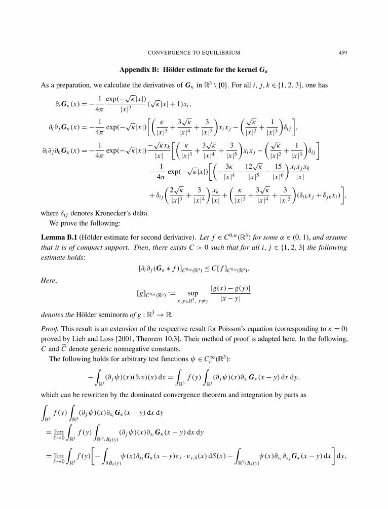
CONVERGENCE TO EQUILIBRIUM 459
Appendix B: Hölder estimate for the kernel Gκ
As a preparation, we calculate the derivatives of Gκ in R3\ {0}. For all i, j, k ∈ {1, 2, 3}, one has
∂i Gκ(x)=−1
4πexp(−
√κ|x |)
|x |3(√κ|x | + 1)xi ,
∂i∂ j Gκ(x)=−1
4πexp(−
√κ|x |)
[(κ
|x |3+
3√κ
|x |4+
3|x |5
)xi x j −
(√κ
|x |2+
1|x |3
)δi j
],
∂i∂ j∂k Gκ(x)=−1
4πexp(−
√κ|x |)−√κxk
|x |
[(κ
|x |3+
3√κ
|x |4+
3|x |5
)xi x j −
(√κ
|x |2+
1|x |3
)δi j
]−
14π
exp(−√κ|x |)
[(−
3κ|x |4−
12√κ
|x |5−
15|x |6
)xi x j xk
|x |
+ δi j
(2√κ
|x |3+
3|x |4
)xk
|x |+
(κ
|x |3+
3√κ
|x |4+
3|x |5
)(δik x j + δ jk xi )
],
where δi j denotes Kronecker’s delta.We prove the following:
Lemma B.1 (Hölder estimate for second derivative). Let f ∈ C0,α(R3) for some α ∈ (0, 1), and assumethat it is of compact support. Then, there exists C > 0 such that for all i, j ∈ {1, 2, 3} the followingestimate holds:
[∂i∂ j (Gκ ∗ f )]C0,α(R3) ≤ C[ f ]C0,α(R3).
Here,
[g]C0,α(R3) := supx,y∈R3, x 6=y
|g(x)− g(y)||x − y|
denotes the Hölder seminorm of g : R3→ R.
Proof. This result is an extension of the respective result for Poisson’s equation (corresponding to κ = 0)proved by Lieb and Loss [2001, Theorem 10.3]. Their method of proof is adapted here. In the following,C and C denote generic nonnegative constants.
The following holds for arbitrary test functions ψ ∈ C∞c (R3):
−
∫R3(∂ jψ)(x)(∂iv)(x) dx =
∫R3
f (y)∫
R3(∂ jψ)(x)∂xi Gκ(x − y) dx dy,
which can be rewritten by the dominated convergence theorem and integration by parts as∫R3
f (y)∫
R3(∂ jψ)(x)∂xi Gκ(x − y) dx dy
= limδ→0
∫R3
f (y)∫
R3\Bδ(y)(∂ jψ)(x)∂xi Gκ(x − y) dx dy
= limδ→0
∫R3
f (y)[−
∫∂Bδ(y)
ψ(x)∂xi Gκ(x − y)e j · νy,δ(x) dS(x)−∫
R3\Bδ(y)ψ(x)∂xi ∂x j Gκ(x − y) dx
]dy,

460 JONATHAN ZINSL AND DANIEL MATTHES
where e j is the j-th unit vector and νy,δ(x) = (x − y)/δ is the unit outward normal vector in x on thesphere ∂Bδ(y).
The first part can be simplified explicitly by the transformation z := (x − y)/δ:
−
∫∂Bδ(y)
ψ(x)∂xi Gκ(x − y)e j · νy,δ(x) dS(x)=1
4π
∫∂B1(0)
ψ(δz+ y) exp(−√κδ)(√κδ+ 1)zi z j dS(z),
which converges as δ→ 0 to ψ(y)δi j/3.For the second part, we split the domain of integration R3
\ Bδ(y) into two parts:∫R3\Bδ(y)
ψ(x)∂xi ∂x j Gκ(x − y) dx
=
∫R3\Bδ(1)
ψ(x)∂xi ∂x j Gκ(x − y) dx +∫{1≥|x−y|≥δ}
ψ(x)∂xi ∂x j Gκ(x − y) dx .
We use integration by parts to insert convenient additional terms:∫R3\Bδ(1)
ψ(x)∂xi ∂x j Gκ(x − y) dx +∫{1≥|x−y|≥δ}
ψ(x)∂xi ∂x j Gκ(x − y) dx
=
∫R3\Bδ(1)
ψ(x)∂xi ∂x j Gκ(x − y) dx +∫{1≥|x−y|≥δ}
ψ(x)∂xi ∂x j Gκ(x − y) dx
−
∫{1≥|x−y|≥δ}
ψ(y)∂xi ∂x j Gκ(x − y) dx
+
∫∂B1(y)
ψ(y)∂x j Gκ(x − y)ei · νy,1(x) dS(x)−∫∂Bδ(y)
ψ(y)∂x j Gκ(x − y)ei · νy,δ(x) dS(x).
Now we calculate again explicitly and obtain in the limit δ→ 0∫∂B1(y)
ψ(y)∂x j Gκ(x − y)ei · νy,1(x) dS(x)−∫∂Bδ(y)
ψ(y)∂x j Gκ(x − y)ei · νy,δ(x) dS(x)
→−13δi j [exp(−
√κ)(√κ + 1)− 1]ψ(y).
In summary, one gets
−
∫R3(∂ jψ)(x)(∂iv)(x) dx=
∫R3ψ(x)
[13δi j f (x) exp(−
√κ)(√κ+1)+
∫R3\B1(x)
f (y)∂xi ∂x j Gκ(x−y) dy
+ limδ→0
∫{1≥|x−y|≥δ}
( f (x)− f (y))∂xi ∂x j Gκ(x − y) dy]
dx .
From α-Hölder continuity of f , we conclude that, independent of δ,
1{1≥|x−y|≥δ}(y)∣∣[ f (x)− f (y)]∂xi ∂x j Gκ(x − y)
∣∣≤ C |x − y|α−3,

CONVERGENCE TO EQUILIBRIUM 461
which is integrable as α− 3+ 2 > −1. So using again the dominated convergence theorem, we have,with [Lieb and Loss 2001, Theorem 6.10],
(∂i∂ jv)(x)= 13δi j exp(−
√κ)(√κ + 1)
+
∫R3\B1(x)
f (y)∂xi ∂x j Gκ(x − y) dy+∫
B1(x)[ f (x)− f (y)]∂xi ∂x j Gκ(x − y) dy. (91)
Obviously, the first term in (91) is Hölder-continuous. For the second term in (91), we obtain for allx, z ∈ R3, x 6= z,∣∣∣∣∫
R3\B1(x)f (y)∂xi ∂x j Gκ(x − y) dy−
∫R3\B1(z)
f (y)∂zi ∂z j Gκ(z− y) dy∣∣∣∣
=
∣∣∣∣∫B1(0)[ f (z− a)− f (x − a)]∂ai ∂a j Gκ(a) da
∣∣∣∣by the transformations a := x − y in the first and a := z − y in the second integrals. From α-Höldercontinuity of f , we get the estimate∣∣∣∣∫
B1(0)[ f (z− a)− f (x − a)]∂ai ∂a j Gκ(a) da
∣∣∣∣≤ C |x − z|α∫
R3\B1(x)|∂ai ∂a j Gκ(a) da|,
where the integral on the right-hand side is finite because ∂ai ∂a j Gκ(a) behaves as r−1 exp(−r) for r→∞,which is integrable.
The same integral transformation yields for the third term in (91)∣∣∣∣∫B1(x)[ f (x)− f (y)]∂xi ∂x j Gκ(x − y) dy−
∫B1(z)[ f (z)− f (y)]∂zi ∂z j Gκ(z− y) dy
∣∣∣∣=
∣∣∣∣∫B1(0)[ f (z)− f (z− a)− f (x)+ f (x − a)]∂ai ∂a j Gκ(a) da
∣∣∣∣.We now proceed as in [Lieb and Loss 2001] and write B1(0)= A∪ B with
A := {a : 0≤ |a|< 4|x − z|},
B := {a : 4|x − z|< |a|< 1},
where B =∅ for |x − z| ≥ 14 , and calculate, using that |∂ai ∂a j Gκ(a)| ≤ C |a|−3,∣∣∣∣∫
A[ f (z)− f (z− a)− f (x)+ f (x − a)]∂ai ∂a j Gκ(a) da
∣∣∣∣≤ ∫A
2C |a|α−3 da = C |x − z|α.
It remains to consider the case |x − z|< 14 . One has∣∣∣∣∫
B[ f (z)− f (x)]∂ai ∂a j Gκ(a) da
∣∣∣∣= ∣∣∣∣∫∂B[ f (z)− f (x)]∂a j Gκ(a)ei · ν(a) dS(a)
∣∣∣∣,

462 JONATHAN ZINSL AND DANIEL MATTHES
and by similar arguments as above,∣∣∣∣∫∂B[ f (z)− f (x)]∂a j Gκ(a)ei · ν(a) dS(a)
∣∣∣∣=
13δi j | f (z)− f (x)|
∣∣exp(−√κ)(√κ + 1)− exp(−4
√κ|x − z|)(4
√κ|x − z| + 1)
∣∣.Note that the real-valued map [0,∞) 3 r 7→ exp(−
√κr)(√κr + 1) is monotonically decreasing. This
yields ∣∣∣∣∫B[ f (z)− f (x)]∂ai ∂a j Gκ(a) da
∣∣∣∣≤ C |z− x |α.
By the transformations b := x − a− z and b := −a, we get∣∣∣∣∫B[ f (x − a)− f (z− a)]∂ai ∂a j Gκ(a) da
∣∣∣∣=
∣∣∣∣∫B
f (z+ b)∂bi ∂b j Gκ(b) db−∫
Df (b+ z)∂bi ∂b j Gκ(b− x + z) db
∣∣∣∣ (92)
with D := {b : 4|x − z|< |b− x + z|< 1}.Note that ∫
B∂bi ∂b j Gκ(b) db =
∫D∂bi ∂b j Gκ(b− x + z) db.
This enables us to rewrite (92) as∣∣∣∣∫B
f (z+ b)∂bi ∂b j Gκ(b) db−∫
Df (b+ z)∂bi ∂b j Gκ(b− x + z) db
∣∣∣∣=
∣∣∣∣∫B[ f (z+ b)− f (z)]∂bi ∂b j Gκ(b) db−
∫D[ f (z+ b)− f (z)]∂bi ∂b j Gκ(b− x + z) db
∣∣∣∣. (93)
We consider (93) separately on the sets B ∩ D, B \ D and D \ B.Note that, by the triangular inequality, B ∩ D ⊂ {b : 3|x − z| < |b| < 1+ |x − z|} and by Taylor’s
theorem
(∂bi ∂b j Gκ)(b)− (∂bi ∂b j Gκ)(b− x + z)=3∑
k=1
(∂k∂i∂ j Gκ)(b∗)(xk − zk)
for some b∗ = b− β(x − z) with β ∈ (0, 1). Therefore, one has, by the triangular inequality, |b∗| ≥|b| −β|x − z| ≥ (1− 1
3β)|b| ≥23 |b| on B ∩ D and consequently
|(∂bi ∂b j Gκ)(b)− (∂bi ∂b j Gκ)(b− x + z)| ≤ C |b∗|−4|x − z| ≤ C |b|−4
|x − z|.

CONVERGENCE TO EQUILIBRIUM 463
This allows us to estimate∣∣∣∣∫B∩D[ f (z+ b)− f (z)][∂bi ∂b j Gκ(b)− ∂bi ∂b j Gκ(b− x + z)] db
∣∣∣∣≤ C |x − z|
∫ 1+|x−z|
3|x−z|r−4+α+2 dr
≤C |x − z|
1−α
[(3|x − z|)α−1
− (1+ |x − z|)α−1] C1−α
|x − z|α.
For the remaining terms, we split up as in [Lieb and Loss 2001]:
B \ D ⊂ E ∪G,
D \ B ⊂ E ′ ∪G ′,where
E := {b : 4|x − z|< |b| ≤ 5|x − z|},
G := {b : 1− |x − z| ≤ |b|< 1},
E ′ := {b : 4|x − z|< |b− x + z| ≤ 5|x − z|},
G ′ := {b : 1− |x − z| ≤ |b− x + z|< 1}.
Consider at first the real-valued map [0, 14 ] 3 s 7→ (1 − s)β for arbitrary β > 0. Obviously, it is
continuously differentiable and therefore α-Hölder continuous because its domain of definition is compact.Hence, the following holds for all 0≤ s ≤ 1
4 :
1− (1− s)β = (1− 0)β − (1− s)β ≤ Csα. (94)
Now, we estimate the integral on B \ D, where we use again the estimate |∂ai ∂a j Gκ(a)| ≤ C |a|−3:∣∣∣∣∫B\D[ f (z+ b)− f (z)]∂bi ∂b j Gκ(b) db
∣∣∣∣≤ C(∫ 5|x−z|
4|x−z|rα−3+2 dr +
∫ 1
1−|x−z|rα−3+2 dr
)=
Cα[(5|x − z|)α − (4|x − z|)α + 1− (1− |x − z|)α] ≤
Cα(5α + C)|x − z|α,
where we have used (94) for β := α in the last step.For the remaining integral on D \ B, we consider the domains E ′ and G ′ separately and note at
first that, using the triangular inequality, E ′ ⊂ {0 < |b| ≤ 6|x − z|}. Subsequently, this yields that|b− x + z|−3 < (4|x − z|)−3
≤ C |b|−3 on E ′. Hence, by the estimate |∂ai ∂a j Gκ(a)| ≤ C |a|−3,∫E ′
∣∣[ f (z+ b)− f (z)]∂bi ∂b j Gκ(b− x + z)∣∣ db ≤ C
∫ 6|x−z|
0rα−3+2 dr = C |x − z|α.
On G ′, one has |b− x + z| ≥ 1− |x − z|> 34 . Consequently, it holds that∫
G ′
∣∣[ f (z+ b)− f (z)]∂bi ∂b j Gκ(b− x + z)∣∣ db ≤ C
( 34
)−3∫ 1
1−|x−z|rα+2 dr
= C[1− (1− |x − z|)3+α] ≤ C |x − z|α,

464 JONATHAN ZINSL AND DANIEL MATTHES
where we have used (94) for β := 3+α in the last step. Together,∣∣∣∣∫D\B[ f (z+ b)− f (z)]∂bi ∂b j Gκ(b− x + z) db
∣∣∣∣≤ C |x − z|α,
and the assertion is proved. �
References
[Agueh 2008] M. Agueh, “Rates of decay to equilibria for p-Laplacian type equations”, Nonlinear Anal. 68:7 (2008), 1909–1927.MR 2009e:35117 Zbl 1185.35017
[Ambrosio et al. 2008] L. Ambrosio, N. Gigli, and G. Savaré, Gradient flows in metric spaces and in the space of probabilitymeasures, 2nd ed., Birkhäuser, Basel, 2008. MR 2009h:49002 Zbl 1145.35001
[Biler et al. 2011] P. Biler, L. Corrias, and J. Dolbeault, “Large mass self-similar solutions of the parabolic-parabolic Keller–Segelmodel of chemotaxis”, J. Math. Biol. 63:1 (2011), 1–32. MR 2012c:35431 Zbl 1230.92011
[Blanchet 2013] A. Blanchet, “A gradient flow approach to the Keller–Segel systems”, preprint, 2013, Available at http://www.tse-fr.eu/sites/default/files/medias/doc/by/blanchet/dec_2010/b4.pdf.
[Blanchet and Laurençot 2013] A. Blanchet and P. Laurençot, “The parabolic-parabolic Keller–Segel system with criticaldiffusion as a gradient flow in Rd , d ≥ 3”, Comm. Partial Differential Equations 38:4 (2013), 658–686. MR 3040679Zbl 1282.35202
[Blanchet et al. 2008] A. Blanchet, V. Calvez, and J. A. Carrillo, “Convergence of the mass-transport steepest descent scheme forthe subcritical Patlak–Keller–Segel model”, SIAM J. Numer. Anal. 46:2 (2008), 691–721. MR 2009a:35113 Zbl 1205.65332
[Blanchet et al. 2009] A. Blanchet, J. A. Carrillo, and P. Laurençot, “Critical mass for a Patlak–Keller–Segel model withdegenerate diffusion in higher dimensions”, Calc. Var. Partial Differential Equations 35:2 (2009), 133–168. MR 2010e:35149Zbl 1172.35035
[Blanchet et al. 2012] A. Blanchet, E. A. Carlen, and J. A. Carrillo, “Functional inequalities, thick tails and asymptotics for thecritical mass Patlak–Keller–Segel model”, J. Funct. Anal. 262:5 (2012), 2142–2230. MR 2876403 Zbl 1237.35155
[Blanchet et al. 2014] A. Blanchet, J. A. Carrillo, D. Kinderlehrer, M. Kowalczyk, P. Laurençot, and S. Lisini, “A hybridvariational principle for the Keller–Segel system in R2”, preprint, 2014. arXiv 1407.5562v1
[Calvez and Carrillo 2012] V. Calvez and J. A. Carrillo, “Refined asymptotics for the subcritical Keller–Segel system and relatedfunctional inequalities”, Proc. Amer. Math. Soc. 140:10 (2012), 3515–3530. MR 2929020 Zbl 1277.35051
[Calvez and Corrias 2008] V. Calvez and L. Corrias, “The parabolic-parabolic Keller–Segel model in R2”, Commun. Math. Sci.6:2 (2008), 417–447. MR 2009m:35518 Zbl 1149.35360
[Carrapatoso and Mischler 2014] K. Carrapatoso and S. Mischler, “Uniqueness and long time asymptotic for the parabolic-parabolic Keller–Segel equation”, preprint, 2014. arXiv 1406.6006v2
[Carrillo and Toscani 2000] J. A. Carrillo and G. Toscani, “Asymptotic L1-decay of solutions of the porous medium equation toself-similarity”, Indiana Univ. Math. J. 49:1 (2000), 113–142. MR 2001j:35155 Zbl 0963.35098
[Carrillo et al. 2003] J. A. Carrillo, R. J. McCann, and C. Villani, “Kinetic equilibration rates for granular media and re-lated equations: entropy dissipation and mass transportation estimates”, Rev. Mat. Iberoamericana 19:3 (2003), 971–1018.MR 2005a:35126 Zbl 1073.35127
[Carrillo et al. 2006a] J. A. Carrillo, M. Di Francesco, and G. Toscani, “Intermediate asymptotics beyond homogeneity andself-similarity: long time behavior for ut = 1φ(u)”, Arch. Ration. Mech. Anal. 180:1 (2006), 127–149. MR 2006k:35131Zbl 1096.35015
[Carrillo et al. 2006b] J. A. Carrillo, R. J. McCann, and C. Villani, “Contractions in the 2-Wasserstein length space andthermalization of granular media”, Arch. Ration. Mech. Anal. 179:2 (2006), 217–263. MR 2006j:76121 Zbl 1082.76105
[Carrillo et al. 2011] J. A. Carrillo, M. Di Francesco, A. Figalli, T. Laurent, and D. Slepcev, “Global-in-time weak measure solu-tions and finite-time aggregation for nonlocal interaction equations”, Duke Math. J. 156:2 (2011), 229–271. MR 2012c:35447Zbl 1215.35045

CONVERGENCE TO EQUILIBRIUM 465
[Corrias and Perthame 2008] L. Corrias and B. Perthame, “Asymptotic decay for the solutions of the parabolic-parabolicKeller–Segel chemotaxis system in critical spaces”, Math. Comput. Modelling 47:7–8 (2008), 755–764. MR 2009c:35200Zbl 1134.92006
[Di Francesco and Rosado 2008] M. Di Francesco and J. Rosado, “Fully parabolic Keller–Segel model for chemotaxis withprevention of overcrowding”, Nonlinearity 21:11 (2008), 2715–2730. MR 2009m:35196 Zbl 1157.35398
[Eisenbach 2004] M. Eisenbach, Chemotaxis, Imperial College, London, 2004.
[Giacomelli and Otto 2001] L. Giacomelli and F. Otto, “Variational formulation for the lubrication approximation of theHele–Shaw flow”, Calc. Var. Partial Differential Equations 13:3 (2001), 377–403. MR 2003a:76046 Zbl 1086.35004
[Gianazza et al. 2009] U. Gianazza, G. Savaré, and G. Toscani, “The Wasserstein gradient flow of the Fisher information and thequantum drift-diffusion equation”, Arch. Ration. Mech. Anal. 194:1 (2009), 133–220. MR 2010i:35371 Zbl 1223.35264
[Hillen and Painter 2009] T. Hillen and K. J. Painter, “A user’s guide to PDE models for chemotaxis”, J. Math. Biol. 58:1–2(2009), 183–217. MR 2009m:92017 Zbl 1161.92003
[Horstmann 2003] D. Horstmann, “From 1970 until present: the Keller–Segel model in chemotaxis and its consequences, I”,Jahresber. Deutsch. Math.-Verein. 105:3 (2003), 103–165. MR 2005f:35163 Zbl 1071.35001
[Jordan et al. 1998] R. Jordan, D. Kinderlehrer, and F. Otto, “The variational formulation of the Fokker–Planck equation”, SIAMJ. Math. Anal. 29:1 (1998), 1–17. MR 2000b:35258 Zbl 0915.35120
[Keller and Segel 1970] E. F. Keller and L. A. Segel, “Initiation of slime mold aggregation viewed as an instability”, J. Theor.Biol. 26:3 (1970), 399–415. Zbl 1170.92306
[Kozono and Sugiyama 2009] H. Kozono and Y. Sugiyama, “Global strong solution to the semi-linear Keller–Segel sys-tem of parabolic-parabolic type with small data in scale invariant spaces”, J. Differential Equations 247:1 (2009), 1–32.MR 2010i:35147 Zbl 1207.35178
[Lapidus and Schiller 1976] I. R. Lapidus and R. Schiller, “Model for the chemotactic response of a bacterial population”,Biophys. J. 16:7 (1976), 779–789.
[Laurençot and Matioc 2013] P. Laurençot and B.-V. Matioc, “A gradient flow approach to a thin film approximation of theMuskat problem”, Calc. Var. Partial Differential Equations 47:1–2 (2013), 319–341. MR 3044141 Zbl 1264.35129
[Lieb and Loss 2001] E. H. Lieb and M. Loss, Analysis, 2nd ed., Graduate Studies in Mathematics 14, Amer. Math. Soc.,Providence, RI, 2001. MR 2001i:00001 Zbl 0966.26002
[López-Gómez et al. 2013] J. López-Gómez, T. Nagai, and T. Yamada, “The basin of attraction of the steady-states for achemotaxis model in R2 with critical mass”, Arch. Ration. Mech. Anal. 207:1 (2013), 159–184. MR 3004770 Zbl 06148937
[Luckhaus and Sugiyama 2006] S. Luckhaus and Y. Sugiyama, “Large time behavior of solutions in super-critical cases todegenerate Keller–Segel systems”, M2AN Math. Model. Numer. Anal. 40:3 (2006), 597–621. MR 2007e:35127 Zbl 1113.35028
[Luckhaus and Sugiyama 2007] S. Luckhaus and Y. Sugiyama, “Asymptotic profile with the optimal convergence rate for aparabolic equation of chemotaxis in super-critical cases”, Indiana Univ. Math. J. 56:3 (2007), 1279–1297. MR 2008k:35272Zbl 1118.35006
[Matthes et al. 2009] D. Matthes, R. J. McCann, and G. Savaré, “A family of nonlinear fourth order equations of gradient flowtype”, Comm. Partial Differential Equations 34:10–12 (2009), 1352–1397. MR 2011e:35149 Zbl 1187.35131
[Mizoguchi 2013] N. Mizoguchi, “Global existence for the Cauchy problem of the parabolic-parabolic Keller–Segel system onthe plane”, Calc. Var. Partial Differential Equations 48:3–4 (2013), 491–505. MR 3116019 Zbl 1288.35286
[Murray 2003] J. D. Murray, Mathematical biology, II: Spatial models and biomedical applications, 3rd ed., InterdisciplinaryApplied Mathematics 18, Springer, New York, 2003. MR 2004b:92001 Zbl 1006.92002
[Nagai and Senba 1998] T. Nagai and T. Senba, “Global existence and blow-up of radial solutions to a parabolic-elliptic systemof chemotaxis”, Adv. Math. Sci. Appl. 8:1 (1998), 145–156. MR 2000a:35241 Zbl 0902.35010
[Nagai et al. 2003] T. Nagai, R. Syukuinn, and M. Umesako, “Decay properties and asymptotic profiles of bounded solutions toa parabolic system of chemotaxis in Rn”, Funkcial. Ekvac. 46:3 (2003), 383–407. MR 2005h:35144 Zbl 02112808
[Otto 2001] F. Otto, “The geometry of dissipative evolution equations: the porous medium equation”, Comm. Partial DifferentialEquations 26:1–2 (2001), 101–174. MR 2002j:35180 Zbl 0984.35089

466 JONATHAN ZINSL AND DANIEL MATTHES
[Perthame 2007] B. Perthame, Transport equations in biology, Birkhäuser, Basel, 2007. MR 2007j:35004 Zbl 1185.92006
[Post 1999] K. Post, A non-linear parabolic system modeling chemotaxis with sensitivity functions, Ph.D. thesis, Humboldt-Universität zu Berlin, 1999, Available at http://edoc.hu-berlin.de/docviews/abstract.php?id=26314.
[Segel 1977] L. Segel, “A theoretical study of receptor mechanisms in bacterial chemotaxis”, SIAM J. Appl. Math. 32:3 (1977),653–665. Zbl 0356.92009
[Senba and Suzuki 2006] T. Senba and T. Suzuki, “A quasi-linear parabolic system of chemotaxis”, Abstr. Appl. Anal. 2006(2006), 23061. MR 2006j:35121 Zbl 1134.35059
[Stein 1970] E. M. Stein, Singular integrals and differentiability properties of functions, Princeton Mathematical Series 30,Princeton University, 1970. MR 44 #7280 Zbl 0207.13501
[Sugiyama 2006] Y. Sugiyama, “Global existence in sub-critical cases and finite time blow-up in super-critical cases to degenerateKeller–Segel systems”, Differential Integral Equations 19:8 (2006), 841–876. MR 2008h:35134 Zbl 1212.35240
[Sugiyama 2007] Y. Sugiyama, “Time global existence and asymptotic behavior of solutions to degenerate quasi-linear parabolicsystems of chemotaxis”, Differential Integral Equations 20:2 (2007), 133–180. MR 2008a:35169 Zbl 1212.35241
[Sugiyama and Kunii 2006] Y. Sugiyama and H. Kunii, “Global existence and decay properties for a degenerate Keller–Segelmodel with a power factor in drift term”, J. Differential Equations 227:1 (2006), 333–364. MR 2008j:35103 Zbl 1102.35046
[Villani 2003] C. Villani, Topics in optimal transportation, Graduate Studies in Mathematics 58, Amer. Math. Soc., Providence,RI, 2003. MR 2004e:90003 Zbl 1106.90001
[Winkler 2010] M. Winkler, “Absence of collapse in a parabolic chemotaxis system with signal-dependent sensitivity”, Math.Nachr. 283:11 (2010), 1664–1673. MR 2011k:35090 Zbl 1205.35037
[Yamada 2011] T. Yamada, “Improvement of convergence rates for a parabolic system of chemotaxis in the whole space”, Math.Methods Appl. Sci. 34:17 (2011), 2103–2124. MR 2012k:35217 Zbl 1242.35054
[Zeidler 1990] E. Zeidler, Nonlinear functional analysis and its applications, II/B: Nonlinear monotone operators, Springer,New York, 1990. MR 91b:47002 Zbl 0684.47029
[Zinsl 2014] J. Zinsl, “Existence of solutions for a nonlinear system of parabolic equations with gradient flow structure”, Monats.Math. 174:4 (2014), 653–679. MR 3233116 Zbl 1302.35202
Received 12 May 2014. Revised 25 Nov 2014. Accepted 9 Jan 2015.
JONATHAN ZINSL: [email protected] für Mathematik, Technische Universität München, Boltzmannstraße 3, 85747 Garching, Germany
DANIEL MATTHES: [email protected] für Mathematik, Technische Universität München, Boltzmannstraße 3, 85747 Garching, Germany
mathematical sciences publishers msp

ANALYSIS AND PDEVol. 8, No. 2, 2015
dx.doi.org/10.2140/apde.2015.8.467 msp
SCATTERING FOR THE RADIAL 3D CUBIC WAVE EQUATION
BENJAMIN DODSON AND ANDREW LAWRIE
Consider the Cauchy problem for the radial cubic wave equation in 1+ 3 dimensions with either thefocusing or defocusing sign. This problem is critical in H 1/2
× H−1/2(R3) and subcritical with respectto the conserved energy. Here we prove that if the critical norm of a solution remains bounded on themaximal time interval of existence, then the solution must in fact be global in time and must scatter tofree waves as t→±∞.
1. Introduction
Consider the Cauchy problem for the cubic semilinear wave equation in R1+3, namely,
ut t −1u+µu3= 0,
Eu(0)= (u0, u1),(1-1)
restricted to the radial setting and with µ ∈ {±1}. The case µ = 1 yields what is referred to as thedefocusing problem, since here the conserved energy,
E(Eu)(t) :=∫
R3
(12(|ut(t)|2+ |∇u(t)|2
)+
14|u(t)|4
)dx = constant, (1-2)
is positive for sufficiently regular nonzero solutions, and the H 1× L2(R3) norm of a solution,
Eu(t) := (u(t), ut(t)),
is bounded by its energy.The case µ=−1 gives the focusing problem, and the conserved energy for sufficiently regular solutions
to (1-1) is given by
E(Eu)(t) :=∫
R3
(12(|ut(t)|2+ |∇u(t)|2
)−
14|u(t)|4
)dx = constant. (1-3)
As we will only be considering radial solutions to (1-1), we will often slightly abuse notation by writingu(t, x)= u(t, r), where (r, ω), with r = |x |, x = rω, ω ∈ S2, are polar coordinates on R3. In this setting
Support of the National Science Foundation, DMS-1103914 for Dodson and DMS-1302782 for Lawrie, is gratefullyacknowledged.MSC2010: 35L05.Keywords: scattering, concentration compactness, double Duhamel.
467

468 BENJAMIN DODSON AND ANDREW LAWRIE
we can rewrite the Cauchy problem (1-1) as
ut t − urr −2r
ur ± u3= 0,
Eu(0)= (u0, u1),
(1-4)
and the conserved energy (up to a constant multiple) as
E(Eu)(t)=∫∞
0
(12(u2
t (t)+ u2r (t)
)±
14
u4(t))
r2 dr. (1-5)
The Cauchy problem (1-4) is invariant under the scaling
Eu(t, r) 7→ Euλ(t, r) :=(λ−1u
(tλ,
rλ
), λ−2ut
(tλ,
rλ
)). (1-6)
One can also check that this scaling leaves unchanged the H 1/2× H−1/2-norm of the solution. It is for
this reason that (1-4) is called energy-subcritical. It is natural to consider the Cauchy problem with initialdata (u0, u1) ∈ H 1/2
× H−1/2. We remark that (1-4) is also invariant under conformal inversion:
u(t, r) 7→1
t2− r2 u(
tt2− r2 ,
rt2− r2
). (1-7)
A standard argument based on Strichartz estimates shows that both the defocusing and focusingproblems are locally well-posed in H 1/2
× H−1/2(R3). This means that for all initial data Eu(0) =(u0, u1) ∈ H 1/2
× H−1/2, there is a unique solution Eu(t) defined on a maximal interval of existenceImax with Eu(t) ∈ C(Imax; H 1/2
× H−1/2). Moreover, for every compact time interval J ⊂ Imax, we haveu ∈ S(J ) := L4
t (J ; L4x). The Strichartz norm S(J ) determines criteria for both scattering and finite-time
blow-up, and we make these statements precise in Proposition 2.4. Here we note that in particular, onecan show that if the initial data Eu(0) has sufficiently small H 1/2
× H−1/2-norm, then the correspondingsolution Eu(t) has finite S(R)-norm and hence scatters to free waves as t→±∞.
The theory for solutions to (1-4) with initial data that is small in H 1/2× H−1/2 is thus very well
understood: all solutions are global in time and scatter to free waves as t→±∞. However, much lessis known regarding the asymptotic dynamics of solutions to either the defocusing or focusing problemsonce one leaves the perturbative regime.
It is well known that there are solutions to the focusing problem that blow up in finite time. To give anexample,
φT (t, r)=
√2
T − t(1-8)
solves the ODE φt t = φ3. Using finite speed of propagation, one can construct from φT a compactly
supported (in space) self-similar blow-up solution to (1-4). Indeed, define EuT (t) to be the solution to(1-4) with initial data EuT (0, x)= χ2T (x)
√2, where χ2T ∈C∞0 (R
3) satisfies χ2T (x)= 1 if |x | ≤ 2T . ThenEuT (t) equals φT (t) for all r ≤ T and 0≤ t < T , and blows up at time t = T . However, such a self-similar

SCATTERING FOR THE RADIAL 3D CUBIC WAVE EQUATION 469
solution must have its critical H 1/2× H−1/2-norm tending to∞ as t→ T :
limt→T‖EuT (t)‖H1/2×H−1/2 =∞.
Indeed, one can show by a direct computation that the L3(R3)-norm of EuT (t, x) tends to∞ as t→ T+.Since H 1/2
⊂ L3, this means that the H 1/2× H−1/2-norm must blow up as well. Such behavior is typically
referred to as type I, or ODE, blow-up.One the other hand, type II solutions, Eu(t), are those whose critical norm remains bounded on their
maximal interval of existence, Imax:
supt∈Imax
‖Eu(t)‖H1/2×H−1/2 <∞. (1-9)
In this paper we restrict our attention to type II solutions, i.e., those which satisfy (1-9). We prove thatif a solution Eu(t) to (1-4) satisfies (1-9), then Eu(t) must in fact exist globally in time and scatter to freewaves in both time directions. To be precise, we establish the following result.
Theorem 1.1. Let Eu(t) ∈ H 1/2× H−1/2(R3) be a radial solution to (1-4) defined on its maximal interval
of existence Imax = (T−, T+). Suppose in addition that
supt∈Imax
‖Eu(t)‖H1/2×H−1/2(R3) <∞. (1-10)
Then Imax = R, i.e., Eu(t) is defined globally in time. Moreover,
‖u‖L4t,x (R
1+3) <∞, (1-11)
which means that Eu(t) scatters to a free wave in each time direction, i.e., there exist radial solutionsEu±L (t) ∈ H 1/2
× H−1/2(R3) to the free wave equation, �u±L = 0, such that
‖Eu(t)− Eu±L (t)‖H1/2×H−1/2(R3)→ 0 as t→+∞. (1-12)
Remark 1. Theorem 1.1 is a conditional result. Other than the requirement that the initial data be smallin H 1/2
× H−1/2, there is no known general criterion that ensures that (1-10) is satisfied by the evolutionfor either the defocusing or the focusing equation. While the methods in this paper apply equally well toboth the focusing and defocusing equations, one should expect drastically different behavior from genericinitial data in these two cases.
Remark 2. The proof of Theorem 1.1 readily generalizes to all subcritical powers p ≤ 3 for whichthere is a satisfactory small data/local well-posedness theory. In particular, the methods presented hereallow one to deduce the exact analog of Theorem 1.1 for radial equations (1-13) for all powers p with1+√
2< p ≤ 3; here 1+√
2 is the F. John exponent [1979; Schaeffer 1985]. We have chosen to presentthe details for only the cubic equation to keep the exposition as simple as possible. We also remark thatonly the material in Section 4 relies on the assumption of radiality.

470 BENJAMIN DODSON AND ANDREW LAWRIE
1A. History of the problem. The cubic wave equation on R1+3 has been extensively studied and wecertainly cannot give a complete account of the vast body of literature devoted to this problem.
For the defocusing equation, the positivity of the conserved energy can be used to extend a localexistence result to a global one if one begins with initial data that is sufficiently regular. Jörgens [1961]showed global existence for the defocusing equation for smooth compactly supported data. There hasbeen a good deal of recent work extending the local existence result of Lindblad and Sogge [1995] inH s× H s−1 for s > 1
2 to an unconditional global well-posedness result, and we refer the reader to [Keniget al. 2000; Gallagher and Planchon 2003; Bahouri and Chemin 2006; Roy 2009] and the referencestherein for details. However, since these works are not carried out in the scaling critical space, the issueof global dynamics, and in particular scattering, is not addressed.
For the focusing equation, type II finite-time blow-up has recently been ruled out for initial data that liesin H 1
× L2 in the work of Killip, Stovall, and Vis,an [Killip et al. 2012]. There are several works that openup interesting lines of inquiry related to the question of asymptotic dynamics. In two remarkable works,Merle and Zaag [2003; 2005] determined that all blow-up solutions must blow up at the self-similar rate.In the radial case, an infinite family of smooth self-similar solutions is constructed by Bizon et al. [2010].Bizon and Zenginoglu [2009] give numerical evidence to support a conjecture that a two-parameter familyof solutions, obtained via time translation and conformal inversion of a self-similar solution, serves as aglobal attractor for a large set of initial data. In fact, Donninger and Schörkhuber [2012] showed that theblow-up profile (1-8) is stable under small perturbations in the energy topology.
Equations of the form
�u =±|u|p−1u (1-13)
for different values of p and for different dimensions have also been extensively studied. For d = 3, theenergy-critical power, p= 5, exhibits quite different phenomena than both the subcritical and supercriticalequations. Global existence and scattering for all finite-energy data was proved by Struwe [1988] for theradial defocusing equation and by Grillakis [1990] in the nonradial, defocusing case.
For the focusing energy-critical equation, type II blow-up can occur, as explicitly demonstrated byKrieger, Schlag, and Tataru [Krieger et al. 2009] via an energy concentration scenario resulting in thebubbling off of the ground state solution, W , for the underlying elliptic equation; see also [Krieger andSchlag 2014a; Donninger et al. 2014; Donninger and Krieger 2013].
Kenig and Merle [2008] initiated a powerful program of attack for semilinear equations (1-13) with theconcentration compactness/rigidity method, giving a characterization of possible dynamics for solutionswith energy below the threshold energy of the ground state elliptic solution. The subsequent work ofDuyckaerts, Kenig, and Merle [Duyckaerts et al. 2011; 2012a; 2012b; 2013] resulted in a classificationof possible dynamics for large energies. In particular, all type II radial solutions asymptotically resolveinto a sum of rescaled solitons plus a radiation term at their maximal time of existence. Dynamics at thethreshold energy of W have been examined by Duyckaerts and Merle [2008] and above the threshold byKrieger, Nakanishi, and Schlag [Krieger et al. 2013a; 2013b; 2014].
Analogs of Theorem 1.1 have been established for radial equations with different powers in 3 dimensions.

SCATTERING FOR THE RADIAL 3D CUBIC WAVE EQUATION 471
Shen [2012] proved the exact analog of Theorem 1.1 for subcritical powers 3< p < 5; and Kenig andMerle [2011], and then Duyckaerts, Kenig, and Merle [Duyckaerts et al. 2014], established the analog ofTheorem 1.1 for all supercritical powers p > 5. Here we address type II behavior in the remainder of thesubcritical range for the radial equation, 1+
√2 < p ≤ 3. While we focus on the cubic equation, our
proof readily generalizes to other subcritical powers. The extra regularity for critical elements proved inSection 4 gives an extension and simplification of the argument in [Shen 2012] which allows us to treatthe cubic and lower-power equations.
Leaving the setting of type II solutions, Krieger and Schlag [2014b] have recently constructed a familyof solutions to the supercritical equation, p > 5, which are smooth, global in time, and stable under smallperturbations, and have infinite critical norm.
1B. Outline of the proof of Theorem 1.1. The proof of Theorem 1.1 follows the concentration compact-ness/rigidity method developed in [Kenig and Merle 2006; 2008]. The proof follows a contradictionargument: if Theorem 1.1 were not true, the linear and nonlinear profile decompositions of Bahouri andGérard would allow one to construct a minimal solution to (1-4), called the critical element, which doesnot scatter (here the minimality refers to the size of the norm in (1-10)). This construction, which is bynow standard in the field and is outlined in Section 3, yields a critical element whose trajectory in thespace H 1/2
× H−1/2 is precompact up to modulation. The goal is then to prove that this compactnessproperty is too rigid a property for a nonzero solution and thus the critical element cannot exist.
A significant hurdle in the way of ruling out a critical element Euc(t) for the cubic equation (or anysubcritical equation) is that Euc(t) is constructed in the space H 1/2
× H−1/2, and thus useful globalmonotone quantities that require more regularity, such as the conserved energy and virial type identities,are not, a priori, well defined. In general, solutions to the cubic wave equation are only as regular as theirinitial data, as evidenced by the presence of the free propagator S(t) in the Duhamel representation forthe solution
Euc(t0)= S(t0− t)Euc(t)+∫ t0
tS(t0− s)(0,±u3) ds. (1-14)
The critical element is rescued by the fact that the precompactness of its trajectory is at odds with thedispersive properties of the free part, S(t0− t)Eu(t), and thus the first term on the right of (1-14) is forcedto vanish weakly as t → sup Imax and as t → inf Imax. The second term on the right thus encodes theregularity of the critical element, and a gain can be expected due to the presence of the cubic term. Theadditional regularity is extracted by way of the “double Duhamel trick”, which refers to the considerationof the pairing ⟨∫ t0
T1
S(t0− s)(0,±u3) ds,∫ T2
t0S(t0− τ)(0,±u3) dτ
⟩H1×L2
,
where T1 < t0 and T2 > t0. This technique was developed by Tao [2007] and utilized in the Kenig–Merleframework for nonlinear Schrödinger problems by Killip and Vis,an [2010a; 2010b; 2013], and forsemilinear wave equations in [Killip and Vis,an 2011; Bulut 2012a; 2012b]. This method is also closelyrelated to the in/out decomposition used by Killip, Tao, and Vis,an in [Killip et al. 2009, Section 6]. For

472 BENJAMIN DODSON AND ANDREW LAWRIE
more details on how to exploit the different time directions above, we refer the reader to Section 4, and inparticular to the proof of Theorem 4.1.
Indeed, we bound the critical element in H 1× L2. We then use the conserved energy to rule out a
critical element which fails to be compact by a low frequency concentration, as such a solution wouldhave vanishing energy; see Section 5A. One is then left with a critical element that is global in time andevolves at a fixed scale. In Section 6, we prove that such a solution cannot exist by way of a virial identity.We note that this virial-based rigidity argument works for precompact solutions to (1-13) with powersp ≤ 3, but fails to produce useful estimates for powers 3< p < 5. However, in this range one can use the
“channels of energy” method pioneered in [Duyckaerts et al. 2013; 2014]; see [Shen 2012]. For more onthis, see Remark 12.
2. Preliminaries
2A. Harmonic analysis. In what follows we will denote by Pk the usual Littlewood–Paley projectionsonto frequencies of size |ξ | ' 2k and by P≤k the projection onto frequencies |ξ |. 2k . These projectionssatisfy Bernstein’s inequalities.
Lemma 2.1 (Bernstein’s inequalities [Tao 2006, Appendix A]). Let 1 ≤ p ≤ q ≤ ∞ and s ≥ 0. Letf : Rd
→ R. Then
‖P≥N f ‖L p . N−s‖|∇|
s P≥N f ‖L p ,
‖P≤N |∇|s f ‖L p . N s
‖P≤N f ‖L p , ‖PN |∇|±s f ‖L p ' N±s
‖PN f ‖L p ,
‖P≤N f ‖Lq . N d/p−d/q‖P≤N f ‖L p , ‖PN f ‖Lq . N d/p−d/q
‖PN f ‖L p .
(2-1)
Next, we define the notion of a frequency envelope.
Definition 3 [Tao 2001, Definition 1]. We define a frequency envelope to be a sequence β = {βk} ofpositive real numbers with β ∈ `2. Moreover, we require the local constancy condition
2−σ | j−k|βk . β j . 2σ | j−k|βk,
where σ > 0 is a small fixed constant; in what follows we will use σ = 18 . If β is a frequency envelope
and ( f, g) ∈ H s× H s−1, then we say that ( f, g) lies underneath β if
‖(Pk f, Pk g)‖H s×H s−1 ≤ βk for all k ∈ Z,
and we note that if ( f, g) lies underneath β, then we have
‖( f, g)‖H s×H s−1 . ‖β‖`2 .
We will require the following refinement of the Sobolev embedding for radial functions, which is aconsequence of the Hardy–Littlewood–Sobolev inequality.

SCATTERING FOR THE RADIAL 3D CUBIC WAVE EQUATION 473
Lemma 2.2 (radial Sobolev embedding [Tao et al. 2007, Corollary A.3]). Let 0 < s < 3 and supposef ∈ H s(R3) is a radial function. Suppose that
β >−3q,
12− s ≤
1q≤
12,
1q=
12−β + s
3,
and at most one of the equalities q = 1, q =∞, 1q + s = 1
2 holds. Then
‖rβ f ‖Lq ≤ C‖ f ‖H s . (2-2)
2B. Strichartz estimates. An essential ingredient for the small data theory are Strichartz estimates forthe linear wave equation in R1+3,
vt t −1v = F,
Ev(0)= (v0, v1).(2-3)
A free wave will mean a solution to (2-3) with F = 0 and will be denoted by Eu(t)= S(t)Eu(0). In whatfollows we will say that a pair (p, q) is admissible if
p, q ≥ 2,1p+
1q≤
12. (2-4)
The Strichartz estimates we state below are standard and we refer the reader to [Keel and Tao 1998;Lindblad and Sogge 1995] or the book [Sogge 2008] and the references therein for more details.
Remark 4. We note that since we will only consider the waves with radial initial data and with F radial,we can allow the endpoint (p, q)= (2,∞) as an admissible pair. The admissibility of (2,∞) in the radialsetting was established in [Klainerman and Machedon 1993]. This endpoint is of course forbidden fornonradial data in dimension d = 3.
Proposition 2.3 [Keel and Tao 1998; Klainerman and Machedon 1993; Lindblad and Sogge 1995; Sogge2008]. Let Ev(t) be a solution to (2-3) with initial data Ev(0) ∈ H s
× H s−1(R3) for s > 0. Let (p, q) and(a, b) be admissible pairs satisfying the gap condition
1p+
3q=
1a′+
3b′− 2=
32− s, (2-5)
where (a′, b′) are the conjugate exponents of (a, b). Then, for any time interval I 3 0, we have theestimates
‖v‖L pt (I ;L
qx ). ‖(v0, v1)‖H s×H s−1 +‖F‖La′
t (I ;Lb′x ). (2-6)
2C. Small data theory — global existence, scattering, perturbative theory. A standard argument basedon Proposition 2.3 with s = 1
2 , (p, q)= (4, 4), and (a′, b′)=( 4
3 ,43
)yields the following small data result.
Proposition 2.4 (small data theory). Let Eu(0) = (u0, u1) ∈ H 1/2× H−1/2(R3). Then there is a unique
solution Eu(t) ∈ H 1/2× H−1/2(R3) defined on a maximal interval of existence Imax(Eu)= (T−(Eu), T+(Eu)).
Moreover, for any compact interval J ⊂ Imax, we have
‖u‖L4t (J ;L4
x )<∞.

474 BENJAMIN DODSON AND ANDREW LAWRIE
A globally defined solution Eu(t) for t ∈ [0,∞) scatters as t→∞ to a free wave, i.e., a solution EuL(t) of�uL = 0, if and only if ‖u‖L4
t ([0,∞),L4x )<∞. In particular, there exists a constant δ > 0 such that
‖Eu(0)‖H1/2×H−1/2 < δ =⇒ ‖u‖L4t (R;L4
x ). ‖Eu(0)‖H1/2×H−1/2 . δ, (2-7)
and hence Eu(t) scatters to free waves as t →±∞. Finally, we have the standard finite-time blow-upcriterion:
T+(Eu) <∞ =⇒ ‖u‖L4t ([0,T+(Eu));L4
x )=+∞. (2-8)
A similar statement holds if −∞< T−(Eu).
For the concentration compactness procedure in Section 3 one requires the following perturbationtheory for approximate solutions to (1-4).
Lemma 2.5 (perturbation lemma). There are continuous functions ε0,C0 : (0,∞)→ (0,∞) such thatthe following holds: Let I ⊂ R be an open interval (possibly unbounded); let Eu, Ev ∈ C(I ;H) satisfy, forsome A > 0,
‖Ev‖L∞(I ;H1/2×H−1/2)+‖v‖L4t (I ;L4
x )≤ A,
‖eq(u)‖L4/3t (I ;L4/3
x )+‖eq(v)‖L4/3
t (I ;L4/3x )+‖w0‖L4
t (I ;L4x )≤ ε ≤ ε0(A),
where eq(u) :=�u±u3 in the sense of distributions, and where Ew0(t) := S(t− t0)(Eu− Ev)(t0), with t0 ∈ Iarbitrary but fixed. Then
‖Eu− Ev− Ew0‖L∞(I ;H1/2×H−1/2)+‖u− v‖L4t (I ;L4
x )≤ C0(A)ε.
In particular, ‖u‖L4t (I ;L4
x )<∞.
2D. Blow-up for nonpositive energies. Finally, we recall that in the case of the focusing equation, anynontrivial solution with negative energy must blow up in both time directions. This result was proved in[Killip et al. 2012] for solutions to (1-4).
Proposition 2.6 [Killip et al. 2012, Theorem 3.1]. Let Eu(t) be a solution to (1-4) with the focusing signand with maximal interval of existence Imax = (T−, T+). If E(Eu)≤ 0, then Eu(t) is either identically zeroor blows up in finite time in both time directions, i.e., T+ <+∞ and T− >−∞.
3. Concentration compactness
In this section we begin the proof of Theorem 1.1. We will follow the concentration compactness/rigiditymethod introduced by Kenig and Merle [2006; 2008]. The concentration compactness part of the argument,which is based on the profile decompositions of Bahouri and Gérard [1999], is by now standard, and wewill essentially follow the scheme from [Kenig and Merle 2010], which is a refinement of the methodsfrom [Kenig and Merle 2006; 2008]. Indeed, the main conclusion of this section is that in the event thatTheorem 1.1 fails, there exists a minimal, nontrivial, nonscattering solution to (1-4), which we will callthe critical element.

SCATTERING FOR THE RADIAL 3D CUBIC WAVE EQUATION 475
We begin with some notation, following [Kenig and Merle 2010] for convenience. For initial data(u0, u1) ∈ H 1/2
× H−1/2, we let Eu(t) ∈ H 1/2× H−1/2 be the unique solution to (1-4) with initial data
Eu(0)= (u0, u1) defined on its maximal interval of existence Imax(Eu) := (T−(Eu), T+(Eu)). For A> 0, define
B(A) :={(u0, u1) ∈ H 1/2
× H−1/2: ‖Eu(t)‖L∞t (Imax(Eu);H1/2×H−1/2) ≤ A
}. (3-1)
Definition 5. We say that SC(A) holds if for all Eu = (u0, u1) ∈ B(A), we have Imax(Eu) = R and‖u‖L4
t L4x<∞. We also say that SC(A; Eu) holds if Eu ∈B(A), Imax(Eu)= R, and ‖u‖L4
t L4x<∞.
Remark 6. Recall from Proposition 2.4 that ‖u‖L4t ;L4
x<∞ if and only if Eu scatters to a free wave as
t→±∞. Therefore Theorem 1.1 is equivalent to the statement that SC(A) holds for all A > 0.
Now suppose that Theorem 1.1 is false. By Proposition 2.4, there is an A0 > 0 small enough thatSC(A0) holds. Given that we are assuming that Theorem 1.1 fails, we can find a threshold, or criticalvalue AC such that for A < AC , SC(A) holds, and for A > AC , SC(A) fails. Note that 0 < A0 < AC .The standard conclusion of this assumed failure of Theorem 1.1 is that there is a minimal nonscatteringsolution Eu(t) to (1-4) such that SC(AC , Eu) fails, which enjoys certain compactness properties.
We will state a refined version of this result below, and we refer the reader to [Kenig and Merle 2010;Shen 2012; Tao et al. 2007; 2008] for the details of the argument. As usual, the main ingredients are thelinear and nonlinear Bahouri–Gérard type profile decompositions [1999] used in conjunction with theperturbation theory in Lemma 2.5.
Proposition 3.1. Suppose that Theorem 1.1 is false. Then there exists a solution Eu(t) such that SC(AC ; Eu)fails. Moreover, we can assume that Eu(t) does not scatter in either time direction:
‖u‖L4((T−(Eu),0];L4x )= ‖u‖L4([0,T+(Eu));L4
x )=∞. (3-2)
In addition, there exists a continuous function N : Imax(Eu)→ (0,∞) such that the set
K :={(
1N (t)
u(
t,·
N (t)
),
1N 2(t)
ut
(t,·
N (t)
)) ∣∣ t ∈ Imax
}(3-3)
is precompact in H 1/2× H−1/2(R3).
Remark 7. After passing to subsequences, scaling considerations, and possibly time reversal, we canassume, without loss of generality, that T+(Eu)=+∞, and N (t)≤ 1 on [0,∞). We can further reducethis to two separate cases: either we have
• N (t)≡ 1 for all t ≥ 0, or
• lim supt→∞ N (t)= 0.
These reductions follow from general arguments and are now standard. See, for example, [Kenig andMerle 2010; Killip et al. 2009; Shen 2012] for more details.
In what follows it will be convenient to give a name to the compactness property (3-3) satisfied by thecritical element.

476 BENJAMIN DODSON AND ANDREW LAWRIE
Definition 8. Let I 3 0 be a time interval and suppose Eu(t) is a solution to (1-4) on I . We will say Eu(t)has the compactness property on I if there exists a continuous function N : I → (0,∞) such that the set
K :={(
1N (t)
u(
t,·
N (t)
),
1N 2(t)
ut
(t,·
N (t)
)) ∣∣ t ∈ Imax
}is precompact in H 1/2
× H−1/2(R3).
Remark 9. A consequence of a critical element having the compactness property on an interval I is that,after modulation, we can control the H 1/2
× H−1/2 tails uniformly in t ∈ I . Indeed, by the Arzelà–Ascolitheorem, for any η > 0 there exists C(η) <∞ such that∫
|x |≥C(η)/N (t)
∣∣|∇|1/2u(t, x)∣∣2 dx +
∫|ξ |≥C(η)N (t)
|ξ ||u(t, ξ)|2 dξ ≤ η,∫|x |≥C(η)/N (t)
∣∣|∇|−1/2ut(t, x)∣∣2 dx +
∫|ξ |≥C(η)N (t)
|ξ |−1|ut(t, ξ)|2 dξ ≤ η,
(3-4)
for all t ∈ I .
Another standard fact about solutions to (1-4) with the compactness property is that any Strichartznorm of the linear part of the evolution vanishes as t→ T− and as t→ T+. A concentration compactnessargument then implies that the linear part of the evolution must vanish weakly in H 1/2
× H−1/2, i.e., forany t0 ∈ I ,
S(t0− t)u(t) ⇀ 0 (3-5)
weakly in H 1/2× H−1/2 as t ↗ sup I , t ↘ inf I ; see [Tao et al. 2008, Section 6; Shen 2012, Proposition
3.6]. This implies the following lemma, which will be crucial in the proof of Theorem 1.1.
Lemma 3.2 [Tao et al. 2008, Section 6; Shen 2012, Proposition 3.6]. Let Eu(t) be a solution to (1-4) withthe compactness property on an interval I = (T−, T+). Then for any t0 ∈ I , we can write∫ T
t0S(t0− s)(0,±u3) ds ⇀ Eu(t0) as T ↗ T+ weakly in H 1/2
× H−1/2,
−
∫ t0
TS(t0− s)(0,±u3) ds ⇀ Eu(t0) as T ↘ T− weakly in H 1/2
× H−1/2.
(3-6)
4. Additional regularity for critical elements
In this section we show that the critical element Eu(t) from Section 3 has additional regularity for t ∈ I . Inparticular, we prove the following result.
Theorem 4.1. Let Eu(t) be a solution to (1-4) defined on a time interval I = (T−,∞) with T− < 0 andsuppose that Eu(t) has the compactness property on I with N (t)≤ 1 for all t ∈ [0,∞). Then for each t ∈ Iwe have Eu(t) ∈ H 1
× L2, and the estimate
‖Eu(t)‖H1×L2(R3) . N (t)1/2 (4-1)
holds with a constant that is uniform for t ∈ I .

SCATTERING FOR THE RADIAL 3D CUBIC WAVE EQUATION 477
Remark 10. We note that all constants this section implicit in the symbol . will be allowed to dependon the L∞t (I ; H 1/2
× H−1/2)-norm of Eu, which is fixed.
We will prove Theorem 4.1 using a bootstrap procedure with two steps. In particular, we will firstshow that if Eu(t) has the compactness property on an interval I as in Theorem 4.1, then Eu(t) must lie inH 2/3× H−1/3. We then use this result to attain Theorem 4.1.
Proposition 4.2. Let Eu(t) be as in Theorem 4.1. Then for any t0 ∈ I , we have
‖Eu(t0)‖H2/3×H−1/3(R3) . N (t0)1/6. (4-2)
We momentarily postpone the proof of Proposition 4.2 and use it to deduce Theorem 4.1.
4A. Proof of Theorem 4.1 assuming Proposition 4.2. The first step is to establish refined Strichartzestimates.
Lemma 4.3. Let Eu(t) satisfy the conclusions of Proposition 4.2. Then there exists δ > 0 sufficiently smallthat for any t0 ∈ I ,
‖u‖L3t L6
x ([t0−δ/N (t0),t0+δ/N (t0)]×R3) . N (t0)1/6. (4-3)
Proof. To simplify notation, let J = [t0− δ/N (t0), t0+ δ/N (t0)]. We also let Y = L∞t L18/5x ∩ L3
t L6x with
the natural norm. Using Strichartz estimates, we have
‖u‖Y (J×R3) . ‖Eu(t0)‖H2/3×H−1/3(R3)+‖u3‖L6/5
t L3/2x (J×R3)
. N (t0)1/6+ (δ/N (t0))1/3‖u‖3/2L3
t L6x (J×R3)
‖u‖3/2L∞t L18/5
x (J×R3)
. N (t0)1/6+ δ1/3(N (t0)−1/6‖u‖Y (J×R3)
)2‖u‖Y (J×R3). (4-4)
Choosing δ = δ(N (t0)−1/6
‖u(t0)‖H2/3×H−1/3
)> 0 small enough, the lemma follows by a standard boot-
strapping argument. We remark that here it is important that the constant in (4-2) is uniform in t0 ∈ I . �
An immediate consequence of Lemma 4.3 is the following estimate.
Corollary 4.4. There exists δ > 0 such that for each t0 ∈ I , we have
‖u3‖L1
t L2x ([t0−δ/N (t0),t0+δ/N (t0)]×R3) . N (t0)1/2. (4-5)
We are now ready to begin the proof of Theorem 4.1 assuming Proposition 4.2.
Proof that Proposition 4.2 implies Theorem 4.1. Fix t0 ∈ I . By translating in time, we can, without loss ofgenerality, assume that t0 = 0. Let
v = u+i√−1
ut . (4-6)
Then we have
‖v(t)‖H1 ' ‖Eu(t)‖H1×L2 . (4-7)

478 BENJAMIN DODSON AND ANDREW LAWRIE
And if Eu(t) solves (1-4), then v(t) is a solution to
vt =−i√−1v±
i√−1
u3, (4-8)
where + corresponds to the focusing equation and − to the defocusing equation. By Duhamel’s principle,for any T such that T− < T < 0,
v(0)= eiT√−1v(T )±
i√−1
∫ 0
Teiτ√−1u3(τ ) dτ. (4-9)
Next, we define an approximate identity {ψM}M>0. Indeed, let ψ ∈ C∞0 (R3) be a radial function,
normalized in L1(R3) so that ‖ψ‖L1 = 1. Set ψM(x) := M3ψ(Mx). We then define the operator QM
given by convolution with ψM :
QM f (x) :=∫
R3ψM(x − y) f (y) dy. (4-10)
Of course QM is also a Fourier multiplier operator, given by multiplication on the Fourier side by ψM ,where ψM(ξ)= ψ
(ξM
). Since ψ ∈ C∞0 , we have ψ ∈ S(R3).
With this setup, it clearly suffices to prove that there exists an M0 > 0 such that
‖QMv(0)‖H1 . N (0)1/2 (4-11)
for all M ≥ M0 > 0 with a constant that is independent of M .To begin, let T− < T1 < 0 < T2 <∞ and let M be a large number to be determined below. By the
Duhamel formula, we have⟨QMv(0), QMv(0)
⟩H1 =
⟨QM
(eiT2√−1v(T2)∓
i√−1
∫ T2
0ei t√−1u3 dt
),
QM
(eiT1√−1v(T1)±
i√−1
∫ 0
T1
eiτ√−1u3 dτ
)⟩H1, (4-12)
where the bracket 〈 · , · 〉H1 is the H 1 inner product, namely
〈 f, g〉H1 = Re∫
R3
√−1 f ·
√−1g.
We start by estimating the term that contains both Duhamel terms:∣∣∣∣⟨QM
(i√−1
∫ T2
0ei t√−1u3(t) dt
), QM
(i√−1
∫ T1
0eiτ√−1u3(τ ) dτ
)⟩H1
∣∣∣∣=
∣∣∣∣⟨QM
(∫ T2
0ei t√−1u3(t) dt
), QM
(∫ 0
T1
eiτ√−1(u3(τ )) dτ
)⟩L2
∣∣∣∣. (4-13)
With δ > 0 as in Corollary 4.4, we use (4-5) to deduce that∫ δ/N (0)
−δ/N (0)‖QM(u3(t))‖L2
x (R3) dt . N (0)1/2. (4-14)

SCATTERING FOR THE RADIAL 3D CUBIC WAVE EQUATION 479
Next, define a decreasing, smooth, radial function χ ∈C∞0 (R3), with χ(x)≡ 1 for all |x | ≤ 1 and χ(x)= 0
if |x | ≥ 2. Also, let c > 0 be a small constant, say c = 14 . We have∥∥∥∥QM
(∫∞
δ/N (0)ei t√−1
(1−χ
(x
c|t |
))u3(t) dt
)∥∥∥∥L2
x (R3)
.∫∞
δ/N (0)
∥∥∥∥(1−χ)( xc|t |
)u3(t)
∥∥∥∥L2
x (R3)
dt. (4-15)
By the radial Sobolev embedding (i.e., Lemma 2.2), we note that∥∥|x |3/2u3∥∥L2
x.∥∥|x |1/2u
∥∥3L6
x. ‖u‖H1/2 . (4-16)
Therefore, ∥∥∥∥(1−χ)( xc|t |
)u3∥∥∥∥
L2x (R
3)
.1|t |3/2‖u‖3H1/2 . (4-17)
Thus, ∫∞
δ/N (0)
∥∥∥∥QM
((1−χ)
(x
c|t |
)u3(t)
)∥∥∥∥L2
x (R3)
dt . δ−1/2 N (0)1/2. (4-18)
The same is also true in the negative time direction. With these estimates in hand, we write (4-13) as apairing
〈A+ B, A′+ B ′〉 = 〈A+ B, A′〉+ 〈A, A′+ B ′〉+ 〈B, B ′〉− 〈A, A′〉, (4-19)
where
A := QM
(∫ δ/N (0)
0ei t√−1u3 dt +
∫ T2
δ/N (0)ei t√−1(1−χ)
(x
c|t |
)u3 dt
),
B := QM
(∫ T2
δ/N (0)ei t√−1χ
(x
c|t |
)u3(t) dt
),
(4-20)
and A′, B ′ are the corresponding integrals in the negative time direction. We start by estimating the term〈A, A′〉. By (4-14) and (4-18),⟨QM
(∫ δ/N (0)
0ei t√−1u3 dt +
∫ T2
δ/N (0)ei t√−1(1−χ)
(x
c|t |
)u3 dt
),
QM
(∫ 0
−δ/N (0)eiτ√−1u3 dτ +
∫−δ/N (0)
T1
eiτ√−1(1−χ)
(x
c|τ |
)u3 dτ
)⟩L2. N (0). (4-21)
Next, we examine the term 〈B, B ′〉, which is given by∫−δ/N (0)
T1
∫ T2
δ/N (0)
⟨QM
(ei t√−1χ
(x
c|t |
)u3(t)
), QM
(eiτ√−1χ
(x
c|τ |
)u3(τ )
)⟩L2
dt dτ
=
∫−δ/N (0)
T1
∫ T2
δ/N (0)
⟨QM
(χ
(x
c|t |
)u3(t)
), QM
(ei(τ−t)
√−1χ
(x
c|τ |
)u3(τ )
)⟩L2
dt dτ.
To estimate the above, we begin by noting that the sharp Huygens principle implies that(ei(t−τ)
√−1χ
(·
c|τ |
)u3(τ )
)(x)

480 BENJAMIN DODSON AND ANDREW LAWRIE
is supported on the set |x | > 34 |t − τ | for c = 1
4 . Also, we note that since t > 0 and τ < 0, we have|t − τ |> |t |, |τ |. Next, recall that the kernel of QM is given by the function ψM(x)= M3ψ(Mx), whereψ ∈ C∞0 . This implies that for M � N (0)−1 large enough, we have
supp(∫
R3ψM(x − z)χ
(z
c|t |
)u3(t, z) dz
)⊂
{|x |< 1
2|t |},
supp(∫
R3ψM(x − y)
(ei(τ−t)
√−1χ
(·
c|τ |
)u3(τ )
)(y) dy
)⊂
{|x |> 1
2|t − τ |
}.
Therefore, as long as M is chosen large enough, say for M ≥ M0� N (0)−1, and since |t |< |t − τ | fort > δ/N (0) and τ <−δ/N (0), we have⟨∫
ψM(x − z)χ(
zc|t |
)u3(t, z) dz,
∫ψM(x − y)
(ei(τ−t)
√−1χ
(·
c|τ |
)u3(τ )
)(y) dy
⟩L2= 0. (4-22)
It remains to estimate the terms 〈A, A′+ B ′〉 and 〈A+ B, A′〉, which are given by⟨QM
(∫ δ/N (0)
0ei t√−1u3(t) dt +
∫ T2
δ/N (0)ei t√−1(1−χ)
(x
c|t |
)u3(t) dt
),
QM
(∫ 0
T1
eiτ√−1u3(τ ) dτ
)⟩L2 (4-23)
and⟨QM
(∫ T2
0ei t√−1u3(t) dt
),
QM
(∫−δ/N (0)
T1
eiτ√−1(1−χ)
(·
c|τ |
)u3(τ ) dτ +
∫ 0
−δ/N (0)eiτ√−1u3(τ ) dτ
)⟩L2. (4-24)
We provide the details for how to handle (4-23), as the estimates for (4-24) are similar. First recall that bythe Duhamel principle (4-9), we can write
QM
∫ 0
T1
eiτ√−1u3(τ ) dτ =∓i
√−1QMv(0)± i
√−1eiT1
√−1QMv(T1). (4-25)
Using again (4-14) and (4-18), we have∣∣∣∣⟨√−1QMv(0), QM
(∫ δ/N (0)
0ei t√−1u3 dt +
∫ T2
δ/N (0)ei t√−1(1−χ)
(x
c|t |
)u3 dt
)⟩L2
∣∣∣∣. N (0)1/2‖QMv(0)‖H1(R3). (4-26)
We remark that all of the estimates established so far have been uniform in T− < T1 < 0< T2 < T+. Thisis important as we will now take limits, T1 ↘ T− and T2 ↗ T+. Indeed, using the weak convergence

SCATTERING FOR THE RADIAL 3D CUBIC WAVE EQUATION 481
result in Lemma 3.2, we claim that for any fixed T2 ∈ (0, T+), we have
limT1↘T−
⟨i√−1eiT1
√−1QMv(T1),
QM
(∫ δ/N (0)
0ei t√−1u3 dt +
∫ T2
δ/N (0)ei t√−1(1−χ)
(x
c|t |
)u3 dt
)⟩L2= 0. (4-27)
In fact, (4-14) and (4-18) imply that letting T2↗ T+, for M fixed,
(−1)1/4 QM
(∫ δ/N (0)
0ei t√−1u3 dt +
∫ T2
δ/N (0)ei t√−1(1−χ)
(x
c|t |
)u3 dt
)converges in L2(R3) to
(−1)1/4 QM
(∫ δ/N (0)
0ei t√−1u3 dt +
∫ T+
δ/N (0)ei t√−1(1−χ)
(x
c|t |
)u3 dt
)∈ L2(R3).
Therefore, since Lemma 3.2 says that eiT1√−1v(T1) ⇀ 0 weakly in H 1/2(R3) as T1↘ T−, we have
limT1↘T−
limT2↗T+
⟨√−1eiT1
√−1QMv(T1),
QM
(∫ δ/N (0)
0ei t√−1u3 dt +
∫ T2
δ/N (0)ei t√−1(1−χ)
(x
c|t |
)u3 dt
)⟩L2= 0. (4-28)
Thus we have proved that ∣∣ limT1↘T−
limT2↗T+
〈A, A′+ B ′〉∣∣. N (0)1/2‖QMv(0)‖H1 . (4-29)
Using an identical argument, we can similarly prove that∣∣ limT1↘T−
limT2↗T+
〈A+ B, A′〉∣∣. N (0)1/2‖QMv(0)‖H1, (4-30)
where A, B, A′, B ′ are defined as in (4-20). Therefore, combining (4-21), (4-26), (4-29), and (4-30), wehave proved that∣∣∣∣ lim
T1↘T−lim
T2↗T+
∫ T2
0
∫ 0
T1
⟨ei t√−1QM(u3), eiτ
√−1QM(u3)
⟩L2 dt dτ
∣∣∣∣. ‖v(0)‖H1(R3)N (0)1/2+N (0). (4-31)
We are left to examine the terms in (4-12) (once expanded) that contain at most one Duhamel integral.Here we will rely heavily on the H 1/2-weak convergence in Lemma 3.2.
Indeed, for a fixed T1 and fixed M , we see that√−1QMv(T1) ∈ H 1/2(R3). Therefore, by Lemma 3.2,
we havelim
T2↗T+
⟨eiT1√−1QMv(T1), eiT2
√−1QMv(T2)
⟩H1 = 0. (4-32)
Next, for fixed T1 > T−, Corollary 4.4 and the bound (4-5) imply that
‖u3‖L1
t L2x ([T1,0]×R3) <∞,

482 BENJAMIN DODSON AND ANDREW LAWRIE
which in turn implies that∫ 0
T1QM ei t
√−1u3 dt ∈ H 1/2(R3), where again we are using that the multiplier
ψM is in S(R3). Therefore, Lemma 3.2 implies
limT2↗T+
⟨QM
(∫ 0
T1
ei t√−1u3 dt
), eiT2
√−1QMv(T2)
⟩H1/2= 0. (4-33)
Finally, we claim that
limT1↘T−
limT2↗T+
⟨QM
(eiT1√−1v(T1)
), QM
(∫ T2
0eiτ√−1u3 dτ
)⟩H1/2= 0. (4-34)
To see this, we use (4-25). Indeed, using Lemma 3.2 again, we have
limT1↘T−
limT2↗T+
⟨QM
(eiT1√−1v(T1)
),√−1QM
(v(0)− eiT2
√−1v(T2)
)⟩H1/2
= limT1↘T−
⟨QM
(eiT1√−1v(T1)
), QM
(√−1v(0)
)⟩H1/2= 0. (4-35)
Therefore, (4-12) together with (4-31)–(4-35) imply that
‖QMv(0)‖2H1(R3). ‖QMv(0)‖H1(R3)N (0)
1/2+ N (0), (4-36)
for all M ≥ M0 and with a uniform-in-M constant. We can then conclude that
‖QMv(0)‖H1(R3) . N (0)1/2 (4-37)
uniformly in M ≥ M0. Therefore, ‖v(0)‖H1(R3) . N (0)1/2. This proves Theorem 4.1, assuming theconclusions of Proposition 4.2. �
4B. Proof of Proposition 4.2. To complete the proof of Theorem 4.1 we prove Proposition 4.2. Webegin with another refined Strichartz-type estimate.
Lemma 4.5. Let η > 0. There exists δ = δ(η) > 0 such that for all t0 ∈ I we have
‖u‖L4t,x ([t0−δ/N (t0),t0+δ/N (t0)]×R3) . η. (4-38)
Proof. Again, without loss of generality, suppose that t0=0. Then define the interval J =[−
δ
N (0),
δ
N (0)
].
Using the Duhamel formula, we have
‖u‖L4t,x (J×R3) ≤ ‖S(t)Eu(0)‖L4
t,x (J×R3)+
∥∥∥∥∫ t
0S(t − s)(0,±u3) ds
∥∥∥∥L4
t,x (J×R3)
. (4-39)
We estimate the first term on the right side of (4-39) as follows. First choose C(η) as in Remark 9, (3-4),so that
‖P≥C(η)N (0)Eu(0)‖H1/2×H−1/2(R3) ≤ η. (4-40)
Note that by compactness, C(η) above can be chosen uniformly in t ∈ I , which is why it suffices to onlyconsider t0 = 0 in this argument. Next, we have
‖S(t)Eu(0)‖L4t,x (J×R3) . ‖S(t)P≥C(η)N (0)Eu(0)‖L4
t,x (J×R3)+‖S(t)P≤C(η)N (0)Eu(0)‖L4t,x (J×R3). (4-41)

SCATTERING FOR THE RADIAL 3D CUBIC WAVE EQUATION 483
We use (4-40) together with Strichartz estimates to handle the first term on the right side above:
‖S(t)P≥C(η)N (0)Eu(0)‖L4t,x (J×R3) . ‖P≥C(η)N (0)Eu(0)‖H1/2×H−1/2(R3) . η. (4-42)
To control the second term we use Bernstein’s inequalities, (2-1), and Sobolev embedding,
‖P≤C(η)N (0)S(t)Eu(0)‖L4x (R
3) . C(η)1/4 N (0)1/4‖u(0)‖H1/2(R3). (4-43)
Taking the L4t (J )-norm of both sides above gives
‖S(t)P≤C(η)N (0)Eu(0)‖L4t,x (J×R3) . C(η)1/4δ1/4. (4-44)
Next we use Strichartz estimates on the second term on the right side of (4-39).∥∥∥∥∫ t
0S(t − s)(0,±u3) ds
∥∥∥∥L4
t,x (J×R3)
. ‖u3‖L4/3
t,x (J×R3). ‖u‖3L4
t,x (J×R3). (4-45)
Combining all of the above, we obtain
‖u‖L4t,x (J×R3) . η+C(η)1/4δ1/4
+‖u‖3L4t,x (J×R3)
. (4-46)
The proof is concluded using the usual continuity argument after taking δ small enough. �
Proof of Proposition 4.2. We can again, without loss of generality, just consider the case t0 = 0. We willprove Proposition 4.2 by finding a frequency envelope αk(0) such that
‖(Pku(0), Pkut(0))‖H2/3×H−1/3 . 2k/6αk(0), ‖{2k/6αk(0)}k∈Z‖`2 . N (0)1/6. (4-47)
Once we find αk(0) satisfying (4-47), Proposition 4.2 follows from Definition 3. With this in mind wefirst establish the following claim:
Claim 4.6. There exists a number η0 > 0 such that the following holds. Let 0 < η < η0 and letJ := [−δ/N (0), δ/N (0)], where δ = δ(η) > 0 is chosen as in Lemma 4.5. Define
ak := 2k/2‖Pku‖L∞t L2
x (J )+ 2−k/2‖Pkut‖L∞t L2
x (J )+ 2k/4‖Pku‖L8
t L8/3x (J ),
ak(0) := 2k/2‖Pku(0)‖L2
x (R3)+ 2−k/2
‖Pkut(0)‖L2x (R
3).(4-48)
Next define frequency envelopes αk and αk(0) by
αk :=∑
j
2−| j−k|/8a j , αk(0) :=∑
j
2−| j−k|/8a j (0). (4-49)
Then, as long as η0 is chosen small enough, we have
ak . ak(0)+ η2∑
j≥k−3
2(k− j)/4a j (4-50)
and
αk . αk(0). (4-51)

484 BENJAMIN DODSON AND ANDREW LAWRIE
Proof of Claim 4.6. To prove (4-50), we note that Strichartz estimates, together with Lemma 4.5, implythat
ak = 2k/2‖Pku‖L∞t L2
x (J )+ 2k/4‖Pku‖L8
t L8/3x (J )
. 2k/2‖Pku(0)‖L2
x (R3)+ 2−k/2
‖Pkut(0)‖L2x (R
3)+ 2k/4‖Pk(u3)‖L8/5
t L8/7x (J )
. ak(0)+ η2∑
j≥k−3
2(k− j)/4a j . (4-52)
To prove the last line above we note that it will suffice, by Hölder’s inequality in time and Lemma 4.5, toshow that
‖Pk(u3)‖L8/7x. ‖u‖2L4
∑j≥k−3
‖Pj u‖L8/3 . (4-53)
First, since Pk((P≤k−4u)3)= 0, we have
‖Pku3‖L8/7
x.∥∥Pk[(P≤k−4u)2 P≥k−3u]
∥∥L8/7 +
∥∥Pk[P≤k−4u(P≥k−3u)2]∥∥
L8/7 +‖Pk[P≥k−3u]3‖L8/7
. ‖u‖2L4‖P≥k−3u‖L8/3,
where the last inequality follows from the boundedness of Pk on L p and by Holder’s inequality. Thisproves (4-53), and thus we have established (4-50).
To prove (4-51), we use (4-50) to obtain∑j
2−| j−k|/8a j .∑
j
a j (0)2−| j−k|/8+ η2
∑j
2−| j−k|/8∑
j1≥ j−3
2( j− j1)/4a j1 . (4-54)
Reversing the order of summation in the second term above gives∑j1≤k
∑j≤ j1+3
2( j− j1)/42( j−k)/8a j1 .∑j1≤k
2( j1−k)/8a j1 . αk,∑j1>k
∑j≤ j1+3
2( j− j1)/42−| j−k|/8a j1 .∑j1>k
(2−(k− j1)/4+ 2−(k− j1)/8
)a j1 . αk .
(4-55)
Therefore, (4-54) implies thatαk . αk(0)+ η2αk, (4-56)
which in turn yields (4-51) as long as η > 0 is small enough. �
We now return to the proof of Proposition 4.2. We note that the calculation in the proof of Claim 4.6also allows us to deduce that
2k/2∥∥∥∥Pk
∫ δ/N (0)
0
e−i t√−1
√−1
u3(t) dt∥∥∥∥
L2x (R
3)
. η2∑
j≥k−3
2(k− j)/4a j . (4-57)
Next, we claim that for any s0 ∈(0, 1
2
]we have the estimate∫
∞
δ/N (0)
∥∥∥∥e−i t√−1
√−1
(1−χ)(
xc|t |
)u3∥∥∥∥
H1/2+s0 (R3)
dt . N (0)s0δ−s0, (4-58)

SCATTERING FOR THE RADIAL 3D CUBIC WAVE EQUATION 485
where c > 0 is a fixed small constant (c = 14 will do) and χ ∈ C∞0 (R
3) is radial, χ(x)= 1 for all |x | ≤ 1,and χ(x)= 0 for all |x | ≥ 2. To prove (4-58), we note that by Sobolev embedding,∥∥∥∥e−i t
√−1
√−1
(1−χ)(
xc|t |
)u3∥∥∥∥
H1/2+s0
=
∥∥∥∥(1−χ)( xc|t |
)u3∥∥∥∥
H−1/2+s0
.
∥∥∥∥(1−χ)( xc|t |
)u3∥∥∥∥
L p,
where1p=
23−
s0
3. Then using the radial Sobolev embedding, i.e., Lemma 2.2, we have
(c|t |)1+s0
∥∥∥∥(1−χ)( xc|t |
)u3∥∥∥∥
L p.
∥∥∥∥(1−χ)1/3( xc|t |
)|x |(1+s0)/3u
∥∥∥∥3
L3p. ‖u‖3H1/2 .
Hence, ∥∥∥∥e−i t√−1
√−1
(1−χ)(
xc|t |
)u3∥∥∥∥
H1/2+s0
. |t |−1−s0‖u‖L∞t H1/2 .
Integrating the above in time from t = δ/N (0) to t =+∞ then yields (4-58).Once again by the weak convergence result in Lemma 3.2, we have
〈Pkv(0), Pkv(0)〉H1/2 =
⟨Pkv(0), Pk
(lim
T2↗T+±
i√−1
∫ T2
0eiτ√−1u3(τ ) dτ
)⟩H1/2
,
which for all T− < T1 < 0 is equal to
limT2↗T+
⟨Pk(eiT1√−1v(T1)
),±i√−1
Pk
(∫ T2
0eiτ√−1u3 dτ
)⟩H1/2
+ limT2↗T+
⟨1√−1
Pk
(∫ 0
T1
ei t√−1u3 dt
),
1√−1
Pk
(∫ T2
0eiτ√−1u3 dτ
)⟩H1/2
. (4-59)
As T1↘ T−, we note that (4-59)→ 0. Indeed, by (4-9),
limT1↘T−
limT2↗T+
⟨Pk(eiT1√−1v(T1)
),±i√−1
Pk
(∫ T2
0eiτ√−1u3 dτ
)⟩H1/2
= limT1↘T−
limT2↗T+
⟨Pk(eiT1√−1v(T1)
), Pk
(v(0)− eiT2
√−1v(T2)
)⟩H1/2
= limT1↘T−
⟨Pk(eiT1√−1v(T1)
), Pk(v(0))
⟩H1/2= 0. (4-60)
Therefore,
〈Pkv(0), Pkv(0)〉H1/2 = limT1↘T−
limT2↗T+
⟨1√−1
Pk
(∫ 0
T1
ei t√−1u3 dt
),
1√−1
Pk
(∫ T2
0eiτ√−1u3 dτ
)⟩H1/2
.
To estimate the right side above, we split each term into two pieces and use the identity
〈A+ B, A′+ B ′〉 = 〈A+ B, A′〉+ 〈A, A′+ B ′〉− 〈A, A′〉+ 〈B, B ′〉, (4-61)

486 BENJAMIN DODSON AND ANDREW LAWRIE
where
A := Pk
(∫ 0
−δ/N (0)
ei t√−1
√−1
u3 dt)+ Pk
(∫−δ/N (0)
T1
ei t√−1
√−1
(1−χ)(
xc|t |
)u3 dt
),
B := Pk
(∫−δ/N (0)
T1
ei t√−1
√−1
χ
(x
c|t |
)u3 dt
),
and A′, B ′ are the analogous quantities in the positive time direction.We begin by estimating the first two terms on the right side of (4-61). In fact, an identical argument
applies to both of these terms, so we only provide details for the term 〈A+ B, A′〉. To begin, we notethat by (4-58), we have∥∥∥∥Pk
(∫ T+
δ/N (0)
eiτ√−1
√−1
(1−χ)(
xc|τ |
)u3 dτ
)∥∥∥∥H1/2. 2−k/6bk, (4-62)
where bk = 2−k(s0(k)−1/6)N (0)s0(k) and we are free to choose any s0 = s0(k) ∈(0, 1
2
]. Setting s0(k)= 5
24if 2k≥ N (0) and s0(k)= 1
8 if 2k < N (0), we have
bk :=
{2−k/24 N (0)5/24δ−5/24 if 2k
≥ N (0),
2k/24 N (0)1/8δ−1/8 if 2k < N (0).(4-63)
Then
‖{bk}‖`2 . N (0)1/6. (4-64)
Therefore with bk as in (4-63), we can combine (4-57) and (4-62) to deduce that∥∥∥∥Pk
(∫ δ/N (0)
0
eiτ√−1
√−1
u3 dt)∥∥∥∥
H1/2+
∥∥∥∥Pk
(∫ T+
δ/N (0)
eiτ√−1
√−1
(1−χ)(
xc|τ |
)u3 dτ
)∥∥∥∥H1/2
. η2∑
j≥k−3
2(k− j)/4a j + 2−k/6bk .
Then since±i√−1
∫ 0
T1
ei t√−1u3 dt ⇀v(0) in H 1/2 as T1↘ T−, (4-65)
we can deduce the estimate
limT1↘T−
limT2↗T+
〈A+ B, A′〉H1/2 = limT1↘T−
limT2↗T+
⟨Pk
(∫ 0
T1
ei t√−1
√−1
u3 dt),
Pk
(∫ δ/N (0)
0
e−iτ√−1
√−1
u3 dτ)+ Pk
(∫ T2
δ/N (0)
eiτ√−1
√−1
(1−χ)(
xc|τ |
)u3 dτ
)⟩H1/2
. ak(0)(η2∑
j≥k−3
2(k− j)/4a j + 2−k/6bk
). (4-66)

SCATTERING FOR THE RADIAL 3D CUBIC WAVE EQUATION 487
An identical calculation in the other time direction gives the same estimate for 〈A, A′+ B ′〉. Next, weestimate 〈A, A′〉, again using (4-57) and (4-62). We have⟨
Pk
(∫ δ/N (0)
0
eiτ√−1
√−1
u3 dτ)+ Pk
(∫ T2
δ/N (0)
eiτ√−1
√−1
(1−χ)(
xc|τ |
)u3 dτ
),
Pk
(∫ 0
−δ/N (0)
ei t√−1
√−1
u3 dt)+ Pk
(∫−δ/N (0)
T1
ei t√−1
√−1
(1−χ)(
xc|t |
)u3 dt
)⟩H1/2
.
(η2∑
j≥k−3
2(k− j)/4a j
)2
+ 2−k/3b2k . (4-67)
Finally, it remains to estimate 〈B, B ′〉, which is given by∫ T2
δ/N (0)
∫−δ/N (0)
T1
⟨Pk
(ei t√−1
√−1
χ
(x
c|t |
)u3(t)
), Pk
(eiτ√−1
√−1
χ
(x
c|τ |
)u3(τ )
)⟩H1/2
dt dτ
=
∫ T2
δ/N (0)
∫−δ/N (0)
T1
⟨χ
(x
c|t |
)u3(t), P2
k
(ei(τ−t)
√−1
√−1
χ
(·
c|τ |
)u3(τ )
)(x)⟩
L2dt dτ. (4-68)
Here we perform an argument similar to our use of the sharp Huygens principle in the proof of (4-22).The kernel of P2
k ei(t−τ)√−1(√−1)−1 is given by
Kk(x)= Kk(|x |)= c∫ 2π
0
∫ei |x |ρ cos θei(τ−t)ρρ−1φ
(ρ
2k
)ρ2 dρ sin θ dθ, (4-69)
where the integrand is written in polar coordinates on R3, where ρ=|ξ |. The function φ( · /2k) above is theFourier multiplier for the Littlewood–Paley projection, Pk , and its support is contained in ρ ∈ [2k−1, 2k+1
].Integration by parts L ∈ N times in ρ gives the estimates
|Kk(x − y)|.L22k⟨
2k∣∣(τ − t)− |x − y|
∣∣⟩L . (4-70)
In (4-68) we have |x | ≤ 14 |t |, |y| ≤
14 |τ |, and therefore |x − y| ≤ 1
4 |τ − t |. Thus we have
(τ − t)− |x − y| ≥ 12 |τ − t |
and hence
|Kk(x − y)|.L22k
〈2k |τ − t |〉L. (4-71)
If 2k� N (0), we use (4-71) with L = 5 to obtain∫ T2
δ/N (0)
∫−δ/N (0)
T1
⟨χ
(x
c|t |
)u3(t), P2
k
(ei(τ−t)
√−1
√−1
χ
(·
c|τ |
)u3(τ )
)(x)⟩
L2dt dτ
. ‖u‖6L∞t L3x2−3k N (0)3 . 2−3k N (0)3 . 2−1/2k N (0)1/2. (4-72)

488 BENJAMIN DODSON AND ANDREW LAWRIE
If 2k . N (0), we use the crude estimate |Kk(x − y)|. 22k in the (t, τ ) region |t − τ |. 2−k , and we use(4-71) with L = 3 in the region where |τ − t | ≥ 2−k . We can then conclude that if 2k . N (0), we have∫ T2
δ/N (0)
∫−δ/N (0)
T1
⟨χ
(x
c|t |
)u3(t), P2
k
(ei(τ−t)
√−1
√−1
χ
(·
c|τ |
)u3(τ )
)(x)⟩
L2dt dτ . 1. (4-73)
Therefore, (4-66), (4-67), (4-72), and (4-73) imply that
a2k (0). ak(0)
(η2∑
j≥k−3
2(k− j)/4a j + 2−k/6bk
)+
(η2∑
j≥k−3
2(k− j)/4a j
)2
+ 2−k/3b2k +min(2−k/2 N (0)1/2, 1). (4-74)
Hence we have
ak(0). η2∑
j≥k−3
2(k− j)/4a j + 2−k/6bk +min(2−k/4 N (0)1/4, 1). (4-75)
Using the definitions of αk(0), αk and (4-55), we get
αk(0). η2αk +∑
j
2−| j−k|/82− j/6b j +∑
j
2−| j−k|/82− j/6 min(2− j/12 N (0)1/4, 2 j/6).
Using (4-51) and choosing η small enough, we then have
αk(0).∑
j
2−| j−k|/82− j/6b j +∑
j
2−| j−k|/82− j/6c j , (4-76)
where the c j :=min(2− j/12 N (0)1/4, 2 j/6) satisfy
‖{c j }‖`2 . N (0)1/6. (4-77)
By Schur’s test, using (4-64) and (4-77), we can finally conclude that
‖2k/6αk(0)‖`2 . N (0)1/6, (4-78)
as desired. This finishes the proof, since αk(0) satisfies (4-47). �
5. No energy cascade and even more regularity when N(t) ≡ 1
In this section we begin by showing that an energy cascade, i.e., the case lim supt→∞ N (t) = 0, isimpossible. This leaves us with the soliton-like critical element N (t) = 1 for all t ≥ 0. We can thenreduce this situation to the case of a soliton-like critical element that is global in both time directions withN (t)≡ 1 for all t ∈ R. Finally, we show that such a solution is in fact uniformly bounded in H 2
× H 1,which in turn means that Eu(t) satisfies the compactness property in H 1
× L2.

SCATTERING FOR THE RADIAL 3D CUBIC WAVE EQUATION 489
5A. No energy cascade. We can quickly rule out the case of a critical element Eu(t) with scale N (t)satisfying lim supt→∞ N (t)= 0. We prove the following consequence of Theorem 4.1 and Proposition 2.6.
Lemma 5.1. Let Eu(t) be a solution to (1-4) defined on a time interval I = (T−,+∞) with T− < 0and suppose that Eu(t) has the compactness property on I with N (t) ≤ 1 for all t ∈ [0,∞). Thenlim sup
t→∞N (t)= 0 is impossible unless Eu(t)≡ 0.
Proof. Since Eu(t) satisfies the conditions of (4-1), we see that
lim supt→∞
‖Eu(t)‖H1×L2 . lim supt→∞
N (t)1/2 = 0. (5-1)
By Sobolev embedding and interpolation, we also have
lim supt→∞
‖u(t)‖L4 . lim supt→∞
‖u(t)‖H3/4 . lim supt→∞
‖u(t)‖1/2H1/2‖u(t)‖
1/2H1 . lim sup
t→∞N (t)1/4 = 0. (5-2)
Therefore the conserved energy E(Eu(t)) is well-defined and (5-1) and (5-2) imply that we must haveE(Eu(t))= 0. If Eu(t) solves the defocusing equation, then E(Eu(t)) is given by (1-2) and we can directlyconclude that we must have Eu(t) ≡ 0. If Eu(t) is a solution to the focusing equation, then we useProposition 2.6 to deduce that Eu(t)≡ 0. �
5B. Additional regularity for a soliton-like critical element. For the case of a soliton-like critical ele-ment, i.e., N (t)≡ 1, the rigidity argument in Section 6 will require that the trajectory Eu(t) be precompactin H 1
× L2(R3) rather that just uniformly bounded in this norm, in time. This is not hard to do given ourwork in the previous sections.
Let Eu(t) be as in Proposition 3.1 and assume that N (t)= 1 for all t ∈ [0,∞). Then, without loss ofgenerality, we can assume that Imax(Eu)= R and we have N (t)≡ 1 for all t ∈ R. Indeed, let tn→∞ beany sequence. Since Eu(t) has the compactness property on (T−(Eu),∞) we can find a subsequence, stilldenoted by tn so that Eu(tn)→ Eu∞ in H 1/2
× H−1/2. Then, using the perturbation theory, one can readilycheck that the solution Eu∞(t) with initial data Eu∞(0)= Eu∞ is global in time and has the compactnessproperty on R with N (t)= 1 for all t ∈ R.
We can now establish the following proposition.
Proposition 5.2. Let Eu(t) be the critical element and assume further that Eu(t) is soliton-like, i.e., Eu(t) isdefined globally in time and N (t)≡ 1. Then the trajectory
K := {Eu(t) | t ∈ R} (5-3)
is precompact in (H 1/2× H−1/2)∩ (H 1
× L2)(R3).
Proof. We prove that in fact we have a uniform-in-time bound on the H 2× H 1-norm of Eu(t). We
only provide a sketch of this fact, as the proof is nearly identical to the proof of Theorem 4.1. Theprecompactness of {Eu(t) | t ∈ R} in H 1
× L2 then follows from its precompactness in H 1/2× H−1/2 and
interpolation, as we have
‖Eu(t)‖H1×L2 . ‖Eu(t)‖2/3H1/2×H−1/2‖Eu(t)‖1/3H2×H1 .

490 BENJAMIN DODSON AND ANDREW LAWRIE
First note that by Theorem 4.1, we have
‖Eu(t)‖H1×L2 . 1. (5-4)
Claim 5.3. There exists a δ > 0 such that for all t0 ∈ R and for J := (t0− δ, t0+ δ), we have
‖u‖L2t L∞x (J×R3) . 1. (5-5)
Remark 11. In (5-5) we make use of the endpoint L2t L∞x Strichartz estimate, which is valid in the radial
setting; see [Klainerman and Machedon 1993]. However, this use of the endpoint is for convenience only,as it will allow for an upgrade of the uniform bound in H 1
× L2 directly to a uniform bound in H 2× H 1.
This implies that the trajectory is precompact in H 1× L2 using the precompactness in H 1/2
× H−1/2 andinterpolating with the H 2
× H 1 bound. As we are only interested in proving the compactness property inH 1× L2, it would also suffice to prove a uniform bound in H 1+ε
× H ε, and for this estimate we wouldnot need the endpoint Strichartz estimate.
Proof of Claim 5.3. First we note that it suffices to prove the claim for t0 = 0. We apply the endpointStrichartz estimates, which are valid in the radial setting. Indeed, denote by Z(J ) the space Z(J ) :=L∞t (J ; H 1
× L2)∩ L2t (J ; L
∞x ). Then we have
‖u‖Z(J ) . ‖Eu(0)‖H1×L2 +‖u3‖L1
t (J ;L2x ). ‖Eu(0)‖H1×L2 +‖u‖3L3
t (J ;L6x )
. ‖Eu(0)‖H1×L2 + δ‖u‖3L∞t (J ;H1x ). ‖Eu(0)‖H1×L2 + δ‖u‖Z(J ), (5-6)
where we remark that we have used the Sobolev inequality and the length of J in the third inequalityabove, and nothing else. In the last inequality we have used (5-4). Choosing δ = δ(‖Eu(0)‖H1×L2) > 0small enough completes the proof. Note that here it is important that the constant in (5-4) is uniform int0 ∈ I . �
The proof of Proposition 5.2 now proceeds exactly as in the proof of Theorem 4.1, except here we seekan H 2 bound. We give a brief sketch. Let Ev(t) be defined as in (4-6), and QM as in (4-10). We prove that
〈QMv(t0), QMv(t0)〉H2 . 1 (5-7)
for all M ≥M0 with a constant that is uniform in M and in t0 ∈R. Extracting weak limits using Lemma 3.2as in the proof of Theorem 4.1, we note that it will suffice to prove the following estimate for the “doubleDuhamel” term:∣∣∣∣⟨QM
(∫ 0
T1
ei t√−1∇(u3)(t) dt
), QM
(∫ T2
0eiτ√−1∇(u3)(τ ) dτ
)⟩L2
∣∣∣∣. 1, (5-8)
where T1 < 0 and T2 > 0 and the constant above is uniform in such T1, T2. Note also that above we haveset t0 = 0, as again this case will be sufficient.
By (5-5), we see that for δ > 0 as in Claim 5.3, we have∥∥∥∥QM
(∫ δ
0eiτ√−1∇(u3)(τ ) dτ
)∥∥∥∥L2.∫ δ
0‖∇(u3)‖L2 . ‖∇u‖L∞t L2‖u‖2L2
t ([0,δ);L∞x ). 1. (5-9)

SCATTERING FOR THE RADIAL 3D CUBIC WAVE EQUATION 491
Next, by the radial Sobolev embedding, ‖|x |3/4u‖L∞x (R3) . ‖u‖H3/4(R3), we have∥∥∥∥(1−χ)( xc|t |
)∇u3(t)
∥∥∥∥L2.
1c3/2|t |3/2
‖∇u‖L∞t L2(R3)‖u(t)‖2H3/4 . |t |
−3/2, (5-10)
where χ ∈ C∞0 (R3), radial, satisfies χ(x)= 1 for |x | ≤ 1 and χ(x)= 0 for |x | ≥ 2, and c = 1
4 . Thereforewe have∥∥∥∥QM
(∫ T2
δ
eiτ√−1
(1−χ
(·
c|τ |
))∇(u3)(τ ) dτ
)∥∥∥∥L2
.∫∞
δ
∥∥∥∥(1−χ(·
c|τ |
))∇(u3)(τ )
∥∥∥∥L2. δ−1/2. (5-11)
Next, using the sharp Huygens principle exactly as in the proof of (4-22), the term⟨QM
(ei t√−1χ
(·
c|t |
)∇(u3)(t) dt
), QM
(eiτ√−1χ
(·
c|τ |
)∇(u3)(τ ) dτ
)⟩=
⟨QM
(χ
(·
c|t |
)∇(u3)(t) dt
), QM
(ei(τ−t)
√−1χ
(·
c|τ |
)∇(u3)(τ ) dτ
)⟩(5-12)
is identically 0 for t <−δ and τ > δ. With (5-9), (5-11), and (5-12) playing the roles of (4-14), (4-18),and (4-22), the proof now proceeds exactly as the proof of Theorem 4.1. We omit the details. �
6. Rigidity via a virial identity
In this section we complete the rigidity argument by proving that a soliton-like critical element (i.e.,N (t)≡ 1) cannot exist. Indeed, we prove the following proposition:
Proposition 6.1. Let Eu(t) ∈ (H 1/2× H−1/2)∩ (H 1
× L2)(R3) be a global-in-time solution to (1-4) suchthat the trajectory
K := {Eu(t) | t ∈ R} (6-1)
is precompact in (H 1/2× H−1/2)∩ (H 1
× L2)(R3). Then u(t)≡ 0.
The proposition will follow from a simple argument based on the following virial identity. We willfix a smooth radial cutoff function χ ∈ C∞0 (R
3) such that χ(r)≡ 1 for 0≤ r ≤ 1, suppχ ⊂ [0, 2], and|χ ′(r)| ≤ C for all r > 0. For each fixed R > 0, we will denote by χR the rescaling
χR(r) := χ(r/R). (6-2)
Lemma 6.2 (virial identity). Let Eu(t) ∈ H 1× L2(R3) be a solution to (1-4). Then for every R > 0,
ddt〈ut | χR(u+ rur )〉 = −E(Eu)(t)+
∫∞
0(1−χR)
(12
u2t +
12
u2r ±
14
u4)
r2 dr
−
∫∞
0
(12
u2t +
12
u2r ±
14
u4)
rχ ′Rr2 dr −∫∞
0uurrχ ′Rr dr, (6-3)

492 BENJAMIN DODSON AND ANDREW LAWRIE
where the bracket 〈 f | g〉 is the radial L2(R3) inner product
〈 f | g〉 :=∫∞
0f (r)g(r)r2 dr.
Proof. The proof follows from (1-4) and integration by parts. �
Remark 12. In general, for a semilinear equation of the form
ut t −1u =±|u|p−1u,
one has the formal virial identity
ddt〈ut | u+ x · ∇u〉 = −E(u)±
(p− 3p+ 1
)‖u‖p+1
L p+1 .
Note that the right side can be bounded from above by a negative constant times the conserved energyin the case 1+
√2 < p ≤ 3, yielding a monotone quantity. But in the case 3 < p < 5, the right side
cannot be controlled by the conserved energy in the case of the focusing equation. However, for therange 3< p < 5, a different rigidity argument is available, based on the “channels of energy” methoddeveloped by Duyckaerts, Kenig, and Merle [2013; 2014]. For an implementation of this strategy for therange p ∈ (3, 5), see [Shen 2012].
We also note that the virial identities and the argument in this section also readily extend to the nonradialsetting.
The proof of Proposition 6.1 will now follow by applying the above lemma to our precompact trajectoryEu(t) in order to show that the energy must be nonpositive. One concludes the proof by noting that asolution to the defocusing equation with nonpositive energy must be identically zero. In the case ofthe focusing equation, we recall Proposition 2.6, which says that a solution with nonpositive energymust either be identically zero or blow up in both time directions, and the latter is impossible under thehypothesis of Proposition 6.1.
Proof of Proposition 6.1. Fix η > 0. We will show that for Eu(t) as in Proposition 6.1, we have
E(Eu)≤ Cη (6-4)
for a fixed constant C which is independent of η. First, note that since {Eu(t) | t ∈ R} is precompact in(H 1/2
× H−1/2)∩ (H 1× L2)(R3), we can find R0 = R0(η) such that for all R ≥ R0 and for all t ∈ R, we
have ∫∞
R(u2
t (t)+ u2r (t))r
2 dr ≤ η. (6-5)
Moreover, due to the embeddings H 1/2∩ H 1 ↪→ H 3/4 ↪→ L4, we can choose R0(η) large enough that we
also have ∫∞
Ru4(t)r2 dr ≤ η (6-6)

SCATTERING FOR THE RADIAL 3D CUBIC WAVE EQUATION 493
for all R ≥ R0 and for all t ∈ R. Finally, we note that for any R > 0 and for any smooth radial function inH 1(R3), we have ∫
∞
Rf 2(r) dr + R f 2(R)=−
∫∞
Rfr (r) f (r)r dr,
which can be obtained by integrating by parts. This implies that∫∞
Rf 2(r) dr ≤
∫∞
Rf 2r (r)r
2 dr.
Therefore, for our precompact trajectory Eu(t), we can use (6-5) to obtain∫∞
Ru2(t, r) dr ≤ η (6-7)
for all R ≥ R0(η) and for all t ∈ R. Letting R ≥ R0(η), we can apply these estimates to the last threeterms on the right side of (6-3):⟨∫
∞
0(1−χR)
(12
u2t +
12
u2r ±
14
u4)
r2 dr⟩≤ Cη,⟨∫
∞
0
(12
u2t +
12
u2r ±
14
u4)
rχ ′Rr2 dr⟩≤ C
∫ 2R
R
(12
u2t +
12
u2r +
14
u4)
r2 dr ≤ Cη,⟨∫∞
0uurrχ ′Rr dr
⟩≤
(∫ 2R
Ru2
r r2 dr)1/2 (∫ 2R
Ru2 dr
)1/2
≤ Cη.
Inserting the above estimates into (6-3) and averaging in time from 0 to T , we obtain the estimate
E(Eu)≤ Cη+1T
∣∣⟨ut(T ) | χR(u(T )+ rur (T ))⟩∣∣+ 1
T
∣∣⟨ut(0) | χR(u(0)+ rur (0))⟩∣∣. (6-8)
Now, set R = T above with T large enough that T � R0(η). We have
E(Eu)≤ Cη+C1T
∫ T
0|ut(T )||u(T )|r2 dr +C
1T
∫ T
0|ut(0)||u(0)|r2 dr
+C1T
∫ T
0|ut(T )||ur (T )|r3 dr +C
1T
∫ T
0|ut(0)||ur (0)|r3 dr. (6-9)
We estimate the second and third terms on the right side of (6-9) by
1T
∫ T
0|ut ||u|r2 dr ≤
1T
(∫ T
0u2
t r2 dr)1/2 (∫ T
0|u|3r2 dr
)1/3 (∫ T
0r2 dr
)1/6
≤ C1
T 1/2 ‖ut‖L2‖u‖H1/2 → 0 as T →∞,
where in the last line we have used the embedding H 1/2 ↪→ L3, the fact that the critical element Eu(t)satisfies supt∈R ‖u(t)‖H
12. 1, and supt∈R ‖ut‖L2 . 1. To estimate the fourth and fifth terms in (6-9), we

494 BENJAMIN DODSON AND ANDREW LAWRIE
note that for T � R(η) we have
1T
∫ T
0|ut ||ur |r3 dr ≤
1T
∫ R(η)
0|ut ||ur |r3 dr +
1T
∫ T
R(η)|ut ||ur |r3 dr
≤R(η)
T‖ut‖L2‖u‖H1 +
(∫ T
R(η)u2
t r2 dr)1/2 (∫ T
R(η)u2
r r2 dr)1/2
= η+ O(T−1) as T →∞.
Thus, letting T →∞ in (6-9), we obtain
E(Eu)≤ Cη,
as desired. Since this holds for all η > 0, we can conclude that
E(Eu)≤ 0. (6-10)
In the case that Eu(t) is a solution to the defocusing equation, we are done, as we can conclude from (6-10)that Eu(t) ≡ 0. In the case that Eu(t) is a solution to the focusing equation, we note that (6-10) togetherwith Proposition 2.6 implies that either Eu(t)≡ 0 or Eu(t) blows up in finite time in both time directions.However, the latter case is impossible, as we have assumed that Eu(t) is global in time. This completes theproof of Proposition 6.1. �
7. Proof of Theorem 1.1
We provide a brief summary of the proof of Theorem 1.1, which is now complete. We argue bycontradiction. If Theorem 1.1 were false, we could, by Proposition 3.1, find a critical element, i.e., anonzero solution Eu(t) to (1-4) with the compactness property in H 1/2
× H−1/2 on an open interval I 3 0with scale N (t). By the remarks following the statement of Proposition 3.1, we can reduce to the caseI = (T−,∞) and N (t)≤ 1 for t ∈ [0,∞). By (4-1), we then have
‖Eu(t)‖H1×L2 . N (t)1/2 for t ∈ [0,∞).
Then, since we are assuming Eu(t) is nonzero, by Section 5A, we can conclude that N (t) ≡ 1 for allt ∈ [0,∞). We can then ensure that Eu(t) is global in time for all t ∈ R, and by Proposition 5.2, we knowthat Eu(t) has a precompact trajectory in H 1/2
× H−1/2∩ H 1
× L2. But then Proposition 6.1 shows thatEu(t)≡ 0, which is a contradiction.
References
[Bahouri and Chemin 2006] H. Bahouri and J.-Y. Chemin, “On global well-posedness for defocusing cubic wave equation”, Int.Math. Res. Not. 2006 (2006), Art. ID #54873. MR 2008b:35178 Zbl 1123.35029
[Bahouri and Gérard 1999] H. Bahouri and P. Gérard, “High frequency approximation of solutions to critical nonlinear waveequations”, Amer. J. Math. 121:1 (1999), 131–175. MR 2000i:35123 Zbl 0919.35089
[Bizon and Zenginoglu 2009] P. Bizon and A. Zenginoglu, “Universality of global dynamics for the cubic wave equation”,Nonlinearity 22:10 (2009), 2473–2485. MR 2010h:35030 Zbl 1180.35129

SCATTERING FOR THE RADIAL 3D CUBIC WAVE EQUATION 495
[Bizon et al. 2010] P. Bizon, P. Breitenlohner, D. Maison, and A. Wasserman, “Self-similar solutions of the cubic wave equation”,Nonlinearity 23:2 (2010), 225–236. MR 2011c:35352 Zbl 1184.35209
[Bulut 2012a] A. Bulut, “The defocusing cubic nonlinear wave equation in the energy-supercritical regime”, pp. 1–11 in Recentadvances in harmonic analysis and partial differential equations (Statesboro, GA and Baltimore, MD, 2011), edited by A. R.Nahmod et al., Contemporary Mathematics 581, American Mathematical Society, Providence, RI, 2012. MR 3013050
[Bulut 2012b] A. Bulut, “Global well-posedness and scattering for the defocusing energy-supercritical cubic nonlinear waveequation”, J. Funct. Anal. 263:6 (2012), 1609–1660. MR 2948225 Zbl 1258.35147
[Donninger and Krieger 2013] R. Donninger and J. Krieger, “Nonscattering solutions and blowup at infinity for the critical waveequation”, Math. Ann. 357:1 (2013), 89–163. MR 3084344 Zbl 1280.35135 arXiv 1201.3258
[Donninger and Schörkhuber 2012] R. Donninger and B. Schörkhuber, “Stable self-similar blow up for energy subcritical waveequations”, Dyn. Partial Differ. Equ. 9:1 (2012), 63–87. MR 2909934 Zbl 1259.35044
[Donninger et al. 2014] R. Donninger, M. Huang, J. Krieger, and W. Schlag, “Exotic blowup solutions for the u5 focusing waveequation in R3”, Michigan Math. J. 63:3 (2014), 451–501. MR 3255688 Zbl 06362112 arXiv 1212.4718
[Duyckaerts and Merle 2008] T. Duyckaerts and F. Merle, “Dynamics of threshold solutions for energy-critical wave equation”,Int. Math. Res. Pap. 2008 (2008), Art. ID #rpn002. MR 2009m:35329 Zbl 1159.35043
[Duyckaerts et al. 2011] T. Duyckaerts, C. E. Kenig, and F. Merle, “Universality of blow-up profile for small radial typeII blow-up solutions of the energy-critical wave equation”, J. Eur. Math. Soc. 13:3 (2011), 533–599. MR 2012e:35160Zbl 1230.35067
[Duyckaerts et al. 2012a] T. Duyckaerts, C. E. Kenig, and F. Merle, “Profiles of bounded radial solutions of the focusing,energy-critical wave equation”, Geom. Funct. Anal. 22:3 (2012), 639–698. MR 2972605 Zbl 1258.35148
[Duyckaerts et al. 2012b] T. Duyckaerts, C. E. Kenig, and F. Merle, “Universality of the blow-up profile for small type II blow-upsolutions of the energy-critical wave equation: the nonradial case”, J. Eur. Math. Soc. 14:5 (2012), 1389–1454. MR 2966655Zbl 1282.35088
[Duyckaerts et al. 2013] T. Duyckaerts, C. E. Kenig, and F. Merle, “Classification of radial solutions of the focusing, energy-critical wave equation”, Camb. J. Math. 1:1 (2013), 75–144. MR 3272053 Zbl 06266536
[Duyckaerts et al. 2014] T. Duyckaerts, C. E. Kenig, and F. Merle, “Scattering for radial, bounded solutions of focusingsupercritical wave equations”, Int. Math. Res. Not. 2014:1 (2014), 224–258. MR 3158532 Zbl 06340330 arXiv 1208.2158
[Gallagher and Planchon 2003] I. Gallagher and F. Planchon, “On global solutions to a defocusing semi-linear wave equation”,Rev. Mat. Iberoamericana 19:1 (2003), 161–177. MR 2004k:35265 Zbl 1036.35142
[Grillakis 1990] M. G. Grillakis, “Regularity and asymptotic behaviour of the wave equation with a critical nonlinearity”, Ann.of Math. (2) 132:3 (1990), 485–509. MR 92c:35080 Zbl 0736.35067
[John 1979] F. John, “Blow-up of solutions of nonlinear wave equations in three space dimensions”, Proc. Nat. Acad. Sci. USA76:4 (1979), 1559–1560. MR 80d:35093 Zbl 0397.35046
[Jörgens 1961] K. Jörgens, “Das Anfangswertproblem im Grossen für eine Klasse nichtlinearer Wellengleichungen”, Math. Z.77 (1961), 295–308. MR 24 #A323 Zbl 0111.09105
[Keel and Tao 1998] M. Keel and T. Tao, “Endpoint Strichartz estimates”, Amer. J. Math. 120:5 (1998), 955–980. MR 2000d:35018 Zbl 0922.35028
[Kenig and Merle 2006] C. E. Kenig and F. Merle, “Global well-posedness, scattering and blow-up for the energy-critical,focusing, non-linear Schrödinger equation in the radial case”, Invent. Math. 166:3 (2006), 645–675. MR 2007g:35232Zbl 1115.35125
[Kenig and Merle 2008] C. E. Kenig and F. Merle, “Global well-posedness, scattering and blow-up for the energy-criticalfocusing non-linear wave equation”, Acta Math. 201:2 (2008), 147–212. MR 2011a:35344 Zbl 1183.35202
[Kenig and Merle 2010] C. E. Kenig and F. Merle, “Scattering for H1/2 bounded solutions to the cubic, defocusing NLS in 3dimensions”, Trans. Amer. Math. Soc. 362:4 (2010), 1937–1962. MR 2011b:35486 Zbl 1188.35180
[Kenig and Merle 2011] C. E. Kenig and F. Merle, “Nondispersive radial solutions to energy supercritical non-linear waveequations, with applications”, Amer. J. Math. 133:4 (2011), 1029–1065. MR 2012i:35244 Zbl 1241.35136

496 BENJAMIN DODSON AND ANDREW LAWRIE
[Kenig et al. 2000] C. E. Kenig, G. Ponce, and L. Vega, “Global well-posedness for semi-linear wave equations”, Comm. PartialDifferential Equations 25:9-10 (2000), 1741–1752. MR 2001h:35128 Zbl 0961.35092
[Killip and Vis,an 2010a] R. Killip and M. Vis,an, “Energy-supercritical NLS: critical H s -bounds imply scattering”, Comm.Partial Differential Equations 35:6 (2010), 945–987. MR 2011m:35357 Zbl 1200.35289
[Killip and Vis,an 2010b] R. Killip and M. Vis,an, “The focusing energy-critical nonlinear Schrödinger equation in dimensionsfive and higher”, Amer. J. Math. 132:2 (2010), 361–424. MR 2011e:35357 Zbl 1208.35138
[Killip and Vis,an 2011] R. Killip and M. Vis,an, “The defocusing energy-supercritical nonlinear wave equation in three spacedimensions”, Trans. Amer. Math. Soc. 363:7 (2011), 3893–3934. MR 2012e:35161 Zbl 1230.35068
[Killip and Vis,an 2013] R. Killip and M. Vis,an, “Nonlinear Schrödinger equations at critical regularity”, pp. 325–442 inEvolution equations (Zürich, 2008), edited by D. Ellwood et al., Clay Mathematics Proceedings 17, American MathematicalSociety, Providence, RI, 2013. MR 3098643 Zbl 1298.35195
[Killip et al. 2009] R. Killip, T. Tao, and M. Vis,an, “The cubic nonlinear Schrödinger equation in two dimensions with radialdata”, J. Eur. Math. Soc. 11:6 (2009), 1203–1258. MR 2010m:35487 Zbl 1187.35237
[Killip et al. 2012] R. Killip, B. Stovall, and M. Vis,an, “Scattering for the cubic Klein–Gordon equation in two space dimensions”,Trans. Amer. Math. Soc. 364:3 (2012), 1571–1631. MR 2869186 Zbl 1252.35203 arXiv 1008.2712
[Klainerman and Machedon 1993] S. Klainerman and M. Machedon, “Space-time estimates for null forms and the local existencetheorem”, Comm. Pure Appl. Math. 46:9 (1993), 1221–1268. MR 94h:35137 Zbl 0803.35095
[Krieger and Schlag 2014a] J. Krieger and W. Schlag, “Full range of blow up exponents for the quintic wave equation in threedimensions”, J. Math. Pures Appl. (9) 101:6 (2014), 873–900. MR 3205646 Zbl 06298840 arXiv 1212.3795
[Krieger and Schlag 2014b] J. Krieger and W. Schlag, “Large global solutions for energy supercritical nonlinear wave equationson R3+1”, preprint, 2014. arXiv 1403.2913
[Krieger et al. 2009] J. Krieger, W. Schlag, and D. Tataru, “Slow blow-up solutions for the H1(R3) critical focusing semilinearwave equation”, Duke Math. J. 147:1 (2009), 1–53. MR 2010h:58045 Zbl 1170.35066
[Krieger et al. 2013a] J. Krieger, K. Nakanishi, and W. Schlag, “Global dynamics away from the ground state for the energy-critical nonlinear wave equation”, Amer. J. Math. 135:4 (2013), 935–965. MR 3086065 Zbl 06203653
[Krieger et al. 2013b] J. Krieger, K. Nakanishi, and W. Schlag, “Global dynamics of the nonradial energy-critical wave equationabove the ground state energy”, Discrete Contin. Dyn. Syst. 33:6 (2013), 2423–2450. MR 3007693 Zbl 1272.35153
[Krieger et al. 2014] J. Krieger, K. Nakanishi, and W. Schlag, “Threshold phenomenon for the quintic wave equation in threedimensions”, Comm. Math. Phys. 327:1 (2014), 309–332. MR 3177940 Zbl 1297.35139
[Lindblad and Sogge 1995] H. Lindblad and C. D. Sogge, “On existence and scattering with minimal regularity for semilinearwave equations”, J. Funct. Anal. 130:2 (1995), 357–426. MR 96i:35087 Zbl 0846.35085
[Merle and Zaag 2003] F. Merle and H. Zaag, “Determination of the blow-up rate for the semilinear wave equation”, Amer. J.Math. 125:5 (2003), 1147–1164. MR 2004g:35163 Zbl 1052.35043
[Merle and Zaag 2005] F. Merle and H. Zaag, “Determination of the blow-up rate for a critical semilinear wave equation”, Math.Ann. 331:2 (2005), 395–416. MR 2005k:35286 Zbl 1136.35055
[Roy 2009] T. Roy, “Adapted linear-nonlinear decomposition and global well-posedness for solutions to the defocusing cubicwave equation on R3”, Discrete Contin. Dyn. Syst. 24:4 (2009), 1307–1323. MR 2010j:35327 Zbl 1178.35267
[Schaeffer 1985] J. Schaeffer, “The equation ut t −1u = |u|p for the critical value of p”, Proc. Roy. Soc. Edinburgh Sect. A101:1-2 (1985), 31–44. MR 87g:35159 Zbl 0592.35080
[Shen 2012] R. Shen, “On the energy subcritical, non-linear wave equation with radial data for p ∈ (3, 5)”, preprint, 2012.arXiv 1208.2108
[Sogge 2008] C. D. Sogge, Lectures on non-linear wave equations, 2nd ed., International Press, Boston, 2008. MR 2009i:35213Zbl 1165.35001
[Struwe 1988] M. Struwe, “Globally regular solutions to the u5 Klein–Gordon equation”, Ann. Scuola Norm. Sup. Pisa Cl. Sci.(4) 15:3 (1988), 495–513. MR 90j:35142 Zbl 0728.35072
[Tao 2001] T. Tao, “Global regularity of wave maps, I: Small critical Sobolev norm in high dimension”, Int. Math. Res. Not.2001:6 (2001), 299–328. MR 2001m:35200 Zbl 0983.35080

SCATTERING FOR THE RADIAL 3D CUBIC WAVE EQUATION 497
[Tao 2006] T. Tao, Nonlinear dispersive equations: local and global analysis, CBMS Regional Conference Series in Mathematics106, American Mathematical Society, Providence, RI, 2006. MR 2008i:35211 Zbl 1106.35001
[Tao 2007] T. Tao, “A (concentration-)compact attractor for high-dimensional non-linear Schrödinger equations”, Dyn. PartialDiffer. Equ. 4:1 (2007), 1–53. MR 2007k:35479 Zbl 1142.35088
[Tao et al. 2007] T. Tao, M. Vis,an, and X. Zhang, “Global well-posedness and scattering for the defocusing mass-criticalnonlinear Schrödinger equation for radial data in high dimensions”, Duke Math. J. 140:1 (2007), 165–202. MR 2010a:35249Zbl 1187.35246
[Tao et al. 2008] T. Tao, M. Vis,an, and X. Zhang, “Minimal-mass blowup solutions of the mass-critical NLS”, Forum Math.20:5 (2008), 881–919. MR 2009m:35495 Zbl 1154.35085
Received 20 May 2014. Revised 12 Oct 2014. Accepted 26 Nov 2014.
BENJAMIN DODSON: [email protected] of Mathematics, Johns Hopkins University, 404 Krieger Hall, 3400 N. Charles Street, Baltimore, CA 21218,United States
ANDREW LAWRIE: [email protected] of Mathematics, University of California, Berkeley, 970 Evans Hall #3840, Berkeley, CA 94720, United States
mathematical sciences publishers msp


ANALYSIS AND PDEVol. 8, No. 2, 2015
dx.doi.org/10.2140/apde.2015.8.499 msp
COUNTEREXAMPLES TO THE WELL POSEDNESS OFTHE CAUCHY PROBLEM FOR HYPERBOLIC SYSTEMS
FERRUCCIO COLOMBINI AND GUY MÉTIVIER
This paper is concerned with the well-posedness of the Cauchy problem for first order symmetrichyperbolic systems in the sense of Friedrichs. The classical theory says that if the coefficients of thesystem and if the coefficients of the symmetrizer are Lipschitz continuous, then the Cauchy problemis well posed in L2. When the symmetrizer is log-Lipschitz or when the coefficients are analytic orquasianalytic, the Cauchy problem is well posed in C∞. We give counterexamples which show that theseresults are sharp. We discuss both the smoothness of the symmetrizer and of the coefficients.
1. Introduction 4992. The counterexamples 5023. Properties of the coefficients 5054. Proof of the theorems 508References 511
1. Introduction
We consider the well-posedness of the Cauchy problem for first order symmetric hyperbolic systems inthe sense of Friedrichs [1954], who proved that if the coefficients of the system and if the coefficients ofthe symmetrizer are Lipschitz continuous, then the Cauchy problem is well posed in L2. This has beenextended to hyperbolic systems which admit Lipschitzian microlocal symmetrizers (see [Métivier 2014]).
The main objective of this paper is to discuss the necessity of these smoothness assumptions and toprovide new counterexamples to the well-posedness. In the spirit of [Colombini and Spagnolo 1989;Colombini and Nishitani 1999], we make a detailed analysis of systems in space dimension one withcoefficients which depend only on time. Even more, we concentrate our analysis on the 2× 2 system
Lu := ∂t u+(
a(t) b(t)c(t) d(t)
)∂x u = ∂t u+ A(t)u. (1-1)
The symbol is assumed to be strongly hyperbolic or uniformly diagonalizable, which means that thereis a bounded symmetrizer S(t), with S−1 bounded, which is positive definite and such that S(t)A(t) issymmetric. This is equivalent to the condition that there is δ > 0 such that
δ((a− d)2+ b2+ c2)≤ 1
4(a− d)2+ bc. (1-2)
Métivier thanks the Centro E. De Giorgi for their hospitality.MSC2010: 35L50.Keywords: hyperbolic systems, the Cauchy problem, nonsmooth symmetrizers, ill-posedness.
499

500 FERRUCCIO COLOMBINI AND GUY MÉTIVIER
If the symmetrizer S and the coefficients are Lipschitz continuous then the Cauchy problem is well posedin L2. Indeed, in this case, solutions on [0, T ]×R of Lu = f satisfy
‖u(t)‖L2 ≤ C(‖u(0)‖L2 +‖Lu‖L2) with C = C0 exp(∫ T
0|∂t S(s)| ds
). (1-3)
Lipschitz smoothness of the symmetrizer is almost necessary for well-posedness in L2, even for verysmooth coefficients:
Theorem 1.1. For each modulus of continuity ω such that t−1ω(t)→+∞ as t→0, there is a system (1-1)with coefficients in
⋂s>1 Gs([0, T ]), with a symmetrizer satisfying
|S(t)− S(t ′)| ≤ Cω(|t − t ′|), (1-4)
such that the Cauchy problem is ill posed in L2 in the sense that there is no constant C such that theestimate (1-3) is satisfied.
Here and below, we denote by Gs([0, T ]) the Gevrey class of functions of order s. They are C∞ func-tions f such that, for some constant C which depends on f ,
‖∂j
t f ‖L∞ ≤ C j+1( j !)s for all j ∈ N.
This theorem extends to systems a similar result obtained in [Cicognani and Colombini 2006] for thestrictly hyperbolic wave equation
∂2t u− a(t)∂2
x u = f. (1-5)
Indeed, there is a close parallel between the energy |∂t u|2+a(t)|∂x u|2 for the wave equation and (S(t)u, u)for the system, and, in this case, the smoothness of S(t) plays a role analogous to the smoothness of a.For the wave equation, when a is log-Lipschitz, i.e., admits the modulus of continuity ω(t)= t |ln t |, theCauchy problem is well posed in C∞ with a loss of derivatives proportional to time [Colombini et al.1979]. In intermediate cases between Lipschitz and log-Lipschitz, that is when (t |ln t |)−1ω(t)→ 0 andt−1ω(t)→+∞, the loss of derivative is effective but is arbitrarily small on any interval [Cicognani andColombini 2006]. The proof of these results extends immediately to systems (1-1) where the smoothnessof the symmetrizer plays the role of the smoothness of the coefficient a.
The next result extends to systems the result in [Colombini et al. 1979; Colombini and Spagnolo 1989]showing that the log-Lipschitz smoothness of the symmetrizer is a sharp condition for the well-posednessin C∞, even for C∞ coefficients.
Theorem 1.2. For each modulus of continuity ω satisfying (t |ln t |)−1ω(t)→+∞ as t → 0, there aresystems (1-1) with C∞ coefficients, with symmetrizers which satisfy the estimate (1-4), such that theCauchy problem is ill posed in C∞, meaning that, for all n and all T > 0, there is no constant C such thatthe estimate
‖u‖L2 ≤ C‖Lu‖Hn (1-6)
is satisfied for all u ∈ C∞0 ([0, T ]×R).

COUNTEREXAMPLES TO THE WELL POSEDNESS OF THE CAUCHY PROBLEM 501
In [Colombini and Nishitani 1999] the question of the well-posedness of the Cauchy problem isconsidered under the angle of the smoothness of the coefficients alone. In this aspect, the analysis isrelated to the analysis of the weakly hyperbolic wave equation (1-5) (see [Colombini et al. 1983]). If thecoefficients are C∞, the problem is well posed in all Gevrey classes Gs , but the well-posedness in C∞
is obtained only when the coefficients are analytic or belong to a quasianalytic class. Indeed, the nexttheorem shows that this is sharp.
Theorem 1.3. There are example of systems (1-1) on [0, T ]×R with uniformly hyperbolic symbols andcoefficients in the intersection of the Gevrey classes
⋂Gs for s > 1, admitting continuous symmetrizers,
such that the Cauchy problem is ill posed in C∞.
This theorem improves the similar result obtained in [Colombini and Nishitani 1999], where thecounterexample had coefficients in
⋂Gs for s > 2. The same construction can be used to provide a
similar improvement to the known result in [Colombini and Spagnolo 1982] for the wave equation:
Theorem 1.4. There are nonnegative functions a ∈⋂
s>1 Gs([0, T ]) such that the Cauchy problem forthe weakly hyperbolic wave equation (1-5) is ill posed in C∞.
The theorems above show that the smoothness of both the coefficients and the symmetrizer play a rolein the well-posedness in C∞. The next theorem is a kind of interpolation between the two extreme casesof Theorem 1.2 and Theorem 1.3.
Theorem 1.5. For all s > 1 and µ < 1− 1/s, there are examples of systems (1-1) on [0, T ] ×R, withuniformly hyperbolic symbols, coefficients in the Gevrey classes Gs and symmetrizers in the Hölderspace Cµ, such that the Cauchy problem is ill posed in C∞.
This leaves open the question of the well-posedness in C∞ when the coefficients belong to Gs and thesymmetrizer to Cµ with µ+ 1/s ≥ 1.
We end this introduction with several remarks about symmetrizers for the 2× 2 system (1-1). Forsimplicity, we assume that the coefficients are real. Write
A(t)= 12 trA(t) Id+A1(t).
Then A21 = h Id with h = 1
4(a− d)2+ bc satisfying (1-2). In particular,
6(t)= A∗1(t)A1(t)+ h(t) Id
is a symmetrizer for A in the sense that 6 and 6A = 12(trA)6+ h A∗1+ h A1 are symmetric. In general,
6 is not a symmetrizer in the sense of Friedrichs, since it is not uniformly positive definite, unless h > 0,which means that the system is strictly hyperbolic. More precisely, 6 ≈ h Id. But 6 has the samesmoothness as the coefficients of A.
On the other hand, since the system is uniformly diagonalizable, there are bounded symmetrizers 61(t)which are uniformly positive definite. For instance, h−16 is a bounded symmetrizer. More generally,writing
12(a− d)= h1/2a1, b = b1h1/2, c = c1h1/2, (1-7)

502 FERRUCCIO COLOMBINI AND GUY MÉTIVIER
one has a21 + b1c1 ≥ δ(a2
1 + b21+ c2
1)≥ δ > 0 and the symmetrizer is of the form
61 =
(α β
β γ
)with 2a1β = b1α− c1γ. (1-8)
Therefore, there is a cone of positive symmetrizers of dimension 2. Their smoothness depends on thesmoothness of a1, b1, c1, that is, of h−1/2 A1. There might be better choices than others. For instance,if the system is symmetric, 61 = Id is a very smooth symmetrizer. Our discussion below concerns thesmoothness of both 6 and 61 and their possible interplay.
2. The counterexamples
We consider systems of the form
LU := ∂tU +(
0 a(t)b(t) 0
)∂xU (2-1)
with a and b real. We always assume that it is uniformly strongly hyperbolic, that is, that σ = a/b > 0and 1/σ are bounded. Our goal is to contradict the estimates (1-3) and (1-6). We contradict the analogousestimates which are obtained by Fourier transform in x , and, more precisely, we construct sequences offunctions uk , vk and fk in C∞([0, T ]), vanishing near t = 0, satisfying
∂t uk + ihka(t)vk = fk, ∂tvk + ihkb(t)uk = 0 (2-2)
with hk→+∞ and such that‖ fk‖L2
‖(uk, vk)‖L2→ 0 as k→∞ (2-3)
in the first case, or, for all j and l,
‖h jk∂
lt fk‖L2
‖(uk, vk)‖L2→ 0 as k→∞ (2-4)
in the second case. Moreover, the support of these function is contained in an interval Ik = [tk, t ′k] with0< tk < t ′k and t ′k→ 0, showing that the problem is ill posed on any interval [0, T ] with T > 0.
Exponentially amplified solutions of the wave equation. In this section we review and adapt the con-struction of [Colombini and Spagnolo 1989]. The key remark is that the function wε(t)= e−εφ(t) cos tsatisfies
∂2t wε +αεwε = 0 (2-5)
if
φ(t)=∫ t
0(cos s)2 ds, αε(t)= 1+ 2ε sin 2t − ε2(cos t)4. (2-6)
The important property of the wε is their exponential decay at +∞. More precisely,
eεt/2wε(t)= eε sin(2t)/4 cos t is 2π -periodic

COUNTEREXAMPLES TO THE WELL POSEDNESS OF THE CAUCHY PROBLEM 503
andwε(t + 2π)= e−επwε(t). (2-7)
Next, one symmetrizes and localizes this solution. More precisely, consider χ ∈ C∞(R), supported in]−7π, 7π [, odd, equal to 1 on [−6π,−2π ] and thus equal to −1 on [2π, 6π ], and such that, for all t ,0≤ χ(t)≤ 1 and |∂tχ(t)| ≤ 1. For ν ∈ N, let
8ν(t)=∫ t
0χν(s)(cos s)2 ds, χν(t)= χ
( tν
). (2-8)
For ε > 0, wε,ν(t)= eε8ν(t) cos t satisfies
∂2t wε,ν +αε,νwε,ν = 0, (2-9)
whereαε,ν(t)= 1+ εχν sin 2t − ε8′′ν − (ε8
′
ν)2
= 1+ 2εχν sin 2t − εχ ′ν(cos t)2− ε2χ2ν (cos t)4. (2-10)
For ε ≤ ε0 =110 and for all ν,
|αε,ν − 1| ≤ 12 , (2-11)
and we always assume below that the condition ε≤ ε0 is satisfied. We note also that αε,ν = 1 for |t | ≥ 7νπ ,since χν vanishes there.
The final step is to localize the solution in [−6νπ, 6νπ ]. Introduce an odd cut-off function ζ(t)supported in ]−6π, 6π [ and equal to 1 for |t | ≤ 4π , and let
wε,ν(t)= ζ( tν
)wε,ν(t). (2-12)
This function is supported in [−6νπ, 6νπ ] and equal to wε,ν on [−4νπ, 4νπ ]. Then
fε,ν = ∂2t wε,ν +αε,νwε,ν = 2ν−1ζ ′
( tν
)∂twε,ν + ν
−2ζ ′′( tν
)wε,ν (2-13)
is supported in [−6νπ,−4νπ ] ∪ [4νπ, 6νπ ].
Lemma 2.1. For all j , there is a constant C j such that, for all ε ≤ ε0 and all ν ≥ 1,
‖∂j
t fε,ν‖L2 ≤ C jν−1e−ενπ‖wε,ν‖L2 . (2-14)
Proof. By symmetry, it is sufficient to estimate fε,ν for t ≥ 0, that is, on [4νπ, 6νπ ]. On [2νπ, 6νπ ],χν =−1, hence 8ν −φ is constant and
wε,ν(t)= cν,εwε(t), cν,ε = eε8ν(2νπ).
Moreover, on this interval αε,ν = αε is bounded with derivatives bounded independently of ε, and hence
‖∂j
t fε,ν‖L2 ≤ C jν−1cν,ε‖(wε, ∂twε)‖L2([4νπ,6νπ ]).
By (2-7), this implies
‖∂j
t fε,ν‖L2 ≤ C jν−1cν,εe−ενπ‖(wε, ∂twε)‖L2([2νπ,4νπ ]).

504 FERRUCCIO COLOMBINI AND GUY MÉTIVIER
On the other hand,‖wε,ν‖L2 ≥ cν,ε‖wε‖L2([2νπ,4νπ ]).
Therefore, it is sufficient to prove that there is a constant C such that, for all ν and ε,
‖(wε, ∂twε)‖L2([2νπ,4νπ ]) ≤ C‖wε‖L2([2νπ,4νπ ]).
Using (2-7) again, one has
‖(wε, ∂twε)‖2L2([2νπ,4νπ ]) =
ν−1∑k=0
e−2(εk+ν)π‖(wε, ∂twε)‖
2L2([0,2π ])
and
‖wε‖2L2([2νπ,4νπ ]) =
ν−1∑k=0
e−2(εk+ν)π‖wε‖
2L2([0,2π ]).
On [0, 2π ], the H 1 norms of the wε are uniformly bounded, while their L2 norms remain larger than apositive constant. �
Construction of the coefficients and of the solutions. For k ≥ 1, let ρk = k−2. We consider intervalsIk = [tk, t ′k] and Jk = [t ′k, tk−1] of the same length ρk = t ′k− tt = tk−1− t ′k , starting at t0 = 2
∑∞
k=1 ρk , andthus such that tk→ 0.
The functions a and b are defined on ]0, t0] as follows: we fix a function β ∈ C∞(R) supported in]0, 1[ and with sequences εk , νk and δk to be chosen later on;
on Ik,{a(t)= δkαεk ,νk (−8πνk + 16π(t − tk)νk/ρk),
b(t)= δk,
on Jk, a(t)= b(t)= δk + (δk−1− δk)β((t − t ′k)/ρk).
(2-15)
Because αε,ν = 1 for |t | ≥ 7νπ , the coefficient a equals δk near the endpoints of Ik . The use of thefunction β on Jk makes a smooth transition between δk and δk−1. Therefore, a and b are C∞ on ]0, t0].The coefficients will be chosen so that they extend smoothly up to t = 0.
This is quite similar to the choice in [Colombini and Nishitani 1999], except that we introduce a newsequence εk , which is crucial to control the Hölder continuity of σ = a/b.
We use the family (2-12) to construct solutions of the system supported in Ik for k large. On Ik , b isconstant and (2-2) reads
∂t uk + ihkδkαkvk = fk, ∂tvk + ihkδkuk = 0 (2-16)
with
αk(t)= αεk ,νk
(−8πνk +
16π(t − tk)νk
ρk
).
Therefore, a C∞ solution of (2-2) supported in Ik is
uk(t)= i∂t wεk ,νk
(−8πνk +
16π(t − tk)νk
ρk
), vk(t)= wεk ,νk
(−8πνk +
16π(t − tk)νk
ρk
)(2-17)

COUNTEREXAMPLES TO THE WELL POSEDNESS OF THE CAUCHY PROBLEM 505
with
fk(t)= 16iπ(νk
ρk
)fεk ,νk
(−8πνk +
16π(t − tk)νk
ρk
)(2-18)
provided that
hk =16πνk
ρkδk. (2-19)
3. Properties of the coefficients
We always assume that
εk ≤ ε0, εkνk→+∞, δk→ 0. (3-1)
Conditions for blow-up.
Lemma 3.1. If
(ρk)−1e−εkνkπ → 0, (3-2)
then the blow-up property in L2, (2-3), is satisfied.
Proof. By Lemma 2.1,
‖ fk‖L2 ≤ Cρ−1k e−εkνkπ‖vk‖L2 . �
Lemma 3.2. If1εkνk
ln(
hkνk
ρk
)→ 0, (3-3)
then the blow-up property in C∞, (2-4), is satisfied.
Proof. By Lemma 2.1, one has
‖∂ lt h j
k fk‖L2
‖(uk, vk)‖L2≤ Clν
−1k h j
k
(16πνk
ρk
)l+1
e−εkνkπ .
This tends to 0 if
εkνkπ − j ln hk − (l + 1) ln(νk
ρk
)→+∞.
If (3-3) is satisfied, this is true for all j and l. �
Smoothness of the coefficients.
Lemma 3.3. Ifln(νk/ρk)
|ln(δkεk)|→ 0, (3-4)
then the functions a and b are C∞ up to t = 0.

506 FERRUCCIO COLOMBINI AND GUY MÉTIVIER
Proof. Both a and b are O(δk) and thus converge to 0 when t→ 0. Moreover, for j ≥ 1,
|∂j
t a| ≤ C j
{δkεk(νk/ρk)
j on Ik,
δkρ− jk on Jk .
The worst situation occurs on Ik and the right-hand side is bounded if
j ln(νk
ρk
)− |ln(δkεk)|
is bounded from above. This is true for all j under the assumption (3-4), implying that a is C∞ on [0, t0].The proof for b is similar and easier. �
Next, we investigate the possible Gevrey regularity of the coefficients. For that we need to make aspecial choice of the cut-off functions χ and β which occur in the construction of a and b. We canchoose them in a class contained in
⋂s>1 Gs and containing compactly supported functions (see, e.g.,
[Mandelbrojt 1952]). We choose them so that there is a constant C such that, for all j ,
supt(|∂
jt χ(t)| + |∂
jt β(t)|)≤ C j+1 j !(ln j)2 j . (3-5)
Lemma 3.4. If (3-5) is satisfied then, for j ≥ 1,
supt∈Ik∪Jk
(|∂
jt a(t)| + |∂ j
t b(t)|)≤ K j+1δkεk
((νk
ρk
)j
+
(1ρk
)j
j !(ln j)2 j). (3-6)
Proof. On Ik we take advantage of the explicit form (2-10) of αε,ν : it is a finite sum of sine and cosineswith coefficients of the form χ(t/ν). Scaled on Ik , each derivative of the trigonometric functions yieldsa factor νk/ρk , while the derivatives of χνk have only a factor 1/ρk . Since χ ′ and χ2 satisfy estimatessimilar to (3-5), we conclude that a satisfies
|∂j
t a(t)| ≤ εkδk K j∑l≤ j
(νk
ρk
)j−l
C l+1l!(ln l)2l,
implying the estimate (3-6) on Ik . On Ik , b is constant. On Jk things are clear by scaling, since thecoefficients are functions of β((t − t ′k)/ρk). �
To estimate quantities such as δk(νk/ρk)j , we use the following inequalities for a > 0 and x ≥ 1:
e−x xa≤ aa (3-7)
and
e−exxa≤
{|ln a|a when a ≥ e,1 when a ≤ e.
(3-8)
Corollary 3.5. Suppose that δk = e−ηk and that, for s > s ′ > 1,(νk
ρk
)≤ Cηs
k and(
1ρk
)j
≤ Cηs′−1k . (3-9)
Then the coefficients belong to the Gevrey class Gs .

COUNTEREXAMPLES TO THE WELL POSEDNESS OF THE CAUCHY PROBLEM 507
If , for some p > 0 and q > 0,
ηk ≥ ekqand
(νk
ρk
)≤ Ck pηk, (3-10)
then the coefficients belong to⋂
s>1 Gs .
Proof. We neglect εk and only use the bound εk ≤ ε0. In the first case, we obtain from (3-7) that
δk
(νk
ρk
)j
≤ e−ηk (Cηk)s j≤ (C ′ j) js, δk
(1ρk
)j
≤ (C ′′ j) j (s′−1),
implying that
|∂j
t (a, b)| ≤ K j+1 j s j .
In the second case, combining (3-7) and (3-8)
e−ηk
(νk
ρk
)j
≤ C ′ j j j k pj e−ηk/2 ≤ C ′′ j j j (1+ ln j)pj/q .
Using (3-8) again for the second term, we obtain that
|∂j
t (a, b)| ≤ K j+1 j j (ln j)r j
with r =max{p, 4}/q. In particular, the right-hand side is estimated by K k+1s j js for all s > 1, proving
that the functions a and b belong to⋂
s>1 Gs . �
Smoothness of the symmetrizer.
Lemma 3.6. Suppose that ω is a continuous and increasing function on [0, 1] such that t−1ω(t) isdecreasing. If
εk ≤ ω
(ρk
νk
)(3-11)
then σ = a/b satisfies
|σ(t)− σ(t ′)| ≤ Cω(|t − t ′|). (3-12)
In particular, if µ≤ 1 and
lim supk
εk
(νk
ρk
)µ<+∞, (3-13)
then σ is Hölder continuous of exponent µ. If
εk
(νk
ρk
)≤ C ln
(νk
ρk
)θ, (3-14)
then ω(t)= t |ln t |θ is a modulus of continuity for σ .

508 FERRUCCIO COLOMBINI AND GUY MÉTIVIER
Proof. On Jk , σ = σ − 1 vanishes and, on Ik ,
σ = εkαεk ,νk
(−8πνk +
16π(t − tk)νk
ρk
),
and thus
|σ | ≤ Cεk, |∂t σ | ≤Cεkνk
ρk. (3-15)
Hence, for t and t ′ in Ik ,
|σ (t)− σ (t ′)| ≤ Cεk min{
1,|t − t ′|νk
ρk
}.
If ρk/νk ≤ |t − t ′|, we use the first estimate and
|σ (t)− σ (t ′)| ≤ Cεk ≤ Cω(ρk
νk
)≤ Cω(|t − t ′|).
If |t − t ′| ≤ ρk/νk , we use the second estimate and the monotonicity of t−1ω(t):
|σ (t)− σ (t ′)| ≤ Cεk
(νk
ρk
)|t − t ′| ≤ C
(νk
ρk
)ω
(ρk
νk
)|t − t ′| ≤ Cω(|t − t ′|).
This shows that (3-12) is satisfied when t and t ′ belong to the same interval Ik .If t belongs to Ik and t ′ ∈ Jk , then σ (t ′)= σ (t ′k)= 0 and
|σ (t)− σ (t ′)| ≤ Cω(|t − t ′k |)≤ Cω(|t − t ′|).
Similarly, if t < t ′ and t and t ′ do not belong to the same Ik ∪ Jk , there are endpoints t j and tl such thatt j ≤ t ≤ t j−1 ≤ tl ≤ t ′ ≤ tl−1. Since σ vanishes at the endpoints of Ik and on Jk ,
|σ (t)− σ (t ′)| ≤ C |σ (t)− σ (t j )| + |σ (t)− σ (t j )|
≤ Cω(|t − t j−1)+Cω(|tl − t ′|)≤ Cω(|t − t ′|),
and the lemma is proved. �
4. Proof of the theorems
We now adapt the choice of the parameters εk , νk and δk so that the coefficients and the symmetrizersatisfy the properties stated in the different theorems. We will choose two increasing functions, f and g,on {x ≥ 1} and define εk and δk in terms of νk through the relations
εkνk
ρk= f
(νk
ρk
), δk = e−ηk , ηk = g
(νk
ρk
). (4-1)
Recall that ρk=k−2. The sequence of integers νk will be chosen to converge to+∞, and thus νk/ρk→+∞.The conditions (3-1) are satisfied if, at +∞,
f (x)� x, g(x)→+∞. (4-2)

COUNTEREXAMPLES TO THE WELL POSEDNESS OF THE CAUCHY PROBLEM 509
Here φ(x)�ψ(x) means that ψ(x)/φ(x)→∞. In particular, the first condition implies that εk→ 0, sothat the condition ε ≤ ε0 is certainly satisfied if k is large enough.
One has
|ln(δkεk)| = ηk + ln(νk
ρk
)+ ln f
(νk
ρk
).
Hence, by Lemma 3.3, the coefficients a and b are C∞ when
ln x � g(x)� x, (4-3)
since with (4-2) this implies that |ln(δkεk)| ∼ ηk � ln(νk/ρk).
Proof of Theorem 1.1. Given the modulus of continuity ω, we choose f (x)= xω(x−1). The assumptionon ω is that f is increasing and f (x)→+∞ at infinity. The essence of the theorem is that f can growto infinity as slowly as one wants. Lemma 3.6 implies that ω is a modulus of continuity for σ = a/b. ByLemma 3.1, the blow-up property (2-3) occurs when
k2e−k−2 f (k2νk)π → 0.
This condition is satisfied if νk satisfies
f (k2νk)≥ k3. (4-4)
Let f1(x)=min{ f (x), ln x}. We choose g(x)= x/ f1(x) and νk such that
2k3≤ f1(k2νk)≤ 4k3.
Note that this implies (4-4). We show that the conditions (3-10) are satisfied with p = q = 3 and C = 4and a suitable choice of νk , so that, by Corollary 3.5, the coefficients belong to
⋂s>1 Gs and the theorem
is proved.Indeed, since f1(k2νk)≤ 4k3, the condition νk/ρk ≤ 4k3ηk is satisfied. Moreover, since ln(k2νk)≥ 2k3,
νk ≥ k−2e2k3≥ ek3
for k large. �
Proof of Theorem 1.2. The proof is similar. Given the modulus of continuityω, we choose f (x)= xω(x−1).The assumption on ω is now that
ln x � f (x). (4-5)
The essence of the theorem is now that f (x)/ ln x can grow to infinity as slowly as one wants. ByLemma 3.6, ω is a modulus of continuity for σ = a/b.
By Lemma 3.2, the blow-up property (2-4) is satisfied if
ln hk = ηk + ln(νk
ρk
)+ ln(16π)� εkνk;
that is, if
ρk f(νk
ρk
)� g
(νk
ρk
)+ ln
(νk
ρk
). (4-6)

510 FERRUCCIO COLOMBINI AND GUY MÉTIVIER
Let ψ(x)= f (x)/ ln x and g(x)=√ψ(x) ln x . Then
ψ(x)� 1, ln x � g(x)� f (x).
Therefore, the condition (4-6) is satisfied when ρk√ψ(νk/ρk)→ +∞, and for that it is sufficient to
choose νk such that
ψ(k2νk)≥ k5. (4-7)
The condition g(x)� ln x implies that the coefficients are C∞, and the theorem is proved. �
Proof of Theorem 1.5. With s > 1 and 0< µ< 1− 1/s, we choose
g(x)= x1/s� f (x)= x1−µ. (4-8)
The choice of f implies that σ = a/b ∈ Cµ. The choice of g implies that
νk
ρk≤
(g(νk
ρk
))s
= ηsk .
With s ′ ∈ ]1, s[, the condition
ρ−1k ≤ η
s′−1k
is satisfied when k2≤ (k2νk)
(s′−1)/s , that is, when
νk ≥ k2p, where p =1+ s− s ′
s ′− 1. (4-9)
In this case, Corollary 3.5 implies that the coefficients a and b belong to the Gevrey class Gs .The blow-up property (2-4) is satisfied when (4-6) holds, that is, when
k−2(k2νk)1−µ� (k2νk)
1/s,
which is true if
νk ≥ k2q , where q =µ+ 1/s
1−µ− 1/s.
Therefore, if νk ≥ k2 max{p,q}, the system satisfies the conclusions of Theorem 1.5. �
Proof of Theorem 1.3. The analysis above shows that if one looks for coefficients in⋂
s>1 Gs , one mustchoose g, and thus f , close to x . We choose here
g(x)=x
(ln x)2� f (x)=
xln x� x
Since f (x)/x→ 0 at infinity, the symmetrizer is continuous up to t = 0, but not in Cµ for any µ > 0.The ill-posedness in C∞ is again guaranteed by the condition (4-6), that is, ln(k2νk)� k2. In particular,
it is satisfied when
νk ≥ ek3. (4-10)

COUNTEREXAMPLES TO THE WELL POSEDNESS OF THE CAUCHY PROBLEM 511
By Corollary 3.5, to finish the proof of Theorem 1.3 it is sufficient to show that one can choose νk
satisfying (4-10) such that νk/ρk ≤ 4k6ηk . This condition reads ln(k2νk)≤ 2k3, or
νk ≤ k−2e2k3
which is compatible with (4-10) if k is large enough. �
Proof of Theorem 1.4. Let a ∈⋂
s>1 Gs denote the coefficient constructed for the proof of Theorem 1.3.The definition (2-15) shows that a ≥ 0, and indeed a > 0, for t > 0. The functions vk defined at (2-17) aresupported in Ik and are solutions of the wave equation (1-5) with source term fk , and we have shown that
‖h jk∂
lt fk‖L2
‖vk‖L2→ 0 as k→∞. �
References
[Cicognani and Colombini 2006] M. Cicognani and F. Colombini, “Modulus of continuity of the coefficients and loss ofderivatives in the strictly hyperbolic Cauchy problem”, J. Differential Equations 221:1 (2006), 143–157. MR 2006i:35213Zbl 1097.35092
[Colombini and Nishitani 1999] F. Colombini and T. Nishitani, “Two by two strongly hyperbolic systems and Gevrey classes”,Ann. Univ. Ferrara Sez. VII (N.S.) 45 (1999), 79–108. MR 2003e:35179 Zbl 0993.35061
[Colombini and Spagnolo 1982] F. Colombini and S. Spagnolo, “An example of a weakly hyperbolic Cauchy problem not wellposed in C∞”, Acta Math. 148 (1982), 243–253. MR 83m:35085 Zbl 0517.35053
[Colombini and Spagnolo 1989] F. Colombini and S. Spagnolo, “Some examples of hyperbolic equations without localsolvability”, Ann. Sci. École Norm. Sup. (4) 22:1 (1989), 109–125. MR 90d:35164 Zbl 0702.35146
[Colombini et al. 1979] F. Colombini, E. De Giorgi, and S. Spagnolo, “Sur les équations hyperboliques avec des coefficients quine dépendent que du temps”, Ann. Scuola Norm. Sup. Pisa Cl. Sci. (4) 6:3 (1979), 511–559. MR 81c:35077 Zbl 0417.35049
[Colombini et al. 1983] F. Colombini, E. Jannelli, and S. Spagnolo, “Well-posedness in the Gevrey classes of the Cauchyproblem for a nonstrictly hyperbolic equation with coefficients depending on time”, Ann. Scuola Norm. Sup. Pisa Cl. Sci. (4)10:2 (1983), 291–312. MR 85f:35131 Zbl 0543.35056
[Friedrichs 1954] K. O. Friedrichs, “Symmetric hyperbolic linear differential equations”, Comm. Pure Appl. Math. 7 (1954),345–392. MR 16,44c Zbl 0059.08902
[Mandelbrojt 1952] S. Mandelbrojt, Séries adhérentes, régularisation des suites, applications, Gauthier-Villars, Paris, 1952.MR 14,542f Zbl 0048.05203
[Métivier 2014] G. Métivier, “L2 well-posed Cauchy problems and symmetrizability of first order systems”, J. Éc. Polytech.,Math. 1 (2014), 39–70. Zbl 06389884
Received 20 Sep 2014. Accepted 9 Jan 2015.
FERRUCCIO COLOMBINI: [email protected] di Matematica, Università di Pisa, Largo B. Pontecorvo 5, I-56127 Pisa, Italy
GUY MÉTIVIER: [email protected] de Mathématiques de Bordeaux, CNRS, UMR 5251, Université de Bordeaux, 351 Cours de la Libération,F-33405 Talence, France
mathematical sciences publishers msp


Guidelines for Authors
Authors may submit manuscripts in PDF format on-line at the Submissionpage at msp.org/apde.
Originality. Submission of a manuscript acknowledges that the manu-script is original and and is not, in whole or in part, published or underconsideration for publication elsewhere. It is understood also that themanuscript will not be submitted elsewhere while under considerationfor publication in this journal.
Language. Articles in APDE are usually in English, but articles writtenin other languages are welcome.
Required items. A brief abstract of about 150 words or less must beincluded. It should be self-contained and not make any reference to thebibliography. If the article is not in English, two versions of the abstractmust be included, one in the language of the article and one in English.Also required are keywords and subject classifications for the article,and, for each author, postal address, affiliation (if appropriate), and emailaddress.
Format. Authors are encouraged to use LATEX but submissions in othervarieties of TEX, and exceptionally in other formats, are acceptable. Ini-tial uploads should be in PDF format; after the refereeing process we willask you to submit all source material.
References. Bibliographical references should be complete, includingarticle titles and page ranges. All references in the bibliography shouldbe cited in the text. The use of BibTEX is preferred but not required. Tagswill be converted to the house format, however, for submission you mayuse the format of your choice. Links will be provided to all literaturewith known web locations and authors are encouraged to provide theirown links in addition to those supplied in the editorial process.
Figures. Figures must be of publication quality. After acceptance, youwill need to submit the original source files in vector graphics format forall diagrams in your manuscript: vector EPS or vector PDF files are themost useful.
Most drawing and graphing packages (Mathematica, Adobe Illustrator,Corel Draw, MATLAB, etc.) allow the user to save files in one of theseformats. Make sure that what you are saving is vector graphics and not abitmap. If you need help, please write to [email protected] with detailsabout how your graphics were generated.
White space. Forced line breaks or page breaks should not be inserted inthe document. There is no point in your trying to optimize line and pagebreaks in the original manuscript. The manuscript will be reformatted touse the journal’s preferred fonts and layout.
Proofs. Page proofs will be made available to authors (or to the des-ignated corresponding author) at a Web site in PDF format. Failure toacknowledge the receipt of proofs or to return corrections within the re-quested deadline may cause publication to be postponed.

ANALYSIS & PDEVolume 8 No. 2 2015
257Smooth parametric dependence of asymptotics of the semiclassical focusing NLSSERGEY BELOV and STEPHANOS VENAKIDES
289Tunnel effect for semiclassical random walksJEAN-FRANÇOIS BONY, FRÉDÉRIC HÉRAU and LAURENT MICHEL
333Traveling wave solutions in a half-space for boundary reactionsXAVIER CABRÉ, NEUS CÓNSUL and JOSÉ V. MANDÉ
365Locally conformally flat ancient Ricci flowsGIOVANNI CATINO, CARLO MANTEGAZZA and LORENZO MAZZIERI
373Motion of three-dimensional elastic films by anisotropic surface diffusion with curvatureregularization
IRENE FONSECA, NICOLA FUSCO, GIOVANNI LEONI and MASSIMILIANO MORINI
425Exponential convergence to equilibrium in a coupled gradient flow system modelingchemotaxis
JONATHAN ZINSL and DANIEL MATTHES
467Scattering for the radial 3D cubic wave equationBENJAMIN DODSON and ANDREW LAWRIE
499Counterexamples to the well posedness of the Cauchy problem for hyperbolic systemsFERRUCCIO COLOMBINI and GUY MÉTIVIER
2157-5045(2015)8:2;1-C
AN
ALY
SIS&
PDE
Vol.8,N
o.22015