Analysis of Timeliness Requirements in Safety-Critical Systems

Rogdrio de Lemos, Amer Saeed and Tom Anderson

Computing Laboratory

University of Newcastle upon Tyne, NE1 7RU, UK

Abstract

Requirements analysis plays a vital role in the development of safety-critical systems since any faults in the requirements specification will corrupt the subsequent stages of system development. Experience in safety-critical systems has shown that faults in the requirements can and do cause accidents. This paper presents a general framework for the analysis of timeliness requirements in safety-critical systems. The analysis is performed in two distinct phases; for each phase we propose different formalisms and time structures. The specification of the timing constraints is based on an event~action model To illustrate the proposed approach an example based on a train set crossing is presented.

Keywords: safety-critical systems, requirements analysis, timeliness requirements, formal models, time modelling.

1. Introduction

A safety-critical system is a system for which there exists at least one failure that can be adjudged to cause a catastrophe (e.g. loss of life). A major motivation for the work presented in this paper is to extend the framework for the requirements analysis of safety-critical systems, previously introduced in/Saeed 91/, to allow analysis of timeliness requirements. The aim of the framework is to locate and remove faults related to timing issues introduced during the requirements analysis in the development of software for safety-critical systems. (Although "safety" is an attribute of the system rather than just software, in this paper attention is restricted to problems related to "software safety".)

The approach to be followed for the analysis of the requirements is based on a clear separation of the mission and the safety requirements. The mission requirements focus on what the system is supposed to achieve in terms of function, timeliness and some dependability requirements - namely the attributes of reliability, availability and security. On the other hand, the safety requirements focus on the elimination and control of hazards, and the limitation of damage in the case of an accident; thus they are related to the safety attribute of dependability/Laprie 90/. In the proposed framework we are concerned with the timeliness requirements that are related to the safety attribute of dependability.

172

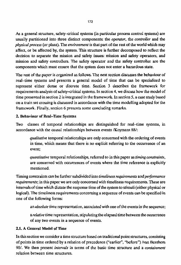
As a general structure, safety-critical systems (in particular process control systems) are

usually partitioned into three distinct components: the operator, the controller and the

physicalprocess (or plant). The environment is that part of the rest of the world which may

affect, or be affected by, the system. This structure is further decomposed to reflect the decision to separate the mission and safety issues: mission and safety operators, and mission and safety controllers. The safety operator and the safety controller are the

components which must ensure that the system does not enter a hazardous state.

The rest of the paper is organized as follows. The next section discusses the behaviour of

real-time systems and presents a general model of time that can be specialized to

represent either dense or discrete time. Section 3 describes the framework for

requirements analysis of safety-critical systems. In section 4, we discuss how the model of time presented in section 2 is integrated in the framework. In section 5, a case study based on a train set crossing is discussed in accordance with the time modelling adopted for the framework. Finally, section 6 presents some concluding remarks.

2. Behaviour of Real-Time Systems

Two classes of temporal relationships are distinguished for real-time systems, in

accordance with the causal relationships between events/Koymans 88/:

qualitative temporal relationships are only concerned with the ordering of events in time, which means that there is no explicit referring to the occurrence of an

event;

quantitative temporal relationships, referred to in this paper as timing constraints, are concerned with occurrences of events where the time reference is explicitly

mentioned.

Timing constraints can be further subdivided into timeliness requirements and performance requirements; in this paper we are only concerned with timeliness requirements. These are intervals of time which dictate the response time of the system to stimuli (either physical or logical). The timeliness requirements concerning a sequence of events can be specified in

one of the following forms:

an absolute time representation, associated with one of the events in the sequence;

a relative time representation, stipulating the elapsed time between the occurrence of any two events in a sequence of events.

2.1. A General Model of Time

In this section we consider a time structure based on traditional point structures, consisting

of points in time ordered by a relation of precedence ("earlier", "before")/van Benthem

90/. We then present intervals in terms of the basic time structure and a containment relation between time structures.

173

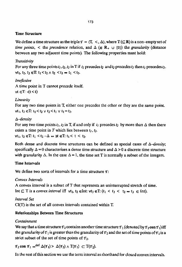
Time Structure

We define a time structure as the triple ~" = (T, < , A), where T ( ~ R) is a non-empty set of

time points, < the precedence relation, and A (E R+ u {0}) the granularity (distance

between any two adjacent time points). The following propert ies must hold:

Transitivity For any three time points tl, t2, t3 in T if tl precedes t2 and t2 precedes t3 then tl precedes 0.

v tb t2, t3 ET:. tl < t2 A t2 < t3 ~* tl < t3.

Irreflexive A time point in T cannot precede itself.

vt ~T: .(t < t)

Linearity For any two time points in T, either one precedes the other or they are the same point.

~1, t2 ET: tl < t2 v t2 < t~ v tl = t2.

A--density For any two time points tl, tz in T, if and only if tl precedes t2 by more than A then there

exists a time point in T which lies between tl, tz. vq, t2 ~T: tt < t 2 - A ,~ at ~T: q < t < t2.

Both dense and discrete time structures can be defined as special cases of A-density; specifically A = 0 characterizes a dense time structure and A > 0 a discrete time structure

with granularity A. In the case A = 1, the time set T is normally a subset of the integers.

Time Intervals

We define two sorts of intervals for a time structure ~r:

Convex Intervals A convex interval is a subset of T that represents an uninterrupted stretch of time.

I n t c T is a convex interval iff vq, t2 ~Int: vt3 ~ . (q < t3 < t2 =, t3 ~ Int).

Interval Set CI(T) is the set of all convex intervals contained within T.

Relationships Between Time Structures

Containment We say that a time structure ~'2 contains another time structure ~'1 (denoted by ~r2 con ~'1) iff

the granularity ofg'l is greater than the granularity of~'2 and the set of time points ofg' l is a strict subset of the set of time points of ~'2-

K2 con 9"1 ~=~def A(ff.X) > A(ff.2) A T(~'I) C T(ff'2).

In the rest of this section we use the term interval as shorthand for closed convex intervals.

174

2.2. An Event/Action Model

From the general model of time defined in the previous section we introduce the concept

of a "timeline", a line marked with the time points ofT, for which consecutive time points are separated by a distance A.

In order to capture temporal ordering we introduce an e v e n t / a c t i o n model based on a

timeline, as defined in/MacEwen 88, PDCS 90/.

A n e v e n t is a temporal marker of no duration, represented as a cut in the timeline

(i.e. an element of T); the time period between two events is a bounded interval

(i.e. an element of CI(T)); a d u r a t i o n is a measure of the length of a bounded

interval (i.e. the distance between the events that mark the boundaries of the interval).

A n a c t i o n is a basic unit of activity which implies a duration in its execution; it is

manifested in the system by its associated set of events: a s tar t e v e n t marks the

initiation of an action, and a f i n i s h e v e n t marks the completion of an action. The

period of the execution of an action is represented as a bounded interval.

Remark: if time structure ~'2 contains time structure g'l, an event observed in ~'1 at time

point t may be an action when observed in ~2 that occurs during a convex interval that is a subset of the interval [t + A(g'l), t -A(~'2)].

A relative time representation of the timeliness requirements of a sequence of events can

impose one of three basic types of timing relations/Dasarathy 85/:

m i n i m u m - no less than t time units must elapse between the occurrence of two events;

m a x i m u m - no more than t time units must elapse between the occurrence of two

events;

d u r a t i o n a l - exactly t time units must elapse between two events.

2.3. Specification of Timeliness Requirements

Here we show how timeliness requirements will be expressed at different levels of

abstraction in the analysis of the safety requirements.

At the highest level of abstraction we introduce an "event-occurrence function" E(t),

which maps the timeline into the occurrence of events. The timing constraints imposed on

the occurrence of one or more events may also be specified in order to consider time

uncertainties, which may be expressed through the timing relations previously introduced. Assuming T to be the set of all points in the timeline and t e the time point at which the event

occurs, the event-occurrence function is formalised as follows:

E(t): T ~ {O,e}

E(t) = 0 vt:t -# t e

E(t) = e vt:t = t e.

175

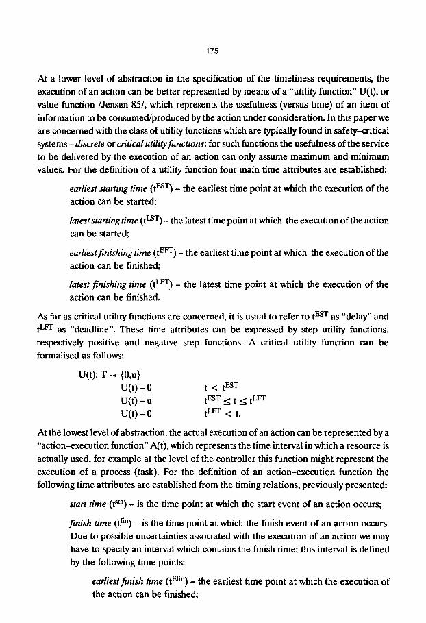
At a lower level of abstraction in the specification of the timeliness requirements, the

execution of an action can be better represented by means of a "utility function" U(t), or

value function/Jensen 85/, which represents the usefulness (versus time) of an item of

information to be consumed/produced by the action under consideration. In this paper we

are concerned with the class of utility functions which are typically found in safety-critical

systems - discrete or critical utility functions: for such functions the usefulness of the service

to be delivered by the execution of an action can only assume maximum and minimum

values. For the definition of a utility function four main time attributes are established:

earliest starting time (t EsT) - the earliest time point at which the execution of the

action can be started;

latest starting time (t LsT) - the latest time point at which the execution of the action

can be started;

earliest finishing time (t EFt) - the earliest time point at which the execution of the

action can be finished;

latest `finishing time (t LFr) - the latest time point at which the execution of the

action can be finished.

As far as critical utility functions are concerned, it is usual to refer to t EsT as "delay" and

t LvT as "deadline". These time attributes can be expressed by step utility functions,

respectively positive and negative step

formalised as follows:

functions. A critical utility function can be

U(t): T ~ (0,u} U( t )=0 t < t EsT U(t)- -u t EsT < t < t LFr

U(t) = 0 t Lv-T < t.

At the lowest level of abstraction, the actual execution of an action can be represented by a

"action-execution function" A(t), which represents the time interval in which a resource is

actually used, for example at the level of the controller this function might represent the

execution of a process (task). For the definition of an action-execution function the

following time attributes are established from the timing relations, previously presented:

start time (t sta) - is the time point at which the start event of an action occurs;

`finish time (t fin) - is the time point at which the finish event of an action occurs.

Due to possible uncertainties associated with the execution of an action we may

have to specify an interval which contains the finish time; this interval is defined

by the following time points:

earliest`finish time (tEnn) - the earliest time point at which the execution of

the action can be finished;

176

latest finish time (t Lfin) - the latest time point at which the execution of the

action can be finished;

execution time (t ext) - is the duration of the interval during which the action is

executed.

An action-execution function may be formalised as follows:

A(t): X ~ {O,a} A(t) = 0 t < t sta A(t) = a tsta _< t < t fin

A(t) = 0 t fin > t.

The action-execution function is used to define the timeliness requirements of a utility

function whenever the duration of the action is known a priori; if no information is available some estimates must be made. The value of t LsT and t EFt, defined for an utility

function, may be used to simulate the detection of errors in the execution of an action;

hence, the value of t LST should be related to the maximum duration in the execution of the action, and the t EFT tO its minimum duration.

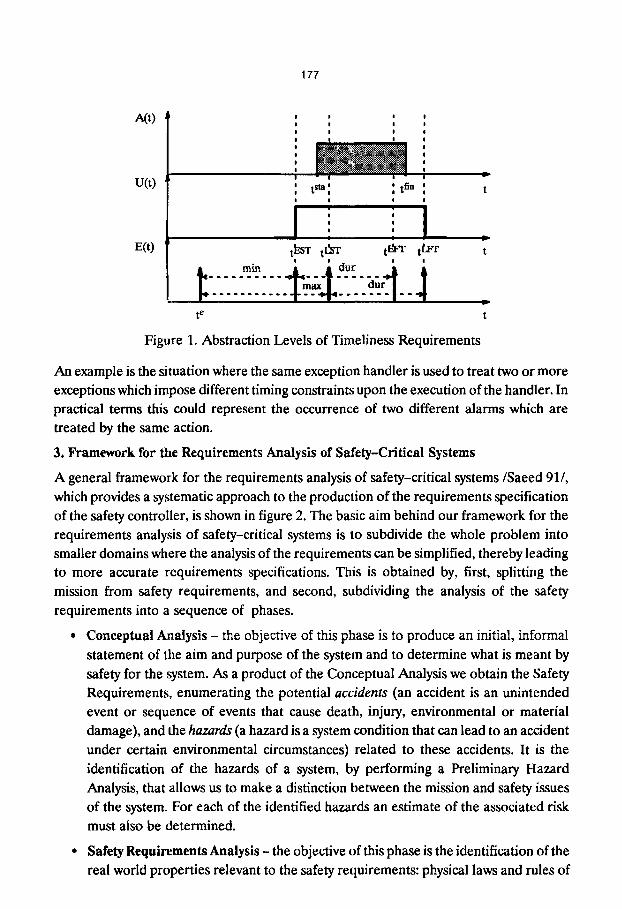
In the following, we present an example, illustrated in figure 1, which shows how the

functions defined above are interrelated in the specification of the timeliness requirements

at different levels of abstraction. The initial step in the specification of the timeliness

requirements for a particular activity is to consider the time points associated with the

occurrence of events in the execution of an action or sequence of actions; this includes

possible time uncertainties which are shown in the figure as timing relations imposed on

the event t e. The utility function is defined in terms of the time points established before,

eliminating some of the time uncertainties of the previous step. Finally, the actual

execution of the action is represented by the function A(t), and must be performed within

the timing constraints imposed by the utility function.

If an action has two or more utility functions imposed on it then, for the execution of that

action to be useful, it must comply with all the imposed utility functions. Below we present

a lemma which allows us to define a utility function which represents the superposition of more than one utility function on an action.

Lemma 1

When two or more utility functions, representing the usefulness in executing the same

action, are superimposed, the resulting utility function imposes the following timing constraints at the start time and finish time of an action:

t sta ~ (t [ max(tl EsT ..... tn EST) < t < min(h LsT ..... tnLST)};

t an ~ {t I max(h Err ..... tn Err) < t < min(h Lrr .... , tnLFa')}.

Proof. Immediate.

177

A(t)

U(t )

E( t )

p i I !

p I I I

pta', : din ! !

o ! q ! e !

t ~ r tt~r t ~ ' r t LFr t I ! i i

min dur

t e t

t

Figure 1. Abstraction Levels of Timeliness Requirements

An example is the situation where the same exception handler is used to treat two or more exceptions which impose different timing constraints upon the execution of the handler. In practical terms this could represent the occurrence of two different alarms which are treated by the same action.

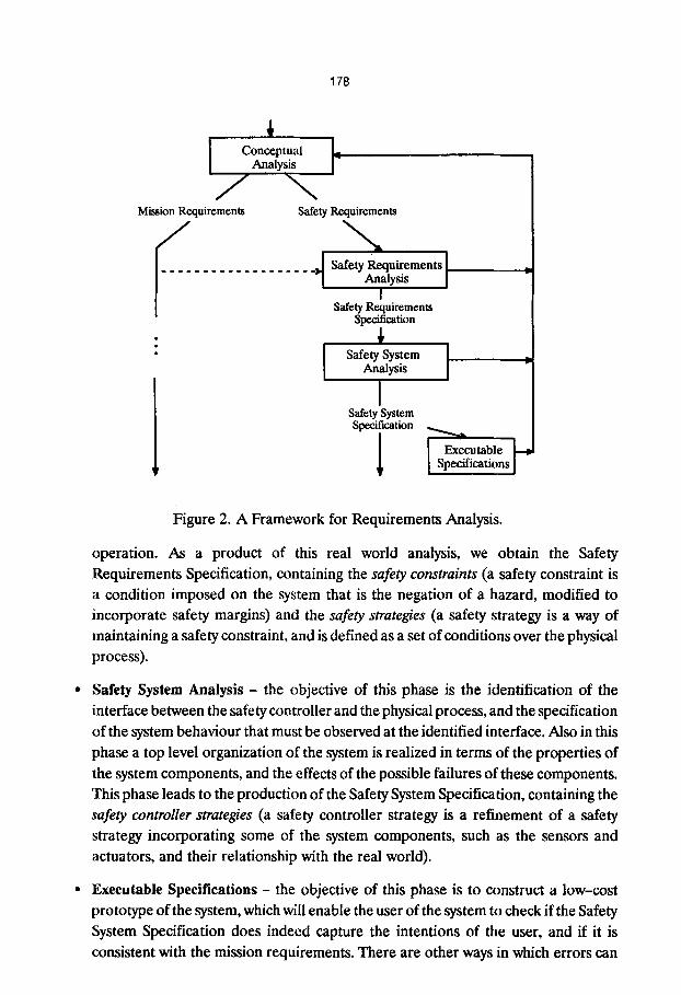
3. Framework for the Requirements Analysis of Safety-Critical Systems

A general framework for the requirements analysis of safety-critical systems/Saeed 91/, which provides a systematic approach to the production of the requirements specification of the safety controller, is shown in figure 2. The basic aim behind our framework for the requirements analysis of safety-critical systems is to subdivide the whole problem into smaller domains where the analysis of the requirements can be simplified, thereby leading to more accurate requirements specifications. This is obtained by, first, splitting the mission from safety requirements, and second, subdividing the analysis of the safety requirements into a sequence of phases.

�9 Conceptual Analysis - the objective of this phase is to produce an initial, informal statement of the aim and purpose of the system and to determine what is meant by safety for the system. As a product of the Conceptual Analysis we obtain the Safety Requirements, enumerating the potential accidents (an accident is an unintended event or sequence of events that cause death, injury, environmental or material damage), and the hazards (a hazard is a system condition that can lead to an accident under certain environmental circumstances) related to these accidents. It is the identification of the hazards of a system, by performing a Preliminary Hazard Analysis, that allows us to make a distinction between the mission and safety issues of the system. For each of the identified hazards an estimate of the associated risk must also be determined.

�9 Safety Requirements Analysis - the objective of this phase is the identification of the real world properties relevant to the safety requirements: physical laws and rules of

178

r Conceptual

Mission Requirements Safety Requirements

. . . . . . . . . . . . . . . ~ Safety Requirements ]

\

,1, / Safety System i _l

Safety System / Specification ~ [

i I Executable~ -r r i Specifications ]

Figure 2. A Framework for Requirements Analysis.

operation. As a product of this real world analysis, we obtain the Safety Requirements Specification, containing the safety constraints (a safety constraint is a condition imposed on the system that is the negation of a hazard, modified to incorporate safety margins) and the safety strategies (a safety strategy is a way of maintaining a safety constraint, and is defined as a set of conditions over the physical process).

Safety System Analysis - the objective of this phase is the identification of the interface between the safety controller and the physical process, and the specification of the system behaviour that must be observed at the identified interface. Also in this phase a top level organization of the system is realized in terms of the properties of the system components, and the effects of the possible failures of these components. This phase leads to the production of the Safety System Specification, containing the safety controller strategies (a safety controller strategy is a refinement of a safety strategy incorporating some of the system components, such as the sensors and actuators, and their relationship with the real world).

Executable Specifications - the objective of this phase is to construct a low-cost prototype of the system, which will enable the user of the system to check if the Safety System Specification does indeed capture the intentions of the user, and if it is consistent with the mission requirements. There are other ways in which errors can

179

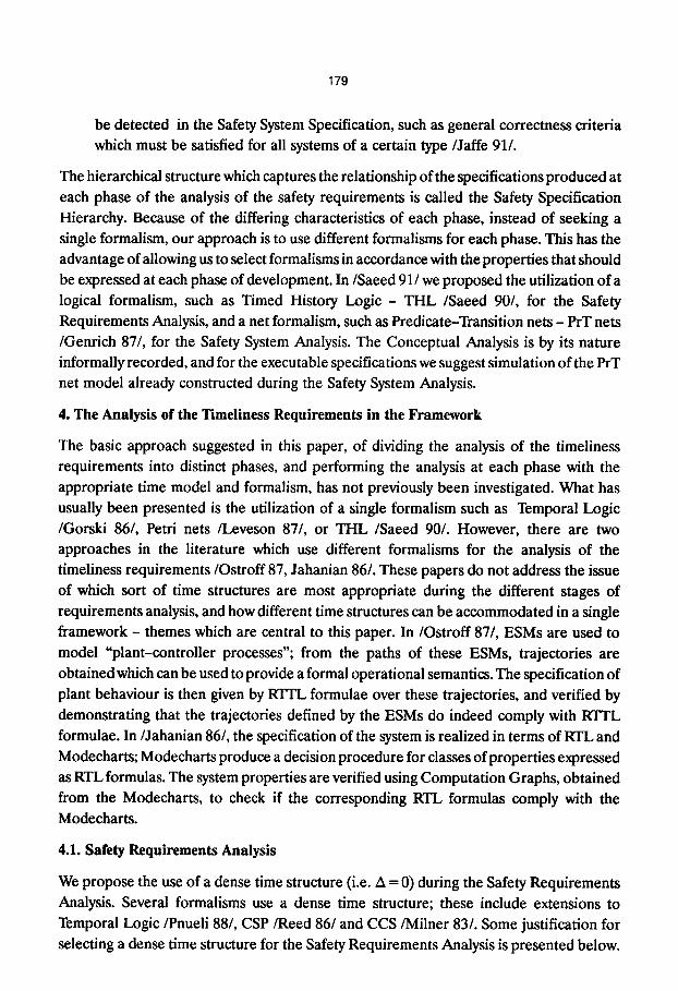
be detected in the Safety System Specification, such as general correctness criteria which must be satisfied for all systems of a certain type/Jaffe 91/.

The hierarchical structure which captures the relationship of the specifications produced at each phase of the analysis of the safety requirements is called the Safety Specification Hierarchy. Because of the differing characteristics of each phase, instead of seeking a single formalism, our approach is to use different formalisms for each phase. This has the advantage of allowing us to select formalisms in accordance with the properties that should be expressed at each phase of development. In/Saeed 91/we proposed the utilization of a logical formalism, such as Timed History Logic - THL /Saeed 90/, for the Safety Requirements Analysis, and a net formalism, such as Predicate-Transition nets - PrT nets /Genrich 87/, for the Safety System Analysis. The Conceptual Analysis is by its nature informally recorded, and for the executable specifications we suggest simulation of the PrT net model already constructed during the Safety System Analysis.

4. The Analysis of the Timeliness Requirements in the Framework

The basic approach suggested in this paper, of dividing the analysis of the timeliness requirements into distinct phases, and performing the analysis at each phase with the appropriate time model and formalism, has not previously been investigated. What has usually been presented is the utilization of a single formalism such as Temporal Logic /Gorski 86/, Petri nets /Leveson 87/, or THL /Saeed 90/. However, there are two approaches in the literature which use different formalisms for the analysis of the timeliness requirements/Ostroff 87, Jahanian 86/. These papers do not address the issue of which sort of time structures are most appropriate during the different stages of requirements analysis, and how different time structures can be accommodated in a single framework - themes which are central to this paper. In/Ostroff 87/, ESMs are used to model "plant-controller processes"; from the paths of these ESMs, trajectories are obtained which can be used to provide a formal operational semantics. The specification of plant behaviour is then given by RTIL formulae over these trajectories, and verified by demonstrating that the trajectories defined by the ESMs do indeed comply with RqTL formulae. In/Jahanian 86/, the specification of the system is realized in terms of RTL and Modecharts; Modecharts produce a decision procedure for classes of properties expressed as RTL formulas. The system properties are verified using Computation Graphs, obtained from the Modecharts, to check if the corresponding RTL formulas comply with the Modecharts.

4.1. Safety Requirements Analysis

We propose the use of a dense time structure (i.e. A -- 0) during the Safety Requirements Analysis. Several formalisms use a dense time structure; these include extensions to Temporal Logic/Pnueli 88/, CSP/Reed 86/and CCS/Milner 83/. Some justification for selecting a dense time structure for the Safety Requirements Analysis is presented below.

180

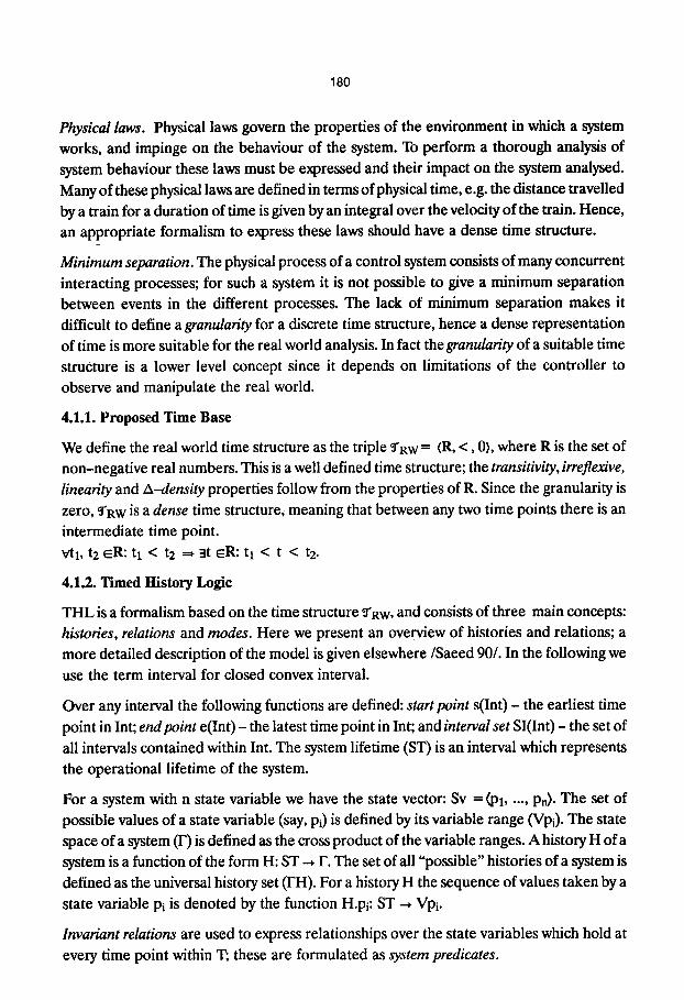
Physical laws. Physical laws govern the properties of the environment in which a system

works, and impinge on the behaviour of the system. To perform a thorough analysis of

system behaviour these laws must be expressed and their impact on the system analysed.

Many of these physical laws are defined in terms of physical time, e.g. the distance travelled

by a train for a duration of time is given by an integral over the velocity of the train. Hence,

an appropriate formalism to express these laws should have a dense time structure.

Minimum separation. The physical process of a control system consists of many concurrent

interacting processes; for such a system it is not possible to give a minimum separation

between events in the different processes. The lack of minimum separation makes it

difficult to define a granularity for a discrete time structure, hence a dense representation

of time is more suitable for the real world analysis. In fact the granularity of a suitable time

structure is a lower level concept since it depends on limitations of the controller to

observe and manipulate the real world.

4.1.1. Proposed Time Base

We define the real world time structure as the triple ~rRW = (R, < , 0), where R is the set of

non-negative real numbers. This is a well defined time structure; the transitivity, irreflexive, linearity and A--density properties follow from the properties of R. Since the granularity is

zero, ~'RW is a dense time structure, meaning that between any two time points there is an

intermediate time point.

Vtl, t2 ER: tl < t2 =* 3t ~R: tl < t < t2.

4.1.2. Timed History Logic

THL is a formalism based on the time structure ~'aw, and consists of three main concepts:

histories, relations and modes. Here we present an overview of histories and relations; a

more detailed description of the model is given elsewhere/Saeed 90/. In the following we

use the term interval for closed convex interval.

Over any interval the following functions are defined: start point s(Int) - the earliest time

point in Int; endpoint e(Int) - the latest time point in Int; and interval set SI(Int) - the set of

all intervals contained within Int. The system lifetime (ST) is an interval which represents

the operational lifetime of the system.

For a system with n state variable we have the state vector: Sv = (Pl ..... Pn). The set of

possible values of a state variable (say, Pi) is defined by its variable range (Vpi). The state

space of a system (F) is defined as the cross product of the variable ranges. A history H of a

system is a function of the form H: ST - , F. The set of all "possible" histories of a system is

defined as the universal history set (FH). For a history H the sequence of values taken by a

state variable Pi is denoted by the function H.pi: ST --, Vpi.

Invariant relations are used to express relationships over the state variables which hold at

every time point within T; these are formulated as system predicates.

181

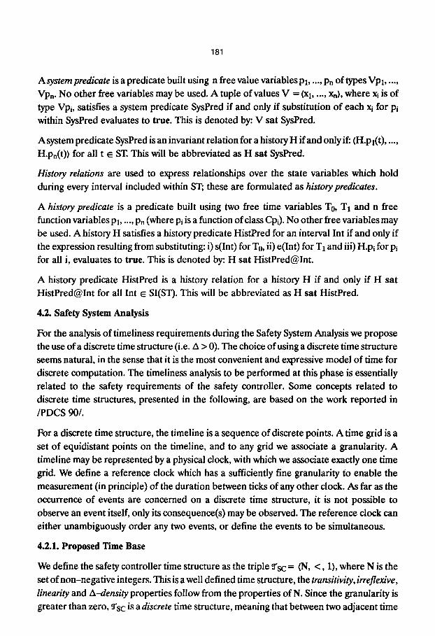
A system predicate is a predicate built using n free value variables Pl ..... Pn of types Vpl ..... Vpn. No other free variables may be used. A tuple of values V = (Xl ..... Xn), where xi is of

type Vpi, satisfies a system predicate SysPred if and only if substitution of each xi for Pi within SysPred evaluates to true. This is denoted by: V sat SysPred.

A system predicate SysPred is an invariant relation for a history H if and only if: (H.pl(t) .....

H.pn(t)) for all t ~ ST. This will be abbreviated as H sat SysPred.

History relations are used to express relationships over the state variables which hold

during every interval included within ST;, these are formulated as history predicates.

A history predicate is a predicate built using two free time variables To, T1 and n free function variables p: ..... Pn (where Pi is a function of class Cpi). No other free variables may be used. A history H satisfies a history predicate HistPred for an interval Int if and only if the expression resulting from substituting: i) s(Int) for To, ii) e(Int) for T1 and iii) H.pi for Pi for all i, evaluates to true. This is denoted by: H sat HistPred@Int.

A history predicate HistPred is a history relation for a history H if and only if H sat HistPred@Int for all Int ~ SI(ST). This will be abbreviated as H sat HistPred.

4.2. Safety System Analysis

For the analysis of timeliness requirements during the Safety System Analysis we propose the use of a discrete time structure (i.e. A > 0). The choice of using a discrete time structure

seems natural, in the sense that it is the most convenient and expressive model of time for discrete computation. The timeliness analysis to be performed at this phase is essentially

related to the safety requirements of the safety controller. Some concepts related to discrete time structures, presented in the following, are based on the work reported in

/PDCS 90/.

For a discrete time structure, the timeline is a sequence of discrete points. A time grid is a

set of equidistant points on the timeline, and to any grid we associate a granularity. A

timeline may be represented by a physical clock, with which we associate exactly one time grid. We define a reference clock which has a sufficiently fine granularity to enable the

measurement (in principle) of the duration between ticks of any other dock. As far as the occurrence of events are concerned on a discrete time structure, it is not possible to

observe an event itself, only its consequence(s) may be observed. The reference clock can

either unambiguously order any two events, or define the events to be simultaneous.

4.2.1. Proposed Time Base

We define the safety controller time structure as the triple ~'sc = (N, <, 1), where N is the

set of non-negative integers. This is a well defined time structure, the transitivity, irreflexive, linearity and A-density properties follow from the properties of N. Since the granularity is greater than zero, ~rsc is a discrete time structure, meaning that between two adjacent time

182

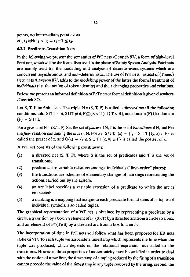
points, no intermediate point exists.

vtl, t2 ~N: tl < t2 ~ t l+ 1 ~ t2.

4.2.2. Predicate-Transition Nets

In the following we present the semantics of PrT nets/Genrich 87/, a form of high-level Petri net, which will be the formalism used in the phase of Safety System Analysis. Petri nets

are mainly used for the modelling and analysis of discrete-event systems which are

concurrent, asynchronous, and non-deterministic. The use of PrT nets, instead of (Timed)

Petri nets/Leveson 87/, adds to the modelling power of the latter the formal treatment of individuals (i.e. the notion of token identity) and their changing properties and relations.

Below, we present an informal definition of PrT nets; a formal definition is given elsewhere /Genrich 87/.

Let S, T, F be finite sets. The triple N = (S, T, F) is called a directed net iff the following

conditions hold: S n T = 0, S U T ~ 0, F ~ ( S x T) U ( T x S ), and domain (F) U codomain (F) = SUT.

For a given net N = (S, T, F), S is the set ofplaces of N, T is the set of transitions of N, and F is

theflow relation containing the arcs of N. For x ~ S U T, I(x) = { y ~ S U T I (Y, x) ~ F} is .called the preset of x, and O(x) = {y ~ S 0 T I (x, y) ~ F} is called the postset of x.

A PrT net consists of the following constituents:

(1) a directed net (S, T, F), where S is the set of predicates and T is the set of transitions;

(2) predicates are variable relations amongst individuals ("first-order" places);

(3) the transitions are schemes of elementary changes of markings representing the actions carried out by the system;

(4) an arc label specifies a variable extension of a predicate to which the arc is connected;

(5) a marking is a mapping that assigns to each predicate formal sums of n-tuples of individual symbols, also called tuples.

The graphical representation of a PrT net is obtained by representing a predicate by a

circle, a transition by a box, an element of FN(S xT) by a directed arc from a circle to a box,

and an element of Ff'I(TxS) by a directed arc from a box to a circle.

The incorporation of time in PrT nets will follow what has been proposed for ER nets

/Ghezzi 91/. To each tuple we associate a timestamp which represents the time when the

tuple was produced, which depends on the relational expression associated to the

transitions. However, three properties of monotonicity must be satisfied in order to deal

with the notion of time: first, the timestamp of a tuple produced by the firing of a transition

cannot precede the value of the timestamp in any tuple removed by the firing, second, the

183

firing time of a transition cannot precede the time of the previous firing of the same

transition, and third, for any firing sequence, the times of the firings should be

monotonically nondecreasing with respect to their occurrence in the sequence.

The basic timing relations associated to a PrT net transition, that we will be assuming, are

expressed as an interval [Tmin, Tmax] which represents, respectively, the minimum and maximum time delay that must elapse between the enabling of the transition and its firing time. Other timing relations which are not directly related to the timestamp of a tuple may

also be employed.

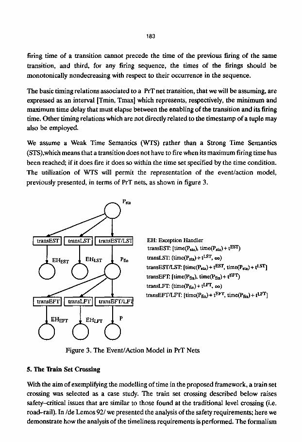
We assume a Weak Time Semantics (WTS) rather than a Strong Time Semantics

(STS),which means that a transition does not have to fire when its maximum firing time has

been reached; if it does fire it does so within the time set specified by the time condition.

The utilization of WTS will permit the representation of the event/action model,

previously presented, in terms of PrT nets, as shown in figure 3.

Psta

I transEST 11 transLSF [1 transEST/LSql ~ ~ Pfin

)

I tr nsEzrl I tr nsL ][ t nsE /I

EH: Exception Handler transES~. [time(Psta), time(Psta) + t EsT)

transl_,S~. (time(Psta) + t LsT oo)

transEST/LS'12. [time(Psta) + t EsT, time(Psta) + t LsT]

transEFE. [time(Pfin), time(Ptin) + t Err)

transLF12 (time(Pfin) + t l-Fr, oo) transEFT/LF12. [time(Ptin) + t EFr, time(Ptin) + t l-Fr]

Figure 3. The Event/Action Model in PrT Nets

5. The Train Set Crossing

With the aim of exemplifying the modelling of time in the proposed framework, a train set

crossing was selected as a case study. The train set crossing described below raises

safety-critical issues that are similar to those found at the traditional level crossing (i.e.

road-rail). In/de Lemos 92/we presented the analysis of the safety requirements; here we demonstrate how the analysis of the timeliness requirements is performed. The formalism

CC

employed for the Safety Requirements Analysis is THL/Saeed 90/, and the formalism employed for the Safety System Analysis is PrT nets/Genrich 87/.

Conceptual Analysis

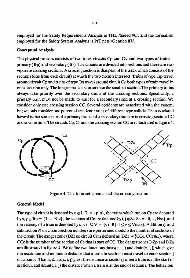
The physical process consists of two track circuits Cp and Cs, and two types of trains -

primary (Trp) and secondary (Trs). The circuits are divided into sections and there are two

separate crossing sections. A crossing section is that part of the track which consists of the sections (one from each circuit) at which the two circuits intersect. Trains of type Trp travel around circuit Cp and trains of type Trs travel around circuit Cs; both types of train travel in one direction only. The longest train is shorter than the smallest section. The primary trains always take priority over the secondary trains at the crossing sections. Specifically, a

primary train must not be made to wait for a secondary train at a crossing section. We consider only one crossing section CC. Several accidents are associated with the system, but we only consider one potential accident: trains of different type collide. The associated

hazard is that some part of a primary train and a secondary train are in crossing section CC at the same time. The circuits Cp, Cs and the crossing section CC are illustrated in figure 4.

Cs

O

184

Figure 4. The train set circuits and the crossing section

General Model

The type of circuit is denoted by c ~ L, L = {p, s}, the trains which run on Cc are denoted by x, y ~ Trc = { 1 ..... Ntc}, the sections of Cc are denoted by i, j ~ Sc, Sc = {0 ..... Nsc}, and

the velocity of a train is denoted by u, v ~ V, V = {v ~ R I 0 _< v < Vmax}. Addition ~ and subtraction O on circuit section numbers are performed modulo the number of sections of

the circuit. The danger zone (DZ) on circuit Cc is defined as: DZc -- {CCc, CCc~I }, where

CCc is the number of the section of Cc that is part of CC. The danger zones DZp and DZs are illustrated in figure 4. We define two functions dmax(c, i, j) and dmin(c, i, j) which give

the maximum and minimum distance that a train in section i must travel to enter section j

on circuit c. That is, dmax(c, i, j) gives the distance to section j when a train is at the start of section i, and dmin(c, i, j) the distance when a train is at the end of section i. The behaviour

185

of the system is captured by three state variables Ptrain, Rtrain and Vtrain (a continuous variable) described below.

NO.

Pl

P2

P3

Name Range

Ptrain Sp Ntp X Ss Nts

Rtrain Rp Nip X Rs Nts

Vtrain v(NtP +Nts)

Comments

The position of each train expressed as a section number, that is, the section containing the front of a train.

The reservation sets of the trains, where Re ffi ~(Sc).

The velocity of the trains.

Ptrain(c, x) denotes the state variable for the position of train x on circuit Cc, Rtrain(c, x) the reservation set of train x on circuit Co, and Vtrain(c, x) the velocity of train x on circuit Cc. FH is the set of all functions H: T--, Sl:~tPxSsNtSxRpNtPxRsN~xV(NtP+m'). A history from FH satisfies a requirements specification, if and only if the system (resp. history) predicates that describe it are invariant (resp. history) relations for that history.

5.1. Safety Requirements Analysis

The analysis performed in /de Lemos 92/ concentrated on the qualitative temporal relationships, here we are concerned with introducing the dimension of time and performing a quantitative temporal analysis.

Physical Law

In the following we present the law (as a history predicate) which captures the relationship between intervals, the velocity of trains, and the positions of trains.

Hrl - For any train, if during any interval [To, T1] the train travels more than the maximum distance between the section it occupies at To and section i, then the train must occupy section i at some time point in [To, Td; and if the train travels less than the minimum distance between the section it occupies at To and section i, then the train is never in section i during [To, T1].

vc eL: vx ~T~c: vi ~Sc: T 1

f Vtrain(c, x).dt _> dmax(c, Ptrain(c, x)(T0), i) at T1]: Ptrain(c, x)(t)=i A m~ E [To, r0

TI

I Vtrain(c, x).dt < dmin(c, Ptrain(c, x)(T0), i) vt T1]: Ptrain(c, x)(t)#i. [To, E

r0

It is vital that the above law is confirmed to be a property of the system, since during the subsequent analysis this law is treated as an axiom of the model. More precisely, henceforth we consider only those histories of FH for which Hrl is a history relation.

As a result of a qualitative analysis of the crossing section, the following safety constraint and safety strategy were derived.

Safety Constraint

186

Either the front of no primary train is in the danger zone DZp or the front of no secondary train is in the danger zone DZs, formalized as a system predicate:

3c E L: vx ~ Trc: Ptrain(c, x) ~ DZc.

Safety Strategy (without priority constrainO

The safety strategy is based on a reservation scheme. The two essential rules which impose

the safety strategy are as follows.

ssa. Reservation Constraint For any train the current section (i.e. the position of the train) and the section behind

the current section must always be reserved:

vc ~ L: vx ~ "It-c: {Ptrain(c, x )e l , Ptrain(c, x)} ~ Rtrain(c, x).

ssb. Exclusion Constraint Section CCp and section CCs cannot both be reserved at the same time:

~c ~ L: (vx ~ Trc: CCc ~ Rtrain(c, x)).

Although the safety strategy for the crossing section is sufficient to prevent collisions involving primary and secondary trains, it ignores the priority of primary trains over secondary trains. Here we consider how the introduction of time can be used to analyse the

priority constraint.

We recall the priority constraint, "a primary train must not be made to wait for a secondary train at a crossing section". By inspection of rule ssb, this can be stated in terms of the

reservation scheme as: the section CCs cannot be reserved by a secondary train, if any

primary train will need to reserve section CCp before the secondary train releases section CCs. From rule ssa we can infer that a secondary train can release section CCs when it

enters section CCs~2, and a primary train must reserve section CCp when it enters section

CCp. Hence a secondary train cannot reserve section CCs if a primary train may enter

section CCp before the secondary train will enter section CCs~2. To analyse this situation in the event/action model, we describe the utility functions UTrs(t) and UTrp(t) illustrated by

the graphs in figure 5, these graphs depict the case when a secondary train does not stop

when approaching DZs and the case when a secondary train must stop.

Events: - EN, marks the time when a secondary train starts to approach DZs.

Actions: - APe, a train of type Trc approaching the danger zone DZc, after a secondary train enters

CCSo1. - CZc, a train of type Trc crossing danger zone DZc.

For simplicity, we assume that the velocity of a moving train x on circuit Cc near to the

crossing section, remains constant and at the value given by the function V(c, x) or is zero.

187

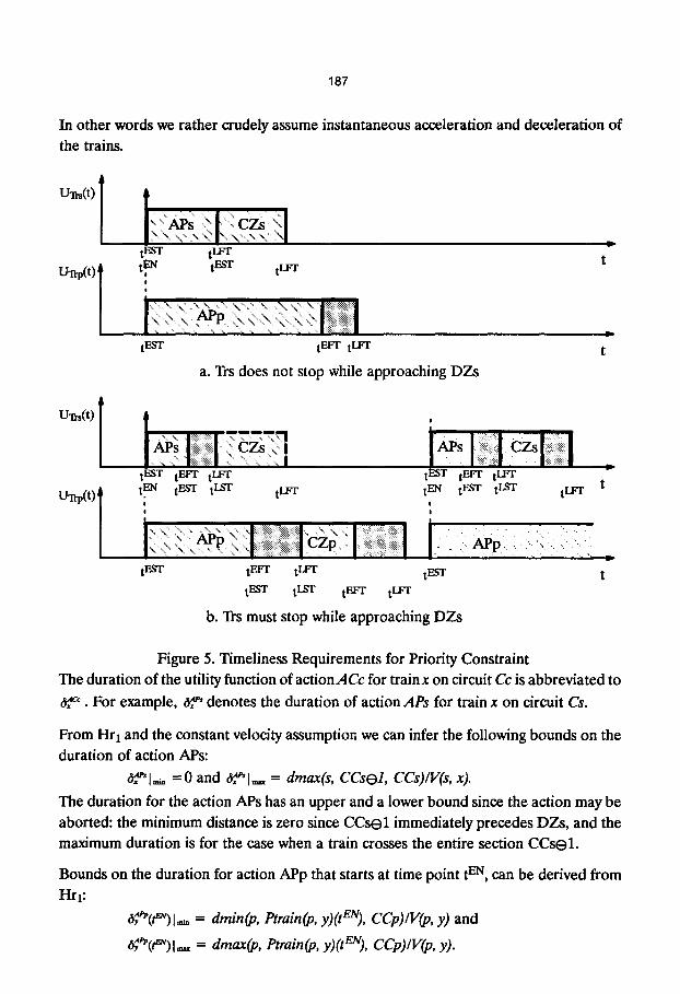
In other words we rather crudely assume instantaneous acceleration and deceleration of the trains.

U'il-s(t)

UTrp(t) l

tEST tLFT t: EN t F-~T tLFF

tEST tEFT tLFr

a. Trs does not stop while approaching DZs

t

t

u~(t)

Ua'rp(t) l

t.~ST tEFT tLFs t EN tEST tINT tl.~-

I ! |

tEST tEFT tLFr

tEST tLST tEFr tLF1 "

I

ps H ::!!iiiii'i~:iiiiiii : :iiiiii!iiiiiiiiiii: ' " I t

tEST tEFF tLFT t tEN tEST tLST tLFr

I

J

t F-~r t

b. Trs must stop while approaching DZs

Figure 5. Timeliness Requirements for Priority Constraint The duration of the utility function of actionACc for train x on circuit Cc is abbreviated to

~c,. For example, ~ ' denotes the duration of action APs for train x on circuit Cs.

From Hrl and the constant velocity assumption we can infer the following bounds on the duration of action APs:

�9 ~* ' lu =0 and ~ ' l ~ = dmax(s, CCse l , CCs)/V(s, x).

The duration for the action APs has an upper and a lower bound since the action may be aborted: the minimum distance is zero since CCsel immediately precedes DZs, and the maximum duration is for the case when a train crosses the entire section CCsel .

Bounds on the duration for action APp that starts at time point t EN, can be derived from Hq:

~fP(t~)lm = drain(p, etrain(p, y)(tEN), CCp)/V(p, y) and

6y~*P(t~)l~ = dmax(p, Ptrain(p, y)(tEN), CCp)/V(p, )1).

188

The duration for the action APp has an upper and a lower bound since the controller knows

that the train is somewhere in section Ptrain(p, y), but does not know exactly where.

Similarly, we can infer the following bounds on the duration of action CZe:

6 cz~ = dmax(c, CCc, CCc~2)/V(c, x).

There are no uncertainties, for the action CZs, since a train always passes a fixed distant at

a constant velocity.

If we consider the behaviour of a secondary train x that is approaching the danger zone

DZs with respect to a primary train y, we observe that train x may cross the danger zone DZs if it will cross DZs before trainy reaches DZp, which can be expressed in terms of the

durations of the actions:

�9 ~ ' 1 ~ + 6~ z" < ~,~PI-,-.

Now, consider the behaviour of a secondary train x that is approaching the danger zone DZs with respect to a sequence of primary trains approaching the danger zone DZp. We observe that trainx may start to cross danger zone DZs only if it will cross DZs before the "nearest primary train" (i.e. the primary train which must pass the Smallest number of

sections to enter DZp) enters DZp. This can be expressed in terms of the durations of the actions: vy ~ Trp:

~ ' 1 ~ + ~z' < ~P(~ ' ) I . - .

We specify the priority constraint as a history predicate that describes the conditions in which a secondary train cannot reserve the section CCs; we say that a history satisfies the

priority constraint if the history predicate that describes it is a history relation. To complete the safety strategy for the crossing section we must add the priority constraint (rule ssc) to the rules ssa and ssb.

ssc. Priority Constraint

For any interval [To, T:], for any secondary train x, if CCs is not reserved byx at To and during [To, TI] the maximum duration for all parts of train x to pass the danger

zone DZs from section CCso1 (when it is moving) is at least the minimum duration

for a primary train y to approach the danger zone DZp or the current section is not CCso1, then the section CCs cannot be reserved by secondary trainx during [To, T1].

vx ~ Trs: [ CCs ~ Rtrain(s, x)(T0) ^

vt ~ [To, T1]: 3y ~ Trp: ~o~1~ + ~cz, > t~p(t)lm V Ptrain(s, x)~ CCso1

=, vt ~ [To, T1]: CCs ~ Rtrain(s, x)(t)].

5.2. Safety System Analysis

In the previous phase of the requirements analysis, the event/action model was employed

with the aim to understand the temporal behaviour of the physical process, in terms of

quantitative relationships, and to identify those timing constraints, or "thresholds", which

189

will be part of the safety strategy. In this phase of the analysis, we investigate how the safety

strategy is to be implemented by the safety controller as safety controller strategy; or

alternatively, the safety strategies must be mapped onto a set of sensors and actuators. The

event/action model, at this stage, considers the timing uncertainties related to the

components of the safety controller, and those that arise from the sensors and actuators.

Safety Controller Strategy

The safety controller strategy must maintain the three rules of safety strategy: rules ssa and ssb which say that any part of a primary and a secondary train cannot be at their respective danger zones, at the same time, and rule ssc which says that a primary train must not be

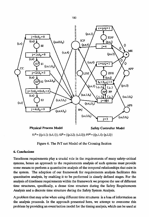
made to wait for a secondary train at a crossing section. The PrT net model of the physical process and the safety controller which implements the rules mentioned above is shown in

figure 6, to specify the timing properties we use: 8s = ~o~*1~ + ~cz, and 8p = 6~'~(t)lm �9

From the net model we noticed that, a primary train is never made to wait for a secondary

train if the time uncertainties of key actions remain within known bounds: minimum time for a primary train to approach the crossing section, the maximum time for a secondary

train to approach the crossing section, and the time it takes for a secondary train to cross the danger zone. Whenever the time uncertainties of one of the key actions are no longer in the known bounds the access to the crossing section is imposed by the mutual exclusion technique, which ignores the priority contraint.

The predicates of the PrT net model of the crossing section are the following:

S0cx, Slcx, S2cx, S3cx - a section of the circuit c is occupied by train x;

CCcx - the crossing section of circuit c is occupied by train x;

ICPcxj - train x in circuit c is allowed to enter section j (= 4, the crossing section);

IPCcxj8e - train x in circuit c has entered section j;

APPpxj - train x in circuit p is in section j = 3, (i.e. x is about to enter DZ);

APSsxjSs- train x in circuit s is in section j = 3, (i.e. x is about to enter DZ), and the actions

approach and crossing danger zone will take 8s;

ZDPpxj -train x in circuit p has access to section j (-- 4, the crossing section);

ZDSsxj -train x in circuit s has access to section j ( - 4, the crossing section);

ME - either primary or secondary trains allowed to enter the crossing section

LDZpxj - the primary train has left the danger zone;

PPpxiSp - train x in circuit p is in section j and the approach action will take 8p.

Further refinements in the PrT net model of the safety controller will consist of introducing

the timing constraints imposed on the exchange of information between the physical

process and the safety controller. We consider, for instance, the introduction of sensors and

actuators, and the estimated execution time of the safety controller actions that are part of the control loop.

190

l j=0ASc~ p= c (c~) ( SO

j = 1ASp = I (c~

j=2ASp=:

(c,x)+ S2

j=3ASp=0A8

(c,x) (c,x)(~ S3

j = 4ABp = (

[E

PP

'S

Physical Process Model Safety Controller Model

S10= {(p,l,1); (s,l,1)}; $2 0= {(p,2,2); (s,2,2)}; ppO= {(p,l,1); ~,2,2)}

Figure 6. The PrT net Model of the Crossing Section

6. Conclusions

Timeliness requirements play a crucial role in the requirements of many safety-critical systems, hence an approach to the requirements analysis of such systems must provide some means to perform a quantitative analysis of the temporal relationships that exist in the system. The adoption of our framework for requirements analysis facilitates this quantitative analysis, by enabling it to be performed in dearly defined stages. For the analysis of timeliness requirements within the framework we propose the use of different time structures, specifically, a dense time structure during the Safety Requirements Analysis and a discrete time structure during the Safety System Analysis.

A problem that may arise when using different time structures is a loss of information as the analysis proceeds. In the approach presented here, we attempt to overcome this problem by providing an event/action model for the timing analysis, which can be used at

191

the different stages. This model enables a link to be established between the timing constraints specified during the different stages. The practical utility of this approach was illustrated by performing the analysis of the timeliness requirements of a train set crossing section.

Acknowledgements

The authors would like to acknowledge the financial support of BAe (DCSC), CAPES/Brazil, and the ESPRIT Basic Research Action PDCS.

References

/Dasarathy 85/B. Dasarathy. "Timing Constraints of Real-Time Systems: Constructs for Expressing them, Methods of Validating them". IEEE Transactions on Software Engineering Vol. SE-11(1). January, 1985. pp 80-86.

/de Lemos 92/R. de Lemos, A. Saeed, T. Anderson. ' ~ Train set as a Case Study for the Requirements Analysis of Safety-Critical Systems". The Computer Journal. February 1992 (to appear).

/Genrich 87/H. Genrich. "Predicate/3a'ansition Nets". Petri Nets: Central Models and their Properties. Eds" W. Brauer, W. Reisig, G. Rozemberg. Lectures Notes in Computer Science Vol. 254. 1987. pp 206-247.

/Ghezzi 91/C. Ghezzi, D. Mandrioli, S. Morasca, M. Pezz6. '~ Unified High-Level Petri Net Formalism for Time-Critical Systems". IEEE Transactions on Software Engineering Vol. SE-17(2). February, 1991. pp 160--172.

/Gorski 86/J. Gorski. "Design for Safety using Temporal Logic". SAFECOMP'86. Sarlat, France. October, 1986. pp 149-155.

/Jaffe 91/M. S. Jaffe, N. G. Leveson, M. P. E. Hiemdahl, B. E. Melhart. "Software Requirements Analysis for Real-Time Process-Control Systems". IEEE Transactions on Software Engineering, Vol SE-17 (3). March 1991. pp 241-258.

/Jahanian 88/E Jahanian, D. A. Stuart. ' ~ Method for Verifying Properties of Modechart Specifications". Proceedings of the Real-Time Systems Symposium 1988. Huntsville, AL. December, 1988. pp 12-21.

/Jensen 85/E. Jensen, D. Locke, H. Tokuda. '~ Time-Driven Scheduling Model for Real-Time Operating Systems". Proceedings of the Real-Time Systems Symposium 1985. San Diego, CA. December, 1985. pp 112-122.

/Koymans 88/R. Koymans, R. Kuiper, E. Zijlstra. "Paradigms for Real-Time Systems". Proceedings of the Symposium in Formal Techniques in Real-Time and Fault-Tolerant Systems. LNCS 331. Springer-Verlag. M. Joseph (Ed.). Warwick, UK. September, 1988. pp 159-174.

192

/Laprie 90/J.C. Laprie. "Dependability: Basic Concepts and Associated Terminology". ESPRIT PDCS Report No 31. 1990.

/Laprie 91/J.-C. Laprie, B. Litflewood. "Quantitative Assessement of Safety-Critical Software: Why and How?". Probabilistic Safety Assessment and Management Conference. Beverly Hills, CA. February, 1991.

/Leveson 87/ N. G. Leveson, J. Stolzy. "Safety Analysis Using Petri Nets". IEEE Transactions on Software Engineering Vol. SE-13(3). March, 1987. pp 386-397.

/Leveson 91/ N. G. Leveson. "Software Safety in Embedded Computer Systems". Communications of the ACM, Vol 34 (2). February, 1991. pp 34-46.

/MacEwen 88/ G. MacEwen, D. Skillicorn. "Using High-Order Logic for Modular Specifications of Real-Time Distributed Systems". Proceedings of the Symposium in Formal Techniques in Real-Time and Fault-Tolerant Systems. LNCS 331. M. Joseph (Ed.). Warwick, UK. September, 1988. pp 36-66.

/Milner 83/R. Milner, "Calculi for Synchrony and Asynchrony". Theoretical Computer Science Vol. 25. 1983. pp 267-310.

/Ostroff 87/ J. S. Ostroff, W. M. Wonham. "Modelling, Specifying and Verifying Real-Time Embedded Computer Systems". Proceedings of the Real-Time Systems Symposium 1987. San Jose, CA. December 1987. pp 124-132.

/PDCS 90/"Real-Time Systems (Specific Closed Workshop)". ESPRIT PDCS Workshop Report W6. London, UK. September, 1990.

/Pnueli 88/A. Pnueli, E. Harel, '~,pplications of Temporal Logic to the Specification of Real Time Systems". Proceedings of the Symposium in Formal Techniques in Real-Time and Fault-Tolerant Systems. LNCS 331. Springer-Verlag. M. Joseph (Ed.). Warwick, UK. September, 1988. pp. 84- 97.

/Reed 86/G. M. Reed, A.W. Roscoe, '~ timed model for communicating sequential processes". Proceedings of 13th International Colloquium on Automata, Languages and Programming. LNCS 226. Springer-Verlag. Laurent Kott (Ed.). Rennes, France. July, 1986. pp 314-323.

/Saeed 90/A. Saeed, T. Anderson, M. Koutny. '~. Formal Model for Safety-Critical Computing Systems". SAFECOMP'90. London, UK. October, 1990. pp 1-6.

/Saeed 91/A. Saeed, R. de Lemos, T. Anderson. "The Role of Formal Methods in the Requirements Analysis of Safety-Critical Systems: a Train Set Example". Proceedings of the 21st Symposium on Fault-Tolerant Computing. Montreal, Canada. June, 1991. pp 478-485.

/van Benthem 90/J. van Benthem. "The Logic of Time". Kluwer Academic Publishers. 1991.