Fast Scheduling of Distributable Real-Time Threads with AssuredEnd-to-End Timeliness

Sherif F. Fahmy1, Binoy Ravindran1, and E. D. Jensen2

1 ECE Dept., Virginia Tech, Blacksburg, VA 24061, USA2 The MITRE Corporation, Bedford, MA 01730, USA

Abstract. We consider networked, embedded real-time systems that operate under run-time uncertaintieson activity execution times and arrivals, node failures, and message losses. We consider the distributablethreads abstraction for programming and scheduling such systems, and present a thread scheduling algo-rithm called QBUA. We show that QBUA satisfies (end-to-end) thread time constraints in the presenceof crash failures and message losses, has efficient message and time complexities, and lower overhead andsuperior timeliness properties than past thread scheduling algorithms. Our experimental studies validateour theoretical results, and illustrate the algorithm’s effectiveness.

1 Introduction

In distributed systems, action and information timeliness is often end-to-end—e.g., a causally dependent, multi-node, sensor to actuator sequential flow of execution in networked embedded systems that control physicalprocesses. Such a causal flow of execution can be caused by a series of nested, remote method invocations.It can also be caused by a series of chained, publication and subscription events, caused due to topical datadependencies—e.g., publication of topic A depends on subscription of topic B; publication of B, in turn, dependson subscription of topic C, and so on. Designers and users of distributed systems, networked embedded systems inparticular, often need to dependably reason about — i.e., specify, manage, and predict — end-to-end timeliness.

Some emerging networked embedded systems are dynamic in the sense that they operate in environmentswith dynamically uncertain properties (e.g., [1]). These uncertainties include transient and sustained resourceoverloads (due to context-dependent activity execution times), arbitrary activity arrivals, arbitrary node failuresand message loss. Reasoning about end-to-end timeliness is a very difficult and unsolved problem in suchdynamic uncertain systems. Another distinguishing feature of motivating applications for this model (e.g., [1]) istheir relatively long activity execution time magnitudes—e.g., milliseconds to minutes. Despite the uncertainties,such applications desire the strongest possible assurances on end-to-end activity timeliness behavior.

Maintaining end-to-end properties (e.g., timeliness, connectivity) of a control or information flow requiresa model of the flow’s locus in space and time that can be reasoned about. Such a model facilitates reasoningabout the contention for resources that occur along the flow’s locus and resolving those contentions to optimizesystem-wide end-to-end timeliness. The distributable thread programming abstraction which first appeared inthe Alpha OS [2] and subsequently in Mach 3.0 [3] (a subset), and Real-Time CORBA 1.2 [4] directly providessuch a model as their first-class programming and scheduling abstraction. A distributable thread is a singlethread of execution with a globally unique identity that transparently extends and retracts through local andremote objects.

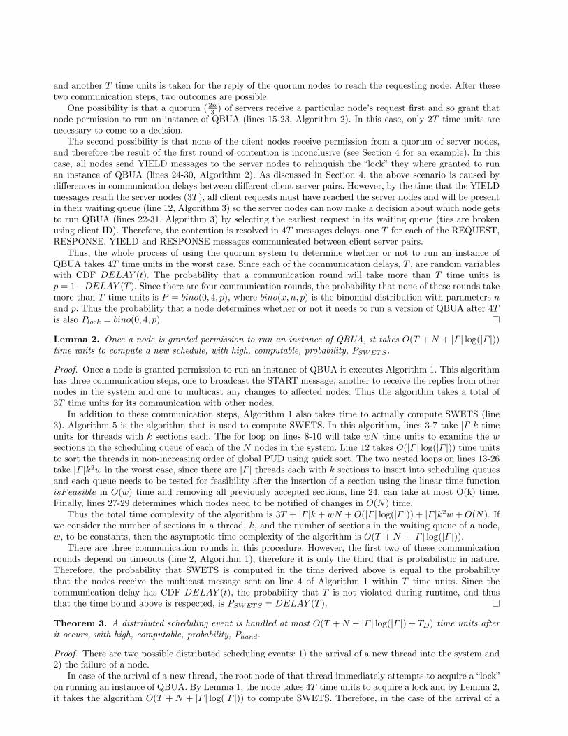
A distributable thread carries its execution context as it transits node boundaries, including its schedulingparameters (e.g., time constraints, execution time), identity, and security credentials. The propagated threadcontext is intended to be used by node schedulers for resolving all node-local resource contention among dis-tributable threads such as that for node’s physical (e.g., processor, I/O) and logical (e.g., locks) resources,according to a discipline that provides application specific, acceptably optimal, system-wide end-to-end time-liness. Figure 1 shows the execution of four distributable threads. We focus on distributable threads as ourend-to-end control flow/programming/scheduling abstraction, and hereafter, refer to them as threads, except asnecessary for clarity.

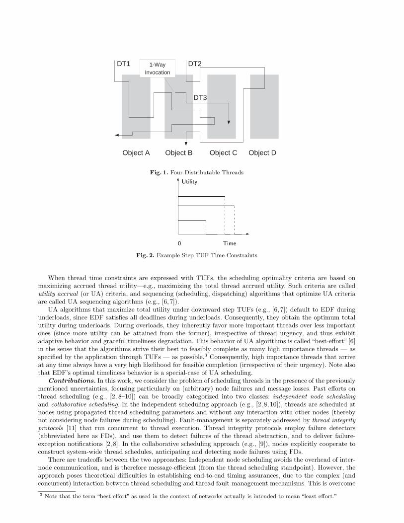
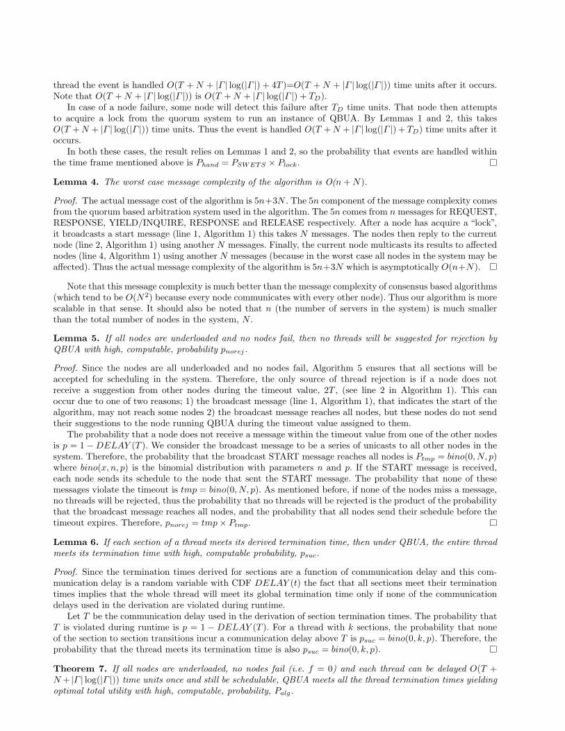
Deadlines cannot express both urgency and importance. Thus, we consider the time/utility function (or TUF)timeliness model [5] that specifies the utility of completing a thread as a function of that thread’s completiontime. We specify a deadline as a binary-valued, downward “step” shaped TUF; Figure 2 shows examples. Athread’s TUF decouples its importance and urgency—urgency is measured on the X-axis, and importance isdenoted (by utility) on the Y-axis.

Object A Object D Object B

DT1

Object C

DT2

DT3

1-Way Invocation

Fig. 1. Four Distributable Threads

-

Time

6Utility

0

Fig. 2. Example Step TUF Time Constraints

When thread time constraints are expressed with TUFs, the scheduling optimality criteria are based onmaximizing accrued thread utility—e.g., maximizing the total thread accrued utility. Such criteria are calledutility accrual (or UA) criteria, and sequencing (scheduling, dispatching) algorithms that optimize UA criteriaare called UA sequencing algorithms (e.g., [6, 7]).

UA algorithms that maximize total utility under downward step TUFs (e.g., [6, 7]) default to EDF duringunderloads, since EDF satisfies all deadlines during underloads. Consequently, they obtain the optimum totalutility during underloads. During overloads, they inherently favor more important threads over less importantones (since more utility can be attained from the former), irrespective of thread urgency, and thus exhibitadaptive behavior and graceful timeliness degradation. This behavior of UA algorithms is called “best-effort” [6]in the sense that the algorithms strive their best to feasibly complete as many high importance threads — asspecified by the application through TUFs — as possible.3 Consequently, high importance threads that arriveat any time always have a very high likelihood for feasible completion (irrespective of their urgency). Note alsothat EDF’s optimal timeliness behavior is a special-case of UA scheduling.

Contributions. In this work, we consider the problem of scheduling threads in the presence of the previouslymentioned uncertainties, focusing particularly on (arbitrary) node failures and message losses. Past efforts onthread scheduling (e.g., [2, 8–10]) can be broadly categorized into two classes: independent node schedulingand collaborative scheduling. In the independent scheduling approach (e.g., [2, 8, 10]), threads are scheduled atnodes using propagated thread scheduling parameters and without any interaction with other nodes (therebynot considering node failures during scheduling). Fault-management is separately addressed by thread integrityprotocols [11] that run concurrent to thread execution. Thread integrity protocols employ failure detectors(abbreviated here as FDs), and use them to detect failures of the thread abstraction, and to deliver failure-exception notifications [2, 8]. In the collaborative scheduling approach (e.g., [9]), nodes explicitly cooperate toconstruct system-wide thread schedules, anticipating and detecting node failures using FDs.

There are tradeoffs between the two approaches: Independent node scheduling avoids the overhead of inter-node communication, and is therefore message-efficient (from the thread scheduling standpoint). However, theapproach poses theoretical difficulties in establishing end-to-end timing assurances, due to the complex (andconcurrent) interaction between thread scheduling and thread fault-management mechanisms. This is overcome

3 Note that the term “best effort” as used in the context of networks actually is intended to mean “least effort.”

in collaborative scheduling, but the approach incurs message overhead costs. In [8, 10], upper bounds areestablished for such message costs.

FDs that are employed in both paradigms in past efforts have assumed a totally synchronous computationalmodel—e.g., deterministically bounded message delay. While the synchronous model is easily adapted for real-time applications due to the presence of a notion of time, as pointed out in [12], this results in systems withlow coverage. On the other hand, it is difficult to design real-time algorithms for the asynchronous model dueto its total disregard for timing assumptions. Thus, there have been several (recent) attempts to reconcile theseextremes. For example, in [13], Aguilera et. al. describe the design of a fast failure detector for synchronoussystems and show how it can be used to solve the consensus problem for real-time systems. The algorithmachieves the optimal bound for both message and time complexity for synchronous systems.

In [14], Hermant and Widder describe the Theta-model, where only the ratio, Θ, between the fastest andslowest message in transit is known. This increases the coverage of algorithms (designed under this model) asless assumptions are made about the underlying system. While Θ is sufficient for proving the correctness ofsuch algorithms, an upper bound on communication delay is needed to establish timeliness properties.

In [10], Binoy et. al. develop HUA, an independent node scheduling algorithm for synchronous systems thatuses propagated thread scheduling information to perform local scheduling. This local scheduling sometimesresults in a locally optimal decision that may not be globally optimal. In [9], a scheduling algorithm for syn-chronous systems that uses the collaborative scheduling approach, CUA, is developed. This algorithm uses fastconsensus [13] to solve the scheduling problem, but does not provide the same best-effort property as QBUA.In [15], Sherif et. al. describe ACUA, a collaborative distributed real-time scheduling algorithm for partiallysynchronous systems. The algorithm has better best effort properties than previous algorithms for the sameproblem but has a high overhead due to its reliance on the uniform consensus problem.

In this paper, we target partially synchronous systems that are neither totally synchronous nor totallyasynchronous. In particular, we consider the partially synchronous model in [16], where message delay andmessage loss are probabilistically described. For such a model, we design a thread scheduling algorithm belongingto the collaborative scheduling paradigm, called the Quorum Based Utility Accrual scheduling (or QBUA). Weshow that QBUA satisfies thread time constraints in the presence of crash failures, We also show that themessage and time complexity of QBUA compares favorably with other algorithms in its class. Furthermore,we show that QBUA has a better best-effort property — i.e., the affinity for feasibly completing as manyhigh importance threads as possible, irrespective of thread urgency — than past thread scheduling algorithmsincluding [9,10]. We also prove the exception handling properties of QBUA.

2 Models and Objective

2.1 Models

Distributable Thread Abstraction. Threads execute in local and remote objects by location-independent invoca-tions and returns. A thread begins its execution by invoking an object operation. The object and the operationare specified when the thread is created. The portion of a thread executing an object operation is called a threadsegment. Thus, a thread can be viewed as being composed of a concatenation of thread segments.

A thread’s initial segment is called its root and its most recent segment is called its head. The head of athread is the only segment that is active. A thread can also be viewed as being composed of a sequence ofsections, where a section is a maximal length sequence of contiguous thread segments on a node. A section’sfirst segment results from an invocation from another node, and its last segment performs a remote invocation.

Execution time estimates of the sections of a thread are assumed to be known when the thread arrives at therespective nodes. The time estimate includes that of the section’s normal code, and can be violated at run-time(e.g., due to context dependence, causing processor overloads).

The sequence of remote invocations and returns made by a thread can typically be estimated by analyzingthe thread code (e.g., [17]). The total number of sections of a thread is thus assumed to be known a-priori. Theapplication is thus comprised of a set of threads, denoted T = {T1, T2, . . .}. The set of sections of a thread Ti

is denoted as [Si1, S

i2, . . . , S

ik].

Timeliness Model. We specify the time constraint of each thread using a Time/Utility Function (TUF) [5].A TUF allows us to decouple the urgency of a thread from its importance. This decoupling is a key propertyallowed by TUFs since the urgency of a thread may be orthogonal to its importance. A thread Ti’s TUF isdenoted as Ui (t). A classical deadline is unit-valued—i.e., Ui(t) = {0, 1}, since importance is not considered.Downward step TUFs generalize classical deadlines where Ui(t) = {0, {m}}. We focus on downward step TUFs,

and denote the maximum, constant utility of a TUF Ui (t), simply as Ui. Each TUF has an initial time Ii,which is the earliest time for which the TUF is defined, and a termination time Xi, which, for a downward stepTUF, is its discontinuity point. Ui (t) > 0, ∀t ∈ [Ii, Xi] and Ui (t) = 0, ∀t /∈ [Ii, Xi] , ∀i.

System Model. Our system consists of a set of client nodes∐

= {1, 2, · · · , N} and a set of server nodes Π ={1, 2, · · · , n}. Bi-directional communication channels are assumed to exist between every client-server and client-client pair. We also assume that the basic communication channels may loose messages with probability p, andcommunication delay is described by some probability distribution. On top of this basic communication channel,we consider a reliable communication protocol that delivers a message to its destination in probabilisticallybounded time (with CDF DELAY (t)) provided that the sender and receiver both remain correct, using thestandard technique of sequence numbers and retransmissions. We assume that each node is equipped with twoprocessors; a processor that executes the tasks hosted on the node and a scheduling coprocessor4. We alsoassume that nodes in our system have access to GPS clocks that can provide each node to a UTC clock withhigh precision [18–20]. Since NCW is our target domain, assuming that each node is equipped with GPS devicesis realistic. We also assume that each node is equipped with QoS FDs [16]. The QoS FD descibed in [16] isdesigned to monitor only one process. Therefore, we equip each node with N − 1 FDs to monitor the status ofall other nodes. On each node, i, these N − 1 FDs output the nodes they suspect to the the same list, suspecti

Exceptions and Abort Model. Each section of a thread has an associated exception handler. We consider atermination model for thread failures including time-constraint violations and node failures.

If a thread has not completed by its termination time, a time constraint-violation exception is raised byQBUA, and handlers are released on all nodes that host the thread’s sections by QBUA. When a handlerexecutes (not necessarily when it is released), it will abort the associated section after performing compensationsand recovery actions that are necessary to avoid inconsistencies—e.g., rolling back/forward, or making othercompensations to logical and physical resources that are held by the section to safe states.

We consider a similar abort model for node failures. When a thread encounters a node failure causingorphans, QBUA delivers failure-exception notifications to all orphan nodes of the thread. Those nodes thenrespond by releasing handlers which abort the orphans after executing compensating actions.

Each handler may have a time constraint, which is specified as a relative deadline. Each handler also hasan execution time estimate. This estimate along with the handler’s deadline are described by the handler’sthread when the thread arrives at a node. Violation of the termination time of a handler’s deadline will causethe immediate execution of system recovery code on that node, which will recover the thread section’s heldresources and return the system to a consistent and safe state.

Failure Model. The nodes are subject to crash failures. When a process crashes, it loses it state memory —i.e., there is no persistent storage. If a crashed client node recovers at a later time, we consider it a new nodesince it has already lost all of its former execution context. A client node is correct if it does not crash; it isfaulty if it is not correct. In the case of a server crash, it may either recover or be replaced by a new serverassuming the same server name (using DNS or DHT — e.g, [21] — technology). We model both cases as serverrecovery. Since crashes are associated with memory loss, recovered servers start from their initial state. A serveris correct if it never fails; it is faulty if it is not correct. QBUA tolerates up to N − 1 client failures and up tofs

max ≤ n/3 server failures. The actual number of server failures is denoted as fs ≤ fsmax and the actual number

of client failures is denoted as f ≤ fmax where fmax ≤ N − 1.

2.2 Scheduling Objectives

Our primary objective is to design a thread scheduling algorithm that will maximize the total utility accruedby all the threads as much as possible. Further, the algorithm must provide assurances on the satisfaction ofthread termination times in the presence of (up to fmax) crash failures. Moreover, the algorithm must exhibitthe best-effort property.

3 Rationale

QBUA is a collaborative scheduling algorithm, which allows it to construct schedules that result in highersystem-wide accrued utility by preventing locally optimal decisions from compromising system-wide optimality.It also allows QBUA to respond to node failures by eliminating threads that are affected by the failures, thus

4 Dual core technology makes this assumption realistic.

allowing the algorithm to gracefully degrade timeliness in the presence of failures. There are two types ofscheduling events that are handled by QBUA, viz: a) local scheduling events and b) distributed schedulingevents.

Local scheduling events are handled locally on a node without consulting other nodes. Examples of localscheduling events are section completion, section handler expiry events etc. For a full list of local schedulingevents please see Algorithm 7. Distributed scheduling events need the participation of all nodes in the systemto handle them. In this work, only two distributed scheduling events exit, viz: a) the arrival of a new threadinto the system and b) the failure of a node. A node that detects a distributed scheduling event sends a STARTmessage to all other nodes requesting their scheduling information so that it can compute a System WideExecutable Thread Set (or SWETS). Nodes that receive this message, send their scheduling information to therequesting node and wait for schedule updates (which are sent to them when the requesting node computes anew system-wide schedule). This may lead to contention if several different nodes detect the same distributedscheduling event concurrently.

For example, when a node fails, many nodes may detect the failure concurrently. It is superfluous for allthese nodes to start an instance of QBUA. In addition, events that occur in quick succession may trigger severalinstances of QBUA when only one instance can handle all of those events. To prevent this, we use a quorumsystem to arbitrate among the nodes wishing to run QBUA. In order to perform this arbitration, the quorumsystem examines the time-stamp of incoming events. If an instance of QBUA was granted permission to runlater than an incoming event, there is no need to run another instance of QBUA since information about theincoming event will be available to the version of QBUA already running (i.e., the event will be handled bythat instance of QBUA).

4 Algorithm Description

As mentioned above, whenever a distributed scheduling event occurs, a node attempts to acquire permissionfrom the quorum system to run a version of QBUA. After the quorum system has arbitrated among the nodescontending to execute QBUA, the node that acquires the “lock” executes Algorithm 1. In Algorithm 1, the nodefirst broadcasts a start of algorithm message (line 1) and then waits 2T time units5 for all nodes in the systemto respond by sending their local scheduling information (line 2). After collecting this information, the nodecomputes SWETS (line 3). The details of the algorithm used to compute SWETS can be seen in Algorihtm 5.After computing SWETS, the node contacts those nodes that where affected by arrival of the new distributedscheduling event (i.e. nodes that will have sections added or removed from their schedule as a result of thescheduling event).

Algorithm 1: Compute SWETS

Broadcast start of algorithm message, START;1:Wait 2T collecting replies from other nodes;2:Construct SWETS using information collected;3:Multicast change of schedule to affected nodes;4:return;5:

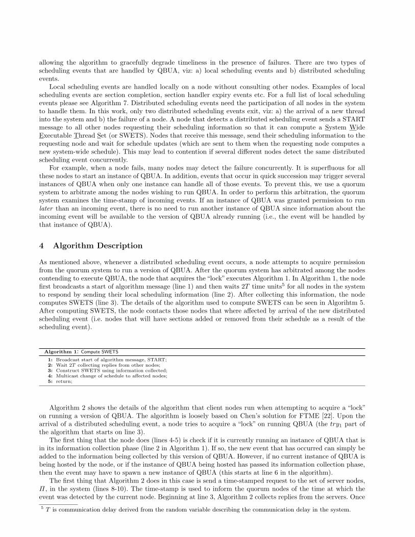
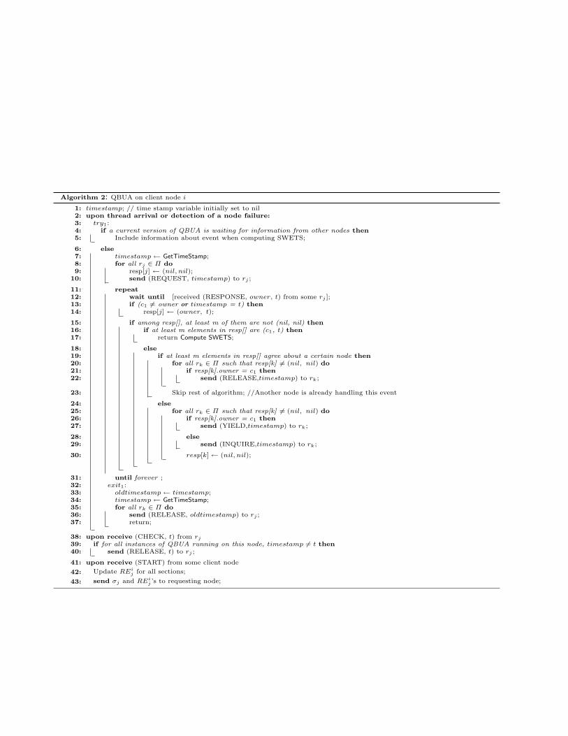
Algorithm 2 shows the details of the algorithm that client nodes run when attempting to acquire a “lock”on running a version of QBUA. The algorithm is loosely based on Chen’s solution for FTME [22]. Upon thearrival of a distributed scheduling event, a node tries to acquire a “lock” on running QBUA (the try1 part ofthe algorithm that starts on line 3).

The first thing that the node does (lines 4-5) is check if it is currently running an instance of QBUA that isin its information collection phase (line 2 in Algorithm 1). If so, the new event that has occurred can simply beadded to the information being collected by this version of QBUA. However, if no current instance of QBUA isbeing hosted by the node, or if the instance of QBUA being hosted has passed its information collection phase,then the event may have to spawn a new instance of QBUA (this starts at line 6 in the algorithm).

The first thing that Algorithm 2 does in this case is send a time-stamped request to the set of server nodes,Π, in the system (lines 8-10). The time-stamp is used to inform the quorum nodes of the time at which theevent was detected by the current node. Beginning at line 3, Algorithm 2 collects replies from the servers. Once5 T is communication delay derived from the random variable describing the communication delay in the system.

Algorithm 2: QBUA on client node i

timestamp; // time stamp variable initially set to nil1:upon thread arrival or detection of a node failure:2:

try1:3:if a current version of QBUA is waiting for information from other nodes then4:

Include information about event when computing SWETS;5:

else6:timestamp ← GetTimeStamp;7:for all rj ∈ Π do8:

resp[j] ← (nil, nil);9:send (REQUEST, timestamp) to rj ;10:

repeat11:wait until [received (RESPONSE, owner, t) from some rj ];12:if (c1 6= owner or timestamp = t) then13:

resp[j] ← (owner, t);14:

if among resp[], at least m of them are not (nil, nil) then15:if at least m elements in resp[] are (c1, t) then16:

return Compute SWETS;17:

else18:if at least m elements in resp[] agree about a certain node then19:

for all rk ∈ Π such that resp[k] 6= (nil, nil) do20:if resp[k].owner = c1 then21:

send (RELEASE,timestamp) to rk;22:

Skip rest of algorithm; //Another node is already handling this event23:

else24:for all rk ∈ Π such that resp[k] 6= (nil, nil) do25:

if resp[k].owner = c1 then26:send (YIELD,timestamp) to rk;27:

else28:send (INQUIRE,timestamp) to rk;29:

resp[k] ← (nil, nil);30:

until forever ;31:exit1:32:

oldtimestamp ← timestamp;33:timestamp ← GetTimeStamp;34:for all rk ∈ Π do35:

send (RELEASE, oldtimestamp) to rj ;36:return;37:

upon receive (CHECK, t) from rj38:if for all instances of QBUA running on this node, timestamp 6= t then39:

send (RELEASE, t) to rj ;40:

upon receive (START) from some client node41:

Update REij for all sections;42:

send σj and REij ’s to requesting node;43:

a sufficient number of replies have arrived (line 15), Algorithm 2 checks whether its request has been acceptedby a sufficient (d 2n

3 e where n is the number of servers, see Section 5) number of server nodes. If so, the nodecomputes SWETS (lines 16-17).

On the other hand, if an insufficient number of server nodes support the request, two possibilities exist. Thefirst possibility is that another node has been granted permission to run an instance of QBUA to handle thisevent. In this case, the current node does not need to perform any additional action and so releases the “lock”it has acquired on some servers (lines 19-22). The second possibility is that the result of the contention to runQBUA at the servers was inconclusive. This may occur due to differences in communication delay. For example,assume that we have 5 servers and three clients wishing to run QBUA and all three clients send their requestto the servers at the same time, also assume that the communication delay between each server and client isdifferent. Due to these communication differences, the messages of the clients may arrive in such a patter sothat two servers support client 1, another 2 servers support client 2 and the last server supports client 3. Thismeans that no client’s request is supported by a sufficient — i.e., 2n

3 — number of server nodes. In this case,the client node sends a YIELD message to servers that support it and an INQUIRE message to nodes that donot support it (line 24-30) and waits for more responses from the server nodes to resolve this conflict. Lines31-37, release the “lock” on servers after the client node has computed SWETS, lines 38-40 are used to handlethe periodic cleanup messages sent by the servers and lines 41-43 respond to the START of algorithm message(line 1, Algorithm 1).

Algorithm 3: QBUA on server node i

cowner[]; Array of nodes holding lock to run QBUA1:towner[]; towner[i] contains time-stamp of event that triggered QBUA for node in cowner[i]2:tgrant[]; tgrant[i] contains time at which node in cowner[i] was granted lock to run QBUA3:Rwait[]; Rwait[i] is waiting queue for instance of QBUA being run by cowner[i];4:upon receive (tag, t)5:

CurrentT ime ← GetTimeStamp;6:

if (c1, t′) appears in (cowner[],towner[]) or Rwait[] then7:if t < t’ then Skip rest of algo; //This is an old message8:

if tag = REQUEST then9:if ∃ tgrant ∈ tgrant[] such that t ≤ tgrant then10:

send (RESPONSE, c, tgrant) to c1; //where c ← cowner[i], such that tgrant[i] = tgrant;11:Enqueue (c1, t) in Rwait[i], such that tgrant[i] = tgrant;12:Skip rest of algorithm;13:

else14:AddElement(cowner [], c1);15:AddElement(towner [], t);16:AddElement(tgrant[], CurrentT ime);17:send (RESPONSE, c1, t) to c1;18:

else if tag = RELEASE then19:Delete entry corresponding to c1, t from cowner[], towner[], tgrant[], and Rwait[];20:

else if tag = YIELD then21:if (c1, t) ∈ (cowner[], towner[]) then22:

For i, such that (c1, t) = (cowner[i], towner[i])23:Enqueue (c1, t) in Rwait[i];24:(cwait, twait) ← top of Rwait[i];25:cowner[i] ← cwait; towner[i] ← twait;26:tgrant[i] ← CurrentT ime;27:send (RESPONSE, cwait, twait) to cwait;28:

if c1 /∈ cowner[] then29:(c, tp) ← (cowner[i], towner[i]), for min i such that t ≤ tgrant[i];30:send (RESPONSE, c, tp) to c1;31:

else if tag = INQUIRE then32:(c, tp) ← (cowner[i], towner [i]), for min i such that t ≤ tgrant[i];33:send (RESPONSE, c, tp) to c1;34:

upon suspect that cowner[i] has failed:35:HandleFailure(cowner[i],cowner [], towner[],tgrant[],Rwait[]);36:

periodically:37:∀ cowner ∈ cowner []:38:

send (CHECK, towner) to cowner; //NB. towner is the entry in towner[] that corresponds to cowner.39:

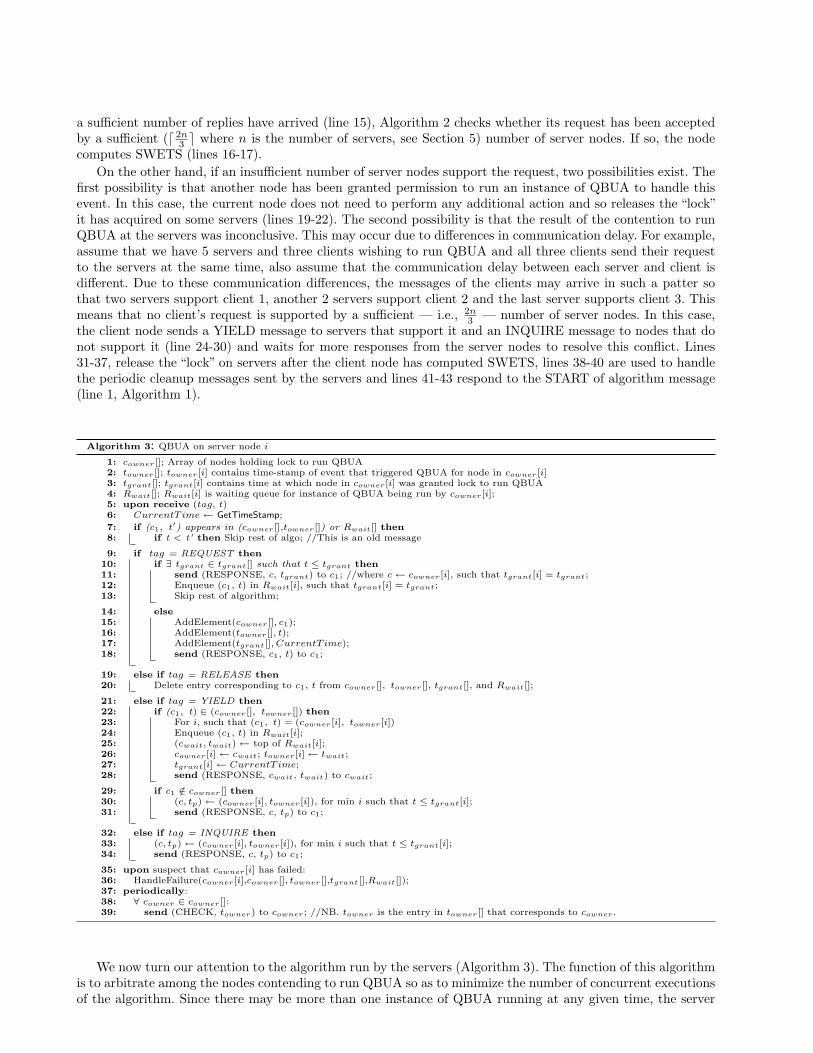
We now turn our attention to the algorithm run by the servers (Algorithm 3). The function of this algorithmis to arbitrate among the nodes contending to run QBUA so as to minimize the number of concurrent executionsof the algorithm. Since there may be more than one instance of QBUA running at any given time, the server

Algorithm 4: HandleFailure(cowner[i],cowner[], towner[],tgrant[],Rwait[])

if Rwait[i] is empty then1:remove cowner[i]’s entry from cowner[], towner[], tgrant[];2:Delete Rwait[i];3:

else4:CurrentT ime ← GetTimeStamp;5:(cwait, twait) ← top of Rwait[i];6:cowner[i] ← cwait; towner[i] ← twait;7:tgrant[i] ← CurrentT ime;8:send (RESPONSE, cwait, twait) to cwait;9:

nodes keep track of these instances using three arrays. The first array, cowner[], keeps track of which nodes arerunning instances of QBUA, the second, towner[], stores the time at which a node in cowner[] sends a request tothe servers (which is the time at which that node detects a certain scheduling event), and tgrant[] keeps trackof the time at which server nodes grant permission to client nodes to execute QBUA. In addition, a waitingqueue for each running instance of QBUA is kept in Rwait[].

When a server receives a message from a client node, it first checks to see if this is a stale message (whichmay happen due to out of order delivery). A message from a client node, c1, that has a time-stamp older thanthe last message received from c1 has been delivered out of order and is ignored (lines 7-8).

Starting at line 9, the algorithm begins to examine the message it has received from a client node. If itis a REQUEST message, the server checks if the time-stamp of the event triggering the message is less thanthe time at which a client node was granted permission to run an instance of QBUA (lines 10-18). If there isindeed such an instance, a new instance of QBUA is not needed since the event will be handled by that previousinstance of QBUA. Algorithm 3, inserts the incoming request into a waiting queue associated with that instanceof QBUA and sends a message to the client (line 11-13).

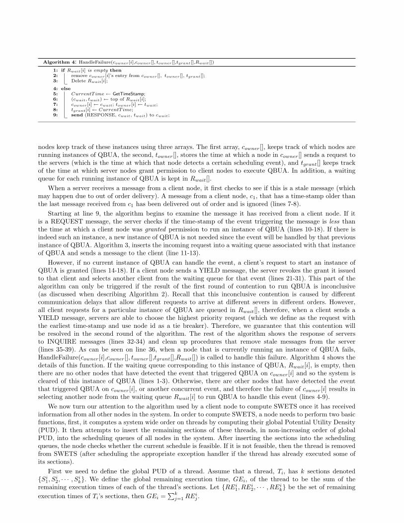
However, if no current instance of QBUA can handle the event, a client’s request to start an instance ofQBUA is granted (lines 14-18). If a client node sends a YIELD message, the server revokes the grant it issuedto that client and selects another client from the waiting queue for that event (lines 21-31). This part of thealgorithm can only be triggered if the result of the first round of contention to run QBUA is inconclusive(as discussed when describing Algorithm 2). Recall that this inconclusive contention is caused by differentcommunication delays that allow different requests to arrive at different severs in different orders. However,all client requests for a particular instance of QBUA are queued in Rwait[], therefore, when a client sends aYIELD message, servers are able to choose the highest priority request (which we define as the request withthe earliest time-stamp and use node id as a tie breaker). Therefore, we guarantee that this contention willbe resolved in the second round of the algorithm. The rest of the algorithm shows the response of serversto INQUIRE messages (lines 32-34) and clean up procedures that remove stale messages from the server(lines 35-39). As can be seen on line 36, when a node that is currently running an instance of QBUA fails,HandleFailure(cowner[i],cowner[], towner[],tgrant[],Rwait[]) is called to handle this failure. Algorithm 4 shows thedetails of this function. If the waiting queue corresponding to this instance of QBUA, Rwait[i], is empty, thenthere are no other nodes that have detected the event that triggered QBUA on cowner[i] and so the system iscleared of this instance of QBUA (lines 1-3). Otherwise, there are other nodes that have detected the eventthat triggered QBUA on cowner[i], or another concurrent event, and therefore the failure of cowner[i] results inselecting another node from the waiting queue Rwait[i] to run QBUA to handle this event (lines 4-9).

We now turn our attention to the algorithm used by a client node to compute SWETS once it has receivedinformation from all other nodes in the system. In order to compute SWETS, a node needs to perform two basicfunctions, first, it computes a system wide order on threads by computing their global Potential Utility Density(PUD). It then attempts to insert the remaining sections of these threads, in non-increasing order of globalPUD, into the scheduling queues of all nodes in the system. After inserting the sections into the schedulingqueues, the node checks whether the current schedule is feasible. If it is not feasible, then the thread is removedfrom SWETS (after scheduling the appropriate exception handler if the thread has already executed some ofits sections).

First we need to define the global PUD of a thread. Assume that a thread, Ti, has k sections denoted{Si

1, Si2, · · · , Si

k}. We define the global remaining execution time, GEi, of the thread to be the sum of theremaining execution times of each of the thread’s sections. Let {REi

1, REi2, · · · , REi

k} be the set of remainingexecution times of Ti’s sections, then GEi =

∑kj=1 REi

j .

Assuming that we are using step-down TUFs, and Ti’s TUF is Ui(t), then its global PUD can be computed asTi.PUD = Ui(tcurr +GEi)/GEi, where U is the utility of the thread and tcurr is the current time. Using globalPUD, we can establish a system wide order on the threads in non-increasing order of “return on investment”.This allows us to consider the threads for scheduling in an order that is designed to maximize accrued utility [7].We now turn our attention to the method used to check schedule feasibility. For a schedule to be feasible, allthe sections it contains should be able to complete their execution before their assigned deadline. Since weare considering threads with end-to-end deadlines, we now turn our attention to deriving the deadlines of thecomponent sections of these threads. The termination time of each section belonging to a thread needs to bederived from that thread’s end-to-end termination time. This derivation should ensure that if all the sectiontermination times are met, then the end-to-end termination time of the thread will also be met.

For the last section in a thread, we derive its termination time as simply the termination time of the entirethread. The termination time of the other sections is the latest start time of the section’s successor minus thecommunication delay. Thus the section termination times of a thread Ti, with k sections, is:

Sij .tt =

{Ti.tt j = kSi

j+1.tt− Sij+1.ex− T 1 ≤ j ≤ k − 1

where Sij .tt denotes section Si

j ’s termination time, Ti.tt denotes Ti’s termination time, and Sij .ex denotes the

estimated execution time of section Sij . The communication delay, which we denote by T above, is a random

variable ∆. Therefore, the value of T can only be determined probabilistically. This implies that if each sectionmeets the termination times computed above, the whole thread will meet its deadline with a certain, high,probability. Using these derived termination times, we can determine the feasibility of a schedule.

In addition, each handler has a relative termination time, Shj .X. However, a handler’s absolute termination

time is relative to the time it is released, more specifically, the absolute termination time of a handler is equalto the sum of the relative termination time of the handler and the failure time tf (which cannot be knowna priori). In order to overcome this problem, we delay the execution of the handler as much as possible, thusleaving room for more important threads. We compute the handler termination times as follows:

Shj .tt =

{Si

k.tt + Shj .X + TD + ta j = k

Shj+1.tt + Sh

j .X + T 1 ≤ j ≤ k − 1

where Shj .tt denotes section handler Sh

j ’s termination time, Shj .X denotes the relative termination time of section

handler Shj , Si

k.tt is the termination time of thread i’s last section, ta is a correction factor corresponding tothe execution time of the scheduling algorithm, and TD is the time needed to detect a failure by our QoS FD.From this termination time decomposition, we compute start times for each handler:

Shj .st =

{Sh

j .tt− Shj .ex 1 ≤ j ≤ k

where Shj .ex denotes the estimated execution time of section handler Sh

j . Thus, we assure the feasible executionof the exception handlers of failed sections, in order to revert the system to a safe state.

Algorithm 5 contains the details of our scheduling algorithm. Once a node has received information fromall other nodes in the system (line 2 in Algorithm 1), it can begin to compute SWETS. Each node, j, sendsthe node running QBUA its current local schedule σp

j . Using these schedules, the node can determine the set ofthreads, Γ , that are currently in the system. Both these variables are used as input to the scheduling algorithm(lines 1 and 2 in Algorithm 5). In lines 3-7, the algorithm computes the global PUD of each thread in Γ usingthe method we describe above.

The next step would be to schedule the threads in non-increasing order of their PUD. However, beforewe schedule the threads, we need to ensure that the exception handlers of any thread that has already beenaccepted into the system can execute to completion before its deadline. We do this by inserting the handlersof sections that were part of each node’s previous schedule into that node’s current schedule (lines 8-11). Sincethese handlers were part of σp

j , and our algorithm always maintains the feasibility of a schedule as an algorithminvariant, then we are sure that these handlers will be able to execute to completion before their deadline.

In line 12, we sort the threads in the system in non-increasing order of PUD. We then consider the threadsfor scheduling in that order (lines 13-26). As can be seen in those lines, we consider each remaining sectionof the thread for scheduling. In lines 15-16 we mark as failed any thread that has a section hosted on a nodethat does not participate in the algorithm. If the thread can contribute non-zero utility to the system (i.e. its

Algorithm 5: ConstructSchedule

input: Γ ; //Set of threads in the system1:input: σp

j , Hj ← nil; //σpj : Previous schedule of node j, Hj : set of handlers scheduled2:

for each Ti ∈ Γ do3:if for some section Si

j belonging to Ti, tcurr + Sij .ex > Si

j .tt then4:Ti.PUD ← 0;5:

else6:

Ti.PUD ← Ui(tcurr+GEi)GEi

;7:

for each task el ∈ σpj do8:

if el is an exception handler for section Sij then9:

Insert(el, Hj , el.tt);10:

σj ← Hj ;11:σtemp ← sortByPUD(Γ );12:for each Ti ∈ σtemp do13:

Ti.stop ←false;14:

if did not receive σj from node hosting one of Ti’s sections Sij then15:

Ti.stop ←true;16:

for each remaining section, Sij , belonging to Ti do17:

if Ti.PUD > 0 and Ti.stop 6=true then18:Insert(Si

j , σj , Sij .tt);19:

if Shj /∈ σp

j then20:

Insert(Shj , σj , Sh

j .tt);21:

if isFeasible(σj)=false then22:Ti.stop ←true;23:

Remove(Sik, σk, Si

k.tt) for 1 ≤ k ≤ j;24:

if Sij /∈ σp

j then25:

Remove(Shj , σj , Sh

j .tt);26:

for each j ∈ N do27:if σj 6= σp

j then28:Mark node j as being affected by current scheduling event;29:

deadline hasn’t passed) and the thread has not been rejected from the system, then we insert that section intothe scheduling queue of the node responsible for it (lines 18-19).

After inserting the section into its corresponding ready queue (at a position reflecting its termination time),we check to see whether this section’s handler had been included in the previous schedule of the node. If so, wedo not insert the handler into the schedule since this has been already taken care of by lines 8-11. Otherwise,the handler is inserted into its corresponding ready queue (lines 20-21). Once the section, and its handler, havebeen inserted into the ready queue, we check the feasibility of the schedule (line 22). If the schedule is notfeasible, we remove the thread’s sections from the schedule (line 24). Notice that if one section belonging to athread cannot be scheduled, all predecessor sections of the thread accepted into the system are removed (line24). This ensures that a thread that cannot complete does not take up the valuable computation resources onany node. However, we first check to see whether the section’s handler was part of a previous schedule beforewe remove it (lines 25-26). The reason we perform this check before removing the handler of the section is thatif the handler was part of a previous schedule, then that section has failed and we should keep its exceptionhandler for clean up purposes. Finally, if the schedule of any node has changed, these nodes are marked to havebeen affected by the current instance of QBUA (lines 27-29). It is to these nodes that the current node needsto multicast the changes that have occurred (line 4, Algorithm 1).

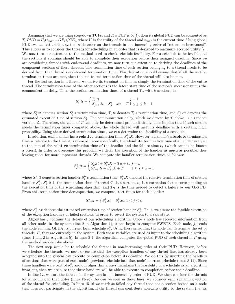
We now turn our attention to the last piece of the puzzle. We use a function isFeasible in Algorithm 5 todetermine the feasibility of the schedules we construct. Algorithm 6 contains the details of this algorithm. Inorder to determine whether a schedule is feasible or not, we need to check if all the sections in the schedule cancomplete before their derived termination times.

The loop on lines 3-6 examines each section in the schedule and attempts to determine whether or not itcan complete before its termination time. Since QBUA is executed before sections have actually arrived atsome of the nodes in the system, we need to provide an estimate for the starting time of each section on anode. A section can start immediately when it arrives at a node or it may wait some time if other sections arescheduled for execution before it. Therefore, the start time of a section is the maximum of the termination timeof the last section scheduled to execute before it (CumExeT ime) and the time it arrives at the node, which

we estimate using the finish time of its predecessor section, plus the communication delay Sij−1.ff + T . Note

that this finish time, Sij−1.ff , is different from the termination time of a section’s predecesor, Si

j−1.tt. Whilethe former is an estimate of the time when the predecessor section will finish on the node that hosts it, thelatter is the worst case finish time that a predecessor section needs to meet in order for its successor sectionsto be seduceable. To this start time, we add the execution time of the section, Si

j .ex, to obtain an estimate ofthe expected completion time of the section (line 4). We then check if this value is greater than the derivedtermination times of the section; if so, the schedule is infeasible (lines 6-7).

Algorithm 6: isFeasible

input: σ;output: true or false;1:Initialization: CumExeTime=tcurr ;2:

for each section Sij ∈ σ do3:

CumExeTime ← max(CumExeTime, Sij−1.ff + T ) + Si

j .ex; // If j=1, then Sij−1.ff = 0 and T = 0;4:

Sij .ff ← CumExeTime;5:

if CumExeTime > Sij .tt then return false;6:

return true;7:

QBUA’s dispatcher is shown in Algorithm 7. As can be seen, only two scheduling events result in collaborativescheduling, viz: the arrival of a thread into the system, and the failure of a node. All other scheduling events arehandled locally by a node. The events and the actions taken in response to these events are self explanatory.

Algorithm 7: Event Dispatcher on each node i

Data: schedevent, current schedule σp;1switch schedevent do2

case invocation arrives for Sij3

mark segment Sij ready;4

case segment Sij completes5

remove Sij from σr,σp;6

remove Shj from H;7

set REij to zero;8

case Shj ∈ H and Sh

i .st expires9

mark handler Shj ready;10

case downstream handler Shj+1 completes11

mark handler Shj ready;12

case handler Shj completes13

remove Shj from σp,H;14

notify scheduler for Shj−1;15

case new thread, Ti, arrives16if origin node, send segments Si

j to all;17

pass event to QBUA;18

case node failure detected19pass event to QBUA;20

execute first ready segment in σp;21

5 Algorithm Properties

We now turn our attention to proving some theoretical results for the algorithm. Below, T is the communicationdelay, and Γ is the set of threads in the system.

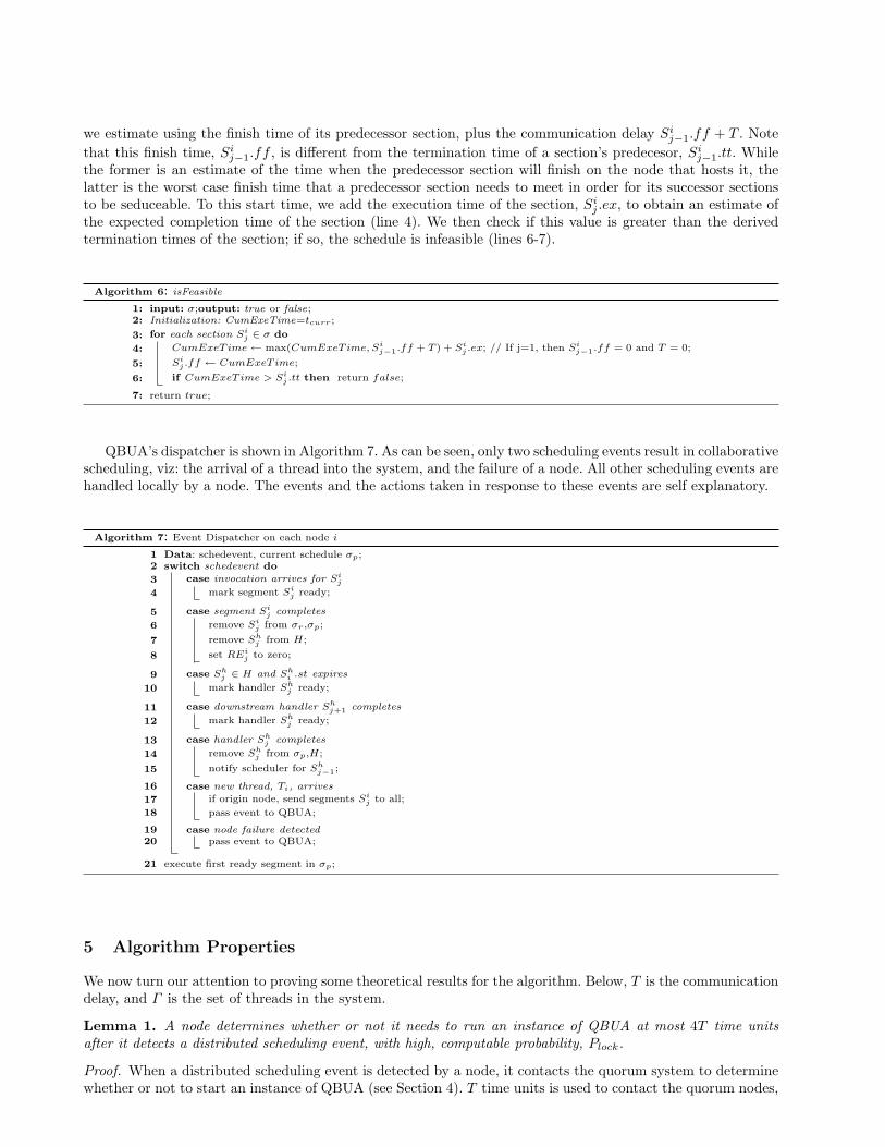
Lemma 1. A node determines whether or not it needs to run an instance of QBUA at most 4T time unitsafter it detects a distributed scheduling event, with high, computable probability, Plock.

Proof. When a distributed scheduling event is detected by a node, it contacts the quorum system to determinewhether or not to start an instance of QBUA (see Section 4). T time units is used to contact the quorum nodes,

and another T time units is taken for the reply of the quorum nodes to reach the requesting node. After thesetwo communication steps, two outcomes are possible.

One possibility is that a quorum ( 2n3 ) of servers receive a particular node’s request first and so grant that

node permission to run an instance of QBUA (lines 15-23, Algorithm 2). In this case, only 2T time units arenecessary to come to a decision.

The second possibility is that none of the client nodes receive permission from a quorum of server nodes,and therefore the result of the first round of contention is inconclusive (see Section 4 for an example). In thiscase, all nodes send YIELD messages to the server nodes to relinquish the “lock” they where granted to runan instance of QBUA (lines 24-30, Algorithm 2). As discussed in Section 4, the above scenario is caused bydifferences in communication delays between different client-server pairs. However, by the time that the YIELDmessages reach the server nodes (3T ), all client requests must have reached the server nodes and will be presentin their waiting queue (line 12, Algorithm 3) so the server nodes can now make a decision about which node getsto run QBUA (lines 22-31, Algorithm 3) by selecting the earliest request in its waiting queue (ties are brokenusing client ID). Therefore, the contention is resolved in 4T messages delays, one T for each of the REQUEST,RESPONSE, YIELD and RESPONSE messages communicated between client server pairs.

Thus, the whole process of using the quorum system to determine whether or not to run an instance ofQBUA takes 4T time units in the worst case. Since each of the communication delays, T , are random variableswith CDF DELAY (t). The probability that a communication round will take more than T time units isp = 1−DELAY (T ). Since there are four communication rounds, the probability that none of these rounds takemore than T time units is P = bino(0, 4, p), where bino(x, n, p) is the binomial distribution with parameters nand p. Thus the probability that a node determines whether or not it needs to run a version of QBUA after 4Tis also Plock = bino(0, 4, p).

Lemma 2. Once a node is granted permission to run an instance of QBUA, it takes O(T + N + |Γ | log(|Γ |))time units to compute a new schedule, with high, computable, probability, PSWETS.

Proof. Once a node is granted permission to run an instance of QBUA it executes Algorithm 1. This algorithmhas three communication steps, one to broadcast the START message, another to receive the replies from othernodes in the system and one to multicast any changes to affected nodes. Thus the algorithm takes a total of3T time units for its communication with other nodes.

In addition to these communication steps, Algorithm 1 also takes time to actually compute SWETS (line3). Algorithm 5 is the algorithm that is used to compute SWETS. In this algorithm, lines 3-7 take |Γ |k timeunits for threads with k sections each. The for loop on lines 8-10 will take wN time units to examine the wsections in the scheduling queue of each of the N nodes in the system. Line 12 takes O(|Γ | log(|Γ |)) time unitsto sort the threads in non-increasing order of global PUD using quick sort. The two nested loops on lines 13-26take |Γ |k2w in the worst case, since there are |Γ | threads each with k sections to insert into scheduling queuesand each queue needs to be tested for feasibility after the insertion of a section using the linear time functionisFeasible in O(w) time and removing all previously accepted sections, line 24, can take at most O(k) time.Finally, lines 27-29 determines which nodes need to be notified of changes in O(N) time.

Thus the total time complexity of the algorithm is 3T + |Γ |k + wN + O(|Γ | log(|Γ |)) + |Γ |k2w + O(N). Ifwe consider the number of sections in a thread, k, and the number of sections in the waiting queue of a node,w, to be constants, then the asymptotic time complexity of the algorithm is O(T + N + |Γ | log(|Γ |)).

There are three communication rounds in this procedure. However, the first two of these communicationrounds depend on timeouts (line 2, Algorithm 1), therefore it is only the third that is probabilistic in nature.Therefore, the probability that SWETS is computed in the time derived above is equal to the probabilitythat the nodes receive the multicast message sent on line 4 of Algorithm 1 within T time units. Since thecommunication delay has CDF DELAY (t), the probability that T is not violated during runtime, and thusthat the time bound above is respected, is PSWETS = DELAY (T ).

Theorem 3. A distributed scheduling event is handled at most O(T + N + |Γ | log(|Γ |) + TD) time units afterit occurs, with high, computable, probability, Phand.

Proof. There are two possible distributed scheduling events: 1) the arrival of a new thread into the system and2) the failure of a node.

In case of the arrival of a new thread, the root node of that thread immediately attempts to acquire a “lock”on running an instance of QBUA. By Lemma 1, the node takes 4T time units to acquire a lock and by Lemma 2,it takes the algorithm O(T + N + |Γ | log(|Γ |)) to compute SWETS. Therefore, in the case of the arrival of a

thread the event is handled O(T + N + |Γ | log(|Γ |) + 4T )=O(T + N + |Γ | log(|Γ |)) time units after it occurs.Note that O(T + N + |Γ | log(|Γ |)) is O(T + N + |Γ | log(|Γ |) + TD).

In case of a node failure, some node will detect this failure after TD time units. That node then attemptsto acquire a lock from the quorum system to run an instance of QBUA. By Lemmas 1 and 2, this takesO(T + N + |Γ | log(|Γ |)) time units. Thus the event is handled O(T + N + |Γ | log(|Γ |) + TD) time units after itoccurs.

In both these cases, the result relies on Lemmas 1 and 2, so the probability that events are handled withinthe time frame mentioned above is Phand = PSWETS × Plock.

Lemma 4. The worst case message complexity of the algorithm is O(n + N).

Proof. The actual message cost of the algorithm is 5n+3N . The 5n component of the message complexity comesfrom the quorum based arbitration system used in the algorithm. The 5n comes from n messages for REQUEST,RESPONSE, YIELD/INQUIRE, RESPONSE and RELEASE respectively. After a node has acquire a “lock”,it broadcasts a start message (line 1, Algorithm 1) this takes N messages. The nodes then reply to the currentnode (line 2, Algorithm 1) using another N messages. Finally, the current node multicasts its results to affectednodes (line 4, Algorithm 1) using another N messages (because in the worst case all nodes in the system may beaffected). Thus the actual message complexity of the algorithm is 5n+3N which is asymptotically O(n+N).

Note that this message complexity is much better than the message complexity of consensus based algorithms(which tend to be O(N2) because every node communicates with every other node). Thus our algorithm is morescalable in that sense. It should also be noted that n (the number of servers in the system) is much smallerthan the total number of nodes in the system, N .

Lemma 5. If all nodes are underloaded and no nodes fail, then no threads will be suggested for rejection byQBUA with high, computable, probability pnorej.

Proof. Since the nodes are all underloaded and no nodes fail, Algorithm 5 ensures that all sections will beaccepted for scheduling in the system. Therefore, the only source of thread rejection is if a node does notreceive a suggestion from other nodes during the timeout value, 2T , (see line 2 in Algorithm 1). This canoccur due to one of two reasons; 1) the broadcast message (line 1, Algorithm 1), that indicates the start of thealgorithm, may not reach some nodes 2) the broadcast message reaches all nodes, but these nodes do not sendtheir suggestions to the node running QBUA during the timeout value assigned to them.

The probability that a node does not receive a message within the timeout value from one of the other nodesis p = 1−DELAY (T ). We consider the broadcast message to be a series of unicasts to all other nodes in thesystem. Therefore, the probability that the broadcast START message reaches all nodes is Ptmp = bino(0, N, p)where bino(x, n, p) is the binomial distribution with parameters n and p. If the START message is received,each node sends its schedule to the node that sent the START message. The probability that none of thesemessages violate the timeout is tmp = bino(0, N, p). As mentioned before, if none of the nodes miss a message,no threads will be rejected, thus the probability that no threads will be rejected is the product of the probabilitythat the broadcast message reaches all nodes, and the probability that all nodes send their schedule before thetimeout expires. Therefore, pnorej = tmp× Ptmp.

Lemma 6. If each section of a thread meets its derived termination time, then under QBUA, the entire threadmeets its termination time with high, computable probability, psuc.

Proof. Since the termination times derived for sections are a function of communication delay and this com-munication delay is a random variable with CDF DELAY (t) the fact that all sections meet their terminationtimes implies that the whole thread will meet its global termination time only if none of the communicationdelays used in the derivation are violated during runtime.

Let T be the communication delay used in the derivation of section termination times. The probability thatT is violated during runtime is p = 1 − DELAY (T ). For a thread with k sections, the probability that noneof the section to section transitions incur a communication delay above T is psuc = bino(0, k, p). Therefore, theprobability that the thread meets its termination time is also psuc = bino(0, k, p).

Theorem 7. If all nodes are underloaded, no nodes fail (i.e. f = 0) and each thread can be delayed O(T +N + |Γ | log(|Γ |)) time units once and still be schedulable, QBUA meets all the thread termination times yieldingoptimal total utility with high, computable, probability, Palg.

Proof. By Lemma 5, no threads will be considered for rejection from a fault free, underloaded system withprobability pnorej . This means that all sections will be scheduled to meet their derived termination times byAlgorithm 5.

By Lemma 6, this implies that each thread, j, will meet its termination time with probability pjsuc. Therefore,

for a system with X = |Γ | threads, the probability that all threads meet their termination time is Ptmp =∏Xj=1 pj

suc. Given that the probability that all threads will be accepted is pnorej , Palg = Ptmp × pnorej .We make the requirement that a thread tolerate a delay of O(T + N + |Γ | log(|Γ |)) time units and still be

schedulable because QBUA takes O(T +N+|Γ | log(|Γ |)) time units to reach its decision about the schedulabilityof a newly arrived thread. Thus if this delay causes any of the thread’s sections to miss their deadlines, thethread will not be schedulable. We only require that the thread suffer this delay once because we assume thatthere is a scheduling coprocessor on each node, thus the delay will only be incurred by the newly arrived threadwhile other threads continue to execute uninterrupted on the other processor.

Theorem 8. If N −f nodes do not crash, are underloaded, and all incoming threads can be delayed O(T +N +|Γ | log(|Γ |)) and still be schedulable, then QBUA meets the execution time of all threads in its eligible executionthread set, Γ , with high computable probability, Palg.

Proof. As in Lemma 5, no thread in the eligible thread set Γ will be rejected if nodes receive the broadcastSTART message and respond to that message on time. The probability of these two events is bino(0, N − f, p)where p = 1 −DELAY (T ). Therefore, the probability that none of the threads in Γ are rejected is Pnorej =bino(0, N−f, p)×bino(0, N−f, p). This means that all the sections belonging to those threads will be scheduledto meet their derived termination times. By Lemma 6, this implies that each of these threads, Tj , will meet theirtermination times with probability pj

suc. Therefore, for a system with an eligible thread set, Γ , the probabilitythat all threads meet their termination times if their sections meet their termination times is Ptmp =

∏j∈Γ pj

suc.The probability that all the remaining threads are execute to completion is thus Palg = Ptmp × pnorej .

Lemma 9. QBUA has a quorum threshold, m, (see Algorithm 2) of d 2n3 e and can tolerate fs = n

3 faultyservers.

Proof. Our algorithm considers a memoryless crash recovery model for the quorum nodes. This means that aquorum node that crashes and then recovers losses all its state information and starts from scratch. What thisimplies is that for our algorithm to tolerate such failures, the threshold m should be large enough such thatthere is at least one correct server in the intersection of any two quorums.

Assume that f is the maximum number of faulty servers in the system (i.e. servers that may fail at sometime in the future), then the above requirement can be expresses as 2m − n > fs. On the other hand, mcannot be too large since some servers will fail and choosing too large a value of m may mean that client nodesmay wait indefinitely for responses from servers that have failed. The requirement translates to m ≤ n − fs.Combining the two we get, fs = n

3 and m can be set to d 2n3 e.

Definition 1 (Section Failure). A section, Sij , is said to have failed when one or more of the previous head

nodes of Sij ’s thread (other than Si

j ’s node) has crashed.

Lemma 10. If a node hosting a section, Sij, of thread Ti fails (per Definition 1) at time tf , every correct

node will include handlers for thread Ti in its schedule by time tf + TD + ta, where ta is an implementation-specific computed execution bound for QBUA calculated per the analysis in Theorem 3, with high, computable,probability, Phand

Proof. Since the QoS FD we use in this work detects a failed node in TD time units [16], all nodes in the systemwill detect the failure of the node at time tf + TD. As a result, the QBUA algorithm will be triggered and willexclude Ti from the system because node j will not send its schedule (lines 15-16 Algorithm 5). Consequently,Algorithm 5 will include the section handlers for this thread in H. Execution of QBUA completes in time taand thus all handlers will be included in H by time tf + TD + ta.

Of all these timing terms, only ta is stochastic. From Theorem 3, we know that ta will be obeyed withprobability Phand, therefore, the time bound derived above is also obeyed with probability Phand.

Lemma 11. If a section Si, where i 6= k, fails (per Definition 1) at time tf and section Si+1 is correct, thenunder QBUA, its handler Sh

i will be released no earlier than Shi+1’s completion and no later than Sh

i+1.tt + T +Sh

i .X − Shi .ex.

Proof. For i 6= k, a section’s exception handler can be released due to one of two events; 1) its start timeexpires (lines 9-10 in Algorithm 7); or 2) an explicit invocation is made by the handler’s successor (lines 11-12in Algorithm 7).

In the first case, we know from the analysis in Section 4 that the start time of Shi is Sh

i+1.tt+Shj .X+T−Sh

j .ex.Thus, by definition, it satisfies the upper bound in the theorem. Also, since Sh

j .X ≥ Shj .ex (otherwise the handler

would not be schedulable), Shi+1.tt + Sh

j .X + T − Shj .ex > Sh

i+1.tt, and this satisfies the lower bound of thetheorem.

In the second case, an explicit message has arrived indicating the completion of Shi+1. Since the message

was sent, this indicates that Shi+1.tt has already passed, thus satisfying the lower bound of the theorem. In

addition, the message should have arrived T time units after Shi+1 finishes execution (i.e at Sh

i+1.tt + T ), sinceSh

i+1.tt+T ≤ Shi+1.tt+T +Sh

i .X−Shi .ex (remember that Sh

i .X ≥ Shi .ex), then the upper bound is satisfied.

An interesting thing about the property above is that it is not probabilistic in nature. At first sight, itwould seem that the property is stochastic due to the probabilistic communication delay used in the second casementioned in the proof. One would expect the upper bound in the property to be respected only probabilisticallyin the second case. However, if the upper bound is not met in the second case (i.e. the stochastic communicationdelay causes the notification of the completion of handler Sh

i+1 to arrive after the upper bound in the theorem),then the first case kicks in and starts the handler before the upper bound expires anyway. Therefore this resultis deterministic in nature.

Lemma 12. If a section Si fails (per Definition 1), then under QBUA, its handler Shi will complete no later

than Shi .tt (barring Sh

i ’s failure).

Proof. If one or more of the previous head nodes of Si’s thread has crashed, it implies that Si’s thread waspresent in a system wide schedulable set previously constructed. This implies that Si and its handler werepreviously determined to be feasible before Si.tt and Sh

i .tt respectively (lines 18-26 of Algorithm 5).When some previous head node of Si’s thread fails, QBUA will be triggered and will remove Si from the

pending queue. In addition, Algorithm 5 will include Shi in H and construct a feasible schedule containing Sh

i

(lines 8-11 and lines 18-26). Since the schedule is feasible and Shi is inserted to meet Sh

i .tt (line 10), then Shi

will complete by time Shi .tt.

We now state QBUA’s bounded clean-up property.

Theorem 13. In the event of a failure of a thread, the thread’s handlers will be executed in LIFO (last-infirst-out) order. Furthermore, all (correct) handlers will complete in bounded time. For a thread with k sections,handler termination times Sh

i .X, which fails at time tf , and (distributed) scheduler latency ta, this bound isTi.X +

∑i Sh

i .X + kT + TD + ta, with high computable probability Pexep.

Proof. The LIFO property follows from Lemma 11. Since it is guaranteed that each handler, Shi , cannot begin

before the termination time of handler Shi+1 (the lower bound in Lemma 11), then we guarantee LIFO execution

of the handlers.The fact that all correct handlers complete in bounded time is shown in Lemma 12, where each correct

handler is shown to complete before its termination time.Finally, if a thread fails at time tf , all nodes will include handlers for this thread in their schedule by time

tf + TD + ta (Lemma 10) with probability Phand and QBUA guarantees that all these sections will completebefore their termination times (Lemma 12). Due to the LIFO nature of handler executions, the last handlerto execute is the first exception handler, Sh

1 . The termination time of this handler (from the equations inSection 4) is Ti.X +

∑i Sh

i .X +kT +TD + ta (which is basically the sum of the relative termination times of allthe exception handlers, plus the termination time of the last section, which is used as an estimate for the worstcase failure time of the threads per the discussion in Section 4, k communication delays T to notify handlers inLIFO order, TD to detect the failure after it occurs and ta for QBUA to execute).

Since Lemma 12 guarantees that all handlers will finish before their derived termination times, the onlystochastic part of the theorem is the probability that QBUA will include the handlers of all the section in timetf + TD + ta. From Lemma 10, we know this probability is Phand, thus Pexep = Phand.

Definition 2. Consider a distributed scheduling algorithm A. DBE is defined as the property that A orders itsthreads in non-increasing order of global PUD while considering them for scheduling and schedules all feasiblethreads in the system in that order. The global PUD of a thread is the ratio of the utility of the thread to thesum of the remaining execution times of all its sections.

Note that the DBE property is essential for any UA algorithm that attempts to maximize system wideaccrued utility by favoring tasks that offer the most utility for the least amount of execution time (which is theheuristic used by DASA [7]). For the proofs of Lemmas 14, 15 and 16, please see [15].

Lemma 14. HUA [10], does not have the DBE property.

Lemma 15. CUA [9] does not have the DBE property.

Lemma 16. ACUA has the DBE property for threads that can survive the scheduling overhead of the algorithm— i.e., threads that can be delayed O(fT + Nk) and still be schedulable.

Lemma 17. QBUA has the DBE property for threads that can survive the scheduling overhead of the algorithm— i.e., threads that can be delayed O(T + N + |Γ | log(|Γ |)) (see Theorem 3) and still be schedulable.

Proof. The DBE property requires all threads to be ordered in non-decreasing order of global PUD, and this isaccomplished in lines 3-7 and line 12 of Algorithm 5. In addition, the DBE property requires that all feasiblethreads be scheduled in non-decreasing order of PUD, and this is accomplished in lines 13-26 of Algorithm 5.Thus QBUA has the DBE property for all threads that can withstand the O(T + N + |Γ | log(|Γ |)) overhead ofthe algorithm and still remain schedulable.

Theorem 18. QBUA has a better best-effort property than HUA and CUA and a similar best-effort propertyto ACUA.

Proof. The proof follows directly from Lemmas 14, 15, 16 and 17. In particular, HUA and CUA do not havethe DBE property while QBUA does, and both QBUA and ACUA have the DBE property but for threads thatcan survive their, different, scheduling overheads.

Lemma 19. The message overhead of QBUA is better than the message overhead of ACUA and scales betterwith the number of node failures.

Proof. The message complexity of ACUA is O(fN2) which is clearly asymptotically more expensive than theO(n+N) message complexity of QBUA. In addition, since the message complexity of ACUA is a linear functionof f , the number of failed nodes, and the message complexity of QBUA does not depend on f —i.e., is notaffected by the number of node failures— the message overhead of QBUA scales better in the presence offailure.

Lemma 20. The time overhead of QBUA is asymptotically similar to the time overhead of ACUA and scalesbetter with the number of node failures. In addition, when the number of threads in the system is fixed, the timecomplexity of QBUA is asymptotically better than that of ACUA and scales better in the presence of failure.

Proof. The time complexities of the two algorithms, O(T + N + |Γ | log(|Γ |)) for QBUA and O(fT + kN) forACUA, are asymptotically similar, but since the time complexity of ACUA is a function of f and QBUA’s isnot, QBUA’s time complexity scales better in the presence of failure.

When the number of threads in the system is fixed, the term |Γ | log(|Γ |) in the time complexity of QBUAbecomes a constant and thus its asymptotic time complexity becomes O(T + N) which is better than the timecomplexity of ACUA, O(fT + kN). Further, since the time complexity of QBUA is not a function of f and thetime complexity of ACUA is, QBUA’s complexity scales better in the presence of failure.

Theorem 21. QBUA has lower overhead than ACUA and its overhead scales better with the number of nodefailures.

Proof. The proof follows directly from Lemmas 19 and 20.

In should be noted that in our computation of time complexity of algorithms, we do not take into accountthe effect of message overhead. However, the message complexity affects the utilization of the communicationchannel and the queue delay at nodes and hence has a direct impact on communication delay (which appears asa term in both time complexities mentioned above). The effect of this higher message complexity can be seenin our experiments (see Section 6), where the higher overhead of ACUA, both message and time overheads,results in performance that is worse than that of QBUA.

Theorem 22. QBUA limits thrashing by reducing the number of instances of QBUA spawned by concurrentdistributed scheduling event.

Proof. Thrashing occurs when concurrent distributed events spawn, superfluous, separate instances of QBUA.QBUA prevents this by having nodes wishing to run an instance of QBUA contact a quorum system to gainpermission for doing so (see Section 4). In lines 9-13 of Algorithm 3, the quorum system does not spawn anew instance of QBUA if there is an instance of QBUA already running that was granted permission to startafter the timestamp of the arriving scheduling event. This occurs because the instance of QBUA that startedafter the scheduling event occurred will have information about that event and will thus handle it. This reducesthrashing by prevent superfluous concurrent instances from running at the same time.

6 Experimental Results

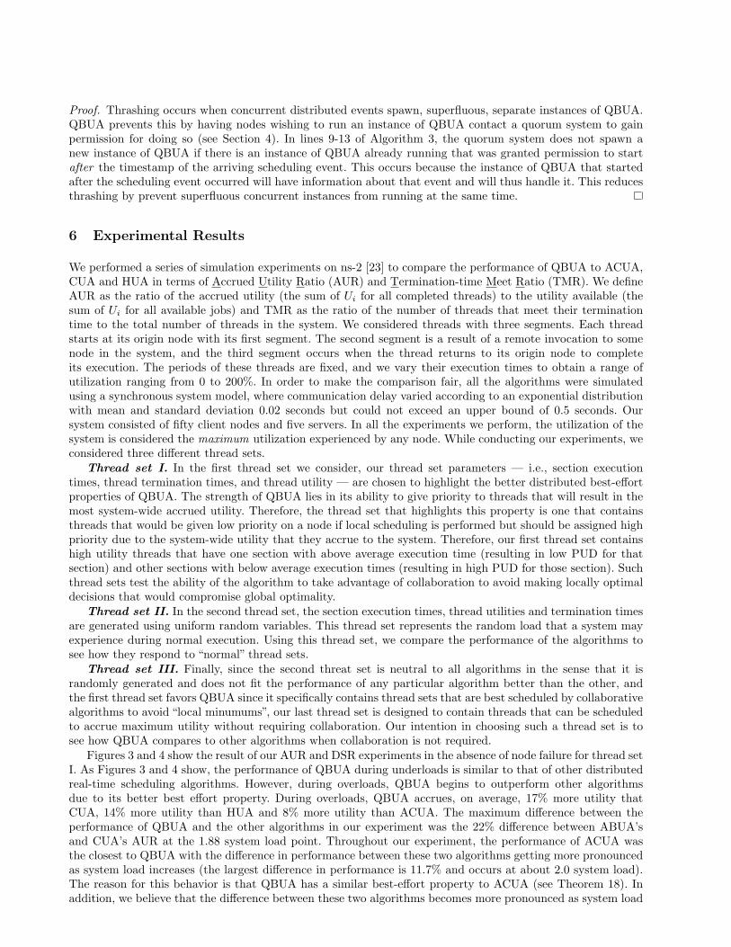
We performed a series of simulation experiments on ns-2 [23] to compare the performance of QBUA to ACUA,CUA and HUA in terms of Accrued Utility Ratio (AUR) and Termination-time Meet Ratio (TMR). We defineAUR as the ratio of the accrued utility (the sum of Ui for all completed threads) to the utility available (thesum of Ui for all available jobs) and TMR as the ratio of the number of threads that meet their terminationtime to the total number of threads in the system. We considered threads with three segments. Each threadstarts at its origin node with its first segment. The second segment is a result of a remote invocation to somenode in the system, and the third segment occurs when the thread returns to its origin node to completeits execution. The periods of these threads are fixed, and we vary their execution times to obtain a range ofutilization ranging from 0 to 200%. In order to make the comparison fair, all the algorithms were simulatedusing a synchronous system model, where communication delay varied according to an exponential distributionwith mean and standard deviation 0.02 seconds but could not exceed an upper bound of 0.5 seconds. Oursystem consisted of fifty client nodes and five servers. In all the experiments we perform, the utilization of thesystem is considered the maximum utilization experienced by any node. While conducting our experiments, weconsidered three different thread sets.

Thread set I. In the first thread set we consider, our thread set parameters — i.e., section executiontimes, thread termination times, and thread utility — are chosen to highlight the better distributed best-effortproperties of QBUA. The strength of QBUA lies in its ability to give priority to threads that will result in themost system-wide accrued utility. Therefore, the thread set that highlights this property is one that containsthreads that would be given low priority on a node if local scheduling is performed but should be assigned highpriority due to the system-wide utility that they accrue to the system. Therefore, our first thread set containshigh utility threads that have one section with above average execution time (resulting in low PUD for thatsection) and other sections with below average execution times (resulting in high PUD for those section). Suchthread sets test the ability of the algorithm to take advantage of collaboration to avoid making locally optimaldecisions that would compromise global optimality.

Thread set II. In the second thread set, the section execution times, thread utilities and termination timesare generated using uniform random variables. This thread set represents the random load that a system mayexperience during normal execution. Using this thread set, we compare the performance of the algorithms tosee how they respond to “normal” thread sets.

Thread set III. Finally, since the second threat set is neutral to all algorithms in the sense that it israndomly generated and does not fit the performance of any particular algorithm better than the other, andthe first thread set favors QBUA since it specifically contains thread sets that are best scheduled by collaborativealgorithms to avoid “local minumums”, our last thread set is designed to contain threads that can be scheduledto accrue maximum utility without requiring collaboration. Our intention in choosing such a thread set is tosee how QBUA compares to other algorithms when collaboration is not required.

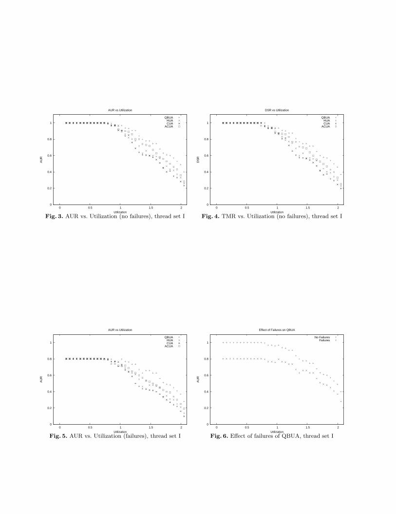
Figures 3 and 4 show the result of our AUR and DSR experiments in the absence of node failure for thread setI. As Figures 3 and 4 show, the performance of QBUA during underloads is similar to that of other distributedreal-time scheduling algorithms. However, during overloads, QBUA begins to outperform other algorithmsdue to its better best effort property. During overloads, QBUA accrues, on average, 17% more utility thatCUA, 14% more utility than HUA and 8% more utility than ACUA. The maximum difference between theperformance of QBUA and the other algorithms in our experiment was the 22% difference between ABUA’sand CUA’s AUR at the 1.88 system load point. Throughout our experiment, the performance of ACUA wasthe closest to QBUA with the difference in performance between these two algorithms getting more pronouncedas system load increases (the largest difference in performance is 11.7% and occurs at about 2.0 system load).The reason for this behavior is that QBUA has a similar best-effort property to ACUA (see Theorem 18). Inaddition, we believe that the difference between these two algorithms becomes more pronounced as system load

0

0.2

0.4

0.6

0.8

1

0 0.5 1 1.5 2

AU

R

Utilization

AUR vs Utilization

QBUAHUACUA

ACUA

Fig. 3. AUR vs. Utilization (no failures), thread set I

0

0.2

0.4

0.6

0.8

1

0 0.5 1 1.5 2

DS

R

Utilization

DSR vs Utilization

QBUAHUACUA

ACUA

Fig. 4. TMR vs. Utilization (no failures), thread set I

0

0.2

0.4

0.6

0.8

1

0 0.5 1 1.5 2

AU

R

Utilization

AUR vs Utilization

QBUAHUACUA

ACUA

Fig. 5. AUR vs. Utilization (failures), thread set I

0

0.2

0.4

0.6

0.8

1

0 0.5 1 1.5 2

AU

R

Utilization

Effect of Failures on QBUA

No FailuresFailures

Fig. 6. Effect of failures of QBUA, thread set I

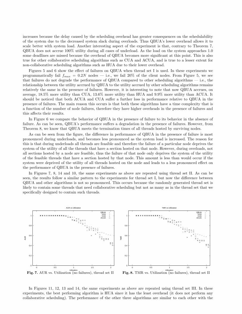
increases because the delay caused by the scheduling overhead has greater consequences on the schedulabilityof the system due to the decreased system slack during overloads. Thus QBUA’s lower overhead allows it toscale better with system load. Another interesting aspect of the experiment is that, contrary to Theorem 7,QBUA does not accrue 100% utility during all cases of underload. As the load on the system approaches 1.0some deadlines are missed because the overhead of QBUA becomes more significant at this point. This is alsotrue for other collaborative scheduling algorithms such as CUA and ACUA, and is true to a lesser extent fornon-collaborative scheduling algorithms such as HUA due to their lower overhead.

Figures 5 and 6 show the effect of failures on QBUA when thread set I is used. In these experiments weprogrammatically fail fmax = 0.2N nodes — i.e., we fail 20% of the client nodes. From Figure 5, we seethat failures do not degrade the performance of QBUA compared to other scheduling algorithms — i.e., therelationship between the utility accrued by QBUA to the utility accrued by other scheduling algorithms remainsrelatively the same in the presence of failures. However, it is interesting to note that now QBUA accrues, onaverage, 18.5% more utility than CUA, 13.6% more utility than HUA and 9.9% more utility than ACUA. Itshould be noticed that both ACUA and CUA suffer a further loss in performance relative to QBUA in thepresence of failures. The main reason this occurs is that both these algorithms have a time complexity that isa function of the number of node failures, therefore they have higher overheads in the presence of failures andthis affects their results.

In Figure 6 we compare the behavior of QBUA in the presence of failure to its behavior in the absence offailure. As can be seen, QBUA’s performance suffers a degradation in the presence of failures. However, fromTheorem 8, we know that QBUA meets the termination times of all threads hosted by surviving nodes.

As can be seen from the figure, the difference in performance of QBUA in the presence of failure is mostpronounced during underloads, and becomes less pronounced as the system load is increased. The reason forthis is that during underloads all threads are feasible and therefore the failure of a particular node deprives thesystem of the utility of all the threads that have a section hosted on that node. However, during overloads, notall sections hosted by a node are feasible, thus the failure of that node only deprives the system of the utilityof the feasible threads that have a section hosted by that node. This amount is less than would occur if thesystem were deprived of the utility of all threads hosted on the node and leads to a less pronounced effect onthe performance of QBUA in the presence of failures.

In Figures 7, 8, 14 and 10, the same experiments as above are repeated using thread set II. As can beseen, the results follow a similar pattern to the experiments for thread set I, but now the difference betweenQBUA and other algorithms is not so pronounced. This occurs because the randomly generated thread set islikely to contain some threads that need collaborative scheduling but not as many as in the thread set that wespecifically designed to contain such threads.

0

0.2

0.4

0.6

0.8

1

0 0.5 1 1.5 2

AU

R

Utilization

AUR vs Utilization

QBUAHUACUA

ACUA

Fig. 7. AUR vs. Utilization (no failures), thread set II

0

0.2

0.4

0.6

0.8

1

0 0.5 1 1.5 2

TM

R

Utilization

TMR vs Utilization

QBUAHUACUA

ACUA

Fig. 8. TMR vs. Utilization (no failures), thread set II

In Figures 11, 12, 13 and 14, the same experiments as above are repeated using thread set III. In theseexperiments, the best performing algorithm is HUA since it has the least overhead (it does not perform anycollaborative scheduling). The performance of the other three algorithms are similar to each other with the

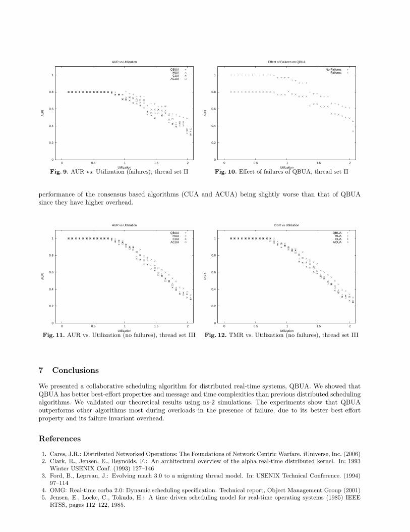
0

0.2

0.4

0.6

0.8

1

0 0.5 1 1.5 2

AU

R

Utilization

AUR vs Utilization

QBUAHUACUA

ACUA

Fig. 9. AUR vs. Utilization (failures), thread set II

0

0.2

0.4

0.6

0.8

1

0 0.5 1 1.5 2

AU

R

Utilization

Effect of Failures on QBUA

No FailuresFailures

Fig. 10. Effect of failures of QBUA, thread set II

performance of the consensus based algorithms (CUA and ACUA) being slightly worse than that of QBUAsince they have higher overhead.

0

0.2

0.4

0.6

0.8

1

0 0.5 1 1.5 2

AU

R

Utilization

AUR vs Utilization

QBUAHUACUA

ACUA

Fig. 11. AUR vs. Utilization (no failures), thread set III

0

0.2

0.4

0.6

0.8

1

0 0.5 1 1.5 2

DS

R

Utilization

DSR vs Utilization

QBUAHUACUA

ACUA

Fig. 12. TMR vs. Utilization (no failures), thread set III

7 Conclusions

We presented a collaborative scheduling algorithm for distributed real-time systems, QBUA. We showed thatQBUA has better best-effort properties and message and time complexities than previous distributed schedulingalgorithms. We validated our theoretical results using ns-2 simulations. The experiments show that QBUAoutperforms other algorithms most during overloads in the presence of failure, due to its better best-effortproperty and its failure invariant overhead.

References

1. Cares, J.R.: Distributed Networked Operations: The Foundations of Network Centric Warfare. iUniverse, Inc. (2006)2. Clark, R., Jensen, E., Reynolds, F.: An architectural overview of the alpha real-time distributed kernel. In: 1993

Winter USENIX Conf. (1993) 127–1463. Ford, B., Lepreau, J.: Evolving mach 3.0 to a migrating thread model. In: USENIX Technical Conference. (1994)

97–1144. OMG: Real-time corba 2.0: Dynamic scheduling specification. Technical report, Object Management Group (2001)5. Jensen, E., Locke, C., Tokuda, H.: A time driven scheduling model for real-time operating systems (1985) IEEE

RTSS, pages 112–122, 1985.

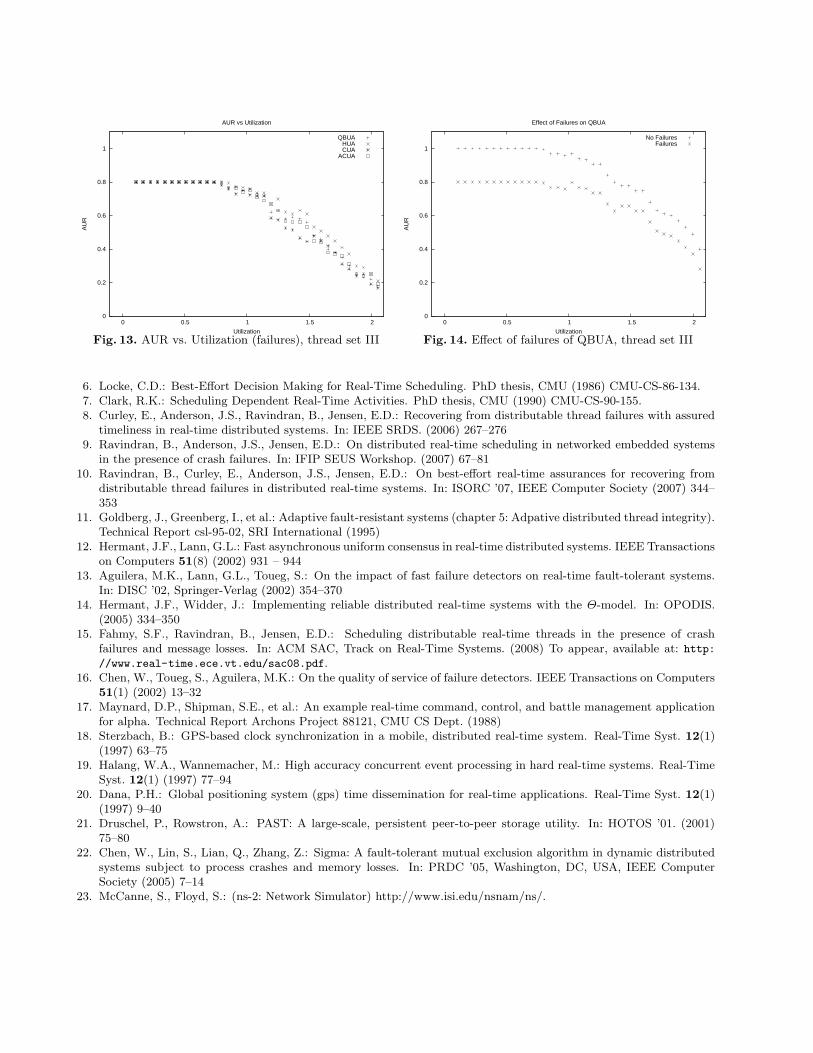
0

0.2

0.4

0.6

0.8

1

0 0.5 1 1.5 2

AU

R

Utilization

AUR vs Utilization

QBUAHUACUA

ACUA

Fig. 13. AUR vs. Utilization (failures), thread set III

0

0.2

0.4

0.6

0.8

1

0 0.5 1 1.5 2

AU

R

Utilization

Effect of Failures on QBUA

No FailuresFailures

Fig. 14. Effect of failures of QBUA, thread set III

6. Locke, C.D.: Best-Effort Decision Making for Real-Time Scheduling. PhD thesis, CMU (1986) CMU-CS-86-134.7. Clark, R.K.: Scheduling Dependent Real-Time Activities. PhD thesis, CMU (1990) CMU-CS-90-155.8. Curley, E., Anderson, J.S., Ravindran, B., Jensen, E.D.: Recovering from distributable thread failures with assured

timeliness in real-time distributed systems. In: IEEE SRDS. (2006) 267–2769. Ravindran, B., Anderson, J.S., Jensen, E.D.: On distributed real-time scheduling in networked embedded systems

in the presence of crash failures. In: IFIP SEUS Workshop. (2007) 67–8110. Ravindran, B., Curley, E., Anderson, J.S., Jensen, E.D.: On best-effort real-time assurances for recovering from

distributable thread failures in distributed real-time systems. In: ISORC ’07, IEEE Computer Society (2007) 344–353

11. Goldberg, J., Greenberg, I., et al.: Adaptive fault-resistant systems (chapter 5: Adpative distributed thread integrity).Technical Report csl-95-02, SRI International (1995)

12. Hermant, J.F., Lann, G.L.: Fast asynchronous uniform consensus in real-time distributed systems. IEEE Transactionson Computers 51(8) (2002) 931 – 944

13. Aguilera, M.K., Lann, G.L., Toueg, S.: On the impact of fast failure detectors on real-time fault-tolerant systems.In: DISC ’02, Springer-Verlag (2002) 354–370

14. Hermant, J.F., Widder, J.: Implementing reliable distributed real-time systems with the Θ-model. In: OPODIS.(2005) 334–350

15. Fahmy, S.F., Ravindran, B., Jensen, E.D.: Scheduling distributable real-time threads in the presence of crashfailures and message losses. In: ACM SAC, Track on Real-Time Systems. (2008) To appear, available at: http://www.real-time.ece.vt.edu/sac08.pdf.

16. Chen, W., Toueg, S., Aguilera, M.K.: On the quality of service of failure detectors. IEEE Transactions on Computers51(1) (2002) 13–32

17. Maynard, D.P., Shipman, S.E., et al.: An example real-time command, control, and battle management applicationfor alpha. Technical Report Archons Project 88121, CMU CS Dept. (1988)

18. Sterzbach, B.: GPS-based clock synchronization in a mobile, distributed real-time system. Real-Time Syst. 12(1)(1997) 63–75

19. Halang, W.A., Wannemacher, M.: High accuracy concurrent event processing in hard real-time systems. Real-TimeSyst. 12(1) (1997) 77–94

20. Dana, P.H.: Global positioning system (gps) time dissemination for real-time applications. Real-Time Syst. 12(1)(1997) 9–40

21. Druschel, P., Rowstron, A.: PAST: A large-scale, persistent peer-to-peer storage utility. In: HOTOS ’01. (2001)75–80

22. Chen, W., Lin, S., Lian, Q., Zhang, Z.: Sigma: A fault-tolerant mutual exclusion algorithm in dynamic distributedsystems subject to process crashes and memory losses. In: PRDC ’05, Washington, DC, USA, IEEE ComputerSociety (2005) 7–14

23. McCanne, S., Floyd, S.: (ns-2: Network Simulator) http://www.isi.edu/nsnam/ns/.