End-to-End Deep Learning in Optical Fibre Communication ...
173
End-to-End Deep Learning in Optical Fibre Communication Systems Boris Karanov A dissertation submitted to University College London for the degree of Doctor of Philosophy Department of Electronic & Electrical Engineering University College London October 2020
-
Upload
khangminh22 -
Category
Documents
-
view
1 -
download
0
Transcript of End-to-End Deep Learning in Optical Fibre Communication ...

End-to-End Deep Learning inOptical Fibre Communication
Systems
Boris Karanov
A dissertation submitted toUniversity College London
for the degree ofDoctor of Philosophy
Department of Electronic & Electrical EngineeringUniversity College London
October 2020

2
I, Boris Karanov, confirm that the work presented in this thesis is my own.Where information has been derived from other sources, I confirm that this hasbeen indicated in the work.

Abstract
Conventional communication systems consist of several signal processing blocks,each performing an individual task at the transmitter or receiver, e.g. coding, mod-ulation, or equalisation. However, there is a lack of optimal, computationally fea-sible algorithms for nonlinear fibre communications as most techniques are basedupon classical communication theory, assuming a linear or perturbed by a smallnonlinearity channel. Consequently, the optimal end-to-end system performancecannot be achieved using transceivers with sub-optimum modules. Carefully cho-sen approximations are required to exploit the data transmission potential of opticalfibres.
In this thesis, novel transceiver designs tailored to the nonlinear dispersive fi-bre channel using the universal function approximator properties of artificial neuralnetworks (ANNs) are proposed and experimentally verified. The fibre-optic systemis implemented as an end-to-end ANN to allow transceiver optimisation over allchannel constraints in a single deep learning process. While the work concentrateson highly nonlinear short-reach intensity modulation/direct detection (IM/DD) fi-bre links, the developed concepts are general and applicable to different models andsystems.
Found in many data centre, metro and access networks, the IM/DD links areseverely impaired by the dispersion-induced inter-symbol interference and square-law photodetection, rendering the communication channel nonlinear with memory.First, a transceiver based on a simple feedforward ANN (FFNN) is investigatedand a training method for robustness to link variations is proposed. An improvedrecurrent ANN-based design is developed next, addressing the FFNN limitationsin handling the channel memory. The systems’ performance is verified in first-in-field experiments, showing substantial increase in transmission distances and datarates compared to classical signal processing schemes. A novel algorithm for end-to-end optimisation using experimentally-collected data and generative adversarialnetworks is also developed, tailoring the transceiver to the specific properties of thetransmission link. The research is a key milestone towards end-to-end optimiseddata transmission over nonlinear fibre systems.

Impact Statement
Optical fibre networks form the major part of the current internet infrastructure andcarry most of the generated digital data traffic. However, the design of conventionalfibre links is based upon classical communication theory, which was developed forlinear systems. Although convenient to engineer, systems using such techniques arenot able to fully exploit the potential for data transmission provided by the nonlin-ear dispersive communication channel, imposing limitations on the achievable datarates and transmission distances. Consequently, fundamentally new methods arerequired to increase the throughput and reach of fibre-optic networks.
This research proposes and, for the first time, demonstrates both numericallyand in lab experiments, a fundamentally new outlook on optical fibre communi-cations. Unlike classical approaches it allows end-to-end optimised transmissionover the channel. The complete fibre-optic system is implemented as an end-to-enddeep artificial neural network (ANN), obtaining transmitter and receiver optimisedin a single process over all channel constraints. The approach is general and can beapplied to different models and systems. The thesis is focused on the applicationto highly nonlinear short-reach optical fibre links, which are the preferred tech-nology in data centre, metro and access networks. Two different end-to-end deeplearning-based designs are proposed – a low complexity system based on a simplefeedforward ANN as well as an advanced design using recurrent neural networksfor nonlinear processing of data sequences. These configurations are successfullyverified in breakthrough experiments. Compared to systems based on state-of-the-art digital signal processing, they can increase the reach or enhance the data rate atshorter distances, while operating with a lower computational complexity. In addi-tion, the developed optimisation algorithms for robustness to link variations and sys-tem self-learning during transmission enable the implementation of efficient, easilyreconfigurable, and versatile transceivers that exploit the data carrying potential ofthe optical fibre to a greater extent. These are key features in keeping operationalcosts low and combined with an efficient hardware implementation can establishthe technology as a prime candidate for deployment in future optical networks.

Acknowledgements
First and foremost, I wish to thank my academic supervisor Prof. Polina Bayvel.Without her trust and encouragement, persuing this dream would not have beenpossible. I will be forever grateful to her for giving me the opportunity to be part ofthe Optical Networks Group (ONG) at UCL. It has been nothing short of an absolutepleasure. Another person to whom I owe a great debt for sharing his experienceand insight is Prof. Laurent Schmalen. His supervision during my secondmentsto Nokia Bell Labs was invaluable for helping me shape the coarse of my Ph.D.I would also like to extend my gratitude to my second academic supervisor Dr.Domaniç Lavery for always providing me with his kind advice.
I gratefully acknowledge the support by the Marie Skłodowska-Curie projectCOIN, a doctorate scheme which gave me the opportunity to develop my researchin both academic and industrial environments. I am extremely thankful to Dr. VahidAref and Dr. Mathieu Chagnon for the great collaboration and discussions duringmy time at Nokia Bell Labs, as well as to Dr. Fred Buchali (Mahlzeit, Fred!), whowas always there to greet me. Special thanks to Dr. Xianhe Yangzhang, with whomwe shared the experience of this unique programme.
For making my Ph.D. journey so exciting and enjoyable, I would like to thankall current and former members of the ONG. Not only for the passionate discussionsabout optical communications over a cup of coffee (for them) or tea (for me), butfor becoming my second family and making 808 my second home. Heartfelt thanksgo to Dr. Paris Andreades (Paaaaris!), Dr. Gabriele Liga, Dr. Gabriel Saavedra,Dr. Sezer Erkilinç, Dr. Kai Shi, Dr. Thomas Gerard and Dr. Eric Sillekens, whowere there for me from day 1 and helped me build my ONG DNA. I hope that Ihave managed to pass a portion of it to the newer members of the group. Dr. FilipeFerreira, Mr. Callum Deakin, Mr. Hubert Dziecol, Mrs. Wenting Yi - no pressure!
I would like to say thank you to Mrs. Mizuho Hino. Her loving kindnesscombined with her endless patience is what got me through this challenging year.
Last but not least, I will mention the unconditional love and moral supportI receive every minute from my mother Yordanka Karanova, my sister DesislavaKaranova, and my grandmother Angelina Mancheva to whom I dedicate this thesis.

Contents
1 Introduction 191.1 Deep learning in communication systems . . . . . . . . . . . . . . 19
1.1.1 Solving communication problems with deep learning . . . . 191.1.2 Applications . . . . . . . . . . . . . . . . . . . . . . . . . 21
1.2 Thesis outline . . . . . . . . . . . . . . . . . . . . . . . . . . . . . 261.3 Key contributions . . . . . . . . . . . . . . . . . . . . . . . . . . . 271.4 List of publications . . . . . . . . . . . . . . . . . . . . . . . . . . 29
2 Artificial neural networks and deep learning 322.1 Artificial neural networks . . . . . . . . . . . . . . . . . . . . . . . 32
2.1.1 Artificial neuron . . . . . . . . . . . . . . . . . . . . . . . 332.1.2 Feedforward ANN . . . . . . . . . . . . . . . . . . . . . . 342.1.3 Recurrent ANN . . . . . . . . . . . . . . . . . . . . . . . . 362.1.4 Generative adversarial network (GAN) . . . . . . . . . . . 40
2.2 Deep learning . . . . . . . . . . . . . . . . . . . . . . . . . . . . . 432.2.1 Gradient descent optimisation . . . . . . . . . . . . . . . . 432.2.2 Backpropagation algorithm . . . . . . . . . . . . . . . . . . 46
3 Optical fibre communication systems for short reach 503.1 Transmitter . . . . . . . . . . . . . . . . . . . . . . . . . . . . . . 51
3.1.1 Digital-to-analogue conversion . . . . . . . . . . . . . . . . 513.1.2 Electro-optical conversion . . . . . . . . . . . . . . . . . . 52
3.2 Propagation over the optical fibre . . . . . . . . . . . . . . . . . . . 533.3 Receiver . . . . . . . . . . . . . . . . . . . . . . . . . . . . . . . . 55
3.3.1 Opto-electrical conversion and amplification . . . . . . . . 553.3.2 Analogue-to-digital conversion . . . . . . . . . . . . . . . . 55
3.4 Communication channel model as a computational graph . . . . . . 56
4 Design of optical fibre systems using end-to-end deep learning 594.1 The optical fibre system as an end-to-end computational graph . . . 60

Contents 7
4.2 Feedforward neural network-based design . . . . . . . . . . . . . . 614.2.1 Transmitter structure . . . . . . . . . . . . . . . . . . . . . 614.2.2 Receiver structure . . . . . . . . . . . . . . . . . . . . . . 64
4.3 Optimisation strategies . . . . . . . . . . . . . . . . . . . . . . . . 664.3.1 Learning at a fixed nominal distance . . . . . . . . . . . . . 684.3.2 Multi-distance learning . . . . . . . . . . . . . . . . . . . . 69
4.4 Numerical investigation of the FFNN auto-encoder performance . . 704.4.1 Bit-to-symbol mapping . . . . . . . . . . . . . . . . . . . . 704.4.2 Generation of training and testing data . . . . . . . . . . . . 714.4.3 Simulation parameters . . . . . . . . . . . . . . . . . . . . 734.4.4 System performance . . . . . . . . . . . . . . . . . . . . . 73
4.5 Summary . . . . . . . . . . . . . . . . . . . . . . . . . . . . . . . 79
5 Recurrent neural network-based optical fibre transceiver 805.1 End-to-end system design . . . . . . . . . . . . . . . . . . . . . . . 81
5.1.1 Transmitter . . . . . . . . . . . . . . . . . . . . . . . . . . 815.1.2 Receiver . . . . . . . . . . . . . . . . . . . . . . . . . . . 855.1.3 Optimisation procedure . . . . . . . . . . . . . . . . . . . . 885.1.4 Sliding window sequence estimation . . . . . . . . . . . . . 905.1.5 Bit labeling optimisation . . . . . . . . . . . . . . . . . . . 93
5.2 Numerical investigation of the system performance . . . . . . . . . 945.2.1 Simulation parameters . . . . . . . . . . . . . . . . . . . . 945.2.2 System performance . . . . . . . . . . . . . . . . . . . . . 95
5.3 Comparisons with state-of-the-art digital signal processing . . . . . 985.3.1 PAM and sliding window feedforward neural network-
based receiver . . . . . . . . . . . . . . . . . . . . . . . . . 985.3.2 SBRNN auto-encoder enhancement via optimisation of the
sequence estimation and bit labeling functions . . . . . . . 1035.3.3 PAM and maximum likelihood sequence detection . . . . . 105
5.4 Summary . . . . . . . . . . . . . . . . . . . . . . . . . . . . . . . 109
6 Experimental demonstrations, comparisons with state-of-the-art DSPand optimisation using measured data 1106.1 Optical transmission test-bed . . . . . . . . . . . . . . . . . . . . . 1116.2 System implementation strategies . . . . . . . . . . . . . . . . . . 1126.3 Collection of representative experimental data for optimisation . . . 1146.4 Experimental demonstration of the FFNN-based auto-encoder . . . 117
6.4.1 Experimental performance results . . . . . . . . . . . . . . 118

Contents 8
6.4.2 Performance comparison with conventional systems . . . . 1216.4.3 Distance-agnostic transceiver . . . . . . . . . . . . . . . . 123
6.5 Experimental demonstration of the SBRNN auto-encoder . . . . . . 1256.5.1 Experimental performance results . . . . . . . . . . . . . . 1276.5.2 Reference PAM systems with state-of-the-art receiver DSP . 1286.5.3 Experimental performance comparison between the
SBRNN auto-encoder and the reference PAM systems . . . 1316.6 End-to-end system optimisation using a generative model . . . . . . 132
6.6.1 Generative adversarial network design . . . . . . . . . . . . 1336.6.2 End-to-end optimisation algorithm . . . . . . . . . . . . . . 1356.6.3 Performance results . . . . . . . . . . . . . . . . . . . . . . 138
6.7 Summary . . . . . . . . . . . . . . . . . . . . . . . . . . . . . . . 139
7 Conclusions and future work 1417.1 Conclusions . . . . . . . . . . . . . . . . . . . . . . . . . . . . . . 1417.2 Future work . . . . . . . . . . . . . . . . . . . . . . . . . . . . . . 144
7.2.1 Advanced optimisation methods for distance-agnostictransceiver enhancement . . . . . . . . . . . . . . . . . . . 144
7.2.2 Extending the auto-encoder framework . . . . . . . . . . . 1457.2.3 Auto-encoders for long-haul coherent optical fibre commu-
nications . . . . . . . . . . . . . . . . . . . . . . . . . . . 146
Appendices 148
A FFNN auto-encoder transmitted signal characteristics 148
B Number of nodes and floating point operations per decoded bit in theSBRNN auto-encoder 152B.1 Counting the number of nodes . . . . . . . . . . . . . . . . . . . . 152B.2 Counting the floating point operations . . . . . . . . . . . . . . . . 153
C Data collection in the experiments 155C.1 SBRNN auto-encoder . . . . . . . . . . . . . . . . . . . . . . . . . 155C.2 Reference PAM systems . . . . . . . . . . . . . . . . . . . . . . . 156
C.2.1 Optimisation of the SFFNN receiver . . . . . . . . . . . . . 156C.2.2 Optimisation of the Volterra receiver . . . . . . . . . . . . . 157C.2.3 Optimisation of the SBRNN receiver . . . . . . . . . . . . 157
D Acronyms 158

Contents 9
Bibliography 161

List of Figures
1.1 General conditions under which deep learning could be consideredas a suitable solution to a communication engineering problem . . . 20
1.2 Basic schematic of a conventional communication system design,showing some of the main signal processing modules at the trans-mitter and the receiver. . . . . . . . . . . . . . . . . . . . . . . . . 22
1.3 Communication system implemented as an end-to-end deep artifi-cial neural network and optimised in a single process. . . . . . . . . 23
1.4 Diagram highlighting the scope and organisation of the thesis. . . . 26
2.1 Basic schematic of an artificial neuron which combines its inputs xi
into an output y. . . . . . . . . . . . . . . . . . . . . . . . . . . . . 33
2.2 Left: sigmoid and hyperbolic tangent (tanh) functions. Right: rec-tified linear unit (ReLU) function. . . . . . . . . . . . . . . . . . . 34
2.3 Schematic representation of a feedforward artificial neural network(FFNN) which transforms an input vector x0 to an output vector xK . 35
2.4 Schematic representation of a recurrent artificial neural network(RNN). . . . . . . . . . . . . . . . . . . . . . . . . . . . . . . . . 37
2.5 Schematic of an RNN “unfolded” in time. . . . . . . . . . . . . . . 37
2.6 Gated recurrent unit (GRU) variant of the long short-term memory(LSTM) cell in recurrent neural networks. . . . . . . . . . . . . . . 38
2.7 Schematic of a bidirectional recurrent neural network (BRNN). . . . 39
2.8 Schematic representation of a generative adversarial network(GAN). The generator aims at transforming the random input vec-tor z into a vector yk, which is statistically identical to yk – a samplevector from the distribution of a real data set. The discriminatoraims at correctly classifying real and fake samples. . . . . . . . . . 41

List of Figures 11
2.9 Illustration of the gradient descent method for minimisation of thefunction f (x) = x2. For f ′(x) < 0 or f ′(x) > 0, the input x is in-creased or decreased, respectively, by a small amount η > 0. Thegradient descent algorithm stops when f ′(x) = 0, where the func-tion f (x) is at a minimum. . . . . . . . . . . . . . . . . . . . . . . 44
2.10 Computational graph representation of the process of computingthe loss in an artificial neural network. For illustrative purposes, thefeedforward network described in Sec. 2.1.2 is used as an ANN ref-erence. It transforms its input x0 to an output xK by performing theoperations xk = αk(Wkxk−1 +bk), k = 1, ..,K. This is followedby the computation of a scalar loss L between xK and the train-ing labels xK . Larger grey nodes are used to highlight the trainableparameters in the graph. . . . . . . . . . . . . . . . . . . . . . . . . 47
3.1 Schematic of an IM/DD communication system, indicating the sig-nal transformations across the transmission link. Tx - transmitter,DSP - digital signal processing, D/A - digital to-analogue conver-sion, E/O - electro-optical conversion, O/E - opto-electrical conver-sion, Amp. - amplification, A/D - analogue-to-digital conversion,Rx - receiver. . . . . . . . . . . . . . . . . . . . . . . . . . . . . . 51
3.2 Schematic showing the communication channel model, which isconsidered as a segment of the end-to-end computational graph,representing the optical fibre communication system. . . . . . . . . 57
4.1 Schematic of the optical communication system implemented as anend-to-end computational graph, which represents the process ofcomputing the loss between the transmitter input and the receiveroutput. . . . . . . . . . . . . . . . . . . . . . . . . . . . . . . . . . 60
4.2 Schematic of the FFNN-based transmitter section of the opticalfibre auto-encoder. The input messages (. . .mt−1,mt ,mt+1 . . .)
are represented as one-hot vectors (. . . ,1m,t−1,1m,t ,1m,t+1 . . .),which are processed independently by the FFNN at each timeinstance to produce the encoded symbols (blocks of samples)(. . .xt−1,xt ,xt+1 . . .), transmitted through the communication channel. 62

List of Figures 12
4.3 Schematic of the FFNN-based receiver section of the optical fibreauto-encoder. The received symbols (. . . ,yt−1,yt ,yt+1 . . .) are pro-cessed independently by the FFNN at each time instance to producethe output probability vectors (. . .pt−1,pt ,pt+1 . . .), which are usedto make a decision on the recovered message as well as to computethe loss of the auto-encoder in the optimisation stage. . . . . . . . . 64
4.4 Schematic of the IM/DD optical fibre communication system im-plemented as a deep feedforward artificial neural network. Optimi-sation is performed using the loss between the input messages andthe outputs of the receiver, thus enabling end-to-end deep learningof the complete system. . . . . . . . . . . . . . . . . . . . . . . . . 67
4.5 Schematic of the training procedure for the FFNN-based auto-encoder, showing how a mini-batch is formed from different trans-mitted sequences of length N over fibre lengths Li and the corre-sponding losses, computed for the central message in every sequence. 69
4.6 BER as a function of transmission distance for a system trainedat 40 km. The horizontal dashed line indicates the 6.7% HD-FECthreshold. The BER with an ideal bit mapping, i.e. a symbol errorresults in a single bit error, is also shown. . . . . . . . . . . . . . . 74
4.7 BER as a function of transmission distance for systems trained ata fixed nominal distance of (20 + i · 10) km, with i ∈ {0, . . . ,6}.The 6.7% HD-FEC threshold is indicated by a horizontal dashedline. Thin dashed lines below the curves give a lower bound on theachievable BER when an ideal bit mapping is assumed. . . . . . . . 75
4.8 Bit error rate as a function of transmission distance for systemswhere the training is performed at normally distributed distanceswith mean µ = 40 km and standard deviation σ . The horizontaldashed line indicates the 6.7% HD-FEC threshold. . . . . . . . . . 76
4.9 Bit error rate as a function of transmission distance for systemswhere the training is performed at normally distributed distancesaround the mean values µ of 20, 40, 60, 80 km and a fixed standarddeviation σ = 4 km. The horizontal dashed line indicates the 6.7%HD-FEC threshold. . . . . . . . . . . . . . . . . . . . . . . . . . . 77
4.10 Bit error rate as a function of transmission distance for systems withdifferent information rates. The training is performed at a fixednominal distance. . . . . . . . . . . . . . . . . . . . . . . . . . . . 78

List of Figures 13
5.1 Schematic of the IM/DD optical fibre communication system im-plemented as a bidirectional deep recurrent neural network. opti-misation is performed between the stream of input messages andthe outputs of the receiver, thus enabling end-to-end optimisationvia deep learning of the complete system. Inset figures show an ex-ample of the transmitted signal spectrum both at the output of theneural network and before the DAC. . . . . . . . . . . . . . . . . . 82
5.2 Schematic of the BRNN-based transmitter section of the optical fi-bre auto-encoder. The input messages (. . .mt−1,mt ,mt+1 . . .), rep-resented as one-hot vectors (. . . ,1m,t−1,1m,t ,1m,t+1 . . .), are pro-cessed bidirectionally at each time instance by the neural networkto produce the sequence of encoded symbols (blocks of samples)(. . .xt−1,xt ,xt+1 . . .). Thick solid lines are used to highlight the theconnections to symbols that have an impact on the processing of mt .Note that a vanilla BRNN cell structure is adopted for illustrativepurposes. . . . . . . . . . . . . . . . . . . . . . . . . . . . . . . . 83
5.3 Schematic of the BRNN-based receiver section of the proposed op-tical fibre auto-encoder. The received symbols (. . . ,yt−1,yt ,yt+1 . . .)
are processed bidirectionally by the BRNN to produce the outputprobability vectors (. . .pt−1,pt ,pt+1 . . .). These are utilised in twoways: to make a decision on the recovered message as well as tocompute the loss of the auto-encoder in the optimisation stage. . . . 86
5.4 Schematic of the sliding window sequence estimation technique inwhich the optimised BRNN transceiver is operated. Note that W =
3 is chosen for illustration purposes. . . . . . . . . . . . . . . . . . 90
5.5 Bit error rate as a function of transmission distance for the 42 Gb/send-to-end vanilla and LSTM-GRU SBRNN auto-encoders com-pared to the 42 Gb/s end-to-end FFNN. . . . . . . . . . . . . . . . . 95
5.6 BER as a function of transmission distance for the FFNN andvanilla SBRNN auto-encoders for different neural network hyper-parameters M, n (FFNN and SBRNN) and sliding window size W(SBRNN). . . . . . . . . . . . . . . . . . . . . . . . . . . . . . . . 96
5.7 Bit error rate as a function of receiver estimation window for the84 Gb/s vanilla and LSTM-GRU SBRNN at 30 km. . . . . . . . . . 97
5.8 Cross entropy loss as a function of optimisation step for the 42 Gb/s(a) vanilla and (b) LSTM-GRU SBRNN systems at 30 km. . . . . . 98
5.9 Schematic of the sliding window FFNN receiver for PAM symbols. 99

List of Figures 14
5.10 BER as a function of transmission distance for the end-to-endvanilla and LSTM-GRU SBRNN systems compared to the end-to-end FFNN as well as the PAM2 system with multi-symbol FFNNreceiver. The systems operate at 42 Gb/s. . . . . . . . . . . . . . . . 101
5.11 Top: SER difference as a function of distance for the two ap-proaches for final probability vector estimation in the sliding win-dow algorithm (W = 10). SERu is obtained assuming a(q) = 1
W ,q =
0, . . . ,W − 1 in Eq. (5.26), while for SERopt the coefficients a(q)
are optimised. Bottom: a(q) assignments after optimisation for thesystem at 100 km. . . . . . . . . . . . . . . . . . . . . . . . . . . . 103
5.12 Bit error rate as a function of distance for a reference vanillaSBRNN auto-encoder, which utilises two different bit-to-symbolmapping approaches: assigning the Gray code to the transmittedmessage m, proposed in Sec. 4.4.1, and performing the combina-torial algorithm-based optimisation, proposed in Sec. 5.1.5. As anindicator, the ideal bit-to-symbol mapping when a single symbolerror gives rise to a single bit error is also displayed. . . . . . . . . . 104
5.13 Schematic diagram of the system used to evaluate the performanceof the MLSD receiver in IM/DD optical links. . . . . . . . . . . . . 105
5.14 Bit error rate as a function of transmission distance for the 42 Gb/sSBRNN auto-encoder and M-PAM & Rx MLSD systems (M ∈{2,4}). In the case of MLSD η = µ log2(M), where µ representsthe number of pre- and post-cursor PAM symbols defining one ofMµ channel states. In the case of SBRNN η = W log2(M) is thenumber of bits inside the processing window. . . . . . . . . . . . . 107
6.1 Diagram showing the three experiments, which were conducted forthe demonstration of the end-to-end deep learning concept in opticalfibre communication systems. . . . . . . . . . . . . . . . . . . . . 110
6.2 Schematic of the experimental optical IM/DD transmission test-bedused for investigation of the digital signal processing schemes inthis chapter. LPF: low-pass filter, DAC: digital-to-analogue con-verter, MZM: Mach-Zehnder modulator, TDM: tunable dispersionmodule, PD: photodiode, TIA: trans-impedance amplifier, ADC:analogue-to-digital converter. . . . . . . . . . . . . . . . . . . . . . 111
6.3 Schematic of the experimental optical IM/DD transmission test-bed, showing the methods for system optimisation using i) numeri-cal simulation of the link; ii) & iii) experimental traces. . . . . . . . 113

List of Figures 15
6.4 Basic schematic showing the data generation, collection and errorcounting. Each of the experiments involved multiple DAC loadswith different random sequences. . . . . . . . . . . . . . . . . . . . 114
6.5 Validation symbol error rate as a function of optimisation step fordifferent lengths lv of the validation pattern. The receiver ANNof the system is optimised using traces from the transmission oftraining sequences with a short pattern ltr = 6 ·102. . . . . . . . . . 115
6.6 Validation symbol error rate as a function of optimisation step fordifferent lengths lv of the validation pattern. The receiver ANN ofthe system is re-trained using data from the transmission of trainingsequences with a long repetition pattern ltr = 104. . . . . . . . . . . 116
6.7 Validation symbol error rate as a function of optimisation step forcontinuously generated random validation messages and differentlengths ltr of the message pattern used for receiver optimisation. . . 117
6.8 Experimental BER performance at 20, 40, 60, 80 km of the FFNN-based auto-encoder trained on an explicit transmission model andapplied “as is” to the optical test-bed. . . . . . . . . . . . . . . . . 119
6.9 Comparison of the experimental BER performance for systemstrained at (20,4) km and (40,4) km (i) without re-training of thereceiver FFNN, (ii) re-training the receiver FFNN by fine-tuning,(iii) training the receiver FFNN by randomization. . . . . . . . . . . 120
6.10 Schematic of a conventional feedforward equaliser, used in the ref-erence PAM transmission for experimental performance comparison. 121
6.11 Experimental BER performance for systems trained at (20,4) kmand (40,4) km. The systems are compared to PAM2 and PAM4systems with receivers based on conventional feedforward equali-sation. . . . . . . . . . . . . . . . . . . . . . . . . . . . . . . . . . 122
6.12 Experimental BER performance for systems trained at (60,4) kmand (80,4) km. The systems are compared to PAM2 and PAM4systems with receivers based on conventional feedforward equali-sation. . . . . . . . . . . . . . . . . . . . . . . . . . . . . . . . . . 123
6.13 Experimental BER performance as a function of transmission dis-tance between 10 and 30 km for a (20,4) km-trained system, whosereceiver ANN parameters are tuned using measured data and themulti-distance learning method proposed in Sec. 4.3.2. . . . . . . . 124

List of Figures 16
6.14 Experimental BER performance as a function of transmission dis-tance between 30 and 50 km for a 42 Gb/s system trained on(40,4) km, whose receiver ANN parameters are tuned using mea-sured data and the multi-distance learning method proposed inSec. 4.3.2. The BER of PAM2 and PAM4 schemes with an FFEreceiver is shown as a performance indicator. Note that the param-eters of the FFE receiver are optimised separately for each distance. 125
6.15 a) Experimental BER performance at 20, 40, 60, 80 km for the42 Gb/s SBRNN-based auto-encoder trained on a channel modeland applied “as is” to the optical fibre transmission test-bed. TheBER of the end-to-end FFNN system is also shown as a perfor-mance indicator. b) BERs at 50, 60 and 70 km as a function of thesliding window size W for the sequence estimation algorithm at theSBRNN receiver. . . . . . . . . . . . . . . . . . . . . . . . . . . . 127
6.16 Schematic of the reference sliding window FFNN receiver for PAMsymbols, utilised in the experiment. . . . . . . . . . . . . . . . . . 129
6.17 Schematic of the second-order nonlinear Volterra equaliser for PAMsymbols, used as a reference system in the experiment. . . . . . . . 130
6.18 BER as a function of transmission distance for 42 Gb/s and 84 Gb/ssystems employing deep learning-based and classical DSP schemesoptimised using experimental data. . . . . . . . . . . . . . . . . . . 131
6.19 Schematic of the utilised conditional GAN for approximating thefunction of the IM/DD transmission link. . . . . . . . . . . . . . . . 133
6.20 Schematic of the experimental setup for end-to-end system opti-misation, showing the forward propagation through the IM/DD linkand the optimisation flow through the generative model, used in lieuof the actual link. . . . . . . . . . . . . . . . . . . . . . . . . . . . 136
6.21 Flow chart of the proposed iterative algorithm for end-to-end deeplearning using measured data. The algorithm includes transmissionand optimisation regimes. . . . . . . . . . . . . . . . . . . . . . . . 136
6.22 Experimental bit error rate as a function of optimisation iteration.Inset figures show: a) error probabilities at k = 0; b) 2D t-SNErepresentation of the waveforms output of the transmitter ANN atk = 10; c) error probabilities at k = 10. . . . . . . . . . . . . . . . . 138

List of Figures 17
7.1 Schematic representation of an auto-encoder system whichparametrises and includes optimisation of the distribution of trans-mitted symbols (pθm) together with the transmitter (θTx) and re-ceiver (θRx) ANN parameters. . . . . . . . . . . . . . . . . . . . . 145
7.2 Schematic diagram of the split step Fourier method used to simulatea small propagation step ∆ along the optical fibre. . . . . . . . . . . 147
A.1 Top: Output of the transmitter ANN, trained at (40,4) km, afterfiltering with 32 GHz brick-wall LPF for the representative randomsequence of 10 symbols (mt)
10t=1 =(2,36,64,40,21,53,42,41,34,13)
transmitted at 7 GSym/s, i.e. T ≈ 143 ps. Bottom: Un-filteredANN output samples, 48 per symbol, for the sub-sequence(mt)
7t=6 = (53,42). . . . . . . . . . . . . . . . . . . . . . . . . . . 149
A.2 All 64 possible outputs (m= 1 to m= 64, upper left to bottom right)of the transmitter FFNN before low-pass filtering. . . . . . . . . . . 150
A.3 t-SNE representation of the multi-dimensional waveforms output ofthe transmitter FFNN on the two-dimensional plane. The points arelabeled with their respective message number m. . . . . . . . . . . . 151
A.4 Spectrum of the 32 GHz brick-wall low-pass filtered waveform atthe output of the transmitter FFNN, trained at (40,4) km. The figurewas generated using 7 MHz spectral bins. . . . . . . . . . . . . . . 151

List of Tables
4.1 FFNN definition at the transmitter . . . . . . . . . . . . . . . . . . 624.2 FFNN definition at the receiver . . . . . . . . . . . . . . . . . . . . 654.3 Simulations parameters assumed for the FFNN-based auto-encoder . 72
5.1 Vanilla and LSTM-GRU cell definitions at the transmitter (singledirection) . . . . . . . . . . . . . . . . . . . . . . . . . . . . . . . 83
5.2 Vanilla and LSTM-GRU cell definitions at the receiver (single di-rection) . . . . . . . . . . . . . . . . . . . . . . . . . . . . . . . . 87
5.3 Simulations parameters assumed for the examined systems . . . . . 945.4 Summary of hyper-parameters for the compared ANN-based systems 102
6.1 Definitions of the transmitter and receiver FFNN used for the exper-imental verification of the end-to-end system optimisation methodusing a generative model . . . . . . . . . . . . . . . . . . . . . . . 133
6.2 Definitions of the generator and discriminator ANNs in the condi-tional GAN . . . . . . . . . . . . . . . . . . . . . . . . . . . . . . 134

Chapter 1
Introduction
1.1 Deep learning in communication systemsThrough decades of innovation, machine learning has been establishing its presenceas a data processing, optimisation and analysis tool in various disciplines, rangingfrom social to natural and applied sciences [1–3]. In recent years, the exponentialincrease and availability of data and computational resources allowed this process topick up an unprecedented speed. One particular class of machine learning methods— deep learning using artificial neural networks— has become the dominant ap-proach for utilising the big data in many areas due to its computational capacity andscalability potential [4, 5]. Powerful deep learning techniques are revolutionisingmany aspects of the modern world, leading a tremendous technology leap in fieldssuch as image and speech analysis [6, 7], and natural language processing [8]. Theapplication to communications engineering follows a similar trajectory and afterearly work in the late 1980s and the 1990s [9], today there is a firm renewal of in-terest in ubiquitously employing machine learning, and deep learning in particular,on various layers of modern communication networks [10, 11].
1.1.1 Solving communication problems with deep learningArtificial neural networks (ANNs) are formed by interconnected processing ele-ments called neurons, organised into multiple layers with nonlinear relation be-tween them [12]. Using a collection of powerful optimisation techniques, such com-putational systems can be optimised to approximate complex nonlinear functions —a process which is often referred to as deep learning. Deep learning is a data-drivenoptimisation approach, which relies on the availability of a large set of examples,representative of the function’s behaviour. It combines well-known algorithms suchas backpropagation [13] and gradient descent [14, 15] with modern adaptive learn-ing techniques, specifically developed for multi-layer (deep) ANNs [16–18].
Using artificial neural networks and deep learning for the design and optimi-
1.1. Deep learning in communication systems 20
DL solution Other solution
ProblemReconstruct x from y Problem solved
Modely “ fpxq
knownunknown
Algorithmx “ finvpyq
available
notavailable
Complexity„ O pdimpyqq
Datayi “ fpxiq, i P N
low
high
available (|N | large) not available (|N | small)
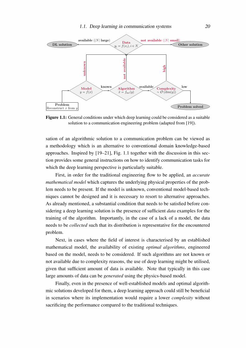
Figure 1.1: General conditions under which deep learning could be considered as a suitablesolution to a communication engineering problem (adapted from [19]).
sation of an algorithmic solution to a communication problem can be viewed asa methodology which is an alternative to conventional domain knowledge-basedapproaches. Inspired by [19–21], Fig. 1.1 together with the discussion in this sec-tion provides some general instructions on how to identify communication tasks forwhich the deep learning perspective is particularly suitable.
First, in order for the traditional engineering flow to be applied, an accuratemathematical model which captures the underlying physical properties of the prob-lem needs to be present. If the model is unknown, conventional model-based tech-niques cannot be designed and it is necessary to resort to alternative approaches.As already mentioned, a substantial condition that needs to be satisfied before con-sidering a deep learning solution is the presence of sufficient data examples for thetraining of the algorithm. Importantly, in the case of a lack of a model, the dataneeds to be collected such that its distribution is representative for the encounteredproblem.
Next, in cases where the field of interest is characterised by an establishedmathematical model, the availability of existing optimal algorithms, engineeredbased on the model, needs to be considered. If such algorithms are not known ornot available due to complexity reasons, the use of deep learning might be utilised,given that sufficient amount of data is available. Note that typically in this caselarge amounts of data can be generated using the physics-based model.
Finally, even in the presence of well-established models and optimal algorith-mic solutions developed for them, a deep learning approach could still be beneficialin scenarios where its implementation would require a lower complexity withoutsacrificing the performance compared to the traditional techniques.

1.1. Deep learning in communication systems 21
Although communication engineering is a field with well-established channelmodels [22–24] as well as algorithms for reliable communication over them [25],they apply only to a sub-class of all communication problems. Moreover, often theavailable domain knowledge can be integrated into the learning algorithm, while thecollection of a sufficiently large amount of data for training in certain situations canbe easier than applying traditional approaches. As a consequence, the advantagesof applying deep learning in place of a conventional technique should be evaluatedon an individual basis.
1.1.2 ApplicationsThe unparalleled growth of interconnected devices nowadays leads to an enormousamount of generated Internet traffic which increases at an exponential rate [26].This results in rapidly increasing complexity and dynamics in all modern network-ing systems, the core part of which is constituted by the optical fibre infrastruc-ture, and presents great challenges for their configuration, management and con-trol [27, 28]. Stringent requirements regarding the quality of service, latency andflexibility to frequent change in conditions are fastly becoming infeasible to realiseusing conventional approaches. In the same time, the ubiquitous collection of var-ious networking data, for example from monitoring reports, has empowered wideinterest in developing scalable, energy-efficient and optimised solutions using deeplearning, artificial neural networks and machine learning in general [29–33]. Forexample, the techniques have been used for the modeling, prediction and classifica-tion of the data traffic flow [34–40], enabling a promising direction for substantiallyreducing the operational cost of the network [34].
From physical layer’s perspective, the application of deep learning, as a col-lection of powerful optimisation tools, is considered particularly suitable for dig-ital signal processing (DSP). Advanced DSP algorithms enable the compensationfor wide variety of transmission impairments and have become an effective ubiq-uitously employed solution for increasing the data rate and transmission reach ofstate-of-the-art communication systems [41, 42]. The conventional communicationtransceiver design consists of several DSP blocks, each employed to perform anindividual task. Figure 1.2 shows a basic schematic representation of such a sys-tem. At the transmitter, signal processing functions such as coding, modulation,pre-compensation and pulse-shaping are applied to the incoming data, shaping thesignal before it is launched into the transmission link. At the receiver, the signal, dis-torted by the communication channel, is typically equalised before functions suchas demodulation and decoding are performed to recover the transmitted data. Such amodular transceiver implementation is convenient from an engineering perspective

1.1. Deep learning in communication systems 22
data in
Transmitter
coding,modulation,pulse-shaping, ..
Transmission link
Receiver
equalisation,demodulation,decoding, ..
data out
Figure 1.2: Basic schematic of a conventional communication system design, showingsome of the main signal processing modules at the transmitter and the receiver.
as it allows separate analysis, optimisation and control of the DSP blocks.Due to their powerful function approximation capabilities, the use of artificial
neural networks combined with deep learning in the DSP chain of modern com-munication transceivers has attracted great interest. Often the techniques are con-sidered for the optimisation or the computational complexity reduction of a specificDSP function. This has been achieved by incorporating varying degrees of the avail-able domain knowledge for completing the DSP task. For example, artificial neuralnetworks and deep learning enabled a low-complexity near-optimal solution for thedemodulation of received symbols in additive white Gaussian noise (AWGN) chan-nels [43]. Applications in the decoding process of forward error correction (FEC)codes have also been widely investigated [44–47]. In [44] deep learning was appliedfor the optimisation of the existing belief propagation decoding algorithm for linearcodes, leading to increased decoding capabilities. This prompted the developmentof methods for complexity reduction of the scheme [48]. In [47] it was shown thatadvanced recurrent neural network architectures can be used for the optimal (up toa specific memory) decoding of convolutional codes.
During propagation through the communication link, the transmitted signalsundergo various distortions which are often mitigated using digital equalisationschemes at the receiver. Typically, the equalisation algorithms are designed us-ing the available mathematical model, which describes the propagation through thetransmission medium. For example, an efficient method for the compensation ofdeterministic distortions in long-haul coherent optical fibre systems is to solve thenonlinear Schrödinger equation, which governs signal propagation over the opti-cal fibre, using negated medium parameters, a technique known as digital back-propagation (DBP) [49]. The algorithm involves multiple iterations of linear andnonlinear processing steps, whose number, and thus the computational complexityof the DBP, increases with the input power, transmission bandwidth and distance.Moreover, exact knowledge of the link parameters is required for optimal compen-sation. A method, known as learned DBP (LDBP), which consists in “unfolding”the iterative algorithm to interpret its steps as ANN layers and apply deep learning,allowed to reduce the complexity and tune the compensation to the specific link pa-rameters [50–52]. Signal equalisation using ANNs has been considered for satellite

1.1. Deep learning in communication systems 23
data in
Neural network
Transmitter
Transmission Link
Neural network
Receiver
data out
End-to-end system optimisation
Figure 1.3: Communication system implemented as an end-to-end deep artificial neuralnetwork and optimised in a single process.
communications in the early 1990s [53, 54], while in recent years the method at-tracted a renewed interest in both long-haul [55,56] and short-reach [57,58] opticalfibre communications.
All aforementioned applications of ANNs and deep learning are exampleswhere the techniques were applied for the optimisation of a specific DSP func-tion in the transmitter or receiver, which themselves consist of signal processingmodules with separated tasks. However, the approach of designing and optimis-ing the communication system independently on a module-by-module basis canbe sub-optimal in terms of the end-to-end performance. A different approach todeep learning-based DSP, which utilises the function approximation capabilities ofartificial neural networks and deep learning to a greater extent, is to interpret thecomplete communication chain from the transmitter input to the receiver output asa single deep ANN and optimise its parameters in an end-to-end process. The ideaof such fully learnable communication transceivers (known as auto-encoders) wasintroduced for the first time for wireless communications in [59–61]. The auto-encoders avoid the modular design of conventional communication systems andhave the potential to achieve an end-to-end optimised performance for a specificmetric. Figure 1.3 shows a simple schematic of such an end-to-end deep learning-based system.
The application of auto-encoders is particularly viable in communication sce-narios where the optimum pair of transmitter and receiver or optimum DSP mod-ules are not known or computationally prohibitive to implement. The approach wasquickly utilised in optical fibre communications aiming at exploiting to a greaterextent the potential for data transmission [62–65]. In particular, the achievable datarates and transmission distance in short reach optical fibre links based on the in-tensity modulation/direct detection (IM/DD) technology are severely limited by thepresence of chromatic dispersion and nonlinear (square-law) signal detection [23].

1.1. Deep learning in communication systems 24
The joint effects of dispersion, which causes intersymbol interference (ISI), andsquare-law detection render the optical IM/DD a nonlinear communication channelwith memory for which optimal, computationally feasible algorithms are not avail-able. State-of-the-art IM/DD systems employ techniques such as nonlinear Volterraequalisation [66] or maximum likelihood sequence detection [67–69] to address thechannel distortions. However, as the channel memory increases, the implementa-tion of such algorithms quickly becomes infeasible because of the associated com-putational complexity. Moreover, their performance can be significantly degradedwhen the complexity is constrained. On the other hand, deep learning, which canapproximate complex nonlinear functions, can be used to provide carefully chosentransmitter and receiver for the optical IM/DD via end-to-end optimisation. TheIM/DD systems play an important role as the enabling technology in many datacentre, metro and access optical fibre networks [70] and the application of end-to-end deep learning for enhancing the system performance is a promising directionfor investigation. Moreover, it should also be noted that the relatively stable linkconditions, typical for guided transmission media such as the optical fibre, furtherfacilitate the prospect of end-to-end system learning.
In the research described in this thesis, the concept of end-to-end deep learn-ing was applied for the first time in optical fibre communications. The work wasfocused on IM/DD systems, but it should be emphasized that the developed designsand methods are not restricted to this scheme and can be extended to different sys-tems. In particular, two different transceiver designs were proposed — a simplestructure using a feedforward ANN (FFNN) as well as an advanced design basedon a recurrent ANN (RNN), tailored to the dispersive properties of the nonlinearchannel. Their performance was extensively investigated in numerical simulationsand successfully verified on an experimental optical IM/DD test-bed. The complex-ity and performance of the auto-encoder systems was compared to state-of-the-artIM/DD transmission schemes based on pulse amplitude modulation with receiversusing classical DSP approaches such as nonlinear Volterra equalisation and maxi-mum likelihood sequence detection. The research included development of novelmethods for the optimisation of the deep learning-based optical transceivers. Firstly,an approach for the generalisation of the ANN parameters, which allowed transmis-sion over varied distances without reconfiguration of the transceivers, was proposedand experimentally demonstrated. Moreover, the concept of end-to-end optical fibresystem optimisation using a generative adversarial network (GAN) and experimen-tally collected data was introduced and verified on the transmission test-bed.
The work in this thesis forms an important step towards establishing end-to-end deep learning as a viable digital signal processing solution for future optical

1.1. Deep learning in communication systems 25
fibre communication networks.

1.2. Thesis outline 26
End-to-end deep learning inoptical fibre communications
Introduction to artificial neural networksand deep learning (Chapter 2)
Artificial neuronOptimisationvia deep learning
FFNN RNN GAN Gradientdescent
Back-propagation
Optical fibre systemsfor short reach (Chapter 3)
Transmissionmodel
Computational graphrepresentation
Deep learning-basedtransceiver designs (Chapters 4 and 5)
FFNN auto-encoder RNN auto-encoder
Tx/Rxprocessing
Optimisationstrategies
Simulationperformance
Tx/Rxprocessing
Complexity
Performancecomparisons
Experimental demonstration ofoptical fibre auto-encoders (Chapter 6)
Datacollection
Implementationstrategies
Performancecomparisons
Learning insimulation
Learning frommeasured data
Receiveroptimisation
End-to-end systemoptimisation using GAN
Figure 1.4: Diagram highlighting the scope and organisation of the thesis.
1.2 Thesis outlineFigure 1.4 shows a diagram which summarises the organisation and highlights thescope of this thesis. The remainder of the thesis is organised as follows:
Chapter 2 gives a detailed description of the artificial neural networks anddeep learning techniques which are used throughout this thesis. It starts with an in-troduction to artificial neural networks (ANNs) of which the simplest feedforwardANN (FFNN) is presented first, followed by the recurrent ANN (RNN) and thegenerative adversarial network (GAN). The deep learning framework for trainingof the neural network parameters is summarised next. This includes introduction tothe gradient descent (GD) optimisation method, as well as the backpropagation al-gorithm for computing gradients. Then, the specific variant of a learning algorithmthat is used in this work is introduced – a stochastic gradient descent optimisationmethod, known as the Adam optimiser.
Chapter 3 presents the physical properties of the intensity modulation/directdetection optical fibre transmission system, used as a reference in the developmentof the end-to-end deep learning concept. It includes a detailed description of themathematical modeling of all the system components.
In Chapter 4 an optical fibre system design based on an end-to-end deep feed-forward neural network is proposed and numerically investigated. The principles

1.3. Key contributions 27
of block-based transmission enabled by the FFNN are explained and the process-ing at the transmitter and receiver sections of the systems are described in detail.Simulation results for the system performance are also presented. Moreover, anovel method for training of the neural network parameters, developed to obtaintransceivers robust to distance variations, is introduced in this chapter.
In Chapter 5 an advanced system design based on a sequence processing us-ing a bidirectional RNN (BRNN) is developed. The neural network functions withinthe transmitter and receiver are described together with the efficient sliding windowsequence estimation algorithm in which the optimised system is operated. Thischapter also includes the procedures developed for coefficient optimisation for theestimation algorithm, as well as techniques for optimising the bit-to-symbol map-ping function. The performance of the end-to-end BRNN-based auto-encoder isnumerically investigated and compared to conventional pulse amplitude modulation(PAM) systems with state-of-the-art nonlinear ANN equalizers as well as maximumlikelihood sequence detection (MLSD). The complexity of the BRNN system is alsoanalysed and compared to these benchmarks.
Chapter 6 focuses on the experimental demonstration of the FFNN and BRNNsystems as well as the verification of the proposed optimisation method for robust-ness to distance variations. It begins with a detailed description of the experimentaloptical IM/DD transmission test-bed. Then, the data collection procedures are ex-plained. The system performance is examined at different transmission distances. Adetailed experimental comparison with PAM transmission and the receivers basedon classical digital signal processing is also carried out. Importantly, the chapterincludes a description and experimental demonstration of the proposed concept forend-to-end system optimisation using a GAN-based model of the actual transmis-sion link obtained using collected data from measurements.
Chapter 7 summarises the work presented in Chapters 4, 5 and 6, and out-lines important future directions for development of the research towards flexibletransceivers and applications in long-haul optical systems.
1.3 Key contributionsi) In Chapter 4 a novel framework for coding and detection in optical fibre com-
munications using end-to-end deep learning is introduced and numerically in-vestigated for the first time. The work was published in [2].
ii) A novel training method for the generalisation of the neural network parame-ters is presented in Chapter 4 and its experimental verification is described inChapter 6. It allows the optimisation of transceivers robust to variations in the

1.3. Key contributions 28
transmission distance. This concept was published in [2], while its experimen-tal demonstration was published in [12].
iii) In Chapter 5 an advanced transceiver design performing nonlinear sequenceprocessing using recurrent neural networks is developed and its performanceis numerically evaluated, outperforming state-of-the-art DSP algorithms. Thework led to publications [1] and [11].
iv) In Chapter 5 an offline method for optimising the weight assignments in thesliding window estimation algorithm in which the recurrent neural networktransceiver is operated is developed. This method, which allowed additionalperformance improvement of the system, was published in [11].
v) In Chapter 5 a bit-to-symbol optimisation method using a combinatorial algo-rithm is proposed. It was published in [11].
vi) In Chapter 5 a comparative study of performance and computational complex-ity with a benchmark maximum likelihood sequence detection system for therecurrent neural network-based transceiver is described. This investigation waspublished in [11].
vii) In Chapter 6 the first experimental demonstration of an optical fibre systemimplemented as an end-to-end deep neural network is presented. The setupand the results from the experiment were reported in [2].
viii) The first-in-field experiment of an end-to-end recurrent neural network-basedoptical system is described in Chapter 6. The system setup and performancewere reported in [8] and [9].
ix) Comprehensive numerical (Chapters 4 and 5) and experimental (Chapter 6)comparisons with conventional IM/DD systems based on linear and nonlinearreceiver digital signal processing were carried out. These results were pub-lished in [2],[8],[11], and [12].
x) The concept and experimental demonstration of an end-to-end optical systemoptimisation using data collected from measurements are presented in Chap-ter 6. The proposed algorithm, which employs a generative adversarial networkfor modeling of the real transmission link, was published in [10].

1.4. List of publications 29
1.4 List of publicationsThe conducted research resulted in the following peer-reviewed publications:
Journal papers1. B. Karanov, D. Lavery, P. Bayvel, and L. Schmalen, "End-to-end optimized
transmission over dispersive intensity-modulated channels using bidirectionalrecurrent neural networks," OSA Opt. Express, vol. 27, no. 14, pp. 19650-19663, 2019
2. B. Karanov, M. Chagnon, F. Thouin, T. Eriksson, H. Bülow, D. Lavery, P.Bayvel, and L. Schmalen, "End-to-end deep learning of optical fiber commu-nications," IEEE/OSA J. Lightwave Technol., vol. 36, no. 20, pp. 4843-4855,15 Oct., 2018
3. Z. Liu, B. Karanov, L. Galdino, J. R. Hayes, D. Lavery, K. Clark, B. C.Thomsen, K. Shi, D. Elson, M. Petrovich, D. J. Richardson, F. Poletti, R.Slavik and P. Bayvel, "Nonlinearity-free coherent transmission in hollow-coreantiresonant fiber," IEEE/OSA J. Lightwave Technol., vol. 37, no. 3, pp. 909-916, 2019
4. B. Karanov, T. Xu, N. Shevchenko, D. Lavery, R. I. Killey, and P. Bayvel,"Span length and information rate optimisation in optical transmission sys-tems using single-channel digital backpropagation," OSA Opt. Express, vol.25, no. 21, pp. 25353-25362, 2017
5. T. Xu, B. Karanov, N. Shevchenko, D. Lavery, G. Liga, R. I. Killey, and P.Bayvel, "Digital nonlinearity compensation in high-capacity optical commu-nication systems considering signal spectral broadening effect," Nature Sci.Rep., vol. 7, pp. 12986, 2017
Conference papers
6. B. Karanov, P. Bayvel, and L. Schmalen, “End-to-end learning in opticalfiber communications: Concept and transceiver design,” in Proc. EuropeanConference on Optical Communications (ECOC), 2020 [Invited]
7. B. Karanov, V. Oliari, M. Chagnon, G. Liga, A. Alvarado, V. Aref, D. Lav-ery, P. Bayvel, and L. Schmalen, “End-to-end learning in optical fiber commu-nications: Experimental demonstration and future trends,” in Proc. EuropeanConference on Optical Communications (ECOC), 2020 [Invited]

1.4. List of publications 30
8. B. Karanov, M. Chagnon, V. Aref, F. Ferreira, D. Lavery, P. Bayvel, andL. Schmalen, “Experimental investigation of deep learning for digital signalprocessing in short reach optical fiber communications,” in Proc. IEEE Inter-national Workshop on Signal Processing Systems (SiPS), 2020 [Invited]
9. B. Karanov, M. Chagnon, V. Aref, D. Lavery, P. Bayvel, and L. Schmalen,“Optical fiber communication systems based on end-to-end deep learning,” inProc. IEEE Photonics Conference (IPC), 2020 [Invited]
10. B. Karanov, M. Chagnon, V. Aref, D. Lavery, P. Bayvel, and L. Schmalen,"Concept and experimental demonstration of optical IM/DD end-to-end sys-tem optimization using a generative model," in Proc. Optical Fiber Commu-nications Conference (OFC), 2020, paper Th2A.48
11. B. Karanov, G. Liga, V. Aref, D. Lavery, P. Bayvel, and L. Schmalen, "Deeplearning for communication over dispersive nonlinear channels: Performanceand comparison with classical digital signal processing," in Proc. Aller-ton Conference on Communication, Control, and Computing, 2019, paperWeB2.5 [Invited]
12. M. Chagnon, B. Karanov, and L. Schmalen, "Experimental demonstrationof a dispersion tolerant end-to-end deep learning-based IM-DD transmis-sion system," in Proc. European Conference on Optical Communications(ECOC), 2018, paper Tu4F.6
13. B. Karanov, T. Xu, N. Shevchenko, D. Lavery, G. Liga, R. I. Killey, andP. Bayvel, "Digital nonlinearity compensation considering signal spectralbroadening effects in dispersion-managed systems," in Proc. Optical FiberCommunications Conference (OFC), 2018, paper W2A.58
14. T. Xu, B. Karanov, N. Shevchenko, D. Lavery, G. Liga, Z. Li, D. Jia, L. Li,L. Kanthan, R. I. Killey, P. Bayvel, "Spectral broadening effects in opticalcommunication networks: Impact and security issue," in Proc. InternationalConference on Advanced Infocomm Technology (ICAIT), 2018 [Invited]
15. T. Xu, N. Shevchenko, B. Karanov, D. Lavery, L. Galdino, A. Alvarado,R. I. Killey, and P. Bayvel, "Nonlinearity compensation and information ratesin fully-loaded C-band optical fibre transmission systems," in Proc. EuropeanConference on Optical Communications (ECOC), 2017, paper P2.SC6.30
16. T. Xu, N. Shevchenko, B. Karanov, G. Liga, D. Lavery, R. I. Killey, andP. Bayvel, "Digital nonlinearity compensation in high-capacity optical fibre

1.4. List of publications 31
communication systems: Performance and optimisation," in Proc. Advancesin Wireless and Optical Communications (RTUWO), 2017 [Invited]
17. Z. Liu, L. Galdino, J. R. Hayes, D. Lavery, B. Karanov, D. J. Elson, K. Shi,B. C. Thomsen, M. N. Petrovich, D. J. Richardson, F. Poletti, R. Slavik, andP. Bayvel, "Record high capacity (6.8 Tbit/s) WDM coherent transmissionin hollow-core antiresonant fiber," in Proc. Optical Fiber CommunicationsConference (OFC), 2017, paper Th5B.8 [Post-deadline]

Chapter 2
Artificial neural networks and deeplearning
The combination of artificial neural networks (ANNs), known as universal func-tion approximators, and deep learning is a powerful tool for the modeling of anycomplex function [12]. This chapter starts with an introduction to the data process-ing and optimisation objective in the different types of artificial neural networks,used to perform the research described in the thesis. This is followed by a detaileddescription of the deep learning techniques enabling the optimisation of the ANNparameters.
2.1 Artificial neural networksThe original concept of artificial neural networks, introduced in the 1940s, was in-spired by the prospect of mimicking the biological neural networks in the humanbrain [71]. Nevertheless, their application as computational entities has been far-reaching. An ANN consist of simple interconnected processing elements, calledartificial neurons, which are typically organised into multiple layers. It has beenmathematically proven in the late 1980s that such structures can be optimised toapproximate an arbitrary mapping from one vector space to another [72–74]. Theoptimisation of an artificial neural network can be performed using a set of labeleddata examples for training, i.e. in the so-called supervised manner. For this purpose,the pairing of an input and a desired output is defined. The training set is formedby such pairings, whose number (set size) is chosen such that the data is represen-tative of the input-to-output mapping function to be approximated by the ANN. Inthis section the data processing in the artificial neuron, the building block of everyANN is discussed. Then, three different types of networks and their optimisationobjectives are introduced — feedforward and recurrent ANNs as well as generativeadversarial networks.

2.1. Artificial neural networks 33
x1
x2
xl
yu
ω1
ω2
ωl
b
Σ αp¨q...x
Figure 2.1: Basic schematic of an artificial neuron which combines its inputs xi into anoutput y.
2.1.1 Artificial neuronFigure 2.1 shows a schematic representation of an artificial neuron. The function ofthe neuron is to map its inputs xi to an output y through an operation given by
y = α
(l
∑i=1
ωixi +b
), (2.1)
where xi ∈ R, i = 1 . . . l are the inputs to the neuron, which can be denoted by thevector x ∈ Rl , y ∈ R is the neuron’s scalar output, ωi ∈ R, i = 1 . . . l and b ∈ Rare the neuron’s weights (one for each input) and bias parameters, while α is theso-called activation function. The neuron’s activation function plays an importantrole in the structure of every ANN as it is typically chosen to introduce a nonlinearrelation between the layers, enabling the approximation of nonlinear functions.
A commonly employed activation function in state-of-the-art ANNs is the rec-tified linear unit (ReLU) [75], which keeps the positive values and equates the neg-ative to zero, i.e. y = αReLU(u) with
y = max(0,u). (2.2)
Another function often used as an activation for the artificial neurons is the sigmoidy = αsigmoid(u) where
y =1
1+ exp(−u). (2.3)
The sigmoid translates its input to an output in the (0;1) region. A function that canoutput negative values and is also often used in practice is the hyperbolic tangent,expressed as y = αtanh(u) with
y =exp(u)− exp(−u)exp(u)+ exp(−u)
. (2.4)

2.1. Artificial neural networks 34
´6 ´4 ´2 0 2 4 6´1
´0.5
0
0.5
1
u
y
y “ sigmoidpuqy “ tanhpuq
´6 ´4 ´2 0 2 4 60
1
2
3
4
5
6
u
y
y “ ReLUpuq
Figure 2.2: Left: sigmoid and hyperbolic tangent (tanh) functions. Right: rectified linearunit (ReLU) function.
The hyperbolic tangent function allows the neuron output to take values in the(−1;1) range. Figure 2.2 exemplifies the ReLU, sigmoid and hyperbolic tangentfunctions. The choice of an activation function for the layers of an ANN has an im-pact on the speed and convergence of the procedure for parameter optimisation. Adetailed description of the optimisation procedure is provided in Section 2.2. Com-pared to the other two popular activation functions, the ReLU has a constant gra-dient, which renders training computationally less expensive and also partly avoidsthe effect of vanishing gradients. This effect occurs for activation functions withasymptotic behaviour, such as sigmoid and tanh, since the gradient can becomesmall and consequently decelerate the convergence of the learning algorithm. A dis-cussion on the vanishing gradient problem in the training of ANNs can be found in[12, Sec. 8.2]. Another important activation function, the softmax function, whichnormalises the whole layer of neurons in order to provide probability outputs, isintroduced in the following section together with the simplest form of organisationof artificial neurons – the feedforward ANN.
2.1.2 Feedforward ANN
2.1.2.1 Data processing
An artificial neural network consists of interconnected layers of neurons. Eachlayer is characterised by an activation function as well as a weight matrix and abias vector where the parameters of its neurons are organised. Figure 2.3 shows aschematic of a feedforward ANN (FFNN), a network where the data is passed onlyin one direction – from the input to the output layer (forward). The network is fullyconnected, i.e. the output of each of the nodes (neurons) in one layer is used as aninput to all nodes in the next layer. A K-layer FFNN maps an input vector x0 to an

2.1. Artificial neural networks 35
x0
xK´1
xK
neuron
. . .
Figure 2.3: Schematic representation of a feedforward artificial neural network (FFNN)which transforms an input vector x0 to an output vector xK .
output vector xK = fFFNN(x0) through the iteratively applied operations of the form
xk = αk(Wkxk−1 +bk), k = 1, ..,K, (2.5)
where xk−1 ∈ Rlk−1 is the output of the (k−1)-th ANN layer, xk ∈ Rlk is the outputof the k-th layer, Wk ∈ Rlk×lk−1 and bk ∈ Rlk are respectively the weight matrix andthe bias vector of the k-th layer and αk is its activation function.
As already mentioned, the ANN can be trained to approximate any complexfunction, which is enabled by the presence of a (typically nonlinear) activation func-tion on each layer. In addition to the most common activation functions describedin the previous section, the softmax is another important function. It is appliedelement-wise and is defined as y = softmax(u) with
yi =exp(ui)
∑j
exp(u j). (2.6)
The softmax function is typically used on the final layer of an ANN in cases wherea probability output is required (e.g. in classification tasks) and performs normali-sation of the whole layer such that ∑
iyi = 1.
2.1.2.2 Optimisation objective
For the optimisation of parameters in the FFNN, pairings between an input vectorx0 and a desired output vector xK are defined as elements in the training set. Let theset of all parameters of the FFNN is denoted by
θ = {φ1, . . . ,φK}, (2.7)

2.1. Artificial neural networks 36
where φk = {Wk,bk} is the set of parameters for the k-th layer. The objective ofthe training is to minimize, over the training set, the loss (error) L (θ) betweenthe desired output xK,i and the ANN output xK,i = fFFNN(x0,i), with respect to theparameter set θ . The loss can be expressed as
L (θ) =1|S| ∑
(x0,i,xK,i)∈S
`(xK,i, fFFNN
(x0,i)) , (2.8)
where `(x,y) denotes the specific per-example loss function that is utilised and |S|denotes the cardinality of the training set, i.e. the number of (x0,i, xK,i) pairings ofinputs and labeled outputs used for training. A ubiquitously employed loss functionin classification tasks, which is as well considered in this thesis, is the cross entropydefined as
`(x,y) =−∑i
xi log(yi). (2.9)
To achieve a machine learning estimator, both the input to the neural network x0
and the desired output xK are typically represented as a one-hot vector of size M,denoted as 1m ∈ RM, where the m-th element equals 1 and the other elements are0. Such one-hot encoding is the standard way of representing categorical valuesin most deep learning algorithms [12]. Accordingly, the final layer in the neuralnetwork uses the softmax activation such that its output xK is a probability vector.Section 2.2 presents the approach for optimisation of the parameter set θ aimed atminimising the computed loss.
2.1.3 Recurrent ANN
2.1.3.1 Data processingAs described in the previous section, feedforward neural networks process eachinput vector independently to obtain an output. The structure of such networksdoes not include mechanisms allowing information to persist when dealing withsequences of data. However, the solutions to many tasks, especially in communica-tion systems, require processing of data sequences. In such cases, the applicationof an advanced ANN architecture – the recurrent neural network (RNN) [13, 76] isbeneficial.
Figure 2.4 illustrates the basic concept of a recurrent neural network. As seenin the figure, the structure of an RNN is characterised by a loop which allows someinformation from the previous processing steps to be included in the processingof the current data input. This is further exemplified in Fig. 2.5, which presents aschematic of the RNN loop “unfolded” in time. The recurrent structure takes as aninput the sequence (. . . ,xt−1,xt ,xt+1, . . .). At time t, the input vector xt is processed

2.1. Artificial neural networks 37
RNN cell
xt
ht
T
Figure 2.4: Schematic representation of a recurrent artificial neural network (RNN).
RNN cell RNN cell RNN cell
xt´1 xt xt`1
ht´1 ht ht`1
. . . . . .
Figure 2.5: Schematic of an RNN “unfolded” in time.
by the recurrent cell together with the previous output ht−1 to produce an updatedoutput ht . In its simplest (vanilla) variant, the processing in the recurrent cell issimilar to the single-layer FFNN, acting on the concatenation between the currentinput and previous output. Thus, the current output of the recurrent cell can beexpressed as
ht = α
(W(
xTt hT
t−1
)T+b), (2.10)
where xt ∈Rl is the RNN input at time t, ht−1 ∈Rn is the RNN output at time t−1,W ∈Rn×(n+l) and b ∈Rn are the weight matrix and bias vector, respectively, and T
denotes the matrix transpose. The activation function is denoted by α .
In addition to the vanilla RNN cell, which processes the simple concatenationof the current input with the most recent output of the network, more advancedstructures have been developed to adequately model long-term dependencies, char-acteristic for certain tasks [77]. The long short-term memory (LSTM) architectureis one of the most widely used designs for learning long-term dependencies in se-quential data, achieved by preserving information in an internal cell state [78]. The

2.1. Artificial neural networks 38
ht´1
xt
ˆgat
1´gbt
ˆ
ˆ
`ht
ht
Figure 2.6: Gated recurrent unit (GRU) variant of the long short-term memory (LSTM) cellin recurrent neural networks.
LSTM is an enabling technique in many fields related to language processing [79]and different variants of the cell structure have been examined to enhance the per-formance, reduce the complexity or improve the convergence speed [80]. A partic-ularly efficient LSTM architecture with state-of-the-art performance is the so-calledgated recurrent unit (GRU), proposed in [81]. Next, the structure of the GRU cellis introduced in more detail.
Figure 2.6 shows a GRU schematic. Compared to the vanilla structure, it con-sists of two additional single-layer memory gates ga
t and gbt employed to control the
information flow in the cell. The gates take as an input the concatenation of thecurrent input xt with the previous output ht−1 and their function is to decide whichelements of the previous output should be preserved for further processing. Thecurrent output of the GRU cell is obtained as
gat = α1
(W1
(xT
t hTt−1
)T+b1
), (2.11)
gbt = α2
(W2
(xT
t hTt−1
)T+b2
), (2.12)
ht = (1−gbt )�ht−1 +gb
t �α3
(W3
(xT
t (gat �ht−1)
T)T
+b3
), (2.13)
where � denotes the Hadamard product (element-wise multiplication of vectors)and Wi and bi are the layers’ weights and biases, whose sizes are identical to thesize of the weight and bias of the vanilla cell. The activation functions of the twogates, i.e. α1 and α2, are typically chosen to be the sigmoid function, while α3 can

2.1. Artificial neural networks 39
ht
Merge
RNN cell
RNN cell
ÐÝh t
ÝÑh t
xt
ÝÑh t´1
ÝÑh t
ÐÝh t`1
ÐÝh t
Figure 2.7: Schematic of a bidirectional recurrent neural network (BRNN).
be the ReLU or the hyperbolic tangent functions.
So far, all aforementioned RNN examples consider dependencies in the se-quence (. . . ,xt−1,xt ,xt+1, . . .) which are stemming only from the preceding data,i.e. the transformation of xt is performed using information from the previous in-puts xt−k, k = 1 . . . t − 1. Such unidirectional processing is inherently unable tomodel any influence on the current input to the RNN occurring from the post-cursordata. To enable the modeling of both preceding and succeeding dependencies ina data sequence, the bidirectional recurrent neural network (BRNN) architecturewas introduced in [82]. Subsequently, the BRNN mechanism has been widely ap-plied for example in the field of speech processing as it allow to efficiently captureimportant contextual information [83].
Figure 2.7 shows a schematic of the BRNN concept. It combines two unidi-rectional RNNs which are responsible for the processing of the input sequence inits original (forward) and reversed (backward) order. In the forward direction, theconcatenation of an input xt at time t with the previous output
−→h t−1 is processed
by the recurrent cell to produce an updated output−→h t . The procedure is performed
on the full data sequence. In order to adequately handle dependencies from the suc-ceeding symbols, the structure is repeated in the backward direction, updating theoutputs
←−h t . Assuming a simple vanilla cell structure in both directions, the process-

2.1. Artificial neural networks 40
ing in the BRNN can be expressed as
−→h t = αfw
(Wfw
(xT
t−→h T
t−1
)T+bfw
), (2.14)
←−h t = αbw
(Wbw
(xT
t←−h T
t+1
)T+bbw
), (2.15)
ht = merge(−→
h t ,←−h t
), (2.16)
where−→h t and
←−h t denote the outputs of the RNN cells in the forward and the back-
ward directions, respectively, Wfw and Wbw are the corresponding weight matricesin the forward (fw) and backward (bw) directions, while bfw and bbw are the biasvectors. The activation functions used in the two directions, which are typicallyidentical, are denoted by αfw and αbw. The outputs of the forward and the backwardpasses at the same time instance t are combined by the merge function. Typically,either an element-wise averaging or a concatenation of the two output vectors, i.e.
ht =12
(−→h t +
←−h t
)or ht =
(−→h T
t←−h T
t
)T, is performed.
2.1.3.2 Optimisation objectiveSimilarly to the FFNN, the optimisation of the RNN (and BRNN) is also typicallyperformed in a supervised manner by using a set of labeled data. The goal is toobtain a set of neural network parameters for the recurrent cell (denoted by θ ), suchthat the loss L (θ), given by
L (θ) =1|S| ∑
((...,xt−1,xt ,xt+1,...),xt)∈S`(xt , fRNN,t(. . . ,xt−1,xt ,xt+1, . . .)) , (2.17)
is minimised. Note that fRNN,t(. . . ,xt−1,xt ,xt+1, . . .) denotes the output of the RNNat the same time instance t as the desired output xt (the label). The per-example lossfunction is denoted by `(x,y) and is typically the cross entropy which was alreadydefined in Sec. 2.1.2, Eq. (2.9).
2.1.4 Generative adversarial network (GAN)
2.1.4.1 Data processingThe generative adversarial network (GAN) is an efficient tool for the learning ofgenerative models [84]. Such models are used to generate new data instances bylearning the probability distribution of a real dataset. In particular, the generativemodel is used to simulate a random vector y, which follows some distribution p(y)that is not known, but for which a representative set of data yk, k = 1 . . .K (samples

2.1. Artificial neural networks 41
z yk
yk
pr{f
real sample
fake sample
Generator Discriminator
Figure 2.8: Schematic representation of a generative adversarial network (GAN). The gen-erator aims at transforming the random input vector z into a vector yk, which isstatistically identical to yk – a sample vector from the distribution of a real dataset. The discriminator aims at correctly classifying real and fake samples.
from p(y)) is available.
The GAN model can be viewed as similar to the inverse transform method [85,Ch. 2] for generating random variables that follow a given distribution by “reshap-ing” random variables with simpler distributions such as the normal or uniformdistributions [86]. Figure 2.8 shows a schematic of a generative adversarial net-work. The GAN employs two artificial neural networks, typically with feedforwardarchitectures, that have competing objective functions (see Sec. 2.1.4.2). The gen-erator ANN aims at translating its input into a (high-dimensional) output vector,mimicking the ground truth distribution of the real dataset. The discriminator actsas a binary classifier between real (ground truth) and fake (generated) vectors. Toachieve its goal, the generator takes as an input an l-dimensional vector of randomsamples, which are typically uniformly- or normally-distributed, i.e. z ∼U
(0,1)l or
z ∼N(0,1)
l , where U (0,1) denotes the uniform distribution over the interval (0,1)and N (0,1) denotes the standard normal distribution. The GAN generator trans-forms z into the fake vector sample
yk = Gθ g (z) , (2.18)
where Gθ g is an operator describing the function of the generator feedforward ANN,with θ g denoting the set of all its weight and bias parameters. Subsequently, thediscriminator is first fed with a sample yk from the real dataset, yielding the output
pr = Dθ d (yk) , (2.19)
where Dθ d is the function of the discriminator feedforward ANN, with θ d beingthe set of all its weight and bias parameters. Afterwards, the the generated (fake)
2.1. Artificial neural networks 42
sample yk is also fed to the discriminator, producing the output
pf = Dθ d (yk) . (2.20)
Typically, the discriminator ANN is designed such that the outputs pr and pf areprobabilities, indicating the confidence whether the input was real or fake.
2.1.4.2 Optimisation objective
For optimisation of the generator and discriminator ANN parameters, labels lr andlf are assigned for the real and fake samples, respectively. When obtaining the lossLG of the generator ANN, the parameters θ d at the discriminator are assumed to befixed. As a result, the loss is a function of θ g given by
LG(θ g) =1|S| ∑
zi,lr∈S`(lr,Dθ d
(Gθ g (zi)
)), (2.21)
where the training set S is formed by the pairings of a random input vector z andthe label for real samples lr, while `(·) denotes the utilised loss function such as thecross entropy. Note that when dealing with probability outputs, the labels can beconveniently set to lr := 1 and lf := 0, for the real and fake samples, respectively.
On the other hand, the loss of the discriminator LD, assuming a fixed set θ g ofgenerator parameters, can be expressed as
LD(θ d) =1|S| ∑
(zi,lf),(yi,lr)∈S[`(lr,Dθ d (yi)
)+ `(lf,Dθ d
(Gθ g (zi)
))]. (2.22)
Note that here the training set is formed by two pairings – one between the generatorinput vector z and the label for fake samples lf, and another between the samplevector yi from the real distribution and the label for real samples lr.
The parameters of the generator and discriminator are optimised iteratively.The objective for the discriminator is to minimise LD(θ d), thus learning to classifyits real (y) and fake (y=Gθ g (z)) inputs correctly. On the other hand, by minimisingthe loss LG(θ g), the generator model learns to translate its random input vector zinto representations y = Gθ g (z) which are statistically similar to the samples y fromthe real distribution. The goal of such an adversarial ANN training algorithm is toconverge to parameter sets for which the generator output, given a random input,approximates the distribution of the real data, while the discriminator is unable todifferentiate between the two distributions (see [84, Sec. 4]).

2.2. Deep learning 43
2.2 Deep learningDeep learning techniques, applied for the optimisation of neural network parame-ters, play an integral role in exploiting their potential for universal function approxi-mation. This section introduces the gradient descent algorithm – a key deep learningstrategy for optimisation of the ANN parameters. It also explains the backpropaga-tion technique which enables efficient computation of gradients in deep ANNs.
2.2.1 Gradient descent optimisationGradient descent (GD) is a powerful and efficient method for minimisation of afunction f (x). The technique was proposed for the first time by Augustin Cauchyin 1847 [14] and later expanded by Haskell Curry for nonlinear optimisation prob-lems [15]. It has a fundamental role in many areas of optimisation theory and deeplearning [5, 12]. The GD method utilises the information given by the gradient∇x f (x) about the slope of the function f (x) at x. It aims at reducing f (x) by ad-justing x in small steps with a sign (direction) opposite to that of the gradient. As asimple illustrative example, consider the function
f (x) = x2, (2.23)
of the scalar variable x ∈ R, whose derivative is f ′(x) = 2x. Figure 2.9 shows bothf (x) and f ′(x). For values x < 0, the derivative f ′(x) is negative, indicating that thefunction is decreasing, i.e. f (x+η) < f (x), with η > 0 and thus the input x canbe increased by a small amount η to reduce f (x). On the other hand, f ′(x)> 0 forx > 0 (the function is increasing) and thus f (x−η)< f (x), i.e. f (x) is reduced byreducing the input with a small amount η . At x = 0 the function reaches a stationarypoint where f ′(x) = 0. There, the derivative provides no information how to adjustx and the GD method halts. For the considered example, reaching the point x = 0,i.e. the end of the GD, coincides with arriving at the global minimum of f (x).This simple GD algorithm can be formally generalised and written using a vectornotation as
xt = xt−1−η ·∇x f (xt−1). (2.24)
The update of x depends on the steepness of the slope of f (x), allowing greaterchanges for steeper slopes (high absolute value of the gradient) and finer stepsaround the stationary points. It is important to mention that often, especially inthe framework of deep learning, the input is multidimensional and the optimisationcan encounter and converge to local minima. As a consequence, deep learning isassociated with performing approximate minimisation of the given objective. Inpractice, state-of-the-art variants of the GD technique (described in the following

2.2. Deep learning 44
´2 ´1.5 ´1 ´0.5 0 0.5 1 1.5 2´4
´2
0
2
4
f 1pxqă0,fpx`ηqăfpxq
f 1pxqą0,fpx´ηqăfpxq
f 1pxq“0,fpxq – minimised at x“0
x
fpxq “ x2
f 1pxq “ 2x
Figure 2.9: Illustration of the gradient descent method for minimisation of the functionf (x) = x2. For f ′(x) < 0 or f ′(x) > 0, the input x is increased or decreased,respectively, by a small amount η > 0. The gradient descent algorithm stopswhen f ′(x) = 0, where the function f (x) is at a minimum.
sections) have been developed to achieve convergence to solutions correspondingto very low function values [12, Sec. 4].
2.2.1.1 Stochastic gradient descentIn order to perform GD minimisation of the computed loss L (θ) in an ANN, thegradient ∇θL (θ) with respect to the ANN parameters needs to be calculated usingthe entire, typically very large, training set. This imposes a great computationalburden to perform the GD algorithm. A commonly employed approach, whichreduces the computational demands, is to use a stochastic approximation [87] ofthe GD, a method known as a stochastic gradient descent (SGD) [12, 18, 88]. TheSGD performs optimisation of the ANN parameters operating on estimates of thegradient obtained from small randomly-selected sub-sets (called mini-batches) ofthe training data. The algorithm aims at updating the set of ANN parameters θ suchthat the loss L (θ) over a mini-batch S, given by (for FFNN)
L (θ) =1|S| ∑
(x0,xK)∈S
`(xK, fFFNN
(x0)) , (2.25)

2.2. Deep learning 45
is minimised. The mini-batch loss for BRNN (Sec. 2.1.3.2) or GAN (Sec. 2.1.4.2)is correspondingly expressed. On the first step of the SGD algorithm, the ANNparameters θ are randomly initialised and then iteratively updated as
θ t = θ t−1−η ·∇θL (θ t−1), (2.26)
where η is referred to as the step-size of the learning algorithm and ∇θL (θ) de-notes the gradient of the mini-batch loss with respect to the parameters θ . Theproduct η ·∇θL (θ) determines the learning rate and speed of convergence of theSGD algorithm and thus many variants for its adaptation has been considered. Anextensive overview and comparison of many popular implementations can be foundin [18] and [12, Sec. 8.3-8.7]. In particular, the “adaptive moment” estimation(Adam) algorithm has been specifically developed for the training of deep ANNsand has become the de facto default optimisation method in the field of deep learn-ing [17, 18, 89]. The Adam optimiser is introduced in the following section andhas been used for the learning of ANN parameters for the research covered by thisthesis.
2.2.1.2 Adaptive moment estimation (Adam) optimiser
The Adam algorithm is a computationally efficient variant of the SGD strategywith an improved convergence achieved by the dynamic adaptation of the learningrate [16]. To control the learning rate, the method utilises biased moving averagesof the gradient µ t and the squared gradient ν t , estimated as [16, Sec. 2]
µ t = β1 ·µ t−1 +(1−β1) ·∇θL (θ t−1), (2.27)
ν t = β2 ·ν t−1 +(1−β2) · (∇θL (θ t−1))2 , (2.28)
respectively. Where ()2 denotes the element-wise square function, and β1 and β2
are the corresponding exponential decay rates, whose default values are empiricallyevaluated and set to β1 = 0.9 and β2 = 0.999 (see [16, Sec. 6.4]). Next, the termsare biased-corrected as
µ t =µ t
1−β t1, (2.29)
ν t =ν t
1−β t2. (2.30)
Subsequently, the update of the ANN parameters is governed by
θ t = θ t−1−η · µ t
(√
ν t + ε), (2.31)

2.2. Deep learning 46
where ε is a small constant used for numerical stability, which is typically set toε = 10−8 as originally suggested in [16, Sec. 2]).
2.2.2 Backpropagation algorithmThe calculation of the gradient of the scalar mini-batch loss ∇θL (θ) with respectto the ANN parameters is a key aspect in the optimisation procedure. A simple andcomputationally efficient method for the computation of gradients, first proposedin [13], is the so-called backpropagation algorithm. In order to introduce the algo-rithm, this section starts with the representation of ANNs as computational graphs,followed by the description of backpropagation, which consists in recursively ap-plying the chain rule of calculus [90] across the graph nodes.
2.2.2.1 Computational graph of an ANNFigure 2.10 shows an example of a computational graph which represent the pro-cess of computing the loss function in an artificial neural network. The nodes onthe graph indicate the variables (in scalar, vector, matrix or other multi-dimensionalform) that are subject to operations (e.g. matrix multiplication, addition, etc.). Inparticular, for illustrative purposes, the presented graph uses as a reference a deepfully-connected feedforward ANN (see Sec. 2.1.2). As already discussed, this net-work translates its input x0 to an output xK through the series of operations of theform xk = αk(Wkxk−1 + bk), k = 1, ..,K. Note that in the computational graphthis transformation is expressed as
uk1 = Wkxk−1, (2.32)
uk2 = uk1 +bk, (2.33)
xk = αk(uk2), (2.34)
such that all intermediate expressions are represented by a node. Importantly, in ad-dition to the ANN operations, the scalar loss L (see Sec. 2.1.2, Eq. (2.5)) betweenthe output xK of the ANN and the corresponding training label xK is also computed.This is indicated by the final node on the graph. Such a representation of an ANNand its loss computation, highlights the dependencies of the optimisation objectiveon all nodes in the deep network. In particular, the goal of the optimisation proce-dure is to update the trainable nodes in the graph (highlighted in grey colour on theschematic) such that L is minimised.
2.2.2.2 Backpropagation algorithmThe backpropagation algorithm consists in recursively applying the chain rule ofcalculus for computing gradients of functions [13], [12, Sec. 6.5]. As an example,

2.2. Deep learning 47
x0 W1
ˆb1
`u11 u12
α1
x1 W2
ˆb2
`u21 u22
α2
x2
...
xK 1 WK
ˆbK
`uK1 uK2
αK
xK xK
L`p¨q
Figure 2.10: Computational graph representation of the process of computing the loss in anartificial neural network. For illustrative purposes, the feedforward networkdescribed in Sec. 2.1.2 is used as an ANN reference. It transforms its input x0
to an output xK by performing the operations xk = αk(Wkxk−1 +bk), k =1, ..,K. This is followed by the computation of a scalar loss L between xK andthe training labels xK . Larger grey nodes are used to highlight the trainableparameters in the graph.

2.2. Deep learning 48
Algorithm 1 The backpropagation algorithm performed over the reference compu-tational graph presented in Fig. 2.10.
1: g← ∇xKL . Initialise with gradient of loss w.r.t final ANN output2: for k = K,K−1 . . .1 do . Iterate starting from the final ANN layer
3: ∇uk2L =(
∂αk(uk2)∂uk2
)Tg . Apply chain rule
4: g← ∇uk2L . Update last computed gradient
5: ∇bkL =(
∂ (uk1+bk)∂bk
)Tg . Compute bias gradient
6: ∇uk1L =(
∂ (uk1+bk)∂uk1
)Tg
7: ∇WkL =(
∂ (Wkxk−1)∂Wk
)Tg . Compute weight gradient
8: ∇xk−1L =(
∂ (Wkxk−1)∂xk−1
)Tg . Compute gradient w.r.t lower layer output
9: g← ∇xk−1L . Update last computed gradient10: end for
assume that the vector x ∈ Rm is mapped to y ∈ Rn, i.e. y = f1(x), and then thescalar variable Z ∈ R is computed via a different mapping Z = f2(y). To obtain thegradient ∇xZ of Z with respect to x, the chain rule can be utilised. In vector notationit is expressed as
∇xZ =
(∂y∂x
)T
∇yZ, (2.35)
where
∂y∂x
=
∂y1∂x1
. . . ∂y1∂xm
... . . . ...∂yn∂x1
. . . ∂yn∂xm
(2.36)
is the n×m Jacobian matrix of the mapping f1 from x to y. For the optimisation ofan ANN, the gradients of the scalar loss with respect to the trainable nodes in theANN graph need to be computed. Using the computational graph from Fig. 2.10as a reference, the backpropagation algorithm allows to obtain the gradients ∇WkL
and ∇bkL , k = 1 . . .K for the network weights and bias parameters. They aresubsequently utilised in the gradient descent optimisation procedure, which wasdescribed in Section 2.2.1. The backpropagation algorithm, whose detailed step-by-step description is given in Algorithm 1, is initialised by computing the gradient∇xKL of the loss L with respect to the final ANN output xK . It then proceeds withcomputing gradients across the computational graph of the ANN, moving in thebackward direction, until all gradients of L , from the K-th to the first layer of theANN, have been computed. It is worth mentioning that in the case of a recurrentANN, the computational graph will include dependencies between different time

2.2. Deep learning 49
instances. In this case, the utilised algorithm for computation of gradients, identicalin its essence to the presented example, is often referred to as backpropagationthrough time.

Chapter 3
Optical fibre communication systemsfor short reach
Short reach optical communications are found in many data centre, metro and ac-cess network scenarios. Such systems crucially rely on the simplicity and cost-effectiveness of a signal transmission scheme based on intensity modulation withdirect detection (IM/DD) [23,70]. The short reach links typically consist of a singlefibre span, thus avoiding the associated costs of deploying in-line optical amplifica-tion. The IM/DD technology enables the utilisation of electronic and optical com-ponents that are inexpensive, have a small footprint and low power consumption.It is thus considered as a prime candidate for fibre to the home (FTTH) systems,realised, for instance, via passive optical networks (PONs).
The optical IM/DD communication links are mainly characterised by the pres-ence of fibre chromatic dispersion, which introduces inter-symbol interference (ISI),and nonlinear (square-law) photodiode (PD) detection. Moreover, due to the hard-ware imperfections and bandwidth limitations in the low-cost components, the sig-nal is corrupted by a significant amount of noise and nonlinearity stemming frommultiple sources at both transmitter and receiver, i.e. modulators, electrical amplifi-cation circuits as well as low resolution digital-to-analogue and analogue-to-digitalconverters. Meeting the ever-increasing data rate demands for such systems be-comes quite a challenging task because of the limitations imposed by these impair-ments and the application of advanced DSP algorithms has attracted great interestin recent years [66, 91, 92].
In this chapter, the transformations and distortions undergone by the signalpropagating between the output of the transmitter DSP module and the input tothe DSP module at the receiver are described in detail. Figure 3.1 shows a gen-eral schematic of an optical intensity modulation/direct detection system, high-lighting the parts of the transmission link where digital-to-analogue/analogue-to-

3.1. Transmitter 51
DSPTx
input data
. . . xi´1, xi . . . D/Axptq
E/Oqp0, tq
O/E+Amp.qpL, tq yptq
A/D . . . yi´1, yi . . .
DSP Rx
output data
fibre
Transmission link (communication channel)
Figure 3.1: Schematic of an IM/DD communication system, indicating the signal trans-formations across the transmission link. Tx - transmitter, DSP - digital signalprocessing, D/A - digital to-analogue conversion, E/O - electro-optical conver-sion, O/E - opto-electrical conversion, Amp. - amplification, A/D - analogue-to-digital conversion, Rx - receiver.
digital, electro-optical/opto-electrical conversions and optical fibre propagation areperformed. The remaining chapters of this thesis are concerned with proposing DSPschemes allowing reliable communication over such a channel.
3.1 Transmitter
3.1.1 Digital-to-analogue conversion
The output samples (. . .xi−1,xi,xi+1 . . .) ∈ R≥0 from the DSP module at the trans-mitter are transformed into an analogue electrical signal x(t) using a digital-to-analogue converter (DAC). The device is characterised by its sampling period Ts [s]from which the DAC sampling rate is obtained as
fs =1Ts
[Hz]. (3.1)
Accordingly, the Nyquist frequency of the DAC is then given by
fNyq. =fs
2. (3.2)
The significance of this expression is that the digital signal applied for DAC conver-sion must have a frequency content limited to fNyq. in order to be fully recoverable.In practice, due to hardware limitations of the device, the actual DAC bandwidthis smaller than fNyq. [93] and typically the signal is low-passed filtered before theconverter. The output of the low-pass filter (LPF) can be expressed as
x′(t) = s(t)∗g1(t) =∞
∑i=−∞
xig1(t− iTs), (3.3)

3.1. Transmitter 52
where g1(t) is the impulse response of the LPF, while the train of input samples isrepresented by the temporal train of Ts-spaced impulses
s(t) =∞
∑i=−∞
xiδ (t− iTs), (3.4)
with δ (·) denoting the Dirac delta function. The impulse response of the so calledbrick-wall LPF, which has a unit frequency gain and sets the the bandwidth of thereal-valued signal to B f is given by
gLPF(t) = sinc(2B f πt). (3.5)
The DAC distorts x′(t) as a consequence of its limited quantisation resolution.This distortion is modeled as an additive and uniformly distributed quantisationnoise [94, 95] and the real-valued analogue electrical signal at the output of theDAC can correspondingly be expressed as
x(t) = x′(t)+n1(t), (3.6)
where n1(t) denotes the noise contribution. In particular, the output signal-to-noiseratio (SNR) of the DAC, and thus the variance of n1(t), is determined by the ef-fective number of bits (ENOB) of the device. The theoretical output SNR of adigital-to-analogue converter with an ENOB of Nb bits is given by [95]
SNR = 6.02Nb +1.76 [dB]. (3.7)
The noise n1(t) is zero mean, i.e.
E(n1(t)) = 0, (3.8)
where E(·) denotes the expectation operator. The corresponding quantisation noisevariance then becomes
σ2n1= 3E
(|x′(t)|2
)·10−(6.02·Nb+1.76)/10. (3.9)
For state-of-the-art high-speed DACs the typical Nb values are between 5 and 6 [96].
3.1.2 Electro-optical conversionAt the electro-optical conversion stage at the transmitter, a Mach-Zehnder modula-tor (MZM) is employed to externally modulate the amplitude of an optical carrierwave, generated by a laser source. The MZM is driven by the electrical signal x(t).

3.2. Propagation over the optical fibre 53
Neglecting laser fluctuations, the electric field of the laser light is given by
ξ (t) = |E0| · exp(− jωct) , (3.10)
where |E0| is the field amplitude and ωc is the angular frequency. The MZM modu-lates ξ (t) with the information-carrying signal x(t), resulting in the complex-valuedbandpass optical signal
q(0, t) = sin(x(t)) · |E0| · exp(− jωct) , (3.11)
where sin(·) is modeling the modulator electric field transfer function [97]. It actson the information signal x(t), whose amplitude thus needs to be restricted in the[−π/2,π/2] interval, e.g. by proper scaling in the DSP. Omitting the carrier termfrom Eq. (3.11), the modulated real-valued baseband signal becomes
q(0, t) = |E0| · sin(x(t)) . (3.12)
This scheme is referred to as Intensity Modulation (IM) since varying the amplitudeof the laser field, results in modulation of the optical intensity I(0, t) at the fibreinput, with the two quantities related as
I(0, t) ∝ |q(0, t)|2. (3.13)
3.2 Propagation over the optical fibreThe propagation of the optical signal q(z, t) through the fibre medium can be de-scribed by the second-order nonlinear partial differential equation (PDE)
∂q(z, t)∂ z
=−α
2q(z, t)− j
β2
2∂ 2q(z, t)
∂ t2 + jγ|q(z, t)|2q(z, t), (3.14)
where α , β2, and γ are the fibre attenuation, chromatic dispersion and Kerr nonlin-earity coefficients, respectively, z denotes the distance along the fibre, and j =
√−1
is the imaginary unit. Equation (3.14) is referred to as the nonlinear Schrödingerequation (NLSE).
The nonlinear Kerr effect is associated with local changes of the fibre refractiveindex due to the intensity of the optical field [24]. Typically, for IM/DD systemsthe intensity at the fibre input I(0, t) is small and subsequently attenuated by themedium. Moreover, as already discussed, such systems do not employ in-line sig-nal amplification. As a consequence, the impact of the Kerr nonlinearity during

3.2. Propagation over the optical fibre 54
propagation along the fibre can be neglected [23]. The fibre-induced attenuation ofthe signal is taken into account in the definition of the noise at the receiver, presentedin Sec. 3.3.
Chromatic dispersion is the dominant fibre effect for IM/DD transmission sys-tems. According to the NLSE, its operation on the propagating signal is expressedby
∂q(z, t)∂ z
=− jβ2
2∂ 2q(z, t)
∂ t2 , (3.15)
which is a second-order linear PDE that can be solved analytically in the frequencydomain, where it is re-written as
∂Q(z,ω)
∂ z= j
β2
2ω
2Q(z,ω), (3.16)
with a solution given by
Q(z,ω) = Q(0,ω)exp(
jβ2
2ω
2z), (3.17)
whereQ(0,ω) = F{q(0, t)}, (3.18)
is the Fourier transform of the transmit signal q(0, t). The time domain opticalsignal at distance z can then be recovered as
q(z, t) = F−1{Q(z,ω)}, (3.19)
where the operator F−1 denotes the inverse Fourier transformation. Often the dis-persion of the optical fibre is specified by the parameter D, from which β2 can beobtained as
β2 =−λ 2
2π · cD, (3.20)
where λ denotes the wavelength, while c is the speed of light in vacuum. Equa-tion (3.17) shows that chromatic dispersion induces a propagation delay betweenthe different components in the frequency content of the propagating pulses. Thiscauses their temporal broadening, an effect which accumulates linearly with dis-tance and quadratically with bandwidth. As a result, a pulse will interact and in-terfere with other preceding and succeeding pulses during propagation through thefibre medium. Chapter 4 and Chapter 5 explain why such a distortion can lead tointer-symbol interference (ISI), introducing memory in the communication channeland imposing severe limitations on the IM/DD optical fibre transmission.

3.3. Receiver 55
3.3 Receiver3.3.1 Opto-electrical conversion and amplificationThe signal q(z, t) at the the output of a fibre span of length z is converted fromthe optical back to the electrical domain by a photodetector. In IM/DD systems,a simple p-i-n photodiode (PD) is used to perform the square-law detection of theincoming optical signal [23, 70]. The output photocurrent of the PD is proportionalto the intensity of the impinging optical field, i.e.
y′(t) = ρ|q(z, t)|2, (3.21)
where ρ ∈ (0,1] is the responsivity of the photodetector. Such a nonlinear signalreception using a single PD is called Direct Detection (DD).
The detection is followed by the electrical amplification of the signal, attenu-ated from the propagation along the fibre link. The amplification is often performedby a transimpedance amplifier (TIA) and in practice the PD and TIA componentsare combined in a single package, referred to as a PIN+TIA module. The TIAamplification circuit is associated with corrupting the signal with an additive whiteGaussian noise [70, 98], i.e.
y(t) = y′(t)+n2(t), (3.22)
The noise is modeled as zero-mean, while its variance σ2ref. can be estimated using
the measured signal-to-noise ratio SNRref. at the output of the amplifier at a refer-ence distance. Taking the fibre attenuation into account will yield different effectiveSNRs at each transmission distance z. To model this, the variance of the noise n2(t)added to the signal as a function of z is obtained as
σ2n2(z) =
σ2ref.
exp(−αz), (3.23)
where α [1/km] is the attenuation coefficient of the fibre in linear units. Typicallyfibre attenuation is specified in decibel units (αdB/km) and thus the conversion α =
αdB/km/4.343 should be considered. Typically, αdB/km = 0.2 [dB/km] for a standardsingle mode fibre, effectively resulting in doubling of the noise every 15 km.
3.3.2 Analogue-to-digital conversionIn the next step, the amplified electrical signal y(t) needs to be converted into adigital form. This is achieved using an analogue-to-digital converter (ADC). Priorto the ADC, similarly to the transmitter chain of operations, the signal is low-pass

3.4. Communication channel model as a computational graph 56
filtered to account for the hardware-induced bandwidth restrictions. The signal canthus be expressed as
y(t) = y(t)∗g2(t) =∞∫−∞
y(τ)g2(t− τ), (3.24)
where g2(t) is the impulse response of the receiver LPF. The function of the ADCcan be modeled in two stages – first, it contributes a zero-mean additive uniformly-distributed quantisation noise n3(t) to y(t), i.e.
y(t) = y(t)+n3(t), (3.25)
whose variance, similarly to the DAC, is given by Eq. (3.9) and thus depends onthe ENOB specification of the ADC. Second, it performs sampling of the contin-uous time analog electrical signal with period Ts (typically identical to the DAC),recovering the sequence of received samples as
y =∞
∑i=−∞
y(t)δ (t− iTs), (3.26)
where y , (. . .yi−1,yi,yi+1 . . .) is used to denote the digitised received signal. Theobtained train of received samples is utilised by the receiver DSP module, wheretypical functions include equalisation of the channel distortions and recovery of thetransmitted messages.
3.4 Communication channel model as a computa-tional graph
In the context of end-to-end optimisation of communication systems via deep learn-ing, which is investigated in this thesis, the complete chain of transmitter DSP,communication channel model and receiver DSP is implemented as a deep artificialneural network. This novel concept, which is described in detail in the followingchapters, allows to optimise the end-to-end signal processing over all constraintsimposed by the channel. Such a framework can be readily applied to scenarioswhere the channel model is known and differentiable. As a consequence, the modelcan be interpreted as being a part (typically with un-trainable parameters) of a com-putational graph, similar to the one presented in Sec. 2.2.2. The graph represents thecomplete communication system and spans from the input messages at the transmit-ter to the output of the receiver, where the system loss is calculated during optimi-

3.4. Communication channel model as a computational graph 57
. . . xi x1ptq˚
xptq`
g1ptq n1ptq
qp0, tqsinp¨q
Qp0, ωqF
Qpz, ωqˆ
ejβ22
ω2z
qpz, tqF´1
y1ptq| ¨ |2
yptq
n2ptq
`yptqyi . . .
g2ptq
˚
n3ptq
`
Eq. (3.3) Eq. (3.6)
Eq. (3.12) Eq. (3.18)
Eq. (3.17)
Eq.(3.19)
Eq. (3.21)Eq. (3.22)Eq. (3.24)Eq. (3.25-6)
Optimisation
Simulation transmission
Tx
Rx
Figure 3.2: Schematic showing the communication channel model, which is considered asa segment of the end-to-end computational graph, representing the optical fibrecommunication system.
sation.Figure 3.2 shows an illustrative schematic of such a representation for the op-
tical IM/DD channel model described in this chapter. The filtering stages at trans-mitter and receiver as well as the chromatic dispersion contribution can be modeledas purely linear stages of the ANN, i.e. multiplications of the signal with corre-spondingly chosen matrices. On the other hand, the modulation and photodetectionstages are modeled by purely nonlinear functions, while the effects of DAC, ADCand the electrical amplifier can be straightforwardly applied as noise layers. Thefast Fourier transform (FFT) and inverse fast Fourier transform (IFFT) algorithms,necessary for conversion between time and frequency domain, also form part of theend-to-end computational graph and are readily available in state-of-the-art deeplearning libraries such as Tensorflow [99]. Crucially, a channel model which can berepresented in such a manner allows to utilise the backpropagation algorithm andcompute gradients for the trainable parameters in the transmitter DSP module withrespect to an end-to-end loss metric computed at the receiver. Such a technique is

3.4. Communication channel model as a computational graph 58
used for the numerical investigation of the developed optical fibre auto-encodersbased on feedforward and recurrent neural networks in Chapter 4 and Chapter 5,respectively. Moreover, it is also utilised in Chapter 6, where the experimental per-formance of transceivers optimised in simulation-only using the channel model andapplied “as is” to the actual transmission link was investigated.

Chapter 4
Design of optical fibre systems usingend-to-end deep learning
In this chapter, the concept of end-to-end deep learning-based transceiver for com-munication over optical fibre channels is developed. In particular, the design, op-timisation and performance of a feedforward ANN (see Sec. 2.1.2) optical fibreauto-encoder is investigated for the IM/DD communication channel described inChapter 3. Adopting Claude Shannon’s famous definition [100], engineering a com-munication system over a channel can be viewed as the task of designing a digitaltransmitter and receiver pair which allows reliable transmission of messages. Inparticular, the transmitter takes a sequence of messages as an input and encodes itinto a sequence of robust samples, fed to the channel, while the receiver aims atreproducing (decoding) with maximum accuracy the transmitted messages from thereceived distorted samples.
Artificial neural networks and deep learning provide the framework to designthe optical communication system by carrying out the optimisation of the encodingand decoding functions in a single end-to-end process. As explained in Sec. 1.1.2,such fully learnable communication systems (auto-encoders) are based on the ideaof implementing the complete chain of transmitter, channel and receiver as an end-to-end deep artificial neural network, as first proposed in [59–61]. Using deep learn-ing, the transmitter and receiver sections are optimised jointly, such that a set ofANN parameters is obtained for which the end-to-end system performance is opti-mised for a specific metric.
This chapter begins with a more detailed description of the auto-encoder con-cept applied to optical fibre communications in Sec. 4.1. The remaining sectionsdescribe the system implementation and optimisation as end-to-end FFNN as wellas the simulation performance over the optical IM/DD transmission model.

4.1. The optical fibre system as an end-to-end computational graph 60
¨˚˝
...mt
...
˛‹‹‚
input loss comput.
Neural network
Transmitter
¨˚˝
...xt
...
˛‹‹‚
channel model
Transmission link ¨˚˝
...yt
...
˛‹‹‚
Neural network
Receiver
¨˚˝
...mt
...
˛‹‹‚
End-to-end computational graph
Figure 4.1: Schematic of the optical communication system implemented as an end-to-end computational graph, which represents the process of computing the lossbetween the transmitter input and the receiver output.
4.1 The optical fibre system as an end-to-end compu-tational graph
Figure 4.1 shows a schematic of the entire optical fibre communication chain oftransmitter, channel model and receiver implemented as an end-to-end deep ANN.The transmitter encodes the sequence of random messages (. . .mt−1,mt ,mt+1 . . .)
from a finite alphabet M into a sequence of symbols (. . .xt−1,xt ,xt+1 . . .), witheach symbol x being a vector (block) of n digital waveform samples. The pro-duced digital waveform is fed to the transmission link, where each sample acquiresnoise as well as interference from preceding and succeeding samples, a processthat is governed by the IM/DD transmission model described in Chapter 3. Theoutput of the channel is distorted waveform samples. These are accordingly or-ganised into the sequence of received symbols (. . .yt−1,yt ,yt+1 . . .). The symbolsare decoded by the receiver in order to obtain the sequence of recovered messages(. . . mt−1, mt , mt+1 . . .). At this point during the optimisation stage, a loss betweenthe transmitted and received messages L = ∑t `(mt , mt) is computed. Because boththe ANN transceiver architecture (see Sec. 2.2.2.1) and the communication chan-nel model (see Sec. 3.4) are suitable for a computational graph representation, thecomplete communication system spanning from the transmitter input to the receiveroutput can be considered as an end-to-end computational graph. Utilising the de-pendencies on the graph, the backpropagation algorithm (see Sec. 2.2.2.2) can bereadily applied to obtain a gradient of the loss with respect to every trainable pa-rameter at both transmitter and receiver. The transceiver is optimised via gradientdescent, described in Sec. 2.2.1, aimed at minimising L , e.g. the message (sym-bol) error rate of the system. The auto-encoder systems are particularly suitablein scenarios, such as optical fibre communication, where the optimum transmitter-receiver pair is unknown or computationally prohibitive.

4.2. Feedforward neural network-based design 61
4.2 Feedforward neural network-based designThis section proposes and describes the design of an optical IM/DD communica-tion system implemented as an end-to-end deep feedforward artificial neural net-work (FFNN). The performance of the FFNN auto-encoder is first investigated nu-merically as a function of transmission distance. Additionally, different trainingstrategies for obtaining optimised transmitter and receiver parameters are discussed.Since FFNN is the simplest and most common ANN architecture, the performanceand the implementation of this auto-encoder formed the benchmark for developmentof other, eventually more advanced end-to-end deep learning-based communicationschemes, which are described in Chapter 5 and Chapter 6. These two chapters alsopresent detailed comparisons both in simulations and transmission experiments be-tween the auto-encoder and other state-of-the-art DSP algorithms for IM/DD.
4.2.1 Transmitter structureFigure 4.2 shows a schematic of the FFNN-based transmitter. As already discussed,its function is to encode the sequence of input messages (. . .mt−1,mt ,mt+1 . . .) intoa corresponding sequence of robust symbols (blocks of digital waveform samples)(. . .xt−1,xt ,xt+1 . . .). Each message in the sequence m ∈ {1, . . . ,M} is indepen-dently chosen from a set of |M |=M total messages. It is encoded by the transmitterinto a block x of n transmit samples.
4.2.1.1 Block-by-block encodingAs explained in Sec. 2.1.2, the feedforward neural network processes each inputindependently. Therefore, an FFNN architecture at the transmitter can be used toencode the input message mt into a symbol xt in a process that does not utilise anyinformation from the encoding of mt−k into xt−k, k = 1 . . . t−1 or the encoding ofmt+k into xt+k, k = 1 . . .Nseq.−t, where Nseq. is the length of the message sequence.Such an FFNN-based encoding scheme is shown in Fig. 4.2. Next, the processing ofmessages by the specific FFNN used as a transmitter in the presented investigationis described.
4.2.1.2 FFNN processingTable 4.1 lists the FFNN hyper-parameters, defined as the neuron layers, their di-mensions and activation functions, which specify the transmitter FFNN. The en-coding of messages by this network is performed in the following way: First, themessage mt is represented as a one-hot vector (see Sec. 2.1.2.2) of size M, denotedas 1m,t ∈ RM, where the m-th element equals 1 and the other elements are 0. Theone-hot vector 1m,t is then fed to the first hidden layer of the FFNN, whose weightmatrix and bias vector are W1 ∈ R2M×M and b1 ∈ R2M, respectively. This is fol-

4.2. Feedforward neural network-based design 62
mtmt´1 mt`1
1m,t1m,t´1 1m,t`1
xtxt´1 xt`1
. . . . . .
. . . . . .
Figure 4.2: Schematic of the FFNN-based transmitter section of the optical fibre auto-encoder. The input messages (. . .mt−1,mt ,mt+1 . . .) are represented as one-hotvectors (. . . ,1m,t−1,1m,t ,1m,t+1 . . .), which are processed independently by theFFNN at each time instance to produce the encoded symbols (blocks of sam-ples) (. . .xt−1,xt ,xt+1 . . .), transmitted through the communication channel.
Table 4.1: FFNN definition at the transmitter
Layer Activation Output dimension
Input one-hot encoding MHidden 1 ReLU 2MHidden 2 ReLU 2M
Final clipping n · s
lowed by a second hidden layer that has parameters W2 ∈ R2M×2M and b2 ∈ R2M.The ReLU activation function (see Sec. 2.1.1) is applied in both hidden layers. Thefinal layer prepares the data for transmission and its output is the encoded block ofsamples xt . The layer parameters correspondingly are W3 ∈R2M×n·s and b3 ∈Rn···,where n denotes the number of block samples representing the message, while s isan integer accounting for oversampling, which is discussed in the next section. Asexplained in Chapter 3, typically for optical systems based on IM/DD, a unipolarsignaling is considered. Thus, the output of the final transmitter layer needs to bepositive. Moreover, due to the function of the modulator (see Sec. 3.1.2) this out-put should be within the operational range [−π/2;π/2] of the MZM. To limit theelements of xt in the relatively linear positive region of MZM operation [0;π/4], anovel clipping activation function, which combines two ReLUs as follows
αClipping(x) = αReLU (x)−αReLU
(x− π
4
), (4.1)

4.2. Feedforward neural network-based design 63
is introduced. In terms of deep learning, it is associated with the advantages ofa pure ReLU function, while also taking the practical signal design considera-tions into account. The encoding function of the FFNN-based transmitter xt =
fEnc.-FFNN (1m,t) can thus be formally described by the series of operations
x′t = αReLU (W11m,t +b1) , (4.2)
x′′t = αReLU
(W2x
′t +b2
), (4.3)
xt = αClipping
(W3x
′′t +b3
), (4.4)
where x′t and x′′t denote the outputs of the first and second hidden layers at the trans-mitter, respectively. For illustrative purposes, Fig. 4.2 indicates only the transmitterinput 1m,t and the corresponding output xt .
4.2.1.3 Coding rateEvery transmitted message m represents the equivalent of log2(M) bits of infor-mation, since it is one of M equiprobable choices. The message is encoded inton transmit samples (excluding oversampling), forming a symbol. The system canthus be viewed as an auto-encoder with a coding rate that can be expressed as
Rcod. =log2(M)
n[b/Sa]. (4.5)
Denoting the DAC sampling rate in the system as Rsamp. [Sa/s], the information rateof the auto-encoder becomes
Rinf. = Rcod. ·Rsamp. [b/s]. (4.6)
These two expressions show that the coding rate and consequently the informationrate of the communication system can be controlled by adjusting the dimensionalityof the input and the final layers of the FFNN. Increasing the size M of the input layerresults in an increased information rate. In contrast, expanding the dimension n ofthe final layer reduces the number of bits per second transmitted through the link.Controlling the dimensionality of the final layer in the transmitter can also be usedfor accommodating an oversampling rate s of the signal, a technique that is oftenadopted in simulation for improving resolution. This is necessary for capturing thepossible spectral broadening effects, which in the optical IM/DD can arise fromnonlinearities in the MZM or photodiode functions. If oversampling is considered,the message is effectively mapped onto a symbol of n ·s samples. Note that in such acase the simulation sampling rate will accordingly be increased to s ·Rsamp., leaving
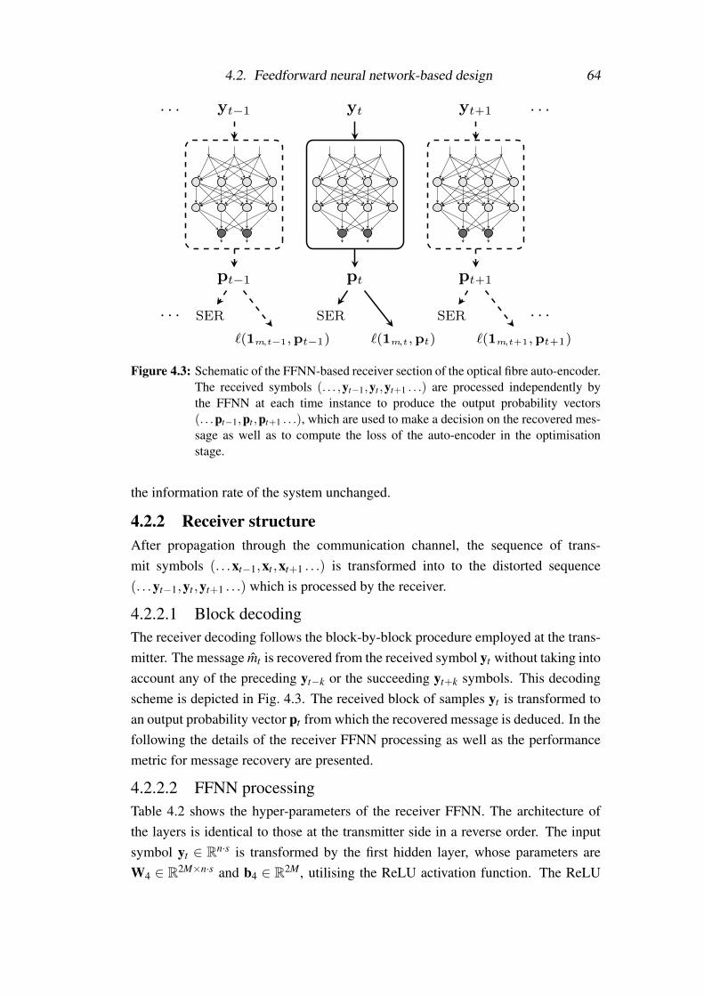
4.2. Feedforward neural network-based design 64
ytyt´1 yt`1
ptpt´1 pt`1
`p1m,t,ptq`p1m,t´1,pt´1q `p1m,t`1,pt`1qSERSER SER
. . . . . .
. . . . . .
Figure 4.3: Schematic of the FFNN-based receiver section of the optical fibre auto-encoder.The received symbols (. . . ,yt−1,yt ,yt+1 . . .) are processed independently bythe FFNN at each time instance to produce the output probability vectors(. . .pt−1,pt ,pt+1 . . .), which are used to make a decision on the recovered mes-sage as well as to compute the loss of the auto-encoder in the optimisationstage.
the information rate of the system unchanged.
4.2.2 Receiver structureAfter propagation through the communication channel, the sequence of trans-mit symbols (. . .xt−1,xt ,xt+1 . . .) is transformed into to the distorted sequence(. . .yt−1,yt ,yt+1 . . .) which is processed by the receiver.
4.2.2.1 Block decodingThe receiver decoding follows the block-by-block procedure employed at the trans-mitter. The message mt is recovered from the received symbol yt without taking intoaccount any of the preceding yt−k or the succeeding yt+k symbols. This decodingscheme is depicted in Fig. 4.3. The received block of samples yt is transformed toan output probability vector pt from which the recovered message is deduced. In thefollowing the details of the receiver FFNN processing as well as the performancemetric for message recovery are presented.
4.2.2.2 FFNN processingTable 4.2 shows the hyper-parameters of the receiver FFNN. The architecture ofthe layers is identical to those at the transmitter side in a reverse order. The inputsymbol yt ∈ Rn·s is transformed by the first hidden layer, whose parameters areW4 ∈ R2M×n·s and b4 ∈ R2M, utilising the ReLU activation function. The ReLU

4.2. Feedforward neural network-based design 65
Table 4.2: FFNN definition at the receiver
Layer Activation Output dimension
Input N/A n · sHidden 1 ReLU 2MHidden 2 ReLU 2M
Final Softmax M
is also applied on the next hidden layer, which has the parameters W5 ∈ R2M×2M,b5 ∈R2M. The parameters of the final layer in the receiver FFNN are W6 ∈R2M×M
and b6 ∈ RM. The final layer’s activation is the softmax function (see Sec. 2.1.2)and thus the output is a probability vector pt ∈ RM with the same dimension as theone-hot vector encoding of the message. Thus, the series of operations
y′t = αReLU (W4yt +b4) , (4.7)
y′′t = αReLU
(W5y
′t +b5
), (4.8)
pt = αsoftmax
(W6y
′′t +b6
), (4.9)
describe the decoding function pt = fDec.-FFNN (yt) of the FFNN receiver. Note thaty′t and y′′t were used to denote the outputs of the first and second hidden layer at thereceiver, respectively. For illustrative purposes, only the receiver input yt and thecorresponding output pt are indicated in Fig. 4.3.
4.2.2.3 Performance metrics
The vector of probabilities which is output of the receiver FFNN can be utilised intwo ways: Firstly, a decision on the received symbol can be made as
mt = argmaxi=1...M
(pt,i), (4.10)
choosing the index mt of the greatest element in pt as the recovered message, i.e.choosing the most probable hypothesis. Such a decoding operation applied to thesoftmax output of the neural network directly corresponds to the initial one-hot vec-tor encoding of messages at the transmitter input. A symbol error occurs at timet when mt 6= mt . The symbol decision is counted in the symbol error rate (SER)estimation for the transmitted sequence of Nseq messages, which is given by
SERseq. =1
Nseq.
Nseq.
∑t=1
1{mt 6= mt} , (4.11)

4.3. Optimisation strategies 66
where 1 denotes the indicator function, equal to 1 when the condition in the bracketsis satisfied, i.e. an error has occurred, and 0 otherwise. During optimisation andtesting of the system both in simulation and experiment, a data set S consisting ofmultiple sequences is utilised. As a consequence, the total symbol error rate of thesystem becomes
SER =1|S|∑i∈S
SERseq.,i, (4.12)
where |S| denotes the cardinality (the number of elements) in the set S.
The probability vector pt is also utilised for computing the loss in the procedureof end-to-end system optimisation, described next.
4.3 Optimisation strategiesThe complete IM/DD optical fibre communication system is implemented as anend-to-end deep FFNN. As explained in the previous sections, such a system isassociated with encoding and decoding in a block-by-block manner. This trans-mission scheme has multiple practical advantages. Firstly, it is computationallysimple, making it attractive for low-cost, high-speed implementations. Secondly, itallows massive parallel processing of the single blocks (symbols). Nevertheless, itis important to note that the proposed structure is only able to compensate for thechannel-induced interference within a block of n · s receiver samples, as there is noconnection between neighboring blocks. The effect of dispersion from neighboringblocks, i.e. the intersymbol interference (ISI), remains uncompensated with such atransceiver design and can thus be viewed as simply introducing extra noise in theencoding and decoding processes. The block size n · s will hence limit the achiev-able distance with the proposed system. As discussed in Sec. 4.4.4.3 and Chapter 5,increasing the block size and thus accounting for more interference can quicklyresult in unfeasibly large neural networks. This necessitated the development oftransceiver designs tailored for recovering symbol sequences. It allowed to keepthe ANN dimensions manageable, while enabling computational structures bettersuited for the approximation of the encoding and decoding functions in communi-cation systems over dispersive channels. In particular, in Chapters 5 and 6 advancedsequence processing transceiver solutions were proposed using a recurrent neuralnetwork structure to encode and decode the blocks or, alternatively, extending thesize of the receiver portion of the FFNN to jointly process multiple blocks and thusdiminish the influence of dispersion. This resulted in communication systems withimproved resilience to ISI, however, at the expense of higher computational com-plexity.
The optimisation of the transmitter and receiver is performed by minimising

4.3. Optimisation strategies 67
Serializer
...
one-hotvector
......
...
...
...
one-hot
vector
......
...
...
...
one-hotvector
......
...
...
M
2M 2M
n
... pN ´ 1q{2
... pN ´ 1q{2
LPF ` MZM ` LPF `
Deseria
lizer
xptqqpL, tq
yptq
nDACptq nRec.ptq nADCptq
fiber
discard
discard
discard
discard
discard
discard
...
Central block...
Communication channel
Transmitter Receiver
End-to-end optimization yielding an autoencoder
One-hot node
ReLU node
Clipping node
Softmax node
Figure 4.4: Schematic of the IM/DD optical fibre communication system implemented as adeep feedforward artificial neural network. Optimisation is performed using theloss between the input messages and the outputs of the receiver, thus enablingend-to-end deep learning of the complete system.
the loss computed at the receiver output between (appropriately chosen) represen-tations of the transmitted m and recovered m messages, effectively minimising theend-to-end symbol error rate. Figure 4.4 depicts a schematic of the FFNN-basedIM/DD system which shows all components affecting the computation of the end-to-end loss at a time instance t, which is obtained as
L (θ) = `(1m,t , fAE-FFNN(1m,t)) = `(1m,t ,pt), (4.13)
whereθ = {W1,b1, . . . ,W6,b6}, (4.14)
and the function fAE-FFNN(·) is used to express the complete input-to-output map-ping function of the FFNN-based autoencoder, which can be defined as
pt = fFFNN-AE(1m,t), fDec.-FFNN (HIMDD {. . . , fEnc.-FFNN (1m,t) , . . .}) , (4.15)
with the operator HIMDD{·} describing the channel transformations. Note that thetransmitted and recovered messages are conveniently represented by their one-hot

4.3. Optimisation strategies 68
vector encoding 1m,t and output probability vector pt , respectively.
The dispersion-induced interference accumulates with distance and can spanbetween several consecutive symbols. As a result, multiple transmitted blocks fromboth preceding and succeeding messages have an impact on the recovery of themessage mt and thus on the computed loss. Such a communication scenario isreferred to as a system with memory. As already mentioned, for the investigatedFFNN design the symbol memory of the channel is treated as extra noise sincethere is no connection in the processing of neighbouring blocks.
In simulation, multiple blocks need to be concatenated to model a realistictransmission for mt . Hence, the output samples of N neighboring blocks (that en-code potentially different inputs) are serialised to form a sequence of N ·n ·s samplesfor transmission over the channel. Note that N needs to be chosen sufficiently largesuch that the number of co-propagating messages exceeds the channel memory. Atthe receiver, the central block is extracted for processing and loss calculation.
The goal is to find a set of trainable parameters from the end-to-end compu-tational graph, i.e. the weight matrices and bias vectors at the transmitter and re-ceiver, that minimise the system loss. The parameters are iteratively updated usingstochastic gradient descent (see Sec. 2.2.1.1) and in particular, the Adam algorithm(see Sec. 2.2.1.2). For this reason, a mini-batch of training examples is used on eachiteration. Figure 4.5 shows a schematic of the procedure. The mini-batch is formedby S sequences, each consisting of N messages. At transmission step i, i = 1 . . .S,the messages in the i-th sequence are encoded by the transmitter FFNN and propa-gated through the channel. At the receiver, the central block is extracted to calculatethe loss Li defined in Eq. (4.13). Obtaining the corresponding losses for each ofthe central blocks in the sequences from the mini-batch, the loss of the batch can beestimated as the average
L (θ) =1S
S
∑i=1
Li. (4.16)
Each iteration of the optimisation algorithm aims at minimising L (θ) computedover a randomly-generated mini-batch. Note that for the purposes of optimising thesystem performance, only the central blocks are considered in this training scheme.During propagation through the channel these are subject to the strongest ISI. More-over, as shown in the following sections, such a scheme enables the generalisationof transmitter and receiver parameters over varied distances.
4.3.1 Learning at a fixed nominal distanceIn this simple training setting, a nominal fibre length L is set. Every sequence ineach of the mini-batches used for training is transmitted through the fixed length of

4.3. Optimisation strategies 69
Serializer
input mini-batch
LB L2 L1m
t´pN´1q{2
mt
mt`pN´1q{2
. . .
mt´pN´1q{2
mt
mt`pN´1q{2
mt´pN´1q{2
mt
mt`pN´1q{2
...
one-hotvector
......
...
...
...
one-hotvector
......
...
...
...
one-hot
vector
......
...
...
M
2M 2M
n
... pN ´ 1q{2
... pN ´ 1q{2
ChannelDeseria
lizer
discard
discard
discard
discard
discard
discard
...
Central block...
Transmitter Receiver
LB . . .L2,L1
loss mini-batch
Figure 4.5: Schematic of the training procedure for the FFNN-based auto-encoder, showinghow a mini-batch is formed from different transmitted sequences of length Nover fibre lengths Li and the corresponding losses, computed for the centralmessage in every sequence.
fibre, thus accumulating identical amounts of ISI. As a consequence, the transmit-ter and receiver are optimised exclusively for communication at the fixed nominaldistance. Operation at distances, significantly different from L would require re-initiating the training stage.
4.3.2 Multi-distance learning
Since every sequence i from the mini-batch is transmitted independently throughthe communication channel, it can be associated with a specific distance Li, whichdictates the amount of ISI-induced distortion on the central block. This has a directimpact on the calculated loss Li, which would increase with distance. As a result,the total batch loss L (θ) comprises of training examples from multiple transmis-sion scenarios. Performing deep learning aimed at minimising L (θ), could thusbe viewed as optimising the set of transmitter and receiver parameters θ for trans-mission over all different Li. A simple scheme would involve assigning to the i-thmini-batch sequence a link length Li which is randomly drawn from a probability
4.4. Numerical investigation of the FFNN auto-encoder performance 70
distribution with appropriately chosen parameters, e.g.
Li ∼N (µ,σ), i = 1 . . . |S|, (4.17)
where N (µ,σ) denotes the Gaussian distribution, whose mean is µ and standarddeviation is σ , and |S| is the number of sequences in the mini-batch.
4.4 Numerical investigation of the FFNN auto-encoder performance
4.4.1 Bit-to-symbol mapping
As explained throughout the chapter, the auto-encoder communication system isdesigned such that the end-to-end symbol error rate is minimised. Nevertheless,a common metric examined as an indication of the communication system perfor-mance is the bit-error rate (BER). Thus, whenever a symbol is received in error, thenumber of incorrect bits that have occurred needs to be counted.
The input and output of the end-to-end ANN are non-binary messages m ∈{1, . . . ,M} and m. In order to guarantee the low bit error rates in the range 10−12
to 10−15, forward error correction (FEC) is required. For complexity reasons, FECschemes in optical communications are usually binary [101] and often based onhard-decision decoding (HDD), in particular for IM/DD applications. An overviewof HDD decoding schemes and their decoding capabilities is given in [102]. Toconvert between the ANN messages and the FEC encoder/decoder output/input, abit labeling function ϕ : {1, . . . ,M}→FB
2 is needed. It maps a message m to a binaryvector b=
(b1, . . . ,bB
), bi ∈F2 = {0,1} of length B= dlog2(M)e. Usually, M and
B are selected such that M = 2B.
For computing the BER, presented for the numerical auto-encoder investiga-tion in this chapter, a simple ad hoc bit mapping was used. It consisted in assigningthe Gray code to the integer input messages m ∈ {1, . . . ,M} [103]. Note that thissimple approach is sub-optimal as the deep learning algorithm will only minimisethe SER and a symbol error may not necessarily lead to a single bit error. In thepresentation of simulation results in this chapter, a lower bound on the achievableBER will hence be provided with an ideal bit mapping by assuming that at mosta single bit error occurs during a symbol error. In Chapter 5 an algorithm for theoptimisation of the bit-to-symbol mapping function was proposed and investigatedfor the recurrent neural network-based auto-encoder.

4.4. Numerical investigation of the FFNN auto-encoder performance 71
4.4.2 Generation of training and testing data
4.4.2.1 Random number generationIt was highlighted in [104] that special care should be taken when applying neu-ral networks in optical communication systems to avoid learning representationsof a sequence, e.g. pseudo-random binary sequence (PRBS). The authors of thepaper provided guidelines to prevent biasing the performance results, which weremeticulously followed when designing both the simulations and transmission ex-periments part of the investigation described in this thesis. In particular, for thesimulations, new random input messages were continuously generated during theoptimisation stage using a Mersenne twister [105] – a random number generatorwith a long sequence. In order to obtain the results presented throughout the thesis,the neural network models are trained and stored to perform testing with indepen-dent data, generated by a different random number generator. More specifically, theTausworthe generator (see [106] for details) was used in the test stage. Chapter 6provides more information on the data generation and collection procedures used inthe experimental verification of the developed systems.
4.4.2.2 Optimisation stageThe cross entropy loss (see Sec. 2.1.2.2) was used during optimisation. The auto-encoder was trained on a set of |S|=25·106 randomly chosen central messages (and(N−1) · |S| random messages of the neighbouring transmit blocks, discarded at thereceiver) using the Adam optimiser with a learning rate of 0.001 (default setting).The deep learning library TensorFlow [99] was used to perform the optimisation.The mini-batch size was set to S = 250, from where the number of optimisationiterations can be accordingly expressed as
I =|S|S. (4.18)
Thus, I = 105 iterations of the optimisation algorithm were performed in the ac-commodated setting. The initialisation of the trainable parameters was carried outas recommended in [12, Sec. 8.1.3]: a truncated normal distribution with standarddeviation σ = 0.1 was used for the weight matrices W. The bias vectors b wereinitialised with 0. Validation of the training was performed during the optimisa-tion process every 5000 iterations. The validation set of data was independentlygenerated and had the size |Sv| = 15 · 106. It is worth noting that in most cases,convergence in the loss and validation symbol error rate of the trained models wasobtained after significantly less than 105 iterations, which was used as a fixed stop-ping criterion – a common way to terminate ANN training (see [12, Sec. 8.3]). The

4.4. Numerical investigation of the FFNN auto-encoder performance 72
Table 4.3: Simulations parameters assumed for the FFNN-based auto-encoder
Parameter Value
Transceiver:
M 64n 12N 11
Oversampling (s) 4Rcod.
12 b/Sa
Channel:
Rsamp. 84 GSa/sSampling rate (s ·Rsamp.) 336 GSa/s
Rinf. 42 Gb/sLPF bandwidth (B f ) 32 GHz
DAC/ADC ENOB (Nb) 6Fibre length (L) varied
Fibre dispersion (D) 17 ps/(nm ·km)Fibre attenuation (αdB/km) 0.2 dB/km
Receiver noise variance (σref.) 2.455 ·10−4
convergence of the results was also confirmed for mini-batch sizes of S = 125 and500. More details on how to choose an appropriate amount of mini-batch examplesfor SGD optimisation can be found in [12, Sec. 8.4]. Finally, the validation resultswere confirmed in the case when the training set was increased to |S| = 50 · 106
input messages.
4.4.2.3 Testing stage
The trained model, i.e. the set θ of optimised weight matrices and bias vectors rep-resenting the transmitter and receiver ANNs, was saved and then loaded separatelyfor testing. Testing was performed over a set of different random input messages,generated by a different random number generator (see Sec. 4.4.2.1). In order toobtain a reliable estimation of the BER, the size of the testing set was increased to|St |=15 ·108. Note that these messages were used to evaluate the performance at aspecific distance. They were encoded by the optimised transmitter FFNN, transmit-ted through the channel and decoded by the optimised receiver FFNN, computingthe symbol and bit error rates over the testing set, as described in Sec. 4.2.2.3 andSec. 4.4.1, respectively. The BER results from the testing phase are shown on thesystem performance figures presented in this chapter.

4.4. Numerical investigation of the FFNN auto-encoder performance 73
4.4.3 Simulation parametersTable 4.3 lists the simulation parameters for the end-to-end deep-learning-based op-tical fibre system under investigation. Input messages from a set of |M |= M = 64total messages, each carrying 6 bits, were encoded by the FFNN at the transmitterinto symbols of n · s = 48 samples at 336 GSa/s in simulation. This rate corre-sponded to the Rsamp. = 84 GSa/s sampling rate of the DAC used in experimentmultiplied by the assumed simulation oversampling factor of s = 4. This resulted inan auto-encoder system with a data rate equal to Rinf. = 42 Gb/s. The bandwidth ofthe signal was restricted at both transmitter and receiver by a brick-wall LPF witha cut-off frequency of B f = 32 GHz to account for the hardware limitations. Notethat in practice, down-sampling by a factor of s = 4 of the filtered series of symbolscan be performed without loss of information. Due to the low-pass filtering, theoriginal series of symbols, each of n · s = 48 samples at 336 GSa/s, can be exactlyreconstructed from the down-sampled symbol series running at the DAC rate of 84GSa/s. Down-sampling was performed during the experimental verification of thesystem reported in Chapter 6. More details on the temporal and spectral representa-tions of the ANN-optimised transmitted signal are provided in Appendix A. For thetransmission simulation, the variance of the additive receiver white Gaussian noisewas set to the experimentally obtained value of σ2
r = 2.455 · 10−4, as explained inSec. 3.3.1. Chapter 6 provides more details on the experiment. The fibre attenuationand dispersion parameters were αdB/km = 0.2 dB/km and D = 17 ps/(nm · km), re-spectively, typical values for a standard single mode fibre [23]. The ENOB of boththe DAC and the ADC was set to Nb = 6.
4.4.4 System performance
4.4.4.1 Transceivers optimised at a fixed nominal distanceThe BER performance of the FFNN auto-encoder optimised at the fixed nominaldistance of 40 km was computed over the testing set as described in Sec. 4.4.1 andthe results obtained at distances between 37.5 and 42.5 km are shown in Fig. 4.6.The 4.5 · 10−3 hard-decision forward error correction (HD-FEC) threshold [107](6.7% overhead) was used as an indicator of the system performance. BER val-ues below the HD-FEC were achieved at distances in the range of 38− 41.25 km.Moreover, around the nominal training distance of 40 km the BER was below 10−4.For distances longer or shorter than the optimum 40 km, the bit error rate increased.The figure also displays the lower bound, denoted “ideal”, on the achievable BERfor each distance. This lower bound was obtained by assuming that a block errorgives rise to a single bit error. The results confirmed that utilising the Gray codeof m as a bit-to-symbol mapping function, an approach discussed in 4.4.1 and used

4.4. Numerical investigation of the FFNN auto-encoder performance 74
37 38 39 40 41 42 4310´6
10´5
10´4
10´3
10´2
10´1
100
HD-FEC
threshold
Transmission distance (km)
BER
Bit mapping:
Gray-coded m
Ideal
Figure 4.6: BER as a function of transmission distance for a system trained at 40 km. Thehorizontal dashed line indicates the 6.7% HD-FEC threshold. The BER with anideal bit mapping, i.e. a symbol error results in a single bit error, is also shown.
in the current investigation, is not optimal for the FFNN auto-encoder. Hence, op-timising the mapping function can lead to additional performance enhancement.This was demonstrated for the developed recurrent neural network-based systemsin Chapter 5, where the optimisation of the bit labeling function was performed.
The BER performance of systems trained at different distances is shown inFig. 4.7. For this set of results, seven FFNN-based transceivers were optimised fordifferent distances in the range of 20 to 80 km in steps of 10 km. As before, theoptimisation was performed at the fixed nominal distance. BERs below the 6.7%hard decision FEC threshold are achieved for all examined distances between 20and 50 km. Moreover, up to 40 km the BER was below 10−4. Systems trained atdistances longer than 50 km achieved BERs above 10−2. The lower bound on theachievable BER was also shown, indicating that the assumed bit-to-symbol map-ping was sub-optimal for all of the examined distances. An important observation isthat the systems achieved their lowest BER values at the nominal distances at whichtheir training was performed. A rapid increase in their error rate was observed whenthe distance changed. For example, the BER of auto-encoder optimised at 40 kmwas degraded from 5 ·10−5 to above 1 ·10−2, when the distance was changed from39.75 km to either 38 or 41.5 km. Such a behaviour is a direct consequence of theimplemented training approach which optimises the system ANN parameters for

4.4. Numerical investigation of the FFNN auto-encoder performance 75
operation at a particular distance, without any incentive for robustness to variations.As the amount of dispersion changes with distance, the optimal neural network pa-rameters differ accordingly. Thus, the system BER will increase when the distanceis varied without accordingly updating the transceiver parameters.
4.4.4.2 Transceivers optimised for operation at multiple distancesTo address the limitations of the training at a fixed nominal distance related to ro-bustness to distance variation, the optimisation method proposed in Sec. 4.3.2 isconsidered next. For such an investigation, the transceiver was trained in a processwhere the distance for every training message was randomly drawn from a Gaus-sian distribution with a mean µ and a standard deviation σ . During optimisation,this will allow the deep learning algorithm to converge to a set of generalised ANNparameters, robust to certain variation of the dispersion. Figure 4.8 shows the testBER performance of the system trained at a mean distance µ = 40 km and differentvalues of the standard deviation. It can be seen that for the cases of σ = 4 km andσ = 10 km this training method allowed BER values below the HD-FEC thresholdin wider ranges of transmission distances than for σ = 0 km, the scenario coveredin the previous investigation. For instance, when σ = 4 km, BER values below the4.5 · 10−3 threshold were achievable between 30.25 km and 49.5 km, yielding an
10 20 30 40 50 60 70 80 9010´6
10´5
10´4
10´3
10´2
10´1
100
HD-FEC
threshold
Transmission distance (km)
BER
Trained (km):
20
30
40
50
60
70
80
Figure 4.7: BER as a function of transmission distance for systems trained at a fixed nomi-nal distance of (20+ i ·10) km, with i∈{0, . . . ,6}. The 6.7% HD-FEC thresholdis indicated by a horizontal dashed line. Thin dashed lines below the curves givea lower bound on the achievable BER when an ideal bit mapping is assumed.

4.4. Numerical investigation of the FFNN auto-encoder performance 76
20 25 30 35 40 45 50 55 6010´5
10´4
10´3
10´2
10´1
100
HD-FECthreshold
Transmission distance (km)
BER
Trained (µ, σ) km:
p40, 0qp40, 4qp40, 10q
Figure 4.8: Bit error rate as a function of transmission distance for systems where the train-ing is performed at normally distributed distances with mean µ = 40 km andstandard deviation σ . The horizontal dashed line indicates the 6.7% HD-FECthreshold.
operating range of 19.25 km. The distance tolerance was further increased whenσ = 10 km was used for the optimisation. It is worth noting that in this case theobtained BERs were higher, due to the increased difficulty in converging to parame-ters valid for the significantly varied distances with the standard deviation of 10 km.Nevertheless, performance below the HD-FEC threshold was achieved by such atransceiver for a distance range of 27.75 km, spanning from 24 km up to 51.75 km.The lowest BER value of the system was significantly increased compared to theauto-encoder trained at the fixed nominal distance of 40 km, i.e. 2 ·10−3 comparedto 5 · 10−4. Thus, there exists a trade-off between system robustness and perfor-mance. The multi-distance learning method can be hugely beneficial for practicalapplications as it introduces both robustness and flexibility of the system to varia-tions in the link distance, without requiring any reconfiguration of the transceiver.
To further investigate the levels of flexibility that such an optimisation tech-nique can offer, the BER performance of the distance-agnostic auto-encoder wasexamined at different values of the mean training distance µ . Figure 4.9 showsthe BER performance of systems trained at the mean distances µ of 20, 40, 60 and

4.4. Numerical investigation of the FFNN auto-encoder performance 77
10 20 30 40 50 60 70 80 9010´8
10´7
10´6
10´5
10´4
10´3
10´2
10´1
100
HD-FEC
threshold
Trained at p20, 4q km
Trained at p40, 4q km
Trained at p60, 4q kmTrained at p80, 4q km
Transmission distance (km)
BER
Figure 4.9: Bit error rate as a function of transmission distance for systems where the train-ing is performed at normally distributed distances around the mean values µ of20, 40, 60, 80 km and a fixed standard deviation σ = 4 km. The horizontaldashed line indicates the 6.7% HD-FEC threshold.
80 km with a fixed standard deviation of σ = 4 km. It can be seen that generalisationof the transceiver parameters was achieved for all setups. An interesting implicationis that only two sets of optimised transceiver parameters, i.e. trained at (20,4) kmand (40,4) km, are required to achieve BER values below the HD-FEC threshold atall distances up to 50 km. In contrast, the system performances shown in Fig. 4.7,indicate that at least 8 different transceivers would need to be used to cover similardistances.
4.4.4.3 Transceivers with different coding ratesThe investigation of the end-to-end deep learning-based optical fibre system re-ported in the previous sections covered the scenario where an input message car-rying 6 bits of information (M = 64) was encoded into a band-limited symbol of48 samples (n · s = 48 with an oversampling factor of s = 4) at 336 GSa/s. Thus,the result was an auto-encoder operating at the information rate of 42 Gb/s. In thefollowing, the implementation of systems with different rates is demonstrated. Thisis achieved by varying the input and the output dimension of the ANNs, i.e. chang-ing the hyper-parameters M and n. For this investigation, the oversampling factorand the sampling rate of the simulation are kept fixed and equal to 4 and 336 GSa/s,respectively. In Figure 4.10 solid lines show the BER performance of the system at
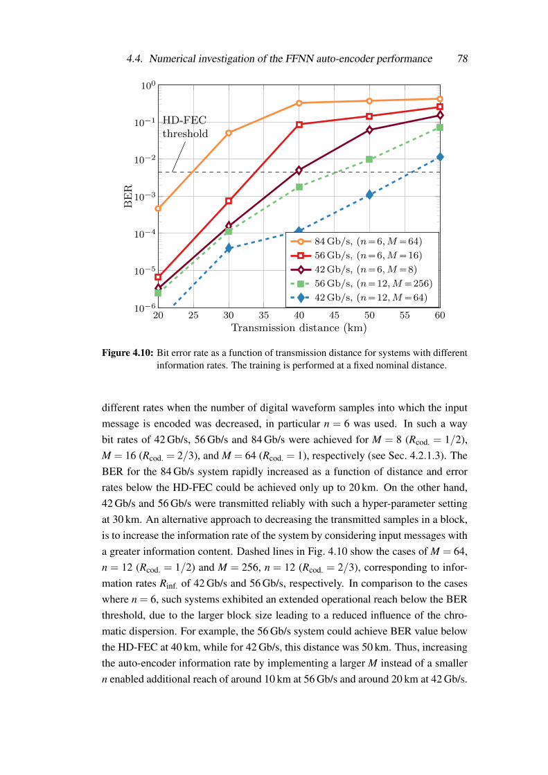
4.4. Numerical investigation of the FFNN auto-encoder performance 78
20 25 30 35 40 45 50 55 6010´6
10´5
10´4
10´3
10´2
10´1
100
HD-FECthreshold
Transmission distance (km)
BER
84Gb/s, pn“6,M“64q56Gb/s, pn“6,M“16q42Gb/s, pn“6,M“8q56Gb/s, pn“12,M“256q42Gb/s, pn“12,M“64q
Figure 4.10: Bit error rate as a function of transmission distance for systems with differentinformation rates. The training is performed at a fixed nominal distance.
different rates when the number of digital waveform samples into which the inputmessage is encoded was decreased, in particular n = 6 was used. In such a waybit rates of 42 Gb/s, 56 Gb/s and 84 Gb/s were achieved for M = 8 (Rcod. = 1/2),M = 16 (Rcod. = 2/3), and M = 64 (Rcod. = 1), respectively (see Sec. 4.2.1.3). TheBER for the 84 Gb/s system rapidly increased as a function of distance and errorrates below the HD-FEC could be achieved only up to 20 km. On the other hand,42 Gb/s and 56 Gb/s were transmitted reliably with such a hyper-parameter settingat 30 km. An alternative approach to decreasing the transmitted samples in a block,is to increase the information rate of the system by considering input messages witha greater information content. Dashed lines in Fig. 4.10 show the cases of M = 64,n = 12 (Rcod. = 1/2) and M = 256, n = 12 (Rcod. = 2/3), corresponding to infor-mation rates Rinf. of 42 Gb/s and 56 Gb/s, respectively. In comparison to the caseswhere n = 6, such systems exhibited an extended operational reach below the BERthreshold, due to the larger block size leading to a reduced influence of the chro-matic dispersion. For example, the 56 Gb/s system could achieve BER value belowthe HD-FEC at 40 km, while for 42 Gb/s, this distance was 50 km. Thus, increasingthe auto-encoder information rate by implementing a larger M instead of a smallern enabled additional reach of around 10 km at 56 Gb/s and around 20 km at 42 Gb/s.

4.5. Summary 79
However, a drawback of such a solution is the larger FFNN size since there is anexponential dependence between M and the coding rate, i.e. M = 2n·Rcod. , thus in-creasing the computational and memory demands as well as the training times ofthe auto-encoder. The investigation shown in Fig. 4.10 highlights that the optical fi-bre auto-encoder concept can be easily applied for designing systems with differentinformation rates and gives an insight on the possible implementation approachesand the trade-offs between performance and complexity associated with their im-plementation.
4.5 SummaryIn this chapter, it was described how the optical fibre communication system canbe implemented as an end-to-end computational graph to perform system optimisa-tion in a single process. In particular, the optical fibre transceiver was designed asa simple feedforward neural network and deep learning was applied to find trans-mitter and receiver ANN parameters that minimise the symbol error rate in the sys-tem. The benefits of this method were illustrated by applying it to intensity mod-ulation/direct detection (IM/DD) systems, showing that bit error rates below the6.7% hard-decision forward error correction threshold can be achieved at distancesbeyond 50 km – links of practical interest for short reach optical fibre communi-cations. A multi-distance transceiver optimisation method was also proposed inthe chapter. It was verified in simulation that the method yields robust and flexibletransceivers that can enable — without reconfiguration — reliable transmission overa large range of link distances. The research was published in [62]. To complementthe simulation results described in this chapter, an experimental verification of theproposed FFNN-based auto-encoder system as well as the multi-distance learningmethod was conducted and described in Chapter 6. Before that, the investigation inChapter 5 addresses the limitations of the FFNN design related to compensating forthe intersymbol interference at longer transmission distances.

Chapter 5
Recurrent neural network-basedoptical fibre transceiver
Chapter 3 introduced the transformations and distortions caused by the opticalIM/DD communication channel on an input sequence of digital samples. In par-ticular, it was described how chromatic dispersion leads to interference betweenpreceding and succeeding samples, thus imposing severe limitations on the achiev-able system reach.
To optimise the transceiver for communication over such a channel, a feed-forward artificial neural network (FFNN)-based auto-encoder was investigated inChapter 4. As explained in Sec. 4.2, this system employed a block-based trans-mission strategy using a transmitter which encodes input messages m from a finitealphabet with size |M | = M, each carrying log2(M) bits, into blocks (symbols) ofn digital waveform samples. At the receiver, the distorted n-dimensional symbolsare decoded block-by-block, recovering the transmitted messages. The describedsystem encodes/decodes each symbol independently, i.e. without information fromthe previous or future encoding/decoding. However, as explained in Sec. 3.2, thedispersion-induced interference is an effect which accumulates linearly with dis-tance and quadratically with the signal bandwidth, quickly extending across mul-tiple adjacent symbols. The presence of intersymbol interference (ISI) renders theoptical IM/DD link a communication channel with memory.
The FFNN auto-encoder system is inherently unable to compensate for ISI,i.e. interference outside of the symbol block, which is treated as extra noise. As aconsequence, the achievable performance, in terms of chromatic dispersion that canbe compensated and hence transmission distance, of such a system is limited by theblock size. The presented results in Sec. 4.4.4.3 investigated the solution of expand-ing the FFNN by including more samples within a symbol block, i.e. implementinglarger n. Nevertheless, in addition to increasing the output FFNN dimension n, for
5.1. End-to-end system design 81
a given coding rate Rcod. (defined in Sec. 4.2.1.3), following this approach wouldrequire an exponential increase of the input neural network dimension M, which isrelated to n as M = 2n·Rcod. . The result is an auto-encoder system that can quickly be-come computationally infeasible to implement due to the rapidly increasing amountof transceiver ANN parameters as a function of compensated interference.
In this chapter, the limitations of the FFNN-based auto-encoder design forcommunication over channels with memory were addressed by developing a deeplearning-based transceiver for sequence processing using a bidirectional recurrentneural network (BRNN). The BRNN-based auto-encoder allows to utilise informa-tion from both pre- and post-cursor symbols in the encoding and decoding pro-cesses. The optimised system was combined with an efficient sliding window se-quence estimation algorithm, yielding a sliding window bidirectional recurrent neu-ral network (SBRNN) auto-encoder. This allowed to control the processing memoryin the BRNN receiver via the estimation window W , external to the end-to-end neu-ral network architecture. As a result, the resilience to ISI could be enhanced, whilekeeping the number of ANN parameters at the transceiver fixed.
In addition to introducing the SBRNN auto-encoder design, this chapter in-cludes an extensive numerical investigation of the system performance. In particu-lar, Sec. 5.3.1 and 5.3.3 describe the study of the SBRNN performance and com-plexity in comparison to classical pulse amplitude modulation (PAM) transmissionwith state-of-the-art nonlinear equalisation or maximum likelihood sequence detec-tion receivers, respectively.
5.1 End-to-end system designThe complete optical fibre communication system is implemented as an end-to-endcomputational graph using ANN-based transmitter and receiver, a concept whichwas introduced in Chapter 4. The transceiver design described here uses a bidirec-tional recurrent neural network to handle the intersymbol interference effects stem-ming from preceding and succeeding symbols, induced by the dispersive opticalchannel. Figure 5.1 shows a schematic of the proposed BRNN-based communica-tion system. This section describes the encoding and decoding performed by thescheme.
5.1.1 Transmitter
5.1.1.1 Bidirectional recurrent encodingWithin the optical fibre auto-encoder framework, described in Sec. 4.1, the functionof the artificial neural network at the transmitter is to encode the stream of inputmessages (. . . ,mt−1,mt ,mt+1, . . .), mt ∈ {1, . . . ,M}, each of which drawn indepen-

5.1. End-to-end system design 82
0 32 64 96 128 160
f (GHz)
0 32 64 96 128 160
f (GHz)
Serializer
RN
Nce
llR
NN
cell
RN
Nce
ll
RN
Nce
llR
NN
cell
RN
Nce
ll
Tx
mer
geT
xm
erge
Tx
mer
ge
one-
hot
vect
oron
e-hot
vect
oron
e-hot
vect
or
...
...
LPF ` MZM ` LPF `D
eserializer
nDACptq nRec.ptq nADCptq
fiber
RN
Nce
llR
NN
cell
RN
Nce
ll
RN
Nce
llR
NN
cell
RN
Nce
ll
Rx
mer
geR
xm
erge
Rx
mer
ge
Sof
tmax
Sof
tmax
Sof
tmax
...
...Communication channel
Transmitter Receiver
End-to-end sequence-based optimization
Figure 5.1: Schematic of the IM/DD optical fibre communication system implemented as abidirectional deep recurrent neural network. optimisation is performed betweenthe stream of input messages and the outputs of the receiver, thus enabling end-to-end optimisation via deep learning of the complete system. Inset figuresshow an example of the transmitted signal spectrum both at the output of theneural network and before the DAC.
dently from an alphabet M of |M | = M total messages, into a sequence of trans-mit blocks of digital waveform samples (symbols) (. . . ,xt−1,xt ,xt+1, . . .) ready fortransmission over the communication channel. Unlike the FFNN system proposedin Sec. 4.2, the BRNN transmitter structure, proposed and investigated in this chap-ter, allows to utilise information from both pre- and post-cursor symbols, i.e. xt−k
or xt+k, into the encoding of the message mt at time t. Thus the BRNN transmitterperforms encoding of input sequences, which is necessary for communication overcommunication channels with ISI.
5.1.1.2 BRNN processing
Figure 5.2 shows a schematic of the BRNN encoding procedure. First, the messagesmt are represented as one-hot vectors 1m,t ∈ RM, which are fed into the recurrentstructure for bidirectional encoding. Two variations of the recurrent cell in the RNNstructure were investigated – a straightforward vanilla concatenation as well as along short-term memory gated recurrent unit structure (LSTM-GRU). The vanillaand LSTM-GRU processing cells were introduced in Sec. 2.1.3.1. In the following,the message encoding performed by each of these cells is described.

5.1. End-to-end system design 83
mtmt´1 mt`1
1m,t1m,t´1 1m,t`1
xtxt´1 xt`1
MergeMerge Merge
. . . . . .
. . . . . .
. . .
. . .
Figure 5.2: Schematic of the BRNN-based transmitter section of the optical fibre auto-encoder. The input messages (. . .mt−1,mt ,mt+1 . . .), represented as one-hotvectors (. . . ,1m,t−1,1m,t ,1m,t+1 . . .), are processed bidirectionally at each timeinstance by the neural network to produce the sequence of encoded symbols(blocks of samples) (. . .xt−1,xt ,xt+1 . . .). Thick solid lines are used to highlightthe the connections to symbols that have an impact on the processing of mt .Note that a vanilla BRNN cell structure is adopted for illustrative purposes.
Table 5.1: Vanilla and LSTM-GRU cell definitions at the transmitter (single direction)
Layer Activation Output dimension
Vanilla:
Input one-hot enc. & concat. M+n · sFinal Clipping n · s
LSTM-GRU:
Input one-hot enc. & concat. M+n · sGate a Sigmoid n · sGate b Sigmoid n · sFinal Clipping n · s
Table 5.1 lists the neural network hyper-parameters used for the investigationpresented in this chapter. The recurrent processing in the backward and forwarddirections is performed using identical network hyper-parameters and architectures.For the vanilla BRNN, in the forward direction the input 1m,t at time t is concate-
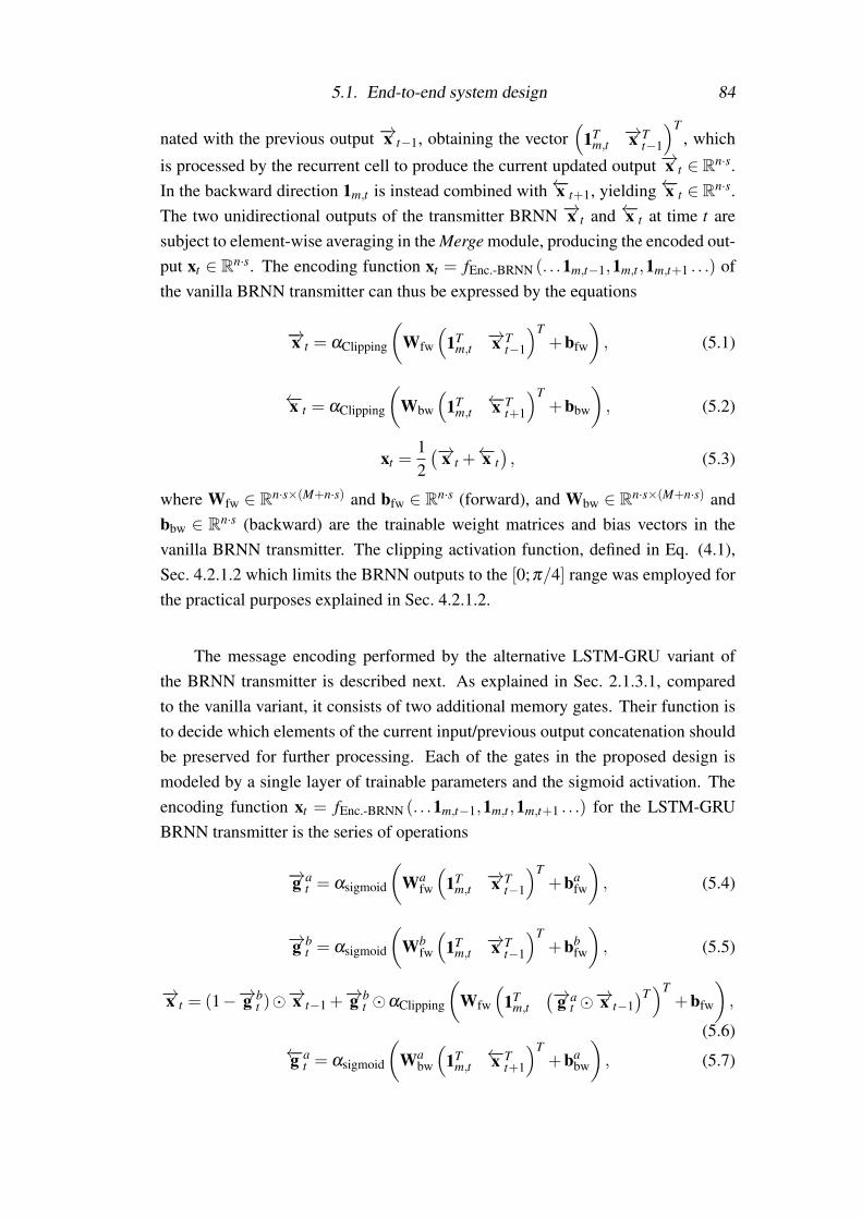
5.1. End-to-end system design 84
nated with the previous output −→x t−1, obtaining the vector(
1Tm,t−→x T
t−1
)T, which
is processed by the recurrent cell to produce the current updated output −→x t ∈ Rn·s.In the backward direction 1m,t is instead combined with←−x t+1, yielding←−x t ∈ Rn·s.The two unidirectional outputs of the transmitter BRNN −→x t and ←−x t at time t aresubject to element-wise averaging in the Merge module, producing the encoded out-put xt ∈ Rn·s. The encoding function xt = fEnc.-BRNN (. . .1m,t−1,1m,t ,1m,t+1 . . .) ofthe vanilla BRNN transmitter can thus be expressed by the equations
−→x t = αClipping
(Wfw
(1T
m,t−→x T
t−1
)T+bfw
), (5.1)
←−x t = αClipping
(Wbw
(1T
m,t←−x T
t+1
)T+bbw
), (5.2)
xt =12(−→x t +
←−x t), (5.3)
where Wfw ∈ Rn·s×(M+n·s) and bfw ∈ Rn·s (forward), and Wbw ∈ Rn·s×(M+n·s) andbbw ∈ Rn·s (backward) are the trainable weight matrices and bias vectors in thevanilla BRNN transmitter. The clipping activation function, defined in Eq. (4.1),Sec. 4.2.1.2 which limits the BRNN outputs to the [0;π/4] range was employed forthe practical purposes explained in Sec. 4.2.1.2.
The message encoding performed by the alternative LSTM-GRU variant ofthe BRNN transmitter is described next. As explained in Sec. 2.1.3.1, comparedto the vanilla variant, it consists of two additional memory gates. Their function isto decide which elements of the current input/previous output concatenation shouldbe preserved for further processing. Each of the gates in the proposed design ismodeled by a single layer of trainable parameters and the sigmoid activation. Theencoding function xt = fEnc.-BRNN (. . .1m,t−1,1m,t ,1m,t+1 . . .) for the LSTM-GRUBRNN transmitter is the series of operations
−→g at = αsigmoid
(Wa
fw
(1T
m,t−→x T
t−1
)T+ba
fw
), (5.4)
−→g bt = αsigmoid
(Wb
fw
(1T
m,t−→x T
t−1
)T+bb
fw
), (5.5)
−→x t = (1−−→g bt )�−→x t−1 +
−→g bt �αClipping
(Wfw
(1T
m,t(−→g a
t �−→x t−1
)T)T
+bfw
),
(5.6)←−g a
t = αsigmoid
(Wa
bw
(1T
m,t←−x T
t+1
)T+ba
bw
), (5.7)

5.1. End-to-end system design 85
←−g bt = αsigmoid
(Wb
bw
(1T
m,t←−x T
t+1
)T+bb
bw
), (5.8)
←−x t = (1−←−g bt )�←−x t+1 +
←−g bt �αClipping
(Wbw
(1T
m,t(←−g a
t �←−x t+1
)T)T
+bbw
),
(5.9)
xt =12(−→x t +
←−x t), (5.10)
where � denotes element-wise multiplication of vectors and Wfw ∈ Rn·s×(M+n·s),bfw ∈ Rn·s, Wa
fw ∈ Rn·s×(M+n·s), bafw ∈ Rn·s and Wb
fw ∈ Rn·s×(M+n·s), bbfw ∈ Rn·s
(forward direction), and Wbw ∈ Rn·s×(M+n·s), bbw ∈ Rn·s, Wabw ∈ Rn·s×(M+n·s),
babw ∈ Rn·s and Wb
bw ∈ Rn·s×(M+n·s), bbbw ∈ Rn·s (backward direction) are all train-
able weight matrices and bias vectors in the LSTM-GRU BRNN transmitter.
Note that the BRNN transmitter encodes the full sequence of input messages.Thus, the forward/backward recurrent processing at the transmitter introduces extralatency of the order of a full data sequence. By termination of the sequences, this la-tency can be limited to a practically manageable level (which can be in the range ofthousands of symbols). Moreover, as described later in Sec. 5.1.4, the auto-encoderis operated in an efficient sliding window algorithm for sequence estimation, signif-icantly reducing the end-to-end processing delay. The sequence lengths and slidingwindow size used in the numerical investigation of the BRNN system are specifiedin Sec. 5.3. For the experimental verification of the system, which is described inChapter 6, these parameters are specified in Sec. 6.5.
5.1.2 ReceiverThe function of the ANN receiver is to decode the sequence of received symbols(. . .yt−1,yt ,yt+1 . . .) obtained at the output of the channel, producing a sequenceof recovered messages (. . . mt−1, mt , mt+1 . . .). The design based on a bidirectionalrecurrent neural network allows to perform the operation by utilising informationfrom previous and future decoding.
5.1.2.1 Recurrent decodingThe BRNN decoding scheme is shown schematically in Fig. 5.3. The BRNN-basedreceiver processing follows an identical recurrent procedure to the one used at thetransmitter. The message mt is recovered from the received symbol yt via decodingthat involves both preceding yt−k and succeeding yt+k symbols. In particular, thereceived block of samples yt is processed to an output probability vector pt fromwhich the per-example loss is calculated during optimisation and also a decision forthe recovered message mt is made. The specific receiver BRNN processing, adoptedfor the proposed auto-encoder design is presented next.

5.1. End-to-end system design 86
ytyt´1 yt`1
ptpt´1 pt`1
`p1m,t,ptq`p1m,t´1,pt´1q `p1m,t`1,pt`1qSERSER SER
Merge
Softmax
Merge
Softmax
Merge
Softmax
. . . . . .
. . .
. . .
Figure 5.3: Schematic of the BRNN-based receiver section of the proposed optical fi-bre auto-encoder. The received symbols (. . . ,yt−1,yt ,yt+1 . . .) are processedbidirectionally by the BRNN to produce the output probability vectors(. . .pt−1,pt ,pt+1 . . .). These are utilised in two ways: to make a decision onthe recovered message as well as to compute the loss of the auto-encoder in theoptimisation stage.
5.1.2.2 BRNN processing
Table 5.2 lists the hyper-parameters for the neuron layers used at the BRNN re-ceiver. For decoding using the vanilla BRNN, the current input yt is concatenatedwith the previous output in the forward direction
−→h t−1 and processed by the cell
with a ReLU activation function, producing−→h t ∈R2M. Identically in the backward
direction yt is concatenated with←−h t+1 and transformed to
←−h t ∈R2M. The two cur-
rent outputs−→h t and
←−h t are concatenated in the Merge module, yielding ht ∈ R4M.
Subsequently, the output ht of the cell is applied to a softmax layer to obtain theoutput probability vector pt ∈ RM, having the dimensionality of the input one-hotvector, and utilised for loss computation and message recovery. The decoding func-tion pt = fDec.-BRNN (. . .yt−1,yt ,yt+1 . . .) of the vanilla BRNN receiver is, hence,
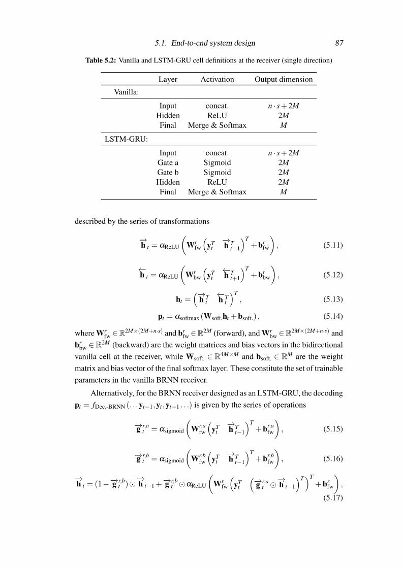
5.1. End-to-end system design 87
Table 5.2: Vanilla and LSTM-GRU cell definitions at the receiver (single direction)
Layer Activation Output dimension
Vanilla:
Input concat. n · s+2MHidden ReLU 2MFinal Merge & Softmax M
LSTM-GRU:
Input concat. n · s+2MGate a Sigmoid 2MGate b Sigmoid 2MHidden ReLU 2MFinal Merge & Softmax M
described by the series of transformations
−→h t = αReLU
(Wr
fw
(yT
t−→h T
t−1
)T+br
fw
), (5.11)
←−h t = αReLU
(Wr
bw
(yT
t←−h T
t+1
)T+br
bw
), (5.12)
ht =(−→
h Tt←−h T
t
)T, (5.13)
pt = αsoftmax (Wsoft.ht +bsoft.) , (5.14)
where Wrfw ∈R2M×(2M+n·s) and br
fw ∈R2M (forward), and Wrbw ∈R2M×(2M+n·s) and
brbw ∈ R2M (backward) are the weight matrices and bias vectors in the bidirectional
vanilla cell at the receiver, while Wsoft. ∈ R4M×M and bsoft. ∈ RM are the weightmatrix and bias vector of the final softmax layer. These constitute the set of trainableparameters in the vanilla BRNN receiver.
Alternatively, for the BRNN receiver designed as an LSTM-GRU, the decodingpt = fDec.-BRNN (. . .yt−1,yt ,yt+1 . . .) is given by the series of operations
−→g r,at = αsigmoid
(Wr,a
fw
(yT
t−→h T
t−1
)T+br,a
fw
), (5.15)
−→g r,bt = αsigmoid
(Wr,b
fw
(yT
t−→h T
t−1
)T+br,b
fw
), (5.16)
−→h t = (1−−→g r,b
t )�−→h t−1+−→g r,b
t �αReLU
(Wr
fw
(yT
t
(−→g r,at �−→h t−1
)T)T+br
fw
),
(5.17)

5.1. End-to-end system design 88
←−g r,at = αsigmoid
(Wr,a
bw
(yT
t←−h T
t+1
)T+br,a
bw
), (5.18)
←−g r,bt = αsigmoid
(Wr,b
bw
(yT
t←−h T
t+1
)T+br,b
bw
), (5.19)
←−h t = (1−←−g r,b
t )�←−h t+1+←−g r,b
t �αReLU
(Wr
bw
(yT
t
(←−g r,at �←−h t+1
)T)T+br
bw
),
(5.20)
ht =(−→
h Tt←−h T
t
)T, (5.21)
pt = αsoftmax (Wsoft.ht +bsoft.) , (5.22)
where Wrfw ∈ R2M×(2M+n·s), br
fw ∈ R2M, Wr,afw ∈ R2M×(2M+n·s), br,a
fw ∈ R2M andWr,b
fw ∈ R2M×(2M+n·s), br,bfw ∈ R2M (forward direction), and Wr
bw ∈ R2M×(2M+n·s),br
bw ∈R2M, Wr,abw ∈R
2M×(2M+n·s), br,abw ∈R
2M and Wr,bbw ∈R
2M×(2M+n·s), br,bbw ∈R
2M
(backward) are the weight matrices and bias vectors in the bidirectional LSTM-GRU cell at the receiver. The weight matrix Wsoft. ∈ R4M×M and the bias vectorbsoft. ∈ RM specify the final softmax layer. The parameters listed above constitutethe set of trainable parameters in the LSTM-GRU BRNN receiver.
The probability vectors pt output of the BRNN receiver are then used in twoways: during the optimisation stage described in Sec. 5.1.3 they were used to com-pute the system loss, while for the testing they were employed within the slidingwindow sequence estimation algorithm, as explained in Sec. 5.1.4.
5.1.3 Optimisation procedureThe set of transmitter and receiver BRNN parameters (denoted here by θ ) is itera-tively updated via the Adam optimiser with a learning rate of 0.001 (default setting).Similarly to the investigation of the FFNN auto-encoder, described in Chapter 4,the deep learning library TensorFlow [99] was used to perform the optimisation.The objective was to minimise the average loss L (θ) over a mini-batch S from thetraining set, given by
L (θ) =1|S| ∑
1m,t∈S`(1m,t , fBRNN-AE,t(. . .1m,t−1,1m,t ,1m,t+1 . . .)
), (5.23)
where `(·) denotes the cross entropy loss function, while fAE-BRNN,t(·) is used todenote the input-to-output mapping function of the BRNN-based auto-encoder attime instance t, which can be expressed as
pt = fBRNN-AE,t(. . . ,1m,t , . . .), fDec.-BRNN (HIMDD { fEnc.-BRNN,t(. . . ,1m,t , . . .)}) ,(5.24)

5.1. End-to-end system design 89
with HIMDD denoting an operator which describes the effects of the optical IM/DDchannel. In the following a detailed step-by-step description of an iteration of theoptimisation procedure is provided.
First, the training set S consisting of Z = 250 different sequences of Ttrain =
106 random input messages mi, j was generated, with i ∈ {1, . . . ,Z} and j ∈{1, . . . ,Ttrain}. At the beginning of the optimisation procedure, the outputs −→x t−1
and ←−x t+1 in the forward and backward directions of the transmitter BRNNas well as the the outputs
−→h t−1 and
←−h t+1 in the forward and backward di-
rections of the receiver BRNN were initialised to 0. At an optimisation steps, the mini-batch S of messages mi,(s−1)V+1, . . . ,mi,sV , for 1 ≤ i ≤ Z and afixed window V = 10 (to keep the batch size computationally manageable), wasprocessed by the transmitter BRNN to obtain the sequence of encoded sym-bols xi,(s−1)V+1, . . . ,xi,sV . Before feeding them into the communication channel,these symbols were transformed into the single long sequence h1,(s−1)V+1, . . . ,
h1,sV ,h2,(s−1)V+1, . . . ,h2,sV , . . . ,hZ,(s−1)V+1, . . . ,hZ,sV . At the input of the receiver,this transformation was reversed and the received blocks yi,(s−1)V+1, . . . ,yi,sV wereapplied to the BRNN, obtaining output probability vectors pi,(s−1)V+1, . . . ,pi,sV .Then, in accordance with Eq. (5.23) from Sec.2.1.3.2, the cross entropy loss wascomputed and averaged over the whole mini-batch, enabling the step of backpropa-gation and SGD and thus concluding a single iteration of the optimisation algorithm.Every 100 steps of the optimisation, the outputs −→x t−1 and ←−x t+1, and
−→h t−1 and
←−h t+1 in the forward and backward passes of the transmitter and receiver BRNN,respectively were re-initialised to 0 in an attempt to avoid local minima. Using val-idation data, the convergence of the loss during training was confirmed well-within100 000 iterations, the maximum number of iterations that were allowed.
After the auto-encoder parameters were optimised, the transceiver wascombined with the sliding window sequence estimation algorithm described inSec. 5.1.4. It is important to mention that, following the discussion in Sec. 4.4.2.1,for the training set a Mersenne twister was used as a random number generator. Toensure that during training parts or construction rules of a pseudo-random sequenceare not learnt, and that training and testing datasets originate from different sources,the Tausworthe random number generator [106] was used to generate an inde-pendent testing set of data using different 250 sequences of 104 randomly chosenmessages.
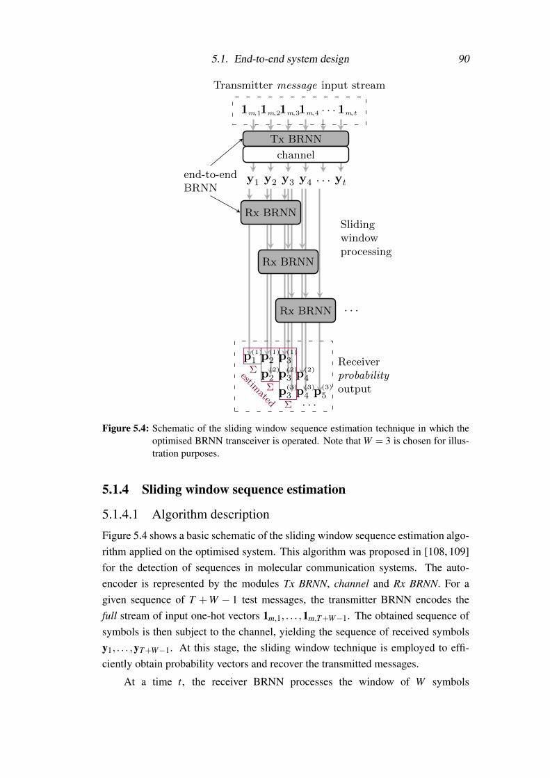
5.1. End-to-end system design 90
1m,11m,21m,31m,4. . .1m,t
Transmitter message input stream
y1 y2 y3 y4 . . . yt
Tx BRNN
channel
pp1q1Σ
pp1q2 pp1q
3
pp2q2Σ
pp2q3 pp2q
4
pp3q3 pp3q
4 pp3q5
Σ
estimated . . .
Rx BRNN
Rx BRNN
Rx BRNN
Slidingwindowprocessing
. . .
Receiverprobabilityoutput
end-to-endBRNN
Figure 5.4: Schematic of the sliding window sequence estimation technique in which theoptimised BRNN transceiver is operated. Note that W = 3 is chosen for illus-tration purposes.
5.1.4 Sliding window sequence estimation
5.1.4.1 Algorithm description
Figure 5.4 shows a basic schematic of the sliding window sequence estimation algo-rithm applied on the optimised system. This algorithm was proposed in [108, 109]for the detection of sequences in molecular communication systems. The auto-encoder is represented by the modules Tx BRNN, channel and Rx BRNN. For agiven sequence of T +W − 1 test messages, the transmitter BRNN encodes thefull stream of input one-hot vectors 1m,1, . . . ,1m,T+W−1. The obtained sequence ofsymbols is then subject to the channel, yielding the sequence of received symbolsy1, . . . ,yT+W−1. At this stage, the sliding window technique is employed to effi-ciently obtain probability vectors and recover the transmitted messages.
At a time t, the receiver BRNN processes the window of W symbols

5.1. End-to-end system design 91
yt , . . . ,yt+W−1, transforming them into W probability vectors p(t)t , . . . ,p(t)
t+W−1 viaits final softmax layer. Then it slides one time slot ahead to process the symbolsyt+1, . . . ,yt+W . Notice that this enables the scheme to provide multiple estimates ofthe probability vector at time t, for t ≥ 2. In particular, the final output probabilityvectors for the first W −1 symbols from the received sequence are given by
pi =1i
i−1
∑k=0
p(i−k)i , i = 1, . . .W −1, (5.25)
while the final probability vectors for the following yW , . . . ,yT symbols in the re-ceived sequence are obtained as
pi =W−1
∑k=0
a(k)p(i−k)i , i =W, . . . ,T, (5.26)
where a(q) ≥ 0,q = 0, . . . ,W − 1 and ∑W−1q=0 a(q) = 1 are weighting coefficients as-
signed to each estimate of the probability output at a specific time instance. Typ-ically, equal weights a(q) = 1
W are assumed by the algorithm, as originally pro-posed in [108]. In Sec. 5.1.4.2 a method for the weight optimisation is proposed,whose performance is examined in Sec. 5.2. Note that the final W − 1 symbolsyT+1, . . . ,yT+W−1 from the received sequence are not fully estimated and are thusnot included in the subsequent symbol error counting. For this reason the sequencelength is chosen such that T �W and thus there is only a negligible reduction inthe data rate of the scheme.
In the following, a concrete example of the first few steps in the operation ofthe sliding window processor is presented with the window size set to W = 3 basedon Fig. 5.4: At t = 1, the receiver BRNN processes the symbols (yt=1,y2,y3) andestimates the output probability vectors
(p(t=1)
1 ,p(1)2 ,p(1)
3
). The receiver has gen-
erated all estimates for the received symbol at t = 1, i.e. y1, and assigns p1 = p(1)1 .
Next at t = 2, the receiver BRNN has shifted a single slot to process (yt=2,y3,y4)
and generates(
p(t=2)2 ,p(2)
3 ,p(2)4
). All estimates for y(2) are obtained at this step and
the final probability vector p2 = 12p(1)
2 + 12p(2)
2 is computed. Similarly, at t = 3, afinal probability vector p3 = a(0)p(3)
3 + a(1)p(2)3 + a(2)p(1)
3 is computed for y3. Thesliding window processing carries on for the remainder of the symbols from thereceived sequence.
5.1.4.2 Optimisation of the weight coefficientsThe weight coefficients a(q) assigned to each of the probability vector estimatesprovided by the sliding BRNN receiver can be optimised in order to enhance the se-

5.1. End-to-end system design 92
quence estimation algorithm and thus improve the overall error rate performance ofthe system. This section proposes an offline optimisation method which consists inpicking a representative test sequence of length T +W−1 for which all correspond-ing BRNN output probability vectors p(i−k)
i , with i =W, . . .T and k = 0, . . . ,W −1are collected. Note that the first W − 1 and the final W − 1 symbols from the se-quence were not considered in the optimisation since the number of weight coef-ficients required for their estimation is lower than W (see Eq.(5.25)). The best setof coefficients a =
(a(0) . . . a(W−1)
)is then obtained by minimising the average
cross entropy, computed as
c(a) :=− 1T −W +1
T
∑i=W
1Tm,i log
(W−1
∑q=0
a(q)p(i−q)i
)(5.27)
between the input one-hot vectors 1m,W , . . . ,1m,T and the estimated final outputprobability vectors pW , . . . ,pT , using the constrained optimisation problem
aopt = argmina
c(a) s.t. a(q) ≥ 0,W−1
∑q=0
a(q) = 1 (5.28)
where q = 0, . . .W −1 and c was used to denote the average cross entropy betweenthe input one-hot vectors and the estimated final output probability vectors. Theoptimisation problem is convex and can easily be solved numerically. Specifically,the MATLAB fmincon function for finding the minimum of constrained nonlinearmultivariable function was used. Section 5.2 presents the results from the performedweight coefficient optimisation and reports the achieved performance improvementusing the method.
5.1.4.3 Performance metric
After the sliding window receiver estimates the final probability vector for a givensymbol, a decision on the transmitted message can be performed as
mt = argmaxj=1...M
(pi, j). (5.29)
A symbol error is counted when mt 6= mt . The symbol error rate (SER) for thetransmitted sequence is given by
SER =1|Te| ∑i∈Te
1{mt 6= mt} , (5.30)

5.1. End-to-end system design 93
where |Te| is the number of fully estimated messages in the test sequence and theindicator function is denoted by 1, and is equal to 1 when the argument is satisfiedand 0 otherwise.
5.1.5 Bit labeling optimisationIn Sec. 4.4.1 it was explained that in order to examine the BER of the developedauto-encoders, a mapping function between the messages processed by the ANNand the FEC encoder/decoder output/input is needed. In particular, a bit labelingfunction expressed as
ϕ : {1, . . . ,M}→ FB2 (5.31)
is required. This function maps a message m to a binary vector b =(
b1, . . . ,bB
),
bi ∈ F2 = {0,1} of length B = dlog2(M)e, with M and B chosen such that M = 2B.In Sec. 4.4.1 the simple method of assigning the binary Gray code to the in-
teger input messages m ∈ {1, . . . ,M} was assumed. However, from the systemperformance results in Sec. 4.4.4.1 it was observed that, although convenient toimplement, such an approach leads to a substantially degraded BER performancecompared to the case when only a single bit error arises from an occurred symbolerror.
Finding a bit labeling function that minimises the bit error rate is an NP-hardtask that is usually solved using combinatorial optimisation, e.g., a bit switchingalgorithm [110]. Here, the use of the Tabu search algorithm [111] with a Tabu listof size 256 is proposed. The algorithm is initialised with a random bit labelingand, using the outcome of the validation run, namely the estimated probabilitiesP(m|m), the expected error rate is used as cost function. For a given bit labeling,the Tabu search tries all possible combinations of two elements and computes theresulting expected BER. The selected combination is the one that leads to the lowestexpected BER and is not in the Tabu list. The Tabu list is then updated with this newassignment in a first-in/first-out fashion. After a pre-defined number of iterations,the overall best assignment is selected. In Sec. 5.2 the resulting BER from theoptimised bit mapping is compared with the trivial (ideal) BER lower bound BER>
P(m 6= m|m)/B, assuming that each symbol error yields exactly a single bit error.It is worth mentioning that an alternative approach was suggested in [112].
It consists in modifying the auto-encoder to encode a set of B bits into a set of Bdecoded bits. In this case, the loss function minimises the average bit error rate.Although a viable alternative, it was found that in many circumstances the trainingcan get stuck in a local minimum, especially when the channel input is heavilyconstrained. Moreover, the results presented in Sec. 5.2 show that the employed bitlabeling optimisation already gives a performance close to the lower bound.

5.2. Numerical investigation of the system performance 94
Table 5.3: Simulations parameters assumed for the examined systems
Parameter Value
Transceiver:
M 64n 12
Oversampling (s) 4Receiver estimation window (W) 10
Test sequence length (T) 104 messagesNumber of test sequences 250
Rcod.12 b/Sa
Channel:
Rsamp. 84 GSa/sSampling rate (s ·Rsamp.) 336 GSa/s
Rinf. 42 Gb/sLPF bandwidth (B f ) 32 GHz
DAC/ADC ENOB (Nb) 6Fibre length (L) varied
Fibre dispersion (D) 17 ps/(nm ·km)Fibre attenuation (αdB/km) 0.2 dB/km
Receiver noise variance (σref.) 2.455 ·10−4
5.2 Numerical investigation of the system perfor-mance
5.2.1 Simulation parametersTable 5.3 lists the simulation parameters assumed for the performance investigationof the proposed SBRNN auto-encoder system. To enable a straightforward com-parison with the FFNN-based auto-encoder presented in Chapter 4, input messagesfrom a set of |M | = M = 64 total messages (6 bits) were assumed in simulation.These were encoded by the transmitter BRNN into symbols of n · s = 48, yieldinga coding rate Rcod. = 1/2, calculated using Eq. (4.5) in Sec. 4.2.1.3. To increasethe simulation resolution, an oversampling by a factor of s = 4 was assumed. Thecorresponding sampling rate thus becomes 336 GSa/s DAC rate, a factor of 4 higherthan the DAC/ADC sampling rate of Rsamp. = 84 GSa/s. The resulting informationrate of the systems was Rinf. = 42 Gb/s. The listed values of all parameters describ-ing the communication channel are identical to the ones used for investigating theend-to-end FFNN system and their description can be found in Sec. 4.4.3. Notethat all ANN-based performance results presented in this section show the testingBER achieved by the best parameter sets found in three independent training runs,

5.2. Numerical investigation of the system performance 95
20 30 40 50 60 70 80 90 10010´6
10´5
10´4
10´3
10´2
10´1
100
HD-FEC threshold
Transmission distance (km)
BER
FFNN auto-enc.
Vanilla SBRNN auto-enc.
LSTM-GRU SBRNN auto-enc.
Figure 5.5: Bit error rate as a function of transmission distance for the 42 Gb/s end-to-endvanilla and LSTM-GRU SBRNN auto-encoders compared to the 42 Gb/s end-to-end FFNN.
obtained with different initialisation of both the ANN parameters and the randomnumber generators.
5.2.2 System performanceThe BER performance of the examined vanilla and LSTM-GRU SBRNN auto-encoder systems, computed by assigning the Gray code to the integer input mes-sages, as described in Sec. 4.4.1, is compared to the FFNN design as a function oftransmission distance at the information rate of 42 Gb/s. The performance resultsare shown in Fig. 5.5. Note that for this investigation all systems are trained sepa-rately for each distance from 20 to 100 km (in steps of 10 km), i.e. using the learningat nominal distance method described in Sec. 4.3.1. Moreover, the fixed windowof W = 10 received symbol blocks was assumed for the SBRNN systems. In con-trast to the FFNN design, the SBRNN handles data sequences, having a structurethat allows mitigation of the inter-symbol interference accumulated during trans-mission. As a consequence, the two SBRNN auto-encoders significantly outper-form the FFNN design at each of the examined distances. In particular, the resultsindicate that the SBRNN designs can enable communication below the 4.5 · 10−3
HD-FEC threshold at distances up to 70 km, which is a substantial increase over theachievable distance of 50 km below HD-FEC for the FFNN.
In the introduction to this chapter, the main differences in the approaches for

5.2. Numerical investigation of the system performance 96
20 30 40 50 60 70 80 9010´4
10´3
10´2
10´1
100
HD-FECthreshold
W“ 10
42Gb/s
M “ 8, n “ 6
M “ 64, n“ 12
M “ 64, n “ 12
W“ 5
W“ 20
W“ 40
Transmission distance (km)
BER
FFNN auto-enc.vanilla SBRNN auto-enc.
Figure 5.6: BER as a function of transmission distance for the FFNN and vanilla SBRNNauto-encoders for different neural network hyper-parameters M, n (FFNN andSBRNN) and sliding window size W (SBRNN).
expanding the processing memory in the FFNN and the SBRNN auto-encoders werehighlighted. In particular, when the coding rate Rcod. of the system is kept fixed, en-hancing the resilience to chromatic dispersion in the FFNN system is associatedwith a rapid increase in the network dimensions (number of nodes), dictated by thehyper-parameters M and n (see Sec. 4.4.3), thus increasing the overall system com-plexity. On the other hand, the processing memory in the SBRNN receiver dependson the size (number of symbol blocks) of the sliding window W in the sequenceestimation algorithm, described in Sec. 5.1.4. The parameter W is external to theBRNN transceiver architecture and thus adjusting it to compensate for more of theinterference does not require any increase in the number of transceiver nodes. Toinvestigate the performance of the FFNN and vanilla SBRNN auto-encoders for dif-ferent M, n and W values, the BER of the systems operating at 42 Gb/s is comparedin Fig. 5.6. It can be seen that for the SBRNN system, increasing W effectively re-duced the BER, allowing transmission below the 6.7% HD-FEC at distances closeto 80 km when W = 40 received blocks are processed – further increasing the im-provement over the FFNN. On the other hand, if the processing memory of theFFNN auto-encoder is expanded to W · n samples, it would require using neuralnetworks with input and output dimensions M = 2W ·n·Rcod. and W · n, respectively,resulting in a number of trainable nodes of the order of ∼ 109 even for W = 5.

5.2. Numerical investigation of the system performance 97
5 10 20 4010´3
10´2
10´1
HD-FECthreshold
84Gb/s at 30 km
Processing window W (# blocks)
BER
Vanilla SBRNN auto-enc.LSTM-GRU SBRNN auto-enc.
Figure 5.7: Bit error rate as a function of receiver estimation window for the 84 Gb/s vanillaand LSTM-GRU SBRNN at 30 km.
Next, the impact of the sliding window size on the performance of the vanillaand LSTM-GRU auto-encoders is studied at a higher data rate. For this investiga-tion, the BER performance at 30 km transmission distance for the vanilla and theLSTM-GRU operating at the 84 Gb/s (achieved by reducing the block size n from12 to 6 samples) was examined for varying window size between 5 and 40 symbolblocks (30 to 240 processed samples). The results from the investigation, which arepresented in Fig. 5.7, show that for both 84 Gb/s systems the window W can be ad-justed such that the BER is reduced. In particular, using W = 40 decreased the BERof the vanilla and LSTM-GRU SBRNN to 2.25 · 10−3 and 1.9 · 10−3, respectively,both values below the HD-FEC threshold. Nevertheless, as also previously indi-cated from the results in Fig. 5.6, diminishing gains for greater W were observedsince system nonlinearity and noise start to dominate when ISI is compensated.Such a behaviour was confirmed in the SBRNN experiment, which is described inChapter 6.
It should be noted that the results from Fig. 5.5 and Fig. 5.7 suggest that thevanilla and the LSTM-GRU SBRNN auto-encoders have a comparable BER per-formance for the examined scenarios. In the following a direct comparison betweenthe proposed vanilla and LSTM-GRU designs was conducted, examining the train-ing convergence of two representative 42 Gb/s systems at 30 km. The average crossentropy loss, computed as described in Sec. 5.1.3, as a function of optimisationstep for the vanilla and LSTM-GRU SBRNN systems is plotted in Fig. 5.8 (a) and

5.3. Comparisons with state-of-the-art digital signal processing 98
0 2,000 4,0000
2
4
42Gb/straining at 30 km
(a)
Optimization step
Loss
Vanilla SBRNN
0 2,000 4,0000
2
4
42Gb/straining at 30 km
(b)
Optimization step
Loss
LSTM-GRU SBRNN
Figure 5.8: Cross entropy loss as a function of optimisation step for the 42 Gb/s (a) vanillaand (b) LSTM-GRU SBRNN systems at 30 km.
5.8 (b), respectively. It can be seen that peaks in the loss value occur every 100optimisation steps. This can be attributed to the fact that the outputs in the forwardand backward passes of the transmitter and receiver BRNN were re-initialised to 0(see Sec. 5.1.3). Moreover, the LSTM-GRU structure required significantly moretraining iterations to converge to low values of the loss. This is an outcome of the in-creased number of parameters in the LSTM-GRU recurrent structure, which entailsa slower training process compared to the vanilla SBRNN. In particular, the de-scriptions of the vanilla and the LSTM-GRU neural network processing, presentedin Sections 5.1.1.2 and 5.1.2.2, shows that there are significantly fewer trainableparameters in the vanilla SBRNN system compared to the LSTM-GRU. However,as already mentioned, the performance of the vanilla design is comparable to thatof the LSTM-GRU. This may be accounted to the fact that, as a result of fibre dis-persion, neighbouring symbols impose stronger interference effects on the currentsymbol. This means that, applied to optical fibre communications, structures suchas the LSTM-GRU which capture long term dependencies in a sequence, do notsignificantly improve the performance over vanilla RNN-based signal processing.
5.3 Comparisons with state-of-the-art digital signalprocessing
5.3.1 PAM and sliding window feedforward neural network-based receiver
In this section the BER performance of the vanilla and LSTM-GRU SBRNN auto-encoders was compared with a reference system based on the conventional pulseamplitude modulation (PAM) and state-of-the-art multi-symbol nonlinear equali-

5.3. Comparisons with state-of-the-art digital signal processing 99
Transmission link
z´1
z´1
z´1
z´1
yt´ Zg´1
2
yt´1
yt
yt`1
yt` Zg´1
2
...
...
ReLU
Softmax
2
pt. . .
Figure 5.9: Schematic of the sliding window FFNN receiver for PAM symbols.
sation at the receiver using a large sliding window FFNN (SFFNN). It has beenshown that such an equaliser performs similarly to classical nonlinear equalisationtechniques [113]. This receiver design has been previously considered in low-costIM/DD links [58, 114] as well as long-haul coherent fibre-optic systems [115]. Thesection also includes a discussion about the number of trainable nodes in the inves-tigated systems, as an indicator of computational complexity.
5.3.1.1 Design of the reference system
For this investigation, 42 Gb/s two-level PAM (PAM2) transmission was considered.In particular, the system was simulated in the following way: The PAM2 transmitterdirectly mapped a sequence of bits into a sequence of PAM2 symbols using the lev-els {0;π/4}. The sequence of PAM symbols was pulse-shaped by a raised-cosine(RC) filter with 0.25 roll-off factor. The shaping was performed at g = 8 samplesper symbol such that 6 PAM2 symbols (6 bits of information) are transmitted over48 samples at the simulation sampling rate of 336 Sa/s. This setup was used toensure that the reference PAM scheme was simulated with the same sampling rateand has coding rate and oversampling factor corresponding to the values assumedin the investigated SBRNN and FFNN auto-encoder setups, which were describedin Table 4.3, Sec. 4.4.3 and Table 5.3, Sec. 5.2, respectively. The obtained PAMsignal was transmitted over the optical IM/DD communication channel, modeled

5.3. Comparisons with state-of-the-art digital signal processing 100
with parameters in accordance to Table 5.3. Figure 5.9 shows a schematic of thereceiver section in the system denoted as “Tx-PAM2 & Rx-SFFNN”. The receivedsequence of samples, distorted after fibre propagation, was processed by a multi-layer FFNN in the following way: samples corresponding to Z neighboring PAMsymbols, were applied to the receiver ANN, which estimates the central of thesesymbols. Thus, the first layer of the neural network had parameters W ∈ RZ·g×Z·g
and b ∈ RZ·g, where Z is the number of symbols processed simultaneously by thereceiver and g = 8, is the assumed oversampling factor. As suggested in [58, 114],the receiver design employed multiple hidden layers which further process the re-ceived samples. The number of nodes on each of the hidden layers was given by⌊Z ·g/(2l−1)
⌋, where l = 1 corresponds to the first hidden layer, l = 2 is for the
second hidden layer, and so on. ReLU activation functions were applied on all lay-ers, except for the final layer, whose output represents an estimation of the centralPAM2 symbol and for which the softmax activation was applied. Thus, the receiveroutput was a probability vector pt ∈ R2 of length 2 used for recovering the trans-mitted PAM symbol as argmaxi=1,2 pt,i. Note that by estimating the central of Zinput PAM symbols, this receiver includes preceding and succeeding symbols inthe equalisation function. After estimation of the current central symbol, the FFNNequaliser is shifted one time slot ahead to the next symbol position and estimates thefollowing PAM2 symbol from the received sequence. It has been shown that suchreceivers can approximate high-order nonlinear Volterra equalisers [58, 113, 114].For this investigation, training of the deep sliding window FFNN was performedby labeling the transmitted PAM2 sequences and using the cross entropy loss be-tween them and the estimated output of the neural network, a standard approach fortraining FFNN, as described in Sec. 2.1.2. Similar to the optimisation proceduresimplemented for the auto-encoder systems, independent data sequences were gener-ated using the Tausworthe generator [106] in the testing phase. Because of the largesize of the receiver FFNN, for the investigation of the Tx-PAM2 & Rx-SFFNN sys-tem with a processing window of Z = 61 symbols, 400 000 optimisation iterationswere used to ensure the training convergence.
5.3.1.2 BER performance
Figure 5.10 shows the BER performance of the investigated 42 Gb/s auto-encodersystems at different transmission distances in comparison with the Tx-PAM2 &Rx-SFFNN, for which the processing window Z was varied. Note that all systemswere optimised separately for each distance. The Tx-PAM2 & Rx-SFFNN (Z =
61) system, whose receiver simultaneously processes relatively the same numberof samples as the SBRNN (Z · g = 488 to W · n · s = 480) was outperformed by

5.3. Comparisons with state-of-the-art digital signal processing 101
20 30 40 50 60 70 80 90 10010´6
10´5
10´4
10´3
10´2
10´1
100
HD-FEC threshold
End-to-end
Rx only
Transmission distance (km)
BER
Tx-PAM2 & Rx-SFFNN Z “ 11
Tx-PAM2 & Rx-SFFNN Z “ 21
Tx-PAM2 & Rx-SFFNN Z “ 61
FFNN auto-enc.
Vanilla SBRNN auto-enc.
LSTM-GRU SBRNN auto-enc.
Figure 5.10: BER as a function of transmission distance for the end-to-end vanilla andLSTM-GRU SBRNN systems compared to the end-to-end FFNN as well asthe PAM2 system with multi-symbol FFNN receiver. The systems operate at42 Gb/s.
both the vanilla and the LSTM-GRU auto-encoder designs for all distances up to80 km. In particular, for distances up to 50 km both SBRNN systems achievedBERs significantly below the value for the Tx-PAM2 & Rx-SFFNN. Moreover, thesimulation prediction indicated that the Tx-PAM2 & Rx-SFFNN (Z = 61) could notachieve transmission below the HD-FEC beyond 60 km. In contrast, the vanilla andLSTM-GRU SBRNN could increase the transmission distance to around 70 km.At longer distances these three systems achieved comparable BER performance,which was, however, above 10−2. Moreover, the presented results showed that theFFNN auto-encoder performed similarly to the Tx-PAM2 & Rx-SFFNN when theprocessing memory of the latter was decreased to Z = 21 or Z = 11.
5.3.1.3 Number of ANN nodes in the investigated systemsIn Sec. 5.2.2 it was discussed that increasing the processing memory in FFNN-basedDSP schemes is typically associated with expanding the neural network dimensions.This section provides a concrete example for the cases of FFNN auto-encoder andTx-PAM2 & Rx-SFFNN systems by investigating their number of nodes, as an in-dicator of computational complexity, in comparison to the SBRNN auto-encoders.For this purpose, Table 5.4 summarises the neural network hyper-parameters forthe aforementioned systems and evaluates them for a reference 42 Gb/s transmis-

5.3. Comparisons with state-of-the-art digital signal processing 102
Table 5.4: Summary of hyper-parameters for the compared ANN-based systems
Param. Tx-PAM2 & Rx FFNN FFNN AE vanilla/GRU AE
Bits/Sym 1 log2(M) = 6 log2(M) = 6Sa/Sym g = 8 n · s = 48 n · s = 48
Proc. w (Sym) Z = 11/21/61 N/A W = 10Proc. w. (Sa) Z ·g n · s W ·n · s
Layers L = 6/7/9 3+3 2 · (1+1)+1
Nodes Z ·g+L−2
∑l=1
⌊Z ·g2l−1
⌋+2 10M+2n · s 15M+6n · s
35M+18n · sNodes at 42 Gb/s 1457 (Z = 61) 736 1248
3104
sion. Detailed descriptions of the hyper-parameters for each system can be foundin Sections 4.2 and 4.4 (FFNN), Sections 5.1 and 5.2.2 (SBRNN), and Sec. 5.3.1.1(Tx-PAM2 & Rx-SFFNN). For the vanilla and LSTM-GRU SBRNN, the processingwindow size was fixed to W =10 symbols, while for the Tx-PAM2 & Rx-SFFNN,the estimation window was increased from Z = 11 to Z = 21 and then Z = 61.The provided summary highlights that the number of layers in the Tx-PAM2 &Rx-SFFNN was increased accordingly as Z increased. In contrast, for the case ofSBRNN, only a single layer network at transmitter or receiver was used in eitherdirection of the bidirectional processing (with an additional softmax layer at thereceiver output). When comparing the number of ANN nodes for the investigatedsystems1, it can be seen that in the recurrent designs there is no dependence on thereceiver processing window W , i.e. expanding the processing memory of the BRNNreceiver does not require an increase in the number of trainable parameters. As ex-plained in 5.2.2 this is in stark contrast to the case of an FFNN auto-encoder, whereexpanding the processing capabilities is associated with larger neural networks atboth transmitter and receiver. Similarly, increasing Z in Tx-PAM2 & Rx-SFFNNsystem would result in a substantial increase in the number of nodes in the receiver.As a consequence, when the number of nodes was evaluated for 42 Gb/s systems,the vanilla SBRNN design had fewer trainable parameters compared to the Tx-PAM2 & Rx-SFFNN, while processing the same amount of received samples. Thisdifference would become even more pronounced when the processing window foreach system is increased to capture more of the interference.
1An example of how the nodes in the SBRNN system were counted is provided in Appendix B.1.

5.3. Comparisons with state-of-the-art digital signal processing 103
60 70 80 90 100
0
0.5
1
1.5¨10´2
Distance (km)
SER
u´
SER
opt
0 1 2 3 4 5 6 7 8 90
0.1
0.2
0.3
q
apq
q
Figure 5.11: Top: SER difference as a function of distance for the two approaches forfinal probability vector estimation in the sliding window algorithm (W = 10).SERu is obtained assuming a(q) = 1
W ,q = 0, . . . ,W − 1 in Eq. (5.26), whilefor SERopt the coefficients a(q) are optimised. Bottom: a(q) assignments afteroptimisation for the system at 100 km.
5.3.2 SBRNN auto-encoder enhancement via optimisation of thesequence estimation and bit labeling functions
In this section, the results from the optimisation of the weight coefficients in the slid-ing window sequence estimation algorithm, a problem formulated in Sec. 5.1.4.2,are presented. Moreover, the performance gains from the optimisation of the bit-to-symbol mapping function, an essential aspect for the auto-encoder systems, usingthe method proposed in 5.1.5 are examined.
5.3.2.1 Performance after weight optimisationFigure 5.11 (top) shows the improvement in symbol error rate (SER) at differentdistances for a fixed sliding window size of W = 10 after optimisation of the coeffi-cients a(q) in Eq. (5.26). The corresponding SER performances when equal weightsa(q) = 1
W ,q = 0, . . . ,W −1 are assigned are used as a reference. Note that the set ofcoefficients is optimised separately for each distance. It can be seen that the ben-efit from weight optimisation becomes more pronounced as the distance increases.

5.3. Comparisons with state-of-the-art digital signal processing 104
50 55 60 65 70 75 80 85 90 95 10010´4
10´3
10´2
10´1
HD-FEC threshold
Transmission distance (km)
BER
Optimised
Gray-coded m
Ideal
Figure 5.12: Bit error rate as a function of distance for a reference vanilla SBRNN auto-encoder, which utilises two different bit-to-symbol mapping approaches: as-signing the Gray code to the transmitted message m, proposed in Sec. 4.4.1,and performing the combinatorial algorithm-based optimisation, proposed inSec. 5.1.5. As an indicator, the ideal bit-to-symbol mapping when a singlesymbol error gives rise to a single bit error is also displayed.
The a(q) assignments after optimisation at 100 km are depicted in Fig. 5.11 (bot-tom). Greater weights are assigned to the middle indices, indicating that a receivedsymbol is estimated with a higher accuracy by the receiver when relatively equalamount of pre- and post-cursor interference is captured.
5.3.2.2 Performance after bit-to-symbol mapping optimisation
The BER as a function of distance for a reference W = 10 vanilla SBRNNauto-encoder, computed using the bit-to-symbol mapping algorithm described inSec. 5.1.5, is plotted in Fig. 5.12. For a comparison, the figure also shows the BERperformance of the system when the ad hoc approach of assigning the Gray codeto the input m ∈ {1, . . . ,M}, proposed in Sec. 4.4.1, is employed. The trivial case(denoted “ideal”) when a single block error results in a single bit error is also shownas a reference. It can be seen that by conducting the bit-to-symbol mapping opti-misation, the performance of the system is improved, leading to an increase in theachievable distance below the HD-FEC threshold to 70 km. Moreover, the obtainedBER after optimisation is close to the ideal case for all examined distances.

5.3. Comparisons with state-of-the-art digital signal processing 105
LPF `
MZM ` LPF
`xptq
yptq
nDACptq
nRec.ptq
nADCptq
fiber
Tx-PAM
RRC
filterPAM
Modulator
xk Viterbi processor(square-root metric)
ChannelEstimation
ylk
νlkpσk, xkq
Rx-MLSD
Ns “ 2x
Figure 5.13: Schematic diagram of the system used to evaluate the performance of theMLSD receiver in IM/DD optical links.
5.3.3 PAM and maximum likelihood sequence detection
5.3.3.1 Design of the reference system
To establish a relevant benchmark for the performance of the SBRNN auto-encoderusing a classical DSP technique, a reference M-PAM transmission system (M ∈{2,4}) with a receiver based on maximum likelihood sequence detection (Tx-PAM&Rx-MLSD) was considered. Receivers based on MLSD have been widelyconsidered for optical IM/DD transmission [68, 69] and represent a valid perfor-mance reference scheme. Nevertheless, it is worth noting that the auto-encoderperforms an optimisation of both the transmitter and receiver designs, while in con-trast, the transmitter is assumed fixed in the Tx-PAM&Rx-MLSD scheme. For thisinvestigation, the vanilla SBRNN design was used, since the results presented inthis chapter clearly showed that in the framework of optical IM/DD communica-tion, the processing capabilities of such an auto-encoder is similar compared to theLSTM-GRU structure, without the associated extra complexity.
The MLSD receiver assumes that the communication channel behaves accord-ing to a Markov process, thus facilitating the use of the Viterbi algorithm [67] whichselects
x = argmaxx
p(y|x), (5.32)
where x = (x1,x2, ...,xNsym) is the sequence of transmitted PAM symbols, y =
(y11,y
21, ...,y
Ns1 ,y1
2,y22, ...,y
Ns2 , ...,yNs
Nsym) is the sequence of corresponding received
samples. Here Nsym and Ns denote the number of PAM symbols in the transmittedsequence and number of samples per symbol, respectively. The joint distributionp(y|x) is an approximation of the true channel likelihood pY|X(y|x), whose accu-racy depends on the number of states and metric used in the Viterbi processor. Foroptical IM/DD systems, a more convenient option for an MLSD receiver is to oper-ate on the distribution p(y|x), where y = (y1
1,y21, ...,y
Ns1 ,y1
2,y22, ...,y
Ns2 , ...,yNs
Nsym) with

5.3. Comparisons with state-of-the-art digital signal processing 106
ylk =
√yl
k for l = 1, ...Ns and k = 1,2, ...,Nsym [69]. The channel state is defined as
σk , (xk− µ
2,xk− µ
2 +1, ...,xk−1,xk+1, ...,xk+ µ
2) (5.33)
where µ is the number of pre- and post-cursor PAM symbols determining the chan-nel memory, the distribution of yl
k conditioned on (σk,xk) was shown to be well-approximated by a Gaussian with equal variances [69]. Under such an approxima-tion, and the assumption of uncorrelated samples yl
k conditional to (σk,xk), p(y|x)can be suitably factorised via the channel state definition in Eq. (5.33) for the use ina Viterbi processor.
The branch metric of the Viterbi trellis at time k can thus be defined as
λk(σk,xk) =Ns
∑l=1
(√yl
k−νlk(σk,xk)
)2
(5.34)
where ylk is the l-th out of Ns samples within the k-th symbol period, and ν l
k(σk,xk)
is given by
νlk(σk,xk) = E
{√yl
k(σk,xk)
}, (5.35)
with ylk(σk,xk) indicating the value of the received sample yl
k when the pair (σk,xk)occurs. The square-root metric in Eq. (5.34) was introduced in [68] as a conve-nient low-complexity alternative to the histogram-based metric with comparableperformance [69]. At the end of each given window of T symbols, the Viterbiprocessor makes a decision on the previous T transmitted symbols by minimis-ing the sequence metric ΛT = ∑
Tk=1 λk(σk,xk) over all surviving state sequences
[σ1,σ2, ...,σT ].
The schematic diagram of the system model employing MLSD is shown inFig. 5.13 (with the channel parameters taken from Table 5.3). At the transmitter, aGray-labelled PAM2 ({0;π/4}) or PAM4 ({0;π/12;π/6;π/4}) mapper was usedto make a transition between bits and symbols. This is followed by pulse-shapingat 2 samples per symbol by a root-raised cosine (RRC) filter with a roll-off factorof 0.25. DAC/ADC rates of 84 GSa/s and 42 GSa/s are assumed for the PAM2 andPAM4 cases, respectively, resulting in a fixed data rate of 42 Gb/s for both systems.A signal corresponding to a sequence of 105 symbols was transmitted through theoptical IM/DD communication channel described in Chapter 3. At the receiver, theestimation of the ν l
k(σk,xk) was first done computing Eq. (5.35) over a sequence of107 symbols. The received signal, sampled at Ns = 2 samples per symbol, is thenpassed directly to the Viterbi processor which performs the MLSD.

5.3. Comparisons with state-of-the-art digital signal processing 107
30 40 50 60 70 80 90 10010´4
10´3
10´2
10´1
100
HD-FEC threshold
Transmission distance (km)
BER
Tx-PAM2&Rx-MLSD pη “ 10qTx-PAM2&Rx-MLSD pη “ 12qTx-PAM4&Rx-MLSD pη “ 12qSBRNN auto-enc. pη “ 12qSBRNN auto-enc. pη “ 60q
Figure 5.14: Bit error rate as a function of transmission distance for the 42 Gb/s SBRNNauto-encoder and M-PAM & Rx MLSD systems (M ∈ {2,4}). In the case ofMLSD η = µ log2(M), where µ represents the number of pre- and post-cursorPAM symbols defining one of Mµ channel states. In the case of SBRNNη =W log2(M) is the number of bits inside the processing window.
5.3.3.2 BER performanceThe performance of the SBRNN auto-encoder was numerically evaluated using thedesign parameters given in Table 5.3. Note that weight optimisation in the slidingwindow estimation was performed as described in Sec. 5.1.4.2. In an attempt to setup a fair comparison between the investigated systems, a parameter η was fixed,which in the case of SBRNN corresponded to the number of information bits pro-cessed inside the sliding window η = W log2(M). For the PAM transmitter withMLSD receiver, this number denoted the amount of bits contained within a channelstate in the Viterbi algorithm η = µ log2(M), where M ∈ {2,4} was the PAM or-der and µ denoted the number of post- and pre-cursor PAM symbols which formeda Viterbi state. Note that in Tx-PAM2&Rx-MLSD and Tx-PAM4&Rx-MLSD, afixed η = 12 also meant using the same number of Viterbi states (4096). Thus,the Tx-PAM4&Rx-MLSD scheme accounted for a decreased amount of memorycompared to the Tx-PAM2&Rx-MLSD.
Figure 5.14 shows the BER performance of the examined systems as a functionof transmission distance. It can be seen that for η = 12, the SBRNN auto-encoderand Tx-PAM2&Rx-MLSD had a comparable performance at all examined distancesbeyond 50 km. Both systems outperformed the Tx-PAM4&Rx-MLSD, where the

5.3. Comparisons with state-of-the-art digital signal processing 108
obtained BER was below the HD-FEC threshold up to 30 km. This was due to thedecreased sensitivity of the PAM4 signal and Viterbi memory (µ = 6). Moreover,the results indicated that assuming a wider processing window of η = 60 for theSBRNN leads to a significant BER improvement. Note that the BER of the SBRNNauto-encoder was obtained using the bit-to-symbol mapping algorithm described inSec. 5.1.5.
5.3.3.3 ComplexityIn this section the computational complexity of the two systems was compared us-ing the floating point operations per decoded bit (FLOPSpdb) as a common metric.In the case of the SBRNN auto-encoder, the counted FLOPS occur in matrix mul-tiplications, bias additions and element-wise nonlinear activations in both directionof the recurrent structures as well as multiplications and additions in the final prob-ability vector estimations. Detailed description of the SBRNN auto-encoder hyper-parameters can be found in Sections 5.1 and 5.2.2. At the transmitter, the numberof FLOPS performed in the encoding of a single bit was given by2
FLOPS[SBRNN-TX]pdb =
2n · s(2(M+n · s)+1)log2(M)
, (5.36)
where M, n and s are hyper-parameters of the neural network, i.e. pre-defined designchoices which do not change with the processing memory. Correspondingly, at thereceiver the number of FLOPS required for decoding were
FLOPS[SBRNN-RX]pdb =
W (24M2 +8Mn · s+5M+2)log2(M)
, (5.37)
which indicates a linear dependence of the floating point operations on the process-ing window W .
For the Viterbi processor, the amount of floating point operations scales lin-early with the number of states in the trellis which is equal to Mµ . Assuming afully populated trellis, the Viterbi processor performs for each trellis section Mµ+1
branch metric calculations, Mµ+1 additions, and Mµ+1 comparisons (other than thestorage of Mµ sequences). As for the computation of the branch metric, a total of3Ns +(Ns−1) FLOPS are required (assuming addition, multiplication, and square-root use 1 FLOP each). Moreover, each comparison is accounted for as 1 FLOPand the additional set of comparisons required for the selection of the most likelysequence at the end of the Viterbi decoding is considered negligible. Thus, the
2An example of how the number of FLOPSpdb in the SBRNN system were counted is providedin Appendix B.2.

5.4. Summary 109
overall number of required FLOPS per decoded bit is approximately given by
FLOPS[MLSD]pdb ≈ 9Mµ+1
log2(M), (5.38)
estimated for Ns = 2. Importantly, the expression in Eq. (5.38) indicates that thenumber of FLOPS[MLSD]
pdb exhibits an exponential dependence on the processingmemory µ of the detector. In presence of strong intersymbol interference this mayresult in computationally prohibitive demands or increasingly sub-optimal perfor-mance.
5.4 SummaryIn this chapter, the design of an optical fibre transceiver using a bidirectional re-current neural network (BRNN) was proposed and investigated. The BRNN-basedauto-encoder was combined with a sliding window sequence estimation algorithm(SBRNN), efficiently handling the memory in the communication channel. The de-tailed numerical investigation showed that such a design has an improved resilienceto intersymbol interference compared the feedforward neural network-based auto-encoder, which was investigated in Chapter 4. Importantly, comparisons with con-ventional PAM transmission based on state-of-the-art nonlinear receivers as well asclassical maximum likelihood sequence detection (MLSD) were carried out. Theconducted research revealed that the SBRNN auto-encoder can increase reach orenhance the data rate for shorter distances compared to the benchmark PAM sys-tems without the associated computational complexity of such schemes. The workwas published in [116–118]. The SBRNN auto-encoder system was successfullyverified on a transmission test-bed as part of the experimental work on end-to-enddeep learning-based optical fibre systems described in Chapter 6. The investigationin Chapter 6 covered detailed comparisons with PAM systems using sliding windowFFNN receivers as well as nonlinear Volterra equalisers.

Chapter 6
Experimental demonstrations,comparisons with state-of-the-artDSP and optimisation usingmeasured data
This chapter describes the setup and presents the results from three different exper-iments, which were conducted throughout the Ph.D. programme to demonstrate theconcept of end-to-end deep learning in optical fibre communications. The diagrampresented in Fig. 6.1 summarises the scope of each experiment. The first two inves-tigations covered the implementation and performance of the feedforward (FFNN)and sliding window bidirectional recurrent neural network (SBRNN) transceiverdesigns proposed in Chapter 4 and Chapter 5, respectively. The third investigationinvolved the development and experimental verification of a novel method for end-to-end system optimisation using a generative model of the optical transmissionlink, a technique which is described in Sec. 6.6.
The chapter is organised as follows: First, the optical IM/DD transmissiontest-bed, common for each of the experiments, is described in Sec. 6.1. Next, Sec-tion 6.2 presents the different strategies which were considered when implementing
Experiment 1 (Sec. 6.4):FFNN auto-encoder& multi-distance learning
Experiment 2 (Sec. 6.5):SBRNN auto-encoder& state-of-the-art DSP comp.
Experiment 3 (Sec. 6.6):End-to-end system optimisationusing generative link model
Auto-encoder implementationon a transmission link
Figure 6.1: Diagram showing the three experiments, which were conducted for the demon-stration of the end-to-end deep learning concept in optical fibre communicationsystems.

6.1. Optical transmission test-bed 111
Transmitter LPF
Resamp.
DAC
84GSa/s Driver amp.
MZM TDM
Laser
PD
TIA
ADC
LPF
Resamp. Receiver
fiber
Figure 6.2: Schematic of the experimental optical IM/DD transmission test-bed used forinvestigation of the digital signal processing schemes in this chapter. LPF: low-pass filter, DAC: digital-to-analogue converter, MZM: Mach-Zehnder modula-tor, TDM: tunable dispersion module, PD: photodiode, TIA: trans-impedanceamplifier, ADC: analogue-to-digital converter.
the auto-encoder systems on an actual transmission link. These include optimisa-tion based on transmission in simulation using the explicit link model (Chapter 3)as well as learning of the transceiver parameters from experimentally collecteddata in an end-to-end or receiver-only mode. The demonstration of the FFNN-based auto-encoder is described in Sec. 6.4 with comparisons to PAM transmissionwith conventional linear equalisation. The section also includes the experimentalverification of the multi-distance learning method from, which was developed inSec. 4.3.2. Section 6.5 details the experimental implementation of the end-to-endSBRNN system. It includes investigation of the SBRNN performance compared tostate-of-the-art receiver DSP based on classical as well as deep learning approaches.The chapter concludes with the description and experimental demonstration of theend-to-end system optimisation algorithm using a generative model.
6.1 Optical transmission test-bedThis section introduces the experimental transmission test-bed used to investigatethe performance of the auto-encoders as well as the reference DSP schemes con-sidered in the chapter. Figure 6.2 shows a schematic of the test-bed. An intensitymodulation/direct detection fibre transmission link without in-line optical amplifi-cation was considered. Note that in the case of auto-encoders, the transmitter andreceiver are artificial neural networks, while for the systems used for performancecomparisons, the transmitter is based on PAM, for which different conventional andANN-based receivers were considered. For all systems, the electrical signal outputof the transmitter was filtered in the digital domain by a brick-wall low-pass filter(LPF) which had a bandwidth of 32 GHz. The signal was then re-sampled (moduleResamp.) and applied to the digital-to-analogue converter (DAC) which was oper-ated at 84 GSa/s. The obtained electrical waveform was pre-amplified by a driveramplifier and used to externally modulate the 1550 nm laser via a Mach-Zehnder

6.2. System implementation strategies 112
modulator (MZM). For the auto-encoder system, the MZM was carefully biasedto match the simulation output, while for the reference PAM experiments, the biaswas set at the quadrature point. The optical power which was input to the fibre forall systems is set to 1 dBm. The modulated optical signal was propagated over afixed length of standard single mode fibre (SSMF) and the received waveform wasdirect-detected by a positive-intrinsic-negative (PIN) photo-diode (PD) combinedwith a trans-impedance amplifier (TIA). The signal was real-time sampled by ananalogue-to-digital converter (ADC). After synchronisation, scaling, offset and re-sampling, the digitised photocurrent was stored for digital signal processing at thereceiver. Note that re-scaling and offset were necessary because the employed re-ceiver was AC-coupled and also has a non-ideal photoresponsivity. It should also benoted that in the experimental setup for the investigation of the FFNN auto-encoder(Experiment 1), a tunable dispersion module (TDM) was deployed to enable sweep-ing the dispersion around a given value set by the SSMF length. The reason wasthe verification of the multi-distance learning method. Thus, for Experiment 1 only,the modulated optical signal first entered the TDM allowing to vary the dispersionfrom −170 to +170 ps/nm in steps of 10 ps/nm, before being launched at a powerof 1 dBm into the SSMF span.
6.2 System implementation strategiesThe different strategies for implementing the auto-encoder systems on an actualtransmission link are summarised with the schematic shown in Fig. 6.3. Within theauto-encoder framework, which was introduced in Sec. 4.1, the channel is consid-ered as a segment of the end-to-end computational graph representing the completecommunication system. Thus, the end-to-end learning concept can be readily ap-plied in scenarios where the channel model is known and differentiable. In this case,the transceiver is optimised via simulation transmission and applied “as is” to thereal system, as shown in Fig. 6.3 i). Such systems present a viable perspective forlow-cost optical fibre communications since no optimisation process is required af-ter deployment. However, as first reported in [61] and also seen from the presentedresults in the chapter, the performance of transceivers learned on a specific modelassumption often deteriorates when applied to an actual transmission link. In suchcases, the ANN parameters could be optimised to the specific link properties usingexperimentally collected data.
The optimisation is easier to implement at the receiver (Fig. 6.3 ii)), becausethe backpropagation [12, 13] for computing gradients extends only to the link out-put. For receiver-only optimisation, the set S of training elements is formed by thepairings of input messages mt and the corresponding received blocks of samples

6.2. System implementation strategies 113
Transmitterx y
LPF
32GHz
Resamp.
DAC
84GSa/s Driver amp.
MZM1 dBm
1550 nm
PD
TIA
ADC
LPF
Resamp. Receiver
SSMF
TX ANN
Transmission model
RX ANNi) End-to-end optimization using explicit link model
ppy|xq
iii) End-to-end optimizationusing generative link model
ii) Receiverfine-tuning
Simulation transmission
Experimental transmission
Direction ofgradient computation
Figure 6.3: Schematic of the experimental optical IM/DD transmission test-bed, showingthe methods for system optimisation using i) numerical simulation of the link;ii) & iii) experimental traces.
(symbols) yt from the experimental traces (see Sec. 6.3). The receiver ANN param-eters θRx are adjusted via the Adam optimiser, described in Sec. 2.2.1.2, aimed atminimising the average loss L , computed at the receiver output, over a mini-batchS from the training set, given by
L (θRx) =1|S| ∑
(mt ,yt)∈S`(mt , frec(. . . ,yt , . . .)) , (6.1)
where frec is used to denote a generic receiver ANN function. Note that, in the caseof an SBRNN auto-encoder the receiver will take multiple received symbols as aninput. In this work, the cross entropy loss function, defined in Sec. 2.1.2.2, Eq. (2.9)was used in the optimisation of receiver parameters using measured data.
However, the transmission link can be considered a black box for which onlyinputs and outputs are observed, precluding backpropagation to the transmitter pa-rameters. As a consequence, optimising the transmitter without the explicit knowl-edge of the model for the underlying physical channel remains an open problem.In this thesis, a framework for transmitter optimisation using a generative modelof the optical link was developed and experimentally demonstrated. The method,which is described in detail in Sec. 6.6 uses a generative adversarial network for ap-proximating the channel conditional distribution p(y|x). As shown in Fig. 6.3 iii),
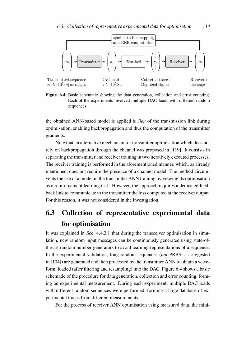
6.3. Collection of representative experimental data for optimisation 114
¨˚˝
...mt
...
˛‹‹‚ Transmitter
¨˚˝
...xt
...
˛‹‹‚ Test-bed
¨˚˝
...yt
...
˛‹‹‚ Receiver
¨˚˝
...mt
...
˛‹‹‚
Transmitted sequence« t5 ¨ 105{numessages
DAC load« 5 ¨ 105 Sa
Collected tracesDigitized signal
Recoveredmessages
symbol-to-bit mappingand BER computation
Figure 6.4: Basic schematic showing the data generation, collection and error counting.Each of the experiments involved multiple DAC loads with different randomsequences.
the obtained ANN-based model is applied in lieu of the transmission link duringoptimisation, enabling backpropagation and thus the computation of the transmittergradients.
Note that an alternative mechanism for transmitter optimisation which does notrely on backpropagation through the channel was proposed in [119]. It consists inseparating the transmitter and receiver training in two iteratively executed processes.The receiver training is performed in the aforementioned manner, which, as alreadymentioned, does not require the presence of a channel model. The method circum-vents the use of a model in the transmitter ANN training by viewing its optimisationas a reinforcement learning task. However, the approach requires a dedicated feed-back link to communicate to the transmitter the loss computed at the receiver output.For this reason, it was not considered in the investigation.
6.3 Collection of representative experimental datafor optimisation
It was explained in Sec. 4.4.2.1 that during the transceiver optimisation in simu-lation, new random input messages can be continuously generated using state-of-the-art random number generators to avoid learning representations of a sequence.In the experimental validation, long random sequences (not PRBS, as suggestedin [104]) are generated and then processed by the transmitter ANN to obtain a wave-form, loaded (after filtering and resampling) into the DAC. Figure 6.4 shows a basicschematic of the procedure for data generation, collection and error counting, form-ing an experimental measurement. During each experiment, multiple DAC loadswith different random sequences were performed, forming a large database of ex-perimental traces from different measurements.
For the process of receiver ANN optimisation using measured data, the mini-

6.3. Collection of representative experimental data for optimisation 115
0 0.1 0.2 0.3 0.4 0.5 0.6 0.7 0.8 0.9 1
¨1050.1
0.15
0.2
0.25
0.3
Optimization step
ValidationSER
random
lv “ 105
lv “ 104
lv “ 5 ¨ 103lv “ 103
lv “ 6 ¨ 102lv “ 102
Figure 6.5: Validation symbol error rate as a function of optimisation step for differentlengths lv of the validation pattern. The receiver ANN of the system is op-timised using traces from the transmission of training sequences with a shortpattern ltr = 6 ·102.
batch of training examples is formed by randomly picking messages and corre-sponding received blocks of symbols from a subset of the database (combiningmultiple measurements). To investigate system performance, the trained and storedmodels are used to perform testing on a disjoint subset of the database of experi-mental traces, having no overlap with the subset used for training. This procedureensures that the presented experimental results are achieved with independent data.However, it is worth noting that, due to the long memory of the fibre, it is not pos-sible to capture the interference effects of all possible sequences of symbols pre-ceding and succeeding the symbol under consideration in the experiment. Hence,a special care should be taken when re-training the receiver ANN, such that it doesnot learn to adapt to the interference pattern of the sequence. The results in thissection investigate the effects of re-training based on repeated sequences to verifythat a sufficiently large set of different experimental traces was captured.
The impact of repeated sequences on the optimisation performance was stud-ied in the following way: In simulation, an auto-encoder system is trained on asimplified channel model, including only a few of the optical IM/DD transmissioneffects described in Chapter 3. Then, transmission of sequences with repeated pat-tern is simulated over the full channel model, collecting the data at the output of

6.3. Collection of representative experimental data for optimisation 116
0 0.1 0.2 0.3 0.4 0.5 0.6 0.7 0.8 0.9 1
¨1055 ¨ 10´2
0.1
0.15
0.2
0.25
HD-FEC thresholdTrained at p20, 4q kmOptimization step
ValidationSER
random
lv “ 105
lv “ 104
lv “ 5 ¨ 103lv “ 103
lv “ 6 ¨ 102lv “ 102
Figure 6.6: Validation symbol error rate as a function of optimisation step for differentlengths lv of the validation pattern. The receiver ANN of the system is re-trained using data from the transmission of training sequences with a long rep-etition pattern ltr = 104.
the channel. Two sets of sequences are used – for re-optimisation of the receiverANN parameters as well as for performance validation. In particular, the FFNNauto-encoder described in Chapter 4 was used as a reference system. It was trained,following the procedure in Sec. 4.4.2.2, on a model which included only transmitterLPF, fibre dispersion and square-law detection. The optimised transceiver was thendeployed for test transmission, simulating the full optical IM/DD channel modelwith low-pass filtering at transmitter and receiver, noise from the DAC, the ADCand the electrical amplification circuit, nonlinearity from the MZM and the square-law detection and fibre dispersion.
Figure 6.5 shows the scenario when the length of the training pattern ltr isset to 600 messages, which are repeated in a long transmitted sequence, e.g. 106
messages. The figure shows the symbol error rate as a function of the receiveroptimisation step for validation sets with different pattern lengths lv. Note that thecase where new validation messages are continuously generated is referred to asrandom. After an initial reduction, the SER in all validation scenarios starts toincrease as optimisation progresses. Such a behaviour can be attributed to the factthat the receiver is optimised using a very short repeated pattern to which the ANNparameters are overfitted.
In order to investigate this effect further, Fig. 6.6 shows the obtained SER

6.4. Experimental demonstration of the FFNN-based auto-encoder 117
0 0.1 0.2 0.3 0.4 0.5 0.6 0.7 0.8 0.9 1
¨1050
0.1
0.2
0.3
0.4
0.5
0.6
0.7
Optimization step
ValidationSER
ltr “ 106
ltr “ 105
ltr “ 104
ltr “ 5 ¨ 103ltr “ 103
ltr “ 6 ¨ 102ltr “ 102
Figure 6.7: Validation symbol error rate as a function of optimisation step for continuouslygenerated random validation messages and different lengths ltr of the messagepattern used for receiver optimisation.
from validations with different pattern lengths versus optimisation step for the casewhere the receiver was re-trained using data from sequences with the significantlylonger pattern length of ltr = 104. In such a scenario, the SER for all validationsdecreases during optimisation. Moreover, apart from the case of lv = 102 (shortvalidation pattern), a convergence of the obtained SERs can be observed at eachstep. The results indicate that the pattern of ltr = 104, utilised in the training processis sufficiently, allowing for generalisation of the ANN parameters, evidenced by thevalidation convergence.
Finally, Figure 6.7 investigated the effects of the training pattern length onthe optimisation performance when the validation is random. Convergence in thevalidation symbol error rate is observed for ltr ≥ 5 ·103. The presented results wereused as general guidelines for transmission experiments and in particular for thecollection of measured data used for optimisation of the ANN parameters.
6.4 Experimental demonstration of the FFNN-basedauto-encoder
Following the simulations presented in Chapter 4, the performance of the opticaltransmission system based on end-to-end FFNN was validated using the experimen-

6.4. Experimental demonstration of the FFNN-based auto-encoder 118
tal IM/DD test-bed. For this experiment, the data rate of the system was 42 Gb/s.The transmitted waveforms were obtained by feeding a random sequence of mes-sages mt (from an alphabet of M = 64) to the transmitter FFNN, which transforms itinto the sequence of encoded symbols xt , with xt ∈Rn·s. The symbol sequence wasdigitally filtered by the LPF, which had a bandwidth of 32 GHz, down-sampled andapplied to the DAC. In the experiment, downsampling by a factor of s = 4 was per-formed on the resulting filtered concatenated series of symbols, each now contain-ing n = 12 samples. Because of the LPF, there is no loss of information, since theoriginal series of symbols, at n · s = 48 samples each and running at 336 GSa/s, canbe exactly regenerated from this downsampled series of symbols, n = 12 samplesper symbol at 84 GSa/s. The obtained electrical waveform was used to modulatethe MZM and applied to the rest of the setup, described in Sec. 6.1. The digitisedreceived waveforms were fed symbol-by-symbol to the receiver FFNN.
In this experiment, 40 ·106 symbols (blocks of samples) were transmitted andreceived for each distance. This was achieved by transmitting 1000 sequences of40 ·103 messages. The performance of the system was investigated in two scenarios:
Firstly, the error rate of the system, calculated between the experimentallytransmitted and received messages (see Fig. 6.4), was studied for transceiver op-timised in simulation-only and applied “as is” to the actual transmission link. Theoptimisation procedure, the simulation setup, and the computation of the BER wereperformed as described in Sec. 4.3 and Sec. 4.4.
Secondly, the performance enhancement of the auto-encoder, achieved by op-timising the receiver ANN parameters with data from the measurements was alsoinvestigated. In particular, for each of the considered distances, a set of |S|= 30 ·106
(75% of all traces) received symbols was used for optimisation, while validationduring the process was performed with a set of |Sv| = 5 · 106 (12.5% of all traces)different received blocks of samples (from different measurements). To obtain theBER performance of the system after receiver re-optimisation, testing was per-formed using the remaining |Stest| = 5 · 106 (12.5% of all traces) data, which wasnot used for training and validation.
6.4.1 Experimental performance resultsThe bit error rate performance of the 42 Gb/s FFNN auto-encoder was investigatedfor the distances of 20, 40, 60, 80 km and the obtained results are presented inFig. 6.8. For this scenario the transceiver was optimised in simulation using theIM/DD transmission model from Chapter 3. At distance of 20 km, the BER of thesystem was 1.1 ·10−3, which is below the 6.7% HD-FEC threshold used as a per-formance indicator. The error rate was 9.8 · 10−2 at 40 km and increased further

6.4. Experimental demonstration of the FFNN-based auto-encoder 119
20 30 40 50 60 70 80 9010´4
10´3
10´2
10´1
100
HD-FECthreshold
Transmission distance (km)
BER
Simulation
Experiment
Figure 6.8: Experimental BER performance at 20, 40, 60, 80 km of the FFNN-based auto-encoder trained on an explicit transmission model and applied “as is” to theoptical test-bed.
at 60 km and 80 km. The results showed that the FFNN auto-encoder optimisedonly in simulation cannot achieve reliable communication below the HD-FEC atdistances longer than 20 km. Moreover, the figure indicates a substantial penalty inBER compared to simulation. It was explained in Sec. 6.2 of this chapter, that theperformance deteriorates as a consequence of any discrepancies between the chan-nel model used in simulation and the actual experimental link. For example, thesecan be stemming from the reduced accuracy of the waveform generation processdue to limited DAC resolution or because of distortions, which were not accountedfor in simulation, e.g. from the TDM module.
For improving the performance, receiver training using the measured data wasconsidered. To study the effects of re-optimisation at different distances, the FFNNauto-encoder was trained using the multi-distance learning method (see Sec. 4.3.2)for this investigation. More specifically, receiver optimisation was carried out intwo different ways, the results of which are shown in Fig. 6.9. In the first approach,denoted “fine-tuning”, the receiver ANN parameters were initialised with the valuespreviously obtained in simulation and then the re-training is carried out using thelabeled experimental samples. In the second approach, denoted “randomization”,the receiver ANN is assigned with randomly initialised parameters, for examplesampled from a truncated normal distribution (similar to the initialisation stage in
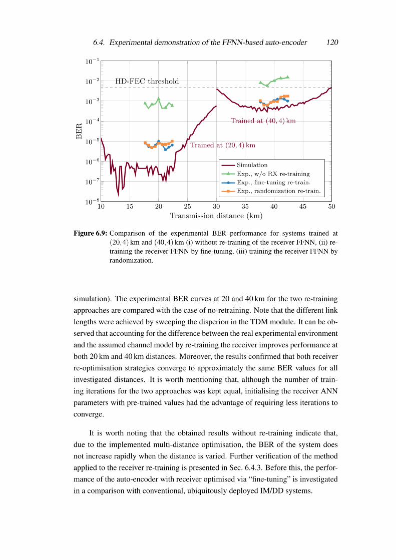
6.4. Experimental demonstration of the FFNN-based auto-encoder 120
10 15 20 25 30 35 40 45 5010´8
10´7
10´6
10´5
10´4
10´3
10´2
10´1
HD-FEC threshold
Trained at p20, 4q km
Trained at p40, 4q km
Transmission distance (km)
BER
Simulation
Exp., w/o RX re-training
Exp., fine-tuning re-train.
Exp., randomization re-train.
Figure 6.9: Comparison of the experimental BER performance for systems trained at(20,4) km and (40,4) km (i) without re-training of the receiver FFNN, (ii) re-training the receiver FFNN by fine-tuning, (iii) training the receiver FFNN byrandomization.
simulation). The experimental BER curves at 20 and 40 km for the two re-trainingapproaches are compared with the case of no-retraining. Note that the different linklengths were achieved by sweeping the disperion in the TDM module. It can be ob-served that accounting for the difference between the real experimental environmentand the assumed channel model by re-training the receiver improves performance atboth 20 km and 40 km distances. Moreover, the results confirmed that both receiverre-optimisation strategies converge to approximately the same BER values for allinvestigated distances. It is worth mentioning that, although the number of train-ing iterations for the two approaches was kept equal, initialising the receiver ANNparameters with pre-trained values had the advantage of requiring less iterations toconverge.
It is worth noting that the obtained results without re-training indicate that,due to the implemented multi-distance optimisation, the BER of the system doesnot increase rapidly when the distance is varied. Further verification of the methodapplied to the receiver re-training is presented in Sec. 6.4.3. Before this, the perfor-mance of the auto-encoder with receiver optimised via “fine-tuning” is investigatedin a comparison with conventional, ubiquitously deployed IM/DD systems.

6.4. Experimental demonstration of the FFNN-based auto-encoder 121
Transmission link
z´1
z´1
z´1
z´1
yt´ Z´1
2
yt´1
yt
yt`1
yt` Z´1
2
...
...
ω1
ωi 1
...
ωi
ωi 1
...ωZ
Σ mt
Figure 6.10: Schematic of a conventional feedforward equaliser, used in the reference PAMtransmission for experimental performance comparison.
6.4.2 Performance comparison with conventional systemsIn this section, the BER performance of the end-to-end FFNN-based system wascompared to conventional schemes based on PAM transmission with linear equal-isation at the receiver. The data rate of the considered PAM systems was also setto 42 Gb/s. In particular, the first system employed 42 Gbaud PAM2 transmissionand raised cosine pulses (roll-off of 0.99). The second system was operating at21 Gbaud with PAM4 and raised cosine pulses (roll-off of 0.4). The receiver DSPfor both schemes employed the conventional feedforward equaliser (FFE), whoseschematic is shown in Fig. 6.10. It processes (Z−1)/2 pre- and post-cursor symbolsfor the equalisation of the central PAM symbol. The implementation was based onZ = 13 taps, at n = 2 taps per PAM symbol, ensuring that the receiver covers a tem-poral window similar to the auto-encoder. It is important to mention that the noisepower of 0.245 mW obtained from a measurement at the receiver was used for thenoise model in Chapter 4 as well as in the simulations for the systems described inChapter 4 and Chapter 5.
Figure 6.11 shows the experimental BER results for the compared systemsfor a fibre of length 20 km and 40 km, respectively. The TDM dispersion valuewas swept between −40 ps and +40 ps, resulting in effective link distances in theranges of 17.65− 22.35 km and 37.65− 42.35 km, respectively. For the systemaround 20 km, BERs below 10−5 were achieved experimentally at all distances. In

6.4. Experimental demonstration of the FFNN-based auto-encoder 122
10 15 20 25 30 35 40 45 5010´8
10´7
10´6
10´5
10´4
10´3
10´2
10´1
100
HD-FEC threshold
Trained at p20, 4q km
Trained at p40, 4q km
Transmission distance (km)
BER
Simulation
Experiment
Tx-PAM2 & Rx-FFE, experiment
Tx-PAM4 & Rx-FFE, experiment
Figure 6.11: Experimental BER performance for systems trained at (20,4) km and(40,4) km. The systems are compared to PAM2 and PAM4 systems withreceivers based on conventional feedforward equalisation.
particular, the lowest BER of 3.73 ·10−6 was obtained at 21.18 km. For comparison,the PAM2 system experimentally achieves 7.77 · 10−4 BER at 20 km. The end-to-end deep learning-based optical system significantly outperforms the referencePAM scheme. At 40 km, the proposed system outperforms both the 42 Gbaud PAM2and the 21 Gbaud PAM4 schemes, as neither of these can achieve BERs below theHD-FEC threshold. On the other hand, the FFNN-based system achieved BERsbelow 1.4 · 10−3 at all distances in the examined range. In particular, BERs of1.05 ·10−3 at 40 km and a lowest BER of 5.75 ·10−4 at 38.82 km have been obtained.
Figure 6.12 shows the experimental results at 60 km and 80 km fibre lengthand TDM dispersion varied between −40 ps and +40 ps, yielding effective linkdistances in the ranges 57.65− 62.35 km and 77.65− 82.35 km, respectively. Forboth systems BERs below the HD-FEC threshold cannot be achieved by the end-to-end deep learning approach, as predicted by the simulation. Nevertheless, at 60 kmthe system outperforms both the PAM2 and PAM4 links. However, for the 80 kmlink, the noise at the receiver becomes more significant due to the low signal powerlevels without optical amplification. This is combined with a significant amountof accumulated dispersion, whose effects at 80 km extend across multiple blocksand cannot be compensated by the block-by-block processing, accommodated inthe FFNN design. The results is an operation close to the sensitivity limits of the

6.4. Experimental demonstration of the FFNN-based auto-encoder 123
50 55 60 65 70 75 80 85 9010´5
10´4
10´3
10´2
10´1
100
HD-FEC threshold
Trained at p60, 4q kmTrained at p80, 4q km
Transmission distance (km)
BER
Simulation
Experiment, no EDFA
Experiment, with extra EDFA
Tx-PAM2 & Rx-FFE, experiment
Tx-PAM4 & Rx-FFE, experiment
Figure 6.12: Experimental BER performance for systems trained at (60,4) km and(80,4) km. The systems are compared to PAM2 and PAM4 systems withreceivers based on conventional feedforward equalisation.
receiver which ultimately restricts the achievable BERs.To further investigate the impact of received signal power on the performance
of the system, an erbium-doped fibre amplifier (EDFA) was included in the test-bedfor pre-amplification at the receiver. Thereby, the received power is increased from-11 and -15 dBm at 60 km and 80 km, respectively to -7 dBm. The obtained BERsat these distances are also shown in Fig. 6.12. It can be seen that by changing thelink to include an extra EDFA, the end-to-end deep learning system achieves signif-icantly improved performance. In particular, at 60 km, a BER of 3.8 · 10−3, belowthe HD-FEC threshold, can be achieved. Nevertheless, the performance of the sys-tem at 80 km is still limited and the measured BER is 2.8 · 10−2. The last set ofresults highlight the potential for performance improvement by including differentlink configurations inside the end-to-end learning process.
6.4.3 Distance-agnostic transceiverThis section describes the experimental verification of the multi-distance learningmethod developed in Sec. 4.3.2. The investigation covers the optimisation of re-ceiver parameters using experimentally collected received traces with deviating dis-persion, set by the tunable dispersion module (TDM). More specifically, the datawas acquired by employing fixed fibre spools of 20 km and 40 km and using theTDM to appropriately sweep the dispersion around these mean values. As previ-

6.4. Experimental demonstration of the FFNN-based auto-encoder 124
10 12 14 16 18 20 22 24 26 28 3010´8
10´7
10´6
10´5
10´4
10´3
10´2
10´1
100
HD-FEC threshold
Transmission distance (km)
BER
Simulation
Experiment
Figure 6.13: Experimental BER performance as a function of transmission distance be-tween 10 and 30 km for a (20,4) km-trained system, whose receiver ANNparameters are tuned using measured data and the multi-distance learningmethod proposed in Sec. 4.3.2.
ously explained (see Sec. 6.1), the TDM allowed to adjust the link dispersion from−170 to +170 ps/nm in steps of 10 ps/nm. The digitized received photocurrent iscollected for each effective distance. The amount of data collected at each pointfollows a Gaussian distribution with a mean µ = 20 km or µ = 40 km and a stan-dard deviation of 67 ps/nm, which effectively corresponds to around 4 km of SSMF(matching the simulation assumption). The system with optimised receiver ANNparameters was tested using a disjoint collection of traces at each distance.
Figure 6.13 shows the achieved BER performance at 42 Gb/s around the meandistance of 20 km. In agreement with simulation, the experimental system reachedBER below the 6.7% HD-FEC threshold for all distances between 10 and 30 km.Moreover, it can be observed that the lowest BER was achieved around 20 km as aresult of the employed strategy of training dispersion values with a Gaussian distri-bution, i.e. the number of training examples around the mean value was greater. InFig. 6.14 the BER performance of the system trained around 40 km is examined atdistances ranging from 30 to 50 km. Moreover, the results are compared to the per-formance obtained for the conventional PAM2/PAM4 42 Gb/s transmission basedon a FFE receiver, which was described in Sec. 6.4.1. Note that, unlike the exam-ined system based on multi-distance learning, the FFE receiver for PAM2/PAM4

6.5. Experimental demonstration of the SBRNN auto-encoder 125
30 32 34 36 38 40 42 44 46 48 5010´4
10´3
10´2
10´1
100
HD-FEC threshold
Trained at p20, 4q km
Transmission distance (km)
BER
Simulation
Experiment
Tx-PAM2 & Rx-FFE
Tx-PAM4 & Rx-FFE
Figure 6.14: Experimental BER performance as a function of transmission distance be-tween 30 and 50 km for a 42 Gb/s system trained on (40,4) km, whose receiverANN parameters are tuned using measured data and the multi-distance learn-ing method proposed in Sec. 4.3.2. The BER of PAM2 and PAM4 schemeswith an FFE receiver is shown as a performance indicator. Note that the pa-rameters of the FFE receiver are optimised separately for each distance.
needs to be optimised separately for each fibre length. The auto-encoder systemenabled BERs below the HD-FEC for all distances between 31 and 46 km. Fur-thermore, it significantly outperformed the reference PAM setups, neither of whichcould achieve BER below the threshold at the examined distances. It can be seenthat the performance of the PAM2 system oscillates as a function of distance, causedby the power fading profile of the signal experiencing different dispersions [120].In contrast, the ANN-based system, specifically trained to tolerate dispersion varia-tions, does not present such a strong dependence on the latter.
The results from the investigation successfully demonstrate the greater robust-ness to link parameter variations achieved for the deep learning-based transceiversoptimised using the proposed multi-distance method.
6.5 Experimental demonstration of the SBRNN auto-encoder
This section describes the implementation and investigates the performance of theSBRNN auto-encoder proposed in Chapter 5 on the experimental IM/DD test-bed.

6.5. Experimental demonstration of the SBRNN auto-encoder 126
The performance of the system is investigated when the transceiver is optimised ona transmission model with parameters applied “as is” to the test-bed as well as inthe case where receiver optimisation using the measured data is performed. Theinvestigation covers comparisons with PAM systems based on receivers optimisedfor handling nonlinear ISI using state-of-the-art deep learning techniques as well asthe classical nonlinear Volterra equalisation.
For the SBRNN auto-encoder experiment, Z = 800 different sequences ofN = 5152 random input messages mi, j (from an alphabet of M = 64 different mes-sages), with i ∈ {1, . . . ,Z} and j ∈ {1, . . . ,N}, are transmitted. Each of the se-quences is first encoded by the transmitter BRNN into series of symbols of n · ssamples before being applied to the experimental test-bed, starting with the LPF.Note that, similarly to the FFNN experiment, an up-sampling factor of s = 4 isused in both transmitter and receiver. Thus the series of encoded blocks are down-sampled by s in experiment after the LPF at the transmitter and then up-sampledafter the receiver LPF. The value of n dictates the information rate of the system andfor 42 Gb/s or 84 Gb/s transmission, n = 12 or n = 6 was selected, respectively. Afull load of the DAC required the concatenation of 8 encoded sequences of symbolsand this is fed to the link for a single transmission iteration. To collect a sufficientamount of data, the experiment involved a total of 100 DAC loads. Similarly to theinvestigation of the FFNN auto-encoder, the performance of the SBRNN systemwas investigated in two scenarios:
First, the error rate between the experimentally transmitted and received mes-sages (see Fig. 6.4), was investigated for transceiver optimised in simulation-onlyand applied “as is” to the actual transmission link. The optimisation procedure, thesimulation setup, and the BER computation were performed as described in Sec. 5.1and Sec. 5.2. All examined systems in this section were trained separately for eachdistance.
Then, the system performance was enhanced by re-training the receiver pa-rameters with the experimental data. For this optimisation and its testing stage, thesequences of digitised received symbols yi, j, with i ∈ {1, . . . ,Z} and j ∈ {1, . . . ,N},were used together with their corresponding labels mi, j. The sequences with indicesi ∈ {1, . . . ,720} were used for training. For convenience, these were organised incontainers of data elements DAE
train and corresponding label elements LAEtrain. The re-
maining sequences with indices i ∈ {721, . . . ,Z}, which are independent from thetraining set, were used for testing, organised in DAE
test and LAEtest. The construction and
utilisation procedure of DAEtrain, LAE
train, DAEtest, and LAE
test is described in Appendix C.1.

6.5. Experimental demonstration of the SBRNN auto-encoder 127
20 30 40 50 60 70 80 9010´4
10´3
10´2
10´1
100
HD-FEC th.
a)
42Gb/sW
“ 10
W “ 10
Transmission distance (km)
BER
FFNN AE, sim.
FFNN AE, exp.
SBRNN AE, sim.
SBRNN AE, exp.
5 10 20 30 4010´3
10´2
HD-FECBER
W(# blocks)
5 10 20 30 4010´3
10´2
HD-FEC
BER
W(# blocks)
5 10 20 30 4010´3
10´2
HD-FECBER
W(# blocks)
70 km
60 km
50 km
b)
Figure 6.15: a) Experimental BER performance at 20, 40, 60, 80 km for the 42 Gb/sSBRNN-based auto-encoder trained on a channel model and applied “as is” tothe optical fibre transmission test-bed. The BER of the end-to-end FFNN sys-tem is also shown as a performance indicator. b) BERs at 50, 60 and 70 km asa function of the sliding window size W for the sequence estimation algorithmat the SBRNN receiver.
6.5.1 Experimental performance resultsThe conducted numerical investigation in Chapter 5 clearly showed that in theframework of optical IM/DD communication, the processing capabilities of thevanilla BRNN auto-encoder are comparable to the long short-term memory struc-ture, without the associated extra complexity. For this reason, the vanilla SBRNNauto-encoder was implemented on the experimental test-bed.
First, the transceiver optimised on the optical IM/DD channel model was ap-plied “as is” to the experimental test-bed. Initially, the fixed sliding window size ofW = 10 was employed. The achieved BER performance at 42 Gb/s as a function ofdistance is shown in Fig. 6.15 a), where it was compared to the end-to-end FFNNsystem, investigated in Sec. 6.4. It can be seen that, in good agreement with sim-ulation, the SBRNN system significantly outperformed the FFNN auto-enocoder.In particular, it allowed transmission below the 6.7% HD-FEC at distances beyond50 km in experiment, a 30 km increase compared to the FFNN.
The conducted investigation in Sec. 5.2.2 showed that the performance of theSBRNN auto-encoder can be improved by increasing the window W , which dictatesthe amount of received symbols used for the sequence estimation algorithm at thereceiver. Greater W allows to effectively capture intersymbol interference effects at

6.5. Experimental demonstration of the SBRNN auto-encoder 128
longer distances. The presented results in Fig. 6.15 b) investigate the experimentalBER of the SBRNN auto-encoder at 50, 60 and 70 km as a function of the slidingwindow W . It can be seen that, as a result of the increased window size, the BERof the system was reduced below the HD-FEC threshold at the distance of 60 km.More specifically, the error rate was below 4 · 10−3 for W ≥ 20. It is important tomention that, in an excellent agreement with the simulation prediction in Sec. 5.2.2,the experiment showed diminishing gains from further increase of W since noiseand system nonlinearities become more dominant when the ISI is compensated.
The approach of enhancing the SBRNN auto-encoder system by using the col-lected experimental data for re-optimisation of the receiver parameters was con-sidered next. The performance of the SBRNN auto-encoder, whose receiver wasoptimised with the measured data, was compared to multi-level PAM systems em-ploying state-of-the-art DSP schemes at the receiver for nonlinear ISI compensa-tion. The processing and optimisation procedures for these reference systems aredescribed in the following section, while Sec. 6.5.3 presents the outcome of theperformance comparison with the auto-encoder.
6.5.2 Reference PAM systems with state-of-the-art receiver DSPThe conventional two- and four-level PAM transmission was considered and theperformance of deep learning approaches for PAM detection based on recurrentand feed-forward neural networks as well as the classical nonlinear Volterra equal-isation were examined. For all three schemes, the experimental data was used foroptimisation of the receiver parameters. The PAM experiment was conducted inthe following way: At the transmitter, PAM2 or PAM4 symbols were generatedand accordingly scaled to sets M = {0;π/4} or M = {0;π/12;π/6;π/4}, respec-tively. Note that, similarly to the auto-encoder systems where a clipping layer wasspecifically designed, scaling of the PAM symbols was necessary to enable oper-ation in the linear region of the MZM. Also note that Gray-coded bit-to-symbolmapping was considered in the case of PAM4 in order to investigate the BER met-ric as an indicator of the system performance. The sequence of PAM symbols waspulse-shaped at n = 2 Sa/sym by a 0.25 roll-off raised cosine filter. It was thenapplied to the experimental test-bed. The experiment involved Z = 100 loads of theDAC, each of them equivalent to a sequence of N = 249750 PAM symbols mi, j,i ∈ {1, . . . ,Z} and j ∈ {1, . . . ,N}. The sequences of received symbols yi, j ∈ Rn af-ter propagation through the test-bed link were utilised together with the labels mi, j
for optimisation of the DSP parameters and testing. Sequences i ∈ {1, . . . ,90} wereused for training, organised in DPAM
train and LPAMtrain for traces and labels, respectively.
The testing was carried out using the disjoint set of remaining sequences with in-

6.5. Experimental demonstration of the SBRNN auto-encoder 129
Transmission link
z´1
z´1
z´1
z´1
yt´ W´1
2
yt´1
yt
yt`1
yt` W´1
2
...
...
ReLU
Softmax
M
pt. . .
Figure 6.16: Schematic of the reference sliding window FFNN receiver for PAM symbols,utilised in the experiment.
dices i ∈ {91, . . . ,100}, organised in DPAMtest and LPAM
test . The database structuring isdescribed in Appendix C.2, where the details regarding the data utilisation in theoptimisation of the different PAM receiver schemes are also provided. The threeconsidered schemes are described in the following.
6.5.2.1 Sliding Window FFNN receiverIn this scheme, already introduced and examined in simulation in Sec. 5.3.1, a PAMsequence is transmitted through the link and the samples of an appropriately chosensub-sequence of received symbols are fed into a multi-layer feed-forward ANN,as shown in Fig. 6.16. It was discussed in Sec. 5.3.1 that a similar approach forthe receiver design has been considered for example in [58, 113–115]. The neuralnetwork estimates the central symbol of the sub-sequence. More specifically, thetransmitted message mt at time t is recovered as mt by processing the train of Wreceived symbols of n = 2 samples (yt−W−1
2, . . . ,yt , . . . ,yt+W−1
2). Note that for this
receiver, the processing memory dictates the size of the ANN layers, the first onehaving parameters W ∈ R4W ·n×W ·n and b ∈ R4W ·n. Subsequently, 6 hidden layersare employed before mt is estimated. The number of nodes on each of these isgiven by
⌊4W ·n/(2i−1)
⌋, where i is the hidden layer index. The ReLU activation
is applied on all of the layers except for the final one, where a softmax activationallows to compute a probability vector pt for the transmitted PAM2/4 symbol with

6.5. Experimental demonstration of the SBRNN auto-encoder 130
Transmission link
z´1
z´1
z´1
z´1
yt´ W´1
2
yt´1
yt
yt`1
yt` W´1
2
...
...N
onlinea
rte
rms
gener
ator
ωi
...
...
ωij
...ωii
y2i ωiiy
2i
yiyj ωijyiyj
...
yi ωiyi
Σ mt
Figure 6.17: Schematic of the second-order nonlinear Volterra equaliser for PAM symbols,used as a reference system in the experiment.
pt ∈R2/4. The processing window slides by one received symbol position ahead toestimate the next symbol in the sequence. Training was performed as described inAppendix C.2.1 using DPAM
train and LPAMtrain .
6.5.2.2 Nonlinear Volterra EqualiserVolterra equalisers, shown schematically in Fig. 6.17, have been widely consideredfor IM/DD links based on PAM [66]. In particular, for the experimental investi-gation in this chapter, a second order Volterra filter was used, allowing the com-pensation of linear and nonlinear ISI. The output of the equaliser can be expressedas
mt = ωdc +
W−12 ·n
∑q1=−W−1
2 ·nωq1 · yt+q1 +
W1−12 ·n
∑q2=−
W1−12 ·n
W1−12 ·n
∑q3=k2
ωq2,q3 · yt+q2 · yt+q3, (6.2)
where W and W1 denote the symbol memory in the first and second order series,respectively, and ωi and ωi, j are the first and second order coefficients. Similar to theother PAM schemes, the algorithm is processing the neighbourhood of W receivedsymbols of n = 2 samples
(yt−W−1
2, . . . ,yt , . . . ,yt+W−1
2
), thus including the ISI from
pre- and post-cursor samples in the detection of the current input. To capture anidentical amount of memory compared to the auto-encoder and the SFFNN receiver,the first order memory of the Volterra equaliser was fixed to W = 61, while W1=21was chosen such that the complexity of the algorithm was kept manageable. The

6.5. Experimental demonstration of the SBRNN auto-encoder 131
20 25 30 35 40 45 50 55 60 65 7010´5
10´4
10´3
10´2
10´1
100
HD-FEC
42Gb/s
84Gb/s
SBRN
N auto-e
nc.
Tx-PAM4 & Rx-SFFNN
Tx-BR
NN& Rx
-SFFN
N
Transmission distance (km)
BER
Tx-PAM2 & Rx-SBRNN
Tx-PAM2 & Rx-Volterra
Tx-PAM2 & Rx-SFFNN
SBRNN auto-enc.
Figure 6.18: BER as a function of transmission distance for 42 Gb/s and 84 Gb/s systemsemploying deep learning-based and classical DSP schemes optimised usingexperimental data.
optimisation of the filter coefficients using is described in Appendix C.2.2.
6.5.2.3 Sliding Window BRNN receiverA system that combines the PAM transmitter with the SBRNN receiver was alsoinvestigated. The receiver was implemented in a way which was identical to the re-ceiver section of the SBRNN auto-encoder. As opposed to the auto-encoder, for theoptimisation of the SBRNN receiver for PAM parameters the databases DPAM andLPAM were used. Details on the training procedure are provided in Appendix C.2.3.
6.5.3 Experimental performance comparison between theSBRNN auto-encoder and the reference PAM systems
For this investigation, the number of bits simultaneously processed by each receiveralgorithm was fixed. The setting was aimed at carrying out a fair comparison be-tween the three different PAM DSP schemes with the SBRNN auto-encoder. Thus,for the auto-encoder, the size of the sliding window was set to W = 10 (60 bits) tomatch the simulation investigation, while for the PAM2 systems W = 61 (61 bits).To allow for a better compensation in the case of PAM4, the window of W = 61PAM symbols was kept, which was the equivalent of processing 122 bits.
Figure 6.18 shows the achieved BER for all experimentally examined systemsat different transmission distances. As previously mentioned, the DSP for these
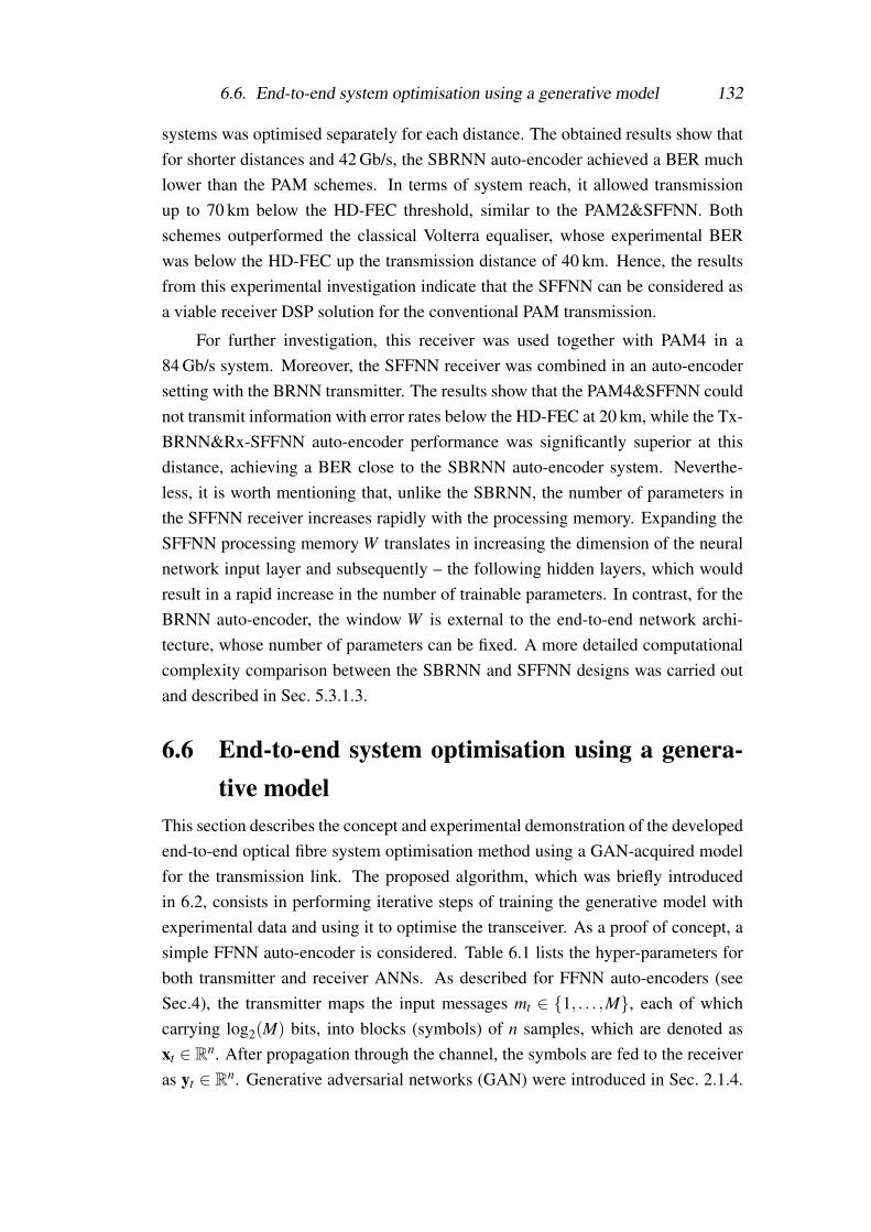
6.6. End-to-end system optimisation using a generative model 132
systems was optimised separately for each distance. The obtained results show thatfor shorter distances and 42 Gb/s, the SBRNN auto-encoder achieved a BER muchlower than the PAM schemes. In terms of system reach, it allowed transmissionup to 70 km below the HD-FEC threshold, similar to the PAM2&SFFNN. Bothschemes outperformed the classical Volterra equaliser, whose experimental BERwas below the HD-FEC up the transmission distance of 40 km. Hence, the resultsfrom this experimental investigation indicate that the SFFNN can be considered asa viable receiver DSP solution for the conventional PAM transmission.
For further investigation, this receiver was used together with PAM4 in a84 Gb/s system. Moreover, the SFFNN receiver was combined in an auto-encodersetting with the BRNN transmitter. The results show that the PAM4&SFFNN couldnot transmit information with error rates below the HD-FEC at 20 km, while the Tx-BRNN&Rx-SFFNN auto-encoder performance was significantly superior at thisdistance, achieving a BER close to the SBRNN auto-encoder system. Neverthe-less, it is worth mentioning that, unlike the SBRNN, the number of parameters inthe SFFNN receiver increases rapidly with the processing memory. Expanding theSFFNN processing memory W translates in increasing the dimension of the neuralnetwork input layer and subsequently – the following hidden layers, which wouldresult in a rapid increase in the number of trainable parameters. In contrast, for theBRNN auto-encoder, the window W is external to the end-to-end network archi-tecture, whose number of parameters can be fixed. A more detailed computationalcomplexity comparison between the SBRNN and SFFNN designs was carried outand described in Sec. 5.3.1.3.
6.6 End-to-end system optimisation using a genera-tive model
This section describes the concept and experimental demonstration of the developedend-to-end optical fibre system optimisation method using a GAN-acquired modelfor the transmission link. The proposed algorithm, which was briefly introducedin 6.2, consists in performing iterative steps of training the generative model withexperimental data and using it to optimise the transceiver. As a proof of concept, asimple FFNN auto-encoder is considered. Table 6.1 lists the hyper-parameters forboth transmitter and receiver ANNs. As described for FFNN auto-encoders (seeSec.4), the transmitter maps the input messages mt ∈ {1, . . . ,M}, each of whichcarrying log2(M) bits, into blocks (symbols) of n samples, which are denoted asxt ∈ Rn. After propagation through the channel, the symbols are fed to the receiveras yt ∈ Rn. Generative adversarial networks (GAN) were introduced in Sec. 2.1.4.

6.6. End-to-end system optimisation using a generative model 133
Table 6.1: Definitions of the transmitter and receiver FFNN used for the experimental veri-fication of the end-to-end system optimisation method using a generative model
Layer Activation Output dimension
Transmitter:
Input one-hot enc. MHidden 1 ReLU 8MHidden 2 ReLU 8M
Final Clipping n
Receiver:
Input N/A nHidden 1 ReLU 8MHidden 2 ReLU 8M
Final Softmax M
z
ÝÑx pµqt
ppyt|ÝÑx pµqt q yt
ÝÑx pµqt
yt ÝÑx pµqt
pr{f
real sample
fake sampleGeneratorDiscriminator
ReLU nodeLinear nodeSoftmax node
Figure 6.19: Schematic of the utilised conditional GAN for approximating the function ofthe IM/DD transmission link.
In the following, the specific design of the GAN that was used in the experimentalinvestigation is introduced. Then, the transmission and optimisation regimes in theproposed method are described and the investigation of the achieved performanceimprovement is presented.
6.6.1 Generative adversarial network designAs explained in Sec. 2.1.4, a GAN typically employs two ANNs – a generator and adiscriminator. They have competing objective functions and are trained iteratively.The generator ANN aims at translating its input into a (possibly high-dimensional)output sample, mimicking the ground truth distribution of the data, which is specificto the problem. The discriminator acts as a binary classifier between real (groundtruth) and fake (generated) samples. Related to communication systems, GANs can

6.6. End-to-end system optimisation using a generative model 134
Table 6.2: Definitions of the generator and discriminator ANNs in the conditional GAN
Layer Activation Output dimension
Generator:
Input concat. 2µ ·nHidden 1 ReLU 30nHidden 2 ReLU 20nHidden 3 ReLU 13nHidden 4 ReLU 8nHidden 5 ReLU 5n
Final Linear n
Discriminator:
Input concat. (µ +1) ·nHidden 1 ReLU 16nHidden 2 ReLU 10nHidden 3 ReLU 6n
Final Sigmoid 1
be used to train a generative model (generator) which mimics the function of thechannel by approximating its conditional probability distribution. In the frameworkof auto-encoder design, the model can be used in the end-to-end system optimisa-tion to enable to computation of gradients via backpropagation.
Since ISI in the optical IM/DD stems from both preceding and succeedingsymbols, the goal of the generative model is to approximate p(yt |~x(µ)t ), where µ , anodd integer, is the modeled symbol memory and
~x(µ)t :=(
xTt−(µ−1)/2 . . . xT
t+(µ−1)/2
)T∈ Rµ·n, (6.3)
is used to denote the concatenation of the pre- and post-cursor neighbourhood of µ
symbols around the symbol xt transmitted at time t. The schematic of the utilisedconditional GAN for approximating p(yt |~x(µ)t ) is shown in Fig. 6.19. To mimic theprobability distribution, the generator takes as an input the concatenation of a vectorof uniformly-distributed random samples z∼U
(0,1)µ·n with~x(µ)t . It transforms it into
the fake symbol
yt = Gθ g
((zT ~x(µ)Tt
)T)∈ Rn, (6.4)
where Gθ g denotes the function of the generator, a feedforward ANN defined by thehyper-parameters listed in Table 6.2.
The discriminator is first fed with the real symbol yt , i.e. obtained in the ex-

6.6. End-to-end system optimisation using a generative model 135
periment, conditioned (concatenated) on~x(µ)t , producing the output probability
pr = Dθ d
((yT
t ~x(µ)Tt
)T)∈ R, (6.5)
where Dθ d describes the function of the discriminator – a feedforward ANN definedby the hyper-parameters listed in Table 6.2, which has a sigmoid activation in thefinal layer. The discriminator is then fed with the fake (output of the generator)symbol yt , also concatenated with~x(µ)t , thus producing
pf = Dθ d
((yT
t ~x(µ)Tt
)T)∈ R. (6.6)
Following the GAN theory (Sec. 2.1.4), the two sets of discriminator (θ d) andgenerator (θ g) ANN parameters are iteratively optimised via stochastic gradientdescent (using the Adam algorithm). The procedure is aimed at minimising theaverage losses
LD(θ d) =1S
S
∑i=1
[`(lr, pr,i)+ `(lf, pf,i)], LG(θ g) =1S
S
∑i=1
`(lr, pf,i), (6.7)
over a mini-batch S of elements from the training set, where lr := 1 and lf := 0 arethe labels for real and fake symbols, respectively. The cross entropy loss function isutilised. Note that the objective of the discriminator is to classify yt and yt correctly.On the other hand, by minimising LG, the generator learns representations yt thatare statistically similar to yt . The conditional GAN is trained over 104 steps usedas a stopping criterion. Each of the steps consists in 4 consecutive discriminatorupdates with the learning rate of 10−3, followed by a generator update with therate gradually reduced every 200 steps from 5 · 10−4 to 10−5. After training, thegenerator ANN model is employed for end-to-end system optimisation.
6.6.2 End-to-end optimisation algorithmThe schematic of the experiment is shown in Fig. 6.20. The flow diagram inFig. 6.21 shows the proposed algorithm for end-to-end system optimisation. Atan algorithm iteration k = 0, the transmitter and receiver ANNs are initialised withparameters trained offline, following Chapter 4, using the complete IM/DD channelmodel from Chapter 3. To collect a sufficient amount of experimental data, Z = 500random sequences (full DAC loads) of w= 8 ·104 messages
(. . .mt−1,mt ,mt+1 . . .
),
from an alphabet of M = 8 (3 bits), were generated and encoded by the transmitterinto the sequences
(. . .xt−1,xt ,xt+1 . . .
)of symbols of n = 6 samples. The symbol
sequences were filtered by the 32 GHz LPF and applied to the 84 GSa/s DAC, result-

6.6. End-to-end system optimisation using a generative model 136
¨˚˝
...mt
...
˛‹‹‚
Transmitter ANN ¨˚˝
...xt
...
˛‹‹‚ time
LPF
DAC
84GSa/s Driver amp.
MZM
Laser
PD
SSMF
TIA
ADC
LPF
¨˚˝
...yt
...
˛‹‹‚
Receiver ANN ¨˚˝
...mt
...
˛‹‹‚
ppyt|ÝÑx pmqt q
Transmission
Optimization
Figure 6.20: Schematic of the experimental setup for end-to-end system optimisation,showing the forward propagation through the IM/DD link and the optimisa-tion flow through the generative model, used in lieu of the actual link.
Tx
Test-bed
Rx
BER
1
2
GAN
Txopt.
Model
Rxopt.
Loss
update
update
Figure 6.21: Flow chart of the proposed iterative algorithm for end-to-end deep learningusing measured data. The algorithm includes transmission and optimisationregimes.
ing in a 42 Gb/s data rate of the system. The electrical waveforms were fed to opticalfibre transmission link, described in Sec. 6.1, which for this experiment consistedof a fixed 20 km span of SSMF. The digital signal
(. . . ,yt−1,yt ,yt+1 . . .
), obtained
at the receiver after ADC sampling, was applied in two ways: i) to the receiverANN for processing, symbol decision and BER calculation using the optimised

6.6. End-to-end system optimisation using a generative model 137
bit-to-symbol mapping, described in Sec. 5.1.5. ii) together with the transmitteddigital sequences
(. . . ,xt−1,xt ,xt+1 . . .
), it was used for GAN training, followed by
transceiver optimisation.
Part of the data (q = 103 elements), grouped as
A :=
m1...
mq
∈ Rq, B :=
yT1...
yTq
∈ Rq×n, (6.8)
was used for the single step of transceiver learning within this algorithm iteration.The remainder, setting µ = 3 for modeling the channel, was structured as (transmit-ted symbols)
C(µ=3) :=
~x(3)Tq+2
...~x(3)TZw−1
∈ R(Zw−q−2)×3n, (6.9)
where ~x(3)i :=(
xTi−1 xT
i xTi+1
)T, i ∈ {q+ 2, . . . ,Zw− 1}. Correspondingly, the
received symbols were structured as
D :=
yT
q+2...
yTZw−1
∈ R(Zw−q−2)×n. (6.10)
First, the generative model was trained via the procedure described in Sec. 6.6.1.Each row i from C(µ=3) and D is used to condition the GAN and provide the groundtruth symbol, respectively (see Eqs. (6.4) – (6.6)). Next, the transceiver learningwas performed. The goal was to minimise the average cross entropy loss of thesystem over the mini-batch of size |S|= q, computed as
L syst.(θ Tx,θ Rx) =1|S|
|S|
∑i=1
`(mi, fRx(yi)) , (6.11)
with mi and yi being rows from A and B, respectively, and fRx denoting the func-tion of the receiver. At this point, the generative model was applied in lieu of thetransmission link. This enables the computation of the gradient of the loss withrespect to both the transmitter (θ Tx) and receiver (θ Rx) parameter sets using back-propagation. Afterwards, these parameters are updated in a single process via SGDusing the Adam algorithm with a learning rate of 10−3. This completed an iterationof the optimisation algorithm. The transmitter and receiver representations were

6.6. End-to-end system optimisation using a generative model 138
0 1 2 3 4 5 6 7 8 9 1010´3
10´2
10´1
HD-FEC th.
Transmitted message (m)
Decoded
message
(m)
ą95%
30%´95%
5%´30%
1%´5%
0.1%´1%
10´5%´0.1%1
1
2
2
3
3
4
4
5
5
6
6
7
7
8
8Transmitted message (m)
Decoded
message
(m)
1
1
2
2
3
3
4
4
5
5
6
6
7
7
8
8
´500 0 500 1,000
´500
0
500
m “ 1
m “ 2m “ 3
m “ 4 m “ 5
m “ 6
m “ 7m “ 8
t-SNE X
t-SNE
Y
a)
b) c)
Iteration of system optimization pkq
BER
Receiver-only
End-to-End
Figure 6.22: Experimental bit error rate as a function of optimisation iteration. Inset fig-ures show: a) error probabilities at k = 0; b) 2D t-SNE representation of thewaveforms output of the transmitter ANN at k = 10; c) error probabilities atk = 10.
updated and the processes of transmission, GAN training and system optimisationwere sequentially repeated.
6.6.3 Performance resultsThe bit error rate of the system as a function of the iteration of the proposed optimi-sation algorithm was investigated and the results are shown in Fig. 6.22. It can beobserved that a monotonic BER reduction was achieved on each iteration. In par-ticular, the BER of the system improved from 2.4 ·10−2 at step k = 0, i.e. the casewithout any transceiver optimisation based on the measured data, to 1.7 ·10−3 afteronly 10 steps of the algorithm. This improvement is further illustrated via inset fig-ures a) and c), which show the error probabilities at k = 0 and k = 10, respectively.As an illustrative example showcasing the improvement, one can observe that noerrors exceeding the 1% threshold occurred at k = 10, which was in stark contrastcompared to the initial stage. For the case of k = 10, the inset figure b) depicts themodulation constellation in two dimensions using the t-distributed stochastic neigh-bor embedding (t-SNE) dimensionality reduction technique [121], used purely forvisualisation purpose. It can be seen that the 8 transmitted constellation points arewell-separated in the t-SNE space, a factor that contributes to the observed messagerecovery enhancement.

6.7. Summary 139
Furthermore, Fig. 6.22 also provides a direct comparison between the perfor-mance achieved using the proposed algorithm for end-to-end optimisation and themethod of optimising only the receiver using measured data. Note that in the lattercase, only the set of receiver ANN parameters (θ Rx) was updated for minimisingthe average cross entropy loss of the system over the mini-batch of size |S|= q, i.e.
L syst.(θ Rx) =1|S|
|S|
∑i=1
`(mi, fRx(yi)) . (6.12)
It can be observed that after only 4 iterations of optimisation, the proposed methodfor end-to-end learning started to outperform the simple receiver-only strategy.The difference in achieved performance increased further as the optimisation pro-gressed. Importantly, the results indicate that the gains from receiver re-trainingstart to diminish. At step k = 10 this method achieved BER of 4 ·10−3, significantlyhigher than the 1.7 ·10−3 enabled by optimising the complete transceiver.
It is worth mentioning that the training of the GAN required 500 transmissionsof different data sequences, which was the time-limiting step in such an experimen-tal setup. It also required stable link parameters to ensure the validity of the obtainedgenerative model. Thus, as a proof of concept, 10 optimisation iterations were per-formed. The presented results clearly show that this already produced substantialperformance gains.
6.7 SummaryThis chapter described the implementation and performance of the developed FFNNand SBRNN auto-encoder designs on an experimental IM/DD transmission test-bed. The conducted experiments for the first time demonstrated the end-to-end deeplearning concept on an optical transmission link. The research was published in [62,63, 122–124]. The investigation showed that for the simple approach of optimisingthe auto-encoders only in simulation, the FFNN auto-encoder can transmit 42 Gb/sat 20 km below the HD-FEC threshold, while for the SBRNN auto-encoder thisreach can be increased to 60 km.
Strategies for system optimisation using the experimentally collected data weredeveloped and successfully implemented. It allowed to further enhance the perfor-mance of the auto-encoders. The proposed systems showed a superior performancefor a fixed processing memory in comparisons with state-of-the-art DSP algorithmsalso optimised with the measured data. In particular, compared to PAM systemwith classical nonlinear Volterra equalisation, the SBRNN auto-encoder allowed toincrease the transmission reach below the HD-FEC with more than 20 km. More-

6.7. Summary 140
over, the SBRNN enabled the transmission of 84 Gb/s below the HD-FEC at 20 km,outperforming the advanced DSP schemes for PAM used as references.
The chapter also includes the experimental verification of the proposed method(Sec. 4.3.2) for multi-distance learning. An auto-encoder system, agnostic to dis-tance variations was successfully demonstrated. More specifically, it allowed trans-mission below the HD-FEC threshold at distances ranging from 31 km to 46 km,without any reconfiguration.
The first end-to-end optimisation of an optical communication system via deeplearning based on measured data was also described - an important step towardspractical end-to-end optimised transmission. Optimisation was achieved by devel-oping an algorithm for transceiver learning using a GAN-based model of the trans-mission link to allow gradient computation at the transmitter via backpropagation.
Chapter 7
Conclusions and future work
7.1 ConclusionsThe research described in the thesis proposes and experimentally demonstrates afundamentally new outlook on fibre communication systems which allows to un-lock the potential of data transmission over the nonlinear, dispersive channel. Morespecifically, the implementation of the complete fibre-optic system as an end-to-endcomputational graph is investigated for the first time. This approach enables the op-timisation of the transceiver, implemented as a deep artificial neural network, in asingle deep learning process over the channel constraints. The benefits of opticalfibre auto-encoder were illustrated by applying it to short reach optical fibre linksbased on the intensity modulation/direct detection (IM/DD) technology. These sys-tems are characterised by a highly nonlinear detection process as well as chromaticdispersion-induced intersymbol interference (ISI). Currently, there is a lack of op-timal, computationally feasible, digital signal processing (DSP) algorithms whichaddress the data rate and system reach limitations imposed by the IM/DD impair-ments.
The implementation of a transceiver based on a feedforward neural network(FFNN), which processes each input independently, was investigated first. Throughextensive numerical simulations it was shown that such systems can achieve bit er-ror rates (BER) below the 6.7% hard-decision forward error correction (HD-FEC)threshold at a range of distances that are suitable for short reach applications. Theseresults were successfully verified in a first-in-field end-to-end deep learning-basedexperiment. In particular, information rates of 42 Gb/s below the HD-FEC thresh-old at distances beyond 40 km were achieved in experiment. For a variety of linkdistances, the proposed FFNN auto-encoder outperformed transmission based ontwo- and four-level pulse amplitude modulation (PAM2/PAM4) with feedforwardequalisation (FFE) – a ubiquitously deployed solution for IM/DD.
Moreover, a novel method for transceiver optimisation based on multi-distance

7.1. Conclusions 142
learning was developed and verified both in simulations and experiment. It yieldsrobust and flexible transceivers that allow—without reconfiguration—reliable trans-mission over a large range of link lengths, offering a significant level of flexibility.In particular, the ANN-based system was trained to tolerate significant deviationsin the link’s dispersion, obtaining transmitter and receiver parameters generalisedfor communication over varied distance. The experimental demonstration of theapproach showed that, without reconfiguration, the optimised transceiver can allowoperation at 42 Gb/s below the HD-FEC at a 15 km range of fibre lengths around40 km. This is in stark contrast with conventional DSP, which is typically optimisedseparately for each distance.
Nevertheless, because the FFNN auto-encoder did not include connections be-tween neighboring symbols, the design was inherently unable to compensate for theintersymbol interference associated with transmission at longer distances. It intro-duced a limitation on the achievable performance of such systems in terms of trans-mission distance. To address this, a transceiver design tailored for communicationover the dispersive nonlinear channel was developed. It is based on the process-ing of data sequences by an end-to-end bidirectional recurrent neural network. Atthe receiver, a sliding window technique for an efficient sequence estimation wasimplemented. A comprehensive numerical study of the performance of the slidingwindow bidirectional recurrent neural network (SBRNN) auto-encoder was carriedout. First, it was shown that the SBRNN system can achieve a significant bit-error-rate reduction for all examined distances in comparison to the previous FFNN-baseddesign, leading to an increased transmission reach or an enhanced information rateat shorter distances. The numerical investigation showed that the SBRNN auto-encoder can enable the transmission of 42 Gb/s and 84 Gb/s below the HD-FECthreshold for link lengths beyond 70 km and 30 km, respectively. The performancewas further enhanced by carrying out essential optimisations of the bit-to-symbolmapping and coefficient assignments in the sliding window scheme.
The SBRNN auto-encoder was compared to state-of-the-art digital signal pro-cessing solutions for nonlinear channels with ISI. In a numerical study of BERperformance and computational complexity covering schemes based on PAM mod-ulation and maximum likelihood sequence detection (MLSD), the obtained resultsindicated that for a fixed memory in the receiver algorithms, the SBRNN auto-encoder can achieve BER close to the scheme based on PAM2. It outperformedthe PAM4 scheme, which was associated with higher sensitivity to noise in the sys-tem. Importantly, in terms of complexity, evaluated in floating point operationsper decoded bit, the SBRNN auto-encoder exhibits linear dependence on the as-sumed memory in the processing algorithm. In contrast, for the benchmark MLSD

7.1. Conclusions 143
scheme this dependence is exponential. The end-to-end SBRNN system was alsocompared to PAM transmission based on the simultaneous processing of multiplereceived symbols by a sliding window FFNN (SFFNN), a receiver scheme widelyinvestigated for optical communications. It was shown that the auto-encoder has animproved BER performance, while training significantly fewer ANN parameters.
To complement the numerical investigation, the SBRNN auto-encoder wassuccessfully demonstrated in an experiment. Using the simplest system implemen-tation method based on optimising the transceiver in simulation and applying it“as is” to the transmission test-bed, communication at information rates of 42 Gb/sbelow the HD-FEC was achieved at fibre lengths up to 60 km. The system was en-hanced by re-optimisation of the receiver using data from measurements, increasingthe achievable distance below HD-FEC to 70 km. This performance was comparedto other DSP schemes optimised on measured data. In particular, the PAM trans-mission with a sliding window FFNN (SFFNN) receiver was also investigated inexperiment. Furthermore, the comparison included a PAM system with a nonlinearVolterra receiver, a classical DSP solution for nonlinear ISI equalisation. Both deeplearning-based systems outperformed the conventional nonlinear Volterra equalisa-tion. Compared to the SBRNN auto-encoder, the 42 Gb/s transmission based onPAM and SFFNN resulted in a degraded BER performance for short distances. In-terestingly, in terms of system reach below the HD-FEC, the performance of thetwo systems was comparable. Nevertheless, when the data rates were increased to84 Gb/s, only the SBRNN design allowed transmission below the HD-FEC at thedistance of 20 km.
The experimental investigation of the optical fibre auto-encoders prompted thedevelopment and successful demonstration in an experiment of a novel method forend-to-end system optimisation based on measured data. The proposed techniqueallows to tailor the deep learning process to the properties of the actual transmissionlink as opposed to using a specific, often simplified, model of the link components.The experimental demonstration of the method forms an important step towardspractical end-to-end optimised optical fibre transmission. The scheme utilised agenerative adversarial network (GAN) for dynamically obtaining an ANN-basedmodel of the transmission link. The generative model was used in lieu of the linkduring the optimisation stage, enabling the computation of gradients at the trans-mitter. The GAN-based method allowed a monotonic reduction in the BER of thesystem on each optimisation step. The outcome was the first end-to-end optimi-sation of an optical communication system via deep learning based on measureddata.
In this thesis, the end-to-end optimisation of optical fibre systems using ar-

7.2. Future work 144
tificial neural networks and deep learning is extensively investigated for the firsttime. The comprehensive numerical and experimental investigations as well as thedetailed comparisons of performance and complexity with state-of-the-art signalprocessing benchmarks, highlight the developed deep learning-based transceiversas superior, lower complexity, solutions for fibre links impaired by nonlinearity andintersymbol interference. The proposed system designs and optimisation methodsare general and can be applied to different models and systems.
7.2 Future workThere is a number of future directions that naturally follow on from the researchpresented in this thesis. They can be generally classified as being related to thedesign of the deep learning-based system, its optimisation procedure as well as theapplication to different types of optical fibre systems and models. This sectionpresents a specific example for each of these directions.
7.2.1 Advanced optimisation methods for distance-agnostictransceiver enhancement
In Section 4.3.2, a method for ensuring tolerance to dispersion variations was pro-posed within the process of transceiver optimisation. The concept, that consists informing a mini-batch of elements experiencing different fibre propagation lengths.was successfully verified in experiment (see Sec. 6.4.3). It allowed to achieve BERsbelow the HD-FEC for a large range of link distances using only a single set oftransmitter and receiver parameters. Especially for the transmitter-based DSP sucha method is of great importance as it does not require any feedback for tuning tothe changing link conditions. Thus, a more detailed investigation on the trade-offbetween system performance and robustness for the distance-agnostic transceiver isan interesting direction for future work.
More specifically, different distributions could be considered when assigningthe distances over which the sequences, elements in a mini-batch, propagate throughthe optical channel. This could potentially lead to a change in the error rate profileas a function of distance for the examined transceiver. For example, in contrastto the presented investigation which assumes a Gaussian distribution, employinga uniform distribution could allow for a relatively constant BER values at differ-ent distances in a specified region. Moreover, the generalisation capabilities of themulti-distance learning method should be investigated in a scheme where the dis-tance is kept fixed within all sequence of a mini-batch. It can then be changed fordifferent batches, i.e. at each optimisation step. Such an implementation wouldgreatly facilitate the application of the approach for recurrent neural network-based
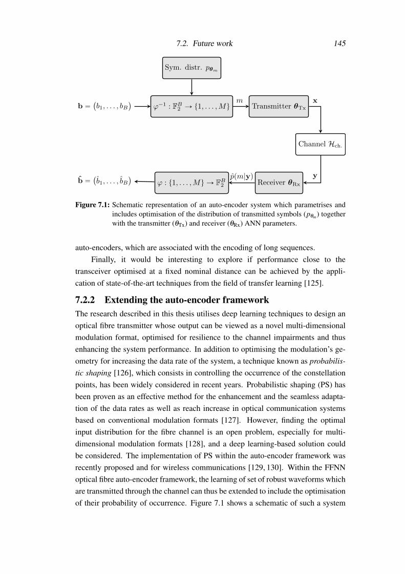
7.2. Future work 145
b “ `b1, . . . , bB
˘ϕ´1 : FB
2 Ñ t1, . . . ,Mu
Sym. distr. pθm
Transmitter θTx
Channel Hch.
m
ppm|yq
x
yReceiver θRxϕ : t1, . . . ,Mu Ñ FB
2b “ `
b1, . . . , bB˘
Figure 7.1: Schematic representation of an auto-encoder system which parametrises andincludes optimisation of the distribution of transmitted symbols (pθm) togetherwith the transmitter (θTx) and receiver (θRx) ANN parameters.
auto-encoders, which are associated with the encoding of long sequences.Finally, it would be interesting to explore if performance close to the
transceiver optimised at a fixed nominal distance can be achieved by the appli-cation of state-of-the-art techniques from the field of transfer learning [125].
7.2.2 Extending the auto-encoder frameworkThe research described in this thesis utilises deep learning techniques to design anoptical fibre transmitter whose output can be viewed as a novel multi-dimensionalmodulation format, optimised for resilience to the channel impairments and thusenhancing the system performance. In addition to optimising the modulation’s ge-ometry for increasing the data rate of the system, a technique known as probabilis-tic shaping [126], which consists in controlling the occurrence of the constellationpoints, has been widely considered in recent years. Probabilistic shaping (PS) hasbeen proven as an effective method for the enhancement and the seamless adapta-tion of the data rates as well as reach increase in optical communication systemsbased on conventional modulation formats [127]. However, finding the optimalinput distribution for the fibre channel is an open problem, especially for multi-dimensional modulation formats [128], and a deep learning-based solution couldbe considered. The implementation of PS within the auto-encoder framework wasrecently proposed and for wireless communications [129, 130]. Within the FFNNoptical fibre auto-encoder framework, the learning of set of robust waveforms whichare transmitted through the channel can thus be extended to include the optimisationof their probability of occurrence. Figure 7.1 shows a schematic of such a system

7.2. Future work 146
implementation. As previously explained (see Sec. 5.1.5), the sequences of bitsb =
(b1, . . . ,bB
)need to be mapped into sequences of messages m. In the presence
of PS this procedure is performed such that the different messages from the alphabetof size M appear with frequencies corresponding to a distribution pθm . This distri-bution is parameterised to facilitate deep learning. Its parameters are optimisedjointly with the transmitter and receiver ANNs. The application of probabilisticshaping within the auto-encoders for optical fibre communication as well as the ex-tension of the method to multi-dimensional modulation formats is both challengingand important.
7.2.3 Auto-encoders for long-haul coherent optical fibre com-munications
As proof of concept, the investigation of end-to-end deep learning for optical fi-bre systems concentrated on short reach IM/DD communications. Nevertheless, itshould be pointed out that the developed methods are general and can be extendedto other, eventually more complex models and systems. In particular, an exten-sion towards coherent optical fibre communications for long-haul transmission isa natural continuation of the work. Deep learning can be used to address the Kerrnonlinearity-induced limitations in such links. These systems are typically asso-ciated with the transmission of multiple wavelength channels over many spans offibre and optical amplification. The higher powers at the input to each span giverise to nonlinear Kerr effects, which, combined with chromatic dispersion, producea more complicated evolution of the transmitted signal (see Sec 3.2). As a result,both the linear and the nonlinear part of the NLSE need to be considered in thechannel model. Such an equation does not have an explicit analytical solution andneeds to be solved numerically.
The most commonly used numerical algorithm for solving the NLSE is thesplit step Fourier method (SSFM) [131]. In general, it consists in representing thedispersion term and the nonlinearity by the operators
D =− jβ2
2∂ 2
∂ t2 , (7.1)
N = jγ|q(z, t)|2, (7.2)
respectively, and separating their effects for sufficiently small distance ∆ along thefibre. The SSFM method is then applied as
q(z+∆, t) = exp(
D∆
2
)exp(N ∆)exp
(D
∆
2
)q(z, t), (7.3)

7.2. Future work 147
qpz, tq F exp`D∆
2
˘F´1 exp pN∆q F exp
`D∆
2
˘F´1 qpz `∆, tq
Figure 7.2: Schematic diagram of the split step Fourier method used to simulate a smallpropagation step ∆ along the optical fibre.
where the symmetrically applied dispersion half-step reduces the approximationerror [24]. As discussed in Sec. 3.2 dispersion is applied in the frequency domain,while nonlinearity is applied in the time domain.
Figure 7.2 shows a schematic diagram of the SSFM. The number of requiredsteps for accurate simulation of fibre propagation increases with input power, band-width and transmission distance. Importantly, in the framework of auto-encoderssuch repeated split-step segments are part of the end-to-end computational graphrepresenting the system. Thus, the optimisation process via backpropagation andSGD becomes more challenging. Nevertheless, deep learning over the SSFMhas been reported in [132], where the authors optimise the shape of a long pulsetransmitted over the fibre. However, the application of auto-encoders to high datarate wide bandwidth coherent optical fibre communication is currently unexplored.Demonstrating the experimental implementation of such systems would be poten-tially of great interest to the field.

Appendix A
FFNN auto-encoder transmittedsignal characteristics
During end-to-end optimisation of the transceiver, the transmitter learns waveformrepresentations which are robust to the optical channel impairments. During actualtransmission on the experimental test-bed (reported in Chapter 6) different longsequences of random messages are applied to the transmitter FFNN, followed by32 GHz LPF to generate the transmit waveforms. This section examines the tempo-ral and spectral representations of such transmit signals.
Figure A.1 (top) shows the filtered output of the neural network, trainedat (40,4) km, for the representative 10-symbol message sequence (mt)
10t=1 =
(2,36,64,40,21,53,42,41,34,13), with mt ∈ {1, . . . ,64} denoting the input mes-sage to the ANN at time/block t. Each symbol carries 6 bits of information, consistsof n · s = 48 samples at 336 GSa/s, and is thus transmitted at 7 GSym/s, yielding asymbol duration of T ≈ 143 ps. It can be observed that, as an effect of the imple-mented clipping layer in the transmitter FFNN, the waveform amplitude is limited inthe linear region of operation of the Mach-Zehnder modulator with small departurefrom the range [0;π/4] due to the filtering effects. Figure A.1 (bottom) also showsthe un-filtered 48 samples for each symbol in the sub-sequence (mt)
7t=6 = (53,42).
These blocks of samples represent the direct output of the transmitter FFNN.
The trained FFNN transmitter can be viewed as a look-up table which simplymaps the input message to one of M = 64 optimised blocks. Figure A.2 illustratesthe 48 amplitude levels in each of these blocks. Interestingly, it can be seen that theextremal values of 0 and π/4 are the prevailing levels. It appears that the FFNN triesto find a set of binary sequences optimised for end-to-end transmission. Neverthe-less, some intermediate values are also used. To bring more clarity, the constellationof this multi-dimensional modulation format is visualised by using a state-of-the-artdimensionality reduction machine learning technique such as t-Distributed Stochas-

149
0 143 286 429 572 715 858 1,001 1,144 1,287 1,430
0
0.5
1
m1 “ 2 m2 “ 36 m3 “ 64 m4 “ 40 m5 “ 21 m6 “ 53 m7 “ 42 m8 “41 m9 “ 34 m10 “13
Time (ps)
Amplitude(V
)
715 858 1,001
0
0.5
1
m6 “ 53 m7 “ 42
Time (ps)
Amplitude(V
)
Figure A.1: Top: Output of the transmitter ANN, trained at (40,4) km, after filtering with32 GHz brick-wall LPF for the representative random sequence of 10 symbols(mt)
10t=1 =(2,36,64,40,21,53,42,41,34,13) transmitted at 7 GSym/s, i.e. T ≈
143 ps. Bottom: Un-filtered ANN output samples, 48 per symbol, for the sub-sequence (mt)
7t=6 = (53,42).
tic Neighbor Embedding (t-SNE) [121]. Figure A.3 shows the two-dimensional t-SNE representation of the un-filtered FFNN outputs of Fig. A.2. It can be seenthat the 64 different waveforms are well-separated in the t-SNE space which is anindication that they can hence be discriminated well enough at the receiver.
Figure A.4 shows the spectrum of the real-valued electrical signal at the trans-mitter after LPF. Because of the low-pass filtering the spectral content is confinedwithin 32 GHz. The LPFs at both transmitter and receiver ensure that the signalbandwidth does not exceed the finite bandwidth of transmitter and receiver hard-ware. It can be further observed that, as a result of the block-based transmission,the signal spectrum consists of strong harmonics at frequencies that are multiplesof the symbol rate.

150
Figure A.2: All 64 possible outputs (m = 1 to m = 64, upper left to bottom right) of thetransmitter FFNN before low-pass filtering.

151
´50 0 50 100
´100
´50
0
50
1
2
3
4
5
6
7
8
9
m “ 1011
12
13
14
15
16
17 18
19
20
21
22
23
24
25
26
2728
29
30
31
32
33
34
35
36
3738
39
4041
42
43
44
45
46
4748
49
50
51
52
5354
55
56
57
58
59 60
61
6263
64
t-SNE X
t-SN
EY
Figure A.3: t-SNE representation of the multi-dimensional waveforms output of the trans-mitter FFNN on the two-dimensional plane. The points are labeled with theirrespective message number m.
0 5 10 15 20 25 30 35 40´20
0
20
40
60
80
f (GHz)
|Fpf
q|2(dB/7MHz)
Figure A.4: Spectrum of the 32 GHz brick-wall low-pass filtered waveform at the outputof the transmitter FFNN, trained at (40,4) km. The figure was generated using7 MHz spectral bins.

Appendix B
Number of nodes and floating pointoperations per decoded bit in theSBRNN auto-encoder
B.1 Counting the number of nodesIn the following, an example for counting the number of nodes in the SBRNN auto-encoder is provided using the vanilla variant of the system as a reference. Thehyper-parameters of the vanilla SBRNN auto-encoder at the transmitter and thereceiver were described in Sections 5.1.1.2 and 5.1.2.2, respectively.
According to Table 5.1, Sec. 5.1.1.2, the input to the transmitter neural networkhas the dimension M + n · s, while the output ANN dimension is n · s. The archi-tecture assumes a single layer in both the forward and backward recurrent passes.Therefore, the number of nodes at the transmitter per single direction is given by
M+n · s+n · s = M+2n · s.
The network architectures in both directions are identical and thus the number ofnodes in the bidirectional RNN at the transmitter becomes
M+2n · s+M+2n · s = 2M+4n · s. (B.1)
At the receiver, the input dimension of the neural network, specified in Table 5.2,Sec. 5.1.2.2, is n · s+ 2M, while the input to the hidden layer is 2M. Accordingly,the number of nodes (in a single direction) is thus
n · s+2M+2M = 4M+n · s.
Accounting for the backward direction at the receiver, which used identical hyper-

B.2. Counting the floating point operations 153
parameters, the total number of nodes at the receiver BRNN accumulates to
4M+n · s+4M+n · s = 8M+2n · s. (B.2)
As explained in Sec. 5.1.2.2, a final softmax layer is applied at the output of thereceiver BRNN to obtain probability vectors of size M used for the optimisation anderror counting procedures. This layer’s input is the concatenation of the outputs inthe hidden layers (each of dimension 2M) for the forward and backward processing,the size of the concatenated input vector thus becomes 4M and the number of nodesfor the softmax stage correspondingly become
4M+M = 5M. (B.3)
The total number of nodes in the vanilla SBRNN design of the auto-encoder canthen be obtained by adding up Equations (B.1), (B.2), and (B.3), resulting in
2M+4n · s+8M+2n · s+5M = 15M+6n · s, (B.4)
which is the expression used in the summary provided in Table 5.4, Sec. 5.3.1.3.
B.2 Counting the floating point operations
For the investigation in Sec. 5.3.3.3, the number of floating point operations re-quired per encoded/decoded bit were considered as a metric which indicates thecomputational complexity of the SBRNN auto-encoder. In particular, as explainedin Sec. 5.3.3.1, a vanilla SBRNN auto-encoder was used for this investigation. In thefollowing, the expression for the number of floating point operations per encodedbit at the transmitter, given by Eq. (5.36), Sec. 5.3.3.3, is derived step-by-step. Forthis calculation, the number of floating points operations (FLOPS) in matrix multi-plication was used, which for matrices A ∈ Ra×b and B ∈ Rb×c is given by [133]
O(bac) = (2b−1)ac. (B.5)
As described in Sec.5.1.1.2, the input vector to the neural network has the size(1T
m,t−→x T
t−1
)T∈RM+n·s, as it is a concatenation between the current one-hot vec-
tor of size M and the previous transmitter output of size n · s. In the forward BRNN
direction, it is multiplied as Wfw
(1T
m,t−→x T
t−1
)T, by a weight matrix with dimen-
sions Wfw ∈ Rn·s×(M+n·s). Using Eq. (B.5), the number of FLOPS for this opera-
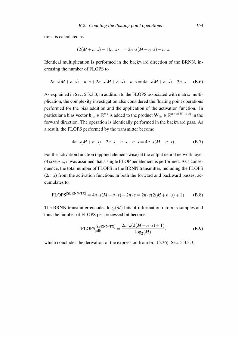
B.2. Counting the floating point operations 154
tions is calculated as
(2(M+n · s)−1)n · s ·1 = 2n · s(M+n · s)−n · s.
Identical multiplication is performed in the backward direction of the BRNN, in-creasing the number of FLOPS to
2n · s(M+n · s)−n · s+2n · s(M+n · s)−n · s = 4n · s(M+n · s)−2n · s. (B.6)
As explained in Sec. 5.3.3.3, in addition to the FLOPS associated with matrix multi-plication, the complexity investigation also considered the floating point operationsperformed for the bias addition and the application of the activation function. Inparticular a bias vector bfw ∈Rn·s is added to the product Wfw ∈Rn·s×(M+n·s) in theforward direction. The operation is identically performed in the backward pass. Asa result, the FLOPS performed by the transmitter become
4n · s(M+n · s)−2n · s+n · s+n · s = 4n · s(M+n · s). (B.7)
For the activation function (applied element-wise) at the output neural network layerof size n ·s, it was assumed that a single FLOP per element is performed. As a conse-quence, the total number of FLOPS in the BRNN transmitter, including the FLOPS(2n · s) from the activation functions in both the forward and backward passes, ac-cumulates to
FLOPS[SBRNN-TX] = 4n · s(M+n · s)+2n · s = 2n · s(2(M+n · s)+1). (B.8)
The BRNN transmitter encodes log2(M) bits of information into n · s samples andthus the number of FLOPS per processed bit becomes
FLOPS[SBRNN-TX]pdb =
2n · s(2(M+n · s)+1)log2(M)
, (B.9)
which concludes the derivation of the expression from Eq. (5.36), Sec. 5.3.3.3.

Appendix C
Data collection in the experiments
C.1 SBRNN auto-encoderThe training data was formed by the sequences with indices i ∈ {1, . . . ,720} andwas organised as follows
DAEtest :=
yT
1,1...N yT2,1...N yT
3,1...N yT4,1...N
yT5,1...N yT
6,1...N yT7,1...N yT
8,1...N...
......
...yT
717,1...N yT718,1...N yT
719,1...N yT720,1...N
, (C.1)
LAEtest :=
m1,1...N m2,1...N m3,1...N m4,1...N
m5,1...N m6,1...N m7,1...N m8,1...N...
......
...m717,1...N m718,1...N m719,1...N m720,1...N
, (C.2)
where DAEtrain ∈ R180×4·N·n·s consists of the data elements yi, j and LAE
train ∈ R180×4·N
contains the label elements mi, j. During the procedure of training the receiver onmeasured data (see Sec. 6.5.1) a window of V columns is picked to form the mini-batch on each stochastic gradient descent optimisation step. More specifically, atan optimisation step s, the mini-batch of elements1 DAE[:,s : (s+V )] was processedby the receiver to obtain corresponding output probability vectors, where V is thetraining window which was fixed to V = 10. The cross entropy loss between theinput messages LAE[:,s : (s+V )] and the probability outputs was computed andaveraged before completing a single iteration of the optimisation algorithm.
To ensure a sufficiently large mini-batch of independent examples, when form-ing the data-sets, one full DAC load was split into two parts, treated indepen-
1Note that the MATLAB notation A[:, i : j] is used to denote extracting the j− i+1 columns ofcolumn indices i, i+1, . . . , j from A.

C.2. Reference PAM systems 156
dently by the learning algorithm, e.g.(
yT1,1...N yT
2,1...N yT3,1...N yT
4,1...N
)and(
yT5,1...N yT
6,1...N yT7,1...N yT
8,1...N
). It was verified that convergence of the loss
is achieved within one epoch of the training data, which was used as a stoppingcriterion. The remaining sequences with indices i ∈ {721, . . . ,Z}, which are in-dependent from the training data, were used to form the testing data, identicallyorganised in DAE
test and LAEtest.
C.2 Reference PAM systemsSequences i ∈ {1, . . . ,90} were used for training, organised as
DPAMtrain :=
yT1,1 . . . yT
1,N/2
yT1,N/2+1 . . . yT
1,N... . . . ...
yT90,1 . . . yT
90,N/2
yT90,N/2+1 . . . yT
90,N
(C.3)
LPAMtrain :=
m1,1 . . . m1,N/2
m1,N/2+1 . . . m1,N... . . . ...
m90,1 . . . m90,N/2
m90,N/2+1 . . . m90,N
(C.4)
where DPAMtrain ∈ R180×N·n/2 consists of the received elements yi, j and LPAM
train ∈R180×N/2 has the elements mi, j. During the DSP optimisation for the deep learning-based PAM systems (see Appendices C.2.1 and C.2.3), a window of W from thedata was picked column-wise to form a mini-batch. Similar to the auto-encodertraining, one full DAC load was split into two parts that are independently treated bythe DSP, e.g.
(yT
1,1 . . .yT1,N/2
)and
(yT
1,N/2+1 . . .yT1,N
), ensuring an identical mini-
batch size. Again, one epoch over the training data was performed during optimisa-tion, while the testing was carried out using the disjoint set of remaining sequenceswith indices i ∈ {91, . . . ,100}, identically formed as DPAM
test and LPAMtest .
C.2.1 Optimisation of the SFFNN receiverThe receiver ANN parameters in this scheme were optimised using the experimentaldata as follows: At an iteration s, the mini-batch of elements DPAM
train [:,s : (s+W )] wasprocessed by the FFNN to obtain the corresponding output probability vectors. Theaverage cross entropy loss between these outputs and the input messages LPAM
train [:,s+ W−1
2 ] was computed to complete an optimisation step of the FFNN parameters

C.2. Reference PAM systems 157
via backpropagation and SGD using the Adam algorithm (see Chapter 2.
C.2.2 Optimisation of the Volterra receiverThe first and second order Volterra filter coefficients were optimised using the MAT-LAB fitlm function for linear and polynomial regression. The optimisation ofthe coefficients was performed on a randomly chosen pair of transmitted sequenceLPAM
train [i, :] and received samples DPAMtrain [i, :].
C.2.3 Optimisation of the SBRNN receiverThe elements of the collected PAM datasets DPAM
train and LPAMtrain were used in the train-
ing algorithm. At an iteration s of the optimisation algorithm, the mini-batch of ele-ments DPAM
train [:,s : (s+V )] was processed by the BRNN to obtain the correspondingoutput probability vectors. The average cross entropy loss was computed betweenthe input messages LPAM
train [:,s : (s+V )] and the probability outputs. Then the opti-misation step of the BRNN was completed via backpropagation and SGD using theAdam algorithm (see Chapter 2. The training window was fixed to V = 61, such thatthe scheme was trained with a processing memory identical to the auto-encoder.

Appendix D
Acronyms
ADC Analogue-to-digital converter
ANN Artificial neural network
AWGN Additive white Gaussian noise
BER Bit error rate
BRNN Bidirectional recurrent artificial neural network
DAC Digital-to-analogue converter
DBP Digital backpropagation
DD Direct detection
DL Deep learning
DSP Digital signal processing
EDFA Erbium-doped fibre amplifier
FEC Forward error correction
FFE Feedforward equaliser
FFNN Feedforward artificial neural network
FFT Fast Fourier transform
FTTH Fibre-to-the-home
FLOPS Floating point operations
GAN Generative adversarial network

159
GD Gradient descent
GRU Gated recurrent unit
HDD Hard decision decoding
HD-FEC Hard-decision forward error correction
IFFT Inverse fast Fourier transform
IM Intensity modulation
IM/DD Intensity modulation/direct detection
ISI Intersymbol interference
LDBP Learned DBP
LPF Low-pass filter
LSTM Long short-term memory
LSTM-GRU Long short-term gated recurrent unit
MAP Maximum a-posteriori probability
ML Machine learning
MLSD Maximum likelihood sequence detection
MZM Mach-Zehnder modulator
NLSE Nonlinear Schrödinger equation
PAM Pulse amplitude modulation
PD Photodiode
PDE Partial differential equation
PIN Positive-intrinsic-negative
PON Passive optical network
PRBS Pseudo-random binary sequence
PS Probabilistic shaping

160
ReLU Rectified linear unit
RNN Recurrent artificial neural network
SBRNN Sliding window bidirectional recurrent artificial neural network
SER Symbol error rate
SFFNN Sliding window feedforward artificial neural network
SGD Stochastic gradient descent
SNR Signal-to-noise ratio
SSFM Split-step Fourier method
SSMF Standard single mode fibre
TDM Tunable dispersion module
TIA Trans-impedance amplifier
t-SNE t-distributed stochastic neighbor embedding

Bibliography
[1] T. Mitchell. Machine learning. McCraw Hill, Inc., 1997.
[2] C. Bishop. Pattern recognition and machine learning. Springer, 2006.
[3] M. de Pardo. Advances in financial machine learning. John Wiley & Sons,2018.
[4] J. Dean, G. Corrado, R. Monga, K. Chen, M. Devin, Q. V. Le, M. Z. Mao,M. Ranzato, A. Senior, P. Tucker, K. Yang, and A. Y. Ng. Large scale dis-tributed deep networks. In Proc. of Advances in Neural Information Process-ing Systems (NIPS) 25, pages 1–9, 2012.
[5] Y. LeCun, Y. Bengio, and G. Hinton. Deep learning. Nature, 521(6):436–444, 2015.
[6] A. Krizhevsky, I. Sutskever, and G. Hinton. ImageNet classification withdeep convolutional neural networks. In Proc. of Advances in Neural Infor-mation Processing Systems (NIPS) 25, pages 1090–1098, 2012.
[7] G. Hinton, L. Deng, D. Yu, G. E. Dahl, A. Mohamed, N. Jaitly, A. Senior,V. Vanhoucke, P. Nguyen, T. N. Sainath, and B. Kingsbury. Deep neuralnetworks for acoustic modeling in speech recognition: the shared views offour research groups. IEEE Signal Processing Magazine, 29(6):82–97, 2012.
[8] R. Collobert, J. Weston, L. Bottou, M. Karlen, K. Kavukcuoglu, andP. Kuksa. Natural language processing (almost) from scratch. Journal ofMachine Learning Research, 12:2493–2537, 2011.
[9] M. Ibnkahla. Applications of neural networks to digital communications—asurvey. Signal Processing, 80(7):1185–1215, 2000.
[10] O. Simeone. A very brief introduction to machine learning with applicationsto communication systems. IEEE Transactions on Cognitive Communica-tions and Networking, 4(4):648–664, 2018.

Bibliography 162
[11] F. N. Khan, Q. Fan, C. Lu, and A. P. T. Lau. An optical communication’sperspective on machine learning and its applications. Journal of LightwaveTechnology, 37(2):493–516, 2019.
[12] I. Goodfellow, Y. Bengio, and A. Courville. Deep Learning. MIT press,2016.
[13] D. Rumelhart, G. Hinton, and R. Williams. Learning representations by back-propagating errors. Nature, 323:533–536, 1986.
[14] A. Cauchy. Méthode générale pour la résolution des syst‘emes d’équationssimultanées. C.R. Acad. Sci. Paris, 25:536–538, 1847.
[15] H. B. Curry. The method of steepest descent for non-linear minimizationproblems. Quarterly of Applied Mathematics, 2(3):258–261, 1944.
[16] D. Kingma and J. Ba. Adam: a method for stochastic optimization. In Proc.of International Conference for Learning Representations, pages 1–15, 2015.
[17] A. Karpathy. A peek at trends in machine learning. Medium. Accessed on:Aug. 4, 2020. [Online]. Available: https://medium.com/@karpathy/a-peek-at-trends-in-machine-learning-ab8a1085a106, Apr. 7, 2017.
[18] S. Ruder. An overview of gradient descent optimization algorithms.arXiv:1609.04747, 2016.
[19] S. Cammerer. Deep learning-based polar code design. presented at the 57thAnnual Allerton Conference on Communication, Control, and Computing(Allerton), Monticello, IL, USA, September 25, 2019.
[20] O. Simeone. A brief introduction to machine learning for engineers. Foun-dations and Trends® in Signal Processing, 12(3-4):200–431, 2017.
[21] E. Brynjolfsson and T. Mitchell. What can machine learning do? Workforceimplications. Science, 358(6370):1530–1534, 2017.
[22] T. S. Rappaport. Wireless communications: Principles and practice, 2nd ed.Prentice Hall, 2002.
[23] G. Agrawal. Fiber-Optic Communication systems, 4th ed. Wiley, 2010.
[24] G. Agrawal. Nonlinear fiber optics, 5th ed. Academic Press, 2013.

Bibliography 163
[25] J. Proakis and M. Salehi. Digital Communications, 5th ed. McGraw-HillEducation, 2007.
[26] Cisco Systems Inc. Cisco global cloud index: Forecast and methodology,2016 - 2021. White Paper, 2018.
[27] H. Kim and N. Feamster. Improving network management with softwaredefined networking. IEEE Communications Magazine, 51(2):114–119, 2013.
[28] Huawei Technologies Co. Ltd. White paper on technological developmentsof optical networks. White Paper, 2016.
[29] D. Cote. Using machine learning in communication networks. IEEE/OSAJournal of Optical Communications and Networking, 10(10):D100–D109,2018.
[30] M. Wang, Y. Cui, X. Wang, S. Xiao, and J. Jiang. Machine learning for net-working: workflow, advances and opportunities. IEEE Network, 32(2):92–99, 2018.
[31] A. Deylamsalehi, D. A. P. Davis, P. Afsharlar, M. Bahrami, W. Chen, andV. M. Vokkarane. Using machine learning to balance energy cost and emis-sions in optical networks. IEEE/OSA Journal of Optical Communicationsand Networking, 10(10):D72–D83, 2018.
[32] F. Musumeci, C. Rottondi, A. Nag, I. Macaluso, D. Zibar, M. Ruffini, andM. Tornatore. An overview on application of machine learning techniques inoptical networks. IEEE Communications Surveys & Tutorials, 21(2):1383–1408, 2019.
[33] R. Boutaba, M. Salahuddin, N. Limam, S. Ayoubi, N. Shahriar, F. Estrada-Solano, and O. M. Caicedo. A comprehensive survey on machine learningfor networking: evolution, applications and research opportunities. Journalof Internet Services and Applications, 9(16):1–99, 2018.
[34] G. Choudhury, G. Thakur, and S. Tse. Joint optimization of packet andoptical layers of a core network using SDN controller, CD ROADMs andmachine-learning-based traffic prediction. In Proc. of Optical Fiber Commu-nications Conference, pages 1–3, 2019.
[35] Z. Fadlullah, F. Tang, B. Mao, N. Kato, O. Akashi, T. Inoue, and K. Mizu-tani. State-of-the-art deep learning: evolving machine intelligence toward

Bibliography 164
tomorrow’s intelligent network traffic control systems. IEEE Communica-tions surveys & tutorials, 19(4):2432–2455, 2017.
[36] F. Morales, M. Ruiz, L. Gifre, L. M. Contreras, V. Lopez, and L. Velasco.Virtual network topology adaptability based on data analytics for traffic pre-diction. IEEE/OSA Journal of Optical Communications and Networking,9(1):A35–A45, 2017.
[37] D. Rafique and L. Velasco. Machine learning for network automation:overview, architecture, and applications. IEEE/OSA Journal of Optical Com-munications and Networking, 10(10):D126–D143, 2018.
[38] Y. Okada, S. Ata, N. Nakamura, Y. Nakahira, and I. Oka. Comparisonsof machine learning algorithms for application identification of encryptedtraffic. In Proc. of 10th International Conference on Machine Learning andApplications, pages 358–361, 2011.
[39] B. Dong and X. Wang. Comparison of deep learning method to tradi-tional methods used for network intrusion detection. In 8th IEEE Interna-tional Conference on Communication Software and Networks, pages 581–585, 2016.
[40] T. P. Oliveira, J. S. Barbar, and A. S. Soares. Multilayer Perceptron andStacked Autoencoder for Internet Traffic Prediction. Springer Berlin Heidel-berg, 2014.
[41] J. Proakis and D. Manolakis. Digital signal processing: principles algo-rithms and applications, 3rd ed. Prentice Hall, 2001.
[42] E. Agrell, M. Karlsson, A. R. Chraplyvy, D. J. Richardson, P. M. Krummrich,P. Winzer, K. Roberts, J. K. Fischer, S. J. Savory, B. J. Eggleton, M. Secon-dini, F. R. Kschischang, A. Lord, J. Prat, I. Tomkos, J. E. Bowers, S. Srini-vasan, M. Brandt-Pearce, and N. Gisin. Roadmap of optical communications.Journal of Optics, 18(6):063002, May 2016.
[43] O. Shental and J. Hoydis. Machine LLRning: learning to softly demodulate.In IEEE Globecom Workshops (GC Wkshps), pages 1–7, 2019.
[44] E. Nachmani, Y. Be’ery, and D. Burshtein. Learning to decode linear codesusing deep learning. In 2016 54th Annual Allerton Conference on Commu-nication, Control, and Computing (Allerton), pages 341–346, 2016.

Bibliography 165
[45] T. Gruber, S. Cammerer, J. Hoydis, and S. ten Brink. On deep learning-basedchannel decoding. In 2017 51st Annual Conference on Information Sciencesand Systems (CISS), pages 1–6, 2017.
[46] S. Cammerer, T. Gruber, J. Hoydis, and S. ten Brink. Scaling deep learning-based decoding of polar codes via partitioning. In GLOBECOM 2017 - 2017IEEE Global Communications Conference, pages 1–6, 2017.
[47] D. Tandler, S. Dörner, S. Cammerer, and S. ten Brink. On recurrent neuralnetworks for sequence-based processing in communications. In 2019 53rdAsilomar Conference on Signals, Systems, and Computers, pages 537–543,2019.
[48] A. Buchberger, C. Häger, H. D. Pfister, L. Schmalen, and A. Graell i Amat.Pruning neural belief propagation decoders. In 2018 IEEE InternationalSymposium on Information Theory (ISIT), pages 1–5, 2020.
[49] E. Ip and J. M. Kahn. Compensation of dispersion and nonlinear impair-ments using digital backpropagation. Journal of Lightwave Technology,26(20):3416–3425, 2008.
[50] C. Häger and H. D. Pfister. Nonlinear interference mitigation via deep neu-ral networks. In Proc. of Optical Fiber Communications Conference andExposition (OFC), pages 1–3, 2018.
[51] C. Fougstedt, C. Häger, L. Svensson, H. D. Pfister, and P. Larsson-Edefors.ASIC implementation of time-domain digital backpropagation with deep-learned chromatic dispersion filters. In Proc. of European Conference onOptical Communication (ECOC), pages 1–3, 2018.
[52] V. Oliari, S. Goossens, C. Häger, G. Liga, R. M. Bütler, M. v. d. Hout,S. v. d. Heide, H. D. Pfister, C. Okonkwo, and A. Alvarado. Revisiting effi-cient multi-step nonlinearity compensation with machine learning: an experi-mental demonstration. Journal of Lightwave Technology, 38(12):3114–3124,2020.
[53] S. Chen, G. J. Gibson, C. F. N. Cowan, and P. M. Grant. Adaptive equal-ization of finite non-linear channels using multilayer perceptrons. SignalProcessing, 20:107–119, 1990.
[54] N. Benvenuto, M. Marchesi, F. Piazza, and A. Uncini. Non linear satelliteradio links equalized using blind neural networks. In [Proceedings] ICASSP

Bibliography 166
91: 1991 International Conference on Acoustics, Speech, and Signal Pro-cessing, pages 1521–1524 vol.3, 1991.
[55] T. Koike-Akino, Y. Wang, D. S. Millar, K. Kojima, and K. Parsons. Neuralturbo equalization: deep learning for fiber-optic nonlinearity compensation.Journal of Lightwave Technology, 38(11):3059–3066, 2020.
[56] V. Kamalov, L. Jovanovski, V. Vusirikala, S. Zhang, F. Yaman, K. Nakamura,T. Inoue, E. Mateo, and Y. Inada. Evolution from 8QAM live traffic to PS 64-QAM with neural-network based nonlinearity compensation on 11000 kmopen subsea cable. In Proc. of Optical Fiber Communications Conferenceand Exposition (OFC), pages 1–3, 2018.
[57] J. Estaran, R. Rios-Mueller, M. A. Mestre, F. Jorge, H. Mardoyan, A. Kon-czykowska, J. . Dupuy, and S. Bigo. Artificial neural networks for linearand non-linear impairment mitigation in high-baudrate IM/DD systems. InProc. of European Conference on Optical Communication (ECOC), pages1–3, 2016.
[58] V. Houtsma, E. Chou, and D. van Veen. 92 and 50 gbps TDM-PON usingneural network enabled receiver equalization specialized for PON. In Proc.of Optical Fiber Communications Conference and Exhibition (OFC), pages1–3, 2019.
[59] T. J. O’Shea, K. Karra, and T. C. Clancy. Learning to communicate: channelauto-encoders, domain specific regularizers, and attention. In 2016 IEEEInternational Symposium on Signal Processing and Information Technology(ISSPIT), pages 223–228, 2016.
[60] T. J. O’Shea and J. Hoydis. An introduction to deep learning for the physicallayer. IEEE Transactions on Cognitive Communications and Networking,3(4):563–575, 2017.
[61] S. Dörner, S. Cammerer, J. Hoydis, and S. ten Brink. Deep learning basedcommunication over the air. IEEE Journal of Selected Topics in Signal Pro-cessing, 12(1):132–143, 2018.
[62] B. Karanov, M. Chagnon, F. Thouin, T. A. Eriksson, H. Bülow, D. Lavery,P. Bayvel, and L. Schmalen. End-to-end deep learning of optical fiber com-munications. Journal of Lightwave Technology, 36(20):4843–4855, 2018.

Bibliography 167
[63] M. Chagnon, B. Karanov, and L. Schmalen. Experimental demonstration of adispersion tolerant end-to-end deep learning-based IM-DD transmission sys-tem. In Proc. of European Conference on Optical Communication (ECOC),pages 1–3, 2018.
[64] R. T. Jones, T. A. Eriksson, M. P. Yankov, and D. Zibar. Deep learning ofgeometric constellation shaping including fiber nonlinearities. In Proc. ofEuropean Conference on Optical Communication (ECOC), pages 1–3, 2018.
[65] S. Li, C. Häger, N. Garcia, and H. Wymeersch. Achievable information ratesfor nonlinear fiber communication via end-to-end autoencoder learning. InProc. of European Conference on Optical Communication (ECOC), pages1–3, 2018.
[66] N. Stojanovic, F. Karinou, Z. Qiang, and C. Prodaniuc. Volterra and wienerequalizers for short-reach 100G PAM-4 applications. Journal of LightwaveTechnology, 35(21):4583–4594, 2017.
[67] G. D. Forney. The Viterbi algorithm. Proceedings of the IEEE, 61(3):268–278, 1973.
[68] P. Poggiolini, G. Bosco, J. Prat, R. Killey, and S. Savory. Branch metrics foreffective long-haul MLSE IMDD receivers. In 2006 European Conferenceon Optical Communications, pages 1–2, 2006.
[69] G. Bosco, P. Poggiolini, and M. Visintin. Performance analysis of MLSEreceivers based on the square-root metric. Journal of Lightwave Technology,26(14):2098–2109, 2008.
[70] M. Chagnon. Optical communications for short reach. Journal of LightwaveTechnology, 37(8):1779–1797, 2019.
[71] W. S. McCulloch and W. Pitts. A logical calculus of the ideas immanent innervous activity. Bulletin of Mathematical Biophysics, 5:115–133, 1943.
[72] K. Hornik, M. Stinchcombe, and H. White. Multilayer feedforward networksare universal approximators. Neural Networks, 2(5):359–366, 1989.
[73] G. Gybenko. Approximation by superpositions of a sigmoidal function.Mathematics of Control, Signals and Systems, 2:303–314, 1989.
[74] K. Hornik. Approximation capabilities of multilayer feedforward networks.Neural Networks, 4(2):251–257, 1991.

Bibliography 168
[75] V. Nair and G. Hinton. Rectified linear units improve restricted boltzmannmachines. In Proc. of Int. Conf. Mach. Learn., pages 807–814, 2010.
[76] P. J. Werbos. Generalization of backpropagation with application to a recur-rent gas market model. Neural Networks, 1:339–356, 1988.
[77] Y. Bengio, P. Frasconi, and P. Simard. The problem of learning long-termdependencies in recurrent networks. In IEEE International Conference onNeural Networks, pages 1183–1188 vol.3, 1993.
[78] S. Hochreiter and J. Schmidhuber. Long short-term memory. Neural Com-put., 9(8):1735–1780, 1997.
[79] I. Sutskever, O. Vinyals, and Q. V. Le. Sequence to sequence learning withneural networks. In Advances in Neural Information Processing Systems(NIPS) 27, pages 3104–3112, 2014.
[80] R. Jozefowicz, W. Zaremba, and I. Sutskever. An empirical exploration ofrecurrent network architectures. In Proceedings of the 32nd InternationalConference on Machine Learning (ICML), pages 2342–2350, 2015.
[81] K. Cho, B. van Merriënboer, c. Gulcehre, D. Bahdanau, F. Bougares,H. Schwenk, and Y. Bengio. Learning phrase representations using RNNencoder-decoder for statistical machine translation. In Proc. of the 2014 Con-ference on Empirical Methods in Natural Language Processing (EMNLP),pages 1724–1734, 2014.
[82] M. Schuster and K. K. Paliwal. Bidirectional recurrent neural networks.IEEE Transactions on Signal Processing, 45(11):2673–2681, 1997.
[83] A. Graves and J. Schmidhuber. Framewise phoneme classification with bidi-rectional LSTM and other neural network architectures. Neural Networks,18(5-6):602–610, 2005.
[84] I. Goodfellow, J. Pouget-Abadie, M. Mirza, B. Xu, D. Warde-Farley,S. Ozair, A. Courville, and Y. Bengio. Generative adversarial nets. In Ad-vances in Neural Information Processing Systems (NIPS) 27, pages 2672–2680, 2014.
[85] L. Devroye. Non-uniform random variate generation. Springer-Verlag, 1986.
[86] W. H. Press, W. Vetterling, S. Teukolsky, and B. P. Flannery. Numericalrecipes, 3rd ed. Cambridge University Press, 2007.
Bibliography 169
[87] H. Robbins and S. Monro. A stochastic approximation method. Annals ofMathematical Statistics, 22(3):400–407, 1951.
[88] L. Bottou. Large-scale machine learning with stochastic gradient descent. InProceedings of 19th International Conference on Computational Statistics,pages 177–186, 2010.
[89] F.-F. Li, R. Krishna, and D. Xu. Convolutional neural networks for visualrecognition. CS231n Class, Module 1: Neural Networks, Lecture: Learningand Evaluation, Stanford University. Accessed on: Aug. 4, 2020. [Online].Available: https://cs231n.github.io/neural-networks-3/, Spring 2020.
[90] G. Strang. Calculus, 3rd ed. Wellesley-Cambridge Press, 2017.
[91] D. Plabst, J. G. Gómez, T. Wiegart, and N. Hanik. Wiener filter for short-reach fiber-optic links. IEEE Communications Letters, pages 1–1, 2020.
[92] Q. Hu, M. Chagnon, K. Schuh, F. Buchali, and H. Bülow. High data ratetomlinson-harashima-precoding-based pam transmission. In 45th EuropeanConference on Optical Communication (ECOC 2019), pages 1–4, 2019.
[93] Application Note. High-speed DACs. Tektronix. Accessed on: Aug. 21, 2020.[Online]. Available: https://www.tek.com/dl/76W_30631_0_HR_Letter.
[94] K. Gentile. The effect of DAC resolution on spurious performance.Analog Devices, Inc. Accessed on: Aug. 21, 2020. [Online]. Avail-able: https://www.analog.com/media/en/training-seminars/design-handbooks/Technical-Tutorial-DDS/Section4.pdf, 1999.
[95] W. Kester. Taking the mystery out of the infamous formula, "SNR =6.02N + 1.76dB," and why you should care. Tutorial MT-001, Ana-log Devices, Inc. Accessed on: Aug. 21, 2020. [Online]. Available:https://www.analog.com/media/en/training-seminars/tutorials/MT-001.pdf,2009.
[96] C. Schmidt, C. Kottke, V. Jungnickel, and R. Freund. High-speed digital-to-analog converter concepts. In Next-Generation Optical Communication:Components, Sub-Systems, and Systems VI, volume 10130, pages 133 – 141,2017.
[97] A. Napoli, M. M. Mezghanni, S. Calabrò, R. Palmer, G. Saathoff, andB. Spinnler. Digital predistortion techniques for finite extinction ratio IQ

Bibliography 170
Mach–Zehnder modulators. Journal of Lightwave Technology, 35(19):4289–4296, 2017.
[98] Application Bulletin. Noise analysis of FET transimpedance amplifiers.Burr-Brown Corp. Accessed on: Aug. 21, 2020. [Online]. Available:https://www.ti.com/lit/an/sboa060/sboa060.pdf, 1994.
[99] Tensorflow. [Online]. Available: https://www.tensorflow.org/, 2020.
[100] C. E. Shannon. A mathematical theory of communication. The Bell SystemTechnical Journal, 27(3):379–423, 1948.
[101] L. Schmalen, A. J. de Lind van Wijngaarden, and S. ten Brink. Forward errorcorrection in optical core and optical access networks. Bell Labs TechnicalJournal, 18(3):39–66, 2013.
[102] E. Agrell and M. Secondini. Information-theoretic tools for optical commu-nications engineers. In 2018 IEEE Photonics Conference (IPC), pages 1–5,2018.
[103] F. Gray. Pulse code communication, US Patent US2632058A, Mar. 1953.
[104] T. A. Eriksson, H. Bülow, and A. Leven. Applying neural networks in op-tical communication systems: possible pitfalls. IEEE Photonics TechnologyLetters, 29(23):2091–2094, 2017.
[105] M. Matsumoto and T. Nishimura. Mersenne twister: A 623-dimensionallyequidistributed uniform pseudo-random number generator. ACM Trans.Model. Comput. Simul., 8(1):3–30, 1998.
[106] D.-U. Lee, J. D. Villasenor, W. Luk, and P. H. W. Leong. A hardware Gaus-sian noise generator using the Box-Muller method and its error analysis.IEEE Transactions on Computers, 55(6):659–671, 2006.
[107] Z. Wang. Super-FEC codes for 40/100 Gbps networking. IEEE Communi-cations Letters, 16(12):2056–2059, 2012.
[108] N. Farsad and A. Goldsmith. Neural network detection of data sequencesin communication systems. IEEE Transactions on Signal Processing,66(21):5663–5678, 2018.

Bibliography 171
[109] N. Farsad and A. Goldsmith. Neural network detectors for molecular com-munication systems. In 2018 IEEE 19th International Workshop on Sig-nal Processing Advances in Wireless Communications (SPAWC), pages 1–5,2018.
[110] K. Zeger and A. Gersho. Pseudo-gray coding. IEEE Transactions on Com-munications, 38(12):2147–2158, 1990.
[111] F. Glover. Tabu search – part i. ORSA Journal on Computing, 1(3):190–206,1989.
[112] R. T. Jones, M. P. Yankov, and D. Zibar. End-to-end learning for GMI opti-mized geometric constellation shape. In 45th European Conference on Opti-cal Communication (ECOC 2019), pages 1–4, 2019.
[113] I. Lyubomirsky. Machine learning equalization techniques for high speedPAM4 fiber optic communication systems. CS229 Final Project Report.Stanford University (2015). Accessed on: Aug. 21, 2020. [Online]. Avail-able: http://cs229.stanford.edu/proj2015/232_report.pdf.
[114] D. van Veen and V. Houtsma. Strategies for economical next-generation 50gand 100G passive optical networks [invited]. IEEE/OSA Journal of OpticalCommunications and Networking, 12(1):A95–A103, 2020.
[115] O. Sidelnikov, A. Redyuk, and S. Sygletos. Equalization performance andcomplexity analysis of dynamic deep neural networks in long haul transmis-sion systems. Opt. Express, 26(25):32765–32776, 2018.
[116] B. Karanov, D. Lavery, P. Bayvel, and L. Schmalen. End-to-end opti-mized transmission over dispersive intensity-modulated channels using bidi-rectional recurrent neural networks. Opt. Express, 27(14):19650–19663, Jul2019.
[117] B. Karanov, G. Liga, V. Aref, D. Lavery, P. Bayvel, and L. Schmalen. Deeplearning for communication over dispersive nonlinear channels: performanceand comparison with classical digital signal processing. In Proc. of 57thAnnual Allerton Conference on Communication, Control, and Computing(Allerton), pages 192–199, 2019.
[118] B. Karanov, P. Bayvel, and L. Schmalen. End-to-end learning in opticalfiber communications: concept and transceiver design. In Proc. of EuropeanConference on Optical Communication (ECOC), pages 1–4, 2020.

Bibliography 172
[119] F. A. Aoudia and J. Hoydis. Model-free training of end-to-end commu-nication systems. IEEE Journal on Selected Areas in Communications,37(11):2503–2516, 2019.
[120] D. J. F. Barros and J. M. Kahn. Comparison of orthogonal frequency-divisionmultiplexing and on-off keying in amplified direct-detection single-modefiber systems. Journal of Lightwave Technology, 28(12):1811–1820, 2010.
[121] L. van der Maaten and G. Hinton. Visualizing data using t-SNE. J. Mach.Learn. Res, 9:2579–2605, 2008.
[122] B. Karanov, M. Chagnon, V. Aref, D. Lavery, P. Bayvel, and L. Schmalen.optical fiber communication systems based on end-to-end deep learning. InProc. of IEEE Photonics Conference (IPC), pages 1–2, 2020.
[123] B. Karanov, M. Chagnon, V. Aref, D. Lavery, P. Bayvel, and L. Schmalen.Concept and experimental demonstration of optical IM/DD end-to-end sys-tem optimization using a generative model. In Proc. of Optical Fiber Com-munications Conference (OFC), pages 1–3, 2020.
[124] B. Karanov, M. Chagnon, V. Aref, F. Ferreira, D. Lavery, P. Bayvel, andL. Schmalen. Experimental investigation of deep learning for digital signalprocessing in short reach optical fiber communications. In Proc. of IEEE In-ternational Workshop on Signal Processing Systems (SiPS), pages 1–6, 2020.
[125] S. J. Pan and Q. Yang. A survey on transfer learning. IEEE Transactions onKnowledge and Data Engineering, 22(10):1345–1359, 2010.
[126] F. R. Kschischang and S. Pasupathy. Optimal nonuniform signaling for gaus-sian channels. IEEE Transactions on Information Theory, 39(3):913–929,1993.
[127] F. Buchali, F. Steiner, G. Böcherer, L. Schmalen, P. Schulte, and W. Idler.Rate adaptation and reach increase by probabilistically shaped 64-QAM: anexperimental demonstration. Journal of Lightwave Technology, 34(7):1599–1609, 2016.
[128] R. Dar, M. Feder, A. Mecozzi, and M. Shtaif. On shaping gain in the nonlin-ear fiber-optic channel. In 2014 IEEE International Symposium on Informa-tion Theory, pages 2794–2798, 2014.
Bibliography 173
[129] M. Stark, F. Ait Aoudia, and J. Hoydis. Joint learning of geometric and prob-abilistic constellation shaping. In IEEE Globecom Workshops (GC Wkshps),pages 1–6, 2019.
[130] F. Ait Aoudia and J. Hoydis. Joint learning of probabilistic and geometricshaping for coded modulation systems. arXiv:2004.05062, 2020.
[131] J. A. C. Weideman and B. M. Herbst. Split-step methods for the solution ofthe nonlinear Schrodinger equation. SIAM Journal on Numerical Analysis,23(3):485–507, 1986.
[132] T. Uhlemann, S. Cammerer, A. Span, S. Dörner, and S. ten Brink. Deep-learning autoencoder for coherent and nonlinear optical communication.arXiv:2006.15027, 2020.
[133] R. Hunger. Floating point operations in matrix-vector calculus. Technicalreport. Technische Universität München (2007). Accessed on: Aug. 21, 2020.[Online]. Available: https://mediatum.ub.tum.de/doc/625604/625604.