IEEE TRANSACTIONS ON COMPUTATIONAL SOCIAL SYSTEMS 1

Analysis of the Impact of High-Frequency Tradingon Artificial Market Liquidity

Isao Yagi , Member, IEEE, Yuji Masuda, and Takanobu Mizuta

Abstract— Many empirical studies have discussed market liq-uidity, which is regarded as a measure of a booming financialmarket. Further, various indicators for objectively evaluatingmarket liquidity have also been proposed and their merits havebeen discussed. In recent years, the impact of high-frequencytraders (HFTs) on financial markets has been a focal concern,but no studies have systematically discussed their relationshipwith major market liquidity indicators, including volume, tight-ness, resiliency, and depth. In this study, we used agent-basedsimulations to compare the major liquidity indicators in anartificial market where an HFT participated was compared toone where no HFT participated. The results showed that allliquidity indicators in the market where an HFT participatedimproved more than those in the market where no HFT partici-pated. Furthermore, as a result of investigating the correlationsbetween the major liquidity indicators in our simulations andthe extant empirical literature, we found that market liquiditycan be measured not only by the major liquidity indicators butalso by execution rate. Therefore, it is suggested that it couldbe appropriate to employ execution rate as a novel liquidityindicator in future studies.

Index Terms— Agent-based simulation, artificial market, finan-cial market, market liquidity, multiagent system (MAS).

I. INTRODUCTION

PRESENTLY, market liquidity is considered to be animportant factor by numerous investors. Typically, a mar-

ket is said to be significantly liquid if participants are able torapidly buy or sell the desired amounts at costs similar to thecurrent market price [1].

Empirical studies on market liquidity have produced variousbeneficial findings [2]–[27]. Different means of assessingthe liquidity of a market were proposed in [2], based ondepth, resiliency, and tightness. Many of the other empir-ical studies, for example, [3]–[7], among others, concerndimensions of market liquidity, that is depth, tightness, andresiliency. In addition to these dimensions, an approach todetermining illiquidity (ILLIQ) was also established in [8]based on a ratio of the absolute value of the daily returnof a stock to the daily dollar volume, with averaging over a

Manuscript received February 29, 2020; revised July 9, 2020; acceptedAugust 18, 2020. This work was supported by JSPS KAKENHI under Grant20K04977. (Corresponding author: Isao Yagi.)

Isao Yagi is with the Department of Information and Computer Sciences,Faculty of Information Technology, Kanagawa Institute of Technology, Atsugi243-0292, Japan (e-mail: iyagi2005@gmail.com).

Yuji Masuda is with the System Development, Information System Group,Card Solution Company, Yamato System Development Company Ltd.,Kawasaki 211-0004, Japan.

Takanobu Mizuta is with the Investment and Research Division, SPARXAsset Management Company Ltd., Minato 108-0075, Japan.

Digital Object Identifier 10.1109/TCSS.2020.3019352

specific time span. Amihud’s work additionally demonstratedthat illiquidity is associated with increased expected assetreturns.

Muranaga [9] performed a cross-sectional assessment of theTokyo stock exchange (TSE) with the aim of determining thecorrelations between three different market liquidity parame-ters (depth, tightness, and resiliency) and trading frequency.In this prior work, market impact, the spread between bidand ask prices, and the rate of convergence of this spreadfollowing trades were respectively used as measurements ofdepth, tightness, and resiliency. The results of this prioranalysis established that trade frequency exhibited correlationswith these parameters. Muranaga [9] additionally examined theeffect of lower TSE tick sizes on liquidity, and reported thata reduced tick size was associated with lower spreads, greatertrading frequencies, and decreased volatility. These resultsconfirmed that tick size can have an effect on market liquidity.The correlation between tick size and the quality of the marketwas established by Chung et al. [10] based on data obtainedfrom a market having varying tick sizes. Their study examinedthe effect of small variations in price on liquidity by assessinginter-temporal and cross-sectional correlations between marketliquidity and tick size. Chung’s work also showed that thereare positive correlations between depth and both turnoverrate and volume, but inverse relationships between depth andboth volatility and market price. Harris [11] noted that ticksize reduction would reduce quoted spreads while causing areduction in depth and additionally Bessembinder [12] notedthat the quoted spread and effective spread would declinebecause of tick size reduction, as well as market volatility.Ahn et al. [13] reported that the quoted spread and effectivespread decreased due to the change in tick size implementedby the TSE in 1998. Olbrys and Mursztyn [3] investigateddepth, tightness, and resiliency using high-frequency datafor 53 companies in the Warsaw stock exchange (WSE). Theyreported that depth and resiliency for the most liquid bigcompanies with the largest market capitalization were higherthan those for the other companies, whereas tightness for theformer companies was lower than that for the other companies.Moreover, they found that tightness was high (low) whendepth was high (low); however, the majority of the correlationcoefficients between tightness and depth were not significantlydifferent from zero, so these indicators can capture varioussources of market liquidity.

It should be noted that liquidity is frequently defined differ-ently depending on the research that is being performed. Asan example, a scenario in which the sales and purchases in

This work is licensed under a Creative Commons Attribution 4.0 License. For more information, see https://creativecommons.org/licenses/by/4.0/

2 IEEE TRANSACTIONS ON COMPUTATIONAL SOCIAL SYSTEMS

a market have minimal effect on price and one in which thevolatility is low can both be considered to represent marketswith high liquidity. Consequently, various studies use differentliquidity indicators and so it can be challenging to directlycompare the results of different research projects.

Due to IT innovations, the transactions of high-frequencytraders (HFTs) now have a great impact on the market.HFTs use powerful computer programs to transact a largenumber of orders in fractions of a second. As they placeboth a buy and a sell order to make a profit—by whichthe sell price exceeds the buy price for an asset—they alsoplay a market maker role. Various HFT strategies have beenreported [28], [29]. ASIC [28] categorized these strategies intothree categories: 1) electronic liquidity provision strategies;2) statistical arbitrage strategies; and 3) liquidity detectionstrategies. A market making strategy is a kind of electronicliquidity provision strategy and majority of the HFT tradingvolume and more than 80% of HFT limit order submissionsare associated with market making strategies [30]. Recently,the rate of transactions attributable to HFTs compared to thetotal number of orders in financial markets has become large.It is estimated that 48.4% of orders in the foreign exchangemarket between the U.S. dollar and Japanese yen are HFTorders [31]. Empirical evidence has been put forward to sug-gest that the transactions of HFTs have increased depth [29].However, there are some critical opinions such as that HFTswere responsible for the flash crash in the US stock marketin 2010.

Thus, there are some unclear points about the effect ofHFTs on market liquidity. The reason why is that the empiricaldata contain many external factors, so that even if some kindof impact can be confirmed in the data, we cannot confirmwhether HFT transactions were the cause.

One method for dealing with situations that defy analysisby previous empirical research methods is to construct anartificial market using an agent-based model [32]–[36]. Inrecent years, much research using multi-agent systems hasbeen performed and achieved many results not only in thefinancial field but also in other fields, such as cognitivearchitecture [37], population dynamics [38], epidemiology[39], and social networks [40], to name a few. In this model,specific agents are given unique trading assignments (suchas only selling or buying) and subsequently act as investorsto perform trading of financial assets. The behavior of theseagents in the market is subsequently monitored. Using thistechnique in conjunction with various market restrictions (suchas applying limitations that promote efficiency and stability,including regulations regarding short selling), the behavior ofinvestors can be assessed together with the effects of investoractions on the market [41]–[43].

Some artificial market simulations have been fruitful interms of producing useful findings [44], [45]. For exam-ple, Yagi et al. [46] set out to investigate the relationshipamong liquidity indicators by changing artificial market fac-tors. Specifically, they explored the relationship among fourtypical indicators—volume, tightness, resiliency, and depth—by changing artificial market factors such as the tick size ofmarket price.

There has already been some discussion on the use ofan artificial market that has implemented HFTs [47]–[49].There have also been many empirical studies that discussedrelationships between high-frequency trading and stock marketliquidity indicators [29], [30]. However, to the best of theauthors’ knowledge, no study has hitherto explored the rela-tionships between liquidity indicators in an artificial marketcontext which has implemented HFTs.

In this study, we investigated changes in well-known marketliquidity indicators and their correlations in markets wherean HFT participated and compared the results with thosein markets where an HFT did not participate as shown byYagi et al. [46]. We found that, when the market was stable,HFT transactions had advantageous effects on all four marketliquidity indicators: volume, tightness, resiliency, and depth.The results mean that market liquidity is supplied by HFTtransactions. Furthermore, we also found that the reason whyvolume correlated with depth in actual markets is not onlythat the variation in the order prices of investors changeddynamically [46], but also that the order frequency of investorschanged dynamically. This finding indicates that market liq-uidity can be measured not only by major market indicatorssuch as volume and depth, but also by the execution rate.Therefore, we observe that execution rate may be appropriateas a new market liquidity indicator.

It is difficult to investigate changes in market liquidityindicators and their correlations between the market wherean HFT participates and the market where an HFT does notparticipate using empirical data. This is because, as alreadymentioned, the empirical data contain many external factorsand it is difficult to identify the HFT transactions among thevarious trader transactions. Moreover, even if HFT transactionscan be identified and removed from the original empiricaldata, the remaining data cannot be regarded as data of themarket where HFTs do not participate. This is because theinvestment behavior of other investors is likely to be affectedby HFT transactions. Actual data are available when HFTs didnot exist yet; however, it is difficult to compare the currentmarket data with HFTs with the market data at that time,as the composition of external factors in the current marketis different from that in the market at that time. Our studyand Yagi et al. [46] confirmed the difference of the change ofmarket liquidity indicators among markets where the tradingstrategies, which are fundamental, technical, and noise, thatinvestors focus on are different. To compare the simulationresults with actual data and investigate whether the results arevalid, it is necessary to measure the number of investors usingthese strategies from actual data. However, that is potentiallyan enormous task. On the other hand, an artificial marketcan deal with some issues that empirical study methods areunsuitable for, as it is possible to investigate the pure effect ofa specific factor on the market by changing only the specificfactor and fixing all other factors in the artificial market.

As has been noted, the validation of artificial market modelswith actual data requires much work, and it would be aseparate research project [35], [50], [51]. LeBaron [50] andChen et al. [35] investigated the validation of previous artificialmarket models by changing various factors in the models.

YAGI et al.: ANALYSIS OF THE IMPACT OF HIGH-FREQUENCY TRADING 3

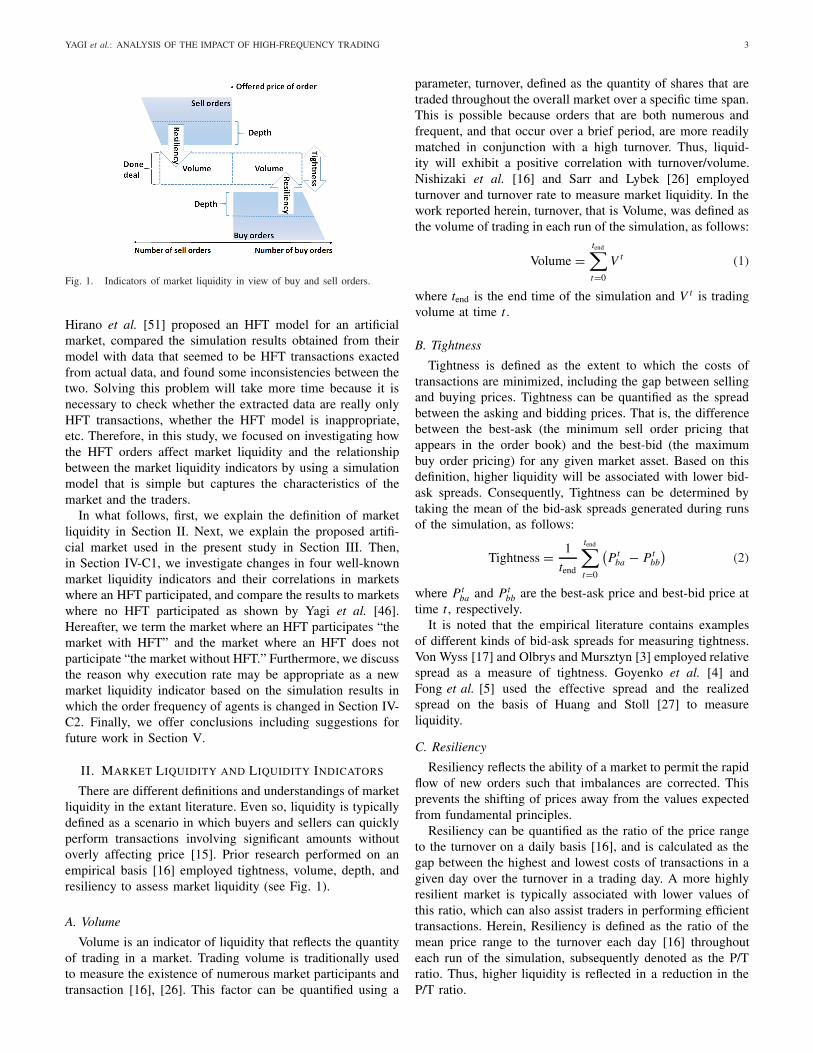
Fig. 1. Indicators of market liquidity in view of buy and sell orders.

Hirano et al. [51] proposed an HFT model for an artificialmarket, compared the simulation results obtained from theirmodel with data that seemed to be HFT transactions exactedfrom actual data, and found some inconsistencies between thetwo. Solving this problem will take more time because it isnecessary to check whether the extracted data are really onlyHFT transactions, whether the HFT model is inappropriate,etc. Therefore, in this study, we focused on investigating howthe HFT orders affect market liquidity and the relationshipbetween the market liquidity indicators by using a simulationmodel that is simple but captures the characteristics of themarket and the traders.

In what follows, first, we explain the definition of marketliquidity in Section II. Next, we explain the proposed artifi-cial market used in the present study in Section III. Then,in Section IV-C1, we investigate changes in four well-knownmarket liquidity indicators and their correlations in marketswhere an HFT participated, and compare the results to marketswhere no HFT participated as shown by Yagi et al. [46].Hereafter, we term the market where an HFT participates “themarket with HFT” and the market where an HFT does notparticipate “the market without HFT.” Furthermore, we discussthe reason why execution rate may be appropriate as a newmarket liquidity indicator based on the simulation results inwhich the order frequency of agents is changed in Section IV-C2. Finally, we offer conclusions including suggestions forfuture work in Section V.

II. MARKET LIQUIDITY AND LIQUIDITY INDICATORS

There are different definitions and understandings of marketliquidity in the extant literature. Even so, liquidity is typicallydefined as a scenario in which buyers and sellers can quicklyperform transactions involving significant amounts withoutoverly affecting price [15]. Prior research performed on anempirical basis [16] employed tightness, volume, depth, andresiliency to assess market liquidity (see Fig. 1).

A. Volume

Volume is an indicator of liquidity that reflects the quantityof trading in a market. Trading volume is traditionally usedto measure the existence of numerous market participants andtransaction [16], [26]. This factor can be quantified using a

parameter, turnover, defined as the quantity of shares that aretraded throughout the overall market over a specific time span.This is possible because orders that are both numerous andfrequent, and that occur over a brief period, are more readilymatched in conjunction with a high turnover. Thus, liquid-ity will exhibit a positive correlation with turnover/volume.Nishizaki et al. [16] and Sarr and Lybek [26] employedturnover and turnover rate to measure market liquidity. In thework reported herein, turnover, that is Volume, was defined asthe volume of trading in each run of the simulation, as follows:

Volume =tend∑

t=0

V t (1)

where tend is the end time of the simulation and V t is tradingvolume at time t .

B. Tightness

Tightness is defined as the extent to which the costs oftransactions are minimized, including the gap between sellingand buying prices. Tightness can be quantified as the spreadbetween the asking and bidding prices. That is, the differencebetween the best-ask (the minimum sell order pricing thatappears in the order book) and the best-bid (the maximumbuy order pricing) for any given market asset. Based on thisdefinition, higher liquidity will be associated with lower bid-ask spreads. Consequently, Tightness can be determined bytaking the mean of the bid-ask spreads generated during runsof the simulation, as follows:

Tightness = 1

tend

tend∑

t=0

(Pt

ba − Ptbb

)(2)

where Ptba and Pt

bb are the best-ask price and best-bid price attime t , respectively.

It is noted that the empirical literature contains examplesof different kinds of bid-ask spreads for measuring tightness.Von Wyss [17] and Olbrys and Mursztyn [3] employed relativespread as a measure of tightness. Goyenko et al. [4] andFong et al. [5] used the effective spread and the realizedspread on the basis of Huang and Stoll [27] to measureliquidity.

C. Resiliency

Resiliency reflects the ability of a market to permit the rapidflow of new orders such that imbalances are corrected. Thisprevents the shifting of prices away from the values expectedfrom fundamental principles.

Resiliency can be quantified as the ratio of the price rangeto the turnover on a daily basis [16], and is calculated as thegap between the highest and lowest costs of transactions in agiven day over the turnover in a trading day. A more highlyresilient market is typically associated with lower values ofthis ratio, which can also assist traders in performing efficienttransactions. Herein, Resiliency is defined as the ratio of themean price range to the turnover each day [16] throughouteach run of the simulation, subsequently denoted as the P/Tratio. Thus, higher liquidity is reflected in a reduction in theP/T ratio.

4 IEEE TRANSACTIONS ON COMPUTATIONAL SOCIAL SYSTEMS

Besides the P/T ratio, there are various versions of measuresfor resiliency in the literature. Olbrys and Mursztyn [3] andGoyenko et al. [4] employed realized spread as a measure ofresiliency. It is noted that defining an indicator to measureresiliency is difficult [18]. Empirical studies have proposedvarious methodologies for Resiliency. For example, some stud-ies employed methodologies based on adopted VAR [19]–[21]and the Kalman filter with the ARMA approach [22]. Olbrysand Mursztyn [6] employed a new methodology for stockmarket resiliency measurement based on the discrete Fouriertransform for high-frequency intraday data. Moreover, theyalso proposed a methodology for stock market resiliencymeasurement based on the short-time Fourier transform forhigh-frequency intraday data [7].

In this article, Resiliency was determined by the P/T ratiofor simplicity. The P/T ratio is calculated as follows:

P/T ratio = 1

tend/tday

tend/tday∑

td=1

Ptd

h − Ptd

l

V d(3)

where tday is number of time steps in one day of the simulationand Ptd

h and Ptd

l are the highest and lowest prices of the td thday, respectively.

D. Depth

The quantity of orders in the highest buy order price rangeand the lowest sell order price range can be used as a definitionof Depth [17], [18], [23], [24]. This parameter is thus relatedto the quantity of orders from potential sellers or buyers thatare either readily uncovered or actually occur and that areeither below or above the current trading price. Based on thisdefinition, a greater Depth will correlate with a higher degreeof liquidity. In previous empirical studies, various proxies wereemployed as depth: for example, order ratio [3], [18], totalnumber of limit orders posted at the bid and ask prices [23],average depth of the buy orders and the sell orders in theorder book [17], [25], and dollar depth calculated in currencyterms [17], [25].

In the work reported herein, data regarding Depth wereobtained from the trading board, based on the total number ofsell orders in the range between the lowest price and 50 ticksabove this price and the total number of sell orders betweenthe highest price and 50 ticks below this price. Here, a tickrepresents the smallest pricing unit (refer to Section III). Thendepth is given by the following equation:

Depth =tend∑

t=0

n∑

i=0

BOrdertbb−i·�P + SOrdert

ba+i·�P

2(4)

where BOrdertbb−i·�P (SOrdert

ba+i·�P ) is the number ofbuy(sell) orders whose price are at the best bid(ask) priceplus(minus) i · �P , i.e., �P is the tick size, of in the orderbook and n is 49.

III. ARTIFICIAL MARKET MODEL

We have built a new artificial market model with an HFTagent on the basis of the artificial market model put forwardby Yagi et al. [46], because their model can reproduce the

statistical characteristics of the kinds of long-term price fluc-tuations observed in empirical analyses. We seek to investigatethe relationship among the four market liquidity indicatorsby changing the parameters. For simplicity, the HFT agent ismodeled on the basis of Kusada et al. [52], which is a marketmaking strategy. The model constructed in the present workhas a single risk asset associated with trading, which is simplyreferred to as an asset, and a non-risk asset is referred to ascash.

The model employs a continuous trading session (that is,a double auction), in which prices are determined based onthe presence of buy or sell order prices within the order bookthat are above or below the agent’s sell or buy target. In suchcases, the order from the agent is instantly assigned to thehighest buy or lowest sell order. This process is designatedas a market order. In the case that the order book does notcontain any orders matching these descriptions, the ordersremain in the book. This scenario is designated as a limit order.These orders will be negated at a specific time, tc, (termed theorder effective period) following placement of the order. Theminimum pricing unit, �P , equals the tick size, and whenorders are sell orders, fractional values smaller than �P arerounded up. By contrast, when orders are buy orders, they arerounded down.

There are two types of agents in our model, namely a normalagent as a general investor and an agent as an HFT. It is notedthat an agent does not correspond to an actual investor, butrepresents a similar trading strategic group. First, we explainthe normal agent model. In the case that the quantity of normalagents is n, each agent j = 1, . . . , n submits an order in turn.Following the order from agent n, agent 1 submits anotherorder. With each order, the time value, t , is increased by 1which represents a stepwise progression even in the case thatthere is no trade, such that the order is transferred to the orderbook. In this mechanism, a single order is placed by eachagent in each step and these agents have essentially infinitecash assets. These agents are also permitted to short sell.

The price of an order by agent j in a given transactionis calculated using the following process. Firstly, the rate atwhich the price anticipated by this agent changes at a giventime, t , (equivalent to the expected return) is designated re

tj

and calculated using the equation

retj =

1

wt1, j +wt

2, j + u j

(wt

1, j ret1, j + wt

2, j ret2, j + u jε

tj

)(5)

where wti, j equals the weight of the i th term associated with

agent j at a given time t , the value of which is determinedbased on a uniform distribution between 0 and wi,max at thesimulation onset and subsequently modified via the learningmechanism discussed below. In addition, u j equals the thirdterm weight and is based on a uniform distribution between 0and umax at the simulation onset but remains unchanged. Thedegree of each trading strategy (that is, technical, fundamental,and noise) is assumed to disperse across all agents, as detailedin the following discussion. Consequently, the trading weightswere modeled as independently selected random variables.

In (5), the first term on the right is used to normalize theeffects of the various trading strategies. The initial term in the

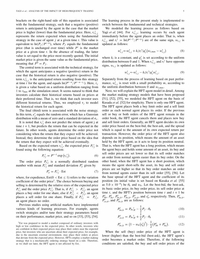
YAGI et al.: ANALYSIS OF THE IMPACT OF HIGH-FREQUENCY TRADING 5

brackets on the right-hand side of this equation is associatedwith the fundamental strategy, such that a negative (positive)return is anticipated by the agent in the case that the marketprice is higher (lower) than the fundamental price. Here, re

t1, j

represents the return expected when using the fundamentalstrategy in the case of agent j at a given time t . This value isequivalent to ln(Pf /Pt−n), where Pf equals the fundamentalprice (that is unchanged over time) while Pt is the marketprice at a given time t . In the absence of trading, the lattervalue is set equal to the price most recently quoted. The initialmarket price is given the same value as the fundamental price,meaning that P0 = Pf .

The central term is associated with the technical strategy, forwhich the agent anticipates a negative (positive) return in thecase that the historical return is also negative (positive). Theterm re

t2, j is the anticipated return resulting from this strategy

at time t for the agent, and equals ln(Pt−n/Pt−n−τ j ). Here, τ j

is given a value based on a uniform distribution ranging from1 to τmax at the simulation onset. It seems natural to think thatinvestors calculate their historical returns based on prices attheir preferred time. That is, we think that each investor usesdifferent historical returns. Thus, we employed τ j to modelthe historical return for each agent.

The final (third) term is associated with the noise strategy.In this term, εt

j equals the random error, which has a Gaussiandistribution with a mean of zero and a standard deviation of σε .

It is noted that retj does not predict the return of agent j at

time t + 1, but predicts the return that can be expected in thefuture. In other words, agents determine the order price notconsidering when the return that they expect will be achieved.Instead, they determine the order price based on the idea thatthe return that they expect will be achieved eventually.

Based on the expected return retj , the expected price Pe

tj is

found using the following equation:Pe

tj = Pt−1 exp

(re

tj

). (6)

The order price Potj is a normally distributed random

number with mean Petj and standard deviation Pt

σ given by

Ptσ = Pe

tj · Est (7)

where, for expedience, Est(0 < Est ≤ 1) refers to the variationcoefficient of the order price1. The choice between buying andselling is determined by the relative sizes of the expected pricePe

tj and the order price Po

tj . That is, if Pe

tj > Po

tj , an agent

places a buy order for one share, else if Petj < Po

tj , an agent

places a sell order for one share. Finally, if Petj = Po

tj ,

an agent places no order.Previous studies using artificial markets have implemented

various kinds of learning processes. For example, agentsswitch strategies and/or tune their strategy parameters basedon their performance, market price, and so on [33], [53], [54].

1Est was prepared to model a market composed of ordinary investors withhigh or low confidence in the expected price. In other words, investors whoare confident in their expected prices may place their orders near the expectedprice, but investors who are uncertain about their expected price, for example,due to the uncertain external environment, may place their orders at pricesthat deviate from the expected price. However, HFTs employ a market makingstrategy that is a mechanically ordering strategy based on a rule. Therefore,as we shall see later, the HFT agent is not affected by Est.

The learning process in the present study is implemented toswitch between the fundamental and technical strategies.

We modeled the learning process as follows based onYagi et al. [44]. For re

ti, j , learning occurs by each agent

immediately before the agent places an order. That is, whenre

ti, j and rl

t = ln(Pt−1/Pt−tl ) are of the same sign, wi, j isupdated as follows:

wti, j←wt

i, j + kl |rlt |qt

j

(wi,max −wt

i, j

)(8)

where kl is a constant, and qtj is set according to the uniform

distribution between 0 and 1. When reti, j and rl

t have oppositesigns, wi, j is updated as follows:

wti, j←wt

i, j − kl |rlt |qt

jwti, j . (9)

Separately from the process of learning based on past perfor-mance, wt

i, j is reset with a small probability m, according tothe uniform distribution between 0 and wi,max.

Next, we will explain the HFT agent model in detail. Amongthe market making strategy models that have been proposed[51], [52], [55], we modeled the HFT agent on the basis ofKusada et al. [52] for simplicity. There is only one HFT agent.The HFT agent places both a buy limit order and a sell limitorder as each normal agent places its order. If the previoussell or buy or both orders of the HFT agent remain in theorder book, the HFT agent cancels them and places new buyand sell limit orders. Generally, an HFT agent decides its ownorder price based on the best-bid, the best-ask, and the spreadwhich is equal to the amount of its own expected return pertransaction. However, the order price of the HFT agent alsodepends on its position, which means the amount of an assetheld by the HFT agent, as it acts to keep its position neutral.That is, when the HFT agent has a long position, which meansthe agent buys and holds some amount of an asset, its buy andsell order prices are set lower so that its sell order matchesan order from normal agents easier than its buy order. On theother hand, when the HFT agent has a short position, whichmeans the agent short-sells the asset, its buy and sell orderprices are set higher so that its buy order matches an orderfrom normal agents easier than its sell order [55], [56]. Letthe base spread of the HFT agent and the coefficient of itsposition (its initial value is set based on Kusaka et al. [55]as 5.0 × 10−8) be θh and wh . Let the best-bid, the best-ask,its basic order price, its buy order price, its sell order price attime t , and the HFT’s position between time t and t + 1 bePt

bb, Ptba , Pt

bv,h , Ptbo,h , Pt

so,h , and sth , respectively. Then, Pt

bo,h ,Pt

so,h , and Ptbv,h are as follows:

Ptbo,h = Pbv

tH −

1

2Pf · θh (10)

Ptso,h = Pbv

tH +

1

2Pf · θh (11)

Ptbv,h =

(1−wh

(st

h

)3) · 1

2

(Pt

bb + Ptba

). (12)

When the sell (buy) order price of the HFT agent islower (higher) than the best-bid (best-ask), the HFT agent’sorder becomes a market order. Therefore, if the followingconditions are satisfied, the buy and sell order prices of the

6 IEEE TRANSACTIONS ON COMPUTATIONAL SOCIAL SYSTEMS

TABLE I

PARAMETERS

TABLE II

PARAMETERS AND SETTINGS

HFT agent are changed [52]. That is, if Ptbo,h ≥ Pt

ba , then

Ptbo,h = Pt

ba −�P (13)

Ptso,h =

(Pt

ba −�P)+ Pf · θh . (14)

If Ptso,h ≤ Pbb

t , then

Ptbo,h =

(Pt

bb +�P) − Pf · θh (15)

Ptso,h = Pt

bb +�P. (16)

IV. SIMULATION RESULTS AND DISCUSSION

A. Overview

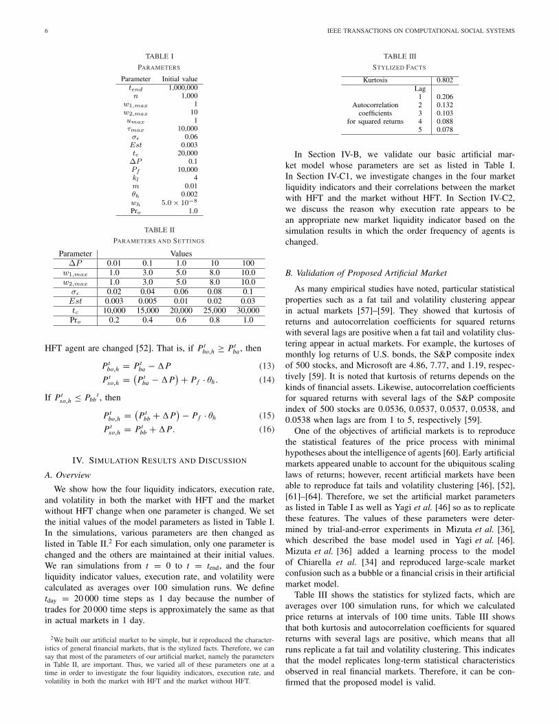
We show how the four liquidity indicators, execution rate,and volatility in both the market with HFT and the marketwithout HFT change when one parameter is changed. We setthe initial values of the model parameters as listed in Table I.In the simulations, various parameters are then changed aslisted in Table II.2 For each simulation, only one parameter ischanged and the others are maintained at their initial values.We ran simulations from t = 0 to t = tend, and the fourliquidity indicator values, execution rate, and volatility werecalculated as averages over 100 simulation runs. We definetday = 20 000 time steps as 1 day because the number oftrades for 20 000 time steps is approximately the same as thatin actual markets in 1 day.

2We built our artificial market to be simple, but it reproduced the character-istics of general financial markets, that is the stylized facts. Therefore, we cansay that most of the parameters of our artificial market, namely the parametersin Table II, are important. Thus, we varied all of these parameters one at atime in order to investigate the four liquidity indicators, execution rate, andvolatility in both the market with HFT and the market without HFT.

TABLE III

STYLIZED FACTS

In Section IV-B, we validate our basic artificial mar-ket model whose parameters are set as listed in Table I.In Section IV-C1, we investigate changes in the four marketliquidity indicators and their correlations between the marketwith HFT and the market without HFT. In Section IV-C2,we discuss the reason why execution rate appears to bean appropriate new market liquidity indicator based on thesimulation results in which the order frequency of agents ischanged.

B. Validation of Proposed Artificial Market

As many empirical studies have noted, particular statisticalproperties such as a fat tail and volatility clustering appearin actual markets [57]–[59]. They showed that kurtosis ofreturns and autocorrelation coefficients for squared returnswith several lags are positive when a fat tail and volatility clus-tering appear in actual markets. For example, the kurtoses ofmonthly log returns of U.S. bonds, the S&P composite indexof 500 stocks, and Microsoft are 4.86, 7.77, and 1.19, respec-tively [59]. It is noted that kurtosis of returns depends on thekinds of financial assets. Likewise, autocorrelation coefficientsfor squared returns with several lags of the S&P compositeindex of 500 stocks are 0.0536, 0.0537, 0.0537, 0.0538, and0.0538 when lags are from 1 to 5, respectively [59].

One of the objectives of artificial markets is to reproducethe statistical features of the price process with minimalhypotheses about the intelligence of agents [60]. Early artificialmarkets appeared unable to account for the ubiquitous scalinglaws of returns; however, recent artificial markets have beenable to reproduce fat tails and volatility clustering [46], [52],[61]–[64]. Therefore, we set the artificial market parametersas listed in Table I as well as Yagi et al. [46] so as to replicatethese features. The values of these parameters were deter-mined by trial-and-error experiments in Mizuta et al. [36],which described the base model used in Yagi et al. [46].Mizuta et al. [36] added a learning process to the modelof Chiarella et al. [34] and reproduced large-scale marketconfusion such as a bubble or a financial crisis in their artificialmarket model.

Table III shows the statistics for stylized facts, which areaverages over 100 simulation runs, for which we calculatedprice returns at intervals of 100 time units. Table III showsthat both kurtosis and autocorrelation coefficients for squaredreturns with several lags are positive, which means that allruns replicate a fat tail and volatility clustering. This indicatesthat the model replicates long-term statistical characteristicsobserved in real financial markets. Therefore, it can be con-firmed that the proposed model is valid.

YAGI et al.: ANALYSIS OF THE IMPACT OF HIGH-FREQUENCY TRADING 7

TABLE IV

LIQUIDITY INDICATORS, EXECUTION RATE, AND VOLATILITY WHEN �P IS CHANGED

TABLE V

LIQUIDITY INDICATORS, EXECUTION RATE, AND VOLATILITY WHEN w1,max IS CHANGED

TABLE VI

LIQUIDITY INDICATORS, EXECUTION RATE, AND VOLATILITY WHEN w2,max IS CHANGED

TABLE VII

LIQUIDITY INDICATORS, EXECUTION RATE, AND VOLATILITY WHEN σε IS CHANGED

C. Results and Discussion

In this section, we investigate the following topics bychanging the parameters as shown in Table II:

1) changes in four market liquidity indicators and theircorrelations in the market with HFT and the marketwithout HFT;

2) difference between the four market liquidity indicatorsand execution rate.

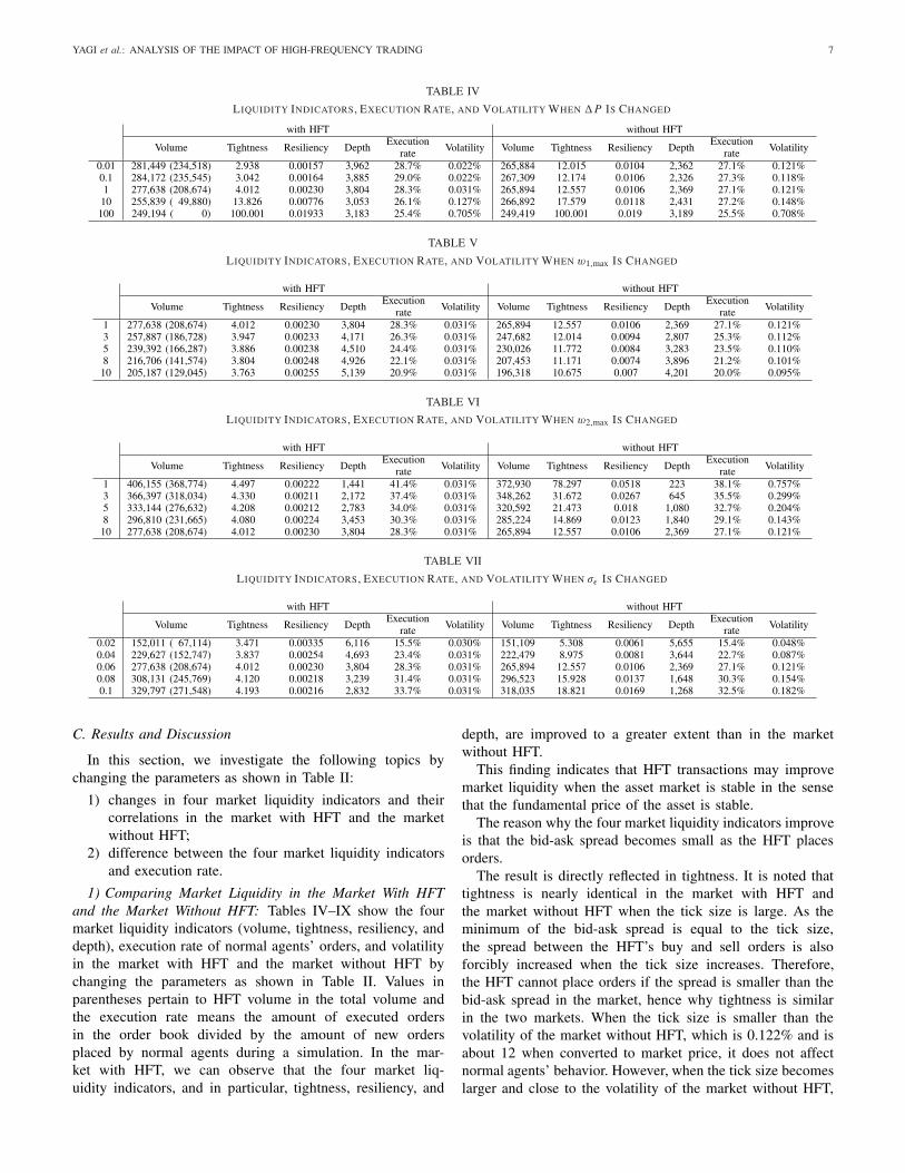
1) Comparing Market Liquidity in the Market With HFTand the Market Without HFT: Tables IV–IX show the fourmarket liquidity indicators (volume, tightness, resiliency, anddepth), execution rate of normal agents’ orders, and volatilityin the market with HFT and the market without HFT bychanging the parameters as shown in Table II. Values inparentheses pertain to HFT volume in the total volume andthe execution rate means the amount of executed ordersin the order book divided by the amount of new ordersplaced by normal agents during a simulation. In the mar-ket with HFT, we can observe that the four market liq-uidity indicators, and in particular, tightness, resiliency, and

depth, are improved to a greater extent than in the marketwithout HFT.

This finding indicates that HFT transactions may improvemarket liquidity when the asset market is stable in the sensethat the fundamental price of the asset is stable.

The reason why the four market liquidity indicators improveis that the bid-ask spread becomes small as the HFT placesorders.

The result is directly reflected in tightness. It is noted thattightness is nearly identical in the market with HFT andthe market without HFT when the tick size is large. As theminimum of the bid-ask spread is equal to the tick size,the spread between the HFT’s buy and sell orders is alsoforcibly increased when the tick size increases. Therefore,the HFT cannot place orders if the spread is smaller than thebid-ask spread in the market, hence why tightness is similarin the two markets. When the tick size is smaller than thevolatility of the market without HFT, which is 0.122% and isabout 12 when converted to market price, it does not affectnormal agents’ behavior. However, when the tick size becomeslarger and close to the volatility of the market without HFT,

8 IEEE TRANSACTIONS ON COMPUTATIONAL SOCIAL SYSTEMS

TABLE VIII

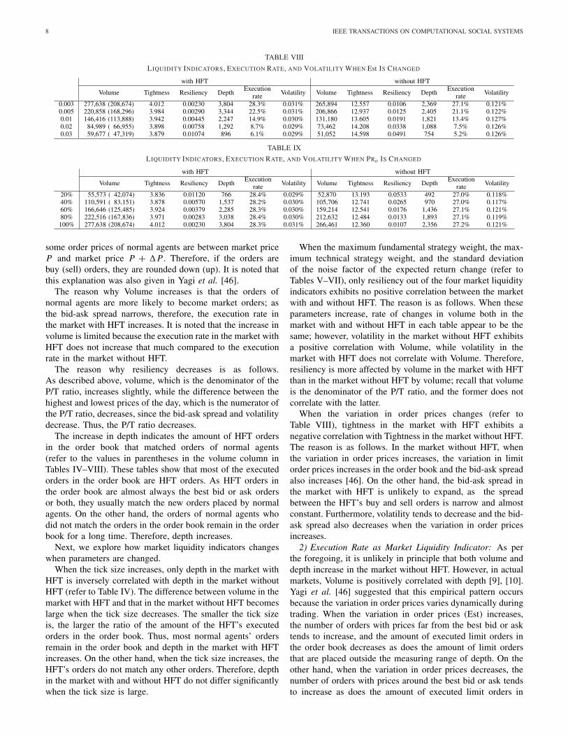
LIQUIDITY INDICATORS, EXECUTION RATE, AND VOLATILITY WHEN Est IS CHANGED

TABLE IX

LIQUIDITY INDICATORS, EXECUTION RATE, AND VOLATILITY WHEN PRo IS CHANGED

some order prices of normal agents are between market priceP and market price P + �P . Therefore, if the orders arebuy (sell) orders, they are rounded down (up). It is noted thatthis explanation was also given in Yagi et al. [46].

The reason why Volume increases is that the orders ofnormal agents are more likely to become market orders; asthe bid-ask spread narrows, therefore, the execution rate inthe market with HFT increases. It is noted that the increase involume is limited because the execution rate in the market withHFT does not increase that much compared to the executionrate in the market without HFT.

The reason why resiliency decreases is as follows.As described above, volume, which is the denominator of theP/T ratio, increases slightly, while the difference between thehighest and lowest prices of the day, which is the numerator ofthe P/T ratio, decreases, since the bid-ask spread and volatilitydecrease. Thus, the P/T ratio decreases.

The increase in depth indicates the amount of HFT ordersin the order book that matched orders of normal agents(refer to the values in parentheses in the volume column inTables IV–VIII). These tables show that most of the executedorders in the order book are HFT orders. As HFT orders inthe order book are almost always the best bid or ask ordersor both, they usually match the new orders placed by normalagents. On the other hand, the orders of normal agents whodid not match the orders in the order book remain in the orderbook for a long time. Therefore, depth increases.

Next, we explore how market liquidity indicators changeswhen parameters are changed.

When the tick size increases, only depth in the market withHFT is inversely correlated with depth in the market withoutHFT (refer to Table IV). The difference between volume in themarket with HFT and that in the market without HFT becomeslarge when the tick size decreases. The smaller the tick sizeis, the larger the ratio of the amount of the HFT’s executedorders in the order book. Thus, most normal agents’ ordersremain in the order book and depth in the market with HFTincreases. On the other hand, when the tick size increases, theHFT’s orders do not match any other orders. Therefore, depthin the market with and without HFT do not differ significantlywhen the tick size is large.

When the maximum fundamental strategy weight, the max-imum technical strategy weight, and the standard deviationof the noise factor of the expected return change (refer toTables V–VII), only resiliency out of the four market liquidityindicators exhibits no positive correlation between the marketwith and without HFT. The reason is as follows. When theseparameters increase, rate of changes in volume both in themarket with and without HFT in each table appear to be thesame; however, volatility in the market without HFT exhibitsa positive correlation with Volume, while volatility in themarket with HFT does not correlate with Volume. Therefore,resiliency is more affected by volume in the market with HFTthan in the market without HFT by volume; recall that volumeis the denominator of the P/T ratio, and the former does notcorrelate with the latter.

When the variation in order prices changes (refer toTable VIII), tightness in the market with HFT exhibits anegative correlation with Tightness in the market without HFT.The reason is as follows. In the market without HFT, whenthe variation in order prices increases, the variation in limitorder prices increases in the order book and the bid-ask spreadalso increases [46]. On the other hand, the bid-ask spread inthe market with HFT is unlikely to expand, as the spreadbetween the HFT’s buy and sell orders is narrow and almostconstant. Furthermore, volatility tends to decrease and the bid-ask spread also decreases when the variation in order pricesincreases.

2) Execution Rate as Market Liquidity Indicator: As perthe foregoing, it is unlikely in principle that both volume anddepth increase in the market without HFT. However, in actualmarkets, Volume is positively correlated with depth [9], [10].Yagi et al. [46] suggested that this empirical pattern occursbecause the variation in order prices varies dynamically duringtrading. When the variation in order prices (Est) increases,the number of orders with prices far from the best bid or asktends to increase, and the amount of executed limit orders inthe order book decreases as does the amount of limit ordersthat are placed outside the measuring range of depth. On theother hand, when the variation in order prices decreases, thenumber of orders with prices around the best bid or ask tendsto increase as does the amount of executed limit orders in

YAGI et al.: ANALYSIS OF THE IMPACT OF HIGH-FREQUENCY TRADING 9

the order book and the amount of limit orders that are placedinside the measuring range of depth (see Table VIII).

However, volume may appear to exhibit a positive cor-relation with depth due to the measuring range of depth.If the range expands, this positive correlation may disappearbecause depth increases even if the variation in order pricesincreases.

One of the reasons why volume may exhibit a positivecorrelation with depth is the variation in the amount of orderssent during a specific period of time. In actual markets, thenumber of market participants and the amount of orders sentby them change depending on the type of risk assets and thetrading time. When the amount of orders changes, the amountof executed orders and the amount of orders that are notexecuted and remain in the order book will also change. Thatis to say, the execution rate in the actual market is consideredto be almost constant.

Then, by changing the order frequency of normal agents,Pro, that is, by changing the amount of orders, we observedhow the four market liquidity indicators changed. It is notedthat each normal agent places an order with probability Pro anddoes not with probability 1 − Pro. The results are shown inTable IX. The findings concur with what has been observed inempirical studies, in that Volume exhibits a positive correlationwith depth.

The results suggest that the actual data may include theeffect of the amount of orders, and if so, it is necessary toevaluate market liquidity by using the data after removing theinfluence of the amount of orders. On the other hand, underthe condition that the amount of orders is constant, changesin artificial market factors such as the characteristics of themarket and the traders affected the execution rate (refer toTables IV–VIII). In other words, market liquidity is roughlydetermined by two factors: the amount of orders and executionrate. If the execution rate is constant and the amount of ordersincreases, volume and depth increase, which agrees with theresults of empirical studies. However, if the amount of ordersis constant and the execution rate increases, volume increasesand depth decreases. In empirical studies, such a result hasnot been clearly measured, but our research could confirmsuch a result by analyzing an internal market mechanism,which makes it possible to clarify how the effects of changingparameters spread inside the market, using an artificial market.Therefore, we suggest that the execution rate may be anappropriate market liquidity indicator.

A lower the execution rate corresponds to a higher liquidity.Investors who place market orders can trade in the marketwith a low execution rate, as orders often remain in the orderbook without being traded despite the large number of ordersso far. Note that a prerequisite is that investors place ordersat a rational price. This is because when the execution ratedrops due to limit orders whose prices deviate far from thefundamental price, it does not have any positive effect on thecurrent transaction (as shown in Table VIII, depth does notincrease although the execution rate decreases). In a futurestudy, we will confirm whether the execution rate can beemployed as a market liquidity indicator with actual marketdata.

Finally, we will explain the mechanism of changes in thefour market liquidity indicators and their correlations betweenthe market with HFT and the market without HFT, when theorder frequency is changed.

When the order frequency decreases, the number of orderswhich normal agents place also decreases per the simulationresults. Then, as both the amount of orders which match ordersin the order book and the amount of orders which do notmatch them and remain in the order book decrease, bothvolume and depth also decrease. As the number of ordersin the order book decreases, the price with no orders in theorder book increases, so once some orders in the order bookare executed, the bid-ask spread tends to expand. Therefore,tightness increases when the order frequency decreases. Thereason why resiliency increases is because volume, which isthe denominator of the P/T ratio, drops sharply, although thevolatility does not change much, so that the difference betweenthe highest and lowest prices of a day, which is the numeratorof the P/T ratio, is relatively stable.

We will compare each indicator in the market with HFT andthe market without HFT. In this comparison, only Tightnessis inversely correlated. When an HFT participates, a narrowspread with almost constant width is always provided by theHFT. However, as the number of new orders increases, theHFT’s orders are matched to them and it is difficult for themto remain in the order book. As a result, the bid-ask spreadwidens and tightness increases.

V. CONCLUSION

We have investigated changes in four well-known mar-ket liquidity indicators and their correlations in a marketwhere an HFT participated and compared the results to thosewhen an HFT did not participate. We found that the HFT’stransactions contributed to improve all four market liquidityindicators when the market was stable. Thus, market liquidityis supplied by the HFT’s transactions. Furthermore, we alsofound that the reason why volume correlates with depth inactual markets is not only that the variation in order prices ofinvestors changes dynamically [46] but also because the orderfrequency of investors changes dynamically. This suggests thatmarket liquidity can be measured not only by the four majormarket liquidity indicators—volume, tightness, resiliency, anddepth—but also by the execution rate.

Future work is as follows. First, we will explore changes inmarket liquidity indicators and the relationships between themin markets where the fundamental price is unstable, as actualmarkets are often unstable. Next, we will confirm whether theresults obtained using an artificial market are valid when actualdata are used. As mentioned in Section I, the validation of thesimulation model and the results obtained from it with actualdata is an enormous task and would be a separate researchproject. Therefore, in this article, we focused on investigatinghow the HFT orders affect market liquidity and the relationshipbetween the market liquidity indicators by using a simulationmodel that is simple but captures the characteristic of themarket and the traders. However, it is necessary to investigateboth the simulation model and the results obtained from itwith actual data.

10 IEEE TRANSACTIONS ON COMPUTATIONAL SOCIAL SYSTEMS

DISCLAIMER

The opinions contained herein are solely those of theauthors and do not necessarily reflect those of SPARX AssetManagement Co., Ltd.

REFERENCES

[1] T. Kurosaki, Y. Kumano, K. Okabe, and T. Nagano, “Liquidity in JGBmarkets: An evaluation from transaction data,” Bank Japan, Tokyo,Japan, Bank Japan Working Paper Series 15-E-2, May 2015. [Online].Available: https://ideas.repec.org/p/boj/bojwps/wp15e02.html

[2] A. S. Kyle, “Continuous auctions and insider trading,” Econometrica,vol. 53, pp. 1315–1336, Nov. 1985.

[3] J. Olbrys and M. Mursztyn, “Depth, tightness and resiliency as marketliquidity dimensions: Evidence from the polish stock market,” Int. J.Comput. Econ. Econometrics, vol. 9, no. 4, pp. 308–326, 2019.

[4] R. Y. Goyenko, C. W. Holden, and C. A. Trzcinka, “Do liquidity mea-sures measure liquidity?” J. Financial Econ., vol. 92, no. 2, pp. 153–181,2009.

[5] K. Y. L. Fong, C. W. Holden, and C. Trzcinka, “What are the bestliquidity proxies for global research?” SSRN Electron. J., vol. 21, no. 4,pp. 1355–1401, 2017.

[6] J. Olbrys and M. Mursztyn, “Measuring stock market resiliency withdiscrete Fourier transform for high frequency data,” Phys. A, Stat. Mech.Appl., vol. 513, pp. 248–256, Jan. 2019.

[7] J. Olbrys and M. Mursztyn, “Estimation of intraday stock marketresiliency: Short-time Fourier transform approach,” Phys. A, Stat. Mech.Appl., vol. 535, Dec. 2019, Art. no. 122413.

[8] Y. Amihud, “Illiquidity and stock returns: Cross-section and time-serieseffects,” J. Financial Markets, vol. 5, no. 1, pp. 31–56, Jan. 2002.

[9] J. Muranaga, “Dynamics of market liquidity of Japanese stocks: Ananalysis of tick-by-tick data of the Tokyo stock exchange,” in MarketLiquidity: Research Findings and Selected Policy Implications, vol. 11.Basel, Switzerland: Bank for International Settlements, 1999, pp. 1–25.[Online]. Available: https://EconPapers.repec.org/RePEc:bis:biscgc:11-13

[10] K. H. Chung, K. A. Kim, and P. Kitsabunnarat, “Liquidityand quote clustering in a market with multiple tick sizes,” J.Financial Res., vol. 28, no. 2, pp. 177–195, 2005. [Online].Available: https://onlinelibrary.wiley.com/doi/abs/10.1111/j.1475-6803.2005.00120.x

[11] L. E. Harris, “Minimum price variations, discrete bid–ask spreads, andquotation sizes,” Rev. Financial Stud., vol. 7, no. 1, pp. 149–178, 1994.

[12] H. Bessembinder, “Trade execution costs and market quality afterdecimalization,” J. Financial Quant. Anal., pp. 747–777, 2003.

[13] H.-J. Ahn, J. Cai, K. Chan, and Y. Hamao, “Tick size change andliquidity provision on the Tokyo stock exchange,” J. Jpn. Int. Economies,vol. 21, no. 2, pp. 173–194, Jun. 2007.

[14] R. Naes and J. A. Skjeltorp, “Order book characteristics and the volume-volatility relation: Empirical evidence from a limit order market,” SSRNElectron. J., pp. 408–432, 2006.

[15] Bank for International Settlements. (1999). Recommendationsfor Design Liquid Markets. [Online]. Available: https://www.bis.org/publ/cgfs13.htm

[16] K. Nishizaki, A. Tsuchikawa, and T. Yagi, “Indicators relatedto liquidity in JGB markets,” Bank Japan, Bank Japan Rev.,Tokyo, Japan, Series 13-E-3, 2013. [Online]. Available: https://EconPapers.repec.org/RePEc:boj:bojrev:13-e-3

[17] R. Von Wyss, “Measuring and predicting liquidity in the stock market,”Ph.D. dissertation, Verlag Nicht Ermittelbar, Univ. St. Gallen, St. Gallen,Switzerland, 2004.

[18] A. Ranaldo, “Intraday market liquidity on the swiss stock exchange,”Financial Markets Portfolio Manage., vol. 15, no. 3, pp. 309–327,Sep. 2001.

[19] M. Coppejans, I. Domowitz, and A. Madhavan, “Resiliency in anautomated auction,” unpublished manuscript, 2004.

[20] D. M. Hmaied, A. Grar, and O. B. Sioud, “Dynamics of market liquidityof tunisian stocks: An analysis of market resiliency,” Electron. Markets,vol. 16, no. 2, pp. 140–153, May 2006.

[21] D. K. Lo and A. D. Hall, “Resiliency of the limit order book,” J. Econ.Dyn. Control, vol. 61, pp. 222–244, Dec. 2015.

[22] J. Dong, A. Kempf, and P. K. Yadav, “Resiliency, the neglected dimen-sion of market liquidity: Empirical evidence from the New York stockexchange,” Tech. Rep., 2007.

[23] H.-J. Ahn, K.-H. Bae, and K. Chan, “Limit orders, depth, and volatility:Evidence from the stock exchange of Hong Kong,” J. Finance, vol. 56,no. 2, pp. 767–788, Apr. 2001.

[24] C. M. C. Lee, B. Mucklow, and M. J. Ready, “Spreads, depths, and theimpact of earnings information: An intraday analysis,” Rev. FinancialStud., vol. 6, no. 2, pp. 345–374, Apr. 1993.

[25] T. Chordia, R. Roll, and A. Subrahmanyam, “Market liquidity andtrading activity,” J. Finance, vol. 56, no. 2, pp. 501–530, Apr. 2001.

[26] A. Sarr and T. Lybek, Measuring Liquidity in Financial Markets, vol. 2.Washington, DC, USA: International Monetary Fund, 2002.

[27] R. D. Huang and H. R. Stoll, “Dealer versus auction markets: A pairedcomparison of execution costs on NASDAQ and the NYSE,” J. FinancialEcon., vol. 41, no. 3, pp. 313–357, Jul. 1996.

[28] A. Securities et al., “Report 215: ‘Australian equity market structure,”’Austral. Secur. Investments Commission, Canberra, ACT, Australia,Tech. Rep. 215, 2010.

[29] G. Hosaka, “Analysis of high-frequency trading at tokyo stockexchange,” Japan Exchange Group, JPX Working Papers, Tokyo, Japan,May 2014, Paper 4. [Online]. Available: https://www.jpx.co.jp/english/corporate/research-study/working-paper/index.html

[30] B. Hagströmer and L. Nordén, “The diversity of high-frequencytraders,” J. Financial Markets, vol. 16, no. 4, pp. 741–770, 2013.[Online]. Available: http://www.sciencedirect.com/science/article/pii/S1386418113000256

[31] K. Kanazawa, T. Sueshige, H. Takayasu, and M. Takayasu, “Derivationof the Boltzmann equation for financial Brownian motion: Direct obser-vation of the collective motion of high-frequency traders,” Phys. Rev.Lett., vol. 120, no. 13, Mar. 2018, Art. no. 138301.

[32] R. G. Palmer, W. B. Arthur, J. H. Holland, B. LeBaron, and P. Tayler,“Artificial economic life: A simple model of a stockmarket,” Phys. D,Nonlinear Phenomena, vol. 75, nos. 1–3, pp. 264–274, Aug. 1994.

[33] W. Arthur, J. Holland, B. Lebaron, R. Palmer, and P. Tayler, “Assetpricing under endogenous expectations in an artificial stock market,” inThe Economy as an Evolving Complex System II. Reading, MA, USA:Addison-Wesley, 1997, pp. 15–44.

[34] C. Chiarella, G. Iori, and J. Perelló, “The impact of heterogeneoustrading rules on the limit order book and order flows,” J. Econ. Dyn.Control, vol. 33, no. 3, pp. 525–537, Mar. 2009.

[35] S.-H. Chen, C.-L. Chang, and Y.-R. Du, “Agent-based economic modelsand econometrics,” Knowl. Eng. Rev., vol. 27, no. 2, pp. 187–219,Apr. 2012.

[36] T. Mizuta, K. Izumi, I. Yagi, and S. Yoshimura, “Regulations’ effective-ness for market turbulence by large erroneous orders using multi agentsimulation,” in Proc. IEEE Conf. Comput. Intell. Financial Eng. Econ.(CIFEr), Mar. 2014, pp. 138–143.

[37] P. Ye, S. Wang, and F.-Y. Wang, “A general cognitive architecture foragent-based modeling in artificial societies,” IEEE Trans. Comput. SocialSyst., vol. 5, no. 1, pp. 176–185, Mar. 2018.

[38] A. Trivedi and S. Rao, “Agent-based modeling of emergency evacuationsconsidering human panic behavior,” IEEE Trans. Comput. Social Syst.,vol. 5, no. 1, pp. 277–288, Mar. 2018.

[39] R. L. Rizzi, W. L. Kaizer, C. B. Rizzi, G. Galante, and F. C. Coelho,“Modeling direct transmission diseases using parallel bitstring agent-based models,” IEEE Trans. Comput. Social Syst., vol. 5, no. 4,pp. 1109–1120, Dec. 2018.

[40] N. Sardana, R. Cohen, J. Zhang, and S. Chen, “A Bayesian multiagenttrust model for social networks,” IEEE Trans. Comput. Social Syst.,vol. 5, no. 4, pp. 995–1008, Dec. 2018.

[41] I. Yagi, T. Mizuta, and K. Izumi, “A study on the effectiveness ofshort-selling regulation in view of regulation period using artificialmarkets,” Evol. Institutional Econ. Rev., vol. 7, no. 1, pp. 113–132,2010.

[42] T. Mizuta, K. Izumi, I. Yagi, and S. Yoshimura, “Design of financialmarket regulations against large price fluctuations using by artificialmarket simulations,” J. Math. Finance, vol. 3, no. 2, pp. 15–22,2013.

[43] A. Nozaki, T. Mizuta, and I. Yagi, “A study on the market impact of therule for investment diversification at the time of a market crash usinga multi-agent simulation,” IEICE Trans. Inf. Syst., vol. E100.D, no. 12,pp. 2878–2887, 2017.

[44] I. Yagi, A. Nozaki, and T. Mizuta, “Investigation of the rulefor investment diversification at the time of a market crashusing an artificial market simulation,” Evol. Institutional Econ.Rev., vol. 14, no. 2, pp. 451–465, Dec. 2017. [Online]. Available:https://link.springer.com/article/10.1007%2Fs40844-017-0070-9

YAGI et al.: ANALYSIS OF THE IMPACT OF HIGH-FREQUENCY TRADING 11

[45] L. Ponta, E. Scalas, M. Raberto, and S. Cincotti, “Statistical analysisand agent-based microstructure modeling of high-frequency financialtrading,” IEEE J. Sel. Topics Signal Process., vol. 6, no. 4, pp. 381–387,Aug. 2012.

[46] I. Yagi, Y. Masuda, and T. Mizuta, “Detection of factors influencingmarket liquidity using an agent-based simulation,” in Network Theoryand Agent-Based Modeling in Economics and Finance. Singapore:Springer, 2019, pp. 111–131.

[47] G. Iori, “A microsimulation of traders activity in the stock market: Therole of heterogeneity, agents’ interactions and trade frictions,” J. Econ.Behav. Org., vol. 49, no. 2, pp. 269–285, 2002.

[48] C. Chiarella and X.-Z. He, “Heterogeneous beliefs, risk, and learningin a simple asset-pricing model with a market maker,” MacroeconomicDyn., vol. 7, no. 4, pp. 503–536, 2003.

[49] S. Ganesh, N. Vadori, M. Xu, H. Zheng, P. Reddy, andM. Veloso, “Reinforcement learning for market making in a multi-agent dealer market,” 2019, arXiv:1911.05892. [Online]. Available:http://arxiv.org/abs/1911.05892

[50] B. LeBaron, “Agent-based computational finance,” Handbook Comput.Econ., vol. 2, pp. 1187–1233, 2006.

[51] M. Hirano, K. Izumi, H. Matsushima, and H. Sakaji, “Comparingactual and simulated HFT traders’ behavior for agent design,” J. Artif.Societies Social Simul., vol. 23, no. 3, 2020. [Online]. Available:http://jasss.soc.surrey.ac.uk/23/3/6.html

[52] Y. Kusada, T. Mizuta, S. Hayakawa, and K. Izumi, “Impact of position-based market makers to shares of markets volumes—An artificial marketapproach,” (in Japanese), Trans. Jpn. Soc. Artif. Intell., vol. 30, no. 5,pp. 675–682, 2015.

[53] T. Lux and M. Marchesi, “Scaling and criticality in a stochasticmulti-agent model of a financial market,” Nature, vol. 397, no. 6719,pp. 498–500, 1999.

[54] T. Nakada and K. Takadama, “Analysis on the number of XCS agents inagent-based computational finance,” in Proc. IEEE Conf. Comput. Intell.Financial Eng. Econ. (CIFEr), Apr. 2013, pp. 8–13.

[55] Y. Kusada, T. Mizuta, S. Hayakawa, and K. Izumi, “Impacts of position-based market makers on markets’ shares of trading volumes—An artifi-cial market approach,” in Proc. Social Modeling Simulations Econophys.Colloq, 2014, pp. 1–2.

[56] Y. Nakajima and Y. Shiozawa, “Usefulness and feasibility of marketmaker in a thin market,” in Proc. Int. Conf. Exp. Econ. Sci. NewApproaches Solving Real-World Problems, Dec. 2004, pp. 1000–1003.[Online]. Available: https://www.cc.kyoto-su.ac.jp/project/orc/execo/EES2004/proceedings.html

[57] M. Sewell. (2006). Characterization of Financial Time Series. [Online].Available: http://financ.emartinsewell.com/stylized-facts/

[58] R. Cont, “Empirical properties of asset returns: Stylized facts andstatistical issues,” Quant. Finance, vol. 1, no. 2, pp. 223–236, Feb. 2001.

[59] R. Tsay, Analysis of Financial Time Series (Wiley Series in Probabilityand Statistics), 2nd ed. Hoboken, NJ, USA: Wiley, 2005.

[60] H. Levy, M. Levy, and S. Solomon, Microscopic Simulation of FinancialMarkets: From Investor Behavior to Market Phenomena. Amsterdam,The Netherlands: Elsevier, 2000.

[61] M. Raberto, S. Cincotti, S. M. Focardi, and M. Marchesi, “Agent-basedsimulation of a financial market,” Phys. A, Stat. Mech. Appl., vol. 299,nos. 1–2, pp. 319–327, Oct. 2001.

[62] B. LeBaron, “Agent-based computational finance: Suggested read-ings and early research,” J. Econ. Dyn. Control, vol. 24, nos. 5–7,pp. 679–702, Jun. 2000.

[63] C. Chiarella and G. Iori, “A simulation analysis of the microstructureof double auction markets,” Quant. Finance, vol. 2, no. 5, pp. 346–353,Oct. 2002.

[64] C. H. Hommes, “Heterogeneous agent models in economics andfinance,” in Handbook of Computational Economics, vol. 2. Amsterdam,The Netherlands: North Holland, 2006, pp. 1109–1186.

Isao Yagi (Member, IEEE) received the Ph.D.degree in information science from the Nara Instituteof Science and Technology, Nara, Japan, in 2006.

He was a Research Assistant Professor withthe Nara Institute of Science and Technologyfrom 2006 to 2009. He was a Post-Doctoral Fel-low with the Tokyo Institute of Technology, Tokyo,Japan, from 2009 to 2011. He was an Associate Pro-fessor with the Kanagawa Institute of Technology,Kanagawa, Japan, from 2011 to 2020, where he iscurrently a Professor. His current research interests

include agent-based modeling and social simulation.

Yuji Masuda received the B.E. and M.E. degrees from the Kanagawa Instituteof Technology, Kanagawa, Japan, in 2018 and 2020, respectively.

He is with Yamato System Development Company Ltd. His research hasfocused on multiagent simulation, and artificial stock market simulation.

Takanobu Mizuta received the B.E. degree from theMeteorological College, Kashiwa, Japan, in 2000,the M.E. degree from the Graduate School of Sci-ence, University of Tokyo, Tokyo, Japan, in 2002,and the Ph.D. degree from the School of Engineer-ing, University of Tokyo, in 2014.

Since 2004, he has been with SPARX Asset Man-agement Company Ltd., where he is currently aFund Manager and a Senior Researcher. Since 2014,he has been a Part-Time Lecturer with the GraduateSchool of Public Policy, University of Tokyo.