Analysis of Genomic and Proteomic Signals Using Signal ...

Analysis of Genomic and Proteomic

Signals Using Signal Processing and

Soft Computing Techniques

Sitanshu Sekhar Sahu

Department of Electronics and Communication Engineering

National Institute of Technology Rourkela

Rourkela – 769 008, India

Analysis of Genomic and Proteomic

Signals Using Signal Processing and

Soft Computing Techniques

Dissertation submitted in partial fulfillment of the requirements for the degree of

Doctor of Philosophy

in

Electronics and Communication Engineering

by

Sitanshu Sekhar Sahu(Roll - 50709001)

under the guidance of

Prof. Ganapati Panda

Department of Electronics and Communication Engineering


Rourkela, Orissa, 769008, India

September 2011

dedicated to my parents with love...

Dept. of Electronics and Communication Engineering

National Institute of Technology, Rourkela

Rourkela-769 008, Orissa, India.

Dr. Ganapati Panda FNAE, FNASc.Professor

September 17, 2011

Certificate

This is to certify that the dissertation entitled “Analysis of Genomic and

Proteomic Signals Using Signal Processing and Soft Computing

Techniques” by Sitanshu Sekhar Sahu, submitted to the National Institute

of Technology, Rourkela for the degree of Doctor of Philosophy, is a record of an

original research work carried out by him in the department of Electronics and

Communication Engineering under my supervision. I believe that the thesis fulfills

part of the requirements for the award of degree of Doctor of Philosophy. Neither

this dissertation nor any part of it has been submitted for any degree or academic

award elsewhere.

Ganapati Panda

Acknowledgement

First of all, I would like to express my reverence to my supervisor Prof. Ganapati

Panda for his guidance, inspiration and innovative technical discussions during the

course of this work. He is not only a great teacher with deep vision but also a very

kind person. His trust and support inspired me for taking right decisions during

tough times in my dissertation work and I consider it a blessing to be associated

with him.

I am thankful to Prof. S. K. Patra, Prof. K. K. Mahapatra, Prof. S. Meher,

Prof. D.P. Acharya, Prof. S. K. Behera of Electronics and Communication Engg.

department and Prof. S.R Samantaray of Electrical Engg. department for extending

their valuable suggestions and help whenever I approached.

Especially, I owe many thanks to Dr. Lalu Mansinha and Dr. Kristy F.

Tiampo of the University of Western Ontario, London, Canada for their moral

boost to complete my dissertation work. I would like to gratefully acknowledge all

their support and guidance during my stay at Ontario. I am also grateful to the

University of Western Ontario for granting me the required access to the resources

available at the department of Earth Sciences.

It is my great pleasure to show indebtedness to my friends like Sudhansu,

Trilochan, Upendra, Pyari, Nithin, Vikas, Rama and Maitrayee for their help during

the course of this work.

Special thanks to Prof. Ajit Sahoo, Mamata Panigrahy, Satyasai Nanda and

my graduate colleague Amitav Panda for infallible motivation and moral support,

whose involvement gave a new breath to my research.

iv

I am also grateful to NIT Rourkela for providing me adequate infrastructure

to carry out the present investigations.

I take this opportunity to express my regards and obligation to my parents

whose support and encouragement I can never forget in my life.

I am indebted to many people who contributed through their support, knowledge

and friendship, to this work and made my stay in Rourkela an unforgettable and

rewarding experience.


v

Abstract

Bioinformatics is a data rich field which provides unique opportunities to use

computational techniques to understand and organize information associated with

biomolecules such as DNA, RNA, and Proteins. It involves in-depth study in the

areas of genomics and proteomics and requires techniques from computer science,

statistics and engineering to identify, model, extract features and to process data

for analysis and interpretation of results in a biologically meaningful manner.

In engineering methods the signal processing techniques such as transformation,

filtering, pattern analysis and soft-computing techniques like multi layer perceptron

(MLP) and radial basis function neural network (RBFNN) play vital role to

effectively resolve many challenging issues associated with genomics and proteomics.

In this dissertation, a sincere attempt has been made to investigate on some

challenging problems of bioinformatics by employing some efficient signal and soft

computing methods. Some of the specific issues, which have been attempted are

protein coding region identification in DNA sequence, hot spot identification in

protein, prediction of protein structural class and classification of microarray gene

expression data. The dissertation presents some novel methods to measure and

to extract features from the genomic sequences using time-frequency analysis and

machine intelligence techniques.

The problems investigated and the contribution made in the thesis are presented

here in a concise manner. The S-transform, a powerful time-frequency representation

technique, possesses superior property over the wavelet transform and short time

Fourier transform as the exponential function is fixed with respect to time axis while

the localizing scalable Gaussian window dilates and translates. The S-transform

uses an analysis window whose width is decreasing with frequency providing a

frequency dependent resolution. The invertible property of S-transform makes it

suitable for time-band filtering application. Gene prediction and protein coding

region identification have been always a challenging task in computational biology,

especially in eukaryote genomes due to its complex structure. This issue is resolved

using a S-transform based time-band filtering approach by localizing the period-3

property present in the DNA sequence which forms the basis for the identification.

Similarly, hot spot identification in protein is a burning issue in protein science due

to its importance in binding and interaction between proteins. A novel S-transform

based time-frequency filtering approach is proposed for efficient identification of the

hot spots. Prediction of structural class of protein has been a challenging problem

in bioinformatics. A novel feature representation scheme is proposed to efficiently

represent the protein, thereby improves the prediction accuracy. The high dimension

and low sample size of microarray data lead to curse of dimensionality problem which

affects the classification performance. In this dissertation an efficient hybrid feature

extraction method is proposed to overcome the dimensionality issue and a RBFNN

is introduced to efficiently classify the microarray samples.

In essence, this dissertation employs some latest signal and soft-computing tools

for obtaining the patterns present in the DNA and protein sequences as well as to

develop efficient feature extraction method for achieving better classification.

Keywords: Gene, Exon, Protein, Hot spot, Microarray, Time-frequency

analysis, S-transform, DCT, AmPseAAC, AR Modeling, F-score

vii

Contents

Certificate iii

Acknowledgement iv

Abstract vi

List of Figures xii

List of Tables xv

List of Acronyms xvii

1 Introduction 2

1.1 Background and scope of the thesis . . . . . . . . . . . . . . . . . . . 3

1.2 Motivation . . . . . . . . . . . . . . . . . . . . . . . . . . . . . . . . . 5

1.3 Objective of the dissertation . . . . . . . . . . . . . . . . . . . . . . . 6

1.4 Dissertation Outline . . . . . . . . . . . . . . . . . . . . . . . . . . . 7

1.5 Conclusion . . . . . . . . . . . . . . . . . . . . . . . . . . . . . . . . . 9

2 Signal Processing and Soft- Computing Techniques Employedin the Investigation 12

2.1 Introduction . . . . . . . . . . . . . . . . . . . . . . . . . . . . . . . . 12

2.2 Signal processing techniques used in the analysis . . . . . . . . . . . . 12

2.2.1 Discrete Fourier transform . . . . . . . . . . . . . . . . . . . . 13

2.2.2 Discrete cosine transform . . . . . . . . . . . . . . . . . . . . . 14

2.2.3 Time-frequency analysis . . . . . . . . . . . . . . . . . . . . . 15

2.3 Soft computing techniques used in the analysis . . . . . . . . . . . . . 20

2.3.1 Artificial neural network . . . . . . . . . . . . . . . . . . . . . 22

viii

2.3.2 Radial basis function network . . . . . . . . . . . . . . . . . . 28

2.4 Sensitivity and Specificity . . . . . . . . . . . . . . . . . . . . . . . . 31

2.5 Conclusion . . . . . . . . . . . . . . . . . . . . . . . . . . . . . . . . . 33

3 Identification of Protein Coding Regions using Time-frequencyFiltering Approach 35

3.1 Introduction . . . . . . . . . . . . . . . . . . . . . . . . . . . . . . . . 35

3.1.1 Genes and Proteins . . . . . . . . . . . . . . . . . . . . . . . . 36

3.1.2 Fundamentals of 3-base periodicity in protein coding regions . 37

3.1.3 Review of the Gene prediction methods . . . . . . . . . . . . . 39

3.2 Numerical mapping of DNA sequences . . . . . . . . . . . . . . . . . 40

3.3 Spectral content measure method . . . . . . . . . . . . . . . . . . . . 41

3.4 Digital filter method . . . . . . . . . . . . . . . . . . . . . . . . . . . 43

3.5 Statistical method of coding region identification . . . . . . . . . . . . 45

3.6 The proposed time-frequency analysis method . . . . . . . . . . . . . 47

3.6.1 Identification of protein coding regions in DNA using

S-transform based filtering approach . . . . . . . . . . . . . . 52

3.7 Results and Performance evaluation . . . . . . . . . . . . . . . . . . . 54

3.7.1 Data resorces . . . . . . . . . . . . . . . . . . . . . . . . . . . 54

3.7.2 Experimetal result . . . . . . . . . . . . . . . . . . . . . . . . 55

3.7.3 Discussion . . . . . . . . . . . . . . . . . . . . . . . . . . . . . 60

3.8 Conclusion . . . . . . . . . . . . . . . . . . . . . . . . . . . . . . . . . 62

4 Localization of Hot Spots in Proteins using a Novel S-transformbased Filtering Approach 64

4.1 Introduction . . . . . . . . . . . . . . . . . . . . . . . . . . . . . . . . 64

4.2 Review of hot spot identification methods . . . . . . . . . . . . . . . 67

4.3 Resonant recognition model . . . . . . . . . . . . . . . . . . . . . . . 68

4.4 Time-frequency analysis . . . . . . . . . . . . . . . . . . . . . . . . . 72

4.5 Hot spot localization in proteins using the proposed S-transform

filtering approach . . . . . . . . . . . . . . . . . . . . . . . . . . . . . 73

ix

4.6 Performance analysis of the proposed approach . . . . . . . . . . . . 77

4.6.1 Evaluation criteria . . . . . . . . . . . . . . . . . . . . . . . . 77

4.6.2 Experimental study . . . . . . . . . . . . . . . . . . . . . . . . 78

4.7 Discussion of results . . . . . . . . . . . . . . . . . . . . . . . . . . . 85

4.8 Conclusion . . . . . . . . . . . . . . . . . . . . . . . . . . . . . . . . . 87

5 A Novel Feature Representation based Classification of ProteinStructural Class 89

5.1 Introduction . . . . . . . . . . . . . . . . . . . . . . . . . . . . . . . . 89

5.1.1 Review of protein structural class prediction . . . . . . . . . . 91

5.2 Feature representation method of protein . . . . . . . . . . . . . . . . 92

5.2.1 Amino acid composition (AAC) feature of protein . . . . . . . 92

5.2.2 Amphiphilic Pseudo amino acid composition (AmPseAAC)

feature of protein . . . . . . . . . . . . . . . . . . . . . . . . . 93

5.2.3 Spectrum based feature of protein . . . . . . . . . . . . . . . . 94

5.3 The proposed DCT amphiphilic pseudo amino acid composition

feature representation scheme of protein . . . . . . . . . . . . . . . . 96

5.4 Classification strategy . . . . . . . . . . . . . . . . . . . . . . . . . . 98

5.5 Performance measures . . . . . . . . . . . . . . . . . . . . . . . . . . 98

5.6 Results and Discussion . . . . . . . . . . . . . . . . . . . . . . . . . . 100

5.6.1 Datasets . . . . . . . . . . . . . . . . . . . . . . . . . . . . . . 100

5.6.2 Experimental Results . . . . . . . . . . . . . . . . . . . . . . . 100

5.7 Conclusion . . . . . . . . . . . . . . . . . . . . . . . . . . . . . . . . . 104

6 An Efficient Hybrid Feature Extraction Method for Classificationof Microarray Gene Expression Data 109

6.1 Introduction . . . . . . . . . . . . . . . . . . . . . . . . . . . . . . . . 109

6.2 Microarray Technology . . . . . . . . . . . . . . . . . . . . . . . . . . 110

6.2.1 Gene expression data . . . . . . . . . . . . . . . . . . . . . . . 113

6.3 Dimension reduction techniques . . . . . . . . . . . . . . . . . . . . . 113

6.3.1 The F-score method of feature selection . . . . . . . . . . . . . 116

x

6.3.2 The AR modeling for feature extraction . . . . . . . . . . . . 117

6.4 Classification strategy . . . . . . . . . . . . . . . . . . . . . . . . . . 119

6.5 Performance evaluation . . . . . . . . . . . . . . . . . . . . . . . . . . 119

6.5.1 Datasets . . . . . . . . . . . . . . . . . . . . . . . . . . . . . . 120

6.5.2 Experimental results . . . . . . . . . . . . . . . . . . . . . . . 122

6.6 Conclusion . . . . . . . . . . . . . . . . . . . . . . . . . . . . . . . . . 125

7 Conclusion and Future work 128

7.1 Conclusion . . . . . . . . . . . . . . . . . . . . . . . . . . . . . . . . . 128

7.2 Future work . . . . . . . . . . . . . . . . . . . . . . . . . . . . . . . . 131

Annexure-I 132

Annexure-II 133

Bibliography 135

Dissemination of Work 151

xi

List of Figures

2.1 The DFT of a periodic signal . . . . . . . . . . . . . . . . . . . . . . 14

2.2 Comparison of the power spectra obtained by STFT, WT and

S-transform of a synthetic time series . . . . . . . . . . . . . . . . . . 19

2.3 The structure of a single neuron . . . . . . . . . . . . . . . . . . . . . 24

2.4 The structure of MLP network . . . . . . . . . . . . . . . . . . . . . . 25

2.5 The architecture of radial basis function network . . . . . . . . . . . . 29

2.6 The process to evaluate sensitivity and specificity . . . . . . . . . . . 32

3.1 The relationship between the DNA sequence, gene, intergenic spaces,

exons, introns and codons . . . . . . . . . . . . . . . . . . . . . . . . 37

3.2 The central dogma of molecular biology (flow of genetic information

from DNA to RNA to Protein) . . . . . . . . . . . . . . . . . . . . . 38

3.3 DFT power spectrum of coding region of gene F56F11.4 . . . . . . . 42

3.4 DFT power spectrum of non-coding region of gene F56F11.4 . . . . . 43

3.5 The anti-notch filter response . . . . . . . . . . . . . . . . . . . . . . 45

3.6 A simple hidden Markov model. . . . . . . . . . . . . . . . . . . . . . 46

3.7 The synthetic time series and its amplitude spectra . . . . . . . . . . 49

3.8 The synthetic time series and its S-transform spectrum . . . . . . . . 50

3.9 The time-band limited filter . . . . . . . . . . . . . . . . . . . . . . . 51

3.10 The recovered signal and its S-transform spectrum . . . . . . . . . . . 51

3.11 Spectrogram of the DNA sequence of gene F56F11.4 . . . . . . . . . . 53

3.12 The flow graph of the S-transform based filtering approach for protein

coding region identification . . . . . . . . . . . . . . . . . . . . . . . . 54

xii

3.13 Comparison of the power spectra of gene F56F11.4 obtained by DFT,

anti-notch filter and S-transform filter . . . . . . . . . . . . . . . . . . 58

3.14 Average accuracy of identification versus threshold of the gene F56F11.4 59

3.15 ROC curves obtained by DFT, anti-notch filter and S-transform filter

of the gene F56F11.4 . . . . . . . . . . . . . . . . . . . . . . . . . . . 59

3.16 Comparison of the power spectra obtained by DFT, anti-notch filter

and S-transform filter for gene AF0099614 . . . . . . . . . . . . . . . 61

3.17 ROC curves obtained by the DFT, anti-notch filter and S-transform

filter (From 50 sequences of HRM195 dataset) . . . . . . . . . . . . . 62

4.1 A schematic view of the hot spots in the complex of human growth

hormone and its receptor . . . . . . . . . . . . . . . . . . . . . . . . . 65

4.2 The numerical sequence and corresponding DFTs of the basic bovine

(left) and acidic bovine (right) . . . . . . . . . . . . . . . . . . . . . . 71

4.3 The consensus spectrum of the FGF family . . . . . . . . . . . . . . . 71

4.4 The contour plot of the spectrum of basic bovine FGF protein using

S-transform . . . . . . . . . . . . . . . . . . . . . . . . . . . . . . . . 74

4.5 The surface plot of S-transform spectrum of the basic bovine FGF

after multiplication with the consensus spectrum . . . . . . . . . . . . 75

4.6 The flow chart of S-transform based filtering approach for hot spot

identification . . . . . . . . . . . . . . . . . . . . . . . . . . . . . . . 76

4.7 Hot spot locations of Human basic bovine FGF protein . . . . . . . . 80

4.8 ROC curve comparison of the proposed method and Digital filtering

method . . . . . . . . . . . . . . . . . . . . . . . . . . . . . . . . . . 82

4.9 The 3D structure of barnase-barstar complex (PDB ID:1brs) showing

the hot spots . . . . . . . . . . . . . . . . . . . . . . . . . . . . . . . 86

5.1 The four structural classes of protein . . . . . . . . . . . . . . . . . . 90

5.2 The flow graph of the proposed feature based classification approach . 99

6.1 The Microarray Techonoly. . . . . . . . . . . . . . . . . . . . . . . . . 112

xiii

6.2 The gene expression matrix . . . . . . . . . . . . . . . . . . . . . . . 114

6.3 The Flow graph of the proposed feature based classification scheme . 120

6.4 The F-score values versus genes of Leukemia dataset. . . . . . . . . . 124

6.5 The LOOCV accuracy for the binary class datasets (Leukemia, Colon

and Prostate). . . . . . . . . . . . . . . . . . . . . . . . . . . . . . . . 125

6.6 The LOOCV accuracy for the multi class datasets (MLL-Leukemia,

Lymphoma and SRBCT). . . . . . . . . . . . . . . . . . . . . . . . . 126

7.1 The EIIP coded sequence (1000 bases) of the gene F56F11.4 . . . . . 132

7.2 Comparison of Jackknife accuracies of all classes of different

classification algorithms using the proposed DCTAmPseAAC feature

representation method . . . . . . . . . . . . . . . . . . . . . . . . . . 133

7.3 Comparison of overall Jackknife accuracies of different classification

algorithms using the proposed DCTAmPseAAC feature

representation method . . . . . . . . . . . . . . . . . . . . . . . . . . 134

7.4 Comparison of overall Jackknife classification accuracy with the three

feature representations using RBFNN and MLP . . . . . . . . . . . . 134

xiv

List of Tables

3.1 The EIIP Values of the 4 nucleotides . . . . . . . . . . . . . . . . . . 41

3.2 Position comparison study of the exons of F56F11.4 by the DFT,

anti-notch, S-transform filter and HMM methods.The length of the

exons are shown in the braces. . . . . . . . . . . . . . . . . . . . . . . 57

3.3 Summary of the best performance (accuracy) of identification of

coding regions in F56F11.4 using the DFT, anti-notch,S-transform

filter and HMM methods. . . . . . . . . . . . . . . . . . . . . . . . . 57

4.1 EIIP values of the 20 amino acids . . . . . . . . . . . . . . . . . . . . 69

4.2 The protein sequences investigated . . . . . . . . . . . . . . . . . . . 78

4.3 Proteins of functional family used for computation of consensus

spectrum . . . . . . . . . . . . . . . . . . . . . . . . . . . . . . . . . . 79

4.4 Comparison study of hot spots identification in proteins by the

proposed method and digital filtering approach . . . . . . . . . . . . 81

4.5 Performance evaluation of S-transform and digital filtering approaches

for hot spot identification . . . . . . . . . . . . . . . . . . . . . . . . 82

4.6 The newly identified hot spots by the proposed S-transform filtering

method . . . . . . . . . . . . . . . . . . . . . . . . . . . . . . . . . . 83

4.7 Comparison study of hot spots identification in proteins by different

computational methods . . . . . . . . . . . . . . . . . . . . . . . . . . 84

4.8 Comparison of performance (in percentage) of different computational

methods . . . . . . . . . . . . . . . . . . . . . . . . . . . . . . . . . . 84

xv

5.1 The Hydrophobicity and Hydrophilicity values of the amino acids . . 95

5.2 Benchmark datasets used for structural class prediction . . . . . . . . 100

5.3 Comparison of Jackknife classification accuracy (in percentage)

of different classification algorithms using new (DCTAmPseAAC)

feature representation method . . . . . . . . . . . . . . . . . . . . . . 101

5.4 Comparison of Jackknife classification accuracy (in percentage) using

different feature representation methods . . . . . . . . . . . . . . . . 102

5.5 Classification accuracy (in percentage) of the proposed

(AmPseAAC+RBF) method for self-consistency and jackknife

tests . . . . . . . . . . . . . . . . . . . . . . . . . . . . . . . . . . . . 103

5.6 Comparison of Jackknife accuracy (in percentage) of the best classifier

that used the proposed feature and the other reported methods (for

204 Dataset) . . . . . . . . . . . . . . . . . . . . . . . . . . . . . . . . 105



277 Dataset) . . . . . . . . . . . . . . . . . . . . . . . . . . . . . . . . 106



498 Dataset) . . . . . . . . . . . . . . . . . . . . . . . . . . . . . . . . 107

6.1 The standard datasets used for the study . . . . . . . . . . . . . . . . 122

6.2 Comparison of LOOCV classification accuracy using the proposed

feature representation method using RBFNN, MLP and LDA. . . . . 123

6.3 Comparison of predictive accuracy (%) of the proposed method with

the best available method in literature . . . . . . . . . . . . . . . . . 126

xvi

List of Acronyms

DNA Deoxy Ribo Nucleic Acid

RNA Ribo Nucleic Acid

FT Fourier Transform

DFT Discrete Fourier Transform

IDFT Inverse Discrete Fourier Transform

FFT Fast Fourier Transform

DCT Discrete Cosine Transform

STFT Short Time Fourier Transform

WT Wavelet Transform

CWT Continuous Wavelet Transform

MLP Multi Layer Perceptron

RBFNN Radial Basis Function Neural Network

ROC Receiver Operating Characteristics

RRM Resonant Recognition Model

Sn Sensitivity

Sp Specificity

xvii

PPV Positive Predictive Value

NPV Negative Predictive Value

AmPseAAC Amphiphilic Pseudo Amino Acid Composition

AAC Amino Acid Acid Composition

AR Auto Regressive

ANN Artificial Neural Network

DSP Digital Signal Processing

TBP Three Base Periodicity

EIIP Electron Ion Interaction Potential

TFA Time Frequency Analysis

TFR Time Frequency Representation

AUC Area Under the Curve

ASM Alanine Scanning Mutagenesis

ASA Solvent Accessible Surface Area

SVM Support Vector Machine

SNR Signal to Noise Ratio

FGF Fibroblast Growth Factor

PDB Protein Data Bank

LOOCV Leave One Out Cross Validation

LDA Linear Discriminant Analysis

xviii

Introduction

Chapter 1

Introduction

Bioinformatics as a discipline has become an essential part of discoveries in molecular

biology. It was created based on the strong need to make sense of the massive

amount of biological information made available by the Human genome project and

similar initiatives of many public and private organizations across the world. It

makes the use of computational techniques to understand and organize information

associated with biomolecules. These biomolecules include genetic materials such as

nucleic acids, deoxy ribo nucleic acid (DNA), ribo nucleic acid (RNA) and proteins,

which give rise to two basic areas of research: genomics and proteomics. This

requires efficient techniques and methodologies to organize, analyze, and interpret

the results in a biologically meaningful manner. The high variability in the data

acquisition process, the huge dimension of the data space and the high complexity

of genetic signals call for sophisticated mathematical modeling, data processing and

information extraction methods. It involves the use of techniques from computer

science, statistics and engineering to solve various biological problems. The digital

nature of genomic information makes it suitable for the application of signal

processing concepts, tools and techniques to better analyze and understand the

characteristics of DNA, RNA, proteins and their interactions. Signal processing

techniques like various transformation methods, filtering and pattern classification

can be effectively used for the analysis of genomic and proteomic signals. Prediction

of genes, protein structure, and protein function greatly utilize pattern recognition

2

Chapter 1 Introduction

techniques, in which machine learning play a central role. Hence application of

signal processing and soft computing techniques have potential future to facilitate

better understanding of the processes, functions and structures associated with

bioinformatics problems.

1.1 Background and scope of the thesis

Genomic sequence, structure and function analysis of various organisms have been a

challenging problem in bioinformatics [1].The exponential growth of the repository

of genomic sequences through many scientific and biological communities has put

a major thrust into the genome research.Basically genes are repositories for protein

coding information and proteins in turn are responsible for most of the important

biological functions in all cells.The determination of patterns in DNA sequences

is useful for many important biological problems such as identifying new genes,

pathogenic islands and phylogenetic relationships among organisms. Hence accurate

prediction of genes has always been a challenging task for computational biologists,

especially in eukaryote genomes due to its complex structure and the presence

of background noise in the sequence. However it has been found that the bases

in the protein coding regions exhibit a period-3 property due to the codon bias

involved in the translation process which has been used as a good indicator of exon

location. Many methods have been applied for the identification of coding regions

which are based on the Fourier spectral content, spectral characteristics, correlation

of structure of DNA sequences and digital filtering [2] [3] [43]. Still it needs an

improvement in the prediction accuracy and also in the computational complexity

of the algorithm.

The biological mechanisms of living organisms like metabolism, gene regulatory

and interaction pathways have put numerous challenges to modern bimolecular

research. In particular, structural identification and characterization of

protein-protein interactions are crucial in protein science due to their complexity

[83] [80]. The protein-protein interactions provide a base to identify and analyze

3


the drugs, molecular medicines, etc. These interactions are very selective in nature.

Proteins interact with the target molecules at specific sites known as active sites

and certain residues that operate as key in binding and recognition are termed

as hot spots. Several structure and sequence based computational methods have

been proposed to identify the hotpots in proteins. Basically these are feature based

classification models which uses some characteristics of protein for the prediction.

Recently a signal processing technique, digital filtering [83] has been applied for this

purpose, which fails to uniquely detect the characteristic frequencies relevant to the

hot spot. Hence there is a need to apply the computational tools and techniques to

completely understand the mechanism behind the interactions.

Prediction of physical structures and subsequent separation into characteristics

groups is also important for analyzing the functional influences of biologically vital

proteins. In the post genomic era the study of sequence to structure relationship and

functional annotation plays an important role in molecular biology [89] [90]. In this

context, the protein fold prediction is one of the major challenges in protein science.

The structural class has become one of the most important features for characterizing

the overall folding type of a protein and has played an important role in rational

drug design, pharmacology and many other applications. Hence there exists a critical

challenge to develop automated methods for fast and accurate determination of the

structures of proteins. The problem of predicting protein structural class mainly

focused on effective representation of protein sequences and then development of the

powerful classification algorithms to efficiently predict the class attribute. Several

in-silico prediction techniques with many amino acid indices and features have been

used for the class prediction issue. Still the accuracy in prediction needs to be

improved which demand an efficient feature representation of protein sequences.

Recent advances in microarray technology have accrued a huge amount of gene

expression profiles of tissue samples at relatively low cost which facilitates scientists

and researchers to characterize complex biological problems. Microarray technology

has been used as a basis to unravel the interrelationships among genes such as

4


clustering of genes, temporal pattern of expressions, understanding the mechanism

of disease at molecular level and defining of drug targets [134] [137]. Generally the

microarray experiments produce large datasets having expression levels of thousands

of genes with a very few numbers (order of hundreds) of samples. Thus, it creates

a problem of ”Curse of dimensionality”. Due to this high dimension, the accuracy

of the classifier decreases as it attains the risk of overfitting. Several dimension

reduction methods have been applied in conjunction with many artificial intelligence

techniques to efficiently analyze the microarray data. Hence there is a need to

develop efficient feature extraction and selection methods for the classification and

clustering of microarray gene expression data.

1.2 Motivation

A lot of research ideas have gone into the development of predictive models and

feature extraction methods based on a range of signal processing and artificial

intelligence techniques over the past few decades to analyze various problems

associated with bioinformatics. There are some significant issues (as mentioned

below) in various bioinformatics problems which need to be addressed and resolved.

1. There are several existing literatures available in protein coding region

identification. However, the prediction accuracy of the existing techniques

suffers due to the presence of background noise in the DNA sequence.

2. The hotspot identification problem has been handled by the conventional

digital filtering technique. However, this approach fails to retrieve the

characteristic frequency component at localized regions in protein sequence

based on time-frequency localization.

3. One of the key issues is the feature representation which affect the performance

accuracy of the protein structural class prediction. The existing research

works investigated the problem by incorporating the sequence order and length

information with the composition of amino acids in the protein sequence.

5


However, the classification accuracy needs to be further improved for better

prediction of structural class.

4. Microarray data classification is essentially a data mining problem in

bioinformatics and thus needs efficient feature selection and extraction to

improve the classification accuracy. Hence standard and organized feature

selection process needs to be investigated for further enhancing the accuracy

measure.

5. Measuring and processing the genomic and proteomic signal in time domain

and frequency domain alone do not provide the complete information regarding

the structure, sequence and pattern of the molecules. Hence, a joint

time-frequency analysis is needed to provide a better understanding of the

hidden artifacts in genomic signals. Time-frequency representations describe

signals in terms of their joint time and frequency contents.

The above issues embodied in this dissertation have motivated us to carry out

research work by developing potential signal processing and soft computing based

techniques.

1.3 Objective of the dissertation

The objective of present research work is to contribute towards furnishing novel

signal processing measures and features for analysis of DNA sequences, protein

and high throughput microarray samples. In summary, the main objectives of this

research work are:

• To formulate a close relationship between genomic sequence analysis issues and

signal processing theories.

• To select suitable signal processing tools either for calculation of measure or

for extraction of features from mapped genomic sequences and gene expression

profiles.

6


• To introduce a novel time-frequency analysis technique to identify or predict

the patterns present in the genomic or proteomic signals.

• To devise a new feature representation for prediction of the protein structural

classes.

• To propose a hybrid feature extraction method for efficient classification of the

cancer microarray gene expression profiles.

• To introduce simple and efficient machine learning techniques for the pattern

identification problems.

• To deal with huge genomic and microarray data in an efficient and effective

manner.

A sincere attempt has been made to address all these issues in this dissertation.

1.4 Dissertation Outline

The outline of the dissertation is as follows:

Chapter 1

This chapter contains an introduction to the bioinformatics problems undertaken

for the analysis, the motivation and the objectives of the research work. It also

contains the chapterwise contribution made in the dissertation.

Chapter 2

A brief outline of the signal processing methods and soft computing techniques

employed for identification and classification purpose are presented in this chapter.

This includes the conventional transformation techniques (such as discrete Fourier

transform (DFT), discrete cosine transform (DCT)) and the time-frequency

representations (such as the short time Fourier transform (STFT), the wavelet

transform (WT) and the S-transform). This Chapter also reviews the existing

machine learning techniques, such as the MLP and the RBF networks, which have

been used in subsequent investigation.

7


Chapter 3

In this chapter, a novel time-frequency filtering scheme has been proposed for the

identification of protein coding regions in DNA sequence. The motivation behind

this investigation is to improve the accuracy of prediction of the coding regions.

First, the spectrum of the DNA sequence is computed to localize the period-3

component in time-frequency plane, which forms the basis of the identification.

Then, this pattern is filtered out using a mask in the time-frequency domain,

thereby producing peaks in the energy sequence wherever the coding regions are

present. The results obtained using the proposed approach are compared with those

obtained by DFT and anti-notch filter methods through the ROC curve analysis

and statistical measures such as sensitivity, specificity and average accuracy.

Chapter 4

A novel S-transform based filtering approach is proposed in this chapter to identify

the hot spots in proteins. It is a sequence based approach which uses the sequence

information rather than structural information to detect the hot spots based

on the resonant recognition model (RRM). The RRM correlates the biological

functioning of the protein to the characteristic frequencies which is obtained

through the consensus spectrum of the functional group. The hot spots which are

relevant to the functioning of the protein have been identified by localizing the

characteristic frequency along the protein sequence. First, the spectrum of the

protein sequence is obtained to show the energy distribution of the frequencies in

the time-frequency domain. Then, a time and band limited filter is used on the

time-frequency spectrum to extract the characteristic frequency. The energy of the

filtered sequence produces peaks corresponding to the hot spots. The performance

of the proposed method is compared with the corresponding results obtained by

existing computational methods, such as digital filtering method, KFC server,

Hotsprint, ISIS and HotPOINT in terms of sensitivity (Sn), specificity (Sp), positive

predictive value (PPV), negative predictive value (NPV) and average accuracy.

8


Chapter 5

This chapter presents a new feature representation scheme based on the Chou’s

pseudo amino acid composition for efficient prediction of protein structural class.

It has suitably embedded the amino acid composition information, the amphiphilic

correlation factors and the spectral characteristics of the protein to form a new

pseudo amino acid feature vector (DCTAmPseAAC). An exhaustive simulation

study is carried out on the standards 204, 277 and 498 datasets to show the

efficiency of the new feature representation. A simple radial basis function neural

network is introduced to predict the structural class which provides better results

as compared to other feature representation and computational methods.

Chapter 6

An efficient hybrid feature extraction method is presented in this chapter to combat

the curse of dimensionality problem occurring in the classification analysis of

microarray gene expression data. First, the F-score method is applied on the gene

space to select the discriminative features from the microarray samples. Then,

autoregressive modeling (AR) is employed on the reduced feature subset to model

and capture the global characteristics of the genes among the samples. A low

complexity machine learning technique, the RBFNN, is introduced to efficiently

classify the cancer microarray samples. The performance of the proposed method

is assessed and compared with the existing methods using standard datasets.

Chapter 7

The overall conclusion of the investigation is reported in this chapter. This chapter

also contains the details of further research work that can be done in the same or

the related field.

1.5 Conclusion

This chapter provides a brief introduction to bioinformatics, its present day

importance and its associated problems. It also systematically outlines the scope,

the motivation which resulted in the investigation and the objectives of the thesis. A

9


concise presentation of research work carried out in each chapter and the contribution

made have also been dealt. In essence this chapter provides a complete overview of

the total thesis in a condensed manner.

10

Signal Processing and Soft-

Computing Techniques Employed

in the Investigation

Chapter 2

Signal Processing and Soft-Computing Techniques Employedin the Investigation

2.1 Introduction

The large scale and rapidly growing biological databases generated by the advanced

technologies in the form of millions of DNA, protein sequences and microarray data,

provide information for revealing the molecular functions and structures. In order to

interpret these genomic information in a meaningful manner, we require fast, efficient

and intelligent techniques from science and engineering. This chapter presents a brief

review of the signal processing and soft-computing techniques used for solving some

challenging problems in bioinformatics.

2.2 Signal processing techniques used in the

analysis

A brief introduction of the signal processing tools and techniques used for the

analysis of genomic sequences is provided in this section.

12

Chapter 2

Signal Processing and Soft- Computing Techniques Employed


2.2.1 Discrete Fourier transform

In many real world applications, the signals represented in time domain, at times,

is unable to infer the hidden information and patterns in the signal. Therefore, it

is necessary to represent the signal in some alternate domains where the internal

characteristics of the signal can be reflected in a better way. The Fourier transform

(FT) provides such a representation by transforming a signal from time domain into

frequency domain. The Fourier transform is an invertible integral transform that

expresses a function in terms of sinusoidal basis functions, i.e. as a sum or integral

of sinusoidal functions of different frequencies [4].

The Fourier transform X(f) of a signal x(t) is defined as

X(f) =

∫

∞

−∞

x(t)e−j2πftdt (2.1)

and its inverse relationship is given by

x(t) =

∫

∞

−∞

X(f)ej2πftdt (2.2)

The discrete version of the Fourier transform is called the discrete Fourier transform

(DFT). This is used when both the time and the frequency variables are discrete.

The DFT of a discrete time signal x(n) of length N can be viewed as a uniformly

sampled version of X(f) at frequencies fk = kN

, for k = 0, 1, · · · , N − 1. The period

of the signal is Nk. The DFT of the signal x(n) is defined as

X

(

k

N

)

=1

N

N−1∑

n=0

x(n)e−j2πnk

N (2.3)

Hence the inverse DFT (IDFT) is defined as

x(n) =N−1∑

k=0

X

(

k

N

)

ej2πnk

N (2.4)

The discrete Fourier transform is one of the most common spectral analysis technique

and has been used in various fields such as image analysis, filtering, pattern analysis,

feature extraction in various areas in engineering, chemistry, biology, etc [2] [3]

13

Chapter 2



[4]. There exist an efficient algorithm, known as fast Fourier transform (FFT) to

reduce the computational complexity in computing the DFT and its inverse. Direct

computation of the DFT coefficients (N -point which is a power of 2) requires O(N2)

operations, whereas the FFT algorithm can compute the same in only O(Nlog2N)

operations. The DFT X(k) of a signal x(n) produces the frequency components

0 10 20 30 40 500

5

10

15

20

25

30

35

40

45

50

Frequency (k)

|X(k

)|

Figure 2.1: The magnitude plot of the DFT of a periodic signal with a period T = 5.

present in the signal. For an illustration, let us consider a signal of length 100,

having a period-5 component. The DFT of the signal is shown in Fig. 2.1 . The

period 5 component is clearly shown by a peak in the plot at frequency k = 1005

= 20.

This property of DFT can be used to identify the periodicities present in the signal.

Further details of the DFT and its properties can be found in the Ref. [4].

2.2.2 Discrete cosine transform

The discrete cosine transform (DCT) is a very well studied technique and has been

successfully applied to variety of applications such as data compression, feature

extraction and classification [6] [7]. The DCT is a real-valued and quasi-orthogonal

transformation, that preserves the norms and angles of the vectors. It represents

14

Chapter 2



a finite sequence of data points in terms of sum of cosine functions oscillating at

different frequencies [5]. The DCT G(k) of a signal x(n) is defined as

G(k) = a(k)L−1∑

n=0

x(n)cos

[

(2n+ 1)kπ

2L

]

, k = 0, 1, 2, · · · · · · , L− 1 (2.5)

where a(k) =

√

1L, k = 0

√

2L, k 6= 0

where G(0) represents the average value of the signal and is called the DC or

constant component and the remaining are called the time varying or harmonic

of the sequence.

In particular, a DCT is a Fourier-related transform similar to the DFT, but uses

only real numbers with even symmetry. Therefore, it involves lower computational

complexities than the DFT. In DFT, the time signal is truncated and is assumed

periodic. Hence, discontinuity is introduced in time domain and some corresponding

artifacts are introduced in the frequency domain. But, in DCT, since even symmetry

is assumed while truncating the time signal, no discontinuity and related artifacts

are present. The DCT leads to uncorrelated transform coefficients, which can be

processed independently, thereby reduces the redundancy present in the signal. It

also exhibits excellent energy compaction for highly correlated images.

2.2.3 Time-frequency analysis

Most of the signals in nature such as in geophysics, biology, environment are non

stationary and time varying. Energy distributions of non stationary signals can not

be analyzed using the classical power spectrum methods based on Fourier transform.

The Fourier transform of a signal gives only information about the frequency contents

of the signal. However, it does not give any explicit indication about when a

frequency component is present, since the value of the Fourier transform is evaluated

by averaging the contributions from all time. For non stationary time series,

the spectral content changes with time and hence, the time averaged amplitude

spectrum computed using Fourier transform is inadequate to track the changes.

15

Chapter 2



No information can be induced from the Fourier amplitude spectrum on when a

particular frequency component exists in a signal. Actually, the time information

of the spectral elements are hidden in the phase spectrum of the signal. Again, if

a particular frequency signal exists for a very small duration in a long time series,

that frequency can not be noticed in the amplitude spectrum. This restriction

gives rise to a new era of spectrum analysis known as time-frequency analysis.

These phenomena demands more efficient way of signal analysis to locally and

simultaneously characterize the signal in both time and frequency domains [8] [9].

The main idea of time frequency distribution is to devise a two dimensional function

of both time and frequency, which will describe the spectral changes in the signal

simultaneously in time and frequency [10]. The most important and widely used

time-frequency representations for spectrum analysis in various fields are: short

time-Fourier transform (STFT), wavelet transform (WT) and the S-transform.

These techniques are described in detail below.

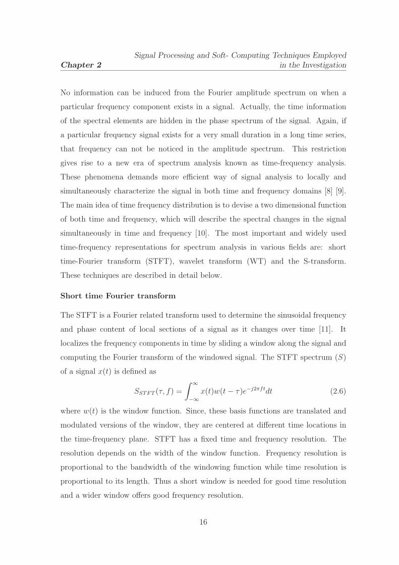
Short time Fourier transform

The STFT is a Fourier related transform used to determine the sinusoidal frequency

and phase content of local sections of a signal as it changes over time [11]. It

localizes the frequency components in time by sliding a window along the signal and

computing the Fourier transform of the windowed signal. The STFT spectrum (S)

of a signal x(t) is defined as

SSTFT (τ, f) =

∫

∞

−∞

x(t)w(t− τ)e−j2πftdt (2.6)

where w(t) is the window function. Since, these basis functions are translated and

modulated versions of the window, they are centered at different time locations in

the time-frequency plane. STFT has a fixed time and frequency resolution. The

resolution depends on the width of the window function. Frequency resolution is

proportional to the bandwidth of the windowing function while time resolution is

proportional to its length. Thus a short window is needed for good time resolution

and a wider window offers good frequency resolution.

16

Chapter 2



Wavelet transform

To partially overcome the problem of fixed resolution with STFT, wavelet transform

(WT) is evolved which introduces a basis function (wavelet) whose width varies with

scale to provide multi-resolution analysis [9] [12]. The wavelet transform of a signal

x(t) is defined as

SWT (a, b) =

∫

∞

−∞

x(t)ψ∗

a,b(t)dt (2.7)

where ψ∗(t) is the specific mother wavelet, a is the dilation parameter and b is the

translation parameter. Hence, the mother wavelet is defined as

ψ∗

a,b(t) =1√aψ

(

t− b

a

)

(2.8)

The wavelet transform is computed by the inner product of the signal, the dilations

and translations version of the mother wavelet. WT is represented as a time

scale plot, where scale is the inverse of frequency. To analyze the low frequency

components in the signal, the analyzing wavelet is dilated in time and compressed

in frequency. To analyze the high frequency components, the analyzing wavelet

is dilated in frequency and compressed in time. This property of WT makes it

very suitable for analysis of signals of high frequency with short duration and low

frequency with long duration. The interpretation of the time scale representations

produced by the wavelet transform require the knowledge of the type of the mother

wavelet used for the analysis. Also the wavelet transform does not retain the absolute

phase information and the visual analysis of the time-scale plots that are produced

by the WT is intricate to interpret.

S-transform

The S-Transform is the hybrid of short time Fourier transform and wavelet

transform. It uses a Gaussian window whose width scales inversely and height

scales directly to provide a frequency dependent resolution while maintaining a direct

relationship with Fourier spectrum. The S-transform is a time-frequency analysis

technique proposed by Stockwell et al. [13], which combines the properties of the

17

Chapter 2



short time Fourier transform and the wavelet transform. The standard S-Transform

of a signal x(t) is defined as

S(τ, f) =

∫

∞

−∞

x(t)w(τ − t, f)e−j2πftdt (2.9)

The window function used in the S-transform is a scalable Gaussian function given

as

w(t, σ) =1

σ(f)√

2πe−

t2

2σ2(f) (2.10)

and the width of the window varies inversely with frequency as

σ(f) =1

|f | (2.11)

Combining Eqs. (2.10) and (2.11) gives

S(τ, f) =

∫

∞

−∞

x(t)

{ |f |√2πe−

(τ−t)2f2

2 e−j2πft

}

dt (2.12)

The advantage of the S-transform over the short time Fourier transform is that

the window width (σ) is a function of frequency (f) rather than a fixed one as in

STFT and thereby provides multiresolution analysis. In contrast to wavelet analysis,

the S-Transform wavelet is divided into two parts as shown within the braces of Eq.

(2.12). One is the slowly varying envelope (the Gaussian window) which localizes the

time and the other is the oscillatory exponential kernel which selects the frequency

being localized. It is the time localizing Gaussian that is translated while keeping the

oscillatory exponential kernel stationary, which is different from the wavelet kernel.

As the oscillatory exponential kernel is not translating, it localizes the real and the

imaginary components of the spectrum independently, thus localizing the phase as

well as the amplitude spectrum. Therefore, it retains the absolute phase of the signal

which is not provided by wavelet transform.

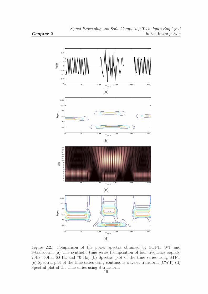
Let us analyse a synthetic time series in order to show the localizing property of

the time-frequency representations. It consists of four different frequencies 20 Hz,

50 Hz, 60 Hz and 70 Hz present at different locations in the time series. The 20 Hz

signal presents during 103-173 samples, the 50 Hz signal presents at 1-70 samples,

18

Chapter 2



0 50 100 150 200 250−2

−1.5

−1

−0.5

0

0.5

1

1.5

2

Time

Amplit

ude

(a)

Time

Freque

ncy

0 50 100 150 200 250

20

40

60

80

100

120

(b)

Time

Scale

s

50 100 150 200 250

1

2

3

4

5

6

7

8

9

10

11

12

13

14

15

16

(c)

Time

Freque

ncy

0 50 100 150 200 250

20

40

60

80

100

120

(d)

Figure 2.2: Comparison of the power spectra obtained by STFT, WT andS-transform, (a) The synthetic time series (composition of four frequency signals:20Hz, 50Hz, 60 Hz and 70 Hz) (b) Spectral plot of the time series using STFT(c) Spectral plot of the time series using continuous wavelet transform (CWT) (d)Spectral plot of the time series using S-transform

19

Chapter 2



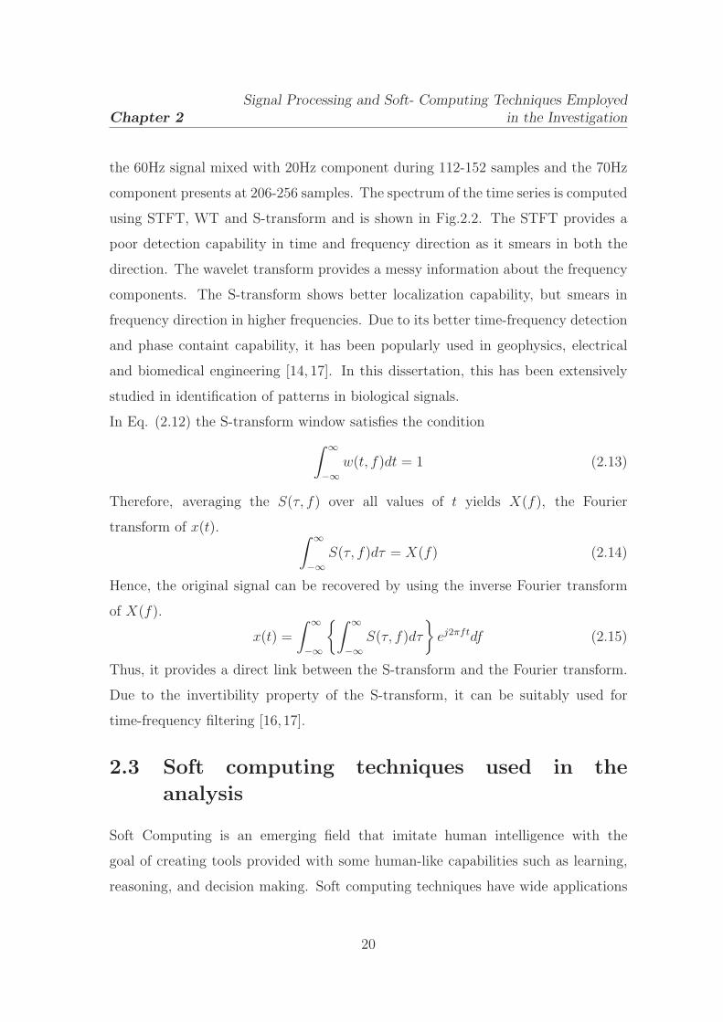
the 60Hz signal mixed with 20Hz component during 112-152 samples and the 70Hz

component presents at 206-256 samples. The spectrum of the time series is computed

using STFT, WT and S-transform and is shown in Fig.2.2. The STFT provides a

poor detection capability in time and frequency direction as it smears in both the

direction. The wavelet transform provides a messy information about the frequency

components. The S-transform shows better localization capability, but smears in

frequency direction in higher frequencies. Due to its better time-frequency detection

and phase containt capability, it has been popularly used in geophysics, electrical

and biomedical engineering [14, 17]. In this dissertation, this has been extensively

studied in identification of patterns in biological signals.

In Eq. (2.12) the S-transform window satisfies the condition

∫

∞

−∞

w(t, f)dt = 1 (2.13)

Therefore, averaging the S(τ, f) over all values of t yields X(f), the Fourier

transform of x(t).∫

∞

−∞

S(τ, f)dτ = X(f) (2.14)

Hence, the original signal can be recovered by using the inverse Fourier transform

of X(f).

x(t) =

∫

∞

−∞

{∫

∞

−∞

S(τ, f)dτ

}

ej2πftdf (2.15)

Thus, it provides a direct link between the S-transform and the Fourier transform.

Due to the invertibility property of the S-transform, it can be suitably used for

time-frequency filtering [16,17].

2.3 Soft computing techniques used in the

analysis

Soft Computing is an emerging field that imitate human intelligence with the

goal of creating tools provided with some human-like capabilities such as learning,

reasoning, and decision making. Soft computing techniques have wide applications

20

Chapter 2



in engineering and science due to their strong learning and cognitive ability and

good tolerance of uncertainty, imprecision, partial truth, and approximation.

Learning is the foundational discipline of the soft computing paradigm. Just as to

learn in animals and humans, machines/computers also can be made intelligent by

learning which leads to a new era of study known as machine learning.

Machine learning

Machine learning is derived from the efforts of psychologists, to make more precise

their theories of animal and human learning through computational models. It refers

to a system capable of acquiring and integrating the knowledge automatically. The

capability of the systems to learn from experience, training, analytical observation,

results in a system that can continuously self-improve and thereby exhibit efficiency

and effectiveness. A major focus of machine learning research is to automatically

learn to recognize complex patterns and make intelligent decisions based on data

samples. The difficulty is that the set of all possible behavior given all possible

inputs is too large to be covered by the set of observed samples (training data).

Hence, the learner must generalize from the given samples, so as to be able to

produce a faithful output in new observations. Traditionally, learning in machine

intelligent has been studied either in the unsupervised paradigm where all the data

are unlabeled or in the supervised paradigm where all the data are labeled.

Supervised learning

Supervised learning is the machine learning task of inferring a function from

supervised training data. The training data consist of a set of training examples.

Each example is a pair consisting of an input object (training data) and a desired

output value (the supervisory signal). A supervised learning algorithm analyzes

the training data and produces an inferred function, which is called a classifier or a

regression function. The inferred function should predict the correct output value

for any valid input object. This requires the learning algorithm to generalize from

the training data to unseen situations in a reasonable way.

21

Chapter 2



Unsupervised learning

Unsupervised learning refers to the problem finding hidden structure in unlabeled

data. Since the observations given to the learner are unlabeled, there is no error or

reward signal to evaluate a potential solution. The unsupervised learning includes

clustering, blind source separation, outlier detection etc.

Another kind of machine learning is reinforcement learning.The training information

provided to the learning system by the environment(external trainer)is in the form

of a scalar reinforcement signal that constitutes a measure of how well the system

operates. The learner is not told which actions to take, but rather discover which

actions yield the best reward, by trying each action in turn.

The components of soft computing includes Artificial neural networks, Fuzzy

logic and evolutionary computing algorithms. In this dissertation work, the artificial

neural networks such as multi layer perceptron (MLP) and radial basis function

network (RBF) with supervised learning have been used and are discussed below.

2.3.1 Artificial neural network

An artificial neural network (ANN) is an information processing system that tries

to simulate biological neural networks i.e the nervous system in brain [18] [19]. Due

to its nonlinear processing, learning capability and massively parallel distributed

structure, ANN’s have become a powerful tool for many complex applications

including functional approximation, nonlinear system identification, control, pattern

classification and optimization [20]- [23]. McCulloch and Pitts first developed the

neural networks in 1943 for different computing machines. The ANN is capable

of performing nonlinear mapping between the input and output space due to its

large parallel interconnection between different layers and the nonlinear processing

characteristics. An artificial neuron basically consists of a computing element that

performs the weighted sum of the input signal and the connecting weight. The sum

is added with the bias or threshold and the resultant signal is then passed through a

nonlinear function. Each neuron is associated with three parameters whose learning

22

Chapter 2



can be adjusted. These are the connecting weights, the bias and the slope of the

nonlinear function. For the structural point of view a neural network may be single

layer or it may be multilayer. In multilayer structure, there is one or many artificial

neurons in each layer and for a practical case there may be a number of layers. Each

neuron of the one layer is connected to each and every neuron of the next layer.

Single neuron structure

The operation in a single neuron involves the computation of the weighted sum

of inputs and threshold. The resultant signal is then passed through a nonlinear

activation function. This is also called as a perceptron, which is built around a

nonlinear neuron. The basic structure of a single neuron is shown in Fig. 2.3. The

output associated with the neuron is computed as

y(k) = f

[

N∑

j=1

Wj(k)Xj(k) + b(k)

]

(2.16)

where Xi, i = 1, 2, · · · , N are inputs to the neuron, wj is the synoptic weights of

the jth input, bk is the bias, N is the total number of inputs given to the neuron and

f(.) is the nonlinear activation function. The activation functions generally used in

neural computation are discussed below.

Activation functions

Log-sigmoid function

This function takes the input and squashes the output into the range of 0 to 1. This

function is represented as

f(x) =1

1 + e−x(2.17)

Hyperbolic tangent sigmoid

This function is defined as

f(x) = tanh(x) =ex − e−x

ex + e−x(2.18)

23

Chapter 2



Figure 2.3: The structure of a single neuron

Signum function

This activation function is represented as

f(x) =

1, if x > 0

0, if x = 0

−1, if x < 0

(2.19)

Threshold function

This function is given by the expression

f(x) =

1, for x ≥ 0

0, for x ≤ 0(2.20)

Piecewise linear function

This function is represented as

f(x) =

1, if x ≥ 0.5

x, if − 0.5 > x > 0.5

0, if x ≤ 0

(2.21)

24

Chapter 2



where the amplification factor inside the linear region of operation is assumed to be

unity. Out of these nonlinear functions, the sigmoid activation function is extensively

used in ANN.

Multi layer perceptron

Multilayer perceptron (MLP) is a feed forward neural network, where the input

signal propagates through the network in the forward direction on a layer by layer

basis [18]. This network has been applied successfully to solve many non linear,

complex and diverse problems in several fields. The structure of a three layer MLP

(1-1-1) is shown in Fig.2.4. It consists of one input layer, one hidden layer and one

output layer. The input to the network is represented by Xi. Wih and Who represent

Figure 2.4: The structure of MLP network

the connecting weights between input layer to hidden layer and hidden layer to

output layer respectively. The bh and bo represent the bias to neurons in hidden and

output layers respectively. f(.) represents the no-linear activation function for both

hidden and output layers and N is the number of inputs at the input layer. The

25

Chapter 2



output at each node of the hidden layer is computed as

ah = fh

(

N∑

i=1

wihxi + bh

)

(2.22)

Hence, the individual output of the neurons at the output layer is defined as

yk = fk

(

n1∑

h=1

whkah + bk

)

(2.23)

where the n1 is the total number of neurons in the hidden layer. Thus the output

of the MLP can be represented as

yk = fk

(

n1∑

h=1

whkfh

(

N∑

i=1

wihxi + bh

)

+ bk

)

(2.24)

The weights and biases of different layers of MLP need to be learned in an efficient

way to get the optimum of the objective function. Learning is an adaptive procedure

by which the weights are systematically changed by a governing rule. Learning the

networks can be of supervised , unsupervised and reinforcement type. Generally

the learning algorithms may be classified into two categories: derivative based and

derivative free. In this dissertation work the back propagation algorithm which is a

derivative based algorithm is used for the learning of the neural networks. The back

propagation algorithm is discussed in the subsequent sections.

Back propagation algorithm

Back propagation (BP) algorithm is the central to the supervised learning of MLP

networks. The parameters of the neural network can be updated by BP in both

sequential and batch mode of operation [19] [22]. In this algorithm, the weights and

the biases are initialized as very small random values.The intermediate and the final

outputs of the MLP are calculated by Eqs.(2.22)and (2.23) respectively. The output

at the kth neuron of the output layer yk(n) is compared with the desired output

dk(n), thereby the resulting error signal ek(n) is computed as

ek(n) = dk(n) − yk(n) (2.25)

26

Chapter 2



The instantaneous value of the total error energy is computed by summing all errors

squared over all neurons in the output layer as given by

ξ(n) =1

2

n2∑

k=1

e2k(n) (2.26)

where n2 is the total number of neurons in the output layer.

The error signal produced by the comparison is used to update the weights between

the layers and biases of the layers. The reflected error components at the hidden layer

are determined by the errors of the last layer and the connecting weights between

the hidden and last layer. These reflected error components are used to update

the weights between the input and hidden layers and bias of the hidden layer. The

weights and the biases are updated in an iterative method until the error becomes

minimum.

The weights between input and hidden layer are updated according to the following

equation

wih(n+ 1) = wih(n) + ∆wih(n) (2.27)

and update equation for weights between hidden and output layer is defined by

whk(n+ 1) = whk(n) + ∆whk(n) (2.28)

where wih(n) and whk(n) are the correction to the synoptic weights and are computed

as

∆whk(n) = −2µ∂ξ(n)

∂whk(n)= 2µe(n)

∂yk(n)

∂whk(n)

= 2µe(n)f 1k

(

n1∑

h=1

whkah + bk

)

ah (2.29)

Similarly, the correction to other synaptic weight can also be computed. The biases

are also updated in similar way as that of weights and the updated equations are

given by

bh(n) = bh(n) + ∆bh(n) (2.30)

27

Chapter 2



bk(n) = bk(n) + ∆bk(n) (2.31)

where ∆bk(n) and ∆bh(n) are the correction to biases of output and hidden layers

respectively. The correction to bias of output layer ∆bk(n) is calculated as

∆bk(n) = −2µ∂ξ(n)

∂bk(n)= 2µe(n)

∂yk(n)

∂bk(n)

= 2µe(n)f 1k

(

n1∑

h=1

whkah + bk

)

ah (2.32)

The correction to other bias which belongs to the hidden layer is also computed in

the similar way.

2.3.2 Radial basis function network

Radial basis function network is a kind of nonlinear layered feed forward neural

network in which the hidden units provide a set of functions that constitute an

arbitrary basis for input patterns when they are expanded into hidden space [24].

The network is designed to perform a non linear mapping from the input space to

the hidden space followed by a linear mapping from the hidden space to the output

space [25]. The RBF networks are suitable for solving function approximation,

system identification and pattern classification problems because of their simple

topological structure and their ability to learn in an explicit manner [25] [26]. In the

classical RBF network, there is an input layer, a hidden layer consisting of nonlinear

node function, an output layer and a set of weights to connect the hidden layer and

output layer. The input layer consists of the source nodes, which are also called

sensory units that connect the network to its environment. The unique hidden layer

in the network applies a nonlinear transformation from input space to hidden space

using radial basis functions. The hidden space is of higher dimensionality in most of

the applications. The response of the network supplied by the output layer is linear

in nature. The basic architecture of the RBF network is shown in Fig. 2.5.

Here xi, i = 1, 2, · · · ,M represents the input vector to the network, φ represents

28

Chapter 2



Figure 2.5: The architecture of radial basis function network

the radial basis function that perform the non-linear mapping and N represents the

total number of hidden units. Each node has a centre vector ck. Wkj represents the

connecting weight between kth hidden unit and jth output unit and they perform

linear regression. For an input feature vector x(n), the output of the jth output

node is given as

yj =N∑

k=1

Wkjφk (2.33)

Radial basis functions

The functional form of the radial basis functions φ(.), which is non singular is given

by φ(x, c) = φ(‖x− c‖), where ‖.‖ denotes the euclidean norm. The radial basis

functions generally used in the applications are described below.

Multiquadrics

φ(r) = (r2 + c2)12 for c > 0 and r ∈ R (2.34)

29

Chapter 2



Inverse multiquadrics

φ(r) =1

(r2 + c2)12

for c > 0 and r ∈ R (2.35)

Gaussian function

φ(r) = exp

(

− r2

2σ2

)

for σ > 0 and r ∈ R (2.36)

In RBFNN, the three parameters that are to be updated are connecting weights

between hidden and output units (Wkj), centre ck and the Gaussian spread σk.

These are updated by using the supervised learning method, which is similar to

stochastic gradient algorithm. The cost function that is to be minimized is given by

ξ(n) =1

2

J∑

j=1

e2j(n) (2.37)

where J is the total number of neurons in output layer, ej(n) represents the error

signal which is the difference between desired output dj and the output obtained yj.

Hence

ej(n) = dj(n) − yj(n)

= dj(n) −N∑

k=1

wk(n)φ {x(n), ck(n)} (2.38)

when the Gaussian function is chosen as the radial basis function, Eq. (2.38) becomes

ej(n) = dj(n) −N∑

k=1

wk(n)exp

(

−‖x(n) − ck(n)‖2

σ2k(n)

)

(2.39)

According to stochastic gradient descent method [22], in order to minimize the cost

function, the updated equations are as follows

w(n+ 1) = w(n) − µw

∂

∂wξ(n) (2.40)

ck(n+ 1) = ck(n) − µc

∂

∂ckξ(n) (2.41)

30

Chapter 2



σk(n+ 1) = σk(n) − µσ

∂

∂σk

ξ(n) (2.42)

Finally, the updated equations of the network is defined as

w(n+ 1) = w(n) + µwe(n)ψ(n) (2.43)

ck(n+ 1) = ck(n) + µc

e(n)wk(n)

σ2k(n)

φ {x(n), ck(n), σk} [x(n) − ck(n)] (2.44)

σk(n+ 1) = σk(n) + µσ

e(n)wk(n)

σ3k(n)

φ {x(n), ck(n), σk} ‖x(n) − ck(n)‖2 (2.45)

where ψ(n) = [φ {x(n), c1, σ1} , φ {x(n), c2, σ2} , · · ·φ {x(n), cN , σN}] is the hidden

layer output and µw, µc, µσ are the learning parameters of the network.

2.4 Sensitivity and Specificity

Basically, to measure and compare the efficacy of a classifier, model or predictor,

some statistical measures such as specificity, sensitivity, positive predictive value,

negative predictive value and accuracy are evaluated through receiver operating

characteristic curves (ROC). The ROC methodology is based on statistical decision

theory and was developed in the context of electronic signal detection and problems

with radar in the early 1950s. In recent years, it has been used in various areas like

geophysics, electrical engineering, communication, medicine, biomedical, machine

learning and data mining. ROC curves provide a global representation of the

prediction accuracy.

In a predictor or binary classifier, for every instance of testing, there are four

possible outcomes. If the instance is positive and it is classified as positive, it

is counted as a true positive (TP). If the instance is positive and is classified as

negative, it is counted as a false negative (FN). If the instance is negative and it is

classified as negative, it is counted as a true negative (TN). If the instance is negative

31

Chapter 2



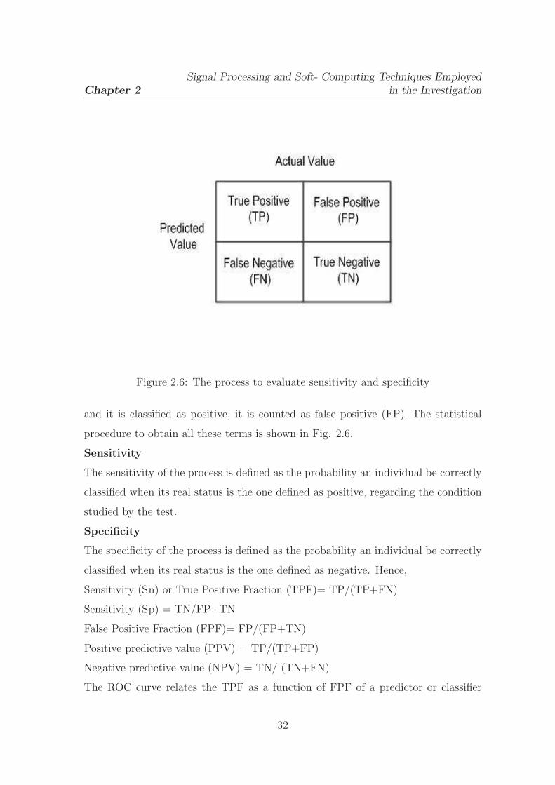
Figure 2.6: The process to evaluate sensitivity and specificity

and it is classified as positive, it is counted as false positive (FP). The statistical

procedure to obtain all these terms is shown in Fig. 2.6.

Sensitivity

The sensitivity of the process is defined as the probability an individual be correctly

classified when its real status is the one defined as positive, regarding the condition

studied by the test.

Specificity

The specificity of the process is defined as the probability an individual be correctly

classified when its real status is the one defined as negative. Hence,

Sensitivity (Sn) or True Positive Fraction (TPF)= TP/(TP+FN)

Sensitivity (Sp) = TN/FP+TN

False Positive Fraction (FPF)= FP/(FP+TN)

Positive predictive value (PPV) = TP/(TP+FP)

Negative predictive value (NPV) = TN/ (TN+FN)

The ROC curve relates the TPF as a function of FPF of a predictor or classifier

32

Chapter 2



for varying threshold values. Basically the ROC curve plots for every possible

decision threshold, which ranges from zero to the maximum value reached by the

predictor, when computing the whole observations and the results are compared

with the real values. The closer the ROC curve is to a diagonal, the less useful is

the predictor. The more the curve moves to the upper left corner on the graph, the

better the predictor. In this dissertation, we have used the ROC curves to evaluate

the efficiency of the predictor developed to detect the patterns present in the genomic

signals.

2.5 Conclusion

Of late it has been observed that detailed understanding and precise collection

of information of bioinformatics require the knowledge of signal processing and

soft computing tools. In the present research study, we have attempted to

investigate on (i) protein coding region identification in DNA sequences (ii) hot

spot identification in proteins (iii) protein structural class prediction and (iv)

classification of microarray gene expression data. To facilitate in-depth investigation

and accurate estimate, the techniques of DSP such as DFT, DCT, S-transform and

soft computing techniques such as MLP, RBFNN have been employed. Therefore in

this section these techniques have been briefly outlined so that understanding of the

work carried out in the subsequent sections will be easier. Further these techniques

have been judiciously selected so that they will be more useful in the respective

application areas. The choice has been made based on the background which I had

in the areas as well as from the literature available in these areas.

33

Identification of Protein Coding

Regions using Time-frequency

Filtering Approach

Chapter 3

Identification of Protein CodingRegions using Time-frequencyFiltering Approach

3.1 Introduction

A major goal of genomic research is to understand the nature of this information

and its role in determining the particular function encoded by the gene. A key

step in deciphering this goal is the identification of the gene locations and the

protein coding regions in the DNA sequence. The enormous amount of genomic

data that are available in public domain inspires the scientific community to

process this information for the benefit of the mankind. The complete genomes

provide essential information for understanding gene functions and evolution. The

determination of patterns in DNA and protein sequences are also useful for many

important biological problems such as identifying new genes, pathogenic islands

and phylogenetic relationships among organisms. With the exponential growth

of the genomic sequence, there has been an increasing demand to accurately

identify the protein coding regions in the DNA sequence. The proliferation of

computational methods in identifying the gene location in last two decades are quite

encouraging and successful, but the efficiency of the prediction methods needs to be

improved. Hence accurate prediction of genes has always been a challenging task

for computational biologists, especially in eukaryote genomes [1] [3]. The 3-base

35

Chapter 3

Identification of Protein Coding Regions using Time-frequency

Filtering Approach

periodicity observed in the coding regions of various organisms has been used as a

marker to identify the protein coding regions of genomes [27] [28]. In this chapter,

we have proposed a novel time-frequency filtering approach to efficiently detect these

protein coding regions in the DNA sequence.

3.1.1 Genes and Proteins

The DNA is a long double stranded molecule that encodes the structure of specific

proteins in the cell, and also carries the information about how these proteins should

be manufactured [1]. Functional elements or cellular instructions are coded within

this string of characters. These instructions are recognized by cellular machinery

and carried out during the growth and functioning of the cell. The DNA sequence

is composed of four different nucleotides, namely adenine (A), cytosine (C), guanine

(G) and thymine (T). The gene structure and expression mechanism in typical

eukaryote cells are very complicated. The eukaryotic DNA is divided into genes

and inter-genic spaces. Genes are further divided into exons and introns. The exons

carry the code for the production of proteins, hence these are called as protein coding

regions. The protein coding regions in DNA sequences are usually neither continous

nor contigous. It is composed of alternating stretches of coding regions (exons) and

non coding regions (introns). The structural relationship between DNA, exons and

introns are shown in Fig. 3.1. When a particular instruction becomes active in a

cell, the corresponding gene is turned on and the corresponding protein is produced

through the transcription and translation process. This process of transcription

and translation is common to all life and hence referred to as the central dogma

of molecular biology [2]. The flow of genetic information to protein is shown in

Fig. 3.2. During the transcription, the double stranded DNA is separated and an

RNA template is generated by matching and chaining nucleotides complementary

to that of DNA sequence. The introns are spliced out of the RNA chain to create a

mature mRNA transcript. The mRNA nucleotides are then read in triplets (codons)

and amino acids are produced by the universal genetic code through the translation

36

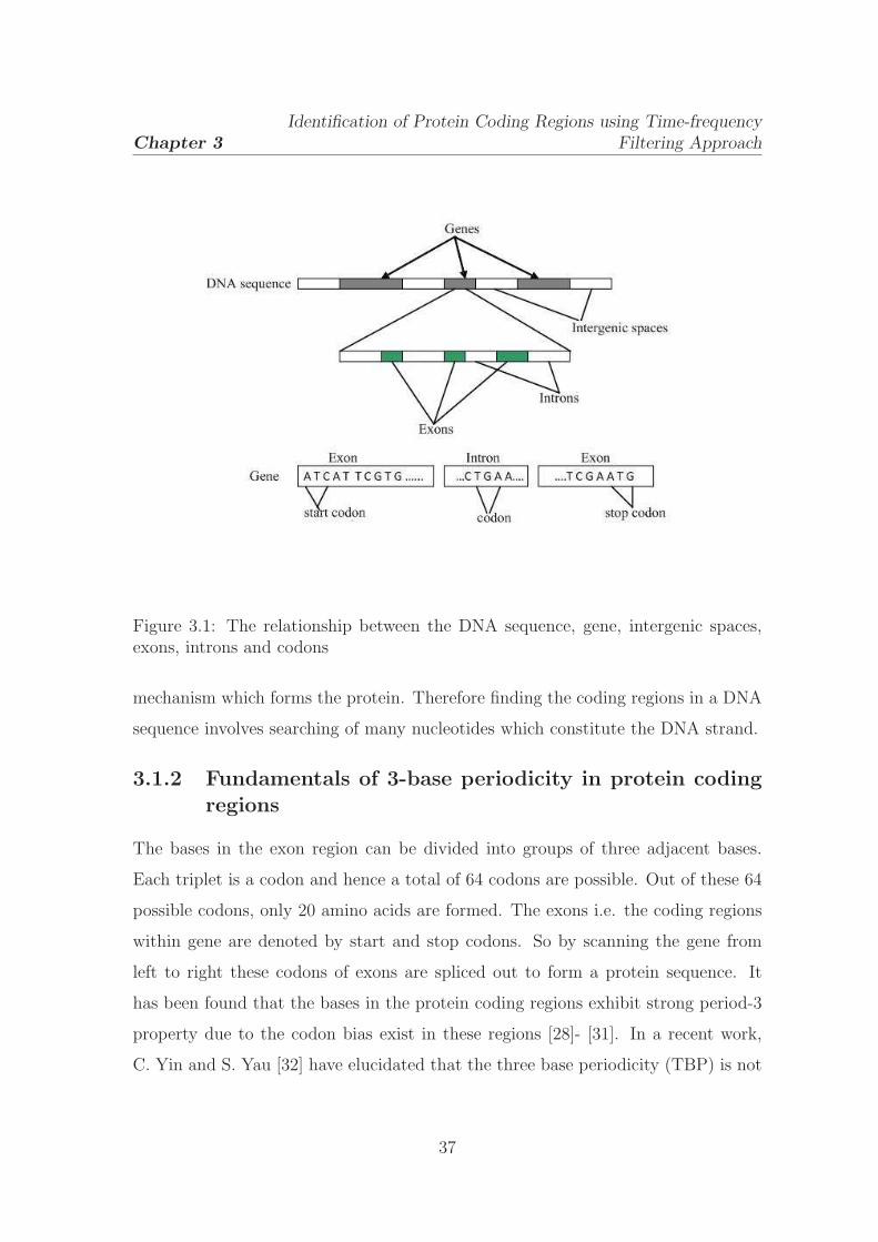
Chapter 3


Filtering Approach

Figure 3.1: The relationship between the DNA sequence, gene, intergenic spaces,exons, introns and codons

mechanism which forms the protein. Therefore finding the coding regions in a DNA

sequence involves searching of many nucleotides which constitute the DNA strand.

3.1.2 Fundamentals of 3-base periodicity in protein codingregions

The bases in the exon region can be divided into groups of three adjacent bases.

Each triplet is a codon and hence a total of 64 codons are possible. Out of these 64

possible codons, only 20 amino acids are formed. The exons i.e. the coding regions

within gene are denoted by start and stop codons. So by scanning the gene from

left to right these codons of exons are spliced out to form a protein sequence. It

has been found that the bases in the protein coding regions exhibit strong period-3

property due to the codon bias exist in these regions [28]- [31]. In a recent work,

C. Yin and S. Yau [32] have elucidated that the three base periodicity (TBP) is not

37

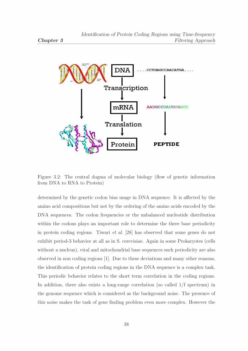
Chapter 3


Filtering Approach

Figure 3.2: The central dogma of molecular biology (flow of genetic informationfrom DNA to RNA to Protein)

determined by the genetic codon bias usage in DNA sequence. It is affected by the

amino acid compositions but not by the ordering of the amino acids encoded by the

DNA sequences. The codon frequencies or the unbalanced nucleotide distribution

within the codons plays an important role to determine the three base periodicity

in protein coding regions. Tiwari et al. [28] has observed that some genes do not

exhibit period-3 behavior at all as in S. cerevisiae. Again in some Prokaryotes (cells

without a nucleus), viral and mitochondrial base sequences such periodicity are also

observed in non coding regions [1]. Due to these deviations and many other reasons,

the identification of protein coding regions in the DNA sequence is a complex task.

This periodic behavior relates to the short term correlation in the coding regions.

In addition, there also exists a long-range correlation (so called 1/f spectrum) in

the genome sequence which is considered as the background noise. The presence of

this noise makes the task of gene finding problem even more complex. However the

38

Chapter 3


Filtering Approach

3-base periodicity property has been used by many researchers as a good indicator

to discriminate between the coding and non coding regions.

3.1.3 Review of the Gene prediction methods

Rapid and accurate determination of the exon locations is important for genome

sequence analysis. Computational approach is the fastest way to find exons in

the genomic DNA sequences. Many techniques have been proposed and proved

successful in locating the exon regions present inside the gene in last two decades.

Several model dependent methods like hidden markov model [33], neural network

[34] [35] and pattern recognition [36] have been used to detect successfully the exons

in the gene. These models are supervised methods which are based on some a prior

information collected from the available databases. These methods are quite useful

in the identification of coding region, but not always. There may be a chance that

the sequenced organism may have coding regions that are not represented on the

available databases. Also many model independent methods have been proposed to

identify the coding regions in DNA sequences. Basically these studies are based on

the Fourier spectral content [2,28,37], spectral characteristics [38] [50] and correlation

of structure of DNA sequences [40]. Niranjan et al. [41] and Akhatar et al. [42]

have proposed a parametric method of spectrum estimation based on autoregresive

modeling. These methods require to define a prior analyzing window within which

the spectrum of DNA sequence is to be computed. As a result it directly affects the

efficiency and computational complexity of the predictor.

Hence there is a need for the development of alternative methods that can reduce

the window length dependency and should be efficient. Recently Vaidyanathan et al.

[43,44] have proposed to use digital filters to identify the coding regions. Also, Jamal

et al. [45] have suggested a multirate DSP model for the same purpose. These model

independent methods do not require the a prior window length and have shown to

be effective in exon identification. But they could not attain satisfactory accuracy

level. In order to solve this problem, a novel time-frequency filtering approach has

39

Chapter 3


Filtering Approach

been proposed in this chapter. This method is independent of the window length

constraint and employ a time-band filter to extract the period-3 component in the

DNA sequence and thereby identify the coding regions in it. It is also robust to the

background noise present in DNA sequence. Case studies on genes from different

organisms have demonstrated that this method can be an effective approach for exon

prediction.

3.2 Numerical mapping of DNA sequences

To apply suitable signal processing methods for the identification of protein coding

regions, the character string of the DNA sequence is converted to a suitable numerical

sequence. This is achieved by assigning a numeral to each nucleotide that forms

the DNA sequence. Hence, different techniques have been suggested to achieve

this particular conversion. The aim of each coding method is to enhance the

hidden information for further analysis. One most widely used mapping is the

Voss mapping [39], where the character string of DNA is converted to four binary

indicator sequences for each base (A, T, C and G). It assigns a numeral ‘1’ when

a particular symbol is found in the sequence otherwise a ‘0’. Anastassiou [2] have

proposed a complex number mapping by assigning a particular complex number

to each base. Silverman et al. [46] have used a tetrahedron mapping in which

each nucleotide is assigned to one of the four corners of a regular tetrahedron.

Niranjan et al. [41] have proposed a real number mapping of the DNA sequence.

Zhang et al. [47,48] presented a Z-curve mapping which is a three dimensional curve

representation for the DNA sequence. Recently, an electron ion interaction potential

(EIIP) indicator sequence [49] [51] have been used to map the character string of

DNA to numeric form. The EIIP is defined as the average energy of delocalized

electrons of the nucleotide. Assigning the EIIP values to the nucleotides, a numerical

sequence is obtained which represents the distribution of the free electrons’ energies

along the DNA sequence. This has been successfully used to identify hot spots in

proteins, for peptide design and also for identification of coding regions [49] [80]. The

40

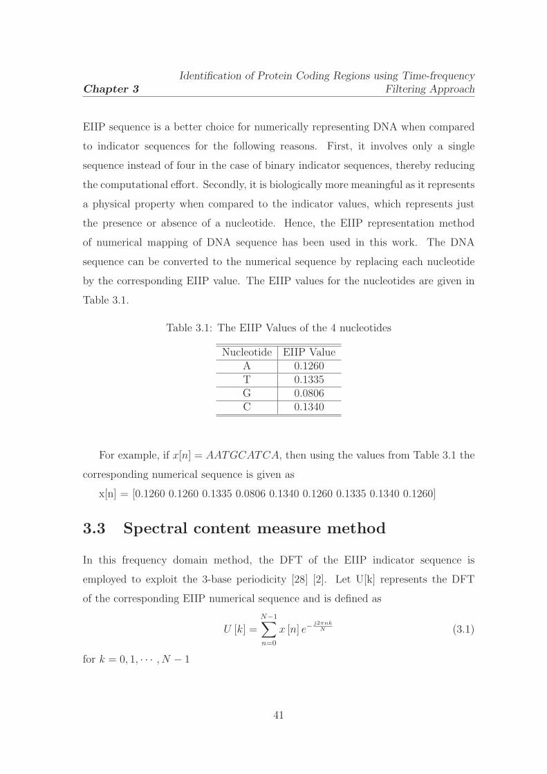
Chapter 3


Filtering Approach

EIIP sequence is a better choice for numerically representing DNA when compared

to indicator sequences for the following reasons. First, it involves only a single

sequence instead of four in the case of binary indicator sequences, thereby reducing

the computational effort. Secondly, it is biologically more meaningful as it represents

a physical property when compared to the indicator values, which represents just

the presence or absence of a nucleotide. Hence, the EIIP representation method

of numerical mapping of DNA sequence has been used in this work. The DNA

sequence can be converted to the numerical sequence by replacing each nucleotide

by the corresponding EIIP value. The EIIP values for the nucleotides are given in

Table 3.1.

Table 3.1: The EIIP Values of the 4 nucleotides

Nucleotide EIIP ValueA 0.1260T 0.1335G 0.0806C 0.1340

For example, if x[n] = AATGCATCA, then using the values from Table 3.1 the

corresponding numerical sequence is given as

x[n] = [0.1260 0.1260 0.1335 0.0806 0.1340 0.1260 0.1335 0.1340 0.1260]

3.3 Spectral content measure method

In this frequency domain method, the DFT of the EIIP indicator sequence is

employed to exploit the 3-base periodicity [28] [2]. Let U[k] represents the DFT

of the corresponding EIIP numerical sequence and is defined as

U [k] =N−1∑

n=0

x [n] e−j2πnk

N (3.1)

for k = 0, 1, · · · , N − 1

41

Chapter 3


Filtering Approach

Then the spectral content at kth instant is

S [k] = |U [k]|2 (3.2)

0 20 40 60 80 100 120 140 160 1800

200

400

600

800

1000

1200

1400

1600

1800

Frequency

Powe

r sp

ectru

m

Figure 3.3: DFT power spectrum of the coding region of gene F56F11.4 ( exon regionfrom 2527-2857 of length 330 relative to the base position 7021). The peak at thefrequency 330/3=110 corresponds to the period-3 component.

S [k] acts as a preliminary indicator of a coding region indicating a peak at the

N/3 frequency. To illustrate this behavior, the spectra of a coding and non-coding

region of gene F56F11.4 of C. elegans chromosome III (a detail description is provided

in section 3.6.1) is used. Figs. 3.3 and 3.4 show the spectra of the coding and

no-coding regions of the gene. This procedure is used to detect the probable

coding regions in the DNA sequence. Hence the coding regions are identified by

evaluating S[N/3] over a window of N samples, then sliding the window by one or

more samples and recalculating S[N/3]. This process is carried out over the entire

DNA sequence. The peaks in the spectra obtained by the sliding window DFT

corresponds to the protein coding regions. We require that the window length (N)

to be sufficiently large (typical sizes are a few hundred to a few thousand), so that the

periodicity effect dominates the background noise spectrum. This approach increases

the computational complexity as it computes the spectrum within a window and also

42

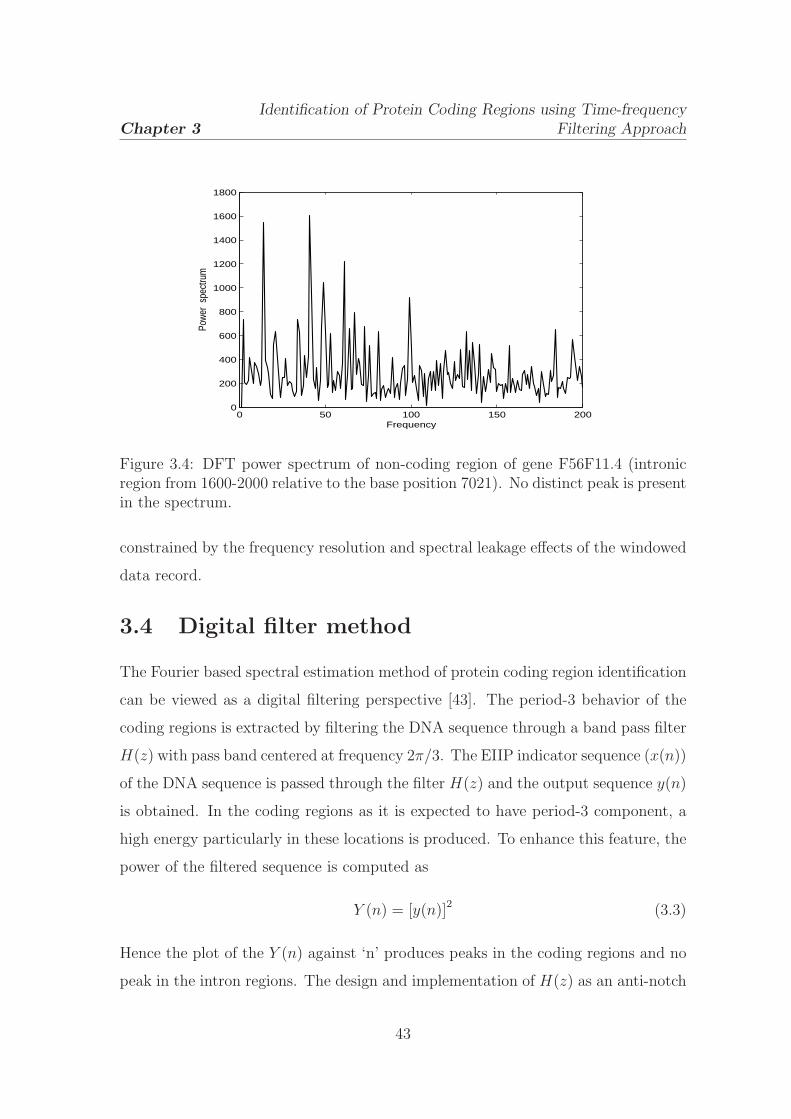
Chapter 3


Filtering Approach

0 50 100 150 2000

200

400

600

800

1000

1200

1400

1600

1800

Frequency

Powe

r sp

ectru

m

Figure 3.4: DFT power spectrum of non-coding region of gene F56F11.4 (intronicregion from 1600-2000 relative to the base position 7021). No distinct peak is presentin the spectrum.

constrained by the frequency resolution and spectral leakage effects of the windowed

data record.

3.4 Digital filter method

The Fourier based spectral estimation method of protein coding region identification

can be viewed as a digital filtering perspective [43]. The period-3 behavior of the

coding regions is extracted by filtering the DNA sequence through a band pass filter

H(z) with pass band centered at frequency 2π/3. The EIIP indicator sequence (x(n))

of the DNA sequence is passed through the filter H(z) and the output sequence y(n)

is obtained. In the coding regions as it is expected to have period-3 component, a

high energy particularly in these locations is produced. To enhance this feature, the

power of the filtered sequence is computed as

Y (n) = [y(n)]2 (3.3)

Hence the plot of the Y (n) against ‘n’ produces peaks in the coding regions and no

peak in the intron regions. The design and implementation of H(z) as an anti-notch

43

Chapter 3


Filtering Approach

filter and its modifications are discussed in many papers [37] [44]. An overview of

the implementation is presented here.

The IIR anti-notch filter

Consider a 2nd order all pass filter defined as

A(z) =R2 − 2Rcosθz−1 + z−2

1 − 2Rcosθz−1 +R2z−2(3.4)

and a filter bank with two filters G(z) and H(z) obtained from the A(z) defined as

G(z)

H(z)

=1

2

1 1

1 −1

1

A(z)

(3.5)

Then G(z) is written as

G(z) = k

[

1 − 2cosw0z−1 + z−2

1 − 2Rcosθz−1 +R2z−2

]

(3.6)

where

cosw0 =2Rcosθ

1 +R2, k =

1 +R2

2(3.7)

When the radius R is less than and close to unity the G(z) is a notch filter with a

zero at frequency w0. Also H(z) and G(z) are power complementary. Hence H(z)

can be a good anti-notch filter defined as

H(z) =1

2

[

(1 −R2)(1 − z−2)

1 − 2Rcosθz−1 +R2z−2

]

(3.8)

The amplitude response of the antinotch filter with radius R = 0.99 is shown in

Fig. 3.5. The DNA sequence can be viewed as a non stationary signal where the

spectral components change along the sequence. Also it contains the background

noise which comes due to the long range correlations among the bases on the DNA

stretch. Under such situation the conventional Fourier domain filtering methods can

not extract properly the occurrence of a period-3 component in the DNA sequence.

Hence the joint time-frequency analysis is needed for analyzing such spectral content

in the sequence.

44

Chapter 3


Filtering Approach

0 0.2 0.4 0.6 0.8 10

0.1

0.2

0.3

0.4

0.5

0.6

0.7

0.8

0.9

1

ω/π

Ampl

itude

resp

onse

Figure 3.5: The anti-notch filter response

3.5 Statistical method of coding region

identification

The statistical methods have found successful to detect the protein coding regions

in DNA sequences. Fickett and Tung [27] have proposed various statistical

determinants of protein-coding potential such as in-frame hexamer frequencies which

were shown to possess good predictive power. Over the years, Markov models [33]

and Bayesian pattern recognition algorithms have been found to be very efficient

for gene modeling and used in several popular algorithms and programs such as

HMMGene, Gene Mark, Gene ID, Genie etc. for prokaryotic as well as eukaryotic

gene prediction.

Hidden Markov Model (HMM)

Hidden Markov models are general statistical modeling techniques for linear

problems like sequences or time series and have been widely used in speech

recognition applications. Following the success in speech recognition applications,

it has been introduced for developing algorithms of pattern recognition in biological

sequences such as protein structural modeling, sequence alignment etc. HMM is

a finite model that describes a probability distribution over an infinite number of

45

Chapter 3


Filtering Approach

Figure 3.6: A simple hidden Markov model. A two-state HMM describing DNAsequence with a heterogeneous base composition is shown.(a) State 1 (top left)generates AT-rich sequence, and state 2 (top right) generates CG-rich sequence.State transitions and their associated probabilities are indicated by arrows andsymbol emission probabilities for A, C, G and T for each state are indicated belowthe states.(b) This model generates a state sequence as a Markov chain and eachstate generates a symbol according to its own emission probability distribution (c).The probability of the sequence is the product of the state transitions and the symbolemissions.

possible sequences. It is composed of a number of states, which might correspond to

positions in a 3D structure or columns of a multiple alignment. Each state ’emits’

symbols (residues/nucleotides) according to symbol-emission probabilities and the

states are interconnected by state-transition probabilities. Starting from some initial

state, a sequence of states is generated by moving from state to state according to

the state-transition probabilities until an end state is reached. Each state then

emits symbols according to that state’s emission probability distribution, creating

an observable sequence of symbols. A simple hidden markov model for a DNA

sequence is described in Fig. 3.6.

Basically an HMM introduces a state sequence A = A1, ..., An, where Ai denotes

the hidden states that ’emit’ the observed (given) DNA sequence S = S1, ..., Sn.

46

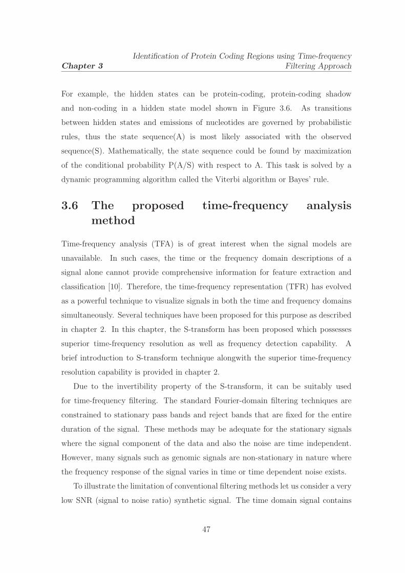
Chapter 3


Filtering Approach

For example, the hidden states can be protein-coding, protein-coding shadow

and non-coding in a hidden state model shown in Figure 3.6. As transitions

between hidden states and emissions of nucleotides are governed by probabilistic

rules, thus the state sequence(A) is most likely associated with the observed

sequence(S). Mathematically, the state sequence could be found by maximization

of the conditional probability P(A/S) with respect to A. This task is solved by a

dynamic programming algorithm called the Viterbi algorithm or Bayes’ rule.

3.6 The proposed time-frequency analysis

method

Time-frequency analysis (TFA) is of great interest when the signal models are

unavailable. In such cases, the time or the frequency domain descriptions of a

signal alone cannot provide comprehensive information for feature extraction and

classification [10]. Therefore, the time-frequency representation (TFR) has evolved

as a powerful technique to visualize signals in both the time and frequency domains

simultaneously. Several techniques have been proposed for this purpose as described

in chapter 2. In this chapter, the S-transform has been proposed which possesses

superior time-frequency resolution as well as frequency detection capability. A

brief introduction to S-transform technique alongwith the superior time-frequency

resolution capability is provided in chapter 2.

Due to the invertibility property of the S-transform, it can be suitably used

for time-frequency filtering. The standard Fourier-domain filtering techniques are

constrained to stationary pass bands and reject bands that are fixed for the entire

duration of the signal. These methods may be adequate for the stationary signals

where the signal component of the data and also the noise are time independent.

However, many signals such as genomic signals are non-stationary in nature where

the frequency response of the signal varies in time or time dependent noise exists.

To illustrate the limitation of conventional filtering methods let us consider a very

low SNR (signal to noise ratio) synthetic signal. The time domain signal contains

47

Chapter 3


Filtering Approach

two sinusoids: 6 Hz and 30 Hz. The 30 Hz signal is present during 1-30 and 65-128

samples and the 6 Hz signal present during 1-64 samples. A white random noise

(n(t)) of strength -6 dB SNR is added to this signal. The time domain and frequency

domain plots of the signal obtained by the use of DFT are shown in Fig. 3.7. The

frequency domain plot indicates poor detection of 6 Hz frequency. Further, the 30

Hz signal which is present at two locations is observed only at one location in the

spectral plot. In this type of application the conventional filtering fails to recover

properly the desired signal.

Hence, for nonstationary signal there is a need for developing filters with

time-varying pass bands and reject bands [16,17]. One of the most practical solutions

to this problem is the joint time-frequency filter. In time-frequency filtering, the time

frequency spectrum of a signal is first estimated and portions which are part of the

noise are removed. Let the signal x(t) is a sum of main signal component, d(t) and

noise component, n(t) as

x(t) = d(t) + n(t) (3.9)

Due to the linearity property of S-transform, it is written as

S(τ, f) = D(τ, f) +N(τ, f) (3.10)

where D and N are the S-transform of the main signal and the noise, respectively.

Therefore, the filtering function A(τ, f) is to be such that

D(τ, f) = A(τ, f).S(τ, f) (3.11)

Using the inversion formula, the denoised signal x(t) is recovered as

x(t) =

∫

∞

−∞

∫

∞

−∞

D(τ, f)ej2πftdτdf

=

∫

∞

−∞

X(f)ej2πftdf (3.12)

where X(f) =∫

∞

−∞D(τ, f)df

Hence multiplying S(τ, f) with the filtering functionA(τ, f) gives the S-transform

of the denoised signal. The potential of the S-transform in localization and time-band

48

Chapter 3


Filtering Approach

0 20 40 60 80 100 120 140−2

−1.5

−1

−0.5

0

0.5

1

1.5

2

2.5

Time

Ampl

itude

(a)

0 10 20 30 40 50 60 700

5

10

15

20

25

30

35

40

45

50

Frequency

Ampl

itude

30 Hz

6 HzNoise

(b)

Figure 3.7: (a)A synthetic time series h(t) is generated by h = zeros(1, 128), t1 =1 : 64, h(1 : 64) = cos (2π6t1/128), t2 = 65 : 128, h(65 : 128) = cos (2π30t2/128),t3 = 1 : 30, h(1 : 30) = h(1 : 30) + cos (2π30t3/128), h(t) = h(t) + n(t) where n isthe additive white noise of SNR -6 dB. (b)The amplitude spectra of h(t)

49

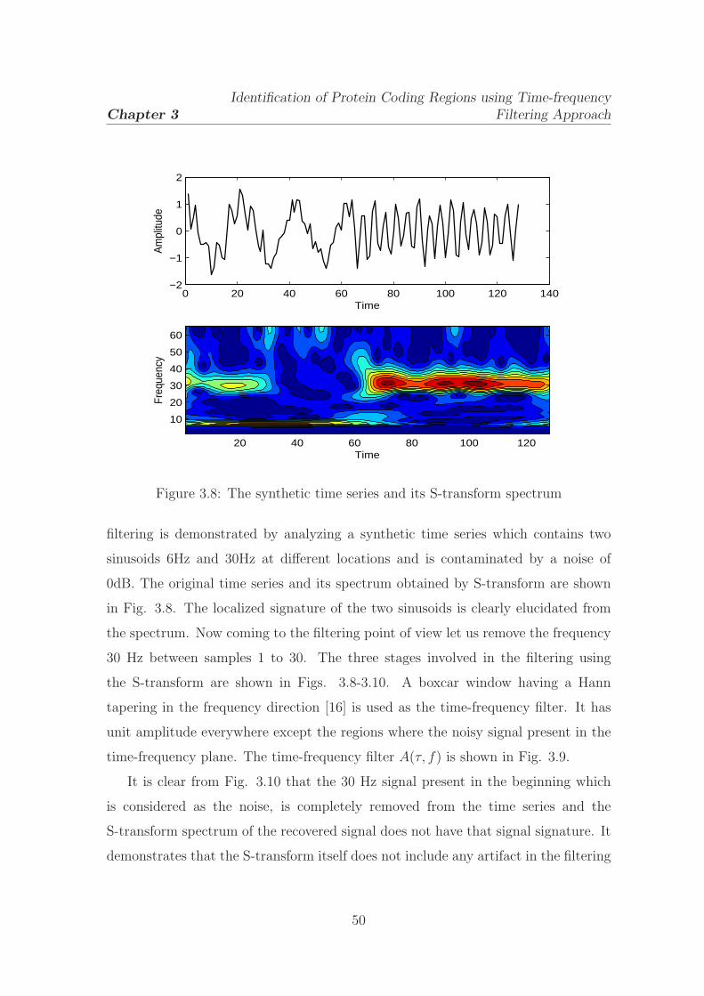
Chapter 3


Filtering Approach

0 20 40 60 80 100 120 140−2

−1

0

1

2

Time

Am

plitu

de

Time

Freq

uenc

y

20 40 60 80 100 120

10

20

30

40

50

60

Figure 3.8: The synthetic time series and its S-transform spectrum

filtering is demonstrated by analyzing a synthetic time series which contains two

sinusoids 6Hz and 30Hz at different locations and is contaminated by a noise of

0dB. The original time series and its spectrum obtained by S-transform are shown

in Fig. 3.8. The localized signature of the two sinusoids is clearly elucidated from

the spectrum. Now coming to the filtering point of view let us remove the frequency

30 Hz between samples 1 to 30. The three stages involved in the filtering using

the S-transform are shown in Figs. 3.8-3.10. A boxcar window having a Hann

tapering in the frequency direction [16] is used as the time-frequency filter. It has

unit amplitude everywhere except the regions where the noisy signal present in the

time-frequency plane. The time-frequency filter A(τ, f) is shown in Fig. 3.9.

It is clear from Fig. 3.10 that the 30 Hz signal present in the beginning which

is considered as the noise, is completely removed from the time series and the

S-transform spectrum of the recovered signal does not have that signal signature. It

demonstrates that the S-transform itself does not include any artifact in the filtering

50

Chapter 3


Filtering Approach

0

50

100

150

0

20

40

60

800

0.2

0.4

0.6

0.8

1

TimeFrequency

Am

plitu

de

Figure 3.9: The time-band limited filter

Time

Freq

uenc

y

20 40 60 80 100 120

10

20

30

40

50

60

0 20 40 60 80 100 120 140−2

−1

0

1

2

Time

Am

plitu

de

Figure 3.10: The recovered signal and its S-transform spectrum

51

Chapter 3


Filtering Approach

process. In essence, the S-transform filtering can be effectively applied to identify

the hot spots by picking up the characteristic frequency in the protein sequence.

In the present case, the period-3 signal in the genomic sequence is considered

as the signal of interest and the rest is treated as noise. Hence, the time-frequency

filtering technique is used as a potential candidate to extract the protein coding

regions in the DNA segment.

3.6.1 Identification of protein coding regions in DNA usingS-transform based filtering approach

The nucleotides are assigned by the corresponding EIIP value as given in Table

3.1, which provides a numerical sequence of the DNA. Then the spectrum of the

DNA sequence under consideration is computed to observe the distribution of the

energy of the frequency components throughout the sequence. A view of the spectral

distribution obtained by the proposed method for gene F56F11.4 of C. elegans

chromosome III is shown in Fig. 3.11. In the S-transform spectrum the high

energy regions (bright areas) in the DNA sequence correspond to the dominant

frequencies in the DNA sequence. As the period-3 frequency is dominant in coding

regions, it provides distinct energy concentrated areas in the time-frequency plane

where that frequency is present which are marked by rectanglear boxes in Fig. 3.11.

Then a specific band limited time-frequency filter (mask) is designed to separate the

frequency of interest. The whole process of S-transform based filtering approach

for protein coding region identification is depicted in a flow graph in Fig. 3.12.

The complete step-by-step procedure of the proposed S-transform based filtering for

identification of hot spots is outlined in sequel:

1. Convert the DNA sequence of interest into a numerical sequence using the

EIIP values (Table 3.1).

2. Compute the spectrum of the DNA sequence using the S-transform technique.

3. Design the band limited filter (mask) in time-frequency domain which

52

Chapter 3


Filtering Approach

relative base location

frequ

ency

1000 2000 3000 4000 5000 6000 7000 8000

500

1000

1500

2000

2500

3000

3500

4000

Figure 3.11: Spectrogram of the DNA sequence of F56F11.4. The high spectrumvalues (bright regions) correspond to the dominant frequency components. Thecoding regions which are relevant to the period-3 frequency are indicated byrectangular boxes in the spectrum.

selects the period-3 frequency and activate during the specific regions in the

time-frequency plane.

4. Filter the DNA numerical sequence of interest by using the time-frequency

filter.

The peaks in the energy of the filtered output signal identify the locations of the

protein coding regions. If the output signal is denoted as y(n), then its energy is

given as

E(n) = |y(n)|2 (3.13)

This energy is referred to as the energy sequence corresponding to three base

periodicity of the DNA sequence. Then the coding regions are predicted by

thresholding the energy sequence.

53

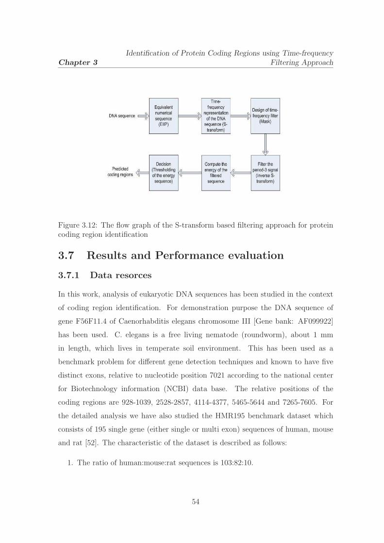
Chapter 3


Filtering Approach

Figure 3.12: The flow graph of the S-transform based filtering approach for proteincoding region identification

3.7 Results and Performance evaluation

3.7.1 Data resorces

In this work, analysis of eukaryotic DNA sequences has been studied in the context

of coding region identification. For demonstration purpose the DNA sequence of

gene F56F11.4 of Caenorhabditis elegans chromosome III [Gene bank: AF099922]

has been used. C. elegans is a free living nematode (roundworm), about 1 mm

in length, which lives in temperate soil environment. This has been used as a

benchmark problem for different gene detection techniques and known to have five

distinct exons, relative to nucleotide position 7021 according to the national center

for Biotechnology information (NCBI) data base. The relative positions of the

coding regions are 928-1039, 2528-2857, 4114-4377, 5465-5644 and 7265-7605. For

the detailed analysis we have also studied the HMR195 benchmark dataset which

consists of 195 single gene (either single or multi exon) sequences of human, mouse

and rat [52]. The characteristic of the dataset is described as follows:

1. The ratio of human:mouse:rat sequences is 103:82:10.

54

Chapter 3


Filtering Approach

2. The mean length of the sequences in the set is 7,096 bp.

3. The number of single-exon genes is 43 and the number of multi-exon genes is

152.

4. The average number of exons per gene is 4.86.

5. The mean exon length is 208 bp, the mean intron length is 678 bp.

6. The proportion of the coding sequence in this dataset is 14%, the intronic

sequence is 46%, and the intergenic DNA is 40%.

The HMR195 dataset is available at http://www.cs.ubc.ca/labs/beta/genefinding/.

3.7.2 Experimetal result

To demonstrate the performance of the proposed method the DNA sequence of

the gene F56F11.4 of C. elegans chromosome III is analyzed. In this chapter,

the existing model independent methods such as conventional sliding window DFT,

the IIR anti-notch filter and statistical method such as hidden markov model are

also simulated and the results obtained are compared with those obtained by the

proposed method. The simulation results of gene F56F11.4 of the model independent

methods are presented in Fig.3.13 for comparison purpose.A graphical representation

of the EIIP coded sequence of gene F56F11.4 is presented in annexure-I. In the

DFT spectrum analysis, a rectangular window of length 351 bp and step size of 1 is

used. The peaks in the spectrum correspond to regions where three base periodicity

is present. Hence, the coding regions are identified by putting a threshold to the

spectrum or filtered energy sequence. The regions having energy above the threshold

are considered as the protein coding regions. As the non coding regions do not have

a period-3 property, the energy in that region is low which is demonstrated in the

Fig. 3.13. It is interesting to note that the first coding region of 112 bp along the

positions 929-1039 has a weak TBP and the remaining four coding regions present

high TBP. The spectral content method and anti-notch filter fail to detect properly

55

Chapter 3


Filtering Approach

that region, but the S-transform filtering approach catches up that region better

than these two methods. In order to have a comparison of the efficiency of these

methods the threshold percentiles from 1 to 99 are used on the measures of the

individual methods for the identification of probable coding regions. Hence, the

statistical parameters such as sensitivity, specificity and average accuracy [42] are

calculated under the same conditions at different threshold values. These measures

have also evaluated for HMM method. The best result achieved in each method

with the corresponding threshold value is listed in Table 3.2. The proposed method

provides the best performance at a threshold of 85 percent with a sensitivity of

0.88, specificity of 0.98 and average accuracy of 0.96. A comparative analysis of

the average accuracy against the threshold values for the three model independent

methods is shown in Fig. 3.14. Further a comparative study of the exon locations

obtained from these four methods with that reported in NCBI database is listed in

Table 3.3. It shows that the proposed method provides better discrimination between

the exons and the introns compared to those offered by the DFT, anti-notch filtering

and HMM methods. To assess the performance of the three model independent

methods, the receiver operating characteristic (ROC) curves are also obtained. It is

a representation of the prediction accuracy of separation of exons and introns in the

gene. The ROC curve relates the true positive rate as a function of false positive

rate for varying threshold values. The ROC curves for all the three methods are

shown in Fig. 3.15. The closer is the ROC curve to a diagonal, the less effective

is the method for discriminating between exon and intron. More steep the curve

towards the vertical axis and then across, the better is the method. A more precise

way of evaluating the performance is to calculate the area under the ROC curve

(AUC). The closer is the area to 0.5, the less effective is the method and closer to

1.0, the better is the method. The area under the ROC curve for the S-transform

filtering method is found to be 0.9288 and the same for the DFT and anti-notch

filter methods are 0.8615 and 0.8369 respectively. Hence the proposed S-transform

filtering method of exon prediction outperforms other methods as it offers highest

56

Chapter 3


Filtering Approach

Table 3.2: Position comparison study of the exons of F56F11.4 by the DFT,anti-notch, S-transform filter and HMM methods.The length of the exons are shownin the braces.

Position in DFT based Anti-notch S-transform HMMGenebank(NCBI) approach filtering filtering method

929-1039(110) 936-1169(233) 942-1164(222) 974-1037(63) 968-1092(125)2528-2857(330) 2573-3005(432) 2538-2956(418) 2539-2908(369) 2566-2906(341)4114-4377(264) 4073-4432(359) 4132-4462(330) 4076-4409(333) 4088-4393(306)5465-5644(180) 5467-5658(191) 5497-5672(175) 5454-5644(190) 5483-5667(185)7255-7605(351) 7396-7806(410) 7406-7728(322) 7305-7597(292) 7348-7692(345)

Table 3.3: Summary of the best performance (accuracy) of identification of codingregions in F56F11.4 using the DFT, anti-notch,S-transform filter and HMM methods.

Method Sensitivity Specificity Average accuracy Threshold

S-transform filter 0.88 0.98 0.96 85DFT based approach 0.82 0.86 0.85 81

Anti-notch filter 0.81 0.82 0.82 82HMM 0.82 0.84 0.83 —

area under the curve.

Further, several DNA sequences from the benchmark dataset HMR195 have been

studied. The gene AF009614 has taken for demonstration and the power spectrum

obtained from all the three methods are shown in Fig. 3.16. The gene AF009614

has two exon regions at positions 1267-1639 and 3888-4513 in the sequence. From

this figure, it is clearly elucidated that the proposed S-transform based filtering

method offers improved performance compared to its counterparts. A classification

experiment has also been carried out to compare the efficiency of the proposed

method. From the HMR195 dataset, 50 sequences whose average exon length is

greater than 200 bases are chosen for the experiment.

Total 222 coding sequences and 237 non coding sequences are used in the

57

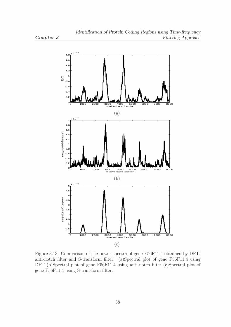
Chapter 3


Filtering Approach

0 1000 2000 3000 4000 5000 6000 7000 80000

0.2

0.4

0.6

0.8

1

1.2

1.4

1.6

1.8x 10

−5

S(N/

3)


(a)

0 1000 2000 3000 4000 5000 6000 7000 80000

0.2

0.4

0.6

0.8

1

1.2

1.4

1.6

1.8

2x 10

−5


energ

y at p

eriod

−3 co

mpon

ent

(b)

0 1000 2000 3000 4000 5000 6000 7000 80000

0.5

1

1.5

2

2.5

3

3.5

4

4.5

5x 10

−5


energ

y at p

eriod

−3 co

mpon

ent

(c)

Figure 3.13: Comparison of the power spectra of gene F56F11.4 obtained by DFT,anti-notch filter and S-transform filter. (a)Spectral plot of gene F56F11.4 usingDFT (b)Spectral plot of gene F56F11.4 using anti-notch filter (c)Spectral plot ofgene F56F11.4 using S-transform filter.

58

Chapter 3


Filtering Approach

Figure 3.14: Average accuracy of identification versus threshold of the gene F56F11.4

0 0.2 0.4 0.6 0.8 10

0.1

0.2

0.3

0.4

0.5

0.6

0.7

0.8

0.9

1

1−specificity

sens

itivity

S−transform filterDFTAnti−notch filter

Figure 3.15: ROC curves obtained by DFT, anti-notch filter and S-transform filterof the gene F56F11.4

59

Chapter 3


Filtering Approach

study.The threshold percentile of 1- 99 is used to discriminate the coding regions

from the non coding regions. Accordingly the ROC curves by the three methods are

obtained as shown in Fig. 3.17. The areas under the ROC curve are also calculated.

These are 0.8602, 0.8316 and 0.8094 for the proposed, DFT and anti-notch filter

methods respectively. Hence the S-transform based filtering method presents a

better performance on the classification, thereby the superiority of the proposed

method is assessed.

3.7.3 Discussion

The existing exon identification methods employ a variety of biological information

and coding techniques in association with many computational methods to predict

the exon regions in DNA. Still the 3-base periodicity pattern has been used as a basis

to identify the coding regions. In this chapter a new time-frequency filtering scheme

based on the TBP has been proposed for the identification of protein coding regions.

The S-transform method provides a pictorial view of the energy distribution of the

frequencies with time which helps in the analysis of the spectral varying signal. It

gives a multi resolution view of the signal so that distinct patches of periodic signal

can be analyzed easily.It is a model independent method which does not require any

training sample to predict and also independent of the window length constraint for

proper computation of the spectra of coding regions. The multi resolution analysis

of the signal enables the proposed method to be effective for both small and larger

coding regions. Another aspect of this study is that the EIIP can be used as an

efficient coding scheme for DNA sequence analysis. The proposed method is found

to be robust against the background noise which occurs due to long range correlation

of bases in the DNA sequence. Thus the coding regions are better discriminated

from the non coding regions and thereby the accuracy of identification increases

considerably. Although the proposed method achieves better accuracy in the

identification of the coding regions, it requires more computational effort. Another

limitation of the S-transform method is that it provides low frequency resolution

60

Chapter 3


Filtering Approach

0 1000 2000 3000 4000 5000 60000

0.5

1

1.5

2

2.5

3x 10

−5

S(N/

3)


(a)

0 1000 2000 3000 4000 5000 60000

1

2

3

4

5

6

7

8x 10

−5


energ

y at p

eriod

−3 co

mpon

ent

(b)

0 1000 2000 3000 4000 5000 60000

1

2

3

4

5

6

7x 10

−5


energ

y at p

eriod

−3 co

mpon

ent

(c)

Figure 3.16: Comparison of the power spectra obtained by the three methods forgene AF0099614. (a) Spectral plot of gene AF0099614 using DFT (b) Spectral plotof gene AF0099614 using anti-notch filter (c) Spectral plot of gene AF0099614 usingS-transform filter.

61

Chapter 3


Filtering Approach

0 0.2 0.4 0.6 0.8 10

0.1

0.2

0.3

0.4

0.5

0.6

0.7

0.8

0.9

1

1−specificity

sens

itivity

S−transform filterDFTAnti−notch filter

Figure 3.17: ROC curves obtained by the DFT, anti-notch filter and S-transformfilter (From 50 sequences of HRM195 dataset)

at higher frequencies and low time resolution at lower frequencies. This occurs due

to the scaling nature of the Gaussian window during spectrum computation, which

may affect the time-frequency filtering operation and also the accuracy. Hence,

improvement of the resolution of the spectrum can further improve the prediction

accuracy.

3.8 Conclusion

Due to lack of the exact knowledge about the sequence features between coding and

non-coding regions, the identification of protein coding regions in DNA sequence has

been a challenging issue in bioinformatics. In this chapter, an efficient time-frequency

filtering approach is proposed for the identification of coding regions in the DNA

sequence. The proposed method employs a multi resolution approach to analyze

both the small and large coding regions and it does not depend on a prior window

length as in case of Fourier methods. The performance of the proposed method

is compared with the existing methods and the results show its superiority in

identification of the exon regions.

62

Localization of Hot Spots in Proteins

using a Novel S-transform

based Filtering Approach

Chapter 4

Localization of Hot Spots inProteins using a Novel S-transformbased Filtering Approach

4.1 Introduction

Biological mechanisms of living organisms like metabolism, gene regulatory and

interaction networks have put numerous challenges to modern biomolecular research.

In particular, identification and characterization of protein-protein interactions is a

burning issue in protein science. Proteins are the basic building blocks of all living

organisms and protein-protein interactions are the basis of all biological processes,

both inside and outside the cell [53] [54]. The protein is made up of amino acids.

There are twenty amino acids and are represented in a protein sequence as a string

of alphabetical symbols with typical lengths ranging from 100 to 10000 [2]. The

protein molecules fold beautifully to form a highly specific 3-dimensional shape,

which defines their particular biological activities. The 3-D structure of a protein

is important because the structure is linked with the biological function. This

3-D shape allows the protein to interact with other molecules known as targets

at specific sites which are referred to as active sites of protein [55] [56]. In active

sites of protein, there are certain residues (amino acids) that operate as an interface

in the binding and recognition between interacting molecules [58] and are termed

as hot spots. Basically the target molecules are proteins, DNA stretches or some

64

Chapter 4

Localization of Hot Spots in Proteins using a Novel S-transform


Figure 4.1: A schematic view of the hot spots in the complex of human growthhormone and its receptor.The human growth hormone (yellow) bound to theextracellular portion of its homodimeric receptors (grey). Available online at:doi:10.1371/journal.pcbi.0030119.g001

other small molecules. The search for protein functions provides the identification

and characterization of each protein as well as in-depth knowledge regarding

their interaction with other proteins and DNA molecules. The protein-protein

interaction or hot spot identification provides a base to identify and analyze the

drugs, molecular medicines, etc. The identification of protein hot spots and solving

the protein structure-function problem [57] is a challenging task for researchers

in biology, engineering and computer science. Many protein-interaction networks

have been modeled to discover the mechanism of protein complexes, but a deep

understanding of this requires the knowledge of interface amino acids that takes

action in protein-protein interactions [59]- [61]. A biological experimental technique

known as Alanine Scanning Mutagenesis (ASM) has been used to identify the hot

65

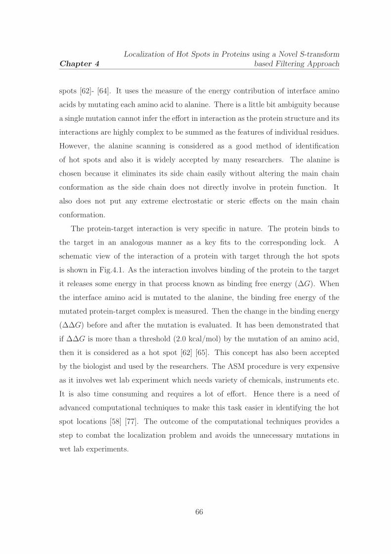
Chapter 4



spots [62]- [64]. It uses the measure of the energy contribution of interface amino

acids by mutating each amino acid to alanine. There is a little bit ambiguity because

a single mutation cannot infer the effort in interaction as the protein structure and its

interactions are highly complex to be summed as the features of individual residues.

However, the alanine scanning is considered as a good method of identification

of hot spots and also it is widely accepted by many researchers. The alanine is

chosen because it eliminates its side chain easily without altering the main chain

conformation as the side chain does not directly involve in protein function. It

also does not put any extreme electrostatic or steric effects on the main chain

conformation.

The protein-target interaction is very specific in nature. The protein binds to

the target in an analogous manner as a key fits to the corresponding lock. A

schematic view of the interaction of a protein with target through the hot spots

is shown in Fig.4.1. As the interaction involves binding of the protein to the target

it releases some energy in that process known as binding free energy (∆G). When

the interface amino acid is mutated to the alanine, the binding free energy of the

mutated protein-target complex is measured. Then the change in the binding energy

(∆∆G) before and after the mutation is evaluated. It has been demonstrated that

if ∆∆G is more than a threshold (2.0 kcal/mol) by the mutation of an amino acid,

then it is considered as a hot spot [62] [65]. This concept has also been accepted

by the biologist and used by the researchers. The ASM procedure is very expensive

as it involves wet lab experiment which needs variety of chemicals, instruments etc.

It is also time consuming and requires a lot of effort. Hence there is a need of

advanced computational techniques to make this task easier in identifying the hot

spot locations [58] [77]. The outcome of the computational techniques provides a

step to combat the localization problem and avoids the unnecessary mutations in

wet lab experiments.

66

Chapter 4



4.2 Review of hot spot identification methods

Several structure and sequence based computational methods have been proposed

in the literature to identify the hot spots in proteins. Kortemme and Baker [66] [67]

proposed a computational alanine scanning method known as Robetta-Ala, which

use a physical model to calculate the energy of the interaction of the mutation to

alanine. Many feature based classification models have been proposed to predict

the hot spots. Ofran and Rost [68] [69] proposed a feature based method, called

ISIS, which predicts the hot spots from the protein primary sequence only. It uses

the physicochemical features, evolutionary and structural features of the protein

through neural network model to predict the hot spots. Recently Darnell et al.

[70] [71] proposed a model which uses a physical and knowledge based approach

to predict the binding hot spots. Guney et al. [72] predicts the hot spots using

the residue conservation and solvent accessible surface area (ASA). Burgoyne and

Jackson [73] used the van der Waals potential, electrostatic potential, desolvation

and surface conservation properties of residues to define hot spots on the protein

surface. Tuncbag et al. [74] used the conservation, solvent accessibility (ASA) and

statistical pairwise residue potential of interface residues to predict the hot spots in

proteins. Ma et al. [75] and Keskin et al. [76] identified the hot spots by analysing

the structurally conserved residues in protein. Chao et al. [59] have applied support

vector machine (SVM) to predict hot spots using sequence, structure and molecular

interaction information based features. Xia et al. [77] also employed SVM with

protrusion index and solvent accessibility feature of the protein to identify the hot

spots. Although these methods are useful for the prediction, they need a large

number of samples for training the model and the accuracy may decrease when

applied to a large set of protein complexes.

However, the hot spots in protein can also be identified by the use of resonant

recognition model (RRM) which correlates the biological functioning of the protein

to the characteristic frequencies [see section 4.3]. These hot spots in protein can be

localized where the characteristic frequencies of the functional groups are dominant.

67

Chapter 4



Each such frequency in the spectral domain signifies a protein function. The signal

processing techniques are the suitable candidates to extract these characteristic

frequencies in the protein sequence, which are based on the sequence information

only. Recently, a signal processing technique known as digital filtering [82] [83] has

been applied for this purpose. A protein sequence is usually noisy and may contain

the hot spots (characteristic frequency) at different locations along the protein

sequence. Under such situation, if the conventional digital filtering technique is

applied, it fails to detect uniquely all characteristic frequencies present in the protein

sequence. Secondly, if the same characteristic frequency is present in more than one

location, the conventional approach of spectral detection identifies the frequencies,

but not the locations at which they occur.

The real life protein sequences are usually characterized by noisy signals and

hence, the use of existing filtering methods to such sequences do not provide accurate

localization and identification of characteristic frequencies. In these applications, the

time-frequency analysis and filtering are required to achieve accurate and effective

solution. In the DSP literature many time-frequency analysis methods, such as

STFT [11], WT [12] and S-transform [17] have been proposed which localize the

events in the signal. A brief introduction to these techniques is provided in chapter

2. Among these, the S-transform possesses superior time-frequency resolution as well

as frequency detection capability. Therefore, the motivation of the present work is

to propose S-transform to detect efficiently all the characteristic frequencies present

in protein and to identify the corresponding hot spot locations.

4.3 Resonant recognition model

Biological functions of proteins are primarily determined by a model of protein-target

interactions known as resonant recognition model (RRM). The RRM is a

physico-mathemati-cal approach that interprets protein sequence information using

signal analysis methods. According to this model, there is a significant correlation

between the spectra of the numerical presentation of amino acid sequences and their

68

Chapter 4



biological activities [78] [79]. To apply suitable signal processing methods for the

analysis, the character string of protein need to be converted to a suitable numerical

sequence. This is achieved by assigning a numeral to each amino acid that forms

the protein.

The assignment of numerical value to each amino acid is based on some physical

properties that are relevant to the protein’s biological functioning. A variety of amino

acid indices have been reported in literature. Cosic et al. [80] have demonstrated

that the best correlation can be obtained with the parameters, that are related

to the energy of delocalized electrons of each amino acid which have strongest

impact on the electronic distribution of the whole protein. An effective way of

assigning the numerical value is the electron-ion-interaction potential (EIIP). The

EIIP is defined as the average energy of delocalized electrons of the amino acid

which can be evaluated by the pseudo potential model reported in [80]. The EIIP

values for the 20 amino acids are listed in Table 4.1. Hence the primary sequence

of protein can be converted to the numerical sequence by replacing each amino

acid by the corresponding EIIP values. Veljcovic et al. [81] have reported that the

Table 4.1: EIIP values of the 20 amino acids

Amino acid EIIP Amino acid EIIPLeucine (Leu) 0.0000 Trypsin(Try) 0.0516Isoleucine(Ile) 0.0000 Tryptophan(Trp) 0.0548

Asparagine(Asn) 0.0036 Glutamine(Gln) 0.0761Glycine(Gly) 0.0050 Methionine(Met) 0.0823Valine(Val) 0.0057 Serine(Ser) 0.0829

Glutamic acid(Glu) 0.0058 Cystrine(Cys) 0.0829Proline(Pro) 0.0198 Threonine(Thr) 0.0941Histidine(His) 0.0242 Phenylalanine(Phe) 0.0946Lysine(Lys) 0.0371 Arginine(Arg) 0.0959Alanine(Ala) 0.0373 Asparatic acid(Asp) 0.1263

Fourier spectral analysis of the EIIP sequence of the protein has strong relevance

to its functional activity. All the proteins belonging to a functional family share

69

Chapter 4



a common spectral component, which characterizes a particular function of the

group. This component is defined as the characteristic frequency of the functional

group. In protein-target interaction both the protein and target share the same

characteristic frequency, but are opposite in phase. This is believed to provide a

resonant recognition in the binding process and hence the mechanism termed as

RRM. The analysis of the function of protein using RRM is generally performed in

two stages. First the symbolic sequence of the protein is converted into the numerical

sequence using the EIIP values. Then the discrete Fourier transform of the proteins

is computed to evaluate the consensus spectrum. It has been observed that the

spectra of a family of protein sequences sharing a common frequency show a peak

in the cross-spectrum function [78] [80]. The common characteristic frequency of

a functional group of K proteins can be computed by the cross-spectral function

defined in (4.1).

S(w) = |X1(w)| |X2(w)| |X3(w)| · · · |XK(w)| (4.1)

where X1(w)X2(w) · · ·XK(w) are the DFTs corresponding to the K proteins. The

product of the amplitude spectra of the protein sequences as in Eq. (4.1) of a

functional group is referred to as the consensus spectrum. Peak frequencies in

the consensus spectrum denote the characteristic frequencies for all the proteins

analyzed. It has been demonstrated that if a group of proteins has only one common

function, then the consensus spectrum has one significant peak. If a protein performs

more than one function, then each function corresponds to a unique characteristic

frequency in the cross spectra. The numerical sequence (basic bovine and acidic

bovine) and the consensus spectrum of the group of fibroblast growth factors (FGF)

are shown in Figs. 4.2 and 4.3, respectively. This constitutes a family of proteins

that affect the growth, differentiation and survival of certain cell. This particular

function of the family is clearly shown as a peak at the normalized frequency of 0.90

in the consensus spectrum.

The RRM characteristic frequency in the consensus spectrum corresponds to a

particular biological function of the family of proteins. Therefore, determination

70

Chapter 4



0 50 100 1500

0.05

0.1

0.15

0.2

Base location

Am

plitu

de

0 50 100 1500

0.05

0.1

0.15

0.2

Base location

Am

plitu

de

0 0.5 10

0.2

0.4

0.6

0.8

1

Frequency

Am

plitu

de

0 0.5 10

0.5

1

1.5

Frequency

Am

plitu

de

Figure 4.2: The numerical sequence and corresponding DFTs of the basic bovine(left) and acidic bovine (right)

0 0.1 0.2 0.3 0.4 0.5 0.6 0.7 0.8 0.9 10

0.1

0.2

0.3

0.4

0.5

0.6

0.7

0.8

0.9

1

Frequency

Ampli

tude

Figure 4.3: The consensus spectrum of the FGF family. The peak corresponds tothe characteristic frequency relevant to a certain biological function

71

Chapter 4



of the characteristic frequency enables identification of the individual amino acids

i.e. the hot spots that contribute to it. A simple procedure has been adopted

to identify the hot spots by altering the amplitude of the Fourier coefficients

corresponding to the characteristic frequencies. It determines those amino acids

which are most affected by the changes in the amplitude that belong to the

characteristic frequency. The difficulty in this method is that a change in one

Fourier coefficient affects all the samples in the numerical sequence of the protein,

thereby provides an unreliable result. As the spectrum of the protein contains more

frequency components along with the characteristic frequency, it confirms that the

characteristics of the signal changes throughout the samples i.e. non-stationary in

nature. A joint time-frequency analysis is needed for analyzing the change of the

characteristic frequency in this case. This issue is resolved in this chapter by using

the S-transform which is a better candidate for time-frequency analysis. Therefore

a new method of time-frequency filtering using the S-transform has been proposed

as a promising method to identify the amino acids (hot spots) corresponding to the

characteristic frequencies.

4.4 Time-frequency analysis

By measuring and processing the genomic signals in time domain and frequency

domain alone do not provide more information regarding the structure, sequence

and pattern of the molecules. Hence a joint time-frequency analysis based approach

has been evolved which provides a better understanding of the hidden artifacts

in genomic signals. Time-frequency representations describe signals in terms of

their joint time and frequency content [9]. These representations are useful for

analyzing signals with both time and frequency variations such as speech, music,

biomedical signal [15] and geophysical signals [17]. Time-frequency analysis is

particularly useful for analyzing signals with continuously time-varying frequency

content i.e. non-stationary signals. Many approaches to time-frequency analysis

have been widely used for a number of years. Time-frequency analysis (TFA) is of

72

Chapter 4



great interest when the signal models are unavailable. In those cases, the time or

the frequency domain descriptions of a signal alone cannot provide comprehensive

information for pattern identification and classification [10]. The time domain lacks

the frequency description of the signals. The Fourier transform of the signal cannot

depict how the spectral content of the signal changes with time, which is critical in

many non-stationary signals in practice. Hence the time variable is introduced in the

Fourier based analysis in order to provide a proper description of the spectral changes

as a function of time. Hence the TFA evaluates the energy concentration along the

frequency axis at a given time instant and thus provides a joint time-frequency

representation of the signal. The S-transform is an excellent time-frequency analysis

technique, which enjoys the advantage of both STFT and wavelet transform.

The localization potentiality of S-transform has been dealt in section 2.2.3 of chapter

2. Further, the new filtering approach using S-transform has been described in

section 3.5 of chapter 3. These two characteristics of S-transform is used in this

chapter for achieving improved identification of hot spots in proteins.

4.5 Hot spot localization in proteins using the

proposed S-transform filtering approach

In order to make suitable the S-transform to apply on the proteins, it needs to

be converted to a numerical sequences. The amino acids are assigned by the

corresponding EIIP value which ranges from 0 to 0.1263, thereby provides a DC

bias (average value) in the numerical sequence of the protein. This is an offset to

the signal that has no meaning in the context of spectrum analysis. Hence the DC

bias may mislead the peaks in the spectrum of the protein which has to be removed

before computing the Fourier transform. Then the consensus spectrum is evaluated

using Eq. (4.1) and the peak in the spectrum corresponds to the characteristic

frequency of the family of proteins. The difficulty in the consensus spectrum is

that it is unable to identify the individual amino acids which contribute to the

characteristic peak frequency. Thus higher domain time-frequency analysis has been

73

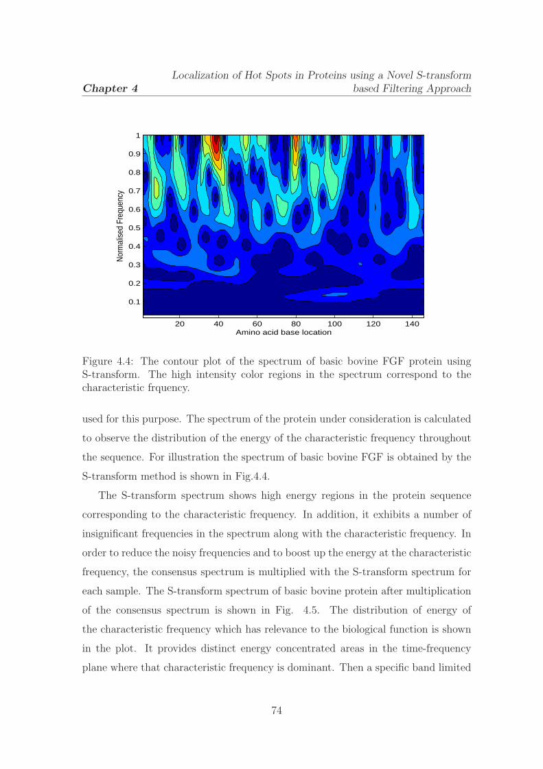
Chapter 4



Amino acid base location

Nor

mal

ised

Fre

quen

cy

20 40 60 80 100 120 140

0.1

0.2

0.3

0.4

0.5

0.6

0.7

0.8

0.9

1

Figure 4.4: The contour plot of the spectrum of basic bovine FGF protein usingS-transform. The high intensity color regions in the spectrum correspond to thecharacteristic frquency.

used for this purpose. The spectrum of the protein under consideration is calculated

to observe the distribution of the energy of the characteristic frequency throughout

the sequence. For illustration the spectrum of basic bovine FGF is obtained by the

S-transform method is shown in Fig.4.4.

The S-transform spectrum shows high energy regions in the protein sequence

corresponding to the characteristic frequency. In addition, it exhibits a number of

insignificant frequencies in the spectrum along with the characteristic frequency. In

order to reduce the noisy frequencies and to boost up the energy at the characteristic

frequency, the consensus spectrum is multiplied with the S-transform spectrum for

each sample. The S-transform spectrum of basic bovine protein after multiplication

of the consensus spectrum is shown in Fig. 4.5. The distribution of energy of

the characteristic frequency which has relevance to the biological function is shown

in the plot. It provides distinct energy concentrated areas in the time-frequency

plane where that characteristic frequency is dominant. Then a specific band limited

74

Chapter 4



0

50

100

150

0

0.2

0.4

0.6

0.80

0.01

0.02

0.03

0.04

0.05

Aminoacids locationFrequency

Am

plitu

de

Figure 4.5: The surface plot of S-transform spectrum of the basic bovine FGF aftermultiplication with the consensus spectrum

time-frequency filter as suggested in section 3.5 of chapter 2 is designed to separate

the frequency of interest (characteristic frequency). The filtered signal contains only

the characteristic frequency which corresponds to the hotspots. Hence, the hot psots

are identified by thresholding the energy of the filtered signal. The whole process of

S-transform based filtering approach for hot spot identification is depicted in a flow

chart as shown in Fig. 4.6.

The complete step-by- step procedure of the proposed approach is described as

follows:

1. Convert the protein sequences belonging to the functional group of interest

into numerical sequences using the EIIP values (Table 4.1).

2. Compute the DFTs of the numerical sequences and their consensus spectrum

to determine their characteristic frequency.

3. Compute the spectrum of the protein sequence of interest using the

75

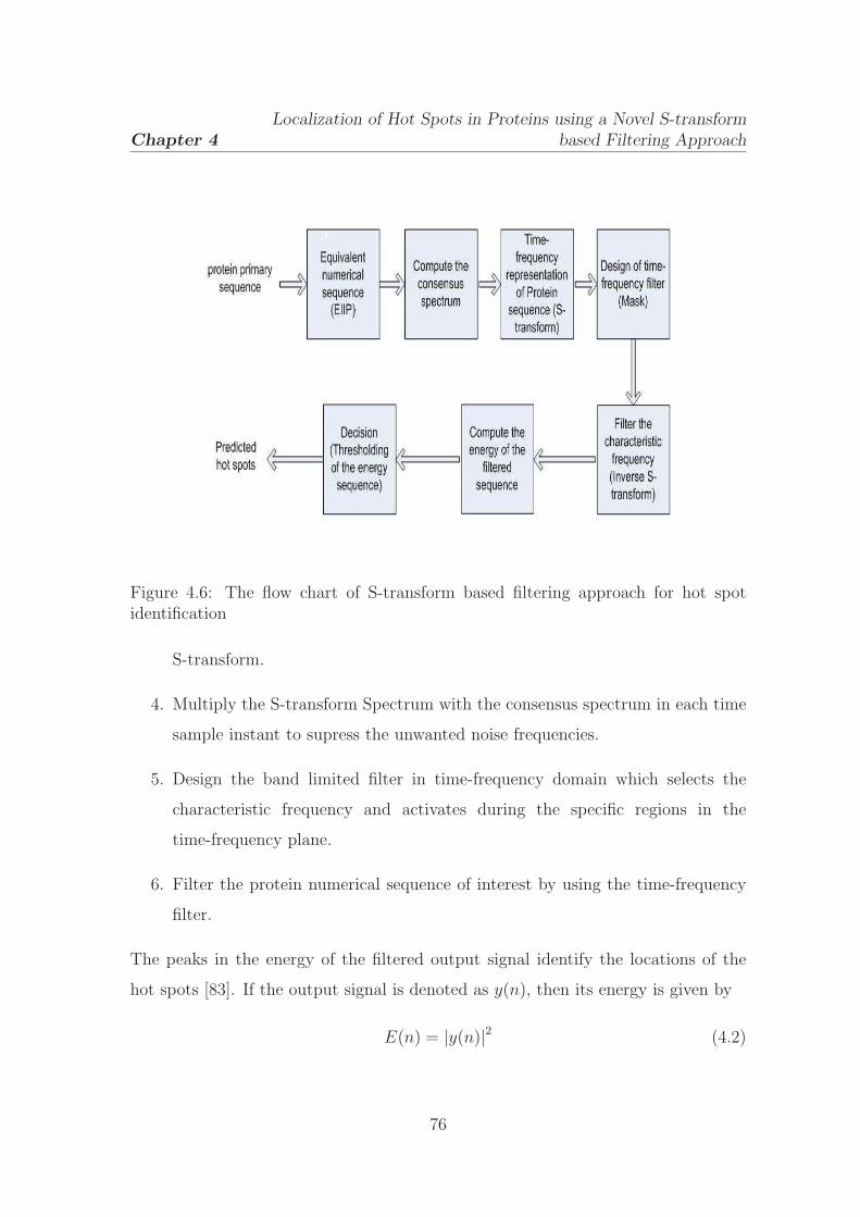
Chapter 4



Figure 4.6: The flow chart of S-transform based filtering approach for hot spotidentification

S-transform.

4. Multiply the S-transform Spectrum with the consensus spectrum in each time

sample instant to supress the unwanted noise frequencies.

5. Design the band limited filter in time-frequency domain which selects the

characteristic frequency and activates during the specific regions in the

time-frequency plane.

6. Filter the protein numerical sequence of interest by using the time-frequency

filter.

The peaks in the energy of the filtered output signal identify the locations of the

hot spots [83]. If the output signal is denoted as y(n), then its energy is given by

E(n) = |y(n)|2 (4.2)

76

Chapter 4



This energy is referred to as the energy sequence corresponding to a protein at the

characteristic frequency.

4.6 Performance analysis of the proposed

approach

The potentiality of the proposed method is illustrated by using a set of 10 proteins

from different functional family obtained from the standard databases. In the dataset

each protein has no significance sequence similarity to any other protein. The

sequence length, characteristic frequency and PDB ID of the corresponding protein

are listed in Table 4.2. The detailed proeins in the same functional group used for

the computation of consensus spectrum are also provided in Table 4.3. There are

many freely available databases like protein data bank (PDB) [87], Swiss-Port [88]

etc., where the primary sequence of the proteins are available. These databases

are reliable and strongly recommended by the biological community. Protein hot

spot location data obtained through alanine-scanning mutagenesis (ASM) have been

compiled into an online database named the alanine scanning energetics database

(ASEdb) [84]. This is a standard repository for hot spot location data used and

maintained by the biological community. Each residue in the database is considered

as hot spot if its corresponding ∆∆G is equal or higher than 2.0 kcal/mol. On the

other hand the computational Robetta interface alanine scanning (Robetta-Ala) [66]

[67] is another method of hot spot prediction which employs the residue’s ∆∆G more

than 1 kcal/mol as threshold to predict the hot spots. These two are well known

energy based methods and have been used for the identification purpose. Hence

both the ASEdb and Robetta-Ala database has used as a benchmark to compare all

the hot spots identified by the proposed method.

4.6.1 Evaluation criteria

The hot spots in the protein sequence can be determined by comparing the energy

at the regions corresponding to characteristic frequency to a reference energy level

77

Chapter 4



Table 4.2: The protein sequences investigated

Organism Protein name PDB ID Sequence Characteristiclength frequency

Human Fibroblast Growth Factor 4fgf 146 0.904C.fimi Endoglucanase C 1ulo 152 0.093Bacteria Trap 1wap 75 0.247Human Human alpha hemoglobin 1vwt 142 0.023Human Human Growth Hormone (HGH) 3hhr 190 0.270Bacteria Barstar 1brs 89 0.321Bacteria Barnase 1brs 110 0.321Human Interleukin-4 (IL4) 1rcb 129 0.587E.Coli Colicin-E9 Immunity (IM9) 1bxi 86 0.190Human Human growth hormone binding 3hhr 203 0.270

(HGHbp)

which governs the resolution of the method. First energy at the characteristic

frequency is computed using Eq. (4.2) which gives rise to peaks at certain regions

where it is dominant in protein sequence. Then the average energy of the filtered

output is computed which is used as a reference level for indicating the hot spots in

protein sequence. The ratio of the energy at the peaks of the filtered sequence to

that average value is set as threshold (tp) criteria for identifying the hot spots. If tp is

1, the threshold is same as the average value, then the energy peaks which are more

than that is considered as hot spots. The efficiency of the method in identifying the

hot spots depends on the threshold value. Hence the tp value acts as a parameter

to control the resolution of the methods used.

4.6.2 Experimental study

To demonstrate the capability of the proposed method, the human basic bovine FGF

protein is used for the analysis and the identified hot spots are shown in Fig. 4.7.

The peaks correspond to the hot spot locations. These locations are identified by

putting a threshold in the energy sequence. The average energy as the threshold

78

Chapter 4



Table 4.3: Proteins of functional family used for computation of consensus spectrum

Protein name Swiss-Port IDFibroblast Growth Factor P05230,P09038,P15656,P55075,O15520,

O54769,Q9EPC2,Q9HCT0,Q9QY10Endoglucanase C P0C2S3,P14090,P19570,P27033,P37699,

P38534,Q93GB3,A3DJ77Trap P19466,P48064,Q2RHB9,Q8EQB3,

C5D3E7,Q9x6J6Human alpha hemoglobin P60524,P01958,P02062,P69905,P68871,P68050,

P01942,P01946,P68048Human Growth Hormone P10912,P16310,P16882,P19941,Q9JI97,(HGH) Q9TU69,Q02092,O46600Barstar P11540,A7FDT9,A9R1V5,B4TJT7,B5pWB6,

C5BAW5,C7MPS8,Q2SZB1,Q62H00Barnase P10912,P00648,D0KFB0,C9NF27,C6XRM1,

C6UF64,C4ZK78,B7M0V1Interleukin-4 (IL4) P05112,P07750,P16382,P20096,P30368,P42202,

P51744,Q8HYB1,Q04745Colicin-E9 Immunity (IM9) P13479,P15176,B9VMA0Human growth hormone P79108,P79194,Q9XSZ1,Q95JF2,Q95ML5,binding Q28575

value is shown by a dotted line. A threshold of 90 percentile of the average energy is

used to locate the hot spots in all the proteins studied. Hence the actual hot spots

for the ten proteins identified by the proposed method are calculated and compared

with those obtained by the digital filtering technique and also with the alanine scan

compiled from both the ASEdb and Robetta-Ala. The hot spots are listed in Table

4.4. It reveals that the proposed method identifies 79% of the total hotspots of

the proteins investigated which is 67% in digital filtering method. In this study

the hot spots obtained from the alanine scans (both ASEdb and Robetta-Ala) have

used as the reference for the comparison. For the detailed study of classification of

hot spots the receiver operating characteristic (ROC) analysis is used. The ROC

curve represents the trade off between the true positive rate (TPR) and the false

positive rate (FPR) achieved by the predictors for varying threhold values on the

79

Chapter 4



0 50 100 1500

1

2

3

4

5

6x 10

−4

Aminoacids location

Ene

rgy

at th

e C

hara

cter

istic

Fre

quen

cy

5

16

2437

48

58

70 81 96 103 112122

132

140

Figure 4.7: Hot spot locations of Human basic bovine FGF protein

average energy of the filtered sequence. These curves for the two methods are shown

in Fig. 4.8. We have also computed the performance measures such as sensitivity

(Sn), specificity (Sp), positive predictive value (PPV ), negative predictive value

(NPV ), area under the curve, (AUC) etc. for both the methods and are presented

in Table 4.5. It is clear that the proposed method provides superior performance

over the frequency domain digital filtering technique in identifying the hot spots.

Some more locations are also identified by the proposed scheme as false positive

which are considered as probable hot spots and are repoted in Table 4.6.

A comparison study of the results of the proposed scheme with the other existing

computational methods [68]- [74] has been done in order to calculate the efficiency of

the proposed method. These computational methods use the knowledge of ASEdb

database for the prediction of the hot spots. In order to have a common platform

to compare the performance of these methods with the proposed signal processing

method, the ASEdb has been used as a standard and used a subset of the dataset

containing five proteins forming complexes (hGH, hGHbp, Barnase, Barstar and

80

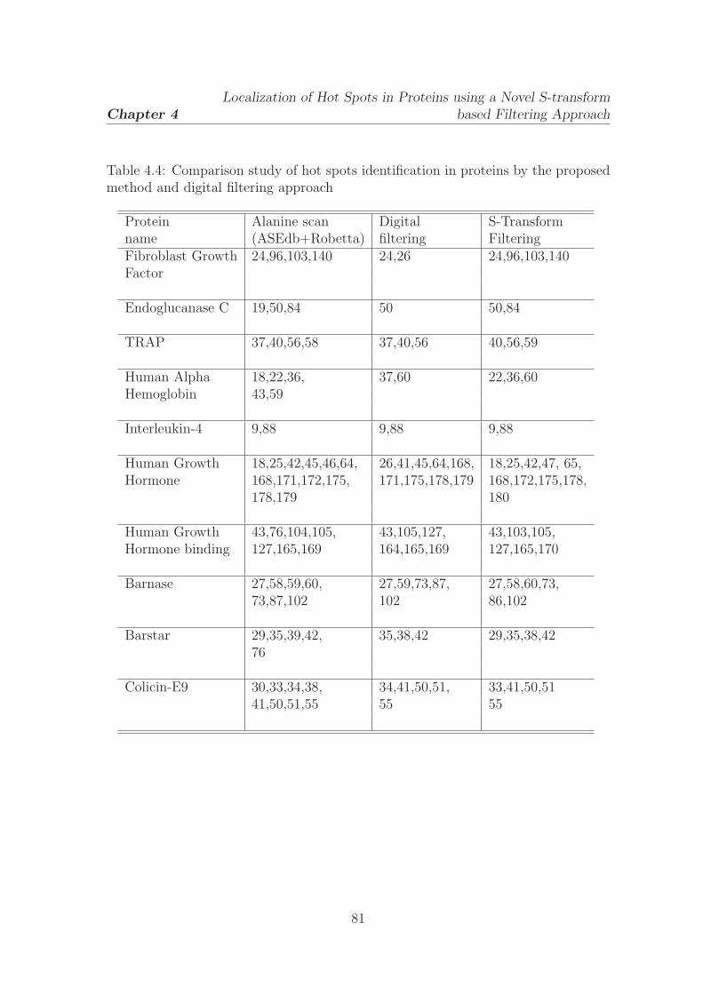
Chapter 4



Table 4.4: Comparison study of hot spots identification in proteins by the proposedmethod and digital filtering approach

Protein Alanine scan Digital S-Transformname (ASEdb+Robetta) filtering FilteringFibroblast Growth 24,96,103,140 24,26 24,96,103,140Factor

Endoglucanase C 19,50,84 50 50,84

TRAP 37,40,56,58 37,40,56 40,56,59

Human Alpha 18,22,36, 37,60 22,36,60Hemoglobin 43,59

Interleukin-4 9,88 9,88 9,88

Human Growth 18,25,42,45,46,64, 26,41,45,64,168, 18,25,42,47, 65,Hormone 168,171,172,175, 171,175,178,179 168,172,175,178,

178,179 180

Human Growth 43,76,104,105, 43,105,127, 43,103,105,Hormone binding 127,165,169 164,165,169 127,165,170

Barnase 27,58,59,60, 27,59,73,87, 27,58,60,73,73,87,102 102 86,102

Barstar 29,35,39,42, 35,38,42 29,35,38,4276

Colicin-E9 30,33,34,38, 34,41,50,51, 33,41,50,5141,50,51,55 55 55

81

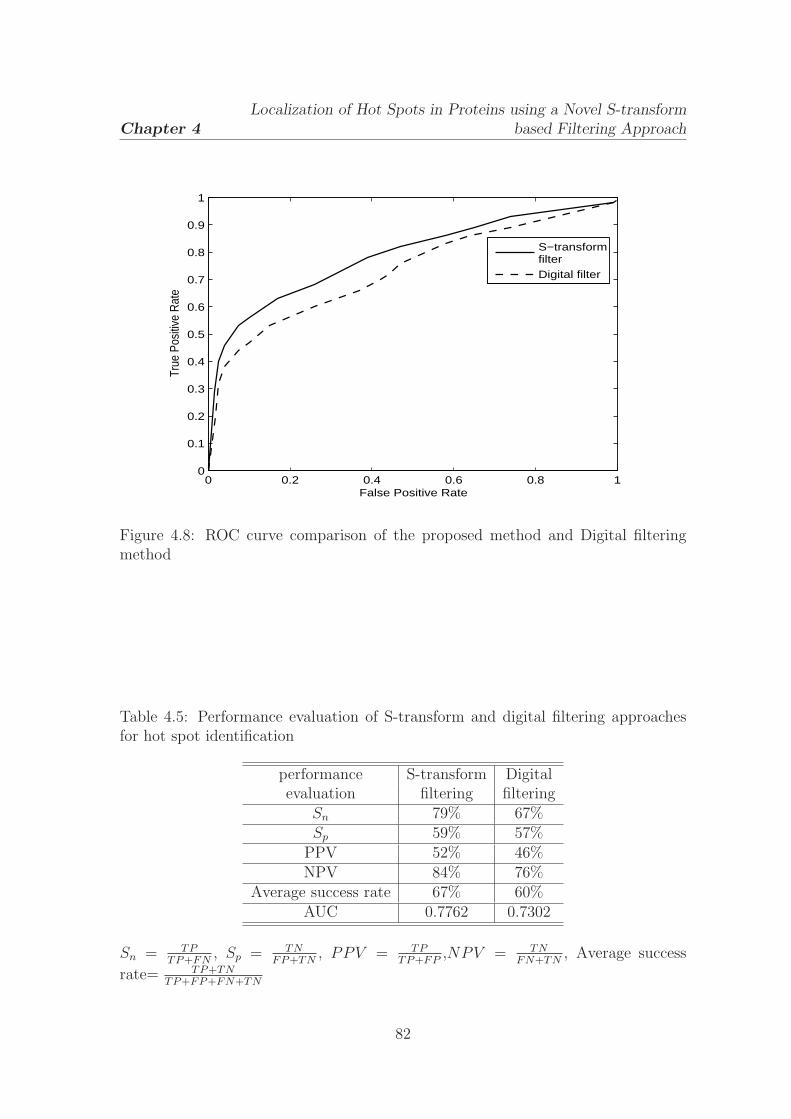
Chapter 4



0 0.2 0.4 0.6 0.8 10

0.1

0.2

0.3

0.4

0.5

0.6

0.7

0.8

0.9

1

False Positive Rate

True

Pos

itive

Rat

e

S−transformfilterDigital filter

Figure 4.8: ROC curve comparison of the proposed method and Digital filteringmethod

Table 4.5: Performance evaluation of S-transform and digital filtering approachesfor hot spot identification

performance S-transform Digitalevaluation filtering filtering

Sn 79% 67%Sp 59% 57%

PPV 52% 46%NPV 84% 76%

Average success rate 67% 60%AUC 0.7762 0.7302

Sn = TPTP+FN

, Sp = TNFP+TN

, PPV = TPTP+FP

,NPV = TNFN+TN

, Average success

rate= TP+TNTP+FP+FN+TN

82

Chapter 4



Table 4.6: The newly identified hot spots by the proposed S-transform filteringmethod

Protein name Newly identified hot spotsFibroblast Growth 6,16,37,48,58,70,81,112,122,132

Factor

Endoglucanase C 66,139

Trap 4,7,12,17,47,65,70

Human alpha 76,131hemoglobin

Human Growth 59,70,74,77,81,85,89,92,96,100,Hormone 103,107,147,150,154,158,161,184

Barstar 4,8,32,45,48,51,55,58,65

Barnase 3,6,9,12,20,65,69,79,82,89,92,96,99

Interleukin-4(IL4) 3,32,35,54,59,61,64,68,71,73,96,98,103,105,118,121,123,125

Colicin-E9 4,62,68,73,79,84Immunity(IM9)

Human growth 2,6,10,14,17,22,26,30,34,38,45,51,55,59,62,66,hormone binding 85,89,93,113,116,133,136,140,144,147,151,

155,159,175,180,183,187,191,195

83

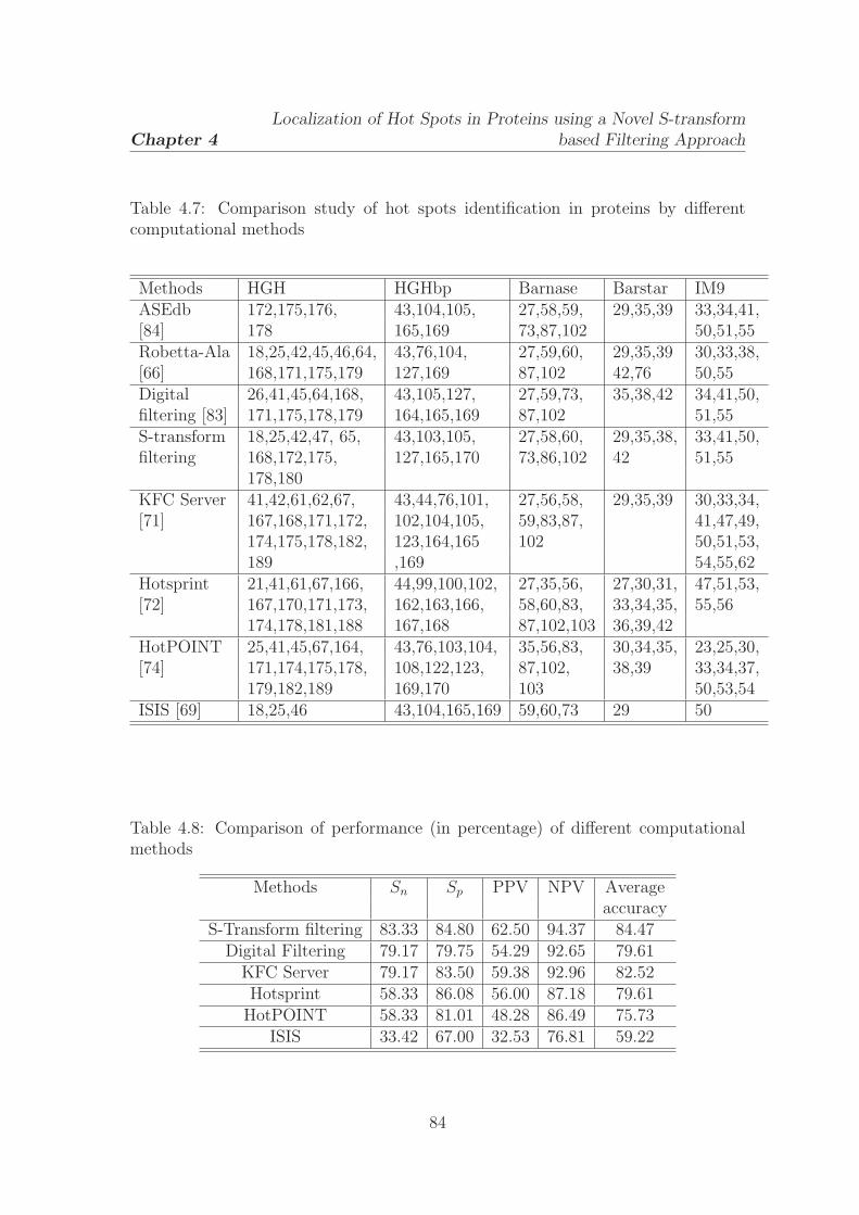
Chapter 4



Table 4.7: Comparison study of hot spots identification in proteins by differentcomputational methods

Methods HGH HGHbp Barnase Barstar IM9ASEdb 172,175,176, 43,104,105, 27,58,59, 29,35,39 33,34,41,[84] 178 165,169 73,87,102 50,51,55Robetta-Ala 18,25,42,45,46,64, 43,76,104, 27,59,60, 29,35,39 30,33,38,[66] 168,171,175,179 127,169 87,102 42,76 50,55Digital 26,41,45,64,168, 43,105,127, 27,59,73, 35,38,42 34,41,50,filtering [83] 171,175,178,179 164,165,169 87,102 51,55S-transform 18,25,42,47, 65, 43,103,105, 27,58,60, 29,35,38, 33,41,50,filtering 168,172,175, 127,165,170 73,86,102 42 51,55

178,180KFC Server 41,42,61,62,67, 43,44,76,101, 27,56,58, 29,35,39 30,33,34,[71] 167,168,171,172, 102,104,105, 59,83,87, 41,47,49,

174,175,178,182, 123,164,165 102 50,51,53,189 ,169 54,55,62

Hotsprint 21,41,61,67,166, 44,99,100,102, 27,35,56, 27,30,31, 47,51,53,[72] 167,170,171,173, 162,163,166, 58,60,83, 33,34,35, 55,56

174,178,181,188 167,168 87,102,103 36,39,42HotPOINT 25,41,45,67,164, 43,76,103,104, 35,56,83, 30,34,35, 23,25,30,[74] 171,174,175,178, 108,122,123, 87,102, 38,39 33,34,37,

179,182,189 169,170 103 50,53,54ISIS [69] 18,25,46 43,104,165,169 59,60,73 29 50

Table 4.8: Comparison of performance (in percentage) of different computationalmethods

Methods Sn Sp PPV NPV Averageaccuracy

S-Transform filtering 83.33 84.80 62.50 94.37 84.47Digital Filtering 79.17 79.75 54.29 92.65 79.61

KFC Server 79.17 83.50 59.38 92.96 82.52Hotsprint 58.33 86.08 56.00 87.18 79.61

HotPOINT 58.33 81.01 48.28 86.49 75.73ISIS 33.42 67.00 32.53 76.81 59.22

84

Chapter 4



Colicin E-9) for the analysis. Total 103 experimental alanine mutations from the

dimers have used for the study, out of which 39 residues are hot spots and rest are

non hot spot residues. The hot spots identified by these methods are presented in

Table 4.7 and the performance comparison is also repoted in Table 4.8. Table 4.8

clearly shows the superiority of our proposed approach over its counterparts as it

provides the best accuracy in predicting the hot spots.

4.7 Discussion of results

The identification of hot spots in protein by the proposed method is validated by

comparing the results with that obtained from biological methods like the alanine

scanning mutagenesis (ASM). Further the hot spots prediction of the proteins has

been analyzed in relation to the 3D structure. For the illustration purpose the

3D structure of the barnase-barstar complex (PDB ID:1brs) is shown in Fig. 4.9.

Barnase is green and barstar is sky-blue in color. The detected true hot spots

are marked as red spacefill for barnase and yellow spacefill for barstar. Similarly,

the probable hot spots are marked as red and yellow sticks for both the proteins

respectively. From Fig. 4.9, it has been seen that the detected true hot spots are

located at the interface region to the neighbour protein. Among the probable ones

some are located at the spatial vicinity of these true hot spots (Gly:65, Arg:69,

Thr:99 in barnase and Glu:32 val:45 in barstar) and are also interface residues

which may provide the structural scaffold of the interface and thus needs further

investigation. The remaining probable hotspots are placed far away from the faced

region, but falsely identified as hot spots. These possible hot spots may provide some

insight that may ameliorate the underlying functioning of the proteins. Although

the proposed S-transform based filtering method identifies the hot spots in a better

way, it also predicts some false positives. The limitations of this approach is that

it provides low frequency resolution at higher frequencies and low time resolution

at lower frequencies. At higher frequencies the signature of the events smears in

frequency direction where as in lower frequencies it smears in time direction. This

85

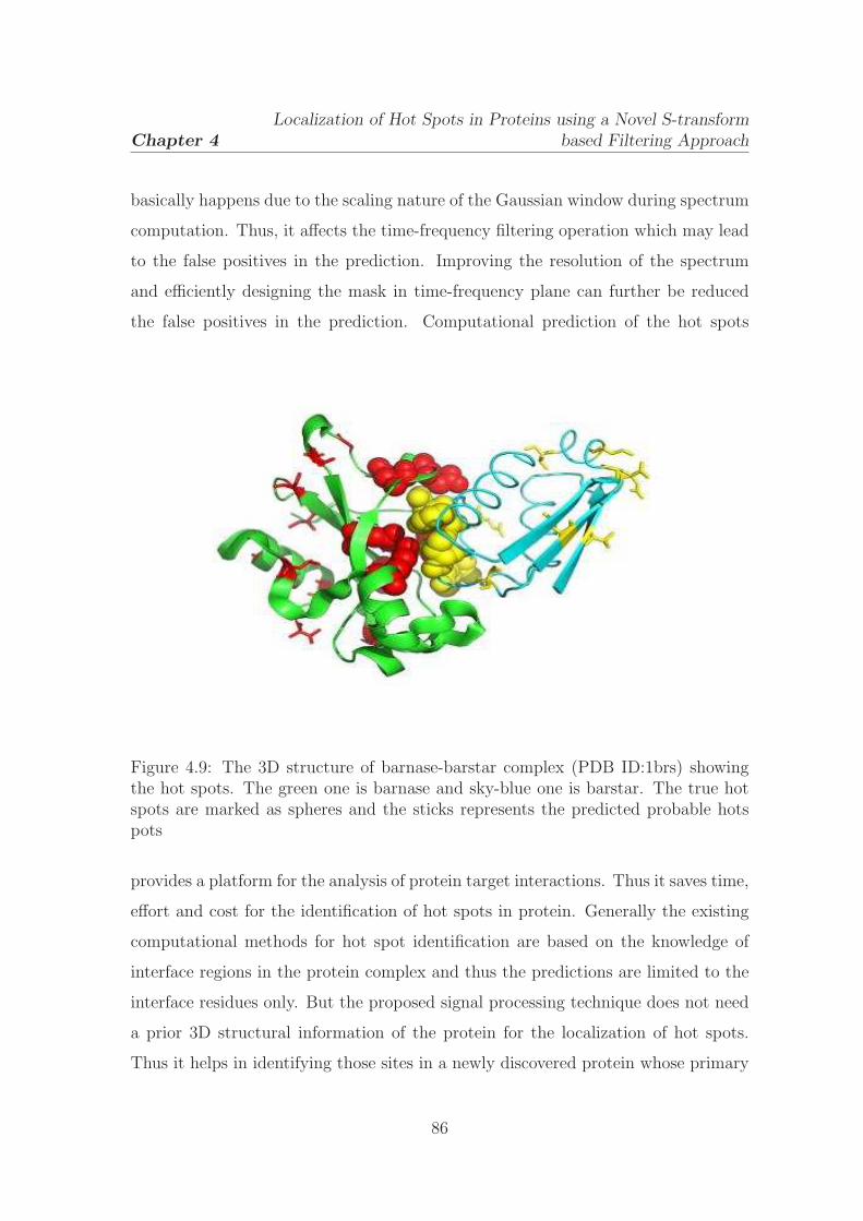
Chapter 4



basically happens due to the scaling nature of the Gaussian window during spectrum

computation. Thus, it affects the time-frequency filtering operation which may lead

to the false positives in the prediction. Improving the resolution of the spectrum

and efficiently designing the mask in time-frequency plane can further be reduced

the false positives in the prediction. Computational prediction of the hot spots

Figure 4.9: The 3D structure of barnase-barstar complex (PDB ID:1brs) showingthe hot spots. The green one is barnase and sky-blue one is barstar. The true hotspots are marked as spheres and the sticks represents the predicted probable hotspots

provides a platform for the analysis of protein target interactions. Thus it saves time,

effort and cost for the identification of hot spots in protein. Generally the existing

computational methods for hot spot identification are based on the knowledge of

interface regions in the protein complex and thus the predictions are limited to the

interface residues only. But the proposed signal processing technique does not need

a prior 3D structural information of the protein for the localization of hot spots.

Thus it helps in identifying those sites in a newly discovered protein whose primary

86

Chapter 4



sequence information only is available.

In-depth study of the nature of protein interactions would further facilitate

development of various new effective drugs and molecular medicines. It would

help in designing peptides with desired spectral and functional characteristics. The

computational identification of the new hot spots by our approach would also help

in the experimental process of effective mutation.

4.8 Conclusion

In this chapter, a new approach for the identification of the hot spots in protein using

S-transform based filtering has been developed. The effectiveness and accuracy of the

proposed method are evaluated by taking some protein sequences and the results

are compared with those obtained by other existing methods. The results have

demonstrated that the proposed method provides improved identification capacity

of hot spots compared to the digital filtering and other existing methods. In addition,

the new approach has identified some unknown locations of hot spots which need

further analysis and investigation. As the proposed method do not use the knowledge

of the structure of protein complex, hence it can be effectively employed in hot spot

prediction where the interface region is unknown.

87

A Novel Feature Representation

based Classification of Protein

Structural Class

Chapter 5

A Novel Feature Representationbased Classification of ProteinStructural Class

5.1 Introduction

In the post genomic era, study of sequence to structure relationship and functional

annotation plays an important role in molecular biology. In this context the protein

fold prediction is one of the major problems in protein science. The structural

class has become one of the most important features for characterizing the overall

folding type of a protein and has played an important role in rational drug design,

pharmacology and many other applications [89]. The functions of protein are

relevant to its 3D structure and can be efficiently determined by the sequence and

structure analysis [90–92]. The knowledge of protein structural class provides useful

information towards the determination of protein structure. The exponential growth

of newly discovered protein sequences by different scientific community has made a

large gap between the number of sequence-known and the number of structure-known

proteins. Hence, there exists a critical challenge to develop automated methods for

fast and accurate determination of the structures of proteins in order to reduce the

gap. Therefore, there is a need to develop computational methods for identifying

the structural classes of newly found proteins based on their primary sequence.

The concept of protein structural classes was reported by Levitt and Chothia [93]

89

Chapter 5

A Novel Feature Representation based Classification of Protein

Structural Class

Figure 5.1: The four structural classes of protein

on a visual inspection of polypeptide chain topologies in a dataset of 31 globular

proteins. They have proposed ten structural classes, four principal and six small

classes of protein structures. But the biological community follows the first four

principal classes, which are: all-α, all-β, α+ β and α/β. The all-α and all-β classes

represent structures that consist of mainly α-helices and β-strands, respectively.

The α/β and α + β classes contain both α-helices and β-strands which are mainly

interspersed and segregated. The α class proteins contain more than 45% α-helices

and less than 5% β-strands. The β class proteins comprise of less than 5% α-helices

and more than 45% β-strands. The α + β class proteins contain more than 30%

α-helices and more than 20% β-strands with dominantly anti-parallel β-strands. The

α/β class proteins contain more than 30% α-helices and more than 20% β-strands,

90

Chapter 5


Structural Class

with dominantly parallel β-strands. These class definitions are well accepted and

are still commonly used by many researchers. A pictorial view of the four structural

classes of protein is shown in Fig. 5.1.

5.1.1 Review of protein structural class prediction

The problem of predicting protein structural classes from the primary sequence

is mainly focused on two aspects. The first one is effective representation of

the protein sequence and the second one is the development of the powerful

classification algorithms to efficiently predict the desired class. Many in-silico

structural class prediction algorithms and methods have been proposed in the last

few decades. During this period many amino acid indices and features are used

for the assignment of the protein sequence. Nakashima et al. [94] have indicated

that the protein structural classes are strongly related to amino acid composition

(AAC). Later on auto-correlation functions based on non-bonded residue energy,

polypeptide composition [95] and complexity measure factor [96] have been used

by many researchers. Subsequently several classification methods such as distance

classifier [97] [98], component coupled methods [99], principal component analysis

[97], Bayesian classifier, fuzzy clustering [100] [101], neural network [102] [103], rough

sets [104] and support vector machines [105] [106] [107] have been suggested in

the literature. Although promising results have been achieved in many cases, the

representation of protein with the AAC lacks the sequence-order and sequence-length

information [108] [109]. Though the amino acid composition pattern of a protein

is closely related to its cell attributes, it is unable to distinguish between two

protein sequences with the same AAC, but different orders of arrangement. Hence,

the sequence order effect should not be ignored as a factor relating to protein

structure [110]. Chou introduced a new concept of pseudo amino acid composition

(PseAAC) [109] [111], in which both the sequence order and length information of

the protein sequence have been considered for the representation of the protein and

is used to predict various attributes of it. The introduction of PseAAC has greatly

91

Chapter 5


Structural Class

stimulated the development of protein structural class prediction. Various variants

of the PseAAC have also been also reported. Many other information regarding

the protein sequence has been embedded in the PseAAC to optimally reflect the

sequence order and length effects. Zhan Li et al. [112] have incorporated the wavelet

power spectrum into the PseAAC to reflect the long range interaction of amino

acids in the protein. Hui Liu et al. [113] [114] have used the Fourier spectrum

analysis with the PseAAC to improve the membrane protein prediction. Basically

the objective of all these representations is to form a discrete model to predict various

attributes of protein. In this chapter a novel method of PseAAC has been proposed

by suitably embedding the amino acid composition information, the amphiphilic

correlation factors and the spectral characteristics of the protein. The proposed

feature vector is expected to reflect the sequence pattern information relevant to the

structure of the protein.

5.2 Feature representation method of protein

5.2.1 Amino acid composition (AAC) feature of protein

In this form of representation, each protein is defined by a 20-dimensional feature

vector in Euclidean space. The protein corresponds to a point whose co-ordinates

are given by the occurrence frequencies of the 20 constituent amino acids.

For a query protein x, let fi(x)(i = 1, 2, · · · , 20) represents the occurrence

frequencies of its 20 constituent amino acids. Hence, the composition of the amino

acids (pk) in the query protein is given by

pk(x) =fk(x)

∑20i=1 fi(x)

, i, k = 1, 2, · · · , 20 (5.1)

The protein x in the composition space is defined as

P (x) = [p1(x), p2(x), · · · , p20(x)] (5.2)

In this type of representation, the protein sequence order and length information are

completely lost which in turn affects the prediction accuracy.

92

Chapter 5


Structural Class

5.2.2 Amphiphilic Pseudo amino acid composition(AmPseAAC) feature of protein

To include all the details of its sequence order and length, the sample of a

protein must be represented by its entire sequence. Unfortunately, it is not

feasible to establish a predictor with such a requirement, as it requires huge

experiments. Further, the lengths of protein sequences vary widely, which pose

an additional difficulty for admitting the sequence-order information in the feature

extraction of protein [116]. To alleviate this problem Chou [111] has proposed an

effective way of representation of protein known as pseudo amino acid composition

(PseAAC). In this representation, the protein character sequence is coded by some

of its physicochemical properties. The hydrophobicity and hydrophilicity of the

constituent amino acids in a protein play very important role on its folding, its

interaction with the environment and other molecules, as well as its catalytic

mechanism [117]. Thus these two indices may be used to effectively reflect the

sequence order effects. Different types of proteins have different amphiphilic features,

corresponding to different hydrophobic and hydrophilic order patterns. Thus, the

sequence-order information of protein can be derived quite effectively as follows:

Suppose a protein P with a sequence of L amino acid residues is defined as

P1P2P3 · · · · · · · · · · · ·PL

where P1 represents the residue at position 1 along the sequence, P2 the residue

at position 2 and so forth. The sequence order effect along a protein chain is

approximately reflected by a set of sequence order correlation factors defined as

θτ =1

L− τ

L−τ∑

i=1

Θ(Pi, Pi+τ ), (τ = 1, 2, · · · , λ and λ < L) (5.3)

In Eq. (5.3), L and θτ denote the length of the protein and the τ th rank of

coupling factor that harbors the τ th sequence order correlation factor respectively.

The correlation function Θ(Pi, Pj) may assume different forms of representation.

93

Chapter 5


Structural Class

The Θ(Pi, Pj) term is defined as

Θ(Pi, Pj) = H(Pi) ×H(Pj) (5.4)

where H(Pi) and H(Pj) represent hydrophobicity values of the amino acids Pi and

Pj, respectively. Similarly the correlation factors for hydrophilicity values are also

calculated. These two types of correlation factors form the basis of amphiphilic

pseudo AAC (AmPseAAC) feature vector of a protein which have been successfully

employed for predicting the enzyme subfamily classes and membrane protein types

[110] [113]. The hydrophobicity and hydrophilicity values of the amino acids defined

by Tanford [118] and Hopp & Woods [119] are used in this study. These values are

listed in Table 5.1. In Eq. (5.3), θ1 is called the first tier correlation factors that

reflect the sequence order correlation between the most contiguous residues along

the protein sequence through hydrophobicity and hydrophilicity. θ2 corresponds

to the second tier correlation factors that reflect the sequence order correlation

between all the second most contiguous residues and so forth. Before substituting

the hydrophobicity and hydrophilicity values in Eq. (5.4), these are subjected to a

standard conversion. The objective of the conversion is to make the coded sequence

as zero mean over the 20 native amino acids. It remains unchanged if it undergoes

through the same conversion procedure again. Hence a considerable amount of

sequence order information has been incorporated into the 2λ correlation factors

through the amphiphilic values of the amino acid residues along a protein chain.

5.2.3 Spectrum based feature of protein

The key idea in this study is to establish a powerful identifier that can catch their

characteristic sequence patterns for different structural classes. Primary structure

of proteins occasionally shows periodic pattern of hydrophobicity. The periodicity

in the hydrophobicity of amino acid sequence was studied for intrinsic membrane

proteins [120]. As a result the frequency information of the sequence pattern are

more effectively incorporated into a set of discrete components, and the prediction

algorithms are used in a straight forward manner on such a formulation of protein

94

Chapter 5


Structural Class

samples [113] [114]. The frequency information is collected by transferring the

protein coded sequence to frequency domain. The goal of this spectral analysis is to

identify the distribution of the power contained in a signal over the frequencies.

The DFT is a potential tool to transform the discrete protein sequence to its

Table 5.1: The Hydrophobicity and Hydrophilicity values of the amino acids

Amino acid Hydrophobicity HydrophilicityAla (A) 0.62 -0.5Cys (C) 0.29 -1.0Asp (D) -0.90 3.0Glu (E) -0.74 3.0Phe (F) 1.19 -2.5Gly (G) 0.48 0.0His (H) -0.40 -0.5Ile (I) 1.38 -1.8

Lys (K) -1.50 3.0Leu (L) 1.06 -1.8Met (M) 0.64 -1.3Asn (N) -0.78 0.2Pro (P) 0.12 0.0Gln (Q) -0.85 0.2Arg (R) -2.53 3.0Ser (S) -0.18 0.3Thr (T) -0.05 -0.4Val (V) 1.08 -1.5Trp (W) 0.81 -3.4Tyr (Y) 0.26 -2.3

corresponding frequency domain. The DFT of the protein sequence (P ) is defined

as

X(k) =L∑

n=1

H(pn)e(−j2πnk

L), k = 1, 2, · · · · · · , L (5.5)

where X(k) represents the periodicity features and the compositional pattern by

sinusoidal waves with various frequencies. Therefore, the sequence order effect of

the protein is partially reflected by the Fourier coefficients [113]. The amplitude

95

Chapter 5


Structural Class

spectra contain the information about the signal and also exhibit the amino acids

sequence order of a protein. The high frequency components are mostly due to noise

and hence the low frequency components are more important [121]. This is similar

to the case of protein internal motions where the low frequency components imply

more biological functions [122] [123]. These dominant low frequency motions have

a major effect on the structure (both alpha helix and beta sheets) formation of the

protein. Hence the low frequency components are chosen as effective feature vector.

5.3 The proposed DCT amphiphilic

pseudo amino acid composition feature

representation scheme of protein

In this work, discrete cosine transform (DCT) [5] has been introduced as a suitable

feature extractor of the complex Fourier coefficients. The DCT is a very well studied

real valued technique and has been successfully used in variety of applications [6] [7].

Due to its useful properties, the DCT is chosen to be a better substitute of DFT in

the context of feature extraction of protein sequences. A brief introduction of DCT

is provided in chapter 2.

The low-frequency components of DCT represent the global information [122] [123]

of the coded sequence. The type of structural class of protein is represented by the

curve of the hydrophobic values of the residues whose global shape represented by the

low-frequency components of the DCT. Hence, the low frequency DCT coefficients

can be used to represent the spectral characteristics of the protein.

In the previous studies, the Fourier spectra of the discrete protein sequence have

been incorporated into the Chou’s pseudo amino acid composition process to form

a feature vector [113] [114]. In many investigations the energy spectra of the

correlation factors [121] [124] have also been used in the pseudo AAC method to

represent a protein sample. Thus, both the correlation factors and the frequency

spectra of the protein sequence have been employed in the pseudo AAC process to

formulate a novel feature representation method. The correlation factors retain the

96

Chapter 5


Structural Class

sequence order effect of the protein sequence and the low frequency coefficients

of DCT preserves the global information of the protein sequence along with

some of the order effect.Therefore, the AAC, the 2λ correlation factors of both

hydrophobic and hydrophilic sequences and the δ low frequency DCT coefficients

are embedded together to form the new pseudo amino acid composition vector, the

DCTAmPseAAC. Accordingly, a protein sample is represented in the new PseAAC

form as

P =

p1

...

p20

p20+1

...

p20+λ

p20+λ+1

...

p20+2λ

p20+2λ+1

...

p20+2λ+δ

where

pu =

fu

20∑

i=1fi +w

2λ∑

j=1θτ+w

δ∑

k=1γk

, (1 ≤ u ≤ 20)

wθu−2020∑

i=1fi +w

2λ∑

j=1θτ+w

δ∑

k=1γk

, (20 + 1 ≤ u ≤ 20 + 2λ)

wγu−(20+2λ)

20∑

i=1fi +w

2λ∑

j=1θτ+w

δ∑

k=1γk

, (20 + 2λ+ 1 ≤ u ≤ 20 + 2λ+ δ)

(5.6)

where fi, i = 1, 2, · · · · · · , 20 are the normalized occurrence frequencies corresponding

to 20 native amino acids in the protein P , the symbol θj represents the j-tier sequence

correlation factor computed using (5.3) . The low frequency DCT coefficients of

97

Chapter 5


Structural Class

the protein are denoted by γk and the symbol w represents the weight factor which

governs the degree of the sequence order effect to be incorporated. The first 20 values

in Eq. (5.6) represent the classic amino acid composition, the next 2λ values reflect

the amphiphilic sequence correlation along the protein chain and the remaining δ

discrete values contain the low frequency global information of the protein.

5.4 Classification strategy

In recent past, many statistical and machine learning algorithms have been applied

to accurately predict the protein structural class. In this work, a kind of neural

network classifier known as radial basis function neural network has been employed

for classification. The RBF networks are suitable for solving function approximation

and pattern classification problems [125] [25] because of their simple topological

structure and their ability to learn in an explicit manner. In the classical RBF

network, there is an input layer, a hidden layer consisting of nonlinear node function,

an output layer and a set of weights to connect the hidden layer and output layer.

The basis functions are usually chosen as Gaussian and the number of hidden units

are fixed apriori using some properties of input data. The weights connecting the

hidden units to the output layer are normally adapted following a least mean square

algorithm. A brief introduction to radial basis function neural network has been

discussed in chapter 2. The complete process of the feature representation and the

class prediction is presented in Fig. 5.2.

5.5 Performance measures

Conventionally, in statistical prediction and classification problems, the prediction

quality generally measured by three typical tests such as re-substitution test,

independent datasets and jackknife test [91].

The re-substitution test is used to examine the self-consistency of a prediction model.

During this process the class label of each protein in the database is predicted using

98

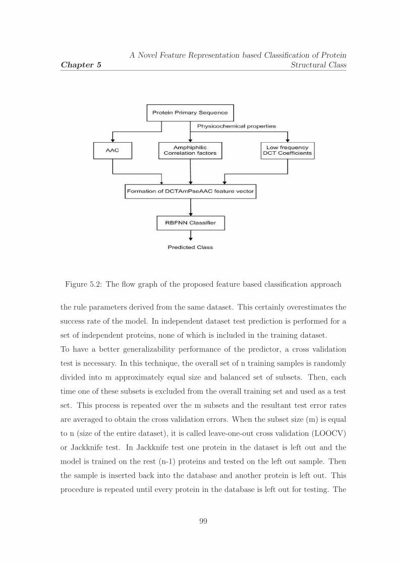
Chapter 5


Structural Class

Figure 5.2: The flow graph of the proposed feature based classification approach

the rule parameters derived from the same dataset. This certainly overestimates the

success rate of the model. In independent dataset test prediction is performed for a

set of independent proteins, none of which is included in the training dataset.

To have a better generalizability performance of the predictor, a cross validation

test is necessary. In this technique, the overall set of n training samples is randomly

divided into m approximately equal size and balanced set of subsets. Then, each

time one of these subsets is excluded from the overall training set and used as a test

set. This process is repeated over the m subsets and the resultant test error rates

are averaged to obtain the cross validation errors. When the subset size (m) is equal

to n (size of the entire dataset), it is called leave-one-out cross validation (LOOCV)

or Jackknife test. In Jackknife test one protein in the dataset is left out and the

model is trained on the rest (n-1) proteins and tested on the left out sample. Then

the sample is inserted back into the database and another protein is left out. This

procedure is repeated until every protein in the database is left out for testing. The

99

Chapter 5


Structural Class

Jackknife test is the most desired one and is a useful test used by most researchers

to test the efficiency of the prediction models.

5.6 Results and Discussion

5.6.1 Datasets

In order to compare the efficiency of the proposed method in predicting the structural

class of proteins, three standard data sets have been used. The first dataset

constructed by Chou [98] contains 204 proteins. The average sequence similarity

scores in the protein classes are 21% for all α, 30% for all β, 15% for α/β and 14%

for α+β class. Hence there is no significant sequence similarity between the proteins

in the dataset. Another two standard datasets constructed by Zhou [115] is also used

in the present study which contains 277 and 498 protein domains respectively. All the

three standard datasets have been used by many researchers in the class prediction

methods. In these datasets the number of protein domains in each class is listed in

Table 5.2.

Table 5.2: Benchmark datasets used for structural class prediction

Dataset All α All β α+ β α/β Total204 Domains 52 61 46 45 204277 Domains 70 61 81 65 277498 Domains 107 126 136 129 498

5.6.2 Experimental Results

To have a comparative performance study the proposed feature representation

method is analyzed with many well studied classifiers such as neural network (multi

layer perceptron), radial basis function network and linear discriminant analysis

(LDA). The success rates of all the classifiers are evaluated with all the three

benchmark datasets (204, 277 and 498 datasets). The results of the analysis are

100

Chapter 5


Structural Class

listed in Table 5.3. From this table, it is evident that the RBF classifier yields best

performance among all the classifiers and for all the three datasets. The average

prediction accuracy of RBF classifier for the three datasets is 93.77 which is almost

5 to 20% higher than those obtained by other classifiers. The prediction accuracy

associated with the 498 dataset is shown to be higher because it contains more

similar/duplicate sequences. Among the four structural classes, α+ β class is more

difficult to predict as it has relatively large variability of helix and strand content for

the protein as compared to other class. However, the proposed method also shows

improved classification performance for the α+ β class for all the datasets. Further

Table 5.3: Comparison of Jackknife classification accuracy (in percentage)of different classification algorithms using new (DCTAmPseAAC) featurerepresentation method

Dataset AlgorithmJackknife Accuracy

All α All β α+ β α/β Overall

204 DomainsRBF 90.38 95.08 89.13 95.56 92.54MLP 90.38 93.44 73.91 86.67 86.76LDA 86.54 93.44 67.39 64.44 79.41



the effect of different features derived from the protein primary sequence have been

examined on the classification accuracy. The classification accuracies of the AAC,

AmPseAAC, and the proposed DCTAmPseAAC method are compared with the

radial basis function network as the classifier. In case of AmPseAAC, empirical

study showed that when λ is set to 10, best performance is achieved for all dataset.

In case of DCT based methods best performance is also observed when δ is chosen to

be 10. Hence 20 amino acid composition features, 20 amphiphilic correlation factors

and 10 low frequency DCT components are embedded together to form the novel

101

Chapter 5


Structural Class

DCTAmPseAAc feature vector. Thus total 50 features have been used to represent

a protein sample. The weight factor (w) is chosen as 0.01 to normalize the feature

vector. The comparative results of all the three representations are summarized

in Table 5.4. The success rate of the proposed feature representation method is

found to be the best as compared to those obtained by others. Hence, it is inferred

that the proposed method captures features more relevant to the protein structure.

Further the classification performance of the proposed feature representation with

the RBF network is studied for the re-substitution and jackknife test. The results are

presented in Table 5.5 for the three datasets. It is interesting to observe that for the

re-substitution test it provides 100% accuracy for all the dataset and for Jackknife

test, the classification accuracy is also higher.The histogram representation of the

results of the proposed method is presented in annexure-II.

Table 5.4: Comparison of Jackknife classification accuracy (in percentage) usingdifferent feature representation methods

Dataset FeatureJackknife Accuracy


204 Domains

AAC 84.62 93.44 82.61 86.67 87.25AmPseAAC 88.46 96.72 80.96 84.44 89.71

DCTAmPseAAC 90.38 95.08 89.13 95.56 92.54

277 Domains

AAC 91.43 93.44 70.77 92.61 87.36AmPseAAC 92.86 95.08 73.85 93.83 89.17

DCTAmPseAAC 92.86 93.44 89.23 95.06 92.78

498 Domains

AAC 91.59 93.65 89.15 94.85 92.37AmPseAAC 90.52 93.65 90.70 97.79 93.57

DCTAmPseAAC 95.33 95.24 94.57 98.53 96.00

The performance of the new method is also compared with those obtained by

recently reported prediction methods and the results are summarized in Tables

5.6-5.8. For the 204 dataset the classification accuracy of proposed scheme is

compared with those obtained by the existing augmented covariant discriminant

algorithm [126], fuzzy clustering [100], logitboost technique [127] [128], nearest

102

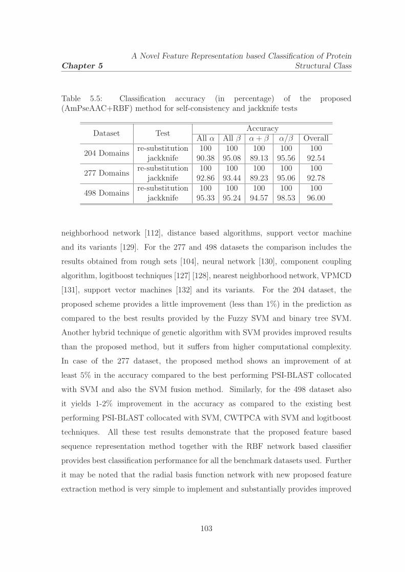
Chapter 5


Structural Class

Table 5.5: Classification accuracy (in percentage) of the proposed(AmPseAAC+RBF) method for self-consistency and jackknife tests

Dataset TestAccuracy


204 Domainsre-substitution 100 100 100 100 100

jackknife 90.38 95.08 89.13 95.56 92.54


jackknife 92.86 93.44 89.23 95.06 92.78


jackknife 95.33 95.24 94.57 98.53 96.00

neighborhood network [112], distance based algorithms, support vector machine

and its variants [129]. For the 277 and 498 datasets the comparison includes the

results obtained from rough sets [104], neural network [130], component coupling

algorithm, logitboost techniques [127] [128], nearest neighborhood network, VPMCD

[131], support vector machines [132] and its variants. For the 204 dataset, the

proposed scheme provides a little improvement (less than 1%) in the prediction as

compared to the best results provided by the Fuzzy SVM and binary tree SVM.

Another hybrid technique of genetic algorithm with SVM provides improved results

than the proposed method, but it suffers from higher computational complexity.

In case of the 277 dataset, the proposed method shows an improvement of at

least 5% in the accuracy compared to the best performing PSI-BLAST collocated

with SVM and also the SVM fusion method. Similarly, for the 498 dataset also

it yields 1-2% improvement in the accuracy as compared to the existing best

performing PSI-BLAST collocated with SVM, CWTPCA with SVM and logitboost

techniques. All these test results demonstrate that the proposed feature based

sequence representation method together with the RBF network based classifier

provides best classification performance for all the benchmark datasets used. Further

it may be noted that the radial basis function network with new proposed feature

extraction method is very simple to implement and substantially provides improved

103

Chapter 5


Structural Class

classification compared to those obtained by other reported classifiers.

5.7 Conclusion

In this chapter, a new promising feature representation method is presented by

embedding the amino acid composition, the amphiphilic correlation factors and the

low frequency DCT coefficients to represent a protein sample. The results of the

Jackknife cross validation test using the standard datasets shows that the proposed

method can be used as an efficient approach for predicting protein structural class.

The present study also demonstrates that the composition of all the three features

better reflects the overall sequence pattern of a protein than the individual one and

enhance the success rate of prediction. The comparison study of the proposed scheme

in association with a simple radial basis function network with the existing methods

showed improvement of 2-5% using the standard datasets. The high success rate

suggests that the proposed feature representation method can be used as a potential

candidate for the protein structural class prediction and also for other related areas.

104

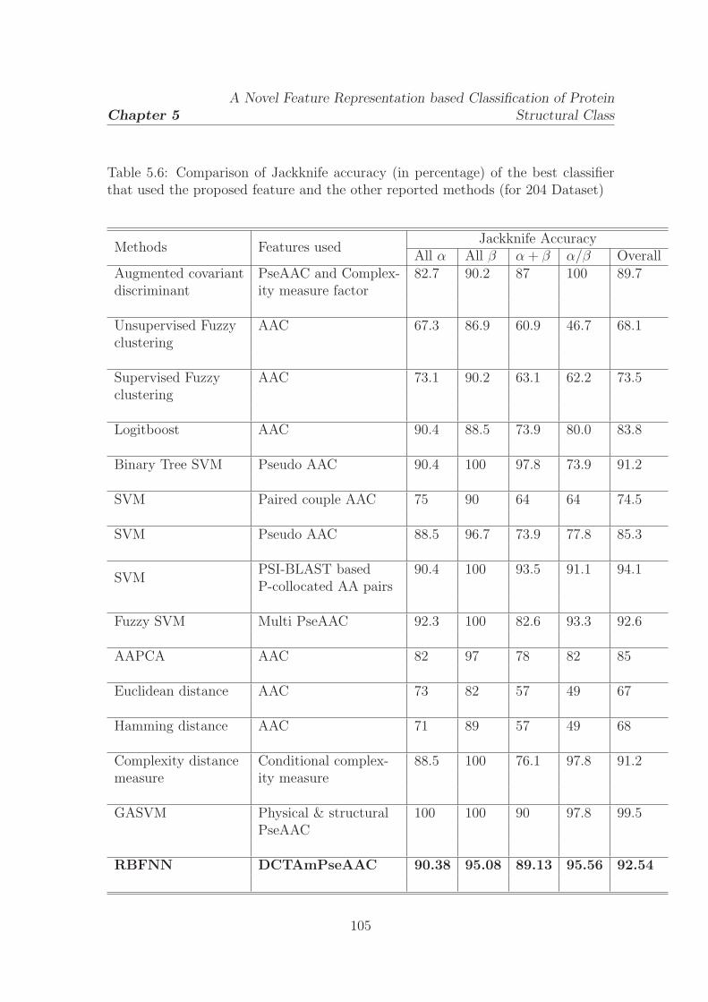
Chapter 5


Structural Class

Table 5.6: Comparison of Jackknife accuracy (in percentage) of the best classifierthat used the proposed feature and the other reported methods (for 204 Dataset)

Methods Features usedJackknife Accuracy

All α All β α+ β α/β OverallAugmented covariant PseAAC and Complex- 82.7 90.2 87 100 89.7discriminant ity measure factor

Unsupervised Fuzzy AAC 67.3 86.9 60.9 46.7 68.1clustering

Supervised Fuzzy AAC 73.1 90.2 63.1 62.2 73.5clustering

Logitboost AAC 90.4 88.5 73.9 80.0 83.8

Binary Tree SVM Pseudo AAC 90.4 100 97.8 73.9 91.2

SVM Paired couple AAC 75 90 64 64 74.5

SVM Pseudo AAC 88.5 96.7 73.9 77.8 85.3

SVMPSI-BLAST based 90.4 100 93.5 91.1 94.1P-collocated AA pairs

Fuzzy SVM Multi PseAAC 92.3 100 82.6 93.3 92.6

AAPCA AAC 82 97 78 82 85

Euclidean distance AAC 73 82 57 49 67

Hamming distance AAC 71 89 57 49 68

Complexity distance Conditional complex- 88.5 100 76.1 97.8 91.2measure ity measure

GASVM Physical & structural 100 100 90 97.8 99.5PseAAC

RBFNN DCTAmPseAAC 90.38 95.08 89.13 95.56 92.54

105

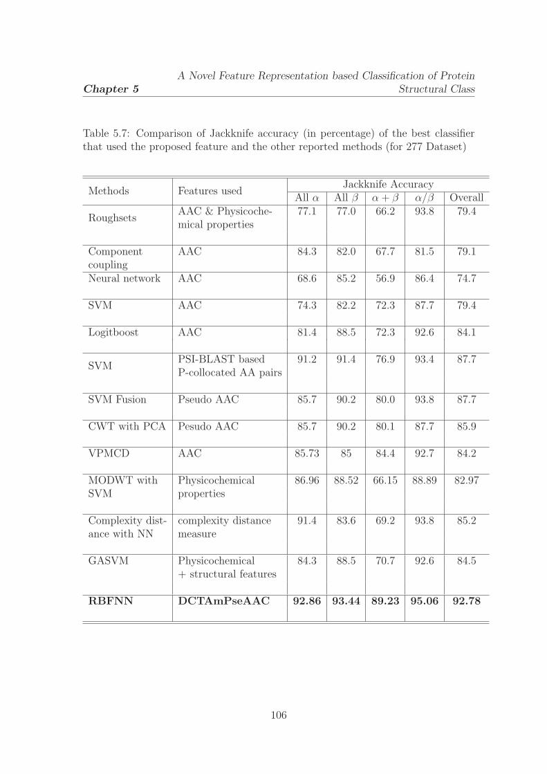
Chapter 5


Structural Class




RoughsetsAAC & Physicoche- 77.1 77.0 66.2 93.8 79.4mical properties

Component AAC 84.3 82.0 67.7 81.5 79.1couplingNeural network AAC 68.6 85.2 56.9 86.4 74.7

SVM AAC 74.3 82.2 72.3 87.7 79.4

Logitboost AAC 81.4 88.5 72.3 92.6 84.1

SVMPSI-BLAST based 91.2 91.4 76.9 93.4 87.7P-collocated AA pairs

SVM Fusion Pseudo AAC 85.7 90.2 80.0 93.8 87.7

CWT with PCA Pesudo AAC 85.7 90.2 80.1 87.7 85.9

VPMCD AAC 85.73 85 84.4 92.7 84.2

MODWT with Physicochemical 86.96 88.52 66.15 88.89 82.97SVM properties

Complexity dist- complexity distance 91.4 83.6 69.2 93.8 85.2ance with NN measure

GASVM Physicochemical 84.3 88.5 70.7 92.6 84.5+ structural features


106

Chapter 5


Structural Class




RoughsetsAAC & Physicoche- 87.9 91.3 86.0 97.1 90.8mical properties

Component AAC 93.5 88.9 84.5 90.4 89.2couplingNeural network AAC 86.0 96.0 86.0 88.2 89.2

SVM AAC 88.8 95.2 91.5 96.3 93.2

Logitboost AAC 92.5 96.0 93.0 97.1 94.8

SVMPSI-BLAST based 98.0 93.3 93.4 95.6 94.9P-collocated AA pairs

SVM Fusion Pseudo AAC 99.1 96.0 91.5 80.9 91.4

CWT with PCA Pesudo AAC 94.4 96.8 92.3 97.0 95.2

VPMCD AAC 93.5 94.3 92.2 97.7 94.5

MODWT with Physicochemical 93.3 94.4 90.7 97.04 93.94SVM properties

Complexity dista- complexity distance 96.3 93.7 89.9 95.6 93.8nce with NN measure

GASVM Physicochemical 96.3 93.6 89.2 97.8 94.2+ structural features

Hybrid neural Dipeptide composition 95.32 88.8 93.02 94.11 92.77discriminant model frequencies


107

An Efficient Hybrid Feature

Extraction Method for

Classification of Microarray

Gene Expression Data

Chapter 6

An Efficient Hybrid FeatureExtraction Method forClassification of Microarray GeneExpression Data

6.1 Introduction

The cells are the basic units in Human body which contain identical genetic material.

Only a few of these genes are active in every cell which determine the properties of

the cell [133]. Evaluation of turned on and turned off states in different cells helps

the scientists to understand the normal cell functions and how they are affected

when various genes do not perform properly. Many genes are used to specify

features unique to each type of cell. For example, Liver cells express genes for

enzymes that detoxify poisons, whereas pancreas cells express genes for making

insulin. To know how cells achieve such specialization, there is a need to identify

the genes expressed by each cell. Molecular biology research evolves through the

development of the technologies used for carrying them out. It is not possible to

research on a large number of genes using traditional methods. The DNA microarray

is one such technologies which helps the researchers to investigate and address

issues which were non-traceable earlier. One can analyze the expression of many

genes in a single reaction quickly and in an efficient manner. The DNA microarray

109

Chapter 6

An Efficient Hybrid Feature Extraction Method for Classification of Microarray


technology has empowered the scientific community to understand the fundamental

aspects underlining the growth and development of life as well as to explore the

genetic causes of anomalies occurring in the functioning of the human body. With

advanced statistical techniques, microarray analysis enables simultaneous study

of the entire genome in a single experiment [134]. It provides substantial effect

on tumor diagnosis and classification, prediction of prognosis and response to

therapy, and understanding of the molecular mechanisms of tumorigenesis and tumor

development. Gene expression profiling by microarray can further refine the future

for individualized treatment for cancer patients based on the molecular classification

of subtypes.

Microarray technology provides the possibility of creating datasets that capture

the information concerning all the relevant genes and proteins for many systems

of biological and clinical interest. Such datasets may help scientists to explore

gene expression patterns and discover gene interaction networks, and pathways

underlying various diseases and biological processes. Such discoveries can in turn

lead to better understanding of the physiological functions in healthy and diseased

cells, and to diagnose and treat diseases in a better way. Large-scale transcription

analyses using microarrays can reveal the molecular mechanisms of physiology

and pathogenesis, and therefore can help scientists to develop new diagnostic and

therapeutic strategies. Hence there is a need to develop faster, automatic and

efficient tools for the analysis of the microarray data.

6.2 Microarray Technology

A microarray is a tool or a laboratory technology for analyzing gene expression that

consists of a small membrane or glass slide or silicon chip containing samples of

many genes arranged in a regular pattern to test which genes are switched on or off

in diseased versus healthy human tissues. A microarray consists of different nucleic

acid probes that are chemically attached to a substrate, which can be a microchip,

a glass slide or a microsphere-sized bead. DNA targets are arrayed onto glass slides

110

Chapter 6



and explored with fluorescent or radioactively labeled probes. The wealth of this

kind of data in different stages of cell cycles helps to explore gene interactions and

to discover gene functions. The whole process is based on hybridization probing, a

technique that uses fluorescently labeled nucleic acid molecules as ”mobile probes”

to identify complementary molecules, and sequences that are able to base-pair with

one another. When a gene is activated, cellular machinery begins to copy certain

segments of that gene and produces messenger RNA (mRNA), which is the body’s

template for creating proteins. The mRNA produced by the cell is complementary,

therefore will bind to the original portion of the DNA strand from which it was

copied. To determine which genes are turned on and which are turned off in a given

cell, first the messenger RNA molecules present in that cell are collected. Then, each

mRNA molecule is labeled using a reverse transcriptase enzyme (RT) that generates

a complementary cDNA to the mRNA. During that process fluorescent nucleotides

are attached to the cDNA. The tumor and the normal samples are labeled with

different fluorescent dyes. The labeled cDNAs are placed onto a DNA microarray

slide which then hybridized to their synthetic complementary DNAs attached on the

microarray slide, leaving its fluorescent tag. Then a special scanner or microscope

is used to measure the fluorescent intensity for each spot/areas on the microarray

slide. If a particular gene is very active, it produces many molecules of messenger

RNA, thus more labeled cDNAs hybridize to the DNA on the microarray slide

and generates a very bright fluorescent area. Genes that are less active produce

fewer mRNAs, thus less labeled cDNAs, and results in dimmer fluorescent spots. If

there is no fluorescence, none of the messenger molecules hybridizes to the DNA,

indicating that the gene is inactive. Hence this technique is frequently used to

examine the activity of various genes at different times. A pictorial view of the

microarray technology is shown in Fig. 6.1. The tumor samples are indicated by

red dye and normal samples are marked by green. In the scanned picture of the

microarray slide, green represents the Control DNA, which indicates either DNA

or cDNA derived from normal tissue and red represents the Sample DNA, which

111

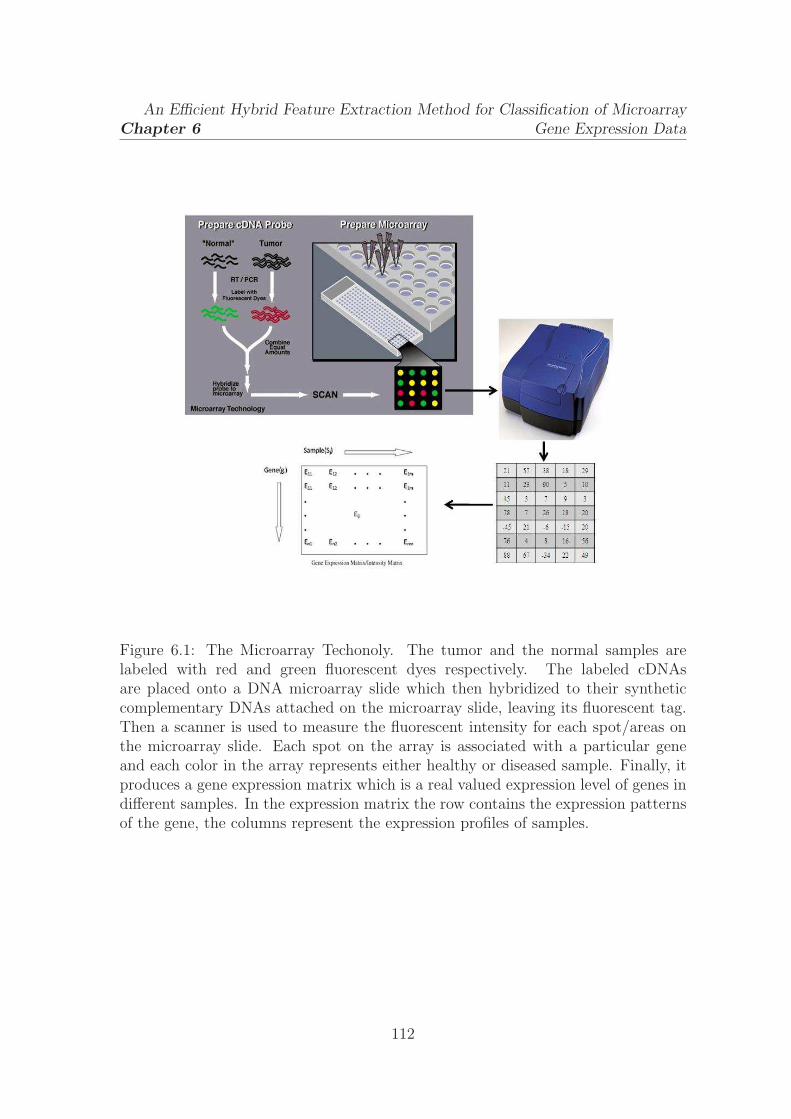
Chapter 6



Figure 6.1: The Microarray Techonoly. The tumor and the normal samples arelabeled with red and green fluorescent dyes respectively. The labeled cDNAsare placed onto a DNA microarray slide which then hybridized to their syntheticcomplementary DNAs attached on the microarray slide, leaving its fluorescent tag.Then a scanner is used to measure the fluorescent intensity for each spot/areas onthe microarray slide. Each spot on the array is associated with a particular geneand each color in the array represents either healthy or diseased sample. Finally, itproduces a gene expression matrix which is a real valued expression level of genes indifferent samples. In the expression matrix the row contains the expression patternsof the gene, the columns represent the expression profiles of samples.

112

Chapter 6



refers to either DNA or cDNA derived from diseased tissue. The yellow represents

a combination of Control and Sample DNA, where both are hybridized equally to

the target DNA. Black represent the areas where neither the Control nor Sample

DNA hybridized to the target DNA. Each spot on the array is associated with a

particular gene and each color in the array represents either healthy (control) or

diseased (sample) tissue. Depending on the type of array used, the location and

intensity of a color will tell us whether the gene, or mutation, is present in either

the control and/or sample DNA. It also provides an estimate of the expression level

of the gene(s) in the sample and control DNA. As a result, if the spot is red, this

means that specific gene is more expressed in tumor than in normal and if a spot

is green, that means that gene is more expressed in the normal tissue. If a spot is

yellow that means that that specific gene is equally expressed in normal and tumor

tissue.

6.2.1 Gene expression data

Generally a microarray experiment typically assesses a large number of DNA

sequences (genes, CDNA clones or expressed sequence tags) under multiple

conditions. These conditions may be a time series during a biological process or

a collection of different tissue samples (normal versus cancerous tissues). In this

chapter, studies have been carried out only on the tissue sample microarray data.

Generally a microarray experiment produces a gene expression matrix E = Eij, 1 ≤i ≤ n, 1 ≤ j ≤ m which is a real valued expression level of genes in different samples

as shown in Fig. 6.2. In the expression matrix, the row contains the expression

patterns of the gene, the columns represent the expression profiles of samples and

each cell is the measured expression level of gene ′i′ in sample ′j′.

6.3 Dimension reduction techniques

Dimension reduction is a subject of study in several research areas including

high-dimensional data analysis, pattern recognition, and machine learning, where

113

Chapter 6



Figure 6.2: The gene expression matrix

one seeks to explain observed high dimensional data using an underlying

low-dimensional representation. Dimension reduction has many applications in

bioinformatics and computational biology.

Generally the microarray experiments produce large datasets having expression

levels of thousands of genes with a very few samples (upto hundreds) i.e high

dimensional data. This creates a problem of “curse of dimensionality”. Due to

this high dimension, the accuracy of the classifier or predictor decreases as it attains

the risk of overfitting [135]. As the microarray data contains thousands of genes, a

large number of genes are not informative for classification because they are either

irrelevant or redundant. Providing a large number of features to learning algorithms

can make them inefficient for computational reasons. In addition, irrelevant data

may confuse algorithms making them to build inefficient classifiers while correlation

between feature sets causes the redundancy of information. Therefore, it is essential

to explore the data and utilize independent features to train classifiers. Hence to

derive a subset of informative or discriminative genes from the entire gene set is

a challenging task in microarray data analysis. The purpose of gene selection or

114

Chapter 6



dimension reduction is to simplify the classifier by retaining small set of relevant

genes and to improve the accuracy of the classifier. For this purpose, researchers

have applied a number of test statistics or discriminant criteria to find genes that

are differentially expressed between the investigated classes.

Dimensionality/feature reduction is essential and can be achieved either by

feature selection or transformation to a low dimensional space [136] [143]. The

feature selection deals with the reduction of original high dimensional data even

further such that the most relevant features are selected for the classification [145].

The methods used for feature selection in the context of microarray data analysis can

be broadly categorized into two groups: filter and wrapper approaches [134] [137].

In the filter approach, a selection process precedes the actual classification process

where features are evaluated only through intrinsic properties of the data. For

each feature a weight value is calculated, and features with better weight values

are chosen to represent the original data set. However, the filter approach does not

account for interactions between features. The wrapper model approach depends

on feature addition or deletion to compose subset features, and uses evaluation

function with a learning algorithm to estimate the subset features. This kind of

approach is similar to an optimal algorithm that searches for optimal results in

a dimension space. The wrapper approach usually conducts a subset search with

the optimal algorithm, and a classification algorithm is used to evaluate the subset.

Contrary to filter methods, wrapper methods select features specific to the classifier.

Hence, they are most likely to be more accurate than filter methods on a particular

classifier, but the features they choose may not be appropriate for other classifiers.

Another limitation of wrapper methods is that the wrappers are computationally

expensive because they need to train and test the classifier for each feature subset

candidate, which can be prohibitive when working with high-dimensional data (such

as text, image, gene, etc). In contrast to the feature selection, transformation based

methods allow modification of the input features to a new feature space. This

method deals with the extraction of relevant features by mapping the raw data

115

Chapter 6



onto a lower dimensional space while maintaining the vital information in terms of

unique attributes. In feature selection, the original representation of the variables

is not changed. Feature selection is typically preferred over transformation when

one wishes to keep the original meaning of the features and wishes to determine

which of those features are important. Moreover, once features are selected, only

these features need to be calculated or collected, whereas, in transformation based

methods, all input features are still needed to obtain the reduced dimension.

Various methods and techniques have been developed in recent past to perform

the gene selection to reduce the dimensionality problem. The filter method basically

use a criterion related to rank and select key genes for classification such as

Pearson correlation coefficient method [137], t-statistics method [138], signal-to-noise

ratio method [151] and many transformation methods such as the partial least

square method, independent component analysis [139], wavelet analysis [141] [142],

linear discriminant analysis and principal component analysis [140] have been used

to extract the important feature from the microarray data. All the methods

transform the original gene space to another domain providing reduced uncorrelated

discriminant components. In this chapter, a novel hybrid method has been proposed

which combines both the feature selection and extraction method to optimally

reflect the characteristics of the microarray data in few feature sets. A F-score

statistics is used to preselect the discriminative features from the raw microarray

data. Then a model is developed by auto regressive (AR) method to extract the

relevant information from gene space.

6.3.1 The F-score method of feature selection

F-score is a popular filter method for gene selection which is based on classical

F-statistics, a generalization of T-test for two sample comparison [146] [147]. F-score

criterion is the ratio of between class sum of squares to within class sum of squares of

individual genes. It is based on statistical F-test and is used for filtering genes with

near constant expression across all the samples from important genes. Intuitively,

116

Chapter 6



F-score will be larger for a gene whose expression varies relatively small within a

class compared to larger variations between other classes. In this method, a F-score

value of each feature in the dataset is computed to show their discriminative power.

The F-score value of ith feature of a two class problem is defined as:

F (i) =(X

c1i −X)2 + (X

c2i −X)2

1nc1−1

nc1∑

k=1

(xc1k,i −X

c1i )2 + 1

nc2−1

nc2∑

k=1

(xc2k,i −X

c2i )2

(6.1)

where X,Xc1i , X

c2i are the average expression level of gene i across all the samples

of c1 and c2 classes and xc1k,i, x

c2k,i are the kth instance of the ith feature for c1 and c2

classes.

The numerator of Eq. (6.1) shows the discriminating power between the classes

and the denominator reveals that within the individual classes. The larger is the

F-score, the more likely the feature is significant in classification. In order to select

the efficient features from entire dataset, a threshold value is employed on the

F-scores of all features. If the F-score value of any feature is bigger than threshold

value, the corresponding feature is added to feature space. Otherwise, it is removed

from feature space. Hence, F-score is the ratio of between class sum of squares to

within class sum of squares. For any gene, if between class sum of squares is very

high for few classes, it may blind the discriminating effect needed for other difficult

class prediction. As a result, many genes are selected for such strong class and a very

few are top ranked for difficult classes. A disadvantage of F-score is that it does not

reveal mutual information among features. Despite of these drawbacks, F-score is

simple and generally quite effective in feature selection in high dimensional dataset.

6.3.2 The AR modeling for feature extraction

The autoregressive model is a popular linear model employed for the modeling of time

series data generated by a stochastic process in application such as speech processing,

image processing, redundancy removal, pattern recognition, etc [41] [42] [148]. It is

a simple and robust method and requires no a priori knowledge of the sequence to

117

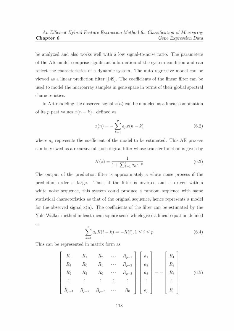
Chapter 6



be analyzed and also works well with a low signal-to-noise ratio. The parameters

of the AR model comprise significant information of the system condition and can

reflect the characteristics of a dynamic system. The auto regressive model can be

viewed as a linear prediction filter [149]. The coefficients of the linear filter can be

used to model the microarray samples in gene space in terms of their global spectral

characteristics.

In AR modeling the observed signal x(n) can be modeled as a linear combination

of its p past values x(n− k) , defined as

x(n) = −p∑

k=1

apx(n− k) (6.2)

where ak represents the coefficient of the model to be estimated. This AR process

can be viewed as a recursive all-pole digital filter whose transfer function is given by

H(z) =1

1 +∑p

k=1 akz−k(6.3)

The output of the prediction filter is approximately a white noise process if the

prediction order is large. Thus, if the filter is inverted and is driven with a

white noise sequence, this system could produce a random sequence with same

statistical characteristics as that of the original sequence, hence represents a model

for the observed signal x(n). The coefficients of the filter can be estimated by the

Yule-Walker method in least mean square sense which gives a linear equation defined

asp∑

k=1

akR(i− k) = −R(i), 1 ≤ i ≤ p (6.4)

This can be represented in matrix form as

R0

R1

R2

...

Rp−1

R1

R0

R2

...

Rp−2

R2

R1

R0

...

Rp−3

· · ·· · ·· · ·...

· · ·

Rp−1

Rp−2

Rp−3

...

R0

a1

a2

a3

...

ap

= −

R1

R2

R3

...

Rp

(6.5)

118

Chapter 6



where Rp is the autocorrelation of the observed signal and ap is the model order or

parameters of the model. The parameters can be computed by the Levinson Durbin’s

recursive process. Further details of the AR modeling is available in Ref. [4].

Each microarray sample can be modeled through the autoregressive process to

capture its global spectral characteristics. The co-efficients of the model contains

the discriminative information regarding the classification of the samples. These

co-efficients can be used as the optimal feature set for the microarray samples.

6.4 Classification strategy

Machine learning techniques are increasingly being used to address problems in

computational biology and bioinformatics. Novel computational techniques to

analyze high throughput data in the form of sequences, gene and protein expressions,

pathways, and images are becoming vital for understanding diseases and future drug

discovery. In this work, a machine learning technique, the radial basis function

network has been used as the classifier to classify the gene expression data. A

detailed discussion of RBFNN has been dealt in chapter 2.

6.5 Performance evaluation

To evaluate the classification performance of the proposed hybrid feature vector, a

leave one out cross validation (LOOCV) or Jackknife test has been employed on

six standard datasets. The Jackknife test is deemed the most objective that can

always yield a unique result for a given benchmark dataset, and hence has been

widely recognized and increasingly used by investigators to examine the accuracy of

various predictors. The generated optimized model has been tested on unseen data

to demonstrate the generalization capability of the system. The experiments were

conducted using radial basis function network as the basic classifier. The flow chart

of the proposed feature extraction scheme along with the classifier is shown in Fig.

6.3.

119

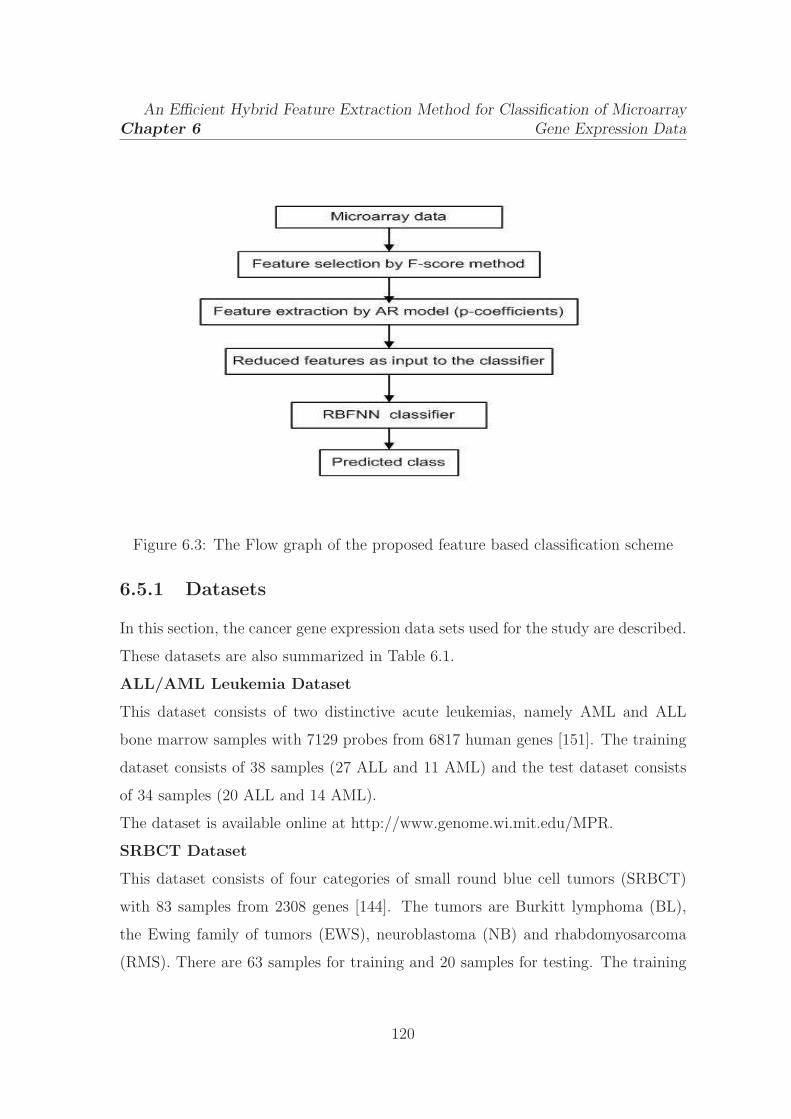
Chapter 6



Figure 6.3: The Flow graph of the proposed feature based classification scheme

6.5.1 Datasets

In this section, the cancer gene expression data sets used for the study are described.

These datasets are also summarized in Table 6.1.

ALL/AML Leukemia Dataset

This dataset consists of two distinctive acute leukemias, namely AML and ALL

bone marrow samples with 7129 probes from 6817 human genes [151]. The training

dataset consists of 38 samples (27 ALL and 11 AML) and the test dataset consists

of 34 samples (20 ALL and 14 AML).

The dataset is available online at http://www.genome.wi.mit.edu/MPR.

SRBCT Dataset

This dataset consists of four categories of small round blue cell tumors (SRBCT)

with 83 samples from 2308 genes [144]. The tumors are Burkitt lymphoma (BL),

the Ewing family of tumors (EWS), neuroblastoma (NB) and rhabdomyosarcoma

(RMS). There are 63 samples for training and 20 samples for testing. The training

120

Chapter 6



set consists of 8, 23, 12 and 20 samples of BL, EWS, NB and RMS, respectively.

The testing set consists of 3, 6, 6 and 5 samples of BL, EWS, NB and RMS,

respectively.

The dataset is available online at http://research.nhgri.nih.gov/microarray/Supplements.

MLL Leukemia dataset

This dataset consists of three types of leukemias namely ALL, MLL and AML with

72 samples from 12582 genes [150]. The training dataset consists of 57 samples (20

ALL, 17 MLL and 20 AML) and the test data set consists of 15 samples (4 ALL, 3

MLL and 8 AML).

The dataset is available online at http:// sdmc.lit.org.sg/GEDatasets/.

Prostate Dataset

This dataset consists of prostate tissue samples from 12,600 genes [153]. The

training dataset consists of 102 samples out of which 52 are from prostate tumor

tissue samples and 50 are from normal tissue sample. The testing dataset consists

of 25 tumor samples and 9 normal samples.

The dataset is available online at http:www. Broad.mit.edu/cgi-bin/cancer/data

sets.cgi.

Lymphoma Dataset

This data set consists of three most prevalent adult lymphoid malignancies [152].

It consists of 62 samples from 4026 genes. This composes 42, 9 and 11 samples of

DLBCL, FL and CL respectively.

The dataset is available online at http://genome-www.stanford.edu/ lymphoma.

Colon Dataset

This dataset consists of total 62 samples collected from colon cancer patients [154].

Among them 40 samples are from tumor tissues and 22 are from healthy parts of

the colons of the same patients. The expression levels are measured for 2000 genes.

The dataset is available online at http://microarray.princeton.edu/oncology.

121

Chapter 6



Table 6.1: The standard datasets used for the study

Dataset number of Classes (number of samples) number of number ofsamples genes classes

Leukemia 72 ALL (47), AML (25) 7129 2Colon 62 normal (22), tumor(40) 2000 2Prostate 102 normal (50), tumor(52) 12,600 2MLL-Leukemia 72 ALL (24), AML (20), 12582 3

MLL (28)Lymphoma 62 DLBCL (42), FL (9), 4026 3

CL (11)SRBCT 83 BL(29), EWS (11), NB (18), 2308 4

RMS (25)

6.5.2 Experimental results

In order to compare the efficiency of the proposed method in predicting the class

of the cancer microarray data, six standard datasets such as Leukemia, SRBCT

and MLL Leukemia, Colon, Prostate and Lymphoma have been used for the study.

All the datasets are categorized into two groups: binary class and multi class to

assess the performance of the proposed method. The Leukemia, Prostate and Colon

dataset are binary class and SRBCT, Lymphoma and MLL Leukemia are multi class

datasets. The feature extraction process proposed in this chapter has two steps.

First, the F-score method is employed on gene space to choose the discriminant

feature set. For example, The F-scores of the genes in Leukemia dataset is shown

in Fig. 6.4.

The average of the F-scores is used as the threshold to select the discriminant

genes. Then, the reduced feature set is modeled by the autoregressive modeling

to capture the global spectral characteristics of the samples. The parameters of

the model contains the information regarding the classification of samples, hence

constitutes the optimal features for class prediction. Through an empirical study

the model parameters are chosen 50 to achieve better accuracy. The leave one

122

Chapter 6



Table 6.2: Comparison of LOOCV classification accuracy using the proposed featurerepresentation method using RBFNN, MLP and LDA.

Dataset Method LOOCV Accuracy

Leukemia

RBFNN 97.22MLP 97.22LDA 76.39

Colon

RBFNN 93.55MLP 90.32LDA 64.52

Prostate

RBFNN 93.13MLP 88.24LDA 71.57

MLL-Leukemia

RBFNN 93.02MLP 88.89LDA 73.61

LymphomaRBFNN 96.77

MLP 93.55LDA 80.65

SRBCTRBFNN 93.98

MLP 84.34LDA 63.86

123

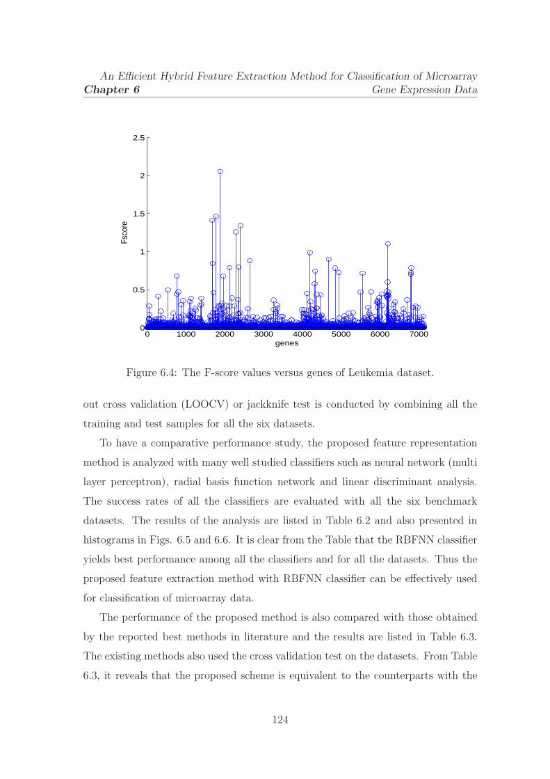
Chapter 6



0 1000 2000 3000 4000 5000 6000 70000

0.5

1

1.5

2

2.5

genes

Fsco

re

Figure 6.4: The F-score values versus genes of Leukemia dataset.

out cross validation (LOOCV) or jackknife test is conducted by combining all the

training and test samples for all the six datasets.

To have a comparative performance study, the proposed feature representation

method is analyzed with many well studied classifiers such as neural network (multi

layer perceptron), radial basis function network and linear discriminant analysis.

The success rates of all the classifiers are evaluated with all the six benchmark

datasets. The results of the analysis are listed in Table 6.2 and also presented in

histograms in Figs. 6.5 and 6.6. It is clear from the Table that the RBFNN classifier

yields best performance among all the classifiers and for all the datasets. Thus the

proposed feature extraction method with RBFNN classifier can be effectively used

for classification of microarray data.

The performance of the proposed method is also compared with those obtained

by the reported best methods in literature and the results are listed in Table 6.3.

The existing methods also used the cross validation test on the datasets. From Table

6.3, it reveals that the proposed scheme is equivalent to the counterparts with the

124

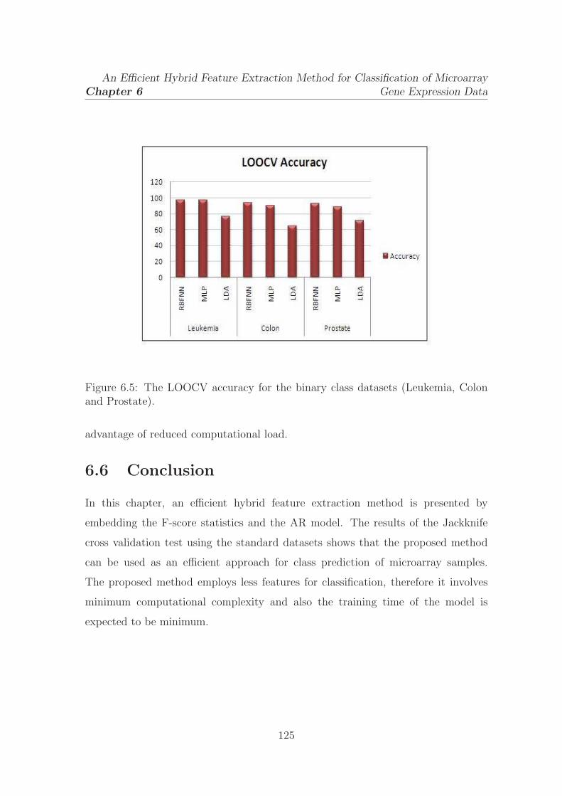
Chapter 6



Figure 6.5: The LOOCV accuracy for the binary class datasets (Leukemia, Colonand Prostate).

advantage of reduced computational load.

6.6 Conclusion

In this chapter, an efficient hybrid feature extraction method is presented by

embedding the F-score statistics and the AR model. The results of the Jackknife

cross validation test using the standard datasets shows that the proposed method

can be used as an efficient approach for class prediction of microarray samples.

The proposed method employs less features for classification, therefore it involves

minimum computational complexity and also the training time of the model is

expected to be minimum.

125

Chapter 6



Figure 6.6: The LOOCV accuracy for the multi class datasets (MLL-Leukemia,Lymphoma and SRBCT).

Table 6.3: Comparison of predictive accuracy (%) of the proposed method with thebest available method in literature

Dataset Proposed method Best available methodLeukemia 97.22 100

Colon 93.55 96Prostate 93.13 96.08

MLL-Leukemia 93.02 100Lymphoma 96.77 100

SRBCT 93.98 100

126

Conclusion and Future Work

Chapter 7

Conclusion and Future work

7.1 Conclusion

In this chapter, the conclusion of the overall thesis is presented and some of the

future research problems which may be attempted by interested readers are outlined.

The dissertation has investigated on four important problems in bioinformatics: the

protein coding region identification in DNA sequences, hot spot identification in

proteins, protein structural class prediction and classification of microarray gene

expression data. The novelty of the present work is the introduction of signal

processing and machine learning techniques to analyze the genomic and proteomic

signals.

Gene prediction and protein coding region identification in DNA sequences

are unsolved and popular research problems in bioinformatics. Several powerful

computational methods have been developed for coding region identification and

their performance is highly dependent on the coding measures that are used for

characterizing DNA sequences. The period-3 property exhibited by the coding

regions is used as the basis to identify them in the sequence. In this dissertation a

new time-frequency filtering approach based on S-transform technique is presented

to efficiently detect the protein coding regions. First, the spectrum of the DNA

sequence is computed using S-transform to localize the period-3 frequency in

time-frequency plane. Then, that pattern is filtered out using a mask in the

128

Chapter 7 Conclusion and Future work

time-frequency domain, thereby producing peaks in the energy sequence wherever

the coding regions present. The potential of the proposed method is assessed by

evaluating ROC curves and statistical parameters (Sp, Sn, Average accuracy) in

C. elegans chromosome and HRM dataset. The results obtained by the proposed

method are also compared with the conventional sliding window DFT and anti-notch

filtering method. The comparison study reveals that the proposed approach provides

an average accuracy of 96% in gene F56F11.4 of C. elegans chromosome III.

Proteins are the biomolecules that govern most of the functions in the living

cells. The function of protein is dependent on the 3-D structure which facilitates the

interactions of protein with other molecules at a specific site known as active sites.

Some residues in these sites, known as hot spots are responsible for the binding.

Hence, the identification of these hot spots in protein is a challenging issue in

protein science. In this dissertation a novel S-transform based filtering approach

is proposed to identify these hot spots. It is a sequence based approach based on the

concept of RRM. The characteristic frequency that corresponds to the interaction of

proteins is first localized in the time-frequency spectrum and then filtered out from

the sequence to provide a measure to identify the hot spots. The performance of

the proposed method is compared with the corresponding results obtained by the

existing computational methods in terms of sensitivity, specificity, positive predictive

value, negative predictive value and average accuracy in some standard examples of

proteins. A comparison study reveals the potentiality of the proposed method. It

also identifies some more unknown hot spot locations in the proteins which need

further investigation to include in the database for future reference.

The structural class is one of the most important features for characterizing the

overall folding type of a protein. Thus prediction of structural class of protein is

necessary and has been a challenging problem in bioinformatics. This dissertation

work presents a novel feature representation scheme (DCTAmPseAAC) based on

the Chou’s pseudo amino acid composition for efficient prediction of the structural

classes of proteins. It efficiently captures the characteristics of protein relevant to

129


structure, thereby improves the performance of the classifier. The potential of the

proposed method is assessed by the Jackknife test on three benchmark datasets: 204,

277 and 498 datasets. A simple radial basis function network is introduced for an

efficient classification of the proteins into different structural classes. An exhaustive

simulation study of the proposed scheme demonstrates its superiority by providing

at least 2-3% improvement in the prediction accuracy over the existing methods.

Microarray technology allows scientists to measure the expression levels of

thousands of genes simultaneously from a single experiment and thereby facilitates

the understanding of the molecular interaction and functions. It provides a way

to characterize the state of cells or tissues and to associate that state with a

phenotypic trait. The outcomes from microarray technology are used to provide

a fundamental understanding of biological development as well as to explore the

underlying genetic causes of many biological functions such as disease. In this

context cancer classification is important for subsequent diagnosis and treatment.

The high dimension and low sample size of microarray data lead to curse of

dimensionality problem which affects the classification performance. In this

dissertation an efficient hybrid feature extraction method is proposed to overcome

the dimensionality problem. First, the discriminative genes are selected by the

F-score statistics and then, the reduced feature set is used by the autoregressive

model to efficiently characterize the samples. Exhaustive simulation study is carried

out on the proposed method with six standard cancer microarray datasets to

demonstrate its potential.The results show that the proposed method is comparable

to the existing best algorithm but with an advantage of reduced complexity.

The objectives of the dissertation proposed in chapter 1 have been met in

introducing novel signal processing methods to compute the measures or extract

features by demonstrating the efficacies of these methods with soft computing

techniques.

130


7.2 Future work

The work carried out in the present dissertation can be extended in many directions.

• The time-frequency resolution of S-transform can further be improved by

efficiently scaling the Gaussian window and the filtering capability can be

improved by efficiently designing the time-frequency filter. Use of such efficient

filter is expected to achieve improved performance in identification tasks.

• In the dissertation a new feature representation that is DCTAmPseAAC has

been suggested.The use of such features has resulted in improved classification

performance. It is proposed that the new feature representation can be

employed for efficient identification of protein membrane type, enzyme family

classification and many such applications.

• In recent years many evolutionary computing algorithms such as genetic

algorithm (GA), differential evolution (DE), particle swarm optimization

(PSO) and artificial immune system (AIS) have been developed and applied to

many fields. In the field of bioinformatics these new optimization techniques

have not been gainfully applied. Hence there are wide scopes of applying these

emerging tools for achieving potential solution of the various bioinformatics

problems attempted in this dissertation.

• Further many bioinformatics problems involving pattern identification and

feature extraction can be formulated or viewed as multiobjective optimization

problems. After such formulation multiobjective optimization algorithms

such as NSGA-II, MPSO and MBFO can be conveniently applied to obtain

improved solutions.

131

Annexure-I

0 100 200 300 400 500 600 700 800 900 10000.08

0.09

0.1

0.11

0.12

0.13

0.14

amino acid bases

EII

P v

alu

e

Figure 7.1: The EIIP coded sequence (1000 bases) of the gene F56F11.4 [87]

132

Annexure-II

Figure 7.2: Comparison of Jackknife accuracies of all classes of different classificationalgorithms using the proposed DCTAmPseAAC feature representation method

133

Annexure

Figure 7.3: Comparison of overall Jackknife accuracies of different classificationalgorithms using the proposed DCTAmPseAAC feature representation method

Figure 7.4: Comparison of overall Jackknife classification accuracy with the threefeature representations using RBFNN and MLP

134

Bibliography

Bibliography

[1] P. P. Vaidyanathan and B. Yoon, “ The role of Signal-Processing

Concepts in Genomics and proteomics”, J. Franklin Inst., vol. 341,

pp. 111-135, 2004.

[2] D. Anastassiou, “Genomic signal processing”, IEEE Signal Processing

Magazine, vol. 18, pp. 8–20, 2001.

[3] J. W. Fickett, “The gene prediction problem: an overview for

developers”, Computers Chem., vol. 20, pp. 103–118, 1996.

[4] J. Proakis and D. Manolakis, Digital Signal Processing-principle,

Algorithm and Applications, 3rd ed., Upper saddle River, NJ: Prentice

Hall,1996.

[5] N. Ahmed, T. Natarajan and K. R. Rao, “ Discrete cosine transforms”,

IEEE Transactions on Computer, vol. C-32, pp. 90–93, 1974.

[6] A. M. Sarhan,“ Iris Recognition Using the Discrete Cosine Transform

and Artificial Neural Networks”, Journal of Computer Science (JCS),

vol. 5, no. 4, pp. 369–373, 2009.

[7] J. Neves, M. Santos and J. Machado,“ Feature Extraction from Tumor

Gene Expression Profiles Using DCT and DFT”, EPIA, pp. 485–496,

2007.

[8] S. Qian and D. Chen, Joint Time-Frequency Analysis: Methods and

Applications, Englewood Cliffs, NJ: Prentice-Hall, 1996.

[9] L. Cohen, Timefrequency analysis, Englewood Cliffs, NJ:Prentice-Hall,

PTR, 1995.

136

Bibliography

[10] E. Sejdic, I. Djurovic and J. Jiang,“ Timefrequency feature

representation using energy concentration:An overview of recent

advances”, Digital signal processing, 2008.

[11] M. R. Portnoff, “Time-frequency Representation of Digital Signals

and Systems based on Short-Time Fourier Analysis”, IEEE Trans. on

Acoustics, Speech and Signal Processing, vol. 28, no. 1, Feb. 1980.

[12] I. Daubechies, “The Wavelet Transform, Time-Frequency Localization

and Signal Analysis”, IEEE Trans. on Information Theory, vol. 36, no.

5, pp. 961–1005, Sep. 1990.

[13] R. G. Stockwell, L. Mansinha and R. P. Lowe,“Localisation of the

complex spectrum: the S transform”, IEEE Trans Signal Processing,

vol. 44, no. 4, pp. 998-1001, 1997.

[14] P. K. Dash, B.K. Panigrahi and G. Panda, “ Power quality analysis

using S-transform”, IEEE Trans. Power Deliv., vol. 18, pp. 406-411,

2003.

[15] P. Rakovi, E. Sejdic, L. J. Stankovi and J. Jiang, “Time-Frequency

Signal Processing Approaches with Applications to Heart Sound

Analysis”, Computers in Cardiology , vol. 33, pp. 197–200, 2006.

[16] C. R. Pinnegar, “Time-frequency and time-time filtering with the

S-transform and TT-transform”, Digital Signal Processing, vol. 15,

pp. 604–620, 2005.

[17] C. R. Pinnegar and L. Mansinha,“ The S-transform with windows of

arbitrary and varying shape”, Geophysics, vol. 68, no.1, pp. 381–385,

2003.

[18] S. Haykin , Neural Networks, Ottawa, ON Canada: Maxwell Macmillan,

1994.

[19] Y. H. Pao, “Adaptive Pattern Recognition and Neural Networks”,

Addison Wesley, Reading, Massachusetts, 1989.

[20] D. H. Nguyen and B. Widrow, “Neural networks for self-learning control

system”, Int. J. Conttr., vol. 54, no. 6, pp. 1439-1451, 1991.

137

Bibliography

[21] T. Poggio and F. Girosi, “Networks for approximation and learning”,

Proceedings of IEEE, vol. 78, no. 9, pp. 1481-1497, 1990.

[22] P. S. Sastry, G. Santharam and K. P. Unnikrishnan, “Memory neural

networks for identification and control of dynamical systems”, IEEE

Trans. Neural Networks, vol. 5, pp. 306–319, 1994.

[23] A. G. Parlos, K. T. Chong and A. F. Atiya, “Application of recurrent

multilayer perceptron in modeling of complex process dynamics”, IEEE

Trans. Neural Networks, vol. 5, pp. 255–266, 1994.

[24] S. V. T. Elanayar and Y. C. Shin, “Radial basis function neural network

for approximation and estimation of nonlinear stochastic dynamic

systems”, IEEE Trans. Neural Network, vol. 5, pp. 594–603, 1994.

[25] S. R. Samantray, P. K. Dash and G. Panda , “ Fault classification and

location using HS-transform and radial basis function neural network”,

Electric Power Systems Research, vol. 76, pp. 897–905, 2006.

[26] Y. J. Oyang, S. C. Hwang, Yu-Yen Ou, C.Y. Chen and Z.W. Chen,

“Data Classification with Radial Basis Function Networks Based on a

Novel Kernel Density Estimation Algorithm”, IEEE Transactions on

Neural Networks, vol. 16, no. 1, pp. 225–236, 2005.

[27] J. W. Fickett and C. S. Tung,“Assessment of protein coding measure”,

Nucleic Acids Res., vol. 20, pp. 6441–6450, 1992.

[28] S. Tiwari,S. Ramachandran,A. Bhattacharya,S. Bhattacharya and R.

Ramaswamy, “Prediction of probable genes by Fourier analysis of

genomic sequences”, CABIOS, vol. 13, pp. 263–270, 1997.

[29] A. A. Tsonis, J. B. Elsner and P. A. Tsonis,“Periodicity in DNA coding

sequences: Implications in Gene Evolution”, J. Theor Biol., vol. 151,

no. 3, pp. 323-331, 1991.

[30] G. Gutierrez, J. L. Oliver and A. Marin,“On the origin of the periodicity

of three in protein coding DNA sequences”, J. Theor Biol., vol.167, no.

4, pp. 413-414, 1994.

138

Bibliography

[31] P. B. Galvan, “Finding borders between coding and non coding DNA

regions by an entropic segmentation method”, Phy. Rev. Lett., vol. 85,

pp. 1342–1345, 2000.

[32] C. Yin and S. S. T. Yau, “ Prediction of protein coding regions by

the 3-base periodicity analysis of a DNA sequence”, J. of Theoretical

Biology, vol. 247, pp. 687–694, 2007.

[33] J. Henderson, S. Salzberg and K. Fasman, “Finding Genes in DNA with

a hidden markov model”, Journal of Computational Biology, 1997.

[34] D. Chriss and I. Dubchak, “ Multi class protein fold recognition using

support vector machines and neural networks”, Bioinformatics, vol. 17,

pp. 349-358, 2001.

[35] E. E. Snyder and G. D. Stormo,“Identification of coding regions in

Genomic DNA sequences:An application of dynamic programming and

neural network”, Nucl. Acids, vol. 21, pp. 607–617, 1993.

[36] T. Eftestel, T. Ryen, S. O. Aase, C. stra’ssle, M.Boos, G. Schuster and

P. Ruff,“ Eukaryotic Gene Prediction by Spectral Analysis and Pattern

Recognition Techniques”, RORSIG, pp. 146–149, 2006.

[37] T. W. Fox and A. Carreira, “A digital signal processing method for

gene prediction with improved noise suppression”, EURASIP Journal

on Applied Signal Processing, vol. 1, pp. 108-114, 2004.

[38] S. Datta and A. Asif, “A Fast DFT-Based Gene Prediction Algorithm for

Identification of Protein Coding Regions”, Proc. 30th IEEE Int’l Conf.

Acoustics, Speech and Signal Processing, vol. 3, pp. 113–116, 2005.

[39] R. Voss, “Evolution of long-range fractal correlations and 1/f noise in

DNA base sequences”, Phys.Rev. Lett., vol. 68, pp. 3805–3808, 1992.

[40] C. A. Chatzidimitriou and D. Larhammer, “Long range correlations in

DNA”, Nature, vol. 361, pp. 212–213, 1993.

[41] N. Chakravarty, A. Spanias, L. D. Iasemidis and K. Tsakalis,

“Autoregresive Modeling and Feauture Analysis of DNA Sequence”,

EURASHIP J. Applied Signal Processing, vol. 1, pp. 13–28, 2004.

139

Bibliography

[42] M. Akhatar, “Comparison of gene and exon prediction techniques for

detection of short coding regions”, Int. J. of Inf. Tech., Special issue on

Bioinformatics and Biomedical Systems , vol. 11, pp. 26–35, 2005.

[43] P. P. Vaidyanathan and B. J. Yoon,“Digital filters for gene prediction

applications”, IEEE Asilomar Conference on Signals, Systems, and

Computers, Monterey, CA, 2002.

[44] P. P. Vaidyanathan, and B. J. Yoon,“Gene and exon prediction using

allpass-based filters”, In Proc. IEEE Workshop on Gen. Sig. Proc and

Stat., 2002.

[45] J. Tuqan and A. Rushdi, “A DSP Perspective to the period-3 detection

problem”, GENESIPS, pp. 53–54, 2006.

[46] B. D. Silverman and R. Linsker, “ A measure of DNA periodicity”, J.

of Theoretical Biology, vol. 118, no. 3, pp. 295-300, Feb 1986.

[47] R. Zhang and C. T. Zhang, “Z curves, an intuitive tool for visualizing

and analyzing the DNA sequences”, J.on Biom. Struc. Dyn., vol. 11,

pp. 767-782, July 1994.

[48] C. T. Zhang and J. Wang, “Recognition of protein coding genes in the

yeast genome at better than 95% accuracy based on Z curve”, Nucleic

Acids Res., vol. 28, pp. 2804–2814, 2000.

[49] A. S. Nair and S. Sreenadhan, “A coding measure scheme employing

electron-ion interaction pseudopotential (EIIP)”, Bioinformation, Open

access hypothesis, pp. 197-202, 2006.

[50] C. K. Onkar, R. Vaigneshwar, V. K. Jayaraman and B. D. Kulkarni,

“Identification of coding and non coding sequences using local Holder

exponent formalism”, Bioinformatics, vol. 21, pp. 3818–3823, 2005.

[51] K. D. Rao and M. N. S. Swamy, “ Analysis of Genomics and Proteomics

Using DSP Techniques”, IEEE Transaction on Circuits and Systems,

vol. 55, no. 1, pp. 370–378, 2008.

[52] S. Rogic, A. K. Mackworth and F. B. F. Ouellette,“Evaluation of gene

finding programs on mammalian sequences”, Genome Res., vol. 11, pp.

817-832, 2001.

140

Bibliography

[53] P. Uetz, L. Giot, G. Cagney, T. A. Mansfield and R. S. Judson, “A

comprehensive analysis of protein-protein interactions in Saccharomyces

cerevisiae”, Nature, vol. 403, pp. 623–627, 2000.

[54] L. Giot, J. S. Bader, C. Brouwer, A. Chaudhuri, B. Kuang, “A protein

interaction map of Drosophila melanogaster”, Science, vol. 302, pp.

1727–1736, 2003.

[55] B. Alberts, A. Johnson, J. Lewis, M. Raff, K. Roberts and P. Walter,

Molecular Biology of the Cell, 4th ed. New York: Garland, 2002.

[56] I. Moreira, P. Fernades and M. Ranos, “Hot spots- A review of the

protein-protein interface determinant amino acid residues”, Genetics

and Molecular biology, vol. 32, no.3, pp. 626–633, 2009

[57] Y. Gao, R. Wang and L. Lai, “Structure-based method for analyzing

protein-protein interfaces”, J. Mol. Model., vol. 10, no. 1, pp. 44–54,

Feb. 2004.

[58] W. L. DeLano, “Unraveling hot spots in binding interfaces: Progress and

challenges”, Curr. Opin. Struct. Biol., vol. 12, no. 1, pp. 14-20,2002.

[59] K. Cho, D. Kim and D. Lee, “A feature based approach to modeling

protein-protein interaction hot spots”, Nucleic Acids research, vol.37,

no. 8, pp. 2672–2687, 2009.

[60] R. H. Higa and C. L. Tozzi, “Prediction of binding hot spot residues by

using structural and evolutionary parameters”, Genetics and Molecular

biology, vol. 32, no.3, pp. 626–633, 2009.

[61] K. C. Zhao and K. Aihara , “A discriminative approach

to identifying domain-domain interactions from protein-protein

interactions”, Proteins, vol. 78, no.5, pp. 1243–1253, 2010.

[62] A. Bogan and K. S. Thorn, “Anatomy of hot spots in protein interfaces”,

J. Mol. Biol., vol. 280, pp. 1–9, 1998.

[63] J. A. Wells, “Systematic mutational analyses of protein-protein

interfaces”, Meth. Enzymol., vol. 202, pp. 390–411, 1991.

141

Bibliography

[64] B. C. Cunningham, P. Jhurani, P. Ng and J. A. Wells, “Receptor

and antibody epitopes in human growth hormone identified by

homologscanning mutagenesis”, Science, vol. 243, no. 4896, pp.

1330–1336, Mar. 1989.

[65] K. S. Thorn and A. A. Bogan, “ASEdb: a databaseof alanine mutations

and their effects on the free energy of binding in protein interactions”,

Bioinformatics, vol. 17, no. 3, pp. 284–285, 2001.

[66] T. Kortemme, D.E. Kim and D. Baker, “Computational alanine

scanning of protein-protein interfaces”, Sci. STKE., vol. 219, pp. l2,

2004.

[67] T. Kortemme and D. Baker, “A simple physical model for binding energy

hot spots in protein-protein complexes”, Proc. Natl. Acad. Sci. U.S.A.

vol. 99, pp. 14116–14121, 2002.

[68] Yanay Ofran and Burkhard Rost, “Protein-Protein Interaction Hotspots

Carved into Sequences”, PLoS computational biology, vol. 3, pp.

1169–1176, 2007.

[69] Yanay Ofran and Burkhard Rost, “ISIS: Interaction Sites Identified from

sequences”, Bioinformatics, vol. 23, pp. 13-16, 2007.

[70] S. J. Darnell, D. Page and J. C. Mitchell, “An automated

decision-tree approach to predicting protein interaction hot spots”,

PROTEINS-NEW YORK, vol. 68, no.4, pp. 813–823, 2007.

[71] S. J. Darnell, L. LeGault and J. C. Mitchell, “KFC Server:interactive

forecasting of protein interaction hot spots”, Nucleic Acids Res., vol.

36, pp. 265-269, 2008.

[72] E. Guney, N. Tuncbag, O. Keskin and A. Gursoy, “HotSprint:database

of computational hot spots in protein interfaces”, Nucleic Acids Res.,

vol. 36, pp. 662-666, 2008.

[73] N. J. Burgoyne and R. M. Jackson, “ predicting protein interaction

site: binding hot-spots in protein-protein and protein-ligand interfaces”,

Structural Bioinformatics, vol. 22, no. 11, pp. 1335–1342, 2006

142

Bibliography

[74] N. Tuncbag, A. Gursoy and O. Keskin , “Identification of computational

hot spots in protein interfaces: combining solvent accessibility and

inter-residue potentials improves the accuracy”, Bioinformatics, vol. 25,

no. 12, pp. 1513–1520, 2009.

[75] B. Ma, T. Elkayam, H. Wolfson and R. Nussinov,“Protein-protein

interactions: structurally conserved residues distinguish between

binding sites and exposed protein surfaces”, Proceedings of the National

Academy of Science, vol. 100, no. 10, pp. 5772–5777, 2003.

[76] O. Keskin, B. Ma and R. Nussinov, “Hot regions in protein-protein

interaction:the organisation and contribution of structuraly conserved

hot spot residues”, Journal of molecular biology, vol. 345, no. 5,

pp.1281–1294, 2005.

[77] J. F. Xia, X. M. Zhao, J. Song and D. S. Huang, “APIS: accurate

prediction of hot spots in protein interfaces by combining protrusion

index with solvent accessibily”, Bioinformatics, vol. 11, no. 174, pp.

1–14, 2010.

[78] I. Cosic, The Resonant Recognition Model of Macromolecular

Bioactivity-Theory and Applications, Basel, Switzerland: Birkhauser

Verlag, 1997.

[79] I. Cosic, E. Pirogova and M. Akay, “Application of the resonant

recognition model to analysis of interaction between viral and tumor

suppressor proteins”, In Proc. 25th Annu. Int. Conf. IEEE EMBS,

Cancun, Mexico, Sep. 17-21, pp. 2398–2401, 2003.

[80] I. Cosic, “Macromolecular bioactivity: Is it resonant interaction between

macromolecules? Theory and applications”, IEEE Trans. Biomed. Eng.,

vol. 41, no. 12, pp. 1101–1114, Dec. 1994.

[81] V. Veljkovic, I. Cosic, B. Dimitrijevic, and D. Lalovic, “Is it possible to

analyze DNA and protein sequencesby the methods of digital signal

processing?”, IEEE Trans. Bio-Med. Eng., vol. BME-32, no. 5, pp.

337–341, May 1985.

[82] P. Ramachandran and A. Antoniou, “Localization of hot spots in

proteins using digital filters”, In Proc. IEEE Int. Symp. Signal

143

Bibliography

Processing and Information Technology, Vancouver, BC, Canada,

pp.926-931, Aug. 2006.

[83] P. Ramachandran and A. Antoniou, “ Identification of Hot-spots

locations in Proteins using Digital Filters”, IEEE journal of selected

topics in signal processing, vol.2, no. 3, June 2008

[84] Alanine Scanning Energetics database (ASEdb).Available online at:

http://nic.ucsf.edu/asedb/index.php

[85] P. Ramachandran, A. Antoniou and P. P. Vaidyanathan, “Identification

and location of hot spots in proteins using the short-time discrete Fourier

transform”, In Proc. 38th Asilomar Conf. Signals, Systems,Computers,

Pacific Grove, CA, pp. 1656–1660, Nov. 2004.

[86] I. Cosic, C. H. De Trad, Q. Fang and Q. M. Akay,“Protein Sequences

Analysis Using the RRM Model and Wavelet Transform Methods: A

Comparative Study Analysis”, Proc. of the IEEE-EMBS Asia-Pacific

Conference on Biomedical Engineering., pp. 405–406, 2000.

[87] Protein Data Bank (PDB), Research Collaboratory for

Structural Bioinformatics (RCSB).Available online at:

http://www.rcsb.org/pdb/.

[88] Swiss-Prot Protein Knowledgebase. Swiss Inst. Bioinformatics

(SIB).Available online at: http://us.expasy.org/sprot/.

[89] G. P. Zhou and N. Assa-Munt, “Some insights into protein structural

class prediction”, Proteins, vol. 44, no.1, pp. 57–59, 2001.

[90] P. Klein, C. Delisi,“Prediction of protein structural class from the amino

acid sequence”, Biopolymers, vol. 25, no.9, pp. 1659–1672, 1986.

[91] K. C. Chou and C. T. Zhang, “Review: Prediction of protein structural

classes”, Crit. Rev. Biochem. Mol. Biol., vol. 30, pp. 275–349, 1995.

[92] K. C. Chou, G. M. Maggiora, “ Domain structural class prediction”,

Prot Eng,, vol. 11, no. 7, pp. 523–538, 1998.

[93] M. Levitt and C. Chothia,“ Structural patterns in globular proteins”,

Nature, vol. 261, no. 5561, pp. 552–558, 1976.

144

Bibliography

[94] H. Nakashima, K. Nishikawa and T. Ooi, “The folding type of a protein

is relevant to its amino acid composition.”, J. Biochem, pp.153–159,

1986.

[95] R. Y. Luo, Z. P. Feng and J. K. Liu , “Prediction of protein structural

class by amino acid and polypeptide composition”, Eur. J. Biochem.,

vol. 269, pp. 4219–4225, 2002.

[96] T. Liu, X. Zheng and J. Wang,“ Prediction of protein structural class

using a complexity-based distance measure”, Amino acids, 2009.

[97] Q. S. Du, Z. Q. Jiang, W. Z. He, D. P. Li, K. C. Chou,“ Amino

Acid Principal Component Analysis (AAPCA) and its Applications in

Protein Structural Class Prediction”, Journal of Bimolecular Structure

and Dynamics., vol. 23, pp. 635–640, 2006.

[98] K. C. Chou,“ A key driving force in determination of protein structural

classes”, Biochem Biophys Res Commun, vol. 264, pp. 216–224, 1999.

[99] K. C. Chou, C. T. Zhang, “ Predicting protein folding types by distance

functions that make allowances for amino acid interactions”, J. Biol.

Chem., vol. 269, no. 35, pp. 22014–22020, 1994.

[100] H. B. Shen, J. Yang, X.J. Liu and K. C. Chou, “ Using supervised

fuzzy clustering to predict protein structural classes”, Biochemical and

Biophysical Research Communications, vol. 334, no. 2, pp.577, 2005.

[101] Y. S. Ding, T. L. Zhang, K. C. Chou, “ Prediction of protein structure

classes with pseudo amino acid composition and fuzzy support vector

machines network,” Protein Peptide Lett., vol. 14, pp. 811–815, 2007.

[102] J. M. Chandonia and M. Karplus, “ Neural networks for secondary

structure and structural class prediction”, Protein Sci., vol. 4, pp.

275–285, 1995.

[103] Y. Cai and G. Zhou,“ Prediction of protein structural classes by neural

network”, Biochimie, vol. 82, no. 8, pp. 783–785, 2000.

[104] Y. F. Cao,S. Liu,L. Zhang,J. Qin,J. Wang and K. X. Tang,“Predictipon

of protein structural class with rough sets”, BMC Bioinformatics, vol.7,

pp.1–6, 2006.

145

Bibliography

[105] Y. D. Cai, X. J. Liu, X. Xu and G. P. Zhou,“ Support vector machines

for predicting protein structural class”, BMC Bioinformatics, vol. 2, no.

3, 2001.

[106] C. Chen, X. Zhou, Y. Tian, X. Zou and P. Cai, “ Predicting protein

structural class with pseudo-amino acid composition and support

vector machine fusion network”, Analytical Biochemistry, vol. 357, pp.

116–121, 2006.

[107] X. D. Sun and R. B. Huang, “ Prediction of protein structural classes

using support vector machine”, Amino Acids, vol. 30, pp. 469–475, 2006.

[108] K. C. Chou,“Prediction of protein structural classes and subcellular

locations”, Curr. Protein Pept. Sci., vol. 1, no. 2, pp.171–208, 2000.

[109] K. C. Chou,“ A novel approach to predicting protein structural classes

in a (20-1)-D amino acid composition space”, Proteins, vol. 21, no. 4,

pp.319–344, 1995.

[110] X. B. Zhou, C. Chen, Z. C. Li and X. Y. Zou, “Using Chou’s

amphiphilic pseudo amino acid composition and support vector machine

for prediction of enzyme subfamily clases”, J. Theor. Biol., vol. 248, pp.

546–551, 2004.

[111] K. C. Chou, “ Prediction of protein cellular attributes using pseudo

amino acid composition”, Proteins, vol.43, pp. 246–255, 2001.

[112] Z. C. Li,X. B. Zhou and Z. Dai, “Prediction of protein structural classes

by Chou’s pseudo amino acid composition: approached using continous

wavelet transform and principal component analysis”, Amino Acids,

doi 10.1007/s00726-009-0276-1, 2008.

[113] H. Liu, M. Wang and K. C. Chou, “ Low-frequency Fourier spectrum

for predicting membrane protein types”, Biochemical and Biophysical

Research Communications, vol. 336, pp.737–739, 2005.

[114] H. Liu, J. Yang, M. Wang, X. Li and K. C. Chou,“ Using Fourier

Spectrum Analysis and Pseudo Amino Acid Composition for Prediction

of Membrane Protein Types”, The Protein Journal, vol. 24, no. 6.

146

Bibliography

[115] G. P. Zhou, “An intriguing controversy over protein structural class

prediction”, J Protein Chem., vol.17(8), pp.729–738, 1998.

[116] K. C. Chou, “ Using amphiphilic pseudo amino acid composition to

predict enzyme”, Bioinformatics, vol. 21, pp. 10–19, 2005.

[117] T. L. Zhang, Y. S. Ding and K.C. Chou, “ Prediction protein structural

classes with pseudo-amino acid composition: approximate entropy and

hydrophobicity pattern”, J. Theor. Biol., vol. 250, pp.186–193, 2008.

[118] C. Tanford, “Contribution of hydrophobic interactions to the stability of

the globular conformation of proteins”, Journal of American Chemical

Society, vol. 84, pp. 4240–4274, 1962.

[119] T. P. Hopp and K. R. Woods,“ Prediction of protein antigenic

determinants from amino acid sequences”, J. Proc. Natl. Acad. Sci.

USA, vol.78, pp. 3824–3828, 1981.

[120] S. Mitaku, S. Hoshi, T. Abe and R. Kataoka, “ Spectral Analysis of

Amino Acid Sequence. I. Intrinsic Membrane Proteins.”, J. Phys. Soc.

Jpn., vol.53, pp.4083–4090, 1984.

[121] T. L. Zhang, Y. S. Ding, “ Using pseudo amino acid composition

and binary-tree support vector machines to predict protein structural

classes”, Amino Acids, vol. 33, pp.623–629, 2007.

[122] K. C. Chou, “Review: Low-frequency collective motion in

biomacromolecules and its biological functions”, Biophys Chem., vol.

30, pp.3–48, 1988.

[123] K. C. Chou, “Low-frequency resonance and cooperativity of

hemoglobin,” Trends Biochem Sci., vol. 14, pp. 212, 1989.

[124] M. Wang, J. Yang, G. P. Liu, Z. J. Xu and K.C. Chou,“

Weighted-support vector machines for predicting membrane protein

types based on pseudo-amino acid composition”, Protein Engineering

Design and Selection, vol. 17, no.6, pp.509–516, 2004.

[125] J. Park and J. W. Sandberg,“ Universal approximation using radial basis

function network”, Neural Computation, vol. 3, pp. 246–257, 1991.

147

Bibliography

[126] X. Xuan, S. H. Shao, Z. Huang and K.C. Chou,“ Using Pseudo Amino

Acid Composition to Predict Protein Structural Classes: Approached

with Complexity Measure Factor”, J. Comput. Chem., vol. 27,

pp.478–482, 2006.

[127] K. Y. Feng, Y. D. Cai and K. C. Chou,“Boosting classifier for predicting

protein domain structural class”, Biochem Biophys Res. Commun., vol.

334, no. 1, vol. 213–217, 2005.

[128] Y. D. Cai, K. Y. Feng, W. C. Lu and K. C. Chou,“ Using LogitBoost

classifier to predict protein structural classes”, Journal of Theoretical

Biology, vol. 238, pp. 172–176, 2006.

[129] K.E. Chen , A. L. Kurgan and J. Ruan,“ Prediction of protein

structural class using Novel Evolutionary Collocation-based sequence

representation”, Journal of Computational Chemistry, vol. 29, no.10,

pp. 1596–1604, 2007.

[130] S. Jahandideh,P. Abdolmaleki,M. Jahandideh and E. B. Asadabadi,“

Novel two-stage hybrid neural discriminant model for predicting proteins

structural class”, Biophysical Chemistry, pp. 87-93.

[131] R. Raghuraj and S. Lakshminarayanan, “ Variable predictive model

based classification algorithm for effective separation of protein

structural classes”, Comput. Biol Chem., vol. 32, pp. 302–306, 2008.

[132] Z. C. Li, X. B. Zhou,Y. R. Lin and X. Y. Zou, “ Prediction of protein

structural class by coupling improved genetic algorithm and support

vector machine”, Amino acids, vol. 35, pp. 581–590, 2008.

[133] T. P. Speed, Statistical Analysis of Gene expression Microarray data,

London: Chapman and Hall, 2003.

[134] M. H. Asyali, D. Colak, O. Demirkaya and M. S. Inan, “ Gene Expression

Profile Classification: A Review”, Current Bioinformatics, vol. 1, pp.

55–73, 2006.

[135] E. R. Dougherty,“Small Sample issue for microarray based

classification”, Comparative and Functional genomics, vol.2, no.1,

pp.28–31, 2001.

148

Bibliography

[136] I. Guyon and A. Elisseeff, “An introduction to variable and feature

selection”, Journal of Machine Learning Research, vol. 3, pp. 1157–1182,

2003.

[137] M. Xiong, L. Jin, W. Li and E. Boerwinkle, “Computational methods

for gene expression-based tumor classification”, BioTechniques, vol. 29,

no. 6, pp. 1264–1268, 2000.

[138] P. Baldi and A. D. Long, “A Bayesian framework for the analysis of

microarray expression data: regularized t-test and statistical inferences

of gene changes”, Bioinformatics, vol. 17, no. 6, pp. 509–519, 2001.

[139] D. S. Huang and C. H. Zheng, “Independent component analysis-based

penalized discriminant method for tumor classification using gene

expression data”, Bioinformatics, vol. 22, no. 15, pp. 1855–1862, 2006.

[140] K. Y. Yeung and W.L. Ruzzo, “Principal component analysis for

clustering gene expression data”, Bioinformatics, vol. 17, pp.763–774,

2002.

[141] Y. Liu, “ wavelet feature extraction for high-dimensional microarray

data”, Neurocomputing, vol. 72, pp. 985-990, 2009.

[142] Y. Liu, “Detect Key Gene Information in Classification of Microarray

Data”, EURASIP Journal on Advances in Signal Processing, pp.1–10,

2007.

[143] I. Guyon, J. Weston, Barnhill and V. Vapnik ,“ Gene selection for cancer

classification using support vector machines”, Mach. Learn., vol. 46, pp.

389–422, 2002.

[144] J. Khan, J. S. Wei, M. Ringner, L. H. Saal, M. Ladany, F. Westermann,

F. Berthold, M. Schwab, C. R. Antonescu, C. Peterson and P. S.

Meltzer, “Classification and diagnostic prediction of cancers using gene

expression profiling and artificial neural networks”, Nature Medicine,

vol. 7, no. 6, pp. 673–679, 2001.

[145] B. Liu, Q. Cui, T. Jiang and S. Ma,“ A combinational feature selection

and ensemble neural network method for classification of gene expression

data”, BMC Bioinformatics, vol. 5, no. 136, pp. 1–12, 2004.

149

Bibliography

[146] S. Gunes, K. Polat and S. Yosunkaya ,“ Multi-class f-score

feature selection approach to classification of obstructive sleep apnea

syndrome”, Expert systems with applications, vol. 37, pp. 998–1004, 2010

[147] K. Polat and S. Gunes,“ A new feature selection method on

classification of medical datasets: Kernel F-score feature selection”,

Expert systemswith Applications, vol. 36, pp.10367–10373, 2009.

[148] J. Makhoul,“ Linear prediction : A Tutorial review”, Proceedings of the

IEEE,vol. 63, pp. 562-580, 1975.

[149] W. R. Wu and P. C. Chen,“ Adaptive AR modeling in white

Gaussian noise”, IEEE transaction on signal processing, vol. 45, pp.

184-1192,1997.

[150] S. A. Armstrong, J. E. Staunton, L. B. Silverman, R. Pieters, de

Boer, M. L. Minden, M. D. Sallan, E. S. Lander, T. R. Golub, S.

J. Korsmeyer,“ MLL translocations specify a distinct gene expression

profile that distinguishes a unique leukemia”, Nature Genetics , vol. 30,

no. 1, pp. 41–47, 2002.

[151] T. R. Golub, D. K. Slonim, P. Tamayo, C. Huard, M. Gaasenbeek, J.

P. Mesirov, H. Coller, M. L. Loh, J. R. Downing, M. A. Caligiuri, C.

D. Bloomfield, E. S. Lander,“ Molecular classification of cancer: Class

discovery and class prediction by gene expression monitoring”, Science,

vol. 286, no. 5439, pp. 531–537, 1999.

[152] M. C. O’Neill and L. Song , “Neural network analysis of lymphoma

microarray data: prognosis and diagnosis near-perfect”, BMC

Bioinformatics, vol. 4, no.13, 2003.

[153] D. Singh, P. G. Febbo, K. Ross, D. G. Jackson, J. Manola, C. Ladd,

P. Tamayo, A. A. Renshaw, A.V. DAmico and J.P. Richie, “Gene

expression correlates of clinical prostate cancer behavior”, Cancer Cell,

vol. 1, pp. 203-209, 2002.

[154] U. Alon, N. Barkai, D. A. Notterman, K. Gish, S. Ybarra, D. Mach and

A. J. Levine, “ Broad patterns of gene expression revealed by clustering

analysis of tumor and normal colon tissues probed by oligonucleotide

arrays”, Proc Natl Acad Sci., vol. 96, pp. 6745-6750, 1999.

150

Dissemination of Work

Journals

1. Sitanshu Sekhar Sahu and Ganapati Panda. Efficient Localization of

Hot Spot in Proteins Using A Novel S-Transform Based Filtering Approach.

IEEE/ACM Transaction on Computational Biology and Bioinformatics, vol.

8, issues 5, pp. 1235-1246, 2011.

2. Sitanshu Sekhar Sahu and Ganapati Panda. Identification of Protein

Coding Regions in DNA Sequence Using a Time-frequency Filtering Approach.

Journal of Genomics, Proteomics and Bioinformatics, Elsevier, vol. 9(1-2),

pp. 45-55, 2011.

3. Sitanshu Sekhar Sahu and Ganapati Panda. A Novel Feature

Representation Method Based on Chou’s Pseudo Amino Acid Composition

for Protein Structural Class Prediction. Journal of Computational Biology

and Chemistry,Elsevier, vol. 34, issues 5-6, pp. 320-327, 2010.

Conferences

1. Sitanshu Sekhar Sahu and Ganapati Panda. A New Approach for

Identification of Hot Spots in Proteins Using S-Transform Filtering. In

IEEE International Workshop on Genomic Signal Processing and Statistics

(GENSIPS). pp. 1–4, Minnesota, USA, 2009.

151

Dissemination of Work

2. Nithin V George,Sitanshu Sekhar Sahu, L. Mansinha, K.F. Tiampo and

Ganapati Panda. Time Localised Band Filtering Using Modified S-Transform.

In International Conference on Signal Processing Systems (ICSPS ). pp.

42–46, Singapore, 2009.

3. Sitanshu Sekhar Sahu, Ganapati Panda and Nithin V. George. An

Improved S-Transform for Time-Frequency Analysis. In IEEE International

Advance Computing Conference(IACC), pp. 315–319, Patiala,India, 2009.

4. Sitanshu Sekhar Sahu, Ganapati Panda and Ramchandra Barik. Cancer

Classification Using Microarray Gene Expression Data: Approached Using

Wavelet Transform and F-score Method. In International Conference on

Electronic Systems(ICES), pp. 42–45, NIT, Rourkela,India, 2011.

5. Sitanshu Sekhar Sahu and Ganapati Panda. A Hybrid Method of

Feature Extraction for Tumor Classification using Microarray Gene expression

Data. In International Joint Conference on Information and Communication

Technology(IJCICT), IIMT, Bhubaneswar,India,2011.

152

Resume


PhD Scholar


Rourkela,Orissa – 769 008, India.

Ph: +91-9437415338(M)

E-mail: [email protected]

Qualification

• Ph.D. (Continuing)

National Institute of Technology (NIT), Rourkela, Orissa, India

• B.E. (Electronics and Communication Engineering)

Biju Patnaik University of Technology, Orissa, India [First division]

• +2 (Science)

Council of Higher Secondary Education, Orissa, India [First division]

• 10th

Board of Secondary Education, Orissa, India [First division]

Publications

• 06 Journal Articles

• 08 Conference Papers

Permanent Address

At: Susuba, PS: Rengali dam site, PO: Podagarh

Dist: Angul- 759 105, Orissa, India.

Date of Birth

20th May, 1983

153

Analysis of Genomic and Proteomic Signals Using Signal ...

Documents

Transcript of Analysis of Genomic and Proteomic Signals Using Signal ...