Analysis of Continuous Feedback Markov FluidQueues and Its Applications to Modeling Optical

Burst SwitchingMehmet Akif Yazıcı and Nail Akar

Dept. of Electrical and Electronics Engineering, Bilkent University06800, Ankara, Turkey

{yazici,akar}@ee.bilkent.edu.tr

Abstract—Optical Burst Switching (OBS) has been proposedas a candidate technology for the next-generation Internet. InOBS, packets are assembled into a burst, and a burst controlpacket is sent in advance to inform and reserve resources atthe optical nodes in the path of the burst. In this study, weanalyze the horizon-based reservation scheme in OBS usingMarkov fluid queues. First, we provide a solution to continuousfeedback Markov fluid queues, then we model the horizon-basedreservation scheme as a continuous feedback Markov fluid queueand numerically study it. We provide numerical examples tovalidate our model and its solution technique as well as to obtainsome insight on the horizon-based reservation mechanism.

I. INTRODUCTION

Optical Burst Switching (OBS) [1] has been the focus ofresearch in the field of optical networks since it offers acompromise between optical packet switching that has yetto be implemented due to lack of optical buffers, and therelatively IP-unfriendly optical circuit switching. Recognizingthe inherent burstiness of broadband multimedia traffic, inthe OBS paradigm, a number of packets are merged into asingle payload, called a burst. A control packet, called theBurst Control Packet (BCP), is sent in the electronic domainin advance of the burst with relevant information in order toreserve resources for the burst. Optical nodes receiving theBCP configure themselves to accommodate the burst to arrive,if possible. The burst is then sent in the optical domain afteran amount of time, called the offset time.

There are different reservation mechanisms for node con-figuration. The simplest is the Just-in-Time (JIT) [2] mecha-nism that reserves a node for an incoming burst and rejectsall arrivals until the burst is entirely transmitted. With thisimmediate reservation method, bursts that would arrive afterthe node becomes available may be blocked if their BCPsarrive when the node is busy. On the other hand, delayedreservation methods such as Just-Enough-Time (JET) [3], [1]and Horizon [4] keep track of the time that the node willbecome idle, allowing bursts that will arrive later than thisvalue (scheduling horizon) to be accommodated. Horizon iseasier to implement than JET that supports void-filling whichis the process of allocating the idle times between consecutivereservations to bursts that can fit in.

The offset time can also be used as a means of providingloss probability-based service differentiation. By assigning

larger offset times to high priority clients, their burst blockingprobability can be reduced. Yoo and Qiao [5] propose such ascheme and provide a method for finding the required offsettime for a certain level of isolation between different priorityclasses.

Other features of OBS networks are fiber delay lines (FDL)that serve as a sort of buffer, and wavelength converters. UsingFDLs, contention can be resolved among multiple bursts thatarrive at a node within each other’s duration. One of thecontending bursts is chosen to be transmitted right away, andthe rest is “stored” within FDLs and they are transmitted afterthe node becomes available, if possible. Wavelength convertersare used in multi-wavelength links to direct an incoming burstto a different wavelength channel from which it is arriving on,since the node it arrives is already transmitting another burston that channel.

The burst blocking probability in OBS networks are studiedextensively in different settings. Ref. [6] analyzes JET withgenerally distributed burst lengths and deterministic offsettimes under low blocking assumption. Morato et al. [7] inves-tigate the blocking time distribution in the existence of FDLswith multiple wavelength channels. In [8], an M/G/k/k approx-imation is used to analyze a JET system with exponential burstsizes and complete isolation between the multiple classes.Ref. [9] gives a comparison of JIT, JET and horizon-basedreservations based on the Erlang-B loss formula. A similaranalysis is carried out in [10]. A slotted OBS-JET approximatemodel is solved using a non-homogeneous Markov chain in[11]. A JET system with uniformly distributed offset times anddeterministic burst lengths is analyzed in [12]. All of thesestudies assume Poisson burst arrivals. In [13], the horizonreservation scheme is studied on a single-channel systemwith Poisson arrivals, PH-type distributed burst lengths anddeterministic offset times. The analysis is based on Markovfluid queues similar to our study. Moreover, as pointed out in[13], analyses based on the Erlang-B loss formula such as [8],[9], [10] cannot reflect the effects of higher order statistics ofthe burst lengths, or the offset times.

In this study, we investigate the horizon reservation schemeon a single-channel OBS system. We base our solution on thetheory of Markov fluid queues, and study the most generalcase that the fluid queue framework allows us. In this setting,

the burst arrivals occur according to a Markovian ArrivalProcess (MAP), the burst lengths possess a phase-type (PH-type) distribution and the offset times are generally distributed.

It is well known that Internet traffic is bursty and correlatedin nature. It is therefore appropriate to use arrivals modelsthat allow autocorrelation, which led us to the choice of MAPas opposed to Poisson process. Offset times are generallyaccepted to be deterministic. However, bursts who have tra-versed more hops tend to have smaller offset times. Therefore,it is common that different bursts will have different offsettimes. Moreover, although the original offset time may bedeterministic, the offset time at a given switch will dependon the processing time of the BCP in the previous hops. Onthe other hand, the processing times may not necessarily bedeterministic. Consequently, we believe that the offset timesat a given switch has a general distribution. Also, we makeno assumptions such as low traffic intensity or low blockingprobability, and our model is exact.

This article is structured as follows. We start by summariz-ing Markov fluid queues in Section II. Then, in Section III, wedescribe feedback Markov fluid queues, namely multi-regimeMarkov fluid queues and continuous feedback Markov fluidqueues, and propose a solution to continuous feedback Markovfluid queues based on the solution of multi-regime Markovfluid queues. Afterwards, we give some examples motivatingMarkov fluid queue analysis in Section IV. In Section V,we describe the stochastic model for the horizon reservationscheme, which is a continuous feedback Markov fluid queue,and derive its parameters. Then, we give numerical examplesrelated to the horizon reservation scheme in Section VI.Conclusions are given in Section VII.

II. MARKOV FLUID QUEUES

A system in which the drift into or out of a buffer of finite orinfinite capacity is determined by a Markov process is called aMarkov fluid queue (MFQ). The Markov process determiningthe drift is called the modulating or the background process,which usually is a continuous-time Markov chain (CTMC).An MFQ is a joint process {X(t), Z(t)}, where Z(t) is thebackground CTMC, and X(t) is the buffer level. Let N <∞ denote the number of states of Z(t). Z(t) modulates theMFQ in the following manner. With every state i, 1 ≤ i ≤ Nof Z(t), there is an associated drift, which we will denotewith ri. When Z(t) = i, X(t) increases (decreases) with rateri if ri > 0 (ri < 0). Of course, when X(t) hits 0, it canbe depleted no further. Therefore, for infinite-capacity MFQs,when the state is Z(t) = i, we have

d

dtX(t) =

{ri, X(t) > 0,

max{ri, 0}, X(t) = 0.

Similarly, if the buffer is of finite capacity, which we denoteby B, when the state is Z(t) = i, we have

d

dtX(t) =

min{ri, 0}, X(t) = B,

ri, B > X(t) > 0,

max{ri, 0}, X(t) = 0.

We define the cdf of the buffer level X(t) as

F (x, t) =[F1(x, t) · · · FN (x, t)

],

where

Fi(x, t) = Pr {X(t) ≤ x, Z(t) = i} , 1 ≤ i ≤ N, t ≥ 0,

with x ∈ [0,∞) for the infinite buffer and x ∈ [0, B] for thefinite buffer. Assuming that Z(t) is irreducible, the steady-state cdf F (x) = limt→∞ F (x, t) always exists for the finitebuffer case, and it exists under a stability condition for theinfinite buffer case. It is well known [14] that the steady-statecdf satisfies

d

dxF (x)R = F (x)Q, (1)

where Q = [qij ], 1 ≤ i, j ≤ N is the infinitesimal generator ofZ(t), and R = diag{r1, · · · , rN} is the diagonal drift matrix.

For the steady-state cdf to exist in the case of infinitebuffer, the system should be stable. This means that the meandrift, r = πR should be negative. Here, π is the stationarydistribution of Z(t), and satisfies

πQ = [0 · · · 0],

π1 = 1,

where 1 denotes a column vector of ones. When the stabilitycondition is met, there are basically two sets of boundaryconditions:

(i) The buffer level X(t) cannot stay at zero for states thathave positive drifts, therefore there can be no probabilitymass at 0 when the Z(t) is in state in which the drift ispositive.

(ii) In the solution of the matrix differential equation (1),positive eigenvalues should be suppressed in order tohave a stable cdf.

Since the buffer is limited on both ends in the finite buffercase, we do not need a stability condition. There are two setsof boundary conditions:

(i) The buffer level X(t) cannot stay at zero for states thathave positive drifts, therefore there can be no probabilitymass at 0 when the Z(t) is in state in which the drift ispositive.

(ii) For the states that have negative drifts, the value of thesteady-state cdf at the upper boundary point B shouldbe equal to the corresponding entry of π.

Spectral method for the solution of MFQ is well known[14]. However, this method is known to exhibit numericalstability problems as shown in [15], in which a novel solutiontechnique is introduced. In this technique, the matrix QR−1,

with the help of a similarity transform, is partitioned into ablock diagonal matrix as

Y −1QR−1Y =

0 0 0

0 A− 0

0 0 A+

,where A− (A+) is a square matrix whose eigenvalues lie inthe open left (right) half-plane. An efficient algorithm basedon Schur decomposition for this partitioning is given in [16].Denoting different parts of the matrix Y −1 with the notation

Y −1 =

L0

L−

L+

,the solution to (1) can be written as

F (x) = a0 L0 + a− eA−x L− + a+ e

−A+(B−x) L+,

where a0 is a scalar and a− and a+ are row vectors to bedetermined from the boundary conditions. As the eigenvaluesof A− and −A+ all have negative real parts, numericalstability is assured. We preferred to employ this algorithmthroughout this article.

Note that we are assuming R is invertible. If the drift is zeroin a state, say j, leading to singular R, we end up with an alge-braic equation for Fj(x) in terms of Fi(x), 1 ≤ i ≤ N, i 6= j.Therefore, Fj(x) can be dropped from the differential equation(1) and computed from the rest of the cdf when the modifieddifferential equation that has an invertiable rate matrix issolved.

III. FEEDBACK MARKOV FLUID QUEUES

Markov fluid queues whose parameters, i.e. Q and R ma-trices, depend on the buffer level are called feedback Markovfluid queues. The dependence can be piecewise constant as inthe case of multi-regime Markov fluid queues, or continuousas in the case of continuous feedback Markov fluid queues.

A. Multi-regime Markov Fluid Queues

Consider a MFQ in which the behavior of the systemchanges when the buffer level exceeds or goes below certainthresholds. These thresholds divide the buffer into “regimes”.In each regime, the Q and R matrices take different values.This system can also be viewed as a collection of MFQsconfined within the regimes and that interact at the thresholdscalled regime boundaries. Such systems are named multi-regime Markov fluid queues (MRMFQ).

The dynamics of the buffer level in a MRMFQ with Kregimes in state Z(t) = i is governed by

d

dtX(t) =

min{ri(k), 0}, X(t) = T (K) = B,

r(k)i , T (k) > X(t) > T (k−1),

ri(k), X(t) = T (k), 0 < k < K,

max{ri(0), 0}, X(t) = T (0) = 0,

where T (k), 0 ≤ k ≤ K, denote regime boundaries. Thedynamics of the infinite buffer case can be written similarly.

Denoting the Q and R matrices belonging to regime k withQ(k) and R(k), it is shown in [16] that the steady-state pdf ofthe buffer level, f(x), satisfies

d

dxf (k)(x)R(k) = f (k)(x)Q(k), 1 ≤ k ≤ K, (2)

along with a set of boundary conditions, which also includethe Q and R matrices at each regime boundary T (k) that aredenoted by Q(k) and R(k), and the probability mass accum-mulation vectors for each regime boundary, c(k), 0 ≤ k ≤ K.We will not list the set of boundary conditions here. Instead,we refer the reader to [16] that also gives the derivation.

To solve a MRMFQ with K regimes, one needs to solve(2), which means solving K MFQs upto constants, and thenfind out the constants using the boundary conditions.

B. Continuous Feedback Markov Fluid Queues

In a continuous feedback Markov fluid queue (CFMFQ),the behavior of the background process and the drifts in eachstate depend on the instantaneous buffer level x in a continuousmanner. The steady-state cdf now satisfies [17]

d

dxF (x)R(x) = F (x)Q(x), (3)

which is obviously more difficult an equation to solve than(1). We propose to solve CFMFQs by artificially dividing thebuffer into K regimes to obtain a MRMFQ that approximatesthe CFMFQ at hand. In this study, we opted for a uniformdiscretization, meaning that for B < ∞, we let T (k) =kB/K, 0 ≤ k ≤ K, and for the infinite buffer, after we picka suitable T (K−1), we let T (k) = kT (K−1)/(K−1), 0 ≤ k ≤K − 1. Then, for each regime boundary, we set

Q(k) = Q(T (k−1)

), 0 ≤ k ≤ K,

R(k) = R(T (k−1)

), 0 ≤ k ≤ K,

and for each regime, we set Q(k) = Q(k−1) and R(k) =R(k−1), 1 ≤ k ≤ K. Then, the method described in [16]is used to solve the system.

The selection of T (K−1) in the infinite buffer case is notstraightforward, and we do not attempt to offer a procedurefor it here. However, the general principal should be selectinga value that is beyond the point the pdf dies out, assumingthat the infinite buffer is stable.

The accuracy of this solution clearly depends on the numberof regimes, K. Fortunately, the linear equations producedby the boundary conditions lead to a block-banded matrixequation, which can be solved by block LU decomposition[18] in linear time with respect to K. This enables us to uselarge values for K, therefore achieving a sufficient level ofaccuracy.

IV. MOTIVATING MARKOV FLUID QUEUE ANALYSIS

In this section, we would like to promote the analysis ofMFQs by demonstrating its capabilities. We will also introducethe transformation method that will be employed to model thehorizon-based reservation in optical burst switching in sectionV.

Although the mapping from the physical system to theMFQ domain is sometimes obvious like in dam systems, MFQanalysis can be used in a broader set of problems. First, weconsider the classical problem of the waiting time in an M/M/1queue. This example is due to [19]. Let the arrival process bePoisson with rate λ, and the service time be exponentiallydistributed with mean 1/µ. This system is equivalent to asystem that has a service rate of 1, and the each customerbrings an amount workload that is exponentially distributedwith mean 1/µ. Then, the waiting time for the M/M/1 queueis the remaining workload in the system. Between arrivals,the workload is depleted with a rate of 1. When an arrivaloccurs, the workload jumps upwards by an amount broughtby the arriving customer. Obviously, we cannot work withsuch abrupt jumps. Therefore, the jumps are replaced by linearincreases of slope 1. These two behaviors define the two statesof the background process of the MFQ. Then, the infinitesimalgenerator of the background process and the diagonal driftmatrix are respectively

Q =

[−µ µ

λ −λ

], R =

[1 0

0 −1

].

After solving the MFQ with the assumption λ < µ, weobtain the pdf of the workload as

f(x) = [ f1(x) f2(x) ] = [ 1 1 ] λµ− λµ+ λ

e(λ−µ)x

along with the probability mass vector at 0

c = [ c1 c2 ] =[0 µ−λ

µ+λ

].

All that remains at this point to find the workload cdf, G(x),is to remove the spurious state by normalizing the pdf overstate 2 to get

G(x) =c2 +

∫ x0+f2(y)dy

c2 +∫∞0+f2(y)dy

= 1− (λ/µ)e(λ−µ)x,

which is the expected result as given in classical texts.Similar examples could be given such as the derivation of

waiting time distribution in an M/PH/1 queue based on MFQanalysis that is given in [20]. Moreover, the MAP/PH/1/1system can be solved through this method, which would be aspecial case of the problem attacked in this study with theoffset times being 0 for all bursts. Note that the adaptiveversions of these problems such as an M/M/1 queue in whichthe arrival rate λ(x) depends on the workload through anadmission policy, or variations such as customer impatiencecan also be solved via fluid queue analysis.

0 2 4 6 8 100

1

2

3

4

5

6

Time

Horizon

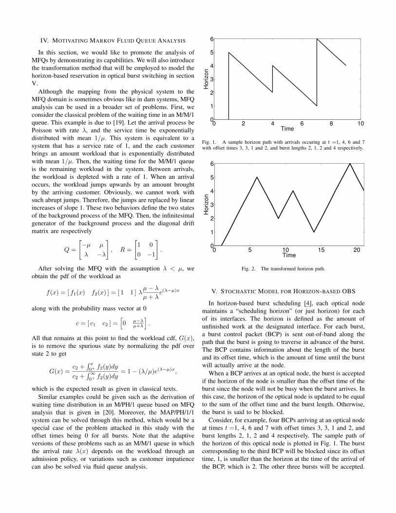
Fig. 1. A sample horizon path with arrivals occuring at t =1, 4, 6 and 7with offset times 3, 3, 1 and 2, and burst lengths 2, 1, 2 and 4 respectively.

0 5 10 15 200

1

2

3

4

5

6

Time

Ho

rizo

n

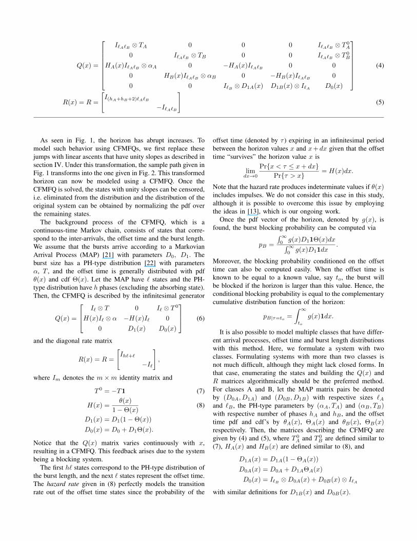
Fig. 2. The transformed horizon path.

V. STOCHASTIC MODEL FOR HORIZON-BASED OBS

In horizon-based burst scheduling [4], each optical nodemaintains a “scheduling horizon” (or just horizon) for eachof its interfaces. The horizon is defined as the amount ofunfinished work at the designated interface. For each burst,a burst control packet (BCP) is sent out-of-band along thepath that the burst is going to traverse in advance of the burst.The BCP contains information about the length of the burstand its offset time, which is the amount of time until the burstwill actually arrive at the node.

When a BCP arrives at an optical node, the burst is acceptedif the horizon of the node is smaller than the offset time of theburst since the node will not be busy when the burst arrives. Inthis case, the horizon of the optical node is updated to be equalto the sum of the offset time and the burst length. Otherwise,the burst is said to be blocked.

Consider, for example, four BCPs arriving at an optical nodeat times t =1, 4, 6 and 7 with offset times 3, 3, 1 and 2, andburst lengths 2, 1, 2 and 4 respectively. The sample path ofthe horizon of this optical node is plotted in Fig. 1. The burstcorresponding to the third BCP will be blocked since its offsettime, 1, is smaller than the horizon at the time of the arrival ofthe BCP, which is 2. The other three bursts will be accepted.

Q(x) =

I`A`B ⊗ TA 0 0 0 I`A`B ⊗ T 0

A

0 I`A`B ⊗ TB 0 0 I`A`B ⊗ T 0B

HA(x)I`A`B ⊗ αA 0 −HA(x)I`A`B 0 0

0 HB(x)I`A`B ⊗ αB 0 −HB(x)I`A`B 0

0 0 I`B ⊗D1A(x) D1B(x)⊗ I`A D0(x)

(4)

R(x) = R =

[I(hA+hB+2)`A`B

−I`A`B

](5)

As seen in Fig. 1, the horizon has abrupt increases. Tomodel such behavior using CFMFQs, we first replace thesejumps with linear ascents that have unity slopes as described insection IV. Under this transformation, the sample path given inFig. 1 transforms into the one given in Fig. 2. This transformedhorizon can now be modeled using a CFMFQ. Once theCFMFQ is solved, the states with unity slopes can be censored,i.e. eliminated from the distribution and the distribution of theoriginal system can be obtained by normalizing the pdf overthe remaining states.

The background process of the CFMFQ, which is acontinuous-time Markov chain, consists of states that corre-spond to the inter-arrivals, the offset time and the burst length.We assume that the bursts arrive according to a MarkovianArrival Process (MAP) [21] with parameters D0, D1. Theburst size has a PH-type distribution [22] with parametersα, T , and the offset time is generally distributed with pdfθ(x) and cdf Θ(x). Let the MAP have ` states and the PH-type distribution have h phases (excluding the absorbing state).Then, the CFMFQ is described by the infinitesimal generator

Q(x) =

I` ⊗ T 0 I` ⊗ T 0

H(x)I` ⊗ α −H(x)I` 0

0 D1(x) D0(x)

(6)

and the diagonal rate matrix

R(x) = R =

[Ih`+`

−I`

],

where Im denotes the m×m identity matrix and

T 0 = −T1 (7)

H(x) =θ(x)

1−Θ(x)(8)

D1(x) = D1(1−Θ(x))

D0(x) = D0 +D1Θ(x).

Notice that the Q(x) matrix varies continuously with x,resulting in a CFMFQ. This feedback arises due to the systembeing a blocking system.

The first h` states correspond to the PH-type distribution ofthe burst length, and the next ` states represent the offset time.The hazard rate given in (8) perfectly models the transitionrate out of the offset time states since the probability of the

offset time (denoted by τ ) expiring in an infinitesimal periodbetween the horizon values x and x+dx given that the offsettime “survives” the horizon value x is

limdx→0

Pr{x < τ ≤ x+ dx}Pr{τ > x}

= H(x)dx.

Note that the hazard rate produces indeterminate values if θ(x)includes impulses. We do not consider this case in this study,although it is possible to overcome this issue by employingthe ideas in [13], which is our ongoing work.

Once the pdf vector of the horizon, denoted by g(x), isfound, the burst blocking probability can be computed via

pB =

∫∞0g(x)D11Θ(x)dx∫∞0g(x)D11dx

.

Moreover, the blocking probability conditioned on the offsettime can also be computed easily. When the offset time isknown to be equal to a known value, say to, the burst willbe blocked if the horizon is larger than this value. Hence, theconditional blocking probability is equal to the complementarycumulative distribution function of the horizon:

pB|τ=to =

∫ ∞to

g(x)1dx.

It is also possible to model multiple classes that have differ-ent arrival processes, offset time and burst length distributionswith this method. Here, we formulate a system with twoclasses. Formulating systems with more than two classes isnot much difficult, although they might lack closed forms. Inthat case, enumerating the states and building the Q(x) andR matrices algorithmically should be the preferred method.For classes A and B, let the MAP matrix pairs be denotedby (D0A, D1A) and (D0B , D1B) with respective sizes `Aand `B , the PH-type parameters by (αA, TA) and (αB , TB)with respective number of phases hA and hB , and the offsettime pdf and cdf’s by θA(x), ΘA(x) and θB(x), ΘB(x)respectively. Then, the matrices describing the CFMFQ aregiven by (4) and (5), where T 0

A and T 0B are defined similar to

(7), HA(x) and HB(x) are defined similar to (8), and

D1A(x) = D1A(1−ΘA(x))

D0A(x) = D0A +D1AΘA(x)

D0(x) = I`B ⊗D0A(x) +D0B(x)⊗ I`Awith similar definitions for D1B(x) and D0B(x).

0 2 4 6 8 100

0.1

0.2

0.3

0.4

Horizon

Horizon p

df

ρ=0.2, analysis

ρ=0.8, analysis

ρ=2.0, analysis

ρ=0.2, simulation

ρ=0.8, simulation

ρ=2.0, simulation

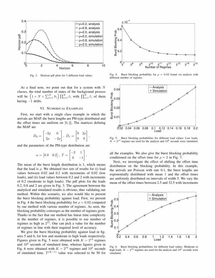
Fig. 3. Horizon pdf plots for 3 different load values.

As a final note, we point out that for a system with Nclasses, the total number of states of the background processwill be

(1 +N +

∑Ni=1 hi

)∏Ni=1 `i with

∏Ni=1 `i of them

having −1 drifts.

VI. NUMERICAL EXAMPLES

First, we start with a single class example in which thearrivals are MAP, the burst lengths are PH-type distributed andthe offset times are uniform on [0, 3]. The matrices definingthe MAP are

D0 =

[−2ρ 0

2ρ −2ρ

], D1 =

[0 2ρ

0 0

],

and the parameters of the PH-type distribution are

α =[0.8 0.2

], T =

[−2 1

0 −1

].

The mean of the burst length distribution is 1, which meansthat the load is ρ. We obtained two sets of results for (i) loadvalues between 0.02 and 0.2 with increments of 0.02 (lowloads), and (ii) load values between 0.2 and 2 with incrementsof 0.2 (moderate to high loads). The pdf plots for the loads0.2, 0.8 and 2 are given in Fig. 3. The agreement between theanalytical and simulated results is obvious, thus validating ourmethod. Within this scenario, we also would like to presentthe burst blocking probability against load. First, we presentin Fig. 4 the burst blocking probability for ρ = 0.02 computedby our method with various number of regimes. As seen, theblocking probability converges as the number of regimes grow.Thanks to the fact that our method has linear time complexityin the number of regimes, it is possible to use number ofregimes as high as 215. One can pick a value for the numberof regimes in line with their required level of accuracy.

We give the burst blocking probability against load in fig-ures 5 and 6, for low and moderate to high loads respectively.Figures given in Fig. 5 were obtained with K = 214 regimesand 108 seconds of simulated time, whereas figures given inFig. 6 were obtained with K = 210 regimes and 106 secondsof simulated time. T (K−1) value was selected to be 50 for

6

6.2

6.4

6.6

x 10−4

Burs

t B

lockin

g P

rob.

Number of Regimes2

152

142

132

122

112

102

92

82

7

Fig. 4. Burst blocking probability for ρ = 0.02 found via analysis withdifferent number of regimes.

0.02 0.04 0.06 0.08 0.1 0.12 0.14 0.16 0.18 0.20

0.01

0.02

0.03

0.04

Load

Burs

t B

lockin

g P

rob.

AnalysisSimulation

Fig. 5. Burst blocking probabilities for different load values: Low loads.K = 214 regimes are used for the analysis and 108 seconds were simulated.

all the examples. We also give the burst blocking probabilityconditioned on the offset time for ρ = 2 in Fig. 7.

Next, we investigate the effect of shifting the offset timedistribution on the blocking probability. In this example,the arrivals are Poisson with rate 0.1, the burst lengths areexponentially distributed with mean 1 and the offset timesare uniformly distributed on intervals of width 5. We vary themean of the offset times between 2.5 and 32.5 with increments

0.2 0.4 0.6 0.8 1 1.2 1.4 1.6 1.8 20

0.1

0.2

0.3

0.4

0.5

Load

Bu

rst

Blo

ckin

g P

rob

.

AnalysisSimulation

Fig. 6. Burst blocking probabilities for different load values: Moderate tohigh loads. K = 210 regimes are used for the analysis and 106 seconds weresimulated.

0 0.5 1 1.5 2 2.5 30.2

0.4

0.6

0.8

1

Offset Time

Co

nd

itio

na

l B

urs

t B

lockin

g P

rob

.

Fig. 7. Burst blocking probability conditioned on the offset time for ρ = 2.

2.5 7.5 12.5 17.5 22.5 27.5 32.50.13

0.131

0.132

0.133

0.134

0.135

Mean Offset Time

Burs

t B

lockin

g P

rob.

Fig. 8. The effect of shifting the offset time distribution on the blockingprobability.

of 5. The blocking probabilities are plotted in Fig. 8. Theblocking probabilites barely change, so we conclude thatshifting the offset time distribution without changing its shapehas only a marginal effect on the blocking probability.

After observing that shifting has a marginal effect, weinvestigate the effect of the offset time variation. We usethe same arrival process and burst length distribution as theprevious example. The offset times are uniformly distributedin the interval [10−u/2, 10+u/2], so the mean offset time isfixed at 10, but the variance increases with the parameter u. InFig. 9, the blocking probability is plotted against u, showingthat increased variation in offset time hurts the performancein terms of blocking probability, i.e. deterministic offset timesare preferable over random ones. This result was also obtainedin [9], but through simulation.

Lastly, we give a two-class example. The arrivals of bothclasses are Poisson and the overall rate is varied between 0.2and 1 with increments of 0.2. Three scenarios in which class 1,the low priority class, brings 25%, 50% and 75% of the overalltraffic are solved. Burst lengths are exponentially distributedwith mean 1 for both classes. In this example, we compare twocases. In the first one, the offset times of the two classes aretaken to be uniform with very small supports. The offset timeof class 1 is uniform in [0, 0.05] whereas the offset time ofclass 2 is uniform in [5, 5.05]. In the second case, we replace

0.1 1 2 4 8 12 16 200.05

0.1

0.15

0.2

0.25

0.3

Support of the Offset Time Distribution u

Bu

rst

Blo

ckin

g P

rob

.

Fig. 9. The effect of shifting the offset time variation.

0.2 0.4 0.6 0.8 10.2

0.4

0.6

0.8

1

Overall Load

Ove

rall

Bu

rst

Blo

ckin

g P

rob

.

Uniform, class 1: 25%

Uniform, class 1: 50%

Uniform, class 1: 75%

Exponential, class 1: 25%

Exponential, class 1: 50%

Exponential, class 1: 75%

Fig. 10. Overall blocking probability with two classes.

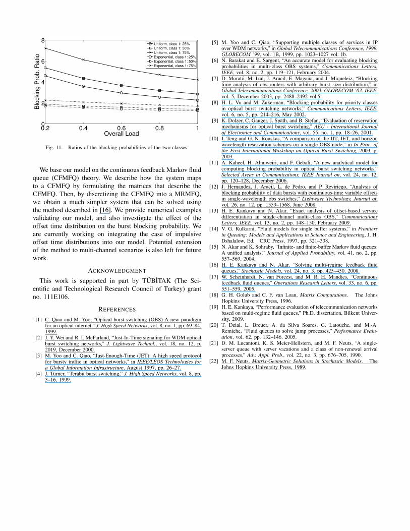
the offset time distribution of class 2 with an exponentialdistribution with mean 5. We had showed that keeping themean constant, offset time distributions with higher varianceslead to increased blocking probabilities. Therefore, an increasein the overall blocking probability is to be expected, which isseen in Fig. 10. However, with this example, we intend toinvestigate the effect of the offset time distribution on thequality of service (QoS) in terms of class separation. Forthis purpose, we plotted the ratio of the blocking probabilityof lower priority class to the blocking probability of higherpriority class in Fig. 11. We see that not only the exponentiallydistributed offset time for the higher priority class increasesoverall blocking probability, it also reduces the separationbetween the classes. Therefore, we conclude that in additionto achieving lower blocking probabilities, deterministic offsettimes also lead to better class separation when QoS is con-cerned.

VII. CONCLUSION

In this study, we model the horizon reservation scheme ona single-channel OBS system and give an exact solution tothe model. We assume no specific circumstances such as lowload. In the most general case, the bursts arrive according toa MAP, burst lengths are PH-type distributed and the offsettime is generally distributed.

0.2 0.4 0.6 0.8 10

2

4

6

8

Overall Load

Blo

ckin

g P

rob

. R

atio

Uniform, class 1: 25%Uniform, class 1: 50%Uniform, class 1: 75%Exponential, class 1: 25%Exponential, class 1: 50%Exponential, class 1: 75%

Fig. 11. Ratios of the blocking probabilities of the two classes.

We base our model on the continuous feedback Markov fluidqueue (CFMFQ) theory. We describe how the system mapsto a CFMFQ by formulating the matrices that describe theCFMFQ. Then, by discretizing the CFMFQ into a MRMFQ,we obtain a much simpler system that can be solved usingthe method described in [16]. We provide numerical examplesvalidating our model, and also investigate the effect of theoffset time distribution on the burst blocking probability. Weare currently working on integrating the case of impulsiveoffset time distributions into our model. Potential extensionof the method to multi-channel scenarios is also left for futurework.

ACKNOWLEDGMENT

This work is supported in part by TUBITAK (The Sci-entific and Technological Research Council of Turkey) grantno. 111E106.

REFERENCES

[1] C. Qiao and M. Yoo, “Optical burst switching (OBS)-A new paradigmfor an optical internet,” J. High Speed Networks, vol. 8, no. 1, pp. 69–84,1999.

[2] J. Y. Wei and R. I. McFarland, “Just-In-Time signaling for WDM opticalburst switching networks,” J. Lightwave Technol., vol. 18, no. 12, p.2019, December 2000.

[3] M. Yoo and C. Qiao, “Just-Enough-Time (JET): A high speed protocolfor bursty traffic in optical networks,” in IEEE/LEOS Technologies fora Global Information Infrastructure, August 1997, pp. 26–27.

[4] J. Turner, “Terabit burst switching,” J. High Speed Networks, vol. 8, pp.3–16, 1999.

[5] M. Yoo and C. Qiao, “Supporting multiple classes of services in IPover WDM networks,” in Global Telecommunications Conference, 1999.GLOBECOM ’99, vol. 1B, 1999, pp. 1023–1027 vol. 1b.

[6] N. Barakat and E. Sargent, “An accurate model for evaluating blockingprobabilities in multi-class OBS systems,” Communications Letters,IEEE, vol. 8, no. 2, pp. 119–121, February 2004.

[7] D. Morato, M. Izal, J. Aracil, E. Magana, and J. Miqueleiz, “Blockingtime analysis of obs routers with arbitrary burst size distribution,” inGlobal Telecommunications Conference, 2003. GLOBECOM ’03. IEEE,vol. 5, December 2003, pp. 2488–2492 vol.5.

[8] H. L. Vu and M. Zukerman, “Blocking probability for priority classesin optical burst switching networks,” Communications Letters, IEEE,vol. 6, no. 5, pp. 214–216, May 2002.

[9] K. Dolzer, C. Gauger, J. Spath, and B. Stefan, “Evaluation of reservationmechanisms for optical burst switching,” AEU - International Journalof Electronics and Communications, vol. 55, no. 1, pp. 18–26, 2001.

[10] J. Teng and G. N. Rouskas, “A comparison of the JIT, JET, and horizonwavelength reservation schemes on a single OBS node,” in In Proc. ofthe First International Workshop on Optical Burst Switching, 2003, p.2003.

[11] A. Kaheel, H. Alnuweiri, and F. Gebali, “A new analytical model forcomputing blocking probability in optical burst switching networks,”Selected Areas in Communications, IEEE Journal on, vol. 24, no. 12,pp. 120–128, December 2006.

[12] J. Hernandez, J. Aracil, L. de Pedro, and P. Reviriego, “Analysis ofblocking probability of data bursts with continuous-time variable offsetsin single-wavelength obs switches,” Lightwave Technology, Journal of,vol. 26, no. 12, pp. 1559–1568, June 2008.

[13] H. E. Kankaya and N. Akar, “Exact analysis of offset-based servicedifferentiation in single-channel multi-class OBS,” CommunicationsLetters, IEEE, vol. 13, no. 2, pp. 148–150, February 2009.

[14] V. G. Kulkarni, “Fluid models for single buffer systems,” in Frontiersin Queuing: Models and Applications in Science and Engineering, J. H.Dshalalow, Ed. CRC Press, 1997, pp. 321–338.

[15] N. Akar and K. Sohraby, “Infinite- and finite-buffer Markov fluid queues:A unified analysis,” Journal of Applied Probability, vol. 41, no. 2, pp.557–569, 2004.

[16] H. E. Kankaya and N. Akar, “Solving multi-regime feedback fluidqueues,” Stochastic Models, vol. 24, no. 3, pp. 425–450, 2008.

[17] W. Scheinhardt, N. van Foreest, and M. R. H. Mandjes, “Continuousfeedback fluid queues,” Operations Research Letters, vol. 33, no. 6, pp.551–559, 2005.

[18] G. H. Golub and C. F. van Loan, Matrix Computations. The JohnsHopkins University Press, 1996.

[19] H. E. Kankaya, “Performance evaluation of telecommunication networksbased on multi-regime fluid queues,” Ph.D. dissertation, Bilkent Univer-sity, 2009.

[20] T. Dzial, L. Breuer, A. da Silva Soares, G. Latouche, and M.-A.Remiche, “Fluid queues to solve jump processes,” Performance Evalu-ation, vol. 62, pp. 132–146, 2005.

[21] D. M. Lucantoni, K. S. Meier-Hellstern, and M. F. Neuts, “A single-server queue with server vacations and a class of non-renewal arrivalprocesses,” Adv. Appl. Prob., vol. 22, no. 3, pp. 676–705, 1990.

[22] M. F. Neuts, Matrix-Geometric Solutions in Stochastic Models. TheJohns Hopkins University Press, 1989.