Analysis and synthesis of multidimensional system classes ...
187
Analysis and synthesis of multidimensional system classes using linear matrix inequality methods
-
Upload
khangminh22 -
Category
Documents
-
view
3 -
download
0
Transcript of Analysis and synthesis of multidimensional system classes ...
Analysis and synthesis of multidimensionalsystem classes using linear matrix
inequality methods

Faculty of Electrical Engineering, Computer Science and TelecommunicationsUniversity of Zielona Góra
Lecture Notes in Control and Computer ScienceVolume 8
Editorial board:
• Józef KORBICZ Editor-in-Chief
• Marian ADAMSKI
• Alexander A. BARKALOV
• Krzysztof GAŁKOWSKI
• Eugeniusz KURIATA
• Andrzej OBUCHOWICZ
• Andrzej PIECZYŃSKI
• Dariusz UCIŃSKI

Wojciech PaszkeInstitute of Control and Computation EngineeringUniversity of Zielona Góraul. Podgórna 5065-246 Zielona Góra, Polande-mail: [email protected]
Referees:
• Andrzej DZIELIŃSKI, Warsaw University of Technology
• Dariusz UCIŃSKI, University of Zielona Góra
The text of this book was prepared based on the author’s Ph.D. dissertation
Partially supported by the State Committee for Scienti¯c Research (KBN)in Poland
ISBN 83-89712-81-4
Camera-ready copy prepared from the author’s LATEX2ε ¯les.Printed and bound by University of Zielona Góra Press, Poland.
Copyright c©University of Zielona Góra Press, Poland, 2005Copyright c©Wojciech Paszke, 2005

CONTENTS
Acknowledgments . . . . . . . . . . . . . . . . . . . . . . . . . . . . . . 8
1 Introduction . . . . . . . . . . . . . . . . . . . . . . . . . . . . . . . . 10
2 2-D(n-D) linear systems and LRPs . . . . . . . . . . . . . . . . . . 192.1 State-space models of 2-D linear systems . . . . . . . . . . . . . . . 19
2.1.1 Roesser state-space model . . . . . . . . . . . . . . . . . . . 202.1.2 Fornasini-Marchesini state-space model . . . . . . . . . . . 212.1.3 State-space models of n-D systems . . . . . . . . . . . . . . 232.1.4 Relation between models . . . . . . . . . . . . . . . . . . . 23
2.2 Linear repetitive processes . . . . . . . . . . . . . . . . . . . . . . . 242.2.1 Linear repetitive processes in terms of RM . . . . . . . . . 272.2.2 Linear repetitive processes in terms of FMM . . . . . . . . 272.2.3 1-D equivalent model . . . . . . . . . . . . . . . . . . . . . . 28
2.3 State-space models of 2-D state-delayed systems . . . . . . . . . . 292.3.1 Roesser model with state delays . . . . . . . . . . . . . . . 292.3.2 Fornasini-Marchesini model with state delays . . . . . . . . 29
2.4 Analysis and synthesis problems in n-D system theory . . . . . . . 302.4.1 Stability problem . . . . . . . . . . . . . . . . . . . . . . . . 30
2.4.1.1 Stability of linear repetitive processes . . . . . . . 332.4.1.2 Stability of 2-D state delayed systems . . . . . . . 36
2.4.2 Stabilisation problem . . . . . . . . . . . . . . . . . . . . . 372.4.3 Robust control problem . . . . . . . . . . . . . . . . . . . . 382.4.4 Control problem with performance requirement . . . . . . . 41
2.5 Applications 2-D systems approach . . . . . . . . . . . . . . . . . . 432.5.1 Iterative learning control . . . . . . . . . . . . . . . . . . . 43
2.5.1.1 Discrete case . . . . . . . . . . . . . . . . . . . . . 432.5.1.2 Continuous case . . . . . . . . . . . . . . . . . . . 44
2.5.2 2-D framework for distributed and parallel computing . . . 452.5.3 Analysis of iterative algorithms in 2-D system framework . 48
2.5.3.1 Discrete case . . . . . . . . . . . . . . . . . . . . . 482.5.3.2 Continuous case . . . . . . . . . . . . . . . . . . . 50
2.6 Software for n-D (LRP) analysis and design . . . . . . . . . . . . . 512.7 Concluding remarks . . . . . . . . . . . . . . . . . . . . . . . . . . 52

6 CONTENTS
3 Linear matrix inequality methods . . . . . . . . . . . . . . . . . . 533.1 Linear matrix inequalities . . . . . . . . . . . . . . . . . . . . . . . 53
3.1.1 Bilinear matrix inequalities . . . . . . . . . . . . . . . . . . 563.2 Algorithms and software for LMI methods . . . . . . . . . . . . . . 57
3.2.1 Ellipsoid algorithm . . . . . . . . . . . . . . . . . . . . . . . 583.2.2 Interior-point algorithm . . . . . . . . . . . . . . . . . . . . 583.2.3 Implementation and computational issues . . . . . . . . . . 593.2.4 Software for solving LMIs . . . . . . . . . . . . . . . . . . . 62
3.2.4.1 LMI Control Toolbox . . . . . . . . . . . . . 623.2.4.2 SeDuMi . . . . . . . . . . . . . . . . . . . . . . . 643.2.4.3 Yalmip . . . . . . . . . . . . . . . . . . . . . . . . 64
3.3 Standard LMI problems . . . . . . . . . . . . . . . . . . . . . . . . 653.3.1 Feasibility problem . . . . . . . . . . . . . . . . . . . . . . . 653.3.2 Linear objective minimization problem . . . . . . . . . . . . 653.3.3 Generalized eigenvalue problem . . . . . . . . . . . . . . . . 66
3.4 Analytic solution of the LMI problem . . . . . . . . . . . . . . . . 693.5 Methods to reformulate hard problems into LMIs . . . . . . . . . . 72
3.5.1 Schur complement formula . . . . . . . . . . . . . . . . . . 733.5.2 Elimination of a norm bounded matrix . . . . . . . . . . . . 743.5.3 Elimination of variables . . . . . . . . . . . . . . . . . . . . 74
3.6 Concluding remarks . . . . . . . . . . . . . . . . . . . . . . . . . . 75
4 Robustness analysis with LMI methods . . . . . . . . . . . . . . . 774.1 Computed-aided methods for robustness problems . . . . . . . . . 774.2 Robust stability and stabilisation of di®erential LRPs . . . . . . . 79
4.2.1 Robust stability . . . . . . . . . . . . . . . . . . . . . . . . 804.2.1.1 Norm-bounded model of uncertainty . . . . . . . . 804.2.1.2 Polytopic model of uncertainty . . . . . . . . . . . 824.2.1.3 Affine model of uncertainty . . . . . . . . . . . . . 84
4.2.2 Robust stabilisation . . . . . . . . . . . . . . . . . . . . . . 844.2.2.1 Norm-bounded model of uncertainty . . . . . . . . 854.2.2.2 Polytopic model of uncertainty . . . . . . . . . . . 88
4.3 Robust stability and stabilisation of discrete LRPs . . . . . . . . . 894.3.1 Robust stability . . . . . . . . . . . . . . . . . . . . . . . . 894.3.2 Robust stabilisation . . . . . . . . . . . . . . . . . . . . . . 92
4.3.2.1 Alternative robust stabilisation . . . . . . . . . . . 944.4 Application examples . . . . . . . . . . . . . . . . . . . . . . . . . . 96
4.4.1 Analysis of ILC processes . . . . . . . . . . . . . . . . . . . 964.4.2 Stability of a parallel computing process . . . . . . . . . . . 99
4.5 Concluding remarks . . . . . . . . . . . . . . . . . . . . . . . . . . 101
5 LMI methods in performance analysis . . . . . . . . . . . . . . . 1025.1 Performance speci¯cations for LRPs and n-D systems . . . . . . . 1025.2 H∞ control of di®erential LRPs . . . . . . . . . . . . . . . . . . . . 104
5.2.1 LMI-based H∞ norm computation . . . . . . . . . . . . . . 1045.2.2 H∞ control with a static feedback controller . . . . . . . . 105

CONTENTS 7
5.2.3 H∞ control with a dynamic pass pro¯le controller . . . . . 1065.2.4 Numerical computations of the Lyapunov matrix . . . . . . 115
5.2.4.1 Product Reduction Algorithm . . . . . . . . . . . 1165.3 H∞ control of uncertain di®erential LRPs . . . . . . . . . . . . . . 117
5.3.1 Norm-bounded model of uncertainty . . . . . . . . . . . . . 1175.3.2 Polytopic model of uncertainty . . . . . . . . . . . . . . . . 119
5.4 H∞ control of discrete LRPs . . . . . . . . . . . . . . . . . . . . . 1205.4.1 LMI-based H∞ norm computation . . . . . . . . . . . . . . 1205.4.2 H∞ control with a static feedback controller . . . . . . . . 1215.4.3 H∞ control with a dynamic pass pro¯le controller . . . . . 122
5.5 H∞ control of uncertain discrete LRPs . . . . . . . . . . . . . . . . 1255.5.1 Alternative robust stabilisation . . . . . . . . . . . . . . . . 127
5.6 H2 control of di®erential LRPs . . . . . . . . . . . . . . . . . . . . 1285.6.1 H2 control with a static feedback controller . . . . . . . . . 132
5.7 Guaranteed cost control of LRPs . . . . . . . . . . . . . . . . . . . 1345.7.1 Di®erential LRP case . . . . . . . . . . . . . . . . . . . . . 135
5.7.1.1 Guaranteed cost bound . . . . . . . . . . . . . . . 1365.7.1.2 Guaranteed cost control with a static feedback con-
troller . . . . . . . . . . . . . . . . . . . . . . . . . 1385.7.2 Discrete LRP case . . . . . . . . . . . . . . . . . . . . . . . 141
5.7.2.1 Guaranteed cost bound . . . . . . . . . . . . . . . 1425.7.2.2 Guaranteed cost control with a static feedback con-
troller . . . . . . . . . . . . . . . . . . . . . . . . . 1445.7.2.3 Guaranteed cost control with a full dynamic pass
pro¯le controller . . . . . . . . . . . . . . . . . . . 1465.8 Concluding remarks . . . . . . . . . . . . . . . . . . . . . . . . . . 150
6 LMI methods for 2-D systems with state delays . . . . . . . . . 1516.1 Stability and stabilisation of 2-D system with state delays . . . . . 152
6.1.1 Connection between 2-D delay-free systems and 1-D state-delayed systems . . . . . . . . . . . . . . . . . . . . . . . . . 155
6.1.2 Multiple state-delayed case . . . . . . . . . . . . . . . . . . 1566.1.3 Commensurate delays case . . . . . . . . . . . . . . . . . . 1576.1.4 Stabilisation of 2-D systems with delays . . . . . . . . . . . 159
6.2 Robust stability and robust stabilisation of 2-D systems with statedelays . . . . . . . . . . . . . . . . . . . . . . . . . . . . . . . . . . 1606.2.1 Robust stability . . . . . . . . . . . . . . . . . . . . . . . . 1606.2.2 Robust stabilisation . . . . . . . . . . . . . . . . . . . . . . 162
6.3 Concluding remarks . . . . . . . . . . . . . . . . . . . . . . . . . . 164
7 Conclusions and future works . . . . . . . . . . . . . . . . . . . . . 165
Abstract (in Polish) . . . . . . . . . . . . . . . . . . . . . . . . . . . . . 168

Acknowledgments
First of all, I would like to express my gratitude to my supervisor Prof. KrzysztofGałkowski. Without his constructive comments, useful suggestions and wealth ofideas this dissertation would have never been completed.I am also grateful to Prof. James Lam from University of Hong Kong and
Prof. Eric Rogers from University of Southampton for their advice and support.Their encouragement, knowledge in the ¯eld of linear matrix inequalities, multi-dimensional systems and repetitive processes greatly contributed to the value ofthis work.I also thank my friends Maciej Patan, Bartłomiej Sulikowski and Bartosz Ku-
czewski for many enlightening discussions.
I would also like to thank my parents, my brother and my sister, for theirunconditional love and support. Finally yet importantly, I dedicate this work tomy wonderful and beloved Rita, without whom nothing would have been possible.

Notation
Abbreviations
1-D one-dimensional2-D two-dimensionaln-D n-dimensional (multidimensional)ARE Algebraic Riccati EquationBMI(s) Bilinear Matrix Inequality(ies)EVP Eigenvalue ProblemFMM Fornasini-Marchesini ModelGEVP Generalized Eigenvalue ProblemILC Iterative Learning ControlIPM Interior-Point MethodLMI(s) Linear Matrix Inequality(ies)LRP(s) Linear Repetitive Process(es)LSE Linear System of EquationsRM Roesser ModelSDP Semi-De¯nite Program(ming)SVD Singular Value Decomposition
Notation
Rn n-dimensional real vector spaceRn×m set of real n×m matricesN set of natural numbersZ set of integer numbersA Â (º) 0 positive (semi-)de¯nite matrixA ≺ (¹) 0 negative (semi-)de¯nite matrixAT transpose of a matrixA−1 inverse of a matrixA−T (AT )−1
I identity matrix0 null matrixtrace(A) trace of a matrixrank(A) rank of a matrixdiag(A1, . . . ,An) matrix with diagonal elements (A1, . . . ,An)det(A) determinant of a matrixker(A) null space of a matrixIm(A) range space of a matrixCo (, , ) convex hullRe(·) real part of a complex numberλ(A) set of eigenvalues of a matrixλmax(A), λmin(A) maximum, minimum eigenvalue of a matrix A
σ(A), σ(A) maximum, minimum singular value of a matrix A
ρ(A) spectral radius of a matrix A
∀ for all

Chapter 1
INTRODUCTION
In the past three decades, progress in technology has been accompanied by thedevelopment of diverse and complicated systems. Among them, are multidimen-sional (n-D) systems characterized by rational functions, or matrices of severalindependent variables which can represent di®erent space co-ordinates or mixedtime and space variables. This is a result of information propagation in more thanone independent direction which is the essential di®erence from the classical, orone-dimensional (1-D) case, where information propagates only in one direction.The interest in n-D systems (Bose, 1982, 1985, 2001; Gałkowski et al., 2003e;
Gałkowski and Wood, 2001; Kaczorek, 1985; Zerz, 2000) has been motivated pre-dominantly by a wide variety of applications, arising in both theory and practicalapplications. Examples of such applications are multidimensional signal and imageprocessing (Bracewell, 1995; Dudgeon and Merserau, 1984; Handkiwicz et al., 2000;Mese and Vaidyanathan, 2002), n-D coding and decoding (Miri and Aplevich, 2000;Shi and Zhang, 2002) and n-D ¯ltering techniques (Basu, 2002; Lu and Antoniou,1992), which are frequently used in computer graphics and animation for objectrendering. Recently, repetitive processes have been the most investigated classof n-D systems (Rogers et al., 2005; Rogers and Owens, 1992, 2001), which areclearly two-dimensional (2-D) systems, with applications ranging from long-wallcoal cutting and metal rolling (see, for example, (Foda and Agathoklis, 1992; Gał-kowski et al., 2003d; Rogers and Owens, 1992)) to iterative learning control (ILC)schemes (Amann et al., 1998; Longman, 2000; Owens et al., 2000) and iterativealgorithms for solving nonlinear dynamic optimal control problems based on themaximum principle (Roberts, 2000a,b, 2002).While studying linear n-D systems and linear repetitive processes (LRPs),
many analysis and synthesis problems arise. Among them are fundamental qu-estions related to stability and stabilisation, feedback control, robust control andperformance measure that should be provided with efficient methods of their so-lution. Unfortunately, linear n-D systems and LRPs cannot be analyzed by directextension of existing methods from 1-D systems theory, because such an approachignores their inherent n-D structure and results in computationally hard problems.This makes most n-D system analysis and synthesis tests not computationally ef-fective and sometimes not feasible.In view of computer-aided analysis and synthesis, the efficiency of a method
involves two main aspects: avoiding extensive storage use and keeping the com-putational complexity as low as possible. The ¯rst requirement implies that the

1. Introduction 11
storage should be proportional to the amount of data de¯ning the system. Due tothe fact that large amounts of memory are available in modern computer worksta-tions, the ¯rst requirement may be neglected. Concerning the second requirement,we focus on some key concepts from the theory of complexity, highlighting their re-levance to systems and control theory (Blondel and Tsitsiklis, 2000b; Fu and Luo,1997; Vidyasagar, 1998). A large proportion of the control problems (especiallyin 1-D systems theory) is algorithmically solvable with polynomial time computa-bility, i.e. the running time of an algorithm on any problem instance of the sizen increases no faster than some polynomial function in n. This class of problemsis so-called P, and the problems which belong to such a class are considered ef-¯ciently solvable. An example of such a problem in 1-D control theory, knownto be polynomial-time solvable, is the stability problem. It can be converted intocomputing of system matrix eigenvalues and verifying whether their moduli are allsmaller than 1 (discrete system case) or that they are all in the open-left half-plane(continuous system case). Since these operations are always performed in polyno-mial time, the stability problem belongs to class P. It is important to note that analternative method is the Routh test, which can also be answered in polynomialtime. This clearly means that the described stability tests of a 1-D system can beefficiently solved even for high-order systems, and hence it is suitable for inclusionin a software package.
The problem is assigned to the NP (nondeterministic polynomial time) classif it is veri¯able (but not necessarily solvable) in polynomial time, i.e. we can ve-rify, in polynomial time, whether a proposed solution is correct. Other problemsare shown to be NP-hard (Blondel and Tsitsiklis, 2000b; Vidyasagar and Blondel,2001), meaning that although these problems may be algorithmically solvable, nopolynomial time algorithm is possible, assuming the validity of a long-standingconjecture in computer science (P 6= NP), which is widely believed to be true.An example of the NP-hard problem in 1-D system theory is a question related tooutput feedback stabilisation with constraints, namely determining whether thereexists a matrix K satisfying K low < K < Khigh and such that A + BKC isstable (Vidyasagar, 1998), where matrices A, B, C, K low and Khigh are given.However, many NP-hard problems can be routinely solved in practice, either exac-tly or approximately using various methods, but generally they are only limitedto low-scale problems. This makes computer implementations possible. Some ofcontrol problems are shown to be undecidable, that is, they are not amenable toan algorithmic solution and frequently the approximate versions of these problemsare also computationally hard. An example of an undecidable problem in controltheory is the one related to the stability of linear time-varying systems (Blondeland Tsitsiklis, 2000a).
It is a natural question to ask if analysis and synthesis problems in n-D sys-tems theory can be considered e®ectively or satisfactorily solved. Unfortunately,nowadays, most of such problems are assumed to be NP-hard or even undecidable.This means that solving many of n-D system analysis and synthesis problems isa nontrivial task. To see this, consider, for example, the stability problem. Whendealing with 2-D (n-D) systems, representations in terms of rational functions of
12
several independent variables are frequently used as a foundation for a systemsanalysis (Bose, 1977, 1982; HÄatÄonen and Ylinen, 2003; Youla and Gnavi, 1979)and allow us to formulate stability tests. However, they turn out to be undeci-dable because we have to check an in¯nite set of system poles, which obviouslycannot be done in ¯nite time. Indeed, zeros of a 2-D (n-D) system characteristicpolynomial (i.e. 2-D (n-D) system poles) are not isolated as in the 1-D case and,in general, they cannot form a ¯nite set. Therefore, to date no e®ective tests(with the complexity being a polynomial in decision variables) exist for decidingif a polynomial of several independent variables has no zeroes in the closed bidisk(n-disk). Furthermore, the problems with computation of n-D system poles areaccompanied by difficulties in applying the pole placement technique, since there isno link between the pole placement and the dynamic response of the n-D system.This immediately makes the controller synthesis a difficult task.It is not a surprise that computational problems of the same kind occur when
dealing with LRPs and we take account of the fact that they reveal an inherent2-D system structure. As an example, the stability test for discrete LRPs can beconsidered. It is shown in (Rogers and Owens, 1992) that the standard test forstability along the pass, involves the computation of the eigenvalues of a potentiallylarge matrix for all points on the unit circle in complex plane. This is clearlyimpossible in practice and means that the stability problem of LRPs is undecidable.In view of these computational difficulties, it is only possible to provide sufficientstability conditions, i.e. conditions which involve only computations for a ¯nitenumber of points. On the other hand, it is difficult to specify the points forchecking. However, in the case of LRP, information propagation in one of twoseparate directions only occurs over a ¯nite duration and therefore the 1-D modelof underlying dynamics can be provided. One of the implications of this fact, is thepossibility of applying 1-D system analysis and synthesis methods. Nevertheless,the resulting process matrices depend on the pass length, which often makes 1-Dsystem theory tests computationally ine®ective (Gramacki, 1999b).Another set of problems with the n-D system theory are those that are cau-
sed by the complexity of the underlying ring structure, i.e. polynomials in twoand more indeterminates where the underlying ring does not have a division al-gorithm (Bose, 1977; Gałkowski, 2001a). The existence of a division algorithmfor Euclidean ring forms constitutes a foundation for the algorithmic derivation ofmany canonical forms and solution techniques in 1-D system theory.To overcome some of these problems, much e®ort has been dedicated to es-
tablishing mathematical tools, outside these required in 1-D system theory, whichcan be used to constitute computationally e®ective methods for n-D systems ana-lysis and synthesis. Among recently developed methods are those based on beha-vioural theory (Pillai et al., 2002; Wood et al., 2001) and GrÄoebner-basis (Basu,2002; Curtin and Saba, 1999; Kalker et al., 1995).The behavioural approach (Polderman and Willems, 1997; Willems, 1991) to
linear systems looks at system equations as just one possible way of representing a‘behaviour’, that is a set of time trajectories of a vector of selected variables. Thispoint of view allows us to consider some hard problems in n-D system theory, e.g.

1. Introduction 13
n-D systems pole placement, but this requires wide-spread knowledge of abstractalgebra (Shankar and Willems, 2000; Wood et al., 2001). In addition to this, thebehavioural approach is still under development and today, this approach cannotbe widely applied in practice as many theoretical problems to overcome remain.
The interest in the GrÄoebner bases, which have been introduced by Buchber-ger (Buchberger, 1985), has been motivated by developing algebraic methods andsoftware to support them. Nevertheless, GrÄoebner bases establish an automaticproving method for many non-trivial theorems which have immediate applicationsin n-D system theory (Lin, 2001; Lin et al., 2001). They need to ¯nd an appro-priate multivariate polynomial set associated with the problem at hand that is ahard task—worst-case complexity is doubly exponential in the number of varia-bles (Bose, 1985). For this reason available software allows us to apply this methodonly to very small problems (systems with ¯ve or six variables), and therefore itis not very useful while solving engineering problems.
Recently, the most popular technique for formulating the stability test forn-D systems is that based on constructing Lyapunov functionals (Bliman, 2002;Hinamoto, 1997; Lu, 1994; Lu and Lee, 1985). Since an appropriate Lyapunovfunctional candidate is provided, the corresponding stability condition can beexpressed in terms of bilinear matrix inequalities (BMIs) (Safonov et al., 1994;VanAntwerp and Braatz, 2000; Vandenberghe and Balakrishnan, 1997) or linearmatrix inequalities (LMIs) (Boyd et al., 1994; Packard et al., 1991). These twoproblem formulations di®er from each other. BMIs introduce a general frameworkto formulate control problems, but they are known to be NP-hard (Toker andÄOzbay, 1995), and hence no polynomial-time algorithm exists to solve them. Onthe other hand, not all problems can be formulated in terms of LMIs, but aresolved with great practical and theoretical efficiency using interior-point algori-thms (Nesterov and Nemirovskii, 1994) which are polynomial-time algorithms. Itturns out that, in practice, that is even more e®ective. Therefore, LMI methodsseem to be especially attractive when dealing with n-D systems and LRPs. Ho-wever, this approach only results in sufficient conditions for stability and requiresthe problem to be formulated in terms of LMIs which is a difficult task. Althoughsome results on converting stability conditions of n-D systems and LRPs into anLMI form have been published (Du and Xie, 2002; Gałkowski et al., 2002d; Lu,2002), it is necessary to provide the results for various classes of n-D systems,especially for these where uncertainties, disturbances and delays may appear.
One of the most challenging problems in control theory of 1-D and n-D systemsare those related to analysis and designing systems in the presence of uncertain-ties. It is a critical issue because physical parameter values are only approximatelyknown or vary in time (Ackerman, 1997; Zhou et al., 1996). Another cause of un-certainty is the imperfect knowledge of some system components, or the alterationof their behaviour due to changes in operating conditions. Finally, we have toconsider the ¯nite precision of computational issues, which can be, for exampleintroduced by a ¯nite wordlength of the Analog to Digital (A/D) converters andthe Digital to Analog (D/A) converters. For these reasons, there is a need to ¯nda method that makes it possible to determine whether or not a system is robustly

14
stable. Unfortunately, the problem of providing such a method that can deal withuncertainties of all sorts, is still unsolved. Moreover, most robust problems areproven to be NP-hard (Blondel and Tsitsiklis, 1997, 2000b). In addition to this,the most common situation encountered when dealing with robust problems isthe fact that the controller parameterization depends explicitly on the state-spacematrices of the system, which are unknown. This immediately leads to a problemformulation in terms of BMIs, which has no e®ective solution. However, there areseveral ways to approximate solutions to robust problems using efficient polyno-mial time algorithms. The most frequently used approach is based on computingupper bounds on parameter values for which the system remains stable. Further,this can be formulated with convex optimization over LMIs (Boyd et al., 1994;El Ghaoui and Niculescu, 1999; Packard et al., 1991). In what follows, this appro-ach can be used even in the area of n-D systems (Du and Xie, 1999b; Gałkowskiet al., 2003b) and their classes i.e. repetitive processes (Gałkowski et al., 2003a,2002a,b). Nevertheless, the works related to the area LRPs or n-D systems provideonly some preliminary results which are suitable for a speci¯c class of systems orprocesses.
Another set of problems, even for 1-D systems, are those related to integra-tion of stability and performance design objectives, but only for some specializedde¯nitions of performance and stability measures. In general, performance optima-lity does not guarantee robust stability. Hence, performance should be optimizedwith a robust stability constraint. To this end, optimization of the H2 and H∞norms representing a performance measure has been proposed recently. Since mostH2 and H∞ control problems are shown to be NP-hard and have no analyticalsolution, we are therefore interested in ¯nding a suboptimal solution which is po-ssible in practice. This strategy involves some numerical search techniques suchas convex optimization, which is frequently adopted for solving problems in 1-Dsystem theory (Gahinet and Apkarian, 1994; Scherer and Weiland, 2002; Skeltonet al., 1998). Recently, some attempts have been made towards the developmentof convex optimization methods involving LMIs to H2 and H∞ design for 2-Dsystems (Du and Xie, 2002; Tuan et al., 2002) but to date, no work has beenreported on a solution to this design problem with performance requirements forLRPs. Hence, there is a need to provide these results.
It is well known that the increasing expectations of system dynamic perfor-mances is accompanied by a selection of adequate models of a system. In thereal world, many systems and process dynamics are a®ected by delays which can-not be neglected and make the control such the systems complicated (Richard,2003). Examples of systems with delays in biology, chemistry, economics, mecha-nics, physics, population dynamics, as well as in engineering sciences are includedin (Boukas and Liu, 2003; Dugard and Verriest, 1998; Mahmoud, 2000; Malek-Zavarei and Jamshidi, 1987; Niculescu, 2001) and references therein.
For this reason, in the last few years, great research e®orts have been spenton the development of analysis and synthesis techniques which, extending resultsfrom the ¯eld of delay-free systems, may apply to time-delay systems. However,it turns out that many analysis and design tests and procedures are not suitable

1. Introduction 15
for computer implementation due to their high computational complexity. Forexample, the design of stabilising controllers for time-delay systems may be, ingeneral, NP-hard (Toker and ÄOzbay, 1996). This has motivated us to seek com-putationally e®ective methods for their analysis and synthesis even if they onlyresult in approximate solutions.The point of interest in 1-D time-delay systems is that they can be modelled
using 2-D dimensional theory (Loiseau and Breth¶e, 1997). Since 1-D time delaysystems are indeed in¯nite-dimensional systems (Hale and Lunel, 1993), then it ishighly attractive to use 2-D (n-D) tools, which are clearly ¯nite-dimensional, toanalyse them (Agathoklis and Foda, 1989; Kamen, 1980).On the other hand, most of the existing works on time-delay systems are
concerned with control problems of 1-D systems, but relatively little has been re-ported on 2-D linear systems with delays. The study of such systems with delayhas been motivated by the fact that time delays, which correspond to transpor-tation or computation times, are encountered e.g. during the processing of visualimages which are intrinsically two-dimensional.In view of the above facts, there is a need to provide a method suitable for
treating many problems of analysis and synthesis of 2-D(n-D) system classes in auni¯ed manner. Additionally, the method to be provided must result in a computernumerical package, which makes not only analysis and synthesis considered systemsto be automated processes, but a reasonable computational cost of computations(i.e. polynomial-time) has to be maintained, even for large-scale problems.In the context of an increasing demand for software that will facilitate the
tedious tasks of data input for automatic system design and analysis, numeroussoftware packages have been created. Indeed, since packages like Control Sys-tem Toolbox for Matlab (The Mathworks Inc., 2002) and Control SystemProfessional Suite integrated withMathematica (Bakshee, 2003) exist, bothclassical and modern methods are available for automated analysis and control de-sign. Moreover, recently developed numerical techniques can be applied to a largenumber of previously unsolved problems (or hard to solve) in system control the-ory. It should also be pointed out that, even though an analytical solution exists, anumerical search method for the same problem might have a lower computationalcomplexity than the analytical solution.Unfortunately, these packages are only available for 1-D systems and up now
there is no commercial software related to n-D systems. Although there existsa Matlab-based package (Gałkowski et al., 2000) to aid control related analy-sis/design of LRPs, its use is mainly restricted to 1-D representation and simu-lation capabilities. However, it provides routines for constructing the discreteapproximation of a di®erential LRP, which is an nontrivial task in the case ofLRPs and 2-D systems in general. The main reason for the lack of software toolsfor n-D systems is that the inherent complex structure of such systems resultedin an absence of satisfactory mathematical and numerical tools for solving relatedanalysis and synthesis problems.It has been indicated that among numerical search techniques, convex and
quasiconvex optimization methods (Boyd and Vandenberghe, 2004) which involve

16
LMIs (Boyd et al., 1994; Dullerud and Paganini, 2000; El Ghaoui and Niculescu,1999) are one of the most promising and e®ective tools for the analysis and synthe-sis of 1-D and n-D systems. Hence, to apply LMI methods as the algorithmic corefor a wide variety of problems which have arisen in n-D control theory, appropriateproblem formulations in terms of LMIs are required.Faced with the above facts, it turns out that convex optimization methods
which involve LMIs lead to computer implementable analysis and synthesis tests,and can generally o®er an escape from some potential difficulties which have ari-sen in n-D system theory. However, there are still many analysis and synthesisproblems for n-D systems and LRPs, which have no LMI formulations. This isespecially valid for n-D system classes for uncertainty, disturbances and delaysoccurrence cases. For these reasons this work is focused on extending recentlydeveloped LMIs methods to solve problems which have arisen in the analysis andsynthesis of such n-D system classes.
The main objective of this work is to convert non-trivial problems in theanalysis and synthesis of LRPs and n-D systems into an LMI frameworkfor solving them e±ciently with recently developed software packages. Inparticular, the problem is to apply LMI methods to n-D system classessubject to parameter uncertainties, disturbances and delays. The resultingLMI conditions are implemented as Matlab m-¯les.
The following thesis can be formulated:
Many analysis and synthesis problems of di®erential and discrete LRPsand generally n-D systems, including very di±cult and practically moti-vated problems where uncertainties, disturbances and delays may appear,can be solved e®ectively with LMI methods.
To con¯rm this thesis, the following problems have been addressed:
Theoretical aspects:
• provision and development of a computer implementable formulations,which involve LMIs, for the following problems:
– stability and stabilisation of LRPs subjected to parameter uncertainty,
– controller synthesis with performance requirements (in the form of H∞and H2 norms) for LRPs,
– guaranteed cost control of LRPs,
– stability and stabilisation of state delayed 2-D systems,
– robust stability and robust stabilisation of state delayed 2-D systems,
• formulating optimization procedures which can be used to attenuate thee®ects of uncertainty and disturbances.

1. Introduction 17
Implementation aspect:
• Implementation of a Matlab-based package which numerically solves con-sidered class of problems.
Application aspects:
• application of LMI methods to study stability and convergence properties ofiterative algorithms such as iterative learning control procedures,
• applications of LMI methods to analyze parallel computing processes.
The following outlines the structure of this dissertation and shortly highlights itscontributions.
Chapter 2: This Chapter reviews the state-space representations of the 2-D (n-D) systems and LRPs that are considered. The models with parameteruncertainty and state delays are also presented. Furthermore, computatio-nal problems associated with the analysis and synthesis of n-D systems andtheir classes (e.g. LRPs) are indicated. In particular, it is shown that existingapproaches to the analysis and synthesis of LRPs and 2-D(n-D) systems arelimited only to a certain type of problem and they may not be suitable forother classes of problems, especially for those where uncertainties, distur-bances and delays may appear. Finally, an example is given to illustrate theapplicability of 2-D state-space representation to describe realistic problemsarising in computer science.
Chapter 3: The aim here is to present some fundamental facts about linear ma-trix inequality methods which are the main tools used in this dissertation.Computational aspects of using LMI methods and software to solve themare also considered. This chapter also presents some mathematical tools tomanipulate matrix inequalities and their applications, to obtain a LMI formfor a given non-LMI formulation.
Chapter 4: This Chapter is devoted to providing a concept of computer-aidedrobust design for uncertain LRPs. It is shown that LMI methods extend theuse of computer software to deal with engineering decision problems withuncertainties. The algorithms to design robust and efficient controllers arealso provided. Some computational experiments are presented to illustratethe e®ectiveness of the proposed algorithms.
Chapter 5: This chapter focuses on providing LMI conditions for analysis andsynthesis purposes with performance requirements. This is accompaniedwith H2 and H∞ control theory. Moreover, the guaranteed cost control pro-blem is considered. The resulting conditions are formulated as optimizationproblems involving LMIs, which allows us to increase the system perfor-mance. It is also shown that most of the problems cannot be solved efficien-tly with classical methods (if a solution exists) or even that there was notan analytical solution.

18
Chapter 6: Here 2-D state delayed systems are considered. The stability andstabilisation results are established. To facilitate the computation process,LMIs methods are employed. An optimization technique to improve nume-rical results is described.
The dissertation concludes with an overview of major results and the contribu-tion of this work. Several directions for future research are identi¯ed.

Chapter 2
2-D(n-D) LINEAR SYSTEMS AND LRPS
The linear state-space models for considered classes of 2-D (n-D) systems havebeen the subject of research for over three decades due to their advantage ofproviding a simple and intuitive way to analysis and synthesis for n-D systems (Duand Xie, 2002; Gałkowski, 2001a; Kung et al., 1977). Although, 2-D state-spacemodels seem to be similar to 1-D state-space models, some essential di®erencesexist between them. One of the major di®erences between 1-D and 2-D (n-D)state-space models is that in the 2-D (n-D) case these models deal only with thelocal state in contrast to the global state which preserves all past information as in1-D case. Therefore, some principal system concepts like stability or controllabilitymust be formulated for both local and global states.The state-space representations of 2-D (n-D) systems and their classes are
described in detail in this chapter. Based on these representations, some basicproperties such as stability, robustness and performance bounds are de¯ned anddescribed. Furthermore, it will be shown that checking these n-D systems proper-ties are not generally amenable to an e®ective algorithmic solution owing to thefact that they are generally characterized as being NP-hard or undecidable pro-blems. Finally, some examples are used to illustrate applications and propertiesof presented models.
2.1. State-space models of 2-D linear systems
During the last few decades, considerable attention has been devoted to 2-D sys-tems due to their practical importance (Kaczorek, 1985). In particular, since thelinear state-space models were introduced in the 1970’s the 2-D systems have beenstudied intensively.There are several state-space models for 2-D systems introduced by Roesser
(Roesser, 1975), Fornasini and Marchesini (Fornasini and Marchesini, 1978), At-tasi (Attasi, 1973) and Kurek (Kurek, 1985) which have been generalized to then-D models later on. These models have been commonly used to describe 2-D(n-D) systems, and to investigate their several properties.Here, we will only concentrate on the most common state-space models i.e.
Roesser model (RM) and Fornasini-Marchesini model (FMM). Originally, RM hadbeen proposed to analyse and control linear iterative circuits, but it can be usedin encoding, decoding and image processing, see (Bose, 1982; Bracewell, 1995; Lu

20 2.1. State-space models of 2-D linear systems
and Antoniou, 1992). One of the key features of this model is that the state vectoris partitioned into horizontal and vertical components, say xh and xv, respecti-vely. An alternative formalism to RM is FMM, which is extensively used in signalprocessing (Du et al., 2000) and control (Du and Xie, 2002; Xie et al., 2002). Itshould be noted that FMM is also used to describe delay-di®erential models, seefor example (Tian and Zhang, 2004; Zhang and Deng, 2001). Both models areeasily generalized to the general n-D (n > 2) case and also to the continuous orhybrid case (Kaczorek, 1994). Moreover, it turns out that RM and FMM are notfully independent of each other therefore one model can be embedded in the secondone.On the other hand, a 2-D framework has proven to be an e®ective tool in
the study of LRPs (Rogers and Owens, 1992) due to their inherent 2-D systemstructure. This allows us to use 2-D state-space models i.e. RM and FMM formodelling both the di®erential and discrete LRPs.The unquestioned popularity of the state-space methods in 1-D and n-D sys-
tem theory stems from the fact that they are well understood and efficient andstable numerical linear algebra routines exist, such as the singular value decom-position (SVD) required when manipulating state-space models. In what follows,state-space methods are less sensitive to the size of perturbation in entry data (Hi-gham et al., 2004). This is why the numerical packages prefer state-space repre-sentations of linear systems by means of matrices and vectors rather than rationalmatrix functions or polynomials. Furthermore, much 2-D (n-D) system analysiscan be done within Lyapunov’s framework, which is most naturally performedin the state space. Additionally, it turns out that the Lyapunov matrix can befound by solving a linear system of equations (LSE), algebraic Riccati equations(ARE) (Doyle et al., 1989) and LMIs (Boyd et al., 1994; Skelton et al., 1998) forwhich polynomial-time algorithms exist. Thus, the state-space methods have acomputational advantage over the transfer function approach and they are usedthroughout this dissertation.
2.1.1. Roesser state-space model
The Roesser state-space model (RM) (Kung et al., 1977; Roesser, 1975) is de¯nedby the following equations
[xh(i+ 1, j)xv(i, j + 1)
]=
[A11 A12
A21 A22
] [xh(i, j)xv(i, j)
]+
[B1
B2
]u(i, j)
y(i, j) =[
C1 C2
] [ xh(i, j)xv(i, j)
]+Du(i, j)
(2.1)
In this model i and j are the positive integer valued horizontal and vertical coef-¯cients, xh ∈ Rnh is the vector of horizontally transmitted information, xv ∈ Rnv
is the vector of vertically transmitted information, u ∈ Rl is the vector of controlinputs and y ∈ Rm is the output vector.This state-space formalism (2.1) has been introduced for a linear iterative
circuit, which is considered as a spatial system. An iterative circuit is the combi-

2. 2-D(n-D) linear systems and LRPs 21
nation of individual cells, each of which is identical, in a regular pattern (Malakorn,2003), and where each cell performs a linear transformation, as it is depicted inFig. 2.1. This type of circuit is used widely in automata and logical circuit theory.From a practical viewpoint, the iterative circuit may be used in encoding, deco-ding and image processing (Roesser, 1975). In this case, the boundary conditions
u(i,j)x (i,j)
v
x (i,j+1)v
x (i,j)h x(i+1,j)
h
y(i,j)
cell(i,j)
Fig. 2.1 . A two-dimensional iterative circuit.
are given by
Xh(0) =xh(0, j) ∀j : j ≥ 0Xv(0) =xv(i, 0) ∀i : i ≥ 0 (2.2)
It should be pointed out, that relationships between polynomial matrix theory andstate-space description are very strong in the 2-D(n-D) linear case. As a result ofapplication two variable Z transform in case of RM (2.1), the following transferfunction is obtained
G2RM(z1, z2) =
[C1 C2
]([ I − z1A11 −z1A12
−z2A21 I − z2A22
])−1 [B1
B2
]+D (2.3)
and the characteristic polynomial is given by
C2RM = det([
I − z1A11 −z1A12
−z2A21 I − z2A22
])(2.4)
2.1.2. Fornasini-Marchesini state-space model
Another commonly used state-space model for 2-D systems is the so-called Fornasini-Marchesini model (FMM) (Fornasini and Marchesini, 1978). The basic model of

22 2.1. State-space models of 2-D linear systems
this type (called the second FMM in literature) has the following form
x(i+1, j+1) =A1x(i+1, j)+A2x(i, j+1)+B1u(i+1, j)+B2u(i, j+1)
y(i, j) =Cx(i, j)+Du(i, j)(2.5)
where, x(i, j) ∈ Rn is the local state vector, u(i, j) ∈ Rl and y(i, j) ∈ Rm arethe control input vector and the output vector respectively with i, j ∈ N. Theboundary conditions are de¯ned by
Xh(0) =x(0, j) ∀j : j ≥ 0Xv(0) =x(i, 0) ∀i : i ≥ 0 (2.6)
This model has been motivated by the algebraic point of view of Nerode equiva-lence where 2-D input-output map had been factorized (Fornasini and Marchesini,1976, 1978; Kung et al., 1977). In contrast to RM, the state vector is not split intohorizontal and vertical components. Moreover, Fornasini and Marchesini were the¯rst to realize that the major di®erence between 1-D and 2-D systems is that wecan introduce a global and a local state in 2-D (n-D) case. The global state pre-serves all past information and it is of in¯nite dimension in general (the diagonalline Lk depicted in Fig. 2.2) while the local state gives us the size of recursion.What is more, the global state, denoted here by Xk, is de¯ned as collection of alllocal states along Lk = (i, j) : i+ j = k, hence
Xk = x(i, j) : i+ j = kIn case of FMM of the form (2.5), the transfer function is
x(i+1,j+1)
x(i,j+1)
x(i+1,j)
i
j Lk+1Lk
Fig. 2.2 . An illustration to FMM and global state.
G2FM(z1, z2) = C (I − z1A2 − z2A1)
−1(z1B2 + z2B1) +D (2.7)
and the characteristic polynomial is de¯ned as
C2FM = det (I − z1A2 − z2A1) (2.8)

2. 2-D(n-D) linear systems and LRPs 23
2.1.3. State-space models of n-D systems
The models de¯ned in (2.1) and (2.5) can be generalized in an easy way to anyn > 2. Hence, the n-D system can be described in state space by the Roesser typemodel of the formx1(i1+1, . . . , in)
...xn(in, . . . , in+1)
=
A11 . . . A1n
.... . ....
An1 . . . Ann
x1(i1, . . . , in)
...xn(i1, . . . , in)
+
B1
...B2
u(i1, . . . , in)
y(i1, . . . , in) =[
C1 . . . Cn
]x1(i1, . . . , in)
...xn(in, . . . , in)
+Du(i1, . . . , in)
(2.9)
where xr(i1, . . . , in), r = 1, 2, . . . , n are the local state sub-vectors, u(i1, . . . , in)and y(i1, . . . , in) are the input vector and the output vector respectively withi1, . . . , in ∈ N. The characteristic polynomial is associated with (2.9) is then
CnRM (z1, . . . , zn) = det
I − z1A11 . . . z1A1n
.... . .
...znAn1 . . . I − znAnn
(2.10)
On the other hand, the Fornasini-Marchesini state-space model for n-D systems is
x(i1+1, i2+1, . . . , in+1)=A1x(i1, i2+1, . . . , in+1)
+A2x(i1+1, i2, i3+1, . . . , in+1)
+ . . .+Anx(i1 + 1, i2 + 1, . . . , in−1 + 1, in)
+B1u(i1, i2 + 1, . . . , in + 1)
+ . . .+Bnu(i1 + 1, i2 + 1, . . . , in−1 + 1, in)
y(i1, i2, . . . , in) =Cx(i1, i2, . . . , in) +Du(i1, i2, . . . , in−1, in)
(2.11)
where x(i1, i2, . . . , in) is the local state vector, u(i1, i2, . . . , in) is the input vectorand y(i1, i2, . . . , in) is the output vector with i1, . . . , in ∈ N. The characteristicpolynomial is given by
CnFM (z1, . . . , zn) = det
(I −
n∑
i=1
ziAi
)(2.12)
2.1.4. Relation between models
It is worth mentioning that RM and FMM are not fully independent of each other.To see this, consider the FMM equations (2.5) and de¯ne a new state ξ(i, j) as
ξ(i, j) = x(i, j + 1)−A1x(i, j) (2.13)

24 2.2. Linear repetitive processes
then
ξ(i+ 1, j) =x(i+ 1, j + 1)−A1(i+ 1, j) +Bu(i, j)
=A0x(i, j) +A2 [ξ(i, j) +A1x(i, j)] +Bu(i, j)
=A2ξ(i, j) + [A0 +A2A1]x(i, j) +Bu(i, j)
Hence[ξ(i+ 1, j)x(i, j + 1)
]=
[A2 A0 +A2A1
I A1
] [ξ(i, j)x(i, j)
]+
[B
0
]u(i, j)
y(i, j) =[0 C
] [ ξ(i, j)x(i, j)
]+Du(i, j)
which is identical to the RM form described by (2.1). On the other hand, byidentifying in (2.1) the vector
x(i, j) =
[xh(i, j)xv(i, j)
]
and the matrices A1, A2, B1 and B2 with
A1 =
[A11 A12
0 0
], A2 =
[0 0
A21 A22
], B1 =
[B1
0
], B2 =
[0
B2
]
and use simple operations as in (Fornasini and Marchesini, 1978) to obtain theFMM form (2.5).Throughout this dissertation, the results are presented for one model (RM or
FMM) only with the understanding that they could be applied to another modelafter the above mentioned transformations.
2.2. Linear repetitive processes
Linear repetitive processes (LRPs) are one of the most important classes of 2-D linear systems of both practical and algorithmic interest (Amann et al., 1998;Roberts, 2000a; Rogers et al., 2005; Rogers and Owens, 1992). The essential uniquecharacteristic of such a process is a series of sweeps, termed passes, through a setof dynamics de¯ned over a ¯xed ¯nite duration known as the pass length. On eachpass an output, termed the pass pro¯le, is produced which acts as a forcing functionon, and hence contributes to, the dynamics of the next pass pro¯le. This, in turn,leads to the unique control problem for these processes in that the output sequenceof pass pro¯les generated can contain oscillations that increase in amplitude in thepass to pass direction.To introduce a formal de¯nition, let α < ∞ denote the pass length (which
is assumed to be constant). Then the pass pro¯le yk(p), 0 ≤ p ≤ α (p is theindependent spatial or temporal variable) generated on the pass k acts a forcingfunction on, and hence contributes to, the dynamics of the new pass pro¯le yk+1(p),0 ≤ p ≤ α, k ≥ 0.

2. 2-D(n-D) linear systems and LRPs 25
The schematic illustration of the dynamics evolution is depicted in Fig. 2.3.This ¯gure also corresponds to the simplest possible case of LRP dynamics whereonly the previous pass pro¯le contributes to the current one. In this case we dealwith unit memory LRPs and within this dissertation, reference will be made onlyto this subclass of LRPs.
pa (= )const
k
k+1
k
p p+1. . .
Fig. 2.3 . Schematic illustration of the dynamics of a LRP.
The intrinsic feature of repetitive processes is that their dynamics evolve intwo separate directions, i.e.
• from pass to pass direction (k-direction),• along a given pass of ¯nite duration (p-direction).
Hence, they clearly have 2-D system structure systems and therefore it is naturalto exploit structural links between 2-D linear systems and LRPs. It is worth notingthat in the case of LRP, information propagation in one of two separate directionsonly occurs over a ¯nite duration. This fact is the key di®erence with other classesof 2-D linear systems (see Fig. 2.4 for illustration). According to the fact thatLRP dynamics can evolve as discrete or continuous function of the independentvariable (which has temporal or spatial characteristic), two subclasses of LRPs canbe considered
• discrete LRPs, where evolution of the dynamics in both directions is discrete,• di®erential LRPs where, in contrast to discrete LRPs, the dynamics along thepass evolves as a continuous function of the independent variable (dynamicsfrom pass to pass is still discrete).
The state-space model of a di®erential LRP has the following, commonlyknown (Rogers and Owens, 1992), form over 0 ≤ t ≤ α, k ≥ 0
xk+1(t) =Axk+1(t) +B0yk(t) +Buk+1(t)
yk+1(t) =Cxk+1(t) +D0yk(t) +Duk+1(t)(2.14)
Here on pass k, xk(t) ∈ Rn is the state vector, yk(t) ∈ Rm is the pass pro¯levector, uk(t) ∈ Rl is the vector of control inputs.

26 2.2. Linear repetitive processes
i
j
p
k
a
A 2-D system An LRP
Fig. 2.4 . Information propagation for 2-D systems and LRPs.
To complete the process description, it is necessary to specify the ‘initialconditions’ - termed the boundary conditions here, i.e. the state initial vector oneach pass xk+1(0) and the initial pass pro¯le (i.e. on the pass number 0) y0(t).The simplest possible form of them are
xk+1(0) = dk+1, k ≥ 0,y0(t) = f(t), 0 ≤ t ≤ α
(2.15)
where f(t) ∈ Rm is a vector whose entries are known functions of t over [0, α] anddk+1 ∈ Rn is a vector with constant entries.In case of discrete LRP, the state-space model has the following form over
0 ≤ p ≤ α, k ≥ 0
xk+1(p+ 1) =Axk+1(p) +B0yk(p) +Buk+1(p)
yk+1(p) =Cxk+1(p) +D0yk(p) +Duk+1(p)(2.16)
Again it is necessary to specify the boundary conditions, which are given by
xk+1(0) = dk+1, k ≥ 0,y0(p) = f(p), p = 0, 1, . . . , α− 1 (2.17)
In some cases (e.g. in the cases of mining or optimal control applications, see (Ro-berts, 2000a,b; Rogers and Owens, 1992)) the following form of (2.17) are used
xk+1(0) = dk+1(0) +α−1∑
j=0
Kjyk(j), k = 0, 1, . . . (2.18)
where Kj is a constant matrix of appropriate dimension. These boundary con-ditions are called dynamic boundary conditions (Gałkowski et al., 2001b; Rogerset al., 2002, 2005). Note that in case of di®erential LRP, j is sample point alongthe previous pass.
2. 2-D(n-D) linear systems and LRPs 27
2.2.1. Linear repetitive processes in terms of Roesser model
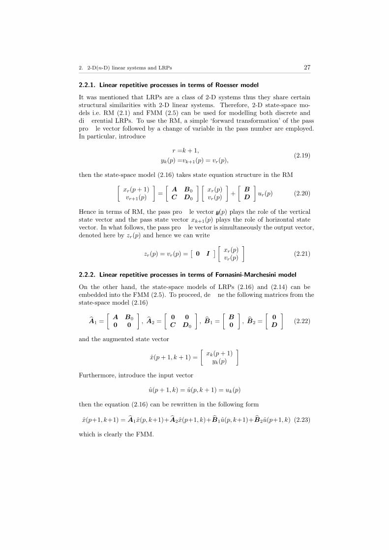
It was mentioned that LRPs are a class of 2-D systems thus they share certainstructural similarities with 2-D linear systems. Therefore, 2-D state-space mo-dels i.e. RM (2.1) and FMM (2.5) can be used for modelling both discrete anddi®erential LRPs. To use the RM, a simple ‘forward transformation’ of the passpro¯le vector followed by a change of variable in the pass number are employed.In particular, introduce
r =k + 1,
yk(p) =vk+1(p) = vr(p),(2.19)
then the state-space model (2.16) takes state equation structure in the RM[xr(p+ 1)vr+1(p)
]=
[A B0
C D0
] [xr(p)vr(p)
]+
[B
D
]ur(p) (2.20)
Hence in terms of RM, the pass pro¯le vector yk(p) plays the role of the verticalstate vector and the pass state vector xk+1(p) plays the role of horizontal statevector. In what follows, the pass pro¯le vector is simultaneously the output vector,denoted here by zr(p) and hence we can write
zr(p) = vr(p) =[0 I
] [ xr(p)vr(p)
](2.21)
2.2.2. Linear repetitive processes in terms of Fornasini-Marchesini model
On the other hand, the state-space models of LRPs (2.16) and (2.14) can beembedded into the FMM (2.5). To proceed, de¯ne the following matrices from thestate-space model (2.16)
A1 =
[A B0
0 0
], A2 =
[0 0
C D0
], B1 =
[B
0
], B2 =
[0
D
](2.22)
and the augmented state vector
x(p+ 1, k + 1) =
[xk(p+ 1)yk(p)
]
Furthermore, introduce the input vector
u(p+ 1, k) = u(p, k + 1) = uk(p)
then the equation (2.16) can be rewritten in the following form
x(p+1, k+1) = A1x(p, k+1)+A2x(p+1, k)+B1u(p, k+1)+B2u(p+1, k) (2.23)
which is clearly the FMM.

28 2.2. Linear repetitive processes
2.2.3. 1-D equivalent model
It is shown (Gramacki, 1999b; Rogers et al., 2005; Rogers and Owens, 1992) thatsome of the properties of LRPs (e.g. asymptotic stability) can be characterizedwith other forms of discrete LRPs (also for di®erential LRPs, after discretizationprocess) using a 1-D equivalent state-space model of the underlying dynamics.Basic steps (for details, see (Gałkowski et al., 2002c; Gramacki, 1999b)) in deri-vation of a such model involve the change of variables (2.19) and de¯nition of theso-called global state, input and pass pro¯le vectors (α denotes the pass length)
Y r =
νr(0)νr(1)...
νr(α− 2)νr(α− 1)
, Xr =
xr(1)xr(2)...
xr(α− 1)xr(α)
, U r =
ur(0)ur(1)...
ur(α− 2)ur(α− 1)
Then the 1-D equivalent state-space model for processes described by (2.16) and(2.17) is de¯ned by
Y (r + 1) =ΦY (r) +∆U(r) +Θxr(0)
X(r) =ΓY (r) +ΣU(r) +Ψxr(0)(2.24)
where the matrices Φ,∆,Θ, Γ, Σ, Ψ are given in (Gałkowski et al., 2002c; Gra-macki, 1999b). It is important to note that use of the presented model allowsus to apply 1-D linear system stability tests (in a few very special cases), whichcan be answered in polynomial time. On the other hand, observing that the ma-trices dimensions are: Φ ∈ Rmα×mα, ∆ ∈ Rmα×lα, Θ ∈ Rmα×n, Γ ∈ Rnα×mα
Σ ∈ Rnα×lα, Ψ ∈ Rnα×n and they clearly depend on pass length. This fact makesstability tests computationally difficult, especially for large pass length (α > 20).A key feature of the model (2.24) is that along the pass dynamics has been
‘hidden’ within the global state, input and pass pro¯le vectors which de¯ne theequivalent 1-D state-space model. Hence, in 1-D linear system terms, the ¯rstequation in (2.24) plays the role of the state vector and the second one is theoutput equation.The 1-D model of the form (2.24) is easily extended to the dynamic boundary
conditions (2.18) by simply inserting (2.18) into (2.24) to yield
Y (r + 1) =ΦY (r) +∆U(r) +Θdr(0)
X(r) =ΓY (r) +ΣU(r) +Ψdr(0)(2.25)
whereΦ = Φ+ΘK, Γ = Γ+ΨK
andK = [K0 K1 · · ·Kα−1]
In this case the dimensions of Φ and Γ are equal to the dimensions of Φ and Γrespectively, and the matrix K ∈ Rn×mα.
2. 2-D(n-D) linear systems and LRPs 29
2.3. State-space models of 2-D state-delayed systems
To this time, most existing works on time-delay systems deal only with 1-D sys-tems (Boukas and Liu, 2003; Dugard and Verriest, 1998; Mahmoud, 2000; Malek-Zavarei and Jamshidi, 1987; Niculescu, 2001). It is well known that many, or evenmost physical systems have natural n-D characteristics. It is only for convenienceand simplicity, and often to avoid computational complexities, that such featureshave been neglected.Due to the fact that time delays correspond to transportation time or compu-
tation time, encountered for instance during the processing of a visual image whichis intrinsically 2-D (Bracewell, 1995), it becomes appropriate to study 2-D time-delay systems. For this purpose, the state-space representation of 2-D systemswith delays in the state are introduced.
2.3.1. Roesser model with state delays
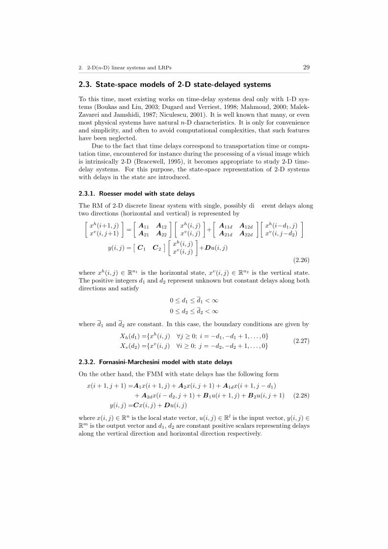
The RM of 2-D discrete linear system with single, possibly di®erent delays alongtwo directions (horizontal and vertical) is represented by[xh(i+1, j)xv(i, j+1)
]=
[A11 A12
A21 A22
] [xh(i, j)xv(i, j)
]+
[A11d A12d
A21d A22d
][xh(i−d1, j)xv(i, j−d2)
]
y(i, j) =[
C1 C2
] [ xh(i, j)xv(i, j)
]+Du(i, j)
(2.26)
where xh(i, j) ∈ Rn1 is the horizontal state, xv(i, j) ∈ Rn2 is the vertical state.The positive integers d1 and d2 represent unknown but constant delays along bothdirections and satisfy
0 ≤ d1 ≤ d1 <∞0 ≤ d2 ≤ d2 <∞
where d1 and d2 are constant. In this case, the boundary conditions are given by
Xh(d1) =xh(i, j) ∀j ≥ 0; i = −d1,−d1 + 1, . . . , 0Xv(d2) =xv(i, j) ∀i ≥ 0; j = −d2,−d2 + 1, . . . , 0
(2.27)
2.3.2. Fornasini-Marchesini model with state delays
On the other hand, the FMM with state delays has the following form
x(i+ 1, j + 1) =A1x(i+ 1, j) +A2x(i, j + 1) +A1dx(i+ 1, j − d1)+A2dx(i− d2, j + 1) +B1u(i+ 1, j) +B2u(i, j + 1)
y(i, j) =Cx(i, j) +Du(i, j)
(2.28)
where x(i, j) ∈ Rn is the local state vector, u(i, j) ∈ Rl is the input vector, y(i, j) ∈Rm is the output vector and d1, d2 are constant positive scalars representing delaysalong the vertical direction and horizontal direction respectively.

30 2.4. Analysis and synthesis problems in n-D system theory
The boundary conditions are given by
Xh(d2) =x(i, j) ∀j ≥ 0; i = −d2,−d2 + 1, . . . , 0Xv(d1) =x(i, j) ∀i ≥ 0; j = −d1,−d1 + 1, . . . , 0
(2.29)
2.4. Analysis and synthesis problems in n-D system theory
In this section we are presenting how a multidimensional system structure af-fects the computational complexity of analysis and synthesis problems for LRPsand generally n-D systems. It should be pointed out that since the frequencydomain methods are used some computational difficulties appear which make exi-sting analysis and synthesis tests difficult or impossible to perform on a computer.Furthermore, when it is not feasible to compute an exact solution to a problem,we are interested in ¯nding an approximate solution as this is better than no solu-tion at all. Therefore the alternative or sometimes only existing solutions to sometheoretical problems are provided for considered system classes, which allow us toapply numerically reliable design algorithms.To make computation efficient, the following approach is employed. First, the
state-space representation of n-D systems and LRPs, that have been described inprevious sections, are used. Next, Lyapunov theory is exploited and the solution tostability and related problems for 2-D(n-D) systems are reduced to the existencepositive de¯ned matrix (the Lyapunov matrix). Finally, equipped by this, theanalysis and synthesis tests are formulated. These tests seem to be computatio-nally attractive when polynomial-time algorithms for solving Lyapunov equations(inequalities) exist. However, this approach only results in sufficient conditions forstability and usually fails, since we deal with uncertain systems or performance ob-jectives. Therefore it is necessary to ¯nd another method which gives us a unifyingpoint of view for most analysis and synthesis problems in n-D system theory.It sounds attractive to apply LMI methods that have been recognized as a
computationally e®ective tool for solving 1-D system control problems, to solveanalysis and synthesis problems in n-D system theory formulated with the state-space representations. This, in turn, makes it possible to create a specializedsoftware tool for automatic n-D system design and analysis.We will start with the stability problem which is a principal requirement for
both LRPs and n-D systems. Next, control objectives and speci¯cations in rela-tion to a stability concept will be considered and control problems will be formu-lated as a combination of these speci¯cations and the closed-loop representation.Here, we will formulate the control problem in the following form: Given a set ofspeci¯cations and an open-loop system, ¯nd a controller, if it exists, so that theclosed-loop ful¯lls the given speci¯cations. This form can be further used to deriveLMI formulation for a speci¯c control problem and for efficient computations.
2.4.1. Stability problem
Concept of an asymptotic stability requires that the n-D system represented bythe state-space model (2.9) or (2.11) without an external input (i.e. u(i, j) = 0)

2. 2-D(n-D) linear systems and LRPs 31
returns to an equilibrium for any values of boundary conditions (2.2) or (2.6).It is well known that necessary and sufficient conditions for asymptotic sta-
bility of n-D systems can be characterized in terms of a characteristic polynomialof the system matrix.
Lemma 1. (Jury, 1978) The n-D system is asymptotically stable if and only ifthe characteristic polynomial given by (2.10) or by (2.12) has no zeros inside theclosed unit n-disc, that is, CnRM (z1, . . . , zn) 6= 0 (or CnFM (z1, . . . , zn) 6= 0) for all(z1, . . . , zn) ∈ U
n, where
Un= (z1, . . . , zn) : |zi| ≤ 1 , i = 1, . . . , n
However, it turns out that this stability test is not computationally efficientand generally the solution is not guaranteed. The main problem here is that zerosof 2-D (n-D) system characteristic polynomial (i.e. system poles) are not isolatedas in 1-D case and they cannot be a ¯nite set. Hence, the stability test is notcomputationally feasible because in¯nitely many points have to be checked.
Example 2.1. To see this, consider a 2-D system with the following characteristicpolynomial
ρ(z1, z2) = 2− z1 − z2 (2.30)
It is straightforward to see that all points (z1, z2) that satisfy ρ(z1, z2) = 0 are po-les of the system (these points can be: . . . , (−1, 3), (0, 2), (1, 1), (2, 0), (3,−1), . . .).That is, there is the in¯nite number of system poles which are zeros of (2.30) andthey form the line (depicted in Fig. 2.5).
z1
z2
z =2-z2 1
-1 1
1
-2
Fig. 2.5 . 2-D system poles.
To make stability tests computationally feasible, it is desirable to providean approximate solution that results in a signi¯cant reduction in computationalcomplexity, but the reduction of computational complexity can only be achievedby introducing some degree of conservativeness i.e. the resulting stability test isonly a sufficient one. One of the ways to obtain such stability conditions is by

32 2.4. Analysis and synthesis problems in n-D system theory
applying Lyapunov theory within state-space models. This approach uses thefollowing candidate of the Lyapunov function
V (i1, . . . , in) = xT (i1, . . . , in)Px(i1, . . . , in)
for some P Â 0. Equipped with this, we now have the following Lemma whichgives the condition for asymptotic stability of n-D system.
Lemma 2. (Gałkowski et al., 2003b) Suppose u(i1, . . . , in) = 0 for i1, ..., in satis-fying i1 + · · ·+ in ≥ 0. If
V0 =∑
i1+···+in=0
V (i1, . . . , in) <∞,
VK =∑
i1+···+in=K
V (i1, . . . , in) <∞,
and
VK+1 ≤ VK (2.31)
then the n-D system represented by the RM (2.9), or by the FMM (2.11) is saidto be Lyapunov stable. Moreover, it is asymptotically stable if (2.31) is satis¯edfor any K∈N and equality holds in (2.31) only when x(i1, . . . , in) = 0.
Above Lemma is a basis for all developments presented in this thesis. It allowsus to formulate a sufficient stability condition in terms of LMI.
Lemma 3. (Gałkowski et al., 2003b) An unforced (i.e. u(i, j) = 0) n-D systemrepresented by the RM (2.9) is asymptotically stable if there exist P  0, Qi  0,i = 1, 2, . . . , n− 1, satisfying
AT1
AT2...
ATn
P[A1 A2 · · ·An
]−
P−n−1∑i=1
Qi 0 · · · 0
0 Q1 · · · 0
....... . . 0
0 0 0 Qn−1
≺ 0 (2.32)
where the matrices A1, A2, . . . ,An are identi¯ed in (2.9) as
A1=
A11 · · · A1n
0 · · · 0.... . ....
0 · · · 0
, . . . ,Ai=
0 · · · 0.... . ....
0 · · · 0Ai1 · · · Ain
0 · · · 0.... . ....
0 · · · 0
, . . . ,A1=
0 · · · 0
.... . ....
0 · · · 0
An1 · · · Ann

2. 2-D(n-D) linear systems and LRPs 33
The most important fact associated with Lemma 3 is that an n-D systemstability condition can be recast into an LMI feasibility problem i.e. ¯nite di-mensional convex optimization problems involving LMI constraints. Indeed, thisstability condition requires only to ¯nd the ¯nite number of scalar variables. Moreprecisely, since each matrix variable in (2.32) has q(q+1)
2 decision variables, then the
resulting number of decision variables to be found when solving (2.32) is n q(q+1)2
(q denotes the number of rows (or columns) of the matrix Ai).Although this result can be further used to solve other analysis and synthesis
problems of 2-D (n-D) system, to date a smaller number of such problems havebeen solved in the area of LRPs and n-D systems with delays. In particular, thelack of results is noticeable for di®erential LRPs. Therefore the main purposeis to provide both e®ective and applicable stability tests for these processes andsystems.
2.4.1.1. Stability of linear repetitive processes
The stability theory of LRPs (Rogers et al., 2005; Rogers and Owens, 1992) isbased on an abstract model in a Banach space setting which includes consideredLRPs as special cases. This theory consists of two distinct stability concepts i.e.
• asymptotic stability, that guarantees the existence of a limit pro¯le which isdescribed by a 1-D linear system state space model,
• stability along the pass, that guarantees the existence of a limit pro¯le andensures that the resulting limit pro¯le is stable along the pass dynamics.
In most cases, asymptotic stability is investigated through the use of 1-D systemtheory applied to the equivalent 1-D model (see Section 2.2.3). However, it turnsout that asymptotic stability cannot guarantee that the resulting pass pro¯le has’acceptable’ characteristic and this can be illustrated by the following examplesfor both di®erential and discrete cases.
Example 2.2. Consider the following di®erential LRP (Benton, 2000), where βis a real scalar,
xk+1(t) =− xk+1(t) + uk+1(t) + (1 + β) yk(t)yk+1(t) =xk+1(t)
xk+1(0) =0, 0 ≤ t ≤ α, k ≥ 0.
In this case, the process is asymptotically stable with limit pro¯le over 0 ≤ t ≤ α
y∞(t) =β y∞(t) + u∞(t)
y∞(0) =0(2.33)
Also if uk+1(t) = 1 and y0(t) ≡ 0, 0 ≤ t ≤ α, k ≥ 0, then it can be easily shownthat the ¯rst pass pro¯le is given by
y1(t) = 1− e−t, 0 ≤ t ≤ α. (2.34)

34 2.4. Analysis and synthesis problems in n-D system theory
But solving the limit pro¯le di®erential equation (2.33) gives
y∞(t) = β−1(eβt − 1), 0 ≤ t ≤ α.
So although the ¯rst pass pro¯le (2.34) is clearly an acceptable dynamic characte-ristic response to the unit step command u1(t) = 1, the resulting limit pro¯le hasunacceptable dynamic characteristics. In particular, for β > 0, the dynamics ofthe limit pro¯le increase exponentially and can be said to be ‘unstable along thepass’ in the obvious intuitive sense.
Example 2.3. Consider the discrete LRP of the form (2.16) described by
xk+1(p+ 1) =− 0.5xk+1(p) + (0.5 + β)yk(p) + uk+1(p)yk+1(p) =xk+1(p)
and assume that xk+1(0) = 0. This process is asymptotically stable but the resultinglimit pro¯le over 0 ≤ p ≤ α
y∞(p+ 1) = βy∞(p) + u∞
is unstable in 1-D sense if |β| ≥ 1.
The reason why asymptotic stability does not guarantee a limit pro¯le whichis ’stable along the pass’ is the ¯nite pass length. Therefore the strongest conceptstability along the pass must be used.
Lemma 4. (Rogers and Owens, 1992) A di®erential LRP (2.14) is stable alongthe pass if and only if the following conditions are satis¯ed:
• ρ(D0) < 1
• Re(ρ(A)) < 0
• all eigenvalues of G(s) = C(sI −A)−1B0 with s = iω have modulus strictlyless than unity ∀ real frequencies ω ≥ 0
where A, B0, C, D0 are matrices from the state-space model of LRP (2.14).
An equivalent set of conditions for stability along the pass can be providedfor a discrete LRP too.
Lemma 5. (Rogers and Owens, 1992) A discrete LRP (2.16) is stable along thepass if and only if the following conditions are satis¯ed:
• ρ(D0) < 1
• ρ(A) < 1
• all eigenvalues of G(z) = C(zI − A)−1B0 ∀|z| = 1 have modulus strictlyless than unity

2. 2-D(n-D) linear systems and LRPs 35
It is clear to see that the third condition is required to make computationsfor all points on the unit circle. This implies that stability of LRPs problem isan undecidable problem. It is then obvious that there is no possibility of solvingsuch a problem in practice. One of the approaches is to perform computations for¯nite a set |z| = 1 that makes a stability test only a sufficient one. However, it isdifficult to determine the number of points for which the computations have to beperformed.Moreover, stability of 1-D equivalent model (2.24) is easily analyzed using the
eigenvalues of the matrix Φ. Unfortunately, this approach cannot be applied inpractise when a large number of points on the pass appear because it dramaticallyincreases the computational complexity of the stability tests. Even if it is possible,or there are no such problems, the 1-D model cannot be used in e®ective robustnessand performance analysis because it adds undue complications to the uncertaintyand disturbances structure.To avoid some of these complications, existing structural links between 2-D
systems and LRPs (see, Sections 2.2.1 and 2.2.2) will be used to develop stabilityresults for these processes. The fact that information propagation in one of theseparate directions occurs over a ¯nite duration, means that existing 2-D systemtheory can be applied after some modi¯cations.To proceed, de¯ne the shift operators z1, z2 in the along the pass (p) and
pass-to-pass (k) directions respectively as
xk(p) :=z1xk(p+ 1),
yk(p) :=z2yk+1(p)
Then the 2-D characteristic polynomial for discrete processes described by (2.16)is de¯ned as
ρ(z1, z2) = det
([I − z1A −z1B0
−z2C I − z2D0
])
On the other hand, by using the s/z transforms instead of z1/z2 one, the charac-teristic polynomial for processes described by (2.14) is obtained
ρ(s, z) := det
([sI −A −B0
−zC I − zD0
])
Based on these characteristic polynomials, the stability of both discrete and di®e-rential LRP can be investigated.
Lemma 6. (Gałkowski et al., 2003c) A LRP is stable along the pass if, and onlyif,
a)ρ(s, z) 6= 0, ∀ (s, z) : Re(s) ≥ 0, |z| ≤ 1
in case of di®erential LRP described by (2.14)
b)ρ(z1, z2) 6= 0, ∀ (z1, z2) : |z1| ≤ 1, |z2| ≤ 1
in case of discrete LRP described by (2.16)

36 2.4. Analysis and synthesis problems in n-D system theory
Again, since stability tests are based on computing zeros of 2-D characteristicpolynomial then there is no e®ective method to check them, because in particular,the set of all zeros cannot be ¯nite.To employ very powerful algorithms for convex optimization based on LMIs,
the results developed for 2-D systems are adopted, therefore the following Lyapu-nov function candidate is used
V (k, p) = V1(k, p) + V2(k, p) = xTk+1(p)P 1xk+1(p) + yTk (p)P 2yk(p) (2.35)
where P 1 Â 0 and P 2 Â 0. It should be pointed out that the above functionsare combination of two independent indeterminates due to the 2-D nature of therepetitive processes considered in this dissertation.In contrary to discrete LRPs, there is no a result for di®erential case. Indeed
there is a need to develop them. It can be done with the following Lyapunovfunction candidate
V (k, t) = V1(k, t) + V2(k, t) = xTk+1(t)P 1xk+1(t) + yTk (t)P 2yk(t) (2.36)
2.4.1.2. Stability of 2-D state delayed systems
The most natural method to analyse a 2-D system with delays is the transformationof such a system into an equivalent non-delayed system and inspect the augmentedmatrix. For example, the system represented by (2.28) can be transformed intothe following
x(i+1, j+1)x(i−d2+1, j+1)x(i−d2, j+1)
...x(i−1, j+1)x(i, j+1)
x(i+1, i−d1)x(i+1, j−d1+1)
...x(i+1, j)
=
A1 A1d 0 · · · 0 0A2d 0 · · ·A2
0 0 I · · · 0 0 0 0 · · · 00 0 0
. . . 0... 0 0 · · · 0
.......... . . I 0 0 0 · · · 0
0 0 0 · · · 0 I 0 0 · · · 0I 0 0 · · · 0 0 0 0 · · · 00 0 0 · · · 0 0 I 0 · · · 00 0 0 · · · 0 0 0 I · · · 0...... · · ·
................ . ....
0 0 0 0 0 0 0 0 · · · I
x(i, j+1)x(i−d2, j+1)
x(i−d2+1, j+1)...
x(i− 2, j + 1)x(i− 1, j + 1)x(i+1, j−d1)
x(i+1, j−d1+1)...
x(i+1, j)
However, immediately some difficulties appear due to the following facts:
• the state delays can be large in both directions, which results in a possiblyvery large dimension of the augmented matrix,
• if the state delays are not exactly known; the dimension of the augmentedmatrix is unknown.
Hence, it is very difficult or even impossible in some cases to provide a computa-tionally e®ective stability test for 2-D state delayed systems in this way. This is
2. 2-D(n-D) linear systems and LRPs 37
the reason why the other methods have to be employed to verify that property, e.g.LMI-based method, which has become a main tool in the analysis and synthesisof 1-D systems (Boukas and Liu, 2003).Moreover, it is important to note that two types of stability problems for
delayed systems exist:
• delay-independent stability (Dugard and Verriest, 1998),• delay-dependent stability (Lee and Kwon, 2002; Moon et al., 2001).
In the ¯rst case, a stability does not depend on delay, which means that systemsare stable for any delay but this stability condition is sometimes restrictive. Toovercome this drawback, a delay-dependent stability condition has to be provided.It turns out that it is relatively simple to provide a delay-independent stability con-dition (for some preliminary results for 2-D linear systems with delays, see (Paszkeet al., 2003, 2004; Trinh and Fernando, 2000)) but there are problems with formu-lating delay-dependent stability conditions.
2.4.2. Stabilisation problem
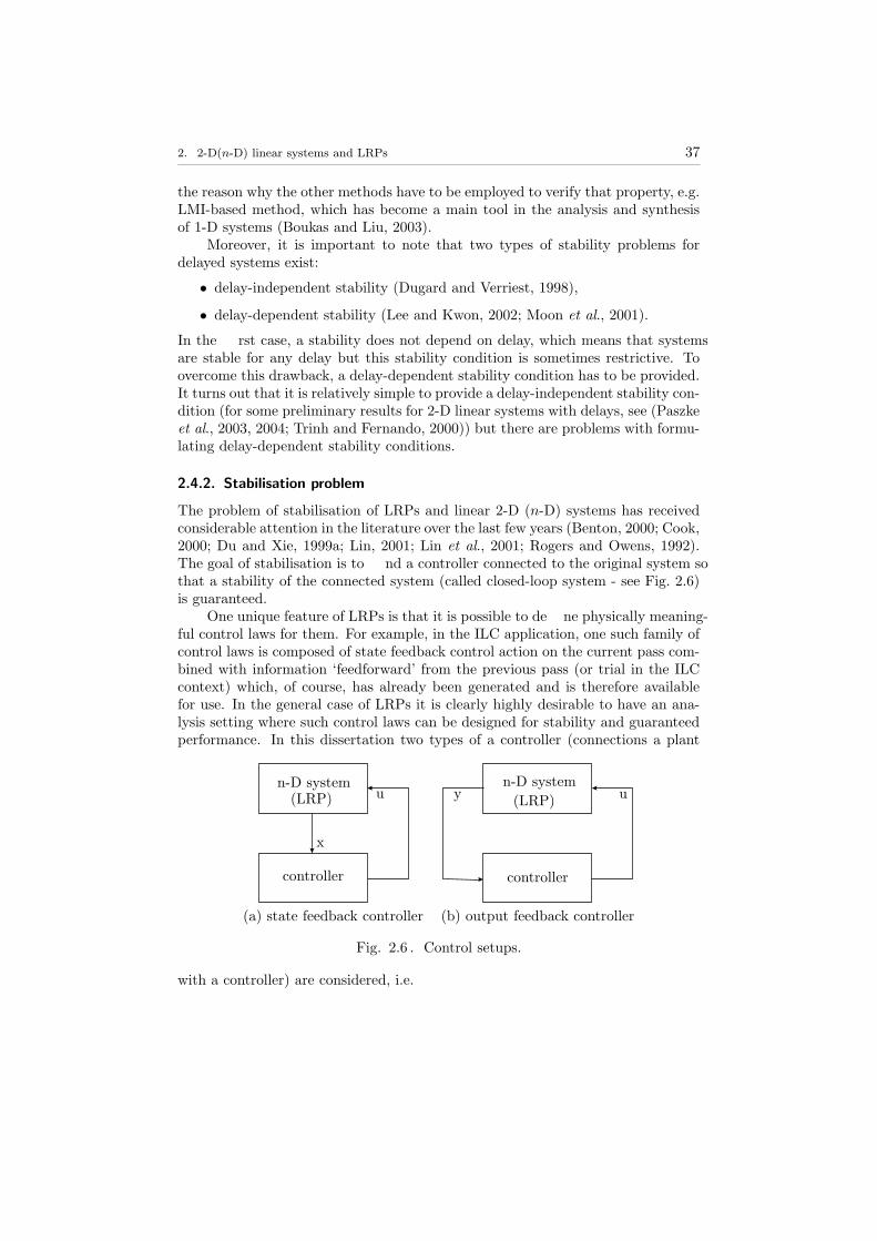
The problem of stabilisation of LRPs and linear 2-D (n-D) systems has receivedconsiderable attention in the literature over the last few years (Benton, 2000; Cook,2000; Du and Xie, 1999a; Lin, 2001; Lin et al., 2001; Rogers and Owens, 1992).The goal of stabilisation is to ¯nd a controller connected to the original system sothat a stability of the connected system (called closed-loop system - see Fig. 2.6)is guaranteed.One unique feature of LRPs is that it is possible to de¯ne physically meaning-
ful control laws for them. For example, in the ILC application, one such family ofcontrol laws is composed of state feedback control action on the current pass com-bined with information ‘feedforward’ from the previous pass (or trial in the ILCcontext) which, of course, has already been generated and is therefore availablefor use. In the general case of LRPs it is clearly highly desirable to have an ana-lysis setting where such control laws can be designed for stability and guaranteedperformance. In this dissertation two types of a controller (connections a plant
n-D system
controller
(LRP) u
x
n-D system
controller
(LRP)y u
(a) state feedback controller (b) output feedback controller
Fig. 2.6 . Control setups.
with a controller) are considered, i.e.

38 2.4. Analysis and synthesis problems in n-D system theory
(a) static feedback controller (see, Fig. 2.6(a)). In this case, we assume that thestate of the system is perfectly available from the state feedback. Hence thefollowing control law can be applied
u(i1, . . . , in) =[
K1 · · · Kn
]x1(i1, . . . , in)
...xn(in, . . . , in)
(2.37)
(b) dynamic output feedback controller (see, Fig. 2.6(b)). This controller is usedwhen no complete state vector is available then one option is to use anobserver to reconstruct it. Therefore the following controller is used
xc1(i1+1, . . . , in)
...xcn(i1, . . . , in+1)
=
Ac11 . . . Ac1n
.... . .
...Acn1
. . . Acnn
xc1(i1, . . . , in)
...xcn(in, . . . , in)
+
Bc1
...Bc2
y(i1, . . . , in)
u(i1, . . . , in) =[Cc1 · · · Ccn
]xc1(i1, . . . , in)
...xcn(in, . . . , in)
+Dcy(i1, . . . , in)
(2.38)
Note that a static output controller, although possible, has a limited use forn-D systems due to much stronger limitations than for the 1-D case, and thedynamic structure is more frequently investigated.
Now the stabilising control problem can be formulated: Given the open-loop LRP(or n-D system) ¯nd a controller (2.37) or (2.38) (if it exists) such that the closed-loop system is stable along the pass (asymptotically stable).The most common situation when we deal with the stabilisation problem
is that the condition for controller existence is clearly bilinear in the Lyapunovmatrix and the controller matrices, which are variables to be found. Therefore,this problem is generally stated as the BMI problem and hence it probably belongsto the class of NP-hard problems.
2.4.3. Robust control problem
Robustness has recently become one of the most important issues in control sys-tems research (Ackerman, 1997; Dullerud and Paganini, 2000; Zhou et al., 1996).This is the result of taking into consideration uncertainties in the modelling pro-cess. When the data is uncertain, there is a need to describe the structure ofperturbation which a®ects system matrices.

2. 2-D(n-D) linear systems and LRPs 39
In common with 1-D linear systems theory, we consider three models of uncer-tainty structure which are introduced below. Note that all uncertainties satisfyingpresented conditions are said to be admissible.
(a) norm-bounded model of uncertainty. This model of uncertainty correspondsto a system which matrices uncertainty are modelled as an additive per-turbation to the nominal system matrices. Therefore a system is said tobe subjected to norm-bounded parameter uncertainty if matrices of such asystem can be written in the form
M = M0 +∆M = M0 +HFE (2.39)
where H and E are some known constant matrices with compatible dimen-sions andM 0 de¯nes the nominal system. F is an unknown, constant matrixwhich satis¯es
FTF ¹ I (2.40)
Note, that the above model of uncertainty has been widely adopted in de-scribing parametric uncertainty of 1-D uncertain systems (see (Khargonekaret al., 1990) and the references therein).
(b) polytopic model of uncertainty. This model of uncertainty corresponds to asystem which matrices range in the polytope of matrices. This means thateach system matrixM is only known to lie in a given ¯x polytope of matricesdescribed by
M ∈ Co (M1,M2, . . . ,Mh) (2.41)
where Co denotes the convex hull. Then, for positive i = 1, 2, . . . , h,M canbe written as
M :=
X :X =
h∑
i=1
αiM i, αi ≥ 0,h∑
i=1
αi = 1
As a simple example, the polytope formed from 4 vertices: M 1,M2,M3
and M4 is depicted in Fig. 2.7. It has to be emphasized that polytopic
M1M
2
M3
M4
Fig. 2.7 . A polytope.
model of uncertainty is only used when we deal with di®erential equationsin the state-space model (2.14). This is motivated by the fact that in thediscrete case, the set all stable matrices may not be a convex set.

40 2.4. Analysis and synthesis problems in n-D system theory
Example 2.4. Let us consider a polytope formed from 2 vertices and assumethat they are
A1 =
[0.5 20 0.5
], A2 =
[0.5 02 0.5
]
Based on well known fact that stability in the discrete case is guaranteed ifand only if all eigenvalues of a system matrix lie in the interior of the unitcircle, it can be seen that the matrices A1 and A2 are stable (λmax(A1) = 0.5and λmax(A2) = 0.5). However, a convex combination yields
A = 0.5A1 + 0.5A2 =
[0.5 11 0.5
]
and λmax(A) = 1.5. This means that A is unstable.
(c) a±ne model of uncertainty. This model of uncertainty corresponds to a systemwhich matrices are modelled as a collection of ¯xed affine functions of somevarying parameters p1, . . . , pk i.e. each matrix can be written in the form
M(p) =M0 + p1M1 + . . .+ pkMk (2.42)
whereM i ∀i = 0, 1, . . . , k are given. Parameter uncertainty is described withrange of parameter values. It means that each parameter pi ranges betweentwo known extremal values pi (minimum) and pi (maximum), therefore itcan be written as
pi ≤ pi ≤ pi
Furthermore, the set of uncertain parameters is
∆ ,p=(p1, p2, . . . , pk) : pi ≤ pi ≤ pi, i=1, . . . , k
and the set of corners of uncertainty region ∆0 is de¯ned as
∆0 ,p=(p1, p2, . . . , pk) : p ∈ pi, pi, i=1, . . . , k
As an example of a set of uncertain parameters, consider 3 parameters:p1, p2, p3 whose values range in the parameter box formed by their extremalvalues in 3-D parameter space - see Fig. 2.8.
Imposing one of the uncertainty model on the state-space model of a di®erentialLRP (2.14) (an uncertain discrete model can be written in this form too) thefollowing uncertain state-space model is obtained
xk+1(t) =Axk+1(t) +B0yk(t) +Buk+1(t)
yk+1(t) =Cxk+1(t) +D0yk(t) +Duk+1(t)(2.43)
where the process matrices A, B0, B, C, D0, D are uncertain and they are de-scribed by one of the model de¯ned above.

2. 2-D(n-D) linear systems and LRPs 41
p2
p3
p2
p3
p2p3
p1
p1
p1
Fig. 2.8 . 3-D parameter space.
Now the robust control problem can be formulated: Given an uncertain open-loop LRP (or n-D system) ¯nd a controller equation (2.37) or (2.38) (if it exists)such that the closed-loop system is stable along the pass (is asymptotically stable)for each admissible system representation.It turns out that, in the presence of uncertainty, many classical methods of
analysis and synthesis may be limited. This is especially valid for robust controlproblems in n-D system theory which, similarly to 1-D case, belongs to the classof NP-hard problems because considered problems are nonlinear and nonconvex.This, in turn, is a result of the dependency of the controller matrices on thestate-space matrices of the system, which are unknown. Additionally, since anypole assignment method is used, then it is difficult to certify if the poles remainin the prescribed region. Therefore, providing sufficiency conditions, based onapproximation techniques, are often about the best we can do. Recently, somepreliminary results on applying LMI methods to deal with uncertain systems andprocesses have been presented (Du and Xie, 1999b; Gałkowski et al., 2003b) butthey need to be developed, especially for LRPs.
2.4.4. Control problem with performance requirement
It often turns out that the model which is stable cannot be used in practice. Hence,the ability e.g. to guarantee the upper bounds on signal is more important thanthe ability to guarantee stability property. For this reason, performance measuresand disturbance rejection or attenuation (when stability is ensured) have becomeimportant issues in recent years, also for n-D systems and LRPs. It is importantto note that disturbance rejection for LRPs and n-D systems have received far lessattention than for standard 1-D systems due to a lack of numerically trackablecontrol design methods. This is mainly caused by difficulties in applying pole

42 2.4. Analysis and synthesis problems in n-D system theory
placement techniques according to the fact that there is no link between the poleplacement and dynamic response of the n-D system. Finally, it is difficult toprovide an analytical solution for such problems or even know if an analyticalsolution exists, a numerical search method for the same problem might have alower computational complexity than the analytical solution.It is therefore desirable to have computationally e®ective methods which make
it possible to apply popular techniques like the H∞ norm (Helton and Merino,1998; Stoorvogel, 1992; Zhou et al., 1996), the H2 norm (Saberi et al., 1995), andguaranteed cost control for LRPs and 2-D (n-D) systems (Guan et al., 2001). Inparticular, the lack of these result is noticeable in the area of di®erential LRP,there is therefore a need to provide and develop them.In this dissertation, the e®ect of disturbances is modelled as an exogenous
input w added to the plant model (see Fig. 2.9). Taking this into consideration
n-D system
controller
(LRP)
z
y
w
u
Fig. 2.9 . The setup for performance.
the additional input results in state-space model (e.g. state-space model of adi®erential LRP)
xk+1(t) =Axk+1(t)+Buk+1(t)+B0yk(t)+B1wk+1(t)
yk+1(t) =Cxk+1(t)+Duk+1(t) +D0yk(t)+D1wk+1(t)
Then, in order to quantify the e®ect of w on output z i.e. pass pro¯le in the caseof LRPs, the H2 and H∞ norms (de¯ned in Chapter 5) are chosen.Now the control problem with performance requirements can be formulated:
Given an open-loop LRP (n-D system) and performance requirements ¯nd a con-troller (2.37) or (2.38) (if it exists) such that the closed-loop system is stable alongthe pass (asymptotically stable) and satisfy performance requirements.It is clear that this design problem requires performance requirements has to
be taken into account, in addition to stability. That is, the main difficulty hereis to provide an e®ective method which can accommodate these objectives intoa single design procedure. It turns out that, in the case of 1-D systems, LMIformulation can overcome this difficulty and make the numerical computationprocess e®ective. Therefore, due to the lack of results in the area of LRPs, thereis a need to ¯nd the LMI formulation for the stabilising control problem withperformance requirements.

2. 2-D(n-D) linear systems and LRPs 43
2.5. Applications 2-D systems approach
Many physical processes and systems can be described by embedding them in a2-D(n-D) framework for further analysis and synthesis (Geng et al., 1990; Kurekand Zaremba, 1993). In addition to this, many, or even most physical systemshave natural 2-D (n-D) characteristics but for simplicity, and often to avoid com-putational complexities, such features have been neglected.Due to these facts, three engineering examples, from the area of computer
sciences, are provided to show use of the 2-D state-space representation and n-Dsystem theory.
2.5.1. Iterative learning control
Iterative learning control (ILC) is a relatively well-known technique for improvingthe tracking response in systems that repeat a given task or operation over andover again. This technique is motivated by human learning and it is mainly usedto learn arti¯cial intelligence systems (e.g. neutral networks) and machines (e.g.robots) and has attracted considerable research interest in recent years (Amann,1996; Chen and Wen, 1999; Moore, 1983; Owens et al., 2000).One of the most interesting results of research on ILC is that the learning
process can be cast into 2-D framework due to information propagation in twoindependent directions i.e. time and iterative directions. This, in turn, leads us toapply 2-D stability theory as a useful method for analysis of learning convergenceand stability.To see this, recall that the basic idea of ILC is to use the information from a
previous execution of the task in order to improve performance from trial to trial,in the sense that the tracking error is sequentially reduced.
2.5.1.1. Discrete case
To formalize the notion of ILC, let a learning iteration (or a trial), denoted hereby the subscript k, be a single execution of the system
xk(p+ 1) =Axk(p) +Buk(p)
yk(p) =Cxk(p)(2.44)
which has input uk(p), output yk(p), and desired output trajectory yd(p) andwhere p ∈ 1, 2, . . . , N . In this case, the boundary conditions are
xk(0) =x0, k = 0, 1, . . .
u0(p) =0, p = 0, 1, . . . , N(2.45)
With this notation the following ILC problem is formulated as: ¯nd, using alearning technique, an appropriate control sequence uk(p), p ∈ [0, N −1] such thattracking error covers to zero along the iterative learning direction (k-direction). Inother words, the problem is to derive the optimal input by evaluating the trackingerror given by
ek(p) = yd(p)− yk(p) (2.46)

44 2.5. Applications 2-D systems approach
This is accomplished by adjusting the input from the current trial i.e. uk(p) to anew input uk+1(p) for the next trial. Therefore, a general iterative control rulecan be de¯ned in the following form
uk+1(p) = uk(p) + ∆uk(p) (2.47)
where ∆uk(p) denotes modi¯cation of the control input. Now, it follows from(2.44), (2.46) and (2.47) that
ek+1(p)− ek(p) = −CAηk(p)−CB∆uk(p− 1)
whereηk(p) = xk+1(p− 1)− xk(p− 1)
Further, from (2.47) and (2.44) can be found
ηk(p+ 1) = Aηk(p) +B∆uk(p− 1)
Then, de¯ning the control law
∆uk(p) =K1ηk(p+ 1) +K2ek(p+ 1)
the RM for ILC is obtained[ηk(p+ 1)ek+1(p)
]=
[A−BK1 −BK2
−CA+CBK1 I −CBK2
] [ηk(p)ek(p)
]
and the boundary condition are given by
ηk(0) =xk+1(0)− xk(0) = x0 − x0 = 0, k = 0, 1, . . .
e0(p) =yd(p)− y0(p) = yd(p)−CATx0, p = 0, 1, . . . , N(2.48)
2.5.1.2. Continuous case
Let us consider the following system
xk(t) =Axk(t) +Buk(t)
yk(t) =Cxk(t)(2.49)
where uk(t) is input, yk(t) is output, and desired output trajectory is yd(t). Fur-ther, it is assumed that 0 < t ≤ T where T denotes the known time horizon. Theboundary conditions are given by
xk(0) =x0, k = 0, 1, . . .
u0(t) =f(t), 0 < t ≤ T(2.50)
The aim is to derive the optimal input by evaluating the tracking error
ek(t) = yd(t)− yk(t) (2.51)
2. 2-D(n-D) linear systems and LRPs 45
Similarly to the discrete system case, it is accomplished by adjusting the input fromthe current trial i.e. uk(t) to a new input uk+1(t) for the next trial. Therefore, ageneral iterative control rule can be de¯ned in the following form
uk+1(t) = uk(t) + ∆uk(t) (2.52)
where ∆uk(t) denotes modi¯cation of the control input. Now, based on (2.49),(2.51) and (2.52) it is seen that
ek+1(t)− ek(t) = −CAηk(t)−CB
∫ t
0
∆uk(τ)dτ
where
ηk(t) =
∫ t
0
[xk+1(t)− xk(t)]
Further, from (2.52) and (2.49) can be found
dηk(t)
dt= Aηk(t) +B
∫ t
0
∆uk(τ)dτ
Hence, under assumption that yd(t) is di®erentiable, the following control law canbe de¯ned
∆uk(t) = K1dηk(t)
dt+K2
dek(t)
dt
and the continuous-discrete form of RM for ILC is obtained[
dηk(t)dt
ek+1(t)
]=
[A−BK1 −BK2
−CA+CBK1 I −CBK2
] [ηk(t)ek(t)
](2.53)
where the boundary conditions are given by
ηk(0) =0, k = 0, 1, . . .
e0(t) =yd(t)−CeAtx0 −∫ t
0
CeA(t−τ)Bu0(τ)dτ
2.5.2. 2-D framework for distributed and parallel computing
Due to a dramatic increase in system complexity and growth of data volume, theproblem of efficient computing becomes of crucial importance. One of the optionsto overcome this problem is to use parallel or distributed computation methods.This, in turn, often requires the use of a networked system. Unfortunately, thee®ect of network congestion (Srikant, 2004), which naturally arises in data ne-tworks such as Internet or ATM and communication delays, can make the resultof computations di®er from the ideal solution, or make the computation processunstable.While such situations occur, available data (samples) can be substituted in
place of the delayed, or even lost samples, to maintain real time requirements and

46 2.5. Applications 2-D systems approach
process stability. Faced with these facts the following problem arises: under whatconditions is the stability of the parallel or distributed process guaranteed?It has been shown in (Bauer et al., 2001) that this problem can be analysed in
a 2-D framework. To proceed, it is assumed that the computation process requiredto evaluate the following di®erence equation
y(n1, n2) =∑
(i,j)∈M0
aijy(n1 − i, n2 − j) +∑
(i,j)∈Mi
bijx(n1 − i, n2 − j) (2.54)
where n1, n2 are the positive integer valued coefficients, aij , bij ∈ R, x(n1, n2) andy(n1, n2) are input and output signals respectively. Further, Mi and M0 de¯neinput and output masks.Suppose now that the equation (2.54) is computed in parallel on C processors.
Then, in order to ensure computability, inputs within inputs masks and previouslycomputed outputs within outputs masks must be available to each processor intime (processors cannot wait for sample to arrive).Adapting results and notation from (Bauer et al., 2001) we consider the case
when C = 4. It is assumed that each processor computes the output for a certainsubregion Si, i = 1, . . . , 4 and they are
S1 = (n1, n2) : 0 ≤ n2 ≤ 10, n1 = 0, 4, 8, . . .S2 = (n1, n2) : 0 ≤ n2 ≤ 10, n1 = 1, 5, 9, . . .S3 = (n1, n2) : 0 ≤ n2 ≤ 10, n1 = 2, 6, 10, . . .S4 = (n1, n2) : 0 ≤ n2 ≤ 10, n1 = 3, 7, 11, . . .
In what follows, the processor assignment function f is (f assigns one out of 4processors to every output sample in the quarterplane)
f(n1, n2) =
1 for (n1, n2) ∈ S12 for (n1, n2) ∈ S23 for (n1, n2) ∈ S34 for (n1, n2) ∈ S4
The processors compute the solutions of the following di®erence equation
y(n1, n2) =a01y(n1, n2 − 1) + a10y(n1 − 1, n2)+ a11y(n1 − 1, n2 − 1) + b00x(n1, n2)
by mapping the function of the form (this function symbolizes the time instant atwhich the sample y(n1, n2) is computed on the processor f(n1, n2))
I(n1, n2) =
n2 + 11n1 for (n1, n2) ∈ S1n2 + 2 + 11(n1 − 1) for (n1, n2) ∈ S2n2 + 4 + 11(n1 − 2) for (n1, n2) ∈ S3n2 + 6 + 11(n1 − 3) for (n1, n2) ∈ S4
As a result we obtain a process for computing the 2-D system response as shownin Fig. 2.10. It is straightforward to see that large delays reduce the amount of

2. 2-D(n-D) linear systems and LRPs 47
Proc 4
Proc 3
Proc 2
Proc 1
Proc 1
outputmask
initialconditions
currentlycomputedsample
n1
n2
1
1
2
2
3
4
5
5
6
6 7 8
9
Fig. 2.10 . Order of computation using 4 processors.
parallelism because some samples are not available (see Fig. 2.11). To ensure realtime implementation of the equation (2.54), available outputs can be substitutedfor the missing output samples. Note however, that these substitutions can make
unavailablesample y(n ,n )1 2
availablesample y(n ,n )1 2
currentlycomputed sample
n1
n2
Fig. 2.11 . Relationship of available output samples between two consecutive maskpositions
our process unstable. To analyse the process behaviour, 2-D system theory can beapplied since results on the stability of 2-D systems are available. In order to usesuch an approach, rewrite (2.54) in terms of RM (2.1) as[xh(n1+1, n2)xv(n1, n2+1)
]=A(n1, n2)x(n1, n2)=
[A11(n1, n2) A12(n1, n2)A21(n1, n2) A22(n1, n2)
][xh(n1, n2)xv(n1, n2)
]
(2.55)

48 2.5. Applications 2-D systems approach
where x(n1, n2) ∈ RH×V is the state vector in a 2-D system of order H in n1 andV in n2. A(n1, n2) is uncertain system matrix which is taken from a set A whichinvolves all matrices A(n1, n2) that correspond to all possible incomplete outputmasks. Therefore, it seems to be appropriate to make use of developing results onrobustness to stability investigation of the system (2.55).
2.5.3. Analysis of iterative algorithms in 2-D system framework
It is well known that most engineering problems are solved on computers with anumerical algorithm. The solution is obtained in an iterative manner where thenumerical algorithm is designed to update the solution in each iteration.One of the important problems solved in this way is the nonlinear optimal
control problem based on maximum principle. It is a standard fact that the appli-cation of maximum principle, results in a set of nonlinear dynamic equations withmixed boundary conditions.Roberts (Roberts, 2000a,b) has recognized that the solution search can be
cast into 2-D framework where
• one dimension is a time horizon of the dynamic system under investigation,
• and another one is the progress of the iterations.
This allows us to use linear a 2-D state-space model and in turn 2-D systemtheory to analyse local stability and convergence properties of a speci¯c algorithmdesigned to achieve the problem solution.
2.5.3.1. Discrete case
Let us consider the real optimal discrete problem (following Roberts (Roberts,2000b))
minu(i)
N−1∑
i=0
L∗(x(i), u(i), i)
subject to
x(i+ 1) = f∗(x(i), u(i), i)
x(0) = x0
where x(i) ∈ Rn and u(i) ∈ Rl are the system state and the control vectorsrespectively, L∗ : Rn × Rm → R is the real performance function, f∗ : Rn ×Rm → Rn represents the real system state equations, and x0 is a de¯ned initialcondition vector. Applications of the maximum principle requires the solution ofthe following two point boundary value problem
x(i+ 1) =f(x(i), p(i), i), x(0) = x0; i ∈ [0, N − 1]p(i+ 1) =g(x(i), p(i), i), p(N) = 0; i ∈ [0, N − 1]

2. 2-D(n-D) linear systems and LRPs 49
where p(i) ∈ Rn is the costate vector and the symbol denotes the optimumvalue. In this case the optimum control is
u(i) = h(x(i), p(i), i)
The solution of a problem of the above form is obtained in an iterative manner byapplying methods such as quasilinearisation or a gradient method in a functionspace. The general form of such an algorithm can be written in the form
Step 1: Select or compute a nominal solution
Y T0 (i) =
u0(i)x0(i)p0(i)
and set the iteration counter k = 0
Step 2: Compute an estimate of the optimal control by solving
Xk(i+ 1) =
[xk(i+ 1)pk(i+ 1)
]= F (Xk(i), Yk(i)), Xk = d0k
uk(i) =h(Xk(i)), i ∈ [0, N − 1]
Step 3: Update the estimated solution
Yk+1(i) = G(Xk(i), Yk(i))
Step 4: Increment k = k + 1 and repeat steps 1-3 above until convergence isachieved.
The above algorithm is clearly in the form of a nonlinear discrete repetitive processwhere d0k
is the initial condition which changes from iteration to iteration andYk(i), i ∈ [0, N ] acts as a driving input from iteration to iteration. However,analysis of the algorithm can be difficult due to the lack of result on nonlinearrepetitive processes. Since we are interested in local convergence properties of thealgorithm, appropriate manipulations enable us to write the algorithm in the formof discrete LRPs (2.16)
Xi(k + 1) =A0Xi(k) +B0Yi(k)
Yi+1(k) =CXi(k) +D1Yi(k)
withXi(0) = di
where the pass length α = N and di is the vector of initial conditions. In thiscase, Xi(k) and Yi(k) are de¯ned as follows
Xi(k) =
[xi(k)pi(k)
], Yi(k) =
ui(k)xi(k)
pi(k + 1)

50 2.5. Applications 2-D systems approach
and the matrices A0, B0, C and D1 are
A0 =
[A+BR
−1BTA−TQ BR
−1BTA−T
−A−1Q A−T
],
B0=
[B∗−BR
−1R∗ A∗−A−BR
−1BTA−T(Q−Q∗) BR
−1(A∗A−1B−B∗)
0 A−T(Q−Q∗) I−(A∗A−1)T
],
C =
kuR
−1BTA−TQ −kuR
−1BTA−T
kxI 0
−kpA−TQ kpA−T
,
D1 =
I − kuR−1
R∗ kuR−1
BTA−T (Q−Q∗) kuR−1(A∗A−1B−B∗)T
0 (1− kx)I 0
0 kpA−T (Q−Q∗) i− kp
(A∗A−1
)T
The matrices R, Q, A, B represent the current solution and R∗, Q∗ representthe optimal solution. The parameters ku, kx and kp are scalar gain parameters.
2.5.3.2. Continuous case
Now consider the problem of determining the solution of the real optimal con-trol (Roberts, 2000a)
minu(t)
φ∗(x(T )) +
∫ T
0
L∗(x(t), u(t))dt
subject to
x(t) = f∗(x(t), u(t))
x(0) = x0
ψ∗(x(T )) = 0
(2.56)
de¯ned over ¯nite time horizon t ∈ [0, T ], where u(t) ∈ Rn and x(t) ∈ Rn arecontinuous control and state vectors respectively, φ∗ : Rn → R is real terminalmeasure, L∗ : Rn×Rm → R is real performance measure function, f ∗ : Rn×Rm →Rn represents real system state equations, and ψ∗ : Rm → Rq is the real terminalconstraint vector.By carrying out required manipulations presented in (Roberts, 2000a), it is
shown that the solution of (2.56) can be found iteratively by solving
d
dtX(i)(t) =A0X
(i)(t) +B0Y(i)(t)
Y (i+1)(t) =CX(i)(t) +D1Y(i)(t)
(2.57)
where
X(i)(t) =
[x(i)(t)p(i)(t)
], Y (i)(t) =
u(i)(t)x(i)(t)p(i)(t)

2. 2-D(n-D) linear systems and LRPs 51
and
A0=
[A BR
−1BT
−Q −A−T
],C=
0 −kuR
−1BT
kxI 0
0 kpI
,
B0 =
[B∗ −BR
−1R∗ A∗ −A BR
−1(B −B∗)
T
0 Q−Q∗ (A−A∗)T
],
D1 =
I − kuR−1
R∗0 kuR
−1(B −B∗)T
0 (1− kx)I 0
0 0 (1− kp)I
which clearly has the form of di®erential LRPs (2.14). Similarly to the discretecase, the matrices A, B, Q and R represent the current solution, R∗, Q∗ standthe optimal solution and ku, kx and kp are scalar gain parameters.
2.6. Software for n-D (LRP) analysis and design
The great advantage of the state-space description is that the analysis and syn-thesis methods derived from it are easily amenable to computer implementation.In what follows, state-space models require manipulation of vectors and matrices,therefore several software packages for engineers can be used for simulating andfor evaluating a system’s behaviour through the state-space representation. Themost widely used software package which supports such a system description isMatlab (The Mathworks Inc., 2004). This package can be easily adopted forsimulating, and also for visualization of LRPs or n-D systems.To date, some packages for simulating and analysis of 2-D (n-D) systems and
LRPs which work under Matlab environment have been presented (D‘Andrea,1999; Gałkowski et al., 2000). Unfortunately, they only provide some simple toolsfor system simulations, analysis and synthesis. The package Lrp Toolbox (Gał-kowski et al., 2000) makes use of 2-D and 1-D models of both di®erential anddiscrete LRPs for their analysis. The 1-D model of LRP can be very easily im-plemented on a computer but becomes quickly impractical when the pass lengthgrows. However, in some simple cases, it is possible to exploit the structure of thematrices. One of the major features of the Lrp Toolbox are routines for con-structing the discrete approximation of a di®erential LRP, which is a nontrivialtask in the case of LRPs and 2-D systems in general (Gramacki, 1999a). Never-theless, this package does not involve any tool to analyse and synthesise uncertainLRPs or performance design purposes.The Multidimensional Systems (MD) Toolbox (D‘Andrea, 1999) invo-
lves many useful routines for n-D system analysis and design. They may be usedto test the stability of n-D systems, to simulate them and to perform control de-sign for these systems. However, this software does not provide tools to solve n-Dsystem theory problems with uncertain data, and there are no routines to manipu-late LRPs and 2-D(n-D) state-delayed systems. Even through LRPs analysis anddesign are possible with 2-D system routines, this package does not exploit LRPs

52 2.7. Concluding remarks
features (e.g. in LRPs case the pass pro¯le vector is simultaneously the outputvector) which leads to other algebraic manipulations and to many simpli¯cationsin relation to a clear 2-D approach.
2.7. Concluding remarks
This chapter gives a brief introduction to n-D state-space models and their abilityto formulate n-D control theory problems. There is no doubt that n-D systemsconstitute the important class of systems according to a wide variety of applicationsarising in both theory and practical applications. Motivated by these applications,the interest in n-D systems is growing and there is a need for numerical software toanalyse them. However, commonly known numerical methods for system analysisand design which are based on computing system poles, cannot be directly appliedto 2-D (n-D) system analysis because of an in¯nite number of 2-D (n-D) systempoles. Therefore, these methods have very high computational cost and theycannot be directly used as a basis to build a software tool for the automatic analysisand synthesis of n-D systems. In order to overcome computational difficulties wepropose to put the alternative problems formulations to some theoretical problemsfor n-D systems and LRPs which results in computationally feasible tests. Theproposed approach is based on combining the state-space representations of aconsidered class of n-D systems with Lyapunov’s framework to derive the problemformulation in terms of LMI which are described in the next chapter.

Chapter 3
LINEAR MATRIX INEQUALITY METHODS
Recently, linear matrix inequality (LMI) methods have become popular among re-searchers from the control community due to their relative simplicity and e®ectivenumerical solution. The basic idea of the LMI methods is to approximate a givenproblem via an optimization problem with a linear objective and LMI constraints.These problems are recognized to belong to the class of P problems because theyare solved with polynomial-time algorithms.LMI methods are reviewed and discussed in detail in this chapter. First, we
need to describe the background information required to understand what LMIsare. Next, the application of modern polynomial-time interior-points methods tosolve optimization problems under LMI constraints are described. In particular,it is shown that convex and quasi-convex optimization problems, which involveLMIs, can be adopted as a core to build software to analyse and synthesise 2-D (or n-D in general) systems and LRPs, where uncertainties, disturbances anddelays occur. Moreover, some software packages used to solve convex optimizationproblems are described.
3.1. Linear matrix inequalities
A linear matrix inequality (LMI) is an expression of the form
F (x) = F (x)T = F0 +
n∑
i=1
xiFi º 0 (3.1)
where
• x = (x1, . . . , xn), x ∈ Rn - is a vector of n real numbers called the decisionvariables to be found,
• F0, . . . ,Fn - a given set of real symmetric matrices of equal dimension,
• the inequality symbol º means that the expression (3.1) is nonnegative de-¯ned, that is zTF (x)z > 0, ∀z 6= 0, z ∈ Rn.
The constraint (3.1) is often used to de¯ne a minimization problem, which iscommonly referred to as a semide¯nite program (SDP) (Vandenberghe and Boyd,

54 3.1. Linear matrix inequalities
1996) of the form
min cTx
subject to F (x) º 0 (3.2)
where the vector c ∈ Rn is given.It is important to note that LMIs have several intrinsic and attractive features.
Firstly, the LMI (3.1) is convex constraint on x (a convex feasibility set). Secondly,while the constraint is matrix inequality instead of a set of scalar inequalities like inlinear programming (LP), a much wider class of feasibility sets can be considered.Indeed, for example, LMIs allow us to describe quadric curves like circles (see,Example 3.1). Thirdly, the convex problems involving LMIs can be solved withpowerful interior-point methods (Nesterov and Nemirovskii, 1994). In this case”solved” means that we can ¯nd the vector of the decision variables x that satis¯esthe LMI, or determine that no solution exists. Sometimes, such solvability problemis called a feasibility problem or an LMI problem in literature. Moreover, the righthand side of (3.1) is symmetric matrix and it is nonnegative de¯ned if, and onlyif, all its eigenvalues are nonnegative.
Example 3.1. To con¯rm that the feasibility set represented by LMI is the convexset, the following inequality is now considered (adopted from (Meinsma, 1997)).1 0 x10 1 x2x1 x2 1
︸ ︷︷ ︸F (x)
=
1 0 00 1 00 0 1
︸ ︷︷ ︸F 0
+x1
0 0 10 0 01 0 0
︸ ︷︷ ︸F 1
+x2
0 0 00 0 10 1 0
︸ ︷︷ ︸F 2
º 0 (3.3)
In this case, we see that the feasible set is the interior of the unit disc(√
x21+x22≤1
),
that is depicted in Fig. 3.1. Note that the Schur complement (for details see Sec-
x1
x2
0.5
0.5
Fig. 3.1 . Example of a feasibility set.
tion 3.5.1) of the block
[1 00 1
]in (3.3) gives the equivalent condition
1−[x1 x2
] [ 1 00 1
] [x1x2
]º 0 ⇔ 1− (x21 + x22) ≥ 0

3. Linear matrix inequality methods 55
It is important to note that since the intersection of two or more convex setsis again convex (Boyd and Vandenberghe, 2004), then the intersection of two ormore convex sets described by LMIs is again a convex set. This means that thereis no distinction between a set of LMIs (where p denotes the number of LMIs)
F (1)(x) º 0...
F (p)(x) º 0
and a single LMIdiag
(F (1)(x), . . . ,F (p)(x)
)º 0
Example 3.2. To illustrate the fact that multiple LMIs can be expressed as a singleLMI, the following example is considered. Suppose, two convex sets described by(3.3) and
x1 + 0.5 ≥ 0are given. They can be expressed by the LMI of the form
1 0 x1 00 1 x2 0x1 x2 1 00 0 0 x1 + 0.5
º 0
which represents the convex set depicted in in Fig. 3.2 (the intersection of hyper-plane and the interior of the unit circle).
x1
x2
0.5
0.5
Fig. 3.2 . Example of a feasibility set 2.
It is worth mentioning that in the case of convex optimization problems withconvex objective functions, any local minimum is a global minimum. This meansthat any algorithm that can compute a local minimum for a convex optimizationproblem, will compute in fact a global minimum.
Remark 3.1. Note that the expressions F (x) ¹ 0 and F (x) ¹ G(x) can berewritten as −F (x) º 0 and G(x) − F (x) º 0 respectively. Moreover, since an

56 3.1. Linear matrix inequalities
LMI is written with º or ¹ then we refer it as a nonstrict LMI. On the other hand,≺ or  denotes that the considered LMI is a strict one. It turns out that a nonstrictLMI can be reduced to an equivalent strict LMI by eliminating equality constraints(a more thorough discussion on this can be found in (Boyd et al., 1994)). Keepingthese facts in mind, we generally deal with strict negative de¯ned LMIs.
3.1.1. Bilinear matrix inequalities
It is a fact that most control problems cannot be directly written in the form ofthe LMI (3.1). Thus, bilinear matrix inequalities (BMIs) have been introduced asa general framework to tackle these control problems (Safonov et al., 1994). BMIhas the following form
F (x, y) = F (x, y)T = F0 +n∑
i=1
xiFi +m∑
j=1
yjGj +n∑
i=1
m∑
j=1
xiyjHij º 0 (3.4)
where the variables are x = (x1, . . . , xn), x ∈ Rn and y = (x1, . . . , ym), y ∈ Rm,and the symmetric matrices F0, Fi, i = 1, . . . , n, Gj , j = 1, . . . ,m and Hij ,i = 1, . . . , n, j = 1, . . . ,m are given data. Unfortunately, BMIs are in generalhighly non-convex optimization problems, which can have multiple local solutions,hence solving a general BMI was shown to be NP-hard (Toker and ÄOzbay, 1995)i.e. no polynomial-time algorithm has been found so far for solving them (wecannot utilize the convex optimization methods) (Goh et al., 1994). This meansthat the solution to the problem formulated in terms of BMI can be providedwith approximation methods. Obviously, this introduces a signi¯cant degree ofconservativeness. In e®ect, BMIs are not so popular as LMIs. However, some ofthe problems recognized as BMI problems (and therefore assumed to be NP-hardproblems) have ”hidden” convexity properties and they can be reformulated interms of LMI.In this dissertation, a BMI problem formulation will be used to indicate that
a considered problem cannot be directly solved with polynomial-time algorithmsbut in some cases exploration of problem properties can lead to the problem for-mulation in terms of LMI.On the other hand, an interesting point to note is that a BMI of the form
(3.4) is an LMI in x for ¯xed y and an LMI in y for ¯xed x. Furthermore, itmeans that BMI is convex in x and convex in y but not jointly convex in x andy (VanAntwerp and Braatz, 2000).
Example 3.3. Consider the following bilinear inequality
1− xy > 0 (3.5)
where x and y are scalar variables. It is clear that (3.5) does not represent aconvex set. To see this, we can consider two points on xy-plane which satisfy theconstraint (3.5), e.g. p1 = (x1, y1) = (0.2, 2) and p2 = (x2, y2) = (4, 0.2) and welook on the Fig. 3.3. Obviously, the point in the half way between the two values,

3. Linear matrix inequality methods 57
0 0.5 1 1.5 2 2.5 3 3.5 4 4.5 50
0.5
1
1.5
2
2.5
3
3.5
4
4.5
5
p1
p2
p3
x
y
Fig. 3.3 . Example of a non-convex set.
i.e.
p3 =1
2(0.2, 2) +
1
2(4, 0.2) = (2.1, 1.1)
does not satisfy (3.5).
Today, problems formulated in BMI framework can be solved with algorithmsbased on a spatial branch and bound strategy which are available only for verysmall problems. Moreover, there remains some problems in the branch and boundapproach therefore these methods are still under development (El Ghaoui andNiculescu, 1999).
3.2. Algorithms and software for LMI methods
Since the simplex algorithm was discovered in the 1940s, much e®ort has beenspent trying to overcome the poor worst-case behaviour of the algorithm - thenumber of iterations may be exponential in the number of unknowns. This e®ortresulted in algorithms with better computational complexity. The¯rst polynomial-time algorithm is the ellipsoid algorithm that was developed in the late 1970’s byKhachiyan (Khachiyan, 1979). This started an intensive search for algorithms witha strong emphasis on convex optimization and computational complexity issues.Then in 1988, interior point algorithms (or interior point method - IPM) had beenestablished by Nesterov and Nemirovskii. This mainly motivates the increasingpopularity of LMI methods (called semi-de¯nite programming - SDP) which areconvex optimization problems and can be solved with IPM.The general features of IPMs are:
• they are efficient in theory - worst-case computational cost of problem solvingis polynomial function of the number of decision variables,

58 3.2. Algorithms and software for LMI methods
• they are efficient in practice i.e. about 5 to 50 iterations, almost independentof input data, are required to ¯nd a solution.
Due to the importance of both ellipsoid and interior point algorithms, they willbe presented in the next two subsections.
3.2.1. Ellipsoid algorithm
The ellipsoid algorithm is the simplest algorithm to solve LMI problems where thesolution with prescribed accuracy is attained in polynomial-time. The basic ideabehind this algorithm is to, given a starting ellipsoid that contains the optimalsolution (i.e. x∗), cut the ellipsoid in half. Then make a minimal volume ellip-soid enclosing that half that contains the optimal solution, and iterate until theoptimum is reached.In more detail, the ellipsoid algorithm contains the following steps
Step 1: Set the iteration counter k = 0 and ¯nd a feasible starting point (withstandard numerical computations) x(0)
Step 2: Compute an ellipsoid E(k) that contains an optimal point x(k)
Step 3: Compute a plane that passes through the centre of the ellipsoid so thatthe solution is guaranteed to lie on one side of the plane
Step 4: Discard that part of the plane which does not contain an optimal point
Step 5: If prescribed accuracy is attained then stop, otherwise set k = k+1 andreturn to the second step
The above steps guarantee that a sequence of ellipsoids contains an optimal pointand the volume of these ellipsoids decreases geometrically (for mathematical detailssee, for example, (Boyd et al., 1994)). However, the ellipsoid algorithm is ratherslow due to slow practical convergence, therefore this algorithm is not particularefficient from a computational point of view. Therefore, available LMI solvers usean interior-point algorithm that currently has many of variations.
3.2.2. Interior-point algorithm
Recently, interior-point methods (IPM) have been applied to optimization pro-blems involving LMIs. The algorithm based on IPM is more computationallyefficient in practice than the ellipsoid one (Nesterov and Nemirovskii, 1994; Van-denberghe and Balakrishnan, 1997; Vandenberghe and Boyd, 1996).The basic idea of the interior-point algorithm is as follows (Meinsma, 1997)
Step 1: Construct a barrier function φ(x) that is well de¯ned for strict feasible xand is −ε (where −∞ < ε¿ 0) only at the optimal x = x∗
Step 2: Generate a sequence x(k) so that
limk→∞
φ(x(k)) = −ε

3. Linear matrix inequality methods 59
Step 3: Stop if φ(x(k)) is negative enough
This algorithm uses the constraints to de¯ne a barrier function which is convexwithin the feasible region and in¯nite outside it. One of the simplest barrierfunctions is
φ(x) = − log det (F (x)) = log det(F−1(x)
)
This barrier function is incorporated into an objective function f0(x) = cTx (c ∈Rn is a given vector), which allows the constrained optimization problem to bereplaced with an unconstrained optimization problem
min f(x) = min f0(x) + µφ(x) = cTx− µ log det (F (x)) (3.6)
where the parameter µ > 0 is to be selected. The optimization problem (3.6)is iteratively solved with the descent method (Beck, 1991; Henrion, 2003) whichproduces a minimizing sequence
xk+1 = xk + tk∆xk (3.7)
where ∆xk is the step of search direction and tk ≥ 0 is the size or step length. Itturns out that for the optimization problem (3.6) Newton’s method can be applied,therefore tk is the gradient of f(x), and ∆xk is the inverse of the Hessian of f(x).As an example of the particular IPM for solving LMIs, we consider the pro-
jective method (Gahinet and Nemirovski, 1997; Nemirovskii and Gahinet, 1994),which has been efficiently implemented in a Matlab-based software (Gahinetet al., 1995). This method guarantees to ¯nd for ε > 0, an ε-solution to theproblem within a ¯nite number of °ops bounded by
mn3 log
(C
ε
)
wherem is the total row size of the LMIs, n is the total number of decision variablesand C is some data-dependent scaling factor. Moreover, no initial feasible solutionis required for the projective method.
3.2.3. Implementation and computational issues
It is known that the vector and matrix operations are fundamental to engineeringand scienti¯c problems. Therefore, several software packages for engineers providemanipulating and computing on vectors and matrices. Among them, Matlabhas become a standard environment for algorithm development and numericalcomputation, including algorithms for solving problems formulated in terms ofLMI. Since most engineering problems are of the form
F (x) =
k∑
p=1
[LpXpR
Tp +RpX
Tp LT
p
](3.8)
where Lp,Rp are given matrices and Xp is the matrix variable which entries aredecision variables x1, . . . , xn, then the canonical representation of LMI (3.1) is

60 3.2. Algorithms and software for LMI methods
inconvenient form which makes notation longer. However, each problem writtenas (3.8) can be formulated in the form (3.1). To see this, the following example isused.
Example 3.4. Consider the following LMI problem
ATPA− P ≺ 0 (3.9)
where P is the matrix variable of the block diagonal structure (i.e. P =diag(P h,P v)P h ∈ Rnh×nh ; P v ∈ Rnv×nv and nh + nv = n) to be found and A ∈ Rn×n is agiven matrix (note that the presented LMI is the stability test for a discrete 2-Dsystem described by RM (Kaczorek, 1985)).Since A ∈ R2×2 (i.e. nh = 1 and nv = 1) then (3.9) can be expressed in terms
of the scalar data and the scalar variables as
[a11 a21a12 a22
] [x1 00 x2
] [a11 a12a21 a22
]−[x1 00 x2
]≺ 0
Noting that
P =
[x1 00 x2
]= x1
[1 00 0
]+ x2
[0 00 1
]= x1P 1 + x2P 2
we have the following expression
x1
[a211 − 1 a11a12a12a11 a212
]+ x2
[a221 a21a22
a22a21 a222 − 1
]≺ 0
which is in the form of (3.1).
Since the decision variables have a matrix structure, i.e. they are matrices,then it may lead to more efficient computation. To see this fact, observe thatthe Newton step ∆xk in (3.7) can be found by a solution of the linear system ofequations (LSE) written in the form
H∆xk = −g (3.10)
where
Hij =trace(F (x)−1F iF (x)
−1F j(x))
i, j = 1, . . . , n
gi =ciµ+ trace
(F (x)−1F i
)i = 1, . . . , n
The standard approach to solve the LSE de¯ned in (3.10) is to form the HessianH
(which in some cases dominates the cost of solving LSE) and the gradient g, andthen use the Cholesky factorization or QR decomposition to ¯nd the result. It isimportant to note that the Cholesky factorization is the most widely used methodfor solving LSE, but the highest accuracy is obtained only for well-conditionedproblems. This means that the method can be used for problems which require

3. Linear matrix inequality methods 61
less accuracy (the standard accuracy for LMI solvers is 10−2). When the problembecomes ill-conditioned (when we are near to the optimum) the LMI solver switchesfrom the Cholesky factorization to the QR decomposition. In most cases, the QRdecomposition is applicable to a wider class of matrices than Cholesky factorizationbut it requires much greater memory and °oating operations. For more details oncomparisons between these two methods of solving LSE, see (Golub and Loan,1996).
Example 3.5. Consider the problem of computation of the lower bound for stabi-lity margin of a 2-D system (for further details see Example 3.9). In this example,we aim to emphasize the trade o® between accuracy and e±ciency (speed) of thesolution when a switch from the Cholesky factorization to the QR decompositionoccurs. To see this, a random system of the order n = 11 has been generatedand the problem has been solved with the LMI solver. The results are listed in Ta-ble 3.1. The LMI solver implemented in Lmi Control Toolbox (Gahinet et al.,
Table 3.1. Solutions obtained via the Choleske and the QR decompositions.accuracy (ε) iterations QR iterations CPU time in sec.
10−2 60 0 11.8710−3 100 15 55.92
1995) detects the situation when the Cholesky factorization fails due to numericalinstabilities and switches to the QR decomposition. This fact is reported by themessage (in this example, it was between 85th and 86th iteration of the performedsimulation).
Solver for generalized eigenvalue minimization
Iterations : Best objective value so far
. .
85 0.261484
* switching to QR
86 0.261223
. .
Note that presented computations have been performed with Lmi Control To-olbox 1.0.8 under Matlab 6.5. The Matlab-¯les have been run on a PC withAMD Duron 600 MHz CPU and 128MB RAM.
It should be pointed out that progress in interior point algorithms and har-dware technology has been dramatic over the past twenty years. Problems thatonce took days to solve can now be solved in minutes. The LMI problem withhundreds of variables and constraints, can be solved in a few hours on a reasonablypriced desktop workstation or parallel computers, see (Benson, 2003; Lustig andRothberg, 1996) for some details.
62 3.2. Algorithms and software for LMI methods
3.2.4. Software for solving LMIs
The growing use of computers and numerical methods result in several softwarepackages for manipulating and for solving LMIs and most of them are available un-derMatlab (The Mathworks Inc., 2004) and Scilab (Gomez, 1999) environment(but also under the other enviroments, for example the Maple-based package,see (Xhafa and Navarro, 1996)). The most popular packages are: Sp, Sdpa (Fuji-sawa et al., 2000), Sdpt3 (Toh et al., 2002), Pennon (Ko·cvara and Stingl, 2003),Maxdet (Wu et al., 1996), Sdpsol (Wu and Boyd, 1999), Dspd (Benson andYe, 2002), Mosek (Andersen, 2001), SeDuMi (Sturm, 1999) and Lmi ControlToolbox (Gahinet et al., 1995). Unfortunately, most of them have their owncommands to formulate the LMI problem and some of them are designed for spe-ci¯c purposes, e.g. Maxdet is designed for determinant maximization problems,Dsdp exploits structure for combinatorics and Pennon is a package for solvingproblems of convex and nonconvex nonlinear programming (aimed at large-scaleproblems with sparse data structure). Moreover, software packages di®er fromeach other on efficiency (see (Mittelmann, 2000) for a recent comparison of thesesolvers). This is why great attention has been paid to provide uniform interface forspecifying LMI. Recently, Yalmip (LÄofberg, 2004) has been created which givesus simple commands for rapid prototyping of LMI problems and it supports mostof the existing LMI solvers.Among a large number of available software packages, the following two are
considered in this dissertation to deal with LMI problems
• Lmi Control Toolbox,• SeDuMi with Yalmip for LMI speci¯cation.
Both packages use Matlab as the working environment and implement IPM.
3.2.4.1. LMI Control Toolbox
The Lmi Control Toolbox (Gahinet et al., 1995) provides a fully integratedgeneral purpose environment for specifying and solving LMI control problems.This package is mainly destined for 1-D systems but its LMI capabilities make ituseful anywhere LMI techniques are applicable, so it can be used for our purposes.Key features of this package are
• support of three LMI solvers: feasibility problems, minimization of linearobjectives under LMI constraints, and generalized eigenvalue minimization,
• interactive LMI editor which allows us to specify LMI as symbolic expres-sions,
• efficient storage and computation of LMI problems.The Lmi Control Toolbox can handle any system of LMIs of the form
(similar to the form represented by 3.8)
NTL(X1,X2, . . . ,Xk)N ≺ MTR(X1,X2, . . . ,Xk)M (3.11)

3. Linear matrix inequality methods 63
where X1,X2, . . . ,Xk are the matrix variables, possibly with some prescribedstructure, N andM are known square matrices of identical dimensions and L(·)and R(·) are symmetric block matrices with identical block structures. Each blockof L(·) and R(·) is an affine expression in the matrix variables X1,X2, . . . ,Xk
and their transposes.In order to solve an LMI, the following basic steps have to be made
Step 1: To initialize internal representation of the LMIs, the command setlmishas to be given as the ¯rst step. All data for structure, dimension of theLMIs and matrix variables will be stored in the initialized vector.
Step 2: For each of the unknown matrix variables X1,X2, . . . ,Xk in (3.11), itsstructure and dimension has to be speci¯ed. This is done with the commandlmivar(type,structure) where type selects from available types of matrixvariables i.e symmetric, rectangular and other structures. The parameterstructure gives further information on the structure of X i, i = 1, 2, . . . , kdepending on its type de¯ned by parameter type.
Step 3: Specify the term content of each LMI with command lmiterm. Thesyntax is lmiterm (id, A, B) where A and B are real matrices, id=[lmi1,i, j, k] refers to the (i, j)th block of L(·) or R(·) in (3.11) and k denotesthe matrix variable number.
Step 4: This is the last step. After declaring the matrix variables and LMIs,the resulting speci¯cation is written in the Matlab variable with the com-mand matlabvariable= getlmis. Finally, invoke one of the implementedsolvers for given problem (one from feasibility, EVP or GEVP problem-seeSection 3.3).
Example 3.6. Consider LMI (3.9) from Example 3.4. Since nh and nv aregiven then A ∈ R(nh+nv)×(nh+nv) and the solution can be found with the followingprogram written under Lmi Control Toolbox
setlmis([]); %Initialize LMI
P=lmivar(1,[nh 1;nv 1]); % P is the matrix variable
% with block-diagonal structure
% nh and nv are given
lmiterm([-1 1 1 P],1,1); % LMI #1: P>0
lmiterm([2 1 1 P],A’,A); % LMI #2: A’*P*A
lmiterm([2 1 1 P],1,-1); % LMI #2: -P
example=getlmis; % LMI name
feasp(example); % try to find the solution
% by solving feasibility problem

64 3.2. Algorithms and software for LMI methods
3.2.4.2. SeDuMi
SeDuMi (Sturm, 1999) is aMatlab-package which allows us to solve optimizationproblems with linear, quadratic and semide¯niteness constraints. It implementsthe primal-dual interior point algorithm (Sturm, 2000). The algorithm has anO(√n log
(1ε
))worst case bound (n denotes the number of decision variables and ε
is an accuracy), and treats initialization issues by means of the self-dual embeddingtechnique of (Ye et al., 1994). The iterative solutions are updated in a productform, which makes it possible to provide highly accurate solutions. SeDuMi hassome features which are not available under Lmi Control Toolbox
• possibility to impose positive semide¯niteness constraints,
• advantage of matrix sparsity is used to make computation faster,
• the computational worst-case cost of performing each iteration is boundedby√n log
(1ε
).
Unfortunately, SeDuMi requires the conic formulation of LMI to specify the pro-blem (recall that the conic formulation is widely used by mathematicians) whichis inconvenient for our purposes. To work with the standard form of LMI and withmatrix variables (see Section 3.2.3 for more details) the pre-processing steps arerequired (it is clear that these steps are time-consuming). Such conversion can beperformed with Yalmip.
3.2.4.3. Yalmip
Yalmip (LÄofberg, 2004) is aMatlab toolbox for rapid prototyping of optimizationproblems. The package initially focused on SDP, but the latest release extendsthis scope signi¯cantly. Yalmip can now be used for convex linear, quadratic,second order cone and SDP, as well as for non-convex SDP, mixed integer, multi-parametric and geometric programming.The main advantages of Yalmip are:
• only 3 new commands are needed to formulate LMIs,
• constraints and objective functions are de¯ned with an intuitive and standardMatlab code,
• supports numerous (approximately 20) external SDP solvers.
Example 3.7. In order to solve the LMI problem described in Example 3.4 underYalmip and SeDuMi, the following set of commands have to be performed (it isassumed that nh = 1 and nv = 1)
P=sparse(1:2,1:2,sdpvar(2,1)); % the matrix P
F=lmi(P>0); % LMI #1
F=lmi(A’*P*A-P<0); % LMI #2
solution=solvesdp(F); % solve optimization problem

3. Linear matrix inequality methods 65
3.3. Standard LMI problems
The LMI software can solve the LMI problems formulated in three di®erent forms:
• feasibility problem,
• linear optimization problem,
• generalized eigenvalue minimization problem.
3.3.1. Feasibility problem
A feasibility problem is de¯ned as follows
De¯nition 3.1. Find a solution x = (x1, . . . , xn) such that
F (x) º 0 (3.12)
or determine that the LMI (3.12) is infeasible.
A typical situation for the feasibility problem is a stability problem whereone has to decide if a system is stable or not (an LMI is feasible or not). As anexample of a feasibility problem, consider Example 3.4.
3.3.2. Linear objective minimization problem
Another standard LMI problem is minimization of a linear objective function underLMI constraint and it is stated as follows
De¯nition 3.2. Minimize a linear function cTx (x = (x1, . . . , xn)), where c ∈Rn is a given vector, subject to an LMI constraint (3.12) or determine that theconstraint is infeasible. Thus the problem can be written as
min cTx
subject to F (x) º 0
This problem can appear in the equivalent form of minimizing the maximum eige-nvalue of a matrix that depends a±nely on the variable x, subject to an LMIconstraint (this is often called EVP)
min λ
subject to λI − F (x) º 0
As an example of using this optimization procedure, the problem of the H∞norm computation for a 2-D discrete system is considered.
Example 3.8. Consider the 2-D system represented by the FMM of the form
x(i+ 1, j + 1) =A1x(i+ 1, j) +A2x(i, j + 1) +B1u(i+ 1, j) +B2u(i, j + 1)
y(i, j) =Cx(i, j) +Du(i, j)

66 3.3. Standard LMI problems
where the matrices A1, A2, B1, B2, C and D are given. Next, introduce thematrices
A =[
A1 A2
], B =
[B1 B2
], C =
[C 0
0 C
], D =
[D 0
0 D
]
and
S =
[P 0
0 0
], R =
[Q 0
0 −Q
]
where P Â 0 and Q Â 0 are matrices to be found. Adapting results from (Duand Xie, 2002; Xie et al., 2002), it can be shown that the problem of ¯nding theminimal H∞ norm bound γ is linear objective minimization
minPÂ0,QÂ0
µ
subject to
[ATPA+R− S +CTC C
TD +ATPB
BTPA+ DTC D
TD − µI +BTPB
]≺ 0
where µ = γ2. Since the matrices A1, A2, B1, B2, C and D are assumed to be
A1 =
0 −1 0 00 0 −1 00 0 0 00 0 0 0
, A2 =
0 −1 0 −10 0 −1 00 0 0 00 0 0 0
, B1 =
0010
, B2 =
101−1
,
C =[1 0 0 0
], D = [0]
(3.13)
then the computation performed with Lmi Control Toolbox gives us the resultγ = 10.1985 (with accuracy ε ≤ 10−2). This result is close to the H∞ norm of thesystem γ = 10.0 obtained in an analytic way (Du and Xie, 2002). This means thatLMI approach to the H∞ norm computation of a 2-D system allows us to providenot conservative conditions, at least for this example.
3.3.3. Generalized eigenvalue problem
The last LMI problem is the generalized eigenvalue problem (GEVP) which allowsus to minimize the maximum generalized eigenvalue of a pair of matrices thatdepend affinely on the variable x = (x1, . . . , xn). The general form of GEVP isstated as follows
min λ
subject to
A(x) ≺ λB(x)
B(x) Â 0C(x) ≺ D(x)
(3.14)
where C(x) ≺ D(x) and A(x) ≺ λB(x) denote set of LMIs. It is necessary todistinguish between the standard LMI constraint, i.e.
C(x) ≺ D(x)

3. Linear matrix inequality methods 67
and the LMI involving λ (called the linear-fractional LMI constraint)
A(x) ≺ λB(x)
which is quasi-convex with respect to the parameters x and λ. However, this pro-blem can be solved by similar techniques as those for previous problems, see (Boydet al., 1994) for details.As an example of using GEVP, let us consider the problem of lower bound for astability margin computation of a 2-D system.
Example 3.9. The lower bound for stability margin σ2 can be obtained by solvingthe following quasi-convex optimization problem (Xu et al., 2004)
maxXÂ0, X1Â0, σ2>0
σ2
subject to
AT
1 XA1+X1−X (1+σ2) AT
1 XA2 0
(1+σ2) AT
2 XA1 −X1 (1+σ2) AT
2 X
0 (1+σ2)XA2 −X
≺0
(3.15)
where the matrices A1, A2 are given and X Â 0, X1 Â 0 are matrix variables tobe found. The above optimization problem cannot be directly solved by one of theLMI solver. This is because the condition (3.15) has no form de¯ned by (3.14).Therefore, the following transformations are required. First, decompose the matrixinequality (3.15) on
(1+σ2)
0 AT
1 XA2 0
AT
2 XA1 0 AT
2 X
0 XA2 0
+
AT
1 XA1+X1−X 0 0
0 −X1 0
0 0 −X
≺0
which further leads to
0 AT
1 XA2 0
AT
2 XA1 0 AT
2 X
0 XA2 0
≺ (1+σ2)−1
−A
T
1 XA1−X1+X 0 0
0 X1 0
0 0 X
Now, it is obvious that under the following substitutions
λ = (1 + σ2)−1
and
A(x)=
0 AT
1 XA2 0
AT
2 XA1 0 AT
2 X
0 XA2 0
, B(x)=
−A
T
1 XA1−X1+X 0 0
0 X1 0
0 0 X

68 3.3. Standard LMI problems
the problem (3.15) can be rewritten as
minXÂ0, X1Â0, λ>0
λ
subject to
A(x) ≺ λB(x)
B(x) Â 0(3.16)
which is clearly the GEVP of the form (3.14).Suppose now the 2-D system represented by RM of the form (2.1) is given
where
A11 = −0.5, A12 = −0.395, A21 = 1, A22 = −0.01and the following matrices
A1 =
[A11 A12
0 0
], A2 =
[0 0
A21 A22
]
are de¯ned. As the result of the computations performed with Lmi ControlToolbox σ2 = 0.2820 has been obtained(with the accuracy ε ≤ 10−2). The com-parison of the lower bounds for the stability margin derived by presented methodhere with previous results is shown in Table 3.2. This comparison shows that
Table 3.2. Comparison of the lower bounds for the stability margin σ2.Agathoklis’s result (Agathoklis, 1988) σ2 = 0.127
Fernando’s and Trinh’s result (Fernando and Trinh, 1999) σ2 = 0.2500LMI result σ2 = 0.2820
the lower bounds for the stability margin obtained in this dissertation are largerthan those obtained by using the methods in (Agathoklis, 1988) and (Fernandoand Trinh, 1999). This means that the lower bounds for the stability margin inthis dissertation are less conservative than those reported in (Agathoklis, 1988)and (Fernando and Trinh, 1999). Moreover, it turns out that the analytic resultis σ2 =
1139 = 0.28205128205128 therefore it proves again that the LMI approach
allows us to provide not conservative conditions.
It should be pointed out that positivity of the term B(x) (see (3.14) and(3.16)) is required for the well-posedness of the problem and the applicability ofpolynomial-time methods (Gahinet et al., 1995). Due to this, the problems wherethe following form of B(x) appears
B(x) =
[B1(x) 0
0 0
], B1(x) Â 0 (3.17)
cannot be solved directly with LMI software. To overcome this difficulty, theconstraints
A(x) ≺ λB(x), B(x) Â 0

3. Linear matrix inequality methods 69
can be replaced by
A(x) ≺[
Y 0
0 0
], Y ≺ λB1(x), B1(x) Â 0
where Y is an additional matrix variable of proper dimensions.
Example 3.10. Let us consider again the problem of the H∞ norm computationfor a 2-D discrete system (see Example 3.8). During formulating this problemas the GEVP, a semi-de¯nite constraint appeared. However, this constraint canbe replaced by another one to obtain the LMI problem formulation as it has beenpresented above.
According to this replacement, the problem of ¯nding of minimal H∞ normbound γ can be formulated as GEVP and has the following form
minPÂ0,QÂ0,Y Â0
µ
subject to
Y ≺ µI[ATPA+R−S+CTC C
TD +ATPB
BTPA+DTC D
TD+BTPB
]≺[0 0
0 Y
] (3.18)
where µ = γ2 and Y is additional variable of proper dimension. In case of thesystem (3.13) the result is γ = 10.2002 (with the accuracy ε ≤ 10−2).
3.4. Analytic solution of the LMI problem
It should be pointed out that in some special cases, the control problems formulatedin terms of LMI (e.g. the stability problem) have an analytic solution which canbe computed by direct and more e®ective methods. This fact can be used to checkor to validate the numerical results.
It can be shown that the LMI (3.1) is equivalent to n polynomial inequalities.To see this, consider the well-known result in matrix theory (Golub and Loan,1996) that given real symmetric matrix F (x) ∈ Rn×n is positive de¯nite if, andonly if, all of its principal minorsmi(x) are positive. This means that the principal

70 3.4. Analytic solution of the LMI problem
minors are multivariate polynomials of indeterminates xi i.e.
m1(x) =F (x)11=F011+
n∑
i=1
xiFi11
m2(x) =det
([F (x)11 F (x)12F (x)21 F (x)22
])=
(F011+
n∑
i=1
xiFi11
)(F022+
n∑
i=1
xiFi22
)
−(F021+
n∑
i=1
xiFi21
)(F012+
n∑
i=1
xiFi12
)
mk(x) =det
F (x)11 · · · F (x)1k...
. . ....
F (x)k1 · · · F (x)kk
mn(x) =det(F (x)) =det
F (x)11 · · · F (x)1n...
. . ....
F (x)n1 · · · F (x)kn
where F (x)kl denotes the element on k-th row and l-th column of F (x).
Example 3.11. Consider again the problem of ¯nding a block-diagonal matrixP Â 0 (P = diag (P h,P v)) such that the following LMI
ATPA− P ≺ 0 (3.19)
or−ATPA+ P Â 0 (3.20)
is satis¯ed. Since P = diag(x1, x2) and the matrix A is given by
A =
[a11 a12a21 a22
]=
[0.4942 0.57060.1586 0.4662
](3.21)
then the solution of the LMI (3.20) is equivalent to the solution of the set ofinequalities
m1(x)=− x1(a211 − 1)− x2a221 = 0.75576636x1 − 0.02515396x2 > 0m2(x)=− x1(a211 − 1)− x2a221 = 0.32558436x1 + 0.78265756x2 > 0m3(x)=
(−x1(a211 − 1)− x2a221
)(−x1a212 − x2(a222 − 1)
)
−(−x1a12a11 − x2a22a21)(−x1a12a11 − x2a22a21)=− 0.32558436x21 + 0.5579956166x1x2 − 0.02515396x22 > 0
(3.22)
withx1 > 0 and x2 > 0 (3.23)
On the other hand, recall that the LMI (3.1) is a convex set in Rn de¯ned as
F =x ∈ Rn : F (x) = F0 +
n∑
i=1
xiFi º 0

3. Linear matrix inequality methods 71
which can be described in terms of principal minors as
F = x ∈ Rn : mi(x) ≥ 0, i = 1, . . . , nHence the inequalities (3.22) and (3.23) describe the convex set which is depictedin Fig. 3.4 as the shaded area. Additionally, the constraints x1 < 2 and x2 < 2
x1
p1
p2
x2
Fig. 3.4 . Feasible set plot.
have been imposed to bound the plot. This plot has been created with Yalmip byrunning the following sequence of commands
A =[ 0.4942 0.5706; 0.1586 0.4662]% the matrix A
x = sdpvar(2,1); % two decision variable: x(1) and x(2)
F = set(-(A(1,1)^2)*x(1)-x(2)*A(2,1)^2+x(1)>0)
F = F+set(-(A(1,2)^2)*x(1)-x(2)*A(2,2)^2+x(2)>0)
F = F+set(x(1)>0)
F = F+set(x(2)>0)
F = F+set(x(1)<2)
F = F+set(x(2)<2)
F = F+set([-(A(1,1)^2)*x(1)-x(2)*A(2,1)^2+x(1),...
-A(1,1)*A(1,2)*x(1)-A(2,1)*A(2,2)*x(2);...
-A(1,1)*A(1,2)*x(1)-A(2,1)*A(2,2)*x(2),...
-(A(1,2)^2)*x(1)-x(2)*A(2,2)^2+x(2)]>0)
plot(F) % plot the feasible set
To validate the result, computations for two points p1 = (x1, x2) = (2, 0.5) andp2 = (x1, x2) = (0.5, 2) will be provided. First consider the point p1. In this case,the matrix below is obtained from the LMI (3.19).
R = ATPA− P =
[−1.4990 0.60100.6010 0.2598
]
Because eigenvalues of the matrix R are λ1 = −1.6847 and λ2 = 0.4456, it is clearthat p1 is not the solution of the considered LMI (see Fig. 3.4 that p1 does not lie

72 3.5. Methods to reformulate hard problems into LMIs
inside the feasible set). Taking p2 into computation yields
R =
[−0.3276 0.28890.2889 −1.4025
]
which is negative de¯ned (its eigenvalues are λ1 = −1.4752 and λ2 = −0.2549).On the other hand, evaluating the principal minors (3.22) yields
Table 3.3. Values of the principal minors.p1 p2
m1(x) 0.3759836866 0.3759836866m2(x) -0.259839940 1.402522940m3(x) 1.498955740 0.327575260
These results clearly show that in the case of the point (p1 not all principal minorsare positive, hence we conclude again that this point does not solve the LMI (3.19)with (3.21).
3.5. Methods to reformulate hard problems into LMIs
This section is devoted to methods which are useful in cases when it is necessaryto obtain the LMI form the non-LMI formulation i.e. when a matrix inequality isnot linear in respect to its parameters (e.g. the BMI form).Before the main methods will be described, an important fact from the matrix
theory is presented. This will be helpful to many transformations required by theproofs. That is, if some matrix F (x) is positive de¯ned than zTF (x)z  0, ∀z 6= 0,z ∈ Rn. Assume now that z = My where M is any given nonsingular matrix,hence
zTF (x)z  0implies that
yTMTF (x)My  0This means that some rearrangements of the matrix elements do not change thefeasible set of LMIs. For example, if the following LMI is feasible
[A B
C D
]≺ 0
then immediately the following LMI is feasible too[
D C
B A
]≺ 0
where [D C
B A
]=
[0 I
I 0
] [A B
C D
] [0 I
I 0
]

3. Linear matrix inequality methods 73
3.5.1. Schur complement formula
Quadratic but convex inequality can be converted into the LMI form using Schurcomplement formula given by the following Lemma.
Lemma 7. (Boyd et al., 1994) Let A ∈ Rn×n and C ∈ Rm×m be symmetricmatrices and A Â 0 then
C +BTA−1B ≺ 0
if and only if
U =
[ −A B
BT C
]≺ 0 or, equivalently, U =
[C BT
B −A
]≺ 0
The matrix C+BTA−1B is called the Schur complement of A in U . The identicalresult holds for a positive de¯ned case.
Example 3.12. Consider a controller design for discrete LRPs (2.16). It can beshown that the following LMI gives su±cient condition for stability along the pass
(Φ+RK)TW (Φ+RK)−W ≺ 0 (3.24)
where W Â 0 is block-diagonal matrix variable, Φ and R are given matricesidenti¯ed in process state-space model (2.16) as
Φ =
[A B0
C D0
], R =
[B 0
0 D
]
and
K =
[K1 K2
K1 K2
]
is the matrix to be found. Applying the Schur complement formula to (3.24) yields
[−W−1
Φ+RK
ΦT +KTRT −W
]≺ 0
The above form is still nonlinear due to the occurrence of terms W −1 and W
(hence it can be stated in terms of BMI). To overcome this problem, introduce thesubstitution P = W−1 and then multiply the result from the left and the right bydiag (I,P ) to obtain
[ −P ΦP +RN
PΦT +NTRT −P
]≺ 0 (3.25)
where N = KP . Now, it is straightforward to see that (3.25) is the feasibilityproblem (see De¯nition 3.1), which is numerically solvable.

74 3.5. Methods to reformulate hard problems into LMIs
3.5.2. Elimination of a norm bounded matrix
In robustness analysis, we often encounter the following terms
HFE +ETFTHT (3.26)
where H , E are known real matrices of appropriate dimensions, and the matrixF represents parameter uncertainties which satis¯es
FTF ¹ I or equivalently ‖F‖ ≤ 1
Inequalities which consist of (3.26) can be transformed into the LMI with thefollowing Lemma
Lemma 8. Let H, E be given real matrices of appropriate dimensions and F
satisfy FTF ¹ I. Then for any ε > 0 the following holds
HFE +ETFTHT ¹ εHHT +1
εETE
Proof. Since it is true that
(ε
1
2 HT − ε− 1
2 FE)T (
ε1
2 HT − ε− 1
2 FE)º 0
then expansion of the above yields
ε−1ETFTFE + εHHT ºHFE +ETFTHT
Next, observe that
‖F‖ ≤ 1⇔ λmax(FTF) ≤ 1⇔ FTF ¹ I
hence
εHHT +1
εETE º ε−1ETFTFE + εHHT º HFE +ETFTHT
and the proof is complete ¥
Note that some part of the proof can be found in (Oliveira, 2002).
3.5.3. Elimination of variables
For certain speci¯c matrix inequalities, if is often possible to eliminate some of thematrix variables.
Lemma 9. (Gahinet and Apkarian, 1994; Iwasaki and Skelton, 1994) Let Ψ ∈Rq×q be a symmetric matrix and P ∈ Rr×q and Q ∈ Rs×q be real matrices thenthere exists a matrix Θ ∈ Rr×s such that
Ψ+ P TΘ
TQ+QTΘP ≺ 0 (3.27)

3. Linear matrix inequality methods 75
if and only if the inequalities
WTPΨWP ≺ 0 andWT
QΨWQ ≺ 0
both hold, whereWP andWQ are full rank matrices satisfying Im(WP ) = ker(P )and Im(WQ) = ker(Q)
This is a key lemma in stabilisation problems where inequalities of the form(3.27) appear. However, it can also be used to eliminate variables from alreadyformulated LMI. Since some variables can be eliminated, the computation burdencan be reduced greatly. To see this, the following example is provided.
Example 3.13. Consider again the stabilisation problem presented in Exam-ple 3.12. The right-hand term in (3.25) can be rewritten as
[ −P ΦP +RN
PΦT +NTRT −P
]=
[ −P ΦP
PΦT −P
]+
[R
0
]N[0 I
]
+
[0
I
]NT
[RT
0]
Using Lemma 9, we obtain
WTR
[ −P ΦP
PΦT −P
]WT
R ≺ 0, WTS
[ −P ΦP
PΦT −P
]WT
S ≺ 0
where WR = diag(ker(R), I) and WS = diag(I,0). These two LMI conditionscan be checked with less computation burden than the LMI condition provided inExample 3.12. Illustrative computations have been performed for processes of pre-scribed order (n) and the results are listed in Table 3.4. Note that all computations
Table 3.4. Execution time comparison.n Example 3.12 (CPU time in sec.) This Example (CPU time in sec.)6 0.11 0.068 0.22 0.1112 1.15 0.615 19.06 1.7620 73.44 7.91
have been performed with Lmi Control Toolbox 1.0.8 under Matlab 6.5. TheMatlab-¯les have been run on a PC with AMD Duron 600 MHz CPU and 128MBRAM.
3.6. Concluding remarks
In this chapter, LMI methods which have become a standard in system theory, havebeen described in detail. It has been done by providing the mathematical theory

76 3.6. Concluding remarks
required to understand what LMIs are and to manipulate them. It is shown thatthe LMI approach is very attractive due to its numerical advantages and relativesimplicity. These numerical advantages lie in the fact that computations requiredto solve LMIs maintain a reasonable computational cost i.e. the computationalcost of solving LMIs is a polynomial function of the number of decision variables.Hence it is clear that a problem formulated in terms of LMI belongs to the classof P-problems.Moreover, LMIs provide an alternate problem formulation in 1-D system the-
ory that avoids direct manipulation on system poles. This makes LMIs especiallyuseful in the solving of n-D system analysis and synthesis problems, because com-putations over system poles are omitted.
Chapter 4
ROBUSTNESS ANALYSIS WITH LMI METHODS
It turns out that LMI methods o®er the chance to approximate many NP-hardproblems via polynomial-time algorithms and therefore, these methods make itpossible to ¯nd a solution for such non-trivial problems. One of the class of pro-blems for which LMI methods are well suited, are control problems with uncertaindata. Indeed, there are many examples of control problems with uncertain datawhich have been e®ectively solved using LMI methods. These solution are frequ-ently obtained under the assumption that a system matrix entries range in a givenconvex set and hence such a set can be described in terms of LMI (El Ghaoui andNiculescu, 1999).A fundamental point to note is that most of the known results are only pre-
sented for 1-D systems. Therefore, due to the lack of results in robust analysis andsynthesis of LRPs, this chapter provides them. Resulting conditions are formu-lated in terms of LMI and hence, in the sense of computational complexity, thisapproach shows that robust analysis and synthesis problems for LRPs and n-Dsystems in general, can be reduced to polynomial-time problems.
4.1. Computed-aided methods for robustness problems
It is known that most robustness problems in both 1-D and n-D system theoryhave been proven to be NP-hard (Blondel and Tsitsiklis, 2000b). One of the waysto overcome the computational problems which have arisen in robustness analysisand synthesis is to use simulation and numerical tools to ¯nd an upper bound onparameter values for which a system remains stable.Using this approach, the robustness of LRP or n-D system with uncertain
parameters can be determined with many simulations of LRP or n-D system per-formed under various scenarios, i.e. with many di®erent parameter values. Foreach run, the simulation results are noted and the in°uence of parameter valuesare studied. An important advantage of such a procedure is that it is easy toperform and an engineer who is interested in an LRP or n-D system robustnessis not required to be an expert in advanced mathematics or n-D system theory.Moreover, this technique can be applied for a very wide variety of n-D systems,including n-D systems with delays. Obviously, values of an uncertain parameterbelong to a set which usually has an in¯nite number of elements, therefore wecannot perform all simulations in ¯nite time. Even though we are interested in

78 4.1. Computed-aided methods for robustness problems
performing a limited number of simulations, we have to keep in mind that theresulting conclusion is only restricted to used parameter values. Further, we donot know for which parameter values the simulations have to be performed.To reduce some of these drawbacks the methods based on LMI problem formu-
lation can be used. However, the main difficulty behind the direct application ofLMI methods to solve a robust design problem is the fact that the stability region(a set of all stable matrices) is generally non-convex. This means that the problemof interest can be generally stated in terms of BMI, which is extremely difficultto solve by existing global optimization approaches. To overcome this problem,a convex approximation of non-convex stability region is used. This immediatelyresults in a sufficiency of obtained LMI conditions, but it is often about the bestwe can do.To proceed, robustness problems in LRP (2-D) system theory e.g. robust sta-
bility and robust stabilisation problems will be reformulated in an LMI frameworkwith the help of convex analysis and matrix theory. In what follows, uncertainparameters are assumed to vary in a prescribed convex set, therefore such a setcan be described in terms of LMI.Suppose now that uncertainty is modelled with a norm-bounded model (2.39)-
(2.40). In this case, the inequality (2.40) represents a convex set. To see this, applythe Schur complement formula to obtain
FTF ¹ I ⇔[
I F
FT I
]º 0 (4.1)
It is illustrated by the following example.
Example 4.1. Since the matrix F is assumed to be dimension 2× 1, then the co-nvex set represented by (4.1) can be depicted on a two-dimensional plane. Considerthe following Yalmip program
x = sdpvar(2,1); % two variables
F = set([eye(2), x; x’, 1]>0); % the constraint (4.1)
plot(F);
which generates the Fig. 4.1. It is straightforward to see that the set depicted inthis ¯gure is the convex set.
It was mentioned that the important property of LMIs is that they form aconvex constraint on the decision variables vector x. This means that any convexcombination of solutions taken from a feasible set of LMIs, are also a solution.This also means that in case of uncertainty modelled with a polytopic model (seethe equation (2.41)), we only need to ¯nd a solution for all vertices of the polytopto obtain a solution for all elements of the uncertainty set. The main advantageassociated with this fact is that we need to compute a solution for a ¯nite numberof LMIs which clearly involves a ¯nite amount of computation.Affine parameter-dependent matrices (2.42) can be easily transformed to the
polytopic form (2.41). It stems from the fact that parameters change their values
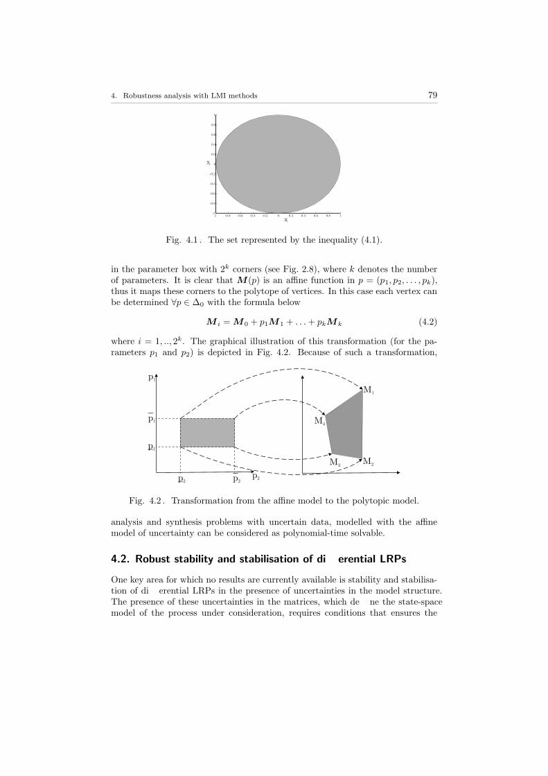
4. Robustness analysis with LMI methods 79
-1 -0.8 -0.6 -0.4 -0.2 0 0.2 0.4 0.6 0.8 1-1
-0.8
-0.6
-0.4
-0.2
0
0.2
0.4
0.6
0.8
1
x
x
2
1
Fig. 4.1 . The set represented by the inequality (4.1).
in the parameter box with 2k corners (see Fig. 2.8), where k denotes the numberof parameters. It is clear that M(p) is an affine function in p = (p1, p2, . . . , pk),thus it maps these corners to the polytope of vertices. In this case each vertex canbe determined ∀p ∈ ∆0 with the formula below
M i = M0 + p1M1 + . . .+ pkMk (4.2)
where i = 1, .., 2k. The graphical illustration of this transformation (for the pa-rameters p1 and p2) is depicted in Fig. 4.2. Because of such a transformation,
p1
p1
p1
p2p2p2
M1
M2
M4
M3
Fig. 4.2 . Transformation from the affine model to the polytopic model.
analysis and synthesis problems with uncertain data, modelled with the affinemodel of uncertainty can be considered as polynomial-time solvable.
4.2. Robust stability and stabilisation of di®erential LRPs
One key area for which no results are currently available is stability and stabilisa-tion of di®erential LRPs in the presence of uncertainties in the model structure.The presence of these uncertainties in the matrices, which de¯ne the state-spacemodel of the process under consideration, requires conditions that ensures the

80 4.2. Robust stability and stabilisation of di®erential LRPs
process to be robustly stable for all admissible uncertainties. Robust stabilityconditions can be further employed to solve the robust stabilisation problem.
4.2.1. Robust stability
4.2.1.1. Norm-bounded model of uncertainty
Consider uncertain di®erential LRPs described by the following state-space modelover 0 ≤ t ≤ α, k ≥ 0
xk+1(t) =(A+∆A)xk+1(t) + (B0 +∆B0)yk(t) + (B +∆B)uk+1(t)
yk+1(t) =(C +∆C)xk+1(t) + (D0 +∆D0)yk(t) + (D +∆D)uk+1(t)(4.3)
The matrices A, B, B0, C, D, D0 de¯ne the nominal model (2.14) and ∆A,∆B, ∆B0, ∆C, ∆D, ∆D0 represent admissible uncertainties which are assumedto be of the form
[∆A ∆B0 ∆B
∆C ∆D0 ∆D
]=
[H1
H2
]F[E1 E2 E3
](4.4)
In this last equation, H1, H2, E1, E2, E3 are known constant matrices of com-patible dimensions, and F is an unknown matrix with constant entries whichsatis¯es
FTF ¹ I (4.5)
For a stability goal, consider the state-space model (4.3) with no control inputsi.e. uk+1(t) = 0, then by de¯ning the following matrices
A1 =
[A B0
0 0
], A2 =
[0 0
C D0
](4.6)
and
∆A1 =
[∆A ∆B0
0 0
], ∆A2 =
[0 0
∆C ∆D0
](4.7)
the process state-space model (4.3) can be rewritten as
[xk+1(t)yk+1(t)
]=
([A B0
C D0
]+
[∆A ∆B0
∆C ∆D0
])[xk+1(t)yk(t)
]
=(A1 +∆A1
)ξ(k, t) +
(A2 +∆A2
)ξ(k, t)
where
ξ(k, t) =
[xk+1(t)yk(t)
](4.8)
With this notation, we have the following sufficient condition for stability alongthe pass in terms of LMI feasibility problem.

4. Robustness analysis with LMI methods 81
Theorem 4.1. A di®erential LRP described by (4.3) is stable along the pass forall admissible uncertainties if there exist matrices P 1 Â 0, P 2 Â 0 and a scalarε > 0 such that
−P 2 P 2C P 2D0 P 2H2 P 2H2
CTP 2 ATP 1+P 1A+εET1 E1 P 1B0 P 1H1 P 1H1
DT0 P 2 BT
0 P 1 −P 2+εET2 E2 0 0
HT2 P 2 HT
1 P 1 0 −εI 0
HT2 P 2 HT
1 P 1 0 0 −εI
≺0 (4.9)
Proof. Let us choose the Lyapunov functional candidate as that de¯ned in (2.36).Since
V1(k, t) = xTk+1(t)P 1xk+1(t) + xTk+1P 1xk+1(t)
and∆V2(k, t) = yTk+1(t)P 2yk+1(t)− yTk (t)P 2yk(t)
then the associated increment for (2.36) is
∆V (k, t) =V1(k, t) + ∆V2(k, t)
=xTk+1(t)P 1xk+1(t)+xTk+1(t)P 1xk+1(t)
+yTk+1(t)P 2yk+1(t)−yTk (t)P 2yk(t)
(4.10)
which together with notation introduced in (4.6), (4.7) and (4.8) gives
∆V (k, t)=ξT (k, t)((A1+∆A1)
TP+P (A1+∆A1)
+(A2+∆A2)R(A2+∆A2)−R)ξ(k, t)
(4.11)
whereP = diag(P 1,0), R = diag(0,P 2) (4.12)
Hence stability along the pass holds if ∆V (k, t) < 0 for ∀ξ(k, t) 6= 0, and a su±cientcondition for this is
(A1+∆A1)TP+P (A1+∆A1) +(A2+∆A2)S(A2+∆A2)−R ≺ 0
where S = diag(P 3,P 2), and P 3 Â 0 is any given matrix of appropriate dimen-sion. Next, an obvious application of the Schur complement formula yields
[−S SA2
AT
2 S AT
1 P + PA1 −R
]+
[0 S∆A2
∆AT
2 S ∆AT
1 P + P∆A1
]≺ 0
or, equivalently (the block −P 3 is negative de¯ned therefore it can be removed),−P 2 P 2C P 2D0
CTP 2 ATP 1+P 1A P 1B0
DT0 P 2 BT
0 P 1 −P 2
+
0 P 2H2 P 2H2
0 P 1H1 P 1H1
0 0 0
F 0 0
0 F 0
0 0 F
0 0 0
0 E1 0
0 0 E2
+
0 0 0
0 ET1 0
0 0 ET2
FT0 0
0 FT0
0 0 FT
0 0 0
HT2 P 2 HT
1 P 1 0
HT2 P 2 HT
1 P 1 0
≺0

82 4.2. Robust stability and stabilisation of di®erential LRPs
Based on the result of Lemma 8, we obtain
−P 2 P 2C P 2D0
CTP 2 ATP 1 + P 1A+ εET1 E1 P 1B0
DT0 P 2 BT
0 P 1 −P 2 + εET2 E2
+ε−1
0 P 2H2 P 2H2
0 P 1H1 P 1H1
0 0 0
0 0 0
HT2 P 2 HT
1 P 1 0
HT2 P 2 HT
1 P 1 0
≺0
Finally, using the Schur complement formula, we ¯nd that the last inequality isequivalent to the LMI (4.9). This concludes the proof. ¥
Remark 4.1. If there are no uncertain matrices in the process model (4.3) thenthe LMI (4.9) reduces into LMI for nominal model - see (Gałkowski et al., 2003c)for details.
4.2.1.2. Polytopic model of uncertainty
Here it is assumed that uncertainty of the di®erential fraction of an uncertaindi®erential LRP (4.3) has a polytopic character, i.e. all possible choices for thematrices which de¯ne the current pass state dynamics in (4.3) can be expressed as
[A B0
]∈ Co
([Ai Bi
0
])(4.13)
where i = 1, 2, . . . , h and
Co([
Ai Bi0
]):=
X : X=
h∑
i=1
αi
[Ai Bi
0
], αi ≥ 0,
h∑
i=1
αi=1
(4.14)
For the current pass pro¯le updating equation in (4.3) a standard norm-bound onthe perturbations is assumed, i.e. the second equation entry in (4.3) takes the form
yk+1(t) = (C +∆C)xk+1(t) + (D0 +∆D0)yk(t) (4.15)
where [∆C ∆D0
]=H2F
[E1 E2
]
and the matrix F satis¯es (4.5). The following result gives an LMI-based sufficientcondition for stability along the pass.
Theorem 4.2. A di®erential LRP of the form described by (4.3), with uncerta-inty structure modelled by (4.13)-(4.14) and (4.15) is stable along the pass for alladmissible uncertainties if there exist matrices P 1 Â 0, P 2 Â 0 and a scalar ε > 0,such that
−P 2 P 2C P 2D0 P 2H2
CTP 2 AiTP 1 + P 1Ai + εET
1 E1 P 1Bi0 + εE
T1 E2 0
DT0 P 2 BiT
0 P 1 + εET2 E1 −P 2 + εE
T2 E2 0
HT2 P 2 0 0 −εI
≺ 0 (4.16)

4. Robustness analysis with LMI methods 83
Proof. Taking account of the uncertainty in the considered process model, we get
−P 2 P 2C P 2D0
CTP 2 AiTP 1 + P 1Ai P 1B
i0
DT0 P 2 BiT
0 P 1 −P 2
+
0
ET1
ET2
FT
[HT
2 P 2 0 0]
+
P 2H2
0
0
F
[0 E1 E2
]≺0
which in view of Lemma 8 is equivalent to
−P 2 P 2C P 2D0
CTP 2 AiTP 1+P 1Ai+εET
1 E1 P 1Bi0+εE
T1 E2
DT0 P 2 BiT
0 P 1+εET2 E1 −P 2+εE
T2 E2
+ ε−1
P 2H2
0
0
[HT
2 P 2 0 0]≺0
Finally, application of the Schur complement formula gives (4.16). This completesthe proof. ¥
Remark 4.2. Some comments are required for Theorem 4.2. First, it should beemphasized that the result has been obtained by keeping P 1 constant and indepen-dent of the index i. The main drawback associated with this fact is that the Lyapu-nov matrix P 1 must work for all uncertain matrices (4.14). This condition canintroduce a signi¯cant degree of conservativeness to the stability condition (4.16).This can be overcome by using parameter-dependent Lyapunov functions (Apka-rian and Tuan, 1998, 2000). Unfortunately, there is no result for LRPs whereparameter-dependent Lyapunov functions are used. Work is proceeding on apply-ing such functions and will be reported on in due course.
It is clear that computation can be only performed in the case when all vertices(i.e. all edge matrices Ai and Bi
0) of a convex polygon are known. Unfortuna-tely, in many practical cases they are unknown, so it is required to determinethese vertices. This is best done with a numerical tool run on a computer. Theexample of such a tool is Geometric Bounding Toolbox (Veres, 2004) whichprovides computations in n-dimensional space. The main objective of this toolboxis the computation of the convex hull of a ¯nite set of points (command convh)which is useful for our purposes. The simplicity of using this software package isdemonstrated with the example below.
Example 4.2. The following set of commands generates a random set of pointsin three-dimensional space and compute their convex hull
points3D = rand(7,3) % 7 random points in 3-D space
cxhull=convh(points3D) % determine their convex hull

84 4.2. Robust stability and stabilisation of di®erential LRPs
However, in the case of systems considered here where matrix representationappears, it is necessary to perform transformation from space of real m by nmatrices to mn-dimensional real vector space, to make computations with theGeometric Bounding Toolbox possible. Then, after computing a convex hullin that real vector space, return to space of matrices and determine what matriceshave to be used in further computations.
4.2.1.3. A±ne model of uncertainty
It was shown that the affine model of uncertainty could be easily transformed tothe polytopic one where a set of vertices corresponds to extremal values of theparameter vector. Faced with this fact, the affine model of uncertainty is notconsidered to be present here any more. On the other hand, the affine modelallows us to maximize a stability region, i.e. the largest portion of the parameterbox where the stability along the pass can be established (for 1-D system case see,for example, (Gahinet et al., 1995)). To proceed, de¯ne the nominal value of theparameter pi as
p0i=pi + pi2
which denotes the center of the interval [pi, pi]. Next, for each interval de¯ne itsradius by
δi =pi − pi2
to yieldpi ∈ [p0i
− µδi, p0i+ µδi]
where µ > 0 is the unknown scalar to be selected. Maximization of µ leads tomaximization of the parameter box wherein stability along the pass is guaranteed.It turns out that maximization of µ can be cast into GEVP.
4.2.2. Robust stabilisation
In practice, it can happen that an uncertain process can be unstable, hence therobust stabilisation problem has to be addressed. To proceed, the following formof the control law is used
uk+1(t) =[
K1 K2
] [ xk+1(t)yk(t)
](4.17)
where K1 and K2 are appropriately dimensioned matrices to be designed. Ine®ect, this control law uses feedback of the current state vector (which is assumedto be available for use) and ‘feedforward’ of the previous pass pro¯le vector. Notethat in repetitive processes, the term ‘feedforward’ is used to describe the casewhere state or pass pro¯le information from the previous pass (or passes) is used as(part of) the input to a control law applied on the current pass, i.e. to informationwhich is propagated in the pass-to-pass (k) direction.

4. Robustness analysis with LMI methods 85
4.2.2.1. Norm-bounded model of uncertainty
Application of the control law (4.17) to (4.3) gives the following form of the closed-loop process
[xk+1(t)yk+1(t)
]=
([A+BK1 B0 +BK2
C +DK1 D0 +DK2
]
+
[∆A+∆BK1 ∆B0+∆BK2
∆C+∆DK1 ∆D0+∆DK2
])[xk+1(t)yk(t)
] (4.18)
where the admissible uncertainties are assumed to be of the form (4.4) and (4.5).In this case, the following theorem gives the condition of existing a controller thatstabilises the process (4.3) for all admissible uncertainties.
Theorem 4.3. Suppose that a di®erential LRP of the form described by (4.3),with uncertainty structure modelled by (4.4) and (4.5), is subjected to a controllaw of the form (4.17). Then the resulting closed-loop process is stable along thepass for all admissible uncertainties if there exist matrices W 1 Â 0, W 2 Â 0, N1
and N2 of compatible dimensions and a scalar ε > 0 such that the following LMIholds
−W 2+2εH2HT2 CW 1+DN1+2εH2H
T1
W 1CT+NT
1 DT+2εH1HT2 W 1A
T+NT1 BT+AW 1+BN1+2εH1H
T1
W 2DT0 +NT
2 DT W 2BT0 +NT
2 BT
0 E1W 1+E3N1
0 0
D0W 2+DN2 0 0
B0W 2+BN2 W 1ET1 +NT
1 ET3 0
−W 2 0 W 2ET2 +NT
2 ET3
0 −εI 0
E2W 2+E3N2 0 −εI
≺0
(4.19)
If the above LMI holds then the controller matrices K1 and K2 are given by
K1 =N1W−11
K2 =N2W−12
(4.20)
respectively.
Proof. Application of Theorem 4.1 result proves that the closed-loop process inthis case is stable along the pass if
[−S SA2
AT
2 S AT
1 P + PA1 −R
]+
[0 S∆A2
∆AT
2 S ∆AT
1 P + P∆A1
]≺ 0
where
A1=
[A+BK1 B0+BK2
0 0
], ∆A1=
[∆A+∆BK1 ∆B0+∆BK2
0 0
],

86 4.2. Robust stability and stabilisation of di®erential LRPs
A2=
[0 0
C+DK1 D0+DK2
],∆A2=
[0 0
∆C+∆DK1 ∆D0+∆DK2
]
Note that this last condition is not linear in P 1, P 2, P 3, K1 and K2. Clearly, itis bilinear in variables P 1,P 2 and K1,K2 and therefore it may be consideredas a BMI problem (3.4), for which e®ective computations cannot be performed.However, this can be reformulated as an LMI problem. To proceed, substitute A1
and A2 into this last expression to obtain (the block −P 3 has been removed dueto the fact the result does not depend on it)
−P 2 P 2C+P 2DK1 P 2D0+P 2DK2
CTP 2+KT1 DTP 2 ATP 1+KT
1 BTP 1+P 1A+P 1BK1 P 1B0+P 1BK2
DT0 P 2+KT
2 DTP 2 BT0 P 1+KT
2 BTP 1 −P 2
+
0 P 2∆C+P 2∆DK1 P 2∆D0+P 2∆DK2
∆CTP 2+KT1∆DTP 2 Ω1 P 1∆B0+P 1∆BK2
∆DT0 P 2+KT
2∆DTP 2 ∆BT0 P 1+KT
2∆BTP 1 0
≺0
where
Ω1 = ∆ATP 1+KT1∆BTP 1+P 1∆A+P 1∆BK1
Next, pre- and post-multiply the result by diag(P−12 ,P−1
1 ,P−12 ) and make changes
of variables W 1 = P−11 , W 2 = P−1
2 , N1 =K1P−11 , N2 =K2P
−12 to yield
−W 2 CW 1+DN1 D0W 2+DN2
W 1CT+NT
1 DT W 1AT+NT
1 BT+AW 1+BN1 B0W 2+BN2
W 2DT0 +NT
2 DT W 2BT0 +NT
2 BT −W 2
+
0 ∆CW 1+∆DN1 ∆D0W 2+∆DN2
W 1∆CT+NT1∆DT
Ω2 ∆B0W 2+∆BN2
W 2∆DT0 +NT
2∆DT W 2∆BT0 +NT
2∆BT0
≺0
(4.21)
where
Ω2 = W 1∆AT+NT1∆BT+∆AW 1+∆BN1
Observe now that the second term in (4.21) can be rewritten as
0 0 0
0 W 1ET1 +NT
1 ET3 0
0 0 W 2ET2 +NT
2 ET3
FT0 0
0 FT0
0 0 FT
0 0 0
HT2 HT
1 0
HT2 HT
1 0
+
0 H2 H2
0 H1 H1
0 0 0
F 0 0
0 F 0
0 0 F
0 0 0
0 E1W 1 +E3N1 0
0 0 E2W 2 +E3N2
≺0
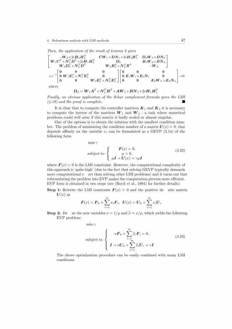
4. Robustness analysis with LMI methods 87
Then, the application of the result of Lemma 8 gives
−W 2+2εH2HT2 CW 1+DN1+2εH2H
T1 D0W 2+DN2
W 1CT+NT
1 DT+2εH1HT2 Ω3 B0W 2+BN2
W 2DT0 +NT
2 DT W 2BT0 +NT
2 BT −W 2
+ε−1
0 0 0
0 W 1ET1 +NT
1 ET3 0
0 0 W 2ET2 +NT
2 ET3
0 0 0
0 E1W 1+E3N1 0
0 0 E2W 2 +E3N2
≺0
whereΩ3 = W 1A
T+NT1 BT+AW 1+BN1+2εH1H
T1
Finally, an obvious application of the Schur complement formula gives the LMI(4.19) and the proof is complete. ¥
It is clear that to compute the controller matrices K1 and K2 it is necessaryto compute the inverse of the matrices W 1 and W 2 - a task where numericalproblems could well arise if this matrix is badly scaled or almost singular.One of the options is to obtain the solution with the smallest condition num-
ber. The problem of minimizing the condition number of a matrix U(x) Â 0, thatdepends affinely on the variable x, can be formulated as a GEVP (3.14) of thefollowing form
min γ
subject to
F (x) Â 0,µ > 0,
µI ≺ U(x) ≺ γµI
(4.22)
where F (x) Â 0 is the LMI constraint. However, the computational complexity ofthis approach is ‘quite high’ (due to the fact that solving GEVP typically demandsmore computational e®ort than solving other LMI problems) and it turns out thatreformulating the problem into EVP makes the computation process more efficient.EVP form is obtained in two steps (see (Boyd et al., 1994) for further details).
Step 1: Rewrite the LMI constraint F (x) Â 0 and the positive de¯nite matrixU(x) as
F (x) = F 0 +
m∑
i=1
xiF i, U(x) = U0 +
m∑
i=1
xiU i
Step 2: De¯ne the new variables ν = 1/µ and x = x/µ, which yields the followingEVP problem:
min γ
subject to
νF 0 +
m∑
i=1
xiF i  0,
I ≺ νU0 +
m∑
i=1
xiU i ≺ γI
(4.23)
The above optimization procedure can be easily combined with many LMIconditions.

88 4.2. Robust stability and stabilisation of di®erential LRPs
4.2.2.2. Polytopic model of uncertainty
Consider now the process which the current pass state updating equation matricesrange in the given polytope of matrices as it is described by
[A B0 B
]∈ Co
([Ai Bi
0 Bi]), i=1, 2, . . . , h (4.24)
and
Co([
Ai Bi Bi0
]):=
X : X =
h∑
i=1
αi
[Ai Bi Bi
0
], αi≥0,
h∑
i=1
αi=1
(4.25)
For the current pass pro¯le updating equation in (4.3) we assume norm-boundedtype of uncertainty, i.e.
yk+1(t) =(C+∆C)xk+1(t)+(D0+∆D0)yk(t) + (D+∆D)uk+1(t) (4.26)
where [∆C ∆D0 ∆D
]=H2F
[E1 E2 E3
](4.27)
and the matrix F satis¯es (4.5).
Theorem 4.4. Suppose that a di®erential LRP of the form described by (4.3),with uncertainty structure modelled by (4.24)- (4.25) and (4.27), is subjected to acontrol law of the form of (4.17). Then the resulting closed-loop process is stablealong the pass for all admissible uncertainties if there exist matrices W 1 Â 0,W 2 Â 0, N1 and N2 of compatible dimensions and a scalar ε > 0, such that
−W 2+2εH2HT2 CW 1+DN1
W 1CT+NT
1 DT W 1AiT+NT
1 BiT+AiW 1+BiN1
W 2DT0 +NT
2 DT W 2BiT0 +NT
2 BiT
0 E1W 1 +E3N1
0 0
D0W 2+DN2 0 0
Bi0W 2+BiN2 W 1E
T1 +NT
1 ET3 0
−W 2 0 W 2ET2 +NT
2 ET3
0 −εI 0
E2W 2 +E3N2 0 −εI
≺ 0
(4.28)
If the LMI (4.28) holds then the controller matrices K1 and K2 are given by(4.20).
Proof. Taking account of the results of Theorem 4.2 and Theorem 4.3, it is clearthat the following inequality holds
−W 2 CW 1+DN1 D0W 2+DN2
W 1CT+NT
1 DT W 1AiT+NT
1 BiT+AiW 1+BiN1 Bi0W 2+BiN2
W 2DT0 +NT
2 DT W 2BiT0 +NT
2 BiT −W 2
+
0 ∆CW 1+∆DN1 ∆D0W 2+∆DN2
W 1∆CT+NT1∆DT
0 0
W 2∆DT0 +NT
2∆DT0 0
≺0
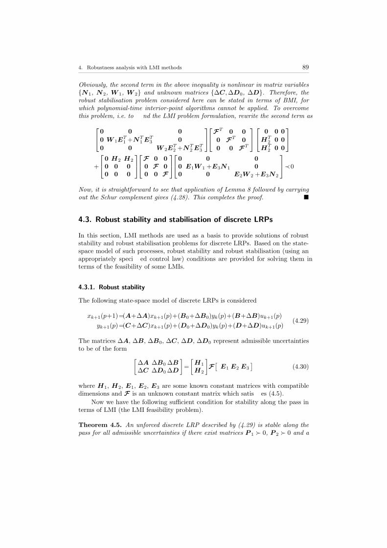
4. Robustness analysis with LMI methods 89
Obviously, the second term in the above inequality is nonlinear in matrix variablesN1, N2, W 1, W 2 and unknown matrices ∆C,∆D0, ∆D. Therefore, therobust stabilisation problem considered here can be stated in terms of BMI, forwhich polynomial-time interior-point algorithms cannot be applied. To overcomethis problem, i.e. to ¯nd the LMI problem formulation, rewrite the second term as
0 0 0
0 W 1ET1 +NT
1 ET3 0
0 0 W 2ET2 +NT
2 ET3
FT0 0
0 FT0
0 0 FT
0 0 0
HT2 0 0
HT2 0 0
+
0 H2 H2
0 0 0
0 0 0
F 0 0
0 F 0
0 0 F
0 0 0
0 E1W 1 +E3N1 0
0 0 E2W 2 +E3N2
≺0
Now, it is straightforward to see that application of Lemma 8 followed by carryingout the Schur complement gives (4.28). This completes the proof. ¥
4.3. Robust stability and stabilisation of discrete LRPs
In this section, LMI methods are used as a basis to provide solutions of robuststability and robust stabilisation problems for discrete LRPs. Based on the state-space model of such processes, robust stability and robust stabilisation (using anappropriately speci¯ed control law) conditions are provided for solving them interms of the feasibility of some LMIs.
4.3.1. Robust stability
The following state-space model of discrete LRPs is considered
xk+1(p+1)=(A+∆A)xk+1(p)+(B0+∆B0)yk(p)+(B+∆B)uk+1(p)
yk+1(p)=(C+∆C)xk+1(p)+(D0+∆D0)yk(p)+(D+∆D)uk+1(p)(4.29)
The matrices ∆A, ∆B, ∆B0, ∆C, ∆D, ∆D0 represent admissible uncertaintiesto be of the form
[∆A ∆B0∆B
∆C ∆D0∆D
]=
[H1
H2
]F[
E1 E2 E3
](4.30)
where H1, H2, E1, E2, E3 are some known constant matrices with compatibledimensions and F is an unknown constant matrix which satis¯es (4.5).Now we have the following sufficient condition for stability along the pass in
terms of LMI (the LMI feasibility problem).
Theorem 4.5. An unforced discrete LRP described by (4.29) is stable along thepass for all admissible uncertainties if there exist matrices P 1 Â 0, P 2 Â 0 and a

90 4.3. Robust stability and stabilisation of discrete LRPs
scalar ε > 0 such that the following LMI holds
−P 1 0 P 1A P 1B0 P 1H1 P 1H1
0 −P 2 P 2C P 2D0 P 2H2 P 2H2
ATP 1 CTP 2 −P 1+εET1 E1 0 0 0
BT0 P 1 DT
0 P 2 0 −P 2+εET2 E2 0 0
HT1 P 1 HT
2 P 2 0 0 −εI 0
HT1 P 1 HT
2 P 2 0 0 0 −εI
≺0 (4.31)
Proof. First, de¯ne the vectors
ξ(k + 1, p) =
[xk+1(p+ 1)yk+1(p)
], ζ(k, p) =
[xk+1(p)yk(p)
](4.32)
and use the matrices (4.6) and (4.7) to rewrite the state-space model (4.29) as
ξ(k + 1, p) = ((A1 +∆A1) + (A2 +∆A2)) ζ(k, p) (4.33)
Further, choose the candidate Lyapunov function as that de¯ned in (2.35). Since
∆V1(k, p) =xTk+1(p+ 1)P 1xk+1(p+ 1)− xTk+1(p)P 1xk+1(p)
∆V2(k, p) =yTk+1(p)P 2yk+1(p)− yTk (p)P 2yk(p)
then the increment is
∆V (k, p) =∆V1(k, p) + ∆V2(k, p)
=xTk+1(p+ 1)P 1xk+1(p+ 1)−xTk+1(p)P 1xk+1(p)
+yTk+1(p)P 2yk+1(p)−yTk (p)P 2yk(p)
(4.34)
which together with (4.32) and (4.33) gives
∆V (k, p)=ζT (k, p)((A1+∆A1)
TP (A1+∆A1)
+ (A2 +∆A2)P (A2 +∆A2)− P ) ζ(k, p)(4.35)
where P = diag(P 1,P 2). Hence stability along the pass holds if ∆V (k, p) < 0 for∀ζ(k, p) 6= 0. Next, use of the Schur complement formula followed by applicationof Lemma 8 yield
−P 1 0 P 1A P 1B0
0 −P 2 P 2C P 2D0
ATP 1 CTP 2 −P 1+εET1 E1 0
BT0 P 1 DT
0 P 2 0 −P 2+εET2 E2
+ε−1
0 0 P 1H1 P 1H1
0 0 P 2H2 P 2H2
0 0 0 0
0 0 0 0
0 0 0 0
0 0 0 0
HT1 P 1 HT
2 P 2 0 0
HT1 P 1 HT
2 P 2 0 0
≺0
Finally, using the Schur complement formula, we ¯nd that the last inequality isequivalent to the LMI (4.31). This completes the proof. ¥
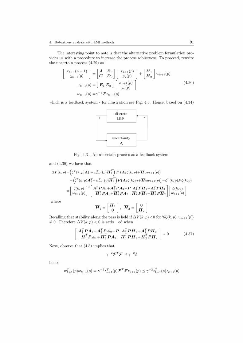
4. Robustness analysis with LMI methods 91
The interesting point to note is that the alternative problem formulation pro-vides us with a procedure to increase the process robustness. To proceed, rewritethe uncertain process (4.29) as
[xk+1(p+ 1)yk+1(p)
]=
[A B0
C D0
] [xk+1(p)yk(p)
]+
[H1
H2
]wk+1(p)
zk+1(p) =[
E1 E2
] [ xk+1(p)yk(p)
]
wk+1(p) =γ−1Fzk+1(p)
(4.36)
which is a feedback system - for illustration see Fig. 4.3. Hence, based on (4.34)
discrete
uncertainty
D
LRPz w
Fig. 4.3 . An uncertain process as a feedback system.
and (4.36) we have that
∆V (k, p)=(ζT (k, p)AT
1 +wT
k+1(p)HT
1
)P(A1ζ(k, p)+H1wk+1(p)
)
+(ζT (k, p)AT
2+wT
k+1(p)HT
2
)P(A2ζ(k, p)+H2wk+1(p)
)−ζ
T (k, p)P ζ(k, p)
=
[ζ(k, p)wk+1(p)
]T[AT
1 PA1+AT2 PA2−P AT
1 PH1+AT2 PH2
HT
1 PA1+HT
2 PA2 HT
1 PH1+HT
2 PH2
][ζ(k, p)wk+1(p)
]
where
H1 =
[H1
0
], H2 =
[0
H2
]
Recalling that stability along the pass is held if ∆V (k, p)<0 for ∀ζ(k, p), wk+1(p)6= 0. Therefore ∆V (k, p) < 0 is satis¯ed when
[AT1 PA1+AT
2 PA2−P AT1 PH1+AT
2 PH2
HT
1 PA1+HT
2 PA2 HT
1 PH1+HT
2 PH2
]≺ 0 (4.37)
Next, observe that (4.5) implies that
γ−2FTF ¹ γ−2I
hence
wTk+1(p)wk+1(p) = γ−2zTk+1(p)F
TFzk+1(p) ¹ γ−2zTk+1(p)zk+1(p)

92 4.3. Robust stability and stabilisation of discrete LRPs
Then, it is straightforward to see that for any wk+1(p), zk+1(p) and ∀γ > 0 thefollowing holds
wTk+1(p)wk+1(p)− γ−2zTk+1(p)zk+1(p) ≤ 0
thus by noting E =[
E1 E2
]we have
wTk+1(p)wk+1(p)− γ−2zTk+1(p)zk+1(p)
=[ζT (k, p) wT
k+1(p)][−ETE 0
0 γ−2I
][ζ(k, p)wk+1(p)
]≤ 0
(4.38)
Combining the results of (4.37) and (4.38) yields the ¯nal LMI condition for robuststability of discrete LRPs as[
AT1 PA1+AT
2 PA2−P +ETE AT1 PH1+AT
2 PH2
HT
1 PA1+HT
2 PA2 HT
1 PH1+HT
2 PH2 − γ−2I
]≺ 0 (4.39)
It is observed that the term γ in the LMI of (4.39) can be minimized by usinglinear objective minimization procedure
minPÂ0
µ
subject to (4.39) with µ = γ−2
which increases the robustness of an uncertain process.
4.3.2. Robust stabilisation
The previous subsection was concerned with robust stability of open-loop proces-ses. Here, a natural extension of obtained results to the case of closed-loop processunder a static feedback is presented. The problem here is to ¯nd a controller ofthe form
uk+1(p) =[
K1 K2
] [ xk+1(p)yk(p)
](4.40)
where K1 and K2 are appropriately dimensioned matrices to be designed, suchthat the closed-loop process is robustly stable. It is seen that the control law (4.40)is composed of the weighted sum of current pass state feedback and feedforwardof the previous pass pro¯le (see (Gałkowski et al., 2002d) for further backgroundon this form of control action).Application of the control law (4.40) to (4.29) yields the closed-loop process[xk+1(p+ 1)yk+1(p)
]=
([A+BK1 B0+BK2
C+DK1 D0+DK2
]
+
[∆A+∆BK1 ∆B0+∆BK2
∆C+∆DK1 ∆D0+∆DK2
])[xk+1(p)yk(p)
] (4.41)
where the admissible uncertainties are assumed to be of the form (4.30) and (4.5).The existence of robustly stabilising K1 and K2 can be characterized in LMI
terms as follows.

4. Robustness analysis with LMI methods 93
Theorem 4.6. Suppose that a discrete LRP of the form described by (4.29), withuncertainty structure modelled by (4.30) and (4.5) is subjected to a control law ofthe form (4.40). Then the resulting closed-loop process is stable along the pass forall admissible uncertainties if there exist matrices W 1 Â 0, W 2 Â 0, N1 and N2
of compatible dimensions and a scalar ε > 0 such that the following LMI holds
−W 1 + 2εH1HT1 2εH2H
T1 AW 1+BN1
2εH1HT2 −W 2 + 2εH2H
T2 CW 1+DN1
W 1AT+NT
1 BT W 1CT+NT
1 DT −W 1
W 2BT0 +NT
2 BT W 2DT0 +N2D
T0
0 0 E1W 1+E3N1
0 0 0
B0W 2+BN2 0 0
D0W 2+DN2 0 0
0 W 1ET1 +NT
1 ET3 0
−W 2 0 W 2ET2 +NT
2 ET3
0 −εI 0
E2W 2+E3N2 0 −εI
≺0
(4.42)
and the required controller matrices in (4.40) are given by (4.20).
Proof. Based on Theorem 4.5 we conclude that the closed-loop process is robustlystabilised by the control law (4.40) if the following matrix inequality is satis¯ed
−P 1 0 P 1A+P 1BK1 P 1B0+P 1BK2
0 −P 2 P 2C+P 2DK1 P 2D0+P 2DK2
ATP 1+KT1 BTP 1 CTP 2+KT
1 DTP 2 −P 1 0
BT0 P 1+KT
2 BTP 1 DT0 P 2+K2D
TP 1 0 −P 2
+
0 0 0 0
0 0 0 0
0 0 ET1 +KT
1 ET3 0
0 0 0 ET2 +KT
2 ET3
FT0 0 0
0 FT0 0
0 0 FT0
0 0 0 FT
0 0 0 0
0 0 0 0
HT1 P 1 HT
2 P 2 0 0
HT1 P 1 HT
2 P 2 0 0
+
0 0 P 1H1 P 1H1
0 0 P 2H2 P 2H2
0 0 0 0
0 0 0 0
F 0 0 0
0 F 0 0
0 0 F 0
0 0 0 F
0 0 0 0
0 0 0 0
0 0 E1 +E3K1 0
0 0 0 E2 +E3K2
≺0
The above inequality is clearly stated in the form of BMI. To reformulate it intoLMIs, make use of the following change of variables W 1 = P−1
1 , W 2 = P−12
and then pre- and post- multiply both sides of this last inequality by diag(W 1,W 2,

94 4.3. Robust stability and stabilisation of discrete LRPs
W 1,W 2). Next, an application of the result of Lemma 8 leads to
ε−1
0 0 0 0
0 0 0 0
0 0 W 1ET1+NT
1 ET3 0
0 0 0 W 2ET2+NT
2 ET3
0 0 0 0
0 0 0 0
0 0 E1W 1+E3N1 0
0 0 0 E2W 2 +E3N2
+
−W 1 + 2εH1HT1 2εH2H
T1 AW 1+BN1 B0W 2+BN2
2εH1HT2 −W 2 + 2εH2H
T2 CW 1+DN1 D0W 2+DN2
W 1AT+NT
1 BT W 1CT+NT
1 DT −W 1 0
W 2BT0 +NT
2 BT W 2DT0 +N2D
T0 −W 2
≺0
where N1 = K1W 1 and N2 = K2W 2. Finally, the Schur complement formulagives (4.42) and the proof is complete. ¥
4.3.2.1. Alternative robust stabilisation
Here another approach to characterize and solve the robust stabilisation problemof discrete LRPs is presented. To proceed, rewrite (4.41) in the form
[xk+1(p+1)yk+1(p)
]= A
[xk+1(p)yk(p)
](4.43)
where
A=
[A+BK1 B0+BK2
C+DK1 D0+DK2
]+
[∆A+∆BK1 ∆B0+∆BK2
∆C+∆DK1 ∆D0+∆DK2
]
Suppose also that the matrices describing the uncertainty in this last model arewritten in the form
[∆A+∆BK1 ∆B0+∆BK2
∆C+∆DK1 ∆D0+∆DK2
]=
[H1
H2
]γ−1F
[E1+E3K1 E2+E3K2
]
=γ−1HFE
(4.44)
where F satis¯es (4.5). The design parameter γ here can be considered as a termwhich is used to attenuate the e®ects of the uncertainty, for which we have thefollowing result.
Theorem 4.7. Suppose that a discrete LRP of the form described by (4.29), withuncertainty structure modelled by (4.44) and (4.5), is subjected to a control law ofthe form (4.40). Then the resulting closed-loop process is stable along the pass forall admissible uncertainties if there exist matrices W 1 Â 0, W 2 Â 0, N1 and N2

4. Robustness analysis with LMI methods 95
of compatible dimensions and a scalar γ > 0 such that the following LMI holds
−W 1 0 AW 1+BN1
0 −W 2 CW 1+DN1
W 1AT+NT
1 BT W 1CT+NT
1 DT −W 1
W 2BT0 +NT
2 BT W 2DT0 +NT
2 DT0
HT1 HT
2 0
0 0 E1W 1+E3N1
B0W 2+BN2 H1 0
D0W 2+DN2 H2 0
0 0 W 1ET1 +NT
1 ET3
−W 2 0 W 2ET2 +NT
2 ET3
0 −γ2I 0
E2W 2+E3N2 0 −I
≺0
(4.45)
Proof. Using the RM and stability condition for a 2-D system, it follows imme-diately that the LRP of the form (4.43) is stable along the pass if there exists ablock-diagonal matrix P = diag (P 1,P 2) Â 0 such that the following LMI holds
ATPA− P ≺0
An obvious application of the Schur complement formula yields
[−P−1
Ω+ γ−1HFE
ΩT + γ−1ETFTHT −P
]≺ 0
where
Ω =
[A+BK1 B0+BK2
C+DK1 D0+DK2
], H =
[H1
H2
], E =
[E1+E3K1 E2+E3K2
]
Applying the result of Lemma 8 to this last condition and then pre- and post-multiplying the result by diag(ε−
1
2 P , ε−1
2 I) gives
[−P + P γ−2HHTP PΩ
ΩTP −P +ETE
]≺0
where a new matrix variable P is introduced as P = ε−1P . Next, an applicationof the Schur complement formula gives
−P PΩ PH 0
ΩTP −P 0 ET
HTP 0 −γ2I 0
0 E 0 −I
≺0 (4.46)
Finally, the proof can be completed in an identical manner to the proof of The-orem 4.6. ¥

96 4.4. Application examples
The term γ in the LMI of (4.45) can again be minimized by using a linearobjective minimization procedure
minW 1Â0,W 2Â0,N1,N2
µ
subject to (4.45) with µ = γ2
which, due to the presence of the term γ−1 in the uncertainty model (4.44), pro-vides an essential advantage as it allows the extension of the uncertainty borders,i.e. it increases the robustness.
4.4. Application examples
4.4.1. Analysis of ILC processes
It is clear that the principal requirement for ILC process is its stability along thedirection of learning iterations in addition to the stability of a control system. Toproceed, make use of the following change of variables
r =k − 1νr(t) =νk−1(t) = ek(t)
to rewrite (2.53) in the di®erential LRP form as[ηr+1(t)νr+1(t)
]=
[A−BK1 −BK2
−CA+CBK1 I −CBK2
] [ηr(t)νr(t)
](4.47)
Since stability of the model (4.47) guarantees the learning convergence, then theresult of Theorem 4.3 provides the LMI condition for stability checking. Hence,omitting the uncertainty, the LMI condition for stability ILC process can be for-mulated as follows
−W 2 −CAW 1+CBN1 W 2−CBN2
−W 1ATCT+NT
1 BTCT W 1AT−NT
1 BT+AW 1−BN1 −BN2
W 2−NT2 BTCT −NT
2 BT −W 2
≺0 (4.48)
whereW 1 Â 0,W 2 Â 0, N1, N2 are the matrices to be found. If they exist thenthe explicit speci¯cation for the learning gain matrices are given by (4.20). It issigni¯cant to note that the LMI condition of (4.48) can be easily implemented andtherefore tools like Lmi Control Toolbox, SeDuMi, or any equivalent softwarecan be used to solve the addressed problem.To show the usefulness of learning gain matrices design method, the following
numerical example is given.
Example 4.3. Let us consider the ILC process (2.49) with the matrices given by
A =
[0.1341 0.26741.1977 1.6292
], B =
[0.5643 0.68761.8219 −0.8877
], C =
[0.3095 −0.35330.0438 0.3968
]

4. Robustness analysis with LMI methods 97
0
5
10
15
0
10
20
30
400
0.2
0.4
0.6
0.8
1
trialstime
lear
ning
err
or
0
5
10
15
0
10
20
30
40−0.35
−0.3
−0.25
−0.2
−0.15
−0.1
−0.05
0
trialstime
ν
learning error state (η)
Fig. 4.4 . Simulation results.
Then the LMI (4.48) is feasible with
W 1 =
[1.0198 0.00000.0000 1.0198
], W 2 =
[0.6579 −0.0251−0.0251 0.6458
],
N1 =
[0.8024 0.97490.2487 −0.3750
], N2 =
[0.0165 0.10040.2332 −0.0297
]
and the learning gain matrices are
K1 =
[0.7868 0.95600.2439 −0.3677
], K2 =
[0.0311 0.15670.3532 −0.0323
]
To con¯rm the learning convergence in this case, the simulation results are provided- see Fig. 4.4. It is assumed that for the ¯rst trial the learning error is 1.
Furthermore, consider the case when (4.47) is subjected to norm-bounded un-certainty i.e. it is assumed that uncertainty is modelled as an additive perturbation(denoted here by ∆A and ∆B) to the nominal ILC process matrices (A and B)
[∆A ∆B] = H1F [E1 E2]
where H1, E1, E2 are given matrices and the matrix F satis¯es (4.5). Hencethe following matrix inequality can provide robust stability condition for the ILCprocess
−W 2 −CAW 1 +CBN1 W 2 −CBN2
−W 1ATCT +NT
1 BTCT W 1AT −NT
1 BT +AW 1 −BN1 −BN2
W 2 −NT2 BTCT −NT
2 BT −W 2
+
0 0 0
0 W 1∆AT −NT1∆BT +∆AW 1 −∆BN1 −∆BN2
0 −NT2∆BT
0
+
0 −C∆AW 1 +C∆BN1 −C∆BN2
−W 1∆ATCT +NT1∆BTCT
0 0
−NT2∆BTCT
0 0
≺ 0
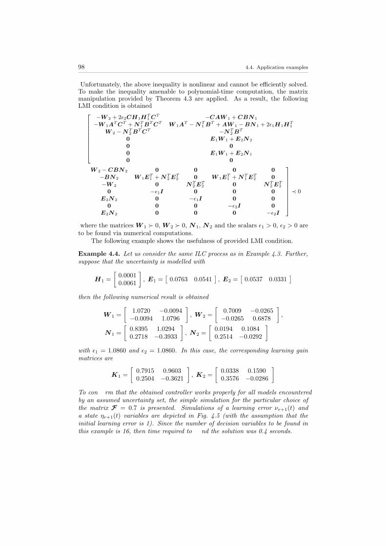
98 4.4. Application examples
Unfortunately, the above inequality is nonlinear and cannot be efficiently solved.To make the inequality amenable to polynomial-time computation, the matrixmanipulation provided by Theorem 4.3 are applied. As a result, the followingLMI condition is obtained
−W 2 + 2ε2CH1HT1 CT −CAW 1 +CBN1
−W 1ATCT +NT
1 BTCT W 1AT −NT
1 BT +AW 1 −BN1 + 2ε1H1HT1
W 2 −NT2 BTCT −NT
2 BT
0 E1W 1 +E2N2
0 0
0 E1W 1 +E2N1
0 0
W 2 −CBN2 0 0 0 0
−BN2 W 1ET1 +NT
2 ET2 0 W 1E
T1 +NT
1 ET2 0
−W 2 0 NT2 ET
2 0 NT2 ET
2
0 −ε1I 0 0 0
E2N2 0 −ε1I 0 0
0 0 0 −ε2I 0
E2N2 0 0 0 −ε2I
≺ 0
where the matricesW 1 Â 0,W 2 Â 0, N1, N2 and the scalars ε1 > 0, ε2 > 0 areto be found via numerical computations.The following example shows the usefulness of provided LMI condition.
Example 4.4. Let us consider the same ILC process as in Example 4.3. Further,suppose that the uncertainty is modelled with
H1 =
[0.00010.0061
], E1 =
[0.0763 0.0541
], E2 =
[0.0537 0.0331
]
then the following numerical result is obtained
W 1 =
[1.0720 −0.0094−0.0094 1.0796
], W 2 =
[0.7009 −0.0265−0.0265 0.6878
],
N1 =
[0.8395 1.02940.2718 −0.3933
], N2 =
[0.0194 0.10840.2514 −0.0292
]
with ε1 = 1.0860 and ε2 = 1.0860. In this case, the corresponding learning gainmatrices are
K1 =
[0.7915 0.96030.2504 −0.3621
], K2 =
[0.0338 0.15900.3576 −0.0286
]
To con¯rm that the obtained controller works properly for all models encounteredby an assumed uncertainty set, the simple simulation for the particular choice ofthe matrix F = 0.7 is presented. Simulations of a learning error νr+1(t) anda state ηr+1(t) variables are depicted in Fig. 4.5 (with the assumption that theinitial learning error is 1). Since the number of decision variables to be found inthis example is 16, then time required to ¯nd the solution was 0.4 seconds.

4. Robustness analysis with LMI methods 99
0
5
10
15
0
10
20
30
400
0.2
0.4
0.6
0.8
1
trialstime
lear
ning
err
or
0
5
10
15
0
10
20
30
40−0.35
−0.3
−0.25
−0.2
−0.15
−0.1
−0.05
0
trialstime
ν
learning error (ν) state (η)
Fig. 4.5 . Simulation results for an uncertain ILC process.
Table 4.1. Computation time.n m p q CPU time in seconds2 2 2 16 0.403 2 3 26 0.725 2 5 52 1.866 5 6 104 7.5310 7 10 252 71.7312 10 12 398 259.09
Obviously, due to the polynomial time complexity of the considered problem,e±ciency is maintained for higher problem dimensions - see Table 4.1. Note thatall computations have been performed with Lmi Control Toolbox 1.0.8 underMatlab 6.5. The Matlab-¯les have been run on a PC with AMD Duron 600MHz CPU and 128MB RAM.The overall number of decision variables q is computed from
q =n(n+ 1)
2+m(m+ 1)
2+ nl +ml + 2
where n is the number of states, m is the number of outputs and l is the numberof inputs. Further, the terms sequence in the above equation denotes the numberof decision variables involved in W 1, W 2, N1, N2 and ε1,2 respectively.
4.4.2. Stability of a parallel computing process
To consider the stability problem of a parallel computing process, note ¯rst thatone of the variables n1 and n2 can have a ¯nite value (in this case n2) then system(2.55) can be considered and analysed as a discrete LRP.It is written in (Bauer et al., 2001) that the use of 2-D state-space models for
parallel computing processes has been motivated by existing results on the stability

100 4.4. Application examples
of such models. Unfortunately, considered in the paper stability conditions arecomputationally ine®ective due to large dimensions of used matrices. Indeed, inthat paper the following matrix is used
Acc(n) =
J(n, 0) 0 · · · 0
K(n, 0) J(n− 1, 1) · · · 0
......
. . ....
0 0 · · · J(0, n)0 0 · · · K(0, n)
where n denotes the time instant and matrices J(n1, n2) and K(n1, n2) are iden-tifying in (2.55) as
J(n1, n2)=
[A11(n1, n2) A12(n1, n2)
0 0
],K(n1, n2)=
[0 0
A21(n1, n2) A22(n1, n2)
]
Hence, it is clear that the dimension of the matrix Acc(n) can be vary large dueto n value, therefore potential computational and numerical problems may occur.Moreover, it is a necessity to perform computations for all possible choices ofincomplete output masks. Therefore, as it is written in (Bauer et al., 2001), thestability problem belongs to the class of NP-hard problems - even for ¯nite n.To overcome these difficulties the approach developed in this chapter can be usedto ¯nd an exact or an approximate solution to the stability problem of parallelcomputing processes.While the number of all possible choices of incomplete output masks is not
large, then the stability test can be based on LMI condition provided by The-orem 4.5 where there are no uncertain matrices in the process model (4.3).On the other hand, it can be assumed that matrices, which are the result of
all possible choices of incomplete output masks, belong to some bounded set of thespace of matrices. Furthermore, suppose that this set is a convex set or it can beapproximated by a convex set represented by HFE where F satis¯es (4.5) andthe matrices H and E are given. That is, matrices uncertainty can be put in thenorm-bounded form and hence (2.55) can be written as
[xh(n1+1, n2)xv(n1, n2+1)
]=
([A11(n1, n2) A12(n1, n2)A21(n1, n2) A22(n1, n2)
]
+
[∆A11(n1, n2) ∆A12(n1, n2)∆A21(n1, n2) ∆A22(n1, n2)
])[xh(n1, n2)xv(n1, n2)
] (4.49)
where[∆A11(n1, n2) ∆A12(n1, n2)∆A21(n1, n2) ∆A22(n1, n2)
]=
[H1
H2
]F[E1 E2
]= HFE
This means that the provided theorems o®er a powerful implementable tool to sta-bility analysis of a parallel or distributed computation process. Even though suchan approach is applied for each time instant (assumed to be ¯nite), determiningthe process stability involves quite a reasonable amount of computations.

4. Robustness analysis with LMI methods 101
4.5. Concluding remarks
This chapter shows that LMI methods, which are standard in 1-D system theory,can be applied to analysis and synthesis for LRPs in the presence of uncertainty.The main obstacles towards applying classical 2-D system theory methods in thesecases are computational problems which are avoided using LMI methods. More-over, as it is shown, LMI methods allow us to extend the uncertainty borders viaan optimization procedure, i.e. increasing the robustness. Also, they are nume-rically efficient and allow the efficient handling of considerably high dimensionalproblems.

Chapter 5
LMI METHODS IN PERFORMANCE ANALYSIS
It has been shown that the condition for the existence of H∞ and H2 controllerscan be written in the form of matrix inequality, which turns out to be bilinearwith respect to its parameters (Helton and Merino, 1998; Saberi et al., 1995;Zhou et al., 1996). Therefore, such a condition cannot be tested with efficientcomputational method. Fortunately, we do not have to solve nonlinear problemsbecause potential difficulties can be omitted using a variety of methods. BothRiccati-based (Doyle et al., 1989) and LMI-based (Boyd et al., 1994; Dullerudand Paganini, 2000; Scherer and Weiland, 2002) solutions have been consideredfor H∞ and H2 control problems in 1-D system theory. It is natural question toask if such computationally e®ective approaches can be extended to 2-D (n-D)linear systems and LRPs. In the case of 2-D discrete linear systems, some workon H∞ and H2 approaches have been reported - see, for example, (Du and Xie,2002; Sebek M., 1993; Tuan et al., 2002). However, these control problems forLRPs still remain unsolved although some preliminary results have already beenreported on H∞ control (Paszke et al., 2003, 2004). This lack of results is mainlyseen for di®erential LRPs, and hence the purpose of this chapter is to ¯ll that gap.In addition to these results, the solution to theH∞ control problem with para-
meter uncertainty in all the matrices of the process state-space model, is provided.Further, the numerical design procedure for a controller maintaining an adequatelevel of performance represented by the quadratic cost, is presented. Searching forsuch a controller is called a guaranteed cost control problem and it has even beenconsidered for 2-D linear systems (Guan et al., 2001). However, this paper onlycontains a design method for a 2-D system represented by FMM, in which the spe-cial case of boundary conditions is taken into account, and it seems that there areno results for LRPs. Therefore, this chapter proposes a design algorithm involvinga convex optimization for an LRP controller achieving a suboptimal guaranteedcost such that the process can be stabilised for all admissible uncertainties.
5.1. Performance speci¯cations for LRPs and n-D systems
One of the most frequently considered ways to describe the performance speci¯ca-tions of a control system is to use H2 and H∞ norms (Zhou et al., 1996) of signalsand systems. These norms turn out to be natural measures of the worst possibleperformance for many classes of input signals.

5. LMI methods in performance analysis 103
In the presented approach, the generalized signals w and z are chosen tocharacterize performance properties to be achieved by the controller. The signalw is the generalized disturbance which collect various disturbance signals. Thissignal is assumed to be member of Lr
2 space i.e. space of signals with ¯nite energywhere the Lr
2 norm is de¯ned. In the case of a 2-D signal described by mixedtime and space variables, Lr
2 norm is de¯ned as follows (see (Du and Xie, 2002)for de¯nition Lr2 norm of discrete 2-D signal).
De¯nition 5.1. The L2 norm of the vector wk(t)∈Rr×1 de¯ned over [0,∞], [0,∞]is given by
‖w‖2 =
√√√√∞∑
k=0
∫ ∞
0
wk(t)Twk(t) dt (5.1)
and wk(t) is said to be a member of Lr2[0,∞], [0,∞], or Lr
2 for short, if ||w||2 <∞.
The signal z represents the controlled variable. Taking into considerationthese additional signals, the state-space models of both di®erential (Gdiff) anddiscrete LRPs (Gdisc) are
Gdiff
xk+1(t) = Axk+1(t) +B0yk(t) +Buk+1(t) +B1wk+1(t)yk+1(t) = Cxk+1(t) +D0yk(t) +Duk+1(t) +D1wk+1(t)
(5.2)
and
Gdisc
xk+1(p+ 1) = Axk+1(p) +B0yk(p) +Buk+1(p) +B1wk+1(p)
yk+1(p) = Cxk+1(p) +D0yk(p) +Duk+1(p) +D1wk+1(p)(5.3)
respectively. In the above equations, wk+1(t) and wk+1(p) are the Rr×1 distur-bance input vectors which belong to Lr
2. Due to the fact that the pass pro¯le vectoris simultaneously the output vector, we can write zk+1(t) = yk+1(t) in di®erentialcase or zk+1(p) = yk+1(p) in discrete one (see also the equation (2.21)).To study H∞ or H2 control of LRPs, de¯nitions of H∞ and H2 norms are
required. First the H∞ norm de¯nition is provided
De¯nition 5.2. A di®erential (discrete) LRP described by (5.2) (by (5.3) respec-tively) is said to have the H∞ disturbance attenuation (the H∞ norm bound) γ ifit is stable along the pass and
sup06=w∈Lr
2
‖y‖2‖w‖2
< γ (5.4)
The above de¯nition corresponds to the maximum gain peak of frequencyresponse, i.e. supremum of the maximum singular value of the frequency responseof the process. This can be computed from
‖G(s, z)‖∞ = supω1∈R,ω2∈[0,2π]
σ[G(jω1, e
jω2)]

104 5.2. H∞ control of di®erential LRPs
in a di®erential case and from
‖G(z1, z2)‖∞ = supω1,ω2∈[0,2π]
σ[G(ejω1 , ejω2)
]
in a discrete case. G(s, z) and G(z1, z2) are the 2-D transfer function matricesbetween pass pro¯le and disturbance signal and they are given by
G(s, z) =[0 I
] [ sI −A −B0
−zC I − zD0
]−1[B1
D1
](5.5)
and
G(z1, z2) =[0 I
] [ I − z1A −z1B0
−z2C I − z2D0
]−1[B1
D1
](5.6)
for di®erential and discrete cases respectively. The H2 norm de¯ned as the squareof the L2 norm of wk(t) is commonly termed the total energy in the signal wk(t)
‖G(s, z)‖2 =√
1
(2π)2
∫ 2π
0
∫ ∞
−∞
trace (G∗(−jω2, ejω1)G(−jω2, ejω1)) dω2dω1
(5.7)where G∗(·) denotes the complex conjugate transpose of G(·).A fundamental point to note is that the H2 norm of a process coincides with
the total output energy in the impulse response of a process. This observationleads immediately to the algorithms that determine the H2 norm of the process -see Section 5.6 for details.
5.2. H∞ control of di®erential LRPs
5.2.1. LMI-based H∞ norm computationTo compute the H∞ norm, consider the case of a di®erential LRP (5.2) with nocontrol inputs but with external disturbance inputs given by
[xk+1(t)yk+1(t)
]=
[A B0
C D0
] [xk+1(t)yk(t)
]+
[B1
D1
]wk+1(t) (5.8)
Noting that the measured output vector is equal to the pass pro¯le vector, we nowhave the following Theorem which gives an H∞ condition for stability along thepass in terms of LMI.
Theorem 5.1. A di®erential LRP which can be written in the form (5.8) is stablealong the pass and has the H∞ disturbance attenuation γ > 0 if there exist matricesP 1 Â 0, and P 2 Â 0 of appropriate dimensions such that the following LMI holds
−P 2 P 2C P 2D0 P 2D1
CTP 2 ATP 1 + P 1A P 1B0 P 1B1
DT0 P 2 BT
0 P 1 −P 2 + I 0
DT1 P 2 BT
1 P 1 0 −γ2I
≺ 0 (5.9)

5. LMI methods in performance analysis 105
Proof. Let us introduce the associated Hamiltonian as
H(k, t) =∆V (k, t)+yTk+1(t)yk+1(t)− γ2wTk+1(t)wk+1(t)
=∆V (k, t)+ ξT (k, t)LTLξ(k, t)−γ2wTk+1(t)wk+1(t)
=[ξT (k, t) wT
k+1(t)]Θ
[ξ(k, t)wk+1(t)
] (5.10)
where ∆V (k, t) is de¯ned in (4.10), ξ(k, t) is introduced by (4.8) and
Θ=
[A
T
1 P+PA1+AT
2 SA2+LTL−R PB1+AT
2 SD1
BT
1 P+DT
1 SA2 DT
1 SD1−γ2I
](5.11)
and P = diag (P 1,0) , S = diag (P 3,P 2) ,
B1 =
[B1
0
], D1 =
[0
D1
], L =
[0 I
]
The matrix P 3 is any given positive de¯ned matrix of appropriate dimension. Thento ensure that stability along the pass and H∞ noise attenuation γ holds, (5.10)must satisfy
H(k, t) ≺ 0Now, it is straightforward to see that the condition Θ ≺ 0 guarantees that (5.4)holds for any nonzero wk+1(t) ∈ Lr
2[0,∞], [0,∞]. This implies that processesdescribed by (5.8) are stable along the pass with the H∞ norm less than γ. Finally,an obvious application of the Schur complement formula gives (5.9) and the proofis complete. ¥
Remark 5.1. In many practice cases it is desirable to compute the minimumdisturbance rejection level γ. This minimum can be obtained by solving a linearobjective minimization problem of the following form
minP 1Â0,P 2Â0
µ
subject to (5.9) with µ = γ2(5.12)
5.2.2. H∞ control with a static feedback controllerThe purpose of this section is to study the solution to the problem of H∞ distur-bance attenuation in the case of full state access, i.e. the case when the controllaw of the form (4.17) is applied.Under these assumptions, the following result shows that the LMI setting
extends to allow the design of a control law of the form (4.17) for stability alongthe pass closed-loop process with a prescribed H∞ disturbance attenuation.Theorem 5.2. Suppose that a di®erential LRP described by (5.2) is subject to acontrol law de¯ned by (4.17). Then the resulting closed-loop process is stable alongthe pass and has the prescribed H∞ disturbance attenuation γ > 0 if there exist
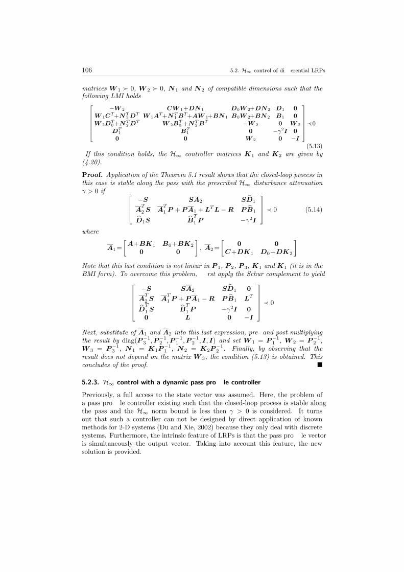
106 5.2. H∞ control of di®erential LRPs
matrices W 1 Â 0, W 2 Â 0, N1 and N2 of compatible dimensions such that thefollowing LMI holds
−W 2 CW 1+DN1 D0W 2+DN2 D1 0
W 1CT+NT
1 DT W 1AT+NT
1 BT+AW 1+BN1 B0W 2+BN2 B1 0
W 2DT0+NT
2 DT W 2BT0 +NT
2 BT −W 2 0 W 2
DT1 BT
1 0 −γ2I 0
0 0 W 2 0 −I
≺0
(5.13)
If this condition holds, the H∞ controller matrices K1 and K2 are given by(4.20).
Proof. Application of the Theorem 5.1 result shows that the closed-loop process inthis case is stable along the pass with the prescribed H∞ disturbance attenuationγ > 0 if
−S SA2 SD1
AT
2 S AT
1 P + PA1 +LTL−R PB1
D1S BT
1 P −γ2I
≺ 0 (5.14)
where
A1=
[A+BK1 B0+BK2
0 0
], A2=
[0 0
C+DK1 D0+DK2
]
Note that this last condition is not linear in P 1, P 2, P 3, K1 and K1 (it is in theBMI form). To overcome this problem, ¯rst apply the Schur complement to yield
−S SA2 SD1 0
AT
2 S AT
1 P + PA1 −R PB1 LT
DT
1 S BT
1 P −γ2I 0
0 L 0 −I
≺ 0
Next, substitute of A1 and A2 into this last expression, pre- and post-multiplyingthe result by diag(P−1
3 ,P−12 ,P−1
1 ,P−12 , I, I) and set W 1 = P−1
1 , W 2 = P−12 ,
W 3 = P−13 , N1 = K1P
−11 , N2 = K2P
−12 . Finally, by observing that the
result does not depend on the matrix W 3, the condition (5.13) is obtained. Thisconcludes of the proof. ¥
5.2.3. H∞ control with a dynamic pass pro¯le controllerPreviously, a full access to the state vector was assumed. Here, the problem ofa pass pro¯le controller existing such that the closed-loop process is stable alongthe pass and the H∞ norm bound is less then γ > 0 is considered. It turnsout that such a controller can not be designed by direct application of knownmethods for 2-D systems (Du and Xie, 2002) because they only deal with discretesystems. Furthermore, the intrinsic feature of LRPs is that the pass pro¯le vectoris simultaneously the output vector. Taking into account this feature, the newsolution is provided.

5. LMI methods in performance analysis 107
To begin consideration of the problem, recall that the following result is usedin this section.
Lemma 10. (Dullerud and Paganini, 2000) Suppose that the n × n matricesΣ Â 0 and Γ Â 0 are given and nc is a positive integer. Then there exists n× ncmatrices Σ2, Γ2 and nc × nc symmetric matrices Σ3, and Γ3, such that
[Σ Σ2
ΣT2 Σ3
]Â0 and
[Σ Σ2
ΣT2 Σ3
]−1=
[Γ Γ2
ΓT2 Γ3
]
if, and only if, [Σ I
I Γ
]º 0
In order to solve the H∞ control problem considered here, introduce thefollowing pass pro¯le feedback controller of the order nc
[xck+1(t)yck+1(t)
]=
[Ac11 Ac12
Ac21 Ac22
][xck+1(t)yck(t)
]+
[Bc1
Bc2
]yk(t)
uk+1(t)=[Cc1 Cc2
] [xck+1(t)yck(t)
]+Dcyk(t)
(5.15)
where xck+1(t) ∈ Rn1×1 is the controller state vector, yck(t) ∈ Rm1×1 is the control-ler output vector and nc = n1 +m1. Next, denote
Φ =
[A B0
C D0
], Ω =
[B1
D1
], B2 =
[B
D
], C2 =
[0 I
],
Ac =
[Ac11 Ac12
Ac21 Ac22
], Bc =
[Bc1
Bc2
], Cc =
[Cc1 Cc2
] (5.16)
Introduce now, the so-called augmented state and pass pro¯le vectors
xk+1(t) =
[xk+1(t)xck+1(t)
], yk(t) =
[yk(t)yck(t)
]
and the matrices
Π =
I 0 0 0
0 0 I 0
0 I 0 0
0 0 0 I
, Π1 =
I 0 0 0
0 0 I 0
0 0 0 0
0 0 0 0
, Π2 =
0 0 0 0
0 0 0 0
0 I 0 0
0 0 0 I
(5.17)
to obtain the closed-loop process of the form[xk+1(t)yk+1(t)
]=A
[xk+1(t)yk(t)
]+Bwk+1(t)
yk+1(t) =C
[xk+1(t)yk(t)
] (5.18)

108 5.2. H∞ control of di®erential LRPs
where
A=Π
[Φ+B2DcC2 B2Cc
BcC2 Ac
]Π
T =(Π1+Π2)
[Φ+B2DcC2 B2Cc
BcC2 Ac
]Π
T
=Π1
[Φ+B2DcC2 B2Cc
BcC2 Ac
]Π
T+Π2
[Φ+B2DcC2 B2Cc
BcC2 Ac
]Π
T=A1+A2
B = Π1
[Ω
0
]+Π2
[Ω
0
]= B1+B2, C =
[C2 0
]Π
T
In the following, introduce the matrix of controller data as
Θ =
[Dc Cc
Bc Ac
](5.19)
and
A1=Π1
[Φ 0
0 0
]Π, A2=Π2
[Φ 0
0 0
]Π, Γ1=Π1
[B2 0
0 I
], Γ2=Π2
[B2 0
0 I
],
C2=
[C2 0
0 I
]Π
T , C=[C2 0
]Π
T , B1=Π1
[Ω
0
], B2=Π2
[Ω
0
]
(5.20)
It allows presenting the closed-loop process matrices in the form affine in thecontroller data matrix Θ as
A1 = A1 + Γ1ΘC2, A2 = A2 + Γ2ΘC2, B1 = B1, B2 = B2,C = C (5.21)
Hence, we have the following result based on Theorem 5.1.
Theorem 5.3. A di®erential LRP described by (5.2) is stable along the pass andhas the H∞ disturbance attenuation γ > 0 if there exist matrices Sv  0, P h  0,such that the following inequality holds
−S SA2 SB2 0
AT
2 S AT
1 P + PA1 −R PB1 CT
BT
2 S BT
1 P −γ2I 0
0 C 0 −I
≺ 0 (5.22)
where S = diag(I,Sv), P = diag(P h, I), R = diag(0,Sv).
This can be resolved to the following form.
Theorem 5.4. If there exist matrices P h11Â 0, Uh11
 0, Sv11 0, T v11
 0such that the LMIs de¯ned by (5.23)–(5.25) hold then there exists a controller ofthe form (5.15) which guarantees that the di®erential LRP described by (5.18) is

5. LMI methods in performance analysis 109
stable along the pass and has the H∞ disturbance attenuation γ > 0.
WTc 0 0
0 I 0
0 0 I
−T v11+D0T v11
DT0 CUh11
+D0T v11BT0
Uh11CT+B0T v11
DT0 Uh11
AT+AUh11+B0T v11
BT0
DT1 BT
1
T v11DT
0 T v11BT0
D1 D0T v11
B1 B0T v11
−γ2I 0
0 −I + T v11
Wc 0 0
0 I 0
0 0 I
≺ 0
(5.23)
[ATP h11
+P h11A+CTSv11
C P h11B1+CTSv11
D1
BT1 P h11
+DT1 Sv11
C DT1 Sv11
D1−γ2I
]≺ 0 (5.24)
[P h11 I
I Uh11
]º 0,
[Sv11 I
I T v11
]º 0 (5.25)
where Wc is full column rank matrix whose image satis¯es
Im (Wc) =ker
([DT
BT
])
Suppose now that the LMIs (5.23)-(5.25) are feasible. Then the followingis a systematic procedure for obtaining the corresponding controller state-spacematrices.
Step 1: Compute the matrices P h12, P v12 using the following formulas
Sv12S−1v22
STv12= Sv11
− T−1v11
P h12P−1
h22P T
h12= P h11
−U−1h11
where P h22 = I and Sv22 = I
Step 2: Construct the matrices P h  0 and Sv  0 as
P h =
[P h11
P Th12
P h12I
], Sv =
[Sv11
STv12
Sv12I
]
and then the matrices S = diag(I,Sv), P = diag(P h, I), R = diag(0,Sv)
Step 3: Compute the matricesM , N and Ψ de¯ned in (5.28)
Step 4: Solve the following LMI
Ψ+MTΘN +NT
ΘTM ≺ 0
to obtain (5.19) i.e. the matrices which de¯ne the controller state-space mo-del (5.15).

110 5.2. H∞ control of di®erential LRPs
Proof. Using matrix de¯nitions (5.21), the inequality (5.22) can be rewritten as
−S SA2 + SΓ2ΘC2 SB2 0
AT2 S+CT
2ΘTΓT2 S AT
1 P+CT2Θ
TΓT1 P+PA1+PΓ1ΘC2−R PB1 CT
BT2 S BT
1 P −γ2I 0
0 C 0 −I
≺ 0
⇔
−S SA2 SB2 0
AT2 S AT
1 P + PA1 −R PB1 CT
BT2 S BT
1 P −γ2I 0
0 C 0 −I
+
0 SΓ2ΘC2 0 0
0 PΓ1ΘC2 0 0
0 0 0 0
0 0 0 0
+
0 0 0 0
CT2Θ
TΓT2 S CT
2ΘTΓT1 P 0 0
0 0 0 0
0 0 0 0
≺ 0
(5.26)
It is straightforward to see that (5.26) can be rewritten as
−S SA2 SB2 0
AT2 S AT
1 P + PA1 −R PB1 CT
BT2 S BT
1 P −γ2I 0
0 C 0 −I
+
SΓ2PΓ10
0
Θ
[0 C2 0 0
]
+[ΓT2 S Γ
T1 P 0 0
]Θ
T
0
CT2
0
0
≺ 0
(5.27)
Now, de¯ne the matrices
Ψ =
−S SA2 SB2 0
AT2 S AT
1 P + PA1 −R PB1 CT
BT2 S BT
1 P −γ2I 0
0 C 0 −I
, MT =
SΓ2PΓ10
0
,
N =[0 C2 0 0
](5.28)
to present (5.27) in the form
Ψ+MTΘN +NT
ΘTM ≺ 0 (5.29)
In the sequel, invoke Lemma 9 to eliminate the matrix variable Θ and obtain
WTMΨWM ≺ 0 and WT
NΨWN ≺ 0 (5.30)
where
WM ∈ ker(M), WN ∈ ker(N) (5.31)

5. LMI methods in performance analysis 111
Next, note that
M =[ΓT2 S ΓT
1 P 0 0]=[ΓT2 Γ
T1 0 0
]
S 0 0 0
0 P 0 0
0 0 I 0
0 0 0 I
=MnV (5.32)
where the matrices P and S are partitioned as
P =
P h11P h12
0 0
P Th12
P h220 0
0 0 I 0
0 0 0 I
, S =
I 0 0 0
0 I 0 0
0 0 Sv11Sv12
0 0 STv12
Sv22
and
P h =
[P h11
P h12
P Th12
P h22
], P v =
[I 0
0 I
], Sh =
[I 0
0 I
], Sv =
[Sv11
Sv12
STv12
Sv22
]
Observe that the solution of (5.22) is independent of the matrices P v and Sh butthey are necessary to compute V −1 (the matrix V is de¯ned in (5.32)). Further-more, it is important now to observe that
ker(MnV ) = V −1 ker(Mn)
and using (5.31) yields that
WM = V −1WMn.
Therefore, the ¯rst inequality in (5.30) is
WTMn
V −TΨV −1WMn
≺ 0Furthermore, introduce the matrix Ξ as
Ξ = V −TΨV −1 =
−S−1 A2P−1 B2 0
P−1AT2 P−1AT
1 +A1P−1 −R B1 P−1CT
BT2 BT
1 −γ2I 0
0 CP−10 −I
Then, two inequalities of (5.30) are
WTMnΞWMn
≺ 0 (5.33)
andWT
NΨWN ≺ 0 (5.34)
These inequalities clearly are in the BMI form, thus to obtain LMI for (5.33) and(5.34) some matrix manipulations are required. First, rewrite matrices in the fullform
Mn =[Γ2
TΓ1
T0 0
]=
0 0 0 0 BT
0 0 0 0 0
0 0 DT0 0 I 0 0 0 0
0 0 0 I 0 0 0 0 0 0
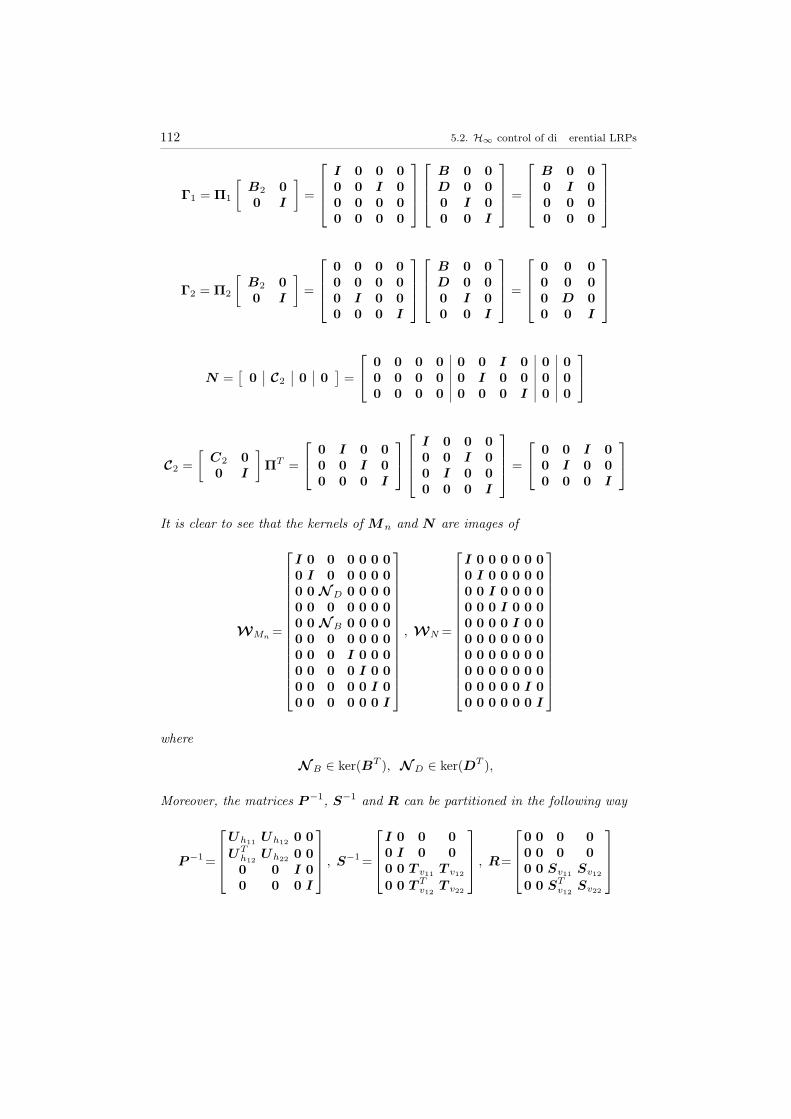
112 5.2. H∞ control of di®erential LRPs
Γ1 = Π1
[B2 0
0 I
]=
I 0 0 0
0 0 I 0
0 0 0 0
0 0 0 0
B 0 0
D 0 0
0 I 0
0 0 I
=
B 0 0
0 I 0
0 0 0
0 0 0
Γ2 = Π2
[B2 0
0 I
]=
0 0 0 0
0 0 0 0
0 I 0 0
0 0 0 I
B 0 0
D 0 0
0 I 0
0 0 I
=
0 0 0
0 0 0
0 D 0
0 0 I
N =[0 C2 0 0
]=
0 0 0 0 0 0 I 0 0 0
0 0 0 0 0 I 0 0 0 0
0 0 0 0 0 0 0 I 0 0
C2 =
[C2 0
0 I
]Π
T =
0 I 0 0
0 0 I 0
0 0 0 I
I 0 0 0
0 0 I 0
0 I 0 0
0 0 0 I
=
0 0 I 0
0 I 0 0
0 0 0 I
It is clear to see that the kernels of Mn and N are images of
WMn=
I 0 0 0 0 0 0
0 I 0 0 0 0 0
0 0 ND 0 0 0 0
0 0 0 0 0 0 0
0 0 NB 0 0 0 0
0 0 0 0 0 0 0
0 0 0 I 0 0 0
0 0 0 0 I 0 0
0 0 0 0 0 I 0
0 0 0 0 0 0 I
, WN =
I 0 0 0 0 0 0
0 I 0 0 0 0 0
0 0 I 0 0 0 0
0 0 0 I 0 0 0
0 0 0 0 I 0 0
0 0 0 0 0 0 0
0 0 0 0 0 0 0
0 0 0 0 0 0 0
0 0 0 0 0 I 0
0 0 0 0 0 0 I
where
NB ∈ ker(BT ), ND ∈ ker(DT ),
Moreover, the matrices P−1, S−1 and R can be partitioned in the following way
P−1=
Uh11Uh12
0 0
UTh12
Uh220 0
0 0 I 0
0 0 0 I
, S−1=
I 0 0 0
0 I 0 0
0 0 T v11T v12
0 0 T Tv12
T v22
, R=
0 0 0 0
0 0 0 0
0 0 Sv11Sv12
0 0 STv12
Sv22

5. LMI methods in performance analysis 113
It allows us to rewrite the matrix Ξ as
Ξ=
−I 0 0 0 0 0 0 0 0 0
0 −I 0 0 0 0 0 0 0 0
0 0 −T v11 −T v12 CUh11CUh12
D0 0 D1 0
0 0 −T Tv12
−T v22 0 0 0 0 0 0
0 0 Uh11CT
0 Uh11AT+AUh11
AUh12B0 0 B1 0
0 0 UT
h12CT
0 UT
h12AT
0 0 0 0 0
0 0 DT0 0 BT
0 0 −Sv11 −Sv12 0 I
0 0 0 0 0 0 −STv12
−Sv22 0 0
0 0 DT1 0 BT
1 0 0 0 −γ2I 0
0 0 0 0 0 0 I 0 0 −I
Consider the ¯rst BMI constraint (5.34)
WTMnΞWMn
≺ 0
By observing that the forth and sixth rows of WMnare zero, the last inequality
can be rewritten as
N T
D N T
B 0 0 0 0
0 0 I 0 0 0
0 0 0 I 0 0
0 0 0 0 I 0
0 0 0 0 0 I
−T v11 CUh11D0 0 D1 0
Uh11CT Uh11
AT+AUh11B0 0 B1 0
DT0 BT
0 −Sv11 −Sv12 0 I
0 0 −STv12
−Sv22 0 0
DT1 BT
1 0 0 −γ2I 0
0 0 I 0 0 −I
×
ND 0 0 0 0
NB 0 0 0 0
0 I 0 0 0
0 0 I 0 0
0 0 0 I 0
0 0 0 0 I
≺0
Next, application of the Schur complement formula yields (5.23). In order toobtain the inequality (5.24), rewrite the matrix Ψ as
Ψ=
−I 0 0 0 0 0 0 0 0 0
0 −I 0 0 0 0 0 0 0 0
0 0 −Sv11 −Sv12 Sv11C 0 Sv11D0 0 Sv11D1 0
0 0 −STv12
−Sv22 STv12
C 0 STv12
D0 0 STv12
D1 0
0 0 CTSv11 CTSv12 ATP h11+P h11
A AP h12P h11
B0 0 P h11B1 0
0 0 0 0 P T
h12A 0 P T
h12B0 0 P T
h12B1 0
0 0 DT0 Sv11 DT
0 Sv11 BT0 P h11
BT0 P h12
−Sv11 −Sv12 0 I
0 0 0 0 0 0 −STv12
−Sv22 0 0
0 0 DT1 Sv11 DT
1 Sv12 BT1 P h11
BT1 P h12
0 0 −γ2I 0
0 0 0 0 0 0 I 0 0 −I
Next, by observing that the some rows of WN are zero, the condition (5.34)

114 5.2. H∞ control of di®erential LRPs
reduces to
−Sv11−Sv12
Sv11C Sv11
D1 0
−STv12
−Sv22ST
v12C ST
v12D1 0
CTSv11CTSv12
ATP h11+ P h11
A P h11B1 0
DT1 Sv11
DT1 Sv12
BT1 P h11
−γ2I 0
0 0 0 0 −I
≺ 0
Further, application of the Schur complement formula gives
ATP h11+P h11
A P h11B1 0
BT1 P h11
−γ2I 0
0 0 −I
+
CTSv11 CTSv12
DT1 Sv11 DT
1 Sv12
0 0
[
T v11 T v12
T Tv12
T v22
][Sv11C Sv11D1 0
STv12
C STv12
D1 0
]≺0
which is equivalent to LMI (5.24). Additionally, applying of Lemma 10 gives asthe result the conditions de¯ned in (5.25) and the proof is completed. ¥
The disturbance attenuation level γ can be optimized by solving the followinglinear minimization problem
minP h11
Â0,Uh11Â0,Sv11
Â0,T v11Â0
µ
subject to (5.23)− (5.25) with µ = γ2(5.35)
To show the usefulness of this result, let us consider the following numerical exam-ple.
Example 5.1. Consider the di®erential LRP of the form (5.2) with matrices givenby
A =
[−1.4684 −1.3745−1.4080 −1.6290
],B0 =
[0.0309 0.25530.0635 0.2229
],C =
[0.0810 0.09480.0610 0.0289
],
D0 =
[0.0494 0.05100.0530 0.0227
], B1 =
[1.9635 0.96441.0872 1.6311
],D1 =
[1.5410 0.11961.2650 0.1512
],
B =
[1.9070 1.28242.6290 2.1252
],D =
[0.2106 1.52490.0572 2.6082
]
With this data, application of the controller design procedure of (5.35) yields
P h11 =
[0.1169 0.10360.1036 0.1740
], Uh11 = 10
6
[8.3795 0.51420.5142 9.1918
],
Sv11 =
[6.1931 −5.8899−5.8899 7.6801
], T v11 =
[0.8599 0.15890.1589 0.8198
]

5. LMI methods in performance analysis 115
and the corresponding H∞ controller matrices are
Ac=
[−3.8573 −1.5123−1.7765 −0.9105
],Bc=
[0.1405 0.15810.0712 0.0991
],
Cc=
[0.7487 0.74300.0520 −0.0499
], Dc=
[−0.1041 −0.2130−0.0180 −0.0040
]
Moreover, the minimum γ derived in this example is 2.1530.
5.2.4. Numerical computations of the Lyapunov matrix
It should be pointed out that providing the Lyapunov matrix results in computa-tional problems which are nontrivial due to required of existence of the matricesXand Y such that Y = X−1. Unfortunately, this problem is non-convex thereforethe convex formulation is required. Moreover, the controller order is equal to therank of X − Y so it is hard to specify the controller order. It is shown in (Fuand Luo, 1997) that computational problems which have arisen in ¯xed outputfeedback design are NP-hard problems.In the above design procedure, the dynamic controller with unspeci¯ed order
was considered. In this case, the constraint Y = X−1 Â 0 can be replacedby Y º X−1 Â 0 (Iwasaki and Skelton, 1994) which, after applying the Schurcomplement formula, leads to
[Y I
I X
]º 0
Thus, the convex formulation has been found and it can be applied in H∞ con-troller design - see conditions in (5.25). Unfortunately, since one of the blockX is chosen as I (the identity matrix) then the condition number of X can belarge. To avoid computation problems, the approach based on the singular valuedecomposition (SVD) is used. As the ¯rst step, SVD of I −XY is computed
I −XY = UΣV T
Next, the matricesM and N are chosen as
M =UΣ1
2
N =V Σ1
2
and they satisfy MNT = I − XY . This allows us to compute the Lyapunovmatrix L from the relation
[Y I
NT0
]= L
[I X
0 MT
]
As the next step, partition L as
L =
[L11 L12
LT12 L22
]

116 5.2. H∞ control of di®erential LRPs
to obtain
L
[I X
0 MT
]=
[L11 L12
LT12 L22
] [I X
0 MT
]=
[L11 L11X +L12M
T
LT12 LT
12X +L22MT
]
Based on the above equation, the blocks of L can be computed from
L11 = Y
LT12 = NT
L11X +L12MT = I
LT12X +L22M
T = 0
thus L22 = Σ1
2 V TXUTΣ− 1
2 and L and its inversion are
L =
[Y N
NT L22
], L−1 =
[X M
MT K
]
where K is any given matrix of appropriate dimension.It should be pointed out that there several algorithms exist which give suffi-
cient condition for ¯nding the matrices X and Y so that Y = X−1 via convexoptimization (Iwasaki and Skelton, 1995a,b). This immediately allows us to applyLMI methods.The idea of these algorithms is based on the observation that for any matrices
X Â 0 and Y Â 0 that satisfy[
Y I
I X
]º 0 (5.36)
the condition trace(XY ) = n (where n denotes the number of rows of the matrixX (or Y )) implies that XY = I. Hence, the solution to the problem of ¯ndingthe matrices X Â 0 and Y Â 0 such that X = Y −1 is reduced to the solution
minXÂ0,Y Â0
trace(XY )
subject to (5.36)
It was illustrated in (Oliveria and Geromel, 1997) that the above optimizationproblem can be solved in an e®ective way using Product Reduction Algorithm(PRA). Moreover, this algorithm is simple in numerical implementation and cantherefore be used for our purposes.
5.2.4.1. Product Reduction Algorithm
The preliminary step of this algorithm is to provide any matrices X0 Â 0 andY 0 Â 0 which satisfy (5.36) then set the iteration counter k = 0 and successivelyperform the following steps

5. LMI methods in performance analysis 117
Step 1: De¯ne the linear function
fk(X,Y ) = trace (XkY + Y kX)
Step 2: Compute Xk+1 and Y k+1 by solving linear objective minimization pro-blem of the form
minXÂ0,Y Â0
fk(X,Y )
subject to (5.36)
Step 3: If prescribed accuracy ε is attained e.g. trace (Xk+1Y +Y k+1X)−2n≤ε(where n denotes the number of rows ofX or Y ) then stop, otherwise returnto the second step.
5.3. H∞ control of uncertain di®erential LRPs
In this section we extend the results of the previous section to a process modelcontaining some uncertainties in all the matrices. The presence of these uncer-tainties in the model structure is the consequence of varying physical parametersand imperfect knowledge on process dynamics. Motivated by this practical fact,we are interested in designing a static feedback controller that stabilises the con-sidered class of LRPs and ensures that the H∞ norm bound does not exceed theprescribed level for all admissible uncertainties. Two representations of uncerta-inty are taken into consideration: norm-bounded and polytopic forms. Both ofthese representations have their advantages and disadvantages and there are alsopractically relevant problem areas where one in more suitable than the other.
5.3.1. Norm-bounded model of uncertainty
Here, we assume that the uncertainty is norm bounded in both the state and passpro¯le updating equations. This form corresponds to the process with uncertaintywhich is modelled as an additive perturbation to the nominal model matrices. Insuch a case we can write the process state-space model in the form[xk+1(t)yk+1(t)
]=
([A B0
C D0
]+
[∆A ∆B0
∆C ∆D0
])[xk+1(t)yk(t)
]+
([B
D
]+
[∆B
∆D
])uk+1(t)
+
([B1
D1
]+
[∆B1
∆D1
])wk+1(t)
(5.37)
where the admissible uncertainties are assumed to be of the form[∆A ∆B0 ∆B ∆B1
∆C ∆D0 ∆D ∆D1
]=
[H1
H2
]F[
E1 E2 E3 E4
](5.38)
and where H1, H2, E1, E2, E3, E4 are known constant matrices of compatibledimensions, and F is an unknown matrix with constant entries which satis¯es

118 5.3. H∞ control of uncertain di®erential LRPs
(4.5). In this case, the following theorem gives the condition of a controller existingthat stabilises the process (5.37) and ensures that the H∞ norm bound does notexceed prescribed level for all admissible uncertainties.
Theorem 5.5. Suppose that a di®erential LRP of the form described by (5.37),with uncertainty structure modelled by (5.38) and (4.5), is subjected to a controllaw of the form (4.17). Then the resulting closed-loop process is stable along thepass for all admissible uncertainties and has the prescribed H∞ disturbance atte-nuation γ > 0 if there exist matricesW 1 Â 0,W 2 Â 0, N1 and N2 of compatibledimensions and a scalar ε > 0 such that the following LMI holds
−W 2+3εH2HT2 CW 1+DN1+3εH2H
T1
W 1CT+NT
1 DT+3εH1HT2 W 1A
T+NT1 BT+AW 1+BN1+3εH1H
T1
W 2DT0 +NT
2 DT W 2BT0 +NT
2 BT
DT1 BT
1
0 0
0 E1W 1 +E3N1
0 0
0 0
D0W 2+DN2 D1 0 0 0 0
B0W 2+BN2 B1 0 W 1ET1 +NT
1 ET3 0 0
−W 2 0 W 2 0 W 2ET2 +NT
2 ET3 0
0 −γ2I 0 0 0 ET4
W 2 0 −I 0 0 0
0 0 0 −εI 0 0
E2W 2+E3N2 0 0 0 −εI 0
0 E4 0 0 0 −εI
≺ 0
(5.39)
If (5.39) holds then the controller matrices K1 and K2 are given by (4.20).
Proof. In view of the proof of Theorem 5.2 it can be shown that the closed-loopprocess is stable along the pass for all admissible uncertainties and has prescribedH∞ disturbance attenuation γ > 0 if the following inequality is satis¯ed
0 ∆CW 1+∆DN1 ∆D0W 2+∆DN2 ∆D1 0
W 1∆CT+NT1∆DT ∆Λ ∆B0W 2+∆BN2 ∆B1 0
W 2∆DT0 +NT
2∆DT W 2∆BT0+NT
2∆BT0 0 0
∆DT1 ∆BT
1 0 0 0
0 0 0 0 0
+
−W 2 CW 1+DN1 D0W 2+DN2 D1 0
W 1CT+NT
1 DTΛ B0W 2+BN2 B1 0
W 2DT0 +NT
2 DT W 2BT0+NT
2 BT −W 2 0 W 2
DT1 BT
1 0 −γ2I 0
0 0 W 2 0 −I
≺0
(5.40)
where Λ = W 1AT +NT
1 BT +AW 1+BN1 and ∆Λ = W 1∆AT+NT1∆BT+
∆AW 1+∆BN1. The ¯rst term in the above inequality can be rewritten as
HFE +ETF
TH
T

5. LMI methods in performance analysis 119
where
H =
0 H2 H2 H2 0
0 H1 H1 H1 0
0 0 0 0 0
0 0 0 0 0
0 0 0 0 0
, F=diag (F ,F ,F ,F ,F) ,
E =diag (0,E1W 1 +E3N1,E2W 2 +E3N2,E4,0)
An obvious application of Lemma 8 followed by application of the Schur comple-ment formula yields (5.39) and the proof is complete. ¥
5.3.2. Polytopic model of uncertainty
Consider the di®erential LRP which the current pass state updating equationmatrices range in the polytope of matrices as it is described by
[A B B0 B1
]∈ Co
([Ai Bi
0 Bi B1
]), i=1, 2, . . . , h (5.41)
and
Co([
Ai Bi0 Bi Bi
1
]):=
X :X=
h∑
i=1
αi
[Ai Bi
0 Bi Bi1
], αi ≥ 0,
h∑
i=1
αi=1
(5.42)
For the current pass pro¯le updating equation in (5.2) we assume a norm-boundedtype of uncertainty
yk+1(t) =(C+∆C)xk+1(t)+(D0+∆D0)yk(t)
+ (D+∆D)uk+1(t)+(D1+∆D1)wk+1(t)
where[∆C ∆D0 ∆D ∆D1
]= H2F
[E1 E2 E3 E4
](5.43)
and the matrix F satis¯es (4.5).
Theorem 5.6. Suppose that a di®erential LRP of the form described by (5.2), withuncertainty structure modelled by (5.41)-(5.42) and (5.43), is subjected to a controllaw of the form of (4.17). Then the resulting closed-loop process is stable alongthe pass for all admissible uncertainties and has the prescribed H∞ disturbanceattenuation γ > 0 if there exist matrices W 1 Â 0, W 2 Â 0, N1 and N2 of

120 5.4. H∞ control of discrete LRPs
compatible dimensions and a scalar ε > 0, such that
−W 2+3εH2HT2 CW 1+DN1
W 1CT+NT
1 DT W 1AiT+NT
1 BiT+AiW 1+BiN1
W 2DT0 +NT
2 DT W 2BiT0 +NT
2 BiT
DT1 BiT
1
0 0
0 E1W 1 +E3N1
0 0
0 0
D0W 2+DN2 D1 0 0 0 0
Bi0W 2+BiN2 Bi
1 0 W 1ET1+NT
1 ET3 0 0
−W 2 0 W 2 0 W 2ET2 +NT
2 ET3 0
0 −γ2I 0 0 0 ET4
W 2 0 −I 0 0 0
0 0 0 −εI 0 0
E2W 2+E3N2 0 0 0 −εI 0
0 E4 0 0 0 −εI
≺0
(5.44)
If the LMI (5.44) holds then the controller matrices K1 and K2 are given by(4.20).
Proof. It can be proven in an identical manner to proofs of previously presentedTheorems. ¥
5.4. H∞ control of discrete LRPs
This section addresses the problem of the H∞ disturbance rejection or attenuationproblem for discrete LRP. Therefore, the aim can be summarized as ¯nding animplementable control law which will give stability along the pass closed loop witha prescribed degree of disturbance rejection, including the case when there is anuncertainty in the model structure.
5.4.1. LMI-based H∞ norm computationConsider the model of a discrete LRP (5.3) with no control inputs but with externaldisturbance inputs given by
[xk+1(p+ 1)yk+1(p)
]=
[A B0
C D0
] [xk+1(p)yk(p)
]+
[B1
D1
]wk+1(p) (5.45)
then with (5.4) we have the following result.
Theorem 5.7. A discrete LRP described by (5.45) is stable along the pass andhas the H∞ disturbance attenuation γ > 0 if there exist matrices P 1 Â 0 andP 2 Â 0 such that the following LMI with P = diag(P 1,P 2) holds
−P PΦ PΩ 0
ΦTP −P 0 CT
2
ΩTP 0 −γ2I 0
0 C2 0 −I
≺ 0 (5.46)

5. LMI methods in performance analysis 121
where Φ, Ω and C2 are de¯ned in (5.16).
Proof. In order to ensure the H∞ noise attenuation γ holds, it is required thatthe associated Hamiltonian de¯ned by
H(k, p) = ∆V (k, p)+yTk+1(p)yk+1(p)− γ2wTk+1(p)wk+1(p) (5.47)
satis¯es
H(k, p) < 0 (5.48)
where ∆V (k, p) is de¯ned in (4.34). Next, by carrying out appropriate substitutionswe obtain
H(k, p)=[ζT (k, p) wT
k+1(p)][ΦTPΦ−P +CT
2C2 ΦTPΩ
ΩTPΦ ΩPΩ−γ2I
][ζ(k, p)wk+1(p)
]
where ζ(k, p) is de¯ned in (4.32). Now the above condition guarantees that (5.48)holds for any ζ(k, p), wk+1(p) 6= 0. Finally, application of the Schur complementformula gives the solution and the proof is complete. ¥
Remark 5.2. Since LRPs share certain structural similarities with 2-D linearsystems then the result can be also obtained via manipulations required for 2-Dlinear systems described by RM, for example, in (Du and Xie, 2002). On theother hand, it should be pointed out that the structure of the control algorithmsare not well founded physically due to the fact that, for example, the concept ofa state for these systems is not uniquely de¯ned. Furthermore, it turns out that,in case of LRP, a control law is a combination of current pass information and‘feedforward’ information from the previous pass. In terms of 2-D systems this isthe equivalent to a clear state feedback control law, which has not been used in (Duand Xie, 2002) for H∞ control. Moreover, it is known in terms of RM, thatthe pass pro¯le vector is simultaneously the output vector which employs di®erentalgebraic manipulations and in e®ect yields a simpli¯ed version in comparison tothe standard 2-D approach of (Du and Xie, 2002; Du et al., 2001).
Remark 5.3. It can be seen that the inequality (5.46) has the same form as theinequality (4.46). Therefore, the robust stabilisation of an uncertain LRP can besolved via H∞ control results developed here.
5.4.2. H∞ control with a static feedback controller
The following result enables (4.40) to be designed to give stability along the passof the closed-loop process with a prescribed disturbance rejection bound.
Theorem 5.8. Suppose that a discrete LRP described by (5.3) is subject to acontrol law of the form (4.40). Then the resulting closed-loop process is stablealong the pass with the prescribed H∞ disturbance attenuation γ > 0 if there exists

122 5.4. H∞ control of discrete LRPs
matrices W 1 Â 0, W 2 Â 0, N1 and N2 such that the following LMI holds
−W 1 0 AW 1+BN1 B0W 2+BN2 B1 0
0 −W 2 CW 1+DN1 D0W 2+DN2 D1 0
W 1AT+NT
1 BT W 1CT+NT
1 DT −W 1 0 0 0
W 2BT0 +NT
2 BT W 2DT0 +NT
2 DT0 −W 2 0 W 2
BT1 DT
1 0 0 −γ2I 0
0 0 0 W 2 0 −I
≺0
(5.49)
and the required controller matrices in (4.40) are given by (4.20).
Proof. Applying the result of Theorem 5.7 it follows immediately that stabilityalong the pass holds if there exist matrices P 1 Â 0 and P 2 Â 0 such that
−P 1 0 P 1A+P 1BK1 Λ1 P 1B1 0
0 −P 2 P 2C+P 2DK1 Λ2 P 2D1 0
ATP 1+KT1 BTP 1 CTP 2+KT
1 DTP 2 −P 1 0 0 0
ΛT1 Λ
T2 0 −P 2 0 I
BT1 P 1 DT
1 P 2 0 0 −γ2I 0
0 0 0 I 0 −I
≺0
where Λ1 = P 1B0+P 1BK2 and Λ2 = P 2D0+P 2DK2, This last inequality is notin LMI form because it is nonlinear with respect to its parameters. Consequently,set P 1 = W−1
1 , P 2 = W−12 and pre and post-multiply by diag(W 1, W 2, W 1,
W 2, I, I), followed by setting N 1 =K1W 1 and N2 =K2W 2 to obtain the LMIof (5.49) and the proof is complete. ¥
Note that the H∞ disturbance attenuation here can be minimized using thelinear objective minimization procedure which leads, in e®ect, to minimization ofthe e®ects of the disturbance.
minW 1Â0,W 2Â0,N1,N2
µ
subject to (5.49) with µ = γ2
5.4.3. H∞ control with a dynamic pass pro¯le controllerThe control law of the previous section requires that the complete current passstate vector is available for measurement. If this is not the case then one optionis to use an observer to reconstruct it. In this section, we consider the control ofprocesses described by (5.3) through use of a full dynamic pass pro¯le feedbackcontroller of the order nc
[xck+1(p+ 1)yck+1(p)
]=
[Ac11 Ac12
Ac21 Ac22
][xck+1(p)yck(p)
]+
[Bc1
Bc2
]yk+1(p)
uk+1(p)=[Cc1 Cc2
] [xck+1(p)yck(p)
]+Dcyk+1(p)
(5.50)
where xck(p) ∈ Rn1 is the controller state vector, yck(p) ∈ Rm1 is the output vectorand nc = n1 +m1.

5. LMI methods in performance analysis 123
To obtain the state-space model of the resulting closed-loop process, use thenotation (5.16)-(5.17) and introduce the so-called augmented state and pass pro¯levectors for the closed-loop process as
xk+1(p) =
[xk+1(p)xck+1(p)
], yk(p) =
[yk(p)yck(p)
]
Then the closed-loop process is given by[xk+1(p+ 1)yk+1(p)
]=A
[xk+1(p)yk(p)
]+Bwk(p)
yk+1(p) =C
[xk+1(p)yk(p)
] (5.51)
where
A=Π
[Φ+B2DcC2 B2Cc
BcC2 Ac
]Π
T , B=Π
[Ω
0
], C =
[C2 0
]Π
T
Next, de¯ne
A =
[Φ 0
0 0
], B2 =
[B2 0
0 I
], C2 =
[C2 0
0 I
], C =
[C2 0
], B =
[Ω
0
]
then it is obvious that the closed-loop state-space model matrices can be writtenin the following form which is affine in the controller data matrix Θ (introducedin (5.19))
A = Π[
A+B2ΘC2]Π
T , C = CΠT , B = ΠB (5.52)
Now we have the following result which gives an existence condition for the con-troller matricesAc, Bc, Cc,Dc to ensure stability along the pass and then enablescontroller design.
Theorem 5.9. Suppose that a dynamic pass pro¯le feedback controller de¯nedby (5.50) is applied to a discrete LRP described by (5.3) with resulting closed-loop state-space model (5.51). Suppose also that there exist matrices P 11 Â 0,(P 11 = diag(P h11,P v11)) and R11 Â 0, (R11 = diag(Rh11,Rv11)) such that theLMIs de¯ned by (5.53)–(5.55) below hold. Then the resulting closed-loop processis stable along the pass and has the H∞ disturbance attenuation γ > 0
N 1 0 0
0 I 0
0 0 I
TΦR11Φ
T−R11 Ω ΦR11CT2
ΩT −γ2I 0
C2R11ΦT
0 −I+C2R11CT2
N 1 0 0
0 I 0
0 0 I
≺0 (5.53)
N 2 0 0
0 I 0
0 0 I
TΦ
TP 11Φ−P 11 ΦTP 11Ω CT
2
ΩP 11Φ ΩTP 11Ω− γ2I 0
C2 0 −I
N 2 0 0
0 I 0
0 0 I
≺0 (5.54)
[P h11 I
I Rh11
]º 0,
[P v11 I
I Rv11
]º 0 (5.55)

124 5.4. H∞ control of discrete LRPs
where N 1 and N 2 are full column rank matrices whose images satisfy
Im (N 1) = ker(BT2
), Im (N 2) = ker(C2)
Proof. Interpreting the result of Theorem 5.7 in terms of the matrices (5.52) givesthe following inequality
Ψ+MTΘN +NT
ΘTM ≺ 0 (5.56)
where
Ψ=
−R RA RB 0
ATR −R 0 CT
BTR 0 −γ2I 0
0 C 0 −I
, MT=
RB2
0
0
0
, N =
[0 C2 0 0
]
and R = ΠTPΠ. Partitioning the matrix R as
R = ΠTPΠ =
P h110 P h12
0
0 P v110 P v12
P Th12
0 P h220
0 P Tv12
0 P v22
=
[P 11 P 12
P T12 P 22
](5.57)
where
P h =
[P h11
P h12
P Th12
P h22
], P v =
[P v11
P v12
P Tv12
P v22
]
it can be written that
P−1h =
[Rh11
Rh12
RTh12
Rh22
], P−1
v =
[Rv11
Rv12
RTv12
Rv22
]
and
R−1 = ΠTP−1Π =
Rh110 Rh12
0
0 Rv110 Rv12
RTh12
0 Rh220
0 RTv12
0 Rv22
=
[R11 R12
RT12 R22
]
After manipulations similar to these described in the proof of Theorem 5.4 theconditions of (5.53) and (5.54) are obtained.The last problem is to provide the conditions which allow us to ¯nd the matrix
P and its inverse. To begin, ¯rst note again that P = diag(Ph,P v) and that onlyP 11 and R11 appear in the ¯rst two LMIs to be satis¯ed. Application of Lemma 10now gives the required conditions and the proof is complete. ¥
If this last result holds then the stabilising controller can be designed usingthe following algorithm
5. LMI methods in performance analysis 125
Step 1: Compute the matrices P h12, P v12 using
P h12P−1h22P
Th12 = P h11 −R−1
h11,
P v12P−1v22P
Tv12 = P v11 −R−1
v11
where P h22 = I and P v22 = I
Step 2: Construct P h  0 and P v  0 and then the matrix P = diag(P h,P v).
Step 3: Compute the matricesM , N and Ψ.
Step 4: Solve the LMI (5.56) (where Θ is the unknown matrix) and hence thecontroller state-space model matrices.
Also the disturbance attenuation level γ can be minimized using the followingoptimization procedure
minP 11Â0, R11Â0
µ
subject to (5.53)− (5.55) with µ = γ2
5.5. H∞ control of uncertain discrete LRPs
This section deals with the robust H∞ control problem for discrete LRPs withnorm-bounded uncertainty. For this purpose consider a discrete LRP with un-certainty modelled as additive perturbations to the nominal model matrices withresulting state-space model
xk+1(p+ 1) =(A+∆A)xk+1(p) + (B +∆B)uk+1(p) + (B0 +∆B0)yk(p)
+ (B1 +∆B1)wk+1(p)
yk+1(p) =(C +∆C)xk+1(p) + (D +∆D)uk+1(p) + (D0 +∆D0)yk(p)
+ (D1 +∆D1)wk+1(p)
(5.58)
where the admissible uncertainties to be of the form (5.38) and (4.5). Now wehave the following result.
Theorem 5.10. Suppose that a discrete LRP described by (5.58) with the un-certainty structure satisfying (5.38) and (4.5) is subject to a control law de¯nedby (4.40). Then the resulting closed-loop process is stable along the pass with theprescribed H∞ disturbance attenuation γ > 0 if there exist a scalar ε > 0 and

126 5.5. H∞ control of uncertain discrete LRPs
matrices W 1 Â 0, W 2 Â 0, and N1, N2 such that the following LMI holds
−W 1 + 3εH1HT1 3εH1H
T2 AW 1+BN1 B0W 2+BN2
3εH1HT2 −W 2 + 3εH2H
T2 CW 1+DN1 D0W 2+DNT
2
W 1AT+NT
1 BT W 1CT+NT
1 DT −W 1 0
W 2BT0 +NT
2 BT W 2DT0 +NT
2 DT0 −W 2
BT1 DT
1 0 0
0 0 0 W 2
0 0 0 W 1ET1 +NT
1 ET3
0 0 0 0
0 0 0 0
B1 0 0 0 0
D1 0 0 0 0
0 0 0 0 0
0 W 2 E1W 1+E3N1 0 0
−γ2I 0 0 E2W 2+E3N2 0
0 −I 0 0 E4
0 0 −εI 0 0
W 2ET2 +NT
2 ET3 0 0 −εI 0
0 ET4 0 0 −εI
≺0
(5.59)
If this condition holds, the corresponding controller matrices are given by (4.20).
Proof. On applying (4.40), the closed-loop process stability along the pass condi-tion can be written in the form
Γ+ HFE + ETF
TH
T ≺ 0
where Γ is left hand side of LMI (5.49) and
H=
0 0H1 H1 H1 0
0 0H2 H2 H2 0
0 0 0 0 0 0
0 0 0 0 0 0
0 0 0 0 0 0
0 0 0 0 0 0
,F =diag (F ,F ,F ,F ,F ,F) ,
E=diag (0,0,E1W 1+E3N1,E2W 2+E3N2,E4,0)
The LMI of (5.59) is now obtained by an application of the inequality of Lemma 8followed by the Schur complement formula and the proof is complete. ¥
To reduce the e®ects of the disturbance vector, the following linear objectiveminimization procedure can be used.
minW 1Â0,W 2Â0,N1,N2,ε>0
µ
subject to (5.59) with µ = γ2

5. LMI methods in performance analysis 127
5.5.1. Alternative robust stabilisation
In this subsection the solution for the H∞ problem is applied to design a pass pro-¯le feedback controller in the presence of norm-bounded parameter uncertainties.Consider the state-space model of a discrete LRP written in the form (4.29).
Further, use the notation (5.16)-(5.17) and introduce
∆Φ =
[∆A ∆B0
∆C ∆D0
]=
[H1
H2
]γ−1F
[E1 E2
],
∆B2 =
[∆B
∆D
]=
[H1
H2
]γ−1F
[E3
]
The matrices H1, H2, E1, E2, E3 are known and constant and a scalar γ > 0is given, hence they are de¯ned in the same form as in (4.30) and the matrix F
satis¯es (4.5). In the case when the pass pro¯le controller (5.50) is applied, theclosed loop process state space model can be written as
[xk+1(p+ 1)yk(p+ 1)
]= (A+∆A)
[xk+1(p)yk(p)
]
yk+1(p) = C
[xk+1(p)yk(p)
](5.60)
with
A+∆A=Π
[Φ+B2DcC2 B2Cc
BcC2 Ac
]Π
T+Π
[∆Φ+∆B2DcC2 ∆B2Cc
0 0
]Π
T
=Π
[Φ+B2DcC2 B2Cc
BcC2 Ac
]Π
T+Π
[γ−1H0
]F[E+E3DcC2 E3Cc
]Π
T
=A+HFE
where the matrices Φ, B2, C2 are as before and
H =
[H1
H2
], E =
[E1 E2
](5.61)
Now we have the following result.
Theorem 5.11. Consider a discrete LRP whose dynamics are described by (5.58).Suppose also that a full dynamic pass pro¯le feedback controller de¯ned by (5.50)is applied. Then the resulting closed-loop process (5.60) is stable along the passholds if there exist matrices P 11 Â 0, (P 11 = diag (P h11,P v11)) and R11 Â 0,(R11 = diag (Rh11,Rv11)) such that the following LMIs hold
N 1 0 0
0 I 0
0 0 I
TΦ
TP 11Ξ−P 11 ΦTP 11H ET
HTP 11Φ HTP 11H −γ2I 0
E 0 −I
N 1 0 0
0 I 0
0 0 I
≺0 (5.62)
128 5.6. H2 control of di®erential LRPs
N 2 0 0
0 I 0
0 0 I
TΦR11Φ
T−R11 ΦR11ET H
ER11ΦT −I+ER11E
T0
HT0 −γ2I
N 2 0 0
0 I 0
0 0 I
≺0 (5.63)
[P h11 I
I Rh11
]º 0,
[P v11 I
I Rv11
]º 0 (5.64)
where N 1 and N 2 are full column rank matrices whose images satisfy
Im(N 1) = ker(CT2 ), Im(N 2) = ker([B
T2 ET
3 ])
Proof. Based on the proof of Theorem 4.7 it can be shown that the closed-loopstability along the pass holds in this case if
−P PA PH 0
ATP −P 0 E
T
HTP 0 −γ2I 0
0 E 0 −I
≺ 0
where A, H, E are de¯ned as before. Next, apply similar transformations to thoseused in the previous proof to obtain (5.62)–(5.64) and the proof is complete. ¥
To increase robustness, the term γ in the LMIs of (5.62)–(5.63) has to be mi-nimized. This can be achieved by using a linear objective minimization procedure
minP 11Â0,R11Â0
µ
subject to (5.62)− (5.64) with µ = γ2
5.6. H2 control of di®erential LRPs
TheH2 norm of the system is another commonly used control performance measurefor control synthesis. For 2-D linear discrete systems, the H2 control problem wasconsidered and solved in (Tuan et al., 2002). However, the H2 control problemin the case of di®erential LRPs is still unsolved and therefore, this problem isinvestigated in this section.It has been mentioned that the H2 norm of a process Gdiff (5.2) is the energy
(L2 norm) of the response g(k, t) to an impuls applied at t = 0, k = 0, and denotedby δ(k, t). Then (5.7) is equivalent to (by invoking Parseval’s theorem in the 2-Dcase)
‖Gdiff‖2 =√‖g(k, t)‖22=
√√√√∞∑
k=0
∫ ∞
0
gT (k, t)g(k, t)dt (5.65)
Note that the above equation is valid for the case of a single input stable along thepass process Gdiff . To extend this de¯nition to vector-valued inputs, introduce
uhk(t) = δ(k, t)eh

5. LMI methods in performance analysis 129
where eh ∈ Rl×1 is the vector whose entries are zero except for a unit entry inposition h, 1 ≤ h ≤ l. Then we have that
‖Gdiff‖2 =
√√√√l∑
h=1
∞∑
k=0
∫ ∞
0
(gh)T (k, t)gh(k, t)dt
To determine gh(k, t),¯rst introduce
ξh(k, t) =
[xhk+1(t)yhk+1(t)
], ζh(k, t) =
[xhk+1(t)yhk (t)
], Ω=
[B
D
], Ψ=
[C D0
]
Then, due to physical applications of LRPs where nonzero boundary conditions(2.15) appear, we have that
ξh(k, t)=(A1+A2)ζh(k, t)+Ωδ(k, t)eh=
Ωh+A2ζ
h(k, t), for k=0, α≥ t≥0(A1+A2)ζ
h(k, t), for k>0, α≥ t≥00, otherwise
(5.66)and
gh(k, t) = Ψζh(k, t) +Dδ(k, t)eh =
Dh+D0yhk (t), for k = 0, α ≥ t ≥ 0
Ψζh(k, t), for k > 0, α ≥ t ≥ 00, otherwise
(5.67)where Dh and Ωh denote h-th column of the matrices D and Ω respectively.The following result gives a sufficient condition for stability along the pass and anupper bound on the H2 norm of the 2-D transfer function matrix.
Theorem 5.12. A di®erential LRP described by (5.2) but without disturbanceinput is stable along the pass and has the H2 norm bound γ > 0, i.e. ‖Gdiff‖2 < γ,if there exist matrices P 1 Â 0 and P 2 Â 0 such that the following LMIs hold
−P 2 P 2C P 2D0
CTP 2 ATP 1+P 1A+CTC P 1B0+CTD0
DT0 P 2 BT
0 P 1+DT0 C −P 2+DT
0 D0
≺ 0 (5.68)
and
trace(αDTD + αBTP 1B + αDTP 2D
)+ trace
(Ψ
TP 2Ψ
∫ α
0
f(t)f(t)T dt
)
+ trace
(DT
0 D0
∫ α
0
f(t)f(t)T dt
)<γ2
(5.69)
Proof. It is straightforward to see that if (5.68) holds then the following−P 2 P 2C P 2D0
CTP 2 ATP 1+P 1A P 1B0
DT0 P 2 BT
0 P 1 −P 2
+
0
CT
DT0
[0 C D0
]≺0 (5.70)

130 5.6. H2 control of di®erential LRPs
holds too. As the second term of the left hand side of (5.70) is clearly non-negativede¯nite, it is obvious that
−P 2 P 2C P 2D0
CTP 2 ATP 1+P 1A P 1B0
DT0 P 2 BT
0 P 1 −P 2
≺ 0 (5.71)
which invoking Theorem 4.1 for process without uncertainty implies that the processis stable along the pass.
To show the H2 performance, recall ¯rst that (5.71) holds if xk+1(t) 6= 0 andyk(t) 6= 0 in
V (k, t) = xTk+1(t)P 1xk+1(t)+xTk+1(t)P 1xk+1(t)+y
Tk+1(t)P 2yk+1(t)−yTk (t)P 2yk(t)
the following is satis¯ed
∆V (k, t) < 0
Next, introduce
∆V h(k, t) = (xhk+1)T (t)P 1x
hk+1(t) + (x
hk+1)
T (t)P 1xhk+1(t)
+ (yhk+1)T (t)P 2y
hk+1(t)− (yhk )T (t)P 2y
hk (t)
(5.72)
and note that
∆V (k, t) =l∑
h=1
∆V h(k, t)
where
∆V h(k, t) = (ζh)T (k, t)(A
T
1 P+PA1 + AT
2 RA2−R)ζh(k, t)
with P , R given in (4.12) and A1, A2 de¯ned in (4.6).
If stability along the pass holds then the following equality holds
∞∑
k=0
∫ ∞
0
∆V h(k, t) =
∞∑
k=0
∫ α
0
∆V h(k, t) = 0 (5.73)
Furthermore, based on (5.66) and (5.72) we have
∞∑
k=0
∫ ∞
0
∆V h(k, t)=
∫ α
0
ΩT
h (P+R)Ωhdt+
∫ α
0
(ζh)T (0, t)AT
2 (P+R)A2ζh(0, t)dt
+∞∑
k=0
∫ ∞
0
(ζh)T (k, t)(A
T
1 P+PA1+AT
2 RA2−R)ζh(k, t)
5. LMI methods in performance analysis 131
Given (5.65), we also have that
‖Gdiff‖22 =l∑
h=1
∞∑
k=0
∫ ∞
0
ghT (k, t)gh(k, t)dt
=
l∑
h=1
(∫ α
0
DT
h Dhdt+
∫ α
0
(yh0 )T (t)DT
0 D0yh0 (t)dt
+
∞∑
k=0
∫ ∞
0
ζhT (k, t)ΨTΨζh(k, t)dt
)
and also, using (5.73),
‖Gdiff‖22 =l∑
h=1
(∞∑
k=0
∫ ∞
0
∆V h(k, t)dt+ αDT
h Dh+
∫ α
0
(yh0 )T (t)DT
0 D0yh0 (t)dt
+
∞∑
k=0
∫ ∞
0
ζhT (k, t)ΨTΨζh(k, t)dt
)
(5.74)
Routine manipulations show that (5.74) is equivalent to
‖Gdiff‖22 =l∑
h=1
(αD
T
h Dh + αBThP 1Bh + αDT
hP 2Dh
+
∫ α
0
(ζh)T (0, t)ΨTP 2Ψζh(0, t)dt+
∫ α
0
(yh0 )T (t)DT
0 D0yh0 (t)dt
+
∞∑
k=0
∫ ∞
0
(ζh)T (k, t)(Ψ
TΨ+A
T
1 P+PA1+AT
2 SA2−R)ζh(k, t)dt
)
(5.75)
Further transformations lead to
‖Gdiff‖22 =trace(αDTD + αBTP 1B + αDTP 2D
)
+ trace
(Ψ
TP 2Ψ
∫ α
0
f(t)f(t)T dt
)+ trace
(DT
0 D0
∫ α
0
f(t)f(t)T dt
)
+
∞∑
k=0
∫ ∞
0
ζT (k, t)(Ψ
TΨ+A
T
1 P+PA1 + AT
2 SA2−R)ζ(k, t)dt
It now follows immediately from this last expression that (5.68) and (5.69) implythat ‖Gdiff‖2 < γ holds and the proof is complete. ¥
Remark 5.4. Note that the H2 norm bound here can be minimized using thefollowing linear objective minimization procedure
minP 1Â0,P 2Â0
µ
subject to (5.68) and (5.69) with µ = γ2(5.76)

132 5.6. H2 control of di®erential LRPs
5.6.1. H2 control with a static feedback controller
Some applications areas clearly require the design of control laws which guaranteestability along the pass and also have the maximum possible disturbance attenu-ation (here as measured by the H2 norm).The problem considered here is as follows: for a given γ > 0, ¯nd a controller
of the form (4.17) for the process (5.2) such that the closed-loop process is stableand the H2 norm of the 2-D transfer function matrix between the disturbancevector and the current pass pro¯le, denoted here by G(s, z) (see, (5.5)) boundedby γ, i.e. ||G(s, z)||2 < γ - is also termed the H2 disturbance rejection bound.The following result gives a solution to this problem with an algorithm for
designing the control law.
Theorem 5.13. Suppose that a di®erential LRP described by (5.2) is subject to acontrol law de¯ned by (4.17). Then the resulting closed-loop process is stable alongthe pass and has the prescribed H2 disturbance rejection bound γ > 0 if there existmatrices W 1 Â 0, W 2 Â 0, N1 and N2 such that the following LMIs hold
−W 2 CW 1+DN1 D0W 2+DN2 0
NT1 DT+W 1C
T W 1AT+AW 1+NT
1 BT+BN1 B0W 2 +BN2 W 1CT
NT2 DT+W 2D
T0 W 2B
T0 +NT
2 BT −W 2 W 2DT0
0 CW 1 D0W 2 −I
≺0
(5.77)
and
trace(X)+trace(DT0 D0Υ+αDT
1 D1) < γ2
X BT1 DT
1 Π1
2
B1 α−1W 1 0 0
D1 0 α−1W 2 0
Π1
2 0 0 W 2
 0,
(5.78)
where X is an additional symmetric matrix variable of proper dimension and
Π=
∫ α
0
ΨT y0(t)y
T0 (t)Ψdt, Υ=
∫ α
0
y0(t)yT0 (t)dt (5.79)
If these conditions hold, the controller matrices K1 and K2 are given by (4.20).
Proof. Interpreting (5.75) (or Theorem 5.12 results) for the closed-loop processyields
−P 2 P 2C + P 2DK1 P 2D0 + P 2DK2
KT1 DTP 2+CTP 2 Λ1 P 1B0 +P 1BK1 +CTD0
KT2 DTP 2+DT
0 P 2 BT0 P 1+KT
2 BTP 1+DT0 C −P 2 +DT
0 D0
≺ 0
where ΩT =[
BT1 DT
1
]and Λ1 = ATP 1+P 1A+KT
1 BTP 1+P 1BK1+CTC.
Now set W 1 = P−11 , W 2 = P−1
2 , and pre- and post- multiply both sides of this

5. LMI methods in performance analysis 133
last inequality by diag (W 2,W 1,W 2) to obtain
−W 2 CW 1 +DK1W 1 D0W 2 +DK2W 2
W 1KT1 DT+W 1C
TΛ2 Λ
T3
W 2KT2 DT+W 2D
T0 Λ3 −W 2 +W 2D
T0 D0W 2
≺ 0
where
Λ2 =W 1AT+AW 1+W 1K
T1 BT+BK1W 1+W 1C
TCW 1
Λ3 =W 2BT0 +W 2K
T2 BT+W 2D
T0 CW 1
An obvious application of the Schur complement formula to the left hand side ofthis last expression and setting N 1 = K1W 1 and N2 = K2W 2 now yields
−W 2 CW 1 +DN1 D0W 2 +DN2 0
NT1 DT+W 1C
T W 1AT+AW 1+NT
1 BT+BN1 B0W 2 +BN2 W 1CT
NT2 DT+W 2D
T0 W 2B
T0 +NT
2 BT −W 2 W 2DT0
0 CW 1 D0W 2 −I
≺0
(5.80)
In what follows, by observing the fact that
trace (P 2Π)=trace(Π
1
2 P 2Π1
2
)
where Π is de¯ned in (5.79) then the inequality (5.69) in this case becomes
trace(αDT
1 D1+DT
0 D0Υ)
+trace
[
BT1 DT
1 Π1
2
]
αW 1 0 0
0 αW 2 0
0 0 W 2
−1
B1
D1
Π1
2
<γ
2(5.81)
which is equivalent to (5.78). To see this, introduce a new matrix variable X andmake use of the following transformation to yield
ΩTΘΩ =
X−αBT1 W−1
1 B1−αDT1 W−1
2 D1−Π1
2 W 2Π1
2 0 0 0
0 W 1 0 0
0 0 W 2 0
0 0 0 W 2
where
Θ =
X α1
2 BT1 α
1
2 DT1 Π
1
2
α1
2 B1 W 1 0 0
α1
2 D1 0 W 2 0
Π1
2 0 0 W 2
, Ω =
I 0 0 0
−α1
2 W−11 B1 I 0 0
−α1
2 W−12 D1 0 I 0
−W−12 Π
1
2 0 0 I
Next, observe that the block (1,1) in the resulting matrix implies that
X Â αBT1 W−1
1 B1 + αDT1 W−1
2 D1 +Π1
2 W−12 Π
1
2
Finally, apply the Schur complement formula and the proof is complete. ¥

134 5.7. Guaranteed cost control of LRPs
Remark 5.5. The H2 disturbance rejection bound γ in the LMI of (5.78) can beminimized by using the linear objective minimization procedure
minW 1Â0,W 2Â0,N1,N2
µ
subject to (5.77) and (5.78) with µ = γ2(5.82)
Let us now show the applicability of this result with the following numericalexample.
Example 5.2. Consider the di®erential LRP represented by (a model of metalrolling process, for details see (Gałkowski et al., 2003d))
A=
[−0.0050 −5.80771 −0.0050
], B0=
[0
0.0494
], C=
[1 0], D0=0.7692 (5.83)
where the boundary condition are
xk+1(0) =
[00
], y0(t) = 1, 0 ≤ t ≤ α
Further, we assume the matrices B, D, B1 and D1 to be
B =
[1.20.8
], D = 1.2, B1 =
[0.70.3
], D1 = 0.8
The purpose is to ¯nd a controller of the form (4.17) such that (5.77) and (5.78)are satis¯ed. By solving the convex optimization problem (5.82) we obtain
W 1 =
[2.6102 0.24200.2420 0.0657
], W 2 = 0.7052,
N1 =[−2.7623 −0.5935
], N2 = −0.4522
Then, the following controller matrices are computed
K1 =[−0.3353 −7.7998
], K2 = −0.6412
That is, the controller guarantees that the closed-loop process is stable along thepass and ensures that the H2 norm bound is never greater than 7.6607. The resultshave demonstrated that the proposed approach is numerically simple and e®ective.
5.7. Guaranteed cost control of LRPs
In previous sections of this chapter, the problem of designing H∞ or H2 controllershas been addressed. Here, another step is taken further to examine the next designapproach called guaranteed cost control (Moheimani and Petersen, 1996; Petersenand McFarlane, 1994; Petersen et al., 1998). This is an area for which no resultscurrently exist and here we develop a solution to the problem of obtaining a controllaw which simultaneously robustly stabilises an uncertain process and guaranteesthat the associated cost function has a value below the prescribed upper bound.Keeping up with this objective throughout the section, we will start by treatingdi®erential LRPs and then deal with discrete LRPs.

5. LMI methods in performance analysis 135
5.7.1. Di®erential LRP case
Consider an uncertain di®erential LRP described by the following state-space mo-del over 0 ≤ t ≤ α, k ≥ 0
xk+1(t) =(A+∆A)xk+1(t) + (B0 +∆B0)yk(t) + (B +∆B)uk+1(t)
yk+1(t) =(C +∆C)xk+1(t) + (D0 +∆D0)yk(t) + (D +∆D)uk+1(t)(5.84)
The matrices A, B, B0, C, D, D0 de¯ne the nominal model and ∆A, ∆B, ∆B0,∆C, ∆D, ∆D0 represent admissible uncertainties which are assumed to be of theform [
∆A ∆B0 ∆B
∆C ∆D0 ∆D
]=
[H1
H2
]F[E1 E2 E3
](5.85)
In this last equation,H1,H2, E1, E2, E3 are known constant matrices of compa-tible dimensions, and F is an unknown matrix with constant entries which satis¯es(4.5).We start by developing the LMI condition which guarantees that the unforced
(the control input terms are deleted) process is stable along the pass and also theassociated cost function is bounded for all admissible uncertainties. These resultsare then extended to design a guaranteed cost controller.It is assumed that the following cost function is associated with the uncertain
process (5.84)
J =
∞∑
k=0
∫ ∞
0
(uTk+1(t)Ψuk+1(t)
)dt+
∞∑
k=0
∫ ∞
0
([xk+1(t)yk(t)
]T[Q1 0
0 Q2
][xk+1(t)yk(t)
])dt
(5.86)
where Ψ Â 0, Q1 Â 0 and Q2 Â 0 are given matrices, is bounded for all admissibleuncertainties.
Remark 5.6. LRPs are de¯ned over the ¯nite pass length α and, in practice,only a ¯nite number of passes, say k∗, will actually be completed. Hence the costfunction (5.86) should be replaced by
J =
k∗∑
k=0
∫ α
0
(uTk+1(t)Ψuk+1(t)
)dt+
k∗∑
k=0
∫ α
0
([xk+1(t)yk(t)
]T[Q1 0
0 Q2
][xk+1(t)yk(t)
])dt
(5.87)
However, it is routine to argue that the signals involved can be extended from [0, α]to the in¯nite interval in such a way that projection of the in¯nite interval solutiononto the ¯nite interval is possible. The same is true for the pass-to-pass directionand hence we can work with (5.86).

136 5.7. Guaranteed cost control of LRPs
5.7.1.1. Guaranteed cost bound
Here we are interested in ¯nding an upper bound for the corresponding cost func-tion of the unforced process (uk+1(t) = 0) with associated cost function
J0 =
∞∑
k=0
∫ ∞
0
([xk+1(t)yk(t)
]T[Q1 0
0 Q2
][xk+1(t)yk(t)
])dt (5.88)
The following theorem gives a sufficient condition for stability along the pass withguaranteed cost.
Theorem 5.14. An unforced di®erential LRP described by (5.84) is robustly stableif there exist matrices P 1 Â 0, P 2 Â 0 and a scalar ε > 0 such that the followingLMI holds
−P 2 P 2C P 2D0 P 2H2 P 2H2
CTP 2 ATP 1+P 1A+Q1+εET1 E1 P 1B0 P 1H1 P 1H1
DT0 P 2 BT
0 P 1 −P 2+Q2+εET2 E2 0 0
HT2 P 2 HT
1 P 1 0 −εI 0
HT2 P 2 HT
1 P 1 0 0 −εI
≺0
(5.89)
Moreover, in this case the cost function (5.88) satis¯es the following upper bound
J0 ≤k∗∑
k=0
xTk+1(0)P 1xk+1(0) +
∫ α
0
yT0 (t)P 2y0(t)dt (5.90)
Proof. Based on Theorem 4.1 proof, it is shown that stability along the pass holdsif ∆V (k, t) < 0 (de¯ned in (4.11)) for ξ(k, t) 6= 0. Next, it is straightforward tosee that the inequality
∆V (k, t) + ξT (k, t)
[Q1 0
0 Q2
]ξ(k, t) ≺ 0 (5.91)
implies that unforced process is stable along the pass. Noting that
Υ =
∞∑
k=0
∫ ∞
0
(ξT (k, t)
[Q1 0
0 Q2
]ξ(k, t)
)dt
and, since the process is stable along the pass, we now have that
Υ≤−∞∑
k=0
∫∞
0
(V1(k, t) + ∆V2(k, t))dt
=−∞∑
k=0
xT
k+1(t)P 1xk+1(t)
∣∣∣∣∣
∞
0
−
∫∞
0
(∞∑
k=0
(yTk+1(t)P 2yk+1(t)− yT
k (t)P 2yk(t))
)dt
=
∞∑
k=0
xT
k+1(0)P 1xk+1(0)−
∫∞
0
(yT
∞(t)P 2y∞(t)−y
T
0 (t)P 2y0(t))dt
=∞∑
k=0
xT
k+1(0)P 1xk+1(0) +
∫∞
0
yT
0 (t)P 2y0(t)dt
(5.92)
5. LMI methods in performance analysis 137
Using (4.11) and (5.91), a su±cient condition for stability along the pass whichensures that (5.90) holds is given by((A1 +∆A1)
TP + P (A1 +∆A1) + (A2 +∆A2)S(A2 +∆A2)−R+Q)≺ 0
where Q = diag(Q1,Q2), S = diag(P 3,P 2), and P 3 Â 0 are any given matricesof the required dimensions. Next, an obvious application of the Schur complementformula yields
−P 3 0 0 0
0 −P 2 P 2C+P 2∆C P 2D0+P 2∆D0
0 CTP 2+∆CTP 2 Λ1 P 1B0+P 1∆B0
0 DT0 P 2+∆DT
0 P 2 BT0 P 1+∆BT
0 P 1 Q2−P 2
≺0 (5.93)
whereΛ1 = ATP 1 +∆ATP 1 + P 1A+ P 1∆A+Q1
On removing the block −P 3 which is always negative de¯nite, (5.93) gives theequivalent condition
−P 2 P 2C P 2D0
CTP 2 ATP 1+P 1A+Q1 P 1B0
DT0 P 2 BT
0 P 1 Q2−P 2
+
0 P 2H2 P 2H2
0 P 1H1 P 1H1
0 0 0
F 0 0
0 F 0
0 0 F
0 0 0
0 E1 0
0 0 E2
+
0 0 0
0 ET1 0
0 0 ET2
FT0 0
0 FT0
0 0 FT
0 0 0
HT2 P 2 HT
1 P 1 0
HT2 P 2 HT
1 P 1 0
≺0
(5.94)
and by an obvious application of the result of Lemma 8, we obtain−P 2 P 2C P 2D0
CTP 2 ATP 1+P 1A+εET1 E1+Q1 P 1B0
DT0 P 2 BT
0 P 1 Q2−P 2+εET2 E2
+ε−1
0 P 2H2 P 2H2
0 P 1H1 P 1H1
0 0 0
0 0 0
HT2 P 2 HT
1 P 1 0
HT2 P 2 HT
1 P 1 0
≺0
(5.95)
Finally, an obvious application of the Schur complement formula gives (5.89) andthe proof is complete. ¥
Remark 5.7. Note that it is possible to minimize the upper bound on the costfunction (5.90) using the following optimization procedure
minP 1Â0,P 2Â0
[k∗∑
k=0
xTk+1(0)P 1xk+1(0) +
∫ α
0
yT0 (t)P 2y0(t)dt
]
subject to : (5.89)
(5.96)

138 5.7. Guaranteed cost control of LRPs
5.7.1.2. Guaranteed cost control with a static feedback controller
Now we proceed with the design of a static controller of the form of (4.17) thatstabilises the process (5.84) and guarantees the cost is bounded.Applying the control law (4.17) to (5.84) gives the closed-loop process state-
space model of the form (4.18) and the associated cost function is
J =
∞∑
k=0
∫ ∞
0
([xk+1(t)yk(t)
]T[Q1+KT
1ΨK1 KT1ΨK2
KT2ΨK1 Q2+KT
2ΨK2
][xk+1(t)yk(t)
])dt (5.97)
where Ψ Â 0, Q1 Â 0 and Q2 Â 0 are given matrices.The existence of stabilising K1 and K2 can be characterized in LMI terms
as follows.
Theorem 5.15. A di®erential LRP described by (5.84) is robustly stable underthe control law (4.17) if there exist matrices W 1 Â 0, W 2 Â 0, N1 and N2 anda scalar ε > 0 such that the following LMI holds
−W 2+2εH2HT2 CW 1+DN1+2εH2H
T1
W 1CT+NT
1 DT+2εH1HT2 W 1A
T+AW 1+NT1 BT+BN1+2εH1H
T1
W 2DT0 +NT
2 DT W 2BT0 +NT
2 BT
0 E1W 1 +E3N1
0 0
0 N1
0 W 1
0 0
D0W 2+DN2 0 0 0 0 0
B0W 2 +BN2 W 1ET1 +NT
1 ET3 0 NT
1 W 1 0
−W 2 0 W 2ET2 +N2E
T3 NT
2 0 W 2
0 −εI 0 0 0 0
E2W 2+E3N2 0 −εI 0 0 0
N2 0 0 −Ψ−10 0
0 0 0 0 −Q−11 0
W 2 0 0 0 0 −Q−12
≺0
(5.98)
where Ψ Â 0, Q1 Â 0 and Q2 Â 0 are the given matrices for the cost func-tion (5.86). Also, if this condition holds, then stabilising control law matrices K1,K2 are given by (4.20). The cost function (5.97) of the closed-loop process (4.18)satis¯es the following upper bound
J ≤k∗∑
k=0
xTk+1(0)W−11 xk+1(0) +
∫ α
0
yT0 (t)W−12 y0(t)dt (5.99)
Proof. Since (5.89) is satis¯ed then applying the some matrix manipulations i.e.setting W 1 = P−1
1 , W 2 = P−12 , U1 = W 1Q1W 1, U2 = W 2Q2W 2 followed by
pre- and post- multiplying of both sides of resulting inequality by diag(W 2,W 1,W 2)we conclude that the closed-loop process (4.18) is robustly stabilised by the control

5. LMI methods in performance analysis 139
law (4.17) if the following matrix inequality is satis¯ed
−W 2 CW 1+DN1 D0W 2+DN2
W 1CT+NT
1 DTΥ B0W 2+BN2+N1ΨNT
2
W 2DT0 +NT
2 DT W 2BT0+NT
2 BT+NT2ΨN1 −W 2+U2+NT
2ΨN2
+
0 H2 H2
0 H1 H1
0 0 0
F 0 0
0 F 0
0 0 F
0 0 0
0 E1W 1+E3N1 0
0 0 E2W 2+E3N2
+
0 0 0
0 NT1 ET
3+W 2ET1 0
0 0 NT2 ET
3+W 2ET2
FT0 0
0 FT0
0 0 FT
0 0 0
HT2 HT
1 0
HT2 HT
1 0
≺0
(5.100)
where N1 = K1W 1, N2 = K2W 2 and Υ = W 1AT+AW 1+NT
1 BT+BN1+U1+NT
1ΨN1. Applying the result of Lemma 8 and making an obvious applicationof the Schur complement formula gives (5.98) and the proof is complete. ¥
Note that it is possible to minimize the upper bound on the cost func-tion (5.90) using the following optimization procedure
minW 1Â0,W 2Â0
[k∗∑
k=0
xTk+1(0)W−11 xk+1(0)+
∫ α
0
yT0 (t)W−12 y0(t)dt
]
subject to (5.98)
(5.101)
The convex optimization algorithm cannot be applied in this case because of thenonlinear termsW−1
1 andW−12 . However, a controller which ensures the minimi-
zation of the guaranteed cost (5.99) can be achieved as follows. First note that,from the fact that trace (XY ) = trace (Y X), we have
k∗∑
k=0
xTk+1(0)W−11 xk+1(0)=
k∗∑
k=0
trace(xTk+1(0)W
−11 xk+1(0)
)
=
k∗∑
k=0
trace(W−1
1 xk+1(0)xTk+1(0)
)
and∫ α
0
yT0 (t)W−12 y0(t)dt=
∫ α
0
trace(yT0 (t)W
−12 y0(t)
)=
∫ α
0
trace(W−1
2 y0(t)yT0 (t)
)
Next, recall that if a matrixM is symmetric and positive semi-de¯nite i.e. M º 0then the eigenvalue decomposition of such a matrix gives
M = VΘV T (5.102)
where V is some unitary matrix and Θ is a diagonal with nonnegative diagonalentries. Therefore, the matrix square root ofM can be de¯ned asM
1
2 = VΘ1
2 V T
140 5.7. Guaranteed cost control of LRPs
and computed (Golub and Loan, 1996). Based on this, the matrices Υ1
2 and Σ1
2
Υ = Υ1
2Υ1
2 =
k∗∑
k=0
xk+1(0)xTk+1(0)
Σ = Σ1
2Σ1
2 =
∫ α
0
y0(t)yT0 (t)dt
can be obtained. The dimensions of Σ1
2 and Υ1
2 are n×n and m×m respectively.Furthermore, introduce the symmetric matrices Ξ, Ω which satisfy
trace(Υ1
2 W−11 Υ
1
2 ) < trace(Ξ)
trace(Σ1
2 W−12 Σ
1
2 ) < trace(Ω)
hence we can write
Υ1
2 W−11 Υ
1
2 ≺ Ξ, Σ1
2 W−12 Σ
1
2 ≺ Ω (5.103)
Carrying out an obvious application of the Schur complement of (5.103) yields[−Ξ Υ
1
2
Υ1
2 −W 1
]≺ 0 and
[−Ω Σ
1
2
Σ1
2 −W 2
]≺ 0 (5.104)
respectively. Finally, the following minimization problem can be formulated as
minW 1Â0,W 2Â0,N1,N2
(trace(Ξ) + trace(Ω))
subject to : (5.98) and (5.104)(5.105)
and the solution (4.20) now guarantees that the cost function is minimized overthe ¯nite pass length in the case when only a ¯nite number of trials is actuallycompleted. Since the minimization problem of (5.105) is the convex optimizationproblem, then it is simple to implement using a computer and computationallye®ective.To show the validity of the above controller design procedure, let us provide
the following numerical example.
Example 5.3. Consider the di®erential LRP represented by (5.83) with the fol-lowing boundary conditions
xk+1(0) =
[00
], y0(t) = 1, 0 ≤ t ≤ α
Suppose also that the matrices B, D, H1, H2, E1, E2 and E3 are
B =
[1.20.8
], D = 1.2, H1 =
[0.20.4
], H2 = 0.1,
E1 =1.0 · 10−3[0.3 0.2
], E2 = 0.2, E3 = 0.5
(5.106)

5. LMI methods in performance analysis 141
Further, it is assumed that
Q1 =
[10 00 10
], Q2 = 20, Ψ = 10
then the application of procedure (5.105) for 20 passes (i.e. k∗ = 20) and α = 10gives the solution matrices
W 1 =
[0.0256 −0.0017−0.0017 0.0022
], W 2 = 0.02249, Σ = 444.5218,
N1 =[−0.0199 −0.0025
], N2 = −0.0050, ε = 0.0069
Hence we get the following controller matrices
K1 =[−0.8965 −1.8275
], K2 = −0.2201
The obtained controller guarantees the stability along the pass of the closed-loopprocess and ensures cost bound (5.99). It is clear that upper cost bound is 444.5218i.e. it is equal to trace (Σ). On the other hand, it follows from (5.99) that
∫ 10
0
yT0 (t)W−12 y0(t)dt = 10 ·W−1
2 = 444.642
This means that the proposed numerical procedure for controller matrices designprovides an e®ective method to obtain the minimum cost.
5.7.2. Discrete LRP case
The problem of designing a controller for a discrete LRP to make the closed-loop process robustly stable and to minimize a quadratic cost has not yet beenconsidered in any paper. However, the solution to this problem for a clear discrete2-D system has been presented in (Guan et al., 2001) therefore it can be the basisfor developing the result in terms of a discrete LRP. Furthermore, due to the factthat in terms of LRPs, the pass pro¯le vector is simultaneously the output vector,this leads to some simpli¯cation in relation to a clear 2-D approach. This allowsus to design the dynamic pass pro¯le controller with the use of Lemma 9 what isnovel to the known results (Guan et al., 2001).Let us consider the following state-space model of discrete LRP
xk+1(p+1)=(A+∆A)xk+1(p)+(B0+∆B0)yk(p)+(B+∆B)uk+1(p)
yk+1(p)=(C+∆C)xk+1(p)+(D0+∆D0)yk(p)+(D+∆D)uk+1(p)(5.107)
The matrices ∆A, ∆B, ∆B0, ∆C, ∆D, ∆D0 represent admissible uncertaintiesto be of the form
[∆A ∆B0∆B
∆C ∆D0∆D
]=
[H1
H2
]F[
E1 E2 E3
](5.108)
142 5.7. Guaranteed cost control of LRPs
where H1, H2, E1, E2, E3 are some known constant matrices with compatibledimensions and F is an unknown constant matrix which satis¯es (4.5).Associated with the uncertain process (5.107) is the cost function
J =
∞∑
k=0
∞∑
p=0
(uTk+1(p)Ψuk+1(p)
)+
∞∑
k=0
∞∑
p=0
([xk+1(p)yk(p)
]T [Q1 0
0 Q2
][xk+1(p)yk(p)
])
(5.109)where Ψ Â 0, Q1 Â 0 and Q2 Â 0 are design matrices to be speci¯ed. This costfunction is bounded for all admissible uncertainties. In physical terms this costfunction can be interpreted as the sum of quadratic costs on the input, state andpass pro¯le vectors on each pass.The approach taken in this section is as follows: we ¯rst derive a sufficient
condition which guarantees that the unforced (the control input terms are deleted)process is stable along the pass with an associated cost function which is boun-ded for all admissible uncertainties and then this result is extended to design aguaranteed cost controller in both the static and dynamic version.
Remark 5.8. It is signi¯cant to note that a discrete LRP is de¯ned over the ¯nitepass length α and, in practice, only a ¯nite number of passes, say k∗, will actuallybe completed. Hence, the cost function bound is computed over ¯nite intervalsp ∈ [0, α] and k ∈ [0, k∗]. However, in theoretic operations the in¯nite intervalin both directions (i.e. along a given pass and from pass to pass directions) areconsidered - see Remark 5.6.
5.7.2.1. Guaranteed cost bound
Since the process is assumed to be unforced (uk+1(p) = 0) then the associated costfunction (5.117) becomes
J0 =
∞∑
k=0
∞∑
p=0
([xk+1(p)yk(p)
]T [Q1 0
0 Q2
][xk+1(p)yk(p)
])(5.110)
The following theorem gives a sufficient condition for stability along the pass witha guaranteed cost.
Theorem 5.16. An unforced discrete LRP described by (5.107) is stable alongthe pass for all admissible uncertainties if there exist matrices P 1 Â 0, P 2 Â 0and a scalar ε > 0 such that the following LMI holds
−P 1 0 P 1A P 1B0 P 1H1 P 1H1
0 −P 2 P 2C P 2D0 P 2H2 P 2H2
ATP 1 CTP 2 Q1−P 1+εET1 E1 0 0 0
BT0 P 1 DT
0 P 2 0 Q2−P 2+εET2 E2 0 0
HT1 P 1 HT
2 P 2 0 0 −εI 0
HT1 P 1 HT
2 P 2 0 0 0 −εI
≺0
(5.111)

5. LMI methods in performance analysis 143
Also if this condition holds, the cost function (5.110) satis¯es the upper bound
J0 ≤k∗∑
k=0
xk+1(0)P 1xk+1(0) +
α∑
p=0
yT0 (p)P 2y0(p) (5.112)
Proof. First, note that the inequality
∆V (k, p) + ζT (k, p)Qζ(k, p) < 0 (5.113)
implies that unforced process (5.107) is stable along the pass where Q=diag(Q1,Q2).Combining (4.35) and (5.113) yields the following su±cient condition for stabilityalong the pass
(A1 +∆A1)TP (A1 +∆A1) + (A2 +∆A2)P (A2 +∆A2)− P +Q ≺ 0 (5.114)
Now suppose that stability along the pass holds and introduce
Υ =∞∑
k=0
∞∑
p=0
ζT (k, p)Qζ(k, p)
then
Υ≤−∞∑
k=0
∞∑
p=0
(∆V1(k, p) + ∆V2(k, p))
=−∞∑
k=0
(∞∑
p=0
xk+1(p+ 1)TP 1xk+1(p+ 1)− xTk+1(p)P 1xk+1(p)
)
−∞∑
p=0
(∞∑
k=0
yTk+1(p)P 2yk+1(p)− yTk (p)P 2yk(p)
)
=
∞∑
k=0
xTk+1(0)P 1xk+1(0) +
∞∑
p=0
yT0 (p)P 2y0(p)
which ensures that (5.112) holds. Next, application of the Schur complement for-mula to inequality (5.114) followed by using the result of Lemma 8 yields
−P 1 0 P 1A P 1B0
0 −P 2 P 2C P 2D0
ATP 1 CTP 2 Q1−P 1+εET1 E1 0
BT0 P 1 DT
0 P 2 0 Q2−P 2+εET2 E2
+ ε−1
0 0 P 1H1 P 1H1
0 0 P 2H2 P 2H2
0 0 0 0
0 0 0 0
0 0 0 0
0 0 0 0
HT1 P 1 HT
2 P 2 0 0
HT1 P 1 HT
2 P 2 0 0
≺ 0
Finally, application of the Schur complement formula to this last expression gi-ves (5.111) and the proof is complete. ¥

144 5.7. Guaranteed cost control of LRPs
Note that it is possible to minimize the upper bound on the cost func-tion (5.112) using the following optimization procedure
minP 1Â0,P 2Â0
[k∗∑
k=0
xTk+1(0)P 1xk+1(0) +
α∑
p=0
yT0 (p)P 2y0(p)
]
subject to (5.89)
5.7.2.2. Guaranteed cost control with a static feedback controller
Here, it is assumed that all states are available for feedbacks then the control lawof the form (4.40) can be applied to a process described by (5.107). Hence theassociated cost function for the resulting closed-loop process is given by
J=
∞∑
k=0
∞∑
p=0
([xk+1(p)yk(p)
]T [Q1+KT
1ΨK1 KT1ΨK2
KT2ΨK1 Q2+KT
2ΨK2
] [xk+1(p)yk(p)
])(5.115)
which is of the form of that in Theorem 5.16 and we have the following result.
Theorem 5.17. Suppose that a control law of the form (4.40) is applied to adiscrete LRP described by (5.107). Then the resulting closed-loop process is stablealong the pass for all admissible uncertainties if there exist matrices W 1 Â 0,W 2 Â 0, N1 and N2 and a scalar ε > 0 such that the following LMI holds
−W 1 + 2εH1HT1 2εH2H
T1 AW 1+BN1 B0W 2+BN2
2εH1HT2 −W 2 + 2εH2H
T2 CW 1+DN1 D0W 2+DN2
W 1AT+NT
1 BT W 1CT+NT
1 DT −W 1 0
W 2BT0 +NT
2 BT W 2DT0 +N2D
T0 −W 2
0 0 E1W 1+E3N1 0
0 0 0 E2W 2+E3N2
0 0 N1 N2
0 0 W 1 0
0 0 0 W 2
0 0 0 0 0
0 0 0 0 0
W 1ET1 +NT
1 ET3 0 NT
1 W 1 0
0 W 2ET2 +NT
2 ET3 NT
2 0 W 2
−εI 0 0 0 0
0 −εI 0 0 0
0 0 −Ψ−10 0
0 0 0 −Q−11 0
0 0 0 0 −Q−12
≺ 0
(5.116)
Also, if this condition holds, then stabilising control law matrices K1, K2 aregiven by (4.20) and the cost function (5.115) of the closed-loop process satis¯esthe following upper bound
J ≤k∗∑
k=0
xTk+1(0)W−11 xk+1(0) +
α∑
p=0
yT0 (p)W−12 y0(p) (5.117)

5. LMI methods in performance analysis 145
Proof. Based on interpreting (5.89) for the state-space model considered here, weconclude that the closed-loop process is robustly stabilised by the control law (4.40)if the following matrix inequality is satis¯ed
−P 1 0 P 1A+P 1BK1 P 1B0+P 1BK2
0 −P 2 P 2C+P 2DK1 P 2D0+P 2DK2
ATP 1+KT1 BTP 1 CTP 2+KT
1 DTP 2 Q1−P 1+KT1ΨK1 KT
1ΨK2
BT0 P 1+KT
2 BTP 1 DT0 P 2+K2D
TP 1 KT2ΨK1 Q2−P 2+KT
2ΨK2
+
0 0 0 0
0 0 0 0
0 0 ET1 +KT
1 ET3 0
0 0 0 ET2 +KT
2 ET3
FT0 0 0
0 FT0 0
0 0 FT0
0 0 0 FT
0 0 0 0
0 0 0 0
HT1 P 1 HT
2 P 2 0 0
HT1 P 1 HT
2 P 2 0 0
+
0 0 P 1H1 P 1H1
0 0 P 2H2 P 2H2
0 0 0 0
0 0 0 0
F 0 0 0
0 F 0 0
0 0 F 0
0 0 0 F
0 0 0 0
0 0 0 0
0 0 E1 +E3K1 0
0 0 0 E2 +E3K2
≺0
Now set W 1 = P−11 , W 2 = P−1
2 , U1 = W 1Q1W 1 and U2 = W 2Q2W 2 andthen pre- and post- multiply both sides of this last inequality by diag(W 1, W 2,W 1, W 2). Next, apply the result of Lemma 8 to obtain
−W 1+2εH1HT1 2εH2H
T1 AW 1+BN1 B0W 2+BN2
2εH1HT2 −W 2 + 2εH2H
T2 CW 1+DN1 D0W 2+DN2
W 1AT+NT
1 BT W 1CT+NT
1 DT U1−W 1+NT1ΨN1 NT
1ΨN2
W 2BT0+NT
2 BT W 2DT0 +N2D
T NT2ΨN1 U2−W 2 +NT
2ΨN2
+ε−1
0 0 0 0
0 0 0 0
0 0 W 1ET1+NT
1 ET3 0
0 0 0 W 2ET2+NT
2 ET3
0 0 0 0
0 0 0 0
0 0 E1W 1+E3N1 0
0 0 0 E2W 2+E3N2
≺0
where N1 = K1W 1 and N2 = K2W 2. Finally, making an obvious applicationof the Schur complement formula gives (5.116) and P 1 = W−1
1 and P 2 = W−12 ,
(5.112) is converted into (5.117). Finally, the bound on the cost function (5.117)can be established in an identical manner to that on J0 in the previous result.Hence the details are omitted here. ¥
The presence of the nonlinear termsW−11 andW−1
2 in (5.117) means that itis not possible to apply a linear objective minimization procedure to minimize thecost function (5.117). However, a controller which ensures the minimization of theguaranteed cost can be achieved as follows. First, use the eigenvalue decomposition
(5.102) to compute the matrices Σ1
2
1 and Σ1
2
2 (i.e. the matrix square roots) whichsatisfy
Σ1
2
1Σ1
2
1 =k∗∑
k=0
xTk+1(0)xk+1(0), Σ1
2
2Σ1
2
2 =α∑
p=0
yT0 (p)y0(p)

146 5.7. Guaranteed cost control of LRPs
and hence we can write
k∗∑
k=0
xTk+1(0)W−11 xk+1(0) = trace(Σ
T1 W−1
1 Σ1)
α∑
p=0
yT0 (p)W−12 y0(p) = trace(Σ
T2 W−1
2 Σ2)
Next, introduce the symmetric matrices Ω1 and Ω2 such that
Σ1
2
1 W−11 Σ
1
2
1 ≺ Ω1, Σ1
2
2 W−12 Σ
1
2
2 ≺ Ω2 (5.118)
Application of the Schur complement formula gives[−Ω1 Σ
1
2
1
Σ1
2
1 −W 1
]≺ 0 and
[−Ω2 Σ
1
2
2
Σ1
2
2 −W 2
]≺ 0 (5.119)
Finally, the following minimization problem can be formulated as
minW 1Â0,W 2Â0,N1,N2
trace(Ω1 +Ω2)
subject to (5.116) and (5.119)
which gives a controller that guarantees the cost function is minimized.
5.7.2.3. Guaranteed cost control with a full dynamic pass pro¯le controller
Under the assumption that the process state is completely accessible to feedback,we developed a static feedback controller that stabilises process (5.107) and gu-arantees an upper bound for the cost function de¯ned by (5.117). When the pro-cess state is not available, we can use a dynamic pass pro¯le controller to stabilisediscrete LRPs and guarantee that the cost is bounded.To simplify notation, the following matrices are introduced
∆Φ =
[∆A ∆B0
∆C ∆D0
]=
[H1
H2
]F[E1 E2
],
∆B2 =
[∆B
∆D
]=
[H1
H2
]F[
E3
]
where H1, H2, E1, E2, E3 are known real matrices satisfying (5.108) and thematrix F satis¯es (4.5).Substituting (5.50) into (5.107) (and assuming Dc = 0) yields the resulting
closed-loop process[xk+1(p+ 1)yk+1(p)
]=(A+∆A)
[xk+1(p)yk(p)
]
yk+1(p) =C
[xk+1(p)yk(p)
] (5.120)

5. LMI methods in performance analysis 147
where
A+∆A =Π
[Φ B2Cc
BcC2 Ac
]Π
T +Π
[∆Φ ∆B2Cc
0 0
]Π
T
=Π
[Φ B2Cc
BcC2 Ac
]Π
T +Π
[H
0
]F[E E3Cc
]Π
T
=A+HFE,
C =[
C2 0]Π
T
and the matrices H and E are given by (5.61). The associated cost function is
J =
∞∑
k=0
∞∑
p=0
([xk+1(p)yk(p)
]TΠ
[Q 0
0 Y
]Π
T
[xk+1(p)yk(p)
])(5.121)
where Q = diag(Q1,Q2), Y = CTc ΨCc and Q1, Q2, Ψ are given matrices of
(5.109).Now we have the following result which gives the existence condition for gu-
aranteed cost controller of the form (5.50) (with Dc = 0).
Theorem 5.18. Suppose that a control law of the form (5.50) is applied to adiscrete LRP of the form considered here with the associated uncertainty structure.Then the resulting closed-loop process is stable along the pass if there exist matricesP 11 Â 0, (P 11 = diag(P h11,P v11)), R11 Â 0, (R11 = diag(Rh11,Rv11)) suchthat the LMIs de¯ned by (5.122)–(5.123) hold
[N 1 0
0 I
]T
ΞTP 11Ξ−P 11 Ξ
TP 11H ET Q1
2
HTP 11Ξ HTP 11H−εI 0 0
E 0 −ε−1I 0
Q1
2 0 0 −I
[
N 1 0
0 I
]≺0 (5.122)
[N 2 0
0 I
]T
ΞR11ΞT−R11 ΞR11E
T0 H ΞR11Q
1
2
ER11ΞT −ε−1I+ER11E
T0 0 ER11Q
1
2
0 0 −I 0 0
HT0 0 −εI 0
Q1
2 R11ΞT Q
1
2 R11ET
0 0 −I
[N 2 0
0 I
]≺0
(5.123)[P h11 I
I Rh11
]Â 0,
[P v11 I
I Rv11
]Â 0 (5.124)
where N 1 and N 2 are full column rank matrices whose images satisfy
Im (N 1) = ker(C2), Im (N 2) = ker([
BT2 ET
3 Ψ1
2
])
and ε is a given positive scalar. If these conditions hold, the cost function (5.121)of the closed-loop process (5.120) satis¯es the following upper bound
J ≤k∗∑
k=0
α∑
p=0
([xk+1(p)yk(p)
]TΠ
[Q 0
0 Y
]Π
T
[xk+1(p)yk(p)
])(5.125)

148 5.7. Guaranteed cost control of LRPs
Proof. Following the steps in the proof of Theorem 4.7 it follows that stabilityalong the pass condition for the uncertain process (5.120) can be written in theform
−P A H 0 0
AT −P 0 E
TS
T
HT
0 −εI 0 0
0 E 0 −ε−1I 0
0 S 0 0 −I
≺ 0 (5.126)
where A, H, E are as before and
S =
[Q
1
2 0
0 Ψ1
2 Cc
]Π
T =
([Q
1
2 0
0 0
]+
[0 0
Ψ1
2 0
] [0 Cc
Bc Ac
][C2 0
0 I
])Π
T
=QΠT+ΨΘC2ΠT
and C2 and Θ (with Dc = 0) are also as before. Next, pre multiply (5.126) bydiag(ΠT ,ΠT , I, I, I), post-multiply it by the transpose of this last matrix, and setR = ΠTPΠ (see, (5.57)) to rewrite (5.126) as
Ψ+MTΘN +NΘTM ≺ 0
where
Ψ=
−R A H 0 0
AT −R 0 ET QT
HT0 −εI 0 0
0 E 0 −ε−1I 0
0 Q 0 0 −I
, MT=
B2
0
0
E4
Ψ
, N=
[0 C2 0 0 0
]
and
H =
[H
0
]E =
[E 0
]E4 =
[E3 0
]
Since
M =[
BT2 0 0 ET
4 ΨT]=
[BT2 0 0 0 0 ET
3 0 Ψ1
2
0 I 0 0 0 0 0 0
]
N =[0 C2 0 0 0
]=
[0 0 C2 0 0 0 0 0
0 0 0 I 0 0 0 0
]
then the kernels of M and N are the images of
WM =
N 11 0 0 0 0 0
0 0 0 0 0 0
0 I 0 0 0 0
0 0 I 0 0 0
0 0 0 I 0 0
N 12 0 0 0 0 0
0 0 0 0 0 I
N 13 0 0 0 0 0
WN =
I 0 0 0 0 0 0
0 I 0 0 0 0 0
0 0 N 2 0 0 0 0
0 0 0 0 0 0 0
0 0 0 I 0 0 0
0 0 0 0 I 0 0
0 0 0 0 0 I 0
0 0 0 0 0 0 I

5. LMI methods in performance analysis 149
where N 11 = ker(BT2 ), N 12 = ker(ET
3 ), N 13 = ker(Ψ1
2 ) and N 2 = ker(C2).Now invoke Lemma 9 to obtain the following conditions which are equivalent to(5.126)
WTMΨWM ≺ 0 and WT
NΨWN ≺ 0Since some rows of WM and WN are zero then
WM =
I 0 0 0 0 0 0
0 0 0 I 0 0 0
0 0 0 0 I 0 0
0 0 0 0 0 I 0
0 I 0 0 0 0 0
0 0 0 0 0 0 I
0 0 I 0 0 0 0
N 11 0 0 0 0
N 12 0 0 0 0
N 13 0 0 0 0
0 I 0 0 0
0 0 I 0 0
0 0 0 I 0
0 0 0 0 I
, WN =
I 0 0 0 0 0 0
0 I 0 0 0 0 0
0 0 N 2 0 0 0 0
0 0 0 I 0 0 0
0 0 0 0 I 0 0
0 0 0 0 0 I 0
0 0 0 0 0 0 I
Routine matrix manipulations yield (5.122)–(5.123). Finally, the cost functionbound is established in an identical manner to that of the previous result and hencethe details are omitted here. ¥
The guaranteed cost controller here can be computed as in the previous case,see for example Section 5.2.3.The interesting point to note is that the presented result provides the alter-
native computational method for designing the guaranteed cost controller by themethod included in (Guan et al., 2001). To illustrate the e®ectiveness and imple-mentation simplicity of the proposed LMI condition for controller computation,the following example is provided.
Example 5.4. Consider the discrete LRP as described by (4.29) and suppose thatthe process data are
A=
[0.4841 0.05990.6488 0.5585
], B0=
[0.1574 0.00000.1312 0.0262
], C=
[0.0990 0.04550.0077 0.0656
],
D0=
[0.8508 0.51330.1863 0.4568
], B=
[1.3672 2.56562.5893 1.4168
], D=
[2.6984 0.75500.9412 1.2990
]
and take the matrices de¯ning the uncertainty model as
H =
0.0326 0.08840.0380 0.04570.0886 0.07990.0761 0.0134
, E =
[0.0065 0.0374 0.0969 0.02530.0375 0.0484 0.0342 0.0585
],
E3 =
[0.0524 0.04860.0163 0.0496
]
and the matrices Q1, Q2 and Ψ in the cost function (5.115) as
Q1 = Q2 =
[80 00 80
], Ψ = 40

150 5.8. Concluding remarks
Application of the controller design procedure of Theorem 5.18 for 10 passes andα = 20 and with the boundary conditions of the form
xk+1(0) =
[11
], y0(p) = 1, 0 ≤ p ≤ α
gives the solution matrices
P h11 =104
[8.5599 −3.7049−3.7049 3.0750
], P v11 = 10
5
[0.5156 −0.8552−0.8552 1.8093
],
Rh11 =
[0.0059 −0.0020−0.0020 0.0080
], Rv11 =
[0.0065 −0.0019−0.0019 0.0062
]
with ε = 800 and hence the following controller matrices are computed
Ac =
−0.1783 −0.8035 0.1885 0.58790.1338 0.4647 −0.2754 −0.75460.2620 0.0693 −0.4416 −1.2719−0.1745 −0.2498 −0.0896 −0.2251
, Bc =
−29.8481 2.9873−16.4800 −3.5272−122.5966 56.0848−36.9975 −89.7781
,
Cc =
[0.0001 0.0007 0.0011 0.00320.0007 0.0009 −0.0005 −0.0014
]
Consequently, the guaranteed cost of uncertain closed-loop process satis¯esJ < 1.6515 · 106.
5.8. Concluding remarks
The purpose of this chapter was to demonstrate the use of LMI methods to obtainnew results on the design of control laws for di®erential and discrete LRPs. The¯rst part develops an H∞ setting for the design of a static control law which,noting the physical basis of these processes in particular, their links to ILC meanthat it is much more powerful than for 2-D linear systems. These results have thenbeen extended to the cases when there are uncertainties in the process models. Wealso show that all these results can be extended to the use of a dynamic controlleractuated by the previous pass pro¯le which, by the process structure, is availablefor use.In the second part of this chapter a guaranteed cost control problems have
been formulated and solved using LMI methods. These are the ¯rst major resultson control for performance for such processes and again the cost function used iswell grounded in terms of the process dynamics and the requirements of industrialexamples.

Chapter 6
LMI METHODS FOR 2-D SYSTEMS WITH STATEDELAYS
It is clear from many practical examples (Górecki et al., 1989; Kolmanovskii andMyshkis, 1999; Malek-Zavarei and Jamshidi, 1987; Niculescu, 2001) that time-delay systems constitute the important class of control systems. Therefore, analy-sis and synthesis of time-delay systems have been made by many researches and, inturn, many results have been presented. Unfortunately, the main focus is on 1-Dsystems and there is no result in the area of 2-D(n-D) systems with state delays.Indeed, there is a large number of applications for 2-D(n-D) systems where statedelays are unavoidable and must be take into account, e.g. during computation in2-D framework, but to date these systems have not been considered.
According to the lack of results on analysis and synthesis of 2-D systems withstate delays, this chapter provides them. It is shown that analysis and synthesis of2-D systems with delays become possible because an efficient computer softwarebased on LMI methods is available.
Here, Lyapunov-like techniques based on Lyapunov-Krasovski functionals (Bo-ukas and Liu, 2003; Kharitonov and Zhabko, 2003; Mahmoud, 2000) have beenutilized to derive sufficient conditions for the stability of 2-D systems with delaysin terms of LMI. This approach gives an e®ective and implementable way to dealwith uncertainties because other approaches, e.g. through augmentation of thelocal state vectors (Mahmoud, 2000; Xu et al., 2001; Young, 2001), usually addundue complications to an uncertainty structure.
The chapter is organized as follows: First we provide the conditions for 2-Dsystems in both single and multiple delay cases. Some connections between delaysystems and n-D delay-free systems will be established. Based on the derivedresults, it will be shown how to obtain conditions for stability and stabilisationunder norm-bounded uncertainties.

152 6.1. Stability and stabilisation of 2-D system with state delays
6.1. Stability and stabilisation of 2-D system with state delays
The class of 2-D systems with delays under consideration, is represented by FMMwith state delays (see-(2.28)) of the form
x(i+ 1, j + 1) =A1x(i+ 1, j) +A2x(i, j + 1) +A1dx(i+ 1, j − d1)+A2dx(i− d2, j + 1) +B1u(i+ 1, j) +B2u(i, j + 1)
y(i, j) =Cx(i, j) +Du(i, j)
(6.1)
where x(i, j) ∈ Rn is the local state vector, u(i, j) ∈ Rl is the input vector, y(i, j) ∈Rm is the output vector and d1, d2 are constant positive scalars representing delaysalong the vertical direction and horizontal direction respectively. The boundaryconditions are given by
Xh(d2) =x(i, j) ∀j ≥ 0; i = −d2,−d2 + 1, . . . , 0Xv(d1) =x(i, j) ∀i ≥ 0; j = −d1,−d1 + 1, . . . , 0
(6.2)
For our purposes, denote Xr = sup‖x(i, j)‖ : i + j = r, i, j ∈ Z, which allowsus to de¯ne the asymptotic stability of the model (6.1).
De¯nition 6.1. The 2-D linear state-delayed system (6.1) is said to be asympto-tically stable if lim
r→∞Xr = 0 for zero input u(i, j) = 0 and any bounded boundary
conditions of (6.2).
The following theorem gives us a sufficient condition for system (6.1) to beasymptotically stable for any d1 ∈ [0,∞) and d2 ∈ [0,∞) (delay independentstability).
Theorem 6.1. The 2-D state-delayed system (6.1) is asymptotically stable if thereexist matrices P Â 0, Q Â 0, Q1 Â 0, Q2 Â 0 such that the following LMI holds
AT1
AT2
AT1d
AT2d
P
[A1 A2 A1d A2d
]−
P−Q−Q1−Q2 0 0 0
0 Q 0 0
0 0 Q1 0
0 0 0 Q2
≺0 (6.3)
Proof. Let a function V (ζ, ξ) that expresses the energy stored in the point x(i+ζ, j+ξ) be de¯ned as
V (ζ, ξ) = xT (i+ζ, j+ξ)W ζξx(i+ζ, j + ξ) (6.4)
whereW ζξ Â 0 is given and ζ ≥ −d1, ξ ≥ −d2. To utilise the Lyapunov-Krasovskiiapproach in establishing the result, we introduce the Lyapunov function candidatesfor the delayed terms as
Vd1(ζ, ξ) = V (ζ, ξ) +
−1∑
θ=−d1
xT (i+ ζ, j + θ)U ζξx(i+ ζ, j + θ)
Vd2(ζ, ξ) = V (ζ, ξ) +
−1∑
θ=−d2
xT (i+ θ, j + ξ)U ζξx(i+ θ, j + ξ)
(6.5)

6. LMI methods for 2-D systems with state delays 153
where U ζξ Â 0 is given. In order to represent the change of the energy in bothsides of (2.28), consider the increment ∆V (i, j) given by
∆V (i, j) = V (1, 1)− Vd1(1, 0)− Vd2
(0, 1) (6.6)
Substituting (6.4) and (6.5) into (6.6), we obtain
∆V (i, j) = [A1x(i+1, j) +A2x(i, j+1) +A1dx(i+1, j−d1) +A2dx(i−d2, j+1)]T
×W 11[A1x(i+1, j)+A2x(i, j+1)+A1dx(i+1, j−d1) +A2dx(i−d2, j+1)]
− xT (i+1, j)W 10x(i+1, j)−
−1∑
θ=−d1
xT (i+1, j+θ)U10x(i+1, j+θ)
− xT (i, j+1)W 01x(i, j+1)−
−1∑
θ=−d2
xT (i+θ, j+1)U01x(i+θ, j+1)
After arranging the terms in the above equation, we have
∆V (i, j)= xTΠx (6.7)
where
Π=
AT1
AT2
AT1d
AT2d
0
0
W 11
[A1 A2 A1d A2d 0 0
]+
−W 10 0 0 0 0 0
0 −W 01 0 0 0 0
0 0 −U10 0 0 0
0 0 0 −U01 0 0
0 0 0 0 −Ω10 0
0 0 0 0 0 −Ω01
,
xT =[xT (i+1, j) xT (i, j+1) xT (i+1, j−d1) xT (i−d2, j+1) xT (i+1, j−1)· · · xT (i+1, j−d1+1) xT (i−1, j+1) · · · xT (i−d2+1, j+1)
],
Ω10 =diag(U10, U10, . . . , U10
), (d1 terms)
Ω01 =diag(U01, U01, . . . , U01
), (d2 terms)
In the case when ∆V (i, j) < 0 for x 6= 0, then a 2-D discrete linear system isasymptotically stable. In order to guarantee this stability condition it is clear thatΠ ≺ 0 has to hold. The last two rows and columns (blocks that only consist of−Ω10 and −Ω01) in (6.7) can be omitted because these terms are always negativede¯nite. Thus we immediately obtain
AT1
AT2
AT1d
AT2d
W 11
[A1 A2 A1d A2d
]−
W 10 0 0 0
0 W 01 0 0
0 0 U10 0
0 0 0 U01
≺ 0
Based on (6.4), the above inequality can be rewritten e®ectively as
V (1, 1) < (V (1, 0) + V (1,−d1)) + (V (0, 1) + V (−d2, 1)) (6.8)

154 6.1. Stability and stabilisation of 2-D system with state delays
This means that the energy associated with the quadratic form V(1, 1) at the point(1, 1) on i + j = 2 is strictly less than those at the adjacent points (1, 0) and(0, 1) and their delayed points (1,−d1) and (−d2, 1). Notice that (1, 0) and (0, 1)are located on i + j = 1. Thus, the condition (6.8) guarantees a local dissipativeproperty. By considering the same e®ect at points along the lines i+j = K+1 andi+ j = K (see Lemma 2) for any nonnegative integer K and taking into accountthe energy transferred to a point at i + j = K is passed to two points along theline i+ j = K + 1 along two directions (horizontal and vertical) and to one pointalong the line i + j = K + 1 + d1 (vertical) and i + j = K + 1 + d2 (horizontal)respectively, we choose
W 11 = P , W 10 = P −Q−Q1 −Q2, W 01 = Q, U10 = Q1, U01 = Q2
The condition (6.8) further implies that
∑
ζ+ξ=K+1
V (ζ, ξ) ≤∑
ζ+ξ=K
V (ζ, ξ)
where the equality sign holds only when
∑
ζ+ξ=K
V (ζ, ξ) = 0
Consequently, from (Hinamoto, 1989), we have limζ+ξ→∞
‖x(i+ ζ, j + ξ)‖ = 0. Theasymptotic stability of the system is established and the proof is complete. ¥
It is straightforward to see that the LMI condition (6.3) is simple in computerimplementation and e®ective because the number of decision variables to be com-puted is 2n(n+1), where n is the dimension of the local state vector (x(i, j) ∈ Rn).
Example 6.1. Consider the following 2-D state-delayed system of type (6.1)
A1=
[0.1 0.40.3 0.2
], A2=
[0.1 −0.30.3 0
], A1d=
[0.1 −0.30.3 0
], A2d=
[0.1 00.1 −0.2
](6.9)
In this case, LMI (6.3) is feasible and the matrices are
P =
[42.6997 −8.8064−8.8064 49.2817
], Q=
[16.4171 −7.6379−7.6379 14.6225
],
Q1=
[7.0795 1.27121.2712 5.9217
], Q2=
[7.2570 −6.0167−6.0167 10.6735
]
This means that the system (6.9) is asymptotically stable independent of the delaysizes according to Theorem 6.1.

6. LMI methods for 2-D systems with state delays 155
6.1.1. Connection between 2-D delay-free systems and 1-D state-delayed sys-tems
The interesting point to note is that existing computer procedures for stabilitychecking 2-D(n-D) systems can be immediately used to analyse 1-D systems withstate delays. To see this, notice that Theorem 6.1 generalised the results for 2-Ddelay-free systems and 1-D state-delayed systems. Speci¯cally, we consider the2-D delay-free system
x(i+ 1, j + 1) = A1x(i+ 1, j) +A2x(i, j + 1) (6.10)
and the 1-D state-delayed system
x(k + 1) = A1x(k) +A1dx(k − d) (6.11)
By deleting appropriate rows and columns in (6.3) and considering the redundancyof certain positive de¯nite variable matrices, we obtain the following corollaries.
Corollary 6.1. The 2-D delay-free system (6.10) is asymptotically stable if thereexist matrices P Â 0 and Q Â 0 such that the following LMI holds:
[AT1
AT2
]P[
A1 A2
]−[
P−Q 0
0 Q
]≺ 0 (6.12)
Corollary 6.1 recovers the asymptotic stability result of 2-D delay-free systemgiven by Lemma 1. It implies that the characteristic polynomial (2.8) has no zerosinside closed unit bidisc U
2= (z1, z2) : |z1| ≤ 1, |z2| ≤ 1.
Corollary 6.2. The 1-D state-delayed system (6.11) is asymptotically stable ifthere exist matrices P Â 0 and Q1 Â 0 such that the following LMI holds:
[AT1
AT1d
]P[
A1 A1d
]−[
P−Q1 0
0 Q1
]≺ 0 (6.13)
By comparing the two corollaries, it can be observed that the LMIs in (6.12)and (6.13) are having an identical LMI structure which provides asymptotic stabi-lity for the two types of systems. In other words, when A1d in the 1-D time-delaysystem is identi¯ed with A2 in the 2-D delay-free system, the delayed signal in the1-D case can be viewed as a signal transmitting through another dimension in the2-D framework.
Remark 6.1. The asymptotic stability of the 2-D delay-free system (6.10) is equ-ivalent to having no (z1, z2) in the unit bidisc such that det(I−z1A1−z2A2) = 0.This clearly implies that there is no z in the unit disc such that det(I − zA1 −zd+1A2) = 0 for any nonnegative integer d which corresponds to the asymptoticstability of the 1-D state-delayed system (6.11).Thus, it can be seen that the asymptotic stability of 2-D delay-free systems
is a fairly strong condition imposing on the system matrices as compared to the

156 6.1. Stability and stabilisation of 2-D system with state delays
asymptotic stability of 1-D State-delayed systems. The connection can be extendedto between n-D delay-free systems and 1-D systems with n di®erent time delays.Other interesting observations related to delay di®erential equations and to 2-Dpolynomials can be found in (Agathoklis and Foda, 1989; Chiasson et al., 1985;Loiseau and Breth¶e, 1997).
6.1.2. Multiple state-delayed case
Consider the 2-D multiple state-delayed system represented by
x(i+ 1, j + 1) =A1x(i+1, j) +A2x(i, j+1) +
s1∑
k=1
A1kdx(i+ 1, j − d1k)
+
s2∑
l=1
A2ldx(i−d2l, j+1) +B1u(i+1, j) +B2u(i, j+1)
(6.14)
where A1, A2, A1kd, k = 1, . . . , s1, A2ld, l = 1, . . . , s2, and B1, B2 are knownconstant matrices, s1, s2 denote the number of delayed terms in each direction.Additionally we assume that d11 < d12 < · · · < d1s1 and d21 < d22 < · · · < d2s2 .In this case the boundary conditions are de¯ned as
Xh(d2s2) =x(i, j) ∀j ≥ 0; i = −d2s2 ,−d2s2 + 1, . . . , 0Xv(d1s1) =x(i, j) ∀i ≥ 0; j = −d1s1 ,−d1s1 + 1, . . . , 0
(6.15)
Theorem 6.2. The 2-D multiple state-delayed system (6.14) is asymptotically sta-ble if there exist matrices P Â 0, Q Â 0, U 11, . . . ,U1s1 Â 0 and U21, . . . ,U2s2 Â 0such that the following LMI holds
AT1
AT2
ΛT1d
ΛT2d
P
[A1 A2 Λ1d Λ2d
]−
P−Q−Φ1−Φ2 0 0 0
0 Q 0 0
0 0 Ω1 0
0 0 0 Ω2
≺0 (6.16)
where
Λ1d =[A11d, A12d, . . . , A1s1d
], Λ2d =
[A21d, A22d, . . . , A2s2d
],
Ω1 = diag(Q11, Q12, . . . , Q1s1
), Ω2 = diag
(Q21, Q22, . . . , Q2s2
),
Q1k=
s1−k+1∑
θ=1
U1θ, Q2l=
s2−l+1∑
θ=1
U2θ, Φ1 =
s1∑
k=1
Q1k, Φ2 =
s2∑
l=1
Q2l

6. LMI methods for 2-D systems with state delays 157
Proof. It can be established in the same manner as in Theorem 6.1 with
Vd1(ζ, ξ) =xT (i+ ζ, j + ξ)W ζξx(i+ ζ, j + ξ)
+s1∑
k=1
−1∑
θ=−d1k
xT (i+ ζ, j + θ)U1kx(i+ ζ, j + θ)
Vd2(ζ, ξ) =xT (i+ ζ, j + ξ)W ζξx(i+ ζ, j + ξ)
+
s2∑
l=1
−1∑
θ=−d2l
xT (i+ θ, j + ξ)U 2lx(i+ θ, j + ξ)
The LMI then follows according to the choice of matrices as
W 11=P , Q1k=
s1−k+1∑
θ=1
U1θ, Q2l=
s2−l+1∑
θ=1
U2θ, W 01=Q,
W 10 = P−Q−Q11−. . .−Q1k−Q21−. . .−Q2l
¥
6.1.3. Commensurate delays case
One potential problem with the computing of the condition (6.16), however, isthe fact that the dimensions of the matrices involved in the LMI based conditionscould well be very large and hence numerical difficulties could arise. This canoccur, for example, when the system dimensionality is large (nÀ 1) and/or manydelays are present.It turns out that in case of commensurate delays in Theorem 6.2 the number of
decision variables can be reduced. To proceed, the following de¯nition is required
De¯nition 6.2. (Niculescu, 2001) Delays h1, · · · , hq are termed noncommensu-
rate if ∃ no integers l1, · · · , lq (not all of them zero) such thatq∑
i=1
lihi = 0. The
underlying delay di®erential system is termed commensurate if q = 1.
It is shown that if all delays present in (6.16) are commensurate, then in-vestigation of the stability properties of a 2-D delay system can be treated equ-ivalently as the stability investigation of a 4-D delay free system. The key toestablishing this fact is the Elementary Operation Algorithm (EOA) developed byGałkowski (Gałkowski, 2001a). The basic idea behind this algorithm is the subse-quent use of elementary operations over multivariable polynomials and the matrixsize augmentation which preserves the matrix determinant, to obtain the requ-ired state-space realization. To see the application of EOA, consider the followingexample.
Example 6.2. In general case, the notation associated with this area is verycumbersome and therefore ease of presentation we only consider the particular

158 6.1. Stability and stabilisation of 2-D system with state delays
case of a 2-D linear system of the form (6.14) with two delays in each direction,i.e. we restrict attention to m1 = m2 = 2. In which case it is clear that theassociated characteristic polynomial for stability is given by the determinant of thefollowing 2-D polynomial matrix
I −A1z−11 −A2z
−12 −A3z
−h1k1 −A4z
−h2k1 −A5z
−p1l2 −A6z
−p2l1 (6.17)
where real scalars k,l are positive and h1, h2, p1, p2 are natural numbers. Nowintroduce the new variables zk1 = z3, z
l2 = z4 and then rewrite (6.17) as
I −A1z−11 −A2z
−12 −A3z
−h1
3 −A4z−h2
3 −A5z−p1
4 −A6z−p2
4
Assume also that h1 = 1, h2 = 2, p1 = 1, p2 = 2 which yields
I −A1z−11 −A2z
−12 −A3z
−13 −A4z
−23 −A5z
−14 −A6z
−24 (6.18)
Application of the EOA to this last 4-D polynomial matrix now gives
I 0 z−14 A5
0 I z−13 A4
z−14 I z−13 I I−A1z−11 −A2z
−12 −A3z
−13 −A6z
−14
(6.19)
which is equivalent to
I − A1z−11 − A2z
−12 − A3z
−13 − A4z
−14 (6.20)
where
A1=
0 0 0
0 0 0
0 0 A1
, A2=
0 0 0
0 0 0
0 0 A2
, A3=
0 0 0
0 0 −A4
0 −I A3
, A4=
0 0 −A5
0 0 0
−I 0 A6
(6.21)Here only elementary operations that preserve the matrix determinant are used,hence it is straightforward to see that (6.18) and (6.20) have the same determinantand the stability property for both system descriptions is the same. Indeed, thesystem with the characteristic polynomial represented by (6.17) is stable if thereexist P Â 0, Q Â 0, Q1 Â 0, Q2 Â 0 such that the following LMI holds
AT
1
AT
2
AT
3
AT
4
P[
A1 A2 A3 A4
]−
P−Q−Q1−Q2 0 0 0
0 Q 0 0
0 0 Q1 0
0 0 0 Q2
≺ 0
where the matrices A1, A2, A3, A4 are de¯ned in (6.21).
It is clear that the above result is easily extended to the partially commen-surate case. In particular, assume that each delay d1v, v = 1, . . . ,m1 is a mul-tiple of one of the basic noncommensurate delays k1, k2, . . . , kt1 and similarly ford1h, h = 1, . . . ,m2 of l1, l2, . . . , lt2 . Then the previous method exploiting this factrequires the investigation of an n-D linear system, where n = t1 + t2 + 2 whereasthe method of Theorem 1 here requires the investigation of an m-D linear systemwith m = m1 +m2 + 2.
6. LMI methods for 2-D systems with state delays 159
6.1.4. Stabilisation of 2-D systems with delays
Consider the 2-D state-delayed system (2.28) and assume that the following statefeedback control law is used
u(i, j) =Kx(i, j) (6.22)
The corresponding closed-loop system is
x(i+ 1, j + 1) = (A1 +B1K)x(i+ 1, j) + (A2 +B2K)x(i, j + 1)
+A1dx(i+ 1, j − d1) +A2dx(i− d2, j + 1)(6.23)
If thereK exists so that (6.23) is asymptotically stable, then the 2-D state-delayedsystem (2.28) is said to be stabilisable.
Theorem 6.3. The 2-D state-delayed system (2.28) is stabilisable with controllaw (6.22) if there exist matrices W Â 0, Z Â 0, Z1 Â 0, Z2 Â 0 and N suchthat
−W A1W+B1N A2W+B2N A1dW A2dW
WAT1 +NTBT
1 W−Z−Z1−Z2 0 0 0
WAT2 +NTBT
2 0 −Z 0 0
WAT1d 0 0 −Z1 0
WAT2d 0 0 0 −Z2
≺0 (6.24)
In this case, a stabilising matrix K is given by NW−1.
Proof. Based on (6.3) and (6.22), the closed-loop system is asymptotically stableif there exist P Â 0, Q Â 0, Q1 Â 0, Q2 Â 0, such that
(A1+B1K)T
(A2+B2K)T
AT
1d
AT
2d
P[A1+B1K A2+B2K A1d A2d
]−
P−Q−Q1−Q2 0 0 0
0 Q 0 0
0 0 Q1 0
0 0 0 Q2
≺0
Applying the Schur complement formula to the above inequality followed by pre-and post-multiplying diag(P , I, I, I, I) and its transpose, we obtain
−P PA1+PB1K PA2+PB2K PA1d PA2d
AT1 P+KTBT
1 P −P+Q+Q1+Q2 0 0 0
AT2 P+KTBT
2 P 0 −Q 0 0
AT1dP 0 0 −Q1 0
AT2dP 0 0 0 −Q2
≺ 0
Note that this last condition is bilinear in matrix variables P and K and thereforeit may be considered as a BMI problem (3.4), which is not amenable for e®ectivecomputations (recall that BMI problems belong to the class of NP-hard problems).

160 6.2. Robust stability and robust stabilisation of 2-D systems with state delays
However, this can be reformulated as an LMI problem and hence solved in poly-nomial time. To see this, let us de¯ne a new variable W = P−1 and pre- andpost-multiplying by diag (W ,W ,W ,W ,W ) to yield
−W A1W+B1KW A2W+B2KW A1dW A2dW
WAT1+WKTBT
1 Υ 0 0 0
WAT2+WKTBT
2 0 −WQW 0 0
WAT1d 0 0 −WQ1W 0
WAT2d 0 0 0 −WQ2W
≺0
where
Υ = −W+WQW+WQ1W+WQ2W
and let Z = WQW , Z1 = WQ1W , Z2 = WQ2W , N = KW we obtain the¯nal form as in (6.24). ¥
6.2. Robust stability and robust stabilisation of 2-D systems withstate delays
In this section, for brevity, we consider a 2-D uncertain system with single delaysdescribed by
x(i+1, j+1) =(A1+∆A1)x(i+1, j)+(A1+∆A1)x(i, j+1)
+(A1+∆A1)x(i+1, j−d1)+(A1d+∆A2d)x(i−d2, j+1)+(B1+∆B1)u(i+1, j)+(B2+∆B2)u(i, j+1)
(6.25)
Suppose the uncertain matrix ∆A be de¯ned in the norm-bounded (Khargonekaret al., 1990; Mahmoud, 2000) form as
∆A =[∆A1 ∆A2 ∆A1d ∆A2d
]=[HFE1 HFE2 HFE1d HFE2d
](6.26)
whereH , E1, E2, E1d, E2d are known constant matrices with compatible dimen-sions and F satis¯es (4.5).For further consideration we rewrite the uncertainty structure of (6.26) as
∆A=[H H H H
]
F 0 0 0
0 F 0 0
0 0 F 0
0 0 0 F
E1 0 0 0
0 E2 0 0
0 0 E1d 0
0 0 0 E2d
≡ HF E (6.27)
6.2.1. Robust stability
Theorem 6.4. A 2-D state-delayed system (6.25) with uncertainty modelled by(4.5) and (6.27) is asymptotically stable if there exist matrices P Â 0, Q Â 0,
6. LMI methods for 2-D systems with state delays 161
Q1 Â 0, Q2 Â 0 and a scalar ε > 0 such that the following LMI holds
−P PA1 PA2 PA1d PA2d PH
AT1 P Υ 0 0 0 0
AT2 P 0 −Q+εET
2 E2 0 0 0
AT1dP 0 0 −Q1+εE
T1dE1d 0 0
AT2dP 0 0 0 −Q2+εE
T2dE2d 0
HTP 0 0 0 0 −0.25εI
≺0 (6.28)
where
Υ = −P+Q+Q1+Q2+εET1 E1
Proof. Based on Theorem 6.1, a su±cient condition for asymptotic stability ofthe 2-D state-delayed system (6.3) can be rewritten in the form to contain theuncertainty modelled by (4.5) and (6.27) as
[AT +∆AT
]P[
A+∆A]+ S ≺ 0 (6.29)
where
A =[A1 A1d A2 A2d
], S =
−P+Q+Q1+Q2 0 0 0
0 −Q 0 0
0 0 −Q1 0
0 0 0 −Q2
By applying the Schur complement to (6.29), we obtain
[−P−1 A+∆A
AT +∆AT S
]=
[−P−1 A
AT S
]+
[0 HF E
ETF
TH
T0
]
By using Lemma 8, (6.29) is implied by
−P−1+4ε−1HHT A1 A1d A2 A2d
AT1 Υ 0 0 0
AT1d 0 −Q+εET
1dE1d 0 0
AT2 0 0 −Q1+εE
T2 E2 0
AT2d 0 0 0 −Q2+εE
T2dE2d
≺ 0
which is BMI form due to occurrence of the terms P and P−1. However, by pre-and post-multiplying diag(P , I, I, I, I) and its transpose and considering the Schurcomplement, we obtain the LMI (6.28). ¥
Remark 6.2. The extension to the multiple delay case follows in a similar wayas in Theorem 6.2.
162 6.2. Robust stability and robust stabilisation of 2-D systems with state delays
6.2.2. Robust stabilisation
Consider the uncertain 2-D state-delayed system described by (6.25). The un-certainties associated with the state matrices are modelled by (4.5), (6.27) andadditionally we have
[∆B1 ∆B2
]=[
HFE1b HFE2b
](6.30)
With the same type of control law as (6.22), the corresponding closed-loop systemis given by
x(i+ 1, j + 1) = ((A1+∆A1)+(B1 +∆B1)K)x(i+1, j)
+((A1+∆A1)+(B2+∆B2)K)x(i, j + 1)
+(A1+∆A1)x(i+1, j−d1)+(A1d+∆A2d)x(i−d2, j+1)(6.31)
A matrix K is said to be robustly stabilising if (6.31) is asymptotically stable forall uncertainties in (6.25) satisfying (4.5), (6.27) and (6.30). The system (6.25) issaid to be robustly stabilisable with K.
Theorem 6.5. The 2-D uncertain state-delayed system (6.25) is robustly stabi-lisable with control law (6.22) if there exist matrices W Â 0, Z Â 0, Z1 Â 0,Z2 Â 0, N and a scalar ε > 0 such that the following LMI holds:
[Υ11 Υ12
ΥT12 Υ22
]≺ 0 (6.32)
where
Υ11=
−W+4εHHT A1W+B1N A2W+B2N A1dW A2dW
WAT1+NTBT
1 −W+Z+Z1+Z2 0 0 0
WAT2+NTBT
2 0 −Z 0 0
WAT1d 0 0 −Z1 0
WAT2d 0 0 0 −Z2
(6.33)
Υ12=
0 0 0 0
0 0 0 0
(E1W +E1bN)T
0 0 0
0 (E2W +E2bN)T
0 0
0 0 WET1d 0
0 0 0 WET2d
(6.34)
Υ22 = diag(−εI, −εI, −εI, −εI
)(6.35)
In this case, a robustly stabilising matrix K is given by NW−1.

6. LMI methods for 2-D systems with state delays 163
Proof. By incorporating the norm-bounded uncertainties to (6.24), we obtain
−W A1W +B1N A2W +B2N A1dW A2dW
WAT1 +NTBT
1 −W +Z +Z1 +Z2 0 0 0
WAT2 +NTBT
2 0 −Z 0 0
WAT
1d 0 0 −Z1 0
WAT
2d 0 0 0 −Z2
+
0 ∆A1W+∆B1N ∆A2W+∆B2N ∆A1dW ∆A2dW
W∆AT1 +NT∆BT
1 0 0 0 0
W∆AT2 +NT∆BT
2 0 0 0 0
W∆AT
1d 0 0 0 0
W∆AT
2d 0 0 0 0
≺0
The second term in the above inequality can be represented using the followingexpression
[H H H H
]
F 0 0 0
0 F 0 0
0 0 F 0
0 0 0 F
E1W +E1bN 0 0 0
0 E2W +E2bN 0 0
0 0 E1dW 0
0 0 0 E2dW
By carrying out the same operation as previously presented for (6.29), we can write
0 ∆A1W+∆B1N ∆A2W+∆B2N ∆A1dW ∆A2dW
W∆AT1 +NT∆BT
1 0 0 0 0
W∆AT2 +NT∆BT
2 0 0 0 0
W∆AT1d 0 0 0 0
W∆AT2d 0 0 0 0
¹diag(4εHHT , ε−1(E1W +E1bN)T (E1W +E1bN),
ε−1(E2W +E2bN)T (E2W +E2bN), ε−1WET1dE1dW , ε−1WET
2dE2dW)
The result then follows by observing that
Υ11 −Υ12Υ−122 Υ
T12 ≺ 0
is a Schur complement of (6.32) where Υ11, Υ12, Υ22 are described by (6.33)-(6.35). ¥
Example 6.3. To illustrate the results of Theorem 6.5, let us consider a systemdescribed by (6.25) with the following matrices
A1=
[−0.2450 0.0307−0.1444 0.0008
], A2=
[0.2860 0.1800
−0.1435 −0.4601
], A1d=
[0.1453 0.14890.0824 0.0536
],
A2d=
[0.0880 0.13670.1867 0.0425
], B1=
[0.8392 0.13380.6288 0.2071
], B2=
[1.0322 0.62981.0708 0.9778
]

164 6.3. Concluding remarks
with uncertainty modelled by (4.5), (6.27) and represented by
E1b=[0.1366 0.0186
], E2b=
[0.0071 0.1225
],
E1d=
[0.3043 0.00820.0079 0.0950
], E2d=
[0.2935 0.18380.0288 0.3157
]
E1 =[0.0272 0.3127
], E2 =
[0.0129 0.3840
], H =
[0.22570.0219
]
In this case, LMI (6.32) is feasible and the matrices are
W =
[2.7354 −0.7082
−0.7082 2.1651
], Z =
[0.7730 −0.1974
−0.1974 0.7353
],
Z1=
[0.7966 −0.2018
−0.2018 0.4507
],Z2=
[0.7883 −0.1620
−0.1620 0.5530
],N=
[1.0029 −0.5007
−1.5858 1.1028
]
and scalar ε = 2.3197 which yields the stabilising matrix K equal to
K =
[0.3351 −0.1216
−0.4893 0.3493
]
The resulting system is asymptotically stable independent of the delay sizes accor-ding to Theorem 6.4 with the following matrices
P =
[2.3227 0.60530.6053 3.0341
], Q=
[0.7478 0.30730.3073 0.9924
],
Q1=
[0.6179 0.10940.1094 0.6936
], Q2=
[0.6605 0.15370.1537 0.7948
]
and ε = 1.3709 computed.
Remark 6.3. In passing, the robust stability and stabilisation results given in thissection can be extended naturally to the multiple delay case in a similar way as inTheorem 6.2.
6.3. Concluding remarks
Time delays are usually result in unsatisfactory performance and are frequentlya source of instability. Therefore their presence must be considered in realisticcontrol design procedures for both 1-D and 2-D(n-D) systems. Due to the lackof results for 2-D systems with delays, this chapter provides the preliminary de-velopments in this area. In particular, the implementable and computationallye®ective conditions for stability, robust stability and stabilisation of 2-D state-delayed systems are presented. Furthermore, it is shown that numerical procedu-res for asymptotic stability of n-D delay-free systems can be used for a stabilityinvestigation of 1-D multiple delay systems. However, the dimension of the ma-trices involved in the LMI based conditions could well be very large and thereforenumerical difficulties could arise. This can occur, for example, when the systemdimensionality is large (nÀ 1) and/or many delays are present. To overcome thispotential problem, the approach based on EOA has been presented.

Chapter 7
CONCLUSIONS AND FUTURE WORKS
Several modern engineering ¯elds such as image enhancement, signal and dataprocessing or digital ¯ltering, use 2-D(n-D) system theory due to the n-D characterof considered processes and systems. Unfortunately, application of the classical(i.e. spectral) methods to analyse and synthesise n-D systems is a source of manycomputational problems, which make known computer-aided methods inefficient.Indeed, the number of system poles (variables) in the case of n-D systems can bein¯nite and no method exists to deal with such a big number of variables. Thereforethe stability problem of n-D systems can be put into the class of undecidableproblems and there is a need in the n-D system community for an appropriatetheoretical framework which leads to easily implementable numerical methods toanalyse and design n-D systems.It turns out that among numerical techniques, convex and quasi-convex opti-
mization methods which involve LMIs are the most promising, powerful tools forthe analysis and design of control for 1-D systems. It is mainly because problemsformulated in terms of LMI can be solved efficiently using a computer and theyo®er a framework for the formulation of problems arising in control.In view of the described situation, the main purpose of this dissertation is to
provide alternate problem formulations and the alternative, or sometimes only exi-sting solutions to some theoretical problems for linear n-D and their class of greatpractical importance i.e. LRPs. The proposed approach is based on combiningstate-space representations of the considered class of n-D systems with the Lyapu-nov framework to derive the problem formulation in terms of BMI, which has beenproven to be NP-hard problems. However, some of the BMI problem formulationscan be transformed into LMIs due to their ”hidden” convexity properties. This isdone using several techniques and further leads to exact or approximate solutionsto the original problem.Due to the fact that little or no work has yet been reported on di®erential
LRPs, the great emphasis is put upon solving the problems of analysis and syn-thesis for this class of 2-D systems. The development of the presented methodresults in a computer numerical package which can assist with the analysis anddesign of considered classes of systems. Availability of such a software makes notonly analysis and design for LRPs and n-D systems automated processes, but canovercome potentially difficult control problems for which traditional methods ofanalysis and synthesis may be limited. This is especially valid for systems wheredelays and/or parameter uncertainty appear.

166
The major developments presented in this dissertation can be summarized asfollows:
• This dissertation provides computer implementable formulation of the follo-wing problems arising in analysis and synthesis 2-D systems and their classesi.e. LRPs.
– The ¯rst results on robust stability and stabilisation of both di®erentialand discrete LRPs allow us to consider the e®ect of uncertainty whichoccurred in system state-space models. It is shown that stability andstabilisation conditions which involve LMIs become easy to check witha computer. Further, it can be seen that it is possible to formulateoptimization procedures which can be used to attenuate the e®ects ofthe uncertainty.
– The numerical solution to the H∞ control problems for LRPs are provi-ded. The LMI formulation of such problems allows not only to providenumerical algorithms for controller design but also makes it possible tooptimize some parameters of the design process. Moreover, the solutionto the problem of the H∞ output controller designing, where nominalcomputational complexity is very high, is given.
– Derives the solution to the robust H∞ control problems for LRPs. Itis shown that LMI methods allow us to formulate and solve the H∞control problems for LRPs with parameter uncertainties.
– Formulation and solving the H2 control problem for di®erential LRPsin spirit of LMI methods. It is proven that LMI techniques allow us todesign the control laws which guarantee stability of the process and themaximum possible H2 disturbance attenuation.
– Derives the solution to the guaranteed cost control problem. It is shownthat control cost can be minimized with provided LMI conditions.
– The last result shows that LMI methods can be applied to analyse andsynthesise 2-D systems with delays. Moreover, it is proven that thisresult can be extended to deal with uncertain 2-D systems with delays.
• Application presented result to analyse and design two processes from com-puter engineering.
• Development of aMatlab-based tool which is a collection of Matlab func-tions to analyse and design considered systems and processes.
It should be pointed out that there are many research directions which shouldbe pursued in order to improve and extend the result presented in this dissertation.In particular, the following research directions must be considered
• multi-objective H2/H∞ control of LRPs and n-D systems,
• further development of LMI methods for systems with state and input delays,

7. Conclusions and future works 167
• attempts to apply LMIs to the analysis of systems with state-dependentdelays,
• application of LMI methods to ¯ltering problems,
• generalizations for processes with nonlinearities and combinations with sto-chastic approaches.
It should be pointed out that it is possible to apply LMI methods to deal with apolynomial of two variables. As it is shown in (Henrion et al., 2001) the stabilitytest of a 2-D polynomial matrix in various regions of the complex plane can becast as a non-convex rank-one LMI feasibility problem. Convex LMI relaxationscan readily be derived from this formulation.Another important issue to be addressed is the further development of the
Matlab-based tool. This should be optimized to improve its efficiency, and exten-ded to support a wider class of repetitive processes e.g. non-unit memory LRPsand (n-D) systems.

Streszczenie
Rozprawa dotyczy rozwiązywania problemów analizy i syntezy liniowych układówwielowymiarowych (ang. multidimensional – n-D), a w szczególności ich podklasytj. liniowych procesów powtarzalnych (ang. linear repetitive processes – LRPs) zzastosowaniem współczesnych metod komputerowej analizy numerycznej.Układy wielowymiarowe charakteryzują się występowaniem więcej niż jednej
zmiennej niezależnej jako wyniku:
• występowania więcej niż jednej zmiennej przestrzennej,• występowania wpływu przestrzeni i czasu,• efektu czasowej/przestrzennej zmiennej oraz indeksu reprezentującego ko-lejną iterację, pas lub krok uczenia.
Generalnie układy wielowymiarowe, a w tym liniowe procesy powtarzalne zna-lazły zastosowanie w opisie wielu zjawisk i procesów występujących w licznychdziedzinach współczesnej techniki. Szczególnie interesującymi zastosowaniami sąprocesy iteracyjnego sterowania z uczeniem, iteracyjnego sterowania suboptymal-nego bazującego na zasadzie maksimum, procesy przetwarzania równoległego i roz-proszonego oraz sterowanie maszynami w górnictwie, hutnictwie, papiernictwiei rolnictwie. Wśród licznych zastosowań układów wielowymiarowych i ich klasznajdujemy również układy wielowymiarowego przetwarzania sygnałów i obrazów,kodowania i dekodowania oraz ¯ltracji sygnałów, które często są używane w gra¯cekomputerowej.Należy jednak podkreślić, że zastosowanie modeli wielowymiarowych jest bar-
dzo ograniczone, głównie ze względu na brak dobrze rozwiniętej teorii układówwielowymiarowych, która dostarczyłaby odpowiedniego formalizmu matematycz-nego, umożliwiającego zapisanie wielu problemów analizy i syntezy w postaci pre-destynującej do zastosowania szerokiego wachlarza efektywnych metod numerycz-nych. Efektywność jest tutaj rozumiana jako praktyczna możliwość rozwiązaniarozważanego problemu w czasie wielomianowym tj. czas potrzebny do rozwią-zania problemu jest ograniczony przez funkcję, która jest wielomianem zmiennejokreślającej wielkość zasobów potrzebnych do zde¯niowania problemu. Problemposiadający taką własność zaliczany jest do klasy problemów P-trudnych.W przypadku układów 1-D pokazano, iż wiele problemów analizy i syntezy
może być sprowadzonych do postaci problemów badania własności pewnych wie-lomianów lub macierzy. Innymi słowy, problemy analizy i syntezy sprowadza sięgłównie do problemów związanych z wyznaczaniem i lokowaniem biegunów układu.Z kolei te problemy, mogą być rozwiązane przy użyciu algorytmów wielomiano-wych. Przykładem problemu, dla którego udowodniono istnienie algorytmu wie-lomianowego do jego rozwiązania jest problem stabilności. Istotnie, rozwiązanie

Streszczenie 169
problemu stabilności może być sprowadzone do wyznaczenia wartości własnychmacierzy systemowej i sprawdzenia czy wszystkie one mają moduły mniejsze od 1(w przypadku układów dyskretnych) lub leżą w lewej półpłaszczyźnie zespolonej(dla układów ciągłych). Z kolei, wartości własne macierzy zawsze mogą być obli-czone w czasie wielomianowym, dlatego problem stabilności należy do klasy pro-blemów P-trudnych. Należy tutaj zaznaczyć, że alternatywną metodą określaniastabilności układu jest użycie kryterium Routh’a, które zawsze daje odpowiedźczasie wielomianowym. Oznacza to również, że istnienie wielomianowego algo-rytmu rozwiązującego problem analizy (stabilność) daje potencjalną możliwośćrozwiązania problemu syntezy (stabilizacja). Co więcej, w przypadku układów1-D, dla dużej liczby problemów zaliczanych do klasy problemów NP-trudnych(czyli takich dla których nie udowodniono istnienia algorytmu wielomianowego)zostało przedstawionych wiele metod heurystycznych umożliwiających uzyskaniezadowalającego rozwiązania danego problemu.
Naturalnym jest postawienie pytania, czy problemy analizy i syntezy ukła-dów wielowymiarowych mogą być równie efektywnie rozwiązane jak to ma miejscew przypadku układów jednowymiarowych. Niestety, okazuje się, że zastosowanieznanych (tj. stosowanych w teorii układów 1-D) i efektywnych metod do rozwiązy-wania problemów analizy i syntezy układów wielowymiarowych jest bardzo ogra-niczone, a często nawet niemożliwe. Trudności te są przede wszystkim związanez brakiem lub wysokim stopniem komplikacji istniejącego formalizmu matema-tycznego, uniemożliwiającym zastosowanie efektywnych metod w celu rozwiązaniaproblemu zapisanego z użyciem tego właśnie formalizmu.
Najbardziej istotnym faktem, związanym z zastosowaniem metod opartychna manipulowaniu biegunami układu wielowymiarowego, jest możliwość istnienianieskończenie wielu biegunów układu. Dlatego też, w kontekście złożoności ob-liczeniowej, problem analizy tychże układów zaliczany jest do klasy problemówNP-trudnych lub nawet nierozstrzygalnych, gdyż trudno jest testować położeniekażdego bieguna układu (gdy ich liczba dąży do nieskończoności), co jest odpowied-nikiem tradycyjnego spektralnego warunku stabilności układu. Dodatkowo należypamiętać, że w przypadku układów 1-D położenie biegunów całkowicie określadynamikę układu i wiemy w jakie miejsca płaszczyzny zespolonej przesuwać bie-guny, aby zapewnić sobie określoną dynamikę. Dla układów wielowymiarowychnie dysponujemy taką wiedzą, możemy tylko, podobnie jak dla przypadku 1-D,scharakteryzować stabilność i ewentualnie marginesy stabilności w terminach bie-gunów.
Ważnymi kwestiami, dominującymi ostatnio w teorii sterowania, są odpornośćukładów na niepewności i zakłócenia oraz sterowanie optymalne przy zadanychwskaźnikach jakości. Dlatego konieczne stało się również rozważanie tych kwestiidla układów wielowymiarowych, a w szczególności dla liniowych procesów powta-rzalnych, dla których odczuwalny jest brak wyników w tym zakresie. Jednakże,okazało się, że badanie odporności układów i procesów w przypadkach występo-wania niepewności parametrów oraz zakłóceń jest zadaniem trudnym z punktuwidzenia informatyki. Trudności te wynikają z bardzo dużej złożoności obliczenio-wej tychże problemów (zakłada się, że są to problemy NP-trudne). Dlatego wciąż

170 Streszczenie
próbuje się sprowadzić większość problemów analizy i syntezy do postaci umoż-liwiającej zastosowanie efektywnych algorytmów, które pozwoliłyby na podaniejakichkolwiek rozwiązań (gdy występuje ich brak) lub umożliwienie zredukowaniakonserwatyzmu istniejących już wyników.Ze względu na dużą liczbę potencjalnych zastosowań liniowych procesów po-
wtarzalnych oraz układów n-D, możliwość sprowadzenia problemów analizy i syn-tezy tychże układów, w szczególności dla przypadków kiedy występują niepewno-ści, zakłócenia i opóźnienia, do postaci pozwalającej na zastosowanie efektywnychi znanych procedur numerycznych, stała się istotnym zagadnieniem.Głównym celem pracy jest zatem zastosowanie liniowych nierówności ma-
cierzowych (ang. linear matrix inequalities – LMI) do sformułowania i rozwią-zania wielu problemów z zakresu sterowania układów wielowymiarowych i ichklas tj. liniowych procesów powtarzalnych celem ich komputerowej analizy i syn-tezy. Atrakcyjność proponowanego podejścia związana jest z istnieniem tzw. al-gorytmów punktu wewnętrznego, posiadających złożoność wielomianową, któresłużą do rozwiązania problemów optymalizacyjnych z ograniczeniami w postaciliniowych nierówności macierzowych. Dodatkowym atutem takiego postępowaniajest możliwość przezwyciężenia wielu problemów występujących przy zastosowaniuklasycznych metod analizy i syntezy dla modeli zawierających niepewności orazopóźnienia, gdyż unikamy bezpośredniego wyznaczania i manipulowania biegu-nami układu wielowymiarowego. Choć otrzymane warunki istnienia rozwiązaniasą tylko warunkami wystarczającymi, to jednak najczęściej stanowią one jedyneznane rozwiązanie. Kwestia ta ma szczególne znaczenie dla liniowych różnicz-kowych procesów powtarzalnych, dla których tylko niewielka liczba rezultatówzostała opublikowana.W celu sformułowania rozważanych problemów analizy i syntezy układów
wielowymiarowych w formie liniowych nierówności macierzowych, w pracy zasto-sowano następujące podejście. Po pierwsze, użyto metod Lapunowa uzyskującproblem w postaci nierówności macierzowej, gdzie występują znane i poszukiwanemacierze. Nierówności te, najczęściej są nieliniowe względem poszukiwanych pa-rametrów, co implikuje brak efektywnych algorytmów do ich rozwiązania. Należyjednak podkreślić, że w wielu przypadkach możliwa jest eksploracja pewnych wła-sności otrzymanych nierówności w celu otrzymania postaci liniowej nierównościmacierzowej. Szczególną uwagę poświęcono problemom analizy i syntezy układówz niepewnościami parametrów, których większość zaliczana jest do klasy proble-mów NP-trudnych. Jednakże, możliwe jest uzyskanie przybliżonego rozwiązaniatakiego problemu przy zastosowaniu metod liniowych nierówności macierzowych.Wszystkie warunki istnienia rozwiązania rozważanych w pracy problemów zo-
stały zaprezentowanie w formie liniowych nierówności macierzowych, umożliwiającimplementację i rozwiązanie z użyciem dostępnego oprogramowania. Przykładyprocedur, stanowiących część opracowanego pakietu numerycznego zostały rów-nież zawarte w pracy. Dodatkowo, opracowane i zaimplementowane procedurynumeryczne zostały zastosowane do analizy praktycznych problemów znajdują-cych się w obszarze zainteresowań informatyki.

BIBLIOGRAPHY
Ackerman J. (1997): Robust Control. Systems with Uncertain Physical Parameters.— Communications and Control Engineering Series, 3rd edn, London, England:Springer-Verlag.
Agathoklis P. (1988): Lower bounds for the stability margin of discrete two-dimensional systems based on the two-dimensional Lyapunov equation. — IEEETransactions on Circuits and Systems, Vol. 35, No. 6, pp. 745–749.
Agathoklis P. and Foda S. (1989): Stability and the matrix Lyapunov equation fordelay di®erential systems. — International Journal of Control, Vol. 49, No. 2,pp. 417–432.
Amann N. (1996): Optimal algorithms for iterative learning control. — PhD thesis,University of Exeter, England.
Amann N., Owens D. H. and Rogers E. (1998): Predictive optimal iterative learnigcontrol. — International Journal of Control, Vol. 69, No. 2, pp. 203–226.
Andersen E. (2001): MOSEK Manual. — MOSEK ApS, Copenhagen, Denmark.Available at http://www.mosek.com/
Apkarian P. and Tuan H. D. (1998): Parameterized LMIs in control theory. —Proc. 37th IEEE Conf. Decision and Control (CDC), Tampa, USA, 16-18 De-cember, 1998, Vol. 1, pp. 152–157.
Apkarian P. and Tuan H. D. (2000): Parameterized LMIs in control theory. —SIAM Journal of Control and Optimization, Vol. 38, No. 4, pp. 1241–1264.
Attasi S. (1973): Systµemes lineaires homogµenes µa deux indices. — Rapport La-bria 31, IRIA.
Bakshee I. (2003): Mathematica. Control System Professional. — Wolfram Rese-arch Inc., Champaign, USA.
Basu S. (2002): Multidimensional causal, stable, perfect reconstruction ¯lter banks.— IEEE Transactions on Circuits and Systems I: Fundamental Theory andApplications, Vol. 49, No. 6, pp. 832–842.
Bauer P. H., Sichitiu M. and Premaratne K. (2001): Stability of 2-D processeswith time-variant communication delays. — Proc. IEEE Int. Symp. Circuitsand Systems (ISCAS), Sydney, Australia, 6-9 May, 2001, Vol. 2, pp. 497–500.

172 BIBLIOGRAPHY
Beck C. (1991): Computational issues in solving LMIs. — Proc. 30th Conf. De-cision and Control (CDC), Brighton, England, 11-13 December, 1991, Vol. 2,pp. 1259–1260.
Benson S. (2003): Parallel computing on semide¯nite programs. — Re-search report ANL/MCS-P939-0302, Mathematics and Computer ScienceDivision, Argonne National Laboratory. Available at http://www-unix.mcs.anl.gov/∼benson/dsdp/
Benson S. and Ye Y. (2002): DSDP4 - a software package implementing the dual-scaling algorithm for semide¯nite programming. — Research report ANL/MCS-TM-255, Mathematics and Computer Science Division, Argonne National La-boratory.
Benton S. E. (2000): Analysis and control of linear repetitive processes. — PhDthesis, University of Southampton, Southampton, England.
Bliman P.-A. (2002): Lyapunov equation for the stability of 2-D Systems. — Mul-tidimensional Systems and Signal Processing, Vol. 13, No. 2, pp. 201–222.
Blondel V. and Tsitsiklis J. N. (1997): NP-hardness of some linear control de-sign problems. — SIAM Journal on Control and Optimization, Vol. 35, No. 6,pp. 2118–2127.
Blondel V. and Tsitsiklis J. N. (2000a): The boundedness of all products of apair of matrices is undecidable. — Systems and Control Letters, Vol. 41, No. 2,pp. 135–140.
Blondel V. and Tsitsiklis J. N. (2000b): A survey of computational complexityresults in systems and control. — Automatica, Vol. 36, No. 9, pp. 1249–1274.
Bose N. K. (1982): Applied Multidimensional Systems Theory. — New York, USA:Van Nostrand-Reinhold.
Bose N. K. (1985): Multidimensional Systems Theory. Progres, Directions andOpen Probles in Multidimensional Systems. — Dordrecht, Holland: D. ReidelPublishing Company.
Bose N. K. (2001): Two decades of multidimensional research and future trends. —in K. Gałkowski and J. Wood (eds), Mutidimensional Signals, Circuits and Sys-tems, Systems and Control Book Series, London, England: Taylor and Francis,pp. 5–27.
Bose N. K. (ed.) (1977): Multidimensional Systems. — Proceedings of the IEEE,Vol. 65, No. 6.
Boukas E. K. and Liu Z. K. (2003): Deterministic and Stochastic Time DelaySystems. — Control Engineering, Boston, USA: BirkhÄauser.

BIBLIOGRAPHY 173
Boyd S., Ghaoui L. E., Feron E. and Balakrishnan V. (1994): Linear MatrixInequalities in System and Control Theory. — SIAM Studies in Applied andNumerical Mathematics, Philadelphia, USA: SIAM, Vol. 15.
Boyd S. and Vandenberghe L. (2004): Convex Optimization. — Cambridge, En-gland: Cambridge University Press.
Bracewell R. N. (1995): Two-dimensional Imaging. — Prentice Hall Signal Pro-cessing Series, Upper Saddle River, USA: Prentice Hall Inc.
Buchberger B. (1985): GrÄobner bases: an algorithmic method in polynomial idealtheory. — in N. K. Bose (ed.), Multidimensional Systems Theory, Dordrecht,Holland: Reidel Publishing Company, pp. 184–232.
Chen Y. and Wen C. (1999): Iterative Learning Control. Convergence, Robust-ness and Applications. — Lecture Notes in Control and Information Sciences,London, England: Springer-Verlag, Vol. 248.
Chiasson J. N., Brierley S. D. and Lee E. B. (1985): A simpli¯ed derivation of theZeheb-Walch 2-D stability test with applications to time-delay systems. — IEEETransactions on Automatic Control, Vol. 30, No. 4, pp. 411–414.
Cook P. A. (2000): Stability of two-dimensional feedback systems. — InternationalJournal of Control, Vol. 73, No. 4, pp. 343–348.
Curtin E. and Saba S. (1999): Stability and margin of stability tests for multidi-mensional ¯lters. — IEEE Transactions on Circuits and Systems I: FundamentalTheory and Applications, Vol. 46, No. 7, pp. 806–809.
D‘Andrea R. (1999): The Multidimensional System Toolbox. Version 1.0. — Rese-arch report, Mechanical and Areospace Engineering. Cornell University. Availa-ble at http://www.mae.cornell.edu/ra®/Software/MDtoolbox/mdtoolbox.pdf
Doyle J. C., Glover K., Khargonekar P. P. and Francis B. A. (1989): State-spacesolutions to standard H2 and H∞ control problems. — IEEE Transactions onAutomatic Control, Vol. 34, No. 8, pp. 831–847.
Du C. and Xie L. (1999a): LMI approach to output feedback stabilization of 2-Ddiscrete systems. — International Journal of Control, Vol. 72, No. 2, pp. 97–106.
Du C. and Xie L. (1999b): Stability analysis and stabilization of uncertain two-dimensional discrete systems: an LMI approach. — IEEE Transactions on Cir-cuits and Systems I: Fundamental Theory and Applications, Vol. 46, No. 11,pp. 1371–1374.
Du C. and Xie L. (2002): H∞ Control and Filtering of Two-dimensional Sys-tems. — Lecture Notes in Control and Information Sciences, Berlin, Germany:Springer-Verlag, Vol. 278.

174 BIBLIOGRAPHY
Du C., Xie L. and Soh Y. C. (2000): H∞ ¯ltering of 2-D discrete systems. —IEEE Transactions on Signal Processing, Vol. 48, No. 6, pp. 1760–1768.
Du C., Xie L. and Zhang C. (2001): H∞ control and robust stabilization of two-dimensional systems in Roesser models. — Automatica, Vol. 37, No. 2, pp. 205–211.
Dudgeon D. E. and Merserau R. M. (1984): Multidimensional Digital Signal Pro-cessing. — Prentice-Hall Signal Processing Series, Englewood Cli®s, USA: Pren-tice Hall.
Dugard L. and Verriest E. I. (1998): Stability and Control of Time-delay Sys-tems. — Lecture Notes in Control and Information Sciences, London, England:Springer-Verlag, Vol. 228.
Dullerud G. E. and Paganini F. (2000): A Course in Robust Control Theory. AConvex Approach. — Texts in Applied Mathematics, New York, USA: Springer-Verlag, Vol. 36.
El Ghaoui L. (eds) and Niculescu S.-I. (1999): Advances in Linear Matrix Ine-quality Methods in Control. — Advances in Design and Control, Philadelphia,USA: SIAM, Vol. 2.
Fernando T. and Trinh H. (1999): Lower bounds for stability margin of two-dimensional discrete systems using the MacLaurine series. — Computers andElectrical Engineering, Vol. 25, No. 2, pp. 95–109.
Foda S. and Agathoklis P. (1992): Control of the metal rolling process: a mul-tidimensional system approach. — Journal of the Franklin Institute, Vol. 329,No. 2, pp. 317–332.
Fornasini E. and Marchesini G. (1976): State-space realization theory of two-dimensional ¯lters. — IEEE Transactions on Automatic Control, Vol. 21, No. 4,pp. 484–492.
Fornasini E. and Marchesini G. (1978): Doubly indexed dynamical systems: statemodels and structural properties. — Mathematical Systems Theory, Vol. 12,pp. 59–72.
Fu M. and Luo Z.-Q. (1997): Computational complexity of a problem arising in¯xed order output feedback design. — Systems and Control Letters, Vol. 30,No. 5, pp. 209–215.
Fujisawa K., Kojima M. and Nakata K. (2000): SDPA (Semide¯nite ProgrammingAlgorithm) - user’s manual. — Technical Report B-308, Tokyo Institute ofTechnology. Available at http://rnc.r.dendai.ac.jp/∼fujisawa/sdpa_doc.pdf
Gahinet P. and Apkarian P. (1994): A linear matrix inequality approach to H∞control. — International Journal of Robust and Nonlinear Control, Vol. 4,pp. 421–448.

BIBLIOGRAPHY 175
Gahinet P. and Nemirovski A. (1997): The projective method for solving linearmatrix inequalities. — Mathematical Programming, Vol. 77, No. 2, pp. 163–190.
Gahinet P., Nemirovski A., Laub A. J. and Chilali M. (1995): LMI Control Toolboxfor use with MATLAB. — The Mathworks Partner Series, Natick, USA: TheMathWorks Inc.
Gałkowski K. (2001a): State-Space Realisations of Linear 2-D Systems with Exten-sions to the General nD Case. — Lecture Notes in Control and InformationSciences, London, England: Springer-Verlag, Vol. 263.
Gałkowski K., Lam J., Rogers E., Xu S., Sulikowski B., Paszke W. and Owens D. H.(2003a): LMI based stability analysis and robust controller design for discretelinear repetitive processes. — International Journal of Robust and NonlinearControl, Vol. 13, No. 13, pp. 1195–1211.
Gałkowski K., Lam J., Xu S. and Lin Z. (2003b): LMI approach to state-feedbackstabilization of multidimensional systems. — International Journal of Control,Vol. 76, No. 14, pp. 1428–1436.
Gałkowski K., Paszke W., Lam J., Rogers E. and Owens D. H. (2002a): Stabilityof uncertain di®erential linear repetitive processes. — Proc. XIV Nat. Conf.Automatic Control (KKA), Zielona Góra, Poland, 24-27 June, 2002, Vol. 1,pp. 297–302.
Gałkowski K., Paszke W., Rogers E., Xu S., Lam J. and Owens D. H. (2003c):Stability and control of di®erential linear repetitive processes using an LMI se-ting. — IEEE Transactions on Circuits and Systems - II: Analog and DigitalSignal Processing, Vol. 50, No. 9, pp. 662–666.
Gałkowski K., Paszke W., Sulikowski B., Rogers E. and Owens D. H. (2002b): LMIbased stability analysis and controller design for a class of 2D continuous-discretelinear systems. — Proc. American Control Conference (ACC), Anchorage, USA,8-10 May, 2002, Vol. 1, pp. 29–34.
Gałkowski K., Rogers E., Gramacki A., Gramacki J. and Owens D. H. (2000):Development of a Matlab Toolbox for a class of 2D linear systems. — SAMS/Systems Analysis - Modelling - Simulation/ special issue on Analysis and Con-trol of Technological Systems, Vol. 38, pp. 313–324.
Gałkowski K., Rogers E., Gramacki A., Gramacki J. and Owens D. H. (2001b):Stability and dynamic boundary condition decoupling analysis for a class of 2-Ddiscrete linear systems. — IEE Proceedings - Circuits Devices Systems, Vol. 148,No. 3, pp. 126–134.
Gałkowski K., Rogers E., Paszke W. and Owens D. H. (2003d): Linear repetitiveprocess control theory applied to a physical example. — International Journalof Applied Mathematics and Computer Science, Vol. 13, No. 1, pp. 87–99.

176 BIBLIOGRAPHY
Gałkowski K., Rogers E., Wood J., Benton S. E. and Owens D. H. (2002c): One-dimensional equivalent model and related approaches to the analysis of discretenonunit memory linear repetitive processes. — Circuits, Systems and SignalProcessing, Vol. 21, No. 6, pp. 525–534.
Gałkowski K., Rogers E., Xu S., Lam J. and Owens D. H. (2002d): LMIs - afundamental tool in analysis and controller design for discrete linear repetitiveprocesses. — IEEE Transactions on Circuits and Systems I: Fundamental Theoryand Applications, Vol. 49, No. 6, pp. 768–778.
Gałkowski K., Sulikowski B. and Paszke W. (2003e): Multidimesional systems. —Pomiary Automatyka Kontrola, No. 2-3, pp. 53–58. (in Polish)
Gałkowski K. and Wood J. (eds) (2001): Multidimensional Signals, Circuits andSystems. — Systems and Control Book Series, London, England: Taylor andFrancis.
Geng Z., Carroll R. and Xie J. (1990): Two-dimensional model and algorithmanalysis for a class of iterative learning control. — International Journal ofControl, Vol. 52, No. 4, pp. 833–862.
Goh K. C., Turan L., Safonov M. G., Papavassilopoulos G. P. and Ly J. H. (1994):Bia±ne matrix inequality properties and computional methods. — Proc. Ameri-can Control Conference (ACC), Baltimore, USA, 29 June - 1 July, 1994, pp. 850–855.
Golub G. M. and Loan C. V. (1996): Matrix Computations. — John Hopkins Seriesin the Mathematical Sciences, 3rd edn, Baltimore, USA: The John HopkinsUniversity Press.
Gomez C. (1999): Engineering and Scienti¯c Computing with Scilab. — Boston,USA: BirkhÄauser.
Górecki H., Fuksa S., Grabowski P. and Koryłowski A. (1989): Analysis andSynthesis of Time-delay Systems. — New York, USA: John Wiley and Sons.
Gramacki A. (1999a): Discretisation methods of linear di®erential repetitive pro-cesses. — PhD thesis, Faculty of Electrical Engineering, Technical University ofZielona Góra, Zielona Góra, Poland. (in Polish)
Gramacki J. (1999b): Stability and stabilisation linear repetitive processes. — PhDthesis, Faculty of Electrical Engineering, Technical University of Zielona Góra,Zielona Góra, Poland. (in Polish)
Guan X., Long C. and Duan G. (2001): Robust optimal guaranteed cost controlfor 2D discrete systems. — IEE Proceedings - Control Theory Applications,Vol. 148, No. 5, pp. 355–361.

BIBLIOGRAPHY 177
Hale J. K. and Lunel S. M. V. (1993): Introduction to Functional Di®erentialEquations. — Applied Mathematical Sciences, New York, USA: Springer-Verlag,Vol. 99.
Handkiwicz A., Kropidłowski M. and Łukowiak M. (2000): Two-dimensional si-gnal processing based on FPGA. — Proc. 2nd Int. Workshop on Multidimen-sional (nD) Systems, Czocha Castle, Lower Silesia, Poland, 27 - 30 June, 2000,pp. 143–148.
HÄatÄonen J. and Ylinen R. (2003): Polynomial systems theory applied to the analysisand design of multidimensional systems. — International Journal of AppliedMathematics and Computer Science, Vol. 13, No. 1, pp. 15–29.
Helton J. W. and Merino O. (1998): Classical Control Using H∞ Methods. Theory,Optimization, and Design. — Philadelphia, USA: SIAM.
Henrion D. (2003): Course on LMI Optimization with applications in control. —Prague, Czech Republic. Available at http://www.laas.fr/∼henrion/courses/lmi
Henrion D., Sebek M. and Bachelier O. (2001): Rank-one LMI approach to stabilityof 2-d polynomial matrices. — Multidimensional Systems and Signal Processing,Vol. 12, No. 1, pp. 33–48.
Higham N. J., Konstantinov M., Mehrmann V. and Petkov P. (2004): The sen-sitivity of computational control problems. — IEEE Control Systems Magazine,Vol. 24, No. 1, pp. 28–43.
Hinamoto T. (1989): The Fornasini-Marchesini model with no over°ow oscilla-tions and its application to 2-D digital ¯lter design. — Proc. IEEE Int. Symp.Circuits and Systems (ISCAS), Portland, USA, 9-11 May, 1989, Vol. 3, pp. 1680–1683.
Hinamoto T. (1997): Stability of 2-D discrete systems described by the Fornasini-Marchesini second model. — IEEE Transactions on Circuits and Systems I:Fundamental Theory and Applications, Vol. 44, No. 3, pp. 254–257.
Iwasaki T. and Skelton R. E. (1994): All controlers for the general H∞ controlproblem: LMI existence conditions and space state formulas. — Automatica,Vol. 30, No. 8, pp. 1307–1317.
Iwasaki T. and Skelton R. E. (1995a): The XY-centering algorithm for the dualLMI problem: a new approach to ¯xed order control design. — InternationalJournal of Control, Vol. 62, No. 6, pp. 1257–1272.
Iwasaki T. and Skelton R. E. (1995b): A uni¯ed approach to ¯xed order controllerdesign via linear matrix inequalities. — Mathematical Problems in Engineering,Vol. 1, No. 1, pp. 59–75.
Jury E. (1978): Stability of multidimensional scalar and matrix polynomial. —Proceedings of the IEEE, Vol. 66, No. 9, pp. 1018–1047.

178 BIBLIOGRAPHY
Kaczorek T. (1985): Two-dimensional Linear Systems. — Lecture Notes in Controland Information Sciences, Berlin, Germany: Springer-Verlag, Vol. 68.
Kaczorek T. (1994): Singular 2D continuous-discrete linear systems. — BulletinPolish Academy of Science. Technical Sciences, Electronics and Electrotechnics,Vol. 42, pp. 417–422.
Kalker T., Park H. and Vetterli M. (1995): GrÄoebner basis techniques in multidi-mensional multirate systems. — Proc. Int. Conf. Acoustics, Speech, and SignalProcessing (ICASSP), Detroit, USA, 9-12 May, 1995, Vol. 4, pp. 2121–2124.
Kamen E. W. (1980): On the relationship between zero criteria for two-variablepolynomials and asymptotic stability of delay di®erential equations. — IEEETransactions on Automatic Control, Vol. 25, No. 5, pp. 983–984.
Khachiyan L. (1979): A polynomial algorithm in linear programming. — SovietMathematics Doklady, Vol. 20, pp. 191–194.
Khargonekar P. P., Petersen I. R. and Zhou K. (1990): Robust stabilization ofuncertain linear systems: quadratic stabilizability and H∞ control theory. —IEEE Transactions on Automatic Control, Vol. 35, No. 3, pp. 356–361.
Kharitonov V. L. and Zhabko A. P. (2003): Lyapunov-Krasovskii approach to therobust stability analysis of time-delay systems. — Automatica, Vol. 39, No. 1,pp. 15–20.
Kolmanovskii V. and Myshkis A. (1999): Itroduction to the Theory and Applica-tions of Functional Di®erential Equations. — Mathematics and Its Applications,Dordrecht, The Netherlands: Kluver Academic Publishers, Vol. 463.
Ko·cvara M. and Stingl M. (2003): PENNON - a code for convex nonlinear and se-mide¯nite programming. — Optimization Methods and Software, Vol. 18, No. 3,pp. 317–330.
Kung S.-Y., L¶evy B., Morf M. and Kaliath T. (1977): New results in 2-D systemstheory, part II: 2-D state-space models - realization and the notions of controlla-bility, observability and minimality. — Proceedings of the IEEE, Vol. 65, No. 6,pp. 945–961.
Kurek J. E. (1985): The general state-space model for a two-dimensional lineardigital system. — IEEE Transactions on Automatic Control, Vol. 30, No. 6,pp. 600–602.
Kurek J. E. and Zaremba M. B. (1993): Iterative learnig control synthesis basedon 2-D system theory. — IEEE Transactions on Automatic Control, Vol. 38,No. 1, pp. 121–125.
Lee Y. S. and Kwon W. H. (2002): Delay-dependent robust stabilization uncertaindiscrete-time state-delayed systems. — Proc. 15th Triennial World Congress ofthe IFAC, Barcelona, Spain, 2002. (CD-ROM)

BIBLIOGRAPHY 179
Lin Z. (2001): Output feedback stabilizability and stabilization of linear n-D sys-tems. — in K. Gałkowski and J. Wood (eds), Mutidimensional Signals, Circuitsand Systems, Systems and Control Book Series, London, England: Taylor andFrancis, pp. 59–76.
Lin Z., Lam J., Gałkowski K. and Xu S. (2001): A constructive approach to stabili-zability and stabilization of a class of nD systems. — Multidimensional Systemsand Signal Processing, Vol. 12, No. 3-4, pp. 329–343.
LÄofberg J. (2004): YALMIP 3. — Available at http://control.ee.ethz.ch/∼joloef/yalmip.msqlLoiseau J. J. and Breth¶e D. (1997): The use of 2-D system theory for the controlof time-delay systems. — Journal Europeen des Systemes Automatises, Vol. 31,pp. 1043–1058.
Longman R. W. (2000): Iterative learning control - dynamic systems that learnin time and repetitions. — Proc. 2nd Int. Workshop on Multidimensional (nD)Systems, Czocha Castle, Lower Silesia, Poland, 27-30 June, 2000, pp. 55–65.
Lu W.-S. (1994): On a Lyapunov approach to stability analysis of 2-D digital¯lters. — IEEE Transactions on Circuits and Systems I: Fundamental Theoryand Applications, Vol. 41, No. 10, pp. 665–669.
Lu W.-S. (2002): A uni¯ed approach for the design of 2-D digital ¯lters via semi-de¯nite programming. — IEEE Transactions on Circuits and Systems I: Funda-mental Theory and Applications, Vol. 49, No. 6, pp. 814–826.
Lu W.-S. and Antoniou A. (1992): Two-dimensional Digital Filters. — ElectricalEngineering and Elecronics, New York, USA: Marcel Dekker,Vol. 80.
Lu W.-S. and Lee E. (1985): Stability analysis for two-dimensional systems viaa Lyapunov approach. — IEEE Transactions on Circuits and Systems, Vol. 32,No. 1, pp. 61–68.
Lustig L. and Rothberg E. (1996): Giga°ops in linear programming. — OperationsResearch Letters, Vol. 18, No. 4, pp. 157–165.
Mahmoud M. S. (2000): Robust Control and Filtering for Time-delay Systems. —Control Engineering Series, New York, USA: Marcel Dekker, Vol. 5.
Malakorn T. (2003): Multidimensional linear systems and robust control. — PhDthesis, Faculty of the Virginia Polytechnic Institute, Blacksburg, USA.
Malek-Zavarei M. and Jamshidi M. (1987): Time-delay Systems: Analysis, Opti-mization and Applications. — North Holland Systems and Control, New York,USA: North-Holland, Vol. 9.
Meinsma G. (1997): Interior Point Methods - Mini Course. —The University of Twente, Enschede, The Netherlands. Available athttp://wwwhome.math.utwente.nl/∼meinsmag/courses/ipm.html

180 BIBLIOGRAPHY
Mese M. and Vaidyanathan P. P. (2002): Recent advances in digital halftoning andinverse halftoning methods. — IEEE Transactions on Circuits and Systems I:Fundamental Theory and Applications, Vol. 49, No. 6, pp. 790–805.
Miri S. A. and Aplevich J. D. (2000): Iterative techniques for decoding n-dimensional codes. — Proc. 2nd Int. Workshop on Multidimensional (nD) Sys-tems, Czocha Castle, Lower Silesia, Poland, 27-30 June, 2000, pp. 155–158.
Mittelmann H. (2000): An independent benchmarking of SDP and SOCP solvers.— Mathematical Programming, Vol. 95, No. 2, pp. 407–430.
Moheimani S. O. R. and Petersen I. R. (1996): Optimal guaranteed cost controlof uncertain systems via static and dynamic output feedback. — Automatica,Vol. 32, No. 4, pp. 575–579.
Moon Y. S., Park P., Kwon W.-H. and Lee Y.-S. (2001): Delay-dependent ro-bust stabilisation of uncertain state-delayed systems. — International Journal ofControl, Vol. 74, No. 14, pp. 1447–1455.
Moore K. L. (1983): Iterative learning control for deterministic systems. — Ad-vances in Indrustrial Control Series, London, England: Springer-Verlag.
Nemirovskii A. and Gahinet P. (1994): The projective method for solving linearmatrix inequalities. — Proc. American Control Conference (ACC), Balimore,USA, 29 June - 1 July, 1994, Vol. 1, pp. 840–844.
Nesterov Y. and Nemirovskii A. (1994): Interior-point Polynomial Algorithms inConvex Programming. — SIAM Studies in Applied and Numerical Mathematics,Philadelphia, USA: SIAM, Vol. 13.
Niculescu S.-I. (2001): Delay E®ects on Stability. — Lecture Notes in Control andInformation Sciences, London, England: Springer-Verlag, Vol. 269.
Oliveira M. C. d. (2002): Linear systems control and LMIs. Lecture No-tes of University of Campinas. — Campinas, Brasil. Available athttp://www.dt.fee.unicamp.br/∼mauricio/
Oliveria M. C. d. and Geromel J. C. (1997): Numerical comparison of outputfeedback design methods. — Proc. American Control Conference (ACC), Albu-querque, USA, 4-6 June, 1997, Vol. 1, pp. 72–76.
Owens D. H., Amann N., Rogers E. and French M. (2000): Analysis of lineariterative learning control schemes - a 2D systems/repetitive processes approach.— Multidimensional Systems and Signal Processing, Vol. 11, No. 1-2, pp. 125–177.
Packard A., Zhou K., Pandey P. and Becker G. (1991): A collection of robustcontrol problems leading to LMI’s. — Proc. 30th Conf. Decision and Control(CDC), Brighton, England, 11-13 December, 1991, Vol. 2, pp. 1245–1250.

BIBLIOGRAPHY 181
Paszke W., Gałkowski K., Rogers E. and Owens D. H. (2003): H∞ control of di-screte linear repetitive processes. — Proc. 42th IEEE Conf. Decision and Control(CDC), Hyatt Regency Maui, USA, 9-12 December, 2003, Vol. 1, pp. 628–633.
Paszke W., Gałkowski K., Rogers E. and Owens D. H. (2004): H∞ control ofdi®erential linear repetitive processes. — Proc. American Control Conference(ACC), Boston, USA, 30 June - 2 July, 2004, Vol. 2, pp. 1386–1391.
Paszke W., Lam J., Gałkowski K. and Rogers E. (2003): H∞ control of 2D linearstate-delayed systems. — Proc. 4th IFAC Workshop on Time Delay Systems(TDS), Paris, France, 8-10 September, 2003. (CD-ROM)
Paszke W., Lam J., Gałkowski K., Xu S. and Lin Z. (2004): Robust stabilityand stabilisation of 2D discrete state-delayed systems. — System and ControlLetters, Vol. 51, No. 3-4, pp. 277–291.
Petersen I. R. and McFarlane D. C. (1994): Optimal guaranteed cost control and¯ltering for uncertain linear systems. — IEEE Transactions on Automatic Con-trol, Vol. 39, No. 9, pp. 1971–1977.
Petersen I. R., McFarlane D. C. and Rotea M. A. (1998): Optimal guaranteedcost control of discrete-time uncertain linear systems. — International Journalof Robust and Nonlinear Control, Vol. 8, No. 8, pp. 649–657.
Pillai H., Wood J. and Rogers E. (2002): On homomorphisms of n-D behaviors.— IEEE Transactions on Circuits and Systems I: Fundamental Theory andApplications, Vol. 49, No. 6, pp. 732–742.
Polderman J. W. and Willems J. C. (1997): Introduction to Mathematical SystemsTheory. A Behavioral Approach. — Texts in Applied Mathematics, New York,USA: Springer-Verlag, Vol. 99.
Richard J.-P. (2003): Time-delay systems: an overview of some recent advancesand open problems. — Automatica, Vol. 39, No. 10, pp. 1667–1694.
Roberts P. D. (2000a): Numerical investigations of a stability theorem arising from2-dimensional analysis of an iterative optimal control algorithm. — Multidimen-sional Systems and Signal Processing, Vol. 11, No. 1-2, pp. 109–124.
Roberts P. D. (2000b): Stability analysis of iterative optimal control algorithmsmodelled as linear unit memory repetitive processes. — IEE Proceedings - Con-trol Theory Applications, Vol. 147, No. 3, pp. 229–237.
Roberts P. D. (2002): Two-dimensional analysis of an iterative nonlinear optimalcontrol algorithm. — IEEE Transactions on Circuits and Systems I: FundamentalTheory and Applications, Vol. 49, No. 6, pp. 872–878.
Roesser R. P. (1975): A discrete state-space model for linear image processing. —IEEE Transactions on Automatic Control, Vol. 20, No. 1, pp. 1–10.

182 BIBLIOGRAPHY
Rogers E., Gałkowski K., Gramacki A., Gramacki J. and Owens D. H. (2002):Stability and controllability of class of 2-D linear systems with dynamic boun-dary conditions. — IEEE Transactions on Circuits and Systems I: FundamentalTheory and Applications, Vol. 49, No. 2, pp. 181–195.
Rogers E., Gałkowski K. and Owens D. H. (2005): Control Systems Theory andApplications for Linear Repetitive Processes. — Lecture Notes in Control andInformation Sciences, Springer-Verlag. (to be published)
Rogers E. and Owens D. H. (1992): Stability Analysis for Linear Repetitive Pro-cesses. — Lecture Notes in Control and Information Sciences, London, England:Springer-Verlag, Vol. 175.
Rogers E. and Owens D. H. (2001): Two decades of research on linear repetitiveprocesses. — in K. Gałkowski and J. Wood (eds), Mutidimensional Signals, Cir-cuits and Systems, Systems and Control Book Series, London, England: Taylorand Francis, pp. 107–147.
Saberi A., Sanuti P. and Chen B. M. (1995): H2 Optimal Control. — Prentice-Hall International Series in System and Control Engineering, London, England:Prentice-Hall International.
Safonov M., Goh K. C. and Ly J. H. (1994): Control system synthesis via bilinearmatrix inequalities. — Proc. American Control Conference (ACC), Baltimore,USA, 29 June - 1 July, 1994, Vol. 1, pp. 45–49.
Scherer C. and Weiland S. (2002): DISC course linear matrix inequalities in con-trol. — Delft University of Technology, Delft, The Netherlands. Available athttp://www.cs.ele.tue.nl/sweiland/lmi.htm
Sebek M. (1993): Sub-optimum H∞ problem for 2-D MIMO systems. — Proc. 2ndEuropean Control Conference (ECC), GrÄoningen, The Netherlands, 28 June - 1July, 1993, pp. 1476–1479.
Shankar S. and Willems J. (2000): Behaviors of n-D systems. — Proc. 2nd Int.Workshop on Multidimensional (nD) Systems, Czocha Castle, Lower Silesia,Poland, 27-30 June, 2000, pp. 23–30.
Shi Y. Q. and Zhang X. M. (2002): A new two-dimensional interleaving techni-que using successive packing. — IEEE Transactions on Circuits and Systems I:Fundamental Theory and Applications, Vol. 49, No. 6, pp. 779–789.
Skelton R. E., Iwasaki T. and Grigoriadis K. (1998): A Uni¯ed Algebraic Approachto Linear Control Design. — Series in Systems and Control, London, England:Taylor and Francis.
Srikant R. (2004): The Mathematics of Internet Congestion Control. — Systems& Control: Foundations & Applications, Boston, USA: BrickhÄauser.
BIBLIOGRAPHY 183
Stoorvogel A. (1992): The H∞ Control Problem. A State Space Approach. —Prentice-Hall International Series in System and Control Engineering, London,England: Prentice-Hall International.
Sturm J. F. (1999): Using SeDuMi 1.02, a MATLAB toolbox for optimizationover symmetric cones. — Optimization Methods and Software, Vol. 11, No. 1,pp. 625–653. Special issue on Interior Point Methods (CD supplement withsoftware)
Sturm J. F. (2000): Central Region Method. — in J. Frenk, C. Roos, T. Terlakyand S. Zhang (eds), High performance optimization, kluwer academic publishers,pp. 157–194.
The Mathworks Inc. (2002): Control System Toolbox user’s gu-ide. — The Mathworks Inc., Natick, USA. Available athttp://www.mathworks.com/access/helpdesk/help/helpdesk.html
The Mathworks Inc. (2004): Matlab. The Language of Technical Com-puting. — The Mathworks Inc., Natick, USA. Available athttp://www.mathworks.com/access/helpdesk/help/helpdesk.html
Tian C. and Zhang J. (2004): Exponential asymptotic stability of delay partialdi®erence equations. — Computers and Mathematics with Applications, Vol. 47,No. 2-3, pp. 345–352.
Toh K. C., Tutuncu R. H. and Todd M. J. (2002): SDPT3 version 3.02 – aMATLAB software for semide¯nite-quadratic-linear programming. — Depart-ment of Mathematics, National University of Singapore, Singapore. Availableat http://www.math.nus.edu.sg/∼mattohkc/sdpt3.html
Toker O. and ÄOzbay H. (1995): On the NP-hardness of solving bilinear matrixinequalities and simultaneous stabilization with static output feedback. — Proc.American Control Conference (ACC), Seattle, USA, 21-23 June, 1995, Vol. 4,pp. 2525–2526.
Toker O. and ÄOzbay H. (1996): Complexity issues in robust stability of linear delay-di®erential systems. — Mathematics of Control, Signals, and Systems, Vol. 9,pp. 386–400.
Trinh H. and Fernando T. (2000): Some new stability conditions for two-dimensional di®erence systems. — International Journal of Systems Science,Vol. 31, No. 2, pp. 203–211.
Tuan H. D., Apkarian P., Nguyen T. Q. and Narikiyo T. (2002): Robust mixedH2/H∞ ¯ltering of 2-D systems. — IEEE Transactions on Signal Processing,Vol. 50, No. 7, pp. 1759–1771.
VanAntwerp J. G. and Braatz R. D. (2000): A Tutorial on linear and bilinearmatrix inequalities. — Journal of Process Control, Vol. 10, No. 4, pp. 363–385.

184 BIBLIOGRAPHY
Vandenberghe L. and Balakrishnan V. (1997): Algorithms and software for LMIproblems in control. — IEEE Control System Magazine, Vol. 17, No. 5, pp. 89–95.
Vandenberghe L. and Boyd S. (1996): Semide¯nite programming. — SIAM review,Vol. 38, No. 1, pp. 49–95.
Veres S. M. (2004): Geometric Bounding Toolbox for MATLAB. — SysBrain Ltd.Available at http://sysbrain.com/gbt/index.shtml
Vidyasagar M. (1998): Statistical learning theory and randomized algorithms forcontrol. — IEEE Control Systems Magazine, Vol. 18, No. 6, pp. 69–85.
Vidyasagar M. and Blondel V. (2001): Probabilistic solutions to some NP-hardmatrix problems. — Automatica, Vol. 37, No. 9, pp. 1397–1405.
Willems J. C. (1991): Paradigms and puzzles in the theory of dynamical systems.— IEEE Transactions on Automatic Control, Vol. 36, No. 3, pp. 259–294.
Wood J., Rogers E. and Owens D. H. (2001): Behaviours, modules, and duality. —in K. Gałkowski and J. Wood (eds), Mutidimensional Signals, Circuits and Sys-tems, Systems and Control Book Series, London, England: Taylor and Francis,pp. 45–55.
Wu S.-P. and Boyd S. (1999): SDPSOL: A parser/solver for semide¯nite programswith matrix structure. — in L. El Ghaoui and S.-I. Niculescu (eds), RecentAdvances in LMI Methods for Control, Vol. 2 of Advances in Design and Control,SIAM, pp. 79–91.
Wu S.-P., Vandenberghe L. and Boyd S. (1996): MAXDET manual. — StanfordUniversity. Available at http://www.stanford.edu/∼boyd/MAXDET.html
Xhafa F. and Navarro G. (1996): A Maple package for semide¯nite program-ming. — Research report LSI-96-28-R, Dept. Llenguatges i Sistemes In-formatics - Universitat Politµenica de Catalunya. Available at http://www-lsi.upc.es/dept/techreps/ps/R96-28.ps.gz
Xie L., Du C., Soh Y. C. and Zhang C. (2002): H∞ and robust control of 2-D sys-tems in FM second model. — Multidimensional Systems and Signal Processing,Vol. 13, No. 3, pp. 265–287.
Xu S., Lam J., Gałkowski K. and Lin Z. (2004): An LMI approach to the compu-tation of lower bounds for stability margins of 2D discrete systems. — Dynamicsof Continuous, Discrete and Impulsive Systems, accepted for publication
Xu S., Lam J. and Yang C. (2001): Quadratic stability and stabilization of un-certain linear discrete-time systems with state delay. — System and ControlLetters, Vol. 43, No. 2, pp. 77–84.

BIBLIOGRAPHY 185
Ye Y., Todd M. J. and Mizuno S. (1994): An O(√nL)-iteration homogeneous and
self/dual linear programming algorithm. — Mathematics of Operations Rese-arch, Vol. 19, pp. 53–67.
Youla D. and Gnavi G. (1979): Notes on n-dimensional system theory. — IEEETransactions on Circuits and Systems, Vol. 26, No. 2, pp. 105–111.
Young S. S. (2001): Stability of discrete state delay systems. — Proc. 40th IEEEConf. Decision and Control (CDC), Orlando, USA, 4-7 December, 2001, Vol. 5,pp. 4727–4732.
Zerz E. (2000): Topics in Multidimensional Linear Systems Theory. — LectureNotes in Control and Information Sciences, London, England: Springer-Verlag,Vol. 256.
Zhang B. G. and Deng X. H. (2001): The stability of certain partial di®erenceequations. — Computers and Mathematics with Applications, Vol. 42, No. 3-5,pp. 419–425.
Zhou K., Doyle J. C. and Glover K. (1996): Robust and Optimal Control. —London, England: Prentice-Hall International.

Lecture Notes in Control and Computer Science
Editor-in-Chief: Józef KORBICZ
Vol. 8: Wojciech PaszkeAnalysis and Synthesis of Multidimensional System Classes Using Linear MatrixInequality Methods188 p. 2005 [83-89712-81-4]
Vol. 7: Piotr StećSegmentation of Colour Video Sequences Using the Fast Marching Method110 p. 2005 [83-89712-47-4]
Vol. 6: Grzegorz ŁabiakWykorzystanie hierarchicznego modelu współbieżnego automatuw projektowaniu sterowników cyfrowych168 p. 2005 [83-89712-42-3]
Vol. 5: Maciej PatanOptimal Observation Strategies for Parameter Estimation of Distributed Systems220 p. 2004 [83-89712-03-2]
Vol. 4: Przemysław JacewiczModel Analysis and Synthesis of Complex Physical Systems Using CellularAutomata134 p. 2003 [83-89321-67-X]
Vol. 3: Agnieszka WęgrzynSymboliczna analiza układów sterowania binarnego z wykorzystaniem wybranychmetod analizy sieci Petriego125 p. 2003 [83-89321-54-8]
Vol. 2: Grzegorz AndrzejewskiProgramowy model interpretowanej sieci Petriego dla potrzeb projektowaniamikrosystemów cyfrowych109 p. 2003 [83-89321-53-X]
Vol. 1: Marcin WitczakIdenti¯cation and Fault Detection of Non-Linear Dynamic Systems124 p. 2003 [83-88317-65-2]

Prace Naukowe z Automatyki i Informatyki
Przewodniczący: Józef KORBICZ
Vol. 8: Wojciech PaszkeAnalysis and Synthesis of Multidimensional System Classes Using Linear MatrixInequality Methods188 p. 2005 [83-89712-81-4]
Vol. 7: Piotr StećSegmentation of Colour Video Sequences Using the Fast Marching Method110 p. 2005 [83-89712-47-4]
Tom 6: Grzegorz ŁabiakWykorzystanie hierarchicznego modelu współbieżnego automatuw projektowaniu sterowników cyfrowych168 s. 2005 [83-89712-42-3]
Tom 5: Maciej PatanOptimal Observation Strategies for Parameter Estimation of Distributed Systems220 s. 2004 [83-89712-03-2]
Tom 4: Przemysław JacewiczModel Analysis and Synthesis of Complex Physical Systems Using CellularAutomata134 s. 2003 [83-89321-67-X]
Tom 3: Agnieszka WęgrzynSymboliczna analiza układów sterowania binarnego z wykorzystaniem wybranychmetod analizy sieci Petriego125 s. 2003 [83-89321-54-8]
Tom 2: Grzegorz AndrzejewskiProgramowy model interpretowanej sieci Petriego dla potrzeb projektowaniamikrosystemów cyfrowych109 s. 2003 [83-89321-53-X]
Tom 1: Marcin WitczakIdenti¯cation and Fault Detection of Non-Linear Dynamic Systems124 s. 2003 [83-88317-65-2]