
Analysis and Monitoring of Laser Welding and Surface Texturing
213
Analysis and Monitoring of Laser Welding and Surface Texturing Rickard Olsson Manufacturing Systems Engineering DOCTORAL THESIS
-
Upload
khangminh22 -
Category
Documents
-
view
0 -
download
0
Transcript of Analysis and Monitoring of Laser Welding and Surface Texturing

Analysis and Monitoringof Laser Welding and Surface Texturing
Rickard Olsson
Manufacturing Systems Engineering
Department of Engineering Sciences and MathematicsDivision of Product and Production Development
ISSN 1402-1544ISBN 978-91-7790-404-5 (print)ISBN 978-91-7790-405-2 (pdf)
Luleå University of Technology 2019
DOCTORAL T H E S I S
Rickard O
lsson Analysis and M
onitoring of Laser Welding and Surface Texturing

Doctoral Thesis
Analysis and Monitoring of Laser Welding and Surface Texturing
Rickard Olsson
Department of Engineering Sciences and MathematicsLuleå University of Technology
Luleå, Sweden
in cooperation withLaser Nova AB
Östersund, SwedenLuleå, November 2019

Printed by Luleå University of Technology, Graphic Production 2019
ISSN 1402-1544 ISBN 978-91-7790-404-5 (print)ISBN 978-91-7790-405-2 (pdf)
Luleå 2019
www.ltu.se

Dedicated to all the fools who never give up


Rickard Olsson Introduction i
Abstract The main topic of this thesis is data analysis for laser materials processing. The three parts of the thesis address different materials processing techniques and applications for which essential data are extracted from process monitoring or post-process surface measurement. Suitable methods and algorithms are developed and applied for comprehensive analysis of the data, to extract essential information. The first part of the thesis looks at the feedback collected during continuous wave laser welding using a co-axial photodiode based process monitoring setup, from a Digital Signal Processing point of view. High speed imaging is used to correlate signal perturbations with process anomalies. Digital signal processing techniques such as Kalman filtering, Principal Component Analysis and Cluster Analysis have been applied to on-line measurement data and have generated new ways to monitor laser welding behavior using parameters such as reflected pulse shape. The limitations of commercially available welding supervision systems have been studied. The second part of the thesis studies pulsed laser structuring of Titanium surfaces for medical implants. An analysis of the laser-material interactions which create surfaces suitable for osseointegration (bone attachment) is presented here. The work concentrates on a commercially available laser surfacing technique used for screw implants in dentistry; BioHelix™. The surface structure is made up of shallow, overlapping melt spots surrounded by spatter droplets. The formation of various levels and types of roughness are analyzed. Laser generated micro-rough surfaces like this are fundamentally different form mechanically produced rough surfaces because they can include overhanging features. In the final part of the thesis statistical techniques are used to classify the complexity of a surface, using information about surface-normal vectors and how they group. This type of analysis can be used to quantify the amount and type of overhanging features on a surface. The presence or otherwise of such features is important because they can affect the wettability of surfaces and thus their suitability for implant surfaces, adhesive bonding, lubrication, etc. Micro Computer Tomography was used to generate typical profiles of the surface under investigation. From algorithms applied to the surface vector normal angles simple and compound overhang features can be identified.

ii Introduction Rickard Olsson

Rickard Olsson Introduction iii
Preface This research has been carried out in parallel with my employment as CTO at Laser Nova AB, Östersund and originates from real industry demands. The work has been carried out together with the Chair/Subject of Manufacturing Systems Engineering, Department of Engineering Sciences and Mathematics at Luleå University of Technology (LTU). I would like to express my deep gratitude to my supervisors Prof. John Powell (LTU/Laser Expertise Ltd, Nottingham UK), Prof. Alexander Kaplan (LTU) and Dr Jan Frostevarg (LTU) for their guidance, support and good advice. I am deeply indebted to my supervisor Prof. John Powell for bringing up good ideas, killing bad ideas and for his continuous pushing and for reviewing the papers in this thesis and to Dr Frostevarg and Prof. Kaplan for keeping an eye on the overall structure and presentation of the material, for good advice and support and lastly to Dr Ingemar Eriksson for all the good discussions and the stimulating co-operation in the first part of this thesis. I would also like to thank Prof. em. Ingemar Ingemarsson at Linköping University for originally leading me into research studies and for introducing me into the beautiful field of Information Theory. Finally, I would like to thank my family and especially Maria for their encouragement and support during this long period. Östersund, September 2019 Rickard Olsson

iv Introduction Rickard Olsson

Rickard Olsson Introduction v
List of publications The main part of the thesis consists of the following six papers, collected in the Annex: Paper I
Olsson R, Eriksson I, Powell J, Kaplan A F H Advances in pulsed laser weld monitoring by the statistical analysis of reflected light, Optics and Lasers in Engineering 2011; 49, 1352-1359. doi:10.1016/j.optlaseng.2011.05.010
Paper II Olsson R, Eriksson I, Powell J, Langtry A V, Kaplan A F H Challenges to the interpretation of the electromagnetic feedback from laser welding, Optics and Lasers in Engineering 2011; 49, 188-194. doi:10.1016/j.optlaseng.2010.08.018
Paper III
Olsson R, Powell J, Palmquist A, Brånemark R, Frostevarg J, Kaplan A F H Production of osseointegrating (bone bonding) surfaces on titanium screws by laser melt disruption, Journal of Laser Applications 2018; 30: 042009. doi:10.2351/1.5078502
Paper IV Olsson R, Powell J, Palmquist A, Brånemark R, Frostevarg J, Kaplan A F H Formation of osseointegrating (bone integrating) surfaces on titanium by laser irradiation, Journal of Laser Applications 2019; 31: 022508. doi: 10.2351/1.5096075
Paper V Olsson R, Powell J, Frostevarg J, Kaplan A F H Normal vector distribution as a classification tool for convoluted rough surfaces with overhanging features, Journal of Laser Applications, 2020 (in press)
Paper VI Olsson R, Powell J, Frostevarg J, Kaplan A F H Topographical evaluation of laser generated surfaces using statistical analysis of surface-normal vector distributions, Submitted to a journal

vi Introduction Rickard Olsson

Rickard Olsson Introduction vii
Table of contents Abstract……………………………………...……….….….….….….. i Preface………………………………………..………….….….…….. iii List of publications ……………………….…..………….….….……. v INTRODUCTION 1. Structure of the thesis……………….………..………….…..……. 1 2. Motivation for the research ………………………..….….….…… 5 3. Methodological approach ………...……….….….….….………… 9 4. Introduction to the technical subjects Part I Data analysis from laser welding.……................................... 11 4.1 Introduction to laser welding and its data analysis........................11 4.2. State of the art laser welding and its data analysis....................... 20 5. Introduction to the technical subjects Part II Data analysis of laser textured implant surfaces................. 37 5.1 Introduction to data analysis of laser textured implant surfaces... 37
5.2 State of the art on data analysis of laser textured implant surfaces.. 43 6. Introduction to the technical subjects Part III Characterisation of data from complex surfaces.............. 47 6.1 Introduction to topography analysis of complex surfaces............ 47
6.2 State of the art on data analysis of complex surfaces................... 53 7. Summary of the papers.................................................................. 57 8. General conclusions........................................................................ 65 9. Future outlook................................................................................ 67 10. References..................................................................................... 69 ANNEX: Paper I: Advances in pulsed laser weld monitoring by the statistical analysis of reflected light…..…..….......……… 81 Paper II: Challenges to the interpretation of the electromagnetic feedback from laser welding…....…....…....….................103 Paper III: The production of osseointegrating (bone bonding) surfaces on titanium screws by laser melt disruption….. 119 Paper IV: The formation of osseointegrating surfaces on Titanium by laser irradiation.…................ …..............…............... 139 Paper V: Normal vector distribution as a classification tool for convoluted rough surfaces with overhanging features. ... 157 Paper VI: Topographical evaluation of laser generated surfaces using statistical analysis of surface-normal vector
distributions……....…................ …..............…............... 175


Rickard Olsson Introduction 1
INTRODUCTION 1. Structure of the thesis This thesis is composed of an introduction section followed by six journal manuscripts Papers I-VI that are the core substance of the scientific work. The common denominator throughout the thesis is processing of data that originate from laser materials processing, for different cases. These cases are grouped into three parts, each comprising two papers. These parts all involve processing and generation of data by monitoring and measuring but also the development of specific algorithms for analysing the data. Part I deals with monitoring and analysis of laser welding processes. Part II addresses surface structuring on medical implants. Part III is about topographical analysis of different surfaces with overhanging features. Each part is divided into a subject introduction and a state-of-the-art description produced when the studies where made (Note: Part I is from 2009). Table 1.1 shows the disposition of the papers and their common denominators.
Organization of the Introduction section: The Introduction section of the thesis has two purposes; to present the six scientific papers as a whole with the 'red wire' linking them and to introduce the thematic subjects and their state-of-the-art to non-experts. The introduction of the thesis starts with the following Chapters:
• Structure of the thesis [Chapter 1]. The present chapter includes an overview of the scientific papers, an explanation of the organization of the thesis and a list of relevant additional publications produced by the author during the doctoral study period which are not included in this thesis.
• Motivation for the research [Chapter 2], explaining the motivation for carrying out the research, linked to each paper, along with a common view and research questions identified.
• Methodological approach [Chapter 3], showing the overall methodology composed of the approaches and methods for the six different papers and the links between them.
Introduction to the technical subjects:
• These survey chapters are followed by an introduction to the technical subjects involved in the six papers, divided into three Parts I-III [Chapters 4,5 and 6], briefly explaining the main techniques studied and methods applied, and highlighting essential state-of-the-art aspects from literature.

2 Introduction Rickard Olsson Subsequent chapters are
• Summaries of the six Papers (I-VI) through their abstracts and conclusions [Chapter 7],
• The general conclusions of the thesis, linked to the Papers [Chapter 8], • Future outlook suggesting research ideas [Chapter 9], and finally • References [Chapter 10].
This Introduction section is then followed as an Annex by the six scientific Papers I-VI, consecutively, which contain the scientific substance and novelty of the PhD-thesis. Table 1.1: Disposition of the six Papers I-VI, grouped into Parts I-III, highlighting the main subjects for each Paper
Part I Part II Part III
Laser welding
Laser surface
texturing
Comparing surfaces
Process sensors
High speed
imaging
SEM
Micro
CT
Data analysis
algorithms
Paper I
Paper II
Paper III
Paper IV
Paper V
Paper VI

Rickard Olsson Introduction 3
Additional relevant work:
Frostevarg J, Olsson R, Powell J, Palmquist A, Brånemark R. Formation mechanisms of surfaces for osseointegration on Titanium using pulsed laser spattering. Applied Surface Science (2019) 485, 158-169. doi: 10.1016/j.apsusc.2019.04.187
In this paper the generation of droplets on the BioHelixTM-surface from intense irradiation of Q-pulsed YAG-laser radiation is analysed from a metallurgical point of view. The thermal and liquid dynamics are explained and the different outcomes from different process parameters are covered.


Rickard Olsson Introduction 5
2. Motivation for the research This research was carried out as part of my employment as Chief Technical Officer (CTO) of Laser Nova AB (Sweden). All the work carried out is a result of industrial problems and research questions, e.g (for Papers I,II):
• For laser welding, can 1-D sensors (like photodiodes) in combination with dedicated software monitor welding processes to identify if the welding process is stable?
• Do the commercially available sensors give the information commonly assumed?
Papers III-VI address the following research questions;
• During production of commercial implants with a well-developed laser (surface structuring) process, how do the process mechanisms work?
• If the behaviour of processing is understood, can the process be designed to be more robust, e.g. by adjusting process settings and processing atmospheres?
• How can measurements made by powerful tools like SEM and Micro-CT, be analysed to extract more comparable data?
• How are these measurements comparable to traditional measurements? These research questions all share the same fundamentals; data analysis and development of tools to extract the data, along with suitable algorithms for data processing and analysis. Part I (Papers I and II) was carried out within the DATLAS project (2007-2009), funded by the Swedish Innovation Agency VINNOVA, which concentrated on the application of simple sensors in complex situations. This work therefore deals only with data collected from 1-dimensional sensors. This part also includes a state-of-the-art review made at the time of these investigations, in 2009. Lasers for materials processing, especially metal processing have been in commercial use since the late 1970’s and have today reached a high level of maturity and acceptance in fields ranging from heavy industry to aerospace, medical devices and basic research. In industry, using lasers for welding purposes introduces a second challenge, namely the problem of how to ensure that the weld is free from defects (or imperfections), by on-line monitoring. In all situations where laser light is absorbed by a metal it is transformed to heat. The way in which this takes place, and how the metal absorbs or reflects the

6 Introduction Rickard Olsson incoming light, is one of the factors determining the weld quality and this is of primary interest for monitoring. For monitoring and analysis two crucial questions are;
- What in the process can be measured? - How accurately can the measurements be made and to what extent can
these measurements be relied and conclusions be derived? Many of today’s commercial systems for weld supervision and fault detection are based upon the idea of a training phase where you tell the system what a good weld is and apply simple thresholds around an “ideal template”. An alarm is triggered if the received signal amplitude level exceeds the given limits. This leads to a situation where much of the supervision is:
- Ad hoc, i.e. theoretical reasons for observed phenomena are not taken into account
- Inflexible, and cannot systematically correlate the received signal, to the reasons for failure
This part of the thesis deals with various approaches towards on-line monitoring and supervision of welding processes with a focus on pulsed Nd:YAG laser welding. Part II (Papers III,IV) and Part III (Papers V,VI) were carried out during the years 2017-2019 as a result of actual customer demands regarding medical implants. Some of the research was made in cooperation with Dr. Anders Palmquist at the Dept. of BioMaterials, Gothenburg University and Prof. Rickard Brånemark at the Dept. of Ortopaedic Surgery, University of California, San Francisco, USA, who are interested in progressing the subject and applications. Medical and dental implants made of Titanium have been available for decades and have proven their usefulness. Roughened surfaces have shown better results concerning speed of bone integration etc. as compared to smooth machined parts. The market provides numerous techniques for generating different kinds of roughness; spraying, coating, grit blasting, etc. In this work a specific kind of pulsed laser disrupted surface has been investigated; the BioHelix™. This surface consists of a surface covered in a combination of evenly spread droplets 1-20 µm, ridges and prolonged, patterned structures. The research has focused upon:
Rickard Olsson Introduction 7
• How and why are the structures generated? • To what extent do parameters like laser beam power, power density,
processing speed etc. affect this formation of structures? • How do different atmospheres like air, Argon or Nitrogen, affect the
process? The problem of classifying surfaces is an old, well-known problem. Every method has its advantages and disadvantages. Some methods are also difficult to perform in an industrial production situation or require expensive equipment. In this work there has been a merging of, on the one hand, Micro Computer Tomography (Micro-CT) for the generation of 3D-topology maps of metallic samples and, on the other hand, software analysis of the results. The software approach has been a novel application of what is sometimes referred to as HONS, Histograms Of Normal Surface vectors, i.e. throughout a surface profile the normal vectors were calculated at evenly spaced intervals and these vectors were then grouped (or binned) in histograms. The distribution of these histograms reveals a lot of the underlying structure of the surfaces in question. Especially the possibility to classify surface features like overhang and compound overhang is enabled using this technique.


Rickard Olsson Introduction 9
3. Methodological approach The thesis as a whole describes the potentials, possibilities and challenges of data analysis of two different laser processes, but also in general for technical surfaces. For the different cases studied, data is generated either in-situ or post-process, by applying different measurement instruments. Data analysis has been carried out by signal processing methods as well as by the development of techniques and algorithms for data processing along with visualisation. In Papers I and II, signal processing methods are applied from time-dependent 1-D sensor information from laser welding cases. Papers III and IV quantify surface structure data acquired by 2D SEM-images from laser textured Titanium implant surfaces. In Papers V and VI, 3D micro-CT measurements are made for implant surfaces manufactured by various processing methods, where the complex 3D surface data are systematically processed via initial conversion into 2D-sections. Paper I presents two ways to detect abnormal weld pool behaviour. In the first section of Paper I, DSP (Digital Signal Processing) methods such as Kalman filtering, CUSUM detectors and statistical analysis were used, on the one hand, to attenuate process and measurement noise and on the other hand to create ways to detect abnormal welding behaviour. This statistical analysis was further expanded as linear regression and clustering techniques were introduced as a way to track the weld behaviour all the way down to a single laser pulse. Paper II presents a theoretical and experimental analysis of the practical limitations in a commercial welding supervision system. One main problem analysed is the correlation between metal plasma/vapour and surface temperature signals found in the measurement data. A new method of visualizing electromagnetic feedback from the weld zone as a 3D data cloud is also presented in this work. The ideas provided are straight-forward and applicable to implementation in hardware and software solutions. Paper III is a study about the formation of bone integrating surface structures on Titanium implants generated by laser texturing, particularly to produce a BioHelixTM surface. These surfaces are produced through multiple pulses by a Q-switched Nd:YAG-laser. Even though these surfaces have been used under clinical conditions for several years, here for the first time their generation and the underlying phenomena have been investigated in detail. Laser parameters like laser pulse power were swept in a predefined process window. High speed imaging was used to observe the process. All surfaces were analysed using SEM-analysis. Chemical analysis was performed to measure the chemical composition of oxide layers at the surface. Paper IV is a deep study about to what degree the important droplet formation for the BioHelix surfaces is influenced by the surrounding atmosphere and power

10 Introduction Rickard Olsson density. The different atmospheres used were; ambient air, pure nitrogen and pure argon. A set of experiments was performed for each gas type. The SEM-images of the samples were analysed by developing a semi-automatic image processing algorithm to count droplets and their corresponding size. This has led to a quantified comparison as an alternative to the currently employed subjective visual quality judgement technique. Paper V presents a statistical approach to the classification of complex surface topologies based upon normal vector distributions. The underlying idea is that smooth surfaces have their normal vector oriented in a defined orientation, while more irregular surfaces have a larger vector orientation spread. Specimens were analysed using micro-CT generating 3D-data of the surface from which 2D surface profiles were extracted and analysed. Paper VI is an extension to Paper V, looking at a multi-angle approach to cover larger surfaces instead of single curves, but also extending the use of normal vectors to be able to classify even complex compound overhangs. Comparison of surface slices of different orientation was used to identify anisotropy. Spatial frequency (periodicity) analysis has been used to identify regular periodic patterns. Summarizing, the thesis deals with data analysis from laser materials processing techniques, where data are acquired from instruments either in-situ (dynamic) or after processing (static). The data follows the full range from one-dimensional (eg. photodiode monitoring), to two-dimensional (like SEM) and three-dimensional (like micro-CT). To some extent, the different data analysis approaches can support each other based on their respective possibilities and limitations. In general, from the data analysis additional information was acquired that enables more rational and more systematic process quality assessment.

Rickard Olsson Introduction 11
4. Introduction to the technical subjects Part I – Data analysis from laser welding 4.1 Introduction to laser welding and its data analysis Laser welding Laser beam welding is a mature and widely used technique for joining materials together by using a focussed laser beam. The laser beam is focussed onto the substrate material as seen in Fig 4.1, creating a concentrated spot with a high power density - generating either a conduction weld or what is called a keyhole weld which penetrates deep into the material.
Fig 4.1: Sketch (side cross section) of the two main principles of laser welding;
left: conduction mode laser welding, right: keyhole mode laser welding (I. laser beam, II. plasma/vapour cloud, III. molten metal. IV. keyhole. V. solidified
melt) Lasers with power densities above typically 100 W/mm2 generally produce a keyholing action. For conduction mode laser welding operated at lower beam power density the laser beam is partially absorbed at the rather flat melt pool surface. In keyhole welding the high beam power density causes boiling of the metal. The ablation pressure (also called vapour pressure or recoil pressure) of the vapour acts on the melt and enables the drilling of a keyhole. Under stable operating conditions this keyhole remains in quasi-steady state, absorbing part of the laser beam deep into the material, which is a favourable distribution of the energy, causing narrow deep weld cross sections. Only a small portion of the metal melt needs to be evaporated to keep this process stable. The vapour continuously flows out of the keyhole. In partial penetration welding the keyhole is closed at the bottom while in full penetration welding it is open and part of the laser beam is transmitted through the workpiece. It can also be distinguished between pulsed spot laser welding and continuous seam laser welding.
Conduction welding Keyhole welding
IV
II
III
V
I

12 Introduction Rickard Olsson Laser welding produces narrow, deep welds with a small heat affected zone or, alternatively, very fast processing of thin sheets. The keyhole welding process is more efficient than a process where the weld shape is governed by thermal conduction only. Typical advantages of laser welding
• Deep narrow welds • Narrow heat affected zone (HAZ) • Low distortion due to thermal impact • High production rates • Flexibility • No tool wear • Ease of automation
Laser welding is used in e.g. • Automotive industry: tailored blanks, car body, gear boxes, truck axes,
etc. • Shipbuilding industry • Aerospace • Machinery: heat exchangers, housings, etc. • Medical devices (stainless steel, titanium): pacemakers, etc. • Medical implants • Micro-mechanics
Figure 4.2 illustrates a processing head for laser welding in an industrial production situation. Here we can see some of the common sources of origins for poor weld quality, which include sheet misalignment, poor edge preparation incorrect focal plane position, non-optimal gas flow, etc.

Rickard Olsson Introduction 13
Fig 4.2: Processing head for butt joint laser welding and origins of poor weld
quality in an industrial production situation Welding imperfections Classification of welding imperfections: The imperfections (defects) relevant to laser welded joints are described and defined in international standards. Some important weld imperfections [1] and their physical origins are summarised in Table 4.1. These imperfections have been under comprehensive investigation because they cause companies considerable problems. The weld has to achieve appropriate mechanical properties under load conditions (static or dynamic) in order to maintain the function of the product in service. Weld failures weaken the material locally and can lead to fracture and catastrophic product failure. Therefore, standardisation of welds and weld imperfections is essential, as well as their detection. All of the above defects have a three-dimensional geometry and are therefore visible by the use of either ultrasound testing, X-ray or by observation of a cross section of the work piece.

14 Introduction Rickard Olsson
Table 4.1: Classification (non-exhaustive) of laser welding imperfections and explanation of their physical cause
Imperfection Explanation of the physical cause Pore, or void, or inclusion
Spherical gas bubble trapped by solidifying material or sharp-edged volume caused by impurities or during re-solidification
Blow-out Caused by a near surface pore that opens and forms a crater Crack (Hot or Cold)
Hot cracks are formed during solidification of the welded zone Cold cracks can form after welding, often in the HAZ
Underfill, or undercut
Locally or overall not enough material in upper weld zone; depends on speed, power and gap
Root dropout Too much molten material in lower weld zone Lack of penetration
Joint not completely penetrated; depends on oxidation, gas protection, contamination of gas or fluctuation of laser power
Lack of fusion The laser misses the joint laterally, partially or fully Reinforcement Too much material in upper weld zone, from fluctuation of
gap width
Process monitoring can support the identification of defect welds. However, as it often lacks full reliability, such detection is usually only indicative. Some of the defects are easy to detect on-line during the process, particularly if generated at the surface, while others are very difficult to observe, particularly internal imperfections. A single reliable sensor would be the most robust setup for industry, as simple but reliable systems are wanted. Microscopic post-process analysis of welding imperfections: To be able to make accurate estimations of the type and level of imperfections (or defects) occurring during welding, several specimens have to be evaluated. This can be done either by destructive mechanical testing (tensile testing, impact testing, fatigue testing, etc.), by destructive microscopic examination, or by non-destructive testing using ultrasound or X-ray methods to look inside the joint. Figs. 4.3a,b show a good laser weld after it has been polished and etched. Figs. 4.3c,d show a hot crack that has formed during re-solidification of the weld. This type of crack can severely reduce the strength of the joint.
Welding imperfections can become the origin for fracture. Under certain load conditions plastic deformation takes place, along with the development of a stress field. Sharp corners or edges and constraints can act as stress raisers where very high stresses occur locally. This can initiate crack formation at the microstructural level, e.g. between grains. From these micro-defects crack propagation takes

Rickard Olsson Introduction 15
place. If the stress cannot locally relax sufficiently quickly, the fracture will propagate through the weld and result in failure. Product design is usually based on defect free welds of certain shapes and throat depths. The detection of welding defects is therefore essential, as imperfections are a main cause for product failure.
Fig. 4.3: Quality of a welded joint: (a) stable weld surface appearance, (b) cross section for a good joint, (c) hot crack, (d) hot-crack, magnified
Process monitoring Process monitoring is an option in production to observe certain processing aspects in-situ during manufacturing, in particular to detect imperfection formation (directly or indirectly) at an early stage. Closed loop control would make use of monitoring to immediately react and improve the process and is powerful but more challenging. A monitoring system for laser welding studied in Papers I,II is depicted in Fig 4.4. In this work we have limited ourselves to the analysis of signals measured by photodiodes, as follows:
• Weld pool infrared emissions. • Plasma/vapour optical emissions (or scattering effect for other emissions) • Reflected laser light

16 Introduction Rickard Olsson
Fig. 4.4: Setup of a process monitoring system for laser welding based on
photodiodes, as studied in Papers I,II These features were stipulated as the goal of the project DATLAS - to investigate the feasibility of using simple 1-D semiconductor photodiode sensors (i.e. only a signal as a function of time is acquired). This is a complement, and in certain situations an alternative, to more expensive and computationally intensive 2D-camera solutions (a 2D-image as a function of time, which then requiring image processing). Fig. 4.5 illustrates the connection between laser welding process defects and how they can be monitored. The laser technique bubble in Fig. 4.5 includes; cw/pw (continuous wave/pulsed wave), keyhole/conduction mode and autonomous laser/hybrid laser-arc type welding.

Rickard Olsson Introduction 17
Fig. 4.5: Process-defect correlations and a classification of process monitoring/inspection methods, for laser welding
Laser welding monitoring can roughly be divided into three different types:
(i) pre-process monitoring, arranged ahead of the welding zone, like seam tracking devices for identifying the edge position
(ii) in-process monitoring, by on-line sensors observing the laser welding process. This can be done by using different sensors like photodiodes, cameras, pyrometers or acoustical sensors
(iii) post-process inspection is done after the weld has solidified, either during the welding process - with camera sensors or later - by visual inspection, microscopy or other inspection or testing methods
The experiments involving pulsed welding in Papers I,II were carried out using the set-up shown in Fig. 4.6: The use of 2D-sensors such as cameras is an obvious and straightforward way of monitoring laser welding. There are, however, a few drawbacks concerning cameras and Digital Image Processing techniques. One such drawback is the need for a high processing speed because the welding process involves dynamic processes in the ~10-20 kHz frequency range. An online monitoring system therefore requires frame rates in the order of several thousand frames per second. Such high frame rates lead to data transfer rates of several Gb/s and to be able to process data in real time this would often require dedicated hardware.

18 Introduction Rickard Olsson
Fig. 4.6: Typical setup of process monitoring of laser welding (side view), as studied in Papers I,II, where the three industrial sensors are photodiodes of
different wavelength ranges while a high speed camera (with illumination laser) was applied for research purposes, to interpret correlations between the acquired
signals from radiations and phenomena in the observed processing zone The need for high frame rates also introduces an illumination problem, because a high light intensity is needed to get clear images. Both these drawbacks lead to costly and technically sophisticated solutions which are inappropriate to smaller companies or low volume production. One of the aims of the research in Papers I,II was to see how much information about the welding process can be gathered using a simpler setup with only three 1D-silicon photodiode sensors. High speed imaging was then used to correlate this data with the observed weld behaviour. A commercial supervision system, having three sensors was therefore used: one sensor for surface temperature (T) measuring radiation in the 𝜆𝜆 ∈ [1100 − 1800] 𝑛𝑛𝑛𝑛 interval, one for plasma radiation (P) (𝜆𝜆 < 600 𝑛𝑛𝑛𝑛), (however, only in CO2-laser welding is significant plasma generated, otherwise it can be scattering of other light by the metal vapour) and one sensor for reflected laser light (R) centred around the Nd:YAG-laser wavelength of 1064 nm, Fig. 4.7. Data from the sensors were sampled at frequencies of 8 kHz. While manifold systems and approaches for process monitoring in laser welding are possible, the photodiode systems studied in Papers I,II have led to insights, assessment and discussions that are to some extent representative for process monitoring in general.
High speed Camera

Rickard Olsson Introduction 19
Fig. 4.7: Wavelength windows of the three photodiode sensors studied in
Papers I,II, and a typical radiation spectrum from the laser welding process
Digital signal processing For analysis of the acquired signals and data, Digital Signal Processing can be applied. Digital Signal Processing is a vast field that has an enormous impact on research, industry and everyday life. Digital Signal Processing (or Signal Processing) can be described in many different ways, one of which is here directly cited from Wikipedia:
“Signal processing is an area of electrical engineering and applied mathematics that deals with operations on or analysis of signals, in either discrete or continuous time, to perform useful operations on those signals. Depending upon the application, a useful operation could be control, data compression, data transmission, de-noising, prediction, filtering, smoothing, de-blurring, tomographic reconstruction, identification, classification, or a variety of other operations.
Signals of interest can include sound, images, time-varying measurement values and sensor data, for example biological data such as electrocardiograms, control system signals, telecommunication transmission signals such as radio signals, and many others.”
λ(nm)]
Sens
or
sens
itivi
ty [a
.u]
1064
R T
IR
P
UV/VIS
600 1100

20 Introduction Rickard Olsson Examples of tools used as Digital Signal Processing algorithms are,
• Fast Fourier transforms (FFT) • Finite impulse response (FIR) filters • Infinite impulse response (IIR) filters • Wiener filters • Kalman filters • Echo cancelling • Beam forming • Adaptive filters • Neural networks • System identification
Signal Processing can be further subdivided into categories like; Audio-, Speech-, Image-, Video-, Array or Statistical Processing.
Statistical signal processing in particular is an area of Signal Processing where signals are treated as being observations from an underlying stochastic process. The processing deals with the statistical properties of the signals, such as mean, covariance, etc. In many areas signals are modelled as a sum y(t) of a deterministic part x(t) and a stochastic component w(t), i.e. y(t) = x(t) + w(t), with the noise part w(t) having a certain distribution such as Gaussian, flat, exponential, Rayleigh etc.
4.2 State of the art of laser welding and its data analysis During the first period of the research of this thesis in 2009, a comprehensive literature study on process monitoring of laser welding was carried out, including accompanying subjects of relevance. In the following, the findings from this study are presented, including occasionally representative newer studies and comments. In particular, a very new literature review, Stavridis, 2018 [1] can be regarded as complementary. As will be discussed, despite clear progress in depth of understanding, the nature of the monitoring systems and studies has not changed too much during this decade, which means that the initial review though from 2009 remains largely representative. Relevant subjects for process monitoring of laser welding defects are: microscopic post-process analysis of weld imperfections, mathematical modelling or numerical simulation of defect mechanisms, high speed imaging of the welding process, in-process monitoring of defects, data analysis of the acquired signals and the development of suitable software algorithms. The motivation of the literature study was the research project DATLAS - which aimed at improving commercial process monitoring systems (photodiode based)

Rickard Olsson Introduction 21
through an improved knowledge of the mechanisms causing the welding defects and monitoring signal changes. To succeed with this, in the project together with eight companies, tests were performed on different materials, joints and material thicknesses to accomplish a matrix correlating the weld defects to the sensor signal for these different setups. However, beside revealing empirical correlation rules, high speed imaging, in cooperation with simulation of radiation emissions impinging on the sensor, was carried out to partially predict and explain the context between the physical mechanism of the dynamic welding process (in particular the defect origins) and dynamic signal changes. The main objective was to improve the capabilities and limitations of the defect-signal and of the signal interpretation. A recently published review [1] on the quality assessment of laser welding confirms that the main methods applied (Fig. 4.8) remained quite unchanged over the last decade.
Fig. 4.8: Systematic description of quality assessment in laser welding before,
during and after the process, from a recent review by Stavridis, 2018 [1]

22 Introduction Rickard Olsson Mathematical modelling Complementary to process monitoring, mathematical modelling and simulation of the formation of weld imperfections can improve our understanding of the physical welding process. Very important and most challenging is the use of computational fluid dynamics, CFD, to simulate the melt pool flow, including heat conduction. Stress formation is also of importance, as is gas/vapour flow, chemical mechanisms and beam absorption. Analytical and semi-analytical modelling can provide simpler estimations. The melt pool behaviour is responsible for the generation of most of the weld imperfections. The laser welding process is too complex to be fully simulated, but successful results in simulating parts of the process have been achieved by such researchers as Amara [2], S. J. Na and A. Otto. The work of Amara involved modelling the keyhole and melt pool movement that is affected by the flow of metal vapour in Nd:YAG laser welding. Fabbro [3,4] has also simulated the movement of the melt pool, metal vapour plume and keyhole during Nd:YAG laser welding. This work is also supported by high speed imaging of the weld pool motions. The work presents explanations of the keyhole behaviour and how the melt pool and vapour are coupled. Jin [5] modelled the keyhole in 3D by taking pictures of the keyhole during welding in glass and used this data to build the model. Progress has been made, but there is still no complete description of the laser welding process, particularly in the context of welding defects.
As example, a semi-analytical model for explaining pore formation during the keyhole collapse after the end of a laser pulse [6] is shown in Fig. 4.9, explaining that re-condensation of the metal vapour after pulse termination sucks the surrounding Ar-shielding gas into the keyhole which then collapses to create a cavity. During contraction the cavity becomes a stable spherical bubble where the surface tension pressure is in balance with the trapped Argon gas volume. During re-solidification the slowly rising bubble becomes frozen into the weld as a pore.

Rickard Olsson Introduction 23
(a)
(b), (c)
Fig. 4.9: Keyhole collapse creates a bubble after termination of a laser pulse: (a) time sequence of X-ray images of the keyhole (side view), (b) contraction
predicted by the model, (c) calculated mixture of metal vapour (Zn) and shielding gas (Ar) in the keyhole/cavity [6]
Further models enable us to calculate the metallurgical composition in the laser weld cross section, for example the amount of martensite formation leading to hot cracking susceptibility for a particular stainless steel [8]. For calculating the local fraction of martensite formed, several authors developed dendritic microstructure diffusion models. J. F. Gould [8] thermodynamically determined the critical cooling rate of martensite for Advanced High Strength Steel (AHSS) using sophisticated multi-scale modelling, e.g. at the grain size scale in conjunction with the macro-continuum scale. Also, crack formation and propagation during load has been modelled to some extent [9-10].
High speed imaging of laser weld imperfection formation The development of a model can also be supported by experimental observation, from which theories can be developed. For observing the process in the simplest way, a standard video camera can be used. However, this has a very limited spatial resolution, giving poor image quality, and a limited frame rate and exposure time. This means that it will not be possible to accurately reproduce an image of laser welding. Several companies [11-14] have therefore developed different cameras that can observe the process. Nowadays frame rates up to several 100 000 frames per second can be achieved. The dynamic range of the camera can be of importance and is typically 8 bit or 12 bit.
To observe the melt pool and keyhole clearly, a high brightness illumination is required whilst, at the same time, filtering out the broad bright spectrum brightness of the weld zone, particularly that of the vapour (or plasma) plume

24 Introduction Rickard Olsson above the keyhole. Such filtering is also needed for laser-arc hybrid welding [15], where the strong plasma radiation from the electric arc can disturb observation. Such illumination can be achieved by either using spectrally narrow lamps, or a laser. As the laser beam gives a well-defined wavelength it is simple to use with filters to get a good image quality. It is also possible to achieve very good quality using halogen lamps - as was done by Fabbro et al. [3], where they look at stabilizing the melt pool with a gas jet, as shown in Fig. 4.10a,b.
Fig. 4.10: High speed imaging of the top side of the melt pool and keyhole [3]: (a) weld pool waves, (b) calmed weld through an additional gas jet directed to the keyhole rear side; (c) example of a set-up for X-ray high speed imaging [6]
Experimentally, in addition to high speed imaging, Matsunawa and Katayama [16] (and a few other research teams) have developed an X-ray imaging system together with a high speed camera to visualize the plasma and melt pool. With these tools they have explained how some aspects of the liquid motion inside the melt pool and the metal vapour flow affect the welding result, e.g. pore formation. As shown in Fig. 4.9a, X-ray illumination of the weld zone from the side enables high speed imaging of the keyhole and pore formation. A typical experimental set-up [7] is shown in Fig. 4.10c. By the addition of tracer particles, e.g. carbides with high melting point, a contrast can be achieved that permits X-ray tracing of the particle trajectories corresponding to the flow inside the melt pool. Tin, having a low melting point, quickly dissolves in the weld pool and gives a contrast on the vertical weld pool shape during X-ray high speed imaging [16].
(c)
(b)
(a)

Rickard Olsson Introduction 25
In-process monitoring of laser welding defects Several monitoring techniques can be applied to laser welding. In-process monitoring is used by several researchers because it gives most information about the process in a robust, simple manner when looking for imperfections, thus it also has high industrial potential. Table 4.1 provides a survey of publications on in-process process monitoring of laser welding and typical sensor use. Table 4.2 shows the legend for the numbers in Table 4.1.
Table 4.1: Survey on publications, made in 2009 on in-process monitoring
studies, categorizing important aspects; the numbers in the table correspond to the legend in Table 4.2
Auth
or
Cou
ntry
Lase
r sys
tem
Tech
noqu
e
Pow
er
Mat
eria
l
Thic
knes
s
Join
t typ
e
Def
ect
Insp
ectio
n ty
pe
Mon
itorin
g se
nsor
Con
trol l
oop
CO2/ cw/ kWNd-YAG pw mm
C. Bagger DK 1 3 1,5 5 ,5 1,25 2 3 13 25 27 31 +A. Ghasempoor Can 1 3 8 6 5 11 17,18,20,24 27 31-34H. K. Tönshoff D 1, 16 3 6 6 10 12 20, 25 27 29-30H.B. Chen UK 1 3 2 5 6 0,6 1 6 11 25 27 30A. Sun US 1 3 1,1 7,4 6 0,91 1,2 13 25 27 30, 34Y. Kawahito Jpn 2 4 0,05 5 0,1 1 15 24 29,31-32 +B.N. Bad'yanov Rus 2 1,4 6 0,5 13 25 27 29-32P.G. Sanders US 1, 2 3, 4 6 1,6 5,6 14 27 30-31K. Kamimuki Jpn 2 6 6,7 10 14 20,21,22,25 27 31K. Kamimuki Jpn 2 3,5 6 6 10 11, 14 18, 20, 25 27 32, 34D. Travis UK 2, 16 3 6 14 31, 33S. Postma Ned 2 2 6 0,7 11 25 30-31 +J. Petereit D 1, 2 25 26-28 29-31M. Kogel-Hollacher D 11 26-28 29J. Beersiek D 1, 2F. Bardin UK 2 4 2,5 8, 10 14 25 27 29, 31 +M. Doubenskaia F 2 3, 4 2 27 31M. Doubenskaia F 2 4 3 6,7 27 31M. Doubenskaia F 2 3 2 9 0,7 1 13 24 27 31Ph. Bertrand F 2 3 3 6,7 11 27 31V.M. Weerasinghe UK 1 3 2 6 11 27 30,32,34H. Gu Can 1 1,7 6 1 11, 13 25 27 34D.P. Hand UK 2 3 2 6 1 11, 13 25 27 30 +S.-H. Baik Kor 2 4 1 6 1 11 27 31L. Li UK 1 2 6 5 27 34L. Li UK 1 3, 4 1,5 5 5,6,8,9 2 0,22 1,5 11,13,15 25 27 30B. Kessler D 1, 2 3 17,19,24,25 26-28 29-33 +W. Wiesemann D 1, 2 26-28 +J. Shao UK 1, 2 17, 19, 25 26-28 29-34

26 Introduction Rickard Olsson
Table 4.2: Legend for Table 4.1; Imperfections and sensor types
Laser type Material Joint Imperfection Inspection type Sensor
1=CO2 5= Al-alloy
11=Butt joint
17=Blow-out 26=Pre-Process
29=CMOS-Camera
2=Nd:YAG 6= Low C-steel
12=T-Joint
18=Void 27=In-Process
30=Plasma/ph.diode
3=Continous wave (cw)
7= Stainless
steel
13=Lap Joint
19=Crack Hot/C. 28=Post-Process
31=T / photodiode
4=Pulsed wave (pw)
8= Titanium
alloy
14=Bead on plate
20=Pores 32=Laser reflect./p.d.
16=Hybrid welding (MIG)
9= Zn-coated steel
15=Spot weld
21=Undercut 33=Voltage / current
10=Incone
l
22=Reinforceme
nt 34=Acousti
c / mic.
23=Root drop-out
24=Lack of fusion
25=Lack of penetration
The studies surveyed in Table 4.2 involve both CO2 and Nd:YAG-lasers in cw (continuous wave) and pw (pulsed wave) modes. Materials include mild and stainless steel and different alloys such as Inconel, aluminium alloys and zinc coated steel. The thicknesses of these materials vary from 0.1 mm to 10 mm. Also the joint types are different, including butt-, T- and lap-joints, simplified bead on plate welds and spot welding. All the defects shown in Table 4.2 were monitored with on-line sensors such as cameras, photodiodes and acoustic emission sensors. Weld defects, monitoring techniques and ways of controlling the process of welding have been reviewed by various authors. Kessler [17] describes pre-, in and post-process monitoring different defects and how to effectively monitor them using two different methods. Wiesemann [18] took an in-depth look at process monitoring for many different laser techniques. He describes what sensors to use with different methods. Shao and Yan [19] surveyed on-line monitoring techniques for laser welding, classifying the sensors into acoustic, optic and other types. More common nowadays are acoustic sensors, thermal vision systems and spectroscopy, including combinations of different sensors, Gao, Webster [20,21].

Rickard Olsson Introduction 27
Since many methods are based on empirical correlations, accompanying machine-learning systems are a promising combination. Photodiode sensor: To be able to observe a process, a sensor is needed. Laser welding is a high temperature process with accompanying thermal emissions so optical sensors are favoured, in contrast to e.g. machining, which is a vibration governed process where acoustic and vibration sensors are preferred. Sensor set-ups for laser welding typically consist of an optical fibre collecting process emissions and guiding them to photodiodes which convert them into a time dependent voltage signal, which will be amplified and digitalized by an A/D-converter. A DSP or a computer carries out signal analysis, enabling us to create threshold rules that distinguish between defect and no defect welding. The thermal emissions from the process contain a lot of information about the process dynamics, like melt pool motion, which is very difficult to interpret. While cameras are suitable for visualisation and for measurement of e.g. the melt pool or keyhole dimensions, one or several photodiodes are powerful tools for simpler, industrial, robust monitoring of the process. The signal integrates the emitted information from the process and this makes it more difficult to interpret, requiring empirical correlations with welding defects or a theoretical understanding of the process, which is limited today. Many researchers have studied this type of sensor successfully [22-28]. Bagger and Olsen [22] placed a single photodiode under the weld zone. The system successfully controlled the power of the laser to achieve full penetration in sheets of variable thicknesses. Using single diodes is also used by Sanders [29], but they have gone a step further by using the signal to detect part misalignment and surface contamination. Ghasempoor et al. [23] used three diodes, one for UV, one for IR and one for visible light. By using this setup they have detected lack of fusion and also, in some cases, porosity. The photodiode can also be combined with other sensing techniques like voltage and current signals in hybrid welding. Using this method Tönshoff [24] detected lack of fusion and porosity defects. Observation of hybrid welding by photodiodes has been carried out by Travis [30], showing that a simple and cheap system can be effectively used. Different sensor combinations were tried by Sun [26] who demonstrated the use of acoustic sensors for monitoring of both solid based and airborne sound emissions. These were combined with UV and IR sensors to detect if the weld had penetrated fully or not. If access to the process zone is difficult, fibre optics can be employed, which later split the signal to different sensors. This method of measuring has been used by Chen [25]. A combination of a variety of sensors provided good insight in the process as Badyanov [28] achieved using IR, UV and temperature diodes together with a pyrometer and a CCD camera. They accomplished a suitable mathematical approximation of the signals and consequently lowered the signal computation

28 Introduction Rickard Olsson efforts. The photodiode is successfully used in heavy industry when welding thick plates [23, 31]. Fig. 4.11 shows the correlation between the photodiode signal and full or partial weld penetration, respectively. Visualisation of the weld pool can be performed by CMOS-cameras, requiring less signal interpretation, but involving image evaluation processing, which is more straightforward. Several authors have studied the setup using photodiodes and cameras. Kawahito et al. have come a long way in introducing adaptive control to laser spot welding [27]. Several system manufacturers have developed mature systems on the market, i.e. Weldwatcher [32], Fraunhofer ILT CPC [33], Precitec [34] and Prometec [35]. Single pictures can be isolated from the camera, correlating to different situations during welding. This has been studied by Bardin [36], monitoring the penetration depth in real time with a photodiode and analysing the pictures from the camera to be able to control the penetration depth.
Pyrometers: The process can also be monitored by a pyrometer, as used by Doubenskaia [37-39] and Bertrand [40]. They used the pyrometer to monitor the surface temperature for different setups like laser cladding [37], not for monitoring of defects but for optimisation of cladding parameters. In [38] a pyrometer monitors the surface temperature profile during a laser pulse, e.g. to control how the melt is formed to avoid thermal decomposition of sensitive materials.
(a) (b)
Fig. 4.11: (a) Photodiode signal detecting full vs. partial weld penetration (cross sections) [41]; (b) pyrometer signal detecting laser weld interruptions (top and
root weld bead surface appearance) [40] Pyrometers can also be used to monitor weld quality during welding of zinc coated steels. This can be effective as the quality of these welds is connected to the joint gap, and the gap gives different temperatures depending on its size [39].

Rickard Olsson Introduction 29
Bertrand [40] used a pyrometer to detect fusion defects and lack of shielding gas, as well as variable speed and gap misalignment, see Fig. 4.11b. Other sensors: More unusual monitoring techniques have been studied by several authors [42-47]. Earlier, Weerasinghe [42] and Gu [43] used acoustic emission sensors to monitor the lack of penetration or the penetration depth. Li [46] compared two different ways of monitoring with acoustic emission sensors. Hand et al. [44] looked at the plasma radiation reflected through the cladding layer of the optic fibre that guides the laser beam. They successfully detected focus errors and shield gas interruption during welding. A similar method of monitoring using the fibre delivery system is presented by Baik et al. [45], however they use so-called chromatic filtering to detect power variations and focus shifts. They measured the thermal radiation of the melt pool at different wavelengths and then identified mathematical correlations to calculate the focus shift and power variation. Another way of monitoring the welding process is to measure the plasma charge. Li [46,47] measured the charge between the nozzle and the work-piece during keyhole welding, enabling the detection of keyhole failure, penetration depth, weld perforation, crater formation, weld humping, gap and beam position shift. One optical method that has rapidly developed and has reached industrial maturity at different levels is measurement of the keyhole depth based on low coherence interferometry of the back-reflected light waves from a probing laser beam [48], see Figs. 4.12, 4.13.
Fig. 4.12: Left principle of low coherence interferometry measurement of the
keyhole depth through a welding head; right: corresponding commercial processing head for welding and monitoring (Precitec) [48]

30 Introduction Rickard Olsson
Fig. 4.13: In-situ measurement of varying penetration depth along the welded joint: (a) long section of the welded joint with varying partial penetration, (b) correlating values from the derived signal [48] Apart from the welding depth, Zhang [49], it is important to measure the width of the weld, for example via camera monitoring of the weld pool shape, Gao, [50].
Digital Signal Processing Supervision of, and fault detection in, laser welding is an area of great importance within both the academic world and also within manufacturing industry. The main parameters of interest are penetration depth, heat affected zone (HAZ), pore and crack formation. The measurable parameters are shown and summarized in the picture below. This section is a survey of how Digital Signal Processing algorithms have been used for supervision and fault detection within research and industry. It consists of three main sections covering; traditional time and frequency domain methods, neural nets and fuzzy logic and statistical modelling methods.
Time domain analysis: Regarding signals in time, this survey is limited to measurements of emissions from the plasma cloud during CO2 laser welding and to acoustic emissions from the weld. One overall problem in welding supervision is the often poor signal to noise ratio. In non-stationary processes, many features overlap both in time and frequency domain and are therefore are inseparable in the measured signal. Signals from e.g. the edges of the work piece can also overlap the desired signal but will not give any information about the welding process itself.
Analysis of emissions from the plasma cloud in CO2 laser welding: A common and straightforward method is to monitor the plasma temperature using photodiode sensors, and apply a tolerance band on the signal, based upon the history of several successful runs of a particular weld. Defects are then detected when the signal goes outside this tolerance band. Examples of this
Rickard Olsson Introduction 31
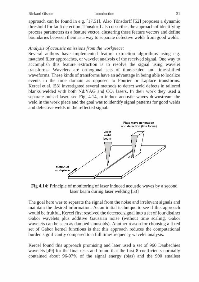
approach can be found in e.g. [17,51]. Also Tönsdorff [52] proposes a dynamic threshold for fault detection. Tönsdorff also describes the approach of identifying process parameters as a feature vector, clustering these feature vectors and define boundaries between them as a way to separate defective welds from good welds. Analysis of acoustic emissions from the workpiece: Several authors have implemented feature extraction algorithms using e.g. matched filter approaches, or wavelet analysis of the received signal. One way to accomplish this feature extraction is to resolve the signal using wavelet transforms. Wavelets are orthogonal sets of time-scaled and time-shifted waveforms. These kinds of transforms have an advantage in being able to localize events in the time domain as opposed to Fourier or Laplace transforms. Kercel et al. [53] investigated several methods to detect weld defects in tailored blanks welded with both Nd:YAG and CO2 lasers. In their work they used a separate pulsed laser, see Fig. 4.14, to induce acoustic waves downstream the weld in the work piece and the goal was to identify signal patterns for good welds and defective welds in the reflected signal.
Fig 4.14: Principle of monitoring of laser induced acoustic waves by a second
laser beam during laser welding [53] The goal here was to separate the signal from the noise and irrelevant signals and maintain the desired information. As an initial technique to see if this approach would be fruitful, Kercel first resolved the detected signal into a set of four distinct Gabor wavelets plus additive Gaussian noise (without time scaling, Gabor wavelets can be seen as damped sinusoids). Another reason for choosing a fixed set of Gabor kernel functions is that this approach reduces the computational burden significantly compared to a full time/frequency wavelet analysis. Kercel found this approach promising and later used a set of 960 Daubechies wavelets [49] for the final tests and found that the first 8 coefficients normally contained about 96-97% of the signal energy (bias) and the 900 smallest

32 Introduction Rickard Olsson coefficients contained mainly noise and that information about pinhole defects could be found in the region between these.
Frequency domain analysis: Frequency analysis can be divided into traditional methods (like FFTs) and alternative methods for analysis in both time and frequency domains, e.g. wavelet analysis, even though the name frequency normally refers to sinusoidal signals, wavelets are neither necessary nor normally sinusoidal in shape. A good introduction to the use of wavelets in laser welding supervision can be found in Zeng et.al [52]. Zeng used wavelet techniques to decompose the signal into different sub-bands before training a neural net.
Analysis of monitoring of CO2-laser welding using audible signals: Both Hongping and Duley [53] and Zeng [52] have found that the spectrum from emitted sound contains information in the 10 Hz - 20 kHz range during welding of mild steel. They used an intensity modulated beam and found that good welds showed more discrete spectral components with harmonics of the modulation frequency compared to defective welds which gave a more smeared spectra. The same tendency could also be seen in spectra from welding with unmodulated beams, i.e. a more discrete spectrum from good welds. These oscillations were explained as coming from the material itself. Is has also been found that the spectra from keyhole welding contains more high frequency components than conduction welding. Oscillations in the range of several hundred kHz was found originating from the keyhole itself – which can be seen as acting like an “organ-pipe”. Hongping [54] also showed that if the emitted acoustic spectra from a CO2-laser weld were divided into 20 distinct bands of 1 kHz each, it was possible to discriminate between overheated, fully penetrated and partially penetrated welds by using Fisher discrimination analysis [55]
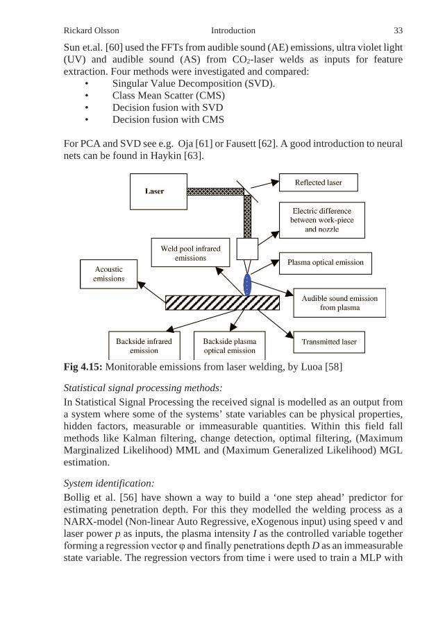
Neural nets and fuzzy logic: Studies of the feasibility of neural nets, as tools for fault detection and classification, have been carried out by several authors such as e.g. Bollig et al. [56] and Jeng et.al. [57]. In general the nets used have been of the standard MLP (Multi Layer Perception) type trained by back propagation (BP) algorithms. Luoa [58] decomposed the audio signal into 7 wavelet components where these components were used to train both a three-layer net as well as a simpler single- layer net, both trained with BP, Fig. 4.15. The conclusion was that a properly chosen and trained net could discriminate between a good weld and an error like a gap, but also that the task of choosing the proper net type and training algorithms and sets is an important but tedious task (which is a known fact in neural net theory). Kwon et al. [59] managed to discriminate between good and defective CO2-laser welds with a success rate of 93% using a three-layer MPL.
Rickard Olsson Introduction 33
Sun et.al. [60] used the FFTs from audible sound (AE) emissions, ultra violet light (UV) and audible sound (AS) from CO2-laser welds as inputs for feature extraction. Four methods were investigated and compared:
• Singular Value Decomposition (SVD). • Class Mean Scatter (CMS) • Decision fusion with SVD • Decision fusion with CMS
For PCA and SVD see e.g. Oja [61] or Fausett [62]. A good introduction to neural nets can be found in Haykin [63].
Fig 4.15: Monitorable emissions from laser welding, by Luoa [58]
Statistical signal processing methods: In Statistical Signal Processing the received signal is modelled as an output from a system where some of the systems’ state variables can be physical properties, hidden factors, measurable or immeasurable quantities. Within this field fall methods like Kalman filtering, change detection, optimal filtering, (Maximum Marginalized Likelihood) MML and (Maximum Generalized Likelihood) MGL estimation.
System identification: Bollig et al. [56] have shown a way to build a ‘one step ahead’ predictor for estimating penetration depth. For this they modelled the welding process as a NARX-model (Non-linear Auto Regressive, eXogenous input) using speed v and laser power p as inputs, the plasma intensity I as the controlled variable together forming a regression vector φ and finally penetrations depth D as an immeasurable state variable. The regression vectors from time i were used to train a MLP with

34 Introduction Rickard Olsson 10-neurons in the hidden layer. Later they also implemented a 25 step ahead predictor.
Kaierle et.al. [64] modelled the welding process as a dynamic system using system identification methods to control weld depth using input power as the controlled variable and the front of the weld pools as the observed variable.
ICA and BSS methods for source separation: Not much work has been carried out in this area, except for one interesting approach made by the colour research group at Joensuu University regarding the separation and identification of independent signal components from colour spectra measurements from CO2 welding using Independent Component Analysis (ICA) [61] and Principal Component Analysis (PCA) [63].
Change detection: The name change detection in this case refers to methods for identifying a change in for instance the mean or variance of a signal and the most probable time of event for this change. A good introduction to this field can be found in Gustafsson [64] and Kay [65]. Here, attempts to detect statistical changes like a change in the mean or variance in signals normally heavily disturbed by noise, most of which is of Gaussian or Poisson distribution are looked at. Conclusions from the literature survey can be drawn as follows: The detection or suppression of laser welding imperfections is essential for successful welding applications. A series of different welding imperfections can be distinguished. Their physical origin is often only partially understood. According to the survey presented here, high speed imaging and mathematical modelling are powerful methods for improved understanding. Nevertheless, as a result of the complexity of the process, only parts of the underlying mechanisms have so far been revealed. Also, mathematical modelling of the resulting fracture mechanisms has been conducted. In-process monitoring of electromagnetic or acoustic emissions by different sensors enables access to information on the process dynamics related to the generation of welding imperfections. Cameras provide images of the top weld pool and keyhole geometry, while photodiode sensors and pyrometers provide more abstract, but industrially more powerful monitoring. Today mainly empirical correlations between sensor signals and imperfections have led to suitable industrial applications, but there is still a strong need for better understanding of the process-signal correlation and in turn for more systematic monitoring.

Rickard Olsson Introduction 35
Regarding signal processing, the general impression is that in the articles little is said about why a particular method is chosen and what the goal was and how well the method chosen fulfilled these goals. A suggestion for future research is to focus on the statistics of the measured signals and after that, system identification or neural nets can be more properly trained from the start.


Rickard Olsson Introduction 37
5. Introduction to the technical subjects Part II – Data analysis of laser textured implant surfaces
5.1 Introduction to data analysis of laser textured implant surfaces
Medical implants and osseointegration Implants for medical or dental use have been in use for centuries. One very early example, see Fig 5.1, was found in a 2300-year-old burial chamber in Le Cheme France in 2014, was an implant made of Iron. Another proof of ancient knowledge in making implants is the example below from a 4000 year old mummy where the teeth have been fixed to each other using gold wire, see Fig. 5.2.
Fig. 5.1: Featured image: Ancient dental implants found in Le Chene, France
(Photo credit: Antiquity Publications Ltd)
Fig. 5.2: Ancient prostheses from a 4000 year old mummy
(Photo credit https://www.ancient-origins.net/sites/default/files/dental-work-mummy.jpg)
Nowadays implants are predominantly manufactured out of Titanium because of its ability to integrate with human bone tissue and form a strong bond between the metal and the bone, Fig. 5.3 This formation is a very complex process involving several stages, as described in Fig. 5.4 Initially after the implant is inserted, blood cells are trapped, followed by vessel formation and finally the growth of new bone.

38 Introduction Rickard Olsson
Fig. 5.3: Principle of dental implants
(Photo credit, innovationdrivedental.com)
Fig. 5.4: Progress of osseointegration
Reprinted with permission from Health, Maintenance, and Recovery of Soft Tissues around Implants.Yulan Wang, MD; Yufeng Zhang, PhD; Richard J. Miron, PhDhuman, ACS Clinical Implant Dentistry and Related Research. DOI: 10.1111/cid.12343. Copyright 2015,
JohnWiley In order to increase the rate of ingrowth, the implant surfaces are often deliberately made rough by techniques like blasting, etching, spraying and various forms of laser treatment. Fig. 5.5 shows six different examples of surface treatment methods.

Rickard Olsson Introduction 39
Fig. 5.5: Different surface treatments. (a) Plasma spray, (b) Etched,
(c) Hydroxy-apatite spray, (d) BioHelixTM, (e) Raw Additive Manufactured, (f) Grit blasted
BioHelix implant surfaces One particular surface roughening technique is called BioHelix™, Fig. 5.5(d). BioHelix is a patent owned by Integrum AB in Sweden. This surface is created by intense bombardment of the surface with short (~200 ns) laser pulses disrupting the surface, creating small ejected droplets and prolonged structures (1-20 µm in size) that re-solidify onto the surface. This type of surface structure has been in industrial production for several years, with proven excellent clinical results. In this work the laser texturing process used to produce these particular surfaces are studied. The BioHelix process is complex and involves the several steps depicted in Fig 5.6 with the final result shown in Fig 5.7. A pulsed laser beam moving across the surface in sweeping patterns generates ejections of molten material, the power density, the high cooling gradients involved, the atmosphere present, the overlap between successive pulses are a few the parameters affecting the final result. The first part of this study described, for the first time, the basic phenomena involved. High speed imaging was used to follow the process in more in detail, together with chemical analysis of the oxides formed.

40 Introduction Rickard Olsson
Fig. 5.6: An overview of the complex processes involved in BioHelixTM
formation
Fig. 5.7: A BioHelixTM surface covered in droplets and prolonged structures
The small re-solidified features, the droplets and prolonged structures play an important role for the functionality of this surface. In the early stages for initial trapping of blood cells, for triggering the body’s healing function and also for a mechanical locking, a trap for the bone cells (osteoblasts). Of great interest for medical device manufacturers are the droplets coverage and how the surface formation can be controlled.
Laser-induced droplet formation mechanism When a surface of Ti is exposed to an intense exposure of Q-switched laser pulses the top layer is rapidly melted and, due to the recoil pressure and liquid dynamics, the surface is disrupted as illustrated in Fig 5.8.

Rickard Olsson Introduction 41
Fig. 5.8. Principle of BiohelixTM laser treatment
The droplets and melt are ejected and fall onto the underlying surface and rapidly re-solidify. On top of the structures a thin (nm size) layer of oxides is also formed. The process is explanined more in detail in Fig 5.9a,b, where from time instant i to instant ix the process of exposure, melt, pressure ejecting molten metal, resolidifcation and overlap is illustrated.
(a)
(b)
Fig. 5.9 Detailed explanation of (a) ridge and (b) droplet formation

42 Introduction Rickard Olsson It has been found that a necessary condition for droplet formation is a large enough vertical velocity component within the melt fulfilling the condition:
(1)
where is the average melt density, R the local radius of curvature and the viscosity. To eject a droplet of diameter D an energy balance condition must be fulfilled where the energy for ejecting a droplet must be greater than the droplet kinetic energy plus the energy of the droplet surface.
(2)
For Titanium, the viscosity as a function of the temperature T η(T) can be expressed as:
[mPas] (3) (The melting temperature Tm for Ti is 1943 K, boiling temperature 2560 K.)
Droplet formation data analysis The production of medical devices demands strict quality control and in this case control of the formation of droplets per unit of area is one factor, together with control of the quality of the formed ridges. Therefore, there has been a request from the industry to develop a quantitative method to count droplet formation as a function of atmosphere, focal position and applied laser power in order to achieve a controllable process. One such a method is described in Fig 5.10. From the original image successive steps are performed. The original image is enhanced with respect to contrast and noise reduction. By software analysis using the software ImageJ in several steps, the number of droplets in each situation then can be calculated and counted.
Fig. 5.10: Workflow for droplet counting, as in Paper IV
zν
2 2z R
σρν >
ρ σ
ejE
32
12ej DDE v Dπρ σ π> +
( )Tσ
3( ) 4.42 6.67 10 ( )mT T Tσ −= − ∗ −

Rickard Olsson Introduction 43
5.2 State of the art on data analysis of laser textured implant surfaces When a medical implant is imbedded in bone, the first substance it comes into contact with is blood. Implant – blood interactions then lead to clot formation and the eventual migration and accumulation of osteogenic (bone creating) cells. Titanium has been found to be a favorable choice of base material for implants in general because if its high mechanical strength and ability to not be rejected by human body. One of the earliest reports on the benefits of making medical implants from titanium (Ti) was presented in 1977 by Brånemark et al. [66] after 10-years of clinical experience of dental implants. In the mid 90’s work on the subject by e.g. Larsson [67] demonstrated that roughened titanium surfaces promoted osseointegration as compared to as-machined surfaces. However, the most commonly used methods of surface roughening (anodic oxidation, grit blasting and acid etching) are non-site specific. Pulsed laser surface melting on the other hand, can create a controlled surface texture in specific, localized areas. Numerous papers have been published around laser surface structuring of medical implants. The effect of Q-switched laser surface texturing regarding osteoblast cell formation was studied by Voisey[68] regarding cell adhesion vs. groove size. Machined and blasted surfaces of Titanium were exposed to high energy pulses by Peto [69], picosecond laser irradiation by Trtica [70], Bussoli [71]. Femtosecond lasers for structuring is covered in e.g. Vilar [72], and by Vorobyev [73] in a study where optimal conditions for the generation of sub-micron structures, grooves, pores in micro- and sub-micros scales and also polishing were identified. The activation of red blood cells trapped on the implant surface plays an important part in subsequent bone growth, and a large number of researchers e.g. Park and Davies [74] have shown that micro-roughened surfaces accumulate red blood cells more effectively than smooth ones. In recent years, it has been demonstrated that osseointegration can be accelerated if the Ti surface is pre-treated to have a specific topology containing both micro- and nano-scale features, Brånemark [75]. The factors affecting the success of osseointegration is described by Nelson [76] where he, as an example, explains how dissociated water molecules together with the surface oxide form an acid and a base-pair who in turn can act as a bipolar, attracting and binding other molecules. E.g. amino acids forming double bands with hydroxylated Ti-oxide. The advantages of small droplets are also addressed by Palmquist and Grandfield [77], where surfaces covered in firmly attached, re-solidified droplets with diameters between 1 and 5 µm have been evaluated. They found that good results could be achieved if the surface of the droplets was covered in a porous or sponge-like layer of oxide with nano-scale features, Palmquist [77] which promotes mechanical interlocking at the nano-scale [79,80]. A summary of the generation of bone growth stimulating surfaces on medical implants of Ti is found in

44 Introduction Rickard Olsson Vilar [72], especially surfaces laser structured by Q-switch pulsed lasers have been investigated Shah et.al [82]. Shah [83] et al. compared osseointegration rates in rabbits for as-machined and droplet covered surfaces, concluding that osseointegration was enhanced by the presence of surface droplets. The effect of single Nd:YAG laser pulses on the surface of titanium has also been investigated by György, who considered surface morphology, [84], surface nitriding [85] and oxidation [86]. The properties of Nd:YAG laser treated Ti-surfaces have been described by Koroshahi et al. [87], who linked the improved biological response of laser textured titanium to an increased wettability of the oxidized, rough surface created. Surface characterization of laser treated biomedical surfaces has been studied by Pfleging [88] who noted that laser texturing gave the surface a higher surface energy, which is beneficial for protein adsorption and cell attachment. The investigation of droplet formation on metals in general explaining macro particle ejection as being due to breakaways from unstable capillary waves in molten metal has been described in detail by Brailovsky [89]. Three types of instabilities are proposed: Instability of the front of liquid evaporation Outflow of molten material from pits to humps Instabilities of vertical columns when the vapor velocity, is much higher
than the velocity of the liquid (Fig 5.1)
Fig. 5.11: a) Melt-vapor boundary b) Instability indicating droplet ejection (Courtesy of Brailovsky [89]) (v0 = velocity on surface, v = ablated material
velocity, λT = instability wavelength, λn = wavelength between columns) Early work of solving the basic equations describing the droplet formation process numerically can be found in Seifert [90]. A literature survey about droplet formation in laser materials processing focusing on evaporation, boiling and hydrodynamic effects can be read in Christensen [91] (2003). A somewhat related phenomenon, the optical breakdown of droplets interacting with high intensity

Rickard Olsson Introduction 45
laser radiation from a HF-laser at λ = 4.2 µm is described by Bulat, Volkov et al. [92]. They developed a mathematical simulation model, numerically simulating the formation of droplets, temperatures in the vapor, pressure distribution, temperatures around the droplets and finally the plasma formation, optical breakdown and explosion, of the droplets. However, these theories are only partially applicable for the studied process.


Rickard Olsson Introduction 47
6. Introduction to the technical subjects Part III – Characterisation of data from complex surfaces
6.1 Introduction to topography analysis of complex surfaces
Topography analysis How would the surface in Fig. 6.1 be described? Is it fine, coarse, rough, red, green, sandy? Is it possible to get a quantitative number to describe it?
Fig. 6.1: Example of a measured surface topography (Image from NanoFocus Corporation) Classifying surfaces and getting a quantitative measure of their roughness is a well known topic within the manufacturing industry. Much work has been put into this over the centuries. There is a strong need to have a uniform nomenclature, so as a framework there are international standards, e.g. ISO 1302 (Terminology), ISO 468 (Parameters) and ISO 25178-2 for 3D surface parameters. In Fig. 6.2 some of the most common properties are illustrated and defined. A very commonly used description of surface roughness is the 1-dimensional average mean deviation, Ra/Sa as described in Fig 6.3. Ra is however, nothing more than the mean absolute deviation from a central line Z0, i.e. if N measures zi are taken from a line then 𝑅𝑅𝑎𝑎 is defined as
𝑅𝑅𝑎𝑎 = 1𝑁𝑁∑ |𝑧𝑧𝑖𝑖 − 𝑍𝑍0|𝑖𝑖=𝑁𝑁𝑖𝑖=0 . (4)

48 Introduction Rickard Olsson
Fig. 6.2: Definition of traditional surface roughness parameters (selection;
standard)
Fig. 6.3: Surface profile with the definition (ISO-standard 4287) of the roughness property Ra In general, a surface topography is first measured and then evaluated for characterization. Established definitions can be combined with new analysis approaches, to describe certain geometrical features or properties of a surface.

Rickard Olsson Introduction 49
Micro-CT Surface topology can be measured by various techniques, including mechanical stylus (tactile) instruments and interferometric devices (like White Light Interferometry). One instrument that is associated with the measurement of inner geometries and features of bodies is Micro Computer Tomography (Micro-CT). This method is however, also highly suitable for surface characterization and was therefore applied in Papers V,VI. Micro-CT is an X-ray technology for 3D high resolution analysis. An X-ray source illuminates the specimen, Fig 6.4 (b). A scintillator detector generates data from one slice. The process is repeated with the specimen gradually rotated and moved in height. The resulting data indicating the X-ray absorption in each slice is transformed by software into a 3D-volume. From this model it is then possible to extract the regions of interest, e.g. in this study to extract the surfaces.
Fig. 6.4: Basic principle of Micro-CT and visualization of resulting data (Source:https://www.researchgate.net/profile/Tom_Shearer/publication/303863351/figure/fig1/AS:370995035688961@1465463517224/Principles-of-microCT-A-B-Interior-of-a-Carl-Zeiss-microCT-system-with-a-schematic.png) Contour tracking The application of normal vectors across surfaces is a suitable concept for post-processing of measured surface data, to study certain surface properties or features. In order to be able to calculate the normal vectors, the contour of the surface must be extracted from the image of the 3D-scan. The contour must be defined and its coordinates stored in an ordered sequence. For this there is an

50 Introduction Rickard Olsson existing algorithm widely used in analysis of medical imaging, “Active Contour Tracking”, or “Active Snake”. This algorithm minimizes the deviation in an image from a closed intensity gradient while keeping certain constraints. Figure 6.5 is an example of identifying the contour of a hand.
Fig. 6.5: Method of identifying the contour of a hand in four steps; an initial guess leads, after successive iterations, to the result (Source:http://personal.ee.surrey.ac.uk/Personal/R.Bowden/publications/bmvc97/image4.gif) The basic idea is to introduce an energy for the contour/snake of the curve v(s), 𝑆𝑆 ∈ [0, 𝐿𝐿] at points s on the curve. This energy consists of three components:
1. Internal energy Einternal controlling the contour’s elasticity and stiffness 2. External energy Eexternal controlling how well the contour matches the image
locally. Often this energy is defined as the absolute magnitude of the local gradient at that point
3. Constraint forces Econstraint encouraging continuity of the curve and punishing sudden jumps. The goal is to gradually adjust the curve to get a minimized energy
The first two variables can be defined as
𝐸𝐸𝑖𝑖𝑖𝑖𝑖𝑖𝑖𝑖𝑖𝑖𝑖𝑖𝑎𝑎𝑖𝑖 = 𝛼𝛼(𝑠𝑠) �𝑑𝑑𝑑𝑑𝑑𝑑𝑑𝑑� + 𝛽𝛽(𝑠𝑠) �𝜕𝜕
2𝑑𝑑𝜕𝜕𝑑𝑑2� (5)
and 𝐸𝐸𝑖𝑖𝑒𝑒𝑖𝑖𝑖𝑖𝑖𝑖𝑖𝑖𝑎𝑎𝑖𝑖 = −|∇𝐼𝐼(𝑥𝑥,𝑦𝑦)|2, (6)
where the coefficient 𝛼𝛼(𝑠𝑠) controls the elasticity/stretch and 𝛽𝛽(𝑠𝑠) controls the stiffness/bending. This leads to a total energy function (in a continuous case) for a curve of (in each iteration) length L.
int int0
L
snake ernal external constraE E E E= + +∫ (7)
int int0 0 0
( ) ( ) ( )L L L
ernal external constraE v s ds E v s ds E v s ds= + +∫ ∫ ∫

Rickard Olsson Introduction 51
These equations can be applied in an algorithm for data analysis. Normal vector classification Much work has been done to classify surfaces in a stringent way. International standards like e.g. ISO 25178 and ISO 4287 focus on this. Very complex surfaces like the one in Fig. 6.6 are extremely difficult to classify, with different shapes to be classified even at microscopic level.
Fig. 6.6. Complex surface from additive manufacturing (measured by micro-CT), with magnification of detailed features As Fig. 6.7a shows, rough surfaces created by grit blasting, abrasion etc. would only have normal surface vectors over a small range of angles – which would never exceed 180°. On the other hand, surfaces with overhanging features, Fig. 6.7b, would have a much larger range of normal surface vectors. Overhanging features can introduce surface normal angles up to 360°. The result from binning the vectors in each case and presenting them as histograms is shown in Figs. 6.8a,b. Here we can see how a grit blasted surface with its very regular shape has a narrow distribution of surface normal vectors. The majority of vectors are clustered around +90 degrees. The result is very different in the case of an etched additive manufactured surface. Such a surface with lots of irregularities has vectors pointing in a much broader range. This also manifests in the histogram (Fig. 6.8b) where the wider spread is clearly seen. This approach is applied in Paper V.

52 Introduction Rickard Olsson
Fig. 6.7: Surface profile with surface normal vectors: (a) surface normal vectors for usual rough surfaces would have a range of less than 180 degrees; (b) overhanging features introduce a much wider range of surface normal vectors
Fig. 6.8: Normal surface vector angle distribution (degree) histogram (a) for a grit blasted surface, (b) for an etched additive manufactured surface This idea can be further extended allowing angles both larger than +360 degrees and less than -360. This allows for a description of compound overhangs like the one in Fig. 6.9. This approach is applied in Paper VI.
Fig. 6.9: Sketch showing a complex structure with compound overhang angles

Rickard Olsson Introduction 53
6.2 State of the art on data analysis of complex surfaces The importance of surface texture for osseointegration, see also Chapter 5, has been investigated by e.g. Albrektsson [93,94] looking at long term results of in vivo response for coated, blasted and etched Ti implants. Wennerberg [95] not only compared bone response to different roughnesses, but also pointed out the limitations of Ra and Sa as measures when comparing different textures. Wennerberg, Albrektsson [96] have pointed out the need for a more uniform terminology. In literature terms like “soft”, or “rough” are often found but these words may have different meanings for different authors, so similar surfaces may at one occasion be described as “soft” and at another time as “rough”. Wennerberg, Albrektsson [96] set up a set of guidelines for the topographic evaluation of surfaces defining parameters like form, waviness or roughness and also how the surface topography of titanium implants affects bone integration. [95]. The importance of roughness as an important factor in prosthetic design and manufacturing is also addressed by Thomas [97], especially in his Chapter 4. Lin [98] looked at how micro and nano-scale topographies affected different mechanisms for micro structures bone cell (osteoblast) formation and nano-scale TiO2 structures protein polymerization and osteoblast adhesion. Pfleging [98] has made a thorough investigation about how linear and dimple geometries created by radiation of 193 nm ArF-laser on Ti-6AL-4V affect the chemical composition on the surface. He used scanning electron microscopy (SEM), electron beam back scattered diffraction (EBSC) and X-rays, finding that dimple structures favoured cell attachment. Laser-treated micro-rough surfaces have been shown to provide an optimum topography for cell growth [100] compared to acid-etching or sandblasting [101]. Laser texturing can also enhance surface energy, which is beneficial for protein adsorption and cell attachment [99]. Some limitations of traditional surface measurement methods are illustrated in Figs 6.10a,b. Figure 6.10a shows how a low pass filtering effect is introduced because the sensor (black) is larger than the structure. This has been explained thoroughly by Rupp [102], where the difficulties using traditional profilometry, SEM-analysis, interferometry, etc. are addressed, including the difficulties of discriminating surface roughness from waviness, non-comparable data and finally the difficulties in correlating these achieved values to biological response. Tactile stylus methods for surface profilometry have been compared with confocal microscopy and interferometric methods (white light, WLI, phase shifting, PSI, etc.) by Vorburger [103]. This work, based on standardized surface properties, paid particular attention to the limitations of the various techniques as a function of surface profile slope.

54 Introduction Rickard Olsson
(a) (b) Fig. 6.10: (a). If a tactile sensor is bigger than the structure details it misses them; (b) difficulty of different surface structures having roughly same Ra
In 1994 Dong [104] wrote a paper discussing the problems and pitfalls in characterizing 3D-surfaces. Especially is there a discussion about the use of the classical Abbot-Firestone Bearing Area Ratio-curve [105]. The same topic has also been described in detail with from Pike-Wilson [106] in an article focusing mainly on boiling flow heat transfer, but with a strong section about the pitfalls in surface measurements and classification. Surfaces involving overhanging features in the field of medical implants have been described by Rupp [102] in a study of bio-response vs. implant surface. Pulsed lasers can be used to create “splashy” surfaces involving the correct type of overhanging features [107,108] including re-solidified droplets of 1-5 µm diameter [102,109,110]. On a more general level the presence of overhanging features could have an influence on a large number of surface-related phenomena including the tribological properties of a surface as well as its wettability by lubricants or adhesives. Overhangs on the mm-scale can also be employed as ratcheted topographies to support self-propelling droplet propulsion [111] and in micromechanical liquid flow sensors overhanging structures can allow the level of wetting to be ‘tuned’ [112] . For super-hydrophobic surface textures the impact of features like micro-pillars, overhangs, two-tier textures with nano/micro-scale roughness and hierarchical textures have been shown to have a substantial impact on droplet contact time [113]. Complex, convoluted surfaces are going to become more commonplace with the rise of additive manufacturing and laser surface texturing and there is therefore a growing need for new surface analysis tools which can identify and quantify features such as overhangs, which are invisible to traditional roughness measurement techniques. Micro Computer Tomography (Micro-CT) can record very complex surfaces in great detail and can be used to present the information as 2D sections for further analysis. A typical tomographic view and cross section is shown in Fig. 6.11.

Rickard Olsson Introduction 55
Fig. 6.11: (a) Typical micro-tomography view of a rough surface created by additive manufacturing - note overhanging features, (b) a cross section taken
from the tomography data One idea to classify surfaces that can both give a number of its complexity as well as its dominating orientation and the occurrence of overhanging features is to calculate, at evenly spaced intervals, the surface normal vectors pointing outward and group them as a histogram. This also enables a description of anisotropic surfaces as they will have a biased distribution. This technique is often referred to as Histograms of Oriented Normal vectors (HONS). Calculating surface-normal vectors and grouping these vectors into histograms for surface classification has been used by e.g. Tang [114]. In this case in computer vision applications for cognition of objects and classification purposes, using information from a depth sensor. HONS for object classification in computer vision applications have been used by e.g. Watanabe [114] and Dalal [116]. One advantage of HONS is the ability to describe surfaces with overhangs, simple or compound. Something traditional methods lack. Other mathematical models are as follows; Another example of surface classification using advanced Signal Processing approaches is e.g. the multi-level filtering using Gabor filters [117], Fig. 6.12, performed by Senin [118]. In this case the surface profile is convoluted with wavelet-like filter kernels in gradually finer resolution, i.e. each of these kernels has an oriented wavelet-like shape, an oriented plane wave multiplied with a Gaussian envelope. Because they are orientated, the convolution operation of each kernel with the original surface dataset will pick up specific oriented texture components wavelengths.

56 Introduction Rickard Olsson
Fig. 6.12: Example of a surface profile for which Gabor filter kernels were
applied, with increasing resolution, image by image (upper row: Re(Ψ(x,y)), lower row: Ψ(u,v))
(http://what-when-how.com/wp-content/uploads/2012/06/tmpdece326.png) The use of structures having self-similar properties in different scales (fractals) for classification of especially medical implant surfaces was found to be useful in discrimination of machined, etched and grit-blasted surfaces especially regarding their roughness organization [119]. A similar article was published by Dohan [120] where the self-similarities in micro- and nano-scale are discussed from a fractal dimension approach. Summarizing, characterization of surfaces can involve various instruments, analysis methods and definitions, strongly depending on the characteristic properties or features under investigation. Despite many studies and efforts, tailored data analysis solutions are often needed.

Rickard Olsson Introduction 57
7. Summary of the papers Paper I Title Advances in pulsed laser weld monitoring by the statistical analysis of reflected light
Abstract This paper describes two new techniques for monitoring the quality of laser welds by statistical analysis of the reflected light signal from the weld surface. The first technique involves an algorithm which analyses the variance of the peak values of the reflected signal as a measure of the stability of the surface during pulsed Nd:YAG laser welding in the heat conduction mode. Kalman filtering is used to separate a useful signal from the background noise. A good correlation between weld disruption and signal fluctuation has been identified. This technique could be used in tandem with the present practice of simply using the peak values of the reflected (or emitted) light as an indicator of weld quality. The second technique investigated involves an assessment of the temporal shape of the power distribution of individual reflected pulses in comparison with an average of the results from a high quality weld. Once again, a high correlation between a poor signal match and inferior quality welding was discovered, which may pave the way towards a new generation of optical weld monitoring devices. Conclusions Kalman filtering is a superior method to cut-off filtering for extracting data from noisy signals
Signal variance data can be used in conjunction with raw signal data to improve the sensitivity and robustness of laser welding monitoring devices
Reflected pulse shape comparisons involving polynomial best fits are a very promising tool for on-line process monitoring for pulsed laser welding.

58 Introduction Rickard Olsson Paper II Title Challenges to the Interpretation of the Electromagnetic Feedback from Laser Welding Abstract This paper considers the point that it is not possible to interpret individual weld perturbations from the raw electromagnetic feedback collected from laser weld zones. The presentation of electromagnetic data as a 3D cloud is presented as a new, useful tool in the analysis of this feedback. For example, it is shown that there is a very low correlation between the plasma or thermal signals and the reflected light signal from the weld zone, and that a strong correlation exists between the plasma and thermal signals. It is also demonstrated that data points from a weld perturbation form a different 3D cluster to those from the stable welding process. A strategy for future on line data analysis is presented in the use of a suitably shaped data cloud envelope. The rates of data fit to the various segments of such an envelope could be correlated with specific weld anomalies. Conclusions
• It is not possible to interpret individual weld perturbations from the raw electromagnetic data collected from laser weld zones.
• The presentation of electromagnetic data as a 3D cloud provides a new, useful tool in the analysis of feedback from laser weld zones.
• There is a very low correlation between the plasma or thermal signals and the reflected light signal from the weld zone.
• There is a strong correlation between the plasma and thermal signals from the weld zone.
• Data points from a weld perturbation (blow out) form a different 3D cluster to those from the stable welding process.
• A strategy for future online data analysis is the use of a suitable data cloud envelope or multi-layered envelopes. The rates of data fit to the various segments of such envelopes could be correlated with specific weld anomalies.

Rickard Olsson Introduction 59
Paper III Title The production of osseointegrating (bone bonding) surfaces on titanium screws by laser melt disruption Abstract Several techniques can be used to modify implant surfaces in order to accelerate bone growth around titanium implants. One method is to generate a surface structure which stimulates bone growth and remodelling. This paper describes and explains a non-ablative method for producing osseointegrating (structural and functional bone bonding) surfaces on titanium implants using laser processing. The focus is especially on surface texturing of dental implant screws, where the ability of a Nd:YAG laser to generate ‘splashy’ surfaces covered in resolidified micro scale droplets coated with nano-scale surface oxides is assessed. The surfaces produced were analysed by scanning electron microscope (SEM) and energy dispersive x-ray spectroscopy (EDS). It is concluded that laser processing using Q-pulsed Nd:YAG lasers can generate surfaces which match the demands set by clinical experience. One important characteristic of the surfaces discussed here is that they involve overhanging features which are suitable for trapping red blood cells and which cannot be created by mechanical or chemical roughening techniques Conclusions This study has shown that:
• A Nd:YAG Q-pulsed laser can generate the osseointegrating surfaces required by medical professionals
• The process has a well-defined process window, within which a ‘splashy’ surface is generated by localized boiling of the melt
• The power density is the most critical factor for forming droplets and the associated oxide coating
• The ‘splashy’ surface contains a considerable number of overhanging features which are suitable for trapping red blood cells, thereby aiding osseointegration

60 Introduction Rickard Olsson Paper IV Title The formation of osseointegrating surfaces on titanium by laser irradiation Abstract There are several techniques that can be used for surface modification in order to accelerate bone growth around titanium medical implants. One goal is to create a surface capable of stimulating bone growth at the implant surface, achieving osseointegration. This paper describes one such technique, using a non-ablative method for producing surfaces on titanium implants using laser surface processing for structural and functional bone growth. Pulsed lasers can be used to modify the titanium surfaces, forming a surface covered in attached droplets with diameters between 1 and 20 microns, an optimum surface for rapid osseointegration. Different surface textures on titanium substrates was produced, resulting in required micro scale 'attached droplet' topologies. This involved using a Q-pulsed Nd:YAG laser and a broad range of laser parameters in an experimental program. The surfaces produced were analysed by scanning electron microscope (SEM) and Micro Computer Tomography (Micro CT). The paper explains how different types of surfaces are created by the laser-material interaction under different pulse conditions and focus characteristics. It is shown that optimization of the laser parameters results in a robust process that produces a surface that is fundamentally different from those created by non-laser methods, including droplets, but also special semi-circular shapes. Conclusions • Pulsed laser melting is a robust process for the generation of osseointegrating
surfaces on the titanium substrates • The surface structure created includes re-solidified droplets between 1 and 10
microns in diameter and a pattern of ridges • The surface structure involves a considerable number of overhang features
which are unique to the pulsed laser surface texturing process. These overhang features provide excellent traps for cells which eventually lead to osseointegration
This study has benefits from a control perspective in defining the characteristics of the surface. We propose that the understanding of for instance droplet formation is critical for clinical success and that the results presented here not only are relevant for laser modified surface but may be extended to also other kinds of surfaces like implants made by Additive Manufactured (AM) technique.

Rickard Olsson Introduction 61
Paper V Title Normal vector distribution as a classification tool for convoluted rough surfaces with overhanging features Abstract Convoluted rough surfaces involving overhanging features can be a natural consequence of Laser Additive Manufacturing and other spray techniques, or can be generated deliberately by laser surface texturing, e.g. to aid osseointegration. Overhanging features add an extra level of complexity to the topography of a rough surface and can have a substantial effect on wettability etc. However, features of this type are invisible to traditional surface roughness measurement techniques. This work presents a computer-based surface analysis method which gives useful information about the presence and nature of overhanging features on rough technical surfaces. The technique uses Micro Computer Tomography to generate a typical cross section of the surface under investigation. The angles of the vectors normal to the surface can then be analyzed to reveal the presence of overhanging features, which can also be indicated by the standard deviation of the normal vector distribution. Titanium surfaces generated by six different techniques were compared. The characteristics of these surfaces varied strongly, as did the shapes of the overhangs involved. These variations are reflected by different statistical distributions of the normal vectors.
Conclusions
Overhangs can be features of the very complex surface topologies created by laser AM or laser texturing. This work demonstrates that Micro Computer Tomography in combination with surface normal vector distribution analysis can be used to provide data and information about the presence of overhanging features on a rough surface. Surfaces with overhanging features will have normal vectors with values over 180 degrees. The standard deviation of the normal vector distribution can act as a single number indicator of surface complexity and the probable presence of overhanging features. The analytical method presented here can be used to extract quantitative information about the nature of the overhanging features on very complex laser-generated surfaces. For the cases studied, different overhang shapes corresponded to different normal vector distributions. In addition to elongated overhang characteristics, asymmetric overhangs have formed, either randomly oriented or in a collective anisotropic manner, which can be identified through histograms, by the proposed method.
62 Introduction Rickard Olsson Paper VI Title Topographical evaluation of laser generated surfaces using statistical analysis of surface-normal vector distributions Abstract Surfaces generated by Additive Manufacturing or laser texturing can involve the solidification of droplets of liquid, which can give rise to overhanging features on the solidified surface. Overhanging features add a layer of complexity to the surface topology and are invisible to standard profilometry and surface roughness measurement techniques. Such features are important because they can have a considerable effect on surface properties such as wettability. New techniques and algorithms are therefore required to analyse and quantify convoluted surfaces with overhanging features. Earlier work by the authors introduced the concept of using X-ray micro-computer-tomography to identify the directions of vectors normal to the surface at any point and thus the presence or otherwise of overhanging features. This paper divides overhanging features into two types; simple and compound, and introduces new analysis techniques which measure what proportion of each type is on the surface. Another extension of the analysis is to compare surface traces taken in different directions in order to identify any surface roughness anisotropies. This work also presents a method for identifying any periodicity in convoluted surfaces which do not lend themselves to Fourier analysis. Conclusions • Additive manufacturing and laser surface texturing can create surfaces
covered in overhanging features; this can have substantial effects on surface properties such as wettability.
• Overhanging features can usefully be divided into two types; simple and compound.
• Micro-CT can reveal the topological details of convoluted surfaces containing both simple and compound overhangs.
• From micro-CT results surface profiles can be extracted; surface-normal vectors can be applied to these profiles along with an angle-based algorithm to quantitatively identify the presence and proportion of simple and compound overhangs; different characteristics were demonstrated for four surfaces.
• Studying surface profiles in different directions facilitates the identification of topological anisotropies.
• Convoluted surface profiles containing overhanging features cannot be subjected to standard Fourier analysis to search for repeating patterns because they have ambiguous vertical coordinates. However, frequency analysis can

Rickard Olsson Introduction 63
be used if the surface is divided up into a series of short, straight-line segments with surface-normal vectors.
• Analysis tools of this type will become increasingly useful as surfaces including overhangs generated by lasers and other technologies become more common.


Rickard Olsson Introduction 65
8. General conclusions Laser Materials processing is an area that is very well suited to on-line monitoring, supervision, data analysis and closed loop control. For example it is possible to monitor the optical setup with sensor equipment. Today’s lasers are able to react to control signals within microseconds and thus the processes can often be regulated in quasi-real time. Many attempts have been made over the years to apply signal processing methods for supervision and control. Process monitoring is less critical but closed loop control requires generalized, robust algorithms to avoid false reactions that can cause damage. Measurement of the quality resulting from a laser process can be carried out on-line just behind the processing zone with sophisticated instruments and high levels of computational performance for data acquisition and processing. One challenge seen in the field of data analysis is the difficulty in bringing the necessary expertise together. Laser physicists, material processing experts, sensor experts and signal/data processing experts have different backgrounds, making it a big task to achieve a mutual understanding and common language about the phenomena found within laser material processing. For example, the research in Papers III-VI revealed how complex the situation is within the area of manufacturing of dental and medical implants, especially the vast spread in nomenclature for describing surfaces, particularly for medical standards. Deeper analysis of the surface structuring process has also revealed its high complexity and its dependence on many process parameters and material properties (particularly on the surface) as well as surrounding conditions. Despite the different nature of laser welding studied in Papers I,II compared to laser surface structuring for medical implants addressed in Papers III-VI, several similar opportunities and challenges in data analysis can be identified. Both during and after the process a vast amount of data and information is offered in both cases. Hardware of sensors and instruments has experienced continuous development but the big difference over the years is the greatly increased computer power that was often a bottleneck in the past. Therefore, in the older high speed imaging work (Papers I-III) it was not possible to acquire the level of spatial and temporal process zone resolution and droplet analysis from SEM-images available in the later work (Paper IV). Surface features from micro-CT (Papers V,VI) can now be evaluated at a large scale, including visualization (Papers II,IV). While some data acquisition and processing steps benefit from improved computation performance, other approaches do not, but face different challenges; Photodiode monitoring of laser welding (Papers I,II) copes with indirect, reduced information on the process physics, requiring empirical or theoretical approaches. The later work of identifying complex overhang features (Papers V,VI) from

66 Introduction Rickard Olsson surface profiles needs suitable strategies and algorithms. These latter challenges do not depend on technical or computational developments but instead on the identification of suitable methods and approaches (signal filtering in Paper I,II, angle algorithms in Papers V,VI, frequency analysis in Paper VI). It is therefore recommended to make use of the different approaches systematically, including sources of valuable information, corresponding access to data, powerful hardware and computational analysis software combined with tailored algorithms and codes, addition of mathematical, statistical methods, visualization, mathematical modelling, etc. which requires cooperation between various experts, as emphasized above.
Rickard Olsson Introduction 67
9. Future outlook Below are suggestions for the continuation of this research; For Part I of the thesis (papers I and II) which dealt with laser welding surveillance, it would be of great value to be able to use improved process signal data analysis to respond to changes quickly. This could be achieved e.g. by applying machine learning or deep-learning neural network analysis, to be able to identify process behavior in-line and off-line, for process control or identification. This could lead to in-line process adaptation to prevent imperfections from occurring or, alternatively, the ability to pause the process to immediately repair any location where an imperfection was detected (if applicable). Also, the use of additional sensor types and correlating data between chosen sensors could be aimed at for improved data analysis and functionality. What data the sensors are actually seeing is another area of interest worthy of further investigation. For Part II, dealing with generation of Titanium surface implants, the process is established and relatively robust (over an area with certain settings, many pulses statistically result in a mean produced surface). There remains the need to expand knowledge of the process by high resolution, high speed monitoring of the interactions and of the resulting surface structures from a chemical point of view. This could lead to further insights that would improve the resulting surface texture as well as its integrity. For Part III, the vector based surface classification technique involves some intermediate steps from micro-CT data to produce the surfaces used for classification. One future improvement could be to use the measured data of the surfaces to generate 2D-classification directly. Challenges include producing surfaces and interpolation between measured data points and procedures to automatically produce several vector analysis in different directions across the sample surface. One additional goal would be to make this technique into a standard technique to characterize complex surfaces – provided 3-Dimensional surface data can be obtained.


Introduction 69
10. References
[1] J. Stavridis, A. Papacharalampopoulos, P. Stavropoulos, Quality assessment in laser welding: a critical review. International Journal of Advanced Manufacturing Technology 2018;94:1825–47. doi:10.1007/s00170-017-0461-4
[2] E. H. Amara, R. Fabbro, F. Hamadi, Modeling of the melted bath movement induced by the vapour flow in deep penetration laser welding, Journal of Laser Applications, v 18, n 1, p 2-11 (2006)
[3] R. Fabbro, S. Slimani, I. Doudet, F. Coste, F. Briand, Experimental study of the dynamical coupling between the induced vapour plume and the melt pool for Nd:YAG CW laser welding, J. Phys. D: Applied Physics, v 39, n 2, p 394-400 (2006)
[4] R. Fabbro, S. Slimani, F. Coste, F. Briand, Study of keyhole behaviour for full penetration Nd:YAG CW laser welding, Journal of Physics D: Applied Physics, v 38, n 12, p 1881-7 (2005)
[5] X. Jin, P. Berger, T. Graf, Multiple reflections and Fresnel absorption in an actual 3D keyhole during deep penetration laser welding, Journal of Physics D: Applied Physics, v 39, n 21, p 4703-12 (2006)
[6] A. F. H. Kaplan, M. Mizutani, S. Katayama and A. Matsunawa, Unbounded keyhole collapse and bubble formation during pulsed laser interaction with liquid zinc, Journal of Physics D: Applied Physics, v 35, p 1218-1228 (2002)
[7] K. Nishimoto, H. Mori, Hot cracking susceptibility in laser weld metal of high nitrogen stainless steel, Sci. Techn. Adv. Mat., v 5, p. 231-240 (2004)
[8] J. F. Gould, S. P. Khurana, T. Li: Predictions of microstructures when welding automotive advanced high strength steel, Weld. J., v 85, p 111s-116s (2006)
[9] S. Hao, W. K. Liu, B. Moran, F. Vernerey, G. B. Olson, Multi-scale constitutive model and computational framework for the design of ultra-high strength high toughness steels, Comput. Meth. Appl. Mech. Eng, v 193, p 1865-1908 (2004)
[10] U. Prahl, S. Papaefthymiou, V. Uthaisansuk, W. Bleck, J. Sietsma, S. van der Zwaag, Micromechanics-based modelling of properties and failure of multiphase steels, Comp. Mat. Sci, v 39, p 17-22 (2007)
[11] www.redlake.com (2009-09) [12] www.pco.de (2009-09) [13] www.dantecmt.com (2009-09) [14] www.photron.com (2009-09) [15] A. Fellman, A. Salminen, V. Kujanpää, A study of the effects of parameters
on filler material movements and weld quality in CO2-laser-MAG hybrid welding, NOLAMP10, 2005, Luleå, p343-354, (2005)
[16] A. Matsunawa, S. Katayama, Understanding physical mechanisms in laser welding for construction of mathematical models, Welding in the World, Le Soudage Dans Le Monde, v 46, n SPEC, p 27-38 (2002)

70 Introduction Rickard Olsson [17] B. Kessler, Online quality control in high power laser welding, White
paper, Precitec KG, Germany, 2003 [18] W. Wiesemann, Process monitoring and closed loop control, Landholt-
Börnstein – Group VIII Advanced Materials and Technologies, v 1C, Springer Berlin Heidelberg, XVIII, p 243-275, ISBN 978-3-540-00105-8, (2004)
[19] J. Shao, Y. Yan, Review of techniques for on-line monitoring and inspection of laser welding, Journal of Physics: Conference Series, v 15, n 1, p 101-7 (2005)
[20] Gao X, Sun Y, You D, Xiao Z, Chen X. Multi-sensor information fusion for monitoring disk laser welding. The International Journal of Advanced Manufacturing Technology 2016;85:1167–75. doi:10.1007/s00170-015-8032-z
[21] P.Webster, C. Galbraith, Advancing next-generation weld monitoring: Paul Webster and Chris Galbraith, of IPG Photonics, report on the development of a new inline weld monitoring system based on technology from Laser Depth Dynamics." Laser Systems Europe, no. 42, 2019, p. 14+. Gale Academic Onefile, Accessed 9 Sept. 2019
[22] C. Bagger, F. O. Olsen, Laser welding closed-loop power control, Journal of Laser Applications, v 15, n 1, p 19-24 (2003)
[23] A. Ghasempoor, P. Wild, M. Auger, R. Mueller, Automatic detection of lack of fusion defects in CO2 laser gear welding, J. Laser Appl., v 15, n 2, p 77-83 (2003)
[24] H. K. Tönshoff, K. Körber, T. Hesse, M. Stallmach, Increased performance and flexibility of process monitoring for deep penetration laser welding, ICALEO 2002. 21st Intl. Congress on App. of Lasers and Electro-Optics, p 1105-13 Vol.2 (2002)
[25] H.B. Chen, L. Li, D.J. Brookfield, W.M. Steen, Multi-frequency fibre optic sensors for in-process laser welding quality monitoring, NDT&E International, v 26, n 2, April 1993, p 67-73 (1993)
[26] A. Sun, Elijah Kannatey-Asibu, Jr., Monitoring of laser weld penetration using sensor fusion, Journal of Laser Applications, v 14, n 2, p 114-21 (2002)
[27] Y. Kawahito, Seiji Katayama, In-process monitoring and control for stable production of sound welds in laser microspot lap welding of aluminium alloy, Journal of Laser Applications, v 17, n 1, p 30-37 (2005)
[28] B.N. Badyanov, A.A. Elizarov, Application of the step by step approximation method for the computer control of laser welding processes, Measurement Techniques, v 46, n 2, p 162-5 (2003)
[29] P. G. Sanders, J. S. Keske, K. H. Leong, G. Kornecki, Real-time monitoring of laser beam welding using infrared weld emissions, J. Laser Appl., v 10, p 205-11 (1998)
[30] D. Travis, G. Dearden, K. G. Watkins, E.W. Reutzel, R.P. Martukanitz, J.F. Tressler, Sensing for monitoring of the laser GMAW Hybrid welding

Introduction 71
process, ICALEO 2004. 23rd International Congress on Applications of Lasers and Electro-Optics, (2004)
[31] K. Kamimuki, T. Inoue, K. Yasuda, M. Muro, T. Nakabayashi, A. Matsunawa, Prevention of welding defect by side gas flow and its monitoring method in continous wave Nd:YAG laser welding, J. Laser Appl., v 14, n 3, p 136-145 (2002)
[32] S. Postma, R.G.K.M. Arts, Penetration control in laser welding of sheet metal, Journal of Laser Applications, v 14, n 4, p 210-214 (2002)
[33] J. Petereit, P. Abels, S. Kaierle, C. Kratzsch, E.W. Kreutz, Failure recognition and online process control in laser beam welding, ICALEO 2002. 21st International Congress on Applications of Lasers and Electro-Optics, pt. 4, p 2501-9 Vol.4 (2002)
[34] M. Kogel-Hollacher, T. Nicolay, A. Kattwinkel, M. G. Muller, J. Muller, On-line process monitoring in laser material processing-techniques for the industrial environment, (PICALO 2004), LMP-SC, p 1-4, (2004)
[35] J. Beersiek, New aspects of monitoring with a CMOS camera for laser materials processing, (ICALEO 2002), pt. 2, p 1181-90 Vol.2 (2002)
[36] F. Bardin, A. Cobo, J. M. Lopez-Higuera, O. Collin, P. Aubry, T. Dubois, M. Högström, P. Nylen, P. Jonsson, J. D. C. Jones, D. P. Hand, Optical techniques for real time penetration monitoring for laser welding, Applied Optics, v 44, n 19, p 3869-76 (2005)
[37] M. Doubenskaia, Ph. Bertrand, I. Smurov, Optical monitoring of Nd:YAG laser cladding, Thin Solid Films, v 453-454, p 477-85 (2004)
[38] M. Doubenskaia, I. Smurov, Surface temperature evolution in pulsed laser action of millisecond range, Appl. Surf. Sci., v 252, n 13 SPEC. ISS., p 4472-4476 (2006)
[39] M. Doubenskaia, Ph. Bertrand, H. Pinon, I. Smurov, On-Line monitoring of Nd-YAG laser lap welding of Zn-coated steel sheets by pyrometer, Proc. BTLA 2006, St. Petersburg (RUS), p 203-209, (2006)
[40] Ph. Bertrand, I. Smurov, D. Grevey, Application of near infrared pyrometry for continous ND:YAG laser welding of stainless steel, Applied Surface Science, v 168, n 1-4, p 182-185 (2000)
[41] K. Kamimuki, T. Inoue, K. Yasuda, M. Muro, T. Nakabayashi, A. Matsunawa, Behaviour of monitoring signals during detection of welding defects in YAG laser welding. Study of monitoring technology for YAG laser welding, Q. Journal of the Japan Welding Society, v 20, n 3, August, 2002, p 369-377 (2002)
[42] V.M. Weerasinghe, J.N. Kamalu, R.D. Hibberd, W.M. Steen, Acoustic signals from laser back reflection, Optics and Laser Technology, v 22, n 6, p 381-6 (1990)
[43] H.P. Gu, W.W. Duley, A statistical approach to acoustic monitoring of laser welding, Journal of Physics D: Applied Physics, v 29, n 3, p 556-560 (1996)
[44] D.P. Hand, C. Peters, J.D.C. Jones, Nd:YAG laser welding process monitoring by non-intrusive optical detection in the fibre optic delivery system, Measurement Science & Technology, v 6, n 9, p 1389-1394 (1995)

72 Introduction Rickard Olsson [45] S.-H. Baik, M.-S. Kim, S.-K. Park, Process monitoring of laser welding
using chromatic filtering of thermal radiation, Meas. Sci. Technol., v 11, n 12, p 1772-7 (2000)
[46] L. Li, A comparative study of ultrasonic emission characteristics in laser processing, Applied Surface Science, v 186, n 1-4, p 604-610 (2002)
[47] L. Li, D. J. Brookfield, W. M. Steen, Plasma charge sensor for in-process, non-contact monitoring of the laser welding process, Measurement Science & Technology, v 7, n 4, p 615-626 (1996)
[48] M. Kogel-Hollacher, André S, Beck T. Low-coherence interferometry in laser processing: a new sensor approach heading for industrial applications. In: North Morris MB, Creath K, Burke J, Davies AD, editors. Interferometry XIX, SPIE; 2018, p. 52. doi:10.1117/12.2501295.
[49] Y. Zhang, Liu T, Li B, Zhang Z. Simultaneous Monitoring of Penetration Status and Joint Tracking During Laser Keyhole Welding. IEEE/ASME Transactions on Mechatronics 2019;24:1732–42. doi:10.1109/TMECH.2019.2916984.
[50] X. Gao, Sun Y, You D, Xiao Z, Chen X. Multi-sensor information fusion for monitoring disk laser welding. The International Journal of Advanced Manufacturing Technology 2016;85:1167–75. doi:10.1007/s00170-015-8032-z
[51] www.prometec.com. (2009-08) [52] H. K. Tonshoff, A. Ostendorf and W. Specker, “Online monitoring and
closed-loop control of laser welding processes,” vol. 1405. In Proc. of 12th international symposium for electromachining (ISEM), May 1998, pp. 603–612.
[53] Stephen W. Kercel, Roger A. Kisnera, “In-process detection of weld defects using laser-based ultrasound,” Oak Ridge National Laboratory, P.O. Box 2008, Oak Ridge, TN 37831-6011, Tech. Rep.
[54] W. D. Hongping. Gu, “Discrete signal components in optical emission during keyhole welding.” ICALEO, 1997, pp. 40–4
[55] S. M. Kay, Fundamentals of Statistical Signal Processing. Prentice-Hall, 1998, vol. II
[56] C. S. A.Bollig, H.Rake, “Application of neuro-predictive control to laser beam welding,” Institute of Automatic Control, Aachen university of Technology, Institute of Automatic Control, Aachen university of Technology, 52056 Aachen , Germany, Tech. Rep., 2002.
[57] Jeng-Ywan Jeng and S.-M. Leuc, “Prediction of laser butt joint welding parameters using back propagation and learning vector quantization networks,” Tech. Rep., 2000
[58] Hong Luoa and Z. Zhoub, “Application of artificial neural network in laser welding defect diagnosis,” Singapore Institute of Manufacturing Technology, 71 Nanyang Drive, Singapore 638075, Singapore bHuazhong University of Science and Technology, Wuhan 430074, PR China, Tech. Rep., June 2005

Introduction 73
[59] Jangwoo Kwon, Osang Kwon Younggun Jang, “Development of neural network based plasma monitoring system for laser welding quality analysis,” TENCON, pp. 678–681, 1999.
[60] M. G. Allen Sun, elijah Kannetey-Abisu Jr, “Monitoring of laser weld penetration using sensor fusion,” Journal of laser applications, vol. 14, no. 2, pp. 114–121, May 2002
[61] A. Hyvarinen, J. Karhunen, and E. Oja, Independent Component Analysis. Wiley-Interscience, May 2001.
[62] L. Fausett, Fundamentals of Neural Networks. Prentice-Hall, 1994, vol. ISBN 0-13-334186-0.
[63] S. Haykin, Neural Networks: A Comprehensive Foundation. Prentice Hall, 1998.
[64] F. Gustafsson, Adaptive Filtering and Change Detection. John Wiley&Sons, 2000.
[65] S. M. Kay, Fundamentals of Statistical Signal Processing. Prentice-Hall, 1998, vol.
[66] Brånemark P I, Hansson B O, Adell R, Breine U, Lindström J, Hallén O and Ohman A 1977 Osseointegrated implants in the treatment of the edentulous jaw. Experience from a 10-year period. Scandinavian journal of plastic and reconstructive surgery. Supplementum 16 1–132
[67] Larsson C, Thomsen P, Aronsson B O, Rodahl M, Lausmaa J, Kasemo B and Ericson L E 1996 Bone response to surface-modified titanium implants: Studies on the early tissue response to machined and electropolished implants with different oxide thicknesses Biomaterials 17 605–16
[68] Voisey K T, Scotchford C A, Martin L and Gill H S 2014 Effect of Q-switched laser surface texturing of titanium on osteoblast cell response Physics Procedia 56 1126–35
[69] Peto G, Karacs A, Paszti Z, Guczi L, Divinyi T and Joob A 2002 Surface treatment of screw shaped titanium dental implants by high intensity laser pulses Applied Surface Science 186 7–13
[70] Trtica M, Gakovic B, Batani D, Desai T, Panjan P and Radak B 2006 Surface modifications of a titanium implant by a picosecond Nd:YAG laser operating at 1064 and 532 nm Applied Surface Science 253 2551–6
[71] Bussoli M, Desai T, Batani D, Gakovic B and Trtica M 2008 Nd:YAG laser interaction with titanium implant surfaces for medical applications Radiation Effects and Defects in Solids 163 349–56
[72] Bandyopadhyay A, Sahasrabudhe H and Bose S 2016 Laser surface modification of metallic biomaterials Laser Surface Modification of Biomaterials ed R Vilar (Sawston, Cambridge: Elsevier) pp 175–95
[73] Vorobyev A Y and Guo C 2007 Femtosecond laser structuring of titanium implants Applied Surface Science 253 7272–80

74 Introduction Rickard Olsson [74] Park J Y and Davies J E 2000 Red blood cell and platelet interactions with
titanium implant surfaces Clinical Oral Implants Research 11 530–9
[75] Brånemark R, Emanuelsson L, Palmquist A and Thomsen P 2011 Bone response to laser-induced micro- and nano-size titanium surface features Nanomedicine:Nanotechnology, Biology and Medicine 7 220–7
[76] Nelson C 2011 Implant Dentistry - A Rapidly Evolving Practice ed I Turkyilmaz (InTech)
[77] Palmquist A, Emanuelsson L, Brånemark R and Thomsen P 2011 Biomechanical, histological and ultrastructural analyses of laser micro- and nano-structured titanium implant after 6 months in rabbit Journal of Biomedical Materials Research Part B: Applied Biomaterials 97B 289–98
[78] Palmquist A, Emanuelsson L and Sjövall P 2012 Chemical and structural analysis of the bone-implant interface by TOF-SIMS, SEM, FIB and TEM: Experimental study in animal Applied Surface Science 258 6485–94
[79] Grandfield K, Gustafsson S and Palmquist A 2013 Where bone meets implant: the characterization of nano-osseointegration Nanoscale 5 4302
[80] Palmquist A, Engqvist H, Lausmaa J and Thomsen P 2012 Commercially Available Dental Implants: Review of Their Surface Characteristics Journal of Biomaterials and Tissue Engineering 2 112–24
[81] Palmquist A, Lindberg F, Emanuelsson L, Brånemark R, Engqvist H and Thomsen P 2009 Biomechanical, histological, and ultrastructural analyses of laser micro- and nano-structured titanium alloy implants: A study in rabbit Journal of Biomedical Materials Research Part A 9999A NA-NA
[82] Shah F A, Grandfield K and Palmquist A 2016 Laser surface modification and the tissue–implant interface Laser Surface Modification of Biomaterials ed R Vilar (Elsevier) pp 253–80
[83] Shah F A, Johansson M L, Omar O, Simonsson H, Palmquist A and Thomsen P 2016 Laser-modified surface enhances osseointegration and biomechanical anchorage of commercially pure titanium implants for bone-anchored hearing systems PLoS ONE 11 1–24
[84] György E, Del Pino A P, Serra P and Morenza J L 2004 Structure formation on titanium during oxidation induced by cumulative pulsed Nd:YAG laser irradiation Applied Physics A: Materials Science and Processing 78 765–70
[85] György E, Pérez Del Pino A, Serra P and Morenza J L 2002 Surface nitridation of titanium by pulsed Nd:YAG laser irradiation Applied Surface Science 186 130–4
[86] György E, Mihailescu I ., Serra P, Pérez del Pino A and Morenza J . 2002 Single pulse Nd:YAG laser irradiation of titanium: influence of laser

Introduction 75
intensity on surface morphology Surface and Coatings Technology 154 63–7
[87] Khosroshahi M E, Mahmoodi M, Tavakoli J and Tahriri M 2008 Effect of Nd:Yttrium-aluminum-garnet laser radiation on Ti6Al4V alloy properties for biomedical applications Journal of Laser Applications 20 209–17
[88] Pfleging W, Kumari R, Besser H, Scharnweber T and Majumdar J D 2015 Laser surface textured titanium alloy (Ti-6Al-4V): Part 1 - Surface characterization Applied Surface Science 355 104–11
[89] Brailovsky A B, Gaponov S V. and Luchin V I 1995 Mechanisms of melt droplets and solid-particle ejection from a target surface by pulsed laser action Applied Physics A Materials Science & Processing 61 81–6
[90] Seifert N, Betz G and Husinsky W 1996 Droplet formation on metallic surfaces during low-fluence laser irradiation Applied Surface Science 103 63–70
[91] Christensen B and Tillack M S 2003 Survey of mechanisms for liquid droplet ejection from surfaces exposed to rapid pulsed heating Energy
[92] Bulat P V., Volkov K N and Ilyina E Y 2016 Model of interaction of laser radiation with a drop of liquid Mathematics Education 11 3009–20
[93] W.A. Albrektsson T, Oral implant surfaces: Part 1--review focusing on topographic and chemical properties of different surfaces and in vivo responses to them., Int J Prosthodont. 17 (2004) 536–43.
[94] T. Albrektsson, A. Wennerberg, Oral implant surfaces: Part 2--review focusing on clinical knowledge of different surfaces., The International Journal of Prosthodontics. 17 (2004) 544–564. doi:10.1098/rsta.2009.0062.
[95] A. Wennerberg, T. Albrektsson, Effects of titanium surface topography on bone integration: a systematic review, Clinical Oral Implants Research. 20 (2009) 172–184. doi:10.1111/j.1600-0501.2009.01775.x.
[96] A. Wennerberg, T. Albrektsson, Suggested guidelines for the topographic evaluation of implant surfaces., The International Journal of Oral & Maxillofacial Implants. 15 (2000) 331–344.
[97] T.R. Thomas, Roughness and function, Surface Topography: Metrology and Properties. 2 (2014). doi:10.1088/2051-672X/2/1/014001.
[98] L. Lin, H. Wang, M. Ni, Y. Rui, T.Y. Cheng, C.K. Cheng, X. Pan, G. Li, C. Lin, Enhanced osteointegration of medical titanium implant with surface modifications in micro/nanoscale structures, Journal of Orthopaedic Translation. 2 (2014) 35–42. doi:10.1016/j.jot.2013.08.001.
[99] W. Pfleging, R. Kumari, H. Besser, T. Scharnweber, J.D. Majumdar, Laser surface textured titanium alloy (Ti-6Al-4V): Part 1 - Surface characterization, Applied Surface Science. 355 (2015) 104–111. doi:10.1016/j.apsusc.2015.06.175.
[100] N. Mirhosseini, P.L. Crouse, M.J.J. Schmidth, L. Li, D. Garrod, Laser

76 Introduction Rickard Olsson
surface micro-texturing of Ti–6Al–4V substrates for improved cell integration, Applied Surface Science. 253 (2007) 7738–7743. doi:10.1016/j.apsusc.2007.02.168.
[101] S. Nayar, Bhuminathan, Mahadevan, S. Santhosh, Vignesh, Comparative evaluation of the three different surface treatments - conventional, laser and Nano technology methods in enhancing the surface characteristics of commercially pure titanium discs and their effects on cell adhesion: An in vitro study, Journal of Pharmacy and Bioallied Sciences. 7 (2015) 89. doi:10.4103/0975-7406.155817.
[102] F. Rupp, L. Liang, J. Geis-Gerstorfer, L. Scheideler, F. Hüttig, Surface characteristics of dental implants: A review, Dental Materials. 34 (2018) 40–57. doi:10.1016/j.dental.2017.09.007.
[103] T. V. Vorburger, H.-G. Rhee, T.B. Renegar, J.-F. Song, A. Zheng, Comparison of optical and stylus methods for measurement of surface texture, The International Journal of Advanced Manufacturing Technology. 33 (2007) 110–118. doi:10.1007/s00170-007-0953-8.
[104] W.P. Dong, P.J. Sullivan, K.J. Stout, Comprehensive study of parameters for characterising three- dimensional surface topography. III: Parameters for characterising amplitude and some functional properties, Wear. 178 (1994) 29–43. doi:10.1016/0043-1648(94)90127-9.
[105] E. J. Abbott and F. A. Firestone, Specifying Surface Quality-A Method Based on Accurate Measurement and Comparison, ASME Journal of Mechanical Engineering. (1933) 569–572.
[106] E.A. Pike-Wilson, T.G. Karayiannis, Flow boiling of R245fa in 1.1 mm diameter stainless steel, brass and copper tubes, Experimental Thermal and Fluid Science. 59 (2014) 166–183. doi:10.1016/j.expthermflusci.2014.02.024.
[107] K.E. Sisti, R. de Rossi, A.M.B. Antoniolli, R.D. Aydos, A.C. Guastaldi, T.P. Queiroz, I.R. Garcia, A. Piattelli, H.S. Tavares, Surface and Biomechanical Study of Titanium Implants Modified by Laser With and Without Hydroxyapatite Coating, in Rabbits, Journal of Oral Implantology. 38 (2012) 231–237. doi:10.1563/AAID-JOI-D-10-00030.
[108] C. Liang, H. Wang, J. Yang, Y. Cai, X. Hu, Y. Yang, B. Li, H. Li, H. Li, C. Li, X. Yang, Femtosecond laser-induced micropattern and Ca/P deposition on Ti implant surface and its acceleration on early osseointegration, ACS Applied Materials and Interfaces. 5 (2013) 8179–8186. doi:10.1021/am402290e.
[109] A. Palmquist, A. Johansson, F. Suska, R. Brånemark, P. Thomsen, Acute Inflammatory Response to Laser-Induced Micro- and Nano-Sized Titanium Surface Features, Clinical Implant Dentistry and Related Research. 15 (2013) 96–104. doi:10.1111/j.1708-8208.2011.00361.x.
[110] A. Palmquist, L. Emanuelsson, P. Sjövall, Chemical and structural analysis of the bone-implant interface by TOF-SIMS, SEM, FIB and TEM: Experimental study in animal, Applied Surface Science. 258 (2012) 6485–

Introduction 77
6494. doi:10.1016/j.apsusc.2012.03.065. [111] J.M. Arter, D.J. Cleaver, K. Takashina, A.T. Rhead, Self-propelling
Leidenfrost droplets on a variable topography surface, Applied Physics Letters. 113 (2018) 243704. doi:10.1063/1.5056249.
[112] P. Peiker, E. Oesterschulze, Geometrically tuned wettability of dynamic micromechanical sensors for an improved in-liquid operation, Applied Physics Letters. 107 (2015) 1–5. doi:10.1063/1.4930173.
[113] C. Lv, P. Hao, X. Zhang, F. He, Drop impact upon superhydrophobic surfaces with regular and hierarchical roughness, Applied Physics Letters. 108 (2016) 141602. doi:10.1063/1.4945662.
[114] S. Tang, X. Wang, X. Lv, T.X. Han, J. Keller, Z. He, M. Skubic, S. Lao, Histogram of Oriented Normal Vectors for Object Recognition with a Depth Sensor, in: Lecture Notes in Computer Science (Including Subseries Lecture Notes in Artificial Intelligence and Lecture Notes in Bioinformatics), 2013: pp. 525–538. doi:10.1007/978-3-642-37444-9_41.
[115] T. Watanabe, S. Ito, K. Yokoi, Co-occurrence histograms of oriented gradients for pedestrian detection, Lecture Notes in Computer Science (Including Subseries Lecture Notes in Artificial Intelligence and Lecture Notes in Bioinformatics). 5414 LNCS (2009) 37–47. doi:10.1007/978-3-540-92957-4_4.
[116] N. Dalal, W. Triggs, Histograms of Oriented Gradients for Human Detection, 2005 IEEE Computer Society Conference on Computer Vision and Pattern Recognition CVPR05. 1 (2004) 886–893. doi:10.1109/CVPR.2005.177.
[117] wikipedia, Gabor filters, (n.d.). https://en.wikipedia.org/wiki/Gabor_filter. [118] N. Senin, R.K. Leach, S. Pini, L.A. Blunt, Texture-based segmentation with
Gabor filters, wavelet and pyramid decompositions for extracting individual surface features from areal surface topography maps, Measurement Science and Technology. 26 (2015). doi:10.1088/0957-0233/26/9/095405.
[119] G. Iezzi, G. Aprile, D. Tripodi, A. Scarano, A. Piattelli, V. Perrotti, Implant surface topographies analyzed using fractal dimension, Implant Dentistry. 20 (2011) 131–138. doi:10.1097/ID.0b013e31820fb171.
[120] D.M. Dohan Ehrenfest, Fractal Patterns Applied to Implant Surface: Definitions and Perspectives, Journal of Oral Implantology. 37 (2011) 506–509. doi:10.1563/aaid-joi-d-11-00081.


79
Annex

80 Introduction Rickard Olsson

Rickard Olsson Paper I. Pulsed laser weld monitoring 81
Paper I
Advances in pulsed laser weld monitoring by the statistical analysis of reflected light

82 Paper I. Pulsed laser weld monitoring Rickard Olsson

Rickard Olsson Paper I. Pulsed laser weld monitoring 83
Advances in pulsed laser weld monitoring by the statistical analysis of reflected light
R. Olsson1,2, I. Eriksson1, J. Powell1 and A.F.H. Kaplan1 1 Luleå University of Technology, SE-971 87 Luleå, Sweden; www.ltu.se/tfm/produktion 2 Laser Nova AB, SE-831 48 Östersund, Sweden;
E-mail: [email protected]; [email protected]; [email protected] [email protected]
Abstract This paper describes two new techniques for monitoring the quality of laser welds by statistical analysis of the reflected light signal from the weld surface. The first technique involves an algorithm which analyses the variance of the peak values of the reflected signal as a measure of the stability of the surface during pulsed Nd:YAG laser welding in the heat conduction mode. Kalman filtering is used to separate a useful signal from the background noise. A good correlation between weld disruption and signal fluctuation has been identified. This technique could be used in tandem with the present practice of simply using the peak values of the reflected (or emitted) light as an indicator of weld quality. The second technique investigated involves an assessment of the temporal shape of the power distribution of individual reflected pulses in comparison with an average of the results from a high quality weld. Once again, a high correlation between a poor signal match and inferior quality welding was discovered, which may pave the way towards a new generation of optical weld monitoring devices.
1. Introduction Several workers have attempted to use the light emitted and reflected from the laser welding process to predict the quality of the weld produced e.g. refs [1–4]. However, feedback systems in this field are always hampered by the high signal to noise ratios involved. Informative electromagnetic signals from the weld zone often overlap, both spatially and in their frequency range, with high levels of noise which carries no useful information. A thorough survey of commonly used monitoring methods can be found in [5]. The simplest and most common method of weld monitoring is to apply a tolerance band to a chosen electromagnetic signal (e.g. the plasma temperature or the reflected laser light from the weld zone), based on historic data of a repeated welding process. Defects are then associated with the signals which exceed this tolerance band. This approach is commonly applied to the monitoring of CO2 laser

84 Paper I. Pulsed laser weld monitoring Rickard Olsson welding in commercial devices [1,2] and in research [3]. Generally, a dynamic threshold for fault detection, which adjusts its value to gradual changes in signal level is employed, see fig. 1. In this paper the reflected signal from the weld pool to the sensor will be referred to as the ‘R’signal. Kaierle [4] describes another approach; the monitored values from different parameters are grouped together as vectors and these ‘feature vectors’ are then allocated threshold values.
Figure 1. The usual method of weld monitoring would involve a threshold value
for the observed signal. Dynamic thresholds, which self-adjust with time (e.g. solid line) are often more effective than static thresholds (e.g. dotted line)
However, in certain cases, the simple application of a tolerance band may not supply sufficient feedback about disruptions to the process. In this paper two different approaches to processing the data collected from a laser welding process are investigated. In the first, the variance of the peak values of the reflected light gives an extra dimension to the feedback from the signal received from the weld pool, and could be used in tandem with existing techniques to improve welding process control. The second technique involves the comparison of the temporal shape of the power profile of reflected pulses compared to an average ‘high quality weld’ reflected pulse. The results show great promise for the improvement of the performance of the next generation of laser welding monitors. These two new statistical analysis techniques will now be discussed separately. 2. Analysis of the variance of the peak values of reflected pulses. 2.1 Description of the technique For this research a new strategy was employed to overcome the problems associated with the high signal to noise ratio and at the same time introduce a computationally moderate approach enabling real time implementation. Rather than simply analysing the electromagnetic signals coming from the weld pool, the variance of those signals was analysed as follows;

Rickard Olsson Paper I. Pulsed laser weld monitoring 85
A) Reflection data was collected from the weld zone using a pin diode at a sampling rate of 8 kHz this gave the raw data of the type shown in figure 2. The data shown here represents the power signal from one laser pulse reflected from the weld zone. A Kalman filter [6-9] was used to remove a lot of the noise from the signal, see figure 3. There are two reasons for the choice of Kalman filtering in preference to low pass filtering; Kalman filters are the optimal linear estimator of a signal of a varying process whose measurements are disturbed by noise. The signal from the reflected light exhibits such sharp peaks and edges it contains a considerable proportion of high frequency information. LP-filtering tends to smooth the peaks and thus disturb the measured signal shape.
Figure 2. An example of the raw reflection data collected from a weld zone
Figure 3. An example of Kalman filtered (noise reduced) reflection data
collected from a weld zone

86 Paper I. Pulsed laser weld monitoring Rickard Olsson B) The raw data was transformed by the CUSUM algorithm (see appendix 2), into simple peak power data – as shown in figure 4.
Figure 4. The raw data was simplified into peak values only
C) The variance between the data peaks was calculated as each new peak (figure 4) was plotted. This gave clear information about perturbations in the welding process – see figure 5.
Figure 5. The variance of the peak values presented in Fig. 4
The variance values of the type shown in figure 5 give valuable information about the stability of the process and this principle could be used in the design of the next generation of laser welding monitoring systems. 2.2 Experimental procedure

Rickard Olsson Paper I. Pulsed laser weld monitoring 87
Three welds were prepared. In each case sheets of 0.14 mm thick Inconel were mounted side by side and welded with an edge joint. For the first two welds the geometrical arrangement was that shown in figure 6 – the laser was aligned along the centre of the join line. In the case of the first weld the welding parameters were set to give a stable welding process and a high quality weld – throughout this paper this will be referred to as the ‘stable’ weld. The second weld was carried out under process parameters chosen to produce an unstable welding process and this weld will henceforth be referred to as the ‘unstable’ weld. In order to test the statistical tools being used a third weld was produced which involved two faults in the weld geometry; a. The weld line was set at an angle to the interface of the two sheets and started on the edge of only one sheet and b. the two sheets were clamped together for the initial part of the weld but became gradually separated as the weld progressed. This complex geometry ensured that the weld would begin with one fault (misalignment to one side of the intended joint) and then become a stable, acceptable weld for a short time before ending with a different fault (weld failure through poor workpiece fit-up). This weld arrangement is shown in figure 7 and the resulting weld will be referred to as the ‘faulty’ weld during the course of this paper. The process parameters for all three welds are presented in Table 1.
Figure 6. A schematic of the edge welding geometry for the ‘stable’ and
‘unstable’ welds

88 Paper I. Pulsed laser weld monitoring Rickard Olsson
Figure 7. A schematic of the edge welding geometry for the ‘faulty’ weld. The weld begins on one workpiece only and then recovers its correct position before
failing as a result of the gap between the workpieces
Table 1. The process parameters for the three welds Weld name Average
Power (W)
Pulse Frequency (Hz)
Pulse Length (ms)
Pulse peak Energy (J)
Welding Speed (m/min)
Stable 70 50 1ms 1.6 0.3 Unstable 70 50 1ms 1.6 0.2 Faulty 70 50 1ms 1.6 0.3
The weld pool was illuminated by a Cavitar Cavilux Smart illumination system using a wavelength of 809nm and a peak power of several hundred Watts, in 1µs pulses synchronized with the high speed camera. The process was filmed at 4000 fps with the Motion Pro X3 Camera. Measurement data was converted into MatLab format for off line analysis and algorithm development. A real time implementation was made in LabView for simultaneous presentation of video and measurement data. The sensor system consisted of Precitec LWM, Sensors for Plasma (P), Temperature (T) and Reflection (R) – with a sampling rate of 8 kHz. 3 Results and Discussion Figure 8 is taken from the high speed imaging of the welding process. The photo shows the production of the stable, high quality weld. Figure 9 presents the reflection data collected during the production of this weld, together with a graph showing the variance of the peak values of the reflection data. With a laser pulse frequency of 50Hz and a sampling rate of 8 kHz. The pulses are very clear and
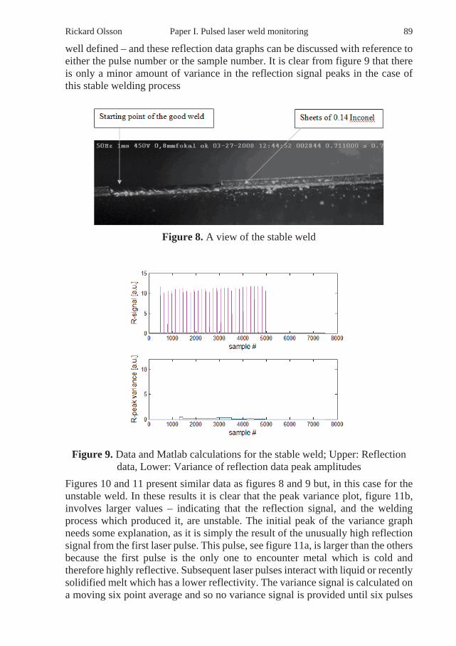
Rickard Olsson Paper I. Pulsed laser weld monitoring 89
well defined – and these reflection data graphs can be discussed with reference to either the pulse number or the sample number. It is clear from figure 9 that there is only a minor amount of variance in the reflection signal peaks in the case of this stable welding process
Figure 8. A view of the stable weld
Figure 9. Data and Matlab calculations for the stable weld; Upper: Reflection
data, Lower: Variance of reflection data peak amplitudes Figures 10 and 11 present similar data as figures 8 and 9 but, in this case for the unstable weld. In these results it is clear that the peak variance plot, figure 11b, involves larger values – indicating that the reflection signal, and the welding process which produced it, are unstable. The initial peak of the variance graph needs some explanation, as it is simply the result of the unusually high reflection signal from the first laser pulse. This pulse, see figure 11a, is larger than the others because the first pulse is the only one to encounter metal which is cold and therefore highly reflective. Subsequent laser pulses interact with liquid or recently solidified melt which has a lower reflectivity. The variance signal is calculated on a moving six point average and so no variance signal is provided until six pulses

90 Paper I. Pulsed laser weld monitoring Rickard Olsson have been monitored. This first variance value is high simply because it includes the unusually energetic first pulse reflection. In general however, the fluctuations in the reflected signal are a function of the fluctuations in the shape of the reflecting surface of the weld. The changes in melt surface geometry shown in the snapshots of figure 10 tend to give a reduced reflection signal but, occasionally, the disturbed melt surface provides a more effective reflector than a stable weld (as happened here in the third pulse from the end of the measurement). In some cases the surface of a poor quality weld might result in repeated high reflection values. In this situation a monitoring device based on a simple threshold might be misled into providing feedback that the process was continuing successfully. It is for this reason that a system designed around the variance of the signals might give additional, useful feedback.
Figure 10. An unstable weld after: (a) 0.167s Sample #1000; (b) 0.300s Sample #2000; (c) 0.467s Sample #3000; (d) 0.603s Sample #4800
(a)
(b)
(c)
(d)

Rickard Olsson Paper I. Pulsed laser weld monitoring 91
Figure 11. Data and Matlab calculations for an unstable weld; Upper: Reflection
data, Lower: Variance of reflection data peak amplitudes Figure 12 is a snapshot taken from the high speed video of the production of the faulty weld just as the weld begins to encounter the gap between the two workpieces. Figure 13 gives the variance of the peak reflection values.
Figure 12. The start of the ‘faulty’ weld

92 Paper I. Pulsed laser weld monitoring Rickard Olsson
Figure 13. Data and Matlab calculations for the ‘faulty’ weld; Upper: Reflection data, Lower: Variance of reflection data peak amplitudes
Figure 13 tells the complex story of the reflection data from the faulty weld which can be interpreted in the following way; a. The first reflection, off the cold metal, has a high peak value. b. The following dozen or so pulse reflections indicate a stable welding process with a much reduced peak value compared to the stable weld. This reduction in signal is due to the different geometry of the weld surface which is concentrated on one side of the join – one workpiece is experiencing only partial melting and thus the reflecting surface of the weld is reduced compared with the stable weld. c. The reflected signal rises as the weld gradually involves the full width of both workpieces – in this zone the weld produced is similar to the stable weld. d. From about sample 4000 the signal becomes very unstable as the weld geometry changes to accommodate the widening of the gap between the two workpieces. e. Between samples 5000 and 6000 the reflected signal decreases to a very low value and remains low because the laser beam is no longer welding – it is simply passing into the gap between the two workpieces. These results show that peak variance analysis can give information which is difficult to interpret in certain complex situations. However, in most cases welds can be classified as either stable or unstable, and it is suggested that peak variance analysis be included in the design of future weld monitoring equipment to achieve a more robust and sensitive feedback system.

Rickard Olsson Paper I. Pulsed laser weld monitoring 93
4. Analysis of the temporal shape of the reflected pulses. The following analysis utilises the same welds and data sets as the previous section but analyses the temporal power profile of the individual pulses rather than their peak values. Figures 14 – 16 present a new view of the original reflected pulses data set for the ‘good’, ‘unstable’ and ‘diverging workpiece’ welds. In each case the power profiles of the reflected pulses are presented using the x-(time) and z-(power) axes. The y-axis used to separate the pulses and display them as a sequence. It is clear from this basic data set that there are large differences in the repeatability of the pulse profiles for the stable and unstable welds.
Figure 14. The basic data set for the ‘good’ weld. The power history for each
reflected pulse is shown and the pulses are stacked next to each other as a sequence
Figure 15. The basic data set for the ‘unstable’ weld. The power history for each
reflected pulse is shown and the pulses are stacked next to each other as a sequence

94 Paper I. Pulsed laser weld monitoring Rickard Olsson
Figure 16. The basic data set for the ‘faulty’ weld. The power history for each reflected pulse is shown and the pulses are stacked next to each other as a
sequence In order to establish a method of qualitative comparison between the data sets presented in figures 14 – 16 it is convenient to reduce the quantitative differences between the peak profiles by normalizing them all to the same maximum height. Comparisons between and within data sets can then be carried out without the extra complication of scaling factors. Figure 17 presents the same information as figure 14 with all the peaks normalised for height in this way.
Figure 17. The basic data set for the stable weld – as in figure 14, but with all the pulses given the same maximum height
With the data in this ‘normalised height’ form it is a simple matter to calculate the curve fit of a fourth order polynomial to the average pulse shape. This gives us a mathematical description of the average power profile of a reflected pulse from a satisfactory welding process. This polynomial fit is presented in figure 18.

Rickard Olsson Paper I. Pulsed laser weld monitoring 95
Figure 18. The polynomial fit of the average values of the temporal power profile of a reflected pulse from a satisfactory welding process
If the polynomial curve in Fig 18 is denoted p(t) then
2 3 40 1 2 3 4( )p t a a t a t a t a t= + + + +
In the case of these results;
0 1 2
3 4
2
3 4
0.4042, 0.6815, 0.3012,0.0404, 0.0021
I.e( ) 0.4042 0.6815 0.30120.0404 0.0021
a a aa a
p t t tt t
= = − == − =
= + +
− + We can now compare the polynomial best fit for every pulse from each of our three welding situations to this mathematical template for a ‘good’ weld reflected pulse by looking at the values of the coefficients a1, a2, a3, and a4. Figures 19 and 20 present the height normalised results for the unstable and faulty welds, and figure 20 compares the values of the polynomial coefficients for all the pulses with the template in figure 18.

96 Paper I. Pulsed laser weld monitoring Rickard Olsson
Figure 19. The basic data set for the ‘unstable’ weld – as in figure 15, but with all the pulses given the same maximum height.
Figure 20. The basic data set for the ‘faulty’ weld – as in figure 16, but with all the pulses given the same maximum height.
Figure 21 gives the expected result that the individual pulses have similar coefficients to the average pulse until the welding process ends after 21 pulses. Between pulses 21 and 30 the movement of the workpiece had stopped so the final pulses were fired into molten material.
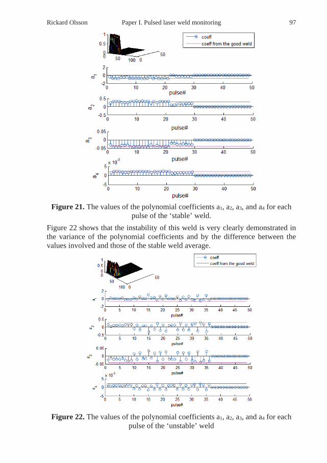
Rickard Olsson Paper I. Pulsed laser weld monitoring 97
Figure 21. The values of the polynomial coefficients a1, a2, a3, and a4 for each pulse of the ‘stable’ weld.
Figure 22 shows that the instability of this weld is very clearly demonstrated in the variance of the polynomial coefficients and by the difference between the values involved and those of the stable weld average.
Figure 22. The values of the polynomial coefficients a1, a2, a3, and a4 for each pulse of the ‘unstable’ weld

98 Paper I. Pulsed laser weld monitoring Rickard Olsson
Figure 23. The values of the polynomial coefficients a1, a2, a3, and a4 for each pulse of the ‘faulty’ weld
The polynomial coefficients in figure 23 reveal the complex history of the faulty weld much more clearly than the peak variance method discussed earlier in this paper. Put simply, it can be seen that the weld goes from ’stable – unsatisfactory’ to ’satisfactory’ to ’unstable – unsatisfactory’, which is an accurate description of the situation. Figures 21–23 make it clear that this polynomial comparison – which could be easily incorporated into a computer based, on line monitoring system, has the capacity to identify process anomalies even in complex situations. The authors recommend that this avenue be investigated by future developers of laser processing monitoring equipment. 5. Conclusions Kalman filtering is a superior method to cut-off filtering for extracting data from noisy signals. Signal variance data can be used in conjunction with raw signal data to improve the sensitivity and robustness of laser welding monitoring devices. Reflected pulse shape comparisons involving polynomial best fits are a very promising tool for on-line process monitoring for pulsed laser welding.

Rickard Olsson Paper I. Pulsed laser weld monitoring 99
Acknowledgments The authors are grateful to VINNOVA – The Swedish Innovation Agency (project DATLAS, no. 2006-00668) and to Laser Nova AB, Östersund, Sweden for their funding and cooperation in the research. References [1] www.precitec.com (2009-07) [2] www.prometec.com (2009-07) [3] Tonshoff H K, Ostendorf A and Specker W, “Online monitoring and closed-
loop control of laser welding processes,” vol. 1405. In Proc. of 12th Int. Symp. for Electromachining (ISEM), May 1998, pp. 603–612.
[4] Kaierle S, Beersiek S, “Online control of penetration depth in laser beam
welding,” vol. 3. Aachen, Germany: Industrial Electronics Society, 1998. IECON '98. Proc. of the 24th Ann. Conf. of the IEEE, Sep 1998, pp. 1694–1698.
[5] Norman P, Engström H, Kaplan A. F. H: State-of-the-art of monitoring and
imaging of laser welding defects, Proc. NOLAMP 11, August 20-22, 2007, Lappeenranta (FIN), Ed.: V. Kujanpää (2007).
[6] Gustafsson F, Adaptive Filtering and Change Detection, Wiley, New
York (2000). [7] http://www.cs.unc.edu/~welch/kalman/ (2009-07) [8] Greval M, Andrews A, Kalman Filtering Theory and Practice using MatLab,
J. Wiley 2001, ISBN 0-471-39254-5 [9] Kalman, R. E (1960). A New Approach to Linear Filtering and Prediction
Problems. Transaction of the ASME—Journal of Basic Engineering, 82(Series D), 35-45.
Appendix 1. Kalman filtering The Kalman filter is named after R.E. Kalman who, in 1960, presented a paper [9] describing a recursive solution to the problem of discrete data linear filtering of a time varying process with measurements disturbed by noise. The Kalman filter is an algorithm rather than an actual filter. Mathematically it is the optimal solution for the linear-quadratic problem i.e. estimating a systems

100 Paper I. Pulsed laser weld monitoring Rickard Olsson “state” whether it may be observable or not using measurement data and minimizing the quadratic error of estimation error covariance. The filter has found a widespread use from telecommunication to image processing, control theory and military applications such as target tracking etc. A good introduction to the subject can be found in [7] and a more thorough derivation in [6]. MatLab applications are treated in [8]. The observed reflection signal y(t) in our experiment was modelled as a sum of the reflection signal s(t) (reflected laser light) plus white noise n(t) with covariance R. I.e. the received signal can be written as
( ) ( ) ( )y t s t n t= + (2) The received signal was modelled in discrete time as an nth order Auto Regressive (AR)-process [6] i.e.:
1 1 2 2 1k k k n k ny a y a y a y− − − −+ + + += (3)
plus a piecewise linear trend between consecutive samples represented at time instant k as b1+b2k. When combining these two into one we can write the received signal yk as:
[ ]
1 1 2 2 1 1 2
1
2
1 2 11
1
2
.... 1 0
k k k n k n
k k k n kn
y a y a y a y b b kaa
y y y CXab
b k
− − − −
− − − −−
+ + + + + += =
= (4)
i.e. in matrix formulation: k kY CX= (5) Using arcov off line in MatLab to estimate the AR coefficients identified that a model order of 2 was sufficient. I.e. the process can be modelled with two coefficients as a first order degree polynomial

Rickard Olsson Paper I. Pulsed laser weld monitoring 101
1 1 2 2k k ky a y a y− −= + (6) 𝑏𝑏1 and 𝑏𝑏2 could now be estimated for each iteration and subtracted from the measured values 𝑦𝑦𝑘𝑘. Using Kalman formulation we have:
The internal state of the process X (7)
The state transition matrix A 𝐴𝐴 = �
0𝐼𝐼𝑖𝑖𝑒𝑒𝑖𝑖 . .
0 0. . 0
0 . .0 . .
1 10 1
� (8)
Kalman gain Kk (9)
Covariance of the estimation error
ˆk ky y− , Pk (10)
Covariance of the measurement noise R (11)
The Kalman equations are given in their iterative form as follows; (12) (13) (14) (15)
where 𝑦𝑦𝑘𝑘 is the observed (measured value) and 𝑦𝑦𝑘𝑘 is the estimated value (used in later calculations). Appendix 2. The CUSUM algorithm To detect the leading and trailing edges of the reflected laser light signal the CUmulative SUM (CUSUM) - algorithm has been used. The CUSUM algorithm is defined as follows [6]: Assume that we want to detect a change in mean of magnitude.
of the signal ( ) s kν We first form an objective function 𝑔𝑔(𝑘𝑘):
( ) max( ( 1) ( ) ,0);alarm if ( )g k g k s k g k hν= − + − > (16)
where the alarm level h is a design parameter and υ in an offset. To detect negative changes, we simply use min instead and negate both h and υ. If we now use 𝑦𝑦�𝑘𝑘 as s(k), then when the alarm is triggered, the actual reflection value 𝑦𝑦�𝑘𝑘is picked from
1
/ ( )( )
( ) ( )ˆ
T Tk k k k k k
k k k k k kT T
k k k k k k k k
k k k
K AP C C P C RX AX K y C X
P A K C P A K C K RKy C X
+
= +
= + −
= − − +
=

102 Paper I. Pulsed laser weld monitoring Rickard Olsson the most probable time of change into peak(k). As a rule of thumb [6] the value is taken at the point
/ (0.5 )k h υ− − (17) i.e.
ˆ( ) ( / (0.5 ))peak k y k h υ= − − (18) and remains constant until the next peak is detected.
For every sample instant , the variance var( ) was calculated in a straight forward k k manner as:
215
5 var( ) ( ( ) ) ; 6.. .
k
j kk peak j m k N
= −
= − =∑ (19)
(Note that peak(k) is a vector of length N but piecewise constant between each peak) N is the number of samples and m the overall mean of the peaks, i.e. the average peak value. The number 6 was chosen as a compromise the get a reasonably fast response. In a real world application it would of course be possible to use e.g. an electronic trigger signal from the laser to identify the rising edge of the signal and e.g. a leaky capacitor solution to detect the peak. An advantage of using CUSUM is that this algorithm is robust to noise and gives a statistically significant indication of an actual change in the measured signal.

Rickard Olsson Paper II. Challenges to the EM feedback from LW 103
Paper II
Challenges to the interpretation of the electromagnetic feedback from laser welding

104 Paper II. Challenges to the EM feedback from LW Rickard Olsson

Rickard Olsson Paper II. Challenges to the EM feedback from LW 105
Challenges to the interpretation of the electromagnetic feedback from laser welding
R. Olsson1,2, I. Eriksson1, J. Powell1, A. V. Langtry3 and A.F.H. Kaplan1
1 Luleå University of Technology, SE-971 87 Luleå, Sweden; www.ltu.se/tfm/produktion 2 Laser Nova AB, SE-831 48 Östersund, Sweden;
3 GE Healthcare, Oxford, UK. E-mail: [email protected]; [email protected] Abstract This paper considers the point that it is not possible to interpret individual weld perturbations from the raw electromagnetic feedback collected from laser weld zones. The presentation of electromagnetic data as a 3D cloud is presented as a new, useful tool in the analysis of this feedback. For example, it is shown that there is a very low correlation between the plasma or thermal signals and the reflected light signal from the weld zone, and that a strong correlation exists between the plasma and thermal signals. It is also demonstrated that data points from a weld perturbation form a different 3D cluster to those from the stable welding process. A strategy for future on line data analysis is presented in the use of a suitably shaped data cloud envelope. The rates of data fit to the various segments of such an envelope could be correlated with specific weld anomalies. Introduction The practice of industrial laser welding often involves continuous monitoring in order to optimise productivity. A common feedback technique involves the use of photodiodes to monitor the electromagnetic emissions from the weld zone. These emissions can be divided into three wavelength ranges associated with reflected laser light, thermal radiation from the weld zone and the higher temperature radiation from the plasma or gas cloud above the weld. Figure 1 describes the optical arrangement of sensors which have individual sensitivities to reflected light (R), thermal radiation (T) and plasma radiation (P).

106 Paper II. Challenges to the EM feedback from LW Rickard Olsson
Fig. 1. The arrangement of the Reflected light (R), Thermal radiation (T) and Plasma radiation (P) sensors, which monitor the electromagnetic radiation from
the laser welding process The signals generated by the photodiodes are continuously compared to a “golden template” of signals historically associated with good quality welds for the specific application involved. Excessive deviation from the ‘good weld’ signal envelope triggers an alarm, which may be used to halt the welding process. This type of monitoring has been developed by purely empirical means with minimal theoretical back-up [1,2]. The work presented in this paper forms part of the early stages of a full analysis of this method of weld monitoring. The eventual outcome of this branch of research should be an improved understanding of the correlation between the signals generated within the weld zone and the defects produced in the welds. The three sensor configuration shown in figure 1 is an adaptation of an original two sensor set-up used to monitor welding carried out with CO2 lasers. The original CO2 laser welding monitors employed only a thermal (infra-red) sensor sensitive over the range of wavelengths from 1300nm to 1800nm and a plasma (ultra-violet) sensor, sensitive to wavelengths below 600nm. The UV range of the plasma sensor is particularly appropriate for CO2 laser welding because the metal vapour boiling off from the weld zone absorbs a substantial proportion of the incident laser light and becomes heated to an ionised plasma state. The stability and intensity of the UV light generated by this plasma can be indicator of weld quality during CO2 laser welding. During Nd:YAG laser welding the plume of vapour above the weld zone is transparent to the laser beam and does not become heated to a plasma state. This

Rickard Olsson Paper II. Challenges to the EM feedback from LW 107
hot vapour radiates as a black body radiator, emitting light over a continuous spectrum. Welding of Zn-coated steel is also well known for its instability and proneness for blow outs due to excessive gas pressure. Welding of Zn-coated steel has been thoroughly investigated by e.g. Norman et.al.[3], Fabbro et.al. [4] and Heyden et.al. [5]. A thorough survey on the state of the art of process monitoring of laser welding can be found in [6]. The reflected light sensor involves a photodiode with a behind a narrow bandpass filter around the laser wavelength and the level of reflected light detected is dependant on the weld pool geometry. Often this R-sensor signal will have a higher variance for bad welds then for good welds because an unstable welding process leads to an extremely variable weld pool surface. Figure 2 is a schematic graph of the observed wavelengths and the light emitted during Nd:YAG welding.
Fig. 2. A schematic of the wavebands of the three monitoring sensors (Plasma,
Reflected and Thermal) Statistical signal processing work has been carried out by a number of workers including Fennander et.al. [7], who looked at Laser hybrid welding using data from high speed imaging fed to a Kalman filter for droplet tracking in conjunction with Principal Component Analysis (PCA) and vector machines for the classification of data. In this case the PCA was used to interpret and simplify the time based 2D-data from the cameras. A similar approach was also used by Jäger [8], who introduced the concept of “Eigen –meltpools”. i.e. mutually orthogonal surface shapes corresponding to the first four eigenvalues–eigenvectors for a typical welding situation. Jäger et al. also describe both the advantages and drawbacks involved in using Independent Component Analysis (ICA) [9] for surface classification. One of their findings was that ICA showed no significant improvement over PCA and their conclusion
λ[nm]
Sens
or
sens
itivi
ty [a
.u]
1064
R T
IR
P
UV/VIS
600 1100
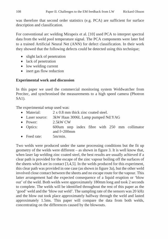
108 Paper II. Challenges to the EM feedback from LW Rickard Olsson was therefore that second order statistics (e.g. PCA) are sufficient for surface description and classification. For conventional arc welding Mirapeix et al. [10] used PCA to interpret spectral data from the weld pool temperature signal. The PCA components were later fed to a trained Artificial Neural Net (ANN) for defect classification. In their work they showed that the following defects could be detected using this technique;
• slight lack of penetration • lack of penetration • low welding current • inert gas flow reduction
Experimental work and discussion In this paper we used the commercial monitoring system Weldwatcher from Precitec, and synchronised the measurements to a high speed camera (Photron SA1). The experimental setup used was:
• Material: 2 x 0.8 mm thick zinc coated steel. • Laser source: 3kW Haas 3006L Lamp pumped Nd:YAG • Power: 2.5kW CW • Optics: 600um step index fibre with 250 mm collimator
and f=200mm • Feed rate: 5m/min.
Two welds were produced under the same processing conditions but the fit up geometry of the welds were different – as shown in figure 3. It is well know that, when laser lap welding zinc coated steel, the best results are usually achieved if a clear path is provided for the escape of the zinc vapour boiling off the surfaces of the sheets which are in contact [3,4,5]. In the welds produced for this experiment, this clear path was provided in one case (as shown in figure 3a), but the other weld involved close contact between the sheets and no escape route for the vapour. This latter arrangement had the expected consequence of a liquid eruption or ‘blow out’ of the weld. Both welds were approximately 180mm long and took 2 seconds to complete. The welds will be identified throughout the rest of this paper as the ‘good’ weld and the ‘blow out weld’. The sampling rate of the sensors was 20 kHz and the blow out took place approximately halfway through the weld and lasted approximately 1.5ms. This paper will compare the data from both welds, concentrating on the differences caused by the blowouts.

Rickard Olsson Paper II. Challenges to the EM feedback from LW 109
(a)
(b) Fig. 3. (a) Experimental situation for the good weld and (b) situation for the
blow out weld Figure 4 presents the raw data from the three sensors for the good weld and the blow out weld. There appears to be a close correlation between the temperature and plasma signals in both cases. It is also clear that the signals are less stable in the case of the blow out weld although there is a considerable level of noise in both sets of signals.

110 Paper II. Challenges to the EM feedback from LW Rickard Olsson
(a) (b) Fig. 4. Raw data from the three sensors for; (a) the good weld and (b) the blow
out weld
It is, of course, very difficult to interpret the data if it is presented in its raw form – although data readings of this type can be used in conjunction with simple threshold values. Extra information can be gathered from the data if it is presented as a three dimensional cloud – as in figure 4. In this case the three data points from every individual time instant are presented as a single point inside a three dimensional graph. For example, if, sometime during the first second of welding, we take our 15,024th reading of the T, R and P signals – the values might be 2.4, 1.2 and 4.5 respectively. We then plot the point 2.4, 1.2, 4.5 on our x,y,z graph – the time element of the information is hidden in this type of display, but we can see the general correlation of the whole data set. In figure 5 we can see that there is some correlation between the data points whilst the welding is taking place – and we can also see that the start up and ending phases of the welding process produce sets of data points which are clearly separate from the main cloud. The welding process is, in effect, disrupted during the start up and ending phases and these ‘disturbed’ welding periods provide distinct, coherent groups of data points. This means that it might be possible to identify specific weld perturbations such as blow outs (see figure 6) or keyhole collapse, by their data point signatures in the three dimensional space of such a graph. Even at this early stage of these results it is interesting to note that the data signature start up phase of the blow out weld is completely different from, and far less cohesive than, that of the good weld – indicating an inherent instability as a result of vapour pressure building up beneath the weld pool.

Rickard Olsson Paper II. Challenges to the EM feedback from LW 111
(a) (b)
Fig. 5 (a) Good weld, (b) Blow out weld Fig. 5. Data clouds taken from the information presented in figure 4
Fig. 6. A weld experiencing a ‘blow out’ – trapped zinc vapour blows a hole in the weld pool as it escapes - leading to the ejection of a considerable amount of
liquid
Although the differences between the start up and ending phases of the weld are interesting, we are really working towards an on line monitor of the main part of the welding process. Figure 7 presents the data clouds of figure 4 with the start up and ending phases removed. In these figures the overall mean has been subtracted from all the data values to generate a zero mean data cloud. This is to enable correct PCA calculations for the resulting eigenvectors shown in subsequent figures.

112 Paper II. Challenges to the EM feedback from LW Rickard Olsson
(a) (b)
Fig. 7. The good weld (a) and blow out weld (b) data clouds after the start and end phases of the welding process have been removed. In these figures the overall mean has been subtracted from all the data values to generate a zero
mean data cloud Figure 7 reveals that there are clear similarities and differences between the two data clouds. The overall cloud shapes and their orientations in the 3D space are similar – but there are considerably more outlying points in the case of the unstable weld. If we look at the overall shape and orientation of the clouds first, we can extract some information from the three side views of the 3D data field – as shown in figures 8,9 and 10.
(a) (b)
Fig. 8. The reflection/temperature relationship of the data clouds for (a) the stable and (b) the unstable welds

Rickard Olsson Paper II. Challenges to the EM feedback from LW 113
(a) (b) Fig. 9. The reflection/plasma relationship of the data clouds for (a) the good and
(b) the blow out welds Figures 7 and 9 reveal that there is a very low correlation between the plasma or thermal signals and the reflected light signal. This low correlation can be explained by the fact that the strength of the reflected signal from the weld zone will largely be dependent on the surface geometry of the melt rather than the temperature of the melt or the vapour cloud.
(a) (b) Fig. 10. The plasma/temperature relationship of the data clouds for (a) the good
and (b) the blow out welds Figure 10 shows that there is a strong correlation between the plasma and thermal signals from the weld zone. This strong correlation could be expected because the rate of vapour generation is governed by the weld pool temperature. Increased weld pool heating will result in increased boiling and so the two thermal signals are linked. Picking the largest eigenvalues and corresponding eigenvectors from the PCA analysis of the data clouds we can identify the direction vector pointing in the direction of maximum variation dirVect for the good weld as:

114 Paper II. Challenges to the EM feedback from LW Rickard Olsson
0.60 ( )
0.79Thermal
dirVect in directionPlasma
= (1)
and for the blow out weld as:
0.65 ( )
0.67Thermal
dirVect in directionPlasma
= (2)
Much of difference between the coefficients can be attributed to the “tail” seen in figures 7a, 8a and 9a which affects the principal component vector. Otherwise it is clear that the core 3D geometry of the clouds for both welds is similar. We can now consider the detailed shape of the blow out weld data in a search for a correlation between weld perturbations and specific data clusters in the 3D cloud. Although the time-based information relevant to each data point is not displayed in the data cloud, it is possible to identify each point from the basic data set. Using the time base given by the high speed video film, it is therefore possible to label the points in the data cloud which are associated with the blow out – these are presented in figure 11 as light points.
Fig. 11. The data cloud for the blow out weld with the data points associated with the blow out identified as light points and the stable periods of this weld
identified by the dark points From the process monitoring point of view, it is encouraging that the data points for the blow out event are not evenly spaced within the data cloud – there is a clear tendency for them to cluster in one sector of the overall cloud. The blow out data is associated with a quadrant of the 3D space where all three signal levels are low but the plasma signal is larger than average for the thermal and reflected signals involved. This could be related to the increased vapour evolution during blow out. The zinc vapour will join the iron vapour – the level of which may also

Rickard Olsson Paper II. Challenges to the EM feedback from LW 115
be increased as a result of increased melt surface area – because the weld zone is much more undulating than normal and airborne droplets are present in the area. The low reflection signal associated with blow outs is also traceable to a physical phenomenon. The reflectivity of the weld decreases with increased melt surface curvature, because a flat weld would be the most effective reflector of the laser light, and the weld surface is considerably more curved when blow outs are taking place. In order to investigate the various shapes of the data clouds for the ‘stable’ and ‘blow out’ parts of the weld, the two are presented separately in figures 12 and 13.
Fig. 12. The data cloud from figure 11 with the ’blow out’ data removed. This is
the shape of the data cloud for the stable part of this weld
Fig. 13. The data cloud for the ‘blow out’ data only
Figures 13 and 14 demonstrate that the two sets of data both form coherent clouds, but give no indication of the overlap between the two. To assess the level of overlap, figure 14 presents two cross sectional slices of the data cloud taken across the ‘thermal’ axis. When the 3D space is rotated so that we view it from the end with the plasma/reflection axes, as in figure 15, we can see the intermingling of

116 Paper II. Challenges to the EM feedback from LW Rickard Olsson the ‘blow out’ and ‘stable welding’ data points. From the images in figure 15, two things are clear; a. the relative proportions of ‘blow out’ and ‘stable weld’ data points change as we move down the long axis of the data cloud, and b. the distribution of the ‘blow out’ data points is not uniform across the cloud cross section (for example, the upper left quadrant of the larger cross section contains relatively few ‘blow out’ data points).
Fig. 14. Taking two cross-sections of the data cloud
Fig. 15. Four cross-sections of the data cloud

Rickard Olsson Paper II. Challenges to the EM feedback from LW 117
The asymmetric distribution of the blow out data point cloud within the stable weld cloud presents us with a possible future strategy for feedback analysis. This would involve the construction of a suitably dimensioned ellipsoid shell divided into eight segments – as described in figure 16. As data points are acquired from the process they could be converted to their 3D format and would fill the various quadrants of the shell. The relative rates of arrival of the data points into the segments would be an indicator of the state of the welding process and could be compared to the rates for a stable weld. Additionally, the extension of the segments outside the shell to the limits of the 3D ‘box’ could give another clearly defined eight zones for data collection and rate comparison. This principle will be the subject of future work by the present authors.
Fig. 16. A strategy for on line data analysis could involve a standard cloud
divided into eight or more sectors Conclusions
• It is not possible to interpret individual weld perturbations from the raw electromagnetic data collected from laser weld zones.
• The presentation of electromagnetic data as a 3D cloud provides a new, useful tool in the analysis of feedback from laser weld zones.
• There is a very low correlation between the plasma or thermal signals and the reflected light signal from the weld zone.
• There is a strong correlation between the plasma and thermal signals from the weld zone.
• Data points from a weld perturbation (blow out) form a different 3D cluster to those from the stable welding process.
• A strategy for future on line data analysis is the use of a suitable data cloud envelope or multi-layered envelopes. The rates of data fit to the various segments of such envelopes could be correlated with specific weld anomalies.
118 Paper II. Challenges to the EM feedback from LW Rickard Olsson Acknowledgments The authors are grateful to VINNOVA – The Swedish Innovation Agency (project DATLAS, no. 2006-00668) and to Laser Nova AB, Östersund, Sweden for their funding and cooperation in the research. References
[1] www.precitec.com
[2] www.prometec.com
[3] P. Norman, I. Eriksson, A. F. H. Kaplan Monitoring Laser beam welding of zinccoated sheet metal to analyze the defects occurring, Proc. 12th NOLAMP, August 24-26, 2009, Copenhagen (DK), FORCE Technology
[4] R. Fabbro, F. Coste, D. Goebels and M. Kielwasser, 2006. Study of CW Nd-Yag laser,Welding of Zn-coated steel sheets. Journal of Physics D: Applied Physics, 39(2), pp. 401-409.
[5] J. Heyden, K. Nilsson, C. Magnusson, Laser Welding of Zinc Coated Steel, Lasers In Manufacturing, Jun., 1989, p. 161-167
[6] P. Norman, H. Engström, A. F. H. Kaplan: State-of-the-art of monitoring and imaging of laser welding defects, NOLAMP 11, August 20-22, 2007, Lappeenranta (FIN), Ed.: V. Kujanpää (2007).
[7] H. Fennander, V. Kyrki, A. Fellman, A. Salminen, and H. Kälviäinen. Visual measurement and tracking in laser hybrid welding. Mach. Vision Appl., 20(2):103–118, 2009.
[8] M. Jäger ; F. A. Hamprecht. Principal component imagery for the quality monitoring of dynamic laser welding processes. Industrial Electronics, IEEE Transactions on, 56(4):1307–1313, April 2009.
[9] E. Oja, A. Hyvarinen and J. Karhunen,. Independent Component Analysis. Wiley-Interscience, May 2001.
[10] J. Mirapeix, P.B. García-Allende, A. Cobo, O.M. Conde, J.M. López-Higuera. Real-time arc-welding defect detection and classification with principal component analysis and artificial neural networks. NDT and E International, 40(4):315–323, 2007.

Rickard Olsson Paper III. Surfaces by laser melt disruption 119
Paper III
The production of osseointegrating (bone bonding) surfaces on titanium screws by laser melt disruption

120 Paper III. Surfaces by laser melt disruption Rickard Olsson

Rickard Olsson Paper III. Surfaces by laser melt disruption 121
The production of osseointegrating (bone bonding) surfaces on titanium screws by laser melt disruption. R. Olsson1,2, J. Powell1, A. Palmquist3, R. Brånemark4, J. Frostevarg1, A.F.H. Kaplan1
1 Luleå University of Technology, SE-971 87 Luleå, Sweden; www.ltu.se/tfm/produktion 2 Laser Nova AB, SE-831 48 Östersund, Sweden; 3 Department of Biomaterials, University of Gothenburg, Gothenburg, Sweden 4Department of Orthopaedic Surgery, University of California, San Francisco, USA Abstract Several techniques can be used to modify implant surfaces in order to accelerate bone growth around titanium implants. One method is to generate a surface structure which stimulates bone growth and remodelling. This paper describes and explains a non-ablative method for producing osseointegrating (structural and functional bone bonding) surfaces on titanium implants using laser processing. The focus is especially on surface texturing of dental implant screws, where the ability of a Nd:YAG laser to generate ‘splashy’ surfaces covered in resolidified micro scale droplets coated with nano-scale surface oxides is assessed. The surfaces produced were analysed by scanning electron microscope (SEM) and energy dispersive x-ray spectroscopy (EDS). It is concluded that laser processing using Q-pulsed Nd:YAG lasers can generate surfaces which match the demands set by clinical experience. One important characteristic of the surfaces discussed here is that they involve overhanging features which are suitable for trapping red blood cells and which cannot be created by mechanical or chemical roughening techniques. Keywords Medical implants, dental implants, osseointegration, titanium, laser surface structuring, high speed imaging. 1. Introduction Titanium has been used in the manufacture of medical and dental implants since the 1960’s and the first investigation into the integration of bone with titanium (Ti) was carried out by Brånemark [1]. Titanium is biocompatible, and does not generate
a harmful immunological response (locally or systematically). Titanium alloys of grades II, IV and V are thus the favoured materials for medical and dental implants of various types. Roughening the surface of a titanium implant on both the nano and micro scales has been shown to improve the

122 Paper III. Surfaces by laser melt disruption Rickard Olsson
rate at which osseointegration takes place [2]. Extensive research has therefore been carried out into developing technologies for the creation of different micro-rough topographies and most of the current commercially available dental implant systems use micro-rough implants [3,4]. However, as Esposito et al. [5] have noted, the lack of randomized controlled trials makes comparisons between different surfaces difficult. New bone formation at the implant surface involves multiple steps by the bone forming (osteoblast) cells:
1. Attachment of osteoprogenitor cells (a pre-stage of osteoblasts)
2. Differentiation into osteoblasts
3. Secretion of extracellular matrix, retracting away from the implant surface
4. Some cells stop producing matrix and become embedded in the bone matrix and differentiate into osteocytes (bone cells).
A nano-scale oxidised surface has the effect of increasing the adsorption of proteins, the deposition of the bone matrix hydroxylapatite (HA), the adhesion of cells and thus the rate of osseointegration, see Shah et.al. [6]. A rough, complex, micro-scale surface increases the amount of nano-surface available in any area, which improves the chances of protein absorption. The micro-scale
topological range of 10-20μm is also effective in trapping red blood cells (erythrocytes), which have a diameter 6-8 μm. A number of workers,[7–9] have identified that this also assists osseointegration. Later in the osseointegration process this microscopically rough, convoluted surface provides excellent mechanical locking between the implant and the bone. Vignesh [10] compared acid-etched, sandblasted and laser treated micro-rough surfaces, finding that laser treated surfaces gave the best results. Mirhosseini et al. [11] investigated the osseointegration of osteoblast cells on previously sandblasted Nd:YAG laser treated surfaces with different surface roughnesses. Their results indicated that there is an optimum roughness for homogeneous cell growth. A considerable amount of work (eg. Karazisis et.al. [12], Omar et.al.[13]) has been carried out on nano-scale surface modifications, and experimental studies have shown that suitable nano-scale features promote bone growth. Rani et al. [14] manufactured nano-surfaces using hydrothermal methods for Ti-oxide growth, finding an increased osseointegration effect compared to a flat machined surface. The nanoscale features of an implant surface seem to be important for biomechanical interlocking, as apatite formation occurs in the nano-scale irregularities (Wang, Grandfield [15,16]). Dental implants with a micro-nano dual surface structure have shown

Rickard Olsson Paper III. Surfaces by laser melt disruption 123
promising clinical results in both the short and long term, with a success rate of better than 99 % at 5 years follow-up [17]. In recent years, it has been demonstrated that osseointegration can be accelerated if the Ti surface is pre-treated with a laser to have a specific topology containing both micro- and nano-scale features [9], see Fig. 1. In a series of experimental studies, surfaces covered in firmly attached, re-solidified droplets with diameters between 1 and 5 microns have been evaluated [9,18–20]). It has been found that the best results are achieved if the surface of the droplets is covered in a porous or spongeous layer of oxide with nano-scale features [9] allowing mechanical interlocking at the nano-scale [16,21]. The use of lasers in biomedical applications is widespread and a thorough survey can be found in Vilar [22], especially in chapter 9 [23]. Generally, laser radiation is used to create various degrees of roughness through ablation, melting and re-solidification, or as in the case presented here, through a combination of melting, melt disruption, droplet generation and oxidation. In contrast to coating
methods, which require powders and are difficult to apply locally, laser processing offers fast, local and direct single step creation of optimum surfaces for osseointegration and is thus of high medical and industrial interest. However, little research been done regarding the actual laser-metal interaction which creates the various micro- and nano-structures, or on the types of surface created. As this paper will demonstrate, under certain conditions a laser can create a micro-rough surface that is fundamentally different to surfaces created by mechanical or chemical methods. Using the correct parameters, a laser can create a ‘splashy’ surface that involves overhanging features that encourage the entrapment of red blood cells and subsequent osseointegration. It is worth noting that standard laser surface structuring is generally either a melting or ablation dominated process – the ‘splashy’ surfaces discussed in this paper are created when the melt is disrupted by localised surface boiling. However, the boiling event is not sufficient to eject the bulk of the material from the surface (thus the process could be described as frustrated ablation).

124 Paper III. Surfaces by laser melt disruption Rickard Olsson
Fig. 1. A ‘splashy’ laser melted surface covered in droplets in the diameter range
1-5 µm, coated with a nano- scale spongeous oxide layer
Fig. 2. Osteocytes (bone cells) in interfacial tissue making direct contact with
the nano-scale surface features via cellular extensions. [8]. Reprinted with permission from High- Resolution Visualization of the Osteocyte Lacuno-Canalicular Network Juxtaposed to the Surface of Nanotextured Titanium
Implants in Human, ACS Biomater. Sci. Eng. 1 (2015) 305–313. doi:10.1021/ab500127y.Copyright 2015,Elsevier
This paper analyses the generation of osseointegrating surfaces on the valleys of the screw thread as described in Figures 3 and 4. A Nd:YAG laser was used to successfully produce suitable surfaces on these screws. The technique described here differs from standard laser surface structuring
because it is not ablation based. In ablation based processes the laser generates a melt that is subsequently removed from the area by explosive evaporation. In the process discussed here, the melt is simply disrupted by a limited amount of localised surface boiling. The vapour pressure from the boiling process pushes down on the

Rickard Olsson Paper III. Surfaces by laser melt disruption 125
melt to produce a ‘splashy’ surface on solidification. Sisti et al. [24] found that this type of surface resulted in a 40% increase in implant-bone bond strength in rabbits (bone integration occurs similarly in human bone and rabbit bone according to retrieval analyses see Shah, Palmquist [6,25]). This compares well with the 20% improvement noted by Peto et al. [26] for surfaces which had been laser surface melted without the ‘splash’ effect (which involves droplet re-attachment and overhanging features). Several other workers e.g. Liang [27] and Vorobyev [28] have employed this type of surface but they do not discuss the laser-material interaction involved. This interaction is discussed and investigated here together with the development of the correct process parameters, and the problems encountered when these parameters are exceeded. The discussion also points out the fact that the ‘splashy’ surface created involves
a great many overhanging features which are believed to be important in the early stages of osseointegration as they form an optimum topology for the entrapment of red blood cells. 2. Methodology The purpose of this experimental program was to examine which laser processing conditions produce structures suitable for osseointegration on the surface of Titanium. Firstly, an inclined plane experiment investigating the effect of laser focal position on surface structure was carried out. Secondly an experiment was carried out on rotating cylindrical screws to create surface structures at the thread bottom with varying power densities and focal positions. Additionally, high speed filming of the process on a rotating screw was carried out, Fig. 3. The equipment used is listed in Table 1.
2.1 Experimental equipment
Fig. 3. Setup for the laser surface structuring of screw implants

126 Paper III. Surfaces by laser melt disruption Rickard Olsson
Table 1. Equipment Equipment Brand Laser ROFIN-SINAR RSY120Q, Galvo Scanlab SK1014
f-Theta lens Rodenstock f=163 SEM Micro CT
Tescan VEGA MV2000JEOL JSM-IT300LV Zeiss Xradia 510 Versa
EDS Oxford Instruments Aztec 3.1 High speed camera Redlake Motion Pro X3
Illumination laser Optical BP- filter Field of view
Cavitar Cavilux Smart, 810nm 810 nm on camera. 2x2 mm
In this study the medical requirements for the surfaces were: 1. A surface covered in
re-solidified splashes and droplets with feature sizes 1-50 μm.
2. A nano-scale surface layer of oxide (as outlined in Fig 4).
It should be noted that the bottom of the thread has a flat surface. In this particular case the flat area was around 0.1 mm wide.
Fig. 4. The geometry of the Ti screw thread to be treated, showing the extent of the treated zone and the position of SEM-analysis 2.2 Experimental procedure 2.2.1 Inclined flat surface samples. A preliminary parameter study revealed that a focussed Nd:YAG laser (wavelength; 1.06 µm) could produce the required type of surface on flat sheet titanium if the following parameters were used:
• Pulse frequency; 3 kHz • Pulse energy; 1.33 mJ
• Pulse on time; 200 nS • Beam diameter at the focus;
120 μm • Pulse overlap 50 %
However, the geometry of the finished screw (as shown in Fig. 3) is complex and requires the laser-material interaction to be effective over a vertical range as well as at different angles of incidence. To

Rickard Olsson Paper III. Surfaces by laser melt disruption 127
clarify the effect of defocussing on the laser-material interaction, an experiment was carried out on an inclined flat sheet of Ti (CP – grade IV) as shown in Fig. 5 with a total treated area of 30x10 mm. This arrangement caused the laser beam to hit the surface over a range of different distances from the focal plane (plus and minus 3mm) and thus with different spot sizes and therefore different power densities (with the maximum power density when the material surface is at the focal point of the lens; fz=0). 2.2.2. Screw thread processing. Having established the effect of defocusing during the inclined plate experiment, laser processing tests were carried out on twelve titanium (CP – grade IV) screws using different pulse energies and focus positions (the bottom of the valley of the screw thread was used as the datum for the focus position). The screws were ultrasonically cleaned in isopropyl alcohol, (IPA) for 20 minutes after processing. This was to simulate the real world
situation where implants must be sterile before implantation. It was therefore of interest to verify that a crusty, oxidised nano-surface was present after cleaning process.
Fig. 5. Inclined flat surface sample production
2.3 Analytical Procedure The different surfaces generated in the inclined surface experiment and the screw tests (before and after cleaning) were analysed by SEM and classified according to the condition of the micro-structure and nano-structure. A random sample of the screws was also analysed using EDS. During the screw tests the process was high-speed filmed at 11 000 fps.
3. Results and discussion. 3.1 Inclined plate experiment. Table 2 and Fig. 6 present the results of the inclined plate experiment. The inclination of the plate generated a gradual change in laser beam focus and SEM photo-graphs were taken at positions on the slope which corresponded to particular defocus conditions. In Fig. 6 the focus
positions fz vary from -3.0 mm to +3.0 mm (i.e. the focal point of the beam was positioned in a range from 3 mm below the surface of the sheet to 3 mm above it). In the inclined surface experiment the laser pulse frequency was kept constant at 3 kHz, the CW power at 4 W and thus the pulse energy was 1.33 mJ/pulse.

128 Paper III. Surfaces by laser melt disruption Rickard Olsson
Table 2. A summary of the inclined plate experiment.
Sample Focus
fz (mm)
Beam radius on surface (mm)
Q-pulse power density
on surface (kW/mm2)
Micro- Structure
Nano- Structure
1 -3.0 0.21 190 Poor Poor 2 -1.5 0.16 309 Poor Poor 3 -1.0 0.15 364 Poor Present 4 -0.5 0.13 463 Present Present 5 0 0.12 588 Present Present 6 +0.5 0.13 463 Present Present 7 +1.0 0.15 364 Poor Present 8 +1.5 0.16 409 Poor Poor 9 +3.0 0.21 190 Poor Poor
The requirement for ‘Microstructure present’ (see Table 2) in this study was that >60% of the surface should be covered with >1-5 μm structures (area of coverage estimated from SEM photographs). The requirement for ‘Nanostructure satisfactory’ was that the microstructure should be covered with a visible spongeous surface on the nano-scale. It is clear from Fig. 6 that the laser parameters employed here
successfully produced the required type of surface in the focus range – 0.5 mm to +0.5 mm (see table 2). Outside of this range the more defocused beam is not capable of producing the type of splash zone required in order to produce the desired surface topology. The ‘surface splash’ laser material interaction required is described in Fig. 7.

129 Paper III. Surfaces by laser melt disruption Rickard Olsson
Fig. 6. Results from the inclined plate experiment
Fig. 7. The generation of a ‘splashy’ surface from overlapping laser melted zones
For every laser pulse a small melt pool is created and the top surface of that pool experiences local boiling at the centre where the temperatures are highest. In ablation-based processes the high vapour pressure from this local boiling event results in the
explosive removal of most of the melt. However, in the process under examination here, the build-up of vapour pressure is less energetic. A melt is formed and the vapour pressure presses down on the melt surface to disrupt the liquid, creating
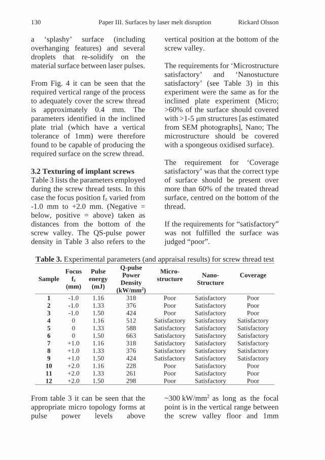
130 Paper III. Surfaces by laser melt disruption Rickard Olsson
a ‘splashy’ surface (including overhanging features) and several droplets that re-solidify on the material surface between laser pulses. From Fig. 4 it can be seen that the required vertical range of the process to adequately cover the screw thread is approximately 0.4 mm. The parameters identified in the inclined plate trial (which have a vertical tolerance of 1mm) were therefore found to be capable of producing the required surface on the screw thread. 3.2 Texturing of implant screws Table 3 lists the parameters employed during the screw thread tests. In this case the focus position fz varied from -1.0 mm to +2.0 mm. (Negative = below, positive = above) taken as distances from the bottom of the screw valley. The QS-pulse power density in Table 3 also refers to the
vertical position at the bottom of the screw valley. The requirements for ‘Microstructure satisfactory’ and ‘Nanostucture satisfactory’ (see Table 3) in this experiment were the same as for the inclined plate experiment (Micro; >60% of the surface should covered with >1-5 μm structures [as estimated from SEM photographs], Nano; The microstructure should be covered with a spongeous oxidised surface). The requirement for ‘Coverage satisfactory’ was that the correct type of surface should be present over more than 60% of the treated thread surface, centred on the bottom of the thread. If the requirements for “satisfactory” was not fulfilled the surface was judged “poor”.
Table 3. Experimental parameters (and appraisal results) for screw thread test
Sample Focus
fz (mm)
Pulse energy (mJ)
Q-pulse Power Density
(kW/mm2)
Micro- structure
Nano- Structure
Coverage
1 -1.0 1.16 318 Poor Satisfactory Poor 2 -1.0 1.33 376 Poor Satisfactory Poor 3 -1.0 1.50 424 Poor Satisfactory Poor 4 0 1.16 512 Satisfactory Satisfactory Satisfactory 5 0 1.33 588 Satisfactory Satisfactory Satisfactory 6 0 1.50 663 Satisfactory Satisfactory Satisfactory 7 +1.0 1.16 318 Satisfactory Satisfactory Satisfactory 8 +1.0 1.33 376 Satisfactory Satisfactory Satisfactory 9 +1.0 1.50 424 Satisfactory Satisfactory Satisfactory 10 +2.0 1.16 228 Poor Satisfactory Poor 11 +2.0 1.33 261 Poor Satisfactory Poor 12 +2.0 1.50 298 Poor Satisfactory Poor
From table 3 it can be seen that the appropriate micro topology forms at pulse power levels above
~300 kW/mm2 as long as the focal point is in the vertical range between the screw valley floor and 1mm

Rickard Olsson Paper III. Surfaces by laser melt disruption 131
above it. Fig. 8 presents confirmation that the required surface topology cannot be created if the beam intensity is too low (Images from samples 5-8 showed similar results to samples 4 and 9 and are therefore not included in figure 8 in the interests of brevity). Focussing the beam 1mm below the valley surface resulted in inadequate splashing, as did focussing the beam 2 mm above the surface. Defocussing 1 mm above the surface was successful in this case because the cross-sectional shape of the screw thread rises towards the focal point. 3.3 Surface Chemical analysis It was mentioned earlier in this paper that the screws are ultrasonically cleaned prior to use as implants. Surface analysis was performed on cleaned and uncleaned surfaces in an attempt to identify the oxides present on the screw surfaces using the Oxford Instruments EDS system on areas 2x2 to 2x5 μm in size. Figures 9a, c and e show the surface chemical analysis of a screw washed for 20 minutes in IPA. The carbon reading can be assumed to be residual oil from the screw manufacturing process. The important chemical result from the point of view of this paper is the ratio (in at.%) of Ti to O.
Calculating from the wt. % results in Figs. 9c and e and using the appropriate atomic masses, the atomic ratio in Spectrum 1 (Fig 9b) was found to be approximately 3.6:1.0 (Ti:O). For Spectrum 2 (Fig 9e) the result was 5.5:1.0 (Ti:O). These results are, of course much higher in Ti than the 1:1 ratio of TiO and the 1:2 ratio of TiO2. Figures 9b, d and f show the surface chemical content of an unwashed screw directly after laser processing. As might be expected, the carbon contamination of the surface is greater in this case. Also, the Ti:O ratios are lower than the results for the washed screw, indicating a higher oxide presence on the surface. Table 4 presents the Ti:O ratios calculated for the washed and unwashed screws. The results presented in table 4 confirm that the surfaces of all the samples are oxidised and that the washing process removes some of the oxide layer. However, these results do not identify the oxidation state of the titanium. This is undoubtedly because the oxide layer (particularly on the washed samples) is thinner than the ~2 μm penetration depth of the EDS.

132 Paper III. Surfaces by laser melt disruption Rickard Olsson
Fig. 8. SEM pictures taken of the screw samples, where those labelled i have a
satisfactory surface. Those labeled ii have poor coverage and inadequate formation of droplets (see table 3).

133 Paper III. Surfaces by laser melt disruption Rickard Olsson
Fig. 9. The surface of processed screw threads and EDS spectrums for washed
(a, c and e) and unwashed (b, d and f) samples Table 4 Ti:O ratio results
Sample Ti:O ratio (at.%) Spectrum 1 (Washed)
3.6 : 1.0
Spectrum 2 (Washed)
5.5 : 1.0
Spectrum 3 (Unwashed)
0.9 : 1.0
Spectrum 4 (Unwashed)
2.1 : 1.0
The EDS reading therefore includes the some of the unoxidized Ti below the oxide surface. Taking these
considerations into account it can be concluded that the cleaned screws are covered in a layer of titanium oxides which is less than ~2 μm thick. 3. Melt disruption and droplet ejection High speed imaging of the process (at 11 000 fps) was carried using the equipment mentioned in Table 1. These films confirmed that some molten material is ejected and resolidified on the trailing edge of the laser-material interaction zone. The
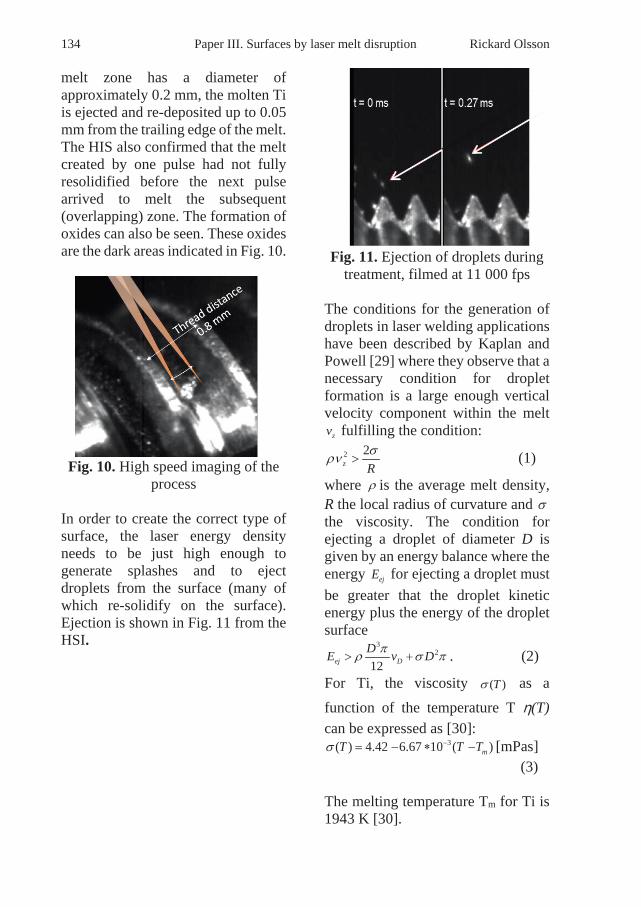
134 Paper III. Surfaces by laser melt disruption Rickard Olsson
melt zone has a diameter of approximately 0.2 mm, the molten Ti is ejected and re-deposited up to 0.05 mm from the trailing edge of the melt. The HIS also confirmed that the melt created by one pulse had not fully resolidified before the next pulse arrived to melt the subsequent (overlapping) zone. The formation of oxides can also be seen. These oxides are the dark areas indicated in Fig. 10.
Fig. 10. High speed imaging of the process
In order to create the correct type of surface, the laser energy density needs to be just high enough to generate splashes and to eject droplets from the surface (many of which re-solidify on the surface). Ejection is shown in Fig. 11 from the HSI.
Fig. 11. Ejection of droplets during treatment, filmed at 11 000 fps
The conditions for the generation of droplets in laser welding applications have been described by Kaplan and Powell [29] where they observe that a necessary condition for droplet formation is a large enough vertical velocity component within the melt
fulfilling the condition:
(1)
where is the average melt density, R the local radius of curvature and the viscosity. The condition for ejecting a droplet of diameter D is given by an energy balance where the energy for ejecting a droplet must be greater that the droplet kinetic energy plus the energy of the droplet surface
. (2)
For Ti, the viscosity as a function of the temperature T η(T) can be expressed as [30]:
[mPas] (3) The melting temperature Tm for Ti is 1943 K [30].
zv
2 2z R
σρν >
ρσ
ejE
32
12ej DDE v Dπρ σ π> +
( )Tσ
3( ) 4.42 6.67 10 ( )mT T Tσ −= − ∗ −

Rickard Olsson Paper III. Surfaces by laser melt disruption 135
A typical droplet speed can be calculated from the HSI-video used to observe the surface texturing process. Given a distance of 0.8 mm between the threads and a frame rate of 11 000 fps the droplet speed in this case was measured from the images to be approximately 6.9 m/s. The density of Ti is 4.43x10³ kg/m3. If the temperature in the melt is assumed to be 1800 ºC and a pulse energy of 1.5 mJ with the viscosity calculated from (3) to be ~5.8 mPas, the energy
needed to create one droplet of radius 10-6 m is in the range of 8x10⁻⁹ J, so a pulse energy level in the mJ range is clearly sufficient to generate droplets. 4. Surface Adhesion It is important to confirm that the surface generated by any roughening process is firmly attached to the substrate. The contiguous nature of the surface generated by this type of
laser surface roughening is confirmed in figure 12 which presents Micro CT tomography generated cross sections of a typical surface and adjoining substrate. It is clear from these images that the surface is an extension of the substrate. It is also noticeable that the surface topography involves overhanging features which would be eminently suitable for trapping cells of the same order of magnitude.
Fig. 12. Micro-CT tomography
generated cross sections of a typical laser generated surface and the
adjacent substrate
5. Conclusions This study has shown that:
• A Nd:YAG Q-pulsed laser can generate the osseointegrating surfaces required by medical professionals.
• The process has a well-defined process window, within which a ‘splashy’ surface is generated by localized boiling of the melt.
• The power density is the most critical factor for forming droplets and the associated oxide coating.
• The ‘splashy’ surface contains a considerable number of overhanging features which are suitable for trapping red blood cells, thereby aiding osseointegration.

136 Paper III. Surfaces by laser melt disruption Rickard Olsson
References [1] Brånemark PI, Hansson BO, Adell
R, Breine U, Lindström J, Hallén O, et al. Osseointegrated implants in the treatment of the edentulous jaw. Experience from a 10-year period. Scandinavian Journal of Plastic and Reconstructive Surgery Supplementum 1977.
[2] Wennerberg A, Albrektsson T. Effects of titanium surface topography on bone integration: a systematic review. Clinical Oral Implants Research 2009;20:172–84. doi:10.1111/j.1600-0501.2009.01775.x.
[3] Palmquist A, Engqvist H, Lausmaa J, Thomsen P. Commercially Available Dental Implants: Review of Their Surface Characteristics. Journal of Biomaterials and Tissue Engineering 2012;2:112–24. doi:10.1166/jbt.2012.1033.
[4] Albrektsson T WA. Oral implant surfaces: Part 1--review focusing on topographic and chemical properties of different surfaces and in vivo responses to them. Int J Prosthodont 2004;17:536–43.
[5] Esposito M, Ardebili Y, Worthington H V. Interventions for replacing missing teeth: different types of dental implants. In: Esposito M, editor. Cochrane Database of Systematic Reviews, Chichester, UK: John Wiley & Sons, Ltd; 2014. doi:10.1002/14651858.CD003815.pub4.
[6] Shah FA, Nilson B, Brånemark R, Thomsen P, Palmquist A. The bone-implant interface - nanoscale analysis of clinically retrieved dental implants. Nanomedicine: Nanotechnology, Biology, and Medicine 2014;10:1729–37. doi:10.1016/j.nano.2014.05.015.
[7] Brånemark PI. The Osseointegration Book. Quintessence books; 2005.
[8] Shah FA, Wang X, Thomsen P, Grandfield K, Palmquist A. High-Resolution Visualization of the
Osteocyte Lacuno-Canalicular Network Juxtaposed to the Surface of Nanotextured Titanium Implants in Human. ACS Biomaterials Science and Engineering 2015;1:305–13. doi:10.1021/ab500127y.
[9] Brånemark R, Emanuelsson L, Palmquist A, Thomsen P. Bone response to laser-induced micro- and nano-size titanium surface features. Nanomedicine:Nanotechnology, Biology and Medicine 2011;7:220–7. doi:10.1016/j.nano.2010.10.006.
[10] Vignesh. Comparative evaluation of the three different surface treatments – conventional, laser and Nano technology methods in enhancing the surface characteristics of commercially pure titanium discs and their effects on cell adhesion: An in vitro study. Journal of Pharmacy & Bioallied Sciences 2015;7:87–91. doi:10.4103/0975-7406.155817.
[11] Mirhosseini N, Crouse PL, Schmidth MJJ, Li L, Garrod D. Laser surface micro-texturing of Ti–6Al–4V substrates for improved cell integration. Applied Surface Science 2007;253:7738–43. doi:10.1016/j.apsusc.2007.02.168.
[12] Karazisis D, Petronis S, Agheli H, Emanuelsson L, Norlindh B, Johansson A, et al. The influence of controlled surface nanotopography on the early biological events of osseointegration. Acta Biomaterialia 2017;53:559–71. doi:10.1016/j.actbio.2017.02.026.
[13] Omar O, Karazisis D, Ballo A, Petronis S, Agheli H, Emanuelsson L, et al. The role of well-defined nanotopography of titanium implants on osseointegration: cellular and&nbsp;molecular events in vivo. International Journal of Nanomedicine 2016:1367. doi:10.2147/IJN.S101294.
[14] Divya Rani V V, Manzoor K, Menon D, Selvamurugan N, Nair S

Rickard Olsson Paper III. Surfaces by laser melt disruption 137
V. The design of novel nanostructures on titanium by solution chemistry for an improved osteoblast response. Nanotechnology 2009;20:195101. doi:10.1088/0957-4484/20/19/195101.
[15] Wang X, Shah FA, Palmquist A, Grandfield K. 3D Characterization of Human Nano-osseointegration by On-Axis Electron Tomography without the Missing Wedge. ACS Biomaterials Science & Engineering 2017;3:49–55. doi:10.1021/acsbiomaterials.6b00519.
[16] Grandfield K, Gustafsson S, Palmquist A. Where bone meets implant: the characterization of nano-osseointegration. Nanoscale 2013;5:4302. doi:10.1039/c3nr00826f.
[17] Thomsson M, Larsson Wexell C. A 5-year retrospective case series evaluating Brånemark Integration BioHelix TM dental implants placed in a private practice by a specialist. Acta Odontologica Scandinavica 2013;71:1195–9. doi:10.3109/00016357.2012.757362.
[18] Palmquist A, Johansson A, Suska F, Brånemark R, Thomsen P. Acute Inflammatory Response to Laser-Induced Micro- and Nano-Sized Titanium Surface Features. Clinical Implant Dentistry and Related Research 2013;15:96–104. doi:10.1111/j.1708-8208.2011.00361.x.
[19] Palmquist A, Emanuelsson L, Brånemark R, Thomsen P. Biomechanical, histological and ultrastructural analyses of laser micro- and nano-structured titanium implant after 6 months in rabbit. Journal of Biomedical Materials Research Part B: Applied Biomaterials 2011;97B:289–98. doi:10.1002/jbm.b.31814.
[20] Palmquist A, Lindberg F, Emanuelsson L, Brånemark R,
Engqvist H, Thomsen P. Biomechanical, histological, and ultrastructural analyses of laser micro- and nano-structured titanium alloy implants: A study in rabbit. Journal of Biomedical Materials Research Part A 2009;9999A:NA-NA. doi:10.1002/jbm.a.32439.
[21] Palmquist A, Emanuelsson L, Sjövall P. Chemical and structural analysis of the bone-implant interface by TOF-SIMS, SEM, FIB and TEM: Experimental study in animal. Applied Surface Science 2012;258:6485–94. doi:10.1016/j.apsusc.2012.03.065.
[22] Vilar R, editor. Laser Surface Modification of Biomaterials: Techniques and Applications. Woodhead Publishing; 2016. doi:10.1016/B978-0-08-100883-6.00006-X.
[23] Shah FA, Grandfield K, Palmquist A. Laser surface modification and the tissue–implant interface. In: Vilar R, editor. Laser Surface Modification of Biomaterials, Elsevier; 2016, p. 253–80. doi:10.1016/B978-0-08-100883-6.00009-5.
[24] Sisti KE, de Rossi R, Antoniolli AMB, Aydos RD, Guastaldi AC, Queiroz TP, et al. Surface and Biomechanical Study of Titanium Implants Modified by Laser With and Without Hydroxyapatite Coating, in Rabbits. Journal of Oral Implantology 2012;38:231–7. doi:10.1563/AAID-JOI-D-10-00030.
[25] Palmquist A, Grandfield K, Norlindh B, Mattsson T, Branemark R, Thomsen P. Bone-titanium oxide interface in humans revealed by transmission electron microscopy and electron tomography. Journal of The Royal Society Interface 2012;9:396–400. doi:10.1098/rsif.2011.0420.
[26] Peto G, Karacs A, Paszti Z, Guczi L, Divinyi T, Joob A. Surface treatment of screw shaped titanium

138 Paper III. Surfaces by laser melt disruption Rickard Olsson
dental implants by high intensity laser pulses. Applied Surface Science 2002;186:7–13. doi:10.1016/S0169-4332(01)00769-3.
[27] Liang C, Wang H, Yang J, Cai Y, Hu X, Yang Y, et al. Femtosecond laser-induced micropattern and Ca/P deposition on Ti implant surface and its acceleration on early osseointegration. ACS Applied Materials and Interfaces 2013;5:8179–86. doi:10.1021/am402290e.
[28] Vorobyev AY, Guo C. Femtosecond laser structuring of titanium implants. Applied Surface Science 2007;253:7272–80. doi:10.1016/j.apsusc.2007.03.006.
[29] Kaplan AFH, Powell J. Spatter in laser welding. Journal of Laser Applications 2011;23:032005. doi:10.2351/1.3597830.
[30] Paradis PF, Ishikawa T, Yoda S. Non-Contact Measurements of Surface Tension and Viscosity of Niobium, Zirconium, and Titanium Using an Electrostatic Levitation Furnace. International Journal of Thermophysics 2002;23:825–42. doi:10.1023/A:1015459222027.

Rickard Olsson Paper IV. Formation of osseointegrating surfaces 139
Paper IV
The formation of osseointegrating surfaces on Titanium by laser irradiation

140 Paper IV. Formation of osseointegrating surfaces Rickard Olsson

Rickard Olsson Paper IV. Formation of osseointegrating surfaces 141
THE FORMATION OF OSSEOINTEGRATING SURFACES ON TITANIUM BY LASER IRRADIATION
Paper 0206_0301_000145
Rickard Olsson1,2, John Powell2, Anders Palmquist3, Rickard Brånemark4, Jan Frostevarg1, Alexander F.H. Kaplan1
1 Luleå University of Technology, SE-971 87 Luleå, Sweden
2Laser Nova AB, SE-831 48 Östersund, Sweden 3Department of Biomaterials, University of Gothenburg, Sweden
4Department of Orthopaedic Surgery, University of California, San Francisco, USA
Abstract
There are several techniques that can be used for surface modification in order to accelerate bone growth around titanium medical implants. One goal is to create a surface capable of stimulating bone growth at the implant surface, achieving osseointegration. This paper describes one such technique, using a non-ablative method for producing surfaces on titanium implants using laser surface processing for structural and functional bone growth. Pulsed lasers can be used to modify the titanium surfaces, forming a surface covered in attached droplets with diameters between 1 and 20 microns, an optimum surface for rapid osseointegration. Different surface textures on titanium substrates was produced, resulting in required micro scale 'attached droplet' topologies. This involved using a Q-pulsed Nd:YAG laser and a broad range of laser parameters in an experimental program. The surfaces produced were analysed by scanning electron microscope (SEM) and Micro Computer Tomography (Micro CT). The paper explains how different types of surfaces are created by the laser-material interaction under different pulse conditions and focus characteristics. It is shown that optimization of the laser parameters results in a robust process that produces a surface that is fundamentally different from those created by non-laser methods, including droplets, but also special semi-circular shapes.
Introduction
This paper presents the results of an experimental program aimed at identifying the relationship between applied laser power density and the formation and distribution of 2-10 µm diameter attached droplets (henceforth referred to simply as ‘droplets’) and structured ripples on the surface of titanium. This kind of disrupted surface structure is of great interest for dental and medical implants as this type of topography may enhance bone growth biomechanical interlocking and osseointegration.
When an implant is imbedded in bone the first thing it comes into contact with is blood. Implant-blood interactions then lead to clot formation and the eventual

142 Paper IV. Formation of osseointegrating surfaces Rickard Olsson
migration and accumulation of osteogenic (bone creating) cells. The activation of red blood cells trapped on the implant surface plays an important part in subsequent bone growth, and a large number of researchers e.g. Park and Davies [1] have shown that micro-roughened surfaces accumulate red blood cells more effectively than smooth ones.
One of the earliest reports on the benefits of making medical implants from Titanium (Ti) was presented in 1977 by Brånemark et al. [2] after including a 10-year clinical experience of dental implants. The generation of bone growth stimulating surfaces on medical implants of Ti has been extensively investigated in e.g. Vilar [3] and is described for the type of structures investigated in this paper by Shah et.al [4]. In the mid 90’s work on the subject by e.g. Larsson [5] demonstrated that roughened titanium surfaces promoted osseointegration as compared to as-machined surfaces. However, the most commonly used methods of surface roughening (anodic oxidation, grit blasting and acid etching) are non-site-specific. Pulsed laser surface melting on the other hand, can create a controlled surface texture in specific, localized areas. The effect of Q-switched laser surface texturing regarding osteoblast cell formation was studied by Voisey [6] regarding the cell adhesion vs. groove size.
In recent years, it has been demonstrated that osseointegration can be accelerated if the Ti surface is pre-treated to have a specific topology containing both micro- and nano-scale features [7]. In a series of experimental studies, surfaces covered in firmly attached, re-solidified droplets with diameters between 1 and 5 microns have been evaluated [8–11]. It has been found that the best results are achieved if the surface of the droplets is covered in a porous or spongeous layer of oxide with nano-scale features [12] which promote mechanical interlocking at the nano-scale [10,13].
Shah [14] et al. compared osseointegration rates in rabbits for as-machined and droplet covered surfaces, concluding that osseointegration was enhanced by the presence of surface droplets.
The investigation of droplet formation on metals in general has been described by Brailovsky [15]. The effect of single Nd:YAG laser pulses on the surface of titanium has also been investigated by György, who considered surface morphology [16], surface nitriding [17] and oxidation [18]. The properties of Nd:Yag-treated Ti-surfaces have been described by Koroshahi et al. [19], who linked the improved biological response of laser textured titanium to an increased wettability of the oxidized, rough surface created. Surface characterization of laser treated biomedical surfaces has studied by Pfleging [20] who noted that laser texturing gave the surface a higher surface energy, which is beneficial for protein adsorption and cell attachment. The aim of this study was to see if there is a clear relationship between applied laser power density and the formation and distribution of droplets and surface ripples on a titanium surface in different atmospheres.

Rickard Olsson Paper IV. Formation of osseointegrating surfaces 143
Methodology
An experimental investigation of the effect of laser focal position on surface structure was carried out using inclined flat sheets of Ti in three different gaseous atmospheres (Air, Nitrogen and Argon). The number of droplets created in each case was analyzed using image analysis software [21]. Micro Computer Tomography (MCT) was used to investigate surface structures and sub-surface features. The equipment used is listed in Table 1.
Experimental equipment
Table 1. Experimental equipment
Equipment Brand Laser Galvo
f-Theta lens
ROFIN-SINAR RSY120Q,
Scanlab SK1014 Rodenstock f=163
SEM MicroCT Software
ZEISS LEO EP1450 Zeiss Xradia 510 Versa Fiji/ImageJ ver. 1.51n
Experimental Procedure
Preliminary trials identified that a focused Nd: YAG laser (wavelength; 1.06 µm) could produce suitable droplet covered surfaces on titanium when the following parameters were used:
• Pulse frequency, 3kHz • Scanning speed 85 mm/s • Pulse on time; 200 nS • Pulse overlap 0.06 mm • Beam diameter on the surface; 120 μm (at focus) • Pulse energy 1.3 mJ • Average power 4W
These conditions were used as a starting point of the laser-material interaction parameters. During the experiments carried out for this investigation the pulse frequency, scanning speed, pulse on time and pulse overlap were all kept constant at these values. The beam diameter and pulse energy (and thus the average energy) were systematically varied to observe their effect on the surface created. The pulse energies and average powers employed are presented in Table 2.

144 Paper IV. Formation of osseointegrating surfaces Rickard Olsson
Table 2. Pulse energies and average powers used in these experiments
Sample Pulse energy (mJ)
Average power (W)
1 0.867 2.6 2 0.967 2.9 3 1.067 3.2 4 1.167 3.5 5 1.267 3.8 6 1.367 4.1 7 1.467 4.4
A large number of experimental results were created by irradiating inclined titanium surfaces with a pulsed Nd:YAG laser beam (using the pulse energies shown in Table 1) in three different gaseous environments; Air, Nitrogen and Argon (molten titanium is highly reactive to both oxygen and nitrogen so these three gasses were chosen to investigate the effects of oxidation on the laser-material interaction). The sloping nature of the irradiated samples (see Fig. 1) caused the laser beam to range in focus position from 3 mm below the surface to 3 mm above.
Figure 1. Experimental setup for irradiating inclined sheets of Ti samples with a
rastered laser beam
This provided samples which demonstrated the effect of different focal conditions and therefore different energy densities (the inclination angle of approximately seven degrees is small enough to have a negligible effect on the laser-material interaction).
The combination of different pulse energies and focal positions generated an array of power densities associated with each pulse condition. This array is presented in Table 3.

Rickard Olsson Paper IV. Formation of osseointegrating surfaces 145
The surfaces generated in the experiment were analyzed by SEM and later classified according to the distribution of droplets (No of droplets /unit area and droplet diameter statistics) using Fiji (ImageJ) [21] and Morphological MorpholibJ [22] plugins, as described in Fig 2. The workflow to generate the results can be described as in Table 4.
Figure 2. Workflow for droplet analysis
Table 3. Q-pulse power density on surface (kW/mm2)
Focal position
(mm)
Average power (W) Beam diameter on
surface (mm)
Spot area
(mm2)
Relative energy density 2.6 2.9 3.2 3.5 3.8 4.1 4.4
+3.0 114 127 140 154 167 180 193 0.22 0.038 0.298 +2.5 138 154 170 186 202 218 234 0.20 0.031 0.360 +2.0 170 190 210 229 249 269 288 0.19 0.025 0.444 +1.5 216 241 265 290 315 340 365 0.16 0.020 0.563 +1.0 245 274 302 330 359 387 415 0.15 0.017 0.640 +0.5 327 364 402 440 477 515 553 0.13 0.013 0.852 0.0 383 428 472 516 560 605 649 0.12 0.011 1.000
-0.5 327 364 402 440 477 515 553 0.13 0.013 0.852 -1.0 245 274 302 330 359 387 415 0.15 0.017 0.640 -1.5 216 241 265 290 315 340 365 0.16 0.020 0.563 -2.0 170 190 210 229 249 269 288 0.18 0.025 0.444 -2.5 138 154 170 186 202 218 234 0.20 0.031 0.360 -3.0 114 127 140 154 167 180 193 0.22 0.038 0.298

146 Paper IV. Formation of osseointegrating surfaces Rickard Olsson
Table 4. Workflow for droplet analysis. Subimage
steps Action 1 Original SEM-image at
1kx magnification 1→2 Smooth out noise and
enhance contrast. 2→3 Morphological
segmentation 3→4 Watershed lines 4→5 Erode and turn into B/W 5→6 Analyze particles 7 Generate results
In the Analyze particles step, filters for minimum and maximum size and also for circularity were applied. The selection criteria for a droplet was a circularity between 0.6 and 1.0, with circularity C* defined as
𝐶𝐶∗ = 4𝜋𝜋 𝐴𝐴𝑖𝑖𝑖𝑖𝑎𝑎𝑃𝑃𝑖𝑖𝑖𝑖𝑖𝑖𝑃𝑃𝑖𝑖𝑖𝑖𝑖𝑖𝑖𝑖2
, (1)
where a value of 1.0 indicates a perfect circle. A cut off for droplet sizes below 1.2 microns in diameter was also applied. Due to the intrinsic problem of defining precisely what a droplet is (see Fig. 3), there was a need to perform some manual tuning in ImageJ for every image to get a reasonable selection of the droplets from similar looking irregularities and partially occluded droplets etc. To get a feeling for the uncertainty of this method, five pictures were manually assessed for the number of droplets and these values were compared to the numbers from ImageJ. The conclusion from this was that the uncertainty is approximately +/- 10%.
Table 5. Approximate number of surface droplets produced in Air per 10 000 µm2 of sample surface
Focal position
(mm)
Average power (W) Beam
diameter on
surface (mm)
Spot area
(mm2)
Relative energy density 2.6 2.9 3.2 3.5 3.8 4.1 4.4
+3.0 0 0 0 0 5 2 0 0.22 0.038 0.298 +2.5 1 5 17 10 25 26 0 0.20 0.031 0.360 +2.0 11 27 39 31 43 44 19 0.18 0.025 0.444 +1.5 26 34 40 39 54 58 49 0.16 0.020 0.563 +1.0 28 32 56 65 72 115 59 0.15 0.017 0.640 +0.5 32 35 49 55 79 124 65 0.13 0.013 0.852 0.0 25 21 40 54 73 86 65 0.12 0.011 1.000
-0.5 9 15 30 36 73 81 80 0.13 0.013 0.852 -1.0 5 7 11 33 45 67 83 0.15 0.017 0.640 -1.5 2 2 5 17 46 66 91 0.16 0.020 0.563 -2.0 0 0 3 4 29 47 106 0.18 0.025 0.444 -2.5 0 0 0 0 3 22 66 0.20 0.031 0.360 -3.0 0 0 0 0 0 0 36 0.22 0.038 0.298

Rickard Olsson Paper IV. Formation of osseointegrating surfaces 147
Figure 3. An illustration of the problem of droplet definition.
Results and Discussion
Droplet Population Density
Tables 5-7 present arrays of the approximate droplet population densities (i.e., number of droplets produced per 0.1 mm x 0.1 mm of the sample surface) in Air, Nitrogen and Argon. The information is reproduced in graphical form in Figs. 4,5.
Figure 4. Droplet generation in (a) Air, (b) Argon and (c) Nitrogen (per
0.01 mm2)

148 Paper IV. Formation of osseointegrating surfaces Rickard Olsson
Figure 5. Droplet population density as a function of energy density in (a) Air,
(b) Argon and (c) Nitrogen
Note that the right hand column; “Relative energy density” presents the relative power density with 1.00 indicating the maximum (at the focus). The actual values of the power density also vary according to the average power involved.
Tables 5-7 and Figs. 4a-c reveal the following trends;
• Higher pulse energies generally produce more droplets • Higher pulse energies generally facilitate droplet production for bigger beam
diameters (i.e. lower energy densities) • Smaller, more intense, beams produce more droplets • More droplets are created in Air than the other two atmospheres • More droplets are produced in Argon than in Nitrogen
Droplet Size Distribution
For a good osseointegrating topology titanium implants require a large population of droplets on the surface – but the droplets must also be of an appropriate size range. E.g. a red blood cell is the shape of a disc with an indented center with a diameter of between 6 and 8 microns and a thickness of approximately 2.5 microns. Titanium droplets close to this size range will interact effectively and also stimulate formation of bone cells and tend to make them accumulate on the implant surface. Figures 6a-c show the distribution of droplet diameters identified for the range of average powers used here, for the three different atmospheres. It

Rickard Olsson Paper IV. Formation of osseointegrating surfaces 149
is clear from Fig. 6 that the droplet size distributions follow a similar trend for all three atmospheres, but as indicated
in the results presented earlier, an air atmosphere is most productive. Figure 6 demonstrates that as the average power rises there is a sharp increase in the number of small (1-2 micron diameter) droplets produced but all the droplets recorded here are within the useful size range (1-10 microns) for interaction with red blood cells and bone cells.
Table 7. Approximate number of surface droplets produced in Argon per 10 000
µm2 of sample surface

150 Paper IV. Formation of osseointegrating surfaces Rickard Olsson
Figure 6. Droplet distribution for (a) Air, (b) Argon and (c) Nitrogen and each
size at focus per 0.01 mm2
The Appearance Of The Irradiated Surfaces
SEM Results
Representative SEM images of the surfaces created by the laser in Air, Argon and Nitrogen are presented in Fig. 7. The Rows in Figs. 7a-c are arranged as: Focal position fz +2.0, 0.0, and -2.0 mm; i.e. with Relative Energy Densities (RED) of 0.44, 1.00 and 0.44 with 1.00 representing the maximum energy density in focus for each power.
From Fig. 7 the following points can be made; The overlapping pulses from the beam produce a structured surface linked to the pulse pattern. At low powers, when the beam is sufficiently defocused (with the focal point above the surface) the melted surface has a repeating pattern which is smooth and undulating in appearance with no droplets evident. In all the other cases shown here the repeating pattern consists of raised ridges. These are created because the laser generates a circular melt pool which experiences a boiling event in its central region where temperatures are at their highest. The vapor pressure of the boiling process presses down on the center of the melt and this pushes melt towards the outer edge where it solidifies as a circular ridge once the laser pulse ends.

Rickard Olsson Paper IV. Formation of osseointegrating surfaces 151
Figure 7. Examples of surfaces produced in (a) Air, (b) Argon, (c) Nitrogen
As the power density rises this ridged pattern is accompanied by progressively more resolidified droplets. At the highest power densities shown here the ridged pattern has begun to be overwhelmed with droplets. In these experiments the droplet density was high over a wide range of average energy densities. For
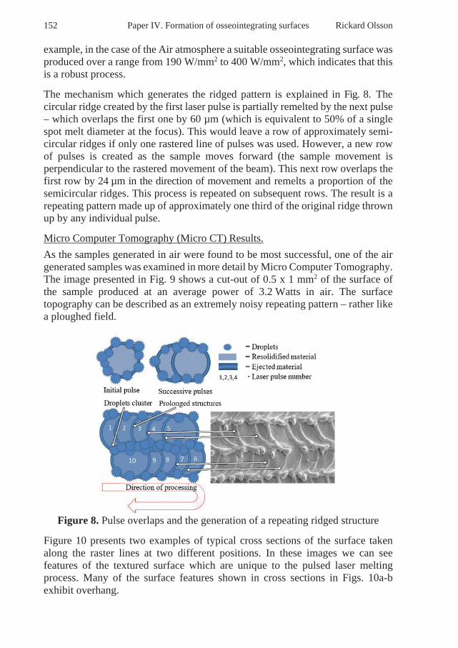
152 Paper IV. Formation of osseointegrating surfaces Rickard Olsson
example, in the case of the Air atmosphere a suitable osseointegrating surface was produced over a range from 190 W/mm2 to 400 W/mm2, which indicates that this is a robust process.
The mechanism which generates the ridged pattern is explained in Fig. 8. The circular ridge created by the first laser pulse is partially remelted by the next pulse – which overlaps the first one by 60 µm (which is equivalent to 50% of a single spot melt diameter at the focus). This would leave a row of approximately semi-circular ridges if only one rastered line of pulses was used. However, a new row of pulses is created as the sample moves forward (the sample movement is perpendicular to the rastered movement of the beam). This next row overlaps the first row by 24 µm in the direction of movement and remelts a proportion of the semicircular ridges. This process is repeated on subsequent rows. The result is a repeating pattern made up of approximately one third of the original ridge thrown up by any individual pulse.
Micro Computer Tomography (Micro CT) Results. As the samples generated in air were found to be most successful, one of the air generated samples was examined in more detail by Micro Computer Tomography. The image presented in Fig. 9 shows a cut-out of 0.5 x 1 mm2 of the surface of the sample produced at an average power of 3.2 Watts in air. The surface topography can be described as an extremely noisy repeating pattern – rather like a ploughed field.
Figure 8. Pulse overlaps and the generation of a repeating ridged structure
Figure 10 presents two examples of typical cross sections of the surface taken along the raster lines at two different positions. In these images we can see features of the textured surface which are unique to the pulsed laser melting process. Many of the surface features shown in cross sections in Figs. 10a-b exhibit overhang.

Rickard Olsson Paper IV. Formation of osseointegrating surfaces 153
The vast majority of roughened surfaces have a cross section similar to that shown in Fig. 11a. Overhanging features will not be created no matter how long this type of surface is abraded or grit blasted. However, when we are dealing with a resolidified surface melt, overhang can be a major feature of the topology – as shown in Fig. 11b. Resolidified ridges and droplets will tend to form overhanging features, and overhangs are excellent trapping geometries to collect particles, or in this case, the cells which need to accumulate to begin the osseointegration process.
Figure 9. A cut-out of 0.5x1 mm2 of the entire surface of the sample created at
3.2 Watts in (a) Air and (b) in a higher magnification view of the surface.
Figure 10. (a) Cross section of the sample and (b) a cross section of the sample
showing overhang and cavities associated with the surface

154 Paper IV. Formation of osseointegrating surfaces Rickard Olsson
Figure 11. (a) A standard roughened surface created by mechanical means does
not contain overhanging features. (b) A laser textured surface created by solidification of an active melt can contain a large number of overhanging
features
Conclusions
• Pulsed laser melting is a robust process for the generation of osseointegrating surfaces on the titanium substrates.
• The surface structure created includes re-solidified droplets between 1 and 10 microns in diameter and a pattern of ridges.
• The surface structure involves a considerable number of overhang features which are unique to the pulsed laser surface texturing process. These overhang features provide excellent traps for cells which eventually lead to osseointegration.
This study has benefits from a control perspective in defining the characteristics of the surface. We propose that the understanding of for instance droplet formation is critical for clinical success and that the results presented here not only are relevant for laser modified surface but may be extended to also other kinds of surfaces like implants made by Additive Manufactured (AM) technique.
Acknowledgments
The authors would like to thank the signature @etarena for invaluable help in finding the correct starting path through all of the opportunities in ImageJ.
References [1] Park J Y and Davies J E 2000 Red blood cell and platelet interactions with titanium
implant surfaces Clinical Oral Implants Research 11 530–9 [2] Brånemark P I, Hansson B O, Adell R, Breine U, Lindström J, Hallén O and Ohman A
1977 Osseointegrated implants in the treatment of the edentulous jaw. Experience from a 10-year period. Scandinavian journal of plastic and reconstructive surgery. Supplementum
[3] Vilar R 2016 Laser Surface Modification of Biomaterials: Techniques and Applications (Woodhead Publishing)
[4] Shah F A, Grandfield K and Palmquist A 2016 Laser surface modification and the tissue–implant interface Laser Surface Modification of Biomaterials ed R Vilar (Elsevier) pp 253–80
[5] Larsson C, Thomsen P, Aronsson B O, Rodahl M, Lausmaa J, Kasemo B and Ericson L E 1996 Bone response to surface-modified titanium implants: Studies on the early tissue response to machined and electropolished implants with different oxide thicknesses Biomaterials 17 605–16
[6] Voisey K T, Scotchford C A, Martin L and Gill H S 2014 Effect of Q-switched laser

Rickard Olsson Paper IV. Formation of osseointegrating surfaces 155
surface texturing of titanium on osteoblast cell response Physics Procedia 56 1126–35 [7] Brånemark R, Emanuelsson L, Palmquist A and Thomsen P 2011 Bone response to laser-
induced micro- and nano-size titanium surface features Nanomedicine:Nanotechnology, Biology and Medicine 7 220–7
[8] Palmquist A, Emanuelsson L, Brånemark R and Thomsen P 2011 Biomechanical, histological and ultrastructural analyses of laser micro- and nano-structured titanium implant after 6 months in rabbit Journal of Biomedical Materials Research Part B: Applied Biomaterials 97B 289–98
[9] Palmquist A, Emanuelsson L and Sjövall P 2012 Chemical and structural analysis of the bone-implant interface by TOF-SIMS, SEM, FIB and TEM: Experimental study in animal Applied Surface Science 258 6485–94
[10] Grandfield K, Gustafsson S and Palmquist A 2013 Where bone meets implant: the characterization of nano-osseointegration Nanoscale 5 4302
[11] Palmquist A, Engqvist H, Lausmaa J and Thomsen P 2012 Commercially Available Dental Implants: Review of Their Surface Characteristics Journal of Biomaterials and Tissue Engineering 2 112–24
[12] Palmquist A, Lindberg F, Emanuelsson L, Brånemark R, Engqvist H and Thomsen P 2010 Biomechanical, histological, and ultrastructural analyses of laser micro- and nano-structured titanium alloy implants: A study in rabbit Journal of Biomedical Materials Research Part A 92 1476–86
[13] Palmquist A, Engqvist H, Lausmaa J and Thomsen P 2012 Commercially Available Dental Implants: Review of Their Surface Characteristics Journal of Biomaterials and Tissue Engineering 2 112–24
[14] Shah F A, Johansson M L, Omar O, Simonsson H, Palmquist A and Thomsen P 2016 Laser-modified surface enhances osseointegration and biomechanical anchorage of commercially pure titanium implants for bone-anchored hearing systems PLoS ONE 11 1–24
[15] Brailovsky A B, Gaponov S V. and Luchin V I 1995 Mechanisms of melt droplets and solid-particle ejection from a target surface by pulsed laser action Applied Physics A Materials Science & Processing 61 81–6
[16] György E, Del Pino A P, Serra P and Morenza J L 2004 Structure formation on titanium during oxidation induced by cumulative pulsed Nd:YAG laser irradiation Applied Physics A: Materials Science and Processing 78 765–70
[17] György E, Pérez Del Pino A, Serra P and Morenza J L 2002 Surface nitridation of titanium by pulsed Nd:YAG laser irradiation Applied Surface Science 186 130–4
[18] György E, Mihailescu I ., Serra P, Pérez del Pino A and Morenza J . 2002 Single pulse Nd:YAG laser irradiation of titanium: influence of laser intensity on surface morphology Surface and Coatings Technology 154 63–7
[19] Khosroshahi M E, Mahmoodi M, Tavakoli J and Tahriri M 2008 Effect of Nd:Yttrium-aluminum-garnet laser radiation on Ti6Al4V alloy properties for biomedical applications Journal of Laser Applications 20 209–17
[20] Pfleging W, Kumari R, Besser H, Scharnweber T and Majumdar J D 2015 Laser surface textured titanium alloy (Ti-6Al-4V): Part 1 - Surface characterization Applied Surface Science 355 104–11
[21] Schindelin, J; Rueden, C.T.;Hiner M . at. al. 2015 Fiji: an open-source platform for biological-image analysis 671–5
[22] Legland D, Arganda-Carreras I and Andrey P 2016 MorphoLibJ: integrated library and plugins for mathematical morphology with ImageJ Bioinformatics 3532–4

156 Paper IV. Formation of osseointegrating surfaces Rickard Olsson

Rickard Olsson Paper V. Normal vector distribution as classification tool 157
Paper V
Normal vector distribution as a classification tool for convoluted rough surfaces with overhanging features

158 Paper V. Normal vector distribution as classification tool Rickard Olsson

Rickard Olsson Paper V. Normal vector distribution as classification tool 159
NORMAL VECTOR DISTRIBUTION AS A CLASSIFICATION TOOL FOR CONVOLUTED ROUGH SURFACES WITH OVERHANGING
FEATURES. Paper #0604
R. Olsson1,2, J. Powell1, J. Frostevarg1, A.F.H. Kaplan1
1Department of Engineering Sciences and Mathematics, Luleå University of Technology, 971 87 Luleå, Sweden;
http://www.ltu.se/research/subjects/Produktionsutveckling 2Laser Nova AB, SE-831 48 Östersund, Sweden;
Abstract
Convoluted rough surfaces involving overhanging features can be a natural consequence of Laser Additive Manufacturing and other spray techniques, or can be generated deliberately by laser surface texturing, e.g. to aid osseointegration. Overhanging features add an extra level of complexity to the topography of a rough surface and can have a substantial effect on wettability etc. However, features of this type are invisible to traditional surface roughness measurement techniques. This work presents a computer-based surface analysis method which gives useful information about the presence and nature of overhanging features on rough technical surfaces. The technique uses Micro Computer Tomography to generate a typical cross section of the surface under investigation. The angles of the vectors normal to the surface can then be analyzed to reveal the presence of overhanging features, which can also be indicated by the standard deviation of the normal vector distribution. Titanium surfaces generated by six different techniques were compared. The characteristics of these surfaces varied strongly, as did the shapes of the overhangs involved. These variations are reflected by different statistical distributions of the normal vectors.
Introduction With the advent of techniques such as laser additive manufacturing,[1] laser surface texturing [2] and thermal spray coating, new types of technical surface have become available which can involve overhanging features like those described in Figs 1a and Fig. 2. Overhanging features can be a consequence of the build-up of material by the impingement of laser-melted droplets, and can play an important role in medical implants, but have historically been difficult to classify. Such features add an extra level of complexity to the topography of a rough surface and can have a substantial effect on wettability etc. However, features of this type are invisible to traditional surface roughness measurement techniques and there is therefore a growing need for new surface analysis tools which can identify and quantify features such as overhangs.

160 Paper V. Normal vector distribution as classification tool Rickard Olsson
Measurement and categorization of such surfaces is difficult. Fig. 1(a) demonstrates the problem in measuring this type of complex, convoluted surface with mechanical stylus probes. A mechanical probe cannot identify overhanging features and also acts as a low pass filter that smooths out fine details. Similar problems arise with optical surface roughness measurement devices (e.g. interferometry, see Fig. 1(b)), and it is clear that theoretical (e.g. Ma [3] and experimental (e.g. Boschkler [4]) work on surface roughness generally fails to take overhanging features into account.
FIG 1. Overhanging surface features are invisible to traditional roughness measuring tools such as; (a) mechanical stylus profiling; (b) White Light
Interferometry (Wyko instrument)
Conoscopic Holography, first described by Sirat and Psaltis[5] in 1984 and later by Sirat[6,7], is a non-contact method based upon the holographic pattern received from a laser beam reflected off the sample surface. Its strengths and weaknesses for characterizing steel surfaces has been studied by e.g. Blanco[8]. However, even this high-tech method of surface measurement cannot provide information about overhanging features. Scanning Electron Microscopy (SEM) can provide phenomenological information about fine detail or the presence of overhangs, but information gathered by this technique is difficult to quantify. Occasionally, SEM is used with secondary electron detection for quantitative topology characterization of technical surfaces, Prolongo [9]. Tactile stylus methods for surface profilometry have been compared with confocal microscopy and interferometric methods (white light, WLI, phase shifting, PSI, etc.) by Vorburger.[10] This work, based on standardized surface properties, paid particular attention to the limitations of the various techniques as a function of surface profile slope.
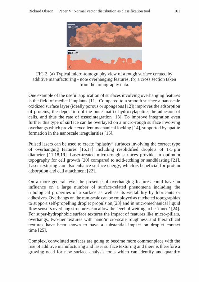
Rickard Olsson Paper V. Normal vector distribution as classification tool 161
FIG 2. (a) Typical micro-tomography view of a rough surface created by
additive manufacturing - note overhanging features, (b) a cross section taken from the tomography data.
One example of the useful application of surfaces involving overhanging features is the field of medical implants [11]. Compared to a smooth surface a nanoscale oxidized surface layer (ideally porous or spongeous [12]) improves the adsorption of proteins, the deposition of the bone matrix hydroxylapatite, the adhesion of cells, and thus the rate of osseointegration [13]. To improve integration even further this type of surface can be overlayed on a micro-rough surface involving overhangs which provide excellent mechanical locking [14], supported by apatite formation in the nanoscale irregularities [15]. Pulsed lasers can be used to create “splashy” surfaces involving the correct type of overhanging features [16,17] including resolidified droplets of 1-5 µm diameter [11,18,19]. Laser-treated micro-rough surfaces provide an optimum topography for cell growth [20] compared to acid-etching or sandblasting [21]. Laser texturing can also enhance surface energy, which is beneficial for protein adsorption and cell attachment [22]. On a more general level the presence of overhanging features could have an influence on a large number of surface-related phenomena including the tribological properties of a surface as well as its wettability by lubricants or adhesives. Overhangs on the mm-scale can be employed as ratcheted topographies to support self-propelling droplet propulsion,[23] and in micromechanical liquid flow sensors overhang structures can allow the level of wetting to be ‘tuned’ [24]. For super-hydrophobic surface textures the impact of features like micro-pillars, overhangs, two-tier textures with nano/micro-scale roughness and hierarchical textures have been shown to have a substantial impact on droplet contact time [25]. Complex, convoluted surfaces are going to become more commonplace with the rise of additive manufacturing and laser surface texturing and there is therefore a growing need for new surface analysis tools which can identify and quantify

162 Paper V. Normal vector distribution as classification tool Rickard Olsson
features such as overhangs, which are invisible to traditional roughness measurement techniques. Micro Computer Tomography (Micro-CT) can record very complex surfaces in great detail and can be used to present the information as 2D cross sections for further analysis. A typical tomographic view and cross section are presented in Fig. 2. X-ray CT is often used for surface analysis of internal shapes in technical applications such as nozzles, at a spatial resolution of 1-4 µm [26]. Surface normal vectors have been applied to identify features from medical X-ray CT applications, like lung cancer detection, where an elevation histogram along with an azimuthal histogram have been derived [27]. For surfaces generated by Additive Manufacturing (AM), which are covered with attached droplets, the topology obtained from X-ray CT can be processed further for stress analysis.[28] In this work by Kantzos et al. overhanging features and surface porosity were identified and visualized qualitatively. Quantitative analysis of AM-generated surfaces measured by X-ray CT has also been carried out, by comparing four surface determination techniques [29]. The method of local iterative surface determination was favoured over focus variation and other methods. Raw Micro-CT tomography data is difficult to interpret and requires statistical tools for its analysis and this paper presents a technique which can be used to identify whether a surface involves overhanging features or not. The technique involves analysis of the distribution of angles subtended by vectors normal to the surface. As Fig. 3a shows, rough surfaces created by grit blasting, abrasion etc. would only have surface-normal vectors over a small range of angles – which would never exceed 180°. On the other hand, surfaces with overhanging features, Fig. 3b, would have a much larger range of normal surface vectors. As we shall see, some overhanging features can introduce surface-normal angles up to 360°.

Rickard Olsson Paper V. Normal vector distribution as classification tool 163
FIG 3. Surface profiles with surface-normal vectors: (a) surface-normal vectors
for traditional rough surfaces would have a range of less than 180 degrees; (b) overhanging features introduce a much wider range of surface-normal
vectors
The idea of using surface-normal vectors and grouping these vectors into histograms for surface classification has been used by e.g. Tang [30] in computer vision applications using depth sensor information for recognition of objects and classification purposes. Similar techniques, using histograms of oriented normal vectors for object classification in computer vision applications have been used by e.g. Watanabe [31] and Dalal [32], but this approach has not previously been used for the classification of technical surfaces.
Methodology The aim of this study was to compare surfaces generated by six different methods to see if they could be classified from their surface-normal vector distribution. Titanium samples were prepared as follows: a. Grit Blasted surface; Grit blasted with Zirconium dioxide. b. Laser BioHelix™ surface; A proprietary laser-textured surface used for medical implants. c. AM surface. A surface produced by additive manufacturing using 50-100 µm powder. d. Brushed AM surface. The raw AM surface (as c. above) brushed with a steel brush. e. Abrasive sponged AM surface. The raw AM surface (as c above) brushed with an abrasive sponge. f. Etched AM surface: The raw AM surface (as c. above) etched with a zinc chloride solution. All six samples were analysed with a resolution of 0.5 µm in three dimensions, XYZ.

164 Paper V. Normal vector distribution as classification tool Rickard Olsson
Slices from Micro-CT 3D topographies of these samples were analysed in MatLab using the following steps: • Isolate region of interest from Micro-CT image. • Generate contour. • Calculate normal vectors at evenly spaced distances and normalize them to
unit length. • Calculate their distribution and present the results as a histogram. The second step, extracting the contour, was performed using “Snakes”, or “Active Contour Tracking” algorithms [33]. An active contour tracking algorithm is a computationally efficient way to track contours. These algorithms minimize the distance between the generated curve and the edge of an image and also minimize bending radii in the generated curve while maintaining a continuous contour and continuous first and second derivatives. For sake of simplicity in this initial study, a 2D-XZ-profile is extracted from the 3D-XYZ-surface measurement. Subsequently the normal vectors are calculated in the 2D-plane. For most overhanging features these 2D-projections or components of the 3D-vectors will be sufficient to give details of the overhangs. Future studies will also consider full 3D normal vector orientation, in order to gather all the information on the surface topology.
Assuming that the contour coordinates stored in a 2D-vector
then, the tangent vectors are calculated as; (1) running in the positive X-direction, i.e.
(2)
and the normal vectors are calculated as;
(3)
The reason behind the i-3, i+3 in equation (1) was to introduce a low pass filter to avoid edge effects and low angular resolution, because of the discrete nature of the pixel coordinates in the images. Calculating vectors using a length of 7 pixels gives an angular resolution of ~8 degrees and at the same time reduces contour noise. The choice of 7 pixels was found to be an optimum balance between angular resolution and noise sensitivity.
1
1
.. ..
.. ..N
N
x xX
y y=
3 3, 3.. 3.
i i iTV X X i N
+ −= − = −
1 6
1 6
.. ..
.. ..
N
N
tvx tvxTV
tvy tvy
−
−
=
1 6
1 6
.. ..
.. ..N
N
NVtvy tvy
tvx tvx−
−
=− −

Rickard Olsson Paper V. Normal vector distribution as classification tool 165
Results and Discussion Figure 4 presents low magnification SEM photographs of the six sample surfaces. Even at this magnification certain features of the surfaces are evident; The grit blasted surface is considerably smoother than any of the others. The appearance of the BioHelix surface makes it clear that it was produced as a pattern of overlapping lines (like a ploughed field), Olsson [34,35].
FIG 4. SEM images of the studied sample surfaces: (a) grit blasted, (b) laser
BioHelixTM, (c) raw AM, (d) steel-brushed AM, (e) abrasive sponge rubbed AM, (f) etched AM
The AM surface (c) and its etched counterpart (f) have the appearance of coral, with lots of overhanging features. The abraded AM samples (d) and (e) show evidence of some flattening of the ‘coral’ surface. Figure 5 presents Micro Computer Tomography images of the samples and these do not provide very much more information to that presented in Fig. 4. However, we can now take slices through the Micro-CT data to give cross sections from which we can identify the surface profile and its normal vector at any point. Figure 6 shows that the presence or otherwise of overhanging features on the surfaces is clearly demonstrated by this type of normal vector analysis. In Fig. 6a the low angular range of the normal vectors indicates a lack of overhanging features. This is what would be expected of a grit-blasted surface. Figures 6b-f clearly involve a much wider range of normal vector angles, indicating the presence of overhanging features in some cases.
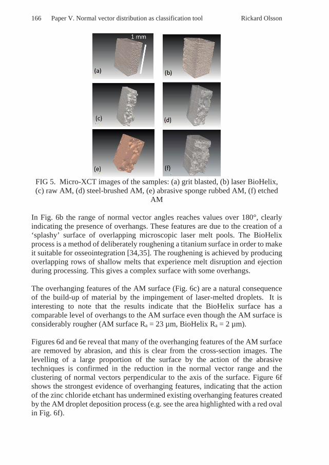
166 Paper V. Normal vector distribution as classification tool Rickard Olsson
FIG 5. Micro-XCT images of the samples: (a) grit blasted, (b) laser BioHelix, (c) raw AM, (d) steel-brushed AM, (e) abrasive sponge rubbed AM, (f) etched
AM
In Fig. 6b the range of normal vector angles reaches values over 180°, clearly indicating the presence of overhangs. These features are due to the creation of a ‘splashy’ surface of overlapping microscopic laser melt pools. The BioHelix process is a method of deliberately roughening a titanium surface in order to make it suitable for osseointegration [34,35]. The roughening is achieved by producing overlapping rows of shallow melts that experience melt disruption and ejection during processing. This gives a complex surface with some overhangs. The overhanging features of the AM surface (Fig. 6c) are a natural consequence of the build-up of material by the impingement of laser-melted droplets. It is interesting to note that the results indicate that the BioHelix surface has a comparable level of overhangs to the AM surface even though the AM surface is considerably rougher (AM surface Ra = 23 µm, BioHelix Ra = 2 µm). Figures 6d and 6e reveal that many of the overhanging features of the AM surface are removed by abrasion, and this is clear from the cross-section images. The levelling of a large proportion of the surface by the action of the abrasive techniques is confirmed in the reduction in the normal vector range and the clustering of normal vectors perpendicular to the axis of the surface. Figure 6f shows the strongest evidence of overhanging features, indicating that the action of the zinc chloride etchant has undermined existing overhanging features created by the AM droplet deposition process (e.g. see the area highlighted with a red oval in Fig. 6f).

Rickard Olsson Paper V. Normal vector distribution as classification tool 167
FIG 6. Surface profile images from micro-CT (upper image) and angular normal
vector distributions (lower image): (a) grit blasted, (b) laser BioHelix, (c) raw AM, (d) steel-brushed AM, (e) abrasive sponge rubbed AM, (f) etched AM
All these points are further clarified in Fig. 7, which presents the normal vector results as angles subtended to the axis of the surface (i.e. 0 and 180 degrees are parallel with the axis of the surface). A normal vector angle in excess of 180 degrees indicates the presence of overhanging features.
∆ x∆
011
0.05
0.50.5
0.1
00
0.15
-0.5-0.5-1-1
01 1
0.05
0.5 0.5
0.1
0 0
0.15
-0.5 -0.5-1 -1
101
0.05
0.50.5
0.1
00
0.15
-0.5-0.5-1-1
101 0.5
0.05
0.5 00
0.1
-0.5-0.5
0.15
-1-1
01 1
0.05
0.5 0.5
0.1
0 0-0.5
0.15
-0.5-1 -1
(b)
(c) (d)
(f) (e)
Overhang
α
100 µm
011
0.05
0.50.5
0.1
00
0.15
-0.5-0.5-1-1

168 Paper V. Normal vector distribution as classification tool Rickard Olsson
FIG 7. Angle distributions of normal vectors: (a) grit blasted, (b) laser BioHelix, (c) raw AM, (d) steel-brushed AM, (e) abrasive sponge rubbed AM, (f) etched
AM.
Figure 8 shows the surface-normal angle distribution of selected overhangs (see profiles in Fig. 6) in relation to the distribution over a wider scale (Fig. 7). As well as an angle histogram, each sub-figure of Fig. 8 contains a cross sectional monochrome outline of the overhang under consideration (as in Fig. 6, black is air). It is clear that the individual overhangs can have very different profiles. Overhangs are often asymmetrical and project either from the left (Figs. 8b,8f.2) or right (Figs. 8f.1,4,5), and this is evident from their vector distributions. While the surface in Fig. 6f has random orientation of overhangs in both directions, Fig. 6b shows a favoured anisotropic behaviour. Some overhangs have sharper normal angle distributions than others, indicating more elongated profiles. To some extent the characteristics of the overhang shapes can be derived from their vector distributions and this should be considered when creating algorithms to evaluate X-CT data from complex surface topologies. All the results presented in this work are taken from individual profiles of the complex surfaces but in future it should be possible to interpret the whole surface from the data collected by micro-computer tomography to produce a range of quantitative measures of the surface topography – including information identifying the presence and type of overhanging features. It should also be borne in mind that the work presented thus far only deals with convoluted surfaces created on otherwise flat, level substrates. If substrates with different geometries (tubes etc) were used the techniques would need to be adjusted to accommodate the underlying substrate macro geometry.

Rickard Olsson Paper V. Normal vector distribution as classification tool 169
FIG 8: Histogram (counts N vs. angle α) of selected overhang profiles compared to the histograms of the wider regions seen in Fig. 7. In each sub-figure there is a monochrome outline of the overhang under consideration (black = air) ; (a)
grit blasted, (b) laser BioHelix, (c) raw AM, (d) steel-brushed AM, (e) abrasive sponge rubbed AM, (f.1-5) etched AM, five selected overhang locations 1-5
Finally, it is interesting to note that a single number, the standard deviation of the normal vector values, can be used as a strong indicator of the presence of overhanging features on a convoluted surface. The standard deviations for our samples from Fig 7 are presented in Table I and it is clear that higher standard deviation values are associated with a more irregular surface and a greater tendency towards overhanging features.

170 Paper V. Normal vector distribution as classification tool Rickard Olsson
Table I. A statistical comparison of the six surface (ref Fig 7)
Surface
Share [%] of
overhangs
Normal angle
standard deviation [°]
(a) Grit-blasted 0% 16°
(b) Laser, BioHelix 2% 59°
(c) Raw AM 3% 52°
(d) Steel-brushed AM 0% 40°
(e) Abrasive sponge AM 2% 28°
(f) Etched AM 24% 79°
Conclusions
• Overhangs can be features of the very complex surface topologies created by laser AM or laser texturing.
• This work demonstrates that Micro Computer Tomography in combination with surface normal vector distribution analysis can be used to provide data and information about the presence of overhanging features on a rough surface.
• Surfaces with overhanging features will have normal vectors with values over 180 degrees.
• The standard deviation of the normal vector distribution can act as a single number indicator of surface complexity and the probable presence of overhanging features.
• The analytical method presented here can be used to extract quantitative information about the nature of the overhanging features on very complex laser-generated surfaces.
• This method has the advantage of being resolution independent i.e. finer resolution in the raw data gives finer resolution in the vectors calculated. In this particular case the Micro-CT resolution of 1µm together with a smoothing of 7 pixels gave a 8.1 degrees resolution between successive pixels.
• For the cases studied, different overhang shapes corresponded to different normal vector distributions.
Acknowledgements The authors would like to thank the Mid Sweden University, Sports Tech Research Centre for kindly providing AM Ti-samples. The authors are also grateful for funding granted by EU-ERDF-Interreg Nord project C3TS, no. 20201279.

Rickard Olsson Paper V. Normal vector distribution as classification tool 171
References [1] Wang Y M, Voisin T, McKeown J T, Ye J, Calta N P, Li Z, Zeng Z, Zhang
Y, Chen W, Roehling T T, Ott R T, Santala M K, Depond P J, Matthews M J, Hamza A V. and Zhu T . (2018) Additively manufactured hierarchical stainless steels with high strength and ductility Nature Materials. 17, 63–70.
[2] Patel D S, Singh A, Balani K and Ramkumar J . (2018) Topographical effects of laser surface texturing on various time-dependent wetting regimes in Ti6Al4V Surface and Coatings Technology. 349, 816–29.
[3] Ma J . (2007) Curvelets for surface characterization Applied Physics Letters. 90, 054109.
[4] Boschker J E and Tybell T . (2012) Qualitative determination of surface roughness by in situ reflection high energy electron diffraction Applied Physics Letters. 100, 151604.
[5] Sirat G and Psaltis D . (1985) Conoscopic holography Optics Letters. 10, 4.
[6] Sirat G Y . (1992) Conoscopic holography I Basic principles and physical basis Journal of the Optical Society of America A. 9, 70.
[7] Sirat G Y . (1992) Conoscopic holography II Rigorous derivation Journal of the Optical Society of America A. 9, 84.
[8] Blanco D, Valiño G, Fernández P, Rico J C and Palomo S . (2013) Influence of roughness on conoscopic holography digitizing of DIN34CrMo4 surfaces Procedia Engineering. 63, 472–80.
[9] Prolongo S G, Gude M R, Del Rosario G and Ureña A . (2010) Surface Pretreatments for Composite Joints: Study of Surface Profile by SEM Image Analysis Journal of Adhesion Science and Technology. 24, 1855–67.
[10] Vorburger T V., Rhee H-G, Renegar T B, Song J-F and Zheng A . (2007) Comparison of optical and stylus methods for measurement of surface texture The International Journal of Advanced Manufacturing Technology. 33, 110–8.
[11] Rupp F, Liang L, Geis-Gerstorfer J, Scheideler L and Hüttig F . (2018) Surface characteristics of dental implants: A review Dental Materials. 34, 40–57.
[12] Grandfield K, Gustafsson S and Palmquist A . (2013) Where bone meets implant: the characterization of nano-osseointegration Nanoscale. 5, 4302.
[13] Furquan A. Shah . (2014) The bone-implant interface - nanoscale analysis of clinically retrieved dental implants 10, 1729–37.
[14] Brånemark R, Emanuelsson L, Palmquist A and Thomsen P . (2011) Bone response to laser-induced micro- and nano-size titanium surface features Nanomedicine:Nanotechnology, Biology and Medicine. 7, 220–7.
[15] Wang X, Shah F A, Palmquist A and Grandfield K . (2017) 3D Characterization of Human Nano-osseointegration by On-Axis Electron Tomography without the Missing Wedge ACS Biomaterials Science & Engineering. 3, 49–55.
[16] Sisti K E, de Rossi R, Antoniolli A M B, Aydos R D, Guastaldi A C,

172 Paper V. Normal vector distribution as classification tool Rickard Olsson
Queiroz T P, Garcia I R, Piattelli A and Tavares H S . (2012) Surface and Biomechanical Study of Titanium Implants Modified by Laser With and Without Hydroxyapatite Coating, in Rabbits Journal of Oral Implantology. 38, 231–7.
[17] Liang C, Wang H, Yang J, Cai Y, Hu X, Yang Y, Li B, Li H, Li H, Li C and Yang X . (2013) Femtosecond laser-induced micropattern and Ca/P deposition on Ti implant surface and its acceleration on early osseointegration ACS Applied Materials and Interfaces. 5, 8179–86.
[18] Palmquist A, Johansson A, Suska F, Brånemark R and Thomsen P . (2013) Acute Inflammatory Response to Laser-Induced Micro- and Nano-Sized Titanium Surface Features Clinical Implant Dentistry and Related Research. 15, 96–104.
[19] Palmquist A, Emanuelsson L and Sjövall P . (2012) Chemical and structural analysis of the bone-implant interface by TOF-SIMS, SEM, FIB and TEM: Experimental study in animal Applied Surface Science. 258, 6485–94.
[20] Mirhosseini N, Crouse P L, Schmidth M J J, Li L and Garrod D . (2007) Laser surface micro-texturing of Ti–6Al–4V substrates for improved cell integration Applied Surface Science. 253, 7738–43.
[21] Nayar S, Bhuminathan, Mahadevan, Santhosh S and Vignesh . (2015) Comparative evaluation of the three different surface treatments - conventional, laser and Nano technology methods in enhancing the surface characteristics of commercially pure titanium discs and their effects on cell adhesion: An in vitro study Journal of Pharmacy and Bioallied Sciences. 7, 89.
[22] Pfleging W, Kumari R, Besser H, Scharnweber T and Majumdar J D . (2015) Laser surface textured titanium alloy (Ti-6Al-4V): Part 1 - Surface characterization Applied Surface Science.
[23] Arter J M, Cleaver D J, Takashina K and Rhead A T . (2018) Self-propelling Leidenfrost droplets on a variable topography surface Applied Physics Letters. 113, 243704.
[24] Peiker P and Oesterschulze E . (2015) Geometrically tuned wettability of dynamic micromechanical sensors for an improved in-liquid operation Applied Physics Letters. 107, 1–5.
[25] Lv C, Hao P, Zhang X and He F . (2016) Drop impact upon superhydrophobic surfaces with regular and hierarchical roughness Applied Physics Letters. 108, 141602.
[26] Li Z, Zhao W, Wu Z, Gong H, Hu Z, Deng J and Li L . (2018) The measurement of internal surface characteristics of fuel nozzle orifices using the synchrotron X-ray micro CT technology Science China Technological Sciences. 61, 1621–7.
[27] Choi W J and Choi T S . (2014) Automated pulmonary nodule detection based on three-dimensional shape-based feature descriptor Computer Methods and Programs in Biomedicine. 113, 37–54.
[28] Kantzos C A, Cunningham R W, Tari V and Rollett A D . (2018) Characterization of metal additive manufacturing surfaces using

Rickard Olsson Paper V. Normal vector distribution as classification tool 173
synchrotron X-ray CT and micromechanical modeling Computational Mechanics. 61, 575–80.
[29] Townsend A, Pagani L, Blunt L, Scott P J and Jiang X . (2017) Factors affecting the accuracy of areal surface texture data extraction from X-ray CT CIRP Annals - Manufacturing Technology. 66, 547–50.
[30] Tang S, Wang X, Lv X, Han T X, Keller J, He Z, Skubic M and Lao S . (2013) Histogram of Oriented Normal Vectors for Object Recognition with a Depth Sensor Lecture Notes in Computer Science (including subseries Lecture Notes in Artificial Intelligence and Lecture Notes in Bioinformatics) vol 7725 LNCS pp 525–38
[31] Watanabe T, Ito S and Yokoi K . (2009) Co-occurrence histograms of oriented gradients for pedestrian detection Lecture Notes in Computer Science (including subseries Lecture Notes in Artificial Intelligence and Lecture Notes in Bioinformatics). 5414 LNCS, 37–47.
[32] Dalal N and Triggs W . (2004) Histograms of Oriented Gradients for Human Detection 2005 IEEE Computer Society Conference on Computer Vision and Pattern Recognition CVPR05. 1, 886–93.
[33] Kass M, Witkin A and Terzopoulos D . (1988) Snakes: Active contour models International Journal of Computer Vision. 1, 321–31.
[34] Olsson R, Powell J, Palmquist A, Brånemark R, Frostevarg J and Kaplan A F H . (2018) Production of osseointegrating (bone bonding) surfaces on titanium screws by laser melt disruption Journal of Laser Applications. 30, 042009.
[35] Olsson R, Powell J, Palmquist A, Brånemark R, Frostevarg J and Kaplan A F H . (2019) Formation of osseointegrating (bone integrating) surfaces on titanium by laser irradiation Journal of Laser Applications. 31, 022508.


Rickard Olsson Paper VI. Topographical evaluation 175
Paper VI
Topographical evaluation of laser generated surfaces using
statistical analysis of surface-normal vector distributions

176 Paper VI. Topographical evaluation Rickard Olsson
Rickard Olsson Paper VI. Topographical evaluation 177
Topographical evaluation of laser generated surfaces using statistical analysis of surface-normal vector distributions
R. Olsson*1,2, J. Powell1, J. Frostevarg1, A.F.H. Kaplan1 1Department of Engineering Sciences and Mathematics, Luleå University of Technology, 971 87 Luleå, Sweden; http://www.ltu.se/research/subjects/Produktionsutveckling 2Laser Nova AB, SE-831 48 Östersund, Sweden; Abstract Surfaces generated by Additive Manufacturing or laser texturing can involve the solidification of droplets of liquid, which can give rise to overhanging features on the solidified surface. Overhanging features add a layer of complexity to the surface topology and are invisible to standard profilometry and surface roughness measurement techniques. Such features are important because they can have a considerable effect on surface properties such as wettability. New techniques and algorithms are therefore required to analyse and quantify convoluted surfaces with overhanging features. Earlier work by the authors introduced the concept of using X-ray micro-computer-tomography to identify the directions of vectors normal to the surface at any point and thus the presence or otherwise of overhanging features. This paper divides overhanging features into two types; simple and compound, and introduces new analysis techniques which measure what proportion of each type is on the surface. Another extension of the analysis is to compare surface traces taken in different directions in order to identify any surface roughness anisotropies. This work also presents a method for identifying any periodicity in convoluted surfaces which do not lend themselves to Fourier analysis.
1. Introduction Additive manufacturing [1], laser surface texturing [2] and thermal spray coating, often involve the attachment of droplets to a solid substrate. These techniques can generate new types of technical surface which include overhanging features like those described in Fig. 1. Overhanging features of this sort cannot be measured by mechanical or optical surface roughness measuring tools.

178 Paper VI. Topographical evaluation Rickard Olsson
Fig. 1. For surface profiles, overhanging features are invisible to traditional roughness measuring devices, such as (a) mechanical stylus profiling or (b)
White Light Interferometry (here measured by a Wyko instrument)
For example, Vorburger et.al. [3] compared tactile stylus methods for surface profilometry with confocal microscopy and interferometric methods (white light, WLI, phase shifting, PSI, etc.). This work, based on standardized surface properties, paid particular attention to the limitations of the various techniques as a function of surface profile slope. One conclusion of this work is that overhanging features are invisible to these measurement methods.
Conoscopic Holography, first described by Sirat and Psaltis [4] in 1984 and later by Sirat [5,6], is a non-contact method based upon the holographic pattern received from a laser beam reflected off the sample surface. Its strengths and weaknesses for characterizing steel surfaces have been studied by e.g. Blanco et.al. [7]. However, even this high-tech method of surface measurement cannot provide information about overhanging features. Scanning Electron Microscopy (SEM) can provide phenomenological information about the presence of overhangs, but information gathered by this technique is difficult to quantify. Occasionally, SEM is used with secondary electron detection (Prolongo et.al. [8]) or Shear Force Microscopy (Romoli [9]) for quantitative characterization of technical surfaces. In recent years an analytical study of the strengths, weaknesses and practical challenges of using 2D spectral analysis for texture analysis of artificially generated surfaces has been presented by Jacobs et.al. [10]. In this work three factors; artefacts arising from windowing (finite length of the data), tilt and skew between sensors and surface and finally the impact of sensor shape were examined. In general, theoretical (Ma [11]) and experimental (Boschkler and Tybell [12]) work on surface roughness has generally failed to take overhanging features into account.
Rickard Olsson Paper VI. Topographical evaluation 179
It is important to know whether or not a surface contains overhanging features because they can have a substantial effect on the macro and micro properties of the surface in such fields as wetting [2] (lubrication, adhesive bonding, biocompatibility etc.) and tribology. Overhangs on the mm-scale can even be employed as ratcheted topographies to support self-propelling droplet propulsion [13], and in micromechanical liquid flow sensors, overhanging structures can allow the level of wetting to be ‘tuned’ [14]. For super-hydrophobic surface textures the impact of features like micro-pillars, overhangs, two-tier textures with nano/micro-scale roughness and hierarchical textures have been shown to have a substantial impact on droplet contact time [15]. Li et al. carried out work on the creation of super-hydrophobic and anti-adhesive surfaces created on aluminium substrates by pulsed laser irradiation. Such surfaces involved micro-craters surrounded by re-solidified droplets but the influence of the overhanging nature of these surface features was not investigated [16]. One example of the useful application of surfaces involving overhanging features is the field of medical implants [17]. The classification of implant surface structures is a field where e.g. Wennerberg and Albrektsson [18] have pointed out the need for a more uniform terminology and have created a set of guidelines for topographic evaluation of surface defining parameters such as form, waviness and roughness. Compared to a smooth surface, a nanoscale oxidized surface layer (ideally porous or spongeous [19]) improves the adsorption of proteins, the deposition of the bone matrix hydroxylapatite, the adhesion of cells, and thus the rate of osseointegration [20] To improve integration even further, this type of surface can be overlayed on a micro-rough surface involving overhangs which provide excellent mechanical locking [21], supported by apatite formation in the nanoscale irregularities [22] Pulsed lasers can be used to create “splashy” surfaces involving the correct type of overhanging features [23,24] including re-solidified droplets of 1-5 µm diameter [17,25,26]. Laser-treated micro-rough surfaces have been shown to provide an excellent topography for cell growth [27] compared to acid-etching or sandblasting.[28] Laser texturing can also enhance surface energy, which is beneficial for protein adsorption and cell attachment [29]. Wennerberg et al. [30] in their study of bone response to different surface roughness, also pointed out the limitations of Ra and Sa as measures when comparing different textures. Laser structuring by overlapping Nd:YAG-laser pulses of various pulse-frequencies and powers on cylindrically shaped Al2O3 structures is described by Kibria [31]. In this study SEM-analysis was used to study the surfaces generated regarding roughness and it was pointed out how useful the SEM-instrument is for surface analysis. Later, Kibira [32] developed this work further, now looking into surface structuring of Titanium and how the roughness was affected by scan speed, average power and pulse overlap. Similar work on the influence of process

180 Paper VI. Topographical evaluation Rickard Olsson
parameters on titanium surface structuring has been carried out by Aguilar-Morales et al. [33]. For surfaces generated by Additive Manufacturing (AM), which are covered with attached droplets, the topology obtained from X-ray computer tomography (X-ray CT) can be processed further for stress analysis [34]. In this work by Kantzos et al. overhanging features and surface porosity were identified and visualized qualitatively. Quantitative analysis of AM-generated surfaces measured by X-ray CT has also been carried out, by comparing four surface determination techniques [35]. A thorough description about classification of complex surfaces (periodic, non-periodic, etc.) can be found in “A Taxonomy for Texture Description and Identification” by Rao [36]. Earlier work by the present authors [37–39] introduced a new approach for the characterization of complex surfaces which enables a quantitative description of overhanging features. The technique uses computer micro-tomography to map the surface. From the tomography data cross sectional traces are generated, which include all the overhanging features (see Fig. 2).
Fig. 2. (a) Typical micro-tomography view of a rough surface created by
additive manufacturing - note overhanging features, (b) a cross section taken from the tomography data
These cross sectional surface traces can have equally spaced surface-normal vectors allocated to them as shown in Fig. 3. Statistical tools can then be employed to analyse the variation in surface-normal vector inclination for different types of surface. The use of normal vector histograms for surface classification has been explored by e.g. Tang[40] in computer vision applications using depth sensor information for the recognition of objects and for object classification. Similar techniques, using histograms of normal vectors for object classification in computer vision applications have been used by e.g. Watanabe [41] and Dalal [42], but this approach has not previously been used for the classification of technical surfaces.

Rickard Olsson Paper VI. Topographical evaluation 181
Fig. 3. Surface profiles with equi-spaced surface-normal vectors: (a) surface
normal vectors for mechanically roughened surfaces would have an inclination range of less than 180 degrees; (b) overhanging features introduce a much wider
range of surface normal vectors
For technical surfaces created by the accumulation of droplets, the distribution of the angles of surface-normal vectors can give quantitative and qualitative information about the presence or otherwise of overhanging features. This paper builds on the earlier work and presents, for the first time, analytical techniques for identifying two types of overhang; simple and compound. Both types of overhang can have a negative effect on wettability, but compound overhangs have a greater ability to trap air and thereby prevent local wetting. This work also presents a statistical tool which can be used for identifying cyclic patterns within the roughness of convoluted surfaces.
2. Methodology Four different types of surface were created for this investigation. Titanium samples were prepared as follows:
• A grit blasted surface; grit blasted with Zirconium dioxide. • A Laser BioHelix™ surface; a proprietary laser-textured surface employed
for medical implants. • An Additive Manufactured (AM) surface; produced by additive
manufacturing using 50-100 µm powder. • An etched AM surface; The raw AM surface (as c above) subsequently
etched with a zinc chloride solution.
All four samples were analysed with a Micro-CT (micro-computer tomography) instrument Zeiss XRADIA 510 Versa with a resolution of 0.5 µm in X-, Y- and Z-direction. Slices from the Micro-CT 3D topographies of these samples were analysed in a MATLAB-code using the steps described in in Table 1 and illustrated in Fig. 4. This produced histograms of the distribution of the surface-normal vectors for each cross-section.

182 Paper VI. Topographical evaluation Rickard Olsson
Table 1. The workflow applied in generating the surface-normal vector histograms.
Step Task a. b. c.
Roughly isolate the region of interest (ROI) from Micro-CT image. Isolate the ROI in detail. Generate contour.
d. Calculate normal vectors at evenly spaced distances and normalize them to unit length.
e. Calculate their distribution and present the results as a histogram (see Fig. 4).
Fig 4. Example surface profile for the workflow: (a) surface profile with six
different domains numbered (1)-(6), (b) calculation of equidistant surface vectors, (c) normal vector angle as a function of the curve position along the
profile, (d) histogram of normal vector angles
The generation of the contour (step c in table 1) was performed using “Snakes”, or “Active Contour Tracking” algorithms [43]. An active contour tracking algorithm is a computationally efficient way to track contours. These algorithms minimize the distance between the generated curve and the edge of an image and also minimize bending radii in the generated curve while maintaining a continuous contour and continuous first and second derivatives. The basic idea of the snakes algorithm is to introduce an energy for the contour/snake of the curve v(s), at points s on the curve of length L. This energy consists of three components:
0,s L ∈

Rickard Olsson Paper VI. Topographical evaluation 183
• An internal energy, Einternal controlling the contour’s elasticity and stiffness. • An external energy, Eexternal controlling the how well the contour matches
the image locally. Often this energy is defined as the absolute magnitude of the local gradient at that point.
• Constraint forces, Econstraint encouraging continuity of the curve and punishing sudden jumps. This term is application dependent and can be applied to manually favour or omit certain features in an image. It may also be omitted. There is no general expression for constraint forces.
The goal is to gradually adjust the curve by iterating the expression to get the minimum energy. The internal energy can be defined as:
, (1)
where the coefficient controls the elasticity/stretch and controls the stiffness/bending. The external energy is defined as
. (2)
This leads to a total energy function (in a continuous case) for a curve of (in each iteration) length L
. (3)
The normal vectors were calculated as follows:
Assuming that the contour coordinates stored in a 2D-vector ,
then the tangent vectors are calculated as; (4)
running in the positive X-direction, i.e.
(5)
and the normal vectors are calculated as;
(6)
The reason behind the indices i-3, i+3 in equation (4) was to introduce a low pass filter to avoid edge effects and low angular resolution, because of the discrete
22 2
int 2( ) ( )ernaldE s sds sν να β ∂= +
∂( )sα ( )sβ
2( , )externalE I x y=−∇
int int0
int int0 0 0
( ) ( ) ( )
L
snake ernal external constra
L L L
ernal external constra
E E E E
E v s ds E v s ds E v s ds
= + + =
+ +
∫
∫ ∫ ∫
1
1
.. ..
.. ..N
N
x xX
y y
=
TV
3 3 , 3.. 3. i i iTV X X i N+ −= − = −
1 6
1 6
.. ..
.. ..N
N
tvx tvxTV
tvy tvy−
−
=
1 6
1 6
.. ..
.. ..N
NNV
tvy tvytvx tvx
−
−
=
− −
184 Paper VI. Topographical evaluation Rickard Olsson
nature of the pixel coordinates in the images. Calculating vectors using a length of 7 pixels gives an angular resolution of ~8 degrees and at the same time reduces contour noise. The choice of 7 pixels was found to be an optimum balance between angular resolution and noise sensitivity. Figures 5(a) and (b) demonstrate two types of overhanging feature which can be created by additive manufacturing and other droplet deposition techniques; Simple and Compound overhangs. An overhanging feature can be generally described as any object which would cast a shadow if exposed to a light shining directly down upon it. Within this category there are sub-categories which could be important to surface phenomena such as wetting. For example, Fig. 5(a) shows a cross section of a simple overhanging feature which might be generated by a single molten droplet attaching itself to a substrate. Depending on the geometry of this type of overhang, and the viscosity/surface tension of the liquid involved, it might be possible to fully wet all of this surface. Fig. 5(b) on the other hand, shows a cross section of a more complex ‘compound’ overhang. In this case it would not be possible to entirely wet this surface because any encroaching liquid would find certain areas of the surface blocked by air bubbles trapped by the geometry of the compound overhang. Compound overhangs cannot be adequately described or identified using a 0-360 degree scale for the direction of normal vectors which was employed in earlier work [39]. It is clear from Fig. 5(b) that, using a 360 degree scale, the shape of this compound overhang would, for example, give rise to two different types of area where the surface normal vector would be 270 degrees (i.e. vertically downwards). For this reason we have developed the surface-normal vector angle analysis to include a range of angles greater than 360 degrees. Fig. 5(c) helps to provide an explanation of this approach. The assignment of angles to the surface normal vectors assumes that the surface contour is a line which is followed from its left hand end to its right hand end (i.e. in the positive x-direction). Surface normal vectors are calculated at equally spaced distances along this line. The angular value given to any vector is incrementally increased or decreased in comparison to the previous value depending on whether the normal vectors are progressing in an anticlockwise or clockwise direction. In this way two different numerical angular values will be given for the same surface-normal vector direction depending on what the previous vector value was. This allows us to differentiate between simple and compound overhangs.

Rickard Olsson Paper VI. Topographical evaluation 185
Fig 5. (a) A simple overhang surface profile, which might allow full surface
wetting; (b) a ‘compound’ overhang surface profile, which would prevent full surface wetting due to trapped air bubbles; (c) surface normal vectors along the
compound overhang surface profile. The presence of surface-normal vector angles greater than 270º degrees of or lower than -90º is indicative of a
compound overhang. Angles in the ranges 0º to -90º (but no lower) or 180º to 270º (but no higher) indicate simple overhangs; (d) illustration of expressing the curve as a sum of linear sections Ti, each of equal length δ, with corresponding
surface normal vectors Ni (starting at position P0) Fig. 5(c) contains only the ordinal vectors (which are not equally spaced) in order to illustrate this point. In this example the initial change in vector angle is from 90 (vertically upwards) to 450 (also vertically upwards). Between these two points the angle continuously increases to 450 because the progression of vector angle values was anticlockwise. At the point at which the value of 450 degrees is

186 Paper VI. Topographical evaluation Rickard Olsson
reached the angle progression changes to clockwise and all subsequent angular values are continuously reducing until we reach the next vertically upwards vector (at the top of the object) which now has an angular value of 90 degrees. Comparison between Fig. 5(a) and Fig. 5(c) makes it clear that the limits on surface normal vector achievable by a simple (non-compound) overhanging feature using this system would be a highest value of 270 degrees and a lowest value of -90 degrees. Therefore angles outside this range are indicative of the presence of compound overhangs. Table 2 summarises the angular ranges of surface-normal vectors for surfaces with no overhangs, simple overhangs and compound overhangs. Table 2. Angular ranges of surface-normal vectors for different surface features Surface feature type Surface-normal vector inclination range No overhangs 0º to 180º Simple overhangs -90º to 0º and/or 180º to 270º Compound overhangs Below -90º and/or above 270º
Figure 6 shows a typical result from the raw Additive Manufacturing sample investigated in this work as an example of how to interpret the surface-normal vector histograms which will be presented in the results section. The thresholds for simple and compound overhangs, see Table 2, are both exceeded in this example showing that both types of overhang are present on the surface. This is confirmed by observation of the black and white image of the cross section at the top of the figure. One of the aims of this work is to develop tools which could be used to identify repeating patterns in the surface roughness which might be correlated to process parameters. For eample the Biohelix process produces a regular pattern of laser surface melts. If we consider the surface profile to be a signal then frequency analysis should reveal this repeating pattern. However, this simple approach is not possible in this case because, when overhangs are involved, the ‘curve’ of the surface trace sometimes includes two or more y values for the same x value, i.e. it has ambiguous coordinates. For a standard frequency (Fourier or Laplace) analysis it is important that the curve in question is single valued, i.e. unambiguous. One way to get around this problem is not to express the profile curve not as y=f(x) but to divide it up into a succession of linear segments – as shown in Fig. 5(d).

Rickard Olsson Paper VI. Topographical evaluation 187
Fig 6. Surface profile (raw AM) with compound overhangs (upper) and its histogram (lower) with thresholds of the angle ranges for no, simple and
compound overhang, respectively. If the profile curve is divided up into short straight lines each of equal length δ, pointing in the tangential direction (see Fig. 5(d)), the position at a point Pi on the curve, can then be expressed as:
(7)
Calculating the normal vectors from the tangents and plotting normal vector angle vs. position now gives a single-valued set of data which is suitable for frequency analysis. This technique is used later in this paper to search for repeating patterns in the surface roughness of the samples.
3. Results and Discussion Fig. 7 presents Micro Computer Tomography images of the four sample surfaces. From these photographs certain features of the surfaces are evident;
• The grit blasted surface is considerably smoother than any of the others. • The appearance of the BioHelix surface makes it clear that it was produced
as a pattern of overlapping lines (like a ploughed field) Olsson [37]. • The AM surface (c) and its etched counterpart (d) have larger surface
features than the BioHelix sample and the grit blasted sample.
00
i
i kk
P P Tδ=
= +∑

188 Paper VI. Topographical evaluation Rickard Olsson
Fig. 7. Micro-CT images of the samples: (a) grit blasted, (b) laser BioHelix, (c)
raw AM, (d) etched AM
We can now take slices through the Micro-CT data to give cross sections from which we can identify the surface profile and its normal vector at any point. Following the procedure laid out in Table 1 and Fig. 4. Figure 8 presents typical profile cross sections of the four samples together with the histograms of the surface-normal vector distributions. Fig. 8(a) confirms the assumption that grit blasting does not create overhanging features in a surface. In this case the range of surface-normal vector inclinations is only 85 degrees; from 50 to 135, with a standard deviation of only 16 degrees. In the case of the BioHelix sample, Fig. 8(b), the range of vector angles is much wider; from -122 degrees to 160, with a standard deviation of 59 degrees. The existence of angles below -90 clearly indicates that there are simple and compound overhanging features on this surface. The presence of such features is obvious in the SEM image of this surface presented in Fig. 9. The BioHelix process is a method of deliberately roughening a titanium surface in order to make it suitable for osseointegration [37,38]. The roughening is achieved by producing a ‘splashy’ surface of overlapping rows of shallow welds that experience melt disruption and ejection during processing. This gives a complex surface with some overhangs. The span of surface-normal vector inclinations and their standard deviations are presented in Table 3 together with the relevant Ra roughness measurements.

Rickard Olsson Paper VI. Topographical evaluation 189
Fig 8. Typical surface profiles of the four samples together with the histograms
of the surface-normal vector distributions: (a) grit blasted, (b) laser BioHelix, (c) raw AM, (d) etched AM
Table 3. Statistical surface properties (surface-normal angle range and roughness) of the four surfaces
Surface Standard deviation of the angles (°)
Angular range (°) of surface-
normal vectors. Ra (µm)
Grit-blasted 16 50 to 135 1.5 Laser BioHelix 59 -122 to 160 2 Raw AM 52 -190 to 270 24 Etched AM 79 -153 to 321 16

190 Paper VI. Topographical evaluation Rickard Olsson
Fig. 9. This higher magnification SEM image of the laser BioHelix sample
surface reveals the presence of overhanging features As might be expected the Raw Additive Manufacturing surface Fig. 8(c) also has a considerable number of overhanging features, surface-normal vector angles from -190 to 270 degrees. The overhanging features of the AM surface are a natural consequence of the build-up of material by the impingement of laser-melted droplets. It is interesting to note that the results indicate that the level of overhanging features on a surface is not related to Ra roughness (see Table 3). Figure 8(d) shows the strong evidence of overhanging features for the etched AM surface, with an inclination angle range of between -153 and 321 degrees. Further investigation of this surface (compare Figs. 8(c) and (d)) indicates that the action of the zinc chloride etchant has undermined existing overhanging features created by the AM droplet deposition process (see the area highlighted with a red oval in Fig. 8(d). The next stage in our analysis of these surfaces was to investigate the differences between tomography cross sections taken in different directions across the sample surface. Slices from each sample were taken using the ParaView-software [44] at four different angles; 0°, 45°, 90° and 135°, as shown in Fig. 10(a)-(d).

Rickard Olsson Paper VI. Topographical evaluation 191
Fig. 10. The four chosen slicing orientations to extract surface profiles from 3D-
data measured by Micro CT: (a) 0°, (b) 45°, (c) 90°, (d) 135°. The sliced results for the four directions in each of the four samples are
presented in Figs 11-14
Figure 11 shows no noticable trends between the cross section directions, with a low level of roughness and low levels of inclination of the surface normal vectors. There are no vector angles below zero or above 180 and so no overhanging features of any sort are present. This is the expected result from a random roughness grit blasted surface. Figs. 13 and 14 also show minimal evidence of differences in profile or normal vector distribution between the four different sampling directions. For these samples there is evidence of simple and compound overhangs in both the cross section images and the vector histograms. Fig. 13 generally has a cluster of vector direction at 90 degrees which is not as distinct in the case of Fig. 14. This indicates that the AM surface has a flatter surface than the etched AM sample. Figure 12 is the only sample which shows clear directional differences between the traces, i.e. anisotropy. The BioHelix sample shows evidence of simple and occassional compound overhangs but also appears to have a repeating pattern within the general roughness in certain cross sectional directions. This makes sense because the surface is generated from parralell rows of surface ‘splashes’ created at a pitch of 59 µm between laser pulses.

192 Paper VI. Topographical evaluation Rickard Olsson
Fig. 11. Grit blasted sample; (a) surface profiles and (b) normal vector angle distribution for the four slicing angle orientations; the angle limits for simple
and compound overhang are highlighted
Fig. 12. BioHelix sample; (a) surface profiles and (b) normal vector angle
distribution for the four slicing angle orientations; the angle limits for simple and compound overhang are highlighted
In order to carry out frequency analysis on the profiles they were divided up into short tangential lines, as discussed earlier with reference to Fig. 5(d) and Equation 7. This subsequent plotting of normal vector angle against position produces the type of results shown in Fig. 15(a,b), which give the results for the 90 degree trace in Fig. 12(c). In Fig. 15(b) a peak can be seen which correlates to a sequence of strong angular twists with a spatial period 59 µm, or 16.9 mm-1, which correlates very well with the laser processing parameters which involved a pulse to pulse distance of 59 µm on the material surface. Figs. 15(c),(d) give the same information for a typical grit blasted surface result and, as would be expected, there is no evidence of a repeating pattern. This demonstrates that this analysis technique is useful in identifying the wavelength of repeating patterns on convoluted surfaces which involve simple and compound overhanging features.

Rickard Olsson Paper VI. Topographical evaluation 193
Fig. 13. Raw AM sample; (a) surface profiles and (b) normal vector angle
distribution for the four slicing angle orientations; the angle limits for simple and compound overhang are highlighted
Fig.14. Etched AM sample; (a) surface profiles and (b) normal vector angle distribution for the four slicing angle orientations; the angle limits for simple
and compound overhang are highlighted
The final stage in this work was to estimate how much of the surface would be shadowed by overhanging features if illuminated from directly above (i.e. how much of the surface is involved in overhanging features). This was calculated by establishing the proportion of surface-normal vectors which were above the inclination thresholds for simple and compound overhangs. The results are presented in Table 4.

194 Paper VI. Topographical evaluation Rickard Olsson
Fig. 15. (a) Surface normal angle along the curve position for Laser Biohelix 90
sample, (b) spatial frequency distribution for the Laser Biohelix 90 sample, identifying the repeating pattern (peak) with a spatial periodicity of 59 µm, (c) surface normal angle along the curve position for the grit blasted sample, (d) spatial frequency distribution for the grit blasted sample showing no distinct
repeating pattern. Table 4 reveals the following points; Once again we can see that there are no overhanging features on the grit blasted surface. The laser-Biohelix surface has evidence of simple overhanging features with a small amount of compound overhangs. Approximately 25% of the Raw AM surface is covered by simple overhangs and, on average, 1.25% of the surface involves compound overhangs. In the case of the etched AM surface approximately 40% of the surface is covered in simple overhangs with 2% of the surface having compound overhangs. This could be expected as a result of etchant corrosion undermining the overhangs created by the AM process.

Rickard Olsson Paper VI. Topographical evaluation 195
Table 4. The proportion of the sample surface covered by simple and compound overhangs expressed as a percentage of the width of the sample, for the four
slicing angles
Trace angles (°) Proportion of
simple overhang (%)
Proportion of compound overhang
(%)
(a) Grit-blasted
0 0 0 0
0 0 0 0
(b) Laser - BioHelix
0.4 2.5 2.4 0.8
0 0
0.4 0
(c) Raw AM
28 36 18 14
0 1 1.6 2.7
(d) Etched AM
41 43 19 49
0.4 7.0 0 0
In future work the algorithms developed here to study overhanging features need to be tested for the limits of their applicability and generalisation. This would lead on to full three dimensional spatial analysis involving even more complex overhangs and surface features. The rapid growth in additive manufacturing and laser surface texturing mean that technical surfaces with overhanging features are likely to become more common. Future work on the characteristics of such surfaces will depend on the type of analytical tools presented here for the quantitative assessment of overhanging features.
0
45
90
135

196 Paper VI. Topographical evaluation Rickard Olsson
4. Conclusions • Additive manufacturing and laser surface texturing can create surfaces
covered in overhanging features; this can have substantial effects on surface properties such as wettability.
• Overhanging features can usefully be divided into two types; simple and compound.
• Micro-CT can reveal the topological details of convoluted surfaces containing both simple and compound overhangs.
• From micro-CT results surface profiles can be extracted; surface-normal vectors can be applied to these profiles along with an angle-based algorithm to quantitatively identify the presence and proportion of simple and compound overhangs; different characteristics were demonstrated for four surfaces.
• Studying surface profiles in different directions facilitates the identification of topological anisotropies.
• Convoluted surface profiles containing overhanging features cannot be subjected to standard Fourier analysis to search for repeating patterns because they have ambiguous vertical coordinates. However, frequency analysis can be used if the surface is divided up into a series of short, straight-line segments with surface-normal vectors.
• Analysis tools of this type will become increasingly useful as surfaces including overhangs generated by lasers and other technologies become more common.
Acknowledgments The authors would like to thank the Mid Sweden University, Sports Tech Research Centre for kindly providing samples of AM Ti samples. The authors are also grateful for funding granted by EU-ERDF-InterregNord project C3TS, no. 20201279. References [1] Y.M. Wang, T. Voisin, J.T. McKeown, J. Ye, N.P. Calta, Z. Li, Z. Zeng, Y.
Zhang, W. Chen, T.T. Roehling, R.T. Ott, M.K. Santala, P.J. Depond, M.J. Matthews, A. V. Hamza, T. Zhu, Additively manufactured hierarchical stainless steels with high strength and ductility, Nature Materials. 17 (2018) 63–70. doi:10.1038/NMAT5021.
[2] D.S. Patel, A. Singh, K. Balani, J. Ramkumar, Topographical effects of laser surface texturing on various time-dependent wetting regimes in Ti6Al4V, Surface and Coatings Technology. 349 (2018) 816–829. doi:10.1016/j.surfcoat.2018.05.032.
[3] T. V. Vorburger, H.-G. Rhee, T.B. Renegar, J.-F. Song, A. Zheng, Comparison of optical and stylus methods for measurement of surface

Rickard Olsson Paper VI. Topographical evaluation 197
texture, The International Journal of Advanced Manufacturing Technology. 33 (2007) 110–118. doi:10.1007/s00170-007-0953-8.
[4] G. Sirat, D. Psaltis, Conoscopic holography, Optics Letters. 10 (1985) 4. doi:10.1364/OL.10.000004.
[5] G.Y. Sirat, Conoscopic holography I Basic principles and physical basis, Journal of the Optical Society of America A. 9 (1992) 70. doi:10.1364/JOSAA.9.000070.
[6] G.Y. Sirat, Conoscopic holography II Rigorous derivation, Journal of the Optical Society of America A. 9 (1992) 84. doi:10.1364/JOSAA.9.000084.
[7] D. Blanco, G. Valiño, P. Fernández, J.C. Rico, S. Palomo, Influence of roughness on conoscopic holography digitizing of DIN34CrMo4 surfaces, Procedia Engineering. 63 (2013) 472–480. doi:10.1016/j.proeng.2013.08.259.
[8] S.G. Prolongo, M.R. Gude, G. Del Rosario, A. Ureña, Surface Pretreatments for Composite Joints: Study of Surface Profile by SEM Image Analysis, Journal of Adhesion Science and Technology. 24 (2010) 1855–1867. doi:10.1163/016942410X507623.
[9] L. Romoli, C.A.A. Rashed, M. Fiaschi, Experimental characterization of the inner surface in micro-drilling of spray holes: A comparison between ultrashort pulsed laser and EDM, Optics and Laser Technology. 56 (2014) 35–42. doi:10.1016/j.optlastec.2013.07.010.
[10] T.D.B. Jacobs, T. Junge, L. Pastewka, Quantitative characterization of surface topography using spectral analysis, Surface Topography: Metrology and Properties. 5 (2017). doi:10.1088/2051-672X/aa51f8.
[11] J. Ma, Curvelets for surface characterization, Applied Physics Letters. 90 (2007) 054109. doi:10.1063/1.2437726.
[12] J.E. Boschker, T. Tybell, Qualitative determination of surface roughness by in situ reflection high energy electron diffraction, Applied Physics Letters. 100 (2012) 151604. doi:10.1063/1.3701610.
[13] J.M. Arter, D.J. Cleaver, K. Takashina, A.T. Rhead, Self-propelling Leidenfrost droplets on a variable topography surface, Applied Physics Letters. 113 (2018) 243704. doi:10.1063/1.5056249.
[14] P. Peiker, E. Oesterschulze, Geometrically tuned wettability of dynamic micromechanical sensors for an improved in-liquid operation, Applied Physics Letters. 107 (2015) 1–5. doi:10.1063/1.4930173.
[15] C. Lv, P. Hao, X. Zhang, F. He, Drop impact upon superhydrophobic surfaces with regular and hierarchical roughness, Applied Physics Letters. 108 (2016) 141602. doi:10.1063/1.4945662.
[16] J. Li, Y. Zhou, F. Fan, F. Du, H. Yu, Controlling surface wettability and adhesive properties by laser marking approach, Optics and Laser Technology. 115 (2019) 160–165. doi:10.1016/j.optlastec.2019.02.023.
[17] F. Rupp, L. Liang, J. Geis-Gerstorfer, L. Scheideler, F. Hüttig, Surface characteristics of dental implants: A review, Dental Materials. 34 (2018)

198 Paper VI. Topographical evaluation Rickard Olsson
40–57. doi:10.1016/j.dental.2017.09.007. [18] A. Wennerberg, T. Albrektsson, Suggested guidelines for the topographic
evaluation of implant surfaces., The International Journal of Oral & Maxillofacial Implants. 15 (2000) 331–344.
[19] K. Grandfield, S. Gustafsson, A. Palmquist, Where bone meets implant: the characterization of nano-osseointegration, Nanoscale. 5 (2013) 4302. doi:10.1039/c3nr00826f.
[20] F.A. Shah, B. Nilson, R. Brånemark, P. Thomsen, A. Palmquist, The bone-implant interface - nanoscale analysis of clinically retrieved dental implants, Nanomedicine: Nanotechnology, Biology, and Medicine. 10 (2014) 1729–1737. doi:10.1016/j.nano.2014.05.015.
[21] R. Brånemark, L. Emanuelsson, A. Palmquist, P. Thomsen, Bone response to laser-induced micro- and nano-size titanium surface features, Nanomedicine:Nanotechnology, Biology and Medicine. 7 (2011) 220–227. doi:10.1016/j.nano.2010.10.006.
[22] X. Wang, F.A. Shah, A. Palmquist, K. Grandfield, 3D Characterization of Human Nano-osseointegration by On-Axis Electron Tomography without the Missing Wedge, ACS Biomaterials Science & Engineering. 3 (2017) 49–55. doi:10.1021/acsbiomaterials.6b00519.
[23] K.E. Sisti, R. de Rossi, A.M.B. Antoniolli, R.D. Aydos, A.C. Guastaldi, T.P. Queiroz, I.R. Garcia, A. Piattelli, H.S. Tavares, Surface and Biomechanical Study of Titanium Implants Modified by Laser With and Without Hydroxyapatite Coating, in Rabbits, Journal of Oral Implantology. 38 (2012) 231–237. doi:10.1563/AAID-JOI-D-10-00030.
[24] C. Liang, H. Wang, J. Yang, Y. Cai, X. Hu, Y. Yang, B. Li, H. Li, H. Li, C. Li, X. Yang, Femtosecond laser-induced micropattern and Ca/P deposition on Ti implant surface and its acceleration on early osseointegration, ACS Applied Materials and Interfaces. 5 (2013) 8179–8186. doi:10.1021/am402290e.
[25] A. Palmquist, A. Johansson, F. Suska, R. Brånemark, P. Thomsen, Acute Inflammatory Response to Laser-Induced Micro- and Nano-Sized Titanium Surface Features, Clinical Implant Dentistry and Related Research. 15 (2013) 96–104. doi:10.1111/j.1708-8208.2011.00361.x.
[26] A. Palmquist, L. Emanuelsson, P. Sjövall, Chemical and structural analysis of the bone-implant interface by TOF-SIMS, SEM, FIB and TEM: Experimental study in animal, Applied Surface Science. 258 (2012) 6485–6494. doi:10.1016/j.apsusc.2012.03.065.
[27] N. Mirhosseini, P.L. Crouse, M.J.J. Schmidth, L. Li, D. Garrod, Laser surface micro-texturing of Ti–6Al–4V substrates for improved cell integration, Applied Surface Science. 253 (2007) 7738–7743. doi:10.1016/j.apsusc.2007.02.168.
[28] S. Nayar, Bhuminathan, Mahadevan, S. Santhosh, Vignesh, Comparative evaluation of the three different surface treatments - conventional, laser and

Rickard Olsson Paper VI. Topographical evaluation 199
Nano technology methods in enhancing the surface characteristics of commercially pure titanium discs and their effects on cell adhesion: An in vitro study, Journal of Pharmacy and Bioallied Sciences. 7 (2015) 89. doi:10.4103/0975-7406.155817.
[29] W. Pfleging, R. Kumari, H. Besser, T. Scharnweber, J.D. Majumdar, Laser surface textured titanium alloy (Ti-6Al-4V): Part 1 - Surface characterization, Applied Surface Science. 355 (2015) 104–111. doi:10.1016/j.apsusc.2015.06.175.
[30] A. Wennerberg, T. Albrektsson, Effects of titanium surface topography on bone integration: a systematic review, Clinical Oral Implants Research. 20 (2009) 172–184. doi:10.1111/j.1600-0501.2009.01775.x.
[31] G. Kibria, B. Doloi, B. Bhattacharyya, Investigation into the effect of overlap factors and process parameters on surface roughness and machined depth during micro-turning process with Nd:YAG laser, Optics and Laser Technology. 60 (2014) 90–98. doi:10.1016/j.optlastec.2014.01.009.
[32] G. Kibria, S. Chatterjee, I. Shivakoti, B. Doloi, B. Bhattacharyya, RSM Based Experimental Investigation and Analysis into Laser Surface Texturing on Titanium using Pulsed Nd:YAG Laser, IOP Conference Series: Materials Science and Engineering. 377 (2018). doi:10.1088/1757-899X/377/1/012203.
[33] A.I. Aguilar-Morales, S. Alamri, T. Kunze, A.F. Lasagni, Influence of processing parameters on surface texture homogeneity using Direct Laser Interference Patterning, Optics and Laser Technology. 107 (2018) 216–227. doi:10.1016/j.optlastec.2018.05.044.
[34] C.A. Kantzos, R.W. Cunningham, V. Tari, A.D. Rollett, Characterization of metal additive manufacturing surfaces using synchrotron X-ray CT and micromechanical modeling, Computational Mechanics. 61 (2018) 575–580. doi:10.1007/s00466-017-1531-z.
[35] A. Townsend, L. Pagani, L. Blunt, P.J. Scott, X. Jiang, Factors affecting the accuracy of areal surface texture data extraction from X-ray CT, CIRP Annals - Manufacturing Technology. 66 (2017) 547–550. doi:10.1016/j.cirp.2017.04.074.
[36] A. Rao, A Taxonomy for Texture Description and Identification, Springer US, New York, NY, 1990. doi:10.1007/978-1-4613-9777-9.
[37] R. Olsson, J. Powell, A. Palmquist, R. Brånemark, J. Frostevarg, A.F.H. Kaplan, Production of osseointegrating (bone bonding) surfaces on titanium screws by laser melt disruption, Journal of Laser Applications. 30 (2018) 042009. doi:10.2351/1.5078502.
[38] R. Olsson, J. Powell, A. Palmquist, R. Brånemark, J. Frostevarg, A.F.H. Kaplan, Formation of osseointegrating (bone integrating) surfaces on titanium by laser irradiation, Journal of Laser Applications. 31 (2019) 022508. doi:10.2351/1.5096075.
[39] R.Olsson; J.Powell; J.Frostevarg; A.F.H Kaplan, Normal vector distribution

200 Paper VI. Topographical evaluation Rickard Olsson
as a classification tool for convoluted rough surfaces with overhanging features., Journal of Laser Applications. In press (2019).
[40] S. Tang, X. Wang, X. Lv, T.X. Han, J. Keller, Z. He, M. Skubic, S. Lao, Histogram of Oriented Normal Vectors for Object Recognition with a Depth Sensor, in: Lecture Notes in Computer Science (Including Subseries Lecture Notes in Artificial Intelligence and Lecture Notes in Bioinformatics), 2013: pp. 525–538. doi:10.1007/978-3-642-37444-9_41.
[41] T. Watanabe, S. Ito, K. Yokoi, Co-occurrence histograms of oriented gradients for pedestrian detection, Lecture Notes in Computer Science (Including Subseries Lecture Notes in Artificial Intelligence and Lecture Notes in Bioinformatics). 5414 LNCS (2009) 37–47. doi:10.1007/978-3-540-92957-4_4.
[42] N. Dalal, W. Triggs, Histograms of Oriented Gradients for Human Detection, 2005 IEEE Computer Society Conference on Computer Vision and Pattern Recognition CVPR05. 1 (2004) 886–893. doi:10.1109/CVPR.2005.177.
[43] M. Kass, A. Witkin, D. Terzopoulos, Snakes: Active contour models, International Journal of Computer Vision. 1 (1988) 321–331. doi:10.1007/BF00133570.
[44] C. Ahrens, James, Geveci, Berk, Law, ParaView: An End-User Tool for Large Data Visualization, Visualization Handbook, Elsevier, 2005.