Analysis and Model of Consumption Patterns and Solar Energy Potentials for Residential Area Smart...

Analysis and Model of Consumption Patterns and Solar Energy Potentials for Residential Area Smart Grid Cells

Erik Vattekar

Master of Science in Engineering Cybernetics (2 year))

Supervisor: Sverre Hendseth, ITK

Department of Engineering Cybernetics

Submission date: June 2014

Norwegian University of Science and Technology

Project description

The system envisioned to create smarter power grids will enable means forbetter monitoring and control of electricity demand. This thesis will exploreautonomy in Smart Grid cells (microgrids) taking part in the future powerdistribution grid, using a graph-based data model. By modelling electricityconsumption, generation and storage, instantiated from different sources, theintention is to investigate measures for autonomously avoiding usage peaksand power outages in microgrids.

a) Do a literature study on consumption patterns in households, and thepotentials of generation and storage of solar energy. Furthermore, find mea-sures for reducing consumption and more efficient use of household energyin microgrids.

b) Study the dynamics of household consumption based on data gatheredfrom the Demo Steinkjer project1, and examine whether usage patterns areconsistent with the previous investigations (studied in a)).

c) Study the dynamics of solar energy generation based on data gatheredfrom elia2 and uncover the potentials of solar energy as a local power sourcein microgrids aimed at avoiding usage peaks and power outages.

d) Model autonomy in a microgrid scenario using the acquired energy con-sumption and generation dynamics (from b) and c)) with purpose of:

• shaving usage peaks in high demand periods by utilizing local energygeneration and storage.

• examining how long a microgrid can stay operational using stored en-ergy reserves and local generation in the event that external energysupply is disrupted, i.e. with purpose of avoiding power outages.

1http://www.demosteinkjer.no2http://www.elia.be

i

Preface

This master thesis was carried out at the Department of Engineering Cyber-netics at the Norwegian University of Science and Technology (NTNU), withAssociate Professor Sverre Hendseth as supervisor.

The author wishes to extend his gratitude to supervisor Sverre Hendsethand co-advisor Roberto Rigolin Ferreira Lopes for their support and guid-ance throughout the study.

Trondheim, June 2nd 2014,

Erik Vattekar

iii

Abbreviations

ICT - Information and Communications TechnologyAMI - Advanced Metering InfrastructureDSM - Demand Side ManagementNVE - Norwegian Water Resources and Energy DirectorateES - Energy StorageBES - Battery Energy StorageUPS - Uninterruptable Power SupplyDOD - Depth of DischargeAMS - Advanced Metering SystemGSM - Global System for Mobile CommunicationsGPRS - General Packet Radio ServicePV - PhotovoltaicCSP - Concentrated Solar Power

v

Abstract

Meanwhile environmental concerns and global energy consumptioncontinue to increase, the current ageing power distribution gridis becoming increasingly inefficient and unreliable. The vision ofSmart Grid is to create a widely distributed energy supply infras-tructure by means of information and communications technology(ICT). By incorporating ICT in all aspects of electricity delivery,generation and consumption the intention is to ensure a bettermatch between supply and demand, while also easing the tran-sition to increased use of renewable energy sources. This studyexplores the dynamics of electricity consumption in householdsand the potentials of photovoltaic energy generation in residen-tial Smart Grid cells (microgrids). That is, by analysing actualconsumption patterns and solar generation data, the aim is to in-vestigate the potential benefits of distributed energy generationand storage in futuristic microgrids. Furthermore, by using theacquired dynamics of energy generation and consumption it is at-tempted to model autonomy in microgrids with purpose of shavingusage peaks and avoiding power outages by use of local generationand storage.

Index Terms - microgrids, household consumption, photovoltaicenergy generation, usage peak shaving, complex network theory

vii

Sammendrag

Hvert ar øker verdens befolkning med 80 millioner mennesker somfølgelig fører til en konstant arlig økning i det globale energiforbru-ket. Samtidig med dette blir de naværende, aldrende kraftdistibu-sjonsnettene i verden stadig mer upalitelig og ineffektive. Hensik-ten med Smart Grid er a skape et distribuert kraftsystem ved hjelpav informasjons- og kommunikasjonsteknologi (IKT). Ved a ta ibruk IKT i alle aspekter av energiforbruk, produksjon og leveranseer intensjonen a oppna en mer effektiv utnyttelse av den produser-te energien, samt a forenkle overgangen til fornybare energikilder.Hensikten med dette studiet er a utforske energiforbruk i hushold-ninger og energipotensialene til solcellepaneler. Ved a analyserefaktiske forbruksmønstre og energiproduksjon fra solcellepanelerer malet a kartlegge potensialene for distribuert energiproduksjoni Smart Grid celler (dvs. ”microgrids”). I tillegg er det forsøkt amodellere autonomi i microgrid-celler med den hensikt a redusereforbrukstopper og unnga strømbrudd ved hjelp av lokal energilag-ring og produksjon.

1

Contents

1 Introduction 21.1 Structure of document . . . . . . . . . . . . . . . . . . . . . . 4

2 Background 52.1 Smart Grid . . . . . . . . . . . . . . . . . . . . . . . . . . . . 5

2.1.1 The microgrid concept . . . . . . . . . . . . . . . . . . 62.1.2 Microgrid operation and structure . . . . . . . . . . . . 72.1.3 Smart Metering . . . . . . . . . . . . . . . . . . . . . . 9

2.2 Household energy consumption in Norway . . . . . . . . . . . 102.3 EU directives . . . . . . . . . . . . . . . . . . . . . . . . . . . 142.4 Battery energy storage systems . . . . . . . . . . . . . . . . . 14

2.4.1 Battery technologies . . . . . . . . . . . . . . . . . . . 162.5 Measures for reduced and more efficient household consumption 17

2.5.1 Energy efficiency measures . . . . . . . . . . . . . . . . 172.5.2 Better end user management of energy consumption . . 182.5.3 Shifting demand from high demand periods . . . . . . 192.5.4 Autonomous peak shaving in high demand periods us-

ing battery energy storage . . . . . . . . . . . . . . . . 202.6 Demo Steinkjer . . . . . . . . . . . . . . . . . . . . . . . . . . 232.7 Solar energy . . . . . . . . . . . . . . . . . . . . . . . . . . . . 24

2.7.1 Photovoltaic solar energy generation . . . . . . . . . . 252.7.2 Elia solar cell generation data . . . . . . . . . . . . . . 28

2.8 Complex network theory . . . . . . . . . . . . . . . . . . . . . 292.8.1 Related investigation: Modelling cascading failures in

the North American power grid . . . . . . . . . . . . . 312.8.2 NetLogo . . . . . . . . . . . . . . . . . . . . . . . . . . 32

xi

3 Analysing dynamics of energy consumption and generation 333.1 Methodology . . . . . . . . . . . . . . . . . . . . . . . . . . . 33

3.1.1 Consumption data from Demo Steinkjer project . . . . 333.1.2 Generation data from elia solar cells . . . . . . . . . . 343.1.3 Database setup . . . . . . . . . . . . . . . . . . . . . . 35

3.2 Results from analysis: Consumption patterns in Demo Steinkjerhouseholds . . . . . . . . . . . . . . . . . . . . . . . . . . . . . 373.2.1 Average hourly consumption from different houses ex-

cluding weekends . . . . . . . . . . . . . . . . . . . . . 383.2.2 Combined daily consumption of multiple households . . 413.2.3 Combined hourly consumption from ten houses over

three months . . . . . . . . . . . . . . . . . . . . . . . 423.2.4 Combined hourly consumption from 20 households over

nine months . . . . . . . . . . . . . . . . . . . . . . . . 433.2.5 Examining monthly variations . . . . . . . . . . . . . . 453.2.6 Conclusion . . . . . . . . . . . . . . . . . . . . . . . . . 47

3.3 Results from analysis: Generation patterns of elia solar cells . 483.3.1 Daily variations in power output . . . . . . . . . . . . 483.3.2 Monthly variations in generated energy . . . . . . . . . 503.3.3 Comparison: predicted and actual energy generation . 523.3.4 Conclusion . . . . . . . . . . . . . . . . . . . . . . . . . 53

4 Model 554.1 Modelling autonomy in microgrids . . . . . . . . . . . . . . . . 56

4.1.1 Solar farm mode . . . . . . . . . . . . . . . . . . . . . 574.1.2 Distributed generation mode . . . . . . . . . . . . . . . 614.1.3 Island mode . . . . . . . . . . . . . . . . . . . . . . . . 654.1.4 Model setup and user interface guide . . . . . . . . . . 65

4.2 Simulations . . . . . . . . . . . . . . . . . . . . . . . . . . . . 674.2.1 Results: Solar farm mode . . . . . . . . . . . . . . . . 674.2.2 Results: Distributed generation mode . . . . . . . . . . 704.2.3 Results: Island mode . . . . . . . . . . . . . . . . . . . 74

5 Discussion 785.1 Demo Steinkjer consumption patterns . . . . . . . . . . . . . . 785.2 Solar cell energy generation . . . . . . . . . . . . . . . . . . . 805.3 Autonomy model . . . . . . . . . . . . . . . . . . . . . . . . . 815.4 Storage in microgrids . . . . . . . . . . . . . . . . . . . . . . . 83

xii

5.5 NetLogo . . . . . . . . . . . . . . . . . . . . . . . . . . . . . . 84

6 Conclusion 85

A Tutorial for setting up database and extracting data 91

B Code: Adding hourly consumption column to Demo Steinkjerdataset 95

C Code: Extracting consumption data from database 97

D Code: Extracting generation data from database 101

E Autonomy model: user interface and code extracts 105

F 20 Demo Steinkjer households with consistent measurements112

G Paper: Towards a user-centric mechanism to compile themicrogrid status collaboratively 114

1

Chapter 1

Introduction

Each year the world population increases with 80 million, causing the needfor energy to increase accordingly. In fact, estimates show that global annualenergy consumption will more than double from its current level by 2050.Furthermore, the environmental impact caused by fossil-based energy sys-tems continue to cause headaches, as we are concerned about the burden weput on coming generations regarding global warming. Further use of fossilfuels for energy generation will produce unacceptable levels of carbon dioxidewhich may have disastrous effects in the future, e.g. with regards to foodproduction [1], [9].

Smart Grid represents the future in power distribution by means of informa-tion and communications technology (ICT). It is a collection of next genera-tion power delivery concepts that includes new power delivery components,improved control and monitoring throughout the grid, and more informedcustomer options. By using two-way flows of both information and energybetween suppliers and consumers the aim of Smart Grid is to manage elec-tricity demand in a more sustainable, reliable and economic manner [10].

The transition to a smarter energy delivery network will also include supportfor more decentralized production and storage of energy. ICT technology isintended to be incorporated in all aspects of electricity generation, deliveryand consumption, thereby increasing the potential for distributed generationand storage. This in turn will contribute to more efficient energy usage anda better balancing of supply and demand, while also easing the transition toincreased use of renewable energy sources [19], [10].

2

Traditionally, the cost of large-scale collection, conversion and storage ofrenewable energy has not been feasible compared to conventional energygeneration. However, the need for reducing the environmental impact offossil-based energy systems has triggered increased research and develop-ment on renewable energy technologies in recent years, which consequentlyhas reduced the costs and made them more competitive. In the dictionary1

renewable energy is defined as ”any naturally occurring, theoretically inex-haustible source of energy”, and examples of such sources include sunlight,wind, biomass and hydroelectric power. However, leading scientists have pro-moted solar driven production of environmentally clean electricity, hydrogenand other fuels as the only sustainable long-term solution for global energyneeds [7].

Furthermore, the implementation of a smarter distribution grid will also en-able means for more efficient energy usage in households, by use of advancedconsumption metering and management-and-control systems [10]. In [3] it isstated that:

”Knowledge of household energy consumption is important forunderstanding future energy consumption trends and for making sounddecisions on measures directed at households. (...) In order to securesufficient electricity on demand for all consumers, there must be an

equilibrium between production and demand, and adequate transmissioncapacity must be in place.”

Smart Grid is currently in a development stage whereas different architec-tural designs are being examined and tested. Thus, exploring householdconsumption patterns and the potentials of solar energy generation with re-spect to energy efficiency measures is of great importance at this stage.

The aim of this study is to explore autonomy in Smart Grid cells (microgrids)taking part in the future power distribution grid, using a graph-based datamodel. First, the consumption patterns of households will be analysed byexamining data from Demo Steinkjer participant. After which, the energygeneration potential of photovoltaic solar cells is investigated using data from

1http://dictionary.reference.com/browse/renewable+energy

3

elia. Finally, the obtained consumption and generation patterns will be uti-lized to model autonomy in a microgrid scenario. This model will investigatepeak shaving in high demand periods (as described in section 2.5.4) and theability of a microgrid to manage the entire energy demand of its participantstemporarily in the event that external energy supply is disrupted, i.e. inisland mode as described in section 2.1.2.

1.1 Structure of document

The thesis is structured as follows:

Chapter 2 addresses the theoretical background needed for performing thisstudy. Chapter 3 describes two analyses performed on energy consumptionpatterns and solar generation potentials, while chapter 4 describes the mi-crogrid autonomy model, and the results from obtained from simulations. Inchapter 5 important issues arisen during the study is discussed, while chap-ter 6 concludes the thesis by summarizing its main findings.

Appendix A describes a tutorial on how to setup the database containingconsumption and generation data, in addition to how one can extract datausing python scripts. Appendix B, C and D contains code examples on howto reproduce the results in the analyses of energy consumption and gener-ation in chapter 3. Appendix E presents the user interface and some codeextracts from the autonomy model described in chapter 4. Appendix F con-tains the Demo Steinkjer IDs of the households used in both the analysis onconsumption patterns in chapter 3 and the autonomy model in chapter 4.

Appendix G consists of the preliminary version of a paper called ”Towards auser-centric mechanism to compile the microgrid status collaboratively”, writ-ten by the co-advisor on this thesis. Some of the results from the analyses ofconsumption patterns and energy generation potentials of solar cells (chap-ter 3) have been contributed to this paper. However, the paper is currentlyincomplete and thus has not been published yet.

Finally, appendix H (the attached CD-ROM) contains the datasets andpython scripts used in the analyses in chapter 3, and the autonomy modeldescribed in chapter 4.

4

Chapter 2

Background

This chapter addresses the theoretical background needed for performing thisstudy. First off, the concept of Smart Grid is described, revealing some of thebenefits and challenges related to the transition into a smarter energy supplyinfrastructure. Secondly, the consumption patterns of Norwegian householdsare researched based on previous investigations, in addition to several meth-ods for reduced and more efficient household consumption. After which, solarenergy harnessing is described, in addition to the potentials of battery energystorage systems. Finally, complex network theory is described with emphasison how it can be used to analyse and understand real world networks, suchas e.g. electrical power grids.

2.1 Smart Grid

Historically, power distribution constitute a centralized unidirectional powerdelivery system that supplies energy to end users over large areas, using highvoltage power lines. However, the growing demand associated with increasedworldwide energy dependency has led to a need for a smarter and more dis-tributed infrastructure in order to keep up with the increasing global energyrequirements [10].

The vision of Smart Grid is to create a widely distributed energy supplyinfrastructure using two-way flows of both information and energy. It canbe regarded as a system incorporated in all aspects of energy generation,delivery and consumption to ensure a more reliable, efficient and sustain-

5

able power distribution. By utilizing advanced consumption metering andmonitoring, and intelligent management-and-control systems, the intentionis to achieve a better match between demand and production, while also en-couraging renewable energy to amount to a greater share of the total energysupply [10].

In [12] they list some of the key aspects that the implementation of SmartGrid is intended to include, i.e.

• Ability for the grid to self heal following a disturbance

• Power supply free from sags, swells, outages, and other power quali-ty/reliability issues

• Support for renewable energy sources

• Better asset utilization via monitoring

• Increased monitoring through low cost sensors

To achieve a smarter power distribution, the overall macrogrid will be dividedinto a several autonomous cells, called microgrids, each with local energy gen-eration and storage capabilities. The intention is that these microgrids cancontrol their own generation and storage in response to e.g. variable sup-ply conditions and demand in an autonomous fashion. Furthermore, theincreased information flow to end users may also provide means for betteruser-centric control of energy consumption, and thereby allow end users totake a more active role in their electricity management [10].

2.1.1 The microgrid concept

In [19] they emphasise how the best way of realizing the emerging potential ofdistributed generation is to take a system approach which views generationand associated loads as a subsystem or microgrid. As mentioned, micro-grids are cells where power is produced, transmitted, consumed, monitoredand managed locally, while still being integrated in a larger central grid.In response to varying demand it will be able to autonomously control itsown generation and storage to e.g. prevent usage peaks. Also, during dis-turbances in the central grid, the generation and corresponding loads of a

6

microgrid can be isolated from the disturbance without harming the trans-mission grid’s integrity, i.e. by islanding the microgrid from the central gridtemporarily [19]. Below, in figure 2.1, the basic concept of a microgrid isillustrated [23].

Figure 2.1: The basic concept of a microgrid [23]

The potential benefits of such an approach are many. Most importantly, itprovides opportunities for better matching energy production with demand,as it will enable means for e.g. evening out usage peaks in the central gridand enabling better user-centric control of energy usage. Furthermore, as thelocal generation sources are intended to be renewable it will also contribute torenewable energy amounting to a greater share of the total energy supply [19].

2.1.2 Microgrid operation and structure

The structure of microgrids is an important design decision which will varydepending on several factors such as e.g. geographical location, and supplyand weather conditions. Furthermore, the intended controller capabilitiesand operational features, accompanied by distributed energy generation andstorage, will also require a conceptually different structural approach than

7

that of conventional power systems [15]. Some of the main reasons for thisare listed in [15], i.e.

• Steady-state and dynamic characteristics of distributed generation andstorage units, particularly electronically coupled ones, are different thanthose of the conventional large turbine-generator units.

• A microgrid is inherently subject to a significant degree of imbalancedue to the presence of single-phase loads and/or distributed generationand storage units.

• A noticeable portion of supply within a microgrid can be from ”non-controllable” sources, such as solar- or wind-based units.

• Short- and long-term energy storage units will play a major role incontrol and operation of a microgrid.

• A microgrid must readily accommodate connection and disconnectionof distributed generation and storage units while maintaining its oper-ation.

• A microgrid may be required to provide prespecified power quality lev-els or preferential services to some loads.

Also, a microgrid is intended to provide sufficient generation capacity, con-trols, and operational strategies to supply at least a portion of the load afterbeing disconnected from the distribution system, i.e. remain operational asan islanded entity. Thus, considering this there must exist provisions forboth islanded and grid-connected modes of operations, and a smooth tran-sition between the two in order to ensure the best utilization of microgridresources [15].

In [22] an example regarding a power system capable of temporarily island-ing parts of a power grid is described, located on the Danish island of Born-holm. The Bornholm distribution system supplies 28,000 customers, andhad a peak load in 2007 of 56 MW. The local generation capacity primar-ily consist of wind turbines and diesel generators, and using this capacitythe system can be operating isolated from the external distribution grid inislanded mode. Therefore, given this ability, the Bornholm power system

8

has become a unique facility for experiments with new Smart Grid technolo-gies [22], [17].

Moreover, in the paper in appendix G it is proposed a microgrid approachusing a preferential attachment structure (as described in section 2.8), aimedat end users with both generation and storage capabilities. Here the idea isthat the microgrid participants are rearranged following the energy availabil-ity as illustrated in figure 2.2 below.

Figure 2.2: Preferential attachment structure (as described in the paper inappendix G)

The diameter of each node (or household) indicates its generation and stor-age capacity which is determined according to its degree (i.e. number ofconnections to other nodes), as described in section 2.8. This structuralapproach is attempted in the distributed generation mode of the autonomymodel described in chapter 4.

2.1.3 Smart Metering

The concept of Smart Grid will depend on an efficient system capable ofhandling a tremendous amount of data from different sources in very shortperiods of time. The primary goal of Smart Metering is to gather data fromremote consumption meters and transfer this information to power utilities,where in turn the data can be processed. The proposed implementation ofthis concept is referred to as the Advanced Metering Infrastructure (AMI).

9

Either on request or on a schedule, AMI systems will be able to measure,collect and analyse the energy usage in households, and communicate theresults to utility companies [12], [26].

The author of [12] lists some of the key attributes that deployment of AMIis intended to provide, i.e.

• Two-way communication to the electric meter to enable time stamp-ing of meter data, outage reporting, communication into the customerpremise, remote service connect/disconnect, on-request reads, and otherfunctions

• Ability of the AMI network to self register meter points

• Ability of the AMI network to reconfigure due to a failure in commu-nications

• AMI system interconnection to utility billing, outage management sys-tems, and other applications

Furthermore, the integration of a smart metering solution will also providemeans for improvements in terms of Demand Side Management (DSM). Thatis, in addition to reducing the expenses related to system maintenance (bye.g. enhanced fault location, faster system restoration after outages etc.)accompanied by the other benefits obtained from an improved informationflow to utility companies, the AMI is also intended to provide means forbetter user-centric monitoring and control of energy consumption. That is,through providing end users real-time and predictive updates regarding e.g.consumption and electricity prices, the end users are allowed to take a moreactive role in their electricity management [26].

2.2 Household energy consumption in Nor-

way

In 2013, the Norwegian Water Resources and Energy Directorate (NVE) pub-lished a report on energy consumption in Norwegian households. This reportassessed the historical growth in energy consumption and also derived an av-erage consumption breakdown of households divided among space heating,

10

water heating, and electrical appliances and lighting. In addition, they inves-tigated how weather conditions affect the annual amount of energy consumedby households, and what energy sources are most contributing to householdconsumption [3].

Their findings yield that consumption growth has flattened out the last 15years and that use of electricity and fuelwood as energy sources increases,while oil consumption decreases. Since 1995 the annual consumption inhouseholds has varied between 44 TWh and 46 TWh, with the exception2010, which was a particularly cold year. This is illustrated in figure 2.3 be-low, where we can observe how the annual consumption has varied from1976 until 2010. We can also observe the distribution of energy supplyamong the different energy sources, revealing electricity as the most sub-stantial source [3].

Figure 2.3: Household energy consumption in mainland Norway, 1976-2010 [3].

In [3] they argue that the flattening in energy consumption is due to severalfactors, most important of which are the implementation of energy efficiencymeasures, better heating systems, and higher outdoor temperatures as a re-sult of climate change. However, their research also shows that annual con-sumption is considerably influenced by outdoor temperatures. In particularwas the consumption in 2010, which had the coldest winter months in over

11

two decades, as much as 5 TWh higher than the average in previous years.Provisional figures from 2011, on the other hand, indicate that annual energyconsumption resumes the flattening trend described above [3].

Furthermore, the reduced growth in floor area per person in recent years hasalso impacted this flattening trend, as energy consumption is closely relatedto the floor area each consumer occupy. That is, less growth in floor area perperson results in less growth in energy consumption [3].

Moreover, in figure 2.4 below, an average breakdown of household consump-tion in Norway is illustrated, unveiling the distribution of energy among thedifferent usage areas for end users.

Figure 2.4: Breakdown of consumption in an average Norwegian house-hold [3].

The research in [3] concludes that, as of 2011, 66 % of all household en-ergy in Norway is used for space heating, 12 % is used for water heating,and 22 % on remaining appliances and lighting. The distribution is basedon an average consumption of 21 kWh/year per household, and thus about13.9 kWh of which is used for space heating. However, they emphasize thatit is difficult to provide an exact conclusion on the breakdown of end-useconsumption. That is, to determine, with a sufficient degree of certainty,the consumption patterns of end users in Norway requires comprehensivemeasurements, which currently is impossible to provide. Factors such as ge-ographical location, size of household, behaviour of household occupants etc.

12

varies significantly, and thus the average distribution presented in figure 2.4may not be representative for the variety of households in Norway. They alsounderline that end-use consumption is dynamic as building stock, technol-ogy, and usage patterns change over time [3].

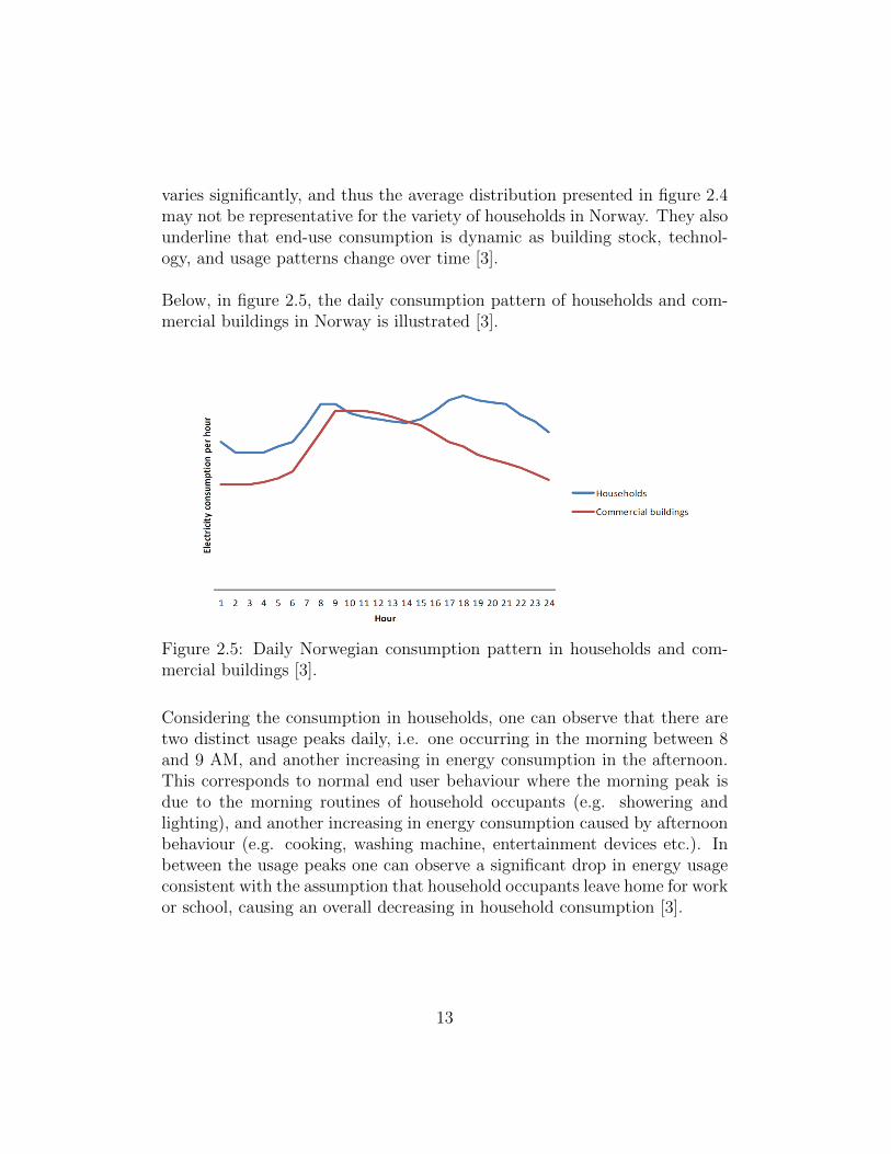
Below, in figure 2.5, the daily consumption pattern of households and com-mercial buildings in Norway is illustrated [3].

Figure 2.5: Daily Norwegian consumption pattern in households and com-mercial buildings [3].

Considering the consumption in households, one can observe that there aretwo distinct usage peaks daily, i.e. one occurring in the morning between 8and 9 AM, and another increasing in energy consumption in the afternoon.This corresponds to normal end user behaviour where the morning peak isdue to the morning routines of household occupants (e.g. showering andlighting), and another increasing in energy consumption caused by afternoonbehaviour (e.g. cooking, washing machine, entertainment devices etc.). Inbetween the usage peaks one can observe a significant drop in energy usageconsistent with the assumption that household occupants leave home for workor school, causing an overall decreasing in household consumption [3].

13

2.3 EU directives

Estimations have predicted that by the year 2050 the global energy require-ments will more than double from its current level. This fact, accompaniedby the need for reducing greenhouse gas emissions, have led to the emergenceof several EU directives aimed at reducing and ensuring a more efficient en-ergy consumption. There are in particular three such directives affectinghouseholds, all of which are implemented in Norwegian law [3], [7]. Theseare [3]:

1. The Renewable Energy Directive, which purpose is to promotean increased production and use of renewable energy, sets mandatorynational requirements for the share of energy consumption which mustoriginate from renewable energy sources. Furthermore, it provides acommon framework for stimulating the construction and upgrading ofinstallations to generate more renewable energy. More formally, EUis aiming for 20% of all energy consumption originating from renew-able energy sources by 2020, in addition to a 20% increasing in energyefficiency, as part of the EU 20-20-20 initiative.

2. The Energy Performance of Buildings Directive concerns im-proving the energy efficiency in the building stock. That is, establishingschemes for energy efficiency certification of all buildings and energyassessments for the technical installations in buildings.

3. The Energy Labelling Directive aims to increase to consumer aware-ness regarding the energy consumption of products. That is, throughenergy-labelling of consumer goods the consumers are provided infor-mation on the energy-efficiency of products, giving incentives for choos-ing more energy-efficient alternatives.

2.4 Battery energy storage systems

In [5] they emphasise how Energy Storage (ES) is expected to play an increas-ingly important role in future power distribution. As power flow no longerwill be limited to one direction (i.e. from power sector to consumers), theneed for managing distributed generation and demand will require BatteryEnergy Storage Systems (BES) for maintaining grid stability and flexibility.

14

In particular, the challenges related to integrating renewable energy sources,given their unpredictable and fluctuating generation patterns, will requiresignificant investment in smaller-scaled and more flexible storage technolo-gies [5].

Currently, BES systems range anywhere from 5 kWh up to 50 MWh andare differentiated by factors such as response time, mobility, and versatilityto be fitted to either high power or high energy applications. As stated insection 2.3, EU aims for 20% of all energy consumption originating from re-newable energy sources by the year 2020, in addition to increasing the energyefficiency by 20%. Thus, BES systems can ensure a better match betweensupply and demand, and ease the transition to renewable energy sourcesamounting to a greater share of the global energy supply [5].

Also, by employing measures for e.g. peak shaving (as described in sec-tion 2.5.4) one can compensate with stored energy in high demand peri-ods, which in turn reduces the need for expensive backup generators specif-ically targeted at handling peak consumption. That is, the electric utilityinfrastructure costs are primarily driven by the need to serve the load dur-ing peak demand periods. Thus, by utilizing BES systems to compensatein high demand periods, one can reduce the peak demand seen from theutility company’s perspective, which consequently will reduce the electricitycosts [25], [5].

There are various services and functions BES systems offer, some of whichare [5]:

• Integration of renewable energy sources: That is, convertinghighly variable renewable energy resources into dispatchable ones byuse of storage. By using BES systems for decentralized storage onemay obtain a dynamic behaviour able to compensate for fluctuatingrenewable energy generation with fast response times.

• Peak shaving: BES systems may store energy when consumption islow, which in turn can be compensated with for shaving usage peaksin high demand periods.

• Voltage control: BES systems can help regulate the voltage profile,guaranteeing standard voltage supply within a defined range. That is,

15

by storing energy when the voltage is high and feeding in when voltageis low.

• Uninterruptible power supply (UPS): BES systems can act asa backup power source in the event that the external energy supplyis disrupted. By temporarily islanding the operation (as describedin section 2.1.2), e.g. a microgrid can be able to manage the entireenergy demand of its participants by utilizing the stored energy of BESsystems.

Furthermore, as stated in [25], it is important to consider that the cost of aBES system is largely associated with its energy storage rating (Wh) ratherthan its power rating (W). That is, the required discharge period in differentapplications will greatly affect the costs of implementing a storage system.

2.4.1 Battery technologies

In [5] they emphasize that all four battery technologies (lead-based, lithium-based, nickel-based and sodium-based) can provide distinctive and importantfunctions to grid operators. Below in table 2.1 some of the similarities anddifferences between the battery technologies are listed based on informationgathered from [5].

Technology Capacity Efficiency Life Cycles TemperatureLead 1 Ah - 16 kAh >85 % 20 years 2000 @ 80% DOD -30 to +50 ◦C

Lithium 1 ≈100 % 20+ years 5000 @ 80% DOD -30 to +60 ◦CNickel 0.5 Ah - 2 kAh >90 % 25 years 30002 -40 to +60 ◦C

Sodium 380 V 40 Ah 92 % 10+ years 4500 @ 80% DOD -30 to +60 ◦C

Table 2.1: Similarities and deviations between different battery technologies(DOD = Depth Of Discharge)

Moreover, due to the current relatively high costs of BES systems, most re-ported installations thus far are considered as pilot projects either partially

1One of the main advantages with Li-ion technology is its scalability. It can be adaptedto virtually any power or energy requirement, ranging from very high power (i.e. 10 kW/ 10 kWh) to very high energy [5].

23000 cycles of nominal capacity

16

or fully funded by government entities. Hence, further research and devel-opment is needed to reduce the prices and improve the performance of eachof the above mentioned battery technologies should they become suitable forsmaller-scaled purposes [25], [5].

2.5 Measures for reduced and more efficient

household consumption

Households account for around 30 per cent of the total stationary energyconsumption in Norway and thus exploring usage patterns and measures forbetter efficiency is important for achieving an overall reduction in power con-sumption [3]. In [3] they list several means for both reducing consumptionand increasing the energy efficiency, some of which are described in sec-tion 2.5.1. Furthermore, in section 2.5.2, the potentials of Smart Grid forbetter end user management is described, i.e. through providing real timeand predictive feedback in terms of electricity usage and pricing details to endusers. Moreover, in section 2.5.3, demand shifting is described as a methodfor reducing the usage peaks in high demand periods, by shifting demandto off-peak periods. Finally section 2.5.4 describes how one can compensateautonomously for daily usage peaks by utilizing the locally generated energyof microgrids in high demand periods with the purpose of ensuring a lessfluctuating daily consumption seen from the utility company’s perspective.

2.5.1 Energy efficiency measures

Energy efficiency measures concerns reducing the energy requirements, e.g.for buildings, either by properly planning low energy requirements prior toconstruction, or improving older houses by e.g. better insulation of lofts,basements and walls, in addition to draught proofing windows and doors.As described in section 2.3, the Energy Performance of Buildings Directiveprovides schemes for energy efficiency certification of buildings aimed at en-suring the previously described improvements. Such means can significantlyreduce the energy requirements for space heating, which as described in sec-tion 2.2 amount to the majority of all energy consumption in Norwegianhouseholds [3].

17

Furthermore, improving the insulation of hot water tanks, installing water-saving showers etc. can also contribute to reducing consumption and improv-ing the energy efficiency. Also, replacing old heating sources (such as oil-firedboilers and paraffin stoves) with better heating systems (e.g., electric heatersor heat pumps) can result in a more efficient heating of households. In ad-dition are consumers increasingly choosing more energy efficient householdappliances and entertainment devices due to measures such as the EnergyLabelling Directive described in section 2.3 [3].

2.5.2 Better end user management of energy consump-tion

Recent investigations have shown that providing real-time and predictiveupdates regarding electricity usage and pricing can incentive consumers toreduce their energy consumption [2], [11], [27].

In [11] they have analysed 15 experiments on household response to dynamicpricing of electricity. The study uncovered that households in fact respondto higher prices by lowering their electricity consumption, and that the po-tential reductions in power generation are considerable. The consumers re-sponded to higher prices during peak periods by reducing the consumptionand/or shifting it to off-peak periods and, as a matter of fact, they concludedthat providing such information to end users can reduce consumption by 5-15% [11].

However, the experiments mentioned above all used time-varying pricing ofelectricity, which was only applied during the periods they investigated. Inmost cases (like e.g. with Norwegian power distribution) the cost of electric-ity is currently determined day-ahead, and thus provide no economic benefitsfor consumers to lower their consumption during usage peak periods. Onceagain, this highlights one of the main advantages that the increased informa-tion flow of Smart Grid is intended to provide. That is, we achieve a betterfoundation for employing such pricing schemes, where we can dynamicallydetermine the cost of electricity based on real-time updates on energy con-sumption.

Furthermore, as described in [6], the American IT company Opower have

18

studied how providing customers information on neighbouring households’energy usage also can incentive reduction in consumption. That is, theyhave examined how social pressure can affect consumption behaviour whenhouseholds are made aware of the consumption patterns in neighbouringhomes of similar size and number of occupants. Their results yielded a con-sumption decrease of 1.9 TWh last year which, in comparison, amount toapproximately half of the generated energy provided by the solar power in-dustry in the US [6].

Given a user-centric gathering and dissemination of information we canachieve a foundation for employing measures such as the ones describedabove. That is, by providing real-time and predictive updates on consump-tion to households and/or adding pricing incentives, such as the previouslydescribed dynamic (demand-dependent) pricing scheme.

2.5.3 Shifting demand from high demand periods

As described in section 2.2, there are variations in power demand daily, andthus, the coinciding habits of consumers causes significant usage peaks tooccur at certain times during the day. Consequently, when constructing apower grid, one must take in account the hour of the year for which electricityconsumption is at its highest (also known as the power grid’s peak load), andensure that the total energy capacity is great enough to cover this demand [3].

For instance, as described in section 2.2, a daily usage peak usually occursaround 7 or 8 AM on week days due to the morning routines of householdoccupants. Thus, considering that most hot water tanks in Norway beginheating water as soon as it is drawn, it is plausible to assume that the expe-rienced morning usage peak is caused by this. By employing an automatedhome energy management mechanism one can shift demand according to auser’s preferences with the aim of reducing the overall consumption in usagepeak periods. In particular, given the above mentioned water-tank example,it would be feasible to postpone the water heating until mid-day when theoverall consumption is significantly less [3].

Considering this, numerous investigations have been performed on measuresfor reducing usage peaks by shifting usage from high to low consumption

19

periods, with the intention of reducing the peak demand, and consequentlythe power grid’s peak load. For instance, in [1] it is proposed such an energymanagement system that shifts usage to off-peak hours and lowers the totalenergy consumption.

2.5.4 Autonomous peak shaving in high demand peri-ods using battery energy storage

Another method for reducing peak demand is by compensating with locallystored energy in high demand periods, henceforth referred to as peak shaving.That is, peak shaving in the sense that local energy is used to compensatefor usage peaks such that the consumption pattern observed at the utilitycompany appear as constant during high demand periods, while the actualenergy usage remain unchanged. Such an approach may also contribute toincreased use of renewable energy sources, as this local energy may originatefrom e.g. solar or wind power.

In [25] it is described a peak shaving study performed performed in Nevada,USA. Here, they have investigated the sizing of a utility-owned BES sys-tem that is planned for installation at the substation end of a residentialfeeder. The purpose was to investigate storing of energy in low-demand pe-riods which in turn could be utilized to compensate for usage peaks. First,they examined the load demand of a residential feeder in the summer months(June - September 2008), amounting to a total of 122 days. After which, thesizing of the BES system was derived from the desired level of peak shavingby load following. Load following, or power control, means that the demanddynamically controls the amount of power provided by the battery system.Finally, the BES system power and energy ratings were quantified. In fig-ure 2.6, a sketch of the setup is illustrated [25].

20

Figure 2.6: Sketch of feeder with BES system and residential area [25]

Below, in the left hand side plot of figure 2.7, the daily load of the residen-tial feeder in the summer months of 2008 is illustrated. Furthermore, themaximum peak load, Pmax

load = 1.46MW occurring on July 8th, was used todetermine the boundary for what was considered a usage peak in the wholetime period. That is, the desired amount of peak shaving, σ, was definedas a percentage of maximum peak load. In this study they used σ = 0.25,and thus the maximum net power which had to be supplied by the batterysystem was [25]:

Pmaxbatt = σ ∗ Pmax

load (2.1)

In addition, they assumed a discharge and power conversion loss of 10%,and denoted the overall system efficiency by η = 0.90. Hence, the maximumpower provided by the BES system was defined as [25]:

PBESS = σ ∗ Pmaxload /η (2.2)

Given σ = 0.25, the BES system had to provide a peak power of Pmaxbatt =

0.365MW , which results in a maximum grid power, Pmaxgrid = 1.095MW . This

boundary is illustrated as the dotted red line in the left hand side plot offigure 2.7, and thus any load change in excess of this threshold was considereda usage peak. The right hand side plot of figure 2.7 illustrates the distributionof hourly consumption with respect to how often they occur, in per cent oftotal time [25].

21

Figure 2.7: Left: Daily feeder load during the four investigated months.Right: Duration of peak period in per cent. [25]

Given the previously described discharge efficiency, η = 0.90, the BES systempower rating was PBESS = 0.4MW . Furthermore, the capacity of the BESsystem was determined by computing the daily energy demand that mustbe supplied the battery in order to avoid power flow from exceeding thedesired maximum grid power contribution, i.e. Pmax

grid = 1.095MW . Thiswas achieved by determining the area between hourly consumption and themaximum grid power boundary [25]. That is [25]:

Eibatt =

∫ 24

0

(P iload − Pmax

grid )dt, P iload ≥ Pmax

grid (2.3)

After which, the maximum value the BES system had to be able to providewas determined, i.e [25]:

Emaxbatt = max{E1

batt, E2batt, ..., E

nbatt}, (2.4)

where n = 122 represents the number of days in the summer period. Finally,they quantified the energy rating of the BES system by dividing the resultobtained in equation 2.4 by the discharge efficiency, η, and adding the min-imum level of energy must remain at all time in the battery, SOCmin (i.e.the minimum State of Charge) [25]. That is [25]:

EBESS =Emax

batt

η+ SOCmin ∗ Emax

batt (2.5)

Their investigation revealed the maximum energy rating of the BES system asEmax

batt = 2.12MWh. Consequently, given a discharge efficiency η = 0.90 and aSOCmin set to 20%, results in a BES system capacity of EBESS ≈ 2.75MWh.

22

Below, in the left hand side plot of figure 2.8, the daily BES system energygeneration of the entire time period is illustrated. Furthermore, the righthand side plot of figure 2.8 illustrates the desired peak power shaving [25].

Figure 2.8: Left: Daily energy provided by BES system. Right: Daily gridpower variations after peak shaving. [25]

In this study, the BES system was intended to recharge during the earlymorning hours when the consumption was low, and thus the right hand sideplot of figure 2.8 shows a higher daily minimum load than the base case il-lustrated in the left hand side plot of figure 2.7 [25].

In the model described in chapter 4, a similar peak shaving approach isattempted using consumption data gathered from the Demo Steinkjer project(described in section 2.6) and photovoltaic solar generation data gatheredfrom elia (described in section 2.7.2).

2.6 Demo Steinkjer

Demo Steinkjer is a Norwegian demonstration project where new solutionsfor measuring and use of electricity can be tested. The testing site is locatedin Steinkjer and contains about 1.000 households, of which 321 have agreedto be active participants meaning they will participate in consumer orientedtests and projects. The remaining households will participate, without directinvolvement, in tests conducted on the grid itself as well as secondary subsys-tems. The intention of the project is to attract entities to test new technologyaimed at an modernization of the power grid with new products and services.Thus, Demo Steinkjer is an arena for which smart energy solutions can be

23

tested with purpose of exploring a suitable design and implementation of thefuture electricity grid in Norway3.

Companies such as SINTEF, Nexans, Telenor, Connexion, SagemCom, andothers have already shown interest in running projects with Demo Steinkjer,and they will have the opportunity to test new products on real consumers.Entities will have access to customer database including anonymous AMSmeter data and high-speed communication capabilities with five net/gridstations. In total, there are about 800 electricity meters installed, including770 AIDON meters and 30 remotely read units through GSM/GPRS3.

2.7 Solar energy

In [7] it is stated that the solar energy reaching the surface of Earth everyhour is enough to meet the annual global energy needs. The challenge, how-ever, reside in harnessing this energy at an affordable cost. Thus far thecost of large-scale collection, conversion, and storage of solar energy has notbeen feasible compared to conventional energy generation. Consequently,solar energy currently makes a negligible contribution to the global energysupply. However, predictions on future increasing in energy consumption,in addition to the environmental effects caused by fossil fuels, have arisenthe need for further research on solutions for solar energy generation. Otherrenewable energy sources (e.g. wind, hydro etc.) and non-renewable (e.g.nuclear) are unable to satisfy the expected increased global energy needs,and thus scientists have proposed solar driven production of environmentallyclean electricity, hydrogen, and other fuels as the only sustainable long-termsolution for global energy needs [7].

In addition to the economic challenges, the availability of solar energy is an-other source of concern. That is, solar power is not always available whereand when needed, and thus daily and seasonal effects have great impacton the energy generation. Moreover, the changing dynamics, non-linearitiesand uncertainties related to solar energy also make prediction of supply dif-ficult [9].

3http://www.demosteinkjer.no

24

There are several methods for generating solar-sourced electricity. Most com-monly used are direct generation using photovoltaic cells (PV) and indirectgeneration, called concentrated solar power (CSP), where collectors use mir-rors and lenses to concentrate sunlight onto a thermal receiver that absorband convert sunlight into heat, which in turn is used to drive a turbine toprovide electric power. In this study, however, only PV energy generationis discussed as it is the most common method of the two, and arguably alsoeasier to implement in microgrid architectures due to the space requirementsof CSP generation facilities [18]. This is also supported in [5], where theystate that the primary renewable energy source for future Smart Grids willbe photovoltaic. In section 2.7.1 below, PV energy generation is describedmore thoroughly, while section 2.7.2 describe the Belgium transmission sys-tem operator elia which publishes data on PV energy generation.

2.7.1 Photovoltaic solar energy generation

Solar cells, or photovoltaic (PV) cells, convert solar radiation directly intoelectricity and is based on the photovoltaic effect. In general, the photovoltaiceffect is defined as the emergence of an electric voltage between two electrodesattached to a solid or liquid system when exposed to light [14]. Below, infigure 2.9, one such PV solar cell installation is depicted [21].

Figure 2.9: A large silicon solar array installed on the roof of a commercialbuilding [21]

25

The efficiency of solar cells, η, can be derived from equation 2.6 below [14],i.e.

η =Pmax

ES ∗ Ac

(2.6)

where Pmax is the nominal power output (i.e. maximum achievable power),ES is the incident radiation flux (i.e. the amount of sunlight power thatreaches the Earth’s surface in W/m2), and Ac is the area of the collector inm2 [14].

The incident radiation flux is considered to be approximately 1000 W/m2,and thus, given 100 % efficiency, solar cells generate 1 kW power per squaremeter during optimal weather conditions. As of now, however, the efficiencyof photovoltaic cells averages at approximately 15 % [20]. Furthermore, thedaily periods for when solar cells generate power varies significantly in differ-ent parts of the world, and thus affect the total amount of energy generated.In figure 2.10 below the annual solar energy potential in all of Europe isillustrated [8].

26

Figure 2.10: Solar energy potential map of Europe [8]

As one can observe the variations are considerable. In particular, comparingthe southern parts of Spain and Portugal (1821 - 1860 kWh/m2) with thesouthern parts of Norway (861 - 900 kWh/m2) reveals an annual differencein energy potential of approximately 1000 kWh/m2.

Furthermore, the power output of solar cell installations are also highlyweather dependent, and thus the nominal power output of an installationis achieved only during optimal weather conditions. In figure 2.11 below,the complete solar power output on July 7th 2013 in all of Germany is illus-trated. In total Germany has, as of 2013, an installed domestic PV capacityof approximately 34 GW. However, due to the varying angles of their solarcell installations, some systems peak at 11 AM while others at 2 PM caus-ing the different installations to achieve generation peaks at different timesduring the day. Consequently, they achieve maximum power output peaks

27

at about 70-80 % of total capacity [13].

Figure 2.11: German solar energy generation on July 7th 2013 [13]

As one can observe the generation peak this day was 24 GW (occurring at13 PM), which amounts to approximately 70 % of total capacity [13].

2.7.2 Elia solar cell generation data

Elia is the high-voltage transmission system operator of Belgium responsiblefor transmitting electricity from generators to distribution systems, whichin turn deliver power to consumers. In order to provide transparency inthe electricity market, elia publishes generation data from renewable energysources (such as wind or solar) as both predictive and actual measurements,which consequently can be used for scientific research4.

In this study, PV solar cell data from elia is used to uncover the potentialsfor solar energy harnessing, and to determine whether or not it is suitable asa local generation source in microgrids. The data used is gathered from allof Brussels, Belgium in 2013 as quarter-hourly updates on power generation,and the total installed PV capacity is 6.92 MW in January until March.

4http://www.elia.be

28

However, in March the nominal capacity was increased to 10.2 MW and thusenergy generation becomes greater. Section 3.1.2 describes this investigation.

2.8 Complex network theory

The use of complex network theory is increasing as a measure for analysingand understanding real world networks. Empirical studies on computer net-works, social networks and electrical power grids, to name a few, have re-vealed that behaviour of such networks is not suitable for modelling by use oftraditional mathematical graph theory. Real world networks have structuresthat are irregular, complex and dynamically evolving with time, and thus themodels proposed in mathematical graph theory are not able to reproduce thedynamical and functional behaviour of such topologies [4], [24].

In [4] they emphasize several reasons for why the study of complex networksare relevant for real world topologies:

• Weighted networks: Often in real topologies the connections be-tween nodes are weighted in terms of edge capacity and intensity, i.e.networks in which a value is associated with each link which may varyas time progresses. Examples of such are existence of weak and strongties between individuals in a social network, different physical distancebetween nodes, and different capabilities for transmitting e.g. electricsignals.

• Dynamical behaviour: Real world networks are composed by largenumbers of interconnected dynamical units. Thus, the collective dy-namics in a complex topology and the local properties of individualnodes greatly affect the interactions in coupled dynamical systems. Forinstance, studying synchronization phenomena in sociology has becomevery relevant for acquiring a better understanding of the mechanismsunderlying the formation of collective social behaviours, such as e.g.the emergence of new habits, fashions or leading opinions.

• Adaptive and dynamical wirings: When networks themselves aredynamical entities, affected by either external or internal actions, thetopology is not fixed. That is, as opposed to dynamical processes withstatic connection schemes, the topology may evolve and adapt with

29

time. A suitable example here is the islanding of a microgrid (describedin section 2.1.2) where its external energy supply is disrupted and thecell must adapt by covering the entire energy demand of its participants.

There are some unifying principals and statistical properties common to allcomplex networks, some of which are listed below [4]:

• Node degree: The degree (or connectivity) describes the number oflinks one node has to other nodes in the network, which can be usedto determine a node’s importance. In fact, the most basic topologicalrepresentation of a graph G can be obtained in terms of its degreedistribution, P (k), defined as the probability that a node in G chosenuniformly at random has degree k. If the graph is directed the degree ofa node has two components, i.e. out-degree (number of outgoing links)and in-degree (number of ingoing links).

• Betweenness centrality: The term betweenness centrality is anothermeasure for deriving a node’s importance within a graph. It quantifiesthe number of times a node acts as a bridge along the shortest path oftwo other nodes. That is,

bi =∑

i 6=j 6=k∈N

njk(i)

njk

(2.7)

where njk is the number of shortest paths between j and k, while njk(i)is the number of shortest paths connecting j and k and passing throughi.

• Graph diameter: The diameter is the greatest shortest path betweenany pair of nodes in a graph. Thus, to determine the diameter, onefirst finds the shortest path between each pair of nodes, where the pathwith greatest length is the diameter.

Moreover, the structure of a network always affects its function. For instance,the robustness and stability of electricity transmission is greatly affected bythe topology of the power grid. The traditional power grid (e.g. the onedescribed in section 2.8.1 below) has a moderately heterogeneous topologycharacterized by an exponential distribution of the number of transmissionlines per substation (i.e. degree distribution). However, as described in sec-tion 2.1.2, the paper in appendix G proposes a different power grid topology

30

using a preferential attachment structure. Here, the basic idea is that nodeswith high degree acquire new links at a higher rate than low-degree nodes,and thus the power generation and storage capacity of each node in the net-work depends on the number of connection it has to other nodes [4], [24].

2.8.1 Related investigation: Modelling cascading fail-ures in the North American power grid

A related investigation with regards to power grids is described in [16]. Herethey have modelled the North American power grid using its actual topologyand investigated the damage inflicted in terms of transmission efficiency inthe event of substation failure. They made plausible assumptions regardingload and overload conditions of transmission substations and observed howoverloads caused by substation malfunctioning leads to cascading effects inthe power network [16].

More generally, they modelled the power grid as a weighted graph G, with Nnodes (substations) and K edges (transmission lines), and represented it asan N x N adjacency matrix {eij}. Each element eij represent the line betweennodes i and j and is a number in the range [0,1], where 0 indicate no directconnection in between the nodes and 1 indicated that the transmission lineworks perfectly [16].

Initially all the existing transmission lines in the power network were set to1 and the efficiency of a path between two substations in the network wasdefined as the harmonic composition of efficiency in the transmission lines inbetween the substations. That is, the harmonic composition of N numbersx1, x2, ..., xN is defined as [

∑Ni 1/xi]

−1. After which, they started to removenodes from the network and observed how the network progressed. It showedthat when removing a substation, its load needs to be redistributed amongthe remaining neighbouring substations in the network, causing other sub-stations to carry larger loads than their capacity. Ultimately, this leads tooverload conditions de-gradating the neighbouring substation’s performanceas well, which in turn creates an cascading effect on the entire network. Infact, they concluded that the removal of one single substation can, in a worstcase scenario, cause a degradation of 25% in terms of overall transmission

31

efficiency [16].

This investigation illustrates how we can use complex network theory toanalyse real world networks. In chapter 4, a similar model for autonomy inmicrogrids is described where the complex network tool NetLogo (describedbelow in section 2.8.2) is used.

2.8.2 NetLogo

NetLogo is a multi-agent programmable modelling environment using anagent-based programming language, meaning that actions and interactions ofautonomous agents (i.e. entities or nodes) can be simulated in order to assesstheir effects on a system as a whole. The tool allows us to facilitate the struc-tural properties of complex systems and examine the collective behaviour ofrule-based agents dynamically interacting as in real world networks5.

As the complexity of a system is closely related to the connectedness and be-haviour of different agents, NetLogo allows us to model robustness in terms ofadapting to internal and external events in a complex system. Thus, we canmodel how a complex real world network with dynamically evolving agentsprogresses with time, and how to handle situations that emerges from theagents’ behaviour and interactions5.

In this study, NetLogo is used for developing the microgrid autonomy modeldescribed in chapter 4. The user interface of this model and parts of theNetLogo-code is presented in appendix E, while the model itself is included inthe folder ”AutonomyModel” on the attached CD-ROM.

5http://ccl.northwestern.edu/netlogo/

32

Chapter 3

Analysing dynamics of energyconsumption and generation

In order to model autonomy in microgrids, one must first investigate thedynamics of energy consumption and generation. This chapter describes twoanalyses, one performed to uncover the dynamics of energy consumption inNorwegian households, and another to reveal the generation potentials ofPV solar cells. The data and patterns obtained in these analyses lay thefoundation for the subsequent autonomy model described in chapter 4.

3.1 Methodology

Section 3.1.1 describes an investigation of energy consumption in Norwegianhouseholds based on data gathered from the Demo Steinkjer project. Insection 3.1.2 an investigation on energy generation in solar cells is describedwhich purpose is to reveal the current potentials of solar energy harnessing.Finally, in section 3.1.3, it is described how to setup the database containingthe energy consumption and generation data used in these analyses.

3.1.1 Consumption data from Demo Steinkjer project

As described in section 2.6, the Demo Steinkjer project1 has gathered con-sumption data from several houses located in the same geographical area ashourly updates over the last two and a half years. Currently this database

1http://www.demosteinkjer.no

33

consists of 7.2 million entries on consumption from 221 buildings, of whichthe great majority is ordinary households. The intention of this analysis is toexamine the consumption data and reveal whether the daily usage patternsof the Demo Steinkjer participants correspond to the description of normalNorwegian household behaviour in section 2.2. Furthermore, the obtainedconsumption patterns gathered from this analysis will lay grounds for thesubsequent model (described in chapter 4) where generation and storage fea-tures are added in a futuristic microgrid scenario.

More particularly, this analysis will examine usage patterns in a selection ofhouseholds participating in the Demo Steinkjer project and determine howenergy consumption varies by investigating:

• hourly consumption over the course of day in different households

• energy usage in different months over a year

• weekday as opposed to weekend consumption

• total and average consumption when aggregating the patterns of mul-tiple households

Thus, the analysis will uncover e.g. when usage peaks occur, the seasonaleffects on energy consumption, and also determine the total daily usage pat-tern of several households combined. Detecting a daily usage pattern thatis consistent when summarizing several households will uncover how we canimplement mechanisms for avoiding usage peaks in microgrids, as describedin section 2.5.4. The results from this analysis are described in section 3.2.

3.1.2 Generation data from elia solar cells

As described in section 2.1, the futuristic aim of Smart Grid is to achievea more distributed energy supply infrastructure where local generation andstorage sources are added to microgrid cells. Using distributed energy genera-tion the microgrids can autonomously control its own generation and storagein response to variable demand and supply conditions. By adding renew-able energy sources (e.g. solar, wind or hydro) to microgrids, one can e.g.compensate for daily high demand periods by utilizing locally stored energyautonomously. Also, in the event that external energy supply from utility

34

company is disrupted, local energy generation and storage can be utilized toavoid power outages.

In this analysis the energy generated from PV solar cells will be examinedwith purpose of investigating the dynamics and sustainability of solar energy.Furthermore, the analysis will also investigate day-ahead predictions, and re-veal with what certainty the harnessing of solar energy can be predicted. Thedata examined is gathered from elia2 and concerns solar energy generationin Brussels, Belgium in 2013.

In particular, the analysis will examine solar generation dynamics by inves-tigating:

• the daily variations in generated energy

• the monthly variations in daily generated energy

• the predictability of solar energy

Thus, the aim of this investigation is to derive and analyse the energy gener-ation potential of PV solar cells. Furthermore, the data obtained from thisanalysis will be utilized in the subsequent model on autonomy in microgridsdescribed in chapter 4. As described in section 2.7.2, elia offer both day-ahead predictions and corrected data on the daily energy generation in solarcells, and thus the investigation will also reveal how accurately solar energygeneration can be predicted. The results from this analysis are described insection 3.3.

As mentioned in section 2.7.2, the PV solar dataset from elia has quarter-hourly updates on power generation. For simplicity, this is converted tohourly average updates in this investigation, i.e. by summarizing the quarter-hourly updates each hour and dividing it by four. Furthermore, the analysisassumes that this hourly average power output is constant each hour.

3.1.3 Database setup

Both the consumption and generation data used in these analyses can bedownloaded in .csv format from Demo Steinkjer1 and elia2, respectively.

2http://www.elia.be

35

However, as described earlier, the datasets are enormous. In particular,the Demo Steinkjer data alone consists of 7.2 million entries on consumptionfrom the last two and a half years. Therefore, in order to simplify the workof investigating this massive amount of data, I needed to represent it in amore easily accessible manner.

To achieve this, I set up an apache server and configured phpMyAdmin suchthat I could create a MySQL database consisting of the datasets. The twodatasets were then separated in different tables in this database, and madeaccessible with SQL commands. See appendix A for a more thorough tutorialon how to set up the database and extract data.

After which, I extracted data from the database using SQL commands inpython scripts, and investigated the dynamics of energy consumption andgeneration as described in sections 3.1.1 and 3.1.2, respectively. Appendix Adescribes, as mentioned, how to setup the database and extract data. How-ever, below I have chosen to list some of the most significant and time-consuming issues that needed to be resolved, in order of appearance. Theseare:

1. The Demo Steinkjer dataset only has a column with the accumulatedenergy consumption each hour. Thus, one must create a new columncalled ”HourlyConsumption” in phpMyAdmin and then run the pythonscript ”addHourlyConsColumn.py”. This separate column is needed forderiving the difference between two consecutive measurements, i.e. theconsumption of the last hour. The script is located both in appendix Band on the attached CD-ROM, and takes approximately four hours torun on the entire database.

2. There are several ”gaps” in the dataset from DemoSteinkjer, i.e. miss-ing measurements. Thus, finding longer periods of time, where noneof these gaps are present, is extremely time-consuming. However, the20 households evaluated in the analysis described in section 3.2 haveconsistent measurements in the time period ranging from October 1st2012 until June 28th 2013. The User IDs of these households are listedin appendix F.

3. One must manually remove the spaces in column names in the datasetson solar generation. That is, the column ”Day-Ahead forecast [MW]”

36

must be changed to ”Day-AheadforecastMW” and ”Corrected UpscaledMeasurement [MW]” to ”CorrectedUpscaledMeasurementMW”. If thisis not done you get errors when attempting to extract data using pythonscripts and subsequently in the NetLogo model (chapter 4).

4. The dataset on solar generation provided by elia uses comma as the dec-imal mark in numbers. This must be exchanged with period, otherwisethe extracted data is treated as a string instead of a decimal numberin python. The script performing this exchange is ”ReplaceCommaW-ithPeriodInDatabase.py”, which is located on the attached CD-ROM.

5. In the solar generation data from elia there exist some duplicate mea-surements, listed consecutively. This issue is resolved by running the”searchingForDuplicate.py” script located on the CD-ROM, and manu-ally removing the database entry indicated by the output of the pythonscript.

In appendix C and D, two scripts (one for extracting and plotting consump-tion patterns and another for generation patterns) are presented. Thesescripts have been included in appendix to give the reader an understandingon how to access the database using python scripts and reproduce the plotsand results described in sections 3.2 and 3.3. However, these are just ex-amples, and thus I refer to the folder ”pythonworkspace” on the attachedCD-ROM to see the complete selection of python scripts used in these inves-tigations.

3.2 Results from analysis: Consumption pat-

terns in Demo Steinkjer households

This section describes the results from the analysis of consumption behaviourin households participating in the Demo Steinkjer project (as described insection 3.1.1). The main purpose of this investigation was to uncover if theconsumption patterns of different homes coincide, i.e. to examine whethermultiple homes have similar daily usage patterns. If so, the knowledge ofthese patterns can be used in further modelling of microgrid scenarios wherelocal generation and storage capabilities are added to microgrids. Knowingsuch patterns can enable means for e.g. utilizing the locally stored energy

37

of microgrids in high consumption periods in order to avoid high electricityprices and power outages as described in section 2.1.

Section 3.2.1 describes the results from an investigation of monthly averageconsumption in several individual households. The purpose of investigatingthis was to examine how consumption varies from month to month, and toreveal similarities and deviations in different households. In section 3.2.2 thecombined daily consumption of several households is examined with purposeof recognizing a common pattern. In section 3.2.3 the investigation concernsa three-month period (i.e. January-March 2013) where the total hourly con-sumption from ten different houses is summarized. Here we can uncover if acertain usage pattern emerges when the consumption of several households ismerged over a longer time period, and also examine the differences betweenweek day and weekend consumption. In section 3.2.4 the total number ofhomes is increased to 20 and the time period to nine months (October 2012- June 2013). Here we can examine if the pattern observed in section 3.2.3remains when increasing the total number of homes and the time periodeven further. In section 3.2.5 the monthly variations in consumption is ex-amined further with purpose of revealing the differences in monthly average,maximum and minimum hourly consumption. Finally, in section 3.2.6, thefindings of this analysis are summarized.

3.2.1 Average hourly consumption from different housesexcluding weekends

In figures 3.1, 3.2 and 3.3 below, the average hourly consumption from differ-ent months in three separate houses is depicted. The consumption patternsof all three households have been gathered from the same time periods, ex-cluding weekends, and we can observe how the average energy usage variesover the course of day in six different months. There are deviations frommonth to month and in between houses, but common for all houses andmonths is that they follow approximately the same curve. That is, we clearlysee a usage peak between 7 and 9 AM and an overall increasing in energyconsumption after 15 PM. Considering this, the patterns observed confirmsthe expected behaviour in Norwegian households described in section 2.2.

38

Figure 3.1: Monthly average consumption (house ID7350049083690884): Left: October, November and December 2012Right: April, May and June 2013


39


As stated in section 2.2, 12% of all household consumption in Norway is usedfor water heating. Given the recurring usage peak between 7 or 9 AM, regard-less of household, it is plausible to assume that this increasing in consumptionis caused by the morning routines of household occupants. Furthermore, wecan observe how the energy usage during daytime (i.e. after the morningpeak and before 15 PM) drops significantly. This is consistent with the as-sumption that household occupants leave home for work or school, whichconsequently reduces the consumption in the household. Moreover, the factthat 66% of all household consumption is used for space heating (as statedin section 2.2) can explain the monthly variations in terms of overall usage.That is, colder months requiring higher energy consumption compared towarmer months due to additional need for space heating caused by loweroutdoor temperatures.

There are, however, variations in the different households. As one can ob-serve in figures 3.1, 3.2 and 3.3, the overall daily pattern described above isconsistent in the different homes, but there are slight differences related tothe exact occurrence and size of usage peaks. This is consistent with how e.g.size of household, habits of household occupants etc. may vary as describedin section 2.2.

40

3.2.2 Combined daily consumption of multiple house-holds

In figures 3.4 and 3.5 the combined consumption of several households isdepicted. The plotted dates are October 1st 2012 (figure 3.4) and February1st 2013 (figure 3.5), and one can observe how the combined consumption ofboth 10 and 20 households affect the daily usage patterns on these dates.

Figure 3.4: Combined consumption October 1st 2012: Left: 10 house-holds Right: 20 households.

Figure 3.5: Combined consumption February 1st 2013: Left: 10 house-holds Right: 20 households.

As one can see, the expected pattern (described above in section 3.2.1) be-comes more and more visible when increasing the number of homes. Hence,

41

the overall pattern when summarizing several homes’ energy usage seems todisguise some of the slight differences of the separate homes, and we endup with a pattern that is more similar to what was described as normalNorwegian household behaviour in section 2.2.

3.2.3 Combined hourly consumption from ten housesover three months

In figure 3.6 below, the total hourly consumption of ten houses in the monthsJanuary, February and March 2013 is depicted. The left hand side plot offigure 3.6 is week day consumption, while the right hand side plot is theweekends in the same period. This investigation reveals that when summa-rizing the total hourly consumption in a group of houses over a three-monthperiod, we get a pattern that more persistently state a behaviour consistentwith what is expected in households. That is, a usage peak in the morning,followed by a drop in consumption during daytime, concluded with anotherincreasing in energy usage between 15 PM and midnight. Furthermore, ifwe compare weekday and weekend consumption we clearly see a change inbehaviour particularly related to morning consumption. That is, while themorning usage peak occurs at around 8 AM on weekdays, it appears closerto 11 AM in weekends. Also, the drop in consumption after the morningpeak is not as significant in weekends as it is on week days.

Figure 3.6: Ten houses total consumption January, February andMarch 2013: Left: Week days Right: Weekends

In figure 3.7 below, the same period is illustrated, only this time as the

42

average hourly consumption per house. Here we can observe that averagehourly week day consumption in the chosen households varies approximatelybetween 2.1 kWh and 3.2 kWh in this three-month period, while averageweekend consumption varies between 2.2 kWh and 3.1 kWh.

Figure 3.7: Ten houses average consumption per household January,February and March 2013: Left: Week days Right: Weekends

3.2.4 Combined hourly consumption from 20 house-holds over nine months

In figure 3.8 below, the number of houses is increased to 20 and the timeperiod to nine months (October 1st 2012 - June 28th 2013). This showsthat the pattern observed in section 3.2.3 remains with further increasingof households and time period. In fact, the expected pattern becomes evenmore apparent when increasing the number of households and the time periodfurther. That is, the two distinct daily peaks on week days emerges morepersistently and the weekend consumption becomes more and more constantfrom 11 AM until evening.

43

Figure 3.8: 20 houses total hourly consumption October 2012 - June2013: Left: Week days Right: Weekends

Below, in table 3.1, the total consumption of both week days and weekendsin all separate months (i.e. October 2012 - June 2013) is listed.

Month Total week day usage [kWh] Total weekend usage [kWh]October 19865.999 (23 days) 7199.140 (8 days)November 23881.559 (22 days) 8419.837 (8 days)December 28184.173 (20 days) 14005.311 (10 days)January 29775.016 (23 days) 10203.065 (8 days)February 25292.664 (20 days) 10398.994 (8 days)March 25226.638 (21 days) 12440.871 (10 days)April 21536.233 (22 days) 7935.068 (8 days)May 14977.876 (23 days) 5168.680 (8 days)June 10578.394 (20 days) 4411.601 (10 days)

Table 3.1: Comparison (20 households): average hourly consumption (weekdays and weekends)

The fact that total consumption of January is approximately 2.8 times higherthan that of June on week days clearly illustrate the impact outdoor tem-peratures has on energy consumption in Norwegian households.

Furthermore, in table 3.2 the average hourly load of week days and weekendsis calculated in the months January - June 2013 (based on the results ob-tained in table 3.1). What is interesting is that although the usage patterns

44

are different on week days compared to weekends, the amount of consumedenergy is approximately equal.

Month Average week day usage (hourly) [kWh] Average weekend usage (hourly) [kWh]October 35.99 37.49November 45.23 43.85December 58.72 58.36January 53.94 53.14February 52.69 54.16March 50.05 51.84April 40.79 41.33May 27.13 26.92June 22.04 22.98

Table 3.2: Comparison (20 households): average hourly consumption (weekdays and weekends)

3.2.5 Examining monthly variations

In figure 3.9 below, the monthly consumption of January and June, andMarch and April 2013 is depicted. As one can observe, the consumption inJanuary varies significantly from that of June, while March and April aremore similar.

Figure 3.9: Combined consumption pattern 20 households Left: Jan-uary and June 2013 Right: March and April 2013

Based on the consumption patterns derived we can examine the monthly

45

variations in average and maximum hourly consumption. In the subsequentautonomy model (described in chapter 4) this knowledge will be utilized fordetermining how to dynamically detect usage peaks in a presumed micro-grid consisting of the 20 households examined in this analysis. In figure 3.10below, the total hourly consumption pattern of January is illustrated, high-lighting the maximum, minimum and average hourly consumption.

Figure 3.10: Consumption pattern highlighting the maximum, minimum andaverage hourly consumption in January 2013

Furthermore, in table 3.3 below, the maximum, minimum and average hourlyconsumption of January through June in the 20 households are listed.

Month Average [kWh] Max [kWh] Min [kWh] Difference (max - min) [kWh]January 1240.626 1491.874 935.403 556.471February 1053.861 1262.196 809.863 452.333March 1051.110 1302.173 853.439 448.734April 897.343 1116.093 690.548 425.545May 624.078 806.253 439.947 366.306June 440.766 569.496 274.199 295.297

Table 3.3: Aggregated maximum, minimum and average hourly consump-tion of months January through June 2013 (as highlighted in figure 3.10)

46

3.2.6 Conclusion

This section summarizes the most important and interesting results achievedfrom the analysis of consumption data in Demo Steinkjer. Based on thehouseholds examined in this analysis, the following conclusions were reached:

• Although energy consumption in households varies, the daily usagepatterns are somewhat similar in the different houses. In all week dayinvestigations performed, the daily usage curve has approximately thesame shape independent of household. That is, a usage peak in themorning, followed by a drop in consumption after the morning peak,and finally, another increasing in energy consumption in the afternoon.This is consistent with previous investigations on behaviour in Norwe-gian households described in section 2.2.

• When summarizing the consumption in several houses over longer timeperiods, the pattern described above emerges more persistently. Thatis, the daily consumption curve becomes more and more similar to theexpected pattern described in section 2.2. In fact, the investigationshows that further increasing number of houses and time period resultsin a pattern more and more similar to what is expected.

• There are considerable differences between weekend and week day con-sumption in households. In particular, the usage peak associated withthe morning routines of household occupants deviate, i.e. occurring at7 AM on weekdays and 11 AM in weekends. Moreover, in weekendsthe energy usage after the morning peak do not decrease as much asexperienced on week days. However, the differences between week daysand weekends are primarily related to when usage peaks occur, and notthe amount of energy consumed daily.

• As mentioned, the shape of the daily consumption curve remains ap-proximately the same in all months evaluated. That is, while the over-all consumption increases in colder months we still experience the sameusage peaks regardless of season. This supports that the variations inmonthly overall consumption is mostly dependent on space heating asdescribed in section 2.2.

47

3.3 Results from analysis: Generation pat-

terns of elia solar cells

This chapter describes the results from the analysis of solar energy genera-tion in elia solar cells (as described in section 3.1.2). The purpose of thisinvestigation was to examine the dynamics and sustainability of PV energygeneration. The knowledge on generation patterns obtained from this anal-ysis will be used in the microgrid autonomy model described in chapter 4.

In section 3.3.1 the daily variations in power output in several months isexamined with purpose of uncovering the day-to-day fluctuations in energygeneration. Furthermore, in section 3.3.2, all twelve months of 2013 areexamined in terms of total monthly and average daily generation each month.Moreover in section 3.3.3 the deviations between predicted and actual energygeneration is examined. Finally, in section 3.3.4, the results from this analysisare summarized.

3.3.1 Daily variations in power output

In figures 3.11 and 3.12 below, the daily power output pattern from four con-secutive days in each of the months January, February, July and August isillustrated. What we can observe here is how the amount of energy generatedmay vary significantly from one day to another in all months. That is, al-though overall generation is considerably higher during the summer months,significant day to day variations are present regardless of season. This sup-ports the presumption that solar energy generation is highly weather depen-dent as described in section 2.7.

48

Figure 3.11: Daily power output on four consecutive days: Left: Jan-uary 2013 Right: February 2013

Figure 3.12: Daily power output on four consecutive days: Left: July2013 Right: August 2013

Furthermore, comparing the generation from January and February (fig-ure 3.11) with the generation from July and August (figure 3.12) revealsthat maximum power output is approximately four times greater in the sum-mer months compared to the winter. Furthermore, the daily time period inwhich the solar cells generate energy is also considerably prolonged duringthe summer months. That is, while January and February experience an en-ergy generation between 9 AM and 18 PM, July and August generate energybetween 7 AM and 22 PM.

49

3.3.2 Monthly variations in generated energy

In figures 3.13 and 3.14, the total generated energy in each month of 2013is illustrated. What we can observe here is how the total generated energyvaries from month to month, and also how the daily time periods for whichthe solar cells are active (i.e. generating energy) varies.

Figure 3.13: Monthly variations in total generated energy: Left: Jan-uary, February and March Right: April, May and June

Figure 3.14: Monthly variations in total generated energy: Left: July,August and September Right: October, November and December

In table 3.4 below, the total and average daily generation of each month islisted, in addition to the daily time periods in each month for which the solarcells are active.

50

Month Total generation [MWh] Average daily generation [MWh] Solar cells activeJanuary 110.78 3.57 9 AM - 18 PMFebruary 304.76 10.88 8 AM - 19 PMMarch 716.61 23.12 7 AM - 20 PMApril 1499.88 49.99 7 AM - 21 PMMay 1513.43 48.82 6 AM - 22 PMJune 1689.93 56.33 6 AM - 22 PMJuly 2021.69 65.21 6 AM - 22 PMAugust 1687.28 54.42 7 AM - 22 PMSeptember 1195.60 39.85 7 AM - 21 PMOctober 745.91 24.06 8 AM - 20 PMNovember 243.23 8.10 8 AM - 18 PMDecember 312.08 10.06 8 AM - 18 PM

Table 3.4: Monthly variations in solar energy generation, Brussels 2013

As expected, the energy generation is highest during the summer months,and consequently lowest during the winter. In fact, this investigation showsthat total solar energy generation in July is approximately 18 times higherthan that of January. Although, as described in section 3.3.2, the Brusselstotal PV capacity had increased by 3.38 MW in July compared to January,the difference in generated energy is significant regardless. Furthermore, thedaily time period for which the solar cells are active is 7 hours longer in Julycompared to January. Below, in figure 3.15, one can observe how the energygeneration through all of 2013 varies from month to month. It shows thatenergy generation, as expected, increases steadily until reaching its peak inJuly, after which it starts to decrease.

51

Figure 3.15: Monthly variations in total generated energy 2013

3.3.3 Comparison: predicted and actual energy gener-ation

As described in section 2.7.2, elia also offer day-ahead predictions on energygeneration in their solar cells. This investigation concerns comparing pre-dicted and actual energy generation in order to uncover with what certaintyone can predict solar energy generation. Below, in figures 3.16 and 3.17,the predicted and actual energy generation of January, March, July andNovember 2013 is plotted. Furthermore, in table 3.5, the predicted and ac-tual energy generation of each month in 2013 is listed, in addition to thecorresponding deviation.

Figure 3.16: Comparison predicted and actual energy generation:Left: January Right: March

52

Figure 3.17: Comparison predicted and actual energy generation:Left: July Right: November

Month Predicted generation [MWh] Actual generation [MWh] Deviation [MWh]January 106.96 110.78 +3.82 (3.57%)February 402.26 304.76 -97.5 (24.24%)March 745.83 716.61 -29.22 (3.92%)April 1404.41 1499.88 +95.47 (6.80%)May 1482.95 1513.43 +30.48 (2.10%)June 1943.36 1689.93 -253.43 (13.04%)July 2152.06 2021.69 -130.37 (6.06%)August 1821.61 1687.28 -133.33 (7.32%)September 1362.56 1195.60 -166.96 (12.25%)October 812.40 745.91 -66.49 (8.18%)November 330.92 243.23 -87.69 (26.50%)December 279.69 312.08 +32.39 (11.58%)

Table 3.5: Predicted vs. actual monthly solar energy generation, Brussel2013

3.3.4 Conclusion

This section summarizes the findings from the analysis of solar cell energygeneration in Brussels 2013. The investigation reached the following conclu-sions:

53

• Daily energy generation may vary, regardless of month, on a day-to-day basis. That is, the energy generation of two consecutive days maydiffer considerably, confirming how varying weather conditions greatlyaffect the amount of generated energy in solar cells. This verifies thesuspected dynamics, nonlinearities and uncertainties of solar energygeneration described in section 2.7.

• There are substantial seasonal differences in solar energy generation.Table 3.4 in section 3.3.2 shows how the total energy generation variesin each month of 2013, revealing monthly differences with factors aslarge as 18. However, as shown in figure 3.15, the variations follow apattern that is expected, i.e. with energy generation increasing steadilyfrom January until the summer months, and decreasing after its peakin July.

• The daily time periods for which the solar cells are active (i.e. gener-ating energy) varies significantly in the different seasons of a year. Infact, the active period in July is as much as 7 hours longer than thatof January. The active period off all months is listed in table 3.4 insection 3.3.2.

• The comparison of predicted and actual generation confirms (as statedin section 2.7) the difficulties regarding prediction of solar energy gen-eration. Table 3.5 in section 3.3.3 shows that in some months the totalenergy generation deviate as much as 26% from the day-ahead predic-tions. Also, more often than not the predictions are too optimistic, i.e.greater than the actual generation.

54

Chapter 4

Model

This chapter describes a model for autonomy in microgrids based on the ac-quired dynamics of energy consumption and generation (described in chap-ter 3). As described in section 2.8.1 the authors of [16] performed a studywhere they used complex network theory to model the damage inflicted ontransmission efficiency as a result of substation failure in the North Americanpower grid.

In this model complex network theory is used to investigate autonomy inmicrogrids by modelling consumption, generation and storage, instantiatedfrom different sources. That is, by adding local generation sources and stor-age capabilities, the model investigates how a microgrid can control its owngeneration and storage in response to varying demand and supply condi-tions. In order to provide realistic microgrid dynamics, the model uses theconsumption data from Demo Steinkjer and generation data from solar cellsanalysed in chapter 3.

More formally, the purpose of this model is to investigate peak shaving (asdescribed in section 2.5.4) using the two different microgrid structures solarfarm mode and distributed generation mode (described below in sections 4.1.1and 4.1.2, respectively). Finally, the mode described in section 4.1.3 concernsa scenario for which external supply is disrupted, and the microgrid needto operate independently of conventional supply from the utility company.Here, the intention is to examine the ability of a microgrid to prevent poweroutages by covering the entire energy demand of its participants temporarily.Thus, the latter will uncover how long a microgrid can stay operational in

55

different months without external supply by utilizing stored energy and localgeneration, i.e. as an islanded entity as described in section 2.1.2.

Section 4.1 describes the implementation of the model including a descriptionof each separate mode, while section 4.2 presents some of the most interestingresults obtained from simulations.

4.1 Modelling autonomy in microgrids

As described above, the purpose of this model is to examine how we cancompensate for daily usage peaks in a futuristic microgrid cell by storingand utilizing locally generated energy in high demand periods. In addition,the model also examines how we can avoid power outages when external en-ergy supply to the microgrid is disrupted, again by using local generation andstored energy temporarily. The research performed on consumption patternsin section 3.2 revealed that the usage curve of households has approximatelythe same shape regardless of season, identified by two distinct daily usagepeaks on week days. Thus, this consistent consumption pattern, combinedwith the dynamics of solar energy generation obtained in section 3.3 lay thefoundation for this model.

As described in section 3.1.3, it was difficult to find households in DemoSteinkjer where there was consistent hourly consumption measurements overlonger periods of time. This was due to ”gaps” in the dataset where mea-surements were missing. However, the analysis (section 3.2) uncovered 20households which had consistent measurements over a time period of ap-proximately nine months (Oct 1st 2012 until June 28th 2013). Furthermore,the solar generation data (analysed in section 3.3) used data gathered fromthe time period January 1st 2013 until December 31st 2013. Hence, thismodel uses consumption and generation data from the overlapping time pe-riod of the two analyses, i.e. from January 1st until June 28th 2013.

For simplicity, as with the analysis described in section 3.3, it is assumedthat the solar power output is constant in each hour in the model.

The model consists of the three different modes listed below, i.e.

• Solar farm mode where there is one large energy source in the mi-

56

crogrid responsible for all local energy generation. Using the energyproduced by this local source, the intention is to compensate for dailyhigh demand periods in the microgrid as a whole.

• Distributed generation mode where the microgrid consists of sev-eral households both generating and storing energy, and the structur-ing of connections between households is arranged in a preferentialattachment manner following the energy availability, as described insection 2.1.2. In other words, households with the largest degree (i.e.most connections to other houses) are the ones with the largest gener-ation and storage capacity. Consequently, this approach aims to com-pensate for usage peaks in each household individually, as opposed tothe solar farm mode which deals with the overall consumption of themicrogrid cell.

• Island mode stages a scenario where the external supply is disruptedand a microgrid must operate independently, i.e. responsible for cov-ering the entire energy demand of its participants temporarily throughlocal energy generation and storage. Here, the structure is similar asthe solar farm mode, i.e. one large generation source responsible for alllocal energy generation.

Sections 4.1.1, 4.1.2 and 4.1.3 below describes these three modes more thor-oughly, while section 4.1.4 describes how the model is set up using the com-plex network tool NetLogo.

4.1.1 Solar farm mode

In solar farm mode the microgrid consists of 20 households, one solar gen-eration farm, and one storage unit. As mentioned, the intention here is tomodel peak shaving by utilizing the locally generated energy from solar cellsin high demand periods. By compensating with local energy during usagepeak periods one can dynamically regulate the external energy supply and,from the utility company’s perspective, ensure a less fluctuating daily usagecurve.

In order to examine realistic consumption patterns the model uses data ob-tained from households investigated in the analysis in section 3.2. Further-more, for the solar generation farm, the data analysed in section 3.3 is used.

57

However, as described in section 2.7.2, the data used in the analysis in sec-tion 3.3 concerns solar energy generation in all of Brussels, Belgium. Thus,for simplicity, this energy generation data is scaled down by a factor of 250making it more suitable for this scenario, while still preserving the dynam-ics of solar energy generation. As described in section 2.7.1, given 100%efficiency, PV solar cells generate 1 kW per square meter during optimalweather conditions. Thus, if we assume that the nominal power output ofthe photovoltaic farm is scaled down by a factor of 250 (i.e. from 10.3 MWpto 41.2 kWp), in addition to a 15 % efficiency in solar generation, we canderive the area of solar cells needed in m2 for this microgrid scenario (usingequation 2.6 in section 2.7.1). That is,

Required solar cell area =41.2kWp

0.15 ∗ 1kW/m2≈ 275m2 (4.1)

Moreover, the model assumes a BES system with a energy capacity of 1MWh. Thus, if stored energy at any time exceeds this limit, the surplusenergy is immediately used regardless of whether or not a usage peak hasoccurred. Also, the model has implemented a discharge and power conver-sion loss of 10% in the BES system, similar to that used in the investigationdescribed in section 2.5.4. Consequently, 10 % of all generated energy in thesolar farm is lost in the BES system.

In total we are able to model a period ranging from January 1st until June28th 2013, with exact and consecutive hourly updates on both consump-tion and generation throughout this time period. Below, in figure 4.1, thestructure of this approach is illustrated.

58

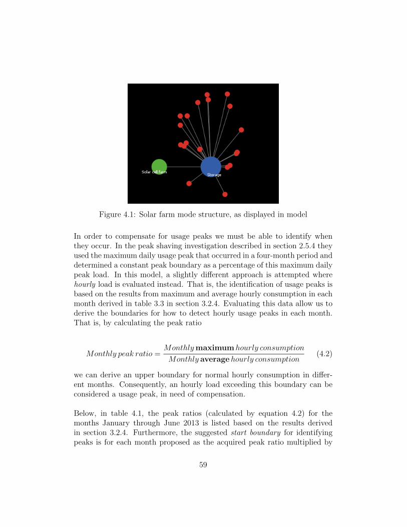
Figure 4.1: Solar farm mode structure, as displayed in model

In order to compensate for usage peaks we must be able to identify whenthey occur. In the peak shaving investigation described in section 2.5.4 theyused the maximum daily usage peak that occurred in a four-month period anddetermined a constant peak boundary as a percentage of this maximum dailypeak load. In this model, a slightly different approach is attempted wherehourly load is evaluated instead. That is, the identification of usage peaks isbased on the results from maximum and average hourly consumption in eachmonth derived in table 3.3 in section 3.2.4. Evaluating this data allow us toderive the boundaries for how to detect hourly usage peaks in each month.That is, by calculating the peak ratio

Monthly peak ratio =Monthlymaximumhourly consumption

Monthly averagehourly consumption(4.2)

we can derive an upper boundary for normal hourly consumption in differ-ent months. Consequently, an hourly load exceeding this boundary can beconsidered a usage peak, in need of compensation.

Below, in table 4.1, the peak ratios (calculated by equation 4.2) for themonths January through June 2013 is listed based on the results derivedin section 3.2.4. Furthermore, the suggested start boundary for identifyingpeaks is for each month proposed as the acquired peak ratio multiplied by

59

the last day average hourly usage. That is, the last day average usage is avariable dynamically calculated and updated after simulating each day in themodel.

Month Peak ratio (PR) Start boundaryJanuary 1.203 PRJan∗Last day averageFebruary 1.198 PRFeb∗Last day averageMarch 1.240 PRMar∗Last day averageApril 1.244 PRApr∗Last day averageMay 1.292 PRMay∗Last day averageJune 1.292 PRJun∗Last day average

Table 4.1: Start boundaries in each month

However, as described in section 3.3.2, there are significant monthly varia-tions in solar energy generation and thus the boundaries need to dynamicallyadjust dependent on how much energy is generated. That is, months wherethe solar energy generation is higher have the potential of compensating for alarger share of the energy consumption, while months with less energy genera-tion primarily must focus on shaving the most significant usage peaks. Thus,the model has implemented a dynamic scheme which determines the peakboundaries based on the amount of stored energy available. Consequently,months with a modest energy generation (e.g. January or February) haveboundaries close to or equal with their start boundary, while months withgreater energy generation have boundaries that deviate more.

In table 4.2 below, the dynamic relationship between stored energy amountrelative to storage capacity, and peak boundaries are listed. If the storedamount is less than 20% the peak boundary equals the start boundary de-scribed in table 4.1. However, if stored power exceeds 20%, the peak bound-ary decreases by 10% relative to previous peak boundary for each 10% in-creasing in storage capacity. That is,

60

Storage status Peak boundary (PB)<20% PR∗Last day average (start boundary)>20% (PR− PR ∗ 0.1)∗Last day average>30% (1− 0.1) ∗ (PR− PR ∗ 0.1)∗Last day average>40% (1− 0.1)2 ∗ (PR− PR ∗ 0.1)∗Last day average>50% (1− 0.1)3 ∗ (PR− PR ∗ 0.1)∗Last day average>60% (1− 0.1)4 ∗ (PR− PR ∗ 0.1)∗Last day average>70% (1− 0.1)5 ∗ (PR− PR ∗ 0.1)∗Last day average>80% (1− 0.1)6 ∗ (PR− PR ∗ 0.1)∗Last day average>90% (1− 0.1)7 ∗ (PR− PR ∗ 0.1)∗Last day average

Table 4.2: Relationship between stored amount and peak boundary

Thus, the peak shaving procedure with the solar farm mode structure is asfollows:

1. After each day of simulation, the microgrid’s last day average hourlyusage is calculated.

2. For each hour the following day, the hourly usage is compared to thelast day average and potential peaks are identified by the monthlyboundaries described in tables 4.1 and 4.2.

3. If a peak occurs, the amount of energy which can be compensated foris determined according to the available energy in the storage unit asdescribed in table 4.2. Hence, the compensation is calculated as:

Compensated amount = Total hourly usage− PB ∗ LDA (4.3)

where PB is the current peak boundary according to storage status,and LDA is the last day average hourly usage.

4.1.2 Distributed generation mode

As with solar farm mode (described in section 4.1.1) the intention of the dis-tributed generation mode is also to compensate for daily high demand periodsby utilizing local energy generation and storage in microgrids. However, un-like the previous mode where there was one large generation source in chargeof all local energy generation, the distributed generation mode attempts a

61

more distributed approach where households themselves are capable of bothgenerating and storing energy. Hence, in this mode the model attempts tocompensate for usage peaks in each household individually.

In figure 4.2 below, a simple model representing the end user of a microgrid isdepicted, as proposed in the paper in appendix G. The user is represented asa circle which diameter indicates the storage capacity, the arrow to the nodeindicate consumption, and the arrow from the node indicate generation.The loop (denoted charging) represent energy produced locally being storedor consumed.

Ø Storage(Ah)

ChargingConsumption

din (KwH)

Generationdout (KwH)

Figure 4.2: End user data model (as described in the paper in appendix G)

By modelling several end users as depicted in figure 4.2 we can observe themicrogrid behaviour when it is consisting of several dynamical entities con-suming, generating and storing energy individually. That is, by modellingthe network as a complex directed graph G(N,E), with N nodes (users) andE edges (transmission lines). The structure of this approach is illustrated infigure 4.3 below, where the diameter of each node indicate its generation andstorage capacity.

62

Figure 4.3: Distributed generation mode structure, as displayed in model.

In this mode the energy generation occurs in each of the households, andthe structuring of connections between households is arranged in a prefer-ential attachment manner following the energy availability (as described insection 2.1.2). Once again, the solar data analysed in section 3.3 is used,and as with solar farm mode described above, this generation data is scaleddown by a factor of 250. However, the amount of generated energy in eachhousehold is set to vary depending on the out-degree of each node in thenetwork (i.e. number of connections to other nodes). The total number ofedges in this model is 38, and below the distribution of energy generation foreach node is listed based on their respective out-degrees.

• Two nodes with out-degree 7: Energygenerated = 738∗Total generation



• 14 nodes with out-degree 1: Energygenerated = 138∗Total generation

Hence, the total energy generated in the microgrid is equal to that of thesolar farm mode, only here it is divided among the different nodes based onthe degree distribution.

63

Potential usage peaks are identified in the same manner as with the solarfarm mode, i.e. by using the boundaries as described above in section 4.1.1.However, as the peak shaving now is enforced on each household, the modelcalculates last day average hourly usage in each individual household as op-posed to just the overall microgrid average. Also, once again the modelassumes a discharge and power conversion loss of 10%.

Furthermore, in order to achieve a more optimal utilization of available en-ergy, it is implemented upper storage boundaries in each of the nodes exceptthe two most central (i.e. the ones denoted 0 and 1 in figure 4.3). Conse-quently, any surplus energy in smaller-degree nodes exceeding their respectiveboundary is transferred to connected higher-degree nodes, with purpose ofensuring a better utilization of the available energy resources in the microgridas a whole. The boundaries are set as follows:

• Nodes with out-degree 3: maximum energy capacity 30 kWh



Thus, the peak shaving procedure using distributed generation mode is asfollows:

1. After each day of simulation, the last day average hourly usage of eachhousehold is calculated.

2. For each hour the following day the hourly usage is compared to thelast day average and potential peaks are identified using the monthlyboundaries described in tables 4.1 and 4.2.

3. If a peak occurs, the amount of energy which can be compensated foris determined according to the available energy in the storage unit asdescribed in table 4.2. Hence, the compensation is calculated as:

Compensated amount = Total hourly usage− PB ∗ LDA (4.4)

where PB is the current peak boundary according to storage status,and LDA is the last day average hourly usage. Also, if the storedamount at smaller-degree nodes is insufficient to cover the requiredpeak shaving, the smaller-degree node may receive contributions fromconnected higher-degree nodes if there is available resources there.

64

4. Finally, if an household has generated more energy than it is allowed tostore, the surplus energy is transferred to the neighbouring householdwith the largest out-degree.

4.1.3 Island mode

In island mode we are able to investigate how long a microgrid can man-age the entire energy demand of its participants, as an islanded entity (asdescribed in section 2.1.2). The purpose of enabling such a feature is to pre-vent potential power outages when the external energy supply is disrupted.Thus, the intention here is to examine the duration for which a microgrid canstay operational in different months using local generation and stored energyreserves. Obviously, this will vary as both consumption and generation variessignificantly in the different months of the model. The structure of this ap-proach is similar to that of the solar farm mode described in section 4.1.1,i.e. one solar farm, one storage unit and 20 households.

At any time during simulation one can cut the external energy supply andobserve how the microgrid starts to utilize its stored energy reserves in ac-commodation to local generation to prevent a power outage. Moreover, themodel assumes a discharge and power conversion loss of 10 % and a BESsystem with a energy capacity of 1 MWh.

4.1.4 Model setup and user interface guide

The model is developed using the complex network tool Netlogo, described insection 2.8.2. Thus, to open the model (located in folder ”AutonomyModel”on attached CD-ROM) one must install NetLogo, which can be downloadedfrom1. Furthermore, the model is also connected to the database containingthe consumption and generation data analysed in chapter 3, and thus will notwork before the database is set up as described in section 3.1.3. Moreover,to be able to set up a connection with a MySQL database one must firstdownload a MySQL wrapper for NetLogo that needs to be included in thesame directory as the model. However, this wrapper is currently includedas required in the model on the attached CD-ROM. Below, a code extract

1http://ccl.northwestern.edu/netlogo/

65

illustrating how to set up the database connection in NetLogo is described,i.e.

to setup -database -connection

sql:configure "defaultconnection" [["host" "localhost"] ["

port" 3306] ["user" "root"]

["password" "root"] ["database" "demosteinkjer"]]

end

The user interface in the model (presented in appendix E) shows the differ-ent user settings which can be manipulated in order to investigate differentscenarios. These are:

• Mode: This setting determines which of the three previously describedmodes the model should run.

• Number of homes: Here one can choose the number of householdsin the microgrid. Maximum amount and default setting is 20.

• Choose house ID for individual plots (1 and 2): Here the user canchoose specific household IDs for individual consumption plots. Thisis particularity useful when running the distributed generation modeof the model as you then can observe the peak shaving in individualhouseholds. One may choose any of the model’s 20 households for thispurpose.

• Number of days for simulation: The simulation starts at January1st 2013, however the user may choose the number of days for whichthe simulation lasts. Maximum amount of days is 179, i.e. until June28th.

• Initial storage state: Here the initial stored amount in per cent oftotal storage capacity can be specified. By default this is set to 20 %(i.e. 200 kWh).

• External supply: This setting is restricted to the island mode of themodel. The external supply can be switched off at any point in thesimulation, causing the microgrid to solely depend on stored energyand local generation to handle the demand of its participants.

66

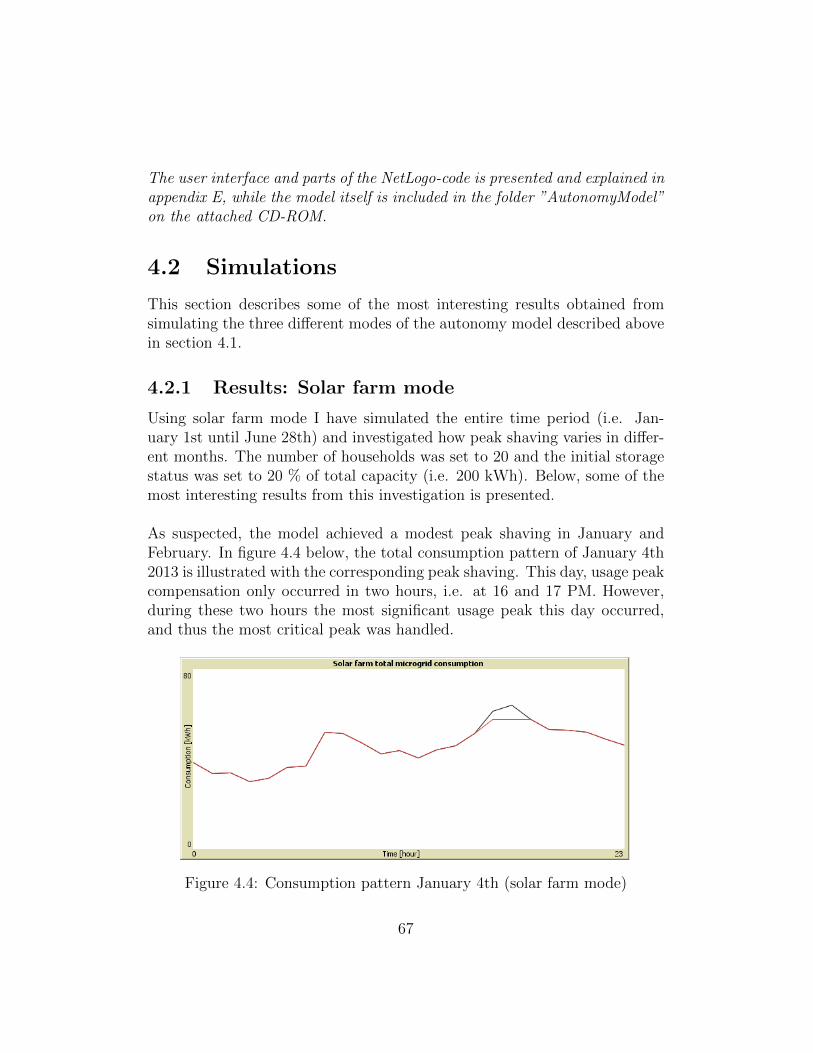
The user interface and parts of the NetLogo-code is presented and explained inappendix E, while the model itself is included in the folder ”AutonomyModel”on the attached CD-ROM.

4.2 Simulations

This section describes some of the most interesting results obtained fromsimulating the three different modes of the autonomy model described abovein section 4.1.

4.2.1 Results: Solar farm mode

Using solar farm mode I have simulated the entire time period (i.e. Jan-uary 1st until June 28th) and investigated how peak shaving varies in differ-ent months. The number of households was set to 20 and the initial storagestatus was set to 20 % of total capacity (i.e. 200 kWh). Below, some of themost interesting results from this investigation is presented.

As suspected, the model achieved a modest peak shaving in January andFebruary. In figure 4.4 below, the total consumption pattern of January 4th2013 is illustrated with the corresponding peak shaving. This day, usage peakcompensation only occurred in two hours, i.e. at 16 and 17 PM. However,during these two hours the most significant usage peak this day occurred,and thus the most critical peak was handled.

Figure 4.4: Consumption pattern January 4th (solar farm mode)

67

In figure 4.5 below, the consumption pattern of the last day of the model,June 28th, is illustrated. Here, one can observe how we achieve a far greaterpeak compensation than that of January 4th above. In fact, each hour from 5AM until 23 PM the energy supplied by the utility company to the microgridis held constant at 15.2 kWh, while the actual usage varies significantly.

Figure 4.5: Consumption pattern June 28th (solar farm mode)

Figure 4.6 below illustrates the greatest hourly peak shaving that occurredin the entire time period. It occurred at 19:00 PM on April 2nd, and theenergy compensated for was ≈ 29kWh of the total consumption this hour.

Figure 4.6: Consumption pattern April 2nd (solar farm mode). Maximumpeak occurring at 19 PM.

68

Furthermore, in figure 4.7 below the maximum daily usage peak shaving inthe entire time period is illustrated. This occurred on April 24th, and thetotal energy compensation was 275.15 kWh.

Figure 4.7: Consumption pattern April 24th (solar farm mode)

In table 4.3 below the maximum hourly peak shaving, maximum daily peakshaving, and total monthly peak shaving of each month is listed.

Month Max hourly peak shave Max daily peak shave Total peak shavingJan 17.21 kWh 105.66 kWh 402.21 kWhFeb 12.67 kWh 99.81 kWh 750.50 kWhMar 23.15 kWh 180.74 kWh 1804.84 kWhApr 28.89 kWh 275.15 kWh 3940.15 kWhMay 23.73 kWh 234.56 kWh 3968.24 kWhJune 25.55 kWh 250.04 kWh 4370.21 kWh

Table 4.3: Max hourly, max daily and total monthly peakshaving in eachmonth (solar farm mode)

In figure 4.8 below, the status of the BES system in use over the entire timeperiod is illustrated, revealing how the amount of stored power varies.

69

Figure 4.8: Variations in stored power (solar farm mode)

Furthermore, in table 4.4 the maximum stored power in each month is listed.Here one can observe how the maximum amount for the entire time periodis 972.14 kWh, occurring on June 8th.

Month Max stored energy [kWh]Jan 210.52Feb 304.19Mar 582.00Apr 667.99May 855.45June 972.14

Table 4.4: Maximum amount of energy stored in each month (solar farmmode)

4.2.2 Results: Distributed generation mode

When simulating the distributed generation mode I used the same initial set-tings as with solar farm mode, i.e. 20 households, initial storage status at20 % of total capacity and simulation period January 1st until June 28th.However, the resulting peak shaving is significantly different.

70

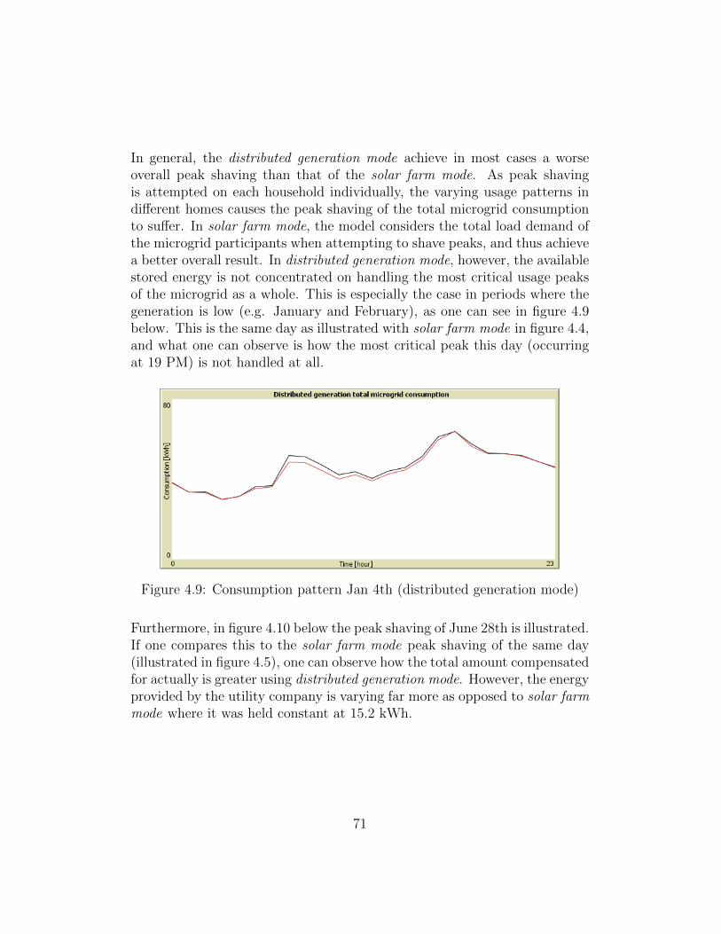
In general, the distributed generation mode achieve in most cases a worseoverall peak shaving than that of the solar farm mode. As peak shavingis attempted on each household individually, the varying usage patterns indifferent homes causes the peak shaving of the total microgrid consumptionto suffer. In solar farm mode, the model considers the total load demand ofthe microgrid participants when attempting to shave peaks, and thus achievea better overall result. In distributed generation mode, however, the availablestored energy is not concentrated on handling the most critical usage peaksof the microgrid as a whole. This is especially the case in periods where thegeneration is low (e.g. January and February), as one can see in figure 4.9below. This is the same day as illustrated with solar farm mode in figure 4.4,and what one can observe is how the most critical peak this day (occurringat 19 PM) is not handled at all.

Figure 4.9: Consumption pattern Jan 4th (distributed generation mode)

Furthermore, in figure 4.10 below the peak shaving of June 28th is illustrated.If one compares this to the solar farm mode peak shaving of the same day(illustrated in figure 4.5), one can observe how the total amount compensatedfor actually is greater using distributed generation mode. However, the energyprovided by the utility company is varying far more as opposed to solar farmmode where it was held constant at 15.2 kWh.

71

Figure 4.10: June 28th

Below, in figure 4.11, the greatest hourly peak shaving in the entire timeperiod using distributed generation mode is illustrated. This occurred at18 PM on June 2nd, and the total compensation was ≈ 23kWh of totalconsumption this hour.

Figure 4.11: Consumption pattern June 2nd (distributed generation mode)

In figure 4.12 the maximum daily usage peak shaving in the entire time periodusing distributed generation mode is illustrated. As with solar farm mode,this occurred on April 24th. However, the total compensation was less, i.e.approximately 237 kWh.

72

Figure 4.12: Consumption pattern April 24th (distributed generation mode)

In table 4.5 below the maximum hourly peak shaving, maximum daily peakshaving, and total monthly peak shaving of each month is listed, using dis-tributed generation mode. Comparing this to table 4.3, one can observe howthe total peak shaving of each month in fact is greater using distributed gen-eration mode than that of solar farm mode. However, the maximum hourlyand daily peak shaving is less in each month.

Month Max hourly peak shave Max daily peak shave Total peak shavingJan 10.26 kWh 87.47 kWh 516.14 kWhFeb 11.09 kWh 75.66 kWh 847.09 kWhMar 14.94 kWh 137.34 kWh 1812.35 kWhApr 21.68 kWh 236.65 kWh 3999.59 kWhMay 20.96 kWh 212.07 kWh 4158.68 kWhJune 22.72 kWh 229.24 kWh 4479.18 kWh

Table 4.5: Max hourly, max daily and total monthly peakshaving in eachmonth (distributed generation mode)

In figure 4.13 below, the combined status of the BES systems in use over theentire time period is illustrated, revealing how the amount of stored energyvaries in distributed generation mode. Comparing this to solar farm mode(figure 4.8) one can see how the utilization of stored energy is significantlygreater using distributed generation mode. Particularly in the three firstmonths (January - March) the stored amount is rarely significant, indicatingthat all produced energy is used immediately to compensate for usage peaks.

73

Figure 4.13: Variations in stored power (distributed generation mode)

In table 4.6 below the maximum stored power of each month is listed. Aswith solar farm mode the maximum amount for the entire simulation periodoccurred on June 8th, however the amount was less (i.e. 799.79 kWh).

Month Max stored energy [kWh]Jan 198.59Feb 71.73Mar 376.06Apr 492.02May 630.60June 799.79

Table 4.6: Maximum amount of power stored in each month (distributedgeneration mode)

4.2.3 Results: Island mode

Using the island mode of the model it is examined how long a microgrid canstay operational without external supply. The external supply was turnedoff at 2 AM on the 15th of each month and what we can observe is how theisland mode duration varies in different seasons. When the external energysupply was turned off the BES system was fully charged (i.e. 1000 kWh), andthus this investigation reveals how long the microgrid can stay operational

74

using its stored reserves in addition to local generation in different months.As with the investigations described in sections 4.2.1 and 4.2.2 above, thenumber of households was set to 20.

In figure 4.14 below the island mode duration on January 15th is illustrated.Average hourly energy usage in the microgrid this day was 55.03 kWh. Asone can observe the microgrid is able to manage the entire demand of itsresidents for 16 hours.

Figure 4.14: Island mode January 15th

In figure 4.15 below the island mode duration on March 15th is illustrated.Average hourly energy usage in the microgrid this day was 52.88 kWh. Asone can observe, the island mode duration is one hour longer in March, i.e.17 hours.

75

Figure 4.15: Island mode March 15th

Furthermore, in figure 4.16 island mode on May 15th is illustrated. Here, theaverage hourly energy usage in the microgrid was 27.90 kWh, and one canobserve that the microgrid is able to manage the entire demand the rest ofthe day. In fact, it is able to manage the demand until 21 PM on May 16th(43 hours in total).

Figure 4.16: Island mode May 15th

Below, in table 4.7 the island mode duration on the 15th in each of themonths in the model is listed.

76

Month Average hourly energy usage [kWh] Island mode durationJan 55.03 (Jan 15th) 2 AM - 18 PM (16 hours)Feb 51.48 (Feb 15th) 2 AM - 20 PM (18 hours)Mar 52.88 (Mar 15th) 2 AM - 19 PM (17 hours)Apr 32.01 (Apr 15th) 2 AM (15th) - 7 AM (16th) (29 hours)May 27.90 (May 15th) 2 AM (15th) - 21 PM (16th) (43 hours)June 24.90 (June 15th) 2 AM (15th) - 7 AM (17th) (53 hours)

Table 4.7: Island mode duration in each month

77

Chapter 5

Discussion

This chapter reflects on some of the results obtained and key issues arisenduring this study.

5.1 Demo Steinkjer consumption patterns

There are some issues worth addressing regarding the results obtained inthe analysis of consumption patterns in Demo Steinkjer (section 3.2). Firstoff, even though the monthly differences in total energy consumption variesconsiderably, the usage peaks are present regardless of season. The analysisshowed that we experience the same usage peaks in all months, occurring atapproximately the same time during the day. Hence, as concluded in sec-tion 3.2.6, this supports how monthly differences in consumption is mostlydependent on space heating caused by the seasonal variations in outdoor tem-peratures. Clearly, this consistency in daily high and low demand periodsemphasize the potentials of many of the efficiency measures made possibleby a transition to a smarter distribution grid, such as the ones presented insection 2.5. In particular, the potential benefits gained from enabling meansfor shaving and shifting of demand in usage peak periods are evident, giventhe knowledge of this consistent daily pattern.

Secondly, the investigation of daily usage patterns in single households (sec-tion 3.2.1) revealed a much more fluctuating pattern than what was achievedwhen analysing the combined energy usage of several homes. The analysisshowed, however, that when aggregating the consumption patterns of several

78

households, the fluctuating behaviour of different homes is disguised, and weachieve a pattern more similar to what is expected. This is also importantto take in account with regards to efficiency measures in microgrids. That is,in order to achieve the best overall microgrid efficiency, using measures suchas autonomous peak shaving, one must focus on handling usage peaks in themicrogrid as a whole as opposed to treating usage peaks in each householdindividually. Once again, this emphasizes the importance of the increasedinformation flow that Smart Grid technology is intended to provide. Thatis, given real-time reporting on consumption from each of the users in a mi-crogrid one can enforce efficiency measures on the microgrid as a whole, andthus ensure a better overall efficiency in energy usage. As discussed in sec-tion 5.3 below, this was also the conclusion reached from the peak shavingmodelling described in sections 4.2.1 and 4.2.2.

Furthermore, the analysis also revealed the apparent differences betweenweek day and weekend consumption in households. While the week day pat-tern revealed two distinct high demand periods daily (one between 7 and 9AM, and another in the afternoon), weekends had a more constant high con-sumption from 11 AM until evening. However, as described in section 3.2.4,the differences between the two was primarily related to when usage peaksoccur, and not the amount of energy consumed daily. In fact, as one canobserve in table 3.2 in section 3.2.4, the collective average hourly consump-tion of 20 households is approximately equal when comparing week days andweekends. Thus, if peak detection is determined according to last day aver-age hourly usage (as proposed in the model described in chapter 4), we donot need to distinguish between week days and weekends in terms of identi-fying a usage peak.

Finally, as discussed earlier, the consumption data provided by Demo Steinkjerhad numerous measurement gaps in the dataset. Thus, finding longer peri-ods of time, where none of these gaps were present, was extremely time-consuming. However, the 20 households used in both the analysis (sec-tion 3.2) and the autonomy model (chapter 4) all have consistent and con-secutive measurements in the time period ranging from October 1st 2012until June 28th 2013. The database IDs of these households are presented inappendix F. The reason for these measurement gaps is unknown. One couldargue that it is caused by packet losses in the communication infrastructure,however this is unlikely due to the fact that when measurements are missing

79

it is not just one hourly update that is lost, it is usually between 10 and 48hours worth of consecutive consumption updates. Thus, it is likely to assumethat the missing data is caused by individual or multiple households ceasingto report as result of e.g. system maintenance or improvement.

5.2 Solar cell energy generation

The investigation of solar cells (section 3.3) also revealed some results worthaddressing. In particular, the substantial seasonal differences in energy gen-eration calls into questioning the suitability of solar energy for Norwegianconditions. As a matter of fact, the analysis showed that total generatedenergy in July was as much as 18 times greater than that of January. Al-though, as described in section 3.3.2, the Brussels total PV capacity hadincreased by 3.38 MW in July compared to January, the difference in gen-erated energy is significant regardless. Hence, given the weather conditionsin Norway, whereas winter months are the clearly most energy demanding,would suggest that solely relying on solar energy in Norwegian microgridsmight not be the best choice compared to other renewable resources. Thatis, the potential benefits of solar energy harnessing is clearly greater in partsof the world with a milder climate and greater generation potentials.

Also, one must bear in mind that the data used in the analysis in section 3.3originates from Belgium, and consequently does not give a precise impressionof what the potentials are for solar energy harnessing in Norway. As describedin section 2.7.1, photovoltaic energy generation is highly weather dependent,and nominal power output (i.e. maximum achievable generation) will onlyoccur during optimal weather conditions. Thus, installing a capacity similarto that of Brussels might, or most probably will, result in a different poweroutput pattern in Norway. In fact, given the variations in solar energy poten-tials in Europe (figure 2.10, section 2.7.1) it is plausible to assume that totalenergy generated in Norway would be significantly less than that of Belgium.Considering this, it would have been interesting to study solar generationdata gathered in Steinkjer in order to provide dynamics more representativefor Norwegian conditions, and consequently more suitable with regards tothe consumption patterns analysed.

Furthermore, the main problem with solar energy, or any other renewable

80

source for that matter, is that supply cannot be manipulated (i.e. we are un-able to control the power output). Consequently, this causes the difficultieswith regards to prediction of supply. The analysis showed that day-aheadpredictions on solar energy supply could vary as much as 26 % from theactual generated amount each month. Also, more often than not these pre-dictions were optimistic (i.e. greater than actual generation). Moreover,as described in section 3.3.1, the day-to-day variations in supply was con-siderable, once again confirming the suspected weather dependency of solarenergy generation. These observations clearly state the challenges associatedwith solar energy, and emphasize the need for a storage technology capableof transforming this highly variable resource into a dispatchable one. Thatis, the most efficient utilization of solar energy would depend on a storagesystem capable of charging during high generation periods, and dischargingin non-generating hours.

Finally, in section 4.1.1 the area of PV cells required to obtain the capacityused in the solar farm mode of the autonomy model was derived (i.e. nominalpower output of 41.2 kW). The calculation revealed that one needs an areaof approximately 275 m2 of photovoltaic cells, given 15 % cell efficiency, inorder to obtain the desired capacity. Arguably, such a size for a solar farminstallation is manageable in futuristic microgrids, and will be possible toimplement regardless of geographical location. That is, by e.g. installing PVcells on several rooftops one would easily meet such a space requirement.

5.3 Autonomy model

The purpose of the microgrid autonomy model (chapter 4) was to investigateusage peak shaving and islanding of microgrid operation. As described insections 4.2.1 and 4.2.2, the two different modes for which peak shaving wasattempted (i.e. solar farm and distributed generation mode) resulted in sig-nificantly different utilization of available stored resources. The simulationsshowed that although total peak shaving performed in distributed generationmode was greater than that of solar farm mode in each month, the maxi-mum hourly and daily peak shaving was less. That is, as peak shaving indistributed generation mode was performed on each individual household, thedifferent usage patterns caused a suboptimal storage utilization in the mi-crogrid as a whole, as available resources was not concentrated on handling

81

the usage peaks of the overall microgrid consumption.

Furthermore, when comparing the variations in stored energy throughoutthe entire simulation period in both modes (depicted in figures 4.8 and 4.13),one can observe the differences in available stored energy in different months.This revealed that using distributed generation mode the capacity in storagewas in the first three months rarely significant, indicating that most of theproduced energy was used immediately. Using solar farm mode, however,there was at all times some resources available, and thus critical usage peaks(i.e. peaks exceeding the start boundary described in section 4.1.1) was neverignored. On the other hand, in the three first months using distributed gen-eration mode all BES systems was often completely discharged, consequentlycausing critical usage peaks to be ignored, both in individual households andin the microgrid as a whole. In particular, this is illustrated in figure 4.9 insection 4.2.2 where one can observe how the most critical usage peak thisday (occurring at 19 PM) is not handled at all.

The observations made by these simulations clearly emphasize the potentialsof the increased information and power flow provided by a smarter distribu-tion grid. As mentioned, employing peak shaving on individual householdsin a microgrid, as opposed to the combined consumption of all microgridparticipants, results in a significantly worse utilization of available resources.Thus, in order to achieve the best overall result it is more feasible to takea subsystem approach that considers a microgrid’s total consumption andgeneration when enforcing efficiency measures. This, however, will requirea continuous collaboration between the microgrid users, and a centralizedcontrol system for utilizing the stored reserves most optimally.

Simulating islanding of microgrid operation also showed significant monthlydifferences. In fact, comparing the island mode duration in January (16hours) and June (53 hours) revealed a difference of 37 hours for which themicrogrid was able to manage its entire energy demand. The simulation alsoshowed that midday energy generation in May and June in fact often wasgreater than the consumption, causing the battery to start charging. Worthaddressing, however, is that in island mode the microgrid instantaneouslytook over when the external energy supply was switched off. This assump-tion is unlikely as some response time is required to switch between the twomodes of operation.

82

Regarding the development of the model there are several issues worth ad-dressing. First off, as described in section 4.1, to simplify I assumed that thesolar power output is constant in each hour. As discussed in section 5.2, thisis rarely the case given the high weather dependency of solar energy genera-tion. Furthermore, I have used the same peak boundaries in both the solarfarm mode and distributed generation mode of the model for detecting usagepeaks. In retrospect, given the varying consumption patterns of individualhouseholds (discussed in section 5.1), this might not have been the best ap-proach. That is, a better solution would clearly be to calculate individualpeak boundaries for each household. Finally, as described in section 2.7.2, thenominal solar generation in the data used had an increasing in power outputcapacity in March, which greatly affected the energy generation. Perhaps itwould have been more feasible to use a dataset that had a constant poweroutput capacity in the entire modelling period.

Also, the model uses hourly updates on both energy consumption and gener-ation. This simplification is inaccurate as the actual load in households andpower output from solar cells may vary significantly within one hour. Thus,in order to achieve a better model it would have been feasible to use datawith greater precision.

5.4 Storage in microgrids

As described in chapter 1, the main focus of this study has been to analyseand model consumption and generation patterns in residential area micro-grids. Thus, the potential issues related to storage of energy is not wellcovered. In the model in chapter 4 it is implemented a discharge and powerconversion loss of 10 % in the BES system used, however other storage-relatedissues such as e.g. minimum state of charge (SOCmin, as described in sec-tion 2.5.4), and further energy loss in the battery system is not taken intoconsideration. Also, as described in section 2.4, the cost of a BES systemis mainly associated with its energy capacity rather than its power rating.Thus, the required period of discharge will greatly affect the costs of thestorage system. In the model (chapter 4) it was simply assumed a 1 MWhbattery system, not considering issues such as response time and requiredperiod of discharge etc. In particular, as described in section 4.2.1, by sim-

83

ulating using the solar farm mode of the model we achieved a maximumhourly consumption shaving of ≈29 kWh and a maximum daily energy com-pensation of 275.15 kWh. Clearly, these observations must be addressed ifone is to design a suitable storage system for this purpose.

5.5 NetLogo

NetLogo proved to be a useful tool for developing the model in chapter 4,and can be recommended for others attempting to model something similar.The agent-based programming language is easy to learn, and there is a lotof online support (e.g. tutorials, troubleshooting forums etc.) that can beof help. On the downside, however, as one can see from the code in thefolder ”AutonomyModel” on the attached CD-ROM, you are required to usea large amount of global variables in order to connect the user interface withthe code. That is, every user-setting, plotting variable, monitoring variableetc. must all be defined as global. This combined with all other shared globalvariables results in a somewhat messy code. Furthermore, when accessing thedatabase using SQL commands in the NetLogo model, the data extractionscan be extremely slow. The advice is to reduce the amount of SQL queriesexecuted in the model, by e.g. providing the start-IDs in the database of thedifferent households’ consumption and generation measurements in the code.

Also, NetLogo is not a supported programming language in editors suchas notepad++. On the attached CD-ROM (in folder ”AutonomyModel”)the code of the model can be viewed by either opening the actual NetLogomodel and pressing the ”code-bar”, or by opening the file ”NetLogoCode.py”.However, the latter interprets it as a python code, and thus the advice is toview the code as intended in NetLogo.

84

Chapter 6

Conclusion

This study has focused on addressing the energy usage patterns of house-holds, and investigating means for reduced and more efficient household con-sumption in futuristic microgrids. Furthermore, two analyses have been per-formed with purpose of examining the dynamics of energy consumption inhouseholds and the energy generation potentials of photovoltaic solar cells.Finally, I have attempted to model autonomy in a microgrid cell using theacquired dynamics of energy generation and consumption obtained from thetwo previously described analyses. The purpose of this model was to exam-ine:

• usage peak shaving in high demand periods using local energy genera-tion and storage.

• how long a microgrid can stay operational using stored energy reservesand local generation when external energy supply is disrupted, i.e. withpurpose of avoiding power outages.

To conclude the thesis, I will summarize the study’s main findings.

The analysis of Demo Steinkjer households (section 3.2) revealed that con-sumption patterns are consistent with previous investigations on behaviourin Norwegian households. The analysis showed that when aggregating theconsumption of several households over longer periods of time, we obtain adaily pattern that varies as expected, with two distinct usage peak periodson week days. Furthermore, the analysis also showed that there are consid-erable differences in consumption when comparing week day and weekend

85

consumption. That is, while we experience these two distinct usage peakson week days (one between 7 and 9 AM, and another in the afternoon), theweekend consumption has a different pattern. In particular, the usage peakassociated with the morning routines of household occupants is shifted sev-eral hours in weekends, from approximately 7 AM to 11 AM. However, asdiscussed in section 5.1 the differences between week day and weekends areprimarily related to when usage peaks occur, and not the amount of energyconsumed daily.

Moreover, the expected patterns of both week day and weekend consump-tion seem to emerge even more persistently when increasing the time periodand the number of households further, despite the monthly variations in totalconsumption. This supports the presumption that usage peaks are consistentregardless of season, and that monthly differences in overall consumption ismostly due to the varying need for space heating in households dependingon outdoor temperatures. However, even though the aggregated consump-tion results in this presumed pattern, the behaviour of individual householdsmay vary significantly. That is, the investigation of consumption in singlehouseholds (section 3.2.1) revealed a much more fluctuating daily usage pat-tern as opposed to what was experienced when the consumption of severalhouseholds was aggregated. Once again, this is consistent with previous in-vestigations (described in section 2.2) as consumption in different householdsmay vary depending on factors such as geographical location, size of house-hold and behaviour of household occupants.

The analysis of solar energy potentials (section 3.3) clearly verified the unpre-dictable dynamics, nonlinearities and uncertainties of solar energy harnessingdescribed in section 2.7. In particular, the investigation on day-to-day varia-tions (section 3.3.1) revealed how the power output on consecutive days maydiffer considerably, confirming the great impact weather conditions have onenergy generation in solar cells. The analysis also showed that day-aheadpredictions on supply could vary as much as 26 % from actual generationeach month, and that the predictions more often than not were too opti-mistic. Furthermore, as discussed in section 5.2, the considerable seasonaldifferences in solar energy generation questions the suitability of solely relyingon solar energy for local microgrid generation given Norwegian conditions.In particular, the analysis showed that energy generation in July was signifi-cantly greater than that of January. Thus, given that winter months are the

86

clearly most energy demanding in Norway would suggest that, in addition tosolar power, it perhaps would be feasible to include other renewable energysources (e.g. wind) in Norwegian microgrids.

As discussed in section 5.2, to obtain a nominal capacity of 41.2 kW, given15 % cell efficiency, one needs an area of approximately 275 m2 of photo-voltaic cells. However, this nominal capacity represent the maximum achiev-able output power which only occurs during optimal weather conditions.Hence, given that global solar radiation varies, installing such a capacity willresult in considerably different energy supply potentials in different parts ofthe world. Thus, Norwegian conditions will require a significantly greaterinstalled capacity in order to achieve a given energy supply compared toother parts of the world with a milder climate and greater solar generationpotentials.

The potential benefits of local energy generation and storage in microgridcells are evident. In particular, given the consistent daily usage pattern inhouseholds, much can be gained from employing measures such as e.g. peakshaving. However, as discussed in section 5.3, the modelling of peak shavingshowed that in order to achieve the most optimal result, it is important toconsider a microgrid’s total consumption and stored reserves when compen-sating in high demand periods. Such a centralized monitoring and controlcan be achieved with the increased information and energy flow intended withSmart Grid. Furthermore, the varying dynamics of solar energy generationemphasizes the need for a storage system capable of charging during genera-tion periods, and discharging in non-generating hours. However, as describedin section 2.4, one of the main advantages with BES systems is this abilityto convert highly variable renewable energy resources into dispatchable ones.

87

Bibliography

[1] F. A. T. Al-Saedi. Peak shaving energy management system for smarthouse. International Journal of Computer Science Engineering andTechnology, Vol 3:359–366, 2013.

[2] S. Aman, Y. Simmhan, , and V. K. Prasanna. Energy managementsystems: State of the art and emerging trends. IEEE CommunicationsMagazine, pages 114–119, 2013.

[3] B. Bergesen, L. Henden Groth, I. Langseth, Benedicte H. Magnussen,D. Spilde, and J. E. Wiik Toutain. Energy consumption 2012. NorwegianWater Resources and Energy Directorate, 2013.

[4] S. Boccaletti, V. Latora, Y. Moreno, M. Chavez, and D. Hwang. Com-plex networks: Structure and dynamics. Physics reports, pages 177–308,2006.

[5] R. Bussar, M. Lippert, and G. e. Bonduelle. Battery energy storage forsmart grid applications. EUROBAT, 2013.

[6] E. Carrol, E. Hatton, and M. Brown. Residential energy use behaviorchange pilot. Franklin Energy, pages 1–26, 2009.

[7] ESF. Harnessing solar energy for the production of clean fuels. Publicdocuments, European Science Foundation, pages 1–58.

[8] Everredtronics. Global solar radiation map of europe(http://www.everredtronics.com/solar.download.html), 25.05 2014.

[9] E. F. Camacho, T. Samad, M. Garcia-Sanz, and I. Hiskens. Control forrenewable energy and smart grids. IEEE Control Systems Society, 2011.

88

[10] X. Fang, S. Misra, G. Xue, and D. Yang. Smart grid - the new and im-proved power grid: A survey. IEEE Communications Surveys Tutorials,14(4):944 –980, quarter 2012.

[11] A. Faruqui and S. Sergici. Household response to dynamic pricing of elec-tricity: a survey of 15 experiments. Journal of Regulatory Economics,38(2):193–225, 2010.

[12] D. G. Hart. Using ami to realize the smart grid. IEEE, pages 1–2, 2008.

[13] T. Gerke. Sunday, solar sunday: Germany’s recent solar energyrecord in-depth. found at: http://theenergycollective.com/thomas-gerke/248721/sunday-solar-sunday-germany-s-july-7-solar-power-record-depth, 2013.

[14] A. Goetzberger and V. Hoffmann. Photovoltaic Solar Energy Genera-tion. Springer, 2005.

[15] F. Katiraei, R. Iravani, N. Hatziargyriou, and A. Dimeas. Microgridsmanagement - control and operation aspects of microgrids. IEEE power& energy magazine, pages 54–65, 2008.

[16] R. Kinney, P. Crucitti, R. Albert, and V. Latora. Modeling cascad-ing failures in the north american power grid. The European PhysicalJournal B, pages 101 – 107, 2005.

[17] J. Kumagai. The smartest, greenest grid. Found at:http://spectrum.ieee.org/energy/the-smarter-grid/the-smartest-greenest-grid, 2013.

[18] N. R. E. Laboratory. Concentrating solar power: Energy from mirrors.pages 1–8, 2001.

[19] R. Lasseter and P. Piagi. Microgrid: A conceptual solution. pages 1–6,2004.

[20] K. Leung Ray. Photovoltaic cell efficiency at elevated temperatures.Massachusetts Institue of Technology, pages 1–23, 2010.

[21] NREL. Solar photovoltaic technology basics. National Renewable EnergyLaboratory, page found at: http://www.nrel.gov/learning/.

89

[22] J. Oestergaard and J. E. Nielsen. The bornholm power system anoverview. Centre for Electrical Technology (CET), pages 1–7, 2011.

[23] C. Ricketts. How microgrids will change the way we get energy froma to b. found at: http://www.geni.org/globalenergy/library/technical-articles/transmission/green.venturebeat.com/how-microgrids-will-change-the-way/index.shtml, 2010.

[24] S. H. Strogatz. Exploring complex networks. insight review articles,pages 268 – 276, 2001.

[25] C. Venu, Y. Riffonneau, S. Bacha, and Y. Baghzouz. Battery storagesystem sizing in distribution feeders with distributed photovoltaic sys-tems. IEEE Bucharest Power Tech Conference, pages 1–5, 2009.

[26] S. Vukmirovic, A. Erdeljan, F. Kulic, and S. Lukovic. A smart meteringarchitecture as a step towards smart grid realization. IEEE InternationalEnergy Conference and Exhibition (EnergyCon), pages 357–362, 2010.

[27] W. Wang, Y. Xu, and M. Khanna. A survey on the communication ar-chitectures in smart grid. Computer Networks, 55(15):3604–3629, 2011.

90

Appendix A

Tutorial for setting up databaseand extracting data

91

Setting up database:The following three steps must be taken in order for the attached pythonscripts and the autonomy model to work.

1. Set up apache server and configure phpMyAdmin and MySQL, e.g. asdescribed in 1

2. Create a database named ”demosteinkjer” in phpMyAdmin.

3. Upload .sql files on consumption and generation (located in folder”Database” on the attached CD-ROM) to database ”demosteinkjer”in separate tables (four tables in total), i.e.

• Create one table called ”consumption” in the ”demosteinkjer”database and import the ”consumption.sql” dataset. Worth notic-ing, however, is that this import must be done via command lineas the file is to large to be imported directly in phpMyAdmin.

• Create one table called ”generationjanfebmaraprmayjun2013” inthe ”demosteinkjer” database and import the ”generationjanfeb-maraprmayjun2013.sql” dataset.

• Create one table called ”generationjulaugsept2013” in the ”de-mosteinkjer” database and import the ”generationjulaugsept2013.sql”dataset.

• Create one table called ”generationoctnovdec2013” in the ”de-mosteinkjer” database and import the ”generationoctnovdec2013.sql”dataset.

As described in section 3.1.3 there are some preprocessing steps that needs tobe performed on the consumption and generation datasets, i.e.

• Add a column called ”HourlyConsumption” to the ”consumption” tablein the database, and run python script ”addHourlyConsColumn.py”,located on the attached CD-ROM (in folder ”pythonworkspace”).

• Remove spaces from all column names in all three generation tables.

• Run python script ”searchingForDuplicate.py” (located in folder ”python-workspace” on attached CD-ROM) on the database, and manually re-move the database entry indicated by output of the python script.

1https://www.youtube.com/watch?v=kZ2zbO6PABk

92

• Run python script ”ReplaceCommaWithPeriodInDatabase.py” on ”Day-AheadforecastMW” and ”CorrectedUpscaledMeasurementMW” columnsin all generation tables in order replace comma with period as decimalmark in numbers.

However, these last four steps are necessary only if one intends to use thedata downloaded from Demo Steinkjer and elia directly. In other words, us-ing the datasets included on the CD-ROM makes it unnecessary to performthese last four steps. Below, in figure A.1 the resulting representation of thedatabase in phpMyAdmin is illustrated.

Figure A.1: Database representation in phpMyAdmin

93

Extracting consumption and generation data from database:

In the folder ”pythonworkspace” on the attached CD-ROM the python scriptsused for extracting and plotting consumption and generation patterns in theanalyses in chapter 3 is located. However, in order to run any of these scriptsthere are some python packages that must be installed, these are:

• MySQLdb

• dateutil

• pyparsing

• matplotlib

• numpy

• re

• six

After having set up the database as described earlier, and installed the neces-sary python packages, all scripts in the folder ”pythonworkspace” can be runwithout any other preprocessing steps. Hence, one can reproduce the resultsobtained in the analyses described in sections 3.2 and 3.3. As described insection 3.1.3, in appendix C and D two of these scripts is presented (one forextracting and plotting consumption patterns and one for generation pat-terns).

Worth noticing is that the consumption dataset provided by Demo Steinkjerhas a lot of ”gaps”, i.e. missing measurements. However, the 20 UserIDspresented in appendix F all have consistent and consecutive hourly mea-surements in the time period October 1st 2012 until June 28th 2013. Asmentioned, these are also the households analysed in section 3.2.

94

Appendix B

Code: Adding hourlyconsumption column to DemoSteinkjer dataset

95

’’’addHourlyConsColumn.py - ’’’

’’’This script calculates the consumption update each hour in

the entire database ’’’

import MySQLdb

import sys

conn = MySQLdb.connect(host="localhost", # host

user="root", # username

passwd="root", # password

db="demosteinkjer") # name of database

conn.autocommit(True)

cur = conn.cursor ()

idcount = 2, data1 = 0, data2 = 0, maxID = 0, hourlycons = 0

cur.execute("SELECT MAX(‘ID ‘) FROM ‘consumption ‘ WHERE ‘

Method ‘=’ ActivePlus ’")

for row in cur.fetchall ():

maxID = row[0]

while(idcount <= maxID):

idcount = idcount - 1

cur.execute("SELECT ‘Consumption ‘ FROM ‘consumption ‘

WHERE ‘ID ‘= %s AND ‘Method ‘=’ ActivePlus ’", idcount)


data1 = row[0]

idcount = idcount +1

print "IDCOUNT: %d" % idcount

cur.execute("SELECT ‘Consumption ‘ FROM ‘consumption ‘

WHERE ‘ID ‘= %s AND ‘Method ‘=’ ActivePlus ’", idcount)


data2 = row[0]

hourlycons = data2 - data1

cur.execute("UPDATE ‘consumption ‘ SET ‘HourlyConsumption

‘= %s WHERE ‘ID ‘= %s AND ‘Method ‘=’ ActivePlus ’", [

hourlycons , idcount ])

print "Hourly cons: %.3f" % hourlycons

idcount = idcount + 1

cur.close()

conn.close()

96

Appendix C

Code: Extracting consumptiondata from database

97

’’’ConsumptionTwentyHouseholdsNineMonths.py -

This script extracts and plots the aggregated daily

consumption pattern on week days of 20 households in

January and February 2013.

’’’

import MySQLdb

import sys

import dateutil

import pyparsing

import matplotlib.pyplot as plt

import numpy

import re

import six

#Connect to database







maxID = 0, prevID = 0, IDcount = 0

cons = [0,0,0,0,0,0,0,0,0,0,0,0,0,0,0,0,0,0,0,0,0,0,0,0]

howmany = [0,0,0,0,0,0,0,0,0,0,0,0,0,0,0,0,0,0,0,0,0,0,0,0]

#Get max measurement ID in database

cur.execute("SELECT MAX(‘ID ‘) FROM ‘consumption ‘ WHERE ‘

Method ‘=’ ActivePlus ’")


print(maxID)

maxID = row[0]

print(maxID)

#The 20 chosen households in Demo Steinkjer database

IDs = [7350049083690884 ,

7350049084530592 ,

7350049084529299 ,

7350049084531155 ,

7350049084529251 ,

7350049084529213 ,

7350049084531209 ,

7350049084529565 ,

7350049084529497 ,

98

7350049084529459 ,

7350049084529404 ,

7350049084531339 ,

7350049084531292 ,

7350049084531537 ,

7350049084531469 ,

7350049084531346 ,

7350049084530974 ,

7350049084530912 ,

7350049084530813 ,

7350049084530745]

#Define x axis for plot

x =

[0,1,2,3,4,5,6,7,8,9,10,11,12,13,14,15,16,17,18,19,20,21,22,23]

#JANUARY#

for IDcount in range (0,20):

prevID = IDs[IDcount]

cur.execute("SELECT ‘ID ‘ FROM ‘consumption ‘ WHERE ‘UserID

‘ = %s AND ‘Date ‘ = ’2013-01-01’ AND ‘Time ‘ =

’00:00:00 ’ AND ‘Method ‘= ’ActivePlus ’", prevID)


ID = row [0]

print "ID = %d" % ID

for day in range (1,32):

if (day !=5 and day !=6 and day !=12 and day !=13 and

day !=19 and day !=20 and day !=26 and day != 27)

:#Week days only

for hour in range (0,24):

cur.execute("SELECT ‘HourlyConsumption ‘ FROM

‘consumption ‘ WHERE ‘ID ‘ = %s", ID)


cons[hour] = cons[hour] + row [0]

howmany[hour] = howmany[hour] + 1

ID = ID + 1

print "day = %d" % day

else:

ID = ID + 24 # Skip weekend

print "Skip weekend"

#FEBRUARY#

for IDcount in range (0,20):

99

prevID = IDs[IDcount]

cur.execute("SELECT ‘ID ‘ FROM ‘consumption ‘ WHERE ‘UserID

‘ = %s AND ‘Date ‘ = ’2013-02-01’ AND ‘Time ‘ =

’00:00:00 ’ AND ‘Method ‘= ’ActivePlus ’", prevID)


ID = row [0]

print "ID = %d" % ID


if (day !=2 and day !=3 and day !=9 and day !=10 and

day !=16 and day !=17 and day !=23 and day != 24):

#Week days only


cur.execute("SELECT ‘HourlyConsumption ‘ FROM

‘consumption ‘ WHERE ‘ID ‘ = %s", ID)


cons[hour] = cons[hour] + row [0]


ID = ID + 1

print "day = %d" % day

else:

ID = ID + 24 # Skip weekend

print "Skip weekend"

#IF AVERAGE

#for hour in range (0 ,24):

# cons[hour] = cons[hour] / howmany[hour]

cur.close()

conn.close()

plt.plot(x,cons)

plt.xticks

([0,1,2,3,4,5,6,7,8,9,10,11,12,13,14,15,16,17,18,19,20,21,22,23])

plt.ylabel("Consumption [kWh]")

plt.xlabel("Time [hour]")

#plt.axis ([0 ,23 ,2600 ,4400]) #To specify axis

plt.grid()

plt.savefig(’test.png’)

plt.show()

100

Appendix D

Code: Extracting generationdata from database

101

’’’

SolarGenerationJanFebMar2013.py - This script gathers and

plots the solar energy generation from January 2013

’’’

import MySQLdb

import sys

import dateutil

import pyparsing

import matplotlib.pyplot as plt

import numpy

import re

import six







IDcounter = 1, hour = 0

gen = [0] * 24

x =

[0,1,2,3,4,5,6,7,8,9,10,11,12,13,14,15,16,17,18,19,20,21,22,23]

howmany = [0] * 24

tempgen = [0] * 24

total1 = 0

#JANUAR 2013#

cur.execute("SELECT ‘CorrectedUpscaledMeasurementMW ‘ FROM ‘

generationjanfebmaraprmayjun2013 ‘ WHERE ‘ID ‘ = %s",

IDcounter)


gen[hour] = float(row [0])

IDcounter = IDcounter + 1


102


cur.execute("SELECT ‘CorrectedUpscaledMeasurementMW ‘ FROM

‘generationjanfebmaraprmayjun2013 ‘ WHERE ‘ID ‘ = %s",

IDcounter)


gen[hour] = float(row [0])





IDcounter)


gen[hour] = gen[hour] + float(row [0])




IDcounter)






IDcounter)



gen[hour] = gen[hour] / 4


print "IDcounter before rest of January = %s" % IDcounter



cur.execute("SELECT ‘CorrectedUpscaledMeasurementMW ‘

FROM ‘generationjanfebmaraprmayjun2013 ‘ WHERE ‘ID ‘

= %s", IDcounter)


tempgen[hour] = tempgen[hour] + float(row [0])





= %s", IDcounter)




103



= %s", IDcounter)






= %s", IDcounter)



tempgen[hour] = tempgen[hour] / 4

gen[hour] = gen[hour] + tempgen[hour]


#IF average

#for hour in range (0 ,24):

# gen[hour] = gen[hour] / howmany[hour]

cur.close()

conn.close()


total1 = total1 + gen[hour]

print total1

total1 = total1 / 31

print total1 # average daily generation

print("Disconnect OK")

plt.plot(x,gen)

plt.xticks

([0,1,2,3,4,5,6,7,8,9,10,11,12,13,14,15,16,17,18,19,20,21,22,23])

plt.ylabel("Generation [MWh]")

plt.xlabel("Time [hour]")

#plt.axis ([0 ,23 ,0 ,12]) #To specify axis

plt.grid()

plt.savefig(’test.png’)

plt.show()

104

Appendix E

Autonomy model: userinterface and code extracts

105

Fig

ure

E.1

:U

ser

inte

rfac

eof

auto

nom

ym

odel

(sol

arfa

rmm

ode)

106

Fig

ure

E.2

:U

ser

inte

rfac

eof

auto

nom

ym

odel

(dis

trib

ute

dge

ner

atio

nm

ode)

107

Fig

ure

E.3

:U

ser

inte

rfac

eof

auto

nom

ym

odel

(isl

and

mode)

108

Below I have included some parts of the NetLogo code, however the com-plete code is 42 pages long and thus not included in appendix due to spacerequirements. To see the complete code either

• open the NetLogo model located in folder ”AutonomyModel” on theattached CD-ROM and click the ”code-bar”,

• or open the file named ”NetLogoCode.py” in the folder ”Autonomy-Model” on the attached CD-ROM.

Below the code executed when pressing setup in the user interface is presented(see user interface above). This function sets up the model with the chosenuser settings. That is, it connects the model to the database, sets the initialvalues on consumption and generation, ensures the correct layout of themicrogrid according to chosen mode etc.

to setup

clear -all

reset -ticks

setup -database -connection

setup -mode

setup -generation

setup -inital -houses

setup -initial -date -and -time

set prevmonth 1 ; start January

end

Below the code executed when pressing the button go in the user interface ispresented. This button starts the simulation, and thus must be executed afterfirst setting up the model. For each ”tick” of simulation (i.e. each hour) thisfunction runs one time until the time period (determined by the initial settingnumber-of-days-for-simulation) is finished. Here, new hourly consumptionand generation updates in the microgrid is continuously extracted from thedatabase and the peak shaving (solar farm and distributed generation mode)or islanding of microgrid operation (island mode) occurs.

to go

if ticks >= (number -of -days -for -simulation * 24 - 1) [stop]

update -consumption

109

update -total -consumption

update -date -and -time

update -generation

tick

end

Finally, the code extract below describes the peak shaving procedure usingthe solar farm mode of the model. Here, the total consumption each hour iscompared to the current peak boundary according to storage status in themicrogrid (as described in section 4.1.1), and the resulting peak shaving isperformed.

to peakshaving -solar -farm

...

ifelse (totalcons > currentpeakboundary * lastdayaverage)[

set need totalcons - (currentpeakboundary *

lastdayaverage)

ifelse (totalstoredenergy > 200 and totalcons < (item

index peakboundaries) * lastdayaverage )[

ifelse (need > totalstoredenergy - 200)[

set need totalstoredenergy - 200

set totalstoredenergy totalstoredenergy - need

set macrogrid totalcons - need

]

[


set need need + need2


]

]

[

set need totalcons - (currentpeakboundary *

lastdayaverage)

ifelse (totalstoredenergy > 0)[

110

ifelse (need > totalstoredenergy)[

set need totalstoredenergy



]

[


set need need + need2


]

]

[

set macrogrid totalcons

set need 0

]

]

]

[

set macrogrid totalcons

set need 0

]

end

111

Appendix F

20 Demo Steinkjer householdswith consistent measurements

112

Below in table F.1, the 20 households analysed in section 3.2 are listed.These households all have consistent and consecutive hourly measurementson consumption in the time period October 1st 2012 until June 28th 2013.

Household ID73500490836908847350049084530592735004908452929973500490845311557350049084529251735004908452921373500490845312097350049084529565735004908452949773500490845294597350049084529404735004908453133973500490845312927350049084531537735004908453146973500490845313467350049084530974735004908453091273500490845308137350049084530745

Table F.1: Consistent households in time period October 1st 2012 until June28th 2013

113

Appendix G

Paper: Towards a user-centricmechanism to compile themicrogrid status collaboratively

114

Analysis and Model of Consumption Patterns and Solar Energy Potentials for Residential Area Smart...

Documents

Transcript of Analysis and Model of Consumption Patterns and Solar Energy Potentials for Residential Area Smart...