Analysis and Abstraction ofGraph Transformation Systems

via Type Graphs

Von der Fakultät für Ingenieurwissenschaften,Abteilung Informatik und Angewandte Kognitionswissenschaft

der Universität Duisburg-Essen

zur Erlangung des akademischen Grades

Doktor der Naturwissenschaften(Dr. rer. nat.)

genehmigte Dissertation

von

Dennis Nolteaus

Willich

1. Gutachter: Prof. Dr. Barbara König2. Gutachter: Prof. Dr.Andrea Corradini

Tag der mündlichen Prüfung: 25. Juni 2019

Diese Dissertation wird über DuEPublico, dem Dokumenten- und Publikationsserver derUniversität Duisburg-Essen, zur Verfügung gestellt und liegt auch als Print-Version vor.

DOI:URN:

10.17185/duepublico/70359urn:nbn:de:hbz:464-20190821-100424-8

Alle Rechte vorbehalten.

To my family and friends

Analysis and Abstraction of Graph Transformation Systems via Type Graphs.© 2019 Dennis Nolte - All rights reserved.

This thesis is based on the following original publications:

. Chapter 1. Introduction:

[Nol17] D. Nolte. “Analysis and Abstraction of Graph TransformationSystems via Type Graphs”. In: STAF 2017 Doctoral Symposium.Vol. 1955. CEUR Workshop Proceedings. 2017.

. Part I. Preliminaries and Foundations:

[KN+18] B. König, D. Nolte, J. Padberg, and A. Rensink. “A Tutorial onGraph Transformation”. In: Graph Transformation, Specifications,and Nets – In Memory of Hartmut Ehrig. Ed. by R. Heckel and G.Taentzer. LNCS 10800. Springer, 2018, pp. 1–22. doi: 10.1007/978-3-319-75396-6_5.

. Part II. Termination Analysis of Graph Transformation Systems:

[BK+15] H. J. S. Bruggink, B. König, D. Nolte, and H. Zantema. “ProvingTermination of Graph Transformation Systems Using Weighted TypeGraphs over Semirings”. In: Proc. of ICGT ’15 (International Confer-ence on Graph Transformation). 2015, pp. 52–68. doi: 10.1007/978-3-319-21145-9_4. arXiv: 1505.01695 [cs.LO].

[ZNK16] H. Zantema, D. Nolte, and B. König. “Termination of Term GraphRewriting”. In: Proc. of WST ’16 (Workshop on Termination). 2016.

. Part III. Specifying Graph Languages:

[CKN17] A. Corradini, B. König, and D. Nolte. “Specifying Graph Languageswith Type Graphs”. In: Proc. of ICGT ’17 (International Conferenceon Graph Transformation). LNCS 10373. Springer, 2017, pp. 73–89.doi: 10.1007/978-3-319-61470-0_5. arXiv: 1704.05263 [cs.FL].

[CKN19] A. Corradini, B. König, and D. Nolte. “Specifying Graph Languageswith Type Graphs”. In: Journal of Logical and Algebraic Methodsin Programming Vol. 104 (2019), pp. 176–200. doi: 10.1016/j.jlamp.2019.01.005.

. Part IV. Abstract Object Rewriting:

[CH+19] A. Corradini, T. Heindel, B. König, D. Nolte, and A. Rensink. “Rewrit-ing Abstract Structures: Materialization Explained Categorically”.In: Foundations of Software Science and Computation Structures.Ed. by M. Bojańczyk and A. Simpson. Cham: Springer InternationalPublishing, 2019, pp. 169–188. doi: 10.1007/978-3-030-17127-8_10.arXiv: 1902.04809 [cs.LO].

A complete list of the author’s publications can be found on page 215.

v

Abstract

The aim of this thesis is to analyse graph specification frameworks based on typegraphs and show their applicability for verification techniques based on formallanguage theory. In order to specify and analyse the behaviour of dynamicallyevolving systems it is important to use suitable specification languages whichsupport practical verification methods. Many concurrent and distributed systemscan be modelled by graphs and graph transformation rules. However, graph-likestructures introduce an additional level of complexity, compared to rule-basedsystems where states have either a word or tree structure. In particular, manycomplex models induce infinite state spaces, such that explicit verification oftenfails, since this requires the construction of the entire state space. Therefore, it isnecessary to also put a focus on abstraction mechanisms.Graph abstractions are used in many frameworks for over-approximation of

graph transformation systems. These frameworks use abstractions that implicitlyspecify graph languages and there exist various approaches which try to find anabstraction that is fine enough to enable successful verification, but coarse enoughto efficiently implement abstract graph rewriting. This work introduces a generalframework which can be suitably instantiated, in order to obtain methods usablein practice.

First, a basic graph specification framework based on type graphs is introduced.The framework is subsequently refined to an approach based on weighted typegraphs which can be used for termination analysis of graph transformation systems.

Second, it is shown how three different refinements of the basic framework influ-ence decidability, expressiveness and closure properties of type graph specificationlanguages. Among these refinements, multiply annotated type graphs are discussedwhich build the foundation for graph specification frameworks expressive enoughto specify strongest postconditions.

Finally, by exploiting universal properties from category theory, a general frame-work for abstract object rewriting is introduced in which strongest postconditionscan be computed for annotated objects in an arbitrary topos. A concrete instanceof the framework, namely the multiply annotated type graph, is implemented in aprototype tool to substantiate the practicability of the framework.

Preface

Over the last four years, I had the pleasure to conduct research as a PhD studentin the theoretical computer science group of Barbara König at the Universityof Duisburg-Essen. Most of the results which were worked out, presented andpublished during this time are summarized in this thesis. Before I present theseresults, I would like to make some short remarks concerning the origins of thematerial as well as express my gratitude to all those wonderful people whoaccompanied me on this adventure called research.

Origins of the MaterialThe tutorial chapter for graph transformation (Chapter 3) as well as the threemain parts (Parts II to IV) of this thesis are based on some of my joint publicationswith other authors. Except for our work presented in [BK+15] and [KN+18],I created initial drafts for all remaining publications, which later served as abasis for the respective final versions. During the writing process of each paper Icontributed the majority of examples and structured the text to generate aneasy to follow flow of thoughts. In this thesis, I streamlined the material withrespect to a fixed notation. In every chapter, I added several examples, addedmore explanations and rewrote text passages whenever I had the feeling that theywere written too densely in the respective publication due to the page restrictions.In every main part, I added an additional preliminary section such that this thesisbecomes self-contained i.e. the consultation of other literature is not mandatory,to be able to understand the corresponding chapters.

I will now comment on the three main parts and my contributions in the creationprocess of the referenced publications in more detail.

Part II: Termination Analysis of Graph Transformation SystemsThe termination analysis approach based on weighted type graphs, as presentedin Chapter 5, is a collaboration with Sander Bruggink, Barbara König and HansZantema. It was the first topic I started contributing on and is a generalization ofan approach introduced by my co-authors in [BKZ14]. The theoretical backgroundwas already worked out in detail, however, the implementation in the tool Grezlacked the capability to produce results whenever non-linear arithmetic expressionswere involved. I extended the SMT encodings used by Grez to overcome this issueand generated examples and termination proofs for several graph transformationsystems. Later on, in [ZNK16], we extended the weighted type graph approachto work for term rewriting systems as well. I contributed substantially in thedevelopment of the basic version interpretation for term graph productions andin the two transformation encodings, namely the number and function encoding.The results of this work are summarized in Chapter 6, though, compared to theoriginal publication, I added a section to properly introduce term rewriting systems.Furthermore, I was responsible for all results of the experiments summarized inAppendix B.

Preface

Part III: Specifying Graph LanguagesPart III of this thesis is based on a joint work with Andrea Corradini and Bar-bara König. During a research stay in Pisa, we worked out several frameworksbased on type graphs. I investigated decidability and closure properties for theseframeworks and wrote down our results, which were then accepted as a conferencepaper [CKN17]. Later, in a special issue journey version [CKN19], we integratedthe proofs in the main text, added additional examples/explanations and I pro-vided a non-trivial proof for the non-closure of annotated type graphs under thecomplement operation.

Part IV: Abstract Object RewritingThe idea for a general abstract rewriting framework arose during discussionsbetween Barbara König and Arend Rensink over a decade ago. At some point,during our own search for an abstraction mechanism suitable for the verificationof systems, sketches from these discussions reappeared, including additional notesfrom Tobias Heindel. Together with Andrea Corradini we were able to work outa materialization category for objects in an arbitrary topos. Before we got thegeneral framework, I already had worked out a concrete instance in form of thematerialization construction for graphs. Later on, I wrote down the connectionbetween the terminal object of our materialization category and the notion ofpartial map classifiers. As a follow up, we then generalised our work on annotatedtype graphs to the abstract rewriting of annotated objects. The results, which areexplained in Part IV of this thesis, got accepted as a conference paper [CH+19].The paper was nominated for the EATCS best paper award.

AcknowledgementsResearch is a continuous process. It can be educational, exciting, frustrating,satisfying, tedious and illuminating, but in the end it is a path chosen by thosewho seek to learn and share knowledge beyond the already discovered. The sharingaspect of research teaches us an important lesson: The journey to wisdom is onethat the researcher does not travel alone. Many astounding people accompaniedand supported me during my adventure and I want to mention them here.First and foremost, I would like to express my gratitude to Barbara König for

her support and guidance as well as for offering me the opportunity to conductresearch under her supervision. She introduced me to graph transformation andprovided me the freedom to follow my intuition and develop my own ideas. I rarelygot stuck in this process since she was always there to answer my questions. Ourfruitful discussions played a major role in every breakthrough result achieved withrespect to the theoretical problems I tackled. Thanks to her, I got to know manyother researchers and I got the chance to work with them too.

Among these researchers, I am greatly indebted to Andrea Corradini for actingas the second assessor of this thesis. I will never forget the inspiring one monthresearch stay in Pisa, where we worked on the foundations of this topic thatsubsequently led to multiple successful publications. I admire the patience heshowed in answering my questions, while he simultaneously introduced me tovarious categorical notions.

x

Furthermore, I would like to thank all my co-authors with which I have collab-orated in several publications, namely (in alphabetical order) Sander Bruggink,Tobias Heindel, Maxime Nederkorn, Julia Padberg, Arend Rensink and HansZantema. I enjoyed working with every one of them.

I consider myself lucky that I was given the chance to be member of a theo-retical computer science group with an awesome working atmosphere and lotsof illuminating discussions during lunch. Therefore, I would like to acknowledgemy former and present colleagues: Harsh Beohar, Benjamin Cabrera, RichardEggert, Matthias Hülsbusch, Henning Kerstan, Christina Mika-Michalski, SebastianKüpper, Lars Stoltenow and Jan Stückrath.

Special thanks go to my friend and former colleague Christoph Blume forsharing his experience in the graduation process with me. Including him, all ofmy colleagues were so kind to provide valuable comments on early drafts of thisthesis.Additionally, I would like to thank my elite tutor team: Rebecca Bernemann,

Philip Garus, Marleen Matjeka and Matthias Schaffeld. They reliably supportedme in my teaching assistance duties for several years, such that I had enough timeto efficiently conduct my research.Finally, I want to express my gratitude to Tamara, our families and friends

for their encouragement and assistance during the whole time. I will be forevergrateful to you. Without your support I would not be who I am today.

Thank you all.

xi

Contents

Abstract vii

Preface ix

1. Introduction 11.1. Context . . . . . . . . . . . . . . . . . . . . . . . . . . . . . . . 11.2. Contributions . . . . . . . . . . . . . . . . . . . . . . . . . . . . 41.3. Structure of this Thesis . . . . . . . . . . . . . . . . . . . . . . 6

I. Preliminaries and Foundations 11

2. Foundations 132.1. Basic Notation . . . . . . . . . . . . . . . . . . . . . . . . . . . 132.2. Basic Category Theory . . . . . . . . . . . . . . . . . . . . . . . 15

3. Graphs and Graph Transformation 233.1. Graphs and Graph Morphisms . . . . . . . . . . . . . . . . . . 243.2. Graph Transformation Systems . . . . . . . . . . . . . . . . . . 25

3.2.1. Graph Rewriting via Graph Gluing . . . . . . . . . . . . 253.2.2. Graph Transformation the Categorical Way . . . . . . . 30

4. Type Graph Languages 334.1. Type Graphs and Graph Languages . . . . . . . . . . . . . . . 334.2. Examples . . . . . . . . . . . . . . . . . . . . . . . . . . . . . . 34

II. Termination Analysis of Graph Transformation Systems 37

Motivation of Part II 39

5. Weighted Type Graphs over Semirings 415.1. Additional Preliminaries - Termination and Semirings . . . . . 41

5.1.1. Termination Analysis of Rewriting Systems . . . . . . . 415.1.2. Matrix Interpretations for String Rewriting . . . . . . . 425.1.3. Ordered Semirings . . . . . . . . . . . . . . . . . . . . . 43

5.2. Weighted Type Graphs . . . . . . . . . . . . . . . . . . . . . . . 455.3. Using Strongly Ordered Semirings . . . . . . . . . . . . . . . . 485.4. Examples . . . . . . . . . . . . . . . . . . . . . . . . . . . . . . 505.5. Grez . . . . . . . . . . . . . . . . . . . . . . . . . . . . . . . . 53

6. Terms, Term Rewriting and Term Graph Encodings 556.1. Additional Preliminaries - Terms and Term Graphs . . . . . . . 55

6.1.1. Terms and Term Rewriting . . . . . . . . . . . . . . . . 566.1.2. Term Graph Rewriting . . . . . . . . . . . . . . . . . . . 59

6.2. Interpreting Term Rewriting in Term Graph Rewriting . . . . . 61

Contents

6.3. From Term Graph Rewriting to Graph Transformation Systems 656.3.1. Function Encoding . . . . . . . . . . . . . . . . . . . . . 656.3.2. Number Encoding . . . . . . . . . . . . . . . . . . . . . 67

6.4. Experiments . . . . . . . . . . . . . . . . . . . . . . . . . . . . . 68

Conclusion of Part II 71Related Work . . . . . . . . . . . . . . . . . . . . . . . . . . . . . . . 71Open Questions . . . . . . . . . . . . . . . . . . . . . . . . . . . . . . 72

III. Specifying Graph Languages 73

Motivation of Part III 75

7. Pure Type Graphs, Restriction Graphs and Type Graph Logic 777.1. Additional Preliminaries - Retracts and Cores . . . . . . . . . . 777.2. Type Graph and Restriction Graph Languages . . . . . . . . . 78

7.2.1. Closure and Decidability Properties . . . . . . . . . . . 797.2.2. Closure under Double-Pushout Rewriting . . . . . . . . 797.2.3. Relating Type Graph and Restriction Graph Languages 80

7.3. Type Graph Logic . . . . . . . . . . . . . . . . . . . . . . . . . 817.3.1. Closure and Decidability Properties for Type Graph Logic 82

8. Annotated Type Graphs 858.1. Additional Preliminaries - Ordered Monoids . . . . . . . . . . . 858.2. Annotations and Multiplicities . . . . . . . . . . . . . . . . . . 868.3. Multiply Annotated Graphs . . . . . . . . . . . . . . . . . . . . 89

8.3.1. Local vs. Global Annotations . . . . . . . . . . . . . . . 928.3.2. Decidability Properties for Multiply Annotated Graphs 938.3.3. Deciding Language Inclusion for Annotated Type Graphs 948.3.4. Closure Properties for Multiply Annotated Graphs . . . 99

Conclusion of Part III 101Related Work . . . . . . . . . . . . . . . . . . . . . . . . . . . . . . . 101Open Questions . . . . . . . . . . . . . . . . . . . . . . . . . . . . . . 102

IV. Abstract Object Rewriting 103

Motivation of Part IV 105

9. Materialization Category 1079.1. Additional Preliminaries - More Categorical Concepts . . . . . 107

9.1.1. Topoi, Subobject Classifiers and Partial Map Classifiers 1079.1.2. Slice Categories and Final Pullback Complements . . . 109

9.2. Object Languages . . . . . . . . . . . . . . . . . . . . . . . . . . 1119.3. Materialization . . . . . . . . . . . . . . . . . . . . . . . . . . . 112

9.3.1. Materialization Category and Existence of Materialization1129.3.2. Characterizing the Language of Rewritable Objects . . . 1139.3.3. Rewriting Materializations . . . . . . . . . . . . . . . . . 115

xiv

Contents

10.Rewriting Annotated Objects 11710.1. Additional Preliminaries - Annotated Objects . . . . . . . . . . 11710.2. Annotation Properties . . . . . . . . . . . . . . . . . . . . . . . 11910.3. Abstract Rewriting of Annotated Objects . . . . . . . . . . . . 121

10.3.1. Abstract Rewriting and Soundness . . . . . . . . . . . . 12110.3.2. Completeness . . . . . . . . . . . . . . . . . . . . . . . . 122

Conclusion of Part IV 127Related Work . . . . . . . . . . . . . . . . . . . . . . . . . . . . . . . 127Open Questions . . . . . . . . . . . . . . . . . . . . . . . . . . . . . . 127

V. Tools and Applications 129

11.DrAGoM 13111.1. An Introduction to DrAGoM . . . . . . . . . . . . . . . . . . . 13111.2. Implementing Categorical Notions . . . . . . . . . . . . . . . . 134

11.2.1. Concrete Construction of the Materialization . . . . . . 13411.2.2. Computation of Annotations . . . . . . . . . . . . . . . 136

11.3. Other Verification Tools . . . . . . . . . . . . . . . . . . . . . . 138

12.Evaluation 14112.1. Thesis Examples . . . . . . . . . . . . . . . . . . . . . . . . . . 14112.2. Invariant Check for Colorability . . . . . . . . . . . . . . . . . . 142

12.2.1. 2-Colorability with Path Extension . . . . . . . . . . . . 14312.2.2. 3-Colorability with Node Replacement . . . . . . . . . . 143

12.3. Invariant Check for a Rail System . . . . . . . . . . . . . . . . 14412.4. Invariant Check for Subgraph Containment . . . . . . . . . . . 14612.5. Overview of the Results . . . . . . . . . . . . . . . . . . . . . . 147

VI. Conclusion 149

13.Conclusion and Future Work 15113.1. Summary and Conclusion . . . . . . . . . . . . . . . . . . . . . 15213.2. Future Work . . . . . . . . . . . . . . . . . . . . . . . . . . . . 154

VII.Appendix 155

A. Proofs 157A.1. Proofs of Chapter 5 . . . . . . . . . . . . . . . . . . . . . . . . 157A.2. Proofs of Chapter 6 . . . . . . . . . . . . . . . . . . . . . . . . 160A.3. Proofs of Chapter 7 . . . . . . . . . . . . . . . . . . . . . . . . 162A.4. Proofs of Chapter 8 . . . . . . . . . . . . . . . . . . . . . . . . 167A.5. Proofs of Chapter 9 . . . . . . . . . . . . . . . . . . . . . . . . 177A.6. Proofs of Chapter 10 . . . . . . . . . . . . . . . . . . . . . . . . 184A.7. Proofs of Chapter 11 . . . . . . . . . . . . . . . . . . . . . . . . 195

xv

Contents

B. Termination Analysis Experiments 199B.1. Termination Proofs of Chapter 6 . . . . . . . . . . . . . . . . . 200

C. DrAGoM Documentation 203C.1. Tutorial: How to Use DrAGoM . . . . . . . . . . . . . . . . . . 203C.2. The GXL Format for Multiply Annotated Type Graphs . . . . 210C.3. The SGF Format for Graph Transformation Systems . . . . . . 213

References 215

Nomenclature 227

Index 233

xvi

“For there is nothing either good or bad, but thinkingmakes it so.”

William Shakespeare (1564-1616)

1Introduction

Due to the rising complexity of systems it is natural to ask for ways to model themon an intuitive level and analyse them efficiently. Many concurrent and distributedsystems, especially those with a dynamically evolving topology, can be modelledby graphs and graph transformation rules. While graph transformation leads to anatural way to model dynamically evolving systems, the question arose, how toverify these systems. Work on the verification of dynamic, graph-like structureshas shown that they introduce an additional level of complexity, compared torule-based systems where states have either a word or tree structure. But sincethese latter structures posses a well-established theory that has been successfullyused for verification in the past, the main idea is to generalize rewriting techniquesfrom strings and trees in the theory of formal languages to the setting of graph-likestructures.

1.1. ContextThe theory of formal languages plays an important role in computer science andthere exists a large number of applications for this theory, for instance in the designof communication protocols, compiler construction and parsing. The theory can beefficiently used to represent states as sets of words or trees and it offers symbolicmanipulation techniques, for instance in form of grammars, to rewrite and analysethe specified context. In this way the theory can also be applied for verificationpurposes. Here we concentrate on automata/formal-language based verificationtechniques, i.e. analysis techniques used in the class of regular languages. Inverification some typical methods are (non-)termination analysis [EZ15; GHW04],reachability analysis [FO97], regular model checking [BJ+00] and counterexample-guided abstraction refinement [CG+03]. Using reachability analysis for example,one can prove the absence of erroneous states.While the theory of formal languages is worked out very well in string and

tree/term rewriting, it is often non-trivial to solve the same problems when itcomes to graph rewriting. Therefore, it is natural to ask for generalizations of theseverification techniques to the framework of graph rewriting and additionally to atheory of graph languages, where these techniques can be applied. The analysisof pointer structures, in the research field of heap analysis, is just one example,

1. Introduction

where the adequate specification of sets of graphs in combination with verificationtechniques is needed. For this purpose, one needs a specification formalisms forgraph languages with suitable closure properties, positive results for decidabilityproblems (such as membership, language inclusion and emptiness) and computablepre- and postconditions. Instead of just tinkering with fitting existing specificationformalisms for any given verification problem, we try to achieve a different maingoal here: One contribution of this thesis is help to understand the essence ofsome selected graph specification languages, which grant them the possibility toadapt the verification techniques.

The Type Graph FrameworkWe focus on specification languages based on type graphs, where the language of atype graph T consists of all graphs that can be mapped homomorphically into T(with potentially extra constraints to extend the framework). Many specificationformalisms that are usually used in abstract graph transformation [SWW11] andverification, are based on type graphs. Usually, one assumes that the rules andthe graphs to be rewritten are typed. This idea serves the purpose of introducingconstraints on the applicability of the rules and therefore type graphs can beunderstood as a form of labelling. However, this is different from the point of viewused throughout this thesis, where graphs and rules remain untyped (even whileworking with labelled graphs) and the type graphs are simply meant to representa possibly infinite set of graphs. Type graphs retain a nice intuition from regularlanguages when it comes to specifying graph languages. The language of a givenfinite state automaton M can be interpreted as the set of all string graphs thatcan be mapped homomorphically to M (respecting initial and final states).

Double-Pushout Graph RewritingThe rewriting formalism for graphs and graph-like structures that we use through-out this thesis is the double-pushout (DPO) approach [CM+97]. Although itwas originally introduced for graphs [EPS73], it is well-defined in any category.However, certain standard results for graph rewriting require that the category has“good” properties. The category of graphs is an elementary topos—an extremelyrich categorical structure—but weaker conditions on categories, for instance adhe-sivity, have been studied [LS05; EH+04; EGH+13]. Since we are interested in theverification of graphs which may model specific systems, the advantage in usingDPO lies in the fact that deletion in unknown contexts is forbidden per default.Therefore, by using DPO instead of other approaches like single-pushout (SPO),we can ensure that the application of our rules never cause unwanted side-effects,which could lead to inadequate models of the described system.

Application Scenarios for Graph Specification LanguagesIn order to better motivate our approach, we will explain how specificationlanguages for graphs can help in system verification. Assume that we are given agraph transformation system, specified by a set R of DPO rules [Ehr79], whichgenerates a transition system on graphs. A transition between two graphs G,H isdenoted by G⇒R H. Then we can consider the following application scenarios:

2

1.1. Context

Invariant Analysis Assume that we are given a graph language L. The aim is toshow that for every transition G⇒R H with G ∈ L it always holds that H ∈ L.We also say that L is closed under rewriting.

One way to show this is to compute the strongest postcondition of L wrt. R,i.e., PostR(L) = H | ∃G ∈ L : G⇒R H and prove that PostR(L) ⊆ L.

Reachability Analysis Given a fixed language I0 of initial graphs, the aim is tocompute all graphs which are reachable from I0 in any number of steps. One cancompute Ii+1 = Ii ∪ PostR(Ii) for successive indices i and terminate wheneverIm+1 = Im for some m. Since in an infinite state space such analyses usuallydo not terminate in a finite number of steps, it is necessary to use wideningrespectively overapproximation techniques to ensure termination.

Termination Analysis The aim is to check if a given graph transformation systemR is uniformly terminating. For this we specify the language L of all possiblegraphs and assign weights, which are elements of a well-founded relation, to thegraphs G ∈ L to be rewritten. Afterwards, one shows that the assigned weight ofthe graph decreases with every rule application.

Non-Termination Analysis Here we ask whether there exists any graph G fromwhich there is an infinite sequence of rewriting steps, i.e., whether there arenon-terminating computations. A solution to this problem given in [EZ15] (forterm rewriting systems) is to find a non-empty language L of graphs such that (i)every G ∈ L contains at least one left-hand side, i.e., a rewriting step is possible;(ii) for every G ∈ L, whenever G⇒R H then H ∈ L holds, i.e., the language Lis closed under rewriting for all rules in the rewriting system R. With these twoproperties one can prove that from every graph in L there exists a non-terminatingsequence of rewriting steps.

Counterexample-Guided Abstraction Refinement The well-known CEGAR ap-proach (see for instance [HJ+04]) is a static analysis technique which starts with acoarse initial abstraction which is then refined step-by-step by eliminating spuriouscounterexamples. One starts with a finite set of local formulas to abstract thestate space. Then one looks for spurious counterexamples (i.e. runs that exist inthe abstraction, but not in reality) in order to generate additional logical formulasand to refine the abstract state space. Instead of a logic it is in principle alsopossible to use other specification mechanisms. We will not go into detail, butCEGAR requires computation of strongest postconditions/weakest preconditions,inclusion and so-called Craig interpolation.In order to actually implement a scenario as above, one needs the required

constructions (computation of postconditions, . . . ), decision procedures (closureunder rewriting, inclusion, . . . ) and closure properties (union, . . . ). On the otherhand, if a specification language with the required properties is provided, one canimplement all the procedures described above where the methods are called as“black boxes”, without any need to know what is going on under the hood.

Needless to say that expressiveness, decidability and efficiency are also a majorissue. The current state-of-the-art is such that for graph transformation there isno single specification language that is suitable for all such purposes.

3

1. Introduction

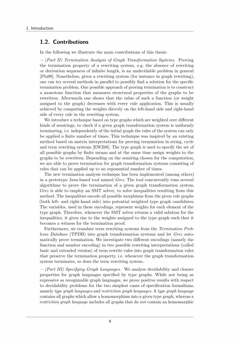
1.2. ContributionsIn the following we illustrate the main contributions of this thesis:

– (Part II) Termination Analysis of Graph Transformation Systems. Provingthe termination property of a rewriting system, e.g. the absence of rewritingor derivation sequences of infinite length, is an undecidable problem in general[Plu98]. Nonetheless, given a rewriting system (for instance in graph rewriting),one can try several methods in parallel to possibly find a solution for the specifictermination problem. One possible approach of proving termination is to constructa monotone function that measures structural properties of the graphs to berewritten. Afterwards one shows that the value of such a function (or weightassigned to the graph) decreases with every rule application. This is usuallyachieved by computing the weights directly on the left-hand side and right-handside of every rule in the rewriting system.

We introduce a technique based on type graphs which are weighted over differentkinds of semirings, to check if a given graph transformation system is uniformlyterminating, i.e. independently of the initial graph the rules of the system can onlybe applied a finite number of times. This technique was inspired by an existingmethod based on matrix interpretations for proving termination in string, cycleand term rewriting systems [EWZ08]. The type graph is used to specify the set ofall possible graphs by finite means and at the same time assign weights to thegraphs to be rewritten. Depending on the semiring chosen for the computation,we are able to prove termination for graph transformation systems consisting ofrules that can be applied up to an exponential number of times.

The new termination analysis technique has been implemented (among others)in a prototype Java-based tool named Grez. The tool concurrently runs severalalgorithms to prove the termination of a given graph transformation system.Grez is able to employ an SMT solver, to solve inequalities resulting from thismethod. The inequalities encode all possible morphisms from the given rule graphs(both left- and right-hand side) into potential weighted type graph candidates.The variables, used in these encodings, represent weights for each element of thetype graph. Therefore, whenever the SMT solver returns a valid solution for theinequalities, it gives rise to the weights assigned to the type graph such that itbecomes a witness for the termination proof.

Furthermore, we translate term rewriting systems from the Termination Prob-lems Database (TPDB) into graph transformation systems and let Grez auto-matically prove termination. We investigate two different encodings (namely thefunction and number encoding) in two possible rewriting interpretations (calledbasic and extended version) of term rewrite rules into graph transformation rulesthat preserve the termination property, i.e. whenever the graph transformationsystem terminates, so does the term rewriting system.

– (Part III) Specifying Graph Languages. We analyse decidability and closureproperties for graph languages specified by type graphs. While not being asexpressive as recognizable graph languages, we prove positive results with respectto decidability problems for the two simplest cases of specification formalisms,namely type graph languages and restriction graph languages. A type graph languagecontains all graphs which allow a homomorphism into a given type graph, whereas arestriction graph language includes all graphs that do not contain an homomorphic

4

1.2. Contributions

image of a given type graph. We extend the formalism in two different ways: First,we introduce boolean connectives between type graphs to generate a type graphlogic and second, we increase the expressiveness of the type graph itself, by addingannotations to the type graph elements.

In case of the type graph logic, one already obtains the desired closure propertiesfor free since they are semantically given by the logical conjunction, disjunctionand negation operators. However, it is still impossible to compute postconditionswithin this formalism. This is due to the fact that one can not express the existenceof a subgraph (here the right hand-side graph from a graph transformation rule)in every graph contained in the specified graph language.Therefore, we define a framework of annotated type graphs, to generate an ab-

stract framework, from which formalisms based on type graphs can be instantiated.Each type graph is enriched with a set of annotations, and annotations can beparametrized. For instance, in one of the settings, the annotations are used toglobally count all elements that can be mapped to the elements in the type graph.This is different from UML multiplicities, which are locally specified on the edges.

By adding annotations to the type graph, the expressiveness is too powerful,such that the language inclusion problem becomes hard to decide. We only obtainpositive results for the language inclusion problem by restricting the analysed graphlanguages to graphs up to a given pathwidth (equivalent to [Blu14]). However, byadding annotations to the formalism, we are able to compute postconditions ofrule applications, which was impossible in the other refinements of the type graphspecification language. In addition, we investigate closure under rule application,i.e. invariant checking for our frameworks.

– (Part IV) Abstract Object Rewriting. Finally, by exploiting universal propertiesfrom category theory, we introduce a materialization construction (similar to[SRW02]) for our annotated type graph framework. A basic observation is thatin most specification frameworks an abstract rewriting step is performed bycomputing the (strongest) postcondition in two steps: by first materializing theleft-hand side of the rule to be applied (also called shift in some specificationformalisms), followed by adding the right-hand side (existentially quantified).Therefore, the notion of annotated type graphs is lifted to a more general frameworkof annotated abstract objects in an arbitrary topos.

For the purely structural aspects of our materialization construction we will usepartial map classifiers in a topos and its slice categories. We furthermore relate theconstruction to the fundamental construction of final pullback complements [DT87].Even though the materialization fully specifies the set of objects which explicitlycontain a copy of the left-hand side of a rule, there still can be objects in thisset which can not be rewritten. Therefore, we refine the materialization into arewritable materialization, which specifies the set of all rewritable objects withrespect to the rule to be applied. However, the abstract object retrieved by theabstract derivation step can only be used to specify the strongest postconditionas long as the information about the explicit copy of the right hand-side is given.To solve this issue we explain how all objects in the construction can be endowedwith annotations and how these annotations can be rewritten.

We give properties for the annotations which need to be satisfied to be able tocompute the strongest postconditions in this generalized abstract setting.Finally, being able to compute postconditions for the specification of graph

5

1. Introduction

languages by using annotated type graphs, we implement verification techniquesfor this formalism in a prototype Java-tool called DrAGoM. We benchmark thetechniques of the tool with respect to some worked examples.

1.3. Structure of this ThesisThe structure of this thesis is as follows1:

The thesis begins with a preliminaries and foundations part (Part I) to remindthe reader of basic mathematical definitions. The notation that is going to be usedis fixed and concepts related to category theory and graph transformation arerecalled as a preparation for later parts to come. The main contributions of thisthesis are split into the three main Parts II-IV, each having their own motivationand conclusion section. This way, the parts can be read independently2 and inany order, while each of them contribute to a larger research context, namelythe analysis and abstraction of graph transformation systems via type graphs.The theoretical results, introduced in the Chapters 8-10, have been implementedinto DrAGoM, a tool which is introduced and evaluated in Part V. In Part VI thethesis ends with a conclusion where all contributions are evaluated in the overallcontext. All proofs, experimental results on termination analysis, a nomenclatureand an index are given in the appendix of this thesis.

The content of the chapters (grouped by their respective part) is the following:

Part I – Preliminaries and Foundations

Chapter 2 – FoundationsIn Chapter 2 we recall and fix mathematical notations. The definitions inthis chapter are used throughout the thesis, whereas additional preliminarysections in the different parts might extend these basic concepts. In orderto establish the background theory (especially needed in Part IV), weadditionally give an introduction to some basic notions of category theoryat the end of the chapter.

Chapter 3 – Graphs and Graph TransformationThis chapter introduces the kind of graphs that will be used in this thesis.Furthermore we give a tutorial on graph transformation that explains theso-called double-pushout approach to graph transformation in a rigorous,but non-categorical way, using a gluing construction. Afterwards, we relatethis gluing construction to its categorical counterpart.

Chapter 4 – Type Graph LanguagesIn this chapter we learn how type graphs can be used to specify (possiblyinfinite) sets of graphs by finite means. We are interested in (pure) typegraphs, where the corresponding language consists of all graphs that can bemapped homomorphically to a given type graph. After giving the formaldefinition of type graph languages we present several examples of specialcases of these languages.

1See also the dependency graph in Figure 1.1 on page 92Exception: It is recommended (but not required) to read Chapter 8 of Part III before readingChapter 10 of Part IV, as the introduced concepts are related to each other.

6

1.3. Structure of this Thesis

Part II – Termination Analysis of Graph Transformation Systems

Chapter 5 – Weighted Type Graphs over SemiringsThis chapter presents techniques, based on so-called weighted type graphs,for proving uniform termination of graph transformation systems. Thesetype graphs can be used to assign weights to graphs and to show that theseweights decrease in every rewriting step in order to prove termination. Wepresent an example involving counters and discuss the implementation in atool called Grez.

Chapter 6 – Terms, Term Rewriting and Term Graph EncodingsIn Chapter 6 we discuss two natural ways to interpret term rewrite rulesas term graph rewrite productions. Afterwards we introduce an approachto transform term graph rewriting to graph transformation, in such a waythat termination of the term graph rewrite system can be concluded fromtermination of the resulting graph transformation system, to be proved byGrez. We propose two such transformations: the function encoding andthe number encoding. We discuss the two transformations and report aboutexperiments.

Part III – Specifying Graph Languages

Chapter 7 – Pure Type Graphs, Restriction Graphs and Type Graph LogicIn this chapter we investigate two more formalisms for specifying type graphlanguages, i.e. sets of graphs, based on type graphs. First, we study languagesspecified by restriction graphs and their relation to type graphs. Second, weextend this basic approach to a type graph logic. We present decidabilityresults and closure properties for both formalisms.

Chapter 8 – Annotated Type GraphsIn Chapter 8 we endow type graphs with annotations, thus making graphlanguages more expressive. In particular we will use ordered monoids in orderto annotate graphs. Similar to the previous chapter, we present decidabilityresults and closure properties. This time we put a little more focus on thelanguage inclusion problem, for which we introduce the notion of a countingcospan automaton functor to solve the problem.

Part IV – Abstract Object Rewriting

Chapter 9 – Materialization CategoryIn this chapter we focus on the so-called materialization of left-hand sidesfrom abstract objects, a central concept in abstract rewriting. We have alook at an accessible, general explanation of how materializations arise fromuniversal properties and categorical constructions, in particular partial mapclassifiers, in a topos. Furthermore, we refine the materialization constructionto a rewritable materialization by exploiting the notion of final pullbackcomplements.

7

1. Introduction

Chapter 10 – Rewriting Annotated ObjectsIn Chapter 10 we combine the previously introduced materialization con-struction with the concept of enriching graphs with annotations from orderedmonoids to create a framework of abstract rewriting for annotated objects.We define properties of annotations which can be used to give a precise char-acterization of strongest postconditions, which are effectively computableunder certain assumptions.

Part V – Tools and Applications

Chapter 11 – DrAGoMThis chapter gives an overview over the prototype tool DrAGoM which is atool to handle and manipulate multiply annotated type graphs. The mainapplication of DrAGoM is to automatically compute strongest postconditionsto check invariants of graph transformation systems in the framework ofabstract graph rewriting. We have a look at the basic functionalities andgive an overview of a typical user interaction with the software. Afterwards,we investigate how the categorical notions of the previous chapters can beimplemented and have a look at other tool approaches.

Chapter 12 – EvaluationIn this chapter we present different case studies which we have conductedusing the tool DrAGoM. First, we compare the generated output with theexpected results of examples from previous chapters. Second, we provideruntime results for several invariant checks and stress test the tool withrespect to language inclusion checks of increasing graph sizes. At the end ofthe chapter, an overview of the case study results and a summary of thetool’s practicability are provided.

Part VI – Conclusion

Chapter 13 – Conclusion and Future WorkIn Chapter 13 we draw the thesis to a close. We summarize the maintheoretical contributions and discuss how they fit into the broader scientificcontext of this thesis. Finally, we provide suggestions of potential next stepsfor future work, resulting from the contribution.

8

1.3. Structure of this Thesis

Chapter 1Introduction

I - Preliminaries and Foundations

Chapter 3Graphs

and GraphTransformation

Chapter 2Foundations

Chapter 4Type GraphLanguages

III - SpecifyingGraph Languages

Chapter 7Pure TypeGraphs,

RestrictionGraphs

and TypeGraph Logic

Chapter 8Annotated

Type Graphs

II - TerminationAnalysis of GTS

Chapter 5Weighted TypeGraphs overSemirings

Chapter 6Terms, TermRewriting andTerm GraphEncodings

IV - AbstractObject Rewriting

Chapter 9Materialization

Category

Chapter 10RewritingAnnotatedObjects

V - Tools and Application

Chapter 11DrAGoM

Chapter 12Evaluation

Chapter 13Conclusion andFuture Work

Figure 1.1.: Dependency graph of this thesis. The dotted arrows visualize prereq-uisites with respect to the chapters. It is recommended to read thechapter(s) at the source of an arrow first before reading its target.

9

Part I.

Preliminaries and Foundations

“Do not worry about your difficulties in Mathematics.I can assure you mine are still greater.”

Albert Einstein (1879-1955)

2Foundations

In this chapter we will remind the reader of basic mathematical definitions andafterwards give a short introduction to a mathematical formalism called categorytheory, which is an alternative to set theory.

Please note, that the purpose of this chapter is not to give a full introduction tobasic mathematical concepts nor to category theory, but rather fix the notationthat is going to be used. Therefore, it is assumed that the reader at least hasa thorough mathematical and computer science background on the level of anundergraduate degree at a university. At the same time, by describing the necessaryconcepts, the thesis becomes self-contained such that the consultation of otherliterature is not mandatory, to be able to understand the upcoming chapters.

Likewise, for readers who are familiar with standard mathematical/categoricalconcepts and the basics of graph rewriting, it is possible to skip this Part I of thethesis and immediately proceed to one of the main Parts II-IV, without missingany important results. A complete list of used symbols together with an index isgiven at the end of the thesis.

2.1. Basic NotationWe start by fixing the notation of the fundamental logical statements which arebeing used in computer science. Afterwards, we recall the basic concepts of settheory and conclude this subsection with a reminder about the definitions of somemathematical structures.

Logical Operators

For the standard logical operations we will use the following symbols:

∧ for conjunction ∨ for disjunction=⇒ for implication ⇐⇒ for bi-implication∃ for existential quantification ∀ for universal quantification.

2. Foundations

Set

The membership relation is denoted by ∈, i.e. whenever an element x is amember of a set X we will simply write x ∈ X. We use X = Y to denote thattwo sets are equal, X ⊆ Y to denote that X is a subset of Y or equal and we useX ⊂ Y to denote that X is a strict subset of Y , i.e. inclusion holds but the setsare not equal. Their corresponding negations are denoted by /∈, 6=, 6⊂ and *. Wedenote by N0 the set of natural numbers 0, 1, 2, . . ., including 0, and by N thenatural numbers without 0. The symbol ∅ is used to denote the empty set, i.e. aset without any element. The powerset of X is denoted by P(X).

For two sets X and Y , the relative complement is denoted by X \Y , i.e. X \Y =x ∈ X | x /∈ Y , the union is denoted by X∪Y , i.e. X∪Y = z | z ∈ X∨z ∈ Y and the intersection is denoted by X ∩ Y , i.e. X ∩ Y = z | z ∈ X ∧ z ∈ Y . Thecartesian product X × Y is the set X × Y = (x, y) | x ∈ X ∧ y ∈ Y of orderedpairs, which are denoted by round parentheses. For n ∈ N, Xn = X × . . . ×X,denotes the n-ary cartesian product of X. The disjoint union X1

⊎X2 for two

sets X1 and X2 is the set X1⊎X2 =

⋃i∈I(x, i) | x ∈ Xi with I = 1, 2.

Relation

For an arbitrary set X a subset R ⊆ X ×X is called (homogeneous) relationon X. We denote by R−1 the inverse relation of R. The relation R is reflexive ifand only if for all x ∈ X we have (x, x) ∈ R; it is transitive if and only if for allx, y, z ∈ X we have (x, y) ∈ R ∧ (y, z) ∈ R =⇒ (x, z) ∈ R; it is symmetric if andonly if for all x, y ∈ X we have (x, y) ∈ R =⇒ (y, x) ∈ R and it is antisymmetricif and only if for all x, y ∈ R we have (x, y) ∈ R ∧ (y, x) ∈ R =⇒ x = y. Thetransitive closure of R is denoted R+, i.e. the smallest relation on X that containsR and is transitive.

Order

For an arbitrary set X, a preorder ≤ on X is a binary relation on X whichis reflexive and transitive. A preorder ≤ is total if for all x, y ∈ X either x ≤ yor y ≤ x (or both) holds. If a preorder ≤ is antisymmetric it is called a partialorder . If a preorder ≤ is symmetric it is called an equivalence and will be denotedby ≡. We denote by X/ ≡ the quotient set of all equivalence classes of X by≡. Furthermore [x]≡ denotes the equivalence class of x ∈ X with respect to ≡,i.e. [x]≡ = y ∈ X | x ≡ y. In the following we omit the subscripts in theequivalence class [x]≡ and simply write [x] whenever ≡ is clear from the context.If ≤ is an order, then we denote by < its strict subrelation e.g. x < y if and onlyif x ≤ y ∧ x 6= y. An order is well-founded if it does not allow infinite, strictlydecreasing sequences x0 > x1 > x2 > · · · .

Function

A binary relation f ⊆ X ×Y , which satisfies the requirement that for all x ∈ Xthere exists a unique y ∈ Y such that (x, y) ∈ f holds, is called a (total) functionfrom X to Y and is denoted by f : X → Y . For a function f : X → Y we callX the domain, Y the codomain and given any x ∈ X we write f(x) (insteadof y) for the unique element satisfying (x, f(x)) ∈ f . We call f(x) the image ofx ∈ X under f : X → Y and say that y ∈ Y has a preimage under f : X → Y if

14

2.2. Basic Category Theory

there exists an x ∈ X with f(x) = y. A function f : X → Y is injective if for allx1, x2 ∈ X we have f(x1) = f(x2) =⇒ x1 = x2 and it is surjective if every y ∈ Yhas a preimage under f . A function f : X → Y is bijective if it is both, injectiveand surjective, and we denote by f−1 : Y → X the inverse of a bijective function.The domain restriction of a function f : X → Y to a set Z ⊆ X is denoted by thefunction f |Z : Z → Y with f |Z = f ∩ Z × Y .

Monoid

For a non-empty set X, a binary operator ⊕ : X × X → X and an elemente ∈ X a 3-tuple (X,⊕, e) is called monoid if the operator ⊕ is associative, i.e. forall x, y, z ∈ X we have x⊕ (y ⊕ z) = (x⊕ y)⊕ z and e is the unit with respectto ⊕, i.e. for all x ∈ X we have e⊕ x = x⊕ e = x. A monoid (X,⊕, e) is calleda commutative monoid if the operator ⊕ is commutative, i.e. for all elementsx, y ∈ X we have x⊕ y = y ⊕ x.

Lattice

Let ≤ be a preorder and X,Y be two sets with Y ⊆ X. An upper bound of Yis an element x ∈ X such that for all y ∈ Y we have y ≤ x. An upper boundx ∈ X is called least upper bound (or join; or supremum) if for each upper boundu ∈ X we have x ≤ u. Likewise, a lower bound is an element x ∈ X such that forall y ∈ Y we have x ≤ y. A lower bound x ∈ X is called greatest lower bound (ormeet; or infimum) if for each lower bound ` ∈ X we have ` ≤ x. We denote theleast upper bound of a set by

∨Y and the greatest lower bound by

∧Y if it exists.

For a set consisting of only two elements y1, y2 ∈ Y we will sometimes write y1∨y2instead of

∨y1, y2 for the least upper bound and y1 ∧ y2 instead of

∧y1, y2 for

the greatest lower bound. Note that a set may have many upper/lower bounds, ornone at all, but at most one least upper/greatest lower bound.

A preordered set (X,≤) is called a lattice if for all subsets Y ⊆ X there exists aleast upper bound

∨Y and a greatest lower bound

∧Y . Moreover, if X is finite,

then X has a unique minimal element ⊥ =∧X (called bottom) and a unique

maximal element > =∨X (called top). For the special case Y = ∅ we have∨

∅ = ⊥ and∧∅ = >.

2.2. Basic Category TheoryCategory theory is a mathematical framework which is used to describe abstractstructures. The theory does not focus on elements, like it is done in set theory,but rather focuses on collections of elements (here called objects) and the relationsbetween these collections (also called arrows or morphisms). In this chapter wehave a look at the basic categorical concepts which are used throughout this thesis.Please note that the definitions and explanations given in this chapter are notmeant to give a full overview to the topic of category theory but rather covers theessential constructions needed in this thesis. At the end of this chapter we givesome literature recommendation for the interested reader, who would like to learnmore about category theory. We start by defining what a category is.

15

2. Foundations

Definition 2.1 (Category). A category is a 4-tuple C = (O,M, , id) whichconsists of

• a class O whose elements are called objects (or C-objects).

• a class M(A,B) for all objects A,B ∈ O whose elements are calledarrows or morphisms (sometimes referred to as C-arrows/C-morphisms).Each morphism f ∈ M(A,B) has a domain dom(f) = A alongside acodomain cod(f) = B and we will write f : A→ B.

• a composition function : M(B,C) × M(A,B) → M(A,C) for allobjects A,B,C ∈ O which assigns to any morphisms f ∈M(A,B) andg ∈ M(B,C) their composed morphism g f : A → C. Furthermore,the composition of morphisms f : A → B, g : B → C and h : C → Dmust be associative, i.e. (h g) f = h (g f).

• a class id of identity morphisms with idA ∈ M(A,A) for all objectsA ∈ O. The identity morphisms must be the neutral elements withrespect to composition, i.e. for all morphisms f : A→ B it holds thatf idA = f and idB f = f .

Example 2.2. The classic example of a category is Set. This category consistsof sets as objects and functions as morphisms, and the composition operation isthe usual composition of functions. Another example is the category Rel wherethe objects are sets, but in contrast to Set, the morphisms are (binary) relationswhich do not need to be functions.

We will use the category Set as a running example in this chapter to providethe reader, who is not familiar with category theory, some intuition behind theconcepts which are described in the following.

Definitions and proofs in category theory extensively use the notion of commutingdiagrams. Diagrams can be visualized as directed graphs, which makes it easierfor the reader to "chase" required commuting properties within the visualisation.

Definition 2.3 (Diagram). Let C be a category. A diagram in C is a subclassof C-objects O′ and a subclass of C-morphismsM′, where for every f ∈M′we have dom(f) ∈ O′ and cod(f) ∈ O′. A diagram commutes if for everytwo well defined sequences of compositions f1 . . . fn and g1 . . . gm ofmorphisms inM′ where dom(fn) = dom(gm) and cod(f1) = cod(g1) we havef1 . . . fn = g1 . . . gm.

Example 2.4. Let the following diagram D consist of the objects A,B,C,D,Eand arrows f : A→ B, g : A→ C, h : B → D, i : C → D, j : B → E, k : E → D.The diagram D (depicted below right) commutes if and only if the following twoequations hold:

h f = i g and k j = h.

As a consequence from above equations we get

i g = h f = k j f

A B

C D E

f

g hi

j

k

16

2.2. Basic Category Theory

With category theory focusing on morphisms rather than elements, there existspecial types of morphisms, which play important roles in their categories.

Definition 2.5 (Monomorphism, Epimorphism, Isomorphism). Let C be acategory and f : A→ B be a C-morphism.

• f is called monomorphism (or mono), if for all morphisms g1 : X → Aand g2 : X → A with f g1 = f g2 it follows that g1 = g2.

• f is called epimorphism (or epi), if for all morphisms h1 : B → Y andh2 : B → Y with h1 f = h2 f it follows that h1 = h2.

• f is called isomorphism (or iso), if there exists a morphism g : B → Asuch that g f = idA and f g = idB.

Example 2.6. In the category Set, the monomorphisms are injective functions,epimorphisms are surjective functions and isomorphisms are bijective functions.

We will denote monomorphisms by A B, epimorphisms by A B andisomorphisms by A ∼−→ B.Category theory gives rise to categorical constructions which can be used

to either create new categories based on given categories or define objects viathe concept of universal properties. By using universal properties for objectspecifications, category theory remains abstract in the sense that it describesobjects by their properties instead by the way how they are constructed. Thisleads to the ability to reuse constructions in several categories.In this thesis, we will use the notion of products for some constructions. In-

tuitively, the product of two objects is the most general object which admits amorphism to each of them.

Definition 2.7 (Product). Let C be a category with some objects A1 and A2.A product of A1 and A2 is an object A1×A2 together with a pair of morphismsπ1 : (A1 ×A2)→ A1, π2 : (A1 ×A2)→ A2 (called projection morphisms) suchthat the following universal property is fulfilled:For every object X and pair of morphismsf1 : X → A1, f2 : X → A2 there exists aunique morphism f : X → (A1 ×A2) suchthat π1 f = f1 and π2 f = f2, i.e., thediagram to the right commutes.

X

A1 ×A2A1 A2

ff1 f2

π1 π2

Example 2.8. In the category Set, the product is the cartesian product.

The category-theoretical dual notion of the product is the coproduct. Dualnotions in category theory usually have the same definitions as their correspondingcounterpart, with the difference that all morphisms are reversed. Essentially, thecoproduct of two objects is the least specific object to which each of them admits amorphism. Products and coproducts, if they exist, are unique up to isomorphism.

17

2. Foundations

Definition 2.9 (Coproduct). Let C be a category with some objects A1 andA2. A coproduct of A1 and A2 is an object A1 ⊕A2 if there exist morphismsi1 : A1 → (A1 ⊕ A2), i2 : A2 → (A1 ⊕ A2) (called embedding morphisms orinjection morphisms) such that the following universal property is fulfilled:For every object X and pair of morphismsf1 : A1 → X, f2 : A2 → X there exists aunique morphism f : (A1 ⊕A2)→ X suchthat f i1 = f1 and f i2 = f2, i.e., thediagram to the right commutes.

X

A1 ⊕A2A1 A2

ff1 f2

i1 i2

Example 2.10. In the category Set, the coproduct is the disjoint union.

Another example for a special kind of object satisfying a universal property isgiven in the following definition of initial, and terminal objects.

Definition 2.11 (Terminal object and initial object). A terminal object in acategory C is an object 1 of C satisfying the following universal property:For every C-object A, there exists a unique morphism !A : A→ 1.

The dual concept to terminal objects are initial objects. An initial object ina category C is an object 0 of C satisfying the following universal property:For every C-object A, there exists a unique morphism ?A : 0→ A.

Example 2.12. In the category Set the terminal object is any one-element setand the initial object is the empty set ∅ (which only admits the empty function).

An initial and a terminal object, if they exist, are unique up to unique isomor-phism. Therefore, we can speak of the initial and the final object of a category.The terminal object will play an important role in several chapters of this thesisas the membership of an object to a language, i.e. a set of objects, is determinedby the existence of a morphism, as we will see in Chapter 4. Therefore, using aterminal object which admits a morphism from any object, one can easily specifythe set consisting of all objects.As described above, category theory focuses on morphisms instead of plain

objects. This concept can be used to abstract the already abstract notion bycategory theory itself. Thus, instead of just analysing the morphisms betweenobjects in a category, category theory introduces functors as structure preservingmorphisms between categories.

Definition 2.13 (Functor). Let C and D be two categories. A functorF : C → D from C to D assigns to each C-object A a D-object F(A)and to each C-morphism f : A → B a D-morphism F(f) : F(A) → F(B)such that the following conditions are satisfied:

• F preserves composition, i.e. for all composable morphisms f and g itholds that F(f g) = F(f) F(g).

• F preserves identities, i.e. for all C-objects it holds that F(idA) = idF(A).

The identity functor of a category C is denoted by IdC.

18

2.2. Basic Category Theory

The notion of functors can be abstracted again to the notion of natural transfor-mation, i.e., morphisms between functors. We will define and use the notion ofnatural transformation in Chapter 9.

One of the main concepts of this thesis are graph transformation systems, i.e.,sets of graph transformation rules. In Section 3.2 we will learn how a gluingconstruction can be used to rewrite graphs. The gluing construction can begeneralized to the idea of pushouts in the sense of category theory. Therefore, wenow introduce pushouts, being the fundamental constructions on which graphrewriting is based on. The relation between the notion of pushouts and the gluingconstruction will be explained in Section 3.2.2.Pushouts are constructed from pairs of morphisms f : A→ B and g : A→ C

which share the same domain. Such a pair of morphisms is also called span and wewill sometimes simply write B f−A −g C to indicate the span. The universalproperty of pushouts essentially states that the pushout is the most general wayto complete a commutative square with two given morphisms.

Definition 2.14 (Pushout (PO)). Given morphisms f : A→ B and g : A→ Cin a category C, a pushout (D, f ′, g′) over f and g isdefined by a pushout object D and two morphismsf ′ : C → D and g′ : B → D with f ′ g = g′ f , suchthat the universal property is fulfilled: For all objectsX and morphisms h : B → X and k : C → X withk g = h f , there is a uniqe morphism x : D → Xsuch that x g′ = h and x f ′ = k, i.e. the diagramto the right commutes.

A B

C D

X

f

g g′

f ′ h

k

x

Example 2.15. In the category Set, the pushout object D over the morphismsf : A→ B and g : A→ C can be constructed as the quotient set B⊎C/ ≡, where≡ is the smallest equivalence relation with f(a) ≡ g(a) for all a ∈ A. The pair ofmorphisms f ′ : C → D and g′ : B → D is defined by f ′(c) = [c] for all c ∈ C andg′(b) = [b] for all b ∈ B.For instance, let the sets A = a, b, c, B = 1, 2, 3 and C = 4, 5, 6 be given.

Furthermore let f : A→ B and g : A→ C be defined as

f(a) = 1 g(a) = 4f(b) = 1 g(b) = 5f(c) = 3 g(c) = 6.

The smallest equivalence relation ≡ yieldsthe classes [1] = [4] = [5] = 1, 4, 5,[2] = 2 and [3] = [6] = 3, 6.Therefore, the pushout object can be de-fined as the set D = [1], [2], [3] along-side the two morphisms f ′ : C → Dwith f ′(x) = [x] and g′ : B → D withg′(x) = [x]. The resulting pushout is de-picted in the commuting diagram to theright.

ab

c

12

3

45

6

[1][2]

[3]

f

f ′

g g′

A B

C D

19

2. Foundations

The generic definition of pushouts via universal properties can take variousforms. For instance, another prototypical example is the supremum or join, where– given two elements x, y of a partially ordered set (X,≤) – we ask for a thirdelement z with x ≤ z, y ≤ z and such that z is the smallest element which satisfiesboth inequalities. There is at most one such z, namely z = x ∨ y, the join of x, y.

The dual notion of pushouts are pullbacks. Pullbacks can be constructed frompairs of morphisms f : C → D and g : B → D which share the same codomain.These pairs are called cospan and are the dual notion of spans. Likewise, we willsometimes write B −gD f− C to indicate the cospan. Pushouts and pullbacks,if they exist, are unique up to isomorphism.

Definition 2.16 (Pullback (PB)). Given morphisms f : C → D and g : B → Din a category C, a pullback (A, f ′, g′) over f and g isdefined by a pullback object A and two morphismsf ′ : A → B and g′ : A → C with f g′ = g f ′, suchthat the universal property is fulfilled: For all objectsX and morphisms h : X → B and k : X → C withf k = g h, there is a uniqe morphism x : X → Asuch that f ′ x = h and g′ x = k, i.e. the diagramto the right commutes.

A B

C D

X

f ′

g′ g

f

h

k

x

Example 2.17. In the category Set, the pullback object A over the morphismsf : C → D and g : B → D is the set A = (c, d) | f(c) = g(b) ⊆ C × B, i.e.,A can be constructed as a subset of the cartesian product C × B. The pair ofmorphisms f ′ : A→ B and g′ : A→ C is defined as the corresponding projections,e.g., f ′((c, b)) = b and g′((c, b)) = c.

For example, let the sets B = 1, 2, 3, C = 4, 5, 6 and D = a, b, c be given.Furthermore let f : C → D and g : B → D be defined as

f(4) = a g(1) = a

f(5) = b g(2) = b

f(6) = b g(3) = c.

Then the pullback object is defined asthe set A = (4, 1), (5, 2), (6, 2) along-side the two morphisms f ′ : A→ B withf ′((x, y)) = y and g′ : A → C withg′((x, y)) = x. The pullback is depictedin the commuting diagram to the right.

(4,1)(5,2)

(6,2)

12

3

45

6

ab

c

f ′

f

g′ g

A B

C D

A generalization of a pullback yields the notion of limits, as the limit of a cospan(if it exists) is a pullback. In the context of this thesis we do not use the notion oflimit but will require the existence of finite limits in Chapter 9 to define a specialclass of categories named Topos (see Definition 9.4).Another class of important categories are so-called adhesive categories. Many

types of graphical structures which are being used in computer science are knownto be examples of adhesive categories, including a category of graphs which wewill extensively use later in this thesis. Adhesive categories provide a vast amount

20

2.2. Basic Category Theory

of structure ensuring properties, guaranteed to hold in any adhesive category,which can be used to analyse the structures within such a category more easily.

Definition 2.18 (Adhesive category). A category C is adhesive if and onlyif the following three conditions are satisfied:

• C has pullbacks • C has pushouts along monomorphisms

• pushouts of monomorphisms are pullbacksand pushouts are stable under pullbacks,i.e., given the cube depicted to the right,where the bottom face is a pushout alongmonomorphisms (also called van Kampensquare) and the back faces are pullbacks:the front faces are pullbacks if and only ifthe top face is a pushout.

A′ // //~~

~~

B′~~

~~

C ′ // //

D′

A // //~~

~~

B

C // // D

Graph rewriting (which we will discuss in Section 3.2.2) is an instance of ageneralised notion of rewriting defined categorically. This rewriting mechanism,that we will be using, is the well known notion of the double-pushout rewriting,which can be used in arbitrary adhesive categories [CM+97; LS05]. A production(or rule) is a span L← I → R in a category C.

Definition 2.19 (Double-pushout rewriting). Let p : L ← I → R be aproduction in a category C and let m : L → X be a morphism (also calledmatch) for an object X in C. Then the object Xrewrites to an object Y in C via production p(and match m), written X p,m=⇒ Y , if there existsa diagram consisting of morphisms (shown to theright) in which both squares are pushouts. Themorphism n is called co-match.

L

m

Ioo

// R

n

X Coo // Y

Note that in the situation above there is not necessarily an object C, makingthe left-hand square a pushout. If the object C exists, we say that the gluingcondition is satisfied. The gluing condition alongside the gluing construction forgraph rewriting will be discussed in the next chapter.

If C is an adhesive category (and thus if it is a topos [LS06]) and the productionconsists of monos, then all remaining arrows of double-pushout diagrams ofrewriting are monos [LS05] and the result of rewriting—be it the object Y or theco-match n—is unique (up to a canonical isomorphism).This ends the summary of basic categorical definitions and brief explanations

needed later in this thesis. The interested reader, who would like to learn moreabout the topic of category theory, is invited to have a look into A Taste ofCategory Theory for Computer Scientists by Benjamin C. Pierce [Pie88], whichprovides a good starting point for computer scientists who would like to explorethe topic. Afterwards, to further consolidate the readers knowledge, one canconsult the free available book Abstract and Concrete Categories - The Joy ofCats [AHS09] or the book Categories for the Working Mathematician by SaundersMac Lane [Mac71]. Of course, there exist many more good introductions.

21

“As for everything else, so for a mathematical theory:beauty can be perceived but not explained.”

Arthur Cayley (1821-1895)

3Graphs and Graph Transformation

A substantial part of computer science is concerned with the transformation ofstructures, the most well-known example being the rewriting of words via Chomskygrammars, string rewriting systems [DJ90] or transformations of the tape of aTuring machine. The focus of this thesis is on systems where transformations arerule-based and rules consist of a left-hand side (the structure to be deleted) and aright-hand side (the structure to be added).

If we increase the complexity of the structures being rewritten, we next encountertrees or terms, leading to term rewriting systems (see also Chapter 6). The nextlevel is concerned with graph rewriting [Roz97], which – as we will see below –differs from string and term rewriting in the sense that we need a notion ofinterface between left-hand and right-hand side, detailing how the right-hand sideis to be glued to the remaining graph.Graph rewriting is a flexible and intuitive, yet formally rigorous, framework

for modelling and reasoning about dynamical structures and networks. Suchdynamical structures arise in many contexts, be it object graphs and heaps,UML diagrams (in the context of model transformations [EE+15]), computernetworks, the world wide web, distributed systems, etc. They also occur in otherdomains, where computer science methods are employed: social networks, as well aschemical and biological structures. Specifically concurrent non-sequential systemsare well-suited for modelling via graph transformation, since non-overlappingoccurrences of left-hand sides can be replaced in parallel. For a more extensivelist of applications see [EE+99].Note that in the context of this chapter we use the terms graph rewriting and

graph transformation interchangeably. We will avoid the term graph grammar ,since that emphasizes the use of graph transformation to generate a graph language,here the focus is just on the rewriting aspect. The specification of graph languageswill be investigated in Chapter 4.

In the following, we first recall the basic notion of directed edge-labelled multi-graphs and graph morphisms. Afterwards, graph transformation systems and theircorrespondence to category theory will be explained in detail.

3. Graphs and Graph Transformation

3.1. Graphs and Graph MorphismsWe start by defining graphs, where we choose to consider directed, edge-labelledgraphs where parallel edges are allowed. Other choices would be to use hypergraphs(where an edge can be connected to any number of nodes) or to add node labels.Both versions can be easily treated by our rewriting approach. Throughout thethesis, we assume the existence of a fixed set Λ from which we take our edge labels.

Definition 3.1 (Graph). Let Λ be a fixed set of edge labels. A Λ-labeledgraph is a tuple G = (V,E, src, tgt, lab), where V is a finite set of nodes, E isa finite set of edges, src, tgt : E → V assign to each edge a source and a targetnode, and lab : E → Λ is a labeling function.

Given a graph G, we denote its components by VG, EG, srcG, tgtG, labG, unlessotherwise indicated. Given an edge e ∈ EG, the nodes srcG(e), tgtG(e) are calledincident to e. The empty graph, i.e. a graph with V = E = ∅, is denoted ∅.Example 3.2. Let VG = v1, v2, EG = e1, e2, e3 and Λ = A,B be given.A graphical representation of the graph G with

srcG(e1) = v1 srcG(e2) = v1 srcG(e3) = v2

tgtG(e1) = v2 tgtG(e2) = v2 tgtG(e3) = v2

labG(e1) = A labG(e2) = B labG(e3) = A

is depicted to the right.

G =v1 v2

A

BA

A central notion in graph rewriting is a graph morphism. Just as a functionis a mapping from a set to another set, a graph morphism is a mapping from agraph to a graph. It maps nodes to nodes and edges to edges, while preserving thestructure of a graph. This means that if an edge is mapped to an edge, there mustbe a mapping between the source and target nodes of the two edges. Furthermore,labels must be preserved.

Definition 3.3 (Graph morphism). Let G, H be two graphs. A graph mor-phism ϕ : G→ H is a pair of mappings ϕV : VG → VH , ϕE : EG → EH suchthat for all e ∈ EG it holds that

• srcH(ϕE(e)) = ϕV (srcG(e)),

• tgtH(ϕE(e)) = ϕV (tgtG(e)) and

• labH(ϕE(e)) = labG(e).

A graph morphism ϕ is called injective (surjective) if both mappings ϕV , ϕEare injective (surjective). Whenever ϕV and ϕE are bijective, ϕ is called anisomorphism. If there exists an isomorphism ϕ : G1 → G2, we say that G1, G2are isomorphic and write G1 ∼= G2. The composition of two graph morphismsis again a graph morphism. Graph morphisms are composed by composingboth component mappings. Composition of graph morphisms is denoted by .

In the following we omit the subscripts in the functions ϕV , ϕE and simplywrite ϕ. Furthermore, the negation of G1 ∼= G2 will be denoted by G1 G2.

24

3.2. Graph Transformation Systems

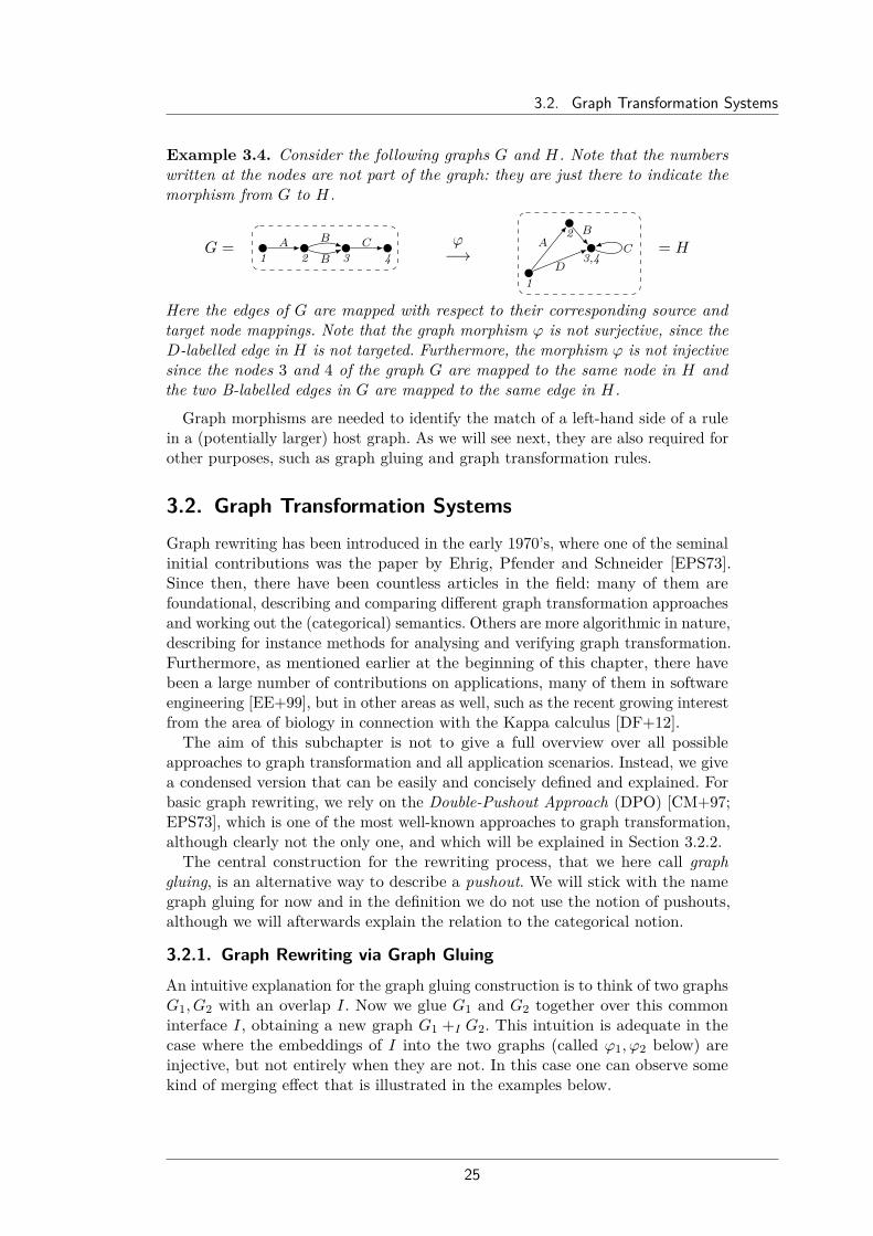
Example 3.4. Consider the following graphs G and H. Note that the numberswritten at the nodes are not part of the graph: they are just there to indicate themorphism from G to H.

G =1 2 3 4

A B

B

C ϕ−→

1

2

3,4A

B

D

C = H

Here the edges of G are mapped with respect to their corresponding source andtarget node mappings. Note that the graph morphism ϕ is not surjective, since theD-labelled edge in H is not targeted. Furthermore, the morphism ϕ is not injectivesince the nodes 3 and 4 of the graph G are mapped to the same node in H andthe two B-labelled edges in G are mapped to the same edge in H.

Graph morphisms are needed to identify the match of a left-hand side of a rulein a (potentially larger) host graph. As we will see next, they are also required forother purposes, such as graph gluing and graph transformation rules.

3.2. Graph Transformation SystemsGraph rewriting has been introduced in the early 1970’s, where one of the seminalinitial contributions was the paper by Ehrig, Pfender and Schneider [EPS73].Since then, there have been countless articles in the field: many of them arefoundational, describing and comparing different graph transformation approachesand working out the (categorical) semantics. Others are more algorithmic in nature,describing for instance methods for analysing and verifying graph transformation.Furthermore, as mentioned earlier at the beginning of this chapter, there havebeen a large number of contributions on applications, many of them in softwareengineering [EE+99], but in other areas as well, such as the recent growing interestfrom the area of biology in connection with the Kappa calculus [DF+12].The aim of this subchapter is not to give a full overview over all possible

approaches to graph transformation and all application scenarios. Instead, we givea condensed version that can be easily and concisely defined and explained. Forbasic graph rewriting, we rely on the Double-Pushout Approach (DPO) [CM+97;EPS73], which is one of the most well-known approaches to graph transformation,although clearly not the only one, and which will be explained in Section 3.2.2.The central construction for the rewriting process, that we here call graph

gluing, is an alternative way to describe a pushout. We will stick with the namegraph gluing for now and in the definition we do not use the notion of pushouts,although we will afterwards explain the relation to the categorical notion.

3.2.1. Graph Rewriting via Graph GluingAn intuitive explanation for the graph gluing construction is to think of two graphsG1, G2 with an overlap I. Now we glue G1 and G2 together over this commoninterface I, obtaining a new graph G1 +I G2. This intuition is adequate in thecase where the embeddings of I into the two graphs (called ϕ1, ϕ2 below) areinjective, but not entirely when they are not. In this case one can observe somekind of merging effect that is illustrated in the examples below.

25

3. Graphs and Graph Transformation

Graph gluing is described via factoring through an equivalence relation.

Definition 3.5 (Graph gluing). Let I,G1, G2 be graphs with graph mor-phisms ϕ1 : I → G1, ϕ2 : I → G2, where I is called the interface. We assumethat all node and edge sets are disjoint.

Let ≡ be the smallest equivalence relation on VG1 ∪EG1 ∪ VG2 ∪EG2 whichsatisfies ϕ1(x) ≡ ϕ2(x) for all x ∈ VI ∪ EI .

The gluing of G1, G2 over I (written as G = G1 +ϕ1,ϕ2 G2, or G = G1 +I G2if the ϕi morphisms are clear from the context) is a graph G with:

VG = (VG1 ∪ VG2)/ ≡ EG = (EG1 ∪ EG2)/ ≡

srcG([e]≡) =

[srcG1(e)]≡ if e ∈ EG1

[srcG2(e)]≡ if e ∈ EG2

tgtG([e]≡) =

[tgtG1(e)]≡ if e ∈ EG1

[tgtG2(e)]≡ if e ∈ EG2

labG([e]≡) =

labG1(e) if e ∈ EG1

labG2(e) if e ∈ EG2

where e ∈ EG1 ∪ EG2 .

Note that the gluing is well-defined, which is not immediately obvious sincethe mappings srcG, tgtG, labG are defined on representatives of equivalence classes.The underlying reason for this is that ϕ1, ϕ2 are morphisms.

Example 3.6. We now explain this gluing construction via some examples.

Let the two graph morphisms ϕ1 : I → G1 andϕ2 : I → G2 to the right be given, where bothϕ1 and ϕ2 are injective. Since the interface Iis present in both graphs G1 and G2, we canglue the two graphs together to construct agraph G1 +I G2 depicted on the bottom rightof the square.

1 2B

1 2B C

1 2B

A

1 2B

A

C

ϕ1

ϕ2

I G1

G2 G1 +I G2

1 2 1,2B

1 2A

1,2

A

B

ϕ1

ϕ2

I G1

G2 G1 +I G2

Now let the graph morphisms ϕ1 : I → G1and ϕ2 : I → G2 to the left be given, whereonly ϕ2 is injective. In the graph G1, theinterface nodes of I are merged via ϕ1. Thegluing graph G1 +IG2 is constructed by merg-ing all nodes in G1, G2, resulting in an A-labelled loop, together with the original B-labelled loop. This graph is depicted at thebottom right of the square.

We are now ready to define graph transformation rules, also called productions.Such a rule consists of a left-hand side graph L and a right-hand side graph R.

26

3.2. Graph Transformation Systems

However, as indicated in the introduction, this is not enough. The problem isthat, if we simply remove (a match of) L from a host graph, we would typicallyhave dangling edges, i.e., edges where either the source or the target node (orboth) have been deleted. Furthermore, there would be no way to specify how theright-hand side R should be attached to the remaining graph.

Hence, there is also an interface graph I related to L and R via graph morphisms,which specify what is preserved by a rule.

Definition 3.7 (Graph transformation rule). A (graph transformation) ruleρ consists of three graphs L, I,R and two graph morphisms LϕL− I −ϕRR.

Given a rule ρ, all nodes and edges in L that are not in the image of ϕL arecalled obsolete. Similarly, all nodes and edges in R that are not in the image ofϕR are called fresh.After finding an occurrence of a left-hand side L in a host graph (a so-called

match), the effect of applying a rule is to remove all obsolete elements and addall fresh elements. As indicated above, the elements of I are preserved, providingus with well-defined attachment points for R.While this explanation is valid for injective matches and rule morphisms, it

does not tell the full story in case of non-injective morphisms. Here, rules mightsplit or merge graph elements. Using the graph gluing defined earlier, it is easy togive a formal semantics of rewriting.

The intuition is as follows: given a rule as in Definition 3.7 and a graph G, weask whether G can be seen as a gluing of L and an (unknown) context C overinterface I, i.e., whether there exists C such that G ∼= L+I C. If this is the case,G can be transformed into H ∼= R+I C.

Definition 3.8 (Graph transformation). Let ρ = (L ϕL− I −ϕR R) be arule. We say that a graph G is transformed via ρ into a graph H (symbolically:G⇒ρ H) if there is a graph C (the so-called context) and a graph morphismψ : I → C such that:

G ∼= L+ϕL,ψ C H ∼= R+ϕR,ψ C

This situation can be depicted by the diagram to theright. The morphism m is called the match, n theco-match.

L

m

IϕLoo

ϕR //

ψ

R

n

G CηLoo

ηR// H

Depending on the morphisms ϕL and ϕR one can obtain different effects:whenever both ϕL and ϕR are injective, we obtain standard replacement. WheneverϕL is non-injective we specify splitting, whereas a non-injective ϕR results inmerging.We now consider some examples. First, we illustrate the straightforward case

where indeed the obsolete items are removed and the fresh ones are added, seeFigure 3.1a. Somewhat more elaborate is the case when the right leg ϕR of a ruleis non-injective, which causes the merging of nodes, see Figure 3.1b.

27

3. Graphs and Graph Transformation

1 21 2A

1 2B

1

2A

C1

2

C1

2B

C

ϕL ϕR

m ψ

ηRηL

n

L I R

G C H

(a) Application of a rule

1 21 2 1,2

1 2A

1 2A

1,2A

ϕL ϕR

m ψ

ηRηL

n

L I R

G C H

(b) Non-injective right leg ϕR

Figure 3.1.: Graph transformation rule examples

Different from string or term rewriting, in graph rewriting it may happen thatwe find a match of the left-hand side, but the rule is not applicable, because nocontext as required by Definition 3.8 exists. There are basically two reasons forthis: either the rule removes a node, without removing all edges connected to thatnode (dangling edge condition, see Figure 3.2a), or the match identifies two graphelements which are not preserved (identification condition) (see Figure 3.2b).

Fact 3.9 (Gluing condition [Ehr79]). Let L ϕL− I −ϕR R be a graphtransformation rule and let m : L → G be a match. Then a context C anda morphism ψ : I → C such that G ∼= L +ϕL,ψ C exist if and only if thefollowing holds:

• Dangling edge condition: Every node v ∈ VL, whose image m(v) isincident to an edge e ∈ EG which is not in the image of m, is notobsolete (i.e. in the image of ϕL).

• Identification condition: Whenever two elements x, y ∈ VL ∪ EL withx 6= y satisfy m(x) = m(y), then neither of them is obsolete.

However, even if the context exists, there might be cases where it is non-unique.

11A

1A

C

1

C

ϕL

m ψ

ηL

L I

G C

(a) Dangling edge condition example

11A

1A ?

ϕL

m ψ

ηL

L I

G C

(b) Identification condition example

Figure 3.2.: Gluing condition examples

28

3.2. Graph Transformation Systems

This happens in cases where ϕL, the left leg of a rule, is non-injective. In this caseone can for instance split nodes (see the rule in Figure 3.3a) and the questionis what happens to the incident edges. By spelling out the definition above, onedetermines that this must result in non-determinism. Either, we do not split(Figure 3.3b) or we split and each edge can non-deterministically “choose” tostay either with the first or the second node (Figures 3.3c–3.3d). Each resultingcombination is a valid context and this means that a rule application may benon-deterministic and generate several (non-isomorphic) graphs. In many paperssuch complications are avoided by requiring the injectivity of ϕL.

1

23

A

1,2 3A 1

23

A

A

ϕL ϕRL

I R

(a) Rule with non-injective left leg ϕL

1

23

A

1,2 3A

1,23

A

B 1,23

A

B

ϕL

m ψ

ηL

LI

G C

(b) Valid context (i)

1

23

A

1,2 3A

1,23

A

B

1 3

2

A

B

ϕL

m ψ

ηL

LI

G C

(c) Valid context (ii)

1

23

A

1,2 3A

1,23

A

B

1 3

2

A

B

ϕL

m ψ

ηL

LI

G C

(d) Valid context (iii)

Figure 3.3.: Non-injective left leg rule with three valid contexts

Finally, we can introduce the notion of a graph transformation system that isused in this thesis.

Definition 3.10 (Graph transformation system). A graph transformationsystem R is a set of graph transformation rules.

In the next subsection, we relate the two notions of graph gluing and pushouts.Afterwards we introduce one of the most popular formalisations of graph transfor-mation systems, namely the Double-Pushout Approach.

29

3. Graphs and Graph Transformation

3.2.2. Graph Transformation the Categorical WayA considerable part of graph transformation theory is concerned with making theresults independent of the specific graph structure under consideration (see [LS05;Löw93]). This however depends on the use of category theory. Therefore, we willconsider the category GraphΛ having Λ-labeled graphs as objects and graphmorphisms as arrows. The set of its objects will be denoted by |GraphΛ|. Thecategorical structure induces an obvious preorder on graphs, defined as follows.

Definition 3.11 (Homomorphism preorder). Given graphs G and H, wewrite G→ H if there exists a graph morphism from G to H in GraphΛ. Therelation → is a preorder (i.e. it is reflexive and transitive) and we call it thehomomorphism preorder on graphs. We write G 9 H if G → H does nothold. Graphs G and H are homomorphically equivalent, written G ∼ H, ifboth G→ H and H → G hold.

Example 3.12. Consider the following three graphs G1, G2 and G3:

A AA

A

G2 G3

G1

As evident from the picture we get G2 ∼ G3, and both G1 → G2, G1 → G3 butG2 9 G1, G3 9 G1. Furthermore it holds that Gi → Gi for all i ∈ 1, 2, 3. Notethat, the fusion of two nodes (while turning in-between binary edges into loops)and the graph expansion in form of adding additional graph structures, lead to agraph which is larger (or equal) in the homomorphism preorder, i.e. these stepspreserve the existence of a morphism between the old and the modified graph.

We will revisit the homomorphism preorder in Chapter 7 when we investigate thenotion of core graphs. There, we show that two graphs can only be homomorphicallyequivalent if they share a common subgraph structure.

As described in Section 2.2, category theory relies on so-called universal proper-ties where, given some objects, one defines another object that is in some relationto the given object and is – in some sense – the most general object which isin this relation. In the case of graphs, the order relation is given by the homo-morphism preorder →, i.e., graph morphisms. Graph gluing can alternatively becharacterized via the categorical notion of pushout (cf. Definition 2.14).

Fact 3.13 (Pushouts and the gluing construction [EE+06]). Let I,G1, G2 begraphs with graph morphisms ϕ1 : I → G1, ϕ2 : I → G2 as in Definition 3.5.Then the equation G ∼= G1 +ϕ1,ϕ2 G2 holds if and only if G is a pushout.

30

3.2. Graph Transformation Systems

Intuitively, the pushout characterization says that G should be a graph wherethe “common” parts of G1, G2 must be merged (since the square commutes), butit should be obtained in the most general way by merging only what is absolutelynecessary and adding nothing superfluous. This corresponds to saying that forany other merge H, G is more general and H can be obtained from G by furthermerging or addition of graph elements (expressed by a morphism from G to H).Please note that in GraphΛ, pushouts can be constructed componentwise for

nodes and edges in the category Set. The source and target functions of thepushout graph are then uniquely determined by the pushout property of the nodeset in the pushout graph.Graph transformation systems are widely used for modeling the evolution of

parallel and distributed systems where the states are represented by graphs, andthe behaviour is modeled by the application of local transformation rules to thestate graph. One of the most popular formalisations of graph transformationsystems is the Double-Pushout Approach (DPO) [Ehr79], where a transformationrule is represented as a pair of graph morphisms with the same source, and theapplication of a rule to a given graph is modeled with a construction involvingtwo pushouts in the category of graphs. Therefore, our double-pushout rewritingis an instance of Definition 2.19 (also compare with Definition 3.8) in the categoryGraphΛ. We do not impose any injectivity constraint on the rule morphisms orto the match, hence graph transformation is non-deterministic.

The specifics such as the dangling edge condition in Proposition 3.9 are typicalto the double-pushout approach that we are following here, i.e., it is forbidden toremove a node that is still attached to an edge, which is not deleted and in thiscase, the rule is not applicable. In other approaches, such as the single-pushout(or SPO) approach [Löw93] however, the deletion of a node to which an undeletededge is attached, is possible. In this case all incident edges are deleted as well. Incontrast to DPO, SPO is based on partial graph morphisms. This is also calleddeletion in unknown contexts.

For more information on the topic of graph transformation a standard referenceis the “Handbook of Graph Grammars and Computing by Graph Transformation”,which appeared in three volumes (foundations [Roz97] – applications, languagesand tools [EE+99] – concurrency, parallelism and distribution [EK+99]). Stronglyrelated to our definitions is the chapter on DPO rewriting by Corradini et al.[CM+97], which is based on the categorical definitions. The well-known book“Fundamentals of Algebraic Graph Transformation” by Ehrig et al. [EE+06]revisits the theory of graph rewriting from the point of view of adhesive categories,a general categorical framework for abstract transformations. In an introductorysection it defines the construction of pushouts via factorization, equivalent to ournotion of graph gluing.

31

“Coffee is a language in itself.”Jackie Chan (1954-present)

4Type Graph Languages

In this chapter we study a specification formalism based on type graphs, where atype graph T represents all graphs that can be mapped homomorphically to T ,potentially taking into account some extra constraints. Type graphs are commonin graph rewriting [CMR96; Roz97]. Usually, one assumes that all items, i.e., rulesand graphs to be rewritten, are typed, introducing constraints on the applicabilityof rules. Hence, type graphs are in a way seen as a form of labelling. This isdifferent from our point of view, where graphs (and rules) are – a priori – untyped(but labeled) and type graphs are simply a means to represent sets of graphs.

There are various reasons for studying languages based on type graphs: First,they are reasonably simple with many positive decidability results and they havenot yet been extensively studied from the perspective of specification formalisms.Second, other specification mechanisms – especially those used in connectionwith verification and abstract graph transformation [Ren04a; SRW02; SWW11] –are based on type graphs: abstract graphs are basically type graphs with extraannotations. Third, while not being as expressive as recognizable graph languages,they retain a nice intuition from regular languages: given a finite state automatonM one can think of the language of M as the set of all string graphs that can bemapped homomorphically to M (respecting initial and final states).

4.1. Type Graphs and Graph LanguagesA type graph language contains all graphs that can be mapped homomorphicallyto a given type graph.

Definition 4.1 (Type graph language). Let T be a Λ-labelled graph. Its typegraph language L(T ) is defined as:

L(T ) = G | G→ T.

Even if the graphs used for specifying type graph languages are just ordinarygraphs, we will in the following call them type graphs in order to emphasize theirrole.

4. Type Graph Languages

Example 4.2. The following type graph T over the edge label set Λ = A,Bspecifies a type graph language L(T ) consisting of infinitely many graphs where nograph in the language contains a B-loop and every target node of a B-edge is notincident to an A-edge or the source of another B-edge.

L( BA ) =∅ , , A B ,

A

A , . . .

Specifying graph languages using type graphs gives us the possibility to forbidcertain graph structures by not including them into the type graph. For example,no graph in the language of Example 4.2 can contain a B-loop or an A-edgeincident to the target of a B-edge. However, it is not possible to force somestructures to exist in all graphs of the language, since the morphism to the typegraph need not be surjective. This point will be addressed with the notion ofannotated type graph in Chapter 8.

4.2. ExamplesWe have a look at some special cases, to convey a better understanding for thespecification of graph languages via our notion of type graphs. We start with sometype graphs which play an important role in the category GraphΛ, namely thecorresponding initial and final object.

Example 4.3. The category GraphΛ has an initial object containing no nodesand edges, i.e. it is the empty graph ∅. For any non-empty graph object G inGraphΛ we get G9 ∅, i.e. if G 6= ∅ it implies G /∈ L(∅). However, in case ofG = ∅, there exists a unique morphisms ϕ : ∅ → ∅ and therefore L(∅) = ∅.Please note, since the empty graph is the initial object in GraphΛ it immediatelyfollows that for any type graph T there exists a unique morphisms ϕ : ∅→ T , i.e.for all T it follows that ∅ ∈ L(T ). Due to this fact, it is impossible to specify anempty graph language in the framework of pure type graphs. Especially T ∈ L(T )always holds since T ∼= T guarantees us the existence of an isomorphism.

While the initial object specifies a type graph language consisting only of onegraph (the empty graph itself), its dual notion in form of the terminal object canbe used to specify the language consisting of all graphs.

Example 4.4. The category GraphΛ has a final object, which we denote by TΛR,

consisting of one node (called flower node R) and one loop for each label in Λ.For any graph object G in GraphΛ there exists a uniquemorphism ϕ : G → TΛ

R which maps all nodes in VG tothe flower node R and all edges to the corresponding loopwith the same label. Therefore L(TΛ

R) = |GraphΛ|. Thegraph TΛ

R for Λ = A,B,C is depicted to the right.

TΛR = A

B

C

We will use the flower node R extensively in Chapter 5 where we want to proveuniform termination of a graph transformation system, i.e. the absence of anyinfinite derivation sequence independent of the starting graph. For this purposeour type graphs will always contain a flower node R to be able to specify the setof all possible starting graphs.

34

4.2. Examples

Another interesting class of graph languages are type graph languages whichcan be described in a dual notion by specifying that a certain subgraph structureis not contained in any graph of the language.

Example 4.5. Consider the following type graph T depicted to the below right.This type graph plays a special role as it specifies agraph language that could alternatively be describedby the following property: L(T ) contains all graphs Gover the edge label set Λ = A,B that do not contain

T =1 2

A,BA B

such a node, which is both, the target of an A-labelled edge and the source of aB-labelled edge at the same time. In fact, any graph G ∈ L(T ) can be mapped tothe type graph T by using the following function ϕV : VG → VT for each v ∈ VG:

ϕV (v) =

1, if v is the target of an A-labeled edge2, if v is the source of a B-labeled edge2, otherwise

Type graph languages which can be described in a dual notion are specified bya type graph T , for which there exists a partner graph R, such that the pair ofR and T forms a so-called duality pair. We will consider these pairs and furtherexplain the special role of the second graph R (also called restriction graph) inChapter 7.

Example 4.6. Consider the following type graph T depicted to the below right.This type graph plays a special role for complexity rea-soning. The type graph language L(T ) consists of all3-colorable graphs, a problem which is known to be NP-complete. Every Λ-labeled edge represents a set of edges,one for each label in Λ. The color of each type graph nodeindicates one of the three colors for the coloring of thegraph node that is mapped into it.

T =Λ

Λ

ΛΛΛΛ

Finally, as a last example we show that different type graphs can specify thesame graph language.

Example 4.7. Let the following two type graphs T1 and T2 over Λ = A,B begiven.

T1 = A

A

B

T2 = B

A

B

Due to the fact that both type graphs T1 and T2 consist of a flower node R overthe label set Λ, we can deduce that L(T1) = L(T2). Please note, that T1 and T2are not isomorphic (T1 T2) but they are homomorphically equivalent (T1 ∼ T2).

The last example gives rise to the question, if there exists a unique minimalrepresentation alongside homomorphically equivalent type graphs which specifiesthe same language. This idea is similar to asking for a minimal deterministic finiteautomata in the field of regular languages. The answer to this question alongsidean investigation of decidability and closure properties for type graph languageswill be discussed in Chapter 7.

35

Part II.

Termination Analysis of GraphTransformation Systems

Motivation of Part II

The question of termination is one of the most fundamental problems studiedin every computational formalism, for instance the halting problem for Turingmachines. For graph transformation systems there has been some work on ter-mination, but this problem has received less attention than, e.g., confluence orreachability analysis. There are several applications where termination analysis isessential: one scenario is termination of graph programs, especially for programsoperating on complex data structures. Furthermore, model transformations, forinstance of UML models, usually require functional behaviour, i.e., every sourcemodel should be translated into a unique target model. This requires terminationand confluence of the model transformation rules.

There is a huge body of termination results in string and term rewriting [Ter03]from which one can draw inspiration. Still, adapting these techniques to graphtransformation is often non-trivial. A helpful first step is often to modify thesetechniques to work with cycle rewriting [ZBK14; SZ15], which imagines the twoends of a string to be glued together, so that rewriting is performed on a cycle.In [BKZ14] it was shown how to adapt methods from string rewriting [Zan95;

KW08] which resulted in a technique based on weighted type graphs, that wasimplemented in the tool Grez. Despite its simplicity the method is quite powerfuland finds termination arguments also in cases which are difficult for humans tocomprehend. However, there are some examples (see for instance the examplediscussed in Section 5.4) where this technique fails. The corresponding techniquesin string rewriting can be seen as matrix interpretations of strings in certainsemirings, more specifically in the tropical and arctic semiring. Those semiringscan be replaced by the arithmetic semiring (the natural numbers with additionand multiplication) in order to obtain a powerful termination analysis method forstring rewriting [HW06; EWZ08].Here we generalize this method to graphs. Due to their non-linear nature, we

have to abandon matrices and instead state a different termination criterion thatis based on weights of morphisms of the left-hand and right-hand sides of rulesinto a type graph.

By introducing weighted type graphs we generalize the matrix-based interpreta-tions for string rewriting in two ways: first, we transform graphs instead of stringsand second, we consider general semirings. Our techniques work for so-calledstrictly and strongly ordered semirings, which have to be treated in a slightlydifferent way.

For termination issues an extensive database of benchmarks has been developed,the so-called Termination Problems Database (short: TPDB). The TPDB consistsof a great number of term rewriting systems which can be used to benchmark newtermination proof concepts and is often used in workshops aimed at terminationcompetitions. Therefore, for testing our weighted type graph approach, it is naturalto filter a suitable selection from this database and try to convert them into graphtransformation systems while preserving termination proving arguments.

We investigate how to interpret a (left-linear non-collapsing) term rewrite ruleas a term graph production. We argue that there are two natural ways to do so.One is called the basic version and the other one is called the extended version,

coinciding with the version as studied in [CD11].We then observe that conceptually there is a strong relationship between term

graph rewriting and graph transformation systems. We propose two transforma-tions from term graph productions to graph transformation rules, namely thefunction encoding and the number encoding. For both we prove soundness, forthe latter also completeness under mild conditions.Last, for a selection of 201 term rewriting systems, we apply Grez on four

variants: both the function encoding and the number encoding on both the ba-sic and the extended version of interpreting term rewriting systems on term graphs.

Outline:After recalling the basic theory in Section 5.1 we introduce termination analysisbased on weighted type graphs in Section 5.2 and Section 5.3. We will discuss anextended example in Section 5.4, followed by a presentation of the implementationin the termination tool Grez in Section 5.5. In Section 6.1 we recall terms andterm graph rewriting. In Section 6.2 we present and discuss the basic and extendedversion to interpret term rewriting rules as term graph rewriting productions.In Section 6.3 we present the function encoding and the number encoding totransform term graph rewriting to graph transformation, and prove the relevantproperties. Finally, we present our experiments on the term rewriting systemsfrom the TPDB in Section 6.4. All proofs can be found in Appendix A.1 and A.2.

“It is the weight, not numbers of experiments that isto be regarded.”

Isaac Newton (1642-1727)

5Weighted Type Graphs over Semirings

In this chapter we introduce techniques for proving uniform termination of graphtransformation systems, based on matrix interpretations for string rewriting. Wegeneralize this technique by adapting it to graph rewriting instead of stringrewriting and by generalizing to ordered semirings. In this way we obtain aframework which includes three variants of type graphs; namely, the tropical typegraphs, the arctic type graphs and the arithmetic type graphs. These weightedtype graphs can be used to assign weights to graphs and to show that theseweights decrease in every rewriting step in order to prove termination.

5.1. Additional Preliminaries - Termination and SemiringsThe weighted type graph technique is strongly influenced by matrix interpretationsfor proving termination in string, cycle and term rewriting systems [HW06; SZ15;EWZ08]. We will generalize this technique, resulting in a technique for graphtransformation systems that has a distinctly different flavour than the originalmethod. In order to point out the differences later and motivate the choices, wewill recall the basic concept of proving termination for a rewriting system andintroduce matrix interpretations for string rewrite systems first. Afterwards, weintroduce ordered semirings which are used to assign weights to the rule morphismsof a graph transformation system.

5.1.1. Termination Analysis of Rewriting SystemsTermination, i.e. the absence of infinite computations, is a desirable property thatis required in many applications. Algorithms that manipulate data structuresor model transformation are just two applications where termination of thecomputation process plays an important role. Both of these example applicationscan be modelled using graph transformation systems in a natural way. Thetermination property for graph transformation systems is defined as follows.

Definition 5.1 (Termination and uniform termination). A graph transforma-tion system is terminating if it does not allow infinite transformation sequencesfrom a fixed set of initial graphs and it is called uniformly terminating if it isterminating for all graphs.

5. Weighted Type Graphs over Semirings

With respect to graph transformation systems, all variants of the terminationproblem, termination on all graphs as well as termination on a fixed set of initialgraphs, are undecidable [Plu98]. This fact follows quite directly from the haltingproblem. Nonetheless, it is important to develop semi-decision procedures whichare able to decide as many instances as possible of the termination problem.One basic approach to prove termination of a rewriting system, is to assign therewritable objects to elements of a well-founded set.

Definition 5.2 (Termination analysis). Let R be a set of rewriting rules.Then R is terminating if and only if there exists an evaluation function | · |and a well-founded order ≤ such that for any object A which can be rewrittento another object B (short A⇒R B) it holds that |A| > |B|.

Since the rewritten object’s value decreases with every rule application, we candeduce the uniform termination property from the fact that the order is well-founded. Therefore, there does not exist an infinity, strictly decreasing sequenceand the objects assigned to the lowest values can not be rewritten any further.

5.1.2. Matrix Interpretations for String RewritingWe are working in the context of string rewrite systems, where a rule is of theform ` → r, where `, r are both strings over a given alphabet Σ. For instance,consider the alphabet Σ = a, b and a string rewriting rule aa→ aba. Startingfrom an example word aaa we can do the following derivation steps:

aaa⇒ abaa⇒ ababa oraaa⇒ aaba⇒ ababa

However, in both derivations the word ababa can not be rewritten anymore(ababa 6⇒). Therefore, the rewriting rule aa→ aba is terminating for the initialword aaa. We would like to know if the rewriting rule (or a rewriting systemconsisting of several such rules) is terminating independent of a given initial word,i.e., uniformly terminating.In termination analysis of string rewriting, strings are assigned to elements in

a well-founded set and it has to be shown that each rule application leads to adecrease with respect to this order (see Definition 5.2). In [HW06] the well-foundedorder is based on square matrices over the natural numbers N0. The order isdefined as follows:

Let A,B be two square matrices A,B over N0 of equal dimension n. We writeA > B if A1,1 > B1,1 and Ai,j ≥ Bi,j for all indices i, j with 1 ≤ i, j ≤ n, i.e., werequire that the entries in the upper left corner are strictly ordered, whereas theremaining entries may also be equal. It holds that A > B implies A · C > B · Cand C ·A > C ·B for a matrix1 C > 0 of appropriate dimension.

Every letter of the alphabet a ∈ Σ is associated with a square matrix A = [a] > 0(where all matrices have the same dimension n). Similarly every word w = a1 . . . anis mapped to a matrix [w] = [a1] · . . . · [an], which is obtained by taking the matricesof the single letters and multiplying them. If we can show [`] > [r] for every rule

1Here 0 denotes the matrix with all entries zero.

42

5.1. Additional Preliminaries - Termination and Semirings

`→ r, then termination is implied by the considerations above and by the factthat the order ≤ on N0 is well-founded.

Example 5.3. For the rule aa→ aba take the following matrices (as in [HW06]):

[a] =(

1 11 0

)[b] =

(1 00 0

)with

[aa] =(

1 11 0

)·(

1 11 0

)=(

2 11 1

)and

[aba] =(

1 11 0

)·(

1 00 0

)·(

1 11 0

)=(

1 11 1

)Since we found matrices [a] and [b] such that [aa] > [aba] holds, the rewriting ruleaa→ aba is uniformly terminating.

For cycle rewriting a similar argument can be given, which is based on the ideathat the trace, i.e., the sum of the diagonal, of a matrix decreases [SZ15].

A natural question to ask is how such matrices can be obtained. We will discussin Section 5.5 how SMT solvers can be employed to automatically generate therequired weights.

In the following, we will generalize this method in two ways: we will replace thenatural numbers by an arbitrary semiring – an observation that has already beenmade in the context of string rewriting – and we will make the step from stringto graph rewriting.

5.1.3. Ordered SemiringsWe continue by defining semirings, the algebraic structures in which we willevaluate the graphs occurring in transformation sequences, and orders on them.We are interested in two types of ordered semirings: strongly ordered semiringsand strictly ordered semirings.

Definition 5.4 (Semiring). A semiring is a 5-tuple (S,⊕,⊗, 0, 1), where S isthe (finite or infinite) carrier set, (S,⊕, 0) is a commutative monoid, (S,⊗, 1)is a monoid, ⊗ distributes over ⊕ and 0 is an annihilator for ⊗. That is, thefollowing laws hold for all x, y, z ∈ S:

(x⊕ y)⊕ z = x⊕ (y ⊕ z) 0⊕ x = x x⊗ 0 = 0(x⊗ y)⊗ z = x⊗ (y ⊗ z) x⊕ 0 = x 0⊗ x = 0(x⊕ y)⊗ z = (x⊗ z)⊕ (y ⊗ z) 1⊗ x = x x⊕ y = y ⊕ xz ⊗ (x⊕ y) = (z ⊗ x)⊕ (z ⊗ y) x⊗ 1 = x

A semiring 〈S,⊕,⊗, 0, 1〉 is commutative if ⊗ is commutative.

We will often confuse a semiring with its carrier set, that is, S can refer to boththe semiring 〈S,⊕,⊗, 0, 1〉 itself and its carrier set. In order to come up withtermination arguments, we need a partial order on the semirings that has to becompatible with its operations.

43

5. Weighted Type Graphs over Semirings

Definition 5.5 (Ordered semiring). A structure (S,⊕,⊗, 0, 1,≤) is an orderedsemiring if (S,⊕,⊗, 0, 1) is a semiring and ≤ is a partial order on S such thatfor all x, y, u, z ∈ S:

• x ≤ y implies x⊕ z ≤ y ⊕ z, x⊗ z ≤ y ⊗ z and z ⊗ x ≤ z ⊗ y for z ≥ 0.

The ordered semiring S is strongly ordered, if

• x < y, z < u implies x⊕ z < y ⊕ u; and

• z > 0, x < y implies x⊗ z < y ⊗ z and z ⊗ x < z ⊗ y.

The strongly ordered semiring S is strictly ordered, if in addition x < y impliesx⊕ z < y ⊕ z for all z ∈ S.

We will denote by Σ (∏) the generalised sum of ⊕ (generalised product of ⊗).

Example 5.6. We consider examples of semirings used in termination proving:

Strictly ordered semirings:

• The natural numbers form a semiring (N0,+, ·, 0, 1,≤), where ≤ is thestandard ordering of the natural numbers. We will call this semiring thearithmetic semiring (on the natural numbers). This is a strictly orderedsemiring because both < and ≤ are monotone in + and ·

Strongly ordered semirings:

• The tropical semiring (on the natural numbers) is:

TN0 = (N0 ∪ ∞,min,+,∞, 0,≤),

where ≤ is the usual ordering of the natural numbers. The tropical semiringis not strictly ordered, because, for example, 2 < 3 but min(1, 2) 6< min(1, 3).It is however still strongly ordered.

• The arctic semiring (on the natural numbers) is

TN0 = (N0 ∪ −∞,max,+,−∞, 0,≤),

where ≤ is the usual ordering of the natural numbers. Like the tropicalsemiring, the arctic semiring is not strictly ordered, but strongly ordered.

All semirings above are commutative.

We will in the following restrict ourselves to commutative semirings, since weare assigning weights to graphs by multiplying weights of nodes and edges, andnodes and edges are typically unordered. Furthermore, in the following chapters,we focus exclusively on uniform termination, i.e., there is only a set of graphtransformation rules, but no fixed initial graph, and the question is whether therules terminate on all graphs. To abstract the set of all weighted graphs we willextend the concept of type graph languages from Chapter 4.

44

5.2. Weighted Type Graphs

5.2. Weighted Type GraphsSimilar to mapping a word to a matrix, we will associate weights to graphs, bytyping them over a type graph with weights from a semiring.

Definition 5.7 (Weighted type graph). Let an ordered semiring S be given.A weighted type graph T over S is a graph with a weight function wT : ET → Sand a designated flower node RT ∈ VT , such that for each label A ∈ Λ thereexists a designated edge eA with srcT (eA) = RT , tgtT (eA) = RT , labT (eA) = Aand wT (eA) > 0.

For a graph G, we denote with flT (G) (or just fl(G) if T is clear from thecontext) the unique morphism from G to T that maps each node v ∈ VG of Gto the flower node RT and each edge e ∈ EG, with labT (e) = A, to eA. Notethat, for a morphism c : G→ H, it is always the case that flT (H) c = flT (G).

Note that every matrix A of dimension n can be associated with an (unlabelled)type graph with nodes 1 . . . n, where an edge from node i to j is assigned weightAi,j (or does not exist if Ai,j = 0). Hence our idea of weighted type graphs isstrongly related with the matrices of Section 5.1.2.Example 5.8. The matrix A shown below left specifies the weighted type graphT shown below right. In our approach, only matrix elements with a weight greaterthan 0 induce an edge in the weighted type graph T .

A =

1 2 32 0 00 1 0

T =

1

2

2

3

1

The node RT is also called the flower node, since the loops attached to it looklike a flower. Those loops correspond to the matrix entries at position (1, 1) andsimilar to those entries they play a specific role. Note that the flower structurealso ensures that every graph can be typed over T (compare with the terminalobject in the category GraphΛ in Example 4.4, which is exactly such a flower).

Based on the weighted type graphs we are now ready to define how the weightof a graph G ∈ L(T ) can be computed. To do so, we first assign weights to thetyping morphisms. With a bit of notation overloading, we assign a weight to eachmorphism t : G→ T with codomain T and arbitrary domain G as follows.

Definition 5.9 (Weight of a morphism). Let T be a weighted type graphand let t : G→ T be a graph morphism. Then the weight of t is obtained bymultiplying the weights of the edges in the image of t, i.e.,

wT (t) =∏e∈EG

wT (t(e)).

That is, we multiply the weights of all edges in the image of t with respect tothe ⊗-operator of the underlying semiring.

Finally, the weight of a graph G with respect to T is defined by summing upthe weights of all morphisms from G to T with respect to ⊕.

45

5. Weighted Type Graphs over Semirings

Definition 5.10 (Weight of a graph). Let G be a graph. The weight of Gis the sum of the weights of the morphisms from G into the weighted typegraph T , i.e.,

wT (G) =∑

tG : G→TwT (tG).

That is, we sum up the weights of all morphisms from G to T with respect tothe ⊕-operator of the underlying semiring.

The subscript T of wT will be omitted if it is clear from the context.

Example 5.11. We give a small example for the weight of a graph.

Consider for instance the type graph T to the right.Edges are labelled a, b and the weights, in this casenatural numbers, are given as superscripts. Consideralso the left-hand side L of rule ρ below, consisting oftwo a-edges (the graph rewriting analogue of the stringrewriting rule aa→ aba considered in Section 5.1.2).

T =

a1

b1

a1

a1

ρ =1 2

a a

1 2 1 2a b a

There are five morphisms ti : L→ T with 0 ≤ i ≤ 4, each having weight 1, as theyare calculated by multiplying the weights of two a-edges which also have weight 1.

• t0 = fl(L) is the flower morphism and maps all nodes to the left node of T .In this situation we have wT (t0) = 1 · 1 = 1.

• t1 is the morphism that maps the first interface node and the middle nodeto the left node of T and the second interface node to the right node of T .In this case we have wT (t1) = 1 · 1 = 1.

• t2 is the morphism that maps the first interface node to the right node of Tand the second interface node together with the middle node to the left nodeof T . In this case we have wT (t2) = 1 · 1 = 1.

• t3 is the morphism that maps the first and second interface node to the rightnode of T and the middle node to the left node of T . In this case we havewT (t4) = 1 · 1 = 1.

• t4 is the morphism that maps the first and second interface node to the leftnode of T and the middle node to the right node of T . In this case we havewT (t3) = 1 · 1 = 1.

Hence the weight of L with respect to T is

wT (L) = wT (t0) + wT (t1) + wT (t2) + wT (t3) + wT (t4)= 1 + 1 + 1 + 1 + 1= 5

More details on the usage of these weights are given in Example 5.15.If we glue two graphs G1, G2 in order to obtain G, the weight of G can be

obtained from the weights of G1, G2.

46

5.2. Weighted Type Graphs

Lemma 5.12. Let S be an ordered commutative semiring and T a weightedtype graph over S.(i) Whenever S is strongly ordered, for all

graphs G, flT (G) : G → T exists andwT (flT (G)) > 0.

(ii) Given the following diagram, where thesquare is a pushout and G0 is discrete, itholds that wT (t) = wT (tϕ1)⊗wT (tϕ2).

G0

G1

G2

G T

ψ1

ψ2

ϕ1

ϕ2

t(po)

Since property (ii) above only holds if G0 is discrete we restrict to discrete graphs Iin the rule interface.2

While the process of obtaining the weight of a graph corresponds to calculatingthe matrix of a word and summing up all its entries, we also require a way to bemore discriminating, i.e., to access separate matrix entries. Evaluating a string-likegraph would mean to fix its entry and exit node within the type graph (similarlyto fixing two matrix indices). However, in graph rewriting, we have interfacesof arbitrary size. Hence, we do not index over pairs of nodes, but over arbitraryinterface graphs, and compute the weight of a graph L with respect to a typedinterface I.

Definition 5.13 (Weight of a morphism wrt. an interface morphism). Letϕ : I → L and t : I → T be graph morphisms, where T is a weighted typegraph. We define:

wt(ϕ) =∑

tL : L→TtLϕ=t

wT (tL).L I

T

ϕ

ttL

Finally, we can define what it means that a rule is decreasing, analogous to thecondition [`] > [r] introduced in Section 5.1.2. In addition we also introduce non-increasingness, a concept that will be needed for the so-called relative terminationarguments.

Definition 5.14 (Non-increasing and decreasing rules). Let a graph transfor-mation rule ρ = LϕL− I −ϕRR, an ordered commutative semiring S anda weighted type graph T over S be given.

(i) The rule ρ is non-increasing if for all tI : I → T it holds that wtI (ϕL) ≥wtI (ϕR).

(ii) The rule ρ is decreasing if it is non-increasing, and wfl(I)(ϕL) > wfl(I)(ϕR).

Example 5.15. We come back to Example 5.11 and check whether rule ρ isdecreasing. For this we have to consider the following four interface morphismst : I → T from the two-node interface into the weighted type graph T :

2Compare also with the “stable under pushouts” property of [BKZ14].

47

5. Weighted Type Graphs over Semirings

• The flower morphism fl(I) which maps both interface nodes to the left node ofT . In this case we have wfl(I)(ϕL) = wT (t0) + wT (t4) = 2 > 1 = wfl(I)(ϕR).

• Furthermore there are three other interface morphisms t1, t2, t3 : I → Tmapping the two interface nodes either both to the right node of T , or the firstinterface node to the left and the second interface node to the right node of T ,or vice versa. In all these cases we have wti(ϕL) = wT (ti) = 1 = wti(ϕR).

Hence, the rule is decreasing. Note also that these weights correspond exactly tothe weights of the multiplied matrices in Example 5.3.

Finally, we have to show that applying a decreasing rule also decreases theoverall weight of a graph. For a non-increasing rule the weight might remain thesame.

Lemma 5.16. Let S be a strictly ordered commutative semiring and T aweighted type graph over S. Furthermore, let ρ be a rule such that G⇒ρ H.

(i) If ρ is non-increasing, then wT (G) ≥ wT (H).

(ii) If ρ is decreasing, then wT (G) > wT (H).

From this lemma we can prove our main theorem that is based on the well-known concept of relative termination [Ges90; Zan03]: if we can find a type graphfor which some rules are decreasing and the rest is non-increasing, we can removethe decreasing rules without affecting termination. We are then left with a smallerset of rules for which termination can either be shown with a different type graphor with some other technique entirely.

Theorem 5.17 (Relative termination based on strictly ordered semirings).Let S be a strictly ordered commutative semiring with a well-founded order ≤and T a weighted type graph over S. Let R be a set of graph transformationrules, partitioned in two sets R< and R=. If all rules of R< are decreasingand all rules of R= are non-increasing then R is terminating if and only ifR= is terminating.

A special case of the theorem is when R= = ∅. Then the statement of thetheorem is that a graph transformation system R is terminating if all its rules aredecreasing with respect to a strictly ordered commutative semiring S and typegraph T over S.

5.3. Using Strongly Ordered SemiringsIn the last section the semirings were required to be strictly ordered. In thissection we consider what happens when we weaken this requirement and alsoallow non-strictly ordered semirings, which must however be strongly ordered.This allows us to work with the tropical and arctic semiring from Example 5.6.It turns out that we obtain similar results to Theorem 5.17 if we strengthen thenotion of decreasingness.

48

5.3. Using Strongly Ordered Semirings

Definition 5.18 (Strongly decreasing rules). Let a rule ρ = LϕL−I−ϕRR,an ordered commutative semiring S and a weighted type graph T over S begiven. The rule ρ is strongly decreasing (with respect to T ) if for all tI : I → Tit holds that wtI (ϕL) > wtI (ϕR).

Using this notion of decreasingness we can also formulate a termination argument,which is basically equivalent to the termination argument presented in [BKZ14].

Lemma 5.19. Let S be a strongly ordered commutative semiring and T aweighted type graph over S. Furthermore, let ρ be a rule such that G⇒ρ H.

(i) If ρ is non-increasing, then wT (G) ≥ wT (H).

(ii) If ρ is strongly decreasing, then wT (G) > wT (H).

Now it is easy to prove a theorem analogous to Theorem 5.17, using Lemma 5.19instead of Lemma 5.16.

Theorem 5.20 (Relative termination based on strongly ordered semirings).Let S be a strongly ordered commutative semiring with a well-founded order ≤and T a weighted type graph over S. Let R be a set of graph transformationrules, partitioned in two sets R< and R=. If all rules of R< are stronglydecreasing and all rules of R= are non-increasing, then R is terminating ifand only if R= is terminating.

In this way we have recovered the termination analysis from [BKZ14], howeverspelt out differently. In order to explain the connection, let us consider whatit means for a rule ρ = L ϕL− I −ϕR R to be non-increasing in the tropicalsemiring where ⊕ is min and ⊗ is + i.e., for each t : I → T into a weighted typegraph T it must hold that

mintL : L→TtLϕL=t

wT (tL) ≥ mintR : R→TtRϕR=t

wT (tR)

wT (tL) is the weight of the morphism tL, obtained by summing up (via +) theweights of all edges in the image of tL.

A different way of expressing that the minimum of the first set is larger orequal than the minimum of the second set, is to say that for each morphismtL : L→ T with tL ϕL = t there exists a morphism tR : R→ T with tR ϕR = tand wT (tL) ≥ wT (tR).

Similarly, a rule ρ = LϕL− I −ϕRR is non-increasing in the arctic semiringwhere ⊕ is max and ⊗ is + whenever for each t : I → T into a weighted typegraph T it holds that

maxtL : L→TtLϕL=t

wT (tL) ≥ maxtR : R→TtRϕR=t

wT (tR)

where again, wT (tL) is the weight of the morphism tL, obtained by summing up(via +) the weights of all edges in the image of tL.

49

5. Weighted Type Graphs over Semirings

A different way of expressing that the maximum of the first set is larger orequal than the maximum of the second set, is to say that for each morphismtR : R→ T with tR ϕR = t there exists a morphism tL : L→ T with tL ϕL = tand wT (tL) ≥ wT (tR). These are exactly the notions of tropically and arcticallynon-increasing of [BKZ14].In hindsight, comparing the results of Theorems 5.17 and 5.20 we notice the

following: as underlying semiring S we can take either a strictly ordered or astrongly ordered one, but if we choose a strongly ordered semiring, the terminationargument becomes slightly harder to prove because for every morphism from theleft-hand side to the type graph there must exist a compatible, strictly smallermorphism from the right-hand side to the type graph.

5.4. ExamplesWe give examples to show that with a weighted type graph over a strictly orderedsemiring (such as the arithmetic semiring), we can prove termination on somegraph transformation systems where strongly ordered semirings fail. We start witha graph transformation system for which a termination argument can be foundusing both variants. Then we will modify some rules and explain why weightedtype graphs over strongly ordered semirings can not find a termination argumentfor the modified system.

Example 5.21. As an example we take a system consisting of several counters,which represent their current value by a finite number of bits. Each counter maypossess an incr marker, that can be consumed to increment the counter by 1.One possible graph describing astate of such a system is givenby G. This is just one possibleinitial graph, since we really showuniform termination, i.e., termi-nation on all initial graphs, eventhose that do not conform to theschema indicated by G.

G = . . .

. . .

1 0

0 0 1 1

1 0 1

incr

incr

count

countcount

We consider the graph transformation system ρ1, ρ2, ρ3, ρ4, adapted from[SZ15], consisting of the following four rules:

ρ1 =1 2

0 countincr

1 2 1 21 count

ρ2 =1 2

1 countincr

1 2 1 2c count

ρ3 =1 2

0 c

1 2 1 21 0

ρ4 =1 2

1 c

1 2 1 2c 0

50

5.4. Examples

Each counter may increment at most once. Rules ρ1 and ρ2 specify that acounter (represented by a count-labelled edge) may increment its least significantbit by 1 if an incr marker was not consumed yet. If the least significant bit is 1,the bit is marked by a label c, to remember that a carry bit has to be passed tothe following bit. Rule ρ3 increments the next bit of the counter by 1 (if it was 0before), while rule ρ4 shifts the carry bit marker over the next 1.The fact that this graph transformation systemis uniformly terminating can be shown usinga weighted type graph over either a strictly orstrongly ordered semiring. For example, using anon-relative termination argument, we evaluatethe rules with respect to the weighted type graphTtrop over the tropical semiring.

Ttrop = count0

incr2

00

c2

11

A relative termination argument is even easier: the rules ρ1 and ρ2 can beremoved due to the decreasing number of incr-labelled edges. Then we can removeρ3 due to the decreasing number of c-labelled edges (which remain constant inρ4) and afterwards remove ρ4 since it decreases 1-labelled edges. With all rulesremoved, the graph transformation system has been shown to terminate uniformly.We now consider the arithmetic semiring andagain use a non-relative termination argument:we evaluate the rules with respect to the weightedtype graph Tarit, where all weights are just in-creased by one with respect to Ttrop. That is dueto the fact, that we are working in the arithmeticsemiring and hence have to make sure that allweights of flower edges are strictly larger than 0.

Tarit = count1

incr3

01

c3

12

Example 5.22. We will now modify rules ρ1 and ρ2 in order to give an exam-ple where weighted type graphs over tropical and arctic semirings fail to find atermination argument.

Consider the graph transformation system ρ′1, ρ′2, ρ′3, ρ′4 consisting of rules ρ3and ρ4 from Example 5.21 with two additional new rules:

ρ′1 =1 2

0 count1 2 1 2

1 count

ρ′2 =1 2

1 count1 2 1 2

c count

ρ′3 =1 2

0 c

1 2 1 21 0 (= ρ3)

ρ′4 =1 2

1 c

1 2 1 2c 0 (= ρ4)

With respect to Example 5.21, the counter may increment its value not only oncebut several times, until the least significant bit is permanently marked by thecarrier bit label c. This will eventually happen, since counters are never extendedby additional digits and carry bits finally accumulate and can not be processed.

We now give a relative termination argument, to show uniform termination ofthis graph transformation system. The termination of this system is not obviousas the numbers of the labels c, 0 and 1 increase and decrease depending on the

51

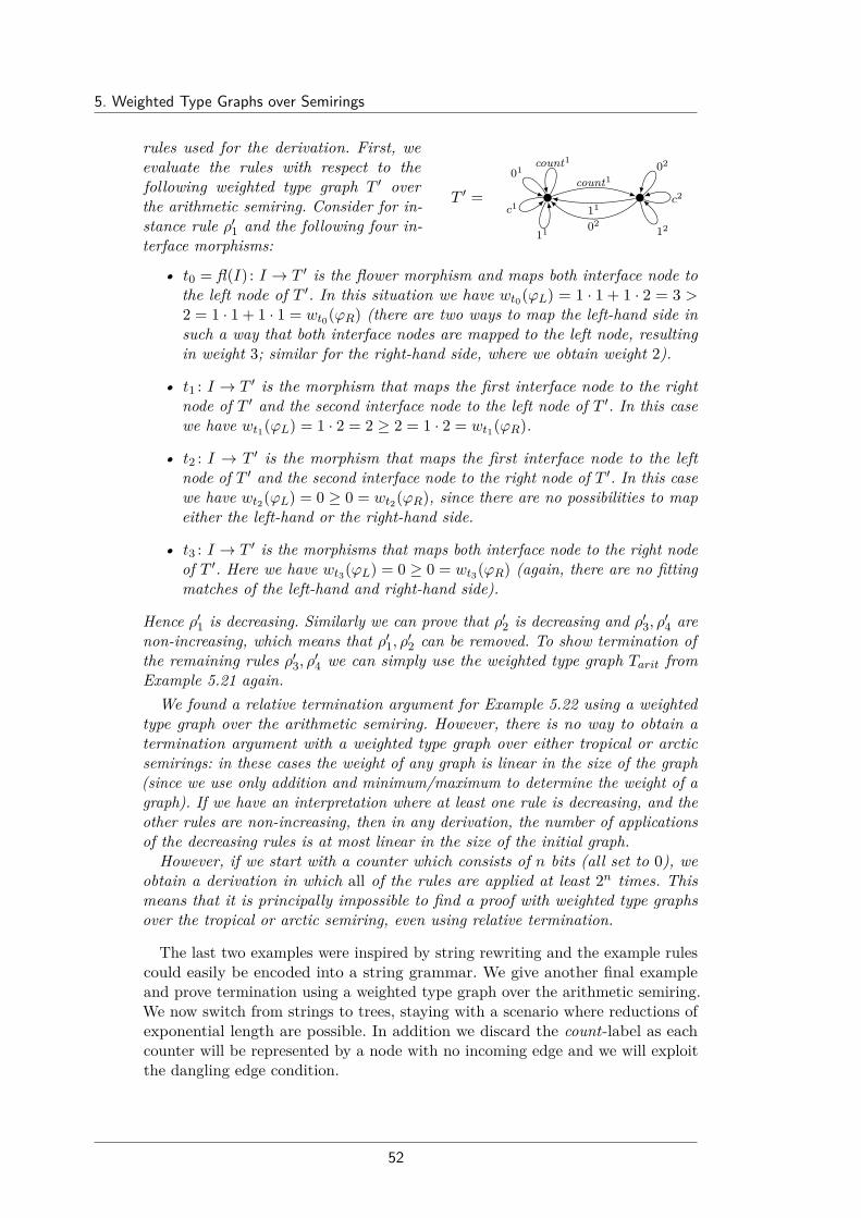
5. Weighted Type Graphs over Semirings

rules used for the derivation. First, weevaluate the rules with respect to thefollowing weighted type graph T ′ overthe arithmetic semiring. Consider for in-stance rule ρ′1 and the following four in-terface morphisms:

T ′ =

count101

c1

11

11

02

count102

c2

12

• t0 = fl(I) : I → T ′ is the flower morphism and maps both interface node tothe left node of T ′. In this situation we have wt0(ϕL) = 1 · 1 + 1 · 2 = 3 >2 = 1 · 1 + 1 · 1 = wt0(ϕR) (there are two ways to map the left-hand side insuch a way that both interface nodes are mapped to the left node, resultingin weight 3; similar for the right-hand side, where we obtain weight 2).

• t1 : I → T ′ is the morphism that maps the first interface node to the rightnode of T ′ and the second interface node to the left node of T ′. In this casewe have wt1(ϕL) = 1 · 2 = 2 ≥ 2 = 1 · 2 = wt1(ϕR).

• t2 : I → T ′ is the morphism that maps the first interface node to the leftnode of T ′ and the second interface node to the right node of T ′. In this casewe have wt2(ϕL) = 0 ≥ 0 = wt2(ϕR), since there are no possibilities to mapeither the left-hand or the right-hand side.

• t3 : I → T ′ is the morphisms that maps both interface node to the right nodeof T ′. Here we have wt3(ϕL) = 0 ≥ 0 = wt3(ϕR) (again, there are no fittingmatches of the left-hand and right-hand side).

Hence ρ′1 is decreasing. Similarly we can prove that ρ′2 is decreasing and ρ′3, ρ′4 arenon-increasing, which means that ρ′1, ρ′2 can be removed. To show termination ofthe remaining rules ρ′3, ρ′4 we can simply use the weighted type graph Tarit fromExample 5.21 again.

We found a relative termination argument for Example 5.22 using a weightedtype graph over the arithmetic semiring. However, there is no way to obtain atermination argument with a weighted type graph over either tropical or arcticsemirings: in these cases the weight of any graph is linear in the size of the graph(since we use only addition and minimum/maximum to determine the weight of agraph). If we have an interpretation where at least one rule is decreasing, and theother rules are non-increasing, then in any derivation, the number of applicationsof the decreasing rules is at most linear in the size of the initial graph.

However, if we start with a counter which consists of n bits (all set to 0), weobtain a derivation in which all of the rules are applied at least 2n times. Thismeans that it is principally impossible to find a proof with weighted type graphsover the tropical or arctic semiring, even using relative termination.

The last two examples were inspired by string rewriting and the example rulescould easily be encoded into a string grammar. We give another final exampleand prove termination using a weighted type graph over the arithmetic semiring.We now switch from strings to trees, staying with a scenario where reductions ofexponential length are possible. In addition we discard the count-label as eachcounter will be represented by a node with no incoming edge and we will exploitthe dangling edge condition.

52

5.5. Grez

Example 5.23. We interweave our counters into a single treelike structure. Eachpath from a root node to a leaf can be interpreted as a counter.One possible graph describing a state ofthe modified system is given by G. Eachcounter shares a number of bits with othercounters, where the least significant bit isshared by all counters. Again this is justone possible initial graph, since we proveuniform termination.

G =

. . .

. . . 00

00

1

1

11

0

Let the following graph transformation system ρ1, ρ2, ρ3, ρ4, ρ5, ρ6 be given:

ρ1 =1

01 1

1 ρ2 =1

11 1

c

ρ3 = 1

23

0

0c 1

23

1

23

1

00 ρ4 = 1

23

0

1c 1

23

1

23

1

10

ρ5 = 1

23

1

0c 1

23

1

23

c

00 ρ6 = 1

23

1

1c 1

23

1

23

c

10

The rules ρ1 and ρ2 increment the shared least significant bit by 1. These tworules can only be applied at the root of the tree (due to the dangling edge conditionof the DPO approach), as long as the edge is either labelled 0 or 1. By applying therules ρ3, . . . , ρ6, a carrier bit can be passed to the next bit. Proving termination ofthis graph transformation system is non-trivial. By applying for instance ρ6, thevalue of the counters containing interface node 1 does not change, while the othercounter values decrease. We evaluate therules with respect to the following weightedtype graph T over the arithmetic semiring.We can prove that ρ1 and ρ2 are decreas-ing and ρ3, . . . , ρ6 are non-increasing, whichmeans that ρ1, ρ2 can be removed using arelative termination argument.

T =

11

01

c1

11

02

12

02

c2

The rules ρ3 and ρ4 can be removed due to the decreasing number of c-labellededges, which remain constant in ρ5 and ρ6. Afterwards we can remove ρ5, ρ6 sincethey decrease the number of 1-labelled edges. The graph transformation system hasbeen shown to terminate uniformly, since there are no rules left.

5.5. GrezThe erstwhile question of how to find suitable weighted type graphs has beenleft open so far. Instead of manually searching for a suitable type graph weemploy a satisfiable modulo theories (SMT) solver (in this case Z3) that can solveinequations over the natural numbers.We fix a number n of nodes in the type graph and proceed as follows: take

a complete graph T with n nodes, i.e., a graph with an edge for every pairi, j ∈ 1, . . . , n of nodes and every edge label a ∈ Λ. Every edge e in this graphis associated with a variable xe. The task is to assign weights to those variablessuch that rules can be shown as either decreasing or non-increasing.

53

5. Weighted Type Graphs over Semirings

Now, for every rule ρ = LϕL− I −ϕRR and every map t : I → T we obtainan inequation: ∑

tL : L→TtLϕL=t

∏e∈EL

xtL(e) ≥∑

tR : R→TtRϕR=t

∏e∈ER

xtR(e)

If we want to show that ρ is decreasing and t is the flower morphism ≥ has to bereplaced by >.

Doing this for each rule and every map t gives us equations that can be used asinput for an SMT-solver. We consider the weights as natural numbers only up to agiven bound by restricting the length of the corresponding bit-vectors. Note thatwe would be outside the decidable fragment of arithmetics otherwise since theequations would contain multiplication of variables (as opposed to multiplicationof constants and variables). By using a bit-vector encoding the SMT-solver Z3can reliably find a solution (if it exists) and especially such solutions are foundfor the examples discussed in Section 5.4. Any solution gives us a valid weightedtype graph.

A prototype Java-based tool, called Grez, has been written and was introducedin [BKZ14]. Given a graph transformation systemR, the tool tries to automaticallyfind a proof for the uniform termination of R. The tool supports relative termina-tion and runs different algorithms (which are chosen by the user) concurrently tosearch a proof. If one algorithm succeeds in finding a termination argument for atleast one of the rules, all processes are interrupted and the corresponding rule(s)will be removed from R. The algorithms are then executed on the smaller set ofrules and this procedure is repeated until all rules have been removed. AfterwardsGrez generates the full proof which can be saved as a PDF-file.

Grez provides both a command-line interface and a graphical user interface.The tool supports the integration of external tools, such as other termination toolsor SMT-solvers. Grez can use any SMT-solver which supports the SMT-LIB2format [BST10]. Grez generates the inequation described above in this formatand passes it, either through a temporary file or via direct output stream, to theSMT-solver. The results are parsed back into the termination proof, as soon asthe SMT-solver terminates and produces a model for the formula.We ran the tool on all examples of this chapter using a Windows workstation

with a 2, 67 Ghz, 4-core CPU and 8 GB RAM. All proofs were generated in lessthan 1 second. The tool, a user manual [Bru15] and the examples from this chaptercan be downloaded from the Grez webpage.3

3Grez homepage: www.ti.inf.uni-due.de/research/tools/grez

54

“Problems are often stated in vague terms. . . becauseit is quite uncertain what the problems really are.”

John von Neumann (1903-1957)

6Terms, Term Rewriting and Term Graph

EncodingsIn the previous Chapter 5 we studied termination analysis inspired by matrixinterpretations on string rewriting and cycle rewriting. In this chapter we will focuson term rewriting instead and describe ways to encode term rewriting systems intograph transformation systems while preserving termination proving arguments, i.e.termination of the term rewriting system can be concluded from the terminationof the corresponding graph transformation system. Furthermore, we can benefitfrom an existing large database of term rewriting systems which we can use ascase studies for our previously introduced weighted type graph technique.

We will introduce term graph rewriting as a natural way to apply term rewritingto graphs. Term graph rewriting provides an efficient way to implement termrewriting. We discuss two natural ways to interpret term rewrite rules as termgraph rewrite productions: one in which implicit unraveling of the term graphis allowed and one in which it is not. We provide techniques to automaticallyprove termination of term graph rewriting and apply them to term rewritingsystems in both ways. The main approach is to transform term graph rewritingto a graph transformation system and then apply the tool Grez from Section 5.5for proving termination of the graph transformation system. We discuss two suchtransformations and report about experiments.

6.1. Additional Preliminaries - Terms and Term GraphsWhen trying to express algorithms in specific domains (that have certain structuresand/or properties), string rewriting systems are not suited very well for describingsemantics in domains by means of homomorphisms. Like string rewriting, termrewriting can describe grammars, but it additionally offers mechanics to describeprocesses in functional programming or analyse logic programs [Mar94]. Therefore,term rewriting systems play an important role in various areas, such as abstractdata type specifications. In order to understand the remainder of this chapter weintroduce the basics of terms and term rewriting systems. A good introductionon terms and term rewriting is given in [DJ90] and a comprehensive overview ofresearch in the area of term rewriting can be found in [Ter03].

6. Terms, Term Rewriting and Term Graph Encodings

6.1.1. Terms and Term RewritingIn term rewriting the following three basic concepts are essential: terms, substitu-tion and matching. We start by defining terms.

Definition 6.1 (Signature and terms). Let X be a countable set of variablesx, y, z, . . ., let 2 be a special symbol denoting an empty space and let F be asignature, i.e. a set of function symbols f, g, . . . each having a fixed aritygiven by a mapping ar : F → N0.

The set of terms over the signature F is the least set T (F ,X ) satisfying:

• If x ∈ X , then x ∈ T (F ,X ).

• If a ∈ F is a constant symbol (i.e., ar(a) = 0), then a ∈ T (F ,X ).

• If f ∈ F is a n-ary function symbol (i.e., ar(f) = n > 0) and t1, . . . , tn ∈T (F ,X ), then f(t1, . . . , tn) ∈ T (F ,X ).

For a term t ∈ T (F ,X ) the set Var(t) contains all variables occurring in t.

• We say that a term t is ground if Var(t) = ∅.

• The term t is called linear if it does not contains multiple occurrence ofthe same variable.

A context is a term containing one occurrence of 2 and is denoted by C[ ]. Ifa term t ∈ T (F ,X ) is replacing 2 the result is denoted by C[t] ∈ T (F ,X )and t is called a subterm of C[t].

The function root : T (F ,X )→ F ∪X returns the symbol labeling the root oft, i.e., root(t) = t if t ∈ X and root(f(t1, . . . , tn)) = f if f ∈ F .

Example 6.2. Let X = x, y and F = f, g, a with ar(f) = 2, ar(g) = 1 andar(a) = 0 be given. We give the following examples:

• The expression f(f(a, g(a))) is not a term in T (F ,X ) since the occurenceof the outer function symbol f is used as if it had arity 1.

• t = f(f(x, a), y) is a term (t ∈ T (F ,X )), which is linear but not groundand the root is root(t) = f .

• The term t′ = f(x, a) is a subterm of t with the context C[ ] = f(2, y).We have t = C[t′].

In term rewriting, not only 2 but also the variables of a term t, can be seen asabstract representations of subterms. These subterms do not have to be groundand could still consist of variables. Variables play an important role when it comesto matches between terms. In term rewriting, a match is a mapping between termswhich preserves function symbols and identifies variables in the source term withsubterms in the target term. The identification of a variable with a term is alsocalled substitution.

56

6.1. Additional Preliminaries - Terms and Term Graphs

Definition 6.3 (Substitution and homomorphic extension). Let T (F ,X ) bea set of terms over the signature F with a set of variables X . A substitutionis a mapping σ : X → T (F ,X ). Substitutions are homomorphically extendedto mappings from terms to terms σ : T (F ,X )→ T (F ,X ) by:

σ(x) = σ(x) and σ(f(t1, . . . , tn)) = f(σ(t1), . . . , σ(tn))

By using substitutions σ, we can define matches between terms. Matches areused to identify an occurrence of a (possibly not ground) left-hand-side term `,from a term rewriting rule `→ r, within a term t that is supposed to be rewritten.

Definition 6.4 (Match). A term ` matches a term t if there exists a substi-tution σ : T (F ,X )→ T (F ,X ) such that t = σ(`). The substitution σ is alsocalled matcher of t against `.

Example 6.5. Let T (F ,X ) be the set of terms from Example 6.2 and let thefollowing three terms `1, `2, t ∈ T (F ,X ) be given:

`1 = f(x, g(y)) `2 = f(x, a) t = f(f(x, a), g(a))

Then the term `1 matches the term t by the substitution σ(x) = f(x, a) andσ(y) = a which leads to t = σ(`1). The term `2 can not be matched with t dueto the constant a (the second argument in f(x, a)) which can not be substitutedto g(a).

We are now ready to define term rewrite rules. Like in many rewrite systemsthese rules consist of two elements from the corresponding framework which arerelated by a rewriting relation.

Definition 6.6 (Term rewrite rule, redex and contractum). A term rewriterule is an ordered pair `→ r, where `, r ∈ T (F ,X ) are called the left-hand-sideand right-hand-side respectively and the following two properties hold:

• ` /∈ X (the left hand side is not a variable), and

• Var(r) ⊆ Var(`) (there is no extra variable in the right-hand-side)

A term rewrite rule `→ r is called left-linear if ` is linear, right-linear if r isa linear and it is called linear if both ` and r are linear terms. The rule iscalled collapsing if the right-hand-side is a single variable (r ∈ X ).

Given a substitution σ, an instance σ(`) of the left-hand-side ` of a termrewriting rule `→ r is called a redex (reducible expression) of the rule andan instance σ(r) of the right-hand-side is called a contractum.

Example 6.7. The term rewrite rule f(x, x)→ f(g(x), a) is right-linear and non-collapsing. For the substitution σ(x) = g(a) the ground term σ(`) = f(g(a), g(a))is a redex and the ground term σ(r) = f(g(g(a)), a) is a contractum.

57

6. Terms, Term Rewriting and Term Graph Encodings

Finally, we define term rewriting systems. Term rewriting systems play animportant role in various areas, for instance for the analysis and implementationof abstract data type specifications, i.e. checking the consistency of properties orused for theorem proving. Just like in other rewriting frameworks, a term rewritingsystem is a set of rewrite rules.

Definition 6.8 (Term rewriting system). A Term Rewriting System is a pairR = (F , R) such that F is a signature and R is a set of rewrite rules over thesignature F .

A term rewriting system R = (F , R) is called left-linear, right-linear or linearif each rule `→ r ∈ R has the corresponding property. On the other hand, Ris called collapsing if at least one of the rules `→ r ∈ R is collapsing.

In the following we will simply denote a term rewriting system R by its set ofrewrite rules R whenever the signature F is clear from the context. A rewritingstep is now based on replacing a redex by a corresponding contractum withinthe same context. Given a term rewriting system R = (F , R) we define the(one-step) rewrite relation →R as the set of all possible rewriting steps over termsin T (F ,X ).

Definition 6.9 (Rewriting relation). Let a term rewriting system R = (F , R)be given. A term t ∈ T (F ,X ) can be rewritten to a term u ∈ T (F ,X )(written t→R u and called a rewriting step) if there exists a term rewritingrule ` → r ∈ R together with a substitution σ : X → T (F ,X ) such thatt = C[σ(`)] and u = C[σ(r)], i.e. a redex is replaced by a correspondingcontractum within the same shared context.

Example 6.10. Consider the following linear, non-collapsing term rewritingsystem R = (F , R) which consists of the two rules ρ1, ρ2 ∈ R:

ρ1 = f(a, x, y)→ h(x, y) and ρ2 = g(b, y)→ a

Let t ∈ T (F ,X ) be the term t = f(g(b, a), h(z, z), b). Then the following rewritingsteps are possible, where the matched subterm is underlined and the applied ruleis written above the rewriting relation:

f(g(b, a), h(z, z), b) ρ2→R f(a, h(z, z), b) ρ1→R h(h(z, z), b)

In implementing term rewriting, an obvious optimization is to share commonsubterms. In this way the objects to rewrite are not terms represented by trees,but by directed graphs. For finite terms the directed graphs are acyclic, but inmany applications, in particular in functional programming ([PE93]), it makessense to also allow cycles, by which after unfolding the represented term is infinite.These graphs are called term graphs, and rewriting on term graphs has beenextensively studied, see e.g. [Plu99; CD11], sometimes under the name of junglerewriting [HKP88; CR93].

58

6.1. Additional Preliminaries - Terms and Term Graphs

6.1.2. Term Graph RewritingWe will now focus on term graphs where every node is labeled by an operationsymbol, and the outgoing edges of such a node are numbered from 1 to the arityof the operation symbol.

Definition 6.11 (Term graph). A term graph over a signature F is a triple(V, lb, succ) in which

• V is a finite set of nodes (vertices),

• lb : V → F is a partial function, called labeling, and

• succ : V → V ∗ is a partial function, called successor, having the samedomain as lb, such that for every v ∈ V for which succ(v) is defined, thelength of succ(v) is equal to the arity of lb(v): |succ(v)| = ar(lb(v)).

A (term graph) morphism ϕ : (V, lb, succ) → (V ′, lb′, succ′) is a functionϕ : V → V ′ such that for all v ∈ V where lb(v) is defined, lb′(ϕ(v)) = lb(v)and succ′(ϕ(v)) = ϕ(v1) · · ·ϕ(vn) with succ(v) = v1 · · · vn.

This definition coincides with the one given in [CD11]. If succ(v) = (v1, . . . , vn)then we see (v, v1), . . . , (v, vn) as the n outgoing edges of v. Note that swappingtwo outgoing edges changes the term graph since edges are ordered. For specifyingground term graphs we are interested in the case where lb and succ are total, butfor defining term graph rewriting it is convenient to allow also partial functions.Furthermore, in the various definitions of term graphs within the literature thereare some syntactical variations, in particular whether or not a term graph isassumed to have a root node. In this chapter we will investigate term graphs thatare not required to have a root. Term graphs are a direct extension of finite terms.

Definition 6.12 (Term graph of a term). For a finite linear term t (thatis, every variable occurs at most once in t) its term graph TG(t) is definedinductively together with root(t) as follows:

• For a constant a the term graph TG(a) consists of a single node v forwhich succ(v) = ε and lb(v) = a, and root(a) = v.

• For a variable x the term graph TG(x) consists of a single node v forwhich succ(v) and lb(v) are both undefined, and root(x) = v.

• For a term t = f(t1, . . . , tn) let Vi be the set of nodes of the term graphof ti, and root(ti) = vi ∈ Vi, for i = 1, . . . , n. Then the set of nodes ofthe term graph TG(t) is defined to be the disjoint union of V1, . . . , Vnand a fresh node v. For nodes in V1, . . . , Vn, the functions lb and succare maintained, and succ(v) = v1 · · · vn, lb(v) = f and root(t) = v.

For a finite non-linear term t its term graph TG(t) is defined in the sameway, with the only difference that the occurrences of a variable are not takendisjoint, but shared.

59

6. Terms, Term Rewriting and Term Graph Encodings

Example 6.13. We construct the term graph for theterm t = f(a(x), h(y, z), c). The corresponding term graphTG(t) is depicted on the right, where the numbers onoutgoing edges from a node v indicate the order in succ(v).

f

ha c

21 3

1 2

Conversely, term graphs can be unraveled to terms: starting from a node v, webuild a term with lb(v) as its root, and for each of its |succ(v)| successors generatethe corresponding argument by applying the same process on the correspondingelement of succ(v). If the term graph is acyclic, this yields a finite term, but assoon as a node is visited that has been visited before, the resulting term will beinfinite.Just as in term rewriting, a term graph transformation rule consists of a left-

hand side and a right-hand side, and the basic idea is that an occurrence of aleft-hand side may be replaced by the corresponding right-hand side. Now left-hand sides and right-hand sides are term graphs themselves, and an occurrence ofa left-hand side may be defined as an injective morphism from the left-hand sideto the term graph to be rewritten. However, for a precise description some extrainformation is required: which nodes of the left-hand side correspond to nodes inthe right-hand side, and what to do with the remainder of the left-hand side.

Definition 6.14 (Term graph production, term graph rewrite systems). Aterm graph production p = L←` I →r R is a span consisting of three termgraphs L, I and R, called the left-hand side, the interface and the right-handside respectively, together with two interface morphisms ` and r which specifythe correspondence of the nodes in L and R.

A term graph rewrite system (TGRS) is a set of (term graph) productions.

In our setting for v ∈ I the partial functions lb and succ are defined for `(v) in Lif and only if they are defined for r(v) in R.1

Since the double-pushout approach is a standard approach for describing graphtransformations in several settings (as discussed in Chapter 3) we can use it todescribe term graph rewriting.

Definition 6.15 (Term graph rewriting step). A term graph G transformsto a term graph H by a production p = L←` I →r R (written G⇒p H) ifand only if an injective morphism g : L→ G, a term graph D and morphismsh : R→ H, i : I → D, dg : D → G and dh : D → H exist such that both theleft square and the right square in the diagram below are pushouts.

L I R

G D H

` r

g i h

dg dh

(po) (po)

1This condition is necessary to avoid non-local unification of terms that might occur otherwise.

60

6.2. Interpreting Term Rewriting in Term Graph Rewriting

6.2. Interpreting Term Rewriting in Term Graph RewritingWe will now focus on left-linear (left-hand sides of all rules are linear) and non-collapsing (right-hand sides of rules are no variables) term rewriting systems andinvestigate natural ways to interpret them as term graph rewriting systems. Theyhave to be non-collapsing, since we restrict to injective morphisms in the rule.In order to apply a term rewriting rule, that is, a rule t→ u in which t and u

are finite terms, to a term graph, there are two natural ways to proceed. In bothways in the corresponding production L←` I →r R, the term graph L is the termgraph of t. The right-hand side corresponds to the term graph of u, where nodesfor every variable that occurs in t, but not in u, are added. The main difference isin the interface I: roughly speaking in the basic version it is as small as possible,while in the extended version it is nearly a full copy of L. It is necessary to alsoadd the additional interface structure to R in the extended version.To motivate and define the two versions, let us first investigate what is really

needed. The basic idea is that a part of the graph to be rewritten coincides with t,and that this is replaced by u. For doing so, the interface should at least containthe root of t and the variables of t.

Definition 6.16 (Basic version). A term graph production L ←` I →r Rbased on a term rewriting rule t→ u is in the basic version if it satisfies thefollowing properties:

• The left-hand side L is the term graph TG(t)

• The interface I consists of the nodes of the term graph L of t thatcorrespond to the root of t and to the variables in t.

• The functions lb and succ are undefined for the nodes in I.

• The right-hand side R is the union of TG(u) with the nodes of Irepresenting variables.

• The mappings `, r map each of the nodes in I to the corresponding copyin L respectively R.

Via the two rule morphisms ` and r the node v ∈ I corresponding to the rootof t is mapped to the node v′ ∈ L representing the same root of t via `. Likewisev is mapped to the node v′′ ∈ R representing the root of u via r. Every node in Icorresponding to a variable in t is mapped to the corresponding node in L and itis similar mapped to R if the variable occurs in u.For string rewriting, that is, term rewriting in which all symbols are unary,

termination of cycle rewriting as studied in [ZBK14; SZ15] coincides with termi-nation of term graph rewriting systems in the basic version; the argument thatsymbols of other arity, not occurring in the rewrite system, do not influence thetermination property, is similar to the argument given in [BKZ14].The other, extended version, exactly corresponds to the version as presented

in [CD11], where it is shown that for orthogonal term rewriting systems, thereis a correspondence between term graph rewriting and term rewriting on thecorresponding unraveled (possibly infinite) terms.

61

6. Terms, Term Rewriting and Term Graph Encodings

Definition 6.17 (Extended version). A term graph production L←` I →r Rbased on a term rewriting rule t→ u is in the extended version if it satisfiesthe following properties:

• The left-hand side L is the term graph TG(t)

• The interface I is a copy of L, in which only the outgoing edges fromthe root are removed, that is, lb and succ are undefined for the nodecorresponding to the root of t

• For all nodes except the root of t, I is a copy of L in which for all nodessucc and lb is defined, and by ` : I → L every node and edge is mappedto itself.

• The right-hand side R is the union of TG(u) with the interface I.

• The morphism r : I → R maps every node or edge of the interface tothe corresponding item in R.

For a term rewriting system R we will denote by Rb(Re) the corresponding termgraph rewriting systems in the basic (extended) version.

Example 6.18. We interpret the term rewriting system R = ρ with the ruleρ = f(a(x), c) → h(x). Then Rb = ρb and Re = ρe are the correspondingsets of productions where the interface morphisms are denoted by the node positions:

Rb Re

f

a c

1 2h f

a c

1 2a c

h

a c

Termination is also called strong normalization and is usually abbreviated toSN. For a term rewriting system R we will write:

• SN(R) if R is terminating on finite terms,

• SNb(R) if Rb is terminating on finite term graphs,

• SNe(R) if Re is terminating on finite term graphs.

Since terms can be interpreted as term graphs, every infinite reduction of termsgives rise to an infinite reduction of term graphs in both versions. Further everystep in the basic version can be mimicked by a step in the extended version. Henceif we have an infinite reduction in the basic version, then this also yields an infinitereduction in the extended version, in which left-over remainders of the left-handsides, are ignored. This yields

SNe(R) =⇒ SNb(R) =⇒ SN(R)

for all right-linear term rewriting systems R.

62

6.2. Interpreting Term Rewriting in Term Graph Rewriting

The following example inspired by [Toy87] shows that right-linearity is essentialfor the last implication. The term rewriting system

R = f(0, 1, x)→ f(x, x, x), a→ 0, a→ 1

is non-terminating in term rewriting as f(0, 1, a) rewrites in three steps to itself:

f(0, 1, a) ρ1→R f(a, a, a) ρ2→R f(0, a, a) ρ3→R f(0, 1, a)

But this cannot be mimicked in term graph rewriting without doing unraveling:our techniques easily prove SNb.For both implications the converse does not hold, as we will show now by

counterexamples. The single rule f(g(x))→ g(f(x)) is the standard example of astring rewrite system that is terminating on strings but not on cycles, see [ZBK14],so this satisfies SN but not SNb.For the other implication, we consider the following single term rewrite rule

ρ = f(g(x)) → f(x) interpreted in both, the basic version Rb = ρb (shownbelow left) and the extended version Re = ρe (shown below right) where theinterface morphisms are again denoted by the node positions:

Rb Re

f

g

f f

g g

f

g

f

g

g

1

2

3

f

g

g

1

2

3

(extended step)⇒

Now let the term graph depicted in the left partof the picture to the right be given. We have threenodes 1, 2, 3 with lb(1) = f , lb(2) = lb(3) = g, andsucc(1) = 2, succ(2) = 3 and succ(3) = 2. In theextended version, an injective morphism from Lto this graph is obtained by mapping the root ofL to 1, and the two nodes below it to 2 and 3respectively. By applying the rule, the outgoingf -edge from 1 is removed, the rest of the left-handside remains, and due to the right-hand side an edge from 1 to 3 is added, resultingin the graph depicted in the right part of the picture. As this graph is isomorphicto the original one, we see that this can be repeated forever, and the single rulef(g(x))→ f(x) does not satisfy SNe.

In contrast, in the basic version the rule does not apply, since the middle node 2has an incoming edge that is not in the left-hand side, and is not part of theinterface. Hence, due to the dangling edge condition, the rule cannot be applied.

An elementary argument for proving termination of the term rewriting systemf(g(x))→ f(x) is by counting the number of g’s: in every step the number of g’sstrictly decreases, so this cannot go on forever. As we will see later, this terminationargument also holds for proving SNb. Hence our single rule f(g(x))→ f(x) doesnot satisfy SNe but satisfies SNb.As we observed, every step in the basic version can be mimicked by a step in

the extended version. Conversely, after doing a number of unraveling steps, a step

63

6. Terms, Term Rewriting and Term Graph Encodings

in the extended version can be mimicked by a step in the basic version. Hereunraveling means that if a node has more than one incoming edge, a new nodemay be created having the same outgoing edges as the original node, while one ofthe incoming edges points to the new

f

g

g

f

g

g

g

f

g

g

(unravel)⇒

(basic step)⇒

node, and the others point to the orig-inal node. In the example this can bedone for the middle node as depictedin the picture to the right, after whicha step in the basic version can be doneyielding the same result as when ap-plying the step in the extended versiondirectly.It is worth to mention that the pushout complement for termgraphs, which is

computed when a term graph production is applied on a term graph, may not beunique. Consider for instance the term rewrite rule ρ = a→ b interpreted as thefollowing term graph production (for this example, both versions look the same):

a b

Applying this term graph production to the term graph representing a singleconstant a, results in two possible rewrite step scenarios. In the following, theterm graphs of the pushout complements are highlighted in the dashed boxes:

a

a

(PO) (PO)

b

b

a

a

(PO)

a

b

7

Please note that both term graphs in the dashed boxes, shown in the diagramsabove left and above right, make the left square a pushout. However, only for theunlabelled node there exists a corresponding right-hand side pushout diagramresulting in the term graph representing a single constant b. In [CD11] theauthors provide properties which ensure the existence of pushouts and pushoutcomplements for the application of term graph productions. These propertiesare guaranteed to hold by using so-called evaluation rules, which are term graphproductions satisfying requirements that make them suitable to represent termrewrite rules. In the following, we restrict our term graph productions to be in thebasic version or extended version. Therefore, similar to evaluation rules, our termgraph productions are based on term rewrite rules (for which we want to showtermination) and the existence of minimal pushout complements is guaranteed,i.e. those term graphs where as many nodes as possible remain unlabelled.

Our next step is to transform term graph productions in the basic version andextended version into graph transformation rules which can be analysed by thetool Grez (see Section 5.5). If the graph transformation system is proven tobe terminating by Grez, we want to deduce termination of the original termrewriting system.

64

6.3. From Term Graph Rewriting to Graph Transformation Systems

6.3. From Term Graph Rewriting to GraphTransformation Systems

We propose two transformations from term graphs to graphs now, both havingthe property that an infinite reduction in term graph rewriting translates toan infinite graph transformation reduction. The main goal is not to developtechniques specific for term graph rewriting systems, but to apply translations tograph transformation systems for which the tool Grez can be applied. Hence if atool such as Grez can prove termination of the translated graph transformationsystem, then we have a proof that the original term graph rewrite system isterminating. The graphs in the graph transformation systems on which Grez canbe applied differ in three ways from term graphs: nodes may have any number ofoutgoing edges, these outgoing edges are not numbered, and the labels are not inthe nodes but on the edges. We now define two transformations from term graphsto graphs, more precisely, we will transform a term graph production to a graphtransformation rule in such a way that reductions are preserved.

6.3.1. Function EncodingThe first transformation is called function encoding. The structure of the graphremains the same. The idea is that for a node labeled by a function symbol f ofarity n ≥ 1, the label of this node is removed, and the n ordered outgoing edgesin the term graph are labeled by f1, . . . , fn, respectively. In order to preserveconstants, we introduce a fresh node c(v), for every node v ∈ V for which lb(v) isa constant; we write c(V ) for the set of all fresh nodes.

Definition 6.19 (Function encoding). For a signature F we define the setFF = fi | f ∈ F , 1 ≤ i ≤ ar(f) ∪ f | f ∈ F , ar(f) = 0. Furthermore,for a term graph (V, lb, succ) over F we define the function encoded graphF (V, lb, succ) = (V ∪ c(V ), E, src, tgt, lab) over F , by

• E = ev,i | v ∈ V, 1 ≤ i ≤ ar(lb(v)) ∪ ev | v ∈ V, ar(lb(v)) = 0),

• src(ev,i) = v for v ∈ V, 1 ≤ i ≤ ar(lb(v)),src(ev) = v if ar(lb(v)) = 0,

• tgt(ev,i) = wi for v ∈ V, 1 ≤ i ≤ ar(lb(v)) and succ(v) = w1w2 · · ·wn,tgt(ev) = c(v) if ar(lb(v)) = 0,

• lab(ev,i) = lb(v)i for v ∈ V, 1 ≤ i ≤ ar(lb(v)),lab(ev) = lb(v) if ar(lb(v)) = 0.

If ϕ : (V, lb, succ)→ (V ′, lb′, succ′) is a term graph morphism, then the graphmorphism F (ϕ) : F (V, lb, succ)→ F (V ′, lb′, succ′) is defined by

• F (ϕ)(v) = ϕ(v) andF (ϕ)(c(v)) = c(ϕ(v)) for v ∈ V ,

• F (ϕ)(ev,i) = eϕ(v),i andF (ϕ)(ev) = eϕ(v) for every edge ev,i and ev in F (V, lb, succ).

If ρ = L ←` I →r R is a term graph production, then we define the graphtransformation rule by F (ρ) = F (L) F (`)− F (I) −F (r) F (R).

It is straightforward to check that the above definition turns F into a functor.

65

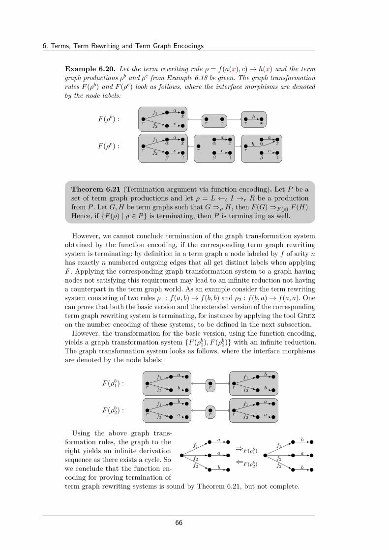
6. Terms, Term Rewriting and Term Graph Encodings

Example 6.20. Let the term rewriting rule ρ = f(a(x), c)→ h(x) and the termgraph productions ρb and ρe from Example 6.18 be given. The graph transformationrules F (ρb) and F (ρe) look as follows, where the interface morphisms are denotedby the node labels:

F (ρb) : x

rf2

f1a

c r x r xh

F (ρe) :β

α x

γ

rf2

f1a

c

β

xα

γ

r

a

c

β

xα

γ

r

a

ch

Theorem 6.21 (Termination argument via function encoding). Let P be aset of term graph productions and let ρ = L ←` I →r R be a productionfrom P . Let G,H be term graphs such that G⇒ρ H, then F (G)⇒F (ρ) F (H).Hence, if F (ρ) | ρ ∈ P is terminating, then P is terminating as well.

However, we cannot conclude termination of the graph transformation systemobtained by the function encoding, if the corresponding term graph rewritingsystem is terminating: by definition in a term graph a node labeled by f of arity nhas exactly n numbered outgoing edges that all get distinct labels when applyingF . Applying the corresponding graph transformation system to a graph havingnodes not satisfying this requirement may lead to an infinite reduction not havinga counterpart in the term graph world. As an example consider the term rewritingsystem consisting of two rules ρ1 : f(a, b)→ f(b, b) and ρ2 : f(b, a)→ f(a, a). Onecan prove that both the basic version and the extended version of the correspondingterm graph rewriting system is terminating, for instance by applying the tool Grezon the number encoding of these systems, to be defined in the next subsection.

However, the transformation for the basic version, using the function encoding,yields a graph transformation system F (ρb1), F (ρb2) with an infinite reduction.The graph transformation system looks as follows, where the interface morphismsare denoted by the node labels:

F (ρb1) :r

f2

f1a

b r rf2

f1b

b

F (ρb2) :r

f2

f1b

a r rf2

f1a

a

f2

f1

f2a

b

a

f2

f1

f2a

b

b

⇒F (ρb1)

⇐F (ρb2)

Using the above graph trans-formation rules, the graph to theright yields an infinite derivationsequence as there exists a cycle. Sowe conclude that the function en-coding for proving termination ofterm graph rewriting systems is sound by Theorem 6.21, but not complete.

66

6.3. From Term Graph Rewriting to Graph Transformation Systems

6.3.2. Number EncodingThe reason why the function encoding is not complete is that in a graph thenode corresponding to the root node of the left-hand side may have more thanone outgoing fi-edge for the same i, since this root node is part of the interface.Instead in the number encoding for non-unary symbols extra nodes and edges areadded by which it is forced that the node with the numbered outgoing edges isnot part of the interface, and hence is not allowed to have dangling edges.

Definition 6.22 (Number encoding). For a signature F in which m is thegreatest occurring arity, we define FN = F ∪ 1, 2, . . . ,m. Furthermore,for a term graph (V, lb, succ) over F we define the number encoded graphN(V, lb, succ) = (V × 0, 1, E, src, tgt, lab) over FN by

• E = ev,i | v ∈ V, 0 ≤ i ≤ ar(lb(v)),

• src(ev,0) = (v, 0) for v ∈ V ,tgt(ev,0) = (v, 1) for v ∈ V if ar(lb(v)) 6= 1,tgt(ev,0) = (succ(v), 0) for v ∈ V if ar(lb(v)) = 1,lab(ev,0) = lb(v) for v ∈ V ,

• src(ev,i) = (v, 1) for v ∈ V , 1 ≤ i ≤ ar(lb(v)), ar(lb(v)) ≥ 2,tgt(ev,i) = (succ(v)i, 0) for v ∈ V , 1 ≤ i ≤ ar(lb(v)), ar(lb(v)) ≥ 2,lab(ev,i) = i for v ∈ V , 1 ≤ i ≤ ar(lb(v)), ar(lb(v)) ≥ 2.

If ϕ : (V, lb, succ)→ (V ′, lb′, succ′) is a term graph morphism, then the graphmorphism N(ϕ) : N(V, lb, succ)→ N(V ′, lb′, succ′) is defined by

• N(ϕ)(v, i) = (ϕ(v), i) for (v, i) ∈ V × 0, 1,

• N(ϕ)(ev,i) = eϕ(v),i for every edge ev,i in N(V, lb, succ).

If ρ = L ←` I →r R is a term graph production, then we define the graphtransformation rule by N(ρ) = N(L) N(`)−N(I) −N(r)N(R).

Again, it is straightforward to check that above definition turns N into a functor.Note that the nodes (v, 1) and the edges ev,1 do not occur if ar(lb(v)) = 1; thesenodes and edges may be ignored respectively removed.Example 6.23. Let the term rewriting rule ρ = f(a(x), c) → h(x) and theterm graph productions ρb and ρe from Example 6.18 be given. Using the numberencoding, the corresponding graph transformation rules N(ρb) and N(ρe) look asfollows, where the interface morphisms are denoted by the node labels:

N(ρb) : x

r

f

2

1 a

c r x r xh

N(ρe) :β

α x

γ

r

f

2

1 a

c

β

xα

γ

r

a

c

β

xα

γ

r

a

ch

Our main result now states, that we can preserve the termination propertybetween term graph rewriting and graph transformation by using the numberencoding on productions in a basic version. The rules of the basic number encodingautomatically conform to the requirements of the following theorem.

67

6. Terms, Term Rewriting and Term Graph Encodings

Theorem 6.24 (Termination argument via basic number encoding). Let Pbe a set of term graph productions, obtained by encoding term rewrite rules,all having an interface which consists only of the root and variable nodes.Then P is terminating on term graphs if and only if the graph transformationsystem N(P ) = N(ρ) | ρ ∈ P is terminating.

Therefore, we can conclude that we have soundness and completeness for thebasic number encoding, since in this case the rules conform to the requirement ofthe theorem. For the extended number encoding the question of completeness isstill open, but we can exploit soundness for our termination proofs.

The remainder of this chapter is devoted to automatically proving terminationof term rewriting systems, interpreted as term graph rewriting systems in bothversions (basic and extended) and converted into graph transformation systemsusing both encodings (function and number).

6.4. ExperimentsWe use term rewriting systems from the Termination Problems Database2 (short:TPDB). The TPDB is a collection of termination problems and is used forbenchmarks in termination competitions. We encode some term rewriting systemsto graph transformation systems using both, the interpretations of the basicversion and the extended version together with the number and function encoding.Afterwards we try to prove termination of the resulting graph transformationsystems by using the weighted type graph technique over ordered semirings fromChapter 5. The following termination proof examples were found by our prototypeJava-based tool Grez (see also Section 5.5). An overview of the experimentstatistics is given in Appendix B. Furthermore, a complete list of all analyzed termrewriting systems and their results can be found in Appendix B.1. The interfacemorphisms in the following examples will always be denoted by letters writtennext to the nodes.

Example 6.25. As a first example we take the term rewriting system called 273.This term rewriting system R = ρ where ρ is defined as

ρ : g(x, a, b)→ g(b, b, a)

satisfies all three properties SN, SNb and SNe. Termination of R follows since thenumber of b’s as third argument of the function g strictly decreases in each rewritingstep. The transformation for the basic version, using the function encoding, resultsin the corresponding graph transformation system F (Rb) = F (ρb), where F (ρb)is depicted below.

F (ρb) :x

rg3

g1

g2a

br x r

x

g3

g1

g2b

a

b

2http://cl2-informatik.uibk.ac.at/mercurial.cgi/TPDB/file/d43b82fe816c/TRS_Standard3TPDB/TRS_Standard/Various04/27.xml

68

6.4. Experiments

We evaluate the rule of F (Rb) with respectto the following weighted type graph Ttropover the tropical semiring. The weights arewritten as superscripts. There is only onepossible morphism for the left-hand sidegraph L into Ttrop which maps every nodeto the left node of Ttrop.

Ttrop =

(g1|g2|a|b)0

g31

a0

g30

For the right-hand side graph R, every node can be mapped to the left nodeof Ttrop, but there exists another morphism. The target of the g3-labeled edgecan be mapped to the right node of Ttrop. Therefore in this situation we getwt(ϕL) = min(1) = 1 > 0 = min(1, 0) = wt(ϕR) where t : I → Ttrop maps allinterface nodes to the left node of Ttrop. Therefore the graph transformation systemF (Rb) is terminating, proving SNb(R) by Theorem 6.21.We found a termination proof for the corresponding graph transformation system

F (Rb) using the function encoding of the basic version. We now use the sametermination proof technique for the function encoding of the extended version. Inthe basic version, only the root node and the nodes representing variables are partof the interface graph. The graph transformation system in the extended versionpreserves almost everything from the left-hand side graph. The result of applyingthe transformation for the extended version, using the function encoding, is thefollowing graph transformation system F (Re) = F (ρe):

F (ρe) :

γ

α β

x

δ

rg3

g1

g2a

br

γ

α β

x

δ

a

br

x

α β

γ δ

g3

g1

g2b

a

b

a

b

To prove termination of the graph transformation system F (Re) we simply usethe weighted type graph Ttrop over the tropical semiring again. There is still onlyone possible morphism for the left-hand side graph L which maps all nodes to theleft node of Ttrop. The weight for the right-hand side graph R remains 0 as theweight of the additional a-, and b-labeled edges do not increase the weight sinceonly the g3-labeled edges have a weight of 1. The graph transformation systemF (Re) is terminating, proving SNe(R) by Theorem 6.21.

Example 6.26. As a next example we take the term rewriting system called z174.This term rewriting system R = ρ1, ρ2, ρ3for the three rules defined to the right sat-isfies SN and SNb, but not SNe. The termrewriting system R is terminating, as fol-lows from proving SNb as we will do now.

ρ1 : f(x, a(b(y)))→ f(c(d(x)), y)ρ2 : f(c(x), y)→ f(x, a(y))ρ3 : f(d(x), y)→ f(x, b(y))

The transformation for the basic version, using the number encoding, results inthe corresponding graph transformation system N(Rb) = N(ρb1), N(ρb2), N(ρb3),where N(Rb) is depicted below.

4TPDB/TRS_Standard/Zantema_05/z17.xml

69

6. Terms, Term Rewriting and Term Graph Encodings

N(ρb1) : x

y

r

1

2

f

a b

x

y

r

y

x

r 2

1fc d

N(ρb2) :y

x

r 2

1fc

x

y

r

x

y

r

1

2

f

a

N(ρb3) :y

x

r 2

1fd

x

y

r

x

y

r

1

2

f

b

We evaluate the rules of N(Rb) with respectto the following weighted type graph T overthe arithmetic semiring. Again the weightsare written as superscripts. We can provethat N(ρb1) and N(ρb2) are non-increasingand N(ρb3) is decreasing, which means that

T =

(a|b|d|f |1)1

(c|2)2 a2

(f |1)1 (b|c|d|f |2)1

(b|d|f |1)1

a2

N(ρb3) can be removed using a relative termination argument. Due to the decreasingnumber of b-labeled edges in rule N(ρb1), which remain constant in N(ρb2), we canremove N(ρb1). Afterward we can remove N(ρb2) since it decreases the number ofc-labeled edges. The graph transformation system N(Rb) is terminating, sincethere are no rules left. This proves SNb(R) by Theorem 6.24.

Last we show that SNe(R) does not hold by giving the infinite reduction below,only using ρe3 at every step.

f

d c

d

1 2f

d b

c

d

1 2f

d b

b

cd

1 2ρe3⇒ρe3⇒

ρe3⇒. . .

Other remarkable examples, which are listed in the table of Appendix B.1, arethe term rewriting system called Ex261Composition5, 019 6, enger-nloop-toOne7

and 2.30 8. In the basic version all can be shown terminating for both the functionand number encoding. The picture becomes more interesting if we restrict tothe arithmetic semiring. Here, we can easily show termination with the functionencoding, but not with the number encoding, for which the SMT solver does notreturn a solution. Hence, even though it is not complete, the function encoding hasits right to exist: since it is simpler, termination proofs for the function encodingare often found in substantially less time than for the number encoding.

5TPDB/TRS_Standard/Applicative_05/Ex2_6_1Composition.xml6TPDB/TRS_Standard/AotoYamada_05/019.xml7TPDB/TRS_Standard/EEG_IJCAR_12/enger-nonloop-toOne.xml8TPDB/TRS_Standard/SK90/2.30.xml

70

Conclusion of Part II

Over the years, automatically proving termination has been a central topic inrewriting research. Although it is widely agreed that term graph rewriting is theway to go for efficient implementation of term rewriting, quite surprisingly hardlyany effort has been done in automatically proving termination of term graphrewriting. One reason could be that for term graph rewriting it is substantiallyharder since techniques strongly exploiting the term structure do not apply, likepath orders and dependency pairs. Being close to graph transformation systems, inthe previous chapters we studied how to transform term graph rewriting systemsto graph transformation systems, in order to apply automated techniques forproving termination of graph transformation systems. In its turn, these techniqueswere inspired by and closely related to matrix interpretations of string and cyclerewriting. The weighted type graph approach does not subsume previous intro-duced termination analysis methods, but rather complements them. In practiceone should always try several methods in parallel threads, as it is done in ourtermination tool Grez. As a side effect, by applying our transformations to aselection of term rewriting systems from the TPDB, we provided a substantialset of test cases for automatically proving termination of graph transformationsystems.

Related WorkThere is some work on termination analysis for graph transformation systems,often using rather straightforward counting arguments. Some work is specificallygeared to the analysis of model transformations, taking for instance layers intoaccount.

The weighted type graphs over general semirings technique and their applicationto the termination analysis of graph transformation systems is a generalization ofthe tropical and arctic weighted type graph based approach of the paper [BKZ14].The paper [BH+05] considers high-level replacement units (hlru), which are

transformation systems with external control expressions. The paper introduces ageneral framework for proving termination of such hlrus, but the only concretetermination criteria considered are node and edge counting, which are subsumedby the weighted type graph method (for more details see [BKZ14]).In [EE+05] layered graph transformation systems are considered, which are

graph transformation systems where interleaving creation and deletion of edgeswith the same label is prohibited and creation of nodes is bounded. The papershows such graph transformation systems are terminating.

Another interesting approach encodes graph transformation systems into Petrinets [VV+06] by introducing one place for every edge label and transformingrules into transitions. Whenever the Petri net terminates on all markings, we canconclude uniform termination of the original graph transformation rules. Note thatExample 5.22 can not be handled in this way by Petri nets. Starting with threeedges labelled 0, 1, count, rule ρ′2 transforms them into three labels 0, c, count,which, via rule ρ′3, are again transformed into 0, 1, count. On the other hand[VV+06] can handle negative application conditions in a limited way, a featurewe did not consider here.

Another termination technique via forward closures is presented in [Plu95]. Notethat the example discussed in this paper (termination of a graph transformationsystem based on the string rewriting rules ab→ ac, cd→ db) can be handled byour tool via tropical type graphs.Furthermore in [Plu18] a modular termination analysis technique based on

sequential critical pairs for hypergraph transformation systems is introduced,which resembles to a relative termination argumentation.

Not only termination techniques but also the interpretations of term rewritingsystems as term graph rewriting systems has been studied in other publicationsas well. Traditionally, term graph rewriting is considered modulo unraveling,by which the extended version is natural. But when splitting up steps in thisextended version into its building blocks of unraveling steps and basic steps, thebasic version is more natural.When restricting to unary symbols the basic version exactly corresponds to

cycle rewriting as investigated in [ZBK14; SZ15].Termination of term graph rewriting in the extended version is closer to infinitary

termination of rewriting than to termination. Infinitary rewriting and its infinitarytermination have been studied in [KV03; KS+05; KV05; Zan08].

Open QuestionsNaturally, integration of (negative) application conditions to the graph transfor-mation rules is an interesting direction for future work. Furthermore techniques forpattern counting, i.e. whether a given graph transformation rule always decreasesthe number of occurrences of a given subgraph, seems like a promising approachwhich could be investigated in more detail.

Another area of future research that might be of great interest is non-uniformtermination analysis, i.e., to analyse whether the rules terminate only on arestricted set of graphs. In applications it is often the case that rules do notalways terminate, but they terminate on all input graphs of interest (lists, cycles,trees, etc.). For this, it will be necessary to find a suitable way to characterizegraph languages that is useful for the application areas and integrates well withtermination analysis.

With respect to the encoding between term graph rewriting systems and graphtransformation systems the question of completeness for Theorem 6.24 in case ofthe extended number encoding is still open.

Part III.

Specifying Graph Languages

Motivation of Part III

Formal languages in general and regular languages in particular play an importantrole in computer science. They can be used for pattern matching, parsing, verifi-cation and in many other domains. For instance, verification approaches such asreachability checking, counterexample-guided abstraction refinement [CG+03] andnon-termination analysis [EZ15] could be directly adapted to graph transformationsystems if one had a graph specification formalism with suitable closure properties,computable pre- and postconditions and inclusion checks. Inclusion checks arealso important for checking when a fixpoint iteration sequence stabilizes.While regular languages for words and trees are well-understood and can be

used efficiently and successfully in applications, the situation is less satisfactorywhen it comes to graphs. Although the work of Courcelle [CE12] presents an ac-cepted notion of recognizable graph languages, corresponding to regular languages,this is often not useful in practice, due to the sheer size of the resulting graphautomata. Many specification formalisms that are usually used in abstract graphtransformation [SWW11] and verification, are based on type graphs. For instance,shape graphs [Ren04a] can be seen as type graphs with additional annotations.Other formalisms, such as application conditions [Ren04b; HP05] and first-orderor second-order logics, feature more compact descriptions, but there are problemswith expressiveness, undecidability issues or unsatisfactory closure properties.1There are many approaches for specifying graph languages. One cannot say thatone is superior to the other, usually there is a tradeoff between expressiveness anddecidability properties, furthermore they differ in terms of closure properties.

Hence, it seems that there exists no one-fits-all solution. However, it is importantto study and compare specification formalisms (i.e., automata, grammars andlogics) that allow to specify potentially infinite sets of graphs. Therefore, our goalin this Part III is to study some selected graph specification languages and classifythem according to their properties.In fact, we investigate three different formalisms based on type graphs: first,

restriction graphs R, where the language consists of all graphs that do not admita homomorphic image of R. We also discuss the connection between type graphand restriction graph languages. Then, in order to obtain a language with betterboolean closure properties, we study type graph logic, which consists of typegraphs enriched with boolean connectives (negation, conjunction, disjunction).Finally, we consider annotated type graphs, where the annotations constrain thenumber of items mapped to a specific node or edge, somewhat similar to theproposals from abstract graph rewriting mentioned above.

In all three cases we are interested in closure properties (such as closure underunion, intersection, complementation and rule application) and in decidabilityissues (such as decidability of the membership, emptiness and inclusion problems)and in expressiveness.

1A more detailed overview over related formalisms is given in the conclusion of Part III onpage 101.

Outline:After introducing additional preliminaries in Section 7.1, in Section 7.2 we consideran alternative specification formalism aside from type graph languages, namelythe restriction graph language of a graph R, consisting of all graphs to which thereis no homomorphism from R. In Section 7.3, in order to obtain languages withbetter boolean closure properties, we study type graph logic, which consists of typegraphs enriched with boolean connectives. Finally, in Section 8.1 we introduceordered monoids which are used to define annotations and multiplicities for graphsin Section 8.2. In Section 8.3 we consider multiply annotated type graphs whichare annotated with sets of pairs of multiplicities. We investigate closure anddecidability properties for all three frameworks in their corresponding subsections.All proofs can be found in Appendix A.3 and A.4.

“High achievement always takes place in the frameworkof high expectation.”

Charles Kettering (1876-1958)

7Pure Type Graphs, Restriction Graphs

and Type Graph Logic

In this chapter we introduce two frameworks of graph languages. One that ischaracterized by a somewhat dual property of the type graph languages (intro-duced in Chapter 4) and one which is enriched by boolean operators. After ashort additional preliminary section which introduces the notion of cores, wedefine restriction graph languages which include all graphs that do not contain ahomomorphic image of a given restriction graph. Next, we discuss for type graphlanguages and restriction graph languages some properties such as closure underset operators, decidability of emptiness and inclusion, decidability of closure underrewriting via double-pushout rules, and discuss the relationship between thesetwo classes of graph languages. Finally, we introduce a logic based on type graphsand analyse the closure and decidability properties of this framework as well.

7.1. Additional Preliminaries - Retracts and CoresWe revisit the concept of retracts and cores from [NT00]. They are a convenientway to minimize type graphs, and can be obtained from any graph of the class byconsidering so-called retracts which further reduce the graph. In [CM77], retractswere also studied under the name of folding to minimize conjunctive queries inrelational database systems. The intuition behind a retract is, to find a propersubgraph structure of a host graph, which admits a total homomorphism from thehost while mapping the subgraph structure to the host via an identity morphism.

Definition 7.1 (Retract and core). A graph H is called a retract of a graphG if H is a subgraph of G and in addition there exists a morphism ϕ : G→ H,which is the identity when restricted to H, i.e., ϕ|H = idH . A graph H iscalled a core of G, written H = core(G), if it is a retract of G and has itselfno proper retracts.

7. Pure Type Graphs, Restriction Graphs and Type Graph Logic

Example 7.2. The graph H is a retract of G, where the inclusion δ is indicatedby the numbers under the nodes, while morphism ϕ is indicated by the numbersover the nodes:

G = 1 2 3 4

5 6

A

A

B

B

B ϕδ

1, 5

1

2, 4

2

3, 6

3A B = H

Since the graph H does not have a proper retract it is also a core of G.

Cores are the minimal representatives of homomorphism equivalence classes,as all graphs G,H with G ∼ H have a unique core up to isomorphism [NT00].Therefore, for all type graphs describing the same type graph language, it makessense to speak of the core. Please note, that the computation of the core is anNP-hard problem. This can be easily seen from a reduction from 3-colourability:Let T be a “triangle” graph with three nodes and edges connecting all pairs ofdistinct nodes (cf. Example 4.6). A graph G is 3-colourable if and only if the coreof G]T (the disjoint union of G and T ) is T . Therefore, in [KNN18] we employedSAT- and SMT-solvers to efficiently compute core graphs.

7.2. Type Graph and Restriction Graph LanguagesAs explained in Chapter 4 specifying graph languages using type graphs gives usthe possibility to forbid certain graph structures by not including them into thetype graph. Another way (possibly more explicit) to specify languages of graphsnot including certain structures, is the following one.

Definition 7.3 (Restriction graph language). Let R be a Λ-labelled graph.Its restriction graph language LR(R) is defined as:

LR(R) = G | R9 G.

Hence, LR(R) includes all graphs G that do not contain a homomorphic imageof R. Restriction graph languages provide another way of representing graphlanguages that is in several respects dual to type graphs.Even if the graphs used for specifying restriction graph languages are just

ordinary graphs, we will in the following call them restriction graphs in order toemphasize their role.

Example 7.4. The following restriction graph R over the edge label set Λ = A,Bspecifies the language LR(R) consisting of those graphs which do not contain anA-labelled loop and a B-labelled loop at the same time:

LR( A B ) =∅ , A , B , A B , . . .

We will consider the relationship between the class of languages introducedin Definitions 4.1 and 7.3 in Section 7.2.3. Next, we investigate closure anddecidability properties for both classes of languages.

78

7.2. Type Graph and Restriction Graph Languages

7.2.1. Closure and Decidability PropertiesGraph languages specified by either a type graph or a restriction graph enjoysimilar decidability properties. We compare the two classes of languages withrespect to decidability of the membership, emptiness and language inclusionproblem.

Proposition 7.5 (Decidability results for type/restriction graph languages).For a graph language L characterized by a type graph T (i.e. L = L(T )) or bya restriction graph R (i.e. L = LR(R)) the following problems are decidable:

1. Membership, i.e. for each graph G it is decidable if G ∈ L holds.

2. Emptiness, i.e. it is decidable if L = ∅ holds.

Furthermore, language inclusion is decidable for both classes of languages:

3. Given type graphs T1 and T2, L(T1) ⊆ L(T2) holds iff T1 → T2.

4. Given restriction graphsR1 andR2, LR(R1) ⊆ LR(R2) holds iffR1 → R2.

Type graph and restriction graph languages enjoy the following complementaryclosure properties with respect to set operators. Note that the product in thecategory of graphs is obtained by taking separately the (cartesian) products ofnodes and edges, which induce the other components in a unique way. Similarly,coproducts of graphs are built by taking coproducts (disjoint unions) of nodesand edges in the category of sets.

Proposition 7.6 (Closure properties of type/restriction graph languages).Type graph languages are closed under intersection (by taking the product oftype graphs) but not under union or complement.Restriction graph languages are closed under union (by taking the coproductof restriction graphs) but not under intersection or complement.

7.2.2. Closure under Double-Pushout RewritingNext, we discuss how we can show that a graph language L is closed under agiven graph transformation rule ρ = (LϕL− I −ϕRR). Given a graph languageL, we say that it is closed under a rule ρ (also called invariant) if membership inL is preserved by the application of ρ, that is, for all graphs G and H such thatG⇒ρ H, it holds that G ∈ L implies H ∈ L. For both type graph languages andrestriction graph languages, separately, we characterize sufficient and necessaryconditions which show that closure under rule application is decidable.

The condition for restriction graph languages is related to a condition alreadydiscussed in [HW95]. It is sufficient to check if for each overlap H of the right-handside and the restriction graph S that S is already present in the predecessor of H,that is, the graph obtained by applying the rule backwards. If this is the case, thenthe absence of the homomorphic image of S is an invariant which is maintainedby rule application.

79

7. Pure Type Graphs, Restriction Graphs and Type Graph Logic

Proposition 7.7 (Closure under DPO rewriting for restriction graphs). Arestriction graph language LR(S) is closed under a rule ρ = (LϕL−I−ϕRR)if and only if the following condition holds: forevery pair of morphisms α : R→ F , β : S →F which are jointly surjective, all graphs Ethat we obtain by applying the rule ρ with(co-)match α backwards to F , satisfy S → E.

L

IϕLoo

ϕR //

R

α

S

βwwE C ′oo // F

Closure under rewriting for a graph language, specified by a type graph, isdecidable as long as the type graph is a core.

Proposition 7.8 (Closure under DPO rewriting for type graphs). A typegraph language L(T ) is closed under a rule ρ = (LϕL−I−ϕRR) if and only iffor each morphism tL : L→ core(T ) there exists a morphism tR : R→ core(T )such that tL ϕL = tR ϕR, that is:

L I R

core(T )

⇔L(T ) is closed under application of ρ

ρ

∀tL

ϕL ϕR

∃tR

To conclude this subsection, we show that the only if part (⇒) of Proposition 7.8cannot be weakened by considering morphisms to the type graph T , instead ofto core(T ). We give a counterexample which shows that there exist type graphs,which are closed under a set of rules R but the diagram to the above right doesnot commute for all possible morphisms tL : L→ T . In fact, consider the followingtype graph T and the rule ρ:

ρ =1 2

A1 2 1 2

BT =

A

B

A

The type graph T contains the flower node, i.e., it has T A,BR

as subgraph.This ensures that each graph G, edge-labeled over Λ = A,B, is in the languageL(T ), and thus by rewriting any graph G ∈ L(T ) into a graph H using ρ it isguaranteed that H ∈ L(T ). However there is a morphism tL : L → T , the onemapping the A-labeled edge of L to the left A-labeled edge of T , such that thereexists no morphism tR : R→ T satisfying tL ϕL = tR ϕR. Namely, by mappingthe binary A-labelled edge in L to the non-loop edge in T . Due to the absence ofa parallel B-labelled edge the diagram can not commute.

7.2.3. Relating Type Graph and Restriction Graph LanguagesBoth type graph and restriction graph languages specify collections of graphsby forbidding the presence of certain structures. This is more explicit with theuse of restriction graphs, though. A natural question is how the two classes oflanguages are related. A partial answer to this is provided by the notion of duality

80

7.3. Type Graph Logic

pairs and by an important result concerning their existence, presented in [NT00].1Intuitively a duality pair consists of a type graph and a restriction graph whosegraph languages are equivalent.

Definition 7.9 (Duality pair). Given two graphs R and T , we call T thedual of R if for every graph G it holds that G→ T if and only if R9 G. Inthis case the pair (R, T ) is called a duality pair.

Clearly, we have that (R, T ) is a duality pair if and only if the restriction graphlanguage LR(R) coincides with the type graph language L(T ).

Example 7.10. Let Λ = A,B be given. The following is a duality pair:

(R, T ) =(

1 2 3A B ,

1 2A,BA B

)

Since node 1 of T is not the source of a B-labeled edge and node 2 is not the targetof an A-labeled edge, for every graph G we have G→ T iff it does not contain anode which is both the target of an A-labeled edge and the source of a B-labelededge. But it contains such a node if and only if R→ G.

One can identify the class of restriction graphs for which a corresponding typegraph exists which defines the same graph language.

Fact 7.11 (Duality pair construction [NT00]). Results from [NT00] state2thatgiven a core graph R, a graph T can be constructed such that (R, T ) is aduality pair if and only if R is a tree.

Thus we have a precise characterisation of the intersection of the classes of typeand restriction graph languages: L belongs to the intersection if and only if it isof the form L = LR(R) and core(R) is a tree. The results from [NT00] can beused to construct a type graph T from a given restriction graph R. It is worthmentioning that the construction of T from R contains two exponential blow-ups.However, the results stated in [NT00] can not be used to derive a construction ofR from T .

All this can be interpreted by saying that type graphs have limited expressivenessif used to forbid the presence of certain structures.

7.3. Type Graph LogicIn this section we investigate the possibility to define a language of graphs using alogical formula over type graphs. Such a logic could alternatively also be definedbased on restriction graphs. A related logic, for injective occurrences of restrictiongraphs, is studied in [OEP08], where the authors also give a decidability resultvia inference rules.

1Note that in [NT00] graphs are simple, but it can be easily seen that for our purposes theresults can be transferred straightforwardly.

2This refers to Lemma 2.3, Lemma 2.5 and Theorem 3.1 in [NT00].

81

7. Pure Type Graphs, Restriction Graphs and Type Graph Logic

We start by defining the syntax and semantics of a type graph logic (TGL).

Definition 7.12 (Syntax and semantics of TGL). A TGL formula F over afixed set of edge labels Λ is formed according to the following grammar:

F := T | F1 ∨ F2 | F1 ∧ F2 | ¬F, where T is a type graph.

Each TGL formula F denotes a graph language L(F ) ⊆ |GraphΛ| definedby structural induction as follows:

L(T ) = G ∈ |GraphΛ| | G→ T L(¬F ) = |GraphΛ| \ L(F )L(F1 ∧ F2) = L(F1) ∩ L(F2) L(F1 ∨ F2) = L(F1) ∪ L(F2)

Example 7.13. Let the following TGL formula F over Λ = A,B be given:

F = ¬ A ∧ ¬ B

The graph language L(F ) consists of all graphs which do not consist exclusively ofA-edges or of B-edges, i.e., which contain at least one A-labeled edge and at leastone B-labeled edge, something that can not be expressed by pure type graphs.

With respect to the closure properties we get more positive results when usingthe TGL formula instead of a pure type graph, which we will show next.

7.3.1. Closure and Decidability Properties for Type Graph LogicUsing pure type graphs to specify the type graph language we got negative resultswith respect to the closure under union and complement (see Proposition 7.6). Inthe case of the type graph logic we can use the semantics of the formulae to getpositive results for all the desired closure properties.

Proposition 7.14 (Closure properties of TGL). Graph languages L(F ) char-acterized by a TGL formula F , are closed under union, intersection andcomplement.

We now present some positive results for graph languages over TGL formulaswith respect to decidability problems. Due to the conjunction and negationoperator, the emptiness (or unsatisfiability) check is not as trivial as it is forpure type graphs. Note also that thanks to the presence of boolean connectives,inclusion can be reduced to emptiness.

Proposition 7.15 (Decidability properties of TGL). For a graph languageL(F ) characterized by a TGL formula F , the following problems are decidable:

• Membership, i.e. for all graphs G it is decidable if G ∈ L(F ) holds.

• Emptiness, i.e. it is decidable if L(F ) = ∅ holds.

• Language inclusion, i.e. given two TGL formulas F1 and F2 it is decidableif L(F1) ⊆ L(F2) holds.

82

7.3. Type Graph Logic

As already mentioned in the introduction of Part III, the different specificationframeworks have the purpose to be used for verification. Therefore, it is natural toask for a framework which is able to compute weakest preconditions and strongestpostconditions, i.e. given a graph language and a set of rules, we want to specifythe language of all successors (or the language of all predecessors) in our formalism.However, neither type graphs nor the type graph logic can count and hence cannot express that all items of the newly created right-hand occur exactly once. Thecomputation of postconditions is impossible in these frameworks.Therefore, in the next chapter we will improve the expressiveness of the type

graphs themselves, rather than using an additional logic to do so.

83

“Truth is ever to be found in simplicity, and not in themultiplicity and confusion of things.”

Isaac Newton (1642-1727)

8Annotated Type Graphs

In this chapter we will equip graphs with additional annotations, thus making ourgraph languages more expressive. As explained in the introduction of Part III, thisidea was already used similarly in abstract graph rewriting [Ren04a]. In contrastto most other approaches, we will investigate the problem from a categorical pointof view. Another reason for considering annotated type graphs is that they are asuitable formalism for computing post-conditions, a task which is studied in moredetail in Chapter 10.

8.1. Additional Preliminaries - Ordered MonoidsWe will annotate each type graph with pairs of annotations, denoting upper andlower bounds for nodes and edges. A graph will belong to the correspondinglanguage only if it has a morphism to the type graph satisfying such bounds.The bounds of the type graph are elements from an ordered monoid, i.e. a

monoid which comes equipped with a partial order for its elements.

Definition 8.1 (Ordered monoid). An ordered monoid (M,+,≤) consists ofa setM, a partial order ≤ and a binary operation + such that

• (M,+, 0) is a monoid.

• The partial order is compatible with the monoid operation, in particulara ≤ b implies a+ c ≤ b+ c and c+ a ≤ c+ b for all a, b, c ∈M.

An ordered monoid is commutative if + is commutative.

We denote by Mon the category having ordered monoids as objects and monoidhomomorphisms which are monotone as arrows. In the following we will sometimesdenote an ordered monoid by its underlying set.

Definition 8.2 (Homomorphisms of ordered monoids). LetM1,M2 be twoordered monoids. A map h : M1 →M2 is called monotone if a ≤ b impliesh(a) ≤ h(b) for all a, b ∈ M1. It is called a homomorphism if in additionh(0) = 0 and h(a+ b) = h(a) + h(b).

8. Annotated Type Graphs

Example 8.3. Let n ∈ N and take Mn = 0, 1, . . . , n, ∗ (zero, one, . . . , n,many) with 0 ≤ 1 ≤ · · · ≤ n ≤ ∗ and addition as monoid operation with theproviso that for x, y ∈ Mn, we have x + y = ∗ if the sum is larger than n. Inaddition x+ ∗ = ∗ for all x ∈Mn.

Furthermore, given a set S and an ordered monoid (M,+,≤), it is easy to checkthat (MS ,+,≤) is an ordered monoid, where the elements of the exponentiationMS = a : S →M are functions from S toM and both, the partial order andthe monoidal operation, are taken pointwise. An ordered monoid likeMn (themonoid given in the previous Example 8.3) can be used to count the number ofnodes or edges contained in a graph. However, there are other monoids, which canfor instance be used to specify whether there exists a path between two nodes.The following path monoid PG is useful if we want to annotate a graph with

information over which paths are present. Note that due to the folding caused bythe abstraction, a path in the type graph does not necessarily imply the existenceof a corresponding path in a graph of the language. Hence annotations based onsuch a monoid can yield useful additional information.

Example 8.4. Given a graph G and the transitive closure E+G ⊆ VG × VG of the

edge relation EG = (srcG(e), tgtG(e)) | e ∈ EG. The path monoid PG of G hasthe carrier set P(E+

G), i.e. the powerset of the transitive closure E+G . The partial

order is simply set inclusion and the monoid operation is defined as follows: givenP0, P1 ∈ PG, we have

P0 + P1 = (v0, vn) | ∃v1, . . . , vn−1 : (vi, vi+1) ∈ Pji ,i ∈ 0, . . . , n− 1, j0 ∈ 0, 1, ji+1 = 1− ji

That is, new paths can be formed by concatenating alternating path fragmentsfrom P0, P1. It is obvious to see that + is commutative and one can also showassociativity. P = ∅ is the unit.

Using ordered monoids we are now ready to define annotations for our graphsand how they are used to make graph languages more expressive.

8.2. Annotations and MultiplicitiesThe annotations are defined, in general, as elements of an ordered monoid, andin the concrete case that we use as running example they are functions mappingnodes and edges of the type graph to corresponding multiplicities. This idea hasearlier been proposed in [Kön99]. Please note that the following formal definitionof our annotations can easily be extended to a functor for objects from an arbitrarygiven category to Mon.

Definition 8.5 (Annotations). Given a functor A : GraphΛ → Mon, anannotation based on A for a graph G is an element a ∈ A(G). We assumethat for each graph G there is a standard annotation based on A that wedenote by sG, thus sG ∈ A(G).

86

8.2. Annotations and Multiplicities

An annotation functor assigns an ordered monoid to every graph. We write Aϕ,instead of A(ϕ), for the action of functor A on a graph morphism ϕ. To makethis notion of an annotation functor easier to understand we introduce a concreteinstance of the functor A in form of the functor Bn.

Definition 8.6 (Multiplicities). Given an ordered monoidMn = 0, . . . , n, ∗with n ∈ N0 we define the functor Bn : GraphΛ →Mon as follows:

• for every graph G, Bn(G) = a : (VG ∪ EG)→Mn =MVG∪EGn ;

• for every graph morphism ϕ : G→ G′ and a ∈ Bn(G),we have Bnϕ(a) ∈ Bn(G′) with:

Bnϕ(a)(y) =∑

ϕ(x)=ya(x), where x ∈ (VG ∪ EG) and y ∈ (VG′ ∪ EG′)

Notice that, if y is not in the image of ϕ, Bnϕ(a)(y) = 0.

Annotations based on the functor Bn are called multiplicities.For a graph G, its standard multiplicity sG ∈ Bn(G) is defined as the

function which maps every node and edge of G to 1.

The action of the functor Bn on a morphism transforms a multiplicity bysumming up (inMn) the values of all items of the source graph that are mappedto the same item of the target graph. Please note, that in the specific case ofthe functor Bn (our running example in this thesis) the ordered monoid is notMn but the set of possible annotation functions from the graph items to Mn.Therefore an annotation based on a functor Bn associates every node or edge of agraph with a number (or the top value ∗).Example 8.7. Let the following graphs G and G′ with multiplicities a ∈ B3(G)be given. The multiplicity of each graph element is indicated by the element ofM3 = 0, 1, 2, 3, ∗ shown in the brackets. Furthermore, let ϕ : G→ G′ be a graphmorphism indicated by the numbers above the nodes.

G =[1] [2] [2] [1] [1]

1 2 3 4 5

A[2]

A[0] B[∗] B[1] ϕ−→ 1, 2 3, 4, 5A B = G′

Let a′ = B3ϕ(a). We compute a′(y) for each element y ∈ G′

by summing up the multiplicities of all preimages, i.e. theybuild the sum of all a(x) ∈ B3(G) for which ϕ(x) = y.The annotation a′ is depicted on the right.

[3] [∗]A[2] B[∗]

Some of the results that we will present in the rest of the chapter will hold forannotations based on a generic functor A, some only for annotations based onfunctors Bn, i.e. for multiplicities.

Note that the multiplicity functor Bn is only one of many possible instances ofour generic annotation functor A. For instance, we can consider an annotationfunctor which records the out-degree of a node or we can consider an annotationfunctor based on the path monoid from Example 8.4. Such a path annotationfunctor T is defined below.

87

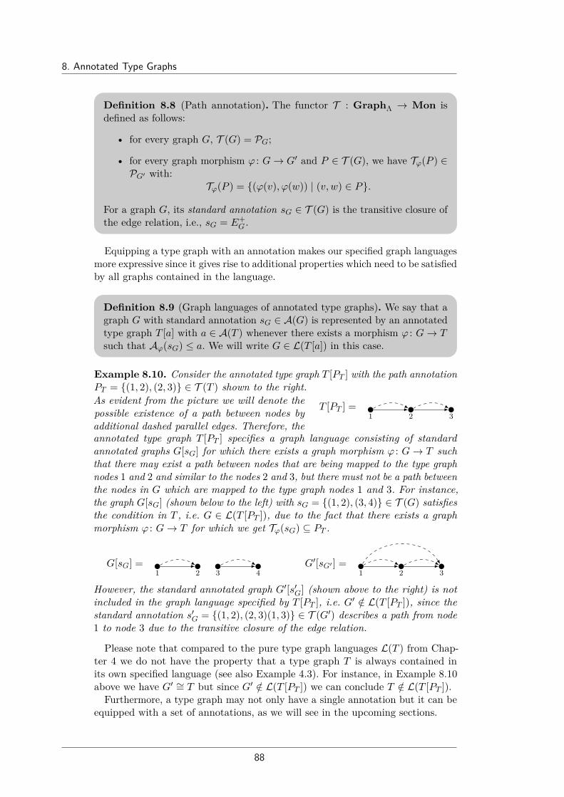
8. Annotated Type Graphs

Definition 8.8 (Path annotation). The functor T : GraphΛ → Mon isdefined as follows:

• for every graph G, T (G) = PG;

• for every graph morphism ϕ : G→ G′ and P ∈ T (G), we have Tϕ(P ) ∈PG′ with:

Tϕ(P ) = (ϕ(v), ϕ(w)) | (v, w) ∈ P.

For a graph G, its standard annotation sG ∈ T (G) is the transitive closure ofthe edge relation, i.e., sG = E+

G .

Equipping a type graph with an annotation makes our specified graph languagesmore expressive since it gives rise to additional properties which need to be satisfiedby all graphs contained in the language.

Definition 8.9 (Graph languages of annotated type graphs). We say that agraph G with standard annotation sG ∈ A(G) is represented by an annotatedtype graph T [a] with a ∈ A(T ) whenever there exists a morphism ϕ : G→ Tsuch that Aϕ(sG) ≤ a. We will write G ∈ L(T [a]) in this case.

Example 8.10. Consider the annotated type graph T [PT ] with the path annotationPT = (1, 2), (2, 3) ∈ T (T ) shown to the right.As evident from the picture we will denote thepossible existence of a path between nodes byadditional dashed parallel edges. Therefore, the

T [PT ] =1 2 3

annotated type graph T [PT ] specifies a graph language consisting of standardannotated graphs G[sG] for which there exists a graph morphism ϕ : G→ T suchthat there may exist a path between nodes that are being mapped to the type graphnodes 1 and 2 and similar to the nodes 2 and 3, but there must not be a path betweenthe nodes in G which are mapped to the type graph nodes 1 and 3. For instance,the graph G[sG] (shown below to the left) with sG = (1, 2), (3, 4) ∈ T (G) satisfiesthe condition in T , i.e. G ∈ L(T [PT ]), due to the fact that there exists a graphmorphism ϕ : G→ T for which we get Tϕ(sG) ⊆ PT .

G[sG] =1 2 3 4

G′[sG′ ] =1 2 3

However, the standard annotated graph G′[s′G] (shown above to the right) is notincluded in the graph language specified by T [PT ], i.e. G′ /∈ L(T [PT ]), since thestandard annotation s′G = (1, 2), (2, 3)(1, 3) ∈ T (G′) describes a path from node1 to node 3 due to the transitive closure of the edge relation.

Please note that compared to the pure type graph languages L(T ) from Chap-ter 4 we do not have the property that a type graph T is always contained inits own specified language (see also Example 4.3). For instance, in Example 8.10above we have G′ ∼= T but since G′ /∈ L(T [PT ]) we can conclude T /∈ L(T [PT ]).

Furthermore, a type graph may not only have a single annotation but it can beequipped with a set of annotations, as we will see in the upcoming sections.

88

8.3. Multiply Annotated Graphs

8.3. Multiply Annotated GraphsThe type graphs which we are going to consider are enriched with a set of pairsof annotations. Each pair can be interpreted as establishing a lower and an upperbound to what a graph morphism can map to the graph. The motivation forconsidering multiple (pairs of) annotations rather than a single one is mainly toensure closure under union.

Definition 8.11 (Multiply annotated graphs). Let A : GraphΛ →Mon bea functor. A multiply annotated graph G[M ] (over A) is a graph G equippedwith a finite set of pairs of annotations M ⊆ A(G)×A(G), such that ` ≤ ufor all (`, u) ∈M . We will write G[`, u] as an abbreviation of G[(`, u)].An arrow ϕ : G[M ] → G′[M ′], also called a legal morphism, is a graph

morphism ϕ : G → G′ such that for all (`, u) ∈ M there exists (`′, u′) ∈ M ′with Aϕ(`) ≥ `′ and Aϕ(u) ≤ u′.

In case of annotations based on Bn, we will often call a pair (`, u) a doublemultiplicity.

Example 8.12. Consider the following multiply annotated graphs (over B2)G[`, u] and H[`′, u′], both having one double multiplicity.

G[`, u] =[1,1] [1,∗]

A [0,1]H[`′, u′] =

[1,∗]A [0,∗]

Referring to the picture, for example G[`, u] is defined as follows: If e is thesingle edge of G, labelled by A, then `, u : e, srcG(e), tgtG(e) → M2, and inparticular `(e) = 0, `(srcG(e)) = `(tgtG(e)) = 1, u(e) = u(srcG(e)) = 1, andu(tgtG(e)) = ∗. Thus multiplicities are represented by writing the lower and upperbounds next to the corresponding graph elements. Note that there is a unique,obvious graph morphism ϕ : G→ H, mapping both nodes of G to the only node ofH. Concerning multiplicities, by adding the lower and upper bounds of the twonodes of G, one obtains the interval [2, ∗] which is included in the interval ofthe node of H, [1, ∗]. Similarly, the double multiplicity [0, 1] of the edge of G isincluded in [0, ∗]. Therefore, since both B2

ϕ(`) ≥ `′ and B2ϕ(u) ≤ u′ hold, we can

conclude that ϕ : G[`, u]→ H[`′, u′] is a legal morphism.

Multiply annotated graphs and legal morphisms form a category.

Lemma 8.13. The composition of two legal morphisms is a legal morphism.

We are now ready to define how a graph language L(T [M ]) looks like.

Definition 8.14 (Graph languages of multiply annotated type graphs). Wesay that a graph G is represented by a multiply annotated type graph T [M ]whenever there exists a legal morphism ϕ : G[sG, sG]→ T [M ], i.e., there exists(`, u) ∈ M such that ` ≤ Aϕ(sG) ≤ u. We will write G ∈ L(T [M ]) in thiscase.

89

8. Annotated Type Graphs

It follows from the definition that whenever M = ∅, then we get L(T [M ]) = ∅. Inthe special case of the functor Bn, the graph language L(T [M ]) coincides withL(T ) from Definition 4.1, if there exists a double multiplicity (`, u) ∈M whichassigns [0, ∗] to every node and edge in T .

Note that pure type graph languages L(T ) are always infinite if T 6= ∅. However,if we use annotations based on Bn, then a graph language L(T [M ]) is finite upto isomorphism if there does not exist a double multiplicity (`, u) ∈ M with uassigning the upper bound ∗ to at least one node or edge in T .

Example 8.15. Let the standard annotated type graph T [sT , sT ] in the figurebelow be given. As evident from the figure, the resulting graph language L(T [sT , sT ])only contains one graph, that is T , up to isomorphism.

∅G0 G1

A

G2

AA

G3

[1, 1]A [1, 1]T [sT , sT ] =

Both, G0 and G1 do not satisfy the lower bound of the A-labelled loop of T [sT , sT ].Furthermore, for G3 one would need to map both of its A-labelled loops to thesingle loop of T [sT , sT ]. Since annotations (in this case the standard annotation 1)are summed up, we would violate the upper bound of the targeted loop. Only forthe graph G2 (which represents T [sG, sG]) there exists a legal morphism into theannotated type graph, which respects all lower and upper bounds.

Multiply annotated type graphs have a higher expressiveness compared to puretype graphs and restriction graphs, since one can enforce certain structures toappear in the language, by increasing the lower bounds as thresholds. The aim ofthis thesis is to find specification mechanisms, which are useful for the verificationof systems. Before investigating decidability results and closure properties forthe graph languages specified by multiply annotated type graphs, we show someexample properties, that can be expressed by annotated type graphs.

Example 8.16. In order to illustrate the use of annotated type graphs in appli-cations, we model a client-server scenario with the following specification:

• There exists exactly one server.

• An arbitrary number of users can connect to the server, even using multipleconnection sessions at the same time.

• There exists one user with special administrative rights.

• At least one user is always connected to the server.

• The server can host an arbitrary number of files from which at most onecan be edited at the same time.

90

8.3. Multiply Annotated Graphs

The scenario above can be modelled using an annotated type graph T1[`, u] (seebelow). We will use the following edge labels: A-labelled loops for administrativerights, C-labelled edges for connections between users and the server and E-labellededges which are pointing to the file that is currently edited. The left-hand noderepresents users, the middle node the server and the right-hand node files.

Now we extend the requirements of our specification:

• The user with the administrative rights is always connected to the server.

• There has to be at least one file on the server.

We use the annotated type graph T2[`′, u′] (depicted below to the right), to modelthe extended scenario.

T1[`, u] =[1, ∗] [1, 1] [0, ∗]

A [1, 1]

C [1, ∗] E [0, 1]T2[`′, u′] = [1, 1] [1, 1] [1, ∗]

[0, ∗]

A [1, 1]

C [1, 1]

C [0, ∗]

E [0, 1]

Since the second scenario is more restrictive than the first,there exist graphs in L(T1[`, u]), which do not fulfill theadditional requirements of the extended specification. Forinstance the graph G shown to the right is such a model,which describes that there exists a user with administrativerights but he is not connected to the server.

A

C

In contrast to type graph languages, core graphs can not be used to minimizeannotated type graphs since they do not preserve graph languages specified bymultiply annotated type graphs.Example 8.17. Consider the following annotated type graph T [`, u] togetherwith the corresponding core graph core(T ) alongside the unique graph morphismϕ : T → core(T ). We annotate the core with the double multiplicity (`′, u′) =(B2

ϕ(`),B2ϕ(u)) such that ϕ′ : T [`, u]→ core(T )[`′, u′] becomes a legal morphism in

the framework of annotated type graphs. Then graph G is a witness for the factthat L(T [`, u]) 6= L(core(T )[`′, u′]) since G ∈ L(core(T )[`′, u′]) but G /∈ L(T [`, u]).

[1, 1] [1, 1] [1, 1]A [0, 1] A [0, 1]

T [`, u] =[2, 2] [1, 1]

A [0, 2] = core(T )[`′, u′]

A

A

G =

ϕ′

The double multiplicity (`′, u′) = (B2ϕ(`),B2

ϕ(u)) is not the only possibility toannotate core(T ). However, by either increasing `′ or decreasing u′, the morphismϕ′ will no longer be legal and one could easily find a graph contained in L(T [`, u])but not in L(core(T )[`′, u′]). On the other hand, by either decreasing `′ or increasingu′ the graph G remains as a witness for the fact that the language is not preserved.Therefore, we can conclude that there can not exist an annotated core graphcore(T )[`′, u′] of T [`, u] specifying the same language.

91

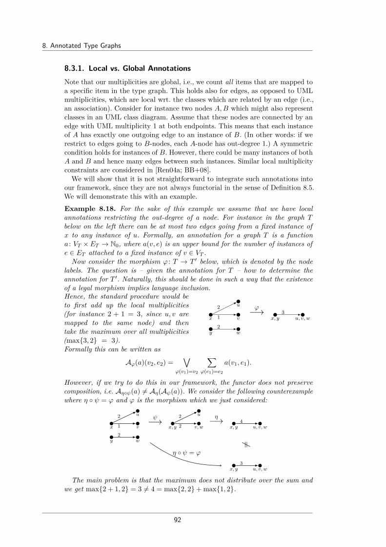
8. Annotated Type Graphs

8.3.1. Local vs. Global AnnotationsNote that our multiplicities are global, i.e., we count all items that are mapped toa specific item in the type graph. This holds also for edges, as opposed to UMLmultiplicities, which are local wrt. the classes which are related by an edge (i.e.,an association). Consider for instance two nodes A,B which might also representclasses in an UML class diagram. Assume that these nodes are connected by anedge with UML multiplicity 1 at both endpoints. This means that each instanceof A has exactly one outgoing edge to an instance of B. (In other words: if werestrict to edges going to B-nodes, each A-node has out-degree 1.) A symmetriccondition holds for instances of B. However, there could be many instances of bothA and B and hence many edges between such instances. Similar local multiplicityconstraints are considered in [Ren04a; BB+08].We will show that it is not straightforward to integrate such annotations into

our framework, since they are not always functorial in the sense of Definition 8.5.We will demonstrate this with an example.

Example 8.18. For the sake of this example we assume that we have localannotations restricting the out-degree of a node. For instance in the graph Tbelow on the left there can be at most two edges going from a fixed instance ofx to any instance of u. Formally, an annotation for a graph T is a functiona : VT ×ET → N0, where a(v, e) is an upper bound for the number of instances ofe ∈ ET attached to a fixed instance of v ∈ VT .Now consider the morphism ϕ : T → T ′ below, which is denoted by the node

labels. The question is – given the annotation for T – how to determine theannotation for T ′. Naturally, this should be done in such a way that the existenceof a legal morphism implies language inclusion.Hence, the standard procedure would beto first add up the local multiplicities(for instance 2 + 1 = 3, since u, v aremapped to the same node) and thentake the maximum over all multiplicities(max3, 2 = 3).Formally this can be written as

x

y

u

v

w

2

1

2

3x, y u, v, w

ϕ−→

Aϕ(a)(v2, e2) =∨

ϕ(v1)=v2

∑ϕ(e1)=e2

a(v1, e1).

However, if we try to do this in our framework, the functor does not preservecomposition, i.e. Aηψ(a) 6= Aη(Aψ(a)). We consider the following counterexamplewhere η ψ = ϕ and ϕ is the morphism which we just considered:

x

y

u

v

w

2

1

2

2

2x, y v, w

u

4x, y u, v, w

3x, y u, v, w

ψ−→ η−→

η ψ = ϕ

6=

The main problem is that the maximum does not distribute over the sum andwe get max2 + 1, 2 = 3 6= 4 = max2, 2+ max1, 2.

92

8.3. Multiply Annotated Graphs

This counterexample of course calls for an extension of our abstract annotationframework. One solution might be to allow lax functors, but a generalization ofour results is not straightforward. (For instance, the proof of the closure underintersection, Proposition 8.33, requires functoriality.) An alternative solution is todefine the annotations in a way such that they yield a functor. We will introduce asimilar local annotation, which fits into our annotation framework, in Chapter 10.

8.3.2. Decidability Properties for Multiply Annotated GraphsWe now address some decidability problems for languages defined by multiplyannotated graphs. We obtain positive results, under mild assumptions, with respectto the membership and emptiness problems. However, for decidability of languageinclusion we only obtain partial results.

For the membership problem we can enumerate all graph morphisms ϕ : G→ Tand check if there exists a legal morphism ϕ : G[sG, sG]→ T [M ], i.e. if there existsa pair of annotations (`, u) ∈M with ` ≤ Aϕ(sG) ≤ u. Clearly, this is decidable ifthe functor is computable and the partial order is decidable, which is certainlytrue if A = Bn. The emptiness check is somewhat more involved, since we have totake care of “illegal” annotations.

Proposition 8.19 (Emptiness check for languages specified by multiplyannotated graphs). For a graph language L(T [M ]) characterized by a multiplyannotated type graph T [M ] over Bn the emptiness problem is decidable:L(T [M ]) = ∅ iff M = ∅ or for each (`, u) ∈ M there exists an edge e ∈ ETsuch that `(e) ≥ 1 and (u(src(e)) = 0 or u(tgt(e)) = 0).

Language inclusion can be deduced from the existence of a legal morphismbetween the two multiply annotated type graphs.

Proposition 8.20 (Language inclusion and legal morphisms). The existenceof a legal morphism ϕ : T1[M ]→ T2[N ] implies L(T1[M ]) ⊆ L(T2[N ]).

Example 8.21. Consider the annotated type graphs T1[`, u] and T2[`′, u′] fromExample 8.16. Since the more restrictive annotated type graph T2[`′, u′] models thesame scenario as T1[`, u], the two languages should be included into each other.Indeed, by Proposition 8.20 it holds that L(T2[`′, u′]) ⊆ L(T1[`, u]), since we caneasily find a legal graph morphism ϕ : T2[`′, u′]→ T1[`, u].

Please note, that this condition is sufficient but not necessary, as shown by thefollowing counterexample. Let the following two multiply annotated type graphsT1[M1] and T2[M2] over B1 be given where |M1| = |M2| = 1:

T1[M1] =[1, ∗]

T2[M2] =[1, 1] [0, ∗]

Clearly we have that the languages L(T1[M1]) and L(T2[M2]) are equal as bothcontain all discrete non-empty graphs. Thus L(T1[M1]) ⊆ L(T2[M2]), but thereexists no legal morphism ϕ : T1[M1] → T2[M2]. In fact, the upper bound of thefirst node of T2 would be violated if the node of T1 is mapped by ϕ to it, whilethe lower bound would be violated if the node of T1 is mapped to the other node.

93

8. Annotated Type Graphs

8.3.3. Deciding Language Inclusion for Annotated Type GraphsIn this section we show that if we allow only bounded graph languages consisting ofgraphs up to a fixed pathwidth, the language inclusion problem becomes decidablefor annotations based on Bn. Pathwidth is a well-known concept from graph theorythat intuitively measures how closely a graph resembles a path. A more formaldefinition is given below. We start by giving the notion of tree decompositions andpath decompositions which were introduced in [RS83; RS86].

Definition 8.22 (Tree and path decomposition). Let G = (V,E, src, tgt, lab)be a graph. A tree decomposition of G is a pair TG = 〈T,X〉, where T is atree and X = Xt1 , . . . , Xtn is a family of subsets of V , called bags, indexedby the nodes of T , such that:

• for each node v ∈ V , there exists a node t of T such that v ∈ Xt;

• for each edge e ∈ E, there is a node t of T such that all nodes v attachedto e are in Xt;

• for each node v ∈ V , the graph induced by the nodes t | v ∈ Xt is asubtree of T .

A path decomposition PG = 〈T,X〉 of a graph G is a tree decomposition whereT is a path.

The treewidth and the pathwidth of a graph can be used to measure how similarthe graph is to a tree or to a path. Please note that in the following definitionwe always decrement the width of a tree decomposition by 1, to ensure that treeshave treewidth 1, paths have pathwidth 1 and discrete graphs have treewidth andpathwidth 0.

Definition 8.23 (Width, treewidth and pathwidth). The width of a treedecomposition TG = 〈T,X〉 is w(TG) =

(maxt∈T |Xt|

)− 1. The pathwidth

pw(G) and the treewidth tw(G) of a graph G are defined as follows:

• pw(G) = minw(PG) | PG is a path decomposition of G,

• tw(G) = minw(TG) | TG is a tree decomposition of G.

Example 8.24. Consider the graph G shown below to the left. Please note thatthe graph G contains a 3-clique. One possible decomposition of G is the pathdecomposition PG shown below to the right which has width w(PG) = 2, due to thefact that the largest bag consists of three nodes.

G =1 2 4 5

3 PG =32 41 2 4 5

For all possible path decompositions this width is the smallest possible since thethree nodes of the 3-clique always have to be in the same bag. Therefore, the graphG has the pathwidth pw(G) = 2.

94

8.3. Multiply Annotated Graphs

The following proof for the decidability of the language inclusion problem isbased on the notion of recognizability, which will be described via automatonfunctors that were introduced in [BK08]. We start with the main result and explainstep by step the arguments that will lead to decidability.

Proposition 8.25 (Language inclusion and bounded pathwidth). The lan-guage inclusion problem is decidable for graph languages of bounded pathwidthcharacterized by multiply annotated type graphs over Bn. That is, given k ∈ Nand multiply annotated type graphs T1[M1] and T2[M2], it is decidable whetherL(T1[M1])≤k ⊆ L(T2[M2])≤k, with L(T [M ])≤k = G ∈ L(T [M ]) | pw(G) ≤ k.

Our automaton model, given by automaton functors, reads cospans (i.e., graphswith interfaces) instead of single graphs. Therefore in the following, the categoryunder consideration will be Cospanm(GraphΛ), i.e. the category of cospans ofgraphs where the objects are discrete graphs J,K and the arrows are cospansc : J → G← K where both graph morphisms are injective [BK08]. We will refer tothe graph J as the inner interface and to the graph K as the outer interface of thecospan c. Although in general interfaces could also be non-discrete, discrete graphssuffice in order to glue graphs and hence we restrict to discrete interfaces. Wewill sometimes abbreviate the cospan c : J → G← K to the short representationc : J # K. Composition of two cospans c1, c2 where the outer interface of c1matches the inner interface of c2 is done via pushouts and denoted by c1; c2.

Definition 8.26 (Composition of cospans). Let c1 : J −ψL G ψR− I andc2 : I −ψ′LG′ ψ′R−K be two cospans in the categoryCospanm(GraphΛ). The cospan com-position c1; c2 : J −fψLH gψ′R− Kis defined by the commuting diagramshown to the right, where the middlesquare is a pushout.

I

J G (PO) G′ K

H

ψR ψ′L

ψL

f g

ψ′R

According to [BB+13] a graph has pathwidth k iff it can be decomposed intocospans where each middle graph of a cospan has at most k + 1 nodes.Our main goal is to build an automaton which can read all graphs of our

language step by step, similar to the idea of finite automata reading words in formallanguages. Since graphs are per se monolithic, we use cospan (de)composition asa means to split graphs into smaller entities. In particular, graph automata readcospans in place of alphabet symbols. Such an automaton can be constructedfor an unbounded language, where the pathwidth is not restricted. However, weobtain a finite automaton only if we restrict the pathwidth.

Then we can use well-known algorithms for finite automata to solve the languageinclusion problem. Note that, if we would use tree automata instead of finiteautomata, our result could be generalized to graphs of bounded treewidth.

We will first introduce the notion of automaton functor (which is a categoricalautomaton model for so-called recognizable arrow languages) and which is inspiredby Courcelle’s theory of recognizable graph languages [CE12].

95

8. Annotated Type Graphs

Definition 8.27 (Automaton functor [BK08]). An automaton functor C is afunctor C : Cospanm(GraphΛ)→ Rel that maps every object J (i.e., everydiscrete graph) to a finite set C(J) (the set of states of J) and every cospanc : J # K to a relation C(c) ⊆ C(J) × C(K) (the transition relation of c).In addition there is a distinguished set of initial states I ⊆ C(∅) and adistinguished set of final states F ⊆ C(∅). The language LC of C is defined asfollows:

A graph G is contained in LC if and only if there exist states q ∈ Iand q′ ∈ F which are related by C(c), i.e. (q, q′) ∈ C(c), wherec : ∅ → G ← ∅ is the unique cospan with empty interfaces andmiddle graph G.

Languages accepted by automaton functors are called recognizable.

As a warm-up let us show an example of an automaton functor, which acceptsthe pure type graph language determined by a graph T . This graph language hasbeen considered before in [BK08].

Example 8.28. Let T be a fixed type graph and let L(T ) be its type graph language,i.e. the set of all graphs G for which a morphism f : G→ T exists. We show thatL(T ) is recognizable, as it is accepted by the automaton functor CT defined asfollows. The automaton functor CT maps every discretegraph J to the set of states CT (J) consisting of allmorphisms fJ : J → T . For a cospan c : J → G ← K,CT (c) is the relation on C(J) × C(K) that relates amorphism fJ : J → T to a morphism fK : K → T (i.e.(fJ , fK) ∈ CT (c)) whenever there exists a morphismf : G→ T such that f ψL = fJ and f ψR = fK (see thediagram to the right).

J G

T

KψL ψR

fJ fKf

Intuitively, a graph is read step-by-step and we always record the current statevia a morphism J → T . Then, whenever we see a new slice G′ of our graph (withinner interface J and outer interface K) we check locally whether we can extendthe map into T , resulting in K → T as the new state.

The initial and final states are defined as I = F = CT (∅) = f∅, wheref∅ : ∅→ T is the unique morphism from the empty graph to T .It follows immediately from the definition that CT accepts L(T ). In fact, a graph

G is accepted by CT iff only the states f∅ ∈ I and f∅ ∈ F are related by CT (c),where c : ∅→ G← ∅. But this holds if and only if there is a morphism f : G→ T ,as the two additional conditions required above (f ψL = f∅ and f ψR = f∅)trivially hold.

As a proof obligation, it would remain to show that CT is well defined as afunctor from Cospanm(GraphΛ) to Rel, i.e. it preserves identities and arrowcomposition. This follows easily from the proof of Proposition 8.31 presented below,where a more complex functor is considered.

We will now define an automaton functor for a type graph T [M ] over Bn. Thefollowing construction is an extension of Example 8.28, where we count nodes andedges in addition.

96

8.3. Multiply Annotated Graphs

Definition 8.29 (Counting cospan automaton). Let T [M ] be a multiplyannotated type graph over Bn. We define an automaton functor CT [M ] (forT [M ]) with CT [M ] : Cospanm(GraphΛ)→ Rel as follows:

• For each object J of Cospanm(GraphΛ) (thus J is a finite discretegraph), CT [M ](J) = (f, b) | f : J → T, b ∈ Bn(T ) is its finite set ofstates

• I ⊆ CT [M ](∅) is the set of initial states with I = (f : ∅ → T, 0),where 0 is the constant 0-function

• F ⊆ CT [M ](∅) is the set of final states with F = (f : ∅ → T, b) |∃(`, u) ∈M : ` ≤ b ≤ u

Let c : J −ψLGψR−K be an arrow in the cat-egory Cospanm(GraphΛ) with discrete interfacegraphs J and K where both graph morphismsψL : J → G and ψR : K → G are injective. Twostates (f : J → T, b) and (f ′ : K → T, b′) are inthe relation CT [M ](c) if and only if there exists amorphism h : G → T such that the diagram tothe right commutes and for all x ∈ VT ∪ ET thefollowing equation holds:

J G K

T

c : J # K

f

ψL

∃h

ψR

f ′

b′(x) = b(x) + |y ∈ (G \ ψR(K)) | h(y) = x|

The set G \ ψR(K) consists of all elements of G which are not targeted bythe morphism ψR, i.e. G \ ψR(K) = (VG \ ψR(VK)) ∪ (EG \ ψR(EK)).

Instead of LCT [M ] and CT [M ] we just write LC and C if T [M ] is clear from thecontext. The intuition behind the construction is to count for each item x ofT , step by step, the number of elements that are being mapped from a graphG (which is in the form of a cospan decomposition) to x, and then check if thebounds of a pair of annotations (`, u) ∈M of the multiply annotated type graphT [M ] are satisfied. We give a short example before moving on to the results.

Example 8.30. Let the following multiply annotated type graph (over B2) T [`, u]and the cospan (c : ∅→ G← ∅) with G ∈ L(T [`, u]) be given:

T [`, u] =[0,1] [1,∗]

A [0,2] B [0,∗] c : ∅ A B ∅

We will now decompose the cospan c into two cospans c1, c2 with c = c1; c2 in thefollowing way:

∅ A B ∅

c1 c2

c

We let our counting cospan automaton parse the cospan decomposition c1; c2 stepby step now to show how the annotations for the type graph T evolve during the

97

8. Annotated Type Graphs

process. According to our construction, every element in T has multiplicity 0 in theinitial state of the automaton. We then sum up the number of elements within themiddle graphs of the cospans which are not part of the right interface. Thereforewe get the following parsing process:

∅ A B ∅

[0] [0]A[0] B[0]

[1] [0]A[1] B[0]

[1] [2]A[1] B[1]

f1 f2 f3

q1 q2 q3

We visited three states q1, q2 and q3 in the automaton with (q1, q2) ∈ C(c1) and(q2, q3) ∈ C(c2). Since C is supposed to be a functor we get that C(c1); C(c2) = C(c)and therefore (q1, q3) ∈ C(c) also holds. In addition we have q1 ∈ I and since theannotation function b ∈ B2(T ) in q3 = (f3, b) satisfies ` ≤ b ≤ u we can infer thatq3 ∈ F . Therefore we can conclude that G ∈ LC holds as well.

We still need to prove that C is indeed a functor. Intuitively this shows that accep-tance of a graph by the automaton is not dependent on its specific decomposition.

Proposition 8.31 (Functoriality of C). Let two cospans c1 : J → G ← Kand c2 : K → H ← L be given and let idG : G → G ← G be the identitycospan.The mapping CT [M ] : Cospanm(GraphΛ)→ Rel is a functor, i.e.

1. CT [M ](idG) = idCT [M ](G)

2. CT [M ](c1; c2) = CT [M ](c1); CT [M ](c2)

The language accepted by the automaton LC is exactly the graph languageL(T [M ]).

Proposition 8.32 (Language of C). Let the multiply annotated type graphT [M ] (over Bn) and the automaton functor C : Cospanm(GraphΛ) → Relfor T [M ] be given. Then LC = L(T [M ]) holds, i.e. for a graph G we haveG ∈ L(T [M ]) if and only if there exist states i ∈ I ⊆ C(∅) and f ∈ F ⊆ C(∅)such that (i, f) ∈ C(c), where c : ∅→ G← ∅.

Therefore we can construct an automaton for each graph language specified bya multiply annotated type graph T [M ], which accepts exactly the same language.In case of a bounded graph language this automaton will have only finitely manystates. Furthermore we can restrict the label alphabet, i.e., the cospans by usingonly atomic cospans, adding a single node or edge (see [BB+12; Blu14]). Once thesesteps are performed, we obtain conventional non-deterministic finite automataover a finite alphabet and we can use standard techniques from automata theoryto solve the language inclusion problem directly on the finite automata.

98

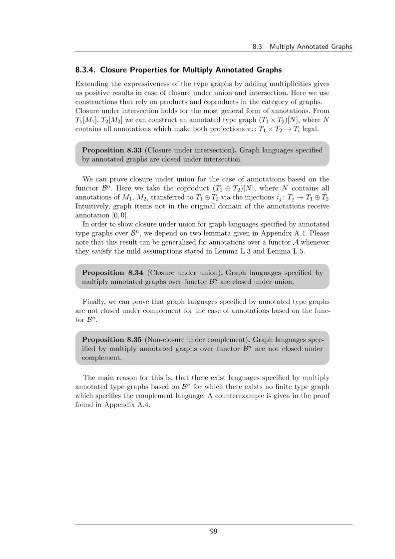
8.3. Multiply Annotated Graphs

8.3.4. Closure Properties for Multiply Annotated GraphsExtending the expressiveness of the type graphs by adding multiplicities givesus positive results in case of closure under union and intersection. Here we useconstructions that rely on products and coproducts in the category of graphs.Closure under intersection holds for the most general form of annotations. FromT1[M1], T2[M2] we can construct an annotated type graph (T1 × T2)[N ], where Ncontains all annotations which make both projections πi : T1 × T2 → Ti legal.

Proposition 8.33 (Closure under intersection). Graph languages specifiedby annotated graphs are closed under intersection.

We can prove closure under union for the case of annotations based on thefunctor Bn. Here we take the coproduct (T1 ⊕ T2)[N ], where N contains allannotations of M1, M2, transferred to T1 ⊕ T2 via the injections ij : Tj → T1 ⊕ T2.Intuitively, graph items not in the original domain of the annotations receiveannotation [0, 0].

In order to show closure under union for graph languages specified by annotatedtype graphs over Bn, we depend on two lemmata given in Appendix A.4. Pleasenote that this result can be generalized for annotations over a functor A wheneverthey satisfy the mild assumptions stated in Lemma L.3 and Lemma L.5.

Proposition 8.34 (Closure under union). Graph languages specified bymultiply annotated graphs over functor Bn are closed under union.

Finally, we can prove that graph languages specified by annotated type graphsare not closed under complement for the case of annotations based on the func-tor Bn.

Proposition 8.35 (Non-closure under complement). Graph languages spec-ified by multiply annotated graphs over functor Bn are not closed undercomplement.

The main reason for this is, that there exist languages specified by multiplyannotated type graphs based on Bn for which there exists no finite type graphwhich specifies the complement language. A counterexample is given in the prooffound in Appendix A.4.

99

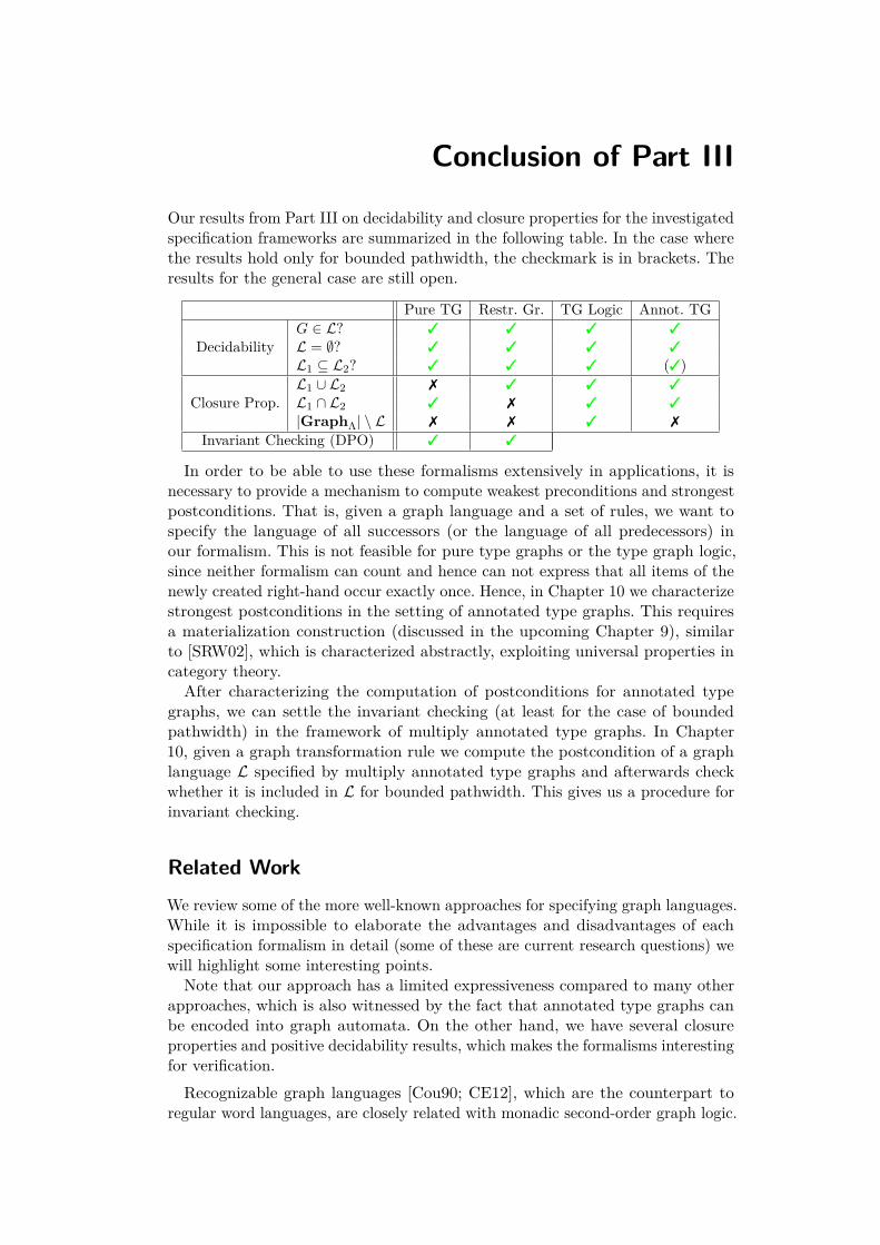
Conclusion of Part III

Our results from Part III on decidability and closure properties for the investigatedspecification frameworks are summarized in the following table. In the case wherethe results hold only for bounded pathwidth, the checkmark is in brackets. Theresults for the general case are still open.

Pure TG Restr. Gr. TG Logic Annot. TGG ∈ L? 3 3 3 3

Decidability L = ∅? 3 3 3 3

L1 ⊆ L2? 3 3 3 (3)L1 ∪ L2 7 3 3 3

Closure Prop. L1 ∩ L2 3 7 3 3

|GraphΛ| \ L 7 7 3 7

Invariant Checking (DPO) 3 3

In order to be able to use these formalisms extensively in applications, it isnecessary to provide a mechanism to compute weakest preconditions and strongestpostconditions. That is, given a graph language and a set of rules, we want tospecify the language of all successors (or the language of all predecessors) inour formalism. This is not feasible for pure type graphs or the type graph logic,since neither formalism can count and hence can not express that all items of thenewly created right-hand occur exactly once. Hence, in Chapter 10 we characterizestrongest postconditions in the setting of annotated type graphs. This requiresa materialization construction (discussed in the upcoming Chapter 9), similarto [SRW02], which is characterized abstractly, exploiting universal properties incategory theory.After characterizing the computation of postconditions for annotated type

graphs, we can settle the invariant checking (at least for the case of boundedpathwidth) in the framework of multiply annotated type graphs. In Chapter10, given a graph transformation rule we compute the postcondition of a graphlanguage L specified by multiply annotated type graphs and afterwards checkwhether it is included in L for bounded pathwidth. This gives us a procedure forinvariant checking.

Related WorkWe review some of the more well-known approaches for specifying graph languages.While it is impossible to elaborate the advantages and disadvantages of eachspecification formalism in detail (some of these are current research questions) wewill highlight some interesting points.

Note that our approach has a limited expressiveness compared to many otherapproaches, which is also witnessed by the fact that annotated type graphs canbe encoded into graph automata. On the other hand, we have several closureproperties and positive decidability results, which makes the formalisms interestingfor verification.Recognizable graph languages [Cou90; CE12], which are the counterpart to

regular word languages, are closely related with monadic second-order graph logic.

If one restricts recognizable graph languages to bounded treewidth (or pathwidthas we did), one obtains satisfactory decidability properties. On the other hand, thesize of the resulting graph automata is often quite intimidating [BB+12; Blu14]and hence they are difficult to work with in practical applications. The use ofnested application conditions [HP05], equivalent to first-order logic [Ren04b],has a long tradition in graph rewriting and they can be used to compute pre-and postconditions for rules [Pen09]. However, satisfiability and implication areundecidable for first-order logic.A notion of grammars corresponding to context-free (word) grammars are

hyperedge replacement grammars [Hab92]. Many aspects of the theory of context-free languages can be transferred to the graph setting.

In heap analysis the representation of pointer structures to be analyzed requiresmethods to specify sets of graphs. Hence both the TVLA approach by Sagiv,Reps and Wilhelm [SRW02], as well as separation logic [OHe07; DOY06] provideformalisms for characterizing graph languages, both based on logic. In [SRW02]heaps are represented by graphs, annotated with predicates from a three-valuedlogics (with truth values yes, no and maybe).A further interesting approach are forest automata [AH+13] that have many

interesting properties, but are somewhat complex to handle.In [RR+09] the authors study an approach called Diagram Predicate Framework

(DPF), in which type graphs have annotations based on generalized sketches. Thisformalism is intended for modelling languages based on Meta Object Facility(MOF) and allows more complex annotations than our framework.

Open QuestionsOne open question that remains is whether language inclusion for annotatedtype graphs is decidable if we do not restrict to bounded pathwidth. Additionally,invariant checking for the type graph logic is still open. As discussed in Section 8.3.1,our edge annotations are global, as opposed to the local multiplicities that finduse in UML. Local annotations only partially fit into our framework as we willsee in Chapter 10, but they are of course quite relevant. Hence, to study thepossibility to fully integrate such multiplicities and investigate the correspondingdecidability and closure properties is another problem left open.

Part IV.

Abstract Object Rewriting

Motivation of Part IV

Abstract interpretation [Cou96] is a fundamental static analysis technique thatapplies not only to conventional programs but also to general infinite-state systems.Shape analysis [SRW02], a specific instance of abstract interpretation, pioneeredan approach for analyzing pointer structures that keeps track of information aboutthe “heap topology”, e.g., out-degrees or existence of certain paths. One centralidea of shape analysis is materialization, which arises as companion operation tosummarizing distinct objects that share relevant properties. Materialization, alsoknown as partial concretization, is also fundamental in verification approachesbased on separation logic [CR08; CD+11; LRC15], where it is also known as rear-rangement [OHe12], a special case of frame inference. Shape analysis—construedin a wide sense—has been adapted to graph transformation [Roz97]. Motivated byearlier work of shape analysis for graph transformation [SWW11; BW07; Bac15;BR15a; RZ10; Ren04a], we want to put the materialization operation on a newfooting, widening the scope of shape analysis.A natural abstraction mechanism for transition systems with graphs as states

“summarizes” all graphs over a specific shape graph. Thus a single graph is usedas abstraction for all graphs that can be mapped homomorphically into it, similarto the concept of graph languages specified via type graphs (see Chapter 4).Further annotations on shape graphs, such as cardinalities of preimages of itsnodes and general first-order formulas, enable fine-tuning of the granularity ofabstractions. While these natural abstraction principles have been successfullyapplied in previous work [SWW11; BW07; Bac15; BR15a; RZ10; Ren04a], theircompanion materialization constructions are notoriously difficult to develop, hardto understand, and are redrawn from scratch for every single setting. Thus, weset out to explain materializations based on mathematical principles, namelyuniversal properties (in the sense of category theory). In particular, we will usepartial map classifiers in the topos of graphs (and its slice categories) which coverthe purely structural aspects of materializations; this is related to final pullbackcomplements [DT87], a fundamental construction of graph rewriting [Löw10;CH+06]. Annotations of shape graphs are treated orthogonally via op-fibrations.

Our main goal in Part IV is to define a rewriting formalism for graph abstractionsthat lifts double-pushout rule-based rewriting from single graphs to multiplyannotated type graphs (introduced in Chapter 8). In this context the type graphsspecifying the language will be referred to as abstract graphs. Abstract graphscannot be rewritten in the same way as ordinary graphs, since an occurrenceof the left-hand side might represent additional structure apart from the match,which cannot simply be deleted. Hence it is necessary to materialize a copy ofthe left-hand side. It is, in slightly different forms, present in all the approachescited above. To achieve the goal of defining a general rewriting framework, wedo not restrict ourselves to the category GraphΛ, but will introduce both, thematerialization construction and the abstract rewriting step, to work for (abstract)objects in an arbitrary topos C.

Outline:First, in Section 9.1, we introduce topoi and additional preliminaries in the

form of categorical constructions such as partial map classifiers, final pullbackcomplements and slice categories. Furthermore, in Section 9.2, we generalise ourconcept of type graph languages to languages of abstract objects in an arbitrarycategory. We define a materialization construction categorically in Section 9.3.1,that enables us to concretize an instance of a left-hand side of a production ina given abstract object. This construction is refined in Section 9.3.2 where werestrict to materializations that satisfy the gluing condition and can thus berewritten via the production. In Section 9.3.3 we present the main result aboutmaterializations showing that we can fully characterize the co-matches obtainedby rewriting. Afterwards, in Section 10.1 we extend abstract rewriting to abstractobjects enriched with the annotations from Chapter 8. In Section 10.2 we defineproperties for annotations which need to be satisfied in order to achieve soundnessand completeness of our abstract rewriting steps. Finally, in Section 10.3 weshow that abstract rewriting with annotations is sound and, with additionalassumptions regarding the properties, complete. We furthermore derive strongestpost-conditions for the case of graph rewriting with annotations. All proofs canbe found in Appendix A.5 and A.6.

“The inventor...looks upon the world and is not con-tented with things as they are. He wants to improvewhatever he sees, he wants to benefit the world; he ishaunted by an idea. The spirit of invention possesseshim, seeking materialization.”

Alexander Graham Bell (1847-1922)

9Materialization Category

In this chapter, we characterize a materialization operation for so-called abstractobjects in a topos in terms of partial map classifiers, which gives us a sound andcomplete description of all occurrences of right-hand sides of rules obtained byrewriting an abstract object. The materialization yields an object which specifiesa language consisting of all objects with a concrete instance of a left-hand sidefrom a production.

9.1. Additional Preliminaries - More Categorical ConceptsSince this chapter presupposes familiarity with the topos structure of graphsand several additional concepts from category theory (in particular elementarytopoi, subobject and partial map classifiers, final pullback complements and slicecategories) we start with some definitions and results related to elementary topoi.

9.1.1. Topoi, Subobject Classifiers and Partial Map ClassifiersFirst, we define the categorical concept of subobject classifiers. Intuitively, asubobject classifier is a morphism which maps the subobjects of an object X totruth values, i.e. assigning “true“ to the elements of the subobject to be classifiedand “false“ to all other elements of X. Hence, a subobject classifier in a categoryC maps objects into a so-called truth value object. The structure of a truth valueobject depends on the category where the subobject classifier is defined.

Definition 9.1 (Subobject classifier). Let C be a category where 1 is theterminal object and for each object X ∈ C let !X : X → 1be the unique arrow from X into the terminal object. Amono true : 1 Ω is a subobject classifier if for every monoi : X Y in C there exists a unique arrow χi : Y → Ω suchthat the diagram to the right is a pullback. In this case objectΩ is called the truth value object.

X //i //

!X

Y

χi

1 // true// Ω

(PB)

Example 9.2. In Set the subobject classifier true : 1 Ω is simply the em-bedding of 1 into the two-element set Ω = 0, 1. A subset X ⊆ Y can becharacterized via its characteristic function χX : Y → 0, 1.

9. Materialization Category

Example 9.3. In the category GraphΛ, where the objects are labelled graphsover the label alphabet Λ, the subobject classifiertrue is shown to the right where every Λ-labellededge represents several edges, one for each λ ∈ Λ.The subobject classifier true from the terminal

true : Λ Λ

Λ ΛΛ

object 1 to Ω allows us to single out a subgraph X of a graph Y , by mapping Y toΩ in such a way that all elements of X are mapped to the image of true.

The category of graphs GraphΛ is an elementary topos, which is an extremelyrich categorical structure. The notion of elementary topoi [Joh02; Law70] is usedin logic and it abstracts from the structure of the category of sets.

Definition 9.4 (Elementary topos). An elementary topos is a category whichhas finite limits, is cartesian closed and has a subobject classifier.

We will often omit the qualifier “elementary” and simply talk about topoi.In addition we will use the notion of natural transformations, which provides a

way of transforming a functor into another functor while respecting the internalstructure of the categories involved. Therefore, similar to functors being theabstract notion of morphisms between categories, natural transformations are theabstract notion of morphisms between functors.

Definition 9.5 (Natural transformation). Let C,D be two categories andlet F and G be functors from C to D. A natural transformation η : F .→ G isa family of arrows from F to G that assigns toevery C-object X a D-arrow ηX : F(X) → G(X)such that for any C-arrow f : X → Y the diagramto the right commutes in D. The morphism ηX isalso called component of η on X.

F(X) ηX //

F(f)

G(X)

G(f)

F(Y ) ηY // G(Y )

Every elementary topos has so-called partial map classifiers [CL03]. Informally,a partial map classifier for a partial map (m, f) : X Y works similar to asubobject classifier, with the difference, that neither the truth value object nor thedomain of the classifier morphism are fixed for the category. Instead, both need tobe constructed from the codomain object Y of the partial map, by constructingan object F(Y ) via a functor F and describing the morphism between Y andF(Y ) via the monic component ηY : Y F(Y ) of a natural transformation η.

Definition 9.6 (Partial map classifier). Let C be a category with pullbacks.A partial map (m, f) : X Y in C is a span X m

Zf→ Y where m : Z X

is a mono. A partial map classifier (F , η) is a functorF : C → C together with a natural transformationη : IdC

.→ F such that for each object Y of C with thecomponent ηY : Y F(Y ) the following holds: foreach partial map (m, f) : X Y there exists a unique

Z //m //

f

X

ϕ(m,f)

Y //ηY // F(Y )

(PB)

arrow ϕ(m, f) : X → F(Y ) such that the diagram to the right is a pullback.

108

9.1. Additional Preliminaries - More Categorical Concepts

Example 9.7. In Set the functor F enriches each set Y with an additionalelement ?, i.e., F(Y ) = Y + ?. Then a partial map p : X Y corresponds toa total map p′ : X → F(Y ) such p′(x) = p(x) if p(x) is defined and p′(x) = ?otherwise.Example 9.8. We now consider a more involved example in the category GraphΛ.Let the partial map (m, f) : G H (depicted below left) and a corresponding spanG

m P

f→ H (depicted below on the right) be given. We use a single edge label,which is omitted. All graph morphisms are indicated by black and white nodes andthe thickness of the edges.

(m, f): /m f

G P → H

The partial map classifier object F(H) alongside the component of the naturaltransformation ηH : H F(H) is depicted below right. Intuitively, the functor Fenriches the codomain H of the partial map(m, f) : G H by an additional structure whichcan be interpreted as the “false“ classification ofa subobject classifier. The natural transformationcomponent ηH maps the graph H to the “true“ partof F(H). As a result the resulting morphism ϕ(m, f)of the pullback diagram classifies every element inG which is defined in the partial map to be “true“and “false“ otherwise.

m

fϕ(m, f)

ηH

(PB)

9.1.2. Slice Categories and Final Pullback ComplementsThe objects in the materialization category that we will introduce in Chapter 9.3,are materializations of the left-hand side of a production over a fixed abstractobject A. We can use slice categories in connection with subobject classifiers tospecify this behaviour. The slice category C ↓ A, of a category C over an objectA, has morphisms with codomain A as objects and commutative triangles asmorphisms.

Definition 9.9 (Slice category). The slice category C ↓ A of a category Cover an object A ∈ C has the arrows f ∈ C suchthat cod(f) = A as objects. An arrow g : f → f ′ inC ↓ A, with f : X → A and f ′ : Y → A, is an arrowg : X → Y ∈ C such that the diagram to the rightcommutes.

Xg

//

f

Y

f ′

A

Please note that the terminal object of a slice category C ↓ A is the identityarrow idA : A A. The existence of a subobject classifier in a slice category overa topos directly follows from the following theorem [MM94].

Theorem 9.10 (Slice category over a topos [MM94]). For any object A in atopos C, the slice category C ↓ A is also a topos.

The subobject classifier in the slice category can be constructed as follows.

109

9. Materialization Category

Fact 9.11 (Subobject classifier in slice category [MM94]). Let C be a toposwith subobject classifier true : 1 Ω and truthvalue object Ω. For any object A ∈ C let A × Ωbe the product with projections π1 : A × Ω → Aand π2 : A × Ω → Ω. Then a subobject classifiertrueA of the slice category C ↓ A is the uniquemono trueA : A A × Ω such that the diagramto the right commutes.

Axx

idA

true !

trueA

A× Ω

π1

π2##

A Ω

Example 9.12. In order to provide an example for a subobject classifier in a slicecategory, we consider again the category GraphΛ, with a single edge label whichis omitted. Let A = be the base graph for the slice category GraphΛ ↓ A ofgraph morphisms into A. The subobject classifier trueA : A A×Ω for this slicecategory is the following graph morphism:

trueA:

Given arrows α,m as in the diagram below, we can construct the most generalpullback, called final pullback complement [DT87; CH+06].

Definition 9.13 (Final pullback complement). A pair of arrows I γ→ Fβ→ G

is a final pullback complement (FPBC) of another pair I α→ L m→ G if

• they form a pullback square

• for each pullback G m← L α′← I ′γ′→ F ′

β′→ G andarrow f : I ′ → I such that α f = α′, thereexists a unique arrow f ′ : F ′ → F such thatβ f ′ = β′ and γ f = f ′ γ′ both hold (seethe diagram to the right).

L

m

Iαoo

γ

I ′

α′

ww

foo

γ′

G Fβoo

(FPBC)

F ′

β′

gg

f ′oo

Example 9.14. Consider the following pair of graph morphisms I α L

m G in

the category GraphΛ:

α m

I L G

The final pullback complement I γ→ Fβ→ G is de-

picted in the diagram to the right. Please note thatfor the pair of graph morphisms I α

Lm G there

does not exist a pushout complement due to the dan-gling edge condition. However, for the final pullbackcomplement construction, all edges attached to theleft black node in G are removed.

α

m γ

β

(FPBC)

Final pullback complements and subobject classifiers are closely related topartial map classifiers (see Definition 9.6 and [DT87, Corollary 4.6]): a category

110

9.2. Object Languages

has FPBCs (over monos) and a subobject classifier if and only if it has a partialmap classifier. These exist in all elementary topoi.

Proposition 9.15 (Final pullback complements, subobject and partial mapclassifiers). Let C be a category with finite limits. Then the following areequivalent:

(1) C has a subobject classifier true : 1 Ω and final pullback complementsfor each pair of arrows I α→ L

m G where m is a mono;

(2) C has a partial map classifier (F : C→ C, η : IdC.→ F).

In the next section, we will generalize the concepts of type graph languages tolanguages of arbitrary objects in a category C.

9.2. Object LanguagesThe main theme of Part IV is “simultaneous” rewriting of entire sets of objectsof a category by means of rewriting a single abstract object that represents acollection of structures—the language of the abstract object. The simplest exampleof an abstract structure is a plain object of a category to which we associate thelanguage of objects that can be mapped to it.

Definition 9.16 (Language of an object). Let A be an object of a category C.Given another object X, we write X 99K A whenever there exists an arrowfrom X to A. We define the language1of A, denoted by L(A), as the setL(A) = X ∈ C | X 99K A.

Whenever X ∈ L(A) holds we will say that X is abstracted by A, and A is calledthe abstract object. Type graphs are an instance of abstract objects alongsidetheir corresponding language (cf. Chapter 4). Therefore, we will sometimes referto type graphs as abstract graphs. We will also need to characterize a class of(co-)matches which are represented by a given (mono) (co-)match.

Definition 9.17 (Language of a mono). Let ϕ : L A be a mono in C.The language of ϕ is the set of monos m with domainL such that ϕ factors through m and the square onthe right is a pullback:

L(ϕ) = m : L X | X 99K A,such that the square to the above right is a pullback.

L

idL

// m // X

∃ψ

L // ϕ// A

(PB)

Intuitively, for any arrow (L m X) ∈ L(ϕ) we have X ∈ L(A) and X has a

distinguished subobject L which corresponds precisely to the subobject L A.In fact ψ restricts and co-restricts to an isomorphism between the images of L in

1Here we assume that C is essentially small, so that a language can be seen as a set instead ofa class of objects.

111

9. Materialization Category

X and A. Intuitively, for graphs, no nodes or edges in X outside of L are mappedby ψ into the image of L in A.

9.3. MaterializationGiven a production p : L I R, an abstract object A and an arrow fromL to A (ϕ : L → A), we want to rewrite the so-called materialization of ϕ inorder to characterize all successors of objects in L(A), obtained by rewriting via pat a match compatible with ϕ. In a sense, we want to lift DPO rewriting tothe level of abstract objects. For this purpose, we will now categorically definea materialization construction, that enables us to concretize an instance of aleft-hand side L of a production p in a given abstract object A. Afterwards, wewill refine the construction in a way such that we restrict to materializations thatsatisfy the gluing condition and can thus be rewritten via p. Last, we presentthe main result of this chapter, which allows us to fully characterize the co-matches obtained by rewriting. Please note that in the following we only considerproductions where both morphisms are monos.

9.3.1. Materialization Category and Existence of MaterializationFrom now on we assume C to be an elementary topos. Let A ∈ C be an abstractobject specifying a language of objects L(A) and let L be the left-hand side of aproduction with L 99K A. We want to find a way to materialize objects with aconcrete image of L from A. To this end we consider the following category.

Definition 9.18 (Materialization). Let ϕ : L→ A be an arrow in C.The materialization category for ϕ, denoted Matϕ, has asobjects all factorizations L X → A of ϕ whose

first factor L X is a mono, and asarrows from a factorization L X → A to another

one L Y → A, all arrows f : X → Y in Csuch that the diagram to the right comprisesa commutative triangle and a pullback square.

L

ϕ

idL

// // X

f

L // //

ϕ

77Y

(PB)

// A

If Matϕ has a terminal object it is denoted by L 〈ϕ〉 → A and is calledthe materialization of ϕ.

Sometimes we will also call 〈ϕ〉 the materialization of ϕ, omitting the arrows.Since we are working in a topos by assumption, the slice category over A provides

us with a convenient setting to construct materializations. Note in particularthat in the diagram in Definition 9.18 above, the span X L L is a partialmap from X to L in the slice category over A. Hence the materialization 〈ϕ〉corresponds to the partial map classifier for L in this slice category.

Proposition 9.19 (Existence of materialization). Let ϕ : L→ A be an arrowin C, and let ηϕ : ϕ→ F(ϕ), with F(ϕ) : A→ A, be the partial map classifierof ϕ in the slice category C↓A (which also is a topos)2. Then L ηϕ→ A

F(ϕ)→ Ais the materialization of ϕ, hence 〈ϕ〉 = A.

112

9.3. Materialization

As a direct consequence of Proposition 9.15 and Proposition 9.19 (and the factthat final pullback complements in the slice category correspond to those in thebase category [Löw10]), the terminal object of the materialization category canbe constructed for each arrow of a topos by taking final pullback complements.

Corollary 9.20 (Construction of the materialization). Let ϕ : L→ A be anarrow of C and let trueA : A A×Ω be the subobject classifier in the slicecategory C ↓ A mapping from idA : A→ A to theprojection π1 : A × Ω → A (see also Fact 9.11).Then the terminal object L

ηϕ 〈ϕ〉 ψ→ A in the

materialization category consists of the arrowsηϕ, ψ = π1 χηϕ , where L

ηϕ 〈ϕ〉

χηϕ→ A× Ω is thefinal pullback complement of L ϕ→ A

trueA A× Ω.

L

ϕ

//ηϕ// 〈ϕ〉

χηϕ

ψ

""

A //trueA// A× Ω π1

//

(FPBC)

A

Example 9.21. We construct the materialization Lηϕ 〈ϕ〉 ψ→ A for the morphism

ϕ : L→ A of graphs with a single (omitted)egde label:

ϕ:

In particular, the materialization is obtainedas a final pullback complement as depictedto the right (compare with the correspondingdiagram in Corollary 9.20). Note that edges

ηϕ

ϕ χηϕ

trueA

ψ

π1

(FPBC)

which are not in the image of ηϕ resp. trueA are dashed.

This construction corresponds to the usual intuition behind materialization: theleft-hand side and the edges that are attached to it are “pulled out” of the givenabstract graph. The concrete construction in the category GraphΛ is spelled outin Chapter 11, so that we can implement the construction in a tool.

We can summarize the result of our constructions in the following proposition,which states that the materialization characterizes all objects X, abstracted overA, which contain a (mono) occurrence of the left-hand side compatible with ϕ.

Proposition 9.22 (Language of the materialization). Let ϕ : L→ A be anarrow in C and let L

ηϕ 〈ϕ〉 → A be the corresponding materialization. Then

L(Lηϕ 〈ϕ〉) = L mL

X | ∃ψ : (X → A). (ϕ = ψ mL).

9.3.2. Characterizing the Language of Rewritable ObjectsA match obtained through the materialization of the left-hand side of a productionfrom a given object may not allow a DPO rewriting step because of the gluingcondition. However, there may exist objects abstracted by the materialization forwhich there exist successors by the application of the production. We illustratethis problem with an example.

2[Fre72, Theorem 2.31].

113

9. Materialization Category

Example 9.23. Consider the materialization L 〈ϕ〉 → A from Example 9.21and the production p : L I Rshown in the diagram to the right. Itis easy to see that the pushout com-plement of morphisms I L 〈ϕ〉does not exist.Nevertheless there exist factorizationsL X → A abstracted by 〈ϕ〉 thatcould be rewritten by p, for instancethe factorization L L→ A.

?

L〈ϕ〉

L I R

Therefore, we want to find the largest subobject (subsequently called 〈〈ϕ,ϕL〉〉)of 〈ϕ〉, abstracting all objects X thatcan be rewritten via a productionL I R and a match ϕL : L→ X.The logical relation between the lan-guages is depicted in the Venn digramshown to the right. Consequently, weconsider the following subcategory ofthe materialization category. L(A)

〈ϕ〉 - Abstraction

〈〈ϕ, ϕL〉〉 - Abstraction

Definition 9.24 (Materialization subcategory of rewritable objects). Letϕ : L → A be an arrow of C and let ϕL : I L be a mono (correspondingto the left leg of a production). The materialization subcategory of rewritableobjects for ϕ and ϕL, denoted MatϕLϕ , is the full subcategory of Matϕ con-taining as objects all factorizations L m

X → A of ϕ, where m is a monoand I ϕL

Lm X has a pushout complement.

Its terminal element, if it exists, is denoted by L nL 〈〈ϕ,ϕL〉〉 → A and is

called the rewritable materialization.

We next show that the subcategory MatϕLϕ has a terminal object.

Proposition 9.25 (Construction of the rewritable materialization). Letϕ : L → A be an arrow and let ϕL : I L be a mono of C. Then therewritable materialization of ϕ w.r.t. ϕL exists and can be constructed as thefollowing factorization L nL

〈〈ϕ,ϕL〉〉ψα−→ A of ϕ. In the diagram shown below

to the left, F is obtained as the final pullback complement of I ϕL L 〈ϕ〉,

where L 〈ϕ〉 ψ→ A is the materialization of ϕ (Definition 9.18). Next thediagram shown below to the right L nL

〈〈ϕ,ϕL〉〉β F is the pushout of the

span L ϕL I F and α is the resulting mediating arrow.

Lϕ

~~

I

ooϕLoo

A 〈ϕ〉ψoo F

(FPBC)

oooo

(9.1) Lϕ

~~

L

nL

ooidLoo I

ooϕLoo

A 〈ϕ〉ψoo 〈〈ϕ,ϕL〉〉ooαoo Foo

βoo uuii

(PO)

(9.2)

114

9.3. Materialization

Example 9.26. We come back to the running example (see Example 9.23) and,as in Proposition 9.25, we determine the final pullback complement I F 〈ϕ〉of I ϕL L 〈ϕ〉 (see diagram below left) and obtain 〈〈ϕ,ϕL〉〉 by taking the pushout

over L I F (see diagram below right).

L〈ϕ〉

L I

(FPBC)

F

I

F

L I

(PO)

〈〈ϕ, ϕL〉〉

It remains to be shown that L 〈〈ϕ,ϕL〉〉 → A represents every factorizationwhich can be rewritten. As before we obtain a characterization of the rewritableobjects, including the match of the left-hand side L into the rewritable material-ization 〈〈ϕ,ϕL〉〉, as the language of an arrow.

Proposition 9.27 (Language of the rewritable materialization). Assumethere is a production p : L ϕL

IϕR R and let L nL

〈〈ϕ,ϕL〉〉 be the match forthe rewritable materialization for ϕ and ϕL. Then we have

L(L nL 〈〈ϕ,ϕL〉〉) = L mL

X | ∃ψ : (X → A). (ϕ = ψ mL ∧Xp,mL=⇒)

where X p,mL=⇒ denotes that the object X can be rewritten.

9.3.3. Rewriting MaterializationsIn the next step we will now rewrite the rewritable materialization 〈〈ϕ,ϕL〉〉 withthe match L

nL 〈〈ϕ,ϕL〉〉, resulting in a co-match R B. In particular, we

will show that this co-match represents all co-matches that can be obtained byrewriting an object X of L(A) at a match compatible with ϕ.

Proposition 9.28 (Rewriting abstract matches). Let a match nL : L Aand a production p : L I R be given. Assume that A is rewritten alongthe match nL, i.e., (L nL

A) p⇒ (R nR B). Then

L(R nR B) = R mR

Y | ∃(L mL X) ∈ L(L nL

A) :((L mL X) p⇒ (R mR

Y ))

Example 9.29. We can rewrite the materialization L 〈〈ϕ,ϕL〉〉 → A as follows:

L〈〈ϕ

,ϕL 〉〉

C B

(PO) (PO)

115

9. Materialization Category

If we combine Prop. 9.27 and Prop. 9.28, we immediately obtain the followingcorollary that characterizes the co-matches obtained from rewriting a matchcompatible with ϕ : L→ A.

Corollary 9.30 (Co-match language of the rewritable materialization). Letϕ : L→ A and a production p : L ϕL

IϕR R be given. Assume that 〈〈ϕ,ϕL〉〉

is obtained as the rewritable materialization of ϕ and ϕL with the matchL

nL 〈〈ϕ,ϕL〉〉 (see Proposition 9.25) and let (L nL

〈〈ϕ,ϕL〉〉) p⇒ (R nR B).

ThenL(R nR

B) = R mR Y |∃(L mL

X), (X ψ→ A) :(ϕ = ψ mL ∧ (L mL

X) p⇒ (R mR Y )

)

This result does not yet enable us to construct post-conditions for languagesof objects. The set of co-matches can be fully characterized as the language ofa mono, which can only be achieved by fixing the right-hand side R and thusensuring that exactly one occurrence of R is represented. However, as soon as weforget about the co-match, this effect is gone and can only be retrieved by addingannotations, which we will do in the next chapter.

116

“The only kind of writing is rewriting.”Ernest Hemingway (1899-1961)

10Rewriting Annotated Objects

In this chapter we endow abstract objects with annotations, with the overall goalto be able to specify post-conditions for abstract rewriting steps. In particular,we will use ordered monoids enhanced with a subtraction operation to annotateobjects. Furthermore, we will instantiate the materialization construction from theprevious chapter in this framework to rewrite abstract objects with annotations.For this purpose, we specify how annotations can be computed within pushoutconstructions. We start by introducing the annotations for the abstract objects.

10.1. Additional Preliminaries - Annotated ObjectsWe will annotate each abstract object with pairs of annotations, denoting upperand lower bounds (see also Chapter 8). An object will belong to the correspondinglanguage only if it has a legal arrow to the abstract object satisfying such bounds.We enrich ordered monoids (introduced in Chapter 8.1) with a subtraction op-eration, which we will need to define annotations for pushout objects. Similarannotations have already been studied in [Kön00] in the context of type systems.

Definition 10.1 (Ordered monoid with subtraction). A tuple (M,+,−,≤),where (M,+,≤) is an ordered monoid and − is a binary operation onM, iscalled an ordered monoid with subtraction.We say that subtraction is well-behaved whenever for all a, b ∈ M it holdsthat a− a = 0 and (a− b) + b = a whenever b ≤ a.

For now subtraction is just any operation, without specific requirements. Laterwe will concentrate on specific subtraction operations and demand that they arewell-behaved. In the following we will consider only commutative monoids.

Definition 10.2 (Subtraction preserving maps). LetM,M′ be two orderedmonoids with subtraction. The category of ordered monoids with subtractionand monotone maps is called Mon−.We say that a map h : M→M′ preserves subtraction if h(a−b) = h(a)−h(b).

10. Rewriting Annotated Objects

We first have a look at some examples for ordered monoids with subtraction.We already introduced examples for ordered monoids in Chapter 8, which we nowenrich with a subtraction operation.

Example 10.3. Let n ∈ N and letMn = 0, 1, . . . , n, ∗ be the ordered monoidfrom Example 8.3. Then subtraction is truncated subtraction, i.e. x − y = 0 ifx ≤ y. Furthermore ∗ − x = ∗ for all x ∈ 0, 1, . . . , n. It is easy to see thatsubtraction is well-behaved.

Given a set S and an ordered monoid with subtractionM, it is easy to checkthat also MS is an ordered monoid with subtraction, where the elements arefunctions from S to M and the partial order, the monoidal operation and thesubtraction are taken pointwise.As another example we extend the path monoid to an ordered monoid with

subtraction.

Example 10.4. Given a graph G, let PG be the path monoid from Example 8.4and P0, P1 ∈ PG. Then subtraction simply returns the first parameter: P0−P1 = P0.

We will now formally define annotations for objects via a functor from a givencategory to Mon−.

Definition 10.5 (Annotations for objects). Given a category C and a functorA : C→Mon−, an annotation based on A for an object X ∈ C is an elementa ∈ A(X). We write Aϕ, instead of A(ϕ), for the action of functor A on aC-arrow ϕ. Similar to Definition 8.5, we assume that for each object X thereis a standard annotation based on A that we denote by sX , thus sX ∈ A(X).

It can be shown quite straightforwardly that the forgetful functor mapping anannotated object X[a], with a ∈ A(X), to X is an op-fibration (or co-fibration[Jac99]), arising via the Grothendieck construction.In Chapter 8 we already introduced two annotation functors for the category

GraphΛ based on the ordered monoidMn and the path monoid PG respectively,i.e. the multiplicity functor Bn (see Definition 8.6) and the path annotationfunctor T (see Definition 8.8). As another example we consider the followinglocal annotation functor Sn, based on the ordered monoidMn, which records theout-degree of a node and where the action of the functor is to take the supremuminstead of the sum.

Definition 10.6 (Node out-degree annotation). Given n ∈ N, we define thefunctor Sn : GraphΛ →Mon− as follows: For every graph G, Sn(G) =MVG

n .For every graph morphism ϕ : G→ H and a ∈ Sn(G), we have Snϕ(a) ∈MVH

n

with:Snϕ(a)(w) =

∨ϕ(v)=w

a(v), where v ∈ VG and w ∈ VH

For a graph G, its standard annotation sG ∈ Sn(G) is defined as the functionwhich maps every node of G to its out-degree (or ∗ if the out-degree is largerthan n).

118

10.2. Annotation Properties

Example 10.7. Let the following graphs G and H with node out-degree annota-tions a ∈ S3(G) be given. The out-degree of each node is indicated by the elementof M3 = 0, 1, 2, 3, ∗ shown in the brackets. Furthermore, let ϕ : G → H be agraph morphism indicated by the numbers above the nodes.

G =[0] [3] [0] [1] [0]

1 2 3 4 5B

BA B ϕ

−→ 1, 2, 4 3, 5BA = H

Let a′ = S3ϕ(a). We compute a′(w) for each node w ∈ VH by

taking the supremum of all a(v) ∈ S3(G) for which ϕ(v) = w.The annotation a′ is depicted on the right. [3] [0]

BA

10.2. Annotation PropertiesIn the following we will consider only annotations satisfying certain properties inorder to achieve soundness and completeness of our abstract rewriting steps.

Definition 10.8 (Properties of annotations). Let A : C → Mon− be anannotation functor, together with standard annotations. We say that the

• Homomorphism property holds if whenever ϕ is a mono, then Aϕ is amonoid homomorphism, preserving also subtraction.

• Adjunction property holds if whenever ϕ : A B is a mono, then– Aϕ : A(A) → A(B) has a right adjoint redϕ : A(B) → A(A), i.e.,

redϕ is monotone and satisfies a ≤ redϕ(Aϕ(a)) for a ∈ A(A) andAϕ(redϕ(b)) ≤ b for b ∈ A(B).1

– redϕ is a monoid homomorphism that preserves subtraction.– it holds that redϕ(sB) = sA, where sA, sB are standard annotations.

Furthermore, assuming that Aϕ has a right adjoint redϕ, we say that the

• Pushout property holds, whenever for each pushout asshown in the diagram to the right, with all arrows monoswhere η = ψ1 ϕ1 = ψ2 ϕ2, it holds that for everyd ∈ A(D):

d = Aψ1(redψ1(d)) + (Aψ2(redψ2(d))−Aη(redη(d))).2

A //ϕ2//

η

ϕ1

C

ψ2

B //ψ1// D

We say that the pushout property for standard annotations holds if wereplace d by sD, redψ1(d) by sB, redψ2(d) by sC and redη(d) by sA.

• Beck-Chevalley property holds if whenever the squareshown to the right is a pullback with ϕ1, ψ2 mono, thenit holds for every b ∈ A(B) that

Aϕ2(redϕ1(b)) = redψ2(Aψ1(b)).

Aϕ2//

ϕ1

C

ψ2

Bψ1// D

(PB)

1This amounts to saying that the forgetful functor is a bifibration when we restrict to monos,see [Jac99, Lem. 9.1.2].

2Note that the brackets are essential, for instance inM3 we have 2+(2−1) = 3 6= ∗ = (2+2)−1.

119

10. Rewriting Annotated Objects

Note that the multiplicity functor from Definition 8.6 satisfies all propertiesabove. In particular, for a given injective graph morphism ϕ : G H the rightadjoint redϕ : MVH∪EH

n →MVG∪EGn to Bnϕ is defined as follows: given an anno-

tation b ∈ MVH∪EHn , redϕ(b)(x) = b(ϕ(x)), i.e., redϕ simply provides a form of

reindexing (see also Lemma L.5 in Appendix A.4).The functors from Definition 8.8 and 10.6 satisfy both the homomorphism

property and the pushout property for standard annotations, but do not satisfyall the remaining requirements (see Lemma L.6, L.7 and L.8 in Appendix A.6).We will now introduce objects with two annotations, giving lower and upper

bounds, which we will call doubly annotated objects. Therefore, doubly annotatedobjects are a generalization of annotated type graphs (see Definition 8.11) wherethe set of annotations consist of only one pair of annotations. Alternatively wecould allow several pairs of annotations for objects, as in Chapter 8, yieldingmultiply annotated objects, however for the sake of simplicity we will only assumea single annotation.

Definition 10.9 (Doubly annotated object). Given a topos C and a functorA : C→Mon−, a doubly annotated object A[a1, a2] is an object A of C withtwo annotations a1, a2 ∈ A(A). An arrow ϕ : A[a1, a2]→ B[b1, b2], also calleda legal arrow, is a C-arrow ϕ : A→ B such that Aϕ(a1) ≥ b1 and Aϕ(a2) ≤ b2.

The language of a doubly annotated object A[a1, a2] (also called the languageof objects which are abstracted by A[a1, a2]) is defined as follows:

L(A[a1, a2]) = X ∈ C | there exists a legal arrow ϕ : X[sX , sX ]→ A[a1, a2]

Note that legal arrows are closed under composition (analogous to Lemma 8.13).Several examples of doubly annotated objects can be found in Section 8.3, wherewe considered an instance of the annotation functor in the category GraphΛ.

Another annotation property is the isomorphism property which – in contrast tothe properties mentioned earlier – is defined specifically for standard annotationsof doubly annotated objects.

Definition 10.10 (Isomorphism property). Let A : C → Mon− be anannotation functor together with standard annotations. Then the functor Asatisfies the isomorphism property if the following holds:

Whenever ϕ : X[sX , sX ]→ Y [sY , sY ] is legal, then ϕ is an isomorphism, i.e.L(Y [sY , sY ]) contains only Y itself (and objects isomorphic to Y ).

The multiplicity functor from Definition 8.6 satisfies the isomorphism property,however the path annotations (Definition 8.8) and the node out-degree annotations(Definition 10.6) violate this requirement: For instance, there exists a graphmorphism ϕ : G→ H mapping a discrete graph G which consists of two nodes intoa discrete graph H consisting of a single node. Clearly, ϕ : G[sG, sG]→ H[sH , sH ]is legal if we consider standard annotations for both functors, however ϕ is not anisomorphism.

120

10.3. Abstract Rewriting of Annotated Objects

10.3. Abstract Rewriting of Annotated ObjectsWe will now show how to actually rewrite annotated objects. The challenge isboth to find suitable annotations for the materialization and to “rewrite” theannotations.

10.3.1. Abstract Rewriting and SoundnessWe first describe how the annotated rewritable materialization is constructed andthen we investigate its properties.

Definition 10.11 (Construction of annotated rewritable materialization).Let p : L ϕL

IϕR R be a production and let A[a1, a2] be a doubly annotated

object. Furthermore let ϕ : L→ A be an arrow.We first construct the factorization L

nL 〈〈ϕ,ϕL〉〉

ψ→ A, obtaining therewritable materialization 〈〈ϕ,ϕL〉〉 from Definition 9.24. Next let M containall maximal1elements of the set

(a′1, a′2) ∈ A(〈〈ϕ,ϕL〉〉)2 | AnL(sL) ≤ a′2,a1 ≤ Aψ(a′1),Aψ(a′2) ≤ a2.

Then the doubly annotated objects 〈〈ϕ,ϕL〉〉[a′1, a′2] with (a′1, a′2) ∈M are theannotated rewritable materializations for A[a1, a2], ϕ and ϕL.

Note that in general there are several materializations, differing for the an-notations only, or possibly none. The definition of M ensures that the upperbound a′2 of the materialization covers the annotations arising from the left-handside. We can not use a corresponding condition for the lower bound, since thematerialization might contain additional structures, hence the arrow nL is onlysemi-legal. A more symmetric condition will be studied in Section 10.3.2.

Proposition 10.12 (Annotated rewritable materialization is terminal). Letp : L ϕL

IϕR R be a production and let L mL

X be the match of L in an objectX such that X p,mL=⇒ , i.e., X can be rewritten. Assume that X is abstracted byA[a1, a2], witnessed by ψ. Let ϕ = ψ mL and let L nL

〈〈ϕ,ϕL〉〉ψ′→ A be the

corresponding rewritable materialization. Then there exists an arrow ζA and apair of annotations (a′1, a′2) ∈M for 〈〈ϕ,ϕL〉〉 (as described in Definition 10.11)such that the diagram below commutes and the square is a pullback in theunderlying category. Furthermore the triangle consists of legal arrows. Thismeans in particular that ζA is legal.

L[sL, sL]

idL

//mL // X[sX , sX ]

ζA

ψ// A[a1, a2]

L[sL, sL] // nL// 〈〈ϕ,ϕL〉〉[a′1, a′2]

(PB)ψ′

77

1Maximal means maximality w.r.t. the interval order (a1, a2) v (a′1, a′2) ⇐⇒ a′1 ≤ a1, a2 ≤ a′2.

121

10. Rewriting Annotated Objects

Once we have performed the materialization, we will now show how to rewriteannotated objects. Note that we cannot simply take pushouts in the category ofannotated objects and legal arrows, since this would result in taking the supremumof annotations, when instead we need the sum (subtracting the annotation of theinterface I, analogous to the inclusion-exclusion principle).

Definition 10.13 (Abstract rewriting step ;). Let p : L ϕL I

ϕR R be a

production and let A[a1, a2] be an annotated abstract object. Furthermore letϕ : L→ A be a match of a left-hand side, let nL : L 〈〈ϕ,ϕL〉〉 be the matchobtained via materialization and let (a′1, a′2) ∈M (as in Definition 10.11).Then A[a1, a2] can be transformed to B[b1, b2] via p whenever there are

arrows such that the two squares below are pushouts in the base categoryand b1, b2 are defined as:

bi = AϕB (ci) + (AnR(sR)−AnRϕR(sI)) for i ∈ 1, 2

where c1, c2 are maximal annotations such that:

a′1 ≤ AϕA(c1) + (AnL(sL)−AnLϕL(sI))a′2 ≥ AϕA(c2) + (AnL(sL)−AnLϕL(sI))

L[sL, sL]

nL

I[sI , sI ]ooϕLoo //

ϕR //

nI

R[sR, sR]

nR

〈〈ϕ,ϕL〉〉[a′1, a′2] C[c1, c2]ooϕAoo //

ϕB // B[b1, b2]

In this case we write A[a1, a2] p,ϕ; B[b1, b2] and say that A[a1, a2] makes anabstract rewriting step to B[b1, b2].

We will now show soundness of abstract rewriting, i.e., whenever an object Xis abstracted by A[a1, a2] and X is rewritten to Y , then there exists an abstractrewriting step from A[a1, a2] to B[b1, b2] such that Y is abstracted by B[b1, b2].Assumption: In the following we will require that the homomorphism propertyas well as the pushout property for standard annotations hold (cf. Definition 10.8).

Proposition 10.14 (Soundness for ;). The relation ; is sound, i.e. ifX ∈ L(A[a1, a2]) (witnessed via a legal arrow ψ : X[sX , sX ]→ A[a1, a2]) andX

p,mL=⇒ Y , then there exists an abstract rewriting step A[a1, a2] p,ψmL; B[b1, b2]such that Y ∈ L(B[b1, b2]).

10.3.2. CompletenessThe conditions that we imposed so far are too weak to guarantee completeness,that is the fact that every object represented by B[b1, b2] can be obtained byrewriting an object represented by A[a1, a2]. This can be clearly seen by the factthat the requirements hold also for the singleton monoid and, as discussed before,the graph structure of B is insufficient to characterize the successor objects orgraphs.

122

10.3. Abstract Rewriting of Annotated Objects

Hence we will now strengthen our requirements in order to obtain completeness.Assumption: In addition to the assumptions of Section 10.3.1, we will needthat subtraction is well-behaved and that the adjunction property, the isomor-phism property, the pushout property and the Beck-Chevalley property hold (cf.Definition 10.8).The multiplicities from Definition 8.6 satisfy all these properties. We will nowmodify the abstract rewriting relation and allow only those abstract annotationsfor the materialization that reduce to the standard annotation of the left-hand side.

Definition 10.15 (Abstract rewriting step →). Given ϕ : L → A, assumethat B[b1, b2] is constructed from A[a1, a2] via the construction described inDefinition 10.11 and 10.13, with the modification that the set of annotationsfrom which the set of maximal annotations M of the materialization 〈〈ϕ,ϕL〉〉are taken, is replaced by:

(a′1, a′2) ∈ A(〈〈ϕ,ϕL〉〉)2 | rednL(a′i) = sL for i ∈ 1, 2,a1 ≤ Aψ(a′1),Aψ(a′2) ≤ a2.

In this case we write A[a1, a2] p,ϕ→ B[b1, b2].

Due to the adjunction property we have AnL(sL) = AnL(rednL(a′2)) ≤ a′2 andhence the set M of annotations of Definition 10.15 is a subset of the correspondingset of Definition 10.13. We give a small example of an abstract rewriting step.Example 10.16. Consider the diagram shown below which depicts an abstractrewriting step. Elements without annotation are annotated by [0, ∗] by default andthose with annotation [0, 0] are omitted. Furthermore elements in the image of thematch and co-match are annotated by the standard annotation [1, 1] to specify theconcrete occurrence of the left-hand and right-hand side.

[1, 1]C [1, 1]

[1, 1][1, 1]

[1, 1]

A [1, 1]

B [1, 1]

[1, 1]

D

DD

D

C [1, 1][1, 1]

D

DD

D

[1, 1][1, 1]

D

DD

DA [1, 1]

B [1, 1]

[1, ∗]C [1, 1]D

ϕL ϕR

ϕA ϕB

nL nI nR

ϕ

A← L I R

〈〈ϕ,ϕL〉〉 C B

First, the concrete instance of the left hand side L is materialized out of theabstract graph A (shown to the left), resulting in the rewritable materialization〈〈ϕ,ϕL〉〉 alongside the match nL. Please note that the materialization only consistsof one C-labelled loop since there is only a standard annotated C-labelled loopavailable in A and we omitted all additional edges which would have the annotation[0, 0]. The rewriting step then replaces the unique C-labelled loop by the concreteinstance of the right-hand side R of the rule, resulting in the annotated type graphB. The annotation of the context C gets carried over during the rewriting processsince all morphisms are monos.

123

10. Rewriting Annotated Objects

The variant of abstract rewriting introduced in Def. 10.15 can be proven to besound and complete, assuming the extra requirements stated above.

Proposition 10.17 (Soundness for →). The relation → is sound, i.e. ifX ∈ L(A[a1, a2]) (witnessed via a legal arrow ψ : X[sX , sX ]→ A[a1, a2]) andX

p,mL=⇒ Y , then there exists an abstract rewriting step A[a1, a2] p,ψmL→ B[b1, b2]such that Y ∈ L(B[b1, b2]).

Proposition 10.18 (Completeness for →). The relation → is complete, i.e. ifA[a1, a2] p,ϕ→ B[b1, b2] and Y ∈ L(B[b1, b2]), then there exists X ∈ L(A[a1, a2])(witnessed via a legal arrow ψ : X[sX , sX ] → A[a1, a2]) such that X p,mL=⇒ Yand ϕ = ψ mL.

Finally, we can show that annotated objects of this kind are expressive enoughto construct a strongest post-condition. For the construction we now allow severalannotations for objects, analogous to Definition 8.11, such that we can representthe strongest post-condition with a single (multiply) annotated object B[N ] whereN is a set of annotations. The structure of the object B is always the same sincethe structure is dependent on the arrow ϕ, but not on the annotation of theabstract object A.

Corollary 10.19 (Strongest post-condition). Let A[a1, a2] be an annotatedobject and let ϕ : L → A. We obtain (several) abstract rewriting stepsA[a1, a2] p,ϕ→ B[b1, b2], where we always obtain the same object B. Now letN = (b1, b2) | A[a1, a2] p,ϕ→ B[b1, b2]. Then the strongest post-condition isthe language of the multiply annotated object B[N ], i.e.

L(B[N ]) = Y | ∃(X ∈ L(A[a1, a2]),witnessed by ψ),(L mL X) : (ϕ = ψ mL ∧X

p,mL=⇒ Y )

We conclude with a worked example which shows that, thanks to the resultabove, multiply annotated type graphs can be used for verification methods suchas invariant checking.

Example 10.20. In the following, we give an example for the computation ofa postcondition. We specify an online-shop scenario using an annotated abstractgraph with the following edge label semantics:

C : The connection of a customer node to the online-shop.

M : The market relation describing which items are purchasable in the shop.

P : The possession relation describing which items are purchased by a customer.

$ : One $-coin of the currency used by customers to buy items in the shop.

Now, we would like to model the following situation: Exactly one of many customershas established a connection to an online-shop. At least one of the customers hasa $-coin to purchase items and the online-shops have an arbitrary number of items

124

10.3. Abstract Rewriting of Annotated Objects

available. A customer can be in possession of an arbitrary number of items. Graphsmodelling this specification can for instance be part of the language described bythe following annotated abstract graph A[a1, a2]:

A[a1, a2] = [1, ∗][1, 1]

[0, ∗]C [1, 1] M [0, ∗]

P [0, ∗]

$ [1, ∗]

The following graph transformation production ρ : L I R specifies, that acustomer, who is in possession of at least one $-coin and who is connected to theonline shop, can purchase one of the items in stock in exchange for the currency.The production morphisms are indicated by the node positions:

ρ = C M

$

C C

P

Please note, that there exists only one possibility to map the left-hand side graphL of the production ρ into the abstract graph A. We now depict the rewritableabstract graph 〈〈ϕ,ϕL〉〉[a′1, a′2] consisting of the abstract graph A (upper part), theleft-hand side graph L (lower part) and the additional edges introduced in theconstruction of Prop. 9.25 alongside a maximal pair of annotations (a′1, a′2) ∈Mconforming to Definition 10.15:

〈〈ϕ,ϕL〉〉[a′1, a′2] =

[0, ∗][0, 0]

[0, ∗]C [0, 0] M [0, ∗]

P [0, ∗]

$ [0, ∗]

[1, 1][1, 1]

[1, 1]C [1, 1] M [1, 1]

$ [1, 1]

C [0, 0] M [0, ∗]P [0, ∗]

$ [0, ∗]

$ [0, ∗] $ [0, ∗]

C [0, 0]

C [0, 0]

M [0, ∗]

M [0, ∗]

P [0, ∗]P [0, ∗]

All elements in 〈〈ϕ,ϕL〉〉[a′1, a′2] annotated with [0, 0] cannot be the target of a legalmorphism and therefore can be removed to simplify the graphical representation. Ifa node annotated with [0, 0] is removed this way, all incident edges are removed aswell independently of their annotation. We apply the production ρ to the simplifiedrewritable abstract graph 〈〈ϕ,ϕL〉〉[a′1, a′2] (shown below to the left) resulting in theabstract graph B[b1, b2] (shown below, to the right):

125

10. Rewriting Annotated Objects

[0, ∗] [0, ∗]P [0, ∗]

$ [0, ∗]

[1, 1][1, 1]

[1, 1]C [1, 1] M [1, 1]

$ [1, 1]

M [0, ∗]P [0, ∗]$ [0, ∗]

$ [0, ∗] $ [0, ∗]M [0, ∗]

P [0, ∗] P [0, ∗]

〈〈ϕ, ϕL〉〉[a′1, a′2]

⇒ρ

[0, ∗] [0, ∗]P [0, ∗]

$ [0, ∗]

[1, 1][1, 1]

[1, 1]C [1, 1]

P [1, 1]

M [0, ∗]P [0, ∗]$ [0, ∗]

$ [0, ∗] $ [0, ∗]M [0, ∗]

P [0, ∗] P [0, ∗]

B[b1, b2]

We can use the postcondition for an invariant check of the graph languageL(A[a1, a2]) with respect to the production ρ. In fact, the annotated abstract graphB[b1, b2] specifies (a part of) the strongest postcondition andtherefore the graph G ∈ L(B[b1, b2]), shown to the right, isa witness for the fact that the graph language L(A[a1, a2]) isnot closed under application of ρ since G /∈ L(A[a1, a2]) dueto a missing $-coin edge in G, which is required by A[a1, a2].

C

P

Please note that the simplification of the visual representation does not influencethe computation of the strongest postcondition, however, it might hide informationwhich is necessary to argue that the computed rewritable materialization iscontained in the initial graph language. We illustrate this effect in a small example.

Example 10.21. Let the graph transformation rule ρ = L ← I → R and theannotated type graph T [a1, a2] shown below be given. Let ϕ : L → T match thesingle node of L with the left node of T [a1, a2]:

ρ = T [a1, a2] =[0, 1] [0, 1]

A [1, 1]

We construct the rewritable materialization〈〈ϕ,ϕL〉〉[a′1, a′2], shown to the right, with amaximal pair of annotations (a′1, a′2) ∈ Mconforming to Definition 10.15. For thenon-simplified version of the rewritablematerialization 〈〈ϕ,ϕL〉〉[a′1, a′2] there clearly

〈〈ϕ,ϕL〉〉[a′1, a′2] =[0, 0]

[0, 1][1, 1]

A [1, 1]

A [0, 0]

exists a non-monic legal morphism into the annotated type graph T [a1, a2]. However,simplifying the visual representation results in the annotated type graph shownbelow left from which we can not infer the existence of a legal morphism anymore,since the lower bound of the A-labeled edge in T [a1, a2] can not be satisfied:

[1, 1] [0, 1]6−→

[0, 1] [0, 1]A [1, 1]

126

Conclusion of Part IV

We have described a rewriting framework for abstract graphs that also applies toobjects in any topos, based on existing work for graphs [SWW11; BW07; Bac15;BR15a; RZ10; Ren04a]. In particular, we have given a blueprint for materializationin terms of the universal property of partial map classifiers. This is a first theoreticalmilestone towards shape analysis as a general static analysis method for rule-basedsystems with graph-like objects as states. Soundness and completeness results forrewriting of abstract objects with annotations in an ordered monoid provide aneffective verification method for the special case of graphs (cf. Example 10.20).The results from Chapters 8,9 and 10, i.e. the materialization construction andthe computation of rewriting steps of abstract graphs enriched with annotationshave been implemented in the prototype tool DrAGoM which we will introduce inthe upcoming chapters.

Related WorkThe idea of shape graphs together with shape constraints was pioneered in[SRW02] where the constraints are specified in a three-valued logic. A similarapproach was proposed in [SWW11], using first-order formulas as constraints.In partner abstraction [Bau06; BW07], cluster abstraction [Bac15; BR15a], andneighbourhood abstraction [RZ10] nodes are clustered according to local criteria,such as their neighbourhood and the resulting graph structures are enriched withcounting constraints, similar to our constraints. The idea of counting multiplicitiesof nodes and edges is also found in canonical graph shapes [Ren04a].

Open QuestionsThe extension of annotations with logical formulas is the natural next step, whichwill lead to a more flexible and versatile specification language, as described inprevious work [SRW02; SWW11]. The logic can possibly be developed in fullgenerality using the framework of nested application conditions [HP05; LO14]that applies to objects in adhesive categories. This logical approach might evenreduce the proof obligations for annotation functors.Another open question is how to integrate widening or similar approximation

techniques, which collapse abstract objects. Ideally, such techniques would lead tofinite abstract transition systems that (over-)approximate the typically infinitetransitions systems of graph transformation systems.

Part V.

Tools and Applications

“Machines take me by surprise with great frequency.”Alan Turing (1912-1954)

11DrAGoM

In this chapter we describe the prototype tool called DrAGoM (abbreviation for:Directed Abstract Graphs over Multiplicities) which is a software to handle andmanipulate multiply annotated type graphs (introduced in Chapter 8). The mainidea of DrAGoM is to be able to automatically check invariants of graph transfor-mation systems, in abstract graph rewriting. For this purpose, we implementedthe categorical notions introduced in Chapter 10 for the category of multiplyannotated type graphs and legal morphisms.First, in Section 11.1, we give an overview of the general functionalities of

DrAGoM. A detailed explanation for the installation and usage of the tool can befound in Appendix C.1. Afterwards, in Section 11.2 we describe how the categoricalnotions of Part IV are implemented as a concrete instance for our annotatedtype graph framework. We close this chapter with a comparison to other graphverification tools in Section 11.3.

11.1. An Introduction to DrAGoMThe implementation of DrAGoM started in Spring 2016 as a prototype tool tovisualize graphs contained in a graph language specified by an annotated typegraph. In Fall 2018 the prototype tool was used as a base to build a new tool ontop of it. Given a graph language specified by a multiply annotated type graph,we implemented techniques which are able to construct an abstract graph thatspecifies the strongest postcondition with respect to a graph transformation rule.To this end, we created DrAGoM.

To compute the strongest postcondition, DrAGoM uses the materializationconstruction introduced in Chapter 9 to extract a concrete instance of the left-hand side graph out of the abstract graph in every possible way. Afterwards,DrAGoM can perform a language inclusion check (see Proposition 8.20) to verifyif the computed postcondition is already covered by the initial graph language.This way, the tool is able to check for invariants.

11. DrAGoM

The DrAGoM-User WorkflowIn this section we describe the typical workflow of a user interaction with DrAGoM.The workflow which we refer to is depicted in Figure 11.1. First, we explain themeaning of all elements in the shown flowchart:

Dialog Box A dialog that offers different functionalities whichdepend on the current user-interaction.

Algorithm/Construction An automatic process which performsseveral serial steps once started.

Visualization The visualization of a created or modified datastructure is updated and displayed.

External File A file from which data structures can be loadedfrom or to save data structures into.

User The user who initializes the workflow. This is the flowchartsstart point.

Choice A point where either the user (symbol shown to the left)or an algorithm (symbol shown to the right) makes a choice.

Flow The control flow (solid arrow) and object flow (dashedarrow) of the flow diagram.

Fork Splits the control flow into several parallel independentsubflows illustrating different tasks.

Join Continues the main control flow once all subflows finish theirtasks and reach the join node.

Algorithm Symbol Symbol which indicates the usage of analgorithm (see also Section 11.2).

In the following we will describe the flowchart (see Figure 11.1) in more detail.The interaction starts with the user who initializes DrAGoM. Before the tool

can start with the analysis, the user needs to create (or load) an annotated typegraph (short: ATG) and a graph transformation system (short: GTS).Annotated type graphs can be directly created via the user interface. After

the creation, the user can add additional multiplicities to extend the annotatedtype graph to a multiply annotated type graph. For loading and storing multiplyannotated type graphs, DrAGoM uses the Xml based standard Graph eXchangeLanguage1 (Gxl) [Win02; KRW02; HS+06]. An example for the file format, of anencoded multiply annotated type graph, is given in Appendix C.2.

1See also http://www.gupro.de/GXL/

132

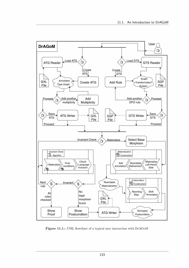
11.1. An Introduction to DrAGoM

DrAGoM

Load ATG

Create ATG

GXL File

SGFFile

Load GTS

Create GTS

Add anothermultiplicity

Add another DPO rule

GXL File

SGF File

Materialize Post- conditions

Check Language

Inclusion

Invariant Check Algorithm

AddAnnotation

Rewritable Refinement

MaterializeLeft-Hand

Side

Materialization Construction

Rewriting Step

Shift Annotation

Postcondition Construction

GXL File

Rewritable Materialization

Strongest Postcondition

Proceed

SaveGTS

SaveATG

Proceed

Proceed Proceed

Invariant Check Materialize

All rules

checked

Annotated Type Graph

GraphTransformation

System

Next rule

No legal morphism found

Invariant

ATG Reader GTS Reader

Create ATG Add Rule

AddMultiplicity

ATG Writer GTS Writer

Select Base Morphism

ATG WriterShowPostcondition

Show Proof

User

Figure 11.1.: UML flowchart of a typical user interaction with DrAGoM

133

11. DrAGoM

Likewise, graph transformation systems can be directly created via the userinterface. The user can create a graph transformation rule which is added to anempty graph transformation system. This process can be repeated until all ruleshave been added. For loading and storing graph transformation systems, DrAGoMuses the Simple Graph Format (Sgf) [Bru15]. Unlike other text-based formats,such as XML-derived formats, which are mainly designed to be easily parsedby a computer program, the Sgf format is designed to be easily written, readand maintained in source form by the user. An example for the file format of anencoded graph transformation system, can be found in Appendix C.3.Once both data structures, the multiply annotated type graph and the graph

transformation system, are created, the user can choose to either compute arewritable materialization or to let DrAGoM perform an invariant check.

For the case that the user wants to compute the rewritable materialization, thecurrently displayed graph transformation rule is used for the construction. The usercan select a semi-legal base morphism (if there are any) and afterwards DrAGoMautomatically computes the rewritable materialization. This materialization canbe used as an input for the computation of the strongest postcondition. Thematerialization algorithm alongside the postcondition algorithm are explained inmore detail in Section 11.2. The user can choose to save the multiply annotated typegraph which specifies the strongest postcondition in the Gxl format. Furthermore,the user can choose to let DrAGoM perform a language inclusion check with respectto the computed postcondition and the initial annotated type graph.If the user chooses to let DrAGoM perform an invariant check instead, both

algorithms, the materialization construction (for all semi-legal base morphisms)and the postcondition construction, are performed in sequence. The gearwheelsymbols in the algorithm steps indicate that these two tasks resemble the twoconstructions depicted on the right side of the diagram. Afterwards, a languageinclusion check is used to possibly find a legal morphism from the graph specifyingthe postcondition to the graph that specifies the initial graph language. If sucha legal morphism can not be found, the corresponding multiply annotated typegraphs are displayed and DrAGoM is unable to prove that the initial specified graphlanguage is an invariant for the given graph transformation system. Otherwise, thealgorithm is restarted until every rule of the graph transformation system is checked.If for all rules and every semi-legal base morphism there exists a correspondinglegal morphism for the postcondition graph, then all legal morphisms are displayedas a proof to the user.

11.2. Implementing Categorical NotionsThe computation of the materialization and its annotations, which was describedcategorically for an arbritrary topos C in Chapter 9, needs to be implemented inDrAGoM as a concrete instance for our annotated type graph framework.

11.2.1. Concrete Construction of the MaterializationWe define a concrete construction of the materialization 〈ϕ〉 in the categoryGraphΛ. Even though GraphΛ is a topos, we do not use the notions of subobjectclassifiers or partial map classifiers for the following step-by-step construction:

134

11.2. Implementing Categorical Notions

Definition 11.1 (Concrete construction of the materialization). Let twographs L = (VL, EL, srcL, tgtL, labL) and A = (VA, EA, srcA, tgtA, labA) overa fixed edge label alphabet Λ be given and let ϕ : L → A be a fixed graphmorphism.

First we define the function ψV : (VL⊎VA)→ VA which maps the nodes of

L and A to the nodes of A with respect to ϕ:

ψV (x) =ϕV (x) if x ∈ VLx otherwise

We construct A = (V,E, src, tgt, lab) in the following way:

V = VL⊎VA

E = EL⊎(e, s, t, l) ∈ EA × V × V × Λ |

srcA(e) = ψV (s) ∧ tgtA(e) = ψV (t) ∧ labA(e) = l

src : E → V src(x) =s if x = (e, s, t, l)srcL(x) otherwise

tgt : E → V tgt(x) =t if x = (e, s, t, l)tgtL(x) otherwise

lab : E → Λ lab(x) =l if x = (e, s, t, l)labL(x) otherwise

This concludes the construction of the graph A.We now define the embedding graph morphismα : L → A where α(x) = x to get the diagramshown to the right.

L A Aα

ϕ

To get a valid factorization L A → A of ϕ, we define the morphismψ : A→ A with ψ = (ψV , ψE) where ψE : E → EA is given by:

ψE(x) =e if x = (e, s, t, l)ϕE(x) otherwise (i.e. x ∈ EL)

Obviously ψ α = ϕ holds. The object L α A

ψ→ Ais a factorization of L ϕ→ A and the diagram shownto the right commutes.

L A Aα

ϕ

ψ

Next, we prove that the above constructed object L α A

ψ→ A is the terminalobject in the materialization category Matϕ, i.e. we have A = 〈ϕ〉.

Proposition 11.2 (Constructed materialization is terminal). Let L ϕ→ A bea fixed graph morphism in GraphΛ. Then the factorization L

α A

ψ→ Afrom Definition 11.1 is the terminal object in the category Matϕ.

Therefore, the construction of Definition 11.1 is a guideline which tells us howto implement a materialization algorithm step-by-step. Since we are working with

135

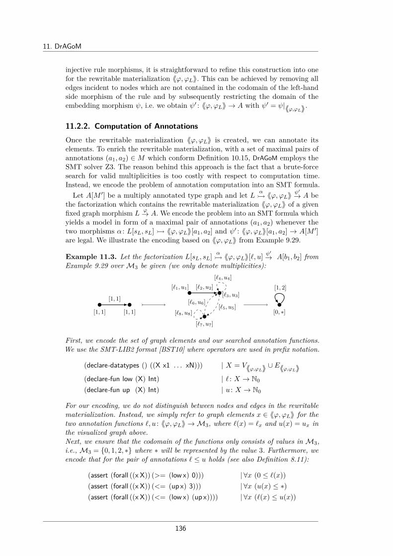
11. DrAGoM

injective rule morphisms, it is straightforward to refine this construction into onefor the rewritable materialization 〈〈ϕ,ϕL〉〉. This can be achieved by removing alledges incident to nodes which are not contained in the codomain of the left-handside morphism of the rule and by subsequently restricting the domain of theembedding morphism ψ, i.e. we obtain ψ′ : 〈〈ϕ,ϕL〉〉 → A with ψ′ = ψ|〈〈ϕ,ϕL〉〉.

11.2.2. Computation of AnnotationsOnce the rewritable materialization 〈〈ϕ,ϕL〉〉 is created, we can annotate itselements. To enrich the rewritable materialization, with a set of maximal pairs ofannotations (a1, a2) ∈ M which conform Definition 10.15, DrAGoM employs theSMT solver Z3. The reason behind this approach is the fact that a brute-forcesearch for valid multiplicities is too costly with respect to computation time.Instead, we encode the problem of annotation computation into an SMT formula.Let A[M ′] be a multiply annotated type graph and let L α

〈〈ϕ,ϕL〉〉ψ′→ A be

the factorization which contains the rewritable materialization 〈〈ϕ,ϕL〉〉 of a givenfixed graph morphism L

ϕ→ A. We encode the problem into an SMT formula whichyields a model in form of a maximal pair of annotations (a1, a2) whenever thetwo morphisms α : L[sL, sL] 〈〈ϕ,ϕL〉〉[a1, a2] and ψ′ : 〈〈ϕ,ϕL〉〉[a1, a2] → A[M ′]are legal. We illustrate the encoding based on 〈〈ϕ,ϕL〉〉 from Example 9.29.

Example 11.3. Let the factorization L[sL, sL] α 〈〈ϕ,ϕL〉〉[`, u] ψ

′→ A[b1, b2] from

Example 9.29 overM3 be given (we only denote multiplicities):

[1, 1] [1, 1]

[1, 1]

[`1, u1][`3, u3]

[`7, u7]

[`2, u2][`4, u4]

[`8, u8][`5, u5]

[`6, u6][0, ∗]

[1, 2]

First, we encode the set of graph elements and our searched annotation functions.We use the SMT-LIB2 format [BST10] where operators are used in prefix notation.

(declare-datatypes () ((X x1 . . . xN))) | X = V〈〈ϕ,ϕL〉〉 ∪ E〈〈ϕ,ϕL〉〉(declare-fun low (X) Int) | ` : X → N0

(declare-fun up (X) Int) | u : X → N0

For our encoding, we do not distinguish between nodes and edges in the rewritablematerialization. Instead, we simply refer to graph elements x ∈ 〈〈ϕ,ϕL〉〉 for thetwo annotation functions `, u : 〈〈ϕ,ϕL〉〉 →M3, where `(x) = `x and u(x) = ux inthe visualized graph above.Next, we ensure that the codomain of the functions only consists of values inM3,i.e.,M3 = 0, 1, 2, ∗ where ∗ will be represented by the value 3. Furthermore, weencode that for the pair of annotations ` ≤ u holds (see also Definition 8.11):

(assert (forall ((x X)) (>= (low x) 0))) | ∀x (0 ≤ `(x))(assert (forall ((x X)) (<= (up x) 3))) | ∀x (u(x) ≤ ∗)(assert (forall ((x X)) (<= (low x) (up x)))) | ∀x (`(x) ≤ u(x))

136

11.2. Implementing Categorical Notions

Instead of encoding the morphisms α and ψ′, we use them to compute sets of nodesand edges with specific requirements. According to Definition 10.15 all elements inthe image of α are annotated with the standard annotation [1, 1]. In our example,α(L) = x1, x2, x3 and therefore we add the following six constraints:

(assert (= (low x1) 1)) | `(x1) = 1(assert (= (low x2) 1)) | `(x2) = 1(assert (= (low x3) 1)) | `(x3) = 1

(assert (= (up x1) 1)) |u(x1) = 1(assert (= (up x2) 1)) |u(x2) = 1(assert (= (up x3) 1)) |u(x3) = 1

Since we search for maximal pairs of annotations we set up the following constraintsfor all remaining elements x ∈ (〈〈ϕ,ϕL〉〉 \ α(L)), i.e. elements which are not partof the left-hand side image: All remaining elements x for which b2(ψ′(x)) = ∗,receive the upper bound u(x) = ∗. In a similar way, the remaining elements x forwhich b1(ψ′(x)) = 0, receive the lower bound `(x) = 0. In our example this yieldsthe constraint for x7:

(assert (= (low x7) 0)) | `(x7) = 0 (assert (= (up x7) 3)) |u(x7) = ∗

Last, we encode constraints for the remaining elements x ∈ (〈〈ϕ,ϕL〉〉 \ α(L))which are mapped onto type graph elements t ∈ A with a multiplicity value b with0 < b < ∗: In case of b1(t) = b, if x ∈ ψ′−1(t) and for the number of left-handside image elements α(L) in ψ′−1(t) we have |α(L) ∩ ψ′−1(t)| ≥ b, then `(x) = 0.Otherwise, the sum of all corresponding lower bounds in ψ′−1(t) must be equal tob. Similarly the sum of all upper bounds in ψ′−1(t) must be equal to b2(t). For ourrunning example we get the following constraints:

(assert (= (low x4) 0)) | `(x4) = 0(assert (= (low x5) 0)) | `(x5) = 0

(assert (= (low x6) 0)) | `(x6) = 0(assert (= (low x8) 0)) | `(x8) = 0

(assert (= (sum (up x2) (up x4) (up x5) (up x6) (up x8)) 2))|u(x2) + u(x4) + u(x5) + u(x6) + u(x8) = 2

This completes the SMT encoding. Whenever the solver finds a model, we get apair of annotations (`, u) which yields a legal morphism ψ′ and the pair is maximalin the sense that we exactly hit all desired bounds, i.e. (`, u) ∈ M conformingDefinition 10.15. We then extend the SMT formula to exclude all previously foundmodels and check for its satisfiability until the formula gets unsatisfiable. In eachiteration step we collect another maximal pair. In our example we receive thefollowing four pairs of annotations for the rewritable materialization 〈〈ϕ,ϕL〉〉[M ]:

〈〈ϕ,ϕL〉〉[`, u] =

[1, 1][1, 1]

[0, ∗]

[1, 1][0, 1]

[0, 0][0, 0]

[0, 0] 〈〈ϕ,ϕL〉〉[`′′, u′′] =

[1, 1][1, 1]

[0, ∗]

[1, 1][0, 0]

[0, 1][0, 0]

[0, 0]

137

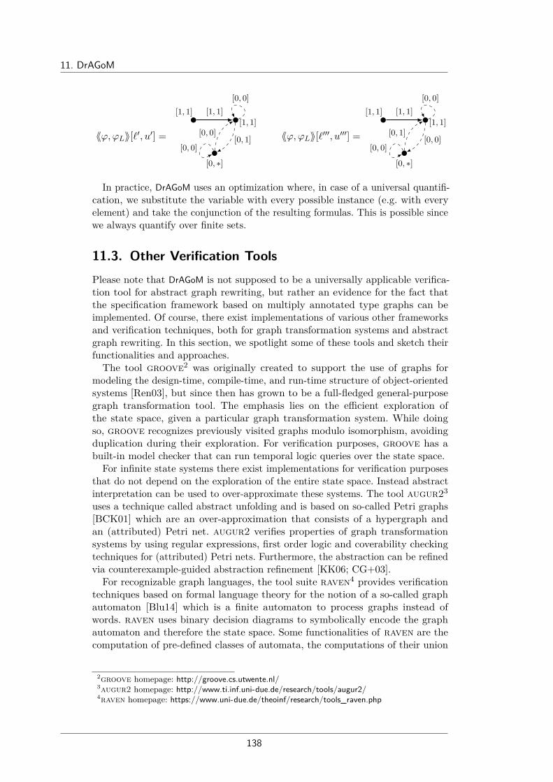
11. DrAGoM

〈〈ϕ,ϕL〉〉[`′, u′] =

[1, 1][1, 1]

[0, ∗]

[1, 1][0, 0]

[0, 0][0, 1]

[0, 0] 〈〈ϕ,ϕL〉〉[`′′′, u′′′] =

[1, 1][1, 1]

[0, ∗]

[1, 1][0, 0]

[0, 0][0, 0]

[0, 1]

In practice, DrAGoM uses an optimization where, in case of a universal quantifi-cation, we substitute the variable with every possible instance (e.g. with everyelement) and take the conjunction of the resulting formulas. This is possible sincewe always quantify over finite sets.

11.3. Other Verification ToolsPlease note that DrAGoM is not supposed to be a universally applicable verifica-tion tool for abstract graph rewriting, but rather an evidence for the fact thatthe specification framework based on multiply annotated type graphs can beimplemented. Of course, there exist implementations of various other frameworksand verification techniques, both for graph transformation systems and abstractgraph rewriting. In this section, we spotlight some of these tools and sketch theirfunctionalities and approaches.The tool groove2 was originally created to support the use of graphs for

modeling the design-time, compile-time, and run-time structure of object-orientedsystems [Ren03], but since then has grown to be a full-fledged general-purposegraph transformation tool. The emphasis lies on the efficient exploration ofthe state space, given a particular graph transformation system. While doingso, groove recognizes previously visited graphs modulo isomorphism, avoidingduplication during their exploration. For verification purposes, groove has abuilt-in model checker that can run temporal logic queries over the state space.

For infinite state systems there exist implementations for verification purposesthat do not depend on the exploration of the entire state space. Instead abstractinterpretation can be used to over-approximate these systems. The tool augur23

uses a technique called abstract unfolding and is based on so-called Petri graphs[BCK01] which are an over-approximation that consists of a hypergraph andan (attributed) Petri net. augur2 verifies properties of graph transformationsystems by using regular expressions, first order logic and coverability checkingtechniques for (attributed) Petri nets. Furthermore, the abstraction can be refinedvia counterexample-guided abstraction refinement [KK06; CG+03].

For recognizable graph languages, the tool suite raven4 provides verificationtechniques based on formal language theory for the notion of a so-called graphautomaton [Blu14] which is a finite automaton to process graphs instead ofwords. raven uses binary decision diagrams to symbolically encode the graphautomaton and therefore the state space. Some functionalities of raven are thecomputation of pre-defined classes of automata, the computations of their union

2groove homepage: http://groove.cs.utwente.nl/3augur2 homepage: http://www.ti.inf.uni-due.de/research/tools/augur2/4raven homepage: https://www.uni-due.de/theoinf/research/tools_raven.php

138

11.3. Other Verification Tools

and product automata, membership checks for the corresponding languages ofcospan decomposed graphs, and invariant checks for graph transformation systems.

Then there exist other implementations which are designed for the analysis ofpointer programs [Ren04a] and for shape analysis [SRW02]. In [SWW10; SW11]and [SWW11] the authors mention an implementation based on the source codeof the shape analysis tool tvla5 [BL+07]. Given a shape graph, a set of shapeproductions and a set of forbidden patterns, the implementation constructsthe set of reachable shape graphs where each graph is represented as a logicalstructure based on three-valued logic. If a reached shape graph contains theforbidden pattern, a counterexample in form of the respective derivation sequenceis returned.

The tool juggrnaut6 [HJ+15] uses hyperedge replacement grammars to specifypointer program structures and their abstractions. The grammar rules are used intwo directions: a backward applications of the rule abstracts a subgraph of theheap into a single nonterminal edge and a forward application can materializeparts of the heap.Another abstraction mechanism, called partner abstraction, is represented in

[Bau06] and implemented in the tool hiralysis. The graph structures are over-approximated by the labels of adjacent nodes. This approach has been extendedto so-called cluster abstractions in [BR15a], where the information about possibleedges between partners is stored using three-valued logic. The tool astra7 [BR15b]uses the cluster abstraction approach and can be used for the static analysis andverification of topological structures in dynamic communication systems.

5tvla homepage: http://www.cs.tau.ac.il/~tvla/6juggrnaut homepage: https://moves.rwth-aachen.de/research/projects/juggrnaut/7astra homepage: http://www.rw.cdl.uni-saarland.de/~rtc/astra/

139

“It doesn’t matter how beautiful your theory is, itdoesn’t matter how smart you are. If it doesn’t agreewith experiment, it’s wrong.”

Richard P. Feynman (1918-1988)

12Evaluation

To evaluate the practicability of the framework based on multiply annotated typegraphs, we conduct different case studies using DrAGoM. We focus on runtimeresults for invariant checking and test the limits of DrAGoM’s inclusion checkswith respect to graph sizes. First, we evaluate the output based on examples ofthis thesis, to check if the materializations and strongest postconditions coincidewith the theoretical results. Afterwards, we perform invariant checks for graphlanguages specified by annotated type graphs and discuss the correctness of theresults.

All tests in this chapter were performed on a machine running a 64-bit versionof Windows 10 on an Intel Xeon e3-1505m v6 processor and 16 GB RAM. Allcase studies are available in the source archive on the DrAGoM homepage.

12.1. Thesis ExamplesTo showcase correct results for the implemented base functionalities in DrAGoM,we use two examples from previous chapters, namely Examples 10.16 and 10.20,to compare the output with the formerly expected results.For all upcoming case studies in this chapter, we indicate rule morphisms by

the numbers below the nodes. Furthermore, in some case studies we might omitedge labels to simplify the visual representation.

Abstract Rewriting Step for Example 10.16Let the graph transformation rule ρ and the annotated type graph T [`, u] overthe label alphabet Λ = A,B,C,D from Example 10.16 be given.

The computation of the rewritable materialization and the subsequent compu-tation of the annotated type graph which specifies the strongest postconditiontakes DrAGoM a few milliseconds. The output of the postcondition construction isthe following annotated type graph T ′ρ[a1, a2]:

T ′[a1, a2] =[1, 1]

C [0, 0]D [0, ∗]

[0, ∗]

C [0, 0]

D [0, ∗] C [0, 0]

D [0, ∗] [1, 1]

A [1, 1]

B [1, 1]

12. Evaluation

As evident from the picture above, we illustrate the concrete instance of the right-hand side graph R by using regular drawn edges and black nodes, whereas freshlyintroduced graph elements are drawn as gray colored nodes and bidirectionaldashed edges. We will use these visual semantics for the remainder of this chapter.The simplification of the computed annotated type graph T ′[a1, a2] coincides

with the expected result from Example 10.16. Furthermore, the invariant checkyields no positive answer and terminates within a few milliseconds, as the initialgraph language does not contain graphs with A-labelled or B-labelled edges.The graph transformation rule and the annotated type graph of this case studyare provided in the source archive on the DrAGoM homepage1 as files namedSimpleExample.sgf and SimpleExample.gxl respectively.

Invariant Check for Example 10.20Let the graph transformation rule ρ and the annotated type graph A[a1, a2] fromExample 10.20 be given. The invariant check of DrAGoM yields no positive answerwithin a few milliseconds and shows the following strongest postcondition graphT ′ρ[b1, b2] which only consists of one pair of multiplicities:

T ′ρ[b1, b2] =

[0, ∗][0, 0]

[0, ∗]C [0, 0] M [0, ∗]

P [0, ∗]

$ [0, ∗]

[1, 1][1, 1]

[1, 1]C [1, 1]

C [0, 0]

M [0, ∗]

P [0, ∗]

P [1, 1]$ [0, ∗]

$ [0, ∗]

C [0, 0]

C [0, 0]

M [0, ∗]

M [0, ∗]

P [0, ∗]P [0, ∗]

Please note that the simplification of T ′ρ[b1, b2] coincides with the simplifiedresult postulated in Example 10.20. Furthermore, thanks to DrAGoM, we canconclude that the pair of multiplicities (b1, b2) is the only maximal pair whichconforms to Definition 10.15. The corresponding files of this case study are namedWorkedExample.sgf and WorkedExample.gxl.

12.2. Invariant Check for ColorabilityIn this section we perform invariant checks for graph language examples inspiredby [Blu14]. Type graphs are expressive enough to specify languages consistingof all k-colorable graphs, i.e., all graphs which can be colored using maximalk different colors, such that every pair of adjacent nodes never share the samecolor. Type graph languages can be simulated using annotated type graphs byannotating every element with the multiplicity pair [0, ∗]. Hence, we let DrAGoMperform an invariant check for 2-colorability and 3-colorability.

1DrAGoM homepage: https://www.uni-due.de/theoinf/research/tools_dragom.php

142

12.2. Invariant Check for Colorability

12.2.1. 2-Colorability with Path ExtensionThe 2-coloring problem can be solved in linear time. The main idea is to assignone of the two colors to a node v1 and subsequently color all adjacent nodeswith the opposite color. This process is repeated for the neighbours of v1 untilevery node in the graph received a color. If no colored node has been assigned toboth colors in this process, the graph is 2-colorable. It is easy to see that every2-colorable graph is bipartite. Therefore, we can use the complete graph with twonodes as a type graph, to specify the set of 2-colorable graphs. Each node in thetype graph resembles a partition of all nodes which share the same color.

Let the following graph transformation system R = ρ1, ρ2 and the annotatedtype graph T [`, u] over a label alphabet Λ with |Λ| = 1 be given. We omit thesingle edge label:

ρ1 =1 2 1 2 1 2

T [`, u] = [0, ∗] [0, ∗][0, ∗]

[0, ∗]ρ2 =

1 2 1 2 1 2

The invariant check takes a few milliseconds and yields no positive answer forthe language of the annotated type graph T [`, u] with respect to rule ρ1. Theannotated type graphs T ′ρ1 [a1, a2] and T ′ρ2 [b1, b2] (both computed by DrAGoM)specify the strongest postconditions for the respective rules. Both annotated typegraphs contain only one pair of multiplicities since the annotation bounds [0, ∗]are always the unique possible maximal pair of multiplicities:

T ′ρ1 [a1, a2] =

[0, ∗] [1, 1]

[0, ∗] [1, 1]

[1, 1]

[0, ∗]

[0, ∗]

[0, ∗]

[0, ∗][1, 1]

[1, 1]

T ′ρ2 [b1, b2] =

[0, ∗] [1, 1]

[0, ∗] [1, 1]

[1, 1]

[1, 1]

[0, ∗]

[0, ∗]

[0, ∗]

[0, ∗]

[1, 1]

[1, 1]

[1, 1]

Clearly the annotated type graph T ′ρ1 [a1, a2] is not bipartite (and hence not2-colorable) due to the triangle subgraph on the right side. Performing an invariantcheck for rule ρ2 only, yields a positive answer. DrAGoM is able to compute the legalmorphism from T ′ρ2 [b1, b2] to T [`, u] within milliseconds. The graph transformationsystem and annotated type graph of this case study are provided as files named2-Colorability.sgf and 2-Colorability.gxl.

12.2.2. 3-Colorability with Node Replacement

Next, we perform an invariant check for the language of an annotated type graphwhich consists of all 3-colorable graphs. The 3-coloring problem is known to beNP-complete. The corresponding type graph without annotations was alreadyconsidered in Example 4.6 and coincides with the complete graph which consistsof three nodes.Let the following graph transformation rule ρ and the annotated type graph

T [`, u] be given. The rule morphisms are indicated by the numbers below thenodes. Similar to the 2-colorability case study we use a single edge label which weomit for the sake of simplicity:

143

12. Evaluation

ρ =

1 2

3 4

1 2

3 4

1 2

3 4

T [`, u] =

[0, ∗] [0, ∗]

[0, ∗]

[0, ∗]

[0, ∗]

[0, ∗][0, ∗

][0, ∗]

[0, ∗]

The invariant check finishes after a few milliseconds and yields a positive answerfor the language of the annotated type graph T [`, u] with respect to rule ρ. DrAGoMfinds and investigates 6 different base morphisms and subsequently computes thestrongest postconditions for each of them. In all cases the annotated type graphT ′ρ[a1, a2] (shown below) which specifies the postcondition is the same graph upto isomorphism and it contains one pair of multiplicities:

T ′ρ[a1, a2] =

[1, 1] [1, 1]

[1, 1] [1, 1]

[1, 1]

[1, 1] [1, 1]

[1, 1] [1, 1]

[0, ∗]

[0, ∗]

[0, ∗]

[1, 1][1, 1]

[1, 1]

[1, 1]

[1, 1]

[1, 1][1, 1] [1, 1]

[1, 1]

[1, 1] [1, 1]

[1, 1][1, 1]

[1, 1]

[1, 1]

[1, 1]

[0, ∗]

[0, ∗]

[0, ∗]

[0, ∗]

[0, ∗]

[0, ∗]

[0, ∗]

[0, ∗]

[0,∗]

[0, ∗]

[0, ∗]

[0, ∗]

[0, ∗]

[0, ∗]

[0,∗]

The outer nodes of the left-hand side graph of the rule can be colored with twoalternating colors such that the third color remains for the inner node. Likewise,using the same 2-color scheme for the interface nodes of the right-hand side graph,we can color the inner rectangle with the complemented colors such that the thirdcolor again remains for the node in the center. Therefore, the graph languageL(T [`, u]) is indeed an invariant for the graph transformation rule ρ. The graphtransformation system is provided in the file named 3-Colorability.sgf andthe file of the annotated type graph is named 3-Colorability.gxl.

12.3. Invariant Check for a Rail SystemWe increase the number of rules, edge labels and possible base morphisms for ournext case study. The following case study is inspired by [DG17]. We specify a railsystem using an annotated type graph with the following edge label semantics:

T : The track of the rail net. P : The position of a train.F : The train is fast. A : The train is accelerating.S : The train is slow. B : The train is put on the brakes.

Now, we would like to model the following situation: Three trains are using therail network which is infinitely large. Each train must be at one position and they

144

12.3. Invariant Check for a Rail System

can travel fast or slow. Furthermore each train can accelerate or brake to switchbetween these states. The graph language of this specification is specified by thefollowing annotated abstract graph T [`, u]:

T [`, u] =

[1, 1]S [0, ∗]

B [0, ∗]A [0, ∗]

F [0, ∗][1, 1]

S [0, ∗]

B [0, ∗]A [0, ∗]

F [0, ∗][1, 1]

S [0, ∗]

B [0, ∗]A [0, ∗]

F [0, ∗]

[1, ∗]T [0, ∗]

P [1, 1] P [1, 1]

P [1, 1]

To specify the movement of the trains alongside their accelerations and brakes,we use the following graph transformation system R = ρi | 1 ≤ i ≤ 7:

ρ1 = 1 2 3TPF 1 2 3TF 12 3T P F

ρ2 = 1 2 3TPF 1 2 3T 12 3T P B

ρ3 = 1 2 3TPB 1 2 3T 12 3T P S

ρ4 = 1 2 3TPS 1 2 3TS 12 3T P S

ρ5 = 1 2 3TPS 1 2 3T 12 3T P A

ρ6 = 1 2 3TPA 1 2 3T 12 3T P B

ρ7 = 1 2 3TPA 1 2 3T 12 3T P F

The rules in R have the following semantics: A fast train can travel over thetracks (ρ1) or brake (ρ2). While the train is put on brake it still travels over thetracks but becomes slow (ρ3). Similar to a fast train, a slow train can travel overthe tracks (ρ4) or it accelerates (ρ5). During the acceleration the train can brakeagain (ρ6) or it can further accelerate to become fast (ρ7).

The invariant check again finishes after a few milliseconds and yields a positiveanswer for the language of the annotated type graph T [`, u] with respect to thegraph transformation system R. DrAGoM finds and investigates 3 different basemorphisms for each of the 7 rules. In all cases the annotated type graph whichspecifies the postcondition consists of 9 annotations, 7 nodes and 48 edges.Please note, that the main purpose of this case study was to increase the

complexity of the invariant check, to stress test DrAGoM. Since the scenario doesnot forbid states where a train is fast, slow, accelerating and braking at the sametime, the rule application boils down to a simple edge relabelling over multipleflower graphs of the specific train state loop labels A,B, F and S. Therefore, thegraph transformation system clearly is an invariant.However, if we restrict the states of the trains in the annotated type graph

T [`, u] (i.e. annotate the edges labelled A,B, F and S, by annotation bounds[0, 1]), the language is no longer an invariant for R. The application of rule ρ7 on atrain which is already fast and accelerating would result in a graph which contains

145

12. Evaluation

two F -labelled loops. Clearly such a graph is not part of the restricted languageand DrAGoM is not able to prove the invariant for such a restricted scenario.The source archive files for the graph transformation system and annotated

type graph of this case study are named RailTrack.sgf and RailTrack.gxlrespectively.

12.4. Invariant Check for Subgraph ContainmentIn this last case study we increase the size of the initial graph. The followingexample is inspired by [Blu14].The framework of multiply annotated type graphs is expressive enough to

specify graph languages which contain all graphs with a specific subgraph. Forinstance, an annotated materialization is able to specify exactly the set of graphswhich contain a concrete image of the left-hand side of a rule. Therefore, we canuse the materialization construction for any given graph S over the final objectTΛ

R of the category GraphΛ(cf. Example 4.4), to compute an annotated typegraph which specifies the subgraph containment language, i.e. the set of all graphswhich contain S as subgraph.

Let the following graph transformation rule ρ and the subgraph S over the edgelabel alphabet Λ = A,B be given:

ρ =1 2

A

1 2 1 2A S =

A

B B

The materialization construction of S over the flower graph T A,BR

takes DrAGoMa few milliseconds and results in the following annotated type graph T [`, u] whichspecifies the initial subgraph containment language for S. Every Λ-labelled edgein the following graph represents a set of edges, one for each label in Λ:

T [`, u] =[1, 1]

Λ [0, ∗]

[0, ∗]Λ [0, ∗]

[1, 1]Λ [0, ∗]

[1, 1]Λ [0, ∗]

A[1,1]

B [1, 1]

B [1, 1]

Λ [0, ∗]

Λ [0, ∗]

Λ [0, ∗]Λ [0, ∗]

Λ [0, ∗]

Λ[0,∗]

The invariant check of T [`, u] with respect to the rule ρ finishes after 4 hours 38minutes 27 seconds and yields a positive answer. DrAGoM finds and investigates14 different base morphisms and computes the strongest postcondition for eachof them. It is worth to mention that the computation of the rewritable material-ization and the strongest postcondition both take a few milliseconds. However,the inclusion check of the postcondition graphs into the initial annotated typegraph T [`, u] is very costly. A multiply annotated type graph which specifies thepostcondition consists of 4 pairs of multiplicities, 6 nodes and 78 edges. Sincethe annotated type graph T [`, u] consists of 4 nodes and 35 edges, DrAGoM hasto check a huge number of possible embedding morphisms to prove that thelanguages are included.

146

12.5. Overview of the Results

Please note that DrAGoM employs the sufficient condition from Proposition 8.20for the inclusion check, i.e., the tool tries to find a legal embedding morphism fromthe postcondition graph into the initial annotated type graph. However, finding amorphism from an input graph into another graph (even if the target graph isfixed) is NP-complete. DrAGoM uses a brute-force approach to find possible graphmorphisms and checks their legality. Hence, it is not surprising that the inclusioncheck is the bottleneck in this approach.

The graph transformation system and annotated type graph of this case studyare provided as files named SubTriangle.sgf and SubTriangle.gxl.

12.5. Overview of the ResultsWe summarize the results of the case studies which we conducted using DrAGoM.The following table shows the important key values for each experiment. Pleasenote that the initial annotated type graph (ATG) T [`, u] always started with onepair of multiplicities:

Case Study GTS R ATG T [`, u] Post ATG T ′[M ] ResultName |Λ| |R| |VT | |ET | |V ′T | |E′T | |M | Invariant Runtime

SimpleExample 4 1 1 2 3 10 1 7 < 1sWorkedExample 4 1 3 4 12 18 1 7 < 1s2-Colorability 1 2 2 2 5 10 1 7 < 1s3-Colorability 1 1 3 6 12 46 1 3 < 1sRailTrack 6 7 4 16 7 48 9 3 < 1sSubTriangle 2 1 4 35 6 78 4 3 4h 38m

The generated outputs for all case studies conform to the expected results.The runtime results for invariant checking seem promising. However, as the lastcase study shows, the inclusion checks become too costly for larger initial graphsizes. This is due to the fact that a brute-force approach for the computation oflegal morphisms is not efficient. Therefore, further exploration of the abstractstate space yields no hope for efficiency unless the postcondition graphs can besimplified.On the other hand, further tests on 100 randomly generated annotated type

graphs (consisting of 10−20 nodes, 10−40% edge existence probability, minimum10 multiplicities onMn where 2 ≤ n ≤ 5) showed that the SMT encodings forthe computation of annotated rewritable materializations scales well. In one ofthese tests, an initial multiply annotated type graph using a single edge labelconsisted of 14 nodes, 72 edges and 64 multiplicities overM2. DrAGoM computeda rewritable materialization (for the single rule of the subgraph containment casestudy in Section 12.4) within 7 seconds. In the process, DrAGoM found 47 possiblesemi legal base morphisms to extract the left-hand side from. One of the computedrewritable materializations consisted of 16 nodes, 92 edges and 2048 annotations.Therefore, we can conclude that the prototype tool DrAGoM shows that con-

crete instances of the general framework for abstract annotated objects can beimplemented. The efficiency for computations of legal morphisms needs to betweaked. Overall, DrAGoM can be used for strongest postcondition computationsand for invariant checks of multiply annotated type graphs, up to sizes similar tothe rail system case study of Section 12.3.

147

Part VI.

Conclusion

“If I’d had some set idea of a finish line, don’t youthink I would have crossed it years ago?”

Bill Gates (1955-present)

13Conclusion and Future Work

The overall aim of this thesis was to analyse graph specification frameworks basedon type graphs and show their applicability for verification techniques based onformal language theory. We first sum up the main contributions of the Parts II-IVand discuss how they fit into this aim. Overall, the results of the main parts canbe summarized as follows:

Part II - Termination Analysis of Graph Transformation Systems• A termination analysis approach for graph transformation systems

based on weighted type graphs (Chapter 5).• An interpretation for term rewriting systems to graph transformation

systems which preserves termination arguments (Chapter 6).

Part III - Specifying Type Graph Languages• An overview of closure and decidability properties for four graph

specification frameworks based on type graphs (Chapters 7 and 8).

Part IV - Abstract Object Rewriting• A construction for rewritable materializations for objects in an arbitrary

topos (Chapter 9).• A general framework to rewrite annotated objects and compute strongest

postconditions (Chapter 10).

All these results originate from one simple idea: to use type graphs not only fortyping purposes but also for the specification of graph languages. This change ofperspective led to a basic graph specification framework which paved the pathfor several refinements. In this thesis, two of these refinements were successfullyapplied to verification techniques, i.e. weighted type graphs for termination analysisand multiply annotated type graphs for invariant checking. However, the keycontribution of this thesis is a generalization of the type graph specificationlanguage to a framework of rewritable annotated objects. This framework can beinstantiated to concrete specification languages for which strongest postconditionscan be computed.

13. Conclusion and Future Work

13.1. Summary and ConclusionDetailed descriptions of related work and open questions were already providedin the conclusion chapters of the respective Parts II-IV. Therefore, in this section,we instead focus on the significance of the accomplished results. Furthermore, wediscuss how these results fit into the broader scientific context and point out thepossible research directions to where this thesis can lead.

In this thesis we focused on specification languages based on type graphs, wherethe language of a type graph T consists of all graphs that can be mapped ho-momorphically into T (with potentially extra constraints in refined frameworks).Many specification formalisms that are usually used in abstract graph transfor-mation and verification, are based on type graphs. There exists no one-fits-allsolution and different frameworks are suited well for different verification purposes.Inspired by matrix interpretations of string and cycle rewriting we first tried toadapt the basic idea of type graph languages to termination analysis for graphtransformation systems.

Achievements in Termination AnalysisWe describe the impact that the introduced termination approach and the encod-ings have on the automatic proving of termination, which has been a central topicin rewriting research over the last years.In Part II of this thesis we introduced a new termination analysis technique

for graph transformation systems based on the notion of weighted type graphsover different kinds of semirings. The weighted type graphs have the purposeto not only specify the language of all graphs, but also to assign weights to allgraphs contained in this language. Then rules of the graph transformation systemcan be classified according to whether their application decreases the weightof every graph, or at least does not increase it. Please note that the weightedtype graph approach does not subsume previous introduced termination analysismethods, but rather complements them. With respect to graph transformationsystems, all variants of the termination problem, termination on all graphs aswell as termination on a fixed set of initial graphs, are undecidable. Therefore,in practice one should always run several methods in parallel, when trying toprove the termination property of a rewriting system. Hence, by providing anothertermination technique, we contributed another piece to the bigger puzzle, tofurther increase chances for a successful termination analysis.Furthermore, we studied how to transform term graph rewriting systems to

graph transformation systems. Although it is widely agreed that term graphrewriting is the way to go for efficient implementation of term rewriting, quitesurprisingly hardly any effort has been done in automatically proving terminationof term graph rewriting. One reason could be that for term graph rewriting it issubstantially harder since techniques strongly exploiting the term structure donot apply, such as path orders and dependency pairs. Being able to transformtermination problems from term graph rewriting to graph transformation systems,our technique works subsequently for term rewriting systems as well. As a sideeffect, by applying our transformations to a selection of term rewriting systemsfrom the Termination Problems Database, we provide a substantial set of testcases for automatically proving termination of graph transformation systems.

152

13.1. Summary and Conclusion

In the end, these results show us that it is worthwhile to build bridges be-tween different kinds of rewriting systems to profit from established techniques.Verification techniques from the theory of formal languages are worked out verywell in string and tree/term rewriting, but it is often non-trivial to use thesetechniques when it comes to graph rewriting. Therefore, it is natural to ask forgeneralizations of these verification techniques to the framework of graph rewritingand additionally to a theory of graph languages, where these techniques can beapplied.

Graph Specification Frameworks based on Type GraphsWe tried to understand the essence of some selected graph specification languages,which grant them the possibility to use verification techniques from the theory offormal languages. In Part III, we classified several extensions of the basic type graphspecification framework with respect to their decidability and closure properties.In order to be able to use type graph formalisms extensively in applications, it isnecessary to provide a mechanism to compute weakest preconditions and strongestpostconditions. That is, given a graph language and a set of rules, we want tospecify the language of all successors (or the language of all predecessors) in ourformalism. We found out that this is not feasible for pure type graphs, restrictiongraphs or the type graph logic, since neither formalism can count and hence cannot express that all items of the newly created right-hand side occur exactly once.Hence, we characterized strongest postconditions in the setting of annotated typegraphs. To cover specification frameworks based on type graphs with differentannotations, we investigated the properties from a categorical point of view, thuswe used notions from category theory to achieve general results.

A First Step Towards a General FrameworkThe key contribution of this thesis is the general framework introduced in Part IV.We have described a rewriting framework for abstract graphs that also applies toobjects in any topos. In particular, we have given a construction for materializationin terms of the universal property of partial map classifiers in slice categories. Thisis a first theoretical milestone towards shape analysis as a general static analysismethod for rule-based systems with graph-like objects as states. Soundness andcompleteness results for rewriting of abstract objects with annotations in anordered monoid provide an effective verification method for the special case ofgraphs. Please note that this general framework is not to be confused with a one-fits-all solution. It is a blueprint from which instances of graph based specificationlanguages, with computable postconditions, decidability of membership and closureunder intersection, can be generated. The other properties depend on the usedtype of annotation. Furthermore, we have shown how annotated type graphs overmultiplicities, one concrete instance of the general framework, can be implementedand used for verification purposes. The prototype tool DrAGoM witnesses thepracticability of the level of abstraction with respect to invariant checking. However,the framework reaches its limits when it comes to further exploration of the statespace. So far, the general framework does not provide techniques to collapseabstract objects derived via rewriting steps.

153

13. Conclusion and Future Work

13.2. Future WorkMany interesting open questions connected to the individual contributions werealready formulated in their respective chapters. Apart from these open questions,this thesis sets the starting point for a large set of possible next steps. Themost interesting directions originate from the main contribution, i.e. the generalframework for specification languages based on annotated type graphs.First and foremost, the evaluation on DrAGoM showed how important it is to

find widening or similar approximation techniques for the general framework,which collapse the abstract objects. Ideally, such techniques would lead to finiteabstract transition systems that (over-)approximate the typically infinite transi-tions systems of graph transformation systems. We have already shown that thenotion of cores does not apply to the framework of annotated type graphs overmultiplicities.If such an approximation technique is provided, DrAGoM can be efficiently

applied to further verification techniques such as reachability analysis or non-termination analysis. The optimization and extension of DrAGoM would still servethe purpose to witness the practicability of further extensions. Among theseoptimizations, the computation of legal morphisms could be outsourced to SATor SMT solvers. We showcased in [KNN18] how morphism computations (for coreconstructions) can efficiently be encoded using SAT and SMT solvers.Another possible direction would be to further extend the general framework

with respect to other types of annotations. The extension of annotations withlogical formulas is just one possible next step, which could lead to a more flexibleand versatile specification language. Furthermore, to build a bridge to applicationsused in practice, it is worth investigating how local multiplicities, which find usein UML, can be fully integrated into the general framework. For the practicabilityof the concrete instances it would be necessary to investigate how decidabilityand closure properties behave in such a refinement. Then it is also natural toask which of the already established specification frameworks would end up as aconcrete instance of such an extension.

Furthermore, since we managed to generalise specification frameworks based onannotated type graphs, it is worth to investigate if there exist other undiscoveredgeneralisations for abstraction frameworks based on non graph-like structures.The take-home message of this thesis is: It is fine to generate ad-hoc solutions forspecific problems - but from time to time one needs to take a higher perspectiveand try to organize the zoo of different established specification frameworks.

154

Part VII.

Appendix

AProofs

A.1. Proofs of Chapter 5Lemma 5.12. Let S be an ordered commutative semiring and T a weighted typegraph over S.(i) Whenever S is strongly ordered, for all

graphs G, flT (G) : G → T exists andwT (flT (G)) > 0.

(ii) Given the following diagram, where thesquare is a pushout and G0 is discrete, itholds that wT (t) = wT (t ϕ1)⊗ wT (t ϕ2).

G0

G1

G2

G T

ψ1

ψ2

ϕ1

ϕ2

t(po)

Proof.

(i) flT (G) exists by construction. Furthermore, since wT (e) > 0 for all edges inthe range of flT (G), it holds that flT (G) > 0.

(ii) Since G0 is discrete and the square is a pushout, the edge set EG is (isomor-phic to) the disjoint union of EG1 and EG2 . Thus:

wT (t) =∏e∈EG

wT (t(e)) =∏

e∈EG1

wT ((t ϕ1)(e))⊗∏

e∈EG2

wT ((t ϕ2)(e))

= wT (t ϕ1)⊗ wT (t ϕ2).

To prove Lemma 5.16 we give the following additional Lemma L.1.

Lemma L.1. Let a pushout PO consisting of objects G0, G1, G2, G be given.Then there exists a bijection between pairsof commuting morphisms t1 : G1 → T ,t2 : G2 → T and morphisms t : G → T(see diagram to the right). For each t weobtain a unique pair of morphisms t1, t2by composing with ϕ1 and ϕ2, respectively.Conversely, for each pair t1, t2 of morphisms

G0

G1

G2

G T

ψ1

ψ2

ϕ1

ϕ2

t

t1

t2

(po)

with t1 ψ1 = t2 ψ2 we obtain a unique t : G→ T as mediating morphism.In this case we will write medPO(t1, t2) = t and med−1

PO(t) = 〈t1, t2〉.

Proof. It is straightforward to verify that medPO and med−1PO are indeed inverse

to each other and hence both are bijections.

A. Proofs

Lemma 5.16. Let S be a strictly ordered commutative semiring and T a weightedtype graph over S. Furthermore, let ρ be a rule such that G⇒ρ H.

(i) If ρ is non-increasing, then wT (G) ≥ wT (H).

(ii) If ρ is decreasing, then wT (G) > wT (H).

Proof. Let ρ = LϕL− I −ϕRR. The rewriting step G⇒ρ H is depicted belowon the left.For every possibility to type G via tG : G → T , there exists a morphism

tC = tG ψL : C → T and we obtain tH : H → T as mediating morphism of theright-hand pushout PO2 (see diagram on the right).

L I R

G C H

ϕL ϕR

m c n

ψL ψR

PO1 PO2

L I R

G C H

T

ϕL ϕR

m c n

ψL ψR

tG

tCtL tR

tH

Now we have (compare with the diagram above on the right):

wT (G) =∑

tG : G→Tw(tG) (A.1)

=∑

tC : C→T

∑tL : L→T

tLϕL=tCc

w(medPO1(tC , tL)) (A.2)

=∑

tC : C→T

∑tL : L→T

tLϕL=tCc

(w(tL)⊗ w(tC)

)(A.3)

=∑

tC : C→T

(w(tC)⊗

∑tL : L→T

tLϕL=tCc

w(tL))

(A.4)

=∑

tC : C→T

(w(tC)⊗ wtCc(ϕL)

)(A.5)

where(A.2) follows from the fact that med is a bijection (see Lemma L.1),(A.3) is an application of the equation w(t) = w(tϕ1)⊗w(tϕ2) of Lemma 5.12,(A.4) follows from distributivity and(A.5) holds by definition. Symmetrically, we have

wT (H) =∑

tC : C→T

(w(tC)⊗ wtCc(ϕR)

).

Using this, we can prove the two parts of the lemma.

(i) Since ρ is non-increasing, it holds by definition that wtCc(ϕL) ≥ wtCc(ϕR)for all tC : C → T , and thus w(tC)⊗ wtCc(ϕL) ≥ w(tC)⊗ wtCc(ϕR). Fromthis it follows that wT (G) ≥ wT (H).

158

A.1. Proofs of Chapter 5

(ii) Since ρ is decreasing, and thus non-increasing, it holds by definition thatwtCc(ϕL) ≥ wtCc(ϕR) for all tC : C → T . Additionally, it holds by assump-tion that wfl(I)(ϕL) > wfl(I)(ϕR). Since wT (fl(C)) > 0 by definition, and Sis a strictly ordered semiring, we have that

wT (fl(C))⊗ wfl(I)(ϕL) > wT (fl(C))⊗ wfl(I)(ϕR)

(we take tC = fl(C) and tC c = fl(I)). From these two facts it follows thatwT (G) > wT (H) (again using the fact that S is a strictly ordered semiring).

Theorem 5.17 (Relative termination based on strictly ordered semir-ings). Let S be a strictly ordered commutative semiring with a well-founded order≤ and T a weighted type graph over S. Let R be a set of graph transformationrules, partitioned in two sets R< and R=. If all rules of R< are decreasing andall rules of R= are non-increasing then R is terminating if and only if R= isterminating.

Proof.⇒: It is an immediate consquence of R being terminating that its subset R= isalso terminating.⇐: For a rule ρ and transition G⇒r H, it holds that wT (G) > wT (H) if ρ ∈ R<and wT (G) ≥ wT (H) if ρ ∈ R= (by Lemma 5.16). From this it follows that eachinfinite transition sequence of R ends in an infinite transition sequence of R=,which do not exist by assumption.

Lemma 5.19. Let S be a strongly ordered commutative semiring and T a weightedtype graph over S. Furthermore, let ρ be a rule such that G⇒ρ H.

(i) If ρ is non-increasing, then wT (G) ≥ wT (H).

(ii) If ρ is strongly decreasing, then wT (G) > wT (H).

Proof. The proof proceeds analogously to the proof of Lemma 5.16. For non-increasing rules the proof is exactly the same.For strongly decreasing rules we have to show∑

tC : C→T

(w(tC)⊗ wtCc(ϕL)

)>

∑tC : C→T

(w(tC)⊗ wtCc(ϕR)

)This holds since wtCc(ϕL) > wtCc(ϕR) for all tC , hence the properties of stronglyordered semirings allow us to conclude.

159

A. Proofs

A.2. Proofs of Chapter 6Theorem 6.21 (Termination argument via function encoding). Let P bea set of term graph productions and let ρ = L←` I →r R be a production from P .Let G,H be term graphs such that G⇒ρ H, then F (G)⇒F (ρ) F (H). Hence, ifF (ρ) | ρ ∈ P is terminating, then P is terminating as well.

Proof. The only effect of applying F (ρ) is that the numbered outgoing edges of anode labeled by f of arity n, which are labeled by f1, . . . , fn, and the label of thenode is removed. By doing this operation on every node, the term graph rewritestep G⇒ρ H can be fully mimicked by F (G)⇒F (ρ) F (H). This is due to the factthat ρ, due to our restrictions on rules, will only add a label and successor nodesif the previous label and successor nodes have been removed. Hence no unificationand non-local effects take place.Hence we obtain that any infinite reduction of a term graph transforms by F

to an infinite reduction of graph transformation steps.

Theorem 6.24 (Termination argument via basic number encoding). LetP be a set of term graph productions, obtained by encoding term rewrite rules,all having an interface which consists only of the root and variable nodes. ThenP is terminating on term graphs if and only if the graph transformation systemN(P ) = N(ρ) | ρ ∈ P is terminating.

Proof. (sketch) Let (V, lab, succ) be a term graph and ρ = L ←` I →r R be aproduction. LetG,H be term graphs such thatG⇒ρ H. ThenN(G)⇒N(ρ) N(H),similar to the argument in the proof of Theorem 6.21. So an infinite P -reductionon term graphs gives rise to an infinite N(P )-reduction on graphs.

Conversely, assume there is an infinite N(P )-reduction on graphs. In the originalgraph mark every edge that is eventually part of a match with a left-hand side insome step of the reduction. As non-marked edges are never touched, they stayforever in the reduction and may be removed, while the rest is still part of aninfinite reduction. Next remove the finite initial part containing marked edgesthat have not yet been rewritten.

Hence in the remaining infinite reduction all edges are created by the replacementof a left-hand side by a right-hand side. As all edges in right-hand sides satisfythe following properties, the same holds for any graph in the remaining infinitereduction:

• for every edge from v to w labeled by a symbol f of arity unequal to 1, theset of incoming edges of w only consists of this single edge, and the set ofoutgoing edges from w consists of exactly ar(f) edges, labeled 1, 2, . . . , ar(f)(hence no edges if ar(f) = 0), and

• for every edge from v to w labeled by a number i, the set of incoming edgesof v only consists of a single edge labeled by a symbol f , and the set ofoutgoing edges from v is exactly 1, 2, . . . , ar(f).

Now, there may still be nodes that have more than one outgoing edge labeledby (function) symbols. This can be avoided by the following argument: let theweight of a node with k symbol-labeled outgoing edges be k−1 if k > 0, otherwise

160

A.2. Proofs of Chapter 6

it is 0. Let the weight of a graph be the sum of the weight of its nodes. Take agraph with infinite reduction with minimal weight. If this weight is strictly largerthan 0, then there is a node with k > 1 outgoing symbol-labeled edges. Due tothe shape of the rules, during the whole infinite reduction this node preserves koutgoing symbol-labeled edges, and hence matches left-hand sides only at the rootor at a variable. Hence we still get an infinite reduction if we add a fresh nodewithout ingoing edges, taking over one of the outgoing symbol-labeled outgoingedges from our special node. But now the adjusted graph has a lower weight,contradicting minimality.

Hence the graph with infinite reduction with minimal weight has weight 0, henceit is the number encoding of a corresponding term graph. After these adjustments,we obtain an infinite rewriting sequence of graphs, where all graphs will be ofthe shape N(G) for a term graph G, and every reduction step is of the shapeN(G′)⇒N(ρ) N(H ′). This gives rise to a P -reduction of G.

161

A. Proofs

A.3. Proofs of Chapter 7Proposition 7.5 (Decidability results for type/restriction graph lan-guages). For a graph language L characterized by a type graph T (i.e. L = L(T ))or by a restriction graph R (i.e. L = LR(R)) the following problems are decidable:

1. Membership, i.e. for each graph G it is decidable if G ∈ L holds.

2. Emptiness, i.e. it is decidable if L = ∅ holds.

Furthermore, language inclusion is decidable for both classes of languages:

3. Given type graphs T1 and T2, L(T1) ⊆ L(T2) holds iff T1 → T2.

4. Given restriction graphs R1 and R2, LR(R1) ⊆ LR(R2) holds iff R1 → R2.

Proof.

1. To decide whether G ∈ L(T ) (or G ∈ LR(R)) holds, we need to checkfor the existence of a morphism ϕ : G → T (or for the non-existence of amorphism ϕ : R→ G), which is obviously possible because graphs are finite.Nevertheless, note that this problem is NP-complete. For instance, searchingfor a morphism from any graph into the 3-clique is equivalent to deciding ifthe graph is 3-colourable.

2. The emptiness problem is almost trivial. If L = L(T ) for a type graph T ,then L(T ) 6= ∅ because it holds ∅ ∈ L(T ) (recall that ∅ is the initial objectof GraphΛ).If instead L = LR(R) for a restriction graph R, then L = ∅ if and onlyif R = ∅. In fact, if R = ∅ then R → G for all G ∈ GraphΛ, and thusLR(R) = ∅. Instead if R 6= ∅ then clearly R9 ∅, thus ∅ ∈ LR(R) 6= ∅.

3. We show that L(T1) ⊆ L(T2) iff T1 → T2, which is decidable.⇒: Assume L(T1) ⊆ L(T2) holds. Since T1 ∈ L(T1) holds then T1 ∈ L(T2)also holds and therefore T1 → T2.⇐: Assume T1 → T2 holds, and let G ∈ L(T1). Therefore G→ T1, and bytransitivity G→ T2, thus G ∈ L(T2).

4. We show that LR(R1) ⊆ LR(R2) iff R1 → R2.⇒: Assume that LR(R1) ⊆ LR(R2) holds. Equivalently, we obtain thatG | R2 → G = LR(R2) ⊆ LR(R1) = G | R1 → G, where we wrote Lfor the complement language (|GraphΛ| \ L). Therefore, since obviouslyR2 → R2, we obtain R1 → R2.⇐: Assume that R1 → R2 holds and that G ∈ LR(R1), which means R1 9 G.If G 6∈ LR(R2), then we have R2 → G and, by transitivity, R1 → G, whichis a contradiction.

Proposition 7.6 (Closure properties of type/restriction graph languages).Type graph languages are closed under intersection (by taking the product of typegraphs) but not under union or complement.Restriction graph languages are closed under union (by taking the coproduct ofrestriction graphs) but not under intersection or complement.

162

A.3. Proofs of Chapter 7

Proof. From the universal property of the product T1 × T2, it follows that forany graph G we have G → T1 × T2 if and only if G → T1 and G → T2. Hence,given two type graphs T1 and T2 we get immediately the following equality:L(T1) ∩ L(T2) = L(T1 × T2).Dually, given two restriction graphs R1 and R2, we now show that we obtainLR(R1)∪LR(R2) = LR(R1 ⊕R2), where ⊕ denotes coproduct in GraphΛ. In fact,G 6∈ LR(R1 ⊕ R2) iff R1 ⊕ R2 → G iff (by the universal property of coproducts)R1 → G and R2 → G iff G 6∈ LR(R1) and G 6∈ LR(R2) iff G 6∈ LR(R1) ∪ LR(R2).For the negative results, we will show counterexamples using the following

graphs over Λ = A,B:

GA =A

GB =B

First, we show by contradiction that type graph languages are not closed underunion. Let the two type graph languages L(GA) and L(GB) be given. Assumethat there exists a type graph T such that L(T ) = L(GA) ∪ L(GB). The typegraph language L(GA) contains all graphs which do not have any B-labelled edge,and L(GB) contains all graphs which do not have any A-labelled edge. SinceGA, GB ∈ L(GA) ∪ L(GB), we would have GA → T and GB → T , and since typegraph languages are closed under coproduct ⊕ this implies that there exists amorphism GA ⊕GB → T , i.e. GA ⊕GB ∈ L(T ). However, GA ⊕GB is neither inL(GA) nor in L(GB), thus yielding a contradiction.Now we show by contradiction that there is no restriction graph R such thatLR(R) = LR(GA)∩LR(GB). In fact, if such an R exists then LR(R) ⊆ LR(GA), andthus R → GA by Proposition 7.5(4), and LR(R) ⊆ LR(GB), and thus R → GB.But R → GA means that R has no B-edges, and R → GB that it has no A-edges, thus R must be discrete. This implies that GA 9 R and GB 9 R, i.e.R ∈ LR(GA) ∩ LR(GB), but clearly R 6∈ LR(R) yielding a contradiction.

The lack of closure under complement immediately follows from these negativeresults and the fact that union can be expressed using intersection and complement,and dually.

Proposition 7.7 (Closure under DPO rewriting for restriction graphs).A restriction graph language LR(S) is closed under a rule ρ = (LϕL− I −ϕRR)if and only if the following condition holds: forevery pair of morphisms α : R→ F , β : S → Fwhich are jointly surjective, all graphs E thatwe obtain by applying the rule ρ with (co-)matchα backwards to F , satisfy S → E.

L

IϕLoo

ϕR //

R

α

S

βwwE C ′oo // F

Proof.⇐: Let G,H with G⇒ρ H. By contraposition we show that H 6∈ LR(S) impliesG 6∈ LR(S).Since G ⇒ρ H we have the following DPO diagram (below, on the left).

Furthermore, since H 6∈ LR(S), there exists a morphism β′ : S → H. Now take thejoint image F of R and S in H, i.e., factor the morphisms α′, β′ into R→ F Hand S → F H, where the arrows R→ F , S → F are jointly surjective.1

1This is also known as pair factorization, see for instance [EE+06].

163

A. Proofs

L

IϕLoo

ϕR //

R

α′

S

β′

G Coo // H

L

IϕLoo

ϕR //

R

α

S

βwwE

C ′

oo // F

G Coo // H

Since we are working in a topos, the pushouts split into pushouts (see the proofof Lemma 4.6 in [LS05] in combination with Corollary 9.5 in [Hei09], i.e. thefact that pushouts are stable under pullback in any topos). This is depicted inthe diagram above on the right. Now, E is obtained from F by applying rule ρbackwards. Hence, the condition implies that there exists a morphism S → E andthis means that there is a morphism S → G, which implies G 6∈ LR(S).⇒: Assume that LR(S) is closed under rewriting via a rule ρ. We show that thecondition holds. Let α : R → F , β : S → F be a pair of morphisms which arejointly surjective and assume that E is obtained from F by applying ρ backwards.Now, since E ⇒ρ F and F 6∈ LR(S), we infer that E 6∈ LR(S), otherwise we

would have a counterexample to closure under rewriting. Hence there exists amorphism S → E.

To prove Proposition 7.8 we recall the following lemma from [NT00].

Lemma L.2 (Lemma 2.1 of [NT00]). Let T be a graph and core(T ) be acore of T . Then for each morphism f : T → core(T ) there exists a morphismf ′ : core(T )→ T such that f f ′ = idcore(T ). Vice versa, for each morphismg′ : core(T )→ T there exists a morphism g : T → core(T ) such that g g′ =idcore(T ).

Proof. Let f : T → core(T ) and g′ : core(T )→ T be arbitrary morphisms. Then,h = f g′ is an automorphism of core(T ). Therefore, the morphisms f ′ = g′ h−1

and g = h−1 f satisfy f f ′ = g g′ = idcore(T ).

Proposition 7.8 (Closure under DPO rewriting for type graphs). A typegraph language L(T ) is closed under a rule ρ = (LϕL− I −ϕR R) if and onlyif for each morphism tL : L→ core(T ) there exists a morphism tR : R→ core(T )such that tL ϕL = tR ϕR, that is:

L I R

core(T )

⇔L(T ) is closed under application of ρ

ρ

∀tL

ϕL ϕR

∃tR

Proof.⇒: Let tL : L → core(T ), and let n : I → core(T ) be defined as n = tL ϕL.Consider the diagram below to the left, where the top span is the rule, and thetwo squares are built as pushouts (A is the pushout of ϕL and n; B is the pushoutof ϕR and n).

164

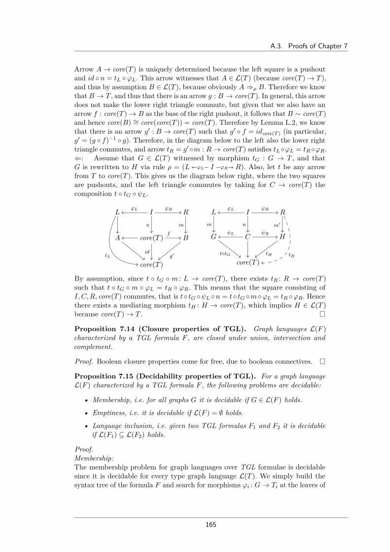
A.3. Proofs of Chapter 7

Arrow A→ core(T ) is uniquely determined because the left square is a pushoutand id n = tL ϕL. This arrow witnesses that A ∈ L(T ) (because core(T )→ T ),and thus by assumption B ∈ L(T ), because obviously A⇒ρ B. Therefore we knowthat B → T , and thus that there is an arrow g : B → core(T ). In general, this arrowdoes not make the lower right triangle commute, but given that we also have anarrow f : core(T )→ B as the base of the right pushout, it follows that B ∼ core(T )and hence core(B) ∼= core(core(T )) = core(T ). Therefore by Lemma L.2, we knowthat there is an arrow g′ : B → core(T ) such that g′ f = idcore(T ) (in particular,g′ = (g f)−1 g). Therefore, in the diagram below to the left also the lower righttriangle commutes, and arrow tR = g′m : R→ core(T ) satisfies tLϕL = tR ϕR.⇐: Assume that G ∈ L(T ) witnessed by morphism tG : G → T , and thatG is rewritten to H via rule ρ = (L ϕL− I −ϕR R). Also, let t be any arrowfrom T to core(T ). This gives us the diagram below right, where the two squaresare pushouts, and the left triangle commutes by taking for C → core(T ) thecomposition t tG ψL.

L

tL

..

IϕLoo

ϕR //

n

R

m

A

""

core(T ) f//oo

id

B

g′||

core(T )

L

m

IϕLoo

ϕR //

n

R

m′

tRpp

G

ttG ##

CψR //

ψLoo

H

tH

core(T )

By assumption, since t tG m : L → core(T ), there exists tR : R → core(T )such that t tG m ϕL = tR ϕR. This means that the square consisting ofI, C,R, core(T ) commutes, that is t tG ψL n = t tG mϕL = tR ϕR. Hencethere exists a mediating morphism tH : H → core(T ), which implies H ∈ L(T )because core(T )→ T .

Proposition 7.14 (Closure properties of TGL). Graph languages L(F )characterized by a TGL formula F , are closed under union, intersection andcomplement.

Proof. Boolean closure properties come for free, due to boolean connectives.

Proposition 7.15 (Decidability properties of TGL). For a graph languageL(F ) characterized by a TGL formula F , the following problems are decidable:

• Membership, i.e. for all graphs G it is decidable if G ∈ L(F ) holds.

• Emptiness, i.e. it is decidable if L(F ) = ∅ holds.

• Language inclusion, i.e. given two TGL formulas F1 and F2 it is decidableif L(F1) ⊆ L(F2) holds.

Proof.Membership:The membership problem for graph languages over TGL formulae is decidablesince it is decidable for every type graph language L(T ). We simply build thesyntax tree of the formula F and search for morphisms ϕi : G→ Ti at the leaves of

165

A. Proofs

the tree. Afterwards we pass the boolean results up to the root to decide whetherG ∈ L(F ) holds.Emptiness:In order to show whether L(F ) = ∅ holds, we transform F into disjunctivenormal form (DNF). It is sufficient to check whether all conjunctions of the form(T0 ∧ ¬T1 ∧ · · · ∧ ¬Tn) are unsatisfiable. We can assume that there is at most onepositive type graph in every conjunction, since type graph languages are closedunder conjunction/intersection (see Proposition 7.6). Furthermore we can evenassume that there is exactly one positive type graph, since we can always add TΛ

\

(the flower graph).Now we have:

L(T0 ∧ ¬T1 ∧ . . . ∧ ¬Tn) = ∅⇐⇒ L(T0 ∧ ¬(T1 ∨ . . . ∨ Tn)) = ∅⇐⇒ L(T0) ∩ L(T1 ∨ . . . ∨ Tn) = ∅⇐⇒ L(T0) ⊆ L(T1 ∨ . . . ∨ Tn)⇐⇒ L(T0) ⊆ L(T1) ∪ . . . ∪ L(Tn)⇐⇒ ∃ϕ : T0 → Tk for some index 1 ≤ k ≤ n

Therefore, it is sufficient to check whether for each conjunction (T0∧¬T1∧· · ·∧¬Tn)in the DNF of F , there exists a morphism ϕ : T0 → Tk for some 1 ≤ k ≤ n.Inclusion:The language inclusion problem can be reduced to the aforementioned emptinessproblem. To solve the language inclusion we use the following equivalence:

L(F1) ⊆ L(F2) ⇐⇒ L(F1 ∧ ¬F2) = ∅

Since the emptiness problem is decidable we can conclude that the languageinclusion problem is decidable as well.

166

A.4. Proofs of Chapter 8

A.4. Proofs of Chapter 8Lemma 8.13. The composition of two legal morphisms is a legal morphism.

Proof. Let ϕ1 : T1[M1] → T2[M2] and ϕ2 : T2[M2] → T3[M3] be two legal mor-phisms in the category of multiply annotated graphs. Since ϕ1 is legal we getthat for all (`1, u1) ∈ M1 there exists (`2, u2) ∈ M2 such that `2 ≤ Aϕ1(`1) andAϕ1(u1) ≤ u2 hold. Furthermore ϕ2 is legal and therefore we get that for all(`2, u2) ∈M2 there exists (`3, u3) ∈M3 such that `3 ≤ Aϕ2(`2) and Aϕ2(u2) ≤ u3hold as well. We define ϕ : T1[M1]→ T3[M3] to be the composed morphism withϕ = ϕ2 ϕ1 and due to the fact that A is a functor which preserves monotonicity,we get the following two inequalities:

`2 ≤ Aϕ1(`1)⇒ Aϕ2(`2) ≤ Aϕ2(Aϕ1(`1))⇒ `3 ≤ Aϕ2(`2) ≤ Aϕ2ϕ1(`1)⇒ `3 ≤ Aϕ(`1)

Aϕ1(u1) ≤ u2

⇒ Aϕ2(Aϕ1(u1)) ≤ Aϕ2(u2)⇒ Aϕ2ϕ1(u1) ≤ Aϕ2(u2) ≤ u3

⇒ Aϕ(u1) ≤ u3

Since both `3 ≤ Aϕ(`1) and Aϕ(u1) ≤ u3 hold, the morphism ϕ is legal.

Proposition 8.19 (Emptiness check for languages specified by multiplyannotated graphs). For a graph language L(T [M ]) characterized by a multiplyannotated type graph T [M ] over Bn the emptiness problem is decidable: L(T [M ]) =∅ iff M = ∅ or for each (`, u) ∈M there exists an edge e ∈ ET such that `(e) ≥ 1and (u(src(e)) = 0 or u(tgt(e)) = 0).

Proof.⇐: Assume that M = ∅, in this case L(T [M ]) is clearly empty as well. Assumethat there is an annotation (`, u) ∈M such that `(e) ≥ 1 and (u(src(e)) = 0 oru(tgt(e)) = 0) for some edge e ∈ ET . Then no graph can satisfy these lower andupper bounds, since we are forced to map at least one edge to e, but are notallowed to map any node to the source respectively target node. If this is true forall annotations, the language of the type graph must be empty.

⇒: Let L(T [M ]) = ∅ and we assume by contradiction that M 6= ∅ and there existsone annotation (`, u) ∈M such that for every edge e ∈ ET with `(e) ≥ 1 we haveu(src(e)) ≥ 1 and u(tgt(e)) ≥ 1).Now take T [`, u] and remove from T all edges and nodes x with u(x) = 0,

resulting in a graph T ′. If a node is removed all incident edges are removed as well.Note that in such a case only edges e with `(e) = 0 will be removed (due to thecondition above). Next define `′ = `|T ′ and u′ = u|T ′ . Due to the considerationsabove there exists a legal morphism (an embedding) T ′[`′, u′]→ T [`, u], since theremoved items had a lower bound of 0. Furthermore each remaining item has anupper bound of at least 1, i.e., it represents at least one node or edge.

Now construct a graph G from T ′ by proceeding as follows: starting with T ′ asbase graph, for every node v with `′(v) = k add k− 1 isolated nodes (zero isolatednodes if k = 0). For every edge e with `′(e) = k add k − 1 parallel edges betweensrc(e), tgt(e). Clearly, there is a morphism ϕ : G→ T ′ obtained by mapping everyitem to the item from which it originated.

167

A. Proofs

Mapping G[sG, sG] to T ′ via ϕ will give us an annotation Bnϕ(sG). By construc-tion, this annotation will coincide with the lower bound ` in all cases, but for thecase where there is a node v with `(v) = 0. In this case Bnϕ(sG)(v) = 1, but this iscovered by the upper bound which is at least 1. Hence ϕ : G[sG, sG]→ T ′[`′, u′] isa legal morphism, and by composing it with morphism T ′[`′, u′]→ T [`, u] we getG ∈ L(T [M ]), thus L(T [M ]) 6= ∅, as desired.

Proposition 8.20 (Language inclusion and legal morphisms). The exis-tence of a legal morphism ϕ : T1[M ]→ T2[N ] implies L(T1[M ]) ⊆ L(T2[N ]).

Proof. Every graph G ∈ L(T1[M ]) has a legal morphism ϕ′ : G[sG, sG]→ T1[M ].Whenever there exists a legal morphism ϕ : T1[M ] → T2[N ] between the twomultiply annotated type graphs, we obtain the morphism η : G[sG, sG]→ T2[N ]with η = ϕ ϕ′ which is legal due to Lemma 8.13. Therefore G ∈ T2[N ] holds andwe can conclude that L(T1[M ]) ⊆ L(T2[N ]) also holds.

Proposition 8.25 (Language inclusion and bounded pathwidth). Thelanguage inclusion problem is decidable for graph languages of bounded pathwidthcharacterized by multiply annotated type graphs over Bn. That is, given k ∈ Nand multiply annotated type graphs T1[M1] and T2[M2], it is decidable whetherL(T1[M1])≤k ⊆ L(T2[M2])≤k, with L(T [M ])≤k = G ∈ L(T [M ]) | pw(G) ≤ k.

Proof. The proof is given in Section 8.3.3.

Proposition 8.31 (Functoriality of C). Let two cospans c1 : J → G ← Kand c2 : K → H ← L be given and let idG : G→ G← G be the identity cospan.

The mapping CT [M ] : Cospanm(GraphΛ)→ Rel is a functor, i.e.1. CT [M ](idG) = idCT [M ](G)

2. CT [M ](c1; c2) = CT [M ](c1); CT [M ](c2)

Proof.1. The identity relation idCT [M ](G) consists of all pairs (i, i) with i ∈ CT [M ](G).Let the two states i, j ∈ CT [M ](G) be given with i = (f1 : G → T, b1) andj = (f2 : G → T, b2). The pair (i, j) is in the relation CT [M ](idG) if and onlyif there exists a morphism h : G → T such that, for all2 x ∈ T the equationb2(x) = b1(x) + |y ∈ (G \ id(G)) | h(y) = x| holds and the following diagramcommutes:

G G G

T

idG : G# G

f1

id

∃h

id

f2

Since the diagram commutes we obtain that f1 = f2 since f1 = h id = f2 holdsand for all x ∈ T the annotation functions b1 and b2 are equal due to the followingequation:

b2(x) = b1(x) + |y ∈ (G \ id(G)) | h(y) = x|2We write x ∈ T as an abbreviation for x ∈ VT ∪ ET .

168

A.4. Proofs of Chapter 8

= b1(x) + |y ∈ ∅ | h(y) = x| = b1(x) + 0 = b1(x)

This is equivalent to i = j and therefore for all i ∈ CT [M ](G) the following equationholds:

CT [M ](idG) = (i, j) ∈ CT [M ](G)× CT [M ](G) | i = j= idCT [M ](G)

Therefore CT [M ](idG) = idCT [M ](G) holds, as clearly all states (i, i) meet thecondition.In the following part let c1 : J−g1Gg2−K and c2 : K−g′1Hg′2−L be given andlet c = c1; c2 with c : J−j1g1G′j2g′2−L be the composed morphism of c1 and c2.

2.” ⊆ ” : Let (i, j) ∈ CT [M ](c1; c2) be given with i ∈ CT [M ](J) and j ∈ CT [M ](L) suchthat i = (f1 : J → T, b1) and j = (f3 : L→ T, b3). Then there exists a morphismh : G′ → T such that b3(x) = b1(x) + |y ∈ (G′ \ (j2 g′2)(L)) | h(y) = x| holdsfor all x ∈ T and the following diagram commutes:

J G K H L

G′

T

c1 : J # K c2 : K # L

f1

g1 g′1 g′2

j1 j2

∃h

g2

f3

To prove that (i, j) ∈ CT [M ](c1); CT [M ](c2) follows from the above properties, weneed to show that there exists a k ∈ CT [M ](K) where k = (f2 : K → T, b2) suchthat (i, k) ∈ CT [M ](c1) and (k, j) ∈ CT [M ](c2). Let f2 = h j1 g2 = h j2 g′1.Then there must exist two morphisms h1 : G → T , h2 : H → T such that thefollowing six properties hold:

(i, k) ∈ CT [M ](c1)

(1) h1 g1 = f1(2) h1 g2 = f2(3) ∀x ∈ T b2(x) = b1(x) + |y ∈ (G \ g2(K)) | h1(y) = x|

(k, j) ∈ CT [M ](c2)

(4) h2 g′1 = f2(5) h2 g′2 = f3(6) ∀x ∈ T b3(x) = b2(x) + |y ∈ (H \ g′2(L)) | h2(y) = x|

We define h1, h2 to be h1 = h j1 and h2 = h j2 which already satisfy thefollowing four properties:

(1) h1 g1 = h j1 g1 = f1 (4) h1 g′1 = h j2 g′1 = f2

(2) h1 g2 = h j1 g2 = f2 (5) h1 g′2 = h j2 g′2 = f3

We define b2 with respect to property (3), such that for all x ∈ T the equationb2(x) = b1(x) + |y ∈ (G \ g2(K)) | h1(y) = x| holds. It remains to show property(6): we conduct the proof by first showing the following equation (7) for all x ∈ T ,from which we can easily derive (6) afterwards:

169

A. Proofs

|y ∈ (G \ g2(K)) | h1(y) = x|+ |y ∈ (H \ g′2(L)) | h2(y) = x|=|y ∈ (G′ \ (j2 g′2)(L)) | h(y) = x| (7)

Since the morphisms j1 and j2 are both injective and G′ is the pushout objectof G and H over the common graph K we get that G′ = j1(G \ g2(K)) ] j2(H).Subtracting all elements x ∈ L that are being mapped into H on both sides ofthe equation, we get that G′ \ (j2 g′2)(L) = j1(G \ g2(K)) ] j2(H \ g′2(L)) holdsas well. Using this fact we can prove equation (7) which holds for all x ∈ T :

|y ∈ (G′ \ (j2 g′2)(L)) | h(y) = x|=|y ∈

(j1(G \ g2(K)) ] j2(H \ g′2(L))

)| h(y) = x|

=|y ∈ j1(G \ g2(K)) | h(y) = x ] y ∈ j2(H \ g′2(L)) | h(y) = x|=|y ∈ G \ g2(K) | (h j1)(y) = x ] y ∈ H \ g′2(L) | (h j2)(y) = x|=|y ∈ G \ g2(K) | h1(y) = x ] y ∈ H \ g′2(L) | h2(y) = x|=|y ∈ (G \ g2(K)) | h1(y) = x|+ |y ∈ (H \ g′2(L)) | h2(y) = x|

Using equation (7) we conclude that property (6) always holds for all x ∈ T :

b3(x) = b1(x) + |y ∈ (G′ \ (j2 g′2)(L)) | h(y) = x|= b1(x) + |y ∈ (G \ g2(K)) | h1(y) = x|+ |y ∈ (H \ g′2(L)) | h2(y) = x|= b2(x) + |y ∈ (H \ g′2(L)) | h2(y) = x|

Therefore (i, j) ∈ CT [M ](c1); CT [M ](c2) holds as well.

2.” ⊇ ” : Let two pairs (i, k) ∈ CT [M ](c1) and (k, j) ∈ CT [M ](c2) be given withi ∈ CT [M ](J), k ∈ CT [M ](K) and j ∈ CT [M ](L) such that i = (f1 : J → T, b1),k = (f2 : K → T, b2) and j = (f3 : L → T, b3). Then in addition there exist twomorphisms h1 : G→ T and h2 : H → T such that for all x ∈ T the two equationsb2(x) = b1(x) + |y ∈ (G \ g2(K)) | h1(y) = x| andb3(x) = b2(x) + |y ∈ (H \ g′2(L)) | h2(y) = x| both hold and the followingdiagram commutes:

J G K H L

T

c1 : J # K c2 : K # L

f1

g1 g′1

f2

g′2

∃h1 ∃h2

g2

f3

To prove that (i, j) ∈ CT [M ](c1; c2) is satisfied from the properties gained so far,we need to show that b3(x) = b1(x) + |y ∈ (G′ \ (j2 g′2)(L)) | h(y) = x| holdsand that there exists a morphism h : G′ → T such that the following diagramcommutes:

170

A.4. Proofs of Chapter 8

J G K H L

G′

T

(PO)

c1 : J # K c2 : K # L

f1

g1 g′1

j1 j2

g′2

h1

∃h

h2

g2

f3

The morphism h : G′ → T exists and is unique due to the universal property ofpushouts. From the two equations b2(x) = b1(x) + |y ∈ (G \ g2(K)) | h1(y) = x|and b3(x) = b2(x) + |y ∈ (H \ g′2(L)) | h2(y) = x| we can derive the followingequation which holds for all x ∈ T :

b3(x) = b1(x) + |y ∈ (G \ g2(K)) | h1(y) = x|+ |y ∈ (H \ g′2(L)) | h2(y) = x|

Using the results of equation (7) from the previous proof direction, we directlycan conclude that b3(x) = b1(x) + |y ∈ (G′ \ (j2 g′2)(L)) | h(y) = x| also holdsand therefore (i, j) ∈ CT [M ](c1; c2) holds, which completes this proof.

Proposition 8.32 (Language of C). Let the multiply annotated type graphT [M ] (over Bn) and the automaton functor C : Cospanm(GraphΛ) → Rel forT [M ] be given. Then LC = L(T [M ]) holds, i.e. for a graph G we have G ∈ L(T [M ])if and only if there exist states i ∈ I ⊆ C(∅) and f ∈ F ⊆ C(∅) such that(i, f) ∈ C(c), where c : ∅→ G← ∅.

Proof. We will prove the following equality:

G ∈ L(T [M ]) ⇐⇒ ∃i ∈ I ⊆ C(∅), ∃j ∈ F ⊆ C(∅) : (i, j) ∈ C(c)

"⇒": Since (c : ∅ → G ← ∅) ∈ L(T [M ]) holds, there exists a legal morphismϕ : G→ T and a pair of multiplicities (`, u) ∈M such that ` ≤ Bnϕ(sG) ≤ u holds.Let (i, j) be i = (f1 : ∅ → T, 0) ∈ I and j = (f2 : ∅ → T,Bnϕ(sG)) ∈ F whichare clearly in the relation C(c), i.e. (i, j) ∈ C(c) since for all x ∈ T the equationBnϕ(sG)(x) = 0 + |y ∈ (G \ g2(∅)) | ϕ(y) = x| = |y ∈ G | ϕ(y) = x| holds bydefinition and the following diagram commutes:

∅ G ∅

T

c : ∅# ∅

f1

g1

ϕ

g2

f2

"⇐": There exists i ∈ I ⊆ C(∅) and j ∈ F ⊆ C(∅) with i = (f1 : ∅ → T, 0) andj = (f2 : ∅→ T, b) such that (i, j) ∈ C(c) holds. Therefore, there exists a pair ofmultiplicities (`, u) ∈M with ` ≤ b ≤ u and we get that there exists a morphismϕ : G→ T such that the following diagram commutes:

171

A. Proofs

∅ G ∅

T

c : ∅# ∅

f1

g1

∃ϕ

g2

f2

For all x ∈ T the following equation holds:

b(x) = 0 + |y ∈ (G \ g2(∅)) | ϕ(y) = x|= |y ∈ G | ϕ(y) = x|= Bnϕ(sG)(x)

From ` ≤ b ≤ u we can infer that ϕ : G→ T is a legal morphism due to the factthat ` ≤ Bnϕ(sG) ≤ u holds as well, and therefore G ∈ L(T [M ]).

Proposition 8.33 (Closure under intersection). Graph languages specifiedby annotated graphs are closed under intersection.

Proof. Let two multiply annotated type graphs T1[M1] and T2[M2] be given. LetT1 × T2 be the usual product graph in the underlying category GraphΛ.

We now consider the multiply annotated type graph (T1× T2)[N ] where the setof annotations N is defined as follows:

N = (`, u) | `, u ∈ A(T1 × T1) such thatπ1 : (T1 × T2)[`, u]→ T1[M1] is legal andπ2 : (T1 × T2)[`, u]→ T2[M2] is legal

Therefore for each (`, u) ∈ N there exist (`1, u1) ∈M1 and (`2, u2) ∈M2 suchthat the following four properties hold:

Aπ1(`) ≥ `1 Aπ1(u) ≤ u1

Aπ2(`) ≥ `2 Aπ2(u) ≤ u2

(T1 × T2)[N ]

π1xx

π2&&

T1[M1] T2[M2]

We will now prove the following equality:

L(T1[M1]) ∩ L(T2[M2]) = L((T1 × T2)[N ])

⊆: Let G ∈ L(T1[M1]) ∩ L(T2[M2]). Then there exist two legal morphismsϕ1 : G[sG, sG]→ T1[M1] and ϕ2 : G[sG, sG]→ T2[M2]. Due to the universal prop-erty of pullbacks in the underlying category GraphΛ, there exists a unique graphmorphism η : G→ T1 × T2 such that the following diagram commutes:

G[sG, sG]

ϕ1

ϕ2

η

(T1 × T2)[N ]

π1xx

π2&&

T1[M1] T2[M2]

172

A.4. Proofs of Chapter 8

Since ϕi = πi η with i ∈ 1, 2 is a legal morphism, there exist annotations(`1, u1) ∈M1 and (`2, u2) ∈M2 such that the following inequalities hold:

`1 ≤ Aϕ1(sG) = Aπ1η(sG) = Aπ1(Aη(sG)) ≤ u1

`2 ≤ Aϕ2(sG) = Aπ2η(sG) = Aπ2(Aη(sG)) ≤ u2

Therefore the pair (Aη(sG),Aη(sG)) is one of the annotations in N and we canconclude that G ∈ L((T1 × T2)[N ]) holds.

⊇: We now assume G ∈ L((T1×T2)[N ]) holds. Then there exists a legal morphismη : G[sG, sG] → (T1 × T2)[N ] with a pair of annotations (`, u) ∈ N such that itholds that ` ≤ Aη(sG) ≤ u. For each such pair (`, u) ∈ N we have two legalmorphisms π1 : (T1 × T2)[`, u] → T1[M1] and π2 : (T1 × T2)[`, u] → T2[M2], byconstruction. We obtain two morphisms ϕ1 : G[sG, sG]→ T1[M1] with ϕ1 = π1 ηand ϕ2 : G[sG, sG]→ T2[M2] with ϕ2 = π2 η, which are legal due to Lemma 8.13.Therefore we can conclude that G ∈ (L(T1[M1]) ∩ L(T2[M2])).

To prove Proposition 8.34 we need the following two Lemma L.3 and Lemma L.5alongside a reduction operation given in Definition A.4.

Lemma L.3. Assume that we are working with annotations over Bn.Let i : A[M ] → T [N ] and ϕ : G[sG, sG] → T [N ] betwo legal graph morphisms where i is injective. Let(`, u) ∈M be one of the double multiplicities of thegraph A. Whenever Bnϕ(sG) ≤ Bni (u), we can deducethat there exists a graph morphism ζ : G→ A withi ζ = ϕ, i.e. the diagram commutes.

G[sG, sG]ϕ

ζ

yy

A[M ] //i// T [N ]

Proof. The morphisms ζ exists if all elements of the form ϕ(x) with x ∈ Gare in the range of i. For such an x we have 1 = sG(x) ≤ Bnϕ(sG)(ϕ(x)), sinceBnϕ(sG)(ϕ(x)) is the sum of the sG-annotations of all preimages of x. FurthermoreBnϕ(sG)(ϕ(x)) ≤ Bni (u)(ϕ(x)). But Bni (u)(y) = 0 for all y ∈ T that are not in therange of i, since the empty sum evaluates to 0. But since Bni (u)(ϕ(x)) ≥ 1, wecan conclude that ϕ(x) has a preimage under i.

In addition, we need the concept of reduction: the reduction operation shiftsannotations over morphisms in the reverse direction.

Definition A.4 (Reduction). Let A be an (annotation) functor. For a mor-phism ϕ : G→ G′ and a monoid element a′ ∈ A(G′) we define the reductionof a′ to G as follows:

redϕ(a′) =∨a | Aϕ(a) ≤ a′.

In the case of multiplicities, the reduction operator satisfies the needed propertygiven in the next Lemma L.5. Further annotation properties which depend on thereduction operation are given in Definition 10.8.

173

A. Proofs

Lemma L.5. Assume that we are working with annotations over Bn. Ifϕ : G→ H is injective, we obtain the following equality for all x ∈ G:

redϕ(a′)(x) = a′(ϕ(x))

Furthermore, if ϕ : G → G′ is injective, it holds that redϕ(Bnϕ(a)) = a forevery a ∈ Bn(G).

Proof. Straightforward from the definition of multiplicities (Definition 8.6).

Proposition 8.34 (Closure under union). Graph languages specified by mul-tiply annotated graphs over functor Bn are closed under union.

Proof. Let two multiply annotated type graphs T1[M1] and T2[M2] be given. LetT1⊕T2 be the usual coproduct graph in the underlying category GraphΛ, togetherwith the embedding morphisms i1 : T1 → T1 ⊕ T2 and i2 : T2 → T1 ⊕ T2:

T1[M1]&&

i1 &&

T2[M2]xx

i2xx

T1 ⊕ T2[N ]

We define the set of annotations N for (T1 ⊕ T2)[N ] using the following two sets:

N1 = (Bni1(`1),Bni1(u1)) | (`1, u1) ∈M1N2 = (Bni2(`2),Bni2(u2)) | (`2, u2) ∈M2

Finally we define N = N1 ∪N2.

By this definition, for all elements x ∈ T1 and for all (`, u) ∈ M1 there exists(`1, u1) ∈ N1 such that Bni1(`)(i1(x)) = `1(i1(x)) and Bni1(u)(i1(x)) = u1(i1(x)).This makes i1 a legal morphism since N1 ⊆ N . The same holds for i2 analogously.We will now prove the following equality:

L(T1[M1]) ∪ L(T2[M2]) = L((T1 ⊕ T2)[N ])

⊆: Let G ∈ (L(T1[M1]) ∪ L(T2[M2])). Then there exists at least one legalmorphism ϕ1 : G[sG, sG] → T1[M1] or ϕ2 : G[sG, sG] → T2[M2]. We assume thatG ∈ L(T1[M1]). Let η : G[sG, sG]→ (T1 ⊕ T2)[N ] be the composed morphism ofi1 and ϕ1 with η = i1 ϕ1. Then η is legal due to Lemma 8.13 and thereforeG ∈ L((T1 ⊕ T2)[N ]) holds. The proof for the case where G ∈ L(T2[M2]) works inthe same way.⊇: We now assume G ∈ L((T1 ⊕ T2)[N ]). Then, there exists a legal morphism

η : G[sG, sG]→ (T1 ⊕ T2)[N ] with an annotation (`, u) ∈ N and ` ≤ Bnη (sG) ≤ u.For each (`, u) ∈ N , we know that the pair belongs to N1 or N2. Assume that(`, u) ∈ N1. Then there exists (`1, u1) ∈ M1 such that ` = Bni1(`1), u = Bni1(u1).Hence Bnη (sG) ≤ u = Bni1(u1). From Lemma L.3 it follows that there exists a graphmorphism ζ1 : G→ T1 with η = i1 ζ1 such that the following diagram commutesin the underlying category GraphΛ:

174

A.4. Proofs of Chapter 8

G[sG, sG]

ζ1xx

η

T1[M1]&&

i1 &&

T2[M2]xx

i2xx

(T1 ⊕ T2)[N ]

We need to prove that ζ1 is a legal graph morphism in the category of multiplyannotated graphs. We get that Bnη (sG) = Bni1ζ1

(sG) = Bni1(Bnζ1(sG)) and since i1

is injective, the following inequality holds due to the fact that redϕ is monotoneand redϕ(Bnϕ(a)) = a holds for every a ∈ Bn(G), whenever ϕ is injective (cf.Lemma L.5):

Bni1(`1) ≤ Bnη (sG) ≤ Bni1(u1)⇒ Bni1(`1) ≤ Bni1(Bnζ1(sG)) ≤ Bni1(u1)⇒ redi1(Bni1(`1)) ≤ redi1(Bni1(Bnζ1(sG))) ≤ redi1(Bni1(u1))⇒ `1 ≤ Bnζ1(sG) ≤ u1

Therefore ζ1 : G[sG, sG]→ T1[M1] is a legal morphism and we can conclude thatG ∈ L(T1[M1]). For a legal morphism η : G[sG, sG] → (T1 ⊕ T2)[N ] with a pair(`, u) ∈ N2 we get a similar proof which shows that G ∈ L(T2[M2]). Summarizing,in all cases G ∈ (L(T1[M1]) ∪ L(T2[M2])) holds.

Proposition 8.35 (Non-closure under complement). Graph languages speci-fied by multiply annotated graphs over functor Bn are not closed under complement.

Proof. We show that there exist languages specified by annotated type graphs forwhich there exists no finite type graph which specifies the complement language.For a counterexample we use the multiply annotated type graph T [`, u] (depictedbelow, on the left) and we observe that for the graph H below on the right, itholds that H ∈ L(T [`, u]):

T [`, u] =[1,∗] [1,1]

A [1,1]A [1,∗] H = AA

Now assume, that graph languages specified by annotated type graphs are closedunder complement and let L(T ′[M ]) = L(T [`, u]) be the complement language,represented by a multiply annotated type graph T ′[M ]. We consider the sub-language L′ ⊂ L(T ′[M ]) of the complement language which contains all graphsGn with a fixed number n ∈ N0 of discrete A-labeled loops, that is:

L′ =∅(G0)

,(G1)

A

,(G2)

A A

,(G3)

A A A

, . . .

175

A. Proofs

Indeed for n ∈ N0 and a graph Gn ∈ L′ we obtain that Gn /∈ L(T [`, u]) sincethere exists no morphism which can fulfill the lower bound of the right node inT [`, u]. Therefore L′ ⊂ L(T [`, u]) holds. We show that there can not exist a finitegraph T ′[M ] with the following two properties:

1. for all n ∈ N0 and Gn ∈ L′, there exists an annotation (`n, un) ∈ M suchthat there exists a legal morphism ϕn : Gn[sGn , sGn ]→ T ′[`n, un].

2. for all graphs H ′ ∈ L(T [`, u]) we have that H ′ /∈ L′.

We first show that given any n ∈ N0, whenever there exists an annotation(`n, un) ∈ M and a legal morphism ϕn : Gn[sGn , sGn ] → T ′[`n, un] which fulfilsproperty (1), where ϕn is non-injective, then property (2) becomes unsatisfiable.

Assume that the legal morphism ϕn : Gn[sGn , sGn ]→ T ′[`n, un] is non-injectiveand maps at least two nodes of Gn (denoted by n1, n2) to the same target node tin T ′[`n, un]. Then the upper bound un(t) must be greater than or equal to 2.Then, there exists a graph H ′ ∈ L(T [`, u]) that allows a legal morphism into

T ′[`n, un] which can be constructed in the following way: Let H ∈ L(T [`, u]) bethe graph defined earlier. Then construct H ′ as the disjoint union of H and Gn−2.The graph H ′ is an element of L(T [`, u]) since we can map all additional n− 2nodes with an A-labeled loop to the left node in T [`, u].Now, in order to show that H ′ ∈ L(T ′[`n, un]), consider the two nodes n1 and

n2 of Gn which are both mapped to t via ϕn. The two nodes of H can both bemapped to t since the upper bound of t admits such a morphism. The formernon-looping edge and the loop are mapped to the target loops of n1 and n2respectively. Now map the remaining n− 2 nodes with loops in H ′ by mimickingthe mapping of the nodes with loops of Gn via ϕn, except n1 and n2. This givesus the same annotations on T ′ as those generated by ϕn, which are consequentlywithin the bound [`n, un].

Hence the morphism from H ′ to T ′[`n, un] is legal, H ′ ∈ L(T ′[`n, un]) holds andtherefore property (2) does not hold. We conclude that all ϕn must be injectiveto guarantee that there exists no graph H ′ ∈ L(T [`, u]) that is also contained inthe complement language.However, to ensure that the morphisms ϕn : Gn → T ′[`n, un] are injective for

any n ∈ N0, the type graph T ′ would need to consist of at least n different nodeswith A-labeled loops attached to them. Since there are infinitely many graphs Gnthere can not exist a type graph T ′[M ] with a finite number of nodes. We concludethat there exists no finite graph T ′[M ] specifying the complement language ofL(T [`, u]).

176

A.5. Proofs of Chapter 9

A.5. Proofs of Chapter 9The following result is known, we give the proof sketch for the convenience of thereader, since the construction plays an important role in Chapter 9 and Chapter 10.

Proposition 9.15 (Final pullback complements, subobject and partialmap classifiers). Let C be a category with finite limits. Then the following areequivalent:

(1) C has a subobject classifier true : 1 Ω and final pullback complements foreach pair of arrows I α→ L

m G where m is a mono;

(2) C has a partial map classifier (F : C→ C, η : IdC.→ F).

Sketch. We just report the corresponding constructions from [DT87], omittingthe proofs of the relevant properties.

(1) ⇒ (2) The component ηY : Y F(Y ) of the natural transformation η atobject Y ∈ C is obtained as the final pullback complement of Y !Y→ 1 true

Ω,as shown in Diagram (A.6).

(2) ⇒ (1) We first observe that, given a partial map classifier (F , η), the subob-ject classifier is obtained as 1 η1

F(1).

We show how to construct a final pullback complement: Given I α→ Lm G,

consider the components of the natural transformation at I and L, andarrow F(α) : F(I) → F(L), as in (A.7). The mono L m

G can be seenas a partial map G

m L

idL L from G to L, and this induces a unique

arrow ϕ(m, idL) making the square a pullback. Now let G h← P → F(I) bethe pullback of G ϕ(m,idL)−→ F(L) F(α)←− F(I). It is easy to see that there isan induced mono (mediating arrow) n : I P and it can be shown thatI

n P h→ G is the final pullback complement of I α→ L

m G.

Y

!Y

//ηY // F(Y )

χηY

1 // true// Ω

(FPBC)

(A.6)

L

m

""

ηL ""

Iαoo

η

!!

ηI

!!

L??

idL

??

m

F(L) F(I)F(α)

oo

Gϕ(m,idL)

<<

Ph

oo

==

(A.7)

Proposition 9.19 (Existence of materialization). Let ϕ : L → A be anarrow in C, and let ηϕ : ϕ→ F(ϕ), with F(ϕ) : A→ A, be the partial map classifierof ϕ in the slice category C↓A (which also is a topos)3. Then L ηϕ→ A

F(ϕ)→ A isthe materialization of ϕ, hence 〈ϕ〉 = A.

Proof. Let L m X α→ A be an object of Matϕ, i.e. a factorization such that

ϕ = α m. Note that this defines a partial map (m, idL) : α ϕ in C ↓ A

177

A. Proofs

consisting of the span α m ϕ

idL→ ϕ. Since ηϕ : ϕ → F(ϕ) is the component ofthe partial map classifier, there exists a unique arrow ϕ(m, idL) : X → 〈ϕ〉 fromα : X → A to F(ϕ) : 〈ϕ〉 → A for which the left square in the following diagramis a pullback and the right triangle commutes. The latter holds since ϕ(m, idL) isan arrow in the slice category.

L

ϕ%%

// m //

idL

X

ϕ(m,idL)

α // A

L // ηϕ// 〈ϕ〉

(PB)

F(ϕ)

NN

Corollary 9.20 (Construction of the materialization). Let ϕ : L → A bean arrow of C and let trueA : A A× Ω be the subobject classifier in the slicecategory C ↓ A mapping from idA : A→ A to theprojection π1 : A×Ω→ A (see also Fact 9.11). Thenthe terminal object L

ηϕ 〈ϕ〉 ψ→ A in the materializa-

tion category consists of the arrows ηϕ, ψ = π1 χηϕ,where L

ηϕ 〈ϕ〉

χηϕ→ A× Ω is the final pullback com-plement of L ϕ→ A

trueA A× Ω.

L

ϕ

//ηϕ// 〈ϕ〉

χηϕ

ψ

""

A //trueA// A× Ω π1

//

(FPBC)

A

Proof. Straightforward from Propositios 9.15 and 9.19 (and the fact that finalpullback complements in the slice category correspond to those in the base category[Löw10]).

Proposition 9.22 (Language of the materialization). Let ϕ : L→ A be anarrow in C and let L

ηϕ 〈ϕ〉 → A be the corresponding materialization. Then

L(Lηϕ 〈ϕ〉) = L mL

X | ∃ψ : (X → A). (ϕ = ψ mL).

Proof. We show that the two sets are included into each other:

• (⊆) Given the materialization Lηϕ 〈ϕ〉 g→ A of a C-arrow ϕ : L → A,

let L mL X be a mono in the language L(L

ηϕ 〈ϕ〉), i.e., it holds that

(L mL X) ∈ L(L

ηϕ 〈ϕ〉). Spelling out Definition 9.17 we obtain the

following commuting diagram where the square is a pullback:

L //mL //

idL

X

f

ψ

L

ϕ

99//ηϕ// 〈ϕ〉

(PB)g// A

Then we define ψ = g f : X → A and observe that the following equationholds:

ϕ = g ηϕ = g ηϕ idL = g f mL = ψ mL

178

A.5. Proofs of Chapter 9

• (⊇) Let the mono L mL X be a factorization of the C-arrow ϕ : L→ A, i.e.

there exists an arrow ψ : X → A such that ϕ = ψ mL. By terminality ofthe materialization L

ηϕ 〈ϕ〉 → A there exists an arrow X → 〈ϕ〉 such that

the following diagram commutes and the square is a pullback:

L //mL //

idL

X

ψ

L

ϕ

99//ηϕ// 〈ϕ〉

(PB)

// A

Therefore (L mL X) ∈ L(L

ηϕ 〈ϕ〉) holds.

Proposition 9.25 (Construction of the rewritable materialization). Letϕ : L→ A be an arrow and let ϕL : I L be a mono of C. Then the rewritablematerialization of ϕ w.r.t. ϕL exists and can be constructed as the followingfactorization L nL

〈〈ϕ,ϕL〉〉ψα−→ A of ϕ. In the diagram shown below to the left, F

is obtained as the final pullback complement of I ϕL L 〈ϕ〉, where L 〈ϕ〉 ψ→ A

is the materialization of ϕ (Definition 9.18). Next the diagram shown below tothe right L nL

〈〈ϕ,ϕL〉〉β F is the pushout of the span L ϕL

I F and α is theresulting mediating arrow.

Lϕ

~~

I

ooϕLoo

A 〈ϕ〉ψoo F

(FPBC)

oooo

(A.8) Lϕ

~~

L

nL

ooidLoo I

ooϕLoo

A 〈ϕ〉ψoo 〈〈ϕ,ϕL〉〉ooαoo Foo

βoo uuii

(PO)

(A.9)

Proof. First note that in Diagram (A.8), F is obtained as the final pullbackcomplement of I ϕL

L 〈ϕ〉, where L 〈ϕ〉 ψ→ A is the materialization of ϕ(Definition 9.18). Arrow I F is monic because it is reflected, while F 〈ϕ〉 ismonic by properties of final pullback complements since ϕL : I L is monic (see[CH+06]).In Diagram (A.9) L nL

〈〈ϕ,ϕL〉〉β F is the pushout of the span L ϕL

I F .Since the right square is a pushout and the outer square commutes, there is aunique arrow α : 〈〈ϕ,ϕL〉〉 → 〈ϕ〉 making the diagram commute. Note that arrowL

nL 〈〈ϕ,ϕL〉〉 is indeed monic, as pushouts preserve monos in a topos, and α is

monic because topoi have effective unions. Therefore the rewritable materializationL

nL 〈〈ϕ,ϕL〉〉 ψα−→ A is an object of Matϕ, and clearly it is also an object of

the subcategory MatϕLϕ , as by Diagram (A.9) I ϕL L

nL 〈〈ϕ,ϕL〉〉 has a pushout

complement.We next prove that the left square of Diagram (A.9) is a pullback, to show that

α is the unique arrow from the rewritable materialization to the materializationin Matϕ. Let the diagram below to the right be given. We already know that theinner square commutes and therefore ηϕ idL = α nL. We will now show thatthe pullback property for the inner square holds:

179

A. Proofs

For any other objectX and two arrows f : X → L andg : X → 〈〈ϕ,ϕL〉〉 where the outer square commutes,there exists a unique arrow h : X → L such thatf = idLh and g = nLh. It is clear that h = f by thisassumption. Since α is a mono, it is a left-cancellativearrow e.g. for any two arrows f1, f2 : X → 〈〈ϕ,ϕL〉〉we get that α f1 = α f2 implies f1 = f2.

Xh

$$

f

""

g

$$

L

nL

//idL // L

ηϕ

〈〈ϕ,ϕL〉〉 // α // 〈ϕ〉

(PB)

We obtain the following equation: α g = ηϕ f = ηϕ idL h = α nL h,which implies that g = nL h since α is a mono. Hence the inner square is apullback. Now let L p

Xq→ A be an object of MatϕLϕ , i.e. a factorization of ϕ

such that the pushout complement of I ϕL L

p X exists, and let I C X be

such a pushout complement. Then the following Diagram (A.10) commutes, whereg : X → 〈ϕ〉 is the unique arrow making the left square a pullback by finality ofthe materialization, and the right square is a pullback because it is a pushoutalong a mono. From the pasting lemma (pullback version) we can conclude thatthe composed square is a pullback as well.

Lϕ

~~

ηϕ

L

p

oooo I

ooϕLoo

A 〈ϕ〉ψoo X

q

ff

goo

(PB)

Coooo

(PB)

(A.10)

InnϕL

L

ηϕ

I

ooϕLoo

=

〈ϕ〉 Foooo

(FPBC)

C

γ

__\\

(A.11)

Combining the outer pullback of Diagram (A.10) with the final pullback com-plement of Diagram (A.8) we get Diagram (A.11). By Definition 9.13 there existsa unique arrow γ such that the diagram commutes (especially the lower triangleand the square to the right).

By composing the arrows γ : C → F from Diagram (A.11) and β : F 〈〈ϕ,ϕL〉〉from Diagram (A.9) we get the arrow c = β γ : C → 〈〈ϕ,ϕL〉〉 shown in thecommuting Diagram (A.12) where the right square is a pushout. The universalproperty of pushouts gives us a unique mediating arrow δ : X → 〈〈ϕ,ϕL〉〉. Toshow that δ defines an arrow in Matϕ from L

p X

q→ A to the rewritablematerialization L nL

〈〈ϕ,ϕL〉〉ψα−→ A we need to prove that q = ψ α δ (which is

easily checked by diagram chasing) and that the left square is a pullback.

L

nL

L

p

oooo I

oooo

〈〈ϕ,ϕL〉〉 Xδoo

(?)

Coooo

c

gg

(PO)

(A.12) L

L

nL

oooo L

p

oooo

〈ϕ〉 〈〈ϕ,ϕL〉〉ooαoo

(PB)

Xδoo

g

gg

(PB)

(A.13)

In order to show that the square marked (?) is a pullback we consider Dia-gram (A.13). The left square is a pullback as we have shown earlier, and theouter square is a pullback by Diagram (A.10). From the pasting lemma (pullbackversion) we can conclude that the right square is a pullback. Also note that thediagram clearly commutes as the three arrows at the bottom are all unique.

180

A.5. Proofs of Chapter 9

Proposition 9.27 (Language of the rewritable materialization). Assumethere is a production p : L ϕL

IϕR R and let L nL

〈〈ϕ,ϕL〉〉 be the match for therewritable materialization for ϕ and ϕL. Then we have

L(L nL 〈〈ϕ,ϕL〉〉) = L mL

X | ∃ψ : (X → A). (ϕ = ψ mL ∧Xp,mL=⇒)

where X p,mL=⇒ denotes that the object X can be rewritten.

Proof. We show that the two sets of arrows are included in one another:

• (⊇) Let L mL X such that there exists an arrow ψ with ϕ = ψ mL and

Xp,mL=⇒ . Then L

mL X

ψ→ A is an object of the materialization categoryof rewritable objects (since the production can be applied, the pushoutcomplement exists) and we obtain a unique arrow X → 〈〈ϕ,ϕL〉〉 that createsa pullback L,L,X,A. Hence mL ∈ L(L nL

〈〈ϕ,ϕL〉〉).

• (⊆) Assume that mL ∈ L(L nL 〈〈ϕ,ϕL〉〉). This implies the existence of an

arrow X → 〈〈ϕ,ϕL〉〉 such that the left square in Diagram (A.14) is a pullback.The arrow ψ : X → A is given by composing X → 〈〈ϕ,ϕL〉〉

α 〈ϕ〉 → A and

by retracing the construction of 〈〈ϕ,ϕL〉〉 (see Proposition 9.25) it can beshown that ϕ = ψ mL.Furthermore we constructed the outer square in Diagram (A.14) as a pushout,which is therefore also a pullback.

L

L

mL

oooo I

ooϕLoo

〈〈ϕ,ϕL〉〉 Xoo

(PB)

Fwwjj

(A.14)InnmLϕL

X

C

oooo

=

〈〈ϕ,ϕL〉〉 Foooo

(PB) =

(A.15)

Now we take the pullback of X → 〈〈ϕ,ϕL〉〉 F and obtain the pullbackobject C with the corresponding arrows (See Diagram (A.15)). Since theouter square commutes, we get a unique arrow I C due to the property ofpullbacks. Note that I C is a mono since I F is a mono. All we needto show is that C is the pushout complement for our rewritable object X.

In order to show that it is a pushout we considerthe diagram to the right. The bottom square is aVan Kampen square4, furthermore the left squareis trivially a pullback, the front square is a pullbackaccording to Diagram (A.14) and the right squareis a pullback by construction (see Diagram (A.15)).Then it follows from classical pullback splittingthat the back square is also a pullback. Finally itfollows from the properties of adhesive categoriesthat the top square is a pushout.

I // //

Czz

zz

L // //

X

I // //

F

L // // 〈〈ϕ,ϕL〉〉

4Since every topos is adhesive, the Van Kampen square property holds. For more details see[LS05].

181

A. Proofs

Therefore X can be rewritten. The existence of the pushout complement isguaranteed using the described construction. This completes the proof.

Proposition 9.28 (Rewriting abstract matches). Let a match nL : L Aand a production p : L I R be given. Assume that A is rewritten along thematch nL, i.e., (L nL

A) p⇒ (R nR B). Then

L(R nR B) = R mR

Y | ∃(L mL X) ∈ L(L nL

A) :((L mL X) p⇒ (R mR

Y ))

Proof.

• (⊆) Assume that (L nL A) p⇒ (R nR

B) and let mR ∈ L(R nR B) where

mR : R Y . That is we have the diagram below, where the bottom squaresare pushouts and the remaining squares are pullbacks (the squares in theback are actually pushouts as well).

L

idL

Ioooo // //

idI

R

idR

mR

Y

L

nL

Ioooo // //

R

nR

A Coooo // // B

Now take the pullback of C B and Y → B, obtaining Z, which gives usI → Z as mediating arrow into the pullback object (see diagram below). Inthe right cube the right square is a pullback, the back square is triviallypullback and the front square is a pullback by construction. This meansthat the left square is also a pullback by pullback splitting. Due to the VanKampen square property this implies that the top square is a pushout. Sinceall pushouts along monos are pullbacks in adhesive categories, the arrowI → Z must be a mono.Finally, take the pushout of I Z and I L, resulting in X, which giveus X → A as a mediating arrow.

L

idL

mL

Ioooo // //

idI

R

idR

mR

X

Zoooo // //

Y

L

nL

Ioooo // //

R

nR

A Coooo // // B

This illustrates that (L mL X) p⇒ (R mR

Y ). Since in the left cube theback square is trivially a pullback and the right square is a pullback as well(see argument above), the front and left squares are pullbacks as well. Thisimplies that (L mL

X) ∈ L(L nL A), as required.

182

A.5. Proofs of Chapter 9

• (⊇) Assume that (L mL X) p⇒ (R mR

Y ) and (L mL X) ∈ L(L nL

A)hold. Together with the fact that (L nL

A) p⇒ (R nR B), this results in

the diagram below (without the dotted arrows), where the top and bottomsquares of the cubes are all pushouts and the vertical squares are pullbacks.

L

idL

mL

Ioooo // //

idI

R

idR

mR

X

Zoooo // //

Y

L

nL

Ioooo // //

R

nR

A Coooo // // B

Due to the Van Kampen square property and the fact that pushout com-plements of mono arrows are unique, the object Z can be constructed intwo ways: either by taking the pullback of X → A and C A or by takingthe pushout complement of I L, L X as shown above. Hence theremust be an arrow Z → C arising from the pullback and the front and rightsquare of the left cube are pullbacks as well.Now the arrow Y → B is obtained as a mediating arrow into the pushoutobject and the front and right faces of the right cube are again pullbacks.This implies that (R mR

Y ) ∈ L(R nR B), as desired.

Corollary 9.30 (Co-match language of the rewritable materialization).Let ϕ : L→ A and a production p : L ϕL

IϕR R be given. Assume that 〈〈ϕ,ϕL〉〉 is

obtained as the rewritable materialization of ϕ and ϕL with the match L nL 〈〈ϕ,ϕL〉〉

(see Proposition 9.25) and let (L nL 〈〈ϕ,ϕL〉〉) p⇒ (R nR

B). ThenL(R nR

B) = R mR Y |∃(L mL

X), (X ψ→ A) :(ϕ = ψ mL ∧ (L mL

X) p⇒ (R mR Y )

)

Proof. Straightforward from Propositions 9.27 and 9.28.

183

A. Proofs

A.6. Proofs of Chapter 10

Lemma L.6. The multiplicity functor from Definition 8.6 satisfies the ho-morphism property, the pushout property, the adjunction property, the Beck-Chevalley property and the isomorphism property.

Proof.

Homomorphism property: Assume ϕ : A→ B to be an injective graph morphism.We first show that Bnϕ preserves the unit, which is a map a : VA ∪EA →Mn

with a(x) = 0 for all x ∈ VA ∪EA. For y ∈ VB ∪EB we have the annotationBnϕ(a)(y) =

∑ϕ(x)=y a(x). Either y has a unique preimage x with a(x) = 0

and in this case the result is 0. Or y has no preimage, in which case we havethe empty sum and the result is also 0.Next, we show that Bnϕ preservers the monoid operation: let two annotationsa1, a2 ∈ VA ∪EA →Mn be given. Then for the monoid operation we haveBnϕ(a1 + a2)(y) =

∑ϕ(x)=y(a1(x) + a2(x)). We distinguish two cases:

• Either y has a unique preimage x and then the result is

a1(x) + a2(x) =∑

ϕ(x)=ya1(x) +

∑ϕ(x)=y

a2(x) = Bnϕ(a1)(y) + Bnϕ(a2)(y)

• Or y has no preimage under ϕ and we obtain

0 = 0 + 0 =∑

ϕ(x)=ya1(x) +

∑ϕ(x)=y

a2(x) = Bnϕ(a1)(y) + Bnϕ(a2)(y)

Preservation of subtraction can be shown analogously.Note that preservation of the monoid operation (but not preservation ofsubtraction) holds for any (also non-injective) graph morphism.

Adjunction property: Assume that ϕ : A→ B is an injective graph morphism.• First we show that the right adjoint of Bnϕ : Bn(A) → Bn(B) is the

functor redϕ : Bn(B) → Bn(A) where for b : VB ∪ EB →Mn we haveredϕ(b)(x) = b(ϕ(x)) (for x ∈ VA ∪ EA). Clearly, redϕ is monotone.Furthermore for a ∈ Bn(A) and x ∈ VA∪EA we can show the following,using the fact that ϕ is injective:

redϕ(Bnϕ(a))(x) = Bnϕ(a)(ϕ(x)) =∑

ϕ(x′)=ϕ(x)a(x′) = a(x)

Finally for b ∈ Bn(B) and y ∈ VB ∪ EB we have:

Bnϕ(redϕ(b))(y) =∑

ϕ(x)=yredϕ(b)(x) =

∑ϕ(x)=y

b(ϕ(x))

=b(y) if y ∈ img(ϕ)0 otherwise

≤ b(y)

184

A.6. Proofs of Chapter 10

• We have to show that redϕ is a monoid homomorphism that preservessubtraction.Let b : VB ∪ EB →Mn be the unit map that satisfies b(y) = 0 for ally ∈ VB ∪ EB. Then redϕ(b)(x) = b(ϕ(x)) = 0 for all x ∈ VA ∪ EA, i.e.,redϕ(b) is also the unit map.Furthermore for b1, b2 : VB ∪ EB →Mn we have

redϕ(b1 + b2)(x) = (b1 + b2)(ϕ(x)) = b1(ϕ(x)) + b2(ϕ(x))= redϕ(b1)(x) + redϕ(b2)(x)

Preservation of subtraction can be shown analogously.• redϕ preserves standard annotations:

redϕ(sB)(x) = sB(ϕ(x)) = 1 = sA(x).

Pushout property: Assume that we have a pushout as in Definition 10.8 (pushoutproperty) and let d ∈ Bn(D). We have to show that

d = Bnψ1(redψ1(d)) + (Bnψ2(redψ2(d))− Bnη (redη(d)))

Let y ∈ VD ∪ ED, then we obtain:

Bnψ1(redψ1(d))(y) + (Bnψ2(redψ2(d))(y)− Bnη (redη(d))(y))

=∑

ψ1(x1)=yd(ψ1(x1)) +

( ∑ψ2(x2)=y

d(ψ2(x2))−∑

η(x0)=yd(η(x0))

)We distinguish the following cases:

• y has a (unique) preimage x1 under ψ1, but no preimage under ψ2.This means that y has no preimage under η as well. In this case weobtain∑ψ1(x1)=y

d(ψ1(x1)) = d(y),∑

ψ2(x2)=yd(ψ2(x2)) =

∑η(x0)=y

d(η(x0)) = 0,

from which the required equality follows.• y has a (unique) preimage x2 under ψ2, but no preimage under ψ1.

This case is analogous to the previous one.• y has a (unique) preimage x1 under ψ1 and a (unique) preimage x2

under ψ2. Hence it must also have a (unique) preimage x0 under η suchthat ϕ1(x0) = x1, ϕ2(x0) = x2. In this case we obtain∑

ψ1(x1)=yd(ψ1(x1)) =

∑ψ2(x2)=y

d(ψ2(x2)) =∑

η(x0)=yd(η(x0)) = d(y),

yielding the result d(y) + (d(y)− d(y)) = d(y).

Beck-Chevalley property: First, observe that since the square from Definition 10.8(Beck-Chevalley property) is a pullback, we can assume that the elements(vertices and edges) of A are as follows:

VA ∪ EA = (x1, x2) | x1 ∈ VB ∪ EB, x2 ∈ VC ∪ EC , ψ1(x1) = ψ2(x2)

185

A. Proofs

Now let b : VB ∪ EB →Mn and x2 ∈ VC ∪ EC . Then we have:

Aϕ2(redϕ1(b))(x2) =∑

ϕ2((x′1,x′2))=x2

b(ϕ1((x′1, x′2)))

=∑

ψ1(x′1)=ψ2(x2)b(ϕ1((x′1, x2))) =

∑ψ1(x′1)=ψ2(x2)

b(x1) = Aψ1(b)(ψ2(x2))

= redψ2(Aψ1(b))(x2)

Isomorphism property: Assume that ϕ : X[sX , sX ] → Y [sY , sY ] is a legal mor-phism. Then, since the standard annotation sY is a lower and upper bound,every element Y must have exactly one preimage in X under ϕ. This isequivalent to the fact that ϕ is an isomorphism.

Lemma L.7. The path annotation functor from Definition 8.8 satisfies thehomorphism property and the pushout property for standard annotations.

Proof.

Homomorphism property: Assume ϕ : A→ B to be an injective graph morphism.First observe that Tϕ(∅) = ∅.Now let P0, P1 ∈ T (A), we have to show that Tϕ(P0 +P1) = Tϕ(P0)+Tϕ(P1).(⊆) Let (w0, wn) ∈ Tϕ(P0 + P1) where w0, wn ∈ VB. Then w0, wn have

(unique) preimages v0, vn ∈ VA with ϕ(v0) = w0, ϕ(vn) = wn and(w0, wn) ∈ (P0 + P1). Then there exist vertices v1, . . . , vn−1 ∈ VA suchthat (vi, vi+1) ∈ Pji , ji ∈ 0, 1, ji+1 = 1− ji, i ∈ 0, . . . , n− 1. Thisimplies that (ϕ(vi), ϕ(vi+1)) = (wi, wi+1) ∈ Tϕ(Pji). By definition ofthe monoid operation + we have (w0, wn) ∈ (Tϕ(P0) + Tϕ(P1)).

(⊇) Let (w0, wn) ∈ (Tϕ(P0) + Tϕ(P1)). Then there exist w1, . . . , wn−1 ∈ VBsuch that (wi, wi+1) ∈ Tϕ(Pji) with ji ∈ 0, 1, ji+1 = 1 − ji wherei ∈ 0, . . . , n− 1.Hence there are preimages vj00 , v

j01 , v

j11 , . . . , v

jn−1n−1 , v

jn−1n ∈ VA of the wi.

In particular ϕ(vji ) = wi and (vjii , vjii+1) ∈ Pji . Then since we have

ϕ(vjii ) = wi = ϕ(vji+1i ) and ϕ is injective, we can infer vjii = v

ji+1i . This

means that (v0, vn) ∈ (P0 +P1) by definition of the monoid operation +.Finally, this implies that (w0, wn) = (ϕ(v0), ϕ(vn)) ∈ Tϕ(P0 + P1).

Furthermore Tϕ trivially preserves subtraction:Tϕ(P0 − P1) = Tϕ(P0) = Tϕ(P0)− Tϕ(P1).

Pushout property for standard annotations: Consider the pushout of injectivegraph morphisms depicted below where η = ψ0 ϕ0 = ψ1 ϕ1:

A //ϕ1//

η

ϕ0

B1

ψ1

B0 //ψ0// D

We have to show that

sD = Tψ1(sB0) + (Tψ2(sB1)− Tη(sA)) = Tψ1(sB0) + Tψ2(sB1)

186

A.6. Proofs of Chapter 10

(⊆) Let (v0, vn) ∈ sD. This means that there exists a path in graph D,consisting of edges e0, . . . , en−1 ∈ ED, from v0 to vn. In particulars(ei) = vi, t(ei) = vi+1.Since D is a pushout, each edge has a preimage in B0 or in B1 (or inboth). Hence we can group consecutive edges according to the originof their preimages and we can (possibly non-uniquely) choose indicesi0 = 0, . . . , ik = n+ 1 such that ei` , . . . , ei`+1−1 have preimages in Bj`where ` ∈ 0, . . . , k − 1, j` ∈ 0, 1 and j`+1 = 1− j`.Now assume that the preimages of the ei are f0, . . . , fn−1 ∈ EB0 ∪EB1

where ψ0(fi) = ei and ψ1(fi) = ei whenever ψ0 respectively ψ1 aredefined on fi.Since ψ0, ψ1 are injective, the edges fi` , . . . , fi`+1−1 form a path in Bj` ,hence (s(fi`), t(fi`+1−1)) ∈ sBj` . This implies that

(vi` , vi`+1) = (s(ei`), t(ei`+1−1)) = (s(ψj`(fi`)), t(ψj`(fi`+1−1)))= (ψj`(s(fi`)), ψj`(t(fi`+1−1))) ∈ Tψj` (sBj` )

Hence, by the definition of the monoid operation + we can infer that(v0, vn) ∈ Tψ1(sB0) + Tψ2(sB1).

(⊇) Let (v0, vn) ∈ Tψ1(sB0) + Tψ2(sB1). Hence there are v1, . . . , vn−1 ∈ VDsuch that (vi, vi+1) ∈ T (sBji ) with ji ∈ 0, 1, ji+1 = 1 − ji wherei ∈ 0, . . . , n− 1.

This means that there are preimages wj00 , wj01 , w

j11 , . . . , w

jn−1n−1 , w

jn−1n of

the vi. In particular wji ∈ VBj and ψj(wji ) = vi. Furthermore thereexists a path from wjii to wjii+1 in Bji . Hence there must also be a pathfrom vi = ψji(wjii ) to vi+1 = ψji(wjii+1) in D. This in turn implies thatthere is a path from v1 to vn in D and hence (v1, vn) ∈ D.

Lemma L.8. The local annotation functor from Definition 10.6 satisfies thehomorphism property and the pushout property for standard annotations.

Proof.

Homomorphism property: Assume ϕ : A→ B to be an injective graph morphism.We first show that Snϕ preserves the unit, which is a map a : VA → Mn

with a(v) = 0 for all v ∈ VA. For w ∈ VB we have Snϕ(a)(w) =∨ϕ(v)=w a(v).

Either w has a unique preimage v with a(v) = 0 and in this case the resultis 0. Or w has no preimage, in which case we have the empty supremumand the result is also 0.We show that Snϕ preservers the monoid operation: let a1, a2 ∈ VA →Mn.Then we have Snϕ(a1 + a2)(w) =

∨ϕ(v)=w(a1(v) + a2(v)). We distinguish two

cases:• Either w has a unique preimage v and then the result is

a1(v) + a2(v) =∨

ϕ(v)=wa1(v) +

∨ϕ(v)=w

a2(v) = Snϕ(a1)(w) + Snϕ(a2)(w)

187

A. Proofs

• Or w has no preimage under ϕ and we obtain

0 = 0 + 0 =∨

ϕ(v)=wa1(v) +

∨ϕ(v)=w

a2(v) = Snϕ(a1)(w) + Snϕ(a2)(w)

Preservation of subtraction can be shown analogously.

Pushout property for standard annotations: In the following we will use thefunction out : V →Mn to assign to a vertex v ∈ V its out-degree, respec-tively m if the out-degree is larger than n.Assume that we have a pushout as in Definition 10.8. We show:

sD = Snψ1(sB) + (Snψ2(sC)− Snη (sA))

Now let w ∈ VD and we distinguish the following cases:• w has a (unique) preimage under ψ1, but no preimage under ψ2. This

means that w has no preimage under η as well. In this case we haveout(w) = out(v) and furthermore:

sD(w) = out(w) = out(v) = sB(v) =∨

ψ1(v)=wsB(v) = Snϕ(sB)(w)

Also Snψ2(sC)(w) = 0 and Snη (sA)(w) = 0 which completes this case.

• w has a (unique) preimage under ψ2, but no preimage under ψ1. Thiscase is analogous to the previous case.

• w has a (unique) preimage v1 under ψ1 and a (unique) preimage v2under ψ2. Hence it must also have a (unique) preimage v0 under η suchthat ϕ1(v0) = v1, ϕ2(v0) = v2.Due to the properties of a pushout out(w) = out(v1)+(out(v2)−out(v0))holds. (Note that due to the placement of the brackets, the left-handside equals m if and only if the right-hand side equals m.)Hence we obtain:

sD(w) = out(w) = out(v1) + (out(v2)− out(v0))= sB(v1) + (sC(v2)− sA(v0))=

∨ψ1(v)=w

sB(v) +( ∨ψ2(v)=w

sC(v)−∨

η(v)=wsA(v)

)= Snψ1(sB)(w) + (Snψ2(sC)(w)− Snη (sA)(w))

Lemma L.9.1. The pushout property for standard annotations implies that for every

mono ϕ : A B we have Aϕ(sA) ≤ sB.2. The adjunction property and the Beck-Chevalley property imply that

redϕ(Aϕ(a)) = a for ϕ : A B, a ∈ A(A).3. The pushout property and the adjunction property imply the pushout

property for standard annotations.

4. The adjunction property implies redϕψ = redψ redϕ for A ψ B

ϕ C.

188

A.6. Proofs of Chapter 10

Proof.

1. Consider the pushout below.

A //ϕ//

ϕ

idA

B

idB

A // ϕ// B

According to the pushout property for standard annotations we have

sB = Aϕ(sA) + (AidB (sB)−Aϕ(sA)) ≥ Aϕ(sA),

since AidB (sB)−Aϕ(sA) ≥ 0 (0 is the bottom element).

2. First, consider the identity morphism idA : A A: then, for a ∈ A(A) wehave a ≤ red idA(AidA(a)) = red idA(a) and red idA(a) = AidA(red idA(a)) ≤ a.Hence red idA(a) = a.Since ϕ : A→ B is a mono, the following diagram is a pullback.

A //idA //

idA

A

ϕ

A // ϕ// B

(PB)

From the Beck-Chevalley property it follows that

redϕ(Aϕ(a)) = red idA(AidA(a)) = a.

3. Consider a pushout of A,B,C,D as in the pushout property for standardannotations with η = ψ1 ϕ1 = ψ2 ϕ2. Due to the pushout property andthe adjunction property we have

sD = Aψ1(redψ1(sD)) + (Aψ2(redψ2(sD))−Aη(redη(sD)))= Aψ1(sB) + (Aψ2(sC)−Aη(sA))

4. We have to show that redϕψ, redψ redϕ are both left adjoints of Aϕψ,then the result follows from the fact that adjoints are unique. This is obviousfor redϕψ and in the other case we obtain for c ∈ A(C):

Aϕψ(redψ(redϕ(c))) = Aϕ(Aψ(redψ(redϕ(c))))≤ Aϕ(redϕ(c))≤ c

and similarly for the other inequality.

189

A. Proofs

Proposition 10.12 (Annotated rewritable materialization is terminal).Let p : L ϕL

IϕR R be a production and let L mL

X be the match of L in anobject X such that X p,mL=⇒ , i.e., X can be rewritten. Assume that X is abstractedby A[a1, a2], witnessed by ψ. Let ϕ = ψ mL and let L nL

〈〈ϕ,ϕL〉〉ψ′→ A be the

corresponding rewritable materialization. Then there exists an arrow ζA and a pairof annotations (a′1, a′2) ∈M for 〈〈ϕ,ϕL〉〉 (as described in Definition 10.11) suchthat the diagram below commutes and the square is a pullback in the underlyingcategory. Furthermore the triangle consists of legal arrows. This means in particularthat ζA is legal.

L[sL, sL]

idL

//mL // X[sX , sX ]

ζA

ψ// A[a1, a2]

L[sL, sL] // nL// 〈〈ϕ,ϕL〉〉[a′1, a′2]

(PB)ψ′

77

Proof. The existence of the arrow ζA follows from the fact that L 〈〈ϕ,ϕL〉〉 → Ais the rewritable materialization (see Definition 9.24). This makes the left-handsquare a pullback. We show that there exists a pair (a′1, a′2) ∈ M (for M as inDefinition 10.11) for which a′1 ≤ AζA(sX) ≤ a′2.It holds that Aψ′(AζA(sX)) = Aψ(sX) ≥ a1 and Aψ′(AζA(sX)) ≤ a2. Further-

more AnL(sL) = AζA(AmL(sL)) ≤ AζA(sX) (using functoriality, Lemma L.9(1.)and monotonicity). Then either (AζA(sX),AζA(sX)) ∈ M or it is subsumed byanother, maximal, pair (a′1, a′2) ∈ M . In both cases this is the desired pair ofannotations.

Proposition 10.14 (Soundness for ;). The relation ; is sound, i.e. ifX ∈ L(A[a1, a2]) (witnessed via a legal arrow ψ : X[sX , sX ] → A[a1, a2]) andX

p,mL=⇒ Y , then there exists an abstract rewriting step A[a1, a2] p,ψmL; B[b1, b2]such that Y ∈ L(B[b1, b2]).

Proof. Since X p,mL=⇒ Y we have that (L mL X) p⇒ (R mR

Y ) for some co-matchmR. We set ϕ = ψ mL and Corollary 9.30 implies that (R mR

Y ) ∈ L(R nR B)

where (L nL 〈〈ϕ,ϕL〉〉) p⇒ (R nR

B) and 〈〈ϕ,ϕL〉〉 is the rewritable materializationwith L nL

〈〈ϕ,ϕL〉〉ψ′→ A (such that ψ′ζA = ψ). This situation can be summarized

in the diagram from the proof of Proposition 9.28 which is depicted below in asimplified form, but with added annotations.

L[sL, sL]

mL

nL

I[sI , sI ]ooϕLoo //

ϕR //

mI

R[sR, sR]

mR

nR

X[sX , sX ]

ζA

Z[sZ , sZ ]ooϕXoo //

ϕY //

ζC

Y [sY , sY ]

ζB

〈〈ϕ,ϕL〉〉[a′1, a′2] C[c1, c2]ooϕAoo //

ϕB // B[b1, b2]

Due to Proposition 10.12 there exists a pair of annotations (a′1, a′2) ∈ M and alegal arrow ζA : X[sX , sX ]→ 〈〈ϕ,ϕL〉〉[a′1, a′2]. Furthermore we assume c1, c2, b1, b2as in Definition 10.13.

190

A.6. Proofs of Chapter 10

It is left to show that ζC and in particular ζB are legal morphisms.To show that ζC is legal, we observe that, due to functoriality, the homomorphismproperty and the pushout property for standard annotations, we have:

AϕA(AζC (sZ)) + (AnL(sL)−AnLϕL(sI))= AζA(AϕX (sZ)) + (AζA(AmL(sL))−AζA(AmLϕL(sI)))= AζA(AϕX (sZ) + (AmL(sL)−AmLϕL(sI)))= AζA(sX)

Since a′1 ≤ AζA(sX) ≤ a′2 we know from Definition 10.13 that there is a (maximal)annotation (c1, c2) satisfying the respective inequalities, i.e., c1 ≤ AζC (sZ) ≤ c2,which implies that ζC is legal.

Second, to show that ζB is legal, we observe that due to the pushout propertyfor standard annotations, the homomorphism property and functoriality:

AζB (sY ) = AζB (AϕY (sZ) + (AmR(sR)−AmRϕR(sI)))= AζB (AϕY (sZ)) + (AζB (AmR(sR))−AζB (AmRϕR(sI)))= AϕB (AζC (sZ)) + (AnR(sR)−AnRϕR(sI))

Since ζC is legal and we have c1 ≤ AζC (sZ) ≤ c2, we obtain from the definition ofb1, b2 and monotonicity that b1 ≤ AζB (sY ) ≤ b2.

Proposition 10.17 (Soundness for →). The relation → is sound, i.e. ifX ∈ L(A[a1, a2]) (witnessed via a legal arrow ψ : X[sX , sX ] → A[a1, a2]) andX

p,mL=⇒ Y , then there exists an abstract rewriting step A[a1, a2] p,ψmL→ B[b1, b2]such that Y ∈ L(B[b1, b2]).

Proof. We modify the proof of Proposition 10.12, on which Proposition 10.14relies. We have to show that there always exists a pair of annotations (a′1, a′2) ∈Mfor which we have a legal arrow ζA : X[sX , sX ]→ 〈〈ϕ,ϕL〉〉[a′1, a′2]. (The rest of theproof of Proposition 10.14 proceeds as before.)As in Proposition 10.12 we show that (AζA(sX),AζA(sX)) is an annotation

(a′1, a′2) which satisfies a1 ≤ Aψ(a′1) andAψ(a′2) ≤ a2. Since the square consisting ofidL,mL, ζA, nL is a pushout, we use the Beck-Chevally property and the adjunctionproperty to prove rednL(AζA(sX)) = AidL(redmL(sX)) = redmL(sX) = sL holds.Hence either (AζA(sX),AζA(sX)) or an annotation subsuming it is contained inthe set M of Definition 10.15.

Proposition 10.18 (Completeness for →). The relation → is complete, i.e.if A[a1, a2] p,ϕ→ B[b1, b2] and Y ∈ L(B[b1, b2]), then there exists X ∈ L(A[a1, a2])(witnessed via a legal arrow ψ : X[sX , sX ] → A[a1, a2]) such that X p,mL=⇒ Y andϕ = ψ mL.

Proof. Since there is a rewriting step from A[a1, a2] to B[b1, b2] we obtain 〈〈ϕ,ϕL〉〉as the materialization (with L

nL 〈〈ϕ,ϕL〉〉

ψ′→ A where ϕ = ψ′ nL) and thefollowing two pushouts below.

L[sL, sL]

nL

I[sI , sI ]ooϕLoo //

ϕR //

nI

R[sR, sR]

nR

Y [sY , sY ]xx

ζBxx

〈〈ϕ,ϕL〉〉 [a′1, a′2] C[c1, c2]ooϕAoo //

ϕB // B[b1, b2]

191

A. Proofs

Furthermore (a′1, a′2) ∈M and

a′1 ≤ AϕA(c1)+(AnL(sL)−AnLϕL(sI)) AϕA(c2)+(AnL(sL)−AnLϕL(sI)) ≤ a′2

bi = AϕB (ci) + (AnR(sR)−AnRϕR(sI)) for i ∈ 1, 2

The arrow ζB is legal and witnesses Y ∈ L(B[b1, b2]), i.e. b1 ≤ AζB (sY ) ≤ b2.

• We first observe that there is a unique maximal pair (c1, c2) satisfying theabove inequalities, in particular ci = redϕA(a′i). We have

a′i

= [PO property]AϕA(redϕA(a′i)) + (AnL(rednL(a′i))−AnLϕL(rednLϕL(a′i))= [rednL(a′i) = sL, Definition of M (from Definition 10.15)]AϕA(redϕA(a′i)) + (AnL(sL)−AnLϕL(sI))

Furthermore let c1 be an annotation satisfying above inequality. Then:

redϕA(a′1)≤ [Mon.]

redϕA(AϕA(c1) + (AnL(sL)−AnLϕL(sI)))= [Adj. prop.]

redϕA(AϕA(c1)) + (redϕA(AnL(sL))− redϕA(AnLϕL(sI)))= [Lemma L.9(2.)]c1 + (redϕA(AnL(sL))− redϕA(AnLϕL(sI)))= [Funct.]c1 + (redϕA(AnL(sL))− redϕA(AϕAnI (sI)))= [Lemma L.9(2.)]c1 + (redϕA(AnL(sL))−AnI (sI))= [Beck-Chevalley]c1 + (AnI (redϕL(sL))−AnI (sI))= [Adj. prop.]c1 + (AnI (sI)−AnI (sI))= [Subtr. well-behaved]c1

And similarly redϕA(a′2) ≥ c2 for an annotation c2 satisfying above equality.

• We will next show that there exists a monomR : R Y with (R mR

Y ) ∈ L(R nR B).

We do this by taking the pullback of thearrows nR, ζB , obtaining the diagram shownto the right.

R′[s′R, s′R]

mR

ι // R[sR, sR]

nR

Y [sY , sY ] ζB // B[b1, b2]

According to the Beck-Chevalley property we have

Aι(sR′) = Aι(redmR(sY )) = rednR(AζB (sY )).

192

A.6. Proofs of Chapter 10

We know that b1 ≤ AζB(sY ) ≤ b2 since ζB is legal and it follows withmonotonicity of rednR that

rednR(b1) ≤ Aι(sR′) ≤ rednR(b2).

Next, we show that rednR(b1) = rednR(b2) = sR:

rednR(bi)= [Definition]

rednR(AϕB (ci) + (AnR(sR)−AnRϕR(sI)))= [Adj. prop.]

rednR(AϕB (ci)) + (rednR(AnR(sR))− rednR(AnRϕR(sI)))= [Lemma L.9(2.)]

rednR(AϕB (ci)) + (sR −AϕR(sI))= [Beck-Chevalley]AϕR(rednI (ci)) + (sR −AϕR(sI))= [Adj. prop.]AϕR(rednI (redϕA(a′i))) + (sR −AϕR(sI))= [Lemma L.9(4.)]AϕR(redϕL(rednL(a′i))) + (sR −AϕR(sI))= [rednL(a′i) = sL, Definition of M ]AϕR(redϕL(sL)) + (sR −AϕR(sI))= [Adj. prop.]AϕR(sI) + (sR −AϕR(sI))= [Subtr. well-behaved]sR

The last equality holds since redϕR(sR) = sI and hence due to the adjunctionproperty AϕR(sI) = AϕR(redϕR(sR)) ≤ sR.This means that ι is a legal arrow and we can infer from the isomorphismproperty that it is an iso, without loss of generality we can assume that it isthe identity. Hence (R mR

Y ) ∈ L(R nR B).

• Since (L nL 〈〈ϕ,ϕL〉〉) p⇒ (R nR

B) we can infer from Corollary 9.30 thatthere exists a match mL : L X where (L mL

X) ∈ L(L nL 〈〈ϕ,ϕL〉〉) and

(L mL X) p⇒ (R mR

Y ). This situation can be summarized in the diagramfrom the proof of Proposition 9.28 which is depicted below with addedannotations.

L[sL, sL]

mL

nL

I[sI , sI ]ooϕLoo //

ϕR //

mI

R[sR, sR]

mR

nR

X[sX , sX ]

ζA

Z[sZ , sZ ]ooϕXoo //

ϕY //

ζC

Y [sY , sY ]

ζB

〈〈ϕ,ϕL〉〉[a′1, a′2] C[c1, c2]ooϕAoo //

ϕB // B[b1, b2]

193

A. Proofs

It is left to show that ζC and in particular ζA are legal.

• For ζC we show that, due to the adjunction property, the Beck-Chevallyproperty and monotonicity:

AζC (sC) = Aζ(redϕY (sY )) = redϕB (AζB (sY )) ≥ redϕB (b1)

and similarly Aζ(sC) = redϕB (AζA(sY )) ≤ redϕB (b2).Therefore, redϕB(b1) ≤ Aζ(sC) ≤ redϕB(b2) holds and it is only left toshow that redϕB (bi) = ci for i ∈ 1, 2. In particular, we have to show thatredϕB (AϕB (ci) + (AnR(sR)−AnLϕR(sI)) = ci and this is analogous to theproof concerning the left-hand square above.

• Now, we show that ζA is legal:

AζA(sX)= [PO prop. for std. ann.]AζA(AϕX (sZ) + (AmL(sL)−AmLϕL(sI)))= [Homom. prop.]AζA(AϕX (sZ)) + (AζA(AmL(sL))−AζA(AmLϕL(sI)))= [Funct.]AϕA(AζC (sZ)) + (AnL(sL)−AnLϕL(sI))≥ [Mon.]AϕA(c1) + (AnL(sL)−AnLϕL(sI))≥ [Definition of c1]a′1

Similarly AζA(sX) ≤ a′2.

Hence we have found mL : L X such that X ∈ L(〈〈ϕ,ϕL〉〉[a′1, a′2]) (witnessed byζA) andX

p,mL=⇒ Y . Since, due to the materialization ψ′ : 〈〈ϕ,ϕL〉〉[a′1, a′2]→ A[a1, a2]is a legal arrow, we have that X ∈ L(A[a1, a2]), witnessed by ψ := ψ′ ζA and itholds that ψ mL = ψ′ ζA mL = ψ′ nL = ϕ.

Corollary 10.19 (Strongest post-condition). Let A[a1, a2] be an annotatedobject and let ϕ : L→ A. We obtain (several) abstract rewriting steps A[a1, a2] p,ϕ→B[b1, b2], where we always obtain the same object B. Now let N = (b1, b2) |A[a1, a2] p,ϕ→ B[b1, b2]. Then the strongest post-condition is the language of themultiply annotated object B[N ], i.e.

L(B[N ]) = Y | ∃(X ∈ L(A[a1, a2]),witnessed by ψ),(L mL X) : (ϕ = ψ mL ∧X

p,mL=⇒ Y )

Proof. Straightforward from Propositions 10.17 and 10.18.

194

A.7. Proofs of Chapter 11

A.7. Proofs of Chapter 11Proposition 11.2 (Constructed materialization is terminal). Let L ϕ→ A

be a fixed graph morphism in GraphΛ. Then the factorization L α A

ψ→ A fromDefinition 11.1 is the terminal object in the category Matϕ.

Proof. Given the factorization L α A

ψ→ A of L ϕ→ A from Definition 11.1 withϕ = ψ α. The morphism α : L→ A is the embedding morphism from L into Aand by the construction of A there exists a second embedding morphism γ : A→ Awith img(α) ∩ img(γ) = ∅ and

γ(x) =x if x ∈ VA(x, srcA(x), tgtA(x), labA(x)) if x ∈ EA

It is easy to see that γ is well-defined.

Let L β G

g→ A be another factorization ofL

ϕ→ A with ϕ = g β. If the object L α A

ψ→ Ais the terminal object in the materializationcategory, there must exist a unique graphmorphism f : G → A such that the diagram tothe right commutes and the square is a pullback.

(PB)

L G

L A

Aβ g

id

α

ϕ

γ

fψ

Define f = (fV , fE) in the following way:

fV : VG → VA fV (x) =αV β−1

V (x) if x ∈ img(βV )γV gV (x) otherwise

fE : EG → EA fE(x) =αE β−1

E (x) if x ∈ img(βE)(gE(x), fV (srcG(x)), fV (tgtG(x)), labG(x)

)otherwise

Note that since β is an injection, the element β−1(x) is unique whenever x is inthe image of β.

We will next prove that f preserves the structure of G, i.e., that it is a well-definedgraph morphism. We need to prove that the following three properties hold forevery edge x ∈ EG:

fV (srcG(x)) = srcA(fE(x)) (A.16)fV (tgtG(x)) = tgtA(fE(x)) (A.17)

labG(x) = labA(fE(x)) (A.18)

There are the following two cases:

Case 1: Suppose x ∈ img(β). Then there exists y ∈ L such that x = βE(y). Inthis case we obtain

fV (srcG(x)) = αV (β−1V (srcG(x))) = αV (β−1

V (srcG(βE(y))))= αV (β−1

V (βV (srcL(y)))) = αV (srcL(y)) = srcA(αE(y))= srcA(αE(β−1

E (x))) = srcA(fE(x))

195

A. Proofs

labG(x) = labG(βE(y)) = labL(y) = labA(αE(y))= labA(αE(β−1

E (βE(y)))) = labA(αE(β−1E (x)))

= labA(fE(x))

The case of the target function (tgt) is equivalent to the source function (src).Case 2: Whenever x /∈ img(β), we get that

fE(x) =(gE(x), fV (srcG(x)), fV (tgtG(x)), labG(x)

).

Since x /∈ img(β) we obtain the following equations:

srcA(fE(x)) = srcA((gE(x), fV (srcG(x)), fV (tgtG(x)), labG(x))

)= fV (srcG(x))

labA(fE(x)) = labA((gE(x), fV (srcG(x)), fV (tgtG(x)), labG(x))

)= labG(x)

Again, the case of the target function is equivalent to the case of the sourcefunction.Therefore f : G→ A is a graph morphism.

We now prove that the following three properties hold for f :

ψ f = g (A.19)f β = α (A.20)

∀x ∈ G, x /∈ img(β) =⇒ f(x) /∈ img(α) (A.21)

Properties (A.20) and (A.21) together ensure that every element of img(α) hasa unique preimage under f , which – together with the commutativity of the square– guarantees that it is a pullback.

Proof of (A.19): Assume x ∈ img(β). Since ψ α = ϕ = g β we get:

(ψ f)(x) = ψ(f(x)) = ψ(α(β−1(x))) = ϕ(β−1(x)) = g(β(β−1(x))) = g(x)

Assume x /∈ img(β). Then x is either a node or an edge of G.First we assume that x ∈ VG and x /∈ img(βV ). Since ψV γV = idV we get:

(ψV fV )(x) = ψV (fV (x)) = ψV (γV (gV (x))) = idV (gV (x)) = gV (x)

Now assume x ∈ EG and x /∈ img(βE):

(ψE fE)(x) = ψE((gE(x), fV (srcG(x)), fV (tgtG(x)), labG(x))

)= gE(x)

Proof of (A.20): Since β is a mono, we get that for all x ∈ L, there exists a uniquey ∈ img(β) such that β(x) = y and β−1(y) = x. By the construction of f , thefollowing equation holds:

(f β)(x) = f(β(x)) = f(y) = (α β−1)(y) = α(β−1(y)) = α(x)

Proof of (A.21): Let x ∈ G be given and x /∈ img(β). Then x is either a node oran edge of G. First we assume that x ∈ VG. Then fV (x) = γV gV (x). By the

196

A.7. Proofs of Chapter 11

construction of A it follows that img(α) ∩ img(γ) = ∅ and therefore we get thatfV (x) /∈ img(α).Now assume x ∈ EG and fE(x) =

(gE(x), fV (srcG(x)), fV (tgtG(x)), labG(x)

). By

the construction of A we have that all edges of EA are either of the form (e, s, t, l),with (e, s, t, l) /∈ img(α) or an edge from EL and therefore in img(α). We get thatfE(x) /∈ img(α).

To prove that f is unique, we show that any other morphism f ′ : G → A,satisfying the properties (A.19), (A.20) or (A.21), equals f . We show equality bychecking that f(x) = f ′(x) for all x ∈ G.

Case 1: Suppose x ∈ img(β). Then there exists an element y ∈ L such thatβ(y) = x and we obtain:

f ′(x) = f ′(β(y)) (A.20)= α(y) = α(β−1(x)) = f(x)

Case 2: Suppose x /∈ img(β) and x is a node of G (e.g. x /∈ img(βV )). Iff ′V (x) ∈ VL = img(αV ), we would get that x ∈ img(βV ), due to property (A.21),which is a contradiction. We can hence conclude that f ′V (x) ∈ VA, which impliesγV (ψV (f ′V (x))) = f ′V (x), and furthermore:

f ′V (x) = γV (ψV (f ′V (x))) (A.19)= γV (gV (x)) = fV (x)

Case 3: Suppose x /∈ img(β) and x is an edge of G (e.g. x /∈ img(βE)). Iff ′E(x) ∈ EL = img(αE), we would get that x ∈ img(βE), due to property (A.21),which is a contradiction. We can hence conclude that f ′E(x) ∈ EA, which impliesthat fE(x) must be of the form (e, s, t, l) ∈ EA. We will now show that

(e, s, t, l) = (gE(x), fV (srcG(x)), fV (tgtG(x)), labG(x)),

which implies f ′E(x) = fE(x).

gE(x) (A.19)= ψE(f ′E(x)) = ψE(e, s, t, l) = e

fV (srcG(x)) = srcA(fE(x)) = srcA((e, s, t, l)) = s

fV (tgtG(x)) = tgtA(fE(x)) = tgtA((e, s, t, l)) = t

labG(x) = labA(fE(x)) = labA((e, s, t, l)) = l

Hence the graph morphism f : G→ A exists and it is unique for all factorizationsL

β G

g→ A of L ϕ→ A with ϕ = g β. Therefore the constructed objectL

α A

ψ→ A is the terminal object in the materialization category, i.e. A = 〈ϕ〉.

197

BTermination Analysis Experiments

The Termination Problems Database (short: TPDB) consists of a folder namedTRS Standard, which contains a total of 1498 term rewriting systems. In ourframework we are interested in non-collapsing left-linear term rewriting systems.Only 621 of these systems are both left-linear and non-collapsing. We discarded386 of the term rewriting systems that exceeded tractability for the resultinggraph transformation systems. Another 34 were left out since they were obviouslynon-terminating. Of the 201 remaining term rewriting systems 95 are right-linear.

Experimental Results (Overview)We ran Grez on 201 examples (including the examples of this paper) using aWindows workstation with a 2, 67 Ghz, 4-core CPU and 8 GB RAM. We used theweighted type graph technique over ordered semirings (see Chapter 5) and tried tofind weighted type graphs which consist of 2 nodes. For all graph transformationsystems, where Grez could find a termination proof, the weighted type graphswere generated within a few seconds. Some term rewriting systems satisfy SN butnot SNb due to cycles. Therefore, using the type graph technique, it is impossibleto prove termination for these examples. To summarize the results, we presentthe following table:

Termination Analysis using GrezTPDB (Standard) 1498

Left-linear + Non-Collapsing 621Too Many Rules (> 9) -235

Generated Graphs Too Large -151Non-Terminating -34Tested Total 201

No Result Found 84Terminating Total 117 24

Terminating using117 115 24 24

Number Function Number FunctionEncoding Encoding Encoding Encoding

Version Basic Extended

B. Termination Analysis Experiments

B.1. Termination Proofs of Chapter 6Version Basic Extend Version Basic ExtendEncoding N F N F Encoding N F N FTPDB Term Rewriting System TPDB Term Rewriting SystemAG01/3.15 3 7 7 7 EEGIJCAR12/emmes-nloop-ex11 3 3 7 7

AG01/3.23 3 3 7 7 EEGIJCAR12/emmes-nloop-ex22 7 7 7 7

AG01/3.24 3 3 7 7 EEGIJCAR12/enger-nloop-expayet 7 7 7 7

AG01/3.26 7 7 7 7 EEGIJCAR12/enger-nloop-isDNat 3 3 7 7

AG01/3.31 7 7 7 7 EEGIJCAR12/enger-nloop-isList-List 3 3 7 7

AG01/3.33 3 3 7 7 EEGIJCAR12/enger-nloop-isList 3 3 7 7

AG01/3.35 7 7 7 7 EEGIJCAR12/enger-nloop-isTrueList 3 3 7 7

AG01/3.37 3 3 7 7 EEGIJCAR12/enger-nloop-swapX 3 3 7 7

AG01/3.38 3 3 7 7 EEGIJCAR12/enger-nloop-swapXY 3 3 7 7

AG01/3.42 7 7 7 7 EEGIJCAR12/enger-nloop-swapXY2 3 3 7 7

AG01/3.47 3 3 7 7 EEGIJCAR12/enger-nloop-swapdecr 3 3 7 7

AG01/3.49 3 3 7 7 EEGIJCAR12/enger-nloop-toOne 3 3 7 7

AG01/3.52 7 7 7 7 EEGIJCAR12/enger-nloop-unbound 3 3 7 7

AG01/3.7 3 3 7 7 EEGIJCAR12/enger-nloop-while-lt 3 3 7 7

AotoYamada05/019 3 3 7 7 GTSSK07/cade01 3 3 7 7

AotoYamada05/025 3 3 7 7 GTSSK07/cade03 3 3 7 7

Applicative05/Ex261Composition 3 3 7 7 GTSSK07/cade05t 3 3 7 7

AProVE04/forwardinst 3 3 7 7 GTSSK07/cade07 3 3 7 7

AProVE04/forwardinst2 3 3 7 7 GTSSK07/cade09 7 7 7 7

AProVE04/IJCAR1 3 3 7 7 GTSSK07/cade10 7 7 7 7

AProVE04/Liveness6.1 7 7 7 7 GTSSK07/cade11 3 3 7 7

AProVE04/Liveness6.2 7 7 7 7 HirokawaMiddeldorp04/n002 7 7 7 7

AProVE04/rta2 3 3 7 7 HirokawaMiddeldorp04/n004 7 7 7 7

AProVE04/rta3 3 3 7 7 HirokawaMiddeldorp04/n005 7 7 7 7

AProVE07/otto03 3 3 7 7 HirokawaMiddeldorp04/n006 7 7 7 7

AProVE07/otto07 3 3 7 7 HirokawaMiddeldorp04/n008 7 7 7 7

AProVE07/thiemann27 3 3 7 7 HirokawaMiddeldorp04/t007 3 3 3 3

AProVE10/andIsNat 3 3 7 7 HirokawaMiddeldorp04/t008 7 7 7 7

AProVE10/challengefab 3 3 7 7 HirokawaMiddeldorp04/t010 3 3 3 3

AProVE10/double 3 3 7 7 HirokawaMiddeldorp04/t011 7 7 7 7

AProVE10/downfrom 3 3 7 7 MixedTRS/5 3 3 7 7

AProVE10/ex1 3 3 7 7 MixedTRS/motivation 3 3 7 7

AProVE10/ex2 3 3 7 7 MixedTRS/test1 7 7 7 7

AProVE10/ex3 3 3 7 7 MixedTRS/while 3 3 7 7

AProVE10/ex5 3 3 7 7 Rubio04/aoto 3 3 7 7

AProVE10/halfdouble 7 7 7 7 Rubio04/bn122 7 7 7 7

AProVE10/isList 3 3 7 7 Rubio04/division 3 3 7 7

AProVE10/isNat 3 3 7 7 Rubio04/lescanne 7 7 7 7

AProVE10/scnp 3 3 7 7 Rubio04/lindau 7 7 7 7

AProVE10/Zan06-03-mod 7 7 7 7 Rubio04/mfp90b 3 3 3 3

Beerendonk07/4 3 3 7 7 Rubio04/mfp95 3 3 3 3

Der95/03 3 3 7 7 Rubio04/nestrec 7 7 7 7

Der95/04 3 3 7 7 Rubio04/p266 3 3 7 7

Der95/06 7 7 7 7 Rubio04/prov 3 3 7 7

Der95/07 7 7 7 7 Rubio04/revlist 3 3 7 7

Der95/08 7 7 7 7 Rubio04/test4 3 3 7 7

Der95/09 7 7 7 7 Rubio04/test829 3 3 7 7

Der95/13 7 7 7 7 Secret05TRS/cime4 3 3 7 7

Der95/18 7 7 7 7 Secret05TRS/matchbox1 3 3 7 7

Der95/27 7 7 7 7 Secret06TRS/4 7 7 7 7

200

B.1. Termination Proofs of Chapter 6

Version Basic Extend Version Basic ExtendEncoding N F N F Encoding N F N FTPDB Term Rewriting System TPDB Term Rewriting SystemSK90/2.08 7 7 7 7 StratRemmixed05/n001 7 7 7 7

SK90/2.15 3 3 7 7 StratRemmixed05/test830 3 3 7 7

SK90/2.17 3 3 7 7 TCSR04/Ex15Luc06GM 7 7 7 7

SK90/2.20 3 3 7 7 TCSR04/Ex15Luc06iGM 7 7 7 7

SK90/2.21 7 7 7 7 TCSR04/Ex15Luc06L 7 7 7 7

SK90/2.24 3 3 7 7 TCSR04/Ex18Luc06GM 7 7 7 7

SK90/2.28 3 3 7 7 TCSR04/Ex18Luc06iGM 7 7 7 7

SK90/2.30 3 3 3 3 TCSR04/Ex18Luc06L 3 3 3 3

SK90/2.37 3 3 3 3 TCSR04/Ex12Luc02cGM 7 7 7 7

SK90/2.40 7 7 7 7 TCSR04/Ex1GL02aL 7 7 7 7

SK90/2.49 3 3 7 7 TCSR04/Ex1GM99GM 7 7 7 7

SK90/2.51 3 3 7 7 TCSR04/Ex1Zan97L 7 7 7 7

SK90/2.56 3 3 3 3 TCSR04/Ex23Luc06GM 7 7 7 7

SK90/4.06 7 7 7 7 TCSR04/Ex23Luc06L 3 3 3 3

SK90/4.16 3 3 7 7 TCSR04/Ex24GM04L 7 7 7 7

SK90/4.17 7 7 7 7 TCSR04/Ex24Luc06GM 7 7 7 7

SK90/4.22 7 7 7 7 TCSR04/Ex25Luc06L 3 3 3 3

SK90/4.33 3 3 7 7 TCSR04/Ex44Luc96bGM 7 7 7 7

SK90/4.35 3 3 3 3 TCSR04/Ex44Luc96biGM 7 7 7 7

SK90/4.36 3 3 7 7 TCSR04/Ex44Luc96bL 3 3 7 7

SK90/4.37 3 3 7 7 TCSR04/Ex4715Bor03L 3 3 3 3

SK90/4.41 3 3 3 3 TCSR04/Ex4777Bor03GM 7 7 7 7

SK90/4.44 3 3 3 3 TCSR04/Ex6GM04C 7 7 7 7

SK90/4.46 3 3 3 3 TCSR04/Ex6GM04GM 3 3 3 3

SK90/4.50 3 3 7 7 TCSR04/Ex6GM04iGM 3 3 7 7

SK90/4.56 3 3 3 3 TCSR04/Ex6GM04L 3 3 3 3

StratRemAG01/4.14 7 7 7 7 TCSR04/Ex6Luc98L 3 3 3 3

StratRemAG01/4.16 3 3 7 7 TCSR04/Ex9BLR02L 3 3 3 3

StratRemAG01/4.2 7 7 7 7 TCSR04/Ex9Luc04GM 7 7 7 7

StratRemAG01/4.20 3 3 7 7 TCSR04/Ex9Luc04L 3 3 7 7

StratRemAG01/4.20a 3 3 7 7 TCSR04/ExConcZan97GM 7 7 7 7

StratRemAG01/4.21 3 3 7 7 TCSR04/ExConcZan97L 3 3 3 3

StratRemAG01/4.22 3 3 7 7 TCSR04/LOFLnosorts-noandL 3 3 3 3

StratRemAG01/4.32 3 3 7 7 Various04/02 7 7 7 7

StratRemAG01/4.37 3 3 7 7 Various04/22 3 3 7 7

StratRemAG01/4.37a 3 3 7 7 Various04/25 3 3 3 3

StratRemAG01/4.7 3 3 7 7 Various04/27 3 3 3 3

StratRemCSR05/Ex14AEGL02 7 7 7 7 Zantema05/z04 7 7 7 7

StratRemCSR05/Ex1GL02a 7 7 7 7 Zantema05/z13 7 7 7 7

StratRemCSR05/Ex1GM99 3 3 7 7 Zantema05/z14 7 7 7 7

StratRemCSR05/Ex1Zan97 7 7 7 7 Zantema05/z15 7 7 7 7

StratRemCSR05/Ex44Luc96b 7 7 7 7 Zantema05/z16 7 7 7 7

StratRemCSR05/Ex6GM04 7 7 7 7 Zantema05/z17 3 7 7 7

StratRemCSR05/Ex6Luc98 7 7 7 7 Zantema05/z18 7 7 7 7

StratRemCSR05/Ex9BLR02 7 7 7 7 Zantema05/z23 7 7 7 7

StratRemCSR05/ExConcZan97 7 7 7 7 Zantema05/z24 7 7 7 7

StratRemmixed05/bn111 7 7 7 7 Zantema05/z27 7 7 7 7

StratRemmixed05/ex1 7 7 7 7 Zantema05/z28 7 7 7 7

StratRemmixed05/ex2 7 7 7 7 Zantema15/delta 3 3 7 7

StratRemmixed05/ex3 7 7 7 7 Zantema15/ex14 3 3 7 7

StratRemmixed05/ex4 7 7 7 7 Legend: 3= Proof found, 7= No solution found

201

CDrAGoM Documentation

C.1. Tutorial: How to Use DrAGoMThe following tutorial provides an overview of the basic functionalities in DrAGoM.A detailed user manual, the API documentation, a pre-compiled version of thetool alongside the source code and additional informations can be found on theDrAGoM homepage1.

System Requirements, Third-Party Libraries and InstallationDrAGoM has been implemented in Java. For the usage of DrAGoM a Java RuntimeEnvironment (JRE) of version 1.8 or higher is required. The tool offers a graphicaluser interface (GUI) which allows the user to create and manipulate graphtransformation systems and multiply annotated type graphs. Since DrAGoM iswritten in Java, it can be used on Linux, MacOS and Windows.DrAGoM depends on the following two third-party libraries:

Z3-Java A Java library of the Z3 theorem prover from Microsoft Research.

JGoodies A Java library which offers reliable building blocks for Java applications.

DrAGoM is distributed under the terms of the 3-clause BSD open source license.The third-party library JGoodies is distributed under relaxed terms (2-clause) ofthe BSD license and Z3-Java is licensed under the MIT license.

The standard DrAGoM distribution is a pre-compiled .jar file that containsall required libraries except for the native library of the Z3 release, since theselibraries depend on the user’s operating system. DrAGoM calls the external SMTsolver Z3 to compute annotations for the rewritable materialization (see alsoSection 11.2.2). Therefore the user has to download a Z3 release which fits theused operating system. The operating system’s search path has to include thefolder which contains the libz3java dynamic link library.

To compile DrAGoM from source instead, the user needs to configure the project’slibrary dependencies. All required external libraries are provided in the resourcefolder of the source code archive on the DrAGoM homepage. A detailed descriptionof the dependencies can be found in the DrAGoM program documentation, alsoavailable on the homepage.In most operating systems, double-clicking on the dragom.jar file will open

DrAGoM in GUI-mode (see Figure C.1). Otherwise, the GUI can be directly startedfrom the command-line via

java -jar dragom.jar1DrAGoM homepage: https://www.uni-due.de/theoinf/research/tools_dragom.php

C. DrAGoM Documentation

Figure C.1.: DrAGoM GUI

In some Linux operating systems, DrAGoM might not be able to immediatelylocate the folder containing the libz3java library. To help the tool find the requiredlibrary the user should set the global variable named LD_LIBRARY_PATH topoint to the corresponding folder path, i.e., DrAGoM is launched by typing

LD_LIBRARY_PATH=<PATH_TO_LIBRARY_FOLDER> java -jar dragom.jar

Figure C.2.: DrAGoM Add-Rule dialog

204

C.1. Tutorial: How to Use DrAGoM

The Main Window and Main MenuThe main window of DrAGoM, which is shown in Figure C.1, has a simple andclean design. The idea behind this puristic presentation is to not overtax the user’sfirst impression after launching DrAGoM. In the beginning, the main window onlyallows interaction with the main menu, i.e., the system bar displayed at the topof the screen. DrAGoM’s main menu contains the following menus and options:

System Includes commands to generate or load graph transformation systemsand multiply annotated type graphs.

• The option ”New. . . ” offers commands to open the Add-Rule dia-log (see Figure C.2) or the Create-Annotated-Type-Graph dialog (seeFigure C.3).

• The options ”Load. . . ” and ”Save. . . ” offer commands to load/savegraph transformation systems in the Sgf format or to load/save mul-tiply annotated type graphs in the Gxl format. All commands inthe option ”Save. . . ” become available, once a corresponding datastructure has been loaded/created.

• The option ”Exit” closes DrAGoM.

Algorithms Includes commands to compute rewritable materializations, strongestpostconditions or to let DrAGoM perform an invariant check. DrAGoM employsthe SMT solver Z3 to compute annotations for the rewritable materialization.If the required native libraries were not found during the booting process,all commands in the Algorithms menu are disabled.

• The option ”Compute. . . ” offers commands to construct a rewritablematerialization and the strongest postcondition. To enable the con-struction for the rewritable materialization, the user has to create/loada graph transformation system and an annotated type graph first. Astrongest postcondition can be constructed once the rewritable materi-alization has been created.

• The option ”Invariant check” is available if and only if the user createdor loaded both, a graph transformation system and an annotated typegraph. This option causes DrAGoM to perform an invariant check.

Help Includes commands to provide further information.• The option ”Visit website. . . ” redirects the user to the DrAGoM home-

page, where the user can find additional information.• The option ”About. . . ” opens a dialog with additional information with

respect to the current version and the DrAGoM license.

Graph Transformation System CreationThe user can select System -> New. . . -> Graph transformation rule from themain menu, to create a new graph transformation system. The Add-Rule dialogappears, which is displayed in Figure C.2. The dialog contains three graph panelswhich can be used to create the left-hand side, the right-hand side and the interfacegraph of a double-pushout graph transformation rule.

205

C. DrAGoM Documentation

By double clicking on the interface graph panel, a node is added to the interfacegraph and two corresponding nodes are added to the left-hand side graph andright-hand side graph respectively. The same holds for loops, which are addedvia a right click on an existing node, and directed binary edges, which are addedvia a drag and drop movement from the source node to the target node whilepressing the right mouse button. This intuitive interaction works similarly for theleft-hand side and right-hand side graph panels. Elements added to either sideonly belong to the corresponding graph. All interface elements are drawn blackand white, elements which only belong to the left-hand side are colored blue andelements which belong only to the right-hand side are colored yellow.

Please note that edge labels are determined during their creation. The user canenter the edge label that one wants to use for the next edge, by entering the labelinto the text field which can be found at the top of the dialog.

To complete the creation process, the user can hit the Apply button located atthe bottom of the dialog. The created rule now is displayed in the top part of themain window and it generates a new graph transformation system which consistsof the single rule. A right click on the rule panel shows a pop up menu wherethe user has the option to either add a new rule, delete the currently displayedrule or switch between the displayed rules of our graph transformation system.Furthermore, the option to save the graph transformation system is now enabledin the main menu.

Figure C.3.: DrAGoM Create-Annotated-Type-Graph dialog

Multiply Annotated Type Graph CreationNext, we explain how one can create an annotated type graph. For this purpose theuser selects System -> New. . . -> Annotated type graph from the main menu. TheCreate-Annotated-Type-Graph dialog appears, which is displayed in Figure C.3.

206

C.1. Tutorial: How to Use DrAGoM

Before the user can create the graph structure, one needs to define a name forthe new annotated type graph and choose a value m which represents the value∗ (many) of the ordered monoidMn (see also Example 8.3 and Definition 8.6).Subsequently, the user fills out the corresponding text fields which are located inthe General Properties section on the top left of the dialog. Once the user filledout both text fields, a click on the Use button confirms the choice. Now the graphpanel on the right side of the dialog gets enabled such that the user can createthe annotated type graph.

The graph creation works similar to the creation of graphs for the graph trans-formation rule. Please note that multiplicities for graph elements are determined atthe moment they are added to the graph. The values are taken from the respectivecombo boxes which are located in the Element Properties section on the left sideof the dialog.

As soon as the user hits the Apply button, the annotated type graph is displayedin the bottom left corner of the main window. The option to save multiplyannotated type graphs is now enabled in the system bar. The user can doubleclick on the graph panel to maximize its view or right click on it to open a popup menu.The first option in the pop up menu is to add a multiplicity to the annotated

type graph, i.e. to turn the annotated type graph into a multiply annotated typegraph. If the user chooses this option the Add-Multiplicity dialog appears, whichis shown in Figure C.4.

Figure C.4.: DrAGoM Add-Multiplicity dialog

To edit multiplicities for graph elements, the user can select the elements in thegraph panel of this dialog. Every time that the user selects an element, two entriesin the lists, which are located in the Graph Elements section on the left side of thedialog, are highlighted. The first list shows the element’s corresponding identifier

207

C. DrAGoM Documentation

while the second list shows the current multiplicity to be added to the element.The default value for all elements is [0,m] which corresponds to the annotationbounds [0, ∗].To change the multiplicity of an element one can select the desired bounds

in the combo boxes in the Multiplicity section located at the bottom left of thedialog. Afterwards, the user can hit the Add multiplicity button to overwrite theselected elements annotation bounds with the ones selected in the combo boxes.Once the user is done, the dialog can be closed by hitting the Apply button.

DrAGoM will check if the new multiplicity was already covered by an existing onein the set of annotations for this multiply annotated type graph. If it was notcovered yet, the created multiplicity is added to the set, otherwise it is discardedand we get a notification.The two remaining options in the pop up menu of the annotated type graph

panel, allows the user to delete existing multiplicities from the set of availableannotations or to switch the currently displayed multiplicity.

Rewritable Materialization ConstructionNow, that the user has created both, a graph transformation system and a multiplyannotated type graph, the option to compute rewritable materializations getsenabled in the menu bar (Algorithms -> Compute. . . -> Materialization). Thegraph transformation rule and the multiply annotated type graph displayed inthe main window are being used for the computation. To proceed the user needsto choose a semi-legal base morphism ϕ from the left-hand side graph of therule to the annotated type graph. The Select-Base-Morphism dialog appears (seeFigure C.5) which displays the set of available morphisms. DrAGoM filters the setof morphisms to only contain semi-legal ones. If there does not exist a semi-legalmorphism, no graph contained in the graph language can be rewritten since noneof them contain a concrete instance of the left-hand side.

The user can select the semi-legal base morphism by choosing a correspondingentry in the combo box, located at the top of the dialog. Afterwards, the user canpress the Apply button, which initializes the materialization algorithm explainedin Section 11.2.1. The rewritable materialization is displayed in the main windowand the option to compute the strongest postcondition is enabled.A right click on the materialization graph panel shows a pop up menu with

options to either switch the currently displayed multiplicity for the rewritablematerialization or to simplify its visualization. The simplification hides all elementsannotated [0, 0] and all edges with a hidden source or target node.

Invariant CheckingTo perform an invariant check the user chooses (Algorithms -> Invariant check).DrAGoM checks for all rules in the graph transformation system and for all semi-legal base morphisms if the language of the constructed postcondition is includedin the initial graph language specified by the multiply annotated type graph. Forthe inclusion check, DrAGoM uses the sufficient condition from Proposition 8.20.Whenever DrAGoM finds legal morphisms between the corresponding multiplyannotated type graphs, we can infer the inclusion. However, if DrAGoM fails to finda legal morphism the inclusion could still hold. In this case, the rule, the rewritable

208

C.1. Tutorial: How to Use DrAGoM

Figure C.5.: DrAGoM Select-Base-Morphism dialog

materialization and the strongest postcondition graph with the multiplicity forwhich the check fails are displayed in the main window. Otherwise, in case of asuccessful check, the Invariant-Proof dialog appears (see Figure C.6) in which theuser can see every found legal morphism by choosing a rule and base morphismvia the combo boxes located at the top of the dialog.

Figure C.6.: DrAGoM Invariant-Proof dialog

209

C. DrAGoM Documentation

C.2. The GXL Format for Multiply Annotated Type GraphsIn this section we give an example for the Gxl encoding of a multiply annotatedtype graph. The annotated graphs are stored into .gxl-files. A detailed descriptionof the Gxl format can be found on the website at http://www.gupro.de/GXL/.Let the following multiply annotated type graph T [M ] be given, with the

set of double multiplicities M = (`1, u1), (`2, u2) over the annotation functorB3, i.e. the multiplicity of each graph element is indicated by an element ofM3 = 0, 1, 2, 3, ∗:

T [`1, u1] =[1, ∗] [1, 3] [0, ∗]

A [1, 1]

B [1, ∗] C [0, 1]T [`2, u2] =

[2, 3] [∗, ∗] [0, 2]

A [0, 2]

B [2, 2] C [0, 3]

The multiply annotated type graph T [M ] is encoded in the following Gxl format:

<?xml version="1.0" encoding="UTF-8"?><!DOCTYPE gxl SYSTEM "http://www.gupro.de/GXL/gxl-1.0.dtd"><gxl>

<graph id="AbstractGraph">

<node id="limit"><attr name="limit">

<int>4</int></attr>

</node>

<node id="n0"><attr name="min">

<seq><int>1</int><int>2</int>

</seq></attr><attr name="max">

<seq><int>4</int><int>3</int>

</seq></attr>

</node>

<node id="n1"><attr name="min">

<seq><int>1</int><int>4</int>

</seq></attr><attr name="max">

210

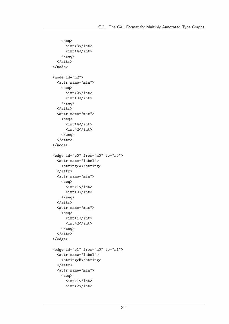
C.2. The GXL Format for Multiply Annotated Type Graphs

<seq><int>3</int><int>4</int>

</seq></attr>

</node>

<node id="n2"><attr name="min">

<seq><int>0</int><int>0</int>

</seq></attr><attr name="max">

<seq><int>4</int><int>2</int>

</seq></attr>

</node>

<edge id="e0" from="n0" to="n0"><attr name="label">

<string>A</string></attr><attr name="min">

<seq><int>1</int><int>0</int>

</seq></attr><attr name="max">

<seq><int>1</int><int>2</int>

</seq></attr>

</edge>

<edge id="e1" from="n0" to="n1"><attr name="label">

<string>B</string></attr><attr name="min">

<seq><int>1</int><int>2</int>

211

C. DrAGoM Documentation

</seq></attr><attr name="max">

<seq><int>4</int><int>2</int>

</seq></attr>

</edge>

<edge id="e2" from="n1" to="n2"><attr name="label">

<string>C</string></attr><attr name="min">

<seq><int>0</int><int>0</int>

</seq></attr><attr name="max">

<seq><int>1</int><int>3</int>

</seq></attr>

</edge>

</graph></gxl>

As evident from the encoding shown above, the Gxl format uses identifiersto encode the structure of the type graph. For completeness sake, we depict theidentifier reference for each element of the encoded type graph T [M ]:

T =n0 n1 n2

e0

e1 e2

212

C.3. The SGF Format for Graph Transformation Systems

C.3. The SGF Format for Graph Transformation SystemsIn this section we give an example for the Sgf encoding of a graph transformationsystem. The graph transformation systems are stored into .sgf-files, where onefile in the Sgf format can contain several graph transformation systems at thesame time. A formal description of the Sgf format is given in [Bru15].

Let the following graph transformation system R = ρ1, ρ2 be given, where ρ1and ρ2 are depicted below:

ρ1 =1 2

A

B C

1 2A

1 2A

D E F

ρ2 =1

A

B

1 1C

The Sgf format represents a double-pushout rule using a corresponding morphismfrom the left-hand side graph to the right-hand side graph instead of saving tworule morphisms and the interface graph. Please note that the Sgf format onlysupports injective rule morphisms. In the encoding, nodes are introduced implicitlyvia edge definitions, in contrast to distinct nodes which need to be added explicitlyin the respective graph encoding.The graph transformation system R is encoded in the following Sgf format:

leftGraph0 = graph e0:A(v0,v2);e1:B(v0,v1);e2:C(v1,v2);

;

rightGraph0 = graph e0:A(v0,v2);e1:D(v0,v1);e2:E(v1,v3);e3:F(v3,v2);

;

Morphism0 = morphism from leftGraph0 to rightGraph0 v0 => v0;v2 => v2;e0 => e0;

;

leftGraph1 = graph e0:A(v1,v0);e1:B(v1,v1);node v2;

;

213

C. DrAGoM Documentation

rightGraph1 = graph e0:C(v1,v0);

;

Morphism1 = morphism from leftGraph1 to rightGraph1 v0 => v0;

;

Rule0 = rule left = leftGraph0;right = rightGraph0;morphism = Morphism0;

;

Rule1 = rule left = leftGraph1;right = rightGraph1;morphism = Morphism1;

;

result = gts rules = [

Rule1,Rule0

];;

For the sake of completeness, we depict the identifier reference for each elementof the encoded graph transformation system result = Rule0, Rule1:

Rule0 =v0 v1 v2

e0

e1 e2v0 v2

e0v0 v1 v3 v2

e0

e1 e2 e3

Rule1 =v0 v1 v2

e0e1

v0 v0 v1e0

214

References

Publications of Dennis Nolte

[CH+19] A. Corradini, T. Heindel, B. König, D. Nolte, and A. Rensink. “Rewrit-ing Abstract Structures: Materialization Explained Categorically”.In: Foundations of Software Science and Computation Structures.Ed. by M. Bojańczyk and A. Simpson. Cham: Springer InternationalPublishing, 2019, pp. 169–188. doi: 10.1007/978-3-030-17127-8_10.arXiv: 1902.04809 [cs.LO].

[CKN19] A. Corradini, B. König, and D. Nolte. “Specifying Graph Languageswith Type Graphs”. In: Journal of Logical and Algebraic Methodsin Programming Vol. 104 (2019), pp. 176–200. doi: 10.1016/j.jlamp.2019.01.005.

[KNN19] B. König, M. Nederkorn, and D. Nolte. “CoReS: A Tool for Comput-ing Core Graphs via SAT/SMT Solvers”. In: Journal of Logical andAlgebraic Methods in Programming (2019). Submitted.

[KNN18] B. König, M. Nederkorn, and D. Nolte. “CoReS: A Tool for Comput-ing Core Graphs via SAT/SMT Solvers (Tool Presentation Paper)”.In: Proc. of ICGT ’18 (International Conference on Graph Transfor-mation). LNCS 10887. Springer, 2018, pp. 37–42. doi: 10.1007/978-3-319-92991-0_3.

[KN+18] B. König, D. Nolte, J. Padberg, and A. Rensink. “A Tutorial onGraph Transformation”. In: Graph Transformation, Specifications,and Nets – In Memory of Hartmut Ehrig. Ed. by R. Heckel and G.Taentzer. LNCS 10800. Springer, 2018, pp. 1–22. doi: 10.1007/978-3-319-75396-6_5.

[CKN17] A. Corradini, B. König, and D. Nolte. “Specifying Graph Languageswith Type Graphs”. In: Proc. of ICGT ’17 (International Conferenceon Graph Transformation). LNCS 10373. Springer, 2017, pp. 73–89.doi: 10.1007/978-3-319-61470-0_5. arXiv: 1704.05263 [cs.FL].

[Nol17] D. Nolte. “Analysis and Abstraction of Graph TransformationSystems via Type Graphs”. In: STAF 2017 Doctoral Symposium.Vol. 1955. CEUR Workshop Proceedings. 2017.

[ZNK16] H. Zantema, D. Nolte, and B. König. “Termination of Term GraphRewriting”. In: Proc. of WST ’16 (Workshop on Termination). 2016.

[BK+15] H. J. S. Bruggink, B. König, D. Nolte, and H. Zantema. “ProvingTermination of Graph Transformation Systems Using Weighted TypeGraphs over Semirings”. In: Proc. of ICGT ’15 (International Confer-ence on Graph Transformation). 2015, pp. 52–68. doi: 10.1007/978-3-319-21145-9_4. arXiv: 1505.01695 [cs.LO].

References

All References[AH+13] P. A. Abdulla, L. Holík, B. Jonsson, O. Lengál, C.Q. Trinh, and T.

Vojnar. “Verification of Heap Manipulating Programs with OrderedData by Extended Forest Automata”. In: Proc. of ATVA ’13. LNCS8172. 2013, pp. 224–239 (cit. on p. 102).

[AHS09] J. Adamek, H. Herrlich, and G.E. Strecker. Abstract and ConcreteCategories: The Joy of Cats. Dover books on mathematics. DoverPublications, 2009 (cit. on p. 21).

[Bac15] P. Backes. “Cluster Abstraction of Graph Transformation Systems”.PhD thesis. Saarland University, 2015 (cit. on pp. 105, 127).

[BR15a] P. Backes and J. Reineke. “Analysis of Infinite-State Graph Transfor-mation Systems by Cluster Abstraction”. In: ed. by Deepak D’Souza,Akash Lal, and Kim Guldstrand Larsen. Vol. 8931. LNCS. SpringerBerlin Heidelberg, 2015, pp. 135–152 (cit. on pp. 105, 127, 139).

[BR15b] P. Backes and J. Reineke. “ASTRA: A Tool for Abstract Interpreta-tion of Graph Transformation Systems”. In: ed. by Bernd Fischer andJaco Geldenhuys. Vol. 9232. LNCS. Springer International Publishing,2015, pp. 13–19 (cit. on p. 139).

[BCK01] P. Baldan, A. Corradini, and B. König. “A Static Analysis Techniquefor Graph Transformation Systems”. In: vol. 2154. LNCS. Springer-Verlag, 2001, pp. 381–395 (cit. on p. 138).

[BST10] C. Barrett, A. Stump, and C. Tinelli. “The SMT-LIB Standard –Version 2.0”. In: Proc. of the 8th International Workshop on Satisfia-bility Modulo Theories (SMT ’10). Edinburgh, Scotland. July 2010(cit. on pp. 54, 136).

[Bau06] J. Bauer. “Analysis of Communication Topologies by Partner Ab-straction”. PhD thesis. Saarland University, 2006 (cit. on pp. 127,139).

[BB+08] J. Bauer, I. Boneva, M. E. Kurbán, and A. Rensink. “A Modal-Logic Based Graph Abstraction”. In: Proc. of ICGT ’08. LNCS 5214.Springer, 2008, pp. 321–335 (cit. on p. 92).

[BW07] J. Bauer and R. Wilhelm. “Static Analysis of Dynamic Communica-tion Systems by Partner Abstraction”. In: Proc. of SAS ’07. LNCS4634. Springer, 2007, pp. 249–264 (cit. on pp. 105, 127).

[Blu14] C. Blume. “Graph Automata and Their Application to the Verifica-tion of Dynamic Systems”. PhD thesis. University of Duisburg-Essen,2014 (cit. on pp. 5, 98, 102, 138, 142, 146).

[BB+12] C. Blume, H. J. S. Bruggink, D. Engelke, and B. König. “EfficientSymbolic Implementation of Graph Automata with Applications toInvariant Checking”. In: Proc. of ICGT ’12. LNCS 7562. Springer,2012, pp. 264–278 (cit. on pp. 98, 102).

[BB+13] C. Blume, H. J. S. Bruggink, M. Friedrich, and B. König. “Treewidth,Pathwidth and Cospan Decompositions with Applications to Graph-Accepting Tree Automata”. In: Journal of Visual Languages & Com-puting 24.3 (2013), pp. 192–206 (cit. on p. 95).

216

References

[BL+07] I. Bogudlo, T. Lev-Ami, T. Reps, and M. Sagiv. “Revamping TVLA:Making Parametric Shape Analysis Competitive”. In: ComputerAided Verification. Ed. by Werner Damm and Holger Hermanns.Berlin, Heidelberg: Springer Berlin Heidelberg, 2007, pp. 221–225(cit. on p. 139).

[BH+05] P. Bottoni, K. Hoffman, F. Parisi Presicce, and G. Taentzer. “High-Level Replacement Units and their Termination Properties”. In:Journal of Visual Languages and Computing 16.6 (2005), pp. 485–507(cit. on p. 71).

[BJ+00] A. Bouajjani, B. Jonsson, M. Nilsson, and T. Touili. “Regular ModelChecking”. In: Computer Aided Verification. Springer Berlin Heidel-berg, 2000, pp. 403–418 (cit. on p. 1).

[Bru15] H. J. S. Bruggink. Grez User Manual. www.ti.inf.uni-due.de/research/tools/grez. 2015 (cit. on pp. 54, 134, 213).

[BK08] H. J. S. Bruggink and B. König. “On the Recognizability of Arrowand Graph Languages”. In: Proc. of ICGT ’08. LNCS 5214. Springer,2008, pp. 336–350 (cit. on pp. 95, 96).

[BK+15] H. J. S. Bruggink, B. König, D. Nolte, and H. Zantema. “ProvingTermination of Graph Transformation Systems Using Weighted TypeGraphs over Semirings”. In: Proc. of ICGT ’15 (International Confer-ence on Graph Transformation). 2015, pp. 52–68. doi: 10.1007/978-3-319-21145-9_4. arXiv: 1505.01695 [cs.LO] (cit. on p. ix).

[BKZ14] H. J. S. Bruggink, B. König, and H. Zantema. “Termination Analysisof Graph Transformation Systems”. In: Proc. of TCS 2014. Vol. 8705.LNCS. Springer, 2014 (cit. on pp. ix, 39, 47, 49, 50, 54, 61, 71).

[CD+11] C. Calcagno, D. Distefano, P. W. O’Hearn, and H. Yang. “Composi-tional Shape Analysis by Means of Bi-Abduction”. In: Journal of theACM 58.6 (2011), 26:1–26:66 (cit. on p. 105).

[CM77] A. K. Chandra and P. M. Merlin. “Optimal Implementation of Con-junctive Queries in Relational Data Bases”. In: Proceedings of theNinth Annual ACM Symposium on Theory of Computing. STOC ’77.Boulder, Colorado, USA: ACM, 1977, pp. 77–90 (cit. on p. 77).

[CR08] B. E. Chang and X. Rival. “Relational inductive shape analysis”. In:Proc. of POPL ’08. ACM, 2008, pp. 247–260 (cit. on p. 105).

[CG+03] E. M. Clarke, O. Grumberg, S. Jha, Y. Lu, and H. Veith.“Counterexample-guided abstraction refinement for symbolic modelchecking”. In: Journal of the ACM 50.5 (2003), pp. 752–794 (cit. onpp. 1, 75, 138).

[CL03] J. R. B. Cockett and S. Lack. “Restriction categories II: partial mapclassification”. In: TCS 294.1–2 (2003), pp. 61–102 (cit. on p. 108).

[CD11] A. Corradini and F. Drewes. “Term graph rewriting and parallel termrewriting”. In: Proceedings of the 6th International Workshop onComputing with Terms and Graphs (Termgraph). Vol. 48. ElectronicProceedings in Theoretical Computer Science. 2011, pp. 3–18 (cit. onpp. 40, 58, 59, 61, 64).

217

References

[CH+06] A. Corradini, T. Heindel, F. Hermann, and B. König. “Sesqui-pushoutrewriting”. In: Proc. of ICGT ’06 (International Conference on GraphTransformation). LNCS 4178. Springer, 2006, pp. 30–45 (cit. onpp. 105, 110, 179).

[CH+19] A. Corradini, T. Heindel, B. König, D. Nolte, and A. Rensink. “Rewrit-ing Abstract Structures: Materialization Explained Categorically”.In: Foundations of Software Science and Computation Structures.Ed. by M. Bojańczyk and A. Simpson. Cham: Springer InternationalPublishing, 2019, pp. 169–188. doi: 10.1007/978-3-030-17127-8_10.arXiv: 1902.04809 [cs.LO] (cit. on p. x).

[CKN17] A. Corradini, B. König, and D. Nolte. “Specifying Graph Languageswith Type Graphs”. In: Proc. of ICGT ’17 (International Conferenceon Graph Transformation). LNCS 10373. Springer, 2017, pp. 73–89.doi: 10.1007/978-3-319-61470-0_5. arXiv: 1704.05263 [cs.FL](cit. on p. x).

[CKN19] A. Corradini, B. König, and D. Nolte. “Specifying Graph Languageswith Type Graphs”. In: Journal of Logical and Algebraic Methodsin Programming Vol. 104 (2019), pp. 176–200. doi: 10.1016/j.jlamp.2019.01.005 (cit. on p. x).

[CMR96] A. Corradini, U. Montanari, and F. Rossi. “Graph Processes”. In:Fundamenta Informaticae 26.3/4 (1996), pp. 241–265 (cit. on p. 33).

[CM+97] A. Corradini, U. Montanari, F. Rossi, H. Ehrig, R. Heckel, andM. Löwe. “Algebraic Approaches to Graph Transformation—Part I:Basic Concepts and Double Pushout Approach”. In: Handbook ofGraph Grammars and Computing by Graph Transformation, Vol. 1:Foundations. Ed. by G. Rozenberg. World Scientific, 1997. Chap. 3(cit. on pp. 2, 21, 25, 31).

[CR93] A. Corradini and F. Rossi. “Hyperedge replacement jungle rewritingfor term-rewriting systems and logic programming”. In: TheoreticalComputer Science 109 (1993), pp. 7–48 (cit. on p. 58).

[Cou90] B. Courcelle. “The Monadic Second-Order Logic of Graphs I. Recog-nizable Sets of Finite Graphs”. In: Information and Computation 85(1990), pp. 12–75 (cit. on p. 101).

[CE12] B. Courcelle and J. Engelfriet. Graph Structure and Monadic Second-Order Logic, A Language-Theoretic Approach. Cambridge UniversityPress, June 2012 (cit. on pp. 75, 95, 101).

[Cou96] P. Cousot. “Abstract Interpretation”. In: ACM Computing Surveys28.2 (1996) (cit. on p. 105).

[DF+12] V. Danos, J. Feret, W. Fontana, R. Harmer, J. Hayman, J. Kriv-ine, C. D. Thompson-Walsh, and G. Winskel. “Graphs, Rewritingand Pathway Reconstruction for Rule-Based Models”. In: Proc. ofFSTTCS ’12. Vol. 18. LIPIcs. Schloss Dagstuhl – Leibniz Center forInformatics, 2012 (cit. on p. 25).

218

References

[DJ90] N. Dershowitz and J.-P. Jouannaud. “Rewrite Systems”. In: FormalModels and Semantics, Handbook of Theoretical Computer Science.Ed. by Jan van Leeuwen. Vol. B. Elsevier, 1990. Chap. 6, pp. 243–320(cit. on pp. 23, 55).

[DOY06] D. Distefano, P. W. O’Hearn, and H. Yang. “A Local Shape Analysisbased on Separation Logic”. In: Proc. of TACAS ’06. LNCS 3920.Springer, 2006, pp. 287–302 (cit. on p. 102).

[DG17] J. Dyck and H. Giese. “K-Inductive Invariant Checking for GraphTransformation Systems”. In: Graph Transformation. Ed. by Juande Lara and Detlef Plump. Vol. 10373. LNCS. Cham: Springer, 2017,pp. 142–158 (cit. on p. 144).

[DT87] R. Dyckhoff and W. Tholen. “Exponentiable morphisms, partialproducts and pullback complements”. In: Journal of Pure and AppliedAlgebra 49.1-2 (1987), pp. 103–116 (cit. on pp. 5, 105, 110, 177).

[Ehr79] H. Ehrig. “Introduction to the Algebraic Theory of Graph Grammars(A Survey)”. In: Graph-Grammars and Their Application to ComputerScience and Biology. Vol. 73. LNCS. Springer, 1979, pp. 1–69 (cit. onpp. 2, 28, 31).

[EE+05] H. Ehrig, K. Ehrig, J. de Lara, G. Taentzer, D. Varró, and S. Varró-Gyapay. “Termination Criteria for Model Transformation”. In: Proc.of FASE 2005. Vol. 3442. LNCS. Springer, 2005 (cit. on p. 71).

[EE+06] H. Ehrig, K. Ehrig, U. Prange, and G. Taentzer. Fundamentals of Al-gebraic Graph Transformation. Monographs in Theoretical ComputerScience. Springer, 2006 (cit. on pp. 30, 31, 163).

[EE+99] H. Ehrig, G. Engels, H.-J. Kreowski, and G. Rozenberg, eds. Handbookof Graph Grammars and Computing by Graph Transformation, Vol.2:Applications, Languages and Tools. World Scientific, 1999 (cit. onpp. 23, 25, 31).

[EE+15] H. Ehrig, C. Ermel, U. Golas, and F. Hermann. Graph and ModelTransformation – General Framework and Applications. Monographsin Theoretical Computer Science. Springer, 2015 (cit. on p. 23).

[EGH+13] H. Ehrig, U. Golas, F. Hermann, et al. “Categorical Frameworksfor Graph Transformation and HLR Systems Based on the DPOApproach”. In: Bulletin of EATCS 3.102 (2013), pp. 111–121 (cit. onp. 2).

[EH+04] H. Ehrig, A. Habel, J. Padberg, and U. Prange. “Adhesive High-Level Replacement Categories and Systems”. In: Proc. of ICGT ’04(International Conference on Graph Transformation). LNCS 3256.2004, pp. 144–160 (cit. on p. 2).

[EK+99] H. Ehrig, H.-J. Kreowski, U. Montanari, and G. Rozenberg, eds.Handbook of Graph Grammars and Computing by Graph Transfor-mation, Vol.3: Concurrency, Parallellism, and Distribution. WorldScientific, 1999 (cit. on p. 31).

219

References

[EPS73] H. Ehrig, M. Pfender, and H. Schneider. “Graph grammars: Analgebraic approach”. In: Proc. 14th IEEE Symp. on Switching andAutomata Theory. 1973, pp. 167–180 (cit. on pp. 2, 25).

[EWZ08] J. Endrullis, J. Waldmann, and H. Zantema. “Matrix Interpreta-tions for Proving Termination of Term Rewriting”. In: Journal ofAutomated Reasoning 40.2–3 (2008), pp. 195–220 (cit. on pp. 4, 39,41).

[EZ15] J. Endrullis and H. Zantema. “Proving non-termination by finiteautomata”. In: RTA ’15. Vol. 36. LIPIcs. Schloss Dagstuhl–Leibniz-Zentrum fuer Informatik, 2015, pp. 160–176 (cit. on pp. 1, 3, 75).

[Fre72] P. Freyd. “Aspects of Topoi”. In: Bulletin of the Australian Mathe-matical Society 7.1 (1972), pp. 1–76 (cit. on p. 113).

[FO97] L. Fribourg and H. Olsén. “Reachability sets of parameterized rings asregular languages”. In: Proceedings of Infinity ’97. Vol. 9. ElectronicNotes in Theoretical Computer Science. Elsevier, 1997 (cit. on p. 1).

[Ges90] A. Geser. “Relative Termination”. PhD thesis. Universität Passau,1990 (cit. on p. 48).

[GHW04] A. Geser, D. Hofbauer, and J. Waldmann. “Match-bounded stringrewriting”. In: Applicable Algebra in Engineering, Communicationand Computing 15.3–4 (2004), pp. 149–171 (cit. on p. 1).

[Hab92] A. Habel. Hyperedge Replacement: Grammars and Languages. LNCS643. Springer, 1992 (cit. on p. 102).

[HKP88] A. Habel, H.-J. Kreowski, and D. Plump. “Jungle Evaluation”. In:Proc. Recent Trends in Data Type Specification. Vol. 332. LNCS.Springer, 1988, pp. 92–112 (cit. on p. 58).

[HP05] A. Habel and K.-H. Pennemann. “Nested Constraints and Applica-tion Conditions for High-Level Structures”. In: Formal Methods inSoftware and Systems Modeling. Essays Dedicated to Hartmut Ehrig,on the Occasion of His 60th Birthday. LNCS 3393. Springer, 2005,pp. 294–308 (cit. on pp. 75, 102, 127).

[HW95] R. Heckel and A. Wagner. “Ensuring consistency of conditionalgraph rewriting – a constructive approach”. In: Proc. of the JointCOMPUGRAPH/SEMAGRAPH Workshop on Graph Rewriting andComputation. Vol. 2. ENTCS. 1995 (cit. on p. 79).

[Hei09] T. Heindel. “A Category Theoretical Approach to the ConcurrentSemantics of Rewriting – Adhesive Categories and Related Concepts”.PhD thesis. Universität Duisburg-Essen, Sept. 2009 (cit. on p. 164).

[HJ+15] J. Heinen, C. Jansen, J.-P. Katoen, and T. Noll. “Verifying pointerprograms using graph grammars”. In: Science of Computer Program-ming 97 (2015), pp. 157–162 (cit. on p. 139).

[HJ+04] T. A. Henzinger, R. Jhala, R. Majumdar, and K. L. McMillan. “Ab-stractions from Proofs”. In: Proc. of POPL ’04. ACM, 2004, pp. 232–244 (cit. on p. 3).

220

References

[HW06] D. Hofbauer and J. Waldmann. “Termination of String Rewritingwith Matrix Interpretations”. In: Proc. of RTA ’06. LNCS 4098. 2006,pp. 328–342 (cit. on pp. 39, 41–43).

[HS+06] R. C. Holt, A. Schürr, S. E. Sim, and A. Winter. “GXL: A graph-based standard exchange format for reengineering”. In: Science ofComputer Programming 60.2 (2006), pp. 149–170 (cit. on p. 132).

[Jac99] B. Jacobs. Categorical Logic and Type Theory. Vol. 141. Studies inLogic and the Foundation of Mathematics. Elsevier, 1999 (cit. onpp. 118, 119).

[Joh02] P. T. Johnstone. Sketches of an Elephant: A Topos Theory Com-pendium. Vol. 1. Clarendon Press, 2002 (cit. on p. 108).

[KS+05] R. Kennaway, P. Severi, R. Sleep, and F.-J. de Vries. “InfinitaryRewriting: From Syntax to Semantics”. In: Processes, Terms andCycles: Steps on the Road to Infinity:Essays Dedicated to Jan WillemKlop on the Occasion of His 60th Birthday. Vol. 3838. LNCS. Springer,2005 (cit. on p. 72).

[KV03] R. Kennaway and F.-J. de Vries. “Infinitary rewriting”. In: TermRewriting Systems, by Terese. Cambridge University Press, 2003,pp. 668–711 (cit. on p. 72).

[KV05] J. W. Klop and R. C. de Vrijer. “Infinitary Normalization”. In: WeWill Show Them! Essays in Honour of Dov Gabbay. Vol. 2. CollegePublications, 2005, pp. 169–192 (cit. on p. 72).

[Kön99] B. König. “Description and Verification of Mobile Processes withGraph Rewriting Techniques”. PhD thesis. Technische UniversitätMünchen, 1999 (cit. on p. 86).

[Kön00] B. König. “A general framework for types in graph rewriting”. In:Proc. of FST TCS ’00. LNCS 1974. Springer-Verlag, 2000, pp. 373–384 (cit. on p. 117).

[KK06] B. König and V. Kozioura. “Counterexample-guided AbstractionRefinement for the Analysis of Graph Transformation Systems”. In:vol. 3920. LNCS. Springer, 2006, pp. 197–211 (cit. on p. 138).

[KNN18] B. König, M. Nederkorn, and D. Nolte. “CoReS: A Tool for Comput-ing Core Graphs via SAT/SMT Solvers (Tool Presentation Paper)”.In: Proc. of ICGT ’18 (International Conference on Graph Transfor-mation). LNCS 10887. Springer, 2018, pp. 37–42. doi: 10.1007/978-3-319-92991-0_3 (cit. on pp. 78, 154).

[KNN19] B. König, M. Nederkorn, and D. Nolte. “CoReS: A Tool for Comput-ing Core Graphs via SAT/SMT Solvers”. In: Journal of Logical andAlgebraic Methods in Programming (2019). Submitted.

[KN+18] B. König, D. Nolte, J. Padberg, and A. Rensink. “A Tutorial onGraph Transformation”. In: Graph Transformation, Specifications,and Nets – In Memory of Hartmut Ehrig. Ed. by R. Heckel and G.Taentzer. LNCS 10800. Springer, 2018, pp. 1–22. doi: 10.1007/978-3-319-75396-6_5 (cit. on p. ix).

221

References

[KW08] A. Koprowski and J. Waldmann. “Arctic Termination ... Below Zero”.In: Proceedings of the 19th Conference on Rewriting Techniques andApplications (RTA). Ed. by A. Voronkov. Vol. 5117. LNCS. Springer,2008, pp. 202–216 (cit. on p. 39).

[KRW02] B. Kullbach, V. Riediger, and A. Winter. “An Overview of theGXL Graph Exchange Language”. In: Software Visualization. Ed.by Stephan Diehl. Vol. 2269. Lecture Notes in Computer Science.Springer, 2002, pp. 324–336 (cit. on p. 132).

[LS05] S. Lack and P. Sobociński. “Adhesive and Quasiadhesive Categories”.In: RAIRO – Theoretical Informatics and Applications 39.3 (2005)(cit. on pp. 2, 21, 30, 164, 181).

[LS06] S. Lack and P. Sobociński. “Toposes are adhesive”. In: Internationalconference on graph transformation, ICGT ’06. Vol. 4178. Springer,2006, pp. 184–198 (cit. on p. 21).

[LO14] L. Lambers and F. Orejas. “Tableau-Based Reasoning for GraphProperties”. In: Proc. of ICGT ’14. LNCS 8571. Springer, 2014,pp. 17–32 (cit. on p. 127).

[Law70] F.W. Lawvere. “Quantifiers and sheaves”. In: Actes du CongrèsInternational des Mathématiciene. 1970, pp. 329–334 (cit. on p. 108).

[LRC15] H. Li, X. Rival, and B. E. Chang. “Shape Analysis for UnstructuredSharing”. In: Proc. of SAS ’15. LNCS 9291. Springer, 2015, pp. 90–108 (cit. on p. 105).

[Löw93] M. Löwe. “Algebraic approach to single-pushout graph transforma-tion”. In: Theoretical Computer Science 109 (1993), pp. 181–224(cit. on pp. 30, 31).

[Löw10] M. Löwe. “Graph Rewriting in Span-Categories”. In: Proc. of ICGT’10. LNCS 6372. Springer, 2010, pp. 218–233 (cit. on pp. 105, 113,178).

[Mac71] S. Mac Lane. Categories for the Working Mathematician. GraduateTexts in Mathematics, Vol. 5. New York: Springer-Verlag, 1971,pp. ix+262 (cit. on p. 21).

[MM94] S. Mac Lane and I. Moerdijk. Sheaves in Geometry and Logic: AFirst Introduction to Topos Theory. Universitext. Springer New York,1994 (cit. on pp. 109, 110).

[Mar94] M. Marchiori. “Logic programs as term rewriting systems”. In: Al-gebraic and Logic Programming. Ed. by Giorgio Levi and MarioRodríguez-Artalejo. Berlin, Heidelberg: Springer Berlin Heidelberg,1994, pp. 223–241 (cit. on p. 55).

[NT00] J. Nešetřil and C. Tardif. “Duality Theorems for Finite Structures(Characterising Gaps and Good Characterisations)”. In: Journal ofCombinatorial Theory, Series B 80 (2000), pp. 80–97 (cit. on pp. 77,78, 81, 164).

[Nol17] D. Nolte. “Analysis and Abstraction of Graph TransformationSystems via Type Graphs”. In: STAF 2017 Doctoral Symposium.Vol. 1955. CEUR Workshop Proceedings. 2017.

222

References

[OHe07] P. W. O’Hearn. “Resources, Concurrency and Local Reasoning”.In: Theoretical Computer Science 375.1–3 (May 2007). ReynoldsFestschrift, pp. 271–307 (cit. on p. 102).

[OHe12] P. W. O’Hearn. “A Primer on Separation Logic (and AutomaticProgram Verification and Analysis)”. In: Software Safety and Security:Tools for Analysis and Verification. Vol. 33. NATO Science for Peaceand Security Series. 2012, pp. 286–318 (cit. on p. 105).

[OEP08] F. Orejas, H. Ehrig, and U. Prange. “A Logic of Graph Constraints”.In: Proc. of FASE ’08. LNCS 4961. Springer, 2008, pp. 179–198(cit. on p. 81).

[Pen09] K.-H. Pennemann. “Development of Correct Graph TransformationSystems”. PhD thesis. Universität Oldenburg, May 2009 (cit. onp. 102).

[Pie88] B. C. Pierce. A Taste of Category Theory for Computer Scientists.CMU-CS. Carnegie Mellon University, Computer Science Department,1988 (cit. on p. 21).

[PE93] M. J. Plasmeijer and M. C. J. D. van Eekelen. Functional Program-ming and Parallel Graph Rewriting. Addison-Wesley, 1993 (cit. onp. 58).

[Plu95] D. Plump. “On termination of graph rewriting”. In: Graph-TheoreticConcepts in Computer Science. LNCS 1017. Springer, 1995, pp. 88–100 (cit. on p. 72).

[Plu98] D. Plump. “Termination of graph rewriting is undecidable”. In: Fun-damenta Informaticae 33.2 (1998), pp. 201–209 (cit. on pp. 4, 42).

[Plu99] D. Plump. “Term Graph Rewriting”. In: Handbook of Graph Gram-mars and Computing by Graph Transformation, Vol. 2: Applications,Languages and Tools. Ed. by G. Rozenberg. World Scientific, 1999(cit. on p. 58).

[Plu18] D. Plump. “Modular Termination of Graph Transformation”. In:Graph Transformation, Specifications, and Nets - In Memory ofHartmut Ehrig. Ed. by Reiko Heckel and Gabriele Taentzer. Vol. 10800.Lecture Notes in Computer Science. Springer, 2018, pp. 231–244 (cit.on p. 72).

[Ren03] A. Rensink. “The GROOVE Simulator: A Tool for State SpaceGeneration”. In: Applications of Graph Transformations with Indus-trial Relevance. Ed. by John L. Pfaltz, Manfred Nagl, and BorisBöhlen. Vol. 3062. Lecture Notes in Computer Science. Springer,2003, pp. 479–485 (cit. on p. 138).

[Ren04a] A. Rensink. “Canonical Graph Shapes”. In: Proc. of ESOP ’04. LNCS2986. Springer, 2004, pp. 401–415 (cit. on pp. 33, 75, 85, 92, 105, 127,139).

[Ren04b] A. Rensink. “Representing First-Order Logic using Graphs”. In: Proc.of ICGT ’04. LNCS 3256. Springer, 2004, pp. 319–335 (cit. on pp. 75,102).

223

References

[RZ10] A. Rensink and E. Zambon. “Neighbourhood Abstraction inGROOVE”. In: Proc. of GraBaTs ’10 (Workshop on Graph-BasedTools). Vol. 32. Electronic Communications of the EASST. 2010 (cit.on pp. 105, 127).

[RS86] N. Robertson and P. D Seymour. “Graph minors. II. Algorithmicaspects of tree-width”. In: Journal of Algorithms 7.3 (1986), pp. 309–322 (cit. on p. 94).

[RS83] N. Robertson and P. D. Seymour. “Graph minors. I. Excluding aforest”. In: Journal of Combinatorial Theory, Series B 35.1 (1983),pp. 39–61 (cit. on p. 94).

[Roz97] G. Rozenberg, ed. Handbook of Graph Grammars and Computing byGraph Transformation, Vol.1: Foundations. World Scientific, 1997(cit. on pp. 23, 31, 33, 105).

[RR+09] A. Rutle, A. Rossini, Y. Lamo, and U. Wolter. “A DiagrammaticFormalisation of MOF-Based Modelling Languages”. In: Proc. ofTOOLS EUROPE ’09. LNBIP 33. Springer, 2009, pp. 37–56 (cit. onp. 102).

[SZ15] D. Sabel and H. Zantema. “Transforming Cycle Rewriting into StringRewriting”. In: 26th International Conference on Rewriting Tech-niques and Applications (RTA’15). Ed. by Maribel Fernandez. Vol. 36.Leibniz International Proceedings in Informatics (LIPIcs). Dagstuhl,Germany: Schloss Dagstuhl–Leibniz-Zentrum fuer Informatik, 2015,pp. 285–300 (cit. on pp. 39, 41, 43, 50, 61, 72).

[SRW02] M. Sagiv, T. Reps, and R. Wilhelm. “Parametric Shape Analysis via3-Valued Logic”. In: TOPLAS (ACM Transactions on ProgrammingLanguages and Systems) 24.3 (2002), pp. 217–298 (cit. on pp. 5, 33,101, 102, 105, 127, 139).

[SWW10] D. Steenken, H. Wehrheim, and D. Wonisch. “Towards A Shape Anal-ysis for Graph Transformation Systems”. In: CoRR abs/1010.4423(2010) (cit. on p. 139).

[SWW11] D. Steenken, H. Wehrheim, and D. Wonisch. “Sound and CompleteAbstract Graph Transformation”. In: Proc. of SBMF ’11. LNCS 7021.Springer, 2011, pp. 92–107 (cit. on pp. 2, 33, 75, 105, 127, 139).

[SW11] D. Steenken and D. Wonisch. “Using shape analysis to verify graphtransformations in model driven design”. In: Aug. 2011, pp. 457–462(cit. on p. 139).

[Ter03] Terese. Term Rewriting Systems. Vol. 55. Cambridge Tracts in Theo-retical Computer Science. Cambridge University Press, 2003 (cit. onpp. 39, 55).

[Toy87] Y. Toyama. “Counterexamples to Termination for the Direct Sumof Term Rewriting Systems”. In: Information Processing Letters 25(1987), pp. 141–143 (cit. on p. 63).

[VV+06] D. Varró, S. Varró-Gyapay, H. Ehrig, U. Prange, and G. Taentzer.“Termination Analysis of Model Transformations by Petri Nets”. In:Proc. of ICGT 2006. Vol. 4178. LNCS. Springer, 2006 (cit. on p. 71).

224

References

[Win02] A. Winter. “Exchanging Graphs with GXL”. In: Graph Drawing. Ed.by Petra Mutzel, Michael Jünger, and Sebastian Leipert. Vol. 2265.Lecture Notes in Computer Science. Springer, 2002, pp. 485–500(cit. on p. 132).

[Zan95] H. Zantema. “Termination of Term Rewriting by Semantic Labelling”.In: Fundamenta Informaticae 24.1/2 (1995), pp. 89–105 (cit. on p. 39).

[Zan03] H. Zantema. “Termination”. In: Term Rewriting Systems. Ed. byMarc Bezem, Jan Willem Klop, and Roel de Vrijer. CambridgeUniversity Press, 2003. Chap. 6 (cit. on p. 48).

[Zan08] H. Zantema. “Normalization of Infinite Terms”. In: Proceedings of the19th Conference on Rewriting Techniques and Applications (RTA).Ed. by A. Voronkov. Vol. 5117. LNCS. Springer, 2008, pp. 441–455(cit. on p. 72).

[ZBK14] H. Zantema, H. J. S. Bruggink, and B. König. “Termination of cyclerewriting”. In: Proceedings of Joint International Conference, RTA-TLCA 2014. Ed. by G. Dowek. Vol. 8560. LNCS. Springer, 2014,pp. 476–490 (cit. on pp. 39, 61, 63, 72).

[ZNK16] H. Zantema, D. Nolte, and B. König. “Termination of Term GraphRewriting”. In: Proc. of WST ’16 (Workshop on Termination). 2016(cit. on p. ix).

225

Nomenclature

Category Theory Symbols

C An arbitrary category, page 16

C ↓ A Slice category of a category C over an object A, page 109

Set Category of sets and functions, page 16

Rel Category of sets and relations, page 16

Mon Category of ordered monoids and monoid morphisms, page 85

Mon− Category of ordered monoids with subtraction, page 117

Matϕ Materialization category over a mono ϕ, page 112

MatϕLϕ Materialization subcategory of rewritable objects, page 114

GraphΛ Category of Λ-labeled graphs and graph morphisms, page 30

|GraphΛ| Set of objects from GraphΛ, page 30

Cospanm(GraphΛ) Category of discrete graphs and cospans, page 94

O A class O of objects, page 16

M A classM of arrows (or morphisms), page 16

id A class id of identity arrows, page 16

dom(f) Domain of an arrow f , page 16

cod(f) Codomoain of a arrow f , page 16

f g Arrow composition, page 16

A B A monomorphism from A to B, page 17

A B An epimorphism from A to B, page 17

A∼−→ B An isomorphism between A and B, page 17

A B A partial map from A to B, page 108

A .→ B A family of arrows from A to B, page 108

A 99K B Denoting existence of an arrow from A to B, page 111

A×B Product object of two objects A and B, page 17

A⊕B Coproduct object of two objects A and B, page 18

1 Terminal object in a category, page 18

0 Initial object in a category, page 18

Nomenclature

!A Unique morphism from an object A to 1, page 18

?A Unique morphism from 0 to an object A, page 18

Ω Truth value object in a category, page 107

true A subobject classifier, page 107

trueA A subobject classifier in a slice category over A, page 109

F : C→ D A functor F from a category C to a category D, page 18

IdC An identity functor from C to C, page 18

C An automaton functor C, page 96

CT [M ] A counting cospan automaton functor CT [M ], page 97

η A natural transformation between functors, page 108

ηA A component of a natural transformation η on A, page 108

B f−A −g C A span, i.e. pair of arrows f : A→ B, g : A→ C, page 19

B −gD f− C A cospan, i.e. pair of arrows f : C → D, g : B → D, page 20

p : L← I → R A production (or rule) p in a category, page 21

Xp,m=⇒ Y Rewriting step from X to Y via rule p at match m, page 21

Xp,m=⇒ Denoting that X can be rewritten via p at m, page 115

; Abstract rewriting relation, page 122

→ Modified abstract rewriting relation, page 123

Graph Symbols

Λ Set of edge labels, page 24

VG Finite set of nodes of a graph G, page 24

EG Finite set of edges of a graph G, page 24

srcG Source function mapping an edge to its source node, page 24

tgtG Target function mapping an edge to its target node, page 24

labG Labeling function for the edges of G, page 24

∅ The empty graph, page 24

ϕ Graph morphism with components ϕV and ϕE , page 24

ϕ ψ Graph morphism composition [(ϕψ)(x) = ϕ(ψ(x))], page 24

G ∼= H Denoting that the graphs G,H are isomorphic, page 24

G H Denoting that the graphs G,H are not isomorphic, page 24

228

Nomenclature

G+I H Gluing of G and H over a common interface I, page 26

→ Homomorphism preorder, page 30

G→ H Denoting existence of a morphism from G to H, page 30

G9 H Denoting non-existence of a morphism from G to H, page 30

G ∼ H Homomorphically equivalent graphs G and H, page 30

core(G) A core graph of G, page 77

(R, T ) A duality pair, page 81

TG Tree decomposition of a graph G, page 94

PG Path decomposition of a graph G, page 94

w(TG) Width of a tree decomposition TG, page 94

tw(G) Treewidth of a graph G, page 94

pw(G) Pathwidth of a graph G, page 94

c : J # K Short cospan representation of c : J → G← K, page 95

c1; c2 Composition of cospans via pushouts, page 95

Graph Transformation Symbols

ρ A graph transformation rule, page 27

LϕL− I −ϕRR A double-pushout graph transformation rule, page 27

G⇒ρ H Graph transformation step from G to H via rule ρ, page 27

C The context graph C in a DPO rewriting step, page 27

R A graph transformation system, i.e., a set of rules ρ, page 29

Termination Analysis Symbols

wT Weight function of a type graph T , page 45

RT Flower node of type graph T , page 45

flT (G) Flower morphism from graph G to type graph T , page 45

wt(ϕ) Weight of a morphism ϕ wrt. a morphism t, page 47

R< Set of decreasing rules, page 48

R= Set of non-increasing rules, page 48

X Countable set of variables, page 56

F Signature, page 56

T (F ,X ) Set of terms over the signature F , page 56

229

Nomenclature

Var(t) Set of variables occuring in a term t, page 56

C[t] Context around a subterm t, page 56

2 Empty space symbol, page 56

σ A substitution of variables to terms, page 57

σ Homomorphically extended substitution, page 57

R A term rewriting system, page 58

Rb A term graph rewriting system (basic version), page 62

Re A term graph rewriting system (extended version), page 62

→R Rewrite relation of term rewriting system R, page 58

TG(t) Term graph of a term t, page 59

p = L←` I →r R A term graph production, page 60

SN(R) Strong normalization of term rewriting system R, page 62

SNb(R) Strong normalization of Rb, page 62

SNe(R) Strong normalization of Re, page 62

Graph Language and Object Language Symbols

T A type graph, page 33

TΛR The flower graph over the label set Λ, page 34

L(T ) A type graph language specified by T , page 33

L(T [a]) Type graph language by an annotated graph T [a], page 88

L(T [M ]) Language by a multiply annotated graph T [M ], page 89

L(T [M ])≤k k-bounded language of L(T [M ]), page 94

R A restriction graph, page 78

LR(R) A restriction graph language specified by R, page 78

L(T1) ⊆ L(T2) Language inclusion of type graph languages, page 79

L(T1) ∪ L(T2) Union of type graph languages, page 82

L(T1) ∩ L(T2) Intersection of type graph languages, page 82

LC Language of an automaton functor C, page 96

LCT [M ] Language of counting cospan automaton functor, page 97

L(A) Object language of an abstract object A, page 111

L(ϕ) Mono language of a monomorphism ϕ, page 111

230

Nomenclature

Materialization Symbols

L X → A Factorization in the materialization category, page 112

L 〈ϕ〉 → A Materialization of ϕ : L→ A, page 112

〈ϕ〉 Short representation of L 〈ϕ〉 → A, page 112

〈〈ϕ,ϕL〉〉 Rewritable materialization of ϕ : L→ A,ϕL : I → L, page 114

Annotation Symbols

A Generic annotation functor, page 86

Aϕ Alternative representation denoting A(ϕ), page 86

sG A standard annotation for a graph G, page 86

Mn Natural number monoid (up to n), page 86

Bn Multiplicities over ordered monoidMn, page 87

Sn Node out-degree annotation over ordered monoidMn, page 118

PG Path monoid of the graph G, page 86

T Path annotation functor over ordered monoid PG, page 87

G[M ] A multiply annotated graph G, page 89

Logical Symbols

∧ Conjunction, page 13

∨ Disjunction, page 13

=⇒ Implication, page 13

⇐⇒ Bi-implication, page 13

∃ Existential quantification, page 13

∀ Universal quantification, page 13

Other Symbols

∈, /∈ Membership relation and its negation, page 14

=, 6= Equality relation and its negation, page 14

⊆,* Subset relation and its negation, page 14

⊂, 6⊂ Strict subset relation and its negation, page 14

∅ The empty set, page 14

P(X) The powerset of a set X, page 14

N0 Set of natural numbers with zero, i.e. 0, 1, 2, . . ., page 14

231

Nomenclature

N Set of natural numbers without zero, i.e. 1, 2, . . ., page 14

X \ Y Relative complement, i.e. x ∈ X | x /∈ Y , page 14

X ∪ Y Union, i.e. z | z ∈ X ∨ z ∈ Y , page 14

X ∩ Y Intersection, i.e. z | z ∈ X ∧ z ∈ Y , page 14

X × Y Cartesian product, i.e. (x, y) | x ∈ X ∧ y ∈ Y , page 14

Xn n-ary cartesian product, i.e. n-times X × . . .×X, page 14

XY Exponentiation, i.e. f : Y → X, page 86

X1⊎X2 Disjoint union, i.e.

⋃i∈I(x, i) | x ∈ Xi, page 14

R,R−1 Binary relation R and its inverse R−1, page 14

R+ Transitive closure R+ of a relation R, page 14

≤ Order relation, page 14

< Strict subrelation of ≤, page 14

≡ Equivalence relation, page 14

X/ ≡ Quotient set of all equivalence classes of X by ≡, page 14

[x]≡ Equivalence class of an element x w.r.t. ≡, page 14

f : X → Y Function with domain X and codomain Y , page 14

f(x) Image of the input value x, page 14

f |Z Function f with a domain restriction to a set Z, page 15∨X Least upper bound (or join, or supremum) of X, page 15∧X Greatest lower bound (or meet, or infimum) of X, page 15

> Maximal element (also called top element), page 15

⊥ Minimal element (also called bottom element), page 15

⊕ Abstract addition-operator, page 43

⊗ Abstract multiplication-operator, page 43

Σ Generalised sum of ⊕, page 44∏Generalised product of ⊗, page 44

232

Index

Abstract ConceptsAbstract graph, 111Abstract match, 115Abstract object, 107Abstract rewriting, 122

Adhesive Category, 20Annotation, 86

Multiplicity, 87Out-degree annotation, 118Path annotation, 87Standard annotation, 86

Annotation PropertiesAdjunction property, 119Beck-Chevalley property, 119Homomorphism property, 119Isomorphism property, 120Pushout property, 119

Arrows, see Category, MorphismsAutomaton Functor, 96

Boolean Connectives, 75Bottom, 15

Category, 16Arrows, 16Codomain, 16Domain, 16Identity class, 16Objects, 16

ClassifierPartial map classifier, 108Subobject classifier, 107

Closure PropertiesClosed under a rule, 79Complement, 79Intersection, 79Union, 79

Codomain, 14, 16Component, 108Context, 27, 56Contractum, 57Coproduct, 17Core, 77Cospan, 20Counting Cospan Automaton, 97

Decidability PropertiesEmptyness, 79Language inclusion, 79Membership, 79

Diagram, 16Domain, 14, 16Domain Restriction, 15Double-Pushout Rewriting, 21, 31Doubly Annotated Object, 120Dual, 81Duality Pair, 81

Elementary Topos, see ToposEmbedding, 18Empty Set, 14Epimorphism, see MorphismsEquivalence

Equivalence class, 14Quotient set, 14

Exponentiation, 86

Factorization, 112Final Pullback Complement, 110Flower Node, 34, 45Folding, 77Function, 14Function Properties

Bijective, 15Injective, 15Surjective, 15

Functor, 18

Global Annotation, 92Gluing Condition, 21, 28

Dangling edge condition, 28Identification condition, 28

Gluing Construction, 19, 26Graph, 24Graph Grammar, 23Graph Language

Restriction graph language, 78Type graph language, 33

Graph Transformation, 27Graph Transformation Rule, 27Graph Transformation System, 29Greatest Lower Bound, 15

Index

Homomorphically Equivalent, 30Homomorphism

Graph homomorphism, 24Monoid homomorphism, 85

Homomorphism Preorder, 30

IdentityIdentity arrow, 16Identity functor, 108

Image, 14Infimum, 15Initial Object, 18Injection, see MorphismsInterface, 26

Inner interface, 94Outer interface, 94

Invariant, 79Isomorphism, see Morphisms

Join, 15

Lattice, 15Least Upper Bound, 15Legal Morphism, 89Limit, 20Local Annotation, 92Logical Operator, 13

Match, 27, 57Materialization, 112Materialization Category, 112Matrix, 42Meet, 15Membership Relation, 14Mono Language, 111Monoid, 15

Ordered monoid, 85Monomorphism, see MorphismsMonotone Morphisms, 85Morphisms, 16

Injection, 18Legal morphism, 89Projection, 17Semi-legal morphism, 121Epimorphism, 17Graph morphism, 24Isomorphism, 17, 24Monomorphism, 17Term graph morphism, 59

Multiplicity, 87

Multiply Annotated Graph, 89

Natural Numbers, 14Natural Transformation, 108

Object Language, 111Order

Equivalence, 14Partial order, 14Preorder, 14

Ordered Monoid, 85Ordered Monoid Subtraction, 117Ordered Semiring, 44

Strictly orderedArithmetic semiring, 44

Strongly orderedArctic semiring, 44Tropical semiring, 44

Partial Map, 108Partial Map Classifier, 108Partial Order, see OrderPath Decomposition, 94Path Monoid, 86Pathwidth, 94Powerset, 14Preimage, 14Preorder, see OrderProduct, 17Production, 21Projection, see MorphismsPullback, 20Pushout, 19

QuantifiersExistencial quantifier, 13Universal quantifier, 13

Recognizable Graph Language, 96Redex, 57Relation, 14Relation Properties

Antisymmetric, 14Reflexive, 14Symmetric, 14Transitive, 14

Relative Complement, 14Relative Termination Analysis, 48Restriction Graph, 78Restriction Graph Language, 78

234

Index

Retract, 77Rewritable Materialization, 114Rewriting Systems

Cycle rewrite system, 43Graph rewrite system, 23, 29String rewrite system, 42Term graph rewrite system, 60Term rewriting system, 58

Rule, 21Rule Attributes

Decreasing rule, 47Non-increasing rule, 47Strongly decreasing rule, 49

Satisfiable Modulo Theories, 53Semiring, see Ordered SemiringSet, 14Set Operation

Cartesian product, 14Disjoint union, 14Intersection, 14Union, 14

Signature, 56Slice Category, 109SMT Solver, 53Span, 19Strongest Post-Condition, 124Subobject Classifier, 107Subset, 14Substitution, 57Subtraction Preservation, 117Supremum, 15

Term Graph, 59Term Graph Encodings

Function encoding, 65Number encoding, 67

Term Graph Production, 60Term Interpretation Versions

Basic version, 61Extended version, 62

Term Rewrite Rule, 57Collapsing, 57Left-linear, 57Linear, 57Right-linear, 57

Terminal Object, 18Termination Analysis, 41Termination Problems Database, 68Terms, 56

Ground terms, 56Linear terms, 56

ToolsGrez, 54DrAGoM, 131

Top, 15Topos, 108Transitive Closure, 14Tree Decomposition, 94Treewidth, 94Truth Value Object, 107Type Graph, 33Type Graph Language, 33Type Graph Logic, 82

Uniform Termination, 41Unit, 15Universal Property, 17Unraveling, 60

Weighted Type Graph, 45Weights

Weight of a graph, 46Weight of a morphism, 45Weight of a rule morphism, 47

Well-Behaved Subtraction, 117Width, 94

235