An Optimal Control Framework for Flight Management Systems
157
An Optimal Control Framework for Flight Management Systems Jesus Villarroel A Thesis in The Department of Electrical and Computer Engineering Presented in Partial Fulfillment of the Requirements for the Degree of Master of Applied Science (Electrical and Computer Engineering) at Concordia University Montr´ eal, Qu´ ebec, Canada February 2015 c Jesus Villarroel, 2015 CORE Metadata, citation and similar papers at core.ac.uk Provided by Concordia University Research Repository
-
Upload
khangminh22 -
Category
Documents
-
view
0 -
download
0
Transcript of An Optimal Control Framework for Flight Management Systems
An Optimal Control Framework for FlightManagement Systems
Jesus Villarroel
A Thesis
in
The Department
of
Electrical and Computer Engineering
Presented in Partial Fulfillment of the Requirements
for the Degree of Master of Applied Science (Electrical and Computer Engineering) at
Concordia University
Montreal, Quebec, Canada
February 2015
c© Jesus Villarroel, 2015
CORE Metadata, citation and similar papers at core.ac.uk
Provided by Concordia University Research Repository
CONCORDIA UNIVERSITY
SCHOOL OF GRADUATE STUDIES
This is to certify that the thesis prepared
By: Jesus Villarroel
Entitled: An Optimal Control Framework for Flight Management Systems
and submitted in partial fulfillment of the requirements for the degree of
Master of Applied Science (Electrical & Computer Engineering)
complies with the regulations of the University and meets the accepted standards
with respect to originality and quality.
Signed by the final examining committee:
ChairDr. S. Hashtrudi Zad
ExaminerDr. C. Skonieczny
External ExaminerDr. A. Akgunduz
SupervisorDr. L. Rodrigues
Approved byDr. A.R. Sebak, Graduate Program Director
Dr. A. Asif, Dean
Faculty of Engineering & Computer Science
February 16, 2015
ABSTRACT
An Optimal Control Framework for Flight Management Systems
Jesus Villarroel
In the present day, the aviation sector is one of the largest contributor of carbon dioxide
emissions in the world. As air traffic growth is expected to outweigh the industry’s efforts
to reduce air pollution, the problem of minimizing fuel consumption in commercial flight
becomes of utmost importance. This thesis proposes an optimal control framework for the
optimization of aircraft trajectories in Flight Management Systems (FMS), focusing on the
problem known as the Economy Mode. This problem consists of minimizing the direct
operating cost of the flight in compliance with a crew-supplied cost index.
The objective of the FMS is to obtain optimal true airspeed references that will then be
followed by the pilot or the autopilot. The optimal top-of-climb and top-of-descent must be
computed as well. A novel approach is proposed based on solving the problem analytically
using a combination of Pontryagin’s maximum principle and the Hamilton-Jacobi-Bellman
equation. For the cruise phase, a sub-optimal algebraic solution for the true airspeed is
obtained in a state-feedback form, which reduces to the well-known maximum range case
when the cost index vanishes. For the climb and the descent, the sub-optimal speed is the
positive root inside the aircraft’s flight envelope of a 5th degree polynomial whose coefficients
involve only the state variables and the aircraft-specific coefficients, which can be found easily
with fast-converging algorithms such as Newton’s method. The exact optimal trajectories are
computed numerically using the shooting method, and simulations show that the sub-optimal
trajectories are close enough for all practical purposes. Moreover, the trajectories exhibit the
expected behavior regarding the locations of the top-of-climb and top-of-descent. Having
attained an analytic solution for the cruise and a computationally inexpensive formulation
for the climb and the descent, the need to have a performance database in the system is
eliminated thus making its implementation faster in real-time.
iii

Overall, the developments presented in this work not only provide a very efficient means
of implementing the optimal speed schedules in an on-board FMS, but also extend the theory
of aircraft performance to the more general minimum-cost case based on the cost index.
iv
ACKNOWLEDGEMENTS
I would like to give very special thanks to my academic supervisor, Dr. Luis Rodrigues,
for his invaluable teachings, guidance and support during the course of my research, without
which this work would have not been possible. I would like also to extend my gratitude
to Mitacs and TRU Simulation + Training (formerly Mechtronix) for providing financial
support, and for giving me the opportunity to obtain much-valued work experience as an
intern by applying the results of my work in a practical environment.
Thanks to all of my friends and peers at the Hybrid Control Systems (HYCONS) Lab-
oratory: Azita, Javier, Julia, Manuel, Miad, Michael Di Perna, Michael El-Jiz, Qasim and
Sina. Thank you all for your continued support, encouragement and for the good times that
we spent together in the laboratory.
Last but not least, I would like to thank all of my family for their unconditional love and
support. Special thanks to my uncle Jorge for his help and guidance both in my academic
and personal life. Finally, I want to give very, very special thanks to my mother Carmen
Elena for being the cornerstone of all that I have achieved so far. This work is for you.
v
Contents
List of Symbols xii
List of Acronyms xv
1 Introduction 1
1.1 Motivation . . . . . . . . . . . . . . . . . . . . . . . . . . . . . . . . . . . . . 1
1.2 Flight Management System Description . . . . . . . . . . . . . . . . . . . . . 2
1.3 Economy Mode and Cost Index . . . . . . . . . . . . . . . . . . . . . . . . . 4
1.4 Objective . . . . . . . . . . . . . . . . . . . . . . . . . . . . . . . . . . . . . 6
1.5 Literature Survey . . . . . . . . . . . . . . . . . . . . . . . . . . . . . . . . . 7
1.5.1 Optimal Control . . . . . . . . . . . . . . . . . . . . . . . . . . . . . 7
1.5.2 Flight Management Systems . . . . . . . . . . . . . . . . . . . . . . . 8
1.5.3 Optimal Control Applied to Aircraft Trajectory Optimization . . . . 9
1.6 Methodology . . . . . . . . . . . . . . . . . . . . . . . . . . . . . . . . . . . 11
1.7 Contributions . . . . . . . . . . . . . . . . . . . . . . . . . . . . . . . . . . . 12
1.8 Structure of the Thesis . . . . . . . . . . . . . . . . . . . . . . . . . . . . . . 13
2 Theoretical Preliminaries 14
2.1 Aircraft Performance . . . . . . . . . . . . . . . . . . . . . . . . . . . . . . . 14
2.1.1 The International Standard Atmosphere (ISA) Model . . . . . . . . . 14
2.1.2 Aerodynamic Forces Acting on an Airplane . . . . . . . . . . . . . . . 17
vi
2.1.3 Equations of Motion in the Longitudinal Plane . . . . . . . . . . . . . 19
2.1.4 Flight Envelope . . . . . . . . . . . . . . . . . . . . . . . . . . . . . . 22
2.1.5 Specific Fuel Consumption . . . . . . . . . . . . . . . . . . . . . . . . 24
2.1.6 Cruise Performance . . . . . . . . . . . . . . . . . . . . . . . . . . . . 25
2.1.7 Maximum Rate of Climb and Rate of Descent Speeds . . . . . . . . . 27
2.2 Optimization and Optimal Control . . . . . . . . . . . . . . . . . . . . . . . 29
2.2.1 Necessary and Sufficient Conditions for Optimality . . . . . . . . . . 29
2.2.2 Optimal Control Problem . . . . . . . . . . . . . . . . . . . . . . . . 31
2.2.3 Pontryagin’s Maximum Principle . . . . . . . . . . . . . . . . . . . . 34
2.2.4 The Shooting Method . . . . . . . . . . . . . . . . . . . . . . . . . . 36
2.2.5 The Hamilton-Jacobi-Bellman Equation . . . . . . . . . . . . . . . . 39
2.2.6 Combining the Hamilton-Jacobi-Bellman Equation with the Maximum
Principle . . . . . . . . . . . . . . . . . . . . . . . . . . . . . . . . . . 41
3 Optimal Solutions for Cruise 43
3.1 Assumptions . . . . . . . . . . . . . . . . . . . . . . . . . . . . . . . . . . . . 43
3.2 Maximum Endurance OCP . . . . . . . . . . . . . . . . . . . . . . . . . . . . 45
3.3 Economy Mode OCP for Cruise . . . . . . . . . . . . . . . . . . . . . . . . . 50
3.3.1 Longitudinal Flight . . . . . . . . . . . . . . . . . . . . . . . . . . . . 50
3.3.2 Extension to Lateral Flight . . . . . . . . . . . . . . . . . . . . . . . 56
3.4 Validation Results . . . . . . . . . . . . . . . . . . . . . . . . . . . . . . . . . 62
3.4.1 Aircraft Model Used for the Simulations . . . . . . . . . . . . . . . . 62
3.4.2 Shooting Method for Cruise . . . . . . . . . . . . . . . . . . . . . . . 63
3.4.3 Comparison between the optimal and sub-optimal trajectories . . . . 65
4 Optimal Solutions for Climb and Descent 68
4.1 Assumptions . . . . . . . . . . . . . . . . . . . . . . . . . . . . . . . . . . . . 68
4.2 Maximum Rate of Climb and Minimum Rate of Descent OCPs . . . . . . . . 70
vii
4.2.1 Maximum Rate of Climb . . . . . . . . . . . . . . . . . . . . . . . . . 70
4.2.2 Minimum Rate of Descent . . . . . . . . . . . . . . . . . . . . . . . . 75
4.3 Economy Mode OCP for Climb . . . . . . . . . . . . . . . . . . . . . . . . . 79
4.4 Validation of Climb Results . . . . . . . . . . . . . . . . . . . . . . . . . . . 88
4.4.1 Shooting Method for Climb . . . . . . . . . . . . . . . . . . . . . . . 89
4.4.2 Comparison between the optimal and sub-optimal trajectories . . . . 90
4.5 Economy Mode OCP for Descent . . . . . . . . . . . . . . . . . . . . . . . . 94
4.6 Validation of Descent Results . . . . . . . . . . . . . . . . . . . . . . . . . . 103
4.6.1 Shooting Method for Descent . . . . . . . . . . . . . . . . . . . . . . 103
4.6.2 Comparison between the optimal and sub-optimal trajectories . . . . 105
4.7 Practical consideration: Estimation of the Top-of-Descent . . . . . . . . . . . 109
5 Conclusions and Future Work 111
5.1 Conclusions . . . . . . . . . . . . . . . . . . . . . . . . . . . . . . . . . . . . 111
5.2 Extensions . . . . . . . . . . . . . . . . . . . . . . . . . . . . . . . . . . . . . 113
A Validation Code for the Cruise Phase 122
B Validation Code for the Climb Phase 130
C Validation Code for the Descent Phase 136
viii
List of Figures
1.1 Block diagram of a Flight Management System. . . . . . . . . . . . . . . . . 2
1.2 Effect of CI on the longitudinal profile. . . . . . . . . . . . . . . . . . . . . . 5
2.1 ISA variation of the temperature with respect to altitude. . . . . . . . . . . . 15
2.2 Aerodynamic forces acting on a wing. . . . . . . . . . . . . . . . . . . . . . . 17
2.3 Coordinate systems for an aircraft flying in the longitudinal plane. . . . . . . 20
2.4 Forces acting on an aircraft flying in the longitudinal plane. . . . . . . . . . 21
2.5 Sketch of a typical flight envelope. . . . . . . . . . . . . . . . . . . . . . . . . 24
2.6 Spring-damper system used for the shooting method example. . . . . . . . . 38
3.1 Aircraft flying in a horizontal plane. . . . . . . . . . . . . . . . . . . . . . . . 57
3.2 Centripetal force in a coordinated turn. . . . . . . . . . . . . . . . . . . . . . 59
3.3 Comparison between the optimal and sub-optimal cruise speeds for different
cost indexes. . . . . . . . . . . . . . . . . . . . . . . . . . . . . . . . . . . . . 66
3.4 Costate J∗W in cruise as a function of the range for different cost indexes. . . 66
4.1 Comparison between the optimal and sub-optimal climb speeds for different
cost indexes. . . . . . . . . . . . . . . . . . . . . . . . . . . . . . . . . . . . . 91
4.2 Costate J∗W in climb as a function of time for different cost indexes. . . . . . 93
4.3 Climb vertical profile for different values of CI. . . . . . . . . . . . . . . . . . 94
4.4 Comparison between the optimal and sub-optimal descent speeds for different
cost indexes. . . . . . . . . . . . . . . . . . . . . . . . . . . . . . . . . . . . . 106
ix
4.5 Costate J∗W in descent as a function of time for different cost indexes. . . . . 107
4.6 Descent vertical profile for different values of CI. . . . . . . . . . . . . . . . . 108
4.7 Estimating the top-of-descent. . . . . . . . . . . . . . . . . . . . . . . . . . . 110
A.1 Simulink block diagram of the cruise 2PBVP. . . . . . . . . . . . . . . . . . 128
A.2 Simulink block diagram of the sub-optimal cruise validation system. . . . . . 128
B.1 Simulink block diagram of the climb 2PBVP. . . . . . . . . . . . . . . . . . . 133
B.2 Simulink block diagram of the sub-optimal climb validation system. . . . . . 135
C.1 Simulink block diagram of the descent 2PBVP. . . . . . . . . . . . . . . . . . 139
C.2 Simulink block diagram of the sub-optimal descent validation system. . . . . 141
x
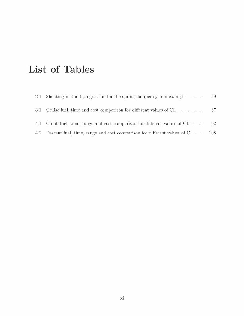
List of Tables
2.1 Shooting method progression for the spring-damper system example. . . . . 39
3.1 Cruise fuel, time and cost comparison for different values of CI. . . . . . . . 67
4.1 Climb fuel, time, range and cost comparison for different values of CI. . . . . 92
4.2 Descent fuel, time, range and cost comparison for different values of CI. . . . 108
xi
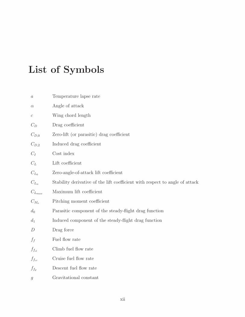
List of Symbols
a Temperature lapse rate
α Angle of attack
c Wing chord length
CD Drag coefficient
CD,0 Zero-lift (or parasitic) drag coefficient
CD,2 Induced drag coefficient
CI Cost index
CL Lift coefficient
CL0 Zero-angle-of-attack lift coefficient
CLα Stability derivative of the lift coefficient with respect to angle of attack
CLmax Maximum lift coefficient
CMo Pitching moment coefficient
d0 Parasitic component of the steady-flight drag function
d1 Induced component of the steady-flight drag function
D Drag force
ff Fuel flow rate
ffcl Climb fuel flow rate
ffcr Cruise fuel flow rate
ffd Descent fuel flow rate
g Gravitational constant
xii
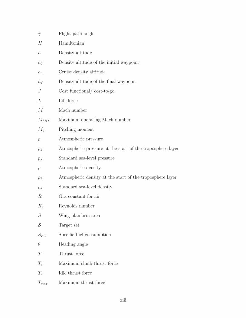
γ Flight path angle
H Hamiltonian
h Density altitude
h0 Density altitude of the initial waypoint
hc Cruise density altitude
hf Density altitude of the final waypoint
J Cost functional/ cost-to-go
L Lift force
M Mach number
MMO Maximum operating Mach number
Mo Pitching moment
p Atmospheric pressure
p1 Atmospheric pressure at the start of the troposphere layer
ps Standard sea-level pressure
ρ Atmospheric density
ρ1 Atmospheric density at the start of the troposphere layer
ρs Standard sea-level density
R Gas constant for air
Re Reynolds number
S Wing planform area
S Target set
SFC Specific fuel consumption
θ Heading angle
T Thrust force
Tc Maximum climb thrust force
Ti Idle thrust force
Tmax Maximum thrust force
xiii
Ts Maximum sea-level climb thrust force
T Atmospheric temperature
T Atmospheric temperature at the tropopause layer
Ts Standard sea-level temperature
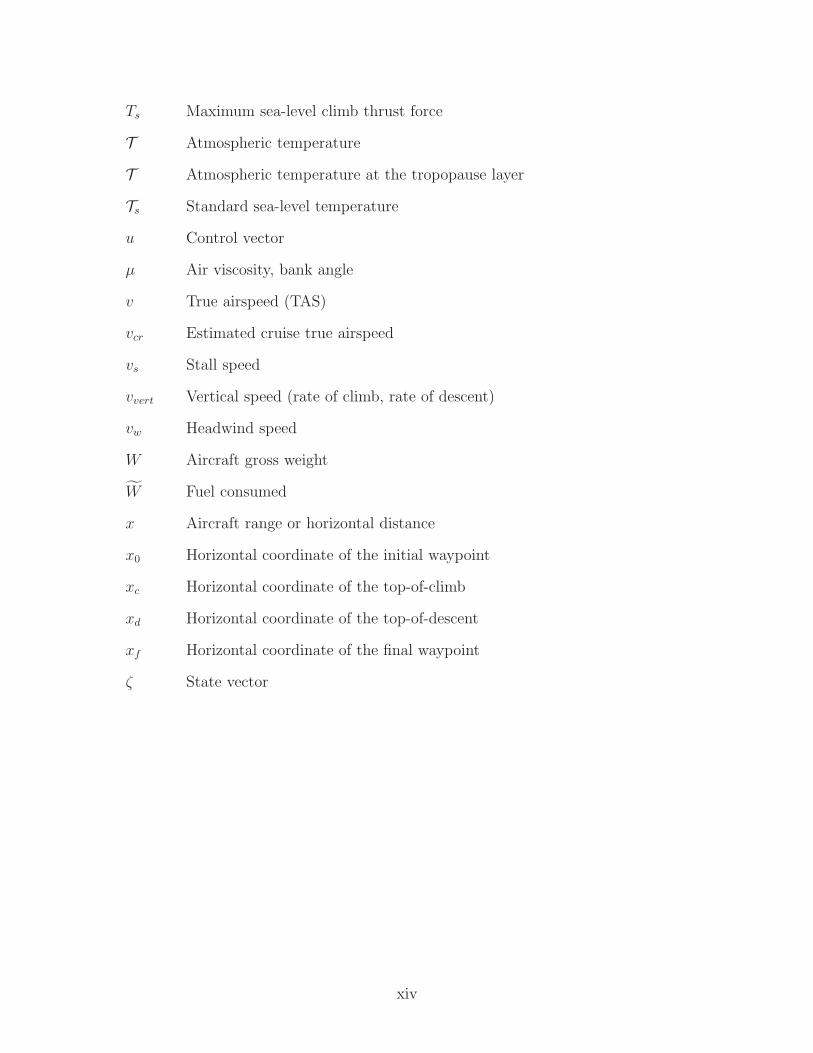
u Control vector
μ Air viscosity, bank angle
v True airspeed (TAS)
vcr Estimated cruise true airspeed
vs Stall speed
vvert Vertical speed (rate of climb, rate of descent)
vw Headwind speed
W Aircraft gross weight
W Fuel consumed
x Aircraft range or horizontal distance
x0 Horizontal coordinate of the initial waypoint
xc Horizontal coordinate of the top-of-climb
xd Horizontal coordinate of the top-of-descent
xf Horizontal coordinate of the final waypoint
ζ State vector
xiv
List of Acronyms
2PBVP Two-point boundary value problem
ATC Air Traffic Control
CDU Control Display Unit
CI Cost Index
ECON Economy (mode)
FMS Flight Management System
FPM Flight Plan Management
TFP Final Turn Point
HJB Hamilton-Jacobi-Bellman
ISA International Standard Atmosphere
ITP Initial Turn Point
LRC Long Range Cruise (mode)
OCP Optimal Control Problem
ODE Ordinary Differential Equation
PDE Partial Differential Equation
ROC Rate of Climb
RTA Required Time of Arrival
SFC Specific Fuel Consumption
SID Standard Instrument Departure
STAR Standard Terminal Arrival Route
xv
TAS True Airspeed
TC Turn Center
TOC Top-of-climb (waypoint)
TOD Top-of-descent (waypoint)
xvi
Chapter 1
Introduction
1.1 Motivation
Carbon dioxide (CO2) emissions in the world have increased steadily during the last two
decades. According to the Netherlands Environmetal Assessment Agency, China emitted
10300 million metric tons of C02 in 2013 making it the largest emitter in the world, followed
by the United States at 5300 million metric tons [1]. The same report identifies international
transport as the most significant factor in global carbon emissions, a fact that is supported by
the U.S. Energy Information Administration [2], which states that the transportation sector
is the largest contributor of C2 emissions in the country, emitting around 2400 million metric
tons in 2013. In addition, recent research suggests that air traffic growth will outweigh the
industry’s efforts to reduce C02 emissions unless ticket prices begin to increase by at least
1.4% annually [3]. Furthermore, the decrease in oil prices by more than half in the end of
2014 is expected to have a negative impact on the environment in oil-importing countries,
as investment in alternate technologies is discouraged and consumers use more gasoline and
larger, less fuel efficient vehicles [4]. Taking all this information into account, the problem
of minimizing fuel consumption in commercial flights becomes of utmost importance and
could potentially reduce CO2 emissions by a significant amount. In an aircraft, the task of
optimizing its trajectory is carried out by the on-board flight management system.
1
1.2 Flight Management System Description
Flight Management Systems (FMS) are the master computers of an aircraft. Since their
introduction in 1982, they have become a staple in every modern aircraft thanks to their
capability of significantly reducing the workload of the crew. This is done by interfacing with
all the navigation systems in order to produce the best possible measurements, providing the
tools for an easy flight plan assembly, synthesizing optimal trajectories and even guiding the
aircraft in order to follows those trajectories, amongst other things. All these functions are
readily accessible to the pilot through a single control panel called the Control Display Unit
(CDU) [5].
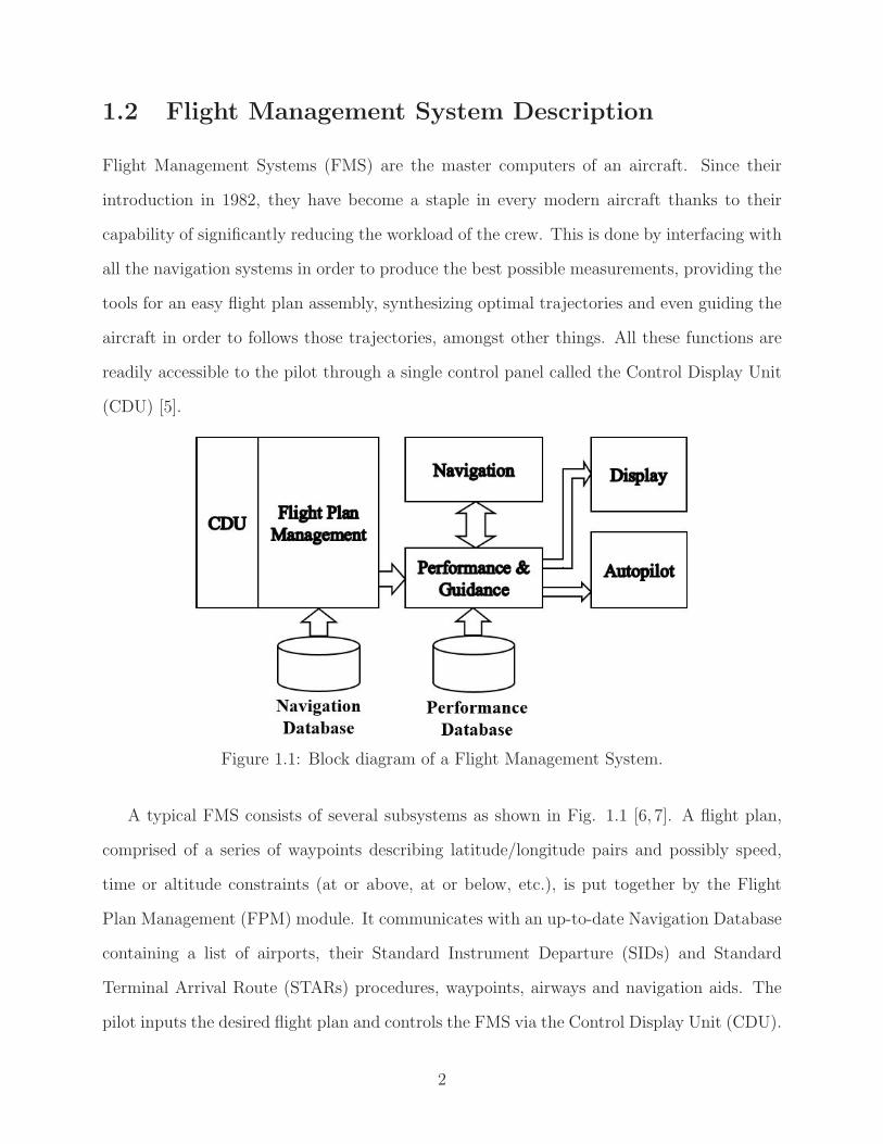
Figure 1.1: Block diagram of a Flight Management System.
A typical FMS consists of several subsystems as shown in Fig. 1.1 [6, 7]. A flight plan,
comprised of a series of waypoints describing latitude/longitude pairs and possibly speed,
time or altitude constraints (at or above, at or below, etc.), is put together by the Flight
Plan Management (FPM) module. It communicates with an up-to-date Navigation Database
containing a list of airports, their Standard Instrument Departure (SIDs) and Standard
Terminal Arrival Route (STARs) procedures, waypoints, airways and navigation aids. The
pilot inputs the desired flight plan and controls the FMS via the Control Display Unit (CDU).
2
The Navigation block determines the best estimate of the position and velocity of the aircraft
as well as the wind velocity by merging the information from the Inertial Reference System
(IRS), Global Positioning System (GPS) and other navigation systems using Kalman filtering
techniques.
The Performance and Guidance module is the most relevant to this work. It is concerned
with generating a trajectory that minimizes a given performance measure, such as the rate
of climb (ROC), aircraft range and overall trip cost. The FMS assumes that the longitudinal
(vertical) and lateral dynamics of the aircraft can be decoupled. The different performance
modes available, named after the performance measure that they minimize, provide different
optimal trajectories., such as [7]:
• Economy (ECON) Mode: Minimize total operating cost of the flight (all fight
phases).
• Required Time of Arrival (RTA): Reach a waypoint at a specified time (all flight
phases).
• Long Range Cruise (LRC): Yield the trajectory that gives 99% of fuel efficiency
(cruise only).
• Maximum Endurance: Maximize the time that the aircraft can stay in the air with
the current fuel reserves (cruise only).
• Maximum Rate of Climb: Minimize the time to reach cruise altitude (climb only).
• Maximum Angle of Climb: Maximize the climb angle (climb only).
The longitudinal trajectory is in the form of an optimal true airspeed command, thrust
target, the top-of-climb (TOC) and top-of-descent (TOD) waypoints, with the cruising alti-
tude being a fixed, crew-entered value determined by Air Traffic Control (ATC). After the
optimization is carried out, the system predicts the estimated time of arrival, fuel remaining,
speed and altitude at each waypoint. Since commercial aircraft fly in quasi-steady flight
3
conditions where accelerations are very small, the thrust is usually constrained to offset the
effect of the aerodynamic forces or is set to pre-determined climb or descent rating. As a
result, it can be computed in a straightforward manner once the speed is known, the latter
becoming the most important parameter involved in the optimization.
In a typical FMS, the optimized speed schedules for the different modes are computed
off-line and stored in the Performance Database, which also contains the data regarding
the aerodynamic, propulsion and fuel consumption of the aircraft necessary to carry out
performance predictions [6, 8]. The lateral path is generated based on the flight plan by
the Guidance block according to a fixed set of rules, which is then shown in the Multi-
function/Navigation Display. This module also sends pitch, thrust and steering commands
to the autopilot to ensure that the aircraft follows the computed lateral and longitudinal
trajectories. Other useful information, such as the desired track and cross-track error, is
calculated and displayed as well.
It is important to note that the FMS is a reference generator: It computes set-points that
are then furnished to a separate autopilot system whose task is to follow those targets using
the aircraft’s flight controls such as the elevator, ailerons and throttle. As a result, the FMS
can be thought of as an outer control loop in the control system, and the dynamics of the
aircraft associated with the speed and flight path angle can be neglected. Such dynamics
then become the concern of the inner loop consisting of the autopilot and auto throttle.
1.3 Economy Mode and Cost Index
The main focus of this thesis is the Economy (ECON) Mode, which is also the default mode
in a FMS and the most important. It is concerned with minimizing the total operating cost
of the flight, expressed by the performance measure
Total Operating Cost = CfΔf + CtΔt,
4
where Δf is the total weight of fuel consumed, Δt is the trip time, Cf is the cost of fuel per
unit of weight and Ct is the cost of the flight per unit time, comprising hourly maintenance
costs, flight crew salaries, leasing costs, amongst others [9, 10]. If Cf is factored from the
equation we get
Total Operating Cost = Cf
(Δf +
Ct
Cf
Δt
)= Cf (Δf + CIΔt)
Since Cf is constant, the problem of minimizing the total operating cost is equivalent to
minimizing the total cost in a fuel-equivalent form, expressed as follows:
Total Fuel-Equivalent Operating Cost = Δf + CIΔt (1.1)
Equation (1.1) computes the total operating cost in terms of a single parameter called the
Cost Index (CI) CI , which can be interpreted as the fuel-equivalent cost of time. A CI of zero
corresponds to a small Ct or a large Cf , which is equivalent to minimizing fuel consumption
disregarding time, while a maximum CI correspond to a large Ct which can be interpreted as
minimizing the trip time regardless of the amount fuel consumed. Thus, being a convenient
way of biasing the FMS between saving fuel or minimizing flight time, the ECON Mode finds
the optimal trajectory that minimizes (1.1) for a given, crew-entered CI [11].
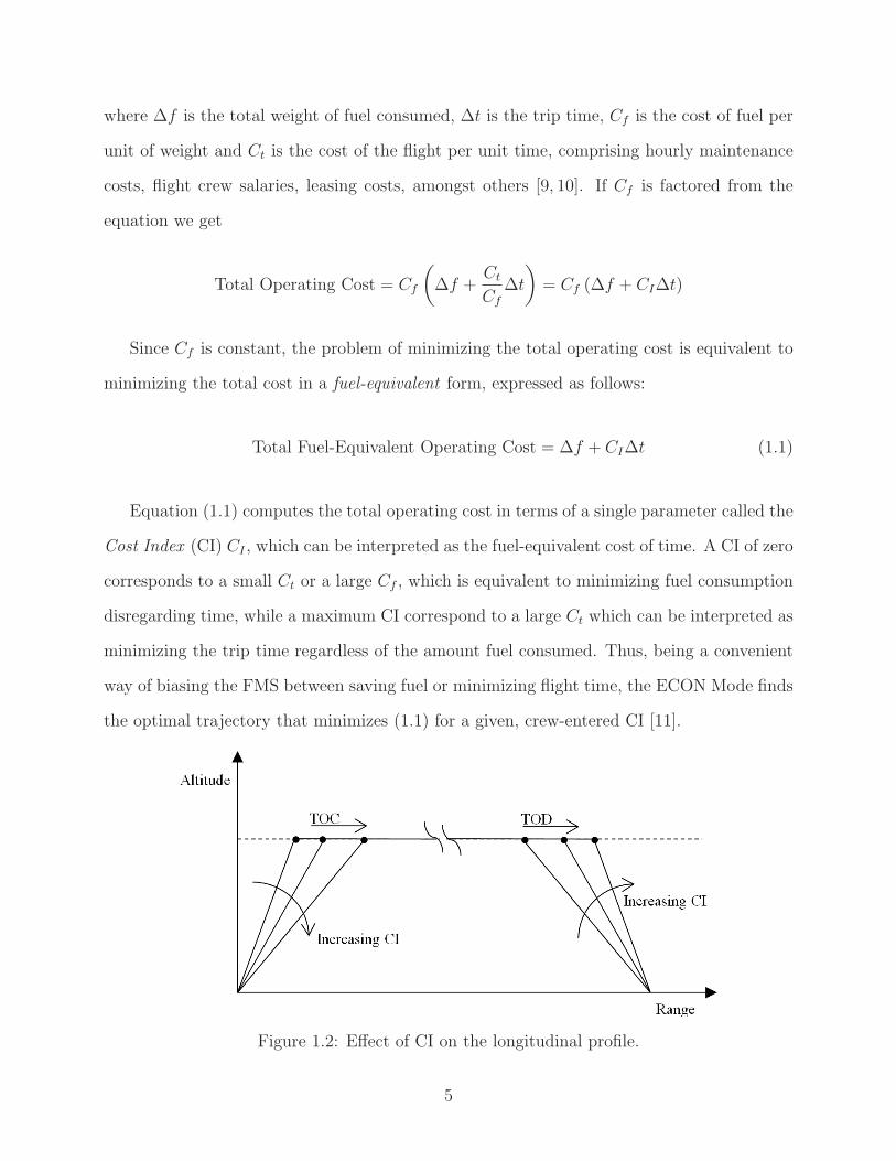
Figure 1.2: Effect of CI on the longitudinal profile.
5
The effects of CI on the longitudinal profile are well known. As depicted in Fig. 1.2,
increasing CI during climb makes the climb angle shallower and pushes farther the TOC,
while in descent the TOD starts later and the descent slope becomes steeper; during cruise
at a constant altitude, a higher CI simply increases the true airspeed and the aircraft burns
more fuel [9, 11, 12]. The opposite behaviors of the TOC and TOD might seem counter-
intuitive at first, since the descent can be thought as a climb backwards in time, but the
main difference between the two phases is the engine’s thrust setting: A high value known
as the maximum climb thrust is used while climbing, whereas a low value known as the idle
thrust is used while descending [13].
The CI’s units and range of allowable values vary depending on the FMS manufacturer
and aircraft type. For example, Boeing defines the cost index in dollars per hour divided by
cents per pound, as explained in [12]. In this work, it is assumed that CI is given in pounds
per seconds (lb/s).
1.4 Objective
As explained in Section 1.2, current FMS contain a Performance Database that stores the
optimal speed schedules for the aircraft in question, which are computed prior to the instal-
lation. The procedure used to generate this data is classified information. While storage
space might not be an issue in today’s systems, employing performance tables to obtain the
speed targets would often require interpolation between the sampling points, as opposed to
implementing a real-time scheme in which the optimal references would be computed directly.
In particular, analytic solutions require the least amount of storage space and computational
time. To the best of the author’s knowledge, most of the open literature regarding trajectory
optimization of aircraft either do not consider the performance modes present in a FMS,
or propose algorithms that require off-line computations or are too taxing for an on-board,
real-time implementation. As a result, finding an explicit, analytic feedback law for the
speed schedules would not only supply a very efficient means of implementation in a FMS,
6
but would also provide an elegant theoretical contribution to the performance analysis of
aircraft.
The objective of this thesis is to obtain state-feedback laws for the optimal true airspeeds
that generate cost-optimal trajectories in terms of CI for the different phases of flight, prefer-
ably as explicit analytic solutions, suitable for implementation in a real FMS. Sub-optimal
solutions are acceptable, provided that they are sufficiently close to the optimal and easily
implementable. The Range, Endurance, Maximum Rate of Climb and Minimum Rate of
Descent problems are also considered.
1.5 Literature Survey
1.5.1 Optimal Control
Optimal control theory is the branch of control systems that is concerned with finding the
control inputs for a system that optimize a given performance measure [14]. After determin-
ing the state-space representation of the system and defining the performance measure, an
Optimal Control Problem (OCP) is formulated and solved using different techniques. There
exists two main approaches to solving OCPs: The maximum principle which is based on
calculus of variations, and dynamic programming leading to the Hamilton-Jacobi-Bellman
(HJB) equation, based on Bellman’s principle of optimality. Nowadays, optimal control the-
ory is well known and documented, and several books have been released on the matter,
including [14–17].
The maximum principle was invented by Russian mathematician Lev Pontryagin et al.
in 1956, and first published in English in reference [18]. This approach yields a Two-Point
Boundary Value Problem (2PBVP) which can be solved analytically in some cases, but
generally require using a computer. An important drawback of the maximum principle is
that, since 2PBVPs specify some conditions at the initial time and others at the final time,
the optimal trajectories and controls attained are usually described in an open-loop fashion,
7
that is, as a function of the time (or the independent variable used). Ideally, it would be
preferable if the control inputs were given in a state-feedback form, as it would be valid for
different initial conditions and it would account for deviations from the optimal trajectory
due to potential disturbances.
In 1957, at around the same time when the maximum principle was proposed, dynamic
programming was formulated by Richard Bellman and published in [19]. Based on the princi-
ple of optimality, this approach provides state-feedback targets but is more computationally
intensive. It demands more storage capacity, as the state-space must be partitioned into
a grid and processed every iteration to obtain the minimal cost-to-go [14]. Its continuous-
time equivalent is the HJB equation which involves a nonlinear Partial Differential Equation
(PDE) and a boundary condition that must be satisfied by the optimal cost. It has the same
advantage as dynamic programming of providing a state-feedback control law, but obtaining
an analytical solution to the HJB is usually very difficult, if not impossible, for most prob-
lems. Nevertheless, an important contribution regarding the solution of PDEs that has been
applied to the HJB equation is the development of viscosity solutions, proposed by P. Lions
et al. in [20] (viscosity solutions are not utilized in this work).
1.5.2 Flight Management Systems
The actual algorithms used in a real FMS to generate the performance database are classified
information. However, there exists some publications by Boeing and Airbus that provide the
intuition behind the speed schedules that are provided by the performance module of the
FMS. For example, [10] is a thorough discussion on aircraft performance by Boeing including
the different performance modes available for each phase of flight in detail, for which examples
in the form of plots and charts are provided without specifying the methodology to obtain the
speed targets. A series of articles published in Boeing Aero Magazine, cited in [11,12,21,22],
summarize the impact of different speed schedules on fuel and cost savings during takeoff,
climb, cruise and descent, including the effect of the CI on the TOC and TOD. Similar
8
documents by Airbus include [9, 13].
In the open literature, Sam Liden from Honeywell (a manufacturer of FMS) has been an
important contributor on the topic. In [6] he presents the history of FMS and their evolution
in time, while in [23] he discusses issues regarding the implementation of the RTA mode
in FMS, which involves computing the CI that meets a time arrival constraint at a given
waypoint. He has also published several patents, including [24] for a FMS that minimizes
operating costs including the arrival error, and [25] for a method for computing optimum
altitude steps considering the effect of winds.
Within Concordia University, a laboratory-based test bed for FMS is developed in [26]
based on a commercial flight simulation software to obtain the aircraft aerodynamic data.
A communication interface between this software and the FMS is developed, as well as a
graphical user interface to operate the test bed.
1.5.3 Optimal Control Applied to Aircraft Trajectory Optimiza-
tion
There has been several contributions in the open literature regarding the optimization of
aircraft trajectories in FMS since the 1980’s, most of which have been based on the theory of
optimal control, involving the definition of an OCP and solving it using the the techniques
mentioned in section 1.5.1.
The maximum principle has been the most applied approach to the optimization of aircraft
trajectories. Books such as [17, 27] apply this approach to the minimum fuel, minimum
time, maximum-range and maximum rate-of-climb for aircraft problems. Some of the first
algorithms for the generation of on-board minimum cost trajectories in FMS using an energy-
state aircraft model, where it is assumed that energy increases monotonically during climb,
stays constant during cruise and decreases monotonically during the descent, can be found
in [28–31]. ATC constraints in these works are either neglected or incorporated in the form
of step-climbs. Computing a CI that meets a time of arrival constraint at a certain waypoint,
9
which is the strategy used by FMS in the RTA mode, is discussed using the Maximum
Principle in [32,33]. A more recent work discusses “next generation” FMS [34], assuming that
the aircraft stays very close to the optimal trajectory allowing to linearize the model about
the trajectory and to design a feedback autopilot. However, the cost functional discussed in
section 1.3 for the Economy mode is not considered, with a quadratic cost functional being
used instead.
Dynamic programming has also been considered in aerospace applications, in works such
as [35], in which issues such as the size of the solution space and enforcing constraints are
discussed. In [36] the Economy Mode is addressed and expanded by adding “at or before”
and “at or after” time constraints, along with several improvements to reduce computation
times. The generation of maximum-range trajectories during descent for commercial aircraft
in engine-out situations using dynamic programming has been considered in [37]. Very recent
publications include [38], in which minimum fuel trajectories are obtained for all flight phases
while taking the wind profile into account and ATC constraints. Finally, the HJB equation
has been applied to trajectory optimization of aerial vehicles, in works such as [39], where
an explicit solution is attained for the minimum time trajectory of a glider in a competition,
and [40], where a numerical method is developed to solve the HJB equation based on viscosity
solutions.
Finally, as a result of the increased computational power for on-board flight management
computers, other methods have emerged that do not rely on the classic optimal control theory.
Instead, these methods rely on converting the OCP into a nonlinear program, such as [41], or a
finite-dimensional optimization, as in [42], and solving the resulting problem using numerical
algorithms or specialized solvers. In [43], a method is developed to obtain the performance
bound of minimum time and minimum fuel descent trajectories, also considering the case of
RTA, and the optimal trajectory is generated using a numerical method known as the Gauss
pseudo-spectral method. Reference [44] considers the so-called inverse dynamics method
to generate minimum-time trajectories, in which the OCP is transformed into a nonlinear
10
program and the optimal trajectory is parametrized using polynomials.
Even though the ECON problem has been treated extensively in the open literature, most
of the contributions are centered around the previously mentioned approaches which resort
to complicated numerical methods, and generally obtain time-dependent descriptions of the
optimal trajectories which require a-priori offline computations. To the best of the authors’
knowledge, there has been no attempt, at least in the open literature, to obtain explicit,
analytic solutions to the ECON problem in a state-feedback form. As a result, the following
methodology will be proposed to attain the objective of this work.
1.6 Methodology
The ECON mode will be formulated and solved as an OCP for each of the flight phases:
climb, cruise and descent. The model of an aircraft flying in the longitudinal plane will be
considered in state-space form, and assumptions will be made to simplify and make it more
tractable for algebraic manipulations. To solve the OCP, both the Pontryagin’s Maximum
Principle and the Hamilton-Jacobi-Bellman equation will be used.
To validate the attained solutions, the Two-Point Boundary Value Problems (2PBVPs)
derived from the Maximum Principle will be solved directly by the means of a shooting
method in Matlab and Simulink. The shooting method is an iterative algorithm that solves
2PBVPs by reducing them to initial value problems. This method is not suitable for a
real-time implementation, as it relies on integrating the governing equations of the 2PBVP
problem each iteration which is generally time consuming, and it requires an initial estimate
of the unknown initial conditions from practical experience or trial and error. However, the
trajectories resulting from the shooting method can be considered as optimal, which are then
compared to the ones generated by the proposed solutions. An aircraft model based on the
Gulfstream Aerospace’s G-IV aircraft is used for the simulations.
11
1.7 Contributions
The following results are obtained in this thesis:
• The well-known true airspeed targets for maximum rate of climb, minimum rate of
descent, maximum range and maximum endurance are obtained by formulating each
scenario as an OCP and solving it by applying classical optimal control techniques.
From a theoretical point of view, this is the first time that these problems have been
approached from this perspective.
• For the cruise phase of the flight, a sub-optimal analytic expression in state-feedback
form is derived for the true airspeed in ECON mode. Moreover, when CI vanishes, the
solution reduces to the maximum-range speed which is known to be equivalent to the
minimum fuel per unit distance case. Simulation results show that the relative error
between the optimal cost (obtained by solving the OCP directly using the shooting
method) and the cost resulting from applying the analytic law is less than or equal to
1 · 10−2% for the cases presented in this thesis, making the sub-optimal approach good
enough for practical purposes. To the best of the author’s knowledge, this is the first
time that an algebraic expression has been proposed for the solution of this problem.
• For the climb and descent phases, a 5th degree polynomial in terms of the sub-optimal
speed is obtained, its coefficients involving only the states of the aircraft. The roots of
such polynomial can be found on-line by fast-converging algorithms such as Newton’s
method. The latter is arguably one of the simplest numerical methods available, making
this approach suitable for implementation in a real-time FMS. As in the cruise phase,
simulations show that, for the cases studied in this thesis, the relative error between
the optimal and sub-optimal cost is less than 1 · 10−3%, and therefore the sub-optimal
trajectory is close enough to the optimal one for practical purposes.
12
1.8 Structure of the Thesis
Chapter 2 starts by the Theoretical Preliminaries, covering the basic background material
required for understanding the rest of the thesis. It is followed by Chapter 3, which formulates
and solves the OCPs for Maximum Endurance and ECON during the cruise phase. For the
latter, a sub-optimal analytic expression for the optimal speed is found, which is compared
to the solution obtained by the shooting method at the end of the chapter. Next, Chapter 4
applies the same treatment to the climb and descent phases, addressing the Maximum Rate
of Climb, Minimum Rate of Descent and ECON problems. A polynomial is found, one of
its roots being the sub-optimal speed target, which is also compared to the shooting method
solution following the same approach as in the cruise. Lastly, Chapter 5 draws the main
conclusions of this thesis and provides extensions for future work.
13
Chapter 2
Theoretical Preliminaries
2.1 Aircraft Performance
The material covered in this section is based on [5, 45–48].
2.1.1 The International Standard Atmosphere (ISA) Model
Aircraft fly in the Earth’s atmosphere and, as a result, the latter has great influence on the
aerodynamic and propulsion properties of the airplane. The main variables that must be
considered in the atmosphere are the density ρ, viscosity μ and pressure p, all of which can
be considered as depending on the air temperature T . The real atmosphere is constantly
changing, so there does not exists a “normal” atmosphere, but the International Standard
Atmosphere (ISA) has been defined as a baseline to obtain standardized conditions from
which analyses can be made. A day whose conditions match the ones in the ISA model is
called a standard day.
The ISA assumes that the gravitational constant g is equal to its value at sea level and
defines the variation of T with altitude h based on empirical data. As shown in Fig. 2.1,
the ISA divides the atmosphere in three layers: The troposphere from sea level to 36150 ft.
where T decreases linearly, one section of the stratosphere called the tropopause from 36150
14
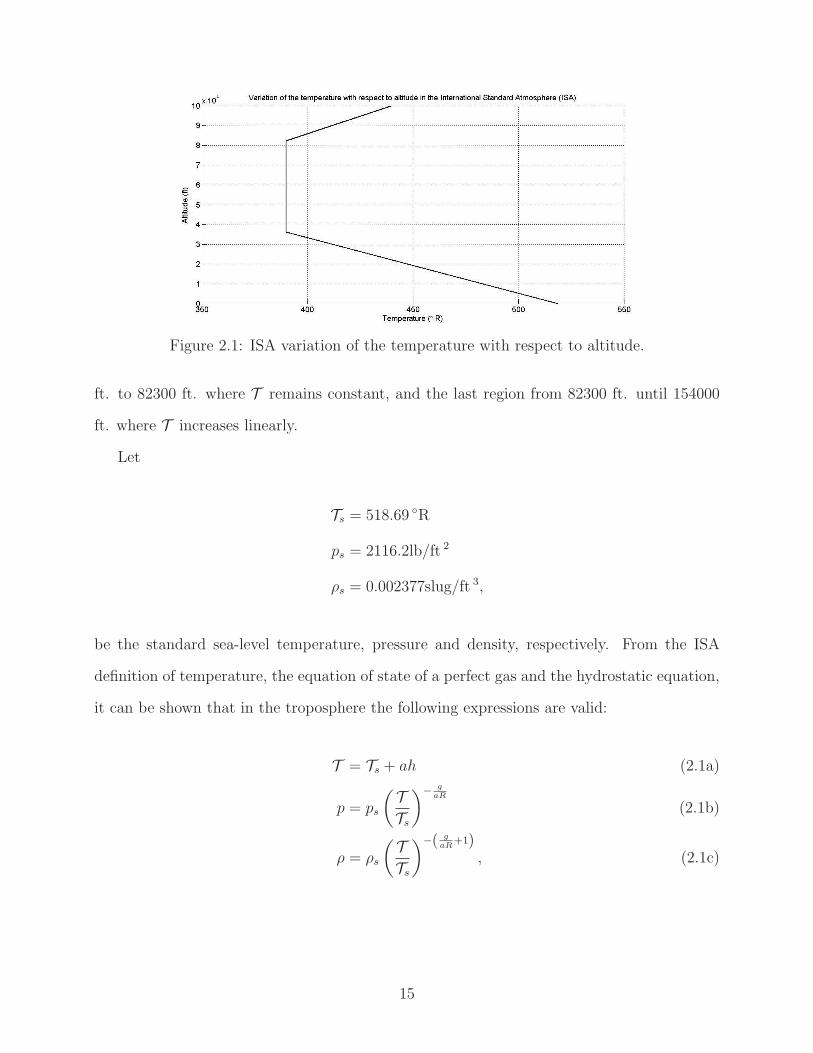
Figure 2.1: ISA variation of the temperature with respect to altitude.
ft. to 82300 ft. where T remains constant, and the last region from 82300 ft. until 154000
ft. where T increases linearly.
Let
Ts = 518.69 ◦R
ps = 2116.2lb/ft 2
ρs = 0.002377slug/ft 3,
be the standard sea-level temperature, pressure and density, respectively. From the ISA
definition of temperature, the equation of state of a perfect gas and the hydrostatic equation,
it can be shown that in the troposphere the following expressions are valid:
T = Ts + ah (2.1a)
p = ps
(TTs
)− gaR
(2.1b)
ρ = ρs
(TTs
)−( gaR
+1), (2.1c)
15
where
a = −0.00356 ◦R/ft
g = 32.17ft/s 2
R = 1718 lb ft slug−1 ◦R−1
are the temperature lapse rate, gravitational constant and gas constant for air, respectively.
Similarly, for the tropopause layer, let
h1 = 36150ft
T1 = 389.99 ◦R
p1 = 472.2lb/ft 2
ρ1 = 7.0539 · 10−4slug/ft 3,
be the altitude. temperature, pressure and density at the point where the tropopause starts,
then the temperature remains constant, and the pressure and density are given by:
p = p1e− g(h−1)
RT (2.2a)
ρ = ρ1e− g(h−1)
RT (2.2b)
Commercial aircraft never fly in the highest region of the stratosphere, therefore the
equations for that layer will not be covered here. The main factor that influences aerodynamic
forces is the density, making (2.1c) and (2.2b) the most important expressions for performance
analysis.
The ISA model is general enough to allow predicting the atmospheric conditions even
in a non-standard day. This is achieved by the means of the density altitude, which is the
altitude above sea level in a standard day at which the standard density would be equal to
the actual density experienced by the aircraft. In colloquial terms, it is the altitude that
16
the aircraft “feels” in the ISA. Strictly speaking, the variable h used throughout this work
must correspond to the density altitude to account for ISA deviations. Then, if the density
altitude is known, parameters such as the density and pressure can be computed using the
formulas presented in this section. The density altitude can be computed in real aircraft from
the pressure altitude read by the altimeter and the outside air temperature, and performance
charts for determining its value are usually available to pilots [5]. The exact procedure to
obtain density altitude is beyond the scope of this work and will not be discussed further.
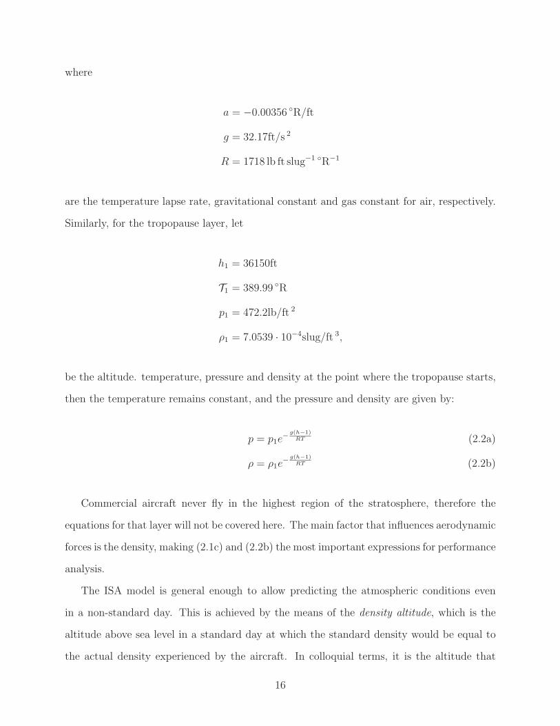
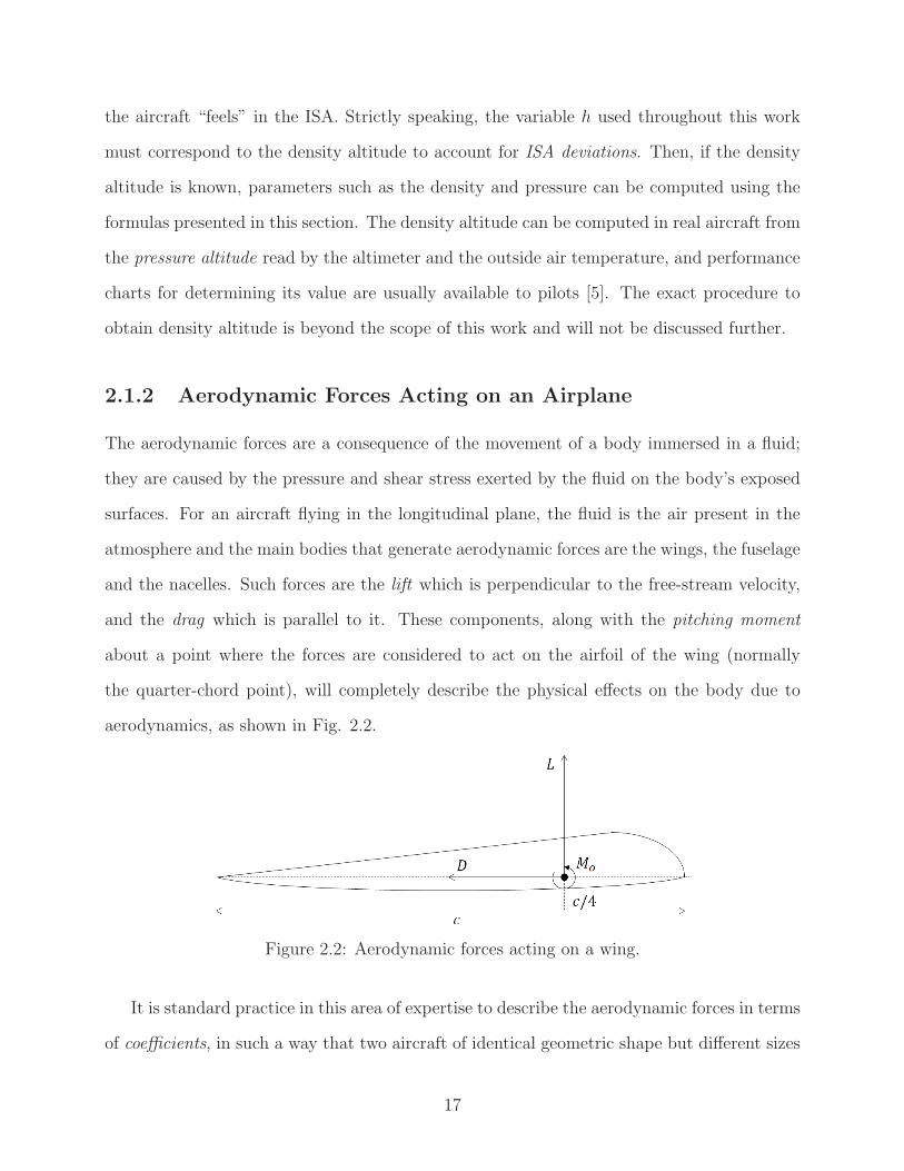
2.1.2 Aerodynamic Forces Acting on an Airplane
The aerodynamic forces are a consequence of the movement of a body immersed in a fluid;
they are caused by the pressure and shear stress exerted by the fluid on the body’s exposed
surfaces. For an aircraft flying in the longitudinal plane, the fluid is the air present in the
atmosphere and the main bodies that generate aerodynamic forces are the wings, the fuselage
and the nacelles. Such forces are the lift which is perpendicular to the free-stream velocity,
and the drag which is parallel to it. These components, along with the pitching moment
about a point where the forces are considered to act on the airfoil of the wing (normally
the quarter-chord point), will completely describe the physical effects on the body due to
aerodynamics, as shown in Fig. 2.2.
Figure 2.2: Aerodynamic forces acting on a wing.
It is standard practice in this area of expertise to describe the aerodynamic forces in terms
of coefficients, in such a way that two aircraft of identical geometric shape but different sizes
17
exposed to the same flow conditions yield the exact same coefficient values, a fact that
propelled the creation of wind tunnels. The lift, drag and pitching moment are therefore
given by
L =1
2CL(α,Re,M)ρSv2 (2.3a)
D =1
2CD(α,Re,M)ρSv2 (2.3b)
Mo =1
2CMo(α,Re,M)ρScv2, (2.3c)
where it can be seen that the coefficients are assumed to depend on the angle of attack
α, Reynolds number Re and the Mach number M . The nature of these dependencies vary
according to the shape of the airfoil. There exists an underlying assumption: commercial
aircraft fly in a quasi-steady regime, meaning that accelerations and moments are very small,
and that the control surfaces deflect slowly and in small increases. As a result, it can
be assumed that control surface deflections do not effect aerodynamic forces. There are
more general models that account for these dependencies, but for performance analysis of
commercial aircraft, the equations presented here provide sufficient precision.
A functional relationship often used for the lift in aircraft performance is given by
CL = CL0(M) + CLα(M)α,
where CL0 and CLα are known aircraft-dependent functions. This expression is consid-
ered valid until the lift coefficient reaches a known maximum value CLmax , after which the
approximately-linear relationship between CL and α is broken and CL drops rapidly. If
this situation is reached, it is said that the aircraft has stalled, and we can compute the
corresponding stall speed by using CLmax and (2.3a) to obtain:
vs =
√2W
ρSCLmax
(2.4)
18
In (2.4) we have assumed that the lift equals the aircraft gross weight, an approximation
that is commonly used for commercial aircraft flying in quasi-steady conditions. It will allow
us to compute CL using the weight, resulting in a required angle of attack such that the lift
coefficient equation is satisfied.
The drag is expressed as a function of the lift coefficient as follows:
CD = CD,0 + CD,2C2L (2.5)
This well-known equation is called the drag polar. Generally speaking, the coefficients
CD,0 and CD,2 should depend on the Mach number, specially in transonic and supersonic flight
where shockwaves form around the wings, greatly increasing the drag. For most commercial
aircraft (which fly at a Mach number of less than 0.8), they can be assumed constant.
There exists well-known expressions to model the pitching moment coefficient CM0 . How-
ever, this work involves commercial aircraft flying in quasi-steady conditions where the rota-
tional dynamics of the aircraft can be neglected. As a result, the pitching moment coefficient
is not relevant to our discussion and will not be covered here.
2.1.3 Equations of Motion in the Longitudinal Plane
It is assumed that the Earth is flat and an inertial reference frame. As shown in Fig. 2.3,
the following coordinate systems are defined:
• The Earth coordinate system xeyeze, attached to the surface of the Earth at sea level
with ye pointing into the plane, such that the xeze plane becomes the longitudinal plane
in which the aircraft flies.
• The horizon coordinate system xhyhzh, whose origin is located at the center of gravity
of the aircraft and its axes stand parallel to the Earth axes.
• The body axes system xbybzb, which is attached to the airplane at its center of gravity,
19
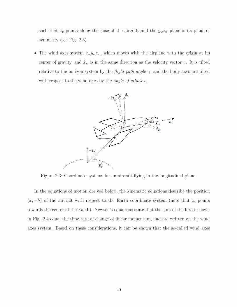
such that xb points along the nose of the aircraft and the ywzw plane is its plane of
symmetry (see Fig. 2.3).
• The wind axes system xwywzw, which moves with the airplane with the origin at its
center of gravity, and xw is in the same direction as the velocity vector v. It is tilted
relative to the horizon system by the flight path angle γ, and the body axes are tilted
with respect to the wind axes by the angle of attack α.
Figure 2.3: Coordinate systems for an aircraft flying in the longitudinal plane.
In the equations of motion derived below, the kinematic equations describe the position
(x,−h) of the aircraft with respect to the Earth coordinate system (note that ze points
towards the center of the Earth). Newton’s equations state that the sum of the forces shown
in Fig. 2.4 equal the time rate of change of linear momentum, and are written on the wind
axes system. Based on these considerations, it can be shown that the so-called wind axes
20
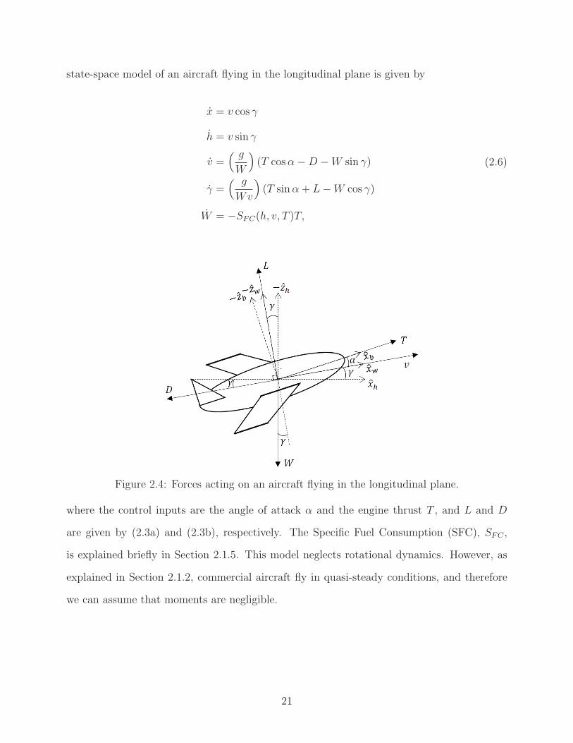
state-space model of an aircraft flying in the longitudinal plane is given by
x = v cos γ
h = v sin γ
v =( g
W
)(T cosα−D −W sin γ)
γ =( g
Wv
)(T sinα + L−W cos γ)
W = −SFC(h, v, T )T,
(2.6)
Figure 2.4: Forces acting on an aircraft flying in the longitudinal plane.
where the control inputs are the angle of attack α and the engine thrust T , and L and D
are given by (2.3a) and (2.3b), respectively. The Specific Fuel Consumption (SFC), SFC ,
is explained briefly in Section 2.1.5. This model neglects rotational dynamics. However, as
explained in Section 2.1.2, commercial aircraft fly in quasi-steady conditions, and therefore
we can assume that moments are negligible.
21
2.1.4 Flight Envelope
In Section 2.1.2 the stall speed, given by (2.4), was introduced. The stall speed becomes a
lower bound on the valid range of True Airspeeds (TAS) that the aircraft may fly at, for
a given value of altitude and weight. It makes sense to ask then if there exists an upper
bound on the TAS as well, and in which region of space can the aircraft sustain steady, level
flight. Such region is called the flight envelope, and is usually given by a curve plotted in
the speed-altitude plane consisting of the locus of maximum and minimum velocities, for a
particular weight.
An upper and lower bound on the TAS can be estimated as a consequence of the engine
limitations and drag characteristics of the airplane: Assume that the aircraft flies in steady,
level-flight. In (2.6), the derivatives of v and γ become zero, as well as γ. If we let T sin(α) <<
W and assume T cos(α) ≈ T , then the neglected dynamics yield the following balance of
forces:
L = W (2.7)
T = D (2.8)
Equations (2.7) and (2.8) are frequently used in the performance analysis of aircraft during
cruise. When in level flight, the amount of thrust needed to equal the drag as in (2.8) is
called the thrust required. Let the engine thrust T be constrained to a given range
Ti ≤ T ≤ Tmax(h), (2.9)
where the idle thrust Ti and maximum thrust Tmax are known for a particular engine. In
fact, the latter is normally a decreasing function of h in turbojet and turbofan engines, and
is specified in tabular or graphical form. Then, combining the expression for the drag (2.3b)
22
and (2.8), we get:
T =1
2CDρSv
2
Substituting the drag coefficient (2.5) gives
T =1
2
(CD,0 + CD,2C
2L
)ρSv2,
which, after solving for CL in (2.3a) and accounting for (2.7), becomes:
T =CD,0ρSv
2
2+
2CD,2W2
ρSv2(2.10)
When T = Tmax(h), solving for v in (2.10) will yield the maximum and minimum velocities
for which the thrust can equal drag and level flight can be sustained, for each value of altitude
and weight. Normally, it is expected that solving (2.10) will yield two positive values for v,
the maximum and the minimum, until an altitude where the maximum thrust has decreased
to the point where both bounds coincide into a single, positive value. When that case
happens, we have reached the maximum altitude or absolute ceiling at which level flight can
be attained, with a rate of climb (ROC) equal to zero.
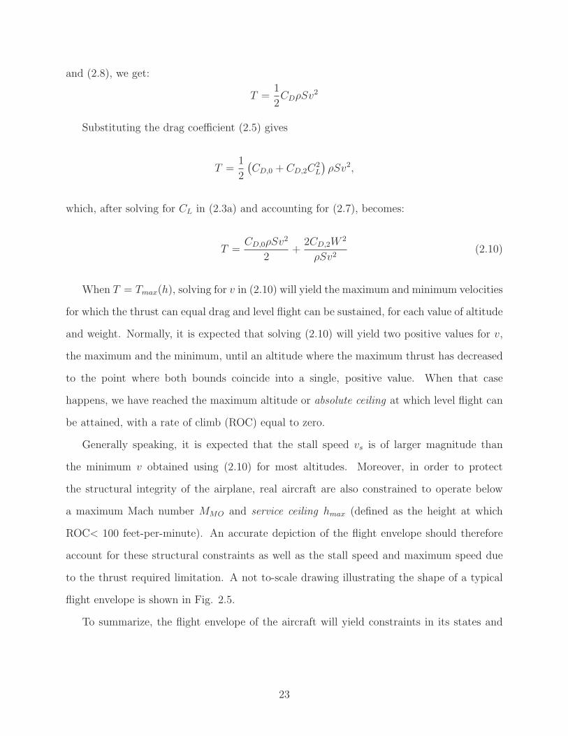
Generally speaking, it is expected that the stall speed vs is of larger magnitude than
the minimum v obtained using (2.10) for most altitudes. Moreover, in order to protect
the structural integrity of the airplane, real aircraft are also constrained to operate below
a maximum Mach number MMO and service ceiling hmax (defined as the height at which
ROC< 100 feet-per-minute). An accurate depiction of the flight envelope should therefore
account for these structural constraints as well as the stall speed and maximum speed due
to the thrust required limitation. A not to-scale drawing illustrating the shape of a typical
flight envelope is shown in Fig. 2.5.
To summarize, the flight envelope of the aircraft will yield constraints in its states and
23
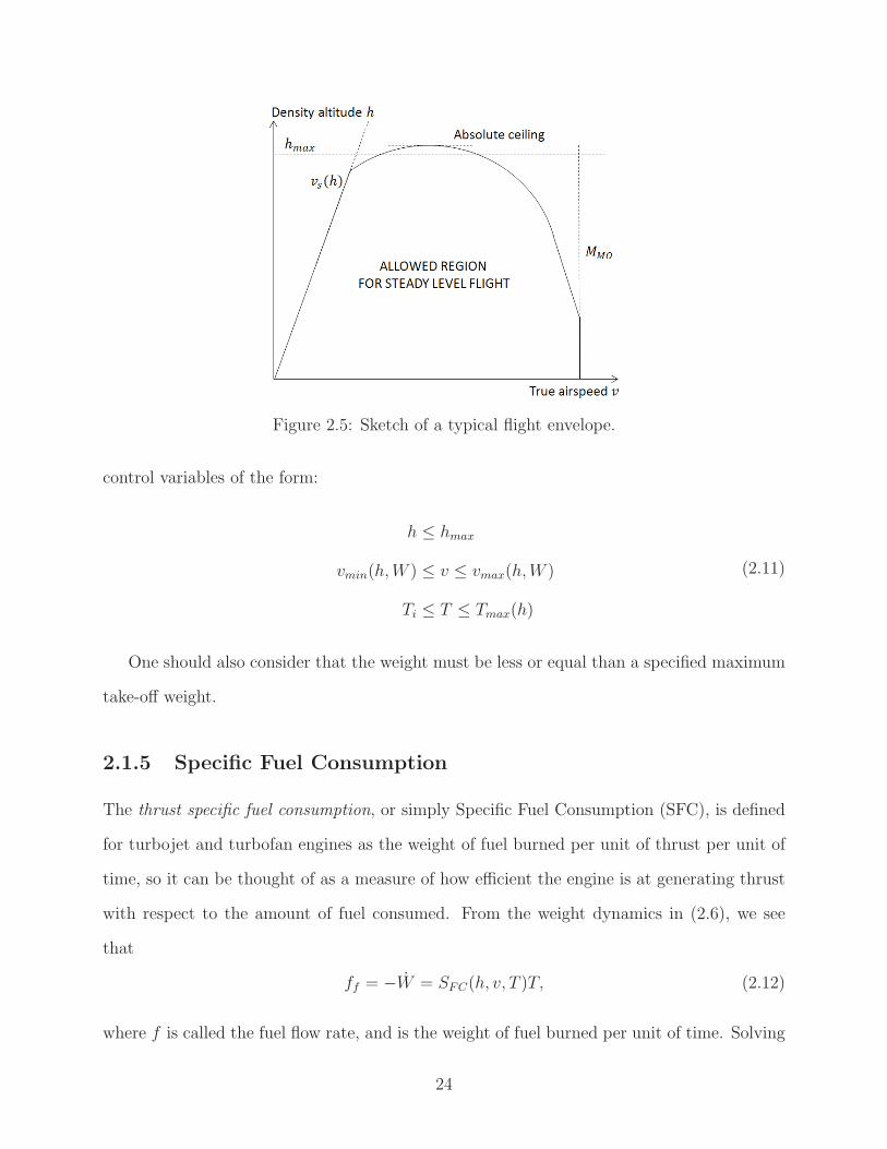
Figure 2.5: Sketch of a typical flight envelope.
control variables of the form:
h ≤ hmax
vmin(h,W ) ≤ v ≤ vmax(h,W )
Ti ≤ T ≤ Tmax(h)
(2.11)
One should also consider that the weight must be less or equal than a specified maximum
take-off weight.
2.1.5 Specific Fuel Consumption
The thrust specific fuel consumption, or simply Specific Fuel Consumption (SFC), is defined
for turbojet and turbofan engines as the weight of fuel burned per unit of thrust per unit of
time, so it can be thought of as a measure of how efficient the engine is at generating thrust
with respect to the amount of fuel consumed. From the weight dynamics in (2.6), we see
that
ff = −W = SFC(h, v, T )T, (2.12)
where f is called the fuel flow rate, and is the weight of fuel burned per unit of time. Solving
24
for SFC yields
SFC =ffT, (2.13)
therefore the units of the SFC is [1/time]. It is accustomed to use hours as the unit of time
when specifying the SFC. For propeller and reciprocating engines, the SFC is defined in terms
of the engine shaft power instead of thrust. However, it is possible to convert the SFC for a
propeller-driven/reciprocating engine to an equivalent thrust specific fuel consumption and
vice versa. The reader should consult [46] for more details. As a result, we will consider
(2.13) as a general expression for SFC that encompasses all engine types.
Generally speaking, SFC is considered as a function of thrust, speed and altitude (to be
specific, it depends on the density, but the latter depends on height in the ISA model), and
may vary drastically from one engine to another. In the performance analysis literature,
simpler models are used where SFC may be constant, altitude-depending or a function of
both altitude and Mach number. This work will consider SFC to be a given function of h
SFC = SFC(h), (2.14)
where its dependency can be linear, quadratic or any other model that fits the data. Its
nature does not affect the results obtained in this thesis.
2.1.6 Cruise Performance
Maximum Range Speed
The range of an aircraft is defined as the total ground distance it can travel for a given
amount of fuel. To obtain the maximum range of an aircraft, one seeks to maximize its fuel
mileage or specific range, a measure of the distance traversed per unit weight of fuel. The
specific range is given by the ground speed (which we assume is equal to TAS due to the
25
absence of wind) divided by the fuel flow rate, that is
rs ≡v
ff,
which, after substituting ff using (2.12), becomes:
rs =v
SFCT(2.15)
Note that (2.15) is in units of distance divided by fuel weight, as desired. Integrating rs
with respect to the weight from the initial gross weight W0 to the zero fuel weight W1 would
then yield the range:
Range =
∫ W0
W1
rsdW
There exists several approaches in the literature to estimate the range; we are interested,
however, in obtaining the maximum range speed, which as explained previously is the one that
maximizes (2.15). It can be shown that for jet-driven aircraft, under steady flight conditions
where (2.7) and (2.8) hold, the maximum range speed can be computed as follows [46]:
vrange =
(2W
ρS
√3CD,2
CD,0
)1/2
(2.16)
It must be emphasized once more that (2.16) is the groundspeed for maximum range,
which equals TAS under zero-wind conditions only. In addition, it is well-known that this
solution yields the best fuel economy: given a certain distance to cover, flying at (2.16)
ensures that the amount of fuel consumed per unit distance is minimized. This fact will be
remarked in Chapter 3 as a way to verify the ECON speed, which must match the minimum
fuel case when CI is zero.
26
Maximum Endurance Speed
Endurance is defined as the amount of time an aircraft can fly with a given amount of fuel.
It is different from the concept of range in the sense that time is now the variable of interest,
not distance, and as a result endurance is more important in surveillance missions or when
executing holding patterns, where the aircraft’s autonomy is more important. The fuel flow
rate ff as defined in (2.12) plays the same role as the specific range in the case of endurance,
since minimizing it with respect to v yields the speed at which endurance is maximized.
Similar to the range, integrating the fuel flow rate with respect to the weight yields the
endurance.
As in the previous section it can be shown that, for jet-powered aircraft under steady
flight conditions, the speed for maximum endurance is given by the expression (see [46])
vendurance =
(2W
ρS
√CD,2
CD,0
)1/2
, (2.17)
which is the same value that minimizes the drag. It is tempting but incorrect to think that
maximizing endurance implies maximum fuel economy, since maximizing the time that the
aircraft can fly does not imply that it will reach its destination in a fuel-efficient manner.
Therefore, flying at the maximum range speed (2.16) will result in minimal fuel consumption
for the flight.
2.1.7 Maximum Rate of Climb and Rate of Descent Speeds
For an aircraft climbing (resp. descending) in quasi-steady flight conditions, the rate of climb
(resp. rate of descent) is defined as the vertical speed of the aircraft, given by
vvert =v(T −D)
W, (2.18)
27
where
T =
⎧⎨⎩ Tc : γ > 0 (during climb)
Ti : γ < 0 (during descent).
In the previous expression Tc is the maximum climb thrust or thrust available, while Ti is
the idle thrust value. We assume that both are independent of v. To maximize vvert during
climb (resp. minimize during the descent), (2.18) is differentiated with respect to v and
equated to zero, known as the necessary condition of optimality (explained in section 2.2.1).
For steady flight conditions, the drag is given by [45]
D(h, v,W ) = d0(h)v2 +
d1(h,W )
v2,
where
d0 =1
2CD,0ρS
d1 =2CD,2W
2
ρS.
As a result, from differentiating (2.18) and setting it to zero, we get
T −D − vDv = 0,
in which we substitute the expression for the drag yielding
3d0v4 − Tv2 − d1 = 0.
This expression can be solved for v2, which is given by
v2 =T ±
√T 2 + 12d0d16d0
,
28
or, after replacing d0 and d1 and taking the positive sign:
v2 =T +
√T 2 + 12CD,0CD,2W 2
3CD,0ρS(2.19)
Expression (2.19) computes the speed for the maximum rate of climb when T = Tc, and
similarly for the minimum rate of descent when T = Ti.
2.2 Optimization and Optimal Control
The material in this section is based on [14,17,27,49–51].
2.2.1 Necessary and Sufficient Conditions for Optimality
The necessary and sufficient conditions for solving a point-wise, finite-dimensional opti-
mization problem will be reviewed. Suppose that we want to minimize a given function
H : Rn × Rm → R, that is
minu
H(x, u),
with respect to the decision variables or control vector u, which is of the form:
u = [u1 · · · um]T
Assuming that there are no constraints on u and that the first and second partial deriva-
tives of H exist everywhere, then the necessary conditions for a minimum are [49]:
∂H
∂u|u∗ = 0 (2.20a)
∂2H
∂u2|u∗ ≥ 0 (2.20b)
Points u∗ that satisfy these conditions are called stationary points. Note that, since u is a
vector, condition (2.20a) implies that each component of the gradient ∂H/∂ui, i = 1, . . . ,m
29
must vanish, and condition (2.20b) reads that the Hessian matrix ∂2H/∂u2 must be positive
semidefinite.
The sufficient condition for optimality is given by [49]
∂2H
∂u2|u∗ > 0 (2.21)
For maximization problems, it can be shown that the sign in (2.21) must be negative.
If (2.21) is satisfied, then u∗ minimizes H. Note that (2.20b) and (2.21) differ only in the
greater or equal sign and, as a result, it is common practice to prove only (2.20a) and (2.21)
when solving optimization problems.
Note that H is a function of two variables: x and u. Often one wants to optimize a
multi-variable function with respect to only one of the variables, such as u. Such is the case
here, where the other variables are treated as constants and partial derivatives are used in
the necessary and sufficient conditions.
Condition (2.21) implies that the Hessian with respect to u of H must be positive definite.
A useful method for determining the positive definiteness of a matrix is by the means of
Sylvester’s criterion, which states that a symmetric matrix A is positive definite if and only
if its leading principal minors are all positive. The kth leading principal minor of a matrix
is defined as the determinant of its upper-left k-by-k matrix. As a result, to test the positive
definiteness of A, we compute the determinant of each k-by-k submatrix, including A itself.
All of these determinants must be positive for A to be positive definite.
For example, if we have a symmetric 2-by-2 matrix
A =
⎡⎣a b
b d
⎤⎦ ,
30
then the following expressions must be satisfied:
a > 0
ad− b2 > 0
d > 0
This work will use the necessary and sufficient conditions presented in this section to
minimize a function called the Hamiltonian with respect to u, where the latter is subject to
strict inequality constraints. It is important to note that the existence of these constraints
does not invalidate the conditions presented here. For instance, suppose that u is constrained
to lie inside a set Ω, described by the vector g composed of p strict inequality constraints
Ω = {u : g(u) < 0} ,
then u∗ must satisfy (2.20a), (2.21) and gi(u∗) < 0, i = 1, . . . , p. That is, u∗ must lie
in the interior of Ω, where the constraints g are not effective and can the problem can
be treated as an unconstrained one. Optimization of functions subject to less-or-equal or
equality constraints is not carried out in this thesis and therefore will not be covered in the
theoretical preliminaries.
2.2.2 Optimal Control Problem
An Optimal Control Problem (OCP) differs from a point-wise, finite-dimensional optimiza-
tion problem in two fundamental components: the existence of a dynamic system and the
performance measure.
A dynamic system could be a physical body (such as an aircraft) or any process whose
outputs vary dynamically as the inputs are applied. Such process needs a mathematical
description that accurately describes its response with respect to the control inputs. A well-
31
known mathematical representation of dynamic systems is the state space representation, in
which the system is characterized by a set of state variables
ζ1(t), . . . , ζn(t),
and the control inputs
u1(t), . . . , um(t),
which are a function of time just like the states. Then, the relationship between the state
variables and control inputs is given by the set of Ordinary Differential Equations (ODEs)
ζ1(t) = f1(ζ1(t), . . . , ζn(t), u1(t), . . . , um(t), t)
ζ2(t) = f2(ζ1(t), . . . , ζn(t), u1(t), . . . , um(t), t)
...
ζn(t) = fn(ζ1(t), . . . , ζn(t), u1(t), . . . , um(t), t),
or, in more compact form:
ζ(t) = f(ζ(t), u(t), t) (2.22)
In (2.22), we denote ζ = [ζ1 · · · ζn]T as the state vector, u = [u1 · · · um]T as the control
vector and f = [f1 · · · fn]T as the dynamic function, which is generally nonlinear and time-
varying. The state space representation is widely used in control systems and provides a
universal framework for the analysis of dynamic systems. Section 2.1.3 will present a model
of an aircraft in state space form, which will be used in this work.
The performance measure, or cost functional, mathematically defines the criterion that
will be used to quantitatively assess the performance of the system. A functional is a real-
valued function that takes arguments from a space of functions, effectively making it a “func-
32
tion of a function”. In optimal control, cost functionals of the form
J(ζ(t0), u(t0), t0) =
∫ tf
t0
L(ζ(t), u(t), t)dt+ φ(ζ(tf ), tf ) (2.23)
are used, in which t0 and tf are the initial and final time, respectively, and φ and L are scalar
functions. For any initial state ζ(t0) and control function u(t) the state is driven by (2.22)
for t ∈ [t0, tf ], and the cost functional (2.23) assigns a real number to the resulting state and
control history. Then, J gives us a quantitative measure of the performance of the system
for that particular control input. Simple examples of cost functionals include those used in
minimum time problems
J =
∫ tf
t0
dt = tf − t0,
and quadratic cost functionals that minimize the energy spent by the control signal
J =
∫ tf
t0
uT (t)Ru(t)dt
Having defined its main components, an OCP is formulated as follows: find the optimal
control function u∗(t) that minimizes the cost functional (2.23), where the optimal state tra-
jectory ζ∗(t) is generated by the system dynamics (2.22) evaluated for u∗(t). The optimization
is also subject to initial and final conditions on the state, and constraints on ζ and u are
described as a set of admissible states Z and control inputs U , respectively. Mathematically,
we write:
J∗(t0) := infu(t)
{∫ tf
t0
L(ζ(t), u(t), t)dt+ φ(ζ(tf ), tf )
}s.t.
ζ(t) = f(ζ(t), u(t), t)
ζ(t) ∈ Z, u(t) ∈ U
ζ(t0) = ζ0
ψ(ζ(tf ), tf ) = 0
(2.24)
33
Note that, while the initial condition ζ0 and the initial time t0 are considered as given,
the final condition ζ(tf ) and the final time tf do not have to be specified. In (2.24) we
have written that the final state and time must satisfy equality constraints ψ(tf , ζ(tf )) = 0.
This encompasses the case where final conditions are given as well. In other words, we want
(tf , ζ(tf )) to belong to a target set :
S = {(ζ(tf ), tf ) : ψ(ζ(tf ), tf ) = 0} (2.25)
The final time tf is then defined as the smallest time such that (tf , ζ(tf )) enters S. The
different types of OCPs are then represented by the choice of S. For instance, a fixed-time,
free-endpoint problem has a target set of the form S = t1×Rn, with t1 known. It is important
to consider that S must be a closed set for tf to be well defined.
The two main approaches used for solving OCPs, the Maximum Principle and Dynamic
Programming, will be the subject of the following subsections.
2.2.3 Pontryagin’s Maximum Principle
The Maximum Principle is a technique that provides necessary conditions that must be met
by a minimizing control u(t). Assume an OCP of the form (2.24) with unspecified terminal
time tf . Then, the system dynamics (2.22) and the final state constraints are adjoined to the
cost functional (2.23) yielding
J =
∫ tf
t0
[L(ζ(t), u(t), t) + λT (t)
(f(ζ(t), u(t), t)− ζ(t)
)]dt
+ φ(ζ(tf ), tf ) + νTψ(ζ(tf ), tf ),
with λ(t) being n time-varying Lagrange multipliers or costates, and ν being also lagrange
multipliers of the same dimension as ψ. Define the Hamiltonian as:
H(ζ(t), u(t), λ(t), t) = L(ζ(t), u(t), t) + λT (t)f(ζ(t), u(t), t) (2.26)
34
It follows from calculus of variations that the necessary conditions for obtaining an optimal
J∗ are [17]:
ζ = f(ζ, u, t) (2.27)
λ = −(∂H
∂ζ
)T
(2.28)
∂H
∂u= 0 (2.29)
λ(tf ) =
(∂φ
∂ζ+ νT ∂ψ
∂ζ
)|tf (2.30)(
∂φ
∂t+ νT ∂ψ
∂t+H
)|tf = 0 (2.31)
ψ(ζ(tf ), tf ) = 0 (2.32)
Equations (2.27) and (2.32) are re-statements of the system dynamics and the final state
constraints, respectively. On the other hand, (2.28) and (2.30) have effectively augmented
the system by providing additional dynamics and boundary conditions for the costates, while
u must be a stationary point of H as stated in (2.29). Equation (2.31) results from the fact
that the final time is not prescribed. In summary, the resulting problem is called a two-point
boundary value problem (2PBVP) because the boundary conditions for the state are given at
the initial time ζ0, while the ones for the costates λf are given at the final time via (2.30).
The approach presented in this section is the most frequently used in the literature when
dealing with OCPs. However, its main disadvantage is that the optimal control policy is
specified as a function of the costates, which must be obtained by integrating (2.28) backwards
in time subject to their boundary conditions. As a result, the control input is obtained as
a function of time. The 2PBVP can be solved numerically using the celebrated shooting
method, which will be explained briefly in the next section.
35
2.2.4 The Shooting Method
The shooting method is a numerical technique to solve 2PBVPs, such as the ones formulated
using the maximum principle, by reducing it to an initial value problem. Suppose we have a
system described by n first order ODEs with some boundary conditions given at the initial
time and others given at the final time, that is:
ζ(t) = f(ζ(t), t), t ∈ [t0, tf ]
ζi(t0), i = 1, . . . , q specified
ζj(tf ), j = q, . . . , n specified
Normally, if ζi(t0) were specified ∀i = 1, . . . , n, the trajectory ζ(t) would easily be gener-
ated by integrating the state equation with the help of a computer. The main idea behind
the shooting method is to guess an initial condition for the states ζj, integrate the ODEs to
obtain the corresponding trajectory, then guess a new (and hopefully more accurate) initial
condition based on the error between the values of ζj at tf and their prescribed ones. The
algorithm would stop when the error in the final conditions are small enough, or when the
difference between consecutive values of the initial conditions (also known as seeds) becomes
negligible.
Letting ζ(k)(t) denote the state trajectory at the kth iteration, the following pseudo-code
is an example of a generic shooting algorithm:
1. Choose initial seeds ζ(0)j (t0)
2. Let k = 0
3. Do:
(a) Simulate the system by integrating the equations forward
(b) εj = ζ(k)j (tf )− ζj(tf )
36
(c) Compute next seed ζ(k+1)j (t0) as a function of ζ
(k)l (t0), εl and l = q, . . . , n, using a
given update law
(d) k = k + 1
4. Until∑n
j=q |εj| < tolerance OR k ≥ Max. Iterations
The 2PBVPs resulting from the Maximum Principle fit into the framework of the shooting
method: in this case, the dynamics of the costates J∗ζ are appended to the ones of the original
state variables ζ to form an “augmented” system in which some boundary conditions will
be prescribed at the initial time, and others at the final time. The optimal control input u
is obtained at every time-step by solving for it using the necessary condition of optimality
(2.29) (which could have an algebraic solution or be a transcendental equation; the way it is
solved would depend on the problem). As a result, the methodology discussed in this section
applies to the Maximum Principle, making the shooting method an attractive approach to
numerically solving OCPs.
It is important to note that the system’s governing equations must be integrated until
the final time each iteration, which could be a time consuming process especially for complex
systems. In addition, it requires selecting ζ(0)j (t0) from practical experience or trial and error.
Thus, even though it can yield precise numerical solutions to 2PBVPs, it is not suitable for a
real-time system implementation. However, it can be used to validate sub-optimal solutions
to OCPs off-line, as is the case in this thesis.
The main challenges when implementing the shooting algorithm include selecting the
initial seed for the states ζj(t0), specifically if they do not have an obvious physical meaning,
and choosing an appropriate update law for the subsequent guesses. A generally accepted
expression for an update law is [27]
ζ(k+1)j (t0) = ζ
(k)j (t0)−
n∑l=q
βl
(ζ(k)l (tf )− ζl(tf )
)(2.33)
where βl are tuning parameters. This work will use update laws of such type. To illustrate
37
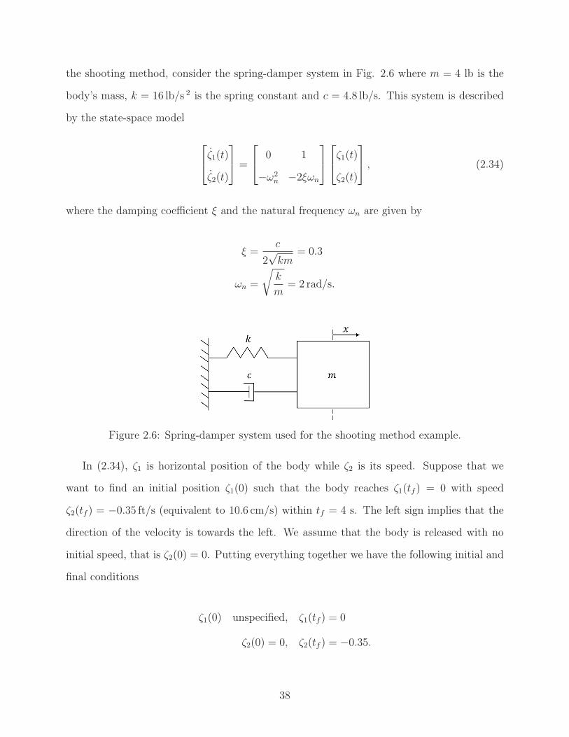
the shooting method, consider the spring-damper system in Fig. 2.6 where m = 4 lb is the
body’s mass, k = 16 lb/s 2 is the spring constant and c = 4.8 lb/s. This system is described
by the state-space model
⎡⎣ζ1(t)ζ2(t)
⎤⎦ =
⎡⎣ 0 1
−ω2n −2ξωn
⎤⎦ ⎡⎣ζ1(t)ζ2(t)
⎤⎦ , (2.34)
where the damping coefficient ξ and the natural frequency ωn are given by
ξ =c
2√km
= 0.3
ωn =
√k
m= 2 rad/s.
Figure 2.6: Spring-damper system used for the shooting method example.
In (2.34), ζ1 is horizontal position of the body while ζ2 is its speed. Suppose that we
want to find an initial position ζ1(0) such that the body reaches ζ1(tf ) = 0 with speed
ζ2(tf ) = −0.35 ft/s (equivalent to 10.6 cm/s) within tf = 4 s. The left sign implies that the
direction of the velocity is towards the left. We assume that the body is released with no
initial speed, that is ζ2(0) = 0. Putting everything together we have the following initial and
final conditions
ζ1(0) unspecified, ζ1(tf ) = 0
ζ2(0) = 0, ζ2(tf ) = −0.35.
38
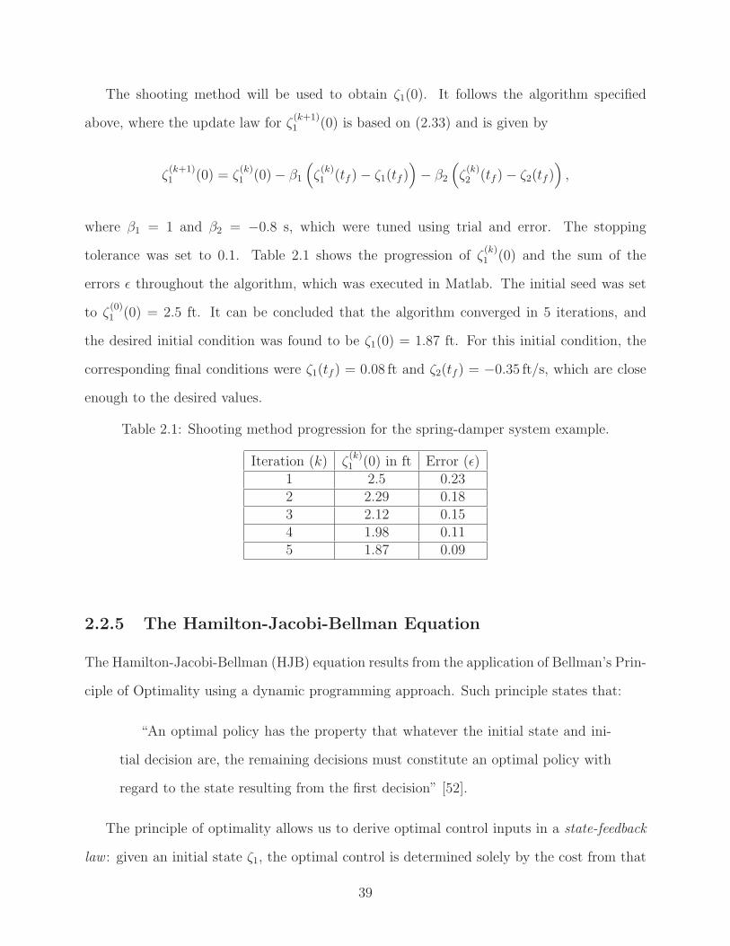
The shooting method will be used to obtain ζ1(0). It follows the algorithm specified
above, where the update law for ζ(k+1)1 (0) is based on (2.33) and is given by
ζ(k+1)1 (0) = ζ
(k)1 (0)− β1
(ζ(k)1 (tf )− ζ1(tf )
)− β2
(ζ(k)2 (tf )− ζ2(tf )
),
where β1 = 1 and β2 = −0.8 s, which were tuned using trial and error. The stopping
tolerance was set to 0.1. Table 2.1 shows the progression of ζ(k)1 (0) and the sum of the
errors ε throughout the algorithm, which was executed in Matlab. The initial seed was set
to ζ(0)1 (0) = 2.5 ft. It can be concluded that the algorithm converged in 5 iterations, and
the desired initial condition was found to be ζ1(0) = 1.87 ft. For this initial condition, the
corresponding final conditions were ζ1(tf ) = 0.08 ft and ζ2(tf ) = −0.35 ft/s, which are close
enough to the desired values.
Table 2.1: Shooting method progression for the spring-damper system example.
Iteration (k) ζ(k)1 (0) in ft Error (ε)
1 2.5 0.232 2.29 0.183 2.12 0.154 1.98 0.115 1.87 0.09
2.2.5 The Hamilton-Jacobi-Bellman Equation
The Hamilton-Jacobi-Bellman (HJB) equation results from the application of Bellman’s Prin-
ciple of Optimality using a dynamic programming approach. Such principle states that:
“An optimal policy has the property that whatever the initial state and ini-
tial decision are, the remaining decisions must constitute an optimal policy with
regard to the state resulting from the first decision” [52].
The principle of optimality allows us to derive optimal control inputs in a state-feedback
law : given an initial state ζ1, the optimal control is determined solely by the cost from that
39
state until the final state ζf . Based on the cost functional (2.23), define the cost-to-go as:
J(ζ(t), u(t), t) =
∫ tf
t
L(ζ(t), u(t), t)dt+ φ(ζ(tf ), tf ) (2.35)
For a given initial state and time (ζ(t), t), and control input u(t), t ∈ [t, tf ], equation
(2.35) returns the cost to be incurred from that given point until the final time, using the
prescribed control history. The additive property of the optimal cost-to-go allows splitting
it as follows, for some time increment Δt:
J∗(ζ(t), t) = infu(τ),t≤τ≤t+Δt
{∫ t+Δt
t
L(ζ(τ), u(τ), τ)dτ + J∗(ζ(t+Δt), t+Δt)
}(2.36)
In (2.36) the superscript ∗ denotes that the cost-to-go is optimal. It can be shown that,
by letting Δt converge to zero and using Taylor series, (2.36) yields a partial differential
equation that must be satisfied by the optimal cost-to-go, given by
0 = J∗t (ζ(t), t) + min
u(t)H(ζ(t), u(t), J∗
ζ (ζ(t), t), t), (2.37)
with
H(ζ(t), u(t), J∗ζ (ζ(t), t), t) = L(ζ(t), u(t), t) + J∗
ζ ζ , (2.38)
and boundary condition:
J∗(ζ(tf ), tf ) = φ(ζ(tf ), tf ) s.t. (ζ(tf ), tf ) ∈ S (2.39)
Equation (2.37) is the celebrated HJB equation, , with H being the Hamiltonian. A
subscript as in J∗t denotes the partial derivative of J∗ with respect to t, and similarly for
the rest of the variables. Note that the boundary condition (2.39) is satisfied only in the
target set, which is given by (2.25). If an optimal u∗ that minimizes H is found using the
40
necessary and sufficient conditions stated in section 2.2.2, then it is guaranteed that such
function minimizes J .
2.2.6 Combining the Hamilton-Jacobi-Bellman Equation with the
Maximum Principle
The Maximum Principle can be used in conjunction with the HJB equation to solve a given
OCP. Both approaches are connected by the means of the Hamiltonian. Comparing H in
(2.37) with (2.26), it can be shown that, as expected, the partial derivatives of the optimal
cost-to-go J∗ζ correspond to the costates that appear in the Maximum Principle, that is
J∗ζ (t) = λT (t). (2.40)
As a result of (2.40), equations (2.28), (2.30) and (2.31) can be used to obtain information
regarding the time evolution and the final values of the partial derivatives of the optimal
cost. Thus, when solving OCPs analytically a combination of the Maximum Principle and
the HJB equation provides the best insight regarding the optimal solution. In subsequent
developments, (2.26), (2.28) and (2.30) will be written as follows:
H(ζ(t), u(t), J∗ζ (t), t) = L(ζ(t), u(t), t) + J∗
ζ (t)f(ζ(t), u(t), t) (2.41)
J∗ζ = −
(∂H
∂ζ
)T
(2.42)
J∗ζ (tf ) =
(∂φ
∂ζ+ νT ∂ψ
∂ζ
)|tf (2.43)
An important result that greatly simplifies the analysis of OCPs using the HJB equation
is that, if the Hamiltonian (2.38) is not an explicit function of time (i.e. ∂H/∂t = 0) and the
final time tf is free, then H must vanish along the optimal trajectory, implying that J∗t = 0
41
and the HJB equation reduces to [14]
0 = minu(t)
H(ζ(t), u(t), J∗ζ (ζ(t), t)) (2.44)
As explained previously, the main advantage of the HJB equation is that it yields an
optimal control function in state-feedback form. However, solving this equation analytically
is extremely difficult. Nevertheless, there exist OCPs of practical interest, such as some of
the problems presented in this thesis, for which the HJB can be solved. The result is an
algebraic solution for the state-feedback controller, which is arguably the most desirable type
of solution for implementation purposes.
42
Chapter 3
Optimal Solutions for Cruise
3.1 Assumptions
Section 2.1.3 presented the equations of motion of an aircraft flying in the longitudinal plane.
In order to make (2.6) more tractable for performance computations, some assumptions must
be made based on the quasi-steady flight conditions in which modern commercial aircraft fly.
Such tractability is important if one wants to find an analytical solution to the resulting OCP;
otherwise, the mathematical expressions involved would be too complicated to manipulate
algebraically.
The assumptions made for the cruise segment of the flight are the following:
• The aircraft flies at a given, constant altitude constrained by Air Traffic Control (ATC)
as is the case with real FMS. This assumption makes γ, γ and h equal to zero.
• The altitude, speed and thrust values lie in the interior of the flight envelope given by
the constraints (2.11). As a result, we do not need to enforce them in the mathematical
formulation of the OCP.
• The angle of attack α is small, allowing to write cosα ≈ 1 and sinα ≈ α. This
assumption is standard practice in performance analysis for commercial aircraft.
43
• The component of the thrust perpendicular to the velocity vector, Tα, is much smaller
than L and W . The thrust force is usually around one order of magnitude smaller than
the weight, therefore multiplying it by a small angle will effectively make it negligible.
• Accelerations are negligible due to the steady-flight condition, and as a result we can
assume that v is approximately zero. Moreover, as explained previously in Section 1.2,
the FMS is not charged with reaching the optimal setpoints using the aircraft’s flight
controls, so we can take v as a control signal, leaving its dynamics to the autopilot.
In light of these assumptions, the simplified aircraft model for steady level flight in the
longitudinal plane is obtained as
x = v
W = −SFCD
(3.1)
L = W (3.2)
T = D (3.3)
The last two equations come from v and γ being equal to zero, using the assumptions
mentioned above (including Tα << W ). Note that they allow computing the required
control inputs to follow a given aircraft configuration in steady level flight. On one hand,
(3.2) effectively constrains the angle of attack to a value such that the lift balances the weight
at any given altitude and airspeed. On the other hand, (3.3) states that the thrust required to
sustain steady level flight will always be equal to the drag, implying that the thrust setpoint
provided by the FMS is easily computed during cruise provided that the optimal TAS is
found.
44
From (2.3a) and (3.2) we can solve for the lift coefficient as follows:
L = W =1
2CLρSv
2
CL =2W
ρSv2(3.4)
Substituting (3.4) into the drag coefficient (2.5) yields
CD = CD,0 + CD,2
(2W
ρSv2
)2
,
which is then used in conjunction with (2.3b) to obtain the equation for the drag in quasi-
steady flight regime
D =1
2CD,0ρSv
2 +2CD,2W
2
ρSv2(3.5)
Note that under the assumptions made, the drag becomes a function of h (indirectly
through the density ρ), v and W . In subsequent developments (3.5) will be written as a
function of TAS as follows:
D(h, v,W ) = d0(h)v2 +
d1(h,W )
v2(3.6)
Obviously, the coefficients d0 and d1 are given by:
d0 =1
2CD,0ρS
d1 =2CD,2W
2
ρS
(3.7)
3.2 Maximum Endurance OCP
To illustrate the usefulness of formulating optimization problems involving dynamic systems
in the framework of the optimal control theory, this section will present a simple problem:
obtaining the TAS that maximizes the endurance of the aircraft during cruise.
45
Suppose that the aircraft weight Wc at TOC is given, and that Wd is the final weight
at which descent can be safely carried out in a given mission. The maximum endurance
problem seeks to maximize the amount of time that the aircraft can stay in the air, that is,
it maximizes the functional
J =
∫ td
tc
dt,
where the final time td has to be free for the problem to make sense. Since no final value
for the range x(td) is prescribed, the x equation in (3.1) becomes irrelevant, reducing the
dynamics to a 1st order system. As a result, the OCP formulation is given by:
J∗ = maxv(t),td
∫ td
tc
dt
s.t.
W = −SFCD
W (tc) = Wc,W (td) = Wd
(3.8)
The following theorem states the solution to OCP (3.8).
Theorem 3.2.1. The optimal solution to OCP (3.8) is given by
v2 =2W
ρS
√CD,2
CD,0
, (3.9)
and the optimal cost-to-go J∗ is
J∗ =1
2SFC
√CD,0CD,2
log
(W
Wd
). (3.10)
Proof. We begin by writing the Hamiltonian as shown in (2.41)
H = 1− J∗WSFCD, (3.11)
46
which, in accordance with both the Maximum Principle and the HJB equation approach,
must be maximized with respect to v(t) (because this is a maximization problem). The
necessary condition explained in Section 2.2.1 is used
∂H
∂v= −J∗
WSFCDv = 0
In the above equation, Dv denotes the partial derivative of the drag with respect to the
speed. It follows that either J∗W , Dv or both must vanish for every t. However, from the
sufficient condition for optimality, we get
∂2H
∂v2= −J∗
WSFCDvv < 0,
implying
J∗W > 0, (3.12)
since SFC is positive and D is convex with respect to the speed. As a result, the necessary
condition becomes
Dv = 0 (3.13)
Using (3.6) as the expression for the drag, condition (3.13) can be used to solve for the
optimal v:
2d0v −2d1v3
= 0 → v4 =d1
d0
Considering (3.7), the speed for maximum endurance is obtained as
v2 =2W
ρS
√CD,2
CD,0
,
which is equal to (3.9) and coincides with (2.17) as presented in Section 2.1.6. In this case,
the value of this approach is that it allows obtaining an expression for the optimal cost-to-go,
which must satisfy the HJB equation (2.37). Since H does not depend explicitly on time and
47
td is free, then from (2.44) we get that the HJB equation
0 = J∗t (ζ(t), t) + min
v(t)H(ζ(t), v(t), J∗
ζ (ζ(t), t), t),
reduces to
minv(t)
H(ζ(t), v(t), J∗ζ (ζ(t), t), t) = min
v(t){1− J∗
WSFCD} = 0 (3.14)
that is, the Hamiltonian must vanish along the optimal trajectory. The boundary condition
for the cost-to-go is obtained by applying (2.39) to this problem, that is:
J∗(td) = 0 s.t. W (td) = Wd (3.15)
Moreover, using (2.42) from the Maximum Principle, we obtain an equation for the time
derivative of J∗W , given by
J∗W = − ∂H
∂W= J∗
WSFCDW
= J∗WSFC
4CD,2W
ρSv2, (3.16)
where (3.5) was used for the drag. From (3.14) evalauted at the optimal v, we can solve for
J∗W
J∗W =
1
SFCD,
where the drag must be evaluated at the optimal v. Substituting (3.9) into (3.5) yields
D = 2W√CD,0CD,2 (3.17)
When (3.17) is replaced into J∗W we get
J∗W =
1
2WSFC
√CD,0CD,2
(3.18)
48
To prove that J∗W satisfies (3.16), the time derivative of (3.18) is taken using the state
equation for W and (3.17) for D to obtain
d
dt
(1
2WSFC
√CD,0CD,2
)= −
2SFC
√CD,0CD,2W(
2WSFC
√CD,0CD,2
)2 =SFCD
2W 2SFC
√CD,0CD,2
,
which, after considering (3.18) and (3.17) becomes
SFCD
2W 2SFC
√CD,0CD,2
=SFCD
WJ∗W = 2SFC
√CD,0CD,2J
∗W .
This is the same expression as (3.16) with v2 substituted by (3.9). The obtained J∗W also
satisfies (3.12), the sufficient condition to maximize the Hamiltonian. The optimal cost-to-go
is therefore obtained by integrating (3.18) with respect to W :
J∗ =1
2SFC
√CD,0CD,2
∫1
WdW =
log(W )
2SFC
√CD,0CD,2
+ C
The constant C is determined by the boundary condition (3.15), which must be satisfied
by J∗:
J∗(Wd, td) =log(Wd)
2SFC
√CD,0CD,2
+ C = 0 → C = − log(Wd)
2SFC
√CD,0CD,2
As a result, the optimal cost function is
J∗ =1
2SFC
√CD,0CD,2
log
(W
Wd
).
By adopting an analytic approach to solving OCPs, it was possible to solve the maximum
endurance problem for an aircraft in cruising flight, recovering the well-known result for the
maximum endurance speed presented in Section 2.1.6, and also obtaining the expression for
the optimal cost-to-go (3.10). It seems reasonable then to apply the same set of tools to the
ECON problem in order to solve for the most economical speed target in terms of CI. Such
49
is the purpose of the next section.
3.3 Economy Mode OCP for Cruise
Section 3.3.1 will derive and solve the ECON mode OCP for cruise in longitudinal flight,
followed by section 3.3.2 which shows that the approach can be extended to handle turns in
the lateral plane.
3.3.1 Longitudinal Flight
Problem Formulation
The ECON mode for cruise will now be formulated as an OCP with a structure as in (2.24).
As explained in Section 1.3, its purpose is to minimize the total operating cost of the flight,
given by (1.1). This performance measure can be rewritten as a cost functional in integral
form as
J =
∫ td
tc
(ff + CI)dt
Here, td is the unspecified time at which the TOD is reached, and tc is the time at which
the cruise phase begins. The fuel flow rate ff , defined in (2.12), becomes
ff = SFCD,
after (3.3) is taken into account. When ff is substituted into the cost functional, we get
J =
∫ td
tc
(SFCD + CI)dt (3.19)
50
The ECON OCP during cruise can now be stated as follows:
J∗ = minv(t),td
∫ td
tc
(SFCD + CI)dt
s.t.
x = v(t)
W = −SFCD
x(tc) = xc, x(td) = xd
W (tc) = Wc
(3.20)
Optimal solution
The following result gives the solution to this problem.
Theorem 3.3.1. The optimal solution to the economy mode OCP stated in (3.20) is given
by
v =
√√√√CI +√C2
I + 12(1− J∗W )2SFC
2CD,0CD,2W 2
(1− J∗W )SFCCD,0ρS
, (3.21)
where the time derivative of J∗W is given by
J∗W = (J∗
W − 1)4SFCCD,2W
ρSv2, (3.22)
with final condition
J∗W (td) = 0. (3.23)
51
Proof. To solve (3.20), the Hamiltonian
H(ζ(t), v(t), J∗ζ (ζ(t), t), t) = L+ J∗
ζ ζ
= SFCD + CI + J∗xv − J∗
WSFCD
= (1− J∗W )SFCD + J∗
xv + CI (3.24)
must be minimized with respect to v(t) (because this is a minimization problem), implying
that the necessary condition for optimality must be satisfied:
∂H
∂v= (1− J∗
W )SFCDv + J∗x = 0,
which allows solving for J∗x yielding
J∗x = −(1− J∗
W )SFCDv. (3.25)
From the sufficient condition for a minimum, we get
∂2H
∂v2= (1− J∗
W )SFCDvv < 0,
which is equivalent to
(1− J∗W ) > 0,
resulting in
J∗W < 1,
because SFC is a positive quantity independent of v, and the curvature of the drag as a
function of the speed is positive. Next, note that the Hamiltonian (3.24) is not an explicit
function of time, and that td is unspecified. As a result, the HJB equation
0 = J∗t (ζ(t), t) + min
v(t)H(ζ(t), v(t), J∗
ζ (ζ(t), t), t),
52
reduces to
minv(t)
H(ζ(t), v(t), J∗ζ (ζ(t), t), t) = 0, (3.26)
that is, J∗t = 0. We substitute (3.24) into (3.26) to obtain
minv
{(1− J∗W )SFCD + J∗
xv + CI} = 0,
or, at the optimal speed
(1− J∗W )SFCD + J∗
xv + CI = 0.
After replacing J∗x from the necessary condition (3.25) and the drag from (3.6), we obtain
the following polynomial in terms of v:
(1− J∗W )SFCD − (1− J∗
W )SFCvDv + CI = 0 (3.27)
≡ (1− J∗W )SFCd0v
4 − CIv2 − 3(1− J∗
W )SFCd1 = 0 (3.28)
This biquadratic equation can be solved easily by letting z = v2, leading to
(1− J∗W )SFCd0z
2 − CIz − 3(1− J∗W )SFCd1 = 0,
whose solution can be found by the formula
z =CI +
√C2
I + 12(1− J∗W )2SFC
2d0d1
2(1− J∗W )SFCd0
.
Since C2I + 12(1 − J∗
W )2SFC2d0d1 > C2
I , and CI can only take positive values, it is true
that√
C2I + 12(1− J∗
W )2SFC2d0d1 > CI . Therefore the solution with the negative sign is
eliminated as it would yield a complex solution for z. To express it in terms of more physically
53
meaningful quantities, the expressions for d0 and d1 are substituted using (3.7) to obtain
v2 =CI +
√C2
I + 12(1− J∗W )2SFC
2CD,0CD,2W 2
(1− J∗W )SFCCD,0ρS
.
This equation computes the TAS that minimizes the operating costs of the cruise phase
analytically as a function of W , CI , ρ and J∗W . Note that J∗
x does not appear in this equation
(a predictable result since the initial and final conditions of x are fixed), making J∗W the
only unknown in (3.21). Using the costate equation (2.42) and the Hamiltonian (3.24) allows
studying the time derivative of J∗W . We get
J∗W = − ∂H
∂W= (J∗
W − 1)4SFCCD,2W
ρSv2
Considering the general form of an OCP in (2.24), there is no terminal cost making the
terminal cost function φ = 0 and, since x(td) is the only prescribed final condition, the
terminal constraint function ψ = x − xd. Then the final value of J∗W is given by (2.43) as
follows:
J∗W (td) =
(∂φ
∂W+ ν
∂ψ
∂W
)|td = 0
Remark: When CI = 0, the solution sought is the airspeed for minimum fuel per unit
distance, which is known to coincide with the maximum range solution [17]. This is indeed
the case if CI vanishes in (3.21), yielding
v =
√√√√2W
ρS
√3CD,2
CD,0
, (3.29)
which is identical to the maximum range speed presented in equation (2.16) of the theoretical
preliminaries.
54
Deriving a sub-optimal control law
Considering that J∗W must be less than one as specified in (3.3.1), we will now proceed to
make the assumption that J∗W is negligible, allowing to approximate J∗
W by its final value,
zero, as per (3.23). This assumption implies that either the product SFCCD,2W is small or
that ρSv2 is large in (3.22). SFC and CD,2 are generally very small quantities, whereas W , S,
and v tend to be large. As an example, let CD,2 = 0.08, S = 950 ft 2 and SFC = 1.92× 10⁻⁴
1/s. These values were taken from the G-IV aircraft model used in the simulations, which is
presented formally in section 3.4.1. Moreover, let W = 74600 (the maximum takeoff weight
for this aircraft) and ρ = 1.07× 10⁻³ slug/ft 3, the density at 25000 ft obtained using (2.1c).
For the following values of v, we obtain these results for SFCCD,2W , ρSv2 and their quotient
v = 650 ft/s : SFCCD,2W = 1.15 lbf/s, ρSv2 = 4.29× 10⁵ lbf, Quotient = 2.68× 10⁻⁶ 1/s
v = 700 ft/s : SFCCD,2W = 1.15 lbf/s, ρSv2 = 4.98× 10⁵ lbf, Quotient = 2.31× 10⁻⁶ 1/s
v = 750 ft/s : SFCCD,2W = 1.15 lbf/s, ρSv2 = 5.72× 10⁵ lbf, Quotient = 2.01× 10⁻⁶ 1/s.
It can be seen that, for this example, SFCCD,2W is considerably smaller than ρSv2,
therefore the assumption that J∗W is negligible, leading to J∗
W ≈ 0, is reasonable from a
physical point of view. Under these considerations, it is possible to derive a sub-optimal
feedback law for v after substituting J∗W = 0 in (3.21), yielding
v =
√√√√CI +√C2
I + 12SFC2CD,0CD,2W 2
SFCCD,0ρS. (3.30)
A validation of the assumption J∗W ≈ 0 is made in section 3.4 by solving the OCP using
the shooting method numerically, and comparing its optimal trajectory with the sub-optimal
one obtained using (3.30). However, prior to presenting the validation results, it will be
shown that the results obtained in this section are also valid when the aircraft is turning,
provided that its bank angle is small.
55
Remark 2: Having neglected J∗W , it is possible to determine the minimum and maximum
values of CI such that the aircraft remains inside the flight envelope. From (3.27) with
J∗W ≈ 0, we can solve for CI to obtain
CI = SFCd0v2 − 3SFCd1
v2.
If the above equation is evaluated at the minimum speed vmin and the maximum speed
vmax, which are part of the flight envelope as shown in (2.11), the corresponding CIs will be
the minimum and maximum, respectively.
3.3.2 Extension to Lateral Flight
The previous section discussed the case of an aircraft flying in cruise at constant altitude while
minimizing the flight’s operating cost. In this section, the effect of turning on the aircraft’s
Economy Mode performance will be studied. Turns usually happen during the cruise when
transitioning from one waypoint to another, and are produced by banking the aircraft by
deflecting the ailerons that are located on the wings. An FMS decouples longitudinal and
lateral dynamics. Nevertheless, this section will account for the lateral dynamics in the OCP
and verify that under the right assumptions it is in fact possible to carry decouple both
dynamics.
We want the aircraft to perform a coordinated turn starting at a point in the horizontal
plane, called the Initial Turn Point (ITP), by tracing a curve in space with a given turn
radius and Turn Center (TC) until the given Final Turn Point (FTP) is reached, at which
longitudinal flight is resumed. The situation is depicted in Fig. 3.1, where θ is the heading
angle and μ is the bank angle. Both μ and the true airspeed v are to be determined by the
FMS. We assume that the aircraft is at the ITP at the initial time. Under these conditions,
56
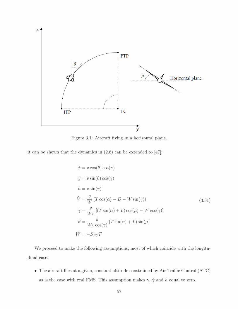
Figure 3.1: Aircraft flying in a horizontal plane.
it can be shown that the dynamics in (2.6) can be extended to [47]:
x = v cos(θ) cos(γ)
y = v sin(θ) cos(γ)
h = v sin(γ)
V =g
W(T cos(α)−D −W sin(γ))
γ =g
Wv[(T sin(α) + L) cos(μ)−W cos(γ)]
θ =g
Wv cos(γ)(T sin(α) + L) sin(μ)
W = −SFCT
(3.31)
We proceed to make the following assumptions, most of which coincide with the longitu-
dinal case:
• The aircraft flies at a given, constant altitude constrained by Air Traffic Control (ATC)
as is the case with real FMS. This assumption makes γ, γ and h equal to zero.
57
• The altitude, speed and thrust values lie in the interior of the flight envelope given by
the constraints (2.11). As a result, we do not need to enforce them in the mathematical
formulation of the OCP.
• The angle of attack α is small, allowing to write cosα ≈ 1 and sinα ≈ α. This
assumption is standard practice in performance analysis for commercial aircraft.
• The component of the thrust perpendicular to the velocity vector, Tα, is much smaller
than L and W .
• Accelerations are negligible due to the steady-flight condition, and as a result we can
assume that v is approximately zero.
• The bank angle μ is sufficiently small such that cos(μ) ≈ 1.
Under these assumptions, (3.31) simplifies to
x = v cos(θ)
y = v sin(θ)
θ =g
WvL sin(μ)
W = −SFCT
L = W
T = D
(3.32)
In addition to the last two constraints, we must enforce that
L sin(μ) =Wv2
gr, (3.33)
which implies that the horizontal component of the lift must provide the centripetal force
used for performing the turn of radius r as shown in Fig. 3.2, where yw and zw are part of
the wind axes system. Note that, after the turn radius is given and the above constraint is
58
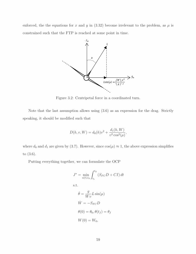
enforced, the the equations for x and y in (3.32) become irrelevant to the problem, as μ is
constrained such that the FTP is reached at some point in time.
Figure 3.2: Centripetal force in a coordinated turn.
Note that the last assumption allows using (3.6) as an expression for the drag. Strictly
speaking, it should be modified such that
D(h, v,W ) = d0(h)v2 +
d1(h,W )
v2 cos2(μ),
where d0 and d1 are given by (3.7). However, since cos(μ) ≈ 1, the above expression simplifies
to (3.6).
Putting everything together, we can formulate the OCP
J∗ = minu(t),td
∫ td
tc
(SFCD + CI) dt
s.t.
θ =g
WvL sin(μ)
W = −SFCD
θ(0) = θ0, θ(tf ) = θf
W (0) = W0,
59
where u = [ v μ ]T , and θ0 and θf are known as the inbound and outbound course respectively.
Briefly considering L cos(μ) = W instead of L = W in (3.32), and from (3.33), we can solve
for μ as a function of v, yielding
tan(μ) =v2
rg. (3.34)
In addition, using (3.33) allows writing θ as
θ =v
r.
As a result, the problem reduces to one unknown and the OCP for lateral flight is given
by
J∗ = minv(t),td
∫ td
tc
(SFCD + CI) dt
s.t.
θ =v
r
W = −SFCD
θ(0) = θ0, θ(tf ) = θf
W (0) = W0.
(3.35)
The following result states the solution of this OCP.
Theorem 3.3.2. The optimal solution to the OCP stated in (3.35) is
v =
√√√√CI +√C2
I + 12(1− J∗W )2SFC
2CD,0CD,2W 2
(1− J∗W )SFCCD,0ρS
(3.36)
Proof. The Hamiltonian is given by
H = SFCD + CI + J∗θ
v
r− J∗
WSFCD. (3.37)
60
The necessary condition for optimality is
∂H
∂v= (1− J∗
W )SFCDv +J∗θ
r= 0, (3.38)
which allows solving for J∗θ /r as follows:
J∗θ
r= −(1− J∗
W )SFCDv (3.39)
Similar to the longitudinal case, the sufficient condition or a minimum results in
∂2H
∂v2= (1− J∗
W )SFCDvv > 0,
from which we obtain
J∗W < 1 (3.40)
Noting that H is not a function of time and td is unspecified, the HJB equation reduces
to infv H = 0. By substituting (3.39) into (3.37) evaluated at the optimal speed, and making
the expression equal to zero, we get
(1− J∗W )SFCD − (1− J∗
W )SFCvDv + CI = 0. (3.41)
This expression is identical to (3.27). The speed that satisfies this equation is
v2 =CI +
√C2
I + 12(1− J∗W )2SFC
2CD,0CD,2W 2
(1− J∗W )SFCCD,0ρS
,
which is the same as (3.21).
The optimal μ is solved as a function of v using (3.34). As a result, we can conclude
that, for a small μ, the speed that minimizes operating costs during cruise does not change,
and the same results that were shown in section 3.3.1 apply to the lateral case as well. The
61
remainder of the chapter will present the shooting algorithm used for validation purposes
and the simulation results.
3.4 Validation Results
3.4.1 Aircraft Model Used for the Simulations
The aircraft model used for all simulations in this work was borrowed from [46], and is
based on the Gulfstream-IV (G-IV) business jet by Gulfstream Aerospace equipped with two
Rolls-Royce Tay 611-8 turbofan engines. The drag coefficients, wing planform area, SFC and
thrust characteristics are
CD,0 = 0.015
CD,2 = 0.08
S = 950 ft 2
SFC = 0.69 1/h
Ts = 27700 lbf
Ti = 200 lbf
m = 1.
The parameters Ts, Ti and m are not used for cruise, but are necessary for the modeling
of maximum climb thrust and idle thrust in Chapter 4. The aircraft operating limits, taken
62
from [53], are given by
Maximum Takeoff Weight = 74600 lbf
Maximum Zero-Fuel Weight = 49000 lbf
Service Ceiling(hmax) = 45000 ft
MMO = 0.88.
When choosing initial and final conditions for the simulations, it is important to ensure
that the aforementioned limits are respected.
3.4.2 Shooting Method for Cruise
The general approach described in Section 2.2.4 will be adapted to solve (3.20) numerically.
From the cruise dynamics (3.1) and (3.22), the augmented system is formed by
x = v
W = −SFCD
J∗W = (J∗
W − 1)4SFCCD,2W
ρSv2
x(tc) = xc, x(td) = xd
W (tc) = Wc,W (td) unspecified
J∗W (tc) unspecified, J∗
W (td) = 0,
(3.42)
where v is computed at every time-step using (3.21) (recall that J∗x has been solved as a
function of the other variables in (3.25), therefore its dynamics do not have to be included in
the augmented system). The goal of the shooting method is to simulate (3.42) for different
J∗W (tc) until one is found for which J∗
W (td) = 0. Following the same notation as in Section
2.2.4, the following pseudo-code states the shooting algorithm for this particular OCP:
1. Choose J∗W
(0)(tc):
63
(a) Estimate an initial value for the speed v(tc) from practical experience.
(b) Solve for J∗W from (3.27) and evaluate at t = tc, yielding the following estimate:
J∗W
(0)(tc) = 1 +
(CI
SFC(D − vDv)
)|tc (3.43)
2. Let k = 0
3. Do:
(a) Simulate (3.42) until x(t) = xd, then td = t
(b) Compute ε = J∗W
(k)(td)− J∗W (td)
(c) Compute the next seed J∗W
(k+1)(tc) using the update law
J∗W
(k+1)(tc) = J∗W
(k)(tc)− βε (3.44)
(d) k = k + 1
4. Until |ε| < tolerance OR k ≥ Max. Iterations
Instead of proposing J∗W
(0)(tc) which is difficult to correlate with the physical variables
of the problem, it is more convenient to estimate an initial cruise speed v(tc) from practical
experience and then solve for J∗W
(0)(tc) using (3.43). β is a tuning parameter and was chosen
to be equal to one for this problem. The algorithm presented in this subsection, as well as
another algorithm that applies the sub-optimal feedback law (3.30), have been implement
in Matlab and Simulink. The implementation code and block diagrams can be found in
Appendix A.
A simulation will now be carried out for the purpose of comparing the exact optimal
trajectory found using the shooting method with the one using the sub-optimal feedback
law.
64
3.4.3 Comparison between the optimal and sub-optimal trajecto-
ries
For this example the following initial and final conditions are used:
tc = 0 s
hc = 25000 ft
xc = 0 mi
xd = 2000 mi
Wc = 70000 lb
Fig. 3.3 compares the sub-optimal true airspeeds with the optimal ones obtained using
the shooting method for different CIs as a function of the aircraft range (time was not used
for the horizontal axis as it changes significantly depending on CI, whereas the range is the
same for all cases). The solid lines represents the optimal solution whereas the dashed lines
represent the sub-optimal one. For a CI of zero both lines are identical. This is an expected
result because the approximation that J∗W ≈ 0 becomes irrelevant when CI vanishes, as shown
in Section 3.3. In fact, the obtained speed profile corresponds to the maximum range speed.
The optimal and sub-optimal references start to change when CI is different than zero.
This is due to the approximation J∗W ≈ 0 being less precise at the start of the simulation,
leading to a more pronounced difference between the optimal and sub-optimal speed. How-
ever, as the final time is reached, this assumption becomes more valid until t = td, where
expressions (3.21) and (3.30) become identical. This is verified in Fig. 3.4 where J∗W is plot-
ted as a function of the range. As a result, it can be said that the sub-optimal control law is
a good approximation for short range flights, and becomes less precise for longer distances.
For this example, it is possible to quantify how sub-optimal the analytical solution is by
computing the total cost. Noting that SFCD = −W in (3.19), the total cruise cost in units
65
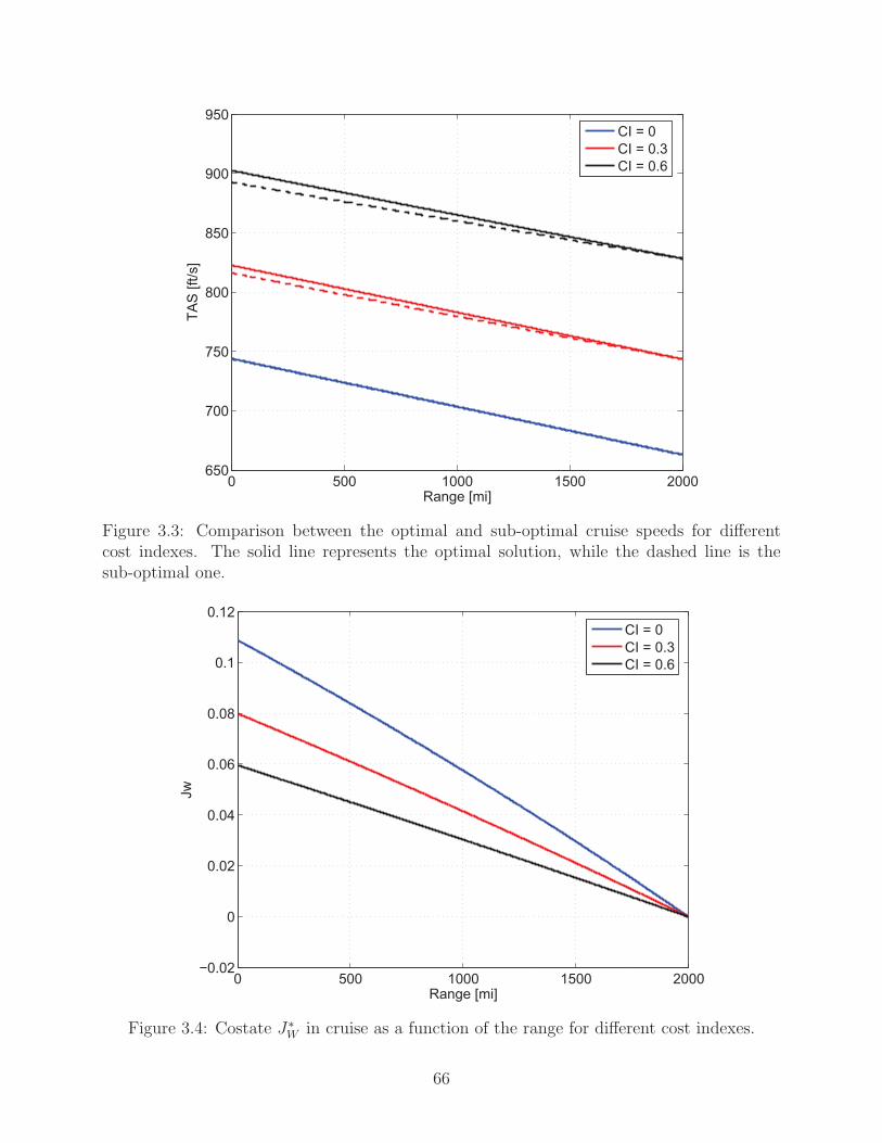
0 500 1000 1500 2000650
700
750
800
850
900
950
Range [mi]
TAS
[ft/s
]
CI = 0CI = 0.3CI = 0.6
Figure 3.3: Comparison between the optimal and sub-optimal cruise speeds for differentcost indexes. The solid line represents the optimal solution, while the dashed line is thesub-optimal one.
0 500 1000 1500 2000−0.02
0
0.02
0.04
0.06
0.08
0.1
0.12
Range [mi]
Jw
CI = 0CI = 0.3CI = 0.6
Figure 3.4: Costate J∗W in cruise as a function of the range for different cost indexes.
66
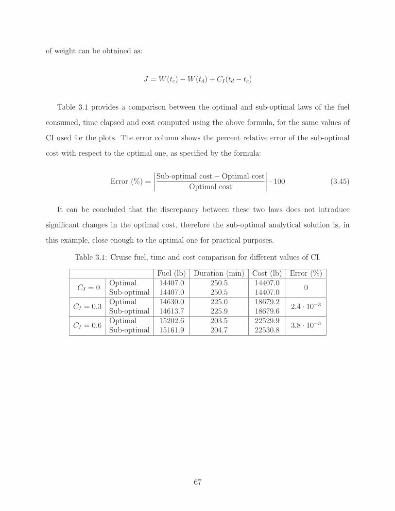
of weight can be obtained as:
J = W (tc)−W (td) + CI(td − tc)
Table 3.1 provides a comparison between the optimal and sub-optimal laws of the fuel
consumed, time elapsed and cost computed using the above formula, for the same values of
CI used for the plots. The error column shows the percent relative error of the sub-optimal
cost with respect to the optimal one, as specified by the formula:
Error (%) =
∣∣∣∣Sub-optimal cost−Optimal cost
Optimal cost
∣∣∣∣ · 100 (3.45)
It can be concluded that the discrepancy between these two laws does not introduce
significant changes in the optimal cost, therefore the sub-optimal analytical solution is, in
this example, close enough to the optimal one for practical purposes.
Table 3.1: Cruise fuel, time and cost comparison for different values of CI.
Fuel (lb) Duration (min) Cost (lb) Error (%)
CI = 0Optimal 14407.0 250.5 14407.0
0Sub-optimal 14407.0 250.5 14407.0
CI = 0.3Optimal 14630.0 225.0 18679.2
2.4 · 10−3
Sub-optimal 14613.7 225.9 18679.6
CI = 0.6Optimal 15202.6 203.5 22529.9
3.8 · 10−3
Sub-optimal 15161.9 204.7 22530.8
67
Chapter 4
Optimal Solutions for Climb and
Descent
4.1 Assumptions
Similar to the approach taken in Chapter 3, this section presents the assumptions made
to simplify the aircraft dynamics (2.6) during the climb and descent phases of the flight.
The purpose of simplifying these equations is to allow solving the OCPs in this chapter
analytically, which would be too difficult to do if the expressions involved are not tractable
enough. Most of the assumptions made in this section are very similar to the ones made in
the cruise phase. They will be repeated here for the sake of clarity.
The assumptions made for the climb and descent segments of the flight are the following:
• The altitude and speed values lie in the interior of the flight envelope given by the
constraints (2.11). As a result, we do not need to enforce them in the mathematical
formulation of the OCP.
• During climb, the thrust is constrained to be equal to a given, known value Tc(h) known
as the maximum climb thrust. Similarly, during the descent, the thrust is equal to a
known value Ti known as the idle thrust.
68
• The angle of attack α and the flight path angle γ are small, allowing to write cosα ≈ 1
and sinα ≈ α, and similarly for γ. This assumption is standard practice in performance
analysis for commercial aircraft.
• The component of the thrust perpendicular to the velocity vector, Tα, is much smaller
than L and W . The thrust force is usually around one order of magnitude smaller than
the weight, therefore multiplying it by a small angle will effectively make it negligible.
• Climb and descent occur under steady flight conditions and as a result we will assume
that v and γ are zero. As explained in Section 1.2, the FMS supplies optimal references
that are then followed by the autopilot using the aircraft’s flight controls. Therefore,
we can take v and γ as control signals, leaving their dynamics to the autopilot.
Taking these assumptions into consideration, we obtain the simplified aircraft model for
quasi-steady climb and descent in the longitudinal plane
x = v
h = vγ
W = −SFCT
(4.1)
L = W (4.2)
T = D +Wγ, (4.3)
Since L = W from (4.2), equations (3.5), (3.6) and (3.7) are valid to compute the drag
during the climb and descent. The last relation to consider is the constraint on the thrust:
T =
⎧⎨⎩ Tc(h) : γ > 0 (during climb)
Ti : γ < 0 (during descent), (4.4)
69
which will be applied in conjunction with (4.3) depending on the flight phase. Ti is considered
constant and known for a particular aircraft, whereas Tc(h) will follow the relation proposed
in [46, 48] for turbojet and turbofan engines:
Tc(h) = Ts
[ρ(h)
ρs
]m
(4.5)
In the above expression, Ts stands for the sea-level maximum climb thrust rating. Ts and
m are given for a particular aircraft, and ρ obeys the ISA equations (2.1c) and (2.2b).
4.2 Maximum Rate of Climb and Minimum Rate of
Descent OCPs
4.2.1 Maximum Rate of Climb
The OCP for maximum rate of climb can be stated as follows: It is desired to climb from
a given initial altitude h0 where the FMS is engaged to the desired cruise altitude hc in
minimum time. The point xc at which hc is reached is unspecified and constitutes the TOC,
and γ > 0. As in (4.4), the thrust must be equal to Tc and γ is subject to the constraint
(4.3). From there, we can solve for γ yielding:
γ =Tc −D
W(4.6)
70
This leaves v as the single control input. In mathematical form the OCP is given by:
J∗ = minv,tc
∫ tc
0
dt
s.t.
x = v
h = vγ
W = −SFCTc(h)
x(0) = x0
h(0) = h0, h(tc) = hc
W (0) = W0
γ =Tc −D
W> 0
(4.7)
The solution of this OCP is stated in the following theorem.
Theorem 4.2.1. The optimal solution for the maximum ROC problem (4.7) is given by
v =
√Tc +
√T 2c + 12CD,0CD,2W 2
3CD,0ρS. (4.8)
Proof. The Hamiltonian
H = 1 + J∗xv + J∗
hvγ − J∗WSFCTc (4.9)
must be minimized with respect to v. The necessary condition for optimality yields
∂H
∂v= 0
≡ J∗x + J∗
h (γ + vγv) = 0,
where γv is the partial derivative of γ with respect to v. The expression (4.6) can be differ-
71
entiated with respect to v to get
γv =∂γ
∂v= −Dv
W, (4.10)
which is substituted into the necessary condition to get
J∗x + J∗
h
(γ − vDv
W
)= 0. (4.11)
Note, however, that the following information can be obtained using the costate equations:
J∗x = −∂H
∂x= 0, (4.12)
and
J∗h = −∂H
∂h
= J∗W (SFCh
Tc + SFCTch)− J∗hvγh. (4.13)
Moreover, since the terminal cost is φ = 0 and the terminal constraint function is ψ =
h− hc, we get:
J∗x(tc) = (φx + νψx)|tc = 0 (4.14)
As a result, J∗x is zero for all t and is eliminated from (4.11) yielding:
J∗h
(γ − vDv
W
)= 0
Since J∗h has nonzero dynamics as in (4.13), it cannot be zero for all t, therefore
γ − vDv
W= 0,
72
which, after substituting γ from (4.6) and the drag from (3.6), yields
Tc −D − vDv = 0
≡ 3d0v4 − Tcv
2 − d1 = 0.
This equation is solved for the optimal speed obtaining
v2 =Tc ±
√T 2c + 12d0d16d0
,
or, after replacing d0 and d1 from (3.7) and taking the positive sign:
v2 =Tc +
√T 2c + 12CD,0CD,2W 2
3CD,0ρS
This equation yields the optimal speed that maximizes the ROC of the aircraft. It co-
incides with (2.19) with T = Tc, which is the expression commonly found in literature.
Obtaining expressions for J∗h, J
∗W and J∗ is not relevant to this discussion, but they could be
obtained by formulating and solving the rest of the equations.
It remains to verify the sufficient condition to minimize H, which is found by taking the
partial derivative of (4.11) with respect to v (keeping in mind that J∗x is zero) and substituting
(4.10), yielding
∂2H
∂v2= J∗
h
[γv −
1
W
∂
∂v(vDv)
]=
J∗h
W[−Dv − (Dv + vDvv)]
= −J∗h
W
(6d0v +
2d1v3
)
This partial derivative must be greater than zero. It follows that either
J∗h < 0 and
(6d0v +
2d1v3
)> 0,
73
or
J∗h > 0 and
(6d0v +
2d1v3
)< 0,
but, since (6d0v + 2d1/v3) is always positive as it involves only positive terms, the sufficient
condition reduces to
J∗h < 0. (4.15)
Since H does not depend explicitly on time and tc in unspecified, the HJB equation
reduces to infv H = 0. It follows from (4.9) evaluated at the optimal speed that
1 + J∗xv + J∗
hvγ − J∗WSFCTc = 0,
from which we solve for J∗h to obtain
J∗h =
−1 + J∗WSFCTc
vγ. (4.16)
To satisfy (4.15), (4.16) must be less than zero. Since γ > 0 from (4.7) and v must be
positive, we get
−1 + J∗WSFCTc < 0,
from which a constraint on J∗W is obtained as
J∗W <
1
SFCTc
(4.17)
Equation (4.17) implies that J∗W is positive and smaller than a very small value, since
SFCTc is a generally a large quantity.
To close this section, we verify that the maximum ROC speed also coincides with the
solution for minimum fuel consumption. Consider the OCP (4.7), but with the minimum
74
fuel cost functional:
J∗ = minv,tc
∫ tc
0
SFCTcdt (4.18)
The Hamiltonian changes to
H = (1− J∗W )SFCTc + J∗
xv + J∗hvγ.
However, since the term (1 − J∗W )SFCTc does not depend on v, the necessary condition
remains the same as (4.11). Furthermore, the same reasoning as the ROC problem can be
followed: J∗x satisfies (4.12) and (4.14) vanishing from the necessary condition, and yielding
(4.8) for the optimal speed. The only equation that changes is J∗h and the constraint on J∗
W
arising from the sufficient condition of optimality.
4.2.2 Minimum Rate of Descent
The minimum rate of descent problem is a very similar problem to the one discussed for
climb. This time, the starting point xd is unspecified, and the aircraft must descend from
cruise altitude to a final value where the performance module of the FMS is disengaged and
the approach phase begins. This takes place at a given final range xf . Define the distance
traveled as
x = x− xd,
resulting in the dynamics and initial and final conditions
˙x = v cos(γ)
x(td) = 0
x(tf ) = xf − xd.
75
This change of variables allows formulating the OCP in standard form, given by
J∗ = maxv,tf
∫ tf
td
dt
s.t.
˙x = v cos(γ)
h = v sin(γ)
W = −SFCTi
x(td) = 0
h(td) = hc, h(tf ) = hf
W (td) = Wd,
(4.19)
where T = Ti and
γ =Ti −D
W. (4.20)
The solution of OCP (4.19) is stated in the following theorem.
Theorem 4.2.2. The optimal solution to OCP (4.19) is given by
v =
√Ti +
√T 2i + 12CD,0CD,2W 2
3CD,0ρS. (4.21)
Proof. Define the Hamiltonian
H = 1 + J∗xv + J∗
hvγ − J∗WSFCTi (4.22)
from which the necessary condition of optimality can be obtained as follows:
∂H
∂v= J∗
x + J∗h (γ + vγv)
76
Using the same approach as in the maximum ROC case, it can be shown that
γv = −Dv
W, (4.23)
which is substituted into the necessary condition yielding
J∗x + J∗
h
(γ − vDv
W
)= 0. (4.24)
Analogous to the climb problem, the costate equations yield
J∗x = −∂H
∂x= 0 (4.25)
J∗x(tf ) = 0, (4.26)
and
J∗h = −∂H
∂h
= J∗WSFCh
Ti − J∗hvγh (4.27)
It follows from (4.25) and (4.26) that J∗x is zero for all t, and (4.24) reduces to
J∗h
(γ − vDv
W
)= 0.
Given that J∗h has the dynamics specified in (4.27), it cannot be zero for all t and the
resulting equation can be solved for the minimum rate of descent speed in the same manner
as in the climb:
γ − vDv
W= 0
77
Substitute (4.20) to get
Ti −D − vDv = 0
≡ 3d0v4 − Tiv
2 − d1 = 0,
which is solved for v yielding
v2 =Ti ±
√T 2i + 12d0d16d0
=Ti +
√T 2i + 12CD,0CD,2W 2
3CD,0ρS
The second partial derivative of H with respect to v is given by
∂2H
∂v2= J∗
h
[γv −
1
W
∂
∂v(vDv)
]= −J∗
h
W
(6d0v +
2d1v3
),
which must be less than zero according to the sufficient condition of optimality. Since (6d0v+
2d1/v3) contains only positive terms, it follows that
J∗h > 0. (4.28)
In the same fashion as in the climb, the HJB equation reduces to infv H = 0 which allows
solving for J∗h using (4.22) evaluated at the optimal v and equated to zero yielding
J∗h =
−1 + J∗WSFCTi
vγ
The above expression must be greater than zero to satisfy (4.28). Since γ is negative dur-
78
ing the descent and v is positive, the numerator must be negative resulting in the constraint
J∗W <
1
SFCTi
. (4.29)
Equation (4.21) yields the minimum ROD speed and is very similar to (4.8), with the
difference that Tc is changed to Ti. It also coincides with (2.19) with T = Ti. Moreover, just
like in the climb phase, it can be shown that (4.21) is equivalent to the minimum fuel descent
speed. The procedure to prove this statement is identical to the one followed in the previous
subsection, and will not be repeated here.
4.3 Economy Mode OCP for Climb
The ECON mode for climb will now be derived and solved as an OCP. While it might seem
tempting to formulate such problem by modifying the ROC minimum fuel cost functional
(4.18) by adding CI to the running cost, the truth is that doing this will not change the
original problem. The Hamiltonian (4.9) would only be changed by the addition of CI , which
would disappear when the partial derivative w.r.t. v is taken for the necessary condition.
As a result, the same procedure developed in Section 4.2.1 would hold and the speed target
would remain unchanged.
The reason why this happens is because if the climb phase is considered alone without
regard to the rest of the flight, reaching cruise altitude in minimum time is already equivalent
to minimizing the fuel consumed during that phase, therefore using CI to quantify a tradeoff
between these two criteria becomes meaningless. To obtain a relevant formulation, the impact
of the climb phase on the rest of the flight must be considered, i.e. we will study the effect of
choosing a given climb speed and flight path angle on the overall operating cost of the flight.
To take the rest of the phases into account, the cost-to-go from the TOC until the end
of the flight must be added to the climb cost functional using the principle of optimality
79
as discussed in Section 2.2.5. However, doing so would require computing the optimal cost-
to-go function of the cruise OCP (3.20), which involves finding analytic expressions for the
costates J∗x and J∗
W by solving the ODE (3.22) and the HJB equation subject to its boundary
condition. Then, we would have to add the cost-to-go of the descent. This is obviously a
very difficult proposition. Nevertheless, the objective of the next subsection is to develop
a formulation that takes the cost-to-go into account an approximate manner, resulting in a
meaningful OCP that can be approached analytically to obtain the cost-optimal speed.
Problem Formulation Using the Principle of Optimality
Suppose that it is desired for the aircraft to climb from a given initial point (x0, h0) to a
prescribed cruise altitude hc. The TOC, xc, and the final time tc are unspecified and must
be determined such that the operating costs are minimized. The initial climb weight W0 is
known. From Section 1.3, we know that the total operating cost of the flight can be expressed
in terms of the fuel flow rate ff as
J =
∫ tf
0
(ff + CI) dt, (4.30)
which is split into the three phases of flight:
J =
∫ tc
0
(ffcl + CI) dt+
∫ td
tc
(ffcr + CI) dt+
∫ tf
td
(ffd + CI) dt (4.31)
The terms ffcl , ffcr and ffd denote the fuel flow rate during climb, cruise and descent
respectively. Then, according to the principle of optimality defined in (2.36), we get
J∗ = infv,tc,0≤t≤tc
{∫ tc
0
(ffcl + CI) dt+ J∗cr,d(tc, ζ(tc))
}, (4.32)
where
J∗cr,d = inf
v,tc≤t≤tf
{∫ td
tc
(ffcr + CI) dt+
∫ tf
td
(ffd + CI) dt
}.
80
The functional J∗cr,d computes the optimal cost-to-go from tc until the end of the flight,
and comprises both the cruise and the descent costs. To simplify the problem, we will assume
that the descent cost is negligible when compared to the cruise cost. This is a reasonable
assumption when considering that most commercial flights spend most of the time cruising,
in addition to the thrust being small during the descent. As a result, the impact of the
cruise on the overall flight time and fuel consumption is more significant than the descent.
Furthermore, we know from Section 3.3 that the cruise cost is given by
Jcr(tc) =
∫ td
tc
(SFCD + CI)dt =
∫ td
tc
(ffcr + CI)dt.
Generally speaking, for a fixed cruise altitude, ffcr changes slowly as the weight decreases
due to fuel burnt and the speed is modified accordingly obeying (3.21). If ffcr is computed
for W = W0, the total cruise cost-to-go can be estimated as follows:
J∗cr(tc) = inf
vcr
{∫ td
tc
(SFCD + CI)dt
}≈ (ffcr |W0 + CI)(td − tc).
Let us approximate (td − tc) by the expression
(td − tc) ≈xd − xc
vcr,
where vcr stands for the cruise speed and can be estimated by evaluating (3.30) at W0.
Putting everything together, we will approximate J∗cr,d ≈ J∗
cr, and from (4.32) the following
cost functional is obtained for the climb phase
J∗(0) ≈ infv,tc
{∫ tc
0
(ffcl + CI) dt+ (ffcr + CI)xd − xc
vcr
}, (4.33)
where ffcr = SFCTc, and ffcr , vcr are assumed to be evaluated at W0. Then, the ECON
81
Climb OCP can be stated mathematically as follows:
J∗(0) = minv,tc
{∫ tc
0
(SFCTc + CI) dt+ (ffcr + CI)xd − xc
vcr
}s.t.
x = v
h = vγ
W = −SFCTc
x(0) = x0
h(0) = h0, h(tc) = hc
W (0) = W0,
(4.34)
where γ satisfies (4.6) and Tc is given by (4.5).
Optimal solution
The following result gives the solution to OCP (4.34).
Theorem 4.3.1. The optimal solution to the ECON mode OCP for climb stated in (4.34)
is given by the solution v of the equation
[(1− J∗W )SFCTc + CI ] (Tc −D − vDv)− J∗
xv2Dv = 0, (4.35)
where γ is obtained from (4.6), J∗x is given by
J∗x = −ffcr + CI
vcr, (4.36)
and the time derivative of J∗W equals
J∗W = −
(J∗xv
W
) (d0v
4 − Tcv2 − d1
3d0v4 − Tcv2 − d1
), (4.37)
82
with final condition
J∗W (tc) = 0. (4.38)
Proof. Define the Hamiltonian as
H = (1− J∗W )SFCTc + J∗
xv + J∗hvγ + CI . (4.39)
To minimize (4.39) with respect to v, the necessary condition for optimality must be
satisfied:
∂H
∂v= J∗
x + J∗h (γ + vγv) = 0
Substitute γv from (4.10)to get
J∗x + J∗
h
(γ − vDv
W
)= 0 (4.40)
Up to this point, the minimum-cost problem seems identical to the maximum ROC one
from Section (4.2.1). In fact, (4.40) and (4.11) are the same. However, the problem changes
drastically once the costate J∗x is taken into account. We get:
J∗x = −∂H
∂x= 0 (4.41)
Moreover, since there is a terminal cost
φ(x) = (ffcr + CI)xd − x
vcr, (4.42)
and
ψ(h) = h− hc, (4.43)
83
then the following value for J∗x is obtained:
J∗x(tc) = J∗
x = (φx + νψx)|tc = −ffcr + CI
vcr
The main difference between this OCP and the maximum ROC is that J∗x does not vanish,
but has a constant, known value given by the above equation. The costate J∗W can be solved
directly as a function of the rest of the variables from (4.40) yielding
J∗h = −
(J∗x
γ − vDv
W
), (4.44)
therefore we do not have to compute its time derivative or final value. For J∗W , the costate
equation gives
J∗W = − ∂H
∂W= −J∗
hvγW (4.45)
Differentiating (4.6) with respect to W yields
γW =1
W 2(−DWW − Tc +D) .
From (3.5)
DW =4CD,2W
ρSv2,
which is substituted into γW along with (3.6) and (3.7) to get
γW =1
W 2
(−4CD,2W
2
ρSv2− Tc + d0v
2 +d1v2
)=
1
W 2
(−2d1
v2− Tc + d0v
2 +d1v2
)= − 1
W 2
(Tc − d0v
2 +d1v2
)(4.46)
84
Substituting (4.46) into (4.45) results in
J∗W =
(J∗hv
W 2
) (Tc − d0v
2 +d1v2
).
If J∗h is replaced by (4.44) one obtains the expression
J∗W = −
(J∗xv
W 2
) (Tc − d0v
2 + d1v2
γ − vDv
W
)
in which γ is substituted using (4.6) and D by (3.6) yielding
J∗W = −
(J∗xv
W
) (Tc − d0v
2 + d1v2
Tc −D − vDv
)
= −(J∗xv
W
) (Tc − d0v
2 + d1v2
Tc − 3d0v2 +d1v2
)
= −(J∗xv
W
) (d0v
4 − Tcv2 − d1
3d0v4 − Tcv2 − d1
)
Its final value is given by
J∗W (tc) = (φW + νψW )|tc = 0.
We will now apply the same result from optimal control theory that we used in the cruise
problem to simplify the HJB equation. Since H and φ are not explicit functions of t and tc
is unspecified, the HJB equation
0 = J∗t +min
vH,
reduces to
minv
H = 0.
85
Replacing the Hamiltonian (4.39) into the HJB equation yields
minv
{(1− J∗W )SFCTc + J∗
xv + J∗hvγ + CI} = 0,
or, at the optimal speed
(1− J∗W )SFCTc + J∗
xv + J∗hvγ + CI = 0. (4.47)
Substitute (4.44) into (4.47) to yield
(1− J∗W )SFCTc + J∗
xv + CI −J∗xvγ(
γ − vDv
W
) = 0.
The above expression can be further manipulated to obtain an equation in terms of v,
J∗W and γ as follows:
[(1− J∗W )SFCTc + CI + J∗
xv]
(γ − vDv
W
)− J∗
xvγ = 0
≡ [(1− J∗W )SFCTc + CI ]
(γ − vDv
W
)− J∗
xv2Dv
W= 0
Using (4.6) yields
[(1− J∗W )SFCTc + CI ] (Tc −D − vDv)− J∗
xv2Dv = 0.
Remark: As opposed to the cruise phase, if CI vanishes in (4.35) then the Maximum
ROC solution presented in Section 4.2.1 is not attained, which was shown to be equivalent
to the minimum fuel case for a standalone climb. This happens as a result of the interaction
between climb and cruise phases. The only way for both speeds to coincide is to ignore the
cruise cost-to-go, which would make J∗x vanish in (4.40) thus recovering the Maximum ROC
solution, regardless of the value of CI .
86
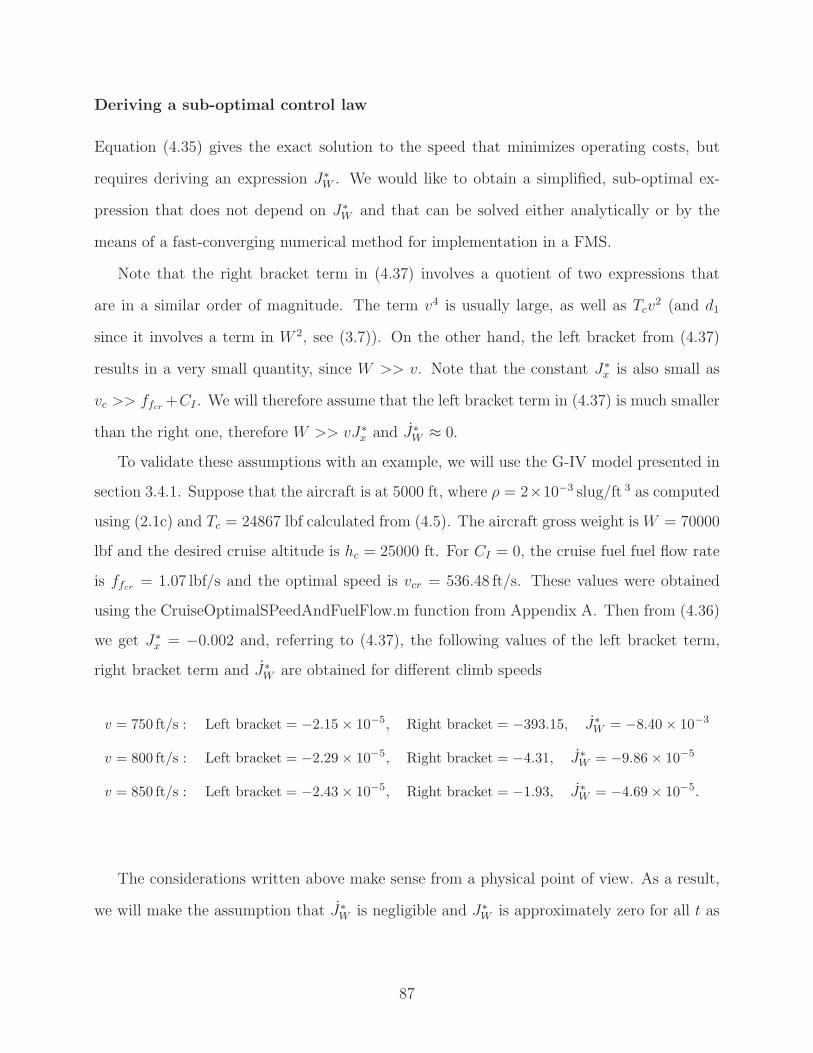
Deriving a sub-optimal control law
Equation (4.35) gives the exact solution to the speed that minimizes operating costs, but
requires deriving an expression J∗W . We would like to obtain a simplified, sub-optimal ex-
pression that does not depend on J∗W and that can be solved either analytically or by the
means of a fast-converging numerical method for implementation in a FMS.
Note that the right bracket term in (4.37) involves a quotient of two expressions that
are in a similar order of magnitude. The term v4 is usually large, as well as Tcv2 (and d1
since it involves a term in W 2, see (3.7)). On the other hand, the left bracket from (4.37)
results in a very small quantity, since W >> v. Note that the constant J∗x is also small as
vc >> ffcr +CI . We will therefore assume that the left bracket term in (4.37) is much smaller
than the right one, therefore W >> vJ∗x and J∗
W ≈ 0.
To validate these assumptions with an example, we will use the G-IV model presented in
section 3.4.1. Suppose that the aircraft is at 5000 ft, where ρ = 2×10⁻³ slug/ft 3 as computed
using (2.1c) and Tc = 24867 lbf calculated from (4.5). The aircraft gross weight is W = 70000
lbf and the desired cruise altitude is hc = 25000 ft. For CI = 0, the cruise fuel fuel flow rate
is ffcr = 1.07 lbf/s and the optimal speed is vcr = 536.48 ft/s. These values were obtained
using the CruiseOptimalSPeedAndFuelFlow.m function from Appendix A. Then from (4.36)
we get J∗x = −0.002 and, referring to (4.37), the following values of the left bracket term,
right bracket term and J∗W are obtained for different climb speeds
v = 750 ft/s : Left bracket = −2.15× 10⁻⁵, Right bracket = −393.15, J∗W = −8.40× 10⁻³
v = 800 ft/s : Left bracket = −2.29× 10⁻⁵, Right bracket = −4.31, J∗W = −9.86× 10⁻⁵
v = 850 ft/s : Left bracket = −2.43× 10⁻⁵, Right bracket = −1.93, J∗W = −4.69× 10⁻⁵.
The considerations written above make sense from a physical point of view. As a result,
we will make the assumption that J∗W is negligible and J∗
W is approximately zero for all t as
87
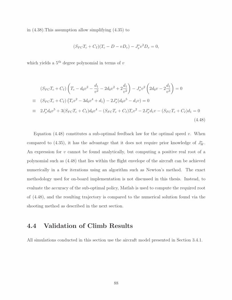
in (4.38).This assumption allow simplifying (4.35) to
(SFCTc + CI)(Tc −D − vDv)− J∗xv
2Dv = 0,
which yields a 5th degree polynomial in terms of v
(SFCTc + CI)
(Tc − d0v
2 − d1v2
− 2d0v2 + 2
d1v2
)− J∗
xv2
(2d0v − 2
d1v3
)= 0
≡ (SFCTc + CI)(Tcv
2 − 3d0v4 + d1
)− 2J∗
x(d0v5 − d1v) = 0
≡ 2J∗xd0v
5 + 3(SFCTc + CI)d0v4 − (SFCTc + CI)Tcv
2 − 2J∗xd1v − (SFCTc + CI)d1 = 0
(4.48)
Equation (4.48) constitutes a sub-optimal feedback law for the optimal speed v. When
compared to (4.35), it has the advantage that it does not require prior knowledge of J∗W .
An expression for v cannot be found analytically, but computing a positive real root of a
polynomial such as (4.48) that lies within the flight envelope of the aircraft can be achieved
numerically in a few iterations using an algorithm such as Newton’s method. The exact
methodology used for on-board implementation is not discussed in this thesis. Instead, to
evaluate the accuracy of the sub-optimal policy, Matlab is used to compute the required root
of (4.48), and the resulting trajectory is compared to the numerical solution found via the
shooting method as described in the next section.
4.4 Validation of Climb Results
All simulations conducted in this section use the aircraft model presented in Section 3.4.1.
88
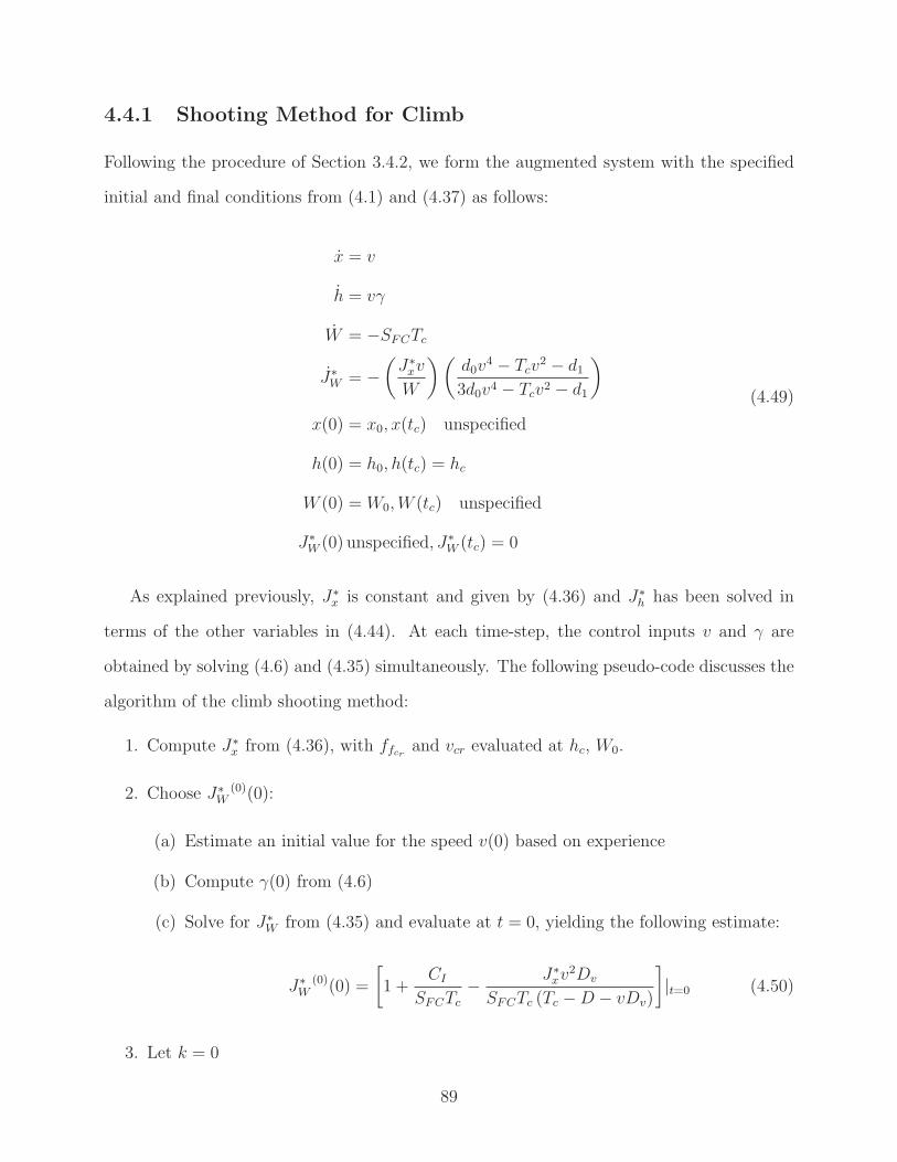
4.4.1 Shooting Method for Climb
Following the procedure of Section 3.4.2, we form the augmented system with the specified
initial and final conditions from (4.1) and (4.37) as follows:
x = v
h = vγ
W = −SFCTc
J∗W = −
(J∗xv
W
) (d0v
4 − Tcv2 − d1
3d0v4 − Tcv2 − d1
)x(0) = x0, x(tc) unspecified
h(0) = h0, h(tc) = hc
W (0) = W0,W (tc) unspecified
J∗W (0) unspecified, J∗
W (tc) = 0
(4.49)
As explained previously, J∗x is constant and given by (4.36) and J∗
h has been solved in
terms of the other variables in (4.44). At each time-step, the control inputs v and γ are
obtained by solving (4.6) and (4.35) simultaneously. The following pseudo-code discusses the
algorithm of the climb shooting method:
1. Compute J∗x from (4.36), with ffcr and vcr evaluated at hc, W0.
2. Choose J∗W
(0)(0):
(a) Estimate an initial value for the speed v(0) based on experience
(b) Compute γ(0) from (4.6)
(c) Solve for J∗W from (4.35) and evaluate at t = 0, yielding the following estimate:
J∗W
(0)(0) =
[1 +
CI
SFCTc
− J∗xv
2Dv
SFCTc (Tc −D − vDv)
]|t=0 (4.50)
3. Let k = 0
89
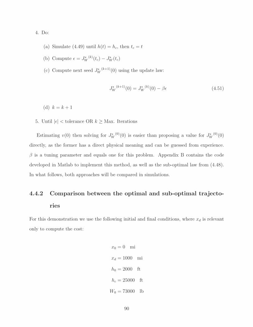
4. Do:
(a) Simulate (4.49) until h(t) = hc, then tc = t
(b) Compute ε = J∗W
(k)(tc)− J∗W (tc)
(c) Compute next seed J∗W
(k+1)(0) using the update law:
J∗W
(k+1)(0) = J∗W
(k)(0)− βε (4.51)
(d) k = k + 1
5. Until |ε| < tolerance OR k ≥ Max. Iterations
Estimating v(0) then solving for J∗W
(0)(0) is easier than proposing a value for J∗W
(0)(0)
directly, as the former has a direct physical meaning and can be guessed from experience.
β is a tuning parameter and equals one for this problem. Appendix B contains the code
developed in Matlab to implement this method, as well as the sub-optimal law from (4.48).
In what follows, both approaches will be compared in simulations.
4.4.2 Comparison between the optimal and sub-optimal trajecto-
ries
For this demonstration we use the following initial and final conditions, where xd is relevant
only to compute the cost:
x0 = 0 mi
xd = 1000 mi
h0 = 2000 ft
hc = 25000 ft
W0 = 73000 lb
90

0 50 100 150 200 250800
850
900
950
1000
1050
Time [s]
TAS
[ft/s
]
CI = 0CI = 0.3CI = 0.6
Figure 4.1: Comparison between the optimal and sub-optimal climb speeds for differentcost indexes. The solid line represents the optimal solution, while the dashed line is thesub-optimal one.
91
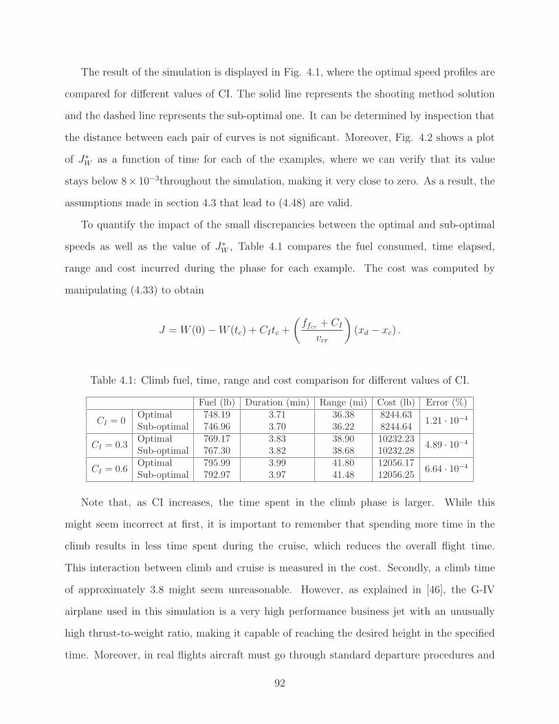
The result of the simulation is displayed in Fig. 4.1, where the optimal speed profiles are
compared for different values of CI. The solid line represents the shooting method solution
and the dashed line represents the sub-optimal one. It can be determined by inspection that
the distance between each pair of curves is not significant. Moreover, Fig. 4.2 shows a plot
of J∗W as a function of time for each of the examples, where we can verify that its value
stays below 8× 10⁻³throughout the simulation, making it very close to zero. As a result, the
assumptions made in section 4.3 that lead to (4.48) are valid.
To quantify the impact of the small discrepancies between the optimal and sub-optimal
speeds as well as the value of J∗W , Table 4.1 compares the fuel consumed, time elapsed,
range and cost incurred during the phase for each example. The cost was computed by
manipulating (4.33) to obtain
J = W (0)−W (tc) + CItc +
(ffcr + CI
vcr
)(xd − xc) .
Table 4.1: Climb fuel, time, range and cost comparison for different values of CI.
Fuel (lb) Duration (min) Range (mi) Cost (lb) Error (%)
CI = 0Optimal 748.19 3.71 36.38 8244.63
1.21 · 10−4
Sub-optimal 746.96 3.70 36.22 8244.64
CI = 0.3Optimal 769.17 3.83 38.90 10232.23
4.89 · 10−4
Sub-optimal 767.30 3.82 38.68 10232.28
CI = 0.6Optimal 795.99 3.99 41.80 12056.17
6.64 · 10−4
Sub-optimal 792.97 3.97 41.48 12056.25
Note that, as CI increases, the time spent in the climb phase is larger. While this
might seem incorrect at first, it is important to remember that spending more time in the
climb results in less time spent during the cruise, which reduces the overall flight time.
This interaction between climb and cruise is measured in the cost. Secondly, a climb time
of approximately 3.8 might seem unreasonable. However, as explained in [46], the G-IV
airplane used in this simulation is a very high performance business jet with an unusually
high thrust-to-weight ratio, making it capable of reaching the desired height in the specified
time. Moreover, in real flights aircraft must go through standard departure procedures and
92
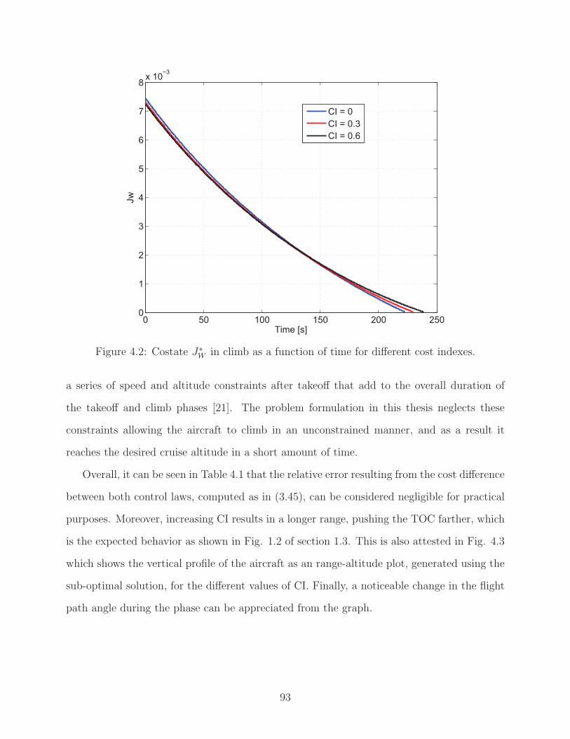
0 50 100 150 200 2500
1
2
3
4
5
6
7
8x 10⁻³
Time [s]
Jw
CI = 0CI = 0.3CI = 0.6
Figure 4.2: Costate J∗W in climb as a function of time for different cost indexes.
a series of speed and altitude constraints after takeoff that add to the overall duration of
the takeoff and climb phases [21]. The problem formulation in this thesis neglects these
constraints allowing the aircraft to climb in an unconstrained manner, and as a result it
reaches the desired cruise altitude in a short amount of time.
Overall, it can be seen in Table 4.1 that the relative error resulting from the cost difference
between both control laws, computed as in (3.45), can be considered negligible for practical
purposes. Moreover, increasing CI results in a longer range, pushing the TOC farther, which
is the expected behavior as shown in Fig. 1.2 of section 1.3. This is also attested in Fig. 4.3
which shows the vertical profile of the aircraft as an range-altitude plot, generated using the
sub-optimal solution, for the different values of CI. Finally, a noticeable change in the flight
path angle during the phase can be appreciated from the graph.
93
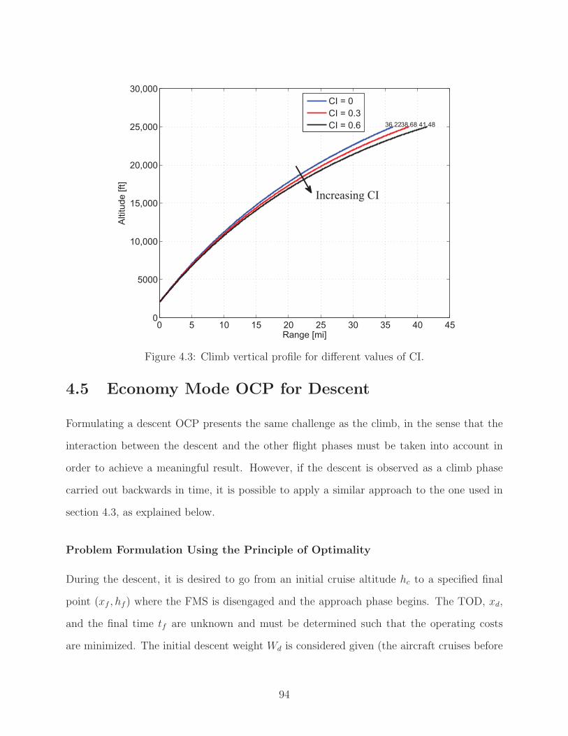
0 5 10 15 20 25 30 35 40 450
5000
10,000
15,000
20,000
25,000
30,000
36.2238.68 41.48
Range [mi]
Alti
tude
[ft]
CI = 0CI = 0.3CI = 0.6
Increasing CI
Figure 4.3: Climb vertical profile for different values of CI.
4.5 Economy Mode OCP for Descent
Formulating a descent OCP presents the same challenge as the climb, in the sense that the
interaction between the descent and the other flight phases must be taken into account in
order to achieve a meaningful result. However, if the descent is observed as a climb phase
carried out backwards in time, it is possible to apply a similar approach to the one used in
section 4.3, as explained below.
Problem Formulation Using the Principle of Optimality
During the descent, it is desired to go from an initial cruise altitude hc to a specified final
point (xf , hf ) where the FMS is disengaged and the approach phase begins. The TOD, xd,
and the final time tf are unknown and must be determined such that the operating costs
are minimized. The initial descent weight Wd is considered given (the aircraft cruises before
94
descending, therefore when xd is known Wd will be automatically determined). We go back
to (4.32) which expresses the overall trip cost in integral form. Instead, this work proposes
applying the same approach as the climb by solving the descent backwards in time, with the
cruise cost-to-go added as a terminal cost function. Define
τ(t) = tf − t, (4.52)
which implies
dτ
dt= −1
τ(0) = tf ≡ τf (4.53)
τ(tc) = tf − tc ≡ τc (4.54)
τ(td) = tf − td ≡ τd (4.55)
τ(tf ) = 0. (4.56)
As a result, we can rewrite (4.32) in terms of τ yielding
J∗ = infv,τd,0≤τ≤τd
{∫ τd
0
(ffcl + CI) dτ + J∗cr,cl(τd, ζ(τd))
}, (4.57)
where
J∗cr,cl = inf
v,τd≤τ≤τf
{∫ τc
τd
(ffcr + CI) dτ +
∫ τf
τc
(ffcl + CI) dτ
}.
In a similar manner as in section 4.3, we will assume that the climb cost is negligible
when compared to the cruise, allowing to express J∗cr,cl as the cruise cost only. This is a
stronger assumption than neglecting the descent with respect to the cruise, which becomes
specially inaccurate in short flights. Longer flights, however, spend most of the time in the
cruising segment, with the other two phases making a very small portion of the overall trip.
As a result, the developments presented in this section can be considered valid for longer,
95
transcontinental flights.
As a result of the new time variable in (4.52), system dynamics (4.1) change to
dx
dτ= −v
dh
dτ= −vγ
dW
dτ= SFCTi.
(4.58)
The initial and final conditions, specified in the initial paragraph of this subsection, must
also change to match τ :
t τ
x(td) = xd x(τd) = xd unspecified
x(tf ) = xf x(0) = xf
h(td) = hc h(τd) = hc
h(tf ) = hf h(0) = hf
W (td) = Wd W (τd) = Wd
W (tf ) = Wf W (0) = Wf unspecified
Following the same procedure as in the climb, the optimal cruise cost is approximated by
J∗cr(τd) = inf
v,τd≤τ≤τc
{∫ τc
τd
(ffcr + CI) dτ
}≈ (ffcr + CI)
xd − xc
vcr,
which allows substituting J∗cr,cl ≈ J∗
cr into (4.57) to obtain the descent cost functional
J∗(0) ≈ infv,τd
{∫ τd
0
(SFCTi + CI) dτ + (ffcr + CI)xd − xc
vcr
}. (4.59)
96
In (4.59), ffcr and vcr are computed at a given initial descent weight Wd and
ffd = SFCTi.
Before stating the OCP formally, an additional change of variables has to be made to
account for the fact that W (τ) is known at the final time τd, but not at τ = 0. Define the
fuel consumed as
W (τ) = W (τ)−Wf , (4.60)
such that its dynamics are the same as W (τ) and its initial and final conditions become
W (0) = Wf unspecified ≡ W (0) = 0 given
W (τd) = Wd given ≡ W (τd) = Wd −Wf unspecified
The ECON Descent OCP can then be stated mathematically in terms of the new variables
τ and W as follows:
J∗(0) = minv,τd
{∫ τd
0
(SFCTi + CI) dτ + (ffcr + CI)xd − xc
vcr
}s.t.
x = −v
h = −vγ
˙W = SFCTi
x(0) = xf
h(0) = hf , h(τd) = hc
W (0) = 0,
(4.61)
In (4.61), γ satisfies (4.20) and Ti is constant. Note the slight abuse of notation, where
97
x denotes the derivative of x with respect to τ , and the same applies to the rest of the state
variables.
Optimal solution
The following theorem states the solution to OCP (4.61).
Theorem 4.5.1. The optimal solution to the ECON mode OCP for descent stated in (4.61)
is given by the solution v of the equation
[(1 + J∗
˜W)SFCTi + CI
](Ti −D − vDv) + J∗
xv2Dv = 0, (4.62)
where γ is obtained from (4.20), J∗x is given by
J∗x =
ffcr + CI
vcr, (4.63)
and the time derivative of J∗˜W
equals
J∗˜W
=
(J∗xv
W
) (d0v
4 − Tiv2 − d1
3d0v4 − Tiv2 − d1
), (4.64)
with final condition
J∗˜W(τd) = 0. (4.65)
Proof. The procedure presented in this section mirrors the one shown in the climb ECON
problem. The Hamiltonian is defined as
H = (1 + J∗˜W)SFCTi − J∗
xv − J∗hvγ + CI , (4.66)
98
which is minimized with respect to v by satisfying the necessary condition
∂H
∂v= −J∗
x − J∗h (γ + vγv) = 0.
Substitute γv using (4.23) to obtain
J∗x + J∗
h
(γ − vDv
W
)= 0. (4.67)
Equation (4.67) is identical to (4.40), the necessary condition for the climb. The costate
J∗x is constant since
J∗x = −∂H
∂x= 0. (4.68)
In this OCP, the terminal cost is
φ(x) = (ffcr + CI)x− xc
vcr, (4.69)
and
ψ(h) = h− hc. (4.70)
As a result of J∗x being constant, its value is given by its boundary condition, which yields
J∗x(τd) = J∗
x = (φx + νψx)|τd =ffcr + CI
vcr.
When compared to (4.36), the above equation differs only in the positive sign. Solving
for J∗h in (4.67) gives
J∗h = −
(J∗x
γ − vDv
W
), (4.71)
therefore we do not need to study its time derivative and final value. For J∗˜W, we get
J∗˜W
= − ∂H
∂W= J∗
hvγ˜W (4.72)
99
Differentiating (4.20) with respect to W yields
γ˜W = γW =
1
W 2(−DWW − Ti +D) .
Using the same procedure as the climb phase, (3.5) is differenciated with respect to W
and substituted into γ˜W along with (3.6) and (3.7) to get
γ˜W = − 1
W 2
(Ti − d0v
2 +d1v2
). (4.73)
Substitute (4.73) into (4.72) to obtain
J∗˜W
= −(J∗hv
W 2
) (Ti − d0v
2 +d1v2
),
which results in the following equation after accounting for (4.20) and (4.71)
J∗˜W
=
(J∗xv
W
) (d0v
4 − Tiv2 − d1
3d0v4 − Tiv2 − d1
).
Again, it is important to remember that in this OCP the time derivatives are with respect
to τ . The final value of this costate is given by
J∗˜W(τd) =
(φ˜W + νψ
˜W
)|τd = 0.
We have that (4.66) and (4.69) do not depend explicitly on τ and τd is unspecified,
therefore the HJB equation
0 = J∗τ +min
vH,
reduces to
minv
H = 0.
100
Replacing the Hamiltonian (4.66) into the HJB equation yields
minv
{(1 + J∗
˜W)SFCTi − J∗
xv − J∗hvγ + CI
}= 0,
or, at the optimal speed
(1 + J∗˜W)SFCTi − J∗
xv − J∗hvγ + CI = 0. (4.74)
Substitute (4.71) into (4.74) to get
(1 + J∗˜W)SFCTi − J∗
xv + CI +J∗xvγ(
γ − vDv
W
) = 0
≡[(1 + J∗
˜W)SFCTi + CI
] (γ − vDv
W
)+
J∗xv
2Dv
W= 0,
or, after using (4.20)
[(1 + J∗
˜W)SFCTi + CI
](Ti −D − vDv) + J∗
xv2Dv = 0.
Remark: The same situation happens in descent as in the climb regarding the minimum
fuel solution. If CI is zero in (4.62), the minimum ROD speed shown in Section 4.2.2 is not
obtained. The only way for both solutions to coincide is to eliminate the terminal cost in the
OCP, making J∗x vanish in (4.67).
Deriving a sub-optimal control law
Equation (4.62) yields the exact solution to the optimal true airspeed v, provided that J∗˜W
is known a-priori. Following the same procedure as the climb, assumptions will be made to
derive a simplified polynomial that can be solved for a sub-optimal control input in state
feedback form.
101
It will be assumed that the left bracket term in (4.64) is much smaller than the rightmost
one, implying that W >> J∗xv, then J∗
˜W≈ 0. Using the G-IV model presented in 3.4.1, an
example will be shown to validate this assumption. Suppose h = 5000 ft, corresponding to a
density of ρ = 2× 10⁻³ slug/ft 3, the desired cruise altitude is hc = 25000 ft and the aircraft
gross weight is W = 70000 lbf. For CI = 0, the cruise fuel fuel flow rate is ffcr = 1.07 lbf/s
and the optimal speed is vcr = 536.48 ft/s, as computed using the CruiseOptimalSPeedAnd-
FuelFlow.m function from Appendix A. Recall from the aircraft model that Ti = 200 lbf.
Then from (4.63) we get J∗x = 0.002 and, referring to (4.64), the following values of the left
bracket term, right bracket term and J∗˜W
are obtained for different descent speeds
v = 350 ft/s : Left bracket = 1.00× 10⁻⁵, Right bracket = −0.91, J∗˜W
= −9.10× 10⁻⁶
v = 400 ft/s : Left bracket = 1.15× 10⁻⁵, Right bracket = −0.09, J∗˜W
= −1.02× 10⁻⁶
v = 450 ft/s : Left bracket = 1.29× 10⁻⁵, Right bracket = 0.12, J∗˜W
= 1.48× 10⁻⁶.
We can conclude from this example that the above considerations appear reasonable from
a physical point of view. As a result, we assume that J∗˜W
is negligible and that J∗˜W
≈ 0,
which is its final value according to (4.65). In light of this assumption, (4.62) is simplified to
(SFCTi + CI) (Ti −D − vDv) + J∗xv
2Dv = 0,
which yields a 5th degree polynomial in v given by
−2J∗xd0v
5 + 3(SFCTi + CI)d0v4 − (SFCTi + CI)Tiv
2 + 2J∗xd1v − (SFCTi + CI)d1 = 0. (4.75)
The sub-optimal equation (4.75) differs with respect to the climb solution (4.48) because
Tc was replaced by Ti and the signs of the terms involving J∗x are symmetric. Nevertheless, J∗
x
itself is negative during climb and positive during descent, so when replaced in the respective
equations the opposite signs cancel resulting in the same expression for both phases, with
102
T = Tc for climb and T = Ti for descent. Equation (4.75) involves only the speed, J∗x and the
state variables, therefore it can be thought of as a state-feedback law. To obtain the optimal
v, a numerical method has to be implemented for finding the roots of a polynomial.
The validation scheme designed to demonstrate the accuracy of the result and of the
assumption J∗W ≈ 0 will be presented in the next section.
4.6 Validation of Descent Results
All simulations conducted in this section use the aircraft model presented in Section 3.4.1.
4.6.1 Shooting Method for Descent
To form the augmented system, the dynamics in terms of τ are taken from (4.58), that is, with
W (τ) instead of W (τ). The latter was used to correctly formulate the OCP in a standard
form as in (2.24), where all initial conditions are specified. However, a value for the weight
W is required for the aerodynamic calculations. In the simulations we will assign a value to
W (0) = Wf . In a practical setting the final aircraft weight Wf cannot be known in advance,
but this modification of the problem does not invalidate the results since the measurements
that assess the optimality of the solution are the amount of fuel consumed during the phase
and the phase duration. Moreover, J∗W = J∗
˜W, therefore the conclusions drawn for the former
also apply to the latter.
103
The augmented system is formed from (4.58) and (4.64), resulting in
x = −v
h = −vγ
W = SFCTi
J∗W =
(J∗xv
W
) (d0v
4 − Tiv2 − d1
3d0v4 − Tiv2 − d1
)x(0) = xf , x(τd) unspecified
h(0) = hf , h(τd) = hc
W (0) = Wf ,W (τd) unspecified
J∗W (0) unspecified, J∗
W (τd) = 0,
(4.76)
where the control inputs are obtained at each time-step by solving (4.20) and (4.62) simul-
taneously, with J∗˜W
= J∗W . The system (4.76) is given in terms of τ , but the results can be
recovered forward in time by mirroring the plots with respect to the time axis. The algorithm
implements the following pseudo-code:
1. Compute J∗x from (4.63), evaluating ffcr and vcr at hc and Wf .
2. Choose J∗W
(0)(0):
(a) Estimate an initial value for the speed v(0) from practical experience
(b) Compute γ(0) from (4.20)
(c) Solve for J∗W from (4.62) and evaluate at τ = 0, yielding the following estimate:
J∗W
(0)(0) = −[1 +
CI
SFCTi
+J∗xv
2Dv
SFCTi (Ti −D − vDv)
]|τ=0 (4.77)
3. Let k = 0
4. Do:
104
(a) Simulate (4.76) until h(τ) = hc, then τd = τ
(b) Compute ε = J∗W
(k)(τd)− J∗W (τd)
(c) Compute next seed J∗W
(k+1)(0) using the update law:
J∗W
(k+1)(0) = J∗W
(k)(0)− βε (4.78)
(d) k = k + 1
5. Until |ε| < tolerance OR k ≥ Max. Iterations
The tuning parameter β equals one for this problem. An example will now be shown that
compares the numerical solution with the sub-optimal one resulting from (4.75). The Matlab
code that implements the algorithms is presented in Appendix C.
4.6.2 Comparison between the optimal and sub-optimal trajecto-
ries
The initial and final conditions for this exercise are
xc = 0 mi
xf = 1000 mi
hc = 25000 ft
hf = 2000 ft
Wf = 55000 lb,
where xc is only relevant to compute the cost. As explained previously, the simulation is
carried out backwards in time, but the plots presented in this section have been corrected to
show the results forward in time. Fig. 4.4 compares the optimal speed profile as a function of
time for different values of CI, with the solid line representing the shooting-method and the
105
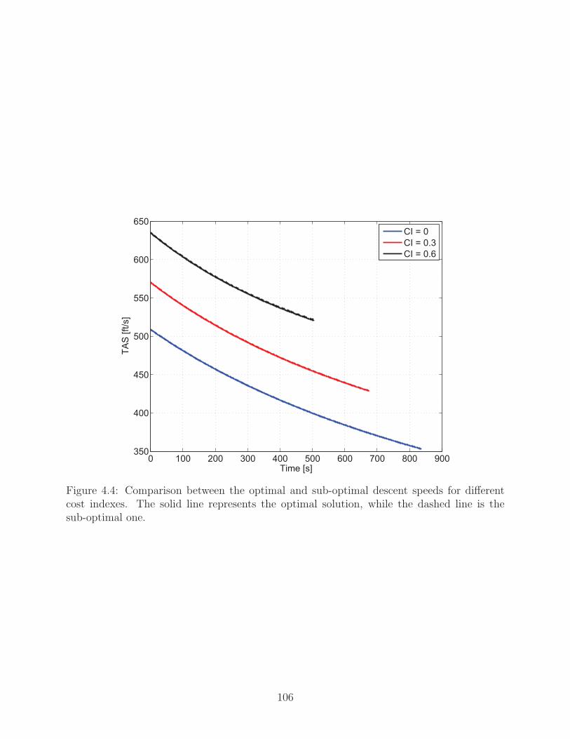
0 100 200 300 400 500 600 700 800 900350
400
450
500
550
600
650
Time [s]
TAS
[ft/s
]
CI = 0CI = 0.3CI = 0.6
Figure 4.4: Comparison between the optimal and sub-optimal descent speeds for differentcost indexes. The solid line represents the optimal solution, while the dashed line is thesub-optimal one.
106
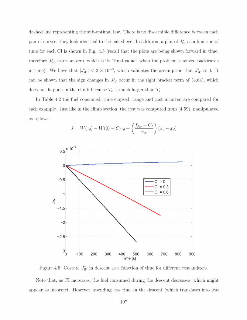
dashed line representing the sub-optimal law. There is no discernible difference between each
pair of curves: they look identical to the naked eye. In addition, a plot of J∗W as a function of
time for each CI is shown in Fig. 4.5 (recall that the plots are being shown forward in time,
therefore J∗W starts at zero, which is its “final value” when the problem is solved backwards
in time). We have that |J∗W | < 3 × 10⁻³, which validates the assumption that J∗
W ≈ 0. It
can be shown that the sign changes in J∗W occur in the right bracket term of (4.64), which
does not happen in the climb because Tc is much larger than Ti.
In Table 4.2 the fuel consumed, time elapsed, range and cost incurred are compared for
each example. Just like in the climb section, the cost was computed from (4.59), manipulated
as follows:
J = W (τd)−W (0) + CIτd +
(ffcr + CI
vcr
)(xc − xd)
0 100 200 300 400 500 600 700 800 900−3
−2.5
−2
−1.5
−1
−0.5
0
0.5x 10⁻³
Time [s]
Jw
CI = 0CI = 0.3CI = 0.6
Figure 4.5: Costate J∗W in descent as a function of time for different cost indexes.
Note that, as CI increases, the fuel consumed during the descent decreases, which might
appear as incorrect. However, spending less time in the descent (which translates into less
107
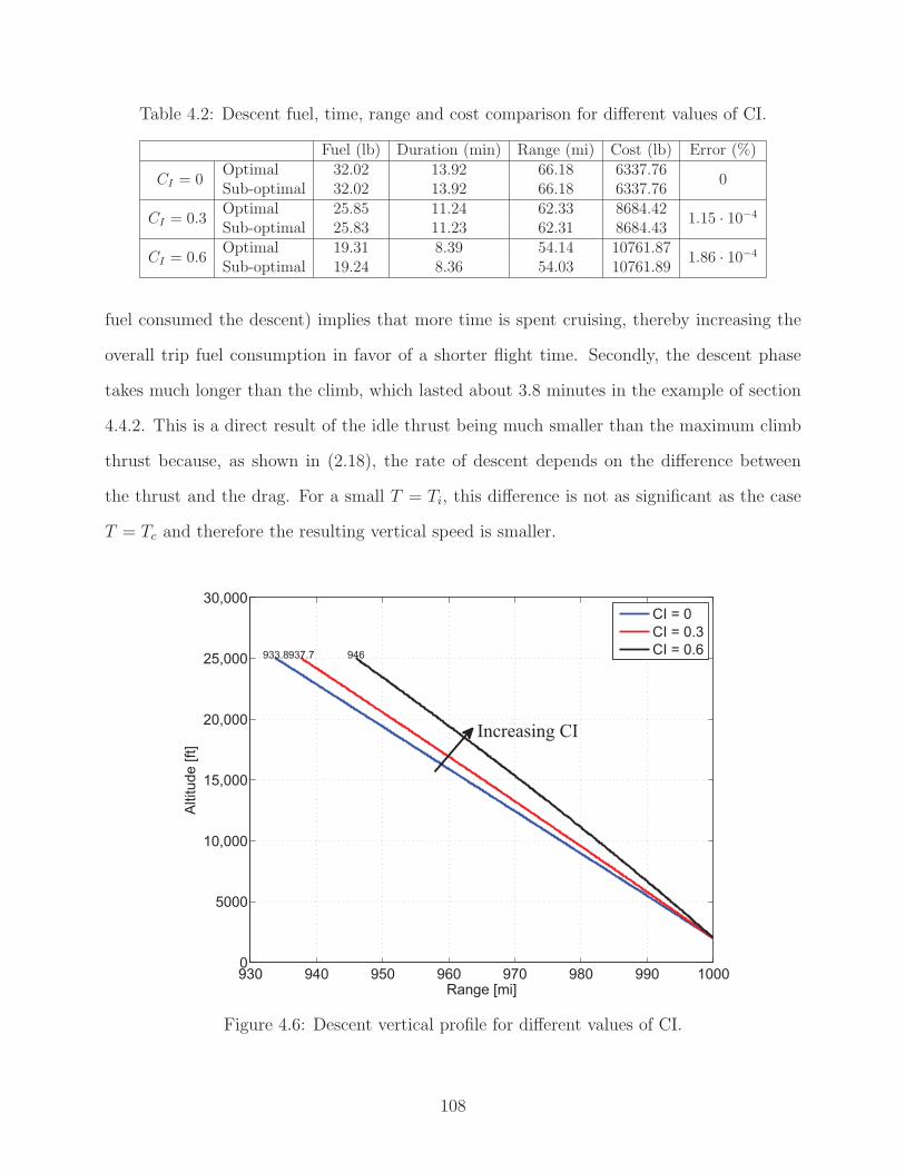
Table 4.2: Descent fuel, time, range and cost comparison for different values of CI.
Fuel (lb) Duration (min) Range (mi) Cost (lb) Error (%)
CI = 0Optimal 32.02 13.92 66.18 6337.76
0Sub-optimal 32.02 13.92 66.18 6337.76
CI = 0.3Optimal 25.85 11.24 62.33 8684.42
1.15 · 10−4
Sub-optimal 25.83 11.23 62.31 8684.43
CI = 0.6Optimal 19.31 8.39 54.14 10761.87
1.86 · 10−4
Sub-optimal 19.24 8.36 54.03 10761.89
fuel consumed the descent) implies that more time is spent cruising, thereby increasing the
overall trip fuel consumption in favor of a shorter flight time. Secondly, the descent phase
takes much longer than the climb, which lasted about 3.8 minutes in the example of section
4.4.2. This is a direct result of the idle thrust being much smaller than the maximum climb
thrust because, as shown in (2.18), the rate of descent depends on the difference between
the thrust and the drag. For a small T = Ti, this difference is not as significant as the case
T = Tc and therefore the resulting vertical speed is smaller.
930 940 950 960 970 980 990 10000
5000
10,000
15,000
20,000
25,000
30,000
933.8937.7 946
Range [mi]
Alti
tude
[ft]
CI = 0CI = 0.3CI = 0.6
Increasing CI
Figure 4.6: Descent vertical profile for different values of CI.
108
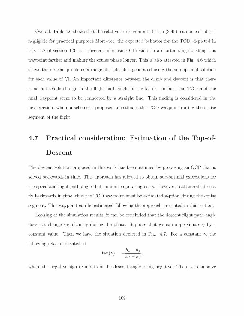
Overall, Table 4.6 shows that the relative error, computed as in (3.45), can be considered
negligible for practical purposes Moreover, the expected behavior for the TOD, depicted in
Fig. 1.2 of section 1.3, is recovered: increasing CI results in a shorter range pushing this
waypoint farther and making the cruise phase longer. This is also attested in Fig. 4.6 which
shows the descent profile as a range-altitude plot, generated using the sub-optimal solution
for each value of CI. An important difference between the climb and descent is that there
is no noticeable change in the flight path angle in the latter. In fact, the TOD and the
final waypoint seem to be connected by a straight line. This finding is considered in the
next section, where a scheme is proposed to estimate the TOD waypoint during the cruise
segment of the flight.
4.7 Practical consideration: Estimation of the Top-of-
Descent
The descent solution proposed in this work has been attained by proposing an OCP that is
solved backwards in time. This approach has allowed to obtain sub-optimal expressions for
the speed and flight path angle that minimize operating costs. However, real aircraft do not
fly backwards in time, thus the TOD waypoint must be estimated a-priori during the cruise
segment. This waypoint can be estimated following the approach presented in this section.
Looking at the simulation results, it can be concluded that the descent flight path angle
does not change significantly during the phase. Suppose that we can approximate γ by a
constant value. Then we have the situation depicted in Fig. 4.7. For a constant γ, the
following relation is satisfied
tan(γ) = −hc − hf
xf − xd
,
where the negative sign results from the descent angle being negative. Then, we can solve
109
Figure 4.7: Estimating the top-of-descent.
for the descent range yielding
(xf − xd) = −hc − hf
tan(γ)(4.79)
Provided that γ is nonzero (which is the case in the descent phase), then (4.79) allows
computing the TOD which equals xd, because xf is known. During cruise, estimations of
the optimal descent v and γ can be made using (4.75) and (4.20) evaluated at the current
aircraft gross weight. Then, using those estimates, (4.79) gives an approximate TOD. As the
aircraft approaches the real xd, its gross weight converges to the real weight at the start of
the descent phase, Wd. As a result the estimate of the TOD will converge to the real TOD.
The only assumption made here is that γ can be approximated by its value at the start of
the descent but, as shown in the simulations, this is a perfectly reasonable assumption.
110
Chapter 5
Conclusions and Future Work
5.1 Conclusions
This thesis has presented a novel approach for solving the Economy Mode problem in FMS.
Using techniques from optimal control theory and algebraic manipulations, an analytic sub-
optimal solution has been found for the true airspeed that minimizes operating costs for the
cruise phase of the flight. For climb and descent, finding a root of the resulting polynomial
that lies in the flight envelope of the aircraft is proposed for on-board implementation using
an iterative approach, such as Newton’s method. In all the examples shown, the relative
error between the optimal and the sub-optimal costs is less than 1 · 10−2%, which is small
enough to be considered negligible in practical scenarios.
The merits of the contributions of this thesis are:
• The airspeed target is in a state-feedback form, thereby avoiding time dependencies
that require offline computations which are common in the open literature and in some
implementations. Moreover, a state-feedback law is more robust in the sense that will
correct small deviations from the optimal trajectory due to possible disturbances. From
a control systems point of view, the FMS under this scheme works as an outer feedback
loop, while the inner loop consists of the autopilot.
111
• Solving for the speed directly eliminates the need of having a performance database
storing the optimal speed schedules in the system. Thus, errors due to interpolation
between points are avoided and the implementation becomes faster. If a performance
database is needed, a look-up table can be created as a function of CI and the state
variables using the proposed sub-optimal equations.
• The climb and descent solutions are not analytic, but the roots of the polynomial
involved can be found using very simple numerical methods, such as Newton’s method.
To ensure a fast convergence, the speed computed at the previous time-step can be
used. This is an effective solution because, as shown in the simulations, the optimal
speed does not change much over small periods of time. In fact, the FMS does not have
to obtain new targets at a very high frequency. The flight management computer would
have plenty of time to compute the next set-point numerically between time-steps.
• From a theoretical standpoint, this formulation provides a significant contribution as it
falls in line with the well-known performance theory present in most books today. Using
this methodology, the maximum-range solution has been recovered when CI vanishes
during cruise, and (3.30) extends the theory naturally and elegantly to a more general
case where CI is not zero. In addition, it unifies all the well-known performance results,
such as maximum endurance and rate of climb, under a single approach.
From this work we can conclude that:
• Practically relevant problems such as the FMS Economy Mode can be formulated as
optimal control problems that can be treated analytically, provided that the correct
assumptions and simplifications are made. While the cruise formulation was simple
enough to perform algebraic manipulations, the climb and descent problems required
that the terminal cost (which is the optimal cost-to-go of the cruise phase) be approx-
imated by a simpler expression involving the cruise fuel flow evaluated at the initial
aircraft weight. This allowed approaching the problem analytically, something that
112
would have been otherwise impossible. As a result, making the right assumptions is an
important step in profiting from the optimal control techniques described in this work.
• The behavior of the TOC and TOD, stated but not derived formally in publications
such as [10, 11], can be verified and explained using Bellman’s principle of optimality,
which models the correlation between the time spent climbing/descending and the time
spent cruising. In addition, because each phase utilizes different thrust settings, their
impact on the overall fuel consumption and flight time is different. As a result the
placement of these two waypoints becomes an important factor in the optimization.
Considering the climb and descent as isolated phases would not have yielded the same
results: in fact, as shown in Chapter 4, the inclusion of the cost index into the problem
does not make sense until the influence of the cruise phase is taken into account.
5.2 Extensions
Several extensions to this work can be proposed for future research, namely:
• Account for wind speeds during the flight. In reality, the existence of wind is one of
the most important factors in a commercial flight, thus the assumption that the wind
speed is zero is the strongest one in this work. Suppose that vw denotes the speed of the
headwind (pointing in the direction of −xh, which is part of the horizon axes system
as defined in section 2.1.3), then the x equation from the aircraft model in (2.6) would
change to [47]
x = v cos(γ)− vw,
with h and the dynamic equations being unchanged. The aerodynamic forces and
specific fuel consumption would remain as functions of the true airspeed. Therefore the
assumptions and OCPs in this thesis would have to account for this modified state-space
model. Even for this simple modification, it will not be possible to obtain a polynomial
in the cruise phase that is solvable analytically because cross terms that multiply v and
113
vw appear in the HJB equation. A similar problem would be present in the climb and
descent phases. The equations of motion for more complex wind scenarios are discussed
in [47].
• Study the impact of the flight length on the validity of the assumptions made to obtain
the sub-optimal solutions. For each flight phase, the costate J∗W (or J∗
˜Wfor the descent)
was approximated by zero, which is its final value. This assumption is less valid for
longer flights. On the other hand, when using the principle of optimality, the assump-
tion that the optimal cost-to-go for the rest of the flight can be approximated by the
cruise cost holds only for long flights, where the cruise phase dominates. As a result,
an interesting extension would involve finding the best compromise between the flight
length and the error due to these assumptions between the sub-optimal trajectory and
the optimal one.
• Find better approximations for J∗W . Note that making J∗
W ≈ 0 is a zero-order Taylor
series expansion in the backward time variable τ , around τ = 0, which is the final
condition. However, if its time derivative J∗W could be estimated at the final time, then
a first-order Taylor series expansion could be made about that point yielding a better
estimate for this costate. A potential drawback of this approach is that the resulting
expression would depend on time. As a result, when substituting J∗W on the optimal
solutions, a time-dependent state-feedback law would be obtained.
• Consider transition periods between phases. Note that the optimal speed for the climb
found using (4.35) does not coincide with the cruise optimal solution (3.21) when h = hc,
and similarly between cruise and descent. Therefore, a period has to exist between these
phases where the aircraft transitions from one speed target to the other. Initially, this
period could be handled by the autopilot. However, it would be an interesting extension
to find the optimal way to change phases, based on the theory of optimal control.
• Extend the formulation to support step climbs during cruise. The main idea is to allow
114
the aircraft to change between ATC-allowed flight levels during cruise to account for
changes in its optimum altitude. Current FMS already support step-climb, but they
must be initiated manually by the pilot. An interesting optimal control formulation
would be finding the “best” point to change altitude while cruising.
• Explicitly account for state and input constraints in the mathematical formulation,
given by the flight envelope of the aircraft. While the current assumption that all
points lie inside the flight envelope is valid for most practical scenarios, it is important
to guarantee that the aircraft does not exceed its structural limits specially when flying
at a high CI value. Using the current formulation, either one can compute CI to
ensure the constraints are verified (see remark 2 in section 3.3 ) or, otherwise, these
constraints must be enforced after the optimal set-points are found. To obtain an
optimal trajectory when close to the boundaries of the flight envelope, the constraints
must be explicitly incorporated in the optimal control problem.
• Compute the optimum altitude, defined as the height where operating costs are mini-
mal. Current FMS compute this value.
• Formulate and solve a Required Time of Arrival (RTA) problem. This mode was
mentioned in Section (1.2), and its purpose is to ensure that a particular waypoint
is reached within a prescribed time window. It would also allow accounting for strict
time of arrival constraints at the destination airport. From an optimal control point of
view, these situations would imply that the final times in the OCPs are now prescribed.
Accounting for these modifications is out of the scope of this thesis, and a preliminary
approach could be to change CI such that the given time constraint is satisfied.
115
Bibliography
[1] P. N. E. A. Agency, “Trends in global co2 emissions report,” 2014. Accessed January
2015.
[2] U. E. I. A. (EIA), “U.s. energy-related carbon dioxide emissions in 2013,” 2014. Accessed
January 2015.
[3] T. Guardian, “Air traffic growth rates will outspace emissions reductions, research
shows,” 2014. Accessed January 2015.
[4] N. Rivers, “Are low oil prices good for the environment?,” December 2014. From the
Ottawa Citizen. Accessed January 2015.
[5] F. A. Administration, Instrument Flying Handbook. U.S. Department of Transportation,
2007.
[6] S. Liden, “The evolution of flight management systems,” in 13th AIAA/IEEE Digital
Avionics Systems Conference, pp. 157–169, October 1994.
[7] R. Walter, The Avionics Handbook, Chapter 15: Flight Management Systems. CRC
Press, 2001.
[8] Z. Sibin, L. Guixian, and H. Junwei, “Research and modelling on performance database
of flight management systems,” in 2nd International Asia Conference on Informatics in
Control Automation and Robotics (CAR), pp. 295–298, March 2010.
116
[9] A. Industries, “Getting to grips with the cost index.” Flight Operations Support and
Line Assistance, 1998.
[10] Boeing, “Jet transport performance methods (d6-1420),” 2009.
[11] B. Roberson, “Fuel conservation strategies: Cost index explained.” Boeing AERO Mag-
azine QTR 02, 2007.
[12] W. Roberson, “Fuel conservation strategies: Cruise flight.” Boeing AERO Magazine
QTR 04, 2007.
[13] A. Industries, “Getting to grips with aircraft performance.” Flight Operations Support
and Line Assistance, 2002.
[14] D. E. Kirk, Optimal Control Theory: An Introduction. Prentice-Hall, 1970.
[15] M. Athans and P. L. Falb, Optimal Control: An Introduction to the Theory and its
Applications. Dover Publications, 2006.
[16] D. Liberzon, Switching in Systems and Control. Boston, USA: Birkhuser, 2003.
[17] A. E. Bryson and Y. Ho, Applied Optimal Control: Optimization, Estimation and Con-
trol. Taylor and Francis Group, 1975.
[18] L. S. Pontryagin, V. Boltyanskii, R. V. Gamkrelidze, and E. F. Mischenko, The Mathe-
matical Theory of Optimal Processes. Interscience Publishers, Inc., 1962.
[19] R. E. Bellman, Dynamic Programming. Princeton University Press, 1957.
[20] P. L. et M. G. Grandall, “Viscosity solutions of hamilton-jacobi equations,” Trans. Amer.
Math. Soc. 277, pp. 1–42, 1983.
[21] W. Roberson, “Fuel conservation strategies: Takeoff and climb.” Boeing AERO Maga-
zine QTR 04, 2008.
117
[22] W. Roberson and J. A. Johns, “Fuel conservation strategies: Descent and approach.”
Boeing AERO Magazine QTR 02, 2010.
[23] S. Liden, “Optimum 4d guidance for long flights,” in Digital Avionics Systems Confer-
ence, pp. 262–267, October 1992.
[24] S. Liden, “Flight management system providing minimum total cost,” 1988. US Patent
4,760,530.
[25] S. Liden, “Apparatus and method for computing wind-sensitive optimum altitude steps
in a flight management system,” 1996. US Patent 5,574,647.
[26] N. Chui, “The development of a dynamic test bed for flight management systems,” 2002.
M. A. Sc. thesis, Concordia University.
[27] A. Tewari, Advanced Control of Aircraft, Spacecraft and Rockets. John Wiley and Sons,
2011.
[28] H. Erzberger, “Optimum climb and descent trajectories for airline missions,” in AGARD
Theory and Applications of Optimal Control in Aerospace Systems, July 1981.
[29] J. Sorensen, S. A. Morello, and H. Erzberger, “Applications of trajectory optimization
principles to minimize aircraft operating costs,” in 18th IEEE Conference on Decision
and Control including the Symposium on Adaptive Processes, pp. 415–421, December
1979.
[30] S. Wu and Y. Shen, “Studies on the flight performance optimization of commercial
aircrafts,” in IEEE Region 10 Conference on Computer, Communication, Control and
Power Engineering, vol. 4, pp. 139–145, October 1993.
[31] S. Wu and S. Guo, “Optimum flight trajectory guidance based on total energy control
of aircraft,” Journal of Guidance, Control, And Dynamics, vol. 17, March 1994.
118
[32] J. Burrows, “Fuel-optimal aircraft trajectories with fixed arrival times,” Journal of Guid-
ance, Control and Dynamics, vol. 6, pp. 14–19, January 1983.
[33] P. Hagelauer and F. Mora-Camino, “Evaluation of practical solutions for onboard air-
craft four-dimensional guidance,” Journal of Guidance, Control and Dynamics, vol. 20,
no. 5, pp. 1052–1054, 1997.
[34] Y. Diaz-Mercado, S. Lee, M. Egerstedt, and S.-Y. Young, “Optimal trajectory generation
for next generation flight management systems,” in IEEE/AIAA 32nd Digital Avionics
Systems Conference, pp. 3C5–1–3C5–10, October 2013.
[35] M. C. Waller, “Considerations in the application of dynamic programming to optimal
aircraft trajectory generation,” in Proceedings of the IEEE Aerospace and Electronics
Conference, vol. 2, pp. 574–579, May 1990.
[36] P. Hagelauer and F. Mora-Camino, “A soft dynamic programming approach for on-line
aircraft 4d-trajectory optimization,” European Journal of Operational Research 107,
pp. 87–95, 1998.
[37] H. Wu, N. Cho, H. Bouadi, L. Zhong, and F. Mora-Camino, “Dynamic programming
for trajectory optimization of engine-out transportation aircraft,” in 24th IEEE Chinese
Control and Decision Conference, pp. 98–103, 2012.
[38] N. K. Wickramasinghe, A. Harada, H. Totoki, T. Miyamoto, and Y. Miyazawa, “Flight
trajectory optimization for modern jet passenger aircraft with dynamic programming,”
in Lecture Notes in Electrical Engineering: Air Traffic Management and Systems, pp. 87–
104, Springer, 2014.
[39] R. Almgren and A. Tourin, “Optimal soaring via hamilton-jacobi-bellman equations.”
Social Science Research Network (SSRN), February 2014.
119
[40] S. Khardi, “Applied methods validating aircraft flight path optimization. theoretical and
experimental considerations,” in HIKARI Ltd. Applied Mathematical Sciences, vol. 7,
pp. 2209–2228, 2013.
[41] B. Tian and Q. Zong, “3dof ascent phase trajectory optimization for aircraft based on
adaptive gauss pseudospectral method,” in IEEE Third International Conference on
Intelligent Control and Information Processing, pp. 431–435, July 2012.
[42] P. Bonami, A. Olivares, M. Soler, and E. Staffetti, “Multiphase mixed-integer control
approach to aircraft trajectory optimization,” Journal of Guidance, Control and Dy-
namics, vol. 36, pp. 1267–1277, September 2013.
[43] S. G. Park and J. Clarke, “Fixed rta fuel optimal profile descent based on analysis of tra-
jectory performance bound,” in IEEE/AIAA 31st Digital Avionics Systems Conference,
pp. 3D3–1 – 3D3–13, October 2012.
[44] R. Drury, A. Tsourdos, and A. Cooke, “Real-time trajectory generation: Improving the
optimality and speed of an inverse dynamics method,” in IEEE Aerospace Conference,
pp. 1–12, March 2010.
[45] R. S. Shevell, Fundamentals of Flight. Prentice Hall, 2 ed., 1988.
[46] J. D. Anderson, Aircraft Performance and Design. WCB/McGraw-Hill, 1999.
[47] D. G. Hull, Fundamentals of Airplane Flight Mechanics. Springer, 2007.
[48] M. Saarlas, Aircraft Performance. John Wiley and Sons Inc., 2007.
[49] S. Boyd, Convex Optimization. Cambridge University Press, 2004.
[50] D. Liberzon, Calculus of Variations and Optimal Control Theory: A Concise Introduc-
tion. Princeton University Press, 2012.
[51] R. Horn and C. Johnson, Matrix Analysis. Cambridge University Press, 1990.
120
[52] R. E. Bellman and S. E. Dreyfus, Applied Dynamic Programming. Princeton University
Press, 1962.
[53] G. Aerospace, “Gulsfream g450 technical specifications.” http://www.gulfstream.
com/aircraft/gulfstream-g450. Accessed 12-2014.
121
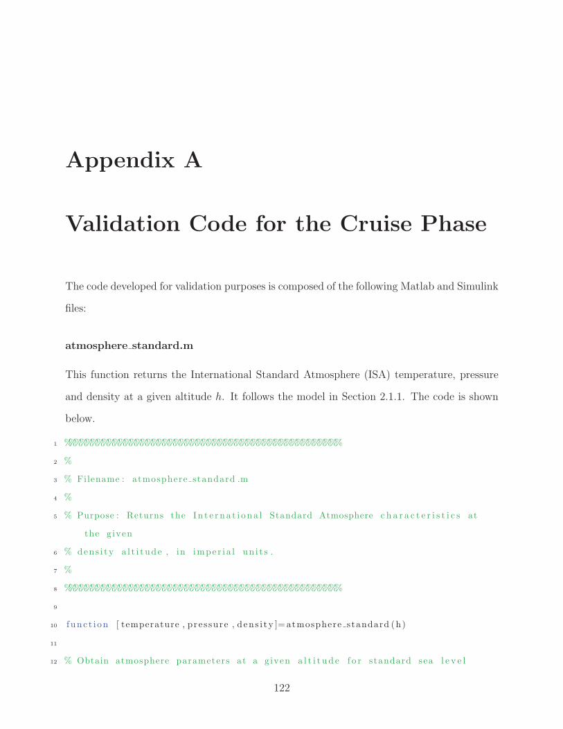
Appendix A
Validation Code for the Cruise Phase
The code developed for validation purposes is composed of the following Matlab and Simulink
files:
atmosphere standard.m
This function returns the International Standard Atmosphere (ISA) temperature, pressure
and density at a given altitude h. It follows the model in Section 2.1.1. The code is shown
below.
1 %%%%%%%%%%%%%%%%%%%%%%%%%%%%%%%%%%%%%%%%%%%%%%%%%%
2 %
3 % Filename : atmosphere standard .m
4 %
5 % Purpose : Returns the I n t e r n a t i o n a l Standard Atmosphere c h a r a c t e r i s t i c s at
the g iven
6 % dens i ty a l t i t ude , in impe r i a l un i t s .
7 %
8 %%%%%%%%%%%%%%%%%%%%%%%%%%%%%%%%%%%%%%%%%%%%%%%%%%
9
10 f unc t i on [ temperature , pres sure , dens i ty ]=atmosphere standard (h)
11
12 % Obtain atmosphere parameters at a g iven a l t i t u d e f o r standard sea l e v e l
122
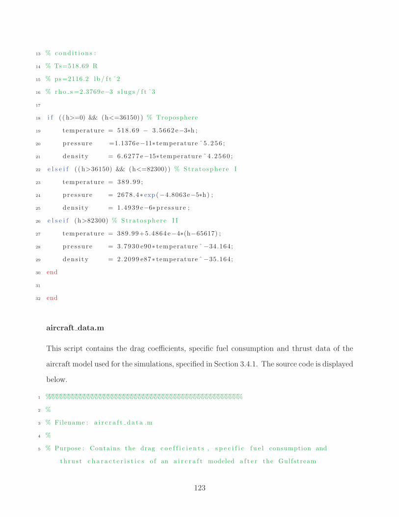
13 % cond i t i on s :
14 % Ts=518.69 R
15 % ps=2116.2 lb / f t ˆ2
16 % rho s =2.3769e−3 s l u g s / f t ˆ3
17
18 i f ( ( h>=0) && (h<=36150) ) % Troposphere
19 temperature = 518.69 − 3 .5662 e−3∗h ;
20 pre s su r e =1.1376e−11∗ temperature ˆ5 . 2 56 ;
21 dens i ty = 6.6277 e−15∗ temperature ˆ4 . 2560 ;
22 e l s e i f ( ( h>36150) && (h<=82300) ) % Stra to sphere I
23 temperature = 389 . 9 9 ;
24 pre s su r e = 2678.4∗ exp (−4.8063e−5∗h) ;
25 dens i ty = 1.4939 e−6∗pre s su r e ;
26 e l s e i f (h>82300) % Stra to sphere I I
27 temperature = 389.99+5.4864 e−4∗(h−65617) ;
28 pre s su r e = 3.7930 e90∗ temperature ˆ−34.164;
29 dens i ty = 2.2099 e87∗ temperature ˆ−35.164;
30 end
31
32 end
aircraft data.m
This script contains the drag coefficients, specific fuel consumption and thrust data of the
aircraft model used for the simulations, specified in Section 3.4.1. The source code is displayed
below.
1 %%%%%%%%%%%%%%%%%%%%%%%%%%%%%%%%%%%%%%%%%%%%%%%%%%
2 %
3 % Filename : a i r c r a f t d a t a .m
4 %
5 % Purpose : Contains the drag c o e f f i c i e n t s , s p e c i f i c f u e l consumption and
thrus t c h a r a c t e r i s t i c s o f an a i r c r a f t modeled a f t e r the Gulfstream
123
Aerospace ’ s G−IV j e t .
6 %
7 % Model source : J . D. Anderson . A i r c r a f t Performance and Design . Chapter 5 ,
Airp lane Performance : Steady F l i gh t . Pages 199−232.
8 %
9 % Source f o r operat ing l im i t s : http : //www. gu l f s t r eam . com/ a i r c r a f t / gu l f s t ream−
g450
10 %%%%%%%%%%%%%%%%%%%%%%%%%%%%%%%%%%%%%%%%%%%%%%%%%%
11
12 % Some d e f i n i t i o n s :
13 M HOUR TO SEG = 3600 ;
14
15 % Gulfstream Aerospace ’ s G−IV data :
16 SFC = 0.69/M HOUR TO SEG; % (1/ s ) . At 30000 f t .
17 Cd0 = 0 . 0 1 5 ;
18 Cd2 = 0 . 0 8 ;
19 S = 950 ; % ( f t ˆ2) .
20 T0 = 2 ∗ 13850 ; % Each Rol l s−Royce Tay 611−8 eng ine i s rated at
13850 ( l b f ) at sea l e v e l .
21 Ti = 200 . 0 ; % ( l b f ) .
22 m = 1 ;
23 Mmo = 0 . 8 8 ; % Maximum operat ing Mach .
24
25 % Make sure that the i n i t i a l c ond i t i on s do not exceed these l im i t s :
26 % Maximum usab le f u e l weight = 29500 lb .
27 % Maximum take−o f f weight = 74600 lb .
28 % Maximum zero f u e l weight = 49000 lb .
29 % Serv i c e c e i l i n g = 45000 f t .
shooting method cruise.m
This script loads the model from aircraft data.m, sets the shooting method and simulation
parameters, and implements the pseudo-code shown in Section 3.4.2. The desired initial,
124
final conditions, CI and initial speed estimate must be specified in this file as well. The
sub-optimal trajectory given by (3.30) is obtained as well. To perform all these functions,
the script makes use of Simulink models sim 2pbvp cruise.mdl and sim analytic cruise.mdl.
The code is shown below. It is important to note that the costate J∗W is named lambda2 in
the implementation.
1 %%%%%%%%%%%%%%%%%%%%%%%%%%%%%%%%%%%%%%%%%%%%%%%%%%
2 %
3 % Filename : shoot ing method c ru i s e .m
4 %
5 % Purpose : Implements the shoot ing method f o r the c r u i s e phase . Also s imu la t e s
the system s im an a l y t i c c r u i s e . mdl which implements the sub−optimal
ana l y t i c s o l u t i o n .
6 %
7 %%%%%%%%%%%%%%%%%%%%%%%%%%%%%%%%%%%%%%%%%%%%%%%%%%
8
9 % Run the s c r i p t f o r the a i r c r a f t model :
10 a i r c r a f t d a t a ;
11
12 % Some d e f i n i t i o n s :
13 Ts = 0 . 1 ; % Simulat ion sampling time .
14 CI = 0 . 0 ;
15 M MILE TO FT = 5280 ; % Conversion from mi l e s to f e e t .
16 rhosea = 0 .002377 ; % ( s lug / f t ˆ2) sea l e v e l dens i ty .
17
18 % Shooting method parameters :
19 t o l e r an c e = 1e−5; % Tolerance on the f i n a l cond i t i on o f lambda2 .
20 e r r o r = 1e3 ; % D i f f e r e n c e between f i n a l lambda2 and
lambda2f .
21 i t e r = 1 ; % I t e r a t i o n count .
22 maxiter = 30 ; % Maximum number o f i t e r a t i o n s .
23 beta = 1 ; % Used in the update law o f lambda2 .
24 lambdas20 ( 1 : maxiter ) = 0 . 0 ; % Store i n i t i a l va lue s o f lambda2 here .
125
25
26 % I n i t i a l and f i n a l c ond i t i on s :
27 hc = 25000 ; % ( f t ) .
28 x0 = 0 . 0 ;
% ( f t ) .
29 xf = 1000∗M MILE TO FT; % ( f t ) .
30 W0 = 70000; % ( l b f ) .
31 lambda2f = 0 ; % % Known boundary
cond i t i on o f lambda2 .
32
33 % Estimate an i n i t i a l va lue f o r the speed :
34 V0 = 900 ;
35
36 % ISA and drag computations :
37 [ ˜ , ˜ , rho , ] = atmosphere standard ( hc ) ;
38 d0 = 0.5∗Cd0∗ rho∗S ;
39 d1 = 2∗Cd2∗W0∗W0/( rho∗S) ;
40 D = d0∗V0ˆ2 + d1/V0ˆ2 ;
41
42 % Compute i n i t i a l va lue o f lambda2 from V0 :
43 i f (CI ˜= 0)
44 lambda20 = 1 + CI/(SFC∗(D − 2∗d0∗V0ˆ2 + 2∗d1/V0ˆ2) ) ;
45 e l s e
46 % lambda2 cannot be equal to 1 . When CI i s zero , i t i s bes t to
es t imate a smal l va lue f o r lambda20 .
47 lambda20 = 1e−3;
48 end
49 lambdas20 ( i t e r ) = lambda20 ;
50
51 % Begin loop :
52 whi le ( e r r o r > t o l e r an c e ) && ( i t e r <= maxiter )
53 sim ( ’ s im 2pbvp cru i s e ’ ) ;
54 i t e r = i t e r + 1
126
55
56 % Next seed f o r lambda20 :
57 e r r o r = abs ( lambda2 ( end )−lambda2f ) ;
58 lambda20 = lambda20 − beta ∗( lambda2 ( end )−lambda2f ) ;
59 lambdas20 ( i t e r ) = lambda20 ;
60 end
61
62 % Display a warning i f the maximum number o f i t e r a t i o n s was reached :
63 i f ( i t e r >= maxiter )
64 di sp ( ’Maximum number o f i t e r a t i o n s reached . Check value o f e r r o r ’ ) ;
65 end
66
67 % Simulate the ana l y t i c sub−optimal s o l u t i o n :
68 sim ( ’ s im an a l y t i c c r u i s e ’ ) ;
69
70 % End o f s c r i p t .
sim 2pbvp cruise.mdl
This Simulink model, shown in Fig. A.1, implements the 2PBVP given by (3.42), where
v at each time-step is computed using (3.21). The blocks x, W, lambda2, V and t store
those variables in the Matlab workspace for further analysis. The block aircraft2pbvp is
a Matlab Level-2 S-Function that specifies the dynamics of the system to Simulink. This
function must comply with a specific template1, and its implementation does not provide
additional information regarding the developments of this thesis. As a result, source code for
the S-functions will not be provided.
1For more information regarding Matlab Level-2 S-Functions, consult the following website: http://www.mathworks.com/help/simulink/sfg/writing-level-2-matlab-s-functions.html
127
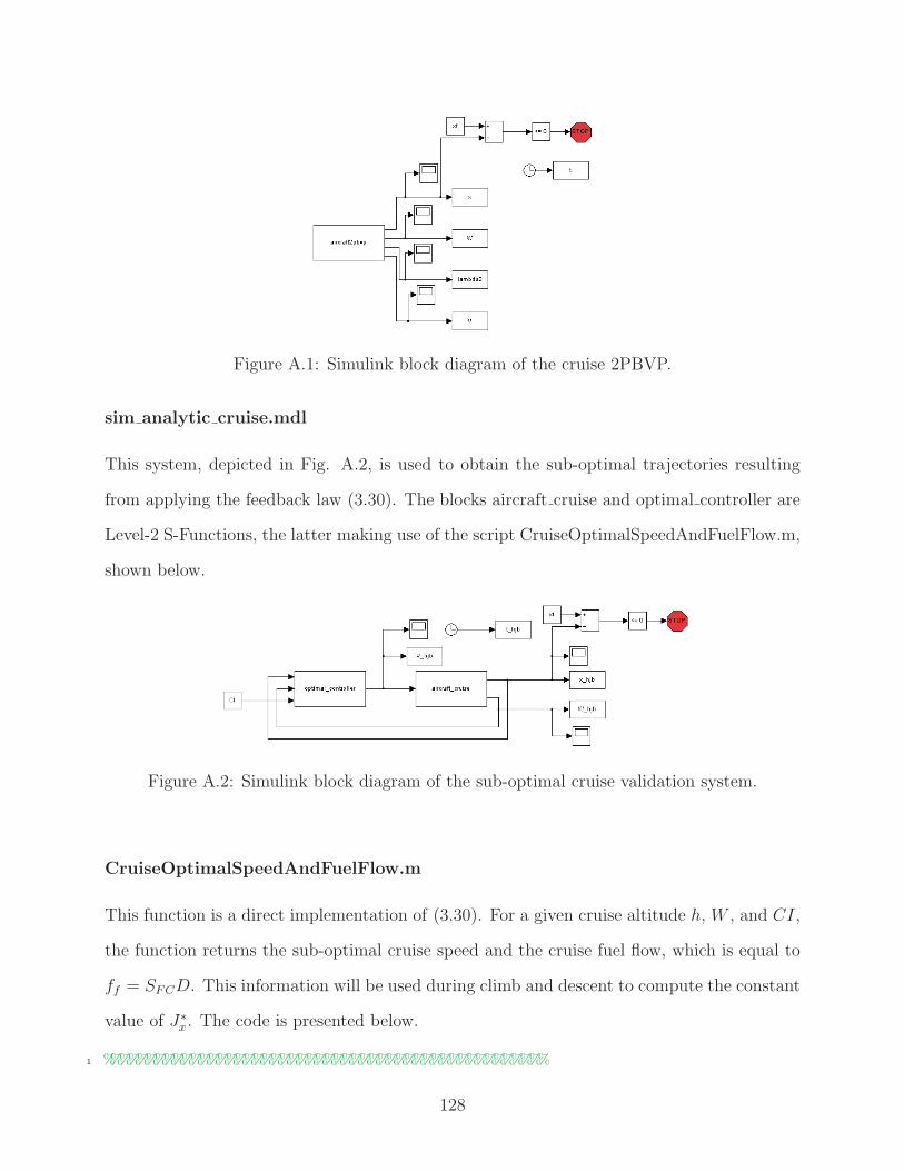
Figure A.1: Simulink block diagram of the cruise 2PBVP.
sim analytic cruise.mdl
This system, depicted in Fig. A.2, is used to obtain the sub-optimal trajectories resulting
from applying the feedback law (3.30). The blocks aircraft cruise and optimal controller are
Level-2 S-Functions, the latter making use of the script CruiseOptimalSpeedAndFuelFlow.m,
shown below.
Figure A.2: Simulink block diagram of the sub-optimal cruise validation system.
CruiseOptimalSpeedAndFuelFlow.m
This function is a direct implementation of (3.30). For a given cruise altitude h, W , and CI,
the function returns the sub-optimal cruise speed and the cruise fuel flow, which is equal to
ff = SFCD. This information will be used during climb and descent to compute the constant
value of J∗x . The code is presented below.
1 %%%%%%%%%%%%%%%%%%%%%%%%%%%%%%%%%%%%%%%%%%%%%%%%%%
128
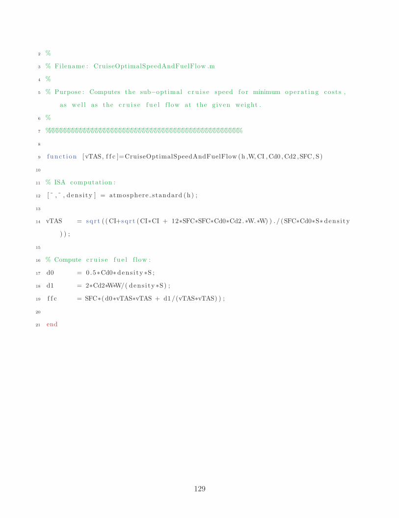
2 %
3 % Filename : CruiseOptimalSpeedAndFuelFlow .m
4 %
5 % Purpose : Computes the sub−optimal c r u i s e speed f o r minimum operat ing cos t s ,
as we l l as the c r u i s e f u e l f low at the g iven weight .
6 %
7 %%%%%%%%%%%%%%%%%%%%%%%%%%%%%%%%%%%%%%%%%%%%%%%%%%
8
9 f unc t i on [vTAS, f f c ]=CruiseOptimalSpeedAndFuelFlow (h ,W, CI , Cd0 ,Cd2 ,SFC, S)
10
11 % ISA computation :
12 [ ˜ , ˜ , dens i ty ] = atmosphere standard (h) ;
13
14 vTAS = sq r t ( ( CI+sq r t (CI∗CI + 12∗SFC∗SFC∗Cd0∗Cd2 .∗W.∗W) ) . / (SFC∗Cd0∗S∗ dens i ty
) ) ;
15
16 % Compute c r u i s e f u e l f low :
17 d0 = 0.5∗Cd0∗ dens i ty ∗S ;
18 d1 = 2∗Cd2∗W∗W/( dens i ty ∗S) ;
19 f f c = SFC∗( d0∗vTAS∗vTAS + d1/(vTAS∗vTAS) ) ;
20
21 end
129
Appendix B
Validation Code for the Climb Phase
The climb implementation makes use of atmosphere standard.m, aircraft data.m and CruiseOp-
timalSpeedAndFuelFlow.m from Appendix A. The following scripts and systems are exclusive
to the climb phase:
shooting method climb.m
This script is analogous to shooting method cruise.m, and its code can be found below. As
its name implies, it implements the shooting method provided in Section 4.4.1, and then
computes the sub-optimal trajectory resulting from the application of the control law (4.48).
Desired initial and final conditions must be specified inside this script. For the simulations,
it runs systems sim 2pbvp climb.mdl and sim analytic climb.mdl. Note that J∗x is referred
to as lambda1 and J∗W is called lambda3 in the code.
1 %%%%%%%%%%%%%%%%%%%%%%%%%%%%%%%%%%%%%%%%%%%%%%%%%%
2 %
3 % Filename : shoot ing method c l imb .m
4 %
5 % Purpose : Implements the shoot ing method f o r the cl imb phase . Also s imu la t e s
the system s im ana l y t i c d e s c en t . mdl which implements the sub−optimal
s o l u t i o n .
6 %
130
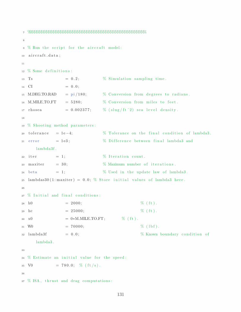
7 %%%%%%%%%%%%%%%%%%%%%%%%%%%%%%%%%%%%%%%%%%%%%%%%%%
8
9 % Run the s c r i p t f o r the a i r c r a f t model :
10 a i r c r a f t d a t a ;
11
12 % Some d e f i n i t i o n s :
13 Ts = 0 . 2 ; % Simulat ion sampling time .
14 CI = 0 . 0 ;
15 MDEG TO RAD = pi /180 ; % Conversion from degree s to rad ians .
16 M MILE TO FT = 5280 ; % Conversion from mi l e s to f e e t .
17 rhosea = 0 .002377 ; % ( s lug / f t ˆ2) sea l e v e l dens i ty .
18
19 % Shooting method parameters :
20 t o l e r an c e = 1e−4; % Tolerance on the f i n a l cond i t i on o f lambda3 .
21 e r r o r = 1e3 ; % D i f f e r e n c e between f i n a l lambda3 and
lambda3f .
22 i t e r = 1 ; % I t e r a t i o n count .
23 maxiter = 30 ; % Maximum number o f i t e r a t i o n s .
24 beta = 1 ; % Used in the update law o f lambda3 .
25 lambdas30 ( 1 : maxiter ) = 0 . 0 ; % Store i n i t i a l va lue s o f lambda3 here .
26
27 % I n i t i a l and f i n a l c ond i t i on s :
28 h0 = 2000 ; % ( f t ) .
29 hc = 25000 ; % ( f t ) .
30 x0 = 0∗M MILE TO FT; % ( f t ) .
31 W0 = 70000; % ( l b f ) .
32 lambda3f = 0 . 0 ; % Known boundary cond i t i on o f
lambda3 .
33
34 % Estimate an i n i t i a l va lue f o r the speed :
35 V0 = 780 . 0 ; % ( f t / s ) .
36
37 % ISA , th rus t and drag computations :
131
38 [ ˜ , ˜ , rho ] = atmosphere standard ( h0 ) ;
39 d0 = 0.5∗Cd0∗ rho∗S ;
40 d1 = 2∗Cd2∗W0∗W0/( rho∗S) ;
41 D = d0∗V0ˆ2 + d1/V0ˆ2 ;
42 Dv = 2∗d0∗V0 − 2∗d1/V0ˆ3 ; % Der iva t i ve o f D with r e sp e c t to V.
43 Tclimb = T0∗( rho/ rhosea ) ˆm;
44
45 % I n i t i a l gamma corre spond ing to V0 :
46 gamma0 = as in ( ( Tclimb − D)/W0 ) ;
47
48 % Compute lambda1 and i n i t i a l lambda3 :
49 [M,vTAS,vKTAS,vKEAS,vKCAS, f f c ] = CruiseOptimalSpeedAndFuelFlow (hc ,W0, CI , Cd0 ,
Cd2 ,SFC, S) ; % Estimated c r u i s e TAS and f u e l f low .
50 lambda1 = − ( f f c + CI ) /vTAS;
51 lambda30 = 1 + CI/(SFC∗Tclimb ) − lambda1∗V0∗V0∗Dv/(SFC∗Tclimb ∗(W0∗
gamma0 − V0∗Dv) ) ;
52 lambdas30 ( i t e r ) = lambda30 ;
53
54 % Run the i t e r a t i v e p roc e s s :
55 whi le ( abs ( e r r o r ) > t o l e r an c e ) && ( i t e r <= maxiter )
56 sim ( ’ s im 2pbvp cl imb ’ ) ; % Run the system .
57 i t e r = i t e r + 1
58
59 % Next seed f o r lambda30 :
60 e r r o r = lambda3 ( end )−lambda3f ;
61 lambda30 = lambda30 − beta ∗ e r r o r ;
62 lambdas30 ( i t e r ) = lambda30 ;
63 end
64
65 ROCfpm = ROC. ∗ 6 0 ; % Change ROC to f e e t per minute .
66
67 % Display a warning i f the maximum number o f i t e r a t i o n s was reached :
68 i f ( i t e r >= maxiter )
132
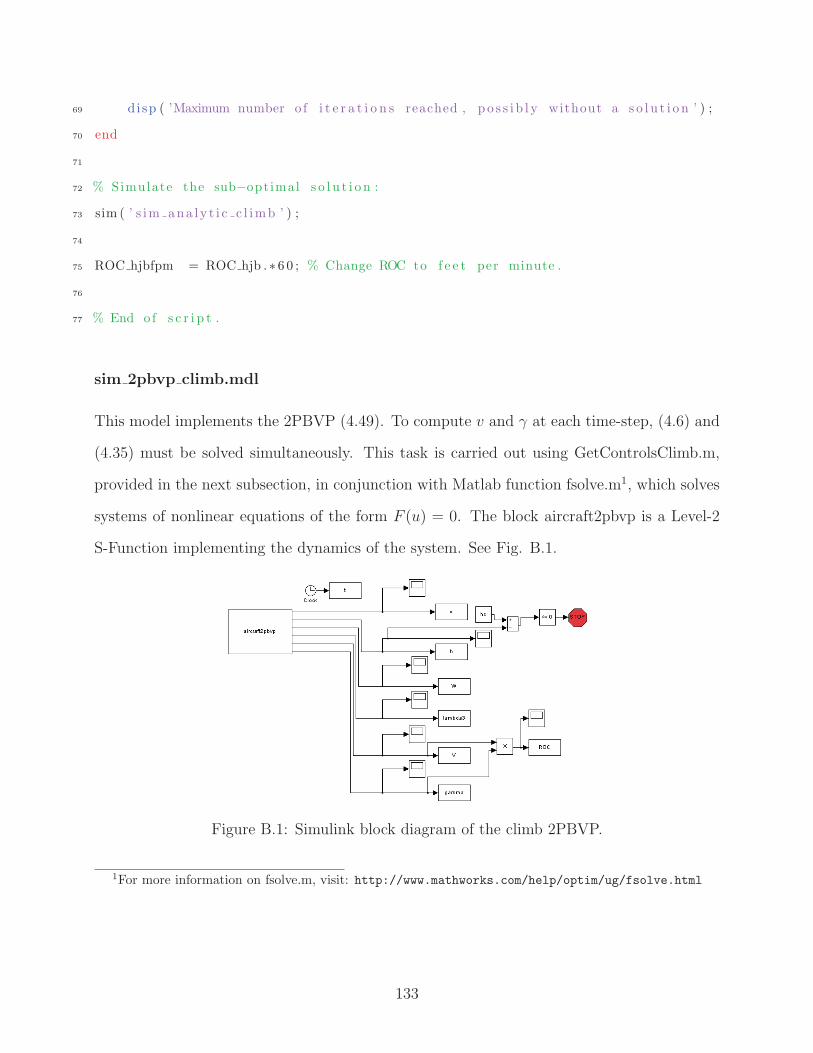
69 di sp ( ’Maximum number o f i t e r a t i o n s reached , p o s s i b l y without a s o l u t i o n ’ ) ;
70 end
71
72 % Simulate the sub−optimal s o l u t i o n :
73 sim ( ’ s im ana l y t i c c l imb ’ ) ;
74
75 ROC hjbfpm = ROC hjb . ∗ 6 0 ; % Change ROC to f e e t per minute .
76
77 % End o f s c r i p t .
sim 2pbvp climb.mdl
This model implements the 2PBVP (4.49). To compute v and γ at each time-step, (4.6) and
(4.35) must be solved simultaneously. This task is carried out using GetControlsClimb.m,
provided in the next subsection, in conjunction with Matlab function fsolve.m1, which solves
systems of nonlinear equations of the form F (u) = 0. The block aircraft2pbvp is a Level-2
S-Function implementing the dynamics of the system. See Fig. B.1.
Figure B.1: Simulink block diagram of the climb 2PBVP.
1For more information on fsolve.m, visit: http://www.mathworks.com/help/optim/ug/fsolve.html
133
GetControlsClimb.m
This function is meant to be used in conjunction with Matlab’s function fsolve.m. The code
evaluates (4.6) and (4.35) at a given u = [ v γ ]T . Using fsolve.m, these two expressions are
continuously evaluated until both equal zero, in which case the optimal point is found.
1 %%%%%%%%%%%%%%%%%%%%%%%%%%%%%%%%%%%%%%%%%%%%%%%%%%
2 %
3 % Filename : GetControlsClimb .m
4 %
5 % Purpose : Returns the value o f the system o f non l i n ea r equat ions that must be
so lved to get the opt imal c on t r o l s (V,gamma) , at u . For use with f s o l v e .
6 %
7 %%%%%%%%%%%%%%%%%%%%%%%%%%%%%%%%%%%%%%%%%%%%%%%%%%
8
9 f unc t i on output = GetControlsClimb ( rho ,W, lambda1 , lambda3 ,SFC,Cd0 ,Cd2 , S , Tclimb ,
u , CI )
10
11 % u conta in s V and gamma:
12 V = u(1) ;
13 gamma = u (2) ;
14
15 % Drag components :
16 d0 = 0.5∗Cd0∗ rho∗S ;
17 d1 = 2∗Cd2∗W∗W/( rho∗S) ;
18
19 % Return the system o f non l i n ea r equat ions eva luated at u :
20 output = ze ro s (2 , 1 ) ;
21
22 Dv = 2∗d0∗V − 2∗d1/(Vˆ3) ; % Der iva t i v e o f the drag .
23 output (1 ) = ((1− lambda3 ) ∗SFC∗Tclimb + CI ) ∗( s i n (gamma) − V∗Dv/W) −
lambda1∗V∗V∗Dv/(W∗ cos (gamma) ) ;
24 output (2 ) = Tclimb − ( d0∗V∗V + d1/V/V) − W∗ s i n (gamma) ;
25
134
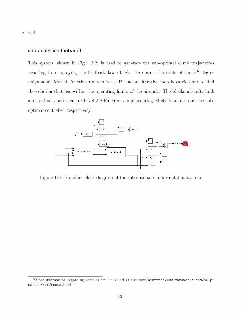
26 end
sim analytic climb.mdl
This system, shown in Fig. B.2, is used to generate the sub-optimal climb trajectories
resulting from applying the feedback law (4.48). To obtain the roots of the 5th degree
polynomial, Matlab function roots.m is used2, and an iterative loop is carried out to find
the solution that lies within the operating limits of the aircraft. The blocks aircraft climb
and optimal controller are Level-2 S-Functions implementing climb dynamics and the sub-
optimal controller, respectively.
Figure B.2: Simulink block diagram of the sub-optimal climb validation system.
2More information regarding roots.m can be found at the website:http://www.mathworks.com/help/matlab/ref/roots.html
135
Appendix C
Validation Code for the Descent Phase
The descent implementation makes use of atmosphere standard.m, aircraft data.m and CruiseOp-
timalSpeedAndFuelFlow.m from Appendix A, as well as the following scripts and systems:
shooting method descent.m
Just like in the previous appendices, this script implements the shooting method provided in
Section 4.6.1, and then computes the sub-optimal trajectory resulting from the application of
the control law (4.75). Desired initial and final conditions must be specified inside this script.
For the simulations, it runs systems sim 2pbvp descent.mdl and sim analytic descent.mdl.
Note that J∗x is referred to as lambda1 and J∗
W is called lambda3 in the code.
1 %%%%%%%%%%%%%%%%%%%%%%%%%%%%%%%%%%%%%%%%%%%%%%%%%%
2 %
3 % Filename : shoot ing method descent .m
4 %
5 % Purpose : Implements the shoot ing method f o r the descent phase . Also
s imu la t e s the system s im ana l y t i c d e s c en t . mdl which implements the sub−
optimal s o l u t i o n .
6 %
7 %%%%%%%%%%%%%%%%%%%%%%%%%%%%%%%%%%%%%%%%%%%%%%%%%%
8
136
9 % Run the s c r i p t f o r the a i r c r a f t model :
10 a i r c r a f t d a t a ;
11
12 % Some d e f i n i t i o n s :
13 Ts = 0 . 2 ; % Simulat ion sampling time .
14 CI = 0 . 6 ;
15 MDEG TO RAD = pi /180 ; % Conversion from degree s to rad ians .
16 M MILE TO FT = 5280 ; % Conversion from mi l e s to f e e t .
17
18 % Shooting method parameters :
19 t o l e r an c e = 1e−4; % Tolerance on the f i n a l cond i t i on o f lambda3 .
20 e r r o r = 1e3 ; % D i f f e r e n c e between f i n a l lambda3 and lambda3f .
21 i t e r = 1 ; % I t e r a t i o n count .
22 maxiter = 30 ; % Maximum number o f i t e r a t i o n s .
23 beta = 1 ; % Used in the update law o f lambda3 .
24 lambdas30 ( 1 : maxiter ) = 0 . 0 ; % Store i n i t i a l va lue s o f lambda3 here .
25
26 % I n i t i a l and f i n a l c ond i t i on s :
27 hc = 25000 ; % ( f t ) .
28 hf = 2000 ; % ( f t ) .
29 xf = 0∗M MILE TO FT; % ( f t ) .
30 Wf = 70000; % ( l b f ) . ”Given” f i n a l weight
at end o f f l i g h t , which becomes an i n i t i a l c ond i t i on .
31 lambda3f = 0 . 0 ; % Known boundary cond i t i on o f lambda3 .
32 % REMINDER: The descent i s so lved backwards in time !
33
34 % Estimate an i n i t i a l va lue f o r the speed :
35 V0 = 520 . 0 ; % ( f t / s ) .
36
37 % ISA and drag computations :
38 [ ˜ , ˜ , rho ] = atmosphere standard ( hf ) ;
39 d0 = 0.5∗Cd0∗ rho∗S ;
40 d1 = 2∗Cd2∗Wf∗Wf/( rho∗S) ;
137
41 D = d0∗V0ˆ2 + d1/V0ˆ2 ;
42 Dv = 2∗d0∗V0 − 2∗d1/V0ˆ3 ; % Der iva t i ve o f D with r e sp e c t to V.
43
44 % I n i t i a l gamma corre spond ing to V0 :
45 gamma0 = as in ( ( Ti − D)/Wf ) ;
46
47 % Compute lambda1 and i n i t i a l lambda3 :
48 [M,vTAS,vKTAS,vKEAS,vKCAS, f f c ]=CruiseOptimalSpeedAndFuelFlow (hc ,Wf, CI , Cd0 ,Cd2 ,
SFC, S) ; % Estimated c r u i s e TAS and f u e l f low .
49 lambda1 = ( f f c + CI ) /vTAS; % Pos i t i v e f o r descent .
50 lambda30 = −1 − CI/(SFC∗Ti ) − lambda1∗V0∗V0∗Dv/(SFC∗Ti ∗(Wf∗gamma0 − V0∗
Dv) ) ;
51 lambdas30 ( i t e r ) = lambda30 ;
52
53 % Run the i t e r a t i v e p roc e s s :
54 whi le ( abs ( e r r o r ) > t o l e r an c e ) && ( i t e r <= maxiter )
55 sim ( ’ s im 2pbvp descent ’ ) ;
56 i t e r = i t e r + 1
57
58 % Next seed f o r lambda30 :
59 e r r o r = lambda3 ( end )−lambda3f ;
60 lambda30 = lambda30 − beta ∗ e r r o r ;
61 lambdas30 ( i t e r ) = lambda30 ;
62
63 end
64
65 RODfpm = ROD. ∗ 6 0 ; % Change ROD to f e e t per minute .
66
67 % Display a warning i f the maximum number o f i t e r a t i o n s was reached :
68 i f ( i t e r >= maxiter )
69 di sp ( ’Maximum number o f i t e r a t i o n s reached , p o s s i b l y without a s o l u t i o n ’ ) ;
70 end
71
138
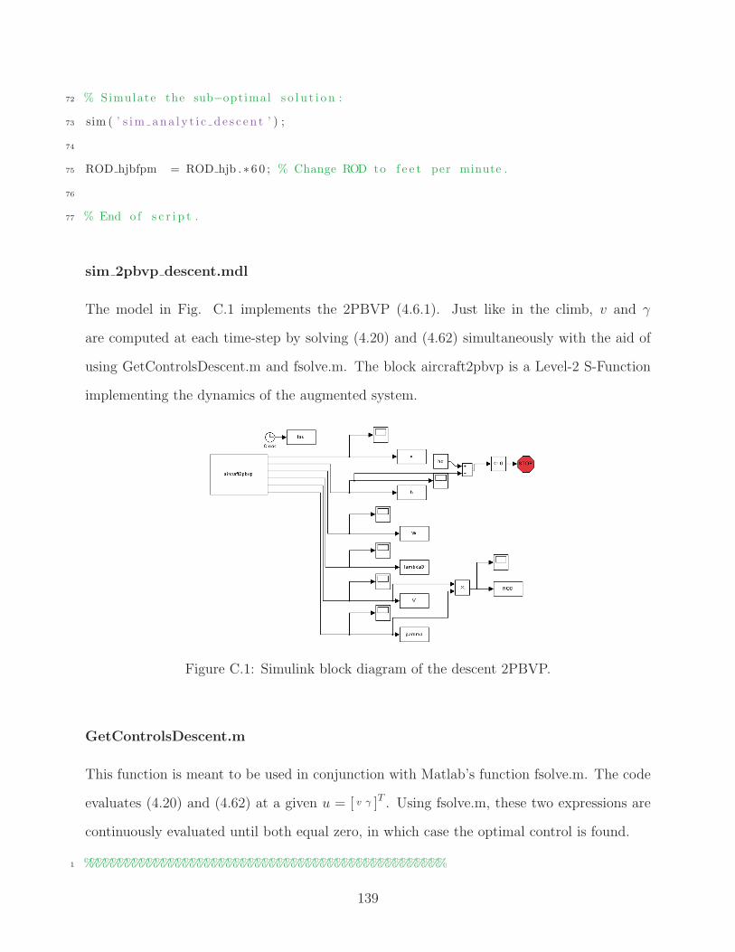
72 % Simulate the sub−optimal s o l u t i o n :
73 sim ( ’ s im ana l y t i c d e s c en t ’ ) ;
74
75 ROD hjbfpm = ROD hjb . ∗ 6 0 ; % Change ROD to f e e t per minute .
76
77 % End o f s c r i p t .
sim 2pbvp descent.mdl
The model in Fig. C.1 implements the 2PBVP (4.6.1). Just like in the climb, v and γ
are computed at each time-step by solving (4.20) and (4.62) simultaneously with the aid of
using GetControlsDescent.m and fsolve.m. The block aircraft2pbvp is a Level-2 S-Function
implementing the dynamics of the augmented system.
Figure C.1: Simulink block diagram of the descent 2PBVP.
GetControlsDescent.m
This function is meant to be used in conjunction with Matlab’s function fsolve.m. The code
evaluates (4.20) and (4.62) at a given u = [ v γ ]T . Using fsolve.m, these two expressions are
continuously evaluated until both equal zero, in which case the optimal control is found.
1 %%%%%%%%%%%%%%%%%%%%%%%%%%%%%%%%%%%%%%%%%%%%%%%%%%
139
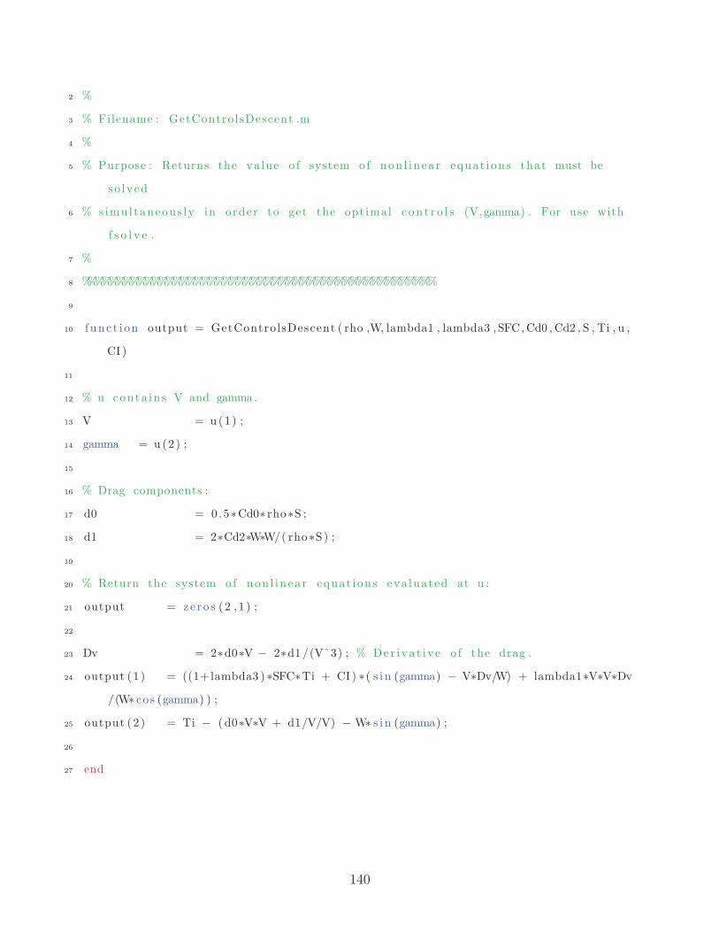
2 %
3 % Filename : GetControlsDescent .m
4 %
5 % Purpose : Returns the value o f system o f non l i n ea r equat ions that must be
so lved
6 % simul taneous ly in order to get the opt imal c on t r o l s (V,gamma) . For use with
f s o l v e .
7 %
8 %%%%%%%%%%%%%%%%%%%%%%%%%%%%%%%%%%%%%%%%%%%%%%%%%%
9
10 f unc t i on output = GetControlsDescent ( rho ,W, lambda1 , lambda3 ,SFC,Cd0 ,Cd2 , S , Ti , u ,
CI )
11
12 % u conta in s V and gamma.
13 V = u(1) ;
14 gamma = u (2) ;
15
16 % Drag components :
17 d0 = 0.5∗Cd0∗ rho∗S ;
18 d1 = 2∗Cd2∗W∗W/( rho∗S) ;
19
20 % Return the system o f non l i n ea r equat ions eva luated at u :
21 output = ze ro s (2 , 1 ) ;
22
23 Dv = 2∗d0∗V − 2∗d1/(Vˆ3) ; % Der iva t i v e o f the drag .
24 output (1 ) = ((1+lambda3 ) ∗SFC∗Ti + CI ) ∗( s i n (gamma) − V∗Dv/W) + lambda1∗V∗V∗Dv
/(W∗ cos (gamma) ) ;
25 output (2 ) = Ti − ( d0∗V∗V + d1/V/V) − W∗ s i n (gamma) ;
26
27 end
140
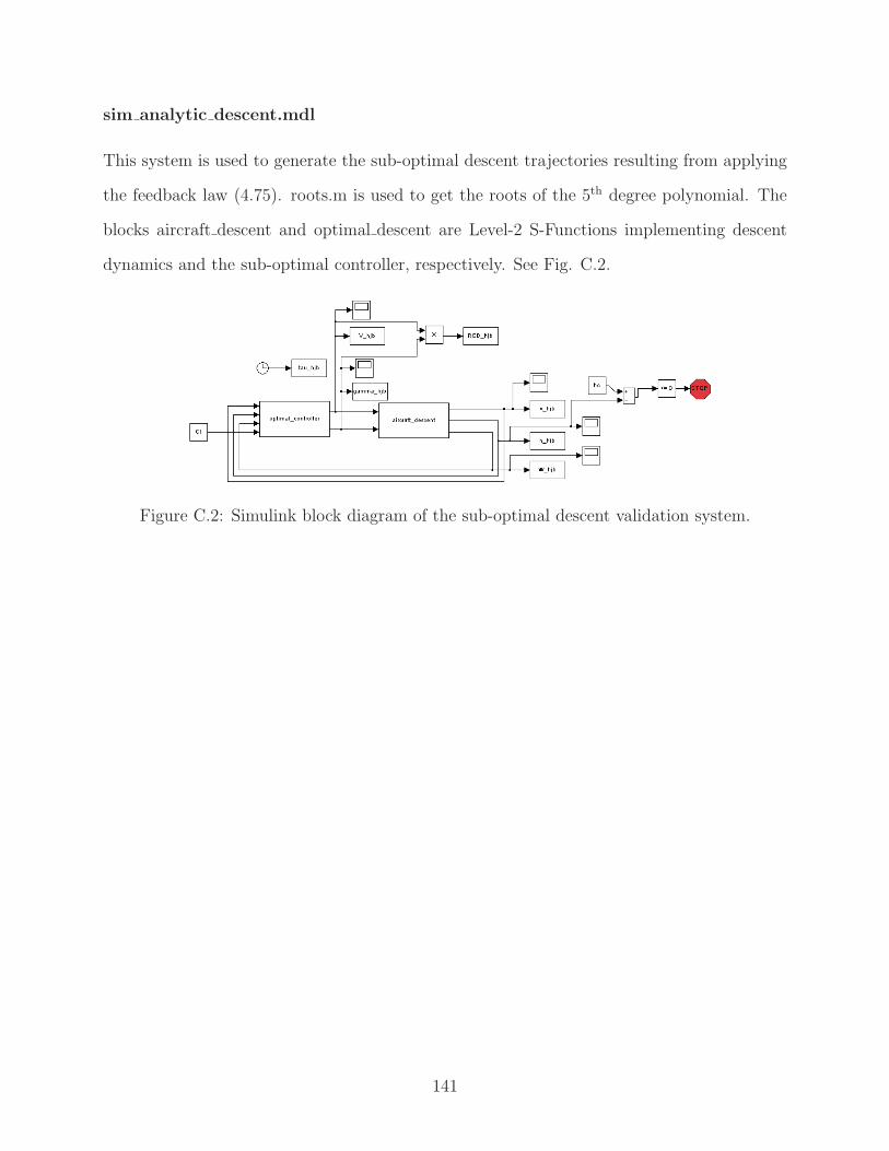
sim analytic descent.mdl
This system is used to generate the sub-optimal descent trajectories resulting from applying
the feedback law (4.75). roots.m is used to get the roots of the 5th degree polynomial. The
blocks aircraft descent and optimal descent are Level-2 S-Functions implementing descent
dynamics and the sub-optimal controller, respectively. See Fig. C.2.
Figure C.2: Simulink block diagram of the sub-optimal descent validation system.
141