An investigation of some theoretical aspects of reversible computing
220
UNIVERSITY OF CALGARY An investigation of some theoretical aspects of reversible computing by Brett Gordon Giles A DISSERTATION SUBMITTED TO THE FACULTY OF GRADUATE STUDIES IN PARTIAL FULFILLMENT OF THE REQUIREMENTS FOR THE DEGREE OF DOCTOR OF PHILOSOPHY DEPARTMENT OF COMPUTER SCIENCE CALGARY, ALBERTA October, 2014 c Brett Gordon Giles 2014
Transcript of An investigation of some theoretical aspects of reversible computing
UNIVERSITY OF CALGARY
An investigation of some theoretical aspects of reversible computing
by
Brett Gordon Giles
A DISSERTATION
SUBMITTED TO THE FACULTY OF GRADUATE STUDIES
IN PARTIAL FULFILLMENT OF THE REQUIREMENTS FOR THE
DEGREE OF DOCTOR OF PHILOSOPHY
DEPARTMENT OF COMPUTER SCIENCE
CALGARY, ALBERTA
October, 2014
c© Brett Gordon Giles 2014

Abstract
The categorical semantics of reversible computing must be a category which combines the
concepts of partiality and the ability to reverse any map in the category. Inverse cate-
gories, restriction categories in which each map is a partial isomorphism, provide exactly
this structure. This thesis explores inverse categories and relates them to both quantum
computing and standard non-reversible computing. The former is achieved by showing that
commutative Frobenius algebras form an inverse category. The latter is by establishing the
equivalence of the category of discrete inverse categories to the category of discrete Cartesian
restriction categories — this is the main result of this thesis. This allows one to transfer the
formulation of computability given by Turing categories onto discrete inverse categories.
i
Acknowledgements
First and foremost, many thanks to my supervisor of the past many, many years, Dr. Robin
Cockett. His indefatigable thirst for mathematical exploration of computer science has been
an inspiration for both my master’s degree and my doctoral studies.
Secondly, thank you to Dr. Peter Selinger, both for his paper on the semantics of quantum
computing which inspired me to write LQPL and the opportunity to work for him at MSRI
in Berkeley for the fall of 2012. His clarity of exposition in research writing remains a target
to which I aspire.
Thank you to Dr. Kristine Bauer and Dr. Peter Høyer for serving on my supervisory
committee, partaking in my qualifying exam and serving on my thesis defence committee. I
always felt your doors were open to me.
Thank you to Dr. Gilad Gour for being my internal examiner.
Thank you to Dr. Bob Coecke for agreeing to be my external examiner.
Many thanks to Dr. Sudarshan Sehgal for encouraging me to return to academia and get
my doctorate.
Thanks to my fellow graduate students (and post-docs) over the years for great conver-
sations, people to hang with while at conferences and critiques of research. Thanks to Craig
Pastro, Xiuzhan Guo, Dana Harrington, Ross Duncan, Jon Grattage, Sean Nichols, Ning
Tang, Brian Redmond, Geoff Cruttwell, Alexander Green, Neil Ross, Jonathan Gallagher,
Chad Nester and Prashant Kumar.
Finally, and most of all, thank you so much to all of my family. My wife, for being with
me for all these years and proof-reading both my master’s and this thesis — learning more
about math than she ever thought she would; my kids, who still remember me; and my
grandkids — who likely don’t remember a time when Grandpa was not in school.
ii

Dedication
To my wife, Marie Gelinas Giles.
iii

Table of Contents
Abstract . . . . . . . . . . . . . . . . . . . . . . . . . . . . . . . . . . . . . . . . . iAcknowledgements . . . . . . . . . . . . . . . . . . . . . . . . . . . . . . . . . . . iiDedication . . . . . . . . . . . . . . . . . . . . . . . . . . . . . . . . . . . . . . . . iiiTable of Contents . . . . . . . . . . . . . . . . . . . . . . . . . . . . . . . . . . . . ivList of Tables . . . . . . . . . . . . . . . . . . . . . . . . . . . . . . . . . . . . . . viList of Figures . . . . . . . . . . . . . . . . . . . . . . . . . . . . . . . . . . . . . . viiList of Symbols . . . . . . . . . . . . . . . . . . . . . . . . . . . . . . . . . . . . . viii1 Introduction . . . . . . . . . . . . . . . . . . . . . . . . . . . . . . . . . . . . 11.1 Summary . . . . . . . . . . . . . . . . . . . . . . . . . . . . . . . . . . . . . 11.2 Background of reversible computation . . . . . . . . . . . . . . . . . . . . . . 11.3 Objectives . . . . . . . . . . . . . . . . . . . . . . . . . . . . . . . . . . . . . 51.4 Outline . . . . . . . . . . . . . . . . . . . . . . . . . . . . . . . . . . . . . . . 72 Introduction to categories . . . . . . . . . . . . . . . . . . . . . . . . . . . . 102.1 Definition of a category . . . . . . . . . . . . . . . . . . . . . . . . . . . . . . 102.2 Properties of maps . . . . . . . . . . . . . . . . . . . . . . . . . . . . . . . . 122.3 Functors and natural transformations . . . . . . . . . . . . . . . . . . . . . . 142.4 Adjoint functors and equivalences . . . . . . . . . . . . . . . . . . . . . . . . 172.5 Enrichment of categories . . . . . . . . . . . . . . . . . . . . . . . . . . . . . 202.6 Examples of categories . . . . . . . . . . . . . . . . . . . . . . . . . . . . . . 202.7 Limits and colimits in categories . . . . . . . . . . . . . . . . . . . . . . . . . 222.8 Symmetric monoidal categories . . . . . . . . . . . . . . . . . . . . . . . . . 253 Restriction categories . . . . . . . . . . . . . . . . . . . . . . . . . . . . . . . 283.1 Definitions . . . . . . . . . . . . . . . . . . . . . . . . . . . . . . . . . . . . . 283.2 Partial order enrichment . . . . . . . . . . . . . . . . . . . . . . . . . . . . . 313.3 Joins . . . . . . . . . . . . . . . . . . . . . . . . . . . . . . . . . . . . . . . . 333.4 Meets . . . . . . . . . . . . . . . . . . . . . . . . . . . . . . . . . . . . . . . 363.5 Partial monics and isomorphisms . . . . . . . . . . . . . . . . . . . . . . . . 393.6 Range categories . . . . . . . . . . . . . . . . . . . . . . . . . . . . . . . . . 403.7 Split restriction categories . . . . . . . . . . . . . . . . . . . . . . . . . . . . 423.8 Partial map categories . . . . . . . . . . . . . . . . . . . . . . . . . . . . . . 453.9 Restriction products and Cartesian restriction categories . . . . . . . . . . . 473.10 Discrete Cartesian restriction categories . . . . . . . . . . . . . . . . . . . . . 484 Inverse categories and products . . . . . . . . . . . . . . . . . . . . . . . . . 554.1 Inverse categories . . . . . . . . . . . . . . . . . . . . . . . . . . . . . . . . . 554.2 Inverse categories with restriction products . . . . . . . . . . . . . . . . . . . 594.3 Inverse products . . . . . . . . . . . . . . . . . . . . . . . . . . . . . . . . . . 60
4.3.1 Inverse product definition . . . . . . . . . . . . . . . . . . . . . . . . 604.3.2 Diagrammatic language . . . . . . . . . . . . . . . . . . . . . . . . . 634.3.3 Properties of discrete inverse categories . . . . . . . . . . . . . . . . . 644.3.4 The inverse subcategory of a discrete Cartesian restriction category . 68
4.4 The “slice” construction on a discrete inverse category . . . . . . . . . . . . 714.4.1 The interpretation of the slice construction in resource theory . . . . 74
iv
5 Constructing a Cartesian restriction category from a discrete inverse category 775.1 The restriction category X . . . . . . . . . . . . . . . . . . . . . . . . . . . . 77
5.1.1 Equivalence classes of maps in X . . . . . . . . . . . . . . . . . . . . 785.1.2 X is a restriction category . . . . . . . . . . . . . . . . . . . . . . . . 805.1.3 X is a discrete Cartesian restriction category . . . . . . . . . . . . . . 86
5.2 Equivalence between the category DInv and the category DCartRest . . . 915.3 Examples of the Cartesian Construction . . . . . . . . . . . . . . . . . . . . 966 Disjointness in inverse categories . . . . . . . . . . . . . . . . . . . . . . . . . 996.1 Coproducts in inverse categories . . . . . . . . . . . . . . . . . . . . . . . . . 99
6.1.1 Inverse categories with restriction coproducts . . . . . . . . . . . . . 1016.2 Disjointness in an inverse category . . . . . . . . . . . . . . . . . . . . . . . . 1026.3 Disjoint joins . . . . . . . . . . . . . . . . . . . . . . . . . . . . . . . . . . . 1097 Disjoint sums . . . . . . . . . . . . . . . . . . . . . . . . . . . . . . . . . . . 1157.1 Disjoint sums . . . . . . . . . . . . . . . . . . . . . . . . . . . . . . . . . . . 1157.2 Disjointness via a tensor . . . . . . . . . . . . . . . . . . . . . . . . . . . . . 1187.3 Disjoint joins via a tensor . . . . . . . . . . . . . . . . . . . . . . . . . . . . 1287.4 Disjoint sums via a disjoint sum tensor . . . . . . . . . . . . . . . . . . . . . 1368 Matrix categories . . . . . . . . . . . . . . . . . . . . . . . . . . . . . . . . . 1398.1 Matrices . . . . . . . . . . . . . . . . . . . . . . . . . . . . . . . . . . . . . . 1398.2 Equivalence between a disjoint sum category and its matrix category . . . . 1469 Distributive inverse categories . . . . . . . . . . . . . . . . . . . . . . . . . . 1529.1 Distributive restriction categories . . . . . . . . . . . . . . . . . . . . . . . . 1529.2 Distributive inverse categories . . . . . . . . . . . . . . . . . . . . . . . . . . 1529.3 Discrete inverse categories with disjoint sums . . . . . . . . . . . . . . . . . . 15710 Commutative Frobenius algebras and inverse categories . . . . . . . . . . . . 16310.1 The category of commutative Frobenius algebras . . . . . . . . . . . . . . . . 163
10.1.1 Dagger categories . . . . . . . . . . . . . . . . . . . . . . . . . . . . . 16310.1.2 Examples of dagger categories . . . . . . . . . . . . . . . . . . . . . . 16610.1.3 Frobenius algebras . . . . . . . . . . . . . . . . . . . . . . . . . . . . 16610.1.4 CFrob(X) is an inverse category . . . . . . . . . . . . . . . . . . . . 169
10.2 Disjointness in CFrob(X) . . . . . . . . . . . . . . . . . . . . . . . . . . . . 17610.3 Disjoint joins in CFrob(X) . . . . . . . . . . . . . . . . . . . . . . . . . . . 17910.4 Disjoint sums in CFrob(X) . . . . . . . . . . . . . . . . . . . . . . . . . . . 18211 Turing categories and PCAs . . . . . . . . . . . . . . . . . . . . . . . . . . . 18611.1 Turing categories . . . . . . . . . . . . . . . . . . . . . . . . . . . . . . . . . 18611.2 Inverse Turing categories . . . . . . . . . . . . . . . . . . . . . . . . . . . . . 19111.3 Partial combinatory algebras . . . . . . . . . . . . . . . . . . . . . . . . . . . 19411.4 Computable functions . . . . . . . . . . . . . . . . . . . . . . . . . . . . . . 19812 Conclusions and future work . . . . . . . . . . . . . . . . . . . . . . . . . . . 20012.1 Future directions . . . . . . . . . . . . . . . . . . . . . . . . . . . . . . . . . 203Bibliography . . . . . . . . . . . . . . . . . . . . . . . . . . . . . . . . . . . . . . 205
v

List of Tables
2.1 Properties of maps in categories . . . . . . . . . . . . . . . . . . . . . . . . . 12
4.1 Two different inverse products on the same category. . . . . . . . . . . . . . 634.2 Structural maps for the tensor in INV(X) . . . . . . . . . . . . . . . . . . . 69
vi

List of Figures and Illustrations
2.1 Pentagon diagram for associativity in an SMC. . . . . . . . . . . . . . . . . . 252.2 Unit diagram and equation in an SMC. . . . . . . . . . . . . . . . . . . . . . 262.3 Symmetry in an SMC. . . . . . . . . . . . . . . . . . . . . . . . . . . . . . . 262.4 Unit symmetry in an SMC. . . . . . . . . . . . . . . . . . . . . . . . . . . . 262.5 Associativity symmetry in an SMC. . . . . . . . . . . . . . . . . . . . . . . . 26
5.1 Equivalence diagram for constructing maps in X. . . . . . . . . . . . . . . . 785.2 Functors between Cartesian restriction categories and inverse categories. . . 96
vii
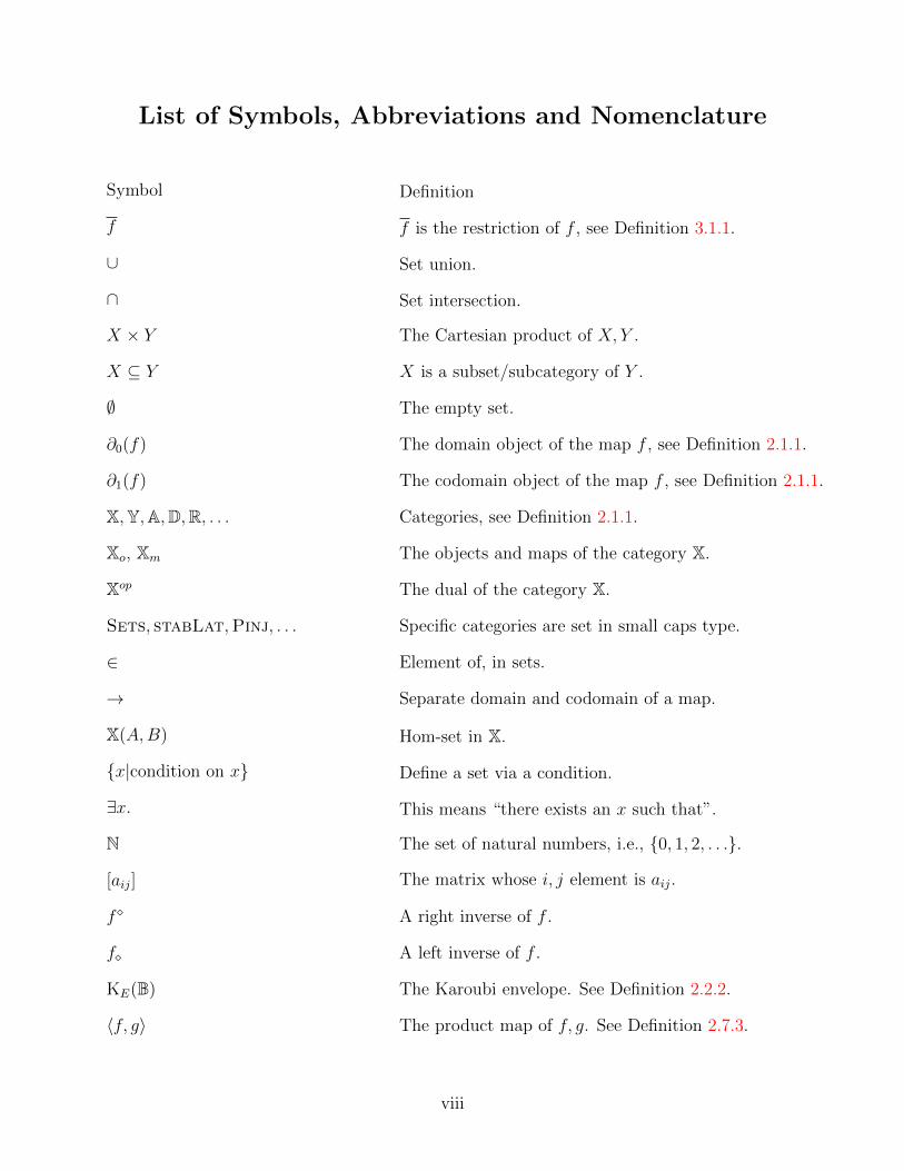
List of Symbols, Abbreviations and Nomenclature
Symbol Definition
f f is the restriction of f , see Definition 3.1.1.
∪ Set union.
∩ Set intersection.
X × Y The Cartesian product of X, Y .
X ⊆ Y X is a subset/subcategory of Y .
∅ The empty set.
∂0(f) The domain object of the map f , see Definition 2.1.1.
∂1(f) The codomain object of the map f , see Definition 2.1.1.
X,Y,A,D,R, . . . Categories, see Definition 2.1.1.
Xo, Xm The objects and maps of the category X.
Xop The dual of the category X.
Sets, stabLat,Pinj, . . . Specific categories are set in small caps type.
∈ Element of, in sets.
→ Separate domain and codomain of a map.
X(A,B) Hom-set in X.
{x|condition on x} Define a set via a condition.
∃x. This means “there exists an x such that”.
N The set of natural numbers, i.e., {0, 1, 2, . . .}.
[aij] The matrix whose i, j element is aij.
f � A right inverse of f .
f� A left inverse of f .
KE(B) The Karoubi envelope. See Definition 2.2.2.
〈f, g〉 The product map of f, g. See Definition 2.7.3.
viii
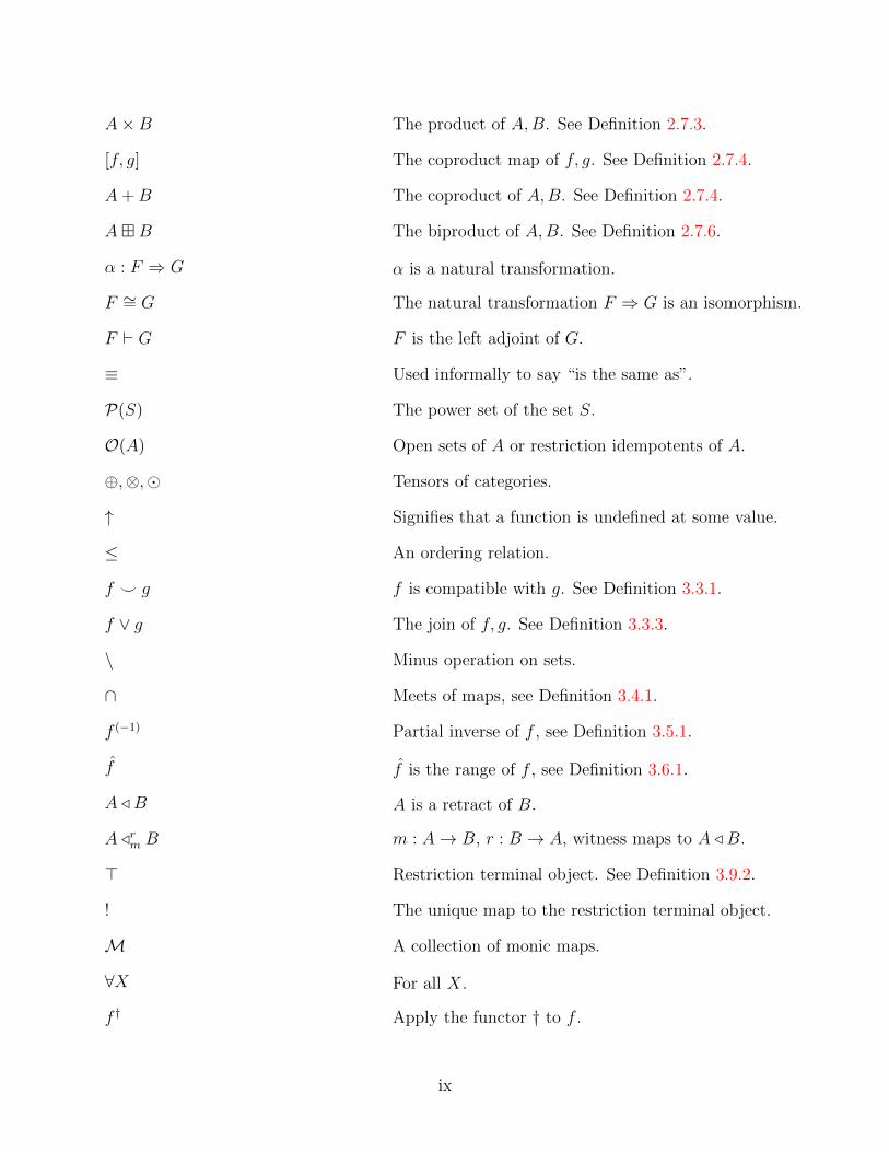
A×B The product of A,B. See Definition 2.7.3.
[f, g] The coproduct map of f, g. See Definition 2.7.4.
A+B The coproduct of A,B. See Definition 2.7.4.
A�B The biproduct of A,B. See Definition 2.7.6.
α : F ⇒ G α is a natural transformation.
F ∼= G The natural transformation F ⇒ G is an isomorphism.
F ` G F is the left adjoint of G.
≡ Used informally to say “is the same as”.
P(S) The power set of the set S.
O(A) Open sets of A or restriction idempotents of A.
⊕,⊗,� Tensors of categories.
↑ Signifies that a function is undefined at some value.
≤ An ordering relation.
f ^ g f is compatible with g. See Definition 3.3.1.
f ∨ g The join of f, g. See Definition 3.3.3.
\ Minus operation on sets.
∩ Meets of maps, see Definition 3.4.1.
f (−1) Partial inverse of f , see Definition 3.5.1.
f f is the range of f , see Definition 3.6.1.
A / B A is a retract of B.
A /rm B m : A→ B, r : B → A, witness maps to A / B.
> Restriction terminal object. See Definition 3.9.2.
! The unique map to the restriction terminal object.
M A collection of monic maps.
∀X For all X.
f † Apply the functor † to f .
ix
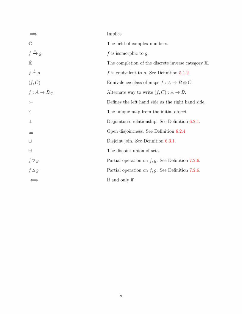
=⇒ Implies.
C The field of complex numbers.
f∼=−→ g f is isomorphic to g.
X The completion of the discrete inverse category X.
fh' g f is equivalent to g. See Definition 5.1.2.
(f, C) Equivalence class of maps f : A→ B ⊗ C.
f : A→ B|C Alternate way to write (f, C) : A→ B.
:= Defines the left hand side as the right hand side.
? The unique map from the initial object.
⊥ Disjointness relationship. See Definition 6.2.1.
⊥ Open disjointness. See Definition 6.2.4.
t Disjoint join. See Definition 6.3.1.
] The disjoint union of sets.
f O g Partial operation on f, g. See Definition 7.2.6.
f M g Partial operation on f, g. See Definition 7.2.6.
⇐⇒ If and only if.
x
Chapter 1
Introduction
1.1 Summary
A “quantum” setting has a duality given by the “dagger” of dagger categories [1, 64]. On
the other hand, classical computation is fundamentally asymmetric and has no duality. In
passing from a quantum setting to a more classical setting, one may want to keep this duality
for as long as possible and, thus, consider the intermediate step of passing to “reversible”
computation — which has an obvious self-duality given by the ability to reverse the compu-
tation. It is reasonable to wonder whether one can then pass from a reversible setting to a
classical setting quite independently from the underlying quantum setting. Such an abstract
passage would allow a direct translation into the reversible world of the classical notions of
computation, as an example.
Of course, from a quantum setting, it is already possible to pass directly to a classical
setting by taking the homomorphisms between special coalgebras, where “special” means
the coalgebra must be the algebra part of a separable Frobenius algebra. That the coalgebra
should be special in this manner may be justified by regarding this as a two step process
through reversible computation. However, this leaves some gaps: How does one pass, in
general, between a quantum setting to a reversible setting and how does one obtain a classical
setting from a reversible setting? This thesis answers these questions.
1.2 Background of reversible computation
In 1961, Landauer [44] examined logically irreversible computing and showed that it must
dissipate energy, i.e., produce heat at a specified minimal level. This is due to applying a
1

physically irreversible operation to non-random data, leading to an entropy increase in the
computer. While there are various objections to the connection between logical irreversibility
and heat generation, summarized by Bennett [7], this led to an interest in exploring reversible
computation, because of its potential energy advantage.
Bennett, in 1973, [6] showed how one can simulate an ordinary Turing machine using a
reversible Turing machine, based on reversible transitions. Since approximately 2000, there
has been an increased interest in reversible computing. Active areas include research in
database theory, specifically the view-update problem [10, 30, 40] and quantum computing.
Recall that quantum computation may be modelled by unitary transforms [56], each of which
is reversible, followed by an irreversible measurement.
An important aspect of the treatment of reversible computing is the consideration of
the partiality inherit in programs, as it is possible for programs to never provide a result
for certain inputs. Some of the reversibility research referenced in this section considers
partiality to a greater or lesser degree, but none of them treat it as a central consideration.
Partiality was shown to have a purely algebraic description by Cockett and Lack in
[21–23]. They introduce a restriction operator on maps, which associated to a map a partial
identity on its domain. In [21], they recalled the concept of inverse category, a category
equipped with a restriction operator in which all the maps have partial inverses, i.e., are
reversible. Categories with restriction operators are presented in Chapter 3, while inverse
categories are explored in Chapter 4.
The semantics of reversible computing has been explored in a variety of ways, including
by developing various reversible programming languages. An early example of this is Janus
[48], an imperative language written as an experiment in producing a language that did
not erase information. However, it does not appear that any semantic underpinnings were
developed for this language. Additionally, there are special purpose reversible languages,
such as biXid [42], a language developed explicitly to transform XML [11] from one data
2
schema to another. The main novelty of biXid is that a single program targets two schemas
and will transform in either direction.
Zuliani [68] provides a reversible language with an operational semantics. He examines
logical reversibility via comparing the probabilistic Guarded Command Language (pGCL)
[53] to the quantum Guarded Command Language (qGCL) [61]. Zuliani provides a method
for transforming an irreversible pGCL program into a reversible one. This is accomplished
via an application of expectation transform semantics to the pGCL program. Interestingly,
in this work, partial programs are specifically excluded from the definition of reversible pro-
grams. The initial definition of a reversible program is strict, i.e., the program is equivalent
to skip which does nothing. To alleviate this and allow us to extract the output, Zuliani
follows the example of [6] and modifies the result so that the output is copied before reversing
the rest of the program.
In addition, a number of reversible calculi have been developed. Danos and Krivine [28]
extend CCS (Calculus for Communicating Systems) [51, 52] to produce RCCS, which adds
reversible transitions to CCS. This is done by adding a syntax for backtracking, together
with a labelling which guides the backtracking. The interesting aspect of this work is the
applicability to concurrent programs.
Phillips and Uladowski [59] take a different approach to creating a reversible CCS from
that of Danos and Krivine. Rather, their stated goal is to use a structural approach, in-
spired by [2]. The paper is only an initial step in this process, primarily explaining how to
turn dynamic rules (such as choice operators) into a series of static rules that keep all the
information of the input. For example (from the paper), in standard CCS, we have the rule
X → X ′
X + Y → X ′.
To preserve information and allow reversibility, this is replaced with
X → X ′
X + Y → X ′ + Y .
3

In [2], Abramsky considers linear logic as his computational model. This is done by
producing a Linear Combinatory Algebra [4] from the involutive reversible maps over a
term algebra and showing these are bi-orthogonal automata. (An automata is considered
orthogonal if it is non-ambiguous and left-linear. It is bi-orthogonal when both the automata
and its converse are both orthogonal). While the paper does use reversible term rewritings
as the basis for computation, its emphasis is on how one can derive a linear combinatory
algebra. Linear combinatory algebras are themselves not reversible systems.
In [54] and [55], Mu, Hu and Takeichi introduce the language Inv, a language that is
composed only of partial injective functions. The language has an operational semantics
based on determinate relations and converses. They provide a variety of examples of the
language, including translations from XML to HTML and simple functions such as wrap,
which wraps its argument into a list. They continue by describing how non-injective functions
may be converted to injective ones in Inv via the addition of logging. In fact, they use this
logging to argue the language is equivalent in terms of power to the reversible Turing machine
of [6].
Some of the ideas of [54, 55] are closely related to the theory developed in this thesis.
For example, given two functions f, g of Inv, constructing their union, f ∪ g requires that
both dom f ∩ dom g = φ and range f ∩ range g = φ. This is an example of a disjoint join as
introduced in Section 6.3.
In [60], Di Pierro, Hankin and Wiklicky consider groupoids as their mathematical model
for reversible computations. This leads them to develop rCL, reversible combinatory logic.
This logic consists of a pair of terms, 〈M |H〉, where M is a term of standard combinatory
logic and H is a history, with a specified syntax. In standard combinatory logic, the k
term is irreversible in that it erases its second argument. In rCL, application of the k term
copies the second argument into the history, preserving reversibility. Groupoids are a specific
example of inverse categories, which are total.
4

A recent reversible language is Theseus, [39], by Sabry and James. Theseus is a functional
language which compiles to a graphical language [37, 38] for reversible computation, based
on isomorphisms of finite sums and products of types. Their chosen isomorphisms include
commutativity and associativity for sums and products, units for product and distributivity
of product over sums. The basic graphical language is extended with recursive types and
looping operators and therefore introduces partiality due to the possibility of non-terminating
loops. Their abstract model for this language is a dagger symmetric traced bimonoidal
category [64].
Additionally, there are a number of quantum programming languages which, as noted,
included reversible operations. Our primary example is LQPL [31], a compiled language
based on the semantics of [62]. The language includes a variety of reversible operations
(unitary transforms) as primitives, a linear type system and an operational semantics. More
recently Quipper [32,33], which focuses on methods to handle very large circuits, is a quantum
language embedded in Haskell [58]. Quipper uses quantum and classical circuits as an
underlying model. An interesting aspect of reversibility in Quipper is the inclusion of an
operator to compute the reverse of a given circuit.
In much of the research on reversibility, specific conditions are placed on some aspect
of the computational model or reversible language to ensure “programs” in this model are
reversible. The variety of models and languages obscures the fundamental commonality of
reversibility. By basing the theory of this thesis on inverse categories, our treatment clarifies
the relationship between these various approaches.
1.3 Objectives
This thesis proposes a categorical semantics for reversible computing. Based upon the review
of current research as noted in Section 1.2, reversibility still lacks a unifying semantic model.
Standard computability has Cartesian closed categories [5] and Turing categories [18], while
5
quantum computing has had much success with dagger compact closed categories [1,63,64].
We present inverse categories as an abstract semantics for partial reversible computation.
Inverse categories admit product-like and coproduct-like structures, respectively called in-
verse product and disjoint sum. Inverse categories with an inverse product are called discrete
inverse categories. The name discrete is derived from topological spaces, where ∆ has an
inverse only when the topological space has the discrete topology. Similarly, when ∆ in a
Cartesian restriction category has an inverse, it will be called a discrete Cartesian restriction
category. Section 5.1 shows how the “Cartesian Completion” of a discrete inverse category
can be constructed. This enables us to create a discrete Cartesian restriction category from a
discrete inverse category. It is then shown that we have an equivalence between the category
of discrete inverse categories and the category of discrete Cartesian restriction categories.
The next step is to show how to add a disjoint sum to an inverse category and how the
Cartesian Completion results in a distributive restriction category when one starts with a
distributive inverse category.
An example of a discrete inverse category with disjoint sums is provided by the commuta-
tive Frobenius algebras in any additive symmetric monoidal category. As Frobenius algebras
are related to bases in finite dimensional Hilbert spaces [27], this provides a connection
between inverse categories and quantum computing.
Finally, we develop the structure of inverse Turing categories and inverse partial combi-
natory algebras, directly based on Turing category and partial combinatory algebras from
[18, 20], using the main result of this thesis. This places the connection between reversible
and irreversible computing on a more abstract footing.
While the thesis does cover many important aspects of reversible computing, there are
interesting areas related to reversible computing that are not within the scope of this thesis.
The thesis does not, in general, consider resource usage or complexity classes. For ex-
ample, although we do mention Turing machines in the introduction, we do not develop
6
this further. In particular the thesis does not consider whether the Cartesian Completion
preserves a given complexity of programs when applied to an inverse category whose maps
are programs. The reader wishing to relate resource theory and the work in this thesis
could use the recent work by Coecke, Fritz and Spekkens [25], which defines a resource the-
ory as a symmetric monoidal category, as a starting point. We do look at this briefly in
SubSection 4.4.1.
Additionally, the thesis does not address the creation or invention of specific algorithms.
For example, in the quantum world, finding the “right” set of invertible transforms to produce
the desired answer is a significant problem [56].
1.4 Outline
We assume a knowledge of basic algebra including definitions and properties of groups, rings,
fields, vector spaces and matrices. The reader may consult [45] if further details are needed.
Chapter 2 introduces the various categorical concepts that will be used throughout this
thesis.
Chapter 3 describes restriction categories, an algebraic formulation of partiality in cat-
egories. We discuss joins, meets and ranges in restriction categories and their relation to
partial map categories. We describe products in restriction categories, and define discrete
Cartesian restriction categories, which will be important to the thesis. Various examples of
restriction categories are given.
Chapter 4 introduces inverse categories and provides examples of them. We show that
inverse categories with a restriction product collapse to a restriction preorder, that is, a
restriction category in which all parallel maps agree wherever they are both defined. Then,
Section 4.3 introduces the concept of inverse products and explores the properties of the in-
verse product. Inverse categories with inverse products are called discrete inverse categories.
Chapter 5 then presents the “Cartesian Completion” — a construction of a discrete
7

Cartesian restriction category from a discrete inverse category. Subsection 5.1.1 presents
the details of the equivalence relation on maps of a discrete inverse category needed in the
construction, while Section 5.1 contains the proof that the construction gives a Cartesian
restriction category. Section 5.2 culminates in Theorem 5.2.6 giving an equivalence between
the category of discrete inverse categories and the category of discrete Cartesian restriction
categories. Note this is not a 2-equivalence of categories. We provide some simple examples.
Chapter 6 begins the exploration of how to add a coproduct-like construction to inverse
categories. Paralleling the previous chapter, we show the existence of a restriction coproduct
implies that an inverse category must be a preorder, i.e., that all parallel maps are equal.
Section 6.2 defines a disjointness relation in an inverse category. We show that disjointness
may be defined on all maps or equivalently only on the restriction idempotents of the inverse
category. This allows us to define the disjoint join in Section 6.3.
Chapter 7 introduces the disjoint sum, an object in an inverse category with a disjoint
join, which behaves like a coproduct. The disjoint sum has injection maps which are subject
to certain conditions. When an inverse category has all disjoint sums, it is possible to define
a symmetric monoidal tensor based on the disjoint sum. The remainder of the chapter
explores what constraints on a tensor will allow the creation of a disjoint sum. We define
a disjoint sum tensor, a symmetric monoidal tensor in the inverse category with specific
additional constraints. A disjoint sum tensor allows us to define both a disjointness relation
and a disjoint join based on the tensor. Disjoint sum tensors do produce disjoint sums and
conversely, the tensor defined by disjoint sums is a disjoint sum tensor.
Chapter 8 introduces a matrix construction on inverse categories with disjoint joins in
order to add disjoint sums. The functor from X to iMat(X) gives us an adjunction between
the category of inverse categories with disjoint joins and the category of inverse categories
with disjoint sums.
In Chapter 9 a distributive inverse category is defined as an inverse category where the
8

inverse product distributes over the disjoint sum. The Cartesian Completion of a distributive
inverse category turns the disjoint sum into a coproduct and, in fact, will create a distributive
restriction category.
Chapter 10 discusses commutative Frobenius algebras. The chapter starts with provid-
ing a background on dagger categories and Frobenius algebras, showing how the latter are
equivalent to bases in a finite dimensional Hilbert space. The category CFrob(X), the cate-
gory of commutative Frobenius algebras in a symmetric monoidal category X, is introduced.
CFrob(X) is shown to be a discrete inverse category. Furthermore, when X is an additive
tensor category with zero maps, CFrob(X) has disjoint sums.
In Chapter 11, Turing categories and partial combinatory algebras are introduced as a
way to formulate computability. The corresponding structures in inverse categories, inverse
Turing categories and inverse partial combinatory algebras, are then investigated. We show
the equivalence of these structures to the ones in discrete Cartesian restriction categories.
Chapter 12 starts with a summary of the contributions of this thesis and concludes with
a short section on potential areas of further exploration.
9

Chapter 2
Introduction to categories
This chapter introduces categories and fixes notation for them. More details for category
theory can be found from, e.g., [5], [19], [49] and [66].
2.1 Definition of a category
A category may be defined in a variety of equivalent ways. As much of our work will involve
the exploration of partial and reversible maps, we choose a definition that highlights the
algebraic nature of these.
Definition 2.1.1. A category A is a directed graph consisting of objects Ao and maps Am.
Each f ∈ Am has two associated objects in Ao, called the domain, ∂0(f), and codomain,
∂1(f). When ∂0(f) is the object X and ∂1(f) is the object Y , we will write f : X → Y . For
f, g ∈ Am, if f : X → Y and g : Y → Z, there is a map called the composite of f and g,
written fg,1 such that fg : X → Z. For any W ∈ Ao there is an identity map 1W : W → W .
Additionally, these two axioms must hold:
[C.1] for f : X → Y, 1Xf = f = f1Y ; (Unit laws)
[C.2] given f : X → Y, g : Y → Z and h : Z → W , then f(gh) = (fg)h. ( Associativity)
For a category A, given objects X, Y ∈ Ao, the set of maps between X and Y is referred
to as the hom-set of A between X and Y and written as A(X, Y ).
Throughout this thesis, we will be working with small categories, that is, those categories
whose collection of maps and collection of objects is, in fact, a set. We will give categories
1Note that composition is written in diagrammatic order throughout this thesis.
10
of “all” sets as an example, and the reader can take that to mean all our sets are very small
and all belong to a some sufficiently large set, U .
We give a few examples of categories:
Example 2.1.2. We set 1 to be the category consisting of a single object A and the identity
arrow 1 : A→ A. This is obviously a category, with 1o = A and ∂0(1) = ∂1(1) = A.
There is also the category 2:
Af //1A 88 B 1Bgg
where f is the only non-identity arrow.
Example 2.1.3 (Preorders are categories). Take any partially ordered set (P,≤) and define
f : a→ b for a, b ∈ P if and only if a ≤ b. This is a category as we always have:
(i) a ≤ a (Identity);
(ii) a ≤ b and b ≤ c implies a ≤ c (Composition).
Note that we have at most one map between any two objects in P , hence [C.1] and [C.2]
are immediately satisfied.
Example 2.1.4 (Dual Category). Given a category B, we may form the dual of B, written
Bop as the following category:
Objects: The objects of B;
Maps: f op : B → A in Bop when f : A→ B in B;
Identity: The identity maps of B;
Composition: If fg = h in B, gopf op = hop.
Note the format of the previous example, where we list the four basic requirements of a
category. This is typically how we will present categories in this thesis. Depending upon the
complexity of the definition, we may add further proof that it meets [C.1] and [C.2].
11

The previous example is an important one, as we will often speak of dualizing a notion, or
that concept “x” is the dual of concept “y”. This means that when “y” holds in a category
B, the “x” holds in Bop.
2.2 Properties of maps
Many useful properties of maps are generalizations of notions used for sets and functions. We
present a few of these in Table 2.1, together with their categorical definition. Throughout
Table 2.1, e, f, g are maps in a category C with e : A→ A and f, g : A→ B.
Sets CategoricalProperty
Definition
Injective Monic f is monic whenever hf = kf means that h = k.
Surjective Epic The dual notion to monic, g is epic whenever gh = gkmeans that h = k. A map that is both monic andepic is called bijic.
Left Inverse Section f is a section when there is a map f � such that ff � =1A. f is also referred to as the left inverse of f �.
Right Inverse Retraction f is a retraction when there is a map f� such thatf�f = 1B. f is also referred to as the right inverse off�. A map that is both a section and a retraction iscalled an isomorphism.
Idempotent Idempotent An endomorphism e is idempotent whenever ee = e.
Table 2.1: Properties of maps in categories
There are number of basic properties of maps enumerated in Table 2.1.
Lemma 2.2.1. In a category B,
(i) If f, g are monic, then fg is monic.
(ii) If fg is monic, then f is monic.
12
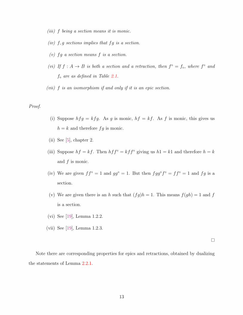
(iii) f being a section means it is monic.
(iv) f, g sections implies that fg is a section.
(v) fg a section means f is a section.
(vi) If f : A → B is both a section and a retraction, then f � = f�, where f � and
f� are as defined in Table 2.1.
(vii) f is an isomorphism if and only if it is an epic section.
Proof.
(i) Suppose hfg = kfg. As g is monic, hf = kf . As f is monic, this gives us
h = k and therefore fg is monic.
(ii) See [5], chapter 2.
(iii) Suppose hf = kf . Then hff � = kff � giving us h1 = k1 and therefore h = k
and f is monic.
(iv) We are given ff � = 1 and gg� = 1. But then fgg�f � = ff � = 1 and fg is a
section.
(v) We are given there is an h such that (fg)h = 1. This means f(gh) = 1 and f
is a section.
(vi) See [19], Lemma 1.2.2.
(vii) See [19], Lemma 1.2.3.
Note there are corresponding properties for epics and retractions, obtained by dualizing
the statements of Lemma 2.2.1.
13

Suppose f : A → B is a retraction with left inverse f� : B → A. Note that ff� is
idempotent as ff�ff� = f1Bf� = ff�. If we are given an idempotent e, we say e is split if
there is a retraction f with e = ff�.
In general, not all idempotents in a category will split. The following construction allows
us to create a category based on the original one, in which all idempotents do split.
Definition 2.2.2. Given a category B and a set of idempotents E of B, we may create the
category of B split over the idempotents E. This is normally written as KE(B), and defined
as:
Objects: (A, e), where A is an object of B, e : A→ A and e ∈ E.
Maps: fd,e : (A, d)→ (B, e) is given by f : A→ B in B, where f = dfe.
Identity: The map ee,e for (A, e).
Composition: Inherited from B.
When E is the set of all idempotents in B, we write K(B).
This is the standard idempotent splitting construction, variously known as the Karoubi
envelope (whence the notation) or Cauchy completion.
2.3 Functors and natural transformations
Definition 2.3.1. A map F : X → Y between categories, as in Definition 2.1.1, is called a
functor, provided it satisfies the following:
[F.1] F (∂0(f)) = ∂0(F (f)) and F (∂1(f)) = ∂1(F (f));
[F.2] F (fg) = F (f)F (g).
Lemma 2.3.2. Categories and functors form a category Cat.
Proof.
14

Objects: Categories.
Maps: Functors.
Identity: The identity functor which takes an object to the same object and a map to the
same map.
Composition: Given F : A → B, G : B → D, define the functor FG : A → D such that
FG(x) = G(F (x)). This is clearly associative.
Note Cat is often regarded as a large category, as its collection of objects is not a set.
A functor F : B→ D induces a map between hom-sets in B and hom-sets in D. For each
object A,B in B we have the map:
FAB : B(A,B)→ D(F (A), F (B)).
Definition 2.3.3. A functor F : X→ Y is full when for each pair of objects A,B in X, and
map g : FA→ FB in Y, there is a map f : A→ B in X such that Ff = g.
Definition 2.3.4. A functor F : X→ Y is faithful when for parallel maps f, f ′, if Ff = Ff ′
then f = f ′.
We may also consider the notion of containment between categories:
Definition 2.3.5. Given the categories B and D, we say that B is a subcategory of D when
each object of B is an object of D and when each map of B is a map of D.
When B is a subcategory of D, the functor J : B → D which takes each object to itself
in D and each map to itself in D is called the inclusion functor. When J is a full functor, we
say B is a full subcategory of D.
We now have the machinery to discuss the relationship between a category B and its
splitting K(B):
15
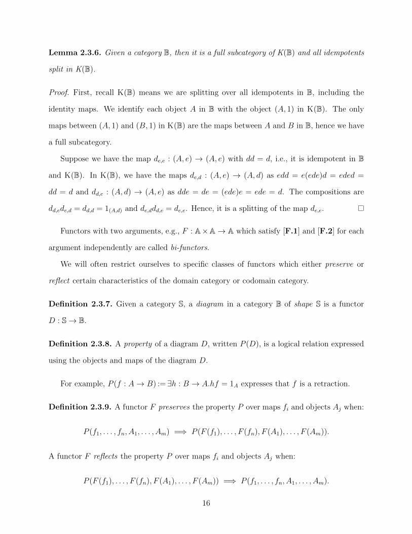
Lemma 2.3.6. Given a category B, then it is a full subcategory of K(B) and all idempotents
split in K(B).
Proof. First, recall K(B) means we are splitting over all idempotents in B, including the
identity maps. We identify each object A in B with the object (A, 1) in K(B). The only
maps between (A, 1) and (B, 1) in K(B) are the maps between A and B in B, hence we have
a full subcategory.
Suppose we have the map de,e : (A, e) → (A, e) with dd = d, i.e., it is idempotent in B
and K(B). In K(B), we have the maps de,d : (A, e) → (A, d) as edd = e(ede)d = eded =
dd = d and dd,e : (A, d) → (A, e) as dde = de = (ede)e = ede = d. The compositions are
dd,ede,d = dd,d = 1(A,d) and de,ddd,e = de,e. Hence, it is a splitting of the map de,e.
Functors with two arguments, e.g., F : A×A→ A which satisfy [F.1] and [F.2] for each
argument independently are called bi-functors.
We will often restrict ourselves to specific classes of functors which either preserve or
reflect certain characteristics of the domain category or codomain category.
Definition 2.3.7. Given a category S, a diagram in a category B of shape S is a functor
D : S→ B.
Definition 2.3.8. A property of a diagram D, written P (D), is a logical relation expressed
using the objects and maps of the diagram D.
For example, P (f : A→ B) :=∃h : B → A.hf = 1A expresses that f is a retraction.
Definition 2.3.9. A functor F preserves the property P over maps fi and objects Aj when:
P (f1, . . . , fn, A1, . . . , Am) =⇒ P (F (f1), . . . , F (fn), F (A1), . . . , F (Am)).
A functor F reflects the property P over maps fi and objects Aj when:
P (F (f1), . . . , F (fn), F (A1), . . . , F (Am)) =⇒ P (f1, . . . , fn, A1, . . . , Am).
16

For example, all functors preserve the properties of being an idempotent or a retraction
or section, but in general, not the property of being monic.
Definition 2.3.10. Given functors F,G : X→ Y, a natural transformation α : F ⇒ G is a
collection of maps in Y, αX : F (X) → G(X), indexed by the objects of X such that for all
f : X1 → X2 in X the following diagram in Y commutes:
F (X1)F (f) //
αX1
��
F (X2)
αX2
��G(X1)
G(f)// G(X2).
In the case where a natural transformation is a collection of isomorphisms, we write
α : F ∼= G or simply F ∼= G.
2.4 Adjoint functors and equivalences
Referring to Section 2.3, we consider relationships between categories. While two categories
may be isomorphic (i.e. there is an invertible functor between them), category theory nor-
mally considers two alternate relations between categories: Equivalence and adjointness.
Adjointness refers to an adjoint pair of functors. There are various equivalent ways of
defining adjoints and we will approach them using universality.
Definition 2.4.1. Given G : B→ A is a functor and A ∈ A, then an object U in B together
with a map ηA : A → G(U) is a universal pair for the G at A if whenever there is a map
f : A→ G(Y ), there is a unique f# : U → Y such that
AηA //
f $$
G(U)
G(f#)��
G(Y )
is a commutative diagram.
17
Consider what happens when we have the situation above, but the U in B is definable
based on the A ∈ A.
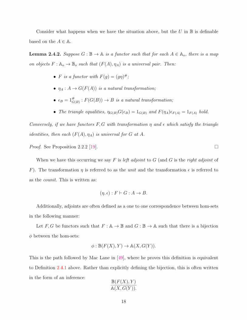
Lemma 2.4.2. Suppose G : B → A is a functor such that for each A ∈ Ao, there is a map
on objects F : Ao → Bo such that (F (A), ηA) is a universal pair. Then:
• F is a functor with F (g) = (gη)#;
• ηA : A→ G(F (A)) is a natural transformation;
• εB = 1#G(B) : F (G(B))→ B is a natural transformation;
• The triangle equalities, ηG(B)G(εB) = 1G(B) and F (ηA)εF (A) = 1F (A) hold.
Conversely, if we have functors F,G with transformation η and ε which satisfy the triangle
identities, then each (F (A), ηA) is universal for G at A.
Proof. See Proposition 2.2.2 [19].
When we have this occurring we say F is left adjoint to G (and G is the right adjoint of
F ). The transformation η is referred to as the unit and the transformation ε is referred to
as the counit. This is written as:
(η, ε) : F ` G : A→ B.
Additionally, adjoints are often defined as a one to one correspondence between hom-sets
in the following manner:
Let F,G be functors such that F : A→ B and G : B→ A such that there is a bijection
φ between the hom-sets:
φ : B(F (X), Y )→ A(X,G(Y )).
This is the path followed by Mac Lane in [49], where he proves this definition is equivalent
to Definition 2.4.1 above. Rather than explicitly defining the bijection, this is often written
in the form of an inference:B(F (X), Y )
A(X,G(Y )).
18
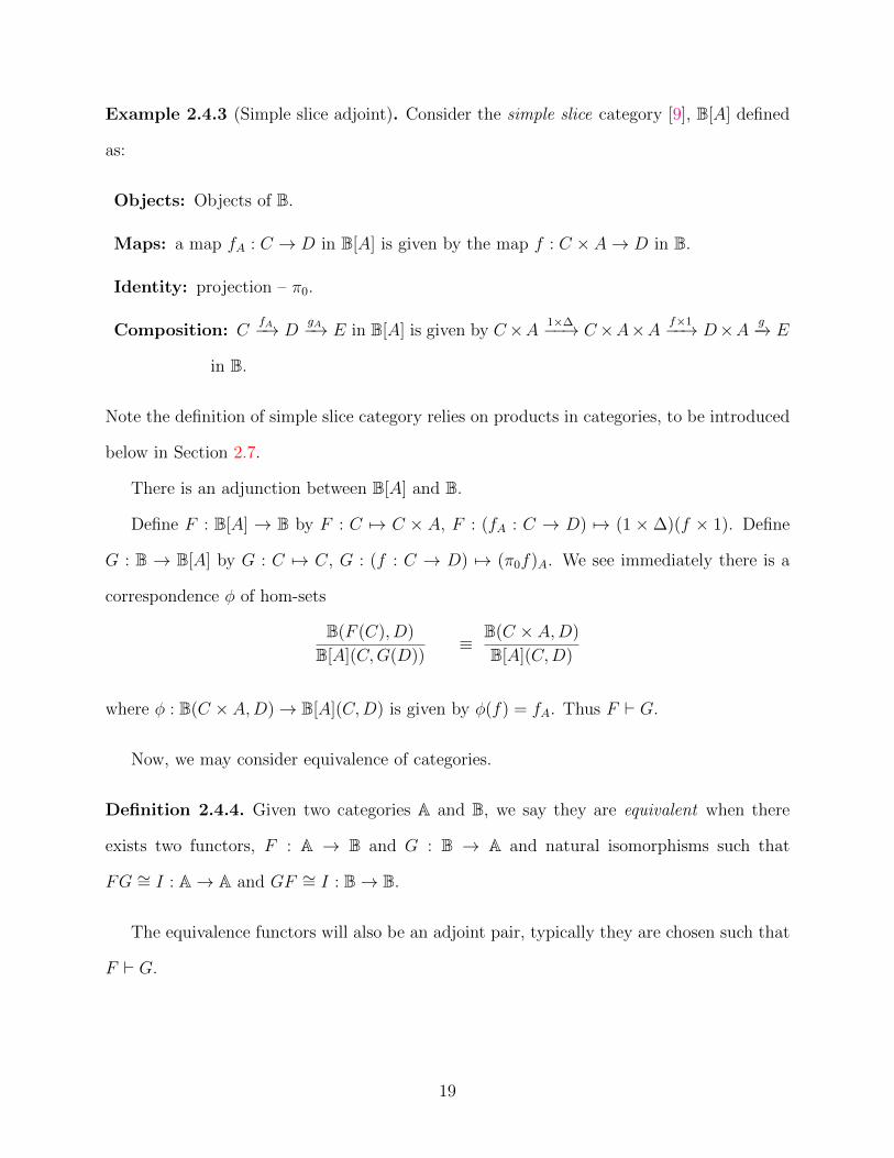
Example 2.4.3 (Simple slice adjoint). Consider the simple slice category [9], B[A] defined
as:
Objects: Objects of B.
Maps: a map fA : C → D in B[A] is given by the map f : C × A→ D in B.
Identity: projection – π0.
Composition: CfA−→ D
gA−→ E in B[A] is given by C×A 1×∆−−→ C×A×A f×1−−→ D×A g−→ E
in B.
Note the definition of simple slice category relies on products in categories, to be introduced
below in Section 2.7.
There is an adjunction between B[A] and B.
Define F : B[A] → B by F : C 7→ C × A, F : (fA : C → D) 7→ (1 ×∆)(f × 1). Define
G : B → B[A] by G : C 7→ C, G : (f : C → D) 7→ (π0f)A. We see immediately there is a
correspondence φ of hom-sets
B(F (C), D)
B[A](C,G(D))≡B(C × A,D)
B[A](C,D)
where φ : B(C × A,D)→ B[A](C,D) is given by φ(f) = fA. Thus F ` G.
Now, we may consider equivalence of categories.
Definition 2.4.4. Given two categories A and B, we say they are equivalent when there
exists two functors, F : A → B and G : B → A and natural isomorphisms such that
FG ∼= I : A→ A and GF ∼= I : B→ B.
The equivalence functors will also be an adjoint pair, typically they are chosen such that
F ` G.
19
2.5 Enrichment of categories
If X is a category, then the maps from A to B in X are denoted X(A,B). If X(A,B) is a set
for all objects in X, we say X is enriched in sets. More generally, categories may be enriched
in any monoidal category. For example a category may be enriched in abelian groups, vector
spaces, posets, categories or commutative monoids.
Specific types of enrichment may force a structure on a category. Examples:
1. If X is enriched in sets of cardinality of 0 or 1, then X is a preorder.
2. If X is enriched in pointed sets with the monoid of smash product, then X has
zero morphisms.
2.6 Examples of categories
In this section, we will offer a few examples of categories.
Example 2.6.1. A group G may be considered as a one-object category G, with object {∗}.
The elements of the group are the maps between {∗}. As G is a group, it has an identity
e and multiplication is associative. In G, the identity map is e, composition is given by the
group multiplication and additionally, each map has an inverse. As G({∗}, {∗}) = G, this
category is enriched in groups.
Four categories whose objects are sets are Rel, Sets, Par, and Pinj:
Example 2.6.2 (Rel). Rel is often of interest in quantum programming language seman-
tics:
Objects: All sets;
Maps: R : X → Y is a relation: R ⊆ X × Y ;
Identity: 1X = {(x, x)|x ∈ X};
20
Composition: RS = {(x, z)| ∃y.(x, y) ∈ R and (y, z) ∈ S}.
Note that Rel is enriched in posets (see Example 2.1.3), via set inclusion. Sets, Par
and Pinj can be viewed as subcategories of Rel, with the same objects, but restricting
the maps allowed — see each example below. Par is also enriched in posets, via the same
inclusion ordering as in Rel.
Example 2.6.3 (Sets). This is the subcategory of Rel which has the same objects (sets)
but only allowing maps which are total functions, i.e., deterministic relations f where for all
x ∈ X, there is a y such that (x, y) ∈ f and if (x, y), (x, y′) ∈ f , then y = y′.
Example 2.6.4 (Par). This is the subcategory of Rel which has the same objects (sets)
but only allowing maps which are partial functions, i.e., deterministic relations f where if
(x, y), (x, y′) ∈ f , then y = y′.
Example 2.6.5 (Pinj). Our final example based on sets is one that will be used throughout
this thesis. The category Pinj consists of the partial injective functions over sets. Similarly
to Sets and Par, it is a subcategory of Rel. The maps f, g (relations in Rel) in Pinj are
subject to two conditions:
(x, y) ∈ f and (x, y′) ∈ f implies y = y′, (2.1)
(x, y) ∈ f and (x′, y) ∈ f implies x = x′. (2.2)
Example 2.6.6 (Top). For a set S, P(S) is the power set of S, that is, the set of all subjects
of S, including the empty set and S itself.
We define O(T ), the open sets of T , as follows:
(i) O(T ) ⊆ P(T );
(ii) T ∈ O(T ) and ∅ ∈ O(T );
(iii) The union of any sets in O(T ) is in O(T );
21
(iv) The intersection of finitely many sets in O(T ) is in O(T ).
A topological space is defined as a pair (T,O(T )) where T is a set and O(T ) are the
open sets of T . Note that we may choose different open sets for T , resulting in different
topological spaces.
Maps between two topological spaces (T,O(T )) and (S,O(S)) consist of a set map f :
T → S such that the inverse image of any open set in S is an open set in T . Such maps are
referred to as continuous functions.
The identity map is always continuous and composition of continuous functions yields
another continuous function, hence setting Topo to be the set of all topological spaces and
Topm to be the continuous maps between them gives us a category.
Our next example shows maps in categories need not always be something normally
thought of as a function or relation.
Example 2.6.7 (Matrix category). Given a rig R (i.e., a ring without negatives, e.g.,
the natural numbers), one may form the category Mat(R). For example, the category of
matrices over natural numbers is:
Objects: N;
Maps: [rij] : n→ m where [rij] is an n×m matrix over N;
Identity: In;
Composition: Matrix multiplication.
2.7 Limits and colimits in categories
We shall review only a few basic limits/colimits in categories, in order to set up notation
and terminology. First we discuss initial and terminal objects.
22
Definition 2.7.1. An initial object in a category B is an object which has exactly one map
to each other object in the category. The dual notion is terminal object. Every object in the
category has exactly one map to the terminal object.
Lemma 2.7.2. Suppose I, J are initial objects in B. Then there is a unique isomorphism
i : I → J .
Proof. First, note that by definition there is only one map from I to I — which must be
the identity map. As I is initial there is a map i : I → J . As J is initial there is a map
j : J → I. But this means ij : I → I = 1 and ji : J → J = 1 and hence i is the unique
isomorphism from I to J .
Dually, we have the corresponding result to Lemma 2.7.2 for terminal objects — they
are also unique up to a unique isomorphism.
In categories, following the terminology in sets, we normally designate the initial object
by 0 and the terminal object by 1. A map from the terminal object to another object in the
category is often referred to as an element or a point.
We now turn to products and coproducts.
Definition 2.7.3. Let A,B be objects of the category B. Then the object A×B is a product
of A and B when:
• There exist maps π0, π1 with π0 : A×B → A, π1 : A×B → B;
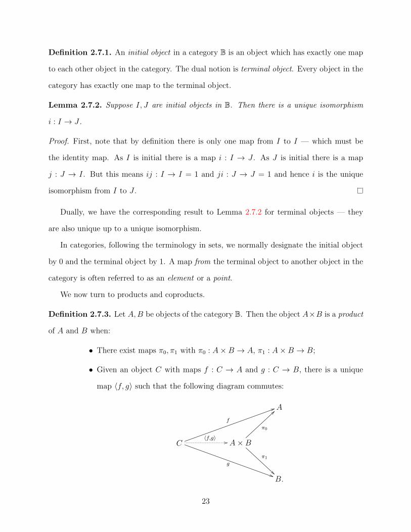
• Given an object C with maps f : C → A and g : C → B, there is a unique
map 〈f, g〉 such that the following diagram commutes:
A
C
f
55
g
))
〈f,g〉 // A×B
π0
>>
π1
B.
23

A coproduct is the dual of a product.
Definition 2.7.4. Let A,B be objects of the category B. Then the object A + B is a
coproduct of A and B when:
• There exist maps q1,q2 with q1 : A→ A+B, q2 : B → A+B;
• Given an object C with maps h : A → C and k : B → C, there is a unique
map [h, k] such that the following diagram commutes:
A
h
))
q1
A+B
[h,k] // C
B.
k
55
q2
>>
It is possible for an object to be both a limit and a colimit at the same time:
Definition 2.7.5. Given a category B, any object that is both a terminal and initial object
is called a zero object. This object is labelled 0.
Note that any category with a zero object has a special map, 0A,B between any two
objects A,B of the category given by: 0A,B : A→ 0→ B.
Definition 2.7.6. In a category B, with products and coproducts, where:
qiπj =
1 i = j
0 i 6= j
and for any two objects, A,B, A×B is the same as A+B, then A×B is referred to as the
biproduct and designated as A � B. A category D is said to have finite biproducts when it
has a zero object 0 and when each pair of objects A,B have a biproduct A�B.
The biproduct is often written as ⊕. This thesis frequently uses ⊕ where it is not a
biproduct, and thus uses � for biproduct instead.
24

A category with finite biproducts is enriched in commutative monoids. If f, g : A → B,
define f + g : A→ B as 〈1A, 1A〉 (f � g) [1B, 1B]. The unit for + is 0A,B. In this thesis, when
discussing a category with finite biproducts, 〈1, 1〉 will be designated by ∆ and [1, 1] by ∇.
2.8 Symmetric monoidal categories
Definition 2.8.1. A symmetric monoidal category [5, 49] D is a category equipped with a
monoid ⊗ (a bi-functor ⊗ : D×D→ D) together with four families of natural isomorphisms:
ulA : I ⊗ A→ A urA : A⊗ I → A
aA,B,C : A⊗ (B ⊗ C)→ (A⊗B)⊗ C cA,B : A⊗B → B ⊗ A.
When the objects are identified in other ways, we often write the maps with the tensor as a
subscript:
ul⊗ : I ⊗ A→ A ur⊗ : A⊗ I → A
a⊗ : (A⊗B)⊗ C → A⊗ (B ⊗ C) c⊗ : A⊗B → B ⊗ A.
These maps must satisfy the coherence diagrams and equations shown in Figures 2.1, 2.2, 2.3,
2.4 and 2.5. The essence of the coherence diagrams is that any diagram composed solely of
the structure isomorphisms will commute. The isomorphisms are referred to as the structure
isomorphisms. I is the unit of the monoid. A symmetric monoidal category is called strict
when each of aA,B,C , urA, ulA and cA,B are identity maps.
A tensor with these properties is also referred to as a symmetric tensor.
A⊗ (B ⊗ (C ⊗D)aA,B,(C⊗D) //
1⊗aB,C,D
��
(A⊗B)⊗ (C ⊗D)a(A⊗B),C,D // ((A⊗B)⊗ C)⊗D
aA,B,C⊗1
��A⊗ ((B ⊗ C)⊗D) aA,(B⊗C),D
// (A⊗ (B ⊗ C))⊗D
Figure 2.1: Pentagon diagram for associativity in an SMC.
25
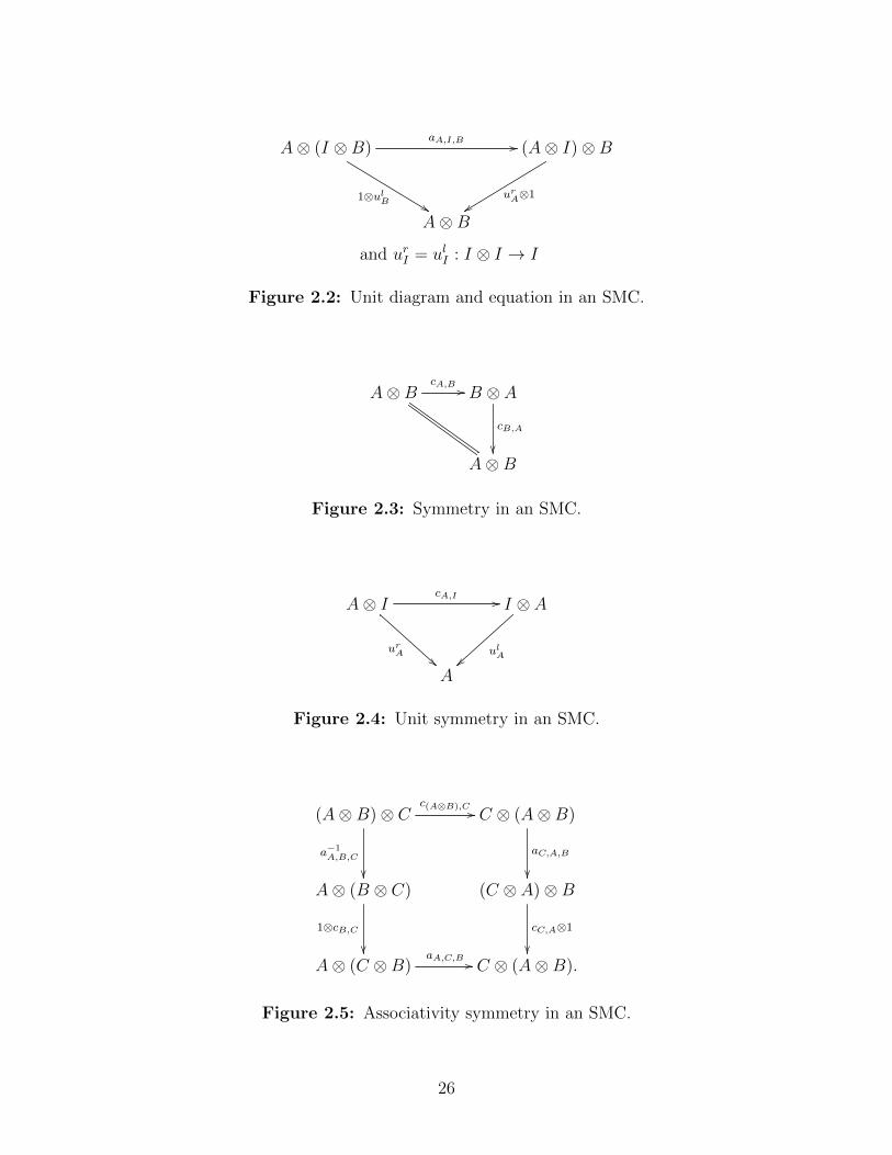
A⊗ (I ⊗B)aA,I,B //
1⊗ulB %%
(A⊗ I)⊗B
urA⊗1yy
A⊗B
and urI = ulI : I ⊗ I → I
Figure 2.2: Unit diagram and equation in an SMC.
A⊗BcA,B // B ⊗ A
cB,A
��A⊗B
Figure 2.3: Symmetry in an SMC.
A⊗ IcA,I //
urA!!
I ⊗ A
ulA}}A
Figure 2.4: Unit symmetry in an SMC.
(A⊗B)⊗ Cc(A⊗B),C //
a−1A,B,C
��
C ⊗ (A⊗B)
aC,A,B
��A⊗ (B ⊗ C)
1⊗cB,C
��
(C ⊗ A)⊗B
cC,A⊗1
��A⊗ (C ⊗B)
aA,C,B // C ⊗ (A⊗B).
Figure 2.5: Associativity symmetry in an SMC.
26
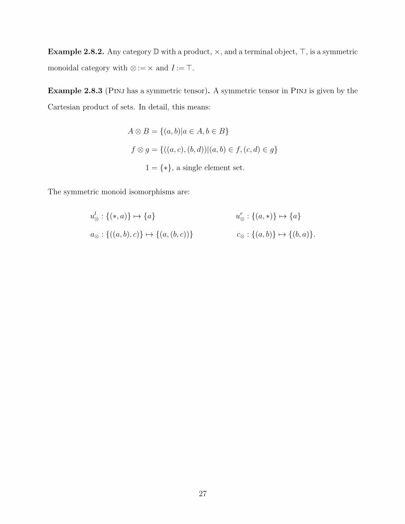
Example 2.8.2. Any category D with a product, ×, and a terminal object, >, is a symmetric
monoidal category with ⊗ :=× and I :=>.
Example 2.8.3 (Pinj has a symmetric tensor). A symmetric tensor in Pinj is given by the
Cartesian product of sets. In detail, this means:
A⊗B = {(a, b)|a ∈ A, b ∈ B}
f ⊗ g = {((a, c), (b, d))|(a, b) ∈ f, (c, d) ∈ g}
1 = {∗}, a single element set.
The symmetric monoid isomorphisms are:
ul⊗ : {(∗, a)} 7→ {a} ur⊗ : {(a, ∗)} 7→ {a}
a⊗ : {((a, b), c)} 7→ {(a, (b, c))} c⊗ : {(a, b)} 7→ {(b, a)}.
27
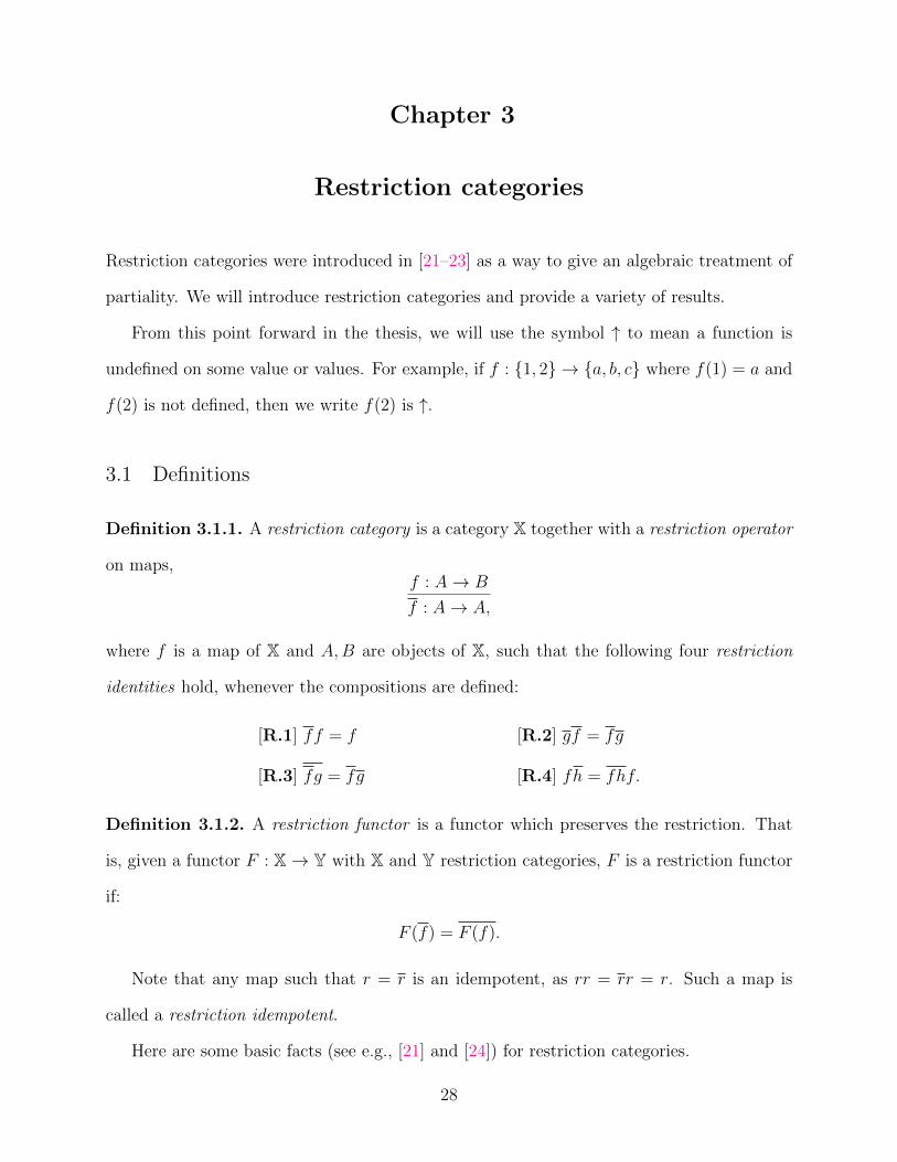
Chapter 3
Restriction categories
Restriction categories were introduced in [21–23] as a way to give an algebraic treatment of
partiality. We will introduce restriction categories and provide a variety of results.
From this point forward in the thesis, we will use the symbol ↑ to mean a function is
undefined on some value or values. For example, if f : {1, 2} → {a, b, c} where f(1) = a and
f(2) is not defined, then we write f(2) is ↑.
3.1 Definitions
Definition 3.1.1. A restriction category is a category X together with a restriction operator
on maps,f : A→ B
f : A→ A,
where f is a map of X and A,B are objects of X, such that the following four restriction
identities hold, whenever the compositions are defined:
[R.1] ff = f [R.2] gf = fg
[R.3] fg = fg [R.4] fh = fhf.
Definition 3.1.2. A restriction functor is a functor which preserves the restriction. That
is, given a functor F : X→ Y with X and Y restriction categories, F is a restriction functor
if:
F (f) = F (f).
Note that any map such that r = r is an idempotent, as rr = rr = r. Such a map is
called a restriction idempotent.
Here are some basic facts (see e.g., [21] and [24]) for restriction categories.
28

Lemma 3.1.3. In a restriction category X,
(i) f is idempotent;
(ii) fg = fg f ;
(iii) fg = fg ;
(iv) f = f ;
(v) f g = f g;
(vi) f monic implies f = 1;
(vii) f = gf =⇒ g f = f .
Proof.
(i) Using [R.3] and then [R.1], we see f f = ff = f .
(ii) Using [R.1], [R.3] and then [R.2], fg = ffg = f fg = fg f .
(iii) Using (ii), [R.3] and then [R.4], fg = fg f = fgf = fg.
(iv) By (iii), f = 1f = 1f = f .
(v) Using [R.3], f g = fg = f g.
(vi) By [R.1] ff = 1f , hence when f is monic, f = 1.
(vii) gf = gf = f .
Note that by Lemma 3.1.3, all maps f are restriction idempotents as f = f .
Definition 3.1.4. A map f : A → B in a restriction category is said to be total when
f = 1A.
Lemma 3.1.5. The total maps in a restriction category form a subcategory Total(X) ⊆ X.
Proof. First, as the identity map 1 is monic, by Lemma 3.1.3, we have 1 = 1 and therefore the
identity map is in Total(X). If f, g are composable maps in Total(X), then f g = fg = f = 1
and hence fg is in Total(X). Therefore, Total(X) is a subcategory of X.
29
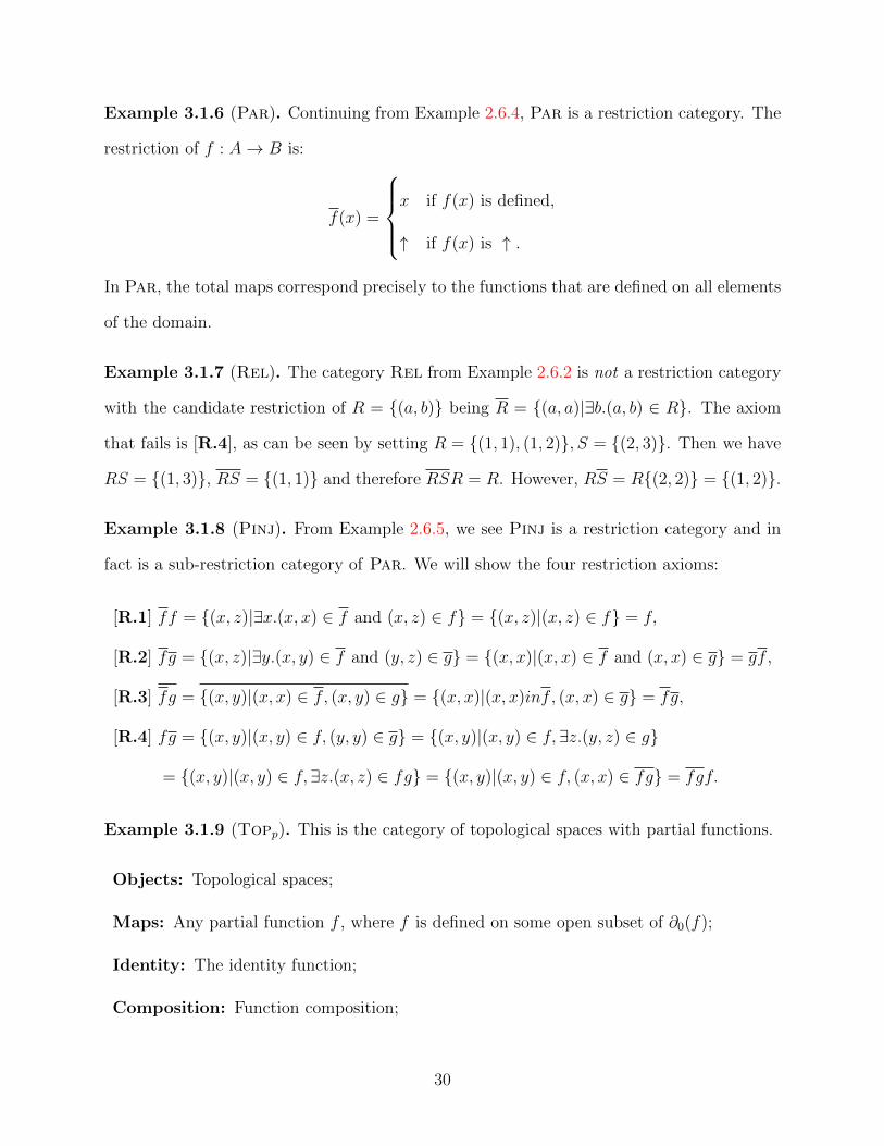
Example 3.1.6 (Par). Continuing from Example 2.6.4, Par is a restriction category. The
restriction of f : A→ B is:
f(x) =
x if f(x) is defined,
↑ if f(x) is ↑ .
In Par, the total maps correspond precisely to the functions that are defined on all elements
of the domain.
Example 3.1.7 (Rel). The category Rel from Example 2.6.2 is not a restriction category
with the candidate restriction of R = {(a, b)} being R = {(a, a)|∃b.(a, b) ∈ R}. The axiom
that fails is [R.4], as can be seen by setting R = {(1, 1), (1, 2)}, S = {(2, 3)}. Then we have
RS = {(1, 3)}, RS = {(1, 1)} and therefore RSR = R. However, RS = R{(2, 2)} = {(1, 2)}.
Example 3.1.8 (Pinj). From Example 2.6.5, we see Pinj is a restriction category and in
fact is a sub-restriction category of Par. We will show the four restriction axioms:
[R.1] ff = {(x, z)|∃x.(x, x) ∈ f and (x, z) ∈ f} = {(x, z)|(x, z) ∈ f} = f,
[R.2] fg = {(x, z)|∃y.(x, y) ∈ f and (y, z) ∈ g} = {(x, x)|(x, x) ∈ f and (x, x) ∈ g} = gf,
[R.3] fg = {(x, y)|(x, x) ∈ f, (x, y) ∈ g} = {(x, x)|(x, x)inf, (x, x) ∈ g} = fg,
[R.4] fg = {(x, y)|(x, y) ∈ f, (y, y) ∈ g} = {(x, y)|(x, y) ∈ f, ∃z.(y, z) ∈ g}
= {(x, y)|(x, y) ∈ f, ∃z.(x, z) ∈ fg} = {(x, y)|(x, y) ∈ f, (x, x) ∈ fg} = fgf.
Example 3.1.9 (Topp). This is the category of topological spaces with partial functions.
Objects: Topological spaces;
Maps: Any partial function f , where f is defined on some open subset of ∂0(f);
Identity: The identity function;
Composition: Function composition;
30

Restriction: The restriction of f : A→ B is:
f(x) =
x if f(x) is defined,
↑ if f(x) is ↑ .
Example 3.1.10. Given S is a symmetric monoidal category, define Copy(S) as the category
whose objects are the objects of S which are commutative comonoids and maps are semigroup
homomorphisms, i.e., maps which do not preserve the unit. As noted in [21], when there is
a counit, ! : B → I where I is the unit of the tensor, this is a restriction category, where the
restriction is given by
Af−→ B
Af−→ A :=A
∆−→ A⊗ A f⊗1−−→ B ⊗ A !⊗1−−→ I ⊗ Aul⊗−→ A.
We may also consider commutative monoids with semigroup morphisms, Copy(S)op.
These will have a corestriction operator, i.e., an operator ( ) on f : A→ B with f : B → B
fulfilling the duals of the restriction axioms.
For example, consider the category of commutative monoids in Ab, the category of
abelian categories. This is the same as (Copy(Abop))op and thus is a corestriction category.
At the same time, this is the category of commutative rings with homomorphisms which do
not preserve the unit.
As another example, consider Frobenius algebras in S (defined below in 10.1.10) with
coalgebra homomorphisms that do not preserve the unit. Again, this category will have a
corestriction.
3.2 Partial order enrichment
We may use the restriction to define a partial order on the hom-sets of a restriction category.
Intuitively, we would think of a map f being less than a map g if f is defined on fewer
elements than g and they agree where they are defined. This can be expressed as:
31

Definition 3.2.1. In a restriction category, for any two parallel maps f, g : A → B, define
f ≤ g if and only if fg = f .
Lemma 3.2.2. Any restriction category X is enriched in a category of partial orders under
the ordering ≤ from Definition 3.2.1 and the following hold:
(i) f ≤ g =⇒ f ≤ g;
(ii) fg ≤ f ;
(iii) f ≤ g =⇒ hf ≤ hg;
(iv) f ≤ g =⇒ fh ≤ gh;
(v) f ≤ g and f = g implies f = g;
(vi) f ≤ 1 ⇐⇒ f = f ;
(vii) f ≤ g, h ≤ k =⇒ fh ≤ gk;
(viii) gf = f implies f ≤ g.
Proof. First, we show the enrichment by showing ≤ is a partial order on X(A,B). With
f, g, h : A → B parallel maps in X, each of the requirements for a partial order is verified
below:
Reflexivity: ff = f and therefore, f ≤ f .
Anti-Symmetry: Given fg = f and gf = g, it follows:
f = ff = fgf = f gf = gff = gf = g.
Transitivity: Given f ≤ g and g ≤ h,
fh = fgh = f gh = fg = f
showing that f ≤ h.
We now show the rest of the claims.
(i) The premise is that fg = f . From this, f g = fg = f , showing f ≤ g.
(ii) Computing, fg f = fg f = fg where the last step is by Lemma 3.1.3(ii).
(iii) hfhg = hfg = hf and therefore hf ≤ hg.
(iv) fg = f , this shows fhgh = fghgh = f ghgh = fgh = fh and therefore fh ≤ gh.
32

(v) g = gg = fg = f .
(vi) As f ≤ 1 means precisely f1 = f .
(vii) fhgk = fh fgk = fhfk = fhk = fh.
(viii) Assuming gf = f , we need to show f g = f . Using [R.2] and then [R.3] we have
f g = gf = gf = f . Hence, f ≤ g.
In a restriction category X, we will use the notation O(A) for the restriction idempotents
of A, an object of X, that is, O(A) = {x : A → A|x = x}. The notation O(A) was chosen
to be suggestive of open sets, as in Topp, see Example 3.1.9.
Lemma 3.2.3. In a restriction category X, O(A) is a meet semi-lattice — a poset with a
top element and binary meets.
Proof. The top of the meet semi-lattice is 1A, under the ordering from Definition 3.2.1. The
meet of any two idempotents is given by their composition.
Let stabLat be the category whose objects are meet semi-lattices and maps are stable
homomorphisms, that is, they preserve the meets but not necessarily the top. From Example
13 in [21], this is a corestriction category, i.e. stabLatop is a restriction category. We see
that the operation O is a functor, O : X→ stabLatop.
3.3 Joins
The restriction operator allows one to algebraically axiomatize the concept of “domain of
definition” for a function. With that axiomatization, we may then consider other questions
about the maps. In this section, we consider when maps are identical on their common
domain of definition. Two maps having this property are called compatible.
33

Definition 3.3.1. Two parallel maps f, g : A→ B in a restriction category are compatible,
written as f ^ g, when fg = gf . A restriction category X is a restriction preorder when all
parallel pairs of maps are compatible.
Example 3.3.2 (Compatibility in Par). In the restriction category Par, two maps, f, g
are compatible when (x, y) ∈ f and (x, y′) ∈ g implies that y = y′.
Given two compatible maps, f, g : A → B, we now want to consider if we can create a
map that combines f and g. Such a map needs to have certain properties:
Definition 3.3.3. Given R is a restriction category with zero maps, then R is said to have
joins [34] whenever there is an operator ∨
Af
⇒gB, f ^ g
Af∨g−−→ B
such that:
(i) f ≤ f ∨ g and g ≤ f ∨ g,
(ii) f ∨ g = f ∨ g,
(iii) f, g ≤ h implies that f ∨ g ≤ h and
(iv) h(f ∨ g) = hf ∨ hg.
Example 3.3.4 (Joins in Par). In the restriction category Par, the join for two compatible
maps is given by:
(f ∨ g)(x) =
f(x)(= g(x)) when both f and g are defined;
f(x) when only f is defined;
g(x) when only g is defined;
↑ when both f and g are undefined.
34

Note that the first line of the definition requires f ^ g.
Showing that the conditions of Definition 3.3.3 hold is straightforward. For example,
f(f ∨ g) = f(x) when f is defined and is undefined otherwise, giving f ≤ f ∨ g and similarly
for g ≤ f ∨ g.
Example 3.3.5 (Joins in Topp). Recall from Example 3.1.9 that the map f : A → B is a
continuous partial function on some open subset of A. f is the identity map on the open
subset of A where f is defined, and as such, may be identified with that open subset. As the
intersection of open subsets of A is again an open subset of A, given f, g : A→ B, define
f ∨ g(x) =
f(x) when x ∈ f ∩ g,
f(x) when x ∈ f \ g,
g(x) when x ∈ g \ f,
↑ otherwise.
Note this is similar to the definition of ∨ in Par and similar reasoning may be used to show
it is a join.
When R is a restriction category with joins, this means that R(X, Y ) is now a join
semi-lattice. Joins are related to the coproduct by the following:
Theorem 3.3.6 (Cockett-Guo). Given a restriction category R with joins, then
Aq1−→ C
q2←− B
is a coproduct if and only if:
(i) q1 and q2 are restriction monics;
(ii) q1(−1)q2
(−1) = 0CC (the zero map required by the definition of join) and
(iii) q1(−1) ∨ q2
(−1) = 1C.
Proof. See [15].
35
3.4 Meets
Definition 3.4.1. A restriction category has meets if there is an operation ∩ on parallel
maps:
Af
⇒gB
Af∩g−−→ B
such that f ∩ g ≤ f, f ∩ g ≤ g, f ∩ f = f, h(f ∩ g) = hf ∩ hg.
Meets were introduced in [17]. Note that, in general, (f ∩ g)h 6= fh∩ gh. In fact equality
only holds when h is a partial monic, as in Definition 3.5.1 below. We give the following
basic results on meets:
Lemma 3.4.2. In a restriction category X with meets, where f, g, h are maps in X, the
following are true:
(i) f ≤ g and f ≤ h ⇐⇒ f ≤ g ∩ h;
(ii) f ∩ g = g ∩ f ;
(iii) f ∩ 1 = f ∩ 1;
(iv) (f ∩ g) ∩ h = f ∩ (g ∩ h);
(v) r(f ∩ g) = rf ∩ g where r = r is a restriction idempotent;
(vi) (f ∩ g)r = fr ∩ g where r = r is a restriction idempotent;
(vii) f ∩ g ≤ f (and therefore f ∩ g ≤ g);
(viii) (f ∩ 1)f = f ∩ 1;
(ix) e(e ∩ 1) = e where e is idempotent.
Proof.
36

(i) f ≤ g and f ≤ h means precisely f = fg and f = fh. Therefore,
f(g ∩ h) = fg ∩ fh = f ∩ f = f
and so f ≤ g ∩ h. Conversely, given f ≤ g ∩ h, we have f = f(g ∩ h) = fg ∩ fh ≤ fg.
But f ≤ fg means f = f fg = fg and therefore f ≤ g. Similarly, f ≤ h.
(ii) From (i), as by definition, f ∩ g ≤ g and f ∩ g ≤ f .
(iii) f ∩ 1 = f ∩ 1(f ∩ 1) = (f ∩ 1f) ∩ (f ∩ 1) ≤ f ∩ 1 from which the result follows.
(iv) By definition and transitivity, (f∩g)∩h ≤ f, g, h therefore by (i) (f∩g)∩h ≤ f∩(g∩h).
Similarly, f ∩ (g ∩ h) ≤ (f ∩ g) ∩ h giving the equality.
(v) Given rf ∩ g ≤ rf , calculate:
rf ∩ g = rf ∩ grf = r(rf ∩ g)f = rrf ∩ rgf = r(f ∩ g)f = rf ∩ gf = r(f ∩ g).
(vi) Using the previous point with the restriction idempotent fr,
fr ∩ g = fr ∩ g = frf ∩ g = fr(f ∩ g) = fr f ∩ gf
= f ∩ g frf = f ∩ gfr = (f ∩ g)r.
(vii) For the first claim,
f ∩ g f = f(f ∩ g) = (ff) ∩ g = f ∩ g.
The second claim then follows by (ii).
(viii) Given f ∩ 1 ≤ f :
f ∩ 1 ≤ f ⇐⇒ f ∩ 1f = f ∩ 1 ⇐⇒ (f ∩ 1)f = f ∩ 1
where the last step is by item (iii) of this lemma.
(ix) As e is idempotent, e(e ∩ 1) = (ee ∩ e) = e.
37

Additionally, when a restriction category has both meets and joins, we have:
Lemma 3.4.3. If R is a meet restriction category with joins, then the meet distributes over
the join, i.e.,
h ∩ (f ∨ g) = (h ∩ f) ∨ (h ∩ g).
Proof.
h ∩ (f ∨ g) = (f ∨ g)h ∩ (f ∨ g)
= (f ∨ g)h ∩ (f ∨ g)
= (f(h ∩ (f ∨ g))) ∨ (g(h ∩ (f ∨ g)))
= (h ∩ f(f ∨ g)) ∨ (h ∩ g(f ∨ g)))
= (h ∩ (f ∨ g)) ∨ (h ∩ (f ∨ g))).
Example 3.4.4 (Meets in Pinj and Par). The restriction category Pinj has meets given
by the intersection of the sets defining the maps. First, we note that the hom-set ordering
for Pinj is given by set inclusion. We immediately have
f ∩ g ⊆ f
f ∩ g ⊆ g
f ∩ f = f
by the properties of sets and intersections. For the final requirement,
h(f ∩ g) = {(x, z)|∃y.(x, y) ∈ h, (y, z) ∈ f ∩ g}
= {(x, z)|∃y.(x, y) ∈ h, (y, z) ∈ f, (y, z) ∈ g}
= {(x, z)|(x, z) ∈ hf, (x, z) ∈ hg} = hf ∩ hg.
Thus, intersection is a meet in Pinj.
Note that the calculations above apply immediately to Par as well, therefore intersection
is a meet in Par.
38
3.5 Partial monics and isomorphisms
Partial isomorphisms play a central role in this thesis. Below we present some of their basic
properties.
Definition 3.5.1. In a restriction category X, a map f may have some of the following
properties:
• f is a partial isomorphism when there is a partial inverse, written f (−1) with
ff (−1) = f and f (−1)f = f (−1);
• f is a partial monic if hf = kf implies hf = kf ;
• f is a restriction monic if it is a section s with a retraction r such that rs = rs.
For example, consider the following maps in Par, f1, f2, f3 : {1, 2} → {a, b, c} where
f1(1) = a, f1(2) = b; f2(1) = a, f2(2) ↑; f3(1) = f3(2) = a.
Then, f1 is a total partial isomorphism and a partial monic and a restriction monic. f2 is a
partial isomorphism and is a partial monic but is not a restriction monic as it is not a section,
i.e., there is no map f2� such that f2f2
� = 1. f3 is none of the items in Definition 3.5.1.
Finally, in the category Topp, we shall see in Example 3.10.2 that the diagonal map, ∆ :
a 7→ (a, a), does not have a partial inverse unless the topological space is discrete. But as ∆
is monic and total, it is a partial monic.
Note that restriction monic is a stronger notion than that of section. In fact, restriction
monics are the partial isomorphisms which are total.
Lemma 3.5.2. In a restriction category:
(i) f and g partial monic implies fg is partial monic;
(ii) The partial inverse of f , when it exists, is unique;
(iii) If f and g have partial inverses and fg exists, then fg has a partial inverse;
39
(iv) A restriction monic s is a partial isomorphism.
Proof.
(i) Suppose hfg = kfg. As g is partial monic, hfg = kfg. Therefore:
hfgf = kfgf [R.4]
hfg f = kfg f fpartial monic
hfg = kfg Lemma 3.1.3, (ii).
(ii) Suppose both f (−1) and f � are partial inverses of f . Then,
f (−1) = f (−1)f (−1) = f (−1)ff (−1) = f (−1)f = f (−1)ff � = f (−1)ff �f �
= f (−1)f �f � = f �f (−1)f � = f �ff (−1)f � = f �ff (−1)ff � = f �ff � = f �.
(iii) For f : A → B, g : B → C with partial inverses f (−1) and g(−1) respectively,
the partial inverse of fg is g(−1)f (−1). Calculating fgg(−1)f (−1) using all the
restriction identities:
fgg(−1)f (−1) = fgf (−1) = fgff (−1) = fg f = f fg = ffg = fg.
The calculation of g(−1)f (−1)fg = g(−1)f (−1) is similar.
(iv) The partial inverse of s is rs r. First, note that rs r = rs r = r rs = r rs = rs.
Then, it follows that (rs r)s = rs = rs = rsr and s(rs r) = srs = s.
3.6 Range categories
Corresponding to Definition 3.1.1 for restriction, which axiomatizes the concept of a domain
of definition, we now introduce range categories [16, 17, 34] which algebraically axiomatize
the concept of the range for a function, in the presence of a restriction. Note this is different
40

from a corestriction category Y, which has a single operator, the corestriction, which is a
restriction in Yop. In general, the range is weaker than a corestriction in that it may fail
[R.4].
Definition 3.6.1. A restriction category X is a range category when it has an operator on
all mapsf : A→ B
f : B → B
where the operator satisfies the following:
[RR.1] f = f [RR.2] ff = f
[RR.3] f g = f g [RR.4]fg = f g
whenever the compositions are defined.
Lemma 3.6.2. In a range category X, the following hold:
(i) gf = f g;
(ii) fg = gf ;
(iii) f g = f g;
(iv) f = 1 when f is epic, hence
1 = 1;
(v) f f = f ;
(vi)ˆf = f ;
(vii) f = f ;
(viii) gf g = f g;
(ix)fg = f g.
Proof. See, e.g., [34].
Lemma 3.6.3. In a range category:
(i) hf ≤ f ; (ii) f ′ ≤ f implies f ′ ≤ f .
Proof.
(i) Noting that hf f = hf f = hf f = hf , we see hf ≤ f .
41
(ii) Calculating f ′f = f ′f = f ′ff = f ′ff = f ′f = f ′, we see f ′ ≤ f .
Note that unlike restrictions, a range is a property of a restriction category. To see this,
assume we have two ranges ( ) and ( ). Then,
f = f f = f f = f f = f f = f .
Example 3.6.4. In Pinj, f = {(y, y)|∃x.(x, y) ∈ f}.
For a further example, see Section 4.1.
3.7 Split restriction categories
The Karoubi envelope of a restriction category, KE(X) as defined in Definition 2.2.2 is a
restriction category.
Note that for f : (A, d)→ (B, e), by definition, in X we have f = dfe, giving
df = d(dfe) = ddfe = dfe = f and fe = (dfe)e = dfee = dfe = f.
When X is a restriction category, there is an immediate candidate for a restriction in KE(X).
If f ∈ KE(X) is e1fe2 in X, then define f as given by e1f in X. Note that for f : (A, d) →
(B, e), in X we have:
df = dfd = fd.
Proposition 3.7.1. If X is a restriction category and E is a set of idempotents, then the
restriction as defined above makes KE(X) a restriction category.
Proof. The restriction takes f : (A, e1) → (B, e2) to an endomorphism of (A, e1). The
restriction is in KE(X) as
e1(e1f)e1 = e1fe1 = e1fe1e1 = e1fe1 = e1f.
42
Checking the 4 restriction axioms:
[R.1] e1ff = e1f = f.
[R.2] e1ge1f = e1e1gf = e1e1fg = e1fe1g.
[R.3] e1(e1fg) = e1e1fge1 = e1fge1 = e1fg = e1fg = e1e1fg = e1fe1g.
[R.4] fe2g = fe2gfe2 = (e1fge1)f = e1fgf.
Given this, provided all identity maps are in E, KE(X) is a restriction category with X
as a full sub-restriction category, via the embedding defined by taking an object A in X to
the object (A, 1) in KE(X).
Proposition 3.7.2. In a restriction category X with meets, let R be the set of restriction
idempotents. Then, K(X) ∼= KR(X). That is, splitting over all the idempotents is equivalent
to splitting over just the restriction idempotents. Furthermore, KR(X) has meets.
Proof. The proof first shows the equivalence of the two categories, then addresses the claim
that KR(X) has meets.
For equivalence, we require two functors,
U : KR(X)→ K(X) and V : K(X)→ KR(X),
with:
UV ∼= IKR(X) (3.1)
V U ∼= IK(X). (3.2)
U is the standard inclusion functor. V will take the object (A, e) to (A, e ∩ 1) and the
map f : (A, e1)→ (B, e2) to (e1 ∩ 1)f .
V is a functor as:
43
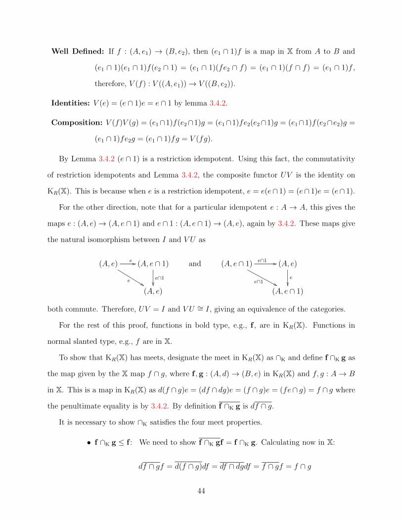
Well Defined: If f : (A, e1) → (B, e2), then (e1 ∩ 1)f is a map in X from A to B and
(e1 ∩ 1)(e1 ∩ 1)f(e2 ∩ 1) = (e1 ∩ 1)(fe2 ∩ f) = (e1 ∩ 1)(f ∩ f) = (e1 ∩ 1)f ,
therefore, V (f) : V ((A, e1))→ V ((B, e2)).
Identities: V (e) = (e ∩ 1)e = e ∩ 1 by lemma 3.4.2.
Composition: V (f)V (g) = (e1∩1)f(e2∩1)g = (e1∩1)fe2(e2∩1)g = (e1∩1)f(e2∩e2)g =
(e1 ∩ 1)fe2g = (e1 ∩ 1)fg = V (fg).
By Lemma 3.4.2 (e ∩ 1) is a restriction idempotent. Using this fact, the commutativity
of restriction idempotents and Lemma 3.4.2, the composite functor UV is the identity on
KR(X). This is because when e is a restriction idempotent, e = e(e∩ 1) = (e∩ 1)e = (e∩ 1).
For the other direction, note that for a particular idempotent e : A → A, this gives the
maps e : (A, e)→ (A, e ∩ 1) and e ∩ 1 : (A, e ∩ 1)→ (A, e), again by 3.4.2. These maps give
the natural isomorphism between I and V U as
(A, e) e //
e%%
(A, e ∩ 1)
e∩1��
(A, e)
and (A, e ∩ 1) e∩1 //
e∩1 &&
(A, e)
e
��(A, e ∩ 1)
both commute. Therefore, UV = I and V U ∼= I, giving an equivalence of the categories.
For the rest of this proof, functions in bold type, e.g., f , are in KR(X). Functions in
normal slanted type, e.g., f are in X.
To show that KR(X) has meets, designate the meet in KR(X) as ∩K and define f ∩K g as
the map given by the X map f ∩ g, where f ,g : (A, d)→ (B, e) in KR(X) and f, g : A→ B
in X. This is a map in KR(X) as d(f ∩ g)e = (df ∩ dg)e = (f ∩ g)e = (fe∩ g) = f ∩ g where
the penultimate equality is by 3.4.2. By definition f ∩K g is df ∩ g.
It is necessary to show ∩K satisfies the four meet properties.
• f ∩K g ≤ f : We need to show f ∩K gf = f ∩K g. Calculating now in X:
df ∩ gf = d(f ∩ g)df = df ∩ dgdf = f ∩ gf = f ∩ g
44

which is the definition of f ∩K g.
• f ∩K g ≤ g: Similarly and once again calculating in X,
df ∩ gg = d(f ∩ g)dg = df ∩ dgdg = f ∩ gg = f ∩ g
which is the definition of f ∩K g.
• f ∩K f = f : From the definition, this is f ∩ f = f which is just f .
• h(f ∩K g) = hf ∩K hg: From the definition, this is given in X by h(f ∩ g) =
hf ∩ hg which in KR(X) is hf ∩K hg.
Consider two objects A,B in a restriction category where we have m : A→ B, r : B → A
with mr = 1A. In this case A is called a retract of B, which we will write as A / B. As m
and r need not be unique, we will also write A/rmB when the specific section and retraction
are to be emphasized. Since m is a section, it is a monic and therefore total. The map rm
is idempotent on B as rmrm = r1m = rm. A is referred to as a splitting of the idempotent
rm. Note there is no requirement that rm = rm when m is simply monic.
3.8 Partial map categories
In [21], it is shown that split restriction categories are equivalent to partial map categories.
The main definitions and results related to partial map categories are given below.
Definition 3.8.1. A collection M of monics is a stable system of monics when:
(i) it includes all isomorphisms;
(ii) it is closed under composition;
(iii) it is pullback stable.
45

Stable in this definition means that if m : A → B is in M, then for arbitrary b with
codomain B, the pullback
A′a //
m′
��
A
m
��B′
b// B
exists and m′ ∈ M. A category that has a stable system of monics is referred to as an
M-category.
Lemma 3.8.2. If nm ∈M, a stable system of monics, and m is monic, then n ∈M.
Proof. The commutative square
A
n
��
1 // A
nm
��A′ m
// B
is a pullback.
Given a category B and a stable system of monicsM, the partial map category, Par(B,M)
is:
Objects: A ∈ B;
Equivalence Classes of Maps: (m, f) : A→ B with m : A′ → A is inM and f : A′ → B
is a map in B. i.e., A′m~~
f
A B
;
Identity: 1A, 1A : A→ A;
Composition: via a pullback, (m, f)(m′, g) = (m′′m, f ′g) where
A′′m′′
}}f ′
!!A′
m�� f !!
(pb) B′
m′}}g!!
A B C;
Restriction: (m, f) = (m,m).
46

For the maps, (m, f) ∼ (m′, f ′) when there is an isomorphism γ : A′′ → A′ such that
γm′ = m and γf ′ = f .
The proof that this is a restriction category is given by Proposition 3.1 in [21].
In [22], it is shown that:
Theorem 3.8.3 (Cockett-Lack). Every restriction category is a full subcategory of a partial
map category.
3.9 Restriction products and Cartesian restriction categories
Restriction categories have analogues of products and terminal objects.
Definition 3.9.1. In a restriction category X, a restriction product of two objects X, Y is
an object X × Y equipped with total projections π0 : X × Y → X, π1 : X × Y → Y where:
∀f : Z → X, g : Z → Y, ∃ a unique 〈f, g〉 : Z → X × Y such
that
• 〈f, g〉π0 ≤ f ,
• 〈f, g〉π1 ≤ g and
• 〈f, g〉 = f g(= g f).
Definition 3.9.2. In a restriction category X, a restriction terminal object is an object >
such that for all objects X, there is a unique total map !X : X → > and the diagram
Xf //
f
��
X!X // >
Y
!Y
55
commutes. That is, f !Y = f !X . Note this implies that a restriction terminal object is unique
up to a unique isomorphism.
47
For example, in Par, the restriction terminal object is the one object set, {∗}. The
product of two sets is the standard Cartesian product, with π0 mapping (x, y) 7→ x and
π1 : (x, y) 7→ y. The product map 〈f, g〉 : Z → X × Y is given as:
〈f, g〉(z) =
(x, y) f(z) = x and g(z) = y
↑ f(z) ↑ or g(y) ↑ .
Definition 3.9.3. A restriction category X is Cartesian if it has all restriction products and
a restriction terminal object.
3.10 Discrete Cartesian restriction categories
Definition 3.10.1. An object A in a Cartesian restriction category is discrete when the
diagonal map
∆ : A→ A× A
is a partial isomorphism. A Cartesian restriction category where all objects are discrete is
called a discrete Cartesian restriction category.
Example 3.10.2 (Topp is not discrete). In any topological space T , the only way that ∆
can have a continuous inverse is when the topology is the discrete topology. This example
is the motivating example for our terminology of discrete.
The topology of T ×T is generated by open sets U×V where U, V are open sets of T . We
see that ∆∩U×V = ∆∩(U∩V )×(U∩V ), so if ∆ ⊆ ∪iUi×Vi, then ∆ ⊆ ∪i(Ui∩Vi)×(Ui∩Vi).
Thus, any open cover of ∆ has a subcover of the form ∪iUi×Ui. For ∆(−1) to be a continuous
map, that means the diagonal must be an open set. But if ∆ is open, then ∆ = ∪iUi × Vi
if and only if ∆ ⊆ ∪i(Ui ∩ Vi)× (Ui ∩ Vi) ⊆ ∪iUi × Ui ⊆ ∆. So, ∆ = ∪iUi × Ui, which gives
us Ui × Ui ⊆ ∆, but this can only happen when Ui = {x}, a singleton set. Therefore, T has
the discrete topology.
48

Example 3.10.3 (Par is discrete). In Par,
∆ : x 7→ (x, x) and ∆(−1) : (x, y) 7→
x x = y,
↑ x 6= y.
Thus, Par is a discrete Cartesian restriction category.
Further examples of discrete and non-discrete Cartesian restriction categories are given
at the end of the section.
Theorem 3.10.4. A Cartesian restriction category X is discrete if and only if it has meets.
Proof. If X has meets, then
∆(π0 ∩ π1) = ∆π0 ∩∆π1 = 1 ∩ 1 = 1.
As 〈π0, π1〉 is identity,
π0 ∩ π1 = π0 ∩ π1〈π0, π1〉
= 〈π0 ∩ π1π0, π0 ∩ π1π1〉
= 〈π0 ∩ π1, π0 ∩ π1〉
= (π0 ∩ π1)∆
and therefore, π0 ∩ π1 is ∆(−1).
To show the other direction, we set f∩g = 〈f, g〉∆(−1). By the definition of the restriction
product:
f ∩ g = 〈f, g〉∆(−1) = 〈f, g〉∆(−1)∆π0 = 〈f, g〉∆(−1)π0 ≤ 〈f, g〉π0 ≤ f.
Then, substituting π1 for π0 above, this gives us f ∩ g ≤ g.
For the left distributive law,
h(f ∩ g) = h〈f, g〉∆(−1) = 〈hf, hg〉∆(−1) = hf ∩ hg.
49
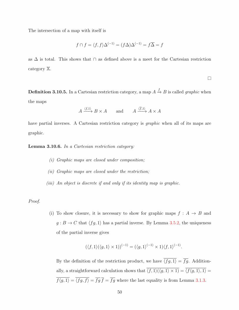
The intersection of a map with itself is
f ∩ f = 〈f, f〉∆(−1) = (f∆)∆(−1) = f∆ = f
as ∆ is total. This shows that ∩ as defined above is a meet for the Cartesian restriction
category X.
Definition 3.10.5. In a Cartesian restriction category, a map Af−→ B is called graphic when
the maps
A〈f,1〉−−→ B × A and A
〈f,1〉−−→ A× A
have partial inverses. A Cartesian restriction category is graphic when all of its maps are
graphic.
Lemma 3.10.6. In a Cartesian restriction category:
(i) Graphic maps are closed under composition;
(ii) Graphic maps are closed under the restriction;
(iii) An object is discrete if and only if its identity map is graphic.
Proof.
(i) To show closure, it is necessary to show for graphic maps f : A → B and
g : B → C that 〈fg, 1〉 has a partial inverse. By Lemma 3.5.2, the uniqueness
of the partial inverse gives
(〈f, 1〉(〈g, 1〉 × 1))(−1) = (〈g, 1〉(−1) × 1)〈f, 1〉(−1).
By the definition of the restriction product, we have 〈fg, 1〉 = fg. Addition-
ally, a straightforward calculation shows that 〈f, 1〉(〈g, 1〉 × 1) = 〈f〈g, 1〉, 1〉 =
f〈g, 1〉 = 〈fg, f〉 = fg f = fg where the last equality is from Lemma 3.1.3.
50

Consider the diagram
A〈f,1〉 //
〈fg,1〉
**
B × A〈g,1〉×1 // C ×B × A
C × A.
1×〈f,1〉
OO
Thus,
〈fg, 1〉(1× 〈f, 1〉)(〈g, 1〉(−1) × 1)〈f, 1〉(−1)
= 〈f, 1〉(〈g, 1〉 × 1)(〈g, 1〉(−1) × 1)〈f, 1〉(−1)
= 〈f, 1〉(g × 1)〈f, 1〉(−1)
= 〈f, 1〉(g × 1)〈f, 1〉〈f, 1〉(−1)
= 〈f, 1〉(g × 1) 〈f, 1〉
= 〈f, 1〉 〈f, 1〉(g × 1)
= 〈f, 1〉(g × 1)
= 〈fg, 1〉(= fg)
showing that 1× 〈f, 1〉(〈g, 1〉(−1) × 1)〈f, 1〉(−1) is a right inverse for 〈fg, 1〉.
For the other direction, note that in general (hk)(−1) = k(−1)h(−1) and that
we have 〈fg, 1〉 = 〈f, 1〉(〈g, 1〉 × 1)(1× 〈f, 1〉(−1)), thus (1× 〈f, 1〉)(〈g, 1〉(−1)×
1)〈f, 1〉(−1) will also be a left inverse and 〈fg, 1〉 is a partial isomorphism.
(ii) This follows from the definition of graphic and that 〈f, 1〉 = f = f = 〈f, 1〉.
(iii) Given a discrete object A, the identity on A is graphic as 〈1, 1〉 = ∆ and
therefore 〈1, 1〉(−1) = ∆(−1). Conversely, if 〈1, 1〉 = ∆ has an inverse, A is
discrete by definition.
51
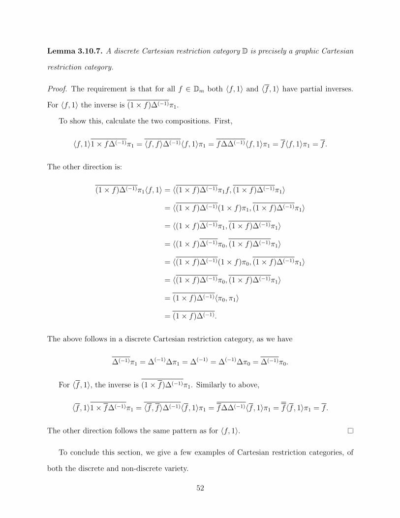
Lemma 3.10.7. A discrete Cartesian restriction category D is precisely a graphic Cartesian
restriction category.
Proof. The requirement is that for all f ∈ Dm both 〈f, 1〉 and 〈f, 1〉 have partial inverses.
For 〈f, 1〉 the inverse is (1× f)∆(−1)π1.
To show this, calculate the two compositions. First,
〈f, 1〉1× f∆(−1)π1 = 〈f, f〉∆(−1)〈f, 1〉π1 = f∆∆(−1)〈f, 1〉π1 = f〈f, 1〉π1 = f.
The other direction is:
(1× f)∆(−1)π1〈f, 1〉 = 〈(1× f)∆(−1)π1f, (1× f)∆(−1)π1〉
= 〈(1× f)∆(−1)(1× f)π1, (1× f)∆(−1)π1〉
= 〈(1× f)∆(−1)π1, (1× f)∆(−1)π1〉
= 〈(1× f)∆(−1)π0, (1× f)∆(−1)π1〉
= 〈(1× f)∆(−1)(1× f)π0, (1× f)∆(−1)π1〉
= 〈(1× f)∆(−1)π0, (1× f)∆(−1)π1〉
= (1× f)∆(−1)〈π0, π1〉
= (1× f)∆(−1).
The above follows in a discrete Cartesian restriction category, as we have
∆(−1)π1 = ∆(−1)∆π1 = ∆(−1) = ∆(−1)∆π0 = ∆(−1)π0.
For 〈f, 1〉, the inverse is (1× f)∆(−1)π1. Similarly to above,
〈f, 1〉1× f∆(−1)π1 = 〈f, f〉∆(−1)〈f, 1〉π1 = f∆∆(−1)〈f, 1〉π1 = f〈f, 1〉π1 = f.
The other direction follows the same pattern as for 〈f, 1〉.
To conclude this section, we give a few examples of Cartesian restriction categories, of
both the discrete and non-discrete variety.
52
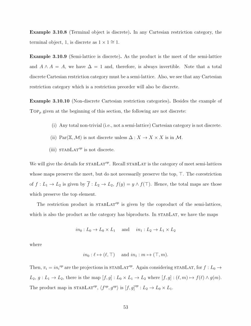
Example 3.10.8 (Terminal object is discrete). In any Cartesian restriction category, the
terminal object, 1, is discrete as 1× 1 ∼= 1.
Example 3.10.9 (Semi-lattice is discrete). As the product is the meet of the semi-lattice
and A ∧ A = A, we have ∆ = 1 and, therefore, is always invertible. Note that a total
discrete Cartesian restriction category must be a semi-lattice. Also, we see that any Cartesian
restriction category which is a restriction preorder will also be discrete.
Example 3.10.10 (Non-discrete Cartesian restriction categories). Besides the example of
Topp given at the beginning of this section, the following are not discrete:
(i) Any total non-trivial (i.e., not a semi-lattice) Cartesian category is not discrete.
(ii) Par(X,M) is not discrete unless ∆ : X → X ×X is in M.
(iii) stabLatop is not discrete.
We will give the details for stabLatop. Recall stabLat is the category of meet semi-lattices
whose maps preserve the meet, but do not necessarily preserve the top, >. The corestriction
of f : L1 → L2 is given by f : L2 → L2, f(y) = y ∧ f(>). Hence, the total maps are those
which preserve the top element.
The restriction product in stabLatop is given by the coproduct of the semi-lattices,
which is also the product as the category has biproducts. In stabLat, we have the maps
in0 : L0 → L0 × L1 and in1 : L2 → L1 × L2
where
in0 : ` 7→ (`,>) and in1 : m 7→ (>,m).
Then, πi = iniop are the projections in stabLatop. Again considering stabLat, for f : L0 →
L2, g : L1 → L2, there is the map [f, g] : L0 × L1 → L2 where [f, g] : (`,m) 7→ f(`) ∧ g(m).
The product map in stabLatop, 〈f op, gop〉 is [f, g]op : L2 → L0 × L1.
53

Using the standard notation of ∇ for the map [1, 1] in stabLat, we see ∆ : L1 → L1×L1
in stabLatop is∇op. For this to have an inverse, we need a map h : L1 → L1×L1 in stabLat
such that ∆hop = 1L1 , i.e., h∇ = 1L1 in stabLat. In stabLat, we may write h as having
two components, that is, h(x) = (h1(x), h2(x)).
As we know that x ∧ y = ∇(h(x ∧ y), we have that h(>) ∧ (x, y) = h(x ∧ y). But this
gives us (h1(>) ∧ x, h2(>) ∧ y) = (h1(x ∧ y), h2(x ∧ y)). Therefore:
h1(x ∧ y) = h1(>) ∧ x and
h2(x ∧ y) = h2(>) ∧ y.
But then we have
x ∧ y = h1(x ∧ y) ∧ h2(x ∧ y) = h1(>) ∧ h2(>) ∧ x ∧ y
which means that h1(>) ∧ h2(>) = >, which gives h1(x ∧ y) = x and h2(x ∧ y) = y. In
any lattice where there is a non top element p, this produces a contradiction as h1(p) =
h1(p ∧ >) = p and h1(p) = h1(> ∧ p) = > which can only happen when > = p. This shows
that the only discrete object in stabLatop is the one element semi-lattice, {>}.
Thus, the map h does not exist in general and stabLatop is not discrete.
54
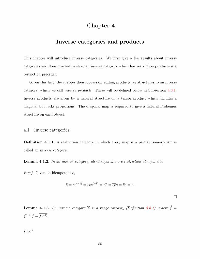
Chapter 4
Inverse categories and products
This chapter will introduce inverse categories. We first give a few results about inverse
categories and then proceed to show an inverse category which has restriction products is a
restriction preorder.
Given this fact, the chapter then focuses on adding product-like structures to an inverse
category, which we call inverse products. These will be defined below in Subsection 4.3.1.
Inverse products are given by a natural structure on a tensor product which includes a
diagonal but lacks projections. The diagonal map is required to give a natural Frobenius
structure on each object.
4.1 Inverse categories
Definition 4.1.1. A restriction category in which every map is a partial isomorphism is
called an inverse category.
Lemma 4.1.2. In an inverse category, all idempotents are restriction idempotents.
Proof. Given an idempotent e,
e = ee(−1) = eee(−1) = ee = eee = ee = e.
Lemma 4.1.3. An inverse category X is a range category (Definition 3.6.1), where f =
f (−1)f = f (−1).
Proof.
55
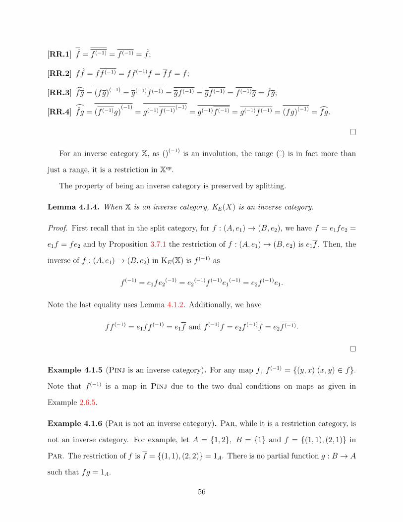
[RR.1] f = f (−1) = f (−1) = f ;
[RR.2] ff = ff (−1) = ff (−1)f = ff = f ;
[RR.3] f g = (fg)(−1) = g(−1)f (−1) = gf (−1) = gf (−1) = f (−1)g = f g;
[RR.4]fg = (f (−1)g)
(−1)= g(−1)f (−1)
(−1)= g(−1)f (−1) = g(−1)f (−1) = (fg)(−1) = f g.
For an inverse category X, as ()(−1) is an involution, the range ( ) is in fact more than
just a range, it is a restriction in Xop.
The property of being an inverse category is preserved by splitting.
Lemma 4.1.4. When X is an inverse category, KE(X) is an inverse category.
Proof. First recall that in the split category, for f : (A, e1)→ (B, e2), we have f = e1fe2 =
e1f = fe2 and by Proposition 3.7.1 the restriction of f : (A, e1)→ (B, e2) is e1f . Then, the
inverse of f : (A, e1)→ (B, e2) in KE(X) is f (−1) as
f (−1) = e1fe2(−1) = e2
(−1)f (−1)e1(−1) = e2f
(−1)e1.
Note the last equality uses Lemma 4.1.2. Additionally, we have
ff (−1) = e1ff(−1) = e1f and f (−1)f = e2f
(−1)f = e2f (−1).
Example 4.1.5 (Pinj is an inverse category). For any map f , f (−1) = {(y, x)|(x, y) ∈ f}.
Note that f (−1) is a map in Pinj due to the two dual conditions on maps as given in
Example 2.6.5.
Example 4.1.6 (Par is not an inverse category). Par, while it is a restriction category, is
not an inverse category. For example, let A = {1, 2}, B = {1} and f = {(1, 1), (2, 1)} in
Par. The restriction of f is f = {(1, 1), (2, 2)} = 1A. There is no partial function g : B → A
such that fg = 1A.
56

Example 4.1.7. Generally, let R be a restriction category, and INV(R) the subcategory of
R having the same objects as R but only the partial isomorphisms as maps. Then, INV(R)
is an inverse category.
Example 4.1.8. A groupoid, which is a category in which every map is an isomorphism, is
an inverse category. As all maps in the groupoid are total, the partial isomorphisms are all
isomorphisms.
As well, we note that for X any inverse category, Total(X) is a groupoid.
Example 4.1.9. Given a category P, create a partial map category as in Section 3.8, where
the stable system of monics, M, contains all of the isomorphisms in P. Then the par-
tial isomorphisms are the maps of the formA′
m~~
m′
A B
, where m′ ∈ M. Its inverse is
A′m′
~~m
B A. The composition is
Am−1m
��m−1m��
A A, which is the identity when m is an iso-
morphism. The partial isomorphisms will have either m or m′ in M, but may not be an
isomorphism. Taking just the partial isomorphisms gives us an inverse category.
Example 4.1.10. A semigroup [57] is a set with an associative binary operation. A semi-
group need not have an identity. An inverse semigroup is a semigroup where each element
x has an associated element x∗ such that:
x = xx∗x and x∗ = x∗xx∗.
In much the same way that a group may be viewed as a one object category, an inverse
semigroup is a one object inverse category, where the elements are the maps. For any map
x, we have x(−1) = x∗.
Example 4.1.11 (Equivalence relations). Equivalence relations of finite sets are repre-
sentable as a pair of surjective functions onto another set. That is,
AE[f,g] // B :=
C
A
f?? ??
B
g____
⇐⇒C
A+B.
[f,g]
OOOO
57
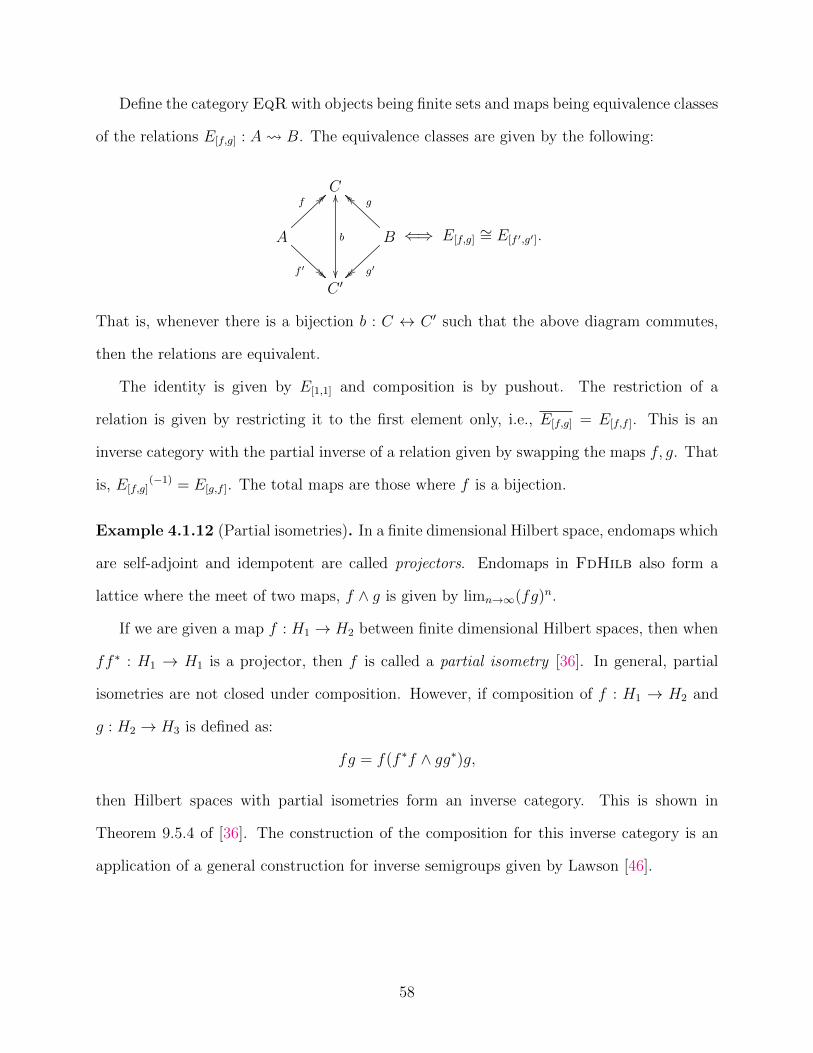
Define the category EqR with objects being finite sets and maps being equivalence classes
of the relations E[f,g] : A B. The equivalence classes are given by the following:
COO
b
��
A
f>> >>
f ′
B
g````
g′~~~~C ′
⇐⇒ E[f,g]∼= E[f ′,g′].
That is, whenever there is a bijection b : C ↔ C ′ such that the above diagram commutes,
then the relations are equivalent.
The identity is given by E[1,1] and composition is by pushout. The restriction of a
relation is given by restricting it to the first element only, i.e., E[f,g] = E[f,f ]. This is an
inverse category with the partial inverse of a relation given by swapping the maps f, g. That
is, E[f,g](−1) = E[g,f ]. The total maps are those where f is a bijection.
Example 4.1.12 (Partial isometries). In a finite dimensional Hilbert space, endomaps which
are self-adjoint and idempotent are called projectors. Endomaps in FdHilb also form a
lattice where the meet of two maps, f ∧ g is given by limn→∞(fg)n.
If we are given a map f : H1 → H2 between finite dimensional Hilbert spaces, then when
ff ∗ : H1 → H1 is a projector, then f is called a partial isometry [36]. In general, partial
isometries are not closed under composition. However, if composition of f : H1 → H2 and
g : H2 → H3 is defined as:
fg = f(f ∗f ∧ gg∗)g,
then Hilbert spaces with partial isometries form an inverse category. This is shown in
Theorem 9.5.4 of [36]. The construction of the composition for this inverse category is an
application of a general construction for inverse semigroups given by Lawson [46].
58
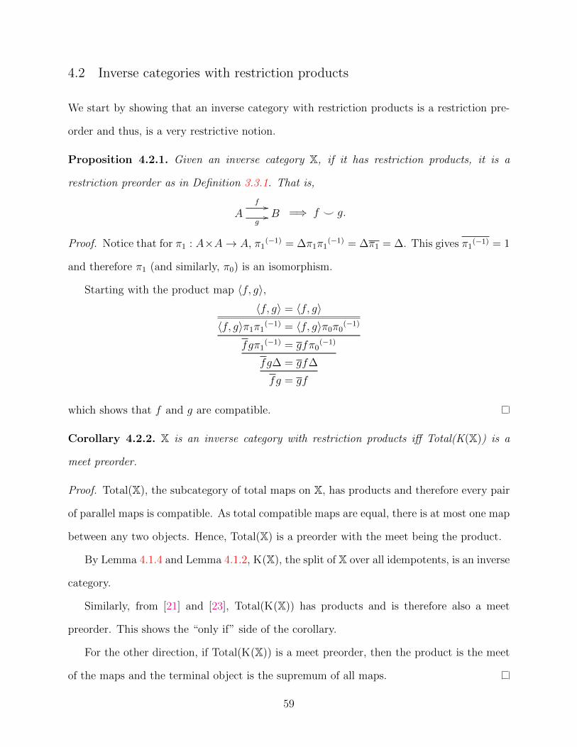
4.2 Inverse categories with restriction products
We start by showing that an inverse category with restriction products is a restriction pre-
order and thus, is a very restrictive notion.
Proposition 4.2.1. Given an inverse category X, if it has restriction products, it is a
restriction preorder as in Definition 3.3.1. That is,
Af //
g// B =⇒ f ^ g.
Proof. Notice that for π1 : A×A→ A, π1(−1) = ∆π1π1
(−1) = ∆π1 = ∆. This gives π1(−1) = 1
and therefore π1 (and similarly, π0) is an isomorphism.
Starting with the product map 〈f, g〉,〈f, g〉 = 〈f, g〉
〈f, g〉π1π1(−1) = 〈f, g〉π0π0
(−1)
fgπ1(−1) = gfπ0
(−1)
fg∆ = gf∆
fg = gf
which shows that f and g are compatible.
Corollary 4.2.2. X is an inverse category with restriction products iff Total(K(X)) is a
meet preorder.
Proof. Total(X), the subcategory of total maps on X, has products and therefore every pair
of parallel maps is compatible. As total compatible maps are equal, there is at most one map
between any two objects. Hence, Total(X) is a preorder with the meet being the product.
By Lemma 4.1.4 and Lemma 4.1.2, K(X), the split of X over all idempotents, is an inverse
category.
Similarly, from [21] and [23], Total(K(X)) has products and is therefore also a meet
preorder. This shows the “only if” side of the corollary.
For the other direction, if Total(K(X)) is a meet preorder, then the product is the meet
of the maps and the terminal object is the supremum of all maps.
59
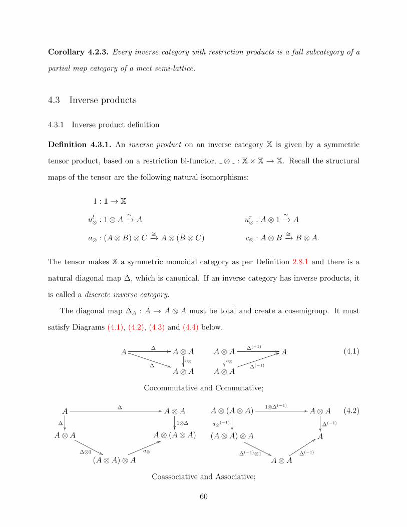
Corollary 4.2.3. Every inverse category with restriction products is a full subcategory of a
partial map category of a meet semi-lattice.
4.3 Inverse products
4.3.1 Inverse product definition
Definition 4.3.1. An inverse product on an inverse category X is given by a symmetric
tensor product, based on a restriction bi-functor, ⊗ : X × X → X. Recall the structural
maps of the tensor are the following natural isomorphisms:
1 : 1→ X
ul⊗ : 1⊗ A∼=−→ A ur⊗ : A⊗ 1
∼=−→ A
a⊗ : (A⊗B)⊗ C∼=−→ A⊗ (B ⊗ C) c⊗ : A⊗B
∼=−→ B ⊗ A.
The tensor makes X a symmetric monoidal category as per Definition 2.8.1 and there is a
natural diagonal map ∆, which is canonical. If an inverse category has inverse products, it
is called a discrete inverse category.
The diagonal map ∆A : A → A ⊗ A must be total and create a cosemigroup. It must
satisfy Diagrams (4.1), (4.2), (4.3) and (4.4) below.
A
∆ **
∆ // A⊗ Ac⊗��
A⊗ A
A⊗ Ac⊗��
∆(−1)// A
A⊗ A∆(−1)
44 (4.1)
Cocommutative and Commutative;
A∆ //
∆��
A⊗ A1⊗∆��
A⊗ A
∆⊗1 ''
A⊗ (A⊗ A)
(A⊗ A)⊗ Aa⊗
66
A⊗ (A⊗ A)1⊗∆(−1)
//
a⊗(−1)
��
A⊗ A∆(−1)
��(A⊗ A)⊗ A
∆(−1)⊗1 ''
A
A⊗ A∆(−1)
99
(4.2)
Coassociative and Associative;
60

A⊗ A
(1⊗∆)a⊗(−1)
��
∆(−1)
''
(∆⊗1)a⊗ // A⊗ (A⊗ A)
1⊗∆(−1)
��
A∆
''(A⊗ A)⊗ A
∆(−1)⊗1
// A⊗ A
(4.3)
∆ is Semi-Frobenius.
If we define the map:
ex⊗ = a⊗(1⊗a⊗(−1))(1⊗ (c⊗⊗ 1))(1⊗a⊗)a⊗(−1)) : (A⊗B)⊗ (C⊗D)→ (A⊗C)⊗ (B⊗D)
then we have:
A⊗B
∆&&
∆⊗∆ // (A⊗ A)⊗ (B ⊗B)
ex⊗vv
(A⊗B)⊗ (A⊗B)
(4.4)
∆ is canonical.
Thus, ∆ is a cocommutative, coassociative map which together with ∆(−1) forms a special
semi-Frobenius algebra. We use the prefix “semi-” since we are not requiring the unit laws
of a Frobenius algebra as presented in Definition 10.1.10.
Note also, cocommutativity implies commutativity, i.e., that c⊗∆(−1) = ∆(−1). One can
see this as:
∆(c⊗∆(−1)) = (∆c⊗)∆(−1) = ∆∆(−1) = ∆ and
(c⊗∆(−1))∆ = (c⊗∆(−1))(∆c⊗) = c⊗∆(−1).
This means that both ∆(−1) and c⊗∆(−1) are partial inverses for ∆ and are therefore equal.
Similarly, coassociativity implies associativity, in that
(1⊗∆(−1))∆(−1) = (∆(1⊗∆))(−1) = a⊗(−1)(∆(−1) ⊗ 1)∆(−1).
61

This can be seen from the following calculation:
∆(1⊗∆)a⊗(−1)(∆(−1) ⊗ 1)∆(−1) = ∆(∆⊗ 1)a⊗a⊗
(−1)(∆(−1) ⊗ 1)∆(−1)
= ∆(∆⊗ 1)(∆(−1) ⊗ 1)∆(−1)
= ∆1∆(−1) = 1.
Example 4.3.2 (Pinj is a discrete inverse category). In the inverse category Pinj (see
Examples 2.6.5 and 4.1.5), we saw in Example 2.8.3 that the Cartesian product is a symmetric
tensor.
Define ∆A = {(a, (a, a))|a ∈ A}. Then Pinj is a discrete inverse category with the inverse
product of ⊗. The required properties of cocommutativity, coassociativity and exchange are
immediately obvious. To show the Frobenius rule for ∆, first note that ∆(−1) is defined only
on the elements of A⊗A which agree in the first and second coordinate. We show the upper
triangle of the Frobenius diagram in detail. Equation (4.5) shows the result of applying
∆(−1) followed by ∆.
∆(∆(−1)(A⊗ A)) = ∆({a|(a, a) ∈ A⊗ A}) = {(a, a)|(a, a) ∈ A⊗ A}. (4.5)
Applying (∆⊗ 1)a⊗ to A⊗ A is shown in Equation (4.6).
a⊗(∆⊗ 1(A⊗ A)) = a⊗({((a, a), a′)|(a, a′) ∈ A⊗ A} = {(a, (a, a′))|(a, a′) ∈ A⊗ A}. (4.6)
Finally, applying 1⊗∆(−1) to the result of Equation (4.6) gives us Equation (4.7).
(1⊗∆(−1))({(a, (a, a′))|(a, a′) ∈ A⊗ A} = {(a, a)|(a, a) ∈ A⊗ A}. (4.7)
Thus, we have ∆(−1)∆ = (∆⊗ 1)a⊗(1⊗∆(−1)) and the Frobenius condition is satisfied.
Example 4.3.3 (Topp does not give a discrete inverse category). Recalling Topp from
Example 3.1.9, we know that the partial isomorphisms of Topp form an inverse category —
INV(Topp). Additionally, Topp has a product, given by the standard Cartesian product.
However, as noted in Example 3.10.2, Topp is not a discrete Cartesian restriction category.
62
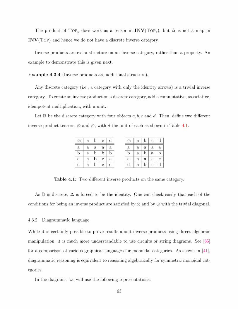
The product of Topp does work as a tensor in INV(Topp), but ∆ is not a map in
INV(Top) and hence we do not have a discrete inverse category.
Inverse products are extra structure on an inverse category, rather than a property. An
example to demonstrate this is given next.
Example 4.3.4 (Inverse products are additional structure).
Any discrete category (i.e., a category with only the identity arrows) is a trivial inverse
category. To create an inverse product on a discrete category, add a commutative, associative,
idempotent multiplication, with a unit.
Let D be the discrete category with four objects a, b, c and d. Then, define two different
inverse product tensors, ⊗ and �, with d the unit of each as shown in Table 4.1.
⊗ a b c d
a a a a ab a b b bc a b c cd a b c d
� a b c d
a a a a ab a b a bc a a c cd a b c d
Table 4.1: Two different inverse products on the same category.
As D is discrete, ∆ is forced to be the identity. One can check easily that each of the
conditions for being an inverse product are satisfied by ⊗ and by � with the trivial diagonal.
4.3.2 Diagrammatic language
While it is certainly possible to prove results about inverse products using direct algebraic
manipulation, it is much more understandable to use circuits or string diagrams. See [65]
for a comparison of various graphical languages for monoidal categories. As shown in [41],
diagrammatic reasoning is equivalent to reasoning algebraically for symmetric monoidal cat-
egories.
In the diagrams, we will use the following representations:
63
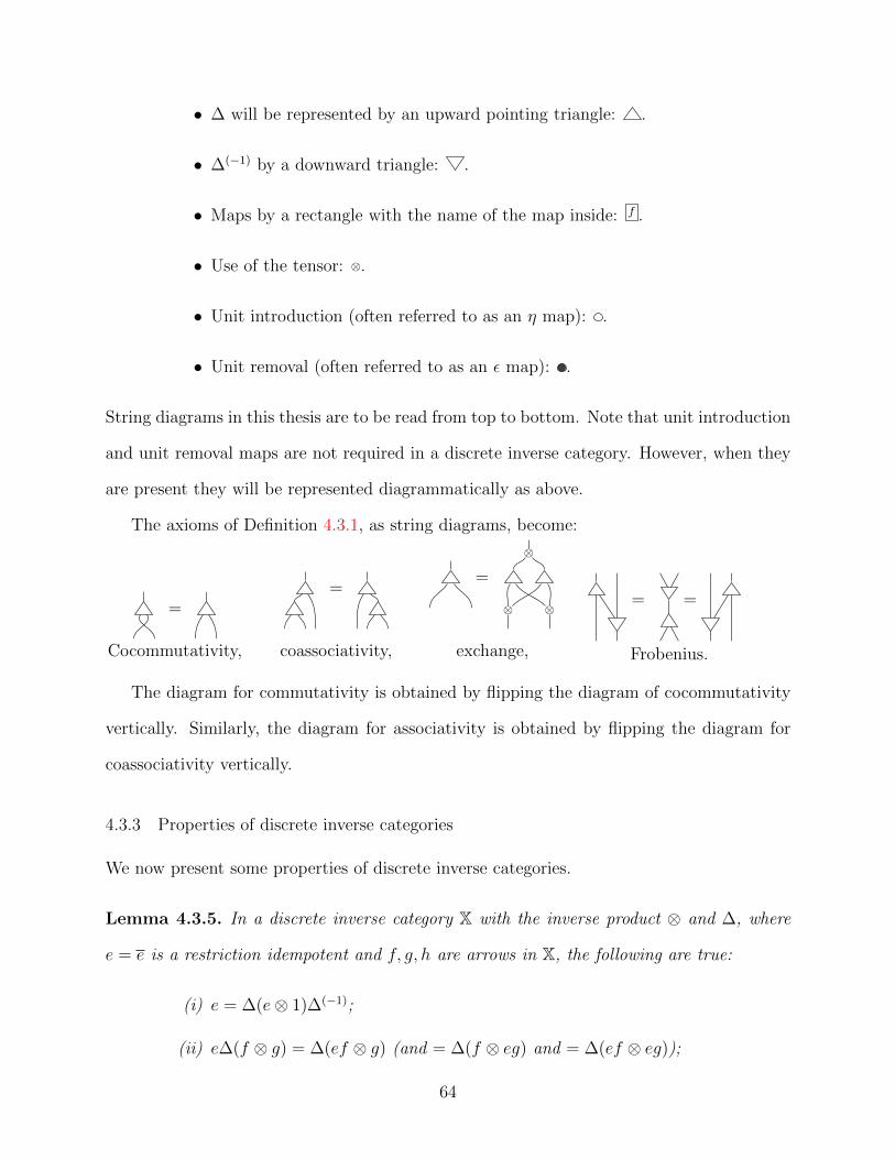
• ∆ will be represented by an upward pointing triangle: .
• ∆(−1) by a downward triangle: .
• Maps by a rectangle with the name of the map inside: f .
• Use of the tensor: ⊗.
• Unit introduction (often referred to as an η map): .
• Unit removal (often referred to as an ε map): .
String diagrams in this thesis are to be read from top to bottom. Note that unit introduction
and unit removal maps are not required in a discrete inverse category. However, when they
are present they will be represented diagrammatically as above.
The axioms of Definition 4.3.1, as string diagrams, become:
=
Cocommutativity,
=
coassociativity,
=
⊗
⊗ ⊗
exchange,
==
Frobenius.
The diagram for commutativity is obtained by flipping the diagram of cocommutativity
vertically. Similarly, the diagram for associativity is obtained by flipping the diagram for
coassociativity vertically.
4.3.3 Properties of discrete inverse categories
We now present some properties of discrete inverse categories.
Lemma 4.3.5. In a discrete inverse category X with the inverse product ⊗ and ∆, where
e = e is a restriction idempotent and f, g, h are arrows in X, the following are true:
(i) e = ∆(e⊗ 1)∆(−1);
(ii) e∆(f ⊗ g) = ∆(ef ⊗ g) (and = ∆(f ⊗ eg) and = ∆(ef ⊗ eg));
64
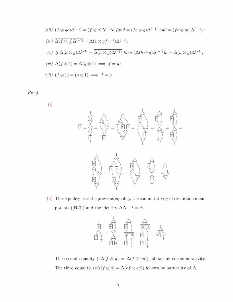
(iii) (f ⊗ ge)∆(−1) = (f ⊗ g)∆(−1)e (and = (fe⊗ g)∆(−1) and = (fe⊗ ge)∆(−1));
(iv) ∆(f ⊗ g)∆(−1) = ∆(1⊗ gf (−1))∆(−1);
(v) If ∆(h⊗ g)∆(−1) = ∆(h⊗ g)∆(−1) then (∆(h⊗ g)∆(−1))h = ∆(h⊗ g)∆(−1);
(vi) ∆(f ⊗ 1) = ∆(g ⊗ 1) =⇒ f = g;
(vii) (f ⊗ 1) = (g ⊗ 1) =⇒ f = g.
Proof.
(i)
e =
e
=
e
= e e e =
e
e
=
e
e
=
e
e
=
e
e
=e e
e
=
e
=
e
= e .
(ii) This equality uses the previous equality, the commutativity of restriction idem-
potents ([R.2]) and the identity ∆∆(−1) = ∆.
e
f g=
e
f g
=
e
∆(−1)
f g
=
∆(−1)
e
f g
= ef g .
The second equality (e∆(f ⊗ g) = ∆(f ⊗ eg)) follows by cocommutativity.
The third equality, (e∆(f ⊗ g) = ∆(ef ⊗ eg)) follows by naturality of ∆.
65

(iii) As in (ii), details are only given for the first equality. This proof is obtained
by reversing the diagrams of (ii).
e
f g
=e
f g
=e
∆(−1)
f g
=fe g
.
The other equalities follow for the same reasons as in (ii).
(iv) Here, we start by using the fact that all maps have a partial inverse, therefore
we have:
∆(f ⊗ g)∆(−1) = ∆(f ⊗ g)∆(−1)∆(f (−1) ⊗ g(−1))∆(−1).
Now, we proceed with showing the rest of the equality via diagrams.
f g
f (−1) g(−1)
=
fg
f (−1)g(−1)
=
fg
f (−1)g(−1)
=g g
ff (−1) =
gf (−1)=
gf (−1)
=gf (−1)
= gf (−1).
(v) Beginning with the assumption that ∆(h ⊗ g)∆(−1) equals its restriction and
66
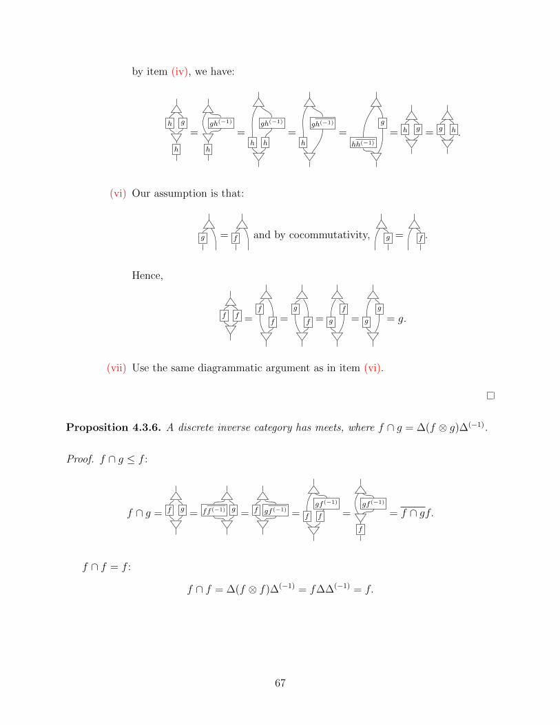
by item (iv), we have:
h g
h
=gh(−1)
h
=gh(−1)
h h
=gh(−1)
h
=g
hh(−1)
= gh = g h .
(vi) Our assumption is that:
g = f and by cocommutativity, g = f .
Hence,
f f =f
f =g
f = g
f
= g
g
= g.
(vii) Use the same diagrammatic argument as in item (vi).
Proposition 4.3.6. A discrete inverse category has meets, where f ∩ g = ∆(f ⊗ g)∆(−1).
Proof. f ∩ g ≤ f :
f ∩ g = f g = ff (−1) g = f gf (−1) = f
gf (−1)
f =gf (−1)
f
= f ∩ gf.
f ∩ f = f :
f ∩ f = ∆(f ⊗ f)∆(−1) = f∆∆(−1) = f.
67

h(f ∩ g) = hf ∩ hg:
h(f ∩ g) = h∆(f ⊗ g)∆(−1) Definition of ∩
= ∆(h⊗ h)(f ⊗ g)∆(−1) ∆ natural
= ∆(hf ⊗ hg)∆(−1) compose maps
= hf ∩ hg Definition of ∩ .
4.3.4 The inverse subcategory of a discrete Cartesian restriction category
Given a discrete Cartesian restriction category, one can pick out the maps which are partial
isomorphisms. Using results from Subsection 4.3.3 and from Section 3.10, we will show that
these maps form a subcategory which is a discrete inverse category.
Proposition 4.3.7. Given X is a discrete Cartesian restriction category, the partial isomor-
phisms of X, together with the objects of X form a sub-restriction category which is a discrete
inverse category. For the restriction category X, we denote this subcategory by INV(X).
Proof. As shown in Lemma 3.5.2, partial isomorphisms are closed under composition. The
identity maps are in INV(X) and restrictions of partial isomorphisms are also partial iso-
morphisms.
The product on the discrete Cartesian restriction category X becomes the tensor product
of the restriction category INV(X). Table 4.2 shows how each of the elements of the tensor
are defined. Note that the last definition makes explicit use of the fact we are in a discrete
Cartesian restriction category and hence the ∆ of X possesses a partial inverse.
The monoid coherence diagrams follow directly from the characteristics of the product in
X. Similarly, ∆ is total as it is total in X. It remains to show cocommutativity, coassociativity
and the Frobenius condition.
68

X INV(X) Inverse map
A×B A⊗B
> 1
π1:>×A→A ul⊗:1⊗A→A 〈!,1〉
π0:A×>→A ur⊗:A⊗1→A 〈1,!〉
aX=〈π0π0,〈π0π1,π1〉〉:(A×B)×C→A×(B×C) a⊗:(A⊗B)⊗C→A⊗(B⊗C) 〈〈π0,π1π0〉,π1π1〉
cX=〈π1,π0〉:A×B→B×A c⊗:A⊗B→B⊗A 〈π1,π0〉
∆X:A→A×A ∆:A→A⊗A ∆X(−1)
Table 4.2: Structural maps for the tensor in INV(X)
Cocommutativity requires ∆c⊗ = c⊗. We have
∆X〈π1, π0〉 = 〈∆Xπ1,∆Xπ0〉 = 〈1, 1〉 = ∆X,
giving us the required cocommutativity.
Coassociativity requires ∆(1⊗∆) = ∆(∆⊗ 1)a⊗. Expressing this in X, it is the require-
ment that
∆X(1×∆X) = ∆X(∆X × 1)aX.
Recalling that f × gπ0 = π0f and f × gπ1 = π1g, we have:
∆X(∆X × 1)aX = ∆X(∆X × 1)〈π0π0, 〈π0π1, π1〉〉
= 〈∆X(∆X × 1)π0π0, 〈∆X(∆X × 1)π0π1,∆X(∆X × 1)π1〉〉
= 〈∆Xπ0∆Xπ0, 〈∆Xπ0∆Xπ1,∆Xπ11〉〉
= 〈1, 〈1, 1〉〉 = ∆X(1×∆X)
and shows that we have coassociativity.
The semi-Frobenius requirement is two-fold:
∆(−1)∆ = (∆⊗ 1)a⊗(1⊗∆(−1)), (4.8)
∆(−1)∆ = (1⊗∆)a⊗(−1)(∆(−1) ⊗ 1). (4.9)
69
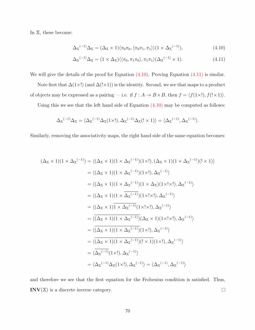
In X, these become:
∆X(−1)∆X = (∆X × 1)〈π0π0, 〈π0π1, π1〉〉(1×∆X
(−1)), (4.10)
∆X(−1)∆X = (1×∆X)〈〈π0, π1π0〉, π1π1〉(∆X
(−1) × 1). (4.11)
We will give the details of the proof for Equation (4.10). Proving Equation (4.11) is similar.
Note first that ∆(1×!) (and ∆(!×1)) is the identity. Second, we see that maps to a product
of objects may be expressed as a pairing — i.e. if f : A→ B×B, then f = 〈f(1×!), f(!×1)〉.
Using this we see that the left hand side of Equation (4.10) may be computed as follows:
∆X(−1)∆X = 〈∆X
(−1)∆X(1×!),∆X(−1)∆X(!× 1)〉 = 〈∆X
(−1),∆X(−1)〉.
Similarly, removing the associativity maps, the right hand side of the same equation becomes:
(∆X × 1)(1×∆X(−1)) = 〈(∆X × 1)(1×∆X
(−1))(1×!), (∆X × 1)(1×∆X(−1))(!× 1)〉
= 〈(∆X × 1)(1×∆X(−1))(1×!),∆X
(−1)〉
= 〈(∆X × 1)(1×∆X(−1))(1×∆X)(1×!×!),∆X
(−1)〉
= 〈(∆X × 1)(1×∆X(−1))(1×!×!),∆X
(−1)〉
= 〈(∆X × 1)1×∆X(−1)(1×!×!),∆X
(−1)〉
= 〈(∆X × 1)(1×∆X(−1))(∆X × 1)(1×!×!),∆X
(−1)〉
= 〈(∆X × 1)(1×∆X(−1))(1×!),∆X
(−1)〉
= 〈(∆X × 1)(1×∆X(−1))(!× 1)(1×!),∆X
(−1)〉
= 〈∆X(−1)(1×!),∆X
(−1)〉
= 〈∆X(−1)∆X(1×!),∆X
(−1)〉 = 〈∆X(−1),∆X
(−1)〉
and therefore we see that the first equation for the Frobenius condition is satisfied. Thus,
INV(X) is a discrete inverse category.
70
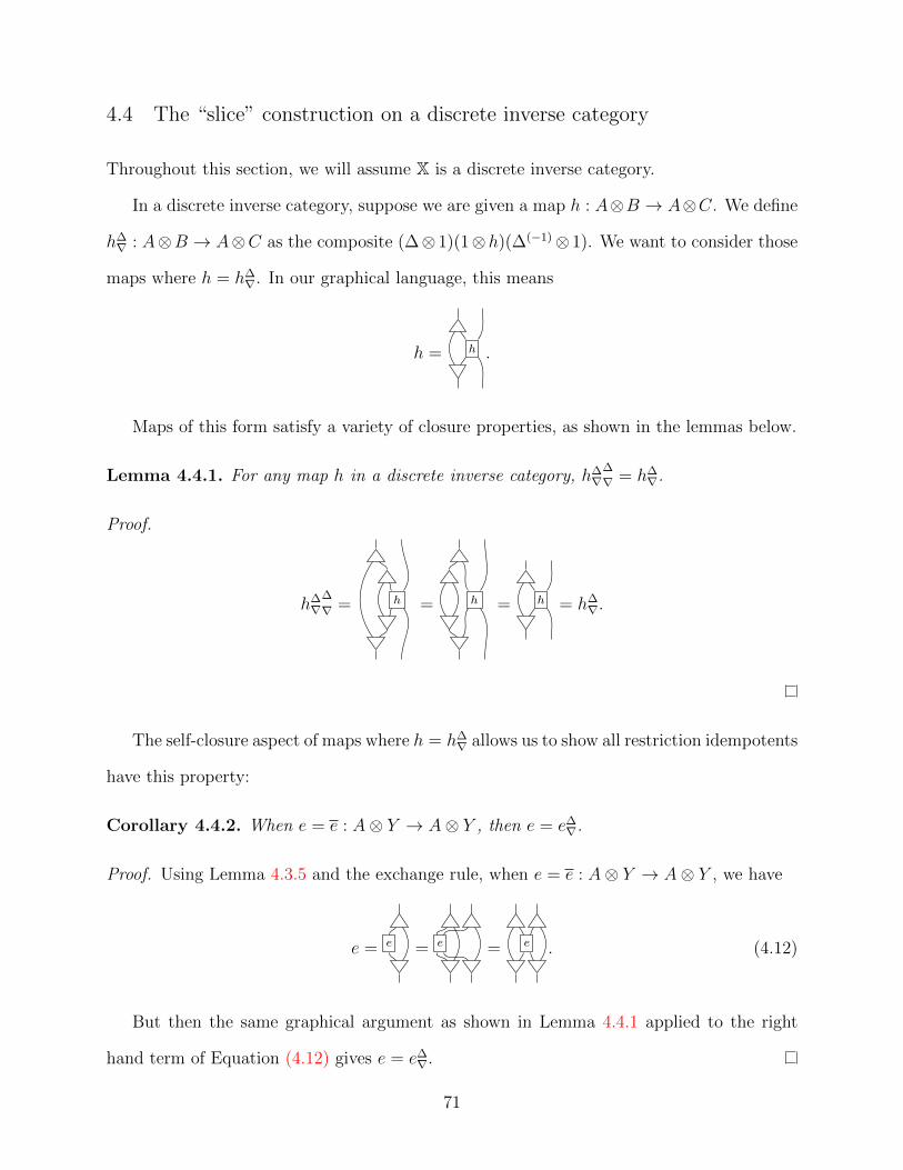
4.4 The “slice” construction on a discrete inverse category
Throughout this section, we will assume X is a discrete inverse category.
In a discrete inverse category, suppose we are given a map h : A⊗B → A⊗C. We define
h∆∇ : A⊗B → A⊗C as the composite (∆⊗ 1)(1⊗h)(∆(−1)⊗ 1). We want to consider those
maps where h = h∆∇. In our graphical language, this means
h = h .
Maps of this form satisfy a variety of closure properties, as shown in the lemmas below.
Lemma 4.4.1. For any map h in a discrete inverse category, h∆∇
∆
∇ = h∆∇.
Proof.
h∆∇
∆
∇ = h = h = h = h∆∇.
The self-closure aspect of maps where h = h∆∇ allows us to show all restriction idempotents
have this property:
Corollary 4.4.2. When e = e : A⊗ Y → A⊗ Y , then e = e∆∇.
Proof. Using Lemma 4.3.5 and the exchange rule, when e = e : A⊗ Y → A⊗ Y , we have
e = e = e = e . (4.12)
But then the same graphical argument as shown in Lemma 4.4.1 applied to the right
hand term of Equation (4.12) gives e = e∆∇.
71

There are a variety of other closure properties:
Lemma 4.4.3. In a discrete inverse category X with the object A define A∆∇ as the set of
maps h : A⊗ Y → A⊗ Z where h = h∆∇. Then A∆
∇ has the following properties:
(i) It is closed under partial inverses;
(ii) it is closed under composition;
(iii) it contains all maps of the form 1⊗ k where k : Y → Z;
(iv) it contains ∆ : A⊗B → A⊗B ⊗ A⊗B.
Proof. For (i), if h = h∆∇, then
h(−1) = ((∆⊗ 1)(1⊗ h)(∆(−1) ⊗ 1))(−1)
=
(∆(−1) ⊗ 1)(−1)
(1⊗ h)(−1)(∆⊗ 1)(−1) = (∆⊗ 1)(1⊗ h(−1))(∆(−1) ⊗ 1).
To show (ii), we compose h and g:
hg =
h
g
=
h
g
=h
g
=h
g
=h
g .
For (iii), this follows immediately from
h = h = 1⊗ h.
To show (iv), recalling the exchange rule, we have
∆∆∇ =
⊗
⊗
⊗
=
⊗
=
⊗
=⊗
= ∆.
72

Because of these closure rules, rather than stating h = h∆∇ we may equivalently say
h ∈ A∆∇ when h = h∆
∇ : A⊗X → A⊗ Y .
From Lemma 4.4.3, we see that we will be able to form a category based on maps h such
that h = h∆∇. Of course, this category is dependent upon the choice of the object A, hence
we will label it X[A], as it is reminiscent of the simple slice category of Example 2.4.3. We
make this precise in the following proposition:
Proposition 4.4.4. Given a discrete inverse category X, define X[A] as the restriction
category:
Objects: The objects of X;
Maps: A map h = h∆∇ : A⊗X → A⊗ Y in X is a map from X to Y in X[A];
Identity: 1⊗ 1 in X;
Composition: Composition in X;
Restriction: h in X[A] is given by h in X.
Then, X[A] is a discrete inverse category.
Proof. Given Lemma 4.4.3, we see immediately that X[A] is a category. By Corollary 4.4.2,
we know h = h∆
∇. We must show that X[A] has a tensor and a Frobenius ∆.
The tensor of objects X ⊗ Y in X[A] is the element A⊗X ⊗ Y in X. For two maps h, g
in X[A], h⊗g is given by the X map (∆⊗1⊗1)(1⊗ c⊗⊗1)(h⊗g)(1⊗ c⊗⊗1)(∆(−1)⊗1⊗1).
This is a map in X[A]:
(h⊗ g)∆∇ = h g = h g = h g = h⊗ g.
73
The ∆ in X[A] is given by the map 1⊗∆ in X. The various identities required of ∆ hold
in X[A] as they hold in X, therefore X[A] is a discrete inverse category.
We note that there are functors between X and X[A], given by:
G : X→ X[A]; G : B 7→ B; G : f 7→ 1⊗ f
and
F : X[A]→ X; F : B 7→ A⊗B; F : f 7→ f.
However, these do not form an adjoint pair as the relation is
X(A⊗X,A⊗ Y )
X[A](X, Y )that is,
X(F (X), F (Y ))
X[A](X,G(Y ))
rather than the requiredX(F (X), Y )
X[A](X,G(Y )).
Example 4.4.5. In Pinj, note that the slice over the object {∗} just gives us a category
where the maps are in bijective correspondence with the maps of Pinj, as {∗} is the identity
for the inverse product.
4.4.1 The interpretation of the slice construction in resource theory
Although resource theory is generally not in the scope of this thesis, the slice construction of
this section may be examined from the viewpoint of resource theory as given in Coecke, Fritz
and Spekkens [25]. Coecke, Fritz and Spekkens describe a mathematical theory of resources
inspired, in part, by the pragmatic approach exemplified in chemistry — understanding
something means being able to make use of it. Specifically in chemistry, this means under-
standing chemicals as resources. The way to model this mathematically is with a symmetric
monoidal category:
Definition 4.4.6 ( [25], Definition 2.1). A resource theory is a symmetric monoidal category
(R,⊗), where the objects Ro represent the actual resources and the morphisms f : A → B
represent the transformation of resource A into resource B which can be done with no cost.
74
In this definition, composition of maps then represent sequential composition of transfor-
mation, the operation ⊗ represents parallel composition of transformation and the identity
I of ⊗ denotes an empty resource.
An important question in such a theory is “Given a resource A, is it possible to transform
it to a resource B?” Of course, answering such a question will depend upon the details of
the category and the difficulty of answering such a question may vary greatly. This may be
reduced to a question of resource convertibility:
Definition 4.4.7 ( [25], Definition 4.1). A theory of resource convertibility (R,+,�, 0) is a
set R with a binary operation +, element 0 ∈ R such that when a ' b := a � b and b � a,
then
a+ (b+ c) ' (a+ b) + c a+ b ' b+ a a+ 0 ' 0 + a
and
a � b, c � d =⇒ a+ c � b+ d.
When R is a resource theory, then if we set R :=Ro, + :=⊗, a � b :=R(a, b) 6= ∅ and
0 := I, then (R,+,�, 0) is a theory of resource convertibility.
From this, it is possible to define what is meant by a catalyst:
Definition 4.4.8 ( [25], Definition 4.8). Given R is a theory of resource convertibility, then
a resource a ∈ R is a catalyst for b, c ∈ R when b � c but a+ b � a+ c.
Lifting this definition to a resource theory says the object A is a catalyst for objects B,C
when there is a map f : A⊗B → A⊗C, but no map g : B → C. We might call such maps
f , catalytic transformations and objects A, catalytic objects.
Here, we begin to see the connection to the slice category in a discrete inverse category.
As a discrete inverse category is also a symmetric monoidal category, it is therefore also a
resource theory and hence may generate a theory of resource convertibility.
However, given X is a discrete inverse category, the slice category X[A] does not corre-
spond directly to the catalytic transformations as defined above for two reasons:
75

(i) For two objects B,C in X[A] with f : B → C in X[A], there is no guarantee
that we do not have a map g : B → C in X.
(ii) There may be maps f : A ⊕ B → A ⊕ C in X, which are not in X[A] since
they do not preserve A.
Continuing with the inspiration of chemistry, we note that X[A] may perhaps be consid-
ered as an alternate way of describing “the catalytic transformations” for A. In chemistry,
one of the requirements is that the catalyst is not changed by the transformation in any way.
The theory of resource convertibility from Definition 4.4.7 handles this by considering the
resource as an indivisible item. In a resource theory, one way to specify that the catalytic
object has not changed is to identify a subcategory of “reversible” transformations and then
to require the catalytic transformation be in X[A].
76
Chapter 5
Constructing a Cartesian restriction category from a
discrete inverse category
The purpose of this chapter is to prove that the category of discrete inverse categories is
equivalent to the category of discrete Cartesian restriction categories. We will show how to
construct a discrete Cartesian restriction category, X, from a discrete inverse category, X.
The construction, to be called the “Cartesian Completion”, is reminiscent of the technique
generally used to make a computation reversible — one adds a history to the function to
make it reversible: Here we know how to add the history to make it invertible!
5.1 The restriction category X
We begin by giving the construction of X.
Definition 5.1.1 (Cartesian Completion). When X is a discrete inverse category, define X,
the Cartesian Completion of X, as:
Objects: objects as in X;
Maps: A map (f, C) : A → B in X is the equivalence class of the map f : A → B ⊗ C
in X (detailed below in Definition 5.1.2). We have the following relationship
between maps in X and X:
A(f,C)−−−−→ B in X
Af−→ B ⊗ C in X;
Identity: by
A(ur⊗
(−1),1)−−−−−−→ A
Aur⊗
(−1)
−−−−→ A⊗ 1;
77

Composition: given by
A(f,B′)−−−−→ B
(g,C′)−−−−→ C
Af−→ B ⊗B′, B g−→ C ⊗ C ′
Af(g⊗1)a⊗−−−−−→ C ⊗ (C ′ ⊗B′)
A(f(g⊗1)a⊗,C′⊗B′)−−−−−−−−−−→ C.
When considering an X map (f, C) : A → B in X, we occasionally use the notation
f : A→ B|C (≡ f : A→ B ⊗ C).
5.1.1 Equivalence classes of maps in X
Definition 5.1.2. In a discrete inverse category X, the map f is equivalent to f ′ in X when
f = f ′ in X and Figure 5.1 is a commutative diagram for some map h ∈ B∆∇ .
B ⊗ C
h
��
A
f 66
f ′ ((B ⊗ C ′
Figure 5.1: Equivalence diagram for constructing maps in X.
Notation 5.1.3. When f is equivalent to g as in Definition 5.1.2 via the mediating map h,
this is written as:
fh' g.
Lemma 5.1.4. Definition 5.1.2 gives a symmetric, reflexive equivalence class of maps in X.
Proof.
Reflexivity: Choose h as the identity map.
Symmetry: Suppose fh' g. Then, f = g and fh = g. Applying h(−1), we have
gh(−1) = fhh(−1) = fh = fhf = gf = ff = f.
78
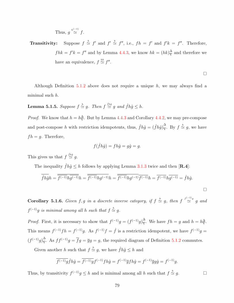
Thus, gh(−1)
' f .
Transitivity: Suppose fh' f ′ and f ′
k' f ′′, i.e., fh = f ′ and f ′k = f ′′. Therefore,
fhk = f ′k = f ′′ and by Lemma 4.4.3, we know hk = (hk)∆∇ and therefore we
have an equivalence, fhk' f ′′.
Although Definition 5.1.2 above does not require a unique h, we may always find a
minimal such h.
Lemma 5.1.5. Suppose fh' g. Then f
fhg' g and fhg ≤ h.
Proof. We know that h = h∆∇. But by Lemma 4.4.3 and Corollary 4.4.2, we may pre-compose
and post-compose h with restriction idempotents, thus, fhg = (fhg)∆
∇. By fh' g, we have
fh = g. Therefore,
f(fhg) = fhg = gg = g.
This gives us that ffhg' g.
The inequality fhg ≤ h follows by applying Lemma 3.1.3 twice and then [R.4]:
fhgh = f (−1)hg(−1)h = f (−1)hg(−1)h = f (−1)hg(−1)f (−1)h = f (−1)hg(−1) = fhg.
Corollary 5.1.6. Given f, g in a discrete inverse category, if fh' g, then f
f(−1)g' g and
f (−1)g is minimal among all h such that fh' g.
Proof. First, it is necessary to show that f (−1)g = (f (−1)g)∆
∇. We have fh = g and h = h∆∇.
This means f (−1)fh = f (−1)g. As f (−1)f = f is a restriction idempotent, we have f (−1)g =
(f (−1)g)∆
∇. As ff (−1)g = fg = gg = g, the required diagram of Definition 5.1.2 commutes.
Given another h such that fh' g, we have fhg ≤ h and
f (−1)gfhg = f (−1)gf (−1)fhg = f (−1)gfhg = f (−1)ggg = f (−1)g.
Thus, by transitivity f (−1)g ≤ h and is minimal among all h such that fh' g.
79

5.1.2 X is a restriction category
Lemma 5.1.7. X as defined above is a category.
Proof. The maps are well defined, as shown in Lemma 5.1.4. As X is a discrete inverse
category, ur⊗(−1) is defined and therefore the (ur⊗
(−1), 1) is a map in X.
It remains to show the composition is associative and that (ur⊗(−1), 1) acts as an identity
in X. For all of these, we will make use of Lemma 4.4.3 (iii), which states 1⊗ f ∈ A∆∇ for all
f .
Associativity: Consider
A(f,B′)−−−→ B
(g,C′)−−−→ C(h,D′)−−−→ D.
To show the associativity of this in X, we need to show in X that
(f(g ⊗ 1)a⊗)(h⊗ 1)a⊗ = f(((g(h⊗ 1)a⊗)⊗ 1)a⊗)
and that there exists a mediating map between the two of them.
To see that the restrictions are equal, first note that by the functorality of ⊗, for any two
maps u and v, we have uv ⊗ 1 = (u⊗ 1)(v ⊗ 1). Second, the naturality of a⊗ gives us that
a⊗(h⊗ 1) = ((h⊗ 1)⊗ 1)a⊗. Thus,
f(g ⊗ 1)a⊗(h⊗ 1)a⊗ = f(g ⊗ 1)a⊗(h⊗ 1)a⊗ Lemma 3.1.3
= f(g ⊗ 1)a⊗(h⊗ 1) a⊗ = 1
= f(g ⊗ 1)((h⊗ 1)⊗ 1)a⊗ a⊗ natural
= f(g ⊗ 1)((h⊗ 1)⊗ 1) Lemma 3.1.3
= f(g ⊗ 1)((h⊗ 1)⊗ 1)(a⊗ ⊗ 1) Lemma 3.1.3
= f((g(h⊗ 1)a⊗)⊗ 1) see above
= f((g(h⊗ 1)a⊗)⊗ 1)a⊗ a⊗ = 1.
For the mediating map, see the diagram below, where the calculation is in X. The path,
starting in the top left at A and going right to D|D′⊗(C′⊗B′), is grouping parentheses to the
80

left. The path which starts with A, then goes down to (D|D′⊗C′)|B′ , followed by continuing
right to D|(D′⊗C′)⊗B′ is grouping parentheses to the right. The commutativity of the diagram
is shown by the commutativity of the internal portions, which all follow from the standard
coherence diagrams for the tensor and naturality of association.
A
f
��
f(g⊗1)a⊗ //
f(g⊗1)
%%
C|C′⊗B′h⊗1 // (D|D′)|C′⊗B′
a⊗ // D|D′⊗(C′⊗B′)
1⊗a⊗(−1)
��
B|B′
(g(h⊗1)a⊗)⊗1
��
g⊗1 // (C|C′)|B′
a⊗
OO
(h⊗1)⊗1 // ((D|D′)|C′)|B′
a⊗
OO
a⊗⊗1
tt(D|D′⊗C′)|B′ a⊗
// D|(D′⊗C′)⊗B′ .
Therefore, we can conclude
(f(g ⊗ 1)a⊗)(h⊗ 1)a⊗1⊗a⊗
(−1)
' f(((g(h⊗ 1)a⊗)⊗ 1)a⊗)
which gives us that composition in X is associative.
Identity: This requires:
(f, C)(ur⊗(−1), 1) = (f, C) = (ur⊗
(−1), 1)(f, C)
for all maps A(f,C)−−−→ B in X. In X, this corresponds to requiring:
f 'f(ur⊗(−1) ⊗ 1)a⊗ and (5.1)
f 'ur⊗(−1)(f ⊗ 1)a⊗. (5.2)
For Equation (5.1), by Lemma 3.1.3 we have f(ur⊗(−1) ⊗ 1)a⊗ = f . Then, calculating in X,
81
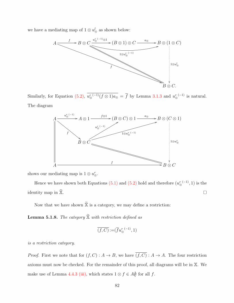
we have a mediating map of 1⊗ ul⊗ as shown below:
Af //
f
))
B ⊗ Cur⊗
(−1)⊗1//
1⊗ul⊗(−1)
33(B ⊗ 1)⊗ C a⊗ // B ⊗ (1⊗ C)
1⊗ul⊗
��B ⊗ C.
Similarly, for Equation (5.2), ur⊗(−1)(f ⊗ 1)a⊗ = f by Lemma 3.1.3 and ur⊗
(−1) is natural.
The diagram
Aur⊗
(−1)
//
f
""
A⊗ 1f⊗1 // (B ⊗ C)⊗ 1
a⊗ // B ⊗ (C ⊗ 1)
1⊗ur⊗
��
B ⊗ C
ur⊗(−1)
88
1⊗ur⊗(−1)
33
Af // B ⊗ C
shows our mediating map is 1⊗ ur⊗.
Hence we have shown both Equations (5.1) and (5.2) hold and therefore (ur⊗(−1), 1) is the
identity map in X.
Now that we have shown X is a category, we may define a restriction:
Lemma 5.1.8. The category X with restriction defined as
(f, C) :=(fur⊗(−1), 1)
is a restriction category.
Proof. First we note that for (f, C) : A→ B, we have (f, C) : A→ A. The four restriction
axioms must now be checked. For the remainder of this proof, all diagrams will be in X. We
make use of Lemma 4.4.3 (iii), which states 1⊗ f ∈ A∆∇ for all f .
82
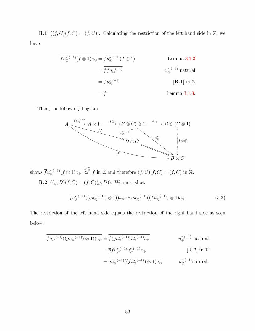
[R.1] ((f, C)(f, C) = (f, C)). Calculating the restriction of the left hand side in X, we
have:
fur⊗(−1)(f ⊗ 1)a⊗ = fur⊗
(−1)(f ⊗ 1) Lemma 3.1.3
= ffur⊗(−1) ur⊗
(−1) natural
= fur⊗(−1) [R.1] in X
= f Lemma 3.1.3.
Then, the following diagram
Afur⊗
(−1)
//
f//
ff
++
A⊗ 1f⊗1 // (B ⊗ C)⊗ 1
a⊗ //
ur⊗
##
B ⊗ (C ⊗ 1)
1⊗ur⊗
��
B ⊗ C
ur⊗(−1)
OO
B ⊗ C
shows fur⊗(−1)(f ⊗ 1)a⊗
1⊗ur⊗' f in X and therefore (f, C)(f, C) = (f, C) in X.
[R.2] ((g,D)(f, C) = (f, C)(g,D)). We must show
fur⊗(−1)((gur⊗
(−1))⊗ 1))a⊗ ' gur⊗(−1)((fur⊗
(−1))⊗ 1)a⊗. (5.3)
The restriction of the left hand side equals the restriction of the right hand side as seen
below:
fur⊗(−1)((gur⊗
(−1))⊗ 1))a⊗ = f(gur⊗(−1))ur⊗
(−1)a⊗ ur⊗(−1) natural
= gfur⊗(−1)ur⊗
(−1)a⊗ [R.2] in X
= gur⊗(−1)((fur⊗
(−1))⊗ 1)a⊗ ur⊗(−1)natural.
83
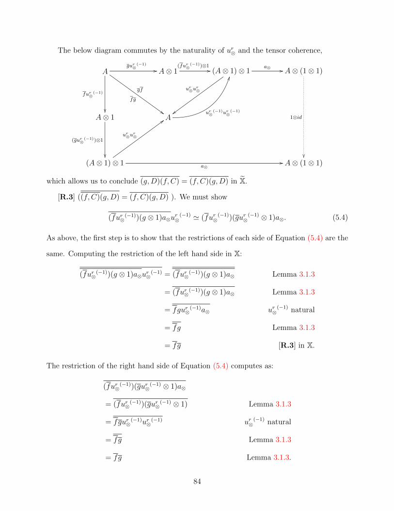
The below diagram commutes by the naturality of ur⊗ and the tensor coherence,
Agur⊗
(−1)
//
fg
gf
##
fur⊗(−1)
��
A⊗ 1(fur⊗
(−1))⊗1// (A⊗ 1)⊗ 1
a⊗ //
ur⊗ur⊗
{{
A⊗ (1⊗ 1)
1⊗id
��
A⊗ 1
(gur⊗(−1))⊗1
��
Aur⊗
(−1)ur⊗(−1)
JJ
(A⊗ 1)⊗ 1 a⊗//
ur⊗ur⊗
;;
A⊗ (1⊗ 1)
which allows us to conclude (g,D)(f, C) = (f, C)(g,D) in X.
[R.3] ((f, C)(g,D) = (f, C)(g,D) ). We must show
(fur⊗(−1))(g ⊗ 1)a⊗u
r⊗
(−1) ' (fur⊗(−1))(gur⊗
(−1) ⊗ 1)a⊗. (5.4)
As above, the first step is to show that the restrictions of each side of Equation (5.4) are the
same. Computing the restriction of the left hand side in X:
(fur⊗(−1))(g ⊗ 1)a⊗ur⊗
(−1) = (fur⊗(−1))(g ⊗ 1)a⊗ Lemma 3.1.3
= (fur⊗(−1))(g ⊗ 1)a⊗ Lemma 3.1.3
= fgur⊗(−1)a⊗ ur⊗
(−1) natural
= fg Lemma 3.1.3
= fg [R.3] in X.
The restriction of the right hand side of Equation (5.4) computes as:
(fur⊗(−1))(gur⊗
(−1) ⊗ 1)a⊗
= (fur⊗(−1))(gur⊗
(−1) ⊗ 1) Lemma 3.1.3
= fgur⊗(−1)ur⊗
(−1) ur⊗(−1) natural
= fg Lemma 3.1.3
= fg Lemma 3.1.3.
84
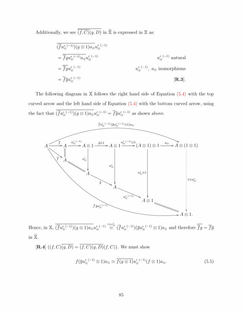
Additionally, we see (f, C)(g,D) in X is expressed in X as:
(fur⊗(−1))(g ⊗ 1)a⊗u
r⊗
(−1)
= fgur⊗(−1)a⊗u
r⊗
(−1) ur⊗(−1) natural
= fgur⊗(−1) ur⊗
(−1), a⊗ isomorphisms
= fgur⊗(−1) [R.3].
The following diagram in X follows the right hand side of Equation (5.4) with the top
curved arrow and the left hand side of Equation (5.4) with the bottom curved arrow, using
the fact that (fur⊗(−1))(g ⊗ 1)a⊗u
r⊗
(−1) = fgur⊗(−1) as shown above.
A
fur⊗(−1)(gur⊗
(−1)⊗1)a⊗
((
f gur⊗(−1)
00
f //
f##
Aur⊗
(−1)
// A⊗ 1g⊗1 //
ur⊗
��
A⊗ 1ur⊗
(−1)⊗1//
ur⊗
��
(A⊗ 1)⊗ 1a⊗ //
ur⊗⊗1
��
A⊗ (1⊗ 1)
1⊗ur⊗
��
A
A
g ''A
ur⊗(−1) ((
A⊗ 1
A⊗ 1.
Hence, in X, (fur⊗(−1))(g ⊗ 1)a⊗u
r⊗
(−1)1⊗ur⊗' (fur⊗
(−1))(gur⊗(−1) ⊗ 1)a⊗ and therefore fg = fg
in X.
[R.4] ((f, C)(g,D) = (f, C)(g,D)(f, C)). We must show
f(gur⊗(−1) ⊗ 1)a⊗ ' f(g ⊗ 1)ur⊗
(−1)(f ⊗ 1)a⊗. (5.5)
85
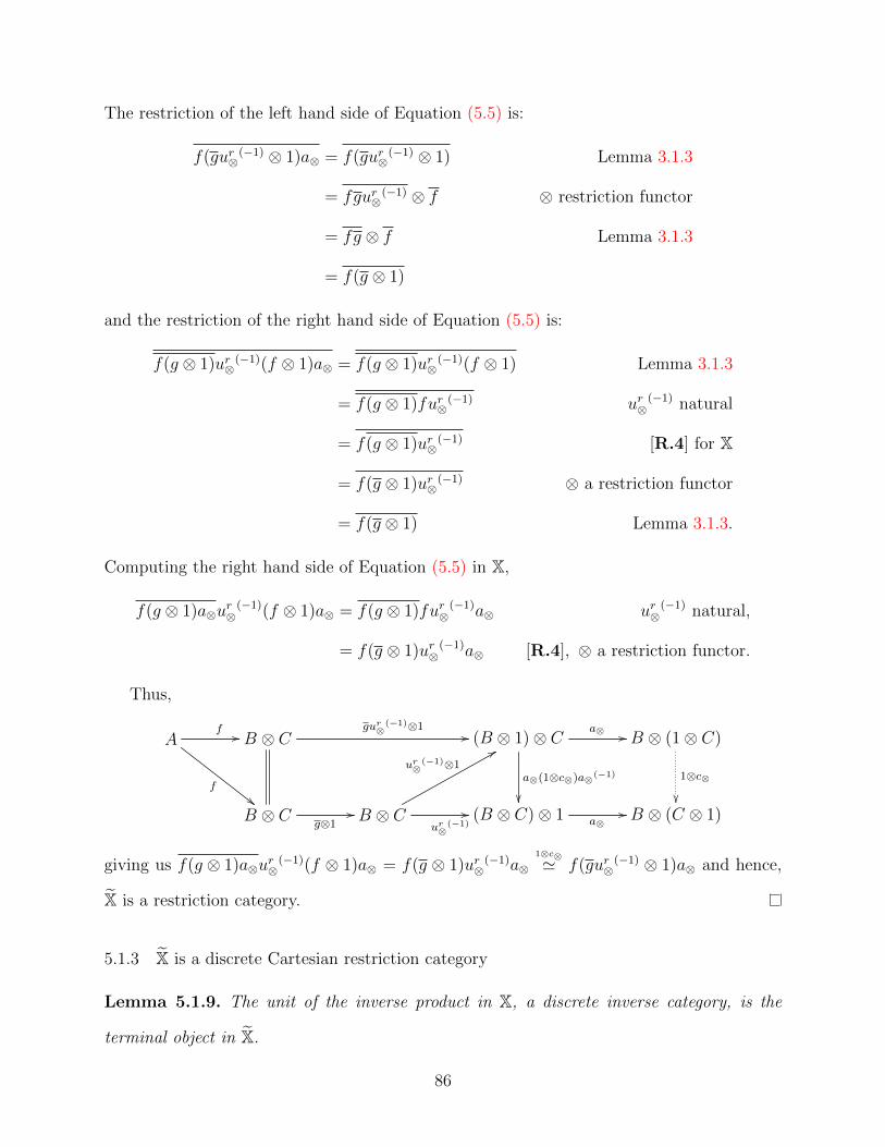
The restriction of the left hand side of Equation (5.5) is:
f(gur⊗(−1) ⊗ 1)a⊗ = f(gur⊗
(−1) ⊗ 1) Lemma 3.1.3
= fgur⊗(−1) ⊗ f ⊗ restriction functor
= fg ⊗ f Lemma 3.1.3
= f(g ⊗ 1)
and the restriction of the right hand side of Equation (5.5) is:
f(g ⊗ 1)ur⊗(−1)(f ⊗ 1)a⊗ = f(g ⊗ 1)ur⊗
(−1)(f ⊗ 1) Lemma 3.1.3
= f(g ⊗ 1)fur⊗(−1) ur⊗
(−1) natural
= f(g ⊗ 1)ur⊗(−1) [R.4] for X
= f(g ⊗ 1)ur⊗(−1) ⊗ a restriction functor
= f(g ⊗ 1) Lemma 3.1.3.
Computing the right hand side of Equation (5.5) in X,
f(g ⊗ 1)a⊗ur⊗
(−1)(f ⊗ 1)a⊗ = f(g ⊗ 1)fur⊗(−1)a⊗ ur⊗
(−1) natural,
= f(g ⊗ 1)ur⊗(−1)a⊗ [R.4], ⊗ a restriction functor.
Thus,
Af //
f
""
B ⊗ Cgur⊗
(−1)⊗1// (B ⊗ 1)⊗ C a⊗ //
a⊗(1⊗c⊗)a⊗(−1)
��
B ⊗ (1⊗ C)
1⊗c⊗
��B ⊗ C
g⊗1// B ⊗ C
ur⊗(−1)//
ur⊗(−1)⊗1
88
(B ⊗ C)⊗ 1 a⊗// B ⊗ (C ⊗ 1)
giving us f(g ⊗ 1)a⊗ur⊗
(−1)(f ⊗ 1)a⊗ = f(g ⊗ 1)ur⊗(−1)a⊗
1⊗c⊗' f(gur⊗(−1) ⊗ 1)a⊗ and hence,
X is a restriction category.
5.1.3 X is a discrete Cartesian restriction category
Lemma 5.1.9. The unit of the inverse product in X, a discrete inverse category, is the
terminal object in X.
86
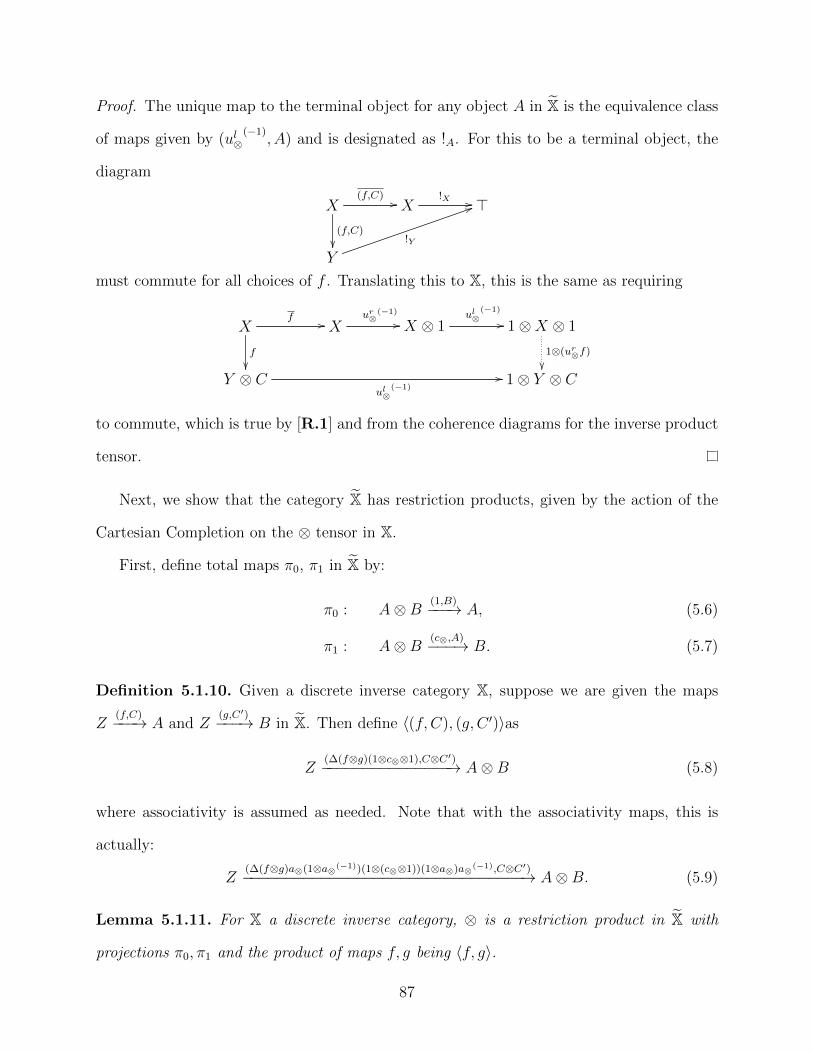
Proof. The unique map to the terminal object for any object A in X is the equivalence class
of maps given by (ul⊗(−1)
, A) and is designated as !A. For this to be a terminal object, the
diagram
X(f,C) //
(f,C)
��
X!X // >
Y
!Y
55
must commute for all choices of f . Translating this to X, this is the same as requiring
Xf //
f
��
Xur⊗
(−1)
// X ⊗ 1ul⊗
(−1)
// 1⊗X ⊗ 1
1⊗(ur⊗f)
��Y ⊗ C
ul⊗(−1)
// 1⊗ Y ⊗ C
to commute, which is true by [R.1] and from the coherence diagrams for the inverse product
tensor.
Next, we show that the category X has restriction products, given by the action of the
Cartesian Completion on the ⊗ tensor in X.
First, define total maps π0, π1 in X by:
π0 : A⊗B (1,B)−−−→ A, (5.6)
π1 : A⊗B (c⊗,A)−−−→ B. (5.7)
Definition 5.1.10. Given a discrete inverse category X, suppose we are given the maps
Z(f,C)−−−→ A and Z
(g,C′)−−−→ B in X. Then define 〈(f, C), (g, C ′)〉as
Z(∆(f⊗g)(1⊗c⊗⊗1),C⊗C′)−−−−−−−−−−−−−−−→ A⊗B (5.8)
where associativity is assumed as needed. Note that with the associativity maps, this is
actually:
Z(∆(f⊗g)a⊗(1⊗a⊗(−1))(1⊗(c⊗⊗1))(1⊗a⊗)a⊗(−1),C⊗C′)−−−−−−−−−−−−−−−−−−−−−−−−−−−−−−−−→ A⊗B. (5.9)
Lemma 5.1.11. For X a discrete inverse category, ⊗ is a restriction product in X with
projections π0, π1 and the product of maps f, g being 〈f, g〉.
87
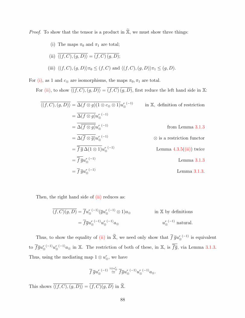
Proof. To show that the tensor is a product in X, we must show three things:
(i) The maps π0 and π1 are total;
(ii) 〈(f, C), (g,D)〉 = (f, C) (g,D);
(iii) 〈(f, C), (g,D)〉π0 ≤ (f, C) and 〈(f, C), (g,D)〉π1 ≤ (g,D).
For (i), as 1 and c⊗ are isomorphisms, the maps π0, π1 are total.
For (ii), to show 〈(f, C), (g,D)〉 = (f, C) (g,D), first reduce the left hand side in X:
〈(f, C), (g,D)〉 = ∆(f ⊗ g)(1⊗ c⊗ ⊗ 1)ur⊗(−1) in X, definition of restriction
= ∆(f ⊗ g)ur⊗(−1)
= ∆(f ⊗ g)ur⊗(−1) from Lemma 3.1.3
= ∆(f ⊗ g)ur⊗(−1) ⊗ is a restriction functor
= f g∆(1⊗ 1)ur⊗(−1) Lemma 4.3.5((ii)) twice
= f gur⊗(−1) Lemma 3.1.3
= f gur⊗(−1) Lemma 3.1.3.
Then, the right hand side of (ii) reduces as:
(f, C)(g,D) = fur⊗(−1)(gur⊗
(−1) ⊗ 1)a⊗ in X by definitions
= fgur⊗(−1)ur⊗
(−1)a⊗ ur⊗(−1) natural.
Thus, to show the equality of (ii) in X, we need only show that f gur⊗(−1) is equivalent
to fgur⊗(−1)ur⊗
(−1)a⊗ in X. The restriction of both of these, in X, is fg, via Lemma 3.1.3.
Thus, using the mediating map 1⊗ ur⊗, we have
f gur⊗(−1)
1⊗ur⊗' fgur⊗(−1)ur⊗
(−1)a⊗.
This shows 〈(f, C), (g,D)〉 = (f, C)(g,D) in X.
88
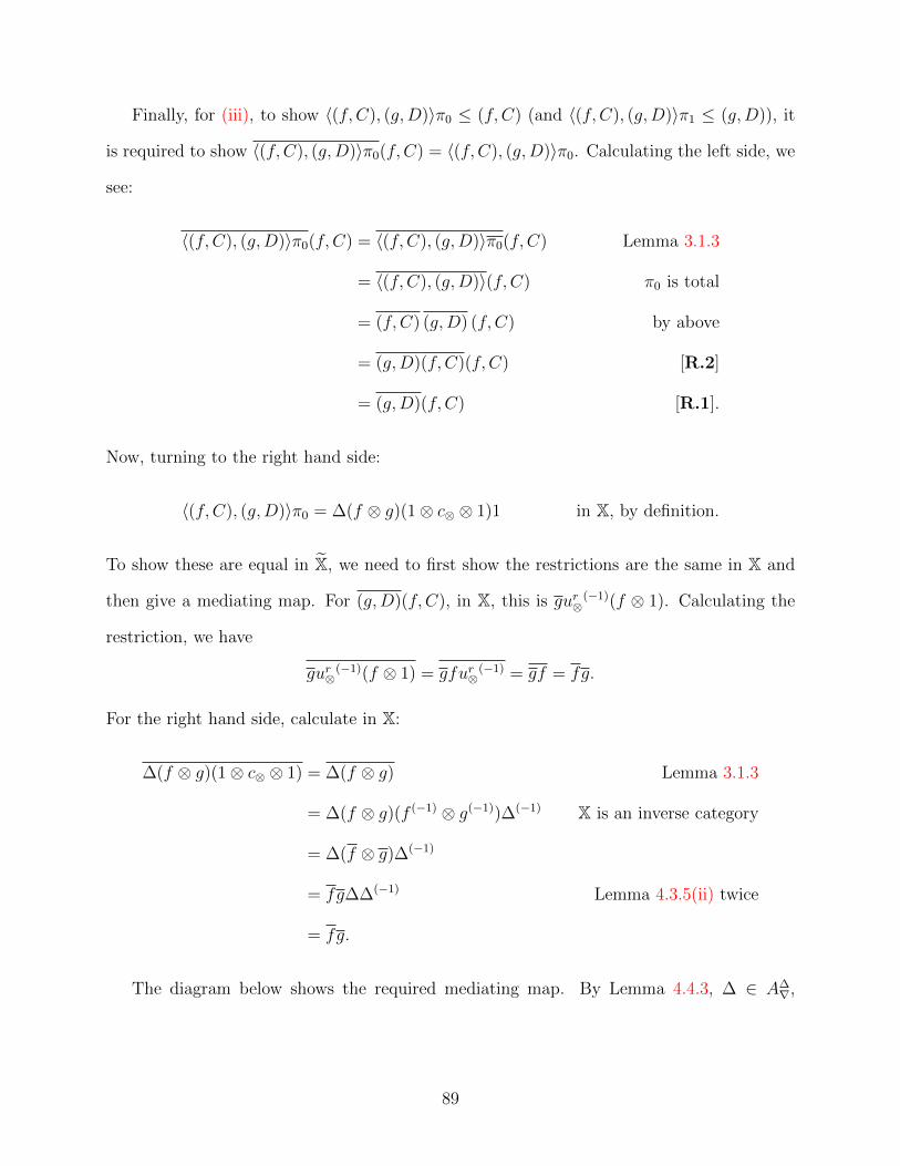
Finally, for (iii), to show 〈(f, C), (g,D)〉π0 ≤ (f, C) (and 〈(f, C), (g,D)〉π1 ≤ (g,D)), it
is required to show 〈(f, C), (g,D)〉π0(f, C) = 〈(f, C), (g,D)〉π0. Calculating the left side, we
see:
〈(f, C), (g,D)〉π0(f, C) = 〈(f, C), (g,D)〉π0(f, C) Lemma 3.1.3
= 〈(f, C), (g,D)〉(f, C) π0 is total
= (f, C) (g,D) (f, C) by above
= (g,D)(f, C)(f, C) [R.2]
= (g,D)(f, C) [R.1].
Now, turning to the right hand side:
〈(f, C), (g,D)〉π0 = ∆(f ⊗ g)(1⊗ c⊗ ⊗ 1)1 in X, by definition.
To show these are equal in X, we need to first show the restrictions are the same in X and
then give a mediating map. For (g,D)(f, C), in X, this is gur⊗(−1)(f ⊗ 1). Calculating the
restriction, we have
gur⊗(−1)(f ⊗ 1) = gfur⊗
(−1) = gf = fg.
For the right hand side, calculate in X:
∆(f ⊗ g)(1⊗ c⊗ ⊗ 1) = ∆(f ⊗ g) Lemma 3.1.3
= ∆(f ⊗ g)(f (−1) ⊗ g(−1))∆(−1) X is an inverse category
= ∆(f ⊗ g)∆(−1)
= fg∆∆(−1) Lemma 4.3.5(ii) twice
= fg.
The diagram below shows the required mediating map. By Lemma 4.4.3, ∆ ∈ A∆∇,
89
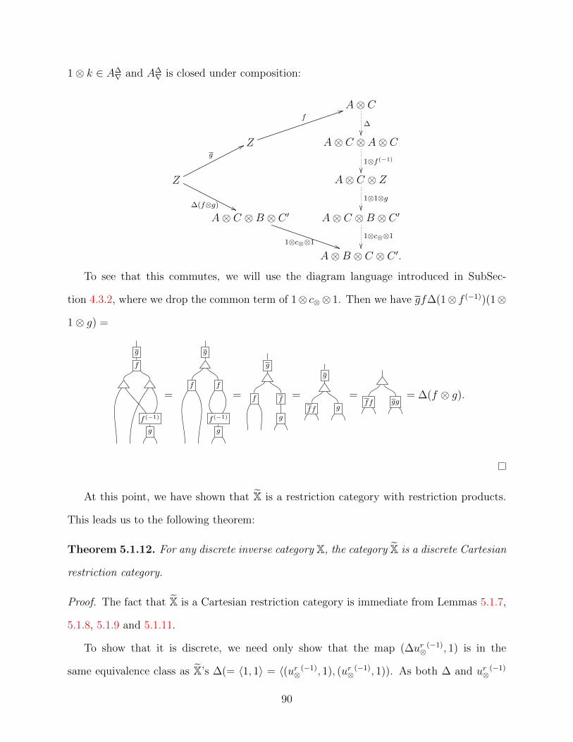
1⊗ k ∈ A∆∇ and A∆
∇ is closed under composition:
A⊗ C∆��
Z
f44
A⊗ C ⊗ A⊗ C1⊗f (−1)
��Z
g
77
∆(f⊗g) ''
A⊗ C ⊗ Z1⊗1⊗g��
A⊗ C ⊗B ⊗ C ′
1⊗c⊗⊗1 ))
A⊗ C ⊗B ⊗ C ′
1⊗c⊗⊗1
��A⊗B ⊗ C ⊗ C ′.
To see that this commutes, we will use the diagram language introduced in SubSec-
tion 4.3.2, where we drop the common term of 1⊗ c⊗⊗ 1. Then we have gf∆(1⊗ f (−1))(1⊗
1⊗ g) =
g
f
f (−1)
g
=
g
f f
f (−1)
g
=
g
f f
g
=
g
ff g
=ff gg
= ∆(f ⊗ g).
At this point, we have shown that X is a restriction category with restriction products.
This leads us to the following theorem:
Theorem 5.1.12. For any discrete inverse category X, the category X is a discrete Cartesian
restriction category.
Proof. The fact that X is a Cartesian restriction category is immediate from Lemmas 5.1.7,
5.1.8, 5.1.9 and 5.1.11.
To show that it is discrete, we need only show that the map (∆ur⊗(−1), 1) is in the
same equivalence class as X’s ∆(= 〈1, 1〉 = 〈(ur⊗(−1), 1), (ur⊗(−1), 1)). As both ∆ and ur⊗
(−1)
90

are total, the restriction of each side is the same, namely 1. The diagram below uses
Lemma 4.4.3 (iii) and shows that the two maps are in the same equivalence class:
A⊗ A⊗ 1
1⊗ur⊗(−1)
��A
∆ur⊗(−1)
33
∆(ur⊗(−1)⊗ur⊗(−1))(1⊗c⊗⊗1)
// A⊗ A⊗ 1⊗ 1.
5.2 Equivalence between the category DInv and the category DCartRest
This section will show that DInv, the category of discrete inverse categories with functors
that preserve the inverse product, is equivalent to DCartRest, the category of discrete
Cartesian restriction categories with restriction functors which preserve the product.
Here are the steps:
1. Give a functor INV from discrete Cartesian restriction categories to discrete
inverse categories and show that it is full and faithful.
2. In
Xη //
F
%%
INV(X)
INV(F#)
��INV(D)
(5.10)
we show that there exists a functor F# : X → D which makes the diagram
commute. As we have INV full and faithful, we may conclude it is unique
and that Diagram (5.10) is a universal diagram.
3. Show that η in Diagram (5.10) is an isomorphism. Note this also follows
directly from the previous point by Proposition 2.2.6 in [19].
91

Once we have completed these steps, we may then conclude that there is an equivalence.
In the following, X will always be a discrete inverse category, D and B will be discrete
Cartesian restriction categories.
The functor INV maps a discrete Cartesian restriction category to its inverse subcate-
gory. It maps a functor between discrete Cartesian restriction categories to a functor having
the same action on the partial inverses. That is, given G : B→ D, then:
INV(G) : INV(B)→ INV(D)
INV(G)(A) = GA (all objects of D are in Inv(D))
INV(G)(f) = G(f) (restriction functors preserve partial inverse).
Lemma 5.2.1. The functor INV from the category of discrete Cartesian restriction cate-
gories to the category of discrete inverse categories is full and faithful.
Proof. To show fullness, we must show INV is surjective on hom-sets. Given a functor
between two categories in the image of INV, i.e., G : INV(B) → INV(D), construct a
functor H : B→ D as follows:
Action on objects: H(A) = G(A),
Objects on maps: H(f) = G(〈f, 1〉)π0, where 〈f, 1〉 is the product map of f and 1 in B.
H is well defined as we know 〈f, 1〉 is an invertible map and therefore in the domain of
G. To see H is a functor:
H(1) = G(〈1, 1〉)π0 = ∆Dπ0 = 1,
H(fg) = G(〈fg, 1〉)π0 = 〈G(fg), 1〉π0 = G(f)〈G(g, 1)〉π0
= 〈G(f), 1〉π0〈G(g), 1〉π0 = G(〈f, 1〉)π0G(〈g, 1〉)π0 = H(f)H(g).
But on any invertible map, H(f) = G(〈f, 1〉)π0 = 〈G(f), 1〉π0 = G(f) and therefore
INV(H) = G, so INV is full.
92

Next, assume we have F,G : B → D with INV(F ) = INV(G). Considering F (f) and
F (g), we know F (〈f, 1〉) = G(〈f, 1〉) as 〈f, 1〉 is invertible. Thus, as the functors preserve
the product structure, i.e., F (π0) = π0 = G(π0), we have
F (f) = F (〈f, 1〉π0) = F (〈f, 1〉)F (π0) = G(〈f, 1〉)G(π0) = G(f).
Thus, INV is faithful.
Next, define η : X → INV(X) as an identity on objects functor. For a map f in X,
η : f 7→ (fur⊗(−1), 1). This is a functor as
η(1) = (ur⊗(−1), 1) and
η(fg) = (fgur⊗(−1), 1) ' (fur⊗
(−1), 1)(gur⊗(−1), 1) = η(f)η(g).
Now, we may define the functor F# : X → D. Recall that INV(D) is a subcategory of
D having the same objects, but only the invertible maps. Given a functor F : X→ INV(D)
define F# as follows:
On objects: F# : A 7→ F (A) ∈ Do.
On maps: F# : (f, C) 7→ F (f)π0 ∈ Dm.
We will now show (5.10) is a universal diagram.
Lemma 5.2.2. Diagram (5.10) above commutes and is a universal diagram. That is,
ηINV(F#) = F
and F# is unique.
93
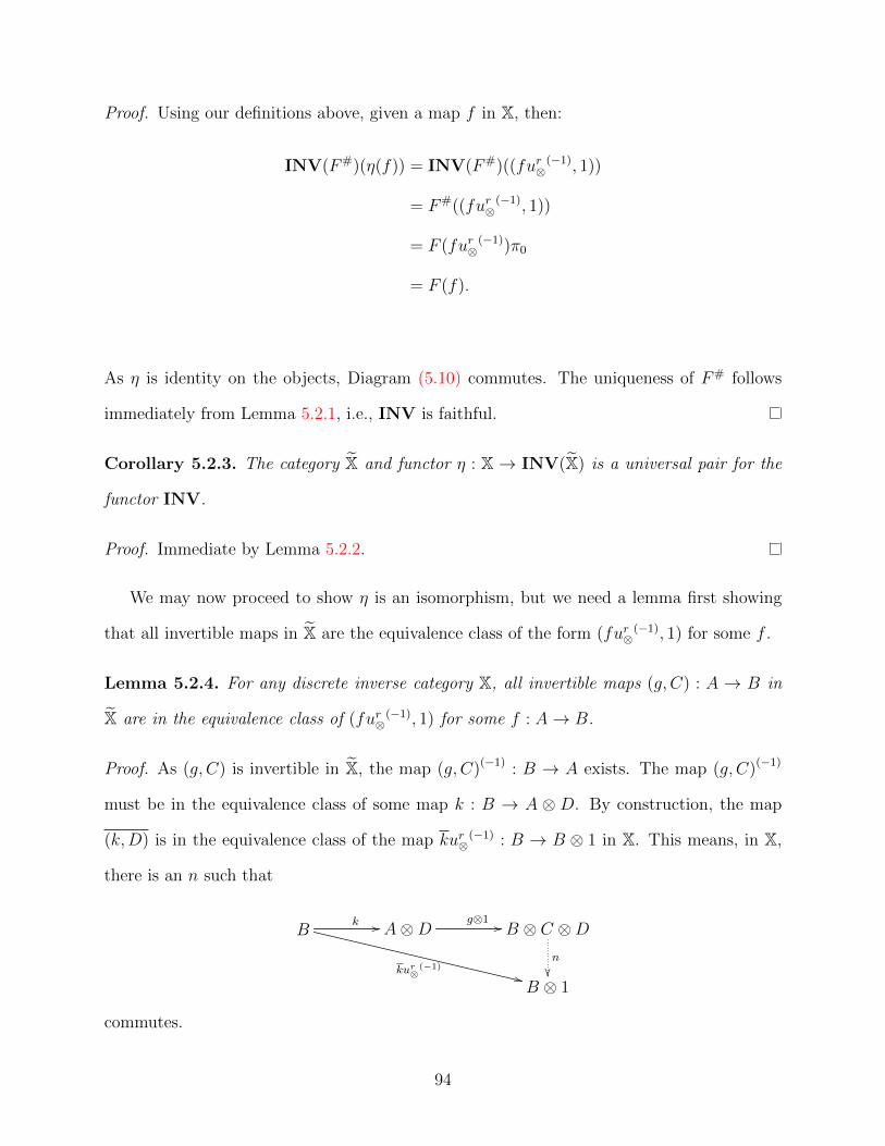
Proof. Using our definitions above, given a map f in X, then:
INV(F#)(η(f)) = INV(F#)((fur⊗(−1), 1))
= F#((fur⊗(−1), 1))
= F (fur⊗(−1))π0
= F (f).
As η is identity on the objects, Diagram (5.10) commutes. The uniqueness of F# follows
immediately from Lemma 5.2.1, i.e., INV is faithful.
Corollary 5.2.3. The category X and functor η : X → INV(X) is a universal pair for the
functor INV.
Proof. Immediate by Lemma 5.2.2.
We may now proceed to show η is an isomorphism, but we need a lemma first showing
that all invertible maps in X are the equivalence class of the form (fur⊗(−1), 1) for some f .
Lemma 5.2.4. For any discrete inverse category X, all invertible maps (g, C) : A → B in
X are in the equivalence class of (fur⊗(−1), 1) for some f : A→ B.
Proof. As (g, C) is invertible in X, the map (g, C)(−1) : B → A exists. The map (g, C)(−1)
must be in the equivalence class of some map k : B → A ⊗ D. By construction, the map
(k,D) is in the equivalence class of the map kur⊗(−1) : B → B ⊗ 1 in X. This means, in X,
there is an n such that
Bk //
kur⊗(−1)
++
A⊗D g⊗1 // B ⊗ C ⊗Dn
��B ⊗ 1
commutes.
94
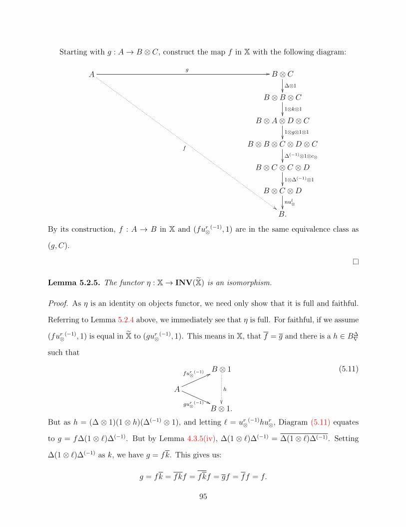
Starting with g : A→ B ⊗ C, construct the map f in X with the following diagram:
Ag //
f
##
B ⊗ C∆⊗1��
B ⊗B ⊗ C1⊗k⊗1��
B ⊗ A⊗D ⊗ C1⊗g⊗1⊗1��
B ⊗B ⊗ C ⊗D ⊗ C∆(−1)⊗1⊗c⊗��
B ⊗ C ⊗ C ⊗D1⊗∆(−1)⊗1��
B ⊗ C ⊗Dnul⊗��B.
By its construction, f : A → B in X and (fur⊗(−1), 1) are in the same equivalence class as
(g, C).
Lemma 5.2.5. The functor η : X→ INV(X) is an isomorphism.
Proof. As η is an identity on objects functor, we need only show that it is full and faithful.
Referring to Lemma 5.2.4 above, we immediately see that η is full. For faithful, if we assume
(fur⊗(−1), 1) is equal in X to (gur⊗
(−1), 1). This means in X, that f = g and there is a h ∈ B∆∇
such that
B ⊗ 1
h
��
A
fur⊗(−1) 66
gur⊗(−1) ((
B ⊗ 1.
(5.11)
But as h = (∆ ⊗ 1)(1 ⊗ h)(∆(−1) ⊗ 1), and letting ` = ur⊗(−1)hur⊗, Diagram (5.11) equates
to g = f∆(1 ⊗ `)∆(−1). But by Lemma 4.3.5(iv), ∆(1 ⊗ `)∆(−1) = ∆(1⊗ `)∆(−1). Setting
∆(1⊗ `)∆(−1) as k, we have g = fk. This gives us:
g = fk = fkf = fkf = gf = ff = f.
95
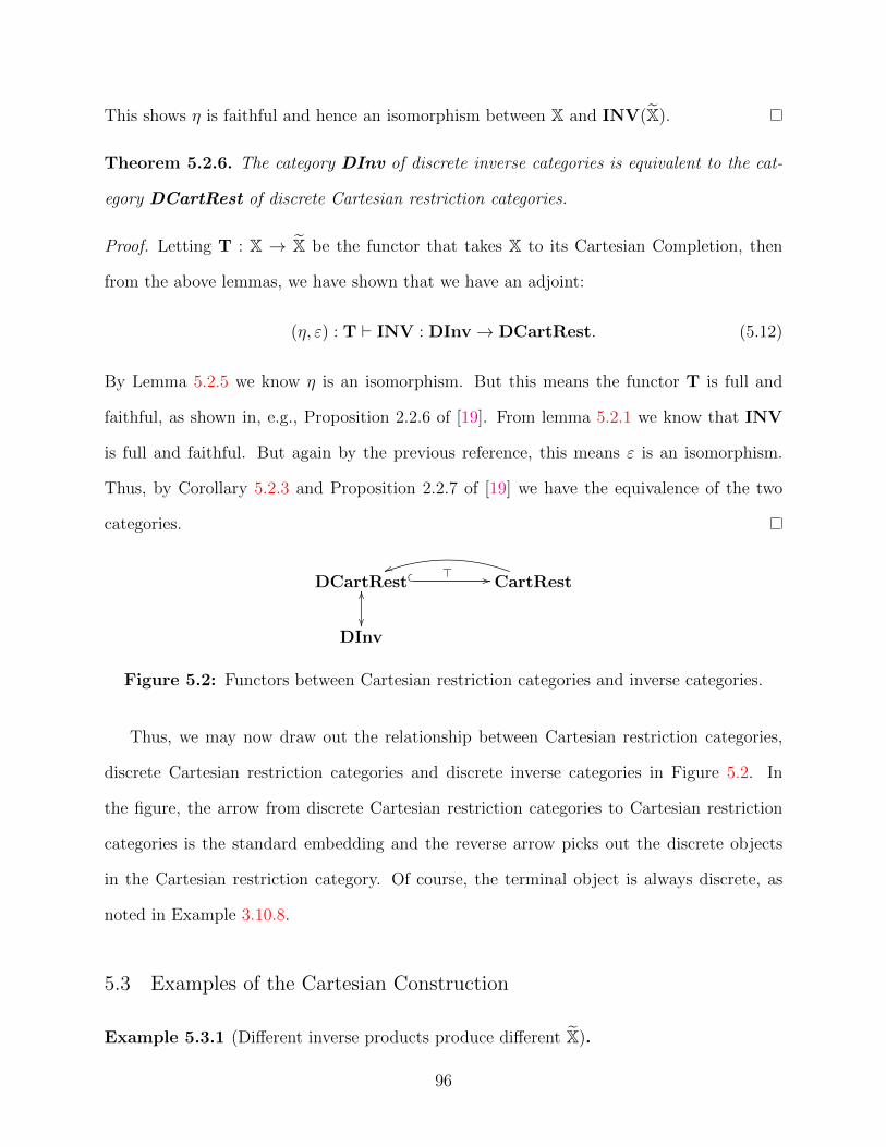
This shows η is faithful and hence an isomorphism between X and INV(X).
Theorem 5.2.6. The category DInv of discrete inverse categories is equivalent to the cat-
egory DCartRest of discrete Cartesian restriction categories.
Proof. Letting T : X → X be the functor that takes X to its Cartesian Completion, then
from the above lemmas, we have shown that we have an adjoint:
(η, ε) : T ` INV : DInv→ DCartRest. (5.12)
By Lemma 5.2.5 we know η is an isomorphism. But this means the functor T is full and
faithful, as shown in, e.g., Proposition 2.2.6 of [19]. From lemma 5.2.1 we know that INV
is full and faithful. But again by the previous reference, this means ε is an isomorphism.
Thus, by Corollary 5.2.3 and Proposition 2.2.7 of [19] we have the equivalence of the two
categories.
DCartRest� � > // CartRest
uu
DInv��
OO
Figure 5.2: Functors between Cartesian restriction categories and inverse categories.
Thus, we may now draw out the relationship between Cartesian restriction categories,
discrete Cartesian restriction categories and discrete inverse categories in Figure 5.2. In
the figure, the arrow from discrete Cartesian restriction categories to Cartesian restriction
categories is the standard embedding and the reverse arrow picks out the discrete objects
in the Cartesian restriction category. Of course, the terminal object is always discrete, as
noted in Example 3.10.8.
5.3 Examples of the Cartesian Construction
Example 5.3.1 (Different inverse products produce different X).
96

Continuing from Example 4.3.4, recall the discrete category of 4 elements with two dif-
ferent tensors. Completing these gives two different lattices: The straight line lattice and
the diamond semi-lattice. Below are the details of these constructions.
Recall D has four elements a, b, c and d, and there are two possible inverse product tensors,
given in Table 4.1. (Repeated here for your convenience).
⊗ a b c d
a a a a ab a b b bc a b c cd a b c d
� a b c d
a a a a ab a b a bc a a c cd a b c d
Table 5.1: Two different inverse products on the same category.
Define ∆ as the identity map. Then, for the first tensor, ⊗ of Table 4.1, D has the
following maps
a(id,a) (≡(id,b)≡(id,c)≡(id,d))−−−−−−−−−−−−−−−−→ a, a
(id,a)−−−→ b, a(id,a)−−−→ c, a
(id,a)−−−→ d
b(id,b) (≡(id,c)≡(id,d))−−−−−−−−−−−−→ b, b
(id,b)−−−→ c, b(id,b)−−−→ d
c(id,c) (≡(id,d))−−−−−−−−→ c, c
(id,c)−−−→ d
d(id,d)−−−→ d.
This shows D is the straight-line (a → b → c → d) lattice. The tensor in D becomes the
meet and hence is a categorical product in D. Note that the only partial inverses in D are
the identity functions and that for all maps f , 〈f, 1〉 = id.
With the second tensor, � from Table 4.1, we have:
a(id,a) (≡(id,b)≡(id,c)≡(id,d))−−−−−−−−−−−−−−−−→ a, a
(id,a)−−−→ b, a(id,a)−−−→ c, a
(id,a)−−−→ d
b(id,b) (≡(id,d))−−−−−−−−→ b, b
(id,b)−−−→ d
c(id,c) (≡(id,d))−−−−−−−−→ c, c
(id,c)−−−→ d
d(id,d)−−−→ d.
97
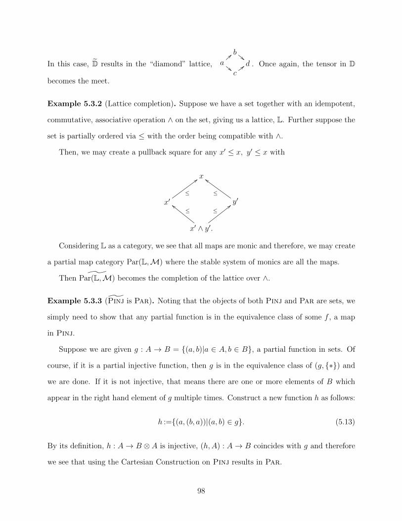
In this case, D results in the “diamond” lattice,
b!!
a
==
""d
c<< . Once again, the tensor in D
becomes the meet.
Example 5.3.2 (Lattice completion). Suppose we have a set together with an idempotent,
commutative, associative operation ∧ on the set, giving us a lattice, L. Further suppose the
set is partially ordered via ≤ with the order being compatible with ∧.
Then, we may create a pullback square for any x′ ≤ x, y′ ≤ x with
x
x′≤
;;
y′≤
cc
x′ ∧ y′.
≤bb
≤<<
Considering L as a category, we see that all maps are monic and therefore, we may create
a partial map category Par(L,M) where the stable system of monics are all the maps.
Then ˜Par(L,M) becomes the completion of the lattice over ∧.
Example 5.3.3 (Pinj is Par). Noting that the objects of both Pinj and Par are sets, we
simply need to show that any partial function is in the equivalence class of some f , a map
in Pinj.
Suppose we are given g : A → B = {(a, b)|a ∈ A, b ∈ B}, a partial function in sets. Of
course, if it is a partial injective function, then g is in the equivalence class of (g, {∗}) and
we are done. If it is not injective, that means there are one or more elements of B which
appear in the right hand element of g multiple times. Construct a new function h as follows:
h :={(a, (b, a))|(a, b) ∈ g}. (5.13)
By its definition, h : A→ B ⊗ A is injective, (h,A) : A→ B coincides with g and therefore
we see that using the Cartesian Construction on Pinj results in Par.
98
Chapter 6
Disjointness in inverse categories
This chapter explores coproduct like structure in inverse categories. It starts by showing, that
similar to the product, having coproducts is too restrictive a notion for inverse categories:
An inverse category with a coproduct is a preorder. Nonetheless it is possible to define
coproduct like structures in an inverse category. To introduce this structure we define a
“disjointness” relation between parallel maps of an inverse category and whence a “disjoint
join” for disjoint maps. The next chapter will then show how a tensor satisfying certain
specific conditions gives rise to both a disjointness relation and a disjoint join. Such a tensor
provides the replacement for “coproducts” in an inverse category.
6.1 Coproducts in inverse categories
A restriction category can have coproducts and an initial object. For example, Par (sets
and partial functions) has coproducts.
Definition 6.1.1. In a restriction category R, a coproduct is a restriction coproduct when
the embeddings q1 and q2 are total.
Lemma 6.1.2. A restriction coproduct + in R satisfies:
(i) f + g = f + g which means + is a restriction functor.
(ii) ∇ : A+ A→ A is total.
(iii) ? : 0→ A is total, where 0 is the initial object in the restriction category.
Proof.
99

(i) + is a restriction functor. Consider the diagram:
Af //
q1
!!
A′
q′1
""A+B
f+g // A′ +B′
B g//
q2
==
B′.
q′2
<<
In order to show f + g = f +g, it suffices to show that q1f + g = q1(f +g) =
fq1.
q1f + g = q1(f + g)q1 [R.4]
= fq′1q1 coproduct diagram
= fq′1q1 Lemma 3.1.3[(iii)]
= fq1 q′1 total.
(ii) ∇ : A+A→ A is total. By the definition of ∇ (= 〈1|1〉) and the coproduct,
the following diagram commutes,
A+ A
∇
��A
q1
==
A A
q2
aa
resulting in:
q1∇ = q1∇q1 = 1q1 = q1.
Similarly, q2∇ = q2, hence, the restriction of ∇ is 1 and therefore ∇ is total.
(iii) ? : 0→ A is total. This follows from
0
?
q2 // A+ 0
A
so ? can be defined as the total coproduct injection.
100
Recall that when an object is both initial and terminal, it is referred to as a zero object
and denoted as 0. This gives rise to the zero map 0A,B : A → 0 → B between any two
objects. Note that for all f : D → A, g : B → C, we have f0A,Bg = 0D,C as this factors
through the zero object.
Definition 6.1.3. Given a restriction category X with a zero object, then 0 is a restriction
zero when for each object A in X, 0A,A = 0A,A.
Lemma 6.1.4 (Cockett-Lack [23], Lemma 2.7). For a restriction category X, the following
are equivalent:
(i) X has a restriction zero;
(ii) X has an initial object 0 and terminal object 1 and each initial map zA is a
restriction monic;
(iii) X has a terminal object 1 and each terminal map tA is a restriction retraction.
6.1.1 Inverse categories with restriction coproducts
Proposition 6.1.5. An inverse category X with restriction coproducts is a preorder.
Proof. By Lemma 6.1.2, ∇ is total and therefore ∇∇(−1) = 1. From the coproduct dia-
grams, q1∇ = 1 and q2∇ = 1. But this gives ∇(−1)q1(−1) = (q1∇)(−1) = 1 and similarly
∇(−1)q2(−1) = 1. Hence, ∇(−1) = q1 and ∇(−1) = q2.
This means for parallel maps f, g : A→ B,
f = q1[f, g] = ∇(−1)[f, g] = q2[f, g] = g
and therefore X is a preorder.
101
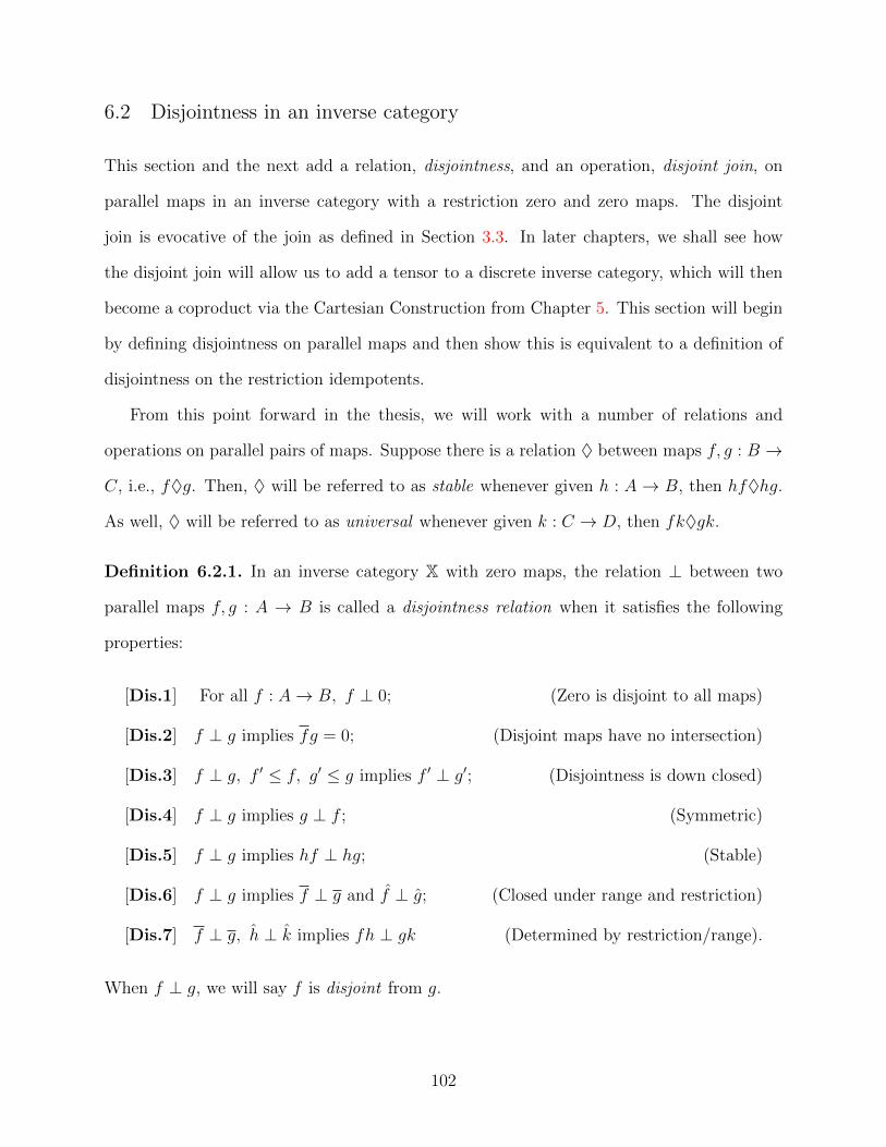
6.2 Disjointness in an inverse category
This section and the next add a relation, disjointness, and an operation, disjoint join, on
parallel maps in an inverse category with a restriction zero and zero maps. The disjoint
join is evocative of the join as defined in Section 3.3. In later chapters, we shall see how
the disjoint join will allow us to add a tensor to a discrete inverse category, which will then
become a coproduct via the Cartesian Construction from Chapter 5. This section will begin
by defining disjointness on parallel maps and then show this is equivalent to a definition of
disjointness on the restriction idempotents.
From this point forward in the thesis, we will work with a number of relations and
operations on parallel pairs of maps. Suppose there is a relation ♦ between maps f, g : B →
C, i.e., f♦g. Then, ♦ will be referred to as stable whenever given h : A → B, then hf♦hg.
As well, ♦ will be referred to as universal whenever given k : C → D, then fk♦gk.
Definition 6.2.1. In an inverse category X with zero maps, the relation ⊥ between two
parallel maps f, g : A → B is called a disjointness relation when it satisfies the following
properties:
[Dis.1] For all f : A→ B, f ⊥ 0; (Zero is disjoint to all maps)
[Dis.2] f ⊥ g implies fg = 0; (Disjoint maps have no intersection)
[Dis.3] f ⊥ g, f ′ ≤ f, g′ ≤ g implies f ′ ⊥ g′; (Disjointness is down closed)
[Dis.4] f ⊥ g implies g ⊥ f ; (Symmetric)
[Dis.5] f ⊥ g implies hf ⊥ hg; (Stable)
[Dis.6] f ⊥ g implies f ⊥ g and f ⊥ g; (Closed under range and restriction)
[Dis.7] f ⊥ g, h ⊥ k implies fh ⊥ gk (Determined by restriction/range).
When f ⊥ g, we will say f is disjoint from g.
102

Lemma 6.2.2. In 6.2.1, given [Dis.1-5], the axioms [Dis.6] and [Dis.7] may be replaced
by:
[Dis.6’] f ⊥ g ⇐⇒ f ⊥ g and f ⊥ g.
Proof. First, we show [Dis.6] and [Dis.7] imply [Dis.6’]:
Given [Dis.6], the =⇒ direction of [Dis.6’] is immediate. To show the other direction,
assume f ⊥ g and f ⊥ g. This also means that f ⊥ g. Then, by [Dis.7], ff ⊥ gg and
therefore f ⊥ g. Thus [Dis.6] and [Dis.7] imply [Dis.6’].
Next, we must show [Dis.6’] implies [Dis.6] and [Dis.7]:
Given [Dis.6’], [Dis.6] follows immediately. To show [Dis.7], assume f ⊥ g, h ⊥ k. As
fh ≤ f and gk ≤ g, [Dis.3] gives us that fh ⊥ gk. Similarly, fh ≤ h and gk ≤ k, giving us
fh ⊥ gk. Then, from [Dis.6’] we may conclude fh ⊥ gk, showing [Dis.7] holds.
Lemma 6.2.3. In an inverse category X with ⊥ a disjointness relation:
(i) f ⊥ g if and only if f (−1) ⊥ g(−1);
(ii) f ⊥ g implies fh ⊥ gh (Universal);
(iii) f ⊥ g implies fg = 0;
(iv) if m,n are monic, then fm ⊥ gn implies f ⊥ g;
(v) if m,n are monic, then m(−1)f ⊥ n(−1)g implies f ⊥ g.
Proof.
(i) Assume f ⊥ g. By [Dis.6], f ⊥ g and f ⊥ g. Since f = f (−1) and f = f (−1),
this means f (−1) ⊥ g(−1) and f (−1) ⊥ g(−1). By [Dis.6’] from Lemma 6.2.2,
f (−1) ⊥ g(−1). The converse follows with a similar argument.
(ii) Assume f ⊥ g. By (i), f (−1) ⊥ g(−1). By [Dis.5], h(−1)f (−1) ⊥ h(−1)g(−1),
giving (fh)(−1) ⊥ (gh)(−1). Applying (i), we now have fh ⊥ gh.
103
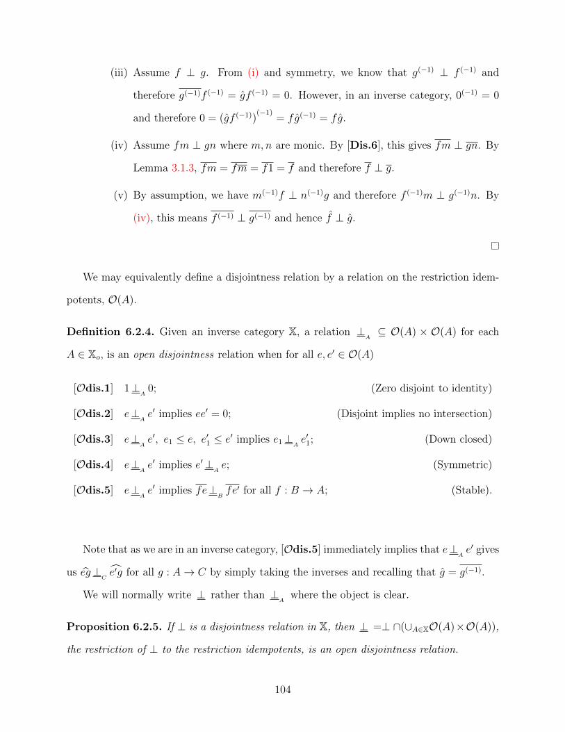
(iii) Assume f ⊥ g. From (i) and symmetry, we know that g(−1) ⊥ f (−1) and
therefore g(−1)f (−1) = gf (−1) = 0. However, in an inverse category, 0(−1) = 0
and therefore 0 = (gf (−1))(−1)
= fg(−1) = fg.
(iv) Assume fm ⊥ gn where m,n are monic. By [Dis.6], this gives fm ⊥ gn. By
Lemma 3.1.3, fm = fm = f1 = f and therefore f ⊥ g.
(v) By assumption, we have m(−1)f ⊥ n(−1)g and therefore f (−1)m ⊥ g(−1)n. By
(iv), this means f (−1) ⊥ g(−1) and hence f ⊥ g.
We may equivalently define a disjointness relation by a relation on the restriction idem-
potents, O(A).
Definition 6.2.4. Given an inverse category X, a relation ⊥A⊆ O(A) × O(A) for each
A ∈ Xo, is an open disjointness relation when for all e, e′ ∈ O(A)
[Odis.1] 1⊥A
0; (Zero disjoint to identity)
[Odis.2] e⊥Ae′ implies ee′ = 0; (Disjoint implies no intersection)
[Odis.3] e⊥Ae′, e1 ≤ e, e′1 ≤ e′ implies e1⊥A
e′1; (Down closed)
[Odis.4] e⊥Ae′ implies e′⊥
Ae; (Symmetric)
[Odis.5] e⊥Ae′ implies fe⊥
Bfe′ for all f : B → A; (Stable).
Note that as we are in an inverse category, [Odis.5] immediately implies that e⊥Ae′ gives
us eg⊥Ce′g for all g : A→ C by simply taking the inverses and recalling that g = g(−1).
We will normally write ⊥ rather than ⊥A
where the object is clear.
Proposition 6.2.5. If ⊥ is a disjointness relation in X, then ⊥ =⊥ ∩(∪A∈XO(A)×O(A)),
the restriction of ⊥ to the restriction idempotents, is an open disjointness relation.
104
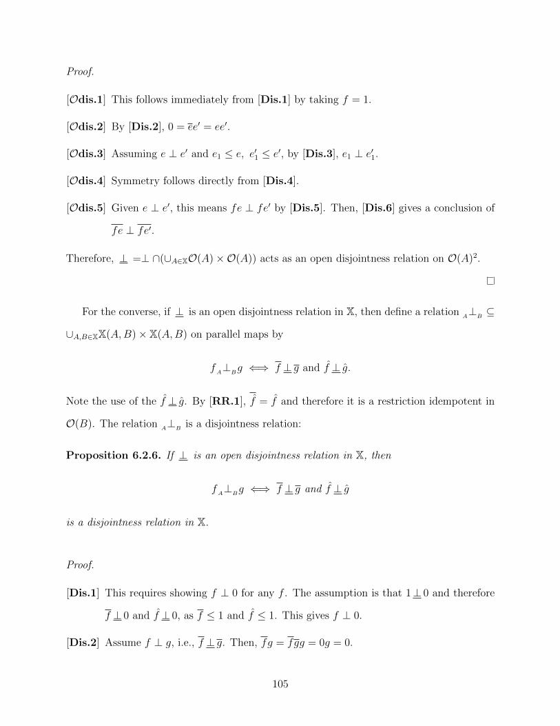
Proof.
[Odis.1] This follows immediately from [Dis.1] by taking f = 1.
[Odis.2] By [Dis.2], 0 = ee′ = ee′.
[Odis.3] Assuming e ⊥ e′ and e1 ≤ e, e′1 ≤ e′, by [Dis.3], e1 ⊥ e′1.
[Odis.4] Symmetry follows directly from [Dis.4].
[Odis.5] Given e ⊥ e′, this means fe ⊥ fe′ by [Dis.5]. Then, [Dis.6] gives a conclusion of
fe ⊥ fe′.
Therefore, ⊥ =⊥ ∩(∪A∈XO(A)×O(A)) acts as an open disjointness relation on O(A)2.
For the converse, if ⊥ is an open disjointness relation in X, then define a relationA⊥
B⊆
∪A,B∈XX(A,B)× X(A,B) on parallel maps by
fA⊥
Bg ⇐⇒ f ⊥ g and f ⊥ g.
Note the use of the f ⊥ g. By [RR.1], f = f and therefore it is a restriction idempotent in
O(B). The relationA⊥
Bis a disjointness relation:
Proposition 6.2.6. If ⊥ is an open disjointness relation in X, then
fA⊥
Bg ⇐⇒ f ⊥ g and f ⊥ g
is a disjointness relation in X.
Proof.
[Dis.1] This requires showing f ⊥ 0 for any f . The assumption is that 1⊥ 0 and therefore
f ⊥ 0 and f ⊥ 0, as f ≤ 1 and f ≤ 1. This gives f ⊥ 0.
[Dis.2] Assume f ⊥ g, i.e., f ⊥ g. Then, fg = fgg = 0g = 0.
105
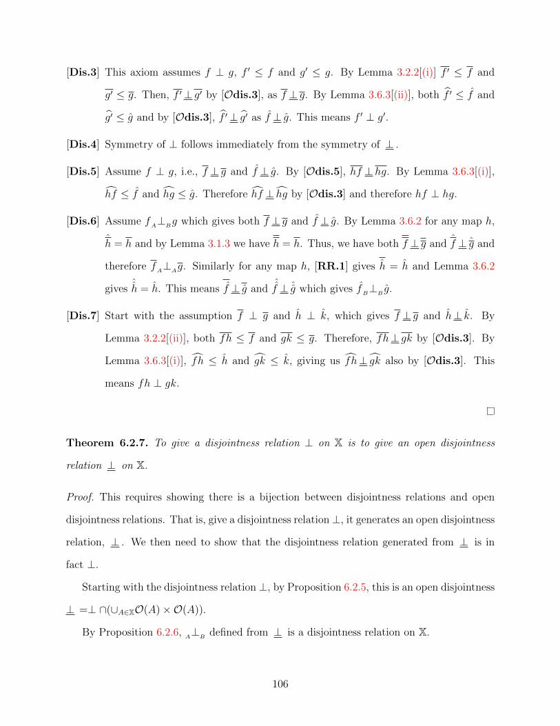
[Dis.3] This axiom assumes f ⊥ g, f ′ ≤ f and g′ ≤ g. By Lemma 3.2.2[(i)] f ′ ≤ f and
g′ ≤ g. Then, f ′⊥ g′ by [Odis.3], as f ⊥ g. By Lemma 3.6.3[(ii)], both f ′ ≤ f and
g′ ≤ g and by [Odis.3], f ′⊥ g′ as f ⊥ g. This means f ′ ⊥ g′.
[Dis.4] Symmetry of ⊥ follows immediately from the symmetry of ⊥ .
[Dis.5] Assume f ⊥ g, i.e., f ⊥ g and f ⊥ g. By [Odis.5], hf ⊥hg. By Lemma 3.6.3[(i)],
hf ≤ f and hg ≤ g. Therefore hf ⊥ hg by [Odis.3] and therefore hf ⊥ hg.
[Dis.6] Assume fA⊥
Bg which gives both f ⊥ g and f ⊥ g. By Lemma 3.6.2 for any map h,
h = h and by Lemma 3.1.3 we have h = h. Thus, we have both f ⊥ g and f ⊥ g and
therefore fA⊥
Ag. Similarly for any map h, [RR.1] gives h = h and Lemma 3.6.2
givesˆh = h. This means f ⊥ g and
ˆf ⊥ ˆg which gives f
B⊥
Bg.
[Dis.7] Start with the assumption f ⊥ g and h ⊥ k, which gives f ⊥ g and h⊥ k. By
Lemma 3.2.2[(ii)], both fh ≤ f and gk ≤ g. Therefore, fh⊥ gk by [Odis.3]. By
Lemma 3.6.3[(i)], fh ≤ h and gk ≤ k, giving us fh⊥ gk also by [Odis.3]. This
means fh ⊥ gk.
Theorem 6.2.7. To give a disjointness relation ⊥ on X is to give an open disjointness
relation ⊥ on X.
Proof. This requires showing there is a bijection between disjointness relations and open
disjointness relations. That is, give a disjointness relation⊥, it generates an open disjointness
relation, ⊥ . We then need to show that the disjointness relation generated from ⊥ is in
fact ⊥.
Starting with the disjointness relation ⊥, by Proposition 6.2.5, this is an open disjointness
⊥ =⊥ ∩(∪A∈XO(A)×O(A)).
By Proposition 6.2.6,A⊥
Bdefined from ⊥ is a disjointness relation on X.
106
Assume f ⊥ g. By [Dis.6] and Proposition 6.2.5, f ⊥ g and f ⊥ g. Then by its definition,
we have fA⊥
Bg.
Assume fA⊥
Bg, which required that both f ⊥ g and f ⊥ g. Therefore f ⊥ g and f ⊥ g.
By Proposition 6.2.3, f ⊥ g.
We have shown f ⊥ g ⇐⇒ fA⊥
Bg. We may also conclude that if we started with
an open disjointness relation ⊥ and used it to constructA⊥
B, then the relation
A⊥
B∩
(∪A∈XO(A)×O(A)) would again be ⊥ .
Hence there is a bijection between disjointness relations and open disjointness relations
on an inverse category X.
Disjointness is additional structure on a restriction category, i.e., it is possible to have
more than one disjointness relation on the category. To see this, consider the trivial disjoint-
ness relation, where f ⊥0 g if and only if f = 0 or g = 0. As 0 = 0 = 0, f ≤ 0 ⇐⇒ f = 0
and h0 = 0 for any map h, axioms [Dis.1] through [Dis.7] are immediately satisfied. ⊥0 is
definable on any inverse category with zero maps, hence is definable on Pinj.
However, Pinj does have a more useful disjointness relation:
Example 6.2.8 (Pinj has a disjointness relation). Consider the inverse category Pinj,
introduced in Example 3.1.8 and Example 4.3.2. Note the restriction zero is the empty set,
∅. Recalling that a map f : A → B in Pinj is given by the set {(a, b)|a ∈ A, b ∈ B} (see
Example 2.6.5), we see the initial map ?A : ∅ → A must be {}, i.e., the empty set. Similarly,
!A : A→ ∅ must be the partial map also given by ∅ and therefore 0A,B = ∅.
Define the disjointness relation ⊥ by f ⊥ g if and only if f ∩ g = ∅ and f ∩ g = ∅.
It is then reasonably straightforward to verify [Dis.1] through [Dis.7]. For example, take
[Dis.7]:
Proof. We are given f ⊥ g and h ⊥ k. This means
f ∩ g = ∅ and h ∩ k = ∅.
107

As discussed in Example 3.4.4, both mn ⊆ m and mn ⊆ n. Hence,
fh ∩ gk ⊆ f ∩ g = ∅
fh ∩ gk ⊆ h ∩ k = ∅.
Therefore, fh ⊥ gk.
The open disjointness relation, ⊥ , on the idempotents is given by e⊥ e′ ⇐⇒ e∩ e′ = ∅.
Although disjointness is additional structure, one can use the disjointness structure of
the base categories to define a disjointness structure on the product category.
Lemma 6.2.9. If X and Y are inverse categories with restriction zeros and respective dis-
jointness relations ⊥ and ⊥′, then there is a disjointness relation ⊥× on X× Y.
Proof. The restriction, the inverse and the restriction zero on the product category are
defined pointwise.
• If (f, g) is a map in X× Y, then (f, g)(−1) = (f (−1), g(−1));
• If (f, g) is a map in X× Y, then (f, g) = (f, g);
• The map (0X ,0Y ) is the restriction zero in X× Y.
Following this pattern, for (f, g) and (h, k) maps in X×Y, (f, g) ⊥× (h, k) iff f ⊥ h and
g ⊥′ k.
Verifying the disjointness axioms is straightforward, we show axioms 2 and 5. Proofs of
the others are similar.
[Dis.2] : Given (f, g) ⊥× (h, k), (f, g)(h, k) = (f, g)(h, k) = (fh, gk) = (0,0) = 0.
[Dis.5] : The assumption is (f, g) ⊥× (h, k). For the map z = (x, y) in X × Y, [Dis.5] in
the base categories gives xf ⊥ xh and yg ⊥ yk. Thus
z(f, g) = (xf, yg) ⊥× (xh, yk) = z(h, k).
108
6.3 Disjoint joins
This section will now consider additional structure on the inverse category, the disjoint
join, dependent upon the disjointness relation. Although we have only considered binary
disjointness up to this point, extending disjointness to sets of maps is done by considering
disjointness pairwise: ⊥ {f1, f2, . . . , fn} := fi ⊥ fk whenever i 6= j.
Definition 6.3.1. An inverse category X with a restriction 0 and a disjointness relation ⊥
has disjoint joins when there is a binary operator on disjoint parallel maps:
f : A→ B, g : A→ B, f ⊥ g
f t g : A→ B
such that the following hold:
[DJ.1] f ≤ f t g and g ≤ f t g;
[DJ.2] f ≤ h, g ≤ h and f ⊥ g implies f t g ≤ h;
[DJ.3] h(f t g) = hf t hg. (Stable)
[DJ.4] ⊥ {f, g, h} if and only if f ⊥ (g t h).
The binary operator, t, is called the disjoint join.
Given a specific disjointness relation on a category, there is only one disjoint join:
Lemma 6.3.2. Suppose X in an inverse category with a disjointness relation ⊥, then if t
and � are disjoint joins for ⊥ then t = � .
Proof. [DJ.1] gives us:
f, g ≤ f t g and f, g ≤ f � g.
By [DJ.2], f t g ≤ f � g and f � g ≤ f t g, hence f t g = f � g.
109
Lemma 6.3.3. In an inverse category with disjoint joins, the disjoint join is a partial asso-
ciative and commutative operation, with identity 0. Additionally, it respects the restriction
and is universal. That is, the following hold:
(i) f t 0 = f ;
(ii) f ⊥ g, g ⊥ h, f ⊥ h implies that (f t g) t h = f t (g t h);
(iii) f ⊥ g implies f t g = g t f ;
(iv) f t g = f t g;
(v) (f t g)k = fk t gk (t is universal).
Proof.
(i) Identity : By [DJ.1], f ≤ f t 0. As 0 ≤ f and f ≤ f , by [DJ.2], f t 0 ≤ f
and therefore f = f t 0.
(ii) Associativity : Note that [DJ.4] shows that both sides of the equation exist.
From [DJ.1] f t g, h ≤ (f t g) t h, which also means f, g ≤ (f t g) t h.
Similarly, g t h ≤ (f t g) t h and then f t (g t h) ≤ (f t g) t h. Conversely,
f, g, h ≤ f t (g t h) and therefore (f t g)t h ≤ f t (g t h) and both sides are
equal.
(iii) Commutativity : Note first that both f and g are less than or equal to each of
f t g and g t f , by [DJ.1]. By [DJ.2], f t g ≤ g t f and g t f ≤ f t g and
thus f t g = g t f .
(iv) As f, g ≤ f t g, [DJ.2] gives f t g ≤ f t g. To show the other direction,
110

consider
f(f t g)(f t g) = (f f t fg)(f t g) [DJ.3]
= (f f t 0)(f t g) [Dis.2]
= f(f t g) (i), Lemma 3.1.3
= f.
Hence, f ≤ (f t g)(f t g) and similarly, so is g. By [DJ.2] and f t g being a
restriction idempotent,
f t g ≤ (f t g)(f t g) ≤ f t g
and therefore f t g = (f t g)(f t g). By Lemma 3.2.2, f t g ≤ f t g and so
f t g = f t g.
(v) First consider when f, g and k are restriction idempotents, say e0, e1 and e2.
Then, (e0 t e1)e2 = e2(e0 t e1) = e2e0 t e2e1 = e0e2 t e1e2. Next, note that for
general f, g, h, by [DJ.2] fk t gk ≤ (f t g)k as both fk, gk ≤ (f t g)k. By
Lemma 3.2.2, we need only show that their restrictions are equal:
(f t g)k = f t g(f t g)k [R.1]
= f t g (f t g)k [R.3]
= (f t g)(f t g)k previous item
= f (f t g)k t g (f t g)k idempotent universal
= f(f t g)k t g(f t g)k [R.3]
= fk t gk [DJ.3]
= fk t gk.
Therefore, as the restrictions are equal, (f t g)k = fk t gk.
111

Note that the previous lemma and proof of associativity allows a simple inductive argu-
ment which shows that having binary disjoint joins extends to disjoint joins of an arbitrary
finite collection of disjoint maps.
Recalling our notation for disjointness of a set of maps, t{fi} will mean the disjoint join
of all maps fi, i.e., f1 t f2 t · · · t fn.
Lemma 6.3.4. In an inverse category X with disjoint joins,
(i) ⊥ {fi} if and only if t{fi} is defined,
(ii) if fi, gj : A → B and ⊥i∈I {fi} and ⊥j∈J {gj}, then ti∈I{fi} ⊥ tj∈J{gj} if
and only fi ⊥ gj for all i ∈ I and j ∈ J .
Proof. For (i), using [Dj.4], proceed as in the proof of Lemma 6.3.3[(ii)], inducting on n.
To show (ii), first assume t{fi} ⊥ t{gj}. By [Dj.4] and associativity, t{fi} ⊥ gj for
each j. Using the symmetry of ⊥, [Dj.4] and associativity, fi ⊥ gj for each i and j.
Next, assume fi ⊥ gj for each i and j. Then by [Dj.4] and associativity, fi ⊥ t{gj} for
each i. Applying [Dj.4] again, t{fi} ⊥ t{gj}.
Clearly the product of two inverse categories with disjoint joins has a disjoint join:
Lemma 6.3.5. Given X,Y are inverse categories with disjoint joins, t and t′ respectively,
then the category X× Y is an inverse category with disjoint joins.
Proof. From Lemma 6.2.9, X×Y has a disjointness relation that is defined point-wise. Define
t× the disjoint join on X× Y by
(f, g) t× (h, k) = (f t h, g t′ k). (6.1)
It remains to prove each of the axioms in Definition 6.3.1 hold.
[DJ.1] From Equation (6.1), since f, h ≤ fth and g, k ≤ gt′k, both (f, g) ≤ (f, g)t×(h, k)
and (h, k) ≤ (f, g) t× (h, k).
112
[DJ.2] Suppose (f, g) ≤ (x, y), (h, k) ≤ (x, y) and (f, g) ⊥× (h, k). Then regarding it
point-wise, (f, g) t× (h, k) = (f t h, g t′ k) ≤ (x, y).
[DJ.3] Calculating,
(x, y) ((f, g) t× (h, k)) = (x(f t h), y(g t′ k)) =
(xf t xh, yg t′ yk) = (xf, yg) t× (xh, yk) =
((x, y)(f, g)) t× ((x, y)(h, k)).
[DJ.4] Given ⊥×[(f, g), (h, k), (x, y)], both f ⊥ (h t x) and g ⊥′ (k t′ y). Hence, (f, g) ⊥×
((h, k) t× (x, y)). The opposite direction is similar.
Example 6.3.6 (Pinj has a disjoint join). Continuing from Example 6.2.8, we show that
Pinj has disjoint joins. If f = {(a, b)} and g = {(a′, b′)} are disjoint parallel maps in Pinj
from A to B, define f t g :={(a′′, b′′)|(a′′, b′′) ∈ f or (a′′, b′′) ∈ g}, i.e., the union of f and g.
This is still a partial injective map, due to the requirement of disjointness. Recall that
f ⊥ g means that f ∩ g = ∅ and f ∩ g = ∅ and that the respective meets will also be ∅. The
empty meet of the restrictions means that f t g is still a partial function, as each a′′ will
appear only once. The empty meet of the ranges gives us that f t g is injective, because
each b′′ is unique.
The axioms for disjoint joins all hold:
[DJ.1] By construction, both f and g are less than f t g.
[DJ.2] f ≤ h, g ≤ h means that h must contain all of the (a, b) ∈ f and (a′, b′) ∈ g
and therefore f t g ≤ h.
113
[DJ.3] Suppose h : C → A = {(c, a)}. Then
h(f t g) = {(c, b)|(∃a, a.a = a, (a, b) ∈ f, (c, a) ∈ h)
or (∃a′, a.a = a′, (a′, b) ∈ g, (c, a) ∈ h)}
= {(c, b)|∃a, a.a = a, (a, b) ∈ f, (c, a) ∈ h}⋃
{(c, b)|∃a′, a.a = a′, (a′, b) ∈ g, (c, a) ∈ h}
= hf t hg.
[DJ.4] Suppose ⊥ [f, f ′, f ′′], f = {(a, b)}, f ′ = {(a′, b′)}, f ′′ = {(a′′, b′′)}. Then the
set {a} intersects neither {a′} nor {a′′} and similarly for the sets {b}, {b′} and
{b′′}. Thus we have f ⊥ (g t h). The reverse direction is argued similarly.
114
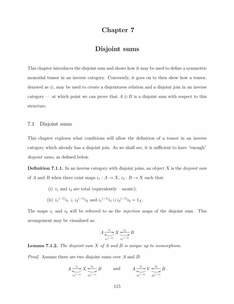
Chapter 7
Disjoint sums
This chapter introduces the disjoint sum and shows how it may be used to define a symmetric
monoidal tensor in an inverse category. Conversely, it goes on to then show how a tensor,
denoted as ⊕, may be used to create a disjointness relation and a disjoint join in an inverse
category — at which point we can prove that A ⊕ B is a disjoint sum with respect to this
structure.
7.1 Disjoint sums
This chapter explores what conditions will allow the definition of a tensor in an inverse
category which already has a disjoint join. As we shall see, it is sufficient to have “enough”
disjoint sums, as defined below.
Definition 7.1.1. In an inverse category with disjoint joins, an object X is the disjoint sum
of A and B when there exist maps i1 : A→ X, i2 : B → X such that:
(i) i1 and i2 are total (equivalently – monic);
(ii) i1(−1)i1 ⊥ i2
(−1)i2 and i1(−1)i1 t i2(−1)i2 = 1X .
The maps i1 and i2 will be referred to as the injection maps of the disjoint sum. This
arrangement may be visualized as:
Ai1 // X
i1(−1)
ff
i1(−1)
88 Bi2oo
Lemma 7.1.2. The disjoint sum X of A and B is unique up to isomorphism.
Proof. Assume there are two disjoint sums over A and B:
Ai1 // X
i1(−1)
ff
i2(−1)
88 Bi2oo and A
j1 // Y
j1(−1)
ff
j2(−1)
88 Bj2oo .
115
We will show that the map i1(−1)j1 t i2(−1)j2 : X → Y is an isomorphism.
Note by the fact that i1, i2 are monic and [Dis.2], 0 = i1(−1)i1i2
(−1) = i1(−1)i1i2
(−1) =
i1(−1)i2
(−1) = i1i2(−1). But then i1i2
(−1) = i1i1i2(−1) = i10 = 0. Similarly, i2i1
(−1) = 0,
j1j2(−1) = 0 and j2j1
(−1) = 0.
Next, by Lemma 6.2.3, i1(−1) ⊥ i2
(−1) as both i1 and i2 are monic. By the same lemma,
j1 ⊥ j2 as j1(−1), j2
(−1) are the inverses of monic maps. Then, from [Dis.7], i1(−1)j1 ⊥ i2
(−1)j2,
hence we may form i1(−1)j1 t i2(−1)j2 : X → Y .
Similarly, we may form the map j1(−1)i1tj2
(−1)i2 : Y → X. Computing their composition:
(i1(−1)j1 t i2(−1)j2)(j1
(−1)i1 t j2(−1)i2)
= (i1(−1)j1(j1
(−1)i1 t j2(−1)i2)) t (i2(−1)j2(j1
(−1)i1 t j2(−1)i2))
= i1(−1)j1j1
(−1)i1 t i1(−1)j1j2(−1)i2 t i2(−1)j2j1
(−1)i1 t i2(−1)j2j2(−1)i2
= i1(−1) 1 i1 t i1(−1) 0 i2 t i2(−1) 0 i1 t i2(−1) 1 i2
= i1(−1)i1 t i2(−1)i2 = 1.
Computing the other direction,
(j1(−1)i1 t j2
(−1)i2)(i1(−1)j1 t i2(−1)j2)
= (j1(−1)i1(i1
(−1)j1 t i2(−1)j2)) t (j2(−1)i2(i1
(−1)j1 t i2(−1)j2))
= j1(−1)i1i1
(−1)j1 t j1(−1)i1i2
(−1)j2 t j2(−1)i2i1
(−1)j1 t j2(−1)i2i2
(−1)j2
= j1(−1) 1 j1 t j1
(−1) 0 j2 t j2(−1) 0 j1 t j2
(−1) 1 j2
= j1(−1)j1 t j2
(−1)j2 = 1.
This shows that the map between any two disjoint sums over the same two objects is an
isomorphism.
When there are “enough” disjoint sums in a category, this gives rise to tensor. In antici-
pation of the result, henceforth we will write A⊕B for the disjoint sum of A and B.
116
First, the next lemma shows how to construct maps between the disjoint sums:
Lemma 7.1.3. Given X an inverse category with all disjoint sums and suppose f : A →
C and g : B → D in X. Then i1(−1)fi1 ⊥ i2
(−1)gi2 : A ⊕ B → C ⊕ D and therefore
i1(−1)fi1 t i2(−1)gi2 : A⊕B → C ⊕D.
Proof. Note that i1(−1)fi1 = i1
(−1)f ≤ i1(−1) and similarly i2
(−1)gi2 ≤ i2(−1). Then, by
[Dis.3], we have i1(−1)fi1 ⊥ i2
(−1)gi2. Similarly, as i1(−1)fi1 ≤ i1 and i2(−1)gi2 ≤ i2, this
gives i1(−1)fi1 ⊥ i2(−1)gi2 and by Lemma 6.2.3, the conclusion is i1(−1)fi1 ⊥ i2
(−1)gi2 and
therefore the disjoint join i1(−1)fi1 t i2(−1)gi2 is a map between the two disjoint sums.
The argument in the above lemma is one we will use from time to time. In particular,
this means i1(−1)g ⊥ i2
(−1)h for arbitrary g, h and that hi1 ⊥ ki2.
Proposition 7.1.4. Given X is an inverse category where every pair of objects has a disjoint
sum, then the tensor ⊕ : X× X→ X where A⊕B is a disjoint sum of A,B is a symmetric
monoidal tensor.
Proof. It is necessary to show that ⊕ is a bi-functor and that the required structural maps
exist.
First note that f ⊕ g is given by i1(−1)fi1 t i2(−1)gi2 as shown in Lemma 7.1.3. By the
definition of the disjoint sum, identity maps are taken to identity maps and by the stability
and universality of the disjoint join, composition is preserved and therefore ⊕ is a bi-functor
as required.
We must now show the restriction zero is the unit of ⊕ and then give the structural maps.
Considering the disjoint sum A ⊕ 0, we see that i2 = 0, the zero map. This gives
1A⊕0 = i1(−1)i1t i2(−1)i2 = i1
(−1)i1t0 = i1(−1)i1 = i1
(−1), meaning i1(−1) is total. Thus, i1
(−1)
is an isomorphism and is ur⊕. Similarly, i2(−1) = ul⊕ : 0⊕ A→ A is an isomorphism.
117

For the symmetry map, note c⊕ = i1(−1)i2 t i2(−1)i1 : A⊕B → B ⊕ A and that
(i1(−1)i2 t i2(−1)i1)(i1
(−1)i2 t i2(−1)i1)
= i1(−1)i2(i1
(−1)i2 t i2(−1)i1) t i2(−1)i1(i1(−1)i2 t i2(−1)i1)
= i1(−1)i2i1
(−1)i2 t i1(−1)i2i2(−1)i1 t i2(−1)i1i1
(−1)i2 t i2(−1)i1i2(−1)i1
= 0 t 1 t 1 t 0
= 1.
Thus, c⊕c⊕ = 1.
For associativity, set a⊕ = i1(−1)i1i1 t i2(−1)i1
(−1)i2i1 t i2(−1)i2(−1)i2 : A ⊕ (B ⊕ C) →
(A⊕B)⊕ C. To visualize this,
B ⊕ C i1(−1)//
i2(−1)
''
Bi2 // A⊕B
i1
��
Ci2
&&A⊕ (B ⊕ C)
i2(−1)
OO
i1(−1)
��
a⊕ // (A⊕B)⊕ C
Ai1
// A⊕B.
i1
OO
The inverse of the a⊕ is obtained by taking the inverses of the arrows in the above diagram,
yielding i1(−1)i1
(−1)i1 t i1(−1)i2(−1)i1i1 t i2(−1)i2i2.
Thus, ⊕ is a symmetric monoidal tensor on X.
7.2 Disjointness via a tensor
The next objective is to characterize when a symmetric monoidal tensor provides a disjoint
sum. The first step will be to show how a disjointness tensor, defined below, may be used to
create a disjointness relation in an inverse category. This is done by first determining when
it is possible for maps to work separately on the components of the tensor. This ability to
118
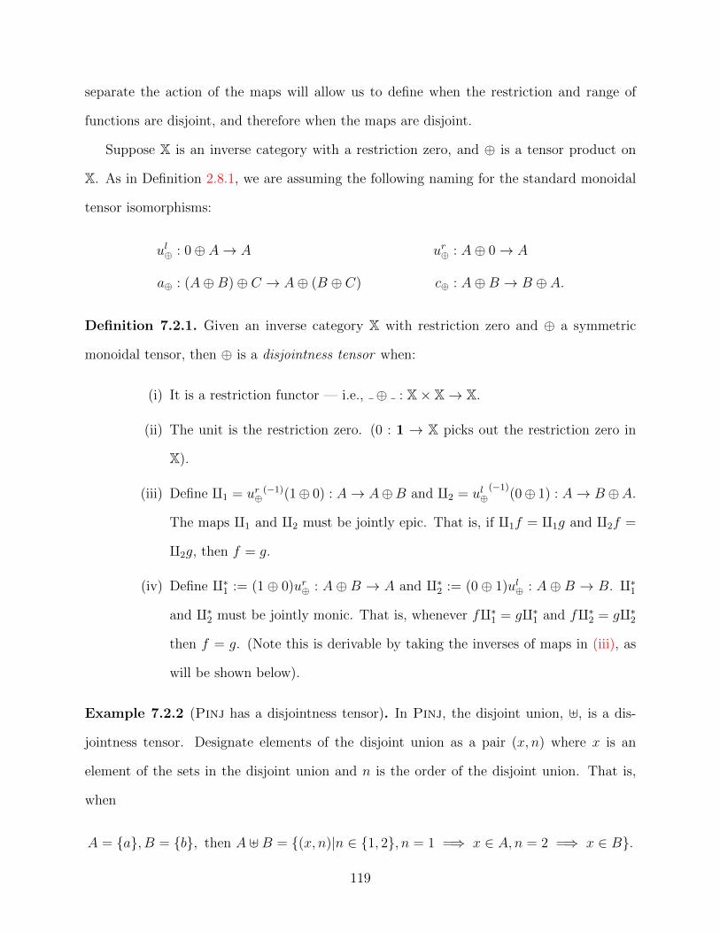
separate the action of the maps will allow us to define when the restriction and range of
functions are disjoint, and therefore when the maps are disjoint.
Suppose X is an inverse category with a restriction zero, and ⊕ is a tensor product on
X. As in Definition 2.8.1, we are assuming the following naming for the standard monoidal
tensor isomorphisms:
ul⊕ : 0⊕ A→ A ur⊕ : A⊕ 0→ A
a⊕ : (A⊕B)⊕ C → A⊕ (B ⊕ C) c⊕ : A⊕B → B ⊕ A.
Definition 7.2.1. Given an inverse category X with restriction zero and ⊕ a symmetric
monoidal tensor, then ⊕ is a disjointness tensor when:
(i) It is a restriction functor — i.e., ⊕ : X× X→ X.
(ii) The unit is the restriction zero. (0 : 1 → X picks out the restriction zero in
X).
(iii) Define q1 = ur⊕(−1)(1⊕ 0) : A→ A⊕B and q2 = ul⊕
(−1)(0⊕ 1) : A→ B ⊕A.
The maps q1 and q2 must be jointly epic. That is, if q1f = q1g and q2f =
q2g, then f = g.
(iv) Define q∗1 := (1 ⊕ 0)ur⊕ : A⊕ B → A and q∗2 := (0 ⊕ 1)ul⊕ : A⊕ B → B. q∗1
and q∗2 must be jointly monic. That is, whenever fq∗1 = gq∗1 and fq∗2 = gq∗2
then f = g. (Note this is derivable by taking the inverses of maps in (iii), as
will be shown below).
Example 7.2.2 (Pinj has a disjointness tensor). In Pinj, the disjoint union, ], is a dis-
jointness tensor. Designate elements of the disjoint union as a pair (x, n) where x is an
element of the sets in the disjoint union and n is the order of the disjoint union. That is,
when
A = {a}, B = {b}, then A ]B = {(x, n)|n ∈ {1, 2}, n = 1 =⇒ x ∈ A, n = 2 =⇒ x ∈ B}.
119
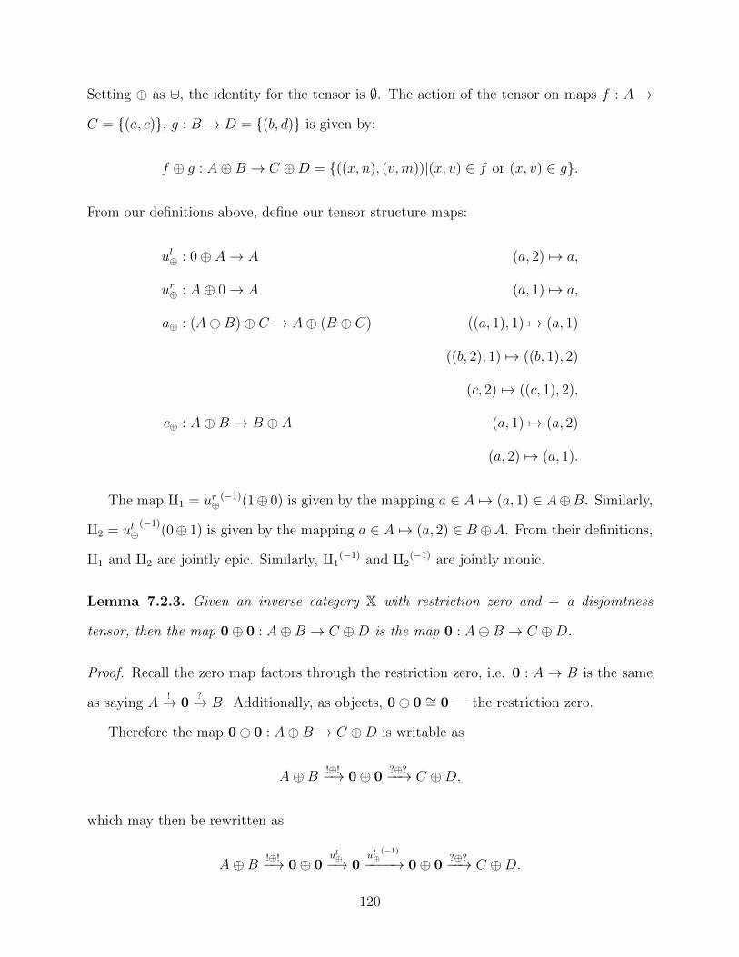
Setting ⊕ as ], the identity for the tensor is ∅. The action of the tensor on maps f : A →
C = {(a, c)}, g : B → D = {(b, d)} is given by:
f ⊕ g : A⊕B → C ⊕D = {((x, n), (v,m))|(x, v) ∈ f or (x, v) ∈ g}.
From our definitions above, define our tensor structure maps:
ul⊕ : 0⊕ A→ A (a, 2) 7→ a,
ur⊕ : A⊕ 0→ A (a, 1) 7→ a,
a⊕ : (A⊕B)⊕ C → A⊕ (B ⊕ C) ((a, 1), 1) 7→ (a, 1)
((b, 2), 1) 7→ ((b, 1), 2)
(c, 2) 7→ ((c, 1), 2),
c⊕ : A⊕B → B ⊕ A (a, 1) 7→ (a, 2)
(a, 2) 7→ (a, 1).
The map q1 = ur⊕(−1)(1⊕ 0) is given by the mapping a ∈ A 7→ (a, 1) ∈ A⊕B. Similarly,
q2 = ul⊕(−1)
(0⊕ 1) is given by the mapping a ∈ A 7→ (a, 2) ∈ B⊕A. From their definitions,
q1 and q2 are jointly epic. Similarly, q1(−1) and q2
(−1) are jointly monic.
Lemma 7.2.3. Given an inverse category X with restriction zero and + a disjointness
tensor, then the map 0⊕ 0 : A⊕B → C ⊕D is the map 0 : A⊕B → C ⊕D.
Proof. Recall the zero map factors through the restriction zero, i.e. 0 : A → B is the same
as saying A!−→ 0
?−→ B. Additionally, as objects, 0⊕ 0 ∼= 0 — the restriction zero.
Therefore the map 0⊕ 0 : A⊕B → C ⊕D is writable as
A⊕B !⊕!−→ 0⊕ 0?⊕?−−→ C ⊕D,
which may then be rewritten as
A⊕B !⊕!−→ 0⊕ 0ul⊕−→ 0
ul⊕(−1)
−−−−→ 0⊕ 0?⊕?−−→ C ⊕D.
120
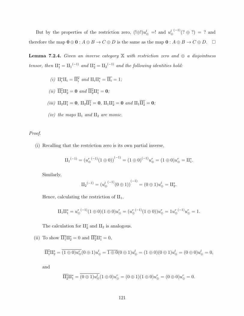
But by the properties of the restriction zero, (!⊕!)ul⊕ =! and ul⊕(−1)
(? ⊕ ?) = ? and
therefore the map 0⊕ 0 : A⊕B → C ⊕D is the same as the map 0 : A⊕B → C ⊕D.
Lemma 7.2.4. Given an inverse category X with restriction zero and ⊕ a disjointness
tensor, then q∗1 = q1(−1) and q∗2 = q2
(−1) and the following identities hold:
(i) q∗iqi = q∗i and qiq∗i = qi = 1;
(ii) q∗1q∗2 = 0 and q∗2q∗1 = 0;
(iii) q2q∗1 = 0, q2q∗1 = 0, q1q∗2 = 0 and q1q∗2 = 0;
(iv) the maps q1 and q2 are monic.
Proof.
(i) Recalling that the restriction zero is its own partial inverse,
q1(−1) = (ur⊕
(−1)(1⊕ 0))(−1)
= (1⊕ 0)(−1)ur⊕ = (1⊕ 0)ur⊕ = q∗1.
Similarly,
q2(−1) = (ul⊕
(−1)(0⊕ 1))
(−1)
= (0⊕ 1)ul⊕ = q∗2.
Hence, calculating the restriction of q1,
q1q∗1 = ur⊕(−1)(1⊕ 0)(1⊕ 0)ur⊕ = (ur⊕
(−1)(1⊕ 0))ur⊕ = 1ur⊕(−1)ur⊕ = 1.
The calculation for q∗2 and q2 is analogous.
(ii) To show q∗1q∗2 = 0 and q∗2q∗1 = 0,
q∗1q∗2 = (1⊕ 0)ur⊕(0⊕ 1)ul⊕ = 1⊕ 0(0⊕ 1)ul⊕ = (1⊕ 0)(0⊕ 1)ul⊕ = (0⊕ 0)ul⊕ = 0,
and
q∗2q∗1 = (0⊕ 1)ul⊕(1⊕ 0)ur⊕ = (0⊕ 1)(1⊕ 0)ur⊕ = (0⊕ 0)ur⊕ = 0.
121
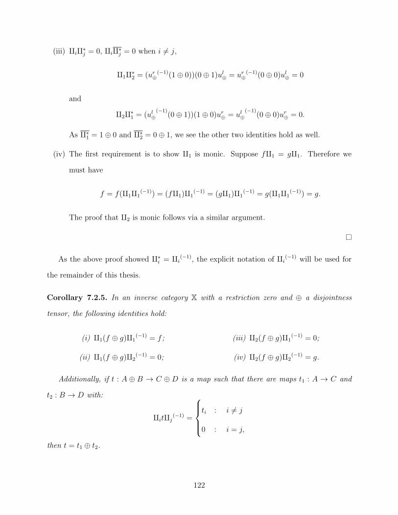
(iii) qiq∗j = 0, qiq∗j = 0 when i 6= j,
q1q∗2 = (ur⊕(−1)(1⊕ 0))(0⊕ 1)ul⊕ = ur⊕
(−1)(0⊕ 0)ul⊕ = 0
and
q2q∗1 = (ul⊕(−1)
(0⊕ 1))(1⊕ 0)ur⊕ = ul⊕(−1)
(0⊕ 0)ur⊕ = 0.
As q∗1 = 1⊕ 0 and q∗2 = 0⊕ 1, we see the other two identities hold as well.
(iv) The first requirement is to show q1 is monic. Suppose fq1 = gq1. Therefore we
must have
f = f(q1q1(−1)) = (fq1)q1
(−1) = (gq1)q1(−1) = g(q1q1
(−1)) = g.
The proof that q2 is monic follows via a similar argument.
As the above proof showed q∗i = qi(−1), the explicit notation of qi(−1) will be used for
the remainder of this thesis.
Corollary 7.2.5. In an inverse category X with a restriction zero and ⊕ a disjointness
tensor, the following identities hold:
(i) q1(f ⊕ g)q1(−1) = f ;
(ii) q1(f ⊕ g)q2(−1) = 0;
(iii) q2(f ⊕ g)q1(−1) = 0;
(iv) q2(f ⊕ g)q2(−1) = g.
Additionally, if t : A ⊕ B → C ⊕D is a map such that there are maps t1 : A → C and
t2 : B → D with:
qitqj(−1) =
ti : i 6= j
0 : i = j,
then t = t1 ⊕ t2.
122
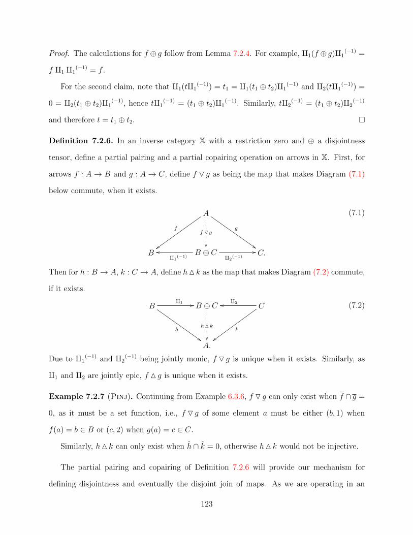
Proof. The calculations for f ⊕ g follow from Lemma 7.2.4. For example, q1(f ⊕ g)q1(−1) =
f q1 q1(−1) = f .
For the second claim, note that q1(tq1(−1)) = t1 = q1(t1 ⊕ t2)q1
(−1) and q2(tq1(−1)) =
0 = q2(t1 ⊕ t2)q1(−1), hence tq1
(−1) = (t1 ⊕ t2)q1(−1). Similarly, tq2
(−1) = (t1 ⊕ t2)q2(−1)
and therefore t = t1 ⊕ t2.
Definition 7.2.6. In an inverse category X with a restriction zero and ⊕ a disjointness
tensor, define a partial pairing and a partial copairing operation on arrows in X. First, for
arrows f : A→ B and g : A→ C, define f O g as being the map that makes Diagram (7.1)
below commute, when it exists.
A
f
{{
g
$$
f O g
��B B ⊕ C
q1(−1)
ooq2
(−1)
// C.
(7.1)
Then for h : B → A, k : C → A, define hM k as the map that makes Diagram (7.2) commute,
if it exists.
Bq1 //
h
##
B ⊕ C
hM k
��
Cq2oo
k
{{A.
(7.2)
Due to q1(−1) and q2
(−1) being jointly monic, f O g is unique when it exists. Similarly, as
q1 and q2 are jointly epic, f M g is unique when it exists.
Example 7.2.7 (Pinj). Continuing from Example 6.3.6, f O g can only exist when f ∩ g =
0, as it must be a set function, i.e., f O g of some element a must be either (b, 1) when
f(a) = b ∈ B or (c, 2) when g(a) = c ∈ C.
Similarly, hM k can only exist when h ∩ k = 0, otherwise hM k would not be injective.
The partial pairing and copairing of Definition 7.2.6 will provide our mechanism for
defining disjointness and eventually the disjoint join of maps. As we are operating in an
123
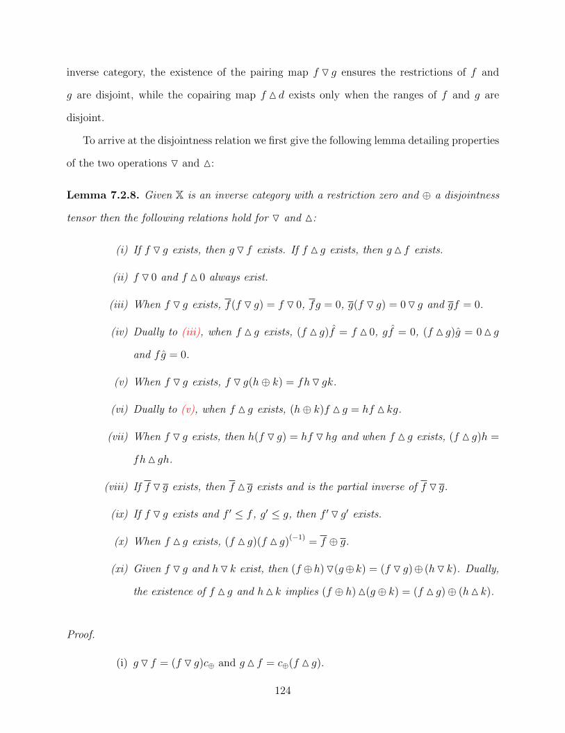
inverse category, the existence of the pairing map f O g ensures the restrictions of f and
g are disjoint, while the copairing map f M d exists only when the ranges of f and g are
disjoint.
To arrive at the disjointness relation we first give the following lemma detailing properties
of the two operations O and M:
Lemma 7.2.8. Given X is an inverse category with a restriction zero and ⊕ a disjointness
tensor then the following relations hold for O and M:
(i) If f O g exists, then gO f exists. If f M g exists, then gM f exists.
(ii) f O 0 and f M 0 always exist.
(iii) When f O g exists, f(f O g) = f O 0, fg = 0, g(f O g) = 0O g and gf = 0.
(iv) Dually to (iii), when f M g exists, (f M g)f = f M 0, gf = 0, (f M g)g = 0M g
and fg = 0.
(v) When f O g exists, f O g(h⊕ k) = fhO gk.
(vi) Dually to (v), when f M g exists, (h⊕ k)f M g = hf M kg.
(vii) When f O g exists, then h(f O g) = hf Ohg and when f M g exists, (f M g)h =
fhM gh.
(viii) If f O g exists, then f M g exists and is the partial inverse of f O g.
(ix) If f O g exists and f ′ ≤ f , g′ ≤ g, then f ′O g′ exists.
(x) When f M g exists, (f M g)(f M g)(−1) = f ⊕ g.
(xi) Given f O g and hO k exist, then (f ⊕h)O(g⊕k) = (f O g)⊕ (hO k). Dually,
the existence of f M g and hM k implies (f ⊕ h)M(g ⊕ k) = (f M g)⊕ (hM k).
Proof.
(i) gO f = (f O g)c⊕ and gM f = c⊕(f M g).
124
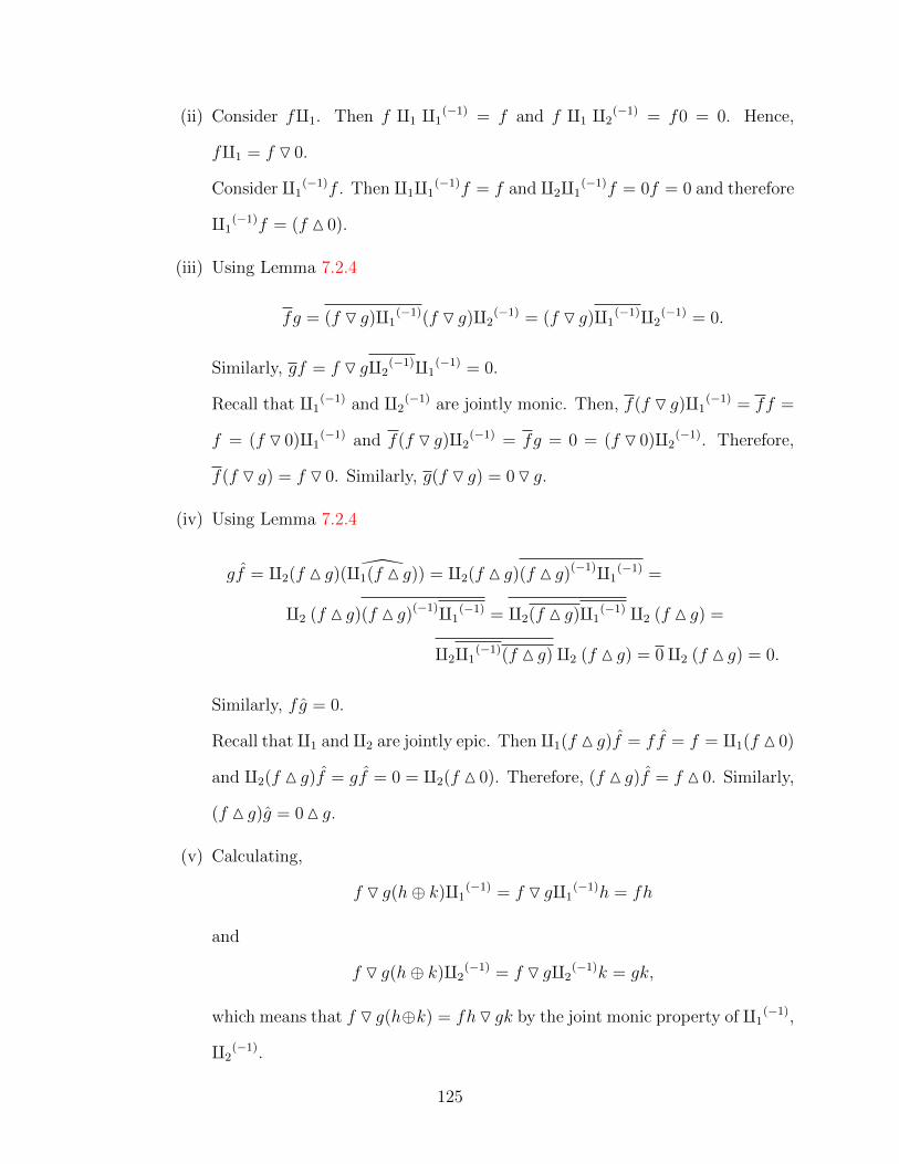
(ii) Consider fq1. Then f q1 q1(−1) = f and f q1 q2
(−1) = f0 = 0. Hence,
fq1 = f O 0.
Consider q1(−1)f . Then q1q1
(−1)f = f and q2q1(−1)f = 0f = 0 and therefore
q1(−1)f = (f M 0).
(iii) Using Lemma 7.2.4
fg = (f O g)q1(−1)(f O g)q2
(−1) = (f O g)q1(−1)q2
(−1) = 0.
Similarly, gf = f O gq2(−1)q1
(−1) = 0.
Recall that q1(−1) and q2
(−1) are jointly monic. Then, f(f O g)q1(−1) = ff =
f = (f O 0)q1(−1) and f(f O g)q2
(−1) = fg = 0 = (f O 0)q2(−1). Therefore,
f(f O g) = f O 0. Similarly, g(f O g) = 0O g.
(iv) Using Lemma 7.2.4
gf = q2(f M g) (q1(f M g)) = q2(f M g)(f M g)(−1)q1(−1) =
q2 (f M g)(f M g)(−1)q1(−1) = q2(f M g)q1
(−1) q2 (f M g) =
q2q1(−1)(f M g)q2 (f M g) = 0q2 (f M g) = 0.
Similarly, fg = 0.
Recall thatq1 andq2 are jointly epic. Thenq1(f M g)f = ff = f = q1(f M 0)
and q2(f M g)f = gf = 0 = q2(f M 0). Therefore, (f M g)f = f M 0. Similarly,
(f M g)g = 0M g.
(v) Calculating,
f O g(h⊕ k)q1(−1) = f O gq1
(−1)h = fh
and
f O g(h⊕ k)q2(−1) = f O gq2
(−1)k = gk,
which means that f O g(h⊕k) = fhO gk by the joint monic property of q1(−1),
q2(−1).
125
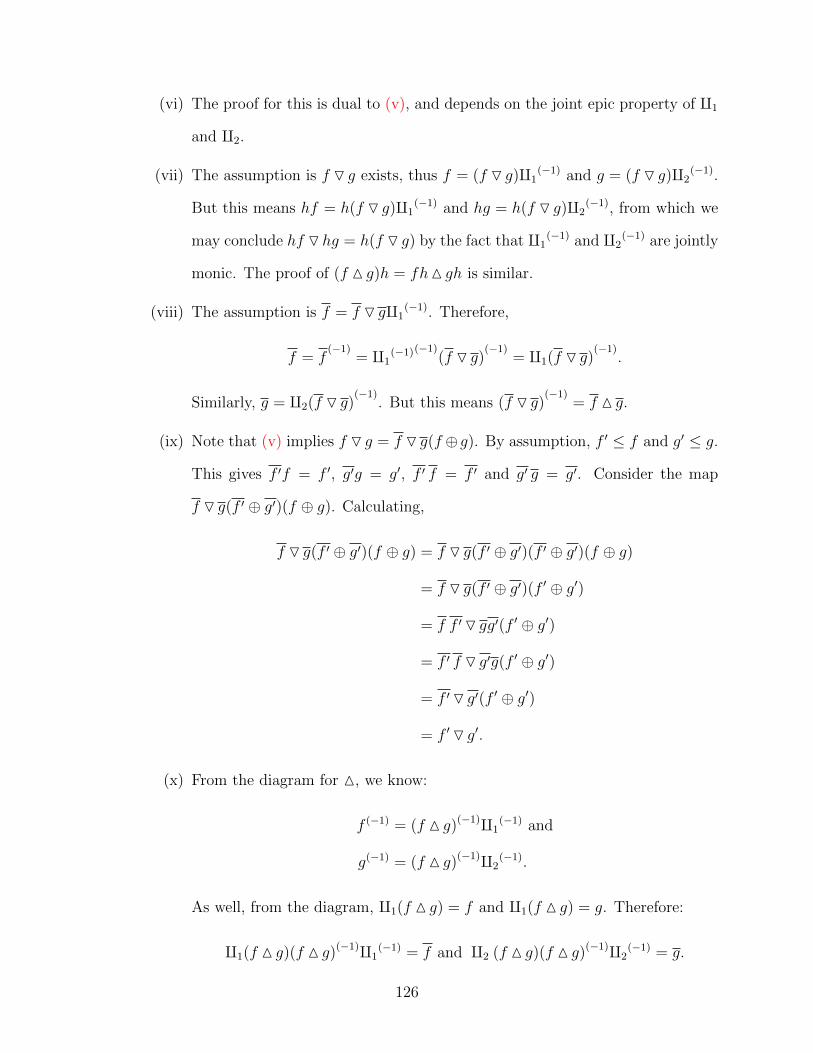
(vi) The proof for this is dual to (v), and depends on the joint epic property of q1
and q2.
(vii) The assumption is f O g exists, thus f = (f O g)q1(−1) and g = (f O g)q2
(−1).
But this means hf = h(f O g)q1(−1) and hg = h(f O g)q2
(−1), from which we
may conclude hf Ohg = h(f O g) by the fact that q1(−1) and q2
(−1) are jointly
monic. The proof of (f M g)h = fhM gh is similar.
(viii) The assumption is f = f O gq1(−1). Therefore,
f = f(−1)
= q1(−1)(−1)
(f O g)(−1)
= q1(f O g)(−1)
.
Similarly, g = q2(f O g)(−1)
. But this means (f O g)(−1)
= f M g.
(ix) Note that (v) implies f O g = f O g(f ⊕g). By assumption, f ′ ≤ f and g′ ≤ g.
This gives f ′f = f ′, g′g = g′, f ′ f = f ′ and g′ g = g′. Consider the map
f O g(f ′ ⊕ g′)(f ⊕ g). Calculating,
f O g(f ′ ⊕ g′)(f ⊕ g) = f O g(f ′ ⊕ g′)(f ′ ⊕ g′)(f ⊕ g)
= f O g(f ′ ⊕ g′)(f ′ ⊕ g′)
= f f ′O gg′(f ′ ⊕ g′)
= f ′ f O g′g(f ′ ⊕ g′)
= f ′O g′(f ′ ⊕ g′)
= f ′O g′.
(x) From the diagram for M, we know:
f (−1) = (f M g)(−1)q1(−1) and
g(−1) = (f M g)(−1)q2(−1).
As well, from the diagram, q1(f M g) = f and q1(f M g) = g. Therefore:
q1(f M g)(f M g)(−1)q1(−1) = f and q2 (f M g)(f M g)(−1)q2
(−1) = g.
126

As f⊥⊕g, by [Dis.2] fg(−1) = fgg(−1) = 0g(−1) = 0 and therefore,
q1(f M g)(f M g)(−1)q2(−1) = 0 and q2 (f M g)(f M g)(−1)q1
(−1) = 0.
By Corollary 7.2.5 this means (f M g)(f M g)(−1) = f ⊕ g.
(xi) The fact that (f O g)⊕ (hO k)q1(−1) = (f O g) and (f O g)⊕ (hO k)q2
(−1) =
(hO k), implies that (f O g)⊕(hO k) satisfies the diagram for (f⊕h)O(g⊕k).
Dually, as q1(f M g) ⊕ (hM k) = (f M g) and q2(f M g) ⊕ (hM k) = (hM k),
(f M g)⊕ (hM k) satisfies the diagram for (f ⊕ h)M(g ⊕ k).
We are now set up to prove that it is possible to create a disjointness relation based on
the existence of our pairing and copairing maps:
Lemma 7.2.9. Define f⊥⊕g (f is tensor disjoint to g) when f, g : A → B and both f O g
and f M g exist. If X is an inverse category with a restriction zero and ⊕ a disjointness
tensor then the relation ⊥⊕ is a disjointness relation.
Proof. The proof requires us to show that ⊥⊕ satisfies the disjointness axioms. We will use
[Dis.6’] in place of [Dis.6] and [Dis.7] as discussed in Lemma 6.2.2.
[Dis.1] The requirement is f⊥⊕0. This follows immediately from Lemma 7.2.8, item (ii).
[Dis.2] Show f⊥⊕g implies fg = 0. This is a direct consequence of Lemma 7.2.8, item (iii).
[Dis.3] This requires that f⊥⊕g, f ′ ≤ f , g′ ≤ g implies f ′⊥⊕g′. From Lemma 7.2.8, item
(ix), f ′O g′ exists. Using a similar argument to the proof of this item, f ′M g′ exists
and hence f ′⊥⊕g′.
[Dis.4] Commutativity of ⊥⊕ follows from the symmetry of the two required diagrams, see
Lemma 7.2.8, item (i).
127

[Dis.5] Show that if f⊥⊕g then hf⊥⊕hg for any map h. By Lemma 7.2.8(vii), when f O g
exists, hf Ohg exists. Assuming f M g, by (vi) of the same lemma, (hf)M(hg) exists
and equals (h⊕ h)(f M g) and therefore hf⊥⊕hg.
[Dis.6’] This requires showing f⊥⊕g if and only if f⊥⊕g and f⊥⊕ g. This follows directly
from Lemma 7.2.8(v) and (vi), which give us f O g = f O g(f ⊕ g) and f M g =
(f ⊕ g)f M g, where the equalities hold if either side of the equation exists.
Example 7.2.10 (⊥⊕ in Pinj). Referring to Example 7.2.7, f O g exists when f ∩g = 0 and
that f M g exists when f ∩ g = 0. But this agrees with the initial definition of disjointness
(⊥) in Pinj from Example 6.2.8 and hence ⊥⊕ is the same relation as ⊥ in Pinj.
Note that this is due to the actual choices of the tensor and ⊥. If we had initially chosen
a different ⊥, such as ⊥0, where f ⊥0 g iff f or g are 0, then ⊥⊕ 6=⊥0.
7.3 Disjoint joins via a tensor
The operations O and M are sufficient to define a disjointness relation on an inverse category.
However, when attempting to extend this to a disjoint join, the two relations are insufficient
to prove [DJ.4], That is, requiring that ⊥⊕ [f, g, h] implies f⊥⊕(g t⊕ h).
Therefore, we must add one more assumption regarding our tensor in order to define
disjointness.
Definition 7.3.1. Let X be an inverse category with ⊕ a disjointness tensor and a restriction
128
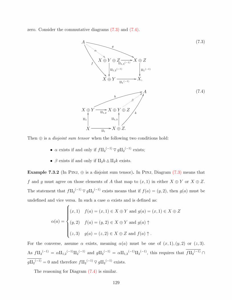
zero. Consider the commutative diagrams (7.3) and (7.4).
A
f
��
g
((
α
$$X ⊕ Y ⊕ Z
q1,2(−1)
��
q1,3(−1)
// X ⊕ Z
q1(−1)
��X ⊕ Y
q1(−1)
// X,
(7.3)
A
X ⊕ Y q1,2
//
h
22
X ⊕ Y ⊕ Z
β
::
X
q1
OO
q1
// X ⊕ Z.
q1,3
OO k
HH (7.4)
Then ⊕ is a disjoint sum tensor when the following two conditions hold:
• α exists if and only if fq2(−1)O gq2
(−1) exists;
• β exists if and only if q2hMq2k exists.
Example 7.3.2 (In Pinj, ⊕ is a disjoint sum tensor). In Pinj, Diagram (7.3) means that
f and g must agree on those elements of A that map to (x, 1) in either X ⊕ Y or X ⊕ Z.
The statement that fq2(−1)O gq2
(−1) exists means that if f(a) = (y, 2), then g(a) must be
undefined and vice versa. In such a case α exists and is defined as:
α(a) =
(x, 1) f(a) = (x, 1) ∈ X ⊕ Y and g(a) = (x, 1) ∈ X ⊕ Z
(y, 2) f(a) = (y, 2) ∈ X ⊕ Y and g(a) ↑
(z, 3) g(a) = (z, 2) ∈ X ⊕ Z and f(a) ↑ .
For the converse, assume α exists, meaning α(a) must be one of (x, 1), (y, 2) or (z, 3).
As fq2(−1) = αq1,2
(−1)q2(−1) and gq2
(−1) = αq1,3(−1)q2
(−1), this requires that fq2(−1) ∩
gq2(−1) = 0 and therefore fq2
(−1)O gq2(−1) exists.
The reasoning for Diagram (7.4) is similar.
129

Lemma 7.3.3. Let X be an inverse category with a disjoint sum tensor as in Definition 7.3.1
where f, g, h : A→ B with ⊥⊕ [f, g, h]. Then both f O(gOh) and f M(gMh) exist.
Proof. As all the maps are disjoint, we know the maps O and M exist for each pair. Consider
the diagram
A
gOh
��
gO f
((
α
$$
f // B
B ⊕B ⊕B
q1,2(−1)
��
q1,3(−1)
// B ⊕B
q1(−1)
��
q2(−1)
OO
B ⊕Bq1
(−1)// B
where we claim α = (gOh)O f .
The lower part of the diagram commutes as it fulfills the conditions of Definition 7.3.1.
The upper rightmost triangle of the diagram commutes by the definition of gO f . Noting
that q0,1(−1) : B⊕B⊕B → B⊕B is the same map as q1
(−1) : (B⊕B)⊕B → (B⊕B) and
q0,2(−1)q2
(−1) : B ⊕ B ⊕ B → B ⊕ B → B is the same map as q2(−1) : (B ⊕ B)⊕ B → B,
therefore α does make the O diagram for gOh and f commute. Therefore by Lemma 7.2.8,
f O(gOh) exists and is equal to αc⊕{01,2}.
A dual diagram and corresponding reasoning shows f M(gMh) exists.
Lemma 7.3.4. In an inverse category X with a disjoint sum tensor, when ⊥⊕ [f, g, h], then:
(i) f O(gOh) = ((f O g)Oh)a⊕ and both exist,
(ii) f M(gMh) = ((f M g)Mh)a⊕ and both exist.
130
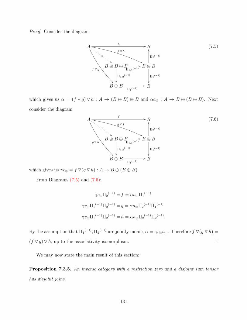
Proof. Consider the diagram
A
f O g
��
f Oh
((
α
$$
h // B
B ⊕B ⊕B
q1,2(−1)
��
q1,3(−1)
// B ⊕B
q1(−1)
��
q2(−1)
OO
B ⊕Bq1
(−1)// B
(7.5)
which gives us α = (f O g)Oh : A → (B ⊕ B) ⊕ B and αa⊕ : A → B ⊕ (B ⊕ B). Next
consider the diagram
A
gOh
��
gO f
((
γ
$$
f // B
B ⊕B ⊕B
q1,2(−1)
��
q1,3(−1)
// B ⊕B
q1(−1)
��
q2(−1)
OO
B ⊕Bq1
(−1)
// B
(7.6)
which gives us γc⊕ = f O(gOh) : A→ B ⊕ (B ⊕B).
From Diagrams (7.5) and (7.6):
γc⊕q0(−1) = f = αa⊕q1
(−1)
γc⊕q1(−1)q0
(−1) = g = αa⊕q2(−1)q1
(−1)
γc⊕q1(−1)q2
(−1) =h = αa⊕q2(−1)q2
(−1).
By the assumption that q1(−1),q2
(−1) are jointly monic, α = γc⊕a⊕. Therefore f O(gOh) =
(f O g)Oh, up to the associativity isomorphism.
We may now state the main result of this section:
Proposition 7.3.5. An inverse category with a restriction zero and a disjoint sum tensor
has disjoint joins.
131

Given two maps f, g with f⊥⊕g, the candidate for disjoint join is the map f t⊕ g =
f O g(f ⊕ g)f M g. The proof that this is a disjoint join will follow after giving an example
and a lemma detailing the properties of t⊕ .
For reference, the map f t⊕ g may be visualized as follows:
A B
f
$$
q1
��A
f
::
f O g //
g
$$
A⊕ A
q1(−1)
OO
q2(−1)
��
f⊕g // B ⊕B f M g // B.
A B
g
::
q2
OO
(7.7)
Using Lemma 7.2.8, this may be rewritten in a variety of equivalent ways:
f t⊕ g = (f O g)(f ⊕ g)(f M g) (7.8)
= (f O g) (f M g) (7.9)
= (f O g) (f M g) (7.10)
= (f O g)(f (−1) ⊕ g(−1))(f M g). (7.11)
In particular, note that f t⊕ g = (f O g)(f M g) as g = g.
Example 7.3.6 (Disjoint sum tensor in Pinj). Using Equation (7.10) for f t⊕ g, calculate:
f O g(a) =
(a, 1) f(a) = a, g ↑
(a, 2) g(a) = a, f ↑(7.12)
and
f M g((a, n)) =
f(a) n = 1
g(a) n = 2.
(7.13)
Combining Equation (7.12) with Equation (7.13) then gives the same definition as that of t
as given in Example 6.3.6.
132
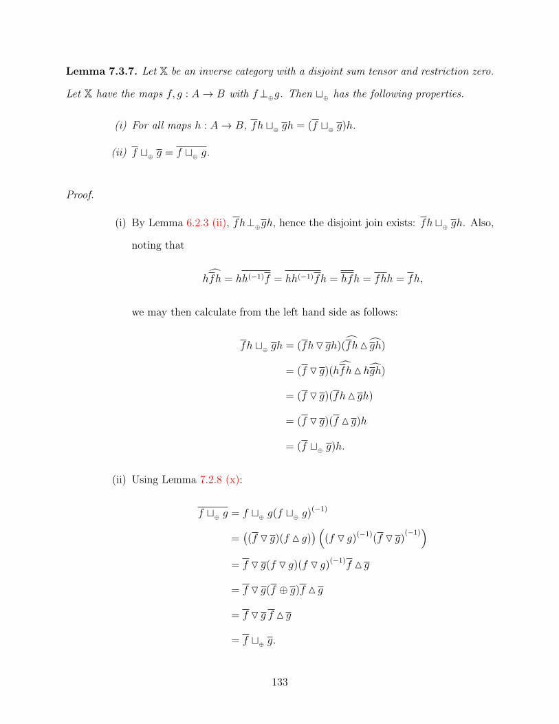
Lemma 7.3.7. Let X be an inverse category with a disjoint sum tensor and restriction zero.
Let X have the maps f, g : A→ B with f⊥⊕g. Then t⊕ has the following properties.
(i) For all maps h : A→ B, fh t⊕ gh = (f t⊕ g)h.
(ii) f t⊕ g = f t⊕ g.
Proof.
(i) By Lemma 6.2.3 (ii), fh⊥⊕gh, hence the disjoint join exists: fh t⊕ gh. Also,
noting that
hfh = hh(−1)f = hh(−1)fh = hfh = fhh = fh,
we may then calculate from the left hand side as follows:
fh t⊕ gh = (fhO gh)(fhM gh)
= (f O g)(hfhMhgh)
= (f O g)(fhM gh)
= (f O g)(f M g)h
= (f t⊕ g)h.
(ii) Using Lemma 7.2.8 (x):
f t⊕ g = f t⊕ g(f t⊕ g)(−1)
=((f O g)(f M g)
) ((f O g)(−1)(f O g)
(−1))
= f O g(f O g)(f O g)(−1)f M g
= f O g(f ⊕ g)f M g
= f O g f M g
= f t⊕ g.
133

We may now complete the proof of Proposition 7.3.5:
Proof. [DJ.1] This requires f, g ≤ f t⊕ g.
f (f O g)f M g = (f O g)q1(−1)(f O g)f M g
= (f O g)q1(−1)(f O g)f M g
= (f O g)q1(−1)f M g
= (f O g)q1(−1) q1 f M g
= ((f O g)q1(−1))(q1(f M g))
= ff
= f.
Thus, f ≤ f t⊕ g. Showing g ≤ f t⊕ g proceeds in the same manner.
[DJ.2] The requirement is that f ≤ h, g ≤ h and f⊥⊕g implies f t⊕ g ≤ h.
f t⊕ g h = fh t⊕ gh h
= (f t⊕ g)hh
= (f t⊕ g)hh
= (f t⊕ g)h (f t⊕ g)h
= (f t⊕ g)h (f t⊕ g)h
= (f t⊕ g)h
= (fh t⊕ gh)
= (f t⊕ g).
[DJ.3] This is the stability of t⊕ , i.e., that h(f t⊕ g) = hf t⊕ hg.
134
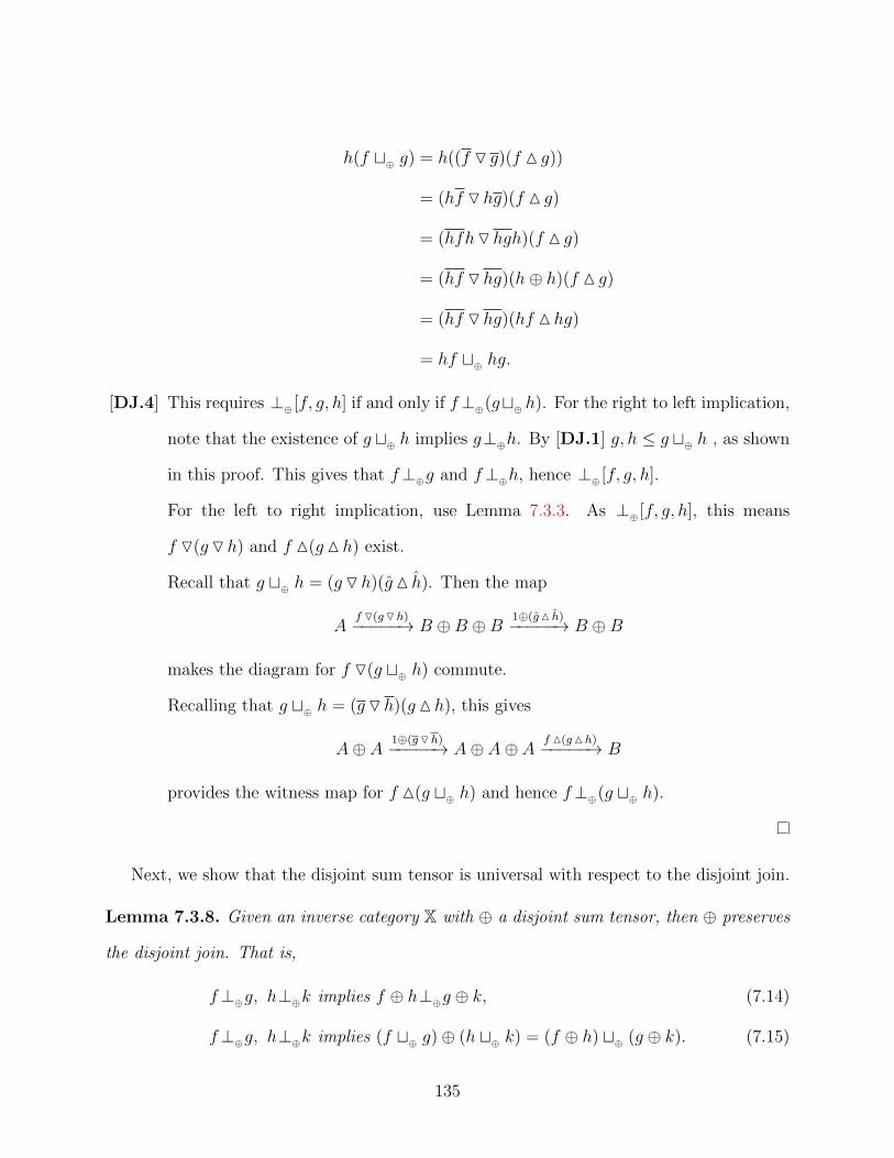
h(f t⊕ g) = h((f O g)(f M g))
= (hf Ohg)(f M g)
= (hfhOhgh)(f M g)
= (hf Ohg)(h⊕ h)(f M g)
= (hf Ohg)(hf Mhg)
= hf t⊕ hg.
[DJ.4] This requires ⊥⊕ [f, g, h] if and only if f⊥⊕(gt⊕ h). For the right to left implication,
note that the existence of g t⊕ h implies g⊥⊕h. By [DJ.1] g, h ≤ g t⊕ h , as shown
in this proof. This gives that f⊥⊕g and f⊥⊕h, hence ⊥⊕ [f, g, h].
For the left to right implication, use Lemma 7.3.3. As ⊥⊕ [f, g, h], this means
f O(gOh) and f M(gMh) exist.
Recall that g t⊕ h = (gOh)(gM h). Then the map
Af O(gOh)−−−−−→ B ⊕B ⊕B 1⊕(gM h)−−−−−→ B ⊕B
makes the diagram for f O(g t⊕ h) commute.
Recalling that g t⊕ h = (gOh)(gMh), this gives
A⊕ A 1⊕(gOh)−−−−−→ A⊕ A⊕ A f M(gMh)−−−−−→ B
provides the witness map for f M(g t⊕ h) and hence f⊥⊕(g t⊕ h).
Next, we show that the disjoint sum tensor is universal with respect to the disjoint join.
Lemma 7.3.8. Given an inverse category X with ⊕ a disjoint sum tensor, then ⊕ preserves
the disjoint join. That is,
f⊥⊕g, h⊥⊕k implies f ⊕ h⊥⊕g ⊕ k, (7.14)
f⊥⊕g, h⊥⊕k implies (f t⊕ g)⊕ (h t⊕ k) = (f ⊕ h) t⊕ (g ⊕ k). (7.15)
135
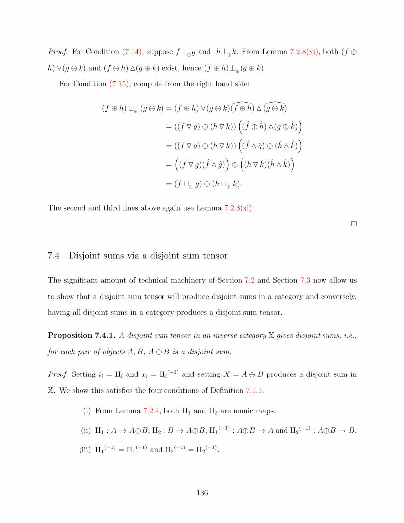
Proof. For Condition (7.14), suppose f⊥⊕g and h⊥⊕k. From Lemma 7.2.8(xi), both (f ⊕
h)O(g ⊕ k) and (f ⊕ h)M(g ⊕ k) exist, hence (f ⊕ h)⊥⊕(g ⊕ k).
For Condition (7.15), compute from the right hand side:
(f ⊕ h) t⊕ (g ⊕ k) = (f ⊕ h)O(g ⊕ k) (f ⊕ h)M (g ⊕ k)
= ((f O g)⊕ (hO k))(
(f ⊕ h)M(g ⊕ k))
= ((f O g)⊕ (hO k))(
(f M g)⊕ (hM k))
=(
(f O g)(f M g))⊕(
(hO k)(hM k))
= (f t⊕ g)⊕ (h t⊕ k).
The second and third lines above again use Lemma 7.2.8(xi).
7.4 Disjoint sums via a disjoint sum tensor
The significant amount of technical machinery of Section 7.2 and Section 7.3 now allow us
to show that a disjoint sum tensor will produce disjoint sums in a category and conversely,
having all disjoint sums in a category produces a disjoint sum tensor.
Proposition 7.4.1. A disjoint sum tensor in an inverse category X gives disjoint sums, i.e.,
for each pair of objects A,B, A⊕B is a disjoint sum.
Proof. Setting ii = qi and xi = qi(−1) and setting X = A ⊕ B produces a disjoint sum in
X. We show this satisfies the four conditions of Definition 7.1.1.
(i) From Lemma 7.2.4, both q1 and q2 are monic maps.
(ii) q1 : A→ A⊕B, q2 : B → A⊕B, q1(−1) : A⊕B → A and q2
(−1) : A⊕B → B.
(iii) q1(−1) = q1
(−1) and q2(−1) = q2
(−1).
136

(iv) i1(−1)i1 = 1⊕ 0⊥⊕0⊕ 1 = i2
(−1)i2 as
1⊕ 0O 0⊕ 1 = (ur⊕(−1) ⊕ ul⊕
(−1)) and 1⊕ 0M 0⊕ 1 = (q1
(−1) ⊕q2(−1)).
For their join,
(1⊕ 0) t⊕ (0⊕ 1) = (ur⊕(−1) ⊕ ul⊕
(−1))(q1
(−1) ⊕q2(−1)) =
ur⊕(−1)q1
(−1) ⊕ ul⊕(−1)q2
(−1) = 1⊕ 1 = 1.
Finally, to complete the cycle:
Proposition 7.4.2. Given X is an inverse category where every pair of objects has a disjoint
sum, then the tensor derived from the disjoint sum of A,B is a disjoint sum tensor.
Proof. Proposition 7.1.4 showed that when ⊕ is derived from the disjoint sum, it is a sym-
metric monoidal tensor. Therefore, it only remains to show that it is a disjointness tensor
and that it satisfies Definition 7.3.1, i.e., is a disjoint sum tensor as well.
First note that we immediately have that it is a disjointness tensor as:
(i) Proposition 7.1.4 shows it is a restriction functor.
(ii) Proposition 7.1.4 shows that the unit is the restriction zero.
(iii) From the above, q1 = i1 and q2 = i2. Assume q1f = q1g and q2f = q2g.
As q1(−1) q1 tq2
(−1)q2 = 1,
f = (q1(−1) q1 tq2
(−1)q2)f = q1(−1) q1 f t q2
(−1) q2 f =
q1(−1) q1 g t q2
(−1) q2 g = (q1(−1) q1 tq2
(−1)q2)g = g
and therefore q1 and q2 are jointly monic.
(iv) q1(−1) and q2
(−1) are jointly epic by a similar argument as (iii).
137

Note that we may also immediately conclude that the original disjointness relation on X
is the same as the one generated by ⊕. This is because f O g will be equal to f q1 tgq2 and
f M g will be equal to q1(−1)f t q2
(−1)g, therefore, f O g and f M g will exist if and only if
f ⊥ g.
To show it is a disjoint sum tensor, we must show the existence of the maps α and β
from Definition 7.3.1.
For Diagram (7.3), assuming fq2(−1)O gq2
(−1) exists, then
α = (fq1(−1))q1 t((fq2
(−1)O gq2(−1))q2)
satisfies the diagram. If α does exist, then αq2(−1) satisfies the diagram for fq2
(−1)O gq2(−1).
The argument for satisfying Diagram (7.4) is analogous.
Therefore, ⊕ is a disjoint sum tensor.
138
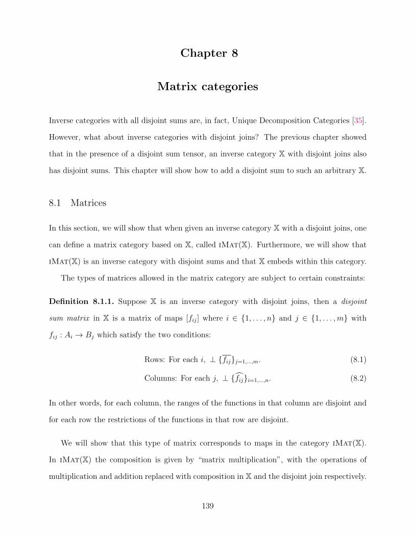
Chapter 8
Matrix categories
Inverse categories with all disjoint sums are, in fact, Unique Decomposition Categories [35].
However, what about inverse categories with disjoint joins? The previous chapter showed
that in the presence of a disjoint sum tensor, an inverse category X with disjoint joins also
has disjoint sums. This chapter will show how to add a disjoint sum to such an arbitrary X.
8.1 Matrices
In this section, we will show that when given an inverse category X with a disjoint joins, one
can define a matrix category based on X, called iMat(X). Furthermore, we will show that
iMat(X) is an inverse category with disjoint sums and that X embeds within this category.
The types of matrices allowed in the matrix category are subject to certain constraints:
Definition 8.1.1. Suppose X is an inverse category with disjoint joins, then a disjoint
sum matrix in X is a matrix of maps [fij] where i ∈ {1, . . . , n} and j ∈ {1, . . . ,m} with
fij : Ai → Bj which satisfy the two conditions:
Rows: For each i, ⊥ {fij}j=1,...,m. (8.1)
Columns: For each j, ⊥ {fij}i=1,...,n. (8.2)
In other words, for each column, the ranges of the functions in that column are disjoint and
for each row the restrictions of the functions in that row are disjoint.
We will show that this type of matrix corresponds to maps in the category iMat(X).
In iMat(X) the composition is given by “matrix multiplication”, with the operations of
multiplication and addition replaced with composition in X and the disjoint join respectively.
139

Definition 8.1.2. Given an inverse category X with disjoint joins, we define the inverse
matrix category of X, iMat(X), as follows:
Objects: Lists of the objects of X;
Maps: Disjoint sum matrices [fij] : [Ai] → [Bj]. In such a matrix each individual map
fij : Ai → Bj is a map in X;
Identity: The disjoint sum matrix I — A diagonal matrix with 1 : Ai → Ai at the i, i
position and zero maps elsewhere;
Composition: Given [fij] : [Ai] → [Bj] and [gjk] : [Bj] → [Ck], then [hik] = [fij][gjk] :
[Ai]→ [Ck] is defined as hik =⊔j fijgjk;
Restriction: We set [fij] to be [f ′ij] where f ′ij = 0 when i 6= j and f ′ii = tjfij.
In the following, we will use the notation diag[dj] for diagonal matrices where the j, j entry
is dj.
Lemma 8.1.3. When X is an inverse category with disjoint joins, iMat(X) is an inverse
category.
Proof. We need to show the following:
• Composition is well defined and associative.
• The restriction is well defined.
• Each map must have a partial inverse.
Composition is well defined: Consider [hik] = [fij][gjk] where [fij] : [A1, . . . , An] →
[B1, . . . , Bm] and [gjk] : [B1, . . . , Bm] → [C1, . . . , C`]. As each of [fij] and [gjk] are dis-
joint sum matrices, by [Dis.7] we know that ⊥ {fijgjk} for each choice of i and k. Hence,
we know the composition hik =⊔j fijgjk is defined and hik : Ai → Ck. We must now show
140
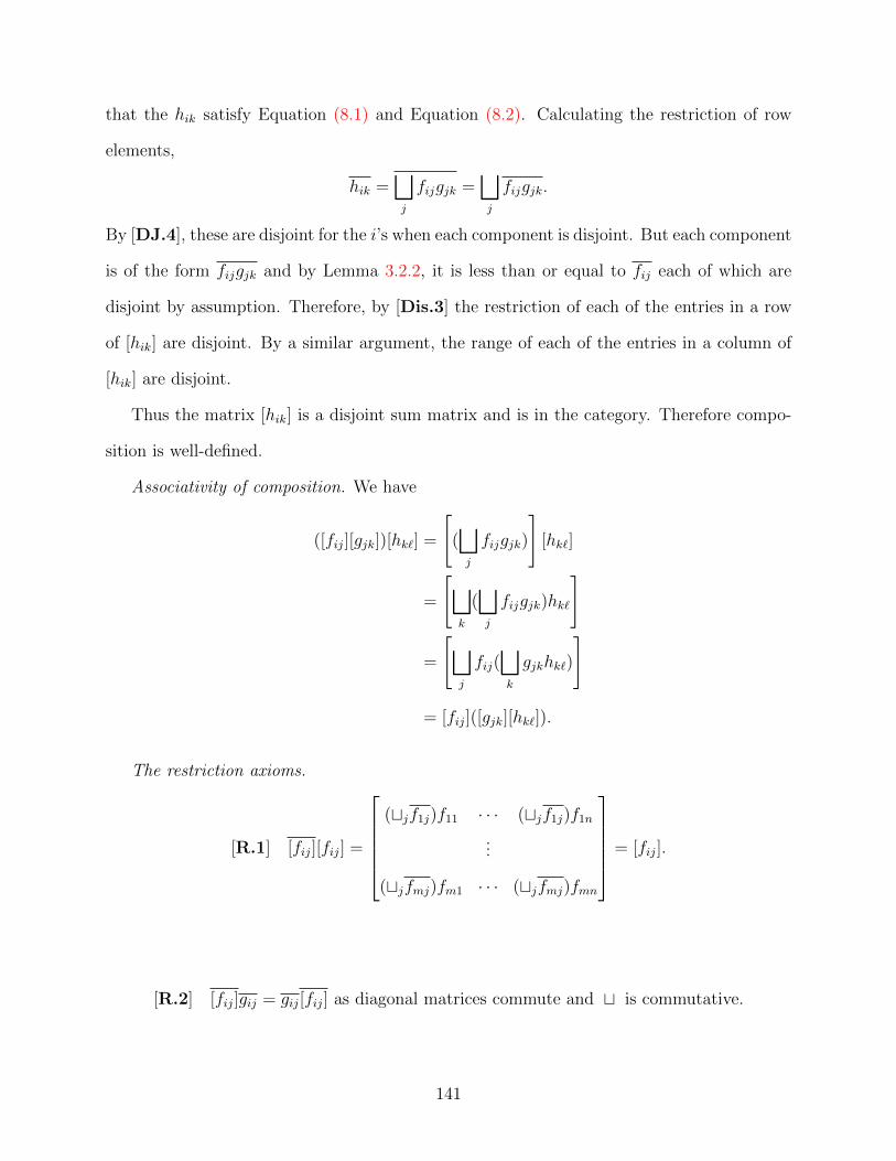
that the hik satisfy Equation (8.1) and Equation (8.2). Calculating the restriction of row
elements,
hik =⊔j
fijgjk =⊔j
fijgjk.
By [DJ.4], these are disjoint for the i’s when each component is disjoint. But each component
is of the form fijgjk and by Lemma 3.2.2, it is less than or equal to fij each of which are
disjoint by assumption. Therefore, by [Dis.3] the restriction of each of the entries in a row
of [hik] are disjoint. By a similar argument, the range of each of the entries in a column of
[hik] are disjoint.
Thus the matrix [hik] is a disjoint sum matrix and is in the category. Therefore compo-
sition is well-defined.
Associativity of composition. We have
([fij][gjk])[hk`] =
[(⊔j
fijgjk)
][hk`]
=
[⊔k
(⊔j
fijgjk)hk`
]
=
[⊔j
fij(⊔k
gjkhk`)
]
= [fij]([gjk][hk`]).
The restriction axioms.
[R.1] [fij][fij] =
(tjf1j)f11 · · · (tjf1j)f1n
...
(tjfmj)fm1 · · · (tjfmj)fmn
= [fij].
[R.2] [fij]gij = gij[fij] as diagonal matrices commute and t is commutative.
141

[R.3] [fij][gjk] = diag[tjf1j, . . . ,tjfnj][gjk]
=
tjf1jg11 . . . tjf1jg1k
...
tjfnjgn1 . . . tjfnjgnk
= diag[tk(tj(f1jg1k)), . . . ,tk(tj(fnj)gnk)]
= diag[tk(tj(f1j)g1k), . . . ,tk(tj(fnj)gnk)]
= diag[(tj(f1j) tk g1k), . . . , (tj(fnj) tk gnk)] = [fij] [gjk].
[R.4] [fij][gjk] = [fij] diagj[tkgjk]
=
f11 tk g1k . . . f1n tk gnk
...
fm1 tk g1k . . . fmn tk gnk
=
tkf11g1k . . . tkf1ngnk
...
tkfm1g1k . . . tkfmngnk
=
tkf11g1kf11 . . . tkf1ngnkf1n
...
tkfm1g1kfm1 . . . tkfmngnkfmn
=
tj tk f1jgjkf11 . . . tj tk f1jgjkf1n
...
tj tk fmjgjkfm1 . . . tj tk fmjgjkfmn
= [fij][gjk][fij].
Thus, iMat(X) is a restriction category.
Existence of partial inverses. The inverse of the map f = [fij] is the map f (−1) :=[fji(−1)].
142
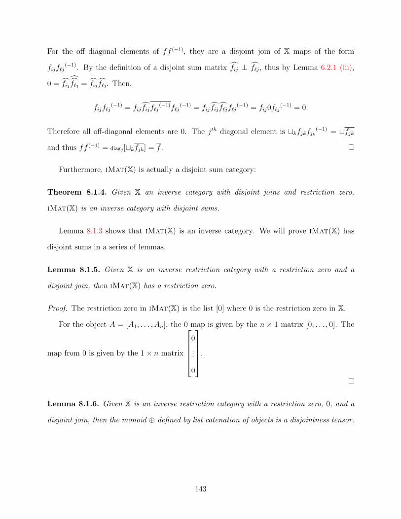
For the off diagonal elements of ff (−1), they are a disjoint join of X maps of the form
fijf`j(−1). By the definition of a disjoint sum matrix fij ⊥ f`j, thus by Lemma 6.2.1 (iii),
0 = fijf`j = fij f`j. Then,
fijf`j(−1) = fij fijf`j
(−1)f`j(−1) = fij fij f`jf`j
(−1) = fij0f`j(−1) = 0.
Therefore all off-diagonal elements are 0. The jth diagonal element is tkfjkfjk(−1) = tfjk
and thus ff (−1) = diagj[tkfjk] = f .
Furthermore, iMat(X) is actually a disjoint sum category:
Theorem 8.1.4. Given X an inverse category with disjoint joins and restriction zero,
iMat(X) is an inverse category with disjoint sums.
Lemma 8.1.3 shows that iMat(X) is an inverse category. We will prove iMat(X) has
disjoint sums in a series of lemmas.
Lemma 8.1.5. Given X is an inverse restriction category with a restriction zero and a
disjoint join, then iMat(X) has a restriction zero.
Proof. The restriction zero in iMat(X) is the list [0] where 0 is the restriction zero in X.
For the object A = [A1, . . . , An], the 0 map is given by the n × 1 matrix [0, . . . , 0]. The
map from 0 is given by the 1× n matrix
0
...
0
.
Lemma 8.1.6. Given X is an inverse restriction category with a restriction zero, 0, and a
disjoint join, then the monoid ⊕ defined by list catenation of objects is a disjointness tensor.
143
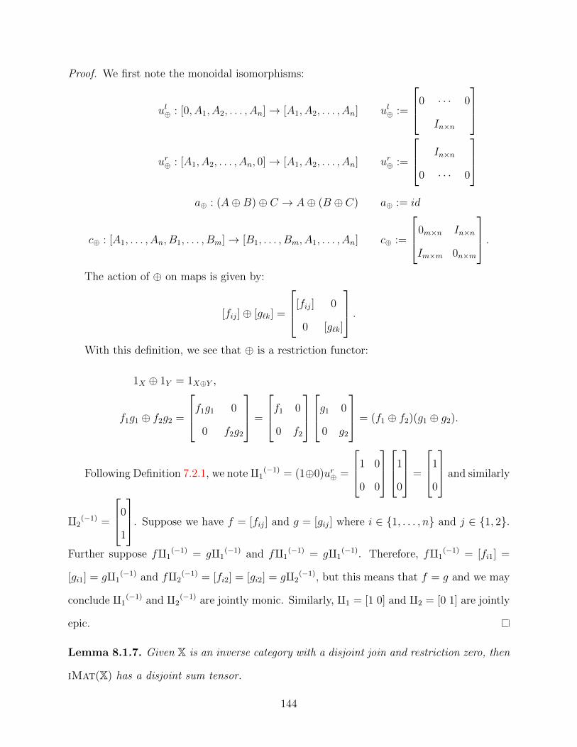
Proof. We first note the monoidal isomorphisms:
ul⊕ : [0, A1, A2, . . . , An]→ [A1, A2, . . . , An] ul⊕ :=
0 · · · 0
In×n
ur⊕ : [A1, A2, . . . , An, 0]→ [A1, A2, . . . , An] ur⊕ :=
In×n
0 · · · 0
a⊕ : (A⊕B)⊕ C → A⊕ (B ⊕ C) a⊕ := id
c⊕ : [A1, . . . , An, B1, . . . , Bm]→ [B1, . . . , Bm, A1, . . . , An] c⊕ :=
0m×n In×n
Im×m 0n×m
.The action of ⊕ on maps is given by:
[fij]⊕ [g`k] =
[fij] 0
0 [g`k]
.With this definition, we see that ⊕ is a restriction functor:
1X ⊕ 1Y = 1X⊕Y ,
f1g1 ⊕ f2g2 =
f1g1 0
0 f2g2
=
f1 0
0 f2
g1 0
0 g2
= (f1 ⊕ f2)(g1 ⊕ g2).
Following Definition 7.2.1, we note q1(−1) = (1⊕0)ur⊕ =
1 0
0 0
1
0
=
1
0
and similarly
q2(−1) =
0
1
. Suppose we have f = [fij] and g = [gij] where i ∈ {1, . . . , n} and j ∈ {1, 2}.
Further suppose fq1(−1) = gq1
(−1) and fq1(−1) = gq1
(−1). Therefore, fq1(−1) = [fi1] =
[gi1] = gq1(−1) and fq2
(−1) = [fi2] = [gi2] = gq2(−1), but this means that f = g and we may
conclude q1(−1) and q2
(−1) are jointly monic. Similarly, q1 = [1 0] and q2 = [0 1] are jointly
epic.
Lemma 8.1.7. Given X is an inverse category with a disjoint join and restriction zero, then
iMat(X) has a disjoint sum tensor.
144

Proof. By Lemma 8.1.6, we know that the tensor defined by list catenation is a disjointness
tensor. To show that it is a disjoint sum tensor, we must show the diagrams and conditions
of Definition 7.3.1 hold.
For the diagram below we show that α exists if and only if fq2(−1)O gq2
(−1):
[A]
f
��
g
((
α
$$[X, Y, Z]
q1,2(−1)
��
q1,3(−1)// [X,Z]
q1(−1)
��[X, Y ]
q1(−1)
// [X].
The existence of fq2(−1)O gq2
(−1) means there is an h = [h1, h2] : [A] → [Y, Z] such that
hq1(−1) = fq2
(−1) and hq2(−1) = gq2
(−1). From the diagram, given that f = [f1, f2] and
g = [g1, g2], we know that f1 = fq1(−1) = gq1
(−1) = g1. We also have h1 = f2 and h2 = g2.
If we set α to the matrix [f1, f2, g2], the diagram above commutes. We need only show that
α is a map in iMat(X). As f, g and h are maps in iMat(X), we know that:
f1q1 ⊥ f2q2
(f1q1 =)g1q1 ⊥ g2q2
(f2q2 =)h1q1 ⊥ h2 q2 (= g2q2).
From this, we can conclude ⊥ [f1q1, f2q2, g2q3].
Conversely, suppose we have an α = [α1, α2, α3] that makes the above diagram commute.
Then h := [α2, α3] is a map in X. Since [α1, α3] = g and [α1, α2] = f , we have hq1(−1) =
fq2(−1) and hq2
(−1) = gq2(−1), hence h = fq2
(−1)O gq2(−1).
145

The proof that β in the diagram below exists if and only if q2hMq2k is similar:
[A]
[X, Y ]q1,2
//
h
22
[X, Y, Z]
β
99
[X]
q1
OO
q1
// [X,Z].
q1,3
OO k
GG
We are now ready to prove Theorem 8.1.4, that iMat(X) has disjoint sums.
Proof. By Lemma 8.1.7, we know iMat(X) has a disjoint sum tensor and therefore by
Proposition 7.3.5, it has a disjoint join. By Proposition 7.4.1 we know that [A,B] = A⊕B is
a disjoint sum of A and B for any two objects in iMat(X), and hence, iMat(X) has disjoint
sums.
8.2 Equivalence between a disjoint sum category and its matrix category
This section starts by giving a functor from an inverse category with disjoint joins to its
matrix category, followed by exhibiting a reflection between inverse categories with disjoint
sums (Disjoint Sum Cats) and categories with a disjoint join (Disjoint Join Cats). That is,
Disjoint Sum Cats �� // Disjoint Join Cats.
Matrix
vv >(8.3)
Then, we will provide a restriction functor from the matrix category of an inverse category
with a disjoint sum to itself, i.e., iMat(X)→ X. Furthermore, we will show in the case where
X is an inverse category with a disjoint sum, X ∼= iMat(X).
146

Definition 8.2.1. Given X has disjoint joins and restriction zero, define M : X→ iMat(X)
by:
On objects: M(A) := [A].
On maps: M(f) := [f ] – The 1× 1 matrix with entry f.
Lemma 8.2.2. The map M from Definition 8.2.1 is a restriction functor.
Proof. From the definition of iMat(X), we have
f : A→ B if and only if M(f) : M(A)→M(B) (i.e., [f ] : [A]→ [B]),
M(idA) = [idA] = idM(A),
M(fg) = [fg] = [f ][g] = M(f)M(g), and
M(f) = [f ] = [f ] = M(f).
Let us represent the category of inverse categories with disjoint sums as DSum and the
category of inverse categories with disjoint joins as DJoin.
Note that any inverse category with disjoint sums is an inverse category with disjoint
joins. Hence, we have the obvious forgetful functor U : DSum → DJoin. From above,
we also have a functor Mat : DJoin → DSum given by Mat : X 7→ iMat(X). From the
definition of iMat(X), we see that we have the correspondence
DSum(iMat(X),Y)
DJoin(X,Y)
meaning that we have an adjunction, Mat ` U : DJoin→ DSum, as noted at the beginning
of this section.
Let us now consider when we apply the matrix construction to an inverse category which
already has a disjoint sum:
147
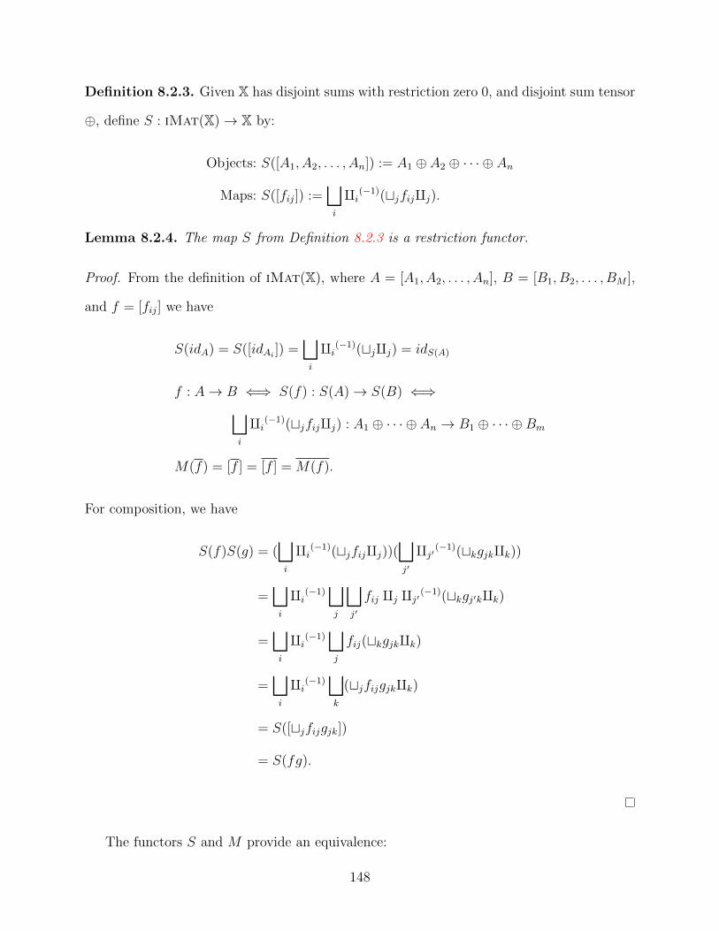
Definition 8.2.3. Given X has disjoint sums with restriction zero 0, and disjoint sum tensor
⊕, define S : iMat(X)→ X by:
Objects: S([A1, A2, . . . , An]) := A1 ⊕ A2 ⊕ · · · ⊕ An
Maps: S([fij]) :=⊔i
qi(−1)(tjfijqj).
Lemma 8.2.4. The map S from Definition 8.2.3 is a restriction functor.
Proof. From the definition of iMat(X), where A = [A1, A2, . . . , An], B = [B1, B2, . . . , BM ],
and f = [fij] we have
S(idA) = S([idAi]) =
⊔i
qi(−1)(tjqj) = idS(A)
f : A→ B ⇐⇒ S(f) : S(A)→ S(B) ⇐⇒⊔i
qi(−1)(tjfijqj) : A1 ⊕ · · · ⊕ An → B1 ⊕ · · · ⊕Bm
M(f) = [f ] = [f ] = M(f).
For composition, we have
S(f)S(g) = (⊔i
qi(−1)(tjfijqj))(⊔j′
qj′ (−1)(tkgjkqk))
=⊔i
qi(−1)⊔j
⊔j′
fij qj qj′ (−1)(tkgj′kqk)
=⊔i
qi(−1)⊔j
fij(tkgjkqk)
=⊔i
qi(−1)⊔k
(tjfijgjkqk)
= S([tjfijgjk])
= S(fg).
The functors S and M provide an equivalence:
148

Proposition 8.2.5. Given an inverse category X with ⊕ a disjoint sum tensor and a re-
striction zero, then the categories X and iMat(X) are equivalent.
Proof. The functors of the equivalence are S from Definition 8.2.3 and M from Defini-
tion 8.2.1.
First, we see that MS : X→ X is the identity functor as
Objects: S(M(A)) = S([A]) = A,
Maps: S(M(f)) = S([f ]) = f.
Next, we need to show that there is a natural transformation and isomorphism ρ such that
ρ(SM) = IiMat(X). For each object A = [A1, A2, . . . , An], set ρA =
[q1
(−1) · · · qn(−1)
].
Note that the functor SM has the following effect:
On objects: M(S([A1, . . . , An])) = M(A1 ⊕ · · · ⊕ An) = [A1 ⊕ · · · ⊕ An].
On maps: M(S([fij]) = M(⊔i
qi(−1)(tjfijqj)) = [⊔i
qi(−1)(tjfijqj)].
We can now draw the commuting naturality square for f = [fij] : [Ai]→ [Bj]:
SM([Ai]) [⊕iAi]
[q1
(−1) · · · qn(−1)
]//
SM(f)
��
[Ai]
f
��SM([Bj]) [⊕jBj] [
q1(−1) · · · qm(−1)
] // [Bj].
.
Following the square by the top–right path from [⊕iAi] to [Bj], by the definition of the
maps in the category iMat(X), we see each Bj = tiqi(−1)fij(⊕iAi). Following the left–
bottom path, composing SM(f) with
[q1
(−1) · · · qm(−1)
]gives us the map[
tiqi(−1)(tjfijqj)q1(−1) · · · tiqi(−1)(tjfijqj)qm(−1)
]=[tiqi(−1)fi1 · · · tiqi(−1)fim
].
149
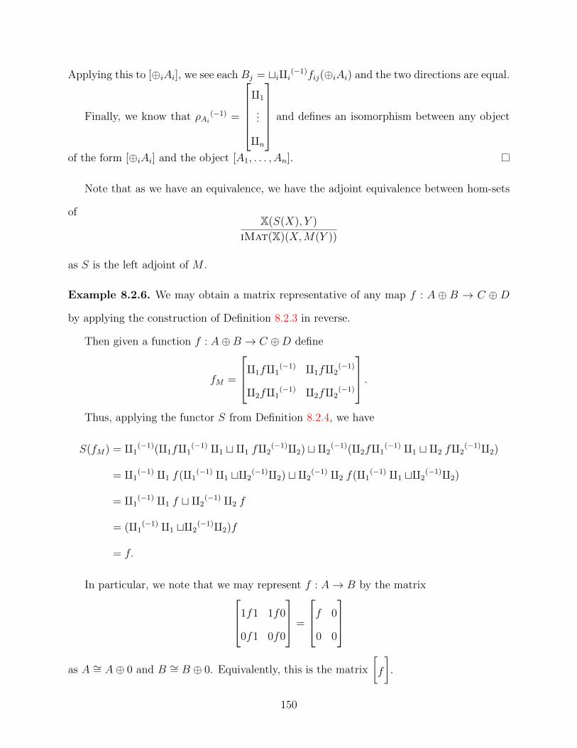
Applying this to [⊕iAi], we see each Bj = tiqi(−1)fij(⊕iAi) and the two directions are equal.
Finally, we know that ρAi(−1) =
q1
...
qn
and defines an isomorphism between any object
of the form [⊕iAi] and the object [A1, . . . , An].
Note that as we have an equivalence, we have the adjoint equivalence between hom-sets
ofX(S(X), Y )
iMat(X)(X,M(Y ))
as S is the left adjoint of M .
Example 8.2.6. We may obtain a matrix representative of any map f : A ⊕ B → C ⊕D
by applying the construction of Definition 8.2.3 in reverse.
Then given a function f : A⊕B → C ⊕D define
fM =
q1fq1(−1) q1fq2
(−1)
q2fq1(−1) q2fq2
(−1)
.Thus, applying the functor S from Definition 8.2.4, we have
S(fM) = q1(−1)(q1fq1
(−1) q1 t q1 fq2(−1)q2) t q2
(−1)(q2fq1(−1) q1 t q2 fq2
(−1)q2)
= q1(−1) q1 f(q1
(−1) q1 tq2(−1)q2) t q2
(−1) q2 f(q1(−1) q1 tq2
(−1)q2)
= q1(−1) q1 f t q2
(−1) q2 f
= (q1(−1) q1 tq2
(−1)q2)f
= f.
In particular, we note that we may represent f : A→ B by the matrix1f1 1f0
0f1 0f0
=
f 0
0 0
as A ∼= A⊕ 0 and B ∼= B ⊕ 0. Equivalently, this is the matrix
[f
].
150
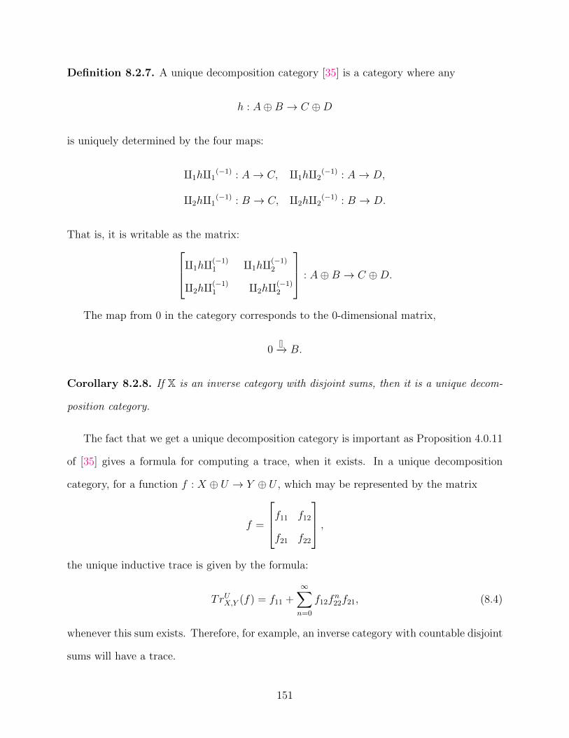
Definition 8.2.7. A unique decomposition category [35] is a category where any
h : A⊕B → C ⊕D
is uniquely determined by the four maps:
q1hq1(−1) : A→ C, q1hq2
(−1) : A→ D,
q2hq1(−1) : B → C, q2hq2
(−1) : B → D.
That is, it is writable as the matrix:q1hq(−1)1 q1hq(−1)
2
q2hq(−1)1 q2hq(−1)
2
: A⊕B → C ⊕D.
The map from 0 in the category corresponds to the 0-dimensional matrix,
0[]−→ B.
Corollary 8.2.8. If X is an inverse category with disjoint sums, then it is a unique decom-
position category.
The fact that we get a unique decomposition category is important as Proposition 4.0.11
of [35] gives a formula for computing a trace, when it exists. In a unique decomposition
category, for a function f : X ⊕ U → Y ⊕ U , which may be represented by the matrix
f =
f11 f12
f21 f22
,the unique inductive trace is given by the formula:
TrUX,Y (f) = f11 +∞∑n=0
f12fn22f21, (8.4)
whenever this sum exists. Therefore, for example, an inverse category with countable disjoint
sums will have a trace.
151
Chapter 9
Distributive inverse categories
We now consider inverse categories with both a disjoint sum and inverse product, where the
inverse product distributes over the disjoint sum in a specific way. This chapter will show
that the Cartesian Completion of such a category is a distributive restriction category where
the product distributes over the coproduct.
9.1 Distributive restriction categories
Definition 9.1.1. A Cartesian category B with coproduct + and is called a distributive [14]
category when
(A×B) + (A× C) ∼= A× (B + C).
Definition 9.1.2. A Cartesian restriction category D (as in Definition 3.9.3), with a restric-
tion zero and coproducts is called a distributive restriction category [23] when there is an
isomorphism ρ such that
A× (B + C)ρ−→ (A×B) + (A× C).
If D is a distributive restriction category, then Total(D) is a distributive category as in
Definition 9.1.1.
9.2 Distributive inverse categories
Definition 9.2.1. A distributive inverse category D consists of the following:
• D is an inverse category;
• D has an inverse product with tensor ⊗, per Definition 4.3.1;
152
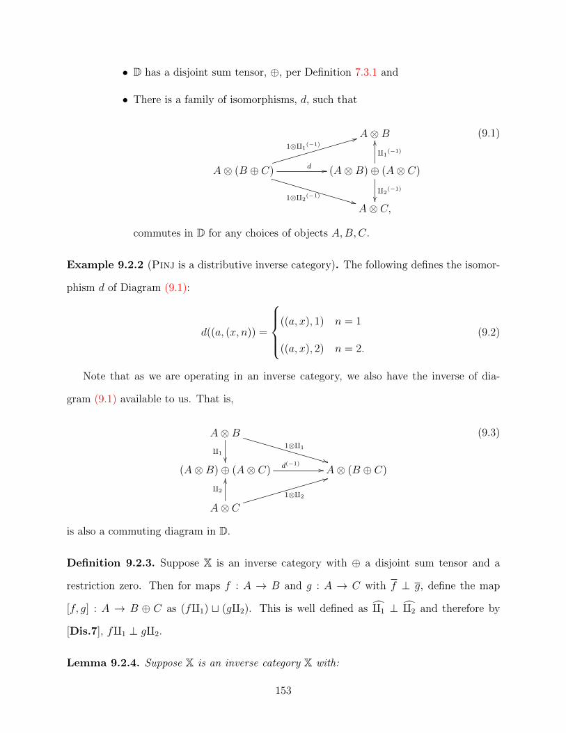
• D has a disjoint sum tensor, ⊕, per Definition 7.3.1 and
• There is a family of isomorphisms, d, such that
A⊗B
A⊗ (B ⊕ C) d //
1⊗q1(−1)
44
1⊗q2(−1)
**
(A⊗B)⊕ (A⊗ C)
q1(−1)
OO
q2(−1)
��A⊗ C,
(9.1)
commutes in D for any choices of objects A,B,C.
Example 9.2.2 (Pinj is a distributive inverse category). The following defines the isomor-
phism d of Diagram (9.1):
d((a, (x, n)) =
((a, x), 1) n = 1
((a, x), 2) n = 2.
(9.2)
Note that as we are operating in an inverse category, we also have the inverse of dia-
gram (9.1) available to us. That is,
A⊗Bq1
��
1⊗q1
**(A⊗B)⊕ (A⊗ C) d(−1)
// A⊗ (B ⊕ C)
A⊗ C
q2
OO
1⊗q2
44
(9.3)
is also a commuting diagram in D.
Definition 9.2.3. Suppose X is an inverse category with ⊕ a disjoint sum tensor and a
restriction zero. Then for maps f : A → B and g : A → C with f ⊥ g, define the map
[f, g] : A → B ⊕ C as (fq1) t (gq2). This is well defined as q1 ⊥ q2 and therefore by
[Dis.7], fq1 ⊥ gq2.
Lemma 9.2.4. Suppose X is an inverse category X with:
153
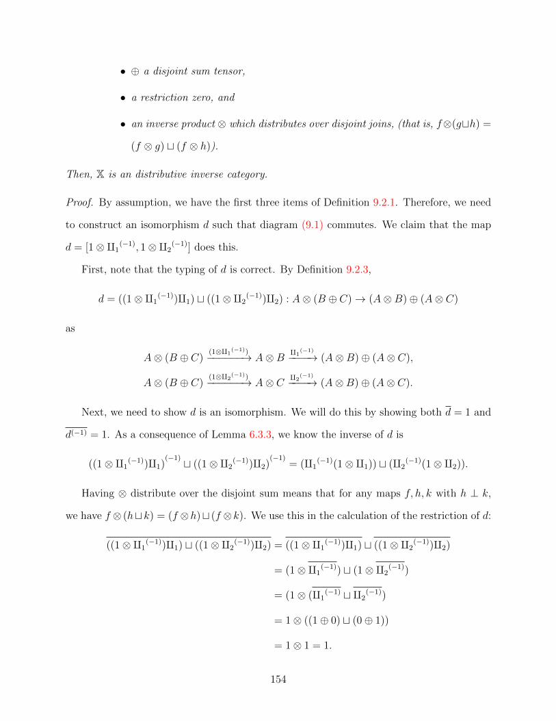
• ⊕ a disjoint sum tensor,
• a restriction zero, and
• an inverse product ⊗ which distributes over disjoint joins, (that is, f⊗(gth) =
(f ⊗ g) t (f ⊗ h)).
Then, X is an distributive inverse category.
Proof. By assumption, we have the first three items of Definition 9.2.1. Therefore, we need
to construct an isomorphism d such that diagram (9.1) commutes. We claim that the map
d = [1⊗q1(−1), 1⊗q2
(−1)] does this.
First, note that the typing of d is correct. By Definition 9.2.3,
d = ((1⊗q1(−1))q1) t ((1⊗q2
(−1))q2) : A⊗ (B ⊕ C)→ (A⊗B)⊕ (A⊗ C)
as
A⊗ (B ⊕ C)(1⊗q1
(−1))−−−−−−→ A⊗B q1(−1)
−−−−→ (A⊗B)⊕ (A⊗ C),
A⊗ (B ⊕ C)(1⊗q2
(−1))−−−−−−→ A⊗ C q2(−1)
−−−−→ (A⊗B)⊕ (A⊗ C).
Next, we need to show d is an isomorphism. We will do this by showing both d = 1 and
d(−1) = 1. As a consequence of Lemma 6.3.3, we know the inverse of d is
((1⊗q1(−1))q1)
(−1) t ((1⊗q2(−1))q2)
(−1)= (q1
(−1)(1⊗q1)) t (q2(−1)(1⊗q2)).
Having ⊗ distribute over the disjoint sum means that for any maps f, h, k with h ⊥ k,
we have f ⊗ (htk) = (f ⊗h)t (f ⊗k). We use this in the calculation of the restriction of d:
((1⊗q1(−1))q1) t ((1⊗q2
(−1))q2) = ((1⊗q1(−1))q1) t ((1⊗q2
(−1))q2)
= (1⊗q1(−1)) t (1⊗q2
(−1))
= (1⊗ (q1(−1) t q2
(−1))
= 1⊗ ((1⊕ 0) t (0⊕ 1))
= 1⊗ 1 = 1.
154

The calculation for d(−1) also shows it is 1:
(q1(−1)(1⊗q1)) t (q2
(−1)(1⊗q2)) = (q1(−1)(1⊗q1)) t (q2
(−1)(1⊗q2))
= (q1(−1)(1⊗q1)) t (q2
(−1)(1⊗q2))
= (q1(−1)) t (q2
(−1))
= (1⊕ 0) t (0⊕ 1)
= 1.
Hence, [1⊗q1(−1), 1⊗q2
(−1)] is an isomorphism. Finally, we must show that diagram (9.1)
commutes:
dq1(−1) =
(((1⊗q1
(−1))q1) t ((1⊗q2(−1))q2)
)q1
(−1)
=(
((1⊗q1(−1))q1)q1
(−1))t(
((1⊗q2(−1))q2)q1
(−1))
=(
(1⊗q1(−1))1
)t(
(1⊗q2(−1))0
)= (1⊗q1
(−1)) t 0
= 1⊗q1(−1)
and
dq2(−1) =
(((1⊗q1
(−1))q1) t ((1⊗q2(−1))q2)
)q2
(−1)
=(
((1⊗q1(−1))q1)q2
(−1))t(
((1⊗q2(−1))q2)q2
(−1))
= 0 t (1⊗q2(−1))
= 1⊗q2(−1).
This shows the fourth condition is satisfied and X is a distributive inverse category.
We have seen that a second tensor distributing over the disjoint joins implies that we
have an inverse distributive category. We now show the converse is true.
Lemma 9.2.5. Given an inverse distributive category X, then h⊗ (f O g) = (h⊗f)O(h⊗g)
whenever f O g exists and h⊗ (f M g) = (h⊗ f)M(h⊗ g) whenever f M g exists.
155

Proof. Let h : A→ B, f : C → D and g : C → E. Consider the following diagram:
B ⊗ E
A⊗ Ch⊗(f O g) //
h⊗g
++
h⊗f
33
B ⊗ (D ⊕ E)∼= //
1⊗q1(−1)
77
1⊗q2(−1)
''
(B ⊗D)⊕ (B ⊗ E)
q2(−1)
��
q1(−1)
OO
B ⊗D.
The two leftmost triangles commute by the diagram for f O g. The right hand triangles
commute as per Definition 9.2.1. By the uniqueness of the O operation we see h⊗ (f O g) =
(h⊗ f)O(h⊗ g),
The argument for showing h⊗ (f M g) = (h⊗ f)M(h⊗ g) follows the same pattern.
Lemma 9.2.6. Given an inverse distributive category X, ⊗ distributes over the disjoint join.
Proof. First recall the definition of f t g = (f O g)(f M g). In order to show h ⊗ (f t g) =
(h⊗ f) t (h⊗ g), we need to show that
h⊗ (f O g)(f M g) = (h⊗ f Oh⊗ g)(h⊗ f Mh⊗ g). (9.4)
Since h⊗ (f O g)(f M g) = (h⊗ (f O g))(h⊗ (f M g)), Equation (9.4) follows directly from
Lemma 9.2.5 and the fact that ⊗ is a restriction functor.
Corollary 9.2.7. Suppose we have an inverse distributive category X. Then,
(i) if f ⊥ g, then (h⊗ f) ⊥ (h⊗ g) for any h,
(ii) if f ⊥ g : A→ B and h ⊥ k : C → D, then (f ⊗ h) ⊥ (g ⊗ k).
Proof.
(i) As f ⊥ g, we have f M g and f O g. By Lemma 9.2.5, both h⊗ f Mh⊗ g and
h⊗ f Oh⊗ g exist and therefore h⊗ f ⊥ h⊗ g.
156
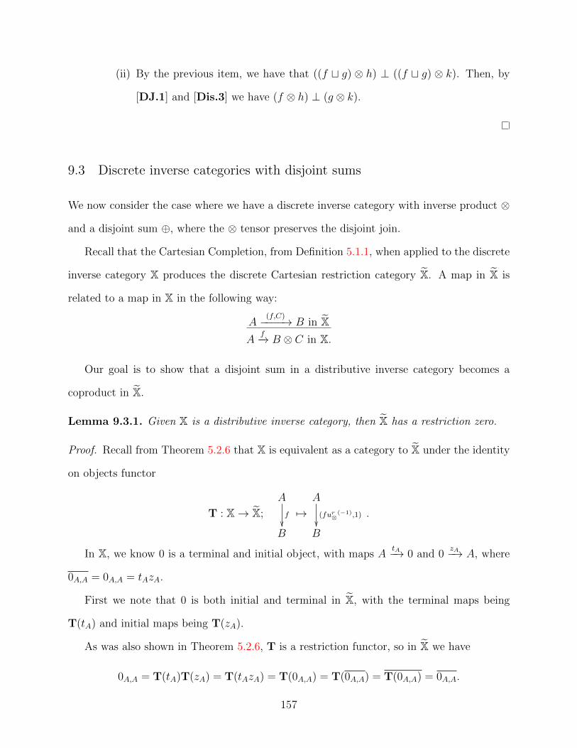
(ii) By the previous item, we have that ((f t g) ⊗ h) ⊥ ((f t g) ⊗ k). Then, by
[DJ.1] and [Dis.3] we have (f ⊗ h) ⊥ (g ⊗ k).
9.3 Discrete inverse categories with disjoint sums
We now consider the case where we have a discrete inverse category with inverse product ⊗
and a disjoint sum ⊕, where the ⊗ tensor preserves the disjoint join.
Recall that the Cartesian Completion, from Definition 5.1.1, when applied to the discrete
inverse category X produces the discrete Cartesian restriction category X. A map in X is
related to a map in X in the following way:
A(f,C)−−−−→ B in X
Af−→ B ⊗ C in X.
Our goal is to show that a disjoint sum in a distributive inverse category becomes a
coproduct in X.
Lemma 9.3.1. Given X is a distributive inverse category, then X has a restriction zero.
Proof. Recall from Theorem 5.2.6 that X is equivalent as a category to X under the identity
on objects functor
T : X→ X;
A
f
��B
7→A
(fur⊗(−1),1)
��B
.
In X, we know 0 is a terminal and initial object, with maps AtA−→ 0 and 0
zA−→ A, where
0A,A = 0A,A = tAzA.
First we note that 0 is both initial and terminal in X, with the terminal maps being
T(tA) and initial maps being T(zA).
As was also shown in Theorem 5.2.6, T is a restriction functor, so in X we have
0A,A = T(tA)T(zA) = T(tAzA) = T(0A,A) = T(0A,A) = T(0A,A) = 0A,A.
157

Hence, 0A,A is a restriction zero in X.
Lemma 9.3.2. In a distributive inverse category X, the following hold:
(i) Given f : A → Y ⊗ C we can construct maps f ′ : A → Y ⊗ (C ⊕ D) and
f ′′ : A→ Y ⊗ (E ⊗ C) for some objects D,E such that f ' f ′ and f ' f ′′.
(ii) Given f : A → Y ⊗ C, g : A → Y ⊗ D, then the f ′ : A → Y ⊗ (C ⊕ D),
g′′ : B → Y ⊗ (C ⊕D) as constructed in (i) satisfies q1(−1)f ′ ⊥ q2
(−1)g′′.
Proof.
(i) Set f ′ = f(1⊗q1). To show f ' f ′, we must first show their restriction is the
same:
f(1⊗q1) = f(1⊗q1) = f1 = f.
The mediating map between f and f ′ is, of course, 1⊗q1:
Y ⊗ C
1⊗q1
��
A
f77
f ′ &&Y ⊗ (C ⊕D).
By the same reasoning we may also create f ′′ : A → Y ⊗ (D ⊕ C) by setting
f ′′ = f(1⊗q2).
(ii) First note we have q1(−1)f ′, q2
(−1)g′′ : A⊕B → Y ⊗(C⊕D). In order to show
q1(−1)f ′ ⊥ q2
(−1)g′′, we will proceed by showing their restrictions and ranges
are disjoint. As q1(−1) ⊥ q2
(−1) and q1(−1)f ′ ≤ q1
(−1) and q2(−1)g′ ≤ q2
(−1),
we immediately have q1(−1)f ′ ⊥ q2
(−1)g′′.
158

For the ranges, we have
q1(−1)f ′ = q1
(−1)(f(1⊗q1)) = ((1⊗q1(−1))f (−1))q1
= ((1⊗q1(−1))f (−1)
≤ (1⊗q1(−1))
and similarly
q2(−1)g′′ ≤ (1⊗q2
(−1)).
Using Lemma 6.2.3 we know that (q1(−1)) ⊥ (q2
(−1)). From Corollary 9.2.7 we
conclude that (1⊗q1(−1)) ⊥ (1⊗q2
(−1)) and giving us q1(−1)f ′ ⊥ q2
(−1)g′′
and therefore q1(−1)f ′ ⊥ q2
(−1)g′′.
Theorem 9.3.3. Given X is a distributive inverse category, then the category X has coprod-
ucts.
Proof. The tensor object A⊕B in X will become the coproduct of A,B in X.
The injection maps of the coproduct are i1 = (q1ur⊗
(−1), 1) and i2 = (q2ur⊗
(−1), 1).
Consider the following diagram in X:
A(f,C)
**i1 ##
A⊕B h // Y.
B(g,D)
44i2
;;
In X, this comes from the diagram:
A
q1 ##
f // Y ⊗ C
A⊕B
B
q2
;;
g // Y ⊗D
(9.5)
159
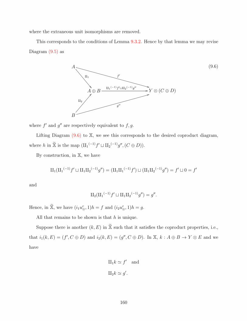
where the extraneous unit isomorphisms are removed.
This corresponds to the conditions of Lemma 9.3.2. Hence by that lemma we may revise
Diagram (9.5) as
A
q1
��
f ′
++A⊕B q1
(−1)f ′tq2(−1)g′′ // Y ⊗ (C ⊕D)
B
q2
AA
g′′
33
(9.6)
where f ′ and g′′ are respectively equivalent to f, g.
Lifting Diagram (9.6) to X, we see this corresponds to the desired coproduct diagram,
where h in X is the map (q1(−1)f ′ t q2
(−1)g′′, (C ⊕D)).
By construction, in X, we have
q1(q1(−1)f ′ t q1q2
(−1)g′′) = (q1q1(−1)f ′) t (q1q2
(−1)g′′) = f ′ t 0 = f ′
and
q2(q1(−1)f ′ t q1q2
(−1)g′′) = g′′.
Hence, in X, we have (i1ur⊗, 1)h = f and (i2u
r⊗, 1)h = g.
All that remains to be shown is that h is unique.
Suppose there is another (k,E) in X such that it satisfies the coproduct properties, i.e.,
that i1(k,E) = (f ′, C ⊕D) and i2(k,E) = (g′′, C ⊕D). In X, k : A ⊕ B → Y ⊗ E and we
have
q1k ' f ′ and
q2k ' g′.
160

Since equivalence is a transitive relation, this means we have
fq1' q1k and
gq2' q2k,
where the maps q1 : Y ⊗C → Y ⊗E and q2 : Y ⊗D → Y ⊗E fulfill the respective equivalence
diagrams.
Explicitly for k, f and q1, this gives us:
Y ⊗ C
q1
��
A
f::
q1k $$Y ⊗ E.
Now, we turn out attention to showing that k ' h = q1(−1)f ′ t q2
(−1)g′′. Consider
Y ⊗ (C ⊕D)
t
��
A
q1(−1)f ′tq2
(−1)g′′66
k ((Y ⊗ E.
(9.7)
As X is an inverse category, we know there is a map t that makes this diagram commute,
namely t = (q1(−1)f ′ t q2
(−1)g′′)(−1)
k. However, we must show this is in Y ∆∇ .
Next, recalling Definition 7.2.6 consider
Y ⊗ C 1⊗q1 //
q1
&&
Y ⊗ (C ⊕D)
q1 M q2
��
Y ⊗D1⊗q2oo
q2
xxY ⊗ E.
The map q1M q2 exists iff q1 ⊥ q2. But, the map t from above does make the diagram
161

commute. This can be shown by
(1⊗q1)(q1(−1)f ′ t q2
(−1)g′′)(−1)
k
= (1⊗q1)(q1(−1)f(1⊗q1) t q2
(−1)g(1⊗q2))(−1)
k
= (1⊗q1)((1⊗q1(−1))f (−1) q1 t(1⊗q2
(−1))g(−1)q2)k
= ((1⊗ 1)f (−1) q1 t(1⊗ 0)g(−1)q2)k
= f (−1) q1 k
= q1
and similarly for q2. Therefore, q1 ⊥ q2.
This means we may form the map q1M q2 : Y ⊗ (C ⊕ D) → Y ⊗ E. But then the map
(q1M q2) makes Diagram (9.7) commute. At the same time, q1, q2 ∈ Y ∆∇ , which gives
q1 =1⊗q1
q1 M q2
=
1⊗q1
q1 M q2
=
1⊗q1
q1 M q2
=
1⊗q1
q1 M q2
=
1⊗q1
q1 M q2
=
1⊗q1
q1 M q2
= (1⊗q1)(q1M q2)∆∇.
Similarly, q2 = (1⊗q2)(q1M q2)∆∇ giving us q1M q2 ∈ Y ∆
∇ by the uniqueness of the M operation.
Therefore q1M q2 provides an equivalence between k and q1(−1)f ′ t q2
(−1)g′′, meaning the
coproduct is unique.
Corollary 9.3.4. When X is a distributive inverse category, X is a distributive restriction
category.
Proof. As X has restriction products by Lemma 5.1.11, restriction coproducts by Theo-
rem 9.3.3 and the equations for distributivity follow directly from the distributivity of the
base tensors, we see X is a distributive restriction category.
162
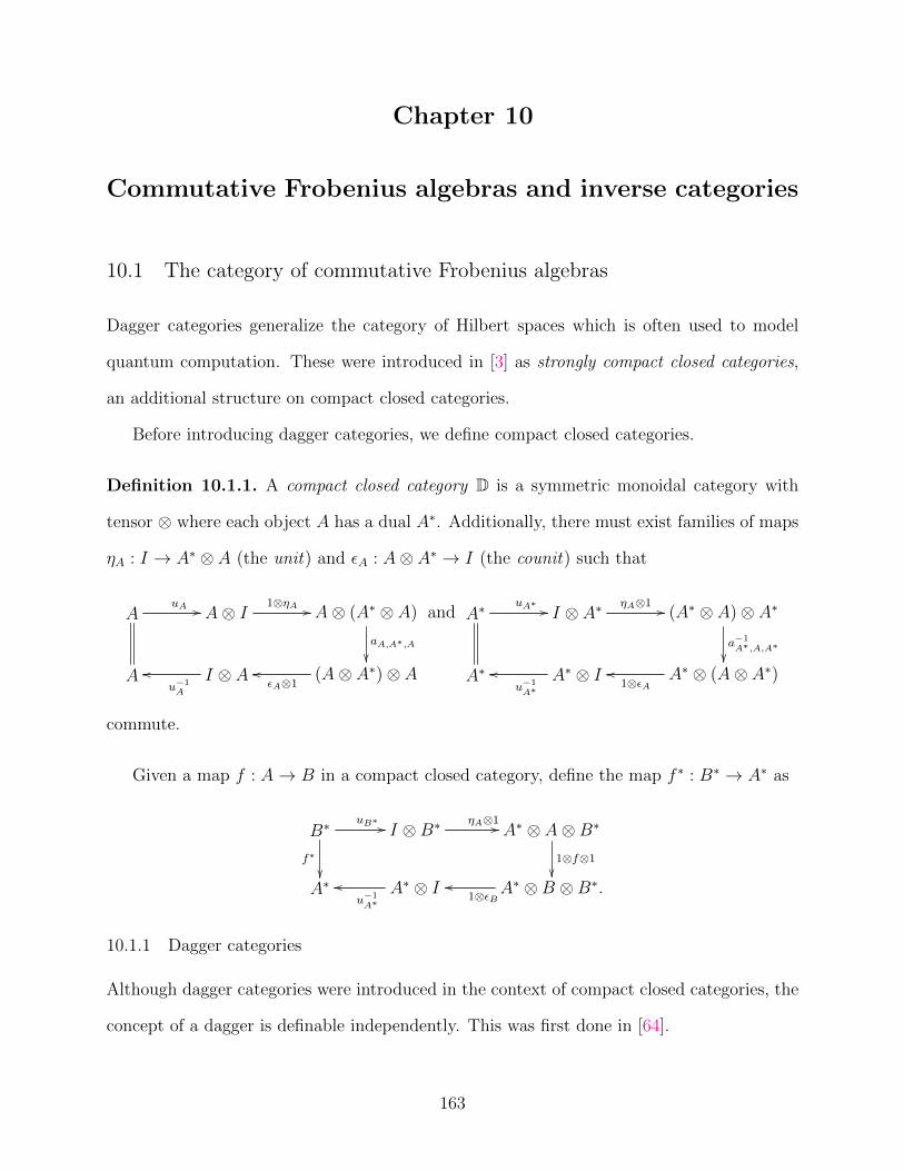
Chapter 10
Commutative Frobenius algebras and inverse categories
10.1 The category of commutative Frobenius algebras
Dagger categories generalize the category of Hilbert spaces which is often used to model
quantum computation. These were introduced in [3] as strongly compact closed categories,
an additional structure on compact closed categories.
Before introducing dagger categories, we define compact closed categories.
Definition 10.1.1. A compact closed category D is a symmetric monoidal category with
tensor ⊗ where each object A has a dual A∗. Additionally, there must exist families of maps
ηA : I → A∗ ⊗ A (the unit) and εA : A⊗ A∗ → I (the counit) such that
AuA // A⊗ I 1⊗ηA // A⊗ (A∗ ⊗ A)
aA,A∗,A��
A I ⊗ Au−1A
oo (A⊗ A∗)⊗ AεA⊗1oo
and A∗uA∗ // I ⊗ A∗ ηA⊗1 // (A∗ ⊗ A)⊗ A∗
a−1A∗,A,A∗��
A∗ A∗ ⊗ Iu−1A∗
oo A∗ ⊗ (A⊗ A∗)1⊗εAoo
commute.
Given a map f : A→ B in a compact closed category, define the map f ∗ : B∗ → A∗ as
B∗uB∗ //
f∗
��
I ⊗B∗ ηA⊗1// A∗ ⊗ A⊗B∗
1⊗f⊗1��
A∗ A∗ ⊗ Iu−1A∗
oo A∗ ⊗B ⊗B∗.1⊗εB
oo
10.1.1 Dagger categories
Although dagger categories were introduced in the context of compact closed categories, the
concept of a dagger is definable independently. This was first done in [64].
163
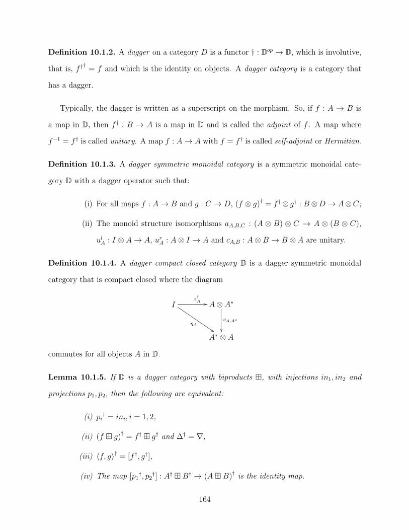
Definition 10.1.2. A dagger on a category D is a functor † : Dop → D, which is involutive,
that is, f ††
= f and which is the identity on objects. A dagger category is a category that
has a dagger.
Typically, the dagger is written as a superscript on the morphism. So, if f : A → B is
a map in D, then f † : B → A is a map in D and is called the adjoint of f . A map where
f−1 = f † is called unitary. A map f : A→ A with f = f † is called self-adjoint or Hermitian.
Definition 10.1.3. A dagger symmetric monoidal category is a symmetric monoidal cate-
gory D with a dagger operator such that:
(i) For all maps f : A→ B and g : C → D, (f ⊗ g)† = f †⊗ g† : B⊗D → A⊗C;
(ii) The monoid structure isomorphisms aA,B,C : (A ⊗ B) ⊗ C → A ⊗ (B ⊗ C),
ulA : I ⊗ A→ A, urA : A⊗ I → A and cA,B : A⊗B → B ⊗ A are unitary.
Definition 10.1.4. A dagger compact closed category D is a dagger symmetric monoidal
category that is compact closed where the diagram
Iε†A //
ηA$$
A⊗ A∗
cA,A∗
��A∗ ⊗ A
commutes for all objects A in D.
Lemma 10.1.5. If D is a dagger category with biproducts �, with injections in1, in2 and
projections p1, p2, then the following are equivalent:
(i) pi† = ini, i = 1, 2,
(ii) (f � g)† = f † � g† and ∆† = ∇,
(iii) 〈f, g〉† = [f †, g†],
(iv) The map [p1†, p2
†] : A† �B† → (A�B)† is the identity map.
164

Proof. (i) =⇒ (ii) To show ∆† = ∇, draw the product cone for ∆,
A
∆��
id
##
id
{{A A� Ap1oo
p2// A
and apply the dagger functor to it. As pi† = ini, and † is identity on objects,
this is now a coproduct diagram and therefore ∆† = ∇.
For (f � g)† = f † � g†, start with the diagram defining f � g as a product of
the arrows:
A
f
��
A�Bp1oo p2 //
f�g��
A
g
��C C �Dp1oo
p2// D.
Then, apply the dagger functor to this diagram. This is now the diagram
defining the coproduct of maps and therefore (f � g)† = f † � g†.
(ii) =⇒ (iii) The calculation showing this is
[f †, g†] = ∇; (f † � g†)
= ∆†; (f † � g†)
= ∆†; (f � g)†
= ((f � g); ∆)†
= 〈f, g〉†.
(iii) =⇒ (iv) Under the assumption,
[p1†, p2
†] = 〈p1, p2〉† = id† = id.
(iv) =⇒ (i) As [in1, in2] : A† � B† → A† � B† = id = [p1†, p2
†], we immediately have
p1† = in1 and p2
† = in2.
Definition 10.1.6. A biproduct dagger compact closed category is a dagger compact closed
category with biproducts where the conditions of Lemma 10.1.5 hold.
165

10.1.2 Examples of dagger categories
Example 10.1.7 (FdHilb). The category of finite dimensional Hilbert spaces is the mo-
tivating example for the creation of the dagger and is, in fact, a biproduct dagger compact
closed category. The biproduct is the direct sum of Hilbert spaces and the tensor for compact
closure is the standard tensor of Hilbert spaces. The dual H∗ of a space H is the space of all
continuous linear functions from H to the base field. The dagger is defined via the adjoint
as being the unique map f † : B → A such that 〈fa|b〉 = 〈a|f †b〉 for all a ∈ A, b ∈ B.
Example 10.1.8 (Rel). The category Rel of sets and relations has the tensor S⊗T :=S×T
and the biproduct S � T :=S ] T . This is compact closed under A∗ :=A and the dagger
is the relational converse. That is, if the relation R = {(s, t)|s ∈ S, t ∈ T} : S → T , then
R† = R∗ = {(t, s)|(s, t) ∈ R}.
Example 10.1.9 (Inverse categories). An inverse category X is also a dagger category when
the dagger is defined as the partial inverse. The unitary maps are the total maps. When the
inverse category X is also a symmetric monoidal category where the monoid ⊗ is actually a
restriction bi-functor, then X is a dagger symmetric monoidal category.
Requirement (i) of Definition 10.1.3 is fulfilled, as
(f ⊗ g)(f ⊗ g)(−1) = f ⊗ g = f ⊗ g = ff (−1) ⊗ gg(−1) = (f ⊗ g)(f (−1) ⊗ g(−1))
and since the partial inverse of f ⊗ g is unique, (f ⊗ g)(−1) = f (−1)⊗ g(−1). Requirement (ii)
is that the structure isomorphisms are unitary. This is, of course, true as each of them are
isomorphisms, hence total and therefore unitary.
10.1.3 Frobenius algebras
Frobenius algebras were originally defined as a finite dimensional algebra over a field together
with a non-degenerate pairing operation. Here we present the general categorical definition:
166
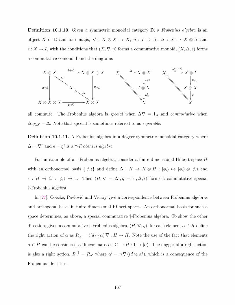
Definition 10.1.10. Given a symmetric monoidal category D, a Frobenius algebra is an
object X of D and four maps, ∇ : X ⊗ X → X, η : I → X, ∆ : X → X ⊗ X and
ε : X → I, with the conditions that (X,∇, η) forms a commutative monoid, (X,∆, ε) forms
a commutative comonoid and the diagrams
X ⊗X 1⊗∆ //
∆⊗1
��
∇
$$
X ⊗X ⊗X
∇⊗1
��
X∆
$$X ⊗X ⊗X
1⊗∇// X ⊗X
X∆ // X ⊗X
ε⊗1��
I ⊗Xul⊗��X
Xur⊗
(−1)
// X ⊗ I1⊗η��
X ⊗X∇��X
all commute. The Frobenius algebra is special when ∆∇ = 1X and commutative when
∆cX,X = ∆. Note that special is sometimes referred to as separable.
Definition 10.1.11. A Frobenius algebra in a dagger symmetric monoidal category where
∆ = ∇† and ε = η† is a †-Frobenius algebra.
For an example of a †-Frobenius algebra, consider a finite dimensional Hilbert space H
with an orthonormal basis {|φi〉} and define ∆ : H → H ⊗ H : |φi〉 7→ |φi〉 ⊗ |φi〉 and
ε : H → C : |φi〉 7→ 1. Then (H,∇ = ∆†, η = ε†,∆, ε) forms a commutative special
†-Frobenius algebra.
In [27], Coecke, Pavlovic and Vicary give a correspondence between Frobenius algebras
and orthogonal bases in finite dimensional Hilbert spaces. An orthonormal basis for such a
space determines, as above, a special commutative †-Frobenius algebra. To show the other
direction, given a commutative †-Frobenius algebra, (H,∇, η), for each element α ∈ H define
the right action of α as Rα := (id ⊗ α)∇ : H → H. Note the use of the fact that elements
α ∈ H can be considered as linear maps α : C→ H : 1 7→ |α〉. The dagger of a right action
is also a right action, Rα† = Rα′ where α′ = η∇ (id ⊗ α†), which is a consequence of the
Frobenius identities.
167

The ( )′ construction is actually an involution:
(α′)′ = η∇(id⊗ α′†)
= u∇(id⊗ (η∇(id⊗ α†))†
= u∇(id⊗ ((id⊗ α)∆ε))
= (u⊗ α)(∇⊗ id)(id⊗∆)(id⊗ ε)
= (u⊗ α)(id⊗∆)(∇⊗ id)(id⊗ ε)
= (u⊗ α)(id⊗ ε)
= α.
Lemma 10.1.12 (Coecke, Pavolvic, Vicary [27]). Any †-Frobenius algebra in FdHilb is a
C∗-algebra.
Proof. The endomorphism monoid of FdHilb (H,H) is a C∗-algebra. From the proceeding,
we have
H ∼= FdHilb(C, H) ∼= R[FdHilb(C,H)] ⊆ FdHilb(H,H).
This inherits the algebra structure from FdHilb (H,H). Furthermore, since any finite di-
mensional involution-closed sub-algebra of a C∗-algebra is also a C∗-algebra, this shows the
†-Frobenius algebra is a C∗-algebra.
Using the fact that the involution preserving homomorphisms from a finite dimensional
commutative C∗-algebra to C form a basis for the dual of the underlying vector space, write
these homomorphisms as φi† : H → C. Then their adjoints, φi : C → H will form a basis
for the space H. These are the copyable elements in H.
This, together with continued applications of the Frobenius rules and linear algebra allow
Coecke, Pavlovic and Vicary to prove the following Theorem.
Theorem 10.1.13 (Coecke, Pavolvic, Vicary [27]). Every commutative †-Frobenius algebra
in FdHilb determines an orthogonal basis consisting of its copyable elements. Conversely,
168

every orthogonal basis {|φi〉}i determines a commutative †-Frobenius algebra via
∆ : H → H ⊗H : |φi〉 7→ |φi〉 ⊗ |φi〉 ε : H → C : |φi〉 7→ 1
and these constructions are inverse to each other.
An interesting aspect of Theorem 10.1.13 is that it uses only algebraic structures to
determine a basis as the “copyable elements”. In a quantum computation, the choice of
basis determines the copyable elements.
Remark 10.1.14. Vicary, in [67], further explores †-Frobenius algebras to define invo-
lution monoids on †-monoidal categories with duals. This led to an alternate proof of
Lemma 10.1.12 based on monoids. From this, Vicary shows that the category of commu-
tative †-monoids in FdHilb, with monoid morphisms as maps, is equivalent to FinSetsop
– the dual of the category of finite sets. Of course, this is another way to move to the
classical world from the quantum world. Vicary goes on in [50] to define a finite quantum
Boolean topos and finite Boolean topos and show that the category of classical structures
in a finite quantum Boolean topos is equivalent to a finite Boolean topos and in fact, every
finite Boolean topos arises in this way.
10.1.4 CFrob(X) is an inverse category
Example 10.1.15 (Commutative separable Frobenius algebras [43]). Let X be a symmetric
monoidal category and form CFrob(X) as follows:
Objects: Commutative separable Frobenius algebras: These are quintuples (A,∇, η,∆, ε)
where A is an object of X with the following maps: ∇ : A⊗A→ A, η : I → A, ∆ : A→ A⊗A,
ε : A → I which are natural maps in X, with (A,∇, η) a monoid and (A,∆, ε) a comonoid.
169

Additionally, these satisfy
A⊗ A
1⊗∆
��
∇
''
∆⊗1 // A⊗ (A⊗ A)
1⊗∇
��
A∆
''(A⊗ A)⊗ A
∇⊗1// A⊗ A
Frobenius
together with the additional property that ∆∇ = 1 (separable).
Maps: The maps of X between the objects of X which preserve multiplication (∇) and
comultiplication (∆) but do not necessarily preserve the units. This means a map f must
satisfy the following commuting diagrams:
A
∆��
f // B
∆��
A⊗ Af⊗f
// B ⊗B
and A⊗ A∇��
f⊗f // B ⊗B∇��
Af
// B.
Lemma 10.1.16. When X is a symmetric monoidal category, CFrob(X) is an inverse
category.
Proof. We need to show that CFrob(X) has restrictions and that each map has a partial
inverse. We do this by exhibiting the partial inverse of a map. For f : X → Y , define f (−1)
as
Y1⊗η−−→ Y ⊗X 1⊗∆−−→ Y ⊗X ⊗X 1⊗f⊗1−−−−→ Y ⊗ Y ⊗X ∇⊗1−−→ Y ⊗X ε⊗1−−→ X.
As a string diagram, this looks like:
f
.
170
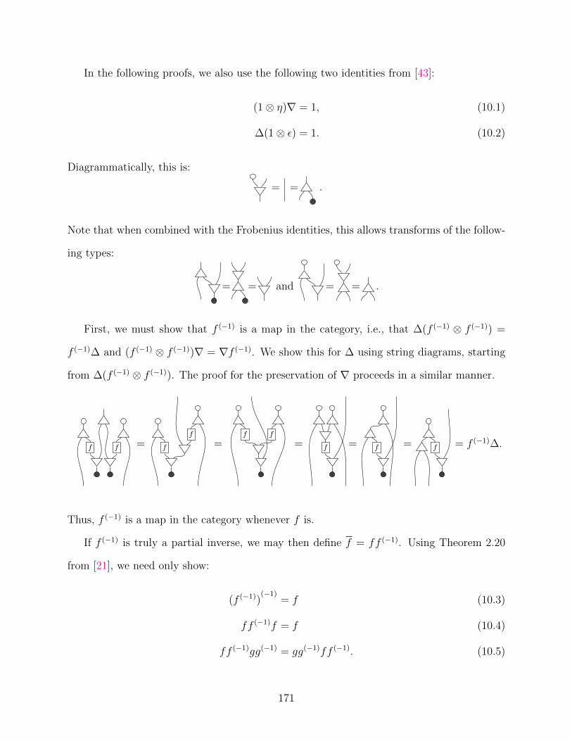
In the following proofs, we also use the following two identities from [43]:
(1⊗ η)∇ = 1, (10.1)
∆(1⊗ ε) = 1. (10.2)
Diagrammatically, this is:
= = .
Note that when combined with the Frobenius identities, this allows transforms of the follow-
ing types:
= = and = = .
First, we must show that f (−1) is a map in the category, i.e., that ∆(f (−1) ⊗ f (−1)) =
f (−1)∆ and (f (−1) ⊗ f (−1))∇ = ∇f (−1). We show this for ∆ using string diagrams, starting
from ∆(f (−1) ⊗ f (−1)). The proof for the preservation of ∇ proceeds in a similar manner.
f f = f
f
=f f
= f = f = f = f (−1)∆.
Thus, f (−1) is a map in the category whenever f is.
If f (−1) is truly a partial inverse, we may then define f = ff (−1). Using Theorem 2.20
from [21], we need only show:
(f (−1))(−1)
= f (10.3)
ff (−1)f = f (10.4)
ff (−1)gg(−1) = gg(−1)ff (−1). (10.5)
171

Proof of Equation (10.3): (f (−1))(−1)
=
f = f = f = f = f = f .
Proof of Equation (10.4): ff (−1)f =
f f f =f f
=f f
= f = f = f .
Proof of Equation (10.5): ff (−1)gg(−1) =
f f g g =f g
=
f
g
=f g
=f g
=g f
= gg(−1)ff (−1)
where the last step is accomplished by reversing all the previous diagrammatic steps. Hence,
CFrob(X) is an inverse category.
Theorem 10.1.17. When X is a symmetric monoidal category, CFrob(X) is a discrete
inverse category.
172

Proof. Lemma 10.1.16 shows CFrob(X) is an inverse category. We need to show the con-
ditions of Definition 4.3.1 are met.
First, we see that the tensor of X is a tensor in CFrob(X). A ⊗ B is an object in
CFrob(X) with ∆A⊗B = (∆A ⊗∆B)(1⊗ c⊗ ⊗ 1), ∇A⊗B = (1⊗ c⊗ ⊗ 1)(∇A ⊗∇B), ηA⊗B =
∆I(ηA ⊗ ηB), and εA⊗B = (εA ⊗ εB)∇I .
The map ∆ : A → A ⊗ A is a map in CFrob(X). To show it preserves ∆, we need to
show ∆A∆A⊗A = ∆A(∆A ⊗∆A):
∆A∆A⊗A = = = = = ∆A(∆A ⊗∆A).
Note that in the last step, we simply reverse the various associativity steps used previously.
To show that ∆ preserves the ∇, we must show that (∆A⊗∆A)∇A⊗A = ∇A∆A. Starting
with (∆A ⊗∆A)∇A⊗A =
= = = = = ∇A∆A.
Note that the proof uses the “special” property in a non-trivial way.
Thus, we have a ∆ in CFrob(X). As ∇ = ∆(−1), the Frobenius requirement for the
inverse product is immediately fulfilled. Commutativity, cocommutativity, associativity,
coassociativity and the exchange rule all follow from the properties of the commutative
Frobenius algebras and therefore CFrob(X) is a discrete inverse category.
Note that the category CFrob(X) possesses additional structure over that of a general
discrete inverse category, specifically, the existence of unit maps η : I → A and ε : A → I
for each object A.
We may also consider CFrob(X) as a bicategory [47], with the following data:
173
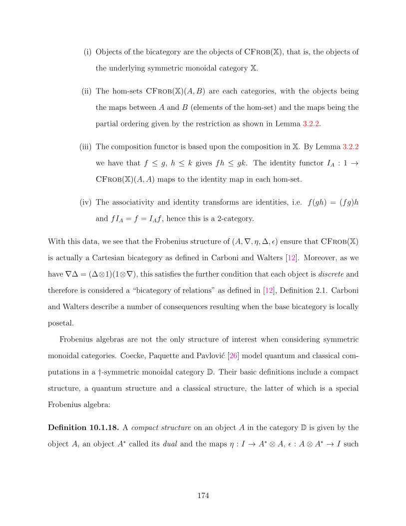
(i) Objects of the bicategory are the objects of CFrob(X), that is, the objects of
the underlying symmetric monoidal category X.
(ii) The hom-sets CFrob(X)(A,B) are each categories, with the objects being
the maps between A and B (elements of the hom-set) and the maps being the
partial ordering given by the restriction as shown in Lemma 3.2.2.
(iii) The composition functor is based upon the composition in X. By Lemma 3.2.2
we have that f ≤ g, h ≤ k gives fh ≤ gk. The identity functor IA : 1 →
CFrob(X)(A,A) maps to the identity map in each hom-set.
(iv) The associativity and identity transforms are identities, i.e. f(gh) = (fg)h
and fIA = f = IAf , hence this is a 2-category.
With this data, we see that the Frobenius structure of (A,∇, η,∆, ε) ensure that CFrob(X)
is actually a Cartesian bicategory as defined in Carboni and Walters [12]. Moreover, as we
have∇∆ = (∆⊗1)(1⊗∇), this satisfies the further condition that each object is discrete and
therefore is considered a “bicategory of relations” as defined in [12], Definition 2.1. Carboni
and Walters describe a number of consequences resulting when the base bicategory is locally
posetal.
Frobenius algebras are not the only structure of interest when considering symmetric
monoidal categories. Coecke, Paquette and Pavlovic [26] model quantum and classical com-
putations in a †-symmetric monoidal category D. Their basic definitions include a compact
structure, a quantum structure and a classical structure, the latter of which is a special
Frobenius algebra:
Definition 10.1.18. A compact structure on an object A in the category D is given by the
object A, an object A∗ called its dual and the maps η : I → A∗ ⊗ A, ε : A ⊗ A∗ → I such
174
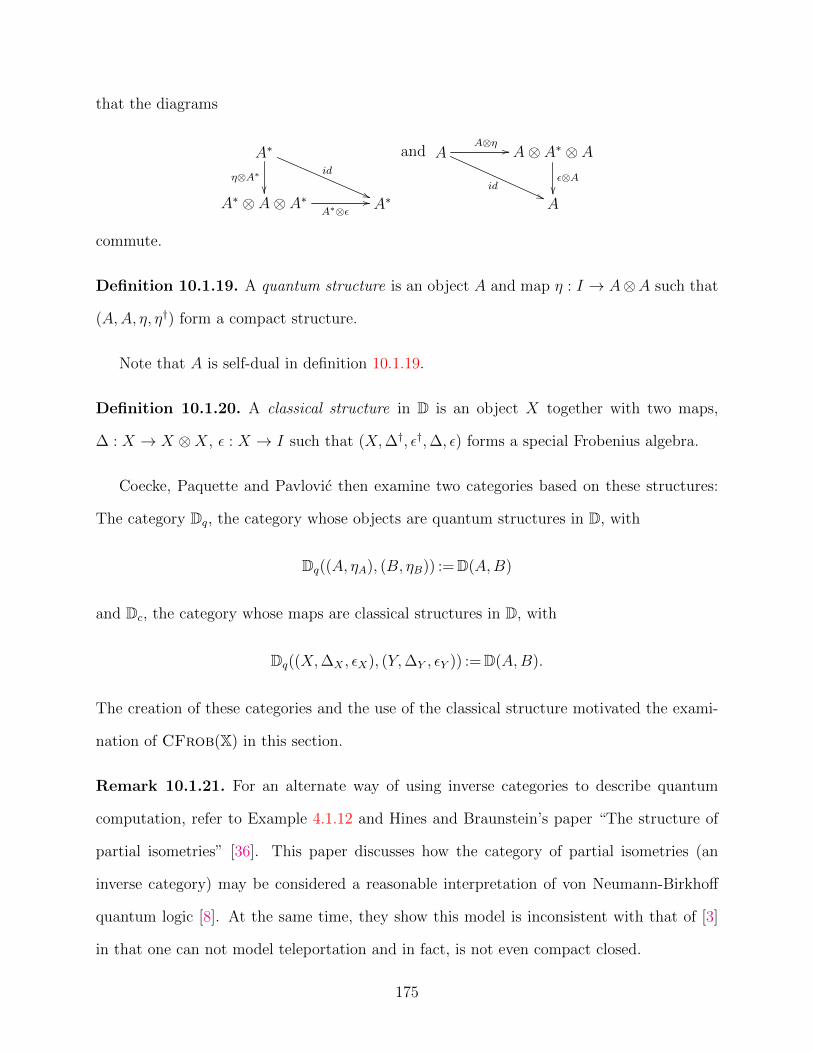
that the diagrams
A∗
id
((η⊗A∗
��A∗ ⊗ A⊗ A∗
A∗⊗ε// A∗
and AA⊗η //
id((
A⊗ A∗ ⊗ Aε⊗A��A
commute.
Definition 10.1.19. A quantum structure is an object A and map η : I → A⊗A such that
(A,A, η, η†) form a compact structure.
Note that A is self-dual in definition 10.1.19.
Definition 10.1.20. A classical structure in D is an object X together with two maps,
∆ : X → X ⊗X, ε : X → I such that (X,∆†, ε†,∆, ε) forms a special Frobenius algebra.
Coecke, Paquette and Pavlovic then examine two categories based on these structures:
The category Dq, the category whose objects are quantum structures in D, with
Dq((A, ηA), (B, ηB)) :=D(A,B)
and Dc, the category whose maps are classical structures in D, with
Dq((X,∆X , εX), (Y,∆Y , εY )) :=D(A,B).
The creation of these categories and the use of the classical structure motivated the exami-
nation of CFrob(X) in this section.
Remark 10.1.21. For an alternate way of using inverse categories to describe quantum
computation, refer to Example 4.1.12 and Hines and Braunstein’s paper “The structure of
partial isometries” [36]. This paper discusses how the category of partial isometries (an
inverse category) may be considered a reasonable interpretation of von Neumann-Birkhoff
quantum logic [8]. At the same time, they show this model is inconsistent with that of [3]
in that one can not model teleportation and in fact, is not even compact closed.
175

10.2 Disjointness in CFrob(X)
An important example of a disjointness system arises naturally from Frobenius Algebras.
Recall that we defined a zero map in Section 6.1 whenever there was a zero object. This
may also be defined directly:
Definition 10.2.1. A family of maps in a symmetric monoidal category with monoid ⊗ is
called a zero map, written as 0 whenever:
• For all f, g, f0g = 0;
• For all f , f ⊗ 0 = 0 and 0⊗ f = 0.
Lemma 10.2.2. If X is a symmetric monoidal category with a zero map, then CFrob(X)
has a zero map.
Proof. As ∆0 = 0 = 0∆ and 0∇ = 0 = ∇0, the zero maps are in CFrob(X). Since
composition is inherited from X, the first item of Definition 10.2.1 is satisfied. Finally,
since the tensor in X is the tensor in CFrob(X), the second item is also satisfied. Hence,
CFrob(X) has zero maps.
Lemma 10.2.3. As shown in Lemma 10.1.16, CFrob(X) is a discrete inverse category.
Suppose X has zero maps. Then for f, g : A→ B, define f ⊥ g when
f g = 0.
Then, the relation ⊥ is a disjointness relation.
Proof. We must show the seven axioms of the disjointness relation hold. We will show [Dis.6]
early on as its result will be used to establish some of the other axioms.
176
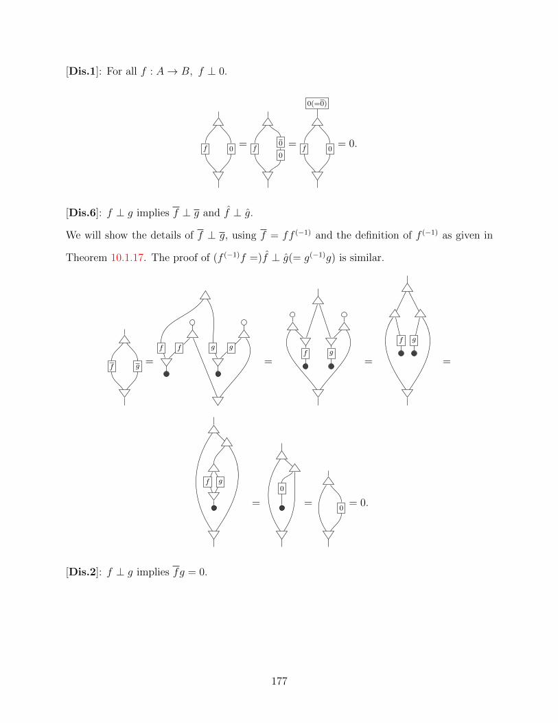
[Dis.1]: For all f : A→ B, f ⊥ 0.
f 0=
f0
0 =
0(=0)
f 0= 0.
[Dis.6]: f ⊥ g implies f ⊥ g and f ⊥ g.
We will show the details of f ⊥ g, using f = ff (−1) and the definition of f (−1) as given in
Theorem 10.1.17. The proof of (f (−1)f =)f ⊥ g(= g(−1)g) is similar.
f g =
f f g g
=f g
=
f g
=
f g
=
0
=0
= 0.
[Dis.2]: f ⊥ g implies fg = 0.
177
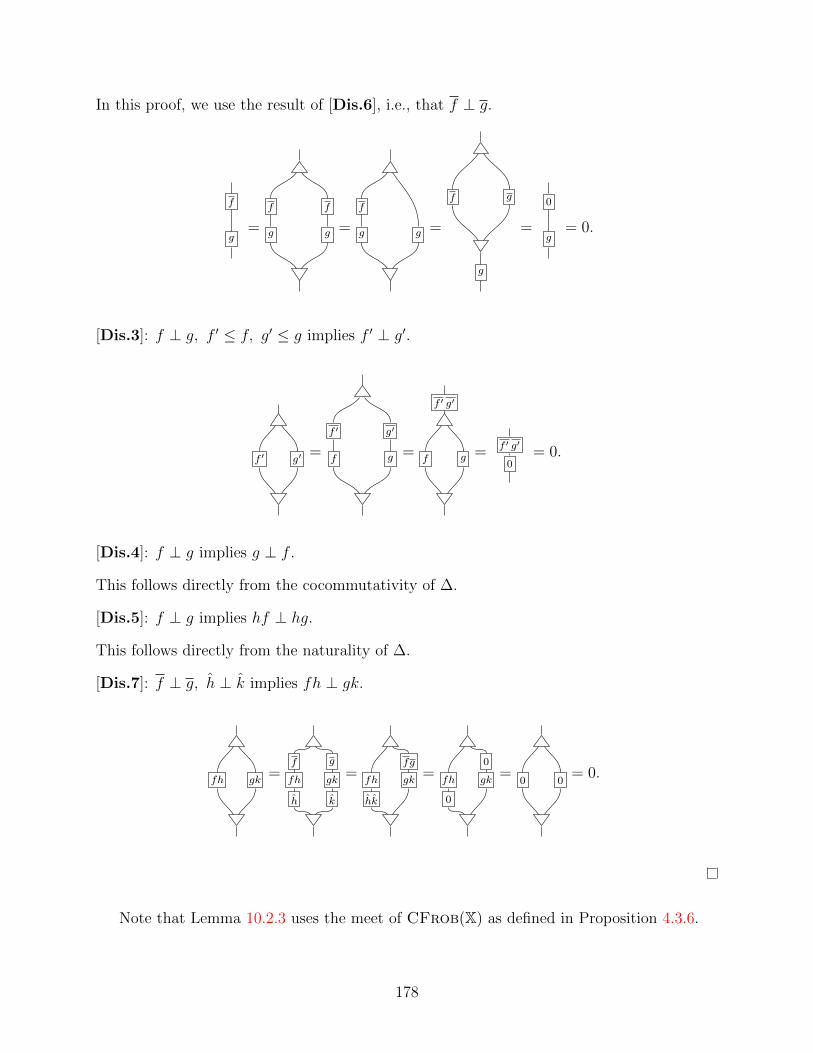
In this proof, we use the result of [Dis.6], i.e., that f ⊥ g.
f
g=
f
g
f
g =
f
g g =
f
g
g
=
0
g= 0.
[Dis.3]: f ⊥ g, f ′ ≤ f, g′ ≤ g implies f ′ ⊥ g′.
f ′ g′=
f ′
f
g′
g =
f ′ g′
f g = f ′ g′
0= 0.
[Dis.4]: f ⊥ g implies g ⊥ f .
This follows directly from the cocommutativity of ∆.
[Dis.5]: f ⊥ g implies hf ⊥ hg.
This follows directly from the naturality of ∆.
[Dis.7]: f ⊥ g, h ⊥ k implies fh ⊥ gk.
fh gk=
f
fh
h
g
gk
k
=fh
hk
fg
gk=
fh
0
0
gk=
0 0= 0.
Note that Lemma 10.2.3 uses the meet of CFrob(X) as defined in Proposition 4.3.6.
178
10.3 Disjoint joins in CFrob(X)
In the previous sections, we have shown that CFrob(X) is a discrete inverse category, with
a disjointness relation whenever X is a symmetric monoidal category with zero maps.
We now show that if X has biproducts and is an additive tensor category, i.e., a symmetric
monoidal category where the hom-sets are enriched in additive monoids, then CFrob(X)
will have a disjoint join. Moreover, in the following section, we shall show it possesses a
disjoint sum. First, we explicitly define additive tensor category:
Definition 10.3.1. Suppose X is a symmetric monoidal category with zero maps and the
hom-sets are enriched in additive monoids. It is an additive tensor category when:
• h(f + g)k = hfk + hgk for all h : A→ B, f, g : B → C and k : C → D;
• (f + g)⊗ k = f ⊗ k + g ⊗ k for all f, g : A→ B and k : C → D.
We begin by showing that given an additive tensor category, we may form an equivalent
category which has biproducts.
Lemma 10.3.2. Suppose X is an additive symmetric monoidal category. If we have the
diagram
Aσ1 // Xπ1
ffπ2
88 Bσ2oo
with
σ1π1 = 1A, σ2π2 = 1B, σ1π2 = 0 = σ2π2
and π1σ1 + π2σ2 = 1, then X is a biproduct of A and B.
Corollary 10.3.3. If F : X → Y is an additively enriched functor, then F preserves all
biproducts.
Corollary 10.3.4. The functor A⊗ : X→ X preserves biproducts.
Thus, if X is additively enriched, we may add biproducts by moving to the matrix category
of X, defined as:
179
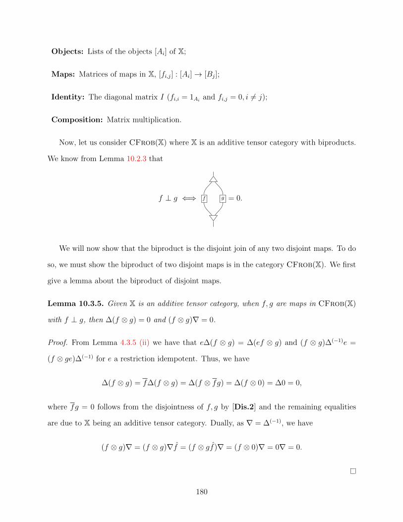
Objects: Lists of the objects [Ai] of X;
Maps: Matrices of maps in X, [fi,j] : [Ai]→ [Bj];
Identity: The diagonal matrix I (fi,i = 1Aiand fi,j = 0, i 6= j);
Composition: Matrix multiplication.
Now, let us consider CFrob(X) where X is an additive tensor category with biproducts.
We know from Lemma 10.2.3 that
f ⊥ g ⇐⇒ f g = 0.
We will now show that the biproduct is the disjoint join of any two disjoint maps. To do
so, we must show the biproduct of two disjoint maps is in the category CFrob(X). We first
give a lemma about the biproduct of disjoint maps.
Lemma 10.3.5. Given X is an additive tensor category, when f, g are maps in CFrob(X)
with f ⊥ g, then ∆(f ⊗ g) = 0 and (f ⊗ g)∇ = 0.
Proof. From Lemma 4.3.5 (ii) we have that e∆(f ⊗ g) = ∆(ef ⊗ g) and (f ⊗ g)∆(−1)e =
(f ⊗ ge)∆(−1) for e a restriction idempotent. Thus, we have
∆(f ⊗ g) = f∆(f ⊗ g) = ∆(f ⊗ fg) = ∆(f ⊗ 0) = ∆0 = 0,
where fg = 0 follows from the disjointness of f, g by [Dis.2] and the remaining equalities
are due to X being an additive tensor category. Dually, as ∇ = ∆(−1), we have
(f ⊗ g)∇ = (f ⊗ g)∇f = (f ⊗ gf)∇ = (f ⊗ 0)∇ = 0∇ = 0.
180

Lemma 10.3.6. Given X is an additive tensor category with biproducts, when f, g are maps
in CFrob(X) with f ⊥ g, then f + g is a map in CFrob(X).
Proof. We must show (f+g)∆ = ∆((f+g)⊗(f+g)) and ∇(f+g) = ((f+g)⊗(f+g))∇. As
this is an additive tensor category and both f, g are in CFrob(X) and using Lemma 10.3.5,
we have
∆((f + g)⊗ (f + g)) = ∆(f ⊗ f + f ⊗ g + g ⊗ f + g ⊗ g) =
∆(f ⊗ f) + ∆(f ⊗ g) + ∆(g ⊗ f) + ∆(g ⊗ g) =
∆(f ⊗ f) + ∆(g ⊗ g) = f∆ + g∆ = (f + g)∆.
Hence, the biproduct of f, g preserves ∆. Similarly, f + g preserves ∇:
((f + g)⊗ (f + g))∇ = (f ⊗ f + f ⊗ g + g ⊗ f + g ⊗ g)∇ =
(f ⊗ f)∇+ (f ⊗ g)∇+ (g ⊗ f)∇+ (g ⊗ g)∇ =
(f ⊗ f)∇+ (g ⊗ g)∇ = ∇f +∇g = ∇(f + g).
Proposition 10.3.7. Given X is an additive tensor category with biproduct ⊕, and f ⊥ g,
then f t g := f + g is a disjoint join.
Proof. We need to show the four axioms of disjoint join from Definition 6.3.1.
[DJ.1] : f ≤ f t g and g ≤ f t g. As f + g = g + f , we need only show the first part
of the axiom. As f ⊥ g, we know fg = 0 by the definition of disjointness and therefore we
have:
f(f + g) = ff + fg = f + 0 = f
and thus f ≤ f t g and [DJ.1] is true.
[DJ.2]: f ≤ h, g ≤ h and f ⊥ g implies f t g ≤ h. We calculate
f + gh = (f + g)h = fh+ gh = f + g
181
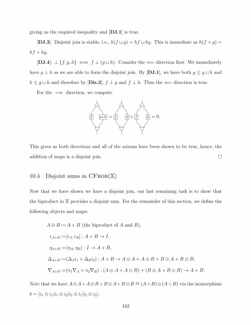
giving us the required inequality and [DJ.1] is true.
[DJ.3]: Disjoint join is stable, i.e., h(f t g) = hf t hg. This is immediate as h(f + g) =
hf + hg.
[DJ.4]: ⊥ {f, g, h} ⇐⇒ f ⊥ (g t h). Consider the ⇐= direction first. We immediately
have g ⊥ h as we are able to form the disjoint join. By [DJ.1], we have both g ≤ g t h and
h ≤ g t h and therefore by [Dis.3], f ⊥ g and f ⊥ h. Thus the ⇐= direction is true.
For the =⇒ direction, we compute
f g+h = f g + f h = 0.
This gives us both directions and all of the axioms have been shown to be true, hence, the
addition of maps is a disjoint join.
10.4 Disjoint sums in CFrob(X)
Now that we have shown we have a disjoint join, our last remaining task is to show that
the biproduct in X provides a disjoint sum. For the remainder of this section, we define the
following objects and maps:
A⊕B :=A+B (the biproduct of A and B),
εA+B :=[εA, εB] : A+B → I,
ηA+B :=〈ηA, ηB〉 : I → A+B,
∆A+B :=(∆Ai1 + ∆Bi2) : A+B → A⊗ A+ A⊗B +B ⊗ A+B ⊗B,
∇A+B :=(π1∇A + π2∇B) : (A⊗ A+ A⊗B) + (B ⊗ A+B ⊗B)→ A+B.
Note that we have A⊗A+A⊗B+B⊗A+B⊗B ∼= (A+B)⊗ (A+B) via the isomorphism
b = 〈i1 ⊗ i1|i1 ⊗ i2|i2 ⊗ i1|i2 ⊗ i2〉.
182

Lemma 10.4.1. Given X is an additive tensor category with biproduct +, then the injection
maps i1, i2 and projection maps π1, π2 of the biproduct are maps in CFrob(X).
Proof. We must show each of the injections and projections preserve ∆ and ∇.
Consider
A
∆
��
i1 // A+B
∆A+B(=∆Ai1+∆Bi2)
��A⊗ A
i1⊗i1//
i1
))
(A+B)⊗ (A+B)
A⊗ A+ A⊗Bi1
// A⊗ A+ A⊗B +B ⊗ A+B ⊗B.
b
OO
The outer arrows commute as i1(f + g) = fi1. The bottom half commutes due to the
isomorphism hence the top rectangle commutes and i1 preserves ∆. Similarly, i2 preserves
∆. By dualizing the diagram, we also have π1, π2 preserve ∇.
Next, we show the projections preserve ∇,
A+B π1//
∆
��
A
∆A
��(A+B)⊗ (A+B)
π1⊗π1 //
b−1
��
A⊗ A
A⊗ A+ A⊗B +B ⊗ A+B ⊗B π1 // A⊗ A+ A⊗B
π1
55
which, by the same argument as above, shows that ∆ is preserved by π1 and similarly by π2.
Once again, dualizing this diagram gives us that ∇ is preserved by i1 and i2.
Lemma 10.4.2. Suppose A and B are Frobenius algebras in CFrob(X) where X, an additive
tensor category, has the biproduct +. Then A⊕B is a Frobenius algebra and is therefore in
CFrob(X).
Proof. To show A⊕B is a Frobenius algebra and therefore in CFrob(X), we must show it
is separable, the unit laws hold and the Frobenius condition hold for A⊕B.
183

For the requirement that it is separable:
∆A+B∇A+B = (∆Ai1 + ∆Bi2)(π1∇A + π2∇B)
= (∆Ai1π1∇A + ∆Bi2π2∇B)
= (∆A∇A + ∆B∇B)
= (1A + 1B) = 1A+B.
To show the comultiplication unit law,
A∆ //
i1��
A⊗ Ai1⊗i1��
A+B∆ // (A+B)⊗ (A+B)
1⊗ε��
A⊗ Ai1⊗i1
oo
1⊗ε��
(A+B)⊗ Iul⊗��
A⊗ Iul⊗��
i1⊗1oo
A+B A.i1
oo
The outer path shows the unit law for the Frobenius algebra A and is what happens to the
A component in the inner path. There is a similar diagram where the outer path A’s are
replaced with a B and the i1 with i2. As these outer paths commute, they show that the
inner path commutes as each component of it commutes.
For the Frobenius law, as we are in a commutative world, we need only show ∇∆ =
(1⊗∆)(∇⊗ 1):
A⊗ A 1⊗∆ //
i1⊗i1��
A⊗ A⊗ Ai1⊗i1⊗i1
��A⊗ A i1⊗i1 //
∇((
(A+B)⊗(A+B)1⊗∆ //
∇
((
(A+B)⊗(A+B)⊗(A+B)
∇⊗1
��
A⊗ A⊗ Ai1⊗i1⊗i1oo
∇⊗1
��
Ai1 //
∆
((
A+B
∆
))(A+B)⊗(A+B) A⊗ Ai1⊗i1oo
A⊗ A.
i1⊗i1
OO
184
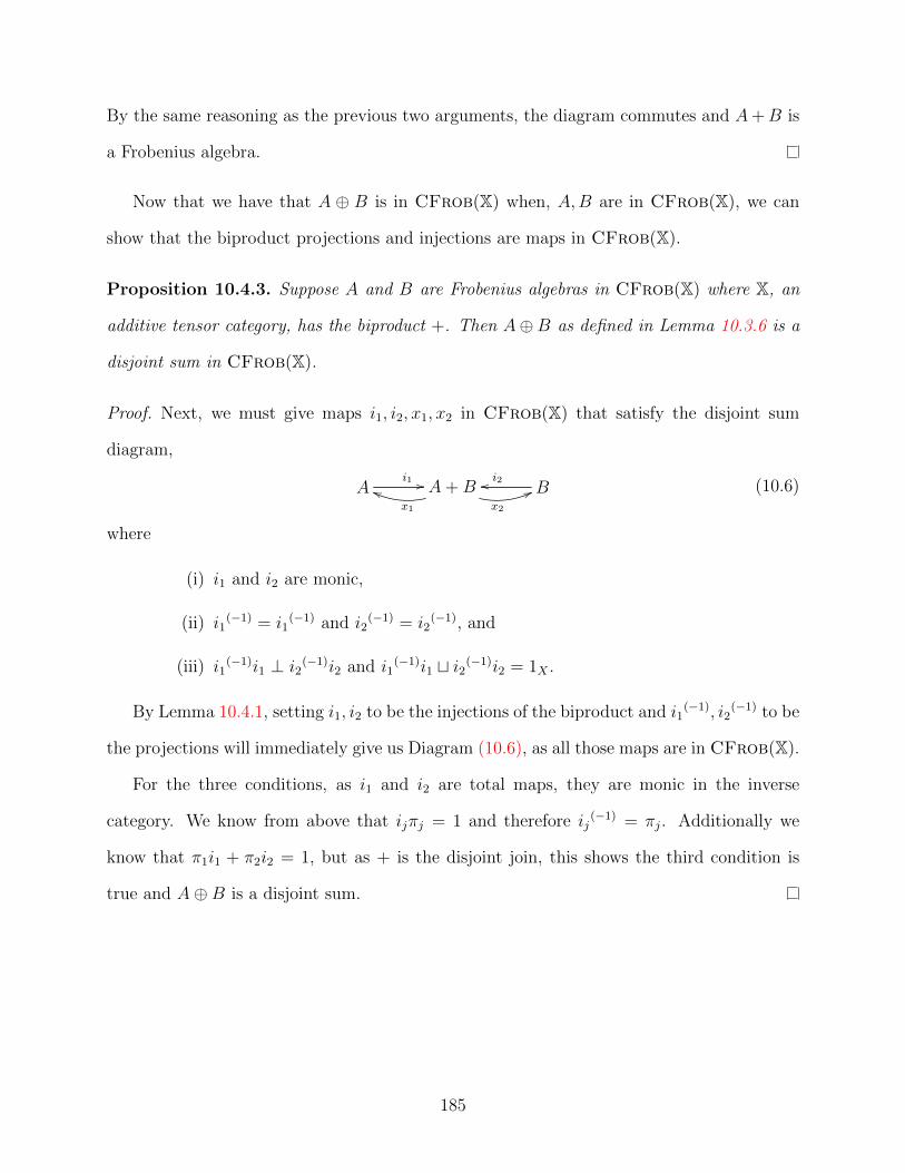
By the same reasoning as the previous two arguments, the diagram commutes and A+B is
a Frobenius algebra.
Now that we have that A ⊕ B is in CFrob(X) when, A,B are in CFrob(X), we can
show that the biproduct projections and injections are maps in CFrob(X).
Proposition 10.4.3. Suppose A and B are Frobenius algebras in CFrob(X) where X, an
additive tensor category, has the biproduct +. Then A⊕B as defined in Lemma 10.3.6 is a
disjoint sum in CFrob(X).
Proof. Next, we must give maps i1, i2, x1, x2 in CFrob(X) that satisfy the disjoint sum
diagram,
Ai1 // A+Bx1
hhx2
66 Bi2oo (10.6)
where
(i) i1 and i2 are monic,
(ii) i1(−1) = i1
(−1) and i2(−1) = i2
(−1), and
(iii) i1(−1)i1 ⊥ i2
(−1)i2 and i1(−1)i1 t i2(−1)i2 = 1X .
By Lemma 10.4.1, setting i1, i2 to be the injections of the biproduct and i1(−1), i2
(−1) to be
the projections will immediately give us Diagram (10.6), as all those maps are in CFrob(X).
For the three conditions, as i1 and i2 are total maps, they are monic in the inverse
category. We know from above that ijπj = 1 and therefore ij(−1) = πj. Additionally we
know that π1i1 + π2i2 = 1, but as + is the disjoint join, this shows the third condition is
true and A⊕B is a disjoint sum.
185

Chapter 11
Turing categories and PCAs
In this chapter, we review the definition and properties of a Turing category and partial com-
binatory algebras [18,20]. Because of the theorems of the earlier chapters, we will be able to
transfer these ideas in a straightforward way from discrete Cartesian restriction categories
to discrete inverse categories. Inverse Turing categories are defined below and correspond to
Turing categories using Theorem 11.2.3: This provides the link between reversible compu-
tation and standard models of computation as promised in the introduction.
As noted in the introduction, Bennett [6] showed how a reversible Turing machine can
emulate a standard Turing machine. As Turing machines can perform the applications of
a partial combinatory algebra, we have a link between inverse Turing categories through
Turing categories to reversible Turing machines.
11.1 Turing categories
Turing categories provide a categorical formulation for computability and includes partial
combinatory algebras, the partial lambda calculus, and various other models as given in [18].
Definition 11.1.1 (Turing category). Given X is a Cartesian restriction category:
(i) For a map τX,Y : A × X → Y , a map f : B × X → Y admits a τX,Y -index
when there is a total pf q : B → A such that
A×XτX,Y // Y
B ×X
pfq×1X
OO
f
<<
commutes.
186

(ii) A map τX,Y : A×X → Y is called a universal application if all f : B×X → Y
admit a τX,Y -index.
(iii) If A is an object in X such that for every pair of objects X, Y in X there is a
universal application τ : A×X → Y , then A is called a Turing object.
(iv) A Cartesian restriction category that contains a Turing object is called a Tur-
ing category.
Note there is no requirement in the definition for the map pf q to be unique. When pf q is
unique for a specific τX,Y , then that τX,Y is called extensional. In the case where the object
B is the terminal object, then the map pf q is a point of A (with f = (pf q × 1)τX,Y ) and pf q is
referred to as a code of f .
Example 11.1.2. This example is due to Cockett and Hofstra [18].
We start with a “suitable” enumeration of partial recursive functions f : N→ N. Based
on the fact that functions such as these can be described by Turing machines, and that
Turing machines may be enumerated as {φ0, φ1, . . .}, each of these functions can be coded
into a single number. This may be extended to partial recursive functions of n variables
which may similarly be enumerated, {φ(n)0 , φ
(n)1 , . . .}. When f is given by φe we say e is a
code for f .
Two facts we will need about the family φ(n)m :
• Universal Functions: There are partial recursive functions such that for
each n > 0,
Φ(n)(e, x1, . . . , xn) = φe(x1, . . . , xn)
which are called the universal functions.
• Parameter Theorem: There are primitive recursive functions Snm for each
n,m > 0 such that:
Φ(n+m)(e, x1, . . . , xm, u1, . . . , un) = Φ(m)(Snm(e, x1, . . . , xm), u1, . . . , un).
187

Suppose we choose such an enumeration and use it for the Kleene-application on the
natural numbers, i.e., N× N •−→ N will be defined as
n • x = φn(x).
Now, consider the category with objects being the finite powers of N and a map Nk → Nm
is an m-tuple of partial recursive function of k variables. When k is zero, the map simply
picks a specific m-tuple of N. We denote this category by Comp(N). Then, Comp(N) is a
Turing category with N being a Turing object, using Kleene-application as the application
map. We know N is isomorphic to N × N and hence we have N × N / N. Application
is guaranteed to be partial recursive by the universal functions item above and the weak
universal property of • is a result of the Parameter Theorem.
Definition 11.1.3. Given T is a Turing category and A is an object of T,
(i) If Υ = {τX,Y : A×X → Y |X, Y ∈ To}, then Υ is called an applicative family
for A.
(ii) An applicative family Υ is called universal for A when each τX,Y is a universal
application. This is also referred to as a Turing structure on A.
(iii) A pair (A,Υ) where Υ is universal for A is called a Turing structure on T.
Lemma 11.1.4. If T is a Turing category with Turing object T , then every object B in T
is a retract of T .
Proof. As T is a Turing object, we have a diagram for τ1,B and π0 : B × 1→ B:
T × 1τ1,B // B
B × 1.
pπq0×11
OO
π0
<<
Note we also have ur : B → B × 1 is an isomorphism and therefore we have 1B = urπ0 =
(ur(pπq0 × 1))τ1,B. Hence, we have B /
τ1,Bur(pπq
0×1)T .
188

This allows for various recognition criteria for Turing categories.
Theorem 11.1.5. A Cartesian restriction category D is a Turing category if and only if
D has an object T for which every other object of D is a retract and T has a universal
self-application map •, written as T × T •−−→ T .
Proof. The “only if” portion follows immediately from setting T to be the Turing object of
D and • = τT,T .
For the “if” direction, we need to construct the family of universal applications τX,Y :
T ×X → Y for each pair of objects X, Y in D.
Let us choose pairs of maps that witness the retractions of X, Y of T , that is:
X /rXmXT and Y /rYmY
T.
Define τX,Y = (1T ×mX) • rY . Suppose we are given f : B ×X → Y . Consider
T ×X 1T×mX // T × T • // TrY // Y
B ×X 1B×mX //
h×1X
OO
B × T
h×1T
OO
1B×rX // B ×X
f
<<
fmY
OO
where h is the index for the composite map (1B × rX)fmY . The middle square commutes
as • is a universal application for T, T . The right triangle commutes as mY rY = 1. The left
square commutes as each composite is h ×mX . Noting that the bottom path from B ×X
to Y is (1B ×mX)(1B × rX)f = f and the top path from T × X to Y is our definition of
τX,Y , this means f admits the τX,Y -index h.
Note that different splittings (choices of (m, r) pairs) would lead to different τX,Y maps.
In fact there is no requirement that this is the only way to create a universal applicative
family for T .
There is another criteria that also gives a Turing category:
Lemma 11.1.6. A Cartesian restriction category T is a Turing category if:
189

(i) T has an object T for which every other object of T is a retract;
(ii) T × T has a map T × T ◦−−→ T and for all f : T → T there exists an element,
f• : 1→ T (which is total) such that
T × T ◦ // T
Tf
;;
〈!f•,1〉
OO
is a commutative diagram.
Proof. We need only show that T has a universal self-application map and then use Theo-
rem 11.1.5.
T having a universal self-application map, •, means for every map f : B × T → T there
is a map, pf q : B → T such that
T × T • // T
B × Tf
;;
pfq×1
OO
commutes.
Let T × T /rm T . Then, consider
T × T r×1 // T × T × T 1×m // T × T ◦ // T
T × T × T
m×1
OO
T × T
〈(rf)•,π0,π1〉
OO 〈(rf)•,π0,π1〉
<<
m// T r
//
〈(rf)•,1〉
OO
T × T.
f
AA
The rightmost quadrilateral commutes by assumption of this lemma. The middle quadrilat-
eral commutes due to the properties of the product map and π0 and π1. The top left triangle
commutes as mr = 1 and the remaining triangle has the same map on both dotted lines.
Thus, we may conclude that • :=(r × 1)(1 × m)◦ and pf q :=〈!(rf)•, 1〉m satisfy the re-
quirements of Theorem 11.1.5 and therefore T is a Turing object in a Turing category.
190
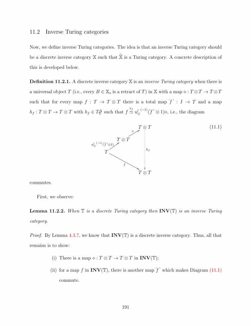
11.2 Inverse Turing categories
Now, we define inverse Turing categories. The idea is that an inverse Turing category should
be a discrete inverse category X such that X is a Turing category. A concrete description of
this is developed below.
Definition 11.2.1. A discrete inverse category X is an inverse Turing category when there is
a universal object T (i.e., every B ∈ Xo is a retract of T ) in X with a map � : T ⊗T → T ⊗T
such that for every map f : T → T ⊗ T there is a total map pf q : I → T and a map
hf : T ⊗ T → T ⊗ T with hf ∈ T∆∇ such that f
hf' ul⊗(−1)
(pf q ⊗ 1)�, i.e., the diagram
T ⊗ T
hf
��
T ⊗ T
� 88
T
ul⊗(−1)
(pfq⊗1);;
f&&T ⊗ T
(11.1)
commutes.
First, we observe:
Lemma 11.2.2. When T is a discrete Turing category then INV(T) is an inverse Turing
category.
Proof. By Lemma 4.3.7, we know that INV(T) is a discrete inverse category. Thus, all that
remains is to show:
(i) There is a map � : T ⊗ T → T ⊗ T in INV(T);
(ii) for a map f in INV(T), there is another map pf q which makes Diagram (11.1)
commute.
191
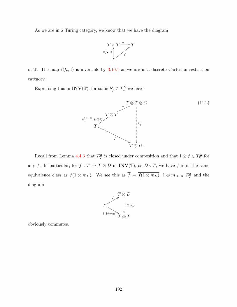
As we are in a Turing category, we know that we have the diagram
T × T ◦ // T
Tf
;;
〈!f•,1〉
OO
in T. The map 〈!f•, 1〉 is invertible by 3.10.7 as we are in a discrete Cartesian restriction
category.
Expressing this in INV(T), for some h′f ∈ T∆∇ we have:
T ⊗ T ⊗ C
h′f
��
T ⊗ T
◦ 66
T
ul⊗(−1)
(f•⊗1);;
f''T ⊗D.
(11.2)
Recall from Lemma 4.4.3 that T∆∇ is closed under composition and that 1⊗ f ∈ T∆
∇ for
any f . In particular, for f : T → T ⊗ D in INV(T), as D / T , we have f is in the same
equivalence class as f(1 ⊗ mD). We see this as f = f(1⊗mD), 1 ⊗ mD ∈ T∆∇ and the
diagram
T ⊗D
1⊗mD
��
T
f 88
f(1⊗mD) &&T ⊗ T
obviously commutes.
192

We use this and the fact that we have both T⊗C/T and D/T , to add to Diagram (11.2):
T ⊗ T1⊗rT⊗C��
T ⊗ T ⊗ C
h′f
��
1⊗mT⊗C55
T ⊗ T ⊗ C
h′f
��
T ⊗ T
◦ 66
T
ul⊗(−1)
((f(1⊗mD))•⊗1);;
f''T ⊗D
1⊗mD ))
T ⊗D1⊗mD��
T ⊗ T.
But this is the required diagram for an inverse Turing category with hf = (1⊗ rT⊗C)h′f (1⊗
mD), and with pf q = (f(1 ⊗ mD))• and with � = ◦(1 ⊗ mT⊗C). Therefore INV(T) is an
inverse Turing category.
We know that applying the Cartesian Completion to X, an inverse Turing category, results
in X, a discrete Cartesian restriction category. Moreover, if A/rAmAT in X, then A/
rAur⊗
(−1)
mAur⊗
(−1) T
in X and thus T will remain universal in X. Hence, we have the basic requirements for a
Turing category as specified in Theorem 11.1.5 and Lemma 11.1.6. All that remains to be
shown is that we have a self-application map and a code for each map f : 1 → T as in
Lemma 11.1.6.
Theorem 11.2.3. When X is an inverse Turing category, X is a Turing category.
Proof. From the discussion, we need to specify the self-application map ◦ : T × T → T and
f• : 1→ T in X.
The diagram of Definition 11.2.1, when raised to X translates to:
T × T(�,T ) // T
T.
〈pfq,1〉
OO
(f,T )
99
193
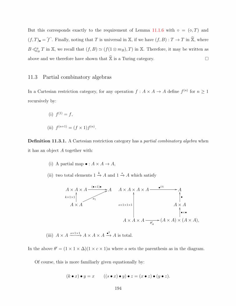
But this corresponds exactly to the requirement of Lemma 11.1.6 with ◦ = (�, T ) and
(f, T )• = pf q. Finally, noting that T is universal in X, if we have (f,B) : T → T in X, where
B /rBmBT in X, we recall that (f,B) ' (f(1⊗mB), T ) in X. Therefore, it may be written as
above and we therefore have shown that X is a Turing category.
11.3 Partial combinatory algebras
In a Cartesian restriction category, for any operation f : A × A → A define f (n) for n ≥ 1
recursively by:
(i) f (1) = f ,
(ii) f (n+1) = (f × 1)f (n).
Definition 11.3.1. A Cartesian restriction category has a partial combinatory algebra when
it has an object A together with:
(i) A partial map • : A× A→ A,
(ii) two total elements 1k−→ A and 1
s−→ A which satisfy
A× A× A(•×1)• // A
A× A
k×1×1
OO
π1
66 A× A× A× A •(3) // A
A× A
•
OO
A× A× A
s×1×1×1
OO
θ′A
// (A× A)× (A× A),
•×•
OO
(iii) A× A s×1×1−−−−→ A× A× A •2−→ A is total.
In the above θ′ = (1× 1×∆)(1× c× 1)a where a sets the parenthesis as in the diagram.
Of course, this is more familiarly given equationally by:
(k • x) • y = x ((s • x) • y) • z = (x • z) • (y • z).
194
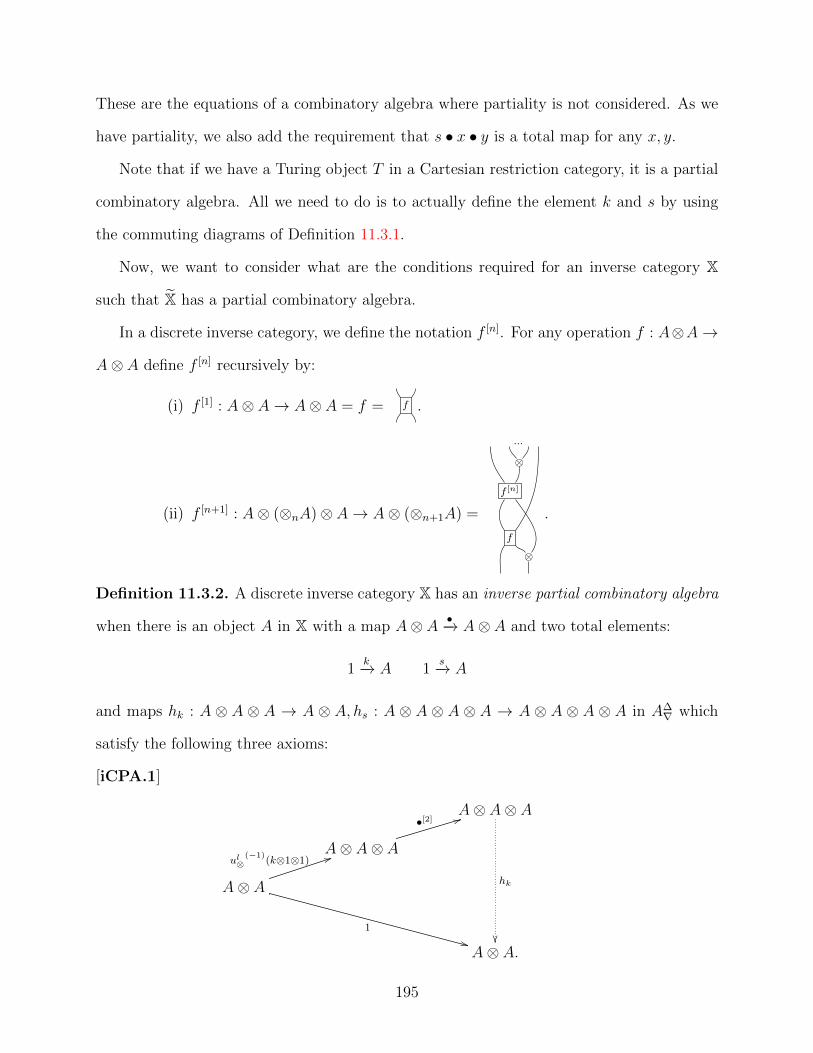
These are the equations of a combinatory algebra where partiality is not considered. As we
have partiality, we also add the requirement that s • x • y is a total map for any x, y.
Note that if we have a Turing object T in a Cartesian restriction category, it is a partial
combinatory algebra. All we need to do is to actually define the element k and s by using
the commuting diagrams of Definition 11.3.1.
Now, we want to consider what are the conditions required for an inverse category X
such that X has a partial combinatory algebra.
In a discrete inverse category, we define the notation f [n]. For any operation f : A⊗A→
A⊗ A define f [n] recursively by:
(i) f [1] : A⊗ A→ A⊗ A = f = f .
(ii) f [n+1] : A⊗ (⊗nA)⊗ A→ A⊗ (⊗n+1A) =
···
⊗
f [n]
f
⊗
.
Definition 11.3.2. A discrete inverse category X has an inverse partial combinatory algebra
when there is an object A in X with a map A⊗ A •−→ A⊗ A and two total elements:
1k−→ A 1
s−→ A
and maps hk : A ⊗ A ⊗ A → A ⊗ A, hs : A ⊗ A ⊗ A ⊗ A → A ⊗ A ⊗ A ⊗ A in A∆∇ which
satisfy the following three axioms:
[iCPA.1]
A⊗ A⊗ A
hk
��
A⊗ A⊗ A
•[2] 44
A⊗ A
ul⊗(−1)
(k⊗1⊗1) 44
1
++A⊗ A.
195
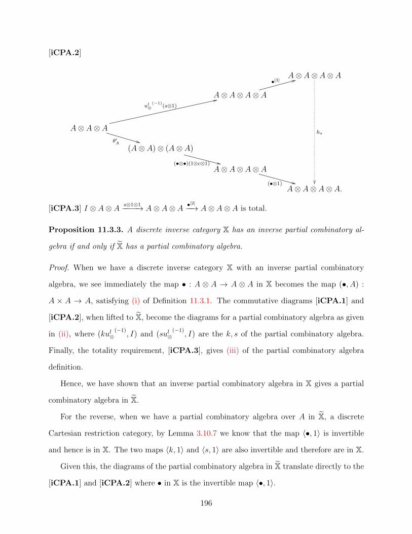
[iCPA.2]
A⊗ A⊗ A⊗ A
hs
��
A⊗ A⊗ A⊗ A
•[3] 33
A⊗ A⊗ A
ul⊗(−1)
(s⊗1)
33
θ′A **(A⊗ A)⊗ (A⊗ A)
(•⊗•)(1⊗c⊗1) ++A⊗ A⊗ A⊗ A
(•⊗1) ++A⊗ A⊗ A⊗ A.
[iCPA.3] I ⊗ A⊗ A s⊗1⊗1−−−−→ A⊗ A⊗ A •[2]−−→ A⊗ A⊗ A is total.
Proposition 11.3.3. A discrete inverse category X has an inverse partial combinatory al-
gebra if and only if X has a partial combinatory algebra.
Proof. When we have a discrete inverse category X with an inverse partial combinatory
algebra, we see immediately the map • : A ⊗ A → A ⊗ A in X becomes the map (•, A) :
A × A → A, satisfying (i) of Definition 11.3.1. The commutative diagrams [iCPA.1] and
[iCPA.2], when lifted to X, become the diagrams for a partial combinatory algebra as given
in (ii), where (kul⊗(−1)
, I) and (sul⊗(−1)
, I) are the k, s of the partial combinatory algebra.
Finally, the totality requirement, [iCPA.3], gives (iii) of the partial combinatory algebra
definition.
Hence, we have shown that an inverse partial combinatory algebra in X gives a partial
combinatory algebra in X.
For the reverse, when we have a partial combinatory algebra over A in X, a discrete
Cartesian restriction category, by Lemma 3.10.7 we know that the map 〈•, 1〉 is invertible
and hence is in X. The two maps 〈k, 1〉 and 〈s, 1〉 are also invertible and therefore are in X.
Given this, the diagrams of the partial combinatory algebra in X translate directly to the
[iCPA.1] and [iCPA.2] where • in X is the invertible map 〈•, 1〉.
196

The totality of s•(2) in X then immediately gives us [iCPA.3], the totality of s•[2] in X.
However, we can simplify the definition of an inverse partial combinatory algebra when A
is powerful in X. (Here, powerful means that 1/A, A⊗A/A, A⊗A⊗A/A, . . .). Note that
if A is a partial combinatory algebra in X, that guarantees it is powerful in X. Assuming
the retractions are An /rnmnA, we have mjrj = 1 and rjmj = rjmj for each j. Thus, each of
the maps are partial inverses in X and therefore in X. Thus, A is a powerful object in X.
Note that our definition of “powerful” does not relate to resource usage or a particular
complexity class. An example of a powerful object is the natural numbers with the Cantor
enumeration.
In a discrete inverse category, we redefine the notation f (n). For any map f : A ⊗ A →
A⊗ A where A is a powerful object define f (n) recursively by:
(i) f (1) : A⊗ A→ A⊗ A = f = f ;
(ii) f (n+1) : ⊗n+2A→ A⊗ A =f (n)
f
m2
.
Lemma 11.3.4. Suppose a discrete inverse category X has a inverse partial combinatory
algebra over A and A is a powerful object in X, with ⊗nA/rnmnA. Then [iCPA.1], [iCPA.2]
and [iCPA.3] may be simplified to:
197

[iCPA′.1]
A⊗ A
h′k
��
A⊗ A⊗ A
•(2)66
A⊗ A
ul⊗(−1)
(k⊗1⊗1)66
1
))A⊗ A.
[iCPA′.2]
A⊗ A
h′s
��
A⊗ A⊗ A⊗ A
•(3)
55
A⊗ A⊗ A
ul⊗(−1)
(s⊗1)55
θ′A ))(A⊗ A)⊗ (A⊗ A)
(•⊗•)(1⊗c⊗1)(1⊗1⊗m2)
))A⊗ A⊗ A
(•⊗1)(1⊗m2) ''A⊗ A.
[iCPA′.3] I ⊗ A⊗ A s⊗1⊗1−−−−→ A⊗ A⊗ A •(2)−−→ A⊗ A is total.
11.4 Computable functions
Given a partial combinatory algebra A in a Cartesian restriction category, one can form
Comp(A), the category of computable partial functions generated by A. These are the
198

maps with an index:
A× (×nA) •(n)// A
(×nA).
pfq×1
OO
f
77
We would like Comp(A) to be a discrete Turing category so that INV(Comp(A)) is an in-
verse Turing category by Lemma 11.2.2. Unfortunately, there is no guarantee that Comp(A)
is a discrete Turing category. However, we can define conditions so that it is true:
Definition 11.4.1. Given a discrete object A in a Cartesian restriction category, A has a
discrete partial combinatory algebra when:
(i) A has a partial combinatory algebra;
(ii) there exists e : 1→ A, a total element, such that
A× A× A •(2) // A,
A× A
e×1
OO
∆(−1)
66
meaning there is a code for ∆(−1).
We immediately have:
Lemma 11.4.2. When A has a discrete partial combinatory algebra, then Comp(A) is a
discrete Cartesian restriction category.
By Lemma 11.2.2, this means that INV(Comp(A)) is an inverse Turing category. Note
it is still the case that there can be a map of Comp(A) which is invertible in X (i.e., is in
X), but is not invertible in Comp(A).
199
Chapter 12
Conclusions and future work
This thesis has studied inverse categories [21], providing conditions for a tensor to act like a
product — the inverse product — and similarly for a second tensor to behave like a coproduct
— the disjoint sum.
The following are the main results of this thesis.
1. Restriction Products and Coproducts in Inverse Categories
We showed in Proposition 4.2.1 that an inverse category with restriction prod-
ucts is a restriction preorder. Similarly, in Proposition 6.1.5, an inverse cate-
gory with coproducts is a preorder.
2. Discrete Inverse Categories
We introduced the inverse product, Definition 4.3.1 and showed that this pro-
vided meets for the inverse category in Proposition 4.3.6. We showed that the
inverse subcategory of a discrete Cartesian restriction category is a discrete
inverse category in Lemma 4.3.7.
Given a discrete inverse category X, we constructed a category X, the Cartesian
Completion of X with the same objects as X and maps being equivalence classes
of maps of X. We showed this was a restriction category in Lemmas 5.1.7 and
5.1.8 and in fact was a discrete Cartesian restriction category as shown in
Theorem 5.1.12.
Finally, in Theorem 5.2.6 we provided an equivalence between the category of
discrete inverse categories and the category of discrete Cartesian restriction
categories. This result, together with its consequences, is the main theoretical
200

contribution of this thesis.
3. Disjointness Relations and Disjoint Joins
In Definition 6.2.1 we defined what a disjointness relation is in an inverse cate-
gory, followed by Definition 6.2.4 which defined disjointness on the restriction
idempotents of the inverse category. Theorem 6.2.7 shows that these two def-
initions are equivalent, allowing us to define disjointness in whichever way is
most convenient.
Disjoint joins are introduced with Definition 6.3.1, providing an analogue to
joins in a restriction category.
4. Disjoint Sums
Disjoint sums in an inverse category are given in Definition 7.1.1 and we show
that an inverse category having all disjoint sums has a symmetric monoidal
tensor in Proposition 7.1.4.
Disjointness tensors, Definition 7.2.1, are shown in Lemma 7.2.9 to provide
enough structure to allow the creation of a disjointness relation. However,
to create a disjoint join requires a disjoint sum tensor. Disjoint sum tensors
are given in Definition 7.3.1 as additional conditions on a disjointness tensor.
Given a disjoint sum tensor, Proposition 7.3.5 defines a disjoint join.
Section 7.4 proves, in Proposition 7.4.1 and Proposition 7.4.2, that a disjoint
sum enables the creation of a disjoint sum tensor and conversely, a disjoint
sum tensor produces disjoint sums.
In Chapter 8, Definition 8.1.2 gives us iMat(X), a matrix category over the
inverse category X with disjoint joins. Theorem 8.1.4 proves this is an inverse
category with disjoint sums. Lemma 8.2.2 shows that there is a functor M
from an inverse category with disjoint joins to its matrix category. The matrix
201

construction gives an adjoint between DSum, the category of inverse categories
with disjoint sums and DJoin, the category of inverse categories with disjoint
joins. Furthermore, Proposition 8.2.5 shows that an inverse category X with
disjoint sums is equivalent to iMat(X).
5. Distributive Inverse Categories
We define distributive inverse categories in Definition 9.2.1 and show that
distributivity of the inverse product over the disjoint join is equivalent to
distributing over a disjoint sum tensor in Lemma 9.2.6.
Then, in Theorem 9.3.3 we show that Cartesian Completion turns a disjoint
sum tensor into a coproduct. From this we conclude that X is a distributive
restriction category in Corollary 9.3.4.
6. Linkage to quantum computation
Chapter 10 starts with a review of Frobenius algebras and how they appear in
models of quantum computation. Theorem 10.1.17 shows the category of com-
mutative Frobenius algebras, CFrob(X), in a symmetric monoidal category
X is actually a discrete inverse category. Furthermore, when the symmet-
ric monoidal category X is an additive tensor category with zero maps and
biproducts, then CFrob(X) is shown in Lemma 10.2.3 to possess a disjoint-
ness relation, given by f ⊥ g ⇐⇒ ∆(f ⊗ g)∆(−1) = 0. Proposition 10.3.7
shows that the addition of maps is a disjoint join in CFrob(X) and Proposi-
tion 10.4.3 shows the biproduct of objects is a disjoint sum.
7. Inverse Turing Categories and Inverse PCAs
Inverse Turing categories and inverse partial combinatory algebras are de-
fined in Definition 11.2.1 and Definition 11.3.2 respectively. First, we show
in Lemma 11.2.2 that if we have a discrete Turing category T, then INV(T),
202

the inverse subcategory of T, is an inverse Turing category. Then we show
that the Cartesian Completion of an inverse Turing category gives a Turing
category. In Proposition 11.3.3 we show that a discrete inverse category X
has an inverse PCA if and only if X has a PCA. Furthermore, we discuss the
category of computable function based on a PCA in a Cartesian restriction
category and show the conditions required for that to be a discrete Cartesian
restriction category in Lemma 11.4.2.
This thesis demonstrates that discrete inverse categories provide a convenient intermedi-
ate link between standard models of computing (i.e., via inverse Turing categories to Turing
categories) and quantum computing (via special commutative Frobenius algebras).
12.1 Future directions
The obvious next step is to use discrete inverse categories to provide a categorical semantics
for existing reversible languages such as Inv [55], and Theseus [37,38]. The examples of the
category of partial injective functions used throughout this thesis provides the basis for the
semantics of Inv.
It would be interesting to understand how to formulate datatypes, higher order structures,
etc. at the inverse category level. The obvious correspondences are from product types to
the inverse product as well as between sum types and the disjoint sum. From there, one
would study the trace and explore infinite and recursive types. Note that some of this work
would follow naturally from exploring the semantics of Theseus from [37,38].
An interesting direction, in my opinion, would be to further investigate the work on
reversible CCS as in [28] and [59]. This could be combined with the work of Chakraborty
on MPL [13] to describe the communication of multiple processes and generalize to a series
of reversible processes.
The connection to quantum computing, as exampled in Chapter 10 would benefit from
203

further investigation. As well, the bulk of current literature on semantics of quantum com-
puting is based on finite dimensional Hilbert spaces. Our construction is not limited to the
finite dimensional case, and as such, may be of use when considering infinite dimensions.
To pursue this area, one would likely start with a consideration of Frobenius algebras in a
linearly distributive category, as described by Egger in [29].
204

Bibliography
[1] S. Abramsky. Abstract scalars, loops, and free traced and strongly compact closedcategories. In CALCO, pages 1–29, 2005.
[2] S. Abramsky. A structural approach to reversible computation. Theoretical ComputerScience, 347(3):441–464, 2005.
[3] S. Abramsky and B. Coecke. A categorical semantics of quantum protocols. In Pro-ceedings of the 19th Annual IEEE Symposium on Logic in Computer Science (LiCS‘04),IEEE Computer Science Press. (extended version at arXiv:quant-ph/0402130), pages415–425, 2004.
[4] S. Abramsky, E. Haghverdi, and P. Scott. Geometry of interaction and linear combina-tory algebras. Mathematical Structures in Computer Scients, 12:625–665, 2002.
[5] Michael Barr and Charles Wells. Category Theory for Computing Science. PrenticeHall, 2nd edition, 1995.
[6] Charles H. Bennett. Logical reversibility of computation. IBM Journal of Research andDevelopment, 6:525–532, 1973.
[7] Charles H Bennett. Notes on landauer’s principle, reversible computation, andmaxwell’s demon. Studies In History and Philosophy of Science Part B: Studies InHistory and Philosophy of Modern Physics, 34(3):501–510, 2003.
[8] Garrett Birkhoff and John Von Neumann. The logic of quantum mechanics. Annals ofMathematics, 37(04):823–843, October 1936.
[9] R.F. Blute, J.R.B. Cockett, and R.A.G. Seely. Cartesian differential categories. Theoryand Applications of Categories, 22(23):622–672, 2009.
[10] Aaron Bohannon, Benjamin C. Pierce, and Jeffrey A. Vaughan. Relational lenses:a language for updatable views. In PODS ’06: Proceedings of the twenty-fifth ACMSIGMOD-SIGACT-SIGART symposium on Principles of database systems, pages 338–347, New York, NY, USA, 2006. ACM.
[11] Tim Bray, Jean Paoli, C. M. Sperberg-McQueen, Eve Maler, and Francois Yergeau.Extensible markup language (xml) 1.0. Technical Report REC-xml-20081126, W3C,2008.
[12] Aurelio Carboni and Robert FC Walters. Cartesian bicategories i. Journal of pure andapplied algebra, 49(1):11–32, 1987.
[13] Subashis Chakraborty. The type system for the message passing language mpl. Master’sthesis, University of Calgary, University of Calgary, 2500 University Drive N.W., Cal-gary, Alberta, Canada T2N 1N4, 1 2014. Available at http://pages.cpsc.ucalgary.ca/~robin/Theses/ucalgary_2014_chakraborty_subashis.pdf.
205

[14] J. Robin B. Cockett. Introduction to distributive categories. Mathematical Structuresin Computer Science, 3(3):277–307, 1993.
[15] J.R.B. Cockett and X. Guo. Join restriction categories and the importance of beingadhesive. Slides for talk at CT 2007, available at http://pages.cpsc.ucalgary.ca/
~robin, July 2007.
[16] J.R.B. Cockett, Xiuzhan Guo, and Pieter Hofstra. Range categories i: General theory.Theory and Applications of Categories, 26(17):412–452, 2012.
[17] J.R.B. Cockett, Xiuzhan Guo, and Pieter Hofstra. Range categories ii: Towards regu-larity. Theory and Applications of Categories, 26(18):453–500, 2012.
[18] J.R.B. Cockett and P.J.W. Hofstra. Introduction to Turing categories. Annals of Pureand Applied Logic, 156:183–209, December 2008.
[19] Robin Cockett. Category theory for computer science. Available athttp://pages.cpsc.ucalgary.ca/˜robin/class/617/notes.pdf, October 2009.
[20] Robin Cockett. Categories and computability. Available athttp://pages.cpsc.ucalgary.ca/˜robin/talks/estonia-winter-2010/estonia-notes.pdf,November 2010.
[21] Robin Cockett and Stephen Lack. Restriction categories I: categories of partial maps.Theoretical Computer Science, 270:223–259, 2002.
[22] Robin Cockett and Stephen Lack. Restriction categories II: Partial map classification.Theoretical Computer Science, 294:61–102, 2003.
[23] Robin Cockett and Stephen Lack. Restriction categories III: colimits, partial limits,and extensivity. Mathematical Structures in Computer Science, 17(4):775–817, 2007.Available at http://au.arxiv.org/abs/math/0610500v1.
[24] Robin Cockett and Ernie Manes. Boolean and classical restriction categories. Mathe-matical Structures in Computer Science, 19:357–416, April 2009.
[25] Bob Coecke, Tobias Fritz, and Robert W Spekkens. A mathematical theory of resources.arXiv preprint arXiv:1409.5531, 2014.
[26] Bob Coecke, Eric Oliver Paquette, and Dusko Pavlovic. Classical and quantum struc-turalism. Semantic techniques for quantum computation, page 43, 2008.
[27] Bob Coecke, Dusko Pavlovic, and Jamie Vicary. A new description of orthog-onal bases. Math. Structures in Comp. Sci., page 13, 2008. 13pp, to appear,arxiv.org/abs/0810.0812.
[28] Vincent Danos and Jean Krivine. Reversible communicating systems. In CONCUR2004-Concurrency Theory, pages 292–307. Springer, 2004.
206

[29] J.M. Egger. The frobenius relations meet linear distributivity. Theory and Applicationsof Categories, 24(2):25–38, 2010.
[30] J. Nathan Foster, Michael B. Greenwald, Jonathan T. Moore, Benjamin C. Pierce,and Alan Schmitt. Combinators for bi-directional tree transformations: a linguisticapproach to the view update problem. SIGPLAN Not., 40(1):233–246, 2005.
[31] Brett Giles. Programming with a quantum stack. Master’s thesis, University of Cal-gary, University of Calgary, 2500 University Drive N.W., Calgary, Alberta, CanadaT2N 1N4, 4 2007. Avaliable at http://pages.cpsc.ucalgary.ca/~robin/Theses/
BrettGilesMSc.pdf.
[32] Alexander S. Green, Peter LeFanu Lumsdaine, Neil J. Ross, Peter Selinger, and BenoıtValiron. An introduction to quantum programming in quipper. In Reversible Compu-tation, pages 110–124. Springer, 2013.
[33] Alexander S. Green, Peter LeFanu Lumsdaine, Neil J. Ross, Peter Selinger, and BenoıtValiron. Quipper: a scalable quantum programming language. In ACM SIGPLANNotices, volume 48-6, pages 333–342. ACM, 2013.
[34] Xiuzhan Guo. Products, Joins, Meets, and Ranges in Restriction Categories. PhD the-sis, University of Calgary, University of Calgary, 2500 University Drive N.W., Calgary,Alberta, Canada T2N 1N4, April 2012. Avaliable at http://pages.cpsc.ucalgary.
ca/~robin/Theses/XuizhanGuoPhd.pdf.
[35] E. Haghverdi. A Categorical Approach to Linear Logic, Geometry of Proofs and FullCompleteness. PhD thesis, University of Ottawa, 1 February 2000.
[36] Peter Hines and Samuel L Braunstein. The structure of partial isometries. SemanticTechniques in Quantum Computation, pages 361–389, 2010.
[37] Roshan P. James and Amr Sabry. Information effects. In ACM SIGPLAN Notices,volume 47-1, pages 73–84. ACM, 2012.
[38] Roshan P. James and Amr Sabry. Isomorphic interpreters from logically reversibleabstract machines. In Reversible Computation, pages 57–71. Springer, 2013.
[39] Roshan P. James and Amr Sabry. Theseus: A high level language for reversible com-puting. Work-in-progress report in the Conference on Reversible Computation, 2014.Available at http://www.cs.indiana.edu/~sabry/papers/theseus.pdf, 2014.
[40] Michael Johnson and Robert Rosebrugh. Constant complements, reversibility and uni-versal view updates. In AMAST 2008: Proceedings of the 12th international conferenceon Algebraic Methodology and Software Technology, pages 238–252, Berlin, Heidelberg,2008. Springer-Verlag.
[41] Andre Joyal and Ross Street. The geometry of tensor calculus i. Advances in Mathe-matics, 88(1):55–122, July 1991.
207
[42] Shinya Kawanaka and Haruo Hosoya. bixid: a bidirectional transformation languagefor xml. In ACM SIGPLAN Notices, volume 41-9, pages 201–214. ACM, 2006.
[43] Joachim Kock. Frobenius Algebras and 2D Topological Quantum Field Theories. Num-ber 59 in London Mathematical Society Student Texts. Cambridge University Press,2004.
[44] Rolf Landauer. Irreversibility and heat generation in the computing process. IBMjournal of research and development, 5(3):183–191, 1961.
[45] Serge Lang. Algebra. Springer-Verlag, Yale University, revised third edition, 2002.ISBN 0-387-95385-X.
[46] Mark V Lawson. Inverse Semigroups: The Theory of Partial Symmetries. World Sci-entific, 1998.
[47] Tom Leinster. Basic bicategories. arXiv preprint math.CT/9810017, 589, 1998.
[48] Christopher Lutz and H. Derby. Janus: a time-reversible language. A letter to Landauer,1986.
[49] Saunders Mac Lane. Categories for the Working Mathematician. Springer Ver-lag, Berlin, Heidelberg, Germany, second edition, 1997. ISBN 0-387-98403-8. DeweyQA169.M33 1998.
[50] Colin McLarty. Elementary categories, elementary toposes. Oxford University Press,1992.
[51] Robin Milner. A calculus of communicating systems, volume 92 of Lecture Notes InComputer Science. Springer, 1980.
[52] Robin Milner. Communication and concurrency. Prentice-Hall, Inc., 1989.
[53] Carroll Morgan and Annabelle McIver. pGCL: Formal reasoning for random algorithms.South African Computer Journal, 22:14–27, 1999.
[54] Shin-Cheng Mu, Zhenjiang Hu, and Masato Takeichi. An algebraic approach to bi-directional updating. In Proceedings of the Second Asian Symposium, APLAS 2004,Taipei, Taiwan, November 4-6, 2004., volume 3302, pages 2–20. Springer Lecture Notesin Computer Science, 2004.
[55] Shin-Cheng Mu, Zhenjiang Hu, and Masato Takeichi. An Injective Language for Re-versible Computation, volume 3125 of Lecture Notes in Computer Science, pages 289–313. Springer Berlin, 2004.
[56] Michael A. Nielsen and Isaac L. Chuang. Quantum Computation and Quantum Infor-mation. Cambridge University Press, The Edinburgh Building, Cambridge CB2 2RU,UK, 2000. ISBN 0 521 63235 8.
208
[57] Mario Petrich. Inverse Semigroups. Pure and Applied Mathematics. Wiley-Interscience,1984.
[58] Simon Peyton Jones, editor. Haskell 98 Language and Libraries. Cambridge UniversityPress, The Edinburgh Building, Cambridge CB2 2RU, United Kingdom, 2003. ISBN-13:9780521826143.
[59] Iain Phillips and Irek Ulidowski. Operational semantics of reversibility in process alge-bra. Electronic Notes in Theoretical Computer Science, 162:281–286, 2006.
[60] Alessandra Di Pierro, Chris Hankin, and Herbert Wiklicky. On reversible combina-tory logic. Electronic Notes in Theoretical Computer Science, 135(3):25 – 35, 2006.Proceedings of the First International Workshop on Developments in ComputationalModels (DCM 2005) Developments in Computational Models 2005.
[61] J. Sanders and P. Zuliani. Quantum programming. In Mathematics of Program Con-struction, volume 1837 of LNCS, pages 80–99. Springer, 2000.
[62] Peter Selinger. Towards a quantum programming language. Mathematical Structuresin Computer Science, 14(4):527–586, 2004.
[63] Peter Selinger. Towards a semantics for higher-order quantum computation. In Proceed-ings of the 2rd International Workshop on Quantum Programming Languages, Turku,Finland, pages 127–143. TUCS General Publication No. 33, June 2004.
[64] Peter Selinger. Dagger compact closed categories and completely positive maps. InProceedings of the 3rd International Workshop on Quantum Programming Languages,Chicago, 2005.
[65] Peter Selinger. A survey of graphical languages for monoidal categories. In New struc-tures for physics, pages 289–355. Springer, 2011.
[66] Various. nlab and n-category cafe. http://nlab.mathforge.org/nlab/show/
HomePage, 2014.
[67] Jamie Vicary. Categorical formulation of finite-dimensional quantum algebras. Com-munications in Mathematical Physics, 304(3):765–796, 2011.
[68] P. Zuliani. Logical reversibility. IBM Journal of Research and Development, 45(6):807–818, November 2001.
209