An Investigation Into The Use of Single Nucleotide

Polymorphisms for Forensic Identification

Purposes

Lindsey Ann Dixon

Thesis submitted to the University of Wales in candidature for the

degree of Doctor of Philosophy

March 2006

Research & Development - The Forensic Science Service® Ltd., Birmingham, UK

School of Biosciences - University of Wales Institute, Cardiff

UMI Number: U584850

All rights reserved

INFORMATION TO ALL USERS The quality of this reproduction is dependent upon the quality of the copy submitted.

In the unlikely event that the author did not send a complete manuscript and there are missing pages, these will be noted. Also, if material had to be removed,

a note will indicate the deletion.

Dissertation Publishing

UMI U584850Published by ProQuest LLC 2013. Copyright in the Dissertation held by the Author.

Microform Edition © ProQuest LLC.All rights reserved. This work is protected against

unauthorized copying under Title 17, United States Code.

ProQuest LLC 789 East Eisenhower Parkway

P.O. Box 1346 Ann Arbor, Ml 48106-1346

D e c l a r a t io n

This work has not previously been accepted in substance for any degree and is not

concurrently submitted in candidature for any degree.

. 'Signed ."Trrrd^ . . . J A A..................................... (candidate)

Date.....................S', j. S . \ .........................................

STATEMENT 1

This thesis is the result of my own investigations, except where otherwise stated.

Other sources are acknowledged by footnotes giving explicit references. A

bibliography is appended.

Signed — ......................................... (candidate)

Date Jprfr..{.c.7il?*?................................................

STATEMENT 2

I hereby give consent for my thesis, if accepted, to be available for photocopying

and for inter-library loan, and for the title and summary to be made available to

outside organisations.

Signed... \ r 77r . A (candidate)

Date A ? ../ 5r^. / 5AC?.

- 1 -

“Cr im e i s c o m m o n . L o g ic i s r a r e . Th e r e f o r e i t i s u p o n t h e l o g ic ra th e r

THAN UPON THE CRIME YOU SHOULD DWELL”

Arthur Conan Doyle (1859 -1930) Scottish author, physician

A c k n o w l e d g e m e n t s

To Peter Gill. You are an inspiration, and if I can get away with being like you

when I grow up, I will be a happy woman. Thank you for always having the time

to help me, for never shouting at me and for always knowing where I could find

the answer if it didn’t come directly from you.

Thanks to Mike Bruford, for all his academic support.

Many thanks to Jon Wetton for agreeing (in a moment of insanity) to read through

this thesis and for sharing all his intelligent thoughts.

And to my Mum and Dad. This is for you, for all the years of worry and for many

more years of happiness. Thank you for believing in me and making me believe

in myself.

S u m m a r y

Major limitations of the short tandem repeat (STR) loci that form the basis of criminal DNA databases are the ‘partial’ profiles that result from degradation of the longer repeat sequences. In contrast, Single Nucleotide Polymorphisms (SNPs) can be encompassed in smaller amplicons increasing the chance of amplification in degraded and limited samples.

To aid SNP analysis a range of studies were performed including creation of the ASGOTH (Automated SNP Genotype Handler) software for rapid and accurate sample genotyping on microarrays. A multiplex assay for simultaneous detection of 20 SNPs plus a sex-determining locus by single-tube PCR amplification and electrophoretic detection was also developed. All loci conformed to Hardy- Weinberg equilibrium and showed independent inheritance. Computer simulations characterised the effects of inbreeding and supported the use of current STR Fst correction factors. Both paternity testing and kinship analysis were compared to STR DNA profiling results.

Interpretation criteria were formulated for correct genotyping of the 21-SNP multiplex to control for stochastic variation at low DNA inputs. Each locus was individually characterised for allele dropout, homozygous thresholds and heterozygous balance.

The performance of the 21-SNP multiplex on degraded samples was compared with the AMPF/STR® SGMplus™ (SGM+) STR method currently used for the UK National DNA Database®and other DNA profiling techniques used across Europe. Applying the 21-SNP multiplex to casework samples previously profiled using low copy number (LCN) SGM+ amplification indicated that partial SNP profiles could be generated in samples that had given partial LCN SGM+ profiles, but samples failing to amplify using LCN PCR parameters would also fail with SNPs.

This study demonstrated the use of SNPs for human forensic identification purposes as an adjunct to current STR methods and has formed the basis of further work on degraded DNA and the design of the next generation of DNA profiling systems.

C o n t e n t s

Declaration..................................................................................................................... iAcknowledgements.....................................................................................................iiiSummary......................................................................................................................ivContents........................................................................................................................ vIndex of Figures.......................................................................................................... ixIndex of Tables........................................................................................................... xiiAbbreviations............................................................................................................. xv

1 In t r o d u c t io n ..................................................................................................................... 1

1.1 Human DNA Polymorphisms.................................................................. 21.1.1 Mutations in the human genome...................................................................... 21.1.2 Tandemly repeated DNA sequences................................................................ 41.1.3 Variable Number of Tandem Repeats (VNTRs).............................................7

1.1.3.1 Method for forensic typing o f VNTRs........................................................................81.1.4 Short Tandem Repeats (STRs).........................................................................91.1.5 Single Nucleotide Polymorphisms (SNPs).....................................................11

1.2 Forensic DNA Profiling ........................................................................ 121.2.1 Method for forensic typing of STRs...............................................................13

1.3 The Use of Statistics in DNA Profiling ........................................... 171A DNA P ackag ing & D e g ra d a t io n ........................................................ 20

1.4.1 DNA packaging in the nucleosome............................................................... 201.4.2 DNA degradation............................................................................................21

1.4.2.1 Enzyme activity......................................................................................................... 211.4.2.2 Microbial enzyme activity........................................................................................ 221.4.2.3 Chemical degradation.............................................................................................. 22

1.5 Single Nucleotide Polymorphisms (SNPs) .......................................241.5.1 The history of SNPs for forensic purposes....................................................241.5.2 The SNP Consortium (TSC) and SNP multiplex design...............................28

1.6 Methods for Genotyping SNPs ............................................................301.6.1 Allele-specific hybridisation.......................................................................... 301.6.2 Primer extension............................................................................................ 311.6.3 DNA ligation..................................................................................................311.6.4 Invasive cleavage........................................................................................... 32

1.7 The Universal Reporter Primer (URP) Principle ......................... 331.8 Populations and Statistical Genetics............................................. 36

1.8.1 Hardy-Weinberg Equilibrium (HWE)...........................................................361.8.2 Exact tests.......................................................................................................37

1.8.2.1 Exact tests for Hardy- Weinberg Equilibrium.........................................................381.8.2.2 Exact tests fo r linkage disequilibrium..................................................................... 38

1.8.3 The effects of genetic drift within a population.............................................401.8.4 Kinship analysis for body identification........................................................421.8.5 Paternity testing using SNPs..........................................................................44

1.9 A im s ..............................................................................................................46

2 M ic r o a r r a y T e c h n o l o g y ........................................................................................47

2.1 In t r o d u c t io n ...........................................................................................................482.2 M a ter ials a n d M e t h o d s ..................................................................................51

2.2.1 The Generation III Microarray System (Amersham Biosciences)............... 512.2.1.1 Array spotter..............................................................................................................512.2.1.2 Array scanner............................................................................................................512.2.1.3 Analysis workstation.................................................................................................522.2.1.4 Analysis o f results..................................................................................................... 53

2.2.2 The computer program - ASGOTH...........................................................55

- v -

2.3 M icroarray Computer Program Validation................................ 572.3.1 Calculation of the negative threshold (7 )...................................................572.3.2 Utilising positive controls to calculate control bins....................................582.3.3 Determination of genotypes for the unknown samples............................... 60

2.4 A SG O TH - A SIMULATION PROGRAM....................................................622.4.1 How many standard deviations?................................................................ 64

2.4.1.1 Calculation o f control bins..................................................................................... 642.4.1.2 Calculation o fT ....................................................................................................... 64

2.4.2 Defining the control bins.......................................................................... 662.5 H o w R ep re sen ta tiv e Is The D a ta S e t? ............................................. 70

2.5.1 Same controls, different unknowns........................................................... 702.5.2 Using the same parameters for a different SNP - TSCO D........................ 70

2.6 Discussion ................................................................................................. 72

3 D e g r a d a tio n St u d ie s ..................................................................................................77

3.1 Introduction.............................................................................................783.2 Materials and Meth o ds .......................................................................83

3.2.1 Boiling DNA samples...................................................................................832.2.1.1 DNA extraction........................................................................................................ 833.2.1.2 Boiling o f DNA extract............................................................................................. 83

3.2.2 Artificially degraded body fluid samples...................................................... 833.2.2.1 Preparation o f artificially degraded samples......................................................... 833.2.2.2 DNA extraction o f artificially degraded samples...................................................843.2.2.3 Dilution series o f control DNA samples..................................................................84

3.2.3 DNA amplification........................................................................................843.2.3.1 SNP multiplex amplification................................................................................... 853.2.3.2 SGM + amplification................................................................................................. 85

3.2.4 Capillary electrophoresis detection............................................................... 863.2.5 Analysis of results..........................................................................................86

3.3 Resu lts .......................................................................................................873.3.1 Boiled DNA samples (SNP 27-plex vs. SGM+)...........................................88

3.3.1.1 Analysis o f variance (ANOVA) calculations........................................................... 933.3.1.2 Chi-Squared analysis using contingency tables...................................................... 953.3.1.3 Allelic dropout compared to fragment length......................................................... 96

3.3.2 Artificially degraded body fluid samples..................................................... 973.3.2.1 Semen samples...........................................................................................................993.3.2.2 Blood samples............................................................................................................993.3.2.3 Saliva samples.........................................................................................................1003.3.2.4 Analysis o f allelic dropout fragment length.......................................................... 101

3.3.3 Comparison of likelihood ratios (LRs)....................................................... 1023.3.4 Dilution series experiments (21 -SNP multiplex)........................................1033.3.5 Testing artificially degraded DNA samples................................................105

3.4 D iscussion ............................................................................................... 108

4 T he 21-SNP M ultiplex Interpretation C r it e r ia .................................113

4.1 Introduction............................................................................................1144.2 Materials & Methods..........................................................................116

4.2.1 Celestial™ automated analysis program.................................................. 1164.2.2 Interpretation criteria............................................................................... 116

4.2.2.1 Heterozygote balance (Hb %)................................................................................. 1164.2.2.2 Homozygous thresholds (Htmafi.............................................................................1174.2.2.3 Baseline threshold (Bt)...........................................................................................117

4.2.3 Experimental procedures......................................................................... 1184.3 Resu lts ..................................................................................................... 119

4.3.1 Celestial preliminary genotyping results..................................................1194.3.2 Heterozygous balance (Hb%)...................................................................120

- vi -

4.3.3 Homozygote thresholds ( / /W )................................................................1214.3.4 Negative control thresholds (Bt) ...............................................................1234.3.5 Analysis of dilution series data.................................................................125

4.4 Discussion ................................................................................................126

5 T h e 21-SNP M u l t i p l e x P o p u la t io n S t u d i e s .................................................. 128

5.1 Introduction........................................................................................... 1295.2 Materials & Methods........................................................................134

5.2.1 DNA extraction and quantification...........................................................1345.2.2 SNP multiplex amplification....................................................................1345.2.3 Detection of PCR products using capillary electrophoresis...................... 1355.2.4 Analysis and interpretation of results.......................................................1355.2.5 Statistical analyses...................................................................................135

5.2.5.1 Genetic Data Analysis (GDA) software............................................................... 1355.2.5.2 CER VUS software................................................................................................135

5.3 SNP Allele Frequencies..................................................................... 1365.4 Linkage Disequilibrium ......................................................................1405.5 Calculation of genetic drift.......................................................... 1425.6 Linkage m apping ...................................................................................1485.7 Paternity Testing ............................................................................... 1495.8 D iscussion ............................................................................................... 156

6 E u r o p e a n C o l l a b o r a t i v e D e g r a d a t io n S tu d y ......................................... 1616.1 In tr o d u c t io n ........................................................................................................1626.2 M aterials & M e t h o d s ................................................................................. 165

6.2.1 Production of degraded DNA samples....................................................... 1656.2.2 Exercise design............................................................................................1656.2.3 Experimental protocols................................................................................1676.2.4 Data analysis................................................................................................168

6.3 Re s u l t s ...................................................................................................................1696.3.1 Extraction methods......................................................................................1696.3.2 Analysis of Variance (ANOVA) calculations............................................ 1726.3.3 Box and whisker plot analysis.................................................................... 1746.3.4 Sample - sample variation...........................................................................1776.3.5 Lab - to - Lab variation...............................................................................1796.3.6 Degradation patterns (allele dropout vs. amplicon size).............................180

6.3.6.1 Total allele dropout in reference samples............................................................ 1806.3.6.2 Total allele dropout across degradation periods.................................................182

6.4 D is c u s s io n ............................................................................................................ 1846.4.1 Sample degradation.....................................................................................1846.4.2 Low copy number amplification................................................................. 1856.4.3 Size of amplicons.........................................................................................186

6.5 Co n c l u sio n ...........................................................................................................188

7 Ca se w o r k Sa m p l e s .....................................................................................................191

7.1 In t r o d u c t io n ....................................................................................................... 1927.2 M a ter ials & M e t h o d s ................................................................................... 195

7.2.1 Casework DNA sample data....................................................................... 1957.2.2 21-SNP multiplex DNA profiling............................................................... 1967.2.3 Likelihood ratio calculations...................................................................... 197

7.3 Re s u l t s ...................................................................................................................1987.3.1 Case 1 -300205756.....................................................................................1987.3.2 Case 2 - 300100756.................................................................................... 2007.3.3 Case 3 - 300091460.................................................................................... 201

- vii -

7.3.4 Case 4 - 300110837.....................................................................................2027.3.5 Case 5 - 300065124.....................................................................................2037.3.6 Case 6 - 300227014.....................................................................................2047.3.7 Comparison of percentage profiles and match probabilities........................2067.3.8 Allele dropout compared to amplicon size................................................. 209

7.4 Discussion ...............................................................................................211

8 G ener al D is c u s sio n .................................................................................................. 214

A p p e n d ic e s .............................................................................................................................. 227

Appendix I - 21-SNP multiplex data..................................................................... 228Appendix II - The computer program ASGOTH..................................................229Appendix III - SNP 27-plex primer sequences......................................................235Appendix IV - SNP 21-plex primer sequences......................................................237Appendix V - PCR amplification parameters........................................................239Appendix VI - Percentage profiles for boiled DNA extracts...............................240Appendix VII - Celestial™ Interpretation Criteria............................................... 241Appendix VIII - Full 21-SNP multiplex genotyping results for Kuwaiti familysamples......................................................................................................................242Appendix IX - Likelihood ratio calculations for kinship analysis....................... 246Appendix X - Likelihood ratio array for kinship analysis....................................247

B ib l io g r a p h y ........................................................................................................................ 248

- viii -

In d e x o f F ig u r e s

Chapter 1 Introduction

Figure

Figure

FigureFigure

FigureFigureFigure

FigureFigureFigure

FigureFigureFigureFigure

FigureFigure

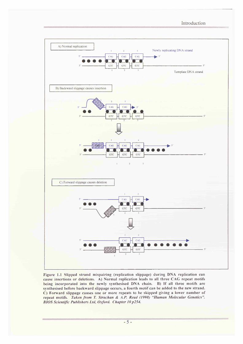
.1 Slipped strand mispairing (replication slippage) during DNAreplication can cause insertions or deletions.....................................5

.2 An autoradiograph example of how VNTR loci may be visualisedusing RFLP analysis........................................................................... 9

.3 An example of a short tandem repeat sequence.............................. 10

.4 Diagrammatical representation of the PCR process used toincorporate fluorescent labels into the targeted STR loci..............15

.5 SGM+DNA profile........................................................................... 16

.6 SGM+ allelic ladder profiles............................................................ 16

.7 Picture of the organisation of DNA around a histone core, forminga nucleosome.....................................................................................20

.8 Target sites for intracellular decay of a DNA molecule.................22

.9 The three possible genotypes at a SNP locus.................................. 24

.10 A line graph showing estimated SNP likelihood ratios from arraysof n loci, assuming the allelic frequency is constant across theset.......................................................................................................27

. 11 Diagram of allele-specific hybridisation......................................... 30

. 12 Allele-specific primer extension......................................................31

. 13 Allele-specific oligonucleotide ligation.......................................... 32

.14 Diagrammatical representation of the Universal Reporter Primer /ARMS Principle............................................................................... 34

.15 A typical electropherogram seen with a 21 - SNP multiplex........... 35

.16 A simple depiction of alleles inherited within an inbredpopulation..........................................................................................41

Chapter 2 Microarray Technology

Figure 2.1 Cy3 fluorescent images of a post-spotted, hybridised glassmicroarray slide.................................................................................52

Figure 2.2 Scattergraph showing clusters of 20 spots for 10 microarraysamples.............................................................................................. 54

Figure 2.3 Flow diagram illustrating the path ASGOTH follows in order tocorrectly genotype samples.............................................................. 56

Figure 2.4 Diagrammatical representation of control bins produced fromloglO Cy5A/Cy5B data.................................................................... 59

Figure 2.5 Flow diagram depicting allocation of genotypes based oncomparison to control sample bins...................................................61

Figure 2.6 Flow diagram depicting the path of the ASGOTH validationbootstrapping program..................................................................... 63

Figure 2.7 Graphical representation of bootstrapping data, using an increasingnumber of standard deviations.........................................................65

Figure 2.8 Graphical representation of genotyping results using an increasingnumber of control samples to generate the control bins................67

Figure 2.9 Graphical representation of the percentage of wrong answers givenby ASGOTH when using a different number of control samples per genotype and varying numbers of spot data sets.............................69

Chapter 3 Degradation Studies

Figure 3.1 Scattergraph showing proportion of allelic dropout seen comparedto fragment length size.................................................................... 96

Figure 3.2 Scattergraph indicating the number of alleles that fail to amplifyusing both SGM+ and the SNP 27-plex compared to the size of theallele fragment................................................................................. 101

Figure 3.3 Electropherograms showing SNP profiles obtained for the dilutionseries of ST control DNA............................................................... 103

Figure 3.4 Scattergraphs of percentage profile data for artificially degradedsaliva and blood samples................................................................ 107

Chapter 4 21-SNP multiplex interpretation criteria

Figure 4.1 Diagrammatical representation of the interpretation criteria used inSNP analysis.................................................................................... 118

Figure 4.2 Example of the theoretical calculation for Ht based on the value ofHb%min and Bt.................................................................................. 122

Chapter 5 21-SNP multiplex population studies

Figure 5.1 Radar graph showing the spread of allele frequencies for threeethnic groups for each of the 20 SNP loci used in the 21-SNPmultiplex......................................................................................... 138

Figure 5.2 Exact test P-P plots for all three population databases and anartificially mixed population.......................................................... 141

Figure 5.3 Evolutionary model used in the simulation of a sub-dividedpopulation........................................................................................ 143

Figure 5.4 Plot of Balding-Nichols corrected likelihood ratio (LR) vs. goldstandard LR, 0 =0.03, sample size =200....................................... 144

Figure 5.5 Plot of logio gold standard vs. the calculated ratio d0bs where 0 =0.03, sample size = 200...................................................................145

Figure 5.6 Graphical depiction of the calculated dQbs values calculated for asub-population of size 200............................................................. 146

Figure 5.7 Graphical depiction of the calculated dQbs values calculated for asub-population size of 1000........................................................... 147

Figure 5.8 A scattergraph of the values observed for the probability ofexclusion (PE) within a Kuwaiti family database.........................152

Figure 5.9 A scattergraph of values observed for the paternity index (PI),calculated for each child-alleged father relationship within aKuwaiti family database..................................................................153

Figure 5.10 Family tree for family 6 depicting the relationships between theseven offspring genotyped and the parents................................... 154

Figure 5.11 Family tree for family 8 depicting the relationships between the five offspring and the parents......................................................... 154

Chapter 6 European collaborative study

Figure 6.1 Preparation of artificially degraded DNA extracts....................... 166Figure 6.2 DNA profiling kits used for a European collaborative study 169Figure 6.3 Box and whisker plot showing the range of quant values received

for each reference individual for each sample type......................170

- x -

Figure 6.4

Figure 6.5

Figure 6.6

Figure 6.7

Figure 6.8

Figure 6.9

Figure 6.10

Figure 6.11

Figure 6.12

Figure 6.13

Chapter 7

Figure 7.1

Figure 7.2

Figure 7.3

Box and whisker plot showing the variation in amount of allele dropout per sample between the participating laboratories, usingstandard STR multiplex DNA profiling kits................................. 175Box and whisker plot showing the variation in amount of allele dropout per sample between the participating laboratories, usingthe Foren-SNP™ multiplex DNA profiling kit............................. 175Box and whisker plot showing the variation in amount of allele dropout per sample between the participating laboratories, usingthe mini-SGM DNA profiling kit...................................................176Box and whisker plot showing the variation in amount of allele dropout per sample between the participating laboratories, usingthe NC01 mini-STR DNA profiling kit........................................ 176Percentage profiles obtained across all labs for all samples andsample types.................................................................................... 178Box and whisker plot showing the variation seen in medianpercentage profiles across labs....................................................... 179Allele dropout compared to amplicon size for reference 1 degradedblood and saliva samples................................................................ 180Allele dropout compared to amplicon size for reference 2 degradedblood and saliva samples................................................................ 180Degradation time series plots for each multiplex tested in theEuropean collaborative study......................................................... 183Graphical representation of the number of molecules seen when simulating the degradation of DNA.............................................. 186

Casework Samples

Percentage profile data obtained for crime scene casework samples using LCN SGM+ DNA profiling and the 21-SNP multiplex.. ..207 LR data obtained from a comparison of the genotype data gainedfor each crime scene sample..........................................................208Scattergraph showing the proportion of allele dropout seen relative to the size of the target amplicon, using both the 21-SNP multiplex and LCN SGM+ DNA profiling....................................................209

In d e x o f T a b l e s

Chapter 1 Introduction

Table 1.1 The major classes of tandemly repeated human DNA......................7Table 1.2 The 10 STR loci used in the current AMPFISTR® SGM plus™

DNA profiling system, plus amelogenin..........................................14Table 1.3 Allele and genotype frequencies calculated for three biallelic loci,

based on Hardy-Weinberg proportions............................................17Table 1.4 Formulae for the likelihood ratio in situations where genotypes of

either both parents or one parent of the deceased individual are available as reference samples.........................................................43

Chapter 2 Microarrav Technology

Table 2.1 Results from ASGOTH simulation using varying numbers ofstandard deviations for the calculation of the negativethreshold............................................................................................ 64

Table 2.2 Results of ASGOTH simulation using varying numbers of controlsamples to create the control bins....................................................66

Table 2.3 Results of ASGOTH simulations using increasing numbers of spotdata sets for both 4 control samples per genotype and 6 control samples per genotype....................................................................... 68

Chapter 3 Degradation studies

Table 3.1 Picogreen DNA quantification values for artificially degradedsaliva, semen and blood samples.....................................................84

Table 3.2 SNP 27-plex profiles obtained for three reference control samples(CAS, DRJ, HER) after varying boiling time intervals................. 89

Table 3.3 SNP 27-plex profiles obtained for two reference control samples(SHM, ST) from differing intervals of boiling............................... 90

Table 3.4 SGM+ profiles obtained for three reference control samples (CAS,DRJ, HER) after varying boiling time intervals..............................91

Table 3.5 SGM+ profiles obtained for two reference control samples (SHM,ST) from differing intervals of boiling............................................ 92

Table 3.6 ANOVA results calculated for the SNP 27-plex and SGM+ forboiled samples...................................................................................94

Table 3.7 Chi-squared Goodness-of-Fit contingency table test results 95Table 3.8 SNP 27-plex profiles obtained for each sample type at each stage

of the degradation experiment..........................................................97Table 3.9 SGM+ profiles obtained for the artificially degraded samples for

saliva, blood and semen................................................................... 98Table 3.10 Percentage profiles and likelihood ratios (LRs) calculated for

artificially degraded samples............................................................ 99Table 3.11 Genotypes generated for control samples using varying amounts of

starting DNA template....................................................................104Table 3.12 SNP profiles obtained from artificially degraded samples 105Table 3.13 Percentage profile data and LR data for the SNP 27-plex, SGM+

28 cycles and the 21-SNP multiplex..............................................106

Chapter 4 21-SNP multiplex interpretation criteria

Table 4.1 Genotypes obtained from a dilution series of each of the controlsamples.............................................................................................119

Table 4.2 Hb% collected from two runs of the AB 3100 instrument at 12 and20 seconds........................................................................................120

Table 4.3 Observed homozygote peak heights (rfu) where allele dropout hasoccurred (Htmax) ............................................................................... 121

Table 4.4 Peak height data for allele drop-in peaks seen on a 96-wellnegative (deionised water) control plate....................................... 124

Table 4.5 Dilution series genotype data generated using the validated rule-sets for homozygote thresholds and heterozygous balance 125

Chapter 5

Table 5.1 Table 5.2

Table 5.3

Table 5.4

Table 5.5 Table 5.6

21-SNP multiplex population studies

Sample types used for SNP multiplex validation experiments... 134 An example of a Goodness-of-Fit test for Hardy-Weinbergequilibrium...................................................................................... 136Allele frequencies for each of the 20 SNP loci used in the multiplex for each ethnic group studied and overall likelihoodratios for each group........................................................................137Hardy-Weinberg equilibrium probability values for each SNP within the three main ethnic code populations, calculated usingGoodness-of-fit Chi-squared analysis and Exact tests................. 139SNP loci that lie on the same chromosome................................... 148Exclusion probability (PE) and paternity index (PI) values for Kuwaiti family samples...................................................................151

Chapter 6 European collaborative study

Table 6.1 Extraction and quant methods and results, as provided by eachlaboratory.........................................................................................170

Table 6.2 ANOVA results for percentage profile data for each laboratory foreach sample type using each multiplex kit...................................172

Table 6.3 Percentage profiles obtained for each sample using data from alllabs analysed by Median polish calculations................................ 177

Table 6.4 Average percentage profiles gained across all samples for eachlab..................................................................................................... 179

Chapter 7 Casework samples

Table 7.1 Casework DNA sample data...........................................................195Table 7.2 DNA quantification values (ng/pL) and PCR volumes for crime

scene and reference samples.......................................................... 197Table 7.3 SGM+ DNA profiling results for case 1 - 300205756................. 198Table 7.4 21-SNP multiplex genotyping results for case 1 - 300205756... 198Table 7.5 SGM+ DNA profiling results for case 2 - 300100756.................200Table 7.6 21-SNP multiplex genotyping results for case 2 - 300100756.. .200Table 7.7 SGM+ DNA profiling results for case 3 - 300091460.................201Table 7.8 21-SNP multiplex genotyping results for case 3 - 300091460.. .201Table 7.9 SGM+ DNA profiling results for case 4 - 300110837..................202Table 7.10 21-SNP multiplex genotyping results for case 4 - 300110837.. .202Table 7.11 SGM+ DNA profiling results for case 5 - 300065124..................203

- xiii -

Table 7.12 21 -SNP multiplex genotyping results for case 5 - 300065124.. .203Table 7.13 SGM+ DNA profiling results for case 6 - 300227014................. 204Table 7.14 21-SNP multiplex genotyping results for case 6 - 300227014.. .204Table 7.15a Percentage profiles and LR data for casework crime scene samples,

based on kinship analysis...............................................................206Table 7.15b Percentage profiles and LR data for casework crime scene samples,

based on allele frequency data.......................................................206

- xiv -

A b b r e v ia t io n s

pg MicrogrampL MicrolitrepM Micromolar6-FAM 6-carboxyfluoresceinA, dATP Adenine, deoxyadenosine triphosphateAB Applied BiosystemsANOVA Analysis of varianceARMS Amplification refractory mutation systemASGOTH Automated SNP Genotype Handlerbp Base pairsBSA Bovine serum albuminC, dCTP Cytosine, deoxycytidine triphosphateCE Capillary electrophoresis°C Degrees CelsiusDNA Deoxyribonucleic AcidE EvidenceEDNAP European DNA profiling GroupEDTA Ethylenediaminetetraacetic acid (disodium salt)ENFSI European Network of Forensic Science InstitutesFSS The Forensic Science Service™Fst Fixation index (6)G, dGTP Guanine, deoxyguanosine triphosphateGDA Genetic Data AnalysisHET or het HeterozygoteHMW High molecular weightHOM or hom HomozygoteHd Hypothesis for the defenceHp Hypothesis for the prosecutionHWE Hardy-Weinberg equilibriumJO E 2,7-dimethoxy-4,5-dichloro-6-carboxy-fluoresceinLCN Low copy numberLMW Low molecular weightLR Likelihood ratioMg MagnesiumMgCL Magnesium chloridemin MinutemL MillilitremM MillimolarMtDNA Mitochondrial DNA

- xv -

NDNAB National DNA Database®

ng NanogramNIST National Institute of Standards and Technology (US)nM Nanomolarnt NucleotideOLA Oligonucleotide ligation assayPAGE Polyacrylamide gel electrophoresisPCR Polymerase chain reaction

Pe Probability of exclusion

Pg PicogramPI Paternity indexPm Match probabilityPr ProbabilityR&D Research and DevelopmentRFLP Restriction Fragment Length Polymorphismrfu Relative fluorescent unitROX 6-carboxy-X-rhodamineSD Standard deviationSDW Sterile Distilled Watersec SecondSGM Second Generation MatrixSGM+ AMP/-7STR® SGM Plus™ systemSLP Single locus probeSTR Short Tandem RepeatSNP Single Nucleotide PolymorphismSWGDAM Scientific Working Group on DNA Analysis MethodsT, dTTP Thymine, deoxythymidine triphosphateTm Melting temperatureTris Tris(hydroxymethyl)methylamineU UnitsURP Universal reporter primerUV UltravioletVBA Visual Basic for ApplicationsVNTR Variable number tandem repeat

Introduction

Introduction

1.1 Human DNA Polymorphisms

1.1.1 Mutations in the human genome

DNA polymorphisms are present throughout the human genome and have been

well studied and documented over the last forty years. In the 1990s the Human

Genome Project set out to determine the entire human DNA sequence, and

revealed the presence, and location, of millions of these DNA sequence variants

throughout the genome (Chakravarti 1999; Kruglyak and Nickerson 2001; Kwok

2001; Venter et. al. 2001). Variations consist of insertions and deletions of a few

to many nucleotides, variation in the repeat number of a motif (mini- and micro­

satellites) or single nucleotide polymorphisms (SNPs) and, on a larger scale,

chromosomal mutations such as inversions and translocations.

The process that produces heritable variations in DNA is driven by mutation. A

mutation appearing in the germline can be transmitted to subsequent generations,

whereas mutations in somatic cells are not inherited. If a mutation event occurs in

an important region of the genome (especially in a coding region) then it is

possible that a genetic disease may be the result. The process of mutation can be

linked to events during chromosome segregation at meiosis, DNA replication and

repair (Jeffreys et. al. 1988a), and spontaneous changes resulting from exposure to

chemicals (Strachan and Read 1998).

According to the Mendelian Law of Segregation, an individual inherits two copies

of the genome, one from the mother and one from the father. At each specific

location on the chromosome, known as a locus, an individual may have a different

genetic sequence. Alternative forms of a genetic locus are known as alleles and

can be characterised by measuring their frequencies within a given population. If

an allelic variant occurs at a frequency greater than 0.01 within a population then

it is classified as a polymorphism, as the probability of it resulting from a chance

recurrent mutation is low hence it is more likely to have been inherited (Strachan

and Read 1998). Polymorphisms are of interest for forensic purposes as they can

be used to distinguish individuals.

Introduction

Variation within a coding DNA sequence can cause an alteration in the function

of a particular protein (Strachan and Read 1998; Venter et. al. 2001). Mutations

found in coding regions take on a number of different forms including nonsense

mutations, where a difference in one base will cause a STOP codon leading to a

shortened protein structure; missense mutations, causing one amino acid in a

chain to be replaced by another; and silent mutations, a base change having no

effect on the resulting amino acid encoded. These are all forms of base

substitutions, also known as point mutations. There are two types of point

mutation, depending on the nature of the base change (Lewin 1998): a transition,

when a pyrimidine is changed to a pyrimidine or a purine to a purine (e.g. G or C

base is exchanged with an A or T base respectively); or a transversion, when a

purine changes to a pyrimidine or a pyrimidine to a purine (e.g. an A/T becomes a

C/G). Transitions are the most common form of polymorphism as they produce

the least marked change to the DNA sequence. Coding regions can also be

affected by base insertions, where a number of bases are added to a sequence;

base deletions, where a number of bases are deleted from a sequence; and large-

scale chromosomal abnormalities.

Mutation provides the raw material for evolution to occur. In particular,

mutations in coding regions may be deleterious to the affected individual, for

example, causing a protein to become dysfunctional with lethal consequences.

Selective pressure consequently reduces the levels of genes that are deleterious in

populations. Sometimes a mutation might benefit an individual resulting in

increased breeding success e.g. sickle cell anaemia in malaria-infested regions

(Wood et. al. 1976; Hill et. al. 1991; Modiano et. al. 1996). Consequently, genes

that increase fitness tend to be preserved and passed on to successive generations.

Evolutionary pressure does not work in the same way within the non-coding

(“junk”) regions of DNA that constitutes more than 95% of the total human

genome (Ono 1972; Zuckerkandl 1992; Nowak 1994; Wong et. al. 2000). Recent

developments in non-coding DNA research have shown that certain regions of

non-coding DNA have higher levels of conservation than predicted, suggesting

regulatory elements connected to genes may make up a large percentage of the

“junk” DNA region (http://www.psrast.org/junkdna.htm). The rest of the non­

Introduction

coding DNA can demonstrate large numbers of polymorphisms, because there is

less selective pressure over time. Polymorphisms mainly take the form of base

substitutions and tandem repeat regions (see sections 1.1.2-1.1.5) and can be used

for forensic identification purposes.

1.1.2 Tandemlv repeated DNA sequences

Over 50% of the human nuclear genome contains highly repeated DNA sequences

(DNA ‘motifs’) that appear to be largely inactive (http://www.euchromatin.org/;

Wyman and White 1980). Some of these sequences are known as “tandemly

repeated DNA” and vary in their size and composition to give three main

subclasses of repeats: satellite DNA; minisatellite DNA (section 1.1.3); and

microsatellite DNA (section 1.1.4). These motif regions are replicated with low

fidelity because of a slippage that occurs between the template and the newly

synthesised DNA strands during replication (Bell, Selby et al. 1982; Capon, Chen

et al. 1983; Goodboum, Higgs et al. 1983; Weller, Jeffreys et al. 1984; Stoker,

Cheah et al. 1985; Tautz 1989). This slippage leads to a varying number of repeat

motifs between individuals.

Introduction

A) Normal replicationNewly replicating DNA strand

^^rg:■ GTC - GTC ■

- CAG

GTC

Template DNA strand

B) Backward slippage causes insertion

CAG CAG

GTC - GTCGTC

- CAG

GTC

C) Forward slippage causes deletion

CAG - CAG

n i jGTC - GTC

• • •

CAG - CAG

GTC GTC

Figure 1.1 Slipped strand mispairing (replication slippage) during DNA replication can cause insertions or deletions. A) Normal replication leads to all three CAG repeat motifs being incorporated into the newly synthesised DNA chain. B) If all three motifs are synthesised before backward slippage occurs, a fourth motif can be added to the new strand. C) Forward slippage causes one or more repeats to be skipped giving a lower number of repeat motifs. Taken from T. Strachan & A. P. Read (1998) “Human Molecular Genetics ”. BIOS Scientific Publishers Ltd, Oxford. Chapter 10 p254.

Introduction

The number of microsatellite repeats present in a DNA molecule changes by a

mutation rate of between 10’3 and 10’4 per locus per gamete per generation

(Weissenbach et. al. 1992; Weber and Wong 1993; Xu et. al. 2000; Huang et. al.

2002). This can increase up to 5 x 10‘2 per gamete, as an extreme, in

micro satellite loci (Jeffreys et. al. 1988a), although loci used in routine forensic'y _____

analysis show rates lower than 10'“ (Jeffreys et. al. 1997). These mutation rates

are low enough for most parent-child transmissions to propagate the same number

of DNA motifs, but also allow sufficient mutation to maintain a high level of

heterozygosity within a population, countering the opposing effect of genetic drift

that tends to increase homozygosity (Jeffreys et. al. 1985a). Individually,

microsatellites have a relatively low discrimination power of around 1 in 100,

therefore analysis of several loci is required for a highly discriminating test

(Sullivan 1994).

Table 1.1 gives an overview of the differences between the three subclasses of

tandem repeats. Satellite DNA regions are large, spanning hundreds of bases,

making them unsuitable for forensic analysis. In humans, minisatellite regions are

found with greater frequency either within the telomeric regions of chromosomes

or close to them. The hypervariable VNTRs (Variable Number Tandem Repeats)

have been utilised for forensic identification but were superseded by microsatellite

loci in the 1990s (see section 1.2). Microsatellite DNA is found across all

chromosomes and is used in current DNA profiling techniques.

Introduction

Class Size of repeat unit (base pairs) Major chromosomal location (s)

Satellite DNA (blocks often from lOOkb to several Mb in length)

Satellites 2 & 3 5 Most, possibly all, chromosomes

Satellite 1 (AT rich) 25-48 Centromeric heterochromatin

a (alphoid DNA) 171 Centromeric heterochromatin

(3 (Sau3A family) 68 Centromeric heterochromatin of 1, 9, 13, 14, 21,22 & Y

Minisatellite DNA(blocks often within 0.1-20kb range)

Telomeric family 6 All telomeres

Hypervariable family (VNTRs) 9-24 All chromosomes, often near telomeres

Microsatellite DNA (STRs) (blocks often less than 150bp) 1-4 All chromosomes

Table 1.1 The major classes of tandemly repeated human DNA. Taken from T. Strachan & A.P. Read (1998) “Human Molecular Ge ne t i c s BI OS Scientific Publishers Ltd, Oxford. Table 8.3.

1.1.3 Variable Number of Tandem Repeats (VNTRs)

Also known as hypervariable minisatellite loci, VNTRs were the first type of

DNA polymorphism described for forensic identification (Gill et. al. 1985a; Gill

et. al. 1985b; Jeffreys et. al. 1985b; Jeffreys et. al. 1985c). A VNTR locus is

comprised of tandemly repeated sequences, usually 9 to 80 bases in length per

repeat unit, with a core sequence of GNNNNTGGG (where N can equal any

nucleotide) (Bell et. al. 1982; Jeffreys et. al. 1985a; Baird et. al. 1986; Jarman et.

al. 1986; Evett et. al. 1989). These loci can be thousands of bases in length, due

to the number of repeat units, making them amenable to detection by restriction

endonuclease methods (see section 1.1.3.1) (Jeffreys et. al. 1985a; Nakamura et.

al. 1987). Jeffreys et al. demonstrated that probes designed for tandem repeats of

the myoglobin locus can detect multiple hypervariable loci producing

“fingerprints” when hybridisations are carried out under low stringency conditions

Introduction

- using high salt concentrations in hybridisation and wash solutions (e.g. washes

using lx saline sodium citrate, SSC) (Jeffreys et. al. 1985b). They showed that

“variant (core)n probes can detect sets o f hypervariable minisatellites to produce

somatically stable DNA ‘fingerprints ’ which are completely specific to an

individual (or to his or her identical twin) and can be applied directly to problems

o f human identification, including parenthood testing ". The bands produced by

these multi-locus probes were shown to be randomly dispersed throughout the

genome and can be considered to be independently inherited. Several

hypervariable VNTR loci were discovered in the early 1980s and include sites

within the insulin gene (Bell et. a l 1982), the Harvey ras oncogene (Capon et. al.

1983) and the alpha globin genes (Jarman et. al. 1986).

1.1.3.1 Method for forensic typing o f VNTRs

Genomic DNA samples were digested using restriction endonucleases such as

HinfI, Alul or HaeIII that recognise well-conserved 4 base pair restriction sites

flanking a specific VNTR locus. The technique was based on restriction length

fragment polymorphism (RFLP) analysis methods for 3’ alpha-globin (Gill et. al.

1985a; Jeffreys et. al. 1985a; Jeffreys et. al. 1985b; Fowler et. al. 1988). The

VNTR locus does not contain the restriction site and therefore remains intact.

Resulting restriction fragments were separated according to size by

electrophoresis through an agarose gel, transferred to a nylon membrane

(Southern blotting) and hybridised with probes labelled with a radioactive isotope.

Multi locus probes were superceded by single locus probes (SLP) because the

former were difficult to reproduce for database purposes. SLPs were hybridised

under high stringency (low salt concentrations). Each SLP used detected a unique

sequence from the corresponding locus, and would only bind at this specific site

(Jarman et. al. 1986; Wong et. al. 1986; Nakamura et. al. 1987; Wong et. al.

1987). The fragments were then visualised using autoradiography (Figure 1.2).

Differences in sizes of the restriction fragments represented integral numbers of

the tandemly repeated unit. The number of repeat sequences varied significantly

between non-related individuals allowing a unique “fingerprint” to be visualised.

Introduction— — — —

OFFSPRING

f l ~2 a i l ? ( f

Figure 1.2 An autoradiograph example of how VNTR loci may be visualised using RFLP analysis. In this case the three offspring have alleles in common with each other and share the same alleles as either the mother or the father. The alternate size products appear due to the varying number of tandem repeats present (photograph courtesy o f Dr. J. Wetton, The Forensic Science Service™, UK).

Most VNTR loci used for human identification exhibited more than 100 alleles

within a population, meaning the typing of four markers was sufficient to

differentiate between unrelated individuals with a discrimination power of 1 in 10 million (Gill et. al. 1991).

1.1.4 Short Tandem Repeats (STRs)

STRs, also known as microsatellites, are repetitive regions of DNA widely distributed throughout the genome, particularly found in non-coding regions of

DNA (Beckman and Weber 1992). The repetitive sequences are between 1 - 6 bases in length and the number of repeats at any given locus varies, giving rise to

different size loci and different allele lengths within an individual locus.

Mononucleotide repeats of A or T are very common in the human genome and make up approximately 10Mb, or 0.3% of the nuclear genome (Huang et. al. 2002). In the case of dinucleotide repeats, arrays of CA repeats are very common

Introduction

and are often highly polymorphic. CT/AG repeats are also common but CG/GC

repeats are rare, due to the propensity of C residues to be methylated and

deaminated into T residues when flanked by a G residue at their 3’ end (Strachan

and Read 1998). Trinucleotide and tetranucleotide repeats are comparatively rare

but highly polymorphic and can be exploited for forensic purposes (Budowle

1999). The number of alleles at a single tetranucleotide STR locus usually ranges

from 5 to 20, making the resulting target region 20 to 100 bases in length.

The use of the Polymerase Chain Reaction (PCR) (Saiki et. al. 1985; Mullis and

Faloona 1987) for amplification of STR loci makes the amplified products larger

than the target region due to the inclusion of sequences that flank the repeat region

(Figure 1.3).

Locus A

STR sequence:

PCR product:

; -CATC-CATC-CATC-CATC-CATC-CATC-CATC-CATC—

Locus B

STR sequence:

PCR product:

— CATC-CATC-CATC-CATC--------

Figure 1.3 The short tandem repeat (STR) sequence of CATC in the above example varies in the number of its repeats between locus A and locus B. By amplifying the target region using flanking primers, PCR products of varying sizes are produced. These PCR products can be visualised when run on an acrylamide gel (Figure 1.5).

PCR was first described in 1985 and enabled DNA molecules to be exponentially

amplified by a series of heating and cooling reactions in the presence of dNTPs

and a DNA polymerase enzyme (Saiki et. al. 1985; Mullis and Faloona 1987). In

1994 Sullivan explained that the development of PCR methods had allowed

multiplex analysis of several loci giving a highly discriminating test, stating: “/>?

this regard, STRs are preferable to VNTRs because the former are more amenable

to co-amplification and have narrow allelic size ranges which enable several loci

Introduction

to be chosen for co-analysis that are non-overlapping in their size ranges"

(Sullivan 1994). STRs were also preferable as a fluorescence detection system

could be used for analysis of the PCR products.

The current DNA profiling system used in the United Kingdom for forensic

identification utilises tetranucleotide repeat STR loci (Cotton et. al. 2000). An

account of the development of the forensic typing systems used in the UK is given

in section 1.2.

1.1.5 Single Nucleotide Polymorphisms (SNPs)

A SNP can be defined as “a position within a DNA molecule where one base can

be substituted by another" (Strachan and Read 1998), as well as other types of

DNA variations such as insertions or deletions at single positions throughout the

genome (Budowle et. al. 2004a). SNPs occur approximately once every 1000

bases in humans (Cooper et. al. 1985; Kruglyak and Nickerson 2001; Venter et.

al. 2001), making them the most abundant form of DNA variation. Like other

DNA polymorphisms, SNPs can be linked back to mutations occurring from

spontaneous errors in chromosome segregation at meiosis, DNA replication and

repair, and spontaneous changes resulting from exposure to chemicals (Strachan

and Read 1998). The use of SNPs as genetic markers is well-documented for

many different applications from human and animal identification, population

studies, disease associations and phylogeny (Gray et. al. 2000; Riley et. al. 2000;

Schork et. al. 2000; Shastry 2002; Emara and Kim 2003; Schmith et. al. 2003).

Sections 1.5 and 1.6 describe the use of SNPs for forensic identification and the

methods that can be used for their detection.

- 11 -

Introduction

1.2 Forensic DNA Profiling

During the early 1990’s DNA forensic science experienced considerable growth,

instigated by the introduction of molecular techniques allowing the development

of highly discriminating DNA profiling methods (Kimpton et. al. 1994; Lygo et.

al. 1994; Sullivan 1994; Gill et. al. 1995b; Gill et. al. 1997; Cotton et. al. 2000;

Grimes et. al. 2001; Lowe et. al. 2001; Lowe et. al. 2002; Hussain et. al. 2003).

The DNA profiling technique described by Jeffreys et al., using specific tandem

repeat (VNTR) regions of DNA (Jeffreys et. al. 1985a), was the first to enable a

‘genetic fingerprint’ of an individual to be generated. The term genetic fingerprint

is no longer used and has been replaced by ‘DNA profiling’ as the comparison

with fingerprints was not particularly helpful - forensic scientists do not use terms

such as uniqueness, preferring to use match probabilities and likelihood ratios.

VNTR polymorphisms are outlined in section 1.1.3. It is the variation within each

locus that is exploited for use in forensic identification.

The introduction of PCR (Saiki et. al. 1985; Mullis and Faloona 1987) allowed

new improved molecular biology methods to be used in forensic typing. PCR

revolutionised many areas of DNA research and accelerated the growth of DNA

analysis. This occurred primarily by use of semi-automated methods which

dramatically decreased turn-round time and costs resulting in increased

throughput of samples. PCR could be used to amplify much smaller quantities of

DNA starting material meaning the types of cases that could be analysed

expanded considerably (Hagelberg et. al. 1991; Jeffreys et. al. 1992). The VNTR

method outlined by Jeffreys in 1985 required 0.5-5 pg of high molecular weight

DNA to gain a significant result. The amount of offender DNA found at a crime

scene was often much lower so the method was deemed unsuitable for many

crime scene investigations. The introduction of PCR allowed the amount of

starting DNA to be reduced to lng (0.001 pg) as template could be exponentially

amplified to a level that was easily detected. Currently, approximately 1 ng

quantity of starting DNA material is used in standard profiling methods (Cotton

et. al. 2000).

- 12-

Introduction

PCR methods using VNTRs were developed (Jeffreys et. al. 1988b) but were

considered to be too time-consuming, too subjective in the interpretation of results

and c.100 ng of DNA was still required to perform the SLP analysis. PCR is not

as efficient at amplifying large DNA fragments (Sullivan 1994). Large VNTR

products were also unsuitable for typing degraded samples, which generally have

much smaller DNA fragments present (Majno and Joris 1995; Johnson and Ferris

2002) (see section 1.4).

In 1994 the first DNA profiling system used by the criminal justice system was

introduced, involving four polymorphic STR loci (Kimpton et. al. 1994; Lygo et.

al. 1994). This system was superseded in 1996 by a more discriminating STR

system using PCR, known as the Second Generation Multiplex (SGM) (Gill et. al.

1995b; Gill et. al. 1997). This consisted of six polymorphic loci plus a non-STR

sex-determining locus - the X-Y homologous amelogenin genes. Amelogenin

primers flank a 6 base pair (bp) deletion within intron 1 of the X homologue,

resulting in 106 bp and 112 bp PCR products from the X and Y chromosomes

respectively (Sullivan et. al. 1993; Mannucci et. al. 1994). The introduction of

the Applied Biosystems (AB) AMPF/STR® SGM plus™ system (SGM+) in 1999,

with an additional 4 STR loci added to the original 6 used in SGM (Cotton et. al.

2000), increased the discrimination power from approximately 1 in 50 million

(SGM) to 1 in 1,000 million. DNA profiling for the UK National DNA Database

(NDNAD®) is carried out using SGM+.

1.2.1 Method for forensic typing of STRs

SGM+ PCR amplifies 10 hypervariable STR loci (Table 1.2) and Amelogenin (for

X/Y chromosome sex discrimination) using dye-labelled locus-specific primers,

allowing fragments to be detected by the use of polyacrylamide gel

electrophoresis (PAGE) (Figure 1.5) or, more recently, capillary gel

electrophoresis (CE). The use of three fluorescent dyes (JOE, FAM & NED)

enables loci with overlapping allele sizes to be labelled with different colours so

they are easily distinguishable from each other.

Introduction

Locus ID Repeat motif Approx. size range (base pairs)

Dye label used for analysis

Chromosomelocation

Amelogenin N/A X = 106; Y = 112 JOE X/Y

D3S1358 (D3) [TCTG][TCTA] 114-142 FAM 3q21.31

HUMVWF31/A(vWA) TCTR* 157-209 FAM 12pl 3.31

D16S539 (D16) GATA 234-274 FAM 16q24.1

D2S1338 (D2) TRCC* 289-341 FAM 2q35

D8S1179 (D8) TCTR* 128-172 JOE 8q24.13

D21S11 (D21) [TCTA][TCTG] 187-243 JOE 21q21.1

D18S51 (D18) AGAA 265-345 JOE 1821.33

D19S433 (D19) AAGG 106-140 NED 19ql2

HUMTHOl (THOl) TCAT 165-204 NED 1 lpl 5.5

HUMFIBRA (FGA) CYKY* 215-353 NED 4q31.3

* R = A or G; Y = C or T; K = G or T

Table 1.2 The 10 STR loci used in the current AMPF7STR® SGM plus™ DNA profiling system, plus Amelogenin (Butler e t a l 2004). Each locus has a different repeat motif and a variable number of repeats. Some loci give a better discrimination than others but, multiplexed, the system has a discrimination power of approximately 1 in 1,000 million, between non-related individuals.

The fluorescent dye labels present on one of the pair of flanking primers are

incorporated into the newly synthesised DNA products during the PCR process,

allowing them to be visualised when run on a polyacrylamide gel or CE

instrument (Figure 1.4).

- 14-

Introduction

\ ►

— Primer annealing

i

Primer extension-TV I M i l l ----------------

It i l l --------------------- Fluorescently labelled

^ -------------------- PCR product

Fluorescent dye label

Primer sequence complementary to flanking sequence

Flanking sequence for primer binding

----------------------- ► Direction o f primer extension

I I 1 I I I I I Hypervariable STR locus

Figure 1.4 Diagrammatical representation of the PCR process used to incorporate fluorescent labels into the targeted STR loci. A) primers are designed complementary to the STR flanking regions and are able to bind to the DNA template during the annealing stage of PCR. B) the primers extend the new DNA strand making it complementary to the target DNA region, exponentially creating new double stranded DNA molecules. C) the resulting DNA product has fluorescent dye labels incorporated into its 5’ ends, allowing it to be detected by PAGE.

Data collection generates an SGM+ DNA profile (Figure 1.5). The number of

repeat sequences within each locus is directly proportional to the size of the PCR

product. STR fragments are given a numerical designation by comparison against

a control allelic ladder run on the same gel (Figure 1.6).

- 15-

Introduction

MO

C06_F46R_(M (u

Figure 1.5 SGM+ DNA profile showing either one or two bands of differing size at each locus. The yellow dye NED is visualised as a black peak. For each dye one band indicates homozygosity at that locus, i.e. the individual has the same number of repeats at each allele. Two bands indicate heterozygosity, i.e. the individual has a different number of repeats at each allele. Locus identity and allele positions are characterised using a separate software program allowing correct genotyping of each allelic peak, by comparison with an allelic ladder (figure 1.6) run in conjunction with the samples on an acrylamide gel.

C ttJtU E U C .U ttO E R .p6 .fM 6

Figure 1.6 Allelic ladder profiles used to correctly score each sample using an automated process. Each peak for each locus represents an STR with a different number of repeat motifs.

Introduction

1.3 The Use of Statistics in DNA Profiling

Statistics are used in DNA forensic analysis as a method of interpreting the results

gained from a sample and assessing the value of the evidence in such a way as to

convey it accurately to a court of law. If DNA evidence shows a match between a

suspect and a crime stain (for example) then an assessment of the probability of

such a match occurring between the stain and any other individual must be made.

The match probability (Pm) is the probability of two random, unrelated

individuals in the general population having an identical DNA profile. Pm can be

calculated using the values of the allele frequencies of each locus in the

population converted into relative genotype proportions, based on Hardy-

Weinberg equilibrium, multiplied together to give the chance of seeing this DNA

profile within the population. This is known as the product rule (Balding and

Nichols 1994; Evett and Weir 1998). The product rule calculation assumes

independence both within and between loci and relies on each locus conforming

to Hardy-Weinberg proportions (section 1.8).

Locus ID Allele Allele frequency (P)

Relative genotype frequenciespAA pBB pAB

LDLR A 0.437 0.19 0.49B 0.563 0.32

GYPA A 0.539 0.29 0.50B 0.461 0.21D7S8 A 0.544 0.30 0.49B 0.456 0.21

Table 1.3 Allele and genotype frequencies calculated for three biallelic loci, based on Hardy- Weinberg proportions. The relative genotype frequencies are calculated using the equation p2 + 2pq + q2 = 1. Adapted from B. Weir (1996) “Genetic Data Analysis H ” Sinauer Associates, Inc. Massachusetts.

Using the genotype frequencies in table 1.3, the Pm for a suspect can be

calculated based on the DNA profile found. For example, if a crime stain found at

a scene had the profile LDLR A/A; GYPA A/B; D7S8 B/B, Pm would be

calculated as:

Introduction

Product rule

pBB)

= 0.19 (LDLR pAA) x 0.50 (GYPA pAB) x 0.21 (D7S8

= 0.01995

this is the probability of a chance match of the profile with another random,

unrelated sample.

This ‘simple’ Pm calculation makes assumptions of independence of loci and

doesn’t take into account effects from sampling error, related individuals, or

population sub-structures i.e. it assumes random mating. The population genetics

imposing correction factors upon the calculations are explained and examined in

more detail in section 1.8.

For more complex situations a likelihood ratio can be calculated. “A likelihood

ratio (LR) involves a comparison o f the probabilities o f the evidence under two

alternative propositions ” (Butler 2005b). The two alternative hypotheses seen in

forensic situations are:

Hp = “the DNA profile at the crime scene came from the suspect” i.e. the

prosecution hypothesis;

Hd = “the DNA profile at the crime scene came from another, unknown

individual” i.e. the defence hypothesis.

The LR is calculated from the following equation:

Where Pr(E|//p) is calculated from the probability of the crime sample and the

suspect sample matching given that the prosecution hypothesis is true, i.e. in

simple scenarios this is equal to 1. Pr(E|//^) is the match probability calculation,

i.e. the probability of the profile given that the defence hypothesis is true. This is

the same as the probability of observing the profile in the general population.

LR

- 18-

Introduction

The difference between the two calculations can be explained as:

“What is the probability of observing a particular profile?” [the match

probability]

and

“Given that I have observed this profile, what is the probability that

another (unprofiled) individual will also have it?” [the likelihood ratio]

(Balding 2005).

- 19-

Introduction

1.4 DNA Packaging & Degradation

1.4.1 DNA packaging in the nucleosome

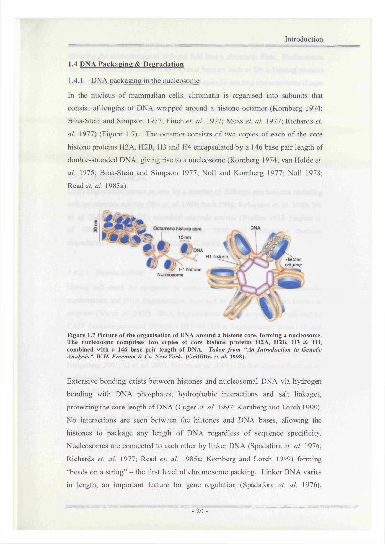
In the nucleus of mammalian cells, chromatin is organised into subunits that

consist of lengths of DNA wrapped around a histone octamer (Komberg 1974;

Bina-Stein and Simpson 1977; Finch et. al. 1977; Moss et. al. 1977; Richards et.

al. 1977) (Figure 1.7). The octamer consists of two copies of each of the core

histone proteins H2A, H2B, H3 and H4 encapsulated by a 146 base pair length of

double-stranded DNA, giving rise to a nucleosome (Komberg 1974; van Holde et.

al. 1975; Bina-Stein and Simpson 1977; Noll and Komberg 1977; Noll 1978; Read et. al. 1985a).

Figure 1.7 Picture of the organisation of DNA around a histone core, forming a nucleosome. The nucleosome comprises two copies of core histone proteins H2A, H2B, H3 & H4, combined with a 146 base pair length of DNA. Taken from “An Introduction to Genetic Analysis”. W.H. Freeman & Co. New York. (Griffiths et al. 1998).

Extensive bonding exists between histones and nucleosomal DNA via hydrogen

bonding with DNA phosphates, hydrophobic interactions and salt linkages,

protecting the core length of DNA (Luger et. al. 1997; Komberg and Lorch 1999).

No interactions are seen between the histones and DNA bases, allowing the

histones to package any length of DNA regardless of sequence specificity.

Nucleosomes are connected to each other by linker DNA (Spadafora et. al. 1976;

Richards et. al. 1977; Read et. al. 1985a; Komberg and Lorch 1999) forming

“beads on a string” - the first level of chromosome packing. Linker DNA varies

in length, an important feature for gene regulation (Spadafora et. al. 1976),

H1 h is to n e v Histoneoctamer

H1 histone Nucleosome

-20-

Introduction

allowing the nucleosomes to coil and fold into a chromatin fibre. Nucleosomes

are more confined to location by physical barriers such as DNA-binding proteins

along the length of the DNA and sequence-specific bending characteristics (Luger

et. al. 1997). As a consequence of this physical limitation, nucleosomes are often

found close to promoter regions and regulatory elements (Simpson 1991; Thoma

1992). The organisation of DNA around a octameric histone core confers some

protection onto the nucleosomal DNA, making it less susceptible to attack from

cellular nucleases (van Holde et. al. 1975; Noll and Komberg 1977).

1.4.2 DNA degradation

DNA degradation occurs in vivo by a number of different mechanisms including

cellular enzymic activity (Bar et. al. 1988; Suck 1992; Robertson et. al. 2000; Wu

et. al. 2002; Poinar 2003), microbial enzymic activity (Bradley 1938; Hughes et.

al. 1986; Madisen et. al. 1987; Poinar 2003) and endogenous chemical

degradation by hydrolysis and oxidation (Lindahl 1993).

1.4.2.1 Enzyme activity

During cell death by apoptosis or necrosis, the nucleus undergoes chromatin

condensation and DNA fragmentation, executed by a group of enzymes known as

caspases (Wu et. al. 2002). DNA fragmentation during apoptosis is mediated by

CAD1 (caspase-activated DNase) / DFF-40 (DNA fragmentation factor) (Rudel

and Bokoch 1997; Sakahira et. al. 1998), although other enzymes, specifically

nucleases, are required for complete histone release (Robertson et. al. 2000;

Hengartner 2001; Li et. al. 2001; Parrish et. al. 2001). Endonucleases function by

hydrolysing the phosphodiester bond in the phosphate-ribose backbone structure

(Suck 1992), causing fragmentation of the DNA molecules. The endonucleases

first target the unprotected linker DNA, leaving monomeric nucleosomes

comprising 146 base pairs of protected DNA. Exonucleases detach single

nucleotides from the terminal end of the DNA strand, gradually shortening the

molecule (Bar et. al. 1988).

-21 -

Introduction

1.4.2.2 Microbial enzyme activity

DNA can be further degraded by bacterial, fungal and insect interaction

(Eglington and Logan 1991), an effective but often incomplete process.

1.4.2.3 Chemical degradation

Hydrolysis and oxidation of bonds within the DNA structure occurs in vivo and is

counteracted by DNA repair mechanisms using endogenous cellular enzymes

(Lindahl 1993; Friedberg et. al. 1995). The glycosidic base - sugar bond is the

main target of direct hydrolytic attack and leads to loss of the base (Figure 1.8).

The abasic site is then vulnerable to single-strand cleavage of the phosphodiester

bond and the strand is sheared, unless repaired by endogenous endonucleases,

phosphodiesterases, DNA polymerase and DNA ligase (Lindahl 1976; Friedberg

et. al. 1995).

Figure 1.8 Target sites for intracellular decay. A section of one strand of the DNA double helix is shown with the four bases (from top: guanine, cytosine, thymine, adenine). Blue arrows indicate sites susceptible to hydrolytic attack and orange arrows indicate oxidative damage. The magnitude of the arrows reflects the potential for activity at each site (not to scale). Adapted from T. Lindahl (1993) “Instability and decay o f the primary structure o f DNA n Nature 362: page 713.

o Sites susceptible to Hydrolytic attackOxidative dam age

O H

Introduction

Exposure to active oxygen can also damage the DNA by oxidative attack across

the 3’-4’ carbon bond of the deoxyribose leading to ring fragmentation and strand

scission (Friedberg et. al. 1995; Poinar 2003). Oxidation can also occur in the

ring structure of the bases (Figure 1.8). Lindahl postulates that “deprived o f the

[DNA] repair mechanisms provided in living cells, fully hydrated DNA is

spontaneously degraded to short fragments over a time period

- 23 -

Introduction

1.5 Single Nucleotide Polymorphisms (SNPs)

1.5.1 The history of SNPs for forensic purposes

The use of single nucleotide polymorphisms (SNPs) for forensic identification purposes was first described in 1993 (Syvanen et. al. 1993). The group used a

method known as ‘solid-phase minisequencing’ (Syvanen et. al. 1990) to amplify

(using PCR), and detect, twelve SNP loci located on different chromosomes.

Analysis of two paternity cases and one murder case suggested “in all three cases

the result was consistent with that obtained by routine methods, which include

typing o f three VNTR loci”. Biallelic SNPs only consist of two variant bases

(Figure 1.9), allowing detection of either base by a range of different techniques

(Kostrikis et. al. 1998; Tyagi et. al. 1998; Berlin and Gut 1999; Howell et. al. 1999; Li et. al. 1999; Hall et. al. 2000; Mei et. al. 2000; Petkovski et. al. 2003;

Inagaki et. al. 2004; Budowle et. al. 2004a).

Allele 1

Allele 2

A-C-T-G-G-G-C-A-C-T-C-T-A-C-G-T-A-C-C

A-C-T-G-G-G-C-A-T-T-C-T-A-C-G-T-A-C-C

Individual A

(homozygote C)

A-C-T-G-G-G-C-A-C-T-C-T-A-C-G-T-A-C-C

A-C-T-G-G-G-C-A-C-T-C-T-A-C-G-T-A-C-C

Individual B

(homozygote T)

A-C-T-G-G-G-C-A-T-T-C-T-A-C-G-T-A-C-C

A-C-T-G-G-G-C-A-T-T-C-T-A-C-G-T-A-C-C

Individual C

(heterozygote C/T)

A-C-T-G-G-G-C-A-C-T-C-T-A-C-G-T-A-C-C

A-C-T-G-G-G-C-A-T-T-C-T-A-C-G-T-A-C-C

Figure 1.9 This diagram illustrates that one biallelic SNP site can give three possible genotypes. An individual may have one of the two possible alleles, making them a homozygote for that particular locus (as shown with individuals A & B), or an individual may have both alleles, making them a heterozygote at that locus (individual C).

Introduction

STRs are currently the preferred method of DNA profiling used in forensic

biology as these proved to be a discriminating form of polymorphism in lower

numbers, and early methods of detection were more reliable and more amenable

to high-throughput techniques (sections 1.1.4 & 1.2). The use of SNPs as a

forensic tool continued to be researched during the 1990s and in 1996 Delahunty

reported on the feasibility of typing SNPs using a semi-automated PCR method

(Delahunty et. al. 1996). Although less informative than STRs, Delahunty

outlined the advantages of using SNPs for identification purposes - including the

frequency of the polymorphisms throughout the genome; the ease of calculating

allelic frequencies due to the biallelic nature of the SNPs; the reliability of PCR

amplification and the ability to automate the process. By this time, automation

techniques had become increasingly more sophisticated and new methods such as

microarray analysis were paving the way for new detection strategies.

The advent of the Human Genome Project (Kruglyak and Nickerson 2001;

Sachidanandam et. al. 2001; Venter et. al. 2001) allowed the sequences flanking

each SNP to be identified, making the process of SNP selection and primer design

much simpler. These sequences became available to the public domain via

Internet websites (section 1.5.2) during the late 1990s (http://snp.cshl.org;

Thorisson and Stein 2003). The Human Genome Project also highlighted the

sheer volume of these polymorphisms throughout the genome in both coding

regions (designated cSNPs) and non-coding regions. The SNPs occurring in non­

coding regions are those readily selected for forensic identification purposes,

although some cSNPs may be used for intelligence work involving physical

characteristics (Grimes et. al. 2001).

In 1999 SNPs were assessed for their power of discrimination against traditionally

used STRs (Chakraborty et. al. 1999). Chakraborty et al. asked the question -

“how many SNP loci would equal the power o f the [sic] combined 13 STR loci?

It was determined that 25-45 biallelic SNP loci would be required to give a

likelihood ratio (LR) (the reciprocal of the Pm) equalling that of an STR system

using 13 STR loci (CSF1PO, TH01, TPOX, FGA, D3S1358, D5S818, D7S820,

D8S1179, D13S317, D16S539, D18S51, D21S11 and vWA), assuming an allelic

frequency distribution of 0.3, 0.7 for the SNPs. A “more asymmetric allele

- 25 -

Introduction

frequency distribution ”, i.e. SNP loci ranging in frequency from 0.1 to 0.9, would

require more loci to give a similar LR as the power of each locus increases with a

frequency closer to 0.5. The ease of automation and miniaturisation of detection

techniques had brought SNPs back into the research domain. Chakraborty

concluded that SNPs could only be used as a supplement to STRs and would not

be able to resolve more complex cases, as the number of SNPs required to equal

the efficiency of the 13 STR loci was a lot higher. He noted “SNP loci had to be

selected very carefully for intra- and inter-locus independence o f alleles and all

SNP loci must be co-amplifiable to remove any systematic bias ”.

In 2001, Gill described the use of SNPs for forensic identification purposes,

particularly with respect to mixture interpretation (Gill 2001a). He determined an

array of 50 SNPs would give the same, or better, discrimination as approximately

[sic] twelve STRs, using a basic assumption that allelic frequency is constant

across the set (i.e. 0.2-0.8) allowing match probabilities to be easily calculated.

Figure 1.10 shows plots using LRs calculated across the allelic frequency range of

0.1 to 0.9 for 50 SNPs, 100 SNPs and 150 SNPs respectively. Each point is based

on all loci being at a constant frequency across the array. An approximate LR of

1.0E+12 is given for STRs based on calculations using SGM+ loci.

- 26 -

Introduction

Estimates of LR from arrays of n loci, assuming fa is constant acrossthe set

1.0E+701.0E+651.0E+601.0E+551.0E+501.0E+451.0E+401.0E+351.0E+301.0E+251.0E+201.0E+151.0E+101.0E+051.0E+00

- n - 50- n - 100

n * 150SGM+

0.1 0.2 0.3 0.4 0.5 0.6allele frequency (fa)

0.7 0.8 0.9

Figure 1.10 A line graph showing estimated likelihood ratios from arrays of n loci, assuming the allelic frequency is constant across the set. The approximate LR for SGM+ is shown as 1 x 1012 across the set. Adapted from P.Gill ‘An assessment o f the utility o f single nucleotide polymorphisms (SNPs) for forensic purposes* Int J Legal Med (2001) 114:204-210.

Gill demonstrated that it would be possible to detect mixtures by use of simple

algorithms, assuming that accurate quantitative detection methods had been

developed. He also showed that relatively small biallelic arrays could be used to

distinguish between closely related individuals such as brothers, using relatedness

formulae devised by Weir et al. (Weir et. a l 1997). The different alternatives; C

= the DNA profile originated from the suspect against C = the DNA profile

originated from a relative of the suspect; were tested.

Using SGM+ DNA profiling, high molecular weight STRs can fail to amplify in

degraded samples - typically affecting any locus greater than 200 nucleotides in

length (Golenberg et. a l 1996). As nucleases preferentially target linker DNA,

the amount of DNA bound to the histone protein core may be closely linked to the

size of the DNA fragments left after degradation (-146 nucleotides plus some

linker DNA nucleotides) (Finch et. a l 1977; Richards et. a l 1977; Trifonov 1978;

Read et. al. 1985a; Wu et. al. 2002). The single-base nature of SNPs allows small

- 27 -

Introduction

fragments of DNA to be targeted for analysis, giving a higher likelihood of

detection in samples containing fragmented degraded DNA.

In August 2002, Orchid Biosciences Inc. issued a press release detailing the use of

a SNP multiplex system, SNPstream™ Ultra High Throughput System (Orchid-

Gene Screen, Dallas, US), in the identification of World Trade Centre terrorism

victims. The company had been awarded a contract to help determine the identity

of remains that had failed to give a full DNA profile by current STR detection

methods. This was the first instance of SNPs being used as a forensic tool, in

conjunction with STR methods.

SNPstream™ is a multiplex assay carried out in a flat-bottom microplate in which

each well contains a total of 16 individual anti-tag sequences for 12 SNPs and

four controls in a gridded array (Budowle 2004b). The system combines solid-

phase chip array technology with a primer extension assay and universal tags.

Each PCR primer comprises a 25bp segment complementary to the region

immediately upstream from the SNP site plus a 20bp ‘tag’ sequence

complementary to the anti-tag sequence attached to the bottom of the well. After

PCR and primer extension, the SNP extension product is transferred to a well and

allowed to hybridise to its complementary anti-tag. Typing of the two possible

SNP alleles is achieved by detection of a fluorescent dye attached to the

incorporated ddNTP terminator. The SNP assay used in the identification of

World Trade Centre victims used 70 autosomal SNPs in five wells of the

microplate.

1.5.2 The SNP Consortium (TSC) and SNP multiplex design

The SNP Consortium (TSC) was established in 1999 as a website collaboration

between several companies to produce a public resource of SNPs in the human

genome (Thorisson and Stein 2003). By the end of 2001, data for 1.4 million

SNPs had been released into the public domain. Data on SNPs has been

submitted to the TSC Data Co-ordinating Centre (http://snp.cshl.org) by

participating laboratories including flanking sequences, contigs used in the SNP

discovery, submitting laboratory references and other information about the

- 28-

Introduction

alleles. More recently, results can be found pertaining to allele frequencies in

several different population groups. All data is backed up and checked by the Co­

ordinating Centre before being released into the public domain.

The Forensic Science Service Ltd. has developed SNP multiplexes containing up

to 26 SNPs plus an amelogenin sex-determining locus as detailed in chapters 3-7

(Hussain et. al. 2003; Dixon et. al. 2005a). The SNP consortium website

(http://snp.cshl.org) was used to select SNP loci for use in this multiplex system.

SNPs were selected based on the G-C content of the flanking regions, the biallelic

bases present [later selections utilised A-T polymorphisms as these were thought

to cause less primer-dimer interactions] and the position of the SNP on the

chromosome away from the telomeres.

- 29-

Introduction

1.6 Methods for Genotyping SNPs

In 2001 Kwok reviewed some of the many techniques available for SNP

genotyping (Kwok 2001), a summary of which is given below. He described an

ideal genotyping method as possessing the following attributes: (a) The assay

must be easily and quickly developed from sequence information; (b) the cost of

the assay development must be low; (c) the reaction must be robust, such that

even sub-optimal DNA samples will yield results; (d) the assay must be easily

automated; (e) the data analysis must be simple with automated, accurate

genotype calling; and (f) the reaction format must be flexible and scalable,

capable of performing a few hundred to a million assays per day.

1.6.1 Allele-specific hybridisation

The hybridisation approach uses two allele-specific probes designed to hybridise

to a target sequence. Each probe is identical in sequence, except for one base

difference at the SNP site (Figure 1.11). Under optimised conditions, this one

base mismatch will be enough to sufficiently destabilise the non-complementary

target probe allowing only the correct probe to hybridise. Different assays use

different methods of reporting the hybridisation event. These include the use of

fluorescent probes or fluorescent DNA target sequences, allowing the hybridised

DNA to be visualised (Kostrikis et. al. 1998; Howell et. al. 1999; Jobs et. al.

2003; Hosking et. al. 2004).

match 1 mismatch

hybridisation no hybridisation

Figure 1.11 Allele-specific hybridisation. Probes are designed to hybridise to a target sequence, each probe being identical in sequence except for a one base difference at the SNP target site. Only the probe complementary to the target sequence present will hybridise.

- 30 -

Introduction

1.6.2 Primer extension

Primer extension assays are based on the ability of DNA polymerase to

incorporate specific deoxyribonucleotides complementary to the DNA template

sequence. These assays either use a sequencing approach, whereby the identity of

the polymorphic base in the DNA is determined and detected by a further analysis

method (such as mass spectrometry or fluorescence resonance energy transfer

(FRET)) (Kostrikis et. al. 1998; Berlin and Gut 1999; Carey and Mitnik 2002), or

an allele-specific PCR approach (Syvanen et. al. 1993; Pastinen et. al. 1997;

Grimes et. al. 2001; Bell et. al. 2002; Inagaki et. al. 2004; Quintans et. al. 2004).

In this instance the DNA polymerase will only amplify the target DNA if the PCR

primers are perfectly complementary to the DNA sequence, or the PCR product is

used as a template and a primer extension probe is used which will only extend if

the 3’ base complements the SNP allele present in the target sequence (Figure

1. 12).

c c

G ------------------------- A--------------------------

^ match ^ mismatch

Gc -------------G ------------------------- A -----------------------

I primer extension I no primerextension

c---------- ■> -----------G ------------------------- A--------------------------

Figure 1.12 Allele-specific primer extension. A primer is designed complementary to the sequence directly upstream from the target SNP site. Only by incorporation of a complementary deoxyribonucleotide will primer extension be successful (adapted from Kwok, 2001).

1.6.3 DNA ligation

When two adjacent oligonucleotides are annealed to a DNA template can only be

efficiently ligated together by a DNA ligase enzyme if they perfectly match the

template at the junction (Figure 1.13). Allele-specific oligonucleotides can be

used to infer the allele present in the target DNA by determining whether ligation

has occurred (Lizardi et. al. 1998). Ligation is a highly specific technique but has

-31 -

Introduction

a slow reaction time and requires a large number of modified probes in most

instances.

p-c

c -------------G -------------------------- A

perfect match I mismatch

cC --------------G ------------------------- A

oligos ligated o ligosnot ligated

Figure 1.13 Allele-specific oligonucleotide ligation. Primers bind to the target template DNA both 3* and 5’ to the SNP locus. Only if the primers match at the SNP site will ligation occur. Ligation has the potential to genotype without previously amplifying the target DNA by PCR.

1.6.4 Invasive cleavage

Structure-specific enzymes cleave a complex formed by the hybridisation of

overlapping oligonucleotide probes. Probes can be designed to have the

polymorphic SNP site at the point of overlap, meaning the correct overlapping

structure is only formed when the allele-specific probe but not the probe with a

one base mismatch is present (Lyamichev and Neri 2003). This method of

genotyping has advantages as it uses an isothermal reaction to cleave the

molecules and gives the potential for genotyping without PCR amplification. At

present there are technical issues involved with the method that need refining to

make the procedure more suitable for SNP genotyping in multiplexes.

Many SNP multiplexing strategies have been developed for use in a clinical or

research setting, but these methods cannot be transferred to a forensic setting due

to the large amount of DNA starting material required, often in excess of 100 ng.

Forensic research has to develop techniques that can be adapted to the low

amounts of starting DNA often found at crime scenes, these samples often give

DNA quantification values of under 1 ng/pL (Lygo et. al. 1994; Sullivan 1994;

Gill 2001a; Gill 2001b; Butler et. al. 2003).

- 32 -

Introduction

1.7 The Universal Reporter Primer (URP) Principle

In the late 1990s a method of PCR amplification was developed by the Forensic

Science Service® which allowed design of biallelic SNP multiplex assays (Gill et.

al. 2000a; Hussain et. al. 2003). This method of amplification has become known

as The Universal Reporter Primer Principle (URP principle) and has enabled

simultaneous detection of up to 26 autosomal SNP loci plus the amelogenin sex-

determination locus. PCR amplification exploits the Amplification Refractory

Mutation System (ARMS) (Newton et. al. 1989) and the URP principle to amplify

DNA fragments ranging from 57 to 211 base pairs in length. During

amplification, two 20bp Universal reporter primer sequences are incorporated

onto the ends of the DNA strand giving PCR products 40 bases longer than the

original genome target size (Figure 1.14). The ARMS principle was developed in

1989 (Newton et. al. 1989) based on the observation that “oligonucleotides with a

mis-matched 3 ’-residue will not function as primers in the PCR under appropriate

conditions”. URP biochemistry comprises two phases, within a single-tube

reaction (Figure 1.14).

There are two locus-specific primers (~40mer) for each SNP targeted, each

carrying a different base (complementary to the biallelic SNP) at its 3 ’ end and a

different 5’ Universal tail, dependent on the base present. The allele-specific

reverse primer also carries a Universal tail, to balance the system. All three

Universal tails are identical for each SNP. The multimix also comprises two

fluorescently labelled Universal primers (20mer) complementary to the two

Universal tails of the locus-specific primers. This allows the PCR to be driven by

only two primers in the second phase. The first phase uses low concentrations of

the locus-specific Universal primers to amplify targets to equivalent levels, whilst

simultaneously incorporating universal tags. This is carried out by a two-phase

cycling regime.

Introduction

Phase laR ay o n o f Locus

specific sequence w ithin pn mars

Locus specific section of the primer binds to the sample DNA as template

Universal sequence 1 -

Universal sequence 2(O at U ) n = : . S'c^unc* nut ccmpUmvnUry no DNA v U iw o n

Reverse pnmer\ l t a l 3

Sam ple 1

Product formed

1 95 °C for 11:002 94°C for 0:303 60° C for 0:154 72°C for 0:155 60°C for 0:156 72°C for 0:157 60°C for 0:158 72°C for 0:159 Go to 2, 5 times

Phase lb Full length primers (locus specific and universal sequences) are used to prime the template formed in Phase 1. Full length primers bind, Tmincreases, therefore annealing & extension

Tutti 11 r« l temperature can be increased to 76°C tospecifically promote binding of full length primers

D N A E x t.n a a r .10. 94°C for 0:3011. 76°C for 1:4512. Go to 10, 28

1 fro duct formed times^ (Jo** of)

Phase 2 F'AM labelled Pnmer. pnm er sequence

complimentary to Unit 1DNA Extension

fro duct formed is fluorW-CSnSly labelled and can be detected Using gel or capillary electrophoresis

Labelling of product by universal reporter primers

13.94°Cfor 1:0014. 60°C for 0:3015. 76°C for 1:0016. Go to 13, 2 times

Figure 1.14 Diagrammatical representation of the Universal Reporter Primer / ARMS Principle. The amplification technique has two distinct phases: phase la uses the locus- specific portion of the -40-mer primers to provide sufficient template with Universal tails for amplification in phase 2. The increase in Tm seen in phase lb allows the whole length of the long primers to bind to the template, dependent on the Universal tail present. By phase 2 all long primers have been exhausted and the annealing temperature is reduced to allow the 20- mer fluorescently labelled Universal primers to anneal and extend.

Firstly, annealing temperatures are low (60°C) (Phase la, Figure 1.14) to allow

the locus-specific portion of the primers to attach to the target template, regardless

of the Universal tail. This allows Universal tails to be incorporated into the

extending DNA chain, creating new DNA template for the second part of phase 1.

Introduction

After three cycles the annealing temperature is increased to 76°C (Phase lb,

Figure 1.14) so only the full-length primers (locus-specific primer + Universal

primer) can anneal and extend. The second phase of the reaction employs the two

20 base Universal primers to fluorescently label the products of the amplification

reaction with either a JOE™ (green) or FAM™ (blue) dye label. The reaction is

driven by these primers regardless of the number of loci incorporated into the

multiplex greatly enhancing the reproducibility of multimix production (Gill et.

al. 2000a; Hussain et. al. 2003). After amplification the PCR products for each

SNP are tagged with either dye label dependent on the base present at the locus

(Figure 1.15), i.e. green = homozygous for allele A; blue = homozygous for allele

B; green/blue = heterozygous A/B.

M 02 06 too 104 100

tooo J I 1200 2

1 ,400 1 | 1 A 1

0 4 . .. _ . -a.- k*_.

1

-

k i jlil IL A M l . J[ i l l

i i . i i II id ill IL ii Jii> /it j[

L J i

Figure 1.15 A typical electropherogram seen with a 21-SNP multiplex, using Applied Biosystems Genescan Analysis™ software. Green peaks represent PCR products labelled with a JOE™ dye label, blue peaks indicate FAM™-labelled PCR products. Products range in size from left (97 bases) to right (186 bases).

Individual SNPs are designated with a ‘TSC’ identifier (appendix I) that can be

traced back to the SNP Consortium identifier.

- 3 5 -

Introduction

1.8 Populations and Statistical Genetics

The study of population genetics follows a model incorporating a series of basic

assumptions. These assumptions generally suggest that the starting population

from which data is subsequently derived is of infinite size and has undergone

random mating. Random mating means that any individual could choose a mate

from any other individual within the population without bias. Migration within

such a population is assumed to be negligible, mutation is ignored and natural

selection does not affect the alleles under consideration.

1.8.1 Hardy-Weinberg Equilibrium (HWE)

The ‘ideal population’ model can be used for the calculation of Hardy-Weinberg

equilibrium (HWE) within a population. If a population conforms to HWE, the

frequency of a genotype can be calculated from the frequencies (pa, pb) of the

alleles (a, b) present, using the formula given in equation 1-1.

p a + 2 p ap b + p b = 1 Equation 1-1

For a heterozygote (AB), the frequency of the genotype is given by 2papb, whereas9 9for the homozygotes, AA or BB, the frequency is given by pa or pb respectively.

The sum of the allele frequencies is equal to 1.

HWE can be investigated using the Goodness-of-Fit Chi-Squared (%2) statistical

test (equation 1-2). This test examines the relationship between the expected

genotypes against the observed genotypes (based on the allele frequency) using

the value of % as an indication of the probability of the data conforming to the

ideal population rules.

2 (observed - exp ected )2X = 9 ------------------------------------ Equation 1-2

exp ected

A null hypothesis is used as the basis of the % test. In the case of HWE, the null

hypothesis suggests that there is no significant difference between the observed

and expected genotypes derived from the allele frequencies. This would indicate

that the locus conforms to HWE.

- 36-

Introduction• y

The value of % is compared to a probability table based on the number of degrees

of freedom (df) associated with the data, d f is equal to the number of classes of

data minus the number of parameters estimated from the data minus 1. For SNP

loci, d f = 1 as there are three genotype possibilities and one parameter (p)

therefore 3 - 1 - 1 = 1 d f A 95% confidence level is used for HWE calculations,

therefore for 1 d f a % value greater than 3.84 would occur with a probability of

less than 0.05 if the null hypothesis were true.

•y

The probability value associated with a particular % test has the following

interpretation: “it is the probability that chance alone could produce a deviation

between the expected and observed values at least as great as the deviation

actually realised. Thus, i f the probability is large, it means that chance alone

could account for the deviation, and it strengthens our confidence in the validity

o f the model used” (Hartl and Clark 1997).

Deviations from HWE suggest the alleles present at the locus under investigation

are influenced by factors outside of the ideal characteristics of a random mating,

infinite population, such as mutation, natural selection and migration. The

identification of loci showing deviations from HWE is important in forensic

research, loci behaving differently to expectations must be investigated as they

can adversely influence the calculation of match probabilities.

1.8.2 Exact tests

Conventional statistical tests such as Chi-squared are useful for identifying loci

that do not conform to HWE, however they are not sensitive enough to highlight

small deviations in genotype frequencies that may arise especially when the allele

counts available for analysis are small.

A method of avoiding spurious results calculated by less powerful statistical

techniques is to use an Exact test (also known as a Probability test) (Fisher 1935).

Exact tests “assume the hypothesis is true and calculate the probability o f the

observed outcome or a more extreme (less probable) outcome " (Evett and Weir

1998). Low values of this probability suggest that the null hypothesis is not true.

Introduction

The tests work by using a cumulative probability based on a number of tests

giving a multinomial distribution. The probability value (P-value) of the observed

data is calculated and the null hypothesis can be rejected if the probability belongs

to the smallest (5%) of possible values.

1.8.2.1 Exact tests fo r Hardy- Weinberg Equilibrium

The use of Exact tests in statistical analysis has been made more amenable by the

availability of genetic analysis software, such as Genetic Data Analysis (GDA)

(Weir 1996; Lewis and Zaykin 2001) and GENEPOP (Raymond and Rousset

1995). HWE can be calculated using Exact tests, allowing a more thorough

investigation of the data to be undertaken. The Exact test for HWE looks at all

“possible sets o f genotypic frequencies for the observed set o f allele frequencies

and rejects the hypothesis o f HWE i f the observed genotypic frequencies turn out

to be unusual under HWE” (Weir 1996).

The formulae for the calculation of Exact tests for HWE is derived from the

probability of the observed genotypic frequencies (aa, ab, bb), assuming HWE,

conditional on the observed allele frequencies (a, b) to give:

n\n 12"“*."at, . ! « . . « * ) = , ,---- : Equation 1-3(2 n y .n J .n J .n J

The expression given in equation 1-3 (adapted from Evett & Weir 1998) is used to

perform an Exact test for HWE, giving a probability value (P-value) that relates to

the significance level of the test.

1.8.2.2 Exact tests for linkage disequilibrium

As well as a study into the associations between alleles at a single locus, it is also

necessary to test for associations between the frequencies of alleles at different

loci. An association between alleles could be detrimental towards the calculation

of match probabilities using the product rule (section 1.3). Any associations

found between alleles are referred to as linkage disequilibrium, although the loci

being investigated are not necessarily physically linked.

- 3 8 -

Introduction

Linkage disequilibrium is calculated by looking at the frequencies of the alleles at

all the loci under investigation, using genotypic data (Weir 1996) to assess the

Chi-squared statistic. Calculations are cumbersome and time-consuming and have

been made more amenable by the use of software again, such as GDA (Lewis and

Zaykin 2001) and GENEPOP (Raymond and Rousset 1995). Exact tests can be

performed by comparing the observed two-locus genotypic counts with the values

expected under various hypotheses (Zaykin et. al. 1995). This gives the

significance of the association as a probability value (p-value) that can be used to

assess the linkage disequilibrium seen between the two loci under investigation,

using the assumption of 95% (0.05) significance.

Associations between alleles at different loci can be indicative of a population not

conforming to the assumptions of an ideal population, i.e. there is non-random

mating and the population is of a finite size. Sub-population effects may cause

significant associations and these need to be further defined in order to properly

calculate match probabilities.

- 39 -

Introduction

1.8.3 The effects of genetic drift within a population

The population genetics statistics discussed so far have focused on an ‘ideal

population’ scenario, where a population is infinite and mating is random. In

reality, populations cannot be infinite, due to geographical location and random

mating cannot occur due to the physical distance between individuals. The

evolutionary processes of mutation, migration and selection have an effect on the

resulting genetic make-up of a population and it is impossible to study complete

populations due to limitations of size and sampling methods. Observations are

made on n individuals who have been randomly sampled from within a

population. Due to the inferences and assumptions made regarding a sampled

population, a method of defining the limitations of the data is necessary. An

estimate of genetic drift and/or inbreeding within a population is essential to be

able to apply a probability to the data obtained from forensic DNA analysis.

“Individuals with common ancestors are said to be related, and their children are

inbred. I f no further qualifications are made then all humans are both inbred and

related to everyone else simply because the population is finite ” (Evett and Weir

1998). The genetic consequences of inbreeding follow Mendelian principles,

whereby an individual receives one allele from each parent and thereby transmits

one of the two alleles to their subsequent offspring. As related individuals share

ancestors, there is a chance that the two alleles received from an individual’s

parents are copies from the same common ancestor (Figure 1.16). In this case, an

allele is known as identical by descent (ibd).

It becomes necessary with forensic genetics to give a probability value to the

likelihood of an allele within a DNA profile being identical by descent. These

calculations are worked out using F statistics. F is the probability that (using the

notation in figure 1.16) A = A, given that A and A are the two alleles of a person

chosen at random from a population. Expanding from this is the calculation for

Fst, also known as 0. Fst is the probability that two alleles are IBD in one sub­

population compared to the population as a whole.

- 40 -

Introduction

AAaa aa

Aa Aa

AA

Figure 1.16 A simple depiction of alleles inherited within an inbred population. Each copy of allele A within the third generation becomes ‘identical by descent9 as each allele is inherited from the same common ancestor.

Fst is a measure of the average progress of sub-populations towards fixation, and

is also known as a ‘fixation index’ (Wright 1951; Balding 2005). 0 = 1 implies

that all sub-populations have reached fixation at a locus, i.e. in figure 1.16 all

individuals would have an AA genotype, conversely 0 = 0 implies that allele

proportions are the same in all sub-populations, and so the population is

homogenous, i.e. there are no alleles that are IBD. An Fst correction factor is

used when calculating statistical data for STR loci (Nichols and Balding 1991;

Balding et. al. 1996; Gill et. a l 2003), to allow for deviations in the expected data

set. This means likelihood ratio statistics are biased towards the defence, as the

calculation decreases the relative allele frequencies used for calculations.

An assessment of Fst for SNPs was performed, to allow correction factors to be

applied to the data obtained from the SNP multiplex used in this study.

-41 -

Introduction

1.8.4 Kinship analysis for body identification

The SNP multiplex was developed as a forensic intelligence tool, to give

information about samples that may have been subjected to high levels of

fragmentation. The use of a SNP multiplex using 20 SNPs plus Amelogenin gives

an LR of approximately 1 in 4.5 million, i.e. there is a one in 4.5 million chance of

seeing the same SNP profile in a randomly selected, unrelated individual.

Samples are compared to a reference sample obtained from personal items

belonging to an individual. Items that can be submitted as a reference sample

include: toothbrushes, razors and hairbrushes, along with saliva samples from

bedding, cigarette butts and handkerchiefs. Reference samples can give varying

levels of DNA dependent on the source of the sample; a razor is more likely to

give a good yield of DNA compared to saliva from a pillowcase.

In cases of mass disaster, or old cases that have been re-opened, there may not be

a suitable reference sample for the deceased individual. In these cases, kinship

analysis (also referred to as pedigree analysis) can be used to ascertain the identity

of the individual, using a modified formulae for calculating a likelihood ratio (LR)

(Weir 1996; Leclair et. al. 2004; Buckleton et. a l 2005).

The scenarios considered in this study were one parent and two parent pedigrees.

The formulae are derived using two basic hypotheses:

Hp = The body is the biological child o f M and/or F

Hd = The body is an unknown, unrelated individual

To give the following equation:

In both scenarios, the allele frequencies of the SNP loci are used to calculate the

likelihood of the two hypotheses based on Hardy-Weinberg expectations. The

formulae derived for both two parent and one parent scenarios are shown Table

Equation 1-4

1.4.

- 42 -

Introduction

Parent 1 Parent 2 Body Likelihood ratio calculationaa aa aa l/a*aa aa aF l/(ax 1) = 1/aaa ab aa l/2a*aa ab aF l/(2a x 1)= l/2aaa ab ab l/4abab ab ab l/4abab ab aF l/(4ax 1) = l/4aab ab Fb 1/(1 x 4b) = l/4bab ab aa l/4azab ab bb l/4b*ab ab bF l/(4b x 1)= l/4baa ab Fb

r-H11/—s

Xaa bb ab l/2abaa bb aF l/(2a x 1) = l/2aaa bb Fb 1/(1 x 2b) = l/2bab bb ab l/4abab bb aF l/(4ax 1) = l/4aab bb Fb 1/(1 x 4b) = l/4bab bb bb l/2bzbb bb bb 1/b*bb bb bF l/(b x 1) = 1/baa - aa 1/aaa - ab l/2aaa - aF l/2aaa - Fb 1

ab - aa l/2aab - ab (a + b)/4abab - bb l/2bab - aF l/4aab - Fb l/4bbb - ab l/2bbb - bb 1/bbb - aF 1

Table 1.4 Formulae for the likelihood ratio in situations where genotypes of either both parents or one parent of the deceased individual are available as reference samples. Alleles have been simplified to a and b, where a = allele 1 (green peak) and b = allele 2 (blue peak). Adapted from J. Buckleton (2005) uForensic DNA Interpretation ” CRC Press, Florida, tables 11.1 & 11.2.

- 43 -

Introduction

1.8.5 Paternity testing using SNPs

In cases of disputed paternity it is possible to use DNA profiling to calculate a

probability of an alleged father being the biological parent of a questioned child.

Calculations assume the DNA profile of the mother and child are known and the

DNA profile of the alleged father is compared to these. Calculations can be

carried out using two methods: probability of parentage (the paternity index PI);

and paternity exclusion (the exclusion probability).

“The determination o f parentage is made based on whether or not alleles are

shared between a child and an alleged father when a number o f genetic markers

are examined” (Butler 2005b). Paternity can be assessed by inclusion or

exclusion of alleles at a locus, based on Mendelian inheritance, which assumes

one allele is inherited from the mother and the other from the father.

PI is calculated using a likelihood ratio LR = — i—,——r based on the following

it is to see the evidence under the first hypothesis compared to the second

hypothesis. PI is calculated for each locus and each individual PI value is

multiplied together for all loci to give a combined PI for the entire set of genetic

loci examined. For inclusion of paternity, a minimum value of 100 is required. A

PI of 100 correlates to the probability that the alleged father has a 99 to 1 better

chance of being the father than a random male in the population.

The exclusion probability is calculated from allele frequencies within a population

and does not depend on the genotypes seen in any particular case. It is calculated

from the combined frequencies of all the genotypes that would be excluded if the

hypotheses:

Hp = the alleged father is the father o f the child

Hd — another unknown individual is the father o f the child.

The likelihood ratio then provides a value indicating how many times more likely

- 44 -

Introduction

pedigree relationships were true assuming Hardy-Weinberg equilibrium (Weir

1996; Evett and Weir 1998; Ayres 2005; Butler 2005b).

By using allele frequency data for the SNPs selected for use in this study, an

assessment of the utility of these SNPs for paternity testing could be carried out.

- 45 -

Introduction

1.9 Aims

The overall aim of this study was to investigate the use of single nucleotide

polymorphisms (SNPs) for forensic identification purposes. In addition, the

chosen technique would need to be validated for use in a casework environment

by studying population genetics, comparison with existing techniques and

effective DNA profiling of true casework samples. The aims were:

1) To identify and develop a technique for genotyping selected SNP loci;

2) To develop a computer program for rapid analysis of SNP data, dependent

on the technique selected for detection;

3) Construction of SNP loci population databases for the major ethnic

classifications of the United Kingdom, namely White Caucasian, British

Affo-Caribbean and Indian sub-continent;

4) To study the population genetics of SNP loci, including an assessment of

Hardy-Weinberg equilibrium, linkage disequilibrium, physical linkage and

the effects of population structure;

5) An evaluation of SNPs compared to current forensic DNA profiling

techniques for genotyping of low copy number and degraded sample

types, including mock samples and true casework samples;

6) To determine the most effective method for amplification and analysis of

degraded sample types through casework studies and collaboration with

European forensic laboratories.

- 46 -

Microarray Technology

Microarray technology

2.1 Introduction

Methods of genotyping SNPs have been widely reviewed in the last few years

(Syvanen 1999; Kwok 2001; Heller 2002). Most systems use fluorescent

detection methods in order to correctly genotype samples (Delahunty et. al. 1996;

Bell et. al. 2002; Ye et. al. 2002; Jobs et. al. 2003; Lyamichev and Neri 2003;

Martinez-Garcia et. al. 2004; Quintans et. al. 2004; Budowle 2004b) but whereas

much research has been carried out to develop such systems, there has been far

less progress to automate the genotyping of the samples. In part this may be

because of the variability between different samples and analytical runs, which in

itself varies depending on the technology used. Computer algorithms must make

allowance for variability between different analyses. The assay method used is

standard across all systems using fluorescence detection for biallelic SNP

genotyping - one of the dyes will fluoresce for homozygous alleles and both will

fluoresce for heterozygotes (Heil et. al. 2002); this information is used to

determine the genotype of the sample.

Many of the major companies interested in SNP detection have developed

genotyping software to complement the technology they provide. Applied

Biosystems™ developed a SNPlex™ Genotyping System which uses an

oligonucleotide ligation assay (OLA) to analyse SNP genotypes using capillary

electrophoresis (Delahunty et. al. 1996; Wenz et. al. 2005). In conjunction with

this technology, Genemapper software was also developed to automatically

genotype samples. This software creates a genotype plot for each SNP (based on

the peak height data) and uses a clustering algorithm (unpublished) to assign

genotypes. The algorithm calculates a genotype based on the peak height data and

the user can manually set a threshold level above which genotypes can be reliably

designated. Genemapper displays data as both a Cartesian plot and a Polar plot,

allowing each locus to be manually viewed. The Cartesian plot measures the

intensity of both peaks relative to each other by plotting the relative fluorescence

data on both the x and y axis whilst the Polar plot measures the intensity of the

peaks on the x axis and the ratio of both peak heights on the y axis.

- 48 -

Microarray technology

SNPstream® instrumentation supplied by Beckman Coulter, Inc. (Bell et. al. 2002;

Budowle 2004b) allows genotyping of up to 1,000,000 SNP genotypes per day,

using a high throughput primer extension assay. Associated software,

GetGenos™, was developed to allow automated genotyping of the samples using

a set of algorithms where the parameters can be manually altered by the user

(Huang et. a l 2004). The software uses cluster geometry to genotype a sample by

analysis of fluorescent signal data into three clusters, according to the ratio of

intensities from two fluorescent colours in the SNP spot.

Microarray technology was developed to carry out DNA analysis using high-

throughput processing (Southern 1995; Southern 1996b; Southern 2001). A

variety of DNA microarray systems have been developed and commercialised,

allowing “DNA and/or RNA hybridisation analysis to be carried out in

microminiaturized highly parallel formats ” (Heller 2002). Thousands of DNA

samples can be processed at one time and, by being automated, there is minimum

scope for both operator and sampling error. DNA microarrays are mainly used for

gene expression profiling in biological samples (Schena 1996; Watson et. al

1998; Golub et. al. 1999; Granjeaud et. al. 1999; Alizadeh et. al. 2000; Jain et. al.

2002), although there are many other applications including pharmacogenetics

(Service 1998; Debouck and Goodfellow 1999), infectious & genetic disease

diagnostics and mutation analysis (Ravine 1999).

The use of microarray technology predominantly for gene expression profiling has

led to the development of automated software capable of estimating gene

expression levels. Software is available both commercially and as ‘freeware’

from the Internet1. Most software options use hierarchical clustering to give

information on gene clusters and gene expression levels in the test samples. Data

is first standardised relative to background levels of fluorescence calculated from

the amount of fluorescence in negative control samples. The conversion of

normalised data into ratios varies between the different programs, with some

deriving a simple ratio from the fluorescence of one allele compared to another

1 GeneMaths XT; http://research.nhgri.nih.gov/microarray/main.html; http://www.bio.davidson.edu/projects/GCAT/GCATprotocols.html;http://www.bio.davidson.edu/projects/magic/magic.html; http://www.tigr.org/software/; ImaGene

- 49-

Microarray technology

allele, whilst others use the data from one allele divided by the total fluorescent

data for the gene being interrogated. Jain et. al. 2002 described one such

microarray analysis program known as ‘UCSF Spot’, available as freeware to

academic research bodies via the internet (Jain et. al. 2002). This program was

developed as there were “a number o f methods available for the quantification o f

images, [however] many o f the software systems in wide use either encourage or

require extensive human interaction at the level o f individual spots on arrays

‘UCSF Spot’ automatically locates and segments microarray spots and estimates

ratios based on either two or three-colour fluorescent images. These data can then

be carried through for more in-depth analyses of expression profiling and DNA

copy number profiling (Jain et. al. 2002).

The availability of software for gene expression profiling has maximised the

effectiveness of microarray technology in the research environment, however

there was a lack of available software for simple SNP genotype calling based on

microarray fluorescence data. For forensic purposes it was necessary to develop a

software program capable of accurately genotyping samples for a number of SNP

loci, whilst maintaining a set of interpretation criteria allowing any anomalous

samples to be identified. Whereas most existing SNP genotyping programs attain

99% accuracy, it was imperative that any software used in the forensic context

had a better accuracy rate to reduce the chance of false positive or false negative

results. In this study a new automated genotyping method was developed that was

suitable for forensic genotyping. This was achieved by producing a population of

negative controls, positive controls and a set of unknown samples (of the same

origin). This strategy enabled a more robust assessment of genotypes than had

been previously been achieved.

- 50 -

Microarray technology

2.2 Materials and Methods

2.2.1 The Generation III Microarray System (Amersham Biosciences)

The Generation III Microarray System comprised the Array Spotter, the Array

Scanner and the Analysis Workstation. The adaptability of the system using

automated spotting, detection and analysis of samples made it ideal for use with

SNP technology for gene mapping and gene discovery, as massive parallel

analyses could be carried out simultaneously. Whereas genome studies have the

benefit of virtually unlimited amounts of DNA to analyse, in forensic applications

the amount is limited, hence a different strategy is required.

2.2.1.1 Array spotter

The spotter facilitated the deposition of minute quantities of amplified DNA

(200pL) onto glass slides (Figure 2.1). The instrument used 12 spotting pens to

deposit the PCR product and could be programmed to spot a maximum of 12

microplates, each with 384 wells, onto 36 glass slides. The glass slides were

coated with a layer of epoxysilane that allowed binding and attachment of the

DNA to the slide. Before spotting, each sample was mixed 50:50 with

dimethylsulphoxide (DMSO) to minimise evaporation and ensure an even spot

morphology. The slides were subsequently hybridised with labelled probes that

attached to the DNA spots on the glass surface, via specific target sites. The

SNPs used were biallelic therefore two slides were needed for each individual

locus, in order to target each allele separately.

2.2.1.2 Array scanner

The Array Scanner detected fluorescently labelled probes using two lasers (green

532nm and red 633nm) to scan the slides and Array Scanner Control software to

collect the data. The two fluorescent labels used were Cy™3 and Cy™5 which

fluoresce at the 575nm and 675nm respectively. The Cy3 label was attached to

locus-specific probes and would only be detected if that locus was present on the

microarray slide. The Cy5 label was attached to allele-specific probes and was

detected if a sample had the specific allele for the SNP being tested.

-51 -

Microarray technology

negative

i• • • • « • • • • • • • • •• • • • • • • • • • • • •

Y280(J.M Weak PCR

products

(A) (B)

Figure 2.1 Cy3 fluorescent images of a post-spotted, hybridised glass slide derived from ImageQuant™. (A) = duplicated spots (L & R) in 12 separate blocks, each block being spotted by a different pen from the 12-pen set. (B) = one block enlarged to show the individual spots, each one indicating a single PCR product.

The presence of a Cy3 signal was indicative of PCR product for the targeted SNP

locus being present. A Cy5 signal would only be present if the specific allele was

present on the microarray slide.

2.2.1.3 Analysis workstation

The Analysis Workstation was connected to the Array Scanner computer enabling

data to be transferred between them. ImageQuant™ software was used initially to

assess slide and spot quality. The Cy3 and Cy5 images for each slide were

created in separate files and Figure 2.1 shows a typical Cy3 slide image seen.

The image files were transferred into Array Vision™ software that used set criteria

to locate spots, quantify fluorescence and generate numerical data for each Cy-

dye. This data was exported into an Excel spreadsheet as Cy-ARVOL-RFU (total

- 5 2 -

Microarray technology

fluorescence), Bkgrd (background signal) and Cy-sARVOL (corrected

fluorescence) [total fluorescence - background]. These definitions were

automatically created by the software within ArrayVision™ and merely relate to

the different fluorescent values that data could be derived from.

2.2.1.4 Analysis o f results

Analysis was carried out by converting the corrected fluorescence data (Cy-

sARVOL) for each allele of a SNP locus into logio values using the following

equation:

log 10

V v Cy5B(Equation 2-1)

J)

Where: A - allele A and B = allele B

A number of spots were deposited on the microarray slide for each sample,

meaning a population of data points was present for analysis. Data was plotted on

a scattergraph, in clusters for each sample, to visually characterise the sample

genotype (Figure 2.2). Data points lay around +1 for samples homozygous for

allele A, -1 for samples homozygous for allele B and zero for heterozygous

samples. Genotyping was manually performed by designation of the clusters

depending on where they lay on the graph.

- 53-

Microarray technology

[ ♦ Log 10 Cy5(A)/Cy5(B) Scatterplot ]

> . 0.50

5; 0.00

- 0.50

- 1.00

- 1.50

Individual

Figure 2.2 Scattergraph showing clusters of 20 spots for 10 samples using the log10(Cy5A/Cy5B) values. In this example the samples 1 to 10 would be genotyped as: HOM B, HET, HOM B, HET, HET, HET, HOM A, HET, HET, HET.

Microarray technology

2.2.2 The computer program - ASGOTH

Manual genotyping analysis of microarray data was subject to operator

interpretation, and therefore the interpretation of some results could vary

depending on the individual performing the analysis. Some samples could show

variation away from the standard patterns seen in figure 2.2, therefore a more

definitive way of genotyping samples was needed. I wrote a computer program

(Automated SNP Genotype Handler - “ASGOTH”) to automate analysis so that it

remained independent of operator subjectivity.

The program was written using Visual Basic for Applications (VBA) in Microsoft

Excel, to allow simulation of microarray experimental data derived from replicate0 .analysis of known genotypes . This data was used to define the requirements of

the process, especially to include: the ability to recognise failed samples;

assessment of negative controls; and the ability to correctly genotype unknown

samples.

The most accurate way to measure any parameter in an experimental protocol is

by using a population and calculating the median or mean of the data. In

microarray technology, three parameters are important: the negative threshold (T),

control sample data (Q and unknown sample data (U). Populations were

obtained by spotting each sample type onto a microarray slide numerous times

and analysing the data obtained from this. One of the important questions to be

answered by validation of the program was - how many spots are needed for each

parameter in order to correctly genotype samples.

The design of the program allowed ASGOTH to genotype unknown samples

analysed by the microarray by comparison to a negative threshold and control

samples (see appendix II). The program used the Logio (Cy5A/CyB) values,

calculated from corrected fluorescent data, to indicate sample genotype based on

the values observed in the control samples.

2 European and US patent pending: P208010WO

- 55-

Microarray technology

ASGOTH was divided into three main sections (Figure 2.3):

- Calculation of the negative threshold (7)

- Utilising positive controls to calculate control bins

- Determination of genotypes for the unknown samples

Calculation of Negative Threshold (T)

Collection of Data

Generation of Control Bins for each Genotype

Comparison of Samples to Control Bins (see figure 2.5)

Select unknown samples If Cy3 < T then disregard in analysis

Select a number of control samples for each genotype If Cy3 < T then reselect

Figure 2.3 Flow diagram illustrating the path ASGOTH follows in order to correctly genotype samples.

- 56-

Microarray technology

2.3 Microarray Computer Program Validation

2.3.1 Calculation of the negative threshold (D

It was important to calculate a negative threshold value (7) to allow identification

of spots where hybridisation had failed or where DNA levels were too low to give

a reliable result. Negative controls consisting of sterile water in place of sample

DNA were run with each batch of samples taken through the microarray process,

in order to obtain data values from which T could be calculated.

The average Cy3-sARVOL (x ) and standard deviation (SD) of the 24 negative

controls were used to calculate T as:

T = X + (6 x SD) (Equation 2-2)

6 SDs were used in the calculation as experimentation had shown that fluorescent

values from the 24 negative controls were always less than this (section 2.4.1.2).

6 SDs approximates to about 99.7% of the range of a normal distribution.

Successful amplification of a locus was characterised by a Cy3 signal for each

allele. If the Cy3 value for a specific spot fell below T it suggested there had been

insufficient hybridisation of probe to that spot. Reasons for spot failure included

failure of samples to amplify by PCR, failure of specific alleles to amplify by

PCR, poor spot morphology, poor slide quality and lack of deposition of the

sample onto the slide.

Cy3-sARVOL was used to calculate T and after subtraction of background

fluorescence, some Cy3 fluorescence commonly remained in the negative control

sample (Figure 2.1). Fluorescence varied depending on the SNP locus being

investigated. A probable cause was non-specific binding of the Cy3 probe to

SD: ----------V n - 1

where: n — number o f observations

- 57-

Microarray technology

primer-dimer formations, alternatively a small quantity of probe may have

become bound to the slide surface during hybridisation.

2.3.2 Utilising positive controls to calculate control bins

Control samples of known genotype were used to define control bins

encompassed by Cmin and Cmax where:

Cmin = median logior C y 5 A ^

= median log 10

Cy5B

CySACy5B

- (n)SDs and

+ (n)SDs

where A = allele A and B = allele B and n = the optimal number of SDs (defined

by experimentation) for each control bin. Three different positive controls were

required for each locus:

1 - C Aa (Homozygote - AA)

2 - C a b (Heterozygote -AB)

3 - C b b (Homozygote - BB)

The control sample data were subject to two filters to ensure that all of the data

used to create the control bins were of appropriate quality. Firstly, for each

fluorescent spot, the program compared the Cy3 fluorescence to T (Figure 2.3). If

the Cy3 value for a specific spot fell below T then it was not selected as it could

not be distinguished from the negative controls. Secondly, C was evaluated, using

the logio calculation set out in equation 3.1. The hybridisation efficiency of Cy5A

and Cy5B could never be absolutely the same, therefore C * 0. Consequently, if a

result was obtained where C = 0, this was used as an indicator of hybridisation

failure as a zero value was indicative of no signal. This allowed the assumption

that there was no product at that spot position and that specific spot would not be

used in the calculation of the control bins.

The control bins were established using the following equations, with optimum

SDs derived from experimental data outlined in section 2.4.1.1:

Microarray technology

Type 1: [C A A ra n g e ] C m in 3 SDCmax > median C

Type 2: [C A B ra n g e] C m in — 4 SD

Cmax "*■ 4 SD

Type 3 : [ C B Brange] C m in < median C

Cmax = median C + 3 SD

Figure 2.4 indicates the positioning of these control bin ranges on a Logio graph.

AArange

BBrange

Figure 2.4 Diagrammatical representation of control bins produced from logio Cy5A/Cy5B data

- 5 9 -

Microarray technology

2.3.3 Determination of genotypes for the unknown samples

Data for unknown samples was obtained from the relative fluorescence of allele A

and allele B and was given an identifier of U, where:

U value = ( . ( C y S A ^logio

J)Cy5B

Umed = median of U for each unknown sample.

for each spot for unknown samples and

For each unknown sample U was calculated and compared to CAArange, CABrange

and CsBrange generated by the first part of the program (Figure 2.5). To be

genotyped correctly, each sample must fall into one of the three control bins.

On most occasions the control bins overlapped. Any Umed value falling within the

overlapping region was classified as ‘inconclusive’, i.e. it could have been either

one of two genotypes. On other occasions there was a gap between the control

bins, giving an unclassified region. If the Umed value fell between two C bins,

then it ‘failed’. The unknown samples were subject to the same two filters as the

control data: comparison of Cy3 sARVOL to T and U ^ 0. Samples failed if none

of the spots within the data set were viable. Any samples giving an incorrect

genotype were scored as ‘wrong’ answers.

A correctly scored sample was defined as either:

a correct genotype (type 1, 2 or 3); or

a failure to score the sample (total Cy3: sARVOL < T, U = 0); or

an inconclusive result (C A A range ^ U CA Brange, C A Brange ^ U CjjBrange)*

Type 1 Type 2 Type 3 No typeTypes 1 and 2 Types 2 and 3

FailHomozygote BHomozygote A InconclusiveHeterozygote A/B Inconclusive

med within C]BBrangeUmed within CAArange me<1 within C,ABrange Umed within CAArange

AND CABrangemed within C,

AND Cggrmge-ABrange

Comparison of" Umed values to CAArange* CABrange *tnd CBBrange

Figure 2.5 Flow diagram depicting allocation of genotypes to unknown samples based on comparison to C (expanded from figure 2.3)

Microarray technology

2.4 ASGOTH - A Simulation Program

31 samples of known genotype, plus one negative control, were taken through the

microarray process to generate data that could be used to determine the following

factors, to ensure correct genotyping of unknown samples:

How many standard deviations were required for both T and the control bins?

How many control samples were needed to define the control bins?

How many spots were needed per sample for both controls and unknowns?

Bootstrapping, with replacement, was used to select a series of data sets that

contained values for known samples for the SNP TSCO Z2. Mock “unknown”

samples were generated from the same data sets to make sure the generated

genotypes were correct before running true unknown samples.

The program was designed to simulate 1000 experiments, using randomly chosen

samples (with replacement) from the same data set each time. Each stage of the

program is outlined in Figure 2.6, from calculation of T to analysis of simulated

data.

- 6 2 -

Analysis of Data

Collection of Data

Calculation of Negative Threshold (T)

Comparison of Samples to Control Bins (Figure 2 A)

Generation o f Control Bins for each Genotype (as described in section 2.3.2)

Randomly select unknown samples If Cy3 < T then disregard in analysis

Randomly select a number o f control samples for each genotype If Cy3 < T then reselect

Figure 2.6 Flow diagram depicting the path of the validation bootstrapping program. Samples are randomly selected (with replacement) and the program was repeated 1000 times.

Microarray Technology

2.4.1 How many standard deviations?

2.4.1.1 Calculation o f control bins

The number of standard deviations used to create the ASGOTH control bins was

based on the assumption of a normal data distribution (data not shown). The

median data value ± 3 SDs was used for [ C AArange] and [ C BBrange]> to incorporate

99.73% of the expected data range. 4 SDs were used for [ C ABrange] to allow the

extremities of the bins to overlap, minimising the number of failures (or wrong

results) but increasing the number of inconclusive results.

2.4.1.2 Calculation o f T

The ASGOTH simulation was set to randomly select 6 spots for 16 control

samples to produce the control bins. These were then used to genotype 24 spots

for 32 unknown samples. Bootstrap, with replacement, was repeated 1000 times,

randomly choosing 6 spots for each control sample each time, thus mimicking

1000 different experiments. A set number of standard deviations (SDs) were used

to calculate T. The total number of correct answers, inconclusive results

(including failures) and wrong answers were collected for all 1000 simulations

before the program was re-set, altering the number of SDs. A total of seven

different SDs were examined, ranging from 1 to 10. Table 2.1 shows the

percentage results for each SD for each of the three specifications looked at, with

Figure 2.7 showing the same results in graphical form.

Number of SDs Correct Genotypes (%) Wrong Answers (%) Inconclusive Results (%)

1 85.4 8.6 6.0

2 91.7 4.8 3.5

4 91.8 0.8 7.3

5 88.4 0.0 11.6

6 87.7 0.0 12.3

8 84.4 0.0 15.6

10 81.3 0.0 18.7

Table 2.1 Results from ASGOTH simulation using varying numbers of standard deviations for the calculation of 7, using randomised data for 16 control samples, 6 spots for each and 32 unknown samples, 24 spots for each. Sample size = 32,000.

- 64-

Microarray Technology

Varing number of standard deviations against simulated results

100

Correct Genotypes (%)

Wrong Answers (%)

Inconclusive Results (%)

60 -

40 -

30 -

standard deviations

Figure 2.7 Graphical representation of the data shown in table 2.1. No wrong answers were seen when a standard deviation above 5 was used to calculate T. However, as the number of SDs was increased from 5 to 10, the number of correct genotypes scored declined and the number of inconclusive results rose. Sample size = 32,000.

Results from these preliminary simulations suggested that (T + >5 SDs) would be

sufficient to eliminate all ambiguous data resulting from spot failure. Using an

SD of 5 or over gave no wrong answers on the ASGOTH simulation. However,

as the SD was increased above 5 the number of correctly genotyped samples fell

and the number of inconclusive results rose (Figure 2.7). This phenomenon

would have been a consequence o f samples failing as Cy-sARVOL-RFU values

fell below T. A decision was made to use 6 SDs in all further validation studies,

to maximise the number of correctly genotyped samples whilst minimising the

number of inconclusive results.

-65-

Microarray Technology

2.4.2 Defining the control bins

Simulations were set up to calculate the number of control samples needed to

define [ C AArange], [C A B range] and [ C BBrange]. Table 2.2 shows the results using

different numbers of control samples, with the spot number remaining constant at

two. In a microarray run, each spot is deposited in duplicate on the same slide, so

the minimum number of spots for each sample is two. By aiming to perfect the

method using the minimum number of spots, the use of more spots in true runs

should give a more accurate result. All simulations used bootstrapping, with

replacement, to select two spot data sets for both controls and unknown samples.

Number of Control Samples (AA, AB, BB)

Correct Genotypes (%) Wrong Answers (%) Inconclusive Results (%)

1AA, 1AB, IBB 69.5 1.1 29.4

2AA, 2AB, 2BB 79.4 0.7 20.0

4AA, 4AB, 4BB 81.6 0.3 18.2

6AA, 6AB, 6BB 81.8 0.3 17.9

8 A A, 8AB, 8BB 81.9 0.3 17.9

Table 2.2 Results of ASGOTH simulation using varying numbers of control samples. All simulations were carried out using 2 random spots from each control AND each unknown sample. All results are shown as percentages of actual data. Sample size = 1000 simulations of 32 samples.

The number of samples scored correctly and the number of wrong answers

observed reached a plateau as the number of control samples was increased above

four, suggesting little variation in data between control samples of the same

genotype (Figure 2.8). This indicated that it was the number of spots used in a

data set as opposed to the number of different samples that defined the scope of

the control bins. By using two random spots for each simulation the number of

wrong answers had steadily declined to 0.3% but never fell to zero.

- 66-

Microarray Technology

G enotypes seen with varying num ber o f control sam ples

100

5 40 -S 30 -Pm

1AA, 1AB, 2AA, 2AB, 4AA, 4AB, 6AA, 6AB, 8AA, 8AB,IBB 2BB 4BB 6BB 8BB

no. of control sam ples (AA:AB:BB)

Figure 2.8 Graphical representation of the data shown in table 2.2. AA = control sample with a homozygous A genotype; AB = heterozygous control; BB = homozygous B control.

It was important to show that ASGOTH could fully genotype samples without

giving any false results, therefore another set o f simulations were set up using four

control samples per genotype and increasing the number o f spot data sets used.

By increasing the numbers o f spots used per sample, it was hoped that the control

bins would become more defined leading to improved scoring o f each unknown

sample. The results o f these simulations are shown in table 2.3, along with results

for simulations using six control samples per genotype.

Microarray Technology

Number of Control Samples (AA, AB, BB)

Number of Spot Data Sets Used

Correct Genotypes (%)Wrong Answers

(%)

Inconclusive Results (%)

4AA, 4AB, 4BB 2 81.55 0.281 18.174AA, 4AB, 4BB 4 85.76 0.144 14.094AA, 4AB, 4BB 6 86.98 0.053 12.974AA, 4AB, 4BB 8 87.09 0.063 12.854AA, 4AB, 4BB 10 87.31 0.022 12.674AA, 4AB, 4BB 12 87.40 0.013 12.594AA, 4AB, 4BB 14 87.46 0.013 12.534AA, 4AB, 4BB 20 87.52 0.003 12.484AA, 4AB, 4BB 22 87.50 0.003 12.504AA, 4AB, 4BB 24 87.50 0.000 12.50

6AA, 6ABB, 6BB 2 81.83 0.288 17.886AA, 6ABB, 6BB 6 86.97 0.050 12.986AA, 6ABB, 6BB 10 87.47 0.022 12.516AA, 6ABB, 6BB 12 87.43 0.013 12.56

6AA, 6ABB, 6BB 14 87.48 0.000 12.52

Table 2.3 Results of ASGOTH simulations using increasing numbers of spot data sets for both 4 control samples per genotype and 6 control samples per genotype. All results are shown as percentages of actual data. Sample size = 1000 simulations of 32 samples.

After performing the first set of simulations using four control samples per

genotype, the data illustrated the need to use a total of 24 spot data sets per sample

in order to get no wrong answers. More simulations were carried out using an

increased number of control samples per genotype to see if fewer spots would be

required. Table 2.3 and Figure 2.9 show the number of wrong answers falling to

zero with 14 spot data sets, as opposed to 24, using six control samples per

genotype. This demonstrates the benefit of using a larger number of control

samples to further define the control bins.

- 68-

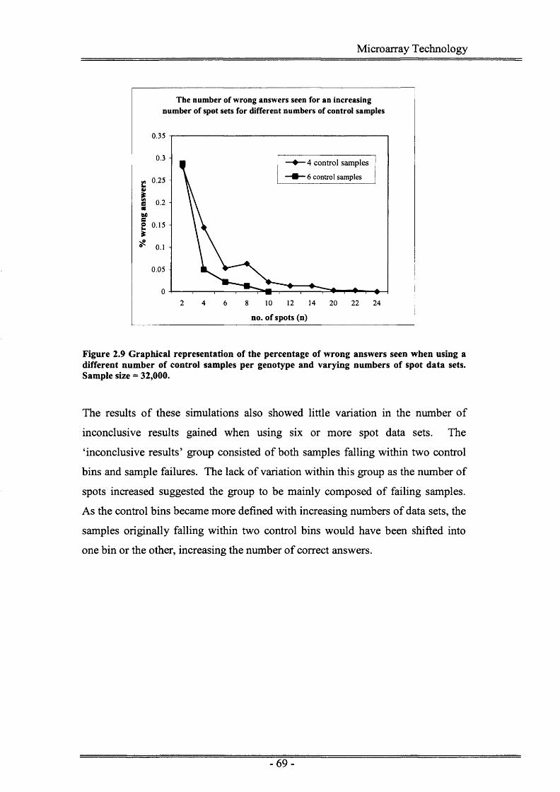
Microarray Technology

The number of wrong answers seen for an increasing number of spot sets for different numbers of control samples

0.35

4 control samples

6 control samplese 0.25 -4>it a te«OX)ses.*£

0.05 -

i ♦14 20 22 242 4 8 10 126

no. of spots (n)

Figure 2.9 Graphical representation of the percentage of wrong answers seen when using a different number of control samples per genotype and varying numbers of spot data sets. Sample size = 32,000.

The results of these simulations also showed little variation in the number of

inconclusive results gained when using six or more spot data sets. The

‘inconclusive results’ group consisted of both samples falling within two control

bins and sample failures. The lack of variation within this group as the number of

spots increased suggested the group to be mainly composed of failing samples.

As the control bins became more defined with increasing numbers of data sets, the

samples originally falling within two control bins would have been shifted into

one bin or the other, increasing the number of correct answers.

- 69-

Microarray Technology

2.5 How Representative Is The Data Set?

2.5.1 Same controls, different unknowns

A simulation was set up to test whether the parameters designed for one

experiment could be used to genotype samples from a different experiment. The

same control samples were used as those described in section 2.3 but a different

unknown sample data set was used, consisting of 16 samples plus one negative

control. Both sets of data were randomised, using 6 control samples per genotype

and 14 spots for both controls and unknown samples. 1000 simulations gave a

sample size of 17,000.

82% of samples were scored with the correct genotype, a further 18% gave an

inconclusive result and no wrong answers were seen with these parameters. The

increased percentage of inconclusive results seen suggested that the control bins

were not well enough defined for this different data set, causing an increased

number of samples to fall with two control bins or to fail completely. Also, the T

value may not have been high enough to guarantee all outliers to be taken out of

the data set, again increasing the number of inconclusive results.

This brief experiment highlighted the need to run control samples on each

separate microarray run. Variations in different experiments could occur during

PCR amplification, during microarray spotting, through slide quality, probe

hybridisation and operator differences. By using control samples on each run,

these variations would be translated into the control bins and samples could be

genotyped accordingly.

2.5.2 Using the same parameters for a different SNP - TSCQ D

A simulation was set up using the same control parameters on an entirely different

data set using a different SNP - TSCO D, to test the limitations of the ASGOTH

system. Only five control samples per genotype were available to create the

control bins for TSCO D and 14 spot data sets were used for both controls and

unknowns. All data were randomised using a random number generator, giving a

sample size of 16,000.

- 70-

Microarray Technology

The same parameters as in section 2.4, but with 15 control samples, generated the

following results when using TSCO D:

Correct results = 93.73%

Inconclusive results = 6.25%

Wrong answers = 0.02%

Only 2 out of 1000 simulations generated the three wrong answers seen with this

SNP. It is most likely the wrong answers were generated by outlier samples that

had managed to pass the negative threshold filter. The amount of fluorescence

seen for each individual SNP varied greatly due to the presence of primer-dimer

formations. Hybridisation probes could bind to the negative control spots if

primer-dimer was present, giving an enhanced fluorescence reading. This

emphasised the need to optimise the system for each separate SNP used on the

microarray system. Optimisation would involve the parameter testing used in

section 2.4 however, the ability to type almost 94% of samples without

optimisation showed the robustness of the ASGOTH automated system.

-71 -

Microarray Technology

2.6 Discussion

The use of microarrays in the research environment has increased significantly in

the last decade as arrays have become more miniaturised and biochemistry has

developed to enable millions of SNPs to be accurately genotyped with very high-

throughput and low error (Southern 1995; Schena 1996; Bowtell 1999; Brown and

Botstein 1999; Southern 2001; Heller 2002; Holloway et. al. 2002; Simon et. al.

2003). Analysis of microarray data uses the same methods as other fluorescent

detection systems, based on relative fluorescence data obtained from samples

compared to controls, however most of the specialised software, such as

ImageQuant™ and ArrayVision™ (Amersham Biosciences), was unsuitable for

automated genotyping of SNPs.

Due to the increased use of microarray technology within gene expression

research, a number of analysis programs were developed to cope with the massive

amounts of data obtained from gene expression experiments. Bowtell (1999)

reviewed the main microarray platforms and software available for data analysis,

with a further, updated, review carried out three years later (Bowtell 1999;

Holloway et. al. 2002). All software programs developed have focussed on

methods to improve the sensitivity and classification of samples in gene

expression experiments, highlighting a need for a simpler method of microarray

analysis that could be translated to the biallelic genotyping required for forensic

use. The main difference between the needs of the different systems being that

gene expression microarrays use pairwise comparisons to assess the amount of

gene expression present in a given gene against a housekeeping control gene; for

forensic purposes there was a requirement to compare a single allele in a biallelic

SNP locus to a single allele in a control sample.

Methods used for gene expression analysis of microarray data could be translated

into a format for use with the data derived from our low-throughput genotyping

work, for example; normalisation of data (Chen et. al. 2002; Park et. al. 2003;

Suzuki et. al. 2003; Munir et. al. 2004), use of reference samples and genotyping

based on fluorescence data (Schena 1996; Watson et. al. 1998; Granjeaud et. al.

1999; Syvanen 1999; Jain et. al. 2002).

- 72-

Microarray Technology

Normalisation of data is defined as “the process o f removing some sources o f

variation which affect the measured [gene expression levels] ” (Park et. al. 2003),

i.e. any fluorescent data collated from a microarray analysis is subject to variation

due to background levels of fluorescence, different affinities of the various dyes

used, differences in samples and differences in operators. Normalisation was

carried out prior to use with ASGOTH software by subtraction of background

fluorescence (Bkgrd) from total fluorescence (Cy-ARVOL-RFU) to give a

corrected fluorescence value (Cy-sARVOL), a calculation automatically

performed by Array Vision™ software. There have been a number of articles

reviewing the benefits and drawbacks of using such a calculation in gene

expression analyses as the subtraction of background fluorescence can vary due to

the algorithms used in different software programs (Brown et. a l 2001; Simon et.

al. 2003; Scharpf et. al. 2005). Background can arise from a number of sources,

including incomplete washing of the slide after hybridisation, features of the slide

that bind dye (such as the epoxysilane layer) and imprecision of the spot grid

during image acquisition (Schuchhardt et. al. 2000). Due to these factors it was

decided that for our purposes it would be better to err on the side of caution and

use background fluorescence subtractions rather than risk gaining false positive

results from inaccurate background readings. A second normalisation procedure -

converting data into log ratios - was performed on the data before importing into

ASGOTH.

Logio ratios were used to standardise the data obtained using our system, as

fluorescence for each allele was obtained from two separate slides spotted with

the same PCR products. Each of the two slides was investigated using a different

probe labelled with the same fluorophore, so hybridisation would only occur if the

sequence complementary to the probe sequence was present within the DNA

sample. Variations in slide quality and hybridisation affinities meant that it was

necessary to normalise the data to directly compare one allele to the other. By

carrying out a log transformation, the data obtained could be standardised across

the set, regardless of slide or hybridisation variability (Thygesen and Zwinderman

2004).

- 73-

Microarray Technology

Positive control samples were essential to provide a basis for defining control bins

by which to analyse data from unknown samples. In gene expression analysis,

housekeeping genes (for which expression levels are known) are used as

references and patterns of expression are compared to them (Schena 1996;

Bowtell 1999; Alizadeh et. al. 2000; Southern 2001; Holloway et. al. 2002; Jain

et. al. 2002; Suzuki et. al. 2003). Statistical analyses are carried out by

hierarchical clustering, using software written for gene expression profiling.

Clustering analysis was not applicable to the samples used in our study, as sample

sizes were small and information needed to be derived from a single sample for a

single SNP being interrogated, therefore a more precise method of analysis was

required. Negative controls, using sterile distilled water samples taken through

the whole microarray process, were used to assess the amount of fluorescence

seen in a sample without DNA. This fluorescence data (7) formed the basis of the

primary interrogation of data for each spot in the experiments.

The initial ASGOTH program was developed to assess how many microarray

features would be required per sample, for both controls and experimental

samples, in order to allow automated genotyping of samples with little operator

intervention. These guidelines could then be used as the basis for all microarray

experimentation, minimising errors and increasing the throughput of the system.

An error rate of up to 1% is seen in microarray technology used for gene

expression experiments, due to the ultra-high throughput of the system and the

less stringent guidelines in place for determining the level of gene expression

(Heil et. al. 2002; Huang et. al. 2004; Wenz et. al. 2005). For forensic purposes a

system needs to be close to 100% efficient, therefore the rules governing the

calling of alleles needs to be infallible. A method of achieving this was developed

by using populations of spots on a microarray, as opposed to single spots. This

allowed median analysis (±SD) to be used to create both control bins and medians

for unknown samples, and the two could then be further compared.

A lack of available data for further SNPs limited the amount of validation that

could be performed using the ASGOTH program. Nevertheless a comprehensive

framework was developed that could be used to evaluate any SNP system. Initial

studies suggested the use of Cy3 fluorescence in negative control spots could be

Microarray Technology

used to filter any ambiguous results resulting from experimental variations in slide

quality, spotting and probe hybridisation.

Random number generator simulations (Monte-Carlo simulations) were used to

test the limits of the ASGOTH system by imitating 1000 different experimental

results. Monte-Carlo simulations have been used in many different research areas

to generate datasets when only a minimal amount of data is initially present

(Triggs and Curran 1995; Chen et. al. 2002; Kimbrough 2004; Gill and Kirkham

2004b; Gill et. al. 2005b). This type of simulation randomly generates values for

uncertain variables over and over to simulate a model and, by defining the

characteristics required for the simulation, any number of experiments can be

performed using a sub-optimal size dataset. For use with the ASGOTH program,

simulations were performed to repeat the experimental outcomes without the need

for re-running the laboratory work, giving a dataset that could be easily

interpreted for validation purposes.

Control bins generated using median data and SD values allowed correct

genotyping of 27994 out of 32000 samples (over 87%) with an unknown

genotype, in an optimised system. No wrong answers were seen when using an

increased number of spots and samples to generate the control bins. Inconclusive

results consisted of samples which either fell into two control bins or which had

failed. Spots not passing the negative threshold, for reasons such as low PCR

amplification or poor spotting quality, would have caused failures. The program

was therefore shown to be 100% efficient in calling alleles, either with a genotype

or with an inconclusive / fail marker.

The ASGOTH system could be adapted for use with other platforms (e.g.

Luminex™, capillary electrophoresis) as well as other biochemical methods on

the microarray, such as reverse dot-blot whereby specific probes are spotted onto

the microarray slide and PCR products are added to the slide for hybridisation.

Further experimental work using SNPs on the microarray was ceased, due to the

inability to produce large multiplexes easily on such a platform. Future work

looked at developing the SNP multiplex for use on a capillary electrophoresis

- 75-

Microarray Technology

platform, where products could be separated by size, thereby minimising the

effects of primer-dimer formations.

Degradation Studies

Degradation Studies

3.1 Introduction

DNA damage, arising from enzymatic activity and errors encountered during

replication, is a relatively common event in metabolically active cells (Lindahl

1993). DNA repair mechanisms are in place that can reverse the vast majority of

changes made to the DNA molecule allowing little irreversible damage to the

cells. In inactive cells (i.e. dead or dormant cells), the mechanisms of DNA

damage persist but the repair mechanisms have been disabled, leading to DNA

degradation (Paabo 1989; Lindahl 1993; Hofreiter et. al. 2001; Willerslev and

Cooper 2005). Spontaneous hydrolysis and oxidation of DNA leads to single­

strand breaks, baseless sites (depurination), miscoding lesions and cross-links, all

of which decrease the chance of successfully amplifying the DNA molecules

(Lindahl 1993; Willerslev and Cooper 2005). The mechanisms of DNA

degradation are described in more detail in chapter 1.

The ancient DNA research community has carried out a great deal of work on the

degradation of DNA. As described by Willerslev & Cooper (2005), "the post­

mortem instability o f nucleic acids is central to the methodological problems

inherent to ancient DNA research ”, and the same can be said when analysing

degraded DNA for forensic purposes. The hydrolytic and oxidative damage seen

in ancient DNA samples has been shown to correlate with the temperature of the

recovery site as opposed to the age of the samples, “thus, while forensic samples

are much younger than ancient samples, these will presumably contain similar

types o f [DNA] damage” (Poinar 2003). Bar et. al. (1988) observed the post­

mortem stability of DNA in various human organs and tissues, using both direct

agarose gel analysis and RFLP analysis with minisatellite probe 33.15. The rate

of DNA fragmentation was found to be variable between the different sample

types, with total degradation of the high molecular weight fragments (15-23 kb)

appearing between five days and three weeks.

With the introduction of the PCR amplification method, a smaller quantity of

initial starting DNA template was needed for forensic analysis, as outlined in

chapter 1. The fragmentation of DNA following degradation reduces the

efficiency of the PCR reaction, in particular it is expected that “(i) PCR o f ancient

Degradation Studies

or degraded DNA should only amplify small fragments; (ii) the amount o f

amplified product should be small compared with similar reactions with (modern)

DNA ” (Golenberg et. al. 1996). Paabo (1989) used PCR techniques for analysis

of several ancient DNA samples ranging in age from four years to 13,000 years.

He found that amplification of a 121bp mitochondrial DNA sequence was

possible from aged samples but when the size of the DNA target was increased,

the amount of product generated rapidly diminished, with no amplification of

ancient DNA sequences longer than 140bp (Paabo 1989).

In the early 1990s, the introduction of STR systems for forensic DNA profiling

increased the success of gaining a result over the previous RFLP methods. The

STR systems amplified shorter target sequences (<500bp) so increased success

rates in fragmented samples (Kimpton et. al. 1994; Lygo et. al. 1994; Gill et. al.

1995b; Wiegand and Kleiber 2001; Tsukada et. al. 2002). As the sensitivity of

the DNA profiling techniques increased, it was observed that the higher molecular

weight STRs would fail to amplify when DNA was degraded or starting DNA

template was sub-optimal (Whitaker et. al. 1995; Gill et. al. 2000b; Whitaker et.

al. 2001; Butler et. al. 2003; Chung et. al. 2004). It was hypothesised that this

was primarily due to fragmentation of the DNA molecule, leaving only small

fragments of DNA that had been protected at the primary level of chromosome

packing, the nucleosome, as outlined in chapter 1.

Forensic DNA samples are subject to varying levels of both DNA degradation and

copy number. Amplification of sub-optimal amounts of DNA can result in partial

profiles, allele dropout, unbalanced loci and failure to generate any profile

(Whitaker et. al. 2001; Gill 2001b; Gill 2002). In the UK, low copy number

(LCN) DNA analysis may be carried out on samples containing sub-optimal

quantities of DNA (generally <100 ng template) to try and increase the likelihood

of gaining a reportable profile. The LCN technique uses SGM+ profiling 34 as

opposed to the standard 28 amplification cycles (Gill et. al. 2000b).

Some sample types, such as bone, teeth and hair shafts, naturally have little

nuclear DNA. For this reason, analysis of these sample types is generally carried

out using mitochondrial DNA (mtDNA) sequencing. MtDNA profiling is also

Degradation Studies

carried out when the sample is suspected to contain little or no DNA, due to the

circumstances surrounding the acquirement of the sample, e.g. the biological

sample may have come from a skeleton or a sample from a high temperature mass

disaster (Budowle et. al. 2005; Graham 2005). MtDNA analysis is routinely

carried out in the United States, as opposed to LCN STR analysis, as it is thought

to be less subject to issues surrounding LCN analysis, i.e. contamination through

secondary transfer (Lowe et. al. 2002), presence of mixtures, allele dropout and

allele drop-in, as well as the reliability of the DNA source

(http://www.ncjrs.gov/pdffilesl/nij/grants/203971.pdf). The main drawback of

mtDNA analysis is the linear inheritance of the DNA material through the

maternal line. This decreases the discrimination power of the test to

approximately 1 in 100, as it cannot distinguish between mothers, siblings and

further progeny. However, in cases where maternal relatives are the only source

of reference, an analysis of the mtDNA sequence can be advantageous

(http://www.forensic.gov.uk/forensic/foi/foi_docs/Mito.pdf; Crespillo et. al. 2000;

Just et. al. 2004).

The nucleosome unit was defined in the 1970s as eight histone molecules

interacting with approximately 200bp DNA (Komberg 1974). The nucleosome

units were attached to each other by lengths of linker DNA, forming a ‘beads on a

string’ effect. Further research used micrococcal nuclease digestion methods to

determine the exact length of the DNA interacting with the histone octamer. The

micrococcal nucleases preferentially targeted the unprotected linker DNA, leaving

146bp of DNA attached to the nucleosome core particle (van Holde et. al. 1975;

Noll and Komberg 1977). A further ten base pairs protmding from each end of

the nucleosome were shown to be more readily digestible than those protected

within the histone octamer, leaving approximately 125bp lengths of DNA

protected by the nucleosome structure (Read and Crane-Robinson 1985b).

To assess the DNA profiling techniques used in forensic laboratories it was

necessary to artificially degrade a set of samples that could be used for analysis of

fragmentation. A number of different methods have been proposed that degrade

DNA in situ, including the use of enzymes such as DNase I & II or micrococcal

nuclease (Wilcox and Smith 1976; Golenberg et. al. 1996; Wu et. al. 2000;

- 80-

Degradation Studies

Cousins et. al. 2004); boiling (Stroop and Schaefer 1989); subjecting DNA to UV

light or microwaves (Stroop and Schaefer 1989); storing samples for periods of

time at room temperature (Tsukada et. al. 2002; Butler et. al. 2003); and storing

samples in a humid environment (Dixon et. al. 2005a). Other studies on DNA

degradation have used samples from animal tissue post-mortem (Johnson and

Ferris 2002); ancient DNA samples (Paabo 1989; Burger et. al. 1999; von

Wurmb-Schwark et. al. 2003; Willerslev and Cooper 2005); and boiled bones

(von Wurmb-Schwark et. al. 2003).

A comparison study was set up, using DNA artificially degraded by two different

methods, to test the hypothesis that the nucleosome was protecting the small

fragments of DNA. One set of samples was degraded by boiling extracted DNA

in solution in a waterbath for a set time course of five hours. The DNA extraction

process would have removed all proteins, including the nucleosome, and enzymes

from the samples prior to boiling. The other set of samples was obtained from a

previous project whereby blood, semen and saliva samples had been deposited on

cotton squares and left in a humid environment at 37°C (to mimic the optimal

temperature for enzyme and bacterial activity) for a period of up to 243 days, with

samples being taken out and stored at -20°C at set periods. DNA was extracted

from the body fluid samples after degradation therefore enzymes and proteins

would still have been present in the samples during the degradation period. By

comparing these two degradation methods, the nucleosome degradation theory

and the pattern of DNA fragmentation could be assessed. Both sets of samples

were DNA profiled using SGM+ STR analysis and the SNP 27-plex method to a)

assess the size of the fragments surviving in the degraded samples and b) assess

the efficiency of the two techniques to amplify degraded DNA.

Initial studies suggested an increased amplification efficiency of samples when

smaller amplicons were used for DNA profiling. As a consequence of this work

the SNP 27-plex was redesigned to only include amplicons less than 186 bases in

length. This allowed fragment sizes of 146 base pairs and lower to be targeted,

incorporating an extra 20 bases at each end of the amplicon in the form of

universal tails. The number of loci that could be detected within the smaller size

range had to be reduced to twenty SNPs plus Amelogenin. This new 21-SNP

Degradation Studies

multiplex allowed products from 96 bases to 186 bases to be amplified and

detected in a single-tube reaction. Work was carried out to validate the technique

for casework situations and to assess the suitability of SNPs for use in

circumstances where limited DNA or DNA of poor quality was available.

Degradation Studies

3.2 Materials and Methods

3.2.1 Boiling DNA samples

S. 2.1.1 DNA extraction

DNA from five reference samples (CAS, DRJ, HER, SHM, ST) was extracted

from 1 mL of liquid blood using the Qiagen™ Genomic-Tip system (Cat no.

10223, 20/G tips) according to the manufacturer’s protocol to obtain between 5-15

ng/pL DNA suspended in 2 mL 1 x TE Buffer (ABD). Liquid blood had been

stored frozen at -20°C and was defrosted at 37°C in a shaking incubator, prior to

DNA extraction. Samples were quantified using a UV spectrophotometer

according to the manufacturer’s protocol (Ultrospec 3100 pro UV/Visible

spectrophotometer, Biochrom Ltd, UK).

3.2.1.2 Boiling o f DNA extract

1 mL of each stock DNA solution was aliquoted into Nunc™ tubes and placed in

a boiling waterbath. DNA extracts were boiled for 5 hours to provide 14 aliquots

per control sample, each 50 pL aliquot taken from the water-bath at different time

intervals (15m, 30m, 45m, lh, lhl5m, lh30m, lh45m, 2h, 2h30m, 3h, 3h30m, 4h,

5h). Aliquots were left to cool to room temperature before being stored in a

refrigerator at 4°C, ready for PCR amplification.

3.2.2 Artificially degraded body fluid samples

3.2.2.1 Preparation o f artificially degraded samples

Blood, saliva and semen samples had been previously degraded for other research

projects. Degradation was carried out by spotting the samples onto cotton squares

before placing in a pipette tip box partly filled with water. This ‘humidity box’

was stored in an incubator at 37°C (normal body temperature) for a period of

approximately 8 months (243 days). At specific time intervals, a number of

cotton squares for each sample were removed from the incubator and stored in the

freezer until the degradation period was complete for all samples. The water level

in the pipette box was kept filled to maintain humidity levels.

- 83-

Degradation Studies

3.2.2.2 DNA extraction o f artificially degraded samples

Degraded DNA from the cotton squares was extracted using the Qiagen™

QiaAmp Mini-Kit (Cat no. 51306). Samples had been stored frozen at -20°C and

were defrosted at room temperature prior to DNA extraction. The manufacturer’s

protocol for each sample type was used to obtain 0-2 ng/pL DNA, suspended in

150 pL 1 x TE Buffer (ABD). Samples were quantified using Picogreen

methodology (Ahn et. al. 1996) (Table 3.1).

Days in humidifier Picogreen quant (ng/|aL)0 0.60

42 0.06> 62 0.05OS 84 0.04

147 0.04243 0.03

0 2.2042 2.00

s62 1.70

<UCA 84 0.70147 0.50243 0.50

0 0.5042 0.50

-oo 62 0.40

s 84 0.30147 0.03243 0.02

Table 3.1 Picogreen DNA quantification values for artificially degraded saliva, semen and blood samples.

3.2.2.3 Dilution series o f control DNA samples

A dilution series of five control samples (CAS, DRJ, HER, SHM, ST) was set up

to give a series of DNA extracts with concentrations ranging from 1 ng/pL down

to 16 pg/pL. These dilution series were used for amplification of the 21-SNP

multiplex.

3.2.3 DNA amplification

The amount of DNA sample added to each PCR reaction varied depending on the

sample type and the length of degradation.

Boiled samples were diluted to 1 ng/pL using DNA quant values given for the

stock DNA solution of each control sample. Samples from time intervals between

0 minutes and 90 minutes were added to both the SNP 27-plex and SGM+

- 84-

Degradation Studies

multimixes in 1 jlxL volumes, as these were shown to over-amplify if higher

volumes of DNA were added (data not shown). Samples boiled for >90 minutes

were added at maximum volumes (14 jllL for SNP 27-plex; 20 pL for SGM+).

Artificially degraded sample DNA was added to the multimixes at a concentration

of 1 ng/pL, using data obtained from Picogreen quantification. Samples that had

DNA concentrations of <0.1 ng/pL were added at maximum volumes (14 pL for

the SNP 27-plex; 12 pL for the SNP 21-plex; 20 pL for SGM+).

For the dilution series experiments using the SNP 21-plex, DNA was added at 1

pL per PCR reaction.

3.2.3.1 SNP multiplex amplification

Both the SNP 27-plex and the SNP 21-plex were used for degradation

experiments. The amplification multimixes consisted of oligonucleotide primers

(synthesised by IBA, Germany) at varying concentrations, 0.4 pg bovine serum

albumin (Boehringer Manheim, Germany), 225 pM dNTPs (dATP, dCTP, dTTP,

dGTP; Boehringer Mannheim, Germany), 1 x PCR Buffer II containing 1.5mM

MgCl2 (Applied Biosystems™, UK) and 5 units Amplitaq Gold® (Applied

Biosystems, UK). Primer sequences and concentrations per reaction are outlined

in appendix III and IV.

Samples were amplified in strips of eight 0.2 mL tubes, without mineral oil, on a

thermal cycler (Applied Biosystems™ GeneAmp PCR system 9600) using the

conditions given in appendix V.

3.2.3.2 SGM+ amplification

SGM+ amplification kits (Cat. No. 4307133) were used, following the

manufacturer’s protocol. Samples were amplified in strips of eight 0.2 mL tubes,

without mineral oil, on a thermal cycler (Applied Biosystems™ GeneAmp PCR

system 9600) using the parameters given in appendix V for low copy number

conditions, i.e. 34 cycles amplification.

Degradation Studies

3.2.4 Capillary electrophoresis detection

1.1 pL of each PCR product (SNPs/SGM+) + 10 pL GS-HD400 ROX (Applied

Biosystems™ Part no. 402985):HI-DI Formamide (Applied Biosystems™) [ratio

1:37] was added to a 96-well micro-titre plate and heat-denatured at 95°C for 2

minutes before running on a capillary electrophoresis (CE) sequencer (AB model

3100) using ABI Collection software vl.l . SGM+ PCR products were run at a

single injection time of 22 seconds whilst SNP 27-plex products were injected for

20 seconds. The SNP 21-plex was injected for 12 seconds.

3.2.5 Analysis of results

Sample data were analysed using ABI Prism™ Genescan Analysis v3.7.1 and

ABI Prism™ Genotyper software v3.7 NT. SGM+ data were interpreted using

STRIPE™ (in-house computer program) to gain likelihood ratios for each sample.

SNP data extracted from Genotyper™ (peak height, peak area, scan number, size

in bases) were transformed into *.csv format and analysed by Celestial™ (chapter

4) to give profile data and likelihood ratios. SGM+ data for each sample were

extracted from Genotyper™ (peak height, peak area, allele designation) and

tabulated.

- 86-

Degradation Studies

3.3 Results

For all three profiling techniques (SNPs and SGM+), over-amplification of loci

was seen with the less degraded samples, i.e. samples boiled for less than 30

minutes or kept for less than 42 days in the incubator. An excess of pull-up peaks

and split peaks made genotyping difficult, however full sequencing of each SNP

had been carried out previously for reference samples and the correct SGM+

profiles for all five individuals were known. Comparison of all results to these

control results verified the profiles that were obtained in these experiments.

The SNP 27-plex failed to give a full profile, even when using optimal amounts of

DNA (i.e. 1 ng). It is possible that degradation of the multiplex occurred whilst in

storage, as the aliquot volumes were small enough (10 pL) to allow freeze-

thawing when subjected to an increase in temperature for a matter of seconds.

The presence of 27 sets of three primers, plus Universal primers, would have

further decreased the efficiency of the multiplex.

For all analyses results were divided into full profiles, low molecular weight

(LMW) profiles and high molecular weight (HMW) profiles, to ascertain whether

there was a significant difference in the amplification efficiency of these loci. The

process of DNA fragmentation by nucleases indicates that linker DNA is targeted

first, leaving fragments of approximately 146 bases in length. During PCR

amplification using the SNP 27-plex, 20 base ‘Universal’ primers were added to

the 3’ and 5’ ends of each SNP locus, making each SNP amplicon 40 bases longer

than its original base pair sequence, i.e. a locus sequence of 120 bases would give

a product of 160 bases in length, therefore LMW SNPs were deemed to be loci

less than 186 bases in length, as opposed to less than 146bp.

The 21-SNP multiplex was designed as a consequence of the initial boiling and

degradation experiments. A comparison of the 21-SNP multiplex is given for the

artificially degraded samples.

-87-

Degradation Studies

3.3.1 Boiled DNA samples (SNP 27-plex vs. SGM+1

Amplification of boiled DNA samples was performed using 1 pL dilutions for the

first seven samples (reference samples - 90 minutes boiling); followed by

maximum volumes for the remaining samples (105 minutes - 300 minutes).

These volumes were determined from previous results obtained that showed over­

amplification of samples boiled for 90 minutes or less when using increased

amounts of DNA. Using 1 pL of these DNA dilutions was sufficient to produce a

full profile. Evaporation of some samples during the boiling process meant that

there was insufficient volume of extract left to assess degradation after 5 hours.

In these instances, any remaining extract was amplified using the SNP 27-plex

instead of SGM+.

SNP profiles were generated by Celestial™, using a set of interpretation rules for

the designation of each SNP, based on a 20-second injection time (Table 3.2 &

Table 3.3). The SNP profiles demonstrated allele dropout in the HMW loci over

190 bases in length at earlier time intervals to the LMW loci.

The SGM+ profiles, generated using Genotyper™ software showed the same

pattern of high molecular weight dropout as the SNP 27-plex (Table 3.4 & Table

3.5).

- 8 8 -

Degradation Studies

SNP (size in bp) Amelo D B6 N4 Y3 A4 0 6 Z2 K3 J2 1 Y6 J8 | X p G L2 W3 H8 L6 ! K4 X7 1 U6 W5 U5 | V4 P7 PS

FileName Time boiled (m)

(97) (103) (109) (113) (117) (124) (129) |(133) (137) (141)1(146) (153)|(157) (164) (171) (174) (180) (186) (190)|(195)|(200)|(204)|(212)|(215)|(221) (226)|(231)

CAS REF 0 X T/C A/T A/T G C/G A T G/C c [ A 1 A 1 C/A C T C c T A/ 1 1 G/C A A/T F/A ! A/T A/T T T/F

CAS 1 15 X T/C A/T A/T G C/G A T G/C c A A |C/A c T C c T A/T G/C A/F F/T F/A | a/T 1 A/T [ T T/F

CAS 2 30 X T/C A/T A/T G C/G A T G/C C A : A ,C/A c T C c T A/T G/C A/F F/T F/A , A/T A/T F T T /F

CAS 3 45 X T/C A/T A/T G C/G A T G/C C A A C/A c T C c T A/T G/C A/F F/T F/A ; A/T A/T I t T/F

CAS 4 60 X T/C- A/T A/T G C/G A T G/C c A A jC/A c T C c r A/T C/c A/F ■F/T F/A | A/T A/T T T /F

CAS 5 75 X T/C A/T A/T G C/G A T G/C c A a ; g A c T c c T A/T C/C A/F f / T F/A

f/ a

[ A/T A/T

A/T A/T T

T/F

T/FCAS 6 90 X T/C I A/T A/T G C/G A T G/C c A | A ,C/A c T c c T A/T G/C A/F |_F/T

CAS 7 105 X T/C A/T A/T G C/G A T G/C c A A M a . c T c c T F/T G/C F/T F/A A/F | F/T T , T/F

CAS 8 120 X T/C A/T A/T G C/G A T G/C c A A , QA |1 c T c c : F/T G/C F/T 1 F/A t / f , t / f

CAS 9 150 X T/C A/T A/T G C/G A T G/C I A [ A | C/A T c _c| : F/T C/C [ F /T F/A T /F

CAS 10 180 X T/C A/T A/T G C/G A T G/C C/F A A F/A [ c T c c T F/A

CAS 11 210 X T/C A/T A/T G C/G A T G/C C/F A A j / A Lc| T J c c I T F/A

CAS 12 240 X T /r A/T A/T G C/G A T G/C C/F A a r 1 c 11 T~1 cl ' F/A

CAS 13 300 X T/C A/T 1 A/T G C/G--------

G/C C/F A 1 A 1 c 1 T

DR3_REF 0 X/Y T A/T | A/T G _cl A n C C/T T | C/A c T c g g l T T G A/T A/T T /F T T T/A j

DRJ_1 15 X/Y T A/T A/T G c Ai ic c C/T T F T Q A lLc T c g e l T T G A/T A/T T/F s T T/A T

DRJ_2 50 X/Y T A/T A/T G c A c c C/T f ] T , C/A ! C T c gc T T G A/T A/T T /F j; t T T/A T

DRJ_3 45—*—— X/Y T A/T A/T G c A 1 C ! c C/T; T

1 S

1- T c C/g | T T G A/T A/T T/F L t T T/A T

DRJ_4 60 X/Y T A/T A/T G c A c c C/T T 1 T T c /a ] c T c g G | : T G A/T A/T ; T / F T T T/A T /F

DRJ_5 75 X/Y T A/T A/T G j cl A cl c C/T; T T | C/A ! c T c g c ] : T G A/T. A/T, T/F IT T T/A , T/F

DRJ_6 90 X/Y IT A/T ;A/T G cl A c c C/T T Lc T c C/G T T G 1A£L A/T T/F T T T/A T /F

DR1 7 105 X/Y T A/T A/T G-- jc A __c c QT T T C/a | c T c g o t T G j F /T T /F T T/A IT /F

DRJ_8 120 X/Y T A/T A/T G c A1 c

c C/T T T C/A c T _ c C/G r T G I ML, T/F T T T/A T/F

DR]_9 150 x/ yJ T A/T J / I . f G------ 1c A i c c C/T T T g A c T c ggl T G F/T T/F m T T/F T /F

DRJ 10 180 x/ y | T A/T i A/T i G c A_J c 1 ? C/T T t g A c T _c g c , T C/F F/T F/T T

DRJ 11 210 T AH’ ! A/T G c A j c c C/T T T C/A c T c gel T T gp F/T F/T 1 F/T

DRJ_12 240 X/Y , T A/TJ A/T G C A c c C/T T I T I C/A 1 C 1 T c C/G i T F/T F/T

DRJ 13 300 X/Y 1 T A/T A/T-------

G1c I A c c

-- ‘C/T T I T ■ ■ i i T c c/ g ] T t 1

HER_REF 0 X T A/T A/T G C/G ! A/T c c C T/A A C/A A T c c T T HH A/T F/A T A F/A

HER_1 15 X T _A/T A/T G C/G , A/T c c C T/A I A I C/A A CT] c c T T G A/T F/A T hri A F/A

HER 2 30 X T A/T A/T G C/G I A/T c _ C 1 c T/A A _ g A . A T; c C1

1 T I ! g ! A/T F/A T T A F/A

HER_3 4 5 X T A/T A/T G I C/G [a/F c c 1 c M /a " A C/A A T c c —5— T T G I A/T F/A F/T . T J A F/A

HER 4 60 X T A/T A/T G I C/G_ A/T c c C/F T/A A . C/A A . T lc c T T ! G A/T F/A T T F/A F/A

HER_5 75 X T A/T A/T G C/G jA/T c c C/F t / A A J C/A A T Lc c T t J G A/T F/A F/T T I F/A F/A

HER 6 90 X T A/T A/T G C/G A/T c c S a | A C/A A T 1 C c T T r g A/T F/A F/T F/T J /A JHER 7 105 X T A/T A/T G C/G A/T c c Ft/ a A C/A A 1 T c c | T T \G~ A/T F/A T A T/A

HER_8 120 X T A/T A/T G I C/G A/T c c c T/A A C/A r r [ t c c T T j [ g _ ! A/T F/A T A ] T /A

HER^9 150 X T A/T A/T G 'C/G A/T c c c T/A A C/A A T c 1 c T T | g | A/T F/A T F/A T/A

HER_10 180 X "Tl"a/ t " A/T G C/G A/T c c c T/A A I C/A A T c \~c~ T 7 g/ f A/T F/A T F/A F/A

HER_11 210 x J . . I A/T A/T G C/G | A/T c c c T/A A C/A A | Tc c T T G/F F/T F/A T

HER_12 240— 5

X 1M i La/ t A/T G ; c/ g A/T c c c •T/A ! A [ C/A

— — A

r ■T ! c 1------- 1

c T T J G/F F /T . F/T

HER 13 300 X-------- 1

T I A/T A/T i G i C/G ATT c c c T/A A F/A A T/F 1c , c 1T F/T G/F

Table 3.2 SNP 27-plex profiles obtained for three reference control samples (CAS, DRJ, HER) using 1 pL of diluted DNA for the first seven time intervals followed by 14 pL for the remaining time intervals. Grey boxes represent alleles that are absent from the profile. SNP loci are shown in size (bp) order from the smallest amplicon (Amelo) to the largest (P5).

Degradation Studies

SNP (size ...... .

Anu-lc D B6 N4 Y3 A4 0 6 Z2 K3 J2 Y6 J8 X F G L21—

W3 H8 L6 K4 X7 U6 W5 1 U5 1 v 4 P7 P5

FileNameTime boiled

(m) (97) (103) (109) (U 3)|(117) (124) (129) (133) (137) (141) (146) (153) (157) (164) (171) (174) (180) (186) (190) (195)

I

(204) (212)|(215) |(221)i (226) (231)

SHM REF 0 X T/C A/T A/T G q c A C/T G/C C T/A A C q A T/C c c T A/T g c A/T T T/A A Lj l T/A TSHM 1 15 X T/C A/T A/T G q c A C/T q c C T/A A c C/A I /C C _C T ' : G/C A/T T T/A A T T/A T

SHM 2 30 X T/C A/T A/T G q G A q r G/C C T/A A c _qA_.T/C c c I A/T G/C. A/T T T/A A T T/A T

SHM 3 45 X T/C A/T A/T G q G A C/T q c C T/A A c C/A T/C c c T A/T G/C A/T T T/A A T T/A L e_SHM 4 60 X T/C A/T A/T G q c A C/T G/C C T/A A c q A T/C c c I A/T G/C A/T T T/A A . T T/A T/FSHM 5 75 X T/C A/T A/T G q c A C/T G/C C T/A A 1 c C/A T/C c c T A/T q d A/T T 1 T/A A T T/A T/FSHM 6 90 X T/C A/T A/T G qG A C/T G/C C T/A A c C/A T/C c c T ■ G/C .A/T T j T/A A T T/A T/FSHM_7 105 X T/C A/T A/T G qG A C/T q c . c T/A A c C/A T/C c c T A/T G/c| F/T T F/A A T T/A T/FSHM 8 120 X T/C A/T A/T G q c A C/T q c c T/A A c qA T/C c c 1 A/T g/ c ; T T/A A , T T/A t / f

SHM_9 150 X T/C A/T A/T G q c A q T G/C c T/A A C q A T/C c c T A/T G/C;52 T , f/ a A T T/FSHM 10 180 X T/C A/T A/T G qG A C/T G/C c T/A A qF .q A ,T/C c c i A/F !..qcjT T T F/A A T ISHM_11 210 X T/C A/T A/T] G qG A q r q c j c T/A A qF h / d C C T F/T q c T [ a J

SHM_12 240 X T/C A/T 1 G C/G, A/F ML G/F | c T/A A q F I F/C C/F C/F A/FSHM_13 300 X T/C A/T 1 G q G FF

qF \ C ~ T/A A T

ST REF 0 X T/C A/T A/T G/C c 1 A L c q c c T/A A | c/ a c T c G T T G A/T t / a A/T T

ST_1 15 X T/C A /L Ia/ t G/C c A c ,G/c c I /A A C/A c T c G ; l ~g | \NL T/A A/T T

s r _2 30 X T/C A/T [ a/ t G/C c ] ~ a ~1 cl G/C c [ T/A A C/A c T c T T G ,'A/T T/A A/T T t

sr_ 3 45 X T/C A/T |A /L G/C c A i [q c C J& A q A c T c G T T j EJ A/T T/A A/T T

ST_4 60 X J T/C .A/T .A/T .G/C c A c G/C C ' T/A [_A q A c T c G T T G A/T T/A A/T I .ST_5 75 X T/C A/T A/T G/C c A _ c q c c T/A A q A . C T c G T T G A/T T/A A/J j F/Ts r .6 90 X T/C A/T A/T G/C c A c .G/C c T/F A q A c T c 6 T T G A/T T/A A/FST_7 105 X T/C A/T,| a/ t G/C c f A c q c c t t a I A q A c T c

. . .G T T G A/J I/A A/T T/F

sr_8 120 X T/C A/T A/T G/C c | a c q c c t/a A q A c T c G T T g | A/T T/A I A/T, T /f

ST_9 150 X T/C A/T! A/T G/C....... 1c [ 1

A c G/C c T/Aj A q A C I T c G T 6 A/T T/A 1A/T T/FST_10 180 X T/C A/T A/T G/C c JLa.; c G/C c T/A , A 1 q A c T c G1 T T qF A/T ?1L, A/T T/F

ST_11 210 X T/C A/T A/T G/C c ] a c q c c T/A A q A c T c ; G TJ G/F F/T A/T

ST 12 240 X T/C A/T A/T G/C — Ic A c q c c T/A A q A c pr~ c l G JT F/T G/F A/T

ST 13 300 X T/C A/T V T T1 A c .G^cl----- -2L T/A A q A i T c g I T F/T

Table 3.3 SNP 27-plex profiles obtained for two reference control samples (SHM, ST) using 1 pL of diluted DNA for the first 7 time intervals followed by 14 pL for the remaining time intervals. Grey boxes represent alleles that are absent from the profile. SNP loci are shown in size (bp) order from the smallest amplicon (Amelo) to the largest (P5).

Degradation Studies

FileNameTime boiled

(m )Amelo D19 D3

r r —D8 VWA Thto d ;21 FG D 16 d :18 C•2

CAS_REF 0 X X 14 14 17 18 13 14 15 18 9 9 30 31 21 24 13 14 13 14 24 24

CAS_1 15 X X 14 14 17 18 13 14 15 18 9 9 30 31 21 24 13 14 13 14 24 24

CAS_2 30 X X 14 14 17 18 13 14 15 18 9 9 30 31 21 24 13 14 13 14 24 24

CAS_3 45 X X 14 14 17 18 13 14 15 18 9 9 30 31 21 24 13 14 13 14 24 24

CAS_4 60 X X 14 14 17 18 13 14 15 18 9 9 30 31 21 24 13 14 13 14 24 24

CAS_5 75 X X 14 14 17 18 13 14 15 18 9 9 30 31 21 24 13 14 13 14 24 24

CAS_6 90 X X 14 14 17 18 13 14 15 18 9 9 30 31 21 24 13 14 13 14 24 24

CAS_7 105 X X 14 14 17 18 13 14 15 18 9 9 30 31 21 24 13 14 13 14 24 24

CAS_8 120 X X 14 14 17 18 13 14 15 18 9 9 30 31 21 24 13 14 13 14 24 24

CAS_9 150 X X 14 14 17 18 13 14 15 18 9 9 30 31 21 24 13 14 13 14 24 24

CAS_10 180 X X 14 14 17 18 13 14 15 18 9 9 30 31 21 24 13 14 13 14 24 24

CAS_11 210 X X 14 14 17 18 13 14 15 18 9 9 30 31 21 24 13 13 14 24 24

CAS_12 240 X X 14 14 17 18 13 14 15 18 9 9 30 31 21 24 14 13 14

DRJ_REF 0 X Y 14 14 15 17 13 15 16 16 8 9 30 30 23 25 10 12 13 15 23 23

DRJ_1 15 X Y 14 14 15 17 13 15 16 16 8 9 30 30 23 25 10 12 13 15 23 23

DRJ_2 30 X Y 14 14 15 17 13 15 16 16 8 9 30 30 23 25 10 12 13 15 23 23

DRJ_3 45 X Y 14 14 15 17 13 15 16 16 8 9 30 30 23 25 10 12 13 15 23 23

DRJ_4 60 X Y 14 14 15 17 13 15 16 16 8 9 30 30 23 25 10 12 13 15 23 23

DRJ_5 75 X Y 14 14 15 17 13 15 16 16 8 9 30 30 23 25 10 12 13 15 23 23

DRJ_6 90 X Y 14 14 15 17 13 15 16 16 8 9 30 30 23 25 10 12 13 15 23 23

DRJ_7 105 X Y 14 14 15 17 13 15 16 16 8 9 30 30 23 25 10 12 13 15 23 23

DRJ_8 120 X Y 14 14 15 17 13 15 16 16 8 9 30 30 23 25 10 12 13 15 23 23

DRJ_9 150 X Y 14 14 15 17 13 15 16 16 8 9 30 30 23 25 10 12 13 15 23 23

DRJ_10 180 X Y 14 14 15 17 13 15 16 16 8 9 30 30 23 25 10 12 13 15

DRJ_11 240 X Y 14 14 15 17 13 15 16 16 8 9 30 30 23 25 12

HER_REF 0 X X 14 16 13 16 12 12 14 18 7 9 .3 30 31 22 23 9 12 17 19 23 24

HER_1 15 X X 14 16 13 16 12 12 14 18 7 9 .3 30 31 22 23 9 12 17 19 23 24

HER_2 30 X X 14 16 13 16 12 12 14 18 7 9 .3 30 31 22 23 9 12 17 19 23 24

HER_3 45 X X 14 16 13 16 12 12 14 18 7 9 .3 30 31 22 23 9 12 17 19 23 24

HER_4 60 X X 14 16 13 16 12 12 14 18 7 9 .3 30 31 22 23 9 12 17 19 23 24

HER_5 75 X X 14 16 13 16 12 12 14 18 7 9 .3 30 31 22 23 9 12 17 19 23 24

HER_6 90 X X 14 16 13 16 12 12 14 18 7 9 .3 30 31 22 23 9 12 17 19 23 24

HER_7 105 X X 14 16 13 16 12 12 14 18 7 9 .3 30 31 22 23 9 12 17 19 24

HER_8 120 X X 14 16 13 16 12 12 14 18 7 9 .3 30 31 22 23 9 12 17 19

HER_9 150 X X 14 16 13 16 12 12 14 18 7 9 .3 30 31 22 23 9 12 17 19

HER_10 180 X X 14 16 13 16 12 12 14 18 7 9 .3 30 31 22 23 9 12 17 19

HER_11 210 X X 14 16 13 16 12 12 14 18 7 9 .3 30 31 22 23 9'—

19

HER_12 240 X X 14 16 13 16 12 12 14 18 7 9 .3 30 31'

22 23 9

HER_13 300 X X 14 16 13 16 12 12 14 18 7 9 .3 30 31 22 9

Table 3.4 SGM+ profiles obtained for three reference control samples (CAS, DRJ, HER) using lpL of diluted DNA for the first 7 time intervals followed by 20pL for the remaining time intervals. Grey boxes represent alleles that are absent from the profile. STR loci are shown in size (bp) order from the smallest amplicon (Amelo) to the largest (D2).

Degradation Studies

FileNameTime boiled

(m)Amelo D19 D3 D8 W VA TPt o d ;21 FG 0 1 6 d ;18 D2

SHM_REF 0 X X 13 15 15 15 14 15 16 18 9 9 28 28 21 24 11 11 16 16 17 20

SHM_1 15 X X 13 15 15 15 14 15 16 18 9 9 28 28 21 24 11 11 16 16 17 20

SHM_2 30 X X 13 15 15 15 14 15 16 18 9 9 28 28 21 24 11 11 16 16 17 20

SHM_3 45 X X 13 15 15 15 14 15 16 18 9 9 28 28 21 24 11 11 16 16 17 20

SHM_4 60 X X 13 15 15 15 14 15 16 18 9 9 28 28 21 24 11 11 16 16 17 20

SHM_5 75 X X 13 15 15 15 14 15 16 18 9 9 28 28 21 24 11 11 16 16 17 20

SHM_6 90 X X 13 15 15 15 14 15 16 18 9 9 28 28 21 24 11 11 16 16 17 20

SHM_7 105 X X 13 15 15 15 14 15 16 18 9 9 28 28 21 24 11 11 16 16 17 20

SHM_8 120 X X 13 15 15 15 14 15 16 18 9 9 28 28 21 24 11 11 16 16 17 20

SHM_9 150 X X 13 15 15 15 14 15 16 18 9 9 28 28 21 24 11 11 16 16

SHM_10 180 X X 13 15 15 15 14 15 16 18 28 28 11 11 16 16

SHM_11 210 X X 13 15 15 15 14 15 18

SHM_12 240 X X 13 15 18

ST_REF 0 X X 13 13 15 17 12 13 17 18 6 9.3 30 31.2 19 22 12 14 12 20 24 25

ST_1 15 X X 13 13 15 17 12 13 17 18 6 9.3 30 31.2 19 22 12 14 12 20 24 25

ST_2 30 X X 13 13 15 17 12 13 17 18 6 9.3 30 31.2 19 22 12 14 12 20 24 25

ST_3 45 X X 13 13 15 17 12 13 17 18 6 9.3 30 31.2 19 22 12 14 12 20 24 25

ST_4 60 X X 13 13 15 17 12 13 17 18 6 9.3 30 31.2 19 22 12 14 12 20 24 25

ST_5 75 X X 13 13 15 17 12 13 17 18 6 9.3 30 31.2 19 22 12 14 12 20 24 25

ST_6 90 X X 13 13 15 17 12 13 17 18 6 9.3 30 31.2 19 22 12 14 12 20 24 25

ST_7 105 X X 13 13 15 17 12 13 17 18 6 9.3 30 31.2 19 22 12 14 12 20 24 25

ST_8 120 X X 13 13 15 17 12 13 17 18 6 9.3 30 31.2 19 22 12 14 12 20 24 25

ST_9 150 X X 13 13 15 17 12 13 17 18 6 9.3 30 31.2 19 22 12 14 12 24

ST_10 180 X X 13 13 15 17 12 13 17 18 6 9.3 30 31.2 19 22 12 14 12 20

ST_11 210 X X 13 13 15 17 12 13 17 18 6 9.3 30 31.2 19 22 12 14

ST_12 240 X X 13 13 15 17 12 13 17 18 6 9.3 30 31.2 19 12

ST_13 300 X X 13 13 15 17 12 13 17 18 6

Table 3.5 SGM+ profiles obtained for two reference control samples (SHM, ST) using lpL of diluted DNA for the first 7 time intervals followed by 20pL for the remaining time intervals. Grey boxes represent alleles that are absent from the profile. STR loci are shown in size (bp) order from the smallest amplicon (Amelo) to the largest (D2).

Degradation Studies

3.3.1.1 Analysis o f variance (ANOVA) calculations3

Percentage profiles for both SNPs and STRs were calculated from the numbers of

allele dropouts for each sample at each time interval (appendix VI) using the

equation:

\- x l O O (Equation 3-1)

V « J

Where a = the number of surviving alleles and n = total number of possible

alleles.

An ANOVA general linear model was performed on the percentage profile data

and results were tabulated (Table 3.6). An ANOVA allows simple analysis of

variance tests to be performed to test the hypothesis that means from two or more

samples are equal. By using a general linear model, more than one sample for

more than one group of data can be tested for variance by generating statistics for

each pairwise comparison.

The results indicated a significant difference between the percentage profiles

obtained for each sample, using both profiling techniques, compared to the

amount of time boiled (P<0.002) (Variant 1. Table 3.6). This suggested that the

DNA had been fragmented in solution causing varying percentage profiles to be

obtained. No significant differences were seen in the percentage profiles obtained

for different individuals for full SGM+ profiles (P=0.339), LMW SGM+ profiles

(P=0.096) or HMW SGM+ profiles (P=0.518), indicating no preferential

amplification of the low molecular weight loci (Variant 2. Table 3.6). There was

a significant difference between individual samples for full SNP profiles

(P=0.010) and HMW SNPs (P=0.001) but not for LMW SNPs (P=0.533) (Variant

2. Table 3.6), suggesting that DNA may have been less efficiently amplified in

some individuals.

A two-factor crossed ANOVA model compared different individuals to the time

boiled (Variant 3. Table 3.6) suggested no significant differences for the SNP 27-

plex and the LMW SNPs (P>0.060), indicating all samples performed with the

3 All statistical analyses were carried out using Minitab Release 14™ software

- 93-

Degradation Studies

same efficiency with these profiling techniques. There was a significant

difference between the different percentage profiles for each sample for the

different boiling times for HMW SNPs and all SGM+ profiling analyses

(P<0.017), suggesting a possible variation between different individuals as well as

between the different DNA profiling methods. This is discussed further in section

3.3.1.2.

Variantconsidered

Analysis of variance tests (ANOVA) R-sq % DF SS F P

SN P 2 7 -p le x 7 2 .2 9 1 3 8 2 5 .8 0 109 .98 < 0 .0 0 1

LM W S N P s 3 1 .5 5 1 16 4 .4 2 13.11 0 .0 0 1

1)H M W S N P s 8 0 .7 7 1 2 8 7 5 2 .7 0 177 .4 7 < 0 .0 0 1

Time boiledSG M + 6 0 .4 0 1 5 2 9 3 .3 2 4 9 .4 0 < 0 .0 0 1

L M W SG M + 5 3 .2 3 1 3 5 1 .1 2 11.00 0 .0 0 2

H M W SG M + 6 2 .4 2 1 18 9 4 7 .8 0 6 1 .2 0 < 0 .0 0 1

S N P 2 7 -p le x 7 2 .2 9 4 6 3 9 .5 9 3.71 0 .0 1 0

L M W S N P s 3 1 .5 5 4 3 2 .1 3 0 .8 0 0 .5 3 3

2)H M W S N P s 8 0 .7 7 4 5 7 4 2 .8 0 5.81 0 .0 0 1

Sample IDSG M + 6 0 .4 0 4 10 0 8 .6 0 1.16 0 .3 3 9

LM W SG M + 53 .2 3 4 6 1 1 .4 9 2 .0 8 0 .0 9 6

H M W SG M + 6 2 .4 2 4 2 2 1 0 .3 0 0 .8 2 0 .5 1 8

SN P 2 7 -p le x 7 2 .2 9 4 3 1 4 .7 3 2 .4 0 0 .0 6 0

L M W S N P s 3 1 .5 5 4 10 6 .9 0 2 .2 7 0 .0 7 3

3)Sample ID x Time boiled

H M W S N P s 80 .77 4 2 0 4 4 .6 0 3 .2 9 0.017

SG M + 6 0 .4 0 4 1 9 9 4 .6 6 5 .13 0 .0 0 1

L M W SG M + 5 3 .2 3 4 1254 .48 9.01 < 0 .0 0 1

H M W SG M + 6 2 .4 2 4 4 1 0 0 .1 0 3 .78 0.009

Table 3.6 ANOVA results (P values, R-Sq %, Sum of Squares (SS) and F statistics) calculated for the SNP 27-plex and SGM+ for boiled samples.

Degradation Studies

3.3.1.2 Chi-Squared analysis using contingency tables

Chi-squared tests were carried out on the percentage profile data (appendix VI) to

highlight any variation between techniques and between the different individuals.

Each technique was divided into full profiles, LMW loci only and HMW loci only

and all percentage profiles were compared. One out of the five control samples

(SHM) showed a significant difference in the percentage data obtained for the

SNP 27-plex compared to SGM+ (P=0.022) (Table 3.7 comparison 1). The SNP

27-plex gave an increased percentage profile, compared to SGM+, at longer

boiling times (78% SNP profile after 3h30m : 32% SGM+ profile; 48% SNP

profile after 4h : 23% SGM+ profile). All other samples showed no variation

between the efficiency of the two techniques.

The most significant differences were seen between LMW and HMW loci for

both SNPs and SGM+. All five individuals showed variation between results for

the LMW and HMW SNPs (Table 3.7 comparison 3) and three out of five

individuals showed variation between LMW and HMW SGM+ profiles (Table 3.7

comparison 5). This suggested an association between percentage profiles and the

size of the target DNA sequence. This is discussed further in section 3.3.1.3.

Two-way CAS DRJ HER SHM STGoodness o f Fit x2 Analysis

d f X 2 P d f X 2 P d f X2 P d f X2 P df X2 P

1SNP 27-

plex * SGM+

12 7.33 0.835 11 0.74 1.000 13 1.62 1.000 12 23.72 0.022 13 4.37 0.987

2

SNP 27- plex * LMW SNPs

12 7.21 0.844 11 2.75 0.994 13 3.68 0.994 12 4.74 0.966 13 2.57 0.999

3

LMW SNPs * HMW SNPs

12 158.34 <0.001 11 42.48 <0.001 13 67.41 <0.001 12 73.65 <0.001 13 66.64 <0.001

4SGM+ *

LMW SGM+

12 1.04 1.000 11 2.98 0.991 13 6.69 0.917 12 14.37 0.278 13 15.17 0.297

5

LMW SGM+ *

HMW SGM+

12 5.19 0.951 11 16.80 0.114 13 41.11 <0.001 12 112.07 <0.001 13 111.99 <0.001

6

LMW SNPs * LMW SGM+

12 0.55 1.000 11 0.00 1.000 13 0.35 1.000 12 11.29 0.504 13 0.22 1.000

Table 3.7 Chi-squared Goodness-of-Fit contingency table test results.

Degradation Studies

3.3.1.3 Allelic dropout compared to fragment length

The proportion o f allelic dropout seen at different amplicon sizes for SNPs and

SGM+ was calculated by amalgamating results for all individual samples,

disregarding the time boiled. These dropout proportions are shown graphically,

compared to the fragment size, in Figure 3.1.

Proportions o f allele dropout se en at d ifferent fragm ent lengths for both SGM+ and SNP 27-plex, using data from boiling experim ents

0.8

0.7

♦ SGM+ allele dropout

■ SNP allele dropout

* 0.6

8*0.5

0.4

0.3

02

0.1

0.00 20 40 60 80 DO 120 140 DO D0| 200 220 240 260 280 300 320 340 360

F ra g m e n t s ize

Figure 3.1 Scattergraph showing proportion of allelic dropout seen compared to fragment length size for both the SNP 27-plex and SGM+, obtained using data from boiling experiments.

The vertical line intersecting the graph at 186 bases indicates the visual boundary

between high and low molecular weight loci, as discussed in section 3.3. The

proportion o f dropout appears to increase above 186 bases in length for both SNPs

and SGM+ and there is a distinct difference between the LMW and HMW

‘populations’ (PO.OOl; df = 65; X2 = 297.9 (SGM+) and 471.7 (SNP 27-plex)).

Profiles obtained in these experiments showed typical signs o f HMW degradation,

using both SNPs and STRs, with over-amplification or better amplification o f the

LMW products less than 200bp in size.

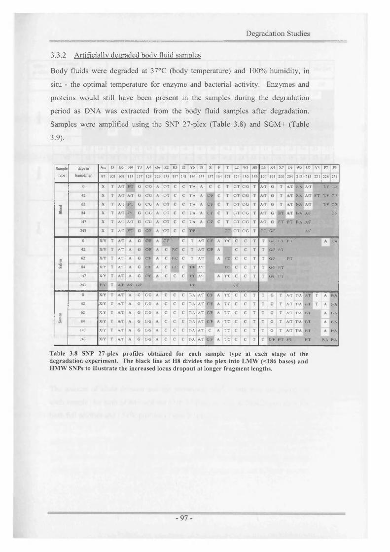
Degradation Studies

3.3.2 Artificially degraded body fluid samples

Body fluids were degraded at 37°C (body temperature) and 100% humidity, in

situ - the optimal temperature for enzyme and bacterial activity. Enzymes and

proteins would still have been present in the samples during the degradation

period as DNA was extracted from the body fluid samples after degradation.

Samples were amplified using the SNP 27-plex (Table 3.8) and SGM+ (Table

3.9).

N4 I Y3 A4 06 Y6Am B6 L2 W3 H8 K4 X7 ' U6 W5 US | V4Sample

type

days in

humidifier 103 109 113 117 124 129 133 137 141 146 153 157 164 171 174 180 186 190 195 200 204 212 215 221 226 231

C/G C/T T/A C/T C/G A/T A/T F/A A/T T/F T/F

C/G C/T T/A O F F/A F/T T/F T/F

C/GA/T F/T T/A C/F C/T i C/G A I A/T F/A T/F T/F

F/T C/G C/T C/FT/A o r C/G F/A A/F T/F

147 A/T A/T C/G T/A C/F C/T C/G AT F T F T F/A A/F

243 C/F GTA T FT T/F T/F C T C/G F T G/F A/F

C/F AT C/F T/C G/F F T FT F/A

AT C/F F/C G/F F T

A T OF F/C A T F/C G/F FT

X/Y A T OF F/C T/F A T T/F G/F FT

147 X/Y OF T/F AT T/C G/F F T

243 A/F A/F G/FF/Y T/F O F

G 'O G T/A AT C/F T/C A T T/A FT

A T G OG T/A A T O F T/C A T T/A F T F/A

X/Y OG T/A A T O F T/C A T T/A FT F/A

OG T/A AT O F T/C FT F/A

147 X/Y A T OG T/A AT T/C FT F/A

243 A T OG T/A AT O F T/C G/F F T FT F T F/A F/A

Table 3.8 SNP 27-plex profiles obtained for each sample type at each stage of the degradation experiment. The black line at H8 divides the plex into LMW (<186 bases) and HMW SNPs to illustrate the increased locus dropout at longer fragment lengths.

Degradation Studies

SGM+profiles

Size range ofST R

loci (bp)102-136 111 -140 124-170 155-207 163-202 185-240 212-353 229-270 262-346 291-345

Days in humidifier D19 D3 D8 VWA THOl D21 FGA D16 D18 D2

0 12 14 15 17 11 15 16 17 6 6 30 30.2 18 23 11 13 15 16 23 F

42 12 14 15 17 11 15 16 17 6 F

cO>

62 12 14 15 17 11 15 16 17 6 F73C/3 84 12 14 15 17 11 15 16 17 6 F

147 15 F 11 F

243

0 12 14 15 17 11 15 16 17 6 6 30 30.2 18 23 11 13 15 16 23 23

42 12 14 15 17 11 15 16 17 6 6 30 30.2 18 23 11 13 15 16 23 23

C 62 12 14 15 17 11 15 16 17 6 6 30 30.2 18 23 11 13 15 16 23 23CQ

CA 84 12 14 15 17 11 15 16 17 6 6 30 30.2 18 23 11 13 15 16 23 23

147 12 14 15 17 11 15 16 17 6 6 30 30.2 18 23 11 13 15 16 23 23

243 12 14 15 17 11 15 16 17 6 6 30 30.2 18 23 11 13 15 16 23 F

0 13 15 16 18 12 13 16 17 6 6 28 32.2 20 21 11 12 12 13 25 25

42 13 15 16 18 12 13 16 17 6 6 28 32.2 20 21 11 12 12 F 25 F

| 62 13 15 16 18 12 13 16 17 6 6 28 32.2 20 21 11 12 12 13 25 25

5 84 13 15 16 18 12 13 16 17 6 6 28 32.2 20 21 11 12 25 F

147 13 15 16 18 12 13 16 17 6 6 11 F

243 13 F F 18

Table 3.9 SGM+ profiles obtained for the artificially degraded samples for saliva, blood and semen. Grey boxes indicate alleles that have failed to amplify. Homozygous loci are designated with one allele or two dependent on the size of the peak present, i.e. the peak height must be >150rfu to be called as a true homozygote. Homozygous peaks falling below this have the second allele designated with an ‘F \

The different sample types showed varying levels o f allele dropout, suggesting a

variable degradation rate dependent on the sample. Saliva showed the highest

level o f degradation, with semen showing very little dropout, even after prolonged

periods in the incubator.

The amount o f allele dropout and the percentage profile data was calculated for

each sample, for both SGM+ and the SNP 27-plex, as well as likelihood ratios for

both full profiles and LMW profiles (Table 3.10).

Degradation Studies

days in humidifier (BLOOO)BLOOO - SNP 27-plex

No. of alleles % profile LR

BLOOO-LMWSNPs: <186BASES

No of ateles % profile LR No. of alleles

BLOOO

% profile

SOM*

LR

BLOOD-

No. of stales

SOM* <1 XBASES

% profile LR

0 48 89 23,200,000 36 1X 68,300 22 1X 16S,0X ,0X ,0X 10 100 113.X0

42 49 91 27,800,000 35 97 25,200 20 91 20,500,000,000 10 100 113,OX

62 47 87 16,700,000 34 94 51,300 22 1 X 165,OX,OX,OX 10 1X 113,OX

84 45 83 6,620,000 34 94 51,300 19 86 20,500,000,000 10 100 113,OX

147 44 81 6,190,000 34 94 25,200 13 59 17.6X .0X 10 1 X 113,OX

243 30 56 13,300 27 75 5,510 4 18 7 2 20 5

days in humidifier (SAUVA)SAUVA - SNP 27-plex

No. of alleles % profile LR

SAUVA - LMW SNPs <188 BASES

No of aleies % profile LR No . of alleles

SAUVA

% profile

-SOM*

LR

SAUVA

No. of aisles

SGM*<1 XBASES

% profile LR

0 39 72 65,200,000 31 86 877,OX 21 95 9,010,OX X 0 ,O X 10 100 X 7 .0 X

42 35 65 899,000 31 86 196,OX 11 SO 67.6X 9 X 67.6X

62 35 65 1,980,000 31 86 823,OX 12 55 125,OX 9 X 67.6X

64 32 59 40,200 26 78 8,770 11 SO 67.6X 9 X 67.6X

147 37 69 7,110,000 33 92 1550,0X 4 18 10 2 20 10

243 6 15 5 8 22 5 2 9 10 1

days In humidifier (SEMEN)SEMEN -SNP 27-plex

No. of alleles % profile LR

SEMBf-LMW SNPs: <186 BASES

No. of stales % profile LR No. of alleles

SEMEN

% profile

SOM*

LR

SEMEN -

No. of stales

SOM* <1X BASES

% profile LR

0 51 94 1,490,000,000 36 1 X 1,570,OX 22 1 X 9,010,OX,OX,OX 10 1 X X 7 .0 X

42 51 94 826,000,000 34 94 962,OX 22 100 9,010,OX,OX,OX 10 1 X 367, OX

62 49 91 97200,000 35 97 964,0X 22 100 9,010,OX,OX,OX 10 100 X 7 .0 X

84 48 89 27,700,000 35 97 964,0X 22 1X 9,010.0X .0X ,0X 10 1X 367.0X

147 47 87 20.1X.000 36 1X 1,570, OX 22 100 9,010,OX,OX,OX 10 100 X 7 .0 X

243 43 80 2,480,000 35 97 128, OX 21 95 9,010,OX,OX,OX 10 1 X 367, OX

Table 3.10 Percentage profiles and likelihood ratios (LRs) calculated for artificially degraded samples. The table includes results for full SNP 27-plex profiles (all 26 loci plus Amelogenin), 27-plex SNPs under 186 bases in length, full SGM+ profiles and STRs under 146 bases in length.

3.3.2.1 Semen samples

The semen samples showed very little degradation in these experiments and a full

SGM+ profile was obtained at all time points, except for one case of STR allele

dropout at 243 days (Table 3.9). The SNP 27-plex did not perform as well as

SGM+.

Within a sperm cell, DNA is associated with protamines and exists in a highly

condensed state, allowing it to be packaged into a very small volume (Ward and

Coffey 1991). This packaging makes it less susceptible to nuclear attack by

enzymes or bacteria, an evolutionary requirement originating from the function of

the mammalian sperm. In these instances, SGM+ can be used to obtain a full

profile with a higher discrimination power than that gained when using SNPs.

5.3.2.2 Blood samples

The SNP 27-plex gave higher percentage profiles for degraded blood samples

compared to SGM+, using both the full 27-plex results and LMW SNP results.

- 99-

Degradation Studies

SGM+ dropped from a 100% profile down to only 18%, whereas SNPs still gave

a 56% profile after the 8 month degradation period (Table 3.10).

The STR profiles showed a distinct degradation pattern for SGM+, with the high

molecular weight loci dropping out of the profile first (Table 3.9). The SNP

profile showed less dropout, although the peak heights for each allele decreased

significantly with time (data not shown). The presence of ‘split’ peaks in the SNP

profile after 8 months degradation was indicative of very low amounts of DNA

starting material, i.e. LCN DNA. Split peaks consisted of two peaks with only

one base pair difference in size, giving the impression of a ‘split’ peak. This

action occurs due to the activity of the Taq polymerase enzyme used during PCR,

preferentially adding an extra base to the PCR product. The presence of split

peaks indicated two populations of PCR products whereby some were the

expected size (n) and some had an extra base added (n+1). This should have been

eliminated by the 45 minute final extension of the PCR amplification, however

the phenomenon of split peaks in LCN DNA samples had been observed during

development of the SNP multiplex methodology (pers. comm. P. Gill).

3.3.2.3 Saliva samples

Saliva is well known to degrade rapidly once outside of the body, both under

room temperature conditions and within a humid environment. This is probably

due to the presence of large numbers of bacteria and digestive enzymes that break

down the proteins and cellular matter found in saliva (Benedek-Spat 1973a;

Benedek-Spat 1973b). The reference sample failed to give a full profile with

either SGM+ or the SNP 27-plex, suggesting that the DNA may have already been

fragmented before the experiment began.

The ability to obtain a profile from an individual’s saliva is dependent upon

factors such as food intake, smoking preferences, alcohol consumption and

caffeine intake. The amount of enzymes and bacteria present in saliva make the

DNA highly susceptible to degradation and this is variable within and between

individuals due to their lifestyles. For these reasons, some saliva samples may

- 100-

Degradation Studies

give full profiles using SNPs or SGM+ whereas others will always give sub-

optimal results.

3.3.2.4 Analysis o f allelic dropout fragment length

Table 3.8 & Table 3.9 illustrate the pattern of allele dropout seen for the

artificially degraded samples for SGM+ and the SNP 27-plex. The LMW SNPs

were described as those being less than 186 bases in length, highlighted by the

black line dividing H8 (fragment length 186 bases) and L6 (fragment length 190

bases). The size of the amplicon was compared to the proportion of allelic

dropout seen using both techniques (Figure 3.2).

Allele dropout vs amplicon size in artificially degraded samples

1.00

■ SNPs deg samples

♦ SGM+ deg samples

Linear (SNPs deg samples)

Linear (SGM+ deg samples)

0.90 -

0.80 -

s 0.70 -oe.£ 0.60 - R2 = 0.7589

0.50 ♦ ♦

0.40 -

fr. 0.30

0.20 -

0.10 -

0.00

amplicon size

Figure 3.2 Scattergraph indicating the number of alleles that fail to amplify using both SGM+ and the SNP 27-plex compared to the size of the allele fragment. This data is based on the allelic dropout seen in tables 3.8 & 3.9 for all three degraded sample types. The dotted line indicates the division between LMW SNPs and HMW SNPs.

A positive regression was observed between the number of alleles failing to

amplify and the size of the amplicon length (Figure 3.2). This suggested the

nucleosome may be protecting the DNA molecule from further degradation,

leaving only small fragments of DNA available for amplification, although it is

possible this linear pattern would be observed even if there was random

fragmentation of the DNA molecules. Bacterial and enzymatic activity brought

- 101 -

Degradation Studies

about by the 37°C temperature and optimal humidity would have sheared the

DNA to only 146 base pairs in length. The addition of universal primers to the

ends of each amplicon increased the locus size to 186 bases and anything above

this showed decreased amplification efficiency. The observations seen here were

used in the development of a 21-SNP multiplex and have been used as an

illustration of degradation patterns in low molecular weight DNA.

3.3.3 Comparison of likelihood ratios (LRs)

Likelihood ratios (LRs) were calculated for each DNA profiling technique for

each sample using STRipe™ for SGM+ and Celestial™ for SNPs (Table 3.10).

The SGM+ profiling method gave a higher LR than the SNP system on most

samples. SNPs were shown to be more discriminating for the most degraded

blood and saliva samples, when the percentage profile for SNPs was significantly

better than for SGM+ (Table 3.10).

The SGM+ system amplifies 10 STR loci to give a ‘DNA profile’ of an individual

(Cotton et. al. 2000). The STRs selected are highly polymorphic in nature and

vary significantly in the number of repeats between unrelated individuals. This

characteristic makes them highly discriminating, so that the likelihood ratio (LR)

of a full SGM+ profile is conservatively estimated at 1 in 1000 million for

randomly selected unrelated individuals. By contrast, the SNPs used in the

multiplex system are biallelic in nature, making them individually much less

discriminating. It was calculated that approximately 50 SNPs, with allelic

frequencies between 0.2 and 0.8, would be needed to give a comparable LR of

SGM+ (Gill 2001a). Using a population database of white Caucasian individuals

(200 unrelated individuals), an LR of approximately 1 in 500 million was

calculated for the SNP 27-plex. The LRs for both systems were highly variable

depending on the alleles present in the profiles obtained.

-102-

Degradation Studies

3.3.4 Dilution series experiments (21-SNP multiplex)

Initial studies suggested the SNP multiplex system could be improved by the use

o f SNPs less likely to fail amplification. This could be done by designing a new

multiplex using smaller amplicon sizes, altering the sizes o f some o f the primers

in the current multiplex or by the addition o f different loci. Further work was

carried out developing a SNP multiplex using these criteria. The 21-SNP

multiplex was designed with products less than 186 base pairs in length, to allow

amplification o f the small DNA fragments found in degraded samples.

The data generated from the dilution series experiments, using the 21-SNP

multiplex, were used to estimate the limit o f detection o f the system.

Electropherograms allowed profiles to be visualised before the data was run

through further analysis programs (Figure 3.3).

500pg

250pg

125pg

62pg

31pg

16pg

Figure 3.3 Electropherograms showing SNP profiles obtained for the dilution series of ST control DNA.

Full profiles were observed for all samples using 1 ng o f DNA template and six

out o f seven samples gave full profiles at 500 pg DNA template (Table 3.11),

although some homozygote peaks gave a peak height (rfu) less than the

homozygote threshold level set in Celestial™ and were subsequently labelled with

an ‘F’ designation (chapter 4). The control samples HER and ST showed full

BB m i . t m MO CW_ST2J».fs»/8TS

1200

aa 518 : 0M.ST3 J 7 .t*a t $73 «ig D M jsn jn .isB /m

mm Ml BN.ST4.M tM / ST4 □a MG : BM.ST4JM f n / ST4

□ 3 818: FM.ST5.11 .fn / STB 3 9 8 G FM_ST5.1I <m /ST»

Degradation Studies

profiles down to 250 pg starting DNA template and Cambio™ male and female

samples were correctly genotyped using 125 pg DNA template. All seven

samples gave partial DNA profiles down to the lowest template level o f 16 pg.

FileN am e Lane A m e b D U6 B6 N4 Y3 P5 A4 0 6 22 K3 J2 Y6 P7 J8 X F G L2 W 3 H8

CAS re fe re n c e A01 G G/B G/B G/B G/B G G G B G G B G B G B G G G B G G G G B

CAS 500pg A02 G/F G/B G/B G/B ■ H G G G B G G B G B G /F F B G G G B G G G G B

CAS 250pg A 03 G G fa G/B G/B G/F G G G B G G B G B G /F B G G G B G G G G B

CAS 125pg A 04 G/F G/B G G C/F G B G B G B G B F B G B G B G BCAS 62pg A 05 G/F G/B G G G B G B G B G B F B GB G B G BCAS 31pg A06 G /F G/F F B G B G B G B G B G BCAS 16pq A 07 G/F G/B G/F G B G B G B

DRJ re fe re n c e B01 G/B G G/B G/B G/B G G G G G B G B G G B B G B G G G gb B

DRJ 500pg B02 G/B G G/B G/B G/B G G G G G B G B G G B B G B G G G gb B

DRJ 250pg B03 G/B G/F G /F G/B G G G G G B F B G B G B B G B G G G G B B

DRJ 125pg B04 G/F G/B G G G/F G/F G B F B G B G B B F B G G B G B B

DRJ 62pg B05 G/B G/F G/B G G G/F G/F G /F B F B G B G B B G gb B

DRJ 31pg B06 G/F G/B G j G /F F B G B G B F B G BDRJ 16pq B07 G/F e g/b F B G B B G B

HER re fe re n c e C01 G G G/B G/B G/B G G B G B G B G B G G B B G G B G B G G G B

HER 500pg C02 G G G/B G/B G/B G G/B G B G B G B G G B B G G B G B G G G B

HER 250pg C03 G G G/B G/B G/B G G/B G B G B G B G G B B G G B G B G G G B

HER 125pg C04 G G/F G/B G/F G G/B G B G B G B G G B B G G B G B G G G BHER 62pg C05 G C £ G/F G/B G G B G B G/F G B G B G B F B G gb G B G G G B

HER 31pg C06 G /F G/B G/F G/F G/B G/F G/F G B G B F B G F B F B G G B

HER 16pq C07 G/F F/B G/F G B G B F B G G B B

SHM re fe re n c e D01 G G/B B G/B G/B G G G B G G B G B G G B G B G G G B G B G G B

SHM 500pg D02 G G/B F/B G/B G/F G G G B G G B G B G G B G B G G gb G B G G BSHM 250pg D03 G G/B G G F B G G B G B G B G B G G G B G B G BSHVl 125pg D04 G/F G/F G/B G G G B G G B G B G /F G B G B G G G B G G BSHM 62pg D05 G G/B G G F B G B G /F G /F G/F G/F G G G B G B G BSHM 31pg D06 G /F G/B G/F G G B G /F G B G B G B G BSHM 16pq D07 G/F 1 G/B G/F F B G B F B G B

ST re fe re n ce E01 G G/B G/B G/B G/B G/B G G G G G B G G B G G G B G G G B B

S T 500pg E02 G G/B G/B G/B G/B G/B G G G G G B G G B G G G B G G G B BS T 250pg E03 G G/F G/F G/B G/F G/B G G G G G B G G B G G G B G G G B BS T 125pg E04 G G/F G/B G/F G/B G G G G G B G G B G G gb G G G B BS T 62pg EOS G/F G/B G/B G G/F G G G B G B G B G G G B G B G G B B BS T 3 1 p g E06 G/F G/B G/F G | G G B G B G F B G B F BST Ib p q E07 G/F F/B G/F F B G B G B F B

C am bio M re fe re n c e F01 G/B G/B B G G G G/B G/B G G B G B G B G G G G G G B G B

C am bio M SOOpg F02 G/B G/B B G G G G B G B G G B G B G B G G G G G G B G BC am bio M 250pg F03 G/B G/B F/B G G/F G G B G B G G B G B G B F B G G G G G gb G BC a m b b M 125pg F04 G/B G/B F/B G G/F G G B G B G G B G B G B F B G G G G G g b G B

C a m b b M 62pg F05 G ^ G G/F G G/F G B G B F B G G G G F B G BC a m b b M 31pg F06 G /F 1 G G/F F B G B G B G G B G B G BC a m b b M 16pq F07 G/F G B G B G B G B F B G B

C am bio F re fe re n c e G01 G G G/B G/B G/B G G B G B G G B B G G G G B gb G G G G B BC a m b b F 500pg G02 G G G/B G/B G/B G G B G B G G B B G G G G B G B G G G G B BC a m b b F 250pg G03 G G G/B G/B G/B G G B G B G G B B G G G G B G B G G G G B BC a m b b F 125pg G04 G G G/B G/B G/F G G B G B G G B B G G G G B G B G G G B G B BC am b io F 62pg G05 G/F G/F G/B G/F G G B G/F G/F G B B G B G B G G B G B G G G B gb BC a m b b F 31pg G06 G/F G/F G/B B G B G B G G B F B G gb BC a m b b F 16pq G07 G/F G/B F B G B G B G B G B

Table 3.11 Genotypes generated for control samples using varying amounts of starting DNA template. The limit of detection appears to be sample dependent. SHM DNA could be fully genotyped down to 62.5pg DNA whereas Cambio™ Female control DNA showed dropout at 250pg.

A total o f seven individual DNA samples at seven different DNA starting

concentrations (n=49) were tested using the 21-SNP multiplex. From these results

it was demonstrated that all samples provided a full, and correct, SNP profile at an

optimal DNA amount o f 1 ng and partial DNA profiles were obtained at a

template level between 500 pg and 16 pg, lower levels were not tested. SGM+

Degradation Studies

amplification routinely gives a full profile above 100 pg starting DNA material

(Gill et. al. 1997; Cotton et. al. 2000; Gill 2002) and LCN SGM+ is used to

provide full or partial profiles at sub-optimal DNA concentrations <100 pg using

LCN amplification conditions (Gill et. al. 2000b).

3.3.5 Testing artificially degraded DNA samples

Artificially degraded blood, saliva and semen samples (section 3.3.2) were re­

amplified and analysed using the 21-SNP multiplex (Table 3.12).

Size of genome target (bp) 57 63 67 69 74 77 82 85 90 94 97 101 107 110 114 118 125 132 135 140 146

Days in humidifier Amelo D U6 B6 N4 Y3 P5 A4 06 22 K3 J2 Y6 P7 J8 X F G L2 W3 H8

Saliv

a

0 X/Y T A/T A T A G A C/G A C C c T/A T/A A/T c C/A T/C C C T42 X/Y T F T AT A G A OG A C C c T/A T/A A/T c C/A T/C C c T

62 X/Y T FT AT A G A C/G A C C c T/A T/A A/T c C/A T/C c c T

84 X/Y T A T A G A C/G A C F C c T/A T/A AT ( C/A T/C c c T147 X/Y T A T A/F G/F A C/G A c F/C c T/A T/A FT C/F C/A T/C c c T

243 F/Y T/F F/A A/F O F

Sem

en

0 X/Y T A T A T A G A C/G A c C c T/A T/A A T c C/A T/C c c T42 X/Y T A T A T A G A C/G A c c c T/A T/A A T c C/A T/C c c T

62 X/Y T A T A T A G A C/G A c c c T/A T/A A T c C/A T/C c c T84 X/Y T A T A T A G A C/G A c c c T/A T/A A T c C/A T/C c c T147 X/Y T AT AT A G A C/G A c c c T/A T/A AT c C/A T/C c c T

243 X/Y T AT AT A G A C/G A c c c T/A T/A A T c C/A T/C c c T

Bloo

d

0 x/x T A T A T T G T C/G A C T c c T/A T A c C T C T C/G T42 x/x T A T AT T G T C/G A C T £ c T/A T A c C T C T C/G T

62 x/x T A T A T T G T C/G A C T c c T/A T A c C T C T C/G T84 x/x T AT A T T G T C/G A C T c c T/A T A c C T C T C/G T147 x/x T A T A T T G T C/G A C T c c T/A T A c C T CT C/G T243 x/x T A T A T T G T C/G A C T c c T/A T A c C T CT C/G T

Table 3.12 SNP profiles obtained from artificially degraded DNA samples. Grey boxes indicate complete locus dropout. F designations indicate single peaks falling below the homozygous threshold (Ht). Heterozygous genotypes are standardised as green peak base / blue peak base.

The percentage profile data for each sample was calculated, based on the number

o f alleles present. This data was compared to the results for the SNP 27-plex and

the SGM+ results (Table 3.13).

The 21-SNP multiplex gave comparable results to SGM+ for the semen samples,

showing a full profile at all time points. This indicated the multimix may be more

optimised than the SNP 27-plex, which showed allele dropout at all time points,

including the reference sample. The likelihood ratio (LR) for the semen samples

was calculated to be 9 x 10'12 for SGM+ (i.e. it would be >9,000 million times

more likely that this profile belonged to the suspect as opposed to another

Degradation Studies

unrelated individual from the population), compared to 1.5 x 10'7 for the 21-SNP

multiplex. In these instances it was suggested that SGM+ should be used in

preference to SNPs, due to the higher match probabilities that can be gained. The

LR values for SNP profiles varied when the percentage profile remained the same,

due to different SNP loci being present in the resulting genotype, for example,

SNP 27-plex data for saliva 42 days and 62 days (Table 3.13).

Days in humidifierSNP 27-plex SGM+ 21-SNP multiplex

No. o f alleles % profile LR No. o f alleles % profile LR No. o f alleles % profile LR

Saliv

a

0 39 72 6.52E+07 21 95 9.01E+12 42 100 1.48E+07

42 35 65 8.99E+05 11 50 6.76E+04 42 100 1.48E+07

62 35 65 1.98E+06 12 55 1.25E+05 39 93 2.40E+06

84 32 59 4.02E+04 11 50 6.76E+04 38 90 1.04E+06

147 37 69 7 .1 1E+06 4 18 1.01E+01 36 85 4.62E+05

243 8 15 5.30 2 9 10 6 10 7.50

Sem

en

0 51 94 1.49E+09 22 100 9.01E+12 40 100 1.48E+07

42 51 94 8.26E+08 22 100 9.01 E+l 2 40 100 1.48E+07

62 49 91 9.72E+07 22 100 9.01E+12 40 100 1.48E+07

84 48 89 2.77E+07 22 100 9.01E+12 40 100 1.48E+07

147 47 87 2.01E+07 22 100 9.01E+12 40 100 1.48E+07

243 43 80 2.48E+06 21 95 4.60E +11 40 100 1.48E-K17

Blo

od

0 48 89 2.32E+07 22 100 1.65E+11 42 100 1.37E+06

42 49 91 2.78E+07 20 91 3.22E+09 42 100 1.37E+06

62 47 87 1.67E+07 22 100 1.65E+11 42 100 1.37E+06

84 45 83 6.62E+06 19 86 1.09E+09 42 100 1.37E+06

147 44 81 6.19E+06 13 59 1.76E+07 42 100 1.37E+06

243 30 56 1.33E+04 4 18 7.19 42 100 1.37E+06

Table 3.13 Percentage profile data and LR data for the SNP 27-plex, SGM+ 28 cycles and the 21-SNP multiplex. Data for the SNP 27-plex and SGM+ were obtained from earlier experiments on the artificially degraded samples (section 3.3.2).

The results for the artificially degraded saliva and blood samples were plotted on

scattergraphs (Figure 3.4). The 21-SNP multiplex performed better than both the

SNP 27-plex and SGM+ on these sample types. The artificially degraded blood

samples gave a full profile at all time points, whereas SGM+ dropped to only an

18% profile after 243 days and the SNP 27-plex gave a 56% profile. This

suggested that the smaller amplicon sizes used with the 21-SNP multiplex were

allowing amplification o f small fragments o f DNA left in the blood samples after

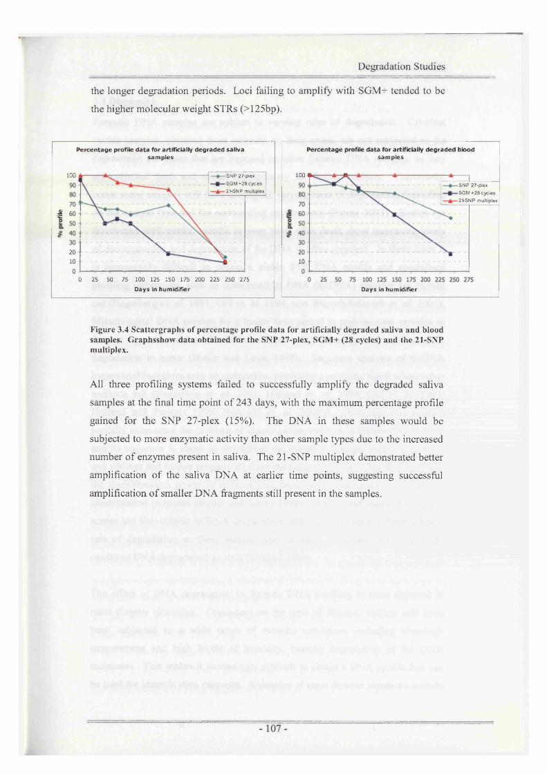
Degradation Studies

the longer degradation periods. Loci failing to amplify with SGM+ tended to be

the higher molecular weight STRs (>125bp).

Percentage profile da ta for artificially degraded saliva samples

Percentage profile data for artificially degraded blood samples

100100 ■ S N P 27-plex

•SG M +28 cycles • 21-SNP multiplex

■ SN P 27-plex

•SG M +28 cycles

•21-SNP multiplex

4■

#20 10 •

0 25 50 75 100 125 150 175 200 225 250 275Days in humidifier Days in humidifier

Figure 3.4 Scattergraphs of percentage profile data for artificially degraded saliva and blood samples. Graphsshow data obtained for the SNP 27-plex, SGM+ (28 cycles) and the 21-SNP multiplex.

All three profiling systems failed to successfully amplify the degraded saliva

samples at the final time point o f 243 days, with the maximum percentage profile

gained for the SNP 27-plex (15%). The DNA in these samples would be

subjected to more enzymatic activity than other sample types due to the increased

number o f enzymes present in saliva. The 21-SNP multiplex demonstrated better

amplification o f the saliva DNA at earlier time points, suggesting successful

amplification o f smaller DNA fragments still present in the samples.

Degradation Studies

3.4 Discussion

Forensic DNA samples are subject to varying rates of degradation. Criminal

justice samples, obtained from suspects on their arrest, are not subjected to the

degradation processes that are imposed on other forensic DNA samples, as they

are collected fresh and stored appropriately for further analysis. Conversely,

crime scene samples will have undergone varying rates of degradation dependent

on the sample type and the surrounding environment (Poinar 2003). Bodies not

discovered until weeks, months or even years after death show increasing levels

of decomposition and degradation of the DNA is often apparent. In these cases it

is increasingly difficult to obtain a viable STR DNA profile and specialised

profiling techniques, such as mitochondrial DNA (mtDNA) analysis are carried

out (Hagelberg et. al. 1991; Gill et. al. 1994; von Wurmb-Schwark et. al. 2003).

Mitochondrial DNA persists for a longer time period in post-mortem samples as

there is a greater number of mitochondria per cell, increasing the time it takes for

degradation to occur (Butler and Levin 1998). Sequence analysis of mtDNA

hypervariable regions may be undertaken, providing a profiling result where other

methods fail (Hagelberg et. al. 1991; Holland et. al. 1993; Gill et. al. 1994;

Holland and Parsons 1999; Budowle et. al. 2004a). Although this method

partially overcomes the problem of identification, mtDNA is maternally inherited

and its sequence is identical throughout the maternal lineage, meaning mothers

and siblings and further progeny all share the same sequence. This factor reduces

the discrimination power of mtDNA and decreases its usefulness as a tool for

identification purposes (Butler and Levin 1998). Body fluid stains from crime

scenes are also subject to DNA degradation, although they tend to have a lower

rate of degradation as these sample types quickly dehydrate and restrict the

oxidative DNA degradation process (Lindahl 1993).

The effect of DNA degradation in forensic DNA profiling is most apparent in

mass disaster situations. Dependent on the type of disaster, victims will have

been subjected to a wide range of extreme conditions including ultra-high

temperatures and high levels of humidity, causing degradation of the DNA

molecules. This makes it increasingly difficult to obtain a DNA profile that can

be used for identification purposes. Examples of mass disaster situations include

- 108-

Degradation Studies

fires (Clayton et. al. 1995a), air crashes (Ballantyne 1997; Olaisen et. a l 1997;

Leclair et. al. 2004), terrorist attacks (OrchidBiosciences 2002; Cash et. al. 2003;

Holland et. al. 2003), tsunamis and earthquakes (Alonso et. al. 2005; Morgan and

de Ville de Goyet 2005). In some of these cases, DNA profiling has proved the

most effective method of body identification due to lack of any other forensic

evidence (Clayton et. al. 1995a; OrchidBiosciences 2002; Leclair et. al. 2004).

Other cases have relied more heavily on traditional methods of identification;

victims of the Asian tsunami in December 2004 were identified predominantly by

dental records and fingerprints with only 1% of the bodies being identified by

DNA profiling (http://www.newscientist.com/channel/opinion/mgl 8725163.900).

DNA degradation begins with apoptosis (programmed cell death) and necrosis in

post-mortem samples (Johnson and Ferris 2002). After this activity by enzymes

such as micrococcal nuclease, DNase I and DNase II causes DNA fragmentation

through single-stranded breaks and depurination of bases (Bar et. al. 1988;

Lindahl 1993; Willerslev and Cooper 2005). As a consequence of this, current

methods of DNA profiling using STR analysis may only provide a partial DNA

profile resulting in a lower discriminating power than would otherwise be

obtained (Whitaker et. al. 1995; Wiegand and Kleiber 2001; Tsukada et. al. 2002;

Chung et. al. 2004). By defining the process of DNA degradation, new DNA

profiling methods could be developed that take factors such as fragmentation into

account, increasing the chance of amplifying the limited amount of DNA

available.

In order to assess the ability of DNA profiling methods to amplify degraded DNA

in the laboratory, artificially degraded DNA is required. By artificially degrading

DNA using a robust method, sets of samples can be produced that are both

quantitative and reproducible. A number of different methods have been used to

artificially degrade DNA. Enzymes such as DNase I & II are routinely used to

provide DNA in solution with varying fragment sizes (Wilcox and Smith 1976;

Szopa and Rose 1986; Golenberg et. al. 1996; Wu et. al. 2000). DNase I favours

purine-pyrimidine sequences (Staynov 2000) and DNase II is an enzyme found in

lysozymes associated with cell apoptosis (Yasuda et. al. 1998). Although

providing a range of DNA fragments in solution, this method of degrading DNA

- 109-

Degradation Studies

is not consistent with the degradation occurring in situ and so cannot be used as a

direct comparison of the DNA found in such conditions. This is also true for

boiled DNA samples, used in this study as a method of fragmenting DNA

irrespective of the protection of the nucleosome. Some studies have used actual

post-mortem samples in their work, such as animal tissue taken from a newly

slaughtered animal (Johnson and Ferris 2002), ancient DNA samples from a

variety of mummified or fossilised samples (Paabo 1989) or post-mortem human

samples (Akane et. al 1993). Forensically directed research studies have used

body fluid stains kept at room temperature for a number of years (Tsukada et. al

2002; Butler et. al 2003). Although viable for a small number of the forensic

samples submitted for forensic DNA profiling, these stains are limited in the

amount of degradation present as DNA has been shown to persist for many years

in a dessicated form (Lindahl 1993; Willerslev and Cooper 2005). By introducing

stains to a humid environment, the hydrolytic and oxidative processes of

degradation are permitted to continue for prolonged periods of time (Lindahl

1993). For this study, artificially degraded samples were obtained from previous

project work. Blood, semen and saliva samples had been spotted onto cotton

squares and left in a humid environment at 37°C for a period of eight months.

Boiling DNA extracts allowed the DNA strands to be rapidly fragmented for use

in this study. The DNA was extracted from cells prior to boiling, leaving it

without nucleosome protection. The results showed the DNA became fragmented

with increased periods of boiling, leaving the lower molecular weight amplicons

relatively more amenable to amplification. The artificially degraded DNA

samples showed a similar pattern of DNA fragmentation, with low molecular

weight loci giving increased amplification efficiency after longer periods of

degradation. Both methods are suggestive of DNA fragmenting with increased

periods of degradation processes. The unprotected DNA in boiled samples would

have undergone random shearing of the DNA molecule, leaving smaller and

smaller lengths of DNA with time. Longer periods of boiling may have produced

DNA fragments too small to be amplified with even the lowest molecular weight

loci. The DNA in the artificially degraded samples may have been gradually

fragmented as linker DNA joining the nucleosomes to each other was cleaved,

leaving only the DNA fragments protected by each nucleosome. It is possible that

-110-

Degradation Studies

after a longer period of boiling DNA amplification would not have been

successful whereas the nucleosome would have continued to protect the DNA

associated with it, causing the amplification efficiency to reach a plateau.

The work carried out in this study suggested that SNPs could have a number of

advantages over STRs for degraded samples. Most sample types gave an

increased percentage profile with SNPs and, although the discrimination power

was lower than for STRs, this may be used as an adjunct to the SGM+ system.

The SNP multiplex system was envisaged as an identification tool predominantly

for use in circumstances where most DNA matter would be highly degraded, for

example in mass disasters. In these circumstances SGM+ profiling could fail

whereas SNPs may give a profile, even if only partial. Reference profiles of

victims could be obtained from personal effects, rendering the discrimination

power less relevant in these instances. The combination of a weak / partial SGM+

profile and a weak / partial SNP profile would also increase the discrimination

power over a weak SGM+ profile alone.

Profiling of artificially degraded samples appeared to show a relationship between

the size of the amplicon and the allele dropout seen. An increased fragment

length above 186 bases was associated with a lower likelihood of amplification in

samples that were artificially degraded. Protection of DNA by the nucleosome

may be responsible for the small fragment sizes seen although other factors, such

as the coiling of the DNA around the chromosome or the effects of secondary and

tertiary protein structure, may have be involved. Five out of the ten STR

amplicons used in SGM+ DNA profiling had lengths above 146 bases and these

readily dropped out of the DNA profile in degraded samples.

The dilution series experiments indicated the 21-SNP multiplex was capable of

amplifying DNA in low copy number conditions. A full SNP profile was

obtained from sub-optimal (<500 pg) DNA template levels, and partial SNP

profiles were seen at levels as low as 15 pg (the equivalent of approximately two

cells). At low template levels, SNP interpretation would be subject to the same

problems as STR profiling, i.e. there would be more chance of contamination

being seen, stochastic variation could give heterozygous imbalance, allele dropout

- I l l -

Degradation Studies

and preferentially amplification of loci. Interpretation criteria needed to be set for

the 21-SNP multiplex, as outlined in chapter 4, using the dilution series data as a

basis for low copy number genotypes.

The 21-SNP multiplex was designed to target smaller DNA fragments thought to

be present when DNA becomes fragmented. The primary structure of

nucleosomes confers protection onto 146 base pairs of the DNA strand, with the

linker DNA joining two nucleosomes together being targeted for fragmentation

first (Read et. al. 1985a; Read and Crane-Robinson 1985b). The results of the

degradation experiments suggested that the 21-SNP multiplex was capable of

amplification when traditional DNA profiling methods failed. Low copy number

(LCN) SGM+ genotyping was not assessed as part of this study due to insufficient

amounts of sample extract. In order to interpret LCN SGM+ profiles, two

duplicate amplifications need to be performed and a consensus profile generated

from the resulting genotypes (Gill 2001b). As part of the validation of the 21-

SNP multiplex, casework samples profiled using LCN SGM+ were re-amplified

and profiled for SNPs (chapter 7). In the artificially degraded samples analysed in

this study, semen was shown to resist DNA degradation in situ probably as a

result of the tight packaging of the DNA molecule within the sperm head. In

these instances an increased LR could be gained by using SGM+ profiling, as

STRs collectively give higher discrimination between non-related individuals

within a population. Saliva and blood samples showed varying degrees of DNA

degradation, with the 21-SNP multiplex more likely to successfully amplify after

longer periods of degradation in both sample types.

4 The 21-SNP Multiplex Interpretation Criteria

Interpretation Criteria

4.1 Introduction

The increased use of DNA profiling in forensic casework led to a greater need for

automated programs capable of accurately genotyping DNA samples that had

been processed using STR DNA profiling systems (Perlin et. al. 1994; Perlin

2001). The SGM+ STR profiling system currently used in forensic casework in

the UK is an optimised system that is both quantitative and well balanced within

and between loci, allowing algorithms to be developed that can be used to

automatically genotype profiles (Cotton et. al. 2000; Perlin 2001). Several STR

automated genotyping systems for forensic use currently exist, and are used for

different aspects of DNA profiling.

STRess™ (STR expert system suite), developed by The Forensic Science

Service® in 1998 (Werrett et. al. 1998), was a program that "accepts raw data

[from Genotyper™ software], generates a file o f allele designations and then

compares this file to one generated by a human operator”. At that time, DNA

profiles analysed for the National DNA Database® were independently analysed

by two separate operators before being compared by a third individual, to

eliminate the possibility of operator differences. This analysis stage caused a

bottleneck to the entire DNA profiling process and therefore automation was

necessary. The optimised SGM+ system is a quantitative system and this allowed

rule sets to be developed that could assess STR peak height and area data and

accurately genotype them. For example, alleles had to be above a defined peak

height to distinguish them from baseline noise and peak area ratios were

calculated to assess the presence of a mixture (Werrett et. al. 1998).

The STRess™ program was complemented with an additional automated

genotyping system known as TrueAllele™ (Perlin 2001). TrueAllele™ allowed

peak data to be analysed and assessed for stutters, artefact peaks and preferential

amplification, before generating genotype data for inputted samples. Both of

these programs were developed to enable high throughput analysis of DNA

profiles used for the National DNA Database® and as a consequence of this,

neither were capable of analysing the more complex DNA mixtures or low copy

number (LCN) profiles that required expert interpretation.

- 114-

Interpretation Criteria

A recently developed program, LoComatioN, is “a hypothesis driven expert

system that enables LRs [likelihood ratios] for any number o f different LCN

scenarios to be evaluated” (Gill et. al 2005c). It remains necessary to manually

genotype the data, but interpretation of resulting profiles is carried out using a set

of algorithms allowing factors such as contamination and allele dropout to be

included in the likelihood ratio calculation.

For SNP genotyping it was necessary to produce a system similar to those

developed for STR DNA profiling. SNP genotyping programs for technologies

such as microarrays and primer extension assays have been developed (chapter 2)

but no program existed to analyse the data format generated by the SNP multiplex

technique developed using the universal reporter primer assay (Hussain et. al.

2003; Dixon et. al. 2005a). A computer program for analysis of SNP data was

developed to quantitatively analyse the peak data present, allowing accurate

genotyping of samples independent of operator variability.

-115-

Interpretation Criteria

4.2 Materials & Methods

4.2.1 Celestial™ automated analysis program

In order for the SNP multiplex to be successfully implemented into a casework

unit, the technique was tested against a number of set validation criteria. An

important part of the validation was the ability to confidently assign genotypes to

the sample data collected. This was carried out effectively by the use of an in-

house program Celestial™, written in Visual Basic, to enable genotyping of the

SNP 27-plex. The purpose of the validation was to define the interpretation

criteria required for correct genotyping of the 21-SNP multiplex.

The program utilised the following data exported from Genotyper™ for each SNP

locus for each sample: scan number, peak height (relative fluorescent units (rfu)),

peak area (rfu) and size in base pairs. Each SNP locus was identified by

Celestial™ according to its size in base pairs. The peak data were used to

genotype SNP loci as homozygous or heterozygous and a SNP profile was

generated for each sample analysed.

In forensic casework it is essential to keep error rates to a minimum. For this

reason, the rules set for Celestial were more conservative than would be found in

a non-caseworking environment.

4.2.2 Interpretation criteria

4.2.2.1 Heterozygote balance (Hb%)

In order to correctly interpret results from each SNP locus, three separate criteria

were characterised (Figure 4.1). Firstly, the relationship of peak heights of each

allele within a locus was established. This was given the term ‘heterozygous

balance’ or Hb% (section 4.3.2). Hb% was calculated from analysis of a dilution

series of control DNA samples (chapter 3) using the equation:

Hb(%) = xlOO (Equation 4-1)

[^S,=smallest peak height (rfu); $>largest peak height (rfu)]

-116-

Interpretation Criteria

Hb% for each SNP were calculated independently of each other as each SNP

locus behaved differently within the multimix.

4.2.2.2 Homozygous thresholds (Htmax)

The homozygote threshold (Htmax) of a SNP locus was defined as the maximum

peak height of either allele A or allele B (<jiA or (/>B) when only one allele is

present in a known heterozygous sample, plus 20% to allow for unobserved

extreme variation, i.e.

Ht*A=0= ^ + 0 . 2 ^ )

(Equation 4-2)

o r / / ^ - ° = ^ + 0 . 2 ( ^ )

This observation can be seen when low levels of DNA are present and stochastic

variation causes only one allele to be amplified. If a homozygous allele from an

experimental sample fell below Htmax, the locus was given an ‘F’ designation

indicating that allele dropout may have occurred and the locus might be

heterozygous. Allele dropout is occasionally seen with the 21-SNP multiplex in

samples with optimal DNA amounts (0.5-1 ng) due to the sensitivity of the system

preferentially amplifying alleles at some loci more than others.

4.2.2.3 Baseline threshold (Bt)

Lastly, the negative baseline (Bt) was set, according to observed allele drop-in

peaks in negative control samples, to minimise the chance of genotyping false

positives (section 4.3.4). Allele drop-in is a consequence of contaminant alleles

and occurs predominantly as a consequence of the high sensitivity of the

amplification method. Allele drop-in peaks are usually low level and can be

distinguished from true allele peaks by their size in comparison to the rest of the

profile.

- 117-

Interpretation Criteria

Ht„

Bt A(f>A <f>B

Figure 4.1 Diagrammatical representation of the interpretation criteria used in SNP analysis. Htmax indicates the homozygous threshold, below which single peaks are given an ‘F’ designation to indicate possible allele dropout. Bt denotes the baseline threshold used to minimise the possibility of drop-in peaks being labelled as allelic peaks. Hb% characterises the heterozygous balance of the peak height of allele A ($4) compared to the peak height of allele B (<f>B). In this example <fA is also the largest peak (<f>L) and 2? is the smallest peak (<AS).

4.2.3 Experimental procedures

To calculate interpretation rule sets, data were collected from the dilution series

experiments carried out in chapter 3.

Samples were amplified with the 21-SNP multiplex using varying amounts of

starting DNA template as follows; 0 pg, 16 pg, 32 pg, 62 pg, 125 pg, 250 pg, 500

pg, 1 ng, to give a range of data from optimal DNA starting template to LCN

amounts (sub-125 pg).

Amplified products were then analysed using the AB 3100CE sequencer with two

injection times of 12 and 20 seconds. Genotyper™ software was used to provide

data in the necessary format - peak height and peak area data, allele size (bp) and

genotype -for interpretation in Celestial™, in the form of *csv file.

Interpretation Criteria

4.3 Results

4.3.1 Celestial preliminary genotyping results

The preliminary rule sets for Celestial™ were relaxed to allow all data to be

designated without ambiguity within Celestial™, i.e. Hb% was set to a base level

threshold o f 5% for all SNP loci, all Htmax thresholds were set to lOOrfu and the Bt

was set to 50rfu, i.e. if Hb%>5% then the locus was recorded as a heterozygote,

only single peaks with //f<100rfu would be labelled with an ‘F’ designation and

only peaks <50rfu were ignored from the interpretation as they fell below the

baseline threshold. This allowed all data to appear without F designations and/or

questioned heterozygotes (Table 4.1).

Amelo 1 D 1 U6 | B6 | N4 | Y3 | P5 1 A4 1 06 1 Z2 1 K3 1 CAS reference G G/B G B G B G B G G GB G G/B GB

CAS 500pg G G B G/B G/B G G G/B G G/B G/BCAS 250pg G G/B G/B G/B G G G G/B G G/B G/BCAS 125pg G G/B I GCAS 62pg G . G / B j | , GCAS 31pg G G

G G/BDR: reference

DRJ 500pgG BG B

G GB G G B

G/BGB

GBGB

G G G G

G G G G G G

BB

G BG B

GG

G B B i G B B i

DRJ 250pg GB G G G B G G G G G B B G G B B iDRJ 125pg G H I G B G G G G G B B G G B BDRJ 62pg DRJ 31pg DRJ 16pq

GBGG

G G BGBGB

Cl u u uG G

BB

a u G

G B B G B

G B

G/B

HER reference HER 500pg HER 250pg HER 125pg HER 62pg HER 31pg HER ;

SHM reference SHM 500pg SHM 250pg SHM 125pg SHM 62pg SHM31pg SHM 16pq

ST reference ST 500pg ST 250pg ST 125pg ST 62pg ST 31pg

.ST “E9Cambio M reference

Cambio M 500pg Cambio M 250pg Cambio M 125pg Cambio M 62pg Cambio M 31pg Cambio M 16pq

G G/B G G/B G G/B

G/B B G/B B

■■■G

G/B G/B G/B G/B G/B G/B G B G G BG B G _B_

G B G B G G B G GG B { G G B G G B GBG B 1 G G GB G G B GBG B I G G B G B GG B G G G B GG B I G B

G/B G/B G/B G/B GyS G/B G/B Gy^ G/B G/B G/B G/B G/B G/B G G/B G G

______G G B G G B GB G G B G G B G B

G B GB G B GB G B G B G B G B G B G B B B

G/B GBG B GB

G G B G G G B G G G B G G G B G G G G

:

G B G G B G G B G G B G GB G

8

G B G B B G B G B B

G G B G B G G G B G B G G G B G B G G GB GB G G G

G

G B GB G B GB G B G B G B G B G B GB B G B

Cambio F reference Cambio F 500pg Cambio F 250pg Cambio F 125pg Cambio F 62pg Cambio F 31pg Cambic^l6|Dc^

G B G B G B G B G B G B G B G B G B G

G B B G B B G B B G B B G B B

i G B G G G G B Bi G B G 1 G B G

GG

G GB G G B

BB

1 G B G i G B G

GG

G G B G G B

BB

G G Bi .B

Table 4.1 Genotypes from a dilution series of each control sample. Celestial™ rule sets were set to allow all data to be captured within the program, without highlighting allele dropout or heterozygous imbalances. Results in BOLD type indicate heterozygotes / below threshold homozygotes.

- 119-

Interpretation Criteria

4.3.2 Heterozygous balance (Hb%)

Data for all individual samples were collated for Hb% for all SNPs at each PCR

template level. The data were tabulated and the lowest Hb% for each SNP at each

PCR template level was noted, regardless of the individual (Table 4.2). At

optimal DNA template levels (0.5-1.0ng) the lowest Hb% (Hb%min) exhibited was

with Y3, at approximately 25%, for both the 12 and 20 second injection times

from the same PCR amplification, i.e. the smaller peak was only 25% of the

height of the larger peak (Table 4.2 bold type). The most balanced heterozygous

SNPs at optimal PCR conditions were G and J2 at both the 12 and 20 second

injection times with Hb%min>68%, comparable to existing STR multiplex systems

(Gill et. al 1997) (Table 4.2 bold type).

12 second injection (</>S/<(L) x 100 (Hb%) 20 second injection (<tS/<fiL) x 100 (Hb%)SNPlocus

Sub125pg 125pg 250pg 500pg-

lngSub

125pg125pg 250pg 500pg-

lngAmelo # a 23.5 31.0 # # 25.9 35.7

D 25.0 39.2 48.0 47.8 # 41.3 55.2 49.7U6 # # 31.5 45.0 # # 36.0 39.4B6 # # 23.6 44.2 # # 23.6 45.1N4 # 11.2 37.5 40.3 # 13.0 34.7 41.6Y3 # # 68.4 25.1 # 63.4 67.3 24.4P5 34.3 # 55.1 54.1 32.3 # 34.6 47.8A4 # 24.8 41.3 41.6 # 23.1 36.8 39.606 16.2 50.0 57.8 40.2 15.6 52.3 61.1 41.3Z2 25.7 29.7 36.3 38.6 25.2 29.8 37.9 39.9K3 16.5 29.7 29.9 33.2 13.6 28.9 29.3 32.0J2 ti­ # 22.6 69.3 # # 24.2 68.4Y6 l l A # 50.2 35.1 30.0 # 51.2 35.9P7 # 15.4 24.8 32.0 # 14.6 22.1 27.7J8 # # 40.7 34.5 # # 40.9 58.7X # # 41.7 56.5 # # 39.8 62.0F 32.7 # 46.1 36.9 33.0 # 52.9 38.4G 31.6 # 69.5 67.5 35.0 # 69.3 71.5L2 # # 51.8 53.0 53.0 # # 53.6W3 # # 13.3 52.7 # 18.3 42.1 53.9H8 # # 61.1 79.7 # # 57.7 81.7

Table 4.2 Hb% collected from two runs of the AB 3100 instrument at 12 and 20 seconds. Heterozygote balance was exported from Celestial™ to Excel for collation and tabulation. # indicates loci with either allele dropout or total dropout, hence no heterozygous balance calculation.

As DNA template level decreased, Hb% decreased, indicating a larger imbalance

between the two peak heights. This was due to stochastic variation at low levels,

consistent with low copy number (LCN) SGM+ profiling. Using SGM+ an

optimal DNA template would give Hb% > 0.6 but at LCN levels the distribution

-120-

Interpretation Criteria

of Hb% can be almost random as a consequence of stochastic effects (Gill et. al

2000b; Gill 2001a). This was an unavoidable consequence of low copy number

DNA templates and special interpretation methods were therefore required for

SNPs, as the multiplex had been designed for LCN and degraded templates. The

most extreme Hb%mm were seen at 11.2% (12s) for N4 and 15.4% (12s) for P7 at

a DNA template level of 125pg, closely followed by 06 (15.6% (12s) and 16.2%

(20s)) and K3 (16.5% and 13.6% for 12s and 20s respectively) at the sub-125pg

PCR template level. The lowest Hb%min, irrespective of DNA template level, was

used for the rule sets in Celestial™ (appendix VII).

4.3.3 Homozygote thresholds (Htmn

Htmax for the known reference samples was estimated from the dilution series

experiments. Data were tabulated, disregarding individual samples, to show Htmax

for each SNP allele for each instrument injection parameter (Table 4.3).

12 second injection (H tmax) 20 second injection (Htmax)SNPlocus

Sub125pg 125pg 250pg 500-

lOOOpgSub

125pg 125pg 250pg 500-lOOOpg

Amelo 403 # # # 560 # # 527D 615 # # # 859 # # #

U6 311 198 141 249 559 464 211 520B6 328 207 # # 450 439 # #N4 422 # # # 613 412 # #Y3 155 # # # 213 # # #P5 424 # # # 617 # # #A4 486 # # # 746 274 # #06 152 # # # 615 # # #Z2 380 # # # 795 # 372 #K3 586 # # # 828 # # #J2 170 # # # # 449 # #Y6 454 # # # 526 # # #P7 191 # # # 274 # # #J8 160 # # 334 # 372 # 850X 390 191 # # 546 334 # 221F 717 # # # 1068 # # #G # # # # 478 # # #L2 230 # # # 329 # # #W3 # 242 # # # 534 # #H8 134 # # # # 377 # #

Table 4.3 Observed homozygote peak heights (rfu) where allele dropout has occurred (Htnax). Allele dropout was identified from known control sample heterozygotes and peaks heights for these collated within Excel. # indicates heterozygous loci giving no allele dropout.

- 121 -

Interpretation Criteria

At optimal DNA template amounts (0.5-1.0 ng), the maximum Htmax (i.e. the

maximum single peak height observed at a known heterozygous locus) was

observed for J8 at both the 12-second injection time (334rfu) and the 20-second

injection time (850rfu). At sub-125 pg template amounts the largest Htmax was

observed at locus F, at a height of 717rfu (12-sec) and 1068rfu (20-sec). This was

at a template level below 125 pg and no allele dropout was observed for this SNP

at the higher template concentrations.

Allele dropout was not observed at locus G at either optimal DNA amounts or the

sub-125 pg level, for a 12 second injection time. Consequently an approximate

theoretical dropout level for G was estimated from the observed Hb%mm and the

negative baseline (Bt) (section 4.3.4), using the equation:

Ht(theoretical) = ------------ r (Equation 4-3)0H b% ^ /100)

This equation allowed the theoretical maximum peak height (Htmax) to be

calculated based on the observed Hb% by comparing the minimum peak height of

the largest peak that would cause the smaller peak height to drop below Bt (Figure

4.2). For example, if Bt was set to lOOrfu, the smallest peak height would need to

be <lOOrfu to ‘drop out’ of the profile. If the Hb%mm was calculated to 50%, both

values could be substituted into the equation to give an estimated value for Ht

(Figure 4.2).

99rfu

Bt=100

Ht(theoretical)=? Ht(theoretical)=(100-1)/(50/l 00)

=.99/0.5

=198rfu

Figure 4.2 Example of the theoretical calculation for Ht based on the value of HbVomin and Bt. In this example Hb%min is set to 50% and Bt is lOOrfu.

To allow for unobserved extremes (potential outlier data), Htmax was adjusted

upwards by 20% within the Celestial™ rule set, in order to be conservative

(appendix VII). Again these guidelines were built upon principles already

- 122-

Interpretation Criteria

established for STRs (Gill et. al. 1997; Gill et. al. 2000b). With STRs, Htmax is set

to 150 rfu (peak height), signifying potential allele dropout across all multiplexed

loci, whereas the SNP multiplex used a different guideline per locus programmed

into Celestial™.

4.3.4 Negative control thresholds (Bt)

LCN is characterised by allele dropout and drop-in (laboratory contamination by

single alleles measured by reference to negative controls) (Gill et. al. 2000b). A

96-well microtitre plate was prepared for SNP amplification using water controls

as negatives instead of DNA samples. The plate was processed through the

system and any drop-in peaks were identified, for both a 12 second injection time

and a 20 second injection time (Table 4.4). For a 12 second injection time the

largest drop-in peak seen was at D (blue) at 81 rfu peak height. For 20 seconds,

the largest peak was 150rfu at G (green). The baseline level Bt was set according

to the greatest drop-in peak seen plus an arbitrary -25% to capture unobserved

outliers. Consequently the thresholds were set at lOOrfu and 200rfu for 12

seconds and 20 seconds respectively, and these were programmed into Celestial™

(appendix VII).

-123-

Interpretation Criteria

12 second injection (peak height rfu)

20 second injection (peak height rfu)

SNP locus Green peak Blue peak Green peak Blue peakAmelo 53(1) 76(1) 77(1)

D 58(1) 81(1) 118(6) 130 (3)U6B6 57(1) 73 (1)N4 92 (2) 56(1)Y3P5 91(1) 75(1)A4 51(1) 79 (2) 72 (2)06 56(1)Z2 133 (2)K3 52(1) 76(1)J2Y6 66(1)P7J8 60(1)XF 119(1)G 150 (2)L2 87 (2)W3H8 56(1)

Table 4.4 Peak height data for allele drop-in peaks seen on a 96-well negative (deionised water) control plate. Brackets indicate the number of peaks seen. Data is for both a 12 second and 20 second injection time.

- 124-

Interpretation Criteria

4.3.5 Analysis of dilution series data

Once the rule sets for heterozygous balance (Hb%), homozygote thresholds

(Htm(lx) and the negative baseline (Bt) had been calculated (as described in sections

4.3.2-4.3.4) and programmed into Celestial™, data from the dilution series

experiments were re-analysed to ensure all incidences of allele dropout were

highlighted by the program (Table 4.5).

FileName Lane Amelo D U6 B6 N4 Y3 P5 A4 0 6 22 K3 J2 Y6 P7 J8 X F G L2 W 3 H8

CAS re ference A01 G G/B G/B G/B G/B G G G/B G G/Br- jO

G/B G B G G/B G/F F/B G G/B G/F B G

G G/BG/BGjB

GGG

GGG

GGG

GGG

B□

CAS 500pg CAS 250pg

A02A03

G/FG

G/BG/B

G/B G/B G/B G/B G/F

1 GG

GG

G/3G/B

GG

Ca/bG/B

bG

DB

CAS 125pg A04 G/F G/B V G G 1 G/F G/B G/B G/F G/F F/B G/F G/F G/F

CAS 62pg A05 G/F G/B K G G | G/B G/B G/F G/F F/B G/F G/F G/F

CAS 31pg A06 G/F G/F F/B G/B G/FG/F

G/F G/F G/F

CAS 16pq A07 G/F G/B G/F G/B G B

DRJ re ference DRJ 500pg

B01B02

G/FG/F

GG

G/B G/B G/B G/B

G/BG/B

GG

GG

GG

G€

GG

BB

G/B G G/B G/B G G/B

BB

G ^lG/B

GG

GG

GG

G/BG/B

BB

DRJ 250pg DRJ 125pg DRJ 62pg

B03 G/B G/F G/F G/B j G G G G G B F/B G/F G/B B G/B G G G G/B B

B04 G/F G/B ' G G G/F G/F G B F/B G/F G/B B F/B G G/F G/F B

B05 G/B G/F G/B 1 G G G F G/F G/F B F/B G/F G/B B | G G/B B

DRJ 31pg B06 G/F G/B G J | G/F F/B G/F G/B F/B G/F

DRJ 16pq B07 G/F G/B F/B G/F B I G/F

HER reference HER 500pg

C01COS

GG

GG

G/B G/B G/B G/B

G/BG/B

GG

G/BG/B

G/BG/B

G/BG/B

GG

BB

G G/B B G G/B B

GG

G/BG/B

G/BG/B

GG

GG

GG

BB

HER 250pg HER 125pg HER 62pg

C03C04C05

GGG

G G/B G/B G/F G/B G/F G/F G/B

G/BG/F

G G

1 G

G/BG/BG/B

G/BG/BG/B

G/BG/BG/F

GGG

BBB

G G/B B G G/B B

G/F G/F F/B

GGG

G/BG/BG/B

G,BG/BGjB

GGG

GGG

GGG

BBB

HER 31pg C06 G/F G/B G/F G/F G/B G/F G/F G B G/F F/B G F/B F/B G G B

HER 16pq C07 G/F ■ ■ F * G/F G B G/F F/B G G/F B

SHM reference D01 G G/BG/B

B G/B F/B G/B

G/B G G G/B G G/B G/B G G/B G/B G G G/B G^J G G B

SHM 500pg D02 G G/F G G G/B G G/B G/B G G/B G/B G G G/B G/B G G B

SHM 250pg D03 G G/B 1 G G F/B G G/B G/B G/F G/B G G G/B G/F G B

SHM 125pg D04 G/F G/F G/B u G G G/B G G/B G/B G/F G/B G/B G G G/B G G B

SHM 62pg DOS G G/B £ G G F/B G/B G/F G/F G/F G/F _ G_ G G/B G/F G B

SHM 31pg D06 G/F G/B G/F G | G/B G/F G/F G/B G/B G/F

SHM 16pq ST re ference

D07E01

G/FG G/B

G/B G/B G/B G/B G/B G G G

G/F

G

F/BG/B

G/B

G G/B G G G/B G

F/BG G

G/FB B

ST 500pg ST 250pg

E02E03

GG

G/BG/F

G/B G/B G/F G/B

G/BG/F

G/BG/B

GG

GG

GG

GG

G/BG/B

G G/B G G G/B G

GG

G/BG/B

GG

GG

GG

BB

BB

ST 125pg E04 G G/F G/B GA= G/B G G G G G/B G G/B G G G/B G G G B B

ST 62pg E05 G/F G/B G/B G G/F G G G/B G/F G/F G G G/B G/F G G/F B B

S T 3 1 p g E06 G/F G/B G/FG J G G/F G/F G F/B G/F F/B

ST 16pq E07 G/F F/B G/F F/B G/F G/F F/B

Cambio M re ference F01 G/B G/B B G G G G/B G/B G G/B G/B G B G G G G G G/B G B

Cambio M 500pg F02 G/B G/B B G G G G/B G/B G G/B G/B G B G G G G G G/B G B

Cambio M 250pg F03 G/B G/B F/B G G/F G G/B G/B G G/B G/B G/F F/B G G G G G G/B G &

Cambio M 125pg F04 G/B G/B F/B G G,F G G/B G/B G G/B G/B G/F F/B G G G G G G/B G B

Cambio M 62pg F05 G/F B G G/F G G/F G/B G/B F/B G G G G F/B G B

Cambio M 31pg - I d G/F i | G G/F F/B G/B G/F G G/F G/F G B

Cambio M 16pq F07 G/F G/B G/F G/F G/F F/B G/F

Cambio F re ference Cambio F 5G0pg

G01G02

GG

GG

G/B G/B G/B G/B

G/BG/B

GG

G/BG/B

G/BG/B

GG

G/BG/B

BB

G G G G G G

G/BG/B

G/BG/B

GG

GG

GG

G/BG/B

BB

Cambio F 250pg Cambio F 125pg

G03G04

GG

GG

G/B G/B G/B G/B

G/BG/F

GG

G/BG/B

G/BG/B

GG

G/BG/B

BB

G G G G G G

G ^G/B

G/BG/B

GG

GG

GG/F

G/BG/B

BB

Cambio F 62pg Cambio F 31pg

G05 G/F G/F G/B G/F G G/B G/F G/F G/B B G/F G/F G G/B G/B G G G/F G/B BG06 G/F G/F G/B

- L G/B

B G/F G/F G G/F F/B G G/B B

Cambio F 16pq G07 G/F F/B G/F G/F G/F G/F

Table 4.5 Dilution series genotype data generated using the validated rule-sets for homozygote thresholds and heterozygous balance.

All heterozygous loci were genotyped correctly by Celestial™ with no questioned

heterozygotes observed. Single peaks falling below Htmax were given an ‘F*

designation. Some homozygous loci became designated with an ‘F’, indicating

possible allele dropout; these were mostly seen at the sub-optimal template levels

for all samples.

- 125-

Interpretation Criteria

4.4 Discussion

Identifying the interpretation criteria was as a crucial part of the validation of the

21-SNP multiplex. Due to factors affecting the amplification of DNA templates

at low levels, it was necessary to devise a set of criteria that could readily

highlight any anomalies in data collected. Allele dropout is a common feature of

LCN templates, with one allele being preferentially amplified over the other due

to the low levels of DNA present (Whitaker et. al. 2001; Gill 2001b). It was

important to construct a system capable of analysing data and automatically

generating genotypes based on a standard rule set.

By preparing a dilution series of control samples, the system was tested against

parameters where dropout was known to occur. The low levels of DNA present

would ‘force’ allele dropout and allow it to be characterised. By amplifying low

template levels of DNA, background levels of allele ‘drop in’ could also be

assessed and a baseline threshold was set above which peaks could be genotyped

with greater accuracy.

Heterozygous balance (Hb%) was shown to be variable between all SNP loci used

in the multiplex. Due to the large number of primers used, some preferential

amplification of loci was already known to occur, even at optimal template levels.

The URP-ARMS method of amplification was developed to minimise the amount

of variation seen between loci by standardising the melting temperature of the

primers used in the second phase of amplification (Hussain et. al. 2003). The use

of three Universal tails, one for each forward primer and one reverse primer,

allowed each SNP amplicon to be tagged with either forward Universal plus the

one reverse Universal tail. The 3’ forward Universal tails were targeted for

amplification in phase three of the PCR process, allowing each product containing

a tail to be fluorescently labelled. Sequence variation caused some primers to be

more efficient than others. Although not completely balanced, the 21-SNP

multiplex could still be characterised by examining each locus individually and

using an interpretation rule for each one. Unlike automated STR genotyping

systems, this program used locus-specific rule sets and characterised each peak

according to the rules laid out for that particular SNP. STR programs interpret

- 126-

Interpretation Criteria

peak characteristics based on criteria relevant to the whole data set (Werrett et. a l

1998; Perlin 2001).

Allele dropout leading to false positive homozygotes was defined from the

dilution series of control samples. The amount of dropout seen was, again,

variable between the different SNP loci with some showing dropout with a large

single peak and others showing no dropout, even at sub-optimal DNA template

levels. By characterising each SNP locus individually, the program was able to

accurately determine genotypes for samples showing variable template levels of

DNA.

Celestial™ was shown to genotype all control samples correctly, even at sub-

optimal levels. By using an automated program, genotyping of SNP data became

independent of operator variation. This allowed all data generated during the

validation to be analysed using the same set of interpretation criteria, regardless of

operator and allowed confidence in the genotyping method.

Interpretation Criteria

5 The 21-SNP Multiplex Population Studies

SNP population studies

5.1 Introduction

Population genetics is the application of statistical analysis of allele frequencies

and allele frequency spectra to populations of organisms. It includes the study of

genetic variation and attempts to understand the processes involved in

evolutionary and adaptive changes within species through time. Genetic variation

is a natural phenomenon modulated by mutation, population size, genetic drift and

selection, passed through the population over time through biological,

demographic and historical processes (Chakravarti 1999). Variation becomes

divergent in different sub-populations through genetic drift, natural selection,

demographic history and gene flow.

The advent of the Human Genome Project and subsequent availability of large

amounts of sequence data, further highlighted the amount of variability between

individuals at certain genetic sites. SNPs have been found to occur approximately

once in every lkb of DNA (Chakravarti 1999; Stoneking 2001) and have been

identified for use in many different areas of population genetics. “Most human

variation influenced by genes can be traced to SNPs, especially in medically

important traits indicating disease susceptibility” (Stoneking 2001). If SNPs are

not directly responsible for disease susceptibility they can still be used in gene

mapping to identify such traits (Riley et. al 2000; Schork et. al. 2000; Shastry

2002; Clark 2003; Schmith et. al. 2003; Kuno et. al. 2004; Powell et. al. 2004).

SNPs can also be used to provide patterns of molecular genetic variation which

can subsequently be used to reconstruct the evolutionary history of human

populations (Collins 2000; Collins et. al. 2001; Reich et. al. 2001; Smith et. al.

2001; Stoneking 2001; Kaessmann et. al. 2002).

Most identified SNPs have been made available within the public domain via

websites such as the International HapMap Consortium (http://www.hapmap.org)

and the SNP Consortium (http://snp.cshl.org). At an early stage in human

forensic population studies SNPs should be characterised and assessed for Hardy-

Weinberg equilibrium (HWE). This allows loci to be assessed for their use in

forensic identification as the frequency of a particular genotype can be calculated

from the frequencies of the alleles present. This is done by screening a number of

- 129-

SNP population studies

individuals from a population and analysing the allele frequencies of selected

SNPs within this population. From the observed allele frequencies, the expected

genotype frequencies can be calculated. If the observed genotype frequencies are

close to the expected frequencies then the population is said to be in HWE for that

locus (Norton and Neel 1965; Hosking et. al. 2004; Butler 2005b). All SNPs

selected for publication on public domain websites undergo testing with different

population samples, including European, African and Asian databases (Reich et.

al. 2003; Hinds et. al. 2005). Selection of appropriate SNPs for forensic

identification purposes requires loci to be in Hardy-Weinberg equilibrium and to

have allele frequencies that vary within different populations, preferably with

frequencies between 0.2 and 0.8 (Delahunty et. al. 1996; Chakraborty et. al. 1999;

Gill 2001a; Petkovski et. al. 2003; Inagaki et. al. 2004; Lee et. al. 2005; Dixon et.

al. 2005a).

SNPs must also be tested for independence between the various loci selected.

Independence indicates that recombination events occur freely and randomly

between loci and there are no factors influencing the inheritance of one allele with

another or increasing the likelihood of their co-occurrence within individuals

(Weir 1996; Butler 2005b). If loci demonstrate independence from each other the

product rule can be used for match probability and likelihood ratio calculations,

increasing the usefulness of the loci under investigation (section 1.3).

Independence testing can be carried out using computer programs available on the

internet, such as GDA (Genetic Data Analysis) (Lewis and Zaykin 2001),

GENEPOP (http://wbiomed.curtin.edu.au/genepop/index.html; Raymond and

Rousset 1995), and TFPGA (Tools for Population Genetic Analyses)

(http://www.marksgeneticsoftware.net/). Each program can perform a variety of

genetic tests such as HWE, linkage equilibrium testing, Exact tests and tests for F-

statistics (Butler 2005b).

Typical human sub-populations are predominantly defined by geographical

separation (e.g. islands) or by clines (where the extremities of a population are

separated by considerable distance). Cosmopolitan human populations are not

defined by geographical boundaries due to the ability to travel worldwide.

Consequently, the boundaries that maintain sub-populations are defined largely by

- 130-

SNP population studies

constraints to mating preferences imposed mainly by tradition, religion,

geopolitical boundaries and language. Typically, the white Caucasian population

is virtually unconstrained by marriage traditions whereas in contrast, some recent

immigrant groups established in the UK in the 1950s exhibit strong

consanguineous mating preferences. For example, differentiation between eight

Indian Hindu castes has been estimated to reflect high levels of inbreeding within

the founder population from the Indian sub-continent (Bittles 2001). The British

Asian population is sub-structured in terms of caste and within castes there are

extended family networks, especially within Pakistani Moslem societies. The

population is not constrained geographically, since marriages are relatively

common between extended family members of the local immigrant group and the

original Indian sub-continental population. This means that the concept of the

sub-population is not straightforward since simple identifiable subdivisions cannot

be identified. There is considerable overlap, making population sub-structure

difficult to identify (Overall et. al. 2003). Furthermore, the fact that census

information divides people into broad categories, e.g. White Caucasian; Pakistani;

Bangladeshi and other Asian gives us no clues about the complex ethnic diversity

within these groups, hence any attempt to define the sizes of sub-populations

within the UK, or any other post-industrial society would be nothing more than

guess-work.

Due to the presence of sub-structuring within the population, it becomes necessary

to apply a correction factor to the allele frequency data, in order to allow an

assessment of match probabilities and likelihood ratios, given that alleles may be

identical by descent (IBD). The inheritance of alleles is not completely random as

most parents share some common ancestry. In highly inbred populations this will

be indicated by a decrease in the number of expected heterozygotes for a locus

and a subsequent increase in the number of observed homozygotes. For STR

databases this population substructure can be adjusted for by using Weir &

Cockerham’s theta (6) calculation (Weir and Cockerham 1984; Nichols and

Balding 1991; Balding and Nichols 1994; Balding et. al. 1996; Weir 1996; Evett

and Weir 1998; Curran et. al. 2003; Gill et. al. 2003; Buckleton et. al. 2005;

Butler 2005b). As outlined by the National Research Council Committee on

DNA Forensic Science recommendations (NRCII), the value for 0 is an

-131 -

SNP population studies

empirically determined measure of population substructure and is set to a value of

0.01 for general populations and 0.03 for smaller, isolated populations (NRCII

1996). Calculations are carried out using 0 to give a corrected allele frequency

value for each locus analysed.

As well as identification involving non-related unknown individuals, SNPs can be

used for paternity testing, for determination of parentage; and kinship cases,

where relatives are available for genetic comparison with remains from, for

example, mass disaster situations or unidentified bodies. Traditionally STRs have

been used for such cases with great success (Jamieson 1994; Whitaker et. al.

1995; Clayton et. al. 1995a; Clayton et. al. 1995b; Cash et. al. 2003; Holland et.

al. 2003; Leclair et. al. 2004; Alonso et. al. 2005; Budowle et. al. 2005), however

the availability of a SNP multiplex for such analyses could prove useful in

situations where the quality and quantity of DNA is limited (Amorim and Pereira

2005).

In cases of disputed paternity it is possible to calculate a probability of an alleged

father being the biological parent of a questioned child. Calculations assume the

DNA profile of the mother and child are known and the DNA profile of the

alleged father is compared to these. Calculations can be carried out using two

methods: probability of parentage (the paternity index PI) and paternity exclusion

(the exclusion probability Pe).

PI is calculated using a likelihood ratio:

It is based on the following hypotheses:

Hp : the alleged father is the father o f the child

Hd : another unknown individual is the father o f the child.

The likelihood ratio compares the strength of the evidence of the two

propositions. The exclusion probability is calculated from allele frequencies

within a population and does not depend on the genotypes in any particular case.

LR =P AE\Hd)

- 132-

SNP population studies

It is calculated from the combined frequencies of all the genotypes that would be

excluded if the pedigree relationships were true assuming Hardy-Weinberg

equilibrium (Weir 1996; Jamieson and Taylor 1997; Evett and Weir 1998; Ayres

2005; Butler 2005b).

-133 -

SNP population studies

5.2 Materials & Methods

5.2.1 DNA extraction and quantification

DNA was extracted from a variety of samples (Table 5.1) using Qiagen™

QiaAmp Mini-Kits (Cat. No. 51306). Samples had been stored frozen at -20°C

and were thawed at room temperature prior to DNA extraction. The

manufacturer’s protocol for each sample type was used to obtain up to 2ng/pL

DNA suspended in 1 x TE Buffer (lOOmM Tris, ImM EDTA disodium).

Samples were quantified using PicoGreen (Ahn et. al. 1996) and/or a UV

spectrophotometer (Biochrom Ltd, UK), according to the manufacturers’

protocols.

Sample reference Sample type Number o f samples

Population database - White Caucasians Buccal swab 201

Population database - Afro-Caribbeans Buccal swab 71

Population database - Indian Sub-continent Buccal swab 86

Kuwaiti family samples Liquid blood 104

Table 5.1 Sample types used for SNP multiplex validation experiments. All samples were extracted using Qiagen™ extraction kits to give quant values of up to 2ng/pL.

5.2.2 SNP multiplex amplification

The SNP multimix for each amplification reaction consisted of oligonucleotide

primers (synthesised by IBA, Germany) at varying concentrations (primer

sequences are listed in appendix IV), 0.4 pg bovine serum albumin (Boehringer

Mannheim, Germany), 225pM dNTPs (dATP, dCTP, dTTP, dGTP; Boehringer

Mannheim, Germany), 1 x PCR Buffer II containing 1.5mM MgCl2 (Applied

Biosystems™, UK) and 5 units AmpliTaq Gold® (Applied Biosystems™, UK).

DNA was added up to a maximum amount of 1 ng per reaction.

DNA extracts were amplified in a total reaction volume of 25 pL in 0.2 mL tubes,

without mineral oil, on a thermal cycler (Applied Biosystems GeneAmp PCR

system 9600) using the parameters set out in appendix V.

SNP population studies

5.2.3 Detection of PCR products using capillary electrophoresis

1.1 pL of each PCR product and 10 pL GS-HD400 ROX size standard (Applied

Biosystems, UK Part no. 402985):HI-DI Formamide (Applied Biosystems) [ratio

1:37] was added to each well in a 96-well micro-titre plate. Samples were run on

a capillary electrophoresis (CE) sequencer (ABI model 3100) using Collection

software v l.l (ABI) according to the manufacturer’s protocol, using a 12 second

injection time.

5.2.4 Analysis and interpretation of results

Sample data from the 3100CE instrument was analysed using ABI Prism™

Genescan™ Analysis v3.7.1 and ABI Prism™ Genotyper™ software v3.7 NT.

SNP data extracted from Genotyper™ (peak height, peak area, scan number, size

in bases) were transformed into *.csv format and analysed by Celestial™ (chapter

4).

5.2.5 Statistical analyses

Chi-squared analysis and likelihood ratio calculations were carried out by

generating the appropriate formulae within Microsoft® Excel. The following

software programs were used for analysis of the population data:

5.2.5.1 Genetic Data Analysis (GDA) software

GDA software was downloaded from the following Internet site -

http://hydrodictvon.eeb.uconn.edu/people/plewis/software.php. The software was

used for calculation of HWE and linkage disequilibrium using Exact tests.

5.2.52 CERVUS software

CERVUS software was downloaded from the following Internet site -

http://helios.bto.ed.ac.uk/evolgen/cervus/cervus.html. The program was designed

for large-scale parentage analysis. For this study it was used to assess the validity

of paternity testing using SNP loci. Genotype data in text file format was used to

analyse allele frequencies, run appropriate simulations and carry out likelihood-

based parentage analysis.

SNP population studies

5.3 SNP Allele Frequencies

Genotype data was generated for 201 White Caucasian, 71 British Afro-Caribbean

and 86 Indian sub-continent DNA samples. These data were used to assess the

viability of the SNPs used in the multiplex for forensic purposes. It was essential

that all SNPs followed Hardy-Weinberg equilibrium (HWE), to allow the data to

be used in the calculation of likelihood ratios. HWE was initially tested using a

traditional Goodness-of-fit test, based on Chi-squared (x2) analysis of the expected

and observed genotypes (Table 5.2) (section 1.8).

Population size 201Frequency

Allele A 308 0.76617Allele B 94 0.23383

No of alleles 402

« 2 Pa 0.58702

^PaPb 0.35831

0.05468

Expected Horn A 117.99005Het AB 72.01990Horn B 10.99005

Observed Horn A 119Het AB 70Horn B 12

Chi-squared Horn A 0.00864HetAB 0.05665Horn B 0.09281

X2 total 0.1581195% confidence 3.8411 degree freedom

Conforms to HWE? TRUEMatch Probability 0.47596

Likelihood ratio 2.10101

Table 5.2 An example of a Goodness-of-Fit test for Hardy-Weinberg equilibrium.

The allele frequencies of each SNP were tabulated (Table 5.3) and HWE was re­

calculated and assessed by Exact tests, using GDA software (section 1.8.2) (Table

5.4).

- 136-

SNP population studies

Pr( 4 h p )Likelihood ratios were calculated using the formula LR = — j—.---- r . Where:p r ( £ | / / d )

Hp : the profile came from the suspect

Hd : the profile came from an unknown unrelated individual. (Buckleton et. al.

2005; Butler 2005b)

White Caucasian British Afro-Caribbean Indian Sub-ContinentSNPlocus

Allele 1 (green) / Allele 2 (blue)

Allele 1 Allele 2 Allele 1 Allele 2 Allele 1 Allele 2

D T /C 0.52 0.48 0.27 0.73 0.49 0.51U6 A / T 0.37 0.63 0.10 0.90 0.32 0.68B6 A /T 0.64 0.36 0.77 0.23 0.57 0.43N4 A /T 0.57 0.43 0.51 0.49 0.53 0.47Y3 G /C 0.92 0.08 0.96 0.04 0.94 0.06P5 T / A 0.72 0.28 0.59 0.41 0.80 0.20A4 C /G 0.71 0.29 0.51 0.49 0.66 0.340 6 A /T 0.75 0.25 0.82 0.18 0.77 0.2322 C /T 0.56 0.44 0.45 0.55 0.45 0.55K3 G /C 0.31 0.69 0.25 0.75 0.39 0.61J2 C /T 0.92 0.08 0.94 0.06 0.94 0.06Y6 T / A 0.63 0.37 0.57 0.43 0.53 0.47P7 T / A 0.62 0.38 0.73 0.27 0.79 0.21J8 A /T 0.77 0.23 0.86 0.14 0.72 0.28X C /A 0.79 0.21 0.89 0.11 0.78 0.22F C /A 0.78 0.22 0.85 0.15 0.80 0.20G T /C 0.75 0.25 0.64 0.36 0.59 0.4112 C /T 0.79 0.21 0.94 0.06 0.90 0.10W3 C /G 0.77 0.23 0.87 0.13 0.77 0.23H8 A / T 0.11 0.89 0.10 0.90 0.15 0.85

Multiplex likelihood ratio (LR) 4,460,764 364,761 3,173,898

Table 5.3 Allele frequencies for each of the 20 SNP loci used in the multiplex for each ethnic group studied and overall likelihood ratios for each group.

The allele frequencies for each ethnic group exhibited divergence from each other

(Figure 5.1). The British Afro-Caribbean ethnic group demonstrated the most

deviation from the other two ethnic groups tested.

- 137-

SNP population studies

Allele frequencies across three different ethnic groups

White Caucasian

British Afro-Caribbean

Indian sub-continentH8

B6W3

N4

A4

0 6

72

K3

Figure 5.1 Radar graph showing the spread of allele frequencies for each ethnic group for each of the 20 SNP loci used in the multiplex.

Using both statistical tests, HWE demonstrated no significant deviation from

expectation (p>0.05) for all 20 SNPs in the white Caucasian population, 19 out o f

20 SNPs for the Afro-Caribbean population (locus 0 6 , p < 0.03) and 18 out o f 20

SNPs for the Indian sub-continent population (locus K3, p < 0.02; locus 0 6 , p =

0.036) (Table 5.4). Using Exact tests, locus 0 6 in the Indian sub-continent

population was not significantly different (p = 0.059).

SNP population studies

SNP locus W hite Caucasian database (n=201) Afro-Caribbean database (n=71) Indian Sub-continent database (n=86)

Chi-squared test Exact test Chi-squared test Exact test Chi-squared test Exact test

D 0.282 0.339 0.115 0.140 0.522 0.674

U6 0.908 1.000 0.222 0.288 0.166 0.070

B6 0.284 0.361 0.681 1.000 0.489 0.505

N4 0.051 0.062 0.904 1.000 0.807 1.000Y3 0.236 0.600 0.758 1.000 0.233 0.284

P5 0.255 0.272 0.994 1.000 0.655 1.000A4 0.625 0.717 0.285 0.353 0.914 1.00006 0.286 0.354 0.022 0.029 0.036 0.059

Z2 0.330 0.401 0.782 0.821 0.725 0.838

K3 0.694 0.744 0.661 0.748 0.008 0.011

J2 0.842 1.000 0.153 0.231 0.238 0.276

Y6 0.626 0.749 0.855 1.000 0.347 0.538

P7 0.342 0.328 0.327 0.360 0.354 0.343

J8 0.691 0.684 0.497 0.595 0.992 1.000X 0.094 0.114 0.135 0.161 0.057 0.105

F 0.205 0.217 0.603 1.000 0.729 1.000G 0.943 1.000 0.664 0.810 0.170 0.190

L2 0.269 0.390 0.615 1.000 0.773 0.567

W3 0.172 0.152 0.880 1.000 0.092 0.120

H8 0.341 0.290 0.070 0.109 0.952 1.000

Table 5.4 Hardy-Weinberg equilibrium probability values for each SNP within the three main ethnic code populations, calculated using Goodness-of-fit Chi-squared analysis and Exact tests. (n=number of individuals sampled)

The use of multiple loci within the SNP multiplex meant that simultaneously

applying 60 significance tests (p>0.05) would naturally result in 5% of them

giving p<0.05 (Weir 1996). To make a distinction between “comparison-wise”

and “experiment-wise” significance levels, a Bonferroni correction was used

(Tarone 1990; Bland and Altman 1995; Weir 1996; Tanner et. al. 1997; Evett and

Weir 1998) which gave a revised significance test level of p=0.01. Re­

examination of the data indicated that only locus K3 (Indian sub-continent) gave a

p<0.01.

On close inspection, the raw data for K3 (data not shown) had an excess of

heterozygotes within the population set suggesting the deviation was probably

sampling error (Pudovkin et. al. 1996), rather than a genetic or biochemical

abnormality such as primer binding site mutation or population sub-structuring

effect - both of which would increase the levels of homozygosity (Devlin et. al.

1990; Steinberger et. al. 1993).

SNP population studies

5.4 Linkage Disequilibrium

Exact tests for linkage disequilibrium were carried out on the population data

using Genetic Data Analysis (GDA) software (Weir 1996; Lewis and Zaykin

2001) to detect associations between alleles at different loci (section 1.8.2).

Linkage disequilibrium was calculated by looking at the frequencies of the alleles

at all the loci under investigation, using genotypic data (Weir 1996) to assess the

Chi-squared statistic. Exact tests were performed by comparing the observed two-

locus genotypic counts with the values expected under various hypotheses

(Zaykin et. al. 1995). This gave the significance of the association as a

probability value (p-value) that was used to assess the linkage disequilibrium seen

between the two loci under investigation, using the assumption of 95% (0.05)

significance.

To create probability (P-P) plots for visualisation of the generated data, a random

number matrix was simulated using statistical programming software, MatLab®6

(The MathWorks, Inc.). The matrix was generated by firstly selecting 210

random numbers (the same number of associations observed for each locus-locus

comparison) a thousand different times. The data was then sorted within each

group of 210 and across each set of 1000. A matrix was plotted using the median

set of values, plus the maximum & minimum and the 5th, 25th, 75th and 95th

percentiles, generating bins within which the experimental data should lie, given a

randomly mating population.

Probability data (p-values), calculated from each locus-locus association for each

of the three populations tested, ranged from 0.0 - 1.0, with little deviation from

the 95% confidence level imposed (Figure 5.2). P-values were plotted against the

random number matrix as a probability (P-P) plot (Curran et. al. 2003; Buckleton

et. al. 2005) (Figure 5.2a-c). All data fitted within the random number bins for

each ethnic group indicating that the SNP loci were behaving as would be

expected within a randomly-mating population with little or no linkage

disequilibrium (Zaykin et. al. 1995; Collins 2000; Ayres and Balding 2001;

Collins et. al. 2001).

- 140-

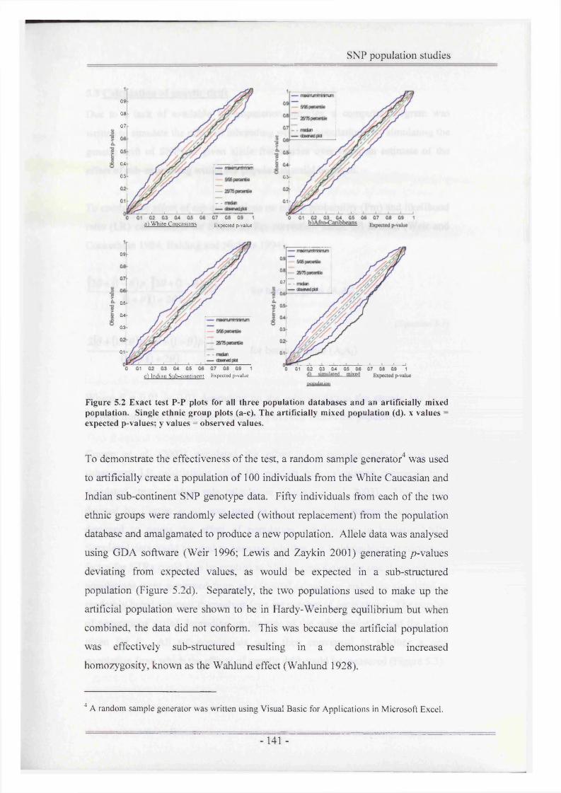
SNP population studies

Q9

Q8Q7

0 4

Q3

a) W hite Caucasians Expected p-value

03

09

Q5-

04

03

01

c~) Indian Sub-continent Expected p-value

07

population

Figure 5.2 Exact test P-P plots for all three population databases and an artificially mixed population. Single ethnic group plots (a-c). The artificially mixed population (d). x values = expected p-values; y values = observed values.

To demonstrate the effectiveness o f the test, a random sample generator4 was used

to artificially create a population o f 100 individuals from the White Caucasian and

Indian sub-continent SNP genotype data. Fifty individuals from each o f the two

ethnic groups were randomly selected (without replacement) from the population

database and amalgamated to produce a new population. Allele data was analysed

using GDA software (Weir 1996; Lewis and Zaykin 2001) generating /^-values

deviating from expected values, as would be expected in a sub-structured

population (Figure 5.2d). Separately, the two populations used to make up the

artificial population were shown to be in Hardy-Weinberg equilibrium but when

combined, the data did not conform. This was because the artificial population

was effectively sub-structured resulting in a demonstrable increased

homozygosity, known as the Wahlund effect (Wahlund 1928).

4 A random sample generator was written using Visual Basic for Applications in M icrosoft Excel.

- 141 -

SNP population studies

5.5 Calculation of genetic drift

Due to a lack of available sub-population samples, a computer program was

written to simulate the effect of inbreeding within a population. By simulating the

genetic drift of SNPs of given allele frequencies over time; an estimate of the

effect of sub-structuring within the population could be given.

To combat the effect of sub-populations on match probability (Pm) and likelihood

ratio (LR) calculations for STRs, an Fst correction factor (0) is used (Weir and

Cockerham 1984; Balding and Nichols 1994):

f° rh o m ° z y g o t e s ( a a )

(Equation 5-1)

2[6+ { i - e ) p ^ + { \ - e ) P j \ r _ (l + dix + w ) for heterozygotes (A,A;)

Where 6 = 0.01 or 0.03 depending on the sub-population the sample has been

derived from; and p = the allele frequency of i or j within the population.

Curran et al (2003) simulated the effect of population sub-division and

subsequent LR calculations using the product rule calculation compared to a

simulated ‘true’ product rule calculation (Curran et. al 2003). The method

devised by Curran et al was used as a basis for the computer simulations

designed to assess the effect of population sub-division in biallelic SNPs.

Simulated data could be used to ascertain whether the Balding-Nichols correction

factor for STRs could also be applied to SNPs. Genotypes for one thousand sub­

populations were generated from an ancestral population and were simulated to

randomly breed amongst themselves for a set number of generations. The number

of generations varied depending on the size of the sub-population and the value

given for 9. All sub-populations were then converged to produce a new

population from which the effects of genetic drift could be measured (Figure 5.3).

SNP population studies

Ancestral population

Sub- V Sub- V Sub-

pop". .. A pop"... A. p°pn- • • yV P°pn n

Sub-Sub- Sub-Sub- V Sub- V Sub­

pop" 2 A pop" 3 A pop"... A pop"...

Sub­

pop" 1 pop"...

Current observable population

- distinct sub-structure

Figure 5.3 Evolutionary model used in the simulation of a sub-divided population. Taken from J. Curran et. a l (2003) “ What is the magnitude o f the subpopulation effect?” Foren. Scl Ink 13 5(1): 1-8.

One thousand sub-populations of size n (where n = 200 or 1000) were created

using a random number generator5. The genotypes for each SNP locus were

randomly generated from an ‘ancestral’ gene pool, based on the mean allele

frequencies of the twenty SNP loci used in the 21-SNP multiplex system (Table

5.3). The allele frequencies were calculated from the white Caucasian database,

giving eleven frequencies in total rounded to the nearest 0.1, for computational

ease. These frequencies formed the basis of the ancestral population (Figure 5.3).

To achieve a desired level of drift within the separate sub-populations, random

breeding was simulated (within each sub-population, with no migration or

mutation) for a fixed number of generations (/), dependent on the size of the sub­

population (Ns) and 6 (0 = 0.01 or 0.03), where:

5 All simulations were carried out using MatLab®6 (MathWorks, Inc.)

-143-

SNP population studies

/ = ln (l - 0)

In 1 —(Equation 5-2 taken from Curran et. al. (2003))

One thousand individuals were then chosen randomly across all sub-populations

to generate a new allele frequency database. For each individual within the

database, two likelihood ratios were calculated: the first was a ‘gold standard’

estimate based on the allele frequencies of the sub-population from which the

sample was chosen; the second estimate was derived from the new allele

frequency values of the total combined population, adjusted for 6 using the

Balding and Nichols (BN) correction (Balding and Nichols 1994).

Simulations were generated for sub-populations of 200 and 1000 individuals using

values of 0.01 and 0.03 for 0. Figure 5.4 illustrates the results obtained for a

simulation with a sub-population size of 200 individuals using a 6 value of 0.03.

i i i i i : i4 5 6 7 8 9 10 11

Fst corrected LR

Figure 5.4 Plot of BN corrected LR vs. gold standard LR, 0 =0.03, sample size =200. Samples below the solid black line are non-conservative and those below the dashed line are non­conservative by an order of magnitude or more.

SNP population studies

For all simulations, application of the BN correction was generally conservative.

For the example given, only nine individual samples out of 1000 deviated from

the ‘gold standard’ LR by more than one order of magnitude (Figure 5.4). None

of the results were greater than two orders of magnitude, for any of the simulated

populations generated.

As well as directly comparing the gold standard LR and the BN corrected LR,

log 10 ratios of the two values were calculated for each individual sample (d0bs\ using the following equation:

= l°giLRg o ld

LR,(Equation 5-3)

s t y

If the LRgoid < LRfst then d0bS was negative and vice-versa. These results were

plotted on a graph using the logio gold standard LR compared to the calculated

d0bs ratio (Figure 5.5).

&

2.5

2

1.5

1

0.5

0

-0.5

-1

-1.5

-2

O-i----------------------------- 1--------------------------- 1------------------------- 1------------------------------1________________ i__________________i

5 6 7 8 9 10 11log 10 gold standard

Figure 5.5 Plot of log10 gold standard vs. the calculated ratio dobs where 9 = 0.03, sample size = 200.

SNP population studies

The data (d0bs) were also ranked in ascending order to illustrate the proportion of

data that were typically under or over-estimated relative to the gold standard LR

(Figure 5.6). Values of 6 from 0.05 down to the lowest possible value, dependent

on population size, were used to create a set of simulations with varying amounts

of genetic drift within the sub-populations.

>=0.0025>=o.oi

>=0.02

>=0.03>=0.05

-0.5 -

100 200 300 400 500 600 700 800 900 1000

rank

Figure 5.6 Graphical depiction of the calculated do5s values calculated for a sub-population of size 200; 0 values ranged from 0.0025 to 0.05.

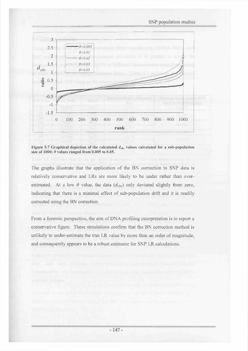
SNP population studies

3

2.5

d obs

_ ---------- 9=0.0059=0.019=0.02

- ........... 9=0.039=0.05

•2 0.5 2

1 1 1 1 1 1 1 1---------------------- 1—

0 100 200 300 400 500 600 700 800 900 1000

rank

Figure 5.7 Graphical depiction of the calculated dobs values calculated for a sub-population size of 1000; 0 values ranged from 0.005 to 0.05.

The graphs illustrate that the application of the BN correction to SNP data is

relatively conservative and LRs are more likely to be under rather than over­

estimated. At a low 6 value, the data (d0bS) only deviated slightly from zero,

indicating that there is a minimal effect of sub-population drift and it is readily

corrected using the BN correction.

From a forensic perspective, the aim of DNA profiling interpretation is to report a

conservative figure. These simulations confirm that the BN correction method is

unlikely to under-estimate the true LR value by more than an order of magnitude,

and consequently appears to be a robust estimator for SNP LR calculations.

SNP population studies

5.6 Linkage mapping

Using the data from the SNP consortium (http://snp.cshl.org; Holden 2002), each

SNP was mapped to the chromosome on which it is located to assess the

likelihood of physical linkage. SNPs on different chromosomes were disregarded,

as there would be no linkage between them. Table 5.5 indicates the mapped

location of each SNP lying on the same chromosome.

SNP locus TSC code Band Distance from p telomere (kb)

Distance from closest SNP used in multiplex (kb)

D 252540 3p25 9,092 33,572J8 709016 3p21 42,664 36,437B6 1342445 3pl3 79,10106 1588825 5pl5 8,346 44,489Y6 627632 5qll 52,835U6 746324 5q35 170,140 117,305P7 897904 6p23 14,070 153,973Z2 86795 6q27 168,043X 31988 8p23 238 91,431

A4 421768 8q21 91,669

Table 5.5 SNP loci that lie on the same chromosome. SNPs were selected based on a maximised distance away from other SNPs on the same chromosome to negate the effects of physical linkage.

On chromosomes 6 and 8, one SNP lay on the short arm (P7 = 6p23; X = 8p23)

and one on the long arm (Z2 = 6q27; A4 = 8q21). Linkage disequilibrium can

typically extend up to a few megabases (Collins et. al. 2001) and is frequently

used for disease mapping studies (Terwilliger and Weiss 1998; Clark 2003; Kuno

et. al. 2004). The shortest distance between any two SNPs in this study was more

than 33Mb (D and J8 on chromosome 3). This was sufficient distance to ensure

that multiple chromosomal recombination events would result in linkage

equilibrium between any pair of loci (Petes 2001). The SNPs used in another

multiplex system for parentage analysis (Orchid Biosciences Inc.) are often less

than half this distance (http://www.cstl.nist.gov/biotech/strbase/SNP.htm).

Consequently, the assumption of independence was reasonable with regard to

physical linkage.

-148-

SNP population studies

5.7 Paternity Testing

The DNA from blood samples obtained from members of thirteen Kuwaiti

families was extracted and amplified using the 21-SNP multiplex. The samples

had been obtained from the Wetherby Casework Unit where paternity testing had

already been performed in relation to immigration regulations. Full SNP

genotyping results are shown in appendix VIII.

Exclusion probabilities (PE) and the probability of parentage (PI) were calculated

for each DNA profile analysed from each child within a family. Following STR

analysis, the maternal parentage for each child was known and analysis of the

SNP genotypes was employed to test the paternity within each family. Statistical

calculations for PE and PI were carried out using the computer program CERVUS

(http://helios.bto.ed.ac.uk/evolgen/cervus/cervus.html; Marshall et. al. 1998; Slate

et. al. 2000).

CERVUS was designed for large-scale parentage analysis. Using genotype data in

text file format, the program analysed the allele frequencies of each SNP locus

before carrying out likelihood-based parentage analysis. Each sample was

analysed by assessing the genotype of the known parent (in the Kuwaiti samples

this was always the mother) against the genotype of the child. The likelihood of

the alleged father being the true father was then assessed against all possible allele

combinations. This value was represented as a paternity index (PI) (Table 5.6).

The PI value is interpreted as the likelihood of observing the paternal component

of the putative offspring’s DNA profile in the alleged father compared to a

random man from the general population, i.e. “it is X (PI value) times more likely

that the alleged father is the true biological father o f the child compared to a

random, non-related male”.

The exclusion probability (PE) for each child was also calculated. This value

represents the probability of a random man in the general population being

excluded as the father of the child (Buckleton et. al. 2005; Butler 2005b). It is

based on the allele frequencies of the SNP loci, rather than the genotypes of the

individuals involved.

- 149-

SNP population studies

In each case, the number of loci compared was noted (Table 5.6). Some DNA

samples failed to give a full profile and only results for SNP loci present in both

samples were compared. The PI values obtained varied depending on the allele

frequencies of the genotypes. A PI value of over one hundred is an internationally

accepted minimum at which paternity can be verified using STR markers

(http://www.dnasupport.co.uk; Panke et. al 2001; Butler 2005b). This value was

used as a basis for the assessment of the use of the 21-SNP multiplex for paternity

testing. The value for Pe was used as a comparison against other studies

investigating the use of both SNPs and STRs for paternity testing. The

determination of exclusion probabilities can be done without having the DNA

profile of the alleged father, as Pe is calculated from the allelic frequency within

the population and can be conditioned depending on the genotypes of the child

and mother (Chakraborty et. al. 1999).

Offspring (O) Oloci Candidate CP loci O-CP loci O-CP loci Exclusion PaternityID typed parent (CP) ID typed compared mismatching probability (PK) Index (PI)

CHILD1A 21 FATHER 1 21 21 0 0.997 44134CHILD1B 21 FATHER1 21 21 0 0.998 15304CHILD1C 21 FATHER 1 21 21 0 0.984 46CH1LD1D 21 FATHER 1 21 21 0 0.996 6153CHILD1E 21 FATHER1 21 21 0 0.967 46CHILD2A 21 FATHER2 21 21 0 0.931 27CHILD2B 21 FATHER2 21 21 0 0.987 6871CHILD2C 21 FATHER2 21 21 0 0.944 82CHILD2E 21 FATHER2 21 21 0 0.972 650CHILD2F 20 FATHER2 21 20 0 0.977 9514CHILD3A 21 FATHER3 21 21 0 0.994 719123CHILD3B 21 FATHER3 21 21 0 0.995 853473CHILD3C 21 FATHER3 21 21 0 0.998 13052467CHILD3D 21 FATHER3 21 21 0 0.997 2633158CHILD3E 21 FATHER3 21 21 0 0.983 10873CHILD4A 21 FATHER4 20 20 0 0.975 299CHILD4B 21 FATHER4 20 20 0 0.999 4009747CHILD4C 21 FATHER4 20 20 0 0.993 18893CHILD4D 21 FATHER4 20 20 0 0.975 396CHILD4E 21 FATHER4 20 20 0 0.998 339598CHILD4F 21 FATHER4 20 20 0 0.991 7274CHILD5A 21 FATHERS 21 21 0 0.992 84240CHILD5B 21 FATHER5 21 21 0 0.993 182546CHILD5C 21 FATHER5 21 21 0 0.998 9732812CHILD5D 21 FATHER5 21 21 0 0.994 1312157CHILD5E 20 FATHER5 21 20 0 0.997 16059442CHIILD5F 21 FATHER5 21 21 0 0.996 683173CHILD6A 21 FATHER6 21 21 0 0.981 396846CHILD6B 20 FATHER6 21 20 0 0.951 19558CHILD6C 21 FATHER6 21 21 0 0.978 392509CHILD6D 21 FATHER6 21 21 0 0.962 41205CHILD6E 21 FATHER6 21 21 0 0.958 67196CHILD6F 21 FATHER6 21 21 0 0.929 5693CIIILD6G 21 FATHER6 21 21 3 0.992 0CHILD7A 21 FATHER7 21 21 0 0.833 2CHILD7B 21 FATHER7 21 21 0 0.999 96966CHILD7C 21 FATHER7 21 21 0 0.920 17CHILD7D 21 FATHER7 21 21 0 0.929 27CHILD7E 21 FATHER7 21 21 0 0.990 5270CHILD7F 21 FATHER7 21 21 0 0.988 482

Offspring (O) ID O loci typed Candidate parent

(CP) IDCP loci typed

O-CP loci compared

O-CP loci mismatching

Exclusion probability (PE)

Paternity Index (PI)

CHILD8A 21 FATHER8 20 20 4 0.990 0CHILD8B 21 FATHER8 20 20 0 0.994 4048344CHILD8C 21 FATHER8 20 20 0 0.997 352730CHILD8D 21 FATIIER8 20 20 3 0.970 0CHILD8E 21 FATHER8 20 20 2 0.962 0CHILD9A 21 FATHER9 18 18 0 0.953 25610CHILD9B 21 FATHER9 18 18 0 0.937 46439CHILD9C 21 FATHER9 18 18 0 0.966 215344CHILD9D 21 FATHER9 18 18 0 0.973 199073CHILD9E 21 FATHER9 18 18 0 0.968 479765

CHILD10A 21 FATHER10 20 20 0 0.994 333166CHILD10B 21 FATHER10 20 20 0 0.998 20361388CHILD10C 21 FATHER10 20 20 0 0.994 454165CHILD10D 21 FATHER 10 20 20 0 0.997 1202324CHILD10E 21 FATHER10 20 20 0 0.932 1237CHILD10F 21 FATHER 10 20 20 0 0.998 3563158CHILD 10G 21 FATHER10 20 20 0 0.999 40788973CHILD11A 21 FATHER11 20 20 0 0.997 808731CH1LD11B 21 FATHER 11 20 20 0 0.994 232885CHILD11C 21 FATHER11 20 20 0 0.981 10095CHILD1 ID 21 FATHER11 20 20 0 0.977 8127CHILD1 IE 21 FATHER11 20 20 0 0.940 2030CHILD1 IF 21 FATHER 11 20 20 0 0.922 291CHILD11G 20 FATHER11 20 19 0 0.997 131563CHILD12A 21 FATHER 12 20 20 0 0.968 4915CHILD12B 21 FATHER12 20 20 0 0.952 2659CH1LD12C 21 FATHER12 20 20 0 0.974 5550CH1LD12D 21 FATHER12 20 20 0 0.968 16006CHILD12E 21 FATHER12 20 20 0 0.921 324CHILD12F 21 FATHER12 20 20 0 0.892 137CHILD12G 21 FATHER12 20 20 0 0.859 39CHILD12H 21 FATHER12 20 20 0 0.958 2070CHILD13A 21 FATHER13 21 21 0 0.983 68375CHILD13B 21 FATHER 13 21 21 0 0.996 3621034CHILD13C 21 FATHER13 21 21 0 0.982 39088CHILD13D 21 FATHER13 21 21 0 0.937 1192CHILD13E 21 FATHER 13 21 21 0 0.996 7997532

Table 5.6 Exclusion probability (PE) and paternity index (PI) values for Kuwaiti family samples. Tables indicate how' many loci for each individual were genotyped and cross-compared for parentage analysis. Samples in BOLD indicate excluded fathers. See appendix VIII for full genotype data.

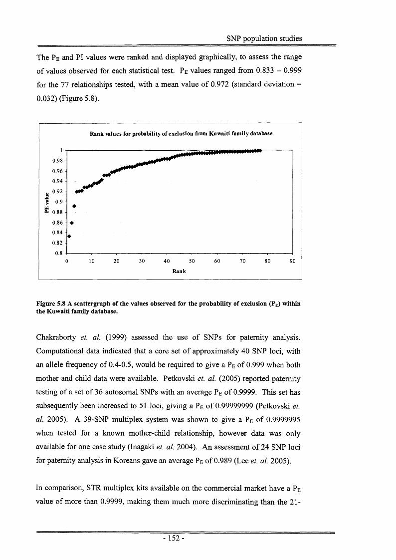
SNP population studies

The Pe and PI values were ranked and displayed graphically, to assess the range

of values observed for each statistical test. P e values ranged from 0.833 — 0.999

for the 77 relationships tested, with a mean value of 0.972 (standard deviation =

0.032) (Figure 5.8).

Rank values for probability of exclusion from Kuwaiti family database

0.98

0 .96

0 .94

0 .924>3

0.86

0 .84

0 .82

30 60 70 800 10 20 40 50 90

R ank

Figure 5.8 A scattergraph of the values observed for the probability of exclusion (PE) within the Kuwaiti family database.

Chakraborty et. al. (1999) assessed the use of SNPs for paternity analysis.

Computational data indicated that a core set of approximately 40 SNP loci, with

an allele frequency of 0.4-0.5, would be required to give a Pe of 0.999 when both

mother and child data were available. Petkovski et. al. (2005) reported paternity

testing of a set of 36 autosomal SNPs with an average Pe of 0.9999. This set has

subsequently been increased to 51 loci, giving a Pe of 0.99999999 (Petkovski et.

al. 2005). A 39-SNP multiplex system was shown to give a Pe of 0.9999995

when tested for a known mother-child relationship, however data was only

available for one case study (Inagaki et. al. 2004). An assessment of 24 SNP loci

for paternity analysis in Koreans gave an average Pe of 0.989 (Lee et. al. 2005).

In comparison, STR multiplex kits available on the commercial market have a Pe

value of more than 0.9999, making them much more discriminating than the 21-

- 152-

SNP population studies

SNP multiplex used in this study. SGM Plus™ (Cotton et. al. 2000; Steinlechner

et. al. 2001; Soltyszewski et. al. 2005), Identifier™

(http://docs.appliedbiosystems.com/pebiodocs/04323291 .pdf) and Powerplex®-16

(Okamoto et. al. 2003; Greenspoon et. al. 2004; Konjhodzic et. al. 2004) have Pe

values significantly higher than 0.9999, due to the increased number of STR loci

used in each kit.

PI values ranged from lxlO'12 - 4.1xl07 (Figure 5.9), with 79% of the non­

excluded data having a value >1000 and 89% higher than 100. The negative PI

values were calculated in families where the man was excluded from being the

biological father by more than two mismatched loci. True exclusion assesses each

locus individually and allows a person to be excluded if one loci mismatches. In

practice, mutation can occur leading to a mismatch at one or two loci, and this is

compensated for in statistical calculations (Chakraborty et. al. 1999; Amorim and

Pereira 2005). In STRs, two loci must mismatch in order for a man to be

excluded from being the alleged father (http://dna-view.com/mudisc.htm; Ayres

2005).

R anked PI values from K uw aiti fa m ily database

100000000

1000000

10000

100

10.01

0.0001

0.000001

0.00000001

IE-10

IE-12

Rank

Figure 5.9 A scattergraph of values observed for the paternity index (PI), calculated for each child-alleged father relationship in the Kuwaiti family samples.

-153-

SNP population studies

PI values o f less than zero were tabulated as zero as the probability o f the alleged

father being the true father became insignificant due to exclusion at more than one

locus (Table 5.1). A PI o f zero was evident in two different families. Child 6G in

family 6 had three mismatched loci when compared to the candidate father (father

6), leading to a PI value o f zero. STR profiling and further family investigation

indicated that this man was unrelated to child 6G (Figure 5.10). In family 8, three

offspring had loci mismatching with the alleged father (father 8), giving PI values

o f zero (Table 5.6). Child 8A had five loci with no match to the alleged father,

child 8D had four mismatches and child 8E had three mismatching loci. Again,

STR profiling and family investigations found this man to be unrelated to the

three offspring (Figure 5.11).

Father 6 8485

UnknownMothermale

Child 6G 8493 PI=0

Child 6B 8488

PI=19558

Child 6F 8492

PI=5693

Child 6A 8487

PI=396846

Child6C8489

PI=392509

Child 6D 8490

PI=41205

Child 6E 8491

PI=67196

Figure 5.10 Family tree for family 6 depicting the relationships between the seven offspring genotyped and the parents.

Father 8 UnknownMother 88830 male8831

Child 8B 8834

PI=4048344

Child 8C 8835

PI=352730

Child 8D 8836 PI=0

Child IE 8837 PI=0

Child 8A 8833 PI=0

Figure 5.11 Family tree for family 8 depicting the relationships between the Five offspring and the parents.

SNP population studies

All offspring in families 3, 4, 5, 8, 9, 10, 11 and 13 had PI values >100,

supporting the case for paternity against the alleged father. The values ranged

from 137 to >40,000,000, dependent on the genotypes of the offspring, the known

mother and the alleged father. The samples with the highest PI values were

shown to have rare alleles at certain SNP loci, greatly increasing the significance

of the result (see appendix VIII for frill SNP genotypes). Some PI values were

less than the threshold value of 100, although paternity was confirmed using STR

analysis. In these cases, all loci matched the alleged father but the allelic

frequencies, once the mother’s alleles had been removed, were too high to give a

significant result compared to an unrelated man from the general population. This

is most likely due to the biallelic nature of the SNPs tested.

These results confirm the use of the 21-SNP multiplex for exclusion of paternity,

using mismatched loci as confirmation that an alleged father cannot be the

biological father of a questioned child. However the low PI values observed in

some cases suggest that STR analysis would be more beneficial, due to the

increased likelihood ratios that can be calculated as a result of more alleles present

at each locus.

- 155-

SNP population studies

5.8 Discussion

It is important to fully recognise the attributes of the DNA profiling system in use

for forensic identification. Factors such as sub-structuring of populations, as well

as sampling error and linkage distances can affect the strength of the evidence

obtained. The population studies carried out on the 21-SNP multiplex

incorporated an analysis of the main types of irregularities, including linkage

disequilibrium, Hardy-Weinberg proportions and a calculation of Fst to allow

correction factors to be used when calculating match probabilities. All SNP loci

demonstrated Hardy-Weinberg equilibrium and no linkage disequilibrium

between SNPs (including those on the same chromosome). The minimum

distance between SNPs on the same chromosome was over 33Mb, sufficient

distance to ensure that multiple recombination events would result in linkage

equilibrium between any pair of loci (Petes 2001).

Many studies on the population genetics of STR loci have been carried out as a

consequence of these loci being routinely used in forensic casework across the

world (Devlin et. al. 1990; Gill et. al. 1991; Nichols and Balding 1991;

Steinberger et. al. 1993; Balding and Nichols 1994; Budowle 1995; Deka et. al.

1995; Gill and Evett 1995a; Balding et. al. 1996; Evett et. al. 1997; Foreman et.

al. 1998; Foreman and Lambert 2000; Foreman and Evett 2001; Ayres et. al.

2002a; Curran et. al. 2003; Overall et. al. 2003). The National Institute of

Standards and Technology (NIST) currently holds references for over 750 STR

population studies on its STRbase™ website (Ruitberg et. al. 2001). The criteria

for selection of STR loci can be applied to the selection of SNP loci as traditional

population genetics analyses holds for both types of DNA polymorphism. Hardy-

Weinberg equilibrium (HWE) is essential for the calculation of match

probabilities and subsequent likelihood ratio calculations. Any deviation from

HWE is suggestive of population sub-structure and / or sampling errors (Evett et.

al. 1996; Weir 1996; Buckleton et. al. 2005) and is likely to give a non­

conservative likelihood ratio. A sample size greater than one hundred is sufficient

to provide enough genotype information to project the frequency of alleles in a

larger population (http://www.promega.eom/geneticidproc/ussymp8proc/l 3.html;

Chakraborty 1992). In this study less than 100 individuals were available for the

-156-

SNP population studies

African-Caribbean and Indian sub-continent databases, meaning the true allele

frequencies may deviate slightly from those calculated here.

The allele frequencies at a particular locus are not fixed within the population and

change over time as a consequence of mutation and genetic drift, however in any

particular population, allele frequencies should maintain HWE. Admixing

between different populations can cause deviation from HWE and leads to

phenomena such as the Wahlund effect (Wahlund 1928), where excess

homozygosity is observed within a population due to the presence of sub­

populations with different allele frequencies. In reality, the presence of sub­

structuring within a population is minimal and has a much less severe affect. In

spite of this, it is important to include an estimate of sub-population bias in all

calculations for forensic purposes (Balding and Nichols 1994). As members of

the same sub-population are more likely to share common alleles, i.e. alleles

identical by descent, the allele frequencies within that sub-population will give a

lower likelihood ratio than would be found in the general population (Budowle

1995; Foreman et. al. 1998; Foreman and Lambert 2000). For calculation of

DNA profiles present on the UK National DNA Database®, three broad allele

frequency databases are used: Caucasian, African-Caribbean and Indian sub­

continent and the BN correction (Equation 5-1) is applied to all LR calculations.

The value for 9 is routinely set to 0.01 for Caucasians and 0.03 for all other ethnic

groups, based on analyses of STR population databases in the 1990s and the

recommendations of the National Research Council in 1994 (Budowle 1995; Gill

and Evett 1995a; Balding et. al. 1996; NRCII 1996; Foreman et. al. 1998). Both

of these estimates are highly conservative and represent extreme values of

inbreeding and/or genetic drift for all populations.

A real population of forensic interest will contain several sub-populations that will

not be completely separate, and may exist as several levels of geographical and

social structure. There are a large number of studies which report estimated

values for 6 for different populations and sub-populations (Bowcock et. al. 1991;

Kidd et. al. 1991; Morris et. al. 1991; Lin et. al. 1994; Weir 1994; Foreman and

Lambert 2000; Zarrabeitia et. al. 2003). Values are highly variable dependent on

the population under consideration, but all are significantly lower than 0.03, with

-157-

SNP population studies

Caucasian populations having 6 < 0.01 in most instances. The populations found

to have the highest values of 6 are the same cultures with the highest levels of

consanguinity. Globally, the most common form of consanguineous union is

between first cousins, in which spouses share 1/8 of their genes inherited from a

common ancestor, making their progeny homozygous at 1/16 of all loci (Bittles

1998). The level of consanguineous unions is directly related to the religious,

ethnic and / or tribal traditions of a population. For example, in Christianity, the

Orthodox churches prohibit consanguineous marriage, the Roman Catholic church

currently requires Diocesan permission for marriages between first cousins, and

the Protestant denominations permit marriages up to and including first cousin

unions (Bittles 1998). Within the Islamic and Buddhist communities, first cousin

marriages are permitted, but are forbidden by the Sikh religion. The increasing

diversity of religious factions within Western countries, due to immigration and

across-country marriages, is leading to an increasing number of individuals

sharing a common ancestor. Migrant communities permanently gaining residence

in Western countries demonstrate an increased level of within-community

marriage, further sub-dividing the population. It is due to these sub-populations

that allele frequencies for whole populations need to be corrected for, to allow for

higher levels of inbreeding within some sub-populations (Zhivotovsky et. al.

2001).

Due to a lack of available sub-population data, simulations were carried out using

0 = 0.01 and 0.03, to assess the effect of inbreeding on SNP allele frequencies,

over a number of generations. The method was derived from simulations for STR

loci carried out by Curran et. al. (2003). The resulting genotype frequencies were

then used to calculate LR values for each sub-population and these values were

compared to LR values for the whole population, calculated using the BN

correction for Fst (Balding and Nichols 1994). The BN correction was found to

be conservative compared to the simulated sub-populations, suggesting the BN

correction was sufficient for SNP LR calculations.

The Exact Test data for linkage disequilibrium (LD) (Weir 1996; Lewis and

Zaykin 2001) indicated that there was no deviation from what would be expected

within a randomly-mating population, for all three populations tested -white

-158-

SNP population studies

Caucasian, British afro-Caribbean and Indian sub-continent. LD occurs when

alleles at two loci occur together in gametes more frequently than expected given

the known allele frequencies and recombination fraction between the two loci.

Evidence for linkage disequilibrium can be helpful in mapping disease genes

since it suggests that the two loci may be very close to one another in the genome.

The Wahlund effect was demonstrated on an artificially created population based

on white Caucasian and Indian sub-continent data. The Exact Test p-values

deviated significantly from that expected from the random number matrix and

indicated the variation expected if the populations under study were effectively

sub-structured. This simulation also demonstrated the ability of the 21-SNP

multiplex to effectively illustrate the presence of sub-structuring within a

population. All SNPs were shown to be in linkage equilibrium, i.e. all loci are

independently inherited. As a consequence of this, all loci can be multiplied

together using the product rule for match probability, and subsequent LR,

calculations. LD studies using SNP loci are increasingly used for disease

mapping in the human genome (Terwilliger and Weiss 1998; Kruglyak 1999;

Collins 2000; Collins et. al. 2001; Ennis et. al. 2001; Saunders et. al. 2001;

Halldorsson et. al. 2004; Kuno et. al. 2004). LD can also be used as an indicator

of population admixture, as demonstrated by the artificially-created population in

this study (Lin et. al. 1994; Zaykin et. al. 1995; Smith et. al. 2001; Gu and Rao

2003).

The independent inheritance of alleles is also important when it comes to paternity

testing using SNP loci. It is essential that each locus is independently inherited in

order to maximise the evidential value of the test. The paternity index (PI) is the

most commonly used form of statistical evidence in the case of paternity analysis

(Butler 2005b). PI is calculated using a likelihood ratio examining the chance of

seeing the genotypes of each locus in a random unrelated individual compared to

the suspected father. PI values for thirteen different families were calculated from

SNP genotype data using the computer program CERVUS

(http://helios.bto.ed.ac.uk/evolgen/cervus/cervus.html; Marshall et. al. 1998; Slate

et. al. 2000). 89% of the PI values were higher than the accepted minimum value

of 100 and two men were excluded as biological fathers of four offspring, using

the observation of over two mismatched loci as a guideline.

-159-

SNP population studies

SNPs have been investigated as a potential alternative to STRs in paternity

analysis. SNPs have a lower mutation rate compared to STRs, due to their

biallelic nature, and the chance of positively excluding a potential male through

mutation at some loci is decreased (Amorim and Pereira 2005; Ayres 2005).

However STR calculations have been derived which incorporate the chance of a

mutational event having occurred, thus allowing a more stringent approach to

paternity analysis using STR loci (Dawid et. al. 2001; Ayres 2002b).

Many studies on paternity analysis using SNPs employ an assessment of the

probability of exclusion (P e). This approach is known as the ‘frequentist

approach’ as it considers the probability of the evidence under one hypothesis

(Buckleton et. al. 2005). In the case of paternity analysis, the frequentist

approach uses the value of Pe as a method of excluding a non-related random man

from the general population, however it makes no inference to the data supplied

from the alleged father. From the data generated for the Kuwaiti families, the PI

value was found to be more informative than the Pe value. For child 6G and 8A

(Table 5.6) a Pe value >0.99 was observed yet the PI values for both offspring was

less than zero, due to mismatched loci. This suggests that Pe is only useful if the

alleged father is a potential parent as it gives the probability of a random person

being excluded as a potential parent.

Computer simulations assessing the utility of SNPs for paternity analysis suggest

that SNPs with an allele frequency of 0.5 are the most discriminating and a set of

40-50 loci would be capable of giving a PI and Pe value similar to STRs

(Chakraborty et. al. 1999; Amorim and Pereira 2005; Ayres 2005). The 21-SNP

multiplex assessed in this study incorporated loci with allele frequencies between

0.1 and 0.9 (Table 5.3). This led to decreased values for PI except in families

where loci with low allele frequencies were present. In cases with rare genotypes

the PI was increased to greater than one million. The 21-SNP multiplex was

capable of excluding an alleged father as the biological father by assessing the

number of mismatched loci present, however some PI values fell below the

accepted minimum of 100. This suggests that this multiplex does not contain

sufficient loci to be as discriminating as current STR methods of parentage

analysis.

European Collaborative Degradation Study

European collaborative study

6.1 Introduction

Chapters 3, 4 and 5 outlined the development and validation of a SNP multiplex

system for use as an alternative forensic DNA profiling method (Dixon et. al.

2005a). The discrimination power of the 21-SNP multiplex (approximately one in

five million) is lower than that gained if a full profile were obtained from STRs

(approximately one in a thousand million), therefore its use is limited to situations

where routine DNA profiling is not possible.

A discussion held by the joint European Network of Forensic Science Institutes

(ENFSI), European DNA Profiling Group (EDNAP) and Scientific Working

Group on DNA Analysis Methods (SWGDAM) made recommendations on the

development of DNA profiling for degraded samples within the forensic

community (Gill et. al. 2004a). Existing Short Tandem Repeat (STR) systems

used in European national DNA databases (NDNADBs) include seven core STR

loci recommended by ENFSI. The core loci6 are included in commercially

available multiplexes (Cotton et. al. 2000; Collins et. al. 2004; Greenspoon et. al.

2004). However, all current markers are relatively high in molecular weight

(between 150 - 450 bp) (Gill 2002).

It has been demonstrated that smaller amplicons are much more likely to be

amplified in samples containing degraded DNA (Hellmann et. al. 2001; Wiegand

and Kleiber 2001; Krenke et. al. 2002; Ohtaki et. al. 2002; Butler et. al. 2003;

Chung et. al. 2004; Schumm et. al. 2004; Coble and Butler 2005; Butler 2005b).

There are two kinds of markers that can bring the size of the amplicon

substantially below 150 bp: ‘mini-STRs’ that have short flanking regions to the

tandem repeat sequence and SNPs.

A small number of validated SNP assays are used in casework and these include

mini-sequencing assays for mitochondrial DNA (mtDNA) (Tully et. al. 1996;

Coble et. al. 2004; Just et. al. 2004; Vallone et. al. 2004), Y chromosome

(Sanchez et. al. 2005), a red hair marker assay (Grimes et. al. 2001) and

autosomal multiplexes (Dixon et. al. 2005a).

6 Core European STR loci - THOl, VWA, D21S11, FGA, D3S1358, D8S1179, D18S51.

- 162-

European collaborative study

To achieve the ultimate lower limit of small amplicons, SNPs are preferable, but

the downside is that a panel of 45-50 loci would be needed to achieve match

probabilities comparable with existing STR multiplexes (Chakraborty et. al. 1999;

Gill 2001a). Furthermore, the larger the multiplex, the more difficult it is to

reliably and to reproducibly construct (Budowle 2004b); loss of amplification

efficiency may ensue, effectively defeating the object of the exercise. To

circumvent this problem, several SNP multiplexes of a dozen loci each can be

used in concurrent multi-tube reactions, however the sample size needs to be

sufficient to allow this option (Bell et. al. 2002; Inagaki et. al. 2004). Large

amounts of DNA from, e.g. bones, can be analysed in this way, but the study of

many small forensic stains is precluded, as the amount of DNA extract available is

limited. In addition, the binary nature of SNPs means that their statistical

characteristics are not amenable to the interpretation of complex samples such as

mixtures. A robust, highly quantitative SNP assay would be required to allow

determination of mixtures using an interpretation strategy based on heterozygous

balance and homozygous thresholds (Gill 2001a).

Mini-STR multiplex systems have been developed as an alternative method of

DNA profiling using traditional STR genetic markers (Butler et. al. 2003; Chung

et. al. 2004; Drabek et. al. 2004). Primers are designed closer to the STR locus,

sometimes overlapping the repeat region. This approach has the benefit of

shortening the length of the amplicon whilst maintaining the higher discrimination

powers seen with STRs as opposed to SNPs. The resulting profiles are also

consistent with STR profiles currently used in national DNA databases, meaning a

direct comparison can be made. Problems can be encountered due to the

polymorphic nature of STRs, making the primer binding sites more prone to

primer-binding site variants. This can increase the number of null alleles seen and

can lead to a higher number of imbalanced peaks within a profile.

It was agreed that markers such as SNPs have the potential to usefully

complement existing STR systems, but there was no published data comparing the

performance of STRs against SNPs at the time. Furthermore, there was no

comparative data published on the performance of other DNA profiling

European collaborative study

techniques, such as low copy number (LCN) DNA profiling using SGM+ or mini-

STR multiplex systems, when looking at degraded DNA samples.

I set up a collaborative study to assess the different DNA profiling techniques

available throughout Europe and the United States for their usefulness in

genotyping artificially degraded samples. The study was designed to assess the

extraction method employed, the current DNA profiling technique used and the

effectiveness of new profiling techniques (SNPs and mini-STRs). Experimental

work and sample genotyping was carried out by each individual laboratory and

results were sent to myself electronically for data analysis and interpretation

(Dixon et. al 2005b).

European collaborative study

6.2 Materials & Methods

6.2.1 Production of degraded DNA samples

A new set of artificially degraded samples was created, to supply enough samples

for each laboratory involved in the collaboration (Pulker 2004). Liquid blood and

saliva samples were collected from two unrelated, white Caucasian volunteers

(one male, one female), whose SNP loci had been fully sequenced as part of the

21-SNP multiplex validation. For artificial degradation, samples were set up in

0.2 ml PCR tubes containing a 4mm2 cotton square saturated with 25 pL sterile

deionised water. 5 pL of whole blood or 10 pL of saliva was added directly to

each cotton square.

Samples were placed in an incubator at 37°C, to accelerate enzymatic degradation.

The individual tubes allowed each sample to be contained within a “micro­

environment” and prevented any loss of material by leeching and, because the

tubes were manufactured for PCR, there would be no loss of moisture by

evaporation. As the cotton remained saturated the environment immediately

associated with the sample maintained 100% humidity. The stains were sampled

at specific time intervals and then frozen at -20°C to suspend the degradation

process; 44 samples of each type were frozen at each time interval to provide a

store for the collaborative study.

6.2.2 Exercise design

Each laboratory was supplied with one ‘Foren-SNPs’ multiplex kit7 (The Forensic

Science Service®, UK), one mini-SGM miniplex kit and one NC01 mini-STR kit

(National Institute of Standards and Technology (NIST) laboratory, US), as well

as sets of artificially degraded DNA stains as follows:

Reference 1 (3 or 4 stains for each time point):

Blood samples - 0,2,8,16 weeks degradation

Saliva samples - 0,2,8,12 weeks degradation

7 Trademark name given to the 21-SNP multiplex system outlined in chapters 4-6.

-165-

European collaborative study

Reference 2 (3 or 4 stains for each time point):Blood samples - 0,2,8,16 weeks degradation

Saliva samples - 0,2,8,12 weeks degradation

Each laboratory was asked to perform the following procedures:

• Extract the DNA stains using standard laboratory protocols;

• Pool each extract for each individual at each time point (Figure 6.1);

• Perform standard DNA profiling techniques on all samples (standard

being defined as the DNA profiling technique routinely used for

analysis of samples in the laboratory carrying out the work);

• Amplify the samples using the SNP multiplex kit provided (each lab

was provided with one Foren-SNPs™ kit comprising primer mix,

reaction mix and Amplitaq Gold®);

• Amplify the samples using the mini-STR kits provided (each kit

contained primer mix and protocol; labs provided their own Amplitaq

Gold® and PCR buffer);

• Record all results on the spreadsheets provided, to allow easy collation

of all data.

e.g. blood, sample 1, 1 week degradation

EXTRACT

W POOL

Final pooled extract for genotyping

Figure 6.1 Preparation of artificially degraded DNA extracts. Separate extractions from the same degradation period were pooled together to minimise the likelihood of stochastic variation from the cotton stains.

European collaborative study

6.2.3 Experimental protocols

DNA extractions were carried out using either QIAamp mini-kits (Cat. No.

51306) or QIAshredder (Cat. No. 79656) supplied by Qiagen™ (Scherczinger et.

al. 1997; Sinclair and McKechnie 2000), Chelex-100 (Walsh et. al. 1991), or by

phenol chloroform methods (Dimo-Simonin and Brandt-Casadevall 1996).

Samples were quantified using Picogreen (Ahn et. al. 1996), Quantifier™ Human

DNA Quantification kit (Cat. No. 4343895) or Slot-blot methodology (Waye et.

al. 1991). One laboratory performed quantification using a real-time quantitative

PCR assay with a fluorogenic Taqman probe, targeting the human Alu repetitive

sequence, with PCR primers adopted from Nicklas and Buel (Nicklas and Buel

2003).

Each laboratory used STR multiplex kits according to the manufacturer’s

protocol. The following STR kits were used in the study: Either AMPF/STR®

SGM Plus™ (Applied Biosystems) (Cotton et. al. 2000), AMPF/STR® Identifier

(Applied Biosystems) (Collins et. al. 2004) or Powerplex®16 system (Promega)

(Greenspoon et. al. 2004); plus mini-SGM and miniNCOl (National Institute of

Standards and Technology (NIST), US) (Butler et. al. 2003). SNP analysis was

carried out by all labs using the Foren-SNPs™ multiplex kit (The Forensic

Science Service®, UK) (Dixon et. al. 2005a).

All PCR products were run on 3100 capillary electrophoresis (CE) sequencers

(Applied Biosystems) with either POP-4 or POP-6 polymer. Results were

analysed using Genescan™ and Genotyper™ analysis software (Applied

Biosystems).

- 167-

European collaborative study

6.2.4 Data analysis

Each laboratory was given an identifier number and genotyping results for each

DNA profiling system for each laboratory were collated on Microsoft® Excel

spreadsheets.

Genotypes were analysed as percentages - e.g. for SGM+ a full genotype

comprised 22 alleles; thus a profile with 11 alleles was 50% of a full profile.

Converting into percentages allowed direct comparisons between the different

multiplex systems. Data were analysed with Minitab™ Release 14 software using

analysis of variance (ANOVA), box-whisker plots and median polish analysis

(Tukey 1977).

Median polish analysis was carried out in order to standardise the data, allowing

data sets from all laboratories to be compared regardless of variability in

laboratory techniques, operator differences and sampling limitations (Tukey

1977).

Identifier® and Powerplex®-16 were omitted from the final results analysis,

except for the inter-laboratory comparison, because only one laboratory used each

multiplex. Low copy number (LCN) SGM+ results were also disregarded from

intra-laboratory analyses, because only two laboratories submitted data.

-168-

European collaborative study

6.3 Results

Results were received from nine laboratories from six European countries and the

United States. All laboratories provided data from one standard STR multiplex

kit plus the Foren-SNPs™ kit and mini-STR kits (Figure 6.2).

DN A profiling kits

SGM+ Powerplex-16 Identifier Foren-SNPs mini-SGM NC01

Figure 6.2 DNA profiling kits used for the collaborative study. NB. One lab did not submit data for the Foren-SNPs™ kit.

6.3.1 Extraction methods

Details o f extraction techniques and corresponding quant values were submitted

from six laboratories (Table 6.1). Quant values ranged from 0 ng/pL for heavily

degraded samples to 33 ng/pL for a reference sample stain, with the range of

values varying greatly from laboratory to laboratory, especially for the reference

samples (Figure 6.3).

European collaborative study

Quant values (ng/^L)Ref 1 blood Ref 1 saliva Ref 2 blood Ref 2 saliva

LabID

Extractionprotocol Quant Owk 2wk 8wk 16wk Owk 2wk 8wk 12wk Owk 2wk 8wk 16wk Owk 2wk 8wk 12wk

1 Qiagen(manual)

Picogreen 1.91 0.22 0.22 0.03 1.03 0.07 0.01 0.01 2.13 0.23 0.23 0.02 0.36 0.03 0.03 0.01

2 Qiagen(robot)

Quantifiler 0.63 0.01 0.00 0.00 0.82 0.00 0.00 0.00 0.72 0.01 0.01 0.00 0.36 0.00 0.00 0.00

3 Phenolchloroform

Quantifiler 2.31 0.22 0.06 0.02 6.59 0.00 0.00 0.00 5.16 0.92 0.25 0.46 8.95 0.06 0.01 0.03

4 Phenolchloroform

Quantifiler 2.18 1.29 0.00 0.00 UND 0.00 0.00 0.00 3.65 2.35 0.96 0.00 8.31 0.00 0.00 0.00

5 Phenolchloroform

Quantifiler 9.67 0.93 0.53 0.12 19.00 0.10 0.03 0.03 10.29 1.64 1.97 1.58 15.8

4 0.06 0.15 0.06

6 Chelex None

7

8 Phenolchloroform

Slot-blot

11.79 0.57 1.00 1.68 33.46 0.12 0.03 0.05 10.15 2.33 4.13 0.80 14.8

8 0.36 0.23 0.05

9 Qiagen(manual) None

Table 6.1 Extraction and quant methods and results, as provided by each laboratory. Grey boxes indicate information was not provided from that laboratory. UND = undetermined DNA quantification result.

Boxplot of quant values obtained from 6 labs for degraded samples

25

Figure 6.3 Box and whisker plot showing the range of quant values received for each reference individual for each sample type. Calculations are based on data submitted from six out of the nine participating laboratories.

The range o f values seen for the degraded samples (i.e. samples >2 wks

incubation) was smaller for saliva samples compared to blood samples. The inter­

quartile (IQ) range for degraded saliva samples varied from 0.03 ng/pL to 0.17

ng/pL, compared to 0.5 ng/pL to 2.3 ng/pL for blood samples. All results gained

showed a DNA concentration o f <2.5 ng/pL.

European collaborative study

In comparison, undegraded control (time zero) reference samples showed

considerable variation in the amount of DNA recovered between laboratories.

More DNA was recovered with phenol-chloroform compared to Qiagen™ but the

variation was much greater in the former (IQ range = 27 ng/pL and 1.4 ng/pL

respectively) (Figure 6.3). The method of quantification may have affected the

DNA quantification values gained. Both laboratories using phenol chloroform

extraction followed by Quantifier™ quantification (labs 3 & 4) gave similar

values, whereas quantification with qPCR (lab 5) and slot-blot (lab 8) produced

much greater values (Table 6.1). However, all phenol chloroform values (for

control samples) were greater than those gained with Qiagen™, regardless of the

quantification method.

The variation seen between different extraction techniques was less marked as the

DNA samples became more degraded (Figure 6.3), most likely as a consequence

of having little or no DNA available to extract. Phenol chloroform extraction

showed the most variation in quant values between the different labs (data not

shown). Organic extraction techniques are routinely difficult to standardise and

the methodology used can vary between different labs, leading to variation in

success rates of the technique. However, quantification results suggest that

phenol chloroform extraction methods can give increased yields of DNA template

compared to other extraction methods and should be used when there is known to

be limited availability of a sample. This may help to maximise the amount of

DNA that can be extracted, subsequently increasing the likelihood of gaining a

DNA profile.

- 171 -

European collaborative study

6.3.2 Analysis of Variance f AN OVA) calculations

Sample data was run through Minitab™ Release 14 software to give ANOVA

calculations (Table 6.2). Assuming a 95% confidence level, there was no

significant difference found between the percentage profiles gained using the

different multiplex kits (p=0.061), suggesting each kit gave comparable results for

each sample and sample type. A significant difference was seen between results

gained from different labs (p<0.001); from different individuals (p=0.006);

different sample types - blood and saliva (p<0.001); and from the different

degradation times. There was also a difference between the percentage profiles

gained for the different individuals when looking at each sample type (p=0.044),

i.e. there was no relationship between the results obtained for each blood sample

or each saliva sample, independent of reference individual.

Analysis of variance (ANOVA) tests DF SS F PMultiplex 3 11705 2.49 0.061

lab ID 7 96328 8.78 0.000ref ID 1 11829 7.55 0.006

sample type 1 177422 118.4 0.000degradation time 3 280931 59.78 0.000Multiplex * lab ID 21 20122 0.61 0.909Multiplex * ref ID 3 553 0.12 0.950

Multiplex * sample type 3 2293 0.51 0.676Multiplex * degradation time 9 2949 0.21 0.993

lab ID* ref ID 7 5841 0.53 0.809lab ID * sample type 7 15431 1.47 0.176ref ID * sample type 1 6126 4.09 0.044

lab ID * degradation time 21 47521 1.44 0.098ref ID * degradation time 3 2867 0.61 0.609

Multiplex * lab ID * ref ID 21 3545 0.11 1.000Multiplex * lab ID * degradation time 63 20937 0.21 1.000Multiplex * ref ID * degradation time 9 2765 0.2 0.994

lab ID * ref ID * degradation time 21 30254 0.92 0.566Multiplex * lab ID * ref * degradation time 63 13408 0.14 1.000

Multiplex * lab ID * sample type 21 8114 0.26 1.000Multiplex * ref ID * sample type 3 262 0.06 0.981

lab ID * ref ID * sample type 7 14042 1.34 0.231Multiplex * lab ID * ref ID * sample type 21 3571 0.11 1.000

Table 6.2 ANOVA results for percentage profile data for each laboratory for each sample type using each multiplex kit.

There was no significance found in the results gained for the different multiplexes

compared to any other factor. This suggested each multiplex could be used

- 172-

European collaborative study

independently by any lab and it would be other factors that affected the result, i.e.

sample type, individual sample or degree of degradation, as opposed to the

multiplex used. There was also no intra-laboratory effect seen, i.e. if a lab

performed well with one multiplex then it would also perform well with another,

and vice versa.

There was no correlation found between the results gained for matching sample

types for different individuals, i.e. the two saliva samples and two blood samples

degraded at different rates to each other. More work would need to be carried out

on different individuals to assess the degradation rates more fully.

-173-

European collaborative study

6.3.3 Box and whisker plot analysis

ANOVA had indicated a significant difference between the results gained for each

laboratory (section 6.3.2). Percentage profiles were calculated for each sample

from each laboratory and the intra-laboratory variation was compared using box

and whisker plots (Figure 6.4-6.7). Variation between labs would indicate the

need for further statistical testing to allow a direct comparison of samples from

the whole data set, otherwise data would appear skewed.

Variation was seen between the different labs for both individuals and sample

types. Reference samples and the most highly degraded samples gave the least

amount of variation between the data sets. Reference DNA samples generally had

higher quant values, allowing an optimal amount of DNA (~1 ng) to be added to

each amplification reaction. The addition of optimal DNA to each multiplex

reaction would decrease the variability seen.

The most consistent multiplex across all laboratories was the mini-STR NC01 kit

(Figure 6.7), with both reference blood samples and reference 2 saliva sample

giving 100% profiles across all nine laboratories. This multiplex consisted of

only three STR loci, DIO, D14 and D22, not found in other commercially

available STR kits.

It is important to take into account the relative number of loci present in each kit

when assessing the results obtained. SGM+ contained 10 STR loci, plus

Amelogenin; Powerplex-16 and Identifiler™ contained 15 STR loci, plus

Amelogenin; Foren-SNPs™ contained 20 SNP loci plus Amelogenin; mini-SGM

contained five STR loci plus Amelogenin and NC01 contained three STR loci. It

is well-documented that an increase in the number of loci (and therefore an

increase in the number of primer pairs used) within a multiplex makes

amplification much less consistent as primers can interact with each other (Shuber

et. al. 1995; Butler 2005a). As well as this, some primer pairs may be more

efficient than others, giving an imbalance in the resulting profiles.

-174-

European collaborative study

100

80

± 60

£.^ 40

20

0

Figure 6.4 Box and whisker plot showing the variation in successful amplification per sample between the participating laboratories, using standard STR multiplex DNA profiling kits

Percentage success with STR multiplex kits

o p

Percentage success with the Foren-SNP kit

100-

80-

2 60-

fc.2? 40-

20 -

£ £

Figure 6.5 Box and whisker plot showing the variation in successful amplification per sample between the participating laboratories, using the Foren-SNP™ multiplex DNA profiling kit

-175-

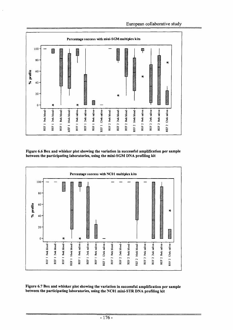
European collaborative study

Percentage success with mini-SGM multiplex kits

100 -

8 0 -

6 0 -< S ©fa.

^ 40'

2 0 '

0-

1

I II

1 *

§n

5f 1X>

1 12 13• i i f ■%00 <N o <N 00 'O

(N <Ntu

— u< U-UJ UJ U. UJ UJ UJ U-©4 o4 UJ

04 04 04 04 UJ04

1 -3I I

Figure 6.6 Box and whisker plot showing the variation in successful amplification per sample between the participating laboratories, using the mini-SGM DNA profiling kit

Percentage success with NC01 multiplex kits

1 0 0 -

8 0 -

± 6 0 -<Sofa.

^ 4 0 -

2 0 -

0-

f f t I I I t I f

Figure 6.7 Box and whisker plot showing the variation in successful amplification per sample between the participating laboratories, using the NC01 mini-STR DNA profiling kit

European collaborative study

6.3.4 Sample - sample variation

Due to variations between the different laboratories, results needed to be

standardised before all data could be used independently of lab effect. This was

carried out using Median polish analysis (Tukey 1977). Median polish analysis

used the residuals of the data to allow a normalised data set to be used for analysis

(Table 6.3), by transforming the data into residuals, analysis of variance became

applicable.

Reference Weeks Median polish values across laboratories (% profiles)ID degradation SGM+ Foren-SNPs Mini-SGM NC01 LCN SGM+

0 100 92 100 100 100^ T 3

2 2 82 80 100 100 100o

d 3 8 80 67 83 100 10016 2 19 56 50 910 100 93 100 100 1002 2 19 42 17 100

<u •—d 3 8 0 4 0 0 45

12 0 9 0 0 180 100 94 100 100 100

<N "O <+* 2 2 86 84 92 100 100<U Opi 3 8 82 66 85 100 82

16 59 57 58 100 730 100 95 100 100 100

<nt i—i . £ 2 9 19 33 33 100<D —d 3 8 0 28 67 67 100

12 0 19 0 0 91

Table 6.3 Percentage profiles obtained for each sample using data from all labs analysed by Median polish calculations.

The data for each sample type and individual is shown graphically (Figure 6.8).

As indicated by ANOVA tests (section 6.3.2), there was a significant difference in

the profiles gained for each sample type (p = <0.001). This would be expected

due to the different physiological characteristics of saliva and blood. DNA is

much more prone to degradation in saliva due to the presence of bacteria and

enzymes that can readily break down the DNA molecules.

-177-

European collaborative study

A) Ref. 1 Blood

100

1e.5?

16 180 2 6 8 10 12 144

Weeks degradation

C) Ref. 2 Blood

100

eIc .S?

0 2 6 8 10 12 14 16 184

Weeks degradation

B) Ref. 1 Saliva

100

1e.

100 2 4 6 8 12 14

Weeks degradation

D) Ref. 2 Saliva

100

1

0 2 8 104 6 12 14

■ SGM+

Mini-SGM

■NC01

■SNPs

LCN SGM+

Weeks degradation

Figure 6.8 Percentage profiles obtained across all labs for all samples and sample types. A) reference 1 blood B) reference 1 saliva C) reference 2 blood D) reference 2 saliva. Values were calculated using median polish analysis to standardise the data obtained from all laboratories.

The four degradation series demonstrated different levels of degradation over the

incubation period. The least degradation was seen in the reference 2 blood sample

which still gave >50% profile, using all four profiling techniques, after 16 weeks

degradation (Table 6.3). Reference 1 saliva showed the highest level of

degradation, with the percentage profile obtained for each system (excluding LCN

SGM+) dropping significantly after 2 weeks. LCN SGM+ continued to give a full

profile until 8 weeks degradation.

All multiplexes showed similar degradation patterns with a particular reference

and sample type but this pattern was not replicated between samples (Figure 6.8).

LCN SGM+ worked significantly better in three out of four samples, compared to

any other profiling method. The SGM+ profiling technique appeared to be the

least efficient method, with Foren-SNPs™ working less efficiently than the two mini-STR systems.

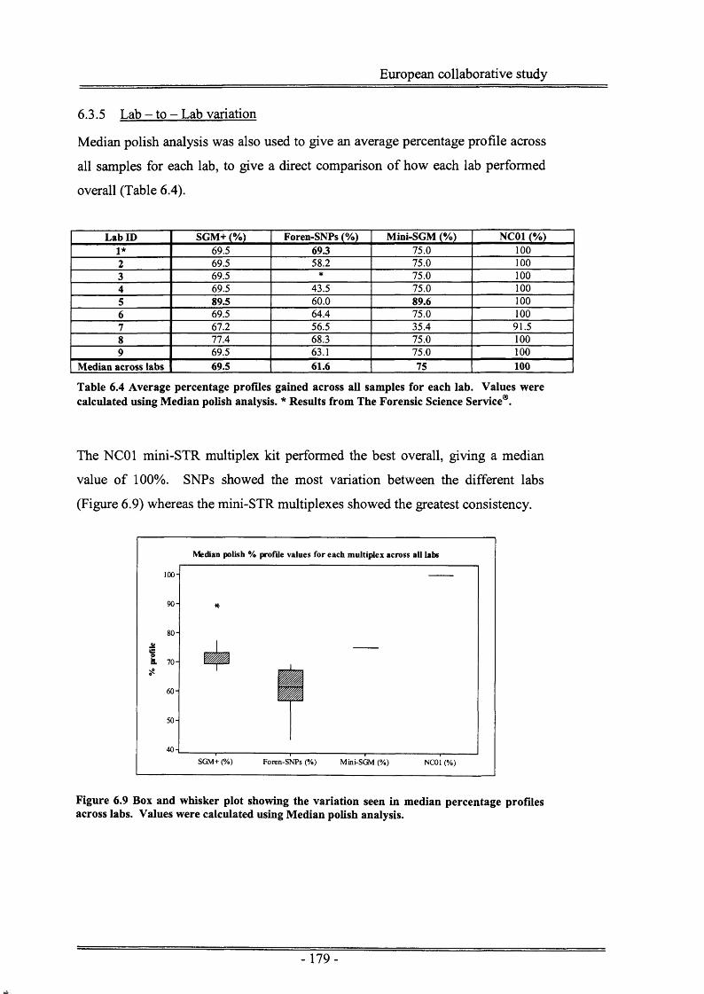
European collaborative study

6.3.5 Lab - to - Lab variation

Median polish analysis was also used to give an average percentage profile across

all samples for each lab, to give a direct comparison of how each lab performed

overall (Table 6.4).

Lab ID SGM+ (%) Foren-SNPs (%) Mini-SGM (%) NC01 (%)1* 69.5 69.3 75 .0 100

2 69.5 58 .2 7 5 .0 100

3 69.5 * 7 5 .0 1004 69.5 43 .5 75 .0 100

5 89.5 6 0 .0 89.6 1006 69.5 6 4 .4 7 5 .0 1007 6 7 .2 56.5 35 .4 9 1 .58 7 7 .4 68.3 75 .0 1009 69.5 63.1 75 .0 100

Median across labs 69.5 61.6 75 100

Table 6.4 Average percentage profiles gained across all samples for each lab. Values were calculated using Median polish analysis. * Results from The Forensic Science Service®.

The NC01 mini-STR multiplex kit performed the best overall, giving a median

value of 100%. SNPs showed the most variation between the different labs

(Figure 6.9) whereas the mini-STR multiplexes showed the greatest consistency.

Median polish % profile values for each multiplex across all labs

100 -

9 0 -

8 0 -

6 0 -

5 0 -

4 0 -

SGM+ (%) Foren-SNPs (%) NC01 (%)

Figure 6.9 Box and whisker plot showing the variation seen in median percentage profiles across labs. Values were calculated using Median polish analysis.

European collaborative study

6.3.6 Degradation patterns (allele dropout vs. amplicon size)

6.3.6.1 Total allele dropout in reference samples

Allele dropout was measured for each reference sample. Initial studies looked at

total dropout for each reference sample, regardless of degradation time (Figure

6.10 & 6.11). Regression analysis was used to assess the relationship between

amplicon size and the proportion of dropout seen.

Allele dropou t - r e f 1 blood sam p le s , all labs com bined

y - -0 0001* -*-0.2123

Allele dropout - re f 1 saliva samples, all labs combined

05

0.7

0.6

0.4

03

1000 50 150 200 250 300 400

y = 0.0002* ♦ 0.7059 y -0.0007x4-0.6617 amplicon • Lee 0.0017* ■ o.4«7o y 0.0004* - 0.6640r - 0.3377 . 0.0493 * &S224 **»0.1313

Figure 6.10 Allele dropout compared to amplicon size for reference 1 degraded blood and saliva samples. Proportion of allele dropout was calculated across the degradation set, regardless of incubation time.

Allele dropout - r e f 2 blood sam ples, all labs combined

■ SNPs

conjoined

0.4

Linear (SGM+)

Linear (mSTRs)

Linear (combined)

•^— Linear (SNPs)

amplicon size y * 0.0033a - 0.1788 y * 0.0003* ♦ 0.2119 R2 = 0.6333 R2 * 0.0273

Allele dropout - ref 2 saliva samples, all labs combined

« SGM+

a s n p s

combined

X mSTRs

Linear (SGM+)

Linear (combined)

Linear (mSTRs)

Linear (SNPs)

0 50 100 150 200 250 300 350 400

y O.OtKMx 0 5.'<33;. 2 am plicon »i/.eR? -0 .1 2 1 5 R* =0.0005 R; 0.4456 R? >0.1024

Figure 6.11 Allele dropout compared to amplicon size for reference 2 degraded blood and saliva samples. Proportion of allele dropout was calculated across the degradation set, regardless of incubation time.

Regression analysis displayed no relationship between the proportion of allele

dropout and amplicon size for any of the samples used, when looking at SNPs (R-

squared = 0.0005-0.0493). STRs and mini-STRs were evaluated both separately

and as a combined set. Initial studies using computer simulations (data not

shown) suggested a linear relationship between degradation and amplicon size,

but these were carried out regardless of the protection factor conferred by the

European collaborative study

nucleosome. The R-squared values for STRs varied between 0.1215 and 0.6181

compared to 0.4087 - 0.6333 for mini-STRs.

For each sample, all observed dropout for each multiplex was combined together

to observe whether all data followed the same regression. This data is indicated

by the red regression line in figures 6.10 & 6.11. The data became skewed due to

the SNP allele dropout data, which showed a random array of scatter points.

Figure 6.10 & 6.11 indicate a positive regression between amplicon size and

proportion of allele dropout, i.e. the proportion of alleles dropping out of the DNA

profile increases as the size of the amplicon increases. This is indicative of the

higher molecular weight amplicons degrading first.

-181 -

European collaborative study

6.3.6.2 Total allele dropout across degradation periods

Allele dropout was measured for each sample at each stage of degradation. The

regression scatters seen for reference 1 blood for each multiplex are shown

(Figure 6.12), data for other samples followed a similar pattern. All multiplexes

showed increasing dropout seen with degradation times with the exception of the

SNP data which appeared to be random and independent of amplicon size and was

the only multiplex that showed allele dropout in control samples (i.e. samples that

had not been subject to any degradation time). The slope of the regressions for

SGM+ appeared to decrease as the samples became more degraded. This

suggested more alleles at the low molecular weight end of the profile were

starting to drop out as the sample became more highly degraded, decreasing the

significance of the regression. The mini-STR systems appeared to show random

dropout with the less degraded samples. A positive regression was observed after

eight weeks degradation and this began to plateau at 16 weeks degradation,

similar to the SGM+ results.

- 182-

European collaborative study

Ref 1 SGM+ Blood time series

| 06 ‘ |§ 0.4 -

l o , -

A A

250 300150 200-0.2

amplicon size (bp)

♦ 0 weeks

■ 2 weeks

A 8 weeks

• 16 weeks

Linear (0 weeks)

“ “ Linear (8 weeks)

Linear (2 weeks)

^ “ Linear (16 weeks)

10.9 -

0.8 -

S 0.7

| 0.6

g 0.5

g. 0.4 2“■ 0.3

0.2

0.1

0

Ref 1 SNPs Blood time series

■ A •• • A

A *A • ■

A ■ •

«A 41___1

50 100 150 200 250 300

amplicon size (bp)

♦ 0 weeks

■ 2 weeks

A 8 weeks

• 16 weeks

Linear (0 weeks)

“ “ Linear (8 weeks)

Linear (2 weeks)

“ “ Linear (16 weeks)

350

Ref 1 Mini-STRs Blood time series

0.9 -

0.8 -

3 0 .7 j22 06 1•o •inouo

•1 , 0 .4 -

2 A , •O. 0.3 - •

0.2 - A A

0.1 -

0 -

♦ 0 w eeks

■ 2 weeks

A 8 w eeks

• 16 weeks

— L inear (0 w eeks)

“ “ L inear (8 w eeks)

L inear (2 w eeks)

^ “ L inear (16 w eeks)

50 100 150 200

amplicon size (bp)

250 300 350

Figure 6.12 Degradation time series plots for each multiplex. Graphs indicate the proportion of allele dropout seen compared to amplicon size for reference 1 blood samples. A) SGM+ profiles B) SNP multiplex profiles C) mini-STR profiles. NB. Mini-STR multiplexes (mini- SGM & NC01) were combined for the mini-STR analysis.

European collaborative study

6.4 Discussion

6.4.1 Sample degradation

Saliva samples showed the highest levels of degradation, with DNA percentage

profiles rapidly decreasing after just two weeks incubation. Saliva contains

numerous enzymes such as lysozymes, amylases, peroxidases and histatins; each

used for a different purpose such as the digestion of food, elimination of bacteria,

viruses and fungi, and the mineralisation of proteins (Benedek-Spat 1973a;

Benedek-Spat 1973b). These enzymes may have a knock-on effect of degrading

salivary DNA more rapidly than DNA found from other sample types. Saliva also

contains numerous bacteria that can have a detrimental effect on the amount of

DNA, as some bacteria are capable of engulfing DNA fragments present in

solution. Degradation of these samples was carried out at 37°C in 100%

humidity, an optimum temperature for many bacterial species. Due to these

factors it is not surprising that the DNA from the saliva showed rapid levels of

DNA degradation in this study.

The reference 2 12 weeks saliva sample was amplified successfully using LCN

SGM+ DNA profiling compared to the reference 1 12 weeks saliva sample that

failed to amplify by any method. This suggested that any DNA present in the

reference 1 DNA was either too degraded [fragmented] to be amplified using the

systems in this study or the DNA had been completely eliminated by bacterial and

enzyme activity. The DNA present in the reference 2 12 weeks saliva sample

must have been in low copy numbers and could only be amplified by the

additional amplification cycles given with LCN SGM+ profiling.

The two reference blood samples showed similar rates of degradation up to 8

weeks (SGM+ gave an 80% and 82% profile for reference 1 and 2 respectively,

using median polish analysis (Table 6.3)). After 8 weeks the reference 1

bloodstain degraded more rapidly, giving a variable success rate with the different

systems after 16 weeks (Figure 6.8A). The reference 2 bloodstain showed the

least degradation out of all four samples (Figure 6.8C).

-184-

European collaborative study

Blood is made up of three main cell types - red blood cells (erythrocytes), white

blood cells (leukocytes) and platelets (thrombocytes). Both the erythrocytes and

thrombocytes are anucleate in nature, therefore the DNA present in blood is

derived only from the leukocytes or free DNA in solution (Poste 1973). The

number of leukocytes present in an individual varies greatly, with the normal

range lying somewhere between 4,500 and 11,000 per cubic millimetre. The

number of cells can decrease during resting periods and increase during periods of

exercise (Nieman and Pedersen 1999) and, as leukocytes are involved in the

immune response, the number also increases if an individual has an infection or

suffers from allergies.

The number of cells present in the reference samples used in this study could

explain the variable degradation rates seen. The reference 2 individual may have

had a higher white blood cell count, meaning more cells were present in the stains

to begin with. The DNA degradation rate may have been the same for both sets of

stains, accounting for the similar results seen in the samples up to 8 weeks

degradation. After this point, the number of cells present in reference 1 would

have decreased to a low copy number level, decreasing the success rate of all

DNA profiling methods except for LCN SGM+ (Figure 6.8A). The number of

cells present in the reference 2 stains allowed standard DNA profiling techniques

to still attain >50% success rates after 16 weeks degradation.

6.4.2 Low copy number amplification

Using PCR simulations, it has been shown that a minimum of 25 molecules are

required to give a full SGM+ DNA profile using 28-cycle PCR (P Gill, per

comms). This number can be decreased to just one molecule by increasing the

number of amplification cycles from 28 to 34, i.e. performing low copy number

amplification parameters.

Further work simulating degradation of DNA fragments has shown that once

DNA starts to degrade, the number of molecules present decreases below the 25

molecules required for standard SGM+ profiling (Figure 6.13). These simulations

help understand why LCN SGM+ is more successful than any other method that

- 185 -

European collaborative study

uses 28 cycle PCR. Both mini-STR kits were amplified using 32 cycle PCR,

according to protocol, allowing both of these DNA profiling methods to work

routinely better than SGM+.

34 cycle sensitivity

5 10No. of surviving m olecules

300 base fragment P degradation =0 95 1r»g total DNA or 167 copies

28 cycle sensitivity

20

”

Figure 6.13 Graphical representation of the number of molecules seen when simulating the degradation of DNA.

The decrease in percentage profile seen with LCN SGM+ profiling after longer

periods of degradation indicate that the DNA in these instances had become

fragmented and the higher molecular weight STR loci failed to amplify.

6.4.3 Size of amplicons

All samples showed a pattern of proportion dropout similar to that shown for each

multiplex (Figure 6.12). The SNP loci showed a random dropout pattern,

indicating that success rates were independent of the amplicon length. The SNP

multiplex was designed with all PCR products below 146bp in length, to allow

amplification of degraded DNA. Dropout is most likely to have occurred as a

consequence of the multimix not being optimised, due to the number of loci

amplified in one reaction (Dixon et. al. 2005a), as opposed to the size of the

amplicons.

European collaborative study

Both mini-SGM and NC01 STR loci were analysed collectively as ‘mini-STRs’,

with a maximum amplicon size of 170bp. The SGM+ and mini-STR dropout

results showed a similar pattern whereby the higher molecular weight amplicons

were the first to drop out of the profile, giving a positive regression. The lower

molecular weight amplicons showed less dropout, until the samples became

highly degraded.

-187-

European collaborative study

6.5 Conclusion

A previous EDNAP study using DNA degraded by sonication and DNase I

(Schneider et. al. 2004), and other studies using degraded body fluid stains

(Wiegand and Kleiber 2001; Krenke et. al. 2002; Ohtaki et. al. 2002; Butler et. al.

2003; Chung et. al. 2004; Schumm et. al. 2004; Coble and Butler 2005; Butler

2005b) and telogen hair roots (Hellmann et. al. 2001), have demonstrated the

efficacy of low molecular weight amplicons to analyse degraded DNA. The

experiment described in this paper followed a different design to those previously

described, as it simulated a time-course series of stains degraded by in situ

enzymatic processes. This was achieved by incubating material spotted with

saliva and blood in 100% humidity at 37°C. Under these conditions, degradation

was greatly accelerated compared to the dried-state process and total degradation

was achieved within a short time-period of 12-16 weeks. By taking samples at

regular intervals, a complete time-course was produced and a point reached which

corresponded to the time where little or no amplifiable DNA remained. We

showed that saliva degraded faster than blood, but this is not surprising as this

body fluid contains enzymes such as lysozymes, amylases, peroxidases and

histatins, as well as numerous bacteria, which contribute nucleases, e.g.

Micrococcus sp. contribute micrococcal nuclease. Micrococcal nuclease is a non­

specific endonuclease, that cuts adjacent to any base, with the rate of cleavage

reported to be 30 times greater at the 5’ side of A or T rather than G or C

(fortunately most STR sequences tend to be GC-rich). Mammalian cells contain

two additional DNases that cleave non-specifically; DNase I, which slightly

favours purine-pyrimidine sequences (Staynov 2000) and DNase II, an enzyme

found in lysozomes associated with cell apoptosis (Yasuda et. al. 1998).

Median polish analysis was carried out in order to standardise the data, allowing

data sets from all laboratories to be compared regardless of variability in

laboratory techniques, operator differences and sampling limitations (Tukey

1977). Transformed data was analysed to investigate degradation rates, allele

dropout and performance of the four assays used in this study. The artificially

degraded samples gave similar results across all laboratories, showing the method

produced samples with consistent levels of degradation across all sets.

-188-

European collaborative study

The mini-STR assays tested gave the best results overall, when compared with

standard SGM+ profiling and the Foren-SNPs™ kit (Dixon et. al. 2005b). Low

copy number (LCN) DNA profiling proved to be the most successful method of

amplification, although this technique was only carried out by three laboratories;

one using Powerplex®16 and two using SGM+. LCN profiling only differs from

standard DNA profiling by the number of cycles used for PCR amplification

(Whitaker et. al. 2001). By increasing the number from 28 cycles to 34 cycles,

the chance of amplifying the few molecules present in the DNA extract is

improved. The mini-STR assays tested in this study used 32 cycles in PCR

amplification, making the method more consistent with LCN profiling (Butler et.

al. 2003; Drabek et. al. 2004; Coble and Butler 2005). As well as increased

cycles for amplification, the reduced amplicon size targeted with mini-STRs

allowed the more degraded (and therefore more fragmented) DNA samples to be

amplified with greater success. The mini-STR assays were also the most robust in

this study as the number of loci targeted was lower than the other DNA profiling

methods tested. NC01, giving the highest percentage profiles overall, only

contained three STR loci and therefore would generally have been easier to

optimise than the Foren-SNP™ multiplex containing 21 loci.

The Foren-SNP™ kit performed poorest out of the four assays tested in this study.

This particular kit was used as it was the only fully-validated forensic SNP

multiplex available (Dixon et. al. 2005a). Other SNP multiplexes have been

developed, but lack the quantitative and qualitative properties for forensic use

(Kwok 2001; Inagaki et. al. 2004; Budowle 2004b). SNP assays based on primer

extension biochemistry, such as GenomeLab™ SNP Stream® (Beckman Coulter)

and SNaPshot™ multiplex system (Applied Biosystems™), are capable of

genotyping thousands of SNPs in a single run but require an increased volume of

either initial DNA template or PCR product, both of which are limited in crime

scene samples. They also have the disadvantage of being multi-stage procedures,

with sample tubes needing to be opened at various stages within the process. The

Foren-SNPs™ kit allowed amplification of all 21 loci in a single tube reaction,

which were then analysed on an electrophoresis instrument. A more highly

optimised SNP multiplex system could give better results on degraded samples as

SNP loci do benefit from being single base sites allowing targeting of much

-189-

European collaborative study

smaller amplicons (Chakraborty et. al. 1999; Gill et. al. 2000a; Gill 2001a). The

ability to obtain a result using SNPs would be beneficial with discrete forensic

sample types, especially if the sample failed to give a profile using standard STR

DNA profiling, however the biallelic nature of SNPs makes it difficult to interpret

mixtures and a perfectly balanced assay would be required to make this feasible

(Gill 2001a). For these reasons, and to be consistent with current national DNA

databases, it would be preferable to use STRs for forensic identification as they

are more amenable to mixture interpretation and a high discrimination power can

be gained from fewer loci (Gill et. al. 2004a).

Degraded samples continue to be the most problematic for current forensic

profiling methods, in part because while it is ideal to maximize the amount of

information gleaned from the extracted DNA, it is imperative that any system be

robust for forensic application. The observed degradation pattern of high

molecular weight loci failing to amplify with increased levels of degradation has

been an enduring feature of this study, providing the incentive to produce a

system targeting the low molecular weight loci most likely to remain in higher

copy number in degraded samples. It is therefore proposed that any further

research into DNA profiling focuses on reducing the size of STR amplicons, such

that they can be more successfully amplified in degraded samples, as well as

supporting amplification under low copy number conditions (Dixon et. al. 2005b;

Gill et. al. 2006).

-190-

Casework Samples

Casework samples

7.1 Introduction

The first criminal case using DNA profiling for identification occurred in the UK

(http://www.forensic.gov.uk/forensic_t/inside/news/list_casefiles.php?case= 1). In

1983, a 15 year old schoolgirl, Lynda Mann, was found raped and murdered. A

semen sample taken from the body was found to belong to a person with type A

blood group and an enzyme profile matching 10% of the male population. With

no other forensic evidence available at the time, the murder enquiry was

suspended. Three years later another 15 year old, Dawn Ashworth, was found

strangled and sexually assaulted in the same area. Semen samples again showed a

suspect with type A blood and the same enzyme profile as the murderer of Lynda

Mann. In 1985, Jeffreys published a method of identification using DNA

‘fingerprints’ (Jeffreys et. al. 1985a; Jeffreys et. al. 1985b). Gill et. al. further

developed this work to allow DNA profiling of material for forensic use (Gill et.

al. 1985b). DNA profiling proved conclusively that the same person had killed

both girls and that the suspect who had admitted both of the murders could not

have been the murderer.

For the first time in criminal history “this suspect became the first person in the

world to be exonerated o f murder through the use o f DNA profiling>'>

(http://www.forensic.gov.uk/forensic_t/inside/news/list_casefiles.php?case=l).

The first DNA ‘mass screen’ was then carried out, to profile men in the local area

in the hope of finding the murderer. In 1988 Colin Pitchfork was sentenced to life

imprisonment after confessing to the murders of both girls.

Since these early cases of DNA being used as evidence, the technology and

sensitivity of the systems used for DNA profiling has rapidly evolved. The

current SGM+ system used for the National DNA Database® has a discrimination

power of one in 1000 million for unrelated individuals (Cotton et. al. 2000) and

can help prove beyond reasonable doubt that an individual is either guilty or

innocent of a crime (Gill 2002). The discrimination power of SGM+ is no more

than that found with earlier methods of VNTR DNA profiling. The technique has

proved more successful due to the increased sensitivity achieved by PCR

amplification, along with the ability to compare profiles within a database as the

precise size and locus of origin can be determined. In identification cases, DNA

Casework samples

profiling can be used to ascertain the likelihood of a sample belonging to the

individual in question, either through reference samples or through samples from

relatives (Jeffreys et. al. 1992; Gill et. al. 1994; Olaisen et. al. 1997; Crespillo et.

al. 2000; Holland et. al. 2003; Leclair et. al. 2004; Budowle et. al. 2005; Butler

2005b).

The 21-SNP multiplex was developed to use in situations where current DNA

profiling methods fail to produce a result, or only produce partial profiles due to

the degradation of the DNA. The current profiling method of choice with difficult

sample types is LCN SGM+ (Gill et. al. 2000b; Whitaker et. al. 2001; Gill 2001b;

Gill 2002), however the amplification of the high molecular weight loci >200bp in

length is hindered in highly degraded samples increasing the likelihood of gaining

a partial profile. LCN SGM+ profiling is also used routinely in casework samples

thought to contain minimal DNA due to the nature of the sample. The biological

make-up of the sample type may mean it contains very little DNA, for example,

bones and hair shafts; or there may only be a minimal amount of sample available

for testing (such as minute blood stains found at a crime scene).

As a final assessment of the 21-SNP multiplex, a number of casework samples

were profiled using the technique. These samples had previously been analysed

using LCN SGM+ DNA profiling methods and had either failed to amplify or had

only produced a partial STR profile.

The likelihood ratio (LR) is based on a comparison of two hypotheses - ‘what is

the probability that the suspect left the crime stain (Hp) against the probability that

the crime stain was left by a random, unrelated, individual (Hd)V. It is defined by

the following equation:

Where Pr(E|//p) is calculated from the probability of the crime sample and the

suspect sample matching given that the prosecution hypothesis is true, i.e. in

simple scenarios this is equal to 1. Pr(E|Hd) is the match probability calculation,

LR

-193 -

Casework samples

i.e. the probability of the profile given that the defence hypothesis is true. This is

the same as the probability of observing the profile in the general population.

All crime scene samples were compared to reference samples to assess the

likelihood of a sample coming from a suspected individual. Reference samples

were obtained from various sources such as a toothbrush head and saliva residue

of a pillow. Kinship analysis was used in some cases due to the lack of a

reference sample from the individual in question. Kinship analysis was carried

out using DNA from one or both parents. The LR values obtained in these cases

were lower than those gained when a reference sample from the suspected

individual was available but nonetheless allowed a value to be assigned to the

data.

- 194-

Casework samples

7.2 Materials & Methods

7.2.1 Casework DNA sample data

Sample DNA extracts from six different closed8 cases were supplied from The

Forensic Science Service® low copy number DNA profiling laboratory in

Wetherby (Table 7.1). DNA extracts consisted of both reference samples, taken

from items belonging to the deceased individual or buccal swabs from parents of

the deceased; and crime scene samples.

Case ID Casefile number Sample ID Sample type Sample origin

1 300205756 85933300 toothbrush head deceased individual

QE03.5043.1 blood crime scene

2 300100756 85298665 buccal mother o f deceased

85298678 buccal father o f deceased

QE03.3529.1 bone crime scene

3 300091460 84477900 buccal father o f deceased

85284421 buccal mother o f deceased

QE03.3074.1 bone crime scene

4 300110837 85287616 buccal father o f deceased

85287661 muscle crime scene

5 300065124 85276633 buccal mother o f deceased

85376643 blood crime scene

6 300227014 85160851 buccal mother

85160860 buccal father

85370230 saliva deceased individual

85369994 blood from hatchback car light crime scene

85407677 blood from towel crime scene

85407691 blood from circular saw crime scene

Table 7.1 Casework DNA sample data.

All DNA samples had been extracted using Chelex® methods (Walsh et. al. 1991)

and reference samples were quantified using Quantiblot® Human DNA

Quantitation kits (Cat. No. N808-0114) according to the manufacturer’s protocol.

Crime scene samples were assumed to be at low copy number levels and were

therefore not quantified.

8 A ‘closed’ case is one that has been taken through the criminal justice system and a verdict has been reached.

-195-

Casework samples

An SGM+ DNA profile had been obtained for each sample collected. Reference

samples from parents had been amplified using standard 28 cycle SGM+

parameters. Reference samples from the deceased individuals’ belongings and

crime scene samples had been amplified using 34 cycles LCN SGM+ DNA

profiling. Genotype data was supplied from the reporting officer casefiles. LCN

SGM+ results were run in duplicate and the resulting profile comprised a

consensus of the two amplifications. Only alleles appearing in both amplification

reactions were considered to be true alleles (Gill et. al. 2000b).

7.2.2 21-SNP multiplex DNA profiling

PCR amplification was carried out as described in chapter 3. All crime scene

DNA extracts were added at a maximum volume of 12 pL. Quant values were

used to estimate the amount of extract to add for the reference samples (Table

7.2).

PCR products were run on a capillary electrophoresis sequencer as described in

chapter 3. Results were analysed using AB Genescan™ and Genotyper™

software before being interpreted using Celestial™ software (chapter 4).

All genotype results for LCN SGM+ and the 21-SNP multiplex were analysed and

compared.

- 196-

Casework samples

Sample ID DNA quant value (ng/pL) Amount added to PCR reaction (max. 12pL)

85933300 0.04 12.0

QE03.5043.1 - 12.0

85298665 0.12 10.0

85298678 0.14 12.0

QE03.3529.1 - 12.0

84477900 0.50 2.0

85284421 0.90 1.0

QE03.3074.1 - 12.0

85287616 2.50 1.0

85287661 - 12.0

85276633 0.90 1.0

85376643 - 12.0

85160851 4.40 1.0 [ 1:4 dilution]

85160860 1.40 1.0

85370230 0.08 12.0

85369994 - 12.0

85407677 - 12.0

85407691 - 12.0

Table 7.2 DNA quantification values (ng/fiL) and PCR volumes for crime scene and reference samples.

7.2.3 Likelihood ratio calculations

Likelihood ratios (LRs) for crime scene samples compared to reference samples

for the deceased individuals were calculated using STRipe™ (in-house computer

program) for SGM+ profiles and Celestial™ for SNP profiles. Kinship analysis

was used for LR calculations where the reference samples were derived from the

parent/s of the deceased individual. LR values for SGM+ data were obtained

from the casefiles. These had been calculated using a commercially available

software package “Kinship” developed by Charles Brenner (Brenner 1997; Leclair

et. al 2004). The allele frequency arrays used for SNP kinship analyses are given

in appendices IX and X.

- 197-

Casework samples

7.3 Results

7.3.1 Case 1 - 300205756

The reference sample in this case (85933300) came from DNA extracted from the

head of a toothbrush found in the bathroom of the deceased’s living

accommodation. A low quantification value of 0.04ng/pL was obtained from the

DNA extract and a maximum volume of 20jiL had been added to the SGM+ PCR

reaction. PCR amplification was carried out at standard 28 cycle parameters and

was analysed accordingly (Table 7.3). A speck of blood found at the crime scene

was extracted (QE03.5043.1) and amplified using LCN SGM+ parameters.

Sample ID D3 VWA D16 D2 AM ELO D8 D21 D18 D19 THO FG A

REF 85933300 h r 14 16 18 12 13 17 22 X Y 12 15 29 30 13 15 14 14 9.3 9.3 20 21

QE03.5043.1a h r 14 16 18 12 13 17 22 X Y 12 15 29 30 (13) (15) (14) - 9.3 9.3 20 21

QE03.5043.1b U R 14 16 18 12 13 17 22 X Y 12 15 29 30 13 15 (14) - 9.3 9.3 20 21

QE03.5043.1 consensus h r 14 16 18 12 13 17 22 X Y 12 15 29 30 13 15 14 F 9.3 9.3 20 21

Table 7.3 SGM+ DNA profiling results for case 1 - 300205756. Designations in (brackets) indicate peaks with heights falling below 50rfu. An ‘F’ designation indicates a locus where only one peak was seen but allele dropout may have occurred due to the low peak height. ‘R’ designation indicates a rare allele.

Both extracts provided were amplified at maximum volumes with the 21-SNP

multiplex and genotyping results were run through Celestial™ to produce a SNP

profile (Table 7.4).

Sample ID Amelo D U6 B6 N4 Y3 P5 A4 0 6 Z2 K3 J2 Y6 P7 J8 X F G L2 W3 H8

REF 85933300 X/Y T/T T/T A/A T T G/G T T C/G A/F C/C C/C C/C F/A T/A A/A C/F C/F T/C T/F C/C T T

QE03.5043.1a X /Y T/T T/T A/A T/T G/G T/T C/G A/A C/C C/C C/C A/A T/A A/A C/C C/C T/C C/T C/C T/T

QE03.5043.1b X/Y T/T A/T? A/A T/T G/G T/T C/G A/A C/C C/C C/C A/A T/A A/A C/C C/C T/C C/T C/C T/T

QE03.5043.1 consensus X /Y T/T T/F A/A T T G/G T T C/G A/A C/C C/C C/C A/A T/A A/A C/C C/C T/C C T C/C T T

Table 7.4 21-SNP multiplex genotyping results for case 1 - 300205756. ‘F’ designations indicate peaks falling below the homozygote threshold calculated for that locus.

The resulting LRs for the two DNA profiling methods, calculated from

Pr(£|#JLR = —j—:---- r were 2.7E+11 (using STRipe™) and 1.25E+08 (usingPrlE \H d )

Celestial™) for SGM+ and SNPs respectively.

Casework samples

The reference sample gave 100% profile using SGM+ but this was decreased to

only 79% for the SNP profile. SGM+ amplification of the crime scene sample in

this case had generated a full profile except for one locus (D19), which showed a

peak below the homozygote threshold set for LCN interpretation. As well as this,

the individual demonstrated a rare allele at locus D3, greatly increasing the result

of the LR calculation. The 21-SNP multiplex also gave a full profile except for

one locus (U6) that had shown a minor heterozygous peak in one of the duplicate

PCR reactions, necessitating the use of an ‘F’ designation.

-199-

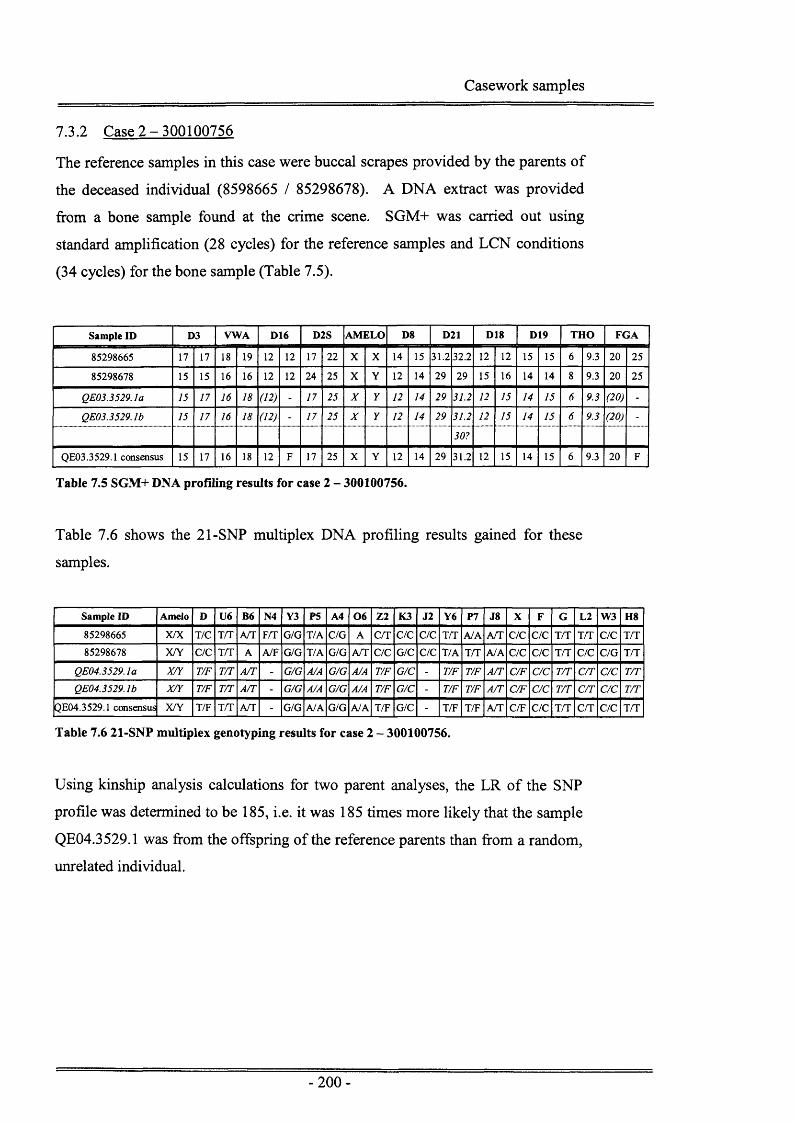
Casework samples

7.3.2 Case 2-300100756

The reference samples in this case were buccal scrapes provided by the parents of

the deceased individual (8598665 / 85298678). A DNA extract was provided

from a bone sample found at the crime scene. SGM+ was carried out using

standard amplification (28 cycles) for the reference samples and LCN conditions

(34 cycles) for the bone sample (Table 7.5).

Sample ID D3 VWA D16 D2S AM ELO D8 D21 D18 D19 THO FGA

85298665 17 17 18 19 12 12 17 22 X X 14 15 31.2 32.2 12 12 15 15 6 9.3 20 25

85298678 15 15 16 16 12 12 24 25 X Y 12 14 29 29 15 16 14 14 8 9.3 20 25

QE03.3529.1a 15 17 16 18 (12) - 17 25 X Y 12 14 29 31.2 12 15 14 15 6 9.3 (20) -

QE03.3529.1b 15 17 16 18 (12) - 17 25 X Y 12 14 29 31.2 12 15 14 15 6 9.3 (20) -

30?

QE03.3529.1 consensus 15 17 16 18 12 F 17 25 X Y 12 14 29 31.2 12 15 14 15 6 9.3 20 F

Table 7.5 SGM+ DNA profiling results for case 2 - 300100756.

Table 7.6 shows the 21-SNP multiplex DNA profiling results gained for these

samples.

Sample ID Amelo D U6 B6 N4 Y3 P5 A4 0 6 Z2 K3 J2 Y6 P7 J8 X F G L2 W3 H8

85298665 X/X T/C T/T ATT FT- G/G T/A C/G A C/T C/C C/C T/T A/A A T C/C C/C T/T T/T C/C T/T

85298678 X/Y C/C T/T A A/F G/G T/A G/G A/T C/C G/C C/C T/A T/T AJA C/C C/C T/T C/C C/G T/T

QE04.3529. la X/Y T/F T/T A/T - G/G A/A G/G A/A T/F G/C - T/F T/F A/T C/F C/C T/T C/T C/C T/t

QE04.3529.1b X/Y T/F T/T A/T - G/G A/A G/G AJA T/F G/C - T/F T/F A/T C/F C/C T/T C/T C/C T/T

QE04.3529.1 consensus X/Y T/F T/T M l - G/G A/A G/G A/A T/F G/C - T/F T/F ATT C/F C/C T/T C/T C/C T/T

Table 7.6 21-SNP multiplex genotyping results for case 2 - 300100756.

Using kinship analysis calculations for two parent analyses, the LR of the SNP

profile was determined to be 185, i.e. it was 185 times more likely that the sample

QE04.3 529.1 was from the offspring of the reference parents than from a random,

unrelated individual.

-200-

Casework samples

7.3.3 Case 3-300091460

As with case 2, case 3 reference samples were derived from the parents of the

deceased (84477900 / 85284421) and the crime scene sample had been extracted

from a piece of bone (QE03.3074.1). Results for SGM+ profiling were obtained

from the casefile (Table 7.7), using 28 cycles for reference samples and 34 cycle

amplification for the crime sample.

Sam ple ID D3 VW A D16 D2S AM ELO D8 D 2I D18 D19 THO F<;a

85294421 15 16 15 15 12 12 17 23 X X 13 13 30 30 12 14 14 15.2 7 9 20 23

84477900 15 17 15 19 9 12 20 25 X Y 10 14 30 30 15 20 15 15 7 9.3 22 23

QE03.3074.1a 15 17 15 15 12 12 23 25 X Y 10 13 30 30 14 15 15 15.2 7 9.3 22 23

QE03.3074.1b 15 17 15 15 12 12 23 25 X Y 10 13 30 30 14 15 15 15.2 7 9.3 22 23

31

QE03.3074.1 consensus 15 17 15 15 12 12 23 25 X Y 10 13 30 30 14 15 15 15.2 7 9.3 22 23

Table 7.7 SGM+ DNA profiling results for case 3 - 300091460.

All three DNA extracts were amplified using the 21-SNP multiplex (Table 7.8).

Sample ID Amelo D U6 B6 N4 Y3 P5 A4 0 6 Z2 K3 J2 Y6 P7 J8 X F G L2 W3 H8

84477900 X/Y T/C A/T A/T - G/G T/A C/C A T C T C/C T T T/A T T A/A C/C C/C T T C/C C/G T T

85284421 X/F T/C T/T A/T - G/C T/T C/C A/A T T G/C - T T T T A/A C/C C/A T T C/C G/G T T

QE04.3074.1a X /Y T/C T/T T/F - G/C T/T C/C A/T T/T C/C - T/A T/F A/A - - T/T C/C G/F T/T

QE04.3074.1b X/Y T/C T/T T/T - G/C T/T C/C A /T T/T C /C - T/A T/T A/A - - T/F C/F G/G T/T

QE04.3074.1 consensus X/Y T/C T/T T/F - G/C T T C/C A T T T C/C - T/A T/F A/A - - T/F C/F G/F T T

Table 7.8 21-SNP multiplex genotyping results for case 3 - 300091460.

Using kinship analysis calculations, the LR of the SNP profile was determined to

be 42, i.e. it was 42 times more likely that the sample QE04.3074.1 was from the

offspring of the reference parents than from a random, unrelated individual.

-201 -

Casework samples

7.3.4 Case 4 -300110837

The father of the deceased individual had provided a single reference sample in

this case (85287616). The crime scene DNA extract was submitted from a section

of deep muscle (85287661). SGM+ DNA profiles (28 cycles for the reference and

34 cycles for the crime sample) were provided from the casefile (Table 7.9) and

21-SNP multiplex results were collated (Table 7.10). Only one LCN SGM+

profile was obtained for the muscle sample, rather than the customary duplicate

profiles.

Sample ID D3 VW A D16 D2 AM ELO D8 D 21 D 18 D 19 T l IO FC;a

REF 85287616 15 15 18 18 11 13 17 19 X Y 14 14 31 32.2 13 18 13 15 7 9.3 22 23

85287661 15 19 X Y 8? 13 14 7 (9.3) - -

Table 7.9 SGM+ DNA profiling results for case 4 - 300110837.

Sample ID Amelo D U6 B6 N4 Y3 P5 A4 0 6 Z2 K3 J2 Y6 P7 J8 X F G L2 W3 H8

REF 85287616 X/Y C/C A/A T/F A/F G/C T/A C/C T/T C/T G/G C/F T/T T/T A/T C/C C/C T/T C/C C/C T/T

85287661. la X /Y T/C A/A - - G/C T/T C/F - C/C G /C C/C T/F T/F - C/C C/C T/T C/C - T/T

85287661.1b X /Y T/C A/A - - G/C T/T C/C - C/C G/C C/F T/T T/T - C/C C/C T/T C/C - T/T

85287661 consensus X /Y T/C A/A - - G/C T/T C/F - C/C G/C C/F T/F T/F - C/C C/C T/T C/C - T/T

Table 7.10 21-SNP multiplex genotyping results for case 4 - 300110837.

Using kinship analysis for a single parent comparison, the LR of the SNP profile

was determined to be 719, i.e. it was 719 times more likely that the sample

85287661 was from the offspring of the reference parents than from a random,

unrelated individual.

-202-

Casework samples

7.3.5 Case 5-300065124

The mother of the deceased individual provided the reference sample in this case

(85276633). The questioned DNA extract came from a bloodstain found at the

suspected crime scene (85376643). SGM+ DNA profiling results were given in

the casefile (Table 7.11), using 28 cycles amplification for the reference sample

and 34 cycles for the crime sample.

Sample ID D3 VW A D16 D2S AM ELO D8 D21 D18 D19 TH O FGA

REF 85276633 15 16 17 18 11 12 19 20 X X 10 13 30 30 13 14 15 15 6 8 22.2 24

85276643.1a 15 15 18 18 12 13 19 19 X Y 10 14 30 30 13 14 13 15 8 9.3 24 25

85276643.1b 15 15 18 18 12 13 19 19 X Y 10 14 30 30 13 14 13 15 8 9.3 24 25

85276643 consensus 15 15 18 18 12 13 19 19 X Y 10 14 30 30 13 14 13 15 8 9.3 24 25

Table 7.11 SGM+ DNA profiling results for case 5 - 300065124.

Both DNA extracts were genotyped using the 21-SNP multiplex, the crime scene

extract being run in duplicate (Table 7.12).

Sample ID Amelo D U6 B6 N4 Y3 P5 A4 06 Z2 K3 J2 Y6 P7 J8 X F G L2 W3 H8

85276633 X/F C/C A/T - - G/G T/T C/C A/A e r r C/C C/C T/A T/A A/T C/C C/A T/C C/C C/C ATT

85376643.1a X /Y C/C A/A A/A - G/G T/T - A/A T/T - C/C - A/A T/T C/C C/A T/C C/C C/C T/T

85376643.1b X /Y C/C A/A A/A A/A G/G T/T C/G A/A T/T G/C C /C T/A A/A T/T C/C C/A T/C C/C C/C T/T

85376643 consensus XJY C/C A/A A/A - G/G T/T - A/A T/T - C/C - A/A T/T C/C C/A T/C C/C C/C T/T

Table 7.12 21-SNP multiplex genotyping results for case 5 - 300065124.

Kinship analysis, using formulae for one parent, was carried out on the consensus

SNP profile and an LR of 82 was calculated, i.e. it was 82 times more likely that

the sample 85376643 was from the offspring of the reference parent than from a

random, unrelated individual.

-203 -

Casework samples

7.3.6 Case 6-300227014

Reference samples were obtained from both parents of the deceased individual

(85160851 / 85160860) as well as a saliva sample taken from a pillowcase in the

deceased individuals’ house. DNA had been extracted from bloodstains acquired

from three individual crime scenes. These had been found on a hatchback light

(85369994), a towel (85407677) and a circular saw (85407691). Only one LCN

SGM+ DNA profile was submitted from each crime scene sample, instead of the

standard duplicate profiles (Table 7.13). All six DNA extracts were amplified

using the 21-SNP multiplex, crime scene samples being run in duplicate (Table

7.14).

Sample ID D3 VW A D16 D2S AM ELO D8 D21 D18 D19 THO FGA

REF 85160851 16 16 16 20 10 13 19 25 X X 10 14 31.2 31.2 16 16 14 15 7 9 20 23

REF 85160860 15 16 14 18 8 8 25 25 X Y 13 16 32.2 32.2 16 18 13 16 6 9 22 23

REF 85370230 15 16 18 20 8 10 19 25 X Y 14 16 31.2 32.2 16 18 13 14 9 9 22 23

85369994 15 16 18 20 8 10 - - X Y 14 16 - - - - 13 14 9 F - -

85407677 15 16 18 20 8 10 - - X Y 14 16 - - - - 13 14 9 9 - -

85407691 15 16 18 20 8 10 - - X Y 14 16 31.2 F - - 13 14 9 F 22 23

Table 7.13 SGM+ DNA profiling results for case 6 - 300227014.

Sample ID Amelo D U6 6 6 N4 Y3 P5 A4 0 6 Z2 K3 J2 Y6 P7 J8 X F G L2 W3 H8

REF 85160851 X/F C T T - G T C A C G/C C/T T/A T A A C T C C/G T

REF 85160860 X /Y T/C A/T A/A - G T C/G A/T C/T C T T/A T/A A/T C/A C T C C T

REF 85370230 X /Y C A/T A/T - G T C A/T C/T G/C T T/A T A/T A c T c C/G T

85369994.1a X /Y - A/F - - G T C/F - C/T G/C F/T T/F T A/T A - T/F C/F - -

85369994.1b X/Y - A/F - - G T C/F - C/T G/C F/T T/F T A/T A - T/F C/F - -

85369994 consensus X/Y - A/F - - G T C/F - C/T G/C F/T T/F T A/T A - T/F C/F - -

85407677.1a X/Y c A/T T/F A/F G T C A/T C/T G/C F/T T/A T A/T A c T C C/G T

85407677.1b X/Y c A/T T/F A/F G T c A/T C/T G/C F/T T/A T A/T A c T c C/G T

85407677 consensus X/Y c A/T T/F A/F G T c ATT C/T G/C F/T T/A T A/T A c T c C/G T

85407691.1a

85407691.1b

85407691 consensus

Table 7.14 21-SNP multiplex genotyping results for case 6 - 300227014.

-204-

Casework samples

STRipe™ was used to calculate an LR for the SGM+ crime scene profiles

compared to the reference saliva sample, using the formula:

The samples gave LRs of 2.9E+07, 2.15E+08 and 2.03E+09 for the bloodstain off

the car light, the blood from the towel and the blood from the circular saw

respectively. An LR was calculated in Celestial™ for each SNP consensus profile

compared to the reference saliva sample obtained in this case. The bloodstain

from the hatchback light gave an LR of 1.21E+05 and the bloodstain from the

towel gave an LR of 4.29E+07. The stain collected from the circular saw failed to

produce a profile in either of the duplicate SNP amplifications.

Kinship analysis was used for evaluating the strength of the evidence given the

SNP parental data. An LR of 131,579 was obtained from the hatchback light.

This LR had been greatly increased by the presence of a rare homozygous T/T

genotype at locus J2. The sample from the hatchback light gave an LR of 28 and

the towel sample gave an LR of 3333. The rare allele in these cases had fallen

below the homozygous threshold and was subsequently labelled with an ‘F’

designation, greatly decreasing the LR for that locus.

LR

-205-

Casework samples

7.3.7 Comparison of percentage profiles and match probabilities

The percentage profiles and LR data for each crime scene sample was calculated

using either kinship analysis (Table 7.15a) or allele frequency data (Table 7.15b).

This allowed all profiles to be compared to each other, regardless of statistical

calculations relating to identity. These results are shown graphically (Figure 7.1).

Case ID Sample ID Sample type SGM + % profile LR (SGM +) SNPs % profile LR (SNPs)

300100756 QE03.3529 cons Bone 91 3.00E+08 79 185300091460 QE03.3074 cons Bone 100 1.00E+09 69 41.7300110837 85287661 cons Muscle 36 4.00 67 714300065124 85276643 cons Blood stain 100 6670 81 83.3300227014 85369994 Blood stain 59 8.00E+06 52* 27.8

“ 85407677 Blood stain 64 5.32E+07 93* 3330“ 85407691 Blood stain 73 2.03E+09 - -

Table 7.15a Percentage profiles and LR data for casework crime scene samples, using kinship analysis. * indicates SNP profiles obtained from two duplicate amplifications when SGM+ was only obtained from one amplification.

Case ID Sam ple ID Sample type SGM + % profile

LR (SGM +) SNPs % profile LR (SNPs)

300205756 QE03.5043 cons Blood stain 95 2.70E +11 98 1.25E+08300227014 85369994 Blood stain 59 2.90E+07 52* 1.21E+05

85407677 Blood stain 64 2.15E+08 93* 4.29E-+0785407691 Blood stain 73 2.03E+09 - -

Table 7.15b Percentage profiles and LR data for casework crime scene samples, based on allele frequency data. * indicates SNP profiles obtained from two duplicate amplifications when SGM+ was only obtained from one amplification.

Three out of eight crime scene samples gave an increased percentage profile when

amplified using the 21-SNP multiplex. One sample (85407691) failed to amplify

using SNPs, in either of the duplicate PCR reactions; therefore five samples gave

increased percentage profiles using LCN SGM+ amplification.

The interpretation criteria used for SNPs were very stringent due to the high

sensitivity of the technique (chapter 4). The percentage profiles obtained were

lower for SNPs due to the presence of more ‘F’ designations in the genotypes.

The ‘F’ designations were also detrimental to the calculation of the LR as an ‘F’

could have indicated either a homozygous or heterozygous locus, decreasing the

power of the result.

Casework samples

Percentage profile data obtained for crime scene samplesSGM+ % profile

SNPs % profile

Blood stain

QE03.5043

Bone Bone Muscle Blood stain Blood stain Blood stain

QE03.3529 QE03.3074 85287661 85276643 8536994 i 85407677

Blood stain

85407691

Figure 7.1 Percentage profile data obtained for crime scene casework samples using LCN SGM+ DNA profiling and the 21-SNP multiplex.

The amount of DNA extract added to the 21-SNP multiplex PCR reactions was

12pL. LCN SGM+ profiling routinely uses a maximum volume of 20pL. At

LCN levels the amount of stochastic variation seen within a DNA extract is high

and it is essential to add as much extract as possible to the PCR reaction to

increase the likelihood of amplifying the few molecules that are present. The

decreased amount of extract added for SNP amplification could have contributed

to the lower success rate seen with the technique.

LR data was shown to be highly variable across the set of casework samples

(Figure 7.2). An increased likelihood ratio was seen in cases where reference

DNA samples were provided, as opposed to parent DNA samples. The use of

kinship analysis allowed an LR to be gained in the absence of a reference DNA

profile (Balding and Nichols 1994; Brenner 1997; Leclair et. al. 2004). LR values

from kinship analysis varied from 42 to more than 130,000, dependent on the

percentage profiles seen and the genotype data obtained.

Casework samples

L ik e lih o o d ra tio (LR) data o b ta in e d for cr im e sc e n e sa m p le s

1.00E+12

1.00E + 11

1.00E +10

1.00E+09

1.00E+08

„ 1.00E+0735 1.00E +06

-3 1.00E+05

1.00E +04

1.00E+03

1.00E+02

1.00E+01

1.00E+00

LR (SGM+)

■ LR (SNPs)

Bone Muscle B loodsta in B loodsta in B loodsta in B loodsta in Blood s ta in B loodsta in Blood stain

QE03.3074 85287661 85276643 QE03.5043 8536994 8536994 85407677 85407677 85407691

(re f) (p a re n ts ) ( re f) (p a ren ts ) (re f)

8S407691( p a r e n t s )

sa m p le ID

Figure 7.2 LR data obtained from a comparison of the genotype data gained for each crime scene sample.

In case 300227014, LR values were 10-fold higher using reference sample DNA

profiles for comparison to the crime scene sample, as opposed to parent profiles.

The 21-SNP multiplex LR values in this case were higher than that generally

estimated for SNP analysis (4.5 million) due to the presence of a rare allele at

locus TSCO J8. This increased the LR to 1 in 43 million, even though the profile

obtained was incomplete (93%).

Overall, only one crime scene sample (85287661) showed an increased LR value

when using the 21-SNP multiplex compared to LCN SGM+ profiling. The DNA

extract in this case was obtained from muscle and was the only example of this

sample type tested. Muscle is known to degrade at a faster rate than other body

tissues after death has occurred due to the enzymes and chemicals present in

muscle cells (Johnson and Ferris 2002). The increased success at profiling this

sample type (67% SNP profile compared to 36% LCN SGM+ profile) using SNPs

was suggestive of an increased amplification efficiency using the smaller target

sites. A much larger sample set would need to be tested to clarify this

observation.

-208-

Casework samples

7.3.8 Allele dropout compared to amplicon size

All crime scene samples were analysed to give an indication of the size of the

amplicons failing to amplify, using both SNPs and SGM+. Not all STR allele

designations were known due to reference samples coming from parents, and

therefore an assumption had to be made concerning the size of the amplicons

failing amplification. An average size was used for each STR locus to allow

analysis across the set of samples9.

Proportion of allele dropout against size of the amplicon for SNPs andSTRs

♦ SNPs dropout

■ SGM+ average dropout

Linear (SNPs dropout)

Linear (SGM+ average dropout)♦

fi. 0.1

R2 = 2E-05 R2 = 0.7712

0.2 -

Amplicon size (bp)

Figure 7.3 Scattergraph showing the proportion of allele dropout seen relative to the size of the target amplicon, using both the 21-SNP multiplex and LCN SGM+ DNA profiling.

The 21-SNP multiplex showed no relationship between the proportion of allele

dropout compared to amplicon size (R2 = 2.0E-05), an observation also seen in the

artificially degraded samples previously genotyped using the technique (chapter

3). R-squared analysis indicated a positive regression when looking at STR allele

dropout against amplicon size (R2=0.7712). The graph clearly shows an increase

in the amount of dropout seen with the higher molecular weight STR loci (Figure

7.3).

9 A verage STR locus size: Am elo 105bp; D19 118bp; D3 126bp; D8 146bp; vW A 180bp; THO 183bp; D21 212bp; FGA 240bp; D 16 249bp; D18 300bp; D2 318bp.

-209-

Casework samples

The pattern of dropout observed for the crime scene LCN samples ties in with the

observations seen for artificially degraded samples. This has a two-fold effect in

that it strengthens the use of artificially degraded samples as a validation of DNA

profiling techniques in the research environment, as well as allowing a study of

the process of DNA degradation in general.

-210-

Casework samples

7.4 Discussion

Six sets of casework samples were received from The Forensic Science Service®

laboratory in Wetherby. DNA extracts from reference samples and crime scene

samples were provided for amplification using the 21-SNP multiplex, to supply

enough information for a comparative study using SNPs and LCN SGM+

profiling.

Reference samples were obtained from either articles pertaining to the deceased

individual, from both parents of the deceased, or from an individual parent. Each

of these reference samples could be used as a comparison to the crime scene

sample(s) obtained, yielding an LR value. Individually STRs are more

discriminating than SNPs, due to their polymorphic nature; therefore a partial

SGM+ profile would give a higher LR than a full or partial SNP profile. This

study proved this observation with LCN SGM+ giving higher match probabilities

for all samples bar one, even when only two or three STR loci were successfully

amplified.

The 21-SNP multiplex gave a higher percentage profile and LR value for one

sample tested. This DNA extract came from a muscle sample and indicated the

need to define the degradation process within different sample types in more

detail to give a more educated rationale behind the choice of DNA profiling

technique to use to gain the best result.

DNA profiling using STRs is highly discriminating and is highly successful in

identifying individuals from biological samples. The National DNA Database®

currently holds over three million samples from both crime scenes and from

individuals arrested for crimes. In 2004 individual samples on the database

provided matches with more than 41,000 crime scenes and linked a further 4,500.

Problems are encountered when the biological samples from which the DNA is

obtained for profiling are compromised in some way, either by degradation or by

the nature of the sample type. Bones, teeth and hair shaft contain limited amounts

of nuclear DNA, making STR profiling difficult. Degraded DNA is fragmented,

-211 -

Casework samples

meaning the larger STR loci may fail to amplify in the PCR reaction, leading to

partial DNA profiles being obtained.

Current methods for obtaining DNA profiles from compromised sample types

include low copy number DNA profiling, whereby the number of amplification

cycles is increased to target the smaller number of molecules available (Gill et. al.

2000b); and mitochondrial DNA profiling, targeting the increased number of

mitochondria present in remaining cells (Butler and Levin 1998; Holland and

Parsons 1999). Both of these methods require specialised techniques for analysis

and suffer from sensitivity issues, meaning there is an increased chance of

contamination being encountered. Mitochondrial DNA has a decreased

discrimination power due to the maternal lineage of the DNA and is incompatible

with current DNA databases, however it can be used for intelligence purposes

with a high degree of success. LCN DNA profiling has become the preferred

method of amplification for compromised samples with strict guidelines for

interpretation of profiles, including duplicate amplifications and the generation of

consensus profiles, allowing a result to be gained in samples which would

previously have failed to amplify (Gill et. al. 2000b). Although routinely used in

casework in the UK, LCN SGM+ profiling has not been readily accepted by the

European and US community. Problems with contamination and the ability to

profile trace amounts of DNA has led to the possibility of innocent transfer

events, e.g. primary and secondary transfer from holding hands or objects, giving

a false positive result (Gill 2002; Lowe et. al. 2002; Butler 2005b).

The results of the casework comparative study suggested that LCN DNA profiling

was more successful than SNPs, mainly due to the higher discrimination power

gained from fewer STR loci. The 21-SNP multiplex failed to give a result for

some casework samples and only gave partial profiles for others. Samples had

previously been stored frozen and there was a variable time lapse between the

LCN DNA profiling and the 21-SNP multiplex amplification. This may have

made a difference to the integrity of the sample and periods of freeze-thawing and

transit of the samples via the mail system may have caused further degradation of

the DNA. The samples had been extracted using Chelex® (Walsh et. al. 1991)

and this may have caused inhibition of the PCR amplification as it is known to

-212-

Casework samples

interact with the Taq polymerase, causing a decrease in amplification efficiency.

The complexity of the 21-SNP multiplex may have made it more sensitive to PCR

inhibition by the Chelex® particles.

Analysis of allele dropout for both SNPs and STRs indicated that SNPs showed a

random pattern of dropout consistent with amplification inefficiency as opposed

to the size of the amplicon. The STR loci showed a positive regression with the

higher molecular weight loci. This result is consistent with the other studies on

amplicon size carried out in this thesis and suggests that targeting smaller size

DNA molecules could result in a greater chance of amplifying degraded DNA

molecules, given an optimised multiplex system.

General Discussion

General Discussion

DNA profiling was first used in criminology in 1986 and, once accepted in court,

quickly became established worldwide as a technique for human identification.

Today, DNA profiling systems used for national DNA databases utilise

polymorphic short tandem repeat (STR) sequences to gain a DNA profile of an

individual. The most significant problem facing the forensic analyst in general

casework is that approximately 50% of crime scene samples yield a partial DNA

profile or no profile at all (P. Gill, per comms). This is often the result of the

material being highly degraded and limited in quantity; consequently insufficient

intact DNA molecules are available for profiling using the current multiplex

systems. The resulting discriminating power of a partial profile may only be of

the order of one in thousands to one in a million and when such profiles are used

to interrogate national DNA databases, multiple matches may be found (Butler

2005b).

The effect of DNA degradation in forensic DNA profiling is most apparent in

mass disaster situations, such as fires (Clayton et. al. 1995a), air crashes

(Ballantyne 1997), terrorist attacks (Holland et. al. 2003), tsunamis and

earthquakes (Alonso et. al. 2005). Dependent on the type of disaster, victims will

have been subjected to a wide range of extreme conditions including ultra-high

temperatures and high levels of humidity, causing degradation of the DNA

molecules. Partial profiles obtained from degraded DNA samples consist mainly

of the STR loci with lower amplicon sizes (Golenberg et. al. 1996; Wiegand and

Kleiber 2001; Butler et. al. 2003; Gill et. al. 2006) making it increasingly difficult

to obtain a DNA profile that can be successfully used for identification purposes.

Research was carried out into the use of single nucleotide polymorphisms (SNPs)

as a possible adjunct to current DNA profiling systems. Autosomal SNP analysis

had been dismissed from high-throughput DNA profiling in the early 1990s in

favour of STRs, as STR loci were more amenable (at that time) to automated

techniques (P. Gill, per comms). Specialist techniques were developed for some

specific SNP applications, including mitochondrial (Hagelberg et. al. 1991;

Holland et. al. 1993; Gill et. al. 1994; Butler and Levin 1998; Holland and

Parsons 1999), Y-chromosome (Di Gaetano et. al. 2004; Hammer et. al. 2005;

Lessig et. al. 2005; Brion 2005a; Brion et. al. 2005b) and red hair SNP analysis

-215-

General Discussion

(Grimes et. al. 2001). Before the introduction of low copy number (LCN) STR

profiling, mitochondrial DNA (mtDNA) analysis was routinely used for

genotyping degraded samples and samples containing little DNA, such as bone,

hair and teeth. Mitochondria are present within cells in high copy number

(approximately 500-2000 per cell (Parsons and Coble 2001)), hence mtDNA is

more likely to survive intact for longer periods. This has made mtDNA analysis

the primary method of genotyping ancient DNA samples (Cooper et. al. 2001; von

Wurmb-Schwark et. al. 2003; Willerslev and Cooper 2005), although the

technique is highly sensitive and results are not always distinguishable from

contamination. MtDNA is maternally inherited; therefore all offspring of a

female will have the same mtDNA sequence, making it less discriminating than

STRs for forensic DNA analysis. Current mtDNA analysis involves complete

sequence determination of two hypervariable regions (HV1 and HV2) within the

mitochondrial control region. The control region is the only significant portion of

mtDNA that doesn’t encode for genes (Parsons and Coble 2001) and, as such,

shows high variation within the population. Full sequencing of mtDNA is labour-

intensive and attempts have been made to develop techniques that are less time-

consuming such as mini-sequencing (Tully et. al. 1996; Quintans et. al. 2004) and

other primer extension assays (Vallone et. al. 2004; Divne and Allen 2005).

Mini-sequencing was also used to develop an analysis method for identification of

hair colour, targeting twelve known SNP loci within the melanocortin 1 receptor

gene (MC1R) (Grimes et. al. 2001). Homozygosity at a locus, or compound

heterozygosity at two loci, was used as an indicator that an individual would have

red hair. Although it is difficult to identify any individual gene for a physical

characteristic, further research is ongoing into the use of SNPs for other physical

traits, such as iris colour (Frudakis et. al. 2003) and skin colour (Bonilla et. al.

2005). Y-chromosome SNPs have been used for determination of ethnicity, using

allele-hybridisation biochemistry in a commercially available kit, “Signet™ Y-

SNP” (Marligen Biosciences Inc.). PCR products are detected by hybridisation to

colour-coded beads using the Luminex®100™ System (Taylor et. al. 2001;

Wetton et. al. 2005). The Y-chromosome is particularly useful as an indicator of

ancestral origin due to the lack of recombination along the majority of the

chromosome. This has resulted in “an accumulation o f mutations in slowly

evolving SNP haplogroups that reflect the progressive diversification o f Y

General Discussion

chromosome lineages during the expansion o f human populations” (Wetton et. al.

2005). As with autosomal loci, STR sequences within the Y-chromosome have an

increased discrimination power to SNPs, and these have been more widely

researched and developed for forensic use in recent years (Corach et. al. 2001;

Hall and Ballantyne 2003; Daniels et. al. 2004; Hanson and Ballantyne 2004;

Mulero et. al. 2006).

The development of microarray technology re-introduced autosomal non-coding

SNPs into the forensic field, as the possibility of high-throughput genotyping was

realised (Southern 1996a; Southern 1996b). This development coincided with the

introduction of the National DNA Database® in 1995. Not all samples

successfully amplified by standard DNA profiling methods, due to degradation

and/or low DNA copy number. SNP loci comprise one base, therefore it was

suggested that the size of PCR amplicons could be reduced, increasing the chance

of amplifying the smaller fragments of DNA found in degraded samples.

Microarray technology was utilised, using fluorescent detection methods, for

detection of SNP loci. Microarrays were originally developed for gene expression

profiling due to the ability to analyse thousands of different samples and / or

different genes in a single run (Southern 1995; Southern 1996b; Bowtell 1999;

Vente et. al. 1999; Southern 2001). It was envisaged that the development of

high-throughput automated microarray technology, in conjunction with the

smaller amplicon size generated from SNP loci, would enable SNPs to be targeted

for forensic DNA profiling. A computer program (ASGOTH) was developed for

automated SNP genotyping. This allowed a precise measurement of the number

of control samples and negative samples needed to allow accurate genotyping of

each SNP locus. ASGOTH proved to be efficient to genotype SNP loci correctly,

however a decision was made to continue the development of a SNP multiplex

system that utilised the Universal Reporter Primer principle to amplify all loci in

one large multiplex for detection using capillary electrophoresis (Hussain et. al.

2003; Dixon et. al. 2005a). The main drive behind this decision was the inability

to produce large multiplexes for detection using fluorescent probes. Due to the

presence of primer-dimer formations, probes were found to bind to the negative

control spots on a microarray glass slide, causing high levels of background

fluorescence. A multiplex of five SNP loci was developed that enabled accurate

-217-

General Discussion

genotyping, but larger multiplexes exhibited high levels of background

fluorescence in the negative controls (Long 2005). Detection using capillary

electrophoresis separated the SNP amplicons according to size, allowing primer-

dimer peaks to be easily separated from the genuine SNP loci. A recent study has

demonstrated the feasibility of using of Microarrays for forensic SNP analysis

(Divne and Allen 2005), however the technique requires large amounts of DNA

(10-50ng) to be successful and it remains difficult to quantify because of the use

of a primer extension reaction. More work is required to increase the robustness

of the system to allow a smaller quantity of DNA to be successfully amplified and

detected.

An assessment of the STR system used on the UK National DNA Database®

(AMPF/STR® SGMplus™ (SGM+)) compared to SNP multiplexes (detected

using capillary electrophoresis) indicated an advantage of targeting smaller

amplicons, leading to the development of a 21-SNP multiplex with amplicon sizes

below 150 bp in length. The discrimination power of the 21-SNP multiplex was

approximately one in four million, although this varied according to the genotypes

gained for an individual sample. This discrimination power was lower than that

obtained from a full STR multiplex result (circa one in a thousand million)

(Cotton et. al. 2000); therefore its use would be limited to selected evidence types

that failed to give an informative STR profile. In relation to parentage analysis

and family reconstruction, STRs have proven to be highly successful in the past,

e.g. the Waco and World Trade Centre disasters (Whitaker et. al. 1995; Clayton

et. al. 1995a; Clayton et. al. 1995b; Holland et. al. 2003); however, a second

system such as a SNP multiplex could prove advantageous in some sample types

where only partial profiles may be obtained due to the degraded state of the

samples.

Studies were performed on blood and saliva samples degraded in situ using

multiplexes that targeted STRs, SNPs or mini-STRs. Degradation was achieved

by maintaining samples at 100% humidity in a 37°C environment (Pulker 2004)

allowing biochemical degradation by both cellular and microbial enzymes

(Lindahl 1993; Poinar 2003). It was hypothesised that the length of DNA

available for amplification could be related to the primary level of DNA coiling

-218-

General Discussion

around a nucleosome complex10. The work carried out in this study suggested

that smaller amplicon sizes increased the likelihood of gaining a DNA profile

using SNP loci, but there was no direct comparison between this and the

nucleosome theory. The interaction between histones and the DNA molecule is

confined to the phophodiester backbone of the double helix and it is generally

considered that no sequence-specificity exists for the regions of the DNA

protected within the core particle (Suck 1992). If the coiling of DNA around the

histones is random, then the sequences found within the linker DNA will also be

random, and SNPs cannot be selected due to their positioning within the

nucleosome structure. However other work has been carried out suggesting that

there may be obligate sites within the DNA for nucleosome positioning (Sewack

and Hansen 1997; Attema et. al. 2002). Thastrom et. al. (2004) suggested the

physical characteristics of particular DNA sequences, rather than the sequences

themselves, were responsible for improved binding to the nucleosome complex

(Thastrom et. al. 2004a; Thastrom et. al. 2004b) and assigned these as

‘nucleosome positioning sequences’. Levitsky et. al. (2005) are compiling data

through the ‘Nucleosome Positioning Region Database’, to identify sites within

the DNA that may have higher affinity for nucleosome binding (Levitsky et. al.

2005). Although research is, as yet, unsubstantiated, further work will be carried

out to identify SNPs that may lie in these regions, allowing a new multiplex to be

developed with loci more resistant to DNA degradation. A panel of SNPs with

known resistance to degradation could greatly increase the chance of successful

amplification with degraded DNA samples, if the nucleosomal protection theory

proves to be correct.

In order to accurately calculate match probabilities and likelihood ratios, it was

necessary to assess the effect of genetic drift on SNP loci. The allele frequencies

10 The nucleosome unit was defined in the 1970s as eight histone molecules interacting with approximately 200 bp DNA (Komberg 1974). The nucleosome units were attached to each other by lengths of linker DNA, forming a ‘beads on a string’ effect. Micrococcal nucleases preferentially targeted the unprotected linker DNA, leaving 146bp of DNA attached to the nucleosome core particle (van Holde et. al. 1975; Noll and Komberg 1977). A further ten base pairs protruding from each end of the nucleosome were shown to be more readily digestible than those protected within the histone octamer, leaving approximately 125 bp lengths of DNA protected by the nucleosome structure (Read and Crane-Robinson 1985b). The inability of the enzymes to digest the nucleosome/DNA complex suggested that in vivo cellular enzymes may also preferentially target the linker DNA leaving only 125 bp fragments of DNA after a prolonged period of degradation.

-219-

General Discussion

of loci within sub-populations vary due to different levels of drift and inbreeding

within ethnic groups. Allele frequency data from three main ethnic groups (White

Caucasian, British Afro-Caribbean and Indian sub-continent) are used for match

probability calculations on the National DNA Database® and corrections must be

made to compensate for the sub-structuring that occurs within these large

population sets (Nichols and Balding 1991; Gill and Evett 1995a). The Balding-

Nichols (BN) equation is used in casework to calculate match probabilities and

likelihood ratios for STR DNA profiles (Balding and Nichols 1994; Balding and

Nichols 1995; NRCII 1996; Gill et. al. 2003) and a large number of population

studies have been carried out across the forensic community to assess STR allele

frequencies within different populations (Balding et. al. 1996; Goodwin et. al.

2001; Ruitberg et. al. 2001; Shimada et. al. 2002; Gill et. al. 2003; Okamoto et.

al. 2003; Overall et. al. 2003; Yoshida et. al. 2003; Konjhodzic et. al. 2004;

Soltyszewski et. al. 2005). A database of DNA samples of sufficient size was

unavailable for testing population sub-structure for the 21-SNP multiplex and so

computer simulations were run to demonstrate the effectiveness of using the BN

equation compared to true allele frequencies found in the simulated sub-structured

population. Ideally it would be better to use a real database of samples from

isolated populations so the true effect of genetic drift could be characterised,

however these samples are difficult to obtain, and large data sets were unavailable

for this study. The simulations demonstrated the applicability of the BN equation

to SNPs as well as STRs, with minimal reduction in discrimination power. This

equation could therefore be used in calculations of match probabilities and

likelihood ratios for the 21-SNP multiplex.

A brief search on the Internet demonstrates the large number of government

agencies and private companies across the world using STR multiplex systems for

parentage analysis. Only accredited companies can provide a service that is

acceptable in a court of law, but all companies can legitimately provide DNA

information from a sample. This study demonstrated that SNPs could be used for

exclusion of an individual as the true father of a child by analysis of the number of

mismatched loci present between the alleged father and offspring. However,

current STR methods of paternity testing are more discriminating than the 21-SNP

multiplex, due to the higher PI values and probability of exclusion that can be

-220-

General Discussion

calculated. The use of SNPs for paternity testing should not be discouraged as

these loci generally have a lower mutation rate than the STR loci used for forensic

identification (Chakraborty et. al. 1999; Amorim and Pereira 2005; Ayres 2005).

This means calculations of exclusion can be based solely on the genotypes

identified in each individual, without correction for mutation. To produce a set of

SNP loci for paternity testing, each locus selected should have an allele frequency

close to 0.5 and approximately 50 SNPs would be needed to match the

discrimination of current STR systems (Chakraborty et. al. 1999; Gill 2001a).

The 21-SNP multiplex developed for this study was not originally designed for

paternity analysis, therefore not all of the selected SNPs conformed to the criteria

required for a maximised discrimination power. With an increased amount of

data now available in the public domain, the opportunity exists to rapidly create

SNP multiplexes with loci of known allele frequency. In cases of disputed

paternity, DNA can be obtained directly from the individual via blood donation or

buccal scrape; therefore optimal amounts can be used for PCR amplification.

This means primer extension detection methods, such as SNaPshot™ or UHT

SNP Stream™, could be used for a multiplex SNP paternity kit without

compromising the accuracy of genotyping. Both methods have been used to

successfully develop SNP multiplexes comprising up to 39 loci (Bell et. al. 2002;

Inagaki et. al. 2004; Brion et. al. 2005b). The main drawback of any primer

extension assay is the secondary extension step, which can be variable in

efficiency, causing disparity between the peak balance of the amplified alleles.

This is less pronounced in samples containing optimal amounts of DNA; therefore

an assay for paternity analysis could be more easily developed than one for

compromised forensic samples. As STR evidence is already readily accepted in

court, it may not be beneficial to alter the system to one that does not give

significantly better results. Nevertheless SNPs could be used as an adjunct to

STR methods, providing further evidence in cases demonstrating mismatched

STR loci between a child and alleged father.

The URP amplification method was developed to be quantitative but the addition

of more loci to the multiplex decreased the robustness of the system as the number

of primers within the multiplex increased. This meant the amplification efficiency

of each locus was different and highly variable for heterozygous balance and

-221 -

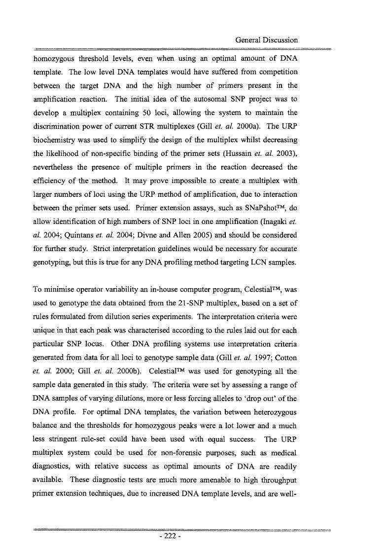
General Discussion

homozygous threshold levels, even when using an optimal amount of DNA

template. The low level DNA templates would have suffered from competition

between the target DNA and the high number of primers present in the

amplification reaction. The initial idea of the autosomal SNP project was to

develop a multiplex containing 50 loci, allowing the system to maintain the

discrimination power of current STR multiplexes (Gill et. al. 2000a). The URP

biochemistry was used to simplify the design of the multiplex whilst decreasing

the likelihood of non-specific binding of the primer sets (Hussain et. al. 2003),

nevertheless the presence of multiple primers in the reaction decreased the

efficiency of the method. It may prove impossible to create a multiplex with

larger numbers of loci using the URP method of amplification, due to interaction

between the primer sets used. Primer extension assays, such as SNaPshot™, do

allow identification of high numbers of SNP loci in one amplification (Inagaki et.

al. 2004; Quintans et. al. 2004; Divne and Allen 2005) and should be considered

for further study. Strict interpretation guidelines would be necessary for accurate

genotyping, but this is true for any DNA profiling method targeting LCN samples.

To minimise operator variability an in-house computer program, Celestial™, was

used to genotype the data obtained from the 21-SNP multiplex, based on a set of

rules formulated from dilution series experiments. The interpretation criteria were

unique in that each peak was characterised according to the rules laid out for each

particular SNP locus. Other DNA profiling systems use interpretation criteria

generated from data for all loci to genotype sample data (Gill et. al. 1997; Cotton

et. al. 2000; Gill et. al. 2000b). Celestial™ was used for genotyping all the

sample data generated in this study. The criteria were set by assessing a range of

DNA samples of varying dilutions, more or less forcing alleles to ‘drop out’ of the

DNA profile. For optimal DNA templates, the variation between heterozygous

balance and the thresholds for homozygous peaks were a lot lower and a much

less stringent rule-set could have been used with equal success. The URP

multiplex system could be used for non-forensic purposes, such as medical

diagnostics, with relative success as optimal amounts of DNA are readily

available. These diagnostic tests are much more amenable to high throughput

primer extension techniques, due to increased DNA template levels, and are well-

General Discussion

established in the gene expression community (Wang et. al. 1998; Heller 2002;

Pusch et. al. 2003; Dudbridge and Koeleman 2004).

LCN casework samples were amplified with variable success using the 21-SNP

multiplex. A comparison of LCN STR and SNP percentage profiles and

likelihood ratios indicated that LCN DNA profiling had a greater chance of

gaining a result, even though the DNA in the samples was degraded. The

discrimination power gained from one STR locus is much higher than that gained

from one SNP locus, due to the presence of many alleles at each STR site

(Chakraborty et. al. 1999; Gill 2001a; Ayres 2005), and a partial STR profile will

give an increased likelihood ratio compared to a partial SNP profile. Validation

of the multiplex indicated that if LCN STR DNA profiling failed then the 21-SNP

multiplex would also fail to amplify. This is most likely due to the amount of

template DNA being too low to exponentially amplify, or there may not have been

any DNA present in the sample collected. As a consequence of this observation,

implementation of the technique into casework was carried out with direction to

only use the technique in situations where a partial LCN DNA profile had been

obtained.

Validation of the 21-SNP multiplex demonstrated the problems associated with

targeting SNP loci as opposed to STRs. The SNP loci selected for use in the

multiplex were biallelic, meaning there were only two alleles per locus. Some

identified SNP loci are triallelic and it may be more beneficial to target these in

future multiplexes (Phillips et. al. 2004). The match probability of each biallelic

SNP locus is much reduced compared to the multi-allelic STR loci, so more loci

need analysing to gain an increased discrimination power (Chakraborty et. al.

1999; Gill 2001a; Phillips et. al. 2004). The biallelic nature of the selected SNPs

also makes it difficult to determine the presence of a mixture in a DNA sample.

By developing a technique that is highly quantitative, mixture analysis would be

feasible by observing the heterozygous balance of a locus, however no technique

currently exists that is quantitative enough to assess mixtures (Gill et. al. 2004a;

Dixon et. al. 2005a; Dixon et. al. 2005b). Mixture analysis can be determined by

examination of the number of heterozygous loci in a single profile. An excess of

heterozygotes can be indicative of a mixed DNA profile; however it is impossible

-223 -

General Discussion

to separate the two genotypes into single profiles due to the presence of only two

alleles, and the profile could feasibly have come from one individual.

Consequently, another recommendation for the implementation of the system into

casework was to only submit discrete sample types, i.e. sample types that were

unlikely to contain a mixture, such as deep muscle and bone. The 21-SNP

multiplex was found to be of a similar sensitivity to the current method of LCN

STR DNA profiling. Due to the problems associated with SNP analysis, along

with the average performance of the 21-SNP multiplex (Dixon et. al. 2005b), a

decision was made to research other methods for analysis of degraded DNA.

A recent extensive collaborative research study by the ENFSI DNA Working

Group and EDNAP demonstrated that the success rate for analysis of degraded

samples can be substantially improved by testing shorter (“mini”) STRs (Dixon et.

al. 2005b). Current STR loci can be redesigned to produce shorter amplicons,

allowing a new mini-STR system to be compatible with current national DNA

databases (Butler et. al. 2003; Chung et. al. 2004; Drabek et. al. 2004). The

smaller mini-STR sequences benefit from being able to target smaller, more

fragmented DNA molecules, whilst maintaining a discrimination power equal to

that already gained from conventional STR systems. Research carried out by the

National Institute of Standards and Technology (NIST) has considerably furthered

the field of mini-STR multiplex development over the last few years (Ruitberg et.

al. 2001; Butler et. al. 2003; Chung et. al. 2004; Drabek et. al. 2004). STR primer

sets used in current multiplex systems are designed up and downstream of the

STR locus, a suitable distance away from the polymorphic region. This method

had the advantage of being able to design highly efficient primers, as well as

making the amplicon sizes such that they could be easily separated using gel (and

later capillary) electrophoresis. Mini-STR primers are simply targeted closer to

the polymorphic region. This has the advantage of decreasing the length of

amplified DNA but can be problematic as the region immediately up and

downstream of the STR is highly polymorphic and primer-binding site mutations

can be present in some individuals. The presence of primer-binding site

mutations and, in some cases, deletions can cause discordance between mini-STR

genotypes compared to STR genotypes derived from current profiling methods

(Drabek et. al. 2004). Full sequencing of STR loci is used to identify any

General Discussion

polymorphisms within these regions that could be detrimental to amplification.

Primers can be designed with alternative bases, such as inosines, to allow binding

within a known polymorphic region.

All existing studies confirm that there are substantial advantages to be obtained by

converting current STR systems to low molecular weight mini-STRs (Butler et.

al. 2003; Chung et. al. 2004; Drabek et. al. 2004; Graham 2005; Dixon et. al.

2005b; Gill et. al. 2006). The discriminating power of current systems would be

maintained and mixture analysis remains feasible, an essential element when

considering highly sensitive DNA profiling techniques which are more likely to

yield low level DNA mixtures. The idea is to construct a “mini” STR multiplex,

based on a set of core loci identified by analysis of all the systems currently in use

across Europe. This mini-STR multiplex could be easily incorporated into the

current DNA profiling systems used, and would be compatible with existing STR

national DNA databases (Gill et. al. 2006). It would also be designed to follow

the recommendations of the House of Commons Science and Technology

Committee, as outlined in a Home Office response note from Gill et. al. in 2005

(http://www.publications.parliament.uk/pa/cm200506/cmselect/cmsctech/427/427

.pdf; Gill et. al. 2005a). As the number of profiles loaded onto the National DNA

Database® increases, the Committee recommends the introduction of a sixteen-

locus STR system. Heeding the advice of Sir Alec Jeffreys: “the consequences o f

even one false match leading to a conviction that was subsequently overturned

could be severe for the DNA database and its public acceptability”; more loci

could be used to decrease the chances of an adventitious match. Gill (2005)

outlines the development of a mini-STR system that will increase the likelihood of

successful amplification on degraded samples, whilst increasing the

discriminating power and improving the comparability to European databases

(Gill et. al. 2005a; Gill et. al. 2006).

This study highlighted the benefits and drawbacks of using a SNP multiplex for

forensic identification. The limited amount of research conducted on the forensic

use of SNPs suggests it is unlikely that SNPs will replace STRs as the DNA

profiling method of choice in the near future, due to incompatibility with current

General Discussion

national DNA databases and difficulties in mixture analysis (Gill et. al. 2004a).

The cost of upgrading a database to SNP DNA profiles far outweighs the benefits

of such a system. Although disregarded from widespread use, there is still a

requirement for a validated SNP multiplex system in the forensic community, to

act as an adjunct to current methods. The ability to design small amplicons allows

fragmented DNA to be targeted, however a more robust system is required to cope

with the stochastic variation recognised at low DNA template levels. Research is

ongoing into primer extension methods of detection but, to date, the 21-SNP

multiplex is the only validated SNP multiplex in the forensic community.

Appendices

Appendices

Appendices

A ppendix I - 21-SNP m ultiplex data

(Amelogenin is omitted from the data)

SNP internal ID TSC identifier Chromosome Polymorphism Amplicon size (bp)

TSCOD 0252540 3 C/T 103

TSCO U6 0746324 5 A/T 107

TSCO B6 1342445 3 A/T 110

TSCO N4 1156239 18 AJT 114

TSCO Y3 0846740 7 C/G 117

TSCO P5 0176551 1 A /T 122

TSCO A4 0421768 8 C/G 125

TSCO 0 6 1588825 5 A /T 129

TSCO Z2 0086795 6 C/T 134

TSCOK3 0078283 21 C/G 137

TSCO J2 0156245 19 C/T 141

TSCO Y6 0627632 5 A /T 147

TSCO P7 0897904 6 A /T 151

TSCO J8 0709016 3 A /T 154

TSCO X 0031988 8 A/C 158

TSCO F 0155410 10 A/C 164

TSCO G 0154197 11 C/T 170

TSCO L2 00384808 17 C/T 174

TSCO W3 0820041 9 C/G 180

TSCO H8 0131214 14 A /T 186

- 228-

Appendices

A ppendix II - The com puter program ASGOTH

Dim intUnknownSamples As Integer Dim intUnknownSpots As Integer Dim RowstoSelect As Integer Dim SamplesUsed As Integer Dim intControlSpots As Variant Dim UnknownsUsed As Integer

Sub ASGQTH20020

Application.StatusBar= "ASGOTH running Please wait..."Application. ScreenUpdating = False

Worksheets(" col lection"). Select Range("Al ").Select

SamplesUsed = Application.InputBox("how many control samples have been used?", "specify numbers", 0 ,, , , , 1)UnknownsUsed = Application.InputBox("how many unknown samples are there?", "specify unknown sample number", 0 , , , , , 1)RowstoSelect = Application.InputBox("how many spots do you want to use in the validation?", "select number of spots", 0 , , , , , 1)

controlsunknowns

For theloop = 1 To 1000

forbootstrappingcontrolsforbootstrappingunknownscomparisoncollectionofdataresetforms

Next

Application.StatusBar = False

End Sub

Sub controlsf)

Worksheets("controls").Select Range("F2"). Select

intControl Samples = SamplesUsed

Er2: intControl Spots = Application.InputBox("how many replicate spots are there per control sample?","control spots", 0 , , , , , 1 + 2)If intControl Spots = False Then Exit Sub

If intControlSpots = "" Then MsgBox "You must enter a valid number of spots", vbOKOnly + vbExclamation

GoTo Er2End If

Err: txtGenotype = Application.InputBox("what is the genotype of the first sample?" & (Chr(13) &Chr(10)) & (Chr(13) & Chr(10)) & " type '1' for Homozygote 1" & (Chr(13) & Chr(10)) & " type '2' for Heterozygote" & (Chr(13) & Chr(10)) & " type '3' for Homozygote 2", "genotypes",, , , , , 1)

If txtGenotype = False Then Exit Sub If txtGenotype = 1 Then

For Cellinuse = 1 To intControlSpots ActiveCell. Value = 1 ActiveCell.Offset(l, 0).Select

NextElself txtGenotype = 2 Then

-229-

Appendices

For Cellinuse = 1 To intControlSpots ActiveCell.Value = 2 ActiveCell.Offset(l, 0).Select

NextElself txtGenotype = 3 Then

For Cellinuse = 1 To intControlSpots ActiveCell.Value = 3 ActiveCell.Offset(l, 0).Select

NextElse

MsgBox "You must enter a genotype 1, 2 or 3", vbOKOnly + vbExclamation, AttentionGoTo Err

End If

counting = 1

For intSample = 1 To ((intControlSpots * intControl Samples) - (intControlSpots)) Step intControlSpots

counting = counting + 1

Err2: txtGenotype = Application.InputBox("what is the genotype of the next sample?" & (Chr(13) &Chr(10)) & " "" " & (Chr(13) & Chr(10)) & " type 1 for Homozygote 1" & (Chr(13) & Chr(10)) & " type 2 for Heterozygote" & (Chr(13) & Chr(lO)) & " type 3 for Homozygote 2", "genotypes",, , , , 1)

If txtGenotype = False Then Exit SubIf txtGenotype = 1 Then

For Cellinuse = 1 To intControlSpots ActiveCell.Value = 1

ActiveCell.Offset( 1,0). Select Next

Elself txtGenotype = 2 ThenFor Cellinuse = 1 To intControlSpots

ActiveCell.Value = 2 ActiveCell.Offset( 1, 0).Select

NextElself txtGenotype = 3 Then

For Cellinuse = 1 To intControlSpots ActiveCell.Value = 3 ActiveCell.Offset(l, 0).Select

NextElse

MsgBox "You must enter a genotype 1, 2 or 3", vbOKOnly + vbExclamation, Attention 'if any other value is added this box comes up

GoTo Err2 End If

Next

Range("E2"). Select

For intSample = 1 To (intControlSpots * intControl Samples)

If ActiveCell.Offset(0, -4).Value >= Range("K18").Value And ActiveCell.Offset(0, -2).Value >= Range("L18").Value ThenIf ActiveCell.Offset(0, -1).Value = 0 Or ActiveCell.Offset(0, -3).Value = 0 Then ActiveCell.Value = ""

ActiveCell.Offset(0, 1). Value = ""ActiveCell.Offset(l, 0).Select

ElseActi veCell. F ormul a = "=LOG10(RC[-3]/RC[-l])"

ActiveCell.Offset(l, 0).Select End If

ElseActiveCell.Value = ""

ActiveCell.Offset(0, 1). Value = ""ActiveCell.Offset(l, 0).Select End If Next End Sub

-230-

Appendices

Sub unknownsO

W orksheets(" unknowns"). Select Range("A2").Select

intUnknownSamples = UnknownsUsed

intUnknownSpots = Application.InputBox ("how many replicate spots are there per unknown sample?", "control spots", 0 , , , , , 1)

If intUnknownSpots = False Then Exit Sub

Range("E2"). Select

For intSample = 1 To (intUnknownSpots * intUnknownSamples)If ActiveCell.Offset(0, -1).Value = 0 Or ActiveCell.Offset(0, -3).Value = 0 Then

ActiveCell.Value = ""ActiveCell.Offset(l, 0).Select

ElseActi veCell. F ormula = "=LOG10(RC[-3]/RC[-l])"

ActiveCell.Offset(l, 0).Select End If

Next

End Sub

Sub forbootstrappingunknownsO

Worksheets("bootstrapunknowns").Select Range("A2"). Select

Worksheets("unknowns").Select

sample = RowstoSelect

Randomize

For intRow = 2 To ((UnknownsUsed * intUnknownSpots) + 1) Step intUnknownSpots

For intSpot = 1 To RowstoSelect

intRowstoPick = Int(24 * Rnd + intRow)

Cells(intRowstoPick, 1). SelectstrStartcell = ActiveCell.Address(False, False)strEndcell = ActiveCell.Offset(0, 5).Address(False, False)strSelection = strStartcell & & strEndcellRange(strSelection). SelectSelection. Copy

Worksheets("bootstrapunknowns").Select ActiveCell. SelectSelection.PasteSpecial Paste^xlValues ActiveCell.Offset(l, 0).Select Worksheets("unknowns"). Select

NextNext

Worksheets( "bootstrapunknowns"). Select

Range("A:A").Select Selection.CopyWorksheets("compare").Select Range("Al"). Select Selection.PasteSpecial Paste:=xlValues

-231 -

Appendices

Worksheets("bootstrapunknowns"). SelectRange("C:C").SelectSelection.CopyWorksheets("compare"). Select Range("B 1"). Select Selection.PasteSpecial Paste:=xlValues

Worksheets("bootstrapunknowns").SelectRange("E:E").SelectSelection.CopyWorksheets(" compare" )• S el ect Range("Cl"). Select Selection.PasteSpecial Paste:=xl Values

End Sub

Sub forbootstrappingcontrolsO

Worksheets("bootstrapcontrols").Select Range("A2"). Select

Worksheets("controls"). Select

sample = RowstoSelect

Randomize

For intRows = 2 To ((SamplesUsed * intControlSpots) + 1) Step intControlSpots

For intSpots = 1 To RowstoSelect

Again:

intRowtoPick = Int(24 * Rnd + intRows)

If Cells(intRowtoPick, 5).Value = "" Then GoTo Again

Cells(intRowtoPick, l).SelectstrStartcell = ActiveCell.Address(False, False)strEndcell = ActiveCell.Offset(0, 5).Address(False, False)strSelection = strStartcell & & strEndcellRange(strSelection). SelectSelection.Copy

Worksheets( "bootstrapcontrols"). Select ActiveCell. SelectSelection.PasteSpecial Paste:=xlValues ActiveCell.Offset(l, 0).Select Worksheets(" controls"). Select

NextNext

Worksheets( "bootstrapcontrol s"). S electColumns("E:F").SelectSelection.CopySheets("bins"). SelectRange("Al"). SelectSelection.PasteSpecial Paste:=xl Values

intHoml = 0 intHet = 0 intHom2 = 0

Range("A2"). Select

For intsamples = 1 To (SamplesUsed * RowstoSelect)

Appendices

If ActiveCell.Offset(0, l).Value = 1 Then intHoml - intHoml + 1 Cells(intHoml, 4).Value = ActiveCell.Value Elself ActiveCell.Offset(0, 1).Value = 2 Then intHet = intHet + 1Cells(intHet, 5).Value = ActiveCell. ValueElself ActiveCell.Offset(0, 1).Value = 3 ThenintHom2 = intHom2 + 1Cells(intHom2, 6).Value = ActiveCell.ValueElseEnd If

ActiveCell.Offset(l, 0).Select

Next

Range("H 1: S4"). Select Selection.Copy Sheets("compare"). Select Range("G8"). Select Selection.PasteSpecial Paste:=xlValues

End Sub

Sub comparisonO

Worksheets("table").Select Range("Al"). Select Worksheets("compare"). Select RangeC’Cl"). Select

For inttotal Samples = 0 To ((RowstoSelect * UnknownsUsed) - RowstoSelect) Step RowstoSelect

ActiveCell.Offset(inttotalSamples + 1, 0).Select

counter -1counter2 = counter2 + 1

For intSample = 1 To RowstoSelect

If ActiveCell. Offset(0, -2).Value > Range("117"). Value And ActiveCell. Offset(0, -1).Value > Range("J17").Value Then

counter = counter + 1Cells(counter, 5).Value = ActiveCell.Value

Else End If

ActiveCell.Offset(l, 0).Select

Next

If Range("I2").Text= "#NUM!" Then Range("S2"). Value = "FAIL"GoTo nextl

Elself Range("I2").Value >= Range("M9") Then Range("S2").Value = 1

Elself Range("I2").Value >= Range("M10") And Range("I2").Value <= Range("N10") Then Range("S2"). Value = 2

ElselfRange("I2").Value<= Range("Nll") Then Range("S2"). Value = 3

End If

If Range("I2").Value <= Range("M9") And Range("I2").Value >= Range("N10") Then Range("S2"). Value = "POSSIBLE TYPE 1 OR 2"

End If

If Range("I2").Value <= Range("M10") And Range("I2").Value >= Range("Nl 1") Then

-233 -

f-

Appendices

Range("S2"). Value - "POSSIBLE TYPE 2 OR 3"End If

nex tl: Range("G2"). Value = counter2

Range("G2:S2").Select Selection.Copy Worksheets("table").Select ActiveCell.Offset(l, 0).Select Selection.PasteSpecial Paste:=xlValues

Worksheets("compare").Select Range("E:E"). Select Selection.ClearContents

RangeC'Cl").Select

Next

Worksheets("table").Select Range("Al"). Value = "Sample Number"

Range("02"). Select

For samples = 1 To intUnknownSamples

If ActiveCell. Offset(0, -1).Value = ActiveCell. Offset(0, -2).Value Then ActiveCell. Value = 1 ActiveCell.Offset(l, 0).SelectElself ActiveCell.Offset(0, -2). Value = "POSSIBLE TYPE 1 OR 2" Then ActiveCell.Offset(0, 2).Value = 1 ActiveCell.Offset(l, 0).SelectElself ActiveCell.Offset(0, -2).Value = "POSSIBLE TYPE 2 OR 3" ThenActiveCell.Offset(0, 2).Value= 1ActiveCell.Offset(l, 0).SelectElself ActiveCell.Offset(0, -2). Value = "FAIL" ThenActiveCell.Offset(0, 2).Value = 1ActiveCell.Offset(l, 0).SelectElseActiveCell. Offset(0, 1). Value = 1 ActiveCell.Offset(l, 0).Select End If Next

End Sub

Sub collectionofdataO

Worksheets(" collection"). Select Worksheets("table").Select Range("0915: Q915"). Select Selection.CopyWorksheets("collection").Select ActiveCell.Offset(l, 0).Select Selection.PasteSpecial Paste:=xlValues

End Sub

Sub resetformsf)

Worksheets("table"). Select Range("A2:M4000").Select Selection.ClearContents Range("02:Q900"). Select Selection.ClearContents

End Sub

-234-

Appendices

APPENDIX III - SNP 27-pl ex p r im e r se q u e n c e s

9, 11 or 13 denotes the Universal sequence found at the 5’ end of the primer sequences.Within the multimix, the locus-specific primers are found at concentrations varying from 50nM to 200nM. Universal primers with fluorescent labels are used at 2pM.

Forward primers Universal 9 tail (CGACGTGGTGGATGTGCTAT)

Amelo X UNI9-CCAGATGTTTCTCAAGTGGTCCTG 44 merTSCO D/9 UN I9-GGG AA ACT GCT GGGT CT GT 39 merTSCO B6/9 UNI9-GGGAGACAGGCCCATGCA 38 merTSCO N4/9 UNI9-CAGAAAAGGCAGGAACCTGGACA 43 merTSCO Y3/9 UNI9-ACCAACCCCACAAAGCAGG 39 merTSCO A4/9 UNI9-GATGCCTCTTGCATTGTGAACG 42 merTSCO 06/9 UNI9-GAGCCAAGAATCGCAGGGAA 40 merTSCO Z2/9 UNI9-CATTGTGTTTCAAACGCGTGCC 42 merTSCO K3/9 UNI9-T GCC ACTCT G AC ACT GAT GCTT G 43 merTSCO J2/9 UNI9-CTGCCTTGGCTCCCAGCC 38 merTSCO Y6/9 UNI9-CAAGATTCCTGGCCCCTGGTAA 42 merTSCO J8/9 UNI9-C AGGG AATGAC AGGG AACC ACT A 43 merTSCO X/9 UNI9-CTGTGCATCCACTGCGCC 38 merTSCO F/9 UNI9-CCTGGAGCATGXGCTGACCAC 41 merTSCO G/9 UNI9-CCATGCCTCACCTCCTGCATT 41 merTSCO L2/9 UNI9-GCATGCCATTGCCAAATTCC 40 merTSCO W3/9 UNI9-GCCAACCAGACCTCCCAGG 39 merTSCO H8/9 UNI9-CTCAGTTGGGTGCTTACGTGCA 42 merTSCO L6/9 UNI9-TGTGCATGTTCCCTGGTGTTCA 42 merTSCO K4/9 UN19-GCGGGAGGAAGGAAGGGAGG 40 merTSCO X7/9 UNI9-TTTACCATTTGCTCCACAGGGAA 43 merTSCO U6/9 UNI9-GCAAGGCCCAAAGCAAAGAA 40 merTSCO W5/9 UNI9-AGGACAGTGGCTTCTGTACTGCTA 44 merTSCO U5/9 UNI9-CTGGAAGGGCTTTGTTTGCCAA 42 merTSCO V4/9 UNI9-CTGGGGAGGAAGGCTGGAGA 40 merTSCO P7/9 UNI9-CTCTTCCAGCAGGCACCATGA 41 merTSCO P5/9 UNI9-GGGGGTACTGGGGAGACCAA 40 mer

Forward primers Universal 11 tail (TGACGTGGCTGACCTGAGAC)

Amelo Y UNI11 -AAAGTGGTTTCTC AAGTGGTCCC A 44 merTSCO D/11 UNI11 -GGG AAACT GCT GGGT CT GC 39 merTSCO B6/11 UNI11 -GGGAGACAGGCCC ATGCT 38 merTSCO N4/11 UNI11-CAGAAAAGGCAGGAACCTGGACT 43 merTSCO Y3/11 UNI 11 -ACCAACCCCAC AAAGCAGC 39 merTSCO A4/11 UNI 11 -GATGCCTCTTGC ATTGTG AACC 42 merTSCO 06/11 UNI11 -GAGCC AAGAATCGCAGGGAT 40 merTSCO Z2/11 UNI11 -CATTGTGTTTCAAACGCGTGCT 42 merTSCO K3/11 UNI11 -TGCC ACTCTG AC ACTGATGCTTC 43 merTSCO J2/11 UNI11 -CTGCCTTGGCTCCCAGCT 38 merTSCO Y6/11 UNI11 -CAAGATTCCTGGCCCCTGGTAT 42 merTSCO J8/11 UNI11-C AGGG AATGAC AGGG AACC ACTT 43 merTSCO X/l 1 UNI 11 -CTGTGC ATCCACTGCGC A 38 merTSCO F/l 1 UNI11 -CCTGGAGC ATGXGCTG ACC AA 41 merTSCO G/l 1 UNI 11 -CCATGCCTCACCTCCTGCATC 41 merTSCO L2/11 UNI11 -GCATGCCATTGCCAAATTCT 40 merTSCO W3/11 UNI11 -GCC AACC AG ACCTCCC AGC 39 merTSCO H8/11 UNI11 -CTCAGTTGGGTGCTTACGTGCT 42 merTSCO L6/11 UNI11 -TGTGCATGTTCCCTGGTGTTCT 42 merTSCO K4/11 UNI11 -GCGGGAGG AAGG AAGGGAGC 40 merTSCO X7/11 UNI11 -TTTACCATTTGCTCCACAGGGAT 43 merTSCO U6/11 UNI11-GCAAGGCCCAAAGCAAAGAT 40 merTSCO W5/11 UNI11 -AGGAC AGTGGCTTCTGT ACTGCTT 44 merTSCO U5/11 UNI11 -CTGGAAGGGCTTTGTTTGCC AT 42 merTSCO V4/11 UNI11 -CTGGGGAGGAAGGCTGGAGT 40 merTSCO P7/11 UNI11-CTCTTCCAGCAGGCACCATGT 41 merTSCO P5/11 UNI11 -GGGGGTACTGGGGAGACCAT 40 mer

Appendices

Reverse primers Universal 13 tail (CAAGCTGGTGGCTGTGCAAG)

Amelo/rev TSCO D/rev TSCO B6/rev TSCO N4/rev TSCO Y3/rev TSCO A4/rev TSCO 06/rev TSCO Z2/rev TSCO K3/rev TSCO J2/rev TSCO Y6/rev TSCO J8/rev TSCO X/rev TSCO F/rev TSCO G/rev TSCO L2/rev TSCO W3/rev TSCO H8/rev TSCO L6/rev TSCO K4/rev TSCO X7/rev TSCO U6/rev TSCO W5/rev TSCO U5/rev TSCO V4/rev TSCO P7/rev TSCO P5/rev

UNI 13- TGCTT A A ACT GGG A AGCT GXT GGT UNI 13- AATGACCTGCCCCACAGGAG UNI 13- GCCATTCAGAACTAACTAGTCTGGGA UNI 13- CGACGGGGGTTGAGTGGTTCAG UNI 13- ATTAGAGCAGCCAAGTCCTGACCA UNI 13- GCTCAACAGCACAACTCTGCTACAGC UNI 13- GCTAAAGCAGCTCTGAAACCCA UNI 13- GG ATC AG AG A A AGT GC AGCT GGT UNI 13- AAT GGGG AG ATT GGCTTGG AC UNI 13- CCTGAACATCCCTGAAGGTATTTCG UNI 13- GATTTGGGAXTTTAGTGACATCTGCA UNI 13- CTGTACATCTTTTAAGACCAACTCCTT UNI 13- TCT AGGCT GGT GCC AGCCC UNI 13- GGCTCT G AAG AAC AAT GGGG AG UNI 13- CAATCCTGTTTGCAGAGTTCCAG UNI 13- TG AGCC AAGGT GT GGGG A UNI 13- TT ACACAGGTCTCCAGCTTG AGC AA UNI 13- AAG AGGG AGC ACT GT GGG ACT G UNI 13- AACGGCCTTGCTTCGCTGA UNI 13- GGGC AGGTC AGG AT GG AGC AG UNI 13- CACCTTGCTGCATCCTGCTG UNI 13- TGGATAGATGATCAGTCTGCGTTC UNI 13- GGCCAGCAGAGATTCACACTGT UNI 13- GATGGAATCACTGTCCTTGCCCT UNI 13- AGCCAAGATCGCACCACTGTA UNI 13- AGTGGTTTGCTGCATGAGTCCA UNI 13- CGGAGGAGATTTTGCCCTGCA

44 mer40 mer46 mer42 mer44 mer46 mer42 mer43 mer41 mer45 mer46 mer47 mer39 mer42 mer43 mer38 mer45 mer42 mer39 mer41 mer40 mer44 mer42 mer43 mer41 mer42 mer41 mer

Universal 9 CGACGTGGTGGATGTGCTAT 20 merUniversal 11 T G ACGT GGCT G ACCT GAG AC 20 mer

5’-JOE-6 dye label 5’-FAM-6 dye label

X = Inosine

Appendices

A ppendix IV - SNP 21-plex prim er sequences

9, 11 or 13 denotes the Universal sequence found at the 5’ end of the primer sequences.

Within the multimix, the locus-specific primers are found at concentrations varying from 50nM to 200nM.

Universal primers with fluorescent labels are used at 2pM.

Forward primers Universal 9 tail (CGACGTGGTGGATGTGCTAT)

Amelo X UNI9-CCAGATGTTTCTCAAGTGGTCCTG 44merTSCO D/9 UNI9-GGG A AACT GCT GGGTCT GT 39merTSCO U6/9 UNI9-GCAAGGCCCAAAGCAAAGAA 40merTSCO B6/9 UNI9-GGG AG AC AGGCCC AT GC A 38merTSCO N4/9 UNI9-CAGAAAAGGCAGGAACCTGGACA 43 merTSCO Y3/9 UNI9-ACCAACCCCACAAAGCAGG 39merTSCO P5/9 UNI9-GGGGGT ACTGGGGAG ACC AA 40merTSCO A4/9 UNI9-GATGCCTCTTGCATTGTGAACG 42merTSCO 06/9 UNI9-G AGCC AAG AAT CGC AGGG AA 40merTSCO Z2/9 UNI9-CATTGTGTTTCAAACGCGTGCC 42merTSCO K3/9 UNI9-TGCCACTCTGACACTGATGCTTG 43merTSCO J2/9 UNI9-CTGCCTTGGCTCCCAGCC 38merTSCO Y6/9 UNI9-CAAGATTCCTGGCCCCTGGTAA 42merTSCO P7/9 UNI9-CTCTTCCAGCAGGCACCATGA 41 merTSCO J8/9 UNI9-CAGGGAATGACAGGGAACCACTA 43merTSCO X/9 UNI9-CTGTGCATCCACTGCGCC 38merTSCO F/9 UNI9-CCTGGAGCATGXGCTGACCAC 41 merTSCO G/9 UNI9-CCATGCCTCACCTCCTGCATT 41 merTSCO L2/9 UNI9-GCATGCCATTGCCAAATTCC 40merTSCO W3/9 UNI9-GCCAACCAGACCTCCCAGG 39merTSCO H8/9 UNI9-CTCAGTTGGGTGCTTACGTGCA 42mer

Forward primers Universal 11 tail (TGACGTGGCTGACCTGAGAC)

Amelo Y UNI11 -AAAGTGGTTTCTCAAGTGGTCCC A 44merTSCO D/11 UNI11-GGGAAACTGCTGGGTCTGC 39merTSCO U6/11 UNI11 -GC AAGGCCC AAAGC AAAG AT 40merTSCO B6/11 UNI11-GGGAGAC AGGCCC ATGCT 38merTSCO N4/11 UNI11 -CAGAAAAGGCAGGAACCTGGACT 43 merTSCO Y3/11 UNI11-ACC AACCCC AC AAAGC AGC 39merTSCO P5/11 UNI11 -GGGGGT ACTGGGGAG ACC AT 40merTSCO A4/11 UNI11 -GATGCCTCTTGCATTGTGAACC 42merTSCO 06/11 UNI11 -GAGCC AAGAATCGC AGGGAT 40merTSCO Z2/11 UNI11 -CATTGTGTTTCAAACGCGTGCT 42merTSCO K3/11 UNI11 -TGCCACTCTGACACTGATGCTTC 43merTSCO J2/11 UNI11 -CTGCCTTGGCTCCCAGCT 38merTSCO Y6/11 UNI11 -CAAGATTCCTGGCCCCTGGTAT 42merTSCO P7/11 UNI11 -CTCTTCCAGCAGGCACCATGT 41 merTSCO J8/11 UNI11 -CAGGGAATGACAGGGAACCACTT 43merTSCO X/l 1 UNI11 -CTGTGCATCCACTGCGCA 38merTSCO F/l 1 UNI11-CCTGGAGCATGXGCTGACCAA 41 merTSCO G/l 1 UNI11-CCATGCCTCACCTCCTGCATC 41 merTSCO L2/11 UNI 11 -GCATGCCATTGCCAAATTCT 40merTSCO W3/11 UNI 11 -GCCAACCAGACCTCCCAGC 39merTSCO H8/11 UNI11-CTCAGTTGGGTGCTTACGTGCT 42mer

-237-

Reverse primers Universal 13 tail (CAAGCTGGTGGCTGTGCAAG)

Appendices

Amelo/13 TSCO D/13 TSCO U6/13 TSCO B6/13 TSCO N4/13 TSCO Y3/13 TSCO P5/13 TSCO A4/13 TSCO 06/13 TSCO Z2/13 TSCO K.3/13 TSCO J2/13 TSCO Y6/13 TSCO P7/13 TSCO J8/13 TSCO X /13 TSCOF/13 TSCO G/13 TSCO L2/13 TSCO W3/13 TSCO H8/13

UNI 13-TGCTT AAACTGGGAAGCTGXTGGT 44merUNI 13-AATGACXTGCCCCAC AGGAG 40merUNI 13-ACAAAGCCCCAAGGCAGAG 39merUNI 13 -GCC ATTC AG A ACT AACT AGTCT GGG A 46merUNI 13-CGACGGGGGTTGAGTGGTTCAG 42merUNI 13-ATT AGAGC AGCC AAGTCCT G ACC A 44merUNI 13-AGGCGGATCCTGGAGGG 37merUNI 13-GCTC AAC AGC AC AACTCTGCTAC AGC 46merUNI 13-GCT AAAGCAGCTCTGAAACCC A 42merUNI 13-GGATCAGAGAAAGTGCAGCTGGT 43merUNI 13-AATGGGGAG ATTGGCTTGGAC 41 merUNI13-CCTGAACATCCCTGAAGGTATTTCG 45merUNI 13 -T AGCCTT AGG AC AT GGT GATT AC AG A 46merUNI 13-GATTTGGGAXTTT AGTGAC ATCTGCA 46merUNI 13-CTGT AC ATCTTTT AAG ACC AACTCCTT 47merUNI 13-TCTAGGCTGGTGCC AGCCC 39merUNI 13-GGCTCTGAAGAACAATGGGGAG 42merUNI13-CAATCCTGTTTGCAGAGTTCC AG 43merUNI 13-TGAGCCAAGGTGTGGGGA 38merUNI13-TTACACAGGTCTCCAGCTTGAGCAA 45merUNI 13-AAGAGGGAGC ACTGTGGG ACTG 42mer

Universal 9 CGACGTGGTGGATGTGCTAT 20 merUniversal 11 T G ACGT GGCTG ACCT GAG AC 20 mer

5’-JOE-6 dye label 5’-FAM-6 dye label

X = Inosine

- 2 3 8 -

Appendices

APPENDIX V - PCR AMPLIFICATION PARAMETERS

SNP multiplex amplification

Temperature Time

95°C 11 min

94°C 30 sec

60°C 15 sec

72°C 15 sec

& 60°C 15 sec’'O 72°C 15 sec

60°C 15 sec

72°C 30 sec

O s - ~94°C 30 sec

<n yo ' 76°C 105 sec

3 94°C 60 sec

& 60°C 30 sec76°C 60 sec

60°C 45 min

4°C Hold

SGM+ amplification

Temperature Time

95°C 11 min

2<5 cy

cles

(st

anda

rd)

/ 34

cycle

s (lo

w

copy

nu

mbe

r) 94°C 60 sec

59°C 60 sec

72°C 60 sec

60°C 45 min

4°C Hold

-239-

Appendices

A p pe n d ix V I - Pe r c e n t a g e pr o file s f o r b o il e d D N A e x t r a c t s

SNPs % SGM+ %

time of boiling (min) Sample ID full 27-plex LMW SNPs HMW SNPs full SGM+ LMW SGM+ HMW SGM+profile only only profile STRs STRs

0 CAS 96 100 89 100 100 10015 CAS 94 100 83 100 100 10030 CAS 94 100 83 100 100 10045 CAS 94 100 83 100 100 10060 CAS 94 100 83 100 100 10075 CAS 94 100 83 100 100 10090 CAS 94 100 83 100 100 100105 CAS 87 100 56 100 100 100120 CAS 81 100 39 100 100 100150 CAS 80 100 33 100 100 100180 CAS 69 94 11 100 100 100210 CAS 69 94 11 95 100 90240 CAS 63 92 6 86 100 70

0 DRJ 98 100 94 100 100 10015 DRJ 98 100 94 100 100 10030 DRJ 98 100 94 100 100 10045 DRJ 98 100 94 100 100 10060 DRJ 96 100 89 100 100 10075 DRJ 96 100 89 100 100 10090 DRJ 96 100 89 100 100 100105 DRJ 91 100 67 100 100 100120 DRJ 93 100 72 100 100 100150 DRJ 89 100 61 100 100 100180 DRJ 83 100 44 91 100 80240 DRJ 78 100 33 77 100 50

0 SHM 100 100 100 100 100 10015 SHM 100 100 100 100 100 10030 SHM 100 100 100 100 100 10045 SHM 100 100 100 100 100 10060 SHM 98 100 94 100 100 10075 SHM 98 100 94 100 100 10090 SHM 98 100 94 100 100 100105 SHM 96 100 83 100 100 100120 SHM 94 100 83 100 100 100150 SHM 91 100 72 91 100 80180 SHM 89 97 67 73 83 60210 SHM 80 97 39 41 75 0240 SHM 52 75 6 23 42 0

0 HER 93 100 78 100 100 10015 HER 93 100 78 100 100 10030 HER 93 100 78 100 100 10045 HER 91 100 72 100 100 10060 HER 89 97 72 100 100 10075 HER 87 97 67 100 100 10090 HER 81 94 56 100 100 100105 HER 89 100 72 95 100 90120 HER 89 100 72 91 100 80150 HER 89 100 67 91 100 80180 HER 85 100 56 91 100 80210 HER 80 100 39 82 100 60240 HER 76 100 28 77 100 50300 HER 67 94 11 73 100 40

0 ST 89 100 67 100 100 10015 ST 89 100 67 100 100 10030 ST 89 100 67 100 100 10045 ST 89 100 67 100 100 10060 ST 89 100 67 100 100 10075 ST 87 100 61 100 100 10090 ST 83 97 50 100 100 100105 ST 87 100 61 100 100 100120 ST 87 100 61 100 100 100150 ST 87 100 61 91 100 80180 ST 83 100 50 91 100 80210 ST 78 100 33 82 100 60240 ST 74 100 22 73 100 40300 ST 63 86 6 50 92 0

-240-

Appendices

A ppe n d ix V II - C ele st ia l™ In t e r pr e t a t io n C r it e r ia

(12 second data / 20 second data)

SNPIDHeterozygous balance

(Hb%min)

Homozygote threshold (Htmax) (rfu)

Amelo 24/26 484/672

D 25/41 738/1031

U6 32/36 373/671

B6 24/24 394/540

N4 11/13 506/736

Y3 25/26 186/256

P5 34/32 509/740A4 25/23 583/895

06 16/16 182/738Z2 26/25 456/954

K3 17/14 703/994J2 23/24 204/539Y6 27/30 545/631P7 15/15 229/329J8 35/41 401/1020X 42/40 468/655F 33/33 860/1282G 32/35 320/574L2 50/50 276/395W3 13/18 290/641H8 50/50 156/452

Heterozygous balance (Hb%) data were calculated using dilution series data. Where the lowest Hb% was greater than 50% the Celestial™ criteria was set at 50% to allow for sample variation. Homozygous threshold (Htmax) criteria were the maximum observed value plus an additional 20% to allow for outliers. The negative baseline (Bt) was set at lOOrfu and 200rfu for 12 and 20 second data respectively.

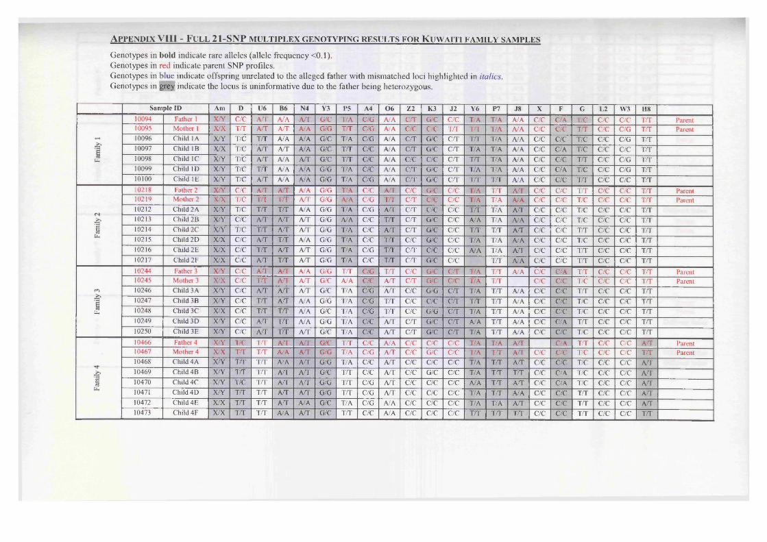
A p p e n d ix V l l l - F u l l 2 1 -S N P m u l t ip l e x g e n o t y p in g r e s u l t s f o r K u w a it i f a m il y s a m p l e s

Genotypes in bold indicate rare alleles (allele frequency <0.1).Genotypes in red indicate parent SNP profiles.Genotypes in blue indicate offspring unrelated to the alleged father with mismatched loci highlighted in italics. Genotypes in grey indicate the locus is uninformative due to the father being heterozygous.

Sample ID Am D U6 B6 N4 Y3 P5 A4 0 6 Z2 K3 J2 Y6 P7 J8 X F G L2 W3 H810094 Father 1 X/Y C/C A T A A A T G/C T/A C/G A A C T G/C C/C T/A T/A A A C/C C/A T/C C/C C/C T T Parent10095 Mother 1 X/X TIT A T A T A A g /g T T C/G A A C/C C/C T T T T T/A A A C/C C/C T T C/C C/G T T Parent10096 Child 1A X/Y T/C T T A A A A G/C T/A C/G A A C T G/C C T T T T/A A A C/C C/C T/C C/C C/G T T10097 Child IB X/X T/C A T A T A A G/C T T C/C A A C T G/C C T T/A T/A A A C/C C/A T/C C/C C/C T T

U* 10098 Child 1C X/Y T/C A T A A A T G/C T T C/C A A C/C C/C C T T T T/A A A C/C C/C T T C/C C/G T T10099 Child ID X/Y T/C T T A A A A G/G T/A C/C A A C T G/C C T T/A T/A A A C/C C/A T/C C/C C/G T T10100 Child IE X/Y T/C A T A A A A G/G T/A C/G A A C T G/C C T T T T T A A C/C C/C T T C/C C/C T Tin: is Father 2 X/Y C/C A T A T A A G/G T/A C/C A T C/C G/C C/C T/A T T A T C/C C/C T T C/C C/C T T Parent10219 Mother 2 X/X T/C T T T T A T G/G A A C/G T T C T C/C C/C T/A T/A A A C/C C/C T/C C/C C/C T T Parent10212 Child 2A X/Y T/C T T T T A A G/G T/A C/G A T C T C/C C/C T T T/A A T C/C C/C T/C C/C C/C T T10213 Child 2B X/Y C/C A T A T A T G/G A A C/C T T C T G/C C/C A A T/A A A C/C C/C T/C C/C C/C T T

1 10214 Child 2C X/Y T/C T T A T A T G/G T/A C/C A T C T G/C C/C T T T T A T C/C C/C T T C/C C/C T T10215 Child 2D X/X C/C A T T T A A G/G T/A C/C T T C/C G/C C/C T/A T/A A A C/C C/C T/C C/C C/C T T10216 Child 2E X/X C/C T T A T A T G/G T/A C/G T T C T C/C C/C A A T/A A T C/C C/C T T C/C C/C T T10217 Child 2F X/X C/C A T T T A T G/G T/A C/C T T C T G/C C/C T T A A C/C C/C T T C/C C/C T T10244 Father 3 X/Y C/C A T A T A A G/G T T C/G T T C/C G/C C T T/A T T A A C/C C/A T T C/C C/C T T Parent10245 Mother 3 X/X C/C T T A T A T G/C A A C/C A T C T G/C C/C T/A T T C/C C/C T/C C/C C/C T T Parent10246 Child 3A X/Y C/C A T A T A T G/C T/A C/G A T C/C G/G C T T/A T T A A C/C C/C T T C/C C/C T T10247 Child 3B X/Y C/C T T A T A A G/G T/A C/G T T C/C C/C C T T T T T A A C/C C/C T/C C/C C/C T T

tit 10248 Child 3C X/X C/C T T T T A A G/C T/A C/G T T C/C G/G C T T/A T T A A C/C C/C T/C C/C C/C T T10249 Child 3D X/Y C/C A T T T A A G/G T/A C/C A T C T G/C C T A A T T A A C/C C/A T T C/C C/C T T10250 Child 3E X/Y C/C A T T T A T G/C T/A C/C A T C T G/C C T T/A T T A A C/C C/C T/C C/C C/C T T10466 Father 4 X/Y T/C T T A T A T G/C T T C/C A A C/C C/C C/C T/A T/A A T C/A T T C/C C/C A T Parent10467 Mother 4 X/X t t T T A A A T G/G T/A C/G A T C/C G/C C/C T/A T T A T C/C C/C T/C C/C C/C T T Parent10468 Child 4A X/Y TAT T T A A A T G/G T/A C/C A T C/C C/C C/C T/A T T A T C/C C/C T/C C/C C/C A T10469 Child 4B X/Y T/T T T A T A T G/C T T C/C A T C/C G/C C/C T/A T T T T C/C C/A T/C C/C C/C A T

i 10470 Child 4C X/Y T/C T T A T A T G/G T T C/G A T C/C C/C C/C A A T T A T C/C C/A T/C C/C C/C A T10471 Child 4D X/Y T/T T T A T A T G/G T T C/G A T C/C C/C C/C T/A T T A A C/C C/C T T C/C C/C A T10472 Child 4E X/X T/T T T A T A A G/C T/A C/G A A C/C C/C C/C T/A T/A A T C/C C/C T T C/C C/C A T10473 Child 4F X/X T/T T T A A A T G/C T T C/C A A C/C C/C C/C T T T T T T C/C C/C T T C/C C/C T T

Sample ID Amelo D U6 B6 N4 Y3 P5 A4 0 6 Z2 K3 J2 Y6 P7 J8 X F G L2 VV3 H88290 Mother 5 X/X T/C T T A T AT G/C TT C/C A/A C/C C/C C/C T/A T/A A/A C/C C/C TT C/C C/G T T Parent8291 Father 5 X/Y T/T A/A A/A AT G/G T/A C/G T T C/C G/C C/C T/A T T A/A C/A C/C T/C C/C C/C T T Parent8292 Child 5A X/Y T/C A T A T A/A G/G T/A C/C A T C/C G/C C/C T/A T/A A/A C/A C/C T T C/C C/C T T8293 Child 5B X/Y T/C A T A/A AT G/C T/A C/G A T C/C C/C C/C TT T/A A/A C/A C/C TT C/C C/C T T

1 8294 Child 5C X/X T/T A T A T AT G/C T/A C/G A T C/C C/C C/C A/A T/A A/A C/A C/C T/C C/C C/C T T8295 Child 5D X/Y T/C A T A/A AT G/G T/A C/G A T C/C G/C C/C T/A T/A A/A C/C C/C T/C C/C C/C T T8296 Child 5E X/Y T T A T A/A TT G/C T/A C/G A T C/C C/C C/C A/A T T A/A C/C T/C C/C C/C T T8297 Child 5F X/Y T T A T A T A/A G/C T/A C/G A T C/C G/C C/C T/A T/A A/A C/C C/C T/C C/C C/G T T8485 Father 6 X/Y T T T T A/A A/A G/G T T C/G A/A CT G/C C/C T/A T T AT C/C A/A T T C/C C/C T T Parent8486 Mother 6 X/X T/C A T T T A/A G/G T/A C/G A/A TT C/C C T A/A T/A AT C/C C/C T T T T C/C A T Parent8487 Child 6A X/Y T T T T A T A/A G/G T T C/C A/A TT G/C C T A/A T/A AT C/C C/A T T C T C/C T T

SO 8488 Child 6B X/X T/C A T A/A G/G T/A C/G A/A CT G/C C T T/A T T A T C/C C/A T T C T C/C T T8489 Child 6C X/Y T T A T A T A/A G/G T/A C/G A/A TT G/C C/C A/A T T A T C/C C/A T T C T C/C A T

Uh 8490 Child 6D X/Y T T T T A T A/A G/G T T C/C A/A CT C/C C T A/A T/A AT C/C C/A T T C T C/C T T8491 Child 6E X/X T T T T A T A/A G/G T T C/G A/A CT C/C C T A/A T/A AT C/C C/A T T C T C/C A T8492 Child 6F X/X T/C A T A T A/A G/G T/A C/G A/A TT C/C C T T/A T T AT C/C C/A T T C T C/C T T8493 Child 6G X/Y T/C T T T/T ;*/T G/G T/A C/G A/A CT C/C C/C A/A A/A A/A C/C C/A T T T/T C/C A T Different father8755 Father 7 X/Y T/C AT A/A A/A G/C T T C/G AT C T G/C C/C T T T T AT C/A C/C T/C CT C/C T T Parent8756 Mother 7 X/X T/C TT A/A A T G/G T/A G/G A T TT G/C C/C T/A T T AT C/C C/C C/C CT C/C A/A Parent

r- 8757 Child 7 A X/X T/C A T A/A A T G/G T/A C/G A T TT G/C C/C T/A T T AT C/C C/C T/C CT C/C A T8758 Child 7B X/X T/C AT A/A A T G/C T/A C/G T T TT G/G C/C T/A T T A/A C/C C/C C/C TT C/C A T

§ 8759 Child 7C X/X T/C TT A/A A/A G/G T T C/G A T TT G/C C/C T/A T T AT C/C C/C C/C C/C C/C A Tbu 8760 Child 7D X/Y T/C TT A/A A T G/G T T C/G A T TT G/C C/C T T T T A/A C/A C/C T/C CT C/C A T

8761 Child 7E X/X T/C TT A/A A/A G/C T T C/G A T T T G/C C/C T/A T T AT C/A C/C T/C C/C C/C A T8762 Child 7F X/Y C/C TT A/A A T G/G T/A C/G T T C T G/C C/C T T T T T T C/A C/C T/C CT C/C A T8830 Father 8 X/Y T T A/A T T AT G/G T/A C/G A T C/C G/C CT T T T T C/C C/A T/C C/C G/G T T Parent8831 Mother 8 XX C/C T T A T A/A G/C T/A C/G T T C T C/C C/C T/A T/A C/C C/A T T C/C C/C T T Parent

00 8833 Child 8A X X C/C T/T T T AT G/G T/A C/C AT T T C/C C/C T T T/A A/A C/C A/A TT C/T C/C T T Different father8834 Child 8B X/Y T/C A T T T A T G/G T/A C/G T T C/C C/C C T T T T/A A/A C/C C/A T/C C/C C/G T T

tu 8835 Child 8C X T T/C A T T T A/A G/G A/A C/C T T C/C C/C C/C T/A T T A/A C/C C/C T/C C/C C/G T T8836 Child 8D X/Y T/C A T A T A/A G/G T/A C/G A T C T G/C C/C ,4/4 T T A/A C/4 C/A T T C/C C/C T T Different father8837 Child 8E X/Y T/C T/T A T A/A G/C TT C/G T T C T C/C C/C T T T/A A/A C/4 C/A TT C/C C/C T T Different father

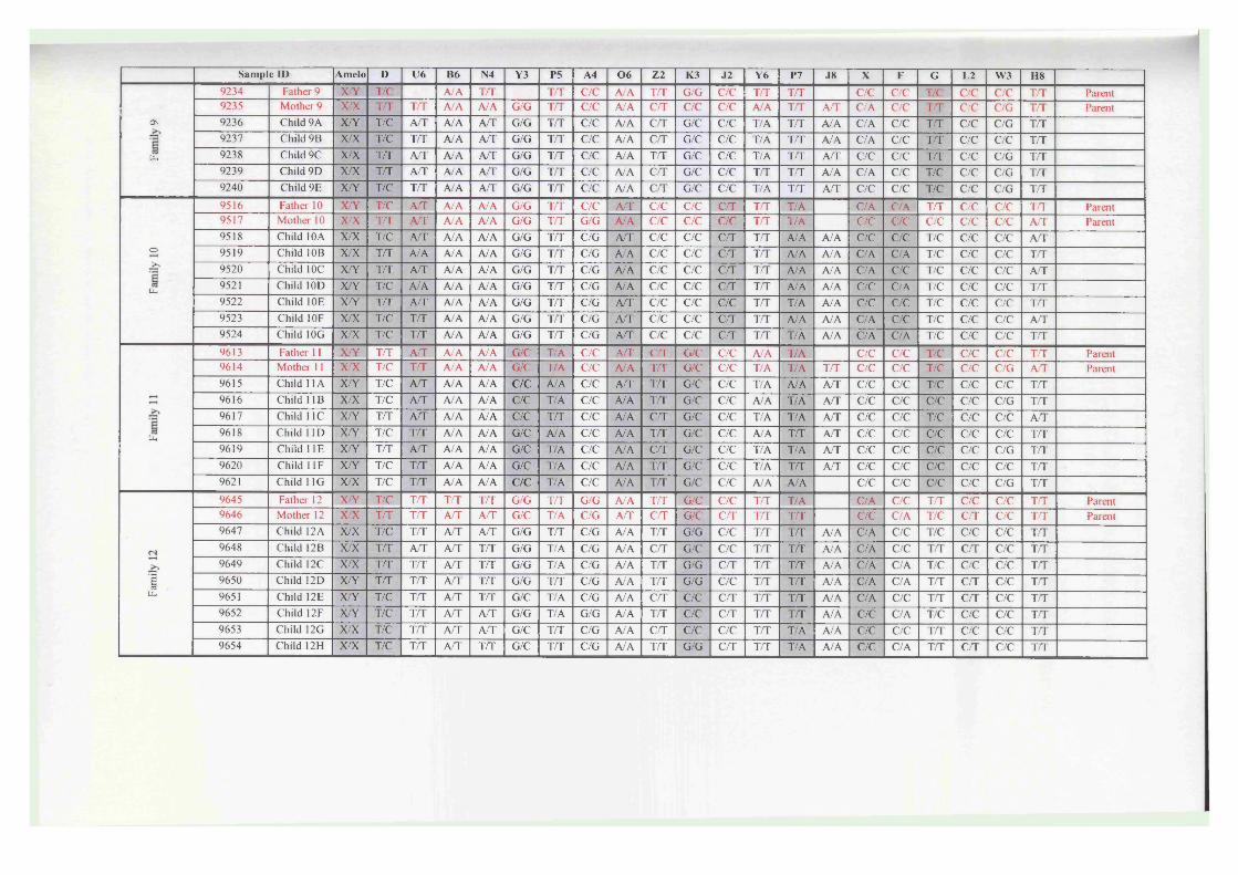
Sample ID Amelo D U6 B6 N4 Y3 P5 A4 0 6 Z2 K3 J2 Y6 P7 J8 X F G L2 VV3 H89234 Father 9 X/Y T/C A/A T T T T C/C A/A T T G/G C/C T T T T C/C C/C T/C C/C C/C T T Parent9235 Mother 9 X/X T/T T T A/A A/A G/G T T C/C A/A C T C/C C/C A/A T T A T C/A C/C T T C/C C/G T T Parent

ON 9236 Child 9A X/Y T/C A T A/A A T G/G T T C/C A/A C T G/C C/C T/A T T A/A C/A C/C T T C/C C/G T T9237 Child 9B X/X T/C T T A/A A T G/G T T C/C A/A C T G/C C/C T/A T T A/A C/A C/C T T C/C C/C T T

Ui 9238 Child 9C X/X T/T A T A/A A T G/G T T C/C A/A T T G/C C/C T/A T T A T C/C C/C T T C/C C/G T T9239 Child 9D X/X T/T A T A/A A T G/G T T C/C A/A C T G/C C/C T T T T A/A C/A C/C T/C C/C C/G T T9240 Child 9E X/Y T/C T T A/A A T G/G T T C/C A/A C T G/C C/C T/A T T A T C/C C/C T/C C/C C/G T T9516 Father 10 X/Y T/C A T A/A A/A G/G T T C/C A T C/C C/C C T T T T/A C/A C/A T T C/C C/C T T Parent9517 Mother 10 X/X T/T A T A/A A/A G/G T T G/G A/A C/C C/C C/C T T T/A C/C C/C C/C C/C C/C A T Parent9518 Child 10A X/X T/C A T A/A A/A G/G T T C/G A T C/C C/C C T T T A/A A/A C/C C/C T/C C/C C/C A T

o 9519 Child 10B X/X T/T A/A A/A A/A G/G T T C/G A/A C/C C/C C T T T A/A A/A C/A C/A T/C C/C C/C T Tr*~~i 9520 Child 10C X/Y T T A T A/A A/A G/G T T C/G A/A C/C C/C C T T T A/A A/A C/A C/C T/C C/C C/C A T

Uh9521 Child 10D X/Y T/C A/A A/A A/A G/G T T C/G A/A C/C C/C C T T T A/A A/A C/C C/A T/C C/C C/C T T9522 Child 10E X/Y T T A T A/A A/A G/G T T C/G A T C/C C/C C/C T T T/A A/A C/C C/C T/C C/C C/C T T9523 Child 10F X/X T/C T T A/A A/A G/G T T C/G A T C/C C/C C T T T A/A A/A C/A C/C T/C C/C C/C A T9524 Child 10G X/X T/C T T A/A A/A G/G T T C/G A T C/C C/C C T T T T/A A/A C/A C/A T/C C/C C/C T T9613 Father 11 X/Y T T A T A/A A/A G/C T/A C/C A T C T G/C C/C A/A T/A C/C C/C T/C C/C C/C T T Parent9614 Mother 11 X/X T/C T T A/A A/A G/C T/A C/C A/A T T G/C C/C T/A T/A T T C/C C/C T/C C/C C/G A T Parent9615 Child 11A X/Y T/C A T A/A A/A C/C A/A C/C A T T T G/C C/C T/A A/A A T C/C C/C T/C C/C C/C T T9616 Child 1 IB X/X T/C A T A/A A/A C/C T/A C/C A/A T T G/C C/C A/A T/A A T C/C C/C C/C C/C C/G T T9617 Child 11C X/Y T T A T A/A A/A C/C T T C/C A/A C T G/C C/C T/A T/A A T C/C C/C T/C C/C C/C A T

U-, 9618 Child 1 ID X/Y T/C T T A/A A/A G/C A/A C/C A/A T T G/C C/C A/A T T A T C/C C/C C/C C/C C/C T T9619 Child HE X/Y T T A T A/A A/A G/C T/A C/C A/A C T G/C C/C T/A T/A A T C/C C/C C/C C/C C/G T T9620 Child 1 IF X/Y T/C T T A/A A/A G/C T/A C/C A/A T T G/C C/C T/A T T A T C/C C/C C/C C/C C/C T T9621 Child 11G X/X T/C T T A/A A/A C/C T/A C/C A/A T T G/C C/C A/A A/A C/C C/C C/C C/C C/G T T9645 Father 12 X/Y T/C T T T T T T G/G T T G/G A/A T T G/C C/C T T T/A C/A C/C T T C/C C/C T T Parent9646 Mother 12 X/X T T T T A T A T G/C T/A C/G A T C T G/C C T T T T T C/C C/A T/C C T C/C T T Parent9647 Child 12A X/X T/C T T A T A T G/G T T C/G A/A T T G/G C/C T T T T A/A C/A C/C T/C C/C C/C T T9648 Child 12B X/X T T A T A T T T G/G T/A C/G A/A C T G/C C/C T T T T A/A C/A C/C T T C T C/C T T9649 Child 12C X/X T T T T A T T T G/G T/A C/G A/A T T G/G C T T T T T A/A C/A C/A T/C C/C C/C T T

1 9650 Child 12D X/Y T T T T A T T T G/G T T C/G A/A T T G/G C/C T T T T A/A C/A C/A T T C T C/C T Tb u 9651 Child 12E X/Y T/C T T A T T T G/C T/A C/G A/A C T C/C C T T T T T A/A C/A C/C T T C T C/C T T

9652 Child 12F X/Y T/C T T A T A T G/G T/A G/G A/A T T C/C C/T T T T T A/A C/C C/A T/C C/C C/C T T9653 Child 12G X/X T/C T T A T A T G/C T T C/G A/A C T C/C C/C T T T/A A/A C/C C/C T T C/C C/C T T9654 Child 12H X/X T/C T T A T T T G/C T T C/G A/A T T G/G C T T T T/A A/A C/C C/A T T C T C/C T T

Sample ID Am D U6 B6 N4 Y3 P5 A4 0 6 Z2 K3 J2 Y6 P7 J8 X F G L2 W3 H89234 Father 13 X/X TA­ A/T A A A A G/G T A C/C A A C A C/C C/C A A T/A C/A C/C TA C/C C/C T A Parent9235 Mother 13 X/Y T/C A A T A TA G/G T A C/G A A C A C/C C/C T A TA A A C/A C/C T A C/C C/C A A Parent9236 Child 13A X/X T/T A A A A A A G/G TA C/G A A C A C/C C/C T/A TA A A C/C C/C T A C/C C/C A A9237 Child 13B X/X T/C A A A A A A G/G T A C/G A A C/C C/C C/C T/A TA A A C/A C/C T A C/C C/C AA

U-, 9238 Child 13C X/X TA­ TA A A A A G/G T A C/G A A C A C/C C/C T/A T/A A A C/A C/C TA C/C C/C A A9239 Child 13D X/Y T/C A A A A A A G/G TA C/G A A TA C/C C/C T/A T/A A A C/A C/C T A C/C C/C TA9240 Child 13E X/Y T/T A A T A A A G/G T A C/G A A TA C/C C/C T/A T/A A A C/A C/C TA C/C C/C A A

Appendices

A p pe n d ix IX - L ik elih o o d r a t io c a l c u l a t io n s f o r k in sh ip a n a l y sis

Parent 1 Parent 2 Body Likelihood ratio calculationaa aa aa 1/a2aa aa aF l/(a x 1) = 1/aaa ab aa l/2a2aa ab aF l/(2a x 1) = l/2aaa ab ab l/4abab ab ab l/4abab ab aF l/(4a x 1) = l/4aab ab Fb 1/(1 x 4b) = l/4bab ab aa l/4a2ab ab bb l/4b2ab ab bF l/(4b x 1) = l/4baa ab Fb l/(4b x 1) = l/4baa bb ab l/2abaa bb aF l/(2a x 1) = l/2aaa bb Fb 1/(1 x 2b) = l/2bab bb ab l/4abab bb aF l/(4a x 1) = l/4aab bb Fb 1/(1 x 4b) = l/4bab bb bb l/2b2bb bb bb 1/b2bb bb bF l/(b x 1)= 1/baa - aa 1/aaa - ab l/2aaa - aF l/2aaa - Fb 1ab - aa l/2aab - ab (a + b)/4abab - bb l/2bab - aF l/4aab - Fb l/4bbb - ab l/2bbb - bb 1/bbb - aF 1

?t(e \H D) Where L R = —) ± .±{

P r(4

Hp = The body is the biological child o f M and/or F

Hd = The body is an unknown, unrelated individual

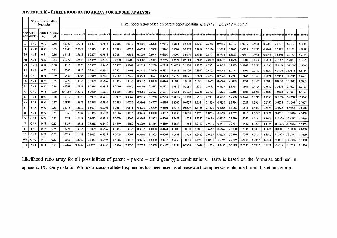
A p p e n d ix X - L ik e l ih o o d r a t io a r r a y f o r k in s h ip a n a l y s is

White Caucasian allele frequencies Likelihood ratios based on parent genotype data [parent 1 + parent 2 = body]

SNPlocus

Allele 1/ Allele 2

Allele 1(a)

Allele 2 (b)

aa+aa=aa aa+aa=aF aa+ab=aa aa+ab=aF aa+ab=ab ab+ab=ab ab+ab=aF ab+ab=Fb ab+ab=aa ab+ab=bb ab+ab=bF aa+ab=Fb aa+bb=ab aa+bb=aF aa+bb=Fb ab+bb=ab ab+bb=aF ab+bb=Fb ab+bb=bb bb+bb=bb ab+bb=bF

D T /C 0.52 0.48 3.6982 1.9231 1.8491 0.9615 1.0016 1.0016 0.4808 0.5208 0.9246 1.0851 0.5208 0.5208 2.0032 0.9615 1.0417 1.0016 0.4808 0.5208 2.1701 4.3403 2.0833

U6 A /T 0.37 0.63 7.3046 2.7027 3.6523 1.3514 1.0725 1.0725 0.6757 0.3968 1.8262 0.6299 0.3968 0.3968 2.1450 1.3514 0.7937 1.0725 0.6757 0.3968 1.2598 2.5195 1.5873

B6 A /T 0.64 0.36 2.4414 1.5625 1.2207 0.7813 1.0851 1.0851 0.3906 0.6944 0.6104 1.9290 0.6944 0.6944 2.1701 0.7813 1.3889 1.0851 0.3906 0.6944 3.8580 7.7160 2.7778

N4 A /T 0.57 0.43 3.0779 1.7544 1.5389 0.8772 1.0200 1.0200 0.4386 0.5814 0.7695 1.3521 0.5814 0.5814 2.0400 0.8772 1.1628 1.0200 0.4386 0.5814 2.7042 5.4083 2.3256

Y3 G /C 0.92 0.08 1.1815 1.0870 0.5907 0.5435 3.3967 3.3967 0.2717 3.1250 0.2954 39.0625 3.1250 3.1250 6.7935 0.5435 6.2500 3.3967 0.2717 3.1250 78.1250 156.2500 12.5000

P5 T /A 0.72 0.28 1.9290 1.3889 0.9645 0.6944 1.2401 1.2401 0.3472 0.8929 0.4823 3.1888 0.8929 0.8929 2.4802 0.6944 1.7857 1.2401 0.3472 0.8929 6.3776 12.7551 3.5714

A4 C /G 0.71 0.29 1.9837 1.4085 0.9919 0.7042 1.2142 1.2142 0.3521 0.8621 0.4959 2.9727 0.8621 0.8621 2.4284 0.7042 1.7241 1.2142 0.3521 0.8621 5.9453 11.8906 3.4483

06 A /T 0.75 0.25 1.7778 1.3333 0.8889 0.6667 1.3333 1.3333 0.3333 1.0000 0.4444 4.0000 1.0000 2.0000 2.6667 0.6667 2.0000 1.3333 0.3333 1.0000 8.0000 16.0000 4.0000

Z2 C /T 0.56 0.44 3.1888 1.7857 1.5944 0.8929 1.0146 1.0146 0.4464 0.5682 0.7972 1.2913 0.5682 1.1364 2.0292 0.8929 1.1364 1.0146 0.4464 0.5682 2.5826 5.1653 2.2727

K3 G /C 0.31 0.69 10.4058 3.2258 5.2029 1.6129 1.1688 1.1688 0.8065 0.3623 2.6015 0.5251 0.3623 0.7246 2.3375 1.6129 0.7246 1.1688 0.8065 0.3623 1.0502 2.1004 1.4493

J2 C /T 0.92 0.08 1.1815 1.0870 0.5907 0.5435 3.3967 3.3967 0.2717 3.1250 0.2954 39.0625 3.1250 6.2500 6.7935 0.5435 6.2500 3.3967 0.2717 3.1250 78.1250 156.2500 12.5000

Y6 T /A 0.63 0.37 2.5195 1.5873 1.2598 0.7937 1.0725 1.0725 0.3968 0.6757 0.6299 1.8262 0.6757 1.3514 2.1450 0.7937 1.3514 1.0725 0.3968 0.6757 3.6523 7.3046 2.7027

P7 T /A 0.62 0.38 2.6015 1.6129 1.3007 0.8065 1.0611 1.0611 0.4032 0.6579 0.6504 1.7313 0.6579 1.3158 2.1222 0.8065 1.3158 1.0611 0.4032 0.6579 3.4626 6.9252 2.6316

J8 A /T 0.77 0.23 1.6866 1.2987 0.8433 0.6494 1.4116 1.4116 0.3247 1.0870 0.4217 4.7259 1.0870 2.1739 2.8233 0.6494 2.1739 1.4116 0.3247 1.0870 9.4518 18.9036 4.3478

X C /A 0.79 0.21 1.6023 1.2658 0.8012 0.6329 1.5069 1.5069 0.3165 1.1905 0.4006 5.6689 1.1905 2.3810 3.0139 0.6329 2.3810 1.5069 0.3165 1.1905 11.3379 22.6757 4.7619

F C /A 0.78 0.22 1.6437 1.2821 0.8218 0.6410 1.4569 1.4569 0.3205 1.1364 0.4109 5.1653 1.1364 2.2727 2.9138 0.6410 2.2727 1.4569 0.3205 1.1364 10.3306 20.6612 4.5455

G T /C 0.75 0.25 1.7778 1.3333 0.8889 0.6667 1.3333 1.3333 0.3333 1.0000 0.4444 4.0000 1.0000 2.0000 2.6667 0.6667 2.0000 1.3333 0.3333 1.0000 8.0000 16.0000 4.0000

L2 C /T 0.79 0.21 1.6023 1.2658 0.8012 0.6329 1.5069 1.5069 0.3165 1.1905 0.4006 5.6689 1.1905 2.3810 3.0139 0.6329 2.3810 1.5069 0.3165 1.1905 11.3379 22.6757 4.7619

W3 C /G 0.77 0.23 1.6866 1.2987 0.8433 0.6494 1.4116 1.4116 0.3247 1.0870 0.4217 4.7259 1.0870 2.1739 2.8233 0.6494 2.1739 1.4116 0.3247 1.0870 9.4518 18.9036 4.3478

H8 A /T 0.11 0.89 82.6446 9.0909 41.3223 4.5455 2.5536 2.5536 2.2727 0.2809 20.6612 0.3156 0.2809 0.5618 5.1073 4.5455 0.5618 2.5536 2.2727 0.2809 0.6312 1.2625 1.1236

Likelihood ratio array for all possibilities of parent - parent - child genotype combinations. Data is based on the formulae outlined in

appendix IX. Only data for White Caucasian allele frequencies has been used as all casework samples were obtained from this ethnic group.

Bibliography

Bibliography

-248-

Bibliography

Ahn, S.J., Costa, J. and Emanuel, J.R. (1996). "PicoGreen quantitation of DNA: effective evaluation of samples pre- or post-PCR." Nucleic Acids Res 24(13): 2623-5.

Akane, A., Shiono, H., Matsubara, K., Nakamura, H., Hasegawa, M. and Kagawa, M. (1993). "Purification of forensic specimens for the polymerase chain reaction (PCR) analysis." J Forensic Sci 38(3): 691-701.

Alizadeh, A.A., Eisen, M.B., Davis, R.E., Ma, C., Lossos, I.S., Rosenwald, A., Boldrick, J.C., Sabet, H., Tran, T., Yu, X., Powell, J.I., Yang, L., Marti, G.E., Moore, T., Hudson, J., Jr., Lu, L., Lewis, D.B., Tibshirani, R., Sherlock, G., Chan, W.C., Greiner, T.C., Weisenburger, D.D., Armitage, J.O., Wamke, R., Levy, R., Wilson, W., Grever, M.R., Byrd, J.C., Botstein, D., Brown, P.O. and Staudt, L.M. (2000). "Distinct types of diffuse large B-cell lymphoma identified by gene expression profiling." Nature 403(6769): 503-11.

Alonso, A., Martin, P., Albarran, C., Garcia, P., Fernandez de Simon, L., Jesus Iturralde, M., Femandez-Rodriguez, A., Atienza, I., Capilla, J., Garcia- Hirschfeld, J., Martinez, P., Vallejo, G., Garcia, O., Garcia, E., Real, P., Alvarez, D., Leon, A. and Sancho, M. (2005). "Challenges of DNA profiling in mass disaster investigations." Croat Med J 46(4): 540-8.

Amorim, A. and Pereira, L. (2005). "Pros and cons in the use of SNPs in forensic kinship investigation: a comparative analysis with STRs." Forensic Sci Int 150: 17-21.

Attema, J.L., Reeves, R., Murray, V., Levichkin, I., Temple, M.D., Tremethick,D.J. and Shannon, M.F. (2002). "The human IL-2 gene promoter can assemble a positioned nucleosome that becomes remodeled upon T cell activation." J Immunol 169(5): 2466-76.

Ayres, K.L. and Balding, D.J. (2001). "Measuring gametic disequilibrium from multilocus data." Genetics 157(1): 413-23.

Ayres, K.L., Chaseling, J. and Balding, D.J. (2002a). "Implications for DNA identification arising from an analysis of Australian forensic databases." Forensic Sci Int 129(2): 90-8.

Ayres, K.L. (2002b). "Paternal exclusion in the presence of substructure." Forensic Sci Int 129: 142-144.

Ayres, K.L. (2005). "The expected performance of single nucleotide polymorphism loci in paternity testing." Forensic Sci Int 154: 167-172.

-249-

Bibliography

Baird, M., Balazs, I., Giusti, A., Miyazaki, L., Nicholas, L., Wexler, K., Kanter,E., Glassberg, J., Allen, F., Rubinstein, P. and et al. (1986). "Allele frequency distribution of two highly polymorphic DNA sequences in three ethnic groups and its application to the determination of paternity." Am J Hum Genet 39(4): 489-501.

Balding, D.J. and Nichols, R.A. (1994). "DNA profile match probability calculation: how to allow for population stratification, relatedness, database selection and single bands." Forensic Sci Int 64(2-3): 125-40.

Balding, D.J. and Nichols, R.A. (1995). "A method for quantifying differentiation between populations at multi-allelic loci and its implications for investigating identity and paternity." Genetica 96(1-2): 3-12.

Balding, D.J., Greenhalgh, M. and Nichols, R.A. (1996). "Population genetics of STR loci in Caucasians." Int J Legal Med 108(6): 300-5.

Balding, D.J. (2005). "Weight-of-evidence for forensic DNA profiles". Chichester, UK, John Wiley & Sons, Ltd.

Ballantyne, J. (1997). "Mass disaster genetics." Nat Genet 15(4): 329-31.

Bar, W., Kratzer, A., Machler, M. and Schmid, W. (1988). "Postmortem stability of DNA." Forensic Sci Int 39(1): 59-70.

Beckman, J.S. and Weber, J.L. (1992). "Survey of human and rat microsatellites." Genomics 12(4): 627-31.

Bell, G.I., Selby, M.J. and Rutter, W.J. (1982). "The highly polymorphic region near the human insulin gene is composed of simple tandemly repeating sequences." Nature 295(5844): 31-5.

Bell, P.A., Chaturvedi, S., Gelfand, C.A., Huang, C.Y., Kochersperger, M., Kopla, R., Modica, F., Pohl, M., Varde, S., Zhao, R., Zhao, X. and Boyce- Jacino, M.T. (2002). "SNPstream UHT: ultra-high throughput SNP genotyping for pharmacogenomics and drug discovery." Biotechniques Suppl: S70-S77.

Benedek-Spat, E. (1973a). "The composition of unstimulated human parotid saliva." Arch Oral Biol 18(1): 39-47.

Benedek-Spat, E. (1973b). "The composition of stimulated human parotid saliva." Arch Oral Biol 18(9): 1091-7.

Berlin, K. and Gut, I.G. (1999). "Analysis of negatively ’charge tagged’ DNA by matrix-assisted laser desorption/ionization time-of-flight mass spectrometry." Rapid Commun Mass Spectrom 13(17): 1739-43.

-250-

Bibliography

Bina-Stein, M. and Simpson, R.T. (1977). ’’Specific folding and contraction of DNA by histones H3 and H4." Cell 11(3): 609-18.

Bittles, A. (2001). "Consanguinity and its relevance to clinical genetics." Clin Genet 60(2): 89-98.

Bittles, A.H. (1998). "Empirical estimates of the global prevalence of consanguineous marriage in contemporary societies" No. 0074 Morrison Institute for Population and Resource Studies, Stanford University Stanford, California pp. 1-69

Bland, J.M. and Altman, D.G. (1995). "Multiple significance tests: the Bonferroni method." Bmj 310(6973): 170.

Bonilla, C., Boxill, L.A., Donald, S.A., Williams, T., Sylvester, N., Parra, E.J., Dios, S., Norton, H.L., Shriver, M.D. and Kittles, R.A. (2005). "The 8818G allele of the agouti signaling protein (ASIP) gene is ancestral and is associated with darker skin color in African Americans." Hum Genet 116(5): 402-6.

Bowcock, A.M., Hebert, J.M., Mountain, J.L., Kidd, J.R., Rogers, J., Kidd, K.K. and Cavalli-Sforza, L.L. (1991). "Study of an additional 58 DNA markers in five human populations from four continents." Gene Geogr 5(3): 151- 73.

Bowtell, D.D.L. (1999). "Options available - from start to finish - for obtaining expression data by microarray." Nat Genet 21(S): 25-32.

Bradley, H.C. (1938). "Autolysis and atrophy." Physiol Rev 18: 179.

Brenner, C.H. (1997). "Symbolic kinship program." Genetics 145(2): 535-42.

Brion, M. (2005a). "Y chromosome SNP analysis using the single-base extension: a hierarchical multiplex design." Methods Mol Biol 297: 229-42.

Brion, M., Sanchez, J.J., Balogh, K., Thacker, C., Blanco-Verea, A., Borsting, C., Stradmann-Bellinghausen, B., Bogus, M., Syndercombe-Court, D., Schneider, P.M., Carracedo, A. and Morling, N. (2005b). "Introduction of an single nucleodite polymorphism-based "Major Y-chromosome haplogroup typing kit" suitable for predicting the geographical origin of male lineages." Electrophoresis 26(23): 4411-20.

Brown, C.S., Goodwin, P.C. and Sorger, P.K. (2001). "Image metrics in the statisttical analysis of DNA microarray data." Proc Natl Acad Sci U S A 98(16): 8944-8949.

-251 -

Bibliography

Brown, P.O. and Botstein, D. (1999). "Exploring the new world of the genome with DNA microarrays." Nat Genet 21(1 Suppl): 33-7.

Buckleton, J., Triggs, C.M. and Walsh, S.J. (2005). "Forensic DNA Interpretation". Florida, CRC Press.

Budowle, B. (1995). "The effects of inbreeding on DNA profile frequency estimates using PCR-based loci." Genetica 96(1-2): 21-5.

Budowle, B. (1999). "Forensically important genetic markers." FBI transcript.

Budowle, B., Planz, J.V., Campbell, R.S. and Eisenberg, A.J. (2004a). "Single nucleotide polymorphisms and microarray technology in forensic genetics - development and application to Mitochondrial DNA." Forensic Sci Rev 16(1): 21-36.

Budowle, B. (2004b). "SNP typing strategies." Forensic Sci Int 146 Suppl: SI 39- 42.

Budowle, B., Bieber, F.R. and Eisenberg, A.J. (2005). "Forensic aspects of mass disasters: Strategic considerations for DNA-based human identification." Leg Med (Tokyo) 7: 230-243.

Burger, J., Hummel, S., Hermann, B. and Henke, W. (1999). "DNA preservation: a microsatellite-DNA study on ancient skeletal remains." Electrophoresis 20(8): 1722-8.

Butler, J.M. and Levin, B.C. (1998). "Forensic applications of mitochondrial DNA." Trends in Biotech 16: 158-162.

Butler, J.M., Shen, Y. and McCord, B.R. (2003). "The development of reduced size STR amplicons as tools for analysis of degraded DNA." J Forensic Sci 48(5): 1054-64.

Butler, J.M., Buel, E., Crivellente, F. and McCord, B.R. (2004). "Forensic DNA typing by capillary electrophoresis using the ABI Prism 310 and 3100 genetic analyzers for STR analysis." Electrophoresis 25(10-11): 1397-412.

Butler, J.M. (2005a). "Constructing STR multiplex assays." Methods Mol Biol 297:53-66.

Butler, J.M. (2005b). "Forensic DNA Typing: Biology, Technology, and Genetics of STR Markers (2nd Edition). " New York, Elsevier Academic Press.

Capon, D.J., Chen, E.Y., Levinson, A.D., Seeburg, P.H. and Goeddel, D.V. (1983). "Complete nucleotide sequences of the T24 human bladder carcinoma oncogene and its normal homologue." Nature 302(5903): 33-7.

-252-

Bibliography

Carey, L. and Mitnik, L. (2002). "Trends in DNA forensic analysis." Electrophoresis 23(10): 1386-97.

Cash, H.D., Hoyle, J.W. and Sutton, A.J. (2003). "Development under extreme conditions: forensic bioinformatics in the wake of the World Trade Center disaster." Pac Symp Biocomput: 638-53.

Chakraborty, R. (1992). "Sample size requirements for addressing the population genetic issues of forensic use of DNA typing." Hum Biol 64(2): 141-59.

Chakraborty, R., Stivers, D.N., Su, B., Zhong, Y. and Budowle, B. (1999). "The utility of short tandem repeat loci beyond human identification: implications for development of new DNA typing systems." Electrophoresis 20(8): 1682-96.

Chakravarti, A. (1999). "Population genetics—making sense out of sequence." Nat Genet 21(1 Suppl): 56-60.

Chen, Y., Kamat, V., Dougherty, E.R., Bittner, M.L., Meltzer, P.S. and Trent, J.M. (2002). "Ratio statistics of gene expression levels and applications to microarray data analysis." Bioinformatics 18(9): 1207-15.

Chung, D.T., Drabek, J., Opel, K.L., Butler, J.M. and McCord, B.R. (2004). "A study on the effects of degradation and template concentration on the amplification efficiency of the STR Miniplex primer sets." J Forensic Sci 49(4): 733-40.

Clark, A.G. (2003). "Finding genes underlying risk of complex disease by linkage disequilibrium mapping." Curr Opin Genet Dev 13(3): 296-302.

Clayton, T.M., Whitaker, J.P. and Maguire, C.N. (1995a). "Identification of bodies from the scene of a mass disaster using DNA amplification of short tandem repeat (STR) loci." Forensic Sci Int 76(1): 7-15.

Clayton, T.M., Whitaker, J.P., Fisher, D.L., Lee, D.A., Holland, M.M., Weedn, V.W., Maguire, C.N., DiZinno, J.A., Kimpton, C.P. and Gill, P. (1995b). "Further validation of a quadruplex STR DNA typing system: a collaborative effort to identify victims of a mass disaster." Forensic Sci Int 76(1): 17-25.

Coble, M.D., Just, R.S., O'Callaghan, J.E., Letmanyi, I.H., Peterson, C.T., Irwin, J.A. and Parsons, T.J. (2004). "Single nucleotide polymorphisms over the entire mtDNA genome that increase the power of forensic testing in Caucasians " Int J Legal Med 118(3): 137-46.

Coble, M.D. and Butler, J.M. (2005). "Characterization of new miniSTR loci to aid analysis of degraded DNA." J Forensic Sci 50(1): 43-53.

-253 -

Bibliography

Collins, A. (2000). "Linkage disequilibrium mapping using single nucleotide polymorphisms—which population?" Pac Symp Biocomput: 651-62.

Collins, A., Ennis, S., Taillon-Miller, P., Kwok, P.Y. and Morton, N.E. (2001). "Allelic association with SNPs: metrics, populations, and the linkage disequilibrium map." Hum Mutat 17(4): 255-62.

Collins, P.J., Hennessy, L.K., Leibelt, C.S., Roby, R.K., Reeder, D.J. and Foxall, P.A. (2004). "Developmental validation of a single-tube amplification of the 13 CODIS STR loci, D2S1338, D19S433, and amelogenin: the AmpFlSTR Identifiler PCR amplification kit." J Forensic Sci 49(6): 1265- 1277.

Cooper, A., Rambaut, A., Macaulay, V., Willerslev, E., Hansen, A.J. and Stringer, C. (2001). "Human origins and ancient human DNA." Science 292(5522): 1655-6.

Cooper, D.N., Smith, B.A., Cooke, H.J., Niemann, S. and Schmidtke, J. (1985). "An estimate of unique DNA sequence heterozygosity in the human genome." Hum Genet 69(3): 201-5.

Corach, D., Filgueira Risso, L., Marino, M., Penacino, G. and Sala, A. (2001). "Routine Y-STR typing in forensic casework." Forensic Sci Int 118(2-3): 131-5.

Cotton, E.A., Allsop, R.F., Guest, J.L., Frazier, R.R., Koumi, P., Callow, I.P., Seager, A. and Sparkes, R.L. (2000). "Validation of the AMPF1STR SGM plus system for use in forensic casework." Forensic Sci Int 112(2-3): 151- 61.

Cousins, D.J., Islam, S.A., Sanderson, M.R., Proykova, Y.G., Crane-Robinson, C. and Staynov, D.Z. (2004). "Redefinition of the cleavage sites of DNase I on the nucleosome core particle." J Mol Biol 335(5): 1199-211.

Crespillo, M., Luque, J.A., Paredes, M., Fernandez, R., Ramirez, E. and Valverde, J.L. (2000). "Casework experience: identification of human remains." Progr Forens GenetS: 539-541.

Curran, J.M., Buckleton, J.S. and Triggs, C.M. (2003). "What is the magnitude of the subpopulation effect?" Forensic Sci Int 135(1): 1-8.

Daniels, D.L., Hall, A.M. and Ballantyne, J. (2004). "SWGDAM developmental validation of a 19-locus Y-STR system for forensic casework." J Forensic Sci 49(4): 668-83.

-254-

Bibliography

Dawid, A.P., Mortera, J. and Pascali, V.L. (2001). "Non-fatherhood or mutation? A probabilistic approach to parental exclusion in paternity testing." Forensic Sci Int 124: 55-61.

Debouck, C. and Goodfellow, P.N. (1999). "DNA microarrays in drug discovery and development." Nat Genet 21(1 Suppl): 48-50.

Deka, R., Shriver, M.D., Yu, L.M., Ferrell, R.E. and Chakraborty, R. (1995). "Intra- and inter-population diversity at short tandem repeat loci in diverse populations of the world." Electrophoresis 16(9): 1659-64.

Delahunty, C., Ankener, W., Deng, Q., Eng, J. and Nickerson, D.A. (1996). "Testing the feasibility of DNA typing for human identification by PCR and an oligonucleotide ligation assay." Am JHum Genet 58(6): 1239-46.

Devlin, B., Risch, N. and Roeder, K. (1990). "No excess of homozygosity at loci used for DNA fingerprinting." Science 249(4975): 1416-20.

Di Gaetano, C., Crobu, F., Guarrera, S., Polidoro, S., Gasparini, M., Underhill, P.A., Matullo, G. and Piazza, A. (2004). "The TDI-FP assay in human Y chromosome SNP haplotyping." Genet Test 8(4): 400-3.

Dimo-Simonin, N. and Brandt-Casadevall, C. (1996). "Evaluation and usefulness of reverse dot blot DNA-PolyMarker typing in forensic case work." Forensic Sci Int 81(1): 61-72.

Divne, A.M. and Allen, M. (2005). "A DNA microarray system for forensic SNP analysis." Forensic Sci Int 154(2-3): 111-21.

Dixon, L.A., Murray, C.M., Archer, E.J., Dobbins, A.E., Koumi, P. and Gill, P. (2005a). "Validation of a 21-locus SNP multiplex for forensic identification purposes." Forensic Sci Int 154(1): 62-77.

Dixon, L.A., Dobbins, A.E., Pulker, H.K., Butler, J.M., Vallone, P.M., Coble, M.D., Parson, W., Berger, B., Grubwieser, P., Mogensen, H.S., Morling, N., Nielsen, K., Sanchez, J.J., Petkovski, E., Carracedo, A., Sanchez-Diz, P., Ramos-Luis, E., Brion, M., Irwin, J.A., Just, R.S., Loreille, O., Parsons, T.J., Syndercombe-Court, D., Schmitter, H., Stradmann-Bellinghausen, B., Bender, K. and Gill, P. (2005b). "Analysis of artificially degraded DNA using STRs and SNPs-results of a collaborative European (EDNAP) exercise." Forensic Sci Int online Dec 2005.

Drabek, J., Chung, D.T., Butler, J.M. and McCord, B.R. (2004). "Concordance study between Miniplex assays and a commercial STR typing kit." J Forensic Sci 49(4): 859-60.

-255 -

Bibliography

Dudbridge, F. and Koeleman, B.P. (2004). "Efficient computation of significance levels for multiple associations in large studies of correlated data, including genomewide association studies." Am J Hum Genet 75(3): 424- 35.

Eglington, G. and Logan, G.A. (1991). "Molecular Preservation." Philos Trans R Soc London Ser. B(1268): 315-327.

Emara, M.G. and Kim, H. (2003). "Genetic markers and their application in poultry breeding." Poult Sci 82(6): 952-7.

Ennis, S., Maniatis, N. and Collins, A. (2001). "Allelic association and disease mapping." Brief Bioinform 2(4): 375-87.

Evett, I.W., Werrett, D.J., Gill, P. and Buckleton, J.S. (1989). "DNA fingerprinting on trial." Nature 340(6233): 435.

Evett, I.W., Lambert, J.A., Buckleton, J.S. and Weir, B.S. (1996). "Statistical analysis of a large file of data from STR profiles of British Caucasians to support forensic casework." Int J Legal Med 109: 173-177.

Evett, I.W., Gill, P.D., Lambert, J.A., Oldroyd, N., Frazier, R., Watson, S., Panchal, S., Connolly, A. and Kimpton, C. (1997). "Statistical analysis of data for three British ethnic groups from a new STR multiplex." Int J Legal Med 110(1): 5-9.

Evett, I.W. and Weir, B.S. (1998). "Interpreting DNA Evidence". Sunderland, Massachusetts, Sinauer Associates, Inc.

Finch, J.T., Lutter, L.C., Rhodes, D., Brown, R.S., Rushton, B., Levitt, M. and Klug, A. (1977). "Structure of nucleosome core particles of chromatin." Nature 269(5623): 29-36.

Fisher, R.A. (1935). "The logic of scientific inference." J. Roy. Stat. Soc. 98: 39- 54.

Foreman, L.A., Lambert, J.A. and Evett, I.W. (1998). "Regional genetic variation in Caucasians." Forensic Sci Int 95(1): 27-37.

Foreman, L.A. and Lambert, J.A. (2000). "Genetic differentiation within and between four UK ethnic groups." Forensic Sci Int 114(1): 7-20.

Foreman, L.A. and Evett, I.W. (2001). "Statistical analyses to support forensic interpretation for a new ten-locus STR profiling system." Int J Legal Med 114(3): 147-55.

-256-

Bibliography

Fowler, S.J., Gill, P., Werrett, D.J. and Higgs, D.R. (1988). "Individual specific DNA fingerprints from a hypervariable region probe: alpha-globin 3'HVR." Hum Genet 79(2): 142-6.

Friedberg, E.C., Walker, G.C. and Siede, W. (1995). "DNA Repair and Mutagenesis". Washington DC., ASM Press.

Frudakis, T., Thomas, M., Gaskin, Z., Venkateswarlu, K., Chandra, K.S., Ginjupalli, S., Gunturi, S., Natrajan, S., Ponnuswamy, V.K. and Ponnuswamy, K.N. (2003). "Sequences associated with human iris pigmentation." Genetics 165(4): 2071-83.

Gill, P., Lygo, J., Fowler, S.J. and Werrett, D.J. (1985a). "An evaluation of DNA 'fingerprinting' for forensic purposes." Electrophoresis 8: 38-44.

Gill, P., Jeffreys, A.J. and Werrett, D.J. (1985b). "Forensic application of DNA 'fingerprints'." Nature 318(6046): 577-9.

Gill, P., Woodroffe, S., Lygo, J.E. and Millican, E.S. (1991). "Population genetics of four hypervariable loci." Int J Legal Med 104(4): 221-7.

Gill, P., Ivanov, P.L., Kimpton, C., Piercy, R., Benson, N., Tully, G., Evett, I., Hagelberg, E. and Sullivan, K. (1994). "Identification of the remains of the Romanov family by DNA analysis." Nat Genet 6(2): 130-5.

Gill, P. and Evett, I. (1995a). "Population genetics of short tandem repeat (STR) loci." Genetica 96(1-2): 69-87.

Gill, P., Kimpton, C.P., Urquhart, A., Oldroyd, N., Millican, E.S., Watson, S.K. and Downes, T.J. (1995b). "Automated short tandem repeat (STR) analysis in forensic casework—a strategy for the future." Electrophoresis 16(9): 1543-52.

Gill, P., Sparkes, R. and Kimpton, C. (1997). "Development of guidelines to designate alleles using an STR multiplex system." Forensic Sci Int 89(3): 185-97.

Gill, P., Hussain, J., Millington, S., Long, A. and Tully, G. (2000a). "An assessment of the utility of SNPs." Progr Forens Genet 8: 405-407.

Gill, P., Whitaker, J., Flaxman, C., Brown, N. and Buckleton, J. (2000b). "An investigation of the rigor of interpretation rules for STRs derived from less than lOOpg of DNA." Forensic Sci Int 112(1): 17-40.

Gill, P. (2001a). "An assessment of the utility of single nucleotide polymorphisms (SNPs) for forensic purposes." Int J Legal Med 114(4-5): 204-10.

-257-

Bibliography

Gill, P. (2001b). "Application of low copy number DNA profiling." Croat Med J 42(3): 229-32.

Gill, P. (2002). "Role of short tandem repeat DNA in forensic casework in the UK—past, present, and future perspectives." Biotechniques 32(2): 366-8, 370, 372, passim.

Gill, P., Foreman, L., Buckleton, J.S., Triggs, CM. and Allen, H. (2003). "A comparison of adjustment methods to test the robustness of an STR DNA database comprised of 24 European populations." Forensic Sci Int 131(2- 3): 184-96.

Gill, P., Werrett, D.J., Budowle, B. and Guerrieri, R. (2004a). "An assessment of whether SNPs will replace STRs in national DNA databases—joint considerations of the DNA working group of the European Network of Forensic Science Institutes (ENFSI) and the Scientific Working Group on DNA Analysis Methods (SWGDAM)." Sci Justice 44(1): 51-3.

Gill, P. and Kirkham, A. (2004b). "Development of a simulation model to assess the impact of contamination in casework using STRs." J Forensic Sci 49(3): 485-91.

Gill, P., Bramley, R. and Jeffreys, A.J. (2005a). "The development and implementation of new markers for the National DNA Database." Home Office report unpublished: 1-4.

Gill, P., Curran, J. and Elliot, K. (2005b). "A graphical simulation model of the entire DNA process associated with the analysis of short tandem repeat loci." Nucleic Acids Res 33(2): 632-43.

Gill, P., Kirkham, A. and Curran, J. (2005c). "The evaluation of multiple propositions in casework using LoComatioN, a continuous probabilistic approach to analyse low copy num ber DNA profiles." in press.

Gill, P., Fereday, L., Morling, N. and Schneider, P.M. (2006). "The evolution of DNA databases-Recommendations for new European STR loci." Forensic Sci Int 156: 242-244.

Golenberg, E.M., Bickel, A. and Weihs, P. (1996). "Effect of highly fragmented DNA on PCR." Nucleic Acids Res 24(24): 5026-33.

Golub, T.R., Slonim, D.K., Tamayo, P., Huard, C., Gaasenbeek, M., Mesirov, J.P., Coller, H., Loh, M.L., Downing, J.R., Caligiuri, M.A., Bloomfield,C.D. and Lander, E.S. (1999). "Molecular classification of cancer: class discovery and class prediction by gene expression monitoring." Science 286(5439): 531-7.

-258-

Bibliography

Goodwin, W., Scoular, C. and Linacre, A. (2001). "13 STR loci frequency data from a Scottish population." Forensic Sci Int 116(2-3): 187-8.

Graham, E.A. (2005). "Mini-STRs." Forensic Sci Med Pathol 1(1): 65-67.

Granjeaud, S., Bertucci, F. and Jordan, B.R. (1999). "Expression profiling: DNA arrays in many guises." Bioessays 21(9): 781-90.

Gray, I.C., Campbell, D.A. and Spurr, N.K. (2000). "Single nucleotide polymorphisms as tools in human genetics." Hum Mol Genet 9(16): 2403- 8 .

Greenspoon, S.A., Ban, J.D., Pablo, L., Crouse, C.A., Kist, F.G., Tomsey, C.S., Glessner, A.L., Mihalacki, L.R., Long, T.M., Heidebrecht, B.J., Braunstein, C.A., Freeman, D.A., Soberalski, C., Bruesehoff, N., Amin, A.S., Douglas, E.K. and Shumm, J.W. (2004). "Validation and implementation of the Powerplex 16 BIO System STR multiplex for forensic casework." J Forensic Sci 49(1): 71-80.

Griffiths, A.J.F., Miller, J.H., Suzuki, D.T., Lewontin, R.C. and Gelbart, W.M. (1998). "An Introduction to Genetic Analysis."

Grimes, E.A., Noake, P.J., Dixon, L. and Urquhart, A. (2001). "Sequence polymorphism in the human melanocortin 1 receptor gene as an indicator of the red hair phenotype." Forensic Sci Int 122(2-3): 124-9.

Gu, C.C. and Rao, D.C. (2003). "Designing an optimum genetic association study using dense SNP markers and family-based sample." Front Biosci 8: s68- 80.

Hagelberg, E., Gray, I.C. and Jeffreys, A.J. (1991). "Identification of the skeletal remains of a murder victim by DNA analysis." Nature 352(6334): 427-9.

Hall, A. and Ballantyne, J. (2003). "The development of an 18-locus Y-STR system for forensic casework." AnalBioanal Chem 376(8): 1234-46.

Hall, J.G., Eis, P.S., S.M., L. and Reynaldo, L.P. (2000). "From the cover: sensitive detection of DNA polymorphisms by the serial invasive signal amplification reaction." Proc Natl Acad Sci U SA 97: 8272-8277.

Halldorsson, B.V., Istrail, S. and De La Vega, F.M. (2004). "Optimal selection of SNP markers for disease association studies." Hum Hered 58(3-4): 190- 202.

Hammer, M.F., Chamberlain, V.F., Kearney, V.F., Stover, D., Zhang, G., Karafet, T., Walsh, B. and Redd, A.J. (2005). "Population structure of Y chromosome SNP haplogroups in the United States and forensic

-259-

Bibliography

implications for constructing Y chromosome STR databases." Forensic Sci Int.

Hanson, E.K. and Ballantyne, J. (2004). "A highly discriminating 21 locus Y-STR "megaplex" system designed to augment the minimal haplotype loci for forensic casework." J Forensic Sci 49(1): 40-51.

Hartl, D.L. and Clark, A.G. (1997). "Principles of Population Genetics". Sunderland, MA, Sinauer Associates, Inc.

Heil, J., Glanowski, S., Scott, J., Winn-Deen, E., McMullen, I., Wu, L., Gire, C. and Sprague, A. (2002). "An automated computer system to support ultra high throughput SNP genotyping." Pac Symp Biocomput’. 30-40.

Heller, M.J. (2002). "DNA microarray technology: devices, systems, and applications." Annu Rev Biomed Eng 4: 129-53.

Hellmann, A., Rohleder, U., Schmitter, H. and Wittig, M. (2001). "STR typing of human telogen hairs—a new approach." Int J Legal Med 114(4-5): 269-73.

Hengartner, M.O. (2001). "Apoptosis. DNA destroyers." Nature 412(6842): 27, 29.

Hill, A.V., Allsopp, C.E., Kwiatkowski, D., Anstey, N.M., Twumasi, P., Rowe, P.A., Bennett, S., Brewster, D., McMichael, A.J. and Greenwood, B.M. (1991). "Common west African HLA antigens are associated with protection from severe malaria." Nature 352(6336): 595-600.

Hinds, D.A., Stuve, L.L., Nilsen, G.B., Halperin, E., Eskin, E., Ballinger, D.G., Frazer, K.A. and Cox, D.R. (2005). "Whole-genome patterns of common DNA variation in three human populations." Science 307(1072-1079).

Hofreiter, M., Jaenicke, V., Serre, D., Haeseler Av, A. and Paabo, S. (2001). "DNA sequences from multiple amplifications reveal artifacts induced by cytosine deamination in ancient DNA." Nucleic Acids Res 29(23): 4793-9.

Holden, A.L. (2002). "The SNP consortium: summary of a private consortium effort to develop an applied map of the human genome." Biotechniques Suppl: 22-4, 26.

Holland, M.M., Fisher, D.L., Mitchell, L.G., Rodriguez, W.C., Canik, J.J., Merril,C.R. and Weedn, V.W. (1993). "Mitochondrial DNA sequence analysis of human skeletal remains: identification of remains from the Vietnam War." J Forensic Sci 38: 60-68.

Holland, M.M. and Parsons, T.J. (1999). "Mitochondrial DNA sequence analysis - validation and use in forensic casework." Forensic Sci Rev 11(1): 21-50.

-260-

Bibliography

Holland, M.M., Cave, C.A., Holland, C.A. and Bille, T.W. (2003). "Development of a quality, high throughput DNA analysis procedure for skeletal samples to assist with the identification of victims from the World Trade Center attacks." Croat Med J 44(3): 264-72.

Holloway, A.J., van Laar, R.K., Tothill, R.W. and Bowtell, D.D.L. (2002). "Options available - from start to finish - for obtaining data from DNA microarrays II." Nat Genet 32(S): 481-489.

Hosking, L., Lumsden, S., Lewis, K., Yeo, A., McCarthy, L., Bansal, A., Riley, J., Purvis, I. and Xu, C.F. (2004). "Detection of genotyping errors by Hardy- Weinberg equilibrium testing." Eur J Hum Genet 12(5): 395-9.

Howell, W.M., Jobs, M., Gyllensten, U. and Brookes, A.J. (1999). "Dynamic allele-specific hybridization. A new method for scoring single nucleotide polymorphisms." Nat Biotechnol 17(1): 87-8.

http://dna-view.com/mudisc.htm [Accessed January 2006]

http://docs.appliedbiosvstems.com/pebiodocs/04323291 .pdf [Accessed January 2006]

http://helios.bto.ed.ac.uk/evolgen/cervus/cervus.html [Accessed December 2005]

http://snp.cshl.org [Accessed September 2005]

http.7/wbiomed.curtin.edu.au/genepop/index.html [Accessed January 2006]

http://www.cstl.nist.gov/biotech/strbase/SNP.htm [Accessed January 2005]

http://www.dnasupport.co.uk [Accessed January 2006]

http://www.euchromatin.org/ [Accessed August 2005]

http://www.forensic, gov.uk/forensic/foi/foi docs/Mito.pdf [Accessed December2005]

http://www.forensic.gov.uk/forensic t/inside/news/list casefiles.php?case=l [Accessed October 2005]

http://www.hapmap.org [Accessed September 2005]

http://www.marksgeneticsoftware.net/ [Accessed February 2006]

http://www.ncirs.gov/pdffiles 1 /nii/grants/203971 .pdf [Accessed October 2005]

-261 -

Bibliography

http://www.newscientist.com/channel/opinion/mgl 8725163.900 [AccessedSeptember 2005]

http://www.promega.com/geneticidproc/ussvmp8proc/13.html [Accessed January2006]

http://www.psrast.org/iunkdna.htm [Accessed February 2006]

http://www.publications.parliament.uk/pa/cm200506/cmselect/cmsctech/427/427. pdf [Accessed March 2006]

Huang, C.Y., Studebaker, J., Yuryev, A., Huang, J., Scott, K.E., Kuebler, J., Varde, S., Alfisi, S., Gelfand, C.A., Pohl, M. and Boyce-Jacino, M.T.(2004). "Auto-validation of fluorescent primer extension genotyping assay using signal clustering and neural networks.” BMC Bioinformatics 5:36.

Huang, Q.Y., Xu, F.H., Shen, H., Deng, H.Y., Liu, Y.J., Liu, Y.Z., Li, J.L., Recker, R.R. and Deng, H.W. (2002). ’’Mutation patterns at dinucleotide microsatellite loci in humans.” Am JHum Genet 70(3): 625-34.

Hughes, M.A., Jones, D.S. and Connolly, R.C. (1986). "Body in the bog but no DNA.” Nature 323(6085): 208.

Hussain, J., Gill, P., Long, A., Dixon, L., Hinton, K., Hughes, J. and Tully, G.(2003). "Rapid Preparation of SNP Multiplexes Utilising Universal Reporter Primers and Their Detection by Gel Electrophoresis and Microfabricated Arrays." Progr Forens Genet 9: 5-8.

Inagaki, S., Yamamoto, Y., Doi, Y., Takata, T., Ishikawa, T., Imabayashi, K., Yoshitome, K., Miyaishi, S. and Ishizu, H. (2004). "A new 39-plex analysis method for SNPs including 15 blood group loci.” Forensic Sci Int 144(1): 45-57.

Jain, A.N., Tokuyasu, T.A., Snijders, A.M., Segraves, R., Albertson, D.G. and Pinkel, D. (2002). "Fully automatic quantification of microarray image data." Genome Res 12(2): 325-32.

Jamieson, A. (1994). "The effectiveness of using co-dominant polymorphic allelic series for (1) checking pedigrees and (2) distinguishing full-sib pair members.” Anim Genet 25 Suppl 1: 37-44.

Jamieson, A. and Taylor, S.C.S. (1997). "Comparisons of three probability formulae for parentage exclusion.” Anim Genet 28: 397-400.

Jarman, A.P., Nicholls, R.D., Weatherall, D.J., Clegg, J.B. and Higgs, D.R. (1986). "Molecular characterisation of a hypervariable region downstream of the human alpha-globin gene cluster.” EmboJ 5(8): 1857-63.

-262-

Bibliography

Jeffreys, A.J., Wilson, V. and Thein, S.L. (1985a). "Hypervariable 'minisatellite' regions in human DNA." Nature 314(6006): 67-73.

Jeffreys, A.J., Wilson, V. and Thein, S.L. (1985b). "Individual-specific 'fingerprints' of human DNA." Nature 316(6023): 76-9.

Jeffreys, A.J., Brookfield, J.F. and Semeonoff, R. (1985c). "Positive identification of an immigration test-case using human DNA fingerprints." Nature 317(6040): 818-9.

Jeffreys, A.J., Royle, N.J., Wilson, V. and Wong, Z. (1988a). "Spontaneous mutation rates to new length alleles at tandem-repetitive hypervariable loci in human DNA." Nature 332(6161): 278-81.

Jeffreys, A.J., Wilson, V., Neumann, R. and Keyte, J. (1988b). "Amplification of human minisatellites by the polymerase chain reaction: towards DNA fingerprinting of single cells." Nucleic Acids Res 16(23): 10953-71.

Jeffreys, A.J., Allen, M.J., Hagelberg, E. and Sonnberg, A. (1992). "Identification of the skeletal remains of Josef Mengele by DNA analysis." Forensic Sci Int 56(1): 65-76.

Jeffreys, A.J., Bois, P., Buard, J., Collick, A., Dubrova, Y., Hollies, C.R., May,C.A., Murray, J., Neil, D.L., Neumann, R., Stead, J.D., Tamaki, K. and Yardley, J. (1997). "Spontaneous and induced minisatellite instability." Electrophoresis 18(9): 1501-11.

Jobs, M., Howell, W.M., Stromqvist, L., Mayr, T. and Brookes, A.J. (2003). "DASH-2: flexible, low-cost, and high-throughput SNP genotyping by dynamic allele-specific hybridization on membrane arrays." Genome Res 13(5): 916-24.

Johnson, L.A. and Ferris, J.A. (2002). "Analysis of postmortem DNA degradation by single-cell gel electrophoresis." Forensic Sci Int 126(1): 43-7.

Just, R.S., Irwin, J.A., O'Callaghan, J.E., Saunier, J.L., Coble, M.D., Vallone, P.M., Butler, J.M., Barritt, S.M. and Parsons, T.J. (2004). "Toward increased utility of mtDNA in forensic identifications." Forensic Sci Int 146 Suppl: S147-9.

Kaessmann, H., Zollner, S., Gustafsson, A.C., Wiebe, V., Lann, M., Lundeberg, J., Uhlen, M. and Paabo, S. (2002). "Extensive linkage disequilibrium in small human populations in Eurasia." Am JHum Genet 70: 673-685.

Kidd, J.R., Black, F.L., Weiss, K.M., Balazs, I. and Kidd, K.K. (1991). "Studies of three Amerindian populations using nuclear DNA polymorphisms." Hum Biol 63(6): 775-94.

-263 -

Bibliography

Kimbrough, S. (2004). "Determining the relative likelihoods of competing scenarios of events leading to an accident." Report Accident Reconstruction SAE 2004-01-1222: 235-243.

Kimpton, C., Fisher, D., Watson, S., Adams, M., Urquhart, A., Lygo, J. and Gill, P. (1994). "Evaluation of an automated DNA profiling system employing multiplex amplification of four tetrameric STR loci." Int J Legal Med 106(6): 302-11.

Konjhodzic, R., Kubat, M. and Skavic, J. (2004). "Bosnian population data for the 15 STR loci in the Power Plex 16 kit." Int J Legal Med 118(2): 119-21.

Komberg, R.D. (1974). "Chromatin structure: a repeating unit of histones and DNA." Science 184(139): 868-71.

Komberg, R.D. and Lorch, Y. (1999). "Twenty-five years of the nucleosome, fundamental particle of the eukaryote chromosome." Cell 98(3): 285-94.

Kostrikis, L.G., Tyagi, S., Mhlanga, M.M., Ho, D.D. and Kramer, F.R. (1998). "Spectral genotyping of human alleles." Science 279(5354): 1228-9.

Krenke, B.E., Tereba, A., Anderson, S.J., Buel, E., Culhane, S., Finis, C.J., Tomsey, C.S., Zachetti, J.M., Masibay, A., Rabbach, D.R., Amiott, E.A. and Sprecher, C.J. (2002). "Validation of a 16-locus fluorescent multiplex system." J Forensic Sci 47(4): 773-85.

Kruglyak, L. (1999). "Prospects for whole-genome linkage disequilibrium mapping of common disease genes." Nat Genet 22(2): 139-44.

Kruglyak, L. and Nickerson, D.A. (2001). "Variation is the spice of life." Nat Genet 27(3): 234-6.

Kuno, S.I., Taniguchi, A., Saito, A., Tsuchida-Otsuka, S. and Kamatani, N.(2004). "Comparison between various strategies for the disease-gene mapping using linkage disequilibrium analyses: studies on adenine phosphoribosyltransferase deficiency used as an example." J Hum Genet.

Kwok, P.Y. (2001). "Methods for genotyping single nucleotide polymorphisms." Annu Rev Genomics Hum Genet 2: 235-58.

Leclair, B., Fregeau, C.J., Bowen, K.L. and Foumey, R.M. (2004). "Enhanced kinship analysis and STR-based DNA typing for human identification in mass fatality incidents: the Swissair flight 111 disaster." J Forensic Sci 49(5): 939-53.

Lee, H.Y., Park, M.J., Yoo, J.-E., Chung, U., Han, G.-R. and Shin, K.-J. (2005). "Selection of twenty-four highly informative SNP markers for human

-264-

Bibliography

identification and paternity analysis in Koreans/' Forensic Sci Int 148: 107-112.

Lessig, R., Zoledziewska, M., Fahr, K., Edelmann, J., Kostrzewa, M., Dobosz, T. and Kleemann, W.J. (2005). "Y-SNP-genotyping - a new approach in forensic analysis." Forensic Sci Int 154(2-3): 128-36.

Levitsky, V.G., Katokhin, A.V., Podkolodnaya, O.A., Furman, D.P. and Kolchanov, N.A. (2005). "NPRD: Nucleosome Positioning Region Database." Nucleic Acids Res 33(Database issue): D67-70.

Lewin, B. (1998). "Genes VI". Oxford, Oxford University Press.

Lewis, P. and Zaykin, D. (2001). "Genetic Data Analysis: Computer program for the analysis of allelic data Version 1.0 (dl6c)" Free program distributed by the authors over the internet fromhttp://hvdrodictvon.eeb.uconn.edu/neople/plewis/software.php

Li, J., Butler, J.M., Tan, Y., Lin, H. and Royer, S. (1999). "Single nucleotide polymorphism determination using primer extension and time-of-flight mass spectrometry." Electrophoresis 20: 1258-1265.

Li, L.Y., Luo, X. and Wang, X. (2001). "Endonuclease G is an apoptotic DNase when released from mitochondria." Nature 412(6842): 95-9.

Lin, A.A., Hebert, J.M., Mountain, J.L. and Cavalli-Sforza, L.L. (1994). "Comparison of 79 DNA polymorphisms tested in Australians, Japanese and Papua New Guineans with those of five other human populations." Gene Geogr 8(3): 191-214.

Lindahl, T. (1976). "New class of enzymes acting on damaged DNA." Nature 259(5538): 64-6.

Lindahl, T. (1993). "Instability and decay of the primary structure of DNA." Nature 362(6422): 709-15.

Lizardi, P.M., Huang, X., Zhu, Z., Bray-Ward, P., Thomas, D.C. and Ward, D.C. (1998). "Mutation detection and single-molecule counting using isothermal rolling-circle amplification." Nat Genet 19(3): 225-32.

Long, A.S. (2005). "An investigation into novel DNA manipulation strategies for forensic applications" The Forensic Science Service / The University o f Southampton, MPhil thesis 236

Lowe, A., Murray, C., Whitaker, J., Tully, G. and Gill, P. (2002). "The propensity of individuals to deposit DNA and secondary transfer of low level DNA from individuals to inert surfaces." Forensic Sci Int 129(1): 25-34.

-265-

Bibliography

Lowe, A.L., Urquhart, A., Foreman, L.A. and Evett, I.W. (2001). "Inferring ethnic origin by means of an STR profile." Forensic Sci Int 119(1): 17-22.

Luger, K., Mader, A.W., Richmond, R.K., Sargent, D.F. and Richmond, T.J. (1997). "Crystal structure of the nucleosome core particle at 2.8A resolution." Nature 389: 251-260.

Lyamichev, V. and Neri, B. (2003). "Invader assay for SNP genotyping." Methods Mol Biol 212: 229-40.

Lygo, J.E., Johnson, P.E., Holdaway, D.J., Woodroffe, S., Whitaker, J.P., Clayton, T.M., Kimpton, C.P. and Gill, P. (1994). "The validation of short tandem repeat (STR) loci for use in forensic casework." Int J Legal Med 107(2): 77-89.

Madisen, L., Hoar, D.I., Holroyd, C.D., Crisp, M. and Hodes, M.E. (1987). "DNA banking: The effects of storage of blood and isolated DNA on the integrity of DNA." Am J Hum Genet 27: 379-390.

Majno, G. and Joris, I. (1995). "Apoptosis, oncosis, and necrosis. An overview of cell death." Am J Pathol 146(1): 3-15.

Mannucci, A., Sullivan, K.M., Ivanov, P.L. and Gill, P. (1994). "Forensic application of a rapid and quantitative DNA sex test by amplification of the X-Y homologous gene amelogenin." Int J Legal Med 106(4): 190-3.

Marshall, T.C., Slate, J., Kruuk, L.E. and Pemberton, J.M. (1998). "Statistical confidence for likelihood-based paternity inference in natural populations." Mol Ecol 7(5): 639-55.

Martinez-Garcia, A., Sastre, I., Tenorio, R. and Bullido, M.J. (2004). "SNP genotyping with FRET probes. Optimizing the resolution of heterozygotes." Mol Cell Probes 18(4): 211-4.

Mei, R., Galipeau, P.C., Prass, C., Bemo, A., Ghandour, G., Patil, N., Wolff, R.K., Chee, M.S., Reid, B.J. and Lockhart, D.J. (2000). "Genome-wide detection of allelic imbalance using human SNPs and high-density DNA arrays." Genome Res 10(8): 1126-37.

Modiano, D., Petrarca, V., Sirima, B.S., Nebie, I., Diallo, D., Esposito, F. and Coluzzi, M. (1996). "Different response to Plasmodium falciparum malaria in west African sympatric ethnic groups." Proc Natl Acad Sci U S A 93(23): 13206-11.

Morgan, O. and de Ville de Goyet, C. (2005). "Dispelling disaster myths about dead bodies and disease: the role of scientific evidence and the media." Rev Panam SaludPublica 18(1): 33-6.

-266-

Bibliography

Morris, D.J., Heim, R.A., Verga, V., Denter, M., Dunn, D.S. and Jenkins, T. (1991). "Study of 30 DNA markers in three southern African populations." Gene Geogr 5(1-2): 1-12.

Moss, T., Stephens, R.M., Crane-Robinson, C. and Bradbury, E.M. (1977). "A nucleosome-like structure containing DNA and the arginine-rich histones H3 and H4." Nucleic Acids Res 4(7): 2477-85.

Mulero, J.J., Chang, C.W., Calandro, L.M., Green, R.L., Li, Y., Johnson, C.L. and Hennessy, L.K. (2006). "Development and validation of the AmpFlSTR Yfiler PCR amplification kit: a male specific, single amplification 17 Y- STR multiplex system." J Forensic Sci 51(1): 64-75.

Mullis, K.B. and Faloona, F.A. (1987). "Specific synthesis of DNA in vitro via a polymerase-catalyzed chain reaction." Methods Enzymol 155: 335-50.

Munir, S., Singh, S., Kaur, K. and Kapur, V. (2004). "Suppression subtractive hybridization coupled with microarray analysis to examine differential expression of genes in virus infected cells." Biol Proced Online 6(1): 94- 104.

Nakamura, Y., Leppert, M., O'Connell, P., Wolff, R., Holm, T., Culver, M., Martin, C., Fujimoto, E., Hoff, M., Kumlin, E. and et al. (1987). "Variable number of tandem repeat (VNTR) markers for human gene mapping." Science 235(4796): 1616-22.

Newton, C.R., Graham, A., Heptinstall, L.E., Powell, S.J., Summers, C., Kalsheker, N., Smith, J.C. and Markham, A.F. (1989). "Analysis of any point mutation in DNA. The amplification refractory mutation system (ARMS)." Nucleic Acids Res 17(7): 2503-16.

Nichols, R.A. and Balding, D.J. (1991). "Effects of population structure on DNA fingerprint analysis in forensic science." Heredity 66 (Pt 2): 297-302.

Nicklas, J.A. and Buel, E. (2003). "Development of an Alu-based, QSY 7-labeled primer PCR method for quantitation of human DNA in forensic samples." J Forensic Sci 48(2): 282-91.

Nieman, D.C. and Pedersen, B.K. (1999). "Exercise and immune function. Recent developments." Sports Med 27(2): 73-80.

Noll, M. and Komberg, R.D. (1977). "Action of micrococcal nuclease on chromatin and the location ofhistone HI." J Mol Biol 109(3): 393-404.

Noll, M. (1978). "Internal structure of the nucleosome: DNA folding in the conserved 140-base-pair core particle." Cold Spring Harb Symp Quant Biol 42 Pt 1:77-85.

-267-

Bibliography

Norton, H.W. and Neel, J.V. (1965). "Hardy-Weinberg Equilibrium And Primitive Populations." Am J Hum Genet 17: 91-2.

Nowak, R. (1994). "Mining treasures from 'junk DNA'." Science 263(5147): 608- 10.

NRCII (1996). "The Evaluation of Forensic DNA Evidence". Washington, DC., National Academy Press.

Ohtaki, H., Yamamoto, T., Yoshimoto, T., Uchihi, R., Ooshima, C., Katsumata, Y. and Tokunaga, K. (2002). "A powerful, novel, multiplex typing system for six short tandem repeat loci and the allele frequency distributions in two Japanese regional populations." Electrophoresis 23(19): 3332-40.

Okamoto, O., Yamamoto, Y., Inagaki, S., Yoshitome, K., Ishikawa, T., Imabayashi, K., Miyaishi, S. and Ishizu, H. (2003). "Analysis of short tandem repeat (STR) polymorphisms by the powerplex 16 system and capillary electrophoresis: application to forensic practice." Acta Med Okayama 57(2): 59-71.

Olaisen, B., Stenersen, M. and Mevag, B. (1997). "Identification by DNA analysis of the victims of the August 1996 Spitsbergen civil aircraft disaster." Nat Genet 15(4): 402-5.

Ono, S. (1972). "So much "junk" DNA in our genome." Brookhaven Symp Biol 23: 366-70.

OrchidBiosciences (2002). "Orchid to Identify World Trade Centre Victims Using SNP Technology". Princeton NJ,http://www.orchid.com/news/view pr.asp?ID=268.

Overall, A.D.J., Ahmad, M., Thomas, M.G. and Nichols, R.A. (2003). "An analysis of consanguinity and social structure within the UK Asian population using microsatellite data." Ann. o f Hum. Genet. 67: 525-537.

Paabo, S. (1989). "Ancient DNA: extraction, characterization, molecular cloning, and enzymatic amplification." Proc Natl Acad Sci U SA 86(6): 1939-43.

Panke, E.S., Schurdak, E., Boyer, T. and King, N. (2001). "DNA paternity tests show probability of paternity of 99% in non-fathers"httv://www. dmalaw. com/CM/Articles/DNA %20Paternitv%20Tests. vd f

Park, T., Yi, S.G., Kang, S.H., Lee, S., Lee, Y.S. and Simon, R. (2003). "Evaluation of normalization methods for microarray data." BMC Bioinformatics 4: 33.

-268-

Bibliography

Parrish, J., Li, L., Klotz, K., Ledwich, D., Wang, X. and Xue, D. (2001). "Mitochondrial endonuclease G is important for apoptosis in C. elegans." Nature 412(6842): 90-4.

Parsons, T.J. and Coble, M.D. (2001). "Increasing the forensic discrimination of mitochondrial DNA testing through analysis of the entire mitochondrial DNA genome." Croat Med J 42(3): 304-9.

Pastinen, T., Kurg, A., Metspalu, A., Peltonen, L. and Syvanen, A.C. (1997). "Minisequencing: a specific tool for DNA analysis and diagnostics on oligonucleotide arrays." Genome Res 7(6): 606-14.

Perlin, M.W., Burks, M.B., Hoop, R.C. and Hoffman, E.P. (1994). "Toward fully automated genotyping: allele assignment, pedigree construction, phase determination, and recombination detection in Duchenne muscular dystrophy." Am J Hum Genet 55(4): 777-87.

Perlin, M.W. (2001). "Computer automation of STR scoring for forensic databases."httv://l 72.19.16.M/forensic/conference/paners/comvauto str.htm.

Petes, T.D. (2001). "Meiotic recombination hot spots and cold spots." Nat Rev Genet 2(5): 360-9.

Petkovski, E., Keyser, C., Ludes, B. and Hienne, R. (2003). "Validation of SNPs as markers for individual identification." Progr Forens Genet 1239: 33-36.

Petkovski, E., Keyser-Tracqui, C., Hienne, R. and Ludes, B. (2005). "SNPs and MALDI-TOF MS: Tools for DNA typing in forensic paternity testing and anthropology." J Forensic Sci 50(3): 535-541.

Phillips, C., Lareu, V., Salas, A. and Carracedo, A. (2004). "Nonbinary single­nucleotide polymorphism markers." Progr Forens Genet 10: 27-29.

Poinar, H.N. (2003). "The top 10 list: criteria of authenticity for DNA from ancient and forensic samples." Progr Forens Genet 1239: 575-579.

Poste, G. (1973). "Anucleate mammalian cells: applications in cell biology and virology." Methods Cell Biol 7: 211-49.

Powell, N., Dudley, E., Morishita, M., Bogdanova, T., Tronko, M. and Thomas, G. (2004). "Single nucleotide polymorphism analysis in the human phosphatase PTPij gene using matrix-assisted laser desorption/ionisation time-of-flight mass spectrometry." Rapid Commun Mass Spectrom 18(19): 2249-54.

-269-

Bibliography

Pudovkin, A.I., Zaykin, D.V. and Hedgecock, D. (1996). "On the potential for estimating the effective number of breeders from heterozygote-excess in progeny." Genetics 144(1): 383-7.

Pulker, H.K. (2004). "Analysis of the degradation of DNA by means of Short Tandem Repeat (STR) analysis compared to Single Nucleotide Polymorphisms (SNPs)" The Forensic Science Service / King's College London in part fulfilment o f MSc degree in Forensic Science 61

Pusch, W., Flocco, M.T., Leung, S.M., Thiele, H. and Kostrzewa, M. (2003). "Mass spectrometry-based clinical proteomics." Pharmacogenomics 4(4): 463-76.

Quintans, B., Alvarez-Iglesias, V., Salas, A., Phillips, C., Lareu, M.V. and Carracedo, A. (2004). "Typing of mitochondrial DNA coding region SNPs of forensic and anthropological interest using SNaPshot minisequencing." Forensic Sci Int 140(2-3): 251-7.

Ravine, D. (1999). "Automated mutation analysis." J Inherit Metab Dis 22(4): 503-18.

Raymond, M. and Rousset, F. (1995). "GENEPOP (version 1.2): population genetics software for exact tests and ecumenicism." J Heredity 86: 248- 249.

Read, C.M., Baldwin, J.P. and Crane-Robinson, C. (1985a). "Structure of subnucleosomal particles. Tetrameric (H3/H4)2 146 base pair DNA and hexameric (H3/H4)2(H2A/H2B)1 146 base pair DNA complexes." Biochemistry 24(16): 4435-50.

Read, C.M. and Crane-Robinson, C. (1985b). "The structure of sub-nucleosomal particles. The octameric (H3/H4)4—125-base-pair-DNA complex." Eur J Biochem 152(1): 143-50.

Reich, D.E., Cargill, M., Bolk, S., Ireland, J., Sabeti, P.C., Richter, D., Lavery, T., Kouyoumjian, R., Farhadian, S.F., Ward, R. and Lander, E.S. (2001). "Linkage disequilibrium in the human genome." Nature 411: 199-204.

Reich, D.E., Gabriel, S.B. and Altshuler, D. (2003). "Quality and completeness of SNP databases." Nat Genet 33: 457-458.

Richards, B., Pardon, J., Lilley, D., Cotter, R., Wooley, J. and Worchester, D. (1977). "The sub-structure of nucleosomes." Cell Biol Int Rep 1(1): 107- lb.

-270-

Bibliography

Riley, J.H., Allan, C.J., Lai, E. and Roses, A. (2000). "The use of single nucleotide polymorphisms in the isolation of common disease genes." Pharmacogenomics 1(1): 39-47.

Robertson, J.D., Orrenius, S. and Zhivotovsky, B. (2000). "Review: nuclear events in apoptosis." J Struct Biol 129(2-3): 346-58.

Rudel, T. and Bokoch, G.M. (1997). "Membrane and morphological changes in apoptotic cells regulated by caspase-mediated activation of PAK2." Science 276(5318): 1571-4.

Ruitberg, C.M., Reeder, D.J. and Butler, J.M. (2001). "STRBase: a short tandem repeat DNA database for the human identity testing community." Nucleic Acids Res 29(1): 320-2.

Sachidanandam, R., Weissman, D., Schmidt, S.C., Kakol, J.M., Stein, L.D., Marth, G., Sherry, S., Mullikin, J.C., Mortimore, B.J., Willey, D.L., Hunt, S.E., Cole, C.G., Coggill, P.C., Rice, C.M., Ning, Z., Rogers, J., Bentley,D.R., Kwok, P.Y., Mardis, E.R., Yeh, R.T., Schultz, B., Cook, L., Davenport, R., Dante, M., Fulton, L., Hillier, L., Waterston, R.H., McPherson, J.D., Gilman, B., Schaffner, S., Van Etten, W.J., Reich, D., Higgins, J., Daly, M.J., Blumenstiel, B., Baldwin, J., Stange-Thomann, N., Zody, M.C., Linton, L., Lander, E.S. and Altshuler, D. (2001). "A map of human genome sequence variation containing 1.42 million single nucleotide polymorphisms." Nature 409(6822): 928-33.

Saiki, R.K., Scharf, S., Faloona, F., Mullis, K.B., Horn, G.T., Erlich, H.A. and Amheim, N. (1985). "Enzymatic amplification of beta-globin genomic sequences and restriction site analysis for diagnosis of sickle cell anemia." Science 230(4732): 1350-4.

Sakahira, H., Enari, M. and Nagata, S. (1998). "Cleavage of CAD inhibitor in CAD activation and DNA degradation during apoptosis." Nature 391(6662): 96-9.

Sanchez, J.J., Borsting, C. and Morling, N. (2005). "Typing of Y chromosome SNPs with multiplex PCR methods." Methods Mol Biol 297: 209-28.

Saunders, C.L., Crockford, G.P., Bishop, D.T. and Barrett, J.H. (2001). "Using single nucleotide polymorphisms to investigate association between a candidate gene and disease." Genet Epidemiol 21 Suppl 1: S415-20.

Scharpf, R.B., Iacobuzio-Donahue, C.A., Sneddon, J.B. and Parmigiani, G.(2005). "When should one subtract background fluorescence in two colour microarrays?" http://www.bepress.com/ihubiostat/paner50.

Schena, M. (1996). "Genome analysis with gene expression microarrays." Bioessays 18(5): 427-31.

-271 -

Bibliography

Scherczinger, C.A., Bourke, M.T., Ladd, C. and Lee, H.C. (1997). "DNA extraction from liquid blood using QIAamp." J Forensic Sci 42(5): 893-6.

Schmith, V.D., Campbell, D.A., Sehgal, S., Anderson, W.H., Bums, D.K., Middleton, L.T. and Roses, A.D. (2003). "Pharmacogenetics and disease genetics of complex diseases." Cell Mol Life Sci 60(8): 1636-46.

Schneider, P.M., Bender, K., Mayr, W.R., Parson, W., Hoste, B., Decorte, R., Cordonnier, J., Vanek, D., Morling, N., Kaijalainen, M., Marie-Paule Carlotti, C., Sabatier, M., Hohoff, C., Schmitter, H., Pflug, W., Wenzel, R., Patzelt, D., Lessig, R., Dobrowolski, P., O'Donnell, G., Garafano, L., Dobosz, M., De Knijff, P., Mevag, B., Pawlowski, R., Gusmao, L., Conceicao Vide, M., Alonso Alonso, A., Garcia Fernandez, O., Sanz Nicolas, P., Kihlgreen, A., Bar, W., Meier, V., Teyssier, A., Coquoz, R., Brandt, C., Germann, U., Gill, P., Hallett, J. and Greenhalgh, M. (2004). "STR analysis of artificially degraded DNA-results of a collaborative European exercise." Forensic Sci Int 139(2-3): 123-34.

Schork, N.J., Fallin, D. and Lanchbury, J.S. (2000). "Single nucleotide polymorphisms and the future of genetic epidemiology." Clin Genet 58(4): 250-64.

Schuchhardt, J., Beule, D., Malik, A., Wolski, E., Eickhoff, H., Lehrach, H. and Herzel, H. (2000). "Normalization strategies for cDNA microarrays." Nucleic Acids Res 28(10): e47.

Schumm, J., Wingrove, R. and Douglas, E. (2004). "Robust STR multiplexes for challenging casework samples." Progress in Forensic Genetics, ICS 1261 10: 547-549.

Service, R.F. (1998). "Microchip arrays put DNA on the spot." Science 282(5388): 396-9.

Sewack, G.F. and Hansen, U. (1997). "Nucleosome positioning and transcription- associated chromatin alterations on the human estrogen-responsive pS2 promoter." J Biol Chem 272(49): 31118-29.

Shastry, B.S. (2002). "SNP alleles in human disease and evolution." J Hum Genet 47(11): 561-6.

Shimada, I., Brinkmann, B., Tuyen, N.Q. and Hohoff, C. (2002). "Allele frequency data for 16 STR loci in the Vietnamese population." Int J Legal Med 116(4): 246-8.

Shuber, A.P., Grondin, V.J. and Klinger, K.W. (1995). "A simplified procedure for developing multiplex PCRs." Genome Res 5(5): 488-93.

-272-

Bibliography

Simon, R.M., Korn, E.L., McShane, L.M., Radmacher, M.D., Wright, G.W. and Zhao, Y. (2003). "Design and Analysis of DNA Microarray Investigations". New York.

Simpson, R.T. (1991). "Nucleosome positioning: occurrence, mechanisms, and functional consequences. Prog Nucleic Acid Res." Mol Biol 40: 143-184.

Sinclair, K. and McKechnie, V.M. (2000). "DNA extraction from stamps and envelope flaps using QIAamp and QIAshredder." J Forensic Sci 45(1): 229-30.

Slate, J., Marshall, T. and Pemberton, J. (2000). "A retrospective assessment of the accuracy of the paternity inference program CERVUS." Mol Ecol 9(6): 801-8.

Smith, M.W., Lautenberger, J.A., Shin, H.D., Chretien, J.-P., Shrestha, S., Gilbert,D.A. and O'Brien, SJ. (2001). "Markers for mapping by admixture linkage disequilibrium in African American and Hispanic populations." Am J Hum Genet 69: 1080-1094.

Soltyszewski, I., Pepinski, W., Piatek, J., Zuk, J., Jozwiak, R. and Janica, J.(2005). "Genetic data on 10 STR loci a population of western Poland." Forensic Sci Int.

Southern, E.M. (1995). "DNA fingerprinting by hybridisation to oligonucleotide arrays." Electrophoresis 16(9): 1539-42.

Southern, E.M. (1996a). "High-density gridding: techniques and applications." Curr Opin Biotechnol 7(1): 85-8.

Southern, E.M. (1996b). "DNA chips: analysing sequence by hybridization to oligonucleotides on a large scale." Trends Genet 12(3): 110-5.

Southern, E.M. (2001). "DNA microarrays. History and overview." Methods Mol Biol 170: 1-15.

Spadafora, C., Bellard, M., Compton, J.L. and Chambon, P. (1976). "The DNA repeat lengths in chromatins from sea urchin sperm and gastrule cells are markedly different." FEBSLett 69(1): 281-5.

Staynov, D.Z. (2000). "DNase I digestion reveals alternating asymmetrical protection of the nucleosome by the higher order chromatin structure." Nucleic Acids Res 28(16): 3092-9.

Steinberger, E.M., Thompson, L.D. and Hartmann, J.M. (1993). "On the use of excess homozygosity for subpopulation detection." Am J Hum Genet 52(6): 1275-7.

-273 -

Bibliography

Steinlechner, M., Berger, B., Scheithauer, R. and Parson, W. (2001). ’’Population genetics of ten STR loci (AmpFlSTR SGM plus) in Austria." Int J Legal Med 114(4-5): 288-90.

Stoneking, M. (2001). "Single nucleotide polymorphisms: From the evolutionary past." Nature 409: 821-822.

Strachan, T. and Read, A.P. (1998). "Human Molecular Genetics". Oxford, BIOS Scientific Publishers Ltd.

Stroop, W.G. and Schaefer, D.C. (1989). "Comparative effect of microwaves and boiling on the denaturation of DNA." Anal Biochem 182(2): 222-5.

Suck, D. (1992). "Nuclease structure and catalytic function." Curr Op Struct Biol 2: 84-92.

Sullivan, K.M., Mannucci, A., Kimpton, C. and Gill, P. (1993). "A rapid and quantitative DNA sex test: Fluorescence-based PCR analysis of X-Y homologous gene amelogenin." Biotechniques 15(4): 637-641.

Sullivan, K.M. (1994). "Amplifying the evidence: PCR in forensic science." The Biochemist.

Suzuki, Y., Hatano, K., Kanaya, S. and Uemura, S. (2003). "Normalization of target fluorescence using reference fluorescence for cDNA microarray method." Genome In f 14: 338-339.

Syvanen, A.C., Aalto-Setala, K., Haiju, L., Kontula, K. and Soderlund, H. (1990). "A primer-guided nucleotide incorporation assay in the genotyping of apolipoprotein E." Genomics 8(4): 684-92.

Syvanen, A.C., Sajantila, A. and Lukka, M. (1993). "Identification of individuals by analysis of biallelic DNA markers, using PCR and solid-phase minisequencing." Am J Hum Genet 52(1): 46-59.

Syvanen, A.C. (1999). "From gels to chips: "minisequencing" primer extension for analysis of point mutations and single nucleotide polymorphisms." Hum Mutat 13(1): 1-10.

Szopa, J. and Rose, K.M. (1986). "Cleavage of the 190-kDa subunit of DNA- dependent RNA polymerase I yields small polypeptides capable of degrading DNA." J Biol Chem 261(19): 9022-8.

Tanner, M.S., Sharrard, M.J. and Rigby, A.S. (1997). "Gene polymorphisms and the use of the bonferroni correction factor: when and when not to apply?" ArchDis Child 76(4): 386.

Bibliography

Tarone, R.E. (1990). "A modified Bonferroni method for discrete data.” Biometrics 46(2): 515-22.

Taylor, J.D., Briley, D., Nguyen, Q., Long, K., Iannone, M.A., Li, M.S., Ye, F., Afshari, A., Lai, E., Wagner, M., Chen, J. and Weiner, M.P. (2001). "Flow cytometric platform for high-throughput single nucleotide polymorphism analysis.” Biotechniques 30(3): 661-6, 668-9.

Terwilliger, J.D. and Weiss, K.M. (1998). "Linkage disequilibrium mapping of complex disease: fantasy or reality?" Curr Opin Biotechnol 9(6): 578-94.

Thastrom, A., Lowary, P.T. and Widom, J. (2004a). "Measurement of histone- DNA interaction free energy in nucleosomes." Methods 33(1): 33-44.

Thastrom, A., Bingham, L.M. and Widom, J. (2004b). "Nucleosomal locations of dominant DNA sequence motifs for histone-DNA interactions and nucleosome positioning." J Mol Biol 338(4): 695-709.

Thoma, F. (1992). "Nucleosome positioning." Biochim Biophys Acta 1130: 1-19.

Thorisson, G.A. and Stein, L.D. (2003). "The SNP Consortium website: past, present and future." Nucleic Acids Res 31(1): 124-7.

Thygesen, H.H. and Zwinderman, A.H. (2004). "Comparing transformation methods for DNA microarray data." BMC Bioinformatics 5: 77.

Trifonov, E. (1978). "The helical model of the nucleosome core." Nucleic Acids Res 5(4): 1371-80.

Triggs, C.M. and Curran, J.M. (1995). "A divisive approach to the grouping problem in forensic glass analysis" Department of Statistics University o f Auckland Auckland 1-19

Tsukada, K., Takayanagi, K., Asamura, H., Ota, M. and Fukushima, H. (2002). "Multiplex short tandem repeat typing in degraded samples using newly designed primers for the TH01, TPOX, CSF1PO, and vWA loci." Leg Med (Tokyo) 4(4): 239-45.

Tukey, J. (1977). "Exploratory data analysis", Addison-Wesley Publishing Co.

Tully, G., Sullivan, K.M., Nixon, P., Stones, R.E. and Gill, P. (1996). "Rapid detection of mitochondrial sequence polymorphisms using multiplex solid- phase fluorescent minisequencing." Genomics 34(1): 107-13.

Tyagi, S., Bratu, D.P. and Kramer, F.R. (1998). "Multicolor molecular beacons for allele discrimination." Nat Biotechnol 16: 49-53.

-275 -

Bibliography

Vallone, P.M., Just, R.S., Coble, M.D., Butler, J.M. and Parsons, T.J. (2004). "A multiplex allele-specific primer extension assay for forensically informative SNPs distributed throughout the mitochondrial genome." Int J Legal Med 118(3): 147-57.

van Holde, K.E., Shaw, B.R., Lohr, D., Herman, T.M. and R.T., K. (1975). "Organization and expression of the eukaryotic genome". Tenth FEBS Meeting, G. Bemardi and F.Gros, eds., Amsterdam: NorthHolland/American Elsevier.

Vente, A., Korn, B., Zehetner, G., Poustka, A. and Lehrach, H. (1999). "Distribution and early development of microarray technology in Europe." Nat Genet 22(1): 22.

Venter, J.C., Adams, M.D., Myers, E.W., Li, P.W., Mural, R.J., Sutton, G.G., Smith, H.O., Yandell, M., Evans, C.A., Holt, R.A., Gocayne, J.D., Amanatides, P., Ballew, R.M., Huson, D.H., Wortman, J.R., Zhang, Q., Kodira, C.D., Zheng, X.H., Chen, L., Skupski, M., Subramanian, G., Thomas, P.D., Zhang, J., Gabor Miklos, G.L., Nelson, C., Broder, S., Clark, A.G., Nadeau, J., McKusick, V.A., Zinder, N., Levine, A.J., Roberts, R.J., Simon, M., Slayman, C., Hunkapiller, M., Bolanos, R., Delcher, A., Dew, I., Fasulo, D., Flanigan, M., Florea, L., Halpem, A., Hannenhalli, S., Kravitz, S., Levy, S., Mobarry, C., Reinert, K., Remington, K., Abu-Threideh, J., Beasley, E., Biddick, K., Bonazzi, V., Brandon, R., Cargill, M., Chandramouliswaran, I., Charlab, R., Chaturvedi, K., Deng, Z., Di Francesco, V., Dunn, P., Eilbeck, K., Evangelista, C., Gabrielian, A.E., Gan, W., Ge, W., Gong, F., Gu, Z., Guan, P., Heiman, T.J., Higgins, M.E., Ji, R.R., Ke, Z., Ketchum, K.A., Lai, Z., Lei, Y., Li, Z., Li, J., Liang, Y., Lin, X., Lu, F., Merkulov, G.V., Milshina, N., Moore, H.M., Naik, A.K., Narayan, V.A., Neelam, B., Nusskem, D., Rusch, D.B., Salzberg, S., Shao, W., Shue, B., Sun, J., Wang, Z., Wang, A., Wang, X., Wang, J., Wei, M., Wides, R., Xiao, C., Yan, C., Yao, A., Ye, J., Zhan, M., Zhang, W., Zhang, H., Zhao, Q., Zheng, L., Zhong, F., Zhong, W., Zhu, S., Zhao, S., Gilbert, D., Baumhueter, S., Spier, G., Carter, C., Cravchik, A., Woodage, T., Ali, F., An, H., Awe, A., Baldwin, D., Baden, H., Bamstead, M., Barrow, I., Beeson, K., Busam, D., Carver, A., Center, A., Cheng, M.L., Curry, L., Danaher, S., Davenport, L., Desilets, R., Dietz, S., Dodson, K., Doup, L., Ferriera, S., Garg, N., Gluecksmann, A., Hart, B., Haynes, J., Haynes, C., Heiner, C., Hladun, S., Hostin, D., Houck, J., Howland, T., Ibegwam, C., Johnson, J., Kalush, F., Kline, L., Koduru, S., Love, A., Mann, F., May,D., McCawley, S., McIntosh, T., McMullen, I., Moy, M., Moy, L., Murphy, B., Nelson, K., Pfannkoch, C., Pratts, E., Puri, V., Qureshi, H., Reardon, M., Rodriguez, R., Rogers, Y.H., Romblad, D., Ruhfel, B., Scott, R., Sitter, C., Smallwood, M., Stewart, E., Strong, R., Suh, E., Thomas, R., Tint, N.N., Tse, S., Vech, C., Wang, G., Wetter, J., Williams, S., Williams, M., Windsor, S., Winn-Deen, E., Wolfe, K., Zaveri, J., Zaveri, K., Abril, J.F., Guigo, R., Campbell, M.J., Sjolander, K.V., Karlak, B., Kejariwal, A., Mi, H., Lazareva, B., Hatton, T., Narechania, A., Diemer, K., Muruganujan, A., Guo, N., Sato, S., Bafna, V., Istrail, S., Lippert, R.,

-276-

Bibliography

Schwartz, R., Walenz, B., Yooseph, S., Allen, D., Basu, A., Baxendale, J., Blick, L., Caminha, M., Cames-Stine, J., Caulk, P., Chiang, Y.H., Coyne, M., Dahlke, C., Mays, A., Dombroski, M., Donnelly, M., Ely, D., Esparham, S., Fosler, C., Gire, H., Glanowski, S., Glasser, K., Glodek, A., Gorokhov, M., Graham, K., Gropman, B., Harris, M., Heil, J., Henderson, S., Hoover, J., Jennings, D., Jordan, C., Jordan, J., Kasha, J., Kagan, L., Kraft, C., Levitsky, A., Lewis, M., Liu, X., Lopez, J., Ma, D., Majoros, W., McDaniel, J., Murphy, S., Newman, M., Nguyen, T., Nguyen, N., Nodell, M., Pan, S., Peck, J., Peterson, M., Rowe, W., Sanders, R., Scott, J., Simpson, M., Smith, T., Sprague, A., Stockwell, T., Turner, R., Venter,E., Wang, M., Wen, M., Wu, D., Wu, M., Xia, A., Zandieh, A. and Zhu, X. (2001). "The sequence of the human genome." Science 291(5507): 1304-51.

von Wurmb-Schwark, N., Harbeck, M., Wiesbrock, U., Schroeder, I., Ritz- Timme, S. and Oehmichen, M. (2003). "Extraction and amplification of nuclear and mitochondrial DNA from ancient and artificially aged bones." Leg Med (Tokyo) 5: S169-S172.

Wahlund, S. (1928). "Zusammensetzung von Populationen und Korrelationserscheinungen von Standpunkt der Vererbungslehre aus betrachtet (Composition of Populations and Correlation Patterns from a Genetic Point of View)." Hereditas 11: 65-106.

Walsh, P.S., Metzger, D.A. and Higuchi, R. (1991). "Chelex 100 as a medium for simple extraction of DNA for PCR-based typing from forensic material." Biotechniques 10(4): 506-13.

Wang, D.G., Fan, J.B., Siao, C.J., Bemo, A., Young, P., Sapolsky, R., Ghandour,G., Perkins, N., Winchester, E., Spencer, J., Kruglyak, L., Stein, L., Hsie, L., Topaloglou, T., Hubbell, E., Robinson, E., Mittmann, M., Morris, M.S., Shen, N., Kilbum, D., Rioux, J., Nusbaum, C., Rozen, S., Hudson, T.J., Lander, E.S. and et al. (1998). "Large-scale identification, mapping, and genotyping of single-nucleotide polymorphisms in the human genome." Science 280(5366): 1077-82.

Ward, W.S. and Coffey, D.S. (1991). "DNA packaging and organization in mammalian spermatozoa: comparison with somatic cells." Biol Reprod 44(4): 569-74.

Watson, A., Mazumder, A., Stewart, M. and Balasubramanian, S. (1998). "Technology for microarray analysis of gene expression." Curr Opin Biotechnol 9(6): 609-14.

Waye, J.S., Michaud, D., Bowen, J.H. and Foumey, R.M. (1991). "Sensitive and specific quantification of human genomic deoxyribonucleic acid (DNA) in forensic science specimens: casework examples." J Forensic Sci 36(4): 1198-203.

-277-

Bibliography

Weber, J.L. and Wong, C. (1993). "Mutation of human short tandem repeats." Hum Mol Genet 2(8): 1123-8.

Weir, B.S. and Cockerham, C.C. (1984). "Estimating F-statistics for the analysis of population structure." Evolution 38(6): 1358-1370.

Weir, B.S. (1994). "The effects of inbreeding on forensic calculations." Ann rev genet 28: 597-621.

Weir, B.S. (1996). "Genetic Data Analysis II". Sunderland, Massachusetts, Sinauer Associates, Inc.

Weir, B.S., Triggs, C.M., Starling, L., Stowell, L.I., Walsh, K.A.J. and Buckleton, J. (1997). "Interpreting DNA mixtures." J Forensic Sci 42: 213-222.

Weissenbach, J., Gyapay, G., Dib, C., Vignal, A., Morisseue, J., Millasseau, P., Vaysseix, G. and Lathrop, M. (1992). Nature 359: 794-801.

Wenz, M.H., Briggs, J.C., Wang, Y. and Tobler, A.R. (2005). "Performance Evaluation of the SNPlex Genotyping System Using Population Validated SNPs", http://docs.appliedbiosvstems.com/nebiodocs/00114299.pdf.

Werrett, D.J., Pinchin, R. and Hale, R. (1998). "Problem solving: DNA data acquisition and analysis." Profiles in DNA: 3-6.

Wetton, J.H., Tsang, K.W. and Khan, H. (2005). "Inferring the population of origin of DNA evidence within the UK by allele-specific hybridization of Y-SNPs." Forensic Sci Int 152(1): 45-53.

Whitaker, J.P., Clayton, T.M., Urquhart, A.J., Millican, E.S., Downes, T.J., Kimpton, C.P. and Gill, P. (1995). "Short tandem repeat typing of bodies from a mass disaster: high success rate and characteristic amplification patterns in highly degraded samples." Biotechniques 18(4): 670-7.

Whitaker, J.P., Cotton, E.A. and Gill, P. (2001). "A comparison of the characteristics of profiles produced with the AMPF1STR SGM Plus multiplex system for both standard and low copy number (LCN) STR DNA analysis." Forensic Sci Int 123(2-3): 215-23.

Wiegand, P. and Kleiber, M. (2001). "Less is more—length reduction of STR amplicons using redesigned primers." Int J Legal Med 114(4-5): 285-7.

Wilcox, K.W. and Smith, H.O. (1976). "Mechanism of DNA degradation by the ATP-dependent DNase from Hemophilus influenzae Rd." J Biol Chem 251(19): 6127-34.

-278-

Bibliography

Willerslev, E. and Cooper, A. (2005). "Ancient DNA." Proc Biol Sci 272(1558): 3-16.

Wong, G.K., Passey, D.A., Huang, Y., Yang, Z. and Yu, J. (2000). "Is "junk" DNA mostly intron DNA?" Genome Res 10(11): 1672-8.

Wong, Z., Wilson, V., Jeffreys, A.J. and Thein, S.L. (1986). "Cloning a selected fragment from a human DNA 'fingerprint': isolation of an extremely polymorphic minisatellite." Nucleic Acids Res 14(11): 4605-16.

Wong, Z., Wilson, V., Patel, I., Povey, S. and Jeffreys, A.J. (1987). "Characterization of a panel of highly variable minisatellites cloned from human DNA." Ann Hum Genet 51 (Pt 4): 269-88.

Wood, W.G., Weatherall, D.J. and Clegg, J.B. (1976). "Interaction of heterocellular hereditary persistence of foetal haemoglobin with beta thalassaemia and sickle cell anaemia." Nature 264(5583): 247-9.

Wright, S. (1951). "The genetical structure of populations." Ann Eugen 15: 323- 354.

Wu, D., Ingram, A., Lahti, J.H., Mazza, B., Grenet, J., Kapoor, A., Liu, L., Kidd, V.J. and Tang, D. (2002). "Apoptotic release of histones from nucleosomes." J Biol Chem 277(14): 12001-8.

Wu, Y.C., Stanfield, G.M. and Horvitz, H.R. (2000). "NUC-1, a Caenorhabditis elegans DNase II homolog, functions in an intermediate step of DNA degradation during apoptosis." Genes Dev 14(5): 536-48.

Wyman, A.R. and White, R. (1980). "A highly polymorphic locus in human DNA." Proc Natl Acad Sci U SA 77(11): 6754-8.

Xu, X., Peng, M. and Fang, Z. (2000). "The direction of microsatellite mutations is dependent upon allele length." Nat Genet 24(4): 396-9.

Yasuda, T., Takeshita, H., Iida, R., Nakajima, T., Hosomi, O., Nakashima, Y. and Kishi, K. (1998). "Molecular cloning of the cDNA encoding human deoxyribonuclease II." J Biol Chem 273(5): 2610-6.

Ye, J., Parra, E.J., Sosnoski, D.M., Hiester, K., Underhill, P.A. and Shriver, M.D. (2002). "Melting curve SNP (McSNP) genotyping: a useful approach for diallelic genotyping in forensic science." J Forensic Sci 47(3): 593-600.

Yoshida, K., Mizuno, N., Fujii, K., Senju, H., Sekiguchi, K., Kasai, K. and Sato,H. (2003). "Japanese population database for nine STR loci of the AmpFlSTR Profiler kit." Forensic Sci Int 132(2): 166-7.

-279-

Bibliography

Zarrabeitia, M.T., Riancho, J.A., Lareu, M.V., Leyva-Cobian, F. and Carracedo, A. (2003). "Significance of micro-geographical population structure in forensic cases: abayesian exploration." Int J Legal Med 117(5): 302-5.

Zaykin, D., Zhivotovsky, L. and Weir, B.S. (1995). "Exact tests for association between alleles at arbitrary numbers of loci." Genetica 96(1-2): 169-78.

Zhivotovsky, L.A., Ahmed, S., Wang, W. and Bittles, A. (2001). "The forensic DNA implications of genetic differentiation between endogamous communities." Forensic Sci Int 119: 269-272.

Zuckerkandl, E. (1992). "Revisiting junk DNA." JM olEvol 34(3): 259-71.

Available online at www.sciencedirect.com

• C I I N C I D I R E C T *1NCIELSEVIER Forensic Science International 154 (2005) 62-77

www.elsevier.com/locate/forsciint

Short communication

Validation of a 21-locus autosomal SNP multiplex for forensic identification purposes

L.A. Dixon*, C.M. Murray, E.J. Archer, A.E. Dobbins, P. Koumi, P. GillResearch & Development, The Forensic Science Service, 2960 Trident Court, Birmingham Business Park,

Solihull Parkway, Birmingham B37 7YN, UK

Received 28 September 2004; received in revised form 1 December 2004; accepted 3 December 2004Available online 20 January 2005

Abstract

A single nucleotide polymorphism (SNP) multiplex has been developed to analyse highly degraded and low copy number (LCN) DNA template, i.e. < 100 pg, for scenarios including mass disaster identification. The multiplex consists of 20 autosomal non-coding loci plus Amelogenin for sex determination, amplified in a single tube PCR reaction and visualised on the Applied Biosystems 3100 capillary electrophoresis (CE) system. Allele-specific primers tailed with shared universal tag sequences were designed to speed multiplex design and balance the amplification efficiencies of all loci through the use of a single reverse and two differentially labelled allele denoting forward universal primers. As the multiplex is intended for use with samples too degraded for conventional profiling, a computer program was specifically developed to aid interpretation. Critical factors taken into account by the software include empirically determined extremes of heterozygous imbalance (Hb) and the drop-out threshold (Hi) defined as the maximum peak height of a surviving heterozygous allele, where its partner may have dropped out. The discrimination power of the system is estimated at 1 in 4.5 million, using a White Caucasian population database. Comparisons using artificially degraded samples profiled with both the SNP multiplex and AMPF/STR® SGM plus™ (Applied Biosystems) demonstrated a greater likelihood of obtaining a profile using SNPs for certain sample types. Saliva stains degraded for 147 days generated an 81% complete SNP profile whilst short tandem repeats (STRs) were only 18% complete; similarly blood degraded for 243 days produced full SNP profiles but only 9% with STRs. Reproducibility studies showed concordance between SNP profiles for different sample types, such as blood, saliva, semen and hairs, for the same individual, both within and between different DNA extracts.© 2004 Elsevier Ireland Ltd. All rights reserved.

Keywords: Single nucleotide polymorphisms; Degraded DNA; Low copy number; Interpretation criteria

1. Introduction

The current method of DNA profiling used for the National DNA Database® (AMPF/STR® SGM plus™ ) exploits the polymorphic nature of short tandem repeat

* Corresponding author. Tel.: +44 121 329 5431; fax: +44 121 622 2051.

E-mail address: lindsey.dixon@fss.pnn.police.uk (L.A. Dixon).

(STR) sequences to discriminate between both related and unrelated individuals [1]. The technique is highly discrimi­nating but is limited by the size of the DNA fragments produced for detection (ranging from 100-360 bases in length). As DNA becomes degraded, the higher molecular weight STR loci fail to amplify [2] giving a ‘partial’ DNA profile that has a lower discrimination power.

During cell death by apoptosis or necrosis, endonu­cleases initially target unprotected linker DNA to leave monomeric nucleosomes with 146 base pairs of protected

0379-0738/$ - see front matter © 2004 Elsevier Ireland Ltd. All rights reserved, doi: 10.1016/j.forsciint.2004.12.011

LA. Dixon et al./Forensic Science International 154 (2005) 62-77 63

DNA [3]. As a consequence of this observation, it may be preferable to develop DNA profiling techniques that can target smaller lengths of DNA, to ensure an improved success rate with degraded samples.

We have developed a multiplex system using biallelic SNPs, selected from The SNP Consortium database [4]. By designing closer to the single polymorphic base, the likelihood of obtaining a result when STRs fail is increased. The dis­crimination power of SNPs increases with the number of loci multiplexed [5]. There are many different assays available for SNP genotyping [6-11], although these are generally used when there is ample DNA available, something not often encountered with forensic DNA profiling. To achieve a large stable multiplex we have used the Amplification Refractory Mutation System (ARMS) [12] combined with Universal reporter primers (URP) [13] in a two-phase PCR reaction (Fig. 1), to amplify DNA fragments ranging from 57 to 146 base pairs in length. During amplification, two 20 bp Universal reporter primer sequences are incorporated onto the ends of the DNA strand giving PCR products 40 bases longer than the original genome target size. The first phase amplifies indivi­dual loci using low concentrations of locus-specific primers to amplify all targets to equivalent levels, whilst simultaneously incorporating URP tags. The second phase of the reaction employs two different Universal primers (Uni-9 5'-JOE-6 dye label (green); Uni-11 5'-FAM-6 dye label (blue)) to fluores- cently label the PCR products. Each product is detected on a capillary electrophoresis (CE) instrument and is visualised as either a green or blue peak for homozygous loci or both a green and blue peak for heterozygous loci.

To validate the SNP multiplex system we investigated segregation patterns, detection limitations, sample-to-sam- ple reproducibility, species specificity and mock casework samples.

2. Materials and methods

2.1. DNA extraction and quantification

DNA was extracted from a variety of samples using Qiagen™ QiaAmp Mini-Kits (Cat. no. 51306) or Qiagen™ Genomic-Tip system (Cat. no. 10223, 20/G tips). Samples had been stored frozen at —20 °C and were thawed at room temperature prior to DNA extraction. The manufacturer’s protocol for each sample type was used to obtain up to 2 ng/ \LL DNA (Mini-Kits) or 5-15 ng/|xL DNA (Genomic-Tips), suspended in lx TE Buffer (100 mM Tris, 1 mM EDTA disodium). Samples were quantified using PicoGreen [14] and/or a UV spectrophotometer (Biochrom Ltd., UK), according to the manufacturers’ protocols.

2.2. SNP multiplex amplification

The SNP multimix for each amplification reaction consisted of oligonucleotide primers (synthesised by IBA,

Germany) at varying concentrations (primer sequences are listed in Appendix A and on the NIST website [15]), 0.4 fig/p,L bovine serum albumin (Boehringer Mannheim, Germany), 225 jjlM dNTPs (dATP, dCTP, dTTP, dGTP; Boehringer Mannheim, Germany), 1 x PCR Buffer II containing 1.5 mM MgCl2 (Applied Biosystems, UK) and 5 units of AmpliTaq Gold® (Applied Biosystems, UK). DNA was added up to maximum of 1 ng DNA tem­plate.

DNA extracts were amplified in a total reaction volume of 25 |aL in 0.2 mL tubes, without mineral oil, on a thermal cycler (Applied Biosystems GeneAmp PCR system 9600) using the following conditions: 95 °C Taq activation for llmins; 6 cycles of 94°C/30s, 60°C/15s, 72°C/15s, 60 °C/15 s, 72 °C/15 s, 60 °C/15 s, 72 °C/30 s; 29 cycles of 94 °C/30 s, 76 °C/105 s; 3 cycles of 94 °C/60 s, 60 °C/ 30 s, 76 °C/60 s; 60 °C extension for 45 min followed by a 4 °C hold.

2.3. SGM plus™ PCR amplification

AMPF/STR® SGM plus™ kit (Applied Biosystems, UK) containing reaction mix, primer mix (for components see Applied Biosystems user manual), AmpliTaq Gold® DNA polymerase at 5 U/p.L and AMPF/STR® control DNA heterozygous for all loci, in 0.05% sodium azide and buffer was used for amplification of STR loci. DNA extract was amplified in a total reaction volume of 50 jaL without mineral oil on a 9600 thermal cycler (Applied Biosystems GeneAmp PCR system 9600) using the following conditions: 95 °C for 11 min, 28 cycles (or 34 cycles for LCN amplification) of 94 °C/60 s, 59 °C/ 60 s, 72 °C/60 s; 60 °C extension for 45 min; holding at 4 °C.

2.4. Detection o f PCR products using capillary electrophoresis

A 1.1 |xL of each PCR product and 10 |xL GS-HD400 ROX size standard (Applied Biosystems, UK, Part no. 402985):HI-DI Formamide (Applied Biosystems) (ratio 1:37) was added to each well in a 96-well micro-titre plate. Samples were run on a CE sequencer (ABI model 3100) using Collection software vl.l (ABI) according to the manufacturer’s protocol. SNP amplification products were run with two alternative injection times—12 and 20 s. A 12-s injection was sufficient for samples with optimal DNA amplification, samples with lower amounts of starting DNA material (<0.5 ng) were injected for a longer time period (20 s) which increased peak heights but also raised the baseline noise.

2.5. Analysis and Interpretation o f results

Sample data from the 3100CE instrument was analysed using ABI Prism™ Genescan™ Analysis v3.7.1 and ABI

64 LA. Dixon et al. / Forensic Science International 154 (2005) 62-17

Phase la Region of I a k u s specific sequence within primers

Locus specific section o f the primer binds to the sample DN A as template

Universal sequence I x (Uni 9) \

Universal sequence (Uni II)

C Sequence not complementary no DNA extension__________________ ^ Sequence complimentary

y DNA extension occursSample DNA

Reverse p r im e r \ Uni 13

Product formed

95°C for 11:00 94°C for 0:30 60°C for 0:15 72°C for 0:15 60°C for 0:15 72°C for 0:15 60°C for 0:15 72°C for 0:15 Goto 2 , 5times

Phase lb

Uni 9 tail .

Uni 11 ta il.

■ C Sequence not complementary no DNA extension

• A ------------------------ ► DNA Extension- T ------------------------------------------

Full length primers (locus specific and universal sequences) are used to prime the template formed in Phase 1. Full length primers bind, Tm increases, therefore annealing & extension temperature can be increased to 76°C to specifically promote binding o f full length primers

DNA Extension

Product formed (lots of )

10. 94°C for 0:3011. 76°C for 1:4512. Goto 10, 28times

Labelling o f product by universal d n a Extension reporter primers

13. 94°C for 1:00^ Product formed is fluoresccntly labelled and can be detected 14. 60°C for 0:30 ” Using gel or capillary electrophoresis 7 6 °C fo r L 0 0

______________________ 16. Goto 13, 2 times

Fig. 1. Diagrammatical representation o f the URP/ARMS Principle. The amplification technique has two distinct phases: phase la uses the locus-specific portion o f the ~40-m er primers to provide sufficient template with Universal tails for amplification in phase 2. The increase in Tm observed in phase lb allows the whole length o f the long primers to bind to the template, dependent on the Universal tail present. By phase 2, all long primers have been exhausted and the annealing temperature is reduced to allow the 20-mer fluorescently labelled Universal primers to anneal and extend.

Phase 2 FAM labelled Primer, primer sequence

complimentary to Uni 11

Prism™ Genotyper™ software v3.7 NT. The ROX size standard peaks were used to determine the size (bp) of peaks present. Data extracted from Genotyper™ (peak height, peak area, scan number, size in bases) were transformed into *.csv format and analysed by Celestial™ (The Forensic Science Service^ proprietary software used to designate alleles). Based on a number of predetermined interpretation criteria (Appendix B) for each SNP locus, genotypes were allocated for each sample.

SNP loci are identified by an arbitrary internal ID reference. The SNP Consortium (TSC) [4] identification numbers are given in Appendix A.

3. Results

3.1. Population studies

Sub-populations, comprising 201 White Caucasian, 71 British Afro-Caribbean and 86 Indian sub-continent DNA samples were genotyped using the SNP multiplex. Allele frequencies were derived from the data (Table 1) and a number of tests were carried out for SNP characterisation including Hardy-Weinberg equilibrium tests, Exact tests for linkage disequilibrium and Monte-Carlo simulations on Exact test data [ 16,17J. Approximate discrimination powers

LA. Dixon et al./Forensic Science International 154 (2005) 62-77 65

Table 1Allele frequencies for each o f the 20 SNP loci used in the multiplex for each race group studied and combined likelihood ratios for each group.

SNP locus Allele 1 (green)/allele 2 (blue) White Caucasian British Afro-Caribbean Indian sub-continent

Allele 1 Allele 2 A llele 1 Allele 2 Allele 1 A llele 2

D T/C 0.52 0.48 0.27 0.73 0.49 0.51U6 ATT 0.37 0.63 0.10 0.90 0.32 0.68B6 ATT 0.64 0.36 0.77 0.23 0.57 0.43N4 ATT 0.57 0.43 0.51 0.49 0.53 0.47Y3 G/C 0.92 0.08 0.96 0.04 0.94 0.06P5 T/A 0.72 0.28 0.59 0.41 0.80 0.20A4 C/G 0.71 0.29 0.51 0.49 0.66 0.340 6 A/T 0.75 0.25 0.82 0.18 0.77 0.23Z2 C/T 0.56 0.44 0.45 0.55 0.45 0.55K3 G/C 0.31 0.69 0.25 0.75 0.39 0.61J2 C/T 0.92 0.08 0.94 0.06 0.94 0.06Y6 T/A 0.63 0.37 0.57 0.43 0.53 0.47P7 T/A 0.62 0.38 0.73 0.27 0.79 0.21J8 A/T 0.77 0.23 0.86 0.14 0.72 0.28X C/A 0.79 0.21 0.89 0.11 0.78 0.22F C/A 0.78 0.22 0.85 0.15 0.80 0.20G T/C 0.75 0.25 0.64 0.36 0.59 0.41L2 C/T 0.79 0.21 0.94 0.06 0.90 0.10W3 C/G 0.77 0.23 0.87 0.13 0.77 0.23H8 A/T 0.11 0.89 0.10 0.90 0.15 0.85Multiplex likelihood ratio 4,460,764 364,761 3,173,898

for each population group were calculated using the method outlined by Jones (1972) [18].

Hardy-Weinberg equilibrium tests demonstrated no significant deviation from expectation (p > 0.05) for all 20 SNPs in the White Caucasian and Afro-Caribbean populations and for 19 out of 20 for the Indian sub-continent population, with Bonferroni correction [19] only locus K3 (Indian sub-continent) gave a p < 0.05. K3 data showed an excess of heterozygotes within the population set sug­gesting that the deviation may be due to sampling error, rather than a genetic or biochemical abnormality, such as primer binding site mutation or population sub-structuring effect—both of which would appear to increase the homo­zygosity.

Exact tests for linkage disequilibrium were carried out on the population data using genetic data analysis (GDA) software [19,20] to detect associations between alleles at different loci. Probability data (p-values), calcu­lated from each locus-Iocus association, were plotted against a random number matrix, as a probability (P-P) plot (Fig. 2a-c). All data fitted within the random number bins for each race group indicating that the SNP loci were behaving as expected within a randomly- mating population with little or no linkage disequilibrium [21,22]. To demonstrate the effectiveness of the test an artificial sub-structured population was created using data from the White Caucasian and Indian sub-continent popula­tions. This generated p-values deviating from expected values as would be expected due to the Wahlund Effect[23] (Fig. 2d).

3.2. Linkage mapping

Using mapping data from The SNP Consortium [4] (Table 2), each pair of SNPs lying on the same chromosome was assessed for the likelihood of linkage. On chromosomes 6 and 8, one SNP lay on the short arm (P7 = 6p23; X = 8p23) and one on the long arm (Z2 = 6q27; A4 = 8q21). Linkage disequilibrium can typically extend up to a few megabases[24]; however, the shortest distance between any two multi­plexed SNPs in this study was more than 33 Mb (D and J8 on chromosome 3). This was sufficient distance to ensure that multiple chromosomal recombination events would result in linkage equilibrium between any pair of loci [25]. Conse­quently, the assumption of independence was reasonable with regard to physical linkage.

3.3. BigDye™ terminator cycle sequencing

A control panel was constructed from five individuals, plus Cambio™ foetal placental male and female DNA, to ensure there was a heterozygous individual represented at every SNP locus. Sequencing of each SNP allele and its flanking region was carried out using Applied Biosystems BigDye™ terminator cycle sequencing according to the manufacturer’s protocol. Each locus was sequenced in duplicate using primers complementary to both the forward and reverse strand, giving a total of four read sequences for each individual for each SNP. Sequenced SNPs were shown to be fully concordant with the electrophoretic results (n = 28 for each of the 20 loci).

66 LA. Dixon et al./Forensic Science International 154 (2005) 62-77

0.9

§

maximum/minimum0.3

— 5/95 percentile

0.2 25/75 percentile

— median— observed plot

i.7 0.8 0.9 1Expected p-value(a) White Caucasians

maximum/minimum

0.9— 5/95 percentile

25/75 percentile

o> 0.7

1i 06-ah 0.5

— median observed plot

0 .3

0.2

0.7 0.8 0.9

Expected p-valueAfro Caribbeans

0.9

maximum/minimum

0.35/95 percentile

0.2 25/75 percentile

— median observed plot

0.7 0.8 0.9 1

Expected p-value(c) Indian Sub continent

maximum/minimum

0.9 — 5/95 percentile

25/75 percentile

« 0.7

II 0.6■o> 0.5

median observed plot

0.3

0.2

0.1

1.1 0.2 0.3 0.4 0.5 0.6 0.7 0.8 0.9 1simulated mixed population Expected p-value(d)

Fig. 2. Exact test linkage disequilibrium P -P plots for all three population databases (a -c) and an artificially mixed population (d) (x values = expected />-values, y values = observed values). Single race group plots (a-c) show all p-values amalgamate within the random distribution bins, i.e. there is no bias or deviation in the data from that expected in a randomly mating population. The artificially mixed population (d) shows deviation away from a random distribution indicating the influence o f the Wahlund effect.

Table 2SNP loci that lie on the same chromosome

SNP locus TSC code Band Distance from p- telomere (kb) Distance from closest SNP used in multiplex (kb)

D 252540 3p25 9,092 33,572J8 709016 3p21 42,664 36,437B6 1342445 3p l3 79,101 36,4370 6 1588825 5p 15 8,346 44,489Y6 627632 5q 11 52,835 44,489U6 746324 5q35 170,140 117,305P7 897904 6p23 14,070 153,973Z2 86795 6q27 168,043 153,973X 31988 8p23 238 91,431A4 421768 8q21 91,669 91,431

SNPs were selected based on a maximised distance away from other SNPs on the same chromosome to minimise the effects o f linkage.

LA. Dixon et al./Forensic Science International 154 (2005) 62-77 67

Comparison of sequencing results to The SNP Consor­tium [4] data revealed additional SNPs within the B6, A4 (C deletion) and J2 sequences that were not present in the Consortium sequences. Two additional SNPs were found within primer-binding regions for locus F and Y6 hence the primers were re-designed to include inosine bases at these positions as inosine is complementary to any A, G, C or T base.

The five control individuals, plus the Cambio™ male and female DNA controls, were used as reference samples for all validation experiments.

3.4. 3100 CE instrument comparison

Control sample data was obtained from two different 3100 CE machines used during the validation experiments. Sizing data (base pairs) for each SNP was collated from Celestial™ and examined for sequencer variation and var­iation between different samples. The maximum standard deviation seen between samples on each instrument was0.08 bp (P5-green, n = 90) and 0.13 bp (P5-green, n = 90) and between instruments for all samples was 0.23 bp (W3- blue, n = 28). The SNP multiplex was designed with an average gap of four base pairs between each SNP locus, with a minimum spacing of 2.7 base pairs between the P5 product (~ 122.7 bases) and the A4 product (~ 125.4 bases). P5 showed the maximum standard deviation on both instru­ments but the 2.7 base pair separation between P5 and A4 enabled the locus bin to be set to one base pair (i.e. 0.5 bases either side of an average value), without compromising the accuracy to designate alleles.

3.5. Interpretation criteria

Every biallelic SNP locus with alleles A and B was characterised in terms of heterozygous balance (.Hb) relative to peak height (Section 3.5.1), where Hb (%) = (0s/ 0 l ) x 100 (0s = smallest peak height; 0 l = largest peak height), determined experimentally from analysis of control reference samples (Section 3.3) (Table 3). Samples were amplified using varying amounts of starting DNA template as follows: 0, 16, 31, 62, 125, 250, 500 pg, 1 ng. Hb data were combined with known allele drop-out data, where 0A or 4>B falls below a threshold level (Ht), determined by the DNA control dilutions (peak height) for each SNP (Section 3.5.2) (Table 4). The minimum value of Hb (Hbmjn) and the maximum value of Ht (Htmax) was recorded for each locus. Hbmin and Htmax were encoded into Celestial™ (Sections 3.5.1 and 3.5.2) for interpretation purposes. If a calculated Hb was less than Hbm\n in an experimental sample for a given SNP, i.e. showed signs of severe imbalance, it was used as an indication of contamination or PCR artefacts (Sections 3.7 and 3.13). If a homozygous allele fell below //fmax, the locus was given an ‘F’ designation [26] indicating that allele drop-out may have occurred and the locus might be heterozygous.

3.5.1. Heterozygous balance (Hb)Data were collated for Hb for all SNPs at all PCR

template levels. The data were tabulated and the greatest imbalance for each SNP at each PCR template concentration was noted (Table 3). At optimal DNA template levels (0.5-1.0ng) the lowest balance exhibited was with Y3, at approximately 25%, for both the 12 and 20 s injection times from the same PCR amplification. The most balanced heterozygous SNPs at optimal PCR conditions were G and J2 at both the 12 and 20 s injection times with Hbmm > 68%, comparable to existing STR multiplex sys­tems [27], As DNA template level decreases, Hb decreases, due to stochastic variation seen at low levels. This is consistent with low copy number (LCN) STRs using systems such as SGM plus™ where optimal DNA template gives Hb > 0.6 but at LCN levels the distribution of Hb is almost random as a consequence of stochastic effects [26]. SNP heterozygous imbalance was most markedly seen with Hbmin at 11.2% (12 s) for N4 and 15.4% (12 s) for P7 at a DNA template level of 125 pg, closely followed by 06 (15.6% (12 s) and 16.2% (20 s)) and K3 (16.5 and 13.6% for 12 and 20 s, respectively) at the sub-125 pg PCR tem­plate level. The most extreme Hbmjn, irrespective of DNA template level, was used for analysis in Celestial™ (Appendix B).

3.5.2. Homozygous thresholds (Ht)If a locus is heterozygous with alleles A and B and either

allele is missing because of drop-out then Ht is defined as the experimentally observed maximum peak height of the remaining allele plus 20% to allow for unobserved extreme variation:

Ht<t>A=o _ 0 # max _)_ O.2(0Bmax)

or

Ht*B=° = 0Amax+O.2(0Amax)

Ht for the known reference samples was estimated from the dilution series experiment. Data were tabulated to show Ht for each SNP allele for each instrument injection parameter (Table 4). At optimal DNA template amounts (0.5-1.0 ng), ///max was observed for J8 at both the 12-s injection time (334 rfu) and the 20-s injection time (850 rfu). At sub- 125 pg template amounts the largest Htmax was observed at locus F, at a height of 717 rfu (12 s) and 1068 rfu (20 s). This was at a template level below 125 pg and no allele drop­out was observed for this SNP at the higher template concentrations. Drop-out was not observed at G at the sub-125pg level. Consequently the theoretical drop-out level for G was calculated based on the observed Hbmin. An understanding of the behaviour of Ht is crucial for interpretation purposes and the most extreme data, plus 20% to allow for unobserved extremes, was used for Ht analysis in Celestial™.

68 LA. Dixon et al./Forensic Science International 154 (2005) 62-77

Table 3Heterozygous balance data [Hb„^n = (<pS/<pL) x 100 (%)] collected from two runs o f the AB 3100 capillary electrophoresis instrument at 12 and 20 s

SNP locus Hbmin 12 s injection x 100 (%) Hbm[n 20 s injection x 100 (%)

Sub 125 pg 125 pg 250 pg 500-1000 pg Sub 125 pg 125 pg 250 pg 500-1000 pgAmelo # # 23.5 31.0 # # 25.9 35.7D 25.0 39.2 48.0 47.8 # 41.3 55.2 49.7U6 # # 31.5 45.0 # # 36.0 39.4B6 # # 23.6 44.2 # # 23.6 45.1N4 # 11.2 37.5 40.3 # 13.0 34.7 41.6Y3 # # 68.4 25.1 # 63.4 67.3 24.4P5 34.3 # 55.1 54.1 32.3 # 34.6 47.8A4 # 24.8 41.3 41.6 # 23.1 36.8 39.60 6 16.2 50.0 57.8 40.2 15.6 52.3 61.1 41.3Z2 25.7 29.7 36.3 38.6 25.2 29.8 37.9 39.9K3 16.5 29.7 29.9 33.2 13.6 28.9 29.3 32.0J2 # # 22.6 69.3 # # 24.2 68.4Y6 27.4 # 50.2 35.1 30.0 # 51.2 35.9P7 # 15.4 24.8 32.0 # 14.6 22.1 27.7J8 # # 40.7 34.5 # # 40.9 58.7X # # 41.7 56.5 # # 39.8 62.0F 32.7 # 46.1 36.9 33.0 # 52.9 38.4G 31.6 # 69.5 67.5 35.0 # 69.3 71.5L2 # # 51.8 53.0 53.0 # # 53.6W3 # # 13.3 52.7 # 18.3 42.1 53.9H8 # # 61.1 79.7 # # 57.7 81.7

(#) Indicates loci with either allele drop-out or total drop-out across all samples used, hence no heterozygous balance calculation.

Table 4Observed homozygote peak heights (rfu) where allele drop-out has occurred

SNP locus 12 s injection (//r) 20 s injection (///)

Sub 125pg 125 pg 250 pg 500-1000 pg Sub 125 pg 125 pg 250 pg 500-1000 pg

Amelo 403 # # # 560 # # 527D 615 # # # 859 # # #U6 311 198 141 249 559 464 211 520B6 328 207 # # 450 439 # #N4 422 # # # 613 412 # #Y3 155 # # # 213 # # #P5 424 # # # 617 # # #A4 486 # # # 746 274 # #0 6 152 # # # 615 # # #Z2 380 # # # 795 # 372 #K3 586 # # # 828 # # #J2 170 # # # # 449 # #Y6 454 # # # 526 # # #P7 191 # # # 274 # # #J8 160 # # 334 # 372 # 850X 390 191 # # 546 334 # 221F 717 # # # 1068 # # #G # # # # 478 # # #L2 230 # # # 329 # # #W3 # 242 # # # 534 # #H8 134 # # # # 377 # #

Allele drop-out was identified from known control sample heterozygotes, from the same dataset used to generate heterozygous balance data (Table 3). (#) indicates heterozygous loci giving no allele drop-out, or complete locus drop-out, across all samples used.

LA. Dixon et al./Forensic Science International 154 (2005) 62-77 69

3.6. Validation of new batches o f multimix

One of the difficulties in preparing new multimix batches is the inevitability that no two batches will be identical because individual manufactured primer sets vary in con­sistency, making it important to balance new batches of multimix. This is not trivial, normally requiring successive rounds of altering primer concentrations in order to optimise the inter/intra locus balance. The problem becomes greater as more loci are added to the reaction, however the con­struction of multiplexes is greatly simplified by the use of URP biochemistry [13]. Nevertheless differences are still observed between multimixes and each one requires separate validation. Performance is dictated by the two parameters previously defined, Hb and Ht, since these are critical to the interpretation strategy. The aim of multimix validation is to ensure that these parameters (a) fall within defined criteria, and, because no two multimixes are the same, (b) to encode the parameters into Celestial™ so that they are effectively multimix specific.

3.7. Negative control thresholds

LCN is characterised by unavoidable allele drop-out and drop-in (laboratory contamination measured by reference to negative controls) [26]. A 96-well microtitre plate was prepared for SNP amplification using water controls as negatives instead of DNA samples. Drop-in peaks could be characterised as environmental contamination due to the lack of any positive DNA controls. The plate was processed through the system and any drop-in peaks were identified, for both a 12-s injection time and a 20-s injection time (Table 5). For a 12-s injection time the largest drop-in peak seen was at D (blue) at 81 rfu peak height. For 20 s, the largest peak was 150 rfu at G (green). The baseline level (Bt) was set according to the greatest experimental drop-in peak observed across loci plus ~25% to take account of batch variations.

= ' "+0.25(S<ln”S ‘l ")

Consequently the thresholds for Celestial™ were set at 100 and 200 rfu for 12 and 20 s, respectively.

3.8. Reporting guidelines

Once Hb and Ht are known then match probability (Pm) calculations are carried out using the following algorithm

Table 5Maximum peak height data (rfu) for allele drop-in peaks seen on a 96-well negative (deionised water) control plate for both 12 and 20 s injection times

SNP locus 12 s injection 20 s injection(peak height rfu) (peak height rfu)

Green peak Blue peak Green peak Blue peak

Amelo 5 3 (1 ) 7 6 (1 ) 7 7 (1 )D 5 8 (1 ) 8 1 (1 ) 118 (6) 130 (3)U6B6 5 7 (1 ) 7 3 (1 )N4 92 (2) 5 6 (1 )Y3P5 91 (1) 7 5 (1 )A4 51 (1) 79 (2) 72 (2)0 6 5 6 (1 )Z2 133 (2)K3 5 2 (1 ) 7 6 (1 )J2Y6 6 6 (1 )P7J8 6 0 (1 )XF 1 1 9 (1 )G 150 (2)L2 87 (2)W3H8 5 6 (1 )

Numbers in brackets indicate total number o f observations for each locus across all 96 wells.

that encompasses all possible scenarios. This algorithm is encoded into Celestial™ and is therefore automated (Fig. 3):

If <f>A > Ht and <pB < Bt then Pmiocus = f ip 2A) (allele A exceeds Ht and locus is homozygous), else If (f>B > Ht and <j>A < Bt then Pm]sxm - flpj)) (allele B exceeds Ht and locus is homozygous), else If 4>A > Ht and <pB > Bt then Pmiocus = K ^P a P b ) (allele A exceeds Ht and allele B exceeds Bt; locus is heterozygous), else if <f>B > Ht and <f>A > Bt then Pmiocus = fi2pAp B) (allele B exceeds Ht and allele A exceeds Bt; locus is heterozygous), else If tpA < Ht and <f>A > Bt and <j>B > Bt then >miocus - K ^ P a P b ) (both alleles exceed Bt; locus is hetero­

zygous),else If <j>B < Ht and <pB > Bt and 4>A > Bt then Pmioaa -A ^ -P a P b ) (both alleles exceed Bt; locus is hetero­zygous),

Fig. 3. An example o f a SNP profile compared to thresholds Htmax and Bt, respectively. In this example, allele A exceeds Htmax - the low level B allele is below Bt and could be explained by background noise or by minor contamination. Consequently, the locus is reported as homozygous A.

70 LA. Dixon et al. / Forensic Science International 154 (2005) 62-77

Table 6Genotypes generated in Celestial1M, using interpretation guidelines indicated in Appendix B, for control DNA samples using varying amounts of starting template from 16 pg to 1 ng (reference profile)

F ileN am e

CAS r e f e r e n c e CAS 5 0 0 p g CAS 2 5 0 p g CAS 1 25pg CAS 6 2 p g CAS 3 1 p q CAS 16pq

DRJ r e f e r e n c e DRJ 5 0 0 p g DRJ 2 5 0 p g DRJ 1 2 5 p g DRJ 6 2 p g DRJ 3 1 p q DRJ 16pq

HER r e f e r e n c e HER 5 0 0 p g HER 2 S 0 p g HER 1 2 5 p g HER 6 2 p g HER 3 1 p g HER 16pq

SHM r e f e r e n c e SHM 5 0 0 p g SHM 2 5 0 p g SHM 1 2 5 p g SHM 6 2 p g _ S H M 3 1 p g SHM 16pq

S T r e f e r e n c e S T 5 0 0 p g S T 2 5 0 p g S T 1 2 5 p q S T 6 2 p g S T 3 1 p g S T 1 6pq

C am b io M r e f e r e n c e C a m b b M 5 0 0 p g C am b io M 2 5 0 p g C a m b b M 12 5 p g C a m b b M 6 2 p g C am b io M 3 1 p g C a m b b M 16pq

C am b io F re f e r e n c e C a m b b F 5 0 0 p q C a m b b F 2 5 0 p g C a m b b F 1 25pg C am bio F 6 2 p g C am bio F 3 1 p g

_ ambioF_16£c

L ane A m e b D U6 B6 1 N4 Y3 P 5 A4

G/B G/B G/B G GG/B G/B ! G : GG/B G/B G /F

G/B

0 6 Z2 K3 J2 Y6 P 7 J8 L2 W 3 H8

i G G G/B G G G G BG G G/B G G G G BG G G/B G G G G B

G/B G/BI G G G G G B G/B G G/B B G/B J . G J [ g ~! G G/B B

G G G G G B G/B G G/B j r j G/B I G G G G/B B

[ G G G G G B F/B G /F G/B B G/B G G G G/B B

f G G G /F G /F G B F/B G /F G/B B F/B G G /F G /F B

1 G G G/F G /F G/F B F/B G /F G/B B 1 G G/B B

G/B G/B

E03E 04

G/B

G/B G/B G/BG/B G/B G/BG/B G/B G/B

■ K G / E G /F

g/bWMG/B F/B

B G/B F/B G/B G/F

G/B

G/B G/B G/BG/B G/B G/BG /F G/B G /F

G/B G/B G/B F/B

G ! G/B G/B I G G /B , G /ft

G G/B G/B G ]G /B ' G /B

| G 1 G/B G/B G /F G/B G/F G/F

L G G G/B

G/F F/B

F --G i B ] G G/B B G G/B G/B G G G BG B G

B GG/B B G G/B G/B G G G B

G G/B B G G/B G/B G G G BG j B G G/B B G G/B G/B G G G B

G B G /F G /F F/B G G/B G/B G G G BG B G /F F/B

B ™G/B G G/B G/B G /B i G G/B G/B G /b M I g /F G/B G/B G/B G/B G/B G /F G /F G /F G /F G /F G /F G/B F/B G/B

F/B F /B G. g w :'\

G G/B G/B GG G/B G/B GG _ S G/B G /FG ■ : G/B G

G B G /F B

G/B G/BG/B G/BG /B j G/B

I G/B G/B G/BG/B G/B G/BG/B G/B G/BG/B G/B G /F

[ g / b

G/B G GG/B G GG/B G GG/B G GG/B ! G G /F ' l i p

G iG/B G/BG G/B G/BG j G/B i G/BG G/B G/BG

G /F j

G G/B G/BG G/B G/BG G/B G/BG G/B G/BG G/B G /F

G/B G GG/B G j G TG /B j G G fG /B ..... G j G iG/B G /F G F/B G/F

l; G/F G G GG 7 g | g

G .......* G GG G G

G/B

‘F’ designations indicate single peaks falling below the homozygote threshold, suggesting that allele drop-out may have occurred and the locus might be heterozygous. Grey boxes indicate complete locus drop-out. Heterozygous genotypes are standardised with green peak base/blue peak base.

else If (pA < Ht and <pA > Bt and (pB < Bt then Pmiocrn = A p I) +J[2paPb) (allele B may have dropped out), else If <pA < Bt and (pB < Ht and (pB > Bt then Pmiocus =f(P 2B>) + A 2PaP b) (allele A may have dropped out), elself <pA < Bt and (pB < Bt then = • (complete locusdrop-out),

then/>«nGenolype= II P">locuSlo c u s= I

3.9. Limit o f detection

Using interpretation guidelines based on the Hb and Ht data, a set of dilution series samples peak data were analysed

LA. Dixon et al. / Forensic Science International 154 (2005) 62-77 71

1 m* w m to* m m >10 120 124 !» m 138 140 144 140 162 l» 100 164 ?W 172 170 180 184 18Sww; uoo; Of# 460 „ 0 . Jg __£

i II I! 11 * i j , IIii '■ Ai n K i P 'I iJl I

A

Jl□□ 2ir« wo vnjr.* 1

J j

..............--4SjB

Bag

-H

'i.:__ J vJ i l l ! I 1

1f 1 i r j |JUl lUiiiLa A I a. Jl j

i 1Li L L L

. AL

U U COO ST3 07 ft* ; STJ

La LAia jl L i 1 ill i {

» ji > .A A . A. A A A. A . j i * j l A__£

0H *• J L . A _1>*/ 3TTO

A /L-J| &

500pg

250pg

I25pg

62pg

3lpg

16pg

Fig. 4. Electropherograms showing SNP profiles obtained for the dilution series o f ST control DNA template.

through Celestial™ to generate genotypes for each sample. The SNP data were collated (Table 6) and an example of the SNP profile electropherograms is presented in Fig. 4.

Full profiles were observed for all samples using l ng of DNA template and six out of seven samples gave full profiles with 500 pg DNA template, although some homozygous peaks were <Ht and were subsequently labelled with an ‘F’ designation (Section 3.5). HER and ST gave full profiles down to 250 pg DNA template and Cam biorM male and female samples were correctly genotyped using 125 pg DNA template. All seven samples gave partial DNA profiles down to the lowest DNA template level of 16 pg.

We tested a total of seven individual DNA samples at seven different DNA starting concentrations (n = 49). From these results it was demonstrated that all samples provided a full and correct, SNP profile at optimal DNA amounts (0.5- 1.0 ng) and partial DNA profiles were obtained with a DNA template between 500 pg and 16 pg, lower levels were not tested. SGM plusIM amplification routinely gives a full profile above UK) pg starting DNA material [1] and LCN SGM plus[M is used to provide full or partial profiles at sub-125pg DNA concentrations using LCN amplification conditions [26].

3.10. Testing the robustness and sensitivity o f the SNP multiplex (artificially degraded samples)

Blood, saliva and semen samples were pipetted onto cotton squares and kept at 37 °C for a period of 243 days. At specific time intervals, a number of cotton squares for each sample were collected and stored at —20 °C. The DNA

was extracted using the Qiagen™ QiaAmp Mini-Kit, using the manufacturer’s protocols for the different sample types. The degraded DNA samples were genotyped using both the SNP multiplex system and SGM plus™ DNA profiling (28 cycles). Standard SGM plus™ amplification methods were used as the sample concentrations exceeded 300 pg/p-L using Picogreen quantification [14], suggesting plentiful DNA template, albeit in degraded form. The results for both SGM plus™ and SNPs are tabulated in Tables 7a and 7b. Partial profiles were classed as those samples exhibiting either allele drop-out, i.e. ‘F’ designa­tions due to peaks falling below Ht, or complete locus drop-out.

The saliva samples exhibited the highest level of DNA degradation using both profiling techniques. SGM plus™ showed a lower amplification efficiency than the SNP multi­plex, most noticeably after 147 days of degradation when SNP profiling still gave an 81 % partial profile, whereas SGM plus™ had decreased to only 18%. Similarly, the blood samples gave a full SNP profile at all degradation time intervals whereas SGM plus1M gave only a 9% partial profile by 243 days. The semen samples showed little degradation in these experiments and a full SGM plus™ profile and SNP profile was obtained at all time intervals except for one allele drop-out in SGM plus™ .

The experiments performed using artificially degraded DNA suggested that the SNP multiplex is capable of giving results where SGM plus™ DNA profiling failed. This may be because the genome target size is much smaller (the SNP multiplex ranges from 56-146 bases compared to 103-359 bases using SGM plus™ ).

72 L A . Dixon et al. / Forensic Science International 154 (2005) 6 2 -7 7

Table 7aSGM plusIM (28 cycles) DNA profiles obtained from artificially degraded DNA samples

SGM Size range

o f S I R

loci(bp)

102-136 111-140 124-170

profiles

Days in

humidifier

155-207

VWA

17

17

163-202

THOl

185-240

D21

30 30.2

212-353

FGA

18 23

229-270

D16

11 13

262-346

D18

15 16

291-345

D2

23

VTVj BVVH

17

17

17

17

17

17

30

30

30

30

30

30

28

28

28

30.2

30.2

30.2

30.2

30.2

30.2

32.2

32.2

32.2

18

18

18

18

18

18

20

20

20

23

23

23

23

23

23

21

21

21

1 1

11

1111

11

13

13

13

13

13

13

121212

15

15

15

15

15

15

12

12

12

16

16

16

16

16

16

13

13

23

23

23

23

23

23

25

25

25

23

23

23

23

23

25

25

Grey boxes indicate com plete locus drop-out. ‘F’ designations indicate single peaks falling below Ht, suggesting that allele drop-out may have occurred and the locus might be heterozygous.

3.11. Reproducibility studies

Various biological samples, including fresh blood and saliva, fingerprints, hairs, semen and post-coital vaginal swabs, from different individuals were used to assess the reproducibility of the SNP multiplex system. PCR was performed (in duplicate for LCN samples) and compared to results from SGM plus™ profiling.

Blood, semen and post-coital extracts gave full profiles using the SNP multiplex. Saliva extracts showed variable allele drop-out (8% mean drop-out) between individuals but

this is also seen for STRs [28J. LCN sample types (hair roots, hair shafts, latent fingerprints) gave variable results for SNPs, both within and between different samples. Each extract was amplified in duplicate following LCN metho­dology described for STRs (26] and, as expected, stochastic variation was seen between amplifications of the same extract. The results showed that samples with optimal DNA template available (0.5-1.0 ng) would routinely give a full SNP profile and different sample types and different extracts had no effect on the results gained for each indi­vidual (data not shown).

Table 7bSNP profiles obtained from artificially degraded DNA samples

SNP

profiles

Size of

genome

target (bp)

57 63 67 69 74 77 82 85 90 94 97 101 107 110 114 118 125 132 135 140 146

Days in

humidifierAmelo D U6 B6 N4 Y3 P5 A4 0 6 Z2 K3 J2 Y6 P7 J8 X F G L2 W3 H8

Saliv

a

0 X/Y T A/T A/T A G A C/G A C C c T/A T/A A T C C/A T/C C C T

42 X/Y T F/T A T A G A C/G A C C c T/A T/A A/T c C/A T/C c C T

62 X/Y T F T A T A G A C/G A C c c T/A T/A A/T c C/A T/C c C T

84 X/Y T A T A G A C/G A C F/C c T/A T/A A T C/F C/A T/C c C T

147 X/YT A T AT G/F A C/G A C F/C c T/A T/A F T C/F C/A T/C c C T

243 X/Y T/F F/A .AT CT ...........

Sem

en

0 X/Y T A/T A T A G A C/G A C C c T/A T/A A/T c C/A T/C c C T

42 X 'Y T A/T A T A G A C/G A c C c T/A T/A A T c C/A T/C c C T

62 X/Y T A/T A T A G A C/G A c C c T/A T/A A T c C/A T/C c C T

84 X/Y T A/T A T A G A C/G A c C c T/A T/A A T c C/A T/C c C T

147 X/Y T A/T A T A G A C/G A c c c T/A T/A A/T c C/A T/C c C T

243 X/Y T A/T A T A G A C/G A c c c T/A T/A A/T c C/A T/C c c T

Blo

od

0 x/x T A T A T T G T C/G A C T c c T/A T A c C T C T C/G T

42 xoc T A/T A T T G T C/G A C T c c T/A T A c c T C T C/G T

62 x/x T A T A T T G T C/G A C T c c T/A T A c c T C T C/G T

84 x/x T A/T A T T G T C/G A C T c c T/A T A c c T C T C/G T

147 x/x T A/T A T T G T C/G A C T c c T/A T A c c T C T C/G T

243 x/x T A/T A T T G T C/G A C T c c T/A T A c c T C T C/G T

Grey boxes indicate complete locus drop-out. ‘F designations indicate single peaks falling below Ht. semen samples were provided by one donor and the blood sample by a different donor.

Heterozygous genotypes are standardised with green peak base/blue peak base. Saliva and

74 LA. Dixon et al./Forensic Science International 154 (2005) 62-77

Allele drop-in was observed for both hair and latent fingerprint samples. Finger marks are most likely to show contamination from other individuals due to the nature of the sample type. Secondary transfer of DNA from one individual to another through touch is well documented [29J. SGM plus™ can be used to assess DNA mixtures and contamina­tion much more readily than SNPs and so, in these cases, STRs should be used in preference. Hair root samples for some individuals also showed some allele drop-in peaks, i.e. peaks not related to the reference sample.

3.12. Species specificity

The following samples were extracted for amplification using the SNP multiplex: dog, cat, guinea pig, ferret, horse, chicken, wolf, toad, rat, bull, deer, badger, pigeon and orang­utan; along with three types of bacteria: Micrococcus luteus, Escherichia coli and Clostridium perfringens. Samples were amplified using the same method as for human samples with optimal DNA starting templates of 1 ng. PCR products were run on the 3100 CE instrument using 20 s injection para­meters and data was analysed in Celestial™. A number of non-allelic peaks with low peak heights (<200 rfu) were observed in all samples, these were not characterised as they fell below the negative threshold baseline (Bt). Only four species samples produced peaks in allelic positions: a horse sample showed a blue peak at W3 (220 rfu), one cat sample gave a green peak at W3 (232 rfu); another cat sample gave a blue peak at D (288 rfu); and a toad sample showed a green peak at P5 (219 rfu). It should be noted that all peaks were below 300 rfu and may be attributable to stochastic mis­printing events as they were not reproducible.

3.13. Artefacts

Artefact peaks were found to be associated with some SNP loci. Negative control logs allowed the possibi­lity of contamination to be disregarded and full sequencing was carried out on samples showing artefact peaks to identify the sample genotypes. Full sequencing identified the samples as homozygotes enabling the peaks to be characterised as true artefacts, possibly derived from pri- mer-primer or primer-sample DNA interactions, as opposed to low Hb peaks.

4. Discussion

There are a number of factors that have to be considered in the development of new SNP multiplexes for forensic identification purposes. They should have low molecular weight genomic targets, i.e. lower than current conventional STR systems with the amplicon size preferably be less than 150 bp. This size of amplicon coincides with the length of DNA wrapped around the octameric hi stone core of the nucleosome [3] and we hypothesise that this covalent attach­

ment actually protects fragments less than this length, and consequently some SNP allele copies, from degradation by nucleases. The use of SNPs for analysis of very highly degraded samples, such as burned or heavily decom­posed bodies, means that to maximise their efficiency we need to implement a stringent interpretation strategy. Degraded samples have a lower amplification efficiency, even when DNA template concentrations are not limiting, due to fragmentation of the DNA, which necessitates the use of LCN guidelines. Also the use of a SNP multiplex should act as an adjunct to current STR profiling techniques[30], allowing the same DNA extracts to be used for both systems.

In this paper, we have developed a candidate low mole­cular weight SNP multiplex that has been validated in order to be used in a comparative study with competing strategies such as conventional STR LCN methods and mini-STRs[31], both of which boost the sensitivity of DNA analysis. The SNP system that we have developed can detect DNA down to sub-100 pg levels in a single multiplex and is able to give a full or partial profile when SGM plus™ fails to give a full profile. In contrast, alternative strategies have used several PCR reactions per sample to achieve large multiplex sizes, e.g. a 70-SNP analysis method using five separate 12 SNP multiplexes, [6], in addition requiring 1-2 ng of DNA in each reaction. Recently, a 39-plex analysis method using multiplex PCR followed by primer extension has been reported [7]. This initially employs a single tube reaction that is subsequently split into five tubes for a primer exten­sion assay. The authors used 1 ng reactions in all analyses. The SNP multiplex presented in this paper is advantageous over other techniques as it is a single tube reaction which could be easily automated; interpretation of the results is possible using an automated software solution; multiplex preparation is standardised due to the use of URP biochem­istry and the technique has been shown to work on degraded DNA samples.

To interpret mixtures, Gill [5] has detailed a theoretical way forward and the SNP multiplex described here can be used as a model to develop the strategy. Details of the limitations of the system will be outlined in a subsequent paper.

5. Conclusions

The 21-locus SNP multiplex was developed to act as an adjunct to the currently available methods of DNA profiling. Validation studies were carried out to verify the use of the technique for casework purposes. This paper indicates that the SNPs selected for use within the multiplex all conform to Hardy-Weinberg expectations and show no linkage disequi­librium. All genotypes obtained were verified using control samples within all PCR amplification batches. Interpretation guidelines were based on dilution series data identifying the threshold limits for both Hb and Ht, allowing both optimal

LA. Dixon et al. /Forensic Science International 154 (2005) 62-77 75

(0.5-1.0 ng) and sub-125 pg DNA template to be amplified and genotyped with confidence in the result. These para­meters were encoded into software in order to automate the process of interpretation. Artificially degraded samples showed a greater level of amplification when looking at SNPs than STRs, due to targeting of smaller DNA fragment

sizes between 57 and 146 bases in length. Genotypes obtained from SNPs were reproducible across a range of different sample types, and for different DNA extracts from the same sample types. This paper supports the use of SNPs for forensic identification purposes, for discrete sample types.

Appendix A. Primer sequences

TSC = The SNP Consortium identification number; () = Arbitrary internal reference code Forward primers Universal 9 tail (CGACGTGGTGGATGTGCTAT)

Amelo X (Am) TSC0252540/9 (D) TSC0746324/9 (U6) TSC 1342445/9 (B6) TSC 1156239/9 (N4) TSC0846740/9 (Y3) TSCO176551/9 (P5) TSC0421768/9 (A4) TSC 1588825/9 (06) TSC0086795/9 (Z2) TSC0078283/9 (K3) TSC0156245/9 (J2) TSC0627632/9 (Y6) TSC0897904/9 (P7) TSC0709016/9 (J8) TSC0031988/9 (X) TSCO155410/9 (F) TSCO 154197/9 (G) TSC0384808/9 (L2) TSC0820041/9 (W3) TSC0131214/9 (H8)

Uni9-CCAGATGTTTCTCAAGTGGTCCTGUni9-GGGAAACTGCTGGGTCTGTUni9-GCAAGGCCCAAAGCAAAGAAUni9-GGGAGACAGGCCCATGCAUni9-CAGAAAAGGCAGGAACCTGGACAUni9-ACCAACCCCACAAAGCAGGUni9-GGGGGTACTGGGGAGACCAAUni9-GATGCCTCTTGCATTGTGAACGUni9-GAGCCAAGAATCGCAGGGAAUni9-CATTGTGTTTCAAACGCGTGCCUni9-TGCCACTCTGACACTGATGCTTGUni9-CTGCCTTGGCTCCCAGCCUni9-CAAGATTCCTGGCCCCTGGTAAUni9-CTCTTCCAGCAGGCACCATGAUni9-CAGGGAATGACAGGGAACCACTAUni9-CTGTGCATCCACTGCGCCUni9-CCTGGAGCATGIGCTGACCACUni9-CCATGCCTCACCTCCTGCATTUni9-GCATGCCATTGCCAAATTCCUni9-GCCAACCAGACCTCCCAGGUni9-CTCAGTTGGGTGCTTACGTGCA

Forward primers Universal 11 tail (TGACGTGGCTGACCTGAGAC)Amelo Y Uni 11 -AAAGTGGTTTCTCAAGTGGTCCCATSC0252540/11 Unil 1-GGGAAACTGCTGGGTCTGCTSC0746324/11 Unil 1-GCAAGGCCCAAAGCAAAGATTSC 1342445/11 Unil 1-GGGAGACAGGCCCATGCTTSC 1156239/11 Unil 1-CAGAAAAGGCAGGAACCTGGACTTSC0846740/11 Unil 1 - ACC AACCCC AC A AAGC AGCTSC0176551/11 Unil 1 -GGGGGTACTGGGG AG ACCATTSC0421768/11 Unil 1 -G ATGCCTCTTGC ATTGTGAACCTSC 1588825/11 Uni 11 -GAGCC AAG AATCGCAGGG ATTSC0086795/11 Uni 11 -C ATTGTGTTTC AAACGCGTGCTTSC0078283/11 Unil 1 -TGCC ACTCTG AC ACTG ATGCTTCTSCO 156245/11 Uni 11 -CTGCCTTGGCTCCC AGCTTSC0627632/11 Unil 1-CAAGATTCCTGGCCCCTGGTATTSC0897904/11 Uni 11 -CTCTTCC AGC AGGC ACC ATGTTSC0709016/11 Unil 1 -C AGGG A ATG AC AGGG A ACC ACTTTSC0031988/11 Unil 1 -CTGTGCATCC ACTGCGC ATSCO 155410/11 Unil 1-CCTGG AGC ATGIGCTG ACC AATSC0154197/11 Uni 11 -CCATGCCTCACCTCCTGCATCTSC0384808/11 Unil 1 -GC ATGCC ATTGCCAA ATTCTTSC0820041/11 Uni 11 -GCC AACCAG ACCTCCCAGCTSC0131214/11 Uni 11 -CTCAGTTGGGTGCTTACGTGCT

76 LA. Dixon et al./Forensic Science International 154 (2005) 62-77

Appendix A. (Continued)

Reverse primers Universal 13 tail (CAAGCTGGTGGCTGTGCAAG)Amelo/13 Uni 13-TGCTTAAACTGGGAAGCTGITGGTTSC0252540/13 Uni 13 - AATG ACITGCCCC AC AGG AGTSC0746324/13 Uni 13-ACAAAGCCCCAAGGCAGAGTSC 1342445/13 Uni 13-GCCATTCAGAACTAACTAGTCTGGGATSC1156239/13 Uni 13-CGACGGGGGTTGAGTGGTTC AGTSC0846740/13 Uni 13 - ATTAG AGC AGCC AAGTCCTG ACC ATSC0176551/13 Uni 13-AGGCGGATCCTGGAGGGTSC0421768/13 Uni 13-GCTCAACAGCACAACTCTGCTACAGCTSC 1588825/13 Uni 13-GCTAAAGCAGCTCTGAAACCCATSC0086795/13 Uni 13-GGATCAGAGAAAGTGCAGCTGGTTSC0078283/13 Uni 13-AATGGGGAGATTGGCTTGGACTSCO 156245/13 Uni 13-CCTGAACATCCCTGAAGGTATTTCGTSC0627632/13 Uni 13-TAGCCTTAGG AC ATGGTG ATTACAG ATSC0897904/13 Uni 13-GATTTGGGAITTTAGTGAC ATCTGCATSC0709016/13 Uni 13-CTGTACATCTTTTAAGACC AACTCCTTTSC0031988/13 Uni 13-TCTAGGCTGGTGCC AGCCCTSC0155410/13 Uni 13-GGCTCTG AAG AAC AATGGGG AGTSCO154197/13 Uni 13-CAATCCTGTTTGCAGAGTTCCAGTSC0384808/13 Uni 13-TGAGCC AAGGTGTGGGGATSC0820041/13 Uni 13-TTACAC AGGTCTCCAGCTTGAGCAATSC0131214/13 Uni 13-AAG AGGG AGCACTGTGGG ACTG

Heterozygous balance (Hb) data were calculated using dilution series data. Where Hbmin was greater than 50% the Celestial™ criteria was set at 50% to allow for sample variation. Homozygous threshold criteria (Htmax) were the maximum observed value plus an additional 20% to allow for sample variation. An upper peak height threshold was set at 7000 rfu and the negative baseline (Bt) was set at 100 and 200 rfu for 12 and 20 s data, respectively.

References

[1] E.A. Cotton, R.F. Allsop, J.L. Guest, R.R. Frazier, R Koumi,I.P. Callow, A. Seager, R.L. Sparkes, Validation o f the AMPF1STR SGM plus system for use in forensic casework, Forensic Sci. Int. 112 (2000) 151-161.

[2] E.M. Golenberg, A. Bickel, P. Weihs, Effect o f highly frag­mented DNA on PCR, Nucleic Acids Res. 24 (1996) 50 2 6 - 5033.

[3] C.M. Read, J.P. Baldwin, C. Crane-Robinson, Structure o f subnucleosomal particles. Tetrameric (H3/H4)2146 base pair DNA and hexameric (H 3/H4)2(H2A/H2B)1146 base pair DNA complexes, Biochemistry 24 (1985) 4435-4450.

[4] http://snp.cshl.org/.[5] P. Gill, An assessment o f the utility o f single nucleotide

polymorphisms (SNPs) for forensic purposes, Int. J. Legal Med. 114 (2001) 204-210.

[6] P.A. Bell, S. Chaturvedi, C.A. Gelfand, C.Y. Huang, M. Kochersperger, R. Kopla, F. Modica, M. Pohl, S. Varde, R.

A ppendix B. Celestial interpretation criteria(12 s data/20 s data)

SNP ID Heterozygous balance (Hb) %

Homozygous threshold (Ht) (rfu)

Amelo 24/26 484/672D 25/41 738/1031U6 32/36 373/671B6 24/24 394/540N4 11/13 506/736Y3 25/26 186/256P5 34/32 509/740A4 25/23 583/8950 6 16/16 182/738Z2 26/25 456/954K3 17/14 703/994J2 23/24 204/539Y6 27/30 545/631P7 15/15 229/329J8 35/41 401/1020X 42/40 468/655F 33/33 860/1282G 32/35 320/574L2 50/50 276/395W3 13/18 290/641H8 50/50 156/452

LA. Dixon et al./Forensic Science International 154 (2005) 62-77 77

Zhao, X. Zhao, M.T. Boyce-Jacino, SNPstream UHT: ultra- high throughput SNP genotyping for pharmacogenomics and drug discovery, Biotechniques 32 (Suppl.) (2002) S70-S77.

[7] S. Inagaki, Y. Yamamoto, Y. Doi, T. Takata, T. Ishikawa, K. Imabayashi, K. Yoshitome, S. Miyaishi, H. Ishizu, A new 39- plex analysis method for SNPs including IS blood group loci, Forensic Sci. Int. 144 (2004) 45-57 .

[8] M. Jobs, W.M. Howell, L. Stromqvist, T. Mayr, A.J. Brookes, DASH-2: flexible, low-cost, and high-throughput SNP geno­typing by dynamic allele-specific hybridization on membrane arrays, Genome Res. 13 (2003) 916-924.

[9] J. Li, J.M. Butler, Y. Tan, H. Lin, S. Royer, L. Ohler, T.A. Shaler, J.M. Hunter, D.J. Pollart, J.A. Monforte, C.H. Becker, Single nucleotide polymorphism determination using primer extension and time-of-fiight mass spectrometry, Electrophor­esis 20 (1999) 1258-1265.

[10] V. Lyamichev, B. Neri, Invader assay for SNP genotyping, Methods Mol. Biol. 212 (2003) 229-240.

[11] D.G. Wang, J.B. Fan, C.J. Siao, A. Bemo, P. Young, R. Sapolsky, G. Ghandour, N. Perkins, E. Winchester, J. Spencer, L. Kruglyak, L. Stein, L. Hsie, T. Topaloglou, E. Hubbell, E. Robinson, M. Mittmann, M.S. Morris, N. Shen, D. Kilbum, J. Rioux, C. Nusbaum, S. Rozen, T.J. Hudson, E.S. Lander, et al. Large-scale identification, mapping, and genotyping of single­nucleotide polymorphisms in the human genome, Science 280 (1998) 1077-1082.

[12] C.R. Newton, A. Graham, L.E. Heptinstall, S.J. Powell, C. Summers, N. Kalsheker, J.C. Smith, A.F. Markham, Analysis o f any point mutation in DNA. The amplification refractory mutation system (ARM S), Nucleic Acids Res. 17 (1989) 2503-2516.

[13] J. Hussain, P. Gill, A. Long, L. Dixon, K. Hinton, J. Hughes, G. Tully, Rapid preparation o f SNP multiplexes utilising universal reporter primers and their detection by gel electrophoresis and microfabricated arrays, Prog. Forensic Genet. 9 (2003) 5 -8 .

[14] S.J. Ahn, J. Costa, J.R. Emanuel, PicoGreen quantitation of DNA: effective evaluation o f samples pre- or post-PCR, Nucleic Acids Res. 24 (1996) 2623-2625.

[15] http://www.cstl.nist.gov/biotech/strbase/SNP.htm.[16] L. Hosking, S. Lumsden, K. Lewis, A. Yeo, L. McCarthy, A.

Bansal, J. Riley, I. Purvis, C.F. Xu, Detection o f genotyping errors by Hardy-Weinberg equilibrium testing, Eur. J. Hum. Genet. 12 (2004) 395-399.

[17] A. Yuan, G.E. Bonney, Exact test o f Hardy-Weinberg equili­brium by Markov chain Monte Carlo, Math. Med. Biol. 20(2003) 327-340.

[18] D.A. Jones, Blood samples: probability o f discrimination, J. Forensic Sci. Soc. 12 (1972) 355-359.

[19] B.S. Weir, Genetic Data Analysis II, Sinauer Associates, Inc., Sunderland, Massachusetts, 1996.

[20] P. Lewis, D. Zaykin, Genetic Data Analysis: computer program for the analysis o f allelic data Version 1.0 (d l6c), in Free program distributed by the authors over the internet from http://lewis.eeb.uconn.edu/lewishome/software.html, 2001.

[21] D. Zaykin, L. Zhivotovsky, B.S. Weir, Exact tests for associa­tion between alleles at arbitrary numbers o f loci, Genetica 96 (1995) 169-178.

[22] P. Gill, L. Foreman, J.S. Buckleton, C.M. Triggs, H. Allen, A comparison o f adjustment methods to test the robustness o f an STR DNA database comprised o f 24 European populations, Forensic Sci. Int. 131 (2003) 184-196.

[23] S. Wahlund, Zusammensetzung von Populationen und Korre- lationserscheinungen von Standpunkt der Vererbungslehre aus betrachtet (composition o f populations and correlation patterns from a genetic point o f view), Hereditas 11 (1928) 65-106.

[24] A. Collins, S. Ennis, P. Taillon-Miller, P.Y. Kwok, N.E. Morton, Allelic association with SNPs: metrics, populations, and the linkage disequilibrium map, Hum. Mutat. 17 (2001) 255-262.

[25] T. Petes, Meiotic recombination hot spots and cold spots, Nat. Rev. Gen. 2 (2001) 360-369.

[26] P. Gill, J. Whitaker, C. Flaxman, N. Brown, J. Buckleton, An investigation o f the rigor o f interpretaton rules for STRs derived from less than 100 pg o f DNA, Forensic Sci. Int. 112 (2000) 17-40.

[27] P. Gill, R. Sparkes, C. Kimpton, Development o f guidelines to designate alleles using an STR multiplex system, Forensic Sci. Int. 89 (1997) 185-197.

[28] J. Abaz, S.J. Walsh, J.M. Curran, D.S. Moss, J. Cullen, J.A. Bright, G.A. Crowe, S.L. Cockerton, T.E. Power, Comparison o f the variables affecting the recovery o f DNA from common drinking containers, Forensic Sci. Int. 126 (2002) 233-240.

[29] A. Lowe, C. Murray, J. Whitaker, G. Tully, P. Gill, The propensity o f individuals to deposit DNA and secondary transfer o f low level DNA from individuals to inert surfaces, Forensic Sci. Int. 129 (2002) 25-34 .

[30] P. Gill, D.J. Werrett, B. Budowle, R. Guerrieri, An assessment of whether SNPs will replace STRs in national DNA data­bases—joint considerations o f the DNA working group o f the European Network o f Forensic Science Institutes (ENFSI) and the scientific working group on DNA analysis methods (SWGDAM), Sci. Justice 44 (2004) 51-53 .

[31] J.M. Butler, Y. Shen, B.R. McCord, The development o f reduced size STR amplicons as tools for analysis o f degraded DNA, J. Forensic Sci. 48 (2003) 1054-1064.

ARTICLE IN PRESS

ELSEVIER

Available online at www.sciencedirect.com "Forensit

Forensic Science International xxx (2005) xxx-xxx

ScienceInternational

www.elsevier.com/locate/forsciint

Analysis of artificially degraded DNA using STRs and SNPs—results of a collaborative European

(EDNAP) exerciseL.A. D ixona’*, A.E. Dobbins3, H.K. Pulker3, J.M. B utlerb, P.M. Vallone6, M.D. C oble6, W. Parson0, B. Berger0, P. Grubwieser0, H.S. M ogensend, N. M orlingd, K. N ielsend, J.J. Sanchezd, E. Petkovski6, A. Carracedof,

P. Sanchez-Dizf, E. Ramos-Luisf, M. B rionf, J.A. Irw ing, R.S. Justg,O. Loreille8, T.J. Parsons8, D. Syndercombe-Courth, H. Schm itter1,

B. Stradmann-Bellinghausenj, K. Benderj, P. G illa“ The Forensic Science Service, Research and Development, Trident Court, Birmingham, UK

b National Institute o f Standards and Technology, Gaithersburg, MD, USA c Institute o f Legal Medicine, Innsbruck M edical University, Austria d Department o f Forensic Genetics, Institute o f Forensic Medicine,

University o f Copenhagen, Copenhagen, Denmark e Institut de Medicine Legale, Strasbourg, France

f Institute o f Legal Medicine, University o f Santiago de Compostela, Spain 8 Armed Forces DNA Identification Laboratory, Rockville, MD, USA

h Departm ent o f Haematology, Queen M ary’s School o f Medicine and Dentistry, London, UK 1 Bundeskriminalamt, Wiesbaden, Germany

* Institute o f Legal Medicine, University o f Mainz, Germany

Received 23 August 2005; received in revised form 8 November 2005; accepted 8 November 2005

Abstract

Recently, there has been much debate about what kinds of genetic markers should be implemented as new core loci that constitute national DNA databases. The choices lie between conventional STRs, ranging in size from 100 to 450 bp; mini-STRs, with amplicon sizes less than 200 bp; and single nucleotide polymorphisms (SNPs). There is general agreement by the European DNA Profiling Group (EDNAP) and the European Network of Forensic Science Institutes (ENFSI) that the reason to implement new markers is to increase the chance of amplifying highly degraded DNA rather than to increase the discriminating power of the current techniques.

A collaborative study between nine European and US laboratories was organised under the auspices of EDNAP. Each laboratory was supplied with a SNP multiplex kit (Foren-SNPs) provided by the Forensic Science Service®, two mini-STR kits provided by the National Institute of Standards and Technology (NIST) and a set of degraded DNA stains (blood and saliva). Laboratories tested all three multiplex kits, along with their own existing DNA profiling technique, on the same sets of degraded samples. Results were collated and analysed and, in general, mini-STR systems were shown to be the most effective.

* Corresponding author. Present address: Research and Development, The Forensic Science Service, 2960 Trident Court, Birmingham Business Park, Solihull Parkway, Birmingham, B37 7YN, UK. Tel.: +44 121 329 5431; fax: +44 121 622 2051.

E-mail addresses: lindsey.dixon@fss.pnn.police.uk (L.A. Dixon), dnapgill@compuserve.com (P. Gill).

0379-0738/$ - see front matter © 2005 Elsevier Ireland Ltd. All rights reserved, doi: 10.1016/j.forsciint.2005.11.011

FSI-4662; No o f Pages 12

ARTICLE IN PRESS2 L A . Dixon et al. /Forensic Science International xxx (2005) xxx-xxx

Accordingly, the EDNAP and ENFSI working groups have recommended that existing STR loci are reengineered to provide smaller amplicons, and the adoption of three new European core loci has been agreed.© 2005 Elsevier Ireland Ltd. All rights reserved.

Keywords: Degraded DNA; Short tandem repeats; Single nucleotide polymorphisms; Mini-STRs

1. Introduction

Existing short tandem repeat (STR) systems used in European national DNA databases (NDNADBs) include seven core STR loci recommended by the European Net­work of Forensic Science Institutes (ENFSI) and agreed by Interpol [1]. The core loci are included in commercially available multiplexes. However, all current markers have relatively large amplicon sizes (between 150 and 450 bp) [2]. It has been demonstrated that smaller amplicons are much more likely to be amplified in samples containing degraded DNA [3-11], There are two kinds of markers that can bring the size of the amplicon substantially below 150 bp: ‘mini-STRs’ that have short flanking regions to the tandem repeat sequence and single nucleotide poly­morphisms (SNPs). See Butler [4] and Budowle [12] for an extensive review of existing technologies. A small num­ber o f validated SNP assays are used in casework and these include mini-sequencing assays for mitochondrial DNA (mtDNA) [13-16], Y chromosome [17], a red hair marker assay [18] and autosomal multiplexes [19]. There has been some debate about which is the best approach [20]. Some existing high molecular weight markers have already been converted into low molecular weight (<130 bp) ‘mini-STR’ multiplexes simply by moving the primer binding sites closer to the STR repeat region [3,7,21]. The advantage of this approach is that it is possible to maintain consistency with existing core loci that are used in NDNADBs. To achieve the ultimate lower limit of small amplicons (ca. 40 bp), SNPs are preferable, but the downside is that a panel of 45—50 loci would be needed to achieve match probabil­ities comparable with existing STR multiplexes [22,23]. Furthermore, the larger the multiplex, the more difficult it is to reliably and to reproducibly construct [12]; loss of amplification efficiency may ensue, effectively defeating the object of the exercise. To circumvent this problem, several SNP multiplexes of a dozen loci each can be used in concurrent multi-tube reactions, however, the sample size needs to be sufficient to allow this option [24,25]. Large amounts of DNA from, e.g., bones, can be analysed in this way, but the study of many small forensic stains is precluded as the amount of DNA extract available is limited. In addition, the binary nature of SNPs means that their statis­tical characteristics are not amenable to the interpretation of complex samples such as mixtures. A robust, highly quan­titative SNP assay would be required to allow determination of mixtures using an interpretation strategy based on hetero­zygous balance and homozygous thresholds [22].

Accordingly, a collaborative EDNAP study was carried out to compare some different DNA profiling techniques for their usefulness in genotyping artificially degraded samples. The study was primarily designed to assess the effectiveness of new techniques (especially SNPs and mini-STRs).

2. M aterials and methods

2. /. Degraded DNA samples

All laboratories were provided with sets of artificially degraded blood and saliva samples. Aliquots of 5 jjlI blood or 10 p.1 saliva were pipetted onto 4 mm2 cotton squares and degraded at 37 °C in a 100% humid environment over a period of 12 and 16 weeks, for saliva and blood, respectively. After set periods of 0 ,2 , 8, 12 [saliva] and 16 [blood] weeks, degradation was suspended by storing the samples at - 2 0 °C until the time course was complete. Laboratories extracted 3—4 stains at each time-interval, combining the extracts together. This protocol was used to average out variation that may be inherent between different stains.

2.2. Extraction and quantification

Standard protocols of laboratories carrying out the ana­lyses were used (Table 1). Methods included: QIAamp or QIAshredder supplied by Qiagen™ [26,27] and phenol- chloroform [28]. Quantification was carried out using Pico- green [29], Q uantifier™ Human DNA Quantification kit (according to manufacturer’s protocol) or Slot-blot meth­odology [30]. One laboratory performed quantification using a real-time quantitative PCR assay with a fluorogenic Taqman probe, targeting the human Alu repetitive sequence, with PCR primers adopted from Nicklas and Buel [31].

2.3. SNP and STR kits and protocols

The following STR kits were used in the study, according to manufacturer’s protocol: AMPF/STR® SGM Plus™ (SGM+) (Applied Biosystems) [7 labs][32]; AMPF/STR® Identifier (Applied Biosystems) [1 lab] [33]; Powerplex®16 system (Promega) [1 lab] [34]; plus mini-SGM and miniNCOl (National Institute of Standards and Technology (NIST), US) [9 labs] [3,6,21], The 21 loci ‘Foren-SNP™’ multiplex kit (The Forensic Science Service®, UK) was used as described by Dixon et al. [9 labs] [19].

Table 1Extraction and quantification methods and results, provided by participants. Grey boxes indicate that no information was received. UND = undetermined data value

Lab ID Extraction Quantification values (ng/uL)protocol Ref 1 blood Ref 1 saliva Ref 2 blood Ref 2 saliva

Quantmethod

0weeks

2weeks

8weeks

16weeks

0weeks

2weeks

8weeks

12weeks

0weeks

2weeks

8weeks

16weeks

0weeks

2weeks

8weeks

12weeks

1 Qiagen(manual)

Picogreen 1.91 0.22 0.22 0.03 1.03 0.07 0.01 0.01 2.13 0.23 0.23 0.02 0.36 0.03 0.03 0.01

2 Qiagen(robot)

Quantifiler 0.63 0.01 0.00 0.00 0.82 0.00 0.00 0.00 0.72 0.01 0.01 0.00 0.36 0.00 0.00 0.00

3 Phenol-chloroform

Quantifiler 2.31 0.22 0.06 0.02 6.59 0.00 0.00 0.00 5.16 0.92 0.25 0.46 8.95 0.06 0.01 0.03

4 Phenol-chloroform

Quantifiler 2.18 1.29 0.00 0.00 UND 0.00 0.00 0.00 3.65 2.35 0.96 0.00 8.31 0.00 0.00 0.00

5

6 nPhenol-chloroformChelex

qPCR

None

9.67 0.93 0.53 0.12 19.00 0.10 0.03 0.03 10.29 1.64 1.97 1.58 15.84 0.06 0.15 0.06

/8

9

Phenol-chloroformQiagen(manual)

Slot-blot

None

11.79 0.57 1.00 1.68 33.46 0.12 0.03 0.05 10.15 2.33 4.13 0.80 14.88 0.36 0.23 0.05

— — IgtiMH k liis t e i iL.A. Dixon et al. / Forensic Science International xxx (2005) xxx-xxx

In addition, two laboratories carried out low copy number AMPF7STR® SGM Plus™ profiling (34 PCR amplification cycles) using the method described by Gill et al. [35]

All PCR products were electrophoresed on AB 3100 capillary electrophoresis (CE) sequencers (Applied Biosys­tems) with either POP-4 or POP-6 polymer. Results were analysed using Genescan™ and Genotyper™ analysis soft­ware (Applied Biosystems).

2.4. Data analysis

Each laboratory was given an identifier number and genotyping results for each DNA profiling system for each laboratory were collated on Microsoft® Excel spreadsheets.

Genotypes were analysed as percentages—e.g. for SGM+ a full genotype comprised 22 alleles, thus a profile with 11 alleles was 50% of a full profile. Converting into percentages allowed direct comparisons between different multiplex systems.

Data were analysed with Minitab™ Release 14 using ANOVA, box-whisker plots, and the median polish method [36]. Box-whisker plots are a convenient method to display the main features of a set of data and facilitate the compar­ison of multiple sets. A box-whisker plot comprises a box, whiskers and outliers. A line is drawn across the box to represent the median; the bottom of the box is the first quartile (Qi) and the top is the third quartile (£?3)— hence half of the data are represented in the inter-quartile (IQ) range Q3 - Q 1 ; 25% of the data values are less than or equal to the value of Q\ \ and 75% are less than or equal to the value of Q3. The whiskers are lines extending from the top and bottom of the box. The lower whisker extends to the lowest value within the lower limit, whilst the upper whisker extends to the highest value within the upper limit. The

limits are defined by: Q\ - L5(Q3 - Q |) (lower limit) and Qj + 1.5(Q3 - Q \) (upper limit). The outliers are unusually high or low data values that lie outside of the lower and upper limits, these are represented by asterisks.

Identifiler® and Powerplex®-16 were omitted from the final results analysis, except for the inter-laboratory com­parison, because only one laboratory used each multiplex. Low copy number (LCN) SGM+ results were also disre­garded from intra-laboratory analyses, because only two laboratories submitted data.

3. Results

3.1. Extraction methods

Details of extraction techniques and corresponding quan­tification values were submitted by six of the laboratories (Table 1). These ranged from 0 ng/p,L for heavily degraded samples to 33 ng/p,L for a reference sample stain (Fig. 1).

The inter-quartile (IQ) range for degraded saliva samples (>2 weeks incubation) varied between 0.03 and 0.17 ng/p,L, compared to 0.5-2.3 ng/|i.L for blood samples indicating that DNA in the saliva stains degraded much more rapidly than in blood.

In comparison, undegraded control (time zero) reference samples showed considerable variation in the amount of DNA recovered between laboratories. More DNA was recovered with phenol-chloroform compared to Qiagen™ but the variation was much greater in the former (IQ range = 27 and 1.4ng/|jiL, respectively) (Fig. 1). The method of quantification may have affected the DNA quantification values gained. Both laboratories using phenol-chloroform extraction followed by Quantifiler™

Q uantification values o f degraded sam ples

5 (9> 2 *T3

8•O

8 11 I a t S j jS X j

U 4d. J d

I S s E S *C4 0 0 N O INI OO

mm M mm r * N rs iu . bu LU —• U . U - Uu— LU UJ u~ U J m He * Ct DC LUOC QC an 0£

Fig. 1. Box-whisker plot showing the range o f quantification values received for each reference individual for each sample type. Calculations are based on data from the six laboratories that submitted data.

ARTICLE IN PRESSL.A. Dixon et a l./F orensic Science International xxx (2005) xxx-xxx 5

Table 2ANOVA results for percentage profile data for each laboratory for each sample type using each multiplex kit. Significant P-values are denoted in bold

Analysis o f variance (ANOVA) tests Degrees o f freedom (DF)

Sum of squares (SS)

F ratio Probability (P )

Multiplex 3 11705 2.49 0.061Lab ID 7 96328 8.78 <0.001Ref ID 1 11829 7.55 0.006Sample type 1 177422 118.4 <0.001Degradation time 3 280931 59.78 <0.001Multiplex * lab ID 21 20122 0.61 0.909Multiplex * ref ID 3 553 0.12 0.950Multiplex * sample type 3 2293 0.51 0.676Multiplex * degradation time 9 2949 0.21 0.993Lab ID * ref ID 7 5841 0.53 0.809Lab ID * sample type 7 15431 1.47 0.176Ref ID * sample type 1 6126 4.09 0.044Lab ID * degradation time 21 47521 1.44 0.098Ref ID * degradation time 3 2867 0.61 0.609Multiplex * lab ID * ref ID 21 3545 0.11 1.000Multiplex * lab ID * degradation time 63 20937 0.21 1.000Multiplex * ref ID * degradation time 9 2765 0.2 0.994Lab ID * ref ID * degradation time 21 30254 0.92 0.566Multiplex * lab ID * ref ID * degradation time 63 13408 0.14 1.000Multiplex * lab ID * sample type 21 8114 0.26 1.000Multiplex * ref ID * sample type 3 262 0.06 0.981Lab ID * ref ID * sample type 7 14042 1.34 0.231Multiplex * lab ID * ref ID * sample type 21 3571 0.11 1.000

quantification (labs 3 and 4) gave similar values, whereas quantification with qPCR (lab 5) and slot-blot (lab 8) produced much greater values (Table 1). However, all phenol-chloroform values (for control samples) were greater than those gained with Qiagen™ , regardless of the quantification method.

3.2. Analysis o f variance (ANOVA) calculations

ANOVA analysis on percentage profile data (Table 2) showed major significant differences as follows: (a) between different laboratories (p < 0.001); (b) between the two donating individuals (ref ID) (p = 0.006); (c) between the

Percentage success with STR multiplex kits100

so­

ts 6 0©^ 4 0 -

20-

0-

» o J2 .2 ■= ■■=JD X> X> 3

------- 1----- o T38 8 8

-C j O UDJ* J** * *

o OC

N (N MU . LU LULU LU LUOL Q£ a :

ee cs> >1 t

Fig. 2. Box-whisker plot showing the variation in percentage profiles per sample between the participating laboratories, using standard STR multiplex DNA profiling kits.

ARTICLE IN PRESSL.A. Dixon el al./Forensic Science International xxx (2005) xxx-xxx

Percentage success with the Foren-SNP kits100-

80-

E f.o-

J? 40-

20 -

t* *

Fig. 3. Box-whisker plot showing the variation in percentage profiles per sample between the participating laboratories, using the Foren-SNP multiplex DNA profiling kit.

sample types— blood and saliva (p < 0.001); and (d) between different degradation times (p < 0.001). There was a smaller (borderline) significant two-way interaction between ref.ID and sample type (p = 0.044), i.e., there may be a significant difference between blood and saliva samples that are dependent on the reference individual. Otherwise, higher order interactions were not obvious in the data-set. Differences between the performance of the four multiplexes were almost significant using ANOVA (p = 0.061). Although there were differences between laboratories, these differences were consistent when averaged across different multiplexes, i.e., if a lab performed well with one multiplex then it would also perform well with another, and vice versa.

3.3. Intra-laboratory variation

Laboratories obtained full DNA profiles from control reference samples (time zero). As samples degraded, there was an increase in the amount of variation between the different laboratories in terms of percentage profile observed (Figs. 2-5). After several weeks, virtually all the DNA had degraded and no profile was obtained.

The most consistent multiplex across all laboratories was the mini-STR NC01 kit (Fig. 5). This multiplex consisted of three STR loci, D10S1248, D14S1434 and D22S1045, which are not available in commercial STR kits. The small number of loci present in the multiplex, compared to the 21

Percentage success with m ini-SC M m ultiplex kits100-

5 60

5? 40

2 0 -

<Nti­l l . u. U- u. Ll. Ll. (JU u.Lu

Fig. 4. Box-whisker plot showing the variation in percentage profiles per sample between the participating laboratories, using the mini-SGM DNA profiling kit.

ARTICLE IN PRESSL.A. Dixon et al. / Forensic Science International xxx (2005) xxx-xxx

Percentage success with NC01 multiplex kits

100-

80-

E 60-ocCL

40-

2 0 -

0-T3 -o

8 1 1> a

9

jC -G jB X i t 1 tM Jd U j*S £ * s* *

© CM OC o o CM OC

u . Ll. Ll — Ll LlLU H l l LU LU (U

OC OC OC OC aC OC OC

Fig. 5. Box-whisker plot showing the variation in percentage profiles per sample between the participating laboratories, using the NC01 mini- STR DNA profiling kit.

loci found in the Foren-SNPs1M kit, eleven loci in SGM+ and seven loci in the mini-SGM multiplex, may have increased the robustness of the system.

In order to standardise the data and allow the different laboratories to be compared without bias, median polish analysis [36] was used. Median polish is similar to analysis of variance tests except that medians are used instead of means, thus adding robustness against the effect of outliers. The degradation time course of each sample averaged across all laboratories was compared and consequently,

the performance of each multiplex—noting that the ANOVA showed no higher order interactions to complicate analysis. All four degradation profiles were quite different from each other (Fig. 6). As indicated by the ANOVA, saliva degraded faster than blood. It can be further general­ised that the mini-STR systems performed better than SGM+. The SNP multiplex was inconsistent, but appeared to work better with the saliva compared to blood, possibly due to the presence of inhibitory factors in the blood samples. Interestingly, LCN SGM+ (34 amplification

Ref. 1 Blood Ref. I Saliva

100± 80© 60 Ua A(\

0 2 4 6 8 10 12 14 16 18(A) W eeks degradation

Ref. 2 Blood

4 6 8 10 12 14W eeks degradation

100

± 80 e £ 60 0.so 40

2 8 120 4 6 10 14(B)

(D)

W eeks degradation

Ref. 2 Saliva

100

E 80 ofc 60S? 40

20 84 6 10 12 14

SGM-t-

— — Mini-SGM

NC01

SNPs

LCN SGM+

W eeks degradation

Fig. 6. Percentage profiles obtained across all labs for all samples and sample types. (A) Reference 1 blood. (B) Reference 1 saliva. (C) Reference 2 blood. (D) Reference 2 saliva. Values were calculated using median polish analysis to standardise the data obtained from all laboratories.

8 L.A. Dixon et al. / Forensic Science International xct (2005) xxx-xxx

Summ ary u f percentage success o f the four DNA profiling m ethods

100 —

90 M

£ 80

• • •m i

60

50

40SGM + Foren-SNPs Mini-SGM NCOI

Fig. 7. Median polish results showing the variation in median percentage profiles across laboratories.

cycles) worked significantly better in three out of four samples (Fig. 6), compared to any other profiling method. Likewise, the single laboratory that reported LCN results with Powerplex0116 achieved results that compared favour­ably to the overall results for the mini-STR multiplexes in this study.

3.4 . In te r -la b o ra to ry v a r ia tio n

Median polish analysis (Fig. 7) was again used to provide a relative comparison of individual laboratory performance (averaged across all samples) (Table 3).

The analysis confirmed that the NCOI mini-STR multi­plex kit performed the best, giving a median value of detected genotypes of 100% followed by mini-SGM (75%). The Foren-SNPrM multiplex gave the lowest median value of detected genotypes (61.6%). This was attributed to the complexity of the SNP multiplex. The multimix com­prised 65 separate primers of which 63 were >35 bp in length. Transporting the multimix to different countries may have permitted freeze-thawing of the solution, causing shearing of the large primers. Consequently, SNPs also

Table 3Median polish analysis results for each laboratory in the study, including median values gained for each multiplex across all labs

Lab ID SGM+(%)

Foren- SNPs (%)

Mini- SGM (%)

NC01(%)

1 69.5 69.3 75.0 1002 69.5 58.2 75.0 1003 69.5 * 75.0 1004 69.5 43.5 75.0 1005 89.5 60.0 89.6 1006 69.5 64.4 75.0 1007 67.2 56.5 35.4 91.58 77.4 68.3 75.0 1009 69.5 63.1 75.0 100Median

across labs69.5 61.6 75.0 100

showed the greatest variation between the different labs (Fig. 7).

To evaluate further, we ranked the SNPs in order of success, and selected the best ten for separate statistical analysis, irrespective of amplicon size. This modified system gave equivalent results to the miniSTR systems (data not shown). The Foren-SNPs™ loci ranged in size from 56 to 146 bp and the maximum amplicon size for mini-STRs was 170 bp. Thus, we concluded that good markers for degraded DNA were dependent upon the small size of the amplicon, and not on the choice of SNP or a mini-STR (unless the former was used to achieve the smallest amplicon size possible).

3 .5 . T otal a l le le d ro p o u t a c r o ss d e g ra d a tio n p e r io d s

Allele dropout was measured for each sample at each stage of degradation, averaged across laboratories plotted against molecular weight (bp). Data from the two mini-STR systems (mini-SGM and NCOI) were combined under a general heading of ‘mini-STRs’, with a maximum amplicon size of 170 bp. Linear regressions were plotted for reference 1 blood sample (Fig. 8a-c), confirming a general trend that lower molecular weight loci were more likely to stay intact. Allele dropout increased with increasing times of degrada­tion for all three DNA profiling techniques. Foren-SNPsrM was the only multiplex to show allele dropout in control samples (time zero). Mini-STRs showed decreased allele dropout with the more degraded samples compared to SGM+.

4. Discussion

A previous EDNAP study using DNA degraded by sonication and DNAse I [37], and other studies using degraded body fluid stains [3,5,6,8-11] and telogen hair roots [7], have demonstrated the efficacy of low molecular weight amplicons to analyse degraded DNA. The experi­ment described in this paper followed a different design to those previously described, as it simulated a time-course series of degraded stains in their ‘natural state’. This was achieved by incubating material spotted with saliva and blood in 100% humidity at 37 °C. Under these conditions, degradation was greatly accelerated compared to the dried- state process and total degradation was achieved within a short time period of 12-16 weeks. By taking samples at regular intervals, a complete time-course was produced and a point reached which corresponded to the time where little or no amplifiable DNA remained. We showed that saliva degraded faster than blood, but this is not surprising as this body fluid contains enzymes such as lysozymes, amylases, peroxidases and histatins, as well as numerous bacteria, which contribute micrococcal nuclease. Micrococcal nucle­ase is a non-specific endonuclease, that cuts adjacent to any base, with the rate of cleavage reported to be 30 times greater

ARTICLE IN PRESSL.A. Dixon et al. / Forensic Science International xxx (2005) xxx-xxx

5 0.8 ©Q.■C•o 0.6.2 0.4t§• 0.2

0- 0.2

(A)

I0.9

1 0.8 §■ 0.7

■c 0.6

o 0.5

| 0.4 g 0.3 ~ 0.2

0.1

00(B)

I0.9

3 0.8 H ©§■ 0.7-1

■© 0.6

J 05 H| 0.4

© 0.3 “ ■ 0.2

0.1 0

(C)

R ef 1 SG M + Blood time series

♦ 0 weeks

■ 2 weeks A 8 weeks• 16 weeks

T Lincnr (0 weeks) Linear (X weeks) Linear i2 weeks)

• A A A

• A A A ■

a a

A^A r^^ m a. A

A A AA A A . 1 i ■

> 50 100 150 200 250 300 3 >0

am plicon size (bp)

Ref 1 SNPs Blood time series• •

— A A

■ At• • A

A •A A ■

A » t■A_______ A »

m A A IS A•A *4 ■ A ■ A ■

0 weeks 2 weeks X weeks

16 weeks

" l inear (0 weeks)

‘ Linear (X weeks)

I, incur <2 weeks)

‘ I in e m (16 weeks)

—. • H m »♦ A ■ 4------- .------ .-----50 100 150 200 250

am plicon size (bp)

R ef 1 M ini-STRs Blood time series

300 350

♦ 0 weeks■ 2 weeks

A 8 weeks» 16 weeks

"Linear (0 weeks)

•Linear (X weeks)

Linear (2 weeks)

•Linear (16 weeks)

50 100 150 200 250am plicon size (bp)

300 350

Fig. 8. Degradation plots for reference 1 blood investigated with SGM+, Foren-SNPs and mini-STR multiplexes. Graphs indicate the proportion of allele dropout compared to amplicon size. (A) SGM+ profiles. (B) SNP multiplex profiles. (C) mini-STR profiles. Mini-SGM & NC01 were combined for the mini-STR analysis.

at the 5' side of A or T rather than G or C (fortunately most STR sequences tend to be GC-rich). Mammalian cells contain two additional DNAses that cleave non-specifically; DNAse I, which slightly favours purine-pyrimidine sequences [38] and DNAse II, an enzyme found in lyso- zomes associated with cell apoptosis [39].

Median polish analysis was carried out in order to standardise the data, allowing data sets from all laboratories to be compared regardless of variability in laboratory techniques, operator differences and sampling limitations

[36]. Transformed data was analysed to investigate degra­dation rates, allele dropout and performance of the four assays used in this study. The artificially degraded samples gave similar results across all laboratories, showing the method produced samples with consistent levels of degra­dation across all sets.

The mini-STR assays tested gave the best results overall, when compared with standard SGM+ profiling and the Foren-SNPs™ kit. Low copy number (LCN) DNA profiling proved to be the most successful method of amplification,

10 L.A. Dixon et al. /Forensic Science International xxx (2005) xxx-xxx

although this technique was only carried out by three labora­tories; one using Powerplex®16 and two using SGM+. LCN profiling only differs from standard DNA profiling by the number of cycles used for PCR amplification [40]. By increas­ing the number from 28 cycles to 34 cycles, the chance of amplifying the few molecules present in the DNA extract is improved. However, when LCN conditions are used, the allelic balance concurrently deteriorates and the chance of allele dropout is increased compromising interpretation. The advantage of mini-STRs is that more fragments are likely to survive degradation, hence it is more likely that a complete DNA profile will be observed using a standard number of cycles. The mini-STR assays tested in this study used 32 cycles in PCR amplification, hence the method was inter­mediate between LCN and standard testing, which may have increased the percentage profiles obtained [3,6,41]. It is possible that the mini-STR assays performed better as a consequence of an increased cycle number compared to standard profiling methods, as opposed to the smaller ampli­con sizes targeted, however it is likely that a combination of both factors contributed to the increased success rates of these assays. Fig. 8 demonstrates the mini-STR loci give a negative regression in relation to amplicon size after 8 weeks of degradation, whereas the higher molecular weight SGM+ loci begin to show allele dropout after 2 weeks The mini- STR assays were also the most robust in this study as the number of loci targeted was lower than the other DNA profiling methods tested. NCOI, giving the highest percentage profiles overall, only contained three STR loci and therefore would generally have been easier to optimise than the Foren- SNP™ multiplex containing 21 loci.

The Foren-SNP™ kit performed poorest out of the four assays tested in this study. This particular kit was used as it was the only fully validated forensic SNP multiplex avail­able [19]. Other SNP multiplexes have been developed, but lack the quantitative and qualitative properties for forensic use [12,24,42]. SNP assays based on primer extension biochemistry, such as GenomeLab™ SNPStream® (Beck­man Coulter) and SNaPshot™ multiplex system (Applied Biosystems™ ), are capable of genotyping thousands of SNPs in a single analysis but require an increased volume of either initial DNA template or PCR product, both of which are limited in crime scene samples. They also have the disadvantage of being multi-stage procedures, with sample tubes needing to be opened at various stages within the process. The Foren-SNPs™ kit allowed amplification of all 21 loci in a single tube reaction which were then analysed on an electrophoresis instrument. The potential certainly exists to further optimise SNP multiplex systems, as loci do benefit from being single base sites, therefore much smaller amplicons can be targeted [22,23,43]. The ability to obtain a result using SNPs would be beneficial, especially if the sample failed to give a profile using standard STR DNA profiling. However, the biallelic nature of SNPs makes it difficult to interpret mixtures and a well balanced assay would be required to make this feasible [22], Consequently,

for crime stain work where mixtures are often encountered, STRs are preferable. STRs also benefit from being con­sistent with, and therefore comparable to, current national DNA databases. For identification of discrete samples, such as bones, teeth and highly degraded tissues commonly encountered in mass-disasters, there is no reason why SNPs may not be used [20,44]. It is therefore proposed that further research is focussed on reducing the size of STR amplicons, so that degraded samples can be amplified with an increased chance of success using both conventional and LCN conditions.

5. Conclusions

The EDNAP and ENFSI groups have recommended that new multiplexes can be made more efficient to detect degraded DNA by re-engineering the STR amplicons so that primers lie closer to the repeat region. To achieve the best sensitivity, amplicons should be lower than 150 bp. Not all existing core loci (e.g. HUMFTBRA/FGA) can be engi­neered to be this small. Since the number of core loci in Europe is currently insufficient for an effective pan-Eur- opean database the EDNAP and ENFSI groups have recom­mended that the three NCOI loci, DIOS 1248, DI4S1434 and D22S1045 be adopted as European standards [45,46].

References

[ 1 ] http://www.promega.com/geneticidproc/ussymp 1 Oproc/con- tent/17martin.pdf.

[2] P. Gill, Role o f short tandem repeat DNA in forensic casework in the UK— past, present, and future perspectives, Biotechni­ques 32 (2002) 366-368.

[3] J.M. Butler, Y. Shen, B.R. McCord, The development o f reduced size STR amplicons as tools for analysis o f degraded DNA, J. Forensic Sci. 48 (2003) 1054-1064.

[4] J.M. Butler, Forensic DNA Typing, Elsevier Academic Press, Burlington, London, 2005, pp. 148-150.

[5] D.T. Chung, J. Drabek, K.L. Opel, J.M. Butler, B.R. McCord, A study on the effects o f degradation and template concentra­tion on the amplification efficiency o f the STR Miniplex primer sets, J. Forensic Sci. 49 (2004) 733-740.

[6] M.D. Coble, J.M. Butler, Characterization o f new miniSTR loci to aid analysis o f degraded DNA, J. Forensic Sci. 50 (2005) 43-53 .

[7] A. Hellmann, U. Rohleder, H. Schmitter, M. Wittig, STR typing of human telogen hairs— a new approach, Int. J. Legal Med. 114 (2001) 269-273.

[8] B.E. Krenke, A. Tereba, S.J. Anderson, E. Buel, S. Culhane, C.J. Finis, C.S. Tomsey, J.M. Zachetti, A. Masibay, D.R. Rabbach, E.A. Amiott, C.J. Sprecher, Validation of a 16-locus fluorescent multiplex system, J. Forensic Sci. 47 (2002) 7 7 3 - 785.

[9] H. Ohtaki, T. Yamamoto, T. Yoshimoto, R. Uchihi, C. Ooshima, Y. Katsumata, K. Tokunaga, A powerful, novel, multiplex typing system for six short tandem repeat loci and

L.A. Dixon et al. / Forensic Science International xxx (2005) xxx-xxx 11

the allele frequency distributions in two Japanese regional populations, Electrophoresis 23 (2002) 3332-3340.

[10] J.W. Schumm, R.S. Wingrove, E.K. Douglas, Robust STR multiplexes for challenging casework samples, Prog. Forensic Genet. ICS 1261 (10) (2004) 547-549.

f 11J P. Wiegand, M. Kleiber, Less is more— length reduction o f STR amplicons using redesigned primers, Int. J. Legal Med. 114 (2001) 285-287.

[12] B. Budowle, SNP typing strategies, Forensic Sci. Int. 146 (Suppl.) (2004) S139-S142.

[13] R.S. Just, J.A. Irwin, J.E. O ’Callaghan, J.L. Saunier, M.D. Coble, P.M. Vallone, J.M. Butler, S.M. Barritt, T.J. Parsons, Toward increased utility o f mtDNA in forensic identifications, Forensic Sci. Int. 146 (Suppl.) (2004) S147-S149.

[14] P.M. Vallone, R.S. Just, M.D. Coble, J.M. Butler, T.J. Parsons, A multiplex allele-specific primer extension assay for forensically informative SNPs distributed throughout the mitochondrial genome. Int. J. Legal Med. 118 (2004) 147- 157.

[15] M.D. Coble, R.S. Just, J.E. O ’Callaghan, I.H. Letmanyi, C.T. Peterson, J.A. Irwin, T.J. Parsons, Single nucleotide poly­morphisms over the entire mtDNA genome that increase the power o f forensic testing in Caucasians, Int. J. Legal Med. 118(2 0 0 4 )1 3 7 -1 4 6 .

[16] G. Tully, K.M. Sullivan, P. Nixon, R.E. Stones, P. Gill, Rapid detection o f mitochondrial sequence polymorphisms using multiplex solid-phase fluorescent minisequencing, Genomics 34 (1996) 107-113.

[17] J.J. Sanchez, C. Borsting, N. Morling, Typing of Y chromo­some SNPs with multiplex PCR methods, Methods Mol. Biol. 297 (2005) 209-228.

[18] E.A. Grimes, P.J. Noake, L. Dixon, A. Urquhart, Sequence polymorphism in the human melanocortin 1 receptor gene as an indicator o f the red hair phenotype. Forensic Sci. Int. 122 (2001) 124-129.

[19] L.A. Dixon, C.M. Murray, E.J. Archer, A.E. Dobbins, P. Koumi, P. Gill, Validation o f a 21-locus autosomal SNP multi­plex for forensic identification purposes Purposes, Forensic Sci. Int. 154 (2005) 62-77 .

[20] P. Gill, D.J. Werrett, B. Budowle, R. Guerrieri, An assessment o f whether SNPs will replace STRs in national DNA data­bases—joint considerations o f the DNA working group of the European Network o f Forensic Science Institutes (ENFSI) and the Scientific Working group on DNA Analysis Methods (SW GDAM), Sci. Justice 44 (2004) 51-53.

[21 ] http://www.cstl.nist.gov/div831 /strbase/miniSTR.htm.[22] P. Gill, An assessment o f the utility o f single nucleotide

polymorphisms (SNPs) for forensic purposes, Int. J. Legal Med. 114 (2001) 204-210.

[23] R. Chakraborty, D.N. Stivers, B. Su, Y. Zhong, B. Budowle, The utility o f short tandem repeat loci beyond human identi­fication: implications for development o f new DNA typing systems, Electrophoresis 20 (1999) 1682-1696.

[24] S. Inagaki, Y. Yamamoto, Y. Doi, T. Takata, T. Ishikawa, K. Imabayashi, K. Yoshitome, S. Miyaishi, H. Ishizu, A new 39- plex analysis method for SNPs including 15 blood group loci, Forensic Sci. Int. 144 (2004) 45-57 .

[25] P.A. Bell, S. Chaturvedi, C.A. Gelfand, C.Y. Huang, M. Kochersperger, R. Kopla, F. Modica, M. Pohl, S. Varde, R. Zhao, X. Zhao, M.T. Boyce-Jacino, SNPstream UHT: ultra-high throughput SNP genotyping for pharmacogenomics

and drug discovery, Biotechniques (Suppl.) (2002) S 70- S77.

[26] C.A. Scherczinger, M.T. Bourke, C. Ladd, H.C. Lee, DNA extraction from liquid blood using QIAamp, J. Forensic Sci. 42 (1997) 893-896.

[27] K. Sinclair, V.M. McKechnie, DNA extraction from stamps and envelope flaps using QIAamp and QIAshredder, J. For­ensic Sci. 45 (2000) 229-230.

[28] N. Dimo-Simonin, C. Brandt-Casadevall, Evaluation and use­fulness o f reverse dot blot DNA-PolyMarker typing in forensic case work, Forensic Sci. Int. 81 (1996) 61-72.

[29] S.J. Ahn, J. Costa, J.R. Emanuel, PicoGreen quantitation of DNA: effective evaluation o f samples pre- or post-PCR, Nucleic Acids Res. 24 (1996) 2623-2625.

[30] J.S. Waye, D. Michaud, J.H. Bowen, R.M. Foumey, Sensitive and specific quantification o f human genomic deoxyribonu­cleic acid (DNA) in forensic science specimens: casework examples, J. Forensic Sci. 36 (1991) 1198-1203.

[31] J.A. Nicklas, E. Buel, Development o f an Alu-based, QSY 7- labeled primer PCR method for quantitation o f human DNA in forensic samples, J. Forensic Sci. 48 (2003) 282-291.

[32] E.A. Cotton, R.F. Allsop, J.L. Guest, R.R. Frazier, P. Koumi, I.P. Callow, A. Seager, R.L. Sparkes, Validation of the AMPF1STR SGM plus system for use in forensic casework, Forensic Sci. Int. 112 (2000) 151-161.

[33] P.J. Collins, L.K. Hennessy, C.S. Leibelt, R.K. Roby, D.J. Reeder, P.A. Foxall, Developmental validation of a single-tube amplification o f the 13 CODIS STR loci, D2S1338, D19S433, and amelogenin: the AmpFlSTR Identifier PCR Amplification Kit, J. Forensic Sci. 49 (2004) 1265-1277.

[34] S.A. Greenspoon, J.D. Ban, L. Pablo, C.A. Crouse, F.G. Kist, C.S. Tomsey, A.L. Glessner, L.R. Mihalacki, T.M. Long, B.J. Heidebrecht, C.A. Braunstein, D.A. Freeman, C. Soberalski,B. Nathan, A.S. Amin, E.K. Douglas, J.W. Schumm, Valida­tion and implementation o f the PowerPlex 16 BIO System STR multiplex for forensic casework, J. Forensic Sci. 49 (2004) 7 1 - 80.

[35] P. Gill, J. Whitaker, C. Flaxman, N. Brown, J. Buckleton, An investigation o f the rigor o f interpretation rules for STRs derived from less than 100 pg o f DNA, Forensic Sci. Int. 112 (2000) 17-40.

[36] J. Tukey, Exploratory data analysis, Addison-Wesley Publish­ing Co, 1977.

[37] P.M. Schneider, K. Bender, W.R. Mayr, W. Parson, B. Hoste, R. Decorte, J. Cordonnier, D. Vanek, N. Morling, M. Karjalainen,C. Marie-Paule Carlotti, M. Sabatier, C. Hohoff, H. Schmitter, W. Pflug, R. Wenzel, D. Patzelt, R. Lessig, P. Dobrowolski, G. O’Donnell, L. Garafano, M. Dobosz, P. De Knijff, B. Mevag, R. Pawlowski, L. Gusmao, M. Conceicao Vide, A. Alonso Alonso, O. Garcia Fernandez, P. Sanz Nicolas, A. Kihlgreen, W. Bar, V. Meier, A. Teyssier, R. Coquoz, C. Brandt, U. Germann, P. Gill, J. Hallett, M. Greenhalgh, STR analysis of artificially degraded DNA-results o f a collaborative Eur­opean exercise, Forensic Sci. Int. 139 (2004) 123-134.

[38] D.Z. Staynov, DNase I digestion reveals alternating asymme­trical protection o f the nucleosome by the higher order chro­matin structure, Nucleic Acids Res. 28 (2000) 3092-3099.

[39] T. Yasuda, H. Takeshita, R. Iida, T. Nakajima, O. Hosomi, Y. Nakashima, K. Kishi, Molecular cloning of the cDNA encod­ing human deoxyribonuclease II, J. Biol. Chem. 273 (1998) 2610-2616.

ARTICLE IN PRESS12 L.A. Dixon e t al. / Forensic Science International xxx (2005) xxx-xxx

[40] J.P. Whitaker, E.A. Cotton, P. Gill, A comparison o f the characteristics o f profiles produced with the AMPF1STR SGM Plus multiplex system for both standard and low copy number (LCN) STR DNA analysis, Forensic Sci. Int. 123 (2001) 215-223.

[41] J. Drabek, D.T. Chung, J.M. Butler, B.R. McCord, Concor­dance study between Miniplex assays and a commercial STR typing kit, J. Forensic Sci. 49 (2004) 859-860.

[42] P.Y. Kwok, Methods for genotyping single nucleotide poly­morphisms, Annu Rev. Genomics Hum Genet. 2 (2001) 2 3 5 - 258.

[43] P. Gill, J. Hussain, S. Millington, A.S. Long, G. Tully, An assessment o f the utility o f SNPs, Prog. Forensic Genet. 8 (2000) 405-407.

[44] B. Budowle, F.R. Bieber, A.J. Eisenberg, Forensic aspects of mass disasters: strategic considerations for DNA-based human identification, Legal Med. (Tokyo) 7 (2005) 230-243.

[45] http://www.enfsi.org/ewg/dnawg/activities/webversionENF- S l_PM_FSI.doc/fi le_view.

[46] P. Gill, L. Fereday, N. Morling, P.M. Schneider, The evolution of DNA databases - Recommendations for new European STR loci, Forensic Sci. Int. (e-pub online July 2005).