AN INTRODUCTION TO THE USA COMPUTING OLYMPIAD
88
AN INTRODUCTION TO THE USA COMPUTING OLYMPIAD Darren Yao 2020 Java Edition
-
Upload
khangminh22 -
Category
Documents
-
view
0 -
download
0
Transcript of AN INTRODUCTION TO THE USA COMPUTING OLYMPIAD
AN INTRODUCTION TO THE
USA COMPUTING OLYMPIAD
Darren Yao2020
R � � Java Edition

Foreword
This book was written as a comprehensive and up-to-date training resource for the USAComputing Olympiad. The goal was to create an “Art of Problem Solving” of sorts for theUSACO: a one-stop-shop guide to prepare competitive programmers for the Bronze and Silverdivisions of the USACO contests.
My primary motivation for writing this book was the struggle to find the right resourceswhen I first started doing USACO contests. When I eventually reached the Platinum division,new competitors often asked me for help in structuring their competitive programmingpractice. Since I always found myself explaining that the USACO lacked comprehensivetraining resources, I decided to write this book.
I would like to thank a number of people for their contributions to this book. In particular,Michael Cao for writing sections 10.6 and 10.7 and helping with content revisions, Jason Chenfor writing section 14.2 and extensive help with both content and LaTeX formatting, andAaryan Prakash, Rishab Parthasarathy, Kevin Wang, and Stephanie Wu for their valuableand constructive feedback on early draft versions of the book.
I’d also like to thank the USACO discord community for supporting me through mycompetitive programming journey; it was because of them that my competitive programmingsuccesses, and this book, are possible.
Cover design by Dylan Yu.
Author’s Profile
Darren Yao is a USACO Platinum competitor. You can find his website at https:
//darrenyao.com/.
Copyright c©2020 by Darren Yao
All rights reserved. No part of this book may be reproduced or used in any manner withoutthe prior written permission from the copyright owner.
i

Contents
I Basic Techniques 1
1 The Beginning 21.1 Competitive Programming . . . . . . . . . . . . . . . . . . . . . . . . . . . . 21.2 Contests and Resources . . . . . . . . . . . . . . . . . . . . . . . . . . . . . . 31.3 Competitive Programming Practice . . . . . . . . . . . . . . . . . . . . . . . 31.4 About This Book . . . . . . . . . . . . . . . . . . . . . . . . . . . . . . . . . 4
2 Elementary Techniques 52.1 Input and Output . . . . . . . . . . . . . . . . . . . . . . . . . . . . . . . . . 52.2 Data Types . . . . . . . . . . . . . . . . . . . . . . . . . . . . . . . . . . . . 9
3 Time/Space Complexity and Algorithm Analysis 103.1 Big O Notation and Complexity Calculations . . . . . . . . . . . . . . . . . . 103.2 Common Complexities and Constraints . . . . . . . . . . . . . . . . . . . . . 11
4 Built-in Data Structures 134.1 Dynamic Arrays . . . . . . . . . . . . . . . . . . . . . . . . . . . . . . . . . . 134.2 Stacks and the Various Types of Queues . . . . . . . . . . . . . . . . . . . . 144.3 Sets and Maps . . . . . . . . . . . . . . . . . . . . . . . . . . . . . . . . . . . 164.4 Problems . . . . . . . . . . . . . . . . . . . . . . . . . . . . . . . . . . . . . . 19
II Bronze 20
5 Simulation 215.1 Example 1 . . . . . . . . . . . . . . . . . . . . . . . . . . . . . . . . . . . . . 215.2 Example 2 . . . . . . . . . . . . . . . . . . . . . . . . . . . . . . . . . . . . . 225.3 Problems . . . . . . . . . . . . . . . . . . . . . . . . . . . . . . . . . . . . . . 23
6 Complete Search 246.1 Example 1 . . . . . . . . . . . . . . . . . . . . . . . . . . . . . . . . . . . . . 246.2 Generating Permutations . . . . . . . . . . . . . . . . . . . . . . . . . . . . . 266.3 Problems . . . . . . . . . . . . . . . . . . . . . . . . . . . . . . . . . . . . . . 27
ii

CONTENTS iii
7 Additional Bronze Topics 287.1 Square and Rectangle Geometry . . . . . . . . . . . . . . . . . . . . . . . . . 287.2 Ad-hoc . . . . . . . . . . . . . . . . . . . . . . . . . . . . . . . . . . . . . . . 287.3 Problems . . . . . . . . . . . . . . . . . . . . . . . . . . . . . . . . . . . . . . 29
III Silver 31
8 Sorting and comparators 328.1 Comparators . . . . . . . . . . . . . . . . . . . . . . . . . . . . . . . . . . . 328.2 Sorting by Multiple Criteria . . . . . . . . . . . . . . . . . . . . . . . . . . . 348.3 Problems . . . . . . . . . . . . . . . . . . . . . . . . . . . . . . . . . . . . . . 34
9 Greedy Algorithms 369.1 Introductory Example: Studying Algorithms . . . . . . . . . . . . . . . . . . 369.2 Example: The Scheduling Problem . . . . . . . . . . . . . . . . . . . . . . . 379.3 Failure Cases of Greedy Algorithms . . . . . . . . . . . . . . . . . . . . . . . 389.4 Problems . . . . . . . . . . . . . . . . . . . . . . . . . . . . . . . . . . . . . . 39
10 Graph Theory 4010.1 Graph Basics . . . . . . . . . . . . . . . . . . . . . . . . . . . . . . . . . . . 4010.2 Trees . . . . . . . . . . . . . . . . . . . . . . . . . . . . . . . . . . . . . . . . 4110.3 Graph Representations . . . . . . . . . . . . . . . . . . . . . . . . . . . . . . 4210.4 Graph Traversal Algorithms . . . . . . . . . . . . . . . . . . . . . . . . . . . 4710.5 Floodfill . . . . . . . . . . . . . . . . . . . . . . . . . . . . . . . . . . . . . . 5110.6 Disjoint-Set Data Structure . . . . . . . . . . . . . . . . . . . . . . . . . . . 5410.7 Bipartite Graphs . . . . . . . . . . . . . . . . . . . . . . . . . . . . . . . . . 5710.8 Problems . . . . . . . . . . . . . . . . . . . . . . . . . . . . . . . . . . . . . . 58
11 Prefix Sums 6011.1 Prefix Sums . . . . . . . . . . . . . . . . . . . . . . . . . . . . . . . . . . . . 6011.2 Two Dimensional Prefix Sums . . . . . . . . . . . . . . . . . . . . . . . . . . 6111.3 Problems . . . . . . . . . . . . . . . . . . . . . . . . . . . . . . . . . . . . . . 63
12 Binary Search 6412.1 Binary Search on the Answer . . . . . . . . . . . . . . . . . . . . . . . . . . 6412.2 Example . . . . . . . . . . . . . . . . . . . . . . . . . . . . . . . . . . . . . . 6512.3 Problems . . . . . . . . . . . . . . . . . . . . . . . . . . . . . . . . . . . . . . 66
13 Elementary Number Theory 6813.1 Prime Factorization . . . . . . . . . . . . . . . . . . . . . . . . . . . . . . . . 6813.2 GCD and LCM . . . . . . . . . . . . . . . . . . . . . . . . . . . . . . . . . . 6913.3 Modular Arithmetic . . . . . . . . . . . . . . . . . . . . . . . . . . . . . . . . 7013.4 Problems . . . . . . . . . . . . . . . . . . . . . . . . . . . . . . . . . . . . . . 70
CONTENTS iv
14 Additional Silver Topics 7114.1 Two Pointers . . . . . . . . . . . . . . . . . . . . . . . . . . . . . . . . . . . 7114.2 Line Sweep . . . . . . . . . . . . . . . . . . . . . . . . . . . . . . . . . . . . 7314.3 Bitwise Operations and Subsets . . . . . . . . . . . . . . . . . . . . . . . . . 7514.4 Ad-hoc Problems . . . . . . . . . . . . . . . . . . . . . . . . . . . . . . . . . 7814.5 Problems . . . . . . . . . . . . . . . . . . . . . . . . . . . . . . . . . . . . . . 78
IV Problem Set 80
15 Parting Shots 81

Part I
Basic Techniques
1

Chapter 1
The Beginning
1.1 Competitive Programming
Welcome to the world of competitive programming! If you’ve had some basic programmingexperience with Java (perhaps at the level of an introductory course like AP Computer ScienceA), and are interested in competitive programming, then this book is for you. (If your primarylanguage is C++, we also have a C++ edition of this book; please refer to that instead). Ifyou currently do not know how to code, there are numerous resources available online to helpyou learn.
This book aims to guide you through your competitive programming journey by providinga framework in which to learn the important contest topics. From competitive programming,not only do you improve at programming, but you improve your problem-solving skills whichwill help you in other areas. If at any point you have questions, feedback, or notice anymistakes, please contact me at [email protected]. Best of luck, and enjoy the ride!
The goal of competitive programming is to write code to solve given problems quickly.These problems are not open problems; they are problems that are designed to be solved inthe short timeframe of a contest, and have already been solved by the problem writer andtesters. In general, each problem in competitive programming is solved by a two-step process:coming up with the algorithm, and then implementing it into working code. The degree ofmathematics knowledge varies from contest to contest, but generally the level of mathematicsrequired is relatively elementary, and we will review important topics in this book.
A contest generally lasts for several hours, and consists of a set of problems. For eachproblem, when you complete your code, you submit it to a grader, which checks the answerscalculated by the your program against a set of predetermined test cases. For each problem,you are given a time limit and a memory limit that your program must satisfy. Gradingvaries between contests; sometimes there is partial credit for passing some cases, while othertimes grading is all-or-nothing. For those of you with experience in software development,note that competitive programming is quite different, as the goal is to write programs thatcompute the correct answer, run quickly, and can be implemented quickly. Note that nowherewas maintainability of code mentioned. This means that you should throw away everythingyou know about traditional code writing; you don’t need to bother documenting your code,because it only needs to be readable to you, during the contest.
2
CHAPTER 1. THE BEGINNING 3
1.2 Contests and Resources
The USA Computing Olympiad is a national programming competition that occurs fourtimes a year, with December, January, February, and US Open contests. The regular contestsare four hours long, and the US Open is five hours long. Each contest contains three problems.Solutions are evaluated and scored against a set of predetermined test cases that are notvisible to the student. Scoring is out of 1000 points, with each problem being weightedequally. There are four divisions of contests: Bronze, Silver, Gold, and Platinum. After eachcontest, students who meet the contest-dependent cutoff for promotion will compete in thenext division for future contests.
While this book is primarily focused on the USACO, CodeForces is another contestprogramming platform that many students use for practice. CodeForces holds 2-hour contestsvery frequently, which are more focused on fast solving compared to USACO. However, wedo think CodeForces is a valuable training platform, so many exercises and problems willcome from there. We encourage you to create a CodeForces account and solve the providedproblems there. CodeForces submissions are all-or-nothing; unlike USACO, there is no partialcredit and you only receive credit for a problem if you pass all of the test cases.
We will also include some exercises from Antti Laaksonen’s website CSES. It contains aselection of standard problems that you can use to learn and practice well-known algorithmsand techniques. You should note that CSES’s grader is very slow, so don’t worry if youencounter a Time Limit Exceeded verdict; as long as you pass the majority of test caseswithin the time limit, and your time complexity is reasonable, you can consider the problemsolved, and move on.
1.3 Competitive Programming Practice
Reaching a high level in competitive programming requires dedication and motivation.For many people, their practice is inefficient because they do problems that are too easy, toohard, or simply of the wrong type. This book aims to correct that by providing comprehensiveproblem sets for each topic covered on the USA Computing Olympiad, as well as an extensiveselection of problems across all topics in the final chapter.
In the lower divisions, most problems use relatively elementary algorithms; the mainchallenge is deciding which algorithm to use, and implementing it correctly. In a contest,you should spend the bulk of your time thinking about the problem and coming up with thealgorithm, rather than typing code. Thus, you should practice your implementation skills,so that during the contest, you can implement the algorithm quickly and correctly, withoutresorting to debugging.
On Exercises and Practice Problems
You improve at competitive programming by solving problems, so we strongly recommendthat you make use of the included exercises in each section before moving on. Some of theproblems will be easy, and some of them will be hard. This is because problems that youpractice with should be of the appropriate difficulty. You don’t necessarily need to completeall the exercises at the end of each chapter, just do what you think is right for you. A

CHAPTER 1. THE BEGINNING 4
problem at the right level of difficulty should be one of two types: either you struggle withthe problem for a while before coming up with a working solution, or you miss it slightly andneed to consult the solution for some small part. If you instantly come up with the solution,a problem is likely too easy, and if you’re missing multiple steps, it might be too hard.
In general, especially on harder problems, I think it’s fine to read the solution relativelyearly on, as long as you’re made several different attempts at it and you can learn effectivelyfrom the solution.
• On a bronze problem, read the solution after 15-20 minutes of no meaningful progress,after you’ve exhausted every idea you can think of.
• On a silver problem, read the solution after 30-40 minutes of no meaningful progress.
When you get stuck and consult the solution, you should not read the entire solution atonce, and you certainly shouldn’t look at the solution code. Instead, it’s better to read thesolution step by step until you get unstuck, at which point you should go back and finish theproblem, and implement it yourself. Reading the full solution or its code should be seen as alast resort.
IDEs and Text Editors
Here’s some IDEs and text editors often used by competitive programmers:
• Java: Visual Studio Code or IntelliJ/Eclipse
• C++: Visual Studio Code, CodeBlocks, vim/gvim, Sublime Text.
• Do not use online IDEs that display your code publicly, like the free version of ideone.This allows other users to copy your code, and you may get flagged for cheating.
1.4 About This Book
This book aims to prepare students for the Bronze and Silver division of the USACO, withthe goal of qualifying for Gold. We will do this by covering all the necessary algorithms, datastructures, and skills to pass the Bronze and Silver contests. Many examples and practiceproblems have been provided; these are the most important part of studying competitiveprogramming, so make sure you pay careful attention to the examples and solve the practiceproblems, which usually come from previous USACO contests. This book is intended forthose who have some programming experience – Basic knowledge of Java at the level ofan introductory class like AP Computer Science is expected. This book begins with somenecessary background knowledge, which is then followed by lessons on common topics thatappear on the Bronze and Silver divisions of USACO, and then examples. At the end ofeach chapter will be a set of problems from USACO, CodeForces, and CSES, where you canpractice what you’ve learned in the chapter.
The primary purpose of this book is to compile all of the topics needed for a beginner inone book, and provide all the resources needed, to make the process of studying for contestseasier.
Chapter 2
Elementary Techniques
2.1 Input and Output
In your CS classes, you’ve probably implemented input and output using standard inputand standard output, or using Scanner to read input and System.out.print to print output.
In CodeForces and CSES, input and output are standard, and the above methods work.However, Scanner and System.out.print are slow when we have to handle inputting andoutputting tens of thousands of lines. Thus, we use BufferedReader and PrintWriter
instead, which are faster because they buffer the input and output and handle it all at onceas opposed to parsing each line individually.
However, in USACO, input is read from a file called problemname.in, and printingoutput to a file called problemname.out. Note that you’ll have to rename the .in and .out
files. Essentially, replace every instance of the word template in the word below with theinput/output file name, which should be given in the problem.
In order to test a program, create a file called problemname.in, and then run the program.The output will be printed to problemname.out.
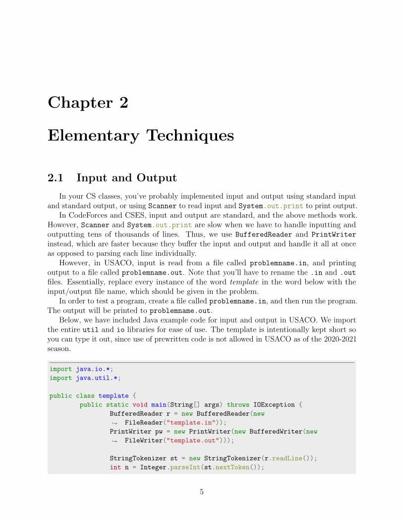
Below, we have included Java example code for input and output in USACO. We importthe entire util and io libraries for ease of use. The template is intentionally kept short soyou can type it out, since use of prewritten code is not allowed in USACO as of the 2020-2021season.
import java.io.*;
import java.util.*;
public class template {
public static void main(String[] args) throws IOException {
BufferedReader r = new BufferedReader(new
FileReader("template.in"));↪→
PrintWriter pw = new PrintWriter(new BufferedWriter(new
FileWriter("template.out")));↪→
StringTokenizer st = new StringTokenizer(r.readLine());
int n = Integer.parseInt(st.nextToken());
5
CHAPTER 2. ELEMENTARY TECHNIQUES 6
r.close();
pw.close();
}
}
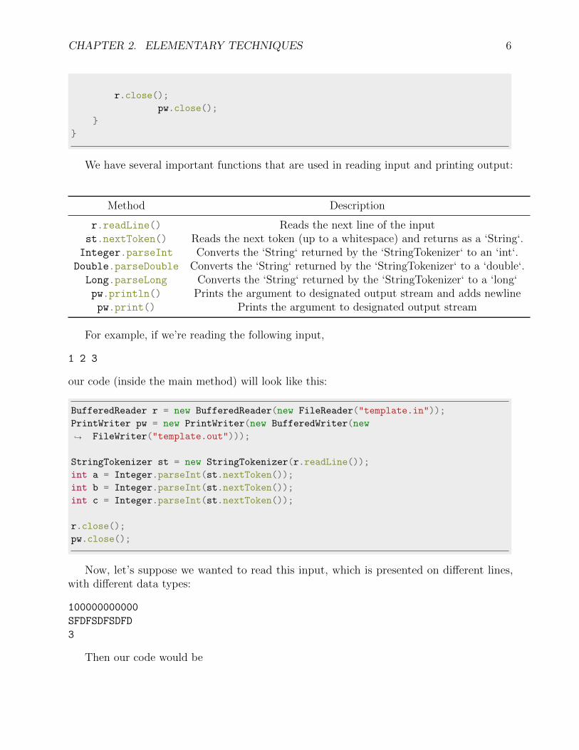
We have several important functions that are used in reading input and printing output:
Method Description
r.readLine() Reads the next line of the inputst.nextToken() Reads the next token (up to a whitespace) and returns as a ‘String‘.Integer.parseInt Converts the ‘String‘ returned by the ‘StringTokenizer‘ to an ‘int‘.Double.parseDouble Converts the ‘String‘ returned by the ‘StringTokenizer‘ to a ‘double‘.Long.parseLong Converts the ‘String‘ returned by the ‘StringTokenizer‘ to a ‘long‘pw.println() Prints the argument to designated output stream and adds newlinepw.print() Prints the argument to designated output stream
For example, if we’re reading the following input,
1 2 3
our code (inside the main method) will look like this:
BufferedReader r = new BufferedReader(new FileReader("template.in"));
PrintWriter pw = new PrintWriter(new BufferedWriter(new
FileWriter("template.out")));↪→
StringTokenizer st = new StringTokenizer(r.readLine());
int a = Integer.parseInt(st.nextToken());
int b = Integer.parseInt(st.nextToken());
int c = Integer.parseInt(st.nextToken());
r.close();
pw.close();
Now, let’s suppose we wanted to read this input, which is presented on different lines,with different data types:
100000000000
SFDFSDFSDFD
3
Then our code would be

CHAPTER 2. ELEMENTARY TECHNIQUES 7
BufferedReader r = new BufferedReader(new FileReader("template.in"));
PrintWriter pw = new PrintWriter(new BufferedWriter(new
FileWriter("template.out")));↪→
StringTokenizer st = new StringTokenizer(r.readLine());
long a = Long.parseLong(st.nextToken());
st = new StringTokenizer(r.readLine());
String b = st.nextToken();
st = new StringTokenizer(r.readLine());
int c = Integer.parseInt(st.nextToken());
r.close();
pw.close();
Note how we have to re-declare the ‘StringTokenizer‘ every time we read in a new line.
For CodeForces, CSES, and other contests that use standard input and output, here is anicer template, which essentially functions as a faster Scanner:
import java.io.*;
import java.util.*;
public class template {
static class InputReader {
BufferedReader reader;
StringTokenizer tokenizer;
public InputReader(InputStream stream) {
reader = new BufferedReader(new InputStreamReader(stream), 32768);
tokenizer = null;
}
String next() { // reads in the next string
while (tokenizer == null || !tokenizer.hasMoreTokens()) {
try {
tokenizer = new StringTokenizer(reader.readLine());
} catch (IOException e) {
throw new RuntimeException(e);
}
}
return tokenizer.nextToken();
}
public int nextInt() { // reads in the next int
return Integer.parseInt(next());
CHAPTER 2. ELEMENTARY TECHNIQUES 8
}
public long nextLong() { // reads in the next long
return Long.parseLong(next());
}
public double nextDouble() { // reads in the next double
return Double.parseDouble(next());
}
}
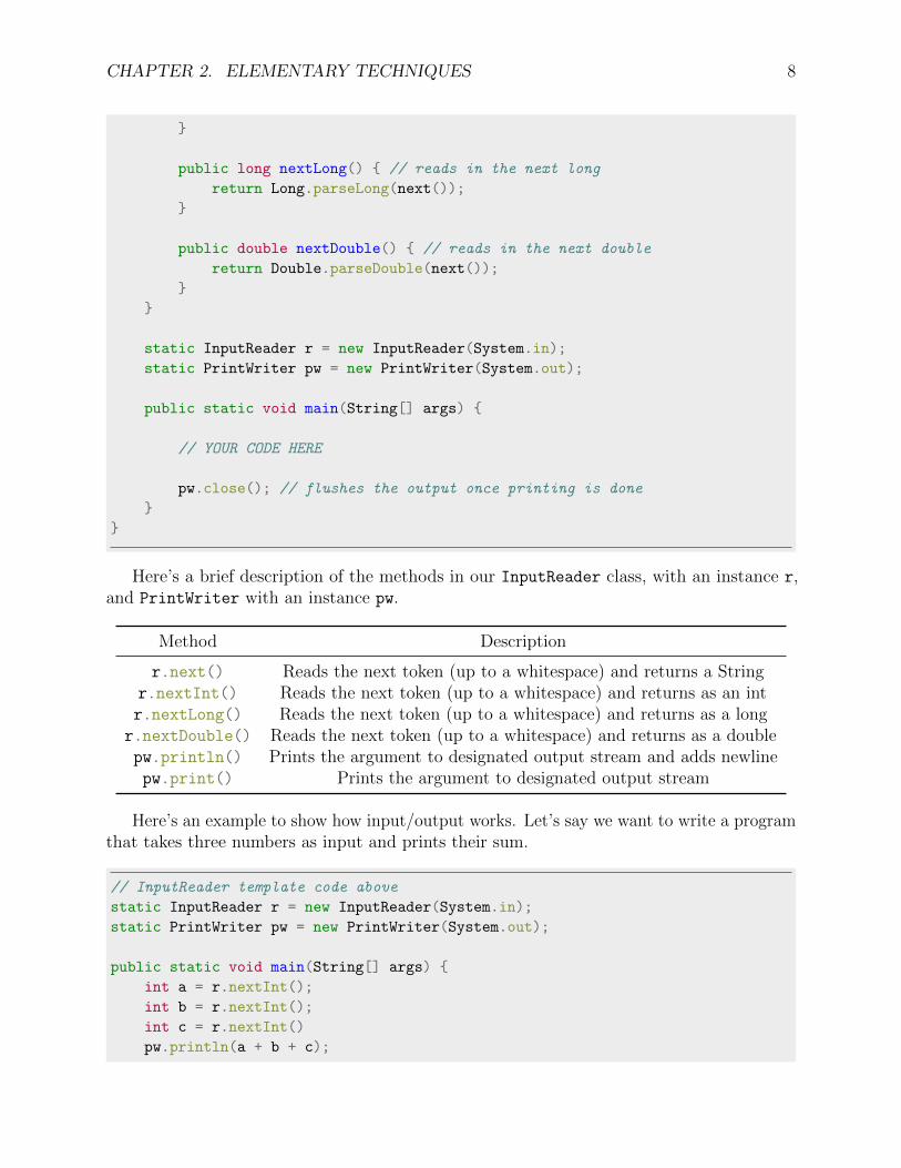
static InputReader r = new InputReader(System.in);
static PrintWriter pw = new PrintWriter(System.out);
public static void main(String[] args) {
// YOUR CODE HERE
pw.close(); // flushes the output once printing is done
}
}
Here’s a brief description of the methods in our InputReader class, with an instance r,and PrintWriter with an instance pw.
Method Description
r.next() Reads the next token (up to a whitespace) and returns a Stringr.nextInt() Reads the next token (up to a whitespace) and returns as an intr.nextLong() Reads the next token (up to a whitespace) and returns as a longr.nextDouble() Reads the next token (up to a whitespace) and returns as a doublepw.println() Prints the argument to designated output stream and adds newlinepw.print() Prints the argument to designated output stream
Here’s an example to show how input/output works. Let’s say we want to write a programthat takes three numbers as input and prints their sum.
// InputReader template code above
static InputReader r = new InputReader(System.in);
static PrintWriter pw = new PrintWriter(System.out);
public static void main(String[] args) {
int a = r.nextInt();
int b = r.nextInt();
int c = r.nextInt()
pw.println(a + b + c);

CHAPTER 2. ELEMENTARY TECHNIQUES 9
pw.close();
}
2.2 Data Types
There are several main data types that are used in contests: 32-bit and 64-bit integers,floating point numbers, booleans, characters, and strings.
The 32-bit integer supports values between −2 147 483 648 and 2 147 483 647, which isroughly equal to ± 2×10⁹. If the input, output, or any intermediate values used in calculationsexceed the range of a 32-bit integer, then a 64-bit integer must be used. The range of the64-bit integer is between −9 223 372 036 854 775 808 and 9 223 372 036 854 775 807 which isroughly equal to ± 9× 10¹⁸. Contest problems are usually set such that the 64-bit integer issufficient. If it’s not, the problem will ask for the answer modulo m, instead of the answeritself, where m is a prime. In this case, make sure to use 64-bit integers, and take theremainder of x modulo m after every step using x %= m;.
Floating point numbers are used to store decimal values. It is important to know thatfloating point numbers are not exact, because the binary architecture of computers can onlystore decimals to a certain precision. Hence, we should always expect that floating pointnumbers are slightly off. Contest problems will accommodate this by either asking for thegreatest integer less than 10k times the value, or will mark as correct any output that iswithin a certain ε of the judge’s answer.
Boolean variables have two possible states: true and false. We’ll usually use booleans tomark whether a certain process is done, and arrays of booleans to mark which components ofan algorithm have finished.
Character variables represent a single Unicode character. They are returned when youaccess the character at a certain index within a string. Characters are represented using theASCII standard, which assigns each character to a corresponding integer; this allows us to doarithmetic with them, for example, System.out.println('f' - 'a'); will print 5.
Strings are effectively arrays of characters. You can easily access the character at a certainindex and take substrings of the string. String problems on USACO are generally very easyand don’t involve any special data structures.

Chapter 3
Time/Space Complexity andAlgorithm Analysis
In programming contests, there is a strict limit on program runtime. This means thatin order to pass, your program needs to finish running within a certain timeframe. ForUSACO, this limit is 4 seconds for Java submissions. A conservative estimate for the numberof operations the grading server can handle per second is 108.
3.1 Big O Notation and Complexity Calculations
We want a method of characterizing how many operations it takes to run each algorithm,in terms of the input size n. Fortunately, this can be done relatively easily using Big Onotation, which expresses worst-case complexity as a function of n, as n gets arbitrarily large.Complexity is an upper bound for the number of steps an algorithm requires, as a function ofthe input size. In Big O notation, we denote the complexity of a function as O(f(n)), wheref(n) is a function without constant factors or lower-order terms. We’ll see some examples ofhow this works, as follows.
The following code is O(1), because it executes a constant number of operations.
int a = 5;
int b = 7;
int c = 4;
int d = a + b + c + 153;
Input and output operations are also assumed to be O(1).In the following examples, we assume that the code inside the loops is O(1).The time complexity of loops is the number of iterations that the loop runs multiplied by
the amount of operations per iteration. The following code examples are both O(n).
for(int i = 1; i <= n; i++){
// constant time code here
}
10

CHAPTER 3. TIME/SPACE COMPLEXITY AND ALGORITHM ANALYSIS 11
int i = 0;
while(i < n){
// constant time node here
i++;
}
Because we ignore constant factors and lower order terms, for loops where we loop up to5n+ 17 or n+ 457737 would also be O(n):
We can find the time complexity of multiple loops by multiplying together the timecomplexities of each loop. The following example is O(nm), because the outer loop runs O(n)iterations and the inner loop O(m).
for(int i = 1; i <= n; i++){
for(int j = 1; j <= m; j++){
// constant time code here
}
}
If an algorithm contains multiple blocks, then its time complexity is the worst timecomplexity out of any block. For example, if an algorithm has an O(n) block and an O(n2)block, the overall time complexity is O(n2).
Functions of different variables generally are not considered lower-order terms with respectto each other, so we must include both terms. For example, if an algorithm has an O(n2)block and an O(nm) block, the overall time complexity would be O(n2 + nm).
3.2 Common Complexities and Constraints
Complexity factors that come from some common algorithms and data structures are asfollows:
• Mathematical formulas that just calculate an answer: O(1)
• Unordered set/map: O(1) per operation
• Binary search: O(log n)
• Ordered set/map or priority queue: O(log n) per operation
• Prime factorization of an integer, or checking primality or compositeness of an integer:O(√n)
• Reading in n items of input: O(n)
• Iterating through an array or a list of n elements: O(n)
CHAPTER 3. TIME/SPACE COMPLEXITY AND ALGORITHM ANALYSIS 12
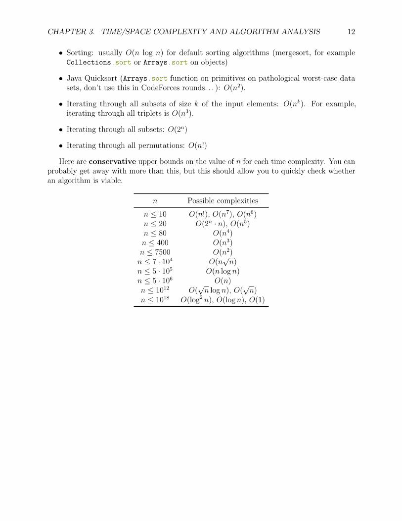
• Sorting: usually O(n log n) for default sorting algorithms (mergesort, for exampleCollections.sort or Arrays.sort on objects)
• Java Quicksort (Arrays.sort function on primitives on pathological worst-case datasets, don’t use this in CodeForces rounds. . . ): O(n2).
• Iterating through all subsets of size k of the input elements: O(nk). For example,iterating through all triplets is O(n3).
• Iterating through all subsets: O(2n)
• Iterating through all permutations: O(n!)
Here are conservative upper bounds on the value of n for each time complexity. You canprobably get away with more than this, but this should allow you to quickly check whetheran algorithm is viable.
n Possible complexities
n ≤ 10 O(n!), O(n7), O(n6)n ≤ 20 O(2n · n), O(n5)n ≤ 80 O(n4)n ≤ 400 O(n3)n ≤ 7500 O(n2)n ≤ 7 · 104 O(n
√n)
n ≤ 5 · 105 O(n log n)n ≤ 5 · 106 O(n)n ≤ 1012 O(
√n log n), O(
√n)
n ≤ 1018 O(log2 n), O(log n), O(1)

Chapter 4
Built-in Data Structures
A data structure determines how data is stored. (is it sorted? indexed? what operationsdoes it support?) Each data structure supports some operations efficiently, while otheroperations are either inefficient or not supported at all. This chapter introduces the datastructures in the Java standard library that are frequently used in competitive programming.
Java default Collections data structures are designed to store any type of object. However,we usually don’t want this; instead, we want our data structures to only store one type ofdata, like integers, or strings. We do this by putting the desired data type within the <>
brackets when declaring the data structure, as follows:
ArrayList<String> list = new ArrayList<String>();
This creates an ArrayList structure that only stores objects of type String.For our examples below, we will primarily use the Integer data type, but note that you
can have Collections of any object type, including Strings, other Collections, or user-definedobjects.
Collections data types always contain an add method for adding an element to thecollection, and a remove method which removes and returns a certain element from thecollection. They also support the size() method, which returns the number of elements inthe data structure, and the isEmpty() method, which returns true if the data structure isempty, and false otherwise.
4.1 Dynamic Arrays
You’re probably already familiar with regular (static) arrays. Now, there are also dynamicarrays (ArrayList in Java) that support all the functions that a normal array does, and canresize itself to accommodate more elements. In a dynamic array, we can also add and deleteelements at the end in O(1) time.
However, we need to be careful that we only add elements to the end of the ArrayList;insertion and deletion in the middle of the ArrayList is O(n).
13

CHAPTER 4. BUILT-IN DATA STRUCTURES 14
ArrayList<Integer> list = new ArrayList<Integer>(); // declare the dynamic array
list.add(2); // [2]
list.add(3); // [2, 3]
list.add(7); // [2, 3, 7]
list.add(5); // [2, 3, 7, 5]
list.set(1, 4); // sets element at index 1 to 4 -> [2, 4, 7, 5]
list.remove(1); // removes element at index 1 -> [2, 7, 5]
// this remove method is O(n); to be avoided
list.add(8); // [2, 7, 5, 8]
list.remove(list.size()-1); // [2, 7, 5]
// here, we remove the element from the end of the list; this is O(1).
System.out.println(list.get(2)); // 5
To iterate through a static or dynamic array, we can use either the regular for loop or thefor-each loop.
Arrays.sort(arr) is used to sort a static array, and Collections.sort(list) a dynamicarray. The default sort function sorts the array in ascending order.
In array-based contest problems, we’ll use one-, two-, and three-dimensional static arraysmost of the time. However, we can also have static arrays of dynamic arrays, dynamic arraysof static arrays, and so on. Usually, the choice between a static array and a dynamic array isjust personal preference.
4.2 Stacks and the Various Types of Queues
Stacks
A stack is a Last In First Out (LIFO) data structure that supports three operations:push, which adds an element to the top of the stack, pop, which removes an element fromthe top of the stack, and peek, which retrieves the element at the top without removing it,all in O(1) time. Think of it like a real-world stack of papers.
Stack<Integer> s = new Stack<Integer>();
s.push(1); // [1]
s.push(13); // [1, 13]
System.out.println(s.size()); // 2
s.pop(); // [1]
System.out.println(s.peek()); // 1
s.pop(); // []
System.out.println(s.size()); // 0
Queues
A queue is a First In First Out (FIFO) data structure that supports three operations ofadd, insertion at the back of the queue, poll, deletion from the front of the queue, and peek,

CHAPTER 4. BUILT-IN DATA STRUCTURES 15
which retrieves the element at the front without removing it, all in O(1) time. Java doesn’tactually have a Queue class; it’s only an interface. The most commonly used implementationis the LinkedList, declared as follows: Queue q = new LinkedList();.
Queue<Integer> q = new LinkedList<Integer>();
q.add(1); // [1]
q.add(3); // [3, 1]
q.poll(); // [3]
q.add(4); // [4, 3]
System.out.println(q.size()); // 2
System.out.println(q.peek()); // 4
Deques
A deque (usually pronounced “deck”) stands for double ended queue and is a combinationof a stack and a queue, in that it supports O(1) insertions and deletions from both thefront and the back of the deque. In Java, the deque class is called ArrayDeque. The fourmethods for adding and removing are addFirst, removeFirst, addLast, and removeLast.The methods for retrieving the first and last elements without removing are peekFirst andpeekLast.
ArrayDeque<Integer> deque = new ArrayDeque<Integer>();
deque.addFirst(1); // [1]
deque.addLast(2); // [1, 2]
deque.addFirst(3); // [3, 1, 2]
deque.addFirst(4); // [3, 1, 2, 4]
deque.removeLast(); // [3, 1, 2]
deque.removeFirst(); // [1, 2]
Priority Queues
A priority queue supports the following operations: insertion of elements, deletion ofthe element considered highest priority, and retrieval of the highest priority element, all inO(log n) time according to the number of elements in the priority queue. Priority is based ona comparator function, but by default the lowest element is at the front of the priority queue.The priority queue is one of the most important data structures in competitive programming,so make sure you understand how and when to use it. By default, the Priority Queue putsthe lowest element at the front of the queue.
PriorityQueue<Integer> pq = new PriorityQueue<Integer>();
pq.add(4); // [4]
pq.add(2); // [4, 2]
pq.add(1); // [4, 2, 1]

CHAPTER 4. BUILT-IN DATA STRUCTURES 16
pq.add(3); // [4, 3, 2, 1]
System.out.println(pq.peek()); // 1
pq.poll(); // [4, 3, 2]
pq.poll(); // [4, 3]
pq.add(5); // [5, 4, 3]
4.3 Sets and Maps
A set is a collection of objects that contains no duplicates. There are two types of sets:unordered sets (HashSet in Java), and ordered set (TreeSet in Java).
Unordered Sets
The unordered set works by hashing, which is assigning a usually-unique code to everyvariable/object which allows insertions, deletions, and searches in O(1) time, albeit with ahigh constant factor, as hashing requires a large constant number of operations. However,as the name implies, elements are not ordered in any meaningful way, so traversals of anunordered set will return elements in some arbitrary order. The operations on an unorderedset are add, which adds an element to the set if not already present, remove, which deletesan element if it exists, and contains, which checks whether the set contains that element.
HashSet<Integer> set = new HashSet<Integer>();
set.add(1); // [1]
set.add(4); // [1, 4] in arbitrary order
set.add(2); // [1, 4, 2] in arbitrary order
set.add(1); // [1, 4, 2] in arbitrary order
// the add method did nothing because 1 was already in the set
System.out.println(set.contains(1)); // true
set.remove(1); // [2, 4] in arbitrary order
System.out.println(set.contains(5)); // false
set.remove(0); // [2, 4] in arbitrary order
// if the element to be removed does not exist, nothing happens
for(int element : set){
System.out.println(element);
}
// You can iterate through an unordered set, but it will do so in arbitrary
order↪→
Ordered Sets
The second type of set data structure is the ordered or sorted set. Insertions, deletions,and searches on the ordered set require O(log n) time, based on the number of elements

CHAPTER 4. BUILT-IN DATA STRUCTURES 17
in the set. As well as those supported by the unordered set, the ordered set also allowsfour additional operations: first, which returns the lowest element in the set, last, whichreturns the highest element in the set, lower, which returns the greatest element strictly lessthan some element, and higher, which returns the least element strictly greater than it.
TreeSet<Integer> set = new TreeSet<Integer>();
set.add(1); // [1]
set.add(14); // [1, 14]
set.add(9); // [1, 9, 14]
set.add(2); // [1, 2, 9, 14]
System.out.println(set.higher(7)); // 9
System.out.println(set.higher(9)); // 14
System.out.println(set.lower(5)); // 2
System.out.println(set.first()); // 1
System.out.println(set.last()); // 14
set.remove(set.higher(6)); // [1, 2, 14]
System.out.println(set.higher(23); // ERROR, no such element exists
The primary limitation of the ordered set is that we can’t efficiently access the kth largestelement in the set, or find the number of elements in the set greater than some arbitrary x.These operations can be handled using a data structure called an order statistic tree, butthat is beyond the scope of this book.
Maps
A map is a set of ordered pairs, each containing a key and a value. In a map, all keysare required to be unique, but values can be repeated. Maps have three primary methods:one to add a specified key-value pairing, one to retrieve the value for a given key, and oneto remove a key-value pairing from the map. Like sets, maps can be unordered (HashSetin Java) or ordered (TreeSet in Java). In an unordered map, hashing is used to supportO(1) operations. In an ordered map, the entries are sorted in order of key. Operations areO(log n), but accessing or removing the next key higher or lower than some input k is alsosupported.
Unordered Maps
In the unordered map, the put(key, value) method assigns a value to a key and placesthe key and value pair into the map. The get(key) method returns the value associated withthe key. The containsKey(key) method checks whether a key exists in the map. Lastly,remove(key) removes the map entry associated with the specified key. All of these operationsare O(1), but again, due to the hashing, this has a high constant factor.
HashMap<Integer, Integer> map = new HashMap<Integer, Integer>();
map.put(1, 5); // [(1, 5)]
map.put(3, 14); // [(1, 5); (3, 14)]
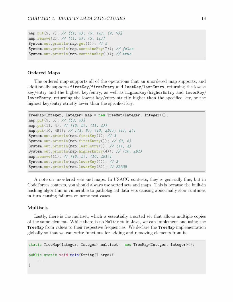
CHAPTER 4. BUILT-IN DATA STRUCTURES 18
map.put(2, 7); // [(1, 5); (3, 14); (2, 7)]
map.remove(2); // [(1, 5); (3, 14)]
System.out.println(map.get(1)); // 5
System.out.println(map.containsKey(7)); // false
System.out.println(map.containsKey(1)); // true
Ordered Maps
The ordered map supports all of the operations that an unordered map supports, andadditionally supports firstKey/firstEntry and lastKey/lastEntry, returning the lowestkey/entry and the highest key/entry, as well as higherKey/higherEntry and lowerKey/lowerEntry, returning the lowest key/entry strictly higher than the specified key, or thehighest key/entry strictly lower than the specified key.
TreeMap<Integer, Integer> map = new TreeMap<Integer, Integer>();
map.put(3, 5); // [(3, 5)]
map.put(11, 4); // [(3, 5); (11, 4)]
map.put(10, 491); // [(3, 5); (10, 491); (11, 4)]
System.out.println(map.firstKey()); // 3
System.out.println(map.firstEntry()); // (3, 5)
System.out.println(map.lastEntry()); // (11, 4)
System.out.println(map.higherEntry(4)); // (10, 491)
map.remove(11); // [(3, 5); (10, 491)]
System.out.println(map.lowerKey(4)); // 3
System.out.println(map.lowerKey(3)); // ERROR
A note on unordered sets and maps: In USACO contests, they’re generally fine, but inCodeForces contests, you should always use sorted sets and maps. This is because the built-inhashing algorithm is vulnerable to pathological data sets causing abnormally slow runtimes,in turn causing failures on some test cases.
Multisets
Lastly, there is the multiset, which is essentially a sorted set that allows multiple copiesof the same element. While there is no Multiset in Java, we can implement one using theTreeMap from values to their respective frequencies. We declare the TreeMap implementationglobally so that we can write functions for adding and removing elements from it.
static TreeMap<Integer, Integer> multiset = new TreeMap<Integer, Integer>();
public static void main(String[] args){
...
}

CHAPTER 4. BUILT-IN DATA STRUCTURES 19
static void add(int x){
if(multiset.containsKey(x)){
multiset.put(x, multiset.get(x) + 1);
} else {
multiset.put(x, 1);
}
}
static void remove(int x){
multiset.put(x, multiset.get(x) - 1);
if(multiset.get(x) == 0){
multiset.remove(x);
}
}
The first, last, higher, and lower operations still function as intended; just use firstKey,lastKey, higherKey, and lowerKey respectively.
4.4 Problems
Again, note that CSES’s grader is very slow, so don’t worry if you encounter a TimeLimit Exceeded verdict; as long as you pass the majority of test cases within the time limit,you can consider the problem solved, and move on.
1. CSES Problem Set Task 1621: Distinct Numbershttps://cses.fi/problemset/task/1621
2. CSES Problem Set Task 1084: Apartmentshttps://cses.fi/problemset/task/1084
3. CSES Problem Set Task 1091: Concert Ticketshttps://cses.fi/problemset/task/1091
4. CSES Problem Set Task 1163: Traffic Lightshttps://cses.fi/problemset/task/1163
5. CSES Problem Set Task 1164: Room Allocationhttps://cses.fi/problemset/task/1164

Part II
Bronze
20

Chapter 5
Simulation
In many problems, we can simply simulate what we’re told to do by the problem statement.Since there’s no formal algorithm involved, the intent of the problem is to assess competencewith one’s programming language of choice and knowledge of built-in data structures. Atleast in USACO Bronze, when a problem statement says to find the end result of someprocess, or to find when something occurs, it’s usually sufficient to simulate the process.
5.1 Example 1
Alice and Bob are standing on a 2D plane. Alice starts at the point (0, 0), and Bobstarts at the point (R, S) (1 ≤ R, S ≤ 1000). Every second, Alice moves M units to theright, and N units up. Every second, Bob moves P units to the left, and Q units down.(1 ≤M,N,P,Q ≤ 10). Determine if Alice and Bob will ever meet (be at the same point atthe same time), and if so, when.
INPUT FORMAT:The first line of the input contains R and S.The second line of the input contains M , N , P , and Q.
OUTPUT FORMAT:Please output a single integer containing the number of seconds after the start at which Aliceand Bob meet. If they never meet, please output −1.
SolutionWe can simulate the process. After inputting the values of R, S, M , N , P , and Q, we cankeep track of Alice’s and Bob’s x- and y-coordinates. To start, we initialize variables for theirrespective positions. Alice’s coordinates are initially (0, 0), and Bob’s coordinates are (R, S)respectively. Every second, we increase Alice’s x-coordinate by M and her y-coordinate byN , and decrease Bob’s x-coordinate by P and his y-coordinate by Q.
Now, when do we stop? First, if Alice and Bob ever have the same coordinates, then weare done. Also, since Alice strictly moves up and to the right and Bob strictly moves downand to the left, if Alice’s x- or y-coordinates are ever greater than Bob’s, then it is impossiblefor them to meet. Example code will be displayed below (Here, as in other examples, inputprocessing will be omitted):
21

CHAPTER 5. SIMULATION 22
int ax = 0; int ay = 0; // alice's x and y coordinates
int bx = r; int by = s; // bob's x and y coordinates
int t = 0; // keep track of the current time
while(ax < bx && ay < by){
// every second, update alice's and bob's coordinates and the time
ax += m; ay += n;
bx -= p; by -= q;
t++;
}
if(ax == bx && ay == by){ // if they are in the same location
out.println(t); // they meet at time t
} else {
out.println(-1); // they never meet
}
out.close(); // flush the output
5.2 Example 2
There are N buckets (5 ≤ N ≤ 105), each with a certain capacity Ci (1 ≤ Ci ≤ 100). Oneday, after a rainstorm, each bucket is filled with Ai units of water (1 ≤ Ai ≤ Ci). Charliethen performs the following process: he pours bucket 1 into bucket 2, then bucket 2 intobucket 3, and so on, up until pouring bucket N − 1 into bucket N . When Charlie poursbucket B into bucket B + 1, he pours as much as possible until bucket B is empty or bucketB + 1 is full. Find out how much water is in each bucket once Charlie is done pouring.
INPUT FORMAT:The first line of the input contains N .The second line of the input contains the capacities of the buckets, C1, C2, . . . , Cn.The third line of the input contains the amount of water in each bucket A1, A2, . . . , An.
OUTPUT FORMAT:Please print one line of output, containing N space-separated integers: the final amount ofwater in each bucket once Charlie is done pouring.
Solution:Once again, we can simulate the process of pouring one bucket into the next. The amount ofwater poured from bucket B to bucket B + 1 is the smaller of the amount of water in bucketB (after all previous operations have been completed) and the remaining space in bucketB + 1, which is CB+1 − AB+1. We can just handle all of these operations in order, using anarray C to store the maximum capacities of each bucket, and an array A to store the currentwater level in each bucket, which we update during the process. Example code is below (notethat arrays are zero-indexed, so the indices of our buckets go from 0 to N − 1 rather thanfrom 1 to N).

CHAPTER 5. SIMULATION 23
for(int i = 0; i < n-1; i++){
int amt = Math.min(A[i], C[i+1]-A[i+1]);
// the amount of water to be poured is the lesser of
// the amount of water in the current bucket and
// the amount of additional water that the next bucket can hold
A[i] -= amt; // remove the amount from the current bucket
A[i+1] += amt; // add it to the next bucket
}
for(int i = 0; i < n; i++){
pw.print(A[i] + " ");
// print the amount of water in each bucket at the end
}
pw.println(); // print newline
pw.close(); // flush the output
5.3 Problems
1. USACO December 2018 Bronze Problem 1: Mixing Milkhttp://www.usaco.org/index.php?page=viewproblem2&cpid=855
2. USACO December 2017 Bronze Problem 3: Milk Measurementhttp://www.usaco.org/index.php?page=viewproblem2&cpid=761
3. USACO US Open 2017 Bronze Problem 1: The Lost Cowhttp://www.usaco.org/index.php?page=viewproblem2&cpid=735
4. USACO February 2017 Bronze Problem 3: Why Did the Cow Cross the Road IIIhttp://www.usaco.org/index.php?page=viewproblem2&cpid=713
5. USACO January 2016 Bronze Problem 3: Mowing the Fieldhttp://www.usaco.org/index.php?page=viewproblem2&cpid=593
6. USACO December 2017 Bronze Problem 2: The Bovine Shufflehttp://usaco.org/index.php?page=viewproblem2&cpid=760
7. USACO February 2016 Bronze Problem 2: Circular Barnhttp://usaco.org/index.php?page=viewproblem2&cpid=616
Chapter 6
Complete Search
In many problems (especially in Bronze), it’s sufficient to check all possible cases inthe solution space, whether it be all elements, all pairs of elements, or all subsets, or allpermutations. Unsurprisingly, this is called complete search (or brute force), because itcompletely searches the entire solution space.
6.1 Example 1
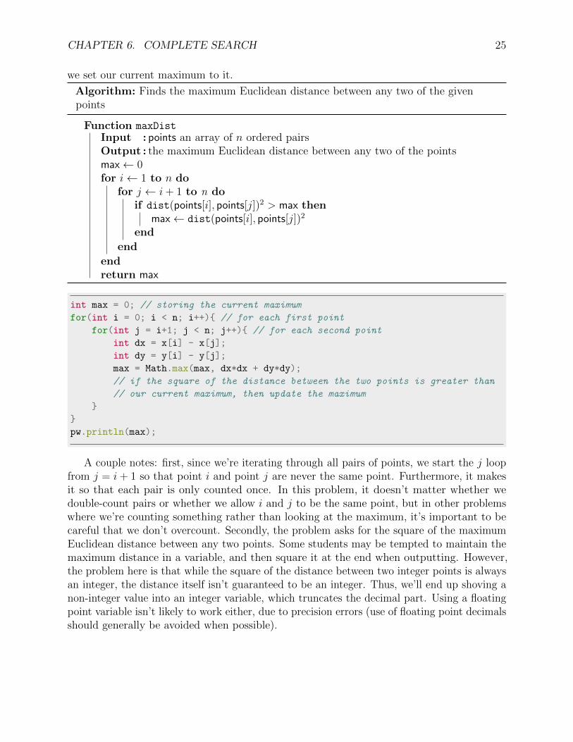
You are given N (3 ≤ N ≤ 5000) integer points on the coordinate plane. Find the squareof the maximum Euclidean distance (aka length of the straight line) between any two of thepoints.
INPUT FORMAT:The first line contains an integer N .The second line contains N integers, the x-coordinates of the points: x1, x2, . . . , xn (−1000 ≤xi ≤ 1000).The third line contains N integers, the y-coordinates of the points: y1, y2, . . . , yn (−1000 ≤yi ≤ 1000).
OUTPUT FORMAT:Print one integer, the square of the maximum Euclidean distance between any two of thepoints.
Solution:We can brute-force every pair of points and find the square of the distance between them,by squaring the formula for Euclidean distance: distance2 = (x2 − x1)2 + (y2 − y1)2. Thus,we store the coordinates in arrays X[] and Y[], such that X[i] and Y[i] are the x- andy-coordinates of the ith point, respectively. Then, we iterate through all possible pairs ofpoints, using a variable max to store the maximum square of distance between any pair seenso far, and if the square of the distance between a pair is greater than our current maximum,
24
CHAPTER 6. COMPLETE SEARCH 25
we set our current maximum to it.
Algorithm: Finds the maximum Euclidean distance between any two of the givenpoints
Function maxDistInput : points an array of n ordered pairsOutput : the maximum Euclidean distance between any two of the pointsmax← 0for i← 1 to n do
for j ← i+ 1 to n doif dist(points[i], points[j])2 > max then
max← dist(points[i], points[j])2
end
end
endreturn max
int max = 0; // storing the current maximum
for(int i = 0; i < n; i++){ // for each first point
for(int j = i+1; j < n; j++){ // for each second point
int dx = x[i] - x[j];
int dy = y[i] - y[j];
max = Math.max(max, dx*dx + dy*dy);
// if the square of the distance between the two points is greater than
// our current maximum, then update the maximum
}
}
pw.println(max);
A couple notes: first, since we’re iterating through all pairs of points, we start the j loopfrom j = i+ 1 so that point i and point j are never the same point. Furthermore, it makesit so that each pair is only counted once. In this problem, it doesn’t matter whether wedouble-count pairs or whether we allow i and j to be the same point, but in other problemswhere we’re counting something rather than looking at the maximum, it’s important to becareful that we don’t overcount. Secondly, the problem asks for the square of the maximumEuclidean distance between any two points. Some students may be tempted to maintain themaximum distance in a variable, and then square it at the end when outputting. However,the problem here is that while the square of the distance between two integer points is alwaysan integer, the distance itself isn’t guaranteed to be an integer. Thus, we’ll end up shoving anon-integer value into an integer variable, which truncates the decimal part. Using a floatingpoint variable isn’t likely to work either, due to precision errors (use of floating point decimalsshould generally be avoided when possible).

CHAPTER 6. COMPLETE SEARCH 26
6.2 Generating Permutations
A permutation is a reordering of a list of elements. Some problems will ask for anordering of elements that satisfies certain conditions. In these problems, if N ≤ 10, we canprobably iterate through all permutations and check each permutation for validity. For a listof N elements, there are N ! ways to permute them, and generally we’ll need to read througheach permutation once to check its validity, for a time complexity of O(N ·N !).
In Java, we’ll have to implement this ourselves, which is called Heap’s Algorithm (norelation to the heap data structure). What’s going to be in the check function depends onthe problem, but it should verify whether the current permutation satisfies the constraintsgiven in the problem.
As an example, here are the permutations generated by Heap’s Algorithm for [1, 2, 3]:
[1, 2, 3], [2, 1, 3], [3, 1, 2], [1, 3, 2], [2, 3, 1], [3, 2, 1]
Algorithm: Iterate over all permutations of a given input array, performing someaction on each permutation
Function generatePermutationsInput : An array arr, and its length kif k = 1 then
process the current permutationelse
generatePermutations (arr, k − 1)for i← 0 to k − 1 do
if k is even thenswap indices i and k − 1 of arr
elseswap indices 0 and k − 1 of arr
endgeneratePermutations (arr, k − 1)
end
end
Code for iterating over all permutations is as follows:
// this method is called with k equal to the length of arr
static void generate(int[] arr, int k){
if(k == 1){
check(arr); // check the current permutation for validity
} else {
generate(arr, k-1);
for(int i = 0; i < k-1; i++){
if(k % 2 == 0){
swap(arr, i, k-1);
// swap indices i and k-1 of arr

CHAPTER 6. COMPLETE SEARCH 27
} else {
swap(arr, 0, k-1);
// swap indices 0 and k-1 of arr
}
generate(arr, k-1);
}
}
}
6.3 Problems
1. USACO February 2020 Bronze Problem 1: Triangleshttp://usaco.org/index.php?page=viewproblem2&cpid=1011
2. USACO January 2020 Bronze Problem 2: Photoshoothttp://www.usaco.org/index.php?page=viewproblem2&cpid=988
(Hint: Figure out what exactly you’re complete searching)
3. USACO December 2019 Bronze Problem 1: Cow Gymnasticshttp://usaco.org/index.php?page=viewproblem2&cpid=963
(Hint: Brute force over all possible pairs)
4. USACO February 2016 Bronze Problem 1: Milk Pailshttp://usaco.org/index.php?page=viewproblem2&cpid=615
5. USACO January 2018 Bronze Problem 2: Lifeguardshttp://usaco.org/index.php?page=viewproblem2&cpid=784
(Hint: Try removing each lifeguard one at a time).
6. USACO December 2019 Bronze Problem 2: Where Am I?http://usaco.org/index.php?page=viewproblem2&cpid=964
(Hint: Brute force over all possible substrings)
7. (Permutations) USACO December 2019 Bronze Problem 3: Livestock Lineuphttp://usaco.org/index.php?page=viewproblem2&cpid=965
8. (Permutations) CSES Problem Set Task 1624: Chessboard and Queenshttps://cses.fi/problemset/task/1624
9. USACO US Open 2016 Bronze Problem 3: Field Reductionhttp://www.usaco.org/index.php?page=viewproblem2&cpid=641
(Hint: For this problem, you can’t do a full complete search; you have to do a reducedsearch)
10. USACO December 2018 Bronze Problem 3: Back and Forthhttp://www.usaco.org/index.php?page=viewproblem2&cpid=857
(This problem is relatively hard)

Chapter 7
Additional Bronze Topics
7.1 Square and Rectangle Geometry
The extent of “geometry” problems on USACO Bronze are usually quite simple andlimited to intersections and unions of squares and rectangles. These usually only include twoor three squares or rectangles, in which case you can simply draw out cases on paper, whichshould logically lead to a solution.
In Java, the Rectangle class may be of use for finding intersections and unions ofrectangles.
Here are some of the functions that the Rectangle class has:
• Find whether a certain point or rectangle is contained within another rectangle
• Find the intersection or union of two rectangles
• Translate, scale, or shrink rectangles
For exact details and documentation, refer to the Rectangle class page on the officialjavadoc: https://docs.oracle.com/javase/7/docs/api/java/awt/Rectangle.html
The problems given at the end of the chapter should encompass all the techniques youneed to know for geometry problems in the Bronze division.
7.2 Ad-hoc
Ad-hoc problems are problems that don’t fall into any standard algorithmic categorywith well known solutions. They are usually unique problems intended to be solved withunconventional techniques. In ad-hoc problems, it’s helpful to look at the constraints given inthe problem and devise potential time complexities of solutions; this, combined with detailsin the problem statement itself, may give an outline of the solution.
Unfortunately, since ad-hoc problems don’t have solutions consisting of well knownalgorithms, we can’t systematically teach you how to do them. The best way of learning howto do ad-hoc is to practice. Of course, the problem solving intuition from math contests (ifyou did them) is quite helpful, but otherwise, you can develop this intuition from practicingad-hoc problems.
28
CHAPTER 7. ADDITIONAL BRONZE TOPICS 29
While solving these problems, make sure to utilize what you’ve learned about the built-indata structures and algorithmic complexity analysis, from chapters 2, 3, and 4. Since ad-hocproblems comprise a significant portion of bronze problems, we’ve included a large selectionof them below for your practice.
7.3 Problems
Square and Rectangle Geometry
1. USACO December 2017 Bronze Problem 1: Blocked Billboardhttp://usaco.org/index.php?page=viewproblem2&cpid=759
2. USACO December 2018 Bronze Problem 1: Blocked Billboard IIhttp://usaco.org/index.php?page=viewproblem2&cpid=783
3. CodeForces Round 587 (Div. 3) Problem C: White Sheethttps://codeforces.com/contest/1216/problem/C
4. USACO December 2016 Bronze Problem 1: Square Pasturehttp://usaco.org/index.php?page=viewproblem2&cpid=663
Ad-hoc problems
5. USACO January 2016 Bronze Problem 1: Promotion Countinghttp://usaco.org/index.php?page=viewproblem2&cpid=591
6. USACO January 2020 Bronze Problem 1: Word Processorhttp://usaco.org/index.php?page=viewproblem2&cpid=987
7. USACO US Open 2019 Bronze Problem 1: Bucket Brigadehttp://usaco.org/index.php?page=viewproblem2&cpid=939
8. USACO January 2018 Bronze Problem 3: Out of Placehttp://usaco.org/index.php?page=viewproblem2&cpid=785
9. USACO December 2016 Bronze Problem 2: Block Gamehttp://usaco.org/index.php?page=viewproblem2&cpid=664
10. USACO February 2020 Bronze Problem 3: Swapity Swaphttp://usaco.org/index.php?page=viewproblem2&cpid=1013
(This problem is quite hard for bronze.)
11. USACO February 2018 Bronze Problem 1: Teleportationhttp://usaco.org/index.php?page=viewproblem2&cpid=807
12. USACO February 2018 Bronze Problem 2: Hoofballhttp://usaco.org/index.php?page=viewproblem2&cpid=808

CHAPTER 7. ADDITIONAL BRONZE TOPICS 30
13. USACO US Open 2019 Bronze Problem 3: Cow Evolutionhttp://usaco.org/index.php?page=viewproblem2&cpid=941
(Warning: This problem is extremely difficult for bronze.)

Part III
Silver
31

Chapter 8
Sorting and comparators
8.1 Comparators
Java has built-in functions for sorting: Arrays.sort(arr) for arrays, and Collections.
sort(list) for ArrayLists. However, if we use custom objects, or if we want to sort elementsin a different order, then we’ll need to use a Comparator.
Normally, sorting functions rely on moving objects with a lower value ahead of objectswith a higher value if sorting in ascending order, and vice versa if in descending order. Thisis done through comparing two objects at a time. What a Comparator does is compare twoobjects as follows, based on our comparison criteria:
• If object x is less than object y, return a negative number
• If object x is greater than object y, return a positive number
• If object x is equal to object y, return 0.
In addition to returning the correct number, comparators should also satisfy the followingconditions:
• The function must be consistent with respect to reversing the order of the arguments:if compare(x, y) is positive, then compare(y, x) should be negative and vice versa
• The function must be transitive. If compare(x, y) > 0 and compare(y, z) > 0, thencompare(x, z) > 0. Same applies if the compare functions return negative numbers.
• Equality must be consistent. If compare(x, y) = 0, then compare(x, z) andcompare(y, z) must both be positive, both negative, or both zero. Note that theydon’t have to be equal, they just need to have the same sign.
Java has default functions for comparing ints, longs, and doubles. The Integer.compare(),Long.compare(), and Double.compare() functions take two arguments x and y and comparethem as described above.
Now, there are two ways of implementing this in Java: Comparable, and Comparator.They essentially serve the same purpose, but Comparable is generally easier and shorter to
32

CHAPTER 8. SORTING AND COMPARATORS 33
code. Comparable is a function implemented within the class containing the custom object,while Comparator is its own class. For our example, we’ll use a Person class that contains aperson’s height and weight, and sort in ascending order by height.
If we use Comparable, we’ll need to put implements Comparable<Person> into theheading of the class. Furthermore, we’ll need to implement the compareTo method. Essentially,compareTo(x) is the compare function that we described above, with the object itself as thefirst argument: compare(self, x).
static class Person implements Comparable<Person>{
int height, weight;
public Person(int h, int w){
height = h; weight = w;
}
public int compareTo(Person p){
return Integer.compare(height, p.height);
}
}
When using Comparable, we can just call Arrays.sort(arr) or Collections.sort(list)on the array or list as usual.
If instead we choose to use Comparator, we’ll need to declare a second Comparator class,and then implement that:
static class Person{
int height, weight;
public Person(int h, int w){
height = h; weight = w;
}
}
static class Comp implements Comparator<Person>{
public int compare(Person a, Person b){
return Integer.compare(a.height, b.height);
}
}
When using Comparator, the syntax for using the built-in sorting function requiresa second argument: Arrays.sort(arr, new Comp()), or Collections.sort(list, new
Comp()).If we instead wanted to sort in descending order, this is also very simple. Instead of the
comparing function returning Integer.compare(x, y) of the arguments, it should insteadreturn -Integer.compare(x, y).

CHAPTER 8. SORTING AND COMPARATORS 34
8.2 Sorting by Multiple Criteria
Now, suppose we wanted to sort a list of Persons in ascending order, primarily by heightand secondarily by weight. We can do this quite similarly to how we handled sorting by onecriterion earlier. What the compareTo function needs to do is to compare the weights if theheights are equal, and otherwise compare heights, as that’s the primary sorting criterion.
static class Person implements Comparable<Person>{
int height, weight;
public Person(int h, int w){
height = h; weight = w;
}
public int compareTo(Person p){
if(height == p.height){
return Integer.compare(weight, p.weight);
} else {
return Integer.compare(height, p.height);
}
}
}
Sorting with more criteria is done similarly.An alternative way of representing custom objects is with arrays. Instead of using a custom
object to store data about each person, we can simply use int[], where each int array is ofsize 2, and stores pairs of height, weight, probably in the form of a list like ArrayList<int[]>.Since arrays aren’t objects in the usual sense, we need to use Comparator. Example forsorting by the same two criteria as above:
static class Comp implements Comparator<int[]>{
public int compare(int[] a, int[] b){
if(a[0] == b[0]){
return Integer.compare(a[1], b[1]);
} else {
return Integer.compare(a[0], b[0]);
}
}
}
I don’t recommend using arrays to represent objects, mostly because it’s confusing, butit’s worth noting that some competitors do this.
8.3 Problems
1. USACO US Open 2018 Silver Problem 2: Lemonade Linehttp://www.usaco.org/index.php?page=viewproblem2&cpid=835

CHAPTER 8. SORTING AND COMPARATORS 35
2. CodeForces Round 633 (Div. 2) Problem B: Sorted Adjacent Differenceshttps://codeforces.com/problemset/problem/1339/B
3. CodeForces Round 579 (Div. 3) Problem E: Boxershttps://codeforces.com/problemset/problem/1203/E
4. USACO January 2019 Silver Problem 3: Mountain Viewhttp://www.usaco.org/index.php?page=viewproblem2&cpid=896
5. USACO US Open 2016 Silver Problem 1: Field Reductionhttp://www.usaco.org/index.php?page=open16results

Chapter 9
Greedy Algorithms
Greedy algorithms are algorithms that select the most optimal choice at each step, insteadof looking at the solution space as a whole. This reduces the problem to a smaller problem ateach step. However, as greedy algorithms never recheck previous steps, they sometimes leadto incorrect answers. Moreover, in a certain problem, there may be more than one possiblegreedy algorithm; usually only one of them is correct. This means that we must be extremelycareful when using the greedy method. However, when they are correct, greedy algorithmsare extremely efficient.
Greedy is not a single algorithm, but rather a way of thinking that is applied to problems.There’s no one way to do greedy algorithms. Hence, we use a selection of well-known examplesto help you understand the greedy paradigm.
Usually, when using a greedy algorithm, there is a heuristic or value function thatdetermines which choice is considered most optimal.
9.1 Introductory Example: Studying Algorithms
Steph wants to improve her knowledge of algorithms over winter break. She has a total ofX (1 ≤ X ≤ 104) minutes to dedicate to learning algorithms. There are N (1 ≤ N ≤ 100)algorithms, and each one of them requires ai (1 ≤ ai ≤ 100) minutes to learn. Find themaximum number of algorithms she can learn.
The solution is quite simple. The first observation we make is that Steph should prioritizelearning algorithms from easiest to hardest; in other words, start with learning the algorithmthat requires the least amount of time, and then choose further algorithms in increasing orderof time required. Let’s look at the following example:
X = 15, N = 6, ai = {4, 3, 8, 4, 7, 3}
After sorting the array, we have {3, 3, 4, 4, 7, 8}. Within the maximum of 15 minutes, Stephcan learn four algorithms in a total of 3 + 3 + 4 + 4 = 14 minutes. The implementationof this algorithm is very simple. We sort the array, and then take as many elements aspossible while the sum of times of algorithms chosen so far is less than X. Sorting the arraytakes O(N logN) time, and iterating through the array takes O(N) time, for a total timecomplexity of O(N logN).
36

CHAPTER 9. GREEDY ALGORITHMS 37
// read in the input, store the algorithms in int[] algorithms
Arrays.sort(algorithms);
int minutes = 0; // number of minutes used so far
int i = 0;
while(minutes + algorithms[i] <= x){
// while there is enough time, learn more algorithms
minutes += algorithms[i];
i++;
}
pw.println(i); // print the ans
pw.close();
9.2 Example: The Scheduling Problem
There are N events, each described by their starting and ending times. Jason would liketo attend as many events as possible, but he can only attend one event at a time, and if hechooses to attend an event, he must attend the entire event. Traveling between events isinstantaneous.
Earliest Ending Next Event (Correct)
The correct approach to this problem is to always select the next possible event that endsas soon as possible.
A brief explanation of correctness is as follows. If we have two events E1 and E2, withE2 ending later than E1, then it is always optimal to select E1. This is because selecting E1
gives us more choices for future events. If we can select an event to go after E2, then thatevent can also go after E1, because E1 ends first. Thus, the set of events that can go after E2
is a subset of the events that can go after E1, making E1 the optimal choice.For the following code, let’s say we have the array events of events, which each contain a
start and an end point. We’ll be using the following static class to store each event (a reviewof the previous chapter!)
static class Event implements Comparable<Event>{
int start; int end;
public Event(int s, int e){
start = s; end = e;
}
public int compareTo(Event e){
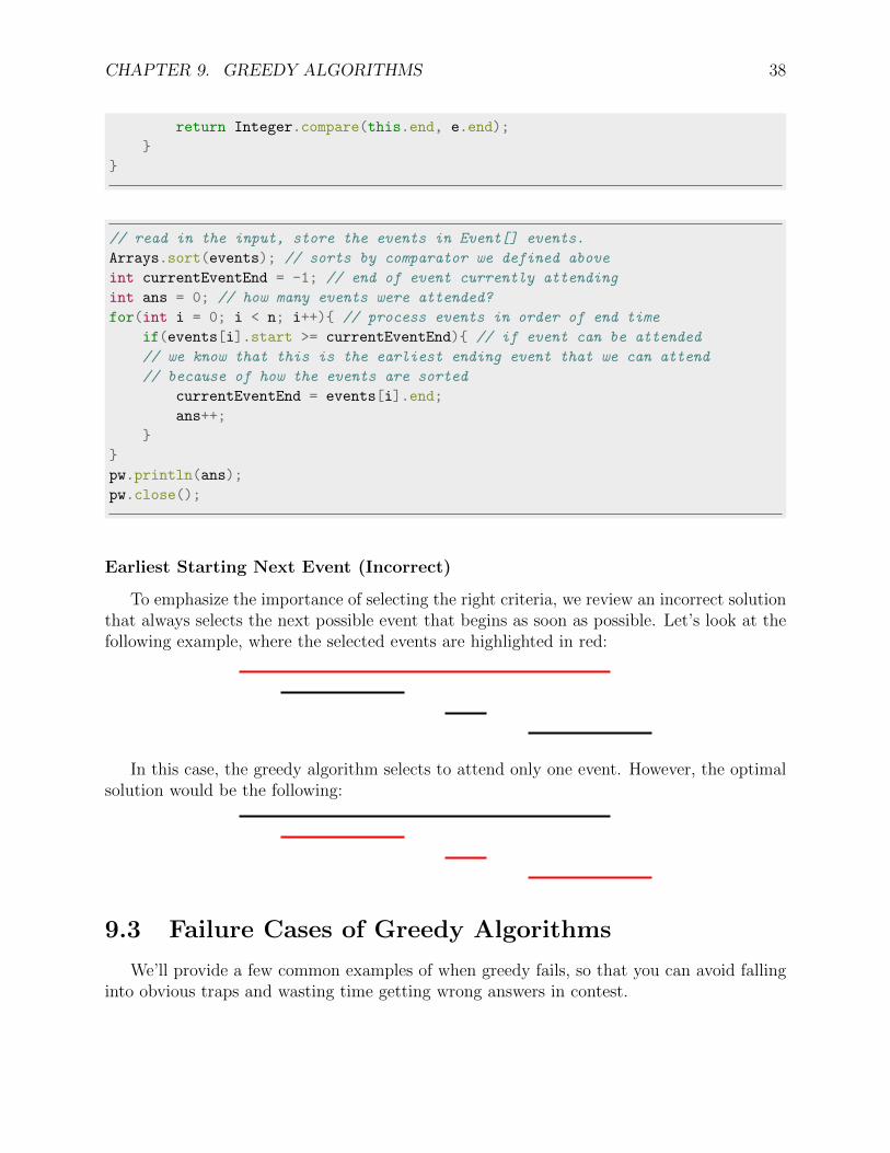
CHAPTER 9. GREEDY ALGORITHMS 38
return Integer.compare(this.end, e.end);
}
}
// read in the input, store the events in Event[] events.
Arrays.sort(events); // sorts by comparator we defined above
int currentEventEnd = -1; // end of event currently attending
int ans = 0; // how many events were attended?
for(int i = 0; i < n; i++){ // process events in order of end time
if(events[i].start >= currentEventEnd){ // if event can be attended
// we know that this is the earliest ending event that we can attend
// because of how the events are sorted
currentEventEnd = events[i].end;
ans++;
}
}
pw.println(ans);
pw.close();
Earliest Starting Next Event (Incorrect)
To emphasize the importance of selecting the right criteria, we review an incorrect solutionthat always selects the next possible event that begins as soon as possible. Let’s look at thefollowing example, where the selected events are highlighted in red:
In this case, the greedy algorithm selects to attend only one event. However, the optimalsolution would be the following:
9.3 Failure Cases of Greedy Algorithms
We’ll provide a few common examples of when greedy fails, so that you can avoid fallinginto obvious traps and wasting time getting wrong answers in contest.

CHAPTER 9. GREEDY ALGORITHMS 39
Coin Change
This problem gives several coin denominations, and asks for the minimum number ofcoins needed to make a certain value. The greedy algorithm of taking the largest possiblecoin denomination that fits in the remaining capacity can be used to solve this problem onlyin very specific cases (it can be proven that it works for the American as well as the Eurocoin systems). However, it doesn’t work in the general case.
Knapsack
The knapsack problem gives a number of items, each having a weight and a value, andwe want to choose a subset of these items. We are limited to a certain weight, and we wantto maximize the value of the items that we take.
Let’s take the following example, where we have a maximum capacity of 4:
Item Weight Value Value Per Weight
A 3 18 6B 2 10 5C 2 10 5
If we use greedy based on highest value first, we choose item A and then we are done, aswe don’t have remaining weight to fit either of the other two. Using greedy based on valueper weight again selects item A and then quits. However, the optimal solution is to selectitems B and C, as they combined have a higher value than item A alone. In fact, there is noworking greedy solution. The solution to this problem uses dynamic programming, which isbeyond the scope of this book.
9.4 Problems
1. USACO December 2015 Silver Problem 2: High Card Winshttp://usaco.org/index.php?page=viewproblem2&cpid=571
2. USACO February 2018 Silver Problem 1: Rest Stopshttp://www.usaco.org/index.php?page=viewproblem2&cpid=810
3. USACO February 2017 Silver Problem 1: Why Did The Cow Cross The Roadhttp://www.usaco.org/index.php?page=viewproblem2&cpid=714

Chapter 10
Graph Theory
Graph theory is one of the most important topics at the Silver level and above. Graphscan be used to represent many things, from images to wireless signals, but one of the simplestanalogies is to a map. Consider a map with several cities and highways connecting the cities.Some of the problems relating to graphs are:
• If we have a map with some cities and roads, what’s the shortest distance I have totravel to get from point A to point B?
• Consider a map of cities and roads. Is city A connected to city B? Consider a region tobe a group of cities such that each city in the group can reach any other city in saidgroup, but no other cities. How many regions are in this map, and which cities are inwhich region?
10.1 Graph Basics
Graphs are made up of nodes and edges, where nodes are connected by edges. Graphscan have either weighted edges, in which each edge has a certain length, or unweighted, inwhich case all edges have the same length. Edges are either directed, which means they canbe traveled upon in one direction, or undirected, which means that they can be traveledupon in both directions.
1
2
3
4
5 6
1
2
3
4
5 6
2
4
5
3
−1
2
5
Figure 10.1: An undirected unweighted graph (left) and a directed weighted graph (right)
40

CHAPTER 10. GRAPH THEORY 41
A connected component is a set of nodes within which any node can reach any othernode. For example, in this graph, nodes 1, 2, and 3 are a connected component, nodes 4 and5 are a connected component, and node 6 is its own component.
1 2
3
4 5
6
Figure 10.2: Connected components in a graph
10.2 Trees
A tree is a special type of graph satisfying two constraints: it is acyclic, meaning thereare no cycles, and the number of edges is one less than the number of nodes. Trees satisfythe property that for any two nodes A and B, there is exactly one way to travel between Aand B.
1
2 3
4 5 6 7
Figure 10.3: A tree graph
The root of a tree is the one vertex that is placed at the top, and is where we usuallystart our tree traversals from. Usually, problems don’t tell us where the tree is rooted at, andit usually doesn’t matter either; trees can be arbitrarily rooted (here, we’ll use the conventionof rooting at index 1).
Every node except the root node has a parent. The parent of a node s is defined asfollows: On the path from the root to s, the node that is one closer to the root than s is theparent of s. Each non-root node has a unique parent.
Child nodes are the opposite. They lie one farther away from the root than their parentnode. Unlike parent nodes, these are not unique. Each node can have arbitrarily many childnodes, and nodes can also have zero children. If a node s is the parent of a node t, then t isthe child node of s.
A leaf node is a node that has no children. Leaf nodes can be identified quite easilybecause there is only one edge adjacent to them.

CHAPTER 10. GRAPH THEORY 42
In our example tree above, node 1 is the root, nodes 2 and 3 are children of node 1, nodes4, 5, and 6 are children of 2, and node 7 is the child of 3. Nodes 4, 5, 6, and 7 are leaf nodes.
10.3 Graph Representations
Usually, in a graph with N edges and M edges, we’ll number the nodes 0 through N − 1.If the problem gives the nodes numbered 1 through N , simply decrease the endpoint nodenumbers of edges by 1 as you input them, in order to accommodate zero-indexing of arrays.However, in problem statements, input and output, the node labels will usually be 1 throughN , so that’s what we’ll use in our examples.
Graphs will usually be given in an input format similar to the following: First, integersN and M denoting the number of nodes and edges, respectively. Then, M lines, each withintegers a and b, representing edges; if the graph is undirected, then there is an edge betweennodes a and b, and if the graph is directed, then there is an edge from a to b.
For example, the input below would be for the following graph (without the comments):
6 7 // 6 nodes, 7 edges
// the following lines represent edges.
1 2
1 4
1 5
2 3
2 4
3 5
4 6
1
2
3
4
5 6
Figure 10.4: The graph corresponding to the above input
Graphs can be represented in three ways: Adjacency List, Adjacency Matrix, and EdgeList. Regardless of how the graph is represented, it’s important that it be stored globallyand statically, because we need to be able to access it from outside the main method, andcall the graph searching and traversal methods on it.

CHAPTER 10. GRAPH THEORY 43
Adjacency List
The adjacency list is the most commonly used method of storing graphs. When we useDFS, BFS, Dijkstra’s, or other single-source graph traversal algorithms, we’ll want to use anadjacency list. In an adjacency list, we maintain a length N array of lists. Each list storesthe neighbors of one node. In an undirected graph, if there is an edge between node a andnode b, we add a to the list of b’s neighbors, and b to the list of a’s neighbors. In a directedgraph, if there is an edge from node a to node b, we add b to the list of a’s neighbors, butnot vice versa.
1
2
3
4
5 6
9
4
3
5
2
41
3
Figure 10.5: An example of a weighted undirected graph
Adjacency list representation of the graph in fig. 10.5:
adj[0] (1, 9), (3, 4), (4, 3)adj[1] (0, 9), (2, 5), (3, 2)adj[2] (1, 5), (4, 4), (5, 1)adj[3] (0, 4), (1, 2), (5, 3)adj[4] (0, 3), (2, 4)adj[5] (2, 1), (3, 3)
Adjacency lists take up O(N +M) space, because each node corresponds to one list ofneighbors, and each edge corresponds to either one or two endpoints (directed vs undirected).In an adjacency list, we can find (and iterate through) the neighbors of a node easily. Hence,the adjacency list is the graph representation we should be using most of the time.
Often, we’ll want to maintain a array visited, which is a boolean array representingwhether each node has been visited. When we visit node k (0-indexed), we mark visited[k]
true, so that we know not to return to it.Code for setting up an adjacency list is as follows:
static int n, m; // number of nodes and edges
static ArrayList<Integer>[] adj; // adjacency list
public static void main(String[] args){
n = r.nextInt(); // reads in number of nodes
m = r.nextInt(); // reads in number of edges

CHAPTER 10. GRAPH THEORY 44
adj = new ArrayList[n]; // adjacency list
// Java doesn't allow ArrayList<Integer>[n]
boolean[] visited = new boolean[n];
for(int i = 0; i < n; i++){
adj[i] = new ArrayList<Integer>(); // initializes the ArrayLists
}
for(int i = 0; i < m; i++){ // reading in each of the m edges
int a = r.nextInt()-1; // we subtract 1 because our array is
zero-indexed↪→
int b = r.nextInt()-1;
adj[a].add(b);
adj[b].add(a); // omit this line if the graph is directed
}
}
If we’re dealing with a weighted graph, we’ll declare an Edge class or struct that storestwo variables: the second endpoint of the edge, and the weight of the edge, and we store anarray of lists of edges rather than an array of lists of integers.
static class Edge{
int to;
int weight;
public Edge(int to, int weight){
this.to = to;
this.edge = edge;
}
}
Adjacency Matrix
Another way of representing graphs is the adjacency matrix, which is an N by N 2-dimensional array that stores for each pair of indices (a, b), stores whether there is anedge between a and b. Start by initializing every entry in the matrix to zero (this is doneautomatically in Java), and then for undirected graphs, for each edge between indices a andb, set adj[a][b] and adj[b][a] to 1 (if unweighted) or the edge weight (if weighted). Ifthe graph is directed, for an edge from a to b, only set adj[a][b].

CHAPTER 10. GRAPH THEORY 45
1
2
3
4
5 6
9
4
3
5
2
41
3
Figure 1.5 repeated for convenience
Adjacency matrix representation of the graph in fig. 1.5:
× 0 1 2 3 4 50 0 9 0 4 3 01 9 0 5 2 0 02 0 5 0 0 4 13 4 2 0 0 0 34 3 0 4 0 0 05 0 0 1 3 0 0
At the Silver level, we generally won’t be using the adjacency matrix much, but it’s helpfulto know if it does come up. The primary use of the adjacency matrix is the Floyd-Warshallalgorithm, which is beyond the scope of this book.
Code for setting up an adjacency matrix is as follows:
static int n, m; // number of nodes and edges
static int[][] adj; // adj matrix
public static void main(String[] args){
n = r.nextInt();
m = r.nextInt();
adj = new int[n][n];
for(int i = 0; i < m; i++){ // read in each of the m edges
int a = r.nextInt()-1;
int b = r.nextInt()-1;
adj[a][b] = 1; // or set equal to w if graph is weighted
adj[b][a] = 1; // or set equal to w if graph is weighted;
// ignore above line if graph is directed
}
}

CHAPTER 10. GRAPH THEORY 46
Edge List
The last graph representation is the edge list. Usually, we use this in weighted undirectedgraphs when we want to sort the edges by weight (for DSU, for example; see section 10.6).In the edge list, we simply store a single list of all the edges, in the form (a, b, w) where aand b are the nodes that the edge connects, and w is the edge weight. Note that in an edgelist, we do NOT add each edge twice; there is only one place for us to add the edges, so weonly do so once.
1
2
3
4
5 6
9
4
3
5
2
41
3
Figure 1.5 repeated for convenience
Edge list representation of the graph in fig. 1.5:
(0, 1, 9), (0, 3, 4), (0, 4, 3), (1, 3, 2), (3, 5, 3), (2, 4, 4), (2, 1, 5), (2, 5, 1)
We’ll need an edge class, such as the following:
static class Edge implements Comparable<Edge>{
int a, b, w;
public Edge(int a, int b, int w){
this.a = a;
this.b = b;
this.w = w;
}
public int compareTo(Edge e){ // sort order is ascending, by weight
// to sort in descending order, just negate the value of the compare
function.↪→
return Integer.compare(w, e.w);
}
}
Code for the edge list is as follows, using the above edge class:
static int n, m; // number of nodes and edges
static ArrayList<Edge> edges;

CHAPTER 10. GRAPH THEORY 47
public static void main(String[] args){
n = r.nextInt();
m = r.nextInt();
edges = new ArrayList<Edge>();
for(int i = 0; i < m; i++){ // for each of the m edges
int a = r.nextInt()-1;
int b = r.nextInt()-1;
// subtract 1 to maintain zero-indexing of vertices
int w = r.nextInt();
edges.add(new Edge(a, b, w)); // add the edge to the list
}
Collections.sort(edges);
}
10.4 Graph Traversal Algorithms
Graph traversal is the process of visiting or checking each vertex in a graph. This is usefulwhen we want to determine which vertices can be visited, whether there exists a path fromone vertex to another, and so forth. There are two algorithms for graph traversal, namelydepth-first search (DFS) and breadth-first search (BFS).
Depth-first search
Depth-first search continues down a single path to the end, then it backtracks to checkother vertices. Depth-first search will process all nodes that are reachable (connected byedges) to the starting node. Let’s look at an example of how this works. Depth first-searchcan start at any node, but by convention we’ll start the search at node 1. We’ll use thefollowing color scheme: blue for nodes we have already visited, red for nodes we are currentlyprocessing, and black for nodes that have not been visited yet.
The DFS starts from node 1 and then goes to node 2, as it’s the only neighbor of node 1:
1 2 3
5 4
1 2 3
5 4
Now, the DFS goes to node 3 and then 4, following a single path to the end until it has nomore nodes to process:

CHAPTER 10. GRAPH THEORY 48
1 2 3
5 4
1 2 3
5 4
Lastly, the DFS backtracks to visit node 5, which was skipped over previously.
1 2 3
5 4
Depth-first search is implemented recursively because it allows for much simpler and shortercode. The algorithm is as follows:
Algorithm: Recursive implementation for depth-first traversal of a graph
Function DFSInput : start, the 0-indexed number of the starting vertexvisted(start)← trueforeach vertex k adjacent to start do
if visited(k) is false thenDFS (k)
end
end
Code:
static void dfs(int node){
visited[node] = true;
for(int next : adj[node]){
if(!visited[next]){
dfs(next);
}
}
}
Breadth-first search
Breadth-first search visits nodes in order of distance away from the starting node; it firstvisits all nodes that are one edge away, then all nodes that are two edges away, and so on.
Let’s use the same example graph that we used earlier: The BFS starts from node 1 andthen goes to node 2, as it’s the only neighbor of node 1:

CHAPTER 10. GRAPH THEORY 49
1 2 3
5 4
1 2 3
5 4
Now, the BFS goes to node 3, and then node 5, because both of them are two edges awayfrom node 1:
1 2 3
5 4
1 2 3
5 4
Lastly, the BFS visits node 4, which is farthest.
1 2 3
5 4
The breadth-first search algorithm cannot be implemented recursively, so it’s significantlylonger. Thus, when both BFS and DFS work, DFS is usually the better option.
BFS can be used for finding the distance away from a starting node for all nodes in anunweighted graph, as we show below:

CHAPTER 10. GRAPH THEORY 50
The algorithm is as follows:
Algorithm: Breadth-first traversal of a graph
Function BFSInput : start, the 0-indexed number of the starting vertexforeach vertex v do
dist[v]← −1visited[v]← false
enddist[start]← 0Let q be a queue of integersAdd start to qwhile q is not empty do
Pop the first element from q, call it vforeach neighbor u of v do
if node u has not yet been visited thendist[u]← dist[v] + 1Add u to q
end
end
end
Once the BFS finishes, the array dist contains the distances from the start node to eachnode.
Example code is below. Note that the array dist[] is initially filled with −1’s to denotethat none of the nodes have been processed yet.
static void bfs(int k){
Arrays.fill(dist, -1); // fill distance array with -1's
Queue<Integer> q = new LinkedList<Integer>();
dist[k] = 0;
q.add(k);
while(!q.isEmpty()){
int v = q.poll();
for(int e : adj[v]){
if(dist[e] == -1){
dist[e] = dist[v] + 1;
q.add(e);
}
}
}
}

CHAPTER 10. GRAPH THEORY 51
Iterative DFS
If you encounter stack overflows while using recursive DFS, you can write an iterativeDFS, which is just BFS but with nodes stored on a stack rather than a queue.
10.5 Floodfill
Floodfill is an algorithm that identifies and labels the connected component that aparticular cell belongs to, in a multi-dimensional array. Essentially, it’s DFS, but on a grid,and we want to find the connected component of all the connected cells with the same number.For example, let’s look at the following grid and see how floodfill works, starting from thetop-left cell. The color scheme will be the same: red for the node currently being processed,blue for nodes already visited, and uncolored for nodes not yet visited.
2 2 12 1 12 2 1
2 2 12 1 12 2 1
2 2 12 1 12 2 1
2 2 12 1 12 2 1
2 2 12 1 12 2 1
2 2 12 1 12 2 1
As opposed to an explicit graph where the edges are given, a grid is an implicit graph.This means that the neighbors are just the nodes directly adjacent in the four cardinaldirections.
Usually, grids given in problems will be N by M , so the first line of the input contains thenumbers N and M . In this example, we will use an two-dimensional integer array to store thegrid, but depending on the problem, a two-dimensional character array or a two-dimensionalboolean array may be more appropriate. Then, there are N rows, each with M numberscontaining the contents of each square in the grid. Example input might look like the following(varies between problems):

CHAPTER 10. GRAPH THEORY 52
3 4
1 1 2 1
2 3 2 1
1 3 3 3
And we’ll want to input the grid as follows:
static int[][] grid;
static int n, m;
public static void main(String[] args){
int n = r.nextInt();
int m = r.nextInt();
grid = new int[n][m];
for(int i = 0; i < n; i++){
for(int j = 0; j < m; j++){
grid[i][j] = r.nextInt();
}
}
}
When doing floodfill, we will maintain an N ×M array of booleans to keep track ofwhich squares have been visited, and a global variable to maintain the size of the currentcomponent we are visiting. Make sure to store the grid, the visited array, dimensions, andthe current size variable globally.
This means that we want to recursively call the search function from the squares above,below, and to the left and right of our current square. The algorithm to find the size of aconnected component in a grid using floodfill is as follows (we’ll also maintain a 2d visited
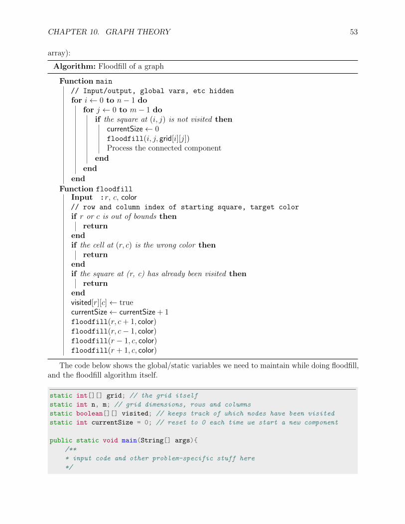
CHAPTER 10. GRAPH THEORY 53
array):
Algorithm: Floodfill of a graph
Function main
// Input/output, global vars, etc hidden
for i← 0 to n− 1 dofor j ← 0 to m− 1 do
if the square at (i, j) is not visited thencurrentSize← 0floodfill(i, j, grid[i][j])Process the connected component
end
end
end
Function floodfillInput : r, c, color// row and column index of starting square, target color
if r or c is out of bounds thenreturn
endif the cell at (r, c) is the wrong color then
returnendif the square at (r, c) has already been visited then
returnendvisited[r][c]← truecurrentSize← currentSize + 1floodfill(r, c+ 1, color)floodfill(r, c− 1, color)floodfill(r − 1, c, color)floodfill(r + 1, c, color)
The code below shows the global/static variables we need to maintain while doing floodfill,and the floodfill algorithm itself.
static int[][] grid; // the grid itself
static int n, m; // grid dimensions, rows and columns
static boolean[][] visited; // keeps track of which nodes have been visited
static int currentSize = 0; // reset to 0 each time we start a new component
public static void main(String[] args){
/**
* input code and other problem-specific stuff here
*/

CHAPTER 10. GRAPH THEORY 54
for(int i = 0; i < n; i++){
for(int j = 0; j < m; j++){
if(!visited[i][j]){
currentSize = 0;
floodfill(i, j, grid[i][j]);
// start a floodfill if the square hasn't already been visited,
// and then store or otherwise use the component size
// for whatever it's needed for
}
}
}
}
static void floodfill(int r, int c, int color){
if(r < 0 || r >= n || c < 0 || c >= m) return; // if outside grid
if(grid[r][c] != color) return; // wrong color
if(visited[r][c]) return; // already visited this square
visited[r][c] = true; // mark current square as visited
currentSize++; // increment the size for each square we visit
// recursively call floodfill for neighboring squares
floodfill(r, c+1, color);
floodfill(r, c-1, color);
floodfill(r-1, c, color);
floodfill(r+1, c, color);
}
10.6 Disjoint-Set Data Structure
Let’s say we want to construct a graph, one edge at a time. We also want to be able toadd additional nodes, and query whether two nodes are connected. We can naively solvethis problem by adding the edges and running a floodfill each time, before finally checkingwhether two nodes have the same color. This yields a time complexity of O(nm) for a graphof n nodes and m edges.
However, we can do better than this using a data structure known as Disjoint-Set Union,or DSU for short. This data structure supports two operations:
• Add an edge between two nodes.
• Check if two nodes are connected.
To achieve this, we store sets as trees, with the root of the tree representing the “parent”of the set. Initially, we store each node as its own set. Then, we combine their sets when weadd an edge between two nodes. The image below illustrates this structure.

CHAPTER 10. GRAPH THEORY 55
In this graph, 1 is the parent of the set containing 3, 2, and 4.To implement this, let’s store the parent of each node in the tree represented by that
node’s set. Then, to merge two sets, we set the parent of one tree’s root to the other tree’sroot, like so:
The following methods demonstrate this idea:
static int[] parent; //stores the parent nodes
static void initialize(int N){
for(int i = 0; i < N; i++){
parent[i] = i; //initially, the root of each set is the node itself
}
}
static int find(int x){ //finds the root of the set of x
if(x == parent[x]){ //if x is the parent of itself, it is the root
return x;
}
else{
return find(parent[x]); //otherwise, recurse to the parent of x
}

CHAPTER 10. GRAPH THEORY 56
}
static void union(int a, int b){ //merges the sets of a and b
int c = find(a); //find the root of a
int d = find(b); //find the root of b
if(c != d){
parent[d] = c; //merge the sets by setting the parent of d to c
}
}
However, this naive implementation of a DSU isn’t much better than simply running afloodfill. As the recursing up the tree of a set to find it’s root can be time-consuming fortrees with long chains, the runtime ultimately degrades to still being O(nm) for n nodes andm edges.
Now that we understand the general idea of a DSU, we can improve the runtime of thisimplementation using an optimization known as path compression. The general idea is toreassign nodes in the tree as you are recursively calling the find method to prevent longchains from forming. Here is a rewritten find method representing this idea:
static int find(int x){
if(x == parent[x]){
return x;
}
else{
// we set the direct parent to the root of the set to reduce path length
return parent[x] = find(parent[x]);
}
}
The following image demonstrates how the tree with parent 1 is compressed after find(6)is called. All of the bolded nodes in the final tree were visited during the recursive operation,and now point to the root.

CHAPTER 10. GRAPH THEORY 57
With this new optimization, the runtime reduces to O(n log n), far better than our naivealgorithm. Further optimizations can reduce the runtime of DSU to nearly constant. However,those techniques and the proof of complexity for these optimizations are both unnecessary forand out of the scope of the USACO Silver division, so they will not be included in this book.
10.7 Bipartite Graphs
A bipartite graph is a graph such that each node can be colored in one of two colors,such that no two adjacent nodes have the same color. For example, the following graph isbipartite:
1 2 3
4 5
A graph is bipartite if and only if there are no cycles of odd length. For example, thefollowing graph is not bipartite, because it contains a cycle of length 3.
1 2 3
4
The following image depicts how a bipartite graph splits vertices into two “groups”depending on their color.

CHAPTER 10. GRAPH THEORY 58
In order to check whether a graph is bipartite, we use a modified breadth-first search.
Algorithm: Bipartiteness check
Function bipartiteInput : a graphOutput : whether the graph is bipartite or notAssign color 1 to the starting vertex// Use the following modified bfs
foreach vertex v processed in bfs dod← dist(start, v)if d is odd then
Assign color 2 to vertex velse
Assign color 1 to vertex vendforeach vertex w adjacent to v do
if w and v are the same color thenreturn false // not bipartite
end
end
endreturn true // bipartite
10.8 Problems
DFS/BFS Problems
1. USACO January 2018 Silver Problem 3: MooTubehttp://www.usaco.org/index.php?page=viewproblem2&cpid=788

CHAPTER 10. GRAPH THEORY 59
2. USACO December 2016 Silver Problem 3: Moocasthttp://www.usaco.org/index.php?page=viewproblem2&cpid=668
3. USACO US Open 2016 Silver Problem 3: Closing the Farmhttp://www.usaco.org/index.php?page=viewproblem2&cpid=644
DSU Problems
Many of these problems do not require DSU. However, they become much easier to do ifyou understand it.
4. USACO US Open Silver Problem 3: The Moo Particlehttp://usaco.org/index.php?page=viewproblem2&cpid=1040
5. USACO January 2018 Silver Problem 3: MooTubehttp://www.usaco.org/index.php?page=viewproblem2&cpid=788
6. USACO December 2019 December Problem 3: Milk Visitshttp://usaco.org/index.php?page=viewproblem2&cpid=968
7. USACO US Open 2016 Gold Problem 2: Closing the Farmhttp://www.usaco.org/index.php?page=viewproblem2&cpid=646
8. USACO January Contest 2020 Silver Problem 3: Wormhole Sorthttp://www.usaco.org/index.php?page=viewproblem2&cpid=992
Other Graph Problems
9. (Bipartite Graphs) USACO February 2019 Silver Problem 3: The Great Revegetationhttp://www.usaco.org/index.php?page=viewproblem2&cpid=920
10. CodeForces Round 595 (Div. 3) Problem B2: Books Exchangehttps://codeforces.com/problemset/problem/1249/B2
Chapter 11
Prefix Sums
11.1 Prefix Sums
Let’s say we have an integer array arr with N elements, and we want to process Q queriesto find the sum of the elements between two indices a and b, inclusive, with different valuesof a and b for every query. For the purposes of this chapter, we will assume that the originalarray is 1-indexed, meaning arr[0] = 0 (which is a dummy index), and the actual arrayelements occupy indices 1 through N (this means that the array actually has length N + 1).
Let’s use the following example 1-indexed array arr, with N = 6:
Index i 0 1 2 3 4 5 6arr[i] 0 1 6 4 2 5 3
Naively, for every query, we can iterate through all entries from index a to index b to addthem up. Since we have Q queries and each query requires a maximum of O(N) operationsto calculate the sum, our total time complexity is O(NQ). For most problems of this nature,the constraints will be N,Q ≤ 105, so NQ is on the order of 1010. This is not acceptable; itwill almost always exceed the time limit.
Instead, we can use prefix sums to process these array sum queries. We designate a prefixsum array prefix[]. First, since we’re 1-indexing the array, set prefix[0] = 0, then forindices k such that 1 ≤ k ≤ n, define the prefix sum array as follows:
prefix[k] =k∑
i=1
arr[i]
Basically, what this means is that the element at index k of the prefix sum array stores thesum of all the elements in the original array from index 1 up to k. This can be calculatedeasily in O(N) by the following formula:
prefix[k] = prefix[k-1] + arr[k]
For the example case, our prefix sum array looks like this:
Index i 0 1 2 3 4 5 6prefix[i] 0 1 7 11 13 18 21
60

CHAPTER 11. PREFIX SUMS 61
Now, when we want to query for the sum of the elements of arr between (1-indexed)indices a and b inclusive, we can use the following formula:
b∑i=a
arr[i] =b∑
i=1
arr[i]−a−1∑i=1
arr[i]
Using our definition of the elements in the prefix sum array, we have
b∑i=a
arr[i] = prefix[b]− prefix[a-1]
Since we are only querying two elements in the prefix sum array, we can calculate subarraysums in O(1) per query, which is much better than the O(N) per query that we had before.Now, after an O(N) preprocessing to calculate the prefix sum array, each of the Q queriestakes O(1) time. Thus, our total time complexity is O(N +Q), which should now pass thetime limit.
Let’s do an example query and find the subarray sum between indices a = 2 and b = 5,inclusive, in the 1-indexed arr. From looking at the original array, we see that this is∑5
i=2 arr[i] = 6 + 4 + 2 + 5 = 17.
Index i 0 1 2 3 4 5 6arr[i] 0 1 6 4 2 5 3
Using prefix sums: prefix[5]− prefix[1] = 18− 1 = 17.
Index i 0 1 2 3 4 5 6prefix[i] 0 1 7 11 13 18 21
11.2 Two Dimensional Prefix Sums
Now, what if we wanted to process Q queries for the sum over a subrectangle of a Nrows by M columns matrix in two dimensions? Let’s assume both rows and columns are1-indexed, and we use the following matrix as an example:
0 0 0 0 0 00 1 5 6 11 80 1 7 11 9 40 4 6 1 3 20 7 5 4 2 3
Naively, each sum query would then take O(NM) time, for a total of O(QNM). This istoo slow.
Let’s take the following example region, which we want to sum:
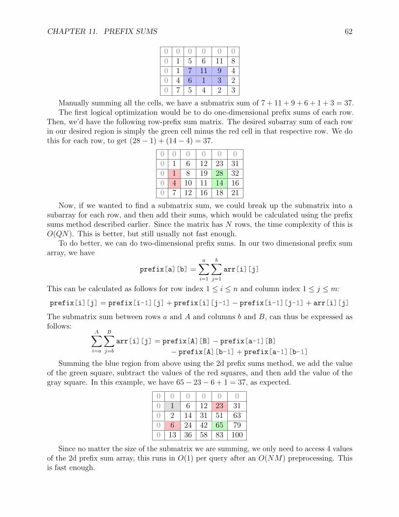
CHAPTER 11. PREFIX SUMS 62
0 0 0 0 0 00 1 5 6 11 80 1 7 11 9 40 4 6 1 3 20 7 5 4 2 3
Manually summing all the cells, we have a submatrix sum of 7 + 11 + 9 + 6 + 1 + 3 = 37.The first logical optimization would be to do one-dimensional prefix sums of each row.
Then, we’d have the following row-prefix sum matrix. The desired subarray sum of each rowin our desired region is simply the green cell minus the red cell in that respective row. We dothis for each row, to get (28− 1) + (14− 4) = 37.
0 0 0 0 0 00 1 6 12 23 310 1 8 19 28 320 4 10 11 14 160 7 12 16 18 21
Now, if we wanted to find a submatrix sum, we could break up the submatrix into asubarray for each row, and then add their sums, which would be calculated using the prefixsums method described earlier. Since the matrix has N rows, the time complexity of this isO(QN). This is better, but still usually not fast enough.
To do better, we can do two-dimensional prefix sums. In our two dimensional prefix sumarray, we have
prefix[a][b] =a∑
i=1
b∑j=1
arr[i][j]
This can be calculated as follows for row index 1 ≤ i ≤ n and column index 1 ≤ j ≤ m:
prefix[i][j] = prefix[i-1][j] + prefix[i][j-1]− prefix[i-1][j-1] + arr[i][j]
The submatrix sum between rows a and A and columns b and B, can thus be expressed asfollows:
A∑i=a
B∑j=b
arr[i][j] = prefix[A][B]− prefix[a-1][B]
− prefix[A][b-1] + prefix[a-1][b-1]
Summing the blue region from above using the 2d prefix sums method, we add the valueof the green square, subtract the values of the red squares, and then add the value of thegray square. In this example, we have 65− 23− 6 + 1 = 37, as expected.
0 0 0 0 0 00 1 6 12 23 310 2 14 31 51 630 6 24 42 65 790 13 36 58 83 100
Since no matter the size of the submatrix we are summing, we only need to access 4 valuesof the 2d prefix sum array, this runs in O(1) per query after an O(NM) preprocessing. Thisis fast enough.
CHAPTER 11. PREFIX SUMS 63
11.3 Problems
1. USACO December 2015 Silver Problem 3: Breed Countinghttp://usaco.org/index.php?page=viewproblem2&cpid=572
2. USACO January 2016 Silver Problem 2: Subsequences Summing to Sevenshttp://usaco.org/index.php?page=viewproblem2&cpid=595
3. USACO December 2017 Silver Problem 1: My Cow Ate My Homeworkhttp://www.usaco.org/index.php?page=viewproblem2&cpid=762
4. USACO January 2017 Silver Problem 2: Hoof, Paper, Scissorshttp://www.usaco.org/index.php?page=viewproblem2&cpid=691
5. (2D Prefix Sums) USACO February 2019 Silver Problem 2: Painting the Barnhttp://www.usaco.org/index.php?page=viewproblem2&cpid=919

Chapter 12
Binary Search
12.1 Binary Search on the Answer
You’re probably already familiar with the concept of binary searching for a number ina sorted array. However, binary search can be extended to binary searching on the answeritself. When we binary search on the answer, we start with a search space, where we knowthe answer lies in. Then, each iteration of the binary search cuts the search space in half,so the algorithm tests O(logN) values, which is efficient and much better than testing eachpossible value in the search space.
Similarly to how binary search on an array only works on a sorted array, binary searchon the answer only works if the answer function is monotonic. Let’s say we have a functioncheck(x) that returns true if the answer of x is possible, and false otherwise. Usually, insuch problems, we’ll want to find the maximum or minimum value of x such that check(x)is true.
In order for binary search to work, the search space must look like something of thefollowing form, using a check function as we described above.
true true true true true false false false false
Then, we find the point at which true becomes false, using binary search.Below, we present two algorithms for binary search. The first implementation may be
more intuitive, because it’s closer to the binary search most students learned, while the
64

CHAPTER 12. BINARY SEARCH 65
second implementation is shorter.
Algorithm: Binary searching for the answer
Function binarySearch1
left← lower bound of search spaceright← upper bound of search spaceans← −1while left ≤ right do
mid← (left + right)/2if check(mid) then
left← mid + 1ans← mid
elseright← mid− 1
endreturn ans
Algorithm: Binary searching for the answer
Function binarySearch2
pos← 0max← upper bound of search spacefor (a = max; a ≥ 1; a /= 2) do
while check(pos + a) dopos← pos + a
end
endreturn pos
12.2 Example
Source: Codeforces Round 577 (Div. 2) Problem Chttps://codeforces.com/contest/1201/problem/C
Given an array arr of n integers, where n is odd, we can perform the following operationon it k times: take any element of the array and increase it by 1. We want to make themedian of the array as large as possible, after k operations.
Constraints: 1 ≤ n ≤ 2 · 105, 1 ≤ k ≤ 109 and n is odd.The solution is as follows: we first sort the array in ascending order. Then, we binary
search for the maximum possible median. We know that the number of operations requiredto raise the median to x increases monotonically as x increases, so we can use binary search.For a given median value x, the number of operations required to raise the median to x is
n∑i=(n+1)/2
max(0, x− arr[i])

CHAPTER 12. BINARY SEARCH 66
If this value is less than or equal to k, then x can be the median, so our check functionreturns true. Otherwise, x cannot be the median, so our check function returns false.
Solution code (using the second implementation of binary search):
static int n;
static long k;
static long[] arr;
public static void main(String[] args) {
n = r.nextInt(); k = r.nextLong();
arr = new long[n];
for(int i = 0; i < n; i++){
arr[i] = r.nextLong();
}
Arrays.sort(arr);
pw.println(search());
pw.close();
}
// binary searches for the correct answer
static long search(){
long pos = 0; long max = (long)2E9;
for(long a = max; a >= 1; a /= 2){
while(check(pos+a)) pos += a;
}
return pos;
}
// checks whether the number of given operations is sufficient
// to raise the median of the array to x
static boolean check(long x){
long operationsNeeded = 0;
for(int i = (n-1)/2; i < n; i++){
operationsNeeded += Math.max(0, x-arr[i]);
}
if(operationsNeeded <= k){ return true; }
else{ return false; }
}
12.3 Problems
1. USACO December 2018 Silver Problem 1: Conventionhttp://www.usaco.org/index.php?page=viewproblem2&cpid=858

CHAPTER 12. BINARY SEARCH 67
2. USACO January 2016 Silver Problem 1: Angry Cowshttp://usaco.org/index.php?page=viewproblem2&cpid=594
3. USACO January 2017 Silver Problem 1: Cow Dance Showhttp://www.usaco.org/index.php?page=viewproblem2&cpid=690
4. Educational Codeforces Round 60 Problem C: Magic Shiphttps://codeforces.com/problemset/problem/1117/C (Also uses prefix sums)
5. USACO January 2020 Silver Problem 2: Loan Repaymenthttp://www.usaco.org/index.php?page=viewproblem2&cpid=991
(Warning: extremely difficult for silver)
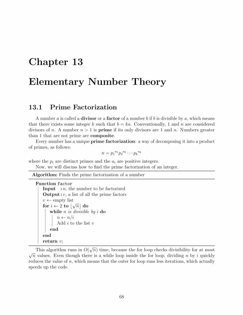
Chapter 13
Elementary Number Theory
13.1 Prime Factorization
A number a is called a divisor or a factor of a number b if b is divisible by a, which meansthat there exists some integer k such that b = ka. Conventionally, 1 and n are considereddivisors of n. A number n > 1 is prime if its only divisors are 1 and n. Numbers greaterthan 1 that are not prime are composite.
Every number has a unique prime factorization: a way of decomposing it into a productof primes, as follows:
n = p1a1p2
a2 · · · pkak
where the pi are distinct primes and the ai are positive integers.Now, we will discuss how to find the prime factorization of an integer.
Algorithm: Finds the prime factorization of a number
Function factorInput :n, the number to be factorizedOutput : v, a list of all the prime factorsv ← empty listfor i← 2 to b
√nc do
while n is divisible by i don← n/iAdd i to the list v
end
endreturn v ;
This algorithm runs in O(√n) time, because the for loop checks divisibility for at most√
n values. Even though there is a while loop inside the for loop, dividing n by i quicklyreduces the value of n, which means that the outer for loop runs less iterations, which actuallyspeeds up the code.
68

CHAPTER 13. ELEMENTARY NUMBER THEORY 69
Let’s look at an example of how this algorithm works, for n = 252.
i n v
2 252 {}2 126 {2}2 63 {2, 2}3 21 {2, 2, 3}3 7 {2, 2, 3, 3}
At this point, the for loop terminates, because i is already 3 which is greater than b√
7c. Inthe last step, we add 7 to the list of factors v, because it otherwise won’t be added, for afinal prime factorization of {2, 2, 3, 3, 7}.
13.2 GCD and LCM
The greatest common divisor (GCD) of two integers a and b is the largest integerthat is a factor of both a and b. In order to find the GCD of two numbers, we use theEuclidean Algorithm, which is as follows:
gcd(a, b) =
{a b = 0
gcd(b, a mod b) b 6= 0
This algorithm is very easy to implement using a recursive function, as follows:
public int gcd(int a, int b){
if(b == 0) return a;
return gcd(b, a % b);
}
Finding the GCD of two numbers can be done in O(log n) time, where n = min(a, b).The least common multiple (LCM) of two integers a and b is the smallest integer
divisible by both a and b.The LCM can easily be calculated from the following property with the GCD:
lcm(a, b) =a · b
gcd(a, b)
If we want to take the GCD or LCM of more than two elements, we can do so two at a time,in any order. For example,
gcd(a1, a2, a3, a4) = gcd(a1, gcd(a2, gcd(a3, a4)))

CHAPTER 13. ELEMENTARY NUMBER THEORY 70
13.3 Modular Arithmetic
In modular arithmetic, instead of working with integers themselves, we work with theirremainders when divided by m. We call this taking modulo m. For example, if we takem = 23, then instead of working with x = 247, we use x mod 23 = 17. Usually, m will be alarge prime, given in the problem; the two most common values are 109 + 7, and 998 244 353.Modular arithmetic is used to avoid dealing with numbers that overflow built-in data types,because we can take remainders, according to the following formulas:
(a+ b) mod m = (a mod m+ b mod m) mod m
(a− b) mod m = (a mod m− b mod m) mod m
(a · b) (mod m) = ((a mod m) · (b mod m)) mod m
ab mod m = (a mod m)b mod m
Under a prime moduli, division does exist; however it’s rarely used in problems and isbeyond the scope of this book.
13.4 Problems
1. CodeForces VK Cup 2012 Wildcard Round 1https://codeforces.com/problemset/problem/162/C
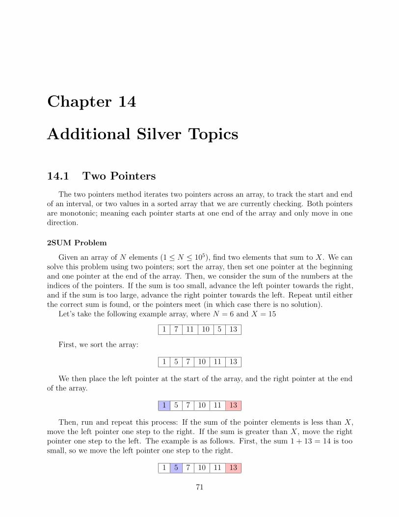
Chapter 14
Additional Silver Topics
14.1 Two Pointers
The two pointers method iterates two pointers across an array, to track the start and endof an interval, or two values in a sorted array that we are currently checking. Both pointersare monotonic; meaning each pointer starts at one end of the array and only move in onedirection.
2SUM Problem
Given an array of N elements (1 ≤ N ≤ 105), find two elements that sum to X. We cansolve this problem using two pointers; sort the array, then set one pointer at the beginningand one pointer at the end of the array. Then, we consider the sum of the numbers at theindices of the pointers. If the sum is too small, advance the left pointer towards the right,and if the sum is too large, advance the right pointer towards the left. Repeat until eitherthe correct sum is found, or the pointers meet (in which case there is no solution).
Let’s take the following example array, where N = 6 and X = 15
1 7 11 10 5 13
First, we sort the array:
1 5 7 10 11 13
We then place the left pointer at the start of the array, and the right pointer at the endof the array.
1 5 7 10 11 13
Then, run and repeat this process: If the sum of the pointer elements is less than X,move the left pointer one step to the right. If the sum is greater than X, move the rightpointer one step to the left. The example is as follows. First, the sum 1 + 13 = 14 is toosmall, so we move the left pointer one step to the right.
1 5 7 10 11 13
71

CHAPTER 14. ADDITIONAL SILVER TOPICS 72
Now, 5 + 13 = 18 overshoots the sum we want, so we move the right pointer one step tothe left.
1 5 7 10 11 13
At this point we have 5 + 11 = 16, still too big. We continue moving the right pointer tothe left.
1 5 7 10 11 13
Now, we have the correct sum, and we are done.Code is as follows:
int left = 0; int right = n-1;
while(left < right){
if(arr[left] + arr[right] == x){
break;
} else if(arr[left] + arr[right] < x){
left++;
} else {
right--;
}
}
// if left >= right after the loop ends, no answer exists.
Subarray Sum
Given an array of N (1 ≤ N ≤ 105) positive elements, find a contiguous subarray thatsums to X.
We can do this in a similar manner to how we did the 2SUM problem: except this time westart both pointers at the left, and the pointers mark the beginning and end of the subarraywe are currently checking. We advance the right pointer one step to the right if the total ofthe current subarray is too small, advance the left pointer one step to the right if the currenttotal is too large, and we are done when we find the correct total.
Maximum subarray sum
Another problem that isn’t quite solved by two pointers, but is somewhat related, is themaximum subarray sum problem.
Given an array of N integers (1 ≤ N ≤ 105), which can be positive or negative, find themaximum sum of a contiguous subarray.
We can solve this problem using Kadane’s algorithm, which works as follows: we iteratethrough the elements of the array, and for each index i, we maintain the maximum subarraysum of a subarray ending at i in the variable current, and the maximum subarray sum of asubarray ending at or before i, in the variable best.
Example code is below.

CHAPTER 14. ADDITIONAL SILVER TOPICS 73
int best = 0; int current = 0;
for(int i = 0; i < n; i++){
current = Math.max(0, current + arr[i]);
best = Math.max(best, current);
}
14.2 Line Sweep
Line sweep is the technique of sorting a set of points or line segments and then processingthem in order (this usually means from left to right). The name line sweep comes from thefact that we are sweeping an imaginary vertical line across the plane containing the points orsegments.
To describe this technique, we’ll be using the 2019 US Open problem, “Cow SteeplechaseII”.
http://usaco.org/index.php?page=viewproblem2&cpid=943
In this problem, we are given some line segments and asked to find one line segment andremove it such that the resulting segments form no intersections. It is guaranteed that this isalways possible.
First of all, let’s observe it is sufficient to find any two line segments that intersect. Oncewe have done this, the solution is guaranteed to be one of these two segments. Then, out ofthe two, the segment with multiple intersections is the answer (because removing any othersegment decreases the number of intersections by at most 1, and only removing the segmentwith multiple intersections ensures there are no intersections).
If both segments have one intersection, that means the intersect with each other, so weshould return the one with the smallest index (as per the problem statement). Now, theproblem reduces to two parts: checking if two line segments intersect, and processing the linesegments using a line sweep.
Checking If Two Segments Intersect
To check if two line segments intersect, we will use a fact from algebra: if we have thepoints A = (xa, ya), B = (xb, yb), and C = (xc, yc), then the (signed) area of 4ABC, denoted[ABC], is (xb − xa)(yc − ya)− (xc − xa)(yb − ya). This can be derived from the cross product
of the vectors−→AB and
−→AC.
The part that will help us is the fact that this area is signed, which means that [ABC] is
positive if A, B, and C occur in counterclockwise order,
negative if A, B, and C occur in clockwise order, and
zero if A, B, and C are collinear.
Then, the key observation is that two segments PQ and XY intersect if the two conditionshold:

CHAPTER 14. ADDITIONAL SILVER TOPICS 74
• [XPQ] and [Y PQ] have different signs
• [PXY ] and [QXY ] have different signs
For example, in the figure below, [X1P1Q1] and [Q1X1Y1] are positive because their verticesoccur in counterclockwise order, and [Y1P1Q1] and [P1X1Y1] are negative because their verticesoccur in clockwise order. Therefore, we know that X1Y1 and P1Q1 intersect. Similarly, onthe right, we know that [P2X2Y2] and [Q2X2Y2] have vertices both going in clockwise order,so their signed areas are the same, and therefore P2Q2 and X2Y2 don’t intersect.
P1 Q1
X1
Y1
P2 Q2
X2
Y2
If the two conditions hold and some of the signs are zero, then this means that the segmentsintersect at their endpoints. If the problem does not count these as intersecting, then considerzero to have the same sign as both positive and negative.
However, there is a special case. If the signs of all four areas are zero, then all four pointslie on a line. To check if they intersect in this case, we just check whether one point isbetween the others. In particular, we check if P or Q is on XY or if X is on PQ. We don’tneed to check if Y is on PQ because if the segments do intersect, we will have two instancesof points on the other segments.
Here’s a full implementation:
public class Point {
public int x, y;
public Point(int x, int y){
this.x = x; this.y = y;
}
}
public static int sign(Point A, Point B, Point C) {
int area = (B.x-A.x) * (C.y-A.y) - (C.x-A.x) * (B.y-A.y);
if (area > 0) return 1;
if (area < 0) return -1;
return 0;
}
public static boolean between(Point P, Point X, Point Y) {
return ((X.x <= P.x && P.x <= Y.x) || (Y.x <= P.x && P.x <= X.x))
&& ((X.y <= P.y && P.y <= Y.y) || (Y.y <= P.y && P.y <= X.y));

CHAPTER 14. ADDITIONAL SILVER TOPICS 75
}
public static boolean intersectQ(Point P, Point Q, Point X, Point Y) {
int[] signs = {sign(P, X, Y), sign(Q, X, Y), sign(X, P, Q), sign(Y, P, Q)};
if (signs[0] == 0 && signs[1] == 0 && signs[2] == 0 && signs[3] == 0)
return between(P, X, Y) || between(Q, X, Y) || between(X, P, Q);
return signs[0] != signs[1] && signs[2] != sign[3];
}
Processing Line Segments
Let’s break apart the N line segments into 2N events, one for each start and end point.We’ll store whether some event is a start point or an end point, and which start pointscorrespond to each end point.
Then, we process the endpoints in order of x coordinate from left to right, maintaining aset of currently processed segments, which is sorted by y. When we hit an endpoint, we eitheradd or remove a segment from the set, depending on whether we start or end a segment.Every time we add a segment, we check it for intersection with the segment above it and thesegment below it. In addition, every time we remove a segment, we check the segment aboveit and the segment below it for intersection. Once we find an intersection, we are done.
14.3 Bitwise Operations and Subsets
Binary Representations of Integers
In programming, numbers are stored as binary representations. This means that a numberx is represented as
x =n∑
i=0
ai2i,
where the ais are either 0 or 1 and n = blog2 xc.For example:
17 = 24 + 20 = 100012
Each digit in the binary representation, which is either 0 or 1, is called a bit.
Bitwise Operations
There are several binary operations on binary numbers called bitwise operations. Theseoperations are applied separately for each bit position. The common binary operations areshown in table 14.1:

CHAPTER 14. ADDITIONAL SILVER TOPICS 76
Bit A Bit B A andB A orB A xorB
1 1 1 1 01 0 0 1 10 1 0 1 10 0 0 0 0
Table 14.1: The outputs of bitwise operations on two bits
The AND operation (&) returns 1 if and only if both bits are 1.
19 & 27
1 0 0 1 1 = 19AND 1 1 0 1 1 = 27
= 1 0 0 1 1 = 19
The OR operation (|) returns 1 if either bit is 1.
19 | 27
1 0 0 1 1 = 19OR 1 1 0 1 1 = 27= 1 1 0 1 1 = 27
The XOR operation (∧) returns 1 if and only if exactly one of the bits is 1.
19 ∧ 26
1 0 0 1 1 = 19XOR 1 1 0 1 1 = 27
= 0 1 0 0 0 = 8
Finally, the left shift operator x << k multiplies x by 2k. Watch for overflow and use thelong data type if necessary. For example:
1 << 5 = 1 · 25 = 32
7 << 2 = 7 · 22 = 28
Exercises
Calculate by converting the numbers to binary, applying the bit operations, and thenconverting back to decimal numbers:
(a) 19 & 34 Answer: 2
(b) 14 | 29 Answer: 31
(c) 10 ∧ 19 Answer: 25
(d) 3 << 5 Answer: 96

CHAPTER 14. ADDITIONAL SILVER TOPICS 77
Generating Subsets
Occasionally in a problem we’ll want to iterate through every possible subset of a givenset, either to find a subset that satisfies some condition, or to find the number of subsets thatsatisfy some condition. Also, some problems might ask you to find the number of partitionsof a set into 2 groups that satisfy a certain condition. In this case, we will iterate through allpossible subsets, and check each subset for validity (first adding the non-selected elements tothe second subset if necessary).
In a set of N elements, there are 2N possible subsets, because for each of the N elements,there are two choices: either in the subset, or not in the subset. Subset problems usuallyrequire a time complexity of O(N · 2N ), because each subset has an average of O(N) elements.
Now, let’s look at how we can generate the subsets. We can represent subsets as binarynumbers from 0 to 2N − 1. Then, each bit represents whether or not a certain element is inthe subset. Let’s look at an example set of a, b, c.
number binary subset
0 000 { }1 001 {a}2 010 {b}3 011 {a, b}4 100 {c}5 101 {a, c}6 110 {b, c}7 111 {a, b, c}
Algorithm: The algorithm for generating all subsets of a given input array
Function generateSubsetsInput : An array arr, and its length nfor i← 0 to 2n − 1 do
Declare listfor j = 0 to n-1 do
if the bit in the binary representation of i corresponding to 2j is 1 thenAdd arr[j] to the list
end
endProcess the list
end
In the following code, our original set is represented by the array arr[] with length n.
int ans = 0;
for(int i = 0; i < (1<<n); i++){
// this loop iterates through the 2^n subsets, one by one.
// 1 << n is a shortcut for 2^n

CHAPTER 14. ADDITIONAL SILVER TOPICS 78
ArrayList<Integer> list = new ArrayList<Integer>();
// we create a new list for each subset and add
// the elements to it
for(int j = 0; j < n; j++){
if((i & (1 << j)) > 0){
// (1 << j) is the number where only the bit representing 2^j is 1.
list.add(arr[j]); // if the respective bit of i is 1,
// add that element to the list
}
}
if(valid(list)){
// code is not included here, but this method will vary depending on the
// problem to check if a certain subset is valid
// and increments the answer counter if so.
ans++;
}
}
14.4 Ad-hoc Problems
The silver division also often has ad hoc problems. They primarily rely on non-standardalgorithmic thinking and problem solving ability. You develop these skills by solving problems;thus, we don’t have much content to teach you about ad hoc problems, but we provide aselection of problems at the end of the chapter for your practice.
14.5 Problems
Two Pointers
1. CSES Problem Set Task 1640: Sum of Two Valueshttps://cses.fi/problemset/task/1640
2. CSES Problem Set Task 1643: Maximum Subarray Sumhttps://cses.fi/problemset/task/1643
Line Sweep
3. USACO US Open 2019 Silver Problem 2: Cow Steeplechase IIhttp://usaco.org/index.php?page=viewproblem2&cpid=943
Subsets
4. (Subsets) CSES Problem Set Task 1623: Apple Divisionhttps://cses.fi/problemset/task/1623

CHAPTER 14. ADDITIONAL SILVER TOPICS 79
Ad hoc problems
5. USACO February 2016 Silver Problem 1: Circular Barnhttp://usaco.org/index.php?page=viewproblem2&cpid=618
6. USACO US Open 2019 Silver Problem 1: Left Outhttp://www.usaco.org/index.php?page=viewproblem2&cpid=942
7. USACO February 2019 Silver Problem 1: Sleepy Cow Herdinghttp://www.usaco.org/index.php?page=viewproblem2&cpid=918
8. USACO January 2017 Silver Problem 3: Secret Cow Codehttp://www.usaco.org/index.php?page=viewproblem2&cpid=692
9. USACO January 2020 Silver Problem 1: Berry Pickinghttp://www.usaco.org/index.php?page=viewproblem2&cpid=990
10. USACO December 2019 Silver Problem 2: Meetingshttp://www.usaco.org/index.php?page=viewproblem2&cpid=967
(Warning: extremely difficult)

Part IV
Problem Set
80

Chapter 15
Parting Shots
You improve at competitive programming primarily by doing problems, so we leave youwith an extensive selection of CodeForces problems for your practice. This consists of fiveproblem sets of ten problems each, increasing in difficulty. The problems mostly use topicscovered in the book, but may require some ingenuity to find the solution. If you get stuck,you can search for the editorial. Best of luck!
Set 1
1. https://codeforces.com/problemset/problem/1227/B
2. https://codeforces.com/problemset/problem/1196/B
3. https://codeforces.com/problemset/problem/1195/B
4. https://codeforces.com/problemset/problem/1294/B
5. https://codeforces.com/problemset/problem/1288/B
6. https://codeforces.com/problemset/problem/1293/A
7. https://codeforces.com/problemset/problem/1213/B
8. https://codeforces.com/problemset/problem/1207/B
9. https://codeforces.com/problemset/problem/1324/B
10. https://codeforces.com/problemset/problem/1327/A
Set 2
1. https://codeforces.com/problemset/problem/1182/B
2. https://codeforces.com/problemset/problem/1183/D
3. https://codeforces.com/problemset/problem/1183/C
4. https://codeforces.com/problemset/problem/1133/C
81

CHAPTER 15. PARTING SHOTS 82
5. https://codeforces.com/problemset/problem/1249/B2
6. https://codeforces.com/problemset/problem/1194/B
7. https://codeforces.com/problemset/problem/1271/C
8. https://codeforces.com/problemset/problem/1326/C
9. https://codeforces.com/problemset/problem/1294/C
10. https://codeforces.com/problemset/problem/1272/B
Set 3
1. https://codeforces.com/problemset/problem/1169/B
2. https://codeforces.com/problemset/problem/1102/D
3. https://codeforces.com/problemset/problem/978/F
4. https://codeforces.com/problemset/problem/1196/C
5. https://codeforces.com/problemset/problem/1154/D
6. https://codeforces.com/problemset/problem/1272/D
7. https://codeforces.com/problemset/problem/1304/C
8. https://codeforces.com/problemset/problem/1296/C
9. https://codeforces.com/contest/1263/problem/D
10. https://codeforces.com/contest/1339/problem/C
Set 4
1. https://codeforces.com/problemset/problem/1281/B
2. https://codeforces.com/problemset/problem/1196/D2
3. https://codeforces.com/problemset/problem/1165/D
4. https://codeforces.com/problemset/problem/1238/C
5. https://codeforces.com/problemset/problem/1234/D
6. https://codeforces.com/problemset/problem/1198/B
7. https://codeforces.com/problemset/problem/1198/A
8. https://codeforces.com/problemset/problem/1077/D
9. https://codeforces.com/problemset/problem/1303/C
10. https://codeforces.com/problemset/problem/1098/A

CHAPTER 15. PARTING SHOTS 83
Set 5
1. https://codeforces.com/problemset/problem/1185/D
2. https://codeforces.com/problemset/problem/1195/D2
3. https://codeforces.com/problemset/problem/1154/E
4. https://codeforces.com/contest/1195/problem/C
5. https://codeforces.com/problemset/problem/1196/E
6. https://codeforces.com/problemset/problem/1328/D
7. https://codeforces.com/problemset/problem/1253/D
8. https://codeforces.com/problemset/problem/1157/E
9. https://codeforces.com/problemset/problem/1185/C2
10. https://codeforces.com/problemset/problem/1209/D