An insight into SAP HANA Architecture

An insight into SAP HANA Architecture

SAP HANA Architecture Overview:

The SAP HANA database is developed in C++ and runs on SUSE Linux Enterprise Server. SAP HANA database consists of multiple serversand the most important component is the Index Server. SAP HANA database consists of Index Server, Name Server, Statistics Server, Preprocessor Server and XS Engine.

Index Server:

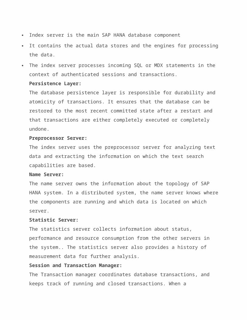
Index server is the main SAP HANA database component

It contains the actual data stores and the engines for processingthe data.

The index server processes incoming SQL or MDX statements in the context of authenticated sessions and transactions.Persistence Layer: The database persistence layer is responsible for durability and atomicity of transactions. It ensures that the database can be restored to the most recent committed state after a restart and that transactions are either completely executed or completely undone. Preprocessor Server: The index server uses the preprocessor server for analyzing text data and extracting the information on which the text search capabilities are based. Name Server: The name server owns the information about the topology of SAP HANA system. In a distributed system, the name server knows wherethe components are running and which data is located on which server. Statistic Server: The statistics server collects information about status, performance and resource consumption from the other servers in the system.. The statistics server also provides a history of measurement data for further analysis. Session and Transaction Manager: The Transaction manager coordinates database transactions, and keeps track of running and closed transactions. When a

transaction is committed or rolled back, the transaction manager informs the involved storage engines about this event so they canexecute necessary actions. XS Engine: XS Engine is an optional component. Using XS Engine clients can connect to SAP HANA database to fetch data via HTTP.

The heart of SAP HANA – Index Server

The SAP HANA Index Server contains the majority of the magic behind SAP HANA.

Connection and Session Management

This component is responsible for creating and managing sessions and connections for the database clients.

Once a session is established, clients can communicate with the SAP HANA database using SQL statements.

For each session a set of parameters are maintained like, auto-commit, current transaction isolation level etc.

Users are Authenticated either by the SAP HANA database itself (login with user and password) or authentication can be delegatedto an external authentication providers such as an LDAP directory.The Authorization Manager This component is invoked by other SAP HANA database components to check whether the user has the required privileges to execute the requested operations.

SAP HANA allows granting of privileges to users or roles. A privilege grants the right to perform a specified operation (suchas create, update, select, execute, and so on) on a specified object (for example a table, view, SQLScript function, and so on).

The SAP HANA database supports Analytic Privileges that representfilters or hierarchy drilldown limitations for analytic queries. Analytic privileges grant access to values with a certain combination of dimension attributes. This is used to restrict access to a cube with some values of the dimensional attributes.

Request Processing and Execution Control: The client requests are analyzed and executed by the set of components summarized as Request Processing and Execution Control. The Request Parser analyses the client request and dispatches it to the responsible component. The Execution Layer acts as the controller that invokes the different engines and routes intermediate results to the next execution step.

SQL Processor:Incoming SQL requests are received by the SQL Processor. Data manipulation statements are executed by the SQL Processor itself.

Other types of requests are delegated to other components. Data definition statements are dispatched to the Metadata Manager, transaction control statements are forwarded to the Transaction Manager, planning commands are routed to the Planning Engine and procedure calls are forwarded to the stored procedure processor.

SQLScript:

The SAP HANA database has its own scripting language named SQLScript that is designed to enable optimizations and parallelization. SQLScript is a collection of extensions to SQL.

SQLScript is based on side effect free functions that operate on tables using SQL queries for set processing. The motivation for SQLScript is to offload data-intensive application logic into thedatabase.Multidimensional Expressions (MDX):

MDX is a language for querying and manipulating the multidimensional data stored in OLAP cubes.

Incoming MDX requests are processed by the MDX engine and also forwarded to the Calc Engine.Planning Engine:

Planning Engine allows financial planning applications to executebasic planning operations in the database layer. One such basic operation is to create a new version of a data set as a copy of an existing one while applying filters and transformations. For example: planning data for a new year is created as a copy of thedata from the previous year.

Another example for a planning operation is the disaggregation operation that distributes target values from higher to lower aggregation levels based on a distribution function.Calc engine:

The SAP HANA database features such as SQLScript and Planning operations are implemented using a common infrastructure called the Calc engine.

The SQLScript, MDX, Planning Model and Domain-Specific models areconverted into Calculation Models. The Calc Engine creates Logical Execution Plan for Calculation Models. The Calculation Engine will break up a model, for example some SQL Script, into operations that can be processed in parallel.

Transaction Manager:

In HANA database, each SQL statement is processed in the context of a transaction. New sessions are implicitly assigned to a new transaction. The Transaction Manager coordinates database transactions, controls transactional isolation and keeps track ofrunning and closed transactions. When a transaction is committed or rolled back, the transaction manager informs the involved engines about this event so they can execute necessary actions. The transaction manager also cooperates with the persistence layer to achieve atomic and durable transactions. Metadata Manager:

Metadata can be accessed via the Metadata Manager component. In the SAP HANA database, metadata comprises a variety of objects, such as definitions of relational tables, columns, views, indexesand procedures.

Metadata of all these types is stored in one common database catalog for all stores. The database catalog is stored in tables in the Row Store. The features of the SAP HANA database such as transaction support and multi-version concurrency control, are also used for metadata management.

In the center of the figure you see the different data Stores of the SAP HANA database. A store is a sub-system of the SAP HANA database which includes in-memory storage, as well as the components that manages that storage.

The Row Store: The Row Store is the SAP HANA database row-based in-memory

relational data engine. The Column Store: The Column Store stores tables column-wise. It originates from the TREX (SAP NetWeaver Search and Classification) product. Want to know more about Row Data and Column Data Storage? Check Column Data Storage vs Row Data Storage: How Different are they Really?

Persistence Layer: The Persistence Layer is responsible for durability and atomicityof transactions. This layer ensures that the database is restoredto the most recent committed state after a restart and that transactions are either completely executed or completely undone.To achieve this goal in an efficient way, the Persistence Layer uses a combination of write-ahead logs, shadow paging and savepoints.

The Persistence Layer offers interfaces for writing and reading persisted data. It also contains the Logger component that manages the transaction log. Transaction log entries are written explicitly by using a log interface or implicitly when using the virtual file abstraction.

Column Data Storage Vs Row Data Storage in HANAOverview of Row Data Storage and Column Data Storage

Relational databases typically use row-based data storage. However Column-based storage is more suitable for many business applications. SAP HANA supports both row-based and column-based

storage, and is particularly optimized for column-based storage.

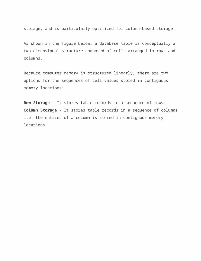
As shown in the figure below, a database table is conceptually a two-dimensional structure composed of cells arranged in rows and columns.

Because computer memory is structured linearly, there are two options for the sequences of cell values stored in contiguous memory locations:

Row Storage - It stores table records in a sequence of rows. Column Storage - It stores table records in a sequence of columnsi.e. the entries of a column is stored in contiguous memory locations.

Traditional databases store data simply in rows. The HANA in-memory database stores data in both rows and columns. It is this combination of both storage approaches that produces the speed, flexibility and performance of the HANA database.

Advantages of column-based tables:

Faster Data Access:Only affected columns have to be read during the selection process of a query. Any of the columns can serve as an index.

Better Compression:Columnar data storage allows highly efficient compression becausethe majority of the columns contain only few distinct values (compared to number of rows).

Better parallel Processing:In a column store, data is already vertically partitioned. This means that operations on different columns can easily be processed in parallel. If multiple columns need to be searched oraggregated, each of these operations can be assigned to a different processor core

Advantages and disadvantages of row-based tables:

Row based tables have advantages in the following circumstances:

The application needs to only process a single record at one time(many selects and/or updates of single records).

The application typically needs to access a complete record (or row).

Neither aggregations nor fast searching are required.

The table has a small number of rows (e. g. configuration tables,system tables).

Row based tables have dis-advantages in the following circumstances:

In case of analytic applications where aggregation are used and fast search and processing is required. In row based tables all data in a row has to be read even though the requirement may be to access data from a few columns.

Which type of tables should be preferred - Row-based or Column-based?

In case of analytic applications where aggregations are used and fast search and processing is required row-based storage are not good. In row based tables all data in a row has to be read even though the requirement may be to access data from a few columns. Hence these queries on huge amounts of data take a lot of time.

In columnar tables, this information is stored physically next toeach other, significantly increasing the speed of certain data queries.

The following example shows the different usage of column and rowstorage, and positions them relative to row and column queries. Column storage is most useful for OLAP queries (queries using anySQL aggregate functions) because these queries get just a few attributes from every data entry. But for traditional OLTP queries (queries not using any SQL aggregate functions), it is more advantageous to store all attributes side-by-side in row tables. HANA combines the benefits of both row- and column-storage tables.

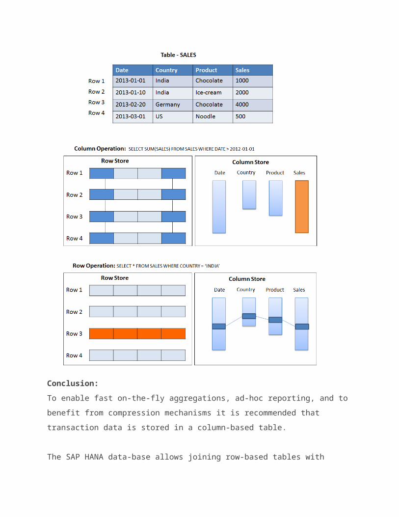
Conclusion: To enable fast on-the-fly aggregations, ad-hoc reporting, and to benefit from compression mechanisms it is recommended that transaction data is stored in a column-based table.

The SAP HANA data-base allows joining row-based tables with

column-based tables. However, it is more efficient to join tablesthat are located in the same row or column store. For example, master data that is frequently joined with transaction data should also be stored in column-based tables.

SAP HANA Memory Usage Explained

Introduction:

SAP HANA is a leading in-memory database and data management platform,

specifically developed to take full advantage of the capabilities

provided by modern hardware to increase application performance. By

keeping all relevant data in main memory (RAM), data processing

operations are significantly accelerated.

"SAP HANA has become the fastest growing product in SAP's history."

A fundamental SAP HANA resource is memory. Understanding how the SAP

HANA system requests, uses and manages this resource is crucial to the

understanding of SAP HANA. SAP HANA provides a variety of memory usage

indicators, to allow monitoring, tracking and alerting.

This article explores the key concepts of SAP HANA memory utilization,

and shows how to understand the various memory indicators.

Memory Concepts:

As an in-memory database, it is critical for SAP HANA to handle and

track its memory consumption carefully and efficiently. For this

purpose, the SAP HANA database pre-allocates and manages its own

memory pool and provides a variety of memory usage indicators to allow

monitoring.

SAP HANA tracks memory from the perspective of the host. The most

important concepts are as follows:

Physical memory:

The amount of (system) physical memory available on the host.

SAP HANA Allocated memory

The memory pool reserved by SAP HANA from the operating system.

SAP HANA Used memory

The amount of memory from this pool that is actually used by the SAP

HANA database.

Determining Physical Memory Size:

Physical memory (DRAM) is the basis for all memory discussions. On

most SAP HANA hosts, it ranges from 256 gigabytes to 2 terabytes. It

is used to run the Linux operating system, SAP HANA, and all other

programs that run on the host. The following table lists the various

ways of determining the amount of physical memory:

You can use the M_HOST_RESOURCE_UTILIZATION view to explore the amount

of Physical Memory as follows:

Determine Available Physical Memory:

Execute the SQL query:

select round((USED_PHYSICAL_MEMORY + FREE_PHYSICAL_MEMORY) /1024/1024/1024, 2)

as "Physical Memory GB"

from PUBLIC.M_HOST_RESOURCE_UTILIZATION;

Execute the Linux command:

cat /proc/meminfo | grep MemTotal

Determine Free Physical Memory:

Execute the SQL query:

select round(FREE_PHYSICAL_MEMORY/1024/1024/1024, 2)

as "Free Physical GB"

from PUBLIC.M_HOST_RESOURCE_UTILIZATION;

Execute the Linux command:

awk 'BEGIN {sum = 0};

/^(MemFree|Buffers|Cached):/ {sum = sum + $2}; END {print sum}' /proc/meminfo

SAP HANA Allocated Memory Pool:

The SAP HANA database (across its different processes) reserves a pool

of memory before actual use.

This pool of allocated memory is pre-allocated from the operating

system over time, up to a predefined global allocation limit, and is

then efficiently used as needed by the SAP HANA database code. More

memory is allocated to the pool as used memory grows. If used memory

nears the global allocation limit, the SAP HANA database may run out

of memory if it cannot free memory. The default allocation limit is

90% of available physical memory, but this value is configurable.

To find the global allocation limit of the database, run below SQL

query:

select HOST, round(ALLOCATION_LIMIT/1024/1024/1024, 2) as "Allocation Limit GB"

from PUBLIC.M_HOST_RESOURCE_UTILIZATION

Effective Allocation Limit:

In addition to the global allocation limit, each process running on

the host has an allocation limit, the process allocation limit. Given

that all processes cannot collectively consume more memory than the

global allocation limit, each process also has what is called an

effective allocation limit. The effective allocation limit of a

process specifies how much physical memory a process can in reality

consume given the current memory consumption of other processes.

Example:

A single-host system has 100 GB physical memory. Both the global

allocation limit and the individual process allocation limits are 90%

(default values). This means the following:

Collectively, all processes of the HANA database can use a maximum of

90 GB.

Individually, each process can use a maximum of 90 GB.

If 2 processes are running and the current memory pool of process 1 is

50 GB, then the effective allocation limit of process 2 is 40 GB. This

is because process 1 is already using 50 GB and together they cannot

exceed the global allocation limit of 90 GB.

SAP HANA Used Memory:

Used memory serves several purposes:

Program code and stack

Working space and data tables (heap and shared memory)

The program code area contains the SAP HANA database itself while it

is running. Different parts of SAP HANA can share the same program

code.

The stack is needed to do actual computations.

The heap and shared memory are the most important part of used memory.

It is used for working space, temporary data and for storing all data

tables.

You can use the M_SERVICE_MEMORY view to explore the amount of SAP

HANA Used Memory as follows:

Total Memory Used:

SELECT round(sum(TOTAL_MEMORY_USED_SIZE/1024/1024)) AS "Total Used MB"

FROM SYS.M_SERVICE_MEMORY;

Code and Stack Size:

SELECT round(sum(CODE_SIZE+STACK_SIZE)/1024/1024) AS "Code+stack MB"

FROM SYS.M_SERVICE_MEMORY;

Total Memory Consumption of All Columnar Tables:

SELECT round(sum(MEMORY_SIZE_IN_TOTAL)/1024/1024) AS "Column Tables MB"

FROM M_CS_TABLES;

Total Memory Consumption of All Row Tables

SELECT round(sum(USED_FIXED_PART_SIZE +

USED_VARIABLE_PART_SIZE)/1024/1024) AS "Row Tables MB"

FROM M_RS_TABLES;

Total Memory Consumption of All Columnar Tables by Schema:

SELECT SCHEMA_NAME AS "Schema",

round(sum(MEMORY_SIZE_IN_TOTAL) /1024/1024) AS "MB"

FROM M_CS_TABLES GROUP BY SCHEMA_NAME ORDER BY "MB" DESC;

Memory Consumption of Columnar Tables:

The SAP HANA database loads columnar tables into memory column by

column only upon use. This is sometimes called "lazy loading". This

means that columns that are never used are not loaded, which avoids

memory waste.

When the SAP HANA database runs out of allocated memory, it may also

unload rarely used columns to free up some memory. Therefore, if it is

important to precisely measure the total, or "worst case", amount of

memory used for a particular table, it is best to ensure that the

table is fully loaded first by executing the following SQL statement:

LOAD table_name ALL.

To examine the memory consumption of columnar tables, you can use the

M_CS_TABLES and M_CS_COLUMNS views.

The following examples show how you can use these views to examine the

amount of memory consumed by a specific table. You can also see which

of its columns are loaded and the compression ratio that was

accomplished.

List All Columnar Tables of Schema 'SYSTEM':

SELECT TABLE_NAME AS "Table", round(MEMORY_SIZE_IN_TOTAL/1024/1024, 2) as "MB"

FROM M_CS_TABLES WHERE SCHEMA_NAME = 'SYSTEM' ORDER BY "MB" DESC;

Show Column Details of Table "TABLE1":

SELECT COLUMN_NAME AS "Column", LOADED AS "Is Loaded",

round(UNCOMPRESSED_SIZE/1024/1024) AS "Uncompressed MB",

round(MEMORY_SIZE_IN_MAIN/1024/1024) AS "Main MB",

round(MEMORY_SIZE_IN_DELTA/1024/1024) AS "Delta MB",

round(MEMORY_SIZE_IN_TOTAL/1024/1024) AS "Total Used MB",

round(COMPRESSION_RATIO_IN_PERCENTAGE/100, 2) AS "Compr. Ratio"

FROM M_CS_Columns WHERE TABLE_NAME = 'TABLE1;

Note: The M_CS_TABLES and M_CS_COLUMNS views contain a lot of

additional information (such as cardinality, main-storage versus delta

storage and more). For example, use the following query to obtain more

information:

SELECT * FROM M_CS_COLUMNS WHERE TABLE_NAME = '"' and COLUMN_NAME = '"'

Memory Consumption of Row-Ordered Tables:

Several system tables are in fact row-ordered tables. You can use the

M_RS_TABLES view to examine the memory consumption of row-ordered

tables.

For instance, you can execute the following SQL query, which lists all

row tables of schema "SYS" by descending size:

SELECT SCHEMA_NAME, TABLE_NAME, round((USED_FIXED_PART_SIZE +

USED_VARIABLE_PART_SIZE)/1024/1024, 2) AS "MB Used"

FROM M_RS_TABLES

WHERE schema_name = 'SYS' ORDER BY "MB Used" DESC, TABLE_NAME

Memory Consumption Configuration:

By default, SAP HANA can pre-allocate up to 90% of the available

physical memory on the host. There is normally no reason to change the

value of this variable, except in the case where a license was

purchased for less than the total of the physical memory. In this

case, you should change the global allocation limit to remain in

compliance with the license.

Example 1:

You have a server with 512GB, but purchased an SAP HANA license for

only 384 GB. Set the global_allocation_limit to 393216 (384 * 1024

MB).

Example 2:

You have a distributed HANA system on four hosts with 512GB each, but

purchased an SAP HANA license for only 768 GB. Set the

global_allocation_limit to 196608 (192 * 1024 MB on each host).

Resident memory:

Resident memory is the physical memory actually in operational use by

a process.

Over time, the operating system may "swap out" some of a process'

resident memory, according to a least-recently-used algorithm, to make

room for other code or data. Thus, a process' resident memory size may

fluctuate independently of its virtual memory size. In a properly

sized SAP HANA appliance there is enough physical memory, and thus

swapping is disabled and should not be observed.

To display the size of the Physical Memory and Resident part, you can

use the following SQL command:

select HOST, round((USED_PHYSICAL_MEMORY + FREE_PHYSICAL_MEMORY)/1024/1024/1024, 2) as

"Physical Memory GB",

round(USED_PHYSICAL_MEMORY/1024/1024/1024, 2) as "Resident GB"

from PUBLIC.M_HOST_RESOURCE_UTILIZATION

Memory Sizing:

Memory sizing is the process of estimating, in advance, the amount of

memory that will be required to run a certain workload on SAP HANA. To

understand memory sizing, you will need to answer the following

questions:

1. What is the size of the data tables that will be stored in SAP

HANA?

You may be able to estimate this based on the size of your existing

data, but unless you precisely know the compression ratio of the

existing data and the anticipated growth factor, this estimate may

only be partially meaningful.

2. What is the expected compression ratio that SAP HANA will apply to

these tables?

The SAP HANA Column Store automatically uses a combination of various

advanced compression algorithms (dictionary, LRE, sparse, and more) to

best compress each table column separately. The achieved compression

ratio depends on many factors, such as the nature of the data, its

organization and data-types, the presence of repeated values, the

number of indexes (SAP HANA requires fewer indexes), and more.

3. How much extra working memory will be required for DB operations

and temporary computations?

The amount of extra memory will somewhat depend on the size of the

tables (larger tables will create larger intermediate result-tables in

operations like joins), but even more on the expected work load in

terms of the number of users and the concurrency and complexity of the

analytical queries (each query needs its own workspace).

SAP Notes 1514966, 1637145 and 1736976 provide additional tools and

information to help you size the required amount of memory, but the

most accurate method is ultimately to import several representative

tables into a SAP HANA system, measure the memory requirements, and

extrapolate from the results.

SAP HANA Studio:

You can view some of the most important memory indicators on the

Overview tab of the SAP HANA studio administrative perspective:

https://service.sap.com/sap/support/notes/1736976#_blank



For even more details, check out the new Memory Overview feature of

the SAP HANA studio. To access it, right click on a system in the

Systems View, and select "Open Memory Overview" in the context menu,

as follows:

This will open the Memory Overview, which looks as follows:

Note: To view the Memory Overview, you need Monitoring privileges.

E.g. use the following SQL statement (replace 'youruser' with the

actual user name): call

GRANT_ACTIVATED_ROLE('sap.hana.admin.roles::Monitoring','youruser')

Summary:

SAP HANA maintains many system views and memory indicators, to provide

a precise way to monitor and understand the SAP HANA memory

utilization. The most important of these indicators is Used Memory and

the corresponding historic snapshots. In turn, it is possible to drill

down into very detailed reports of memory utilization using additional

system views, or by using the convenient Memory Overview from the SAP

HANA studio.

Since SAP HANA contains its own memory manager and memory pool,

external indicators, like the host-level Resident Memory size, or the

process-level virtual and resident memory sizes, can be misleading

when estimating the real memory requirements of a SAP HANA

deployment.

System Generated Schemas in SAP HANA

A database schema is a way to logically group objects such as tables, views, stored procedures etc. Think of a schema as a container of objects.

Types of Schemas

There are 3 types of schemas.

1. User Defined Schema

2. System Defined Schema

3. SLT Derived SchemaUser Defined Schema:These are created by user (DBA or System Administrator)

SLT Derived Schema:When SLT is configured, it creates schema in HANA system. All thetables replicated into HANA system are contained in this schema

System Defined Schema:These schemas are delivered with the SAP HANA database and contains HANA system information. There are system schemas like _SYS_BIC, _SYS_BI, _SYS_REPO, _SYS_STATISTICS etc.

System Generated Schemas

_SYS_BIC:This schema contains all the columns views of activated objects. When the user activates the Attribute View/Analytic View/Calculation View/Analytic Privilege /Procedure, the respective run-time objects are created under _SYS_BIC/ Column Views.

_SYS_REPO:Whatever the objects are there in the system is available in repository. This schema contains the list of Activated objects, Inactive Objects, Package details and Runtime Objects informationetc. Also _SYS_REPO user must have SELECT privilege with grant option on the data schama. Read more about "GRANT SELECT PRIVILEGE ON _SYS_REPO"

_SYS_BI:This schema stores all the metadata of created column Views. It contains the tables for created Variables, Time Data (Fiscal, Gregorian), Schema Mapping and Content Mapping tables.

_SYS_STATISTICS:This schema contains all the system configurations and parameters.

_SYS_XS:This schema is used for SAP HANA Extended Application Services.

SAP HANA Backup and Recovery

SAP HANA is an in-memory database. This means all the data is in RAM. As we all know that RAM is a volatile memory and all the data get lost when power goes down. This leads to a very obvious question: What happens when power goes down in SAP HANA? Do we loose all the valuable data?

The answer is NO.SAP HANA is an in-memory database which means all the data resides in RAM. But there is also a disc memory just for backup purpose.

In-memory computing is safe: The SAP HANA database holds the bulk

of its data in memory for maximum performance, but still uses persistent storage (disk memory) to provide a fallback in case offailure.

Why Backup is Required?In database technology, atomicity, consistency, isolation, and durability (ACID) is a set of requirements that guarantees that database transactions are processed reliably: A transaction has to be atomic. That is, if part of a transactionfails, the entire transaction has to fail and leave the database state unchanged. The consistency of a database must be preserved by the transactions that it performs. Isolation ensures that no transaction is able to interfere with another transaction. Durability means that after a transaction has been committed it will remain committed.

While the first three requirements are not affected by the in-memory concept, durability is a requirement that cannot be met bystoring data in main memory alone. Main memory is volatile storage. That is, it looses its content when it is out of electrical power. To make data persistent, it has to reside on non-volatile storage, such as hard drives, SSD, or Flash devices.

How Backup and Recovery Works in SAP HANA?

The main memory (RAM) in SAP HANA is divided into pages. When a transaction changes data, the corresponding pages are marked and written to disk storage in regular intervals. In addition, a database log captures all changes made by transactions. Each committed transaction generates a log entry that is written to disk storage. This ensures that all transactions are permanent.

Figure below illustrates this. SAP HANA stores changed pages in savepoints, which are asynchronously written to disk storage in regular intervals (by default every 5 minutes).

The log is written synchronously. That is, a transaction does notreturn before the corresponding log entry has been written to persistent storage, in order to meet the durability requirement, as described above.

After a power failure, the database can be restarted like a disk-based database. The database pages are restored from the savepoints, and then thedatabase logs are applied (rolled forward) to restore the changesthat were not captured in the savepoints.This ensures that the database can be restored in memory to exactly the same state as before the power failure.

Data backup can be taken manually or can be scheduled.

Few Important Concepts:What is Database Backup and RecoveryBackup and Recovery is the process of copying/storing data for the specific purpose of restoring. Backing up files can protect against accidental loss of user data, database corruption, hardware failures, and even natural disasters.

Savepoint:A savepoint is the point at which data is written to disk as backup. This is a point from which the Database Engine can start applying changes contained in the backup disk during recovery after an unexpected shutdown or crash. The database administrator determines the frequency of savepoints.

Data and Log:Data backups

Contain the current payload of the data volumes (data and undo information)

Manual (SAP HANA studio, SQL commands), or scheduled (DBA Cockpit)

Log backups

Contain the content of closed log segments; the backup catalog isalso written as a log backup

Automatic (asynchronous) whenever a log segment is full or the timeout for log backup has elapsed

SAP Notes:Check below SAP notes to find out more about SAP HANA backup and recovery.

Scheduling the SAP HANA Backups: 1651055 SAP HANA database backup and recovery: 1642148

SAP HANA Modeling IntroductionSAP HANA Modeling at a glance:

SAP HANA Information Modeling which also known as SAP HANA Data Modeling is the heart of HANA application development. You can create modeling views on top of database tables and implement business logic to create a meaningful report.

These modeling views can be consumed via Java or HTML based applications or SAP HANA native applications. You can also use SAP tools like SAP Lumira or Analysis Office to directly connect to HANA and report modeling views. It is also possible to use 3rdparty tools like MS-Excel to connect to HANA and create your

report.

Modeling SAP HANA Information Views are important for successfully exploiting the power of SAP HANA. These views are classified as

Attribute Views Analytic Views Calculation Views

At run-time these views make implicit use of optimized SAP HANA In-Memory calculation engines and thus enable for best performance.

HANA Data Modeling is only possible for Column Tables i.e. Information Modeler only works with column storage tables.

Attribute View:

Attribute views are dimensions, BW characteristics or master data.

Attribute views are used to join to a dimension or attribute view.

In most cases used to model master data like entities (like Product, Employee, Business Partner)

Highly re-used and shared in Analytic- and Calculation Views

Example : An attribute view "FLIGHT" can show together Airline Code, Airline Connection Number and flight Date into one Object. This attribute view can be used in analytic and calculation viewswhere entities are relevant.

Generally attribute views represent master data. But, however

technically there is no restriction and it's possible to make attribute views on transaction data.

Analytic View:

Analytic views are star schemas or fact tables surrounded by dimensions, calculations or restricted measures.

In the language on SAP BW analytical views can be roughly compared with Info Cubes or Info Sets.

Analytic views are typically defined on at least one fact table that contains transactional data along with number of tables or attribute views.

Analytic views leverage the computing power of SAP HANA to calculate aggregate data, e. g., the number of bikes sold per country, or the maximum power consumed per month.

It is specifically designed to execute star schema queries

Calculation View:

Calculation views are composite views used on top of analytical and attribute views.

It can perform complex calculations not possible with other views.

It can be defined as either graphical views or scripted views depending on how they are created. Graphical views can be modeled

using the graphical modeling features of the SAP HANA Modeler. Scripted views are created as sequences of SQL statements.

Calculation views can be referred as combination of tables, attributes views and analytical views to deliver a complex business requirement. They offer to combine different analytical views into one source of data for reporting.

Want to do some hands-on? Please read Build Your First SAP HANA Model in 10 Minutes

SAP HANA Modeling View Processing:

SAP HANA has mainly 3 types of engines that are used based on theviews required by the model.

Join Engine: Used for Attribute Views

OLAP Engine: Used for Analytic Views (without calculated

columns)

Calculation Engine: Used for Analytic views with calculated attributes, Calculation views

To know more about SAP HANA Engine, please read Understanding SAPHANA Engine

Build Your First SAP HANA Model in 10 MinutesThis article describes how to build a simple model using data stored on SAP HANA. By the end of this, you will have created tables, attribute views, and analytical views in SAP HANA.

Prerequisite: You have SAP HANA Studio installed on your machine. You have added an SAP HANA system in HANA Studio

Create new tables in SAP HANA and fill them with data:

1. Open HANA Studio and expand the SAP HANA system.2. Go to your schema. Right-click on your schema and select SQL

editor.

Note: In this example schema name is "SAP_HANA_TUTORIAL". In caseyou want to create a new schema use below query.create schema <schema_name>;

3. Copy and paste the below script in SQL editor and execute.

--REPLACE <YOUR SCHEMA> WITH YOUR SCHEMA NAME

-- Create Product table

create column table "<YOUR SCHEMA>"."PRODUCT"(

"PRODUCT_ID" INTEGER null,

"PRODUCT_NAME" VARCHAR (100) null default ''

);

insert into "<YOUR SCHEMA>"."PRODUCT" values(1,'Shirts');

insert into "<YOUR SCHEMA>"."PRODUCT" values(2,'Jackets');

insert into "<YOUR SCHEMA>"."PRODUCT" values(3,'Trousers');

insert into "<YOUR SCHEMA>"."PRODUCT" values(4,'Coats');

insert into "<YOUR SCHEMA>"."PRODUCT" values(5,'Purse');

-- Create Region table

create column table "<YOUR SCHEMA>"."REGION"(

"REGION_ID" INTEGER null,

"REGION_NAME" VARCHAR (100) null default '',

"SUB_REGION_NAME" VARCHAR (100) null default ''

);

insert into "<YOUR SCHEMA>"."REGION" values(1,'Americas','North-America');

insert into "<YOUR SCHEMA>"."REGION" values(2,'Americas','South-America');

insert into "<YOUR SCHEMA>"."REGION" values(3,'Asia','India');

insert into "<YOUR SCHEMA>"."REGION" values(4,'Asia','Japan');

insert into "<YOUR SCHEMA>"."REGION" values(5,'Europe','Germany');

-- Create Sales table

create column table "<YOUR SCHEMA>"."SALES"(

"REGION_ID" INTEGER null,

"PRODUCT_ID" INTEGER null,

"SALES_AMOUNT" DOUBLE null);

insert into "<YOUR SCHEMA>"."SALES" values(1,1,100);









4. After executing the scripts you should have 3 tables created. If there are no tables, try right-clicking on your schema and refreshing.

Grant schema SELECT rights to _SYS_REPO user:

Open the SQL editor of your schema and execute the following command line:GRANT SELECT ON SCHEMA <YOUR SCHEMA> TO _SYS_REPO WITH GRANT OPTION;

If you miss this step, an error will occur when you activate yourviews later. Click here to know more about this.

Create an attribute view:

1. Open HANA Studio and make sure you are in Modeler perspective

2. Create a new package under the content folder. Right-click on the content folder and choose "New" -> "Package." Fill the fields "Name" and "Description" and click "OK."If you dont see the new package after this, try right-clicking onthe content folder and refreshing.

3. Right click on the package and choose "New Attribute View." Entera name and a description and click "Finish"

4. The attribute view will be opened in the HANA studio editor. Select "+" sign on "Data Foundation"

5. Search for table "REGION" and select it.

6. Now add the columns from the REGION table to output. Simply rightclick on the column and select "Add to Output". Add all 3 columns

REGION_ID, REGION_NAME, SUB_REGION_NAME to the output. Once it is done, you will see the selected column in right side pane.

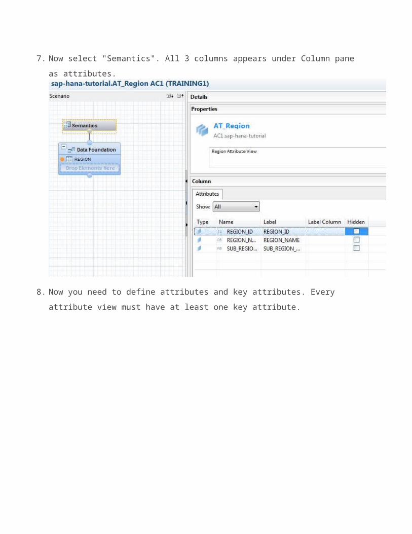
7. Now select "Semantics". All 3 columns appears under Column pane as attributes.

8. Now you need to define attributes and key attributes. Every attribute view must have at least one key attribute.

9. Click on the "Type" to select key attribute for REGION_ID.

10. Click on the "Save and Activate" button on top right corner to activate the view.

11. In the "Job log" Pane you will see an activation completed message.

12. Attribute view is created and activated. To see the output of this view click on the "Data Preview" buttonon top right corner.

Then select "Raw Data" tab.

Congratulation!! You have successfully created your first modeling view.

Next step is to create an analytic view.

Create an Analytic View:

1. Right click on the package and choose "New Analytic View." Enter a name and a description and click "Finish"

2. Click on "+" sign of "Data Foundation" and add table SALES.

3. Right Click on the columns of table SALES and add REGION_ID and SALES_AMOUNT to output.

4. Click on "+" sign of "Logical Join" and add attribute view "AT_Region" which was created earlier.

5. Click on the REGION_ID from "Data Foundation" and connect it to the REGION_ID of attribute view AT_Region. In the properties paneselect join type as left outer join and cardinality as n..1

6. Select "Sementics". In the right side change the column type of SALES_AMOUNT as measure.

7. Activate the analytic view similar to attribute view.Right-click on your analytic view and choose "Data Preview." After that, you can browse through the tabs named raw data, distinct values, and analysis.

Congratulation!! You have successfully created your first Analytic View.

SAP HANA Calculation ViewCalculation views are composite views and can be used to combine other views. It canconsume other Analytical, Attribute, other Calculation Views & tables. It can perform complex calculations not possible with other views.

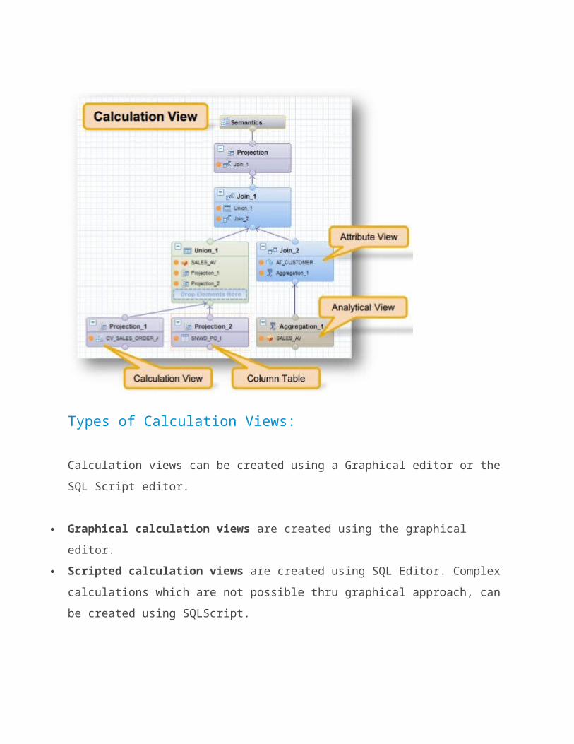
Types of Calculation Views:

Calculation views can be created using a Graphical editor or the SQL Script editor.

Graphical calculation views are created using the graphical editor.

Scripted calculation views are created using SQL Editor. Complex calculations which are not possible thru graphical approach, can be created using SQLScript.

Capabilities of Calculation Views:Graphical Calculation Views

Can consume other Analytical, Attribute, other Calculation Views & tables

Built-in Union, Join, Projection & Aggregation nodes

Provides additional features like Distinct, Count, Calculation, dynamic joins

No SQL or SQL Script knowledge requiredSQLScript-based Calculation Views

Can be regarded as a function, defined in the HANA-specific language “SQLScript”, which is built upon SQL commands or specialHANA pre-defined functions

Must be read-only

Create Graphical Calculation View in 10 minutesCalculation view can be defined as either graphical views or scripted views. In this article we will learn how we can create graphical calculation view.

Prerequisite: You have SAP HANA Studio installed on your machine. You have added an SAP HANA system in HANA Studio

Scenario: Suppose there are 3 tables PRODUCTS, REGION and SALES.

We need to find out

What are the sales value for "Asia" region?

What are the total sales value for "Shirts"?

What are the total sales value for "Europe" for "Jackets"?Let us create a graphical calculation view to get answer of the above mentioned questions.

Create new tables in SAP HANA and fill them with data:

1. Open HANA Studio and expand the SAP HANA system.2. Go to your schema. Right-click on your schema and select SQL

editor.

Note: In this example schema name is "SAP_HANA_TUTORIAL". In caseyou want to create a new schema use below query.create schema <schema_name>;

3. Copy and paste the below script in SQL editor and execute.

----REPLACE <YOUR SCHEMA> WITH YOUR SCHEMA NAME

---- Create Product table

create column table "<YOUR SCHEMA>"."PRODUCT"(

"PRODUCT_ID" INTEGER,

"PRODUCT_NAME" VARCHAR (100),

primary key ("PRODUCT_ID")

);

insert into "<YOUR SCHEMA>"."PRODUCT" values(1,'Shirts');

insert into "<YOUR SCHEMA>"."PRODUCT" values(2,'Jackets');

insert into "<YOUR SCHEMA>"."PRODUCT" values(3,'Trousers');

insert into "<YOUR SCHEMA>"."PRODUCT" values(4,'Coats');

insert into "<YOUR SCHEMA>"."PRODUCT" values(5,'Purse');

-- Create Region table

create column table "<YOUR SCHEMA>"."REGION"(

"REGION_ID" INTEGER,

"REGION_NAME" VARCHAR (100),

"SUB_REGION_NAME" VARCHAR (100),

PRIMARY KEY ("REGION_ID")

);

insert into "<YOUR SCHEMA>"."REGION" values(100,'Americas','North-America');

insert into "<YOUR SCHEMA>"."REGION" values(200,'Americas','South-America');

insert into "<YOUR SCHEMA>"."REGION" values(300,'Asia','India');

insert into "<YOUR SCHEMA>"."REGION" values(400,'Asia','Japan');

insert into "<YOUR SCHEMA>"."REGION" values(500,'Europe','Germany');

-- Create Sales table

create column table "<YOUR SCHEMA>"."SALES"(

"REGION_ID" INTEGER ,

"PRODUCT_ID" INTEGER ,

"SALES_AMOUNT" DOUBLE, PRIMARY KEY ("REGION_ID", "PRODUCT_ID") );










4. After executing the scripts you should have 3 tables created. If there are no tables, try right-clicking on your schema and

refreshing.

Grant schema SELECT rights to _SYS_REPO user:

Open the SQL editor of your schema and execute the following command line:GRANT SELECT ON SCHEMA <YOUR SCHEMA> TO _SYS_REPO WITH GRANT OPTION;

If you miss this step, an error will occur when you activate yourviews later. Click here to know more about this.

Steps for creating calculation view:

1. Open HANA Studio and make sure you are in Modeler perspective. Right click on the package and choose "Calculation View"

2. Enter a name and a description. Select Subtype as "Graphical" andData Category as "Cube". Then click on "Finish".

3. You will see the graphical editor as shown in image below.

4. Click on the "Join" symbol and drag it in the scenario area to create Join block. Click on "+" sign of "Join" and add REGION

tables.

5. Similarly add SALES table.

6. Select the REGION_ID from REGION table. Drag it and drop it on the REGION_ID of SALES table. Join type can be changed in the

Properties tab. Let it be Inner Join as of now.

7. Add REGION_NAME, SUB_REGION_NAME, PRODUCT_ID AND SALES_AMOUNT to the Columns by right clicking and clicking on "Add To Output". Alternatively you can also click on the grey color circle before the column name to add it to output.

8. Click on the "Join" symbol again and drag it in the scenario areato create another Join block. Connect the previous Join block to

new Join block with the arrow.

9. Click on "+" sign of new Join block and add PRODUCT table.

10. Select the PRODUCT_ID from Join_1. Drag it and drop it on the PRODUCT_ID of PRODUCT table. Select the Join type as Inner Join. Add REGION_NAME, SUB_REGION_NAME, PRODUCT_ID, SALES_AMOUNT and PRODUCT_NAME to the Columns by right clicking and clicking on "Add To Output".

11. Add the Join block "Join_2" to "Aggregation" block by arrow.Add all the columns to output.

12. Select Semantics. Now we need to specify which columns are attributes and which columns are measures. Click on the "Auto Assign" button to do it automatically. Alternatively you can also specify the Attribute/measure by clicking on Type down-arrow. Select SALES_AMOUNT as measure and

rest of the column as attribute.

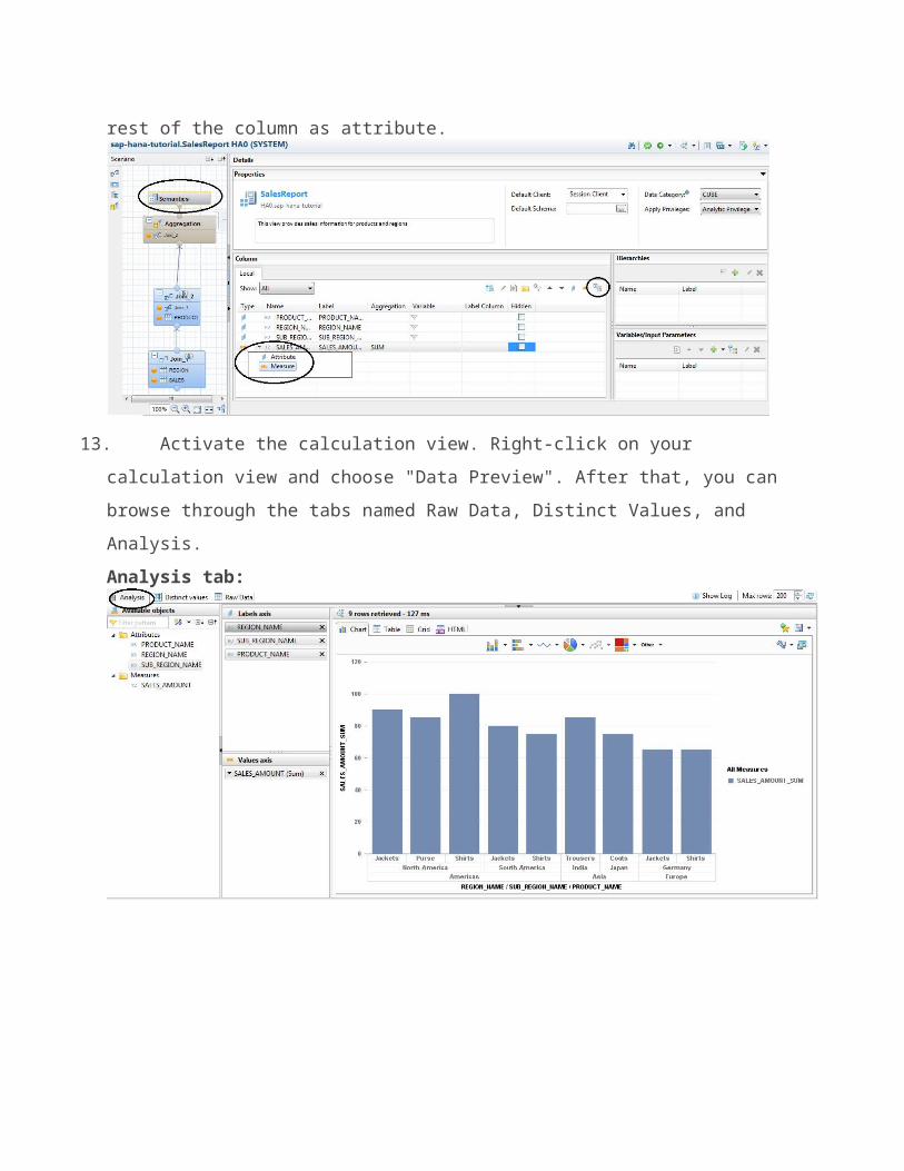
13. Activate the calculation view. Right-click on your

calculation view and choose "Data Preview". After that, you can browse through the tabs named Raw Data, Distinct Values, and Analysis. Analysis tab:

Raw Data tab:

Congratulation!! You have successfully created your first Graphical Calculation View.

Understanding SAP HANA EngineSAP HANA Engine:

SAP HANA has mainly 3 types of engines that are used based on theviews required by the model.

Join Engine:

Used when querying an Attribute View

The join engine is also used, when you run plain SQL.

OLAP Engine:

Used for Analytic view (without calculated columns).

Calculation Engine:

Used for Analytic views with calculated attributes and Calculation views

Note: To check what engine is used to process a query: simply runthe Plan Visualization on your query.

Q1: What If I execute a standard ANSI92 SQL statement from a BI tool or in SAP HANA Studio. What engines will be used? Ans: Depends on what objects you reference in your query. If you're just querying plain base tables then the join engine will be used. As soon as you reference an analytic or calculation view, the other engines will be employed as well.

Q2: If my Analytic View foundation is joined to attribute views, is both the OLAP and JOIN Engine used? Ans: Nope - during activation of the analytic views, the joins inthe attribute views get 'flattened' and included in the analytic view run time object. Only the OLAP engine will be used then.

SAP HANA Join Types - All You Ever Wanted to Know

A Join clause combines records from two or more tables /view in a

database.

SAP HANA supports following types of join.

Inner Join

Left Outer Join

Right Outer Join

Full Outer Join

Referential Join

Text Join

In this article you will learn the details of all these type of

joins.

We are going to use 2 tables to explain the different types of Join.

CUSTOMER and SALES_ORDER.

SQL Script to create the above mentioned tables:

-- REPLACE <Schema_Name> WITH YOUR SCHEMA

CREATE COLUMN TABLE <Schema_Name>."CUSTOMER" (

"CustomerID" nvarchar(10) primary key,

"CustomerName" nvarchar(50)

);

INSERT INTO <Schema_Name>."CUSTOMER" VALUES ('C1', 'Alfred');

INSERT INTO <Schema_Name>."CUSTOMER" VALUES ('C2', 'John');

INSERT INTO <Schema_Name>."CUSTOMER" VALUES ('C3', 'Maria');

INSERT INTO <Schema_Name>."CUSTOMER" VALUES ('C4', 'Harry');

CREATE COLUMN TABLE <Schema_Name>."SALES_ORDER" (

"OrderID" integer primary key,

"CustomerID" nvarchar(10),

"Product" nvarchar(20),

"Total_Units" integer

);

INSERT INTO <Schema_Name>."SALES_ORDER" VALUES (101, 'C1','Camera',300);

INSERT INTO <Schema_Name>."SALES_ORDER" VALUES (102, 'C1','Mobile',200);

INSERT INTO <Schema_Name>."SALES_ORDER" VALUES (103, 'C2','iPod',500);

INSERT INTO <Schema_Name>."SALES_ORDER" VALUES (104, 'C3','Television',400);

INSERT INTO <Schema_Name>."SALES_ORDER" VALUES (105, 'C5','Laptop',800);

Inner Join:

The INNER JOIN selects the set of records that match in both the

Tables.

Syntax

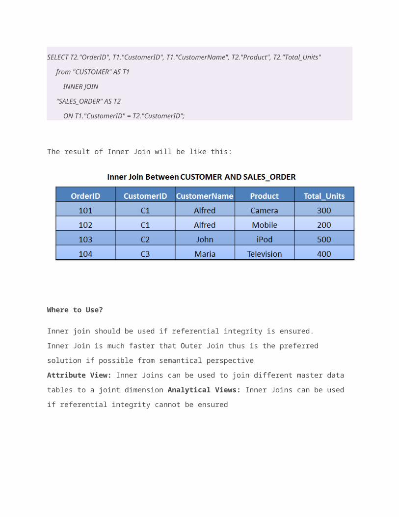
SELECT T2."OrderID", T1."CustomerID", T1."CustomerName", T2."Product", T2."Total_Units"

from "CUSTOMER" AS T1

INNER JOIN

"SALES_ORDER" AS T2

ON T1."CustomerID" = T2."CustomerID";

The result of Inner Join will be like this:

Where to Use?

Inner join should be used if referential integrity is ensured.

Inner Join is much faster that Outer Join thus is the preferred

solution if possible from semantical perspective

Attribute View: Inner Joins can be used to join different master data

tables to a joint dimension Analytical Views: Inner Joins can be used

if referential integrity cannot be ensured

Left Outer Join:

The Left Outer Join selects the complete set of records from first

table (CUSTOMER), with the matching records (where available) in

second table (SALES_ORDER). If there is no match, the right side will

contain null.

Syntax



LEFT OUTER JOIN

"SALES_ORDER" AS T2


The result of Left Outer Join will be like this:

Right Outer Join:

The Right Outer Join selects the complete set of records from second

table (SALES_ORDER), with the matching records (where available) in

first table (CUSTOMER). If there is no match, the left side will

contain null.

Syntax



RIGHT OUTER JOIN

"SALES_ORDER" AS T2


The result of Right Outer Join will be like this:

Full Outer Join:

The INNER JOIN selects the set of records that match in both the

Tables.

Syntax



FULL OUTER JOIN

"SALES_ORDER" AS T2


The result of Full Outer Join will be like this:

All the 4 types of joins explained above are standard database join

types.

SAP HANA also supports 2 new type of joins. Referential Join and Text

Join. These 2 type of joins can only be used in modeling views.

Let's take a look into these 2 new type of joins.

SAP HANA Referential Join:

Referential Join is semantically an inner join that assume that

referential integrity is given.

Note: Referential integrity is the property of database which ensures

that each foreign key value in a table exists as a primary key in the

referenced table.

Referential join is performance wise better than inner join, but only

be used when you are sure that referential integrity is maintained.

SAP HANA Text Join:

Text Join is used in order to get language-specific data.

You have a product table that contains product IDs without

descriptions and you have a text table for products that contains

language-specific descriptions for each product. You can create a text

join between the two tables to get the language-specific details. In a

text join, the right table should be the text table and it is

mandatory to specify the Language Column.

SAP HANA Text Join - Fetch Language Specific Data

Text Join is used in order to get language-specific data.

Before understanding the text join, it is important that we understand

Text Tables.

Text Tables:

Table A is a text table of table B if the key of A comprises the key

of B and an additional language key field (field of data type LANG).

Table A may therefore contain explanatory text in several languages

for each key entry of B.

Text Join in SAP HANA:

Text Join is used to fetch the description based on user's session

language. Once we implement the text join in SAP HANA, it

automatically find out user's language and give description in that

language.

Implementation of Text Join in SAP HANA:

Example:

Suppose there is a table called "PRODUCT" which contains Product ID

and Product Name.

There is also a text table of "PRODUCT", which is called

"PRODUCT_TEXT_TABLE". The text table contains the description of

products in different language. For example "Cotton Shirts" in English

and "Baumwoll-Shirts" in German.

Purpose:

Create a calculation view which will give Product Name and Product

Description. The Product Description should be only in user's session

language.

Implementation:

1. Open HANA Studio. Right click on your schema and open SQL Editor. Copy

the below SQL script to create 2 tables - "PRODUCT" and

"PRODUCT_TEXT_TABLE".

-- REPLACE WITH YOUR ACTUAL SCHEMA NAME

-- PRODUCT table

CREATE COLUMN TABLE ""."PRODUCT"(


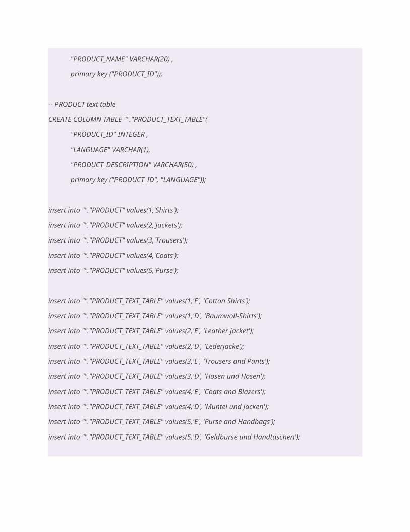
"PRODUCT_NAME" VARCHAR(20) ,

primary key ("PRODUCT_ID"));

-- PRODUCT text table

CREATE COLUMN TABLE ""."PRODUCT_TEXT_TABLE"(


"LANGUAGE" VARCHAR(1),

"PRODUCT_DESCRIPTION" VARCHAR(50) ,

primary key ("PRODUCT_ID", "LANGUAGE"));

insert into ""."PRODUCT" values(1,'Shirts');

insert into ""."PRODUCT" values(2,'Jackets');

insert into ""."PRODUCT" values(3,'Trousers');

insert into ""."PRODUCT" values(4,'Coats');

insert into ""."PRODUCT" values(5,'Purse');

insert into ""."PRODUCT_TEXT_TABLE" values(1,'E', 'Cotton Shirts');

insert into ""."PRODUCT_TEXT_TABLE" values(1,'D', 'Baumwoll-Shirts');

insert into ""."PRODUCT_TEXT_TABLE" values(2,'E', 'Leather jacket');

insert into ""."PRODUCT_TEXT_TABLE" values(2,'D', 'Lederjacke');

insert into ""."PRODUCT_TEXT_TABLE" values(3,'E', 'Trousers and Pants');

insert into ""."PRODUCT_TEXT_TABLE" values(3,'D', 'Hosen und Hosen');

insert into ""."PRODUCT_TEXT_TABLE" values(4,'E', 'Coats and Blazers');

insert into ""."PRODUCT_TEXT_TABLE" values(4,'D', 'Muntel und Jacken');

insert into ""."PRODUCT_TEXT_TABLE" values(5,'E', 'Purse and Handbags');

insert into ""."PRODUCT_TEXT_TABLE" values(5,'D', 'Geldburse und Handtaschen');

Note: The Language code for English is "E" and for German is "D"

2. Right click on your schema and refresh to see the 2 tables created.

3. Go to "Content" and right click on your package. Select Calculation

view.

4. Give Name and Description of the Calculation View. Select Data

Category as "Dimension".

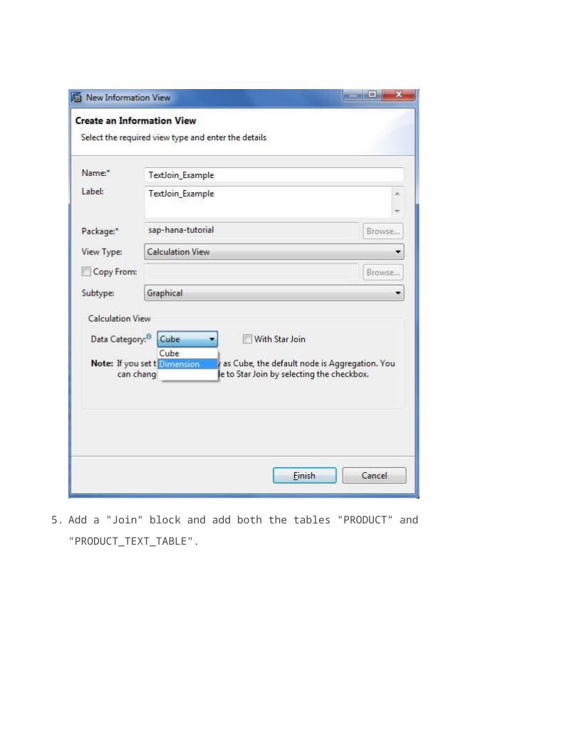
5. Add a "Join" block and add both the tables "PRODUCT" and

"PRODUCT_TEXT_TABLE".

6. Make a join on the column "PRODUCT_ID". Specify the Join Type as "Text

Join". Click on the Language option and select "Language" column. Add

"PRODUCT_ID", "PRODUCT_NAME" and "PRODUCT_DESCRIPTION" to output.

7. Connect the Join block to Projection Block. Add all the 3 column to

output.

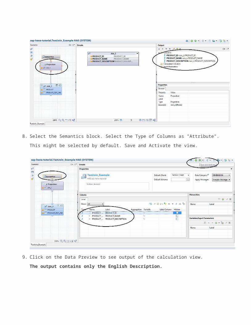
8. Select the Semantics block. Select the Type of Columns as "Attribute".

This might be selected by default. Save and Activate the view.

9. Click on the Data Preview to see output of the calculation view.

The output contains only the English Description.

Change User Session Language (Locale) and Check The Output Again:

1. Right click on the HANA system and select "Properties".

2. Click on the tab "Additional Properties" and select the Locale as

"German"

Click on "OK".

3. Check the output of the calculation view. Now the output contains

German Description.

SAP HANA Analytic PrivilegeIn this article we will explain what is Analytic privilege in HANA and how does it work.

What is Analytic Privileges?

Analytic privileges control access to SAP HANA data models. Analytic privileges are used to grant different users access to different portions of data in the same view depending on their business role. It allows us to maintain row-level access.

Why do we need Analytic Privilege?

SQL privileges implement authorization at object level only. Users either have access to an object, such as a table, view or procedure, or they do not.

While this is often sufficient, there are cases when access to data in an object depends on certain values or combinations of values. Analytic privileges are used in the SAP HANA database to provide such fine-grained control of which data individual users can see within the same view.

Example:

Suppose there is a calculation view which contains the sales dataof all the regions like Asia, Europe and America.

The regional managers must have access to the calculation view tosee the data. However, managers should only see the data for

their region. The manager of America region should not be able tosee data of other region.

In this case, an analytic privilege could be modeled so that theycan all query the view, but only the data that each user is authorized to see is returned.

Important Facts about Analytic Privileges:

Analytic privileges are intended to control read-only access to SAP HANA information models, that is

Attribute views

Analytic views

Calculation views Analytic privileges do not apply to database tables or views

modeled on row-store tables.

Create and Manage Analytic Privilege.

Here is the sequence of steps to achieve this

1. Create Analytic Privilege and assign restriction for region “Asia”.

2. Assign the Analytic Privilege to User to restrict the data on HANA Views.

SAP HANA System Privileges Required to Create/ManageAnalytic Privilege:

To create analytic privileges, the system privilege CREATE STRUCTURED PRIVILEGE is required. To drop analytic privileges, the system privilege STRUCTUREDPRIVILEGE ADMIN is required.

In the SAP HANA modeler, repository objects are technically created by the technical user _SYS_REPO, which by default has thesystem privileges for both creating and dropping analytic privileges. The database user requires the package privileges REPO.EDIT_NATIVE_OBJECTS and REPO.ACTIVATE_NATIVE_OBJECTS to activate and redeploy analytic privileges in the Modeler.

Steps to Create an Analytic Privilege:

Prerequisite:We need to create the modeling view first which will be used in the Analytic Privilege. Create a calculation view by following the article Create a calculation view in 10 minutes.The output of the calculation view is

Let us see how we can restrict the output only for "Asia" region.

1. Right click on the package and select “Analytic Privilege”

2. Specify Name and label for the Analytic Privilege

3. Select the calculation view and click on Add button. Then click on “Finish”.

4. Click on Add button as shown below and select the column REGION_NAME.

5. Now we need to assign the restriction. Click on the add button asshown below and select the value “Asia”.

6. Save and activate the analytic privilege.The analytic privilege is ready. Now we can assign this analytic privilege to any user.

Assign Analytic Privilege to a User:

Note: You must have authorization to create/assign privileges to a user.

1. Go to Security -> Users. Right click and create a new user. Specify user name and password.

2. Click on the “Analytic Privileges” tab and add the analytic privilege created in previous step.

3. You also need to assign following privileges required to get access to modeling views.

Execute & Select access on _SYS_BI

Execute & Select access on _SYS_BIC

Execute on REPOSITORY_RESTDone!! We have created an analytic privilege and assign that to auser. Now add the same HANA system using new user. Open the data preview of the same calculation view. It will show only the data for region “Asia”.

Variables and Input Parameters in HANAIn this article we learn what are Variables and Input Parameters in HANA and how do they work.

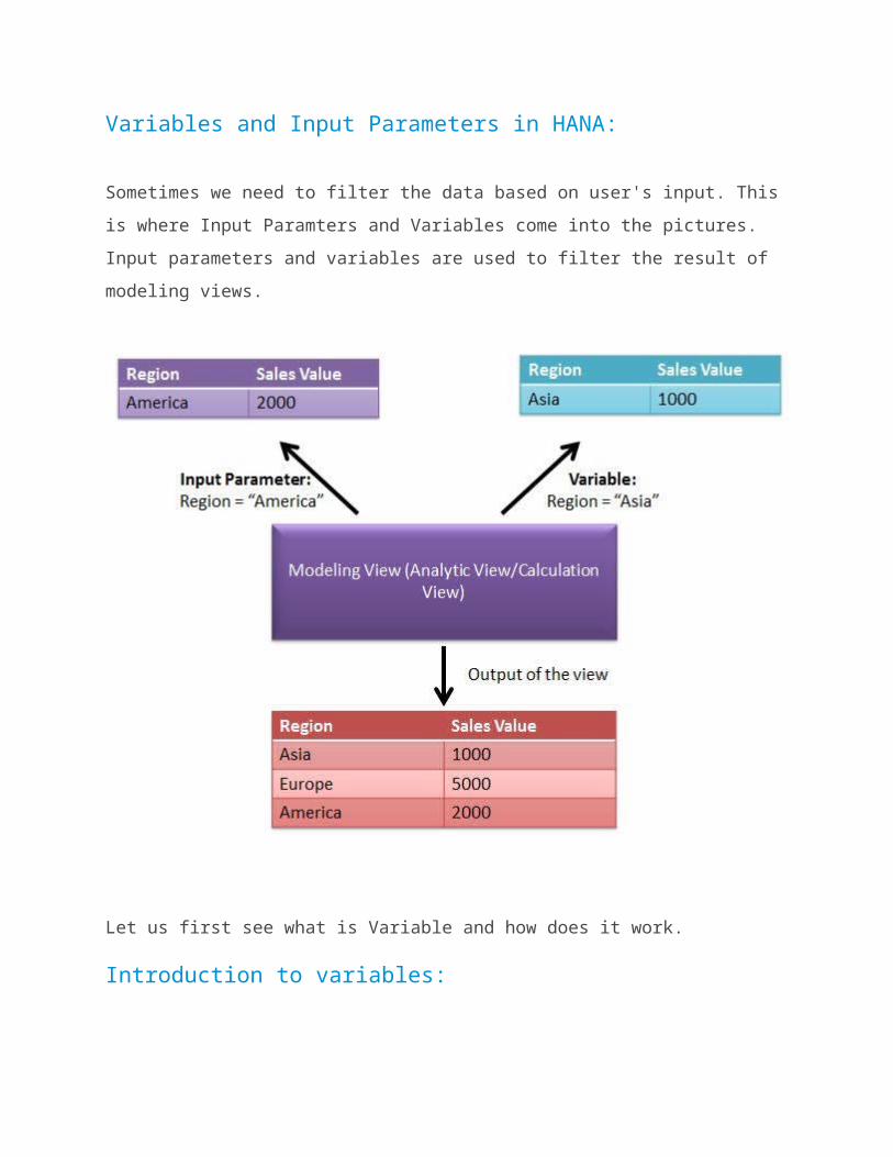
Variables and Input Parameters in HANA:

Sometimes we need to filter the data based on user's input. This is where Input Paramters and Variables come into the pictures. Input parameters and variables are used to filter the result of modeling views.

Let us first see what is Variable and how does it work.

Introduction to variables:

Variables are bound to columns and are used for filtering using WHERE clauses. As such, they can only contain the values available in the Columns they relate to.

Sounds confusing?? Let us take a simple example. In the article Create Graphical Calculation View in 10 minutes, we created a calculation view which has 4 columns PRODUCT_NAME, REGION_NAME, SUB_REGION_NAME and SALES_AMOUNT. REGION_NAME contains different regions like “America”, “Asia” and“Europe”. The calculation view gives all the region’s details in output.

Now suppose we want to filter the data on region basis. The calculation view will prompt the user to specify Region Name and the output data will be filtered based on that.

For example if the user provides the value as “Asia”, the calculation view will show data only for “Asia” region.

How to create and use variables in modeling view:

Now we will see how to implement this using variable.

Note: We will refer to the calculation created in the article Create Graphical Calculation View in 10 minutes.

1. Open the calculation view. On Right-Bottom side you will see a pane called “Variables/Input Parameters”. Click on the down arrowof “+” icon and select “Variable”

2. Specify Name of the Variable. Click on the drop down arrow besides “Attribute” and select REGION_NAME. Click on ok.

3. Activate the calculation view. Now click on the data preview.

4. A pop-up window will appear. Click on Open Value Help besides “From” and select “Asia” region. Click on ok.

5. Go to Raw Data tab to see complete output. It contains data only for “Asia” region.

Important features of variables:

You use variables to filter data at runtime. You assign values tothese variables by entering the value manually, or by selecting it from the drop-down list.

You can also define whether the Variable is Mandatory or if it should have aDefault Value.

You can apply variables only in analytic and calculation views.

Variable Types:

The following types of Variables are supported:

Single Value: Use this to apply a filter to a Single Value. Interval: Use this where you want the user to specify a set start

and end to a selected Interval. Range: Use this when you want the end user to be able to use

operators such as “Greater Than” or “Less Than”.

System Tables to see Variable Information:

There are 4 system tables under the schema _SYS_BI which containsinformation about Variables.

BIMC_VARIABLE

BIMC_VARIABLE_ASSIGNMENT

BIMC_VARIABLE_VIEW

BIMC_VARIABLE_VALUEIntroduction to Input Parameters:

Sometimes you might not want a variable to just restrict the dataof a view. But you also want to take input from the user and process it, returning dynamic data based on the user selection. Input Parameters makes this possible.

How to create and use input parameters in modeling view:

Example Scenario:

Let us consider the same calculation view we created before whichhas following attributes and measures.Attributes: PRODUCT_NAME, REGION_ID, REGION_NAME, SUB_REGION_NAME Measures: SALES_AMOUNT

Suppose we want the end user to decide whether SALES_AMOUNT or

NET_AMOUNT should be shown in the output. We can create a input parameter of type “Static List” which will have 2 values “SalesAmount” and “NetAmount”. The calculation view will prompt for the input parameter. The user will choose either “SalesAmount” or “NetAmount”. Based on this selection, the output will be shown.

Let us create the input parameter.

1. Open the same calculation view. On Right-Bottom side you will seea pane called “Variables/Input Parameters”. Click on the down arrow of “+” icon and select “Input Parameter”.

2. Provide Name, description and select the data type as INTEGER.

3. Select the Aggregation block and right click on “Calculated Columns” to create a new column.

4. Specify the name as “NET_AMOUNT”, Data Type as double. In the expression editor provide the expression as "SALES_AMOUNT" - ( "SALES_AMOUNT" * $$DISCOUNT$$ /100)

Note that we are using Input parameter DISCOUNT by using syntax$$DISCOUNT$$

5. Activate the calculation view.

6. Click on data preview. A pop-up window will be opened. Provide the Region Name as ‘Asia’ and Discount value as 10.

7. The NET_AMOUNT will be calculated as per the given DISCOUNT value.

Important Features of Input Parameters:

Input Parameters can contain any value the reporting user has to enter to parameterize the result. Therefore, a data type must be specified for each Input Parameter.

Input Parameters are passed by Placeholders and used in Formulas.

Input Parameter Types:

The following types of Input variables are supported.

Currency: Use this during currency conversion where the end user should specify a source or target currency.

Date: Use this to retrieve a date from the end user using a calendar type input box.

Static List: Use this when the end user should have a set list of values to choose from.

Attribute Value: When an Input Variable has this type, it serves the same purpose as a normal Variable.

None: If none of the above applies you do not have to specify an Input Variable type. The Type can be left blank.

How to Pass Input Parameters and Variables in SQL Query:

Open the data preview of calculation view as mentioned in previous step. Click on the “Show Log” and then double click on the message highlighted below. A new window will be opened which contains theSQL query.

The generated query is:SELECT TOP 200 "PRODUCT_NAME", "REGION_NAME", "SUB_REGION_NAME", "NET_AMOUNT",

sum("SALES_AMOUNT") AS "SALES_AMOUNT"

FROM "_SYS_BIC"."sap-hana-tutorial/SalesReport"

('PLACEHOLDER' = ('$$DISCOUNT$$', '10'))

WHERE ("REGION_NAME" IN ('Asia') )

GROUP BY "PRODUCT_NAME", "REGION_NAME", "SUB_REGION_NAME", "NET_AMOUNT"

Note that in your case package name might be different and query might be slightly different.

Input Parameter is passed using PLACEHOLDER:

The value of Input Parameter is passed using PLACEHOLDER clause. ('PLACEHOLDER' = ('$$DISCOUNT$$', '10'))

WHERE:The value of Variable is passed using WHERE clause. WHERE ("REGION_NAME" IN ('Asia') )

An insight into SAP HANA Architecture

Documents

Transcript of An insight into SAP HANA Architecture