Available online at www.sciencedirect.com

Behavior Therapy 40 (2009) 357–367www.elsevier.com/locate/bt

An Improved Effect Size for Single-Case Research:Nonoverlap of All Pairs

Richard I. ParkerKimberly Vannest

Texas A & M University

Nonoverlap of All Pairs (NAP), an index of data overlapbetween phases in single-case research, is demonstrated andfield tested with 200 published AB contrasts. NAP is a novelapplication of an established effect size known in variousforms as Area Under the Curve (AUC), the CommonLanguage Effect Size (CL), the Probability of Superiority(PS), the Dominance Statistic (DS), Mann-Whitney’s U, andSommers D, among others. NAPwas compared with 3 othernon-overlap-based indices: PND (percent of nonoverlappingdata), PEM (percent of data points exceeding the median),and PAND (percent of all nonoverlapping data), as well asPearson’s R2. Five questions were addressed about NAP: (a)typical NAP values, (b) its ability to discriminate amongtypical single-case research results, (c) its power andprecision (confidence interval width), (d) its correlationwith the established effect size index, R2, and (e) itsrelationship with visual judgments. Results were positive,the new index equaling or outperforming the other overlapindices on most criteria.

NONOVERLAPPING DATA AS AN indicator of perfor-mance differences between phases has long been animportant part of visual analysis in single-caseresearch (SCR) (Sidman, 1960) and is included inrecently proposed standards for evaluating SCR(Horner et al., 2005). The extent to which data inthe baseline (A) versus intervention (B) phases donot overlap is an accepted indicator of the amountof performance change. Data overlap between

Address correspondence to Richard I. Parker, Ph.D., Texas A &MUniversity, Educational Psychology Department, College Station,TX 77843; e-mail: rparker@tamu.edu.0005-7894/08/357–367$1.00/0© 2008 Association for Behavioral and Cognitive Therapies. Published byElsevier Ltd. All rights reserved.

phases has also been quantified. Twenty-five yearsago, Scruggs and Casto (1987) defined “percent ofnonoverlapping data” (PND) as the percent ofphase B datapoints which exceed the single highestphase A datapoint. More recently, Parker, Hagan-Burke, and Vannest (2007) defined the “percent ofall nonoverlapping data” (PAND) as the “percentof all data remaining after removing the minimumnumber of datapoints which would eliminate alldata overlap between phases A and B.” A thirdoverlap index was also published recently, Ma’s(2006) PEM, the “percentage of phase B datapointsexceeding the median of the baseline phase.” Thepresent paper describes a fourth index of nonover-lapping data, designed to remedy perceived weak-nesses of these three. Briefly, those weaknesses are:(a) lack of a known underlying distribution(disallowing confidence intervals) (PND); (b)weak relationship with other established effectsizes (PEM); (c) low ability to discriminate amongpublished studies (PEM, PND); (d) low statisticalpower for smallN studies (PND, PAND, PEM); and(e) open to human error in hand calculations fromgraphs (PND, PAND, PEM).Quantifying results in SCR is not always needed;

an approximate visual judgment of “a lot” versus“little or none” may suffice for practitionersmaking in-house, low-stakes decisions (Parsonson& Baer, 1992). Quantifying data overlap is mostneeded when the interventionist needs to makemore precise statements about the amount ofimprovement—for example, for (a) documentingevidence of clinical effectiveness for insurance,government, and legal entities; (b) comparing therelative effectiveness of two or more interventions;(c) providing support for a knowledge base of“evidence-based practices”; (d) including a study inmeta-analyses; and (e) applying for competitive

358 parker & vanne s t

funding. These five instances are not unrelated andare an increasing part of the scientific practice ofclinical and school psychology (Chambless &Ollendick, 2001; Kratochwill & Stoiber, 2002).For example, special educators and school psychol-ogists are being charged by federal legislation(IDEA, 2004) with measuring student improvementwithin multitiered “Response to Intervention”models. Student response to Tier 2 and 3 interven-tions is commonly measured by progress monitor-ing, with results depicted as a line graph. Butmeasuring the amount of change with knownprecision is best accomplished by an effect sizeindex. The precision of the index is shown byconfidence intervals around the effect size.“Nonoverlap of All Pairs” (NAP), presented in

this paper, summarizes data overlap between eachphase A datapoint and each phase B datapoint, inturn. A nonoverlapping pair will have a phase Bdatapoint larger than its paired baseline phase Adatapoint. NAP equals the number of comparisonpairs showing no overlap, divided by the totalnumber of comparisons. NAP can be calculated byhand from a SCR graph, from intermediatestatistics available from the Wilcoxon Rank-SumTest (Conover, 1999), or directly as Area Under theCurve (AUC) from a Receiver Operator Character-istics (ROC) diagnostic test module. Both handcalculation and computer methods are detailed inthe Method section.NAP was developed primarily to improve upon

existing overlap-based effect sizes for SCR. ButNAP also offers advantages over parametricanalyses (t-tests, analyses of variance, ordinaryleast squares [OLS] regression), which are generallybelieved to possess greater statistical power. Themain limitations in using parametric effect sizes are:(a) SCR data commonly fail to meet parametricassumptions of serial independence, normality andconstant variance of residual scores (Parker, 2006);(b) parametric effect sizes are disproportionatelyinfluenced by extreme outliers, which are commonin SCR (Wilcox, 1998); and (c) interpretation of R2

as “percent of variance accounted for” or Cohen’s das “standardized mean difference” are alien tovisual analysis procedures (May, 2004; Parsonson& Baer, 1992; Weiss & Bucuvalas, 1980).Parker (2006) examined a convenience sample of

166 published SCR datasets and found that 51%failed the Shapiro-Wilk (Shapiro&Wilk, 1965) testof normality, 45% failed the Modified Levene(Brown & Forsythe, 1974) test of equal variance,and 67% failed a lag-1 autocorrelation test, usingstandards suggested for SCR (Matyas & Green-wood, 1996). Over three-fourths of the datasetsfailed one or more of these parametric assumptions

(note: serial independence is also a nonparametricassumption). Given such datasets, Wilcox pro-claimed standard OLS regression as, “one of thepoorest choices researchers could make” (Wilcox,1998, p. 311). He and others have challenged theaccuracy of OLS effect sizes and their confidenceintervals when calculated from small samples withatypical distributions, as are common in SCR.Nevertheless, R2 is well-established in groupresearch and generally believed to be more dis-criminating and to have superior statistical power,so it was included as an external standard in thisstudy. R2 is calculated here in an OLS linearregression module, with Phase dummy-coded (0/1).NAP was developed mainly to improve upon

existing SCR overlap-based effect sizes: PND,PAND, and PEM. NAP should offer five compara-tive advantages. First, NAP should discriminatebetter among results from a large group ofpublished studies. Our earlier research indicatedless than optimal discriminability by the other threenonoverlap indices (PND, PAND, PEM). An effectsize showing equal discriminability along its fulllength would be most useful in comparing resultswithin and across studies (Cleveland, 1985). Thesecond NAP advantage should be less human errorin calculations than the other three hand-calculatedindices. On uncrowded graphs, PND, PAND andPEM are calculated with few errors, but not so onlonger, more compacted graphs. PAND can becalculated objectively by a sorting routine, but thatprocedure may be confusing. NAP is directly outputfrom an ROC module as the AUC percent and iscalculated easily from Mann-Whitney U intermedi-ate output.A third advantage sought from NAP was

stronger validation by R2, the leading effect sizein publication. Cohen’s d was not calculated forthis paper, as it can be directly computed from

R R =dffiffiffiffiffiffiffiffiffiffiffiffi

d2 + 4p

� �(Rosenthal, 1991; Wolf, 1986).

Since NAP entails more data comparisons (NA×NB)than other nonoverlap indices, it should relate moreclosely to R2, which makes fullest use of data. Thefourth anticipated advantage of NAP was strongervalidation by visual judgments. The reason for thatexpectation was that visual analysis relies on multi-ple and complex judgments about the data, whichshould be difficult to capture with simpler indicessuch as PEM and PND. NAP is not a test on meansormedians, but rather on location of the entire scoredistribution, and is not limited to a particularhypothesized distribution shape.The fifth and final advantage expected from NAP

was greater score precision, indicated by narrowerconfidence intervals (CIs). CI width is determined

359nonoverlap all pa i r s

by the particular statistical model used, by the Nused in calculations (narrower CIs for larger Ns),and by effect size magnitude (narrower CIs forlarger effect sizes). PEM relies on the binomial test,its N being the number of datapoints in phase B.PAND can be considered an effect size but islacking in some desirable attributes. Two PAND-derived effect sizes from its 2×2 table contingencytable are Pearson Phi and Risk Difference (RD; thedifference between two proportions). Phi isobtained from a chi-square test, and RD from asimilar “test of two proportions,” both performedon the original 2×2 PAND table. Phi and RD areoutput with standard errors for calculating CIs,and RD is usually accompanied by CIs. Both Phiand RD analyses use as N the total datapoints inphases A plus B (NA+NB). The final nonoverlapindex, PND, has no known sampling distribution,so CIs cannot be calculated. The new NAP index,output as AUC from an ROC module, is accom-panied by CIs. In addition, CIs are calculated byspecially developed software by Newson (2000,2002) as add-on macros for Stata statistical soft-ware. Nonparametric AUC modules are found inmost statistics packages, including NCSS, SPSS,Stata, StatExact, and SAS, which output the AUCscore, its standard error of measurement, and CIs.Robust methods for NAP’s CIs have been producedby Wilcox (1996) in Minitab and S-Plus. Methodsfor manual CI calculation are summarized byDelaney and Vargha (2002).The overlap index here termed NAP has several

names for slight variations and different areas ofapplication (Grissom & Kim, 2005). To statisti-cians, it is best known in its most general form, p(X1NX2), or “the probability that a score drawn atrandom from a treatment groupwill exceed that of ascore drawn at random from a control group.” Itcan be quickly derived from UL, or the larger of twoU values from the nonparametric Mann-Whitney Utest (also known as the Wilcoxon Rank-Sum test;Cliff, 1993). For diagnostic work in medicine andtest development, it is “Area Under the Curve”(AUC). The qcurveq in AUC is the receiver operatorcharacteristic (ROC) curve, also known as the“sensitivity and specificity” curve, for detailingerror types (false positives, false negatives) (Hanley& McNeil, 1982). Applied to continuous data it isthe Common Language Effect Size (CL) (McGraw&Wong, 1992). CL was critiqued and extended byVargha and Delaney (2000) to cover ordinal anddiscrete data, and they renamed the new index the“Measure of Stochastic Superiority.” Similarly, Cliff(1993) promoted use a slight variation of AUC,renaming it the “Dominance Statistic” (d). Stillother variations exist, often differing by how ties are

handled and by their score ranges: AUC ranges from.5 to 1 (or 0 to 1 to include deteriorating scores),Cliff’s d ranges from 0 to 1, and McGraw andWong’s CL ranges from –1 to +1. Since this overlapindexwithCIs is obtainedmost readily as AUC, thatis the name utilized from here on.AUC has been recommended as a broad replace-

ment for Cohen’s d (Acion, Peterson, Temple, &Arndt, 2006). It is popular in evidence-basedmedicine, in which researchers require statisticswhich are not saddledwith parametric assumptions,are easily interpretable, and offer confidence inter-vals (D'Agostino, Campbell, & Greenhouse, 2006).“AUC works well with continuous, ordinal andbinary variables, and is robust and maintainsinterpretability across a variety of outcome mea-sures, distributions, and sample characteristics”(e.g., skewed distributions, unequal variances)(D'Agostino et al., p. 593). The score overlapinterpretation of AUC is direct and intuitive. AUCis considered by some to be superior to median shift(or even mean shift), as these latter methodsoveremphasize central tendency. For ill-shapeddistributions, the mean or median may poorlyrepresent most data points, so an index like AUC,which emphasizes all data values equally, ispreferred (Delaney & Vargha, 2002; Grissom &Kim, 2005).Applied to SCR, NAP (AUC) can be defined as

“the probability that a score drawn at random froma treatment phase will exceed (overlap) that of ascore drawn at random from a baseline phase,”withties receiving one-half point. A simpler wording is“the percent of non-overlapping data betweenbaseline and treatment phases.” This concept ofscore overlap is identical to that used by visualanalysts of SCR graphs and is the same as iscalculated in the other overlap indices, PAND, PEMand PND.NAP’smajor theoretical advantage is thatit is a comprehensive test of all possible sources ofdata overlap, i.e. all baseline versus all treatmentdatapoint comparisons, a total of NA×NB pairs.NAP is a probability score, normally ranging from.5 to 1. If datapoints from two phases cannot bedifferentiated, then AUC=.5; there is a fifty percentchance that scores from one group will exceed thoseof the other. For deteriorating performance duringtreatment phase, one must take the extra step ofspecifying in an AUC module the Control orBaseline phase as the high score. By doing so, theAUC range is extended to 0 to 1. Any score from0 to.4999 represents deteriorating performance.Given two samples with normal distributions and

equal variance (unlikely in SCR), AUC or NAP canbe estimated from Cohen’s d: AUC=1-.5⁎(1 - d/3.464)2 (Acion et al., 2006). The formula for

360 parker & vanne s t

estimating Cohen’s d from NAP is: d=3.464⁎(1-√(1-NAP)/.5). So Cohen’s (1988) estimates of small,medium and large d values (.2, .5, .8) correspond toNAP (on a .5 to 1 scale) values of .56, .63, and .70,respectively. And using the equivalence, d=2R/√(1-R2) (Wolf, 1986), the three NAP values correspondto R2 values of .01, .06, and .14, respectively. Butour results will show that Cohen’s guidelines do notapply to SCR.This paper first illustrates with a fabricated dataset

the calculation of NAP and the three other non-overlap indices. Next, all four indices, alongwithR2,are applied to a sample of 200 phase AB contrastsfrom 122 SCR designs, published in 44 articles. Thisfield test informs us about the newNAP index: (a) itstypical values, (b) its ability to discriminate amongtypical single-case research results, (c) its power andprecision (CI width), (d) its correlation with estab-lished indices of magnitude of effect, and (e) itsrelationship with visual judgments.

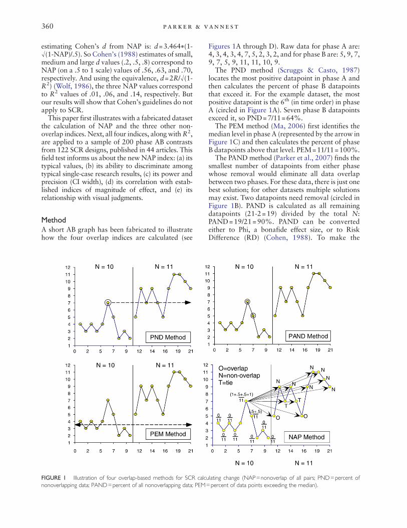
MethodA short AB graph has been fabricated to illustratehow the four overlap indices are calculated (see

FIGURE 1 Illustration of four overlap-based methods for SCR calcunonoverlapping data; PAND=percent of all nonoverlapping data; PEM=

Figures 1A through D). Raw data for phase A are:4, 3, 4, 3, 4, 7, 5, 2, 3, 2, and for phase B are: 5, 9, 7,9, 7, 5, 9, 11, 11, 10, 9.The PND method (Scruggs & Casto, 1987)

locates the most positive datapoint in phase A andthen calculates the percent of phase B datapointsthat exceed it. For the example dataset, the mostpositive datapoint is the 6th (in time order) in phaseA (circled in Figure 1A). Seven phase B datapointsexceed it, so PND=7/11=64%.The PEM method (Ma, 2006) first identifies the

median level in phase A (represented by the arrow inFigure 1C) and then calculates the percent of phaseB datapoints above that level. PEM=11/11=100%.The PAND method (Parker et al., 2007) finds the

smallest number of datapoints from either phasewhose removal would eliminate all data overlapbetween two phases. For these data, there is just onebest solution; for other datasets multiple solutionsmay exist. Two datapoints need removal (circled inFigure 1B). PAND is calculated as all remainingdatapoints (21-2=19) divided by the total N:PAND=19/21=90%. PAND can be convertedeither to Phi, a bonafide effect size, or to RiskDifference (RD) (Cohen, 1988). To make the

lating change (NAP=nonoverlap of all pairs; PND=percent ofpercent of data points exceeding the median).

361nonoverlap all pa i r s

conversions, datapoints needing and not needingremoval from each phase are entered into a 2×2table. Phi is obtained from a chi-square analysis ofthese data (Phi= .82). RD is obtained from a “twoindependent proportions” analysis of these data(RD=.81). In a balanced table, Phi and RD areidentical. CIs are sometimes output for Phi butnearly always for RD. Calculation of Phi and RDare detailed in Parker et al. (2007), and in Parker,Vannest, and Brown (in press), respectively.The NAP hand-calculation method (Figure 1D)

compares, in turn, each phase A datapoint witheach phase B datapoint. Arrows in Figure 1D showthese paired comparisons and results for only onephase A datapoint, the 6th in order (value=7). NAPhand calculation has two procedural options. Onemay begin counting all nonoverlapping pairs, or bycounting all overlapping pairs, and subtract fromthe total possible pairs to obtain the nonoverlapcount. The total possible pairs (total N) is thenumber of datapoints in phase A times phase B(NA×NB), here 10×11=110. For most datasets, it isfaster to begin counting only overlap, then subtractfrom the total possible pairs. The notations onFigure 1D are for counting overlap.For the example dataset, only two of the phase A

datapoints show any overlap, those with values of 7and 5. We begin with the 7, and compare it, in turn,with each phase B datapoint. An overlap counts asone point, and a tie counts as half a point. For theFigure 1 example, comparing the 6th phase Adatapoint (value=7) with all phase B datapointsyields: (1, 0, .5, 0, .5, 1, 0, 0, 0, 0, 0)=3. Comparingthe 7th phase A datapoint (value=5) with all phase Bdatapoints yields: (.5, 0, 0, 0, 0, .5, 0, 0, 0, 0, 0)=1.Thus, the overlap sum is 3+1=4. Subtracting fromthe total possible pairs, we get 110 – 4=106. Finally,NAP=106/110=96%.NAP also is obtained directly as the AUC percent

from a ROC analysis. We used NCSS (Hintze,2006), where “ROC Curves” is located under“Diagnostic Tests.” Settings to use are as follows:“Actual Condition Variable=Phase , CriterionVariable = Scores, Positive Condition Value=B(phase B), Test Direction=High×Positive.” Outputis “Empirical AUC=.96,” along with CIs.NAP also can be calculated from intermediate

output of the Wilcoxon Rank-Sum Test, usuallylocated in statistical packages within “Two Samplet-Test” or “Non-Parametric Test” modules. Wil-coxon yields a “U” value for each phase, defined as“…the number of times observations in one sampleprecede observations in the other sample in rank-ing” (Statsdirect Help, 2008). The larger U value(UL) for phase B equals the number of nonoverlap-ping data comparisons (ties weighted .5). UL

divided by the total number of data comparisons(NA×NB) equals NAP. For our example data, theWilcoxon UL is 106, and NAP=106/110=.96, thesame result obtained by hand.From our example data, similar results were

obtained by the overlap indices PAND (90%),PEM (100%), and NAP (96%), whereas PND issmaller (64%). And the PAND-derived effect sizesare RD (81%) and Phi (.82). But the size of anindex is less important than attributes such as itspower and precision (indicated by CI width), itsrelatedness to established indices (criterion-relatedvalidity), its ability to discriminate among typicalpublished results (indicated by a distributionprobability plot), and its agreement with visualjudgments.

confidence intervals

CIs indicate the confidence or assurance we canhave in an obtained effect size, also termed“measurement precision.” Awide confidence inter-val or band around an effect size indicates lowprecision, allowing little trust or assurance in thatobtained value. Precision is directly related to thestatistical power of a test; a test with low powercannot measure medium-sized and smaller effectswith precision. CIs are strongly recommended foreffect sizes by the 1999APATask Force on StatisticalInference (Wilkinson & The Task Force on Statis-tical Inference, 1999), and by the APA PublicationManual (2001). CIs are interpreted as follows: for acalculated effect size of .55, and a 90% confidenceinterval: .38b .55b .72, we can be 90% certain thatthe true effect size lies somewhere between .38 and.72 (Neyman, 1935). Omitted from this comparisonwas PND, for which CIs cannot be calculatedbecause we do not know its chance level nor itsunderlying sampling distribution.Exact CIs for PEM are provided by a binomial

single-sample proportions test against a 50%chance level, easily computed from most statisticspackages. From Figure 1C (11/11=100%), theexact 90% CI for PEM is: .87b1.00b1.00. ForPAND, the same single-sample proportions test canprovide CIs. The PAND of 90% is tested against a50% chance level withN=NA+NB=21 to yield this90%CI: .73 b .90 b .98, a CI width of .25. But as aneffect size, PAND is less suitable than two respectedindices which can be calculated from a 2×2 table ofPAND data: Pearson’s Phi and Risk Difference(RD). From a chi-square test on the 2×2 table, Phiwith 90% CI is: .46 b .82 b1.0, a CI width of .54.From a two proportions test on the same data, RDwith 90% CI is: .49 b .80 b .95, a CI width of .46.Details for calculating these Phi and RD CIs arefound in Parker et al. (2007; 2009).

Table 1Key percentile ranks for four overlap indices (NAP, PND, PAND,

2

362 parker & vanne s t

CIs for NAP are available with the AUC statistic asdirect output. For this example, the 90% CI is: .84b .96 b .99, a CI width of .15. From a total N of 18–20, we can expect reasonably accurate 90% CIs.From a total N of 30, we can expect accurate 95%CIs. And from an N of 60, accurate 99% CIs can beexpected (Fahoome, 2002). Procedures have beendeveloped for narrower CIs (greater measurementprecision), which are also robust against unequalvariances (Delaney&Vargha, 2002), but they are notyet available as standard output from generalstatistics packages. As noted earlier, some CI algo-rithms are available as add-ons to Stata and S-Plus.

field test

The four overlap indices were applied to aconvenience sample of 200 phase A versus B (AB)contrasts from 122 SCR designs in 44 publishedarticles (available on request from the first author).The sample was composed of 166 AB contrastscollected 5 years ago, plus 34 contrasts recentlyadded, to total 200. Datasets were obtained fromERIC and PsychLIT literature searches for termssuch as: “single case,” “single subject,” “baseline,”“multiple baseline,” “phase,” AB, ABA, ABAB, etc.The first 300 articles located were culled to findthose with graphs clear and large enough foraccurate digitizing. The first 200 useable contrastswere chosen from those articles. The AB contrastswere chosen without regard for dataseries length,intervention effectiveness, design type, etc. All clear,useable graphs were digitized using I-Extractorsoftware (Linden Software Ltd, 1998). The litera-ture search and digitizing procedure are describedin more detail in previous articles (Parker et al.,2005; Parker & Brossart, 2003).For the 200 selected AB contrasts, the median

length of a full dataseries was 18 datapoints, withan interquartile range (IQR; middle 50% of scores)of 13 to 24. Phase A had Median=8, IQR=5-12,and Phase B length had Median=9, IQR=5–13.Few articles included statistical analyses, andnone provided CIs. Even for weak and moderateresults, visual analysis alone was used to drawconclusions.

PEM) and the standards R , based on 200 published samples

10th Percentile Rank Values 90th

25th 50th 75th

NAP .50 .69 .84 .98 1.00PND 0.00 .24 .67 .94 1.00PAND .60 .69 .82 .93 1.00PEM .50 .79 1.00 1.00 1.00R2 .05 .16 .42 .65 .79

Note. NAP=nonoverlap of all pairs; PND=percent of nonoverlap-ping data; PAND=percent of all nonoverlapping data; PEM=per-cent of data points exceeding the median.

ResultsThe field test with 200 published AB contrasts wasconducted to inform how NAP performs on typicaldatasets: (a) What are typical NAP effect sizemagnitudes? (b) How well does NAP discriminateamong typical published SCR results? (c) Howmuch confidence can one have in the calculatedNAP values (their precision)? (d) How does NAPrelate to the other indices? and (e) How well does

NAP match visual judgments of client improve-ment? To answer these questions, NAP, PND,PAND, PEM and Pearson’s R2 were all calculatedon the 200 contrasts.

typical values

Table 1 presents key percentile ranks for each ofseven indices. The tabled percentile ranks show R2

with lower scores than the four overlap indices.This is especially noticeable in the upper ranges; allfour overlap indices hit their maximum (1.00) at the90th percentile. At the 50th percentile, the overlapindex values are about double R2 , and for values atthe 10th percentile, some differences are by a factorof 10. The exception is PND, which hits the floor ofzero at the 10th percentile. For NAP, a fulldistribution would show that the 10th percentilevalue of .50 does not represent a floor effect. Thesmall number of graphs with deterioration resultsearned scores between 0 and .50.All of the overlap magnitudes differ enough from

R2 that they need new interpretation guidelines. Formost of the studies sampled, authors described quitesuccessful interventions, for which one would antici-pate large effects. Even so, overlap results were muchlarger than Cohen’s guidelines for point-biserial R2

values: qlargeq (R2=.14); qmediumq (R2=.06); andqsmallq (R2=.01) (Cohen, 1988, p. 82). The tabledeffect size magnitudes underscore the warning byCohen and others that his guidelines are from largeNsocial science group research and should not beroutinely applied in other contexts (Cohen, 1988;Kirk, 1996;Maxwell,Camp,&Avery, 1981;Mitchell& Hartmann, 1981; Rosnow & Rosenthal, 1989).

discriminability

The usefulness of any new index will depend inpart on its ability to discriminate among resultsfrom published studies. Given a large sample, auniform probability distribution can indicate dis-criminability (Cleveland, 1985). Distributions with

FIGURE 2 Uniform probability plots for five indices of change inSCR (NAP=nonoverlap of all pairs; PND=percent of nonover-lapping data; PAND=percent of all nonoverlapping data;PEM=percent of data points exceeding the median).

363nonoverlap all pa i r s

high discriminability appear as diagonal lines,without floor or ceiling effects, and without gaps,clumping, or flat segments (Chambers, Cleveland,Kleiner, & Tukey, 1983; Hintze, 2006). Figure 2shows superior probability distributions for Pear-son’s R2, forming a nearly diagonal line across thescore range. The next best distributions are byNAP and PAND, both of which show ceilingeffects around their 80th percentiles. So NAP andPAND do not discriminate well among the mostsuccessful 20% of interventions. PND may appearsimilar to these two at first glance, but it alsoshows a floor effect around its 18th percentile.Also, the ceiling effect of PND is more severe, nearits 75th percentile. So PND discriminates poorlyamong 18+25=43% of the published studies. Themost problematic distribution is PEM, with nofloor effect, but a major ceiling effect — over 50%of the samples scored a perfect 100%.

level of confidence in effect sizes

The confidence one can have in an obtained effectsize is reflected in its CIwidth and the standard errorused to calculate the CI. Narrower CIs are generally

Table 2Ninety-percent confidence intervals on six indices of change, from small

N=13

25th %ile 50th %ile

NAP .33b .67b .87 .49b .84b .95PAND .42b .77b .88 .59b .88b .97PND ?b .26b? ?b .70b?PEM .34b .80b .94 .65b1.00b1.00R2 0b .16b .45 .04b .42b .68

Note. Ns are numbers of datapoints in a single data series, across pnonoverlapping data; PAND=percent of all nonoverlapping data; PEM=

believed to come from parametric analyses such as t-tests, analysis of variance, and OLS regressionrather than nominal-level nonparametric tests suchas NAP. Ninety percent CIs were calculated forbenchmark values of NAP, PAND, PEM, and R2.CIs could not be calculated for PND because thatindex lacks a known sampling distribution. Fromthe 200 datasets, CIs were calculated for small andlarge sample sizes (N=13 and N=24, respectively)and for weak and medium results (25th and 50th

percentile values, respectively).A binomial proportions test provides CIs for PEM

and PAND. The PAND analysis N was NA + NB .The N for the PEM analysis was NB only. PearsonR2 values were bootstrap estimates from individualstudies whichmost closely met the criteria of samplesize and effect size magnitude. NAP CIs were theAUC confidence intervals from an ROC testmodule. Thoughmore precise intervals are availablefrom specialized software, they were not exploredhere. ForR2, exact, asymmetrical CIs were obtainedfrom the stand-alone R2 utility, one of the few withthis capability (Steiger & Fouladi, 1992).Table 2 contains 90% CIs for weak and medium

effect sizes. For example, for weak results and asmall N (13) for NAP, the Table gives: .33 b .67b .87. This is interpreted: “We can be 90% sure thatthe true effect size for the obtained value of .67 issomewhere between .33 and .87 (a spread of .54points).” PAND showed the greatest precision, itsfour tabled CI widths averaging .30. Second placewas earned by NAP, averaging .43 over its four CIs.Ranked third was R2, with tabled CI widthsaveraging .48. In last place was PEM, whichproduced artificially narrow CIs because two ofthem hit the 1.0 ceiling. Without the 1.0 ceiling,PEM’s CI widths would average about .53.

relatedness to r2

The most commonly published effect sizes in thesocial sciences are members of the R2 family(including Eta2) (Kirk, 1996), though they entaildata assumptions that single case studies often

and medium sample sizes, and for weak and medium size effects

N=24

25th %ile 50th %ile

.40b .67b .80 .62b .84b .94

.61b .77b .91 .70b .88b .96?b .26b? ?b .70b?.53b .80b .93 .80b1.00b1.000b .16b .38 .17b .42b .63

hase A and B. NAP=nonoverlap of all pairs; PND=percent ofpercent of data points exceeding the median.

364 parker & vanne s t

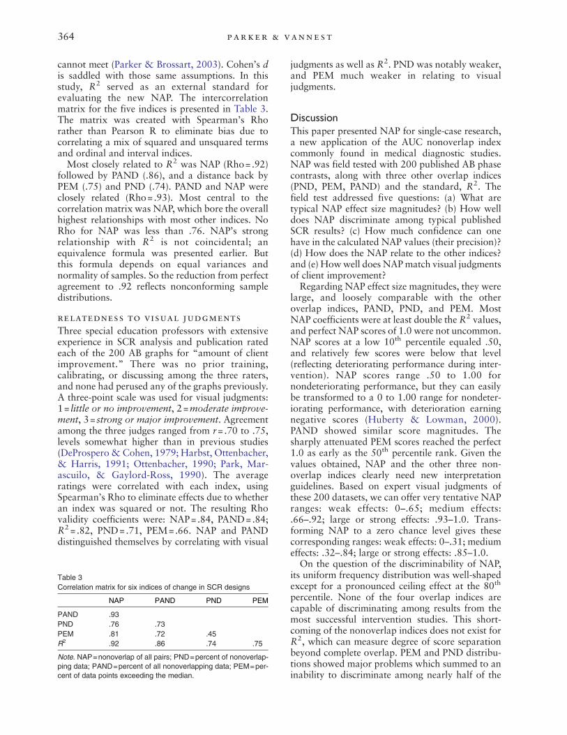
cannot meet (Parker & Brossart, 2003). Cohen’s dis saddled with those same assumptions. In thisstudy, R2 served as an external standard forevaluating the new NAP. The intercorrelationmatrix for the five indices is presented in Table 3.The matrix was created with Spearman’s Rhorather than Pearson R to eliminate bias due tocorrelating a mix of squared and unsquared termsand ordinal and interval indices.Most closely related to R2 was NAP (Rho=.92)

followed by PAND (.86), and a distance back byPEM (.75) and PND (.74). PAND and NAP wereclosely related (Rho=.93). Most central to thecorrelation matrix was NAP, which bore the overallhighest relationships with most other indices. NoRho for NAP was less than .76. NAP’s strongrelationship with R2 is not coincidental; anequivalence formula was presented earlier. Butthis formula depends on equal variances andnormality of samples. So the reduction from perfectagreement to .92 reflects nonconforming sampledistributions.

relatedness to visual judgments

Three special education professors with extensiveexperience in SCR analysis and publication ratedeach of the 200 AB graphs for “amount of clientimprovement.” There was no prior training,calibrating, or discussing among the three raters,and none had perused any of the graphs previously.A three-point scale was used for visual judgments:1= little or no improvement, 2=moderate improve-ment, 3=strong or major improvement. Agreementamong the three judges ranged from r=.70 to .75,levels somewhat higher than in previous studies(DeProspero & Cohen, 1979; Harbst, Ottenbacher,& Harris, 1991; Ottenbacher, 1990; Park, Mar-ascuilo, & Gaylord-Ross, 1990). The averageratings were correlated with each index, usingSpearman’s Rho to eliminate effects due to whetheran index was squared or not. The resulting Rhovalidity coefficients were: NAP=.84, PAND=.84;R2= .82, PND=.71, PEM=.66. NAP and PANDdistinguished themselves by correlating with visual

Table 3Correlation matrix for six indices of change in SCR designs

NAP PAND PND PEM

PAND .93PND .76 .73PEM .81 .72 .45R2 .92 .86 .74 .75

Note. NAP=nonoverlap of all pairs; PND=percent of nonoverlap-ping data; PAND=percent of all nonoverlapping data; PEM=per-cent of data points exceeding the median.

judgments as well as R2. PND was notably weaker,and PEM much weaker in relating to visualjudgments.

DiscussionThis paper presented NAP for single-case research,a new application of the AUC nonoverlap indexcommonly found in medical diagnostic studies.NAP was field tested with 200 published AB phasecontrasts, along with three other overlap indices(PND, PEM, PAND) and the standard, R2. Thefield test addressed five questions: (a) What aretypical NAP effect size magnitudes? (b) How welldoes NAP discriminate among typical publishedSCR results? (c) How much confidence can onehave in the calculated NAP values (their precision)?(d) How does the NAP relate to the other indices?and (e) Howwell does NAPmatch visual judgmentsof client improvement?Regarding NAP effect size magnitudes, they were

large, and loosely comparable with the otheroverlap indices, PAND, PND, and PEM. MostNAP coefficients were at least double the R2 values,and perfect NAP scores of 1.0 were not uncommon.NAP scores at a low 10th percentile equaled .50,and relatively few scores were below that level(reflecting deteriorating performance during inter-vention). NAP scores range .50 to 1.00 fornondeteriorating performance, but they can easilybe transformed to a 0 to 1.00 range for nondeter-iorating performance, with deterioration earningnegative scores (Huberty & Lowman, 2000).PAND showed similar score magnitudes. Thesharply attenuated PEM scores reached the perfect1.0 as early as the 50th percentile rank. Given thevalues obtained, NAP and the other three non-overlap indices clearly need new interpretationguidelines. Based on expert visual judgments ofthese 200 datasets, we can offer very tentative NAPranges: weak effects: 0–.65; medium effects:.66–.92; large or strong effects: .93–1.0. Trans-forming NAP to a zero chance level gives thesecorresponding ranges: weak effects: 0–.31; mediumeffects: .32–.84; large or strong effects: .85–1.0.On the question of the discriminability of NAP,

its uniform frequency distribution was well-shapedexcept for a pronounced ceiling effect at the 80th

percentile. None of the four overlap indices arecapable of discriminating among results from themost successful intervention studies. This short-coming of the nonoverlap indices does not exist forR2, which can measure degree of score separationbeyond complete overlap. PEM and PND distribu-tions showed major problems which summed to aninability to discriminate among nearly half of the

365nonoverlap all pa i r s

sample datasets. The smaller deficiencies of PANDand NAP showed them still useful for most (80%)of the sample studies, but not among the moresuccessful interventions.The research question about precision of results

was answered in the favor of PAND, whose CIwidths averaged±.15 points, reflecting a reason-able degree of certainty. Next most satisfactorywere NAP (±.21 points) and R2 values, (±.24points), whereas PEM was least satisfactory(approximately± .26 points). Relative precision ofthe nonoverlap techniques was quite predictablefrom the N used. The surprise was the relativelywide CIs around R2 values; however, Acion et al.(2006) document low power and precision ofparametric statistics when sample data do notdisplay constant variance and normality. MostNAP CI widths were not narrow, i.e., lacking inprecision. Methods do exist for more precise NAPCIs, but they are not yet standard offerings of anystatistics package, so they were not explored here.Regarding the question of relationship to the R2

standard, NAP was clearly superior to the otherthree nonoverlap indices. Besides the close relation-ship (Rho=.93) with R2, NAP was the most highlyrelated index with all others. The high .93 correla-tion between NAP and PAND reflects the con-ceptual similarity of these two indices.The question of NAP’s relationship with visual

analysis judgments received a similarly positiveanswer. NAP tied with PAND at a substantialRho=.84 in predicting visual judgments, a levelalmost equaled by R2. The superior distribution ofR2 may be counterbalanced by the nonnormality ofthe data, and by the R2 tendency to be heavilyinfluenced by outliers.A purpose of this study was finding an efficient

and reliable calculation method. PAND has proveditself a strong index against most criteria, but handcalculation can lead to human errors, and the Excelsorting method of calculation is proving complex.NAP can be achieved without human error. It isdirectly output as the AUC statistic from ROCanalysis with confidence intervals, and it can becalculated in one step from Mann-Whitney Uoutput. NAP also can be calculated by hand froma graph as nonoverlapping datapoints, to give moremeaning to the statistic for traditional visualanalysts.It is acknowledged that some group researchers

would be hesitant to apply NAP or any analytictechnique for independent groups—parametric ornonparametric—to single subject time series data.The concern is about lack of independence withinthe time series data. We have two main responses.First, the problem of serial dependence in SCR

has been studied extensively (Hartmann et al., 1980;Huitema & McKean, 1991; Sharpley & Alavosius,1988; Suen & Ary, 1987). It is acknowledged toexist, and it can be removed prior to analysis,although in most cases its impact on effect sizesis minor (Parker, 2006). The second response isthat several respected researchers, while acknow-ledging the problem of serial independence,indicate those concerns are outweighed by thebenefits of applying statistical analyses to phasecomparisons (Matyas & Greenwood, 1996). Ourconservative position is to prefer nonparametrictechniques which are least affected by distributionirregularities.Single-case research offers unique advantages for

documenting progress and intervention successwith atypical individuals and small groups. Estab-lishing intervention success requires a strongresearch design. But documenting amount ofimprovement requires a strong index of magnitudeof change, or effect size. Criteria for a strong effectsize index for SCR include accuracy and efficiency,precision, interpretability, external validity, andvalid application to ill-conforming data. TheAchilles heels of Cohen’s d and R2 in SCR havebeen their unmet data assumptions and their poorinterpretability. Any overlap-based index will haveimproved interpretability, and will require few dataassumptions. Where NAP showed greateststrengths was in accuracy and efficiency of calcula-tion and in external validation against both R2 andvisual analyst judgments. NAP did not do as well asPAND in precision (measured by CI width), whichis important for small datasets. So the outcome ofthis study pits PAND’s greater precision with NAP’sgreater external validity, as well as its computationefficiency and accuracy. Another advantage forNAP is that the index, variously named Area Underthe Curve, Mann-Whitney UL/NA×NB, CommonLanguage Effect Size, p(X1NX2), Probability ofSuperiority, Dominance Statistic, or Sommers D,etc., has a long and broad history of use. PAND is anovel index. PAND is anchored by two respectedindices, Phi and Risk Difference, but they are notthemselves overlap indices. PAND is closely relatedto these two companion indices (R=.84 to .92), butnot identical to them.Considering the weak showing of PND in this

and earlier articles (Parker et al., 2007) and theextensive debate on its appropriateness a decadeago (Allison & Gorman, 1994), these authorsquestion further use of that index. Similarly, therelatively new index, PEM, showed the weakestperformance, confirming results of a recent PEMstudy (Parker & Hagan-Burke, 2007). AlthoughPEM has now been field tested in only three studies,

366 parker & vanne s t

two of those showed performance so weak that itscontinued use is not recommended.NAP’s competitive performance against PAND in

this study should be replicated with other publishedsamples, but the present sample is of respectablesize, among the largest for studies on single-casemethods. Considering the scarcity of large-samplevalidations for overlap-based effect size indices,NAP could be used now. As a new, experimentalindex, its use should be monitored, and a cumula-tive record of its outcomes, strengths, and weak-nesses should be reviewed regularly.Since the greatest weakness of NAP appears to be

the width of its CIs as output from AUC, othernewer methods should be systematically evaluatedwith real data. The difficulty with Monte Carlostudies in SCR is that extreme patterns that arecommon in real life are rarely seen in simulations. Atypical extreme yet common example from thepresent sample of 200 is: 0, 0, 0, 100, 10, 10, 5, 10,100, 45, 50, 0, 0, 0, 100, 0, 0, 100. The neweranalytic methods that need to be assayed includethose on specialized software and those not yetintegrated into software.Limitations of this study include its restriction to

simple AB contrasts and lack of consideration ofdata trend. The existence of prior positive trend inphase A is not uncommon in published data(Parker, Cryer & Byrns, 2006), yet it is a seriouschallenge to conclusion validity from simple meanor median shift tests, as well as from overlap tests.After establishing the applicability of NAP tosingle-case data, three major tasks are foreseen:(a) improving confidence interval estimation, (b)making NAP sensitive to linear trend in data, and(c) applying NAP to more complex designs.

ReferencesAcion, L., Peterson, J. J., Temple, S., & Arndt, S. (2006).

Probabilistic index: An intuitive non-parametric approachto measuring the size of treatment effects. Statistics inMedicine, 25, 591–602.

Allison, D. B., & Gorman, B. S. (1994). Make things as simpleas possible, but no simpler: A rejoinder to Scruggs andMastropieri. Behaviour Research and Therapy, 32,885–890.

American Psychological Association. (2001). Publication man-ual of the American Psychological Association, 5th ed.Author: Washington, DC.

Brown, M. B., & Forsythe, A. B. (1974). Robust tests for theequality of variances. Journal of the American StatisticalAssociation, 69, 364–367.

Chambers, J., Cleveland, W., Kleiner, B., & Tukey, P. (1983).Graphical methods for data analysis. Emeryville, CA:Wadsworth.

Chambless, D. L., & Ollendick, T. H. (2001). Empiricallysupported psychological interventions: Controversies andevidence. Annual Review of Psychology, 52, 685–716.

Cleveland, W. (1985). Elements of graphing data. Emeryville,CA: Wadsworth.

Cliff, N. (1993). Dominance statistics: Ordinal analyses toanswer ordinal questions. Psychological Bulletin, 114,494–509.

Cohen, J. (1988). Statistical power analysis for the behavioralsciences, 2nd ed. Hillsdale, NJ: Lawrence ErlbaumAssociates.

Conover, W. J. (1999). Practical nonparametric statistics, 3rded. New York: Wiley.

D’Agostino, R., Campbell, M., & Greenhouse, J. (2006). TheMann–Whitney statistic: Continuous use and discovery.Statistical Medicine, 25, 541–542.

Delaney, H. D., & Vargha, A. (2002). Comparing two groupsby simple graphs. Psychological Bulletin, 79, 110–116.

DeProspero, A., & Cohen, S. (1979). Inconsistent visualanalyses of intrasubject data. Journal of Applied BehaviorAnalysis, 12, 573–579.

Fahoome, G. (2002). Twenty nonparametric statistics and theirlarge-sample approximations. Journal of Modern AppliedStatistical Methods, 1(2), 248–268.

Grissom, R. J., & Kim, J. J. (2005). Effect sizes for research: Abroad practical approach. Mahwah, NJ: Lawrence ErlbaumAssociates.

Hanley, J., & McNeil, B. (1982). The meaning and use of thearea under a receiver operating characteristic (ROC) curve.Radiology, 143, 29–36.

Harbst, K. B., Ottenbacher, K. J., & Harris, S. R. (1991).Interrater reliability of therapists' judgments of grapheddata. Physical Therapy, 71, 107–115.

Hartmann, D. P., Gottman, J. M., Jones, R. R., Gardner, W.,Kazdin, A. E., & Vaught, R. S. (1980). Interrupted time-series analysis and its application to behavioral data. Journalof Applied Behavior Analysis, 13, 543–559.

Hintze, J. (2006).NCSS and PASS: Number Cruncher StatisticalSystems [Computer software]. Kaysville, UT: NCSS.

Horner, R. H., Carr, E. G., Halle, J., McGee, G., Odom, S., &Wolery, M. (2005). The use of single-subject research toidentify evidence-based practice in special education. Excep-tional Children, 71, 165–179.

Huberty, C. J., & Lowman, L. L. (2000). Group overlap as abasis for effect size. Educational and Psychological Mea-surement, 60, 543–563.

Huitema, B. E., & McKean, J. W. (1991). Autocorrelationestimation and inference with small samples. PsychologicalBulletin, 110, 291–304.

Individuals with Disabilities Education Improvement Act of2004, Pub. L. No. 108-446, 118 Stat. 2647 [Amending 20 U.S.C. § 1462 et seq.].

Kirk, R. E. (1996). Practical significance: A concept whose timehas come. Educational and Psychological Measurement, 56,746–759.

Kratochwill, T. R., & Stoiber, K. C. (2002). Evidence-basedinterventions in school psychology: Conceptual foundationsof the Procedural and CodingManual of Division 16 and theSociety for the Study of School Psychology Task Force.School Psychology Quarterly, 17, 341–389.

Linden Software. (1998). I-Extractor Graph digitizing software[Computer software]. United Kingdom: Linden Software Ltd.

Ma,H.H. (2006). An alternativemethod for quantitative synthesisof single-subject research: Percentage of data points exceedingthe median. Behavior Modification, 30, 598–617.

Matyas, T. A., & Greenwood, K. M. (1996). Serial dependencyin single-case time series. In R. D. Franklin, D. B. Allison, &B. S. Gorman (Eds.), Design and analysis of single-caseresearch (pp. 215–243). Mahwah, NJ: Lawrence ErlbaumAssociates.

367nonoverlap all pa i r s

Maxwell, S. E., Camp, C. J., & Avery, R. D. (1981). Measuresof strength of association: A comparative examination.Journal of Applied Psychology, 66, 525–534.

May, H. (2004). Making statistics more meaningful for policyand research and program evaluation. American Journal ofProgram Evaluation, 25, 525–540.

McGraw, K., & Wong, S. (1992). A common language effectsize statistic. Psychological Bulletin, 111, 361–365.

Mitchell, C., & Hartmann, D. P. (1981). A cautionary note onthe use of omega squared to evaluate the effectiveness ofbehavioral treatments. Behavioral Assessment, 3, 93–100.

Newson, R. (2002). Parameters behind “nonparametric”statistics: Kendall’s tau, Somers’ D and median differences.The Stata Journal, 2, 45–64.

Newson, R. B., 2000. snp15.1: Update to somersd. StataTechnical Bulletin 57: 35. In Stata Technical BulletinReprints, vol. 10, 322–323. College Station, TX: Stata Press.

Neyman, J. (1935). On the problem of confidence intervals.Annals of Mathematical Statistics, 6, 111–116.

Ottenbacher, K. J. (1990). Visual inspection of single-subject data:An empirical analysis. Mental Retardation, 28, 283–290.

Park, H., Marascuilo, L., & Gaylord-Ross, R. (1990). Visualinspection and statistical analysis of single-case designs.Journal of Experimental Education, 58, 311–320.

Parker, R. I. (2006). Increased reliability for single case researchresults: Is the Bootstrap the answer? Behavior Therapy, 37,326–338.

Parker, R. I., & Brossart, D. F. (2003). Evaluating single-caseresearch data: A comparison of seven statistical methods.Behavior Therapy, 34, 189–211.

Parker, R. I., Brossart, D. F., Callicott, K. J., Long, J. R., Garciade Alba, R., Baugh, F. G., et al. (2005). Effect sizes in singlecase research: How large is large? School PsychologyReview, 34, 116–132.

Parker, R. I., Cryer, J., & Byrns, G. (2006). Controlling trend insingle case research. School Psychology Quarterly, 21,418–440.

Parker, R. I., & Hagan-Burke, S. (2007). Median-based overlapanalysis for single case data: A second study. BehaviorModification, 31, 919–936.

Parker, R. I., Hagan-Burke, S., & Vannest, K. (2007). Percent ofall non-overlapping data (PAND): An alternative to PND.Journal of Special Education, 40, 194–204.

Parker, R. I., Vannest, K. J., & Brown, L. (2009). Theimprovement rate difference for single case research.Exceptional Children, 75, 135–150.

Parsonson, B. S., & Baer, D. M. (1992). The visual analysis ofdata, and current research into the stimuli controlling it. InT. R. Kratochwill, & J. R. Levin (Eds.), Single-case research

design and analysis (pp. 15–40). Hillsdale, NJ: LawrenceErlbaum Associates.

Rosenthal, R. (1991). Meta-analysis procedures for socialscience research. Beverly Hills, CA: Sage.

Rosnow, R., & Rosenthal, R. (1989). Statistical procedures andthe justification of knowledge in psychological science.American Psychologist, 44, 1276–1284.

Scruggs, M., & Casto, B. (1987). The quantitative synthesis ofsingle-subject research. Remedial and Special Education(RASE), 8, 24–33.

Shapiro, S. S., &Wilk,M. B. (1965). An analysis of variance testfor normality (complete samples). Biometrika, 52(3 & 4),591–611.

Sharpley, C. F., & Alavosius, M. P. (1988). Autocorrelation inbehavioral data: An alternative perspective. BehavioralAssessment, 10, 243–251.

Sidman, M. (1960). Tactics of scientific research. Boston:Authors Cooperative, Inc.

StatsDirect Ltd. Stats Direct statistical software. http://www.statsdirect.com. England: StatsDirect Ltd. 2008.

Steiger, J.H.,&Fouladi, R. T. (1992). R2: A computer program forinterval estimation, power calculations, sample size estimation,and hypothesis testing in multiple regression. BehavioralResearchMethods, Instruments, andComputers, 24, 581–582.

Suen, H. K., & Ary, D. (1987). Autocorrelation in appliedbehavior analysis: Myth or reality? Behavioral Assessment,9, 125–130.

Vargha, A., & Delaney, H. D. (2000). A critique andimprovement of the LC common language effect sizestatistics of McGraw and Wong. Journal of Educationaland Behavioral Statistics, 25, 101–132.

Weiss, C. H., & Bucuvalas, M. J. (1980). Social science researchand decision-making. New York: Columbia UniversityPress.

Wilcox, R. R. (1996). Statistics for the social sciences. NewYork: Academic Press.

Wilcox, R. R. (1998). How many discoveries have been lost byignoring modern statistical methods? American Psycholo-gist, 53, 300–314.

Wilkinson, L.The Task Force on Statistical Inference. (1999).Statistical methods in psychology journals: Guidelines andexplanations. American Psychologist, 54, 594–604.

Wolf, F. M. (1986). Meta-analysis: Quantitative methods forresearch synthesis. Beverly Hills, CA: Sage Publications.

RECEIVED: April 6, 2008ACCEPTED: October 8, 2008Available online 6 November 2008