AN EXTENSION TO THE CORRESPONDING STATES PRINCIPLE - TRAD APRIL 2012 (Corr. 2)

1

ANEXTENSIONTO THE CORRESPONDINGSTATES PRINCIPLE

PREDICTION AND CORRELATION OF THERMOPHYSICALPROPERTIES

USING THE CORRESPONDING STATES PRINCIPLE

G = G(0

)(Tc,Pc) +

ω G(1

)(Tc,Pc,ω)+

2

ξ G(2

)(Tc,Pc,ω,ξ)

Iván Jesús Castilla-Carrillo

e-mail:[email protected]@hotmail.com

Iván Jesús Castilla-Carrillo, Mérida, Yucatán, MéxicoApril, 2012.

mailto:[email protected]

3

AN EXTENSION TO THECORRESPONDING

STATES PRINCIPLE

Iván Jesús Castilla - Carrillo

© 2010 Iván Jesús Castilla – Carrillo

For the translation:

© 2010 Felipe Riancho-Seguí

No total or partial reproduction of this work is allowed or itscomputerized treatment, nor its transmission in any way, is itelectronic, mechanical, by photocopy, or any other method withoutprevious written authorization of the copyrighters.

First edition: 2012


4

P R E F A C EI really do not remember when I dedicated myself to study and understand the “Corresponding States Principle” (CSP), also called Theorem of Corresponding States or Law of Corresponding States. It was not during my first years of attending the National Polytechnic Institute, since at that time, equations such as the Van der Waals were too complicated for me and the BWR equation, I believed it was impossible to apply. The only equation that to me was reasonable to use,with the aid of a calculator was the ideal gases.

During my time as a Fellow at the Mexican Petroleum Institute (IMP), from 1976 to 1977, I worked under the direction of Raúl Acosta García, PhD. Using the BWRS equation for the prediction of cryogenic fluids vapor-liquid equilibrium. It was then I became familiar with the multi-parametric equations of state, mathematical modeling and scientific literature.

In 1978, I worked in the late company Bufete Industrial in the physical properties project and it seems that it was here where I started becoming interested on the Principle of Corresponding States. My boss and friend, Ing. Manuel Del Villar Casillas allowed me to use the Lee-Kesler equation for prediction of physical properties and vapor-liquid equilibrium of simple and normal fluids. However, it did not work for polar fluids which are of the most importance on secondary petrochemical. It is then that I believe that my interest to make the CSP work for abnormal or polar fluids was aroused.

The information I am presenting in this Part 1 was obtained or collectedduring 9 months prior to May, 1983. I remember in those days, we did nothave personal computers and there was no internet network. I used to process my programs on a HP-3000 mini-computer that was installed on thethird floor of building N° 8 which comprised the Superior School of Chemical Engineering and Extracting Industries (ESIQUIE) at the NationalPolytechnic Institute (IPN).


5

Mateo Gómez-Nieto(†) PhD., my thesis director and friend and I, spent many hours reading and trying to understand the specialized literature on the theme.

Our workshops were fun since we had them at a known coffee shop named Sanborns, a few blocks away from the IPN Campus in San Pedro Zacatenco. For very long hours we had coffee, made comments and argued on the interpretation of the Principle of Corresponding States. He always cautioned me about scientific literature, “do not believe everything that I read, many specialists in the matter do not really understand what the Principle of Corresponding States is really about, and they write and publish mathematical models that do not work and only lead youto confusion”.

He also recommended me to maintain the mathematical models as simple aspossible and not to fall in redundancies and over parameterized models.This is an error found frequently in the scientific community.Researchers think that the larger and more complicated models workbetterand this is definitely untrue. The more correlational parameters, themore correction terms, have no sense and they will not make our modelsbetter if they are not based upon correct observations and measurementsand overall in the comprehension and understanding of reality.

“EVEN THOUGH YOU ARE NO LONGER WITH US, I THANK YOU MATEO(†) FOR MAKE METHINK DIFFERENT”

(PAGE INTENTIONALLY

LEFT IN BLANK)


6

DIVERSION

1910 Physics Nobel prize, Johannes Diderik van der Waals(1837-1923)

Biography

Johannes Diderik van der Waalswas born on November, 1837 inLeyden, The Netherlands, the son of Jacobus Waals andElizabeth van den Burg. After having finished elementaryeducation ay his birthplace he became a schoolteacher.Although he had no knowledge of classic languages, and thuswas not allowed to take academic examinations, he continuedstudying at Leyden University in his spare time during 1862-65. In this way he also obtained teaching certificates inmathematics and physics.

In 1864 he was appointed teacher at a secondary school inDeventer; in 1866 he moved to The Hague, first as a teacher


7

and later as Director of one of the secondary schools inthat city.

New legislation whereby university students in science wereexempted from the conditions concerning prior classicaleducation enabled Van der Waals to sit for universityexaminations.In 1873 he obtained his doctor’s degree for athesis entitled Over de Continuïteit van den Gas - en Vloeistoftoestand(About the continuity of the gas and liquid state), whichput him at once in the foremost rank of physicists. In thisthesis he put forward an “Equation of State”embracing boththe gaseous and the liquid state; he could demonstrate thatthese two states of aggregation not only mix each other in acontinuous manner, but that they are in fact of the samenature. The importance of this conclusion from Van derWaals’ very first paper can be judged from the remarks ofJames Clerk Maxwell in Nature, “that there can be no doubtthat the name of Van der Waals will soon be among theforemost in molecular science” and “it has certainlydirected the attention of more than one inquirer to thestudy of the Low-Dutch language in which it is written”(Maxwell probably meant to say “Low German”which would alsobe incorrect since Dutch is a language in its own right).Subsequently, numerous papers on this and related subjectswere published on the Proceedings of the Royal Netherlands Academy ofSciences and in the Archives Néerlandaises, and they were alsotranslated into other languages.

When in 1876, the new Lawon Higher Education was establishedwhich promoted the Athenaeum Ilustre of Amsterdam touniversity status, Van der Waals was appointed Professor ofPhysics. Together with Van’t Hoff and Hugo de Vries, thegeneticist, he contributed to the fame of the University,and remained faithful to it until his retirement, in spiteof tempting invitations elsewhere.

The immediate cause of Van der Waals’ interest on thesubject of his thesis was R. Clausius treatise consideringheat as a phenomenon of motion, which led him to look for an


8

explanation for T. Andrews’ experiments (1869) revealing theexistence of “critical temperatures” on gases. It was Vander Waals’ genius that made him see the necessity of takinginto account the volume of molecules and intermolecularforces (“Van der Waal’s forces as they are now generallycalled) in establishing the relationship between thepressure, volume and temperature on gases and liquids.

A second great discovery – arrived after much arduous work –was published in 1880 when he enunciated the Law ofCorresponding States. This showed that if pressure isexpressed as a simple function of the critical pressure,volume as one of the critical volume, and temperature as oneof the critical temperature, a general form of the equationof state is obtained which is applicable to all substances,since the three constants a,b, and R in the equation whereexpressed in the critical quantities of a particularsubstance, will disappear. It was this Law who served as aguide which ultimately led to the liquefaction of hydrogenby J. Dewar in 1898 and of helium by H. Kamerlingh Onnes in1908. The latter, who in 1913 received the Nobel Prize forhis low temperature studies and his production of liquidhelium, wrote “that Van der Waals’ studies have always beenconsidered as a magic wand for carrying out experiments andthat the Cryogenic Laboratory at Leyden has developed underthe influence of his theories”.

Ten years later, in 1890, the first treatise on the “Theoryof Binary Solutions” appeared in the Archives Néerlandises –another great achievement of Van der Waals. By relating hisequation of state with the Second Law of Thermodynamics, inthe form first proposed by W. Gibbs treatises on theequilibrium of heterogeneous substances, he was able toarrive at a graphical representation of his mathematicalformulations in the form of a surface which he called “Psisurface” in honor of Gibbs, who had chosen the Greek letterPsi as a symbol for the free energy, which he realized wassignificant for the equilibrium. The theory of binary


9

mixtures gave rise to numerous series of experiments, one ofthe first being carried out by J.P. Kuenen who foundcharacteristics of critical phenomena fully predictable bythe theory. Lectures on this subject were subsequentlyassembled in the Lehrbuch der Thermodynamik (textbook ofthermodynamics byVan der Waals and Ph. Kohnstamm.

Mention should be made of Van der Waals’ thermodynamictheory of capillarity, which in its basic form firstappeared in 1893.In this, he accepted the existence of agradual, though very rapid, change of density at theboundary layer between liquid and vapor – a view whichdiffered from that of Gibbs, who assumed a sudden transitionof the density of the fluid into that of vapor. In contrastto Laplace, who had earlier formed a theory on thesephenomena, van der Waals also held the view that themolecules are in permanent, rapid motion.Experiments withregard to phenomena in the vicinity of the criticaltemperature decided in favor of Van der Waals’ concepts.

Van der Waals was the recipient of numerous honors anddistinctions, of which the following should be particularlymentioned: He received an honorary doctorate of theUniversity of Cambridge; was made honorary member of theImperial Society of Naturalists of Moscow; the Royal IrishAcademy and the American Philosophical Society;corresponding member of the Institut de France and the RoyalAcademy of Sciences of Berlin; associate member of theAcademy of Sciences of Belgium; and foreign member of theChemical Society of London; the National academy of Sciencesof the U.S.A. and of the Accademia dei Lincei of Rome.

In 1864, Van der Waals married Anna Magdalena Smit, who diedearly. He never married again. They had three daughters andone son. The daughters were Anne Madeleine who, after hermother’s early death, ran the house and looked after herfather; Jaqueline Elizabeth who was a teacher of history anda well-known poetess; and Johanna Diderica who was a teacherof English. The son, Johannes Diderik Jr., was professor of


10

Physics at Groningen University from 1903 to 1908, andsubsequently succeeded his father in the Physics Chair ofthe University of Amsterdam.

Van der Waals’ main recreations were walking, particularlyin the country, and reading. He died in Amsterdam on March8, 1923.

FromNobel Lectures, Physics 1901-1921, Elsevier Publishing Company,Amsterdam, 1967

This autobiography/biography was written at the time of the award and first published in the books seriesLes Prix Nobel. Itwas later edited and republished in Nobel Lectures. To cite this document, always make mention of the source as shown above.

Copyright © The Nobel Foundation 1910 TO CITETHIS PAGE: MLA style: "J. D. van der Waals - Biography". Nobelprize.org. 19 Jan 2012 http://www.nobelprize.org/nobel_prizes/physics/laureates/1910/waals-bio.html


11

DIVERSION

Kenneth S. Pitzer (1914–1997) Biography

Kenneth S. Pitzerwas born on January 6, 1914 in Pomona,California, U.S.A. His father, Russell K. Pitzer, was alawyer, orange grower and banker. His mother, Flora SanbornPitzer, was teacher of mathematics. His father contributedto the development of superior education institutions suchas the Claremont Colleges, including the Harvey MuddCollege, the Pitzer College, and what it is now known asClaremontMcKennaCollege.

Pitzer graduated in chemistry in 1935 at the CaliforniaInstitute of Technology. In his first year he began researchand investigation work along with on the field of reactions


12

of oxide-reduction on solutions of silver salts.Pitzerpublished his first independent paper in 1935 in relation tothe crystalline structure of a perrenato salt, following thesuggestion of Linus Pauling.

After graduation, Pitzer began his graduate career at theUniversity of California at Berkeley finishing his doctoratedegree in just two years. He gained a position as instructorin the same University in 1937. By 1945, he became a fulltenure professorIn spite of several interruptions due tomilitary service. During World War II, he worked on militaryinvestigation at the Maryland Laboratory of Investigationwhere he worked as technical director during 1943 and 1944.

After the war, Pitzer returned to the University ofCalifornia at Berkeley, leaving it almost immediately tostart a long career of public work and administrativework.In 1949, he became the first director of investigationat the Atomic Energy Commission, which under his leadershipbegan to finance basic investigation. He returned to theUniversity of California at Berkeley in 1951 and wasappointed dean of the Chemical College until 1960.

In 1961, Pitzer became the third president of RiceUniversity in Houston, Texas, U.S.A. In those days, Rice wasa regional technological institute and Pitzer contributed toconvert itinto a university with national recognition. Thisprocess included the racial integration; recruiting a newbody of faculty professors; adding academic programs andbuilding new buildings.

Subsequently, in 1968, Pitzer became president of Stanford University. He drove the University through the turbulent period of the end of that 1960 decade. In 1971 he returned to his role as professor of chemistry to the University of California at Berkeley.

Throughout his administrative career, Pitzer supported in amasterly manner an investigation program. His work includedthe utilization of quantic mechanics and statistical


13

mechanics to explain the thermodynamic and conformationalproperties of the molecules.He was a pioneer of the theoryof the quantic dispersion to describe the chemical reactionsand contributed to the statistical theory of liquids, solidsand solutions.

Pitzer was a prolific contributor to scientific literature,publishing more than 334 papers, half of them in the periodfrom1935 to 1960.While working as president of Rice heworked only with doctorate graduate students and publishedaround 30 papers, abandoning research while being presidentat Stanford. At his return to the University of Californiaat Berkeleyat the age of 57, he re-started hisinvestigations again and continued to work on them evenafter retiring from teaching in 1984. In this latter part ofhis career he published 140 papers.He is considered thefounder of the modern theoretical chemistry at theUniversity of California at Berkeley where the Pitzer Centerfor Theoretical Chemistry was created in 1999.Pitzer marriedJean Mosher (Jean Pitzer) and had three children: Anne E.Pitzer, Russell M. Pitzer y John S. Pitzer.

Professor Pitzer retired from the University of Californiaat Berkeley in 1985, but continued his investigations aboutthermodynamics and quantic theory until his death of a heartfailure on December 26, 1997 at the age of eighty-three. Hisbeloved wife, Jean, passed away on 22 April 2000. They aresurvived by three children, Ann, Russell and John.

Bibliography: Information obtained through internet.


14

ANEXTENSION TO THE CORRESPONDINGSTATESPRINCIPLEPREDICTION AND CORRELATION OF THERMOPHYSICALPROPERTIES USING THE CORRESPONDING STATESPRINCIPLE.

PART 1Excerpts of my professional thesis to obtainthe degree of Industrial Chemical Engineer atthe Superior School of Chemical Engineeringand Extractive Industries at the NationalPolytechnic Institute, México, D.F.Individual professional thesis developedunder the direction and guidance of MateoGómez-Nieto PhD.


15

Comments and actualizations not on theoriginal thesis work are included.


16

(PAGE INTENTIONALLY

LEFT IN BLANK)


17

INDEXOF THEMESGLOSSARY 1

5EXTRACT 1

9I. INTRODUCTION. 2

3II.

THE TWO PARAMETER CORRESPONDING STATES PRINCIPLE (CSP). 27

III.

THE THREE-PARAMETER CORRESPONDING STATES PRINCIPLE (CSP). 31

1.

CSP proposed by Meissner y Seferian. 31

2.

CSP proposedby Riedel. 32

3.

CSP proposed by Pitzer. 33

a. Modificationby Lee-Kesler. 35

b. Modification by Teja. 36

c. Modification by Castilla-Carrillo. 37

IV.

THE FOUR-PARAMETER CORRESPONDING STATES PRINCIPLE (CSP). 45

1.

CSP proposed by Eubank-Smith. 45

2.

CSP proposed by Thompson. 47

3.

CSP proposed by Halm-Stiel. 49

4.

CSP proposed by Harlacher. 51

5.

CSP proposed by Passut. 53

6.

CSP proposed by Tarakad. 55

7.

CSP proposed byCastilla-Carrillo. 57

8.

CSP proposed by Wilding-Rowley. 62

V. USES AND APPLICATIONS OF CSP. 6


18

3VI.

OBSERVATIONS. 65

VII.

RECOMMENDATIONS. 68

BIBLIOGRAPHY1. REFERENCES ON THE CORRESPONDING STATES PRINCIPLE. 6

92. REFERENCES ON EXPERIMENTAL VALUES OF THERMOPHYSICAL

PROPERTIES.72

3. RECOMMENDED READING. 72

INDEX OF TABLESTable 1. Deviations of Lee-Kesler vapor pressure equation for linearn-alkanes from C1 to C20.

37

Table 2. Comparison of deviations for Lee-Kesler and Castilla-Carrillovapor pressure equations for linear n-alkanes from C1 to C20.

40

Table 2.1Used data and comparison of deviations for Lee-Kesler andCastilla-Carrillo vapor pressure equations for 98 fluids y5931 points.

414243

Table 3. Average deviations in vapor pressure predictions of differentfour-parameter CSP with respect to experimental data.

59

Table 4. Correlation parameters used in the models of Thompson, Halm-Stiel, Passut and Harlacher.

60

Table 5. Correlation of parameters used in the model of Castilla-Carrillo.

61


19

(PAGE INTENTIONALLY

LEFT IN BLANK)


20

SYMBOLS

GLOSSARY

a1(i),

a2(i), a3

(i)- Coefficients for equation 76.

a, b - Constants for Van der Waals’ equation.a, b - Slope and intercept of equation 44.A, B, C - Main molecular inertia moments.B, C - Constants of ecuación 94.B, C, D - Constants of Frost-Kalkwarf equation.Bn, Cn - Constants of Frost-Kalkwarf equation for n-

paraffins.B - Second virial coefficient.B* - Reduced second virial coefficient.C - Necessary specific constant in definition of

Eubank-Smith fourth parameter.G - Any correlatable property by the corresponding

states principle.G(0) - Generalized or universal function that considers

the fluid as a simple fluid.G(1) - Generalized or universal function to correct

molecularsize-shape deviations. G(2) - Generalized or universal function to correct

molecular polarity deviations.G(3) - Generalized or universal function to correct

inseparable size-shape-polarity deviations(according to the four-parameters CSP proposedbyThompson).

G(1)’, G(3)’, G(3)”

- Generalized or universal functions necessary inHarlacher model.

G(r) - Generalized or universal function for evaluation ofproperties or behavior of a reference fluid (r).

G(r1) - Generalized or universal function for evaluation ofproperties or behavior of a reference fluid (r1).

G(r2) - Generalized or universal function for evaluation ofproperties or behavior of a reference fluid (r2).

G(1)(ω), G(1)(ω),

- Generalized or universal function proposed in thiswork to correct the deviations for molecular size-shape. This function changes with each value of ωor ω.

G(2)(ω,ξ) - Generalized or universal function proposed in this


21

work to correct the deviations for molecularpolarity. This function changes with each value ofω and ξ.

M - Molecular weight.n - Constant in the fourth parameter definition of

Eubank and Smith (n=5/3).P - Absolute pressure.P’ - Vapor pressure.P* - Fourth parameter proposed by Eubank and Smith.Pa - Parachor.Pc - Critical pressure.Pr - Reduced pressure.Prh - Homomorph reduced pressure.Pr’ - Reduced vapor pressure.Pr’b - Reduced vapor pressure at the normal boiling point.Pr’(n) - Reduced vapor pressure of a normal fluid.Pr’(0) - Reduced vapor pressure of a fluid considered as a

simple fluid.Pr’(1) - Generalized or universal function of correction for

molecular size-shape deviations fo the reducedvapor pressure.

Pr’(2) - Generalized or universal function of correction formolecular polarity deviations for the reduced vaporpressure.

Pr’(1)(ω) - Generalized or universal function of correctionproposed in this work for molecular size-shapedeviations for the reduced vapor pressure.Itchanges with the molecular size-shape of eachnormal or polar fluid.

Pr’(2)(ω, ξ)

- Generalized or universal function of correctionproposed in this work for molecular size-shape-polarity deviations for the reduced vaporpressure.It changes with the molecular size-shape-polarity of each abnormal or polar fluid.

R - Constant of the ideal gases.R - Geometrical radius of gyration proposed by

Thompson.T - Absolute temperature.Tc - Critical temperature.Tr - Reduced temperature.Trh - Homomorph reduced temperature.Trb - Reduced temperature of normal boiling point.V - Volume.


22

V0 - Hypothetical molar volume at absolute zero degrees(cm3/gmol)

Vc - Critical volume.Vr - Reduced volume.X - 1/Trb. Y - Atmospheric pressure/Pc.Z - Compressibility factor.Z(0) - Compressibility factor considered as a simple

fluid.Z(1) - Generalized or universal function of correction for

molecular size-shape deviations for thecompressibility factor.

Z(2) - Generalized or universal function of correction formolecular polarity deviations for thecompressibility factor.

Zc - Critical compressibilityfactor.


23

GREEK LETTERS

αc - Third parameter proposed by Riedel.α1, α2 - Correction factors for the B and C constants B y C

of the Frost-Kalkwarf equation utilized in thePassut model.

γ - Surface tension.Є, σ - Parameters of Stockmayer potential intermolecular

function.κ - Fourth parameter proposed by Passut.μ - Dipolar moment.μr - Reduced dipolar moment.π - 3.1415926536ρl - Density of a saturated liquid.ρv - Density of saturated vapor.σo - Hypothetical surface tension at absolute zero

degrees (dines/cm).τ - Fourth parameter proposed by Thompson.Ф - Fourth parameter proposed by Tarakad.χ - Fourth parameter proposed by Halm-Stiel.ω - Pitzer’s acentric factor.ω - True acentric factor calculated for polar

substances.ωh - Homomorph acentric factor.ω(r) - Acentric factor of an r referenced fluid.ω(r1) - Acentric factor of an r1 referenced fluid.ω(r2) - Acentric factor of an r2 referenced factor.

SUBSCRIPTS

c - Property at the critical point.calc - Calculated value.exp - Experimental value.h - Homomorph property.l - Saturated liquid property.n - Lineal paraffin property.rb - Reduced property at the normal boiling point.v - Saturated vapor property.o - Evaluated property at absolute zero degrees.


24

SUPERINDEX

‘ - Vapor pressure.(0), (1) … - Universal or generalized functions utilized in the

correlations of corresponding states.

FUNCTIONS

f( ) - Functions in general.θ(Tr) - Pr/Tr – 1 + 2 Ln Trθ(0.7) - θ(Tr) evaluated at Tr=0.7ψ(Tr) - 1 – (Ln Tr)/TrΨ(0.7) - ψ(Tr) evaluated at Tr=0.7


25

SUMMARY

In 1873, J. D. van der Waals (55)discovered the CorrespondingStates Principle (CSP)that says:

G = G(Tc,Pc) or also thatG = G(Tr,Pr) sinceTr = T/Tc Pr = P/Pc

Where:G - Any correlatable property using the (CSP).Tc - Critical Temperature.Pc - Critical Pressure.Tr - Reduced temperature.Pr - Reduced pressure.

However, the van der Waals CSP(two parameters CSP) only works forsome noble gases as well as methane.

In 1955, Pitzer and his colleagues extended the application ofCSP to substances different than noble gases through theinclusion of the acentric factor to correct deviations due tomolecular size-shape.

G= G(0)(Tr,Pr) + ωG(1)(Tr,Pr)

ω = -log P’r (Tr=0.7) - 1.0

Where:G - Any correlatable property using the CSP.Tr - Reduced temperature.Pr - Reduced pressure.ω - Acentric factor.logP’r(Tr=0.7)

- Base 10 logarithm of experimental reduced vaporpressure at reduced temperature of 0.7.

G(0)(Tr,Pr) - Property calculated considering fluid as simplefluid.

G(1)(Tr,Pr) - Correction due to a molecularsize-shape.

In the Pitzer’s three-parameterCSP,the molecular size-shape areappropriately characterized but the correction function is thesame for all substances, which means it doesn’t change with the


26

molecular size-shape.This deficiency can be clearly appreciatedin the deviations presented in his model when applied to normalfluids of high molecular weight.


27

In 1983, Castilla-Carrillo (58) proposed the following modification to the Pitzer’s three parameter CSP:

G= G(0)(Tr,Pr) + ωG(1)(Tr,Pr,ω)

ω = -log P’r (Tr=0.7) - 1.0

Where:G - Any correlatable property using the CSP.Tr - Reduced temperature.Pr - Reduced pressure.ω - Acentric factor characterizes the molecular

size-shape.logP’r(Tr=0.7)

- Base 10 logarithm of the reduced vapor pressureat reduced temperature of 0.7.

G(0)(Tr,Pr) - Calculated property considering the fluid as asimple fluid.

G(1)

(Tr,Pr,ω)- Correction function that changes due to

molecular shape- size.

In the three-parameter CSP proposed by Castilla-Carrillo in 1983(58), the molecular size-shape is appropriately characterized bythe acentric factor and the correction function changes with themolecularsize-shape.

In the same work, Castilla-Carrillo (58) proposed the followingfour-parameter CSP:

G= G(Tr,Pr)(0) + ωG(1)(Tr,Pr,ω) + ξG(2)(Tr,Pr,ω,ξ)

ω = -log P’r (Tr=0.7) - 1.0

ξ = B [1+(1+4C/B2)0.5]/2

B = 1.037824ω – 0.09573304

C = log P’r(Tr=0.6)/1.272854 – 0.005396275ω2 + 1.337863ω +1.215762

ω = ω - ξ

The restrictions must meet the values of ω y ξ are:


28

0 <= ω<= ω0 <= ξ<= ωω = ω + ξ

Where:G - Any correlatable property using the CSP.Tr - Reduced temperature.Pr - Reduced pressure.ω - Pitzer’s acentric factor. logP’r(Tr=0.7)

- Base 10 logarithm of experimental reducedvapor pressure at reduced temperature of 0.7.

G(0)(Tr,Pr) - Calculated property considering the fluid as asimple fluid.

G(1)

(Tr,Pr,ω)- Correction due to molecular size-shape that

changes with the molecular size-shape.ξ - Polar factor proposed in my thesis.logP’r(Tr=0.6)

- Base 10 logarithm of the experimental reducedvapor pressure at reduced temperature of 0.6.

G(2)

(Tr,Pr,ω,ξ)Correction due to molecular size-shape-polarity that changes with the molecular size-shape-polarity.

For the case of normal fluids it is assumed,ξ = 0ω = ω

In the four-parameter CSP proposed by Castilla-Carrillo (58), topredict the behavior of simple, normal and polar fluids, thebehavior of simple fluid is provided by the van der Waals CSP. The third-parameter is used for characterization of molecularsize-shape and the correction function changes with the third-parameter; this means changes with the molecular size-shape. Thefourth parameter is used for the characterization of polarity ofthe molecules and the correction function changes with the thirdand fourth-parameter; this means changes with the molecular size-shape- polarity.

The only additional necessary information is an experimentalvapor pressure point to a reduced temperature of 0.6

For the specific case of vapor pressure, the proposed four-parameter CSP takes the following form:


29

Ln Pr’ = Ln Pr’(0)(Tr) + ω Ln Pr’(1)(Tr, ω) + ξ Ln Pr’(2)(Tr, ω, ξ)

Where the values of ω and ξ were defined before and the generalized or universal functions are:

Ln Pr’(0)(Tr) = -5.928773 (1/Tr -1) -1.018383 Ln Tr + 0.1346956 (Tr7 -1)

Ln Pr’(1)

(Tr,ω)= - (14.91911 + 2.568562 ω) (1/Tr -1)

- (12.60737 + 4.373356 ω) Ln Tr+ (0.4271343 + 0.5203998 ω) (Tr7 -1)

Ln Pr’(2) (Tr,ω , ξ)

= - (10.76377 + 45.56516 ω- 4.557136 ξ) (1/Tr -1)- (8.137270 + 50.35548 ω- 7.992805 ξ) Ln Tr+(0.6392783 - 1.691165 ω- 0.9771521 ξ) (Tr7 -1)

The proposed four-parameter CSP allows to predict the behavior ofsimple, normal and polar fluids with deviations below 1%.


30

We note that for simple fluids the CSP proposed by Castilla-Carrillo (58)is reduced to 2 parameters CSP proposed by van derWaals in 1873 (55).For normal fluids is reduced to three-parameters CSP proposed byPitzer in 1955(6,36) but with a correction function that changesmolecular size-shape.For abnormal or polar fluids, is necessary the full fourth-parameter CSP.


31

I. INTRODUCTION.In the design of process equipment and plants, engineers oftenfound the need for accurate values of thermophysical andtransport properties for the fluids of process.These propertiesare essential for determining the size of equipment, powerrequirements, separation ratios and operating conditions. Thereliability of these design calculations are always influenced bythe accuracy of the data used during execution.With the arrival of computers, new design concepts have beencreated. The use of optimization techniques for process design iswidespread. These techniques require reliable data in a widerange of compositions and operating conditions. Small tolerancesrequired in the final design, create the need for thermophysicalproperty data and transport as accurately as possible.The most desirable method for obtaining design data is theexperimental one. However,the number of industrially importantchemical compounds is quite large. Experimental determinations ofthe interest properties for each one of the compounds over theentire PVT region could never be completed.The situation is even worse in the case of mixtures. To get anidea, let us consider the binary systems important paraffinichydrocarbons in the set C1 to C10. The"API Data Book" of 1970(2)lists 150 paraffins in this set. In order to document thebehavior of vapor-liquid equilibrium of all binary systems at 10different pressures, for 10 different temperatures, 20 million ofexperimental determinations are required.Fortunately, these extensive determinations are neither necessarynor desirable.Using knowledge on physical chemistry, molecularphysics and mathematical techniques, engineers can predict orcorrelate data for a wide variety of systems, based onexperimental data of some known systems. For this reason,the newexperimental data should be obtained so as to allow thedevelopment and extension of correlations for predictingproperties over wide ranges of temperature and pressure,applicable to new classes of compounds.


32

The thermophysical and transport correlations may be classifiedin the following basic categories:

1. Specific correlations. Which apply only to a property and one type ofcompound.These are obtained by fitting data to mathematicalequations that lacks theoretical foundation.The truepredictive power of these correlations is limited. Usuallyvery little theoretical knowledge is required to developthese correlations and are rather considered as means ofdata storage and interpolation. Extrapolation outside of theexperimental data used for its development is not advisable.

2. Generalized correlations.In these, the available experimental data for some classesof compounds are described for characteristic parameters,also called correlation parameters.The same correlationparameters can be used to estimate more than oneproperty.Examples of these are: The critical temperature(Tc); the Critical pressure (Pc) and the Critical volume(Vc), among others. The correlation parameters areidentified as those quantities for which variations fromcompound to compound may be related to the structure andnature of the compound. Ideally, the number of correlationparameters required must be small and all should be mutuallyindependent.

3. Correlations based in the functional groups method.These consist in the definition of groups of atoms necessaryfor the composition of a molecule. Then you get the value ofthe contribution of each group to the property of interestby using experimental data of known molecules.Finally, themolecule in study is assembled with the calculated values ofproperties of the known groups.It really seems to be thesolution to all problems, but until today it doesn’t work;its deviations are too large to be usedin engineering designwhere data with deviations within the experimental error areneeded. Experience has shown that value obtained from aCH3- functional group, is not the same in ethane (CH3-CH3)than it is in methanol (CH3-OH). The most accuratefunctional group correlations depends on an experimentalvalue related to the desired property. Example, the bestcorrelations for critical temperature depends on the normalboiling point temperature.

4. Correlations based on artificial intelligence algorithms.


33

With the arrival of personal computers becoming morepowerful every day, and less expensive, it is now possiblethe use of models called “artificial intelligencemodels”.They are so called because they use one scheme of“learning” or “training”; another one of “validation” andfinally the one for “prediction”.They work according to whatyou propose, like “functional groups”; “families ofcompounds” or whatever you are interested into.There areseveral algorithms, "back propagation", "forwardpropagation", "ARTMAP fuzzy logic" and others. You do notneed a mathematical model and appear to be the solution toall problems. This will be discussed in Part 2 of thismonograph.

5. Correlations based on molecular similarity.Is about to correlate the properties of the compound ofinterest using the known properties of similar compounds.Theoretically, if we have the properties of n-eicosane andn-triacontane, we can get the properties of all n-alkanesfrom C21 to C29. It seems a great idea and if it’s put towork, would be a particularization of the CSP.

Once above these ratings will take care of our case that is the development of generalized correlations.The development of generalized correlations of physicalproperties requires knowledge about the molecular structure(size-shape) and about the nature of the intermolecular forces(polarity and hydrogen bonding) of substances to be included inthe correlation, since these factors govern the observedmacroscopic properties. Its use, however, is very simple and theycan be used even with a manual calculator or a programmable cellphone.For its wide range in terms of easy application and coverage,generalized correlations have gathered great attention fromphysicists, chemists and chemical engineers. Many generalizedcorrelations using different characterization parameters havebeen proposed. These are based upon the powerful correlationalframework called Corresponding States Principle (CSP) also calledcorresponding states law. Some authors also name it correspondingstates theorem since they consider it to be “a non-evident butdemonstrable reality”.


34

The Van der Waal’s state equation (55)is the first and simplestform of the corresponding states principle (CSP). With only twoparameters: critical temperature (Tc) and critical pressure (Pc)its correlative and predictive capacity is limited. It is onlyapplicable to some noble gases (Ar, Kr and Xe) and to methane(CH4)The inclusion of a third parameter, Zc de Meissner and Zeferian,αc from Riedel or the acentric factor from Pitzer (ω), thecapacity of CSP increases considerably. Its use is extended tonon-polar and lightly polar compounds. As the most hydrocarbonsare included in this classification, the three-parameter CSP is apowerful tool widely accepted and used in the petroleum industry.In its macroscopic form, the three-parameter CSP is able toaccurately predict the thermo-physical and transport propertiesrequired for the sizing and design the necessary equipment in theprocesses and unit operations of the industry.The three-parameter CSP solves the problem of prediction andcorrelation of Thermophysical properties for non-polar andslightly polar compounds, however, for the case of polar andhydrogen bonding compounds (water, alcohols, aldehydes, ketones,and others) the three-parameter CSP shows significant deviations.Despite the efforts made, procedures and techniques have not beenfound to predict or correlate the behavior of these substancesusing the three-parameter CSP. It is then; at this point, there is a clear need to add a fourthparameter to the CSP.Numerous attempts to introduce a fourth parameter to CSP havebeen done.These attempts have not been entirely successful andthe theories upon which are based are not completely understood,nor accepted.In 1983, I proposed a four parameter CSP (58) for prediction ofvapor pressures of simple, normal and polar fluids. To date, May2012, the deviations obtained have not been matched or improved.At that time, my purpose was to develop the necessary parametersto extend the CSP to polar and hydrogen bonding compounds. Toachieve this, I had to redefine the role of the correctionfunction for three-parameter CSP, to propose a fourth parameter


35

and the shape of the correction function for the four-parameterCSP. These parameters were developed with emphasis on thecharacterization of the effects of shape-size and polarity. Ialso emphasized to develop parameters that must be obtained witha minimum of experimental information. I also developed the ideaof a correction function that change with the molecular shape-size for the three-parameter CSP and a correction function thatchange with the molecular size-shape-polarity for fourth-parameter CSP. Thus redefining the conceptual form of the CSP.

My four-parameter CSP was laid aside since I dedicated myself towork for a living and to learn other matters but I never lostsight the advances and evolution of CSP.

With the arrival of internet and personal computers, I decidedto show my fourth-parameter CSP. It was then I decided to publishmy original thesis work:

http://www.scribd.com/doc/72775877/UNA-EXTENSION-DEL-PRINCIPIO-DE-ESTADOS-CORRESPONDIENTES-AN-EXTENSION-OF-THE-CORRESPONDING-STATES-PRINCIPLE

This, with the purpose of allowing the scholars and researchersto see that it is possible to develop models that work and avoidworking focused on wrong thesis and ideas.I also decided toupdate these developments to offer them at no cost to theengineering and science community of the entire world for itsacademic and personal use on a non profit basis. However,individuals and companies that derive their income by chargingconsulting; sale simulators or usage of simulation programs andrequire of physical properties or are dedicated to the sale ofphysical property data, should contact me to obtain a writtenpermission before including or referencing my correlations intheir activities. This permit will be granted at no cost and thecollected data will be treated confidentially and will be usedexclusively for statistical and control purposes.


36

The present work purpose is then:1. To provide the knowledge of the proposed concepts included

in my thesis, since I am sure it will be of utility tospecialized scholars and scientists in this area.

2. To realize a revision and actualization to compare them withmodels developed for the last 28 years by different groupsof researchers.

3. To donate the use of this model to the community ofEngineers and Scientists that do not profit through theiruse.

4. To promote the use of this model at industrial level and togrant the corresponding permits to those who request it.

Correlations and ideas appearing herewith are appropriatelyregistered at the international bureaus of industrial property,intellectual property and author’s copyright. Its commercialexploitation without the corresponding written authorization willresult in legal sanctions that apply in each case.


37

II. THE TWO PARAMETER CORRESPONDING STATES PRINCIPLE (CSP).

The corresponding states principle was discovered in 1873 whenVan der Waals (55) proposed an empirical modification to theequation of state of the ideal gas to interrelate the stateproperties pressure, volume and temperature of fluids;

(P + a/V2) (V-b) = RT . . .[1]

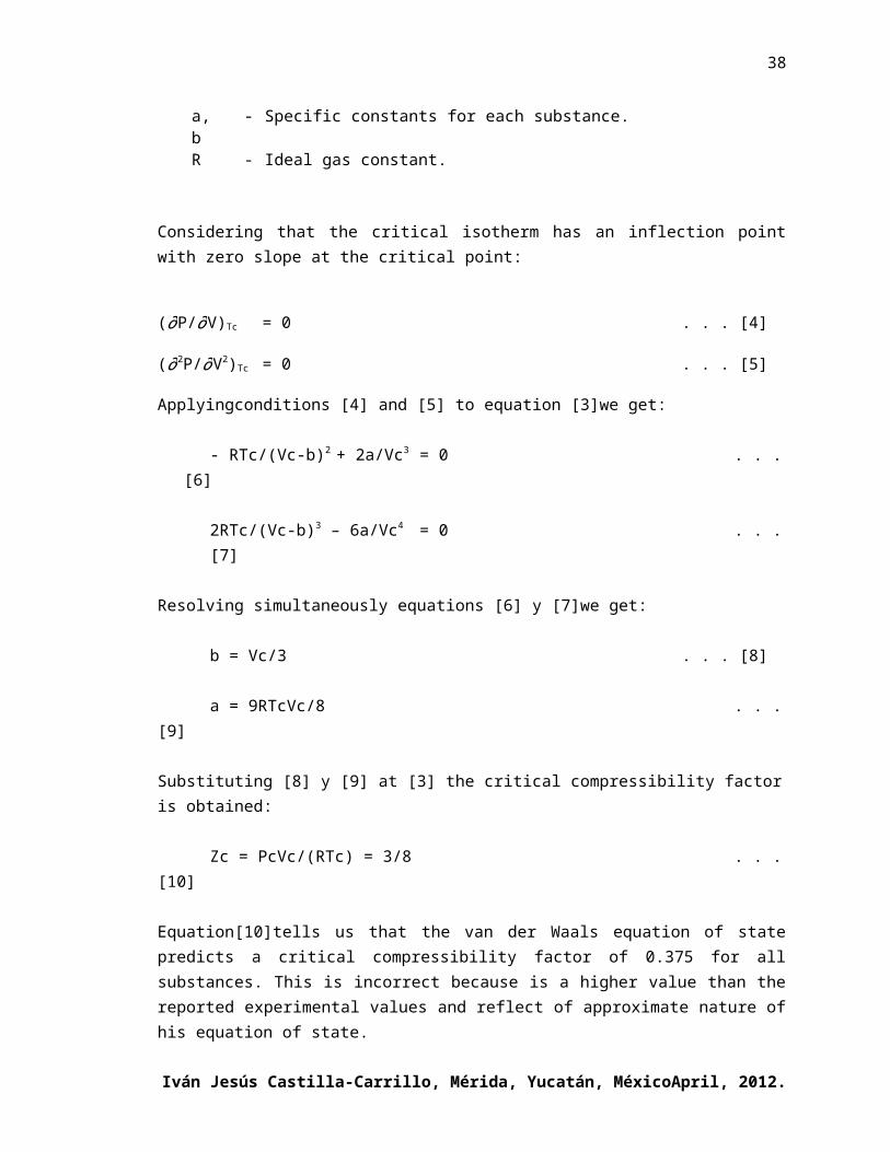
Where:P - Absolute pressure.V - Molar volume.T - Absolute temperature.a,b

- Specific constants for each substance.

R - Ideal gas constant.

Constant “a” varies according to attractive intermolecular forcesof each substance. Constant “b” is a measure of the “excluded”volume, occupied by the molecules, which is not available for themolecular movement.

But, how do we get to the theorem of corresponding states?

Let us clear P from the equation [1]

P = RT/(V-b) – a/V2 . . .[2]

Let us apply the equation at the critical point;

Pc = RTc/(Vc-b) – a/Vc2

. . . [3]

Where:Pc - Critical pressure.Vc - Critical volume.Tc - Critical temperature.


38

a,b

- Specific constants for each substance.

R - Ideal gas constant.

Considering that the critical isotherm has an inflection pointwith zero slope at the critical point:

(∂P/∂V)Tc = 0 . . . [4]

(∂2P/∂V2)Tc = 0 . . . [5]

Applyingconditions [4] and [5] to equation [3]we get:

- RTc/(Vc-b)2 + 2a/Vc3 = 0 . . .[6]

2RTc/(Vc-b)3 – 6a/Vc4 = 0 . . .[7]

Resolving simultaneously equations [6] y [7]we get:

b = Vc/3 . . . [8]

a = 9RTcVc/8 . . .[9]

Substituting [8] y [9] at [3] the critical compressibility factoris obtained:

Zc = PcVc/(RTc) = 3/8 . . .[10]

Equation[10]tells us that the van der Waals equation of statepredicts a critical compressibility factor of 0.375 for allsubstances. This is incorrect because is a higher value than thereported experimental values and reflect of approximate nature ofhis equation of state.


39

Substituting [8] and [9] in [1];

(P+(9RTcVc/8)/V2) (V-Vc/3) = RT . . .[11]

Dividing both sides between Pc y Vc:

(P/Pc + (9RTcVc/(8Pc))/V2) (V/Vc-1/3) =RTc/(PcVc). . . [12]

Substituting Zc = PcVc/(RTc)and re-arranging:

(P/Pc+9(1/Zc)(Vc/V)2/8)(V/Vc-1/3) = (T/Tc)(1/Zc). . . [13]

Multiplying both sides by Zc;

(Zc(P/Pc)+9(Vc/V)2/8)(V/Vc-1/3) = T/Tc. . . [14]


40

Defining the reduced conditions as the relation between thetemperature, pressure or volume of the system and thecorresponding one in the critical point:

Pr = P/Pc . . . [15]Tr = T/TcVr = V/Vc

Where:Pr - Reducedpressure.Tr - Reducedtemperature.Vr - Reduced volumen.

Substituting deffinitions [15] in [14];

(ZcPr+9/(8Vr2))(Vr-1/3) = Tr. . . [16]

Since Zc has a unique value of 3/8 for all substances, equation[16]is a generalized function which contains only 2 independentvariables.

As of this moment, the two-parameter CSP takes the followingform:

G = G(Tc,Pc) or also . . .[17]G = G(Tr,Pr) sinceTr = T/Tc Pr = P/Pc

Where:G - Any correlatable property using the Corresponding

State Principle (CSP).Tc - Critical temperature.Pc - Critical pressure.Tr - Reducedtemperature.Pr - Reducedpressure.T - Temperature.P - Pressure.


41

The importance of equation [16] resides in the formalestablishment of the two-parameter CSP which in its more generalform tells us:

“ALL SUBSTANCES AT THE SAME CONDITIONS OF REDUCED TEMPERATURE ANDPRESSURE WILL HAVE THE SAME REDUCED VOLUME”.

In other words, equation [16] establishes that the reduced volumeis only a function of reduced temperature and of reducedpressure. There are other opinions about the shape of thefunction since this, from its origin is approximate.

Once formally established, CSP began to be utilized to predictand correlate the behavior of substances. Soon, practicingdemonstrated that this works with good precision for very fewsubstances.In 1939, Pitzer(35) explained the limited predictive capacity ofCSP. In the first part of his work, demonstrated that the twoparameter CSP, equation [17], only works for spherical moleculessuch as Argon, Krypton and Xenon. For substances that follow thetwo parameter CSP behavior, he proposed the name of “perfectliquids”.In the second part of his work, Pitzer (35)explainedwhy substances that have more complex molecules deviate from thisbehavior and propose for them the name of “imperfect liquids”.

It is from this moment (1939) that from a scientific point ofview, establishing the need to add additional CSPcharacterization parameters if it is wished to apply it to morecomplex fluids than Argon, Krypton y Xenon.


42

III. THE THREE-PARAMETER CORRESPONDING STATES PRINCIPLE(CSP).

When considering different substances (more complex) than Argon,Krypton and Xenon results that the behavior established by theequation [17], is inadequate for describing their properties.The physical properties of the interest substances cannot becorrelated only with Tc and Pc.In order to try and extend the application of the correspondingstates principle (CSP) to more complex substances, attempts weremade to add more characterization parameters to the basicparameters Tc and Pc already existing.

1. CSP proposed by Meissner y Seferian.One of the first CSP extensions was proposed by Meissner ySeferian(28). They observed that the critical compressibilityfactor should be identical for all substances if the reducedvolume was in reality a two parameter function, but not beingthe case, the consideration of a unique compressibility factorutilized on van der Waals equation to reach the formal CSPproposition, is basically incorrect. It is for this reason,they proposed the compressibility factor at the critical pointas a third characterization parameter to be used inconjunction with the critical temperature and criticalpressure.

Zc = PcVc/(RTc) . . .[18]

Where:Zc - Compressibility factor at the critical point.Pc - Critical pressure.Vc - Critical volumen.R - Constant volume.The ideal gas.Tc - Critical volumen.

Later on, Lydersen, Greenkorn y Hougen(27), used the criticalcompressibility factor as a third-parameter to develop


43

generalized correlations.These correlations are presented in atabular form as well as graphics and include the densitiescalculation and thermodynamic derived properties, based uponthe formal extension proposition:

G = G(Tc,Pc,Zc) or else . . .[19]G = G(Tr,Pr,Zc) sinceTr = T/Tc Pr = P/Pc


44

The work of Lydersen, Greenkorn and Hougen(27) extends theapplication of the corresponding state principle and improvesthe prediction of the previous correlations, but the fact ofusing the critical compressibility factor as a third parameterhas its drawbacks;1. The critical compressibility does not change regularly with

the molecular size-shape and polarity therefore they are notproperly characterized.

2. The inherent experimental error during the critical volumedetermination.

The introduction of Zc as third parameter attempts to correctthe three-parameter CSP deviations due to molecular size-shapeand polarity, because in the development of theircorrelations, Lydersen, Greenkorn y Hougen (27) usedindiscriminately all kinds of “imperfect liquids”, this isnon-polar substances, polar ones and hydrogen bonding.Thisincreases the generality of the method but decreasesaccuracy.The accuracy of the Lydersen, Greenkorn and Hougen(27) method is good in the critical region, but decreases awayfrom it.

2. CSP proposed by Riedel.Riedel(41), proposed a third parameter based on the slope ofthe reduced vapor pressure curve at the critical point.

αc = dLn Pr’/dLnTr | Tr=Pr=1 . . .[20]

Where:αc - Compressibility factor at the critical point.Pr’

- Reduced vapor pressure.

Tr - Reduced temperature.Pr - Reduced pressure.

With the extension proposed by Riedel(41), the correspondingstates principle (CSP) takes the following form:


45

G = G(Tc, Pc, αc) or else . . . [21]G = G(Tr,Pr, αc) sinceTr = T/Tc Pr = P/Pc

Riedel developed tabular correlations and graphics for theprediction of vapor pressures, vaporization enthalpies,surface tension and thermal conductivities as functions ofthese three-parameters (41,42,43,44). These tables were madefor hydrocarbons; polar and hydrogen bonding compounds werenot included. Although these tables are less general than thetables from Lydersen, Greenkorn and Hougen(27), they are moreaccurate for non-polar compounds.


46

3. CSP proposed by Pitzer.Pitzer et al(36,37)developed a third parameter that accordingto their work, only takes in consideration the deviations dueto molecular size-shape.He called this parameter the acentricfactor, which was defined in terms of the deviation of base 10logarithms from the reduced vapor pressure calculated by thetwo parameter CSP (simple fluid) with respect to theexperimental vapor pressure at a reduced temperature of 0.7.

ω = log Pr’(0) (Tr=0.7)-log Pr’exp (Tr=0.7). . . [21.1]

The two-parameter CSP predicts a reduced vapor pressure forsimple fluids of 0.1 at a reduced temperature of 0.7 and theequation takes the form that we all know:

ω = -log Pr’exp (Tr=0.7) – 1. . . [22]

Where:ω - Acentric factor.Pr’exp

- Experimental reduced vapor pressure.

Tr - Reduced temperature.

Pitzer selected the vapor pressure to define his third parameter because the effects of molecular interaction are more pronounced in the change of phase of vapor-liquid.

With Pitzer third parameter, CSP takes the following form:G = G(Tc, Pc, ω) or else

. . . [23]G = G(Tr,Pr, ω) sinceTr = T/Tc Pr = P/Pc

Curl and Pitzer (6) and Pitzer et al (36,37,38,and 39)developed extensive tabular correlations for the prediction offugacity, enthalpies, entropies, compressibility factors and


47

vapor pressures.Correlations have the form of a term thatconsiders a two parameter CSP plus the acentric factormultiplying to a term that is considered as the contributionor correction due to the molecular size-shape.

For the case of the prediction of the compressibility factor,the correlation takes the following form:

= Z(0)(Tr,Pr)+ ωZ(1)(Tr,Pr) . . .[24]


48

Where:Z(0)

(Tr,Pr)- Universal or generalized compressibility

factor, the fluid being under study as a simplefluid.

ω - Pitzer acentric factor, ec. [22].Z(1)

(Tr,Pr)- Universal or generalized function for the

correction of the deviations due to molecularsize-shape.

Pitzer also defined a new name for the “perfect liquids”mentioned in his previous work, he called them “simple fluids”and the “imperfect liquids” whose deviations to the behaviorof the simple fluid is attributed to its molecular size-shapehe called them “normal fluid”. These names anddefinitions are still valid and its use is common today.

To have a definition of the normal fluids, Curl y Pitzer basedupon Riedel observations (42), presented the followingequation:

σoVo2/3/Tc = 1.86 + 1.18ω . . .

[25]

Where:σo - Hypothetical superficial tension at absolute zero

degrees (dina/cm).Vo

2/

3- Hypothetical molar volume at absolute zero degrees

cm3/mol).

The hypothetical superficial tension and hypothetical molarvolume necessary in the equation [25]are calculated using anexperimental superficial tension point and another of anyavailable Tr density and the tables presented by Curl andPitzer(6). If the value obtained at evaluating the right side of theequation [25]has a maximum deviation of 5% with respect to thepredicted one at the left side the fluid may be considered asa “normal fluid”.


49

Curl and Pitzer correlations (36,37,38, 39 and 6)for vaporpressures, enthalpies of vaporization, vaporization entropies,fugacity, enthalpies and entropies have been extended at lowerreduced temperatures by Carruth and Kobayashi (5) due to itsample acceptance in the oil industry.The correlation forcompressibility factors has been extended to very high reducedtemperatures and pressures.Besides the wide acceptance of the correlations from Curl andPitzer (6) and Pitzer et al(36,37, 38 and 39)the thirdparameter proposed by Pitzer has shown to be useful in othercorrelations. For example, el acentric factor has been used inthe correlation and prediction of the constants of manyequations of state.

A revision of acentric factors basedon the original definitionby Pitzer was developed by Passut and Danner (33).


50

a. Modificationby Lee-KeslerLee and Kesler (25) modified the Pitzer’s three-parameter CSP as follows:

Z = Z(0) + ω/ω(r) (Z(r)-Z(0)). . . [25.1]

Where:Z - Compressibility factor predicted by theLee-Kesler

three-parameter CSP. Z(0

)- Compressibility factor for the fluid considered

as a simple fluid.ω - Pitzer’s acentric factor.ω(r

)- Pitzer’s acentric factor for a reference fluid

(r) of non-spherical molecules.A value of 0.3978 was granted, corresponding to the acentric factorof n-octane.

Z(r

)- Experimental compressibility of the referenced

fluid (r).

The three-parameter modification to the CSP proposed by Lee-Kesler, equation [25.1] provides more exact predictionsthan Pitzer’s model, since it effects an interpolation whenthe fluid has an acentric factor comprised in the 0 <ω <ω(r)

interval and extrapolations for every fluid whose acentricfactor is ω> ω(r).Lee and Kesler (35) developed an analytical representationof the tabular correlations developed by Pitzer and hiscollaborators.

Yuh-Jen and Lu (57) developed a tabular correlation for thecompressibility factor , apparently more precise than theone proposed by Lee-Kesler (25).

It’s very important to mention that Lee-Kesler did not useequation [25.1]in the development of their correlation forvapor pressure.


51


52

b. Modification by Teja.Teja(51) proposed a modification to the three-parameter CSPthat uses two non-spherical reference fluids (r1) y (r2) andhas the following form.

Z = Z(r1) + (ω- ω(r1)) /( ω(r2) - ω(r1)) (Z(r2) -Z(r1)). . . [25.2]

Where:Z - Compressibility factor predicted by Teja three-

parameter CSP.Z(r

1)- Compressibility factor for the r1 reference

fluid.ω - Pitzer acentric factor of the interest fluid or

under study.ω(r

1)- Pitzer acentric factor for a reference fluid (r1)

on non-spherical molecules.ω(r

2)- Pitzer acentric factor for a reference fluid (r2)

of non-spherical molecules.Z(r

1)- Experimental compressibility factor for the fluid

of reference (r1).Z(r

2Experimental compressibility factor of the fluid of reference (r2).

The fluid of reference (r1) must have a minor acentricfactor than the fluid of interest or under study. The fluid of reference (r2) must have a major acentricfactor than the fluid of interest or under study.

In such a way that ω(r1)<ω<ω(r2).

So far I have not found in the open literaturerecommendations about generalized values of some propertyfor the (r1) and (r2) fluids.

The correlative and predictive of Teja’s model (51) appearsto be good according to Sorner work (66)who used it tocorrelate vapor pressures of 15 different compounds,including methane; ethane; propane; n-butane; neopentane;refrigerants and carbon tetrachloride.


53

The average of absolute deviation was of 0.46%.

From my point of view, Teja’s model (51) is rather aparticularization of the CSP for families of compounds,thana generalization of the three-parameter CSP.


54

c. Modification by Castilla-Carrillo.In May 1983, I wrote the following (58):

It is necessary to eliminate or to minimize at maximum thedeviations resulting from the three-parameter CSP when it isapplied to normal fluids with a larger molecular weight toavoid carrying on the deviations obtained by the three-parameter CSP to the four-parameter one.

This idea is based on my own observations about thedeviations reported by the equation of vapor pressuredeveloped by Lee-Kesler (25) using the Pitzer three-parameter CSP (36,37,38 y 39) when applied to heavier normalfluids.These deviations can be clearly appreciated in page 35 of(58), which I am copying and adapting as follows:

Component No.CarbonAtoms

Acentric

factor

AAD%Lee-

KeslerMethane 1 0.0077 0.66Ethane 2 0.0958 1.00n-propane 3 0.1511 1.18n-butane 4 0.1985 1.14n-pentane 5 0.2526 2.40n-hexane 6 0.3008 2.41n-heptane 7 0.3509 1.94n-octane 8 0.3974 2.41n-nonane 9 0.4517 1.64n-decane 10 0.5011 1.50n-undecane 11 0.5539 1.81n-dodecane 12 0.6073 2.14n-tridecane 13 0.6614 2.62n-tetradecane

14 0.7150 3.11

n-pentadecane

15 0.7708 3.63

n-hexadecane

16 0.8260 4.17


55

n-heptadecane

17 0.8847 5.90

n-octadecane

18 0.9361 6.46

n-nonadecane

19 0.9892 7.87

n-eicosane 20 1.0471 9.10Table 1. Deviations presented by Lee-Kesler’s equation for

vapor pressurePrediction for C1 to C20 linear hydrocarbons.

AAD% = 100/N Σ abs [(P’r calc – P’r exp)/P’r exp]


56

My observations are as follows:1.

The acentric factor increases as the size of the linealchain increases and consequently the molecular weight,which makes us conclude that the effects of size-shapeare appropriately characterized by it; however, thedeviations also increase as the molecular size andweight increases.

2.

If the acentric factor correctly characterizes themolecular size-shape, the correction function is theonly responsible for the deviations.

In his original work Pitzer (36,37) proposes a three-parameter CSP for normal fluids and show us an equation thathas been inadvertently overviewed by all, and is thesolution to this problem:

Z = Z(0) + ω(∂Z(1)/∂ω) . . .[25.3]

Which later Pitzer converted it in the expression we know:

Z = Z(0) + ωZ(1) . . .[25.4]

Equation 25.3 is an exact mathematical expression and itsdeviation should be 0% for normal fluids, if they follow thethree-parameter CSP proposed by Pitzer and if thefunction(∂Z(1)/∂ω) is expressed in the right way.

Equation 25.4 is a simplification and a way to expressequation 25.3 but is not the right one since it presentsdeviations shown on Table 1.

Based on observations 1 and 2 on deviations shown on table1, the equation [25.3] from the work of Pitzer and themodifications proposed by Lee-Kesler (25) and Teja (51), Iproposed in 1983 (58) the following equation:

Z = Z(0) + ωZ(1)(ω) . . .[25.5]


57

Where:Z - Compressibility factor predicted by Teja’s

three-parameter CSP for the fluid under study.Z(0) - Compressibility factor for the simple fluid.

Is the same one from Pitzer proposal for athree-parameter CSP, or the same one proposedby Van der Waals.

ω - Pitzer acentric factor.Z(1)

(ω)- Correction for molecular size-shape

deviations.This function is different for eachacentric factor because is a function ofthis.


58

Applying the proposed equation [25.5] to calculate vapor pressures, we have:

Ln Pr’ = LnPr’(0)(Tr)+ ωLn Pr’(1)(Tr,ω). . . [25.6]

Where:

Ln Pr’(0)

(Tr)= -5.928773 (1/Tr -1) -1.018383 Ln Tr +

0.1346956 (Tr7 -1)

. . . [25.7]

ω - Pitzer’s acentric factor calculated according to equation (22).

Ln Pr’(1)

(Tr,ω)= - (14.91911 + 2.568562 ω) (1/Tr -1)

- (12.60737 + 4.373356 ω) Ln Tr+ (0.4271343 + 0.5203998 ω) (Tr7 -1)

. . . [25.8]

The three-parameter CSP I proposed in equations[25.5, 25.6,25.7 y 25.8]is an improvement to the one proposed byPitzer(35, 36, 37, 38 and 39).The improvement consists inthat the correction function changes with the molecularsize-shape.In other words, the correction function is notonly one as suggested by Pitzer, or interpolations between 2fluids (one spherical and another one of reference (r))assuggested by Lee-Kesler(25) nor interpolations eitherbetween 2 non-spherical reference fluids as suggested byTeja(51 y 52).


59

It is a continuous correction function that changes with themolecular size-shape and it works very well. Maybe it lackssome mathematical refinements but this is the general form.

The percentage of average absolute deviations (AAD) gottenin the calculation of the reduced vapor-pressure of n-alkanes from C1 to n-C20 can be appreciated in Table2. Inall cases the proposed model (58) was more accurate than theLee-Kesler (25).



60

In my original work (58),table 1 (pages 39 and 40) thefollowing deviations can be appreciated:

Component No.CarbonAtoms

Acentricfactor

AAD%Lee-Kesler

AAD%Castilla-Carrillo

Methane 1 0.0077 0.66 0.38Ethane 2 0.0958 1.00 0.66n-propane 3 0.1511 1.18 0.73n-butane 4 0.1985 1.14 0.47n-pentane 5 0.2526 2.40 0.76n-hexane 6 0.3008 2.41 0.68n-heptane 7 0.3509 1.94 0.41n-octane 8 0.3974 2.41 0.88n-nonane 9 0.4517 1.64 0.44n-decane 10 0.5011 1.50 0.56n-undecane 11 0.5539 1.81 0.39n-dodecane 12 0.6073 2.14 0.33n-tridecane 13 0.6614 2.62 0.41n-tetradecane

14 0.7150 3.11 0.36

n-pentadecane

15 0.7708 3.63 0.42

n-hexadecane

16 0.8260 4.17 0.31

n-heptadecane

17 0.8847 5.90 0.33

n-octadecane

18 0.9361 6.46 0.31

n-nonadecane

19 0.9892 7.87 0.53

n-eicosane 20 1.0471 9.10 0.57Table2.Deviations from the models by Lee-Kesler and Castilla-Carrillo for vapor pressure prediction of C1 to C20linear hydrocarbons. Data for critical temperature(Tc), critical pressure (Pc) and experimental pointsfor reduced vapor pressure at Tr=0.7 were taken fromthe work of Gomez-Nieto and Papadopoulos (13).ThePitzer acentric factor(ω) was calculated using itsoriginal definition Eq.[22].


61

The most precise generalized equation available in 1983, forcalculation or prediction of vapor pressure, was the Lee-Kesler (25). The percentage average absolute deviations (AAD%) ranges from 0.66% for methane to 9.10% for n-eicosane,while the proposed model deviations ranges from 0.38% formethane to 0.57% for n-eicosane.

The AAD% for reduced vapor pressure calculation orprediction to 98 simple and normal fluids including somenoble gases, n-alkanes, iso-alkanes, cyclo-alkanes, n-alkenes, iso-alkenes, n-alkenes, alkynesand aromatics for5,931 experimental data points, is 0.76%.In all cases the proposed model(58)was more accurate thanthe model from Lee-Kesler (25).


Used data and deviations are shown in Table 2.1Component Tc

KPcAtm

ωFacAc

IntervalTr

No.of

Points

AAD%L-K

AAD%Prop

Ref.

Argon 150.60

48.00

-0.001

7

0.56-1.0

171 0.27 0.25 101, 102

Krypton 209.40

54.17

-0.001

3

0.55-1.0

95 0.48 0.33 101, 102

Xenon 289.75

57.64

0.0030

0.56-1.0

74 0.22 0.18 101, 102

Methane 191.04

46.06

0.0077

0.47-1.0

182 0.66 0.38 101, 102

Ethane 305.44

48.20

0.0958

0.43-1.0

138 1.00 0.66 101, 102

n-Propane 369.98

42.01

0.1511

0.45-1.0

160 1.18 0.73 101, 102

n-Butane 425.18

37.47

0.1985

0.46-1.0

104 1.14 0.47 101, 102

n-Pentane 465.79

33.31

0.2526

0.44-1.0

127 2.40 0.76 101, 102


62

n-Hexane 507.87

29.94

0.3008

0.48-1.0

152 2.41 0.68 101, 102

n-Heptane 540.18

27.00

0.3509

0.50-1.0

155 1.94 0.41 101, 102

n-Octane 569.37

24.54

0.3974

0.47-1.0

133 2.41 0.88 101, 102

n-Nonane 593.80

22.60

0.4517

0.53-0.76

51 1.64 0.44 101, 102

n-Decane 616.10

20.70

0.5011

0.54-0.77

50 1.50 0.56 101, 102

n-Undecane 636.00

19.18

0.5539

0.55-0.78

50 1.81 0.39 101, 102

n-Dodecane 653.90

17.83

0.6073

0.56-0.80

52 2.14 0.33 101, 102

n-Tridecane 670.10

16.64

0.6614

0.57-0.81

45 2.62 0.41 101, 102

n-Tetradecane 684.90

15.58

0.7150

0.58-0.82

42 3.11 0.36 101, 102

n-Pentadecane 698.20

14.64

0.7708

0.59-0.83

41 3.63 0.42 101, 102

n-Hexadecane 710.40

13.79

0.8260

0.60-0.84

47 4.17 0.31 101, 102

n-Heptadecane 721.30

13.14

0.8847

0.60-0.84

31 5.90 0.33 101, 102

n-Octadecane 731.20

12.31

0.9361

0.61-0.85

31 6.46 0.31 101, 102

n-Nonadecane 740.30

11.67

0.9892

0.62-0.86

31 7.87 0.53 101, 102

n-Eicosane 748.70

11.09

1.0471

0.63-0.87

31 9.10 0.57 101, 102

2-Methyl propane

409.20

36.36

0.1787

0.46-0.68

40 2.02 0.37 101, 102

2-Methyl butane 460.56

33.48

0.2288

0.47-0.70

51 2.88 0.73 101, 102

2,2-Dimethyl propane

433.00

31.74

0.2060

0.59-0.70

21 1.08 0.14 101, 102

2-Methyl pentane

498.70

29.98

0.2723

0.48-0.72

45 1.41 0.55 101, 102

3-Methyl pentane

504.00

31.40

0.2827

0.48-0.71

45 2.64 1.07 101, 102

2,2-Dimethyl butane

491.14

30.94

0.2235

0.47-0.70

51 2.34 0.68 101, 102


63

2,3-Dimethyl butane

500.52

31.43

0.2510

0.48-0.71

44 2.55 0.65 101, 102

2-Methyl hexane 532.20

26.99

0.3178

0.49-0.73

51 1.69 0.64 101, 102

3-Methyl hexane 535.42

28.05

0.3264

0.50-0.73

51 2.38 0.47 101, 102

3-Ethyl pentane 541.10

29.21

0.3168

0.49-0.73

49 2.62 0.59 101, 102

2,2-Dimethyl pentane

519.76

28.00

0.3005

0.49-0.73

49 2.39 0.99 101, 102


537.87

29.28

0.3011

0.49-0.72

51 2.84 0.77 101, 102


522.27

27.10

0.3064

0.49-0.73

50 2.64 0.64 101, 102


536.52

30.19

0.2774

0.48-0.72

50 2.80 1.50 101, 102

2,2,3-Trimethylbutane

533.66

29.93

0.2452

0.47-0.71

50 2.87 0.83 101, 102

2-Methyl heptane

556.96

24.69

0.4038

0.51-0.75

51 3.23 1.49 101, 102

3-Methyl heptane

564.02

25.42

0.3722

0.51-0.74

51 1.70 0.38 101, 102

4-Methyl heptane

562.01

25.33

0.3729

0.51-0.74

31 1.51 0.42 101, 102

Table 2.1 Used data and deviations by the Lee-Kesler (25)and proposedmodels(58) for vapor pressures of 98 fluids and 5931 points.Component Tc

KPcAtm

ωFacAc

IntervaloTr

No.Puntos

AAD%L-K

AAD%Prop

Ref.

3-Ethyl hexane 566.60

26.22

0.3598

0.50-0.74

31 1.52 0.45 101, 102

2,2-Dimethyl hexane 550.27

25.32

0.3412

0.50-0.74

31 1.56 0.37 101, 102


26.35

0.3412

0.50-0.73

31 1.42 0.55 101, 102


25.43

0.3378

0.50-0.74

31 0.99 0.93 101, 102


24.86

0.3663

0.50-0.74

31 2.15 1.07 101, 102


26.81

0.3198

0.50-0.72

31 2.92 1.01 101, 102


64


27.24

0.3517

0.50-0.73

31 2.80 1.06 101, 102

2-Methyl, 3-ethyl pentane

568.30

27.24

0.3298

0.50-0.72

31 1.86 0.29 101, 102

3-Methyl, 3-ethyl pentane

577.71

28.84

0.3095

0.49-0.72

31 2.92 1.60 101, 102

2,2,3 Trimethyl pentane

566.68

27.86

0.2904

0.49-0.72

31 2.46 0.63 101, 102


543.64

25.64

0.3087

0.49-0.73

51 2.33 0.56 101, 102


567.91

27.46

0.3120

0.49-0.73

51 2.01 0.27 101, 102


567.12

29.34

0.3077

0.67-0.72

17 1.22 0.53 101, 102

Etene 283.10

50.30

0.0843

0.42-1.00

82 0.97 0.92 101, 102

Propene 365.00

45.60

0.1419

0.44-1.00

61 1.09 0.91 101, 102

1-Butene 419.60

39.70

0.1902

0.43-1.00

61 1.31 0.68 101, 102

2 cis-Butene 435.20

40.90

0.2020

0.46-0.68

44 1.86 0.90 101, 102

2 trans-Butene 430.20

41.20

0.2083

0.46-0.68

46 4.02 1.60 101, 102

1-Pentene 464.20

34.95

0.2407

0.47-0.70

39 2.81 0.87 101, 102

2 cis-Pentene 474.80

35.95

0.2494

0.47-0.72

45 1.84 0.23 101, 102

2 trans-Pentene 473.90

35.88

0.2483

0.47-0.72

45 1.85 0.25 101, 102

1-Hexene 503.80

31.22

0.2856

0.48-0.71

44 2.21 0.36 101, 102

1-Heptene 537.50

28.11

0.3311

0.47-0.73

51 2.08 0.39 101, 102

1-Octene 566.80

25.50

0.3785

0.51-0.74

49 1.57 0.54 101, 102

Propadiene 385.86

52.37

0.1845

0.45-0.67

31 5.47 4.60 101, 102

1,2-Butadiene 450.98

45.36

0.1986

0.45-0.67

31 2.87 1.17 101, 102

1,3-Butadiene 425.20

42.80

0.1934

0.38-1.00

60 2.47 0.83 101, 102


65

1,2-Pentadiene 491.92

38.87

0.2390

0.47-0.70

31 1.73 1.11 101, 102

1,3 cis-Pentadiene 485.71

38.54

0.2717

0.47-0.70

31 3.24 1.49 101, 102

1,3 trans-Pentadiene

485.62

38.19

0.2457

0.47-0.70

31 2.19 0.64 101, 102

1,4 Pentadiene 458.00

36.90

0.2556

0.42-0.70

43 3.60 1.67 101, 102

2,3 Pentadiene 492.12

39.42

0.2838

0.48-0.70

31 2.39 0.63 101, 102

Etine 309.65

61.60

0.1823

0.62-1.00

42 1.32 0.49 101, 102

Propine 391.75

47.58

0.2577

0.47-0.81

33 3.00 1.27 101, 102

1-Butine 436.63

43.86

0.2661

0.44-0.69

45 3.42 0.61 101, 102

2-Butine 471.33

47.25

0.2487

0.51-0.68

27 2.34 0.41 101, 102

1-Pentine 474.76

37.78

0.3042

0.48-0.70

28 2.83 0.85 101, 102

2-Pentine 504.06

39.62

0.2833

0.47-0.70

28 2.77 0.75 101, 102

Cyclopropane 401.70

57.00

0.1153

0.45-0.70

14 2.27 1.48 101, 102

Cyclobutane 464.40

50.29

0.1579

0.43-0.62

22 2.86 0.58 101, 102

Cyclopentane 512.10

44.60

0.1972

0.44-1.00

58 2.23 0.50 101, 102

Table 2.1 (Continuation).Used data and deviations by theLee-Kesler (25)and proposed models(58)for vapor pressures of 98 fluids and 5931 points.

Component TcK

PcAtm

ωFacAc

IntervaloTr

No.Puntos

AAD%L-K

AAD%Prop

Ref.

Methyl cyclopentane 534.20

37.44

0.2238

0.46-0.70

47 1.58 0.72 101, 102

Ethyl cyclopentane 570.80

33.56

0.2643

0.48-0.70

51 2.07 0.38 101, 102

Cyclohexane 553.20

39.80

0.2123

0.51-1.0

108 1.29 0.93 101, 102

Methyl cyclohexane 570.90

34.18

0.2447

0.47-0.70

51 2.57 0.38 101, 102


66

Ethyl cyclohexane 603.40

30.90

0.2992

0.49-0.72

38 2.57 0.59 101, 102

Cycloheptane 593.20

36.30

0.2970

0.57-0.73

16 3.29 2.17 101, 102

Cyclooctane 626.10

33.07

0.3740

0.59-0.75

16 4.72 3.56 101, 102

Benzene 562.20

48.50

0.2132

0.49-1.0

143 1.20 0.65 101, 102

Toluene 593.50

41.36

0.2590

0.47-1.0

108 1.79 0.80 101, 102

Ethylbenzene 621.10

36.31

0.2886

0.48-0.70

51 2.47 0.70 101, 102

o-Xylene 632.10

36.83

0.2990

0.48-0.70

51 1.69 0.79 101, 102

m-Xylene 620.10

36.01

0.3151

0.49-0.71

51 2.25 0.67 101, 102

p-Xylene 618.20

35.01

0.3119

0.49-0.71

51 2.57 0.42 101, 102

Naphthalene 749.70

39.10

0.2909

0.48-0.70

47 1.98 1.08 101, 102

1-Methylnaphthalene 769.30

34.39

0.3519

0.49-0.72

48 2.54 0.21 101, 102

2-Methylnaphthalene 764.30

34.39

0.3488

0.49-0.72

48 1.75 0.76 101, 102

Table 2.1 (Continuation)Used data and deviations by theLee-Kesler (25)and proposedmodels(58) for vapor pressures of 98 fluids and 5931 points. Datafor critical temperature (Tc), critical pressure (Pc) andexperimental points for reduced vapor pressure at Tr=0.7 were takenfrom the work of Gomez-Nieto and Papadopoulos (13). The Pitzeracentric factor(ω) was calculated using its original definition Eq.[22].

Based on deviations from tables 2 y 2.1 we can concludethat:


67

1. The proposed model meets the accuracy requirements bydesigners of new products, designers of plants and newprocesses.

2. Estimated or correlated data values can be used inequipment sizing.

3. The three-parameter CSP does not add or carry deviationsto the four-parameter CSP.


68

(PAGE INTENTIONALLY

LEFT IN BLANK)


69

IV. THE FOUR-PARAMETER CORRESPONDING STATES PRINCIPLE (CSP)1.CSP proposed by Eubank y Smith.

One of the first four-parameter CSP was developed by Eubank ySmith (9). They developed compressibility factors andenthalpies correlations at the vapor phase.The method wasdeveloped as an extension of the Pitzer et al (36 y37).Correlations developed by Curl and Pitzer (36, 37, 38 y 39)were used to take into account the spherical moleculesproperties (simple fluid)and the deviations of size-shape(normal fluid). Due to that the polar molecules exhibit muchlarger acentric factors than the one that could indicate itssize-shape measure, the homomorph idea was used.This idea wasoriginally proposed by Bondi and Simkin (4). The acentricfactor of polar material is taken as the acentric factor ofits homomorph hydrocarbon.For example, the acentric factor ofethylic alcohol is that of the propane, which its homomorphhydrocarbon. Also, the critical properties of the homomorphare taken as the critical properties of the fluid under study.The fourth parameter, utilized to take into account theeffects of polarity, was determined as of the reduced dipolarmoment which is defined in terms of the Stockmayerintermolecular potential function.

μr = μ/(Єσ3)1/2 . . . [26]

Where:

μr - Reduced dipolar moment.Μ - Dipolar moment.Є,σ

- Constants of the Stockmayer intermolecularpotential function.

The fourth parameter was defined as:

P* = C μrn . . .

[27]

Where:


70

P - Fourth parameter proposed by Eubank and Smith.C - Specific constant for each substance.μr - Reduced dipolar moment. n - Exponent equal to 5/3.

For the case of compressibility factor, we have:

Z = Z(0)(Trh,Prh) + ωh Z(1)(Trh,Prh) + P*Z(2)(Tr,Pr). . . [27.1]

Trh = T/TchPrh = P/PchTr = T/TcPr = P/Pc

Where:

Z - Compressibility factor of the fluid under study orof interest.

Trh - Homomorph reduced temperature.Prh - Homomorph reduced pressure.Tch - Homomorph critical temperature.Pch - Homomorph critical pressure.Z(0) - Homomorph compressibility factor of the fluid under

study or of interest, considered as a simple fluid.ωh - Homomorph acentric factor.Z(1) - Function to correct the deviations due to

molecular size-shape effects presented by thehomomorph compressibility factor.

P* - Fourth parameter proposed by Eubank-Smith.Z(2) - Function to correct deviations due to molecular

polarity effects presented by the compressibilityfactor.

Tr - Reduced temperature.Pr - Reduced pressure.Tc - Critical temperature.Pc - Critical pressure.

Eubank and Smith’s CSP has the following form:

G = G(Tch, Pch, ωh, P*,Tc, Pc) or else. . . [28]


71

G = G(Trh, Prh,ωh, P*,Tr, Pr ) sinceTrh = T/Tch Prh = P/PchTr = T/TcPr = P/Pc

Eubank and Smith proposed extension represents an advance inthe application of the CSP to polar substances, but it has thefollowing drawbacks:

1. Arbitrariness of constant C, completely destroys therigorous theoretical image created while using thereduced dipolar moment.

2. The dipolar moment in itself is not completely ableof characterize the polar behavior.

3. No previsions were made for inorganic substances thathave a difficult to find homomorph, which limits thecorrelation to the polar substances that have ahomomorph hydrocarbon.

4. It is a CSP that uses six characterization parametersand even so, it does not work.

In spite of these inconveniences, Eubank and Smith’s (9) workhas the importance to be the first formal intent of extendingthe three-parameter CSP proposed by Pitzer, to four-parametersin order to try to include polar substances within the samecorrelational framework.

2. CSP proposed by Thompson.The best fundamentally based four-parameter CSP is the oneproposed byThompson (53), who observed the third parameterproposed by Pitzer (35,36,37,38 y 39) To characterize thebehavior of the normal fluids, could not be utilized forabnormal or polar fluids since it was not developed for thattask. It was developed to characterize the deviations ofmolecular size-shape, dominant in the normal fluids and thusit does not work to characterize the deviations presented inthe abnormal or polar fluids. In other words, Pitzer’sacentric factor calculated for abnormal or polar fluids,includes besides the deviations caused by the molecular size-


72

shape, deviations caused by molecular polarity.In an attemptto correlate these deviations, Thompson (53) developed a thirdparameter in terms of the molecular structure of thesubstances to which he called the “true acentric factor”.The “true acentric factor” was defined as a function of the“molecular modified geometrical radius of gyration”, which wasexpressed for molecules that have a three dimensionalconfiguration as:

R = (2π(ABC)1/3/M)1/2 . . .[30]

And for two dimensional molecules as:

R = (2π(AB)1/2/M)1/2 . . . [31]

Where:

R - Geometrical radius of gyration in angstroms.A,B,C

- Principal moments of inertia calculated using onlythe molecular configuration.

M - Molecular weight.

In the case of molecules with more than one structuralconfiguration, the inertia moments were taken as an averagevalue.Later on, Thompson developed a ω, acentric factor plot as ageometrical ratio function for normal fluids, obtaining thus acorrespondence between the radius of gyration and the “trueacentric factor” for the abnormal or polar fluids. Thisrelation is represented by the following equations:

ω = 0.01533 R + 0.00767R

for 0 <R< 3.5

ω = 0.115 R – 0.1885 for 3.5 <R< 6.0ω = 0.6775 + 0.04225 R –

2.58 / Rfor 6.0 <R

. . . [32]


73

Once developed, the third parameter in function, just of themolecular size-shape effects, the fourth parameter, tocharacterize the effects of polarity was defined as thedifference between the acentric factor value by Pitzer(36,37) and the “true acentric factor”.

τ = ω – ω . . .[33]

where:τ - The fourth parameter proposed by Thompson to

characterize the molecular polarity.ω - Pitzer’s acentric factor.ω - “True acentric factor” developed by Thompson.

In accordance with equation [33], the Pitzer acentric factorcalculated for polar substances is the sum of twocontributions: one contribution for size-shape and another forpolarity. For non-polar substances equation [33]is reducedto:

ω = ω . . . [34]

With the addition of the fourth parameter proposed byThompson(53), CSP takes the following form:G = G(Tc, Pc,ω, τ) or else

. . . [35]G = G(Tr,Pr,ω, τ) sinceTr = T/TcPr = P/Pc

To demonstrate the predictive capacity of the developedparameters, Thompson generalized the Frost-Kalkwarf(11)equation for the prediction of vapor pressures and developedan expression for the critical compressibility factorcalculation. Both equation have the following form:

G = G(0) + ωG(1) + τ G(2) + ωτ G(3)

. . . [36]

Where:G - Any correlatable property using the CSP.


74

G(0) - Property of the interest fluid or under studyconsidered as a simple fluid.

ω - “True acentric factor” developed by Thompson.G(1) - Function for correction of the deviations due to

molecular size-shape.τ - Fourth parameter developed by Thompson.G(2) - Function for the correction of deviations due to

molecular polarity.G(3) - Function for the correction of deviation of

inseparable size-shape-polarity.

The fourth parameter CSP proposed by Thompson is today thebest intent to correlate the deviations by molecular size-shape and the deviations by molecular polarity but it presentsthe following drawbacks:


75

1. The presence of a cross term that talks aboutinseparable effects of size-shape-polarity,contradicts the definition expressed by equation[33].

2. Data getting and processing data for molecularconfigurations is more complicated and costly thanthe experimental measurement of the interestproperty.

3. Thompson model predictions for vapor pressure arenot good.

3. CSP proposed for Halm-Stiel.In an attempt to characterize the behavior for polarcompounds, Halm-Stiel (15) Added an extra parameter to Pitzercorrelation (35 ,36 ,37 and 39). The extra or fourth parameterwas developed to correct the deviations presented by PitzerCSP when applied to polar substances and was defined in asimilar way to the acentric factor, being the basic differenceof base 10 logarithm of experimental reduced vapor pressureless base 10 logarithm of the reduced vapor pressure thatpredicts Pitzer CSP for normal fluids at a Tr = 0.6, this is:

χ = log10 Pr’ exp (Tr=0.6) – log10Pr’(n)(Tr=0.6). . . [37]

But:

– log10Pr’(n)(Tr=0.6) = 1.57ω + 1.552. . . [38]

Then:

χ = log10 Pr’ exp (Tr=0.6) + 1.57ω + 1.552. . . [39]

Where:


76

χ - Fourth parameter proposed by Halm-Stielto characterize the behavior of theabnormal or polar fluids.

log10 Pr’ exp

(Tr=0.6)- Base 10 logarithm of the experimental

reduced vapor pressure at a reducedtemperature of 0.6.

log10Pr’(n)

(Tr=0.6)- Base 10 logarithm of the reduced vapor

pressure calculated with Pitzer CSP ata reduced temperature of 0.6.

ω - Pitzer acentric factor.

With Halm- Stiel proposed fourth parameter, the CSP takes thefollowing form:

G = G(Tc, Pc, ω, χ) or else. . . [40]

G = G(Tr, Pr, ω, χ) sinceTr = T/TcPr = P/Pc

For the case of vapor pressure, Halm-Stiel proposed the following equation:

log10 Pr’= log10Pr’(0) + ω log10 Pr’(1) + χlog10 Pr’(2)

. . . [41]

Where:

log10

Pr’- Base 10 logarithm of the reduced vapor pressure

of the fluid under study or of interestpredicted by the CSP of Halm-Stiel.

log10

Pr’(0)- Base 10 logarithm of the reduced vapor pressure

of the fluid under study or of interestpredicted in the three-parameter CSP by Pitzer,considering the fluid as a simple fluid.

ω - Pitzer acentric factor.log10

Pr’(1)- Correction function that considers the fluid

under study or of interest as normal fluid.χ - Fourth parameter proposed by Halm-Stiel To

characterize the behavior of the abnormal orpolar fluids.

log10 - Correction function that considers the fluid


77

Pr’(2) under study or of interest as an abnormal orpolar fluid.

Halm-Stiel suggested that the polarity correction is necessaryonly at reduced temperatures below de 0.7 consequently, theterm log10Pr’(2)should be only used under these conditions. Atreduced temperatures higher than 0.7, the correlation of Halm-Stiel is identical to Pitzer.Halm-Stiel (15, 16, 17) developed tabular correlations for thevaporization entropy, liquid densities, saturated vapor andvirial coefficients.Yuan y Stiel (56) developed a correlation to calculatecalorific capacities at the saturation zone.Stipp, Bai y Stiel (47) developed tabular correlations tocalculate compressibility factors in the gaseous and liquidregions.Hung-Stiel (25) developed a correlation to calculate thesecond virial coefficient of polar fluids.Kalback-Starling (24) developed a generalizationof theequation of state by Lee-Keslerfor the calculation of thecompressibility factor in liquid phase, vapor or gas for polarfluids.These correlations are complex and have terms of mayor orderin ω and χ.For the case of the second virial coefficient we have:

B Pc/(RTc) = f(0)(Tr) + ω f(1)(Tr) + χ f(2)(Tr) + χ2f(3)(Tr) + ω6

f(4)(Tr) + ωχ f(5)(Tr). . . [42]

Many of the terms on equation [42] are irregular and cannot berepresented analytically in a simple form.The most important failure is that the χ parameter isincongruent in itself, since even inside the same group ofcompounds presents inconsistencies as in the case of alcohols.Alcohols have approximately the same dipolar moment (1.7 +/-0.03 Debyes), while χ has values of


78

0.037 for methanol, 0.003 for ethanol and -0.057 for n-propanol.

Also, a very polar component might have anχ = 0,parameter,while a non-polar compound might have an χ different thanzero.Finally the χ parameter is highly sensible to small errors inthe vapor pressure data utilized to calculate it.The complexities and inconsistencies due to the lack of acorrelational adequate surrounding are very clear in the four-parameter CSP by Halm-Stiel.

4. CSP proposed by Harlacher.Harlacher (18,19) revised the method of trying to provide asimplified calculation procedure and found a correspondencebetween the parachor defined by Sugden (48) and the Thompsonradius of gyration.

The parachor was defined by Sugden (48) as:

Pa = γ1/4 (M/(ρl - ρv)) . . .[43]

Where:Pa

- Parachor.

γ - Superficial tensión.M - Molecular weight.ρl - Density of a saturated liquid.ρv - Density of saturated vapor.

Later on, Quayle (40) developed a group contribution methodfor the calculation of the parachor. This procedure eliminatesthe need for equation (43) but it does not make differencesbetween isomers. For easy to calculate the parachor, Harlacher decided to useit to characterize the deviations for the molecules size-shape.


79

ω = a Pa + b . . .[44]

The fourth parameter was defined by equation [45]proposed byThompson:

τ = ω – ω . . .[45]Harlacher substituted equations [44] y [45]in equation [46]proposed also by Thompson.

G = G(0) + ωG(1) + τ G(2) + ωτG(3) . . .[46]

Arranging:

G = G(0) + a Pa G(1)’ + ωG(2) + ωPaG(3) – Pa2 G(3)’’

. . . [47]

G(1)’= G(1) - G(2)

G(3)’= a G(3)

G(3)’’= a2 G(3)

Where:G - Any correlatable property using CSP.G(0) - Universal function that considers the fluid under

study as a simple fluid.Pa - Parachor.ω - Pitzer acentric factor.a,b

- Are slope and intercept respectively of equation44.

G(1)

G(2)

G(3)

G(1)’

G(3)’

’

-----

Generalized or universal correction functionsnecessary in the Harlachermodel.


80

According to Harlacher the corresponding states principle hasthe following form:

G = G(Tc, Pc, ω, Pa) or else . . .[48]G = G(Tr, Pr, ω, Pa) sinceTr = T/TcPr = P/Pc

Harlacher (18, 19) developed correlations to calculate vaporpressures, critical compressibility factorsand densities ofsaturated liquid and vapor using the proposed extension.All his correlations are more complicated and less accuratethan those of Thompson, therefore are not used.

5. CSP proposed byPassut.Passut (31, 32) utilized the radius of gyration proposed byThompson directly as a third parameter. Because of the factthat the radius of gyration is strictly defined fromstructural considerations, the presence of polar effectstheoretically does not affect its magnitude.This provides apossibility for the separation and correlation of deviationscaused by the size-shape and polarity.Passut selected theFrost-Kalkwarf (11) equation as the base todefine his fourth parameter. The reduced form of Frost-Kalkwarf equation is:

Ln Pr’ = B (1-1/Tr) + C ln1/Tr + D (Pr’/Tr2 -1). . . [49]

Where:

Pr’ - Reduced vapor pressure.Tr - Reduced temperature.B,C

- Frost-Kalkwarf equation constants specific for eachsubstance.

D - Constant with a unique value of 0.4218


81

Passut eliminated the constant C forcing equation[49]to gothrough the normal boiling point.

C = (Ln Prb’ – B (1-1/Trb) – 0.4219 (Prb’/Tr2 -1)) / Ln 1/Trb. . . [50]

Subscript rb represents variables reduced in the normalboiling point.For normal paraffins, Passut represented constants B y C in ageneralized form, with less than 1% of deviation by theequations:

Bn = 4.6776 + 1.8324R – 0.03501 R 2 . . .[51]

Cn = 0.7751 Bn – 2.6354 . . .[52]

The subscript n means normal paraffins. For all othercompounds, the predicted constants by equations[51]and[52]arecorrected by association effects.

B = Bn + α1 . . . [53]

C = Cn + α2 . . . [54]

α1 y α2 are correction factors by association for Bn y Cn. Substituting equations [53] y [54]in equation [49] we have:

Ln Pr’ = (Bn + α1) (1-1/Tr) + (Cn + α2) ln 1/Tr + D (Pr’/Tr2 -1) . . . [55]

Then Passut defined his fourth parameter to which he called association factor as:

K = ((1-1/Tr) + α2 ln 1/Tr) / (1-1/Tr + ln 1/Tr). . . [56]

Combining equations[55]and[56], K is written as:


82

K = [Ln Pr’ – Bn (1-1/Tr) – Cn Ln 1/Tr - D(Pr’/Tr2 -1)] / [1 –1/Tr + Ln 1/Tr] . . . [57]

Applying equation 57 to the normal boiling point, the Kdefinition becomes:

K = [Ln Y – Bn (1-X) – Cn Ln X – 0.4218 (Y/X2 -1)] / [1 – X + Ln X] . . . [58]

Where:X = 1/TrbY = Pr’b

Constants of equation[49]for any fluid are given by:

B = 4.7016 + 1.9639R - 0.04971R2 + 0.4976K. . . [59]

C = 0.7272 + 1.7163R - 0.05925R2 + 0.3906K. . . [60]

According to Passut, CSP has the following form:

G = G(Tc, Pc, R,K) or else. . . [61]

G = G(Tr, Pr, R, K) sinceTr = T/TcPr = P/Pc

Using parameters Tc, Pc, R y K, Passut generalized the Frost-Kalkwarf equation with excellent results.He also utilized the proposed parameters to generalize thesecond virial coefficient of polar compounds, but theprecision of the correlation obtained is not good.The principal inconvenient of Passut model is that there isnot a direct significance for the K parameter, but is more afitting parameter.


83

The polar contribution to the configurational properties, itwas thought to be characterized by the deviations in theindividual coefficient of the Frost-Kalkwarf (11).These coefficients are parameters for the adjustment of curvesand do not have any physical significance.Furthermore, the Kparameter assumes positive and negative values. To correlatethe behavior of simple fluids as Argon and Krypton, fourparameters are necessary when is well known that two-parameterCSP can describe adequately the behavior of these.Likewise, substances like carbon tetrachloride, where thepolar effects are definitively absent, have a K valuedifferent from zero.Finally, all the hydrocarbons other than the normal paraffins,require four-parameters, as is well known that these can becorrelated by the three-parameter CSP.

6. CSP proposed by Tarakad.Tarakad (49, 50) proposed an extension to CSP using the turnratio proposed by Thompson (53) directly as the thirdparameter to characterize the molecular size-shape effects.Asa fourth parameter he proposed the deviation presented by thesecond virial coefficient of the polar substances with respectto the second virial coefficient of the normal fluids at areduced temperature of 0.6.Tarakad characterized the behavior of the simple fluids usingthe first term of the correlation by Tsonopoulos (54) for thecalculation of the second virial coefficient:

B*simple fluid = B Pc/(R Tc) simplefluid = 0.1445 -0.3300/Tr –

0.1395/Tr2

- 0.0212/Tr3 – 0.000607/Tr8 . . .[62]Where;

B* - Second reduced virial coefficient.Pc - Critical pressure.R - Constant of the ideal gases.Tc - Critical temperature.Tr - Reduced temperature.


84

To characterize deviations for molecular size-shape, Tarakad included a correction term that utilizes the radius of gyration proposed by Thompson (53):

B*correction= B Pc/(R Tc) correction = ( - 0.00787 + 0.0812/Tr2 –

0.0646/Tr6)Rsize-shape size-shape

- ( 0.00347/Tr2 – 0.000149/Tr7)R 2 . . . [63]

Where:B* - Second reduced virial coefficient.Pc - Critical pressure.R - Constant of the ideal gases.Tc - Critical temperature.Tr - Reduced temperature.R - Radius of gyration proposed by Thompson, expressed

in Angstroms.

Tarakad noted that the normal fluid concept proposed byPitzer (36,37) for the fluids that follow the behavior of thethree-parameter corresponding states principles is notadequate when the radius of gyration is utilized as the thirdparameter and introduced the concept of standard fluid:

B*standard fluid = B*

simple fluid + B* correcction

. . . [64]size-shape

A fluid can be considered as standard if deviates a maximum of5% of the behavior defined by equation [64] at reducedtemperatures of 0.75. It is the clarification that thedefinition given by equation[64]does not contemplate the socalled quantum fluids.Once the behavior of the standard fluid is established, thefourth parameter was defined as:

Ф = - [B*total - B*standard]Tr=0.6 . . .[65]


85

By definition the value of Ф is zero for all the fluids thatobey the standard fluid behavior.

The correction function developed for polar fluids has the shape:

B*polar = - (0.028/Tr) Ф. . . [66]

correction

The generalized equation to predict the behavior of anysimple, standard or polar liquidis expressed as:

B* = B* simple fluid + B* size-shape + B* polar

. . . [67] correction correction

According with Tarakad the four-parameter CSP has the following form:

G = G(Tc, Pc, R, Ф) or else. . . [68]

G = G(Tr, Pr, R, Ф) sinceTr = T/TcPr = P/Pc

Tarakad demonstrated the correlative ability of his modelthrough the second virial coefficient of simple, standard andpolar fluids but the dependency of his model from the radiusof gyration and experimental second virial coefficient atTR=0.6 produces that his four-parameter CSP not to be used.


86

7. CSP proposed byCastilla-Carrillo.Analyzing the literature, I realized that Thompson four-parameter CSP(53) is the most convincing from the theoreticalpoint of view; but the Halm-Stiel (15) is the most often usedby the ease to calculate its fourth parameter.So, why not develop a four-parameter CSP that have bothbenefits ?

According with my original idea that if the three-parameterCSP correction function must change with the molecular size-shape, then the correction function for the fourth-parameterCSP must change with the molecular size-shape-polarity.

Putting these ideas and observations in the same context, weobtain the following equation:

G = G(0) + ωG(1)(ω) + ξG(2)(ω,ξ) . . .[82]

Where:G - Any correlatable property using the CSP.G(0) - Property of the fluid under study considered as

a simple fluid.ω - True acentric factor proposed by Thompson.G(1)(ω) - Function of correction to take into account the

molecular size-shape.This function variesaccording with the molecular size-shape.

ξ - Fourth parameter proposed in my thesis work.G(2)

(ω,ξ)- Function of correction to take into account the

molecular polarity.This function varies inaccordance to the molecular size-shape-polarity.

Applying equation[82]to calculate or predict vapor pressures,results:

Ln Pr’ = Ln Pr’(0) + ω Ln Pr’(1)(ω) + ξLn Pr’(2)(ω,ξ). . . [83]

Knowing the experimental values of Pr’to Tr=0.7, Pitzer’sacentric factor is calculated according to its originaldefinition:


87

ω = -log P’r (Tr=0.7) - 1.0

With the experimental value of Pr’ to Tr=0.6, let uscalculate the polar factor proposed in this work:

ξ = B [1+(1+4C/B2)0.5]/2 . . .[84]

B = 1.037824ω – 0.09573304 . . .[85]

C = log P’r(Tr=0.6)/1.272854 – 0.005396275ω2 + 1.337863ω +1.215762

. . . [86]

Finally we calculate the contribution by size-shape.

ω = ω–ξ . . . [87]

Another way of obtaining the third and fourth parameters isestablishing a two equations system with two unknownquantities (With the experimental values of Pr’ a Tr=0.6 yTr=0.7) and equations 83, 25.7, 25.8 y 91. Later we will solveby iteration using some numerical method.

In both cases restrictions to be complied with the values of ωand ξ are:

0 <= ω<= ω0 <= ξ<= ω . . .[88]ω = ω + ξ

Once the third and fourth parameters are defined, thecorrection function proposed for the deviations of size-shape-polarity for the correlation of the vapor pressure, has thefollowing form:

Ln Pr’(2) (ω , ξ)

= - (10.76377 + 45.56516 ω- 4.557136 ξ) (1/Tr -1)


88

- (8.137270 + 50.35548 ω- 7.992805 ξ) Ln Tr+(0.6392783 - 1.691165 ω- 0.9771521 ξ) (Tr7 -1)

. . . [91]

Equations 25.7, 25.8 y 91 were utilized along with equation 83for the prediction of vapor pressures of simple, normal andpolar fluids. Table 3, compares deviations of the proposedmodel with some already mentioned.


89

Component AAD%Thompso

n

AAD%Halm-Stiel

AAD%Harlach

er

AAD%Passut

AAD% Castilla-Carrillo

Ammonia 10.71 1.11 1.57 12.81 0.54Acetone 5.53 0.49 3.22 2.08 0.36Diethylether 9.66 0.55 1.37 0.78 0.40Acetic acid 2.21 1.03 5.69 4.92 0.62Phenol 4.59 0.98 2.17 6.99 0.72Phosgene 8.41 0.98 1.26 21.73 0.98Methylfluoride 4.76 0.99 1.75 2.78 0.46Ethyl fluoride 4.87 0.56 1.42 1.43 0.54Methyl Chloride 17.77 1.89 0.89 4.23 0.83Ethyl Chloride 9.06 0.76 0.73 1.29 0.43Chloroform 11.94 1.25 1.13 2.36 1.10Fluorobenzene 7.73 0.63 1.64 0.86 0.36Chlorobenzene 11.74 1.18 1.47 6.06 0.86Piperidine - 1.26 - - 0.80Aniline 3.6 0.61 4.90 5.60 0.53Chlorhydric acid 8.47 0.93 0.75 1.28 0.44Sulphur dioxide 10.69 0.77 0.96 2.86 0.55Water 10.28 1.08 2.89 13.94 0.43Methanol 2.82 0.72 1.86 3.86 0.30Ethanol 3.83 0.92 1.27 1.88 0.301-propane 7.37 2.09 3.96 3.23 0.361-butane 8.93 2.21 4.92 5.13 0.381-pentane - 1.79 - - 0.89Table 3. Average deviations in vapor pressure predictions of differentfour-parameter CSP with respect to experimental data.

The avergeabsolute deviation percentage(AAD%) obtained incalculation of the reduced vapor pressure of 23 polar fluidsfor a total of 1,287 experimental points, is of 0.57%.

AAD% = 100/N Σ abs [(P’r calc – P’r exp)/P’r exp

As it may be observed, in all the cases the proposed model wasmore accurate than all those published in the literature .


90

The original table is located on page 59 of my original thesiswork (58).


91

The correlation parameters utilized in the Thompson, Halm-Stiel, Passut y Harlacher models are:

Component Tc0K

PcAtm

ω RAngst

χ Pa К

Ammonia 403.50

111.30

0.2727

0.8533

0.0194

64 6.9221

Acetone 508.10

46.38

0.3076

2.7404

0.0123

161 3.1677

Diethyléter 466.74

35.90

0.2805

3.1395

-0.000

7

210 1.3295

Acetic acid 594.80

57.00

0.4415

2.5950

0.0402

131 7.2091

Phenol 692.40

60.40

0.4468

3.5496

-0.006

1

222 4.3831

Phosgene 455.20

56.15

0.1942

2.8269

-0.000

9

152 2.8269

Methyl fluoride

315.80

58.00

0.2152

1.4186

0.0222

82 4.2800

Ethyl fluoride 375.31

49.72

0.2160

2.1758

0.0116

122 2.3345

Methyl chloride

418.30

65.80

0.1421

1.4500

0.0062

111 2.7997

Ethyl chloride 460.40

52.00

0.1903

2.2800

0.0038

152 1.3946

Chloroform 534.60

54.15

0.2197

3.1779

-0.001

5

190 -0.410

5Fluorobenzene 559.8

044.6

00.248

73.345

40.001

9215 -

0.3441

Chlorobenzene 634.40

44.50

0.2388

3.5684

-0.000

7

245 -0.849

9Piperidine 588.0

044.0

00.272

7-- -

0.0003

-- --

Aniline 696.80

52.60

0.3973

3.3926

0.0086

234 3.3293


92

Chlorhydric acid

324.60

81.60

0.1242

0.2989

0.1080

71 5.4689

Sulphur dioxide

430.70

77.80

0.2561

1.6379

0.0031

127 4.8707

Water 647.31

218.17

0.3438

0.6150

0.0230

51 9.4339

Methanol 512.64

79.91

0.5647

1.5360

0.0382

88 14.296

Etanol 513.92

60.58

0.6463

2.2495

0.0058

127 14.794

1-propanol 536.71

50.92

0.6220

2.7359

-0.047

5

165 13.117

1-butanol 562.98

43.55

0.5905

3.2250

-0.078

3

203 10.569

1-pentanol 584.90

38.30

0.6091

-- -0.067

8

-- --

Table 4. Data for critical temperature(Tc), critical pressure (Pc), andthe necessary experimental reduced vapor pressure points toTr=0.6and Tr=0.7 were taken from the works of Gómez-Nieto andPapadopoulos (13). Pitzer acentric factor (ω) and Halm-Stiel fourth parameterwere calculated using its original definition eqs. [22] and[39]The radius of gyration, the Parachor (Pa) and the Harlacherassociation factor (К)were calculated or taken from the tablesauthors present in their original works.


93

Correlation parameters utilized in the Castilla-Carrillo modelequations [25.7], [25.8] y [91] are the following:

Component Tc0K

PcAtmosphe

re

ω ξ ω=ω - ξ

Ammonia 403.50 111.30 0.2727 0.2376 0.0351Acetone 508.10 46.38 0.3076 0.2490 0.0586Diethylether 466.74 35.90 0.2805 0.1727 0.1078Acetic acid 594.80 57.00 0.4415 0.4297 0.0118Phenol 692.40 60.40 0.4468 0.3434 0.1034Phosgene 455.20 56.15 0.1942 0.0529 0.0963Methyl fluoride 315.80 58.00 0.2152 0.1986 0.0166Ethyl fluoride 375.31 49.72 0.2160 0.1638 0.0522Methyl chloride 418.30 65.80 0.1421 0.0727 0.0694Ethyl chloride 460.40 52.00 0.1903 0.0986 0.0917Chloroform 534.60 54.15 0.2197 0.0662 0.1535Fluorobenzene 559.80 44.60 0.2487 0.1504 0.0983Chlorobenzene 634.40 44.50 0.2388 0.1201 0.1187Piperidine 588.00 44.00 0.2727 0.1656 0.1071Aniline 696.80 52.60 0.3973 0.3267 0.0706Chlorhydric acid 324.60 81.60 0.1242 0.0904 0.0338Sulphur dioxide 430.70 77.80 0.2561 0.1645 0.0916Water 647.31 218.17 0.3438 0.3086 0.0352Methanol 512.64 79.91 0.5647 0.5387 0.0260Ethanol 513.92 60.58 0.6463 0.5754 0.07091-propanol 536.71 50.92 0.6220 0.4594 0.16261-butanol 562.98 43.55 0.5905 0.2940 0.29651-pentanol 584.90 38.30 0.6091 0.3888 0.2203Tabla 5. The necessary data of critical temperature to (Tc), criticalpressure (Pc) and the experimental reduced vapor pressurepoints to Tr =0.6 y Tr=0.7 were taken from the works of Gómez-Nieto y Papadopoulos (13). The Pitzer acentric factor (ω) wascalculated using his original definition, equation[22]. Thepolar parameter (ξ), was calculated according to definitionequations [84], [85], [86] y [87].

According to my work, the four-parameter CSP takes the following form:


94

G = G(Tc, Pc, ω, ξ) or else. . . [92]

G = G(Tr, Pr, ω, ξ) sinceTr = T/TcPr = P/Pc


95

8. CSP proposed by Wilding-Rowley.Wilding (59) and Wilding-Rowley (60) extended the applicationof Lee-Kesler model(ELK)to polar fluids through theintroduction of polarity factor β and replacing the Pitzeracentric factor ω with a factor of size-shape α.The necessary parameters are those already required by thetwo-parameter CSP,critical temperature (Tc) and criticalpressure (Pc). The radius of gyration(R), to take inconsideration the geometrical deviations of the CSP and adensity of liquid at a known condition to calculate the fourthparameter that takes in consideration the molecular polar andassociation effects.Separating in this manner the CSPdeviations for simple fluids from deviations for size-shapeand polarity.To evaluate the departure functions reference fluids used byLee-Kesler are used and water as reference polar fluid.

Fort the case of compressibility factor, we have:

Z(Tr,Pr)= Z0(Tr,Pr)+ α Z(1)(Tr,Pr)+ βZ(2)(Tr,Pr). . . [93]

Z(1)= (Z1−Z0)/α1 . . .[94]

Z(2)= [ (Z2-Z0) – α2/α1 (Z1-Z0) ] / β2

. . . [95]

β2 = 1 . . . [96]

The third parameter was defined as:

α = -7.706x10-4 + 0.0330R + 0.01506R2 – 9.997x10-4R3

. . . [97]

Where:R is the radius of gyration measured in Angstroms.

The fourth parameter was defined as:

β = [Z-Z0 – α(Z1-Z0)/α1] / (Z2-Z’2). . . [98]


96

Z2’ = Z0 + α2(Z1-Z0)/α1 . . .[99]

The values of Z0 and Z1are obtained from the modified BWRequation proposedby Lee-Kesler (25) and the values of Z2

are obtained from the Keenan equation(61). The resultsobtained for non-polar fluids are equivalent to the onesobtained by the three-parameter method of Lee-Kesler (25). Theaccuracy of the results for polar fluids are not acceptable tobe used in process simulation or in process equipment sizing.

According with Wilding-Rowley (59 y 60) the four-parameter CSPhas the following form:

G = G(Tc, Pc, α, β) or else. . . [100]

G = G(Tr, Pr, α, β) sinceTr = T/TcPr = P/Pc

V. USES AND APPLICATIONS OF CSP.The Corresponding States Principle (CSP) is not only used for theprediction of thermodynamic predictions, it could be said that ithas unlimited applications and that it can be used almost foranything, referring by this, to unitary processes and operationswithin Chemical Engineering.As examples we have:

Helfand y Rice (20), developed in a general way the basic theoryabout the utilization of the CSP for the prediction of transportproperties.

Hirschfelder, Curtiss, Bird y Spotz (21,22) developed basiccorrelations with theoretical fundament, in terms of reducedvariables with the parameters of intermolecular potential Є andσf the prediction of viscosities, diffusivities and thermalconductivities in the region of the ideal gas.

Damasius y Thodos (7), prepared correlations of correspondingstates for obtention of the necessary parameters in thecorrection of the Enskog dense gas for the calculation ofmixture viscosities of hydrocarbons and quantic gases.


97

Teja and Rice (52), developed a generalized method for theprediction of liquid mixtures viscosities.

Abe y Nagashima (1), developed a CSP for the prediction ofviscosities of melted salts of pure and mixed alkaline halides.

Dean y Stiel (8), Shimotake y Thodos (46), y Giddings (12),utilized the concept of residual properties of transport in thepreparation of reduced correlations for the prediction of highpressure viscosities.Owens y Thodos (29,30), utilized a similarapproach for the prediction of thermal conductivity of monoatomicgases and Shaefer y Thodos (45) did the same for the case of thediatomic gases.

Frisch, Bak y Webster (10), offered an interesting discussionabout the possibility of developing a CSP for the prediction ofconstants of reaction velocity.

Guggenheim (14), Utilizedthe CSP to predict the behavior of solidArgon.

Bake, Erdelyi y Kedues (3), proposed a reduced equation of statefor metals.

Paulatis y Eckert (34), developed a generalized model for theprediction of thermodynamic properties of mixtures for liquidmetals.

The works mentioned previously show the practically unlimitedpotential of the CSP in the prediction of the substances behavioralthough actually there is no theory formally established thatcan support this supposition.


98

VI. OBSERVATIONS.There have been many more attempts to extend the CSP applicationto complex, polar and hydrogen bonding molecules. In Part 1, Ihave shown the main ones or the most significant ones, accordingto their publication date and correlational framework.

In 1968, Leland and Chappelear (26), discussed the use of Zccompared with the use of parameters derivative from the vaporpressure.

In 1981, Nishiumi and Robinson (65), expressed thecompressibility factor for a fluid in terms of Pitzer’s acentricfactor, ω, and a fourth parameter ψE, obtained from the secondvirial coefficient data at low reduced temperatures. Theircalculations showed that their predictions are good for polarsubstances in liquid and gaseous phases. However, the propertiesof substances like methanol and ethanol were not able to becorrelated.

In 1985, Wu and Stiel (63), developed a four-parameter CSP usingPitzer ω acentric factor as a third parameter and a fourthparameter, Y, calculated from P-V-T data.

In 1987, Valderrama and Cisternas (62), compared the ω acentricfactor and the Zc critical compressibility factor, as to which isthe best third parameter and selected the criticalcompressibility factor as the best third parameter. With the Zcas a third parameter, they developed successful correlations forthe prediction of volumetric properties of pure compounds andvapor-liquid equilibrium for certain types of fluids. Theyfinally concluded that more than three-parameters are necessaryto generalize equations of state that work for simple, normal andpolar fluids.

In 1994, Golobic and Gaspersic (64), introduced 2 new parametersfor the calculation of volumetric properties and 2 additional


99

parameters for the calculation of pressures and otherthermodynamic properties.

In 1996, Sorner M. (66), proposed a four-parameter CSP for theprediction of thermodynamic properties of refrigerants. Her thirdparameter is based on considerations of molecular geometry andher fourth parameter is calculated using dipolar moment andmolecular polarizability.The reported results are not better thanthose provided by the three-parameter Teja’s model using 2 freonsas reference fluids.

In 2005, Sun y Ely (67), in a very intense work proposed a four-parameter CSP that seems as an extension of the Wilding y Rowley(59,60 ) model, since it utilizes the simple fluid just like theydid, two non-spherical reference fluids, while, Wilding y Rowleyonly used one and the water as a polar reference fluid.The stateequation to correlate the behavior of all the fluids thatparticipate was developed by them on a previous work thatutilizes fitting parameters. The third parameter used is Pitzeracentric factor and as a fourth parameter, they defined polarityfactor obtained by fitting.The results obtained seem to be goodfor the properties and compounds used in the fitting, but thecorrelative capacity for other properties and predictive fordifferent substances to the treated ones is null.

The last four-parameter CSP that from my point of view presents anew idea is the work of Wilding-Rowley (59,60)but the resultsobtained are not good.

Through these pages I have proved with results the following:1. The Pitzer three-parameter CSP (36, 37, 38 y 39) really

works for simple and normal fluids with molecules not solong or that its shape is not too different to the sphericalone.

2. The Pitzer’s three-parameter CSP needed a correctionfunction that varies with the size-shape.This is,the


100

correction function for the n-pentane is not the same thatthe one for the neopentane or for the n-eicosane.Thecorrection function changes with the molecular size-shape.This can be appreciated on table 2 of this monographwhere the results of the deviations obtained are of less tan1%.To these results no statistic test was applied toeliminate compounds with possible errors in theirmeasurements.

3. The Lee-Kesler (25) and Teja (51) Works, are proofs of thenecessity for a correction function for the three-parameterCSP that changes with the size-shape.

4. The Eubank-Smith approach (9) that the acentric factorshould not be used for polar substances and in its place thehomomorph factor should be used for the calculation of theshape-size contribution since this is correct and works. Butthe balance of his correlation is not correct.

5. The Thompson approach (53) that the Pitzer (35,36,37,38 and39) acentric factor calculated for polar substances, are twocontributions; 1) size-shape and 2). Polarity, is correct. Iam not quite sure that it is a sum, since the correlationswhere it works are logarithmic.The concept of the “true acentric factor” is also correctand it works but not the correlation that he proposed. Thecorrection function to size-shape and polarity are not theadequate ones.

6. My own results demonstrate that the Pitzer acentricfactor(35,36) calculated for polar substances offers twocontributions; 1. Size-shape and 2. Polarity. What I cannotassure is that it is a sum; this is, I am not sure that ω =ω + ξ for other properties because the proposed vaporpressure equation is logarithmic. The relation between ω yξ may be different if different models other than thelogarithmic ones are used. I realized this when I tried to


101

correlate the Zc values for n-alkanes from C1 to C-20,results were not so good. Possible explanations for thisare: 1. The Vc values are subject to much uncertainty forbeing an extensive property, difficult to measure. 2. Thatthe lineal model does not work. Also, it may be both things.This correlation appears in my original thesis work (58) andthe case is treated in the Part 2 of this monograph.

7. There are two ways of solving the problem of size-shape-polarity:1. Through the calculation of the contribution to the size-shape using the radius of gyration by Thompson; the Parachoror the acentric factor of the homomorph and from there applythe equation ξ = ω – ω and thus calculate the polar factorto be applied to our correlations.2. Utilize in additional point of vapor pressure assuggested by Halm-Stiel (15,16 y 17) and me (58).In 1982 when I prepared this work, the possibility ofcalculate the radius of gyration for new or unknownsubstances was unthinkable.Nowadays, I would prefer the first method and the second asan alternative option.

8. Wilding-Rowley work (59,60) is a proof that the four-parameter CSP needs correction functions that vary with thepolarity of the substances.

9. Sun and Ely work (67) is definitely very intense and theydevoted many computational resources and hours. However, isonly a demonstration that CSP needs correct characterizationparameters and adequate correction functions. From myperspective adds nothing new to the CSP.

10. The four-parameter model presented by Castilla-Carrillo(58) in 1983 offers better predictions for vaporpressures than all the models encountered in all the openliterature available until today, April, 2012.


102

The problem, however, is not solved yet, isolated and repetitiveefforts are being done. The same mistakes are made once and againin different dates and in different parts of the world. Nontrustable experimental data and manipulated statistical analysisare common problems encountered in the scientific literature.

CSP was discovered in 1873 by J. D. van der Waals (55) and it wasuntil 1955 when it could be applied to more complex substancesthan the so called simple fluids (Argon, Krypton, Xenon andMethane). This means it took 82 years since its discovery.

From 1955 through 1975, it was not possible to improve the CSPpredictions from Pitzer (36,37) three-parameter. Twenty years hadto go by until Lee-Kesler (25) accomplished it.This time was toolong because by then the necessary mathematical tools wereavailable even with electronic data processing.Even so, theproblem of the normal fluids was not totally resolved due to thatthe correction functions were not the adequate ones to correlatewith good precision the generality of the normal fluids.

The four-parameter CSP that pretends to include the abnormal orpolar fluids, has not had better luck. In 1961, Eubank y Smith(9) proposed the first four-parameter modeland it was until 1983that the problem is visualized already resolved with the proposalof my model. It took 22 years and in my opinion it is a too longperiod.

Supposing that the problem of thermophysical property predictionsof pure simple, normal and polar fluids is solved, it still lacksthe difficult problem of the mixtures. Because there is not a setof mixing rules for a mixture that contains simple, normal andpolar fluids.

The previous reasons, demonstrate that the efforts made, a lot ortoo little, good or bad, have not given positive results in the


103

development of the necessary correlations for the utilization ofthe CSP.


104

VII. RECOMMENDATIONSThe CSP has a lot to offer to engineering and science, it isnecessary, however, to analyze and put under one context thefollowing:1.

Critical properties.It is necessary to standardize and if possible, to obtainmore precise experimental values at the critical point, bothat the critical point of Tc, Pc y Vc as to the differentpredicting properties.Many of the reported values areinferred and therefore divergent and subject to significanterrors that impair the development of our correlations.

2.

Experimental data.There are reliable experimental data but they are notavailable to all at no cost.It is necessary to implementprocedures that allow reliable data available at no cost forall of those that are providing something good for science.

3.

Characterization parameters.Which is the best set of characterization parameters: Tc andPc, Tc and Vc or maybe Pc y Vc?Which are the indicated ones for size-shape?All parameters for size-shape are correlated, why then usetwo or three characterization parameters for size-shape?Which ones are the indicated ones for polarity?(Dipolar moment, quadrupolar moment, octupolar moment,multipolarmoment, molecule polarizibility, etc.)

4.

We need generalized models for all thermophysicalproperties.That are flexible and can be applied to Argon, n-Octane, n-eicosane, water, i-propanol, carbon dioxide, etc.The curves must be able to be to fit all these componentsindividually to then proceed to generalize them. Actuallyeach group of researchers uses the models that they think arecorrect by families of substances and this only complicatesthe work.BWRS equation is superior to the BWR and BWR-32 is betterthan BWRS?In a generalized context, which model must be used?It does not matter how big or how many parameters are.Theoretically, there is only one work to do at once and thenobtain benefits for a lifetime.If the molecule is simple like that of argon and methane,some or many parameters will be zero and if the molecule iscomplicated as in the case of the freons or water, all


105

parameters will have a value.

The last recommendation and perhaps the most important one is tothink before acting, make a correct analysis of the problems tosolve. Optimization and data fitting are tools that do not solveproblems by themselves.

I conclude Part 1 of this monograph saying that:In the universe there is nothing messy or chaotic and much lesserratic, things that happen are causalities of physical laws wellestablished.The disordered and chaotic is our understanding and knowledgeabout reality, the universal order and the laws governing themand CSP is a proof of that.

This reminds me of Albert Einstein when he said:“God does not play dices”

BIBLIOGRAPH

REFERENCES ABOUT THE CORRESPONDING STATES PRINCIPLE.

1. Y. Abe y A. Nagashima, “THE PRINCIPLE OF CORRESPONDINGSTATES FOR ALKALI HALIDES”, J. Chem. Phys., 75, 3977(1981).

2. API “TECHNICAL DATA BOOK, PETROLEUM REFINING”, SecondEdition, The American Petroleum Institute, Washington D.C. (1970).

3. D. L. Beke, G. Erdelyi, y F. J. Kedues, “THE LAW OFCORRESPONDING STATES FOR METALS”, J. Phys. Chem. Solids,42, 163 (1981).

4. A. Bondi, y D. J. Simkin, “HEATS OF VAPORIZATION OFHYDROGEN-BONDED SUBSTANCES”, Aiche J., 3, 473 (1957).

5. G. F. Carruth y R. Kobayashi, “EXTENSION TO LOW REDUCEDTEMPERATURES OF THREE-PARAMETER CORRESPONDING STATES:VAPOR PRESSURES, ENTHALPIES AND ENTROPIES OF VAPORIZATIONAND LIQUID FUGACITY COEFFICIENTS”, Ind. Eng. Chem. Fund.,11, 509 (1972).

6. R. F. Curl Jr. y K. S. Pitzer, “VOLUMETRIC ANDTHERMODYANIC PROPERTIES OF FLUIDS-ENTHALPY, FREE ENERGYAND ENTROPY”, Ind. Eng. Chem., 50, 265 (1958).


106

7. G. Damasius y G. Thodos, Ind. Eng. Chem. Fund., 2, 73(1963).

8. D. E. Dean y L. I. Stiel, AICHE J., 11, 526 (1965).9. P. T. Eubank y J. M. Smith, “THERMODYNAMIC PROPERTIES OF

POLAR GASES IN THE DILUTE PHASE”, AICHE J., 8, 117 (1962).10.

H. L. Frisch, T. A. Bak, y E. R. Webster, J. Phys. Chem.,66, 2101 (1962).

11.

A. A. Frost y D. R. Kalkwarf, “A SEMI-EMPIRICAL EQUATIONFOR THE VAPOR PRESSURE OF LIQUIDS AS A FUNCTION OFTEMPERATURE”, J. Chem. Phys. 21, 264 (1953).

12.

J. G. Giddings, “THE VISCOSITY OF LIGHT HYDROCARBONMIXTURES AT HIGH PRESSURES: THE METHANE-PROPANE SYSTEM”,Ph. D. Thesis, Rice University, Houston, Tex., (1963).

13.

M. A. Gomez-Nieto y C. G. Papadopoulos, “THE VAPORPRESSURE BEHAVIOR OF POLAR AND NONPOLAR SUBSTANCES”,Northwestern University, Rept. Of Chem. Eng. Dept. (1976).

14.

E. A. Guggenheim, “APPLICATION OF STATISTICAL MECHANICS”,Clarendon Press, Oxford, 1996.

15.

R. L. Halm y L. I. Stiel, “A FOURTH PARAMETER FOR THEVAPOR PRESSURE AND ENTROPY OF VAPORIZATION OF POLARFLUIDS”, AICHE J., 13, 351 (1967).

16.

R. L. Halm y L. I. Stiel, “SATURATED-LIQUID AND VAPORDENSITIES FOR POLAR FLUIDS”, AICHE J., 2, 259 (1970).

17.

R. L. Halm y L. I. Stiel, “SECOND VIRIAL COEFFICIENTS OFPOLAR FLUIDS AND MIXTURES”, AICHE J., 2, 259 (1971).

18.

E. A. Harlacher, “A FOUR-PARAMETER EXTENSION OF THETHEOREM OF CORRESPONDING STATES”, Pd. D. Thesis, ThePennsylvania State University, University Park, Pa.(1968).

19.

E. A. Harlacher y W. G. Braun, “A FOUR-PARAMETER EXTENSIONOF THE THEOREM OF CORRESPONDING STATES”, Ind. Eng. Chem.Proc. Des. Dev., 9, 479 (1970).

20.

E. Helfand y S. A. Rice, J. Chem. Phys., 32, 1642 (1960).

21.

J. O. Hirschfelder, R. B. Bird, y E. L. Spotz, J. Chem.Phys., 16, 968 (1948).

22.

J. O. Hirschfelder, C. F. Curtiss y R. B. Bird, “MOLECULARTHEORY OF GASES AND LIQUIDS”

23.

Lin Hung-Huei y L. I. Stiel, “SECOND VIRIAL COEFFICIENTSOF POLAR GASES FOR A FOUR-PARAMETER MODEL”, Can. J. Chem.Eng., 55, 597 (1977).

24.

W. M. Kalback y K. E. Starling, “A FOUR-PARAMETERCORRESPONDING STATES CORRELATION FOR FLUID COMPRESSIBILITY


107

FACTORS”, Proc. Okla. Acad. Sci., 56, 125 (1976).25.

B. I. Lee y M. G. Kesler, “A GENERALIZED THERMODYNAMICCORRELATION BASED ON THREE-PARAMETER CORRESPONDINGSTATES”, AICHE J., 21, 510 (1975).

26.

T. W. Leland Jr., y P. S. Chappelear, “THE CORRESPONDINGSTATES PRINCIPLE: A REVIEW OF CURRENT THEORY ANDPRACTICE”, Ind. Eng. Chem., 60(7), 15-43 (1968).

27.

A. L. Lydersen, R. A. Greenkorn, y O. A. Hougen,“GENERALIZED THERMODYNAMIC PROPERTIES OF PURE FLUIDS”,College of Engineering, University of Wisconsin Eng. Sta.,Report No. 4 (Oct., 1955).

28.

H. P. Meissner y R. Seferian, “P-V-T RELATION OF GASES”,Chem. Eng. Prog., 47, 579 (1951).

29.

E. J. Owens y G. Thodos, AICHE J., 3, 454 (1957).

30.

E. J. Owens y G. Thodos, AICHE J., 6, 676 (1960).

31.

C. A. Passut, “DEVELOPMENT OF A FOUR-PARAMETERCORRESPONDING STATES METHOD FOR POLAR FLUIDS”, Ph. D.Thesis, The Pennsylvania State Univ., University Park, Pa.(1973).

32.

C. A. Passut y R. P. Danner, “DEVELOPMENT OF A FOUR-PARAMETER CORRESPONDING STATES METHOD: VAPOR PRESSUREPREDICTION”, AICHE Simp. Ser., 70, 30.

33.

C. A. Passut y R. P. Danner, “ACENTRIC FACTOR, A VALUABLECORRELATING PARAMETER FOR THE PROPERTIES OF HYDROCARBONS”,Ind. Eng. Chem. Proc. Des. Dev., 12, 365 (1973).

34.

M. E. Paulatis y C. A. Eckert, “A PERTURBED HARD-SPHERE,CORRESPONDING STATES FOR LIQUID METAL SOLUTIONS”, AICHEJ., 27. 418 (1981).

35.

K. S. Pitzer, “CORRESPONDING STATES FOR PERFECT LIQUIDS”,J. Chem. Phys., 7, 583 (1939).

36.

K. S. Pitzer, “THE VOLUMETRIC AND THERMODYNAMIC PROPERTIESOF FLUIDS – I; THEORETICAL BASIS AND VIRIAL COEFICIENTS”,J. Am. Chem. Soc., 77, 3427 (1955).

37.

K. S. Pitzer, D. Z. Lippman, R. F. Curl Jr., G.M. Hugginsy D. E. Petersen, “THE VOLUMETRIC AND THERMODYNAMICPROPERTIES OF FLUIDS – II; COMPRESIBILITY FACTOR, VAPORPRESSURE AND ENTROPY OF VAPORIZATION”, J. Am. Chem. Soc.,77, 3433 (1955).

38.

K. S. Pitzer, y R. F. Curl, Jr., “THE VOLUMETRIC ANDTHERMODYNAMIC PROPERTIES OF FLUIDS – III; EMPIRICALEQUATION FOR THE SECOND VIRIAL COEFFICIENT”, J. Am. Chem.


108

Soc., 79, 2369 (1957).39.

K. S. Pitzer, y G. O. Hultgren, “THE VOLUMETRIC ANDTHERMODYNAMIC PROPERTIES OF FLUIDS – V; TWO COMPONENTSSOLUTIONS”, J. Am. Chem. Soc., 80, 4793 (1958).

40.

O. R. Quayle, “THE PARACHORS OF ORGANIC COMPOUNDS”, Chem.Rev., 53, 439 (1953).

41.

L. Riedel, “EINE NUE UNIVERSELLE DAMPFRUCKFORMEL”,Chemie.-Ing.-Tech., 26, 83 (1954).

42.

L. Riedel, “DIE FLUSSIGKEITSDICHTE IM SATTIGUNGSZUSTAND”,Chemie.-Ing.-Tech., 26, 250 (1954).

43.

L. Riedel, “KRITISCHER KOEFFIZIENT, DICHTE DES GESATTIGTENDAMPFEST AND VERDAMPFUNGSWORME”, Chemie.-Ing.-Tech., 26,679 (1954).

44.

L. Riedel, “KOMPRESSIBILITAT, OBERFLACHENSPANNUNG UNDWARMELEITFAHIGKEIT IM FLUSSIGEN ZUSTAND”, Chemie.-Ing.-Tech., 27, 209 (1955).Schaefer, C. A., y G. Thodos, AICHE J., 5, 367 (1959).

45.

C. A. Shaefer y G. Thodos, AIChE J., 5, 367 (1959).

46.

H. Shimotake y G. Thodos, AICHE J., 4, 257 (1958).

47.

G. K. Stipp, S. D. Bai y L. I. Stiel, “COMPRESSIBILITYFACTOR OF POLAR FLUIDS IN THE GASEOUS AND LIQUID REGIONS”,AICHE J., 19, 1227 (1973).

48.

S. Sugden, “A RELATION BETWEEN SURFACE TENSION, DENSITY,AND CHEMICAL COMPOSITION”, J. Chem. Soc., 125, 1977(1924).

49.

R. R. Tarakad, “AN IMPROVED CORRESPONDING STATES METHODFOR POLAR FLUIDS”, Ph. D. Thesis, The Pennsylvania StateUniv., University Park, Pa. (1976).

50.

R. R. Tarakad y Ronald P. Danner, “AN IMPROVEDCORRESPONDING STATES METHOD FOR POLAR FLUIDS; CORRELATIONOF SECOND VIRIAL COEFFICIENTS”, AICHE J., 23, 685 (1977).

51.

A. S. Teja, “A CORRESPONDING STATES EQUATION FOR SATURATEDLIQUID DENSITIES-I; APPLICATION TO LNG”, AICHE J., 26, 337(1980).

52.

A. S. Teja y P. Rice, “GENERALIZED CORRESPONDING STATESMETHODS FOR THE VISCOSITIES OF FLUID MIXTURES”, Ind. Eng.Chem. Fund., 20, 77 (1981).

53.

W. H. Thompson, “A MOLECULAR ASSOCIATION FACTOR FOR USE INTHE EXTENDED THEOREM OF CORRESPONDING STATES”, Ph. D.Thesis, The Penssylvania State Univer., University Park,Pa. (1966).


109

54.

C. Tsonopoulos, “AN EMPIRICAL CORRELATION OF SECOND VIRIALCOEFFICIENTS”, 20, 263 (1974).

55.

J. D. Van der Waals Sr., “ON THE CONTINUITY OF THE GASEOUSAND LIQUID STATE”, Ph. D. Thesis, Univ. of Leiden, Holland(1873).

56.

T. F. Yuan y L. I. Stiel, Ind. Eng. Chem. Fund., 9, 383(1970).

57.

Hsiao Yuh-Jen y B. C. –Y. Lu., “EXTENSION OF THE PITZERCORRELATIONS FOR COMPRESSIBILTY FACTOR CALCULATIONS”, Can.J. Chem. Eng., 57, 102 (1979).

58.

I. J. Castilla-Carrillo, “UNA EXTENSION DEL PRINCIPIO DEESTADOS CORRESPONDIENTES”, Tesis Ing. Quim., EscuelaSuperior de IngenieríaQuímica e Industrias Extractivas,Instituto Politécnico Nacional, MéxicoD.F., Mayo de 1983.

59.

W. V. Wilding, “A FOUR-PARAMETER CORRESPONDING-STATESMETHOD FOR THE PREDICTION OF THERMODYNAMIC PROPERTIES OFPOLAR AND NONPOLAR FLUIDS”, Ph. D. Thesis, RiceUniversity, Houston, TX, USA (1985).

60.

W. V. Wilding y R. L. Rowley, “A FOUR-PARAMETERCORRESPONDING-STATES MESTHOD FOR THE PREDICTION OFTHERMODYNAMIC PROPERTIES OF POLAR AND NONPOLAR FLUIDS”,Int. J. Thermophys. 7, 525 (1986).

61.

J. H. Keenan, F. G. Keyes, P. G. Hill y J. G. Moore, STEAMTABLES, (Wiley, New York, 1969).

62.

J. O. Valderrama y L.A. Cisternas, “ON THE CHOICE OF ATHIRD (AND FOURTH) GENERALIZING PARAMETER FOR EQUATIONS OFSTATE”, Chem. Eng. Sci., 42(12), 2957-2961 (1987).

63.

G. Z. A. Wu y L. I. Stiel, “A GENERALIZED EQUATION OFSTATE FOR THE THERMODYNAMIC PROPERTIES OF POLAR FLUIDS”,AIChE J., 31 (10), 1632-1644 (1985).

64.

I. Golobic y B. Gaspersic, “A GENERALIZED EQUATION OFSTATED FORPOLAR ANDNON-POLAR FLUIDS BASED ON FOUR-PARAMETER CORRESPONDING STATES THEOREM”, Chem. Eng. Com.,130, 105-126 (1994).

65.

H. Nishiumi y D. B. Robinson, “COMPRESIBILITY FACTOR OFPOLAR SUBSTANCES DASED ON A FOUR-PARAMETER CORRESPONDINGSTATES PRINCIPLE”, J. Chem. Eng. J., 14 (4), 259-266(1981).

66.

M. Sorner, “CORRESPONDING STATES CORRELATIONS FOR THEPREDICTION OF THERMODYNAMIC PROPERTIES OF REFRIGERANTS”,Ph. D. Thesis, Chalmers University of Technology,Goteborg, Sweden (1996).

67 L. Sun y J. F. Ely, “A CORRESPONDING STATES MODEL FOR


110

. GENERALIZED ENGINEERING EQUATIONS OF STATE”, Int. J. ofTherm., Vol. 26, No. 3, 705-728 (2005).

REFFERENCES ABOUT EXPERIMENTAL VALUES.

1.

API “TECHNICAL DATA BOOK, PETROLEUM REFINING”, SecondEdition, The American Petroleum Institute, Washington D. C.(1970).

2.

M. A. Gomez-Nieto and C. G. Papadopoulos, “THE VAPORPRESSURE BEHAVIOR OF POLAR AND NONPOLAR SUBSTANCES”,Northwestern University, Rept. Of Chem. Eng. Dept. (1976).

3.

K. R. Hall, “VAPOR PRESSURE OF CHEMICALS”, Landolt-Bornstein, Group IV, Vol. 20, Springer-Verlag, 1999.

4.

N. B. Vargaftik, “HANDBOOK OF PHYSICAL PROPERTIES OF LIQUIDAND GASES”, Sec. Ed., Hemisphere Pub. Corp., 1975.

5.

R. C. Wilhoit and B. J. Zwolinski, “PHYSICAL ANDTHERMODYNAMIC PROPERTIES OF ALIPHATIC ALCOHOLS”, Jour. OfPhys. And Chem. Ref. Data, Vol. 2, 1973, Sup. 1.

RECOMMENDED READINGS

1. A. Bondi, “Physical Properties of Molecular Cristals”,John Wiley & Sons, 1968.

2. J. H. Dymond and E. B. Smith, “THE VIRIAL COEFFICIENTS OFGASES”, Clarendon Press, 1969.

3. W. J. Lyman, W. F. Reehl and D. H. Rossenblatt, “HANDBOOKOF CHEMICAL PROPERTY ESTIMATION METHODS”, McGRAW-HILL,1981.

4. B. Poling, J. M. Prasusnitz and J. P. O’Connel, “THEPROPERTIES OF GASES AND LIQUIDS”,Fifth Ed., McGRAW-HILL,2001.

5. R. C. Reid, J. M. Prasusnitz and T. K. Sherwood, “THEPROPERTIES OF GASES AND LIQUIDS”,Third Ed., McGRAW-HILL,1977.

6. R. C. Reid, J. M. Prasusnitz and B. E. Poling, “THEPROPERTIES OF GASES AND LIQUIDS”,Fourth Ed., McGRAW-HILL,1987.

7. W. C. Reynolds, “THERMODYNAMIC PROPERTIES IN SI”, StanfordUniversity, 1979.

8. Z. Sterbaceck, B. Biskup and P. Tausk, “CALCULATION OFPROPERTIES USING CORRESPONDING STATES METHODS”, ElsevierScientific, 1979.


111

9. S. Sugden, “THE PARACHOR AND VALENCY”, The MayflowerPress, 1930.

10.

H. W. Xiang, “THE CORRESPONDING-STATES PRINCIPLE AND ITSPRACTICE”, Elsevier, 2005.

11.

R. C. Reid, T. K. Sherwood, “THE PROPERTIES OF GASES ANDLIQUIDS”, Second Ed., McGRAW-HILL, 1966.

12.

R. C. Reid and T. K. Sherwwod, “THE PROPERTIES OF GASESAND LIQUIDS: Their Estimation and Correlation”, McGRAW-HILL, 1958.

13.

A. Hinchliffe, “MOLECULAR MODELING FOR BEGINNERS”, Sec.Ed., Wiley & Sons, 2008.

(PAGE INTENTIONALLY

LEFT IN BLANK)


112

(PAGE INTENTIONALLY

LEFT IN BLANK)


113

ANEXTENSION OF THECORRESPONDING STATESPRINCIPLEPREDICTION AND CORRELATION OF THERMOPHYSICAL

PROPERTIES USING THE CORRESPONDING STATESPRINCIPLE.

PART 2Investigation and development of the four-parameter corresponding states principledeveloped in the thesis work that I presentedto obtain the degree of Industrial ChemicalEngineerat the Superior School of Chemical


114

Engineering and Extractive Industries of theNational Polytechnical Institute,MEXICO,D.F.


115

(PAGE INTENTIONALLY

LEFT IN BLANK)


116

IN PREPARATION

MEANWHILE, BE HAPPY.


117


AN EXTENSION TO THE CORRESPONDING STATES PRINCIPLE - TRAD APRIL 2012 (Corr. 2)

Documents

Transcript of AN EXTENSION TO THE CORRESPONDING STATES PRINCIPLE - TRAD APRIL 2012 (Corr. 2)