An Excel sheet for inferring children’s number-knower levelsfrom give-N data

James Negen & Barbara W. Sarnecka & Michael D. Lee

Published online: 26 July 2011# Psychonomic Society, Inc. 2011

Abstract Number-knower levels are a series of stages ofnumber concept development in early childhood. A child’snumber-knower level is typically assessed using the give-Ntask. Although the task procedure has been highly refined,the standard ways of analyzing give-N data remainsomewhat crude. Lee and Sarnecka (Cogn Sci 34:51–67,2010, in press) have developed a Bayesian model ofchildren’s performance on the give-N task that allowsknower level to be inferred in a more principled way.However, this model requires considerable expertise andcomputational effort to implement and apply to data. Here,we present an approximation to the model’s inference thatcan be computed with Microsoft Excel. We demonstrate theaccuracy of the approximation and provide instructions forits use. This makes the powerful inferential capabilities ofthe Bayesian model accessible to developmental researchersinterested in estimating knower levels from give-N data.

Keywords Cognitive development . Cognitive modeling .

Bayesian inference . Bayesian cognitive modeling .

Number-word learning . Numerical cognition

Children learn very early (often as young as 2 years old) torecite the number-word list in order (Fuson, 1988). But atthe beginning, the words are merely placeholders—childrenrecite the list without knowing what the individual numberwords mean. Over time, children fill in the words withmeaning, one at a time and in order (Carey, 2009; Sarnecka& Lee, 2009). The child’s progress on this front is called

their number-knower level, or just knower level. A childwho does not yet know any number word meanings iscalled a pre-number-knower or 0-knower. A child who onlyknows the meaning of “one” is a 1-knower; knowing “one”and “two” makes her a 2-knower; and so forth. Afterreaching the 3-knower or 4-knower level, children becomecardinality-principle-knowers (or CP-knowers, for short).That transition happens when they figure out the cardinalityprinciple of counting, which allows them to infer themeanings of all higher number words through counting.

Number-knower level has been a useful construct inseveral lines of research. For example, Ansari et al. (2003)used it to examine deficits caused by Williams Syndrome;Le Corre and Carey (2007) used it to investigate when andhow the approximate-number system becomes linked tointeger concepts; Sarnecka, Kamenskaya, Yamana, Oguraand Yudovina (2007) used it to examine cross-linguisticvariation in number development; Carey (2009) usedknower levels as a window into the general process ofconceptual change.

The task most commonly used to assess knower level isthe give-N task. In this task, children are given a large bowlof small items and told that they are going to play a gamewith a puppet. The experimenter asks the child to give acertain number of items to the puppet—for instance, “Canyou give Mr. Bunny TWO bananas?” The numbersrequested generally include “one” through “six” (a fewstudies include higher numbers), with about three trials pernumber word.

In the past, researchers typically inferred the knowerlevels of individual children either by ad hoc heuristics(e.g., Sarnecka & Gelman, 2004; Wynn, 1992) or bylooking for convergence in a titrating method (e.g., Barner,Chow & Yang, 2009). In both of these paradigms, childrenare given credit for knowing a certain number word when

J. Negen (*) : B. W. Sarnecka :M. D. LeeDepartment of Cognitive Sciences, University of California,Irvine, CA, USAe-mail: jnegen@uci.edu

Behav Res (2012) 44:57–66DOI 10.3758/s13428-011-0134-4

some cutoff in performance is reached (often 2/3 correct);however, the cutoffs are not motivated by any particulartheoretical principles.

As an alternative to relying on heuristics to analyzegive-N behavior, Lee and Sarnecka (2010, in press)developed a formal Bayesian model of how children withdifferent levels of number knowledge behave on the task.Their model provides a principled basis for knower-levelinference. However, implementing the model wouldrequire most developmental researchers to learn a host ofnew technical skills; since the model does not provide asimple formula for the estimate of a child’s knower level, acomputational approach is required to put the model touse. Here we present a reasonable approximation of theLee and Sarnecka (2010, in press) model that onlyrequires the user to interact with Microsoft Excel, thustaking away much of the technical burden.

In this article, we first describe the model itself indetail, and then describe how it is approximated in theExcel sheet. After that, we describe the two give-N datasets used to (1) create the point estimates that are neededfor the approximation and (2) test the quality of theapproximation. We then describe the results of applyingthe model to the calibration data set. After that, wecompare the model’s inference to the Excel sheet’sinference, as well as to inferences by a popular ad hocmethod. The results suggest that the Excel sheet providesestimation of knower levels comparable to that obtainedwith the full Bayesian model, and that it provides severaladvantages over ad hoc methods. Finally, we provideinstructions for using the sheet itself.

Model description

Lee and Sarnecka (2010, in press) developed a probabilisticgenerative model of children’s behavior on the give-Ntask. The model is based on the idea that children’sanswers can be understood as Bayesian reasoning basedon (a) their prior knowledge of number concepts and (b)the data provided by experimenter instructions on eachtrial. Thus, one contribution of the model is that itspecifies a base rate—a distribution of prior probabilitiesdescribing what “chance” responding on the give-N tasklooks like.1 This base rate, which is inferred from give-N

data, corresponds roughly to the answers children givewhen they have no idea how many objects have beenrequested (because they don’t know the meaning of thenumber word used in the prompt). This base rate is thenmodified, following Bayes’s rule, when the child is askedfor a particular number of items. To be specific, severalthings happen when the child is asked for N items:

If the child knows the meaning of the word N (e.g.,“two”), the likelihood of them giving N (e.g., 2) itemsbecomes higher than it was in the base rate. The evidencevalue, v, represents the size of this change.

All of the other number-word meanings that the childknows become less likely responses (i.e., less likely thanthey were in the base-rate distribution) by the same factor v.For example, when a 3-knower is asked for “two” items,the likelihood of giving 2 goes up and the likelihoods ofgiving 1 and 3 go down, all by the same factor v.

If the child does not know the meaning of N (e.g., whena 3-knower is asked for “six”), all known numbers (e.g., 1,2, and 3) become less likely responses as described above,and all unknown numbers (e.g., 4, 5, 6, 7, 8, 9, . . .) retainthe relative probabilities that they had in the base rate.(Their absolute probabilities go up, because the entiredistribution must sum to 1.)

This model provides a principled way to predict patternsof data coming from the give-N task, sorted by knowerlevel.2 This makes it possible to infer a child’s knower levelfrom the data.

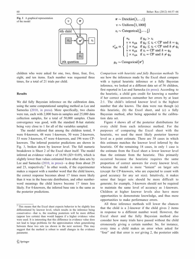
Following Lee and Sarnecka (2010, in press), we used agraphical model as our implementation, as shown in Fig. 1.Graphical models are a standard language in machinelearning, statistics, and (more recently) cognitive science(e.g., Griffiths, Kemp & Tenenbaum, 2008; Jordan, 2004;Koller, Friedman, Getoor & Taskar, 2007; Lee, 2008,2011; Shiffrin, Lee, Kim & Wagenmakers, 2008). Theyspecify how unobserved psychological variables generatethe observed data. The model takes the form of a graph,whose nodes represent the variables and the data. Thelinks indicate the dependencies between them. Discretevariables are indicated by square nodes; continuousvariables are indicated by circular nodes. Stochastic variablesare indicated by single-bordered nodes; deterministic

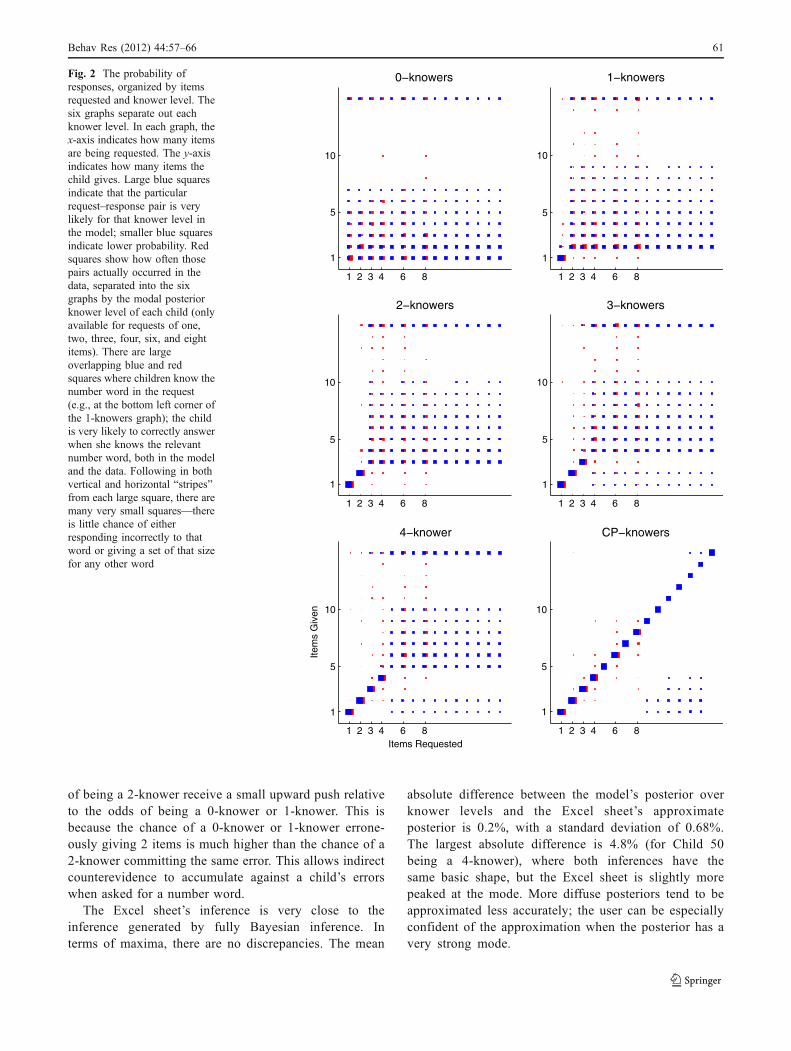
1 It is intuitively easy to understand that, all else being equal, childrenare more likely to give some set sizes than others. For example,children often give all of the objects in the bowl to the puppet; theyrarely give all but one. The base rates are very high for giving 1 item,2 items, or all 15 items. The curve in the middle (from 3 to 14) is highfor small numbers and decays steadily as it moves to larger ones. For avisualization, look ahead to Fig. 2.

2 For readers who are curious what the patterns are like: When themodel is applied to data, it turns out that pre-number-knowers justgive the base-rate number of items. 1-knowers almost always give 1when asked for “one,” but rarely give 1 when asked for anything else.Of course, 1-knowers sometimes give 2 for “two,” because the overallprobability of giving 2 objects (specified by the base rate) is high.Likewise, 2-knowers give 2 when asked for “two” and rarely give 2for anything else, and so forth. CP-knowers have a very good chanceof getting any number correct, because they can use counting to solvethe task. (For children who do not yet understand the cardinalityprinciple, counting is not available as a strategy.)

58 Behav Res (2012) 44:57–66

variables (included for conceptual clarity) are indicatedby double-bordered nodes. Shaded nodes are the ob-served data; unshaded nodes are latent variables. Finally,encompassing plates are used to denote independentreplications of the graph structure within the model.

In our implementation of the knower-level model(Fig. 1), the data are the observed qij and gij variables.They give the number asked for (the “question”) and theanswer (the number “given”), respectively, for the ith childon his or her jth trial.3 The base-rate probabilities arerepresented by the vector π, which is updated to π'according to the Bayesian updating process describedabove. This probability space is visualized in Fig. 2. Thisprocess depends on the knower level zi of the child and anevidence value v that measures the strength of the updating.The child’s actual behavior (i.e., the number of items given)represents a sample from the distribution expressed by π'.The base-rate and evidence parameters, which are assumedto be the same for all children, are given uninformativepriors (i.e., initial distributions that assume very little,allowing for a very large range of possible inferences).There is a separate knower-level parameter for each child,with no prior preference for any of the six knower levels.

Lee and Sarnecka (2010, in press) used this graphicalmodel implementation (and associated computationalsampling methods) to demonstrate that the model can(1) describe children’s behavioral data, (2) make usefulinferences about the knower level of specific children,and (3) describe the base-rate and evidence-strengthparameters. One of the most obvious and usefulapplications of the model is to infer a child’s knowerlevel from their give-N behavior. The goal of this article isto provide an approximation of the full model that isnonetheless accurate in making these estimations and thatcan be implemented in Microsoft Excel.

Approximation in the Excel sheet

Next we describe an approximation that provides estimationof knower levels comparable to that obtained with the fullBayesian model. To create the approximation, we eliminatedall of the continuous distributions in the full model,thereby removing the need for Markov chain MonteCarlo techniques. The node π'—the final probability ofevery possible response, given the knower level and therequest—was filled with point estimates; the parameters πand v were removed entirely. In the full model, π' issubject to implied distributions (through π, v, and the

updating logic) that need to be integrated out. In theapproximation, π' is just a set of summary pointprobabilities—for example, the chance that a 1-knowerwill give 1 when asked for “one” is 83.33%. Theseprobabilities were found by applying the full model to acalibration data set (described in the next section) andcalculating the posterior predictive.4

The remaining computational machinery is simpleenough to be captured in a single equation. Theprobability that the ith child is at a given knower level Zcan be written as

p Z ¼ zijp0; qij; gij� � ¼

pðZÞQjp0Z ;qij;gij

P6

z¼1pðzÞQ

jp0z;qij;gij

" #

Since π' is a set of point probabilities in the approxima-tion, nothing further is needed for it to work. Following theusual Bayesian form, the top part of the equation is just theprior times the (simplified) likelihood function. Since eachtrial is assumed to be independent, calculating the likeli-hood just requires multiplying over the probabilities of allthe observed responses. The bottom part is the normaliza-tion constant. Since there are a total of six discrete knowerlevels, the constant is just the sum of the top part over allknower levels. This approximation can work in Excelbecause no integration is required—with set values for π'and Z, the right-hand side of the above equation can beworked just by multiplying, adding, and dividing. Then, bysimply repeating over the six possible values of Z, the fulldistribution is calculated.

Data

We based our approximation on empirical data fromexperiments reported by Negen and Sarnecka (2010). Forthis data set, children were asked to give one, two, three,four, six, and eight items. Each request was repeated threetimes, for a total of 18 trials, which were presented in oneof two pseudorandom orders. The present analysisincludes only sessions in which the child completed atleast 15 of the 18 trials, a total of 423 sessions. (Theoriginal data set included an additional 31 sessions inwhich the child failed to complete at least 15 trials. Thesesessions were excluded.)

The independent data used to compare the modelinferences and Excel sheet inferences came from Lee andSarnecka (in press). This data set includes data from 56

3 Note that the jth trial does not necessarily involve the child beingasked for j items. The value of qij is the number of items the ith childwas asked for on the jth experimental trial completed.

4 For readers who are unfamiliar with this term: the posteriorpredictive is the distribution of predicted future data, given the currentobserved data and the assumptions in the model.

Behav Res (2012) 44:57–66 59

children who were asked for one, two, three, four, five,eight, and ten items. Each number was requested threetimes, for a total of 21 trials per child.

Results

We did fully Bayesian inference on the calibration data,using the same computational sampling method as Lee andSarnecka (2010, in press). More specifically, two chainswere run, each with 2,000 burn-in samples and 25,000 datacollection samples, for a total of 50,000 samples. Chainconvergence was good, with the standard R-hat statisticbeing very close to 1 for all of the variables sampled.

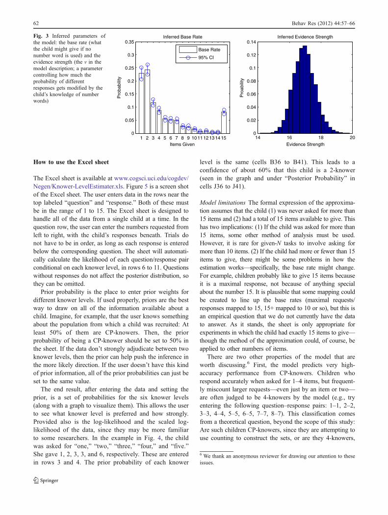
The model inferred that among the children tested, 9were 0-knowers, 48 were 1-knowers, 50 were 2-knowers,53 were 3-knowers, 67 were 4-knowers, and 196 were CP-knowers. The inferred posterior predictions are shown inFig. 3, broken down by knower level. The full numericbreakdown is Sheet 2 of the Excel sheet itself. The modelinferred an evidence value v of 16.94 (SD=0.69), which isslightly lower than values estimated from other data sets byLee and Sarnecka (2010, in press)—a drop from about 29and 23, respectively.5 In other words, if the experimentermakes a request with a number word that the child knows,the correct response becomes about 17 times more likelythan it was in the base-rate distribution, and other number-word meanings the child knows become 17 times lesslikely. For 0-knowers, the inferred base rate is the same asthe posterior predictions.

Comparison with heuristic and fully Bayesian methods Tosee how the inferences made by the Excel sheet comparewith a typical heuristic inference or a fully Bayesianinference, we looked at a different data set of 56 children,first reported in Lee and Sarnecka (in press). According tothe heuristic, a child gets credit for knowing a numberif her correct answers outnumber her errors by at least2:1. The child’s inferred knower level is the highestnumber that she knows. The data were run though (a)this heuristic, (b) the Excel sheet, and (c) a fullyBayesian method, after being appended to the calibra-tion data set.

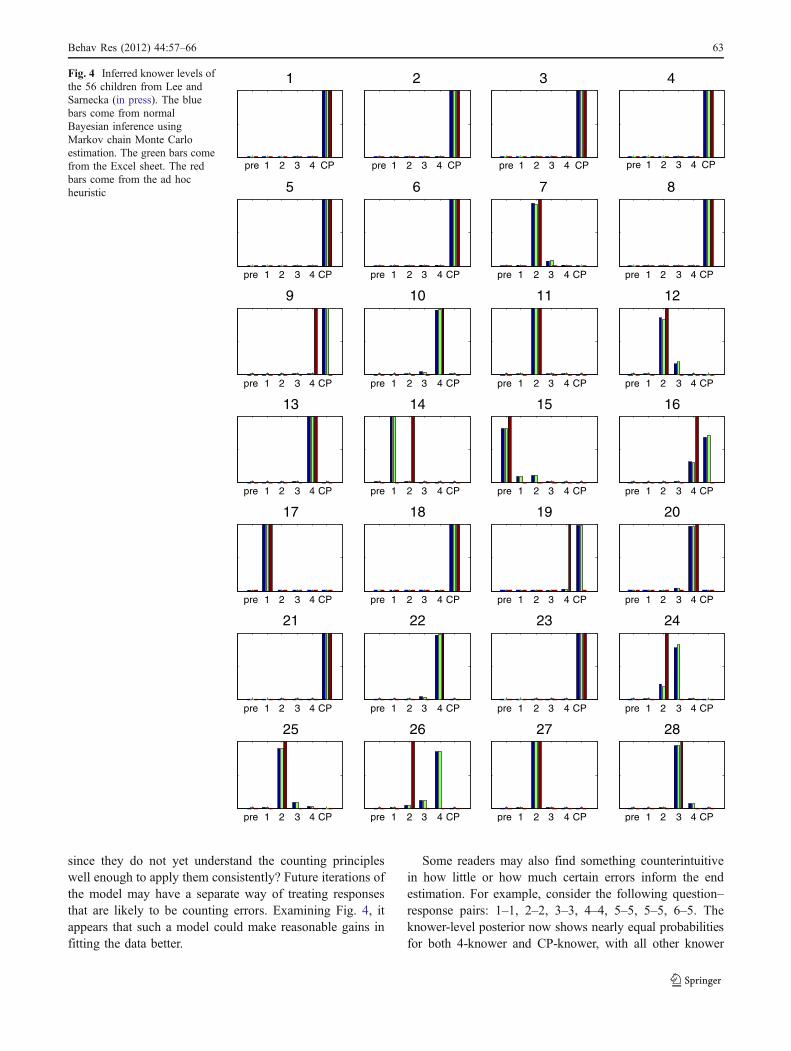
Figure 4 shows all of the posterior distributions forevery child from each inference method. For thepurposes of comparing the Excel sheet with theheuristic, we used the most likely posterior knowerlevel as a point estimate. There are 38 cases in whichthis estimate matches the knower level inferred by theheuristic. Of the remaining 18 cases, in only 1 case isthe estimate from the Excel sheet a lower knower levelthan the estimate from the heuristic. This primarilyoccurred because the heuristic requires the sameproportion of correct answers for every knower level,whereas the model is more “lenient” on larger sets(except for CP-knowers, who are expected to count withgood accuracy for any set size). Intuitively, it makessense that larger sets should be more difficult togenerate; for example, 3-knowers should not be requiredto maintain the same level of accuracy as 1-knowers.Children at higher knower levels also have moreopportunities to demonstrate knowledge, and thus moreopportunities to make performance errors.

All three inference methods will lower the chancesthat the child is a 2-knower if the child gives 2 itemsin response to a different number word. However, theExcel sheet and the fully Bayesian method alsoconsider how many trials have passed without the childerroneously giving a certain number. So, for instance,every time a child makes an error when asked for“four” and that error is not giving 2, the posterior odds

5 This means that the Excel sheet expects behavior to be slightly lessdifferentiated by knower level, which results in the inference beingconservative—that is, the resulting posteriors will be more diffuse(appear less certain) than would happen if a higher evidence valuewere used. It is interesting that this difference in evidence value doesnot lead to large problems for the approximation when generalizingbetween these two sets (as shown in the next section). This maysuggest that the method is robust to small changes in the evidenceparameter.

Fig. 1 A graphical representationof the model

60 Behav Res (2012) 44:57–66

of being a 2-knower receive a small upward push relativeto the odds of being a 0-knower or 1-knower. This isbecause the chance of a 0-knower or 1-knower errone-ously giving 2 items is much higher than the chance of a2-knower committing the same error. This allows indirectcounterevidence to accumulate against a child’s errorswhen asked for a number word.

The Excel sheet’s inference is very close to theinference generated by fully Bayesian inference. Interms of maxima, there are no discrepancies. The mean

absolute difference between the model’s posterior overknower levels and the Excel sheet’s approximateposterior is 0.2%, with a standard deviation of 0.68%.The largest absolute difference is 4.8% (for Child 50being a 4-knower), where both inferences have thesame basic shape, but the Excel sheet is slightly morepeaked at the mode. More diffuse posteriors tend to beapproximated less accurately; the user can be especiallyconfident of the approximation when the posterior has avery strong mode.

1 2 3 4 6 8

1

5

10

1 2 3 4 6 8

1

5

10

1 2 3 4 6 8

1

5

10

1 2 3 4 6 8

1

5

10

1 2 3 4 6 8

1

5

10

Items Requested

Item

s G

iven

1 2 3 4 6 8

1

5

10

0−knowers 1−knowers

2−knowers 3−knowers

4−knower CP−knowers

Fig. 2 The probability ofresponses, organized by itemsrequested and knower level. Thesix graphs separate out eachknower level. In each graph, thex-axis indicates how many itemsare being requested. The y-axisindicates how many items thechild gives. Large blue squaresindicate that the particularrequest–response pair is verylikely for that knower level inthe model; smaller blue squaresindicate lower probability. Redsquares show how often thosepairs actually occurred in thedata, separated into the sixgraphs by the modal posteriorknower level of each child (onlyavailable for requests of one,two, three, four, six, and eightitems). There are largeoverlapping blue and redsquares where children know thenumber word in the request(e.g., at the bottom left corner ofthe 1-knowers graph); the childis very likely to correctly answerwhen she knows the relevantnumber word, both in the modeland the data. Following in bothvertical and horizontal “stripes”from each large square, there aremany very small squares—thereis little chance of eitherresponding incorrectly to thatword or giving a set of that sizefor any other word

Behav Res (2012) 44:57–66 61

How to use the Excel sheet

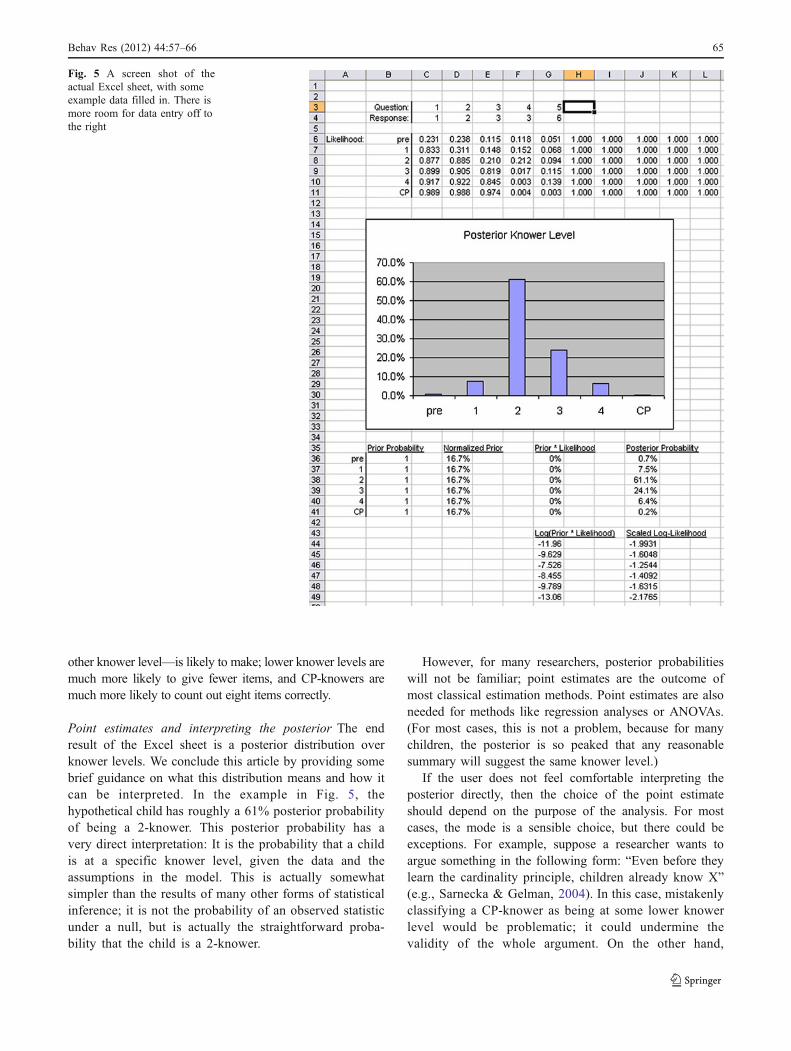
The Excel sheet is available at www.cogsci.uci.edu/cogdev/Negen/Knower-LevelEstimater.xls. Figure 5 is a screen shotof the Excel sheet. The user enters data in the rows near thetop labeled “question” and “response.” Both of these mustbe in the range of 1 to 15. The Excel sheet is designed tohandle all of the data from a single child at a time. In thequestion row, the user can enter the numbers requested fromleft to right, with the child’s responses beneath. Trials donot have to be in order, as long as each response is enteredbelow the corresponding question. The sheet will automati-cally calculate the likelihood of each question/response pairconditional on each knower level, in rows 6 to 11. Questionswithout responses do not affect the posterior distribution, sothey can be omitted.

Prior probability is the place to enter prior weights fordifferent knower levels. If used properly, priors are the bestway to draw on all of the information available about achild. Imagine, for example, that the user knows somethingabout the population from which a child was recruited: Atleast 50% of them are CP-knowers. Then, the priorprobability of being a CP-knower should be set to 50% inthe sheet. If the data don’t strongly adjudicate between twoknower levels, then the prior can help push the inference inthe more likely direction. If the user doesn’t have this kindof prior information, all of the prior probabilities can just beset to the same value.

The end result, after entering the data and setting theprior, is a set of probabilities for the six knower levels(along with a graph to visualize them). This allows the userto see what knower level is preferred and how strongly.Provided also is the log-likelihood and the scaled log-likelihood of the data, since they may be more familiarto some researchers. In the example in Fig. 4, the childwas asked for “one,” “two,” “three,” “four,” and “five.”She gave 1, 2, 3, 3, and 6, respectively. These are enteredin rows 3 and 4. The prior probability of each knower

level is the same (cells B36 to B41). This leads to aconfidence of about 60% that this child is a 2-knower(seen in the graph and under “Posterior Probability” incells J36 to J41).

Model limitations The formal expression of the approxima-tion assumes that the child (1) was never asked for more than15 items and (2) had a total of 15 items available to give. Thishas two implications: (1) If the child was asked for more than15 items, some other method of analysis must be used.However, it is rare for given-N tasks to involve asking formore than 10 items. (2) If the child had more or fewer than 15items to give, there might be some problems in how theestimation works—specifically, the base rate might change.For example, children probably like to give 15 items becauseit is a maximal response, not because of anything specialabout the number 15. It is plausible that some mapping couldbe created to line up the base rates (maximal requests/responses mapped to 15, 15+ mapped to 10 or so), but this isan empirical question that we do not currently have the datato answer. As it stands, the sheet is only appropriate forexperiments in which the child had exactly 15 items to give—though the method of the approximation could, of course, beapplied to other numbers of items.

There are two other properties of the model that areworth discussing.6 First, the model predicts very high-accuracy performance from CP-knowers. Children whorespond accurately when asked for 1–4 items, but frequent-ly miscount larger requests—even just by an item or two—are often judged to be 4-knowers by the model (e.g., tryentering the following question–response pairs: 1–1, 2–2,3–3, 4–4, 5–5, 6–5, 7–7, 8–7). This classification comesfrom a theoretical question, beyond the scope of this study:Are such children CP-knowers, since they are attempting touse counting to construct the sets, or are they 4-knowers,

1 2 3 4 5 6 7 8 9 10 11 12 13 14 150

0.05

0.1

0.15

0.2

0.25

0.3

0.35

Items Given

Pro

babi

lity

Inferred Base Rate

Base Rate

95% CI

14 16 18 200

0.02

0.04

0.06

0.08

0.1

0.12

0.14Inferred Evidence Strength

Evidence Strength

Pro

abili

ty

Fig. 3 Inferred parameters ofthe model: the base rate (whatthe child might give if nonumber word is used) and theevidence strength (the v in themodel description; a parametercontrolling how much theprobability of differentresponses gets modified by thechild’s knowledge of numberwords)

6 We thank an anonymous reviewer for drawing our attention to theseissues.

62 Behav Res (2012) 44:57–66

since they do not yet understand the counting principleswell enough to apply them consistently? Future iterations ofthe model may have a separate way of treating responsesthat are likely to be counting errors. Examining Fig. 4, itappears that such a model could make reasonable gains infitting the data better.

Some readers may also find something counterintuitivein how little or how much certain errors inform the endestimation. For example, consider the following question–response pairs: 1–1, 2–2, 3–3, 4–4, 5–5, 5–5, 6–5. Theknower-level posterior now shows nearly equal probabilitiesfor both 4-knower and CP-knower, with all other knower

pre 1 2 3 4 CP

1

pre 1 2 3 4 CP

2

pre 1 2 3 4 CP

3

pre 1 2 3 4 CP

4

pre 1 2 3 4 CP

5

pre 1 2 3 4 CP

6

pre 1 2 3 4 CP

7

pre 1 2 3 4 CP

8

pre 1 2 3 4 CP

9

pre 1 2 3 4 CP

10

pre 1 2 3 4 CP

11

pre 1 2 3 4 CP

12

pre 1 2 3 4 CP

13

pre 1 2 3 4 CP

14

pre 1 2 3 4 CP

15

pre 1 2 3 4 CP

16

pre 1 2 3 4 CP

17

pre 1 2 3 4 CP

18

pre 1 2 3 4 CP

19

pre 1 2 3 4 CP

20

pre 1 2 3 4 CP

21

pre 1 2 3 4 CP

22

pre 1 2 3 4 CP

23

pre 1 2 3 4 CP

24

pre 1 2 3 4 CP

25

pre 1 2 3 4 CP

26

pre 1 2 3 4 CP

27

pre 1 2 3 4 CP

28

Fig. 4 Inferred knower levels ofthe 56 children from Lee andSarnecka (in press). The bluebars come from normalBayesian inference usingMarkov chain Monte Carloestimation. The green bars comefrom the Excel sheet. The redbars come from the ad hocheuristic

Behav Res (2012) 44:57–66 63

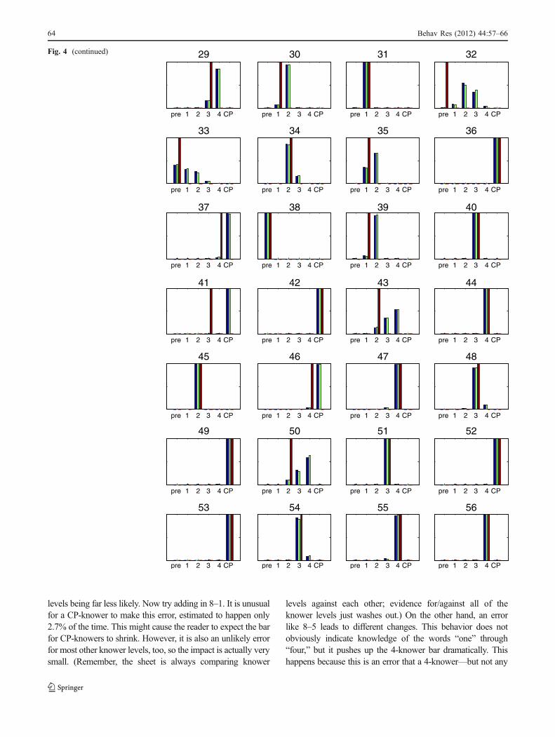
levels being far less likely. Now try adding in 8–1. It is unusualfor a CP-knower to make this error, estimated to happen only2.7% of the time. This might cause the reader to expect the barfor CP-knowers to shrink. However, it is also an unlikely errorfor most other knower levels, too, so the impact is actually verysmall. (Remember, the sheet is always comparing knower

levels against each other; evidence for/against all of theknower levels just washes out.) On the other hand, an errorlike 8–5 leads to different changes. This behavior does notobviously indicate knowledge of the words “one” through“four,” but it pushes up the 4-knower bar dramatically. Thishappens because this is an error that a 4-knower—but not any

pre 1 2 3 4 CP

29

pre 1 2 3 4 CP

30

pre 1 2 3 4 CP

31

pre 1 2 3 4 CP

32

pre 1 2 3 4 CP

33

pre 1 2 3 4 CP

34

pre 1 2 3 4 CP

35

pre 1 2 3 4 CP

36

pre 1 2 3 4 CP

37

pre 1 2 3 4 CP

38

pre 1 2 3 4 CP

39

pre 1 2 3 4 CP

40

pre 1 2 3 4 CP

41

pre 1 2 3 4 CP

42

pre 1 2 3 4 CP

43

pre 1 2 3 4 CP

44

pre 1 2 3 4 CP

45

pre 1 2 3 4 CP

46

pre 1 2 3 4 CP

47

pre 1 2 3 4 CP

48

pre 1 2 3 4 CP

49

pre 1 2 3 4 CP

50

pre 1 2 3 4 CP

51

pre 1 2 3 4 CP

52

pre 1 2 3 4 CP

53

pre 1 2 3 4 CP

54

pre 1 2 3 4 CP

55

pre 1 2 3 4 CP

56

Fig. 4 (continued)

64 Behav Res (2012) 44:57–66

other knower level—is likely to make; lower knower levels aremuch more likely to give fewer items, and CP-knowers aremuch more likely to count out eight items correctly.

Point estimates and interpreting the posterior The endresult of the Excel sheet is a posterior distribution overknower levels. We conclude this article by providing somebrief guidance on what this distribution means and how itcan be interpreted. In the example in Fig. 5, thehypothetical child has roughly a 61% posterior probabilityof being a 2-knower. This posterior probability has avery direct interpretation: It is the probability that a childis at a specific knower level, given the data and theassumptions in the model. This is actually somewhatsimpler than the results of many other forms of statisticalinference; it is not the probability of an observed statisticunder a null, but is actually the straightforward proba-bility that the child is a 2-knower.

However, for many researchers, posterior probabilitieswill not be familiar; point estimates are the outcome ofmost classical estimation methods. Point estimates are alsoneeded for methods like regression analyses or ANOVAs.(For most cases, this is not a problem, because for manychildren, the posterior is so peaked that any reasonablesummary will suggest the same knower level.)

If the user does not feel comfortable interpreting theposterior directly, then the choice of the point estimateshould depend on the purpose of the analysis. For mostcases, the mode is a sensible choice, but there could beexceptions. For example, suppose a researcher wants toargue something in the following form: “Even before theylearn the cardinality principle, children already know X”(e.g., Sarnecka & Gelman, 2004). In this case, mistakenlyclassifying a CP-knower as being at some lower knowerlevel would be problematic; it could undermine thevalidity of the whole argument. On the other hand,

Fig. 5 A screen shot of theactual Excel sheet, with someexample data filled in. There ismore room for data entry off tothe right

Behav Res (2012) 44:57–66 65

misclassifying a less knowledgeable child as a CP-knowerwould not undermine the argument; it would only remove asmall amount of data. In such a case, a sensible estimatewould be the highest knower level with posterior probabilitythat exceeds the prior probability. This method would tend tosort children into higher knower levels where the data wereambiguous, and thus would be unlikely to misclassify a CP-knower. Researchers with very particular needs could evenexplicitly define a utility function—though a full discussion ofthat topic is outside the scope of this article.

Summary

Knower levels are one of the most useful landmarks ofnumber-concept development in young children. Data fromthe standard give-N task can be analyzed using a generativemodel of the task, thereby drawing inferences in a moreprincipled way than heuristic methods. The model’sestimates also provide information about how certain wecan be of the knower-level classification for each child, andthey empower the researcher to decide ambiguous cases inthe way that is most appropriate for the problem at hand.The software presented in this article computes a closeapproximation to the model’s inference while remainingquick and easy to use. It is available at www.cogsci.uci.edu/cogdev/Negen/Knower-LevelEstimater.xls.

Author note This research was supported by NIH GrantR03HD054654 to B.W.S. We thank the children and families whoparticipated in the study, as well as the teachers and administrators ofthe following Irvine, California, preschools: Jenny Hart EarlyEducation Center, Temple Bat Yahm Preschool, Turtle Rock Preschool,UCI Children’s Center, UCI Early Childhood Education Center, UCIInfant and Toddler Center, and University Montessori. Thanks also toresearch assistants Annie Ditta, Christina Do, Ryan Galli, NiyatiGupta, Elisa Hasrouni, Caroline Lee, Meghan Li, Sarah Pachman,Grace Park, Diego San Martin, Tamanna Shah, Christina Tajali, JamieTibajia, Farah Toullier, and Archana Vaidyanathan, and to labmanagers Helen Braithwaite and Cristina Flores.

References

Ansari, D., Donlan, C., Thomas, M. S. C., Ewing, S. A., Peen, T., &Karmiloff-Smith, A. (2003). What makes counting count? Verbaland visuo-spatial contributions to typical and atypical number

development. Journal of Experimental Child Psychology, 85, 50–62. doi:10.1016/S0022-0965(03)00026-2

Barner, D., Chow, K., & Yang, S.-J. (2009). Finding one’s meaning: Atest of the relation between quantifiers and integers in languagedevelopment. Cognitive Psychology, 58, 195–219. doi:10.1016/j.cogpsych.2008.07.001

Carey, S. (2009). The origin of concepts. New York: OxfordUniversity Press.

Fuson, K. C. (1988). Children’s counting and concepts of number.New York: Springer.

Griffiths, T. L., Kemp, C., & Tenenbaum, J. B. (2008). Bayesianmodels of cognition. In R. Sun (Ed.), Cambridge handbook ofcomputational cognitive modeling (pp. 59–100). Cambridge:Cambridge University Press.

Jordan, M. I. (2004). Graphical models. Statistical Science, 19, 140–155.

Koller, D., Friedman, N., Getoor, L., & Taskar, B. (2007).Graphical models in a nutshell. In L. Getoor & B. Taskar(Eds.), Introduction to statistical relational learning. Cambridge:MIT.

Le Corre, M., & Carey, S. (2007). One, two, three, four, nothing more:An investigation of the conceptual sources of the verbal countingprinciples. Cognition, 105, 395–438. doi:10.1016/j.cognition.2006.10.005

Lee, M. D. (2008). Three case studies in the Bayesian analysis ofcognitive models. Psychonomic Bulletin & Review, 15, 1–15.doi:10.3758/PBR.15.1.1

Lee, M. D. (2011). How cognitive modeling can benefit fromhierarchical Bayesianmodels. Journal of Mathematical Psychology,55, 1–7. doi:10.1016/j.jmp.2010.08.013

Lee, M. D., & Sarnecka, B. W. (2010). A model of knower-levelbehavior in number concept development. Cognitive Science, 34,51–67. doi:10.1111/j.1551-6709.2009.01063.x

Lee, M. D., & Sarnecka, B. W. (in press). Number knower-levels inyoung children: Insights from a Bayesian model. Cognition.

Negen, J., & Sarnecka, B. W. (2010). Analogue magnitudes andknower-levels: Re-visiting the variability argument. In S. Ohlsson& R. Catrambone (Eds.), Proceedings of the 32nd AnnualConference of the Cognitive Science Society (pp. 1252–1257).Austin: Cognitive Science Society.

Sarnecka, B. W., & Gelman, S. A. (2004). Six does not just mean a lot:Preschoolers see number words as specific. Cognition, 92, 329–352. doi:10.1016/j.cognition.2003.10.001

Sarnecka, B. W., & Lee, M. D. (2009). Levels of number knowledgeduring early childhood. Journal of Experimental Child Psychol-ogy, 103, 325–337. doi:10.1016/j.jecp.2009.02.007

Sarnecka, B. W., Kamenskaya, V. G., Yamana, Y., Ogura, T., &Yudovina, Y. B. (2007). From grammatical number to exactnumbers: Early meanings of “one”, “two”, and “three” inEnglish, Russian, and Japanese. Cognitive Psychology, 55, 136–168. doi:10.1016/j.cogpsych.2006.09.001

Shiffrin, R. M., Lee, M. D., Kim, W., & Wagenmakers, E.-J. (2008). Asurvey of model evaluation approaches with a tutorial onhierarchical Bayesian methods. Cognitive Science, 32, 1248–1284. doi:10.1080/03640210802414826

Wynn, K. (1992). Children’s acquisition of the number words and thecounting system. Cognitive Psychology, 24, 220–251.doi:10.1016/0010-0285(92)90008-P

66 Behav Res (2012) 44:57–66