California State University, San Bernardino California State University, San Bernardino

CSUSB ScholarWorks CSUSB ScholarWorks

Electronic Theses, Projects, and Dissertations Office of Graduate Studies

6-2016

Mathematical Reasoning and the Inductive Process: An Mathematical Reasoning and the Inductive Process: An

Examination of The Law of Quadratic Reciprocity Examination of The Law of Quadratic Reciprocity

Nitish Mittal California State University - San Bernardino

Follow this and additional works at: https://scholarworks.lib.csusb.edu/etd

Part of the Number Theory Commons, and the Set Theory Commons

Recommended Citation Recommended Citation Mittal, Nitish, "Mathematical Reasoning and the Inductive Process: An Examination of The Law of Quadratic Reciprocity" (2016). Electronic Theses, Projects, and Dissertations. 282. https://scholarworks.lib.csusb.edu/etd/282

This Thesis is brought to you for free and open access by the Office of Graduate Studies at CSUSB ScholarWorks. It has been accepted for inclusion in Electronic Theses, Projects, and Dissertations by an authorized administrator of CSUSB ScholarWorks. For more information, please contact scholarworks@csusb.edu.

Mathematical Reasoning and the Inductive Process: An Examination of

the law of Quadratic Reciprocity

A Thesis

Presented to the

Faculty of

California State University,

San Bernardino

In Partial Fulfillment

of the Requirements for the Degree

Master of Arts

in

Mathematics

by

Nitish Mittal

June 2016

Mathematical Reasoning and the Inductive Process: An Examination of

the law of Quadratic Reciprocity

A Thesis

Presented to the

Faculty of

California State University,

San Bernardino

by

Nitish Mittal

June 2016

Approved by:

Dr. James Paul Vicknair, Committee Chair Date

Dr. Zahid Hassan, Committee Member

Dr. Rolland Trapp, Committee Member

Dr. Charles Stanton, Chair, Dr. Corey Dunn

Department of Mathematics Graduate Coordinator,

Department of Mathematics

iii

Abstract

This project investigates the development of four different proofs of the law of

quadratic reciprocity, in order to study the critical reasoning process that drives discovery

in mathematics. We begin with an examination of the first proof of this law given by

Gauss. We then describe Gauss’ fourth proof of this law based on Gauss sums, followed

by a look at Eisenstein’s geometric simplification of Gauss’ third proof. Finally, we finish

with an examination of one of the modern proofs of this theorem published in 1991 by

Rousseau. Through this investigation we aim to analyze the different strategies used in

the development of each of these proofs, and in the process gain a better understanding

of this theorem.

iv

Acknowledgements

I wish to thank Dr. James Paul Vicknair for all his help and support during the prepa-

ration of this paper. I would also like to thank Dr. Hassan and Dr. Trapp for their

comments and contribution to this thesis. I would especially like to thank Dr. Stanton

for helping me fully assimilate into the graduate program, and Dr. Dunn in helping me

re-enter the program after an extended leave of absence. I would further like to acknowl-

edge my classmates and friends Leonard Lamp, Kevin Baccari, and Avi Misra whose help

and support played a pivotal role in my learning and development throughout my tenure

in the masters program.

v

Table of Contents

Abstract iii

Acknowledgements iv

List of Figures vi

1 Introduction 11.1 Observation and Induction in Mathematics . . . . . . . . . . . . . . . . . 11.2 The Law of Quadratic Reciprocity . . . . . . . . . . . . . . . . . . . . . . 21.3 What is Covered in this Project . . . . . . . . . . . . . . . . . . . . . . . . 3

2 Background Definitions and Theorems 42.1 Theory of Congruences . . . . . . . . . . . . . . . . . . . . . . . . . . . . . 42.2 Wilson’s and Fermat’s Theorems . . . . . . . . . . . . . . . . . . . . . . . 72.3 Euler’s Criterion and Legendre Symbol . . . . . . . . . . . . . . . . . . . . 82.4 Gauss’ Lemma . . . . . . . . . . . . . . . . . . . . . . . . . . . . . . . . . 122.5 Gauss Sums . . . . . . . . . . . . . . . . . . . . . . . . . . . . . . . . . . . 152.6 Normal Subgroups and Quotient Groups . . . . . . . . . . . . . . . . . . . 172.7 The Chinese Remainder Theorem . . . . . . . . . . . . . . . . . . . . . . . 20

3 Proofs of The Law of Quadratic Reciprocity 243.1 The Law of Quadratic Reciprocity . . . . . . . . . . . . . . . . . . . . . . 243.2 Gauss’s First Proof of Quadratic Reciprocity . . . . . . . . . . . . . . . . 243.3 Gauss’s Fouth Proof of Quadratic Reciprocity . . . . . . . . . . . . . . . . 363.4 Eisenstein’s Geometric Proof of Quadratic Reciprocity . . . . . . . . . . . 423.5 Rousseau’s Proof of Quadratic Reciprocity . . . . . . . . . . . . . . . . . . 46

4 Conclusion 50

Bibliography 51

vi

List of Figures

3.1 Eisenstein’s Lattice Points . . . . . . . . . . . . . . . . . . . . . . . . . . . 42

1

Chapter 1

Introduction

1.1 Observation and Induction in Mathematics

There are even many properties of numbers with which we are well ac-quainted, but which we are not yet able to prove; only observations have ledus to their knowledge. Hence we see that in the theory of numbers, which isstill very imperfect, we can place our highest hopes in observations; they willlead us continually to new properties which we shall endeavor to prove after-wards. The kind of knowledge which is supported only by observations and isnot yet proved must be carefully distinguished from the truth; it is gained byinduction as we usually say. Yet we have seen cases in which mere inductionled to error. Therefore we should take care not to accept as true such prop-erties of the numbers which we have discovered by observation and which aresupported by induction alone. Indeed, we should use such a discovery as anopportunity to investigate more than exactly the properties discovered and toprove or disprove them; in both cases we may learn something useful.

Leonhard Euler (in [Pol54])

Euler’s quote about the use of observation in mathematics is a great commentary

on mathematical reasoning and the inductive process itself. As Euler mentions above

even in fields as abstract as pure mathematics and the theory of numbers, observation

and induction are important tools in helping identify the various intriguing behaviors and

patterns of numbers. However, observation alone is not sufficient and the true strength of

mathematical discovery lies in the use of mathematical tools to prove without exception

what is being observed. As students of mathematics we are no strangers to this process.

Identifying a pattern in a given example and applying inductive reasoning to generalize

2

said pattern is the basis of modern mathematics; however, as Euler notes, we should be

vary of proofs by induction alone. The strongest conjectures are those which can not only

be supported by inductive reasoning, but proved and reproved using other methods as

well. The Law of Quadratic Reciprocity is one such example in the theory of numbers.

[Pol54]

1.2 The Law of Quadratic Reciprocity

Dubbed the golden theorem of number theory by the prince of mathematics, Carl

Friedrich Gauss, the law of quadratic reciprocity is one of the most pursued theorems of

18th and 19th century mathematics. The theorem was first formulated by Euler in 1783

and later tackled by Legendre in 1785, and again in Essai sur la Theorie des Nombres in

1798. Though both his proofs were later shown to be invalid, the elegant notation em-

ployed by Legendre eventually became the modern Law of Quadratic Reciprocity. The

first complete proof of the theorem was written by Gauss when he was 18, and pub-

lished in his book Disquisitiones Arithmaticae in 1801. In his first attempt Gauss looked

at individual cases and used elementary techniques to prove the law and subsequently

generalized it using mathematical induction. Gauss later published 6 more proofs of the

same theorem, each time employing a different method, refining the proof and making it

more elegant. [Buh81]

We will begin with examining thoroughly Gauss’s first attempt, which, though

rather long, uses only basic techniques. We will then examine two of his latter proofs to see

the developments he made over time to further refine his proof. We will look at iterations

or simplifications of his third and fourth proofs of the law of quadratic reciprocity. In

his fourth proof Gauss used Gaussian sums to prove the law. We will describe his proof

in complete detail and examine the differences between this proof and his first attempt,

the most apparent of which is the sheer difference in length between the two. We will

then analyze his third proof of this theorem. In this proof Gauss employed the use of

Gauss’s lemma to prove the fundamental theorem in a very concise and elegant fashion.

Eisenstein’s simplification of this proof is perhaps one of the most commonly used in

elementary number theory courses. Finally, we will conclude with a modern elementary

proof of the law of quadratic reciprocity.

3

1.3 What is Covered in this Project

This project will take us through the first known proof of one of the fundamental

laws of the theory of numbers and one of the most scrutinized theorems in all of mathe-

matics, and illustrate the ways in which it was reformulated and refined over time. The

project is an interesting examination of the essence of the process of “inductive reason-

ing” described by Polya and provides us a firsthand experience whilst also examining one

of Gauss’ celebrated contributions to the field of mathematics. While the significance of

the latter cannot be denied we stand to gain much more from the former. The “inductive

attitude” has been a major driving force for continuous investigation and invention in

mathematics and other natural sciences. The process is a telling tale of how the human

mind works and how new knowledge is discovered. A journey that is not very different

from that of a diamond, starting off as a pebble in a mine and constantly cleaned and

refined along the way until it is finally cut and polished to reveal the elegant jewel that

it is.

This project outlines a paradigm that has been employed in the discovery of

countless other theorems in the past and will continue to help discover countless more

in the future. It highlights the process from the recognition of patterns observed by

the investigation of special cases, to forming a conjecture and eventually using known

techniques to simplify, generalize and prove our conjecture. It further illustrates the

importance of continued investigation in helping uncover new implications and interpre-

tations of a theorem. This project ultimately highlights the point that while the saying

“necessity is the mother of all invention” may hold true in other natural sciences, the

“inductive” attitude and reasoning are certainly the root of all discovery in the abstract

field of pure mathematics.

4

Chapter 2

Background Definitions and

Theorems

We will begin by giving some elementary definitions and theorems in number

theory, which can be found in the following sources: [Bur07] [Nag51]

2.1 Theory of Congruences

Definition 2.1. Let n be a fixed positive integer. Two integers a and b are said to be

congruent modulo n, symbolized by

a ≡ b(mod n)

if n divides the difference a− b; that is, given that a− b = kn for some integer k.

Lemma 2.2. Let a, b and n > 0 be integers, then a ≡ b(mod n)⇔ n|(a− b).

Proof. If a ≡ b(mod n), then a and b have the same remainder when divided by n. Thus,

by the division algorithm a = np+r and b = nq+r, for integers p, q and r with 0 ≤ r ≤ n.

Now we have,

a− np = b− nq

⇒ a− b = np− nq

⇒ a− b = n(p− q)

5

Thus, n|(a − b). Conversely, If n|(a − b), then there exist integers x and y such that,

a = nx+ r1 and b = ny = r2, where 0 ≤ r1 ≤ n and 0 ≤ r2 ≤ n. Then,

a− b = (nx+ r1)− (ny + r2)

⇒ a− b = n(x+ y)− (r1 − r2)

Thus, since n|(a − b), n must also divide (r1 − r2). However |r1 − r2| < n, thus −n <r1 − r2 < n, therefore r1 − r2 = 0 and r1 = r2, and so a ≡ b(mod n).

Example 2.3. Let n = 7, then 10 ≡ 24(mod 7) since, 24 − 10 = (2)(7). On the other

hand, 25 6≡ 12(mod 7), since 25− 12 6= (k)(7) for any integer k.

Theorem 2.4. Let n > 1 and a, b, c, d be integers, then the following properties hold:

(a) a ≡ a(mod n).

(b) If a ≡ b(mod n), then b ≡ a(mod n).

(c) If a ≡ b(mod n) and b ≡ c(mod n), then a ≡ c(mod n).

(d) If a ≡ b(mod n) and c ≡ d(mod n), then a+ c ≡ b+ d(mod n) and ac ≡ bd(mod n).

(e) If a ≡ b(mod n), then a+ c ≡ b+ c(mod n) and ac ≡ bc(mod n).

(f) If a ≡ b(mod n), then ak ≡ bk(mod n) for any positive integer k.

Proof. For any integer a, a − a = 0 ∗ n, so that a ≡ a(mod n). Furthermore, if a ≡b(mod n), then a− b = kn for some integer k. And, b− a = −kn = (−k)n and since −kis an integer property (b) holds.

Now suppose a ≡ b(mod n) and also b ≡ c(mod n), then there exist integers p, q

such that a− b = pn and b− c = qn. Then,

a− c = (a− b) + (b− c) = pn+ qn = (p+ q)n

⇒ a ≡ c(mod n)

Similarly, if a ≡ b(mod n) and c ≡ d(mod n), then a − b = pn and c − d = qn

for some p, q and

(a+ c)− (b+ d) = (a− b) + (c− d) = pn+ qn = (p+ q)n⇒ a+ c ≡ b+ d(mod n)

6

Also,

ac = (b+ pn)(d+ qn) = bd+ (bq + dp+ pqn)n

⇒ n|(ac− bd) and ac ≡ bd(mod n)

The result of property (e) follows from property (d) and property (a). For

property (f) we can use mathematical induction. Since the argument holds for k = 1, we

can assume ak ≡ bk(mod n). Given that a ≡ b(mod n), (d) implies:

aak ≡ bbk(mod n)⇔ ak+1 ≡ bk+1(mod n)

Lemma 2.5. If gcd(a, n) = 1 and n > 0, then there exists a unique integer x modulo n,

such that ax ≡ 1(mod n).

Proof. Given gcd(a, n) = 1, we can write ax + ny = 1 for some integers x and y. This

can be rewritted as ax− 1 = n(−y), thus n|(ax− 1) and ax ≡ 1(mod n).

Suppose ax ≡ 1(mod n) and ax′ ≡ 1(mod n), then

ax ≡ ax′(mod n)⇔ n|(ax− ax′)⇔ n|a(x− x′)

Since gcd(a, n) = 1, n must divide (x− x′) and x ≡ x′(mod n). Therefore the solution x

is unique modulo n.

Example 2.6. Let a = 3 and n = 5 then, we know that gcd(a, n) = 1 and (2)(3) = 6 ≡1(mod 5).

Theorem 2.7. If ca ≡ cb(mod n), then a ≡ b(mod nd ), where d = gcd(c, n).

Proof. Let, c(a − b) = ca − cb = kn for som integer k. Given that gcd(c, n) = d, there

exist relatively prime integers p and q such that c = dp and n = dq. Then,

dp(a− b) = kdq ⇒ p(a− b) = kq

Thus q|p(a− b), and since gcd(p, q) = 1, then by Lemma 2.2

q|(a− b)⇒ a ≡ b(mod q) or a ≡ b(modn

d)

Example 2.8. Let a = 7, b = 2 and n = 20, then for c = 4, 28 ≡ 8(mod 20) and

gcd(c, n) = d = 4. Therefore, 7 ≡ 2(mod 204 )⇒ 7 ≡ 2(mod 5).

7

2.2 Wilson’s and Fermat’s Theorems

Theorem 2.9. Wilson’s Theorem. If p is a prime, then (p− 1)! ≡ −1(mod p).

Proof. It is apparent that this theorem holds for p = 2 or 3, therefore let p > 3. Suppose

a is an integer from

1, 2, 3, ..., p− 1

Since p is a prime number, gcd(a, p) = 1 and by Lemma 2.5 there is a unique integer a′

such that, 1 ≤ a′ ≤ p− 1, that satisfies aa′ ≡ 1(mod p).

Since p is prime, a = a′ if and only if a = 1 or p − 1. As we can see a2 ≡ 1(mod p) is

equivalent to (a − 1)(a + 1) ≡ 0(mod p). Thus, either a − 1 ≡ 0(mod p) and a = 1 or

a+ 1 ≡ 0(mod p) and a = p− 1.

If we remove 1 and p− 1 the remaining integers 2, 3, ..., p− 2 can be grouped in to pairs

a, a′ such that a 6= a′ and aa′ ≡ 1(mod p). Thus,

(p− 2)! ≡ 1(mod p)

multiplying both sides by p− 1, we get

(p− 1)! ≡ −1(mod p)

Example 2.10. Let p = 7, then (p − 1)! = 6! = 720 and 720 + 1 = (103)(7) ⇒ 720 ≡1(mod 7).

Similarly, for p = 19, then (p− 1)! = 18! = 6402373705728000

and, 6402373705728000 + 1 = (336967037143579)(19)

⇒ 6402373705728000 ≡ −1(mod 19).

Theorem 2.11. Fermat’s little Theorem. Let p be a prime and suppose that p - a.

Then ap−1 ≡ 1(mod p).

Proof. Let us consider the first p− 1 postitive multiple of a:

a, 2a, 3a, ..., (p− 1)a

8

These numbers are not congruent modulo p to each other or to zero. Otherwise,

ma ≡ na(mod p) where, 1 ≤ m < n ≤ p− 1

⇒ m ≡ n(mod p)

which is impossible. Thus it is apparent that these integer multiples of a are distinct and

must be congruent modulo p to 1, 2, 3, ..., p− 1. Multiplying these together we get,

a · 2a · 3a · · · (p− 1)a ≡ 1 · 2 · 3 · · · (p− 1)(mod p)

⇒ ap−1(p− 1)! ≡ (p− 1)!(mod p)

By cancelling (p− 1)! from both sides we get the desired result.

Example 2.12. Let p = 7 and a = 5, then 7 - 5 and,

57−1 = 56 = 15625 and 15625− 1 = (2232)(7)

⇒ 15625 ≡ 1(mod 7)

Similarly, for p = 13 and a = 28, then 13 - 28 and,

2813−1 = 2812 = 232218265089212416

⇒ 232218265089212416− 1 = (17862943468400955)(13)

⇒ 232218265089212416 ≡ 1(mod 13)

2.3 Euler’s Criterion and Legendre Symbol

Definition 2.13. Let p be an odd prime and gcd(a, p) = 1. If the quadratic congruence

x2 ≡ a(mod p) has a solution, then a is said to be a quadratic residue of p. Otherwise,

a is called a quadratic nonresidue of p.

Example 2.14. Let p = 11 then,

12 ≡ 102 ≡ 1, 22 ≡ 92 ≡ 4, 32 ≡ 82 ≡ 9

42 ≡ 72 ≡ 5, 52 ≡ 62 ≡ 3(mod 11)

Thus 1, 3, 4, 5, and 9 are quadratic residues of 11 and 2, 6, 7, 8, and 10 and nonresidues

of 11.

9

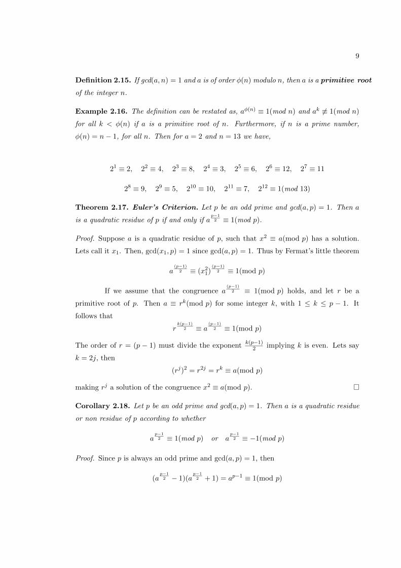
Definition 2.15. If gcd(a, n) = 1 and a is of order φ(n) modulo n, then a is a primitive root

of the integer n.

Example 2.16. The definition can be restated as, aφ(n) ≡ 1(mod n) and ak 6≡ 1(mod n)

for all k < φ(n) if a is a primitive root of n. Furthermore, if n is a prime number,

φ(n) = n− 1, for all n. Then for a = 2 and n = 13 we have,

21 ≡ 2, 22 ≡ 4, 23 ≡ 8, 24 ≡ 3, 25 ≡ 6, 26 ≡ 12, 27 ≡ 11

28 ≡ 9, 29 ≡ 5, 210 ≡ 10, 211 ≡ 7, 212 ≡ 1(mod 13)

Theorem 2.17. Euler’s Criterion. Let p be an odd prime and gcd(a, p) = 1. Then a

is a quadratic residue of p if and only if ap−12 ≡ 1(mod p).

Proof. Suppose a is a quadratic residue of p, such that x2 ≡ a(mod p) has a solution.

Lets call it x1. Then, gcd(x1, p) = 1 since gcd(a, p) = 1. Thus by Fermat’s little theorem

a(p−1)

2 ≡ (x21)(p−1)

2 ≡ 1(mod p)

If we assume that the congruence a(p−1)

2 ≡ 1(mod p) holds, and let r be a

primitive root of p. Then a ≡ rk(mod p) for some integer k, with 1 ≤ k ≤ p − 1. It

follows that

rk(p−1)

2 ≡ a(p−1)

2 ≡ 1(mod p)

The order of r = (p − 1) must divide the exponent k(p−1)2 implying k is even. Lets say

k = 2j, then

(rj)2 = r2j = rk ≡ a(mod p)

making rj a solution of the congruence x2 ≡ a(mod p).

Corollary 2.18. Let p be an odd prime and gcd(a, p) = 1. Then a is a quadratic residue

or non residue of p according to whether

ap−12 ≡ 1(mod p) or a

p−12 ≡ −1(mod p)

Proof. Since p is always an odd prime and gcd(a, p) = 1, then

(ap−12 − 1)(a

p−12 + 1) = ap−1 ≡ 1(mod p)

10

Hence, either ap−12 ≡ 1(mod p) or a

p−12 ≡ −1(mod p), but not both, otherwise 1 ≡

−1(mod p) and p|2. A quadratic nonresidue of p does not satisfy ap−12 ≡ 1(mod p),

therefore it must satisfy ap−12 ≡ −1(mod p).

Definition 2.19. Let p be an odd prime and let gcd(a, p) = 1. The Legendre symbol(ap

)is defined by

(a

p

)=

1 if a is a quadratic residue of p

−1 if a is a quadratic nonresidue of p

0 if a ≡ 0(mod p)

Legendre’s symbol is only defined for primes p. Jacobi later introduced a more general

symbol known as the Jacobi Symbol(aP

), for all natural odd numbers P , when:

P = pe11 pe22 · · · p

emm

is a product of primes pe11 , pe22 , . . . , p

emm , and when a is relatively prime to P . Then:

( aP

)=

(a

p1

)e1 ( a

p2

)e2· · ·(a

pm

)emwhere the factors on the right hand side are Legendre symbols. Thus when P is a quadratic

residue of a,(aP

)= 1 since all the factors on the right hand side equal 1. However, when

P is not a quadratic residue it is not necessarily true that(aP

)= −1. This is because

when an even number of factors on the right hand side have the value −1, the resulting

product will be +1. We will use Jacobi symbol in Gauss’ first proof of quadratic reciprocity

and we note that the Jacobi symbol in not defined for the integers P < 0 or for even P .

Example 2.20. Using legendre symbol, we can rewrite Example 2.14 as:(1

11

)=

(3

11

)=

(4

11

)=

(5

11

)=

(9

11

)= 1

and (2

11

)=

(6

11

)=

(7

11

)=

(8

11

)=

(10

11

)= −1

Theorem 2.21. Let p be and odd prime and let a and b be integers that are relatively

prime to p. Then the Legendre symbol has the following properties:

(a) If a ≡ b(mod p), then(ap

)=(bp

).

11

(b)(a2

p

)= 1

(c)(ap

)≡ a

(p−1)2 (mod p).

(d)(abp

)=(ap

)(bp

).

(e)(1p

)= 1,

(−1p

)= −1

(p−1)2 , and

(0p

)= 0.

(f)(ab2

p

)=(ap

)(b2

p

)=(ap

).

Proof. If a ≡ b(mod p), then the two congruences x2 ≡ a(mod p) and x2 ≡ b(mod p)

have the same exact solutions, and thus either both are solvable or both unsolvable, hence(ap

)=(bp

). For property (b) integer a trivially satisfies the congruence x2 ≡ a(mod p),

hence(a2

p

)= 1. Property (c) is a direct result of Euler’s criterion. Using (c) we get(

ab

p

)≡ (ab)

(p−1)2 ≡ a

(p−1)2 b

(p−1)2 ≡

(a

p

)(b

p

)(mod p)

Since Legendre symbol assumes only values 1 or −1, if(abp

)6=(ap

)(bp

)we would get

1 ≡ −1(mod p) or 2 ≡ 0(mod p), but p > 2. Thus,(ab

p

)=

(a

p

)(b

p

)The first part of property (e) is a special case of property (b), when a = 1, and the

second part is derived from property (c) when a = −1. The result for property (f) follows

directly from properties (b) and (d).

Theorem 2.22. If p is an odd prime, then

p−1∑a=1

(a

p

)= 0

Hence, there are precisely (p−1)/2 quadratic residues and (p−1)/2 quadratic nonresidues

of p.

Proof. Let r be a primitive root of p. Then modulo p, the powers r, r2, ..., rp−1 are just

a permutation of the integers 1, 2, ..., p − 1. Thus for any a between 1 and p − 1, there

exists a unique positive integer k(1 ≤ k ≤ p − 1), such that a ≡ rk(mod p). By Euler’s

criterion we have(a

p

)=

(rk

p

)≡ (rk)

(p−1)2 = (r

(p−1)2 )k ≡ (−1)k(mod p)

12

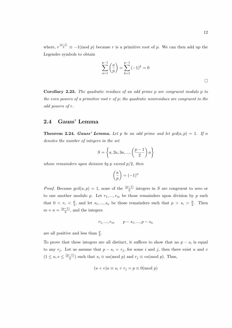
where, r(p−1)

2 ≡ −1(mod p) because r is a primitive root of p. We can then add up the

Legendre symbols to obtain

p−1∑a=1

(a

p

)=

p−1∑k=1

(−1)k = 0

Corollary 2.23. The quadratic residues of an odd prime p are congruent modulo p to

the even powers of a primitive root r of p; the quadratic nonresidues are congruent to the

odd powers of r.

2.4 Gauss’ Lemma

Theorem 2.24. Gauss’ Lemma. Let p be an odd prime and let gcd(a, p) = 1. If n

denotes the number of integers in the set

S =

{a, 2a, 3a, ...,

(p− 1

2

)a

}whose remainders upon division by p exceed p/2, then(

a

p

)= (−1)n

Proof. Because gcd(a, p) = 1, none of the (p−1)2 integers in S are congruent to zero or

to one another modulo p. Let r1, ..., rm be those remainders upon division by p such

that 0 < ri <p2 , and let s1, ..., sn be those remainders such that p > si >

p2 . Then

m+ n = (p−1)2 , and the integers

r1, ..., rm p− s1, ..., p− sn

are all positive and less than p2 .

To prove that these integers are all distinct, it suffices to show that no p − si is equal

to any rj . Let us assume that p − si = rj , for some i and j, then there exist u and v

(1 ≤ u, v ≤ (p−1)2 ) such that si ≡ ua(mod p) and rj ≡ va(mod p). Thus,

(u+ v)a ≡ si + rj = p ≡ 0(mod p)

13

However, u+ v 6≡ 0(mod p) since 1 < u+ v ≤ p− 1. The central point is that the (p−1)2

numbers

r1, ..., rm p− s1, ...p− sn

are the integers 1, 2, ..., (p−1)2 (in some order). Thus, their product is (p−1)2 !:(

p− 1

2

)! = r1 · · · rm(p− s1) · · · (p− sn)

≡ r1 · · · rm(−s1) · · · (−sn)(mod p)

≡ (−1)nr1 · · · rms1 · · · sn(mod p)

We know that r1, ..., rm, s1, ..., sn are congruent modulo p to a, 2a, ..., (p−1)2 a (in some

order), thus (p− 1

2

)! ≡ (−1)na · 2a · · ·

(p− 1

2

)a(mod p)

≡ (−1)na(p−1)

2

(p− 1

2

)!(mod p)

Since(p−12

)! is relatively prime to p, we can cancel it from both sides:

1 ≡ (−1)na(p−1)

2 (mod p)

multiplying both sides by (−1)n, we get

a(p−1)

2 ≡ (−1)n(mod p)

Using Euler’s criterion we get:(a

p

)≡ a

(p−1)2 ≡ (−1)n(mod p)

⇒(a

p

)= (−1)n

Example 2.25. Now we can look at Gauss’s lemma with an example, where a = 7 and

p = 17. Then (p− 1)/2 = 8 and:

S = {7, 14, 21, 28, 35, 42, 49, 56}

14

Modulo 17, we can rewrite S as the following:

S = {7, 14, 4, 11, 1, 8, 15, 5}

Three of these are greater that 17/2; therefore, n = 3, and according to Theorem 2.24:(7

17

)= (−1)3 = −1

We can also confirm this using the Corollary 2.18 to Euler’s criterion:

7( 17−12 ) ≡ 16 ≡ −1(mod 17)

Theorem 2.26. Using Gauss’s lemma, we can show that if p is an odd prime, then

(2

p

)=

1 if p ≡ ±1(mod 8)

−1 if p ≡ ±3(mod 8)

Proof. According to Gauss’s lemma,(2p

)= (−1)n where n is the number of integers in

the set

S =

{2, 4, 6, ..., 2

(p− 1

2

)}whose remainders upon division by p are greater than p/2. Since all members of S are

less than p modulo p it suffices to count the number of even integers 1 < 2k < (p− 1)/2

that exceed p/2. We see that 2k < p/2 when k < p/4; therefore, if we let [p/4] be the

largest even integer less than p/2, then

n =p− 1

2−[p

4

]Now we can look at the individual cases for the four different forms of p:

If p = 8M + 1, then n = 4M −[2M +

1

4

]= 4M − 2M = 2M

If p = 8M + 3, then n = 4M + 1−[2M +

3

4

]= 4M + 1− 2M = 2M + 1

If p = 8M + 5, then n = 4M + 2−[2M + 1 +

1

4

]= 4M + 2− 2M − 1 = 2M + 1

If p = 8M + 7, then n = 4M + 3−[2M + 1 +

3

4

]= 4M + 3− 2M − 1 = 2M + 2

Thus, when p ≡ ±1 (mod 8) ⇔ p = 8M + 1 or 8M + 7, n is even and (−1)n is 1.

Conversely, if p ≡ ±3 (mod 8) ⇔ p = 8M + 3 or 8M + 5, n is odd and (−1)n is −1.

15

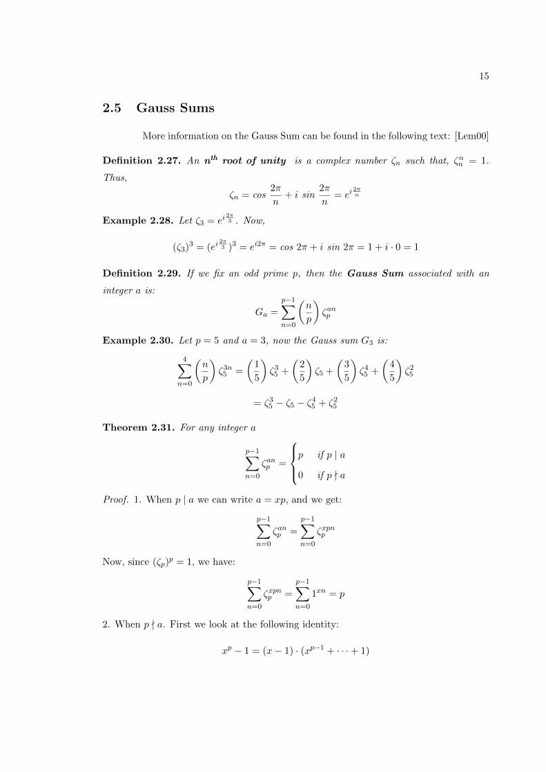
2.5 Gauss Sums

More information on the Gauss Sum can be found in the following text: [Lem00]

Definition 2.27. An nth root of unity is a complex number ζn such that, ζnn = 1.

Thus,

ζn = cos2π

n+ i sin

2π

n= ei

2πn

Example 2.28. Let ζ3 = ei2π3 . Now,

(ζ3)3 = (ei

2π3 )3 = ei2π = cos 2π + i sin 2π = 1 + i · 0 = 1

Definition 2.29. If we fix an odd prime p, then the Gauss Sum associated with an

integer a is:

Ga =

p−1∑n=0

(n

p

)ζanp

Example 2.30. Let p = 5 and a = 3, now the Gauss sum G3 is:

4∑n=0

(n

p

)ζ3n5 =

(1

5

)ζ35 +

(2

5

)ζ5 +

(3

5

)ζ45 +

(4

5

)ζ25

= ζ35 − ζ5 − ζ45 + ζ25

Theorem 2.31. For any integer a

p−1∑n=0

ζanp =

p if p | a

0 if p - a

Proof. 1. When p | a we can write a = xp, and we get:

p−1∑n=0

ζanp =

p−1∑n=0

ζxpnp

Now, since (ζp)p = 1, we have:

p−1∑n=0

ζxpnp =

p−1∑n=0

1xn = p

2. When p - a. First we look at the following identity:

xp − 1 = (x− 1) · (xp−1 + · · ·+ 1)

16

⇒ (xp−1 + · · ·+ 1) =(xp − 1)

(x− 1)

Now, if we substitute ζap for x, we get:

p−1∑n=0

(ζap )n = ((ζap )p−1 + · · ·+ 1) =(ζapp − 1)

(ζap − 1)

Now, since (ζp)p = 1, we get:

(ζapp − 1)

(ζap − 1)=

(1a − 1)

(ζap − 1)= 0

Corollary 2.32. For any integer x, y

p−1∑n=0

ζ(x−y)np =

p if x ≡ y(mod p)

0 if x 6≡ y(mod p)

The proof for Corollary 2.31 is exactly the same as that of Theorem 2.30, and

can be acheived by replacing (x− y) with a.

Example 2.33. Let p = 3 and a = 6, then p | a and:

2∑n=0

ζ6n3 =2∑

n=0

(ζ33)2n

=2∑

n=0

12n = 1 + 1 + 1 = 3 = p

Example 2.34. Let p = 3 and a = 2, then p - a and:

2∑n=0

ζ2n3 = 1 + ζ23 + ζ3 (2.1)

We know that ζ3 is a solution for the equation x3 − 1 = 0, which can be expanded to

(x−1)(x2 +x+1). Here we take the right hand side of the product to be 0 (since ζ3 6= 1),

then x2 + x+ 1 = 0 and x2 = −x− 1. Substituting ζ3 back in for x, we get ζ23 = −ζ3− 1.

Applying this to Equation 2.1 above, we get:

2∑n=0

ζ2n3 = 1− ζ3 − 1 + ζ3 = 0

Theorem 2.35. The Gauss Sum G0 = 0.

17

Proof.

G0 =

p−1∑n=0

(n

p

)ζ0np =

p−1∑n=0

(n

p

)Now by applying Theorem 2.22 to the right hand side, we get:

p−1∑n=0

(n

p

)= 0

since there are exactly (p− 1)/2 quadratic residues and (p− 1)/2 quadratic nonresidues

of p.

Example 2.36. Let p = 3 and a = 0, then:

G0 =2∑

n=0

(n3

)ζ0n3 =

(0

3

)· 1 +

(1

3

)· 1 +

(2

3

)· 1

⇒ 0 + 1− 1 = 0

2.6 Normal Subgroups and Quotient Groups

More information on the theorems and definitions of group theory delineated

below can be found in the following text: [Rom05]

Definition 2.37. An abelian group G∗ is a set G with a binary operation ∗ such that

the following properties hold:

1. (Closure) If x, y ∈ G, then x ∗ y ∈ G.

2. (Associativity) x ∗ (y ∗ z) = (x ∗ y) ∗ z, for all x, y, z ∈ G.

3. (Identity) There exists an element e ∈ G, such that e ∗ x = x for all x ∈ G.

4. (Inverse) For all x ∈ G, there exists y ∈ G, such that x ∗ y = e.

5. (Commutativity) x ∗ y = y ∗ x for all x, y ∈ G.

Example 2.38. The group of all integers Z is an abelian group under addition.

1. The sum of any two integers is an integer.

2. The associativity law applies to all integers. Eg: 2 + (3 + 4) = (2 + 3) + 4.

3. The additive identity for all integers is 0.

18

4. The additive inverse for any integer x is −x, which is also an integer.

5. Integer addition is commutative. Eg: 2 + 3 = 3 + 2

Example 2.39. The group of rational numbers Q, without 0, is an abelian group under

multiplication. We need to remove 0, because 0 does not have a multiplicative inverse.

1. The products of two rational numbers is a rational number.

2. Integers are a subgroup of rationals, thus associativity applies as seen in the example

above.

3. The multiplicative identitiy for rationals is 1.

4. The multiplicative inverse for any rational xy , where x, y ∈ Z is y

x .

5. Rational multiplication is commutative. Eg. 2 ∗ 3 = 3 ∗ 2.

Definition 2.40. A subset S of a group G, is said to be a subgroup of G, if it is a

group itself.

Example 2.41. Consider the set of real numbers R, which is a group under addition.

Then the integers Z, which are a subset of real numbers, and also form a group under

addition (see Example 2.38), are said to a be a subgroup of R.

Definition 2.42. Let H be a subgroup of G, and let x ∈ G be an element of G, then we

define x ∗H, as the subset {x ∗ h | h ∈ H}, to be a left coset of H, and H ∗ x, as the

subset {h ∗ x | h ∈ H} to be the right coset of H. Where ∗ is a binary operation, such

as addition or multiplication, depending on the definition of the group G.

Example 2.43. Consider the set of all even integers 2Z, it is clear that this is a group

under addition. We also know that the set of all integers Z is a group, thus 2Z is clearly

a subgroup of Z. Then we can say that, 1 + 2Z is a left coset of 2Z, and 2Z+ 1 is a right

coset of 2Z.

Definition 2.44. A subgroup H is said to be a normal subgroup of G, if the left cosets

of H are equal to the right cosets of H. That is x ∗H = H ∗ x for all x ∈ G.

Example 2.45. Let’s look at the subgroup 2Z from Example 2.43 above. We can see that

the left coset of 2Z, 1 + 2Z, is equal to the set of odd integers {. . . ,−3,−1, 1, 3, . . . }.Furthermore, the right coset of 2Z, 2Z + 1, is also equal to the set of odd integers

{. . . ,−3,−1, 1, 3, . . . }. Thus, 2Z is a normal subgroup of Z.

19

Definition 2.46. If H is a normal subgroup of G, then we can construct a group G/H

by multiplying the left cosets of H, such that for all α, β ∈ G, αHβH = αβH. The group

G/H is called the quotient group of G by H. (Note: Here we say left cosets for the

sake of illustration. However, since H is a normal subgroup of G, the left and the right

cosets of H are equal.)

Example 2.47. Let G = Z6 = {0, 1, 2, 3, 4, 5} and let H be the normal subgroup {0, 3}.The cosets of H are:

{0, 3} , 1 + {0, 3} = {1, 4} , 2 + {0, 3} = {2, 5}

Then the quotient group G/H is a group of order 3 containing the following elements:

{0, 3}, {1, 4}, {2, 5}.

20

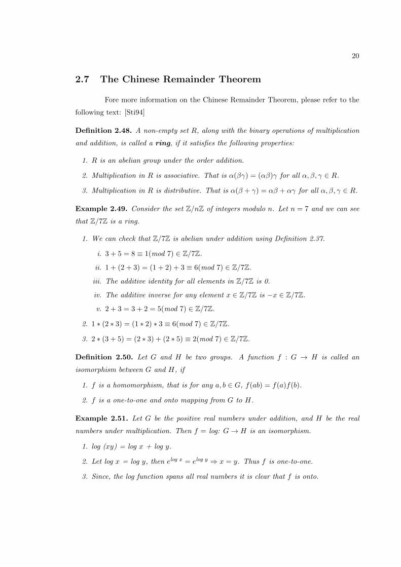
2.7 The Chinese Remainder Theorem

Fore more information on the Chinese Remainder Theorem, please refer to the

following text: [Sti94]

Definition 2.48. A non-empty set R, along with the binary operations of multiplication

and addition, is called a ring, if it satisfies the following properties:

1. R is an abelian group under the order addition.

2. Multiplication in R is associative. That is α(βγ) = (αβ)γ for all α, β, γ ∈ R.

3. Multiplication in R is distributive. That is α(β + γ) = αβ + αγ for all α, β, γ ∈ R.

Example 2.49. Consider the set Z/nZ of integers modulo n. Let n = 7 and we can see

that Z/7Z is a ring.

1. We can check that Z/7Z is abelian under addition using Definition 2.37.

i. 3 + 5 = 8 ≡ 1(mod 7) ∈ Z/7Z.

ii. 1 + (2 + 3) = (1 + 2) + 3 ≡ 6(mod 7) ∈ Z/7Z.

iii. The additive identity for all elements in Z/7Z is 0.

iv. The additive inverse for any element x ∈ Z/7Z is −x ∈ Z/7Z.

v. 2 + 3 = 3 + 2 = 5(mod 7) ∈ Z/7Z.

2. 1 ∗ (2 ∗ 3) = (1 ∗ 2) ∗ 3 ≡ 6(mod 7) ∈ Z/7Z.

3. 2 ∗ (3 + 5) = (2 ∗ 3) + (2 ∗ 5) ≡ 2(mod 7) ∈ Z/7Z.

Definition 2.50. Let G and H be two groups. A function f : G → H is called an

isomorphism between G and H, if

1. f is a homomorphism, that is for any a, b ∈ G, f(ab) = f(a)f(b).

2. f is a one-to-one and onto mapping from G to H.

Example 2.51. Let G be the positive real numbers under addition, and H be the real

numbers under multiplication. Then f = log: G→ H is an isomorphism.

1. log (xy) = log x + log y.

2. Let log x = log y, then elog x = elog y ⇒ x = y. Thus f is one-to-one.

3. Since, the log function spans all real numbers it is clear that f is onto.

21

Theorem 2.52. The Chinese Remainder Theorem.

If gcd(m,n) = 1, then the map f(x) = (x mod m, x mod n) is an isomorphism of Z/mnZ

onto (Z/mZ) ∗ (Z/nZ).

Proof. Let m be a non-zero integer, then there is a ring homomorphism g : Z → Z/mZ

such that g(x) = x (mod m). We have already seen in an example above that Z/mZ is

indeed a ring. We can also see that it is a homomorphism:

g(x+ y) = (x+ y)(mod m)

= x(mod m) + y(mod m)

= g(x) + g(y)

and

g(xy) = (xy)(mod m)

= x(mod m)y(mod m)

= g(x)g(y)

Similarly, if n is another non-zero integer, then h(x) = x (mod n) is another ring homo-

morphism that takes Z→ Z/nZ.

Let f be a mapping that combines these two homomorphisms, such that f : Z→ (Z/mZ)∗(Z/nZ), by defining:

f(x) = (g(x), h(x))

= (x(mod m), x(mod n))

Now, the ring operations on (Z/mZ) ∗ (Z/nZ) are component-wise addition and multi-

plication.

(x, u) + (y, v) = (x+ y, u+ v)

(x, u)(y, v) = (xy, uv)

where x, y ∈ Z/mZ and u, v ∈ Z/nZ.

Now, we can see that f is a homomorphism, since:

22

f(x+ y) = (g(x+ y), h(x+ y))

= (g(x) + g(y), h(x) + h(y))

= (g(x), h(x)) + (g(y), h(y))

= f(x) + f(y)

and

f(xy) = (g(xy), h(xy))

= (g(x)g(y), h(x)h(y))

= (g(x), h(x))(g(y), h(y))

= f(x)f(y)

Moreover, we also note that:

f(x+mn) = ((x+mn(mod m)), (x+mn(mod n)))

= ((x(mod m)), (x(mod n)))

= f(x)

Thus it is clear that f(x) only depends on x (mod mn), and we can say that f is a

homomorphism from Z/mnZ to (Z/mZ) ∗ (Z/nZ).

Now we only need to show that f is one-to-one and onto from Z/mnZ to (Z/mZ)∗(Z/nZ).

We can show that f is one-to-one if f(x) = 0 ↔ x = 0. Let us assume that f(x) = 0,

then:

f(x) = 0 = (0 mod m, 0 mod n)

= (x mod m,x mod n)

⇒ x = 0 mod m, and 0 mod n

Since, gcd(m,n) = 1, x must be congruent to 0 mod mn. Thus, x = 0 in Z/mnZ and f

is one-to-one.

In order to show that f is onto, for any two integers a, b, there exists an integer x, such

that:

23

f(x) = (a mod m, b mod n)

Thus, we have:

x = a mod m and x = b mod n (2.2)

Now, since m and n are relatively prime, we know that there exist unique integers u and

v, such that:

um+ nv = 1 (2.3)

We claim that

x = bum+ anv (2.4)

is a solution to Equation 2.2. We can test this by first multiplying a to both sides of

Equation 2.3:

aum+ anv = a (2.5)

Now, combining Equation 2.4 and 2.5, it is clear that:

x mod m ≡ anv mod m ≡ a mod m

A similar calculation can be done by multiplying Equation 2.3 with b:

bum+ bnv = b (2.6)

Now, combining Equation 2.5 and 2.6, we get:

x mod n ≡ bum mod n ≡ b mod n

This shows that x = a mod m and x = b mod n, therefore f is also an onto

mapping. This proves that f is indeed an isomorphism and completes our proof.

24

Chapter 3

Proofs of The Law of Quadratic

Reciprocity

3.1 The Law of Quadratic Reciprocity

The Law of Quadratic Reciprocity is one of the fundamental theorems of number

theory. Legendre attempted two incomplete proofs of the law in 1785 and 1798 respec-

tively, and it was eventually proved by Gauss in 1801. Despite Legendre’s incomplete

attempts to prove the law, his elegant notation, most importantly the Legendre symbol,

eventually became the modern Law of Quadratic Reciprocity. The iteration of Gauss’s

first proof of quadratic reciprocity described here was composed with information from

the following sources: [Bau15] [Dir91] [GC86] [Lem00]

Theorem 3.1. Quadratic Reciprocity Law.

If p and q are distinct odd primes, then(p

q

)(q

p

)= (−1)

p−12

q−12

3.2 Gauss’s First Proof of Quadratic Reciprocity

In his first proof Gauss utilized the method of induction to prove the Generalized

Quadratic Reciprocity Law. The startegy he used was to show that if we assume the

Quadratic Reciprocity Law to be true for every distinct pair of odd primes less than a

prime q then it must also hold true for every combination of those primes with q. Since,

25

the theorem holds true for the two smallest odd primes 3 and 5, that is:(35

)=(53

)= −1,

then it must also hold for every combination of 3 and 5 with the next largest prime 7.

Consequently, if it holds true for every combination of the primes 3, 5 and 7, then it must

also hold true for every combination of 3, 5 and 7 with the prime 11 and so on. Thus by

mathematical induction it will hold true for every pair of distinct odd primes.

In the first proof, Gauss looked at each of the following eight cases for the primes

p and q, where p is an odd prime less than q and we assume that Theorem 3.1 holds for

each pair of distinct odd primes less than q. The eight cases are as follows:

1. If q = 4n+ 1, p = 4n+ 1 and(pq

)= 1, then we have to prove that

(qp

)= 1;

2. If q = 4n+ 1, p = 4n+ 3 and(pq

)= 1, then we have to prove that

(qp

)= 1;

3. If q = 4n+ 1, p = 4n+ 1 and(pq

)= −1, then we have to prove that

(qp

)= −1;

4. If q = 4n+ 1, p = 4n+ 3 and(pq

)= −1, then we have to prove that

(qp

)= −1;

5. If q = 4n+ 3, p = 4n+ 3 and(pq

)= 1, then we have to prove that

(qp

)= −1;

6. If q = 4n+ 3, p = 4n+ 1 and(pq

)= 1, then we have to prove that

(qp

)= 1;

7. If q = 4n+ 3, p = 4n+ 3 and(pq

)= −1, then we have to prove that

(qp

)= −1;

8. If q = 4n+ 3, p = 4n+ 1 and(pq

)= −1, then we have to prove that

(qp

)= −1;

Later demonstrations by Dedekind and Bachmann showed that these 8 possi-

bilites can be collapsed into the following two mutually exclusive cases, which encompass

all of the possibilities listed above:

i. at least one of(pq

)or(−pq

)is 1, then

(qp

)= (−1)

p−12

q−12

(pq

);

ii. q is of the form 4M + 1 and(pq

)= −1, then

(qp

)= −1

We know from the Corollary 2.18 to Euler’s criterion that(−1q

)= (−1)

q−12 , therefore

case (i) covers the following possibilities:

q is of the form 4M + 3 and

(q

p

)= 1;

q is of the form 4M + 3 and

(q

p

)= −1;

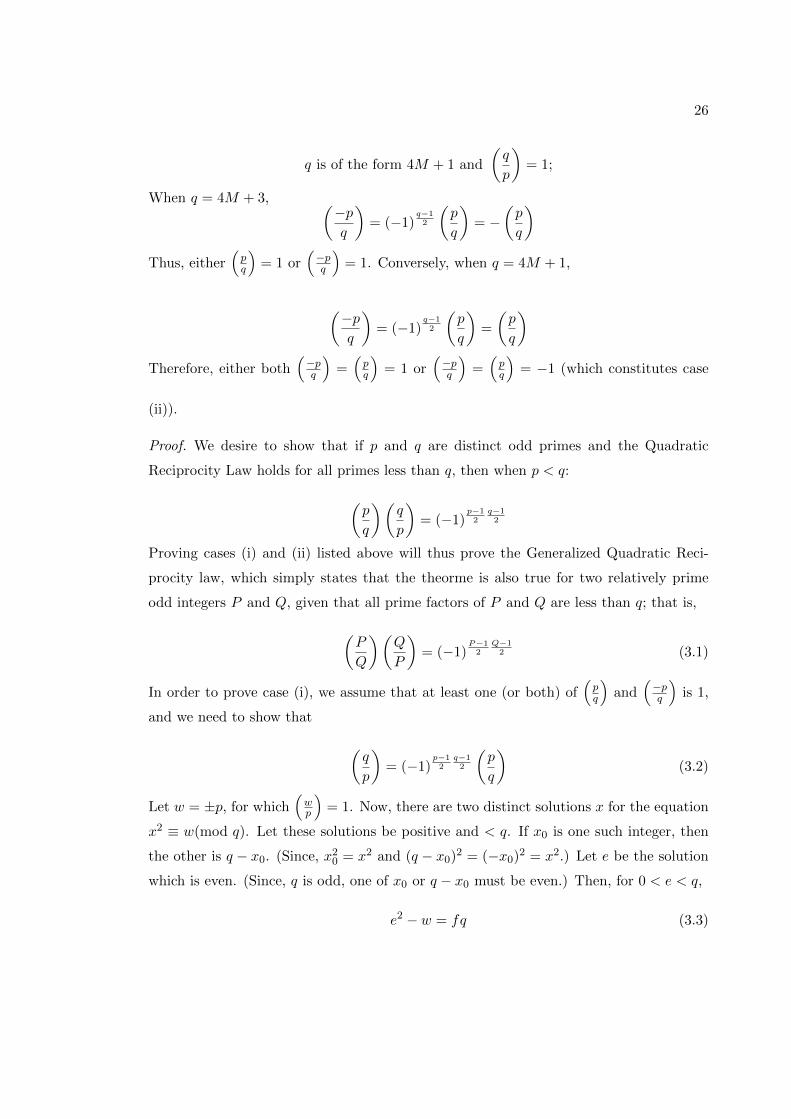
26

q is of the form 4M + 1 and

(q

p

)= 1;

When q = 4M + 3, (−pq

)= (−1)

q−12

(p

q

)= −

(p

q

)Thus, either

(pq

)= 1 or

(−pq

)= 1. Conversely, when q = 4M + 1,

(−pq

)= (−1)

q−12

(p

q

)=

(p

q

)Therefore, either both

(−pq

)=(pq

)= 1 or

(−pq

)=(pq

)= −1 (which constitutes case

(ii)).

Proof. We desire to show that if p and q are distinct odd primes and the Quadratic

Reciprocity Law holds for all primes less than q, then when p < q:

(p

q

)(q

p

)= (−1)

p−12

q−12

Proving cases (i) and (ii) listed above will thus prove the Generalized Quadratic Reci-

procity law, which simply states that the theorme is also true for two relatively prime

odd integers P and Q, given that all prime factors of P and Q are less than q; that is,

(P

Q

)(Q

P

)= (−1)

P−12

Q−12 (3.1)

In order to prove case (i), we assume that at least one (or both) of(pq

)and

(−pq

)is 1,

and we need to show that

(q

p

)= (−1)

p−12

q−12

(p

q

)(3.2)

Let w = ±p, for which(wp

)= 1. Now, there are two distinct solutions x for the equation

x2 ≡ w(mod q). Let these solutions be positive and < q. If x0 is one such integer, then

the other is q − x0. (Since, x20 = x2 and (q − x0)2 = (−x0)2 = x2.) Let e be the solution

which is even. (Since, q is odd, one of x0 or q − x0 must be even.) Then, for 0 < e < q,

e2 − w = fq (3.3)

27

Now we can see that f cannot be negative. In order for f to be negative, p would have to

be positive and greater than e2. Consequently, p − e2 = fq, where p − e2 is divisible by

q; however, since p− e2 < p and p < q this is impossible because q is a prime and cannot

divide any number smaller than itself. Furthermore, f < q because both e and w are less

than q and therefore: fq = e2−w ≤ (q−1)2−w = q2−2q− (w−1) < q2−3q = q(q−3).

Therefore, f < q. Moreover, f is odd, since fq = e2 − w is odd. Now there are two

possibilities for Equation 3.3.

1. e and f are coprime to w.

Since, e2 ≡ fq (mod w),(fq|w|

)= 1, and

(f|w|

)=(

q|w|

). Also, e2 ≡ w (mod f), therefore,(

wf

)= 1. Now, both f and w are relatively prime odd integers less than q, therefore we

can apply Equation 3.1 and we get:(q

|w|

)=

(f

|w|

)=

(|w|f

)(−1)

w−12

f−12 = (−1)

w−12

f−12 (3.4)

Since e is even, e2 is divisible by 4. Therefore, −w ≡ fq (mod 4). Also:

−w − 1 = fq − 1(mod 4) and−w − 1

2=fq − 1

2(mod 2)

Setting f ′ = (f − 1)/2 and q′ = (q − 1)/2, we get

fq − 1 = (2f ′ + 1)(2q′ + 1)− 1 = 4f ′q′ + 2f ′ + 2q′

Now,fq + 1

2= 2f ′q′ + f ′ + q′

⇒ −(w + 1)

2=fq + 1

2= f ′ + q′(mod 2)

⇒ −(w + 1)

2=f − 1

2+q − 1

2(mod 2)

Multiplying both sides by (w − 1)/2, we get

−w + 1

2

w − 1

2=f − 1

2

w − 1

2+q − 1

2

w − 1

2(mod 2)

Since, (w + 1)/2 and (w − 1)/2 are consecutive integers, their product is even and we

have:

−f − 1

2

w − 1

2=q − 1

2

w − 1

2(mod 2)

28

Since, 1 (mod 2) = −1 (mod 2), we can remove the negative sign from the left side of the

equation above. Thus,

f − 1

2

w − 1

2=q − 1

2

w − 1

2(mod 2)

Applying this to Equation 3.4, we get:(q

|w|

)= (−1)

w−12

q−12 (3.5)

Now, when w = p and(wq

)=(pq

)= 1, we have:(

q

p

)= (−1)

w−12

q−12

(p

q

)

When w = −p and(wq

)=(−pq

)= 1, we have:(

q

p

)= (−1)

−w−12

q−12

(p

q

)(−1

q

)

⇒(q

p

)= (−1)

q−12 (−1)

−w−12

q−12

(p

q

)⇒ (−1)

q−12 (−1)

−w−12

q−12

(p

q

)= (−1)(

−w−12

q−12

)+( q−12

)

(p

q

)⇒ (−1)

−w+12

q−12

(p

q

)= (−1)−

(w−1)2

q−12

(p

q

)

Since, the only two solutions for this equation are 1 and −1 and raising either of them

to the −1 power does not change the result, we can remove the negative sign from the

exponent without affecting the solution. Therefore, when w = −p we also have:(q

p

)= (−1)

w−12

q−12

(p

q

)

This proves Case (i), when e and f are coprime to w. Next we look at the second

possiblity:

29

2. f and e are divisible by w

Let f = wf1, for some odd number f1 < f and let e = we1 for some even number e1 < e.

Now we can rewrite Equation 3.3 as:

e21w2 − w = wf1q ⇒

w(e21w − 1)

w= f1q

⇒ e21w − 1 = f1q or e21w = 1 + f1q (3.6)

Then, e21w ≡ 1 (mod f1) and(e21|f1|

)=(w|f1|

)= 1. Moreover, 12 ≡ −f1q (mod w);

therefore,(−f1|w|

)=(

q|w|

). Since f1 and w are both less than q, we can apply Equation

3.1 and get: (|f1||w|

)= (−1)

|w−1|2|f1|−1

2

(|w||f1|

)⇒(|f1||w|

)= (−1)

|w|−12|f1|−1

2

Now, we can see that: (q

|w|

)=

(−f1|w|

)=

(−1

|w|

)(f1|w|

)⇒(q

|w|

)=

(−1

|w|

)(−1)

w−12

f1−12

⇒(q

|w|

)= (−1)

w−12 (−1)

w−12

f1−12 = (−1)(

w−12

)+(w−12

f1−12

)

Therefore, now we have:

(q

|w|

)= (−1)

f1+12

w−12 (3.7)

We know that e1 is even, therefore e21 ≡ 0 (mod 4). Now from Equation 3.6 we have

e21w ≡ 0 (mod 4) ≡ f1q + 1 (mod 4). Since, both f1 and q are odd f1q + 1 ≡ 0 (mod 4),

if and only if one of f1 or q is of the form 4M + 1 and the other is of the form 4M + 3.

In either case we have:

f1 + 1

2≡ q − 1

2(mod 2)

30

Applying this to Equation 3.7, we get:

(q

|w|

)= (−1)

q−12

w−12 (3.8)

Now we can see that Equation 3.8 is analogous to Equation 3.5 above and holds true for

both w = p and w = −p. This concludes the proof for Case (i). Now we look at Case

(ii).

In Case (ii) we need to show that when q is of the form 4M + 1 and(pq

)= −1 and p

is not a quadratic residue mod q, then q is also a non residue mod p and(qp

)= −1. In

order to prove this, we will first prove the following lemma give by Gauss.

Lemma 3.2. If q is a prime of the form 4N + 1, there exists an odd prime p′ < q for

which(qp′

)= −1.

Proof.

1. This is apparent when q is of the form 8N + 5. In this case, q+12 is of the form 4N + 3.

Now since, not all of its prime factors can be of the form 4N + 1. There must be a prime

factor p′ of the form 4N + 3, which divides q+ 1 such that q+ 1 ≡ 0 (mod p′) and q ≡ −1

(mod p′). Thus:

(q

p′

)=

(−1

p′

)= (−1)

p′−12 = −1

2. When q is of the form 8N + 1, if we assume that q is a quadratic residue of every odd

prime less than 2m + 1 < q. Then since we know from Theorem 2.26 that(2q

)= 1, we

can see that q is also a quadratic residue of every positive integer which is a product of

numbers ≤ 2m + 1. Now if M = 1 · 2 · 3 · · · 2m(2m + 1), then, the congruence x2 ≡ q

(mod M) is solvable. Let k = x be one of its solutions, then k and q are relatively prime

to M , and:

(k2 − 12) · · · (k2 −m2) ≡ (q − 12) · · · (q −m2)(mod M)

Moreover,

k·(k2−12) · · · (k2−m2) ≡ (k+m)(k+m−1) · · · (k+1)k(k−1) · · · (k−(m−1))(k−m)(mod M)

31

The right side of the equation is a product of (2M + 1) consecutive integers, it must be

divisible by M , thus the product:

(q − 12)(q − 22) · · · (q −m2)

1 · 2 · · · (2m+ 1)

is an integer. Furthermore, since (2m+ 1)! can be rewritten as:

[(m+ 1)−m] · [(m+ 1)− (m− 1)] · · · [(m+ 1)− 1] · [(m+ 1)− 0]

·[(m+ 1) +m] · [(m+ 1) + (m− 1)] · · · [(m+ 1) + 1]

⇒ (m+ 1)[(m+ 1)2 −m2] · · · [(m+ 1)2 − 12]

Therefore, the following is an integer:

1

m+ 1

q − 12

(m+ 1)2 − 12q − 22

(m+ 1)2 − 22· · · q −m2

(m+ 1)2 −m2(3.9)

Now, if we choose m = [√q] to be the largest integer less than

√q, such that m <

√q <

m + 1, then m2 < q < (m + 1)2, and every factor of the product in Equation 3.9 is a

proper fraction, which is a contradiction. Furthermore, since q is of the form 8N + 1, and

the smallest possible prime of that form is 17, q ≥ 17, and it is apparent that 8 < (q−3)2.

Then, 4q < q2 − 2q + 1 = (q − 1)2, and 2√q < q − 1 or 2

√q + 1 < q. Since we chose

m = [√q] to be the largest integer less than

√q, it follows that 2m+ 1 < q. Thus, there

must exist some prime p′ < 2m + 1 < q, which is a quadratic non residue of q if q is of

the form 8M + 1. This completes the proof for Lemma 3.2.

Now, if q = 4N + 1, there is an odd prime p′ < q with(qp′

)= −1, then

(p′

q

)must also

be −1. If(p′

q

)= 1, then we can apply Case (i), and we get:(

q

p′

)= (−1)

(p′−1)2

(q−1)2 = 1

This contradicts the assumption that(qp′

)= −1. In order to complete the proof of Case

(ii), we only need to show that if there exists another prime p < q separate from the

existing prime p′, such that(pq

)= −1, then also

(qp

)= −1 or in other words:(

q

pp′

)= 1 (3.10)

32

Now we know that(p′

q

)= −1, and by assumption we have

(pq

)= −1, thus(

pp′

q

)= +1, and the congruence x2 ≡ pp′ (mod q) is solvable. Then the solutions for x

are x0 and q − xo, let e be the solution which is even, then:

e2 = pp′ + fq (3.11)

where f is an odd integer less than q. Now we can look at the following cases:

1. e and f are not divisible by p or p′.

Then we can see that e2 ≡ pp′ (mod f), and(pp′

|f |

)= 1. Moreover, e2 ≡ qf (mod pp′),

therefore,(qfpp′

)= 1, and

(fpp′

)=(

qpp′

). Now when f > 0 we get:(

q

pp′

)=

(f

pp′

)= (−1)

(pp′−1)2

(f−1)2 (3.12)

Furthermore, when f is negative, we get:(q

pp′

)=

(f

pp′

)(−1

pp′

)= (−1)

(pp′−1)2

(−f−1)2 (−1)

(pp′−1)2

⇒(q

pp′

)= (−1)

(pp′−1)2

(−f+1)2 = (−1)

(pp′−1)2

(f−1)2

Since e is even, we have −pp′ ≡ fq (mod 4). Moreover, since q ≡ 1 (mod 4), −pp′ ≡ f

(mod 4):f − 1

2≡ −pp

′ + 1

2≡ pp′ + 1

2(mod 2)

Since pp′+12 and pp′−1

2 are consecutive integers, their product is even. Thus replacing f−12

with pp′+12 in Equation 3.12 gives us an even exponent and yields:(

q

pp′

)= 1

which is what we wanted to show.

2. e and f are divisible by p′, but not p.

Then we can set f = p′f1, and e = p′e1. Then Equation 3.11 takes the form:

p′e21 − p = f1q (3.13)

From Equation 3.13 we see that p′e21 ≡ p (mod f1). Therefore,(p′e21|f1|

)=

(p′

|f1|

)(e21|f1|

)=

(p′

|f1|

)=

(p

|f1|

)

33

Now,(p′p|f1|

)= 1. Moreover, (

f1q

p

)=

(p′

p

)=

(−pp′

)Also, (

q

pp′

)=

(|f1|pp′

)2( q

pp′

)=

(|f1|pp′

)(|f1|qpp′

)Since |f1| and pp′ are less than q, by our assumption the generalized quadratic reciprocity

law holds for |f1| and pp′, and we get:(|f1|pp′

)= (−1)

|f1|−12

pp′−12

(pp′

|f1|

)= (−1)

|f1|−12

pp′−12

Now if f1 > 0, we have: (q

pp′

)= (−1)

f1−12

pp′−12

(f1q

p

)(f1q

p′

)

⇒(q

pp′

)= (−1)

f1−12

pp′−12

(p′

p

)(−pp′

)⇒(q

pp′

)= (−1)

f1−12

pp′−12

+ p′−12

(p′

p

)(p

p′

)Since the quadratic reciprocity law also holds for p and p′, we get:(

q

pp′

)= (−1)

f1−12

pp′−12

+ p+12

p′−12 (3.14)

If f1 < 0, we have:

(q

pp′

)= (−1)

−f1−12

pp′−12

(−1

p

)(−1

p′

)(f1q

p

)(f1q

p′

)⇒(q

pp′

)= (−1)

−f1−12

pp′−12

+ p−12

+ p′−12

(p′

p

)(−pp′

)⇒(q

pp′

)= (−1)

−f1−12

pp′−12

+ p−12

+ p−12

p′−12

⇒(q

pp′

)= (−1)

f1+12

pp′−12

+ p−12

p′+12

Since e1 in Equation 3.13 is even and q ≡ 1 (mod4), we get f1 (mod 4) ≡ −p (mod 4).

Thus:f1 − 1

2≡ −p− 1

2(mod 2)

34

Now,f1 − 1

2

pp′ − 1

2+p′ − 1

2

p− 1

2≡ −p+ 1

2

pp′ − 1

2+p′ − 1

2

p+ 1

2

p+ 1

2

1− pp′

2+p′ − 1

2≡ p+ 1

2

−pp′ + p′

2≡ −p′ p+ 1

2

p− 1

2

Moreover,

f1 + 1

2≡ p− 1

2(mod 2)

Therefore,

f1 + 1

2

pp′ − 1

2+p− 1

2

p′ + 1

2≡ p− 1

2

pp′ − 1

2+p− 1

2

p′ + 1

2

p− 1

2

pp′ + p′

2≡ p− 1

2p′p+ 1

2≡ p′ p− 1

2

p+ 1

2

Since p+12 and p−1

2 are consecutive integers, their product is even. Thus in both cases

where either f1 > 0 or f1 < 0, we have:(q

pp′

)= 1

which is what we wanted to show.

3. Since in the proof of 2. above, we did not utilize the fact that(qp′

)= −1, we can see

that simply interchanging p′ with p in the proof above will similarly prove the case where

e and f are divisible by p, but not p′.

4. The final case is where e and f are divisible by both p and p′.

Let f = pp′f1, and e = pp′e1. Then Equation 3.11 takes the form:

pp′e21 − 1 = f1q (3.15)

From Equation 3.15, we can see that:

1 =

(pp′e21|f1|

)=

(pp′

|f1|

)and

(−f1qpp′

)= 1

Thus, we can see that: (q

pp′

)=

(−f1pp′

)=

(−1

pp′

)(f1pp′

)

35

Since, f1 and pp′ are less than q, we can apply the generalized quadratic reciprocity law

and we get: (|f1|pp′

)=

(pp′

|f1|

)(−1)

|f1|−12

pp′−12

Thus when f1 > 0, (q

pp′

)= (−1)

pp′−12

+f1−1

2pp′−1

2 = (−1)f1+1

2pp′−1

2 (3.16)

And when f1 < 0,

(q

pp′

)= (−1)

pp′−12

+ pp′−12

+−f1−1

2pp′−1

2 = (−1)f1+1

2pp′−1

2

Now, since e1 is even and q ≡ 1 (mod 4), we can see from Equation 3.15 that f1 ≡ −1

(mod 4), thus f1+12 is even and consequently the exponent is even in both cases for f1.

Therefore, (q

pp′

)= 1

which is what we wanted to show.

This concludes the proof for Case (ii), and hence completes Gauss’s first proof of the Law

of Quadratic Reciprocity by induction.

Although Gauss looked at each of the eight cases outlined at the beginning of this

proof in his seminal demonstration, here we chose a slightly smaller version of the proof,

which allowed us to collapse several of these cases. This by no means takes aways from

the purpose of this demonstration, which was to show that such a fundamental theorem of

number theory could be proven via observation and the very basic technique of induction.

We also add that while Gauss listed each of the eight cases separately in his own proof in

Disquisitiones Arithmeticae, he also chose to forgo repetition of the proof in cases where

the strategy was the same as one of the earlier cases. This brings up an important insight

that can be gleaned from this proof. Despite the fact that we were able to collapse our

version of the proof into two mutually exclusive cases, these two cases still presented

us with several distinctions and subdivisions. Yet many of these subdivisions utilized

very similar strategies, specifically, they entailed equating the quadratic character of q to

another odd prime less than q and then determining whether the resulting combination

36

of exponents would be even or odd. This should suggest that it would be possible to

further collapse this proof and identify approaches which are even shorter.

Indeed, in his second proof Gauss used the genus theory of quadratic binary

forms, which consisted of establishing a bound on the number of existing genera of the

quadratic forms of a given determinant and subsequently investigating the only two cases

for the primes p and q. The resulting proof is far shorter than his first proof. We will

not look at his second proof here, but the original proof can be found in Disquisitiones

Arithmeticae, and another version of it can be seen in The Quadratic Reciprocity Law:

A Collection of Classical Proofs. Instead we will investigate Gauss’s fourth proof, which

made use of quadratic Gauss sums and eventually helped advance the field of algebraic

number theory. The first step of our journey showed us how observation and induction

helped establish one of the fundamental theorems of number theory. Next, we will look

at how further attempts to refine and strengthen this theorem resulted in the discovery

of new territories and gave rise to new features of the mathematical landscape.

3.3 Gauss’s Fouth Proof of Quadratic Reciprocity

In his fourth proof Gauss used quadratic Gauss sums to investigate the Law of

Quadratic Reciprocity. This proof extended the law of quadratic reciprocity to cyclotomic

fields and in so doing contributed greatly to the development of this field. We have already

defined Gauss Sums and given some of their fundamental characteristics in the previous

chapter. In order to give the proof of quadratic reciprocity, we first need to prove two

additional propositions, which will then allow us to proceed with the complete proof

using Gauss Sums. For more information on this proof please refer to the following texts:

[Bau15] [Lan94] [Lem00]

Proposition 3.3. For any integer a,

Ga =

(a

p

)G1

Proof.

1. When p | a, a ≡ 0 (mod p) and:

G0 = G1

(0

p

)= 0

37

2. In the more difficult case, where p - a, we need to show that(a

p

)Ga = G1 ⇒ Ga =

(a

p

)G1

Now, (a

p

)Ga =

(a

p

) p−1∑n=0

(n

p

)ζanp =

p−1∑n=0

(an

p

)ζanp

Since p - a, we can see that the product an will permute all the numbers 0 < n < p

modulo p. Therefore, the sum:

p−1∑n=0

(an

p

)ζanp =

p−1∑n=0

(n

p

)ζnp = G1

Example 3.4. Let a = 3 and p = 5, then:

G3 =4∑

n=0

(n5

)ζ35 =

(1

5

)ζ35 +

(2

5

)ζ5 +

(3

5

)ζ45 +

(4

5

)ζ25

G3 = ζ35 − ζ5 − ζ45 + ζ25 (3.17)

G1 =4∑

n=0

(n5

)ζn5 =

(1

5

)ζ5 +

(2

5

)ζ25 +

(3

5

)ζ35 +

(4

5

)ζ45

G1 = ζ5 − ζ25 − ζ35 + ζ45 (3.18)

We know that(35

)= −1. Therefore, from Equations 3.17 and 3.18, we can see that:

G3 = (−1)G1

Proposition 3.5. For any integer a, such that p - a:

G2a = (−1)

(p−1)2 p

38

Proof.

Since p - a, from the definition of Gauss Sum, we have:

G2a =

p−1∑a,b=1

(ab

p

)ζa+bp

Moreover, because p - a, b and both a and b range over 1, . . . , p−1. We can rewrite b ≡ ac(mod p) (where c also ranges over 1, . . . , p− 1). Then:

G2a =

p−1∑a=1

p−1∑c=1

(a2c

p

)ζa+acp

Since(a2

p

)= 1, we can further simplify to:

G2a =

p−1∑c=1

(p−1∑a=1

ζa(1+c)p

)(c

p

)Now if 1 + c 6≡ 0 mod p, then the sum of the series 1, ζ

(1+c)p , ζ

2(1+c)p , . . . , ζ

(p−1)(1+c)p =

ζpp−1ζp−1 = 0. Thus,

p−1∑a=1

ζa(1+c)p = −1

Now if 1 + c ≡ 0 mod p, then we are summing p− 1 ones, and:

p−1∑a=1

ζa(1+c)p = p− 1

Here we note that c = p− 1↔ 1 + c ≡ 0 mod p. Therefore,

G2a =

p−1∑c=1

(p−1∑a=1

ζa(1+c)p

)(c

p

)= −

p−2∑c=1

(c

p

)+ (p− 1)

(−1

p

)We can sum from 1 to p− 1, if we add

(−1p

). Therefore, we get:

G2a = −

p−1∑c=1

(c

p

)+ (p)

(−1

p

)Here we can see that the summation on the left is equal to 0, by Theorem 2.22. Moreover,(−1p

)= −1

(p−1)2 , by Theorem 2.21. Thus we have:

G2a = (−1)

(p−1)2 p

39

Example 3.6. Let p = 3 and a = 1, then:

G21 = −1

(3−1)2 3 = −3

Using the definition of Gauss Sum, we get:

G1 =

(1

3

)ζ3 +

(2

3

)ζ23 = ζ3 − ζ23

We know that by definition of the nth root of unity ζ33 = 1 or ζ33 − 1 = 0. Moreover,

x3 − 1 = (x − 1)(x2 + x + 1) = 0, therefore x2 = −x − 1. Substituting x for ζ3 we get

ζ23 = −ζ3 − 1. Now,

G1 = ζ3 − ζ23 = ζ3 + ζ3 + 1 = 2ζ3 + 1

and:

G21 = (2ζ3 + 1)2 = 4ζ23 + 4ζ3 + 1

Substituting for ζ23 = −ζ3 − 1 again, we get:

G21 = −4ζ3 − 4 + 4ζ3 + 1 = −3

Using Propositions 3.3 and 3.5, we can now prove the law of Quadratic Reci-

procity via Gauss Sums. In order to prove the law we will calculate Gq1 in two different

ways and show them to be equal. Let us restate the theorem here before we begin the

proof:

Theorem 3.7. If p and q are distinct odd primes, then(p

q

)(q

p

)= (−1)

p−12

q−12

Proof.

i) Let p∗ = (−1)p−12 p. Let G = G1 =

∑p−1n=0

(np

)ζnp ∈ C. Then from Proposition 3.5 we

know that:

G2 = p∗

Moreover, from Corollary 2.18 we know that:(p∗

q

)≡ (p∗)

q−12 (mod q)

40

Now, we can see that:

Gq = Gq−1 ·G = (G2)q−12 ·G

Thus,

Gq ≡ (p∗)q−12 ·G(mod q) ≡

(p∗

q

)·G(mod q) (3.19)

ii) G = G1 =∑p−1

n=0

(np

)ζnp ∈ C. Therefore,

Gq =

(p−1∑n=0

(n

p

)ζnp

)q=

p−1∑n=0

(n

p

)qζqnp

Since, q is an odd prime, we know that(np

)q≡(np

). Therefore:

Gq ≡p−1∑n=0

(n

p

)ζqnp ≡ Gq

Now we can apply Proposition 3.3 to the equation above and we get:

Gq ≡ Gq ≡(q

p

)·G(mod q) (3.20)

By combining Equations 3.19 and 3.20, we can see that:

Gq ≡(p∗

q

)·G(mod q) ≡

(q

p

)·G(mod q)

By cancelling G from both sides, we have:

(p∗

q

)≡(q

p

)Since both residue symbols are ±1 and q is odd, we can say that

(p∗

q

)=(qp

)and:(

q

p

)= (p∗)

q−12 = (−1)

p−12

q−12 · p

q−12

⇒(q

p

)= (−1)

p−12

q−12

(p

q

)Multiplying both sides by

(pq

)we get:

(p

q

)(q

p

)= (−1)

p−12

q−12 (3.21)

41

which is what we wanted to show.

The proof using Gauss sums can also be restated using elementary techniques

from basic algebraic number theory. In particular, one can use Galois theory and algebraic

number theory to first define the following concepts: quadratic subfields of cyclotomic

fields, the spilitting of prime ideals and the Frobenius element. Then, using these prop-

erties one can then produce a relatively simple proof of quadratic reciprocity, similar in

principle to the one above. Interestingly, these theories did not fully develop until the late

19th century (after Gauss’ time). Yet Gauss was able to utilize Gauss sums to construct

a unique quadratic subfield and indetify the splitting of the prime q, without using any

of the definitions or language from either of these theories. Gauss had done some early

work with cyclotomic fields in connection to the construction of a 17-gon. His later work,

which generalized the law of quadratic reciprocity to cyclotomic fields, helped demon-

strate properties which eventually became an important part of the theory of cyclotomy.

This may shed some light on Gauss’ motivation to explore his “fundamental theorem”

using different techniques. He was not simply looking for more arguments in support of

his theorem, instead his ultimate goal was to explore new branches of mathematics as he

worked through his various proofs, in order to identify techniques and strategies which

would eventually form the basis of modern number theory.

Next, we will look at a variation of Gauss’ third proof of the law of quadratic

reciprocity. Gauss considered his third proof to be the most direct and natural of the eight

proofs of this theorem provided by him. This third proof greatly simplifies and reduces

the number of steps required to acheive the desired conclusion in his first proof. However,

rather than look at the proof provided by Gauss himself, here we will instead focus on a

further version on Gauss’ third proof provided by Gotthold Eisenstein. Although Gauss’

third proof was simpler and more direct than his first proof, it utilized Gauss’ lemma and

required several technical manipulations before his lemma could be successfully applied.

In the version presented here, Eisenstein follows a very similar outline to the one used

by Gauss; however, is able to use a geometric transformation to greatly simplify some of

the steps, which otherwise required Gauss to consider several different cases to arrive at

the desired conclusion. For more information on this proof, please refer to the following

sources: [Bau15] [Bur07] [LP94]

42

Figure 3.1: Eisenstein’s Lattice Points

3.4 Eisenstein’s Geometric Proof of Quadratic Reciprocity

The strategy for Eisenstein’s proof of the law of quadratic reciprocity will be as

follows. First, we will introduce a geometric coordinate system on the cartesian xy plane

using familiar notation. We will then show how equations that are very visually apparent

from this geometric system relate to Gauss’s lemma and in the process we will arrive at

the desired conclusion. Let us restate the theorem here before we begin our proof.

Theorem 3.8. If p and q are distinct odd primes, then(p

q

)(q

p

)= (−1)

p−12

q−12

Proof. Consider the rectangle R in figure 3.1 whose vertices are (0, 0), (p/2, 0), (0, q/2)

and (p/2, q/2).

Here the diagonal D, which goes from (0, 0) to (p/2, q/2) has the equation y =

(q/p)x or py = qx. Let us define lattice points as point whose coordinates have integer

values. Then we can see that none of the lattice points inside the rectangle R lie on

43

the diagonal D. For if that were the case, then p would divide qx. However, this is not

possible because we know that gcd(p, q) = 1, and 1 ≤ x ≤ p−12 . Let us now divide the

rectangle R into two symmetrical triangles T1 and T2.

Now, we can use the floor function [x], where [x] represents the largest integer

less than the number x, to count the total number of lattice points that are below the

diagonal D and contained within the triangle T1. We can see that for each value of k, the

corresponding point on the diagonal can be calculated using the equation y = kq/p. Since

we have already determined that the diagonal D does not contain any lattice points, then

the lattice points in T1, corresponding to each value of k, are less than y = kq/p or equal

to[kqp

]. Thus the total number of lattice points in T1 are:

(p−1)/2∑k=1

[kq

p

](3.22)

Since triangles T1 and T2 are symmetrical, it is apparent that the total number

of lattice points in T2 can be calculated similarly, by switching p with q and k with f .

Thus the total number of lattice points in T2 are:

(q−1)/2∑f=1

[fp

q

](3.23)

Now we will give a lemma, which shows that the summations in Equations 3.22

and 3.23 are equivalent modulo 2, to the exponent n seen in Gauss’ Lemma (Theorem

2.24). That is:

Lemma 3.9. Let p and q be odd primes and let gcd(q, p) = 1. Then,

(q

p

)= (−1)n = (−1)

∑(p−1)/2k=1

[kqp

]

or in other words:

n =

(p−1)/2∑k=1

[kq

p

]Proof. Let us consider the set:

S =

{q, 2q, . . . ,

p− 1

2q

}

44

If we divide each multiple of q by p, we get:

kq = ykp+ tk 0 < tk < p− 1

Now, kq/p = yk + tk/p, here we know that yk is an integer whose value is equal

to[kqp

]. Thus, for 1 ≤ k ≤ p−1

2 , we may then write kq in the form:

kq =

[kq

p

]p+ tk (3.24)

Here if the remainder tk < p/2 then we say that it is one of the integers

r1, . . . , rm; on the other hand if tk > p/2, then it belongs to the set s1, . . . , sn. Now

we can see that the sum for 1 ≤ k ≤ (p− 1)/2 in Equation 3.24 is:

(p−1)/2∑k=1

kq =

(p−1)/2∑k=1

[kq

p

]p+

m∑k=1

rk +

n∑k=1

sk (3.25)

We already saw in the proof of Gauss’ Lemma (Theorem 2.24), that the (p−1)/2 numbers

r1, . . . , rm p− s1, . . . , p− sn

are simply a rearrangement of the numbers 1, 2, . . . , (p− 1)/2. Thus we can write:

(p−1)/2∑k=1

k =m∑k=1

rk +n∑k=1

(p− sk) = np+m∑k=1

rk −n∑k=1

sk (3.26)

We can now subtract Equation 3.26 from Equation 3.25 and we are left with:

(q − 1)

(p−1)/2∑k=1

k = p

(p−1)/2∑k=1

[kq

p

]− n

+ 2 ·m∑k=1

rk (3.27)

Since, p and q are odd primes, we know that p ≡ q ≡ 1 (mod 2). Therefore,

0 ·(p−1)/2∑k=1

k ≡ 1 ·

(p−1)/2∑k=1

[kq

p

]− n

(mod 2) + 0 ·m∑k=1

rk

which then gives us:

n ≡(p−1)/2∑k=1

[kq

p

](mod 2) (3.28)

45

or

(q

p

)= (−1)n = (−1)

∑(p−1)/2k=1

[kqp

](3.29)

Thus from Lemma 3.9, and Equations 3.22 and 3.23 we have:

(q

p

)(p

q

)= (−1)

∑(p−1)/2k=1

[kqp

]+∑(q−1)/2f=1

[fpq

](3.30)

We are now nearly done with our proof. Recall the rectangle R from figure 3.1.

We know that the summations in Equations 3.22 and 3.23 represent the total

number of lattice points in the triangles T1 and T2 respectively. We also know that none

of the lattice points in R lie on the diagonal D, which divides R into the the triangles T1

and T2. Thus the total number of lattice points in R is equal to the sum of the lattice

points in T1 and T2 (which is exactly the exponent in Equation 3.30). Looking at figure

3.11, it should be apparent that the total number of lattice points in R is:

(p− 1)

2

(q − 1)

2

Thus:

(p−1)/2∑k=1

[kq

p

]+

(q−1)/2∑f=1

[fp

q

]=

(p− 1)

2

(q − 1)

2(3.31)

46

Combining Equations 3.30 and 3.31, we get the desired result:

(p

q

)(q

p

)= (−1)

p−12

q−12

This completes Eisenstein’s simplification of Gauss’ third proof of quadratic reci-

procity based on Gauss’ lemma. Gauss’ version of this proof is longer and a bit more

technical; however Eisenstein was able to greatly simplify it when he realized that the

exponent in Gauss’ lemma can be restated as the sum of lattice points on a geomet-

ric coordinate system. We saw this result in Lemma 3.9, which can be referred to as

Eisenstein’s Lemma. Once we accept the truth of this lemma, the result of quadratic

reciprocity becomes very apparent simply by looking at the rectangle R with coordinates

bounded by p/2 and q/2. The product is a streamlined and simple proof of Gauss’ fun-

damental theorem, which is one of the most common proofs of this law, and often used

as the introductory proof for this theorem in many elementary number theory texts.

3.5 Rousseau’s Proof of Quadratic Reciprocity

We have now looked at three iterations of Gauss’ original proofs of the law of

quadratic reciprocity. All of these proofs were developed during early to mid 1800s and

greatly shaped the field of number theory. This process of proving also helped set the

basis for new disciplines in mathematics, such as the field of cyclotomy. Next, we will

switch gears and look at one of the most recent proofs of the law of quadratic reciprocity.

This proof was described by Rousseau in 1991 [Rou91], it does not rely on Gauss’ lemma

or even Eisenstein’s lattice counting, but instead utilizes only Wilson’s theorem, Euler’s

formula and the Chinese Remainder Theorem to directly prove quadratic reciprocity.

The strategy for this proof is rather simple and utilizes the construction of

ring isomorphisms formed by the cyclic group of integers modulo prime numbers. First

we describe a normal subgroup for integers modulo the prime numbers p and q, and

then we calculate the product of all the coset representatives for this subgroup using two

different strategies. The end result is a very short and direct proof of the law of quadratic

reciprocity. Let us restate the theorem once again, before we proceed with the proof:

47

Theorem 3.10. If p and q are distinct odd primes, then(p

q

)(q

p

)= (−1)

p−12

q−12

Proof. Let us define (Z/pZ)∗ as the multiplicative group of non-zero integers modulo a

prime p. Now cosider the group G = (Z/pZ)∗ ∗ (Z/qZ)∗ for odd primes p and q. We know

that H = {(1, 1), (−1,−1)} is a normal subgroup of G. (It is clear that H is a group in

and of itself, and as such a subgroup of G. Moreover, it is normal since component-wise

multiplication of any element of (a, b) ∈ G with H from either the right or the left side

will yield the same results.) Let A = G/H the quotient group, then we can find the

product of all elements of A, by listing out and multiplying all the coset representatives

for H.

We know that any element (a, b) ∈ G can be written as (a,±b), where 1 ≤ a ≤p − 1 and 1 ≤ b ≤ q−1

2 . Moreover, since (Z/pZ)∗ is a group and both a and −a are in

(Z/pZ)∗ for every value of a, multiplying a with 1 or −1 in H will not affect the first

coordinate of these elements of G. Thus, we can list the set of coset representatives for

H as: S = {(x, y) | 1 ≤ x ≤ p− 1, 1 ≤ y ≤ q−12 }. Taking a product of all the element of

S gives us:

((p− 1)!

q−12 ,

(q − 1

2

)!p−1

)Since, we know that in (Z/qZ)∗,

(q − 1

2

)!2 = (−1)

q−12 (q − 1)!

⇒((

q − 1

2

)!2) p−1

2

=(

(−1)q−12 (q − 1)!

) p−12

= (−1)q−12

p−12 (q − 1)!

p−12

Thus the product of all elements of S can be rewritten as:

((p− 1)!

q−12 , (−1)

q−12

p−12 (q − 1)!

p−12

)(3.32)

We know from the Chinese Remainder Theorem (2.52), that the group G =

(Z/pZ)∗ ∗ (Z/qZ)∗ is isomorphic to the group (Z/pqZ)∗, which is the set of elements from

1 to pq, which are relatively prime to pq. Let us define the set: T = {(k mod p, k mod q) |

48

k = 1, 2, . . . , pq−12 ; gcd(k, pq) = 1}, which maps k → (k mod p, k mod q). Since,

multiplication of T with H will generate all the elements of G, it is clearly another

set of coset representatives.

Now, let us look at the product of all elements (x, y) ∈ T . Where x is the product

of all k modulo p and y is the product of all k taken modulo q. Since gcd(p, q) = 1, the

product of k modulo p is:

x ≡

(∏p−1i=1 i

)(∏p−1i=1 p+ i

)· · ·(∏p−1

i=1

(q−12 − 1

)p+ i

)(∏p−1i=1

(q−12

)p+ i

)(1 · q)(2 · q) · · · (pq−12 · q)

⇒ x ≡ (p− 1)!q−12

qp−12

Using a similar product for y ≡ k modulo q, we get:

y ≡ (q − 1)!p−12

pq−12

Thus the product of all elements (x, y) ∈ T is equal to:((p− 1)!

q−12

qp−12

,(q − 1)!

p−12

pq−12

)Applying Euler’s Criterion (Theorem 2.17), we get:

((p− 1)!

q−12

(q

p

), (q − 1)!

p−12

(p

q

))(3.33)

We have already stated that the sets S and T , represent the same set of coset

representatives for H in G, and as such, their products are equal. Therefore, we can put

together Equations 3.32 and 3.33 to yield:

((p− 1)!

q−12 , (−1)

q−12

p−12 (q − 1)!

p−12

)= α

((p− 1)!

q−12

qp−12

,(q − 1)!

p−12

pq−12

)

where α = ±1. By equating the first coordinates we get α =(qp

), and by equating the

second coordinates we get:

49

(q

p

)= (−1)

p−12

q−12

(p

q

)Multiplying both sides by

(pq

), we get the quadratic reciprocity law:

(p

q

)(q

p

)= (−1)

p−12

q−12

This completes Rousseau’s proof of the law of quadratic reciprocity. An elegant

proof in its own right, which does not depend on Gauss’ Lemma or even Eisenstein’s

lattice counting. Instead it relies solely on some very basic priniciples of group theory.

We see that by looking at the product of the coset representatives of the cyclic group

of integers, modulo the odd primes p and q in two different ways we arrive directly at

the conclusion of the quadratic reciprocity law. This strategy is reminiscent of the one

we saw in Gauss’ fourth proof of this law, where we calculated the Gauss sum using two

different methods, and ended up with the law of quadratic reciprocity. Although the field

of Group Theory as we know it today did not exist in Gauss’ time, therefore this notation

and these elementary definitions were not yet available to Gauss for his own proofs.

50

Chapter 4

Conclusion

.

The Law of Quadratic Reciprocity has played an important role in the devel-

opment of number theory. While Gauss was the first to give a complete proof of this

theorem, his predecessors Euler and Legendre had attempted to prove the law as well.

Gauss eventually gave 8 different proofs of quadratic reciprocity, and with each attempt

he explored new territories, along the way contributing greatly to the expansion and

development of new areas in number theory. Following Gauss, other great mathemati-

cians, including Eisenstein, Cauchy and Kronecker each gave their own proofs of this law,

and in the process introduced new ways to approach this seemingly simple congruence

relationship between two odd primes.

To date, there are over 300 different published proofs of the Law of Quadratic

Reciprocity, with the latest one published as recently as 2014. Yet many more proofs

may still exist. The search for higher reciprocity laws resulted in the development of

algebraic number theory, and serves as the perfect example for how the inductive attitude

and the pursuit of discovery has advanced the field of mathematics. Here we explored

four different proofs of quadratic reciprocity and analyzed the strategies utilized in each

attempt. We identified the differences and similarities in the different proofs and along

the way deepened our understanding of the Law of Quadratic Reciprocity.

51

Bibliography

[Bau15] Oswald Baumgart. The Quadratic Reciprocity Law: A Collection of Classical

Proofs. Springer International Publishing, Heidelberg, New York, 2015.

[Buh81] Walter Kaufmann Buhler. Gauss: A Biographical Study. Springer-Verlag,

Berlin, New York, 1981.

[Bur07] David M Burton. Elementary Number Theory. McGraw-Hill Higher education.

McGraw-Hill Higher Education, Boston, 6th edition, 2007.

[Dir91] P G L Dirichlet. Lectures on Number Theory. History of mathematics / History

of mathematics. American Mathematical Society, 1991.

[GC86] Carl Friedrich Gauss and Arthur A. Clark. Disquisitiones Arithmeticae.

Springer-Verlag, New York, 1986.

[Lan94] Serge Lang. Algebraic Number Theory. Applied Mathematical Sciences.

Springer-Verlag, New York, 1994.

[Lem00] Franz Lemmermeyer. Reciprocity Laws: From Euler to Eisenstein. Monographs

in Mathematics. Springer-Verlag, Berlin, New York, 2000.

[LP94] Reinhard C. Laubenbacher and David J. Pengelley. Eisenstein’s Misunderstood

Geometric Proof of the Quadratic Reciprocity Theorem. The College Mathe-

matics Journal, 25(1):29, jan 1994.

[Nag51] Trygve Nagell. Introduction to Number Theory. John Wiley & Sons, Inc.,

Uppsala, 1st edition, 1951.

[Pol54] George Polya. Induction and Analogy in Mathematics. Mathematics and plau-

sible reasoning. Princeton University Press, Princeton, 1954.

[Rom05] Steve Roman. Field Theory. Graduate Texts in Mathematics. Springer, New

York, 2nd edition, 2005.

52

[Rou91] G Rousseau. On the quadratic reciprocity law. Journal of the Australian Math-

ematical Society, 51(03):423, dec 1991.

[Sti94] John Stillwell. Elements of Algebra: Geometry, Numbers, Equations. Under-

graduate Texts in Mathematics. Springer-Verlag, New York, 1994.