NBER WORKING PAPER SERIES

AN EMPIRICAL MODEL FOR STRATEGIC NETWORK FORMATION

Nicholas A. ChristakisJames H. FowlerGuido W. Imbens

Karthik Kalyanaraman

Working Paper 16039http://www.nber.org/papers/w16039

NATIONAL BUREAU OF ECONOMIC RESEARCH1050 Massachusetts Avenue

Cambridge, MA 02138May 2010

We are grateful for discussions with Paul Goldsmith-Pinkham, Matt Jackson and Markus Möbius,and for comments from participants at seminars at Harvard/MIT and the University of Chicago BoothSchool of Business. Financial support for this research was generously provided through NSF grants0631252 and 0820361. The views expressed herein are those of the authors and do not necessarilyreflect the views of the National Bureau of Economic Research.

NBER working papers are circulated for discussion and comment purposes. They have not been peer-reviewed or been subject to the review by the NBER Board of Directors that accompanies officialNBER publications.

© 2010 by Nicholas A. Christakis, James H. Fowler, Guido W. Imbens, and Karthik Kalyanaraman.All rights reserved. Short sections of text, not to exceed two paragraphs, may be quoted without explicitpermission provided that full credit, including © notice, is given to the source.

An Empirical Model for Strategic Network FormationNicholas A. Christakis, James H. Fowler, Guido W. Imbens, and Karthik KalyanaramanNBER Working Paper No. 16039May 2010JEL No. C0,C01,C11

ABSTRACT

We develop and analyze a tractable empirical model for strategic network formation that can be estimatedwith data from a single network at a single point in time. We model the network formation as a sequentialprocess where in each period a single randomly selected pair of agents has the opportunity to forma link. Conditional on such an opportunity, a link will be formed if both agents view the link as beneficialto them. They base their decision on their own characateristics, the characteristics of the potential partner,and on features of the current state of the network, such as whether the two potential partners alreadyhave friends in common. A key assumption is that agents do not take into account possible future changesto the network. This assumption avoids complications with the presence of multiple equilibria, andalso greatly simplifies the computational burden of anlyzing these models. We use Bayesian markov-chain-monte-carlo methods to obtain draws from the posterior distribution of interest. We apply our methodsto a social network of 669 high school students, with, on average, 4.6 friends. We then use the modelto evaluate the effect of an alternative assignment to classes on the topology of the network.

Nicholas A. ChristakisHarvard Medical SchoolDepartment of Health Care Policy180 Longwood AvenueBoston, MA 02115-5899christakis@hcp.med.harvard.edu

James H. FowlerDepartment of Political ScienceUniversity of San Diegojhfowler@ucsd.edu

Guido W. ImbensDepartment of EconomicsLittauer CenterHarvard University1805 Cambridge StreetCambridge, MA 02138and NBERimbens@fas.harvard.edu

Karthik KalyanaramanDepartment of EconomicsUniversity College LondonLondon, UKkarthikbos@gmail.com

1 Introduction

In this paper we develop and analyze an empirical model for strategic network formation. The

example we have in mind is the formation of a network of friendship links between individuals in

a community. Following Jackson (2008) we refer to these models as Strategic Network Formation

Models. Such models are also referred to as Network Evolution Models (Toivonen et al, 2009),

or Actor Based Models (Snijders, 2009; Snijders, Koskinen, and Schweinberger, 2010). Starting

with an empty network, with a finite set of individuals, each with a fixed set of characteristics,1

we model the network as the result of a sequential process, driven by a combination of what

Currarini, Jackson, and Pin (2009b) call chance (through randomly arising opportunities for

the formation of links) and choice (in the form of optimal decisions by the individuals whether

to establish the potential links), culminating in a complete network. See also Moody (2001),

Snijders, Koskinen, and Schweinberger (2010), and Zeng and Xie (2008) for related models.

The goal of the current paper is to develop an empirical model that, using observations from

a single network, at a single point in time, in combination with information on the characteristics

of the participants, can be used for predicting features of the network that would arise in a

population of agents with different characteristics or different constraints. To make this specific,

in the application we consider the effects that alternative assignments of students to classes (e.g.,

based on ability tracking, or single sex classrooms) might have on the topology of the network

of friendships in a high school.

The motivation for focusing on determinants of network formation comes from the large

literature that has found that links in networks are associated with correlations in outcomes.

For example, Christakis and Fowler (2007) find that changes in weight of individuals is a

predictor of weight changes in their friends. Calvo-Armengol and Jackson (2004) find that

social networks are correlated with employment prospects. Uzzi (1996) and Uzzi and Sprio

(2005) find that certain network configurations are correlated with improved group performance.

In experimental settings Leider, Mobius, Rosenblat, and Do (forthcoming), and Fowler and

Christakis (2010), find the networks matter for altruism. See Christakis and Fowler (2009)

and Jackson (2009) for surveys of this literature. In the related literature on peer effects,

researchers have found that outcomes and measures of behavior of an individual’s classmates

predicts outcomes for that individual (Angrist and Lang, 2004; Carrell, Fullerton, and West,

2009). In the peer effect literature the peer group is often defined broadly in terms of easily

measurable characteristics, e.g., being in the same class. It is plausible that these correlations

are stronger for individuals who identify themselves as connected through friendship or other

social networks.

If policy makers have preferences over these outcomes, and if the correlations between

networks or peer groups and outcomes found in the aforementioned studies are causal, policy

makers may be interested in policies that affect the formation of networks. The current study

is potentially useful in understanding how the various manipulations policymakers may be able

to carry out affect the networks, and thus indirectly affect the outcomes of interest. It will

also shed light on the plausibility of the causal interpretation of the claims by adding to the

1The model could be extended to allow for time-varying characteristics.

[1]

understanding of the determinants of network formation. The models for network formation

developed in the game-theoretic literature (e.g., Myerson (1977), Auman and Myerson (1988),

Jackson and Wolinsky (1996) often imply that networks are at least partly the result of random

shocks (through randomly arising opportunities for forming links) that imply that established

links are partially exogenous, even if individuals optimally decide to form links when such

opportunities arise.

We focus on models for network formation based on individual choices motivated by util-

ity maximization. This follows in the econometric tradition on discrete choice established by

McFadden (1981, 1984), and the theoretical work on strategic network formation by Jackson

(2003, 2008). One approach would be to consider the utilities each individual associates with

all possible networks, and formulate rules for the game that determines the realized network

given the preferences of all individuals simultaneously. This set up often leads to multiple

equilibria. Such models also tend to be computationally extremely demanding, for both the

agents, and for the econometrician, even in moderately sized networks, given that the number

of links is quadratic in the number of nodes, and the number of possible networks is exponential

in the number of possible links. In the context of our application with 669 individuals, these

considerations severely constrain the ability to analyze such models.

Here, we side-step these complications by modeling the network formation as a sequential

process, where at each step a single pair of individuals is offered the chance to establish a

link. Alternative sequential network formation models have been considered in Myerson (1977),

Currarini, Jackson and Pin (2009b), and Snijders, Koskinen, and Schweinberger (2010). In our

model both members of the pair that is given the opportunity to form a link, weigh the options

open to them, taking into account the current state of the network and their own, as well as

their potential partner’s, characteristics. If both individuals view the link as beneficial (that

is, if their utility from establishing the link is higher than the utility of not establishing the

link), the link materializes. After a number of opportunities for links have arisen, the network

is complete. A key restriction we impose is that at each step (that is, at each opportunity to

form a link), the potential partners take into account the current state of the network, but do

not anticipate future changes in the network: they compare the net utility from forming (or

breaking) a link as if the current state of the network will remain unchanged in the future. Such

myopic behavior eases the computational burden for both the agents and the econometrician

substantially, as well as removes the complications arising from multiple equilibria. Jackson

(2008) discusses some arguments in support of such behavior, and the relation to pairwise

stability. Despite this assumption, the computational burden for this model remains large.

With N nodes the number of different sequences of meetings (opportunities to form links) is

equal to (N × (N − 1)/2)!. Nevertheless, we illustrate in the application that for these data

with N = 669 that this model is still tractable.

We specify the function that describes the utility an individual derives from a link in terms of

characteristics of the individual and the potential partner, and the current state of the network,

as a function of unknown preference parameters. A key feature is that we explicitly allow the

decision of the individuals to form a link to depend on features of the current state of the

network. Earlier work, (e.g., in a similar context, Moody, 2001, and in a different context, Fox,

[2]

2009ab), allows the utility to depend only on individual characteristics, which greatly improves

the computational tractability. Specifically, in our application, we allow the utility of a link

to depend on ex ante degrees of separation between the potential friends and the number of

friends they already have. We shall demonstrate in the context of our application that this

dependence on network features substantially improves the ability of the model to generate

commonly observed features of networks, such as clustering.

We focus on Bayesian methods for inference and computation. One reason is that no

large sample asymptotic theory has been developed for the maximum likelihood estimator in

such models (see Kolaczyk (2009) for some discussion). A second argument is that obtaining

draws from the posterior distribution is much easier than calculating the maximum likelihood

estimates. We illustrate these methods using data from a network of high school friends with

669 individuals and 1,541 mutual friendships (hence an average of 4.5 friendships per person).

2 Set Up

Consider a population of N individuals, the nodes, indexed by i = 1, . . . , N . Individual i has

observed attributes Xi, where Xi is a K-vector. In our application to a network of friendships

among high school students, these attributes include sex, age, current grade, and participation

in organized sports. Let X be the N ×K matrix with ith row equal to X ′i. Pairs of individuals

i and j, with i, j ∈ 1, . . . , N, may be linked. The symmetric matrix D, of dimension N ×N ,

with

Dij =

1 if i and j are friends,

0 otherwise,

is called the adjacency matrix. This is the dependent variable in our analysis. The diagonal

elements Dii are normalized to zero. We focus in the current paper on undirected links (so

D is symmetric). In some settings it may be more appropriate to allow the links to have a

direction, and the methods here can be extended to cover such cases. We will also allow for

link-specific covariates. For ease of exposition we only allow for one link-specific covariate,

although generalizing this is straightforward in principle. For pair (i, j), let Cij be the link-

specific covariate, with C the symmetric N × N matrix with typical element Cij . In our

application Cij is the number of classes individuals i and j have in common. One can think of

Cij as a function of individual characteristics, that is, a function of the list of all classes taken

by each individual, but we analyze it here as a link-specific covariate.

There are N · (N −1)/2 different pairs (i, j) with i 6= j. For each such pair there either is, or

is no, friendship link, so there are 2N ·(N−1)/2 different values possible for the adjacency matrix

D. We are interested in modeling the probability associated with adjacency matrix D, given

the matrix of individual characteristics X, and given the matrix of link-specific characteristics

C. Let p(D|X, C; θ) denote this probability, as a function of an unknown vector of parameters

denoted by θ.

Using the observed data, including the adjacency matrix Dobs, the individual characteristics

Xobs, and the link characteristics Cobs, and postulating a prior distribution for θ, we can use

[3]

the model p(D|X, C; θ) to derive the posterior distribution of θ given (Dobs, Xobs, Cobs):

p(θ|Dobs, Xobs, Cobs) ∝ p(Dobs|Xobs, Cobs; θ) · p(θ). (2.1)

We then use this model to calculate the probabilities of (features of) particular networks given

alternative populations of individuals, associated with alternative values for X and C, say X′

and C′. The predictive distribution of the network for this new configuration of characteristics,

conditional on the parameters θ, is p(D|X′, C′; θ). Unconditionally, the predictive distribution

that is ultimately the main object of interest in our analysis, is

p(D|X′, C′) =

∫

θp(D|X′, C′; θ)p(θ|Dobs, Xobs, Cobs)dθ. (2.2)

Specifically, in our example of a network of high school students, one may be interested in

features of the network that would emerge if classes were configured in different ways. Leading

examples include ability tracking, where students would be allocated to classes based on prior

grades, or single sex classes. Given a fixed set of individuals (or a fixed distribution from which

future cohorts are drawn), such changes in allocation rules would change the value of some com-

ponents of the matrices X and C, and thus generate different probabilities on future networks.

A school administration may care about the network, for example wishing to avoid networks

where many students have no friends, networks with many separate cliques, or networks that

are associated with undesirable behavior, and generally preferring networks with a high degree

of cohesion and a well-connected student body. We do not directly address the question of the

optimal configuration of classes, that is optimal assignment of X and C given restrictions (see

for some related discussion Graham, Imbens and Ridder, 2009), but note that the derivation

of a predictive distribution for the network would be an important component of some such

analyses.

There are two main challenges confronting these analyses. First, we need to specify a model

for the adjacency matrix given characteristics, p(D|X, C; θ). We do not do so directly, instead

specifying a technology for sequential network formation that implies a distribution for D given

(X, C), indexed by a parameter θ. This model need not merely fit the data well. In order for

the prediction exercise to be accurate, it also needs to be a structural model in the Goldberger

(1991) sense that its parameters θ do not change if we change the distribution of the covariates

X and C. Second, we need computational methods for drawing from the predictive distribution

of D given the observed data. The main specific challenge in this is obtaining draws from the

posterior distribution of θ given the observed data, in the context of a single, fairly large network

and a rich model for network formation. In our application there are 669 individuals, with 1,541

friendships among the set of 223,446 potential links.

It is useful to have some additional notation. Let F to be the N ×N matrix equal to D′D.

The diagonal element Fii of F is equal to the number of friends individual i has, and Fij, for

i 6= j, is equal to the number of friends individuals i and j have in common. Define G to be

[4]

the N × N matrix that gives the degree of separation between individuals, or the geodesic:

Gij =

0 if i = j,

1 if Dij = 1,2 if Dij = 0, and Fij ≥ 1,

3 if Dij = 0, Fij = 0, ∃(k 6= m), Dik = 1, Dkm = 1, Dmj = 1,...∞ if there is no path between i and j.

3 Exponential Random Graph and Strategic Network Forma-

tion Models

In this section we discuss two approaches to modelling network formation. Models in the first

approach are referred to Exponential Random Graph (ERG) models. These models directly

focus on distributions for the adjacency matrix itself. Models in the second approach are referred

to as Strategic Network Formation (SNF) models. They start by modelling the probability

of two nodes forming a link. See for a discussion of some of these models from a statistics

perspective Kolaczyk (2009).

3.1 Exponential Random Graph Models

Exponential Random Graph models, for example those developed by Holland and Leinhardt

(1981) and Frank and Strauss (1987), Anderson, Wasserman, and Crouch, (1999) and Snijders

(2005), can capture commonly observed structures in the network such as transitivity and

clustering. ERG models tend to be parsimonious models effective at generating commonly

observed structure in networks, and these models often do well at matching the predicted and

actual degree distribution. The basic approach is to specify the probability of a network D

in terms of some functions of D. The simplest model is the Erdos-Reny model, where the

probability of any link is the same:

p(D = d) =∏

i<j

αDij (1− α)1−Dij .

An important early extension is the p1 model by Holland and Leinhardt (1981), who allow

the probability of a link to vary by node. Holland and Leinhardt model the probability of a

network D (in the absense of attribute information), simplified to the undirected link case, as

p(D = d) = exp

(

N∑

i=1

αifii(d) − k(α1, . . . , αN)

)

.

Here fii(d) is the number of friends individual i has in network d, fii(d) =∑N

j=1 dij. The

unknown parameters are α1, . . . , αN , and k(α1, . . . , αN) is a constant that ensures that the

probability distribution sums up to one, with the summing over all 2N×(N+1)/2−N possible

values of the adjacency matrix D.

[5]

Alternative versions of these models, for example the p∗ models in Anderson, Wasserman,

and Crouch (1999) use additional functions h(d) in the exponential specification,

p(D = d) = exp(

θ′h(d)− k(θ))

.

These functions may include the number of triangles (the number of triples (i, j, k) such that

dij = djk = dik = 1), and other features of the network topology.

There are two features of these models that make them unattractive for our purposes. The

main problem is that, once estimated, it is difficult to simulate networks from these models

in new settings with a different number of nodes, or a different distribution of characteristics.

There is no clear reason why the parameters of the ERG models remain the same under such

changes. As a result, they do not naturally lead to the prediction of network features in new

settings, e.g., the prediction of networks given alternative rules for assigning students to classes.

A second problem is that these models are difficult to estimate. The function k(θ) is is difficult

to evaluate, and as a result the likelihood function cannot easily be evaluated at multiple values

for θ. Various approximations have been suggested but the accuracy of these methods is not

clear. For a recent survey, see Kolaczyk (2009).

3.2 Strategic Network Formation Models

The second approach to modeling networks consists of what Jackson (2009) refers to as Strategic

Network Formation (SNF) models. Such models are also referred to as Network Evolution

Models (Toivonen et al, 2009), or Actor Based Models (Snijders, 2009). These models share

features with the structural matching models studied in the econometric literature by Fox

(2009ab), Choo and Siow (2006), and Galichon and Salanie (2009), and the models studied in

the sociology and physics literature by Moody (2001), Barabasi and Albert (1999), and Fowler,

Dawes, and Christakis (2009) . The game theoretic background to these models is discussed in

Myerson (1977) , Roth and Sotomayor (1989), and Jackson (2003). Empirical examples of such

models include Fox (2009ab), Currarini, Jackson and Pin (2009), and Snijders, Koskinen, and

Schweinberger, (2010).

The key feature of these models is the recognition that links are at least partially the result

of individual choices. These models assume that links between individuals are established,

conditional on an opportunity for such a link arising, if both individual view these links as

beneficial. The specific models differ in the amount of structure they place on the objective

functions of the individuals. Most of the matching models (e.g., Fox, 2009ab; Choo and Siow,

2006; and Galichon and Salanie 2009) where each individual matches with at most one other

individual, and some of the general network models (Moody, 2001) assume that the utility

function depends only on the characteristics of the potential partner. Here, in a context where

individuals can form links with multiple others, we explicitly allow the utility of a link between

i and j to depend on the the existence of common friends of i and j. As in our application,

Snijders, Koskinen, and Schweinberger (2010) allow for network effects in the utility function.

Their model is very rich in allowing the probability of opportunities to form links to arise as

a function of individua’s characteristics, but in order to do so they can only deal with a small

[6]

number of nodes (their application has 32 individuals), and need multiple observations on the

network over time.

4 The Model

There are three components to our model. The first component concerns the arrival of oppor-

tunities for the formation of links. Starting with a fixed population of N individuals or nodes,

and an empty network, a sequence of opportunities or meetings (the “chances” in the terminol-

ogy of Currarini, Jackson and Pin, 2009) arises. In each period a single pair of individuals is

given the opportunity to form a link. The second component of the model determines whether

a link gets formed or discontinued. Whether it does depends on the utility the two potential

partners derive from such a link (the “choice” in the terminology of Currarini, Jackson and Pin,

2009b). The rule for forming a link may require that both potential partners derive positive net

utility from the link, or there may be transfers so that a combination of the utilities determines

whether the link is formed. The third part of the model consists of the preferences, in the form

of a utility function relating the attributes of the potential partners and the current state of the

network to the utility derived from a potential link. In the next three subsections we discuss

these three aspects of the model.

4.1 Opportunities for Establishing Links

In our model there are T periods in the network formation, starting with an empty network.

The total number of periods may be tied to the number of individuals in the network, N . In

fact, when we implement the model the number of periods is exactly equal to the number of

distinct pairs, T = (N × (N − 1)/2. More generally, we may allow each pair of individuals to

meet more than once, and there may be many periods, possibly an infinite number of them.

When a pair of individuals is presented with an opportunity to evaluate a link, there are two

possible states they may find themselves in. If they currently have no link, they must decide to

form a link or not. If they currently have a link, they must decide whether or not to continue

the link. This process leads to a slowly evolving network.

This decision to form or discontinue a link is assumed to be based on their characteristics,

and on features of the current state of the network. Let Dt denote the value of the adjacency

matrix, that is, the state of the network, at the end of period t, with D0 the empty network,

with D0,ij = 0 for all (i, j), and D = DT the final network. In period t, two individuals,

say individuals i and j have the opportunity to form or discontinue a link. The only possible

change in the network in that period is in the values of the (i, j) (and, by symmetry, the (j, i))

th element of Dt−1. Thus, for (k, l) 6= (i, j) and (k, l) 6= (j, i), it follows that Dt,kl = Dt−1,kl,

whereas Dt,ij may differ from Dt−1,ij. In the next period a new pair of individuals gets the

opportunity to consider a link. After T periods the network is complete.

In the current version of the model we assume T = N · (N − 1)/2, with a unique pair of

individuals presented with an opportunity to evaluate the benefits of a link, so that each pair of

individuals has exactly one opportunity to meet. The order in which the pairs meet is completely

random. Because each pair meets only once, links, once established, will never get dissolved.

[7]

Conceptually it is straightforward to extend the technology to allow for multiple meetings

of pairs of individuals. If a pair of individuals has already formed a link, such subsequent

opportunities can lead to the re-evaluation of the link, and through that channel to a severance

of the existing link. If a new meeting takes place between individuals whose previous meeting did

not result in a link, the change in the network status may lead the individual to reconsider and

establish a link. The main restriction in extending the model to allow for multiple meetings

between pairs is computational. A second extension involves allowing the probability of a

meeting to depend on the current state of the network, or on characteristics of the individuals.

Although in the absence of direct information on the sequence of meetings it may be difficult

to separate the parameters from the technology of meetings from those of the preferences for

links, such extensions may lead to additional flexibility of the models. These extensions may

also make the assumption that individuals do not take into account possible future changes to

the network more palatable.

4.2 Link Formation

The decision to form a link between a pair, at the point when they meet, is based on their

stochastic utility. The utility, for individual i, of forming a link with j, depends on the charac-

teristic of i, the characteristics of j, and the current state of the network, and the time period

t in which they meet. Thus, if i and j meet in period t, with the state of the network at

the beginning of period t equal to Dt−1, the net utility for i of forming a link can be written,

without loss of generality, as

Ui(j|X, C, Dt−1, t).

Similarly, the net utility for individual j of forming a link is

Uj(i|X, C, Dt−1, t).

Whether or not a link gets formed, or whether a link gets discontinued if already formed,

depends on these two utilities. We consider three different link formation rules.

One possibility, and the one we focus on in the application, is the non-cooperative version.

If i and j meet at in period t, they will form a link if both potential partners i and j see the

link as increasing their utility:

Dt,ij = 1 if Ui(j|X, C,Dt−1, t) ≥ 0, and Ui(j|X, C,Dt−1, t) ≥ 0. (4.3)

This is the link formation rule we will use in the application in Section 6.

A second link formation rule allows for cooperative behavior through the possibility of

transfers:

Dt,ij = 1 if(

Ui(j|X, C,Dt−1, t) + Ui(j|X, Dt−1, t))

≥ 0. (4.4)

Fox (2009ab) considers such matching models for marriage markets.

[8]

More generally, one can allow for the possibility of partial transfers of utility, making the link

formation an increasing function of both utilities, with some limited degree of substitutability:

Dt,ij = 1 if g(

Ui(j|X, C,Dt−1, t), Ui(j|X, C,Dt−1, t))

≥ 0. (4.5)

Both the non-cooperative version (4.3) and the cooperative version (4.4) are special cases of the

general rule (4.5) . Although we focus in the current paper on settings with mutual friendships,

often data are available on directed friendships where i may consider j a friend, but j need not

consider i a friend. In such cases the value of Dij may reflect the net benefits for i of being

friends with j, not depending on the utility j attaches to a friendship with i.

4.3 Preferences

The first, and most important restriction we impose on the utility function is that it does not

depend on t:

Ui(j, X, C, D, t) = Ui(j, X, C,D). (4.6)

This is a crucial restriction. In the early periods of the game the adjacency matrix is still

relatively sparse: few friendships have been established at that point. In deciding to evaluate

the benefits of potential links, however, we assume that individuals do not anticipate future

changes to the network. Given the current network, the probability of a link does not depend

on whether the opportunity arose early (and therefore the network is likely to subsequently

change) or late (when it the network is close to its final value). This restriction to myopic

behavior is more plausible if the technology allows for multiple meetings between each pair

of individuals, and it it allows for opportunities to sever existing links. See Jackson (2008)

for more discussion on this and the link to the concept of pairwise stability of the resulting

network. Relaxing this assumption is difficult. It would require individuals to take into account

the likelihood of further links, and the impact such links would have on the utility of their own

links. Problems concerning the presence of multiple equilibria would arise, as well as severe

computational difficulties.

Next, we specify a parametric form for the stochastic utility function Ui(j, X, D) in terms of

some unknown preference parameters θ. This follows in the econometric tradition established

by McFadden (1981, 1984). Call this function Ui(j, X, C,D, εij; θ). In this expression εij

represents a component of the utility that is not observed by the econometrician. Combined

with a parametric model for the joint distribution of the unobserved components εij for all i

and j, this leads to a parametric form for the probability of a link with individual j having

positive net utility for individual i:

Pi(j, X, C, D; θ) = Pr (Ui(j, X, D, C, εij; θ) > 0) .

The methods we suggest for inference work generally for any specification of the probability,

although in practice we need to limit the dependence of the utility (and thus indirectly the

dependence of the probability of a profitable link) on the state of the network. Here we discuss

some of the restrictions we may impose on the utility function.

[9]

First, we restrict the dependence of the utility function Ui(j, X, C,D, εij; θ) on the current

state of the network to be a function of the number of friends j already has, Fjj; the degree of

separation (distance, or geodesic), Gij; the match-specific covariate Cij ; and a scalar stochastic

term indexed by the match (i, j). Moreover the dependence on the characteristics is only

through the characteristics of i and j themselves:

Ui(j, X, D, C; εij; θ) = U(

Xi, Xj, Fjj, Gij, Cij, εij; θ)

.

The particular parametric form we use in the application in Section 6 is

U(x1, x2, f22, g12, ε; θ) = β0 + β′1x2 (4.7)

−(x1 − x2)′Ω(x1 − x2)

+α1f22 + α2f222 + α31g12=2 + α41g12=3

+δCij + ε,

where full parameter vector is θ = (β0, β1, Ω, α). There are four components to the utility

function. First, individuals may have direct preferences over the attributes of the potential

partners. This is captured by the β′1x2 term. More generally, the preferences of individual i

for attributes of potential partners, captured by β − 1, may vary by characteristics of i, and

we could model β1 as βi1 = B′xi, leading the first term of the utility function to have the form

x′iBxj . This component of the utility is similar to the way utility functions are specified in

the analysis of the demand for differentiated products in the Industrial Organization literature

(e.g., Ackerberg, Benkard, Berry, and Pakes, 2007), where xj would capture characteristics

of choice j and xi would correspond to characteristics of the agent that affect the marginal

utility of choice characteristics. A component of the utility function that is less familiar from

the traditional econometric discrete choice literature is the second term, (x1 − x2)′Ω(x1 − x2).

This term captures the disutility associated with differences in the characteristics between the

two potential partners. The tendency of individuals to form links with individuals who are

similar to them, referred to as homophily in the network literature (Jackson, 2009; Christakis

and Fowler, 2009), has been found to be pervasive in social networks (e.g., Christakis and

Fowler, 2009). In our specification Ω is a diagonal matrix. The third component, including four

terms, captures network effects. The utility is allowed to depend quadratically on the number

of friends the alter already has, f22, and whether the degree of separation is two or three. The

first two terms simply capture that the utility of having j as a friend may depend on how

many friends j has already. On the one hand, one may not want to have friends who have too

many friends already, but on the other hand there may be benefits associated with having very

popular friends. Including a quadratic function in the number of friends in the specification

of the utility function allows us to potentially capture both effects. A common finding in the

social network literature is that if i and j are friends, and j and k are friends, i and k are more

likely to be friends than one would expect if links were formed randomly. The dependence of

the utility function on attributes of the potential partners, and in particular the homophily,

may already generate such patterns in the network, but α3 and α4 allow for more flexibility in

[10]

generating patterns commonly observed in networks. Finally, the fourth component allows the

utility of the link to depend directly on the link-specific characteristic Cij .

As as second, more restrictive, specification we use

U(x1, x2, f11, f22, f12, g12, ε; θ) = β0 + β′1x2 − (x1 − x2)

′Ω(x1 − x2) + δCij + ε. (4.8)

Here we rule out network effects (α1 = α2 = α3 = α4 = 0), so that the utility of a link between

i and j depends only on characteristics of i and j, and not on the the degree of separation

between i and j, or on how many friends they already have. This model is more in the spirit

of the models used by Moody (2001) and Fox (2009ab), and so we will pay particular attention

to the empirical evidence that the additional parameters that explicitly capture the network

dependence, contribute substantially to the explanatory power of the model.

In the implementation below, we assume that the εij are independent across all pairs (i, j),

including independent of εji, and that the εij have a logistic distribution. We also assume

that the εij do not vary across meetings between the same pair. Thus, if individuals i and j

meet more than once, their decision whether to form or dissolve a link may change over time.

The reason for the difference in the decision comes from the changes in the network between

meetings. This property implies that if the number of meetings T is infinitely large, so that

all pairs meet at least once after the final network has been established, and if the sequence of

networks converge, the final network will be pairwise stable (Jackson, 2008).

The assumption of a type I extreme value distribution for εij implies that the log odds of

individual i being in favor of establishing the link is

ln

(

Pi(j, X, C, D; θ)

1 − Pi(j, X, C,D; θ)

)

= β0 + β′1Xj − (Xi − Xj)Ω(Xi − Xj)

+α1Fjj + α2F2jj + α31Gij=2 + α41Gij=3 + δCij,

where again

Pi(j, X, C, D; θ) = Pr (Ui(j, X, D, C; εij; θ) > 0) .

As a result of the independence of the εij , the probability of the establishment of a link between

individuals i and j in period t, given their characteristics and given the current state of the

network, and given that the opportunity for establishing a link between i and j arises in period

t, is the product of the probabilities that both individuals perceive a net benefit from such a

link:

Pr(Dt,ij = 1|Xi, Xj, Dt−1, C, (m1t, m2t) = (i, j))

= Pi(j, X, C,Dt−1; θ) · Pj(i, X, C,Dt−1; θ).

4.4 The Likelihood Function

The model outlined above describes a stochastic mechanism for generating a network, given

a population of N individuals, with characteristics X1, . . . , XN , and given link characteristics

[11]

Cij . Associated with a matrix of characteristics X and a matrix of match characteristics C,

and conditional on a vector of parameters θ, there is therefore a probability for the adjacency

matrix D,

Pr(D|X, C; θ),

leading to a likelihood function associated with the sample (D, X, C),

L(θ|D, X, C) = Pr(D|X, C; θ).

How can we analyze and estimate such models? The difficulty is that even in settings with only

a moderate number of nodes and links, the likelihood function can be hard to evaluate directly.

To see this, let us rewrite the likelihood function in terms of the ordered meetings. Let M

be the matrix of ordered meetings. The matrix M is an (N · (N −1)/2)×2 dimensional matrix,

with t-th row mt a pair of indices, mt = (mt1, mt2), such that mt1, mt2 ∈ 1, . . . , N. The set

of possible values for M, denoted by M, has (N · (N − 1)/2))! distinct elements.

First we construct the augmented data likelihood function Pr(D, M|X, C; θ). In order to

get the observed data likelihood function we then sum over the distribution of opportunities

M:

L(θ|D, X, C) = Pr(D|X, C; θ) =∑

M∈M

Pr(M|X, C; θ) · Pr(D|M, X, C; θ).

A key observation is the fact that, given M and D, we can recover the entire sequence of

networks, D0, D1, . . . , DN ·(N+1)/2−N, and thus recover the full set of decisions faced and made

by each agent. First let us look at the augmented data likelihood of a sequence of networks

and opportunities. Let Mt be the t× 2-dimensional matrix containing the first t rows of M, so

that MN ·(N+1)/2−N = M, and let M0 = 0. Then the complete data likelihood function is

Pr(D, M|X, C; θ) = Pr(D0, D1, . . . , DN ·(N−1)/2, M1, . . . , MN ·(N−1)/2|X, C; θ)

=

N ·(N−1)/2∏

t=1

Pr(Mt|Dt−1, Mt−1, X; θ) · Pr(Dt|Dt−1, Mt, X, C; θ)

= Pr(M) ·

N ·(N−1)/2∏

t=1

Pr(Dt|Dt−1, Mt, X, C; θ)

= Pr(M) ·

N ·(N−1)/2∏

t=1

(

Pmt1(mt2, X, C, Dt; θ) · Pmt2

(mt1, X, C, Dt; θ))Dmt1,mt2

×(

1 − Pmt1(mt2, X, C, Dt; θ) · Pmt2

(mt1, X, C, Dt; θ))1−Dmt1,mt2

The marginal (or conditional) probability of the sequence of meetings is simply

Pr(M) = Pr(M|X, C) =1

(N · (N − 1)/2)!.

[12]

Hence the (observed data) likelihood function is

L(θ|D, X, C) = Pr(D|X, C; θ) =∑

M∈M

Pr(M|X, C; θ) · Pr(D|M, X, C; θ) (4.9)

=1

(N · (N − 1)/2)!·∑

M∈M

N ·(N−1)/2∏

t=1

(

Pmt1(mt2X, C, Dt; θ) · Pmt2

(mt1, X, C, Dt; θ))Dmt1,mt2

×(

1 − Pmt1(mt2, X, C, Dt; θ) · Pmt2

(mt1X, C, Dt; θ))1−Dmt1,mt2

]

.

The likelihood function is a sum over (N · (N − 1)/2)! terms, each of which is a product over

(N · (N − 1)/2) factors. In our application the number of nodes is N = 669, so that directly

evaluating the likelihood function is not feasible. We therefore use simulation methods.

Note that these difficulties in evaluating the likelihood function with network effects would

not arise if the network effects were not present (all the parameters αk equal to zero). If the

probability of a link between i and j depends only on the characteristics of the individuals i

and j, and not on the current state of the network, the order of meetings does not matter, and

calculating the log likelihood function for a given value of the parameters is straightforward. In

that case

P (i(j|X, C,D; θ) = P (Xi, Xj, Cij; θ),

and we can write the likelihood function as

L(θ|D, X, C) =

N−1∏

i=1

N∏

j=i+1

(

P (Xi, Xj, Cij; θ)P (Xj, Xi, Cij; θ))Dij

(

1−P (Xi, Xj, Cij; θ)P (Xj, Xi, Cij; θ))1−Dij

.

Although the number of factors in the likelihood function is larger than the sample size (N ·

(N − 1)/2), this likelihood function is straightforward to work with, and standard properties

apply.

5 Markov-Chain-Monte-Carlo Methods

A key insight is that the likelihood function for the model with network effects would be easier

to evaluate if we knew the history of opportunities, and, by implication, the history of the

network formation. Snijders, Koskinen and Schweinberger (2010) exploit this in a setting with

repeated observations on a network.

We exploit this by imputing the unobserved sequence of meetings in a Bayesian approach.

The Markov-Chain-Monte-Carlo algorithm consists of two parts. Given the parameters θ

and the observed data, and given an initial value for the sequence of meetings M, we use

a Metropolis-Hastings step to update the sequence of meetings. In the second step, given the

sequence of meetings, parameters and data we update the vector of parameters, again in a

Metropolis-Hastings step. Let (θk, Mk) denote the sequence of values in the chain. We describe

these two steps in more detail in the next two subsections.

[13]

5.1 Drawing from the Posterior Distribution of the Parameters Given the

Augmented Data

Let the prior distribution for θ be p(θ). (We will use independent Gaussian prior distributions

for all elements of θ, centered at zero, and with unit variance, but the algorithms apply more

generally.) Then, given the augmented data (X, C, D, Mk), including the imputed sequence of

meetings Mk, and given a current value for the parameters θk, we draw θ from a candidate

distribution qθ(θ|θk, X, C, D,Mk). We then calculate the ratio

ρθ(θ, θk, X, C, D,Mk) = min

1,Pr(D|Mk, X, C; θ) · p(θ) · qθ(θk|θ, X, C, D, Mk)

Pr(D|M, X, C; θk) · p(θk) · qθ(θ|θk, X, C, D,Mk)

.

As the candidate distribution qθ(θ|θk, X, C, D,Mk) we take a gaussian distribution:

qθ(θ|θk, X, C,D, Mk) ∼ N (θk, Σ),

where Σ is a positive definite matrix. (In the application we run an initial chain with a diagonal

matrix Σ and then choose Σ proportional to the covariance matrix of θ based on the results

from that initial chain.) As a result of the choice of qθ(·) it follows that

qθ(θk|θ, X, C, D, Mk) = qθ(θ|θk, X, C, D,Mk),

which implies that the candidate distribution qθ(·|·) drops out of the expression for the transition

probability ρθ(·), leaving us with

ρθ(θ, θk, X, C, D,Mk) = min

1,Pr(D|Mk, X; θ) · p(θ)

Pr(D|Mk, X; θk) · p(θk)

.

The mcmc chain jumps to the new value with probability ρθ(θ, θk, X, C, D,Mk), so that the

new value is

θk+1 =

θ with probability ρθ(θ, θk, X, C, D, Mk),θk with probability 1 − ρθ(θ, θk, X, C, D,Mk).

5.2 Updating the Sequence of Opportunities

Now consider imputing Mk+1 given current θk and given the data D, X, and C, and the

currently imputed Mk. The conditional probability for a value M given the data (X, C, D)

and the current value of the parameter θk is

Pr(M|D, X, C; θk) =Pr(M) · Pr(D|M, X, C; θk)

Pr(D|X, C; θk).

We draw a potential new value M from a distribution qM(M|Mk, X, C, D; θk). Then define

the transition probability

ρM(M, Mk, X, C,D, θk) = min

1,Pr(D|M, X, C; θk) · Pr(M) · qM(Mk|M, X, C,D, θk)

Pr(D|Mk, X, C; θk) · Pr(Mk) · qM(M|Mk, X, C, D, θk)

.

[14]

With the marginal distribution of M uniform on M, so that Pr(M) = Pr(Mk), this transition

probability simplifies to

ρM(M, Mk, X, C, D, θk) = min

1,Pr(D|M, X,C; θk) · qM(Mk|M, X, C,D, θk)

Pr(D|Mk, X, C; θk) · qM(M|Mk, X, C, D, θk)

.

For the candidate distribution qM(M|Mk, X, C, D; θk) we random re-order a fraction pM of

the elements of Mk. (In the application we fix pM = 0.01, so that 2,234 out of the 223,446

meetings are randomly reordered. The fraction pM = 0.01 is set by trial and error so that

the jump probabilities are not too high or too low on average, aiming for a jump probability

of 0.4.) This choice of qM(·) implies that the candidate distribution is symmetric in M and

Mk, implying qM(M|Mk, X, C, D; θk) = qM(Mk|M, X, C,D; θk), so that the expression for

the transition probability is free of dependence on the candidate distribution qM(·|·):

ρM(M, Mk, X, C, D, θk) = min

1,Pr(D|M, X,C; θk)

Pr(D|Mk, X, C; θk)

.

The mcmc chain jumps to the new value with probability ρM(M, Mk, X, C, D, θk), so that the

new value is

Mk+1 =

M with probability ρM(M, Mk, X, C, D, θk),Mk with probability 1 − ρM(M, Mk, X, C, D, θk).

6 An Application to High School Friendships

In this section, we we estimate the model for network formation on a network of friendships

among high school students. We estimate the specific parametric model with utility function

U(x1, x2, f22, g12, ε; θ) = β0 + β′1x2 − (x1 − x2)

′Ω(x1 − x2)

+α1f22 + α2f222 + α31g12=2 + α41g12=3

+δCij + ε,

with a type I extreme value distribution for the ε, independent across all pairs of students. We

assume there are T = N · (N + 1)/2 − N periods in the network formation phase, with each

pair of individuals having a single opportunity to establish a link. Links are formed if both

potential partners derive net positive utility from the link. There are no utility transfers in

the model. We also estimate a restricted version of this model with no network effects, where

α1 = α2 = α3 = α4 = 0. We refer to this as the covariates-only model or the no-network-effects

model.

We will first estimate these two models using mcmc methods. Next we investigate the fit of

the model, focusing on network features such as clustering, the degree or distance distribution,

and the distribution of the number of friendships or links. We assess the fit by comparing the

actual feature, e.g., the clustering coefficient, to the predictive distribution of the clustering

coefficient given the data. Third, we predict the effect, on the network characteristics, of an

alternative distribution of characteristics, corresponding to making all classrooms single sex, so

that the number of classes in common for pairs of students of different sex is zero.

[15]

6.1 Data

The data are from a single school in the AddHealth data set. The data set contains information

on 669 students (nodes) in this school, and a total of 1,541 friendships (links), out of a set of

223,446 pairs of distinct students. We use four student characteristics, an indicator for sex (0

for male, 1 for female), grade (ranging from 8 to 13), age (ranging from 13.3 to 21.3), and

an indicator for participation in sports. We also use a match-specific characteristic, Cij , the

number of classes individuals i and j have in common. When estimating the model we subtract

10 from the grade and 17 from the age variables.

Table 1 presents some summary statistics for the 669 students. Table 2 presents some

summary statistics for the 223,446 pairs. Table 3 gives the triangle census of the network and

the overall clustering coefficient. (The overall clustering coefficient is calculated as the ratio of

the number of distinct triples with three friendships to the number of distinct triples with at

least two friendships.) Given that the number of individuals in our sample is 669 and given that

there are 1,541 links, if the links were formed completely randomly, the expected number of

triangles with three edges would be 16.3, and the clustering coefficient would be 0.0023. In the

actual network there are 656 triangles with three edges, and the clustering coefficient is 0.083,

much higher than can be explained by completely random formation of links. The finding

that there are many more triangles in the actual network than in a corresponding random

network is common in the network literature, and developing models that are consistent with

such clustering is one of the challenges facing researchers.

Table 4 presents summary statistics on the degree distribution. On average, students have

4.6 friends. Out of the full population of 669 students, 70 students have no friends in the grades

surveyed. There is one student with seventeen, and one with eighteen friends. The two modes

of the distribution of the number of friends are 4 and 5.

Table 5 provides statistics on the distribution of the degree of separation or geodesic. There

is one large community, comprising 579 of the 669 students in the sample. The remaining 120

students consist of 70 students with no friends in the sample, 8 pairs, and 1 groups of four.

6.2 Estimation and Inference

We estimate two versions of the model in 4.7. First, the model with all network parameters fixed

at zero (the “no-network-effects” model, or the “covariates-only” model), and then the model

allowing for network effects (the “network-effects” model). For the covariates-only model we use

two estimation methods. First, we calculate the maximum likelihood estimates. As discussed

in Section 4.4, in the model without network effects we can evaluate the likelihood function

relatively easily. Next we approximate the posterior distribution for the parameters in the

covariates-only model. There are a couple of reasons for focusing on posterior distributions.

One is computational. Obtaining draws from the posterior distribution is easier than evaluating

the likelihood function. Second, ultimately our goal is to predict features of the network given

chances in the distribution of the characteristics of the individuals, and for such a prediction

problem Bayesian methods are particularly well suited.

We use independent normal prior distributions on all parameters, with prior mean equal to

[16]

zero, and prior variance equal to one. For both versions of the model we run one initial mcmc

chain with 1,000 iterations. We fit a multivariate normal distribution to the output from these

chains, after taking out the first 500 iterations. We then randomly draw 10 starting values for θ

from this normal distribution, after multiplying the variance by 100 to ensure that the starting

values are dispersed relative to the posterior distribution. We run the ten mcmc chains until,

for all fourteen (full model with network effects) or ten (covariates only model) parameters,

the ratio of the between-chain-variance of the ten chain means, and average of the ten within-

chain-variances, is less than 0.1, following the suggestion in Gelman and Rubin (1992). Table 6

presents summary statistics for the posterior distribution. Prior to the estimation, we normalize

two of the two covariates, subtracting 10 from the grade and 17 from the age.

There are a couple of interesting observations from the posterior distributions. First, the

link-specific variable, the number of classes potential friends have in common, with parameter δ

is very important in explaining friendship patterns. Each additional class in common increases

the log odds ratio of friendship by approximately 0.12. Note that friends have on average 2.1

classes in common, and non-friends have on average 0.6 classes in common. Conditional on

that grade, age, sex and sports participation are only moderately predictive of friendships.

Second, the homophily effects as captured by Ω are substantial, for all four covariates.

Third, network effects are very important. The number of friends a potential friend already

has, Fjj , is somewhat important, with people preferring, everything else equal, friends who do

not have many friends yet. Much more important though is the distance between individuals

in the current network. If potential friends already have friends in common, the log odds go

up by 2.66, and even if the degree of separation or geodesic distance is three (some friends of i

have friends in common with j), the log odds goes up by 1.22. Compared to the effect of the

covariates and the number of classes in common, these effects are large.

6.3 Goodness of Fit

Here we look at the two estimated models and compare features of the predicted networks with

actual features of the network to assess the goodness of fit. We focus on three features of the

network.

First, we focus on the triangle census and the clustering coefficient. The results are presented

in Table 3. The model with the covariates only does a poor job in replicating the clustering

present in the actual network. This model predicts that there would be very few full triangles

(39.0), compared to the 656 triangles in the actual network. The model with the network effects

predicts 459.6 triangles, ten times as much as the model without network effects, although still

a little less than the actual number of closed triangles.

Second, we look at the degree distribution, that is, the distribution of the number of friends

each individual has. The results are presented in Table 4 and in Figure 1a-c. Not surprisingly,

both models predict accurately the mean number of friendships. The model with network effects

does slightly better than the model with only covariates in terms of matching the dispersion of

the distribution.

Third, we compare the distribution of the geodesic or degree of separation. The results are

presented in Table 5 and in Figure 2a-c. Here the model with network effects does a considerably

[17]

better job than the model with covariates only. The model with covariates under predicts the

number of pairs with high degrees of separation.

6.4 The Effect of Single-Sex Classrooms on Network Formation

Now let us consider the effect on network formation of policies the school may consider. Here

we take a fairly extreme policy. Instead of the current mixed sex classrooms, we impose single

sex classrooms, so that all boys and girls have no classes in common. Keeping the values of the

individual characteristics Xi the same as in the actual data set, we change the value of Cij to

zero if (i, j) are a mixed-sex pair (Xi1 6= Xj1). Given the new values for C, and the current

values for X, we simulate the network multiple times, and calculate the number of boy-boy,

boy-girl and girl-girl friendships. Table 7 presents the results. The main quantity of interest

is the rate of boy-girl friendships. In the actual network this is 0.0056. The network model

predicts that to be 0.0055, again a sign that the model fits well. If we change C so that boys

and girls have no classes in common, the model predicts that this rate will decrease to 0.0037.

More generally, the school may consider various policies of assigning students to classes and

grades, for example tracking students by ability. Such policies would change the interactions the

students would have and as a result would change the social network in desirable or undesirable

ways.

7 Conclusion

In this paper we develop an empirical model for network formation. The model allows for

the formation of links depending on the characteristics of the nodes as well as on the status

of the network. The model proposed here may be used for several analytic objectives. Its

flexibility, and the fact that it can include information about the attributes of the nodes as well

as capture aspects of topological constraints on tie formation, allows us to estimate the relative

importance of such factors. Moreover, nested models allow for the determination of which

elements of network structure are responsible for the formation of modules or communities in

the network. For example, the tendency of students of the same race to form cliques may be

a function of their attributes or at least partly a result of the tendency of people to befriend

their friends’ friends.

Such models may also be used in the service of policy objectives. For example, a school may

face decisions concerning the assignment of a cohort of students to a number of classrooms. They

can create homogenous classrooms by putting students together with similar characteristics,

e.g., similar academic record, or on the basis of other interests, or create more heterogenous

classrooms by putting together students with different characteristics. As a focal policy, consider

a school contemplating segregating classrooms by sex. Such a policy will likely affect the

properties of the network of friendships that will emerge, including the number of friendships,

and the degree distribution. The school may have preferences over the possible networks that

may arise, because they expect that peers affect educational outcomes, such as test scores.

Other policy makers might directly intervene in networks, pairing high and low productivity

students, or introducing, or closing triads.

[18]

One alternative approach would be to focus directly on the effect of the manipulable variables

(e.g., classroom composition) on the ultimate outcomes (e.g., test scores). Graham, Imbens and

Ridder (2007, 2009) follow such an approach. The attraction of explicitly modeling the network

formation first is that it requires fewer data: to evaluate the effect of classroom participation

on test scores would require a substantial number of classrooms, whereas the approach in the

current paper allows for estimation of the network formation parameters from a single network.

Our model also offers certain other potentially desirable properties for future exploration.

The explicit inclusion of situations in which utilities Ui(j) and Uj(i) are unequal allows the

existence of a continuous measure of tie asymmetry, and not just the simple directionality of a

tie. It may be possible to use such tie asymmetry as an identification strategy (Christakis and

Fowler, 2007; Bramoulle, Djebbaria, and Fortin, 2009.

[19]

References

Allison, P. and N. Christakis, (19940, Sociological Methodology, Vol. 24: 199-228.

Anderson, C., S. Wasserman, and B. Crouch, (1999) “A p∗ primer: logit models for social

networks,” Social Networks 21: 37-66.

Aumann, R., and R. Myerson, (1988) “Endogenous Formation of LInks Between Players and Coali-

tions: An Application of the Shapley Value,” The Shapley Value, A. Roth (ed.) 175-191, Cam-

bridge University Press.

Ackerberg, D., L. Benkard, S. Berry, and A. Pakes, (2007), “Econometric Tools for Analyzing

Market Outcomes,” in Handbook of Econometrics, , Vol. 6A, Heckman and Leamer (eds.), Elsevier.

Angrist, J., and K. Lang, (2004), “Does School Integration Generate Peer effects? Evidence from

Bostons Metco Program,” American Economic Review, Vol. 94(5): 1613-1634.

Barabasi, A., and R. Albert, (1999), “Emergence of Scaling in Random Networks,” Science, 286:

509-512.

Bramoulle, Y., H. Djebbaria, and B. Fortin, (2009), “Identification of peer effects through social

networks,” Journal of Econometrics, Volume 150(1): 41-55.

Calvo-Armengol, A., and M. Jackson, (2004) “The Effects of Social Networks on Employment

and Inequality,” American Economic Review, Vol. 94(3), 426-454.

Carrell, S., R. Fullerton, and J. West (2009): “Does Your Cohort Matter? Estimating Peer

Effects in College Achievement,” Journal of Labor Economics, 27(3): 439-464.

Carrell, S., B. Sacerdote and J. West (2009): “Beware of Economists Bearing Reduced Forms?

An Experiment in How Not To Improve Student Outcomes.” unpublished manuscript, Department

of Economics, UC Davis.

Christakis, N. and J. Fowler, (2007) “The Spread of Obesity in a Large Social Network Over 32

Years,” New England Journal of Medicine 357(4): 370-379.

Christakis, N. and J. Fowler, (2009) Connected: The Surprising Power of Our Social Networks

and How They Shape Our Lives , Little, Brown and Company.

Choo, E., and A. Siow (2006): “Who Marries Whom and Why,” Journal of Political Economy, 114,

175-201.

Currarini, S., M. Jackson, and P. Pin, (2009a), “An Economic Model of Friendship: Homophily,

Minorities, and Segregation,”Econometrica, 77(4): 1003:1046.

Currarini, S., M. Jackson, and P. Pin, (2009b), “Identifying the Roles of Choice and Chance in

Network Formation: Racial Biases in High School Friendships,” Forthcoming in the Proceedings

of the National Academy of Sciences.

[20]

Durrett, R., (2007) Random Graph Dynamics, Cambridge University Press, Cambridge.

Fowler, J. and N. Christakis, (2007), ”Cooperative Behavior Cascades in Human Social Networks,”

PNAS: Proceedings of the National Academy of Sciences, 107(12): 5334-5338.

Fowler, J. and N. Christakis, (2010), ”Cooperative Behavior Cascades in Human Social Networks,”

PNAS: Proceedings of the National Academy of Sciences, 107(12): 5334-5338.

Fowler, J., C. Dawes, and N. Christakis, (2009), “A Model of Genetic Variation in Human Social

Networks,” PNAS: Proceedings of the National Academy of Sciences, 106(6): 1720-1724.

Fox, J., (2009a), “Identification in Matching Games,”Unpublished Manuscript, University of Chicago.

Fox, J., (2009b), “Estimating Matching Games with Transfers,”Unpublished Manuscript, University

of Chicago.

Frank, O. and D. Strauss, (1986) “Markov graphs,” Journal of the American Statistical Association,

81: 832 -842.

Galichon, A., and B. Salanie, (2009) “Matching with Tradeoffs: Revealed Preferences over Com-

peting Characteristics,” unpublished working paper, Columbia University.

Gelman, A., and D. Rubin, (1992), “Inference from Iterative Simulations Using Multiple Sequences,”

(with discussion), Statistical Science, Vol. 7, 457-511.

Goldberger, A., (1991) A Course in Econometrics, Harvard University Press, Cambridge, MA.

Goldsmith-Pinkham, P., and G. Imbens, (2010), “Large Sample Properties of Maximum Likelihood

Estimators for Network Models,” Unpublished Manuscript.

Graham, B., G. Ridder and G. Imbens, (2007). “Complementarity and aggregate implications of

assortative matching: a nonparametric analysis,” Mimeo.

Graham, B., G. Imbens, and G. Ridder, (2009). “Measuring the Average Outcome and Inequality

Effects of Segregation in the Presence of Social Spillovers,” Mimeo.

Holland, P., and S. Leinhardt, (1981), “An Exponential Family of Probability Distributions for

Directed Graphs,”Journal of the American Statistical Association, 76(373): 33-50.

Jackson, M., (2003) The Stability and Efficiency of Economis and Social Networks, Advances in

Economic Design, Koray and Sertel (eds.), Springer, Heidelberg.

Jackson, M., (2006) “The Economics of Social Networks,” in Volume I of Advances in Economics

and Econometrics, Theory and Applications: Ninth World Congress of the Econometric Society,

Richard Blundell, Whitney Newey, and Torsten Persson, (editors) Cambridge University Press.

Jackson, M., and A. Wolinsky, (1996) A Strategic Model of Social and Economic Networks, Journal

of Economic Theory, Vol. 71(1), pp 890-915.

[21]

Jackson, M., and B. Rogers, (2007) Meeting Strangers and Friends of Friends: How Random are

Socially Generated Networks? American Economic Review, Vol. 97, No. 3, pp 890-915.

Jackson, M., (2008) Social and Economic Networks, Princeton University Press, Princeton, NJ.

Kolaczyk, E.., (2009) Statistical Analysis of Network Data, Springer.

Leider, S., M. Mobius, T. Rosenblat, and Q. Do, (forthcoming) “Directed Altruism and Enforced

Reciprocity in Social Networks” Quarterly Journal of Economics .

O’Malley, J., and N. Christakis, (2009), “The Role of Health Traits in the Longitudinal Forma-

tion and Dissolution of Friendship Ties in a Large Social Network Over 32 Years,”Unpublished

Manuscript, Department of Sociology, Harvard University.

Manski, C., (1993), “Identification of Endogenous Social Effects: The Reflection Problem,”Review of

Economic Studies, 60, 531-542.

Manski, C., (2000), “Economic Analysis of Social Interactions,”Journal of Economic Perspectives,

14(3), 115-136.

McFadden, D., (1981), “Econometric Models of Probabilistic Choice, ”in Manski and McFadden (eds),

Structural Analysis of Discrete Data with Econometric Applications, MIT Press, Cambridge, MA.

McFadden, D., (1984), “Econometric Analysis of Qualitative Response Models,”in Griliches and

Intriligator (eds), Handbook of Econometrics, Vol. 2, 1395- 1457, Amsterdam, North Holland.

Moody, (2001) Race, School Integration, and Friendship Segregation in America1 American Journal

of Sociology , Vol 107(3), 679716.

Myerson, R., (1977) Graphs and Cooperation in Games Math. Operations Research, Vol. 2, pp

225229.

Newman M., (2001) Clustering and preferential attachment in growing networks. Phys Rev E Stat

Nonlin Soft Matter Phys 64:025102.

Roth, A., and M. Sotomayor, (1989), Two-sided Matching, Econometric Society Monographs, 18,

Cambridge University Press.

Snijders, T., (2005), “Models for Longitudinal Network Data,” Chapter 11 in P. Carrington, J. Scott,

& S. Wasserman (Eds.), Models and methods in social network analysis, New York: Cambridge

University Press.

Snijders, T., J. Koskinen, and M. Schweinberger, (2010), “Maximum Likelihood Estimation

for Social Network Dynamics,” Annals of Applied Statistics, forthcoming.

Toivonen, R., L. Kovanen, M. Kivela, J. Onnela, J. Saramaki, and K. Kaski, (2009), “A

Comparative Study of Social Network Models: Network Evolution Models and Nodal Attribute

Models,”Social Networks, 31: 240-254.

[22]

Uzzi, B., (1996), “The Sources and Consequences of Embeddedness for the Economic Performance of

Organizations: The Network Effect,” American Sociological Review 61: 674-698.

Uzzi, B. and J. Spiro, (2005), “Collaboration and Creativity: The Small World Problem,” American

Journal of Sociology, 111: 447-504.

Vazquez A, Pastor-Satorras R, Vespignani A, (2002) Large-scale topological and dynamical

properties of the Internet. Phys Rev E Stat Nonlin Soft Matter Phys 65:066130.

Zeng, Z., and Y. Xie, (2008), “A Preference-Opportunity-Choice Framework with Applications to

Intergroup Friendship,”American Journal of Sociology, 114(3): 615-648.

[23]

Table 1: Summary Statistics of Student Characteristics (N=669)

Characteristic Mean Standard Deviation median Min Max

Sex (0 Male, 1 Female) 0.48 (0.50) 0 0 1Grade 10.7 (1.1) 11.0 8.0 13.0

Age 17.3 (1.3) 17.3 13.3 21.3Sports Participation 0.49 (0.50) 0 0 1

Number of Friendships 4.6 (3.3) 4 0 18

Table 2: Summary Statistics of Student Pair Characteristics (223,446 Pairs)

All (223,446) Friends (1,541) Not Friends (221,905)Characteristic Mean SD Mean SD Mean SD

# Classes in Common 0.65 1.45 2.13 2.48 0.64 1.44Abs Diff in Gender 0.50 0.50 0.41 0.49 0.50 0.50

Abs Dif in Grade 1.21 1.01 0.43 0.67 1.22 1.01Abs Diff in Age 1.43 1.07 0.70 0.64 1.43 1.07

Abs Dif in Sports Participation 0.50 0.50 0.40 0.49 0.50 0.50

[24]

Table 3: Triangle Census (total number of triples 49,679,494)

Actual Predicted Count

Triangle Type Count Model I Model IICovariates Only Network Effects

No Edges 48,660,171 48,660,484.8 48,697,654.4

Single Edge 1,011,455 1,010,674.3 974,304.9Two Edges 7,212 8,294.5 7,075.2

Three Edges 656 40.3 459.6

Overall Clustering Coefficient 0.083 0.005 0.061

[25]

Table 4: Number of Friendships (669 Individuals)

Number of StudentsActual Predicted Network

Number of Friendships Network Model I Model IICovariates Only Network Effects

0 70 39.7 50.8

1 67 59.5 72.82 60 77.0 8545

3 77 87.5 89.14 79 89.6 82.65 79 81.3 71.8

6 57 69.7 58.97 52 55.0 47.6

8 38 41.0 35.79 35 27.5 25.4

10 21 17.6 17.511 14 6.3 7.6

12 10 3.5 4.813 4 1.6 3.1

14 3 0.7 1.515 1 0.3 0.916 0 0.2 0.7

17 1 0.1 0.318 1 0.0 021

19 0 0.0 0.120 0 0.0 0.1

21 0 0.0 0.022 0 0.0 0.0

23 0 0.0 0.024 0 0.0 0.0

≥ 25 0 0.0 0.0

Average Number of Friendships 4.60 4.60 4.44

Stand Dev of Number of Friendships 3.29 2.92 3.15

[26]

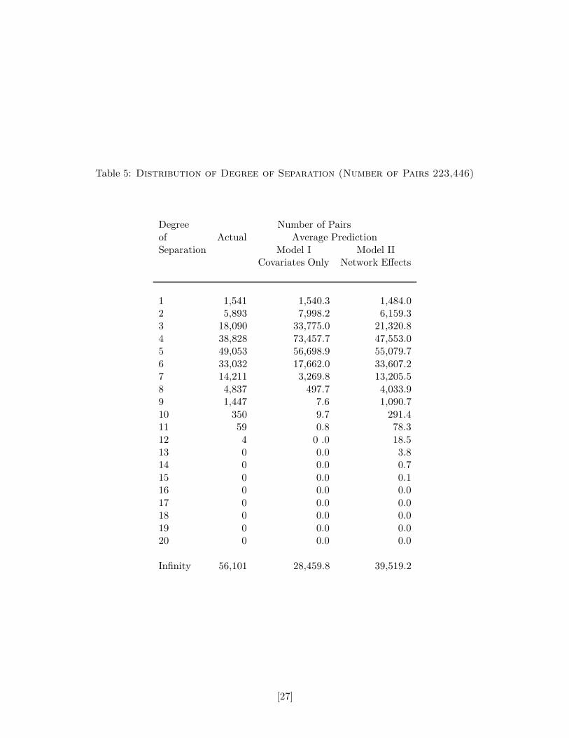
Table 5: Distribution of Degree of Separation (Number of Pairs 223,446)

Degree Number of Pairs

of Actual Average PredictionSeparation Model I Model II

Covariates Only Network Effects

1 1,541 1,540.3 1,484.02 5,893 7,998.2 6,159.33 18,090 33,775.0 21,320.8

4 38,828 73,457.7 47,553.05 49,053 56,698.9 55,079.7

6 33,032 17,662.0 33,607.27 14,211 3,269.8 13,205.5

8 4,837 497.7 4,033.99 1,447 7.6 1,090.7

10 350 9.7 291.411 59 0.8 78.3

12 4 0 .0 18.513 0 0.0 3.814 0 0.0 0.7

15 0 0.0 0.116 0 0.0 0.0

17 0 0.0 0.018 0 0.0 0.0

19 0 0.0 0.020 0 0.0 0.0

Infinity 56,101 28,459.8 39,519.2

[27]

Table 6: Estimates of Preference Parameters

ML Estimates Moments of Posterior DistributionModel I Model I Model II

No Network Effects No Network Effects Network EffectsParameter Description est. s.e. mean s.d. mean s.d.

α1 # of friends of alter 0 – 0 – -0.14 (0.03)

α2 total # of friends of alter sq 0 – 0 – 0.004 (0.003)α3 degr of sep is two 0 – 0 – 2.66 (0.07)

α4 degr of sep is three 0 – 0 – 1.22 (0.07)

β0 intercept -2.12 (0.05) -2.11 (0.04) -2.11 (0.06)β1 female -0.06 (0.04) -0.06 (0.04) -0.04 (0.05)β2 alter grade 0.08 (0.03) 0.08 (0.03) 0.07 (0.03)

β3 alter age 0.05 (0.03) 0.05 (0.03) 0.05 (0.03)β4 participates in sport 0.10 (0.04) 0.09 (0.04) 0.04 (0.05)

Ω11 diff in sex 0.19 (0.03) 0.19 (0.03) 0.20 (0.03)

Ω22 diff in grades squared 0.17 (0.02) 0.17 (0.01) 0.14 (0.01)Ω33 diff in age squared 0.10 (0.02) 0.10 (0.01) 0.09 (0.01)

Ω44 diff in sports participation 0.21 (0.03) 0.22 (0.03) 0.19 (0.03)

δ # of classes in common 0.14 (0.01) 0.14 (0.01) 0.12 (0.01)

Table 7: Friendship Rates by Sex Composition

Actual Predicted Rate Network Model

# of Frienship Current Assignment CounterfactualFriendship Type Pairs Rate (Mixed Sex Classrooms) (Single Sex Classrooms)

Boy-Boy 61,075 0.0087 0.0082 0.0079

Boy-Girl 111,650 0.0056 0.0055 0.0037Girl-Girl 50,721 0.0076 0.0074 0.0071

[28]

0 5 10 15 20 250

20

40

60

80Figure 1a: Histogram Number of Friends

0 5 10 15 20 250

20

40

60

80

100Figure 1b: Histogram Predicted Number of Friends (covariates only)

0 5 10 15 20 250

20

40

60

80

100Figure 1c: Histogram Predicted Number of Friends (network effects)

0 2 4 6 8 10 12 14 16 18 200

5

10x 10

4 Figure 2a: Histogram Path Length

0 2 4 6 8 10 12 14 16 18 200

5

10x 10

4 Figure 2b: Histogram Predicted Path Length (covariates only))

0 2 4 6 8 10 12 14 16 18 200

5

10x 10

4 Figure 2c: Histogram Predicted Path Length (network effects)