An empirical investigation of the relationship between market ...

University of Massachusetts Amherst University of Massachusetts Amherst

ScholarWorks@UMass Amherst ScholarWorks@UMass Amherst

Doctoral Dissertations 1896 - February 2014

1-1-1979

An empirical investigation of the relationship between market An empirical investigation of the relationship between market

share and the competitive market position of a firm. share and the competitive market position of a firm.

P. Varadarajan University of Massachusetts Amherst

Follow this and additional works at: https://scholarworks.umass.edu/dissertations_1

Recommended Citation Recommended Citation Varadarajan, P., "An empirical investigation of the relationship between market share and the competitive market position of a firm." (1979). Doctoral Dissertations 1896 - February 2014. 5981. https://scholarworks.umass.edu/dissertations_1/5981

This Open Access Dissertation is brought to you for free and open access by ScholarWorks@UMass Amherst. It has been accepted for inclusion in Doctoral Dissertations 1896 - February 2014 by an authorized administrator of ScholarWorks@UMass Amherst. For more information, please contact [email protected].

https://scholarworks.umass.edu/

https://scholarworks.umass.edu/dissertations_1

https://scholarworks.umass.edu/dissertations_1?utm_source=scholarworks.umass.edu%2Fdissertations_1%2F5981&utm_medium=PDF&utm_campaign=PDFCoverPages

https://scholarworks.umass.edu/dissertations_1/5981?utm_source=scholarworks.umass.edu%2Fdissertations_1%2F5981&utm_medium=PDF&utm_campaign=PDFCoverPages

mailto:[email protected]

AN EMPIRICAL INVESTIGATION OF THE

RELATIONSHIP BETWEEN MARKET SHARE AND

THE COMPETITIVE MARKET POSITION OF A FIRM

A Dissertation Presented

By

POONDI VARADARAJAN

Submitted to the Graduate School of the University of Massachusetts in partial fulfillment

of the requirements for the degree of

DOCTOR OF PHILOSOPHY

February 1979

School of Business Administration

(C)

P. Varadarajan

All Rights Reserved

1978

Ill

AN EMPIRICAL INVESTIGATION OF THE

RELATIONSHIP BETWEEN MARKET SHARE AND

THE COMPETITIVE MARKET POSITION OF A FIRM

A Dissertation Presented

By

P. VARADARAJAN

Approved as to style and content by

Ion), Chairperson of Committee

(Parker M. Worthing), Membe

IV

ACKNOWLEDGEMENTS

I wish to express my sincere appreciation and gratitude

to my parents and wife for their encouragement and support.

My special thanks and appreciation go to my wife, Prabha, for

her cheerful and skillful handling of the typing of this thesis.

I am thankful to Professor William R. Dillon for the time

and effort he devoted as my major advisor and chairman of my

dissertation committee. His direction and involvement during

every stage of this research effort is gratefully acknowledged.

I am also thankful to Professors Parker M. Worthing and

Donald G. Frederick for their valuable guidance and advice.

My special thanks to Professor Parker Worthing for the time

and effort he devoted during the early stages of this research

effort.

I also wish to express my thanks to Professor Bradley

T. Gale for his expert counsel. His involvement is this

thesis and related projects is sincerely appreciated. I am

also thankful to the Strategic Planning Institute, Cambridge,

Massachusetts for their financial assistance and providing

me with access to their data base.

Finally, the advice, assistance and support I have re¬

ceived from many other faculty members ana fellow doctoral

students is gratefully acknowledged.

ABSTRACT

An Empirical Investigation of the

Relationship Between Market Share and

The Competitive Market Position of a Firm

(February 1979)

P. Varadarajan, B.Sc., Bangalore University

B.E., Indian Institute of Science

M. Tech., Indian Institute of Technology

Ph.D., University of Massachusetts

Directed by: Professor. William R. Dillon

The objective of this thesis was to investigate the re¬

lationship between the market share and the competitive market

position of a business along certain marketing effort dimen¬

sions and product-market growth dimensions. Identifying the

key factors for success in an industry, and assessing the

strengths and weaknesses of the firm relative to its compe¬

titors in terms of these factors is a major step in the stra¬

tegy formulation process. This approach enables the firm to

identify the strengths it can capitalize on and the weaknesses

it will have to overcome to effectively compete in a dynamic

business environment. More specifically, in the marketing

context, there is a need to identify the marketing effort

dimensions and product-market growth dimensions that are rela-

VI

tively more important. A position of competitive superiority

or parity along these dimensions may be the key to success

in an industry. This study is intended to provide an in¬

sight of the competitive position effects on market share.

The theory of competitive position effects presented in

this thesis posits the existence of a significant relation¬

ship between market share and the competitive market position

of a business along certain marketing effort dimensions and

product-market growth dimensions; and, in addition, the exis¬

tence of a differential relationship for different types of

businesses.

Two models are advanced, referred to as the competitive

position effects model and the intensive growth strategy model,

which are operationalized via the predictors, marketing effort

and product-market growth variables, respectively. Specifi¬

cally, the marketing effort variables examined include, pro¬

duct line breadth, product quality, new product activity,

personal selling, advertising, sales promotion, quality of

customer services, price,, and degree of forward vertical in¬

tegration. The product-market growth variables examined in¬

clude, product line breadth, product quality, average size of

customers served, and average number of types of customers

served. The competitive market positions considered are, com¬

petitive superiority, parity, and inferiority, respectively.

Vll

Multiple regression analysis was used for testing pur¬

poses with relative market share as the dependent variable

and dummy coding specifications for the explanatory variables.

The Profit Impact of Marketing Strategy (PIMS) data on the

competitive market position and relative market share of

two broad classes of businesses, the consumer nondurable busi¬

nesses and the capital goods businesses were investigated.

The empirical analysis of the competitive position effects

model and the intensive growth strategy model supported the

hypothesis of a differential relationship for different types

of businesses. For the competitive position effects model

for consumer nondurable businesses, the hypothesis of a sig¬

nificant relationship between relative market share and the

competitive market position of a business along the dimensions,

product line breadth, product quality, and advertising was

supported. For capital goods businesses the significant dimen¬

sions were product line breadth, product quality, quality of

customer services, and degree of forward vertical integration.

Finally, for the intensive growth strategy model, the

hypotheses of a significant relationship between relative

market share and certain product-market growth variables and

the interaction of certain product-market growth variables

were supported.

TABLE OF CONTENTS

PAGE

ACKNOWLEDGEMENTS . iv

ABSTRACT . v

LIST OF TABLES. x

LIST OF FIGURES. xiv

CHAPTER

I. AN OVERVIEW. 1

II. LITERATURE REVIEW . 8

Introduction . 8 Market Share Strategy - Concepts

and Principles. 11 Market Share Theory Development .... 32 Empirical Studies . 45

III. THEORETICAL FRAMEWORK . 96

Problem Statement . 96 Theory Development . 98

IV. EMPIRICAL MODEL SPECIFICATION . 124

The Competitive Position Effects Model. 128

The Intensive Growth Strategy Model. 134

V. TESTS FOR MODEL EVALUATION . 145

Specification Error Analysis . 146 Tests of Significance of the Multiple

Regression Model . 160

VI. MODEL TESTING - THE COMPETITIVE POSITION EFFECTS MODEL . 173

Consumer Nondurable Businesses . 174 Capital Goods Businesses . 194

VII. MODEL TESTING - THE INTENSIVE GROWTH STRATEGY MODEL . 217

Consumer Nondurable Businesses . 218 Capital Goods Businesses . 336

VIII. CONCLUSION. 255

SELECTED BIBLIOGRAPHY. 265

APPENDIX. 272

X

LIST OF TABLES

PAGE

1. Perceived Importance of the Facets of

Competitive Strategy by Type of Industry. 58

2. Perceived Importance of Specific Marketing

Activities by Type of Industry. 59

3. Summary of Studies on Market Share Theory . 101

4. Competitive Position Effects Theory -

A Summary . 104

5. Operationalizing Intensive Growth Strategies ... 118

6. Illustration of Design Matrix for Dummy Coding.. 133

7. Surrogate Measures of Market Penetration, Market

Development, and Product Development . 141

8. Regression Analysis for Identifying Variables

Most Strongly Affected by Multicollinearity... 177

9. Partial Correlations Between Independent

Variables. 178

10. Simple Correlations Between Independent

Variables. 179

11. Test of Coefficient Estimate Sensitivity to

Sample Size Variation. 181

12. Estimates of Standardized Regression

Coefficients . 187

xi

List of Tables (continued)

PAGE

13. Measures of Relative Importance of Marketing

Effort Variables . 193


Most Seriously Affected by Multi-

collinearity. 196


Variables. 198


Variables. 199




Coefficients. 207

19. Measures of Relative Importance of Marketing

Effort Variables. 213


Variables. 221



collinearity. 222


Variables. 223

Xll


PAGE

23. Test of Coefficient Estimate Sensitivity

to Sample Size Variation. 224


Coefficients. 230

25. Test of Significance of Product-market

Growth Variables. 231

26. Test of Significance of Interactions. 233

27. Measures of Relative Importance of Product-

market Growth Variables. 235


Variables. 237


Variables. 238



collinearity. 239




Coefficients. 245

33. Test of Significance of the Product-market

Growth Variables. 246

Xlll


34. Test of Significance of Interactions.

35. Measures of Relative Importance of Product-

PAGE

248

market Growth Variables 249

xiv

LIST OF FIGURES

PAGE

1. Product-market Scope and Growth Vector

Alternatives - A. 17


Alternatives - B . 18


Alternatives - C . 21


Alternatives - D. 22

5. Theory Development in Marketing . 99

6. The Competitive Position Effects Model . 110

7. The Competitive Position Effects Model -

Consumer Nondurable Businesses . 113

8. The Competitive Position Effects Model -

Capital Goods Businesses . 114

9. Intensive Growth Strategies . 116

10. The Intensive Growth Strategy Model . 121

11. Intensive Growth Strategy Effects on Market

Share: The Main Effects Formulation . 136

12. Scatterplot - Possible Patterns and Their

Implications . 159

13. Residual Plot - Consumer Nondurables . 184

XV

List of Figures (continued)

PAGE

14. Scatterplot - Consumer Nondurables . 185

15. Residual Plot - Capital Goods . 203

16. Scatterplot - Capital Goods . 204

17. Residual Plot - Consumer Nondurables . 226

18. Scatterplot - Consumer Nondurables . 227

19. Residual Plot - Capital Goods . 241

20. Scatterplot - Capital Goods . 242

CHAPTER I

AN OVERVIEW

Market share has been the focus of numerous studies in

the marketing literature. Various authors have examined the

determinants of market share in varying degrees of generality

and with various orientations. The growing interest in market

share determinants is attributable to its close relation to

profitabilityygrowth, survival, risk reduction, and market

power. Marketing literature is rich in conceptual studies

on topics such as, strategies for increasing market share,

strategies for high market share and low market share com-

panies, market share strategies and the product life cycle,

market share management strategies, etc. On the empirical

side stochastic and empirical models have been widely used to

explain market share movement. The cumulative efforts of

many researchers has resulted in market share models which

have become progressively more elaborate and better approxi¬

mations of the actual market mechanism. The focus of this

study as well is market share. Stated briefly, the objective

of this study is to investigate the relationship between

market share and the competitive market position of businesses

along various marketing effort dimensions and growth dimen¬

sions .

2

Study rationale. Econometric methods have been widely used

to investigate the relationship between market share and

marketing decision variables. In most of the early empirical

studies the marketing decision variables are expressed in

absolute terms - that is, actual dollar expenditures. In

effect,- these models failed to consider the influence of

competitors* actions. For this reason later studies incor¬

porated the effects of competitors' actions in a number of

ways. One approach has been to transform the independent

variables either through subtracting or dividing them by the

appropriate mean value. A second approach has been to create

a relative marketing variable by computing the ratio of the

value for the brand to the corresponding value for all other

brands combined. A third approach has been to create a share

marketing variable by computing the ratio of the value for

the brand to the corresponding value for all brands combined,

including the brand under consideration. The choice of which

relative measure to use is critical as they do not lead to

the same results. Use of any of these approaches requires

extensive data on the firm's actions and competitors' actions

with regard to each marketing decision variable considered.

While it would be possible for a firm to obtain accurate in¬

formation about its own actions, often it may not be possible

for any single firm to obtain reliable estimates of competi-

3

tors’ actions. Consequently, much of the published research

to date has focused on a single brand or the leading brands

within a product class. As Parsons and Schultz-®- note, the

breadth of empirical studies on market share theory have not

generally extended beyond "frequently purchased branded goods"

and thus broad knowledge of the demand structure for goods

and services is severely restricted.

While it may not be possible for any single firm to

obtain precise estimates of competitors' actions with regard

to various marketing decision variables, in most cases a firm

is in a position to furnish data on its own competitive posi¬

tion relative to its competitors, as well as the relative

competitive position of its competitors. Thus, it is possible

to determine for each competing firm the specific marketing

effort dimensions and growth dimensions along which it is in

a position of competitive superiority, parity and inferiority.

In addition, if a firm is a multi-product line conglomerate,

it will be in a position to generate this kind of data for

each' of its product lines separately. Pooling data on differ¬

ent product lines (after testing for appropriateness of pool¬

ing) would enable the firm to examine the relationship bet¬

ween market share and the competitive market position of busi¬

nesses along various marketing effort dimensions, and growth

dimensions for a broad class of goods such as consumer non-

4

durables, consumer durables, industrial supplies, capital

goods, etc. This is one advantage of competitive market

position data over other forms of data such as differences

from mean, ratio to mean, relative, and share data. Further,

the relevant literature reveals that the relationship between

market share and the competitive market position of a busi¬

ness along various marketing effort dimensions and growth

dimensions has not been satisfactorily investigated. Because

of the paucity of research in this specific area the useful¬

ness of these variables in terms of their ability to explain

market share, and the decision situations in which such infor¬

mation would be of assistance to the decision maker is a parti¬

cularly important issue. The purpose of the study reported

here is to address this issue.

Statement of objectives. The principle objectives of this

study are:

1. To investigate the relationship between market share and

the competitive market position of businesses along

various marketing effort dimensions.

2. To investigate the relationship between market share and

the competitive market position of businesses along

various growth dimensions.

To determine whether the significant marketing effort

dimensions are the same or different for different types

3.

5

of businesses.

The research approach. The research approach used in this

study can be largely characterized as econometric in nature.

The following steps briefly describe the general approach.

Study of the system

Theory development

Model formulation

Designing appropriate tests for model evaluation

Statement of hypotheses

Confronting the model with data

Estimating the parameters of the model

Evaluating the usefulness of the model

Scope of the study. This study is confined to businesses in

the maturity stage of the product life cycle. The rationale

for this is simply that the maturity stage of the product

life cycle poses the most formidable challenge to marketing

management. The analysis is confined to two product cate¬

gories, consumer nondurable businesses and capital goods

businesses. The source of data for this study is the Profit

Impact of Marketing Strategy (PIMS) data base.

Organization of the dissertation. Chapter II presents a re¬

view of the relevant marketing literature. This chapter is

made of three main sections; Market share strategies - con-

6

cepts and principles, market share theory, and empirical

studies on market share theory.

Chapter III is addressed to the issues of formal state¬

ment of problem and research objectives, theory development,

and model formulation.

Chapter IV is devoted to empirical specification of

the proposed models.

In Chapter V, the statistical tests used in this study

for specification error analysis and model evaluation are

described.

In Chapter VI and VII the results of specification error

analysis, statistical tests of significance of the full model,

and individual parameters of the model are discussed.

The final chapter is devoted to a summary of findings,

action implications, limitations of the study, and a brief

discussion of additional avenues for study.

FOOTNOTES

^"Leonard J. Parsons, and Randall L. Schultz, Marketing

Models and Econometric Research (New York: North - Holland

Publishing Company, 1976), pp. 21-23

CHAPTER II

LITERATURE REVIEW

Introduction

Market share is among the most widely used measures of

managerial performance and has been found to be an effective

aid to management diagnosis. Market share measures are

widely used to determine whether management should continue

with its current policies (which is the conclusion usually

drawn if the firm has expanded its market share), or whether

it should alter its policies if it has lost market position.

If used properly, market share measurements could play a

central role in diagnosing business successes and failures.

Such data reveal how buyers have responded to the whole com¬

plex of actions taken by all firms in an industry. One can

understand what policies make for market success and failure

in an industry by studying the experience of all firms in

that industry.

A major reason for the universal interest in market

share among marketing practitioners is its close relation

to profitability, growth, survival, risk reduction, and

market power. Day lists the following as the major benefits

associated with market dominance.

1. The market leader is usually the most

profitable

8

9

2. During economic downturns, customers are likely to concentrate their pur¬

chases in suppliers with large shares, and distributors and retailers will try to cut inventories by eliminating the marginal supplier

3. During periods of economic growth, there is often a bandwagon effect with a large share presenting a positive image to customers and retailers. Gains in market share tend to perpe¬ tuate the firm's product because poten¬ tial customers are more easily per¬ suaded to purchase a product that is growing than one that is losing its position in the market placed

It is this close link between market share on the one

hand and profits, growth, survival, risk reduction and market

power on the other that seems to be the main reason behind

the widespread interest in the study and analysis of facets

pertaining to market share. Much, if not all, of the studies

pertaining to market share which have been analyzed, researched

and reported fall into the following classes:

Marketing management oriented concepts and principles.

1. Setting market share objectives

2. Using market share as objective measures of performance

3. Strategies for increasing market share

4. Market share management strategies (building, holding

and harvesting strategies)

Market share strategies for dominant firms versus trail¬

ing firms

5.

10

6.

7.

8.

The link between market share strategies and the product

life cycle

The link between market share objectives and other busi¬

ness objectives such as profits, growth, survival, risk

reduction, and market power

Dangers inherent in the blind pursuit of market share

building strategies

Theoretical studies on market share.

1. Market share theory

2. Logical consistency of market share models

Empirical studies on market share.

1. Studies on the link between market share and profitabi¬

lity, and the effectiveness of alternate marketing

strategies

2. Econometric market share models

3. Stochastic market share models

This chapter is devoted to a review of pertinent litera¬

ture. The review is organized into the three main sections

outlined above, namely:

Marketing management oriented concepts and principles

Market share theory

Empirical studies on market share theory

11

Market Share Strategy-Concepts and Principles

Market share measurements: Uses and limitations. Manage¬

ment normally employs market share measurements for three

primary purposes:

- To appraise performance

- To express market targets

- To assist in forecasting sales

Oxenfeldt states that the main reason for using market

share changes as a standard for appraising a management's

performance is the belief that such measurements separate

changes in sales resulting from forces outside the firm -

such as general prosperity, recession, shortages, industry

wide changes in price, etc., - from those for which manage¬

ment can be held reasonably responsible. Unlike other market

share measurements such as dollar or unit sales volume, market

share measurements automatically adjust for conditions that

are common to the industry as a whole.

A second reason for appraising performance by market

share changes is that it demands reasonable performance on

the part of management. In effect, this standard compares

the management of the firm with the average performance of

all other companies in the industry taken in combination,

rather than with the performance of the best.

A third reason why firms use market share to appraise

12

performance is that, while the marketing efforts of any single

firm is likely to have only minimal impact on influencing

total industry sales, the quality of the marketing efforts

of a firm serves to allocate the total industry demand bet-

ween the firms.

Another major use of market shares is to express top

management's marketing objectives. Marketing objectives are

normally expressed in terms of sales volume and/or market

share, and marketing programs are typically designed to attain

a predetermined share of the market.

Finally, market share data are used for sales forecast¬

ing; that is, it is common practice for forecasters to esti¬

mate total sales of a product at the industry level, and

arrive at a sales forecast for their firm by projecting its

recent market share.

Concerning the validity of assumptions. Oxenfeldt^ cautions

against indiscriminate use of market share measures pointing

to a number of potential pitfalls. First, he argues that

entrance of new firms will inevitably lead to a decline in

the market share of some firms and the exit of some firms

will lead to higher market share for others, neither being

attributable to any satisfactory or meritorious action on

their own part. Also, it is possible that significant differ¬

ences exist between firms in terms of financial and personnel

13

resources, command over strategic locations, natural resources,

ties with customers and other possible sources of competitive

advantages. If such differences were to exist, then the

assumption that every firm is always affected equally by all

outside forces is invalid.

Second, he points to the fact that while market share is

closely associated with profitability, improved chances of

survival and minimizing the risk of loss, market share cannot

be considered a business objective in and of itself. Hence,

setting market share objectives without concern for the ex¬

penditure necessary to attain them may adversely affect pro¬

fitability, thereby leading to goal conflict.

Contrary to this position, the Boston Consulting Group

(BCG) in its reports whole heartedly supports the idea of

5 setting market share objectives m and of themselves. BCG

posits that market share is the single most important deter¬

minant of profitability and profits. The BCG reports in

their total perspective are considered at a later stage.

Lastly, referring to use of market share in sales fore¬

casting, Oxenfeldt^ takes the position that where market

shares are relatively stable, projection of market share

may be an extremely useful forecasting device. But in indus¬

tries where market share fluctuate widely and erratically,

their use in sales forcasting is limited. In addition,

because the goals of most managements is to attain larger

14

market share for themselves at the expense of others, the

usefulness of market share for forecasting purposes is ques¬

tionable .

In short, Oxenfeldt seems to take the position that while

market share can be an extremely useful measure, care and

good judgement must be exercised especially where the requi¬

site conditions for its effective use are not in place.

Strategies for increasing market share. A great deal of in¬

terest has been focused on strategies for increasing market

share. For example, the present day marketing strategist

talks about a battery of strategies for increasing market

share which include market segmentation, product differentia¬

tion, product development, market modification, product modi¬

fication, marketing mix modification, multibrand strategy,

brand extension strategy, product innovation strategy, market

fortification strategy, and market stretching strategy. While

a certain degree of overlap between these strategies exists,

in some sense, each has its own unique characteristic(s) as

well.

Smith,^ for example, proposed the idea of product differ¬

entiation and market segmentation as alternative marketing

strategies; product differentiation is designed to bring

convergence of individual market demands to a single product

line, and market segmentation based on the principle of di-

15

vergent demands involves adjusting product lines to meet

o these different demands. Similarly, Adler outlined a number

of strategies including market segmentation, market stretch¬

ing, multibrand strategy, brand extension strategy, distribu¬

tion breakthroughs, and technological breakthroughs as alter¬

native approaches for increasing sales and market share, while

Levitt outlined four broad strategies to increase sales:

- Finding new uses for the product

- Promoting more frequent usage of the product among current users

- Developing more varied usage of the product among current users

- Creating new users for the product by expanding the market.^

While Levitt conceptualized growth strategies in terms

of new users and new uses, in marketing literature use of

the product-market scope and growth vector conceptualization

of strategies for growth is more widespread. These two com¬

ponents of strategy relate to the general product and market

entries of the firm, and the alternative growth directions

available to the firm, respectively. Johnson and Jones^

used this framework in the context of describing the rela¬

tionship between new product responsibilities and the various

departments in an organization. Their article basically

dealt with the need for introducing a steady stream of new

products in order to be successful in the market place and

16

the need for a proper organizational set up with a new pro¬

duct department for this purpose. The framework outlined by-

Johnson and Jones is shown in Figure 1. Ansoff^ explicitly

addressed the issue of strategies for growth. In his work

Ansoff states that there are four basic growth strategies

open to a business: (1) market penetration, (2) market deve¬

lopment, (3) product development, and (4) diversification.

Market penetration refers to a company's seeking increased

sales for its present products in its present markets; market

development refers to a company's seeking increased sales by

taking its present products into new markets; and product

development refers to a company's seeking increased sales by

developing improved products for its present markets. The .

term diversification is usually associated with a change in

the characteristics of the company's product line and/or

market in contrast to market penetration, market development,

and product development, which represent other types of

changes in the product-market structure. While the latter

are usually followed with the same technical, financial and

merchandising resources that are used for the original pro¬

duct line, diversification generally requires new skills,

new techniques and new facilities. For this reason, market

penetration, market development, and product development are

usually referred to as intensive growth strategies. The

17

Figure 1

PRODUCT-MARKET SCOPE AND GROWTH VECTOR ALTERNATIVES - A

NO TECHNOLOGICAL

CHANGE

IMPROVED TECHNOLOGY

NEW TECHNOLOGY

NO MARKET CHANGE

Reformula¬ tion

Replace¬ ment

STRENGTHENED Remerchan- Improved Product- MARKET dising Product line

Extension

NEW New Market Diversifi- MARKET Use Extension cation

Source: Samuel C. Johnson and Conrad Jones, "Hew to Orga¬ nize for New Products," Harvard Business Review, vol. 35 (May-June T957), pp. 49-62

18

Figure 2

PRODUCT-MARKET SCOPE AND GROWTH VECTOR ALTERNATIVES - B

Present

Products New

Products

Present Market Product Markets Penetration Development

New Market Markets Development (Diversification)

Source: H.Igor Ansoff, "Strategies for Diversifica- cation," Harvard Business Review, Vol.35 (September - October 1957), pp. 113-124.

Also see: H.Igor Ansoff, Corporate Strategy, (New York: McGraw-Hill, Inc., 1965), p.109

19

12 framework suggested by Ansoff is shown in Figure 2. Kotler

classifies growth opportunities as intensive, integrative,

and diversification growth opportunities. Here again, market

penetration, market development and product development are

viewed as intensive growth strategies. While each of these

strategies describes a distinct path a business can take to¬

wards growth, it should be noted that in most real life situa¬

tions a business would be pursuing more than one strategy at

the same time.

From an operational perspective, market penetration

possibilities include increasing the frequency of purchase

and average quantity purchased by the present users of the

firm's products, attracting competitors customers, and con¬

verting nonusers into users. Market development possibili¬

ties include tapping new market segments within the geographic

market presently served by the firm and expanding into new

geographic markets. Product development possibilities in¬

clude developing new product features, creating different

quality versions of the product, improving the quality of

current offerings, and developing additional models and sizes.

Modified versions of the growth matrices outlined by

Johnson and Jones, and by Ansoff have been discussed by other

1 2 writers. For example, Kollat, Blackwell and Robeson con¬

ceptualize growth strategy as consisting of a product-market

20

scope and growth vector, a synergy component, and a differen¬

tial advantage requirement. Their version of the growth

matrix is shown in Figure 3. Day-^ on the other hand views

the growth vector, and emphasis on innovation versus imita¬

tion, as the basic issues involved in plotting a growth stra¬

tegy. Day's perspective of product-market scope and growth

vector alternatives is shown in Figure 4. Variations of the

15 simple growth matrix are also discussed in Cundiff and Still,

and Nimer.^

In contrast to the conceptual treatment characteristic

of the studies reviewed so far, Fogg's analysis of strategies

for increasing market share is more direct. He lists'the

following as the most important strategies for gaining market

share in an industrial market.

1. Lowering prices below competitive levels to take business away from competition among price-conscious

customers.

2. Introducing product modifications or significant innovations that meet customer needs better and displace existing products or expanding the total market by meeting and stimulat¬

ing new needs.

3. Improving customer service by offering more rapid delivery than competition to

service-conscious customers; improving the type and timeliness of information that customers need from the service organization; information such as items in stock, delivery promise dates, invoice

and shipment data, and the like.

PR

OD

UC

T-M

AR

KE

T

SC

OP

E

AN

D

GR

OW

TH

VE

CT

OR

AL

TE

RN

AT

IVE

S

21

U

I

Source:

David T

.Koll

at,

Ro

ger

D.B

lackw

ell

, and

Jam

es

F.

Ro

beso

n,

Strateg

ic

Mark

eti

ng,

(New

Yo

rk:

Ho

lt,

Rin

ehart

and

Win

sto

n

Inc.

, 1

97

2)

, p.2

.1

22

Figure 4

PRODUCT-MARKET SCOPE AND GROWTH VECTOR ALTERNATIVES - D

r\^^roducts

Markets \

Present Product

Improved

Product

New Product/ Related

Technology

Existing Market

Market Penetration

Replace¬ ment

Product line Extension

Expanded Markets

Promotion/ Merchandis¬

ing-increased

usage rates

Market Segmentation/ Product Differentiation

New Market

Market Development

Market Extension

Source: George S.Day, "A Strategic Perspective of Product Planning, " Journal of Contemporary Business; (Spring 1975), p.27

23

4. Strengthening and improving the quality of marketing effort by fielding a larger, better-trained, higher quality sales force targeted at customers who are not getting adequate quality or quantity of attention from competition; building a larger or more effective distribu¬ tion network.

5. Increasing advertising and sales pro¬ motion of superior product, service, or price benefits to under penetrated or untapped customers; advertising new or improved benefits to all customers.^

1 o In addition to these five key strategies, Foggxo suggests

other approaches such as improving product quality, expanding

engineering assistance offered to customers, offering special

product testing facilities, broadening the product line to

offer a more complete range of products, improving the general

corporate image, offering the facilities to build special

designs quickly, and establishing inventories dedicated to

serving one customer.

In certain respects Fogg seems to suggest the desirabi¬

lity of concentrating on select segments of the market such

as, price-conscious customers, service-conscious customers

not getting adequate quality or quantity of attention from

competition, under penetrated customers, and untapped custo¬

mers. This in a way means that Fogg recommends following a

market segmentation strategy in certain situations.

Given that a set of significant distinct advantages com¬

pared to competition can be offered to the customers, and

24

these distinct advantages are sustainable for a sufficient

period of time to gain targeted share, and significant enough

to cause target customers to shift their business from a

competitor to the firm attempting market share gain, the

strategies suggested by Fogg would require one or more of

the following actions to be implemented by the firm.

1. Lowering the price

2. Focusing on product modification and product

innovation

3. Increasing the size and quality of sales force

4. Improving the quality of service

5. Increasing the advertising outlay

6. Increasing the sales promotion budget

7. Improving product quality

8. Broadening the product line

9. Improving the general corporate image

10. Improving the quality of distribution

From this we note that besides market segmentation stra¬

tegies, to a large extent the strategies outlined by Fogg

call for incorporating changes in the marketing mix. That

is, in part at least, several of the strategies outlined by

Fogg fall under the class of strategies normally referred

to as marketing mix modification strategies.

25

The desirability of a market share building strategy. While

a number of authors have written on strategies for increasing

market share, Furhen1^ questions the wisdom benind blind

20 pursuit of share building strategies, and Bloom and Kotler

raise the issue, What should a company do after it builds

a high market share?

Pointing to the dangers inherent in the blind pursuit

of high market share, Furher?^ suggests that business strate¬

gists should answer the following questions before launching

an aggressive market share expansion strategy:

1. Does the company have the necessary

financial resources?

2. Will the company find itself in a viable

position if its drive for expanded market

share is thwarted before it reaches its

market share targets?

3. Will the regulatory authorities permit

the company to achieve its objective

with the strategy it has chosen to follow?

Negative responses to these questions would obviously in¬

dicate that a company should forego market share expansion

until the right conditions are created.

22 The concept of optimal market share. Bloom and Kotler

point to the fact that while high market share would lead

26

to higher profits, for some firms the costs and risks may

outweigh expected gains. In their view, a company that

acquires a very high market share exposes itself to a

number of risks that its smaller competitors do no encounter.

Competitors, customers and governmental authorities are

more likely to take actions such as anti-trust suits and

comparitive advertising against high share companies than

against small share companies. The authors suggest that

an organization's goal should not be to maximize market share,

but rather to attain an optimal market share. Their defini¬

tion of optimal market share is the position from which a

departure in either direction would alter the company's

long-run profitability or risk (or both) in an unsatisfactory

manner. They suggest that a company should determine its

optimal market share by:

- Estimating the relationship between

share and profitability

- Estimating the amount of risk asso¬ ciated with each share level, and

- Determining the point at which an increase in market share can no longer be expected to bring enough profit to compensate for the added

risks to which the company would expose itself^

27

Bloom and Kotler^4 state that in some cases a firm could

benefit more by reducing or maintaining its share, rather

than increasing its share. The idea of market share manage¬

ment has been addressed by several authors and, therefore,

a brief discussion of this material is presented next.

Market share management strategies. Market share management

strategies are generally viewed as falling into three broad

categories, namely:

- Share building strategies

- Share holding strategies, and

- Share harvesting strategies

In addition. Bloom and Kotler^ suggest a fourth classifica¬

tion, especially relevant to the high market share companies,

which they refer to as 'risk reduction strategies.' Which

of these market share strategies is desirable and feasible

depends on a number of factors, including the firm's present

position, the strength of competitors, stage in the product

life cycle, the resources available to support a strategy,

and the firm's needs and preferences for current earning

versus future earnings.

Catry and Chevalier^6 for example, posited that the com-

paritive value of market share for a product would vary with

its stage in the product life cycle. In their view the best

market share strategy would be to build market share in the

28

early stages of development of the product life cycle, attain

a dominant position at the maturity level and disinvest before

the overall market enters its decline stage. Similarly, the

BCG reports^ favor setting market share objectives early in

the product life, gaining and maintaining market share through

the growth phases, and only in the maturity stage sacrificing

market share objectives for cash.

Market share strategies for high market share businesses

versus low market share businesses. The proposition that

the strategic options appropriate for a low market share

business are different from the ones appropriate for a high

market share business has been expressed by a number of

authors. In particular, Kotler lists the following as the

broad strategic options available to a dominant firm during

the maturity stage.

- Strategy of innovation

- Strategy of segmentation or fortification

- Strategy of confrontation, and

- Strategy of persecution

He also states that the last two strategies are less attrac¬

tive options and should be avoided to the extent possible.

For trailing firms the options cited are:

- Searching for differential advantage over

competitors

29

- Searching for profitable segments that

the larger firm is failing to cater to

- Finding new ways to distribute goods that

offer substantial economies or covers

particular segments of the market more

efficiently

- Trying to develop superior advertising

campaigns

In another article. Bloom and Kotler^S list share build¬

ing, share maintenance, share reduction and risk reduction

as market share strategies open to a high market share busi¬

ness. Included in the list are: product innovation, market

segmentation, distribution innovation, and promotion innova¬

tion as appropriate strategies for share building; product

innovation, market fortification and confrontation as appro¬

priate strategies for share maintenance; and application

of general or selective demarketing principles such as rais¬

ing prices, cutting back on advertising and promotion, re¬

ducing service, lowering product quality and reducing con¬

venience features for share reduction.

For businesses which would prefer to reduce their risk

rather than their share. Bloom and Kotler suggest that a

number of measures be taken to reduce the insecurity that

surrounds these high market share companies such as, public

30

relations, competitive pacification, diversification and

social responsiveness.

The strategy of innovative imitation outlined by Levitt^

can also be viewed as a strategic option open to a low market

31 share business. Blackwell also takes the position that

low market share businesses should rely on market segmenta¬

tion strategies rather than on market share dominance stra¬

tegies. In time, he states, such strategies may lead to

such dominancy of a market "niche" that a path is discovered

toward dominating the whole.

Marketing strategies in the mature stage. Marketing stra¬

tegies in the mature stage have been widely discussed in market¬

ing literature. However, in order to avoid duplication, the

discussion is confined to the concepts presented in two

sources, namely: Levitt's classic on exploiting the pro-

33 duct life cycle, and Kotler's perspective of marketing

strategies in the maturity stage of the product life cycle.

As stated earlier, Levitt^ outlined four broad strate¬

gies to extend the life of the product, namely: promoting

more frequent usage, more varied usage, identifying new users,

and new uses. These life extension strategies assume greater

importance during the maturity stage than during the other

3 5 stages. Kotler views market modification, product modi¬

fication, and marketing mix modification as the three basic

31

strategies appropriate during the maturity stage. One

approach to market modification is extending the product to

new markets and market segments. A second approach is to

increase the usage rate among present customers. Obviously,

it is evident that what Kotler refers to as market modifica-

36 37 tion strategies overlaps with what Adler and Levitt refer

to as market stretching or life extension strategies. Also,

it should be noted that a common bond exists between market

development and market penetration strategies outlined by

3 8 Ansoff and market modification strategies outlined by

Kotler.

Product modification strategies involve incorporating

changes in the product's characteristics that will attract

new users and/or more usage from current users. The major

product modification strategies include quality improvement,

feature improvement, and style improvement. A quality improve¬

ment strategy aims at improving the functional performance of

products - such traits as its durability, reliability, speed

and taste. A style improvement strategy aims at increasing

the aesthetic appeal of the product in contrast to its func¬

tional appeal.

Marketing mix modification strategies involve stimulat¬

ing sales through altering one or more elements of the market¬

ing mix. These possibilities include lowering prices, better

32

advertising, aggressive and attractive promotions and moving

into other market channels; these actions are taken with

the intent of drawing new segments into the market as well

as attracting other brand users. Note again that overlap

3 9 exists between the strategies outlined by Fogg for gaining

market share and what Kotler views as marketing mix modifica¬

tion strategies for sales growth.

Summary. In this section, some of the concepts and principles

pertaining to market share were considered. The literature

reviewed in this section is fairly representative of the

nature of material available on this subject. The next sec¬

tion is devoted to review of literature on market share theory.

Market Share Theory Develooment ---=-

Of the three broad areas of study pertaining to market

share, market share theory development appears to be the

area in which very little is available in the form of an

organized body of literature. In large part this stems from

the difficulty of predicting market response to variations

of marketing effort. Kotler in discussing this point cites

a number of potential problem areas. Among the more impor¬

tant problems are included:

The nature of sales response. The shape of the

functional relationship between the market's response and the level of marketing effort is

33

typically unknown. Summarizing the market's behavior into a total sales response function and specifying the ranges of increasing, con¬ stant and diminishing returns to marketing effort is a challenging task.

Marketing mix interaction. Marketing effort is a composite of many different types of activities undertaken by the firm. To model these joint effects on a conceptutal level and measure them on an empirical level is a difficult problem.

Competitive effects. The market's response is a function of the competitor's efforts as well as the firm's efforts. The firm has imperfect to little or no control over competitor's moves. Its knowledge and forecast of competitor's moves is also imperfect.

Delayed response. The market's response to current marketing outlays is not immediate but in many cases stretches out over several time periods beyond the occurrence of outlays.

Multiple territories. Different territories have dissimilar rates of response to additional marketing effort.

Environment uncertainity effect. Factors such as legislation, technological changes, and economic fluctuations cause systematic and random distur¬ bances in the sales response function that must be taken into account in the marketing planning

process.^

In the light of these problems, it is hardly surprising

that little unified information is available in the area of

market share theory; nevertheless, the following briefly

sketches the available literature.

Market share theory. The most fundamental theory of market

share is that market shares of various competitors will be

34

proportional to their marketing efforts. In mathematical

form this can be expressed as:

M\

s. =--- , (2.1) 1 n

Z M. i=l 1

where S^= company i's market share, M^= company i's market¬

ing effort and n = number of competing firms. It is imme¬

diately apparent that this formulation is overly naive and

somewhat incomplete. For example, the effectiveness with

which firms expend their marketing efforts is not considered.

If E^, represents the effectiveness of a dollar spent by firm

*i*, (with E = 1.00 for average effectiveness), then (2.1)

can be expressed as:

n E E.

i=l ‘

(2.2)

Thus, the market share of a firm is viewed as a function of

its effective effort share. While (2.2) is superior to (2.1)

in the sense that it takes into account both the amount and

quality of marketing effort, its main drawback is that it

is often impossible to compute measures of marketing effec¬

tiveness E•, for each one of the competitors efforts. In

the absence of a satisfactory measure of effectiveness, most

35

of the empirical studies conducted use variations of equa¬

tion (2.1) with marketing effort being expressed in terms

of the marketing mix elements - price (P^), advertising (A^),

distribution (D^), and product quality (R^).

If the marketing mix variables are assumed to be linearly

related, then an expression for market share takes the form

S i

k.- pP^+ aA,*+ dD^+ rR; 1^1 i i i

n £ (kj_- pPj_+ aAj_+ dDj_+ rRj_)

i=l

(2.3)

where k^= constant term

p = coefficient of sales response to price

a = coefficient of sales response to advertising

d = coefficient of sales response to distribution

r = coefficient of sales response to product quality.

On the other hand, if the marketing mix elements are

thought to interact in a multiplicative fashion, then (2.1)

can be expressed as:

S i n

£ k. i=l '

(2.4)

In an attempt to develop . a market share theorm, Bell,

Keeny and Little41 replaced marketing effort of a firm with

its resulting attractiveness. They defined attraction as

36

the resultant outcome of the firm’s marketing actions and

assumed that the competitive situation is completely defined

by the vector of attractions.

a = 'ai a2.ai.an] (2'5)

where a = attraction vector, n = the number of competing

firms, and a^ is the attraction value for the i”n firm which

is a function of its marketing decision variables; that is,

a. = f(P.,A-,D•,Q■) (2.6) i 1 -L i i

The authors state that attraction completely determines market

share if the following assumptions are valid:

1. The attraction vector is non negative and non zero

2. A seller with zero attraction has no market share

3. Two sellers with equal attraction have equal market

share

4. The market share of a given seller is affected in the

same manner if the attraction of any other seller is in¬

creased by a fixed amount

Translating their attraction concept into a market share

theorem the authors state that if market share is assigned

to each seller based only on the attraction vector and in

such a way that assumptions 1 to 4 are satisfied, then market

37

share is given by:

a.

S = 1 (2.7) i n

E a. i=l 1

The advantage of this version of market share theorem is that

subject to certain basic assumptions relating the vector quan¬

tity attraction to the scalar quantity market share, mathe¬

matical consistency implies that market share is a simple

linear normalization of attraction. However, note that the

fourth assumption does not accomodate assymmetry and nonlinea-

4 9 rity and, therefore, as Barnett has pointed out this formu¬

lation is directly applicable only in a limited number of

circumstances. (Assymmetry could arise if changes in the

attraction of one seller were differentially effective on the

customers of another. Nonlinearity would be evidenced if

adding an increment to a small attraction produced a different

effect on others compared to adding the same amount to a

large attraction). In order to extend the scope of the theory

Barnett proposed dropping the assumptions of symmetry and

linearity in favor of more general axioms. In his attempts

to modify the theorem, Barnett allowed for nonlinearity and

assymmetry by introducing elasticity coefficients which allow

for different assessments of market behavior for different

products.

38

Critique on market share theorem. Bell et al offer no con¬

vincing explanation as to how and why using an attraction

vector to determine market share is superior to the more

conventional approaches given in (2.1) and (2.2). In addi¬

tion, no explanations are offered as to how the attractive¬

ness measures and elasticity measures are to be computed.

Further more, Chatfield^ points to the fact that attraction-

can be negative in certain cases. The illustration he uses

is that of going to a dentist, in which case one would tend

to choose the least unattractive seller (here the attractions

are negative).

Concerning the Logical Consistency of Market Share

Models

The subject of logically consistent market share models

has received increasing attention in marketing literature.

This section is devoted to a review of some of the relevant

studies. For a market share model to be considered logically

consistent, it should satisfy two conditions - the sum con¬

straint and the bound constraint. The sum constraint re¬

quires that the predicted market shares should sum to 1.0

and the bound constraint requires that the predicted market

shares of individual businesses should be between 0 and 1.0.

Consider, for the moment, models of the general form(2.8):

39

Y.. = x. 3 ., + x. it “ilt "'ll' “L2t Pi2‘r + xj_jt +

+ x. 3 + £. , (i=l,2,-n for all t) ipt ip it

(2.8)

where is the market share of brand 1i' in period 't'

for a product class consisting of ' n' brands and is expressed

as a proportion, the x- . .'s, (j=l,.p) are the explanatory 131

variables, and the f^'s are random disturbances.

For linear market share models of the above form to be

logically consistent, it is required that the sum of the

market shares of all brands in the product class must be

unity in every time period, i.e.,

Yu+ Yo + It 2t

+ Y , = 1, for all 1t' nt

(2.9)

In order to eliminate the possibility of the expected values

of some of the dependent variables being negative or greater

than one, the expected market shares for each brand should

be constrained between zero and unity; i.e.,

0 < Y < 1 for all 'i' during all 't?. (2.10)

Equations (2.9) and (2.10) specify respectively, the 'sum

constraint' and 'bound constraint' that have to be satisfied

for a model to be logically consistent.

Obviously, these constraints impose certain restrictions

on model specification. Naert and Bultez^4 took the position

that for a market share model to be logically consistent, its

40

functional form will have to be almost invariably intrinsi¬

cally nonlinear. Therefore, logical consistency leads to

more complicated market share functions, and necessitates

more sophisticated estimation techniques. Using a study by

Beckwith^ and other illustrations the authors stated that,

in order to insure that the expected market shares lie bet¬

ween zero and one requires either a nonlinear specification

or restrictions on the models variables and parameters. An

alternative specification which considers both the bound con¬

straint and the sum constraint on the dependent variables

4 6 was later presented by McGuire and Weiss. Here the authors

show that certain parametric restrictions are necessary if

linear market share models are to be logically consistent.

According to the authors, for the sum of the predicted market

shares over all brands in (2.8) to be unity, the explanatory

variables and the parameters must satisfy certain conditions.

The restrictions on explanatory variables and parameters are:

1. Constant. There may be one constant term or none. That

is every brand must have the same intercept if the constant

term is the first variable.

2. Brand dummies. Brand dummies are variables which allow

each brand to have its own intercept. There can be as

many as'n’ brand dummy variables. However, if there are

'n’ brand dummies, by necessity there cannot be a con-

41

stant term. The restrictions associated with the con¬

stant term and the brand dummies are a function of other

variables in the model.

3. Homogeneous variables. Each variable in this class has

the property that the ratio of this variable in any pair

of equations is constant across all observations, although

the value of this ratio may vary for different pairs of

equations. Thus if variable * j1 is an homogeneous vari¬

able then

x ijt

x k j t

a ikj ,

(2.11)

and consequently the ’a^j^'s* must satisfy the relation¬

ship

(2.12)

Hence, logical consistency requires the coefficients of

each homogeneous variable to satisfy the restriction

alj 3lj+ a2j 32j+ + anj ^nj (2.13)

where the a. .'s are equation-specific factors.

McGuire and Weiss further describe homogeneous vari¬

ables as vehicles by which variables such as advertising,

which can take on values over a broad range and which do

42

not satisfy any special restrictions across equations,

can be modeled as level rather than as shares. To accom¬

plish this, it is not sufficient for the advertising

variable for any firm to appear in one brand’s equation

alone; if it is contained in any equation, it must be

present in atleast two equations. Most commonly, if

there are *n* brands there will be ’n’ advertising vari¬

ables. That is, if x^jt is the value of brand j’s

advertising in period ' t’ (so that jt= x^jt, for all

i and k) then each x. , j=l,.. J ^

included in each equation, i=l.

,n generally will be

-- n.

4. Other variables. The final category of explanatory vari¬

ables includes all variables which do not belong to one

of the foregoing three classifications. These variables

have to satisfy the restriction

Z = 1 (j=l. p) • (2.14)

A linear market share model satisfying these conditions will

satisfy the sum constraint, but there is no gurantee that

predicted market shares will never be negative or exceed

unity.

McGuire and Weiss also state that an alternative speci¬

fication which takes account of both the boundedness of the

dependent variable and its linear restriction and which allows

a variable's response to vary across brands is the multi-

43

nominal extension of the linear logit model proposed by

Thiel.47

Economic consistency. Besides logical consistency the rele¬

vance of economic consistency has also been discussed in

literature. Two major contributions to the analysis of

market share from the economic consistency perspective are

the homogeneity condition and the Slutsky symmetry conditions.

The homogeneity condition requires that market share func¬

tions must be homogeneous of degree zero in prices and in¬

come; that is, market shares must not be affected by equi-

proportionate changes in income and all prices. The Slutsky

symmetry conditions require that substitution effects must be

equal for all pairs of brands X and Y; that is, the rate of

change in the quantity of brand X demanded with respect to

the price of brand Y must equal the rate of change of the

quantity of brand Y demanded with respect to the price of

, - 49 brand X.

5 0 In a recent article McGuire, Weiss and Houston discuss

economic consistency in the context of the multinomial logit

model which is viewed as the most general logically consis¬

tent multiplicative model amenable to least squares estima¬

tion which has been formulated to date. Under certain assump¬

tions, the authors show that the general multinomial logit

model satisfies the homogeneity condition but not the Slutsky

44

symmetry conditions. However, a number of models within the

class of multinomial logit models satisfy both the economic

consistency conditions. The process of linearization of the

multinomial logit model, parameter estimation, error speci¬

fication and model testing have been discussed in this article.

The data analysed covers the purchase histories of 900 indi¬

vidual families over a four year period covering three brands

of mayonnaise and mayonnaise-like dressings and spreads. The

superior fit of the logically and economically consistent

multinomial logit models vis-a-vis general linear models is

demonstrated in this article.

Summary. In summary, a review of the literature suggests

that while logically consistent models have the desirable

features of satisfying the sum constraint and bound constraint,

the restrictions placed on explanatory variables and para¬

meters often lead to models that are complex. As pointed by

51 Naert and Bultez, linear or linearizable models have the

desirable features of ease of interpretation and are less ex¬

pensive. One has to trade-off between model simplicity and

logical consistency. In certain cases, models although logi¬

cally inconsistent may provide sufficiently close approxi¬

mations of actual market share.

45

Empirical Studies: Review of Literature

The BCG and PIMS studies. Two contemporary approaches to

strategic planning have been especially helpful in substan¬

tiating the proposition that, 'market share is the key to

profitability', and in validating and evaluating the effec¬

tiveness of alternative marketing strategies; these are the

works of the Boston Consulting Group (BCG), and the Profit

Impact of Market Strategy (PIMS) project of the Strategic

Planning Institute (SPI).

The profit-market share link: The PIMS findings. Schoeffler,

Buzzel and Heany-^ report of a profit model developed by SPI

involving 37 distinct variables. These 37 variables investi¬

gated and analysed accounted for more than 80% of the varia¬

tion in profit in more than 600 business units analysed.

Among the major determinants of ROI are market share, rela¬

tive market share (the firm's market share divided by the

combined share of the three largest competitors), relative

product quality, and investment intensity (investment divided

by value added). The analysis of Schoeffler et al_ gave strong

support to the proposition that market share is a major in¬

fluence on profitability. Their analysis of PIMS data re¬

vealed that ROI goes up steadily as market share increases.

On the average, businesses with market share above 36% earned

more than three times as much relative to investment, as

46

businesses with less than 7% share of their respective market.

53 In another article, Buzzel, Gale and Sultan reported that

a difference of 10 percentage points in market share was

found to be accompanied by a difference of about five points

in pretax ROI. Schoeffler^ however, reports that, while a

positive relationship was found to exist between market share

and ROI, a negative relationship was found to exist between

55 the rate of change of market share and ROI. Gale reports

that from the ROI angle, while market share is valuable dur¬

ing all stages of the product life cycle, the ROI differen¬

tial between low and high market share businesses was greatest

in the middle stage of the product life cycle and smallest

in the late stage of the product life cycle.

The PIMS profit model earlier reported by Schoeffler

5 6 et al has since been updated. Gale, Heany and Swire have

reported on the PIMS par ROI equation. This equation has

40 variables, 28 of which are basic profit influencing factors

and the remaining 12 represent the joint impact of basic pro¬

fit factors. Abour 75% of the variation in ROI among the

businesses in PIMS data base is accounted for by the 28 pro¬

fit influencing factors and the 12 interaction terms of the

par ROI equation.

47

57 In a recent PIMS report, Schoeffler states that the

nine major strategic influences on profitability are, invest¬

ment intensity, productivity, market position, growth of the

served market, quality of products and/or services offered,

product innovation/differentiation, vertical integration,

cost push and current strategic effort. These nine major

strategic influences were found to account for a major fraction of

the determination of business success or failure.

58 The PIMS study by Buzzel et al_ revealed four impor¬

tant differences between high market share and low market

share businesses, which in a way explains the ROI-market

share link.

- As market share rises, profit margin on

sales increases sharply

- As market share rises, the purchases-to-

sales ratio falls sharply

- As market share rises, there is some ten¬

dency for marketing costs, as a percentage

of sales, to decline

- Market leaders develop unique competitive

strategies and have higher prices for their

higher-quality products than do smaller share

businesses

48

The BCG studies. Relevant to this study are the BCG studies

pertaining to the experience curve concept, the pricing stra¬

tegy implications of experience curve theory, and their re¬

lation to market share strategy and product portfolio stra-

5 9 tegy. The basic finding regarding experience curves is

that unit costs and prices tend to decline by a constant

percentage between 20% and 30% with each doubling (100% in¬

crease) in accumulated output.

Marketing strategy implications of the experience curve find¬

ings . Commenting on the relevance of experience curves to

fi 0 marketing strategy, Cox notes that it is the competitor

with the largest experience who will have the highest market

share as well as the largest profits. Another dimension of

the market share position is that the value of changes in

market share is directly related to the rate of growth in

the market. In high growth markets accumulated experience

is doubled rapidly so that costs should decline substantially

for all producers, but even -more rapidly for competitors who

are rapidly gaining market share. Thus, a relatively high

investment in improving or maintaining market share in high

growth markets is warranted, while low growth markets provide

few opportunities for improving market share positions.

The BCG therefore, places a business in one of four

categories according to its market share and the industry's

49

growth rate and a strategy is prescribed for businesses in

each category. BCG suggests that low market share businesses

in low-growth industries should be divested, high market share

businesses in low-growth industries should be ’’milked" or

"harvested" for cash; high market share businesses in high-

growth industries should maintain their growth; and low

market share businesses in high-growth industries should in¬

crease their market share.

The BCG reports view market share as the single most

important determinant of profits. As such, at the mature

stage of the product life cycle the firm with the highest

market share has the most experience, the lowest costs, the

most profits, and is highly cash generating. Since market

share is easiest to obtain when market growth is high (when

competitors may be lulled by sales increases into an uninten¬

tional loss of market share) the BCG approach argues for

setting market share objectives early in the product life

cycle, gaining and maintaining market share through the growth

phases and only in the maturity stage sacrificing market share

1 for cash by pursuing a harvesting strategy.

The effectiveness of alternative market share strategies:

The PIMS findings. As stated earlier market share strategies

fall into three broad classes, namely:

50

- Share building strategies

- Share holding strategies, and

- Harvesting strategies

Of interest to the marketing practitioner, is the question.

When does each of these strategies seem most appropriate?

The PIMS findings provide certain clues to this question

and are briefly summarized below.

Buzzel et al° report that in many businesses a minimum

rate of return requires some minimum market share. If the

market share of a business falls' below this minimum, its

strategic choices boil down to two - increase share or with¬

draw. If the business decision is to build, it should be

realized that big increases in share are seldom achieved

quickly and expanding share is almost always expensive in

the short run. Based on the analysis of PIMS data, the

authors report that businesses which were building share had

ROI less than those that maintained share. In addition, the

short term cost of building was found to be greatest for

small share businesses. The authors suggest that whenever

the market position of a business is reasonably satisfactory,

or when further building of share seems excessively costly,

managers ought to follow holding strategies. The findings

reported by Branch^ further substantiate this point. Branch

reports that efforts to build market share through actions

51

such as increasing advertising, research and development

expenditures, and introducing new products tends to reduce

ROI in the short run.

A key question for businesses that are pursuing holding

strategies is, what is the most profitable way to maintain

6 4 market share? Buzzel et. al * report that large share busi¬

nesses pursuing holding strategies usually earn higher ROI

when they charge premium prices accompanied by premium qua¬

lity. Also ROI is found to be greater for large share busi¬

nesses when they spend more than their major competitors in

relation to sales, on sales force effort, advertising, and

research and development. It was found that for small share

businesses, the most profitable holding strategy is just the

opposite. On the average, ROI was found to be highest for

small share businesses when their prices were somewhat below

the average of leading competitors and when their rates of

spending on marketing, and research and development were re¬

latively low. Finally, the authors report that only large

share businesses are able to harvest successfully. Harvest¬

ing was found to lead to a ROI increases in the short run,

but a reduced ROI in the longer run.

In a recent PIMS report on the relationship between price

and quality, Buzzel^ notes that producers of premium quality

products can and usually do charge premium prices. The author

52

also reports that when market share changes are related to

relative price and relative quality, the best combination is

likely to be one of high quality and a moderate price pre¬

mium. In another PIMS report, Land^ notes that conventional

thinking on pricing which runs along the lines that higher

prices would lead to higher profits at the expense of market

share and lower prices would lead to market share gains at

the expense of current profits may not always be true. The

author reports that the level of price relative to competi¬

tion has little to do with the trade-off between current

profits and market share gains. Based on a study of 1000

plus businesses, the author states that this was found to be

true, even after related factors such as advertising and pro¬

duct quality are taken into account.

As might be recalled, the PIMS studies view low market

share businesses as facing only two strategic options: either

fight to increase its market share or withdraw from the in¬

dustry; and the BCG studies recommend that low market share

businesses in high-growth industries should strive to increase

their market share. The generality of these inferences has

6 7 been contested by Hammermesh, Anderson and Harris. The

authors state that such generalities offer little consolation

to those businesses that for one reason or the other find

themselves in a poor market position and must devise a specific

strategy that will lead to the best possible performance re-

53

gardless of their position. In their study the authors focus

on three specific low market share businesses (Burroughs Cor¬

poration, Crown Cork & Seal Co., Inc., and Union Camp Cor¬

poration) that have consistently outperformed much larger com¬

panies in their industries in several important performance

categories. The authors identify and analyze four characteri¬

stics that help explain their success, namely: they carefully

segment their markets and compete only in areas where their

particular strengths are most highly valued; they make effi¬

cient use of limited research and development funds; they

emphasize profits rather than sales growth or market share,

and specialization rather than diversification; (when they

do diversify, they tend to enter closely related areas;) and

they are characterized by the persuasive influence of the

chief executive. Although the authors do not refute the re-

search finding that on an average, the return on investment

of low market share businesses is significantly less than

that of businesses with high market shares they do take the

position that low market share is not necessarily a handicap,

and that maximizing return on invested capital must have higher

priority than maximizing market share.

The PIMS and BCG findings are based on real life market

data. For example, the PIMS center piece is a data base of

the marketing experiences of over a thousand businesses.

54

Similarly for the BCG, data on semiconductor industry pro¬

vided the initial evidence on the basis of which the experi-

R ence curve concept was developed. Udell on the other hand

adopted a different approach to determine the relative im¬

portance of the various elements of a marketing strategy for

different types of industries. Udell obtained data from

marketing personnel for his study. The findings of Udell's

studies are considered next.

Udell's Studies

The primary objective of Udell's studies was to develop

a decision model for explaining and determining the nonprice

competitive strategy of the business firm in an oligopolostic

environment. Two studies on the marketing strategies for

successful products were conducted by Udell for this pur¬

pose. The first study (1964) covered 200 producers of in¬

dustrial and consumer goods. The sample was selected from

companies which were supposedly well managed, according to

the criteria developed by the American Institute of Manage¬

ment. The purpose of the study was to identify key policies

and procedures that were common to successful marketing manage¬

ments in various industries. A study of twelve general policy

areas revealed that competitive activities relating to the

product facet and sales effort were considered to be the most

55

important to success by a majority of the respondents. A

breakdown of responses by type of industry revealed certain

differences. Respondents from the consumer goods sector

viewed the advertising, sales promotion and personal selling

facets of marketing effort to be more important, while those

from the industrial goods sector stressed the importance of

the product facet of competitive strategy. The influence of

company’s size on management’s selection of the facets of

marketing strategy was not found to be significant.

The second study (1972) was far more comprehensive. In

this study, Udell obtained information on the competitive

strategies for 485 specific products covering a wide spectrum

of consumer durables, consumer nondurables and industrial

goods. Most of the executives who participated in the study

were either vice-presidents or general managers. In select¬

ing firms, emphasis was placed on profitability and the growth

of sales and profits. The respondents were asked to select a

product which was important to their company in terms of its

contribution to total sales and profits and were asked to

estimate the relative importance of the competitive activi¬

ties used in marketing the product. Respondents were asked

to allocate 100 points among the activities according to the

estimated contribution of each to the success of the product.

The average respondent allocated 41.1 points to sales efforts.

56

27.8 points to product effort, 18.4 points to pricing efforts,

12.2 points to distribution efforts, and 0.5 points to other

activities. Udell hypothesized that the competitive stra¬

tegy, will vary with the nature of the product and its

market; and the expected relationship between the attributes

of a product-market and marketing activities were stated in

the form of product effort and sales effort hypothesis, as

detailed below:

Product effort hypothesis. The relative importance of

product effort will vary directly with the strength of opera¬

tional buying motives, the purchasing efforts and the know¬

ledge of the buyer, and the technical nature of the product.

Sales effort hypothesis. The relative importance of

sales effort will vary directly with the strength of socio-

psychological buying motives, while varying inversely with

the purchasing efforts and knowledge of the buyer and the

technical nature of the product.

If the product effort hypothesis were to be correct,

it was expected that the relative importance of the product

facet would be greatest for industrial goods and least for

consumer nondurable goods. While if the sales effort hypo¬

thesis were correct, it was expected that marketing commu¬

nications would be the most important in the sale of con¬

sumer goods, especially consumer nondurables. A separate

57

analysis of data for consumer nondurables, durables, and

industrial goods revealed that the sales effort and product

effort were considered to be more important than pricing and

distribution by all three groups. While the order of impor¬

tance of these facets was the same for all three classes, it

was observed that the relative importance varied with the

industry. As hypothesized by Udell, the relative importance

of the producet facet was greatest for industrial goods and

least for consumer nondurables, and the relative importance

of the sales facet was observed to be greatest for consumer

nondurables. A brief summary of these observations is pre¬

sented in Table 1.

The four major facets were further subdivided into spe¬

cific competitive activities. The results of the study on

the perceived importance of specific marketing activities

are shown in Table 2. From the table it appears that the

most important competitive activity for all types of manufac¬

turers was sales management and personal selling. Among

nonprice activities, product service, and technical research

and development were second and third in importance for in¬

dustrial goods producers. Among nonprice activities manufac¬

turers of consumer durables rated selection and development

of distribution channels and advertising as second and third

in importance. Consumer nondurable manufacturers perceived

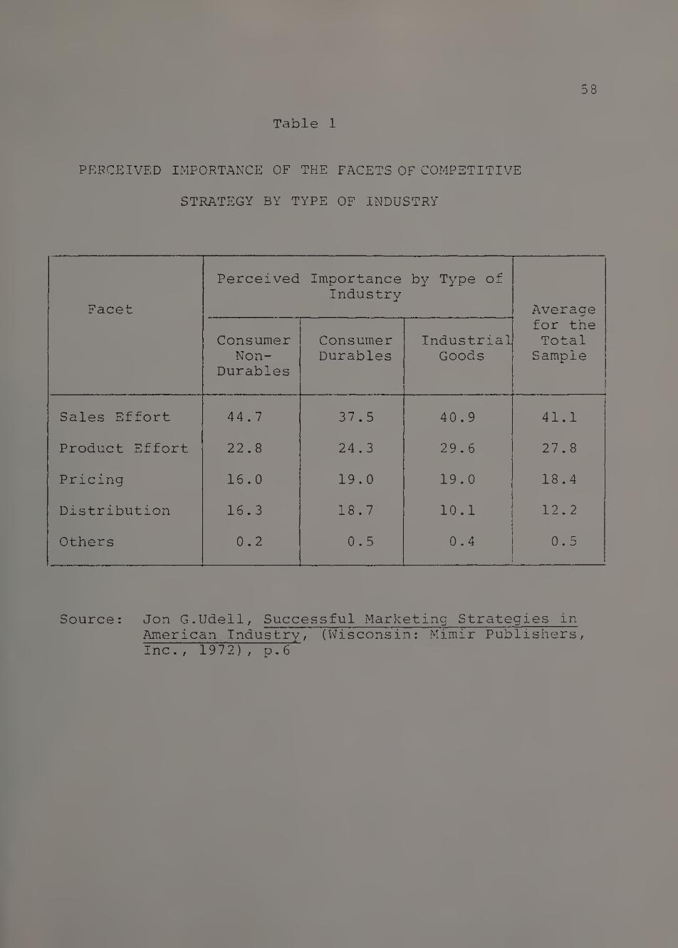
58

Table 1

PERCEIVED IMPORTANCE OF THE FACETS OF COMPETITIVE

STRATEGY BY TYPE OF INDUSTRY

Facet

Perceived Importance Industry

by Type of

Average for the Total

Sample Consumer

Non- Durables

Consumer Durables

Industrial Goods

Sales Effort 44.7 37.5 40.9 41.1

Product Effort 22.8 24.3 29.6 27.8

Pricing 16.0 19.0 19.0 18.4

Distribution 16.3 18.7 10.1 12.2

Others 0.2 0.5 0.4 0.5

Source: Jon G.Udell, Successful Marketing Strategies in American Industry, (Wisconsin: Mimir Publishers, Inc., 1972), p.6

PE

RC

EIV

ED

IMP

OR

TA

NC

E

OF

SP

EC

IFIC

MA

RK

ET

ING

AC

TIV

ITIE

S

BY

TY

PE

OF

IND

US

TR

Y

59

So

urc

e:

Jon

G.

Ud

ell

, S

uccessfu

l Mark

eti

ng S

trate

gie

s

in

Am

eri

can

In

du

str

y,

(Wis

co

nsin

: M

imir P

ub

lish

ers,

In

c.,

1972),

p.5

2

60

advertising to be as important as sales management, and tech¬

nical research and development, and selection and development

of distribution channels as next in importance.

Summary. In conclusion, the major findings of Udell's studies

can be summarized as below:

- The sales and product facets of the competitive

strategy were perceived to be more important

than distribution and pricing by respondents

from all types of industries.

- The relative importance of specific competitive

activities were found to differ for consumer

nondurable, consumer durable and industrial

goods.

- Udell's study is unique in the sense of its ex¬

tensive coverage of various types of industries

and has few parallels. However, scant use of

statistical methods to confirm or discredit the

stated hypotheses, and to test whether the ob¬

served differences are statistically significant

seems to be the major weakness of this study.

Econometric Market Share Models

The purpose of this section is to review advances that

have been made in the measurement of sales response to market-

61

ing decision variables. The survey of literature covers

single equation models and multiple equation models, models

with and without carryover effects incorporated, and models

with and without the influence of competitors' actions in¬

corporated.

Single Equation Models

6 9 Weiss' study. Weiss examined several econometric models to

explain market share movement of three national brands of a

low cost, frequently purchased consumer product. The data

employed represented the purchasing activities of 899 panel

families who purchased 123 different brands over a four year

period.

Initially the following four econometric formulations of

the demand relationship were fitted to the data to explain

the market share movement of three national brands studied.

1. Model with no transformation on data

SB,t V aiPB,t+ a2AB,t;

2. Differences from mean model

(2.15)

S = a + a (P B,t 0 1 B,t

Ratio to mean model

P ) + a0(A„ t 2 B, t

At); (2.16)

SB,t = a0 + al -= B,t + a,

A,

3. (2.17)

62

4. Log of ratio to mean model

where

Log e

P t

SB,t = V alloge ^ + a2loge ^ ; <2-18) Pt At

= market share for Brand B at time t

= price (dollars per ounce) for Brand B at time t

= advertising expenditures (thousands of dollars)

for Brand B at time t

= average price (weighted by volume) for all

three brands for period t

3

Further, to account for product quality differences,

superior in-store promotional activities, preferential shelf

space allocations within stores, cumulative effects of past

advertising efforts, or more effective use of advertising

expenditures, etc, dummy variables were added to the model

as proxies. The models utilizing dummy variables are given

below:

S B, t V alPB,t+ a2AB,t+ a3°l+ a4Q2

(Model 5); (2.19)

a0 + al<PB,t“ V + a2(AB,t" V + a3°l+ a4°2 (Model 6); (2.20)

S B, t ao+

P B, t

P t

+ A t

+ a3Qx+ a4Q2

(Model 7); (2.21)

63

t

+ S3Q-L+ a4Q2

(Model 8) (2.22)

where Q^= 1 for Brand B = 1 and 0 otherwise

Q^= 1 for Brand B = 2 and 0 otherwise

and the other variables remain as previously defined.

Note that the influence of competitive factors is repre¬

sented in models 2,3,4,6,7, and 8 by transforming the indepen¬

dent variables through either subtracting or dividing by the

appropriate mean value for the period.

Results. Weiss observed that in models 1 and 4, the price

coefficient was positive contrary to a priori expectations.

He conjectured that this may be due to the exclusion of cer¬

tain important variables such as quality which have a positive

association with both market share and price. This suspicion

was confirmed from models 6-8 which used dummy variables;

that is, the addition of dummy variables as proxies for other

marketing activities lead to negative price coefficients and

considerably improved the explanatory power of models. Models

6,7 and 8 produced the best fits with 's of .925, .922 and

.935, respectively.

Weiss viewed the superior fit of model 8 as supportive

of Kuehn’s70 contention that price and advertising interact

and do not produce linear effects on either market share or

64

volume. The multiplicative structure of model 8 allows this

joint influence of price and advertising on sales to he exa¬

mined .

71 Banks1 study. Banks postulated a linear relationship bet¬

ween the managerial decision variables and market share. The

model postulated related brand share with price, advertising,

point of purchase effort, and other marketing decision vari¬

ables. The results of this study indicated that advertising

was an important determinant of market share for coffee, but

not for scouring cleanser. For scouring cleanser, price and

promotional effort were important. The study was a cross-

sectional one in which the individual entities were brands:

9 for cleanser and 21 for coffee.

7 7 Parsons and Schultz note that since the results of

Banks' study are based on cross-section data, these results

are applicable to the market as a whole, but they may not be

applicable to an individual brand.

Note, in addition, the Banks' study did not take into

consideration the influence of competitors' actions and carry¬

over effects. However, in six of the eight models considered

by Weiss, the influence of competitors' actions is adequately

represented. Implicit in both works is the notion that all

variables act contemporaneously. The presence of carryover

effects has been ignored. Carryover effects are normally

65

represented in models by the use of lagged variables. Single

equation models with carryover effects represented by lagged

variables are considered next.

7 3 Sexton*s study. Sexton developed two negative exponential

models to estimate the marketing policy effects on sales of

a frequently purchased product. The first to predict a

brand’s share of a product’s total sales for a time period,

and the second model to predict the product’s share of the

total sales of the product and its substitute products for

a time period. Coupled with a time series model of the total

sales of the product and its substitutes, these models serve

to estimate a brand’s sales as a function of marketing poli¬

cies .

These models may be expressed in their general form as follows

Model - I. Brand Share Model

S = D.T [l-e-f(q'a'P'd)]

or

B = —— = [l-e-f(q'a'P'd)]

D.T

(2.23)

Model - II. Product Share Model

T = D.P [l-e-q(q'a'P'd> ]

or (2.24)

q = - = [1_e-g(^'a'P'd)] D.P

66

where for any period:

S = $ sales of brand

T = $ sales of product

P = $ sales of product and substitute products

D = Distribution coverage (%)

B = Brand share

Q = Product share

q = Quality index for brand or product

a = Advertising expenditures or share given separately

for each of current and previous time periods and

for each medium for brand or product

p = Relative price in current time period for brand or

product

d = Relative deal magnitude and coverage in current

time period for brand or product

(f and g are linear functions)

In his empirical models, Sexton treated network television,

spot television, magazine advertising, and newspaper adver¬

tising as separate variables. The other variables considered

were, quality, price, and dealing. The negative expoenential

models were cast in the Koyck^ distributed lag from to re¬

present the carryover effects. By taking logarithms, the

ralations were expressed as linear functions to which stan¬

dard multiple regression techniques were applied.

67

Results. For the brand share model, pricing and dealing

were found to be more important than advertising. The rela¬

tively more effective media were found to be magazines and

newspapers. For the product share model, the last period's

market share and pricing were found to be the major determi¬

nants of this period's product share.

7 5 Lambin's study. Lambin describes the steps involved in

developing and implementing a dynamic, competitive marketing

mix model for a major oil company combining econometric methods,

simulation techniques, and subjective judgements. The basic

model hypothesizes that a brand's market share is determined

by the relationship of its marketing expenditures to the total

for the industry. The model is expressed as

MS . 1/1

DS i nl,i i, t

EDS. i 1/1

DO. lit

n2,i —

E DO. i lit

ST -in3,i

if t

E ST. i lit

(2.25)

where MS = market share

DS = number of service stations

DO = number of other outlets

ST = total advertising expenditures

n = elasticity coefficients

l = company

68

t = time period

This model can be estimated directly for each competing brand

by the Ordinary Least Squares (OLS) method. Further, Lambin

outlined the following dynamic linear version of the above

model incorporating lagged effects:

MS = k + b1DSt* + b2DOt* + c1STt* + c^T^.^

+ XMSt-1+ Mt (2.26)

DSt where, DS * = - , etc.

ZDSt

Ais an estimate of each brand's retention rate. Lambin assumed

both advertising and distribution to have lagged effects. There¬

fore ,

A = A 6 + A96, (2.27) 1 ^

where 6 = relative weight of the goodwill capital created by

the distributive network (in percent)

0 = relative weight of the goodwill created by advertis¬

ing (in percent)

Thus X^ and X^ are parameters to be estimated. While he

assumed both advertising and distribution to have lagged effects

he postulated different time share reactions for advertising

and distribution. For advertising share XST*, Lambin postu¬

lated that market share was a function of two unweighted lagged

advertising variables and a geometrically weighted average of

69

all other past advertising shares; since there was little

variation in service station share DS*, a geometric proges-

sion was assumed from the first period onwards. With these

assumptions, Lambin expressed the exponentially distributed

lag model as:

OO l ■k * * ★

MS = k + b, E i=0

DSt_i+ b2DOt+ C1 ST + c 0ST t 2 t-1

OO i * + c ^ E A _ ST + u (2.28)

2 . « 1=0 2 t-i-1 t

The geometrically weighted averages in the above equation

were calculated as follows:

oo i * * * 2 * E A DS = DS + A _DS + A, DS +. rH

O

1! •H

t-1 t i t-i i t -2

+ 5 *

A DS, (2.29) 1 t-5

oo i * * 2 * 3 * E A0 ST = A^ ST. A ST A ST

i-0 2 t-i-1 2 t-2 2 t-3 2 t-4

4 * (2.30) + A^ ST

2 t-5

Lambin justifies this approximation since ' •

A1' decreases

rapidly as *i' increases. The transformed variables were

computed for values of A^ from 0.5 to 0.9, and from 0.1

to 0.9. The pair of values for A-, and A9 maximizing the

adjusted of the original model was ultimately selected.

Lambin compared the exponentially distributed lag model

70

with four other models: viz:

1. Linear - no lagged variables

2. Double log - no lagged variables

3. Linear - lagged market share

4. Double log - lagged market share

Results. Lambin found that model 3 and the exponentially

distributed lag model, yielded the best fit in terms of

adjusted and F-ratios. The Durbin - Watson statistic for

serial correlation was at an acceptable level for the exponen¬

tially distributed lag model, and multicollinearity seemed

not to be a serious problem. Overall, the linear models pro¬

vided good fits, and the lag model clearly established the

contribution of advertising and the presence of lagged adver¬

tising effects.

7 6 Houston and Weiss1 study. In this study, Houston and Weiss

reported the findings of an empirical investigation of the

77 movement of competitive market share. Palda's cumulative

advertising model was adapted to include a price variable,

and the analysis was extended to a multibrand market. The

statistical methodology employed in the investigation overtly

recognizes the competitive interdependence of the brands

studied and exploits this interdependence in the estimation

procedure. The product studied was a frequently purchased,

71

low cost, branded food item distributed in grocery stores

and delicatessens, and the market was dominated by three

nationally advertised and distributed brands. Their model

postulated a current period effect from price and advertis¬

ing expenditures as well as a lagged effect from prior adver¬

tising expenditures. The lagged advertising relationship

was hypothesized to be one of constant exponential decay.

Results. The findings of Houston and Weiss support the theory

that there can be cumulative effects from a firm's advertis¬

ing efforts. In addition observed differences in parameters

estimated suggested that marketing variables can play unique

roles for individual brands.

7 8 Prasad and Ring's study. Prasad and Ring investigated the

individual and interactive effect upon market share of

price and advertising and the way these effects were modulated

by the aggregate level of TV advertising. The product investi¬

gated was a frequently purchased canned food item. The sample

consisted of two matched panels of 750 families each. One

of the panels was exposed to twice as much TV advertising as

the other.

A linear model was hypothesized for each experimental

panel with the experimental brand's market share as the de¬

pendent variable. The set of independent variables included

72

lagged market share, and concurrent and lagged measures of

relative price, TV advertising, retailer advertising in news¬

papers, and magazine advertising. Interactions were included

as pairwise multiplicative variables. Competitor's variables

included were magazine and newspaper advertising.

Results. Two approaches were used in analysing the data in

each panel. In the first approach, the coefficients were

estimated for each panel by a step-up regression method.

With this approach, the regression coefficient for relative

price was -1.0000 and -.378, for the panels exposed to high

and low levels of advertising, respectively. Thus a frequent

expectation that higher advertising levels will support higher

prices was not supported for this brand. Price and the pre¬

vious period's market share were found to be the dominant

determinants of current market share for the panels exposed

to high and low levels of TV advertising, respectively.

The second approach used in analysing data was the step-

down approach. For the high advertising input panel, the

immediate effects of marketing variables appeared to be domi¬

nant, where as for the low advertising input panel, the effect

of carryover effects of prior period marketing variables were

significant. However, Chow's*^ test for the equality of the

full set of coefficients for both panels could not be rejected

at a reasonable level of significance.

73

Finally, certain problems common to most single equa¬

tion models discussed are considered next.

The identification problem. Concern has been often expressed

about the single equation models because of the implicit and

assumed unidirectional flow of influence in the model. A

frequently expressed criticism is that, although sales is a

function of advertising, advertising too is function of sales.

This leads to identification problems.

It is for these reasons that many authors have expressed

the view that market share relationships should be estimated

simultaneously even when these relationships are seemingly

unrelated. However, Rao^ after comparing the performance

of various single equation models with multiple equation model

observed that the adjusted R was not significantly different

for some of the single equation models compared with the simul

taneous equation model. Thus, Rao notes that if forecasting

were to be the purpose, the researcher may be better off choos

ing among single equation models.

The measurement of carryover effects. Carryover effects refer

to the influence of current marketing expenditures on sales

in future time periods. In order to properly assess the effec¬

tiveness of marketing decisions, the fraction of total sales

in the current period and each succeeding period which are

attributable to the current marketing effort must be measured,

and the duration of the carryover effect must be determined.

The geometric distribution is the most commonly used

distributed lag model in marketing. The maximum impact of

marketing expenditures on sales is registered instantaneously,

then, the influence declines geometrically to zero.

Given a geometric distribution of the form

w = (1-A) Xt, t = 0,1,2,. (2.31)

where 0< A<1, the specification of the sales response func¬

tion becomes

V = 6 + B, (1-A) ? At X + f . (2.32) a. ui t_Q oc-t cc

This relationship is nonlinear in the parameter A. Thus,

OLS cannot be used as the estimation method. To solve this

o t

estimation problem, Koyck proposed the following transfor¬

mation. Consider the sales response function for the time

period (<*-l) ,

CO t— 1 y =3+3,(1-A) I A X + e (2.33)

oc-l 0 1 t=l oc-t °c-l

Multiplying (2.33) by Aresults in:

CO +-

Ay = A3 + 3, (1-A) LAX +Af , (2.34) oc-i 0 1 t=1 oc-t «-l

Subtracting equation (2.34) from the original sales response

function (2.32) leads to:

75

y cc (2.35)

This transformation is referred to as Koyck transformation.

The validity of the geometric lag hypothesis. Based on a

review of a number of studies employing the geometric lag

8 7 model Parsons and Schultz " note that much of the statistical

evidence has failed to support the geometric lag hypothesis.

The authors also state than an alternative to the geometric

lag model is the partial adjustment model. In the partial

adjustment model sales in the current period are similar to

sales in the previous period except for a response to the

marketing insturment. The model can be expressed as

(2.36) y cc

The authors note that this model tends to fit any time series

with inertia quite well.

The issue of constant variance. Whenever the dependent

variable is stated as a proportion, as market share is, one

runs the risk of violating the assumption that the variance

of the disturbance term is constant. However, an arc sin

transformation may help stabilize the variance of the pro-

8 3 portion. Nevertheless, as pointed by Parsons and Schultz,

the use of arc sin transformation is atypical. The double

log transformation practice is widely prevalent. Most of

76

the studies reviewed, have considered both the untransformed,

O A

and transformed models. However, Prasad and Ring in their

study report that the results obtained after an arc sin trans¬

formation were virtually the same as those obtained with un¬

transformed current and lagged market shares. For this reason,

the authors report only the results of the untransformed ver¬

sion, and acknowledge that the assumption of homoscedasticity

may not be tenable because of the untransformed nature of the

dependent variables.

Multiple Equation Models

8 5 Lambin's study. Lambin explored the gasoline retail market.

A single equation regression model was used to identify the

determinants of total gasoline consumption. The influence

of advertising on primary demand was found to be negligible.

Instead, the role of advertising was found to increase the

level of selective demand. A two equation model was used to

describe the systematic dependence between advertising and

market share.

Lambin examined the extent to which there were signifi¬

cant differences between three media-press, radio and TV.

Press advertising was found to be the most important medium.

In addition, he examined the extent to which the introduction

of an advertising - quality variable improved the model. Two

77

brands ran campaigns of very different types. The first was

a promotional game, and the second, an image building type

of campaign. A dummy variable was used to evaluate the im¬

pact of each campaign. The effect on market share of the

promotional game was found to be more than three times higher

than that for the image-building campaign.

o c Schultz’s study. Schultz investigated the air-travel market

between two cities using data which represented a quarterly

time series from 1960 to 1968. The unit of study being a

one-way air trip between cities R and S (nondirectional).

He defined the problem as one of measuring determinants of

demand and market share in the city pair R - S, and to use

these measurements in planning marketing activity. Schultz

developed a single - equation multiple regression model for

demand analysis and a simultaneous - equation multiple regres¬

sion model for market share analysis. Schultz's experimental

design also provides for comparing linear versus loglinear,

and lagged versus unlagged versions of the basic model.

Results.

Demand estimates. Disposable personal income, seasona¬

lity and price were found to be significantly related to total

industry demand. The linear and log linear versions with no

lag performed slightly better than the corresponding lagged

78

versions.

Marketing system estimates. Frequency share, lagged

advertising share, and Airline K's population share in city

R were found to be significant in both lagged regression ver¬

sions. Schultz attributed the appearance of only lagged ad¬

vertising, rather than contemporaneous advertising as a sig¬

nificant variable to the wide variation in frequency of air

travel for consumers, which causes the average effect of a

change in advertising to be spread out over a longer period.

The managerial implication being that scheduling may be a

more effective tool for immediate gains in market share.

o 7 Beckwith*s study. Beckwith studied a frequently purchased,

inexpensive consumer nondurable good. This product class

was at the maturity stage of the product life cycle. The

top five brands accounted for 98% of the industry sales. All

brands were sold at uniform retail and wholesale prices, and

no price changes occured during the period investigated.

Advertising was the predominant marketing instument. Beckwith's

model assumed that for each brand i.

MS . = B . MS , .+ . AS .+ 6 . <*,1 li cc-l,i 2l cc, i °ci

for i = 1,2,

(2.37)

5;

where MS = market share

AS = advertising

a = time period

79

Results. OLS estimation of these equations revealed that

only two of the five advertising coefficients were signifi¬

cantly different from zero. However, it was recognized that

the contemporaneous covariance matrix was not diagonal. The

sales shares of Brands ’A’ and ' B' varied together as did

those of 'D' and 'E'. Moreover, the shares of ’A', 'B' and

' C' were oppositely affected by the disturbances from 'D'

and 'E'. Consequently, Beckwith reestimated the equations

by the iterative seemingly unrelated equations approach.

With this approach four out of the five advertising coeffi¬

cients were found to be significantly different from zero

and differed significantly between brands.

In Beckwith's study, the simultaneous nature of competi¬

tion among the brands was explicitly acknowledged in three

ways:

1. Brand sales shares were used as the dependent variables.

2. The effect of advertising was assumed proportional to a

brand's current share of all advertising expenditures.

3. The covariance structure of the disturbances was utilized

to estimate the consistent interaction between specific

brand pair distributions.

Rao1s study. Rao^ examined five methods of estimation and

four ways of specifying dependent variables in sales-adver-

tising models for cigaratte sales data covering six compa-

80

nies. The five alternative models tested were: the multiple

regression model with and without serially independent errors,

the Koyck model with and without serially independent errors,

and the simultaneous equation model. The dependent variable

was defined in four ways: per capita sales, logarithm of

per capita sales, market share, and logarithm of market share.

Two criteria were used to judge the model's goodness of fit -

2 adjusted R , and the mean absolute percentage error (MAPE)

between the actual and predicted values, respectively.

Results. The results showed that no method consistently

fared better for all companies and for all models, but, a

2 method which performed better on the adjusted R criterion

also did so on the MAPE criterion. The simultaneous equation

model did not excel over others, as expected. The adjusted

2 R was found to be high for all methods except the simulta¬

neous system model.

The study also revealed that while using MAPE as a cri¬

terion, the manner of specifying the dependent variable was

a significant factor in model building. However, with adjusted

R* 2 as the criterion, the method of estimation appeared to be

a significant factor in model building, thereby suggesting

that the choice of an appropriate method of estimation and

specification be treated in practice as a trade-off between

the two criteria.

81

8 9 Wildt's study. Wildt studied a product sold predominately

in retail food outlets. The product is purchased by the

consumer on an irregular and infrequent basis. He developed

a nine equation model of the competitive system incorporat¬

ing characteristics such as, the simultaneous nature of com¬

petitive effects, the complete marketing mix, carryover effects,

and interactions among variables. His study is unique with

respect to the number and nature of the decision variables

considered. Wildt focussed on the competitive behavior of

three major firms in the industry. Nine variables dealing

with market share, advertising and promotion expenditures of

the three major firms were considered endogenous to the system

while, new variety activity, seasonal variables and relative

price were considered as exogenous.

The equation system presented was block recursive in

nature. Wildt viewed this to be consistent with the market

environment where firm performance (market share) is deter¬

mined by the market mechanism operating during the time period

of concern, and the decision variables (promotion and adver¬

tising) are the result of management decisions made in ad¬

vance of the immediate time period. In a block recusive

model, each system can be estimated by whatever method seems

appropriate in the context of that particular subsystem. Wildt

estimated the parameters in the market share subsystem by the

82

seemingly unrelated equations technique and the managerial

decision variables sudsysuer. by two-stage least squares.

Results.

each firm

The results indicated that the market share of

was affecred by the relative market position of

in the preceding time period and the current rela¬

tive price of the product sold by the firm. These effects

were found tc be less severe for one of the firms, which

seemed consistent with its strategy7 of emphasizing new variety

sales. In addition, the market share of this firm was found

tc be significantly affected by its new variety activity and

those of its competitors. The sales of the market leader

was found to be directly affected by the major advertising

and promcuior. of the ether two leading competitors. Overall

the parameter estimates differed significantly fer brands.

While analysis of industry demand indicated that primary

demand was significantiy affected only by industry promotion,

the simultaneous model at the firm level provided evidence

cf competition among firms along the advertising, new variety

introduction and promotion dimensions.

The issue of entity aggregations. In the literature reviewed

thus far, considerations about the level of aggregation have

been totally ignored. It is an accepted premise that dirrerenr

the market are likely to respond differently to segments cf

83

q n various marketing inputs. If this were true, Sexton argues

that initially the effect of marketing policies should be esti¬

mated segment by segment. The overall market response func¬

tion should then be estimated by aggregating the response

functions estimated separately for each segment. That is,

if

S± = fi(A,P,D), (2.38)

where S_^ = brand sales in segment i

A = measure of advertising level in market

P = measure of price level in market

D = measure of deal level in market

then

S = l S. = £ f (A,P,D) (2.39)

i 1 i i

where S = brand sales in the entire market

It is for these reasons Sexton employs a cluster analytic

approach to estimate the market response function as described

below.

91 Sexton's study. In this study, Sexton outlines a cluster

analytic approach to estimate market response functions.

Cluster analysis was employed to disaggregate the data into

market segments. The marketing policy effects were estimated

separately for each segment and later aggregated for the entire

84

market. This approach enables the researcher to examine the

differences in marketing policy effect on various segments.

The data analysed in this study consisted of all the purchases

of all brands of regular and instant coffee and tea by a sta¬

tionary sample of 569 families over a period of two and a

half years. Clusters were formed using data on purchase

habit variables such as brand purchased, price, amount by

weight, store where purchased, and whether or not purchased

under a deal. The four clusters formed were (1) low usage

and low loyalty, (2) low usage and high loyalty, (3) high

usage and low loyalty, and (4) high usage and high loyalty.

Depandent variables considered included both sales and brand

share. The independent variables explored included time, the

dependent variable lagged one time period, and advertising,

pricing, and dealing, all lagged up to two or three time periods.

In addition, three different forms of the relationship between

these various combinations of variables were investigated,

namely: linear, loglinear, and negative exponential.

Results. Sexton reported that the set of coefficient esti¬

mates differed significantly across the four clusters. The

coefficient estimates between clusters of families with similar

usage rates but different loyalty rates, and similar loyalty

85

rates, but different usage rates were found to be significantly

different. The price coefficient was found to be larger for

heavier usage clusters.

The linear and negative exponential models were found

to be much superior to the loglinear model with respect to

goodness of fit.

The issue of spatial aggregation. Pointing to the widespread

Q O

prevalance of spatial aggregation, Moriarty points that

such aggregation suppresses the variability between regions,

which could be an important source of information to the

company about differences between regions. Prior to pooling

cross-section data, Moriarty stresses the need to verify

whether the parameters of the model are the same for different

cross-sections. Moriarty developed a variance components,

cross-sectional, time series model covering 25 sales districts

and 25 sales quarters. His study, which is discussed next,

focusses on the issue of spatial aggregation.

Moriarty's study. Most studies of the relationship between

market share and marketing decision variables are done at

the industry level or the company level. This approach des¬

troys the variability between brands or between districts

which often represents important sources of information with

respect to brand competition or sales district uniqueness.

86

The author posits that characteristics which might tend to

create district variability include product availability,

degree of price and local advertising competition, stage of

product life cycle, strength of sales force and socio-economic

and cultural differences between regions. The author states

that some of these variables influences could be viewed as

creating quasi-permanent differences (cross-sectional) and

some as creating influences which cause variation both over

time and over regions. With this rationale, Moriarty deve¬

loped a variance components cross-sectional, time-series

model. The model is disaggregative in nature; that is, it

allows for unexplained variances between cross-sectional units

to be accounted for by the model.

The product considered was a frequently purchased in¬

expensive consumer good sold almost exclusively in super

markets. The data employed consisted of 25 equivalent time

period observations for 25 sales districts.

Pooling cross-sectional districts requires that the para¬

meters of the process generating market share be the same

across the sales districts. Therefore, OLS time-series re¬

gression models were developed for each of the 25 sales dis¬

tricts in the sample. Prior to pooling districts, tests of

consistency of response parameters across districts were per¬

formed to test for the appropriateness of pooling. The con-

87

elusion was that the districts were heterogeneous in response

to the variables under consideration in the model. Next the

districts were grouped into three subsets (segments) based

on criteria such as geographical location, historical firm

performance and advertising expenditure allocation policy.

Consistency tests on subsets of districts suggested that the

response to marketing variables was homogenous within each

segment.

Summary. A review of the literature on market share models

reveals a number of facts. Most studies reported relate to

consumer nondurable products. In most cases the focus of

study is either on a particular brand or on the leading brands

within the product class. Studies at the industry level are

few in number. Competitive effects and the interactive effects

of marketing mix variables have been receiving increasing atten¬

tion. The issue of carry over effects has been addressed in

a number of studies, but this is largely confined to the carry¬

over effects of advertising.

A large number of alternative model formulations have

been investigated. These include single equation models and

multiple equation models; incorporating competitive effects,

interaction effects, and carryover effects; models accounting

for differences in sales response to marketing mix levels

88

across market segments and geographic regions; intrinsically

linear and intrinsically nonlinear models, to name just a

few. However, aside from model fitting considerations the

focus of mosu studies in either on price and/or advertising.

That is, few studies have systematically addressed the market¬

ing policy effects of other marketing instruments such as pro¬

duce activity, and personal selling activity.

In this chapter a number of imoortant studies on market

mare strategies - principles and concepts, market share theory,

and empirical studies on market share have been reviewed. In

the next chapeer problem statement, theory development, and

model soecificamior. are considered.

89

FOOTNOTES

Goerge S. Day, "A Strategic Perspective of Product Planning," Journal of Contemporary Business (Spring 1975), pp. 1-34.

2 Alfred R. Oxenfeldt, "How to use Market Share Measure¬

ment," Harvard Business Review (January-February 1959), pp. 103-112.

^Leonard J. Parsons, and Randall L. Schultz, Marketing Models and Econometric Research (New York: North-Holland Publishing Company, 1976), p. 138.

^Oxenfeldt, pp. 103-104.

^The Boston Consulting Group, Perspectives on Experience

(Boston: The Boston Consulting Group, 1968).

^Oxenfeldt, p. 111.

' "^Wendell R. Smith, "Product Differentiation and Market Segmentation as Alternative Marketing Strategies," Journal of Marketing (July 1956) pp. 3-8.

^Lee Adler, "A New Orientation for Plotting Marketing

Strategies," Business Horizons (Winter 1964) pp. 37-50.

^Theodore Levitt, "Exploit the Product Life Cycle," Harvard Business Review (November-December 1965) pp. 81-94.

-^Samuel C. Johnson and Conrad Jones, "How to Organize for New Products," Harvard Business Review (May-June 1957), pp. 49-62.

Hh. Igor Ansoff, "Strategies for Diversification," Harvard Business Review (September-October 1957), pp. 113-124.

l^philip Kotler, Marketing Management: Analysis, Planning,

and Control, 3rd ed. (New Jersey: Prentice-Hall, Inc., 1976),

pp. 49-50.

13David T. Kollat, Roger D. Blackwell, and James F. Robeson,

Strategic Marketing (New York: Holt, Rinehart and Winston, Inc.,

1972), pp. 21-23.

Day, p. 27.

90

^Edward W. Cundiff, and Richard R. Still, Basic Market¬

ing: Concepts, Decisions and Strategies, 2nd ed. (New Jersey: Prentice-Hall, Inc., 1971), pp. 247-249.

l^Daniel A.Nimer, "Marketing Planning by Matrix Analysis, Industrial Marketing (September 1972), pp. 50-60.

17C. Davis Fogg, "Planning Gains in Market Share," Journal of Marketing (July 1974) pp. 30-38.

^Ibid. , p. 31.

l^William e. Furhan, "Pyrrhic Victories in Fights for

Market Share," Harvard Business Review (September-October 1972), pp. 100-107.

20paul N. Bloom, and Philip Kotler, "Strategies for High Market Share Companies," Harvard Business Review (November- December 1975), pp. 63-72.

2J-Furhan, p. 102.

22Bloom and Kotler, p. 65.

23ibid.

24lbid., p. 69.

25ibid., pp. 70-72.

^Bernard Catry, and Michel Chevalier, "Market Share

Strategy and the Product Life Cycle," Journal of Marketing (October 1974), pp. 29-34.

27 The Boston Consulting Group.

^Kotler, pp. 239-241.

^Bloom and Kotler, p. 67.

3^Theodore Levitt, "Innovative Imitation," Harvard Busi¬

ness Review (September-October 1966), pp. 63-70.

31Roger D. Blackwell, "Strategic Planning in Marketing: Discussion," in Ronald C. Curhan, ed., Combined Proceedings, (Chicago: American Marketing Association, 1974), pp. 465-469.

33Levitt, Product Life Cycle, pp. 81-94.

91

■^Kotler, pp. 237-239.

^Levitt, Product Life Cycle, p. 89.

^Kotler, p. 237.

^Âdler, p. 44.

-^Levitt, Product Life Cycle, p. 87.

Ânsoff, pp. 113-116.

~^Fogg, pp# 31-34.

4<^Philip Kotler, Marketing Decision Making - A Model Building Approach (New York: Holt, Rinehart, and Winston, Inc 1971), pp. 2-5.

^David E. Bell, Ralph L. Keeny, and John D.C. Little, "A Market Share Theorem," Journal of Marketing Research (May 1975), pp. 136-141.

Ârnold I. Barnett, "More on a Market Share Theorem," Journal of Marketing Research (February 1976), pp. 104-109.

^Christopher Chatfield, "A Comment on A Market Share

Theorem," Journal of Marketing Research (August 1976) pp. 309 311.

"^Philippe A. Naert, and Alain Bultez, "Logically Con¬

sistent Market Share Models," Journal of Marketing Research (August 1973), pp. 334-340.

^Neil E. Beckwith, "Multivariate Analysis of Sales Responses of Competing Brands of Advertising," Journal of Marketing Research (May 1972), pp. 168-176.

^Timothy W. McGuire, and Doyle L. Weiss, "Logically Consistent Market Share Models II," Journal of Marketing Research (August 1976), pp. 296-302.

^7Henri Theil, "A Multinomial Extension of the Linear Logit Model," International Economic Review (October 1969),

pp. 251-259.

4 °Richard Stone, "Linear Expenditure Systems and Demand

Analysis: An Application to the Pattern of British Demand," The Economic Journal (September 1954), pp. 511-527.

92

49james M. Henderson, and Richard E. Quandt, Micro-

economic Theory: A Mathematical Approach, 2nd ed. (New York:

McGraw-Hill Publishing Company, 1971), p. 36.

^Timothy W. McGuire, Doyle L. Weiss, and Frank S. Houston,

"Consistent Multiplicative Market Share Models," in Ken Bernhardt ed., Combined Proceedings (Chicago: American Marketing Associa¬ tion, 1977), pp. 129-134.

->-*-Naert and Bultez, p. 338.

^Sidney Schoeffler, Robert D. Buzzel, and Donald F. Heany, "Impact of Strategic Planning on Profit Performance," Harvard Business Review (March-April 1974), pp. 137-145.

^Robert D. Buzzel, Bradley T. Gale, and Ralph G.M. Sultan, "Market Share - A Key to Profitability," Harvard Business Re¬ view (January-February 1975), pp. 97-106.

54 Sidney Schoeffler, "Cross Sectional Study of Strategy,

Structure and Performance: Aspects of the PIMS Program," SSP Conference, Indiana University, November 1975.

55Bradley T. Gale, "Selected Findings from the PIMS Pro¬ ject: Market Strategy Impacts on Profitability," in Ronald C. Curhan, ed., Combined Proceedings (Chicago: American Market¬ ing Association 1974), pp. 471-475.

^Bradley t. Gale, Donald F. Heany, and Donald J. Swire,

The Par ROI Report: Explanation and Sample (Cambridge, Mass:

The Strategic Planning Institute, 1977).

^Sidney Schoeffler, Nine Basic Findings on Business Strategy (Cambridge, Mass.: The Strategic Planning Institute,

1978).

^Buzzel, Gale and Sultan, p. 102-105.

~*^The Boston Consulting Group.

^William E. Cox, "Product Portfolio Strategy: A Review of the Boston Consulting Group Approach to Marketing Strategy," in Ronald C. Curhan, ed., Combined Proceedings (Chicago: American Marketing Association 1974) pp. 471-475.

^Noel Capon, and Joan Robertson Spogli, "Strategic Marketing Planning: A Comparison and Critical Examination of Two Contemporary Approaches," in Ken Bernhardt ed.. Combined Proceedings (Chicago: American Marketing Association 1977),

pp. 219-223.

93

^Buzzel, Gale and Sultan, pp. 102-105.

6^Ben Branch, Deviation from Par ROI (Cambridge, Mass.: The Strategic Planning Institute, 1977).

64Buzzel, Gale and Sultan, pp. 104-105.

^Robert D. Buzzel, Product Quality (Cambridge, Mass.: The Strategic Planning Institute, 1973).

Stephen Land, How Premiums and Discounts Affect Per- formance (Cambridge, Mass.: The Stratecic Planning Institute, 1978) .

6 7 Richard G. Hamermesh, M. Jack Anderson, and J. Elizabeth

Harris, "Strategies for Low Market Share Businesses," Harvard Business Review (May-June 1978), pp. 95-102.

fi 8 Jon G. Udell, "How Important is Pricing in Competitive

Strategy?" Journal of Marketing (January 1964), pp. 44-48, and, Successful Marketing Strategies (Madison: Mimir Publishers, Inc., 1972).

^Donald L. Weiss, "Determinants of Market Share," Journal of Marketing Research (August 1968) pp. 290-295.

"^Alfred A. Kuehn, and Doyle L. Weiss, "How Advertising Performance Depends on Other Marketing Factors," Journal of

Advertising Research (March 1962), pp. 2-10.

71 Seymour Banks, "Some Correlates of Coffee and Cleanser

Brand Shares," Journal of Advertising Research (June 1961), pp. 22-28.

72Parsons, and Schultz, p. 139.

72Donald E. Sexton, "Estimating Marketing Policy Effects on Sales of a Frequently Purchased Product," Journal of Market¬

ing Research (August 1970), pp. 338-347.

7^L.M.Koyck, Distributed Lags and Investment Analysis (Amsterdam: North Holland Publishing Company, 1954).

7^Jean-Jacques Lambin, "A Computer On-Line Marketing Mix Model," Journal of Marketing Research (May 1972), pp. 119-

126.

94

7 6 Franklin S. Houston, and Doyle L. Weiss, "An Analysis

of Competitive Market Behavior," Journal of Marketing Research

(May 1974), pp. 151-155.

77Kristian S. Palda, The Measurement of Cumulative Adver¬ tising Effects (New Jersey: Prentice-Hall, Inc., 1964).

78V. Kanti Prasad and L. Winston Ring, "Measuring Sales

Effects of Some Marketing Mix Variables and Their Interactions," Journal of Marketing Research (November 1976), pp. 391-396.

"^Gregory c. Chow, "Test of Equality Between Sets of

Coefficients in Two Linear Regressions," Econometrica (July 1960), pp. 591-605.

88Vithala R. Rao, "Alternative Econometric Models of Sales-Advertising Relationships," Journal of Marketing Re¬ search (May 1972), pp. 177-181.

81Koyck.

83Parsons and Schultz, p. 170.

83Ibid., pp. 151-152.

8^Prasad and Ring, p. 393.

83Jean-Jacques Lambin, "Optimal Allocation of Competitive Marketing Efforts: An Empirical Study," Journal of Business (October 1970), pp. 468-484.

88Randall L. Schultz, "Market Measurement and Planning With a Simultaneous Equation Model," Journal of Marketing

Research (May 1971), pp. 153-164.

87Beckwith, pp. 168-176.

88Rao, pp. 177-181.

8^Albert R. Wildt, "Multifirm Analysis of Competitive Decision Variables," Journal of Marketing Research (February 1974), pp. 50-62.

90Donald E. Sexton, "A Cluster Analytic Approach to

Market Response Functions," Journal of Marketing Research

(February 1974), pp. 109-114.

91 Ibid., pp. 109-114.

95

Q O

Mark Moriarty, "Cross-Sectional, Time-Series Issues

in the Analysis of Marketing Decision Variables," Journal of Marketing Research (May 1975), pp. 142-150.

CHAPTER III

THEORETICAL FRAMEWORK

This chapter addresses the issues of problem state¬

ment, theory development, and model building. The material

presented mainly relies on the inductive approach to theory

development. The econometric approach to model building

is taken to develop the theoretical framework for this study

This chapter is organized into three sections. First, the

problem statement is formulated. Second, theory and model

aspects related to marketing effort dimensions are developed

in some detail; and finally we focus on product-market

growth dimensions.

Problem Statement

Let i=l,2..T be the number of types of businesses,

j=l,2,.N the number of businesses of type 'J', and

k=l,2 .n the number of marketing effort dimensions

which are known to influence the sales and market share of

any business. If the competitive position of business 'j'

is assessed along the 'n' marketing effort dimensions, then

it is possible to describe this business as in a position

of competitive superiority along ' n1 marketing effort dimen

sions, in a position of competitive parity along market

96

97

ing effort dimensions, and in a position of competitive in¬

feriority along 1n^' marketing effort dimensions, where

nl+n2+n3 = n, the total number of marketing effort dimen¬

sions. Let 'Yj' be market share of this business. In a

similar fashion the competitive position of all 'N* busi¬

nesses of type 'J' along each of the 1n' marketing effort

dimensions can be assessed and their market share determined.

Given this data, our first research objective is to

investigate the relationship between market share Y, and the

competitive market position of businesses (j=1,2,....N),

along the marketing effort dimensions (k=l,2,.n). It

is also our objective to examine whether the significant

marketing effort dimensions are the same or different for

different types of businesses.

Alternatively, letting k=l,2,.n represent the number

of product-market growth dimensions, it is also our objective

to investigate the relationship between market share Y, and

the competitive market position of businesses (j=l,2,.N),

along product-market growth dimensions X, (k=l,2,.n).

And to determine whether the significant growth dimensions

are the same or different for different types of businesses.

Towards accomplishing these objectives, we now focus on

developing a theoretical framework describing the relation¬

ship between market share and the competitive market position

98

of a business along certain marketing effort dimensions and

growth dimensions.

Theory Development

Elements of marketing theory. Parsons and Schultz^ are of

the belief that the theory development process in marketing

involves a number of steps. They view marketing theory as

constructs capable of being tested. The source of market¬

ing theories are marketing generalizations, and in the in¬

ductive approach, a generalization about some phenomenon is

viewed as an approximate summary of the data which describes

that phenomenon. This view holds that the origin of gene¬

ralization (and hence theory) is data, and as such observa¬

tion of the phenomenon is a necessary precondition to theory

development. This approach commonly referred to as the

inductive approach to theory development, views empirical

observation of marketing phenomena as leading to marketing

generalizations which in turn lead to premises, the build¬

ing blocks of theory. On the other hand, use of the deduc¬

tive approach to marketing generalization is less common

and is based on a priori reasoning about marketing phenomena.

Figure 5 summarizes the steps involved in the two approaches.

For the most part, in this section we rely on empirical ob¬

servation of marketing phenomena as the basis for marketing

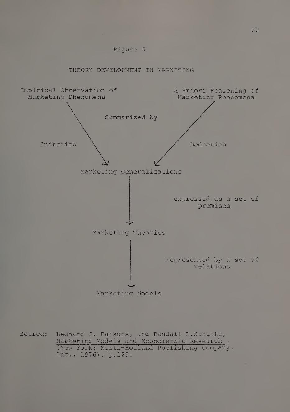
99

Figure 5

THEORY DEVELOPMENT IN MARKETING

A Priori Reasoning of

Marketing Phenomena

Empirical Observation of

Marketing Phenomena

expressed as a set of

premises

Marketing Theories

represented by a set of

relations

Marketing Models

Source: Leonard J. Parsons, and Randall L.Schultz,

Marketing Models and Econometric Research ,

(New York: North-Holland Publishing Company,

Inc., 1976), p.129.

100

generalizations. Because of their relevance to the generali¬

zations made in this study some of the empirical studies on

market share theory are summarized in Table 3. While all

of these studies were discussed in some detail in the litera¬

ture review section, we summarize them here for purposes of

completeness and to provide the foundation for the market¬

ing generalizations and premises developed in the next

section.

Marketing generalizations and premises. Stated briefly, a

generalization is a statement of the existence of a relation¬

ship between two variables and the direction of the relation¬

ship. To qualify as a theory, a number of specific asser¬

tions or premises about the generalization must be embodied

in the statement. In particular, a premise could be made

about the significance of the relationship and the condi¬

tions under which the relationship is expected to hold. With

this in mind consider the following generalization and pre¬

mises based on the marketing studies discussed in Chapter 2

and summarized in Table 3.

Generalization. There exists a relationship between

market share and the following marketing

effort variables: advertising, sales pro¬

motion, personal selling, corporate image

101

Table 3

SUMMARY OF STUDIES ON MARKET

SHARE THEORY

Study Product/Service Investigated

Marketing effort vari¬ ables found to be sig¬ nificantly related to market share

Banks (1961) Coffee Cleansers

Advertising i) Price

ii) Sales promotion

Weiss (1968) Low cost, fre¬ quently purchased consumer product

i) Price ii) Advertising

Sexton (1970) Frequently pur¬ chased consumer

product

i) Price ii) Sales promotion

Lambin (1970) Gasoline i) Advertising ii) Sales promotion

Lambin (1972) Gasoline i) Advertising ii) Service station

share

Beckwith (1972)

Frequently pur¬ chased inexpensive consumer product

Advertising

Rao (1972) Cigaratte Advertising

Houston and

Weiss (1974) Frequently pur¬ chased low cost, branded food item

i) Price ii) Advertising

Wildt (1974) Infrequently pur¬ chased consumer

product

i) New product activity ii) Price iii) Advertis¬

ing iv) Sales promo¬

tion

102

Table 3 (Continued)

SUMMARY OF STUDIES ON MARKET

SHARE THEORY

Study Product/Service Investigated

Marketing effort vari¬ ables found to be sig¬ nificantly related to market share

Sexton (1974) Coffee and tea Price

Moriarity (1975)

Frequently .pur¬ chased inexpen¬ sive consumer product

Price

Prasad and

Ring (1976)

Frequently pur¬ chased canned food

item

Advertising

Udell (1964,1972)

Consumer non¬

durables

i) Sales management and personal selling

ii) Advertising

iii) Price

Consumer durables i) Price ii) Sales management

and personal selling iii) Channel selection

and development

iv) Advertising

Industrial goods i) Sales management and personal selling

ii) Price iii) Product service iv) Technical research

and development

PIMS studies Consumer goods, industrial goods, and services

Quality

103

*

Premises.

building, product variety, product quality,

new product activity, research and deve¬

lopment activity, customer services, price,

and distribution. Further, while the direc¬

tion of the relationship between price and

market share is not clear, it appears that

there exists a positive relationship bet¬

ween market share and the other marketing

effort variables listed.

1. For all types of businesses, a signifi¬

cant:: positive relationship exists bet¬

ween market share and the competitive

market position of a business along the

product quality dimension. (PIMS studies)

2. For consumer nondurable businesses, a

significant positive relationship exists

between market share and the competitive

market position of a business along the

advertising effort dimension. (Banks,

Weiss, Lambin (1970), Lambin (1972),

Beckwith, Rao, Houston and Weiss, Wildt,

Prasad and Ring, and Udell).

3. For consumer nondurable businesses, a

significant positive relationship exists

104

between market share and the competi¬

tive market position of a business

along the sales promotion effort dimen¬

sion. (Banks, Sexton, Lambin (1970),

and Wildt).

4. For capital goods businesses a signifi¬

cant positive relationship exists bet¬


market position of a business along

the marketing effort dimensions personal

selling, customer services, and techni¬

cal research and development. (Udell)

5. For all types of businesses a signifi¬

cant positive relationship exists bet¬


market position of a business along

the breadth of product line dimension.

The last premise is based on the argument that the key

to operationalizing strategies such as market development,

product development, market segmentation, and product inno¬

vation is broadening the product line. These strategies

are generally viewed as the most effective means for increas¬

ing market share for all types of businesses of all sizes.

However, surprisingly the relationship between breadth of

105

product line and market share has not received much atten¬

tion in the empirical literature to date. Even though the

premise on breadth of product line cannot be substantiated 4

with empirical studies, numerous conceptual studies reviewed

in Chapter 2 lend credence to this premise.

This concludes our discussion on premises. These pre¬

mises taken together are used to develop a potential market¬

ing theory which can be tested by examining its conformity

with marketing data.^

Statement of theory. The competitive position effects theory

posited in this section is a statement of the relationship

between market share and the competitive market position

of businesses along various marketing effort dimensions. To

a large extent the discussion is confined to consumer non¬

durable businesses and capital goods businesses.

Prior to stating the theory it is perhaps necessary to

define What is meant by theory? Theory has been defined in

a number of ways in the literature. Kotler , for example,

defines theory as an explicit and coherent system of vari¬

ables and relationships with potential or actual empirical

foundations, addressed to gaining understanding, prediction,

or control of an area of phenomena. Kerlinger^ defines theory

as a set of interrelated constructs (concepts), definitions,

106

and propositions that present a systematic view of phenomena

by specifying relations among variables, with the purpose

of explaining and predicting the phenomena. Parsons and

S'chultz^ define marketing theories (equivalent to marketing

hypotheses) as constructs capable of being falsified by

empirical data, which is to say that they are constructs

capable of being tested. For purposes of theory generation

we adopt the approach suggested by Parsons and Schultz, along

with the marketing generalizations stated in this section.

The competitive position effects theory. The competitive

position effects theory in reference to marketing effort

dimensions posits the existence of a significant relationship

between market share and the competitive market position

of a business along certain marketing effort dimensions, and

the existence of a differential relationship for different

types of businesses. In particular, with regard to the con¬

sumer nondurable businesses and capital goods businesses as

summarized in Table 4 it is theorised that:

1. A positive significant relationship

exists between market share and the

competitive market position of a busi¬

ness along the marketing effort dimen¬

sions, product quality, breadth of pro¬

duct line, advertising, and sales pro-

107

motion for consumer nondurable busi¬

nesses .

2. For capital goods businesses, it is *

theorised that a positive significant

relationship exists between market

share and the competitive market posi¬

tion of a business along the marketing

effort dimensions, product quality,

breadth of product line, personal sell¬

ing, and quality of customer services.

Model development. The purpose of a model is to represent-

theory. The model outlined in this section which describes

the relationship between market share and the competitive

market position of businesses along certain marketing effort

dimensions will henceforth be called the competitive posi¬

tion effects model. Figures 6,7, and 8 describe the various

facets of .the model. In these figures the X^s represent the

marketing effort dimensions. A position of competitive

superiority along any dimension is represented by a set of

three parallel lines (n) , a position of competitive parity

by a pair of parallel lines (~) , and a position of compeitive in¬

feriority by a single line (—) . The area of the embedded circle

in these figures is a measure of market share Y. The B^s

108

Table 4

COMPETETIVE POSITION EFFECTS THEORY - A SUMMARY

Type of business Marketing effort dimensions

theorized to be significant

Consumer nondurables

Product quality

Breadth of product line

Advertising

Sales promotion

Capital goods

Product quality

Breadth of product line

Personal selling

Quality of customer services

109

are measures of the strength of the relationship between mar¬

ket share and the marketing effort dimensions.

Figure 6 models a general situation where all the market¬

ing effort dimensions, X^, X2..XN are assumed to have a

significant effect on market share. If this were to be true,

then according to theory, a business in a position of competi¬

tive superiority along a greater number of significant market¬

ing effort dimensions should have a higher market share than

businesses in a position of competitive superiority along

fewer significant marketing effort dimensions. This aspect

of the theory is incorporated in the model as described

below.

In Figures 6.a, 6.b, and 6.c, X-,, X9..X represent the

marketing effort dimensions all of which are assumed to have

a significant effect on market share. Figure 6.a models a

situation where a business is in a position of competitive

superiority along a relatively large number of marketing effort

dimensions; Figure 6.b models a situation where a business is

in a position of competitive superiority along relatively fewer

marketing effort dimensions; and Figure 6.c models a situation

where a business is in a position of competitive superiority

along only one marketing effort dimension. Accordingly, the

area of the embedded circle representing market share (Y)

is shown to be the largest in Figure 6.a, the second

110

Figure 6

THE COMPETITIVE POSITION EFFECTS MODEL

6a 6b

6c Key to Figures 6, 7, and 3

Y - Market share 0 - Area of the embedded cir¬

cle is a measure of mar¬ ket share 'Y'

'1 .X -Marketing effort

n dimensions

- Represents a position of competitive superio- ri ty along 'X ^1

- Represents comoetitive parity

- Represents competitive 'inferiority

B?,...3n - Measures of the ^strength of association

between Y and tne 'X.'s

Ill

largest in Figure 6.b, and the smallest in Figure 6.c. Thus

the direct relationship between market share and the number

of significant marketing effort dimensions along which a

business is in a position of competitive superiority is

evidenced in Figures 6.a, 6.b, and 6.c.

More specifically, it was theorised that, of the 'N1

marketing effort dimensions a subset of 'n’ dimensions happen

to be significant, (n <. N) and these are different for

different types of businesses. Figures 7 and 8 illustrate

these points. Figure 7 can be viewed as a representative

model for consumer nondurable businesses. Here, the dimen¬

sions theorized to be significant, namely: breadth of pro¬

duct line, product quality, advertising, and sales promotion

are shown as X^, , X^ and X^ respectively. In Figure 8

which serves as a model for capital goods businesses, the

dimensions theorised to be significant, breadth of product

line, product quality, personal selling, and quality of

customer services are represented by X , X^, X^, and X^.

Figures 7.a and 8.a model businesses in a position of com¬

petitive superiority along all four significant marketing

effort dimensions. Figures 7.b and 8.b model businesses in

a position of competitive superiority along only two of the

four significant marketing effort dimensions. And Figures

7.c and 8.c model businesses in a position of competitive

112

superiority along four marketing effort dimensions, but only

two of these are significant dimensions.

A comparison of Figures 7.a and 8.a shows that the set

of significant marketing effort dimensions are different

for different types of businesses.

A comparison of Figures 7.a and 7.b illustrates the

effect on market share of being in a position of competitive

superiority along all the significant marketing effort dimen¬

sions (X^ ,X^ ,Xj- ,X^) vis-a-vis being in a position of com¬

petitive superiority along only some of the significant

marketing effort dimensions (X^,X^). Note that in this case

Y is greater than Y, . a b

Further, a comparison of Figures 7.a and 7.c illustrates

the effect on market share of being in a position of com-

petetive superiority along all the significant marketing

effort dimensions (X-^ ,X^, X^ ,X^) vis-a-vis being in a position

of superiority along the same number of marketing effort

dimensions (X3 ,X^ ,X-y ,XN) , but only some of these dimensions

are significant ones (X3,X^). In this case Y^ is greater

than Y , thereby implying that being in a position of com-

petitive superiority along the dimensions X^ and X^_ has

little effect on market share.

In summary. Figures 6,7, and 8 jointly serve as a theo-

P

retical model of competitive position effects along cer-

113

Figure 7

THE COMPETITIVE POSITION EFFECTS MODEL - CONSUMER NONDURABLE BUSINESSES

114

Figure 8

THE COMPETITIVE POSITION EFFECTS MODEL - CAPITAL GOODS BUSINESSES

115

tain marketing effort dimensions. For purposes of empirical

investigation, we need to develop alternative mathematical

formulations of the above models. This issue is considered

in the chapter on empirical testing.

The next section is devoted to developing a theoretical

framework for the purpose of investigating the relationship

between market share and the competitive market position of

a business along certain product-market growth dimensions.

Theory Development

The product-market growth dimensions. The product-market

scope and growth vector conceptualization of strategies for

growth is widely prevalent in the marketing literature. As

stated earlier, market penetration, market development, and

product development strategies, constitute the growth oppor¬

tunities open to a firm within its present product-market

activity scope, and these strategies are jointly referred

to as the intensive growth strategies. Figure 9 summarizes

the classification of intensive growth strategies based on

cross-classifying product-market extension possibilities.

The material presented in this section is largely based on

this taxonomy which is developed from the works of Ansoff ,

Kotler7, Kollat et al8, and others, all of which were re¬

viewed in Chapter II. A review of these sources suggest

116

Figure 9

INTENSIVE GROWTH STRATEGIES

Present New Products Products

Present Market Product Markets Penetration Development

New Market Markets Development (Diversification)

H.Igor Ansoff, Corporate Strategy, (New York: McGraw-Hill Book Company, 1965) pp. 109

Source:

117

that certain product-market variables are the key to opera¬

tionalizing market penetration, market development, and

product development strategies. The variables involved and

the operational procedure are summarized in Table 5. While

these variables constitute the major product-market growth

dimensions, these are obviously not the only ones. However,

for purposes of this study, we assume that these variables

constitute the major product-market growth dimensions.

In order to develop a theoretical framework, certain

other assumptions need to be made. Two assumptions critical

to this study are:

1. The present competitive market position of a business

along the product-market growth dimensions is a measure

of its pursuit of market penetration, market development,

and product development strategies in the past.

2. Pursuit of market penetration, market development, and

product development strategies by a business will even¬

tually lead to an increase in market share.

Generalizations, premises, and theory. The conceptual studies

reviewed in Chapter II, together with the key variables in¬

volved in operationalizing intensive growth strategies summa¬

rized in Table 5, lead to the following generalizations:

There exists a positive relationship

between market share and the product-

113

Table 5

OPERATIONALIZING INTENSIVE GROWTH STRATEGIES

Variable Involved Operationalizing Procedure

1. Market penetration

X-,- Purchase freauencv Increasing the frequency of pur¬ chase among present users

X - Purchase quantity Increasing the average quantity purchased each time by present users

X - Number of users Increasing number of users by: i) attracting users of competi¬

tors products

ii) converting nonusers into users

2. Market development

X.- Number of tvpes of 4 users

Increasing number of users by i) tapping new market segments

ii) tapping new geographic mar¬ kets through regional, na- nal, or international expan¬ sion

3. Product development

X=- Product line breadth Increasing breadth of product line by: i) introducing different quality

versions of the basic product ii) introducing additional models

and sizes

Xf~ Product quality Improving the quality of the current product offerings

X_- Product features Adding new product features to current product offerings

119

market growth dimensions, purchase

frequency, purchase quantity, number

of users, number of types of users,

product line breadth, product quality,

and the number of product features.

Beyond generalizing the existence of a relationship

between market share and product-market growth dimensions,

the state of art does not enable us to make any specific

assertions or premises about the generalization. For

example, it would have been desirable to comment on the sig¬

nificance of the relationship, and conditions under which

the relation can be expected to hold. The absence of litera¬

ture on empirical studies pertaining to intensive growth

strategies lead to use of an approach which is more 'empiri¬

cist' and less 'positivist' in nature. Also, in the theory

generation process, we adopt the approach outlined by

Kerlinger.^

The conceptual studies on intensive growth strategies

reviewed earlier, and the resulting generalization, coupled

with the assumptions stated, enable us to outline the com¬

petitive position effects theory wTith reference to product-

market growth dimensions as stated below:

There exists a positive relationship

between the market share and the

120

competitive market position of a

business along the product-market

growth dimensions, purchase fre¬

quency, purchase quantity, number

of users, number of types of users,

product line breadth, product quality,

and number of product features.

Model development. The theoretical formulation of the model

is shown in Figure 10. Here, the X^s represent the product-

market growth dimensions. A position of competitive superi¬

ority along any dimension is shown by a set of three parallel

lines (E)/ a position of competitive parity by a pair of

parallel lines (=) , and a position of competitive inferiority

by a single line (—) . The area of the embedded circle is a

measure of market share Y. The b!s are measures of the 1

strength of the relationship between market share and the

product-market growth dimensions. In formulating the model

it is assumed that all the product-market growth dimensions

X-^,X^,.X^ have a significant effect on market share.

Figure 10.a models a business situation where a business is

in a position of competitive superiority along most dimen¬

sions. Figure 10.b depicts a business situation where a

business is in a position of superiority along some dimen¬

sions, in a position of parity along most dimensions, and

. 121

Figure 10

THE INTENSIVE GROWTH STRATEGY MODEL

10a 10b

and 10c

Y - Market share 0 - Area of the embedded cir¬

cle is a measure of market share ' Y '

Xi ,X2,...X7 - Product-market growth dimensions - Represents a position

of competitive suoerio- rity along growtn dimens-

ion X •

- Represents competitive pari ty

- Represents competitive inferiority

B-j , Bg » • • • B7 - Measure of strength of association between 'Xi's and Y

122

in a position of inferiority along few dimensions. On the

other hand. Figure 10.c models a business situation where a

business is in a position of competitive inferiority along

most dimensions. The direct relationship between the market

share of a business and the number of dimensions along which

it is in a position of competitive superiority is evidenced

by examining Figures 10.a, 10.b, and 10.c. In these figures

we note that Y > Y,> Y , since, the number of dimensions of a c c

superiority is of the form N^> N .

Summary. This chapter has addressed the issues of problem

statement, theory and model development. The competitive

position effects theory was outlined, and the theoretical

formulation of the competitive position effects model with

reference to marketing effort dimensions, and product-market

growth dimensions (the intensive growth strategy) were pre¬

sented. The next chapter is devoted to the empirical speci¬

fication of these models.

123

FOOTNOTES

^"Leonard J. Parsons, and Randall L. Schultz, Marketing Models and Econometric Research (New York: North Holland Publishing Company, 1976), p. 136.

^Ibid., p. 126.

3 Philip Kotler, Marketing Decision Making - A Model

Building Approach (New York: Holt, Rinehart and Winston, Inc., 1971), p. 7.

^Fred N. Kerlinger. Foundations of Behavioral Research (New York: Holt, Rinehart and Winston, Inc., 1965), p. 9.

c Parsons and Schultz, p. 125.

£

H. Igor Ansoff, "Strategies for Diversification", Harvard Business Review (September - October 1957), pp. 113-124.

7 Philip Kotler, Marketing Management: Analysis, Plann-

ing, and Control, 3rd ed. (New Jersey: Prentice-Hall, Inc., 1976), pp. 49-50.

o David T. Kollat, Roger D. Blackwell, and James F. Robeson,

Strategic Marketing (New York: Holt, Rinehart and Winston, Inc., 1972), pp. 21-23

Q Kerlinger, pp. 16-47

CHAPTER IV

EMPIRICAL MODEL SPECIFICATION

The previous chapter addressed the issues of problem

statement, theory development, and theoretical model formu¬

lation. The focus of this chapter is empirical specifica¬

tion of both the competitive position effects and the inten¬

sive growth strategy models. This material is preceded by

a brief discussion of the scope of empirical analysis, source

of empirical data, and operational definitions of key vari¬

ables .

Scope of analysis. The analysis is confined to businesses

in the maturity stage of the product life cycle. The

rationale for this is that the maturity stage of the product

life cycle poses the most formidable challenge to marketing

management. There are many reasons for this; for example:

- Most products are in the maturity stage of the life cycle, and therefore most of marketing management deals with the maturity stage.

- With the weaker competitors slowly dropping out, there is intense competi¬ tion among the well entrenched competi¬ tors during the maturity stage.

- Firms view an extended maturity stage and/or a new growth phase as a way out to delay the onset of the decline stage.

124

125

- Market stretching (life extension) strategies assume greater importance during the maturity stage than in the earlier' stages.

Source of data: The PIMS data base. The source of data for

this study is the PIMS data base. The PIMS program is a

cross-sectional study of business-strategic experience

which attempts to explain the experienced differences in

operating results across the 1000 - plus businesses on the

basis of strategic moves and the competitive settings in

which they were made. The unit of observation in PIMS is a

business; each business is either a division, product line,

or other profit center within its parent company, selling a

distinct set of products and/or services to an identifiable

group of customers in competition with a well defined set

of competitors. The information on each business consists of

about 100 items, descriptive of the characteristics of the

market environment, the state of competition, the strategy

pursued by the business, and the operating results obtained.

For the purposes of this study we consider the relative

market share and competitive market position data for 157

consumer nondurable businesses and 161 capital goods busi¬

nesses for the operating year 1973.

The dependent variable: Relative market share. While analyz¬

ing cross-section data of an industry, it is common practice

126

to employ market share or sales as a measure of marketing

effectiveness."*" However, because the PIMS data base pools

cross-sectional data from a sample of businesses across

different industries, (e.g., the consumer nondurables data

pool may possibly include businesses from the frozen food,

breakfast cereals, beverages, toileteries and cosmetics, etc.,)

relative market share is a more appropriate measure of market¬

ing effectiveness. Use of relative market share allows us

to compare the market share of a business which competes in

a market environment characterized by intense competition,

with that of a business competing in a market environment

characterized by moderate competition. To clarify this point

we present a few illustrations. Consider the following three

hypothetical markets, and the market shares of four leading

businesses in these markets:

Market 1, A=15%, B=13 %, C=9%, D=8%, others=55%;

Market 2, A=20%, B=15%, C=14%, D=ll%, others=40%;

Market 3, A=30%, B=24 %, C=21%, D=15%, others=10%;

Note that, the leading business in these markets has a share

of 15%, 20%, and 30%, respectively. Also note that, the

share of the market leader (A) inmarket 1 is equal to the

share of the fourth ranking business (D) in market 3. Next,

consider relative market share, which in PIMS is defined as

the market share of the business divided by the sum of the

market shares of the three major competitors. We note that

127

the relative market share of the market leader in all these

cases is 50%, even though their absolute market shares are

15, 20, and 30% respectively. Next, consider a different

situation, where the absolute market share of the market

leader is the same in the three markets, but the competitive

environment differs.

Market

i—1 A=21%, B=20%, C=20%, D=20%, others=19%;

Market 2, A= 21%, B=15%, C=10%, D=5%, others=49%;

Market 3, A= 21%, B=10%, C=5%, D=5%, others=59%;

The relative market share of the market leader in these

three markets is 35%, 70%, and 105% respectively. Note that

in market 1, the market leader is only marginally ahead of

its competitors, while in market 3, the market leader is

significantly ahead of the rest. Thus, relative market

share enables us to capture the competitive essence of the

market situation in a data pool created by pooling businesses

from a number of industries. For these reasons, relative

market share has been used as a measure of marketing effec¬

tiveness in the models considered in preference to sales

and absolute market share.

The specific marketing effort dimensions and the product-

market growth dimensions considered in this study are detailed

in the sections devoted to the competitive position effects

model and the intensive growth strategy model respectively.

We will first consider the competitive position effects model.

128

The Competitive Position Effects Model

Mathematical formulation of the model. As is true in most

research situations, here again we do not have a clear idea

of the exact functional relationship between relative market

share and the competitive market position of businesses along

various marketing effort dimensions. In the absence of such

information, the usual recourse is to investigate the good-

nees-of-fit of alternative functional forms. Here, the

goodness-of-fit of the linear, multiplicative and quadratic

formulations are investigated.

Let Y. be the market share of business 1 j' and X., the 3

competitive market position of business 'j1 along the market¬

ing effort dimensions, k=l,2,.n. A simple linear addi¬

tive formulation of the competitive position effects model

described in Figures 6,7, and 8 could be written as

Y . = Bn + B X + B X + 3 1 jl ^ j 2

(4.1)

The multiplicative formulation can be written as

or

log Y. = logB_ + B logX. + B0logX. + D 0 1J1 2 J 2

+ B logX. + f . n Dn j

(4.2)

And finally, the quadratic formulation of the model can be

129

written as

Y. = B + B_ X . +BX + 3 0 1 31 2 j 2

,X2 +. B n+2‘ 32

... .+ B X . + B X2 + n 3n n+i jx

+ B X2 . + f . . 2n 3n j

(4.3)

In order to examine the goodness-of-fit of these models,

one would require real life market data or simulated market

data. In addition, the specific marketing effort dimensions

to be considered need to be stated. These issues are con¬

sidered next.

As stated earlier, the source of data for this study

is the PIMS data base and the dependent variable used is the

relative market share. The next step is to select the rele¬

vant marketing effort dimensions upon which to focus. In

the PIMS data base the competitive market position of a busi¬

nesses is measured with respect to nine marketing effort

dimensions: Product quality, new product activity, breadth

of product line, sales force expenditure levels, advertising

expenditure levels, sales promotion expenditure levels,

quality of customer services, degree of forward vertical

integration, and relative price level. . With these variables,

the linear, multiplicative, and quadratic formulations of the

empirical competitive position effects model can be written

as shown in 4.4, 4.5, and 4.6, respectively.

Yj = V Vjl+ Vj2+.+ Vj9+ f j' (4.4)

130

log Y. = log B + B, log X. + B0log X. +.+ 1 0 1 31 2 ^ 32

Vog *j9 + * - (4.5)

Y. = B + B, X . + B_X . + 3 0 1 jl 2 D2

B^X2 . +..... 11 32

.+ B9Xj 9+ B10X j!+

+B18X2j9+ V (4.6)

where, Y.= Relative market share of business ’ j’ 3 J

X_._^= Breadth of product line

X = Degree of forward vertical integration j 2

X. = Sales force expenditure levels 3 3

X_.^ = Advertising expenditure levels

X. = Sales promotion expenditure levels 35

X^= Quality of customer services

X. = Product quality measure 37

X. = New product activity measure 38

X. = Relative price 39

Given these mathematical formulations, an immediate issue

is one of model underspecification. This may occur because

certain ’important' variables are excluded from the model due

to measurement limitations. On the other hand, however, it

should be noted that in the vast majority of the econometric

studies reviewed in Chapter II the number of marketing effort

variables considered rarely exceeded two or three.

An approach to data analysis with dummy variables. Given the

qualitative nature of the data an appropriate coding proce-

131

dure must be used. In the coding procedure selected 's-l'

dummy variables are created for each variable having 's'

levels. Since a business can be in a position of competitive

superiority, parity or inferiority along each one of the

marketing effort dimensions, two dummy variables are created

to represent each one of the marketing effort variables.

Therefore, the linear formulation of the competitive position

effects model assumes the form:

B.+ B, X. + B.. X. + B0o X. + BonX-„ + 0 Is 3is lp jip 2s 32s 2P 32p

Bn X. + Bn X. + f • 9s J9s 9p 39p 3 /

+

(4.7)

where, Yj = Relative market share of business ' j', and X^,X2r

.Xg= Marketing effort dimensions as defined earlier;

note that this model has an intercept Bq, and 18 regression

coefficients, Bgs,B.^,.B9s'B9p In each of these re¬

gression coefficients, the first subscript relates to the

variable and the second subscript relates to the competitive

market oosition. Thus Bn contrasts the effects of a posi-

tion competitive superiority with inferiority along the

marketing effort dimension * 1', and so on.

As an illustration, the dummy coding procedure for

variable X^ is described below.

X.. =1 and X. = 0 if business 'j' is in 31s 3 Ip

a position of competitive superiority along

the marketing effort dimension ’ X^'.

132

X. =0 and X. = 1 if business 'j * is 31s Dip

in a position of competitive parity along

the marketing effort dimension 1X-^'.

X. =0 and X. = 0 if business * j1 is 3 is DIP J

in a position of competitive inferiority

along the marketing effort dimension 1 X^'.

Variables X^ to X^ are coded in a similar

manner.

Table 6 shows the design matrix for variable

While it is meaningful to describe the competitive posi¬

tion of a business as one of competitive superiority, parity,

or inferiority while referring to variables X^ to Xg, this

description is not appropriate for the price variable, XQ.

The competitive position of a business along the price dimen¬

sion is better described in terms of the following three

states:

Price higher than the average for competitors

Price comparable to the average for competitors

Price lower than the average for competitors

We adopt this coding for the price dimension in the remainder

of this work.

In a similar fashion dummy variables for other formula-

133

Table 6

ILLUSTRATION OF DESIGN MATRIX FOR DUMMY CODING

Relative Market

Marketing effort

dimension-Xj_

Remarks

Share Y

Dummy Variables

Xls xlp

Yi 1 0 Businesses in a posi¬

tion of competitive

Y2 1 0 suepriority dlong

marketing effort

Y3 1 0 dimension 1X 1

Y4 0 1 Businesses in a posi¬

tion of competitive

Y5 0 1 parity along market-

ing effort dimension

Y6 0 1 ’V

Y7 0 0 Businesses in a posi¬

tion of competitive

Y8 0 0 inferiority along

marketing effort

Y9 0 0 dimension 'X 1

134

tions of the competitive position effects model, i.e., the

multiplicative and quadratic formulations, can be easily

created by extending this basic approach.

The Intensive Growth Strategy Model

In this section we focus on the empirical specification

of the intensive growth strategy model. As noted earlier,

intensive growth strategies are broadly classified as market

penetration, market development, and product development

strategies. And the key product-market growth variables

involved in operationalizing these strategies are:

- average purchase frequency

- average purchase quantity

X3 - number of users

X^ - number of types of users

X - breadth of product line 5

Xg - measure of product quality

X7 - measure of number of product featues

Since we do not have an idea of the exact functional

relationship between market share and product-market growth

dimensions, we need to examine the goodness-of-fit of alter¬

native functional relationships. In doing so, we first

specify the functional relationship between market share and

market penetration, market development and product develop-

135

ment.

The alternative empirical formulations examined are:

1. the main effects formulation

2. the main effects plus interaction effects formulation

3. the multiplicative formulation

In proposing the main effects formulation it is assumed

that the effects of market penetration, market development,

and product development are linear and additive. That is,

intensive growth strategy effect on market share is assumed

to be given by the sum of market penetration effects plus

market development effects plus product development effects.

A schematic representation of this is shown in Figure 11.

Thus, given a main effects functional formulation, the inten¬

sive growth strategy model can be written as:

Yj = Bq+ 3lXji+ +.+ B7Xj7+ *-j <4'3)

where, for business * j'

Y. = Relative market share 3

= Average purchase frequency

X. = Average Durchase cuantitv 32 *

X . = Number of users 33

X. = Number of tyoes of users 34

x . ^ 35

= Breadth of product line

Xj6 = Measure of product quality

X3 7 = Measure of number of prcduc

136

Figure 11

INTENSIVE GROWTH STRATEGY EFFECTS ON MARKET SHARE:

THE MAIN EFFECTS FORMULATION

137

Focussing next on interaction effects, logical reason¬

ing suggests that a synergistic relationship could exist

between product development and market penetration strate¬

gies. That is, product development activities such as improv¬

ing the quality of the present product offerings, broadening

the product line, and adding new features to the current

product offerings can contribute to the effectiveness of

market penetration possibilities such as increasing the fre¬

quency of purchase among present users, increasing the average

quantity purchased by present users, attracting users of com¬

petitors products, and converting nonusers into users.

A similar relationship could exist between market deve¬

lopment and product development strategies. As stated earlier,

market development implies tapping new market segments with¬

in the present geographic markets and expanding into new

geographic markets. Effectively exploiting these growth

opportunities would call for broadening the product line;

that is, creating different product versions of the basic

product to meet the distinct needs of different types of

customers, and improving the quality of the current product

offerings in order to make the product acceptable to more

number of types of customers.

The relationship between market penetration and market

development strategies suggests a third source of interac-

138

tion effects. And finally the interaction between variables

that are specific to a strategy present a fourth source of

interaction effects. (eg., the interaction between product

development activities such as quality improvement, new

product activity and product line breadth.) Therefore, a

functional relationship incorporating main effects and inter¬

action effects sounds logical. The full model with main

effects and interaction effects represented can be written

as:

Y . 1

Bn+ B,X. + B0X. + 0 1 31 2 32

B0X. X + 9 31 33

..+ B-.X. + B„X. X + 7 37 8 jl j2

+ B X X. + f- . , 28 36 37 3

(4.9)

where Y.,X. ,X. ..X. are as previouslv defined. 3 31 32 37

Finally, if the effects of market penetration, market

development, and product development were to be multiplica¬

tive, and not additive, then the model can be written as:

Y. 3

B

= B0Xj]_ ^X

B

32

B

X 7

j 7 (4.10)

or

logY = logBQ+ BnlogX_.^+ B2logX_.2 + +

B7logXj 7+ f ,

where Y • , X . ,X. ..X are 3 31 32 37

Equations 4.8,4.9, and 4.10

as previously defined,

are alternative mathematical

formulations of the intensive growth strategy model in their

139

general form. While using a data base for purposes of deve¬

loping an empirical model, an important step is to identify

variables which would reasonably serve as surrogate measures

of the variables included in the proposed mathematical formu¬

lations. In doing so it is unlikely that surrogate measures

can be developed for each variable specified in the general

model. Hence, the problem of model underspecification may

again reappear. For the present, we focus on the choice

of surrogate measures, postponing discussion on model under¬

specification to a later chapter.

PIMS variables as surrogate measures. Market penetration

possibilities include increasing the frequency of purchase "

and the average quantity purchased by present users, attract¬

ing users of competitors products, and converting nonusers

into users. The PIMS variable 'relative size of customers

served' is used as a surrogate measure of the product of

purchase frequency and the average quantity purchased- Un¬

fortunately, the PIMS data base does not provide us with a

surrogate measure of the other two market penetration possi¬

bilities .

Market development possibilities include tapping new

market segments within the geographic markets presently

served by the firm and expanding into new geographic markets.

140

In this study, the PIMS variable relative number of types

of customers served by the business is used as a surrogate

measure of market development.

Finally, product development possibilities include

improving the quality of the present product offerings,

broadening the product line, etc. The PIMS variables rela¬

tive product quality and relative breadth of product line

are used as surrogate measures of product development. Table 7

presents a summary description of the PIMS variables which

are used as surrogate measures for market penetration, market

4 development, and product development strategies.

With the variables listed in Table 7 employed as surro¬

gates of product-market growth variables, the alternative

formulations of the intensive growth strategy model can be

written as follows:

Main effects model

Yj = V Bixjl+ B2Xj2+ B3X j 3+ B4X j 4+ <-j (4-11)

Full model

Y j

B + B X + B X + B X. + B X. + B X. X. + 0 1 j1 2 J2 3 ] 3 4 34 $ 31 J2

B.X. X. + B-X. X. + BQX. X. + BQX. X..+ 6 31 33 7 31 34 8 32 33 9 32 34

B,nx. x. + e• 10 33 34 3

Multiplicative model

(4.12)

B. B, B

= B0Xji ^X- ^X 32 j 3 ~X

B

34 Y .

3

or

141

Table 7

SURROGATE MEASURES OF MARKET PENETRATION,

MARKET DEVELOPMENT, AND PRODUCT DEVELOPMENT

GROWTH STRATEGY SURROGATE MEASURE(S)

Market penetration Relative average size of customers served (x^)

Market development Relative number of types of customers served (X^)

Product development Relative breadth of product

line (X^) Relative product quality (X )

142

logY . = lcgB0+ B-^logX . + B2logX.2+ B_,logX. + 1 _j -l * 2 3

B4logXj4 (4.13)

where Y^= Relative market share

Xj^= Relative average size of customers

Xj2= Relative number of types of customers served

X. = Relative breadth of product line 3 3

Xj4= Relative product quality

Since the variables X- are <lualitativa in JJ- J J J ^

nature, we again use the dummy variable coding approaching

discussed earlier. Recall that, with this approach, ’s-11

dummy variables are created to represent each of the vari¬

ables having ’s’ levels. Using dummy coding in the context

of the intensive growth strategy model yields the following

linear formulation:

Yj = B0+ Blsxjls+ BlpXjlp+ B2sXj 2s+ B2pXj2p+.+

B4sXj4s+ B4pXj4p+ ' (4‘14)

where, Yj = Relative market share of business 'j1, and Xj^,

X. ,X. ,X. are the product-market growth dimensions des- 32 33 34

cribed in Table 7. In each of the regression coefficients,

the first subscript relates to the variable and the second

subscript relates to the competitive market position. Thus

B-^s contrasts the effect of a position of competitive superi¬

ority with inferiority along the product-market growth dimen¬

sion ' X^’- The product-market interaction and multiplica-

143

tive formulations with dummy variables can be written in a

similar manner.

Summary. This chapter has been devoted to an empirical

specification of the competitive position effects model and

the intensive growth strategy model. Alternative mathemati¬

cal formulations of the models, variables included in the

model, and coding procedures have been discussed. In the

next chapter, statistical tests for specification error

analysis and model testing are discussed.

144

FOOTNOTES

Leonard J. Parsons, and Randall L. Schultz, Marketing Models and Econometric Research (New York: North Holland Publishing Company, 1976), p. 138.

^For a detailed discussion on the uses and limitations of the relative market share measure see Noel Capon, and Joan R. Spogli, "Strategic Marketing Planning: A Comparison and Critical Examination of Two Contemporary Approaches," in Ken Bernhardt, ed., Combined Proceedings (Chicago: American Marketing Association, 1977), pp. 219 -223.

^See questions 139, 316-318, 319, 323-324, 325, 329,

330, 331, and 332 in PIMS data forms in Appendix.

^See questions 316-318, 325, 326, and 328 in PIMS data

forms in Appendix.

CHAPTER V

TESTS FOR MODEL EVALUATION

In this chapter, the tests used for evaluating the pro¬

posed empirical models are described. The actual testing

and the results of the tests are discussed in the chapters

on model testing. The evaluation of a model begins with the

testing of the statistical assumptions underlying the model.

This step in model evaluation is commonly referred to as

specification error analysis. Parsons and Schultz'*' list the

following as the most common types of specification errors:

a) Heteroscedasticity

b) Autocorrelation

c) Multicollinearity

d) Incorrect functional form

e) Model underspecification

f) Nonnormality of the disturbance term

g) Errors in variables

The specification error analysis is followed by tests

of significance of the entire linear relationship, individual

regression coefficients and subsets of coefficients. In addi¬

tion, if the researcher has developed more than one model to

explain the underlying phenomenon tests for selecting from

among alternative models are to be performed. In this chapter

we discuss the tests employed for specification error analysis,

145

146

corrections and adjustments for specification errors, and

methods for evaluating the full model.

Specification Error Analysis

Heteroscedasticity. It has been assumed that the variance

of the disturbance term is constant. If the disturbances are

heteroscedastic, OLS estimates of the regression coefficients

of the model will be unbiased and consistent, but not be effi¬

cient. The solution then is to use GLS regression.

Test for heteroscedasticity. The test against hetero-

2 scedasticity is due to Goldfeld and Quandt. This test as

3 described by Johnston involves the following steps.

1. Ordering the observations according to increasing values

of the dependent variable

2. Omitting the ’ c* central observations. The value of ' c'

being chosen so as to maximize the power of the test

(In this study the number of central observations omitted

was set at one)

3. Fitting separate regressions by ordinary least squares

to the first (T-c)/2 observations and to the last (T-c)/2

observations.

4. Testing the ratio of the residual sum of squares from the

two regressions using the F distribution with (T-c-2(k+1))/2

and (T-c-2(k+1))/2 degrees of freedom.

147

In computing the F ratio, it is common practice to use the

larger of the two residual sums of squares as the numerator

value, since the standard F-tables are constructed for F-ratios

greater than one.

Under the null hypothesis that the variances are homo-

scedastic, the statistic

F =

T-c Residual sum of squares of first (second) 2

_observations_ T-c

Residual sum of squares of second (first) 2 observations

is distributed as

T-c-2(k+1) T-c-2(k+1) (5.1)

It should be noted that this test does not assume the existence

2 2 of T different variances, but only two variances a and o ,

A B

generated from the two groups of obseravations.

Correction for heteroscedasticity. Whenever the depen¬

dent variable is stated as a proportion, as market share is,

there is a risk of violating the assumption of homosceaasticity.

The common corrections for heteroscedasticity are the arc sin

transformation, the log transformation and the double log

transformation. However, the use of arc sin transformation

is atypical. The log and double log transformations are more

common. With a log transformation of the dependent variable.

148

the general linear model takes the form

log Y = Bq+ B1X1+ B2X2+.+ BnXn+ 6 ? (5.2)

with a double log transformation the model takes the form

log Y = log Bq+ B-^logX-^+ B2logX2+.+ BnlogXn

+ log k , (5.3)

while in the exponential form, the model can be written as:

B -i B 9 Bn

Y = B0 X1 x2 .xn n e

The advantage of the multiplicative model (5.3) lies in

the fact that the parameters of the model can be interpreted

directly as elasticities. Since elasticities are pure num¬

bers they can be compared without concern about the measure¬

ment units of the independent variables. The elasticity of

a marketing decision variable is defined as the ratio of the

percentage change in market share associated with a percentage

change in the marketing decision variable, i.e.,

n mdv = dffs/-MS . - (5.4) dMDV/MDV

Unfortunately the multiplicative model is not suited since,

the variables considered in this study are qualitative in

nature and, therefore, it would be impossible to measure the

percentage change in the decision variable as required for

the elasticity measure. In addition, when dummy variables

are used to represent the original qualitative variables, the

149

dummy variables assume a value of 1 or 0 with dummy coding,

and 1, -1 or 0 with effect coding. Since log^ 0 is not de¬

fined, a model with double log transformation such as 5.3

cannot be used in a model with dummy variables. For these

reasons the double log transformation as a correction for

heteroscedasticity would be inappropriate when the indepen¬

dent variables are qualitative in nature.

Autocorrelation. The standard linear model assumes that

successive disturbances are independent. An alternate hypo¬

thesis is that the successive disturbances are positively

or negatively autocorrelated. When autocorrelation exists,

the estimates of the regression coefficients based on the

OLS model are unbiased but the sampling variances are either

underestimated or overestimated depending on whether the dis¬

turbances are positively or negatively autocorrelated. Con¬

sequently, the t-statistic is overestimated or underestimated.

The usual tests against autocorrelation are the modified von

4 5 Neumann ratio and the Durbin-Watson statistic. Since auto¬

correlation is primarily a problem associated with time-series

data, and in view of the fact that this study concerns with

cross-section data, no tests for autocorrelation were per¬

formed .

Multicollinearity. Multicollinearity occurs when the predic-

150

tor variables are strongly related to each other. In the

presence of multicollinearity, the influence of one variable

cannot be separated from another. Consequently, the explana¬

tory power of the regression is unaffected, but the estimates

of the coefficients are not precise. Johnston lists the

following as the major effects of multicollinearity.

1. A reduction in the precision of estimates of coefficients

2. Difficulty, if not the impossibility, of disentangling

the separate effects of each predictor variable

3. Incorrect dropping of the predictor variables (perhaps mecha

nically as in stepwise regression procedures) because of

high standard errors

4. Estimation of regression coefficients may become highly

sensitive to the specific sample; addition or deletion

of a few observations may produce marked differences in

the values of the regression coefficients, including

changes in algebric sign

In summary, multicollinearity often increases the likeli¬

hood of accepting the null hypothesis when the alternate hypo

thesis should have been accepted. Variables that should have

been in the model tend to be dropped. However, the regres¬

sion coefficient estimates are still unbiased and consistent,

but are no longer efficient.

7 Farrar and Glauber developed a procedure for diagonos-

151

ing multicollinearity in regression problems. The test pro¬

cedure described by Farrar and Glauber involves three major

phases.

1. Test for detecting multicollinearity within the indepen¬

dent variable set

2. Test for identifying the independent variables most

seriously affected by multicollinearity

3. Tests for identifying the pattern of interdependence

among the variables most seriously affected by multi¬

collinearity

These tests are described next.

Test for detecting multicollinearity within the indepen¬

dent variable set. The existence of multicollinearity with¬

in the independent variable set can be detected by transform¬

ing |R|, the determinant of the simple correlation matrix,

into a chi-square statistic:

X2 = -(T-l- ~(2k+5))log R (5.5)

Under the null hypothesis that the variables are orthogonal

this statistic is distributed as x k(k-l)

Test for identifying variables most strongly affected

by multicollinearity. This localization is accomplished by

regressing each independent variable against all the remaining

k-1 independent variables and evaluating each resulting co-

2 efficient of determination (R ). Under the null hypothesis

152

that the variable ' i' is orthogonal to the other k-1 vari¬

ables, the statistic

2 R./k-1

F = _ (5.6)

2 l-R^/T-k-2

is distributed as F(k-1, T-k-2). Rejection of the null hypo¬

thesis indicates those variables which show a significant

linear dependence with other independent variables.

Test for identifying the pattern of interdependence

between variables affected most by multicollinearity. The

test for detecting multicollinearity and identifying the sub¬

set of variables affected most by multicollinearity is followed

by methods aimed at identifying the pattern of interdependence

within the subset. This can be revealed by considering the

pairwise partial correlations 1r—' of these variables. Under

the null hypothesis that these variables are unccrrelated, the

statistic

t

r../T-k ID

is distributed as t(T-k).

(5.7)

Corrections for multicollinearity. The most desirable

solution is to obtain new data or information which would

153

resolve the multicoliinearity issue. This might involve

estimating some of the parameters in a time-series model by

a cross-section study. Then these estimates would replace

the corresponding unknown parameters in the time-series model,

and, the remaining unknown parameters could be estimated

using the time-series data.

Another possible solution is to use ridge regression.

In ridge regression some bias is accepted in order to reduce

the variance. The ridge estimater is

- 1 -1 1 3 = (X X + kl) X Y, (5.8)

where "k* is a nonzero scalar. Variance is a decreasing

function of 1k' while bias is an increasing function of 1 k'.

The procedure of choosing ' k' has been described by Hoerl

and Kennara.^

A third approach for handling multicoliinearity is the

common factor analysis approach. This procedure involves

decomposing 'X’ a matrix of ' T' observations on 'n' multi-

collinear explanatory variables into a set of statistically

significant orthogonal common factors and residual components

U such that

X = F A + U (5.9)

With this approach, the ’n’ multicollinear dimensions are

transformed into m<.n orthogonal dimensions.

Besides these three approaches for dealing with the

multicoliinearity problem, there is a fourth approach, which

154

could be appropriately termed 'a pragmatic approach for handl¬

ing multicollinearity problems.1 This approach although in¬

ferior to the other three approaches in terms of statistical

sophistication, has the highly desirable features of simplcity

and ease of analysis. Essentially, this approach utilizes

adhoc rules of thumb in order to handle the collinearity pro¬

blem. For example, some of these rules described in Green

9 10 and Tull and Klein are:

1. Any pair of predictor variables must not correlate more

than 0.8. If so, one of the predictors is discarded.

In doing so, one would retain that member of the pair

whose measurement reliability and/or theoretical impor¬

tance is higher in the substantive problem under study.

2. The correlation between any predictor variable and all

other predictor variables must not be more than 0.8; if

so, that predictor variable is discarded.

3. Multicollinearity is not necessarily a problem unless it

is high relative to the overall degree of multiple corre¬

lation. That is, if 'r..’ is the zero order correlation

between two independent variables, and '' is the multi¬

ple correlation between the dependent variable and the

independent variable set, multicollinearity is considered

to be 'harmful* only if

r . • >. R 13 y

(5.10)

155

If so, the pair of predictor variables ’i,j * needs to be

examined further, and one of them would be discarded.

4. One may have multicollinearity in the predictor variable

and still have strong enough effects that the estimates

of coefficients remain reasonably stable. To check for

this, one may randomly drop some subset of the cases

(10% or 20%), rerun the regression, and then check to

see if the signs and relative sizes of the regression co

efficients are stable. If so, the problem of multicolli

nearity can be ignored.

5. Multicollinearity may be prominent only in a subset of

predictors, a subset that may not contribute much to

accounted for variance anyway. If this were to be the

case, the problem of multicollinearity may be ignored.

Test for curvilinearity. As a specific test for curvilinea-

rity the model

log Y = B + B.X..+ B_X0+.+ B, X + f (5.11) 0 112 2 kk

is tested against the quadratic model

2 2 log Y = B0+ BXX1+ B2X2+.+ BRXk+ B^X^

+.+ B2kXk + <■ (5'12)

The appropriate F test for the null hypothesis that the in-

2 cremental adjusted R attributable to the quadratic terms is

insignificant is:

-2 -2 _ (R quadratic model - R linear model)/k (5.13)

-2 (1-R quadratic model)/T-2k-l

156

The F ratio has an F distribution with k and T-2k-l degrees

of freedom.

A scatterplot of residuals versus Y estimate is also

helpful for detecting deviations from linearity. The pattern

of residuals may indicate the need for adding terms to the

equation such as multiplicative terms to handle interaction

and polynomial terms to handle curvilinearity. This aspect

is discussed as part of residual analysis.

11 Tests for model underspecification. As Liu points, data

limitations rather than theoretical limitations are primarily

responsible for a persistent tendency to underspecify (or to

oversimplify) econometric models. This limitation is felt

even to a greater extent when using an existing data base as

is the case in this study. The omission of important indepen¬

dent variables can be detected by examining the scatterplot

of residuals against Y estimate as explained in the section

on residual analysis. It goes without saying that the error

caused in the standard linear model by the omission of some

explanatory variables is captured by the disturbances. Subject

to the validity of the functional form of the model, the sums

2 of squares of residuals, and the unexplained variance, (1-R ),

serve as measures of model underspecification.

Test for nonnormality of the disturbance term. Here again

157

analysis of residuals is employed to test for the nonnorma¬

lity of the disturbance term. The extent to which the resi¬

duals exhibit tendencies that tend to conform or deviate from

the stated assumptions can be inferred by examining a plot

of the residuals.

As discussed in the foregoing paragraphs, residual ana¬

lysis aids in dealing with three aspects of specification

error analysis, namely:

1. Nonlinearity

2. Model underspecification

3. Nonnormality of the disturbance term

The procedure involved in analysis of residuals is described

in the following section:

Residual analysis. Under the usual OLS assumptions, the error

terms are assumed to be independently and identically distri¬

buted with mean zero and constant variance. In applying tests

of significance it is also assumed that the error terms are

normally distributed. Thus if the fitted model were to be

correct, the residuals should exhibit tendencies that tend to

confirm the assumptions made about them, or atleast, should

not exhibit a pattern which makes this assumption of ques¬

tionable validity.

Residual plot. If the model were to be correct, a plot

of the residuals should resemble observations from a normal

158

distribution with zero mean. In this study, the extent to

which the residuals exhibit tendencies that tend to conform

or deviate from the stated assumptions is examined with a

plot of residuals. A histogram of residuals with a reasonable

number of intervals can also be used as an approximation of

the detailed residual plot.

Scatterplot of residuals against Y estimate. A scatter-

plot of residuals against Y, and Y estimate has been used to

test for variance homogeneity and model adequacy. Some of

the patterns that could result and their implications are

as presented in Figure 12.

Errors in variables. The standard linear model assumes that

the exogenous variables have been measured without error. As

mentioned earlier, the only error represented in the standard

linear model

Y = X* *B + (- (5.14)

is that caused by the omission of some explanatory variables

from the model which is captured by the disturbance term. In

order to understand the effects of errors in variables,

★ consider 5.14, where the X equals the matrix of true values

of the exogenous variables.

Let V equal the matrix of measurement errors.

Then the observed matrix of values

X = X* + y or (5.15)

*

X X (5.16)

159 Figu re 1 2

SCATTERPLOT - POSSIBLE PATTERNS AND THEIR IMPLICATIONS

Likely patterns of scatterpl ot

Implications

A horizontal band indicates no abnormality and the least square analysis would not appear to be invalidated.

Variance not constant as assumed; indicates need for weighted least squares or a transforma¬ tion of the Y. observations for analysis.

Indicates systematic error in analysis; the departure from the fitted equation is systema¬ tic; this could be due to omission of certain independent variables .

Indicates that the model is in¬ adequate; additional terms needed, such as multiplicative terms to handle interaction and polynomial terms to hand curvi1inearity; or a transformation of the Y. obser¬ vations may be required prior to analysis.

Source: Draper, N.R., & Smith, H. Applied Regression Analysis (New York: John Wiley & Sons, Inc., 1966)

160

Substituting for X in the standard linear model 5.14, we

get

Y = xe + (t - W (5.17)

12 Theil shows that the OLS estimates of 5.17 will be biased

and inconsistent.

A solution to errors in variables is to adjust the data.

A prerequisite for use of this method, however, is a know¬

ledge of the sources of observational error.

This concludes our discussion on specification error

analysis and corrections and adjustments for specification

errors. The following section addresses tests of signifi¬

cance, the significance of entire linear model, and other

related issus.

Tests of Significance of the Multiple Regression Model

The very first issue to be resolved is whether the same

model could be employed to represent the relationship between

the independent variables and the dependent variable for con¬

sumer nondurables as well as capital goods businesses. The

test for differences between sets of coefficients in linear

13 regressions developed by Gregory C.Chow will be used to re¬

solve this issue.

Tests for differences between sets of coefficients in linear

regressions: The Chow test. In using the competitive posi-

161

tion effects model to represent the relationship between re¬

lative market share and the competitive market position of

businesses along various marketing effort dimensions, and the

relationship between relative market share and the competitive

market position of businesses along various growth dimensions,

the question arises as to whether the same relationship holds

for consumer nondurable businesses as well as capital goods

businesses. The Chow test involves the following steps.

Let equal the number of observations in the consumer non¬

durables samples.

Let T2 equal the number of observations in the capital goods

sample; then,

T, + T_ = T, the total sample. 12

The Chow test requires the following quantities to be com¬

puted .

A - sum of squares of T^+T2 deviations of the dependent vari¬

able from the regression estimated by T^+T2 observations

with T^+T^-k-1 degrees of freedom.

B - sum of squares of T^ deviations of the dependent variable

from the regression estimated by the T-^ observations in

the consumer nondurables sample, with T^-k-1 degrees of

freedom.

C - sum of squares of T0 deviations of the dependent variable

from the regression estimated by the T ' observations in

162

the capital goods sample, with T2”k-1 degrees of freedom.

The statistic

p = (A-(B+C))/k+l (5.18) (B+C)/T1+T2-2k-2

is distributed as F(k+1, T-^+T2“2k-2) under the null hypothesis

that both groups of observations belong to the same regression

model.

Test of significance of the full model. The significance of

the full model is tested in the following manner:

2 The null hypothesis (H^: r =0) states that in the population

from which the samples are drawn, there exists no linear re¬

lationship between the independent variables and the depen¬

dent variable. The test statistic is:

p _ Regression sum of squares/k Residual sum of squares/T-k-1

9 (5.19)

R /k

(1-R* 2 * * * * * * 9)/T-k-1

2 where R = coefficient of determination for the full model

k = number of independent variables in the model

T = number of observations.

The F statistic has an approximate F distribution with k and

T-k-1 degrees of freedom.

163

Test of significance of the parameters of the model. In order

to test the significance of the parameters of the model, the

null hypothesis H : 3 = 0 is tested against the alternate 0 i

hypothesis H : 3^ ^ 0. The null hypothesis is that there

exists no linear relationship between the independent vari¬

able 1i' and the dependent variable.

The test statistic is:

t =

3.-6, i i

S6

6i (5.20)

e. 1

where 3^ = estimate of the regression coefficient for

variable *i’

= standard error of the estimate

T = number of observations

This 11' statistic has a 't* distribution with T-2 degrees of

freedom.

Test of significance of a subset of variables in the model.

In certain situations, we would be interested in testing the

significance of a subset of variables in the model.

Let i = 1,2,.,k^, k^+1, k^+2,.,k be the total

number of independent variables in the model. The appropri-

2 ate F test for the null hypothesis that the incremental R

attributable to the subset of variables, i = 1,2,.k^

164

is insignificant, assumes the form:

incremental sum of squares due to variables/k-^

F = -*-

residual sum of squares for the full model/T-k-1

.1,2, , ki k^+1, r2

,k- y.k1+l,k1+2,.

(5.21).

,k)/k1

(1 Ry.1,2,.,k1 kx+l,...,k)/T-k-1

where k = total number of independent variables in the model

k^ = number of independent variables in the subset whose

significance is being tested

T = number of observations

2 R _ _ . . = coefficient of determi-

y .1,2,.,k1/k1+l,..k

nation of the full model

R = coefficient of determination y. k^+l, kj_+2 ... k

of the linear regression model with the subset of vari¬

ables k^+1, k^+2,.,k alone included.

This F statistic has an F distribution with k^ and T-k-1

degrees of freedom.

Model selection. Here the issue is one of investigating alter¬

native regression models according to some criterion and select¬

ing one of them. Two widely used criterion for model selec¬

tion are discussed next.

165

The adjusted R^ criterion for model selection. The most

common criterion for choosing among alternative linear models

with nonstochastic exogenous variables is to select the model

2 -2 with the largest adjusted R , (R ) where.

r2 = r2- (k~1} (1-R2) (T-k)

(5.22)

The adjustment approximately corrects for the bias caused by

2 the fact that R can be increased by simply adding more vari¬

ables .

The embedded alternatives approach for model selection.

A formal decision rule involving hypothesis testing is the

’embedded alternatives approach.' Here, the two alternative

models are embedded within one general model. For instance,

suppose a choice has to be made between the two alternative

models,

Y = Bq+ B1X1+ B2X2+ (- (5.23)

and

Y = B + B X,+ B X-5+ (- (5.24) 0 I1 3 3

The two models can be embedded in the general model, by in¬

cluding both X2 and X^: viz.

Y = Bq+ B1X1+ B2X2+ B3X3+ (- (5.25)

If either B2 or B3, but not both and B7 equal zero,

then it would be possible to choose between the two models.

166

For example, if = 0 and ^ 0, then model-A would be re¬

jected, where as, if = 0 and B0, then model-B would be

rejcted. The embedded alternatives approach involving tests

of hypothesis is superior to the informal decision rule based

2 on the adjusted R criterion. However, this approach cannot

be employed in certain situations as explained below:

Suppose, the alternative models under consideration are:

Y = Bq+ B1X1+ B2X2+ B3X3+ B4X4+ f (5.26)

and

Y = BQ+ B1X1+ B5X2X3+ B6X3X4+ f ; (5.27)

then the embedded model would be:

Y = Bq+ BlX1+ B2X2+ B3X3+ B4X4+ B5X2X3+ B^X^ <•

(5.28)

In this model, the multiplicative terms X2X3 and X3X4 would

be highly multicollinear with their component predictor vari¬

ables X2,X3 and X . The estimation problems that would arise

in the presence of multicollinearity were discussed earlier.

For this reason, it would not be advisable to use the embedded

alternatives approach for model selection. In such situations

2 the adjusted R criterion would be a better choice.

Measures of relative importance of predictor variables.

Finally, we address to the issue of appropriate measures of

predictor variable importance. Unfortunately, given the

167

present state of art, there is no unambiguous answer to the

question of relative importance when the predictor variables

are intercorrelated, as is the usual case in most studies.

As discussed previously, in the presence of multicolli-

nearity, the standardized regression coefficients, the most

widely used measure of relative importance do not provide

an unambiguous answer to the question of relative importance

of a predictor variable. Four other measures which have been

the focus of research are:

1. the squared simple correlation

2.

3.

4.

3 - the squared standardized multiple regression j

coefficient

B..r - the product of the standardized regression 3 Y-Xj

coefficient and simple

y"'j -V<2 X. X. j-1 *j+-l

X k

correlation coefficient

- the squared partial

correlation

14 Darlington in an exposition of the properties of the above

measures indicates that none of these provides an unambiguous

picture of relative importance of predictors in the realistic

case when predictor variables are correlated. Some of the

15 properties of these measures discussed in Green and Tull

are considered next.

The squared simple correlation. This measure has the

168

virtue of being unaffected by the addition or deletion of

variables. But Green and Tull note that it is possible to

have a squared simple correlation of zero or almost zero and

still a variable could contribute markedly to the variance

accounted for in the criterion variable through its correla¬

tion with other predictors. This indirect contribution (in¬

volving what is known as "suppressor" effect) would not be

picked up by looking only at squared simple correlation.

The squared beta coefficient. This measure is affected

by the addition or deletion of correlated predictors. How¬

ever, the 3j's provide the best estimates of the true regres¬

sion when the following assumptions are met: a) the func¬

tional form of regression model is correctly specified; b) all

variables that might affect the criterion variable are either

included in the regression or else are uncorrelated with the

variables that are included.

The independent contribution measure: (3.r j y.x.

). This

measure sums to R , even when the predictor variables are

correlated. But in some cases B.r could be zero or even D Y.Xj

negative (as might be found if suppressor variables are pre¬

sent) in cases in which the predictor variable x ^ contributes

substantially to the estimation of the criterion variable.

The squared partial correlation. This measure repre¬

sents the squared correlation of Y with each x. when the D

169

effects of all other predictors on both Y and x^ are held

constant.

16 Green, Carrol and DeSarbo have proposed a new measure

2 of predictor variable importance - called § , - which has the

j 2

desirable features of being non-negative and summing to R .

2 The new measure $ . is closely related to the measure proposed

*1 7 by Gibson for a similar purpose. Gibson's method involved

the following steps:

1. Replacing the original set of normalized predictors with

a set of best fitting orthonormal predictors

2. Regressing the normalized criterion Y on the set of ortho¬

normal predictors yielding a set of beta weights

Gibson's measure consisted of the squared betas which,

in the orthonormal case, equal the squared simple correlations.

2 The <5_. measure proposed by Green et al_ involves relating Gibson's

squared betas in turn, to the original variables through the

following additional steps.

3. Regressing each orthonormal predictor on the original set

of predictors and determining the contributions of the

original predictors to the accounted for variance in each

orthonormal variable

4. Decomposing the Gibson's squared beta weights into the

contributions made by each original predictor to the

orthonormal predictor associated with that beta weight

Determining the importance of each original predictor by 5.

170

summing its relative contribution to each squared beta

weight across the full set of beta weights.

The authors view the additional steps as desirable from an

interpretive point. In addition, as pointed earlier, the

2 2 <5_.’s possess the desirable properties of summing to R and

being non-negative.

For this study the squared simple correlation, the

squared standardized multiple correlation coefficient, the

product of standardized regression coefficient and the simple

correlation coefficient, and the squared partial correlation

coefficient are computed for each variable along with the

rank order of importance of predictor variables. We consider

all four measures in order to identify those variables that

consistently rank as more important predictor variables.

Summary. In this chapter, appropriate tests for evaluating

the competitive position effects model and the intensive

growth strategy model have been considered. The major topics

covered include, specification error analysis, corrections

and adjustments for specification errors, and tests of signi¬

ficance of the full model and parameters. The actual results

of these tests have been presented in the chapters on model

testing.

171

FOOTNOTES

Leonard J. Parsons, and Randall L. Schultz, Marketing Models and Econometric Research (New York: North Holland Publishing Company, 1976), pp. 99-119.

o Stephen M. Goldfeld, and Richard E. Quandt, "Some Tests

for Homoscedasticity," Journal of the American Statistical Association (June 1965), pp. 539-547.*

^J. Johnston, Econometric Methods, 2nd ed. (New York: McGraw-Hill Book Company, 1972), p. 2T9.

^ J. von Neumann-, "Distribution of the Ratio of the Mean Square Successive Difference to the Variance," Annals of Mathematical Statistics (1941), pp. 367-395.

c J. Durbin, and G.S. Watson, "Testing for Serial Correia

tion in Least Squares Regression," Biometrika (1950), pp. 409 428, and (1951), pp. 159-178.

^Johnston, p. 160.

7 Donald E. Farrar, and Robert R. Glauber, "Multicolli-

nearity in Regression Analysis: The Problem Revisited," The Review of Economics and Statistics (February 1967), pp. 92-107.

^Arthur E. Hoerl, and Robert W. Kennard, "Ridge Regres¬ sion: Biased Estimation for Nonorthogonal Problems," Techno¬ metrics (February 1970), pp. 55-67.

^Paul Green, and Donald S. Tull, Research for Marketing Decisions, 3rd ed. (New Jersey: Prentice-Hall, Inc., 1975), pp. 478-480.

^Lawrence R. Klein, An Introduction to Econometrics (New Jersey: Prentice-Hall, Inc., 1962), p. 101.

H-Ta Chung Liu, "Underidentification, Structural Estima¬ tion and Forecasting," Econometrica (October 1960), p. 856.

•^Henri Theil, Principles of Econometrics (New York: John Wiley Publishing Company, 1971), pp. 607-609.

172

13 Gregory C.Chow, "Tests of Equality Between Sets of

Coefficients in Two Linear Regressions," Econometrica (July 1960), pp. 591-605.

l^Richard b. Darlington, "Multiple Regression in Psycho¬ logical Research and Practice," Psychological Bulletin (1968) pp. 181-182.

^Green and Tull, pp. 480-484.

-^Paul e. Green, J. Douglas Carrol, and Wayne S. DeSarbo, "A New Measure of Predictor Variable Importance in Multiple Regression," Journal of Marketing Research (August 1978), pp. 356-360.

a. Gibson, "Orthogonal Predictors: A Possible Resolu¬ tion of the Hoffman-Ward Controversy," Psychological Reports (1962), pp. 32-34.

CHAPTER VI

MODEL TESTING - THE COMPETITIVE POSITION

EFFECTS MODEL

This chapter deals with the empirical testing of the

proposed competitive position effects model. We address the

issues of specification errors, appropriateness of the model,

the significance of individual variables, and related issues.

The focus is on the linear formulation of the competitive

position effects model, namely:

Yj V BlsXjls+ BlpXjlp+

B9pXj9P+

+ B9sxj9s+

(6.1)

For reasons stated in the previous chapter, we do not

consider the multiplicative formulation of the model in this

chapter. However, we consider the appropriateness of the

quadratic formulation by first testing for the significance

of the quadratic terms. The specification error analysis

and model tests are preceded by the Chow test.

Tests for differences between sets of coefficients in linear

regression: The Chow test. This test is performed in order

to ascertain whether the same relationship holds for consumer

nondurable businesses and capital goods businesses. The

following quantities were estimated towards this end.

173

174

A - The residual sums of squares of the OLS model fitted to

the pooled sample (= 669050)

B - The residual sums of squares of the OLS model fitted to

the consumer nondurables sample (= 270210)

C - The residual sums of squares of the OLS model fitted to

the capital goods sample (= 335364)

For these estimates of A, B, and C the statistic

F = A-(B+C)/K+1 = 1 57 (6.2) (B+C)/T-(2K+2)

Since Fcrj_-tical= F 05 19 280 = F*^5, the alternate hypothesis

that the regression coefficient sets are different is accepted.

Hence, we proceed with analysis of the consumer nondurables

sample and the capital goods sample separately.

Consumer Nondurable Businesses

Specification error analysis. In this section, the results of

the tests for the following types of sepcification errors are

reported.

a) Heteroscedasticity

b) Multicollinearity

c) Curvilinearity

d) Model underspecification

e) Nonnormality of the disturbance term

The Goldfeld - Quandt test of heteroscedasticity. In

order to test for heteroscedasticity, the following quantities

were computed.

175

A - The residual sums of squares for the OLS model fitted to

the first 78 observations (= 4028)

B - The residual sums of squares for the OLS model fitted to

the last 78 observations (= 92970)

The ratio B/A equals 23.08 and since this is the greater

than F, critical = F.05,59,59 = -1*53' we do not accept the hypo¬

thesis of homoscedasticity. However, with a log transformation

of the dependent variable, the assumption of homoscedasticity

was found to be satisfied.

The Farrar and Glauber's test for multicollinearity.

This test is performed with the intent of detecting the pre¬

sence of multicollinearity within the independent variable

set. The tests were performed on the untransformed data.

(i.e., before the log transformation of the dependent vari¬

able and dummy coding of independent variables .) The deter¬

minant of the simple correlation matrix of independent vari¬

ables |R| equals 0.349705 and the corresponding Chi square

statistic equals 160. At the .05 level of significance'

2 ? X critical = ^ 05 36 = A comparison of the two Chi square

values indicates the presence of multicollinearity within the

independent variable set. Hence, the null hypothesis of ortho¬

gonality of the independent variables is rejected.

Test for identifying variables most strongly affected by

multicollinearity-. The localization of highly collinear

176

variables is accomplished by regressing each independent

variable against all the remaining independent variables.

The coefficients of determination and the associated F

statistic are computed for each case. The results of this

exercise are reported in Table 8. From the table, note that

on the basis of the computed F ratios (and their respective

levels of significance) we are lead to reject the null hypo¬

thesis of orthogonality with respect to all variables except,

variable X2, which describes the degree of forward vertical

integration of a business. A study of the coefficients of

determination and the associated F ratios for the other re¬

maining predictors shows that variables and Xg are strongly

affected by multicollinearity, variables X^,X^ and X-y are

moderately affected by multicollinearity, while variables X3,

Xg and Xg are only slightly affected by multicollinearity.

Identifying the pattern of interdependence between

independent variables. In order to identify the pattern of

interdependence between the independent variables, we con¬

sider the highest order pairwise partial correlations

of these variables. In Table 9, the partial correlations

(' r-. 1 s ') between pairs of independent variables controlling -J

for the effects of all other independent variables are pre¬

sented; besides the 1 r—’s' the level of significance of

the associated ' t' statistic are also presented. Table 10 pre¬

sents the zero order correlations between pairs of indepen-

RE

GR

ES

SIO

N

AN

AL

YS

IS

FO

R

IDE

NT

IFY

ING

VA

RIA

BL

ES

MO

ST

SE

RIO

US

LY

177

0 o

Mm £ C id

O o ro r- o o c o 00 o i—1 *H o r- o o o o o in o 0 Mm o r- o o o o o o o > -H 0 £ J Cn

• • • • • • • • •

•H oi

ro t***

0- CN <T> CN ro r-4 iH o rH VC in CO 'sT ro cn o o H

Cm • • • • • • • • • LO CN 00 in ro in CN 00

54

0 VD ro ID ro n- o o pH 00 c CO in o o 00 in Ou CN ID in CN ro CO rH ro in

•H CO ■^r ro O' i-m ID <n CN Eh 4-1 'vf i—! ro in •^r CN in H 1-i • • • • • • • • • & £ < X W 52 H

LD CN CN cn cn CN ro VO in O H ro ID in r- 00 rH o u CN co r—i <n ro ro vr oo VO VO H •H ro CN rH 00 CN 0- rH CO [-"• Eh C* CN O rH CN CN rH CN o CN i-l • • • • • • • • • D ^4

0 0 >H Td £ 5m 1 CQ 0 1 •H £ £

0 4-1 01 £ 1—1 £ 4-> 0 in Q -H £ 0 0 0 i •H a 0 4-1 M XI 0 0 a 4-1 •H •H Td X 0 U Eh fd Td 5m 0 u 44 Td £ 0 0 £ U •h £ tr> £ fd £ 0 •H T3 w 5m 0 0 £ Td 5m 0 a £ > >i 0 Cm id &j 54 -H cn 0 Cn CM X 0 54 4-1 54 Cm >0 0 5m 0 X 0 •h cn 0 •H CM C Td Td 5rn rH CM 4-1 0 4-1 i—1 cn rH

4-1 £ 0 rP £ cn Cn 0 0 fd £ £ cn rd ,£ (d Mm •H 0 i—i £ E > Mm £ 0 0 fd 4-1 -H 0 O 0 •H 0 0 0 d1 £

Td 0 0 54 rH 54 > cn H rH £ Id rH fd jp fd Td 0 0 •H a >i 4-1 4-> 0 0 X! H > 4-1 O !m Mm rH ■P cn 0 4-1 0 £ Cl) 4-) fd i—i Td •h rd cn H *H w 54 •H £ 0 0 0 rd -h id 4-J fd 4J £ 0 0 0 0 0 £ H Td O 0

Tj 0 U £ 0 £ 54 iH 5m > > rH -P fd 0 5m •H £ 5m fd £ 0 5m 0 0 td P n 0 fd *h £ 5m 0 54 H 4-1 > o d m > Mm 01 4-1 rfj i—i ai nd a CM Cm CM

0 pH 5m ja 0 fd 4d rH CN ro in CD r- CO cn

•H £ X X X X X X X X 5m £ fd 2 >

PA

RT

IAL

CO

RR

EL

AT

ION

S

BE

TW

EE

N

IND

EP

EN

DE

NT

VA

RIA

BL

ES

178

03

X

oo X

x

X

X

in X

X

x X

CN

X

r—I

X

CD o X

o

■^r

co CM

o r- 1 CN rH

1 CO in rH

c CO CO • • •

o CO X CO O rH 0s! o CN X CN CO o rH O CN rH

1 1

rH

O O

o

r-~ CO CN

1 ^ r~ o o in in CN 00 rH 03 r- C—N 03 x CN rH o o

l

CN o CN o CN

00 CN X m in rr CN CN in CN TJ< C0 CO 03 rH CO O CN 03 CN 03 CN o CO o CN O O

1

CO O

1

CO CN o CO o

X

o co

rH

rH rH CO o LO

CD LO m

m CN CO

LO 03 CO

CN o CO O o 03 rH CN c 00 1-\ o O CN o rH o o c N* o N"

03 0 0 -p

•H w -P •H W •—1

•H -P 0 0 u ■P cO W

1 03 - X -P - O

-P 03 0 i—1

-P X cO

•H in O 0 0 rH w rQ w CO (0 •H

u U-t 0 o >

0 >1 o X3 c CO 03 0 0

•H •P U-l c •H 0 c w tr> 0

•H p w Clr

0 <H P 0

w rH c 0 0 > •H 0 ir. PJ c

0 1 e •H

* *

-P P 0

C u-1 O M-l

•H O

P in co o ID CO 03 X 0 Cn

I 03 CO N* O rH rH CO ID X m ID CM r~ X rH C 1 rH o O X ID C* cc 'V rH rH X o X 0 •H •

O C N- o CN o rH c o CM o p -u X

P 0 1 1 1 o 0

u p rH 0 XI

rH E 0 * * 0 H co ■K 00 LO m rH ID rH X •H 0

1 o V rH CM t" 03 X X rH CM rH LO c ro -p r— 0 1 CN O o o 03 co O o CM o X m w *• rH p E-« •H

o rH rH o c CM CO 00 o O rH o X 0

1 i

(P 1

1 *

* * * * 4C

»H CN co N1 LO ID C' X C3

X X X X X X X X X

SIM

PL

E

CO

RR

EL

AT

ION

S

BE

TW

EE

N

IND

EP

EN

DE

NT

VA

RIA

BL

ES

170

o o o

X «

rH T3 0 ■P W

• o •H o CM rH

CO o VO

X o o 0 0 • Vh

rH 0

o X

VO o o r- rH 0

r~ o r~ ui 4J X o o CO

• • • rH

H X

w 0

rH CO r- rH XI

O CM r- CO 0 vo o r- o O •H

X o o o CN Vh • » • • 0

•H >

>1 XI

CO CO CO CO 'O O VO VO 0 o CM CM CM o -U

o CM O rH CM c • • • • • 0

rH w

0 G 0 u

LO C'' cv ro o VO C\ ro o VO (0

■vr o CO CO in VO o c

X o CO rH rH CM 0 • 0 • • • • •H

rH w

C 0

e CO rH in CM m r-" •H

o CO CM CM in VO o CO o CM CM in o CO o CM

X o rH CO rH o o rH CO -U

VO H rH cv O

VO UH • UH

O 0 CO r- "3* •vr o o ro II to

O VO VO o ro (■" CO CO c o in cv o rH rH X •H o o o o rH o o o • +J 00

rH 1 • • • •

0 0

V-l rH 0 X>

- E 0 CM EH

CO in ■vr CO VO o r- r- X 0 * o CM vo in CM C- CM CO x: c

rH o CM o rH in VO ■*r ro 00 rH >rH X o O o CM rH CO CO rH rH

• i «H I

U *

rH cm co in vo coc> xxxxxxxxx

180

dent variables and the multiple correlation between the de¬

pendent variable and the independent variable set. Inspec¬

tion of these tables reveals that while multicollinearitv

does exist the degree is not too severe. We base this con¬

clusion on the following points:

1. The highest multiple correlation between any predictor

variable and all other predictor variables is of the

order of 0.53.(Table 8)

2. None of the highest order partial correlations between

pairs of predictor variables is of the order of 0.80.

(Table 9)

3. Finally, none of the zero order simple correlations bet¬

ween pairs of predictor variables is greater than the

multiple correlation between the dependent variable

and the independent variable set.• (Table 10)

Evaluating these observations in the light of the rules of

thumb on What constitutes serious multicollinearity? (des¬

cribed in Chapter V), we are justified in believing that

though multicollinearity does exist, its degree does not

appear too serious.

Examining coefficient sensitivity to sample size varia¬

tion in the presence of multicollinearity. One of the major

problems posed by multicollinearity is the problem of co¬

efficient sensitivity to sample size. When multicollinearity

is severe estimation of regression coefficients becomes highly

181

Table 11

TEST OF COEFFICIENT ESTIMATE SENSITIVITY

TO SAMPLE SIZE VARIATION

Variable

Estimate of unstandardised regression co¬

efficients with:

Number

All observations included

10% of the observations randomly excluded

X1 o * .422 .406 x • xlp .236 .289

X2s -.182 -.208

x‘ •2p

.002 .007

x3s .072 .065 X0

3p .076 .038

X._ .158 .200 x4s x4p

.217 .233

X5s .030 .023

5p .006 -.012

.176 .168 y 6 S

X6p .122 .112

X7 Q .268 .259 x7s X7P

.046 .039

X0o .027 .012

v 8 s X8p

.025 .005

X0 .012 -.044

X^S .052 .067 9P

* For description of the variables X-^S,X^D, reader is referred to Table 12.

'X9 S 'X9p' the

182

sensitive to the specific sample: that is, addition or dele¬

tion of a few observations often produces marked differences

in the values of regression coefficients including changes

in algebraic sign. However, in situations where multicolli-

nearity is not severe, the estimates of coefficients remain

reasonably stable. A check for coefficient stability can be

easily accomplished by randomly dropping some observations

from the sample and reestimating the coefficients. Table 11

presents the results for the case where 10% of the sample

was randomly excluded. Notice that the coefficients remain

fairly stable and there are no major sign reversals of vari¬

ables contributing significantly to the explained variance.

Hence, we again conclude that multicollinearity is not serious.

Test for curvilinearitv. As a specific test for curvi-

linearity, the proposed linear formulation (before coding)

log Y. = Bq+ B]_X j x+ B2Xj2+.+ BgXj9+ f- ^ (6.3)

was tested against the quadratic formulation

log Y. = B0+ BlXjl+ B2Xj2+....+ B9Xj9+ BioX2^

+ BliX2j2+.+ Bl8x2j9+ <-j (6’4)

The estimated adjusted for the linear regression model

and for the quadratic model are 0.42887 and 0.42972, respec-

tively. The F ratio for the incremental adjusted R~ attri¬

butable to the quadratic terms is 0.024. Since F q5 9 i40=

1.94, the alternate hypothesis of the significance of the

183

quadratic terms is not accepted.

Residual analysis.

Residual plot. A histogram plot of residuals is shown

in Figure 13. The shape of the residual plot indicates

that there is no serious violation of the assumption of

normality of the disturbance term.

Scatterplot of residuals versus Y estimate. A scatter-

A

plot of residuals versus Y, the Y estimate is shown in

Figure 14. The observed pattern is close to a horizontal

band which means that there is no serious abnormality, and

therefore, the least.squares approach seems appropriate.

This concludes the discussion on specification error

analysis for the competitive position effects model for con¬

sumer nondurable businesses. Tests on individual parameters

and the full model is considered next.

Tests of Significance of the Model

In this section we consider the statistical significance

of the full model and the individual parameters of the model.

As stated in Chapter III, we are interested in testing the

significance of the relationship between market share and

the competitive market position of a business along certain

marketing effort dimensions. More specifically, the hypo¬

thesis to be tested is:

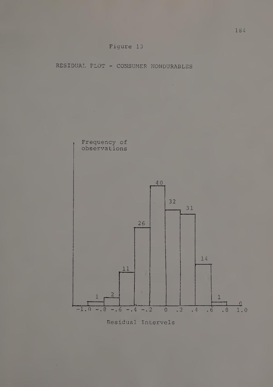
184

Figure 13

RESIDUAL PLOT - CONSUMER NONDURABLES

Residual Intervels

SC

AT

TE

RP

LO

T -

CO

NS

UM

ER

NO

ND

UR

AB

LE

S

185

► 4-4 ►*« ♦ MM M ♦ M M M M ♦ M M MM 4 M MMM

(1) >

•H 0)

■P P

0) d d

■p w rH x d rH V CO

E d & •H d '— -P

4J ^5 0 a)

O •H r—)

a> U) tn p

<v 0 d

>• Cm X S

44 44 II

w c

w :*

0 0 P a 4 4

0 O

< P

<u

x

M M ►-» 4-4 5

4-4 M

ru

4-4 t%-

* *

• *

• e

• * ♦

ru

• • * * ** • *

o *

♦ c c

* o

* (VI •

9 *

• O *(vl

Of * *

** 'Cl

• *

* * o ru

% •

(VI

ru

• *

• a

* a

a c* *

* •*

♦ ♦ M M |

* *

Cl *.

cn

« cu

*

4 MMMM4 MMMM4 MM MM 4 M M M M 4 4 M M ^ m 4 MM MM 4

1 o I in ♦ •

o

o

o

cc o <u

I

o

I

o

cc •

I

0S42

0E

*2

01*2

06

*!

0i*

l 0

3*

1

0£ • l O

fl

06

*

0i*

186

In the competitive position effects

model for consumer nondurables, the

estimates of the regression coeffi¬

cients for the variables breadth of

product line (3pS, , relative

product quality (3^s, 3^p), relative

advertising expenditure levels (3^s, 34P)*

and relative sales promotion expenditure

levels (3c;c., 3,. ) will be significant. 5s' 5p ^

Results. The estimates of standardised regression coeffi-

2 cients, coefficient of determination, and adjusted R obtained

by fitting the competitive position effects model to a sample

of 157 consumer nondurable businesses in the maturity stage

of the life cycle is shown in Table 12. The estimate of R^

for the full model equals 0.48486 with an associated F-stati-

stic of 7.22. At the .01 level of significance, Fcritical=

F Q1 -^g i2Q~ 2.06. Comparing the two F ratios leads us to

conclude that there exists a significant relationship between

relative market share and the independent variable set.

Further as shown in Table 12, the estimates of the

standardised regression coefficients for the variables, rela¬

tive breadth of product line (6]_s/ 3^p) / and relative adver¬

tising expenditure levels (642, 64^) are significant as hypo¬

thesised. For the relative product quality variable, we

ES

TIM

AT

ES

OF

ST

AN

DA

RD

IZE

D

RE

GR

ES

SIO

N

CO

EF

FIC

IEN

TS

187

co

ntd

.

Tab

le

12

(contd

. 188

co 0 in CO 0) c

•H cn 2 m

0 H

.Q 0 P 2

13 a o s

5-1 0 e 3 co G 0 U

P o

4h

<D 03 O 2

co -P O 0)



•H -p •H -P 0 04 e o o

0 CO 0 O

CO CO G co O rH

•H -p II 0 *> H P I 0 M

CN CO 40 O'* 40

r-" 40 r- rH

CO

A o

I Eh

P 40 CN H - 00 g;

40 0 CO 13 H

r- in co

II II

Eh *£.

H H 04 *

•rH -P II

0 CN P • co r- 2

co in co

t

CN

O

o

o CN H

•P

00 in 40

in o

o CN

Ol CO CN

O CN

DCN 13 2 « < IP

•H 0

■2

0 G O

0 rH A 0 p 0 Cu B 0 u

I

u

p 0 £ Cn

•H

i

ffi

>i -P •H p 0

C-i

I

(P

>1 -p •H P O

•H P 0 & 2 cn

i

02

G O

•H ■P 0

P> o 2

-P a

•H P o CO .a G 02

189

find that, only the estimate of the standardized regression

coefficient contrasting superiority with inferiority (£73) is

significant, but not the estimate of the coefficient contrast¬

ing parity with inferiority (£7p). Finally, the estimates of

the standardized regression coefficients for the variable, re¬

lative sales promotion expenditure levels (£53/ £^p) are not

found to be significant contrary to a priori expectations. In

order to obtain an idea of the strategy implications of these

results we consider the competitive positions of a few hypo¬

thetical businesses.

Strategy implications. Initially consider a business that is

in a position of competitive parity along the strategically

important dimensions of product quality, breadth of product

line and advertising; in this case one could postulate that it

would be beneficial for this firm to initially focus its efforts

on improving its competitive position along the product quality

dimension, and then along the breadth of product line dimension.

The rationale for this suggestion rests on consideration of the

difference between £^s and 3-^p, and £^g and 3^ . Note that, for

product line breadth the difference (£ - £. ) is approximately is lp

0.20, while for product quality the corresponding difference

(£ -£ ) is approximately 0.24, and that £ is nonsignificant. / s / p / P

In addition, it has to be pointed that the relative costs of

improving the competitive market position along alternative

marketing effort dimensions have not been considered here.

190

Consider next a business in a position of competitive

inferiority along the strategically important dimensions

of product quality, breadth of product line and advertising;

for this firm it would be beneficial to focus its efforts

initially on improving its competitive position along the

breadth of product line and advertising dimensions, since

it appears that for a quality improvement strategy to pay off

requires an all out effort on the part of firm to strive for

a position of competitive superiority. Note that while for

the variables, breadth of product line and advertising, the

estimated regression coefficients contrasting parity with

inferiority are significant (SjD and 3^), the same is not

true of the product quality variable (3yp). However, for

all three variables, the estimated regression coefficients

contrasting superiority with inferiority are significant.

Interestingly enough, in a PIMS study on product quality,

Buzzel^ notes that the market response to differences in qua¬

lity is not a smooth continuous phenomenon, and for'quality

to matter, the difference must be substantial.

As for advertising, we note that the estimated regres¬

sion coefficient contrasting parity with inferiority (e4p)

is greater than the estimate regression, coefficient contrast¬

ing superiority with inferiority (34s)* possible explana¬

tion of this result is that the sales response to certain

191

marketing decision variables exhibits diminishing returns to

scale rather than constant or increasing returns to scale.

Kotler-- notes that sometimes demand may initially exhibit

increasing marginal returns and then only subsequently shovz

diminishing returns to scale with respect to various levels

of marketing effort. The logistic function is often used to

depict such an S-shaped relationship. Moreover, a nonsymme-

tric S-shaped curve is considered to be more appropriate in

marketing applications. However, the nature of data employed

in this study is not suited either to determine the inflexion

point at which the change from increasing to decreasing

returns occurs, or the saturation level. While the results

presented in this study support the hypothesis, that a sig¬

nificant relationship exists between market share and the

competitive market position of a business along the advertis¬

ing effort dimension, it is not clear as to whether a posi¬

tion of competitive superiority is desirable to position of

competitive parity.

Contrary to a priori expectations, a significant rela¬

tionship between relative market share and relative sales

promotion expenditure levels was not observed. At this

stage it would be appropriate to point to certain problems

confronted in measuring the markets response to sales promo¬

tion efforts. Sales promotion covers a wide variety of sales

192

stimulating devices, including temporary price reductions,

premiums, cupons, and free samples. The total sales promo¬

tion expenditure incurred over a variety of sales promotion

activities has to be determined with caution. For example,

consider the sales promotion expenditure incurred by way

of a temporary price reduction. Here, besides the cost of

promoting the price reduction, one has to take into account

the amount of price reduction and the duration of the promo¬

tion deal. The cost of promoting the price reduction plus

the difference between the dollar revenue the brand sales

would have brought at full price and the reduced price during

this period is normally considered as the sales promotion

expenditure incurred on a temporary price reduction. How¬

ever, note that no real out of pocket expenses are incurred,

and as result of the price reduction, the total revenue may

go up rather than down depending of course on the elasticity.

Furthermore, the effectiveness of sales promotion efforts is

influenced by personal selling, distribution, and advertising

effectiveness. We mention these points to emphasize the need

for a more comprehensive investigation.

The relative importance of marketing effort dimensions. The

estimates of the squared simple correlation, the squared

standardised regression coefficient, the product of the

standardised regression coefficient and the simple correla-

ME

AS

UR

ES

OF

RE

LA

TIV

E

IMP

OR

TA

NC

E

OF

MA

RK

ET

ING

EF

FO

RT

VA

RIA

BL

ES

193

Rank

ord

er

of

imp

orta

nce

show

n

in b

rack

ets

194

tion coefficient, and the squared partial correlation are

presented in Table 13. The relatively greater importance

of the breadth of product line (X-^) , product quality (Xy) ,

and advertising (X^), is once again reflected in all four

measures. The stability across all four measures lends

further credence to the importance of these dimensions.

In summary, with respect of consumer nondurable busi¬

nesses, the parameter tests and measures of relative impor¬

tance of variables lead to the conclusion that breadth of

product line, product quality and advertising are mere impor¬

tant than certain other marketing effort variables. A posi¬

tion of competitive superiority along these dimensions seems

to be highly desirable from the market share viewpoint.

The results of fitting the competitive position effects

model to data on the competitive position and the associated

relative market share of capital goods businesses is consi¬

dered next.

Capital Goods Businesses

Specification error analysis. The results of the specifica¬

tion error analysis and parameter model tests are reported

in the sequence mentioned previously. The first of the speci¬

fication error tests considered here is the test for hoftio--

scedasticity.

195

The Goldfeld - Quandt test for heteroscedasticity. Here

again, the linear formulation of the competitive position

effects model with relative market share as the dependent

variable (6.2) was not found to satisfy the assumption of

homoscedasticity. To correct for the problem we once again

employ a log transformation of the dependent variable - rela¬

tive market share.

Test for detecting multicollinearity within the indepen¬

dent variable set. The determinant of the correlation matrix

of independent variables ! R! = 0.204

2 The transformed Chi-square statistic, X = 248

IX1X I

o 2 For the 5% level of significance, y. . . = X _ = 50

critical .05,36

Hence, on the basis of Farrar and Glauber's test for multi¬

collinearity the null hypothesis of orthogonality of inde¬

pendent variables is again rejected.

Identifying variables most strongly affected by multi¬

collinearity . The coefficients of determination and the

associated F-statistic resulting from regressing each inde¬

pendent variable on all other independent variables is shown

in Table 14. Ah examination of the estimated coefficients

of determination and their associated F-ratios show that

variables X^,X„ and X7 are strongly affected by multicolli¬

nearity, variables Xg,Xg and X^ are moderately affected by

multicollinearity, and variables X^,X2 and Xg are slightly

RE

GR

ES

SIO

N

AN

AL

YS

IS

FO

R

IDE

NT

IFY

ING

VA

RIA

BL

ES

MO

ST

SE

RIO

US

LY

196

>H Eh H

< ia 2; H P P O CJ H Eh

P s >H

CQ

Q W Eh U w U-l

&4

197

affected by multicollinearity. Compared to the case of con¬

sumer nondurables, the degree of multicollinearity seems to

be considerably higher.

To examine the pattern of interdependence consider

Tables 15 and 16 which show the highest order pairwise par¬

tial correlations between the independent variables (and the

level of significance of the associated t-statistic) and the

zero order correlations between pairs of independent variables

and the multiple correlation between the independent variable

set and the dependent variable, respectively.

Table 15 reveals that there are no partial correlations

of the order of 0.8; however, in relation to other values,

the partial correlation between and X^_ (advertising ex¬

penditure levels and sales promotion expenditure levels)

appears high. Referring to the results of regressing each

independent variable on all other independent variables

(Table 14) we find the resulting multiple correlations for

these two variables are of the order of 0.65 and 0.70, res¬

pectively. Finally referring to Table 16, the simple corre¬

lation between these two variables is of the order of 0.62.

This is slightly higher than the multiple correlation bet¬

ween the dependent variable and the independent variable set

which is approximately 0.58.

Thus, in order to identify variables most seriously

PA

RT

IAL

CO

RR

EL

AT

ION

S

OF

IND

EP

EN

DE

NT

VA

RIA

BL

ES

198

CO X

oo X

in oo CM

o • •

I

r- X

co X

in X

X

CO X

CM X

H X

CM r- o CM

co in

o o

o f"* o o

CM

CO r- o o

o CO O CM

LO O O

co i—l co o

OO i—i o

CO o

CP, o

o

00 o CO

CO CO

rH

CM O

o

I

* H*

* * uo CO

rH co co go r- CM o co h CM o I—1 o o

CO CM

in rH CM o

CO CO co

o o CM

o CO o CM UO

1 H1 1-1 CO I O CO

•

1 • •

H1 CO in OO rH uo CM co CO O CO CO uo CO O o co rH

• • •

1 • •

i

CO o co uo CO 00 CO co o O r- uo CM co o O rH o o

r- CO o co p' o co i—1 rH co U0 H

o rH o rH

l i i

co uo CO O 00 CO uo o uo CM o CO co o O' CM o o

1

uo CM co CO co in 00

O0 rH O' CO H CO i—! rH o O CM o

I 1

CM O p" o CM CO o H1 O', r- 00 uo CO CM CO o o rH rH O o

i 1

o o

oo CM o

o o CM

o 00 o

CO co CO

o o CM

CO

CO

■* * *

r

X CM

X co

X X X in

X CO

X CO

X X O',

!

*

* * *

Parti

al

correla

tions,

**

-

Level

of sig

nif

icance

of

the asso

cia

ted

' t

1 statistic

-

Th

e m

ark

eti

ng effort

dim

en

sio

ns

represente

d

by v

aria

ble

s

X-.

to

Xq

are li

ste

d

in

Table

14

SIM

PL

E

CO

RR

EL

AT

ION

S

BE

TW

EE

N

IND

EP

EN

DE

NT

VA

RIA

BL

ES

199

o o

cn o X •

rH

r- o rH o LO

00 o rH X • •

rH I

rH CN o in o o rH

r- o rH nT X • • •

rH 1

in o ro o CO nr nT o <y\ rH CN

VO o ro O O X • • • •

rH 1

c-i ro in CN o 00 VO VO r^

in o iH c VO o X o ro rH iH o

• • • • • rH I

vo nr ro CN CO o nr CN m in ro

nT o CN rH CN ro CO X o VO CN o o o

• • • • • • rH |

uo UO 00 ro ro VO o rH VO ro go o o

ro o rH in r- •nr CN CN u X c nr nr rH o CN O u

• • • t • • • a rH 1 i/

ro 00 CO o in O r"-

1

o ro CO •nr rH nr ro nr > CN o VC 00 uo vo CO CO CN

X o o o o o o o o

rH 1 1 1

c X

CO rH CO vo H' oo CN CO * o H1 VO o ro nr CO o 1

rH o CN cr> 00 O ro ro CN X X o CN rH rH rH CN rH rH o •

• >-• rH i 5m

rH CN ro nT UO VO r- 00 CO X X X X X X X X X

Ol

CN

I

*

The

mark

eti

ng effort

dim

en

sio

ns

represente

d

by v

aria

ble

s

X-,

to

X

are

li

ste

d

in

Table

14

200

affected by multicollinearity, if one were to use the rule

of thumb based on ^either partial correlations between pairs

of independent variables or the multiple correlation between

any independent variable and all other independent variables

the conclusion will be that the degree of multicollinearity

is not severe and therefore, can be safely ignored.

On the other hand, if one were to employ the rule based

on comparing the zero order correlations between pairs of

variables with the multiple correlation between the dependent

variable and the predictor variable set either or X- would

V

be a candidate for removal since, r„ „ is less y.x1,x2,-x9

than r To resolve this inconsistencv, we consider the X4X5.

relative contribution of X. and X to the explained variance * 5

of the dependent variable. As pointed in Chapter V, Green

4 .... and Tull are of the view that, if multicollinearity is pro¬

minent in a subset of predictors that do not contribute sig¬

nificantly to the explained variance, then the presence of

multicollinearity within this subset can be ignored. Farrar

and Glauber^ also suggest this approach. As summarized in

Table 18, the results of the tests of significance of the

contributions of X and Xc to the explained variance in Y 4 5

indicate that these variables do not contribute significantly

to the explained variance and therefore, neither variable

will be dropped.

201

As a final test, 10% of the observations were randomly

dropped and the regression coefficients reestimated to examine

coefficient sensitivity to sample size variations in the pre¬

sence of multicollinearity. The results of this exercise

are presented in Table 17. It is observed from Table 17

that a 10% reduction in the sample size, neither leads to

drastic changes in estimates of coefficients nor sign rever¬

sals. In summary, the series of tests performed to study

the severity of multicollinearity are supportive of the con¬

clusion that the multicollinearity problem is not too severe,

and therefore we proceed with further analysis of data with

all nine variables included in the predictor set.

9 Test for curvilinearity. The estimates of adjusted R“

for the linear regression model and the quadratic model are

2 .27887 and .26852 respectively. Since the adjusted R for

2 the quadratic model is less than the adjusted R for the

linear regression model, we conclude that the contribution

of quadratic terms to the linear model is not significant.

Hence the alternate hypothesis of the significance of the

quadratic terms is rejected.

Residual analysis. =t

Residual plot. A histogram plot of residuals is shown

in Figure 15. The shape of the residual plot approximates

a normal distribution. Hence, we conclude that there is no

202

Table 17

TEST OF COEFFICIENT ESTIMATE SENSITIVITY

TO SAMPLE SIZE VARIATION

*For a description variables x-,s'xip' reader is referred to Table 18.**’

,X9s'X9p the

203

Figure 15

RESIDUAL PLOT - CAPITAL GOODS

Residual Intervels

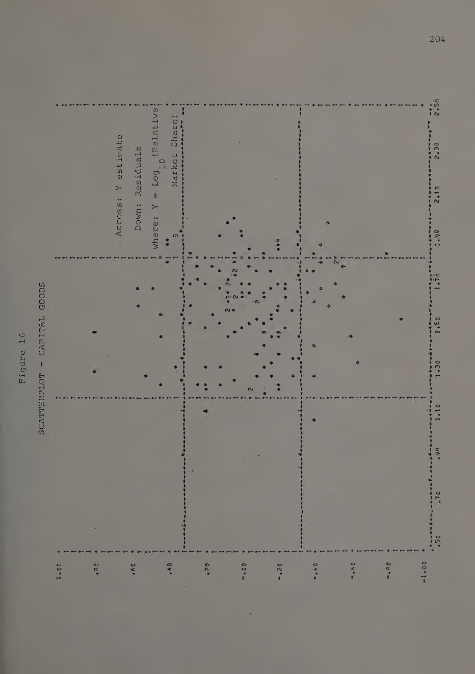
SC

AT

TE

RP

LO

T -

CA

PIT

AL

GO

OD

S

204

+ M 4-9 M M 4 4-9 M M M 4-« ♦ 4-9 4-9 4-9 4-9 4

<D

> •H

4-i

rd

O



a •H 0

C/) P

(1)

• 4

K II

W • 9 >c

W c

0 s 44

0 <D

O p 5~l

< a

p I

5 • 4-9 4-9 M M M 4—% ^ 4-9

* •

M K 4 M M MM 4 M M M M 4 M M

in *

M >-< ♦

I

I I t I I I I • I I I I » I ( I I < • I I I I I I

• I

• I I

M M 1-4

9 •*

* « 9 4 9 ►— C 9 ►- 44 4 *r »-4 * ►- 4 4-4 ►-< O *— 4 I

-» - I -> CU

9 * * I * M *9 I * *

•9 9 •9 -9 •*

99 (M99 991 9 9 9 9 I 9

9 9 9 9 1 9 (V (VJ 9 9 9 I 9 -r.

9 9 (VI 9 9

-9 9 9 -9

9 9 9 9 * 9 C

9 9

9 9 9 CM

9 9

>

t 9 » I

I I I I 9

I r i t

9 « t I I

9 I t I > I

-9 4~ ►— 4— *— ►— 4- | 4-4 4* |

I

I

9 -1 I » * I

I

I

I I I I 9 I

M M M* M 4 4—» M 9-9 M 4 M 4-9 9—9 9-9 4 4-9 4-9 4-* 4-9 f 4^ 4-9 4-9 4-9 4 4—9 M M 4-9 4 4-9 4-9 4—» M 4 4-9 4-9 4-9 4— 4 4— M 4-9 M 4 M M I

o

o a •o

<c o

IV o

o o

IV ♦

o o

GC

.50

.70

.90

1.1

0

1*

30

1«

5o

l*7

o

I.9

O

2*10

2*

30

?.5

ft

205

serious violation of the assumption of normality of the dis¬

turbance term, thereby justifying applying statistical tests

of significance. A

Scatterplot of residuals versus Y, the Y-estimates. The

A

scatterplot of residuals and Y, the Y estimates is shown in

Figure 16. Since most of the observations fall within a

horizontal band extending to a narrow range on either side

of the horizontal axis, it appears that there is no serious

violation of the OLS assumption and the least squares analysis

is plausible.


Recall that in formulating the competitive position

effects theory for capital goods (Chapter III), we posited

that there exists a significant relationship between market

share and the competitive market position of a business along

the dimensions, product quality, breadth of product line,

personal selling efforts, and quality of customer services.

In order to test the above theory, we use the linear formula¬

tion of the competitive position effects model (equation 6.2)

with logarithm of relative market share as the dependent

variable. The hypothesis to be tested can be stated as follows:

In the competitive position effects

model for capital goods businesses, the

206

estimated regression coefficients for

relative product quality (3-/3 )/ 7s 7p

relative breadth of product line (B^g,

3lP} ' relative sales force expenditure

levels (3 , B_ ), and relative quality 3 s 3 p

of customer services (3gS/ Bgp) will

be significant.

The estimate of the R for the full model eauals 0.34283

with an associated F-statistic of 4.12. Since F

F

critical

= 2.06, we conclude that a significant relation- •01,18,142

ship exists between relative market share and the independent

variable set.

The estimated standardised regression coefficients for

the independent variable set, the associated t-statistic

(and their significance level) are summarized in Table 18.

We note that the estimated standardised regression coeffi¬

cients for the relative-breadth of product line (B-j_S' B]_p)

are significant (p <.01). In addition the estimated stan¬

dardised regression coefficients for relative quality of

customer services (3gs, B^ ) are also significant (p <0.05).

However, for the relative product quality variable only the

regression coefficient contrasting superiority with inferio¬

rity (B_ ) is significant (p <.l). In addition, the coeffi¬

cients for the relative degree of forward vertical integra¬

tion (B2Sr B2?)/ are significant (p <.l). Finally, for the

ES

TIM

AT

ES

OF

ST

AN

DA

RD

ISE

D

RE

GR

ES

SIO

N

CO

EF

FIC

IEN

TS

207

4h O

0 0 -h O 4-> G co fd -H U -U

i—I *h nj 0 4-t -p > -H CO O G l J tJi-P

•H co 4h

o

o o • •

o o

in o

o •H -P CO

•H -P fd -P CO I

-P

CO 00 in

• •

in co

in in

CT\ in LO co o co 00 H1 rH CO CO • • • • • • O o O 1 o o

4H Td co 0 0 -P

CO G G CO •H 0 0 a> •H •H CO -p P CO a rH CN <d fd CO •H in CO E T3 0 4-1 • •

•H G P 4-1 ■P fd tr» 0 CO ■P 0 0 W co p O

co in <H i—!

CO (N co r- o o

co

o rH O

•

I

CsJ O', CO CM O O

0 0 p p

co cl 1 I 3 3 i i fd fd -p 4-) 0 0 p p 0 0 0 0 •H •H 0 G G tn Cn P p p P T5 id 6 •H *H 0 0 3 3 3 3 G G id rH rH -P -P -P -P -p -P 0 0 Z G G •H ■H •H CL CL -P -P H H id ts nd Td X X 0 a o G G G G Eid <—i 3 3 rH rH 0 0 0 0 JC T5 T3 fd fd CL CL CL CL G G fd 0 0 o O X X X X 0 o •H P P •H •H w H Eh Eid •H •H p CL CL ■P -P 4-> 4-1 fd P P 0 0 tr> tn 0 0 > 4-1 4-1 0 0 o O G G g g 0 0 > > p P •H •H 0 0

0 co 0 CL CO CO CO CL P CO P CL -G JG HG Eh i Eh 1 "H 1 •H 1 CL 1 CL 1 -P -P P co P CL CO CO -p CO -P CO CO CO T* 'r3 fd 1 fd 1 CO rH CO rH H rH P rH CO rH CO rH <d fd G £ G 0 0 0 0 0 0 0 0 0 0 0 0 0' 0 P O P 0 rH I> rH > > > > > rH > rH > p p 0 ■H 0 •H fd 0 fd 0 Td 0 T5 0 fd 0 3 0

CL CQ Eh -P Eh •P co pi co PI Z

-JC

CO CL rH rH

X X

CO CL CN CM

X X

CO Q-I CO CO

X X

CO

X

a

X

CO in

X

a m

X

co

ntd

Table

18

(contd

.

208

w CD CO CO 0 G

•H CO 3 fa

CO 03 O O U

03 X •H Cu 03 CJ

u o fa

rH 0

T3 O s

co X O 0

4-1 4-1 fa

G O

*H X •rH

CO o

CM

0 >

•H X "H x 0 cu a o u

0 CO 03 U

CM co G rH O

•H || -P o3 i—I > U 0 CO

XI o

CM in LO co in

co in

in CM

i X

i Eh

VO 00 I—I I—I

II II

Eh X

p cocm co • oo fa in

CM LO 0 T3 rH H CO 0 rH

4J • CM . •H X II rH peg s fa

CO H1 3 •n II T3 < fa

00 in co

•

CM

O CM

00 in vo

in o

o CM

(?) 00 CM

•

rH

II

o CM

•H 03 Eh

0 G O

0 rH X 0 Sm 0 CM a o u

I

u

p 0 X tjl

•H fa

I

o fa

X •H p 0 fa

I

fa

>1

X •H p o

•H P 0 fa 3

C/3

I

W

G O

•rH x 0 X o 2

X a

•rH P o CO X 3 cn ■K

209

relative price variable, the regression coefficient contrast¬

ing a price level higher than the industry average with a

price level lower than the industry average £93/ is positive

and significant, (p <.l)

Strategy implications. Once again, we observe a strong re¬

lationship between market share and breadth of product line

(Big' $lp)* Also, for product quality, only the estimated

coefficient contrasting superiority with inferiority (g )

is significant, but only at the .10 level while the estimate

of the coefficient contrasting parity with inferiority (3yp)

is nonsignificant. This seems to suggest that, in order to

benefit from a quality improvement strategy an all out commit¬

ment on the part of the firm to strive for a position of com¬

petitive superiority is necessary. The results seem to support

Buzzel's^ findings that for quality to matter, the quality

differences must be substantial. From Table 18, we also note

that, the difference between the estimates of the standar¬

dized regression coefficients contrasting superiority with

inferiority and parity with inferiority is less than 0.02

for relative degree of forward vertical integration (60s“ $2p^

and relative quality of customer services (B_ - B^)- From o 6P

a strategic point of view, it appears that a business stands

to gain little by improving its competitive position from

the parity level to the superiority level. That is, while

210

the significance of the estimated standardized regression

coefficients contrasting parity with inferiority for relative

forward vertical integration (3 ) and relative quality of ^ XT

customer services (3^ ) seem to suggest the desirability

of maintaining a position of competitive parity along these

dimensions, the small difference between the estimate of the

coefficients contrasting superiority with inferiority, and

parity with inferiority for these two variables (62s“ $2p'

36s” ^6p^ suggests that while maintaining competitive parity

along these dimensions may be necessary in order to meet the

competitive demands of the market, striving for superiority

along these dimensions is not likely to lead to sizeable

gains in market share.

Considering next the price variable, economic theory

postulates an inverse relationship between price and demand

under conditions of perfect competition. Therefore, for the

price variable considered here one would expect the estimated

regression coefficients contrasting a higher price with a

lower price 3gs/ and a comparable price with a lower price

Bgp, to be negative. But as shown in Tables 12 and 18 the

price coefficients are positive. Possible explanations for

this include the price - advertising and price - quality

relationships. Recalling some of the issues discussed in

n

Chapter II we again note that, Kuehn hypothesized that

211

higher advertising levels can support higher price levels.

o Furthermore, Weiss observed that his models with price and

advertising as independent variables resulted in positive

price coefficients, but when a dummy variable was included

as a proxy for quality, the price coefficients were found

9 to have the logically correct sign. Land on the other hand,

reported that even after related factors such as quality and

advertising were accounted for, the positive price coeffi¬

cient continued to persist. Also, Buzzel^ states that when

market share changes are related to price and quality, the

best combination is likely to be one of high quality and a

moderate price premium. These studies as well as the results

of the current study serve to emphasize the fact that, while m

evaluating the desirability of marketing a product at a price

level higher than, comparable to or lower than competitive

levels one has to consider the competitive market position of

a business along certain other related dimensions such as

relative advertising expenditure levels and relative product

quality.

Measures of relative importance. Estimates of the squared

simple correlation, the squared standardized multiple regres¬

sion coefficient, the product of the standardized regression

coefficient and the simple correlation coefficient, and the

squared partial correlation are presented in Table 19. The

212

rank order of each relative importance measure is also given.

The relatively greater importance of the breadth of product

line (Xj_) , and quality customer services (Xg) is revealed

by the consistently high rank order of these variables across

all four measures. Besides these two effort dimensions, for¬

ward vertical integration (X2)/ product quality (X7) and re¬

lative price (Xg) also seem to be relatively more important,

though their rank order across various measures of relative

importance is inconsistent. These measures of relative impor¬

tance together with their rank order also lead us to conclude

that the strength of relationship between market share and the

competitive market position varies across marketing effort

dimensions. This in turn suggests that a position of competi¬

tive superiority along certain marketing effort dimensions

is desirable to a similar position along certain other dimen¬

sions. Further, the differences in the relative importance

and rank order of marketing effort dimensions for consumer

nondurable businesses and capital goods businesses summarized

in Tables 13 and 19 lend further credence to the theory that

the significant marketing effort dimensions are likely to be

different for different types of businesses.

Summary. In this chapter we have considered the results of the

competitive position effects model for consumer nondurable busi¬

nesses and capital goods businesses. The results suggest that fcr

ME

AS

UR

ES

OF

RE

LA

TIV

E

IMP

OR

TA

NC

E

OF

MA

RK

ET

ING

EF

FO

RT

VA

RIA

BL

ES

213

i TS rH (13 0 fd i-H fd P -H 0 O fd -P U -H P 5-4 p -P tr <d o

03 o, o

CO r" cm

l I -P fd -P

CQ C '—I c

0 <D <D <D TJ P -H

<L) Do 0 CO 0 -H

P -H P U O -H

•H p 4H 0 4-1 T5 m-i m p 0 0 0 0 fd i—i o i—10

o^o a< o c -h g td -p c -h c •P rH o CO o CO 3 -H -H

in r-H CO rH

g CO X -P

TS O -P

d n c c 0 -H O 0 P T5 *H -H fd P CO O ^ fd CO -H CTJ 0 4H

co cd p mh fd Do 0 -p 0 o co P o

o in O

rH

I 'O fd 0 0 rH C P rH 0 O id apH p g p -p ct-h o

CO CO o

r-

co

CO

r- co CO o

co o

co CO CM O

in

oo co

o

CD <n CM uo oo

CO 00 rH CO

rH o O o o O

• • •

00 CO CO co CO CO CM rH co CM o CO o o o o

• • • •

ao co co

in CO r- 00 co rH CM Is" CO CM o co o O o o

• • • •

ao co

o o co co o o o o o o o o

-■—■> rr—V ^—s ✓—s CN VO uo no

—*' •—«» —✓

o o CO 00 rH r" rH 00 ■^r o i—1 CM o o O O

• • • •

CO 00 r-

o CM 00 o 00 oo n1 1—1 CM o o o

CM CO oo ■^r ' v— —

rH Cl CO co CO r~ o oo co CO o O o o o

9 • • • • • • • •

1 p -P 1 1 X 0 o fd sd 0 g

rH p rH 0 0 to 0 •fd TS fd a P rH -p >i -P to 0 u X X 0 0 to -P £ 0 •H 0 p •H 0 co 0 to •H > p •H 0 0 fr to rH cu -p rH rH -P 0 0 rH fd •H <d & P c 0 0 Do Q) 0 rH fd u £_) 0 <d 4-l 0 0 0 > fd > g 4h p 4H a

0 ■H 0 > *H P 0 •H 0 0 0 0 a1 0 • • CJ p -P 0 rH CO rH p p to CO 0 0 fd rC T3 fd 4H •H cr p >1 0 -p -P -P > CO > -p p p 0 -p 0 -p -p 0 0 fd 0 •H fd TJ fd DO co p p p CO -H •H -H p 0 P -p U fd 0 £ 0 0 p 0 p 0 T3 rH > ts 0 nD td

0 c p -p rH -P > -p rH fd fd p 0 P 0 rH P -H 0 C <d -h n0 -H rd 0 p 0 p 0 P 0 03 rH CP *H 03 TJ < t 03 a O to PH (P CP Cd

f3 0 > 2

rH CN CO -vT in CD 00 CO

XXXXXXXXX

*R

an

k o

rd

er

of

imp

ort

an

ce

sho

wn

in brackets

214

different types of businesses a position of competitive

superiority along certain dimensions seems to be more desi¬

rable vis-a-vis a similar position along certain other dimen¬

sions .

The competitive position effects model can be employed

to determine the desirability of various strategic moves.

While it would be erroneous to draw causal inferences using

a regression model, the overall results do seem to suggest

that given the competitive position of a business along

various strategically important marketing effort dimensions,

the model could possibly be employed to weigh the desirabi¬

lity of alternate strategic moves.

Finally, before concluding this chapter a brief discus¬

sion on the operational definition of ’relative product qua¬

lity' as used in this study is considered to be in order. In

the PIMS study, product quality is operationally defined as

"the percent of sales of a business originating from products

judged by the market to be superior to competitive offerings

minus the percent of sales originating from products judged

by the market to be inferior to competitive offerings."^ More

precisely it is managements judgement of market's judgement

of the firm's product offerings. While answering, PIMS suggests

to the responding companies that the ideal entry would be equi¬

valent to a reading obtained from a blind test with identifi-

215

cation concealed. It is also pointed to responding companies

that marketing research firms maintain consumer panels and

conduct periodic surveys to gather realistic data on relative

product quality thereby pointing to a potential source of

12 information on relative product quality. These points are

mentioned here to emphasize the fact that a certain degree

of caution has to be excercised while drawing inferences about

the strategic importance of the product quality variable,

given the limitations inherent in the operational definition

of relative product quality as used in this study. In addition,

the practical problems confronted in operationally defining a

variable such as product quality also need to be considered.

216

FOOTNOTES

-^-Robert D. Buzzel, Product Quality (Cambridge, Mass.: The Strategic Planning Institute, 1978).

^Philip Kotler, Marketing Decision Making - A Model Building Aoproach (New York: Holt, Rinehart and Winston, Inc., 1971), pp. 96-97.

3John D.C. Little, "BRANDAID: A Marketing-Mix Model, Part 1: Structure," Operations Research (July-August 1975), pp. 628-673.

^Paul E. Green, and Donald S. Tull, Research for Market¬ ing Decisions, 3rd ed. (New Jersey: Prentice-Hall, Inc., 1975), pp. 476-480.

^Donald E. Farrar, and Robert R. Glauber, "Multicolli- nearity in Regression Analysis: The Problem Revisited," The Review of Economics and Statistics (February 1967) pp. 92-107.

^Buzzel, p. 4.

"^Alfred A. Kuehn, and Doyle L. Weiss, "How Advertising Performance Depends on Other Marketing Factors," Journal of Advertising Research (March 1962), pp. 2-10.

^Doyle L. Weiss, "Determinants of Market Share," Journal of Marketing Research (August 1968), pp. 290-295.

^Stephen Land, How Premiums and Discounts Affect Perfor- mance (Cambridge, Mass.: The Strategic Planning Institute, 1978),

l^Buzzel, p. 10.'

H-See questions 316-318 in PIMS data forms in Appendix.

l^The Strategic Planning Institute, The PIMS Data Manual (Cambridge: The Strategic Planning Institute, 1976), p. 31.

CHAPTER VII

MODEL TESTING - THE INTENSIVE GROWTH

STRATEGY MODEL

This chapter deals with the empirical testing of the

intensive growth strategy models. First we focus on the

main effects model given by:

Yj = V BlXj!+ B2Xj2+ B3Xj3+ B4Xj4+ ^' <7-D

where, Yj = Relative market share

Xji= Relative average size of customers served

X. = Relative number of types of customers served 32

X. = Relative breadth of product line

X_.^ = Relative product quality

Later we focus on the full model with main effects and inter¬

action effects incorporated.

The dummy variable specification of 7.1 is given by:

Y. = Bn+ B,«,X. + B X . + B0 X . 0 + B0 X . o + J 0 is jis IP jlp 2s 32s 2p D2P

B00X. + B_ X. + B.cjX.^ + B X . + f.., 3s 33s 3P 33P 4S 34s 4P 34p j'

(7.2)

where, Y. reoresents the relative market share of business 3

’j’ The procedure for creating dummy variables to represent

the product-market growth variables X. ,X. ,X. , and X. was * 31 32 33 34

described in Chapter IV. Once again, the specification error

analysis and tests of significance of the model are preceded

by the Chow test for differences between sets of regression

217

218

coefficients. The F ratio for the Chow test equals 2.3 and

since this is greater than F . . = F _ = 1*88, we critical .05,9,300

conclude that the two sets of regression coefficients are

different. Therefore, we proceed with the analysis of con¬

sumer nondurables and capital goods businesses separately.

Consumer Nondurable Businesses

Specification error analysis. As in the previous sections the

model tests are preceded by specification error analysis.

Test for heteroscedasticity. The main effects formula¬

tion of the intensive growth strategy model (7.2) was not

found to satisfy the assumption of homoscedasticity. (F computed

20.8; F ... = F __ „ = 1.54) To correct for this, we critical .05,64,64

once again employ a log transformation of the dependent variable

Test for multicollinearity. In this section, the test for

multicollinearity within the independent variable set, tests

for identifying variables most seriously affected by multi¬

collinearity and the pattern of interdependence- among the

affected variables, and coefficient estimate sensitivity to

sample size variations in the presence of multicollinearity

are considered. These tests are performed on untransformed

data. (That is, prior to log transformation of Y_. , and dummy

coding of the Xj's.)

The zero order correlations between the independent

219

variables are shown in Table 20. The determinant of the

simple correlation matrix of independent variables, |R|,

equals 0.473115. Transformed into a Chi square statistic

2 2 2 we obtain v (v) as .115 and with y ... = y c =

A XXX A critical A *05,6

2.6, the Farrar and Glauber's test for multicollinearity

indicates the presence of multicollinearity within the inde¬

pendent variable set.

Considering next, the R , associated F, and multiple 1 r’

resulting from regressing each independent variable on all

other independent variables shown in Table 21, we note that

variable X^ is affected least by multicollinearity, variable

Xj_ is moderately affected by multicollinearity, while vari¬

ables X2 and X^ are more seriously affected by multicolli¬

nearity. By examining the partial correlations between pairs

of independent variables shown in Table 22, we note that even

the largest of these values is less than 0.4, which suggests

that the degree of multicollinearity cannot be considered

severe.

In summary from Tables 20, 21, and 22 we conclude:

1. None of the zero order correlations between pairs of in¬

dependent variables is greater than the multiple correla¬

tion between the dependent variable and the independent

variable set. (Table 20)

None of the multiple correlations resulting from regress- 2.

220

ing each independent variable on all other independent

variables is of the order of 0.8 or higher. (Table 21)

3. None of the partial correlations between pairs of inde¬

pendent variables is of the order of 0.8 or higher.

(Table 22)

These observations evaluated on the basis of rules of

thumb on What constitutes serious multicollinearity? leads

us to believe that while multicollinearity does exist, the

degree cannot be considered to be severe and therefore no

additional action is warranted.

Finally, the results of the test of coefficient estimate

sensitivity to sample size variation in the presence of multi¬

collinearity are presented in Table 23. The results indicate

that there are no drastic changes in the magnitudes of co¬

efficient estimates nor sign reversals and therefore we pro¬

ceed with further analysis with all independent variables in¬

cluded in the predictor variable set.

Test of curvilinearity. As a specific test for curvi-

lienarity,' the linear formulation

1Ogi0Yj = V BlXjl+ Vj2+ B3Xj3+ B4xj4+ '

is tested against the quadratic formulation

log Y. = B„+ B X. +.+ B X. + B.X2 +.+ y10 3 0 1 31 4 34 5 31

B X2 + (- (7.3) 8 34 j

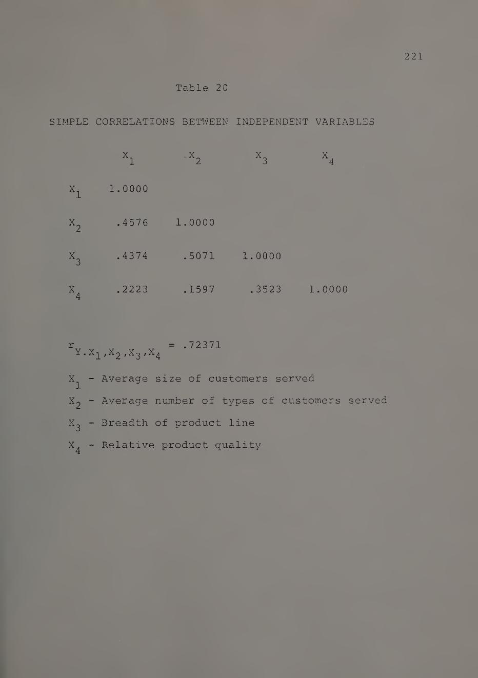
221

Table 20

SIMPLE CORRELATIONS BETWEEN INDEPENDENT VARIABLES

X1 -X2 X3 X4

X1 1.0000

X2 .4576 1.0000

X3 . 4374 .5071 1.0000

X4 . 2223 .1597 . 3523 1.0000

1-1 X

•

X

u

f^2'^4 = .72371

- Average size of customers served

X2 - Average number of types of customers served

X^ - Breadth of product line

X^ - Relative product quality

222

Eh 03 O S

in w pH !-q Eh PQ M < PS H c PCJ w < z > H

1-5 O Z o H u >l H Pm Eh H

r—i Eh D CN Z 2

W 0) Q pH

p—i H C3

rd & Q Eh O W

Pm Eh CJ

in w H Pm in Pm >H <

< >H 53 C 03

D Z O O H H PS 03 w 03 03 w « o w PS

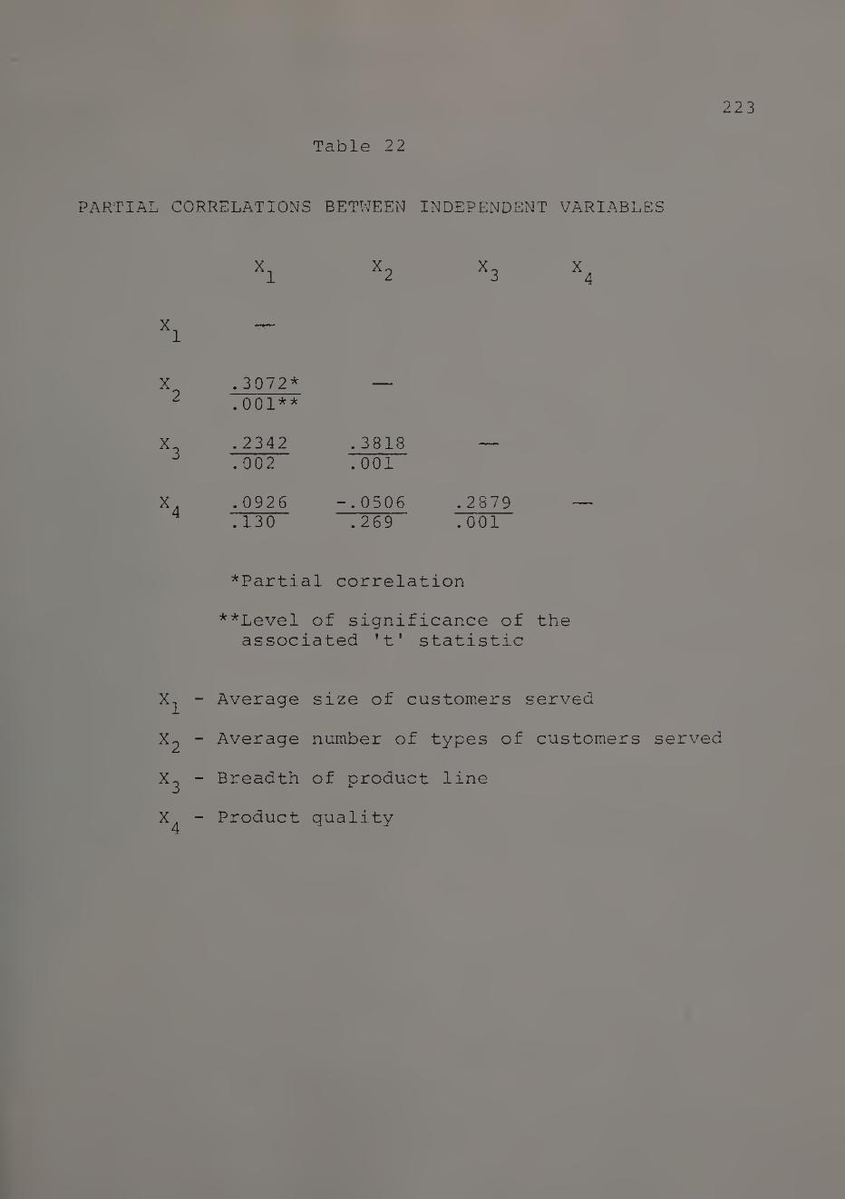
223

Table 22

PARTIAL CORRELATIONS BETWEEN INDEPENDENT VARIABLES

X 4

X 1

X„ .3072* — 2 .001**

X, .2342 .3818 J .002 .001

X 4

.0926 -.0506 .2879

.130 .269 .001

*Partial correlation

**Level of significance of the associated 'tf statistic

X^ - Average size of customers served

X2 - Average number of types of customers served

X^ - Breadth of product line

X^ - Product quality

TE

ST

OF

CO

EF

FIC

IEN

T

ES

TIM

AT

E

SE

NS

ITIV

ITY

TO

SA

MP

LE

SIZ

E

VA

RIA

TIO

N

224

225

The estimates of adjusted R2 obtained for the linear

and quadratic formulations were 0.48861 and 0.49943, respec¬

tively. Fratio For incremental adjusted R2 attributable

to the quadratic terms equals 0.8 and F . . = Fn c . = critical 0.5,4,149

2.41. Since Fcritical is greater than Fcomputed, we conclude

that the incremental R2 attributable to the quadratic terms

is nonsignificant.

Residual analysis. A histogram plot of residuals is shown

in Figure 17. The shape of the residual plot indicates that

there is no serious violation of the assumption of normality.

From the scatterplot of residuals versus Y, the Y estimate

shown in Figure 18 we note that most of the observations fall

within a horizontal band streching to either side of the hori

zontal axis indicating the absence of any serious abnormality

With this we conclude our discussion on specification

error analysis. Tests of significance of the proposed models

are considered next.


In this section we address the issue of statistical sig¬

nificance of the full model and the individual parameters of

the model. In Chapter III, it was theorised that a positive

significant relationship exists between market share and the

competitive market position of a business along the dimen-

226

Figure 17

RESIDUAL PLOT - CONSUMER NONDURABLES

Residual Intervels

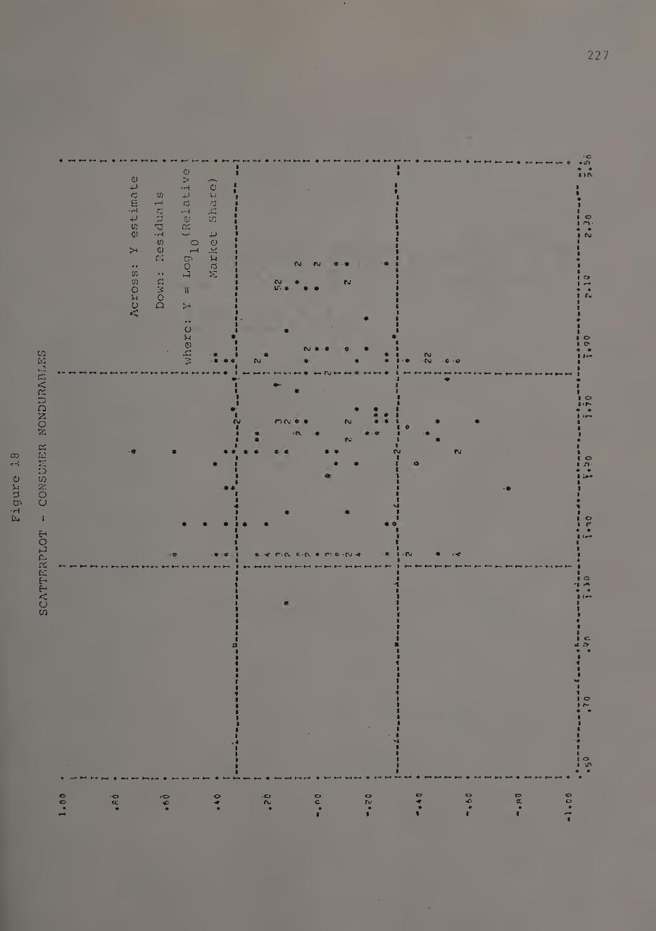
SC

AT

TE

RP

LO

T -

CO

NS

UM

ER

NO

ND

UR

AD

LE

S 227

' 4 MMMM *-* * #—■ ♦ M M •— ♦ M M M MM ♦ M MMM 4 M M MM 4 M M M M

0 1 1

1 1

0 > .—. 4J •H O

• * _ , 1

•

rj W 4J U ? 1

w |

E rH f3 <3 t 1

•rH rd 1—i jC 1 1

4-> 3 0 CO 1 |

t |

W "0 C£ 9 1

Q) •H 4-> 1 1

W O 0 1 I

1

>» 0 !-1 X t ft tr> P 9 •

• • 0 f3 1 •

CNJ CVJ 9 -9 9 1 ■

w • • £ V

1 • 1

w c 1 CVJ 9 CM 1

0 II » IT. 9 9 9 1

u 0 1 |

ft |

0 Q 1 ft

C • •

1

•

1 9 •

•

a V

• 9 ft P *

1 9 |

0 1 cvj 9 9 9 9 ft •C * 1 a 9 t

■ * 9 9 4

CVJ 9 9 *9 t • 9

k-4 MM M M* »~a *-♦ M M 9 1 M* M M M M M$ MPJMM# MMt 1 M

CVI

*

•99

9 *

ncj»$ tv .#

9 9

♦ 9 * 9

rv 9 $

• •9

9 9 rvi

-9 < c%cv c*f\ 9 r> 9 »cvj «e -9

M M *-» M t~« «

fvj CVJ 9 -9

CM

ru 9 .<

• o • m • •

• M M M 4 M M M M ♦ M r-« M M 4 ►« ►— 4 *—* M »-* M 4 M M M ♦ •«* M *—• M 9 M M M ^ ♦ M M M 4 M M M M ♦ •

o f\J

o C-

o cv o

9 I

o a

.70

.9o

i.ko

ioo

Y*^

o i»

70

T.9

0

?.i

o

2,3

0

5.5

b

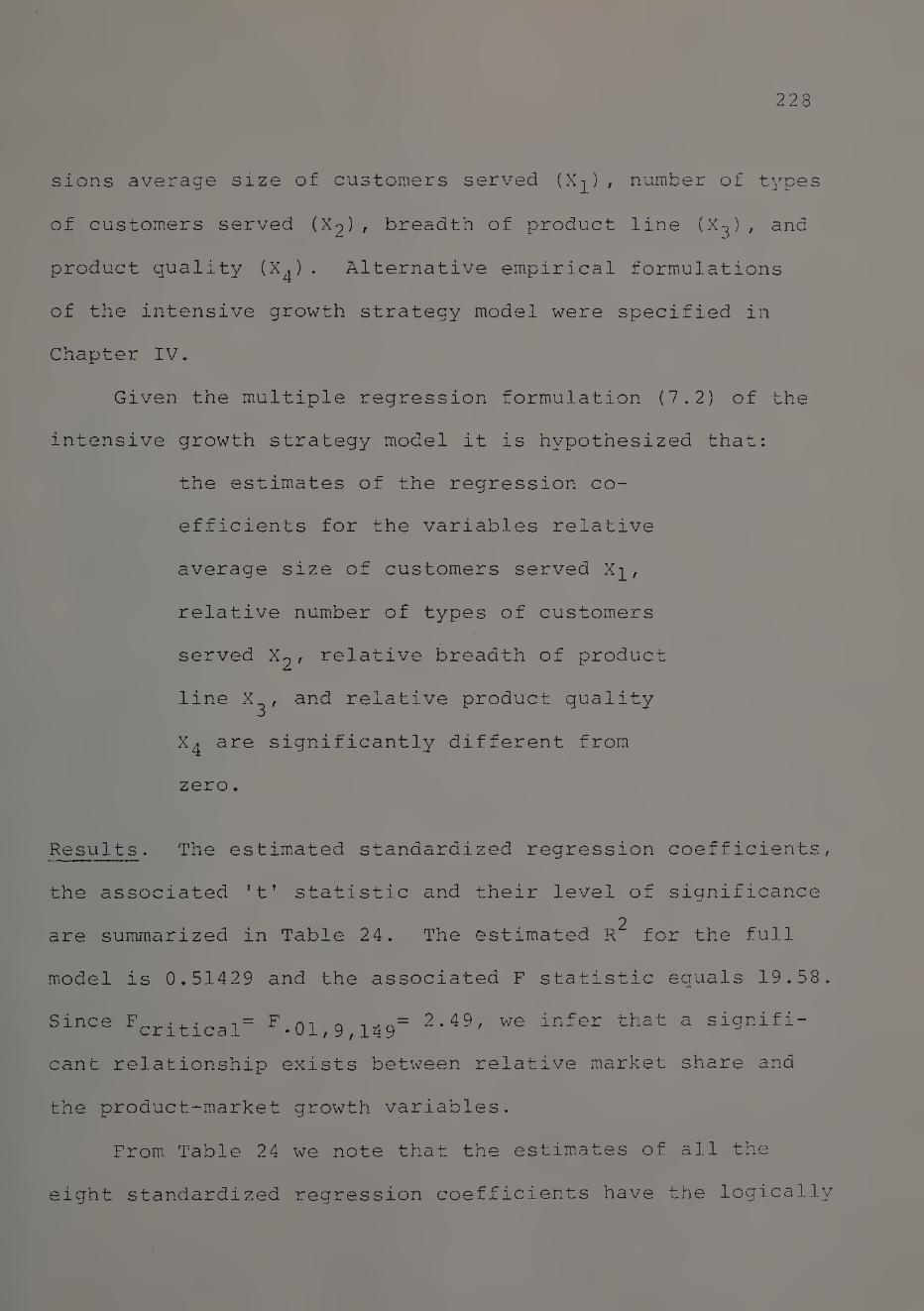
228

sions average size of customers served (X^), number of types

of customers served (X2), breadth of product line (X3), and

product quality (X^). Alternative empirical formulations

of the intensive growth strategy model were specified in

Chapter IV.

Given the multiple regression formulation (7.2) of the

intensive growth strategy model it is hypothesized that:

the estimates of the regression co¬

efficients for the variables relative

average size of customers served X]_,

relative number of types of customers

served X2, relative breadth of product

line X^, and relative product quality

X^ are significantly different from

zero.

Results. The estimated standardized regression coefficients,

the associated 't' statistic and their level of significance

2 are summarized in Table 24. The estimated R for the full

model is 0.51429 and the associated F statistic equals 19.58.

Since Fcr itical= F-01,9,M9= 2'49' we infer that a si9nifi~

cant relationship exists between relative market share and

the product-market growth variables.

From Table 24 we note that the estimates of all the

eight standardized regression coefficients have the logically

229

correct sign, and except for all other coefficients are

significant at the 0.05 level. As with the competitive posi¬

tion effects model, here again for product quality, we note

that while the regression coefficient contrasting superiority

with inferiority (3^s) is significant, the coefficient con¬

trasting parity with inferiority (B^p) is nonsignificant.

Focussing next on pairs of regression coefficient, we

note that for product quality (B^s- B^p) is of the order of

0.22, but only 6. is significant (p <.05); for breadth of ~r O

product line (B^s" B^p) -*-s aPProximately 0.15? for relative

average size of customers served (3^s~ B]_p) is approximately

0.03; and finally for relative number of types of customers

served $2s an<^ ^2p are more or less of the same magnitude.

The results of the tests of significance of product-market

growth variables are presented in Table 25. The results

suggest a significant relationship (p <.01) between relative

market share and relative average size of customers served

(X-^) , relative breadth of product line (X^) , and relative

product quality (X^).

Strategy implications. In order to get an idea of the stra¬

tegy implications of these results we once again resort to

the approach of considering a few hypothetical businesses

and their competitive market position.

ES

TIM

AT

ES

OF

ST

AN

DA

RD

IZE

D

RE

GR

ES

SIO

N

CO

EF

FIC

IEN

TS

230

35 <4-1 o 0

0 *H 4-1 G 44 U 0

0 0 •H -H <4-1 O -H p 4-1 >i 0 G -P -p 3 4-1

(d fd rH r-H LT) in i—! rH H 1 0 4-1 •H rH 0 4-> o o O o o o o 1 0 0 p 0 •h 0 • • • • • • • ft S 0

> m i -- •H >i 0 •H -P -P P 4-> ft c 0 CL 0 -H

CP 0 0 •H 04 P •H ft 0 p 3 3 0 -P 0 o CO ft

0 0

1 1 G ft •H 3

u 0 CO CO ft •H 3 - •

-p PCI 0 CD LD CP o 00 

35 0 0 G -P P r— N 0 G 0 3

•H •H 0 £ u 35 0 -H CP CO ■*r CD rH ro r- h 3 •r

P cn u 00 in in in CP oo 0 4- CP 00 00 3 0 *H co ro rH rH ro CN CN o G •r co in in

35 P <4-1 0 5- cn cd ro G Cp ft u O • • • fd 0 0 -P H H CN 44 P 0 . p CO 0 0 1 II II II

<4H in h rH H O O

rH •H • • • 0 3 o o o

35 4-> ^ H ^ 0 o o o

<4H ft -P 4-1 2 0 in mm 0 0 O O G H H H

3 3 >i O 4-> 4-1 44 ft ft CO 0 35 35 >i Ph

0 0 0 0 0 O 0 4-> 4-1 0

£ C4 CU P P •H H 44 <d 0 0 CL CL rH rH 3 !S N N -P ft 3 3 P

•H •H ft ft 3 3 4-1 0 CO CO m <4H 0 0 tr cn CO

I—1 0 0 r-~ CO

ft 0 35 0 35 35 35 ft; ft 4-1 -P ft in ■^r tP 0 CP 0 P 0 P 0 4-1 4-) u u 4-1 1—1 r-

•H 0 > fd > 0 > 0 > 35 35 3 3 II ii P P P p p ft P ft P 3 3 35 35 . 0 0 i— fd 0 0 0 0 £ 0 £ 0 0 0 0 0 p G i fO > > CO > CO 3 0 3 0 P P P P o 0 ft O

0 fd G G ft ft CL CL •H i 00

CO ro CO 0 0 -P E- 00

0 P 0 P 0 P 0 P 0 0 0 0 > 3 > 0 > 0 > 0 > 0 > > > > •H > •

•H £ •H £ *H £ •H £ •H •H •H H 0 P 05 II ft 0 ft 0 ft 0 ft 0 4-1 4-1 4-1 4-> G H 0 0 CN 0 -P fd -P 3 -P 3 4-1 3 0 3 0 3 3 0 0 0 1- ft

f—1 CO H CO rH 0 rH 0 rH C rH G rH rH 4-1 35 ft ft • 3 ro

1—1 • CO CL 0 a 0 a 0 (ft 0 • CO II -ro CN ft 0 rH rH CN CN ro ro H -d’ 3 0 II CN 35 II

> !Z X X X X X X X X U 2 ft R

A

F

TE

ST

OF

SIG

NIF

ICA

NC

E

OF

PR

OD

UC

T-M

AR

KE

T

GR

OW

TH

VA

RIA

BL

ES

231

co O

•H p -p CO <U fa

0) CO 3 u

UD O

co

o LO

CM

o to

CM **

LO O

fa fa

00

O'* II CM ^ r—I r-C I lc M

• I O Eh CO

II II II II

CM fa M Eh Pc! Q

0) 03 O e

3 fa

o co

•

CM

O in

CM

rH

fa

15

7

ob

serv

ati

on

s

232

Initially, consider a business in a position of competi¬

tive parity along the dimensions, average size of customers

served (X-^) , average number of types of customers served (X2) ,

breadth of product line (X3), and product quality (X4). Noting

that ^3s“ ^3p) and (843- 84p) are of considerable magnitude

but not (6^ - B]_p) and (82S“82p) we posit that, for this

business, it would be desirable to focus its efforts on im¬

proving its competitive market position along the product

development dimensions, product line breadth (X^), and product

quality (X4).

Considering next the magnitude of the estimated standar¬

dized regression coefficients S^p and 3^p in relation to $2p

and 84p, it appears that for a business in a position of com¬

petitive inferiority along dimensions X-^,X2/X3, and X4 the

desirable course is one of striving to improve its competi¬

tive market position along certain product development dimen¬

sions and market penetration dimensions.

Tests of significance of interactions. The discussion thus

far was confined to the restricted model, wherein the main

effects of the product-market growth variables were considered.

Here we test for the significance of the multiplicative terms

by considering their squared semi-partial correlations. From

the results of this excercise summarized in Table 26 we note

that the term relative number of types of customers served

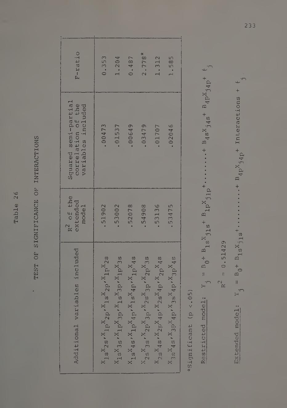
TE

ST

OF

SIG

NIF

ICA

NC

E

OF

INT

ER

AC

TIO

NS

233

t

0 ■K •H ro H1 r- CO CM in -p in O 00 r- rH 00 cd ro CM H1 r- ro in u • • • • • •

1 o rH O CM 1—1 i—1 h

partial

of

the

elu

ded

ro r-« CO Cl r- in 1 G r" ro r- o H1

•H G -H H1 in ID r- O £ 0 O rH O ro rH CM CD -H CO O o O o o O CO -P CD • • • • • •

(d rH A3 <H jQ

CD CD fd U P -H cd p p P o fd O1 o > w

CD JC A3 -P 0 H CM CM 00 CO in

A3 CD O o r» o ro 4-4 G A3 o> o o Cl rH "nT 0 CD 0 rH ro CM H* CO CO

-P £ in in m uo in in CM X • • • • • •

CD

A3 CD

A3 CO CO CO CO CO CO G CM ro H* ro H*

rH X X X X X X o Cu O o O a a G rH l—1 rH CM CM ro

•H X X X X X X

CO Or o & C4 0. cu CD CM ro •^r ro

rH X X X X X X JC CO CO CO 03 CO £0 cd rH rH rH CM CM ro

•H X X X X X X p W. cd cu C4 a, a a CQ > CM ro ro H1

X X X X X X rH Or 0. o P4 C4 a cd rH rH rH CM CM ro G X X X X X X 0

•H CO CO co CO CO CO -P CM ro ro H* •H X X X X X X A3 CO CO CO CO CO CO A3 rH rH rH CM CM ro C X X X X X X

in o

•

v

a

-P G <d O

•H 4-1 •H G

•H C/2 *

•ro sU

+ a

•ro X

& 'sP

CQ

+ CO

-ro X

CO

CQ

+

X a

i—I

CQ

+ CO <H

•r—> X

CO Ol rH CM

CQ ^

in

o

CM

CG

r—I

CD A3 0 £

CD 4-> U

•H U -P CO CD

Exte

nded

model:

Y

=

BQ+

Bls

X^ls+

.+

B4p

Xj4

p+

Interactions

234

times relative breadth of product line (X2X3) is significant

(p <.05) . As might be recalled, it was stated in earlier

chapters that, market development possibilities include tapp¬

ing new market segments within 'geographic markets presently

served by the firm and expanding into new geographic markets,

(i.e., reaching for new types of customers.) Further in

Chapter IV it was stated that reaching a larger number of types

of customers would often require the broadening of the pro¬

duct line in order to meet the distinct needs of different

types of customers. The significance of X2X3 (p <.05) seems

to support this position. That is, in certain situations

better results can be obtained thro' exploiting market deve¬

lopment strategies when they are supported by product deve¬

lopment activities.

Measures of relative importance. Once again we consider the

same four measures of relative importance namely: squared

simple correlation, squared standardized regression coeffi¬

cient, product of standardized regression coefficient and

simple correlation coefficient, and squared partial correla¬

tion. From the results summarized in Table 27 we note that

all four measures lead to the same rank order: 1) breadth

of product line (X^), 2) product quality (X^), 3) average

size of customers served (X^), and 4) number of types of

customers served (X^). Further the results seem to suggest

ME

AS

UR

ES

OF

RE

LA

TIV

E

IMP

OR

TA

NC

E

OF

PR

OD

UC

T-M

AR

KE

T

GR

OW

TH

VA

RIA

BL

ES

235

G 0

03 i—1 -H ro rH CM 0 cd +J P -H 0

’ " ' — —'

n3 -P >—i 'vT CTc 00 r- 3 P 0 ro CO iH O'. td 0 p 1—1 o ro CM wap o o rH rH

0 • • • • o

rd 0 G -P G -P N 0 G 0 G „_s

•H •H 0 0 -H 0 ro rH CM 03 CO *H i—1 -P -H V—■ — P co u tid u 0 0 *H Q i—1 *H o cr> r* GO

03 P 4-1 -H 0 m rH ro CM G Cd4-1 CO P 4-1 ro LO 0 0 0 P 0 o o rH 1-1 -P P 0 X O 0 • • • • ca O UO

03 0 G -P

d N o G ro <0 rH CM 0 -H -H 0 P 03 0 *H

' ■

0 P 0 0 o GO o CM 3 (d 0 -h CM CO CO rH td03 p 4-) rH O CM o

CA G CP4-4 o O rH rH 0 0 0 •P P 0 CO O

• t • •

G K 0 v

03 -H ro *0 1—1 cm 0 0 -p Pi—10

N—' ' —’

0 £L( i—! CO CO 00 o 3 £ 0 (J\ ro 1—1 o td -H P ro ro r-1 ro

CO CO p rH rH ro CM 0 • • • • o

4-1 -P 0 0

03 0! 3 0 4-1 0 0 0 03

rH 0 > 0 > 0 -P rQ P 0. P P •P 0 0 0 >i 0 CG rH

•H N CO -P 0 0 p ■H 4-1 3 0 CO 0 4-1 0 0 td > P C P

0 0 0 rC -p tp 6 P £ -P 0 0 0 0 0 03 3 p -p -Q 4J 0 0 03 0 0 £ 0 0 G 0 > 3 3 3 P •H P < 0 2 0 PQ i—! CG

0 CD 0 0 0) G

•H

CO 3

CQ

0 r—I

rQ 0

P 3

03 G O Z

P 0

s 3 co C o u

0

co 0 o

*R

an

k order

of

imp

orta

nce

sh

ow

n

in brackets

236

that and are substantially more important than x^ and

X2- The results of the analysis of capital goods businesses

is considered next.

Capital Goods Businesses

Specification error analysis. As was true in earlier situa¬

tions it was necessary to use a log transformation of the

dependent variable to correct for heteroscedasticity.

The Farrar and Galuber's test for multicollinearity lead

to the rejection of the null hypothesis of orthogonality of

the independent variables. However, further consideration of

the simple correlation between pairs of independent variables

(Table 28), second order partial correlation between pairs of

independent variables (Table 29), the multiple correlations

resulting from regressing each independent variable on all

other independent variables (Table 30) and coefficient esti¬

mate sensitivity to sample size variation in the presence of

multicollinearity (Table 31) lead to the conclusion that the

degree of multicollinearity is not severe and can therefore

be safely ignored.

As a specific test for nonlinearity, the linear model was

2 tested against the quadratic model. The adjusted R for the

quadratic model (0.48405) was found to be lower than the

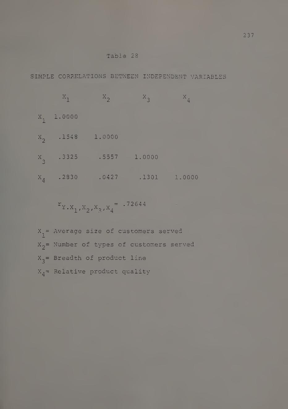
Table 28

SIMPLE CORRELATIONS BETWEEN INDEPENDENT VARIABLES

X1 X2 X3 X4

X1 1.0000

X2 .1548 1.0000

X 3

.3325 .5557 1.0000

X4 .2830 .0427 .1301 1.0000

'Y.X,, X2 ' X3 ' X4

72644

X = 1

Average size of customers served

X2= Number of types of customers served

V Breadth of product line

X^= Relative product quality

238

Table 29

PARTIAL CORRELATIONS BETWEEN INDEPENDENT VARIABLES

X 4

X 1

X„ 0225* — 2 .389**

X0 .2646 .5414 .001 .001

X 4

.2560 -.0290 .0516

.001 .359 .260

*Partial correlation

**Level of significance of the associated 1t*

X^= Average size of customers served

X2= Number of types of customers served

X^ = Breadth of product line

X^= Relative product quality

statistic

239

o CO

0 «—I

fa! rd

fa 03 D O H fa fa! 03

Eh 03 O s 03 fa! fa fa < H fa < > O 25 H

fa H

Eh S W Q H

fa o fa

03 H

03 >H fa <

<

o H

03 03 fa! fa O fa! fa

>H

Eh H

fa < fa 53 H fa fa O u H Eh

fa

>H fa

Q fa! Eh

U fa! fa fa <

TE

ST

OF

CO

EF

FIC

IEN

T

ES

TIM

AT

E

SE

NS

ITIV

ITY

TO

SA

MP

LE

SIZ

E

VA

RIA

TIO

N

240

241

Figure 19

RESIDUAL PLOT - CAPITAL GOODS

Residual Intervels

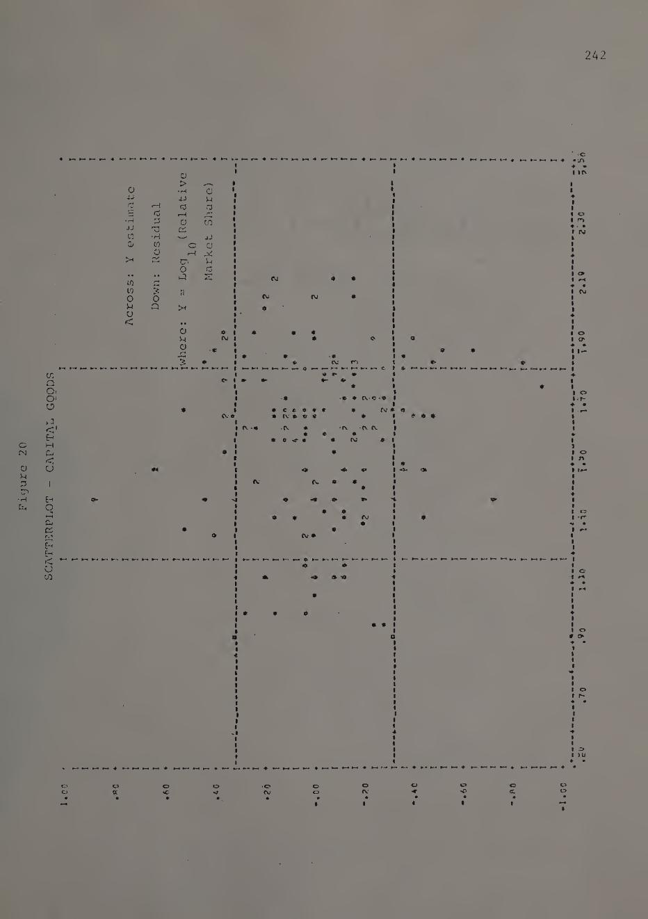
242

c CN

0 u

a •H Ck

U'j

a o. O' o

E" H P-

 ^ » 1 1 O •H O 1 t JJ 4-> U '

9 |

♦ ■

£ 1—i ra a i 1 • ■ •

Q Cj »H ,C 1 9 O •H 3 0 tn !

1 ■ • r*>

4J ■rs CS l 1 ♦ - • f rvj

to •H — 4J 1 i 0 CO o a ;

1 1

l

a 1 l 4 rv>*

*—4 cr, u ; 1 »

0 a 1 9

• ft ft ft i-5 £ CVi 9 9

1 1

C a» 1 r4

UJ M • ♦ • to :< If 1 I CSi

0 o CVJ CVJ * 1

■ 1

Vj Q 9 • i

1 •

u • ♦ < • • •

l 9

0 « i $ * 9 • i

1 1 o

U M « 9 0 1 9 • o

.« ; 1 1 9 9

♦ • • fft~

i ♦ • •9 1 * 1 s *► ♦ cvj m t 9 9 1

ft-« ft—ft ft—* ft— ft-* *-* *—• »—« »—■ ^4 •—* | ft— ft* ft* ft-* ft— ft—• •— *— C 1 *> M M M I I I I I I I I I ft* ft* Mft* 1 • » t ♦

ft 1 • 1 9 I 9 I

l 1 o * •9 ■9 CV.C-* 1 • »r-

1 9 • ft « c e 9 9 9 9 f\l * <* f ••"*

Cwft $ a* 9 9 ft 1 9 9 9 1 1 t

fv. •* *cv. 9 f\ cv r\. i 1 * 9 9 i ♦

» 9 m 9 ru « i t i I

ft 1 • i 1 o i 1 n i ■* 9 •

#* a *> i <% • Ift- * i »

IV (V. • • i 1 • i 1

i ♦ ft M * •9 > » 1> 9

i • * O i 1 c

o * 9 CJ 1 9 9 -r* * i 9 •

ft | 9 • 1 H » 1 0j * i 9

i 1 i 9 i 4

ft—• ft* *—• ft— ft* ft“» ft—* ft—* ft"* ft— ft* | T I T T T I ♦ ft— ►— ft— ►* M M ft— ft— M ft* ft— ft-* M V— ft— ft* ft— | ♦

^ 'O

• *

l l o 1 M ♦ ft » M I I I ♦ I I I o 9 O ♦ • » I I

I I 9 O f h- ♦ • I 9 9 9

I I I O 9 )U ♦ •

*-* M 4 ^4 M ft- »-« ♦ ft-* »>« ft* ft-* 4 M M M 4 M M •->« ft* ♦ »-* ►* M ♦ M »-4 »-»♦-» 4 ►* ft-* ^ ft"- ft- M ft* ft— 4 ft* ft* ft* M 4

o o

o a

o o •o Oj

o o 9V

I

o o cc I

243

adjusted for the linear model (0.48878) leading to the

rejection of the alternate hypothesis of significance of the

quadratic terms.

A histogram plot of residuals (Figure 19) and a scatter-

plot of residuals versus Y, the Y estimate (Figure 20), lead

us to believe that there is no serious violation of the assump

tion of the normality of the disturbance term.

In summary, the results of the various specification

error tests considered together suggest that there is no

serious abnormality or violation of the underlying assumptions

Therefore, we proceed with tests of significance of the model.


As described in earlier chapters, we are interested in

testing the following hypothesis:

In the intensive growth strategy model

for capital goods businesses, the esti-

• mates of the regression coefficients

for the variables, relative average

size of customers served (X-^) , relative

number of types of customers served (X2),

relative breadth of product line (X^),

and relative product quality (X^) are

significantly different from zero.

244

Results. The results of the regression analysis of capital

goods businesses are summarized in Tables 32 and 33. First,

we note that the estimated for the restricted model is

0.50044 . (FComputed=19*03; Fcritical= F.01,9,152=2* 49 *}

Therefore, we infer that a significant relationship exists

between relative market share and the product-market growth

variables.

Considering next the estimated standardized regression

coefficients gls, @xp'.'64s'64p , we note that all have

the logically correct sign. We also note that , g-^D...

are significant (p <.05). In addition, once again it

is observed that for product quality, the estimated coeffi¬

cient contrasting superiority with inferiority is signifi¬

cant (£43)/ but not the coefficient contrasting parity with

inferiority (34^)* This leads us to believe that for quality

to matter, the quality differences will have to be substantial

in all market situations.

As regards the differences between pairs of regression

coefficients, we note that for relative average size of

customers served (X-, ) , (3 - 3 ) is approximately 0.20. The 1 1P

corresponding differences for relative number of types of

customers served (625” ^2p^' relative breadth of product

line (£35“ S 3p) / and relative product quality (£ $ 4^) are

of the order of 0.17, 0.07 and 0.08, respectively.

ES

TIM

AT

ES

OF

ST

AN

DA

RD

IZE

D

RE

GR

ES

SIO

N

CO

EF

FIC

IEN

TS

245

0

O 6

0) -P o

•H P ■P 03 CD

£ 03 CD 03 03 CD G

•H 03 G

CQ

03

o O O

fd -P •H a <d u

p o

*H

CD "d o s

in CD -p fd P -P in

jc -p

o p o

CD >

•H 03 G CD -P G

M

CD 03 fd u

G O

•H -P fd -P O

-P P,

•H P O 03 jn G in

03 a) G

rH

fd >

fd o

•H ■P •H P o

-p

I

•H fd -P

0 G o

>1 -p •H P o

•H P -P 0 *H CX P G fd m g

i i

in g

co co o> in in oo in co CM • •

• rH CM rH

II II II LHH <H o O

• • •

O O O K K »k

o o o lo m ld i—I rH I—!

-p -p -p

IT)

00 r>

03 G 0

•H

-P fd > o p 0 II 03 ^roM

rr PC o o LO

,Q 0

CM LO

rH

II rH

I X

I Eh

03 0

i—I A fd

•H P fd >

VD • rH O

0 -p 03 CO

CO O

•

cn

II II *n || || cm T3

Eh PC < X fa

TE

ST

OF

SIG

NIF

ICA

NC

E

OF

TH

E

PR

OD

UC

T-M

AR

KE

T

GR

OW

TH

VA

RIA

BL

ES

246

M 0 U) cn 0 £

•H m £

PQ

W T5 O O U

rtf 4-> •H a rtf u

o

0

O S

CD -M O

•H J-l JJ cn CD fa

CD co rtf U

II O in rH

s.

04 v

i—I O

■^r

o o IT)

i£> O

•

co

O in

04

in c

fa fa

04 in

m £ O

•H -P rtf > U CD

II C/) XI

rH 0 I

X r* I ID

Eh CO H

II II II II

04 fa

fa ^ Eh Q

0

O S

£ fa

o ro

•

04

04

fa

15

0

247

From the results of the tests of significance of pro¬

duct market growth variables (Table 33), we infer that a

sifnificant relationship exists between relative market share

and relative average size of customers served (X^, p <.01),

relative number of types of customers served (X^, p <.01),

and relative breadth of product line (X^, p <.01). The stra¬

tegy implications of these results are considered next.

Strategy implications. Firstly, in relation to other vari¬

ables the estimated standardized regression coefficients for

relative size of customers served ($^s, $^ ) are large. Be¬

sides the standardized regression coefficients, this trend

persists across all four measures of relative importance

(Table 35). A possible explanation for this lies in market

characteristics. The market for industrial goods in general,

and capital goods in particular, is characterized by rela¬

tively fewer customers (as compared to consumer goods) and

a fair degree of product specialization.^ As a result, the

average size of each customer (determined by factors such as

the frequency of purchase, average quantity purchased each

time, the cumulative amount purchased during a given time

period, etc.,) tendstoassume greater importance. In addition,

given the possibility that the total number of customers of

any type are likely to be few, the need to reach more number

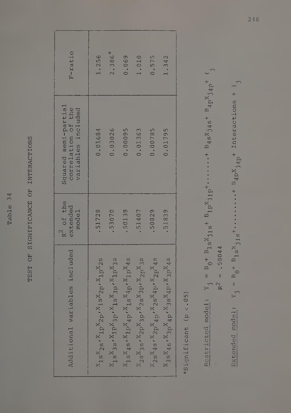
TE

ST

OF

SIG

NIF

ICA

NC

E

OF

INT

ER

AC

TIO

NS

248

0 •X •H in in cn o in CM ■p m CO in rH r- H4 cd CM CO o o in CO p • • • • • •

i rH CM o rH o 1-1 fa

partial

of

th

e

eluded

"S1 in in CO in in 1 G CO CM C\ in 00 CTi

•H G *H in O o co r~- r-« e o iH CO o rH o rH (U -H 01 o o o o o o co -p a) • • • • • •

id i—i o o o o o o TJ rH Q) Q) (d P P -H Id 4 4 3 0 id C1 o >

c/o

the

ed

1

CO o <T\ r- Cl <J\ T3 0 CM r- CO o CM CO

4-1 G t r- o rH H4 CO CO o a) o rH CO o rH o rH

+J g in in in in in in cm X • • • • • •

fa <y

■P 0 t CO CO co co CO CO 3 CM CO H* CO H4 H4

rH X X X X X X O ■a fa fa fa fa fa G rH rH rH CM CM CO

•H X X X X X X

co fa fa fa fa fa fa (U CM co H4 CO H4 M1

i—1 X X X X X X ,Q CO CO CO CO CO CO rd rH 1—1 rH CM CM co

•H X X X X X X ■ p ** **

rd fa fa fa fa fa fa i> CM co H4 CO H4 H4

X X X X X X rH fa fa fa fa fa fa td 1—1 rH rH CM CM CO G X X X X X X 0 V. ** w *«. V.

•H CO CO CO CO CO CO -p CM co CO H4 H4 •H X X X X X X T5 CO CO CO CO CO CO t rH rH rH CM CM CO

< X X X X X X

o •

v

fa

-P G rd U

•H 4-1 •H G

•H C/0 ■X

•1—1

+ fa

•i—>

X fa H4

ffl

+ co h4

•i—> X

co ^J4

ca +

•i—i

x fa i—i

CQ

+ CO

•I—I

X CO rH •o4

CQ ^ o

+ o o m

CQ

II II

•1—1 CM

<u TS 0 &

<D -P U

•H p

■p co CD

Ex

ten

ded

mo

del:

Y_;

=

B^+

B1e.X

., +

.+

B

^X

. + Interactions

-

3

0

is jis

4P

34p

ME

AS

UR

ES

OF

RE

LA

TIV

E

IMP

OR

TA

NC

E

OF

PR

OD

UC

T-M

AR

KE

T

GR

OW

TH

VA

RIA

BL

ES

249

3 0 V

t H -H rH CM CO CD rtf -P P -H 3

"-" V-' ■—

3 -P H •-1 VO 3 P CD co rH 00 o CT 3 P CO o o CO

C/2 & P pH «—1 o o 0 • • • • 0

X 3 3 -P

CD 3 -P 0 3 N 0 3 0 -H 0 rH CM co

•H •H CD i—1 -P •H >— — -- ■—- 3 0 -H pLi 3 O p CO U £ H •H pH in 1-1 CD 3 CD -H -H CD <4-1 *3 CO CO VO 3 P 44 0 P 44 O CM CO CD 3 CH4-I p 0 CM rH o o 3 0 0 0 0 • • • • -P P 0 O o co O

3 0 3 -P

3 N 0 3 rH CM CO 0 *H *H 0 P 3 0 -H

' " —' —'

3 P CO U 02 rH 02 r- 3 3 0 -H CM rH p- 02

CT3 P 44 in 02 o co C/2 3 tn M-l rH O o o

3 0 0 4-> P 0 CO O

• ♦ • •

3 * 0

33 *H 1—1 CM CO 0 0 -P P r-H 3

— —' ■—'

3 0_i <—1 O' r-" CO 3 £ 0 04 in 'sF 1—1 t-H P 0- O' CO rH

CO 0 P CM •—1 rH rH 0 • • • • • 0

m ■P 0 o

0 33 3 3 rH 44 0 0 0 3 >1

rQ 0 > 0 > 0 ■p 3 P a P P •H

•H 0 0 >i 0 a rH p N 0 ■P 0 3 3 •H 44 3 > 0 CO 04 0 0 31

P 0 P 0 0 0 43 -p t7> £ P £ -P 0 3 0 0 0 3 3 P -P 3 -P 3 0 3 0 0 £ to 0 3 0 > 3 3 3 P •H P < 0 2 0 33 r-j Oh

0 CD 0 CO CD 3 CD

■H O CO 3 3 fO 33 -P

P CO O 3 a O £ O -H O

44 rH O n3 -P P •H 0 Oh 3 3 P U 0

• • rVl

0 r*

0 3 3 Pd U *

sho

wn

in brackets

250

of types of customers also assumes considerable importance.

The significance (p <.01) of 3 , 3 , 32s and 3 probably IS 1 p 2 P

reinforces the nature of the capital goods market just des¬

cribed .

Focussing next on the tests of significance of inter¬

action effects (Table 34) we note that X-^X^ (relative average

size of customers served x relative breadth of product line)

is significant (p <.05). It was stated earlier (Chapter IV)

that product development activities such as broadening the

product line can contribute to the effectiveness of market

penetration possibilities such as increasing the frequency

of purchase and the average quantity purchased by present

customers. The significance of X^X^ is suggestive of such

a relationship. It might be recalled that for consumer non¬

durables the interaction term X2X^ (relative number of types

of customers served x breadth of product line) was found

to be significant. A discussion of the strategy implications

of the significance of the interaction terms (X-^X3 and X2X2)

and possible synergistic relationship between market growth

dimensions and product growth dimensions calls for consider¬

ing the basic identity relating total sales and the market

growth dimensions.

Let 1=1,2,.T be the number of types of customers served

by business T j1, N^= the number of customers of type I

251

served by business ’ j ' , and the average purchase fre¬

quency and average purchase quantity respectively, for custo¬

mers of type 111 served by business 'j *. For business ’j•

the total sales (S^) originating during a given period from

customers of type *1' can be expressed as a product of N^,F.

and Q^, That is,

Si = Ni x Fi x Qi (7.4)

Further, the cumulative sales (S) originating during a

given period from among all types of customers (i=l,2,.T)

is given by

S = N1F1Q1+ N2F2Q2+.+ NtFtQt

or

(7.5)

S = T Z

i=l N.F.Q. l ii

Thus, a firm wanting to increase its total sales can

achieve this objective by effecting an increase in one or

more of the right hand side variables in (7.5) namely; T,N,F

and Q. In general, it can be stated that a market penetra¬

tion growth opportunity presented by market 'I' has been

successfully exploited by business ’j', if for market 'I'

during the next time period, the number of customers, average

purchase frequency and average purchase quantity were to be

N.+ AN.,F•+ A F., and Q■+ A Q., where AN., A F•, and A Q- re- -L JL -1- _L _L

present positive increments.

252

Further, it can be stated that a market development

growth opportunity presented by the whole market has been

successfully exploited by business ’ j' if during the next

time period the number of customers served by business 'j'

were to 1T+N’, where N represents the number of new types

of customers reached by the business.

Therefore, the incremental sales volume originating from

successfully exploiting market penetration and market deve¬

lopment growth opportunities is given by

T T AS = E (N.+ AN.) (F.+ AF.) (Q.+ AQ,)- I N.F.Q.

i=l 1 1 1 5- 1 1 i=i 1 1 1

N + Z N.F.Q.. (7.6)

i=T+l 111

While executing market penetration and market development

strategies we would hope for AN^ and/or AF_^ and/or AQ^ for

i=l,2..T, and N,N±,Fi,Q± for i=T+i,T+2,.,T+N to be

substantial. This can be facilitated by product development

related activities such as quality imporvement, new product

activity, product line extension, etc. The significance of

X-^X^ and ^2^3 in the intensive growth strategy models points

to the possible existence of 'a synergistic relationship

between market penetration and product development and market

development and product development, and the possibility that

product development related activities can facilitate effec-

253

tive exploitation of market growth opportunities.

Finally, the measures of relative importance summarized

in Table 35 lend further credence to the ’competitive position

effects theory’ presented in this study. The results suggest

that a position of competitive superiority along certain pro¬

duct-market growth dimensions are likely to have a greater

effect on market share vis-a-vis a similar position along

certain other dimensions. A comparison of the relative im¬

portance measures for consumer nondurables (Table 27) and

capital goods (Table 35) once again lead us to infer that a

differential relationship exists for different types of busi¬

nesses .

Summary. This chapter has been devoted to testing the inten¬

sive growth strategy model for consumer nondurables and capital

goods businessess. Overall, there appears to be a signifi¬

cant relationship between relative market share and the com¬

petitive market position of a business along certain product-

market growth dimensions. The results also suggest the pre¬

sence of a synergistic relationship between these growth

dimensions. Finally, the results suggest that the relative

importance of the product-market growth dimensions vary by

type of business.

In the next chapter we attempt to summarize the major

findings and their implications for future research.

254

FOOTNOTES

Alternative approaches to segmenting industrial markets

such as, by product, by end-use' application, by geography, and by buyer behavior, and their appropriateness during various stages of market development are discussed in E. Raymond Corey, Industrial Marketing: Cases and Concepts, 2nd ed. (New Jersey: Prentice-Hall, Inc., 1976), pp. 5-8.

CHAPTER VIII

CONCLUSION

The purpose of this chapter is to briefly summarize the

major findings of this thesis and consider some of the poten¬

tial applications and limitations of this study.

A brief summary. As might be recalled from Chapter III, the

theory of competitive position effects posits a significant

relationship between market share and the competitive market

position of a business along certain marketing effort dimen¬

sions; and, in addition, the existence of a differential

relationship for different types of businesses.

Empirical support for the theory was evidenced in the

results presented in Chapters VI and VII. The analysis of

the competitive position effects model for consumer nondurable

businesses lead us to infer that a significant relationship

exists between relative market share and the competitive

market position of a business along the marketing effort

dimensions, relative product line breadth, relative product

quality, and relative advertising expenditure levels. For

capital goods businesses the significant dimensions were,

relative product line breadth, relative product quality, re¬

lative quality of customer services, and relative degree of

forward vertical integration.

255

256

For the intensive growth strategy model, the hypothesis

of a significant relationship between relative market share

and certain product-market growth variables, and the inter¬

action of certain product-market growth variables were sup¬

ported. The analysis in both cases was supportive of the

hypothesis of a differential relationship for different types

of businesses. The strategy implications of these and other

findings w^re also discussed in Chapters VI and VII. We

consider next some of the potential applications and limita¬

tions of this study. As a prelude to this discussion, some

of the problems confronted in cross-section studies are con¬

sidered first.

Problems in cross-section studies. First, we note that cross

section studies in marketing are often limited by' competitive

considerations; that is, it is often impossible for a re¬

searcher to obtain data on all firms in an industry. As

Liu^ points, data limitations rather than theoretical limita¬

tions are primarily responsible for a persistent tendency to

underspecify (or to oversimplify) econometric models. Second

as pointed in Chapter II, most econometric studies in market¬

ing have been at the brand level or firm level, and there

have been few studies at the industry level. Most of these

studies deal with frequently purchased branded goods. Other

257

than price and advertising, few studies have systematically

addressed the marketing policy effects of other marketing

instruments such as product quality, new product activity,

personal selling, etc. Some of these views are also expressed

m Parsons and Schultz. We consider next the relevance of

competitive market position data to econometric studies in

marketing in the context of this background information.

Potential applications. First, we note that cross-section

data on the competitive market position of the firm and its

competitors along certain marketing effort dimensions can

be obtained with relative ease. On the other hand, cross-

section data on competitors' actions in absolute, share,

relative, or ratio form may be hard to obtain.

Second, as a result of the relative ease with which

competitive market position data can be obtained, it may be

possible to extend the scope of the study by including in

the data pool competitive market position data originating

from similar types of industries. This has to be preceded

however, by tests for appropriateness of pooling. The ra¬

tionale for suggesting this approach is that the breadth of

most studies in marketing has generally not extended beyond

frequently purchased goods, and therefore, generalizations

applicable for a broad class of goods and services are

258

desirable.

Consider next the issue of data limitations rather than

theoretical limitations constraining the number of variables

considered. As a result of the relative ease with which com¬

petitive market position data can be obtained, the researcher

will be in a position to investigate the effects of a number

of variables. In addition to analyzing variables at the

macro level, such as, relative advertising efforts, relative

sales promotion efforts, etc., it might be desirable to

analyze after decomposing these into finer, less aggregate

components such as television advertising efforts, newspaper

advertising efforts, magazine advertising efforts, trade pro¬

motion efforts, consumer promotion efforts, etc. This approach

can be helpful in providing an insight of the merits of alter¬

native courses of action in a broad perspective. That is,

the dimensions along which a position of competitive superio¬

rity is strongly associated with market share, the dimensions

along which a business should strive to maintain a position

of competitive superiority, etc.

We consider next some of the limitations inherent in

competitive market position data. In comparison to absolute,

share, relative or ratio data, the information content in com¬

petitive market position data and the inferences drawn by

using this kind of data in conjunction with the competitive

259

position effects model and the intensive growth strategy

model are obviously limited. The approach described in this

study can be helpful in evaluating the relative merits of

broad directions of actions, and in identifying the more

important effort dimensions along which a position of competi¬

tive superiority is likely to benefit the firm to a greater

extent. Contrast these applications with some of the recent

studies in marketing where the thrust has been in the direc¬

tion of building and implementing decision models to help

managers make decisions on optimum advertising appropriation,

pricing, sales force effort, and so on. [See: Lambin, Naert,

and Bultez^ (1975), Wittink^ (1975), Wildt^ (1974), Parsons^

(1974)]. If this were to be the primary purpose of the study,

the usefulness of competitive market position data is res¬

tricted to exploratory stages as described next.

In general, optimal marketing decision models are neither

developed nor used to determine the optimal level in respect

of each marketing decision variable. Most models focus on

two or three key decision variables. Lambin, Naert and Bultez

for example, focussed on advertising, price, and product qua¬

ff 9 . lity. Wildt and Wittink focussed on advertising and price.

In these kind of studies, during the exploratory stages, the

competitive position effects model can be used to identify

the key decision variables to be included in an optimal deci-

260

sion model.

Data on marketing-mix variables either in absolute, re¬

lative, ratio, or share form have been used in a number of

studies to examine market share movement among competing

brands. Likewise, competitive market position data and data

on changes in competitive market position can be used to

examine market share movement among competing brands. How¬

ever, for the same number of variables considered models

employing absolute, relative, share, or ratio form of data

will tend to result in higher than models employing com¬

petitive market position data, because of the qualitative

nature of the latter form of data. But, because of the re¬

lative ease of accessibility of competitive market position

data it would be possible to examine the effects of a ..larger

number of variables. These in effect are the trade offs

involved.

The preceding section serves to summarize the potential

applications of this study together with its associated

strengths and weaknesses. A related issue arises out of the

fact that in this study we have taken the approach of deve¬

loping models for consumer nondurable businesses and capital

goods businesses. Other classification schemata also pre¬

sent promising avenues for research. This issue is consi¬

dered next.

261

Potential applications using alternative classification

schemes. The usefulness of competitive market position data

is not limited to determining significant marketing effort

dimensions and product-market growth dimensions for different

types of businesses, such as consumer durable businesses,

consumer nondurable businesses, capital goods businesses, etc.

Rather, product characteristics are not the only basis for

classifying products and businesses. Businesses can be classi¬

fied as pioneers, early followers, and late entrants on the

basis of their timing of entry into the market. Alterna- :

tively, on the basis of consumer buying habits, goods can be

classified as convenience goods, shopping goods, and specia¬

lity goods; on the basis of frequency of purchase as fre¬

quently purchased, infrequently purchased and occassionally

purchased; on the basis of unit value as high, moderate and

low unit value products. Using alternative classification

schemes competitive market position data can be used to exa¬

mine such issues as:

Which marketing effort variables contribute to the

success of pioneers, early followers, and late en¬

trants .

The marketing effort dimensions along which a posi¬

tion of competitive superiority or parity is desi¬

rable for frequently purchased versus infrequently

262

purchased goods, for high unit value items versus

low unit value items, etc.

With this we conclude our discussion on potential applications

and consider next some of the limitations of the data base

used for this study.

Limitations of the data base. The PIMS data base although

extensive and unique is not without limitations. Some of the

limitations directly relevant to this study are discussed in

this section.

Representativeness. Smaller companies are under repre¬

sented in the PIMS data base. A majority of the participants

are large, diversified companies. As a matter of fact, in

the PIMS data base small companies are defined as those with

sales volume under $750 million. Thus, the limited range of

corporate size represented in the data base could possibly

limit the extent to which the results of the study can be

generalized. However, in terms of types of businesses, such

as consumer durables, nondurables, etc., and size of businesses,

such as low, average and high market share, the data base is

fairly representative.

Unit of analysis. In place of conventional units of

analysis such as, brand, product line, profit center, divi¬

sion, or firm, the PIMS study uses a 'business' as a unit of

analysis. The question of what constitutes a business is

left to the discretion of individual participants. PIMS

263

offers only guidelines to its member participants for pur¬

poses of defining a business. According to a published PIMS

source, the suggested guidelines are: "Each business should

have a majority of its cost items identified in separate

accounts, and each business should serve some identifiable

market where key competitors can be singled out. More often

a business is defined in terms of a product or product line

and a well defined customer group and set of competitors."'*'0

The correct identification of these is critical to the PIMS

study.

Pooling of data. Finally as pointed in Chapter IV, the

PIMS data base pools cross-sectional data from a sample of

businesses across different industries. (e.g., the consumer

nondurable data pool may possibly include businesses from

the frozen food, breakfast cereals, beverages, toileteries

and cosmetics and many other types of businesses.) Pooling

of cross-section data across industries without testing for

the appropriateness of pooling is yet another major short¬

coming of the data base.

Summary. In this concluding chapter, a brief summary of

this thesis has been presented. In addition, the issues of

potential applications and limitations of the study have

been addressed.

264

FOOTNOTES

^Ta Chung Liu, "Underidentification, Structural Estima- mation and Forecasting," E'conometrica (October 1960), p. 856 .

2Leonard J. Parsons, and Randall L. Schultz, Marketing

Models and Econometric Research (New York: North Holland Publishing Company, 1976), pp. 21-22.

o JJean-Jacques Lambin, Philippe A. Naert, and Alain Bultez,

"Optimal Marketing Behaviour in Oligopoly," European Economic Review (1975), pp. 137-140.

^Dick R. Wittink, "Systematic and Random Variation in the Relationship Between Marketing Variables," Unpublished

Doctoral Dissertation, Purdue University, 1975.

^Albert R. Wildt, "Multifirm Analysis of Competitive Decision Variables," Journal of Marketing Research (February 1974), pp. 50-62.

^Leonard J. Parsons, "An Econometric Analysis of Adver¬ tising, Retail Availability, and Sales of a New Brand," Management Science (February 1974), pp. 938-947.

^Lambin, pp.50-62.

®Wildt, pp.50-62.

^Wittink.

■*-^The Strategic Planning Institute, The PIMS Data Manual

(Cambridge: The Strategic Planning Institute, 1976), p. 2.

SELECTED BIBLIOGRAPHY

Adler, Lee. "A New Orientation for Plotting Marketing Strate¬ gies." Business Horizons (Winter 1964), 37-50.

Ansoff, H. Igor. "Strategies for Diversification.’" Harvard Business Review (September-October 1957), 113-124.

_. Corporate Strategy. New York: McGraw-Hill, 1965.

Banks, Seymour. "Some Correlates of Coffee and Cleanser Brand Shares." Journal of Advertising Research (June 1961), 22-28.

Barnett, Arnold I. "More on a Market Share Theorem." Journal of Marketing Research (February 1976), 104-109.

_. "Comment on 'A Comment on Market Share Theorm.'" Journal of Marketing Research (August 1976), 312.

Beckwith, Neil E. "Multivariate Analysis of Sales Responses of Competing Brands of Advertising." Journal of Marketing

Research (May 1972), 168-176.

Bell, David E.; Keeny, Ralph L.; and Little, John D.C. "A Market Share Theorem." Journal of Marketing Research (May 1975), 136-141.

Blackwell, Roger D. "Strategic Planning in Marketing." Com¬ bined Proceedings. Chicago: American Marketing Associa¬ tion, 1974, 465-469.

Bloom, Paul N.; and Kotler, Philip. "Strategies for High Market Share Companies." Harvard Business Review (November- December 1975), 63-72.

Buzzel, Robert D.; Gale, Bradley T.; and Sultan, Ralph G.M. "Market Share - A Key to Profitability." Harvard Business Review (January-February 1975), 97-106.

_. Product Quality. Cambridge: The Strategic Planning

Institute, 1978.

Branch, Ben. Deviation from Par ROT. Cambridge: The Strategic

Planning Institute, 1977.

265

266

Capon, Noel, and Spogli, Joan Robertson. "Strategic Market¬ ing Planning: A Comparison and Critical Examination of

Two Contemporary Approaches." Combined Proceedings. Chicago: American Marketing Association, 1977, 2T9-223.

Catry, Bernard., and Chevalier, Michel. "Market Share Strategy

and the Product Life Cycle." Journal of Marketing (October 1974), 29-34.

Chatfield, Christopher. "A Comment on ’A Market Share Theorem.'" Journal of Marketing Research (August 1976), 309-311.

Chow, Gregory C. "Tests of Equality Between Sets of Coeffi¬ cients in Two Linear Regressions." Econometrica (July 1960), 591-605.

Corey, E. Raymond. Industrial Marketing: Cases and Concepts. 2nd ed. New Jersey: Prentice-Hall, 1976.

Cox, William E. "Product Portfolio Strategy: A Review of the Boston Consulting Group Approach to Marketing Strategy."

Combined Proceedings. Chicago: American Marketing Asso¬ ciation, 1974, 471-475.

Cundiff, Edward W., and Still, Richard R. Basic Marketing: Concepts, Decisions and Strategies. 2nd ed. New Jersey: Prentice-Hall, 1971.

Darlington, Richard B. "Multiple Regression in Psychological Research and Practice." Psychological Bulletin (1963), 181-182.

Day, George S. "A Strategic Perspective of Product Planning." Journal of Contemporary Business (Spring 1975), 1-34.

Durbin, J., and Watson, G.S. "Testing for Serial Correlation in Least Squares Regression." Biometrika (1950), 409-428

and (1951), 159-178.

Farrar, Donald E., and Glauber, Robert R. "Multicollinearity in Regression Analysis: The Problem Revisited." The Review of Economics and Statistics (February 1967), 92-107.

Fogg, C. Davis. "Planning Gains in Market Share." Journal

of Marketing (July 1974), 30-38.

267

Furhan, William E. "Pyrrhic Victories in Fights for Market Share." Harvard Business Review (September-October 1972), 100-107.

Gale, Bradley T. "Selected Findings from the PIMS Project: Market Strategy Impacts on Profitability." Combined

Proceedings. Chicago: American Marketing Association, 1974, 471-475.

_.; Heany, Donald F.; and Swire, Donald J. The Par ROI

Report: Explanation and Sample. Cambridge: The Strategic Planning Institute, 1977.

. "Planning for Profit." Planning Review (January 1978), 4-7, 30-32.

Gibson, W.A. "Orthogonal Predictors: A Possible Resolution of the Hoffman-Ward Controversy." Psychological Reports (1962), 32-34.

Goldfeld, Stephen M., and Quandt, Richard R. "Some Tests for Homoscedasticity." Journal of the American Statistical Association (June 1965), 539-547.

Green, Paul., and Tull, Donald S. Research for Marketing Deci¬

sions . 3rd. ed. New Jersey: Prentice-Hall, 1975.

_.; Carroll, J. Doulglas.; and De Sarbo, Wayne S. "A New Measure of Predictor Variable Importance in Multiple Regression." Journal of Marketing Research (August 1978),

356-360.

Hamermesh, Richard G.; Anderson, M. Jack.; and Harris, J. Elizabeth. "Strategies for Low Market Share Businesses." Harvard Business Review (May-June 1978), 95-102.

Henderson, James M.; and Quandt, Richard E. Microeconomic Theory: A Mathematical Approach. 2nd. ed. New York:

McGraw-Hill, 1971.

Hoerl, Arthur E.; and Kennard, Robert W. "Ridge Regression: Biased Estimation for Nonorthogonal Problems." Techno¬

metrics (February 1970), 55-67.

Houston, Franklin S.; and Weiss, Doyle L. "An Analysis of Com¬ petitive Market Behavior." Journal of Marketing Research

(May 1974) , 151-155.

268

Johnson, Samuel C.; and Jones, Conrad. "How to Organize for New Products. "Harvard Business Review (May-June 1957),

49-62.

Johnston, J. Econometric Methods. 2nd. ed. New York: McGraw- Hill, 1972 .

Kerlinger, Fred N. Foundations of Behavioral Research. New York: Holt, Rinehart and Winston, 1965.

Klein, Lawrence R. An Introduction to Econometrics. New Jersey: Prentice-Hall, 1962.

Kollat, David T.; Blackwell, Roger D.; and Robeson, James F.

Strategic Marketing. New York: Holt, Rinehart and Winston, 1972.

Kotler, Philip. Marketing Decision Making - A Model Building Approach. New York: Holt, Rinehart and Winston, 1971.

_. Marketing Management: Analysis, Planning, and Control. 3rd. ed. New Jersey: Prentice-Hall, 1976.

Koyck, L.M. Distributed Lags and Investment Analysis. Amsterdam: North Holland, 1954.

Kuehn, Alfred A.; and Weiss, Doyle L. "How Advertising Perfor¬ mance Depends on Other Marketing Factors." Journal of Advertising Research (March 1962), 2-10.

Lambin, Jean - Jacques. "Optimal Allocation of Competitive Marketing Efforts: An Empirical Study." Journal of Busi¬

ness (October 1970), 468-484.

_. "A Computer On-Line Marketing Mix Model." Journal of Marketing Research (May 1972), 119-126.

_Naert, Philippe A.; and Bultez, Alain. "Optimal Marketing Behavior in Monopoly." European Economic Review

(1975), 134-140.

Land, Stephen. How Premiums and Discounts Affect Performance. Cambridge: The Strategic Planning Institute, 1978.

Levitt, Theodore. "Exploit the Product Life Cycle." Harvard Business Review (November-December 1965), 81-94.

269

_. "Innovative Imitation." Harvard Business Review

(September-October 1966), 67-70.

Liu, Ta Chung. "Underidentification, Structural Estimation

and Forecasting." Econometrica (October 1960), 855-865.

Little, John D.C. "BRANDAID: A Marketing Mix Model, Part I:

Structure." Operations Research (July-August 1975),

628-673.

_. "Reply to ‘A Comment on Market Share Theorem.'"

Journal of Marketing Research (August 1976), 313.

McGuire, Timothy W.; and Weiss, Doyle L. "Logically Consistent

Market Share Models II." Journal of Marketing Research

(August 1976), 296-302.

_.; Weiss, Doyle.; and Houston, Frank S. "Consistent

Multiplicative Market Share Models." Combined Proceedings.

Chicago: American Marketing Association, 1977, 129-134.

Moriarty, Mark. "Cross-sectional, Time-Series Issues in the

Analysis of Marketing Decision Variables." Journal of

Marketing Research (May 1975), 142-150.

Naert, Philippe A.; and Bultez, Alain. "Logically Consistent

Market Share Models." Journal of Marketing Research

(August 1973), 334-340.

Nimer, Daniel A. "Marketing Planning by Matrix Analysis.

Industrial Marketing (September 1972), 50-60.

Oxenfeldt, Alfred R. "How to Use Market Share Measurement."

Harvard Business Review (January-February 1959), 103-

112. Palda, Kristian S. The Measurement of Cumulative Advertising

Effects. New Jersey: Prentice-Hall, 1964.

Parsons, Leonard J. "An Econometric Analysis of Advertising,

Retail Availability, and Sales of a New Brand." Manage¬

ment Science (February 1964), 938-947.

_.; and Schultz, Randall L. Marketing Models and Econo¬

metric Research. New York: North Holland, 1976.

Perspectives on Experience.

Group, 1968.

Boston: The Boston Consulting

270

Prasad, V. Kanti.; and Ring, L. Winston. "Measuring Sales

Effects of Some Marketing Mix Variables and Their Inter¬

actions.” Journal of Marketing Research (November 1976),

391-396.

PIMS Data Manual, The. Cambridge: The Strategic Planning

Institute, 1976.

Rao, Vithala R.' "Alternative Econometric Models of Sales-

Advertising Relationships." Journal of Marketing Research

(May 1972), 177-181.

Schoeffler, Sidney.; Buzzel, Robert D.; and Heany, Donald F.

"Impact of Strategic Planning on Profit Performance."

Harvard Business Review (March-April 1974), 137-145.

_. "Cross Sectional Study of Strategy, Structure and

Performance: Aspects of the PIMS Program." SSP Conference.

Indiana University, November 1975.

_. Nine Basic Findings of Business Strategy. Cambridge:

The Strategic Planning Institute, 1978.

Schultz, Randall L. "Market Measurement and Planning with a

Simultaneous Equation Model." Journal of Marketing Re¬

search (May 1971), 153-164.

Sexton, Donald E. "Estimating Marketing Policy Effects on

Sales of a Frequently Purchased Product." Journal of

Marketing Research (August 1970), 338-347.

_. "A Cluster Analytic Approach to Market Response

Functions." Journal of Marketing Research (February 1974),

109-114.

Smith, Wendell R. "Product Differentiation and Market Segmenta¬

tion as Alternative Marketing Strategies." Journal of

Marketing (July 1956), 3-8.

Stone, Richard. "Linear Expenditure Systems and Demand Analysis:

An Application to the Pattern of British Demand." The

Economic Journal (September 1954): 511-527.

Theil, Henri. "A Multinomial Extension of the Linear Logit

Model." International Economic Review (October 1969),

251-259.

271

. Principles of Econometrics.(New York: John Wiley,

1971.

Udell, Jon G. "How Important is Pricing in Competitive Stra¬

tegy? "Journal of Marketing (January 1964), 44-48.

_. Successful Marketing Strategies. Madison: Mimir

Publishers, 1972.

Weiss, Donald L. "Determinants of Market Share." Journal of

Marketing Research (August 1968), 290-295.

Wildt, Albert R. "Multifirm Analysis of Competitive Decision

Variables." Journal of Marketing Research (February 1974),

50-62.

Wittink, Dick R. "Systematic and Random Variation in the

Relationship Between Marketing Variables." Ph.D disserta¬

tion, Purdue University, 1975.

APPENDIX

PIMS QUESTIONNAIRES

273

Line

100: SUITABILITY FOR RESEARCH

This business is real (suitable for research)

is simulated (not suitable for research)

has undergone dramatic short-term abnormalities (possibly unsuited for research)

101: TYPE OF BUSINESS

This business is best described as . . . (Check one of the following eight boxes)

CONSUMER PRODUCTS MANUFACTURING:

... Durable Products

... Non-Durable Products

INDUSTRIAL/COMMERCIAL/PROFESSIONAL PRODUCTS MANUFACTURING:

... Capital Goods CHECK

... Raw or Semi-Finished Materials

.. . Components for Incorporation into Finished Products ONE

... Supplies or Other Consumable Products Un L I

SERVICES

RETAIL AND/OR WHOLESALE DISTRIBUTION

PRODUCTS AND SERVICES

102: AGE OF PRODUCT CATEGORY OR TYPE

When were the types of products or services sold by this business first developed? (Please indicate date of development applicable to current basic technology.) (Check one)

Prior to 1930 1930-1949 1950-1954 1955-1959 1960-1964 1965-1969 1970-1974 1975-

□ ° [II2 I]3 (Zb [I5 D6 □ ? 103: "LIFE CYCLE" STAGE OF PRODUCT CATEGORY

How would you describe the stage of development of the product category or type sold by this

business during the last three years? (Check one)

... Introductory Stage: Primary demand for product just starting to grow; products or services still unfamiliar to many potential users

. . . Growth Stage: Demand growing at 10% or more annually in real terms; technology and/or competitive structure still changing L>

... Maturity Stage: Products or services familiar to vast majority of prospective users; technology and competitive structure reasonably stable

. Decline Stage: Products viewed as commodities; weaker competitors beginning to exit

3

/t

104: When did your company first enter this business? (Year of initial commercial sales.)

Prior to 1930 1930-1949 1950-1954 1955-1959 1960-1964 1965-1969 □ o □' D2 □ * □ * 1970-1974 1975-

□ * □’

274

105: At the time your company first entered this business, was it .. . (Cheek one)

... One of the pioneers in first developing such products or services?

. . . An early follower of the pioneer(s) in a still growing, dynamic market?

... A later entrant into a more established market situation?

1

2

3

106-107: PATENTS AND TRADE SECRETS

Does this business benefit to a significant degree from patents, trade secrets, or other proprietary

methods of production or operation?

106: PERTAINING TO NO □<. 107: PERTAINING TO NO

PRODUCTS OR PROCESSES

SERVICES? Y6S □' YES

108: STANDARDIZATION OF PRODUCTS/SERVICES — Are the products or services of this business

... (Check one)

□ '

... More or less standardized for all customers?

.,. Designed and/or produced to order for individual customers?

103: FREQUENCY OF PRODUCT CHANGES

0

1

Is it typical practice for the business and its major competitors to change all or part of the line of

products/services offered.. . (Check one)

... Annually (for example, annual model changes)

... Seasonally?

.,. Periodically, but at intervals longer than one year?

... No regular, periodic pattern of change?

110: TECHNOLOGICAL CHANGE

1

2

3

4

Have there been major technological changes in the products offered by the business and/or its

major competitors, or in methods of production, during the last 8 years? (If in doubt about

whether a change was “major", answer NO.)

NO

YES

0

1

111: DEVELOPMENT TIME FOR NEW PRODUCTS/SERVICES

For your business and for its major competitors, what is the typical time lag between the

beginning of development effort for a new product and market introduction? (Check one)

... Less than 1 year

... 1 — 2 years

... 2 - 5 years

. .. More than 5 years

. .. Not applicable; little or no new product development occurs in this business

275

END USERS AND IMMEDIATE CUSTOMERS

Lines 112 - 132 deal with (1) the end users of the products or services of this business, i.e., the persons

or organizations that either consume your products or services OR incorporate them into other

products; and (2) the immediate customers to whom you sell Businesses and institutions that use

your products or services are end users unless they re sell products in identical form.

Line

112-116: DISTRIBUTION OF USE AMONG END USER GROUPS

Approximately what percentages (to the nearest 5%) of the output of the business are used by .. .

112: . Households, individual consumers

113: ... Manufacturers (including use as components, materials, etc. in their end products)

114: ... Institutional, commercial, professional customers (including farms)

115: ... Government

116: ... Contractors

NOTE: Please enter a percentage for every one of the above lines even if the percentage is zero. TOTAL = 100%

117: NUMBER OF END USERS

During the most recent year for which you are entering data, within the served market, ap¬

proximately how many end users were there for the products or services of this business

{Check one)

19 or fewer

20-99

100- 999

1,000-9,999

10,000 - 99,999

118: NUMBER OF IMMEDIATE CUSTOMERS

During the most recent year for which you are entering data, approximately how many immediate

customers were served by your business?

(NOTE: If this business sold directly and exclusively to end users, your answer to this question is

simply a more detailed estimate than that given in Line 117, immediately preceding.) fCheck one)

5

6

7

8

3 or fewer 1 50 - 99

4-9 2 100 - 999

10- 19 3 1,000- 9,999

20-49 4 10,000 or more

100,000 - 999,999

1,000,000 - 9,999,999

10,000.000 - 24,999,999

25,000,000 — or more

119-121: CONCENTRATION OF PURCHASES - END USERS

119: What proportion of the total number of end uses account for 50% of total purchases of PER CENT

your products or services?

276

120: During the last 5 years, has this proportion (Check One)

.. . DECREASED?

. . . REMAINED STABLE?

. . . INCREASED?

121: Is the proportion reported in Line 119 ... (Check one)

. .. SMALLER than for leading competitors?

.. . ABOUT THE SAME AS leading competitors?

. . . LARGER than for leading competitors?

122-124: CONCENTRATION OF PURCHASES - IMMEDIATE CUSTOMERS

122: What proportion of the total number of immediate customers account for 50% of total

sales?

123: During the last 5 years has this proportion (Check one)

... DECREASED?

... REMAINED SAME?

... INCREASED?

124: Compared to your major competitors, is the proportion reported in Line 122 .. . (Check

one)

. .. SMALLER than for leading competitors?

. .. ABOUT THE SAME AS leading competitors?

. .. LARGER than for leading competitors?

125-126: PURCHASE FREQUENCY - END USERS AND IMMEDIATE CUSTOMERS

How often do end users and immediate customers typically buy the products or services of your

.business? (Check one in each column; focus on vendor selection or source decision rather than

delivery schedule.)

125: END

USERS 126:

Weekly or more frequently

Between once/week and once/month

Between once/month and once/6 months

Between once/6 months and once/year

Between once/year and once/5 years

Between once/5 years and once/10 years

Other

PER CENT

□ ’

2

L>

1

2

3

IMMEDIATE

CUSTOMERS

277

Line

127-123: TYPICAL PURCHASE AMOUNT - END USERS AND IMMEDIATE CUSTOMERS

Is the typical amount of your products or services bought by an end user and an immediate

customer m a single transaction . . . (Cheek one in oath column)

127- END 12g IMMEDIATE USERS “'CUSTOMERS

. . . Less than SI.00?.

. . . From Si up to S9.99?.

. . . From S10 up to $99?.

... From S100 up to $999? ....

... From $1,000 up to $9,999? . . .

... From $10,000 up to $99,999? . .

... From SI00,000 up to S999,999? .

... From SI,000,000 up to $9,999,999?

. . . Over S10 Million?.

NOTE: These amounts are in actual NOT disguised dollars. When customers buy on a contract

basis covering a period of time, the total amount covered by such a contract should be regarded as

a single transaction.

1

)

3

A

‘j

— 6

7

a

9

129-130: IMPORTANCE OF PRODUCTS/SERVICES TO END USERS AND IMMEDIATE CUSTOMERS

Indicate the proportion of the typical immediate customer's and typical end user's total annual

purchases accounted for by purchases of the types of .products and services sold by this business.

(Check one)

. .'. Less than 0.25% . . .

.. . Between 0.25% and 1.0%

. .. Between 1% and 5%

. . . Between 5% and 25% .

. . . Over 25%.

129: END USERS

IMMEDIATE 130:

CUSTOMERS

3

131: IMPORTANCE OF AUXILIARY SERVICES TO END USERS

Are installation, repair, customer education, or other product-related services provided to end

users. .. (Check one)

.. . Of relatively little or no importance?

. . . Of some importance?

.. . Of great importance?

o

i

Z

278

Line

132: RELIANCE ON PROFESSIONAL ADVISERS

In making buying decisions, do end users rely on outside advisers — such as physicians, architects,

or consulting engineers . . . (Check one)

. . . Never

. . . Occasionally

.. . Usually .always

133-136: DISTRIBUTION CHANNELS

Approximately what percentages of the sales of your businesses are made: PER CENT

133.. .Direct to end users

134.. .To end users via company-owned retail or wholesale distribution facilities

135.. .To wholesalers

136.. .To retailers TOTAL = 100 o

NOTE: Please enter a percentage for every one of the above lines even if the percentage is zero.

137: GROSS MARGINS - DISTRIBUTION CHANNELS

What is the approximate total gross margin realized by wholesalers and/or retailers, expressed 3S a

combined percentage of the selling price to end users? (Please estimate to the nearest 5 percentage

points, e.g., 20%, 25%, etc. If all sales are made direct to users, answer zero.)

138-141: VERTICAL INTEGRATION

Compare the degree of vertical integration of this business relative to its leading competitors... Backward (toward raw materials)....Forward (toward customer).

PER CENT

DEGREE OF INTEGRATION

133: BACKWARD 139: FORWARD

... Less 1

. .. Same 2

... More 3

Compare the degree of integration of your company in this line of business with that of your

leading competitors . . .

DEGREE OF INTEGRATION

140: BACKWARD 141: FORWARD

... Less 1 "

i L _

.. . Some 2 _

... More 3

279

COMPANY RELATIONSHIPS

Lines 142-148 apply to the most recent year for which you are entering data. Line

142-145; PURCHASES FROM AND SALES TO OTHER COMPONENTS OF THE COMPANY

142; Approximately what per cent of the total purchases of materials, supplies, etc. of this business

were obtained from other components of the same company?

143: Estimate the average incremental profit on each additional dollar of sales to this business

from other components of the same company. Express the estimate in before-t3x dollars

(e.g. $.10= 10$; $.00* N/A)

144: Approximately what percent of the total sales of this business were made to other compo¬

nents of the same company? .

I'l K CENT

$

PER CENT

. □ 145: Do the general managers of other organizational components that are significant suppliers or

customers of this business report to the same immediate superior as the general manager of

this business?

... Yes, for both "purchases from ..." and "sales to ... "

... No, for both "purchases from ..." and "sales to ... "

... Yes, tor only "purchases from ..."

... Yes, for only "sales to ... "

... Not applicable

□ «

□ ’

146: SHARED FACILITIES

To what extent did this business share its manufacturing or operating plant and equipment facilities and personnel with other components of the company? (Check one)

.. . Less than 10% of its plant and equipment

.. . Between 10% and 80% of its plant and equipment

. . . 80% or more of its plant and equipment

147: COMMON MARKETS/DISTRIBUTION CHANNELS

Approximately what per cent of the sales of this business were to customers also served by other components of the same company? (Check one)

. . . Less than 25%

. . . 25% - 49%

... 50% - 74%

. . . 75% or more

t

2

/

280

148: SHARED MARKETING PROGRAMS

To what extent were the products and services of this business handled by the same sales force and/or promoted tnrough the same advertising and sales promotion programs, as those of other components of the company? (Check one)

. . . Less than 10% of its marketing expenditures

, . . Between 10% and 80% of its marketing expenditures

. . . 80% or more marketing of its expenditures

CAPACITY OR SUPPLY LIMITATIONS, PRICING RESTRICTIONS

t

2

3

Line

149-152:

149:

151:

153:

During the most recent data year were there any constraints on the ability of this business to

increase its output by, say, 10%, on account of:

Scarcity of NO 0 150: Scarcity of fuels NO 0

Materials? YES 1 and energy? YES 1

Scarcity of NO 0 152: Plant capacity NO 0

Personnel? YES 1 limitations? YES 1

During 1972- -73, did this business operate under governmental price controls? NO 0

YES 1

154: If yes, to what extent do you estimate that controls affected profitability?

. . . Slightly (less than 0.1% on sales) or not at all

... Moderately

... Substantially (more than 1% on sales)

... Not applicable

SUPPLY CONDITIONS

c

1

2

3

Line

155: What per cent of your total external purchases are made from your three largest suppliers?

156: Express the sales of the three largest external suppliers to this business as a per cent of their

total sales?

. 157: Does this business have good alternate sources of supply for the purchases referred to in Line 155?

...No

... Yes, but with difficulty

... Yes, with no difficulty

T58: Are any of your three laigest external suppliers integrated forward . . . (Check one)

PER CENT

. . . No

. . . Yes but not into your served market

. . . Yes and into your served market 2.

281

109. |f your answer to Line 153 was "NO", is it economically fejsable and likely that any would

integrate forward?

ORGANIZATION

NO

YES

Line

160: Do other "Businesses" in your company offer products and services that compete directly with the

products and services of this business?

0 YES i

161: What per cent of the employees of this business are unionized? Accuracy wKhm 10% is adequate.

PER CENT

PRODUCTION PROCESS

Line

162—165: During the most recent data year what percentage of this business' sales was derived from

products manufactured by each of the following methods? (Accuracy within 10% is ade¬

quate.)

162: Unit or small batch methods (production runs normally under 200);

163: Large batch or mass methods (e.g., assembly line);

164: Continuous process;

165: Non-manufacturing activities (e.g., service) (Businesses with no manufacturing

should mark 100% in this box.);

PE3 CENT

1 ?Ea CENT

1 nr PEP CE NT

! 1 i

5Ea CE NT ! 1 1

NOTE: Please enter a percentage for every one of the above lines even if the percentage is zero. TOTAL = 100%

End of Form 1

282

SALES AND EXPENSES

Please make certain that the disguise factor (designated hy ”D" on Foim 2) is the seme as that used for Line 301. 'S.ve

of Served Market". (Please note also that Line 301 should be scaled so that its largest value falls between $1 COO and $99,009.) -

Line

201: NET SALES (TOTAL REVENUE) (D)

Revenue realized from goods shipped or services rendered net of (1) bad debts (2) returns (3) allowances. Include lease

revenue and progress payments applicable to a given year. Exclude orders not covered by invoices.

202: LEASE REVENUES (D)

Revenue received from customers for use of equipment or facilities owned by this business. (Note: These revenues are

also included above in Line 201.)

203: ORDER BACKLOG

Enter order backlog as a percentage of annual sales volume for each year (accuracy within 5% is adequate). (Enter ”0"

if not relevant.)

204: PURCHASES (D)

Indicate the value of raw materials, energy, components, assemblies, supplies and/or services purchased or consumed.

These may be obtained from other companies or from other businesses in your company. Exclude (1) capital expendi¬

tures and associated expenses (2) cost of modifying plant and/or equipment whether done in-house or contracted to

others and (3) purchases for stockpile rather than use.

205: VALUE ADDED (D)

Value added * sales minus purchases (line 201 — 204).

206: MANUFACTURING & PHYSICAL DISTRIBUTION EXPENSES (D)

Indicate the cost of bringing inputs to this business to final form plus all logistical costs (e.g., warehousing, fre ght,

insurance, breakage, etc.) (Depreciation expenses shown on Line 215 should not be included here.)

207: PRODUCT OR SERVICE R&D EXPENSE (D)

Show all expenses incurred to secure innovations and/or advances in the products or services of this business. Include

improvements in packaging as well as product design/features/functions. Exclude expenses for process improvement;

these belong in Line 203.

208: PROCESS R&D EXPENSE (D)

Indicate all expenses for process improvements for the purpose of reducing the cost of manufacturing, processing,

and/or physical handling of goods by this business.

209: GOVERNMENT-FUNDED R&D EXPENSE

Approximately what percentage of this business’ total R&D expenditures (sum of line 207 and 203) we re govern¬

ment-funded?

210: SALES FORCE EXPENSES (D)

This includes (1) compensation and expenses incurred by salesmen, (2) commissions paid to brokers or agents,

and (3) cost of sales force administration.

211: ADVERTISING & SALES PROMOTION EXPENSES (D)

Include all expenditures for (1) media advertising (2) catalogs (3) exhibits and displays (4) premiums (5) coupons

(6) samples (7) temporary price reductions for promotional purposes whether to users, distributors or dealers.

212: ADVERTISING EXPENSES (D)

Isolate expenditures for media advertising within the total shown in Line 211.

283:

LINE 1971 1972 1973 1974 i

1975

• •

.

•

201

• •

202 ! i l i

203 % % % %

! ./ /o 1

•

204 i i

_1 1 •

205 •

•

206 i i '

• l 1 1

_1

207 • ■

.1 • 4

208 1 .

1 • *

209 1

% i

% 1 y A % %

210

211

212

284

Line

213: OTHER MARKETING EXPENSES (D)

include those marketing expenses not already reflected in Lines 210 or 211 (e.g., marketing and administration; market

research; customer service).

214: TOTAL MARKETING EXPENSES ID)

The sum of Lines 210, 211 and 213.

215: DEPRECIATION EXPENSE (D)

Isolate, if possible, the annual depreciation charge on the major fixed assets of this business' manufacturing plant and

equipment. (Depreciation expenses shown here should not be included in line 206.)

216: OTHER EXPENSES iD)

Indicate all other expenses or charges needed in order to compute net income but not called for in Lines 204 through

215. Include corporate assessments, if any. Exclude (1) charges for corporate debt (2) federal income taxes and (3) non¬

recurring costs. Your answer will be used as a "balancing" item.

217: NET INCOME (D) < 4

Enter the operating profit of this business prior to deduction of (1) federal income taxes (2) corporate assessment for

interest on corporate debt and (3) special non-recurring costs such as those linked to starting up a new facility. The con¬

servative accounting principles reflected in your entries in Lines 201 or 202 apply to Line 217 as well.

CHECK: Line 217 - (201) - (204+206+207+203+214+215+216).

218-219: (RESERVED FOR FUTURE USE)

BALANCE SHEET ITEMS

220: AVERAGE NET RECEIVABLES (D)

Show average receivables for the year net of allowances for bad debts.

221: AVERAGE FINISHED GOODS INVENTORY (D)

Show average for the year, net of reserves for losses.

222: AVERAGE INVENTORY OF RAW MATERIALS, COMPONENTS AND WORK IN PROCESS (D)

Show average for the year, net of reserves for losses.

285

JNE 1971 1972 1973 1974 1975

• •

!13

’14

•

15 .

•

16 •

•

17

!18 •

•

19

•

-

20

i ■ 1

i

•

'21 •

>22 -

-*

'

286

Line

223: GROSS BOOK VALUE OF PLANT AND EQUIPMENT (D)

Indicate the original value of buildings, real estate, manufacturing equipment, plus all transportation equipment owned. (Show average for each year)

224: NET BOOK VALUE OF PLANT AND EQUIPMENT (D)

This is Line 223 net of accumulated depreciation to date, (Show average for each year.)

225: Express, as a percentage, your best estimate of current gross replacement cost of assets referred to in line 223 to the most

recent gross took value in the last year listed on line 223.

226: CASH (D)

Show average for each year.

227: OTHER ASSETS (D)


228: AVERAGE INVESTMENT (D)

Indicate the average investment for each year identifiable as particular to this business. Include both fixed and

working capital at book value. Exclude corporate investment not specific to this business (e.g., corporate aircraft).

If a significant portion of total assets is leased, include the capitalized value of the annual lease obligation, i.e.,

estimate the book value of the assets as if they were owned.

229: SHORTTERM BORROWINGS (D)


230: OTHER CURRENT LIABILITIES ID)

(Such as accounts payable.) Show average for each year.

231: TOTAL ASSETS (D)

. Enter the sum of Lines 228 and 229 and 230. _

Check: Balance sheet figures should satisfy the equation: (22G *227) M2201221 f222 +22*1) : (228-*-229 l2~Q) - 231

287

LINE 1971 1972 1973 1974 1975

>23

124

!26

127

128

!29

30

31

288

Line

232: (RESERVED FOR FUTURE USE)



OTHER DATA ON THE PRODUCTION PROCESS

235: STANDARD CAPACITY (D)

The sales value of the maximum output that this business C3n achieve with (1) facilities normally in operation and (2) current

constraints (e.g., technology, work rules, labor practices, etc.). For most manufacturing businesses, this wiil consist of 2-

shifts, 5-days per week. For process businesses, a 3-shift, 6-day period is typical.

236: CAPACITY UTILIZATION, PER CENT

The percentage of standard capacity utilized on average during the year.

237: ACCOUNTING METHOD FOR INVENTORY VALUATION

233: SALES FER EMPLOYEE [NOTDISGUISED)*

Using actual data, divide annual sales volume plus lease revenues by the total number of persons (full-time equivalents)

employed in the business. A precise figure is not required. Express in 1,0C0’s of U.S. S's.

239: SALES PER SALESMAN [NOTDISGUISED}*

Again using actual data, divide annual sales volume plus lease revenues by the average number of (full-time equivalent)

salesmen employed in the business. Express in 1,000's of U.S. S's.

289

LINE 1971 1972 1973 1974 1975

* For Lines 238 and 239 enter the actual ratio, not a disguised ratio. Also, be sure to express in 1,000's of U.S. S's.

/?- End of Form 2

Line 290

The question which gives you the option of identifying your StancJaiu Industrial Classification code now appears at the bcyj-nmng

of form 4 (line 401).

SERVED MARKET

301: SIZE OF SERVED MARKET (D)

Indicate the total value of sales in the market actively served by this business. Your entry should (1) include price changes, (2) be

comparable to your entry in Line 201 and (3) reflect the same disguise factor as in Line 201.

Please note that whenever the largest value entered for line 301 is Jess than S1.CC0 or more than $99.000.50 the computer will

automatically rescale all Form 2 and 3 data designated "(D)". This automatic rescaling or moving of decimal points is necessitated

by computer print-out constraints. In view of these constraints it is advisable to choose a disguise factor that limits the largest

value on Line 301 to either four or five significant digits.

302: GEOGRAPHIC LOCATION OF SERVED MARKET

Was the served market for this business, as measured in Line 301, primarily located in .... (Check one)

Entire United States □ ’ Regional within U.S. and/or Canada □ *

Regional within Europe * |

All of Canada □ * United Kingdom * O

Z

T

n>

•» • □

U.S. and Canada □ * Common Market * □ 6

* If this box is checked, supplementary data forms will follow.

303: NUMBER OF COMPETITORS

Relative to the last year of data being entered, approximately how many competing businesses were there in the served market?

Ignore competitors with less than 1% of the served market.

5 or fewer 6-10 11-20 21-50 51 or Higher

□ ■ □ * □ • D5

304: ENTRY OF COMPETITORS

During the past 5 years, have any major competitors entered the served market? ("Major"

means competitors with at least 5% market share.)

NO Q 0 YES Qj t

305: EXIT OF COMPETITORS

During the past 5 years, have any major competitors dropped out of the served market? ("Major"

means competitors with at least 5% market share.)

no □ o ves □ ,

1971 1972 1973 1974 1975

501

502

Lines 306 310: MARKET SHARES

292

For each year, report the share of the served market accounted for by this business and by each of the three largest

competing businesses. Share of rnaiket ‘ is defined as being the sales of a business as a percentage of the served maikot (defined m Line 30*).

30G. THIS BUSINESS

307: COMPETITOR "A" (the largest competing business)

308: COMPETITOR "8” (second largest competitor)

309: COMPETITOR "C" (third largest competitor)

310: THREE LARGEST COMPETITORS. COMBINED TOTAL

{Not including this business)

311: YOUR MARKET SHARE RANK: s

Relative to the latest year of data, what was the rank of this business in terms of market share

within the served market?

312: INDEX OF PRICES (1973 = 100%)

For each year, estimate the percentage of selling prices charged by this business relative to the level in 1973. This cercen-

tage should reflect changes in prices of identical products, not changes in the product mix.

313: INDEX OF BASIC MATERIALS COSTS (1973 - 100%)

For each year, estimate the percentage of purchase prices for the most important category(ies) of materials (including

fuel and energy, if important) used by this business, relative to the level in 1973.

314: INDEX OF AVERAGE HOURLY WAGE RATES (1973 - 100%)

For each year, estimate the average level of hourly wage rates paid by this business, relative to the level in 1973.


COMPARISON WITH COMPETITORS

I questions in this section deal with the quality, price, cost of product and service offerings of this Lu: - ess relat'.e to The

m.iiur competitors referred to in Lines 307, 303 and 309 in the served market. The standard of comparison in each question

iv 11!»• ./ivnye of leading competitors.

316-318: OVERALL RELATIVE PRODUCT QUALITY

For each year, estimate the percentage of your sales voiunv* accounted for by products and rvices that frert rhe

perspective of the ci/stomer arc assessed as “Superior", “Equivalent", and “Interior" to those available from leuJmg

competitors. (Note: The sum of Linos 3iG 313 should total 100%)

293

LINE 1971 1972 1973 1974 1975

306 % % % % o/ /o

307 % % % % o/ /o

308 % % % % o/ /o

_l

309 % % % %

o/ /o

310 % % % % %

311

312 % % 100% %

1

%i 1

313 % % 100% % O/ /o

314 % % 100% % %

315

316 SUPERIOR

317 EQUIVAir.NT

'HP o lo

INFERIOR

% % ■%

% % %

o/ /o

O' ./'o

o/ /o

% % . -J

%

1 o/ /o 1

o/ o/ /o , o

* The sum of 316-318 should total 100 in each column.

294

319: RELATIVE PRICES (Average for Leading Competitors = 100%)

For each year, estimate the average level of selling prices of your products and services, relative to the average price of

leading competitors. (Example: If your prices averaged 5% above those of leading competitors, report 105%.)

320: RELATIVE DIRECT COSTS PER UNIT (Average for Competitors = 100%)

For each year, estimate the average level of your direct costs per unit of products and services, relative to that of

leading competitors. Include costs of materials, production, and distribution, but exclude marketing and administrative

costs.

321: RELATIVE HOURLY WAGE RATES (Average for Leading Competitors » 100%)

For each year, estimate the level of hourly wage rates paid by this business relative to the average level paid by leading

competitors, regardless of their locations.

322: RELATIVE SALARY LEVELS (Average of Leading Competitors * 100%)

For each year, estimate the average level of compensation paid to salaried workers by this business, relative to the

average level paid by leading competitors, regardless of their locations.

323-324: NEW PRODUCTS, PER CENT OF TOTAL SALES .

For each year, estimate what percentage of the total sales was accounted for by products introduced during the 2 pre¬

ceding years both for this business and for leading competitors.

(Example: for !974,"New Products" should include 323: THIS BUSINESS

those introduced in 1972,1973,and 1974.)

325: BREADTH OF PRODUCT LINE

324: LEADING COMPETITORS

Relative to the product lines of leading competitors, estimate the breadth of the product line of .this business.

. .. Less Broad

... Same Breadth

... Broader

t

2

3

326-328: Estimate the breadth of this business's served market, relative to the average of its leading competitors.

326: . . . Types of Customers

327: . . . Number of Customers

328: . . . Si/e of Customers

Less Than

Competitors

. Same As

Competitors

2

2

More Than

Compvftors

LINE

319

320

321

322

323

324

325

326

327

328

295

1972 1973 1974 1975

•

©/ /o %

o/ /o % %

°/ /o % % % %

% % % % %

% % % % %

% % % % %

% % % % %

296

NOTE: QUESTIONS 329 333 CALL FOR COMPARISONS OF RELATIVE LEVELS OF MARKETING F\PFN

DirURES. EXPRESSLU AS PERCENTAGES OF SALES. IN I UESI- QUESTIONS "ABOUT THE SAME" is d< linad

as within 1 1 pi-fcrnij’(L' point; "SOMEWHA I MORE OR LESS" means 1 to 3 percentage points more or less; "MUCH

MORE OR LESS" moans moie than 3 points more or less.

329: SALES FORCE EXPENDITURES

Relative to leading competitors, did this business spend "About the Same" percentage of its sales on sales force effort?

Or "Somewhat More" (or Less)? Or Much More" (or Less)?

330: RELATIVE ADVERTISING EXPENDITURES

Relative to leading competitors, did this business spend "About the Same" percentage of its sales on media advertising

Or "Somewhat More" (or Less)? Or "Much More" (or Less)?

331: RELATIVE SALES PROMOTION EXPENDITURES

Relative to leading competitors, did this business spend "About the Same" percentage of its sales on sales promotion

efforts? Or "Somewhat More” (or Less)? Or "Much More" (or Less)?

332: QUALITY OF CUSTOMER SERVICES

Was the quality of services this business provided to end users in conjunction with the sale of its primary products and

services "About the Same"? "Somewhat Better" (or Worse)? or "Much Better" (or Worse) than that provided by

leading competitors?

333: RELATIVE PRODUCT IMAGE/COMPANY REPUTATION

Were end users’ perceptions of "product image" and/or company reputation (for quality, depend ability, etc.) forth.;

business "About the Same”, "Somewhat Better" (or Worse) or "Much Better" (or Worse) than their perceptions c* tr.e

image/reputation of leading competitors?

297

LINE CODE 1971 1972 1973 1974 1975

329

330

331

332

333

1 = Much. Less

2 = Somewhat Less

3 = About the Same

4 = Somewhat More

5 = Much More

1 = Much Worse

2 * Somewhat Worse

3 = About the Same

4 * Somewhat Better

5 = Much Better

/ o

i 1 i

2 2 2

3 3 3

4 4 4

5 5 5

1 1 1

2 2 2

3 3 3

4 4 4

5 5 5

1 *= Much Less 1 1 1 1

2 * Somewhat Less 2 2 2 2

3 * About the Same 3 3 3 o

4 = Somewhat More 4 4 4 4

5 * Much More 5 5 5 5

1 “ Much Less 1 1 1 “1 ]

2 = Somewhat Less 2 2 2 2

3 = About the Same 3 3 •3 3

4 * Somewhat More 4 4 4 4

5 = Much More 5 5 5 5

n i 3

1 = Much Worse 1 1 i 1 “1

2 * Somewhat Worse 2

O dm 2 2 1

:

3 = About the Same 3 3 3 3

4 - Somewhat Better 4 4 4 4

5 = Much Better 5 a 5 5

End of Form 3

298

Respond either to

• Lino 401, or to

® Lines 40? thiouyh 4?5

401: SIC CODE

Identify your Standard Industrial Classification group, using at least a 4-digit category (5 or 6

digits if possible or appropriate). Please enter zeros for the fifth and/or sixth digits if they are

unknown or otherwise unavailable. • '-V- 4 DIGIT 5TH 6TH

OR GROUP DIGIT

If you do not wish to identify your SIC category, please complete lines 402 — 425 below. Also, for any item

on this form, if you feel that government-supplied statistics on the SIC cods entered above are not appropriate

for your served market, please enter your own estimates in the proper boxes. Any data so entered will be used

in preference to government data for researen and report purposes.

402-405: (USE MOST RECENT DATA AVAILABLE)

402: INDUSTRY CONCENTRATION RATIO

This is the percentage of industry shipments that is accounted for by the shipments of the four largest

firms in that 4-digit SIC or a comparable industry grouping. If your industry spans several SIC groups,

enter a weighted average, using dollar shipments as weights.

PER CENT

3/ / 0

403: INDUSTRY VALUE-ADDED PER EMPLOYEE

NUV2ER This is total dollars of value-added in your industry divided by total employment in your industry. Fori-j-

example, if industry value-added is 300 million dollars and industry employment is 15,000 then industry _

value-added per employee is $20,000.

404: INDUSTRY EXPORTS

This is the value of your industry's exports from the geographic market defined in Line 301 to other

countries as a per cent of the value of that industry's total shipments.

PER CENT

J

405: INDUSTRY IMPORTS

This is the value of imports from other countries into your market expressed 3s a percentage of "indus¬

try shipments, minus exports, plus imports." (If data is not available enter your best estimate.)

PER CENT

299

406-407: SIC GROWTH RATE AND INSTABILITY INDEX.

No entries are required for line 406-407. These values will be calculated from industry sales entered

on lines 415-424. 0 he calculated values will be printcd-out on the edit report for this business.)

408-414: (RESERVED FOR FUTURE USE)

415-425: INDUSTRY SALES

Supply the best data you have for Industry Sales and Lease Revenues for the last 10 years. Industry

"Long-Run Growth Rate" and "Instability Index" will be calculated from this data. If you do not like

the values calculated, you will have the ooportunity to change them on the edit forms. It is desirable

but not necessary to fill out all 10 years. The Growth Rate and Instability Index will be calculated

from the years supplied. (Enter the first year of data on line 415 and the last year of data on line 424.)

415 no years ago) 416 417 418

423 424 (Last year)

ESTIMATE

425: For the 10 years of data entered in line 415—424 the last year is

End of Form 4

MO

ST

LIK

EL

Y

AS

SU

MP

TIO

NS

(Act

ual

resu

lts

equal

ly

likel

y

to b

e ab

ov

e o

r bel

ow

th

ese

fig

ure

s.)

300

i

co x < Ui >•

X <N 10 UJ O o O ►- m ID in

o 2 O

in c

5 IV

o

-O c

UJ

> to jQ -O

C 2 3 3 O O E u

CO 2 O P Q Q < > h- O < CL

< o

to 2 3 x ^ n

VO

> Lc —“ 4-> 03

I ° o c o u o

b c

*•- LO o cn to fN

s' s _ C i

o

! s O) a —

i * •5

•s -s £ $

«/> cn

03 SC

~ -c ts -C JZ 5 §

o a a>

3 s ^ S. Q x a C r3

* O "3 54 ]2 <o ™ 2 c c ^

• — CO

CN T— in

m <d

Nl £ co jr

E § uj c

£ 5J 2 .« << CO

X § U U L_ to

2 ■“ u5 5

° § CC -c UJ - a. .2

, -C

< X 2 2 <

UJ V cc < 2 D UJ

> x UJ c/0

c\i u.

° O UO !

UJ O < CC UJ > <

00 O

E v» C k. o o

u. *-< a

- E o 2 CO VO TO 03 u- c o & □ VO ■4-/ c:

VO C3 c fO U U 03 V. Q»

a> O VO c: 3 c Q. « o «-» 03 T. a» VO

,v ■5

V— cz C" ca •O n

E C3 C * *•» "O 0)

J0 "C»

03 > Co a> cn

3 o ♦-»

03 x: co w.

of C» «J

E C3 C r c c ♦ * VO ♦ vo 03

•13 i 1» c c 03 o 0* -C r.

*3 H- u

o in

co X H u.

2 O

UJ CO O w

u >

2 < X CC o UJ I- J2 2 co uj f- O O

X O o cc Q.

cc UJ a. _J

< 3 UL 2 O 2 < M UJ uj cj O —

x

O

«x —

o uj W

I oo o in

co

E

o u.

N co

a> c

o ♦■J WO

T> C o a V.

o v. i. o

L)

CO GO ILI •“* «..

co- X UJ

to t— 00 O O 2

UJ a 2 < X CJ

I- 2 iu CJ

CC UJ Q.

< X 2

< UJ

e? < c: u

<

cji O If)

I lO C.3 UJ

00

to UJ 2 CO X C3

CO

X H-

> CO

o UJ CJ

co c X E k—

o CO LU _l < £2 K CJ

IU 0) t— C < -n S o

-LJ c o n

U. O o o

a CO

QJ

co oo UI 2

2 cn 3

UJ CJ

a 2 00

< in

O

H 2

BY

UJ CJ

CC

Q

< CO

IU Cu E* CL w

to o

< UJ f—

LU

D < r— X CO

cl 03 ., < UJ d UJ

UJ a 3 h-

a < o <

< ♦*» cc

(X K UJ

> __J

c o

< cc n •-» O

2 t. C )

cn o o oo

o i.i CJ D

i o

o o m LO

33 SC

tfl wo V.

♦-< s? JO

o> r~ o 3 cz

r— T3

3 | 03 a

E vO ov

w 3 4-*

o o

00 3

rv. w c 03

C C 3

T5 CJ

c o

O u

VO o wo 3 c ■D 03

a.' S— J0 O

c *-* VO

3 3 03 O

**— o SI

VO O VO

03 wo

wo 03

cn V.

♦-< E C3 o>

c "5 3

VO 03

U- .O WO

a> 3 • * **— o c o >- — 33 «♦— lt» — c:

UJ t- < X ui O X <

CJ

3 to E u w U c

TJ 03 Q. r;

03 -D

3 O

o CT3

O’ cn

U

a* 03 TD > 0» 6 _j C.

C VO v-» 3 03 <

ro U

c !** V- • m 03 to 3

1c 03 >

03 > > cn

03 C O) o *03 c E J3 ’5

E 3 CL o

o O "3 u > o VO 4-* • M n sc

v3 zn cz 3

b O 03 •—

«3 "w r-

s ”wo VO

w 4* cn

• • 03 C’ Ov. UJ >

wO lO CJ

X

< cn £

uo rs.. C to

X to C

c > cn 03

3 n J- 3

f" 03 UJ d

to VO

X •n n ST.

< Sk C

5 3 O

7- G u

bt

1) X lO so

03

c r* *3 ■S* •St

>o X -

> c

< VO 3

Sj

CJ) CT) -J

r—

m

An empirical investigation of the relationship between market ...

Documents

Transcript of An empirical investigation of the relationship between market ...