An Efficient Approach for Sidelobe Level Reduction Based on ...
22
symmetry S S Article An Efficient Approach for Sidelobe Level Reduction Based on Recursive Sequential Damping Yasser Albagory * and Fahad Alraddady Citation: Albagory, Y.; Alraddady, F. An Efficient Approach for Sidelobe Level Reduction Based on Recursive Sequential Damping. Symmetry 2021, 13, 480. https://doi.org/10.3390/ sym13030480 Received: 28 February 2021 Accepted: 12 March 2021 Published: 15 March 2021 Publisher’s Note: MDPI stays neutral with regard to jurisdictional claims in published maps and institutional affil- iations. Copyright: © 2021 by the authors. Licensee MDPI, Basel, Switzerland. This article is an open access article distributed under the terms and conditions of the Creative Commons Attribution (CC BY) license (https:// creativecommons.org/licenses/by/ 4.0/). Department of Computer Engineering, College of Computers and Information Technology, Taif University, P.O. Box 11099, Taif 21944, Saudi Arabia; [email protected] * Correspondence: [email protected] Abstract: Recently, antenna array radiation pattern synthesis and adaptation has become an essential requirement for most wireless communication systems. Therefore, this paper proposes a new recur- sive sidelobe level (SLL) reduction algorithm using a sidelobe sequential damping (SSD) approach based on pattern subtraction, where the sidelobes are sequentially reduced to the optimum required levels with near-symmetrical distribution. The proposed SSD algorithm is demonstrated, and its performance is analyzed, including SLL reduction and convergence behavior, mainlobe scanning, processing speed, and performance under mutual coupling effects for uniform linear and planar arrays. In addition, the SSD performance is compared with both conventional tapering windows and optimization techniques, where the simulation results show that the proposed SSD approach has superior maximum and average SLL performances and lower processing speeds. In addition, the SSD is found to have a constant SLL convergence profile that is independent on the array size, working effectively on any uniform array geometry with interelement spacing less than one wavelength, and deep SLL levels of less than -70 dB can be achieved relative to the mainlobe level, especially for symmetrical arrays. Keywords: antenna arrays; sidelobe level reduction; tapered beamforming; optimization techniques 1. Introduction 1.1. Background and Motivation Antenna arrays and beamforming systems have become essential parts for most recent wireless communication systems and play important roles in the provision of high capaci- ties and data rates. Signals can be received more efficiently, and the system performance can be enhanced greatly by using beamforming techniques with antenna arrays such as in multiple-input multiple-out (MIMO) mobile systems, radar, sonar, satellite, and many other recent applications, such as wireless sensors and medical networks [1–8]. To improve the system capacity and provide higher data rates for users, it is necessary to utilize millimeter wave frequencies such as in the fifth-generation (5G) mobile systems and networks beyond that, where larger bandwidths are available. However, the millimeter wave frequencies are characterized by high atmospheric propagation losses and require being boosted by efficient antenna array systems [9]. One of the most important capabilities of antenna arrays is the capability to concentrate the radiation pattern in the desired directions and control the level of unwanted radiations such as the sidelobes, which usually collect the unwanted interfering signals. Therefore, providing a high-gain mainlobe while reduc- ing the sidelobe levels (SLLs) is one of the most important requirements for achieving a higher signal-to-interference ratio and spectral efficiency. There are many SLL reduction techniques in the literature, including simple constant tapering windows [10–15], opti- mized tapering windows [16–18], and many other efficient optimization techniques [19–29]. These techniques differ in complexity, ranging from simple straightforward feeding as in the tapered beamforming techniques to more sophisticated optimization techniques that Symmetry 2021, 13, 480. https://doi.org/10.3390/sym13030480 https://www.mdpi.com/journal/symmetry
-
Upload
khangminh22 -
Category
Documents
-
view
0 -
download
0
Transcript of An Efficient Approach for Sidelobe Level Reduction Based on ...
symmetryS S
Article
An Efficient Approach for Sidelobe Level Reduction Based onRecursive Sequential Damping
Yasser Albagory * and Fahad Alraddady
�����������������
Citation: Albagory, Y.; Alraddady, F.
An Efficient Approach for Sidelobe
Level Reduction Based on Recursive
Sequential Damping. Symmetry 2021,
13, 480. https://doi.org/10.3390/
sym13030480
Received: 28 February 2021
Accepted: 12 March 2021
Published: 15 March 2021
Publisher’s Note: MDPI stays neutral
with regard to jurisdictional claims in
published maps and institutional affil-
iations.
Copyright: © 2021 by the authors.
Licensee MDPI, Basel, Switzerland.
This article is an open access article
distributed under the terms and
conditions of the Creative Commons
Attribution (CC BY) license (https://
creativecommons.org/licenses/by/
4.0/).
Department of Computer Engineering, College of Computers and Information Technology, Taif University,P.O. Box 11099, Taif 21944, Saudi Arabia; [email protected]* Correspondence: [email protected]
Abstract: Recently, antenna array radiation pattern synthesis and adaptation has become an essentialrequirement for most wireless communication systems. Therefore, this paper proposes a new recur-sive sidelobe level (SLL) reduction algorithm using a sidelobe sequential damping (SSD) approachbased on pattern subtraction, where the sidelobes are sequentially reduced to the optimum requiredlevels with near-symmetrical distribution. The proposed SSD algorithm is demonstrated, and itsperformance is analyzed, including SLL reduction and convergence behavior, mainlobe scanning,processing speed, and performance under mutual coupling effects for uniform linear and planararrays. In addition, the SSD performance is compared with both conventional tapering windows andoptimization techniques, where the simulation results show that the proposed SSD approach hassuperior maximum and average SLL performances and lower processing speeds. In addition, the SSDis found to have a constant SLL convergence profile that is independent on the array size, workingeffectively on any uniform array geometry with interelement spacing less than one wavelength, anddeep SLL levels of less than −70 dB can be achieved relative to the mainlobe level, especially forsymmetrical arrays.
Keywords: antenna arrays; sidelobe level reduction; tapered beamforming; optimization techniques
1. Introduction1.1. Background and Motivation
Antenna arrays and beamforming systems have become essential parts for most recentwireless communication systems and play important roles in the provision of high capaci-ties and data rates. Signals can be received more efficiently, and the system performancecan be enhanced greatly by using beamforming techniques with antenna arrays such as inmultiple-input multiple-out (MIMO) mobile systems, radar, sonar, satellite, and many otherrecent applications, such as wireless sensors and medical networks [1–8]. To improve thesystem capacity and provide higher data rates for users, it is necessary to utilize millimeterwave frequencies such as in the fifth-generation (5G) mobile systems and networks beyondthat, where larger bandwidths are available. However, the millimeter wave frequenciesare characterized by high atmospheric propagation losses and require being boosted byefficient antenna array systems [9]. One of the most important capabilities of antennaarrays is the capability to concentrate the radiation pattern in the desired directions andcontrol the level of unwanted radiations such as the sidelobes, which usually collect theunwanted interfering signals. Therefore, providing a high-gain mainlobe while reduc-ing the sidelobe levels (SLLs) is one of the most important requirements for achieving ahigher signal-to-interference ratio and spectral efficiency. There are many SLL reductiontechniques in the literature, including simple constant tapering windows [10–15], opti-mized tapering windows [16–18], and many other efficient optimization techniques [19–29].These techniques differ in complexity, ranging from simple straightforward feeding as inthe tapered beamforming techniques to more sophisticated optimization techniques that
Symmetry 2021, 13, 480. https://doi.org/10.3390/sym13030480 https://www.mdpi.com/journal/symmetry

Symmetry 2021, 13, 480 2 of 22
optimize the array parameters to achieve the required optimum levels. Tapering windowfunctions can provide very deep sidelobe levels but suffer from the lack of adaptabilityand may result in very wide beamwidths. Optimized tapering windows, such as Dolph-Chebyshev, Taylor, and Kaiser windows [16–18,30], are efficient at reducing SLLs, especiallyfor small-sized arrays. The Dolph-Chebyshev window provides the smallest beamwidth ata certain SLL among other tapered window techniques [30]. On the other hand, swarmoptimization techniques are effective for designing antenna arrays of any size [29] withoutthe constraints found in [16,17]. For nonuniform linear antenna arrays, genetic algorithms(GAs) [28] can be used for SLL reduction, while particle swarm optimization (PSO) [20]is used for optimizing circular arrays and concentric ring arrays. Other revolutionarytechniques optimize the element currents as well as the element separation distances, suchas the firefly algorithm (FA) [22]. Additionally, some techniques focus on suppressing thehighest SLL as the main objective, such as the flower pollination algorithm (FPA) [19],cuckoo search algorithm (CS) [23], invasive weed optimization (IWO), biogeography-basedoptimization (BBO), bat algorithm (BA), whale optimization algorithm (WOA), atom searchoptimization (ASO) [24–27], and many other algorithms. Most of these techniques are usedfor optimizing the radiation patterns of linear and circular antenna arrays, such as FPA,BBO, and IWO, while CS optimizes large planar arrays [29]. For concentric ring arrays, PSO,CS, and FA were examined and proved their efficient SLL reduction. Many comparisonshave been conducted between these optimization algorithms, such as in [27–29], where theASO, WOA, FPA, and BA provided much lower SLLs for the same array size comparedwith the BBO, PSO, IWO, CS, and FA techniques where, for a 16 element uniform lineararray (ULA), the lowest SLL of −41 dB relative to the mainlobe level was provided bythe ASO algorithm [27], while the highest SLL of −17 dB was obtained using PSO [27,29].In addition, chicken swarm optimization (CSO) [31] has been developed for simple opti-mization applications, including SLL reduction. However, it is not suitable for complexoptimization problems due to its exploitation ability. The grey wolf optimizer (GWO) [32] isanother optimization technique based on a nature-inspired metaheuristic algorithm. In theGWO, the social hierarchy and hunting behavior of gray wolves inspired the optimizationprocess, which is applied in solving many optimization problems, including antenna arraypattern synthesis. However, the work done in [32] to improve the SLL level optimized theelement locations, which limited the flexibility of application in different communicationscenarios. Other optimization techniques, such as the differential search algorithm [33],Taguchi method [34], and backtracking search optimization [35], have been applied tolinear array optimization. However, providing a deep SLL requires a larger number ofiterations and hence a longer processing time to achieve the optimum solution, which isnot suitable for real-time communication scenarios. Additionally, some techniques provideefficient solutions for SLL reduction in specific array geometries while failing in others.For example, tapering window techniques are straightforward for all ULAs, while theycan be applied without an optimum solution for planar or concentric ring arrays such asin [13], where the design of the Dolph-Chebyshev window to provide a −80 dB SLL fora linear array provided −40 dB in a uniform concentric ring array. In addition, these fastconventional tapering windows produce constant SLL profiles for a fixed array size andsuffer from the lack of adaptation.
1.2. Paper Contribution
To provide a general and array configuration-independent SLL reduction techniquewith a faster convergence time and adaptive beampattern generation, this paper proposes arecursive, adaptable SLL reduction and control technique by sidelobe sequential damping(SSD), which is performed successively on the local maximum SLL in the radiation pattern.The proposed algorithm starts by finding the maximum SLL, then cancelling it, determiningthe new resulting weighted vector, proceeding to the resulting next maximum SLL, andso on. The process is continued until the acceptable SLL is reached or the required shapeof the radiation pattern is achieved. The proposed technique has adaptation and SLL

Symmetry 2021, 13, 480 3 of 22
control capabilities, as in most optimization techniques, but with a faster convergencetime, an ability to work on any array configuration with interelement spacing less than onewavelength in distance, and being able to effectively work under mutual coupling. Animportant feature of the proposed SSD technique is that the number of iterations to find theoptimum weights is independent on the array size, and the processing time can be sped upby finding the best angular sampling step sizes. The comparison with various conventionaltapering windows shows that the proposed SSD algorithm provides much deeper SLLlevels at the same beamwidth and provides a lower average SLL level compared with theDolph-Chebyshev technique, while the comparison with optimization techniques showsthe capability of the SSD algorithm to provide much deeper SLLs with lower averagevalues at a slightly wider beamwidth.
1.3. Paper Organization
Section 2 models the proposed technique, with its performance analyzed in Section 3,while in Section 4, a performance comparison is performed between the proposed SSDtechnique and various windows and optimization techniques. In Section 5, the impactof mutual coupling on the SSD algorithm is discussed, while Section 6 discusses theapplication of SSD on two-dimensional planar arrays with the presence of mutual coupling.Section 7 discusses the operational constraints and limitations of the proposed SSD, andfinally, Section 8 concludes the paper.
2. Modelling of the Proposed SSD Technique
Consider the geometry shown in Figure 1a,b of uniform arrays formed by isotropicantenna elements, with uniform element separation of less than a wavelength in distanceand where it is essential to form only one mainlobe in the radiation pattern.
Symmetry 2021, 13, x FOR PEER REVIEW 3 of 22
required shape of the radiation pattern is achieved. The proposed technique has adapta-tion and SLL control capabilities, as in most optimization techniques, but with a faster convergence time, an ability to work on any array configuration with interelement spacing less than one wavelength in distance, and being able to effectively work under mutual coupling. An important feature of the proposed SSD technique is that the number of iter-ations to find the optimum weights is independent on the array size, and the processing time can be sped up by finding the best angular sampling step sizes. The comparison with various conventional tapering windows shows that the proposed SSD algorithm provides much deeper SLL levels at the same beamwidth and provides a lower average SLL level compared with the Dolph-Chebyshev technique, while the comparison with optimization techniques shows the capability of the SSD algorithm to provide much deeper SLLs with lower average values at a slightly wider beamwidth.
1.3. Paper Organization Section 2 models the proposed technique, with its performance analyzed in Section
3, while in Section 4, a performance comparison is performed between the proposed SSD technique and various windows and optimization techniques. In Section 5, the impact of mutual coupling on the SSD algorithm is discussed, while Section 6 discusses the applica-tion of SSD on two-dimensional planar arrays with the presence of mutual coupling. Sec-tion 7 discusses the operational constraints and limitations of the proposed SSD, and fi-nally, Section 8 concludes the paper.
2. Modelling of the Proposed SSD Technique Consider the geometry shown in Figure 1a,b of uniform arrays formed by isotropic
antenna elements, with uniform element separation of less than a wavelength in distance and where it is essential to form only one mainlobe in the radiation pattern.
Let us start with the ULA configuration shown in Figure 1a and assume that the an-tenna elements are weighted by a vector 𝑊, which is initially set to have unity amplitude coefficients with linear phase shifts to steer the mainlobe toward the desired direction 𝜃 , as in the delay-and-sum beamformer.
In general, the array factor, 𝐴(𝜃), can be written as follows: 𝐴(𝜃) = 𝑊 𝑆(𝜃) (1)
where 𝑆(𝜃) is the array steering vector and 𝐻 is the Hermitian operator. For delay-and-sum beamforming, we set 𝑊 = 𝑆(𝜃 ), and the array factor is given by 𝐴(𝜃) = 𝑆 (𝜃 )𝑆(𝜃) (2)
(a) (b)
Figure 1. Uniform array configurations for (a) a one-dimensional array and (b) a two-dimensional array.
Figure 1. Uniform array configurations for (a) a one-dimensional array and (b) a two-dimensional array.
Let us start with the ULA configuration shown in Figure 1a and assume that theantenna elements are weighted by a vector W, which is initially set to have unity amplitudecoefficients with linear phase shifts to steer the mainlobe toward the desired direction θo,as in the delay-and-sum beamformer.
In general, the array factor, A(θ), can be written as follows:
A(θ) = WHS(θ) (1)
where S(θ) is the array steering vector and H is the Hermitian operator. For delay-and-sumbeamforming, we set W = S(θo), and the array factor is given by
A(θ) = SH(θo)S(θ) (2)
Symmetry 2021, 13, 480 4 of 22
The sidelobe directions, θi can be obtained by finding the local maxima of A(θ), atwhich the partial derivative with θ is equal to zero as follows:
∂A(θ)
∂θ|θ=θi = 0, subject to
∂A(θ)
∂θ|θ=θi+δθ
< 0, i = 0, 1, 2, . . . , I (3)
where δθ is an infinitesimal angular increment. The set of sidelobe directions θi is obtainedby arranging the corresponding array factor values at θ = θi in a descending order andexcluding the first element in this set, which corresponds to the mainlobe as follows:
APeaks =
A(θo)A(θ1)
:A(θi)
:A(θI)
(4)
where APeaks contains the radiation peaks, which include the mainlobe and all sidelobes,and the sidelobe levels vector ASide is therefore given by
ASide =
A(θ1)A(θ2)
:A(θi)
:A(θI)
(5)
and the corresponding sidelobe directions θSide are given by
θSide =
θ1θ2:θi:
θI
(6)
with the maximum sidelobe gain A(θ1) and direction θ1.For some uniform array structures, the sidelobe peaks may have an infinite or multiple
number of directions with the same level, and in this case, only one peak with any of thedirections is selected and inserted into Equation (4) while the others are neglected. Thetechnique in the first iteration will provide perturbation for the array pattern, which easessubsequent sidelobe damping.
To cancel the maximum sidelobe, a secondary mainlobe is formed with the same leveland phase as A(θ1) and the same direction as θ1. Then, the array factor of this secondarymainlobe is subtracted from the original array factor as follows:
Ar(θ) = SH(θo)S(θ)−(
1|A(θ)|max
A∗(θ1)S(θ1)
)HS(θ) (7)
or
Ar(θ) =
(S(θo)−
1|A(θ)|max
A∗(θ1)S(θ1)
)HS(θ) (8)
where Ar(θ) is the damped sidelobe array factor with only one sidelobe suppressed and|A(θ)|max is the maximum value of the array factor.
The operation can be repeated to sequentially suppress the sidelobes, where in eachcycle, the highest sidelobe is canceled out. After the sidelobe suppression, the overall

Symmetry 2021, 13, 480 5 of 22
gain is affected, and the previously suppressed sidelobes may appear diminished, so theactual effect is the damping of the sidelobes rather than nulling them out. If the numberof damping cycles is K, then the array factor at the kth damping cycle can be determinedaccording to the following recursive equation:
Ak(θ) = Ak−1(θ)−1
|Ak−1(θ)|maxA∗k−1
(θk−1
1
)S(
θk−11
), k = 1, 2, . . . , K (9)
where A0(θ) = SH(θo)S(θ) is the array gain, corresponding to the uniform feeding casewith the highest sidelobe direction at θo = θ0
1 .The SSD weighting vector, WSSD(θo), after K damping cycles is given by
WSSD(θo) = S(θo)−K
∑k=1
(1
|Ak(θ)|maxA∗k(
θk1
)S(
θk1
))(10)
The proposed technique can be extended for two-dimensional arrays of a size NM,shown in Figure 1b as follows:
WSSD(θo, Oo) = S(θo, Oo)−K
∑k=1
(1
|Ak(θ, O)|maxA∗k(
θk1, Ok
1
)S(
θk1, Ok
1
))(11)
where (θo, Oo) is the mainlobe direction and K is the number of the damping cycles for SLLreduction in the two dimensions (θ, O).
SSD can be performed to achieve a certain SLL by starting with a certain smallervalue of K and updating it until the required SLL is achieved. The flowchart in Figure 2demonstrates the iterative SSD, where the initial conditions are first defined and then thesidelobes are sequentially reduced in a one-by-one fashion to achieve the required SLL.
Symmetry 2021, 13, x FOR PEER REVIEW 5 of 22
𝐴 (𝜃) = 𝐴 (𝜃) − 1|𝐴 (𝜃)| 𝐴∗ (𝜃 )𝑆(𝜃 ), 𝑘 = 1,2, … , 𝐾 (9)
where 𝐴 (𝜃) = 𝑆 (𝜃 )𝑆(𝜃) is the array gain, corresponding to the uniform feeding case with the highest sidelobe direction at 𝜃 = 𝜃 .
The SSD weighting vector, 𝑊 (𝜃 ), after 𝐾 damping cycles is given by
𝑊 (𝜃 ) = 𝑆(𝜃 ) − 1|𝐴 (𝜃)| 𝐴∗ (𝜃 )𝑆(𝜃 ) (10)
The proposed technique can be extended for two-dimensional arrays of a size NM, shown in Figure 1b as follows:
𝑊 (𝜃 , ∅ ) = 𝑆(𝜃 , ∅ ) − 1|𝐴 (𝜃, ∅)| 𝐴∗ (𝜃 , ∅ )𝑆(𝜃 , ∅ ) (11)
where (𝜃 , ∅ ) is the mainlobe direction and K is the number of the damping cycles for SLL reduction in the two dimensions (𝜃, ∅).
SSD can be performed to achieve a certain SLL by starting with a certain smaller value of 𝐾 and updating it until the required SLL is achieved. The flowchart in Figure 2 demon-strates the iterative SSD, where the initial conditions are first defined and then the side-lobes are sequentially reduced in a one-by-one fashion to achieve the required SLL.
Figure 2. Flowchart representation for the recursive sidelobe sequential damping (SSD) sidelobe level (SLL) reduction algorithm.
The damping process is examined as shown in Figure 3 for several damping cycles, using the ULA of 20 elements spaced at a 𝜆/2 distance. In Figure 3a, the two highest side-lobes are damped using two damping cycles, and the resulting array weighting profile is shown in Figure 3b. The operation starts to null the highest sidelobe on the left of the
Figure 2. Flowchart representation for the recursive sidelobe sequential damping (SSD) sidelobelevel (SLL) reduction algorithm.

Symmetry 2021, 13, 480 6 of 22
The damping process is examined as shown in Figure 3 for several damping cycles,using the ULA of 20 elements spaced at a λ/2 distance. In Figure 3a, the two highestsidelobes are damped using two damping cycles, and the resulting array weighting profileis shown in Figure 3b. The operation starts to null the highest sidelobe on the left of themainlobe, then null the other sidelobe on the right, and the overall result is mainly nullingthat on the right while damping the previously canceled out one on the left. Therefore, it isexpected after a large number of damping cycles that many sidelobes are damped whilethe last one is canceled out. In Figure 3c, the number of damping cycles is increased to 50and the SLL is reduced to −36 dB, and the final weighting profile is shown in Figure 3d.Further increasing the damping cycles will reduce the SLL as shown in Figure 3e, where K= 10,000 and the SLL is greatly reduced to −65 dB.
Symmetry 2021, 13, x FOR PEER REVIEW 6 of 22
mainlobe, then null the other sidelobe on the right, and the overall result is mainly nulling
that on the right while damping the previously canceled out one on the left. Therefore, it
is expected after a large number of damping cycles that many sidelobes are damped while
the last one is canceled out. In Figure 3c, the number of damping cycles is increased to 50
and the SLL is reduced to −36 dB, and the final weighting profile is shown in Figure 3d.
Further increasing the damping cycles will reduce the SLL as shown in Figure 3e, where
𝐾 = 10,000 and the SLL is greatly reduced to −65 dB.
(a) (b)
(c) (d)
Figure 3. Cont.

Symmetry 2021, 13, 480 7 of 22Symmetry 2021, 13, x FOR PEER REVIEW 7 of 22
(e) (f)
Figure 3. SLL reduction by SSD at different damping cycles. (a) 𝐾 = 2 with (b) the weighting profile at 𝐾 = 2, (c) 𝐾 = 50
with (d) the weighting profile at 𝐾 = 50, and (e) 𝐾 = 10,000 with (f) the weighting profile at 𝐾 = 10,000.
3. SSD Performance Analysis
3.1. SSD Damping Behavior
Figure 4 demonstrates the SLL reduction behavior with the number of damping cy-
cles for a 20 element ULA where there was a great and fast reduction in the SLL, especially
at the beginning of the SSD damping operation. The SLL dropped to less than −40 dB at
values of 𝐾 < 100, while at 𝐾 ≈ 300, it dropped to −50 dB, and further increases in 𝐾
had less of an effect on decreasing the SLL. The damping curve almost had a decaying
exponential behavior, where increasing 𝐾 from 1000 to 10,000 reduced the SLL only by
approximately 10 dB. This exponential decaying behavior was due to the splitting of the
canceled sidelobe peak into two reduced peaks in every damping cycle with some inter-
action with the neighboring peaks, which may have resulted in slightly increasing their
levels. By proceeding with more damping cycles, the sidelobes were decreased in magni-
tude and became nearly equal in levels, and the possibility of interaction between the sub-
tracted peak from the overall pattern increased with the other nearest peaks, which
slowed down the SLL reduction process. However, increases in the damping cycles were
always converging to produce lower SLLs, but they required longer processing times due
to the interaction between the newly formed sidelobes and the existing ones. On the other
hand, the SLL damping profile at different array sizes is shown in Figure 5, where the
decaying exponential convergence behavior of the average SLL values had the same rate
or profile. For array sizes larger than 10 elements, the SLL reduction by the recursive SSD
had the same convergence profile and almost had the same average values. This interest-
ing feature made the proposed SSD technique independent of the array size, where for
any array size, we could obtain the same SLL at the same number of damping cycles 𝐾.
Figure 3. SLL reduction by SSD at different damping cycles. (a) K = 2 with (b) the weighting profile at K = 2, (c) K = 50with (d) the weighting profile at K = 50, and (e) K = 10,000 with (f) the weighting profile at K = 10,000 .
3. SSD Performance Analysis3.1. SSD Damping Behavior
Figure 4 demonstrates the SLL reduction behavior with the number of damping cyclesfor a 20 element ULA where there was a great and fast reduction in the SLL, especiallyat the beginning of the SSD damping operation. The SLL dropped to less than −40 dBat values of K < 100, while at K ≈ 300, it dropped to −50 dB, and further increases in Khad less of an effect on decreasing the SLL. The damping curve almost had a decayingexponential behavior, where increasing K from 1000 to 10,000 reduced the SLL only byapproximately 10 dB. This exponential decaying behavior was due to the splitting ofthe canceled sidelobe peak into two reduced peaks in every damping cycle with someinteraction with the neighboring peaks, which may have resulted in slightly increasingtheir levels. By proceeding with more damping cycles, the sidelobes were decreased inmagnitude and became nearly equal in levels, and the possibility of interaction betweenthe subtracted peak from the overall pattern increased with the other nearest peaks, whichslowed down the SLL reduction process. However, increases in the damping cycles werealways converging to produce lower SLLs, but they required longer processing times dueto the interaction between the newly formed sidelobes and the existing ones. On the otherhand, the SLL damping profile at different array sizes is shown in Figure 5, where thedecaying exponential convergence behavior of the average SLL values had the same rate orprofile. For array sizes larger than 10 elements, the SLL reduction by the recursive SSD hadthe same convergence profile and almost had the same average values. This interestingfeature made the proposed SSD technique independent of the array size, where for anyarray size, we could obtain the same SLL at the same number of damping cycles K.

Symmetry 2021, 13, 480 8 of 22Symmetry 2021, 13, x FOR PEER REVIEW 8 of 22
Figure 4. Recursive SSD damping performance.
Figure 5. Variation of SSD damping with the number of damping cycles at different array sizes.
3.2. SSD Behavior at Different Angular Step Sizes To speed up the recursive SSD algorithm, we should find the directions at which the
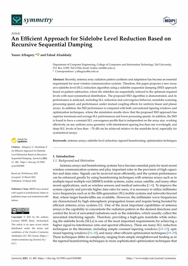
radiation peaks exist (𝜃 ), and this includes determining the array factor 𝐴(𝜃) and then finding its peaks and their corresponding 𝜃 , otherwise solving the differential equation in (3), which may be mathematically complicated, especially for large ULA sizes and two-dimensional arrays with a large number of damping cycles. The samples of 𝐴(𝜃) at the angular steps or increments ∆𝜃 affected the accuracy of finding 𝜃 and the SLL reduction performance. As shown in Figure 6, for a ULA of 20 elements, an angular resolution or step size greater than 1° resulted in some higher spikes in the damping curve, which re-sulted from inaccurate directions of the sidelobes, and a retrodictive effect on the SLL re-duction process occurred, while for the angular resolution ≤ 1°, the damping behavior was nominal and converging. However, the overall damping of the SSD converged in a broad sense, and the recursive SSD still worked, but on a rough SLL estimation and in a reduced fashion. In addition, the flowchart presented in Figure 2 provides a solution for the cases where large angular step sizes were used, where the process ended at the ac-cepted SLL regardless of the rough SLL estimation and reduction.
Figure 4. Recursive SSD damping performance.
Symmetry 2021, 13, x FOR PEER REVIEW 8 of 22
Figure 4. Recursive SSD damping performance.
Figure 5. Variation of SSD damping with the number of damping cycles at different array sizes.
3.2. SSD Behavior at Different Angular Step Sizes To speed up the recursive SSD algorithm, we should find the directions at which the
radiation peaks exist (𝜃 ), and this includes determining the array factor 𝐴(𝜃) and then finding its peaks and their corresponding 𝜃 , otherwise solving the differential equation in (3), which may be mathematically complicated, especially for large ULA sizes and two-dimensional arrays with a large number of damping cycles. The samples of 𝐴(𝜃) at the angular steps or increments ∆𝜃 affected the accuracy of finding 𝜃 and the SLL reduction performance. As shown in Figure 6, for a ULA of 20 elements, an angular resolution or step size greater than 1° resulted in some higher spikes in the damping curve, which re-sulted from inaccurate directions of the sidelobes, and a retrodictive effect on the SLL re-duction process occurred, while for the angular resolution ≤ 1°, the damping behavior was nominal and converging. However, the overall damping of the SSD converged in a broad sense, and the recursive SSD still worked, but on a rough SLL estimation and in a reduced fashion. In addition, the flowchart presented in Figure 2 provides a solution for the cases where large angular step sizes were used, where the process ended at the ac-cepted SLL regardless of the rough SLL estimation and reduction.
Figure 5. Variation of SSD damping with the number of damping cycles at different array sizes.
3.2. SSD Behavior at Different Angular Step Sizes
To speed up the recursive SSD algorithm, we should find the directions at which theradiation peaks exist (θi), and this includes determining the array factor A(θ) and thenfinding its peaks and their corresponding θi, otherwise solving the differential equationin (3), which may be mathematically complicated, especially for large ULA sizes andtwo-dimensional arrays with a large number of damping cycles. The samples of A(θ) at theangular steps or increments ∆θ affected the accuracy of finding θi and the SLL reductionperformance. As shown in Figure 6, for a ULA of 20 elements, an angular resolution or stepsize greater than 1◦ resulted in some higher spikes in the damping curve, which resultedfrom inaccurate directions of the sidelobes, and a retrodictive effect on the SLL reductionprocess occurred, while for the angular resolution ≤1◦, the damping behavior was nominaland converging. However, the overall damping of the SSD converged in a broad sense, andthe recursive SSD still worked, but on a rough SLL estimation and in a reduced fashion. Inaddition, the flowchart presented in Figure 2 provides a solution for the cases where largeangular step sizes were used, where the process ended at the accepted SLL regardless ofthe rough SLL estimation and reduction.
Symmetry 2021, 13, 480 9 of 22Symmetry 2021, 13, x FOR PEER REVIEW 9 of 22
Figure 6. SSD damping behavior at variable angular step sizes.
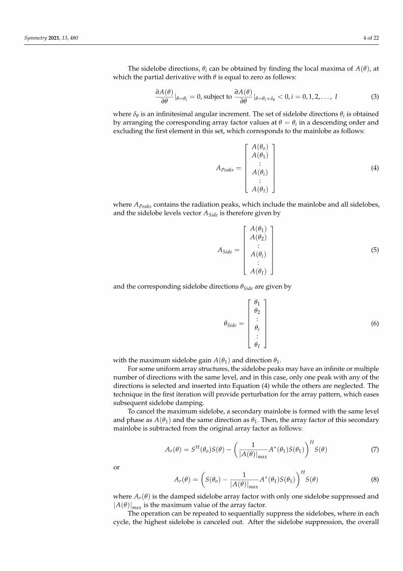
The processing time variation with the sampling angular step sizes for 200 damping cycles at different array sizes is shown in Figure 7, where it varied with exponentially decaying profiles with the angular step size and reduced greatly with the array size. Therefore, choosing the proper value of the angular step size is very important to achieve a lower processing time and smoother convergence to the desired SLL.
Figure 7. SSD processing time variation with angular step sizes at variable array sizes.
A rough estimation for the maximum sampling angular step size could be used as one third of the mainlobe beamwidth, which ensured finding the sidelobe peaks in the provided array factor samples. For the ULA, the maximum sampling angular step size ∆𝜃 can be considered as follows: ∆𝜃 ≈ , degrees (12)
where 𝑁 is the array size. Therefore, the maximum angular step size was adapted with the array size, and this empirical equation was considered as the maximum applicable value for ∆𝜃, as shown in Figure 8, which helped in finding fewer samples of 𝐴(𝜃) and speeding up the processing time. The curves shown in this figure correspond to 200 damp-ing cycles, as previously considered in Figure 7. For two-dimensional arrays, N was con-sidered as the largest number of elements in one of the two directions of the array. Com-pared to Figure 7, the processing time could be decreased to less than one sixth of its value at ∆𝜃 = 0.1°, especially for large array sizes.
Proc
essi
ng ti
me
in s
econ
ds
Figure 6. SSD damping behavior at variable angular step sizes.
The processing time variation with the sampling angular step sizes for 200 dampingcycles at different array sizes is shown in Figure 7, where it varied with exponentiallydecaying profiles with the angular step size and reduced greatly with the array size.Therefore, choosing the proper value of the angular step size is very important to achieve alower processing time and smoother convergence to the desired SLL.
Symmetry 2021, 13, x FOR PEER REVIEW 9 of 22
Figure 6. SSD damping behavior at variable angular step sizes.
The processing time variation with the sampling angular step sizes for 200 damping
cycles at different array sizes is shown in Figure 7, where it varied with exponentially
decaying profiles with the angular step size and reduced greatly with the array size.
Therefore, choosing the proper value of the angular step size is very important to achieve
a lower processing time and smoother convergence to the desired SLL.
Figure 7. SSD processing time variation with angular step sizes at variable array sizes.
A rough estimation for the maximum sampling angular step size could be used as
one third of the mainlobe beamwidth, which ensured finding the sidelobe peaks in the
provided array factor samples. For the ULA, the maximum sampling angular step size
∆𝜃𝑚𝑎𝑥 can be considered as follows:
∆𝜃𝑚𝑎𝑥 ≈29
𝑁, degrees (12)
where 𝑁 is the array size. Therefore, the maximum angular step size was adapted with
the array size, and this empirical equation was considered as the maximum applicable
value for ∆𝜃, as shown in Figure 8, which helped in finding fewer samples of 𝐴(𝜃) and
speeding up the processing time. The curves shown in this figure correspond to 200 damp-
ing cycles, as previously considered in Figure 7. For two-dimensional arrays, N was con-
sidered as the largest number of elements in one of the two directions of the array. Com-
pared to Figure 7, the processing time could be decreased to less than one sixth of its value
at ∆𝜃 = 0.1°, especially for large array sizes.
Figure 7. SSD processing time variation with angular step sizes at variable array sizes.
A rough estimation for the maximum sampling angular step size could be used asone third of the mainlobe beamwidth, which ensured finding the sidelobe peaks in theprovided array factor samples. For the ULA, the maximum sampling angular step size∆θmax can be considered as follows:
∆θmax ≈29N
, degrees (12)
where N is the array size. Therefore, the maximum angular step size was adapted with thearray size, and this empirical equation was considered as the maximum applicable valuefor ∆θ, as shown in Figure 8, which helped in finding fewer samples of A(θ) and speedingup the processing time. The curves shown in this figure correspond to 200 damping cycles,as previously considered in Figure 7. For two-dimensional arrays, N was considered as thelargest number of elements in one of the two directions of the array. Compared to Figure 7,the processing time could be decreased to less than one sixth of its value at ∆θ = 0.1◦,especially for large array sizes.

Symmetry 2021, 13, 480 10 of 22Symmetry 2021, 13, x FOR PEER REVIEW 10 of 22
Figure 8. Maximum angular step size with the number of elements in the array.
3.3. Impact of SSD on the Beamwidth
Generally, SLL reduction resulted in an increase in the beamwidth, and so did the
proposed SSD technique, as shown in Figure 9 for a 20 element ULA. During the first 100
damping cycles, the beamwidth increased rapidly where the SLL decreased rapidly, while
after 𝐾 = 100, the beamwidth increased slightly, where the variation was less than 1° for
an increase in 𝐾 from 100 to 1000.
Figure 9. Beamwidth variation with the number of damping cycles and highest SLL.
3.4. SSD Performance with Interelement Spacing
As the proposed SSD algorithm depended on beam space processing, in which the
sidelobes were removed sequentially, it would therefore be efficient only for interelement
spacing values that were less than one wavelength 𝜆 due to the appearance of secondary
major lobes in the visible region. The SSD performance with some typical values of the
interelement spacing distance is shown in Figure 10, where the proposed algorithm still
worked efficiently at a very low spacing of 𝜆/4 as well as a very large spacing of 0.9𝜆.
This performance consistency can be interpreted as the SSD also being efficient for wider
frequency bands. Furthermore, if the interelement spacing were incorporated in the array
synthesis process, the problem of increased beamwidth could be solved while maintain-
ing the required SLL.
Figure 8. Maximum angular step size with the number of elements in the array.
3.3. Impact of SSD on the Beamwidth
Generally, SLL reduction resulted in an increase in the beamwidth, and so did theproposed SSD technique, as shown in Figure 9 for a 20 element ULA. During the first100 damping cycles, the beamwidth increased rapidly where the SLL decreased rapidly,while after K = 100, the beamwidth increased slightly, where the variation was less than 1◦
for an increase in K from 100 to 1000.
Symmetry 2021, 13, x FOR PEER REVIEW 10 of 22
Figure 8. Maximum angular step size with the number of elements in the array.
3.3. Impact of SSD on the Beamwidth
Generally, SLL reduction resulted in an increase in the beamwidth, and so did the
proposed SSD technique, as shown in Figure 9 for a 20 element ULA. During the first 100
damping cycles, the beamwidth increased rapidly where the SLL decreased rapidly, while
after 𝐾 = 100, the beamwidth increased slightly, where the variation was less than 1° for
an increase in 𝐾 from 100 to 1000.
Figure 9. Beamwidth variation with the number of damping cycles and highest SLL.
3.4. SSD Performance with Interelement Spacing
As the proposed SSD algorithm depended on beam space processing, in which the
sidelobes were removed sequentially, it would therefore be efficient only for interelement
spacing values that were less than one wavelength 𝜆 due to the appearance of secondary
major lobes in the visible region. The SSD performance with some typical values of the
interelement spacing distance is shown in Figure 10, where the proposed algorithm still
worked efficiently at a very low spacing of 𝜆/4 as well as a very large spacing of 0.9𝜆.
This performance consistency can be interpreted as the SSD also being efficient for wider
frequency bands. Furthermore, if the interelement spacing were incorporated in the array
synthesis process, the problem of increased beamwidth could be solved while maintain-
ing the required SLL.
Figure 9. Beamwidth variation with the number of damping cycles and highest SLL.
3.4. SSD Performance with Interelement Spacing
As the proposed SSD algorithm depended on beam space processing, in which thesidelobes were removed sequentially, it would therefore be efficient only for interelementspacing values that were less than one wavelength λ due to the appearance of secondarymajor lobes in the visible region. The SSD performance with some typical values of theinterelement spacing distance is shown in Figure 10, where the proposed algorithm stillworked efficiently at a very low spacing of λ/4 as well as a very large spacing of 0.9λ.This performance consistency can be interpreted as the SSD also being efficient for widerfrequency bands. Furthermore, if the interelement spacing were incorporated in the arraysynthesis process, the problem of increased beamwidth could be solved while maintainingthe required SLL.

Symmetry 2021, 13, 480 11 of 22Symmetry 2021, 13, x FOR PEER REVIEW 11 of 22
Figure 10. Performance of SSD at different interelement spacings.
3.5. SSD Performance with the Mainlobe Direction The SSD algorithm was run for obtaining a −50 dB SLL for the 20 element array as
shown in Figure 11 at ten various mainlobe directions with 20° steps, and it showed in-dependency with the mainlobe direction. The SLL converged during the recursive SSD process even at 𝜃 = 0° or 180°. This robust performance helped form scanning beams with very low sidelobe levels, which is essential in many practical applications.
Figure 11. Performance of SSD at various mainlobe directions.
4. SSD Performance Comparisons and Discussions 4.1. Comparisons with Conventional Tapering Windows
There are many well-known and efficient tapering windows [9] used for SLL reduc-tion, such as triangular (Bartlett), Hamming, Hanning, Dolph-Chebyshev, Kaiser, Black-man, Cosine-square, and Gaussian windows [13]. Among these windows, the Dolph-Che-byshev and Gaussian ones provide the lowest sidelobe levels with a smaller increase in the beamwidth. Therefore, the proposed SSD technique was compared with these two efficient tapering windows as shown in Figure 12a,b. The comparison was based on providing a radiation pattern that had the same beamwidth from the proposed SSD tech-nique and the benchmarking windows. The results shown in Figure 12a,b investigated the SLL performance improvement obtained by the proposed SSD, where the two bench-marking windows provided SLL levels at least 2 dB higher than that achieved by the pro-posed SSD technique, although the Dolph-Chebyshev window provided the narrowest beamwidth compared with any other window at the same SLL level [9]. The Gaussian
Figure 10. Performance of SSD at different interelement spacings.
3.5. SSD Performance with the Mainlobe Direction
The SSD algorithm was run for obtaining a −50 dB SLL for the 20 element arrayas shown in Figure 11 at ten various mainlobe directions with 20◦ steps, and it showedindependency with the mainlobe direction. The SLL converged during the recursive SSDprocess even at θo = 0◦ or 180◦. This robust performance helped form scanning beams withvery low sidelobe levels, which is essential in many practical applications.
Symmetry 2021, 13, x FOR PEER REVIEW 11 of 22
Figure 10. Performance of SSD at different interelement spacings.
3.5. SSD Performance with the Mainlobe Direction The SSD algorithm was run for obtaining a −50 dB SLL for the 20 element array as
shown in Figure 11 at ten various mainlobe directions with 20° steps, and it showed in-dependency with the mainlobe direction. The SLL converged during the recursive SSD process even at 𝜃 = 0° or 180°. This robust performance helped form scanning beams with very low sidelobe levels, which is essential in many practical applications.
Figure 11. Performance of SSD at various mainlobe directions.
4. SSD Performance Comparisons and Discussions 4.1. Comparisons with Conventional Tapering Windows
There are many well-known and efficient tapering windows [9] used for SLL reduc-tion, such as triangular (Bartlett), Hamming, Hanning, Dolph-Chebyshev, Kaiser, Black-man, Cosine-square, and Gaussian windows [13]. Among these windows, the Dolph-Che-byshev and Gaussian ones provide the lowest sidelobe levels with a smaller increase in the beamwidth. Therefore, the proposed SSD technique was compared with these two efficient tapering windows as shown in Figure 12a,b. The comparison was based on providing a radiation pattern that had the same beamwidth from the proposed SSD tech-nique and the benchmarking windows. The results shown in Figure 12a,b investigated the SLL performance improvement obtained by the proposed SSD, where the two bench-marking windows provided SLL levels at least 2 dB higher than that achieved by the pro-posed SSD technique, although the Dolph-Chebyshev window provided the narrowest beamwidth compared with any other window at the same SLL level [9]. The Gaussian
Figure 11. Performance of SSD at various mainlobe directions.
4. SSD Performance Comparisons and Discussions4.1. Comparisons with Conventional Tapering Windows
There are many well-known and efficient tapering windows [9] used for SLL reduc-tion, such as triangular (Bartlett), Hamming, Hanning, Dolph-Chebyshev, Kaiser, Black-man, Cosine-square, and Gaussian windows [13]. Among these windows, the Dolph-Chebyshev and Gaussian ones provide the lowest sidelobe levels with a smaller increasein the beamwidth. Therefore, the proposed SSD technique was compared with these twoefficient tapering windows as shown in Figure 12a,b. The comparison was based on pro-viding a radiation pattern that had the same beamwidth from the proposed SSD techniqueand the benchmarking windows. The results shown in Figure 12a,b investigated the SLLperformance improvement obtained by the proposed SSD, where the two benchmarkingwindows provided SLL levels at least 2 dB higher than that achieved by the proposed SSDtechnique, although the Dolph-Chebyshev window provided the narrowest beamwidthcompared with any other window at the same SLL level [9]. The Gaussian window, on the

Symmetry 2021, 13, 480 12 of 22
other hand, provided an SLL level that was higher than the proposed SSD technique by2.83 dB at the same beamwidth, as shown in Figure 12b.
Symmetry 2021, 13, x FOR PEER REVIEW 12 of 22
window, on the other hand, provided an SLL level that was higher than the proposed SSD technique by 2.83 dB at the same beamwidth, as shown in Figure 12b.
(a) (b)
Figure 12. SLL comparison between the proposed SSD technique (blue curves) and conventional windows (red curves) at the same beamwidth. (a) A comparison with the Dolph-Chebyshev window. (b) A comparison with the Gaussian window.
In addition, the property of constant levels of all sidelobes resulting from the Dolph-Chebyshev window was relaxed in the proposed SSD technique, where the average SLL obtained from the Dolph-Chebyshev window was −53.38 dB while that of the SSD tech-nique was −54.4 dB, which was an advantage of 1 dB less for the proposed technique.
Table 1 summarizes the SLL performance comparison between the SSD technique with well-known efficient windows at the same beamwidth. These windows included the triangular, Hamming, Hanning, Blackman, Dolph-Chebyshev, Kaiser, Gaussian, and Kai-ser windows. The comparison results in this table show that the SLL obtained from the SSD algorithm at the same beamwidth was lower than any window, where the improve-ment in the SLL was approximately 12 dB compared with the cosine square window.
Table 1. SLL level comparison between conventional windows and the SSD algorithm at the same beamwidth.
Benchmarking Window
Window SLL (dB)
SSD SLL (dB)
Relative Reduction in the Maximum
SLL (dB)
Beamwidth (Degrees)
Triangular window −26.39 −32.32 6.32 7.12° Hamming −27.89 −30.5 2.61 7.14° Hanning −27.6 −30.6 3 7.14° Blackman −37.74 −44.83 7.09 8.06°
Dolph-Chebyshev −50 −52 2 8.38° Kaiser −35.96 −46.55 10.59 8.2°
Gaussian −37.19 −40.02 2.83 7.74° Cosine square −28 −40 12 7.74°
4.2. Comparisons with Optimization Techniques In this section, the proposed SSD SLL reduction technique is compared to some of
the most efficient and recent techniques, such as FPA, WOA, ASO, IWO, and CS. These
Figure 12. SLL comparison between the proposed SSD technique (blue curves) and conventional windows (red curves) atthe same beamwidth. (a) A comparison with the Dolph-Chebyshev window. (b) A comparison with the Gaussian window.
In addition, the property of constant levels of all sidelobes resulting from the Dolph-Chebyshev window was relaxed in the proposed SSD technique, where the average SLLobtained from the Dolph-Chebyshev window was −53.38 dB while that of the SSD tech-nique was −54.4 dB, which was an advantage of 1 dB less for the proposed technique.
Table 1 summarizes the SLL performance comparison between the SSD techniquewith well-known efficient windows at the same beamwidth. These windows included thetriangular, Hamming, Hanning, Blackman, Dolph-Chebyshev, Kaiser, Gaussian, and Kaiserwindows. The comparison results in this table show that the SLL obtained from the SSDalgorithm at the same beamwidth was lower than any window, where the improvement inthe SLL was approximately 12 dB compared with the cosine square window.
Table 1. SLL level comparison between conventional windows and the SSD algorithm at thesame beamwidth.
BenchmarkingWindow
Window SLL(dB)
SSDSLL (dB)
Relative Reductionin the Maximum
SLL (dB)
Beamwidth(Degrees)
Triangular window −26.39 −32.32 6.32 7.12◦
Hamming −27.89 −30.5 2.61 7.14◦
Hanning −27.6 −30.6 3 7.14◦
Blackman −37.74 −44.83 7.09 8.06◦
Dolph-Chebyshev −50 −52 2 8.38◦
Kaiser −35.96 −46.55 10.59 8.2◦
Gaussian −37.19 −40.02 2.83 7.74◦
Cosine square −28 −40 12 7.74◦
4.2. Comparisons with Optimization Techniques
In this section, the proposed SSD SLL reduction technique is compared to some ofthe most efficient and recent techniques, such as FPA, WOA, ASO, IWO, and CS. Thesetechniques were tested and compared in [27,29] for ULAs of 16 and 32 antenna elements

Symmetry 2021, 13, 480 13 of 22
and were examined with the same design parameters presented in these three referencesfor the purpose of comparison with SSD. For the 16 element ULA, the work in [27] showedthat the FPA, WOA, and ASO outperformed the PSO and BA algorithms, with the ASOoption being the best. Therefore, we compared the proposed SSD algorithm with thesethree efficient techniques. On the other hand, for the 32 ULA arrays, the work in [29]showed that the IWO and CS methods outperformed FA, BBO and PSO. Therefore we alsocompared the performance of the proposed SSD algorithm with the ASO, IWO, and CSalgorithms. Therefore, comparisons between the proposed SSD algorithm with the PSO,FA, BA, and BBO algorithms were not needed. Starting with the case where the ULA wasformed by 16 elements, four values for the number of damping cycles were examined,which were 50, 100, 150, and 200, and the SLL resulting from each was compared with thementioned optimization techniques as presented in Figure 13a–d.
Symmetry 2021, 13, x FOR PEER REVIEW 13 of 22
techniques were tested and compared in [27,29] for ULAs of 16 and 32 antenna elements and were examined with the same design parameters presented in these three references for the purpose of comparison with SSD. For the 16 element ULA, the work in [27] showed that the FPA, WOA, and ASO outperformed the PSO and BA algorithms, with the ASO option being the best. Therefore, we compared the proposed SSD algorithm with these three efficient techniques. On the other hand, for the 32 ULA arrays, the work in [29] showed that the IWO and CS methods outperformed FA, BBO and PSO. Therefore we also compared the performance of the proposed SSD algorithm with the ASO, IWO, and CS algorithms. Therefore, comparisons between the proposed SSD algorithm with the PSO, FA, BA, and BBO algorithms were not needed. Starting with the case where the ULA was formed by 16 elements, four values for the number of damping cycles were examined, which were 50, 100, 150, and 200, and the SLL resulting from each was compared with the mentioned optimization techniques as presented in Figure 13a–d.
(a) (b)
(c) (d)
Figure 13. SLL comparison between the proposed SSD technique (black curves) and different optimization techniques in a 16 element uniform linear array (ULA) at (a) 𝐾 = 50, (b) 𝐾 = 100, (c) 𝐾 = 150, and (d) 𝐾 = 200. Figure 13. SLL comparison between the proposed SSD technique (black curves) and different optimization techniques in a16 element uniform linear array (ULA) at (a) K = 50, (b) K = 100, (c) K = 150, and (d) K = 200.
The SSD performance showed lower SLL levels compared with the three efficienttechniques, especially at K ≥ 100. However, at K = 50, the SSD algorithm had betteraverage SLLs than any of the other techniques, as shown in Figure 14. Increasing the valueof K would improve the SSD performance in terms of both the maximum and average SLLs,

Symmetry 2021, 13, 480 14 of 22
where the maximum SLL of−45 dB was lower than the achieved ASO SLL by 4 dB, and theaverage SLL was −53 dB, which was also lower than that corresponding to ASO by 12 dBat K = 200. The processing time consumed by the SSD algorithm was also much smallerthan all these techniques, where for the 16 element ULA, the proposed SSD algorithmrequired only one second at K = 200, while the CPU processing time for ASO in [27] wasapproximately 27 s when using the same platform specification. However, the improvedperformance of the SLL achieved by SSD compromised slightly wider beams, especially atlarger numbers of damping cycles, as shown in Figure 15, where an increase of less thanone degree resulted from SSD compared with the ASO at K = 200.
Symmetry 2021, 13, x FOR PEER REVIEW 14 of 22
The SSD performance showed lower SLL levels compared with the three efficient techniques, especially at 𝐾 ≥ 100. However, at 𝐾 = 50, the SSD algorithm had better av-erage SLLs than any of the other techniques, as shown in Figure 14. Increasing the value of 𝐾 would improve the SSD performance in terms of both the maximum and average SLLs, where the maximum SLL of −45 dB was lower than the achieved ASO SLL by 4 dB, and the average SLL was −53 dB, which was also lower than that corresponding to ASO by 12 dB at 𝐾 = 200. The processing time consumed by the SSD algorithm was also much smaller than all these techniques, where for the 16 element ULA, the proposed SSD algo-rithm required only one second at 𝐾 = 200, while the CPU processing time for ASO in [27] was approximately 27 s when using the same platform specification. However, the improved performance of the SLL achieved by SSD compromised slightly wider beams, especially at larger numbers of damping cycles, as shown in Figure 15, where an increase of less than one degree resulted from SSD compared with the ASO at 𝐾 = 200.
Figure 14. Maximum and average SLL comparison between the proposed SSD technique (black curves) and different optimization techniques for a 16 element ULA at 𝐾 = 50, 100, 150, and 200.
Figure 15. Mainlobe beamwidth comparison between the proposed SSD technique and different optimization techniques for a 16 element ULA at 𝐾 = 50, 100, 150, and 200.
Figure 14. Maximum and average SLL comparison between the proposed SSD technique (blackcurves) and different optimization techniques for a 16 element ULA at K = 50, 100, 150, and 200.
Symmetry 2021, 13, x FOR PEER REVIEW 14 of 22
The SSD performance showed lower SLL levels compared with the three efficient techniques, especially at 𝐾 ≥ 100. However, at 𝐾 = 50, the SSD algorithm had better av-erage SLLs than any of the other techniques, as shown in Figure 14. Increasing the value of 𝐾 would improve the SSD performance in terms of both the maximum and average SLLs, where the maximum SLL of −45 dB was lower than the achieved ASO SLL by 4 dB, and the average SLL was −53 dB, which was also lower than that corresponding to ASO by 12 dB at 𝐾 = 200. The processing time consumed by the SSD algorithm was also much smaller than all these techniques, where for the 16 element ULA, the proposed SSD algo-rithm required only one second at 𝐾 = 200, while the CPU processing time for ASO in [27] was approximately 27 s when using the same platform specification. However, the improved performance of the SLL achieved by SSD compromised slightly wider beams, especially at larger numbers of damping cycles, as shown in Figure 15, where an increase of less than one degree resulted from SSD compared with the ASO at 𝐾 = 200.
Figure 14. Maximum and average SLL comparison between the proposed SSD technique (black curves) and different optimization techniques for a 16 element ULA at 𝐾 = 50, 100, 150, and 200.
Figure 15. Mainlobe beamwidth comparison between the proposed SSD technique and different optimization techniques for a 16 element ULA at 𝐾 = 50, 100, 150, and 200. Figure 15. Mainlobe beamwidth comparison between the proposed SSD technique and differentoptimization techniques for a 16 element ULA at K = 50, 100, 150, and 200.

Symmetry 2021, 13, 480 15 of 22
On the other hand, the performance improvement in both the maximum and av-erage SLL values obtained from the SSD algorithm came with a price paid in a slightlylarger beamwidth (less than 1◦) compared with the three optimization techniques, asshown in Figure 15. Therefore, if the slightly increased beamwidth could be tolerated forachieving better SLL performance, then the SSD would be the best choice among the otheroptimization techniques.
The normalized coefficients of the three optimization techniques, along with theuniform feeding coefficients, are displayed in Figure 16a for a 16 element linear array, whilethe four cases of the SSD coefficients are displayed in Figure 16b.
Symmetry 2021, 13, x FOR PEER REVIEW 15 of 22
On the other hand, the performance improvement in both the maximum and average SLL values obtained from the SSD algorithm came with a price paid in a slightly larger beamwidth (less than 1°) compared with the three optimization techniques, as shown in Figure 15. Therefore, if the slightly increased beamwidth could be tolerated for achieving better SLL performance, then the SSD would be the best choice among the other optimi-zation techniques.
The normalized coefficients of the three optimization techniques, along with the uni-form feeding coefficients, are displayed in Figure 16a for a 16 element linear array, while the four cases of the SSD coefficients are displayed in Figure 16b.
(a) (b)
Figure 16. Normalized antenna coefficients for a 16 element ULA. (a) Optimization benchmarking techniques and (b) the SSD algorithm at different values for 𝐾.
The comparison was also performed for a larger 32 element ULA between the pro-posed SSD algorithm and the three most efficient techniques in [27,29], which were the ASO, IWO, and CS algorithms, as shown in Figures 17–19. As expected, SSD provided a much-improved maximum and average SLL performance—as shown in Figure 18—com-pared with all of the three techniques, even at lower values of 𝐾. Moreover, the increase in beamwidth by the SSD technique was less than 0.5° compared with the most efficient ASO technique.
(a) (b)
Figure 16. Normalized antenna coefficients for a 16 element ULA. (a) Optimization benchmarking techniques and (b) theSSD algorithm at different values for K.
The comparison was also performed for a larger 32 element ULA between the pro-posed SSD algorithm and the three most efficient techniques in [27,29], which were the ASO,IWO, and CS algorithms, as shown in Figures 17–19. As expected, SSD provided a much-improved maximum and average SLL performance—as shown in Figure 18—comparedwith all of the three techniques, even at lower values of K. Moreover, the increase inbeamwidth by the SSD technique was less than 0.5◦ compared with the most efficientASO technique.
Symmetry 2021, 13, x FOR PEER REVIEW 15 of 22
On the other hand, the performance improvement in both the maximum and average SLL values obtained from the SSD algorithm came with a price paid in a slightly larger beamwidth (less than 1°) compared with the three optimization techniques, as shown in Figure 15. Therefore, if the slightly increased beamwidth could be tolerated for achieving better SLL performance, then the SSD would be the best choice among the other optimi-zation techniques.
The normalized coefficients of the three optimization techniques, along with the uni-form feeding coefficients, are displayed in Figure 16a for a 16 element linear array, while the four cases of the SSD coefficients are displayed in Figure 16b.
(a) (b)
Figure 16. Normalized antenna coefficients for a 16 element ULA. (a) Optimization benchmarking techniques and (b) the SSD algorithm at different values for 𝐾.
The comparison was also performed for a larger 32 element ULA between the pro-posed SSD algorithm and the three most efficient techniques in [27,29], which were the ASO, IWO, and CS algorithms, as shown in Figures 17–19. As expected, SSD provided a much-improved maximum and average SLL performance—as shown in Figure 18—com-pared with all of the three techniques, even at lower values of 𝐾. Moreover, the increase in beamwidth by the SSD technique was less than 0.5° compared with the most efficient ASO technique.
(a) (b)
Figure 17. Cont.

Symmetry 2021, 13, 480 16 of 22Symmetry 2021, 13, x FOR PEER REVIEW 16 of 22
(c) (d)
Figure 17. SLL comparison between the proposed SSD technique (black curves) and different efficient optimization tech-niques for a 32 element ULA at (a) 𝐾 = 50, (b) 𝐾 = 100, (c) 𝐾 = 150, and (d) 𝐾 = 200.
Figure 18. Maximum and average SLL comparison between the proposed SSD technique (black curves) and different optimization techniques for a 32 element ULA at 𝐾 = 50, 100, 150, and 200.
Figure 19. Mainlobe beamwidth comparison between the proposed SSD technique and different optimization techniques for a 32 element ULA at 𝐾 = 50, 100, 150, and 200.
Figure 17. SLL comparison between the proposed SSD technique (black curves) and different efficient optimizationtechniques for a 32 element ULA at (a) K = 50, (b) K = 100, (c) K = 150, and (d) K = 200.
Symmetry 2021, 13, x FOR PEER REVIEW 16 of 22
(c) (d)
Figure 17. SLL comparison between the proposed SSD technique (black curves) and different efficient optimization tech-niques for a 32 element ULA at (a) 𝐾 = 50, (b) 𝐾 = 100, (c) 𝐾 = 150, and (d) 𝐾 = 200.
Figure 18. Maximum and average SLL comparison between the proposed SSD technique (black curves) and different optimization techniques for a 32 element ULA at 𝐾 = 50, 100, 150, and 200.
Figure 19. Mainlobe beamwidth comparison between the proposed SSD technique and different optimization techniques for a 32 element ULA at 𝐾 = 50, 100, 150, and 200.
Figure 18. Maximum and average SLL comparison between the proposed SSD technique (blackcurves) and different optimization techniques for a 32 element ULA at K = 50, 100, 150, and 200.
Symmetry 2021, 13, x FOR PEER REVIEW 16 of 22
(c) (d)
Figure 17. SLL comparison between the proposed SSD technique (black curves) and different efficient optimization tech-niques for a 32 element ULA at (a) 𝐾 = 50, (b) 𝐾 = 100, (c) 𝐾 = 150, and (d) 𝐾 = 200.
Figure 18. Maximum and average SLL comparison between the proposed SSD technique (black curves) and different optimization techniques for a 32 element ULA at 𝐾 = 50, 100, 150, and 200.
Figure 19. Mainlobe beamwidth comparison between the proposed SSD technique and different optimization techniques for a 32 element ULA at 𝐾 = 50, 100, 150, and 200. Figure 19. Mainlobe beamwidth comparison between the proposed SSD technique and differentoptimization techniques for a 32 element ULA at K = 50, 100, 150, and 200.

Symmetry 2021, 13, 480 17 of 22
Figure 19 displays the beamwidth values of the different compared techniques atdifferent values of K where there was a slight increase, which was less than 1◦ in the caseof the SSD algorithm. Deep SLL levels as low as −44 dB with an average of −52 dB couldbe achieved, which were much better than the other three algorithms, but at a price of a0.8◦ increase in beamwidth.
The normalized array coefficients for the 32 element ULA are also displayed Figure 20afor the benchmarking algorithms, while Figure 20b displays the normalized SSD coefficientsat different values of K, where the curves become steeper at larger values of K, increasingthe tapering profile and resulting in reducing the SLL to deeper levels.
Symmetry 2021, 13, x FOR PEER REVIEW 17 of 22
Figure 19 displays the beamwidth values of the different compared techniques at dif-
ferent values of 𝐾 where there was a slight increase, which was less than 1° in the case
of the SSD algorithm. Deep SLL levels as low as −44 dB with an average of −52 dB could
be achieved, which were much better than the other three algorithms, but at a price of a
0.8° increase in beamwidth.
The normalized array coefficients for the 32 element ULA are also displayed Figure
20a for the benchmarking algorithms, while Figure 20b displays the normalized SSD co-
efficients at different values of 𝐾, where the curves become steeper at larger values of 𝐾,
increasing the tapering profile and resulting in reducing the SLL to deeper levels.
(a) (b)
Figure 20. Impact of mutual coupling on the SSD performance for a 16 element ULA at (a) 𝐾 = 100 and (b) 𝐾 = 1000.
5. Mutual Coupling Effects on the SSD Performance
The previous analysis for the SSD technique was performed on isotropic antenna el-
ements, which is now done using practical antenna models along with the inclusion of
mutual coupling effects. For a 16 element ULA using half-wave dipoles as antenna ele-
ments operating at 5 GHz, Figure 21 displays the resulting normalized radiation patterns
at two numbers of damping cycles, namely 100 and 1000. The two sets of curves in this
figure include the isotropic isolated antenna elements, practical isolated elements (i.e.,
without mutual coupling effects), and practical antenna elements with the effect of mutual
coupling. For both values of the number of damping cycles, the normalized power pat-
terns displayed very deep SLLs using the SSD algorithm, where the impact of the mutual
coupling just appeared to increase in the mainlobe at very low radiation levels below −30
dB. However, the maximum and average SLLs were still very acceptable and sometimes
below the isotropic elements case.
Figure 20. Impact of mutual coupling on the SSD performance for a 16 element ULA at (a) K = 100 and (b) K = 1000.
5. Mutual Coupling Effects on the SSD Performance
The previous analysis for the SSD technique was performed on isotropic antennaelements, which is now done using practical antenna models along with the inclusion ofmutual coupling effects. For a 16 element ULA using half-wave dipoles as antenna elementsoperating at 5 GHz, Figure 21 displays the resulting normalized radiation patterns at twonumbers of damping cycles, namely 100 and 1000. The two sets of curves in this figureinclude the isotropic isolated antenna elements, practical isolated elements (i.e., withoutmutual coupling effects), and practical antenna elements with the effect of mutual coupling.For both values of the number of damping cycles, the normalized power patterns displayedvery deep SLLs using the SSD algorithm, where the impact of the mutual coupling justappeared to increase in the mainlobe at very low radiation levels below −30 dB. However,the maximum and average SLLs were still very acceptable and sometimes below theisotropic elements case.

Symmetry 2021, 13, 480 18 of 22Symmetry 2021, 13, x FOR PEER REVIEW 18 of 22
(a) (b)
Figure 21. Impact of mutual coupling on the SSD performance for a 16 element ULA at (a) 𝐾 = 100 and (b) 𝐾 = 1000.
6. SSD for Two-Dimensional Planar Arrays As mentioned in Section 3, the application of the proposed SSD technique was inde-
pendent of the array configuration and therefore could be applied for any array geometry if there was only one mainlobe in the visible region of the radiation pattern with some relatively lower sidelobes to guarantee SSD convergence. The radiation pattern of a uni-formly fed two-dimensional planar array had plenty of sidelobes compared to the ULA, and therefore the SSD damping process required more damping cycles to achieve the re-quired SLL. The process followed the recursive process in Equation (11) and could be ex-amined for a planar array of 20 × 20 half-wavelength dipole elements as shown in Figure 22a, operating at 5 GHz with a beam formed in the broadside direction (90°, 0°). The nor-malized power levels for the uniform feeding case are shown in Figure 22b, and the high-est SLL was −13.4 dB relative to the mainlobe level. The improvement in the SLL appeared clearly in Figure 22c with the effect of mutual coupling, where the SLL was reduced to −30 dB at 𝐾 = 100, while it dropped to less than −47 dB at 𝐾 = 1000, where 1000 sidelobes had been suppressed from the power pattern.
(a) (b)
Figure 21. Impact of mutual coupling on the SSD performance for a 16 element ULA at (a) K = 100 and (b) K = 1000.
6. SSD for Two-Dimensional Planar Arrays
As mentioned in Section 3, the application of the proposed SSD technique was inde-pendent of the array configuration and therefore could be applied for any array geometryif there was only one mainlobe in the visible region of the radiation pattern with some rela-tively lower sidelobes to guarantee SSD convergence. The radiation pattern of a uniformlyfed two-dimensional planar array had plenty of sidelobes compared to the ULA, and there-fore the SSD damping process required more damping cycles to achieve the required SLL.The process followed the recursive process in Equation (11) and could be examined for aplanar array of 20× 20 half-wavelength dipole elements as shown in Figure 22a, operatingat 5 GHz with a beam formed in the broadside direction (90◦, 0◦). The normalized powerlevels for the uniform feeding case are shown in Figure 22b, and the highest SLL was−13.4 dB relative to the mainlobe level. The improvement in the SLL appeared clearly inFigure 22c with the effect of mutual coupling, where the SLL was reduced to −30 dB atK = 100, while it dropped to less than −47 dB at K = 1000, where 1000 sidelobes had beensuppressed from the power pattern.
Symmetry 2021, 13, x FOR PEER REVIEW 18 of 22
(a) (b)
Figure 21. Impact of mutual coupling on the SSD performance for a 16 element ULA at (a) 𝐾 = 100 and (b) 𝐾 = 1000.
6. SSD for Two-Dimensional Planar Arrays As mentioned in Section 3, the application of the proposed SSD technique was inde-
pendent of the array configuration and therefore could be applied for any array geometry if there was only one mainlobe in the visible region of the radiation pattern with some relatively lower sidelobes to guarantee SSD convergence. The radiation pattern of a uni-formly fed two-dimensional planar array had plenty of sidelobes compared to the ULA, and therefore the SSD damping process required more damping cycles to achieve the re-quired SLL. The process followed the recursive process in Equation (11) and could be ex-amined for a planar array of 20 × 20 half-wavelength dipole elements as shown in Figure 22a, operating at 5 GHz with a beam formed in the broadside direction (90°, 0°). The nor-malized power levels for the uniform feeding case are shown in Figure 22b, and the high-est SLL was −13.4 dB relative to the mainlobe level. The improvement in the SLL appeared clearly in Figure 22c with the effect of mutual coupling, where the SLL was reduced to −30 dB at 𝐾 = 100, while it dropped to less than −47 dB at 𝐾 = 1000, where 1000 sidelobes had been suppressed from the power pattern.
(a) (b)
Figure 22. Cont.

Symmetry 2021, 13, 480 19 of 22Symmetry 2021, 13, x FOR PEER REVIEW 19 of 22
(c) (d)
Figure 22. Two-dimensional planar array configuration formed by 20 × 20 dipole antennas with mutual coupling effects. (a) Array configuration. (b) Normalized power pattern with uniform feeding. (c) Normalized power pattern with SSD feeding at 𝐾 = 100. (d) Normalized power pattern with SSD feeding at 𝐾 = 1000.
7. SSD Operational Constraints and Limitations Discussion In this section, the operational constraints and limitations of the proposed SSD algo-
rithm are explored and discussed. These constraints include the operational interelement spacing and the impact of antenna element failures.
The SSD algorithm was designed mainly for antenna arrays of any configuration that had symmetrical and uniform antenna distributions with interelement spacings that were less than one wavelength. These antenna arrays produce one mainlobe and a set of smaller sidelobes, which allows the SSD to sequentially reduce the sidelobe. If the interelement separation were a distance of more than one wavelength, the SSD could not work as re-quired due to the appearance of secondary major lobes in the radiation pattern, which may have led to the suppression of the required mainlobe. Therefore, in this case, there would be no convergence, and the secondary major lobes would suppress each other in the pattern alternately. The SSD can be modified to select only the sidelobes and exclude the secondary major lobes in Equation (4), so it will work effectively, but without suppres-sion or reduction of the secondary major lobes. However, practically, we almost built ar-rays with antenna elements separated by a distance that was less than one wavelength—specifically around half the wavelength value—so the SSD could work fine. On the other hand, if the interelement spacing is very small, the SSD still efficiently works, as shown previously in Figure 10, even at a one-quarter wavelength interelement separation, which is practically difficult to implement due to the increase of mutual coupling effects and the physical antenna dimensions.
The second operational constraint for the SSD algorithm is the impact of antenna el-ement failure on the SLL damping performance. If all antenna elements are operating nor-mally, the SSD performs efficiently, but if one or more antenna elements fail or are turned off in the array, then the symmetry structure is perturbed, which affects the SSD SLL re-duction performance as the radiation pattern changes. Figure 23 demonstrates the impact of one antenna element’s complete failure at different locations in a 16 element ULA, where it is noticed that the shutdown or malfunctioning antenna elements at the array ends will not affect the SSD damping behavior, and the SSD still works fine. On the other hand, if the failed element is located at the array’s center, then the SSD may fail completely to reduce the SLL, and it is recommended in this case that the number of damping cycles
Figure 22. Two-dimensional planar array configuration formed by 20× 20 dipole antennas with mutual coupling effects.(a) Array configuration. (b) Normalized power pattern with uniform feeding. (c) Normalized power pattern with SSDfeeding at K = 100. (d) Normalized power pattern with SSD feeding at K = 1000.
7. SSD Operational Constraints and Limitations Discussion
In this section, the operational constraints and limitations of the proposed SSD algo-rithm are explored and discussed. These constraints include the operational interelementspacing and the impact of antenna element failures.
The SSD algorithm was designed mainly for antenna arrays of any configuration thathad symmetrical and uniform antenna distributions with interelement spacings that wereless than one wavelength. These antenna arrays produce one mainlobe and a set of smallersidelobes, which allows the SSD to sequentially reduce the sidelobe. If the interelementseparation were a distance of more than one wavelength, the SSD could not work asrequired due to the appearance of secondary major lobes in the radiation pattern, whichmay have led to the suppression of the required mainlobe. Therefore, in this case, therewould be no convergence, and the secondary major lobes would suppress each other in thepattern alternately. The SSD can be modified to select only the sidelobes and exclude thesecondary major lobes in Equation (4), so it will work effectively, but without suppressionor reduction of the secondary major lobes. However, practically, we almost built arrays withantenna elements separated by a distance that was less than one wavelength—specificallyaround half the wavelength value—so the SSD could work fine. On the other hand, if theinterelement spacing is very small, the SSD still efficiently works, as shown previously inFigure 10, even at a one-quarter wavelength interelement separation, which is practicallydifficult to implement due to the increase of mutual coupling effects and the physicalantenna dimensions.
The second operational constraint for the SSD algorithm is the impact of antennaelement failure on the SLL damping performance. If all antenna elements are operatingnormally, the SSD performs efficiently, but if one or more antenna elements fail or areturned off in the array, then the symmetry structure is perturbed, which affects the SSDSLL reduction performance as the radiation pattern changes. Figure 23 demonstrates theimpact of one antenna element’s complete failure at different locations in a 16 element ULA,where it is noticed that the shutdown or malfunctioning antenna elements at the array endswill not affect the SSD damping behavior, and the SSD still works fine. On the other hand,if the failed element is located at the array’s center, then the SSD may fail completely toreduce the SLL, and it is recommended in this case that the number of damping cycles isreduced to the value that gives the best SLL level. The element failure can be expressed inthe array steering vector as a zero element, which indicates the absence of that element.

Symmetry 2021, 13, 480 20 of 22
Symmetry 2021, 13, x FOR PEER REVIEW 20 of 22
is reduced to the value that gives the best SLL level. The element failure can be expressed in the array steering vector as a zero element, which indicates the absence of that element.
Figure 23. The impact of one antenna element failure on the SDD performance at different loca-tions in a 16 element ULA.
The absence of multiple elements in the array can be handled and tolerated by the SSD algorithm, except in the case where the malfunction element is located at the array’s center. Figure 24 displays this scenario for some of the antenna elements that failed to work in two cases. The first case includes elements 2, 3, 8, 13, and 14, where element 8 represents the central element, which seriously impacts the SSD convergence behavior. On the other hand, the symmetry or near-symmetrical distribution of failed antenna ele-ments, excluding the central antenna, can be handled by the proposed SSD algorithm, which appears to have the robust convergence behavior.
Figure 24. The impact of multiple antenna element failures on the SDD performance at different locations in a 16 element ULA.
We can conclude from this discussion that the proposed SSD algorithm has robust SLL reduction performance under abnormal operating conditions, which include one or more antenna element failing except for the case where the malfunctioning element is lo-cated at the array’s center.
Figure 23. The impact of one antenna element failure on the SDD performance at different locationsin a 16 element ULA.
The absence of multiple elements in the array can be handled and tolerated by theSSD algorithm, except in the case where the malfunction element is located at the array’scenter. Figure 24 displays this scenario for some of the antenna elements that failed to workin two cases. The first case includes elements 2, 3, 8, 13, and 14, where element 8 representsthe central element, which seriously impacts the SSD convergence behavior. On the otherhand, the symmetry or near-symmetrical distribution of failed antenna elements, excludingthe central antenna, can be handled by the proposed SSD algorithm, which appears to havethe robust convergence behavior.
Symmetry 2021, 13, x FOR PEER REVIEW 20 of 22
is reduced to the value that gives the best SLL level. The element failure can be expressed in the array steering vector as a zero element, which indicates the absence of that element.
Figure 23. The impact of one antenna element failure on the SDD performance at different loca-tions in a 16 element ULA.
The absence of multiple elements in the array can be handled and tolerated by the SSD algorithm, except in the case where the malfunction element is located at the array’s center. Figure 24 displays this scenario for some of the antenna elements that failed to work in two cases. The first case includes elements 2, 3, 8, 13, and 14, where element 8 represents the central element, which seriously impacts the SSD convergence behavior. On the other hand, the symmetry or near-symmetrical distribution of failed antenna ele-ments, excluding the central antenna, can be handled by the proposed SSD algorithm, which appears to have the robust convergence behavior.
Figure 24. The impact of multiple antenna element failures on the SDD performance at different locations in a 16 element ULA.
We can conclude from this discussion that the proposed SSD algorithm has robust SLL reduction performance under abnormal operating conditions, which include one or more antenna element failing except for the case where the malfunctioning element is lo-cated at the array’s center.
Figure 24. The impact of multiple antenna element failures on the SDD performance at differentlocations in a 16 element ULA.
We can conclude from this discussion that the proposed SSD algorithm has robust SLLreduction performance under abnormal operating conditions, which include one or moreantenna element failing except for the case where the malfunctioning element is located atthe array’s center.
8. Conclusions
Antenna arrays became essential in many recent communication systems to achievehigh-quality connectivity performance and higher capacities through proper spatial filter-ing. Therefore, in this paper, spatial filtering has been achieved by a sequential sidelobedamping algorithm (SSD), where the sidelobes are sequentially damped for sidelobe level(SLL) reduction. The proposed algorithm can be applied for any uniform array geometry,

Symmetry 2021, 13, 480 21 of 22
and the SLL can be set to the required level according to the number of the dampingcycles. Additionally, the algorithm has been thoroughly analyzed, and the processingtime, convergence, and performance with practical scenarios have been investigated, show-ing independent and very fast convergence times compared with many of the currentoptimization techniques. In addition, comparisons between the proposed SSD with thewell-known windows showed that the SSD achieved lower SLLs at the same beamwidth,while comparisons with many of the recent optimization techniques such as FPA, PSO,WOA, BA, ASO, IWO, FA, CS, and BBO indicated that the proposed SSD can providelower SLLs at a slightly wider beamwidth, but at a much higher speed of processing andconvergence, which is essential in real-time communication scenarios, in addition to thecapability of application in any uniform array configuration.
Author Contributions: Conceptualization, Y.A. and F.A.; methodology, Y.A.; software, Y.A.; valida-tion, F.A., and Y.A.; formal analysis, Y.A.; investigation, F.A.; writing—original draft preparation,Y.A.; writing—review and editing, F.A.; visualization, Y.A.; funding acquisition, Y.A. All authorshave read and agreed to the published version of the manuscript.
Funding: Taif University Researchers Supporting Project number (TURSP-2020/161), Taif University,Taif, Saudi Arabia.
Acknowledgments: The authors would like to thank Taif University Researchers Supporting Projectnumber (TURSP-2020/161), Taif University, Taif, Saudi Arabia for supporting this work.
Conflicts of Interest: The authors declare no conflict of interest.
References1. Akyildiz, I.F.; Nie, S.; Lin, S.-C.; Chandrasekaran, M. 5G roadmap: 10 key enabling technologies. Comput. Netw. 2016, 106, 17–48.
[CrossRef]2. Li, J.; Ma, Z.; Mao, L.; Wang, Z.; Wang, Y.; Cai, H.; Chen, X. Broadband Generalized Sidelobe Canceler Beamforming Applied to
Ultrasonic Imaging. Appl. Sci. 2020, 10, 1207. [CrossRef]3. Wang, Y.; Yang, W.; Chen, J.; Kuang, H.; Liu, W.; Li, C. Azimuth Sidelobes Suppression Using Multi-Azimuth Angle Synthetic
Aperture Radar Images. Sensors 2019, 19, 2764. [CrossRef] [PubMed]4. Hasan, M.Z.; Al-Rizzo, H. Beamforming Optimization in Internet of Things Applications Using Robust Swarm Algorithm in
Conjunction with Connectable and Collaborative Sensors. Sensors 2020, 20, 2048. [CrossRef]5. Nguyen, A.H.; Cho, J.-H.; Bae, H.-J.; Sung, H.-K. Side-lobe Level Reduction of an Optical Phased Array Using Amplitude and
Phase Modulation of Array Elements Based on Optically Injection-Locked Semiconductor Lasers. Photonics 2020, 7, 20. [CrossRef]6. Issa, K.; Fathallah, H.; Ashraf, M.A.; Vettikalladi, H.; Alshebeili, S. Broadband High-Gain Antenna for Millimetre-Wave 60-GHz
Band. Electronics 2019, 8, 1246. [CrossRef]7. Albagory, Y. An efficient WBAN aggregator switched-beam technique for isolated and quarantined patients. AEU-Int. J. Electron.
Commun. 2020, 123, 153322. [CrossRef]8. Albagory, Y. Direction-independent and self-reconfigurable spherical-cap antenna array beamforming technique for massive 3D
MIMO systems. Wirel. Netw. 2020, 26, 6111–6123. [CrossRef]9. Prabhu, K.M.M. Window Functions and Their Applications in Signal Processing; Taylor & Francis: Abingdon, UK, 2014.10. Juárez, E.; Panduro, M.A.; Reyna, A.; Covarrubias, D.H.; Mendez, A.; Murillo, E. Design of Concentric Ring Antenna Arrays
Based on Subarrays to Simplify the Feeding System. Symmetry 2020, 12, 970. [CrossRef]11. Nofal, M.; Aljahdali, S.; Albagory, Y. Tapered beamforming for concentric ring arrays. AEU-Int. J. Electron. Commun. 2013,
67, 58–63. [CrossRef]12. Dessouky, M.; Sharshar, H.; Albagory, Y. Optimum normalized-Gaussian tapering window for side lobe reduction in uni-form
concentric circular arrays. Prog. Electromagn. Res. 2007, 69, 35–46. [CrossRef]13. Dessouky, M.; Sharshar, H.; Albagory, Y. An Approach for Dolph-Chebyshev Uniform Concentric Circular Arrays. J. Electromagn.
Waves Appl. 2007, 21, 781–794. [CrossRef]14. Dessouky, M.I.; Sharshar, H.A.; Albagory, Y.A. Efficient sidelobe reduction technique for small-sized concentric circular arrays.
Prog. Electromagn. Res. 2006, 65, 187–200. [CrossRef]15. Nofal, M.; Aljahdali, S.; Albagory, Y. Simplified Sidelobe Reduction Techniques for Concentric Ring Arrays. Wirel. Pers. Commun.
2013, 71, 2981–2991. [CrossRef]16. Lau, B.; Leung, Y. A Dolph-Chebyshev approach to the synthesis of array patterns for uniform circular arrays. In Proceedings of
the 2000 IEEE International Symposium on Circuits and Systems, Emerging Technologies for the 21st Century, Proceedings (IEEECat No. 00CH36353), Geneva, Switzerland, 28–31 May 2000; Volume 1, pp. 124–127.

Symmetry 2021, 13, 480 22 of 22
17. Sarker, M.A.; Hossain, M.S.; Masud, M.S. Robust beamforming synthesis technique for low side lobe level using taylor excitedantenna array. In Proceedings of the 2016 2nd International Conference on Electrical, Computer & Telecommunication Engineering(ICECTE), Rajshahi, Bangladesh, 8–10 December 2016; pp. 1–4.
18. Aljahdali, S.; Nofal, M.; Albagory, Y. A modified array processing technique based on Kaiser window for concentric circulararrays. In Proceedings of the 2012 International Conference on Multimedia Computing and Systems, ICMCS 2012, Tangiers,Morocco, 10–12 May 2012.
19. Singh, U.; Salgotra, R. Synthesis of linear antenna array using flower pollination algorithm. Neural Comput. Appl. 2018, 29, 435–445.[CrossRef]
20. Chakravarthy, V.; Rao, P.M. Circular array antenna optimization with scanned and unscanned beams using novel particle swarmoptimization. Indian J. Appl. Res. 2015, 5, 790–793.
21. Mehrabian, A.; Lucas, C. A novel numerical optimization algorithm inspired from weed colonization. Ecol. Inform. 2006,1, 355–366. [CrossRef]
22. Sharaqa, A.; Dib, N. Circular antenna array synthesis using firefly algorithm. Int. J. RF Microw. Comput. Aided Eng. 2014,24, 139–146. [CrossRef]
23. Sun, G.; Liu, Y.; Chen, Z.; Zhang, Y.; Wang, A.; Liang, S. Thinning of concentric circular antenna arrays using improved discretecuckoo search algorithm. In Proceedings of the 2017 IEEE Wireless Communications and Networking Conference (WCNC), SanFrancisco, CA, USA, 19–22 March 2017; pp. 1–6.
24. Li, H.; Liu, Y.; Sun, G.; Wang, A.; Liang, S. Beam pattern synthesis based on improved biogeography-based optimization forreducing sidelobe level. Comput. Electr. Eng. 2017, 60, 161–174. [CrossRef]
25. Van Luyen, T.; Giang, T.V.B. Interference Suppression of ULA Antennas by Phase-Only Control Using Bat Algorithm. IEEEAntennas Wirel. Propag. Lett. 2017, 16, 3038–3042. [CrossRef]
26. Mirjalili, S.; Lewis, A. The Whale Optimization Algorithm. Adv. Eng. Softw. 2016, 95, 51–67. [CrossRef]27. Almagboul, M.A.; Shu, F.; Qian, Y.; Zhou, X.; Wang, J.; Hu, J. Atom search optimization algorithm based hybrid antenna array
receive beamforming to control sidelobe level and steering the null. AEU-Int. J. Electron. Commun. 2019, 111, 152854. [CrossRef]28. Liang, S.; Fang, Z.; Sun, G.; Liu, Y.; Qu, G.; Zhang, Y. Sidelobe Reductions of Antenna Arrays via an Improved Chicken Swarm
Optimization Approach. IEEE Access 2020, 8, 37664–37683. [CrossRef]29. Sun, G.; Liu, Y.; Li, H.; Liang, S.; Wang, A.; Li, B. An Antenna Array Sidelobe Level Reduction Approach through Invasive Weed
Optimization. Int. J. Antennas Propag. 2018, 2018, 4867851. [CrossRef]30. Balanis, C.A. Antenna Theory: Analysis and Design, 4th ed.; Wiley: Hoboken, NJ, USA, 2016; ISBN 978-1-118-64206-1.31. Meng, X.; Liu, Y.; Gao, X.; Zhang, H. A New Bio-inspired Algorithm: Chicken Swarm Optimization. In Advances in Swarm
Intelligence; Tan, Y., Shi, Y., Coello, C.A.C., Eds.; ICSI: Lecture Notes in Computer Science; Springer: Cham, Switzerland, 2014;Volume 8794. [CrossRef]
32. Saxena, P.; Kothari, A. Optimal Pattern Synthesis of Linear Antenna Array Using Grey Wolf Optimization Algorithm. Int. J.Antennas Propag. 2016, 2016, 1205970. [CrossRef]
33. Guney, K.; Durmus, A.; Basbug, S. Antenna Array Synthesis and Failure Correction Using Differential Search Algorithm. Int. J.Antennas Propag. 2014, 2014, 276754. [CrossRef]
34. Weng, W.-C.; Yang, F.; Elsherbeni, A.Z. Linear antenna array synthesis using Taguchi’s method: A novel optimization techniquein electromagnetics. IEEE Trans. Antennas Propag. 2007, 55, 723–730. [CrossRef]
35. Guney, K.; Durmus, A. Pattern Nulling of Linear Antenna Arrays Using Backtracking Search Optimization Algorithm. Int. J.Antennas Propag. 2015, 2015, 713080. [CrossRef]