Title An efficient algorithm for the evacuation problem in a certainclass of networks with uniform path-lengths

Author(s) Kamiyama, Naoyuki; Katoh, Naoki; Takizawa, Atsushi

Citation Discrete Applied Mathematics (2009), 157(17): 3665-3677

Issue Date 2009-10-28

URL http://hdl.handle.net/2433/123378

Right Copyright © 2009 Elsevier B.V.

Type Journal Article

Textversion author

KURENAI : Kyoto University Research Information Repository

Kyoto University

An Efficient Algorithm for the Evacuation Problem in a Certain

Class of Networks with Uniform Path-Lengths

Naoyuki Kamiyama∗ Naoki Katoh† Atsushi Takizawa‡

October 13, 2008

Abstract

In this paper, we consider the evacuation problem in a network which consists of a directedgraph with capacities and transit times on its arcs. This problem can be solved by thealgorithm of Hoppe and Tardos [8] in polynomial time. However their running time is high-order polynomial, and hence is not practical in general. Thus, it is necessary to devise afaster algorithm for a tractable and practically useful subclass of this problem. In this paper,we consider a network with a sink s such that (i) for each vertex v 6= s the sum of the transittimes of arcs on any path from v to s takes the same value, and (ii) for each vertex v 6= sthe minimum v-s cut is determined by the arcs incident to s whose tails are reachable fromv. This class of networks is a generalization of grid networks studied in the paper [11]. Wepropose an efficient algorithm for this network problem.

1 Introduction

In December 2004, the Sumatra-Andaman earthquake occurred. It triggered tsunamis, andtragedy fell upon many people. Furthermore, the Sichuan earthquake recently occurred inChina. Not only earthquakes but also diverse disasters occurred and caused serious damages inmany countries. Therefore, it is very important to establish crisis management systems againstlarge-scale disasters such as big earthquakes, conflagrations and tsunamis to secure evacuationpathways and to effectively guide residents to a safe place. The problem of finding the mosteffective plan to evacuate people to a safe place has been modelled as the evacuation problem byusing dynamic flows [7]. In the evacuation problem, we are given a directed graph D = (V, A)which consists of a vertex set V with the supply b(v) on each v ∈ V , an arc set A with thecapacity c(e) and the transit time τ(e) on each e ∈ A and a sink s ∈ V . If we consider urbanevacuation, vertices model buildings, rooms, exits and so on, and arcs model pathways or roads.For each v ∈ V , the supply b(v) represents the number of people which exist at v. For eache ∈ A, the capacity c(e) represents the number of people which can enter e per unit time, andthe transit time τ(e) represents the time required to traverse e. Then, the evacuation problemasks to find the minimum time required to send all the supplies to the sink and a dynamic flowwhich attains the optimal evacuation time.

Given time horizon T , the decision problem of whether we can send all the supplies to thesink within T can be transformed to the maximum flow problem in the time-expanded networkwhich is an ordinary network introduced by Ford and Fulkerson [3]. However, the time-expanded

∗Kyoto University, Kyoto, Japan. is.kamiyama@archi.kyoto-u.ac.jp†Kyoto University, Kyoto, Japan. naoki@archi.kyoto-u.ac.jp‡Kyoto University, Kyoto, Japan. kukure@archi.kyoto-u.ac.jp

1

network consists of O(T ) copies of original vertices and arcs and hence does not directly leadus to an efficient algorithm. Furthermore, when we consider evacuation planning in practicalsituations, we need to consider memory requirement in addition to running time. Kamiyamaet al. [12] showed that we can not solve a large instance with appropriate granularity of unittime by using the algorithm based on the time-expanded network through numerical examplesmodelling Kyoto city in Japan. More precisely, even when the input dynamic network is a20 × 20 grid network in which a single supply is set to four persons and unit time is set tofive seconds, the time required is about forty minutes and the number of vertices of the time-expanded network becomes more than four hundred million. (These experiments were done ona PC with Anthlon64, 2.20GHz with 1.00GB memory.) If we adopt finer granularity, we can notsolve this problem by using the time-expanded network on an ordinary PC.

A polynomial time algorithm for the evacuation problem was proposed by Hoppe and Tar-dos [8] for the first time. However, it requires to use a submodular function minimizationalgorithm as a subroutine. Their algorithm requires O(log(nT + B)) submodular function min-imizations for computing the optimal evacuation time where we denote by n the number ofvertices and T = maxe∈A τ(e) and B =

∑v∈V b(v). Hence, the running time is high-order poly-

nomial, and the algorithm is not practical in general. Therefore, it is necessary to devise a fasteralgorithm for a tractable and practically useful subclass of this problem. We should remark thatFleischer and Skutella [1] presented an FPTAS for the evacuation problem by using a maximumflow computation in a transformed time-expanded network1.

As a special case, Mamada et al. [13] gave an O(n log2 n) algorithm for tree networks. Hallet al. [6] studied the case called uniform path-lengths where for each vertex v 6= s the sum oftransit times of arcs on any path from v to s takes the same value. They showed that in this casethe time-expanded network can be condensed to the so-called condensed time-expanded networkwhose size is polynomial in the input size. Kamiyama et al. [11] have shown that we can computein O(n log n) time the optimal evacuation time for a

√n × √n grid network with uniform arc

capacity and uniform transit time in which the arcs are directed so that the uniform path-lengthscondition holds. Their algorithm is constructed by using the uniform path-lengths condition andthe underlying special structure of grid networks in terms of the local arc-connectivity, and thisalgorithm does not explicitly use the time-expanded network. In this paper, we will generalizethe class of networks to which the ideas developed in [11] can be applied. More precisely, weconsider dynamic networks satisfying the following two conditions.

1. For each vertex v 6= s, the sum of transit times of arcs on any path from v to s takes thesame value.

2. For each vertex v 6= s, the minimum v-s cut is determined by the arcs incident to s whosetails are reachable from v.

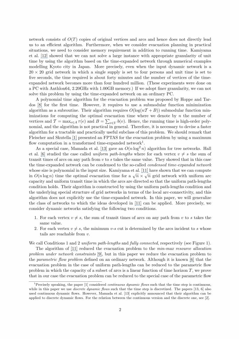
We call Conditions 1 and 2 uniform path-lengths and fully connected, respectively (see Figure 1).The algorithm of [11] reduced the evacuation problem to the min-max resource allocation

problem under network constraints [9], but in this paper we reduce the evacuation problem tothe parametric flow problem defined on an ordinary network. Although it is known [6] that theevacuation problem in the case of uniform path-lengths can be reduced to the parametric flowproblem in which the capacity of a subset of arcs is a linear function of time horizon T , we provethat in our case the evacuation problem can be reduced to the special case of the parametric flow

1Precisely speaking, the paper [1] considered continuous dynamic flows such that the time step is continuous,while in this paper we use discrete dynamic flows such that the time step is discretized. The papers [13, 6] alsoused continuous dynamic flows. However, Mamada et al. [13] explicitly announced that their algorithm can beapplied to discrete dynamic flows. For the relation between the continuous version and the discrete one, see [2].

2

s

2

2

23

3 2

1

1

1

11

4

5

6

3

Figure 1: Example of a fully connected network with uniform path-lengths in which the capacity ofevery arc is one and the number attached to each arc indicate the transit time.

problem studied by [4] which can be solved more efficiently than that considered in [6]. Thus,under Conditions 1 and 2, our algorithm is faster than using the condensed time-expandednetwork. In particular, our algorithm becomes much faster when the in-degree of the sink issmall or considered to be a constant which is often the case with road networks.

The rest of this paper is organized as follows. Section 2 introduces notations and basicresults. Section 3 shows the main result of this paper, i.e., an algorithm for the evacuationproblem in fully connected networks with uniform path-lengths. In Section 4, we consider thecase of grid networks. Section 5 concludes this paper with a further result.

2 Preliminaries

We denote by R+ and Z+ the sets of nonnegative reals and nonnegative integers, respectively.Throughout this paper, we may not distinguish between a singleton {x} and its element x. Fora set X and a singleton {x}, the union of X and {x} is abbreviated by X + x while X \ {x} byX − x. Given a function f : X → R+ on a set X, we use the abbreviation f(Y ) =

∑x∈Y f(x)

for each Y ⊆ X.

2.1 Directed graphs

Let D = (V, A) be a directed graph which may have parallel arcs. A vertex v is said to bereachable from a vertex u when there is a directed path from u to v. We denote by e = uv anarc e whose tail and head are u and v, respectively. If e = uv has no parallel arc, we may simplywrite uv. Furthermore, for each e ∈ A we denote by t(e) and h(e) the tail and the head of e,respectively. For each X ⊆ V , let δD(X) (resp. %D(X)) be the set of arcs e ∈ A with t(e) ∈ Xand h(e) /∈ X (resp. t(e) /∈ X and h(e) ∈ X). For each distinct u, v ∈ V , we denote by λ(u, v;D)the local arc-connectivity from u to v in D, i.e., λ(u, v;D) = min{|%D(W )| : v ∈ W ⊆ V − u}.By Menger’s theorem, λ(u, v;D) is equal to the maximum number of the arc-disjoint directedpaths from u to v in D (see [16, Corollary 9.1b]). For each X ⊆ V , let D[X] denote the directedsubgraph of D induced by X.

2.2 Dynamic networks

Let N = (D = (V, A), c, τ, b, s) be a dynamic network which consists of a directed graph D =(V, A), a capacity function c : A → R+ which represents the upper bound for the rate of flowthat enters each arc per unit time, a transit time function τ : A → Z+ which represents the timerequired to traverse each arc, a supply function b : V → R+ which represents the supply of eachvertex and a sink s ∈ V . We define the length of a directed path P by

∑e∈P τ(e). Since we

3

consider evacuation to s, we assume that %D(s) = ∅ and b(s) = 0, and s is reachable from everyvertex.

We define a dynamic flow f : A × Z+ → R+ as follows. For each e ∈ A and θ ∈ Z+, wedenote by f(e, θ) the flow rate entering e at the time step θ which arrives at h(e) at time stepθ + τ(e). We call f feasible if it satisfies the following three conditions capacity constraint, flowconservation, and demand constraint.

• Capacity constraint. For every e ∈ A and θ ∈ Z+,

0 ≤ f(e, θ) ≤ c(e).

• Flow conservation. For every v ∈ V and Θ ∈ Z+,

∑

e∈δD(v)

Θ∑

θ=0

f(e, θ)−∑

e∈%D(v)

Θ−τ(e)∑

θ=0

f(e, θ) ≤ b(v).

• Demand constraint. There exists Θ ∈ Z+ with

∑

e∈%D(s)

Θ−τ(e)∑

θ=0

f(e, θ) = b(V ). (1)

For a feasible dynamic flow f , we define the evacuation time of f by the minimum time stepΘ satisfying (1), which is denoted by Θ(f). Then, the evacuation problem asks to find theminimum evacuation time among all feasible dynamic flows (denoted by Θ(N )) and a feasibledynamic flow which attains the minimum evacuation time. Given time horizon T , the decisionversion of the evacuation problem with time horizon T asks if there exists a feasible dynamicflow f with Θ(f) ≤ T .

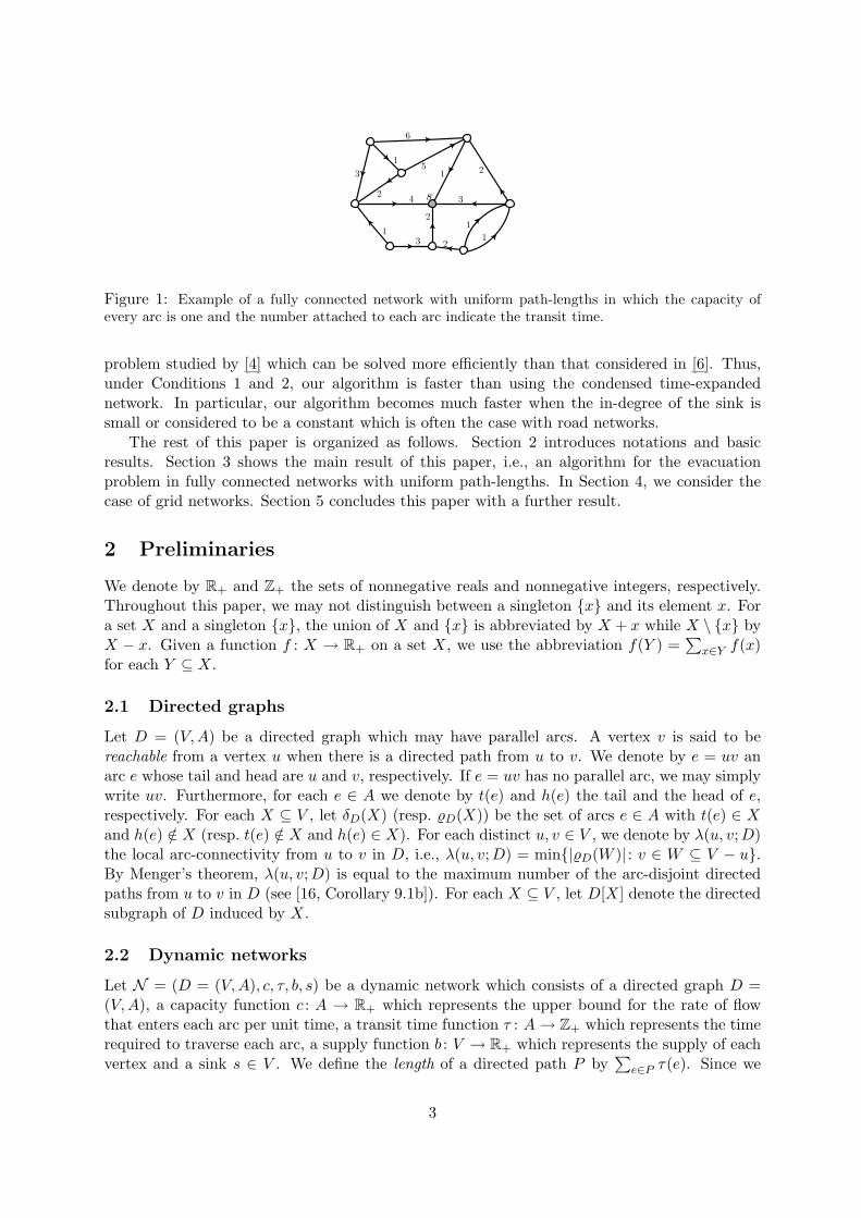
Throughout this paper, we denote |V | and |A| by n and m, respectively. In a figure of adynamic network, the pair of numbers attached to each arc indicates its capacity and transittime. Moreover, the number attached to each vertex indicates its supply (see Figure 2(a)).

2.3 Static networks

Let Ns = (Ds = (Vs, As), cs, bs, Ss) be a static network which consists of a directed graphDs = (Vs, As), a capacity function cs : As → R+, a supply function bs : Vs → R+, and a set ofsinks Ss ⊆ Vs. We call fs : As → R+ a feasible flow if it satisfies the following two conditionscapacity constraint and flow conservation.

• Capacity constraint. For every e ∈ As,

0 ≤ fs(e) ≤ cs(e).

• Flow conservation. For every v ∈ Vs \ Ss,

fs(δDs(v))− fs(%Ds(v)) = bs(v).

Throughout this paper, we denote |Vs| and |As| by ns and ms, respectively. In a figure ofa static network, the number attached to each arc and each vertex indicates its capacity andsupply, respectively. If no number is attached to an arc, it means that its capacity is infinite.Moreover, if no number is attached to a vertex, its supply is equal to zero (see Figure 2(b)).

4

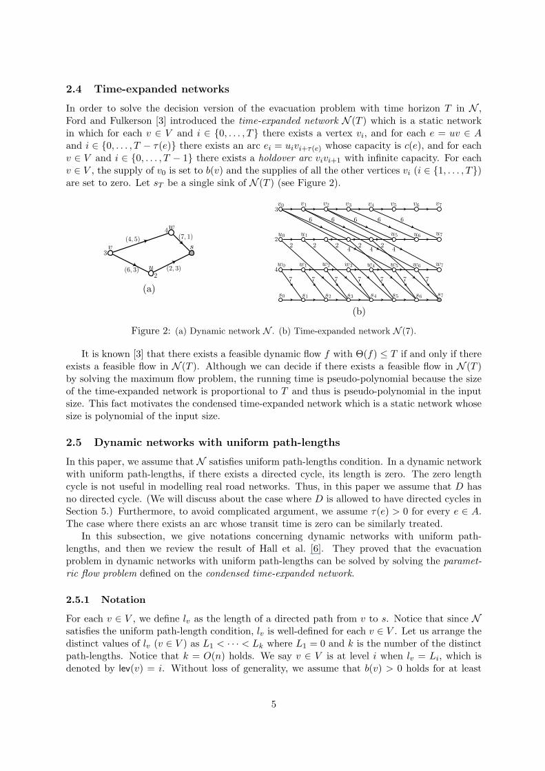
2.4 Time-expanded networks

In order to solve the decision version of the evacuation problem with time horizon T in N ,Ford and Fulkerson [3] introduced the time-expanded network N (T ) which is a static networkin which for each v ∈ V and i ∈ {0, . . . , T} there exists a vertex vi, and for each e = uv ∈ Aand i ∈ {0, . . . , T − τ(e)} there exists an arc ei = uivi+τ(e) whose capacity is c(e), and for eachv ∈ V and i ∈ {0, . . . , T − 1} there exists a holdover arc vivi+1 with infinite capacity. For eachv ∈ V , the supply of v0 is set to b(v) and the supplies of all the other vertices vi (i ∈ {1, . . . , T})are set to zero. Let sT be a single sink of N (T ) (see Figure 2).

sv

u

w

(4; 5) (7; 1)

(6; 3) (2; 3)2

3

4

(a)

6

24

7

6

24

7

6

4

6 6

2

7

2

7

2

777

s0 s1 s2 s3 s4 s5 s6s7

w0 w1 w2 w3 w4 w5 w6 w7

u0 u1 u5 u6u7

v0 v1 v2 v3 v4 v5 v6 v7

4

3

2

(b)

Figure 2: (a) Dynamic network N . (b) Time-expanded network N (7).

It is known [3] that there exists a feasible dynamic flow f with Θ(f) ≤ T if and only if thereexists a feasible flow in N (T ). Although we can decide if there exists a feasible flow in N (T )by solving the maximum flow problem, the running time is pseudo-polynomial because the sizeof the time-expanded network is proportional to T and thus is pseudo-polynomial in the inputsize. This fact motivates the condensed time-expanded network which is a static network whosesize is polynomial of the input size.

2.5 Dynamic networks with uniform path-lengths

In this paper, we assume that N satisfies uniform path-lengths condition. In a dynamic networkwith uniform path-lengths, if there exists a directed cycle, its length is zero. The zero lengthcycle is not useful in modelling real road networks. Thus, in this paper we assume that D hasno directed cycle. (We will discuss about the case where D is allowed to have directed cycles inSection 5.) Furthermore, to avoid complicated argument, we assume τ(e) > 0 for every e ∈ A.The case where there exists an arc whose transit time is zero can be similarly treated.

In this subsection, we give notations concerning dynamic networks with uniform path-lengths, and then we review the result of Hall et al. [6]. They proved that the evacuationproblem in dynamic networks with uniform path-lengths can be solved by solving the paramet-ric flow problem defined on the condensed time-expanded network.

2.5.1 Notation

For each v ∈ V , we define lv as the length of a directed path from v to s. Notice that since Nsatisfies the uniform path-length condition, lv is well-defined for each v ∈ V . Let us arrange thedistinct values of lv (v ∈ V ) as L1 < · · · < Lk where L1 = 0 and k is the number of the distinctpath-lengths. Notice that k = O(n) holds. We say v ∈ V is at level i when lv = Li, which isdenoted by lev(v) = i. Without loss of generality, we assume that b(v) > 0 holds for at least

5

one vertex v ∈ V with lev(v) = k. For each i ∈ {1, . . . , k}, let V≤i be the set of vertices v ∈ Vwith lev(v) ≤ i. Letting Lk+1 = T + 1, we partition interval [0, T ] into disjoint subintervalsI1, I2, . . . , Ik such that Ii = (Li, Li + 1, . . . , Li+1− 1) holds for each i ∈ {1, . . . , k}. For example,for the dynamic network illustrated in Figure 2(a) with T = 7, (ls, lw, lu, lv) = (0, 1, 3, 6). Thus,we have k = 4 and I1 = (0), I2 = (1, 2), I3 = (3, 4, 5), I4 = (6, 7).

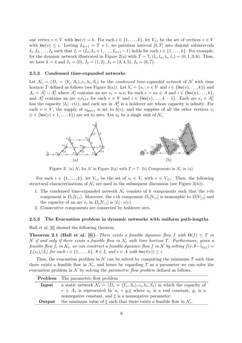
2.5.2 Condensed time-expanded networks

Let Nc = (Dc = (Vc, Ac), cc, bc, Sc) be the condensed time-expanded network of N with timehorizon T defined as follows (see Figure 3(a)). Let Vc = {vi : v ∈ V and i ∈ {lev(v), . . . , k}} andAc = A1

c ∪ A2c where A1

c contains an arc ei = uivi for each e = uv ∈ A and i ∈ {lev(u), . . . , k},and A2

c contains an arc vivi+1 for each v ∈ V and i ∈ {lev(v), . . . , k − 1}. Each arc ei ∈ A1c

has the capacity |Ii| · c(e), and each arc in A2c is a holdover arc whose capacity is infinity. For

each v ∈ V , the supply of vlev(v) is set to b(v), and the supplies of all the other vertices vi

(i ∈ {lev(v) + 1, . . . , k}) are set to zero. Let sk be a single sink of Nc.

s1 s2 s3 s4

w2 w3 w4

u3u4

v4

14

6

2114

12 8

4

2

3

4

(a)

s1 s2 s3 s4

w2 w3 w4

u3u4

v4

14

6

21

4

14

12 8

4

2

3

V1

V2

V3

V4

(b)

Figure 3: (a) Nc for N in Figure 2(a) with T = 7. (b) Components in Nc in (a).

For each i ∈ {1, . . . , k}, let Vc,i be the set of vi ∈ Vc with v ∈ V≤i. Then, the followingstructural characterizations of Nc are used in the subsequent discussion (see Figure 3(b)).

1. The condensed time-expanded network Nc consists of k components such that the i-thcomponent is Dc[Vc,i]. Moreover, the i-th component Dc[Vc,i] is isomorphic to D[V≤i] andthe capacity of an arc ei in Dc[Vc,i] is |Ii| · c(e).

2. Consecutive components are connected by holdover arcs.

2.5.3 The Evacuation problem in dynamic networks with uniform path-lengths

Hall et al. [6] showed the following theorem.

Theorem 2.1 (Hall et al. [6]). There exists a feasible dynamic flow f with Θ(f) ≤ T inN if and only if there exists a feasible flow in Nc with time horizon T . Furthermore, given afeasible flow fc in Nc, we can construct a feasible dynamic flow f in N by setting f(e, θ− lt(e)) =fc(ei)/|Ii| for each i ∈ {1, . . . , k}, θ ∈ Ii and e ∈ A with lev(t(e)) ≤ i.

Thus, the evacuation problem in N can be solved by computing the minimum T such thatthere exists a feasible flow in Nc, and hence by regarding T as a parameter we can solve theevacuation problem in N by solving the parametric flow problem defined as follows.

Problem The parametric flow problemInput a static network Ns = (Ds = (Vs, As), cs, bs, Ss) in which the capacity of

e ∈ As is represented by ae + geξ where ae is a real constant, ge is anonnegative constant, and ξ is a nonnegative parameter;

Output the minimum value of ξ such that there exists a feasible flow in Ns.

6

It is known [15] that the parametric flow problem can be solved by solving the maximumflow problem O(ms) times in Ns. Since for each e ∈ A the capacity of ek is equal to |Ik| · c(e) =(T − Lk + 1) · c(e) by Lk+1 = T + 1, the evacuation problem in N can be solved by solving theparametric flow problem in Nc. Strictly speaking, recalling that what we want to compute isthe minimum nonnegative integer T such that there exists a feasible flow in Nc, the evacuationproblem in N and the parametric flow problem in Nc are not equivalent. This is because theoptimal value of the parametric flow problem may not be an integer. However, letting T ∗ bethe optimal value of the parametric flow problem in Nc, Θ(N ) = dT ∗e holds since a feasibledynamic flow f with Θ(f) ≤ T exists in N if and only if there exists a feasible flow in Nc withtime horizon T .

By |Vc| = O(kn) and |Ac| = O(km), the result of [6] implies that the evacuation problemin N can be solved in O(k3m2n log(kn2/m)) time by the algorithm of [5] solving the maximumflow problem in a static network with ns vertices and ms arcs in O(msns log(n2

s/ms)) time.

3 The Evacuation Problem in Fully Connected Networks

In this section, we assume that N not only satisfies the uniform path-lengths condition butalso satisfies the fully connected condition. For each v ∈ V , let Rv be the set of verticesw ∈ V such that there exists e ∈ %D(s) with t(e) = w and w is reachable from v. Recall thatN = (D = (V, A), c, τ, b, s) is called fully connected if for each v ∈ V − s the minimum v-s cut isdetermined by the arcs incident to s whose tails are reachable from v. That is, the value of theminimum v-s cut is equal to

∑{c(e) : e ∈ %D(s) with t(e) ∈ Rv}. In the subsequent discussion,we concentrate on the unit capacity case, i.e., the capacity of every arc is equal to one. (We willshow that our algorithm can be applied to the integral capacity case in Sections 3.7.) In theunit capacity case, N is fully connected if and only if for each v ∈ V − s

λ(v, s;D) = |{e ∈ %D(s) : t(e) ∈ Rv}|. (2)

We will prove that the evacuation problem inN can be solved by solving the restricted parametricflow problem defined in the following subsection.

3.1 The restricted parametric flow problem

Given a static network Ns = (Ds = (Vs, As), cs, bs, Ss) in which for each e ∈ As

cs(e) =

ae + geξ where ae is a constant, ge is a nonnegativeconstant and ξ is a nonnegative parameter, if e ∈ %Ds(Ss),

constant, otherwise,

the restricted parametric flow problem asks for finding the minimum value of ξ such that thereexists a feasible flow in Ns. This problem can be transformed into the parametric maximum flowproblem studied in [4] by introducing a super source vertex q and arcs from q to every vertexv with bs(v) > 0 such that the capacity of an arc qv is set to bs(v). It is then easy to see thatthere exists a feasible flow in Ns for a fixed ξ if and only if the maximum flow value from q toSs in the transformed problem is equal to bs(Vs).

Lemma 3.1 (Gallo et al. [4]). The maximum flow value from q to Ss in the transformednetwork is a non-decreasing piecewise linear concave function in ξ (which is denoted by κ(ξ)),and the largest breakpoint of κ(ξ) can be found in O(msns log(n2

s/ms)) time.

7

Lemma 3.2. We can determine whether there exists ξ such that there exists a feasible flow inNs, and the minimum such value can be found if one exists in O(msns log(n2

s/ms)) time.

Proof. By the above discussion, there exists a feasible flow in Ns when there exists ξ such thatmaximum flow value in the transformed problem is equal to bs(Vs). On the other hand, themaximum flow value in the transformed problem can not exceed bs(Vs). Thus when ξ is largerthan the largest breakpoint the slope of κ(ξ) is zero and κ(ξ) is less than or equal to bs(Vs).Checking whether there exists ξ such that there exists a feasible flow in Ns reduces to computingthe largest breakpoint of κ(ξ). Moreover, if there exists ξ such that there exists a feasible flowin Ns, the minimum value of such ξ is equal to the largest breakpoint of κ(ξ). Thus, the lemmafollows from Lemma 3.1.

As was defined in Section 2.5, the capacity of ek ∈ A1c inNc contains the parameter T , i.e., it is

a linear function of T . In Figure 3(a), regarding T as the parameter, we have cc(u4s4) = 2(T−5),cc(w4s4) = 7(T − 5), cc(v4u4) = 6(T − 5) and cc(v4w4) = 4(T − 5). Thus, the arcs which are notincident to the sink have the parametric capacities. Therefore, we can not in general reduce theevacuation problem to the restricted parametric flow problem.

3.2 Property of fully connected networks

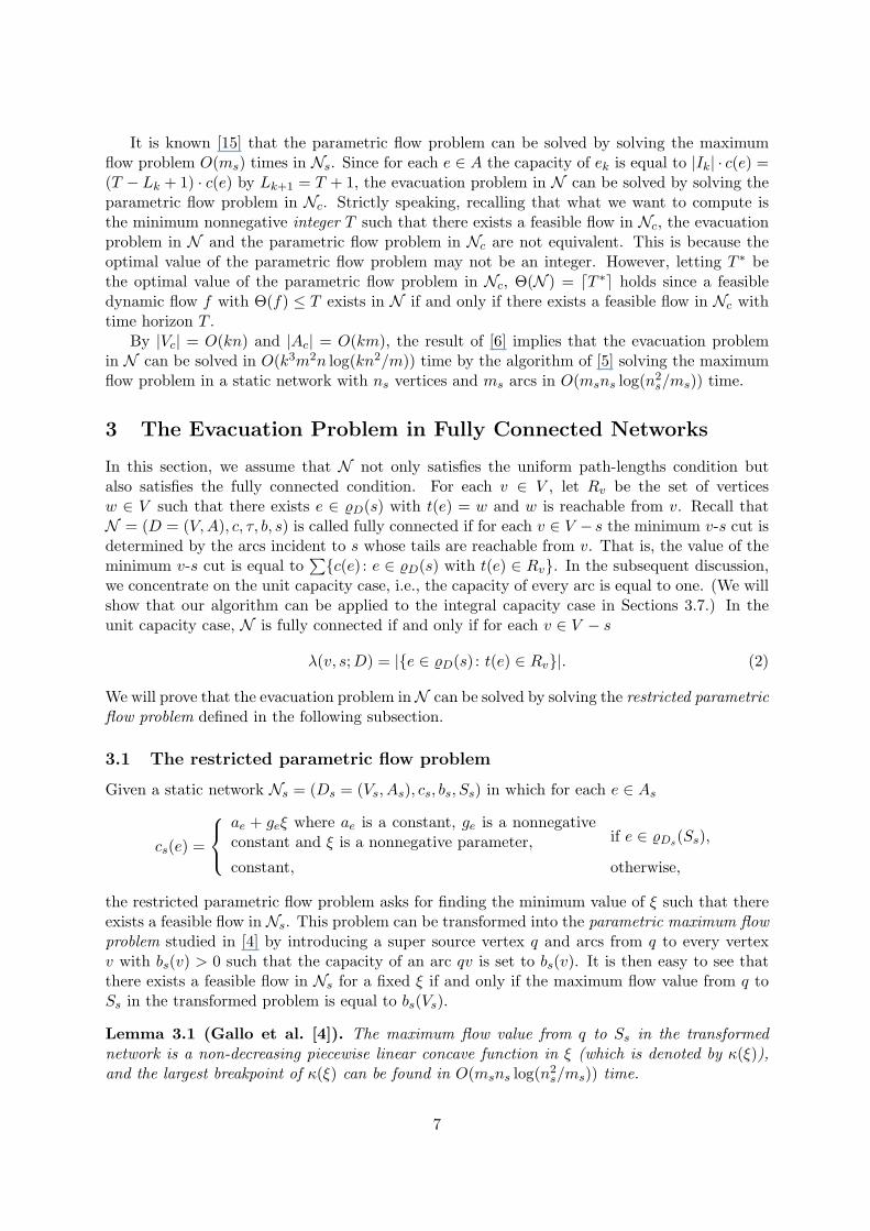
In this subsection, we introduce a property of a fully connected network which plays a crucialrole in the sequel. For each e ∈ %D(s), let V e = {v ∈ V : t(e) is reachable from v} ∪ {s}.Lemma 3.3. There exist arc-disjoint in-trees De = (V e, Ae) (e ∈ %D(s)) rooted at s such thatDe spans V e if and only if (2) holds, i.e,. N is fully connected.

For example, a directed graph D in Figure 4(a) contains two arc-disjoint in-trees De and Df

which satisfy the above condition (see Figures 4(b) and (c)).

sf

e

(a) (b) (c)

Figure 4: (a) D = (V, A). (b) De = (V e, Ae). (c) Df = (V f , Af ).

Proof. It is not difficult to see that the “only if-part” holds. We then prove the “if-part”.We prove that there exist in-trees satisfying the lemma statement for D[V≤i] by induction oni ∈ {2, . . . , k}. For i = 2, this lemma clearly holds.

Assuming that the lemma holds for D[V≤t] with t ≥ 2, we will prove the lemma also holdsfor D[V≤t+1]. For an arbitrary v ∈ V≤t+1 \V≤t, we define a bipartite graph G = (V +∪V −, E) asfollows. Let V + and V − represent arcs of δD(v) and arcs e ∈ %D(s) with t(e) ∈ Rv, respectively.For each e ∈ δD(v) (resp. e ∈ %D(s) with t(e) ∈ Rv), we denote by v+(e) (resp. v−(e)) the vertexin V + (resp. V −) corresponding to e. For each e ∈ δD(v) with h(e) 6= s (resp. h(e) = s) ande′ ∈ %D(s) with t(e′) ∈ Rv, v+(e) and v−(e′) are joined by an edge in E if and only if t(e′) isreachable from h(e) (resp. e = e′) (see Figure 5). Notice that we assume τ(e) > 0 for everye ∈ A, all heads of arcs in δD(v) belong to V≤t.

In order to prove that the lemma holds for D[V≤t ∪ {v}], it is sufficient to prove that thereexists a matching M which saturates V − in G because if there exists such M, by the induction

8

eö2

eö1

eö3

e1

e2

e3

D[Vôt]

sv w2

w3

u1

u2

u3

w1

e4 = eö4

Rv = fv; u1; u2; u3gRw1 = fu1g

Rw2 = fu2gRw3 = fu2; u3g

(a)

V+

Và

và(eö1) v

à(eö2) và(eö3) v

à(eö4)

v+(e1) v

+(e2) v+(e3) v

+(e4)

(b)

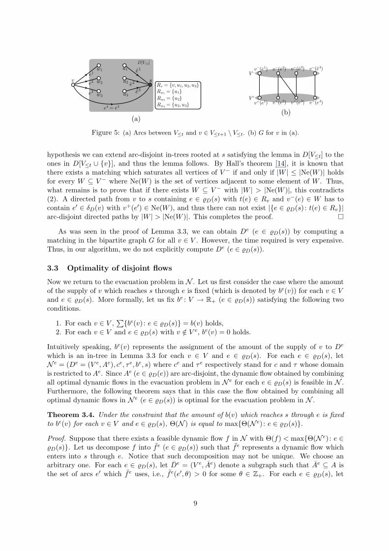
Figure 5: (a) Arcs between V≤t and v ∈ V≤t+1 \ V≤t. (b) G for v in (a).

hypothesis we can extend arc-disjoint in-trees rooted at s satisfying the lemma in D[V≤t] to theones in D[V≤t ∪ {v}], and thus the lemma follows. By Hall’s theorem [14], it is known thatthere exists a matching which saturates all vertices of V − if and only if |W | ≤ |Ne(W )| holdsfor every W ⊆ V − where Ne(W ) is the set of vertices adjacent to some element of W . Thus,what remains is to prove that if there exists W ⊆ V − with |W | > |Ne(W )|, this contradicts(2). A directed path from v to s containing e ∈ %D(s) with t(e) ∈ Rv and v−(e) ∈ W has tocontain e′ ∈ δD(v) with v+(e′) ∈ Ne(W ), and thus there can not exist |{e ∈ %D(s) : t(e) ∈ Rv}|arc-disjoint directed paths by |W | > |Ne(W )|. This completes the proof.

As was seen in the proof of Lemma 3.3, we can obtain De (e ∈ %D(s)) by computing amatching in the bipartite graph G for all v ∈ V . However, the time required is very expensive.Thus, in our algorithm, we do not explicitly compute De (e ∈ %D(s)).

3.3 Optimality of disjoint flows

Now we return to the evacuation problem in N . Let us first consider the case where the amountof the supply of v which reaches s through e is fixed (which is denoted by be(v)) for each v ∈ Vand e ∈ %D(s). More formally, let us fix be : V → R+ (e ∈ %D(s)) satisfying the following twoconditions.

1. For each v ∈ V ,∑{be(v) : e ∈ %D(s)} = b(v) holds,

2. For each v ∈ V and e ∈ %D(s) with v /∈ V e, be(v) = 0 holds.

Intuitively speaking, be(v) represents the assignment of the amount of the supply of v to De

which is an in-tree in Lemma 3.3 for each v ∈ V and e ∈ %D(s). For each e ∈ %D(s), letN e = (De = (V e, Ae), ce, τ e, be, s) where ce and τ e respectively stand for c and τ whose domainis restricted to Ae. Since Ae (e ∈ %D(e)) are arc-disjoint, the dynamic flow obtained by combiningall optimal dynamic flows in the evacuation problem in N e for each e ∈ %D(s) is feasible in N .Furthermore, the following theorem says that in this case the flow obtained by combining alloptimal dynamic flows in N e (e ∈ %D(s)) is optimal for the evacuation problem in N .

Theorem 3.4. Under the constraint that the amount of b(v) which reaches s through e is fixedto be(v) for each v ∈ V and e ∈ %D(s), Θ(N ) is equal to max{Θ(N e) : e ∈ %D(s)}.Proof. Suppose that there exists a feasible dynamic flow f in N with Θ(f) < max{Θ(N e) : e ∈%D(s)}. Let us decompose f into fe (e ∈ %D(s)) such that fe represents a dynamic flow whichenters into s through e. Notice that such decomposition may not be unique. We choose anarbitrary one. For each e ∈ %D(s), let De = (V e, Ae) denote a subgraph such that Ae ⊆ A isthe set of arcs e′ which fe uses, i.e., fe(e′, θ) > 0 for some θ ∈ Z+. For each e ∈ %D(s), let

9

N e = (De = (V e, Ae), ce, be, τ e, s) where ce and τ e respectively represent c and τ whose domainis restricted to Ae. In order to prove the theorem, we show that for each e ∈ %D(s)

Θ(N e) = Θ(N e). (3)

In order to prove (3), we need the following new dynamic network Pe (see Figure 6). We firstshow how the underlying graph Dp = (Vp, Ap) of Pe is constructed. Combining vertices v ∈ V e

with lev(v) = i into a single vertex pi and arranging vertices pk, . . . , p1 along the directed pathin this order, we obtain Dp = (Vp, Ap) where Vp = {pi : i ∈ {1, . . . , k}}, Ap = {pi+1pi : i ∈{1, . . . , k−1}} and p1 is the sink of Pe. The supply of pi is the sum of supplies be(v) over v ∈ V e

with lev(v) = i. Notice that even if there exists no vertex v ∈ V e with lev(v) = i, we preparepi whose supply is zero. The capacity of p2p1 is one, and the capacities of all the other arcs isset to infinity. The transit time of pi+1pi is determined in such a way that the length of thesubpath from pi to p1 is the same as that from v ∈ V with lev(v) = i to the sink s in N .

1

4

1

3

3

3

16

2

2

s3

23

4

u

v

x

y

w

e

(a)

1

4

1

3

3

16

s

3

3

4

(b)

(1; 1)

4371

p1

p2

p3

p4

p5(1; 3) (1; 2) (1; 1)

(c)

Figure 6: (a) Input network N where the numbers attached to each arc represent the transit time. Foreach v ∈ V , let be(v) = b(v). (b) N e. (c) Pe.

Then, we will show that N e, N e and Pe are equivalent in terms of the minimum evacuationtime, which implies (3).

Lemma 3.5. Θ(N e) = Θ(N e) = Θ(Pe).

Proof. The justification behind the lemma is intuitively explained as follows. Since the capacityof every arc in N e is equal to one and De is an in-tree, the bottleneck lies in the arc e (theunique arc incident to s in De). This implies that even if we increase the capacity of all theother arcs to infinity, the minimum evacuation time remains the same. Let N e∞ stand for thedynamic network such that the capacities of all arcs except e are increased to infinity. Then, wehave Θ(N e) = Θ(N e∞) (we give a formal proof later). Since Pe and N e∞ are essentially the same,it is not difficult to see that Θ(Pe) = Θ(N e∞), and thus we have Θ(Pe) = Θ(N e). Furthermore,we can apply the same argument to N e by considering an arbitrary spanning in-tree network inN e. Thus, the lemma follows.

Now we will give a more formal proof of Θ(N e) = Θ(N e∞). In order to prove Θ(N e) =Θ(N e∞), it is sufficient to show Θ(N e) ≤ Θ(N e∞) since the other direction is obvious. Let usconsider a dynamic flow f∞ in N e∞ which attains Θ(N e∞), and we show that we can constructa feasible dynamic flow f in N e which attains Θ(N e∞). Now let us focus on f∞ that enters intothe arc e in N e∞. Since the capacity of e is equal to one, at most one unit of the supply entersinto e at one time. Let us assume that we know from which vertex the supply originally comes.Let us consider f∞(e, θ) (θ ∈ {0, . . . ,Θ(N e∞)−τ(e)}), and decompose it into f∞(e, θ; v) (v ∈ V e)such that f∞(e, θ; v) is equal to the amount of the supply of f∞(e, θ) which originally comesfrom v. We will construct a feasible flow f in N e such that f(e, θ) = f∞(e, θ) holds for every θ.More precisely, we will first construct the subflow f(·, ·; v) of f for every v ∈ V e that representsthe flow of supplies which originate from v in such a way that f(e, θ; v) = f∞(e, θ; v) holds forevery θ. If the arc e′ is on the unique path in De from v to t(e), f(e′, θ; v) is obtained by simply

10

translating f(e, θ; v) by −α where α is the distance from t(e′) to t(e). Otherwise, f(e′, θ; v) isset to zero for all θ. The feasible flow f in N e is then defined as f(e′, θ) =

∑v∈V e f(e′, θ; v)

for every e′ ∈ Ae and θ. Since the capacity of e in N e∞ is equal to one,∑

v∈V e f(e′, θ; v) ≤ 1holds for every e′ ∈ Ae and every θ. Notice that

∑v∈V e f∞(e, θ; v) ≤ 1 holds for any θ since the

capacity of e is equal to one in N e∞, and f is constructed by translating f∞(e, θ). This impliesthat the unit capacity constraint is satisfied for f in N e. It is not difficult to see that f satisfiesthe other constraints.

Now we return to the proof of the theorem. For each e ∈ %D(s), since fe is a feasible dynamicflow in N e, Θ(fe) ≥ Θ(N e) holds. Hence,

Θ(f) = max{Θ(fe) : e ∈ %D(s)} ≥ max{Θ(N e) : e ∈ %D(s)}.

By Lemma 3.5, Θ(N e) = Θ(N e) holds for each e ∈ %D(s). Thus, max{Θ(N e) : e ∈ %D(s)} =max{Θ(N e) : e ∈ %D(s)} holds. This contradicts Θ(f) < max{Θ(N e) : e ∈ %D(s)}.

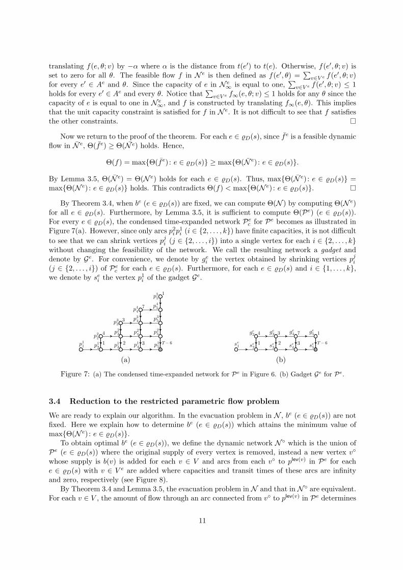
By Theorem 3.4, when be (e ∈ %D(s)) are fixed, we can compute Θ(N ) by computing Θ(N e)for all e ∈ %D(s). Furthermore, by Lemma 3.5, it is sufficient to compute Θ(Pe) (e ∈ %D(s)).For every e ∈ %D(s), the condensed time-expanded network Pe

c for Pe becomes as illustrated inFigure 7(a). However, since only arcs p2

i p1i (i ∈ {2, . . . , k}) have finite capacities, it is not difficult

to see that we can shrink vertices pji (j ∈ {2, . . . , i}) into a single vertex for each i ∈ {2, . . . , k}

without changing the feasibility of the network. We call the resulting network a gadget anddenote by Ge. For convenience, we denote by ge

i the vertex obtained by shrinking vertices pji

(j ∈ {2, . . . , i}) of Pec for each e ∈ %D(s). Furthermore, for each e ∈ %D(s) and i ∈ {1, . . . , k},

we denote by sei the vertex p1

i of the gadget Ge.

4

3

7

1

1 2 3 Tà 6p11 p1

2

p22

p13

p23

p33

p14

p24

p34

p44

p15

p25

p35

p45

p55

(a)

4 3 7 1

1 2 3 Tà 6

ge2

ge3

ge4

ge5

se1 se

2se3

se4

se5

(b)

Figure 7: (a) The condensed time-expanded network for Pe in Figure 6. (b) Gadget Ge for Pe.

3.4 Reduction to the restricted parametric flow problem

We are ready to explain our algorithm. In the evacuation problem in N , be (e ∈ %D(s)) are notfixed. Here we explain how to determine be (e ∈ %D(s)) which attains the minimum value ofmax{Θ(N e) : e ∈ %D(s)}.

To obtain optimal be (e ∈ %D(s)), we define the dynamic network N ◦ which is the union ofPe (e ∈ %D(s)) where the original supply of every vertex is removed, instead a new vertex v◦

whose supply is b(v) is added for each v ∈ V and arcs from each v◦ to plev(v) in Pe for eache ∈ %D(s) with v ∈ V e are added where capacities and transit times of these arcs are infinityand zero, respectively (see Figure 8).

By Theorem 3.4 and Lemma 3.5, the evacuation problem in N and that in N ◦ are equivalent.For each v ∈ V , the amount of flow through an arc connected from v◦ to plev(v) in Pe determines

11

Pe

Pf

xîyîuîvîwî

43431

p1p2p3p4p5

p1p2p3p4p5

Figure 8: The dynamic network N ◦ for N in Figure 6.

be(v). In order to compute Θ(N ◦), we will use a static network Nr which is composed of Ge

(e ∈ %D(s)) as well as source vertices and their incident arcs. Notice that the supplies of verticesin Ge are set to zero.

Theorem 3.6. The evacuation problem in N can be solved by solving the restricted parametricflow problem.

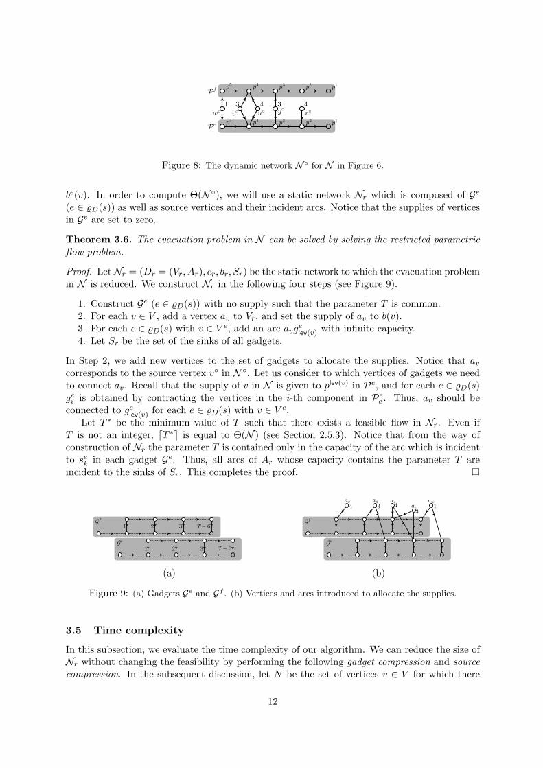
Proof. LetNr = (Dr = (Vr, Ar), cr, br, Sr) be the static network to which the evacuation problemin N is reduced. We construct Nr in the following four steps (see Figure 9).

1. Construct Ge (e ∈ %D(s)) with no supply such that the parameter T is common.2. For each v ∈ V , add a vertex av to Vr, and set the supply of av to b(v).3. For each e ∈ %D(s) with v ∈ V e, add an arc avg

elev(v) with infinite capacity.

4. Let Sr be the set of the sinks of all gadgets.

In Step 2, we add new vertices to the set of gadgets to allocate the supplies. Notice that av

corresponds to the source vertex v◦ in N ◦. Let us consider to which vertices of gadgets we needto connect av. Recall that the supply of v in N is given to plev(v) in Pe, and for each e ∈ %D(s)gei is obtained by contracting the vertices in the i-th component in Pe

c . Thus, av should beconnected to ge

lev(v) for each e ∈ %D(s) with v ∈ V e.Let T ∗ be the minimum value of T such that there exists a feasible flow in Nr. Even if

T is not an integer, dT ∗e is equal to Θ(N ) (see Section 2.5.3). Notice that from the way ofconstruction of Nr the parameter T is contained only in the capacity of the arc which is incidentto se

k in each gadget Ge. Thus, all arcs of Ar whose capacity contains the parameter T areincident to the sinks of Sr. This completes the proof.

2 3 Tà 6

1 2

1

3 Tà 6Gf

Ge

(a)

4 3 1

ax ay auav4

3

aw

Gf

Ge

(b)

Figure 9: (a) Gadgets Ge and Gf . (b) Vertices and arcs introduced to allocate the supplies.

3.5 Time complexity

In this subsection, we evaluate the time complexity of our algorithm. We can reduce the size ofNr without changing the feasibility by performing the following gadget compression and sourcecompression. In the subsequent discussion, let N be the set of vertices v ∈ V for which there

12

exists e ∈ %D(s) with t(e) = v.Gadget compression. Since we construct one gadget for each e ∈ %D(s), the number of gadgetsin Nr is equal to |%D(s)|. However, we can reduce the number of gadgets to |N |. Consider asubset B of %D(s) for which t(e) (e ∈ B) are identical. Since t(e) (e ∈ B) are identical, V e

(e ∈ B) are identical. Thus, vertices in {av : v ∈ V } which are connected to Ge are identical forevery e ∈ B. Hence we can combine Ge (e ∈ B) into a single gadget by magnifying the capacitiesof arcs |B| times.Source compression. We add a new vertex av for each v ∈ V . However, consider the casewhere there exist u, v ∈ V with lev(u) = lev(v) and Ru = Rv. Then, au and av are connectedto the same vertices ge

i for each i = lev(u) = lev(v) and e ∈ %D(s) with u, v ∈ V e. Furthermore,arcs which connects au and av to gadgets have infinite capacities. Thus, it is sufficient to addonly one vertex whose supply is equal to b(u)+ b(v). That is, letting V (i, Q) = {v ∈ V : lev(v) =i and Rv = Q}, we only prepare one vertex ai,Q for each nonempty V (i, Q).

Let Nr be the network obtained from Nr by applying gadget compression and source com-pression. Moreover, let Dr = (Vr, Ar) be the underlying graph of Nr. Let us analyze the size ofNr. Let η be the number of distinct combinations of the path-length from a vertex v ∈ V to sand Rv, i.e., η = |{(lv, Rv) : v ∈ V }|. Notice that η is equal to the number of vertices added toallocate the supplies in Nr, i.e., all ai,Q defined above, and η = O(n) and η ≥ k hold. Thus, wehave |Vr| = O(k|N |+ η) and |Ar| = O(η|N |).

Next we consider the time required to construct Nr.

Lemma 3.7. We can construct Nr in O(min{m + n2|N |,m|N |}+ n log n) time.

Proof. We construct Nr as follows. We first compute lv for all v ∈ V in O(m) time by breadthfirst search from s since N satisfies the uniform path-length condition. After this, we cancompute lev(v) for all v ∈ V in O(n log n) time by sorting {lv : v ∈ V }. Furthermore, we canconstruct all gadgets in O(|%D(s)|+ k|N |) time.

To add the vertices and arcs to allocate the supplies, we compute V (i, Q). First we obtainRv for all v ∈ V by depth-first search from all u ∈ N in O(min{m + n2|N |,m|N |}) time. Then,we partition V according to lev(v) in O(n) time to obtain the set of vertices v whose lev(v) takesthe same value. Next we assign the values 21, . . . , 2|N | to each u ∈ N . Then, for each set Wof vertices v whose lev(v) takes the same value, we compute the sum of the values of u ∈ Rv

for each v ∈ W , and sort the vertices v ∈ W according to the sum of the assigned values ofu ∈ Rv. Notice that for v, w ∈ V with Rv 6= Rw the sum of the assigned values of the verticesin Rv can never be equal to that of the vertices in Rw. The time required to complete thisoperation for all levels i ∈ {1, . . . , k} is O(n|N |+ n log n). Thus, this step can be completed inO(min{m + n2|N |,m|N |}+ n log n) time, which completes the proof.

The following theorem holds from the above two lemmas and Theorem 3.2.

Theorem 3.8. Given a fully connected dynamic network N with uniform path-lengths in whichthe capacity of every arc is equal to one, Θ(N ) can be computed in O(η|N |(k|N | + η) log n +min{m + n2|N |,m|N |}+ n log n) time.

Let us express the running time given in the above theorem in terms of n and m. Recallthat the number of arcs added to allocate the supplies is O(η|N |). Thus, this number is O(n2)by η = O(n) and |N | = O(n). However, we show that the number of the arcs added to allocatethe supplies is O(m). This number is at most

∑v∈V−s |Rv| since ai,Rv is connected to at most

|Rv| gadgets. By Rv ⊆ N for each v ∈ V − s, it is clear that∑

v∈V−s|Rv| ≤∑

v∈V−s|{e ∈ %D(s) : t(e) ∈ Rv}|.

13

Furthermore, |δD(v)| ≤ |{e ∈ %D(s) : t(e) ∈ Rv}| for each v ∈ V − s since N is fully connectedand the capacity of any arc is one. Thus, we have

∑v∈V−s |Rv| ≤

∑v∈V−s |δD(v)| = m. Since

the number of arcs in all gadgets is equal to O(k|N |), |Ar| = O(min{n2, kn + m}) holds. Thus,the following corollary follows from Lemma 3.2.

Corollary 3.9. Given a fully connected dynamic network N with uniform path-lengths in whichthe capacity of every arc is equal to one, Θ(N ) can be computed in O(min{m+kn3 log n, (k2n2 +kmn) log n}) time.

If we simply apply the algorithm of [6] to solve the evacuation problem in a fully connectednetwork N with uniform path-lengths, the time complexity is O(k3m2n log(kn2/m)). Our algo-rithm much improves the time bound in the fully connected and uniform path-lengths case. Inmany practical cases, the in-degree of the sink (i.e. |N |) can be considered as a constant, andthus the time complexity of our algorithm becomes O(m+n2 log n) in this case by Theorem 3.8.

3.6 Computing an optimal flow

The algorithm described in Section 3.4 only computes Θ(N ), but not an optimal dynamic flow.If we explicitly obtain N e (e ∈ %D(s)), an optimal flow in N can be computed by separatelycomputing Θ(N e) (e ∈ %D(s)) by using the algorithm of [13] which can compute an optimalflow in a dynamic tree network. However, the time required to compute N e (e ∈ %D(s)) is veryexpensive (see Section 3.2). Thus, in this subsection, we present an algorithm to compute anoptimal flow without computing N e (e ∈ %D(s)).

Our algorithm presented in Section 3.4 relies on the restricted parametric flow algorithm forNr. Recall that a gadget Ge is a static network with no supply which is obtained by shrinkingcertain vertex sets of Pe

c . Thus, it is a nontrivial task to obtain an optimal dynamic flow evenafter we obtain a feasible flow in Nr with T = Θ(N ). Notice that if we can find a feasibleflow in the condensed time-expanded network Nc with T = Θ(N ), we can easily constructa feasible dynamic flow by Theorem 2.1. Thus, since we already know Θ(N ), we can findan optimal dynamic flow by a single computation of the maximum flow in Nc. This requiresO(k2mn log n) time by using the maximum flow algorithm of [5] by |Vc| = O(kn) and |Ac| =O(km), respectively. However, we want to do it faster. In this subsection, we show that anoptimal flow can be computed in O(kmn log n) time by using the information of a feasible flowobtained in Nr with T = Θ(N ). In our algorithm, we sequentially compute a feasible flow inthe i-th component of Nc from i = 1 to k instead of computing a feasible flow for the whole Nc

at one time. In this section, we fix the value of T to Θ(N ).

3.6.1 Recovering a feasible flow in Nr from a feasible flow in Nr

We first construct a feasible flow fr inNr from a feasible flow fr inNr. Recall thatNr is obtainedfrom Nr by applying gadget compression and then source compression (see Section 3.5). LetNr′ be the network obtained from Nr by performing gadget compression. For each v ∈ N , letGv

r be the gadget in Nr. We first compute a feasible flow fr′ in Nr′ from a feasible flow fr inNr. After this, we compute a feasible flow fr in Nr from fr′ .From fr to fr′. Let us consider a vertex ai,Q in Nr, and suppose that ai,Q is connected togadgets Gv

r (v ∈ N ′) with N ′ ⊆ N . Recall that ai,Q was obtained by combining vertices ofV (i, Q) into a single one. Thus, for each v ∈ V (i, Q) we will determine the flow value of an arcfrom av to Gw

r (w ∈ N ′). This is simply done by arbitrarily splitting the values of fr for arcsfrom ai,Q to Gv

r (v ∈ N ′) so that the sum of the flow values of arcs from av to Gvr (v ∈ N ′)

14

does not exceed b(v) (see Figure 10). Notice that even if we split the values of fr for arcs fromai,Q, the amount of flow entering into each gadget does not change. Thus, flow conservation issatisfied at vertices in Gv

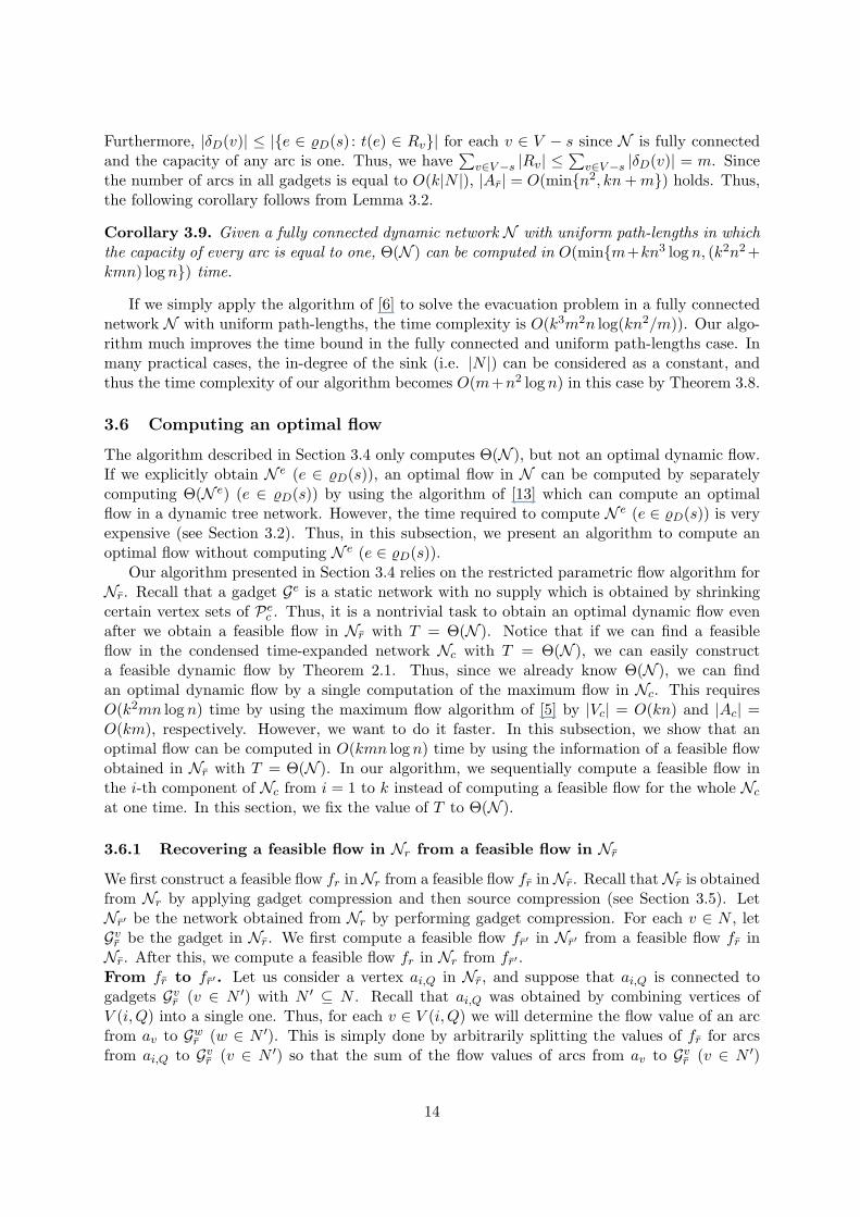
r (v ∈ N ′). This step is done in O(n2) time.From fr′ to fr. Let us consider a gadget Gv

r in Nr, and suppose that Nr is obtained bycombining gadgets Ge (e ∈ B) with B ⊆ %D(s). The values of fr for arcs in Ge (e ∈ B) canbe obtained by simply equally dividing the value of fr′ by |B|. Similarly, for each v ∈ V , thevalues of fr for arcs connected from av to vertices in Ge (e ∈ V ) can be also simply computedby equally dividing the value of fr′ by |B|. This step is done in O(nm) time. Thus, the timerequired to compute fr from fr does not affect total time of the algorithm.

0 0

1

1

1

1

2

22

2

2

3

33

3

3

44

1

a2;fxg a3;fx;yg a4;fx;yg a5;fx;yg

(a)

ax ay auav

aw

11

2

22

2

2

33

3

4

1

0 01

3 221

2

1

(b)

Figure 10: (a) Feasible flow fr in Nr for N in Figure 6(a). The number attached to an arc indicates thevalue of flow. (b) Feasible flow fr′ in Nr′ .

3.6.2 Computing a feasible flow in Nc

In this section, we explain how to find a feasible dynamic flow in Nc. For this, we introducenecessary definitions. Recall that for each v ∈ V , only vlev(v) has the positive supply among vi

(i ∈ {lev(v), . . . , k}) in Nc. Let us consider a feasible flow fc in Nc, and suppose that we candistinguish the supplies originating from each vlev(v) in fc. When the supplies originating fromvlev(v) does not pass through holdover arcs other than vivi+1 (i ∈ {lev(v), . . . , k − 1}) for everyv ∈ V , fc is called simple. The algorithm explained below finds a simple feasible flow in Nc.

For a feasible flow fc in Nc and each v ∈ V , if a certain amount of the supply of vlev(v)

flows into arcs of the i-th component, this amount is called the supply of v consumed in thei-th component and is denoted by σi(v). Here we show that if we know σi(v) (i ∈ {1, . . . , k}and v ∈ V ), we can restore a simple feasible flow fc. Notice that σi(v) = 0 for each v ∈ V andi ∈ {1, . . . , lev(v)− 1}, and b(v) =

∑ki=1 σi(v) hold for each v ∈ V . Since fc is a simple feasible

flow, fc(vivi+1) is b(v)−∑it=1 σt(v) for each v ∈ V and i ∈ {1, . . . , k − 1}. Then the flow value

on arcs in the i-th component can be found by simply obtaining a feasible flow by setting thesupply value at vi ∈ Vc to σi(v) in the i-th component which has a single sink si. Namely, wecan restore fc by computing maximum flow problems k times for the network with O(n) verticesand O(m) arcs once we know σi(v) (i ∈ {1, . . . , k} and v ∈ V ).

If σi : V → R+ (i ∈ {1, . . . , k}) represent the supply amount consumed in the i-componentsfor some simple feasible flow in Nc, they are called eligible. Thus, our aim is to obtain σi

(i ∈ {1, . . . , k}) which are eligible. Recall that for each e ∈ %D(s) and v ∈ V e, fr(avgelev(v))

is equal to be(v), i.e., the allocation of the supply of v to N e. For each e ∈ %D(s), let N ec be

the condensed time-expanded network of N e with the supply of v ∈ V e set to be(v). For eache ∈ %D(s), we first obtain σe

i : V → R+ (i ∈ {1, . . . , k}) which is eligible in N ec where σe

i isdefined in a manner similar to σi. Since Ae (e ∈ %D(s)) are disjoint, the union of simple feasibleflows of N e

c (e ∈ %D(s)) becomes a simple feasible flow of Nc. Thus, we can obtain an eligibleσi (i ∈ {1, . . . , k}) by setting σi(v) =

∑{σei (v) : e ∈ %D(s)} for each v ∈ V . Hence, we will focus

15

on how to compute σei (i ∈ {1, . . . , k}) which is eligible in N e

c for each e ∈ %D(s). The algorithmis described in Procedure 1. We will prove its correctness. Notice that in the procedure we donot need to obtain N e, but we only need to know V e.

Procedure 11: For each i ∈ {1, . . . , k} and v ∈ V , set σe

i (v) = 0．2: For each e ∈ %D(s) and v ∈ V e, set σe

lev(v)(v) = fr(avgelev(v)).

3: for each i ∈ {1, . . . , k − 1} and e ∈ %D(s) do4: if

∑v∈V σe

i (v) > fr(gei s

ei ) then

5: Set σei : V → R+ so that σe

i (V ) = fr(gei s

ei ) with 0 ≤ σe

i (v) ≤ σei (v).

6: for each v ∈ V with σei (v) < σe

i (v) do7: Set σe

i+1(v) = σei (v)− σe

i (v), and then set σei (v) = σe

i (v).8: end for9: end if

10: end for

Let us fix e ∈ %D(s), and we prove that σei (i ∈ {1, . . . , k}) by Procedure 1 are eligible in

N ec . For this, it is sufficient to prove the following statements by the definition of eligibility.

1. For every v ∈ V \ V e and i ∈ {1, . . . , k}, σei (v) = 0 holds.

2. For every v ∈ V e and i ∈ {1, . . . , lev(v)− 1}, σei (v) = 0 holds.

3. For each i ∈ {1, . . . , k}, there exists a feasible flow in the i-th component with setting thesupply of vi to σe

i (v).

Conditions 1 and 2 clearly hold. Therefore, we prove that Statement 3 holds.In order that there exists a feasible flow in N e

c , it is sufficient to show σei (V

e) ≤ |Ii| since thei-th component of N e

c is an in-tree rooted at si and every arc capacity is equal to |Ii|. However,this obviously holds since the procedure at lines 7 carries over the excess of σe

i (Ve) − fr(ge

i sei )

to the (i + 1)-st component which is equal to fr(gei g

ei+1), and fr(ge

i sei ) ≤ cr(ge

i sei ) = |Ii| holds

by the capacity constraint in Nr. Since the time complexity of Procedure 1 is clearly O(knm),we obtain the following theorem. Recall that once we obtain eligible σi (i ∈ {1, . . . , k}), we canrestore a feasible flow in O(kmn log n) time.

Theorem 3.10. Given a fully connected dynamic network N with uniform path-lengths, anoptimal flow for the evacuation problem in N can be computed in the time required to computeΘ(N ) plus O(kmn log n) time.

3.7 Integral capacity case

In the case where the capacities of arcs are integral, we can prove by splitting each arc with morethan unit capacity into parallel ones whose capacity is one that our algorithm can be appliedto this case. However, in this case, the number of arcs added to Nr for allocation of supplies isnot O(m). That is, in this case we can not say that the time complexity required to computeΘ(N ) is O(k2n2 + kmn log n) unlike the unit capacity case. Notice that since we assume thatthere exist no parallel arcs without loss of generality, the time required to compute an optimalflow is dominated by that required to compute the optimal value.

Theorem 3.11. Given a fully connected dynamic network N with uniform path-lengths such thata capacity of every arc is integral, we can compute Θ(N ) in the same complexity of Theorem 3.8or O(m + kn3 log n). Moreover, an optimal flow can be computed in O(m + kn3 log n) time.

16

4 Evacuation Problem in Grid Networks with Unit Capacity

In the paper [11], we considered the evacuation problem in a√

n×√n grid network with uniformarc capacity and uniform transit time such that the arc is directed so that the condition ofuniform path-lengths holds. In the previous section, we generalized the class of networks whichthe ideas developed in [11] can be applied to. We again consider in this section the evacuationproblem in grid networks with unit capacity.

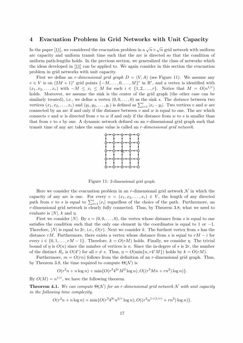
First we define an r-dimensional grid graph D = (V, A) (see Figure 11). We assume anyv ∈ V is on (2M + 1)r grid points {−M, . . . , 0, . . . , M}r in Rr, and a vertex is identified with(x1, x2, . . . , xr) with −M ≤ xi ≤ M for each i ∈ {1, 2, . . . , r}. Notice that M = O(n1/r)holds. Moreover, we assume the sink is the center of the grid graph (the other case can besimilarly treated), i.e., we define a vertex (0, 0, . . . , 0) as the sink s. The distance between twovertices (x1, x2, . . . , xr) and (y1, y2, . . . , yr) is defined as

∑ri=1 |xi−yi|. Two vertices v and w are

connected by an arc if and only if the distance between v and w is equal to one. The arc whichconnects v and w is directed from v to w if and only if the distance from w to s is smaller thanthat from v to s by one. A dynamic network defined on an r-dimensional grid graph such thattransit time of any arc takes the same value is called an r-dimensional grid network.

s

Figure 11: 2-dimensional grid graph.

Here we consider the evacuation problem in an r-dimensional grid network N in which thecapacity of any arc is one. For every v = (x1, x2, . . . , xr) ∈ V , the length of any directedpath from v to s is equal to

∑ri=1 |xi| regardless of the choice of the path. Furthermore, an

r-dimensional grid network is clearly fully connected. Thus, by Theorem 3.8, what we need toevaluate is |N |, k and η.

First we consider |N |. By s = (0, 0, . . . , 0), the vertex whose distance from s is equal to onesatisfies the condition such that the only one element in the coordinates is equal to 1 or −1.Therefore, |N | is equal to 2r, i.e., O(r). Next we consider k. The furthest vertex from s has thedistance rM . Furthermore, there exists a vertex whose distance from s is equal to rM − i forevery i ∈ {0, 1, . . . , rM − 1}. Therefore, k = O(rM) holds. Finally, we consider η. The trivialbound of η is O(n) since the number of vertices is n. Since the in-degree of s is 2r, the numberof the distinct Rv is O(4r) for all v 6= s. Thus, η = O(min{n, r4rM}) holds by k = O(rM).

Furthermore, m = O(rn) follows from the definition of an r-dimensional grid graph. Thus,by Theorem 3.8, the time required to compute Θ(N ) is

O(r2n + n log n) + min{O(r342rM2 log n), O((r3Mn + rn2) log n)}.By O(M) = n1/r, we have the following theorem.

Theorem 4.1. We can compute Θ(N ) for an r-dimensional grid network N with unit capacityin the following time complexity.

O(r2n + n log n) + min{O(r342rn2/r log n), O((r3n1+(1/r) + rn2) log n)}.

17

If r = 2, the time complexity is O(n log n). This matches the result of [11] in the case of2-dimensional grid network.

5 Discussion

Here we consider the algorithm for the evacuation problem in the case where the underlyinggraph is not acyclic. As mentioned before, the length of a directed cycle is zero in a dynamicnetwork with uniform path-lengths. Thus, the existence of directed cycles with zero length ispractically meaningless, but it may be of theoretical interest to consider the case where thereexist directed cycles from the theoretical viewpoint. In fact, we use the fact that the underlyinggraph of the input dynamic network is acyclic only to prove Lemma 3.3, and it is clear thatthe other discussions hold without acyclicity assumption. Recently, Kamiyama et al [10] provedthat Lemma 3.3 also holds in the case where the underlying graph is allowed to have cycles.Thus, we can apply the algorithm presented in this paper to dynamic networks with cycles.

As a related problem to the evacuation problem, there exists the universally quickest flowproblem defined as follows. Given a dynamic network, the problem asks for finding a dynamicflow which attains the minimum evacuation time and also maximizes the amount of the suppliesthat has reached the sink at every time step. We have recently proved that this problem can beefficiently solved in a fully connected network with uniform path-lengths. However, the proofneeds several non-trivial discussions. Thus, we will present this result elsewhere.

Acknowledgement. We appreciate the comments of anonymous reviewers who helped im-prove the presentation of this paper. The first author is supported by JSPS Research Fellowshipsfor Young Scientists. The second and third authors are supported by the project New Horizonsin Computing, Grant-in-Aid for Scientific Research on Priority Areas, MEXT Japan.

References

[1] L. Fleischer and M. Skutella. Quickest flows over time. SIAM J. Comput., 36(6):1600–1630,2007.

[2] L. Fleischer and E. Tardos. Efficient continuous-time dynamic network flow algorithms.Oper. Res. Lett., 23(3-5):71–80, 1998.

[3] L.R. Ford and D.R. Fulkerson. Flows in Networks. Princeton University Press, 1962.

[4] G. Gallo, M. D. Grigoriadis, and R. E. Tarjan. A fast parametric maximum flow algorithmand applications. SIAM J. Comput., 18(1):30–55, 1989.

[5] A. V. Goldberg and R. E. Tarjan. A new approach to the maximum-flow problem. J. ACM,35(4):921–940, 1988.

[6] A. Hall, S. Hippler, and M. Skutella. Multicommodity flows over time: Efficient algorithmsand complexity. Theor. Comput. Sci., 379(3):387–404, 2007.

[7] H. W. Hamacher and S. A. Tjandra. Mathematical modelling of evacuation problem: stateof the art. In M. Schreckenberg and S. D. Sharma, editors, Pedestrian and EvacuationDynamics, pages 227–266. Springer, 2002.

18

[8] B. Hoppe and E. Tardos. The quickest transshipment problem. Mathematics of OperationsResearch, 25(1):36–62, 2000.

[9] T. Ibaraki and N. Katoh. Resource allocation problems under submodular constraints. InResource Allocation Problems : Algorithmic Approaches, pages 144–176. MIT Press, 1988.

[10] N. Kamiyama, N. Katoh, and A. Takizawa. Arc-disjoint in-trees in directed graphs. Com-binatorica. to appear. Preliminary version has appeared in Proc. of the nineteenth AnnualACM-SIAM Symposium on Discrete Algorithms (SODA2008), pages 518–526, 2008.

[11] N. Kamiyama, N. Katoh, and A. Takizawa. An efficient algorithm for evacuation problemin dynamic network flows with uniform arc capacity. IEICE Transaction on Infromationand Systems, E89-D:2372–2379, 2006.

[12] N. Kamiyama, N. Katoh, and A. Takizawa. Theoretical and practical issues of evacuationplanning in urban areas. In Proc. the eighth Hellenic European Research on ComputerMathematics and its Applications Conference (HERCMA2007), pages 49–50, 2007.

[13] S. Mamada, T. Uno, K. Makino, and S. Fujishige. An O(n log2 n) algorithm for the op-timal sink location problem in dynamic tree networks. Discrete Applied Mathematics,154(16):2387–2401, 2006.

[14] W.R. Pulleyblank. Matchings and extensions. In R.L. Graham, M. Grotschel, and L. Lovasz,editors, Handbook of Combinatorics, volume 1, pages 179–233. MIT Press, 1995.

[15] T. Radzik. Parametric flows, weighted means of cuts, and fractional combinatorial opti-mization. In P.M. Pardalos, editor, Complexity in Numerical Optimization, pages 351–386.World Scientific, 1993.

[16] A. Schrijver. Combinatorial Optimization: Polyhedra and Efficiency (Algorithms and Com-binatorics). Springer, 2003.

19