An Automatic System for Longitudinal Control Of Individual Vehicles R. L. COSGRIFF, J. J. ENGLISH and W. B. ROECA

Department of Electrical Engineering, Ohio State University

•IT APPEARS today that considerable improvement in high-density traffic flow can be achieved by automatic control of individual highway vehicles. An automatic system for controlling an individual vehicle in a traffic stream in response to the immediately preceding vehicle is currently being studied. It has been found that there are a number of requirements which must be met by any system for control of vehicles in traffic. The proposed system which meets these requirements is a combination of several con -trol techniques. It should not be surprising that the system is in some ways similar to the driver himself.

This paper includes a short description of the traffic situation variables, the re­quirements on the system, a description of the system itself, and a discussion of the performance of the system. It is of course impossible to treat the several aspects of this control problem in detail.

NOTATION

Consider a line of n vehicles progressing along a highway in the direction of + x as shown in Figure 1. The lead car will be indexed 1, the indexes of the others progress­ing to Nat the rear; xi is the distance from a fixed origin on the road to the front of the i th car. The velocity of the i th car relative to the road is

or, in operator notation,

where

The absolute acceleration (relative to the road) of the i th car is

or , in operator form,

dv. l

ai = dt

Paper sponsored by Committee on Vehicle Characteristics.

7

8

Vj Vi- 1 V2 v, ----+ ;--I-L . . .. ,.,

~t~ ~ ~ 11D ~ XN \+1 x. X. x x

I 1-1 z 0 +x

\ 1..- h;----..1 / (break in scale ) ...../

Figure 1. Traffic system variables.

The headway of the i th car is

INCREASING TIME - x.

l

The relative velocity or rate of closure between the i th and i - 1 st vehicle is

Figure 2. Typical phase plane trajectory.

The relative acceleration of the i - 1st car from the i th car is

- a. l

These are all instantaneous values of variable functions of time.

- " 'i

These variables are conveniently represented by points on phase plane plots. On a phase plane plot, the abscissa of a point is the instantaneous value of the variable, and the ordinate is the instantaneous value of the time derivative of the variable. As time increases, the point representing the variable and its derivative traces out a phase plane trajectory. A typical plot is shown in Figure 2. If the i th car in a line of cars is controlled by an automatic control system, then the point p (the leading end of the phase trajectory) represents the curr ent head,.i.ray and relative velocity existing be­tween the controlled car and the lead car. The region R r epr esents a set of situations which can exist between the controlled car and the lead car. If the point p is in the region R as shmvn (Fig. 2) , the traffic situation vll.11 be r eferred to as being "in regfon R" for the purpose of brevity.

Techniques have been developed which make possible the sensing of the lead car by the controlled car. When it is sensed, the controlled car is in the region of influen.ce of the lead car. This region is finite in length, but adequate. Also, the variables vr.

1 and hi _ 1 can be computed by electronic circuits in the controlled i th car.

l -The outputs of these circuits are electrical signals proportional to Vr and h. 1 .

i - 1 l -

In the remainder of this paper this measurement of Vr. _ 1

and hi _ 1 is considered ideal. 1

9

REQUIREMENTS OF INDIVIDUAL VEIIlCLE CONTROL SYSTEM

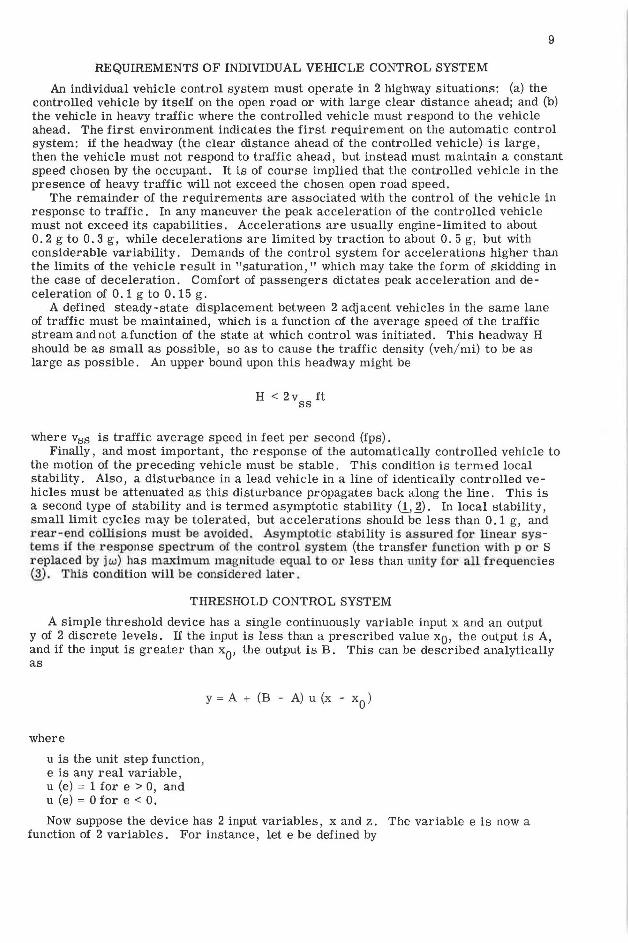
An individual vehicle control system must operate in 2 highway situations: (a) the controlled vehicle by itself on the open road or with large clear distance ahead; and (b) the vehicle in heavy traffic where the controlled vehicle must respond to the vehicle ahead. The first environment indicates the first requirement on the automatic control system: if the headway (the clear distance ahead of the controlled vehicle) is large, then the vehicle must not respond to traffic ahead, but instead must maintain a constant speed chosen by the occupant. It is of course implied that the controlled vehicle in the presence of heavy traffic will not exceed the chosen open road speed.

The remainder of the requirements are associated with the control of the vehicle in response to traffic. In any maneuver the peak acceleration of the controlled vehicle must not exceed its capabilities. Accelerations are usually engine- limited to about 0. 2 g to 0. 3 g, while decelerations are limited by traction to about 0. 5 g, but with considerable variability. Demands of the control system for accelerations higher than the limits of the vehicle result in "saturation," which may take the form of skidding in the case of deceleration. Comfort of passengers dictates peak acceleration and de­celeration of 0.1 g to 0.15 g.

A defined steady-state displacement between 2 adjacent vehicles in the same lane of traffic must be maintained, which is a function of the average speed of the traffic stream and not afunction of the state at which control was initiated. This headway H should be as small as possible, so as to cause the traffic density (veh/ mi) to be as large as possible. An upper bound upon this headway might be

H < 2v ft SS

where Vss is traffic average speed in feet per second (fps). Finally, and most important, the response of the automatically controlled vehicle to

the motion of the preceding vehicle must be stable. This condition is termed local stability. Also, a disturbance in a lead vehicle in a line of identically controlled ve­hicles must be attenuated as this disturbance propagates back along the line. This is a second type of stability and is termed asymptotic stability (!, ~. In local stability, small limit cycles may be tolerated, but accelerations should be less than 0.1 g, and rear-end collisions must be. avoided. Asymptotic stability is assured for linear sys­tems if the response spectrum of the control system (the transfer fw1ction with p or S replaced by jw) has maximum magnitude equal to or less than unity for all frequencies ~). This condition will be considered later.

THRESHOLD CONTROL SYSTEM

A simple threshold device has a single continuously variable input x and an output y of 2 discrete levels. If the input is less than a prescribed value x0 , the output is A, and if the input is greater than x0, the output is B. This can be described analytically as

where

u is the unit step function, e is any real variable, u (e) = 1 for e > 0, and u (e) = 0 for e < 0.

y = A + (B - A) u (x - x0

)

Now suppose the device has 2 input variables, x and z. The variable e is now a function of 2 variables. For instance, let e be defined by

10

z2 e = x - x0 -

2

z2 Now y =A when e < 0, or when x < x 0 + 2

z2 When x > x 0 + 2, y = B. If a plot is

made of z vs x, the threshold is a parabola

which divides the z - x plane into 2 regions, one to the left of the parabola and one to its right.

Tf thP. variable x is replaced by headway : the variable z by relative velocitv, the variable y by acceleration of the controlled car, and if B = 0 and A = a deceleration level, then a very s}mple control system is described. When the headway hi_ 1 is less

(vr. - 1 )~ than x

0 + 1

2 , the controlled car is decelerated by A ft/ sec2

, and when

(vri-1)2 hi _ 1 > x

0 + 2 ,the controlled car's velocity is constant.Thus the

vn - 1 - hi - 1 phase plane is divided into 2 regions by the parabola,

( vri - 1 )2 hi - 1 = XO + 2

To meet the requirements of the traffic environment, a combination of threshold devices is needed which divides the v - h.

1 phase plane into several regions

ri - 1 1 -

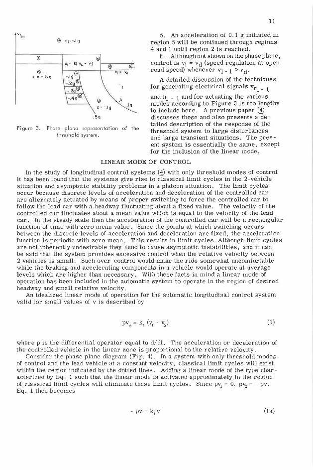
(Fig . 3) . There are of cour s e m any alternative s , which are being investigated at t he pr esent tim e. A s implified version of Figure 3 is discussed elsewhere (1) in detail, including the per for mance of the threshold system and the e lectronic operations ne­cessary to its actuation. The major difference in Figure 3 is the addition of a linear mode, which is discuss ed in t he next section .

'The phase plane representation for the threshold ~orrtrol of thP i i-h c~:.:.r is riivid8d into a number of regions (Fig. 3). Each region has associated with it a certain mode of control of the i th car. For example, if v and h.

1 are coordinates of a

ri - 1 i -

point in region 2, the ith car is decelerating at a constant 0.1 g. The boundaries of the regions are not trajectories , although certain trajectories can be coincident with some of the boundaries. For instance, the parabolic trajectory of constant relative acceleration a of + 0.1 g magnitude would be coincident with the parabolic bound-

ri - 1 ary between regions 1 and 2 if the initial point of the trajectory wer e on the boundar y , such as point A. The control in the individual regions is as follows (numbers of regions are circled in Figure 3):

1. In region 1 the system is a speed regulator with constant speed v d chosen by the driver.

2. In regions 2, 3, 5, 7, 8 , 9, and 10, the controlled car is accelerated at the constant values indicated for each region.

3. Region 6 i s a linear mode as shown; this provides stability, which will be dis­cussed in the next section.

4. Region 4 control depends on that of the pr evious region. If region 4 is entered from r egion 3, then ai = - 0. 5 g. If region 4 is entered from region 5, ai = + 0.1 g in region 4. If region 4 is entered from region 6, a. = + 0 . 1 gin region 4.

1

@ O;=+.\g

@ ® 1--------< O; = k( V;_1- V;) 1---~@--~h-l-i

@ Vj • Ve a =-.5g

Figure 3.

@ A

a= - .\ g .lg

.5g

Phase plane representation of the thresho Id system.

11

5. An acceleration of 0. 1 g initiated in region 5 will be continued through regions 4 and 1 until region 2 is reached.

6. Although not shown on the phase plane, control is Vi = v d (speed regulation at open road speed) whenever vi _ 1 > v d.

A detailed discussion of the techniques for generating electrical signals vq _ 1 and hi _ 1 and for actuating the various modes according to Figure 3 is too lengthy to include here. A previous paper (1) discusses these and also presents a de­tailed description of the response of the threshold system to large disturbances and large transient situations. The pres -ent system is essentially the same, except for the inclusion of the linear mode.

LINEAR MODE OF CONTROL

In the study of longitudinal control systems (1) with only threshold modes of control it has been found that the systems give rise to classical limit cycles in the 2-vehicle situation and asymptotic stability problems in a platoon situation. The limit cycles occur because discrete levels of acceleration and deceleration of the controlled car are alternately actuated by means of proper switching to force the controlled car to follow the lead car with a headway fluctuating about a fixed value. The velocity of the controlled car fluctuates about a mean value which is equal to the velocity of the lead car. In the steady state then the acceleration of the controlled car will be a rectangular function of time with zero mean value. Since the points at which switching occurs between the discrete levels of acceleration and deceleration are fixed, the acceleration function is periodic with zero mean. This results in limit cycles. Although limit cycles are not inherently undesirable they tend to cause asymptotic instabilities, and it can be said that the system provides excessive control when the relative velocity between 2 vehicles is small. Such over control would make the ride somewhat uncomfortable while the braking and accelerating components in a vehicle would operate at average levels which are higher than necessary. With these facts in mind a linear mode of operation has been included in the automatic system to operate in the region of desired headway and small relative velocity.

An idealized linear mode of operation for the automatic longitudinal control system valid for small values of v is described by

(1)

where p is the differential operator equal to d/ dt. The acceleration or deceleration of the controlled vehicle in the linear zone is proportional to the relative velocity.

Consider the phase plane diagram (Fig. 4). In a system with only threshold modes of control and the lead vehicle at a constant velocity, classical limit cycles will exist within the region indicated by the dotted lines. Adding a linear mode of the type char­acterized by Eq. 1 such that the linear mode is activated approximately in the region of classical limit cycles will eliminate these limit cycles. Since pv1 = 0, pv2 = - pv. Eq. 1 then becomes

- pv = k1

v (la)

12

which has the solution

-k t v = v e i

0

Integrating both sides of Eq. la,

v = - k (h + h ) l 0

which is the trajectory in the linear mode. Thus in the linear mode the trajectory approaches the v = 0 axis along a straight line, and the limit cycles are eliminated.

The transfer function* Gv (p) for this type of control relating the velocities of 2 vehicles, v1 and v

2, is

v2

(p) k 1

Gv (p) = v1 (p) = P + k1

The asymptotic stability of a platoon of vehicles requires that

I G (jw) I < 1

kl

(2)

(3)

(4)

which is less than or equal to one for all frequencies. Ther efor e , the system is as­ymptotically stable for operation entirely within the linear mode.

Another requirement on an automatic system restricts the maximum acceleration and deceleration of a controlled vehicle to approximately 0.1 g for norm al operation. The ma..ximum magnitude of t r ailing car accelerat ion will occur at either the upper or lower boundary of the region of linear operation. The peak acceleration requirement is satisfied, and also the system acceleration is continuous when switching from the nonlinear region of operation to the linear mode if the velocity boundary of the linear mode is given by

3.22 = --fps kl

(5)

*The transfer function is a common way ot representing a device whose output y is re lated to its input x by a linear differential equation such as (ozp2 + 01p + a

0) y = (b1p = b

0) x. The ratio

bip + bo L =------x

is termed the transfe r fun ct ion of the device . If x is assumed to be of the form sin wt, the n replacing p by jw gives the magnitude and phase of the steady sta te sol ution y re lat ive to the sinusoida l input x .

13

Classical Limit Cycle of Thre.;hold System

v,

Trajectory for Linear Mode Operation

Region of Limit Cycles I Tlueshold Modes Only

----- -.. ' I

\Region of Linea< Mode Operation

Figure 4. Comparison of trajectories for a system with and without a line.or mode of operation ( v1 = constant).

In a platoon of vehicles in steady state traffic flow, lead vehicle velocity may be expressed as

where

vL = lead vehicle velocity v1 if the first in a platoon; v ss = constant component of lead vehicle velocity ; and

vp = component due to perhtrbation .

(6)

In this analysis vp is periodic . The frequency of vp can vary over a range of values, which are bounded by the dynamic response of an actual vehicle. The lead vehi cle velocity is now expressed as

vL = v + V sin (wt + 0) SS a

(7)

The peak magnitude of lead vehicle acceleration is

(8)

In measuring response characteristics, the magnitude of the lead vehicle acceleration was within the range

0. 03 g < I wV a I < 0. 5 g (9)

14

Va= 10 ft/sec.

P b F 0 3 rady er. req.=. sec. (a)

-~,.

Perb. Freq. =0.6 •uu/sec.

Vy I

( c)

Va = I 0 ft1sec.

Perb. Freq.:. 1.0 radi'sec. (e)

2nd Vehicle Trajectories

( b)

( d)

( f)

3rd Vehicle Trajectories

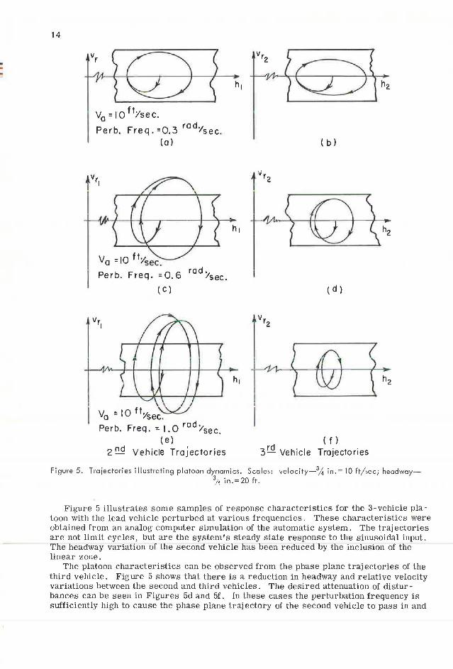
Figure 5. Trajectories illustrating platoon dynamics. Scales: velocity-3,4in.=10 ft/sec; headway-314 in. = 20 ft.

Figure 5 illustrates some samples of response characteristics for the 3-vehicle pla­toon with the lead vehicle perturbed at various frequencies. These characteristics were obtained from an analog computer simulation of the automatic system. The trajectories are not limit cycles, but are the system's steady state response to the sinusoidal input. The headway variation of the second vehicle has been reduced by the inclusion of the linear zone.

The platoon characteristics can be observed from the phase plane trajectories of the third vehicle. Figure 5 shows that there is a reduction in headway and relative velocity variations between the second and third vehicles. The desired attenuation of distur -bances can be seen in Figures 5d and 5f. In these cases the perturbation frequency is sufficiently high to cause the phase plane trajectory of the second vehicle to pass in and

Activating S i g nals for Thresh ol d Mo des

\ 02

+

a +

Switch Positions : 1) Linear Mode of Ope ration, .::) Thre s hold Modes of Operation

Figure 6. Block diagram of automatic system (azc = command acceleration).

out of the region of linear mode control. In spite of this, the trajectory of the third vehicle remains entirely within the linear mode region of control with considerable attenuation in the headway and relative velocity variations.

DESIGN OF A PRACTICAL LINEAR MODE SYSTEM

15

It is now necessary to include important factors which will be inherent in an actual system but which were not considered in the ideal system of the previous section. The performance of such a vehicle may be approximated by

1 v ::. tii'"+1

c a

where

v a = actual velocity of ve hicl e. v c = velocity command to vehicle, and t = automobile time constant. a

(10)

This will be termed a velocity controller. If the acceleration of the controlled vehicle is made to have a component proportional to the headway, several problems arise (_!). To actually achieve constant accelerations and decelerations of the controlled vehicle, acceleration feedback is required. A somewhat idealized acceleration feedback loop is shown in Figure 6 because it is relatively straightforward. In practice, however , it is much more convenient to accomplish the same synthesis starting with a r earrange­ment of Figure 6 which is dynamically equivalent to that shown. The transfer function of an accelerometer can be represented by

where

am = output signal of the accelerometer, v 2 = velocity of vehicle ,

(11)

.. "I

!!!

16

t 2 = time constant associated with accelerometer, and k2 = gain factor associated with accele1·ometer .

In the forward path of the system, proportional and integral control are included to provide design flexibility. The system may be represented in block diagram form (Fig. 6). The open - loop transfer function of the acceleration loop is

ka (k.1t3p2 + k4p + k3)

GH - -------~~--- (tmp + 1) (t2 p + 1) (tap+ 1)

where G is the forward oath transfer function and H is the feedback path transfer function. The zeros of GH may be used to cancel the poles at - l/t2 and - 1/ta by setting

k4

[ 1 - :: ] k =-

3 t a

and

1 1 1 ---+ + ta •2 •m

(12)

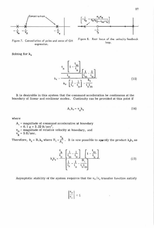
The complex frequency plane considering the poles and zeros of the expression given by Eq. 12 is shown in Figure 7.

The transfer function of the system with the velocity feedback path open is

v r

- -,a [ -1 - ::-=----] P -=---['m P-+ 1 +-ta [-~·- ~-] ]

(see Fig. 6). The root locus is shown in Figure 8. v2 (p) This design procedure enables one to specify the dominant pole of Gv (p) = --(-)

V1 p

(13)

which determines the transient response of the system. Further specification of the system will be accomplished by fixing the dominant pole of the closed loop transfer function at an arbitrary value - 1/ t . To have a pole of the transfer function at - 1/t

0,

the gain factor 0

is determined by

1 t

0

(14)

17

/Cancellation~

~~x~~ ~

- ...!_ - j__

Figure 7. Cancellation of poles and zeros of GH expression.

Figure 8. Root locus of the velocity feedback loop.

Solving for k4

•. [1 -~] [i -1..J t t t

1r o m o ~ =~--':o..-~~-=-~---~

[ ]

k 2 k 1._1.. -

5 t t t t 2 o om

(15)

It is desirable in this system that the command acceleration be continuous at the boundary of linear and nonlinear modes. Continuity can be provided at this point if

where

A1 = magnitude of command acceleration at boundary = 0.1g=3.22 ft/sec 2

,

v 0 = magnitude of relative velocity at boundary, and vk = 5 It/ sec.

(16)

vk Therefore, ~ = B1k5 where B1 =A . It is now possible to specify the product k4k 5 as

1

(17)

Asymptotic stability of the system requires that the v2 / v1 transfer function satisfy

I:: I < 1

18

For this system,

(18)

The inequality is easily satisfied by investigating the magnitude of Eq. 18 as a function of frequency. The constraints that have already been placed on the system performance have also insured asymptotic stability of the system.

SUMMARY

An automatic longitudinal control system for control of individual vehicles in the traffic stream has been presented. In order to meet the many requirements on such a system it was necessary to combine both linear and nonlinear modes of control in the system. The system has been analyzed in the car-following situation in single lane t r affic with up t o 3 cars in a line. Mor e extensive eva luation for m any cars in a platoon and for comparison with the present manual system has not been completed. However, the results of present analysis indicate that good performance can be expected.

REFERENCES

1. Cosgriff, R. L., Roeca, W. B. , Thomas , A. C. , and Todosiev, E. P. Studies of the Two - Vehicle Situation. 1964 IEEE International Convention Record, Part 8-Instrumentation.

2. Herman, Montroll, Potts, and Rothery. Traffic Dynamics: Analysis of Stability in Car Following. Journal of the Operations Research Society of America, p. 86, Jan. -Feb. 1959.

3. Barbosa. Studies of Traffic Flow Models. Master's Thesis, Ohio State University, 1961.

4. Roeca, W. B. , and Thomas, A. C. An Anti-Rear - End Collision System. Highway Research Record 10, pp . 1- 9, 1963 .